
Facoltà di Scienze Matematiche Fisiche e Naturali XXVI...
209
Facoltà di Scienze Matematiche Fisiche e Naturali XXVI Ciclo Dottorato in CHIMICA ANALITICA DEI SISTEMI REALI Food quality control and authentication through coupling chemometrics to instrumental fingerprinting techniques Relatore Dottorando Prof. R. Bucci Riccardo Nescatelli
Transcript of Facoltà di Scienze Matematiche Fisiche e Naturali XXVI...
Facoltà di Scienze Matematiche Fisiche e Naturali
XXVI Ciclo
Dottorato in CHIMICA ANALITICA DEI SISTEMI REALI
Food quality control and authentication through coupling
chemometrics to instrumental fingerprinting techniques
Relatore Dottorando
Prof. R. Bucci Riccardo Nescatelli
i
Tables of Contents
CHAPTER 1: INTRODUCTION
1.1 Quality control of food 1
1.2 Traceability and authentication of food 6
1.2.1 Analytical techniques 8
1.3 Revision of methods of food chemical analysis 11
1.4 The role of chemometrics in food analysis 13
1.5 Aim of the Thesis 17
CHAPTER 2: CHEMOMETRIC METHODS
2.1 Experimental Design 19
2.2 Multivariate calibration 29
2.3 Multivariate classification: Partial Least Squares Discriminant Analysis 33
2.4 Data Pretreatment 36
2.4.1 Baseline correction: Asymmetric Least Square 36
2.4.2 Alignment of chromatographic peaks: icoshift 37
2.4.3 Variables selection: Backward Interval Partial Least Square 38
2.4.4 Variables selection: Genetic Algorithms 39
2.5 Validation of chemometric methods 40
CHAPTER 3: EXTRA VIRGIN OLIVE OIL
Geographical Traceability of Sabina PDO
3.1 Introduction 42
3.2 Materials and methods 44
3.2.1 Samples 44
3.2.2 Optimization of extraction of the phenolic fraction from olive oil 45
3.2.3 HPLC-DAD analysis of the phenolic fraction 46
3.2.4 Identification of potential PDO markers by HPLC/ESI-MS 47
3.2.5 Signal pre-processing 47
3.2.6 Classification 48
3.3 Results and discussion 48
3.3.1 PLS-DA analysis on individual data matrices 51
3.3.2 Data Fusion 54
3.3.3 Identification of potential traceability markers for PDO Sabina 55
ii
3.4 Conclusions 56
CHAPTER 4: HONEY
Geographical and Botanical Traceability
4.1 Introduction 58
4.2 Honey samples 60
4.3 Materials 62
4.3.1 Solvents 62
4.3.2 Standards 62
4.3.3 Instrumentation and software 63
4.4 Sample preparation 63
4.5 Validation of the extraction procedure 68
4.6 Botanical and geographical classification by phenolic fingerprint 70
4.6.1 Botanical classification by HPLC-DAD 70
4.6.2 Geographical classification by HPLC-DAD 82
4.7 Botanical and geographical classification by NIR Spectroscopy 98
4.7.1 Botanical classification by NIR 100
4.7.2 Geographical classification by NIR 104
4.8 Conclusion: botanical and geographical origin of honey 114
CHAPTER 5: HONEY
Determination of Quality Parameters
5.1 Introduction 116
5.1.1 Regulation of honey quality 117
5.2 Official methods 118
5.3 Determination of reducing sugars, water content and 5-HMF 119
5.3.1 Reducing sugars 120
5.3.2 Water content through refractometric analysis 122
5.3.3 Water content through thermogravimetric analysis 124
5.3.4 Hydroxymethylfurfural 124
5.4 Acquisition of NIR spectra 125
5.5 Results – official methods 126
5.5.1 Determination of reducing sugars 126
5.5.2 Apparent water content 127
5.5.3 Determination of 5-HMF 128
5.6 Results – chemometric analysis 131
5.6.1 Determination of water content 134
5.6.2 Determination of the content of reducing sugars 136
5.6.3 Determination of 5-HMF 138
iii
5.7 Conclusions 140
CHAPTER 6: SAFFRON
MAE-HPLC-DAD for the Determination of Quality
6.1 Quality of saffron 142
6.2 Microwave-assisted extraction of crocin, picrocrocin and safranal 147
6.2.1 Samples and chemicals 147
6.2.2 Microwave-assisted extraction procedure 148
6.2.3 HPLC-DAD analysis 150
6.2.4 Optimization of the microwave-assisted extraction 150
6.2.5 Validation of MAE-HPLC-DAD method 155
6.3 Determination of safranal, crocin, picrocrocin in saffron 164
6.4 Geographical origin by NIR 168
6.4.1 Acquisition of NIR spectra of saffron samples 168
6.4.2 PLS-DA model 169
6.5 Conclusion 172
CHAPTER 7: WATER
Determination of Benzotriazoles in Water Samples
7.1 Introduction 173
7.2 Experimental 175
7.2.1 Standard, solvent and material 175
7.2.2 Samples and sample preparation 176
7.2.3 GC-MS condition 177
7.2.4 DLLME performance and sample quantification 178
7.3 Results and discussion 179
7.3.1 Preliminary experiments 179
7.3.2 Optimization of sample preparation condition 181
7.3.3 Performance of the method 187
7.3.4 Real sample analysis 190
7.4 Conclusion 192
CHAPTER 8: OVERALL CONCLUSION
OVERALL CONCLUSION 193
BIBLIOGRAPHY 194

1
CHAPTER 1
INTRODUCTION
1.1 QUALITY CONTROL OF FOOD
Food is any substance consumed to provide nutritional support for the body. It can be of plant
or animal origin, and contains essential nutrients, such as carbohydrates, fats, proteins,
vitamins, or minerals. The substance is ingested and assimilated by the organism in an effort
to produce energy, maintain life or stimulate growth. Consequently, in recent years attention
has been increasingly focused on what we eat, trying to ameliorate the quality of food
consumed by improving the standard of living.
Today, most of the food energy consumed by the world population is supplied by the food
industry so that, together with the food industry, the concepts of food safety and food quality
were born at the same time.
Food safety is a discipline born to describe handling, preparation and storage of food in ways
that prevent foodborne illness. These include a number of routines (rules) that should be
followed to avoid potentially severe health hazards. The tracks within this line of thought are
safety between industry and the market and then between the market and the consumer. Food
safety includes the origins of food, the processes relating to food labeling, food hygiene, food
additives and pesticide residues, as well as policies on biotechnology and food and guidelines
for the management of governmental import and export inspection and certification systems
for foods. In considering market to consumer practices, the usual thought is that food ought to
2
be safe in the market and the concern is safe delivery and preparation of the food for the
consumer.
There are many agencies responsible for food safety monitoring. In particular, in the
European Union (EU) the EU parliament is informed on food safety matters by the European
Food Safety Authority (EFSA) created by European Regulation 178/2002 laying down the
general principles and requirements of food law, establishing the European Food Safety
Authority and enacting procedures in matters of food safety [1,2]. The EFSA provides
scientific advice and effective communication regarding risks, existing and emerging,
associated with the food chain.
Consumers worldwide always demand to have their foods of higher standards or better
quality. However, the term “standard” or “quality” is often not unclear. “Food quality” may
have different meaning. Food quality encompasses the quality characteristics of food that are
acceptable to consumers. These include external factors as appearance (size, shape, color,
gloss), texture, and flavor; internal factors such as chemical, physical and microbiological
properties.
Food quality also deals with product traceability, e.g. of ingredient and packaging suppliers,
should a recall of the product be required. It also deals with labeling issues to ensure there is
correct ingredient and nutritional information.
There are many existing international quality institutes testing food products in order to
indicate which are higher quality products. Founded in 1961 in Brussels, the international
quality institute Monde Selection is the oldest one in evaluating food quality. During the
analysis the products must meet the following selection criteria, required by the institute:
sensory analysis, bacteriological and chemical analysis, the nutrition and health claims and
the utilization notice. In short, the judgments are based on the following areas: taste, health,
convenience, labeling, packaging, environmental friendliness and innovation. As many
consumers rely on manufacturing and processing standards, the institute Monde Selection
takes into account the European Food Law [3,4].
In order to guarantee food quality there must be an adequate quality control. The aim of
quality control is to achieve a good and a consistent standard of quality in the product being
produced as it is compatible with the market for which the product is designed, and the price
at which it will sell.
Quality control is often considered under the following three headings:
3
Control of raw material
Control of the process
Control of the finished product
Each heading is important and indispensable. A given raw material may be examined and
analyzed in different ways, with different techniques, depending on the information that we
wish to obtain. In the same way, the finished products must be analyzed in order to check the
chemical, physical, biological and/or organoleptic parameters. Clearly it is difficult to discuss
raw material control without reference to process control. It is equally difficult to talk about
process control without assuming that proper raw material control is carried out and that the
materials are known to have reached the standard required for proper processing: they are
simultaneously in operation. In planning a process control scheme, it is necessary first to list
in sequence the steps in the process or to draw a flow diagram taking care to show the
alternative processing steps, where these exist, to introduce changes in raw material. For each
processing steps, one must identify the critical points, and define which trouble may arise
which may be reflected in the quality of the finished product; for this reason it is necessary to
establish controls in all these operations.
We often confuse “Quality Assurance” (Q.A.) with “Quality Control” (Q.C.). Quality control
focuses on the product, while quality assurance focuses on the process. Quality control
includes evaluating an activity, a product, process, or service while quality assurance aims to
ensure processes are sufficient to meet clearly defined objectives. Further on, quality
assurance ensures a product or service is created, implemented, or produced correctly,
whereas quality control determines if the end product results are satisfactory or not.
Quality control in a typical food processing system begins right from the production stage of a
food and runs till the stage of its sale and distribution. Some of the common quality control
measures at each stage of a processed food are highlighted below:
PRODUCTION
- Control on the use of pesticides, veterinary drugs, and fertilizers.
- Quality control at the time of harvesting.
- Post-harvest handling particularly during storage (temperature, humidity and
time control)
PROCESSING
- Use of Good Manufacturing Practices (GMPs)
4
- Application of Hazard Analysis of Critical Control Points (HACCP) approach
to achieve optimum results with regard to the quality and safety of the product.
- The application of ISO 9000 series of standards to establish Q.C. regimes.
DISTRIBUTION AND SALE
- The ambient conditions under which food is stored or transported (e.g., time,
temperature, humidity).
Developed countries have structured food safety regulatory systems that are increasingly
comprehensive and more stringent. They are adopting a mix of regulatory approaches
depending on the problem addressed, including process standards such as HACCP,
performance standards for testing final products and even increasing labeling standards to
communicate about food safety to consumers [5-7].
As above mentioned, the quality of end products is influenced primarily by the raw materials
used. For this reason, close cooperation between agriculture and processing plants is needed.
The farmers, in many cases, make agreements with the food industry, not only on the quantity
of raw materials produced, but also all on their quality. In all cases, the raw materials must
fulfill all standards requirements. Great attention is put on the presence of different kinds of
contaminants such as toxic metabolites of microorganisms, toxic and heavy metals, residues
of pesticides, the presence of undesired materials and others. In perishable raw materials, the
chemical and microbiological quality of the raw material plays an important role and has to be
controlled. For quality control of individual raw materials, different quality parameters are
chosen, according to the quality requirements of the final products for which the raw material
will be used [8]. Different evaluation methods based on different principles may be used. In
particular, as far as the authentication of the quality of raw materials is concerned, usually
rapid and accurate controls methods are preferred, for example through the use of NIRS (near-
infrared spectroscopy) and HPLC (high performance liquid chromatography) but their choice
depends on many factors [9-11].
Quality of finished food products is the most important indicator for the consumer. Finished
products have to fulfill all requirements on quality. They should have the appropriate nutritive
value, typical sensory characteristics and above all, meet all standards from a safety point of
view. For this reason the quality control of finished products is the crucial point of the whole
quality control chain. For the consumers, it is important that the quality of such products
remains at the level declared by the producer during the whole storage period guaranteed.
Labeling of food is also important; its purpose is to provide the consumer with the data
5
necessary for making an informed choice in the marketplace. The label must always bear the
statement of identity; declaration of net contents; name and address of the manufacturer,
packager, distributor; and a list of ingredients. The date of production and expiration date is
most important, especially in perishable foods. National regulations usually require further
information, such as nutrients and energy contents, and information about food additives with
appropriate E number. The first step of quality control of finished food products starts in the
factory. The producers are responsible for the quality of products. Therefore, they use the
technological procedure in which the HACCP system is incorporated. This means that at least
the critical control points are regularly examined. The high quality of produced foods is also
important as a competition factor. In this respect, the producers are economically stimulated
to produce foods of better quality than a competitive company. Factory laboratories are on
high standard and are reasonably equipped. Moreover, when the analyses could not be
possible without special and usually expensive equipment, the producers hire the services of
special laboratories. The state protects consumers by running its own state control
laboratories; their organization varies from state to state. Such laboratories, in developed
countries, are well equipped, not only as far as the instrumentation is concerned but also with
skilled and qualified analytical staff. Consumer organizations are also engaged in the food
control system and play an important role. These organizations inform consumers about the
results of quality comparative studies and draw attention to products that don‟t fulfill given
quality requirements. Generally, the activity of such laboratories is focused on observation of
the chemical composition, organoleptic properties, quality of packaging, microbiological
state, presence of food additives and contaminants. Controlled products have to fulfill
requirements for their given type of product and they especially have to be safe for the
consumer. Such controls have to rule out the possibilities of health hazards and to guarantee
that food products have not been adulterated. The food that the consumer receives from the
farm or factory via food distribution system may exhibit important compositional changes that
may be relevant to health or may not correspond to production claims, the label or trade
agreements. The consumer is now more conscious about what he wants and the industry is
eager to deliver the quality the consumer prefers. At the same time, scientific advances are
making available tools and techniques that are more and more enhancing the sensibility,
specificity and reproducibility of analytical methods. This information arising from the basic
chemical sciences has assisted the analytical researcher in identifying new indicators of
quality and authenticity of food. In many countries, mandatory provisions in food legislation
are becoming more rigorous, especially for what concerns safety aspects. The objective of the

6
food analyst is to encompass, in addition to detection of adulteration, characterization of the
food with respect to its source, the history of its handling, storage, preprocessing and so on
[12-14].
The benefits of food laws to the consumers and the processing industry depend upon the
effectiveness with which the laws are implemented. This requires not only a well-organized
national infrastructure for inspection and quality control, but also the availability of reliable
methods of analysis, which could be used to check the quality standards and safety. In this
way, industries can be advised to make improvements in their food products and legal actions
taken when necessary to protect the consumers. Therefore, in recent years, new methods for
the analysis of food have been developed, together with the attempts to improve the existing
ones. In this respect, one must recall that the analyses concern all aspects of a food, such as
chemical, physical and microbiological. In this way, it is possible for instance to check that a
food possesses certain nutritional parameters. In addition, it is possible to identify frauds,
adulterations and guarantee to the consumers the quality standards of a food. Regarding the
quality control of food, the key issues are both to check that a food has certain indices,
determined according to well defined analyses, within specifications, and to identify the new
parameters of control that are able to guarantee the quality of a specific food. In recent years,
research has made significant progress in the knowledge of the main factors that contribute to
define the quality of a food. Thanks to the development of new technologies, it has been
possible to modify and improve the existing methods for the determination of the quality
parameters and it has also been possible to create new methods for food analysis [15]. As
mentioned previously, the development of fast and precise analytical methods are essential to
ensure product quality, safety, authenticity and compliance with labeling.
1.2 TRACEABILITY AND AUTHENTICATION OF FOOD
Open markets and the development of the circulation of natural and processed foods in the
European Union involves the necessity to inform consumers and predisposed organs about all
the elements that contribute to the identification of food products.
7
Traceability means the ability to trace and follow a food, feed, food-producing animal or
substance that will be used for consumption, or expected to be incorporated into a food or
feed, through all stages of production, processing and distribution. The need for traceability
systems is well recognized throughout the world. In fact, traceability can protect consumers
against deceptive marketing practices and/or frauds. Traceability can also allow to improve
food safety, therefore it is a clear advantage for consumers and for food industry.
The possibility of tracing the origin of foodstuff is assuming an increasingly important role at
the legislative level, as a tool that may allow to check whether quality requirements are met. It
allows to establish the identity, history and origin of product. The evolution of the discipline
of traceability is accomplished in two stages: in a first time, traceability was provided only for
certain products (not-food) and for some individual foods; in a second step, it was extended to
all products and foods. In the food industry, laws began to speak about traceability in relation
to the organic production of agricultural products (Reg. CEE 24.06.1991 n 2092 art 9-12).
The regulation disposed that Member States should ensure that the inspections relate to all
stages of production, slaughter, cutting and any other preparation up to the sale to the
consumer in order to guarantee, as far as technically possible, the traceability of products.
Subsequently, on January 28th 2002, the European Parliament and the Council adopted
Regulation (EC)178/2002 laying down the General Principles and requirements of Food Law.
The aim of the General Food Law Regulation is to provide a framework to ensure a coherent
approach in the development of food legislation. At the same time, it provides the general
framework for those areas not covered by specific harmonized rules, where the functioning of
the Internal Market is ensured by mutual recognition. It lays down definitions, principles and
obligations covering all stages of food/feed production and distribution. According to this
regulation, each business operator must be able to produce data about who their customers
and suppliers are and have those systems and procedures to identify the product, so that it
could be easier to withdraw it in case of danger for the consumers‟ health. However, it lacks a
true commitment towards what has been called "traceability evolved", a wide range of
methodologies aiming at the monitoring of various production processes, the control of
mixing techniques and treatment of raw materials and the protection of the area of origin.
Therefore, if on one side there are extremely positive national policy-making aimed at the
preservation, protection and development of the "typical" local as a synonym for quality, on
the other hand it is extremely complex, for the control authorities, to be able to provide those
aspects of sanitation residing at the base of the rules on food safety for consumers. It is clear
that, in a context so articulated, any action to market low-cost products derived from

8
imitation, adulteration and counterfeiting of traditional foods represents a potential risk to the
health of consumers and it is also a damage for “legal” economies. Therefore, the
development of innovative techniques and methods for the control of food products is a top
priority in the development plans of both Community and National authorities, to pursue the
objectives of increasing security and protection of the quality. The movement of food has no
borders in a globalized supranational context. For these reasons the consumer world requires
insistently a more detailed and accurate information about the nutritional parameters to
guarantee the quality of food.
The authenticity of the product and its geographical traceability are therefore two fundamental
aspects for a food.
The authentication of a food is the process by which it is possible to verify that the product
conforms to the statements on the label, and possibly to what established in the in force
regulations. In particular, the use of non-destructive, rapid, precise, accurate and highly
performant analytical methods represents, for the authorities, a valuable and irreplaceable tool
to verify the authenticity of a product. In addition, scientific innovation and technological
evolution of instrumentation and methodologies, can allow to identify fraud and adulteration
even if particularly sophisticated, or specifically designed to evade inspection of law currently
applied. By definition, the authentication of a product invests issues that are very different
among themselves, which largely depend on the type of fraud mainly practiced for each food.
They include both the identification of possible adulteration and falsification, and the
differentiation from other substitute products, the differentiation by age, or the identification
of the geographical and varietal origin.
1.2.1 ANALYTICAL TECHNIQUES
There is no magic solution to improve the traceability but effective systems must comprise a
number of key elements.
a) Regular labeling
b) Electronic labeling
c) Animal ear tags, passports
9
d) Production Records (one step forward-one step back)
However, these elements are not sufficient to ensure the traceability and authenticity of foods
and the consumers are not completely protected against food frauds.
The analytical techniques, being a posteriori techniques, are essential for food safety, food
quality control and for the traceability and authentication of food products. In fact, the
analytical methods can provide feedback to prove that a system is working, troubleshoot and
identify weaknesses and can provide traceability data where there is a breakdown in the chain.
In addition the analytical techniques are effective internationally, and constitute a valid tool in
order to prevent fraud and to confirm the authenticity of products. There are many emerging
techniques available that can provide traceability information. Especially when used in
combination, these techniques can provide extremely powerful tools.
The analytical techniques most commonly used for food authentication and traceability are
the following:
• Stable isotope measurements (IRMS)
• Spectroscopic techniques (MIR, NIR, Raman, UV-VIS)
• Chromatographic techniques (GC, HPLC)
• Mass Spectrometric techniques (MS, MSMS)
• DNA-PCR methods
• Chemometric techniques (in next chapters the chemometric techniques used in this thesis
will be discussed in detail)
Ratios of stable isotopes have been shown to be a valuable tool to discriminate foodstuffs
according to their geographical origin and/or the technological processes applied during
manufacture (production origin). In particular, determination of the isotopic ratios of the light
elements, hydrogen (δ2H), carbon (δ
13C), nitrogen (δ
15N), oxygen (δ
18O), and sulfur (δ
34S),
the so-called bioelements, combined with ratios of heavy isotopes (δ87
Sr) and trace elements
have been used successfully to provide information on the origin of food products [16-20].
However, although some official methods using isotope ratios have been introduced, they are
usually reliant on commodity specific databases which are expensive to produce and to
maintain.
10
Spectroscopy is the study of interaction between photons of radiation and molecules. Among
the most widely used spectroscopic techniques for the authenticity of the food, there are MIR
(mid-infrared) and NIR(near-infrared) spectroscopy. Even if the electromagnetic radiation
used is of different frequency (range 4000-400 cm-1
is referred to as mid-infrared and 12500
and 4000 cm-1
is known as near-infrared radiation), the response of the instrument consists of
absorption bands due to chemical compounds, that can be observed, in the spectral regions of
the MIR and NIR, as a result of molecular vibrations of these compounds thus giving rise to
spectral signatures which are characteristic of the food composition and which may be
considered as “fingerprints” of the food [21,22].
Chromatographic methods are widely used for the measurement of the „fingerprints‟ of
foodstuffs. Gas chromatography (GC) and high performance liquid chromatography (HPLC)
provide high-resolution compound separations, and can be used in conjunction with different
detectors such as a diode array detector (DAD) or a mass spectrometer (GC-MS, GC-
MS/MS, LC-MS, LC-MS/MS). The mass spectrometers are highly sensitive and universal,
able to detect almost any organic compound, regardless of its class or structure. As reported
for spectroscopic profiles, the chromatographic profiles may be used as the fingerprint of the
food to control the quality of food and to guarantee its authenticity [23,24].
Analysis of specific nucleic acids in food allows control laboratories to determine the
presence or absence of certain ingredients in complex products or the identification of specific
characteristics of single food components. In food analysis, DNA detection is increasingly
applied as an answer to different needs, such as for GMO detection, microbial pathogen
determination, assessment of the presence of undeclared allergenic ingredients [25]. These
analyses are based on nucleic acids probes, including the polymerase chain reaction (PCR),
which allow the detection of minute amounts of degraded nucleic acids and their sequence.
These methods may be also used for the identification of meat or fish species and the
recognition of genetically altered foods [26].

11
1.3 REVISION OF METHODS OF FOOD CHEMICAL
ANALYSIS
As mentioned in the previous paragraphs, the control of food quality, food safety, traceability
and authentication of food have considerable importance. Therefore, scientific research is
increasingly addressing the development of new methods that can ensure the
geographical/botanical traceability [27]. In particular, in recent years, some successful
examples of application of fingerprinting techniques for assessing the origin of foods have
been reported in the literature [28,29]. In this context, the possibility of relying on the
outcome of a fingerprinting technique to authenticate the origin of a foodstuff has a high
potential as it would allow the traceability of the product without being tied to the labeling or
production records.
Parallel to this – and always with the aim of guaranteeing the consumers by assessing the
quality of a food, especially if with added value, and to characterize foods identifying the
nutraceutical components – scientific research has also put a big effort in the revision of the
traditional methods of food chemical analysis, with the objective of developing methods with
better performance compared to the ones currently used for the determination of the
constituents of foods. In fact, even if several methods for the chemical analysis of some
characteristics of the food already exist, for instance all the analytical methods described in
the laws, the continuous innovation and technological development have made researchers
trying to develop methods for food analysis resulting in better performance than the currently
adopted ones in terms of accuracy and precision, trueness, limits of detection and
quantification etc. Together with these aspect, also the possibility of reducing the times and
costs of analysis without loss in accuracy is also often investigated, as it could allow carry out
a higher number of controls in the same timespan and with the same budget.
On the other hand, in recent years the international community is laying attention on
environmental issues and on green chemistry. Green chemistry is the design of chemical
products and processes that reduce or eliminate the use and generation of hazardous
substances [30]. In addition to being innovative, the approach of green chemistry is, at the
same time, not-regulatory and attentive to the economic aspects. Therefore, developing
methods for chemical analysis with the intention of preventing the pollution can be defined a
new scientific approach to eliminate or minimize the environmental problems. More
generally, whenever possible, it is appropriate to replace the traditional obsolete test methods
12
with others who maintain their functional efficacy while reducing toxicity to humans and the
environment.
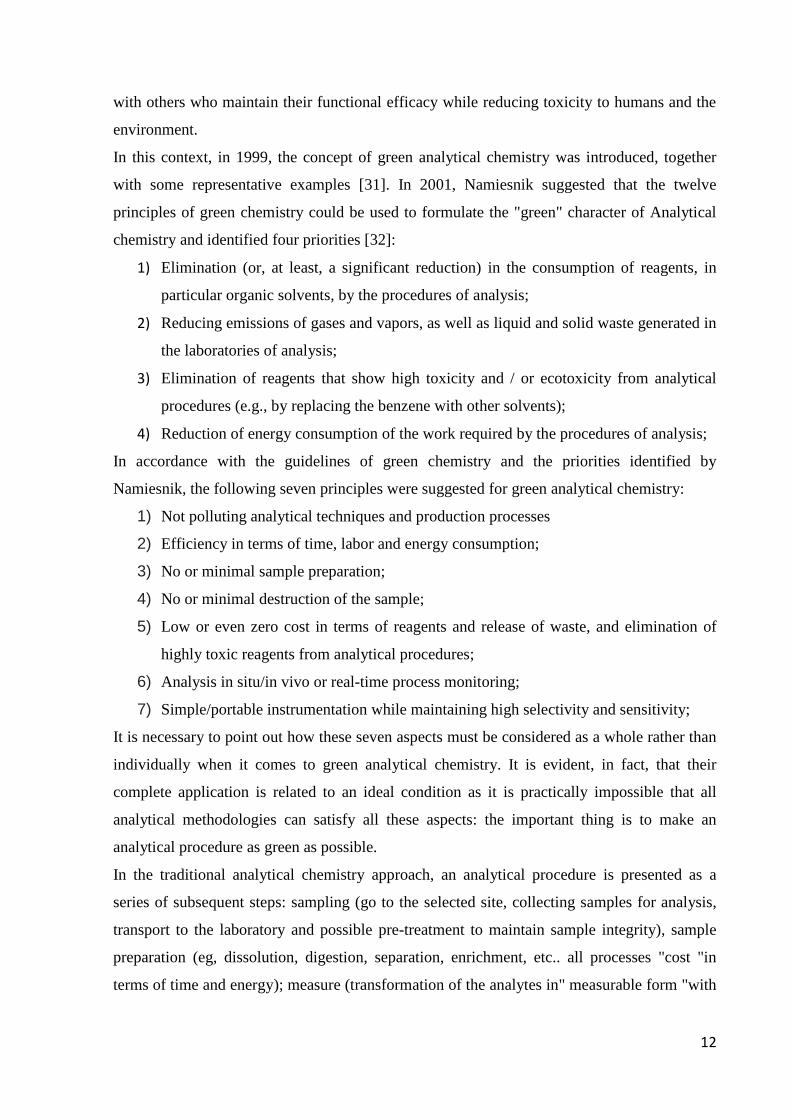
In this context, in 1999, the concept of green analytical chemistry was introduced, together
with some representative examples [31]. In 2001, Namiesnik suggested that the twelve
principles of green chemistry could be used to formulate the "green" character of Analytical
chemistry and identified four priorities [32]:
1) Elimination (or, at least, a significant reduction) in the consumption of reagents, in
particular organic solvents, by the procedures of analysis;
2) Reducing emissions of gases and vapors, as well as liquid and solid waste generated in
the laboratories of analysis;
3) Elimination of reagents that show high toxicity and / or ecotoxicity from analytical
procedures (e.g., by replacing the benzene with other solvents);
4) Reduction of energy consumption of the work required by the procedures of analysis;
In accordance with the guidelines of green chemistry and the priorities identified by
Namiesnik, the following seven principles were suggested for green analytical chemistry:
1) Not polluting analytical techniques and production processes
2) Efficiency in terms of time, labor and energy consumption;
3) No or minimal sample preparation;
4) No or minimal destruction of the sample;
5) Low or even zero cost in terms of reagents and release of waste, and elimination of
highly toxic reagents from analytical procedures;
6) Analysis in situ/in vivo or real-time process monitoring;
7) Simple/portable instrumentation while maintaining high selectivity and sensitivity;
It is necessary to point out how these seven aspects must be considered as a whole rather than
individually when it comes to green analytical chemistry. It is evident, in fact, that their
complete application is related to an ideal condition as it is practically impossible that all
analytical methodologies can satisfy all these aspects: the important thing is to make an
analytical procedure as green as possible.
In the traditional analytical chemistry approach, an analytical procedure is presented as a
series of subsequent steps: sampling (go to the selected site, collecting samples for analysis,
transport to the laboratory and possible pre-treatment to maintain sample integrity), sample
preparation (eg, dissolution, digestion, separation, enrichment, etc.. all processes "cost "in
terms of time and energy); measure (transformation of the analytes in" measurable form "with
13
procedures which may require energy, reagents, and can lead to release of polluting products);
waste disposal (residues of the sample, reagents used, products reaction, etc.).
Therefore, the conventional procedures of chemical analysis, often necessarily destructive, are
generally expensive not only because they consume time, reagents and energy, but also
because they produce waste that, being dangerous to humans and to the environment, require
special treatments for disposal. The aim of green analytical chemistry is to follow analytical
procedures that generate less hazardous wastes and which are more secure to use both for both
man and environment [33].
1.4 THE ROLE OF CHEMOMETRICS IN FOOD ANALYSIS
Chemometrics, according to the definition of the International Chemometrics Society, is “the
chemical discipline that uses mathematical and statistical methods to design or select optimal
procedures and experiments, and to provide maximum chemical information by analyzing
chemical data”. Already from the definition, the importance of chemometrics for the chemist
is clear. Chemometrics has a key role in all areas of chemistry, including analytical chemistry.
Consequently, chemometrics is a necessary and powerful tool in the field of food analysis and
control [34]. It is widely known that the application of advanced statistical and mathematical
methods has been continuously increasing in food science, once the use of such techniques
has allowed the extraction and identification of important results from complex data matrices.
Nowadays these statistical techniques are necessary for the academy and food industry during
the development and evaluation of food products and processes, as well as during the study of
the mechanisms underlying different phenomena that may affect the product‟s quality or unit
operations in the food development. Thus, the interest and application of new and complex
statistical and mathematical techniques in food science has significantly increased [35,36].
The issues related to authentication, typicality, traceability and overall quality of foods are of
particular importance for researchers, regulatory entities and most importantly for consumers.
The need to guarantee quality (nutritional value, absence of adulterations, traceability, food
safety, typicality, sensory properties including image analysis and other intrinsic quality
parameters) has led researchers and sanitary vigilance authorities to develop and use effective
14
statistical tools to investigate food-related problems and to address limitations on processes
and shelf life. Once food matrices become complex, the way to investigate and try to solve
problems related to sensory, chemical, physical and rheological issues is multivariate and thus
require multidimensional data. Thus, the use of multivariate statistical techniques has gained
strength in Food Science, especially for monitoring the unit operations and the quality of food
products, including beverages.
Technological innovation implies the use of increasingly sophisticated instruments, through
which it is possible to face and overcome analytical problems otherwise unsolvable. The
chemist has at its disposal tools more precise, accurate, sensitive and which allow to
determine qualitatively and quantitatively compounds even in trace. These techniques and
tools also result in thousands of data in which useful information is often "hidden". Often we
have too much data and too less information. In fact, a serious imbalance is developing in
science, between the technical capacity to generate lots of good data and the human capacity
to interpret and understand all these data. Indeed, it should be emphasized that the fact of
having many data is not a synonym of having many information, in fact data is not the same
as information. The fact that the analytical chemist has innovative tools available, almost
always very expensive, but from which he then fails to obtain all possible information without
fully interpreting them is, as once Harald Martens, a famous norwegian chemometrician, said,
“like having a grand pianos and playing with only one finger”.
Near-infrared spectroscopy represents one example. The information enshrined in an entire
NIR spectrum is poorly selective, as it depends on a particularly large number of physical
variables, chemical and structural properties, which often make the recognition of differences
between the samples subjected to analysis very difficult. To obtain useful information, as for
instance the amount of a particular substance in a food sample, or the identification of
possible differences between samples subjected to NIR analysis, it is necessary to use
mathematical and statistical techniques without which it would be impossible to solve some
analytical problems.
Chemical analysis of food is also part of the issue of traceability and fingerprinting techniques
as a tool to characterize, identify, and ensure the authenticity of the food. In fact, the term
“fingerprinting techniques” describes a variety of analytical methods that can measure the
composition of foodstuffs in a non-selective way such as by collecting a spectrum or a
chromatogram. Mathematical processing of the information contained in such fingerprints
may permit the characterization of foodstuffs. Fingerprinting techniques produce a large
volume of information. Most of the information may not be useful for solving the problem of
15
authentication or identity confirmation. Mathematical tools, such as classification models,
must be applied to these signals to extract that information which is helpful to solve the
problem being investigated [37]. Simply, a model is a mathematical equation which can
convert measurements, may be many hundred or more, made by one or more fingerprinting
techniques into indicators or numbers that are easily interpretable; when mathematical and
statistical methods are applied to the fingerprint of a given sample, the outcomes of the
corresponding model can for example represent the answer to the question “Is this food what
it claims to be on the product label?”
Without these mathematical processes, it would be impossible to carry out the classification
of foods, especially if there are thousands of variables such as the points that constitute a
spectrum, a chromatogram or the innumerable chemical compounds that describe and
characterize a food.
The mathematical and statistical techniques play a key role also in the context of Identity
Confirmation (IC). Methodology to confirm that a food is in compliance with claimed
identity. An important aspect of food production is to produce a good which always has the
same characteristics and therefore, by extension, with the same fingerprinting. The food
industry can verify the consistency of their product using fingerprinting techniques and
mathematical techniques [38].
Other issues that can be addressed with chemometrics concern process monitoring and the
quality control of foods. In fact, to ensure the control of the quality of a food, which depends
on several factors/variables, a multivariate analysis of the entire system is then required.
Indeed, it is not sufficient to carry out quality control or monitoring of a production process in
a univariate mode, because the system is a multivariate system. Therefore, there is an
increasing need for the analytical chemist to use mathematical tools which allow to treat
systems, more or less complex, also described by thousands of variables. Accordingly, in
quality control in general, and in particular in food quality control, there has been a transition
from using systems such as the univariate control charts to multivariate systems [39].
When dealing with n quality variables, the usual approach consists in verifying whether the
value of each variable measured on the final product is inside some predefined limits. If all
the variables are inside the range, then the product is said to be within specification. Probably
this statement is not always correct. The problem with using univariate control charts for
separately monitoring key variables on the final product is that the variables are not
independent on one another, and none of them adequately defines product quality by itself.
16
Product quality is defined by the simultaneous correct values of all the measured properties;
thus, a multivariate property requires multivariate analysis methods [40].
Chemometric plays an important role also in the choice of the experiments to be carried out
for the optimization of an analytical method, allowing for the development phase of an
analytical method a saving of time and money. In fact, the use of experimental designs makes
it possible to define a priori the experiments to be executed and the data to be collected.
While the standard way of developing an analytical method is very often to select possible
influencing factors, vary them one-by-one and evaluate their influence on the response(s) of
interest (OVAT – One Variable at A Time – approach), experimental design represents a valid
alternative to this approach. In fact, it is an even better alternative because for a given number
of experiments the experimental domain is more completely covered and interaction effects
between factors can be evaluated.
Mention was also made about the development of the analytical instruments of analysis that
enabled to overcome analytical problems, but there are issues that can be overcome by the
application of chemometric methods. Unstable baselines occur in many types of instrumental
measurements. They can cause severe problems, especially when detection limits are
approached [41]. These baselines hamper the interpretation of spectra or chromatograms. In
addition, the baseline varies greatly from spectrum to spectrum (or from chromatogram to
chromatogram), even for similar samples. In quantitative analysis, these inconsistent baselines
are able to reduce the simplicity and robustness of a calibration model that is built on these
spectra or chromatograms. In these cases the application of mathematical processing tool can
help to improve the baseline allowing a better interpretation of the data.
Chemometric comes to the aid of the analytical chemist also to solve problems related to the
shift of the retention times which may be due to multiple causes such as variations in
temperature between a chromatographic run and another run, the chromatographic column not
being well conditioned, etc [42]. In fact, the importance of always having the same retention
time for the same analyte present in different samples is rather obvious, especially when
analyzing complex matrices such as foods. The "shift" is not, however, a phenomenon
concerning only the retention time in chromatography. Many analytical techniques yield data
where the same underlying factor may result in signals at different positions or which may
have different „durations‟ depending on the specific analytical conditions.
17
1.5 AIM OF THESIS
Food safety and authenticity are, nowadays, themes of growing interest and increasing
importance. As a result, the European Union has issued over the years, regulations to
guarantee consumers relating to food safety and traceability [43,44] and, together with the
monitoring bodies, encourages the development of effective methods to combat food fraud
not only caused by the fraudulent addition of substances, but also those due to
misrepresentation on the label [45].
In addition to developing new methods for the analysis of foods that make it possible to check
the authenticity of a food and to discover new food fraud, research is moving towards the
improvement of the performance of the existing ones, even with the support of mathematical-
statistical methods and therefore with chemometrics.
For these reasons, the aim of this thesis was to develop new methods of chemical analysis for
the verification of the authenticity and the traceability of food. In this context, the developed
methods focus on the verification of two aspects which are closely related:
i) the chemical characterization of foods, in terms of monitoring their composition
and quantifying their constituents
ii) the identification of the origin of foods
On one hand, therefore, chemical methods of analysis for the determination of some
components presents in different foods have been developed and validated.
In particular, a spectroscopic method based on NIR spectroscopy for the determination of the
some of the indices required by law for the quality control of honey samples – water, reducing
sugars and hydroxy methyl furfural (HMF) – has been developed. Another purpose was to
develop an innovative method based on the extraction with microwaves and subsequent
chromatographic analysis for the determination of the quality of saffron.
Concurrent acetylation-dispersive liquid-liquid microextraction (DLLME) combined with gas
chromatography mass spectrometry (GC-MS) has been proposed, for the first time, for the
sensitive determination of several polar benzotriazolic compounds in water samples. In fact,
even if the water is not considered a food, the ingestion of water in some form is widely
recognized as essential for human life.
The methods of analysis have been improved compared to traditional and law methods, by
reducing the economic costs and times of analysis and also considering the environmental
18
impact, trying to reduce the environmental costs by eliminating or minimizing the use of toxic
and hazardous solvents.
On the other hand, chemical methods have been developed to verify and authenticate the
origin of foods. Specifically, a method for the analysis of extra virgin olive oil, which allows
to identify and discriminate Sabina PDO extra virgin olive oils from the others, was
developed and validated.
Analogously, the same approach was followed to verify the origin of two other high value-
added food products, honey and saffron. In particular, a method of analysis that allows to
determine both the geographical (Italian/non-Italian) and the botanical origin of different
honeys, was designed, developed, optimized and validated. The same strategy was followed
to design and optimize a method for characterizing the geographical origin of saffron, also
taking into account the possible differences in the growing and production processes.
Given the different foods and the different problems faced, the research was articulated and
configured in a way which has necessarily involved the use of multiple methods of analysis.
Indeed, depending on the type of food and the issues to be solved, the most appropriate and
cost-effective strategy, both in terms of analytical platform and of chemometric techniques
chosen, was always selected.
More in detail, the experimental work was focused on the following research topics:
1- Olive oil: Geographical traceability of extra virgin olive oils from Sabina PDO
by chromatographic fingerprinting of the phenolic fraction coupled to
chemometrics (chapter 3)
2- Honey: Geographical and botanical traceability of honey by chromatographic
and spectroscopic fingerprinting coupled to chemometrics (chapter 4);
Determination of quality parameters of honey by Near-Infrared spectroscopy
and chemometrics (chapter 5)
3- Saffron: Determination of quality of saffron samples by microwave-assisted
extraction and chromatography (chapter 6)
4- Water: Determination of benzotriazoles in water samples by concurrent
derivatization-dispersive liquid-liquid microextraction followed by gas
chromatography mass spectrometry (chapter 7)
19
CHAPTHER 2
CHEMOMETRIC METHODS
2.1 EXPERIMENTAL DESIGN
In analytical chemistry, especially in method development, it is of utmost importance to be
able to optimize all parameters that can affect the performances of the method itself. In this
framework, the objective is to perform a limited number of experiments – ideally as few as
possible, but at the same time to be able to determine how the experimental variables
influence the outcomes of the analysis and whether there are any interactions between the
factors.
Based on these assumptions, it is evident how in all cases where there is the need to optimize
a process or a response, as for instance an extraction procedure, or the yield of a reaction, or
when it is necessary to evaluate the incidence of multiple factors (experimental variables) on a
procedure, it is advantageous and often essential to think and operate in a multivariate way.
Indeed, varying one variable at a time while keeping all other constants, the so-called OVAT
approach, apart from requiring in general a significantly higher number of experiments to be
performed, almost always lead to suboptimal solution, as it doesn‟t take into account the
possibility that factors interact with one another.
An experimental design can be considered as a series of experiments that, in general, are
defined a priori and allow the influence of a predefined number of factors (experimental
variables) in a predefined number of experiments to be evaluated [46].
20
In order to properly design the experiments to be conducted, the first step is to define the
analytical problem (what do we need to investigate?), what are the experimental variables that
screened and controlled and what is the response(s) that better describe the propertie(s) to be
optimized? Once the experimental variables and the responses have been clearly defined, the
experiments can be planned and performed in such a way that a maximum of information is
gained from a minimum of experiments.
At each of the design points, one or more responses are determined, so that the effect of the
controlled factors and their interactions on them can be evaluated. For instance, in the
simplest case when a factor is controlled only at two levels, then its effect can be calculated as
the difference between the average value of the response obtained when this factor is at its
high and at its low levels. The relevance of the effects (i.e., the significance of their difference
from the variability which can be ascribed to the experimental error) is either statistically or
graphically evaluated [47].
Different types of experimental designs are available to the analytical chemist, depending on
the analytical problems to face, and, in particular, depending on the number and type of
variables that one wants to optimize. In this framework, the different kinds of experimental
designs can be roughly divided in two categories, those aimed at screening and the ones for
optimization [48].
Screening designs are used to search for possibly important factors during method
optimization or in robustness testing. They can be used if there is little knowledge of the
possible factors that may affect the response: in these cases, all the possible factors that can
influence the results of a method should be selected. With the use screening designs, it is
possible to identify the factors that have a major influence on the response(s) of interest.
Generally, two-level designs are used for screening, as they allow screening a relatively high
number of factors in a rather low number of experiments. These designs can also be used to
verify the robustness of an analytical method. In this context, the difference between the
screening and robustness testing lies in the amplitude of the explored experimental domain,
i.e. in the interval between the two levels of the factors [49]. Indeed, for any given factor, a
relatively large interval is considered for optimization, while in robustness testing the
intervals are much smaller and do not exceed much the experimental error.
The optimization of a method can be performed with a stepwise strategy. This means that
groups of experiments can be performed sequentially. For instance, it is possible to make a
first experimental design in a given experimental domain and, depending on the result,
repeating another experimental design but choosing a different range of variability for the
21
factors to be investigated. This process can be repeated step by step until a pre-determined
criterion is met. For example, if for the optimization of an extraction method a recovery of
80% is sufficient and, with the experimental design, it is possible to identify the portion of the
experimental domain that allows an extraction efficiency higher than 80%, it is not necessary
to perform additional experiments. If, instead, the best experimental setting still does not
result in a recovery of at least 80%, then there is the need to perform additional experiments
by extending the experimental domain in the direction of the optimal conditions obtained with
the previous experimental design.
HOW TO START
The first step of any experimental design consists in determining which factors could
influence the response(s) and in choosing the domain of variability for each controlled factor.
Sometimes one knows which factors have an effect on the response, but often this information
is not available. In this case, it is possible to start writing down all the possible factors that
could have an effect on the response and make a screening of which factors may have an
effect by using the highest possible fraction of a factorial design or the corresponding
Plackett-Burman„s designs which are performed on two levels with a number of experiments
increasing by multiples of 4 [50]. After choosing the factors, it is necessary to fix the limits of
the experimental domain, i.e. the extreme levels for each experimental variable. The next step
is often to obtain a model that describes in a quantitative manner the effect of the factors on
the response. Finally, based on the model, one tries to find the optimal conditions, or, in other
words, the values of the factors that result in the best features of the product, process or
procedure studied [51].
EXPERIMENTAL MODELS
The response Y of an experiment (the area of a peak, the intensity of a signal, etc.) is
influenced by the experimental conditions. Mathematically Y = f (x). The function f (x) is a
polynomial function that, within the experimental domain, relates the controlled factors to the
response. There are three types of polynomial models that describe the Y response. The first
and simplest is the linear model, where the relationship between the experimental variables
and the response is linear. For instance, in the case where two factors x1 and x2 are
controlled:
22
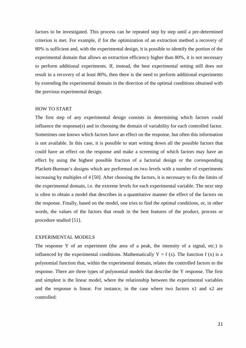
y= b0 + b1x1 + b2x2 + e (1)
e being the residual, i.e. the portion of the variability in the response y not explained by the
model.
On the other hand, if there are interactions among variables, terms accounting for these
interactions should be added. Usually, only second order interactions, i.e. those involving pair
of factors, are considered to be possibly significant. Under this assumption, in the case of two
factors, equation 1 transforms to:
y= b0 + b1x1 + b2x2 + b12x1x2 + e (2)
These two models, linear model and second order interaction model, are the ones most often
used to do a screening and/or robustness tests.
In all the cases where it is not possible to assume a linear relationship between the
experimental variables and the response, higher order polynomial terms should also be
included. However, the models customarily used in experimental design very rarely exceed
second order polynomials, meaning that a quadratic function is fitted to the data. In the case
of two controlled factors, this translates to:
y= b0 + b1x1 + b2x2 + b12x1x2 +b11x1
2 + b22x2
2 + e (3)
Of course, even though the functions reported in equations 1-3 refer to the case when only
two factors are controlled, they can be easily generalized to a higher number of variables.
The polynomial functions described contain unknown parameters (b0, b1, b2, etc.), which
need to be estimated based on the results of the experiments carried out and for each model an
appropriate experimental design exists.
FULL FACTORIAL DESIGN
The full factorial design with two levels are used to determine if some factors and / or
interactions between two or more factors have effect on the response, and to estimate the
magnitude of this effect. It requires that experiments be conducted at all possible
combinations of the two levels of the k factors studied. Therefore, the number of these
experiments is 2k, which is also the way these designs are indicated [52].
23
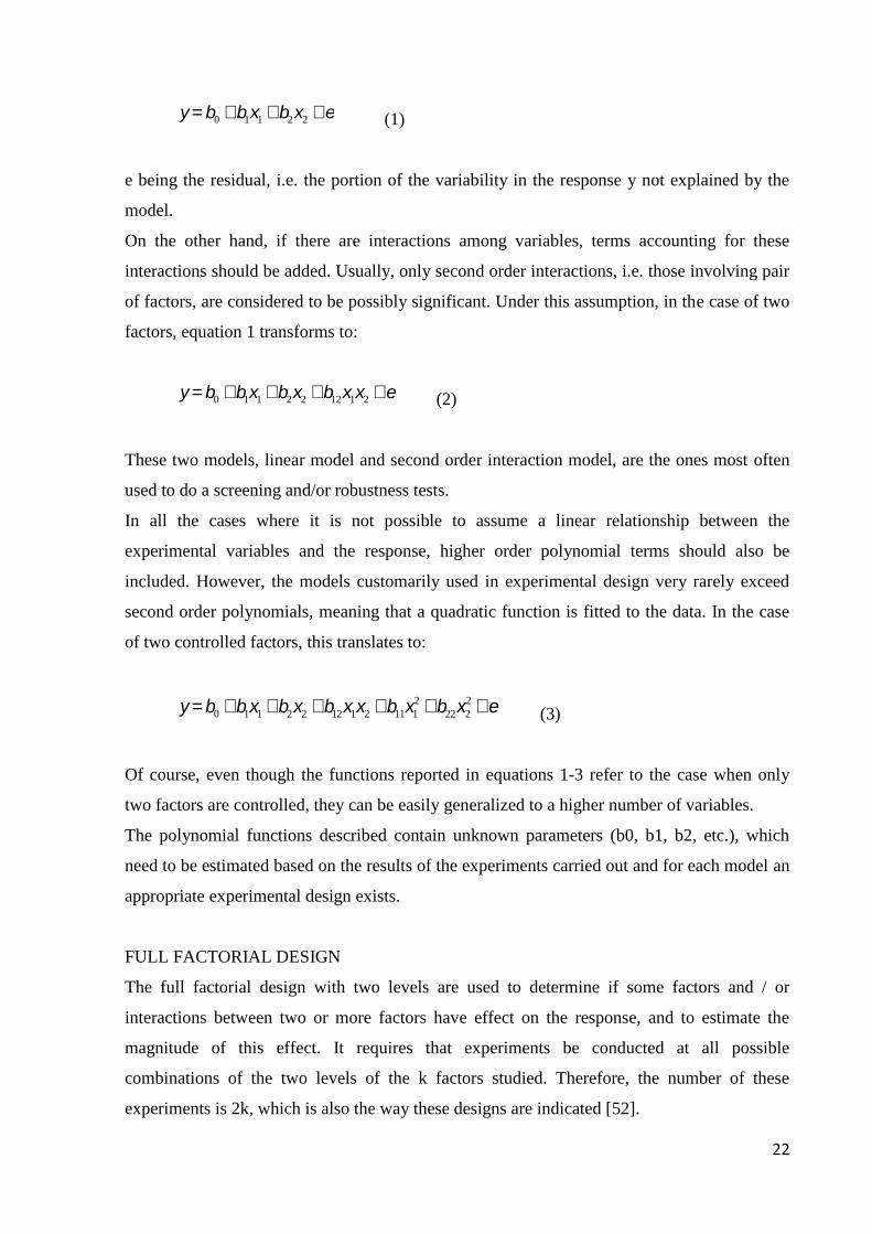
As an example, the experimental matrices describing the factor levels for the full factorial
designs in the case of 2, 3, and 4 controlled factors are reported in Tables 2.1-2..3.
Table 2.1: full factorial design for 2 factors
experiment number variable 1
b(1)
variable 2
(b2)
1 -1 -1
2 -1 +1
3 +1 -1
4 +1 +1
Table 2.2: full factorial design for 3 factors
experiment number variable 1
(b1)
variable 2
(b2)
variable 3
(b3)
1 -1 -1 -1
2 -1 -1 +1
3 -1 +1 -1
4 -1 +1 +1
5 +1 -1 -1
6 +1 -1 +1
7 +1 +1 -1
8 +1 +1 +1
24
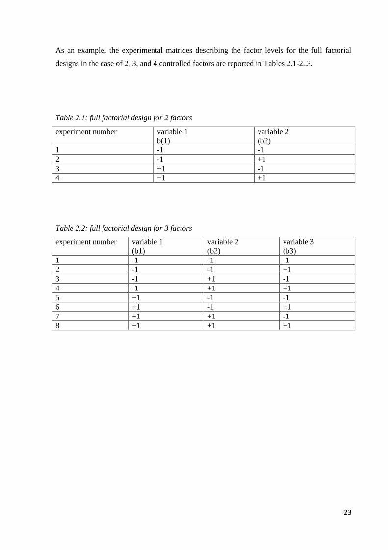
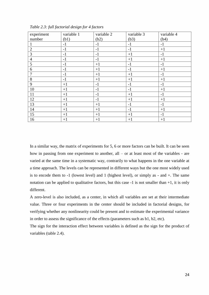
Table 2.3: full factorial design for 4 factors
experiment
number
variable 1
(b1)
variable 2
(b2)
variable 3
(b3)
variable 4
(b4)
1 -1 -1 -1 -1
2 -1 -1 -1 +1
3 -1 -1 +1 -1
4 -1 -1 +1 +1
5 -1 +1 -1 -1
6 -1 +1 -1 +1
7 -1 +1 +1 -1
8 -1 +1 +1 +1
9 +1 -1 -1 -1
10 +1 -1 -1 +1
11 +1 -1 +1 -1
12 +1 -1 +1 +1
13 +1 +1 -1 -1
14 +1 +1 -1 +1
15 +1 +1 +1 -1
16 +1 +1 +1 +1
In a similar way, the matrix of experiments for 5, 6 or more factors can be built. It can be seen
how in passing from one experiment to another, all – or at least most of the variables - are
varied at the same time in a systematic way, contrarily to what happens in the one variable at
a time approach. The levels can be represented in different ways but the one most widely used
is to encode them to -1 (lowest level) and 1 (highest level), or simply as - and +. The same
notation can be applied to qualitative factors, but this case -1 is not smaller than +1, it is only
different.
A zero-level is also included, as a center, in which all variables are set at their intermediate
value. Three or four experiments in the center should be included in factorial designs, for
verifying whether any nonlinearity could be present and to estimate the experimental variance
in order to assess the significance of the effects (parameters such as b1, b2, etc).
The sign for the interaction effect between variables is defined as the sign for the product of
variables (table 2.4).
25
Table 2.4: 22 full factorial design with interactions
experiment number variable 1
(b1)
variable 2
(b2)
interaction 1 and 2
(b12)
1 -1 -1 +1
2 -1 -1 +1
3 -1 +1 -1
4 -1 +1 -1
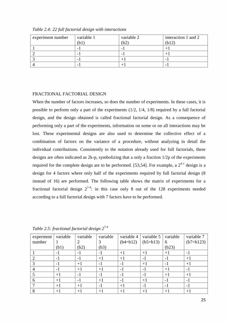
FRACTIONAL FACTORIAL DESIGN
When the number of factors increases, so does the number of experiments. In these cases, it is
possible to perform only a part of the experiments (1/2, 1/4, 1/8) required by a full factorial
design, and the design obtained is called fractional factorial design. As a consequence of
performing only a part of the experiments, information on some or on all interactions may be
lost. These experimental designs are also used to determine the collective effect of a
combination of factors on the variance of a procedure, without analyzing in detail the
individual contributions. Consistently to the notation already used for full factorials, these
designs are often indicated as 2k-p, symbolizing that a only a fraction 1/2p of the experiments
required for the complete design are to be performed. [53,54]. For example, a 24-1
design is a
design for 4 factors where only half of the experiments required by full factorial design (8
instead of 16) are performed. The following table shows the matrix of experiments for a
fractional factorial design 27-4
: in this case only 8 out of the 128 experiments needed
according to a full factorial design with 7 factors have to be performed.
Table 2.5: fractional factorial design 27-4
experment
number
variable
1
(b1)
variable
2
(b2)
variable
3
(b3)
variable 4
(b4=b12)
variable 5
(b5=b13)
variable
6
(b23)
variable 7
(b7=b123)
1 -1 -1 -1 +1 +1 +1 -1
2 -1 -1 +1 +1 -1 -1 +1
3 -1 +1 -1 -1 +1 -1 +1
4 -1 +1 +1 -1 -1 +1 -1
5 +1 -1 -1 -1 -1 +1 +1
6 +1 -1 +1 -1 +1 -1 -1
7 +1 +1 -1 +1 -1 -1 -1
8 +1 +1 +1 +1 +1 +1 +1

26
Of course reduction in the number of experiments comes with a cost: by using 2k-p
experiments to evaluate 2k effects (model coefficients), then each terms is confused with other
2p-1
. For instance, considering the matrix of experiments in Table 2.5, it is possible to see that
it was built from the matrix of experiments of a full factorial design of the same dimensions
(23) by using the interaction terms to account for the sign combination of the other factors to
be accommodated. Specifically, the signs for the variable 4 are the same as those of the
interaction between variables 1 and 2, those for variable 5 as the ones of the interaction
between factors 1 and 3, those for variable 6 as the interaction between factors 2 and 3 and the
ones for variable 7 as the ternary interaction among variables 1, 2, and 3. Since only 1/16 of
the original experiments are performed, each of these terms is confounded also with other 14
effects. When, as in the case reported in Table 2.5, the highest possible fraction of
experiments is performed, the corresponding fractional factorial design is often used for
screening and In model building assumption is made that only the terms corresponding to the
main effect are significant, so that other confounded terms are neglected:
y = b0 + bi xii=1
k
å + e (4)
In factorial or fractional factorial designs all variables are normalized between -1 and +1. For
continuous variables, the scaling is made so that the original variables vary continuously
within the interval from -1 to +1. Since all variables used in the model are normalized in this
way, the relative change of a variable is directly related to the size of its regression
coefficient. This means that if the model parameters have either a large positive or negative
value the corresponding variable has a large influence on response.
IDENTIFY SIGNIFICANT EFFECTS
Once the design has been chosen and the experiments performed, to calculated the effect of
the factors and their significance a simple procedure can be adopted, as far as full or fractional
factorial designs are concerned. First of all, the offset b0 can be estimated as the average of
the responses by summing the responses and dividing the sum obtained by the number of
experiments carried out. On the other hand, calculation of all other coefficients is carried out
multiplying point to point the column of the design matrix corresponding to the coefficient
that has to be estimated by the column of the response and than taking the average of the
results. Once the model coefficients are calculated, their statistical significance must be
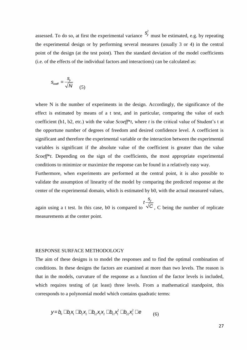
27
assessed. To do so, at first the experimental variance sy
2
must be estimated, e.g. by repeating
the experimental design or by performing several measures (usually 3 or 4) in the central
point of the design (at the test point). Then the standard deviation of the model coefficients
(i.e. of the effects of the individual factors and interactions) can be calculated as:
scoeff =
sy
N (5)
where N is the number of experiments in the design. Accordingly, the significance of the
effect is estimated by means of a t test, and in particular, comparing the value of each
coefficient (b1, b2, etc.) with the value Scoeff*t, where t is the critical value of Student‟s t at
the opportune number of degrees of freedom and desired confidence level. A coefficient is
significant and therefore the experimental variable or the interaction between the experimental
variables is significant if the absolute value of the coefficient is greater than the value
Scoeff*t. Depending on the sign of the coefficients, the most appropriate experimental
conditions to minimize or maximize the response can be found in a relatively easy way.
Furthermore, when experiments are performed at the central point, it is also possible to
validate the assumption of linearity of the model by comparing the predicted response at the
center of the experimental domain, which is estimated by b0, with the actual measured values,
again using a t test. In this case, b0 is compared tot
sy
C , C being the number of replicate
measurements at the center point.
RESPONSE SURFACE METHODOLOGY
The aim of these designs is to model the responses and to find the optimal combination of
conditions. In these designs the factors are examined at more than two levels. The reason is
that in the models, curvature of the response as a function of the factor levels is included,
which requires testing of (at least) three levels. From a mathematical standpoint, this
corresponds to a polynomial model which contains quadratic terms:
y= b0 + b1x1 + b2x2 + b12x1x2 +b11x1
2 + b22x2
2 + e (6)

28
The differences with other multivariate optimization approaches such as the simplex one
resides in the fact that models for the responses are built and that one assumes that the
optimum of the method is situated in the experimental domain created by the selected extreme
levels of the different factors.
It is a good way to graphically illustrate the relation between different experimental variables
and the responses.
Box-Behnken designs (BBD) [55] are a class of second-order designs based on three-level
incomplete factorial designs. For three factors, its graphical representation can be seen in two
forms (A and B): A is a cube where there are a central point and the middle points of the
edges (figure 2.1.a); B consists in a central point and three interlocking 22 factorial designs
(figure 2.1.b).
Figure 2.1: (a) the cube for BBD and three interlocking 2
2 factorial design (b) [56]

29
Table 2.1.6: Coded factor levels for a BBD of a three variable system
number of
experiments
variable 1 variable 2 variable 3
1 -1 -1 0
2 +1 -1 0
3 -1 +1 0
4 +1 +1 0
5 -1 0 -1
6 +1 0 -1
7 -1 0 +1
8 +1 0 +1
9 0 -1 -1
10 0 +1 -1
11 0 -1 +1
12 0 +1 +1
Central 0 0 0
Central 0 0 0
Central 0 0 0
The number of experiments (N) required for the development of BBD is defined as
N=2*k*(k−1)+C0, (where k is number of factors and C0 is the number of central points). The
BBD is an efficient design, where the concept of efficiency is mathematically expressed as the
ratio of the number of number of coefficients in the estimated model to the number of
experiments. In fact, with a limited number of experiments it is possible to determine the
linear terms and the quadratic terms. Another advantage of the BBD is that it does not contain
combinations for which all factors are simultaneously at their highest or lowest levels. So
these designs are useful in avoiding experiments performed under extreme conditions, for
which unsatisfactory results might occur [56].
2.2 MULTIVARIATE CALIBRATION
Multivariate calibration techniques are widely used for the characterization of complex
matrices, as, if experiments are carefully planned so that all the relevant sources of variability
are spanned, they allow to reduce to a minimum or even completely bypass possibly
30
expensive chemical treatments and preventive separative operations. These operations are
necessary when you use univariate methods of quantification, as complete selectivity of the
measurement is assumed. In contrast to the univariate approach, which makes use, for the
determination, of only one variable extrapolated from the entire set of those monitored (for
example, an absorbance value at a wavelength corresponding to a maximum of a spectral
profile), the multivariate approach allows to take advantage of the information obtained by the
measurement operations [57].
The multivariate approach allows obtaining many benefits: for example, it is possible to build
calibration models using techniques not perfectly selective, as the NIR spectroscopy, or build
models for chromatographic and/or spectroscopic fingerprint.
Generally, a multivariate calibration involves the following steps:
1 defining the problem: selecting the property to determine;
2 selection of standards for the model construction: choose a sufficiently large number
of samples that will guarantee a good statistical coverage of the calibration domain;
3 recording the signals (the variables): collect information about samples in a
reproducible way;
4 building the regression model: finding the relation between response(s) and the
variables measured on the samples (predictors);
5 validating the model: verifying the predictive ability of the model on “unknown”
samples.
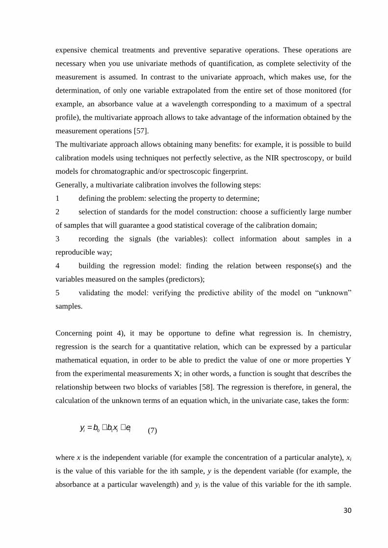
Concerning point 4), it may be opportune to define what regression is. In chemistry,
regression is the search for a quantitative relation, which can be expressed by a particular
mathematical equation, in order to be able to predict the value of one or more properties Y
from the experimental measurements X; in other words, a function is sought that describes the
relationship between two blocks of variables [58]. The regression is therefore, in general, the
calculation of the unknown terms of an equation which, in the univariate case, takes the form:
yi = b0 + b1xi + ei (7)
where x is the independent variable (for example the concentration of a particular analyte), xi
is the value of this variable for the ith sample, y is the dependent variable (for example, the
absorbance at a particular wavelength) and yi is the value of this variable for the ith sample.
31
The terms b0 and b1 are the intercept (or offset term) and the regression coefficient,
respectively, and represent the unknown terms that a regression problem aims to find. Finally,
the term ei is the residual for sample i, i.e. the error committed by the equation, which is
defined as the difference between the predicted and the true values of yi.
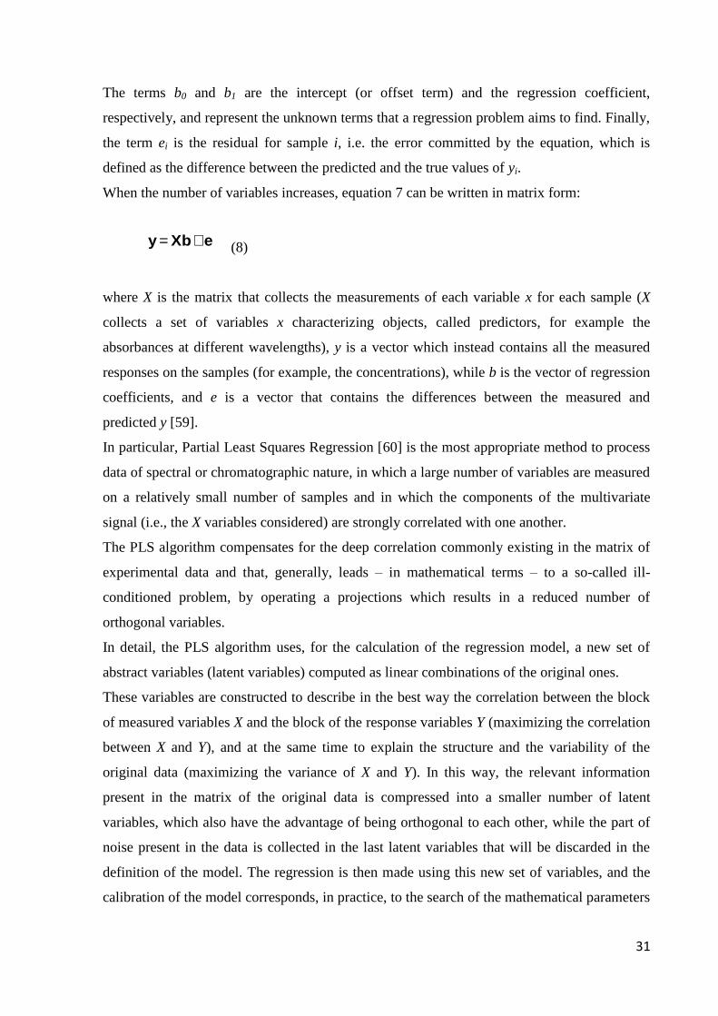
When the number of variables increases, equation 7 can be written in matrix form:
y = Xb+ e (8)
where X is the matrix that collects the measurements of each variable x for each sample (X
collects a set of variables x characterizing objects, called predictors, for example the
absorbances at different wavelengths), y is a vector which instead contains all the measured
responses on the samples (for example, the concentrations), while b is the vector of regression
coefficients, and e is a vector that contains the differences between the measured and
predicted y [59].
In particular, Partial Least Squares Regression [60] is the most appropriate method to process
data of spectral or chromatographic nature, in which a large number of variables are measured
on a relatively small number of samples and in which the components of the multivariate
signal (i.e., the X variables considered) are strongly correlated with one another.
The PLS algorithm compensates for the deep correlation commonly existing in the matrix of
experimental data and that, generally, leads – in mathematical terms – to a so-called ill-
conditioned problem, by operating a projections which results in a reduced number of
orthogonal variables.
In detail, the PLS algorithm uses, for the calculation of the regression model, a new set of
abstract variables (latent variables) computed as linear combinations of the original ones.
These variables are constructed to describe in the best way the correlation between the block
of measured variables X and the block of the response variables Y (maximizing the correlation
between X and Y), and at the same time to explain the structure and the variability of the
original data (maximizing the variance of X and Y). In this way, the relevant information
present in the matrix of the original data is compressed into a smaller number of latent
variables, which also have the advantage of being orthogonal to each other, while the part of
noise present in the data is collected in the last latent variables that will be discarded in the
definition of the model. The regression is then made using this new set of variables, and the
calibration of the model corresponds, in practice, to the search of the mathematical parameters
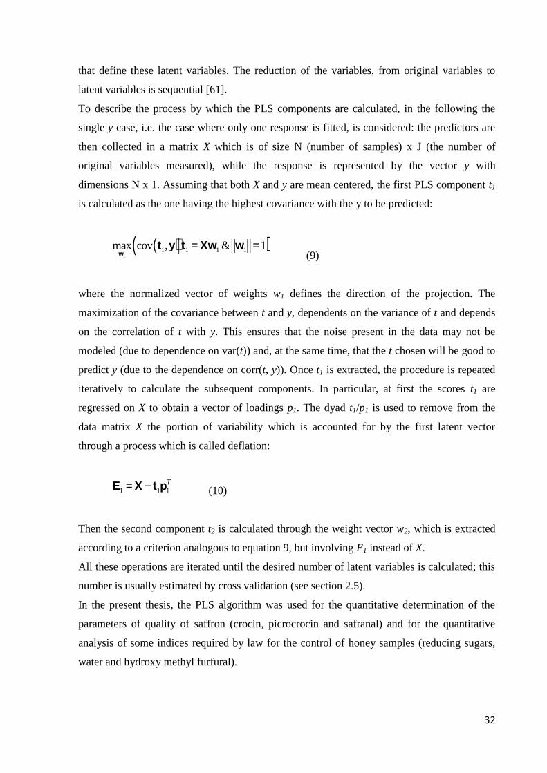
32
that define these latent variables. The reduction of the variables, from original variables to
latent variables is sequential [61].
To describe the process by which the PLS components are calculated, in the following the
single y case, i.e. the case where only one response is fitted, is considered: the predictors are
then collected in a matrix X which is of size N (number of samples) x J (the number of
original variables measured), while the response is represented by the vector y with
dimensions N x 1. Assuming that both X and y are mean centered, the first PLS component t1
is calculated as the one having the highest covariance with the y to be predicted:
max
w1
cov t1,y( ) t1 = Xw1 & w1 = 1( ) (9)
where the normalized vector of weights w1 defines the direction of the projection. The
maximization of the covariance between t and y, dependents on the variance of t and depends
on the correlation of t with y. This ensures that the noise present in the data may not be
modeled (due to dependence on var(t)) and, at the same time, that the t chosen will be good to
predict y (due to the dependence on corr(t, y)). Once t1 is extracted, the procedure is repeated
iteratively to calculate the subsequent components. In particular, at first the scores t1 are
regressed on X to obtain a vector of loadings p1. The dyad t1/p1 is used to remove from the
data matrix X the portion of variability which is accounted for by the first latent vector
through a process which is called deflation:
E1 = X - t1p1
T
(10)
Then the second component t2 is calculated through the weight vector w2, which is extracted
according to a criterion analogous to equation 9, but involving E1 instead of X.
All these operations are iterated until the desired number of latent variables is calculated; this
number is usually estimated by cross validation (see section 2.5).
In the present thesis, the PLS algorithm was used for the quantitative determination of the
parameters of quality of saffron (crocin, picrocrocin and safranal) and for the quantitative
analysis of some indices required by law for the control of honey samples (reducing sugars,
water and hydroxy methyl furfural).
33
2.3 MULTIVARIATE CLASSIFICATION: PARTIAL LEAST
SQUARES DISCRIMINANT ANALYSIS (PLS-DA)
The qualitative methods of multivariate analysis are commonly known as pattern recognition.
These techniques define the mathematical criteria that enable to quantify the similarity,
usually in terms of distance, between two different samples or between a sample and a class.
A class can thus be defined as a collection of objects that meet certain specific criteria
dependent on the problem at issue. In chemical terms, therefore, the recognition is made
according to the results of the measurements made on different samples.
The fundamental problem of pattern recognition can also be represented geometrically,
considering each pattern as a vector that describes a point in the hyperspace of variables,
namely in the multidimensional space whose n axes correspond to the experimental variables
monitored. In this way, each group of samples defines a set of points, a cluster. In this
context, the purpose of pattern recognition, therefore, is to separate the hyperspace in a series
of distinct and well-identified regions, in such a way that all the points that are located within
them belong to the same class [62]. Depending on whether these classes are known a priori or
not, it is possible to distinguish two different types of techniques: the first is called supervised
learning or classification methods, while the other unsupervised learning or clustering
methods. The term supervised highlights the use of a data set (training set), collected on
samples the classes of which are known in advance, in order to extrapolate a classification
rule. In many cases, to allow the evaluation of the real predictive capacity of the model
developed, a second data set, also made of samples of known attribution (test set), can be
used. Whenever a supervised learning strategy is adopted, it is possible to demonstrate that
the decision rule minimizing the prediction error is called Bayes‟ rule, according to which a
sample has to be assigned to the class it has the highest probability of belonging to.
From the applicative point of view, an important division which can be made is between
discriminant (or pure) classification methods and class-modeling ones.
Discriminant techniques mainly focus on the differences between samples from different
categories and divide the space of the variables in as many regions as there are classes: a
sample is always assigned to one and only one of those [63]. The probability that a sample
described by the vector x belongs to the class g - p(g|x) - can be calculated, on the basis of
Bayes' theorem, as the product of the probability of obtaining a vector of measurements x for
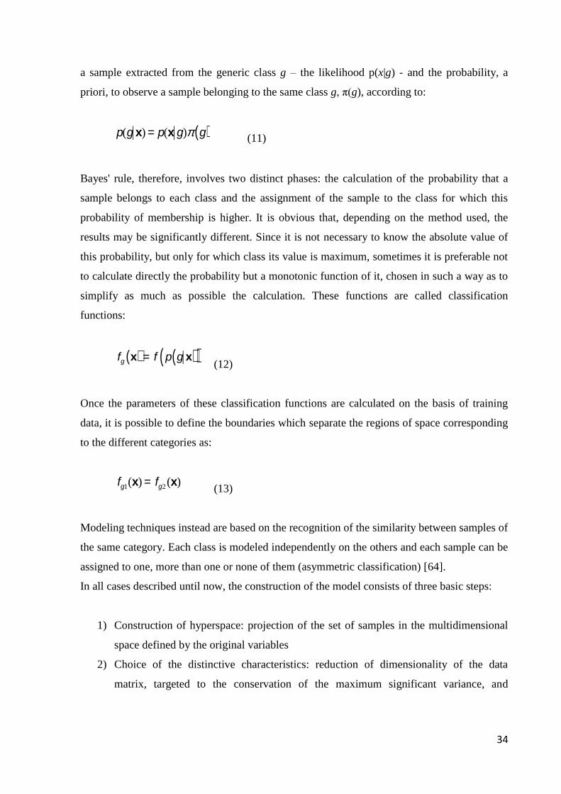
34
a sample extracted from the generic class g – the likelihood p(x|g) - and the probability, a
priori, to observe a sample belonging to the same class g, π(g), according to:
p(g x) = p(x g)p g( ) (11)
Bayes' rule, therefore, involves two distinct phases: the calculation of the probability that a
sample belongs to each class and the assignment of the sample to the class for which this
probability of membership is higher. It is obvious that, depending on the method used, the
results may be significantly different. Since it is not necessary to know the absolute value of
this probability, but only for which class its value is maximum, sometimes it is preferable not
to calculate directly the probability but a monotonic function of it, chosen in such a way as to
simplify as much as possible the calculation. These functions are called classification
functions:
fg x( ) = f p g x( )( )
(12)
Once the parameters of these classification functions are calculated on the basis of training
data, it is possible to define the boundaries which separate the regions of space corresponding
to the different categories as:
fg1(x) = fg2(x)
(13)
Modeling techniques instead are based on the recognition of the similarity between samples of
the same category. Each class is modeled independently on the others and each sample can be
assigned to one, more than one or none of them (asymmetric classification) [64].
In all cases described until now, the construction of the model consists of three basic steps:
1) Construction of hyperspace: projection of the set of samples in the multidimensional
space defined by the original variables
2) Choice of the distinctive characteristics: reduction of dimensionality of the data
matrix, targeted to the conservation of the maximum significant variance, and
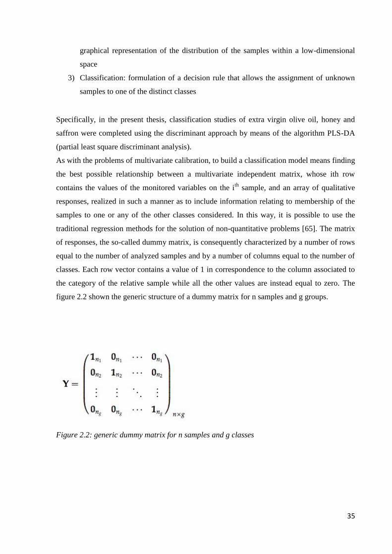
35
graphical representation of the distribution of the samples within a low-dimensional
space
3) Classification: formulation of a decision rule that allows the assignment of unknown
samples to one of the distinct classes
Specifically, in the present thesis, classification studies of extra virgin olive oil, honey and
saffron were completed using the discriminant approach by means of the algorithm PLS-DA
(partial least square discriminant analysis).
As with the problems of multivariate calibration, to build a classification model means finding
the best possible relationship between a multivariate independent matrix, whose ith row
contains the values of the monitored variables on the ith
sample, and an array of qualitative
responses, realized in such a manner as to include information relating to membership of the
samples to one or any of the other classes considered. In this way, it is possible to use the
traditional regression methods for the solution of non-quantitative problems [65]. The matrix
of responses, the so-called dummy matrix, is consequently characterized by a number of rows
equal to the number of analyzed samples and by a number of columns equal to the number of
classes. Each row vector contains a value of 1 in correspondence to the column associated to
the category of the relative sample while all the other values are instead equal to zero. The
figure 2.2 shown the generic structure of a dummy matrix for n samples and g groups.
Figure 2.2: generic dummy matrix for n samples and g classes
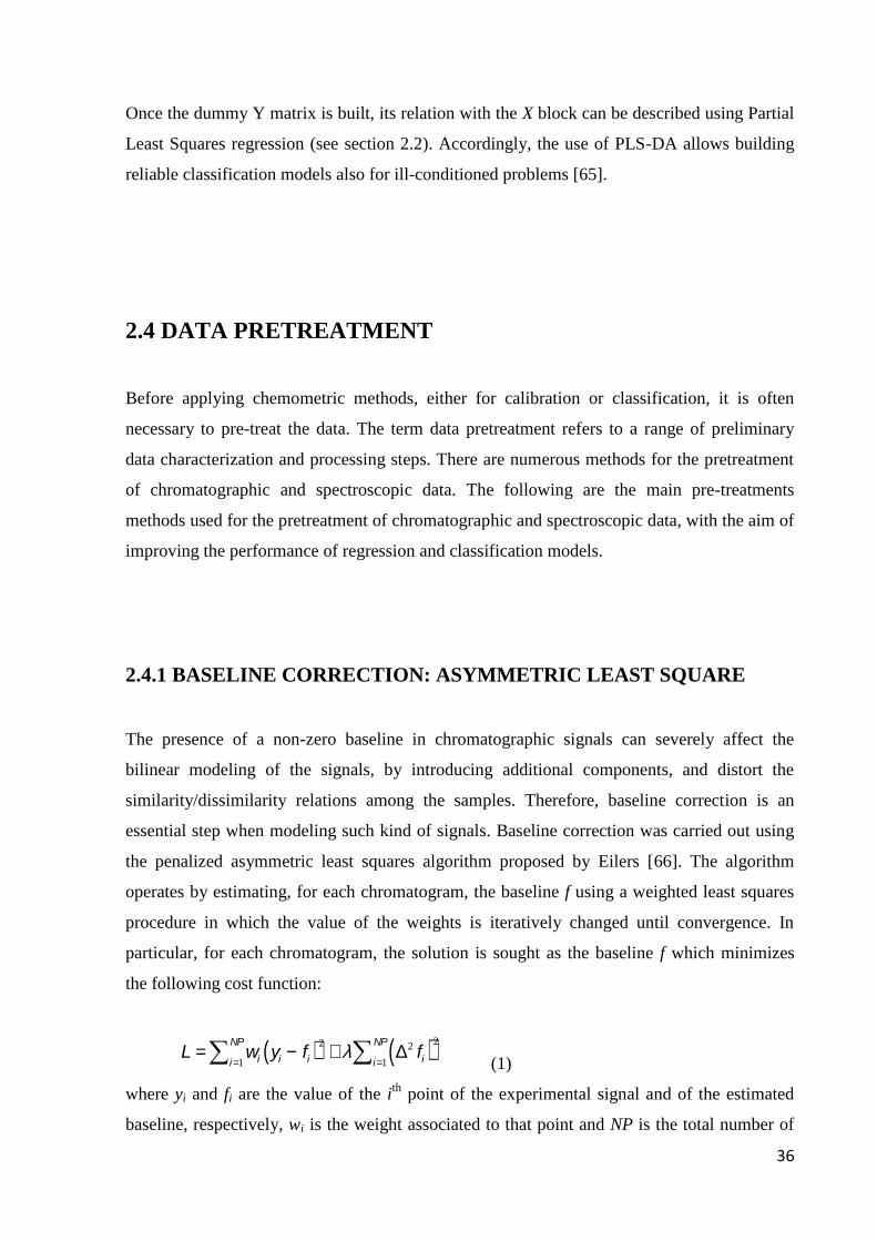
36
Once the dummy Y matrix is built, its relation with the X block can be described using Partial
Least Squares regression (see section 2.2). Accordingly, the use of PLS-DA allows building
reliable classification models also for ill-conditioned problems [65].
2.4 DATA PRETREATMENT
Before applying chemometric methods, either for calibration or classification, it is often
necessary to pre-treat the data. The term data pretreatment refers to a range of preliminary
data characterization and processing steps. There are numerous methods for the pretreatment
of chromatographic and spectroscopic data. The following are the main pre-treatments
methods used for the pretreatment of chromatographic and spectroscopic data, with the aim of
improving the performance of regression and classification models.
2.4.1 BASELINE CORRECTION: ASYMMETRIC LEAST SQUARE
The presence of a non-zero baseline in chromatographic signals can severely affect the
bilinear modeling of the signals, by introducing additional components, and distort the
similarity/dissimilarity relations among the samples. Therefore, baseline correction is an
essential step when modeling such kind of signals. Baseline correction was carried out using
the penalized asymmetric least squares algorithm proposed by Eilers [66]. The algorithm
operates by estimating, for each chromatogram, the baseline f using a weighted least squares
procedure in which the value of the weights is iteratively changed until convergence. In
particular, for each chromatogram, the solution is sought as the baseline f which minimizes
the following cost function:
L = wi yi - fi( )
2
i=1
NP
å + l D2 fi( )2
i=1
NP
å (1)
where yi and fi are the value of the ith
point of the experimental signal and of the estimated
baseline, respectively, wi is the weight associated to that point and NP is the total number of
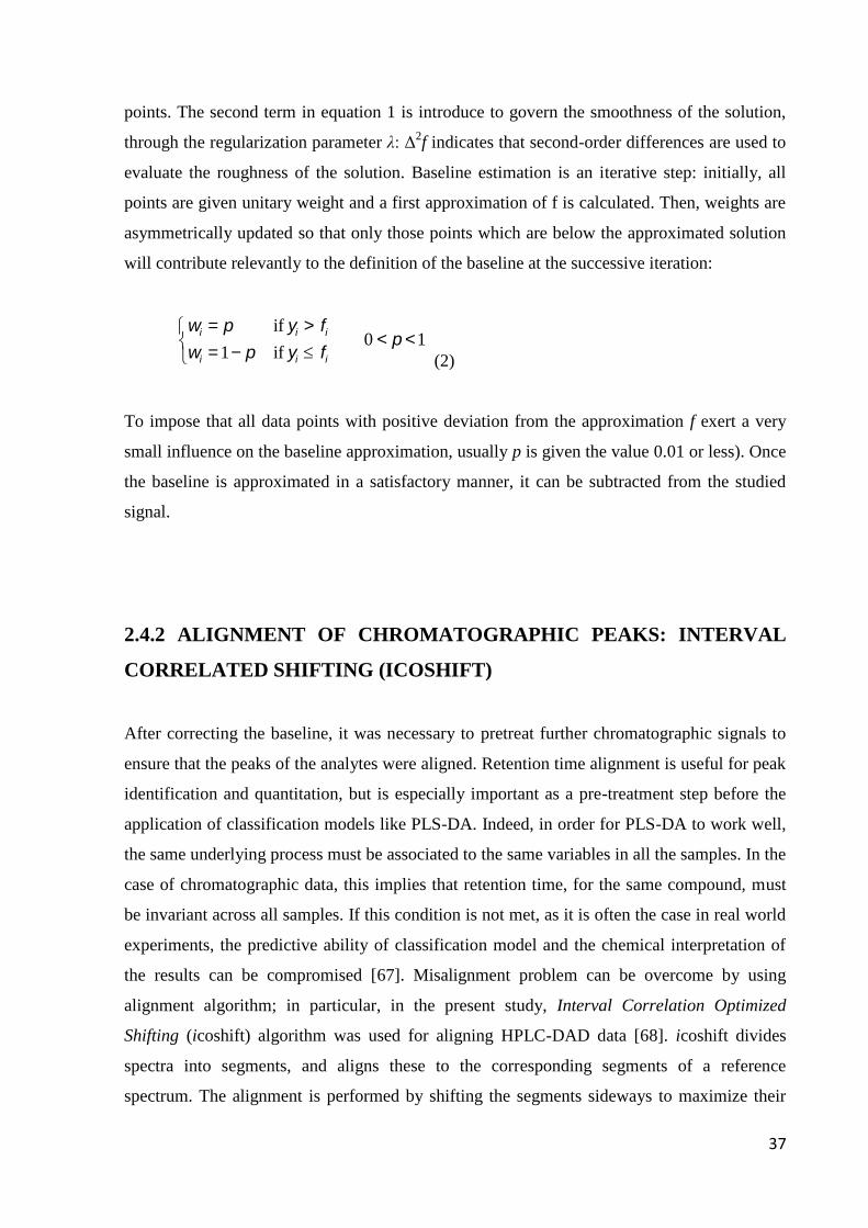
37
points. The second term in equation 1 is introduce to govern the smoothness of the solution,
through the regularization parameter λ: Δ2f indicates that second-order differences are used to
evaluate the roughness of the solution. Baseline estimation is an iterative step: initially, all
points are given unitary weight and a first approximation of f is calculated. Then, weights are
asymmetrically updated so that only those points which are below the approximated solution
will contribute relevantly to the definition of the baseline at the successive iteration:
wi = p if yi > fi
wi = 1- p if yi £ fi
ìíî
0 < p <1
(2)
To impose that all data points with positive deviation from the approximation f exert a very
small influence on the baseline approximation, usually p is given the value 0.01 or less). Once
the baseline is approximated in a satisfactory manner, it can be subtracted from the studied
signal.
2.4.2 ALIGNMENT OF CHROMATOGRAPHIC PEAKS: INTERVAL
CORRELATED SHIFTING (ICOSHIFT)
After correcting the baseline, it was necessary to pretreat further chromatographic signals to
ensure that the peaks of the analytes were aligned. Retention time alignment is useful for peak
identification and quantitation, but is especially important as a pre-treatment step before the
application of classification models like PLS-DA. Indeed, in order for PLS-DA to work well,
the same underlying process must be associated to the same variables in all the samples. In the
case of chromatographic data, this implies that retention time, for the same compound, must
be invariant across all samples. If this condition is not met, as it is often the case in real world
experiments, the predictive ability of classification model and the chemical interpretation of
the results can be compromised [67]. Misalignment problem can be overcome by using
alignment algorithm; in particular, in the present study, Interval Correlation Optimized
Shifting (icoshift) algorithm was used for aligning HPLC-DAD data [68]. icoshift divides
spectra into segments, and aligns these to the corresponding segments of a reference
spectrum. The alignment is performed by shifting the segments sideways to maximize their
38
correlation. In practice, this involves calculating the crosscorrelation between the segments by
a fast Fourier transform (FFT) engine that aligns all signals of a data set simultaneously.
2.4.3 VARIABLES SELECTION: BACKWARD INTERVAL PARTIAL
LEAST SQUARE (BiPLS)
PLS and PLS-DA algorithms were used for the construction of quantification and
classification models. Before constructing a model, in addition to the correction of the base
line and the alignment of the chromatographic peaks, it can be useful to reduce the number of
variables.
The predictive capability of a multivariate classification or regression model can be affected
by the presence of a large number of variables: not all the points that constitute the
instrumental profile carry relevant information, so that a selection of portions of the signal can
significantly improve the results. For this purpose, in the present thesis the technique
Backwards Interval PLS (Bi-PLS) coupled to Genetic Algorithms (GA) was used [69].
The BiPLS algorithm allows to calculate local PLS models using as predictors only variables
contained in equidistant intervals in the matrix X. In particular, in its backward
implementation, at every iteration, the calibration is carried out using a data matrix built by
eliminating from the entire instrumental profile the selected intervals. For each model, a cross
validation step, with a certain number of cancellation groups, is executed: the interval whose
elimination results in the minimum value of the RMSECV (see section 2.5) error, is the one
which is finally excluded before the algorithm proceeds with the next iteration. The routine is
thus interrupted once a minimum value of selected variables is reached. However, in many
practical cases, to avoid problems related to the possibility that a peak is divided between two
intervals, the entire procedure described is repeated by gradually increasing the number of
intervals up to a fixed maximum value. At the end of these repetitions the frequency of
selection of the variables is evaluated, on the basis of which the final set of variables to store
is defined [69].
39
2.4.4 VARIABLES SELECTION: GENETIC ALGORITHMS
To finalize the selection of variables, it is essential to apply to the data matrix, previously
reduced by biPLS, characteristic genetic algorithms (GA). The coupling between the two
procedures is necessary since, due to the enormous amount of monitored variables, it is not
possible to use only GA [70]. In particular, genetic algorithms constitute an optimization
method which is based on biological evolution. By analogy, any possible solution provided
for a specific problem is called chromosome, while each iteration of the computational
procedure is defined generation. More than one solution at a time is tested, so that in general
one speaks of a population of chromosomes. The aim of the application of genetic algorithms
is to evolve the population along several generations to find the best solution to the problem.
To determine the quality of these solutions, the concept of fitness, i.e. any mathematical
criterion that determines the goodness, is introduced. Usually, the fitness is defined as the
minimum error committed by the model during cross-validation. As this problem concerns the
selection of the variables, each chromosome will correspond to a binary vector of length equal
to the number of points that constitute the whole signal and will contain zeros in the positions
of the variables to not be selected and ones elsewhere. The algorithm is initialized by
generating at random a number of possible solutions, or of groups of variables: these variables
are then used to build the corresponding regression or classification models, and the relative
error in cross validation is calculated. Once the chromosomes are sorted in descending order
of fitness, the algorithm proceeds by using two different operators, crossover and mutation,
which allow at the same time the exploitation of the “genetic” material in the actual
population and the exploration of new possible solutions.
In particular, the crossover modifies the structure of two chromosomes selected operating an
exchange in blocks between their internal values. The mutation, instead, operates by inverting
the values of each position of the chromosome with a probability equal to 0.1%.
Consequently, for each iteration two new chromosomes will be built, the quality of which
should then be evaluated. The solutions that are characterized by a better fitness compared to
those present in population at that particular generation will replace the worst ones [71].
The entire procedure is then repeated for a fixed number of generations, the end of which, the
chromosome, or the group of variables, corresponding to the higher fitness is selected as the
best. To ensure high consistency of results, generally, a genetic algorithm is not applied only
once to a matrix of data, but for a sufficiently large number of times, equal to 100 in our case,
40
so that, in the end, one will include in the final model only the variables most frequently
selected.
2.5 VALIDATION OF CHEMOMETRIC METHODS
The validation of the developed models, for the study of multivariate classification or
quantification, is of uttermost importance for the evaluation of the reliability of their
performances. To this purpose, there are different techniques useful for the control and the
determination of the quality of the results obtained by chemometric analysis, which differ
according to the type of problem in exam and samples available. More generically, the
validation procedures are to be able to provide information of two kinds: in fact they allow to
obtain both indications on how to maximize the sensitivity of the model and its effective
capacity to characterize unknown samples, confirming the reliability and ensuring that their
solutions are generalizable [72].
The increase in the quality of a chemometric model depends on the possibility to minimize the
error in the prediction of a certain type of response, which for the ith
sample can be
determined according to the following equation:
ei = yi - yi (14)
where ŷi and yi represent the value of the response predicted by the built model and its
reference value, respectively. However, in sets of samples very different from one another, a
common situation in the case of multivariate calibration and classification, it is not much
important reducing the prediction error on the individual object, but rather the average error
made on the totality of the validation group (test set). This error is defined RMSEP, Root
Mean Square Error of Prediction; if nnew samples, different than those used for model
construction, are used to validate the model, RMSEP is calculated as:
RMSEP =ep
Tep
nnew (15)
41
where ep is a vector containing the differences between the reference and the predicted values
for all the test set samples.
Similarly, it is possible to determine the error of the model in the calibration phase, the
RMSEC, Root Mean Square Error of Calibration, according to the following equation:
RMSEC =ec
Tec
n- df (16)
In this case, ec is formed by the residuals associated with the n samples on the basis of which
the model has been realized, while df is equal to the number of degrees of freedom lost in the
estimation of its parameters. In addition to the classical procedure of external validation, it is
possible perform a kind of systematic resampling of all available data for subsequent
evaluation of different sets, this operation is called cross-validation. It acts by splitting the set
of samples available in a number k of so-called cancellation groups. Iteratively, each of these
sets is not included in the calibration phase and it is used as a validation set. In total, therefore,
k different models will be constructed, so that eventually the RMSECV, Root Mean Square
Error of Cross Validation, is evaluated as:
RMSECV =yi - yi ,cv( )
2
i=1
n
ån- df (17)
where and
yi ,cv are the reference value of the response for the ith sample and its predicted
value from the model built when the sample is left out in one of the k cancellation groups,
respectively, while the other terms have the same meaning as in equation 17.
Generally, while external (test set) validation is used to evaluate the predictive ability of the
models, cross-validation is employed to estimate the optimal model complexity, i.e. the
number of components needed for the construction of the best model [73].
42
CHAPTER 3
EXTRA VIRGIN OLIVE OIL:
GEOGRAPHICAL TRACEABILITY
OF SABINA PDO
3.1 INTRODUCTION
In recent years, the issues of food quality and safety have received a special attention both
from the producers and the consumers [74-77]. In this context, a key role is played by the
identification, authentication and traceability of foodstuff [78-80]. In particular, while the
former terms indicate, in general, to what extent the products comply to what declared on the
label and to the law, the latter concentrates on the ability to track any food through all stages
of production, processing and distribution. Based on this definition, it is evident how the
possibility of well-enacted food traceability protocols could on one hand represent an
effective way of managing the risks connected to foods and feeds, for instance by allowing to
quickly isolate contaminated products and prevent them from reaching consumers, or guiding
targeted withdrawals when needed. On the other hand, since the largest share of traceability
issues is related to the verification of the geographic, species or production origin of the
goods, it can also represent a solid ground to protect local and/or regional foods, to help
producers obtain a proper price for their authentic products, and to avoid the unfair market
43
competition by products, which may be of inferior quality. In the framework of the European
Union, this necessity of protecting and promoting the names of traditional, regional and
quality foodstuff has been enforced through the introduction of the geographical indication
marks: protected designation of origin (PDO), protected geographical indication (PGI), and
traditional specialties guaranteed (STG) [81,82]. In particular, the attribution of a
geographical indication mark certifies that the quality of the foodstuff is significantly or
exclusively determined by its geographical environment, including natural and human factors,
and that its production, processing and preparation took place within the determined
geographical area [83].
Extra virgin olive oil (EVOO), due to its chemical composition and characteristics, in
particular its nutritional and biological properties [84,85], represents a high quality and value-
added product, whose price can be even 6-7 times higher than that of other edible vegetable
oils. Given the specificities of its production, EVOO is one of the foods whose quality is most
closely related to the terroir, i.e. “the set of special characteristics that the geography, geology
and climate of a certain place, interacting with the plant's genetics, express in agricultural
products” [86], and consequently already many oils from different European countries
(mainly Italy, Spain, Greece, France and Portugal) are protected by the PDO mark. Among
these, Sabina EVOO is the first Italian oil to have gained the PDO status, in 1996 [87]. It is
produced in the homonymous territory in the Lazio region, which is part of the provinces of
Rome and Rieti and owes its name to the fact that this area was originally occupied by the
ancient Sabines tribe; indeed, Sabina has been an oil producing region since 7th
-6th
century
B.C. Nowadays, the production disciplinary for the PDO [88] provides that Sabina oil should
be made from the following olive varieties, either combined or singularly: “Raja”, “Leccino”,
“Frantoio”, “Carboncella”, “Pendolino”, “Olivastrone”, “Salviana”, “Rosciola”, “Olivago”
and “Moraiolo”. Its sensory characteristics are defined as: golden yellow color, with greenish
tinges when very fresh, fruity aroma and smooth, even, fruity, fragrant, sweet, flavors, bitter
when very fresh. As a consequence of their provenance and of the reported organoleptic
characteristics, Sabina PDO oils are considered high quality products and due to their higher
market price can be subjected to frauds, such as the addition of cheap oils and/or the
marketing of oils from other regions under the same name. However, from the quality control
standpoint, the traceability system enacted so far by the European authorities operates mainly
a priori, defining in detail the percentages of specified cultivar olives, cultural practices,
circumscribed geographical production areas, chemical and sensorial properties needed to
obtain the PDO label in the production disciplinary, and relying only on the inspection of the
44
production registries for the verification of the authenticity of the products. On the other hand,
at present no analytical indices exist which could be measured on the final product, allowing,
a posteriori, to distinguish it from other oils of lesser value. Accordingly, the possibility of
building traceability models by coupling chemometric classification methods to the analytical
characterization of the products (often by fingerprinting techniques) is becoming more and
more fundamental for the verification of the authenticity of foods with geographical
indication marks [89-94]. In this framework, variations in the phenolic composition of virgin
olive oils related to cultivars, ripening and production techniques were already reported in the
literature [95-97], suggesting that the chromatographic fingerprinting of this fraction could be
a valuable tool for tracing the origin of the product. On the other hand, considering the
increasing attention to the potential health benefits associated to different classes of
biophenols (for instance, prevention against cardiovascular diseases, immunoregulation
diseases, or asthma [98-100]), the possibility of relating the higher quality of the product to
the phenolic composition would be of utmost importance for its characterization. Therefore,
aim of the present study was to verify the potential of using the chromatographic
fingerprinting of the phenolic fraction coupled to chemometric data processing for the
authentication of the PDO Sabina oils. To this purpose, at first Partial Least Square-
Discriminant Analysis (PLS-DA) was used to process the chromatographic profiles recorded
at three selected wavelengths (254, 280 and 340nm), while in a second stage, mid-level data
fusion was used to integrate portions of the signals at the different wavelengths, selected by a
successive application of backwards interval Partial Least Squares (biPLS) and genetic
algorithms (GA), in order to achieve better classification performances and easier
interpretability.
3.2 MATERIALS AND METHODS
3.2.1 SAMPLES
Sabina samples (20 oils) were all taken from different oil mills in various place of the region,
covering as representatively as possible the whole production area in terms of geographical
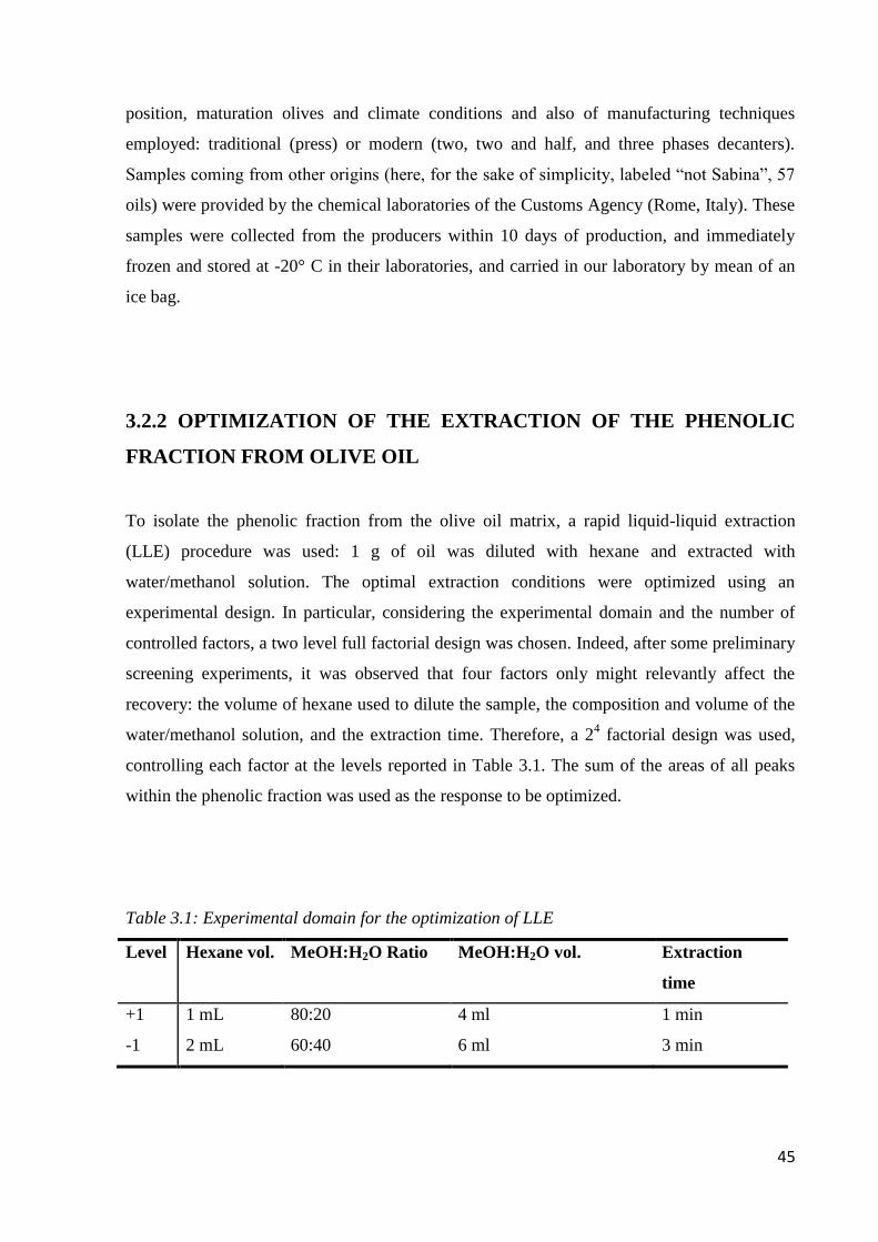
45
position, maturation olives and climate conditions and also of manufacturing techniques
employed: traditional (press) or modern (two, two and half, and three phases decanters).
Samples coming from other origins (here, for the sake of simplicity, labeled “not Sabina”, 57
oils) were provided by the chemical laboratories of the Customs Agency (Rome, Italy). These
samples were collected from the producers within 10 days of production, and immediately
frozen and stored at -20° C in their laboratories, and carried in our laboratory by mean of an
ice bag.
3.2.2 OPTIMIZATION OF THE EXTRACTION OF THE PHENOLIC
FRACTION FROM OLIVE OIL
To isolate the phenolic fraction from the olive oil matrix, a rapid liquid-liquid extraction
(LLE) procedure was used: 1 g of oil was diluted with hexane and extracted with
water/methanol solution. The optimal extraction conditions were optimized using an
experimental design. In particular, considering the experimental domain and the number of
controlled factors, a two level full factorial design was chosen. Indeed, after some preliminary
screening experiments, it was observed that four factors only might relevantly affect the
recovery: the volume of hexane used to dilute the sample, the composition and volume of the
water/methanol solution, and the extraction time. Therefore, a 24 factorial design was used,
controlling each factor at the levels reported in Table 3.1. The sum of the areas of all peaks
within the phenolic fraction was used as the response to be optimized.
Table 3.1: Experimental domain for the optimization of LLE
Level Hexane vol. MeOH:H2O Ratio MeOH:H2O vol. Extraction
time
+1 1 mL 80:20 4 ml 1 min
-1 2 mL 60:40 6 ml 3 min
46
When analyzing the results, none of the interaction terms and only two of the main effects
resulted to be significant: the composition of the water/methanol solution and the extraction
time, their optimal values being MeOH/H2O 80:20 v/v and 3 min, respectively. Since the
effect of the other two factors was shown to be not statistically relevant, their values were
fixed at the level which resulted more advantageous in terms of rapidity and costs (1 mL
hexane and 4 mL hydroalcoholic solution, respectively). Accordingly, the final extraction
procedure resulted to be the following: 1 g of olive oil was diluted with 1mL of hexane and
then extracted with 4mL MeOH:H2O 80:20 v/v for 3 minutes. Then, the hydroalcoholic
extract containing the analytes was filtered and evaporated to dryness in rotavapor at 30 °C;
the residue was dissolved in 200 µL of MeOH:H2O (50:50, v/v) and 20µL of the solution
were injected into the HPLC. This extraction showed a good reproducibility (RSD < 5%), and
it was used for the analysis of all EVOO samples.
3.2.3 HPLC-DAD ANALYSIS OF THE PHENOLIC FRACTION
For the chromatographic analysis of olive oil samples, biochanin A was used as internal
standard (10 µg/g olive oil). The extracts prepared according to what described in section
3.2.2 were analyzed by HPLC-DAD with a Thermo Quest Spectrasistem LC (Thermo Fisher
Scientific, Waltham, MA) equipped with a P4000 pump, a UV6000 UV-Vis Diode Array
Detector, and a SN4000 interface to be operated via a personal computer. Extracted
compounds were separated using an Eclipse XDB-C18 analytical column (4.6x250mm, 5µm
particle size; Agilent Technologies, Santa Clara, CA) protected by a guard cartridge of the
same packing, operating at 25° C. The mobile phase consisted of a binary solvent system
using water (solvent A) and methanol (solvent B) both acidified with 0,1% formic acid kept at
a flow rate of 0.8 mL/min. The gradient program started with 90% eluent A and 10% eluent
B. This percentage was maintained for 5 minutes and eluent B was ramped linearly to 20% in
5 min and kept constant for 10 min; eluent B was ramped again linearly to 30% at 30 min and
to 70% at 45 min. The chromatographic profiles were collected at 254, 280 and 340 nm.
47
3.2.4 IDENTIFICATION OF POTENTIAL PDO MARKERS BY
HPLC/ESI-MS
For the qualitative analysis and, in particular, to identify which compound could be most
significant for characterizing the PDO Sabina, HPLC/ESI-MS analysis was carried out. In
particular, selected portions of the eluate from the HPLC-DAD system were sampled at the
detector, evaporated to dryness under N2, dissolved in 50μL of MeOH and injected into the
HPLC/ESI-MS system. In particular, a Perkin-Elmer series 200 (Norwalk, CT, USA) liquid
chromatograph, equipped with a binary pump and a vacuum degasser was used. Electrospray
ionization tandem mass spectrometry (ESI-MS/MS) was conducted using a QTRAPTM
quadrupole linear ion trap (QLIT) instrument equipped with a TurboIon-Spray (TISP)
interface (Applied Biosystems/MDS Sciex, Concord, ON, Canada) operated in positive and
negative ion modes. The whole apparatus was controlled by Analyst software (Applied
Biosystems/MDS Sciex). The chromatographic column was an Alltima-C18 (2.1x250mm,
5µm particle size; Alltech, Deerfield, IL, USA). The mobile phase and gradient program were
the same described for HPLC-DAD analysis (section 3.2.3) while flow rate was 200µL/min.
Each sample was analyzed twice, once in positive ionization mode and once in negative
ionization mode in the ranges 100-850 m/z (MS) and 90-850 m/z (MS/MS) using an
information-dependent data acquisition (IDA) protocol.
3.2.5 SIGNAL PRE-PROCESSING
Since chromatographic signals could be affected by unwanted sources of variability, which
could result in baseline contributions and shifts in the position of peak maxima, prior to the
classification analysis a data preprocessing step was carried out. Baseline correction and peak
alignment are essential steps, and in this study they were carried out using the penalized
asymmetric least squares algorithm and interval correlation optimized shifting (icoshift)
algorithm (described in the previous chapter, Sections 2.4.1 and 2.4.2)
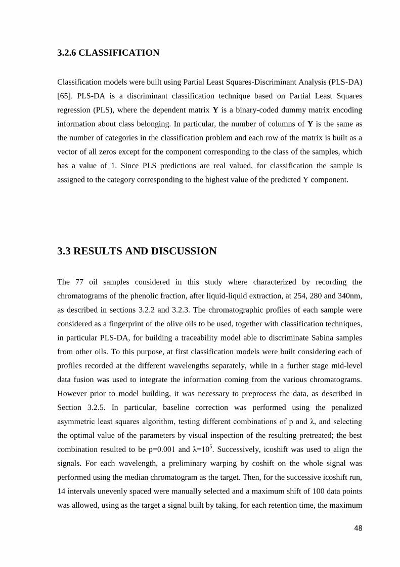
48
3.2.6 CLASSIFICATION
Classification models were built using Partial Least Squares-Discriminant Analysis (PLS-DA)
[65]. PLS-DA is a discriminant classification technique based on Partial Least Squares
regression (PLS), where the dependent matrix Y is a binary-coded dummy matrix encoding
information about class belonging. In particular, the number of columns of Y is the same as
the number of categories in the classification problem and each row of the matrix is built as a
vector of all zeros except for the component corresponding to the class of the samples, which
has a value of 1. Since PLS predictions are real valued, for classification the sample is
assigned to the category corresponding to the highest value of the predicted Y component.
3.3 RESULTS AND DISCUSSION
The 77 oil samples considered in this study where characterized by recording the
chromatograms of the phenolic fraction, after liquid-liquid extraction, at 254, 280 and 340nm,
as described in sections 3.2.2 and 3.2.3. The chromatographic profiles of each sample were
considered as a fingerprint of the olive oils to be used, together with classification techniques,
in particular PLS-DA, for building a traceability model able to discriminate Sabina samples
from other oils. To this purpose, at first classification models were built considering each of
profiles recorded at the different wavelengths separately, while in a further stage mid-level
data fusion was used to integrate the information coming from the various chromatograms.
However prior to model building, it was necessary to preprocess the data, as described in
Section 3.2.5. In particular, baseline correction was performed using the penalized
asymmetric least squares algorithm, testing different combinations of p and λ, and selecting
the optimal value of the parameters by visual inspection of the resulting pretreated; the best
combination resulted to be p=0.001 and λ=105. Successively, icoshift was used to align the
signals. For each wavelength, a preliminary warping by coshift on the whole signal was
performed using the median chromatogram as the target. Then, for the successive icoshift run,
14 intervals unevenly spaced were manually selected and a maximum shift of 100 data points
was allowed, using as the target a signal built by taking, for each retention time, the maximum
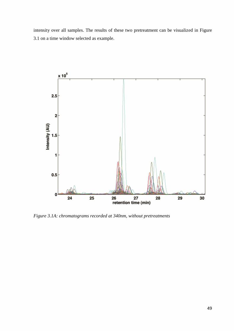
49
intensity over all samples. The results of these two pretreatment can be visualized in Figure
3.1 on a time window selected as example.
Figure 3.1A: chromatograms recorded at 340nm, without pretreatments
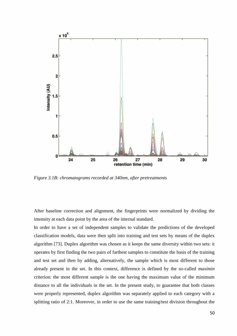
50
Figure 3.1B: chromatograms recorded at 340nm, after pretreatments
After baseline correction and alignment, the fingerprints were normalized by dividing the
intensity at each data point by the area of the internal standard.
In order to have a set of independent samples to validate the predictions of the developed
classification models, data were then split into training and test sets by means of the duplex
algorithm [73]. Duplex algorithm was chosen as it keeps the same diversity within two sets: it
operates by first finding the two pairs of farthest samples to constitute the basis of the training
and test set and then by adding, alternatively, the sample which is most different to those
already present in the set. In this context, difference is defined by the so-called maximin
criterion: the most different sample is the one having the maximum value of the minimum
distance to all the individuals in the set. In the present study, to guarantee that both classes
were properly represented, duplex algorithm was separately applied to each category with a
splitting ratio of 2:1. Moreover, in order to use the same training/test division throughout the
51
study, the selection algorithm was operated on a matrix obtained by concatenating the scores
along the significant principal components extracted from the three data set corresponding to
the signals at 254, 280 and 340 nm. Accordingly, 50 samples (13 from Sabina and 37 from
other origins were selected as training set and the remaining 27 (7 from Sabina and 20 from
other origins) left out as external validation set.
3.3.1 PLS-DA ANALYSIS ON INDIVIDUAL DATA MATRICES
At first separate PLS-DA models were built on the individual data matrices containing the
chromatographic profiles recorded at 254, 280 and 340 nm, after mean centering. Selection of
the optimal complexity of the latent variable models was made on the basis of the minimum
classification error in 5-fold cross-validation. The results obtained are reported in Table 3.2.
Table 3.2: Results of PLS-DA modeling on individual data sets without variable selection
Wavelength LVs %Correct Class.
Calibration
%Correct Class.
CV
%Correct Class.
Prediction
Sabina Not Sabina Sabina Not Sabina Sabina Not Sabina
254nm 4 92,3% 89,2% 84,6% 75,7% 71,4% 75,0%
280nm 3 92,3% 81,1% 84,6% 78,4% 57,1% 75,0%
340nm 3 84,6% 83,8% 80,4% 83,1% 57,1% 85,0%
It can be observed from the Table that in all cases rather parsimonious models are obtained,
and that in general a rather good classification ability is observed both in calibration and
cross-validation. However, when the trained model are applied on the external test set, the
performances are significantly worse, especially for the class Sabina. Based on these results,
in order to improve the classification ability of the models, by including only those parts of
the signal carrying the discriminant information, variable selection was carried out by means

52
of a sequential application of backward interval-PLS and genetic algorithms (biPLS-GA)
[69]. The biPLS step, indeed, allows to operate a preliminary variable reduction, so that the
genetic algorithm can operate of a number of predictors which is low enough (usually <250)
to minimize the risk of overfitting. In detail, biPLS was algorithm was run 21 times, changing
the interval size at each iteration (each of the data matrices, after autoscaling was divided in a
number of intervals ranging from 25 to 45) and the predictors most frequently selected over
the runs, were pooled to constitute the data set on which GA variable reduction was operated.
Leardi‟s hybrid GA [101] was used with a population of 30 chromosomes and probabilities of
cross-over and mutation of 0.5 and 0.01 respectively, on autoscaled data. Classification error
in 5-fold cross-validation was used as the fitness function and the optimal number of
evaluations was chosen on the basis of randomization tests, as the one minimizing the risk of
selecting irrelevant variables and overfitting [101]. The results of PLS-DA analysis after
variable selection are reported in Table 3.3.
Table 3.3: Results of PLS-DA modeling on individual data sets after variable selection by
biPLS-GA
Wavelength LVs %Correct Class.
Calibration
%Correct Class.
CV
%Correct Class.
Prediction
Sabina Not
Sabina
Sabina Other
origin
Sabina
DOP
Sabina
254nm 4 92,3% 91,1% 84,9% 75,7% 85,7% 77,0%
280nm 3 92,1% 86,5% 88,5% 85,0% 85,7% 85,0%
340nm 3 92,3% 91,9% 83,5% 85,0% 85,7% 85,0%
It can be seen from the Table that variable selection significantly improved the classification
ability of the models, especially for the class Sabina, which is the one of interest. Moreover,
better results are obtained on the data sets at 280 and 340 nm with respect to the one at 254
nm, as it could be expected, since the signals at higher wavelengths are more selective and
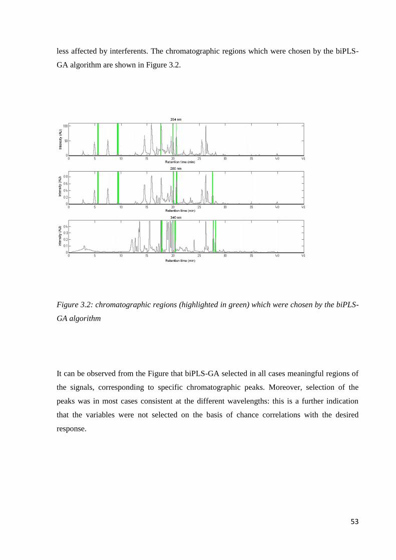
53
less affected by interferents. The chromatographic regions which were chosen by the biPLS-
GA algorithm are shown in Figure 3.2.
Figure 3.2: chromatographic regions (highlighted in green) which were chosen by the biPLS-
GA algorithm
It can be observed from the Figure that biPLS-GA selected in all cases meaningful regions of
the signals, corresponding to specific chromatographic peaks. Moreover, selection of the
peaks was in most cases consistent at the different wavelengths: this is a further indication
that the variables were not selected on the basis of chance correlations with the desired
response.
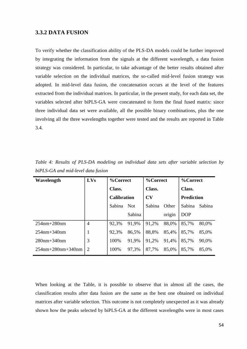
54
3.3.2 DATA FUSION
To verify whether the classification ability of the PLS-DA models could be further improved
by integrating the information from the signals at the different wavelength, a data fusion
strategy was considered. In particular, to take advantage of the better results obtained after
variable selection on the individual matrices, the so-called mid-level fusion strategy was
adopted. In mid-level data fusion, the concatenation occurs at the level of the features
extracted from the individual matrices. In particular, in the present study, for each data set, the
variables selected after biPLS-GA were concatenated to form the final fused matrix: since
three individual data set were available, all the possible binary combinations, plus the one
involving all the three wavelengths together were tested and the results are reported in Table
3.4.
Table 4: Results of PLS-DA modeling on individual data sets after variable selection by
biPLS-GA and mid-level data fusion
Wavelength LVs %Correct
Class.
Calibration
%Correct
Class.
CV
%Correct
Class.
Prediction
Sabina Not
Sabina
Sabina Other
origin
Sabina
DOP
Sabina
254nm+280nm 4 92,3% 91,9% 91,2% 88,0% 85,7% 80,0%
254nm+340nm 1 92,3% 86,5% 88,8% 85,4% 85,7% 85,0%
280nm+340nm 3 100% 91,9% 91,2% 91,4% 85,7% 90,0%
254nm+280nm+340nm 2 100% 97,3% 87,7% 85,0% 85,7% 85,0%
When looking at the Table, it is possible to observe that in almost all the cases, the
classification results after data fusion are the same as the best one obtained on individual
matrices after variable selection. This outcome is not completely unexpected as it was already
shown how the peaks selected by biPLS-GA at the different wavelengths were in most cases
55
the same, and so the selected features which were fused carry almost identical information.
The only exception was the data set resulting from the fusion of the variables selected at 280
nm and 340 nm, which allow to improve the sensitivity of the models, as the correct
classification rate for the not Sabina oils increased to 90%.
3.3.3 IDENTIFICATION OF POTENTIAL TRACEABILITY MARKERS
FOR THE PDO SABINA
To interpret the results obtained after variable selection in terms of chemical species which
could carry a discriminant information and, hence, which could be used as traceability
markers for the PDO Sabina, HPLC/ESI-MS analysis was carried out, as described in Section
3.2.4. The analytes corresponding to the peaks selected by biPLS-GA were identified by
tandem MS either in positive or negative mode and they are listed in Table 3.5.

56
Table 3.5: Compounds identified by HPLC/ESI-MS
Retention
time
Compound Ion
modea
m/z Fragmentsb
Identificationc
5.4 vanillic acid negative 167.1 108.0(100);151.8(10) A
9.1 p-coumaric acid negative 163.1 119.1(100);167.1(27);
91.1(13)
A
18.2 luteolin negative 285.2 133.2(100);107.2(20);
151.2(17)
A
19.9 pinoresinol positive 359.1 359.1(100);327.1(10) A
21.0 acetoxypinoresinol positive 417.4 417.4(100);358.4(10) B
26.8 apigenin negative 269.0 117.0(100);107.0(17);
151.0(12)
A
27.9 methoxyluteolin negative 299.4 299.4(100);199.4(25);
191.4(20)
B
a collision energy was 25eV for negative ion mode and 30eV for positive ion mode;
b the relative abundances are shown in brackets;
c identification was based on: (A) retention time and MS data consistent with those of
authentic standard; (B) MS data consistent with literature.
3.4. CONCLUSIONS
The results obtained in the present study suggest that the phenolic composition of olive oils
can constitute a reliable basis to discriminate PDO oils, when coupled to chemometric
classification techniques. In particular, it was shown that by selecting specific portions of the
chromatograms recorded at 280 nm or 340 nm, it was possible to correctly classify about 85%
of samples in external validation. Moreover, when the information from these two
wavelengths was combined through a mid-level data fusion strategy, the specificity of Sabina
with respect to the oil of the other origin raised to 90%. The use of variable selection
strategies, together with improving the correct classification rate of the models, allowed also
to identify a reduced set of predictors carrying the greatest part of the discriminant

57
information, which could then be thought of as a potential traceability markers for the PDO
Sabina. Identification of these analytes by HPLS-MS analysis showed that the substances
which contributed the most to the discrimination of Sabina PDO from other oils are all
phenols of high nutritional and biological value: vanillic acid, p-coumaric acid, luteolin,
pinoresinol, acetoxypinoresinol, apigenin, methoxyluteolin.
58
CHAPTER 4
HONEY: GEOGRAPHICAL AND
BOTANICAL TRACEABILITY
4.1 INTRODUCTION
Honey is a food consumed all over the world and appreciated as a quick source of energy, but
also for its antibacterial and antioxidant activity. Commercially there are both mono-floral
honeys (mainly made from a single botanical species) and polyfloral honeys (obtained from
different plant species). Each one has its own composition and organoleptic characteristics
derived from the type of flora worked by bees that make the honey undoubtedly a product
linked to the area of production.
Honey is a food often adulterated; moreover, differences in price and quality are present
between honeys of European countries, China or South America, but there are also differences
between honeys of the various European countries or even between regions within the same
country. The European Union Commission is encouraging the development of new analytical
methods for monitoring and verifying the quality of the different honeys and for identifying
their geographical origin. The product label must show the country or countries of origin
where the honey has been produced. When the honey originates in more Member States or
third country the indication may be replaced by one of the following sentences: "blend of CE
honeys", "blend of non-CE honeys 'or' blend of honeys not originating in the CE". In addition,
59
the botanical origin of honey must also be indicated on the label, so it must be declared
whether a honey is polyfloral or it is obtained from a specific species of plant.
The method that is currently used in the determination of the botanical origin of honey,
consists of the pollen analysis (melissopalynological analysis), because the pollen reflects the
type of vegetation from which nectars were collected. This analysis presents some limitations,
since a good knowledge of the morphology of pollen and qualified staff are needed.
Moreover, due to the limited amount of pollen present in the samples, usually it takes a long
time to perform the analysis.
This work has as purpose to classify the honeys, both on the basis of botanical origin and in
terms of geographical origin. Analyses of the phenolic fraction present in honey were
conducted by HPLC-DAD. The honey samples were also analyzed by NIR spectroscopy and
the classification method Partial least squares-discriminant analysis (PLS-DA) was applied to
both the chromatographic and the spectroscopic data.
In particular, aim of the present project was to develop a reliable method to characterize the
floral origin of honeys produced in the same geographical area (in order to avoid problems
related to geographical variability), and which could constitute a valid alternative to pollen
analysis. As said, at the same time, a similar approach was followed, to discriminate the
geographical origin of polyfloral honey. The methods developed are easy, quick and
objective, not relying on the subjective interpretation of the analyst as instead happens for the
melissopalynological analysis.
HPLC-DAD analysis of the polyphenol content present in honey was chosen for instrumental
fingerprinting because it is strongly linked to the geographical and floral origin of the
foodstuff, and to the climatic characteristics of the local production [102-105]. The literature
describes numerous analytical methods developed to test the authenticity of honey, in
particular with respect to the declared geographical and floral origins [106-108]. However, a
simple and effective procedure has not yet been identified which, individually, is sufficient to
the evaluation of the "complex" characteristics of a honey, such as its geographical or floral
origin or, more generally, its belonging to a particular denomination of origin.
The polyphenol content could be a significant "discriminating" factor in order to establish a
standard method (currently absent) for the analytical control of the geographic and floral
origin of honey. In fact, from the literature, phenolic compounds appear to be an important
quality parameter which gives the product added value and it also justifies the different cost of
sales [109]; in addition, observing the differences in the quantitative composition of phenolic
compounds (i.e. the fingerprint of the whole phenolic fraction) may be more useful for the
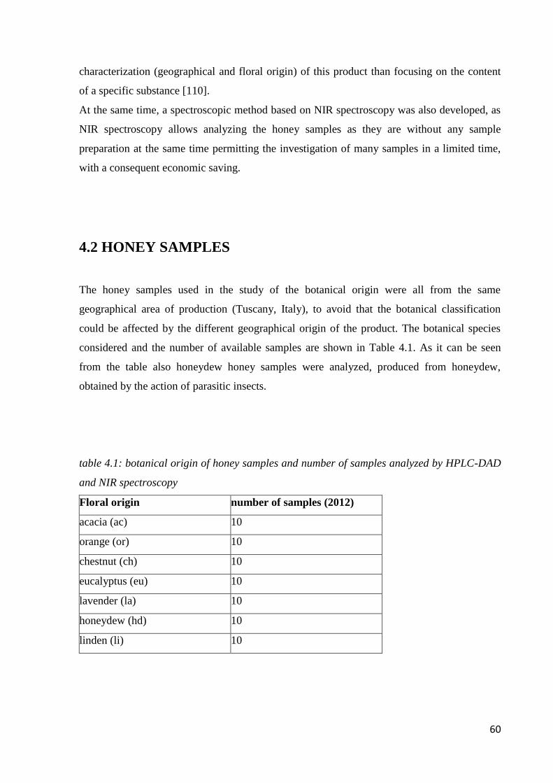
60
characterization (geographical and floral origin) of this product than focusing on the content
of a specific substance [110].
At the same time, a spectroscopic method based on NIR spectroscopy was also developed, as
NIR spectroscopy allows analyzing the honey samples as they are without any sample
preparation at the same time permitting the investigation of many samples in a limited time,
with a consequent economic saving.
4.2 HONEY SAMPLES
The honey samples used in the study of the botanical origin were all from the same
geographical area of production (Tuscany, Italy), to avoid that the botanical classification
could be affected by the different geographical origin of the product. The botanical species
considered and the number of available samples are shown in Table 4.1. As it can be seen
from the table also honeydew honey samples were analyzed, produced from honeydew,
obtained by the action of parasitic insects.
table 4.1: botanical origin of honey samples and number of samples analyzed by HPLC-DAD
and NIR spectroscopy
Floral origin number of samples (2012)
acacia (ac) 10
orange (or) 10
chestnut (ch) 10
eucalyptus (eu) 10
lavender (la) 10
honeydew (hd) 10
linden (li) 10
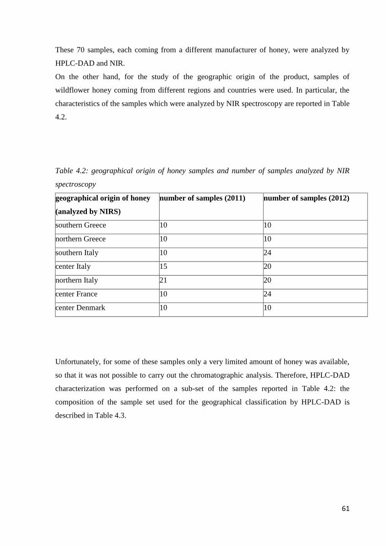
61
These 70 samples, each coming from a different manufacturer of honey, were analyzed by
HPLC-DAD and NIR.
On the other hand, for the study of the geographic origin of the product, samples of
wildflower honey coming from different regions and countries were used. In particular, the
characteristics of the samples which were analyzed by NIR spectroscopy are reported in Table
4.2.
Table 4.2: geographical origin of honey samples and number of samples analyzed by NIR
spectroscopy
geographical origin of honey
(analyzed by NIRS)
number of samples (2011) number of samples (2012)
southern Greece 10 10
northern Greece 10 10
southern Italy 10 24
center Italy 15 20
northern Italy 21 20
center France 10 24
center Denmark 10 10
Unfortunately, for some of these samples only a very limited amount of honey was available,
so that it was not possible to carry out the chromatographic analysis. Therefore, HPLC-DAD
characterization was performed on a sub-set of the samples reported in Table 4.2: the
composition of the sample set used for the geographical classification by HPLC-DAD is
described in Table 4.3.
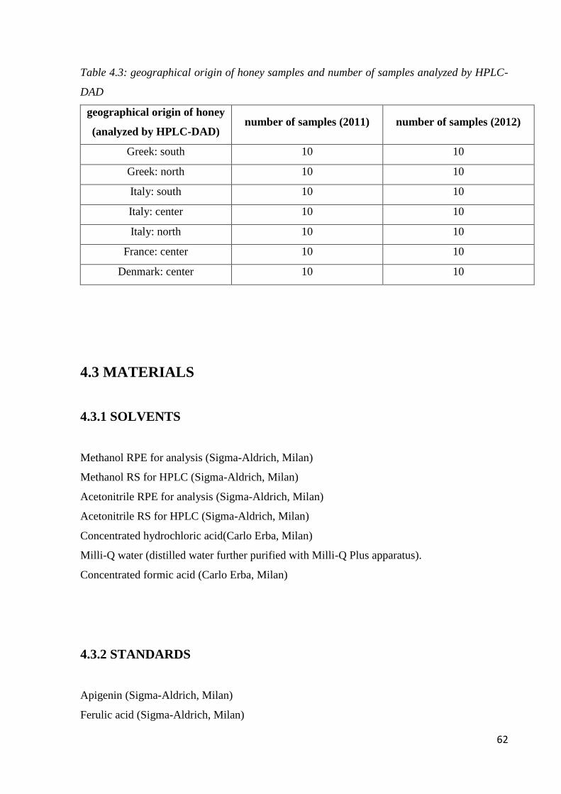
62
Table 4.3: geographical origin of honey samples and number of samples analyzed by HPLC-
DAD
geographical origin of honey
(analyzed by HPLC-DAD) number of samples (2011) number of samples (2012)
Greek: south 10 10
Greek: north 10 10
Italy: south 10 10
Italy: center 10 10
Italy: north 10 10
France: center 10 10
Denmark: center 10 10
4.3 MATERIALS
4.3.1 SOLVENTS
Methanol RPE for analysis (Sigma-Aldrich, Milan)
Methanol RS for HPLC (Sigma-Aldrich, Milan)
Acetonitrile RPE for analysis (Sigma-Aldrich, Milan)
Acetonitrile RS for HPLC (Sigma-Aldrich, Milan)
Concentrated hydrochloric acid(Carlo Erba, Milan)
Milli-Q water (distilled water further purified with Milli-Q Plus apparatus).
Concentrated formic acid (Carlo Erba, Milan)
4.3.2 STANDARDS
Apigenin (Sigma-Aldrich, Milan)
Ferulic acid (Sigma-Aldrich, Milan)
63
p-hydroxybenzoic acid (Sigma-Aldrich, Milan)
Kaempferol (Sigma-Aldrich, Milan).
4.3.3 INSTRUMENTATION AND SOFTWARE
The extraction of the phenolic component present in honey was performed using C18 SPE
cartridges (Applied Separations); the chromatographic analysis was performed using a HPLC
apparatus SpectraSystem LC of ThermoFisher, equipped with a degasser SCL1000 model, a
two-way pump model P4000 and a UV-Visible photodiode model UV6000LP. The
chromatograph was interfaced to a personal computer for acquiring and processing the data
through the interface SN4000. The acquisition of the chromatograms and the subsequent
processing of the data was performed using the software ChromQuest 5.0, supplied by the
manufacturer of the instrument. The column used was Agilent XDB-C18, 250 x 4.6 mm,
packed with 5μm particles.
Rotary evaporator was used in the development of the method and in the preparation of the
samples.
A Nicolet 6700 FT-NIR instrument (Thermo Scientific Inc., Madison, WI), equipped with a
tungsten-halogen source and an InGaAs detector, was used for the acquisition of spectra in the
near infrared range. The spectra were acquired at room temperature and without any further
sample treatment, in transflectance mode, through the use of an integrating sphere (Thermo
Scientific Inc., Madison, WI).
4.4 SAMPLE PREPARATION
As far as NIR spectroscopy is concerned, honey samples did not require any sample
preparation prior to the analysis.
On the other hand, a preliminary extraction step was necessary to prepare the honey samples
for the HPLC-DAD analysis. In particular, the phenolic fraction present in honey was
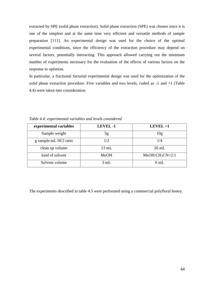
64
extracted by SPE (solid phase extraction). Solid phase extraction (SPE) was chosen since it is
one of the simplest and at the same time very efficient and versatile methods of sample
preparation [111]. An experimental design was used for the choice of the optimal
experimental conditions, since the efficiency of the extraction procedure may depend on
several factors, potentially interacting. This approach allowed carrying out the minimum
number of experiments necessary for the evaluation of the effects of various factors on the
response to optimize.
In particular, a fractional factorial experimental design was used for the optimization of the
solid phase extraction procedure. Five variables and two levels, coded as -1 and +1 (Table
4.4) were taken into consideration.
Table 4.4: experimental variables and levels considered
experimental variables LEVEL -1 LEVEL +1
Sample weight 5g 10g
g sample:mL HCl ratio 1/2 1/4
clean up volume 13 mL 26 mL
kind of solvent MeOH MeOH:CH3CN=2:1
Solvent volume 3 mL 6 mL
The experiments described in table 4.5 were performed using a commercial polyfloral honey.
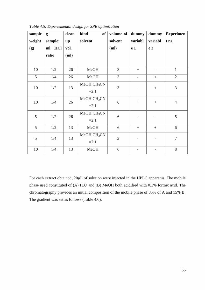
65
Table 4.5: Experiemental design for SPE optimization
sample
weight
(g)
g
sample:
ml HCl
ratio
clean
up
vol.
(ml)
kind of
solvent
volume of
solvent
(ml)
dummy
variabl
e 1
dummy
variabl
e 2
Experimen
t nr.
10 1/2 26 MeOH 3 + - 1
5 1/4 26 MeOH 3 - + 2
10 1/2 13 MeOH:CH3CN
=2:1 3 - + 3
10 1/4 26 MeOH:CH3CN
=2:1 6 + + 4
5 1/2 26 MeOH:CH3CN
=2:1 6 - - 5
5 1/2 13 MeOH 6 + + 6
5 1/4 13 MeOH:CH3CN
=2:1 3 - - 7
10 1/4 13 MeOH 6 - - 8
For each extract obtained, 20μL of solution were injected in the HPLC apparatus. The mobile
phase used constituted of (A) H2O and (B) MeOH both acidified with 0.1% formic acid. The
chromatography provides an initial composition of the mobile phase of 85% of A and 15% B.
The gradient was set as follows (Table 4.6):
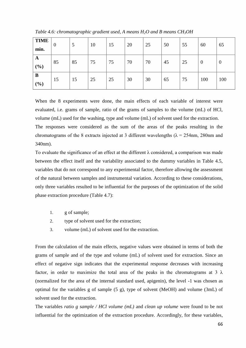
66
Table 4.6: chromatographic gradient used, A means H2O and B means CH3OH
TIME
min. 0 5 10 15 20 25 50 55 60 65
A
(%) 85 85 75 75 70 70 45 25 0 0
B
(%) 15 15 25 25 30 30 65 75 100 100
When the 8 experiments were done, the main effects of each variable of interest were
evaluated, i.e. grams of sample, ratio of the grams of samples to the volume (mL) of HCl,
volume (mL) used for the washing, type and volume (mL) of solvent used for the extraction.
The responses were considered as the sum of the areas of the peaks resulting in the
chromatograms of the 8 extracts injected at 3 different wavelengths (λ = 254nm, 280nm and
340nm).
To evaluate the significance of an effect at the different λ considered, a comparison was made
between the effect itself and the variability associated to the dummy variables in Table 4.5,
variables that do not correspond to any experimental factor, therefore allowing the assessment
of the natural between samples and instrumental variation. According to these considerations,
only three variables resulted to be influential for the purposes of the optimization of the solid
phase extraction procedure (Table 4.7):
1. g of sample;
2. type of solvent used for the extraction;
3. volume (mL) of solvent used for the extraction.
From the calculation of the main effects, negative values were obtained in terms of both the
grams of sample and of the type and volume (mL) of solvent used for extraction. Since an
effect of negative sign indicates that the experimental response decreases with increasing
factor, in order to maximize the total area of the peaks in the chromatograms at 3 λ
(normalized for the area of the internal standard used, apigenin), the level -1 was chosen as
optimal for the variables g of sample (5 g), type of solvent (MeOH) and volume (3mL) of
solvent used for the extraction.
The variables ratio g sample / HCl volume (mL) and clean up volume were found to be not
influential for the optimization of the extraction procedure. Accordingly, for these variables,
67
the level -1, i.e. a ratio g sample / HCl volume (mL) of ½ and a volume of 13mL for clean up,
was selected. Indeed, the choice of level -1 has been made to reduce the cost, speed and
improve the overall efficiency of the method.
The optimized extraction procedure was the following:
1. g of sample: 5;
2. ratio g sample/volume (mL) HCl: 1/2;
3. volume used for the washing: 13mL (3mL HCl + 10mL H2O);
4. kind of solvent used for the extraction: MeOH;
5. volume of solvent used per the extraction: 3mL.
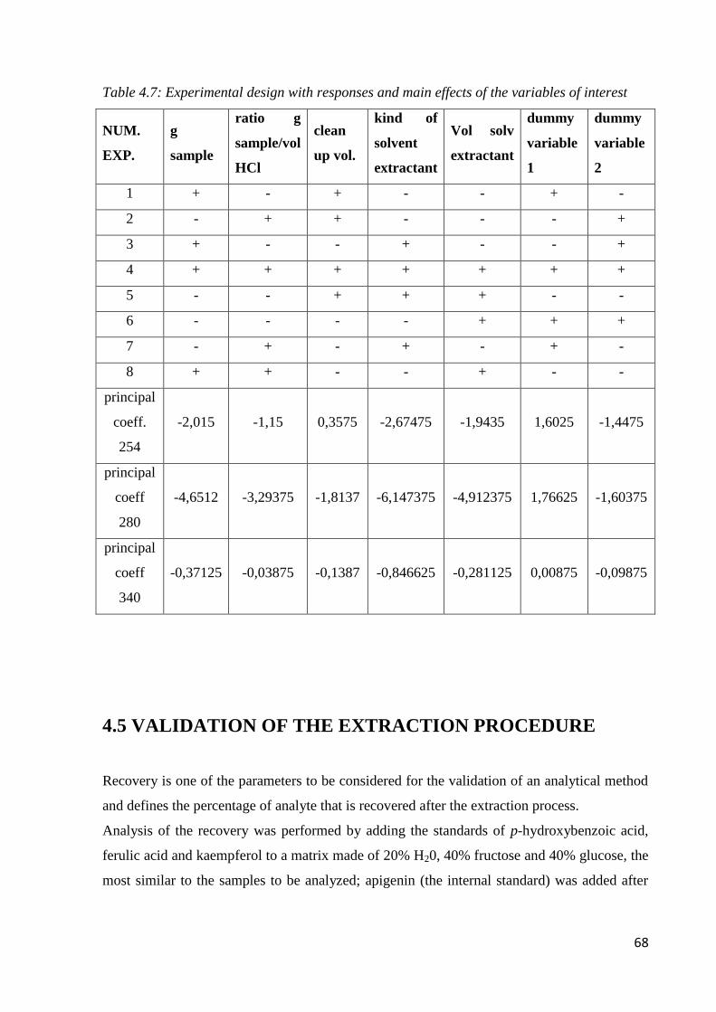
68
Table 4.7: Experimental design with responses and main effects of the variables of interest
NUM.
EXP.
g
sample
ratio g
sample/vol
HCl
clean
up vol.
kind of
solvent
extractant
Vol solv
extractant
dummy
variable
1
dummy
variable
2
1 + - + - - + -
2 - + + - - - +
3 + - - + - - +
4 + + + + + + +
5 - - + + + - -
6 - - - - + + +
7 - + - + - + -
8 + + - - + - -
principal
coeff.
254
-2,015 -1,15 0,3575 -2,67475 -1,9435 1,6025 -1,4475
principal
coeff
280
-4,6512 -3,29375 -1,8137 -6,147375 -4,912375 1,76625 -1,60375
principal
coeff
340
-0,37125 -0,03875 -0,1387 -0,846625 -0,281125 0,00875 -0,09875
4.5 VALIDATION OF THE EXTRACTION PROCEDURE
Recovery is one of the parameters to be considered for the validation of an analytical method
and defines the percentage of analyte that is recovered after the extraction process.
Analysis of the recovery was performed by adding the standards of p-hydroxybenzoic acid,
ferulic acid and kaempferol to a matrix made of 20% H20, 40% fructose and 40% glucose, the
most similar to the samples to be analyzed; apigenin (the internal standard) was added after
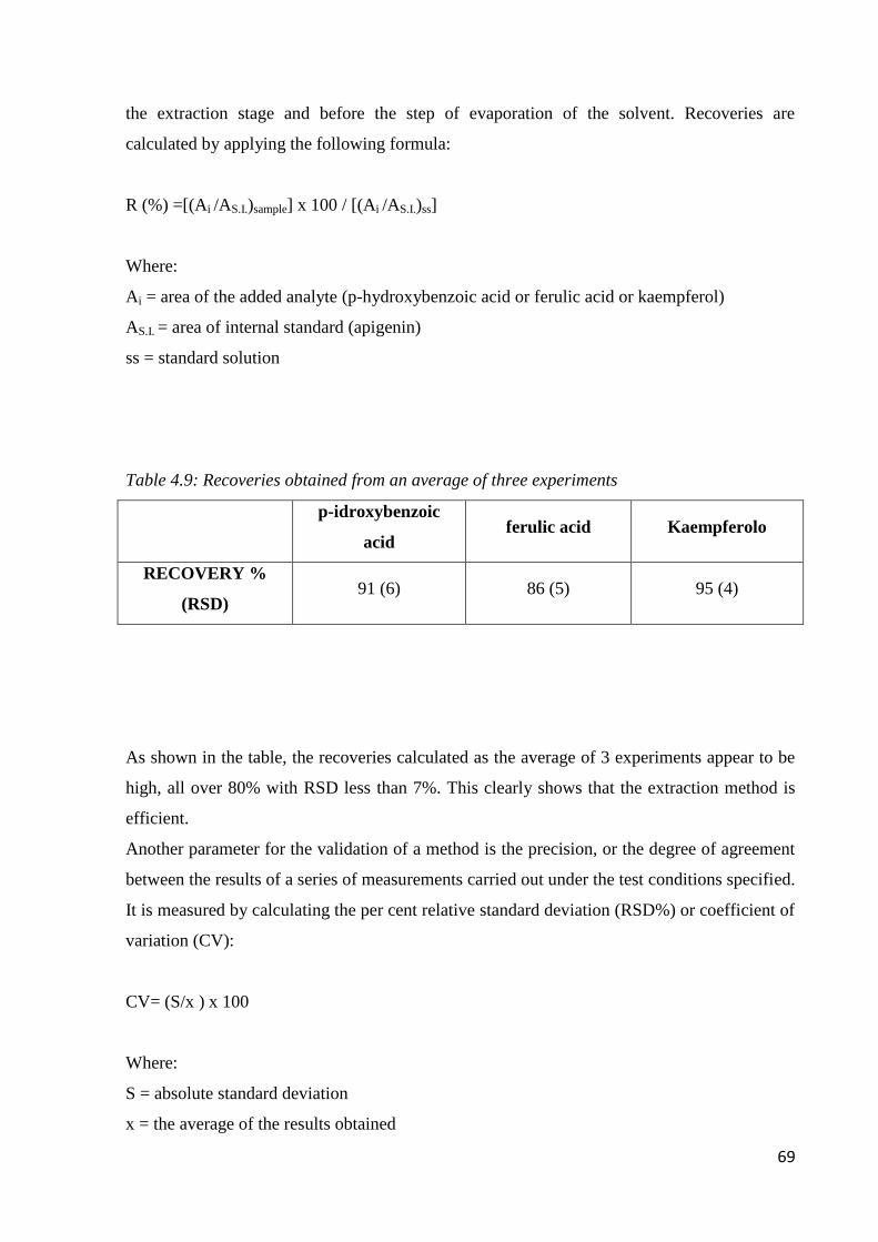
69
the extraction stage and before the step of evaporation of the solvent. Recoveries are
calculated by applying the following formula:
R (%) =[(Ai /AS.I.)sample] x 100 / [(Ai /AS.I.)ss]
Where:
Ai = area of the added analyte (p-hydroxybenzoic acid or ferulic acid or kaempferol)
AS.I. = area of internal standard (apigenin)
ss = standard solution
Table 4.9: Recoveries obtained from an average of three experiments
p-idroxybenzoic
acid ferulic acid Kaempferolo
RECOVERY %
(RSD) 91 (6) 86 (5) 95 (4)
As shown in the table, the recoveries calculated as the average of 3 experiments appear to be
high, all over 80% with RSD less than 7%. This clearly shows that the extraction method is
efficient.
Another parameter for the validation of a method is the precision, or the degree of agreement
between the results of a series of measurements carried out under the test conditions specified.
It is measured by calculating the per cent relative standard deviation (RSD%) or coefficient of
variation (CV):
CV= (S/x ) x 100
Where:
S = absolute standard deviation
x = the average of the results obtained
70
The precision of the method is considered as:
Intra-day precision (repeatability) is evaluated as the CV of mutually independent evidence
obtained under the same experimental conditions, by the same operator on the same day and
laboratory, with the same instruments and the same materials.
To check if extraction procedure used is repeatable, 5 analyses are performed on the same day
and the area of each analyte is measured. For each compound a RSD% always less than 2%
was obtained and for each extract the sum of the areas of each chromatogram also remained
practically constant. This shows, therefore, that the method proposed is repeatable.
Inter-day precision (reproducibility) is evaluated as the CV of mutually independent tests
obtained by the same method and the same laboratory but on different days.
To assess the reproducibility of the method applied, 5 extractive tests (one every week, for 5
weeks) were performed. Areas of each peak were calculated and the RSD% resulted to be
always less than 2%.
4.6 BOTANICAL AND GEOGRAPHICAL CLASSIFICATION
BY PHENOLIC FINGERPRINT
The extraction procedure, optimized and validated in terms of recovery and precision, was
then applied to the extraction of the phenolic fraction present in available honey samples.
For each sample of honey the procedure previously described was applied. Successively,
20μL of each extract were injected into the HPLC-DAD system and the chromatograms were
recorded at 254, 280, and 340 nm.
The chromatographic profiles of each sample were considered as fingerprint.
4.6.1 BOTANICAL CLASSIFICATION BY HPLC-DAD
The chromatographic data of 70 samples of honey analyzed with the HPLC-DAD procedure
were used for the construction of classification models.
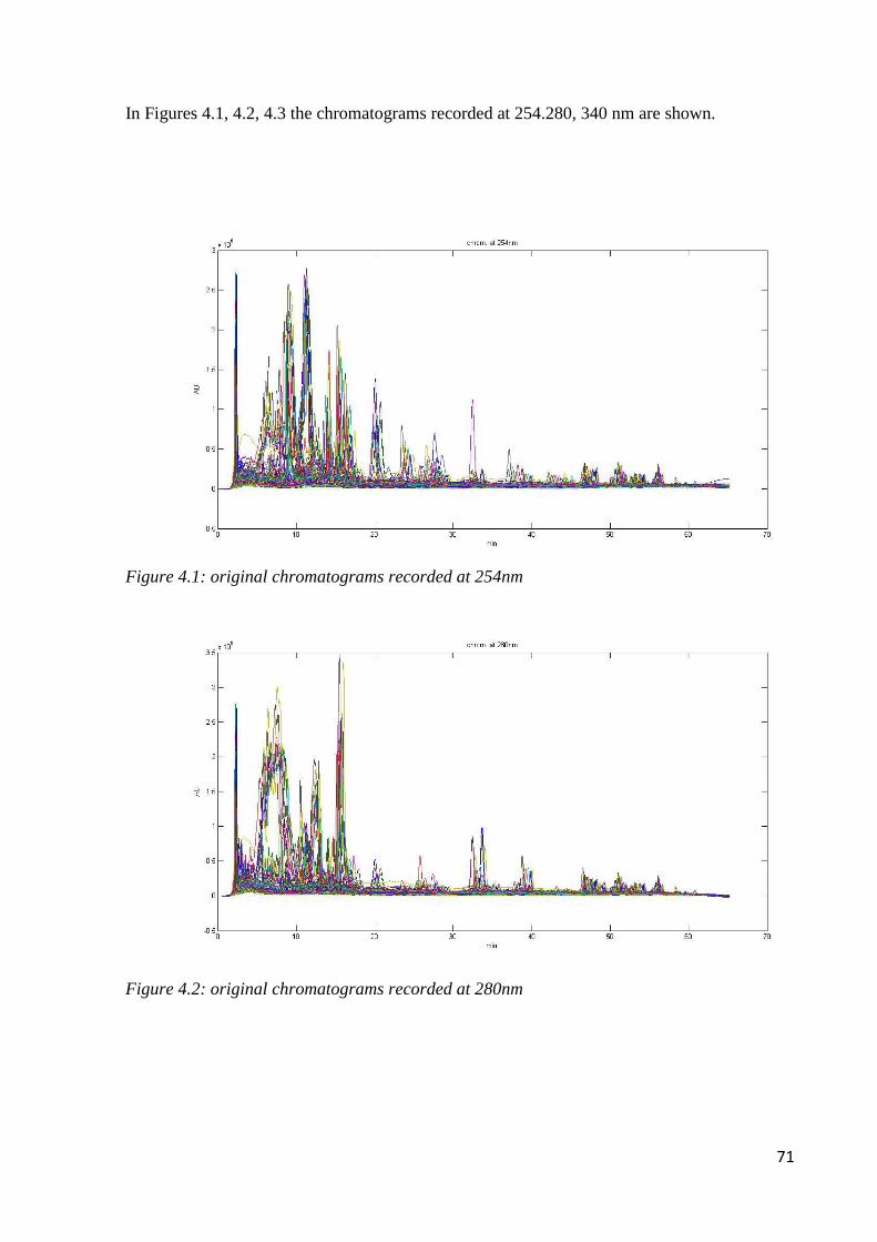
71
In Figures 4.1, 4.2, 4.3 the chromatograms recorded at 254.280, 340 nm are shown.
Figure 4.1: original chromatograms recorded at 254nm
Figure 4.2: original chromatograms recorded at 280nm

72
Figure 4.3: original chromatograms recorded at 340nm
Before applying the PLS-DA classification method, it was necessary to correct the baseline, to
align the chromatographic peaks and, obviously, to normalize the signals, dividing them by
the area of the internal standard.
Asymmetric Least Square method (described in section 2.4.1) was used to correct the
baseline. The alignment of the chromatographic peaks was carried out using the algorithm
Icoshift (described in section 2.4.2).
Three PLS-DA models were constructed, one for each of the wavelengths considered. The
corresponding results are reported in tables 4.10, 4.11, 4.12. Considering the number of
samples available for each class, the models were validated using the procedure of cross
validation.
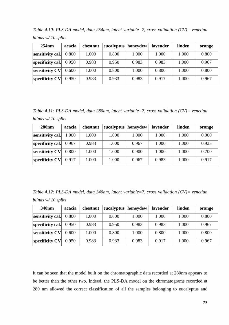
73
Table 4.10: PLS-DA model, data 254nm, latent variable=7, cross validation (CV)= venetian
blinds w/ 10 splits
254nm acacia chestnut eucalyptus honeydew lavender linden orange
sensitivity cal. 0.800 1.000 0.800 1.000 1.000 1.000 0.800
specificity cal. 0.950 0.983 0.950 0.983 0.983 1.000 0.967
sensitivity CV 0.600 1.000 0.800 1.000 0.800 1.000 0.800
specificity CV 0.950 0.983 0.933 0.983 0.917 1.000 0.967
Table 4.11: PLS-DA model, data 280nm, latent variable=7, cross validation (CV)= venetian
blinds w/ 10 splits
280nm acacia chestnut eucalyptus honeydew lavender linden orange
sensitivity cal. 1.000 1.000 1.000 1.000 1.000 1.000 0.900
specificity cal. 0.967 0.983 1.000 0.967 1.000 1.000 0.933
sensitivity CV 0.800 1.000 1.000 0.900 1.000 1.000 0.700
specificity CV 0.917 1.000 1.000 0.967 0.983 1.000 0.917
Table 4.12: PLS-DA model, data 340nm, latent variable=7, cross validation (CV)= venetian
blinds w/ 10 splits
340nm acacia chestnut eucalyptus honeydew lavender linden orange
sensitivity cal. 0.800 1.000 0.800 1.000 1.000 1.000 0.800
specificity cal. 0.950 0.983 0.950 0.983 0.983 1.000 0.967
sensitivity CV 0.600 1.000 0.800 1.000 0.800 1.000 0.800
specificity CV 0.950 0.983 0.933 0.983 0.917 1.000 0.967
It can be seen that the model built on the chromatographic data recorded at 280nm appears to
be better than the other two. Indeed, the PLS-DA model on the chromatograms recorded at
280 nm allowed the correct classification of all the samples belonging to eucalyptus and
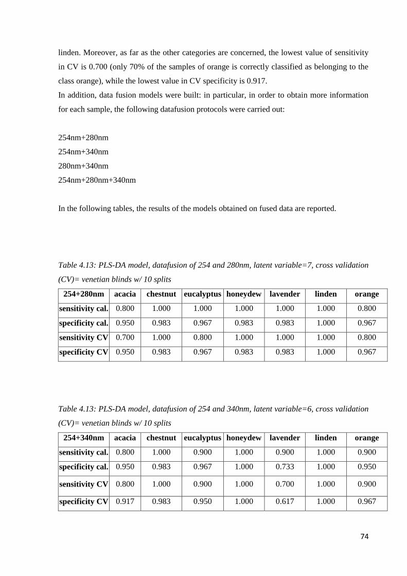
74
linden. Moreover, as far as the other categories are concerned, the lowest value of sensitivity
in CV is 0.700 (only 70% of the samples of orange is correctly classified as belonging to the
class orange), while the lowest value in CV specificity is 0.917.
In addition, data fusion models were built: in particular, in order to obtain more information
for each sample, the following datafusion protocols were carried out:
254nm+280nm
254nm+340nm
280nm+340nm
254nm+280nm+340nm
In the following tables, the results of the models obtained on fused data are reported.
Table 4.13: PLS-DA model, datafusion of 254 and 280nm, latent variable=7, cross validation
(CV)= venetian blinds w/ 10 splits
254+280nm acacia chestnut eucalyptus honeydew lavender linden orange
sensitivity cal. 0.800 1.000 1.000 1.000 1.000 1.000 0.800
specificity cal. 0.950 0.983 0.967 0.983 0.983 1.000 0.967
sensitivity CV 0.700 1.000 0.800 1.000 1.000 1.000 0.800
specificity CV 0.950 0.983 0.967 0.983 0.983 1.000 0.967
Table 4.13: PLS-DA model, datafusion of 254 and 340nm, latent variable=6, cross validation
(CV)= venetian blinds w/ 10 splits
254+340nm acacia chestnut eucalyptus honeydew lavender linden orange
sensitivity cal. 0.800 1.000 0.900 1.000 0.900 1.000 0.900
specificity cal. 0.950 0.983 0.967 1.000 0.733 1.000 0.950
sensitivity CV 0.800 1.000 0.900 1.000 0.700 1.000 0.900
specificity CV 0.917 0.983 0.950 1.000 0.617 1.000 0.967
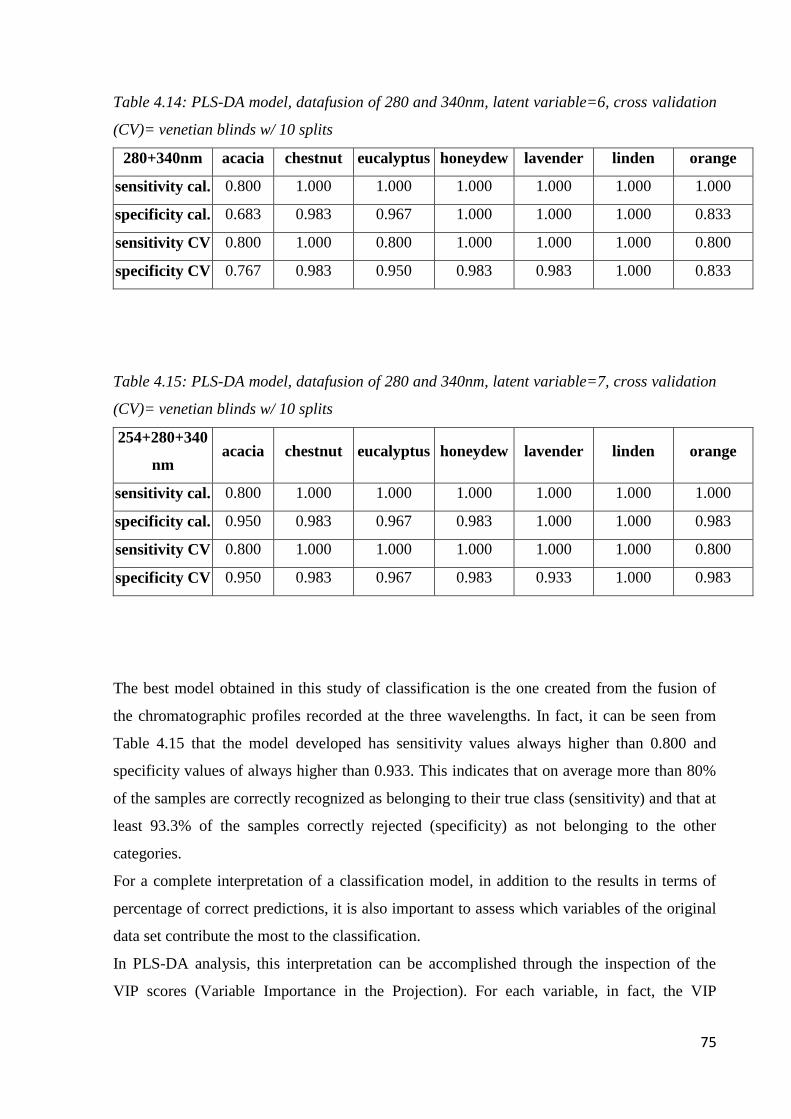
75
Table 4.14: PLS-DA model, datafusion of 280 and 340nm, latent variable=6, cross validation
(CV)= venetian blinds w/ 10 splits
280+340nm acacia chestnut eucalyptus honeydew lavender linden orange
sensitivity cal. 0.800 1.000 1.000 1.000 1.000 1.000 1.000
specificity cal. 0.683 0.983 0.967 1.000 1.000 1.000 0.833
sensitivity CV 0.800 1.000 0.800 1.000 1.000 1.000 0.800
specificity CV 0.767 0.983 0.950 0.983 0.983 1.000 0.833
Table 4.15: PLS-DA model, datafusion of 280 and 340nm, latent variable=7, cross validation
(CV)= venetian blinds w/ 10 splits
254+280+340
nm acacia chestnut eucalyptus honeydew lavender linden orange
sensitivity cal. 0.800 1.000 1.000 1.000 1.000 1.000 1.000
specificity cal. 0.950 0.983 0.967 0.983 1.000 1.000 0.983
sensitivity CV 0.800 1.000 1.000 1.000 1.000 1.000 0.800
specificity CV 0.950 0.983 0.967 0.983 0.933 1.000 0.983
The best model obtained in this study of classification is the one created from the fusion of
the chromatographic profiles recorded at the three wavelengths. In fact, it can be seen from
Table 4.15 that the model developed has sensitivity values always higher than 0.800 and
specificity values of always higher than 0.933. This indicates that on average more than 80%
of the samples are correctly recognized as belonging to their true class (sensitivity) and that at
least 93.3% of the samples correctly rejected (specificity) as not belonging to the other
categories.
For a complete interpretation of a classification model, in addition to the results in terms of
percentage of correct predictions, it is also important to assess which variables of the original
data set contribute the most to the classification.
In PLS-DA analysis, this interpretation can be accomplished through the inspection of the
VIP scores (Variable Importance in the Projection). For each variable, in fact, the VIP
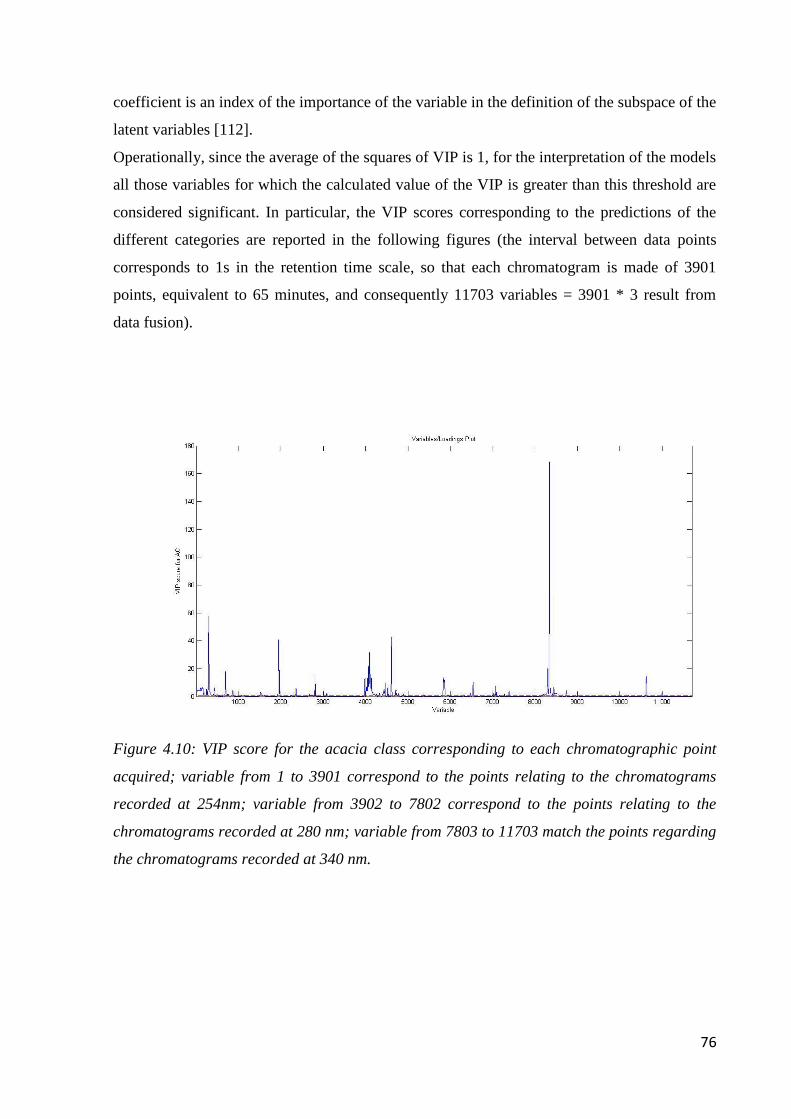
76
coefficient is an index of the importance of the variable in the definition of the subspace of the
latent variables [112].
Operationally, since the average of the squares of VIP is 1, for the interpretation of the models
all those variables for which the calculated value of the VIP is greater than this threshold are
considered significant. In particular, the VIP scores corresponding to the predictions of the
different categories are reported in the following figures (the interval between data points
corresponds to 1s in the retention time scale, so that each chromatogram is made of 3901
points, equivalent to 65 minutes, and consequently 11703 variables = 3901 * 3 result from
data fusion).
Figure 4.10: VIP score for the acacia class corresponding to each chromatographic point
acquired; variable from 1 to 3901 correspond to the points relating to the chromatograms
recorded at 254nm; variable from 3902 to 7802 correspond to the points relating to the
chromatograms recorded at 280 nm; variable from 7803 to 11703 match the points regarding
the chromatograms recorded at 340 nm.
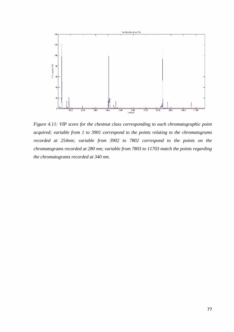
77
Figure 4.11: VIP score for the chestnut class corresponding to each chromatographic point
acquired; variable from 1 to 3901 correspond to the points relating to the chromatograms
recorded at 254nm; variable from 3902 to 7802 correspond to the points on the
chromatograms recorded at 280 nm; variable from 7803 to 11703 match the points regarding
the chromatograms recorded at 340 nm.
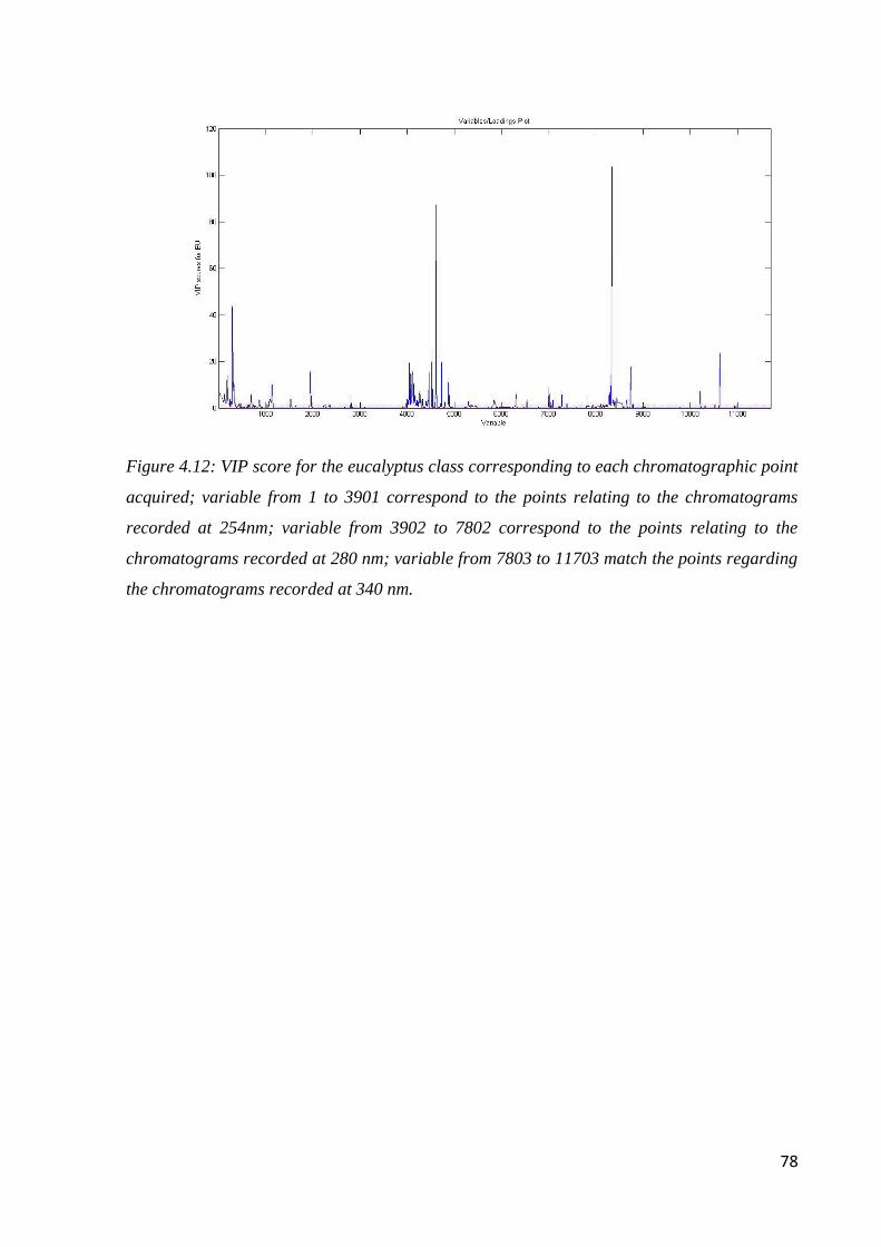
78
Figure 4.12: VIP score for the eucalyptus class corresponding to each chromatographic point
acquired; variable from 1 to 3901 correspond to the points relating to the chromatograms
recorded at 254nm; variable from 3902 to 7802 correspond to the points relating to the
chromatograms recorded at 280 nm; variable from 7803 to 11703 match the points regarding
the chromatograms recorded at 340 nm.

79
Figure 4.13: VIP score for the honeydew class corresponding to each chromatographic point
acquired; variable from 1 to 3901 correspond to the points relating to the chromatograms
recorded at 254nm; variable from 3902 to 7802 correspond to the points relating to the
chromatograms recorded at 280 nm; variable from 7803 to 11703 match the points regarding
the chromatograms recorded at 340 nm.
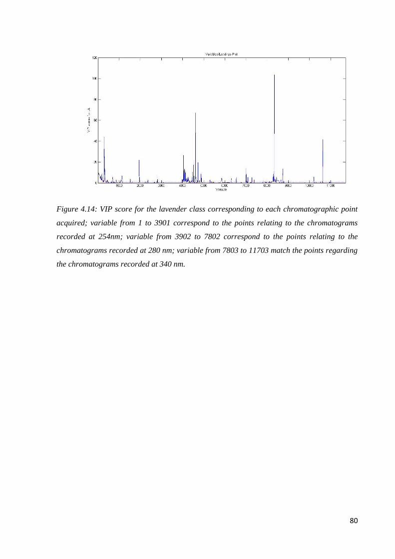
80
Figure 4.14: VIP score for the lavender class corresponding to each chromatographic point
acquired; variable from 1 to 3901 correspond to the points relating to the chromatograms
recorded at 254nm; variable from 3902 to 7802 correspond to the points relating to the
chromatograms recorded at 280 nm; variable from 7803 to 11703 match the points regarding
the chromatograms recorded at 340 nm.
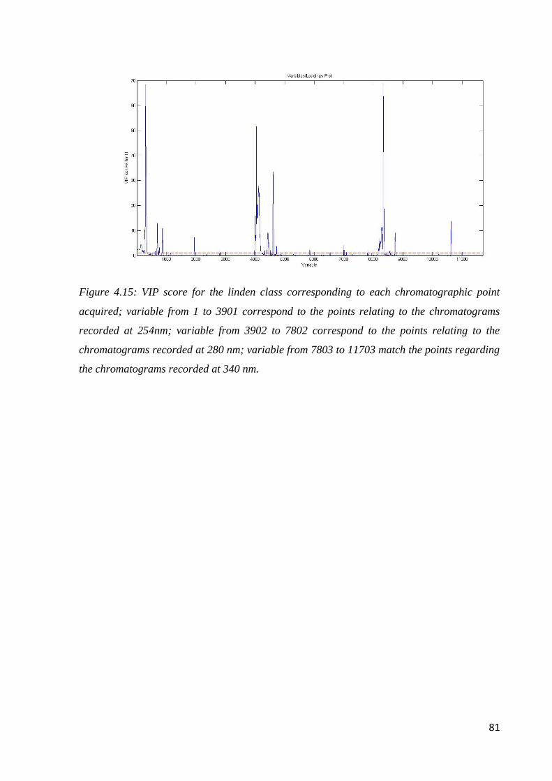
81
Figure 4.15: VIP score for the linden class corresponding to each chromatographic point
acquired; variable from 1 to 3901 correspond to the points relating to the chromatograms
recorded at 254nm; variable from 3902 to 7802 correspond to the points relating to the
chromatograms recorded at 280 nm; variable from 7803 to 11703 match the points regarding
the chromatograms recorded at 340 nm.
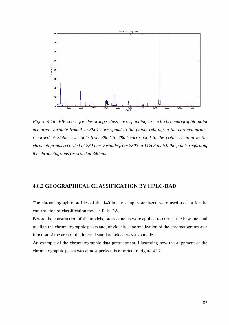
82
Figure 4.16: VIP score for the orange class corresponding to each chromatographic point
acquired; variable from 1 to 3901 correspond to the points relating to the chromatograms
recorded at 254nm; variable from 3902 to 7802 correspond to the points relating to the
chromatograms recorded at 280 nm; variable from 7803 to 11703 match the points regarding
the chromatograms recorded at 340 nm.
4.6.2 GEOGRAPHICAL CLASSIFICATION BY HPLC-DAD
The chromatographic profiles of the 140 honey samples analyzed were used as data for the
construction of classification models PLS-DA.
Before the construction of the models, pretreatments were applied to correct the baseline, and
to align the chromatographic peaks and, obviously, a normalization of the chromatograms as a
function of the area of the internal standard added was also made.
An example of the chromatographic data pretreatment, illustrating how the alignment of the
chromatographic peaks was almost perfect, is reported in Figure 4.17.
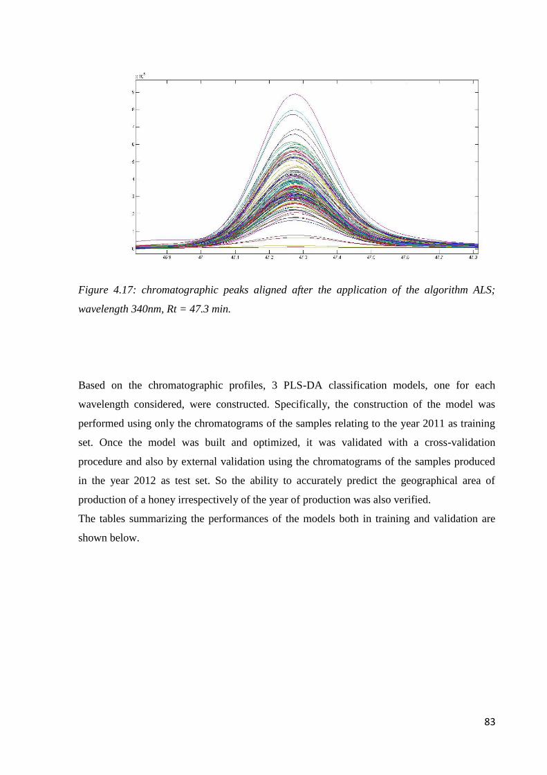
83
Figure 4.17: chromatographic peaks aligned after the application of the algorithm ALS;
wavelength 340nm, Rt = 47.3 min.
Based on the chromatographic profiles, 3 PLS-DA classification models, one for each
wavelength considered, were constructed. Specifically, the construction of the model was
performed using only the chromatograms of the samples relating to the year 2011 as training
set. Once the model was built and optimized, it was validated with a cross-validation
procedure and also by external validation using the chromatograms of the samples produced
in the year 2012 as test set. So the ability to accurately predict the geographical area of
production of a honey irrespectively of the year of production was also verified.
The tables summarizing the performances of the models both in training and validation are
shown below.
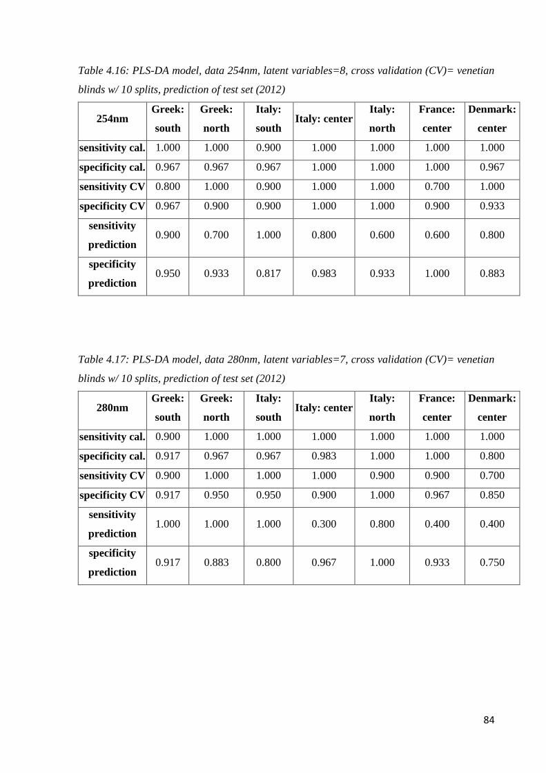
84
Table 4.16: PLS-DA model, data 254nm, latent variables=8, cross validation (CV)= venetian
blinds w/ 10 splits, prediction of test set (2012)
254nm Greek:
south
Greek:
north
Italy:
south Italy: center
Italy:
north
France:
center
Denmark:
center
sensitivity cal. 1.000 1.000 0.900 1.000 1.000 1.000 1.000
specificity cal. 0.967 0.967 0.967 1.000 1.000 1.000 0.967
sensitivity CV 0.800 1.000 0.900 1.000 1.000 0.700 1.000
specificity CV 0.967 0.900 0.900 1.000 1.000 0.900 0.933
sensitivity
prediction 0.900 0.700 1.000 0.800 0.600 0.600 0.800
specificity
prediction 0.950 0.933 0.817 0.983 0.933 1.000 0.883
Table 4.17: PLS-DA model, data 280nm, latent variables=7, cross validation (CV)= venetian
blinds w/ 10 splits, prediction of test set (2012)
280nm Greek:
south
Greek:
north
Italy:
south Italy: center
Italy:
north
France:
center
Denmark:
center
sensitivity cal. 0.900 1.000 1.000 1.000 1.000 1.000 1.000
specificity cal. 0.917 0.967 0.967 0.983 1.000 1.000 0.800
sensitivity CV 0.900 1.000 1.000 1.000 0.900 0.900 0.700
specificity CV 0.917 0.950 0.950 0.900 1.000 0.967 0.850
sensitivity
prediction 1.000 1.000 1.000 0.300 0.800 0.400 0.400
specificity
prediction 0.917 0.883 0.800 0.967 1.000 0.933 0.750
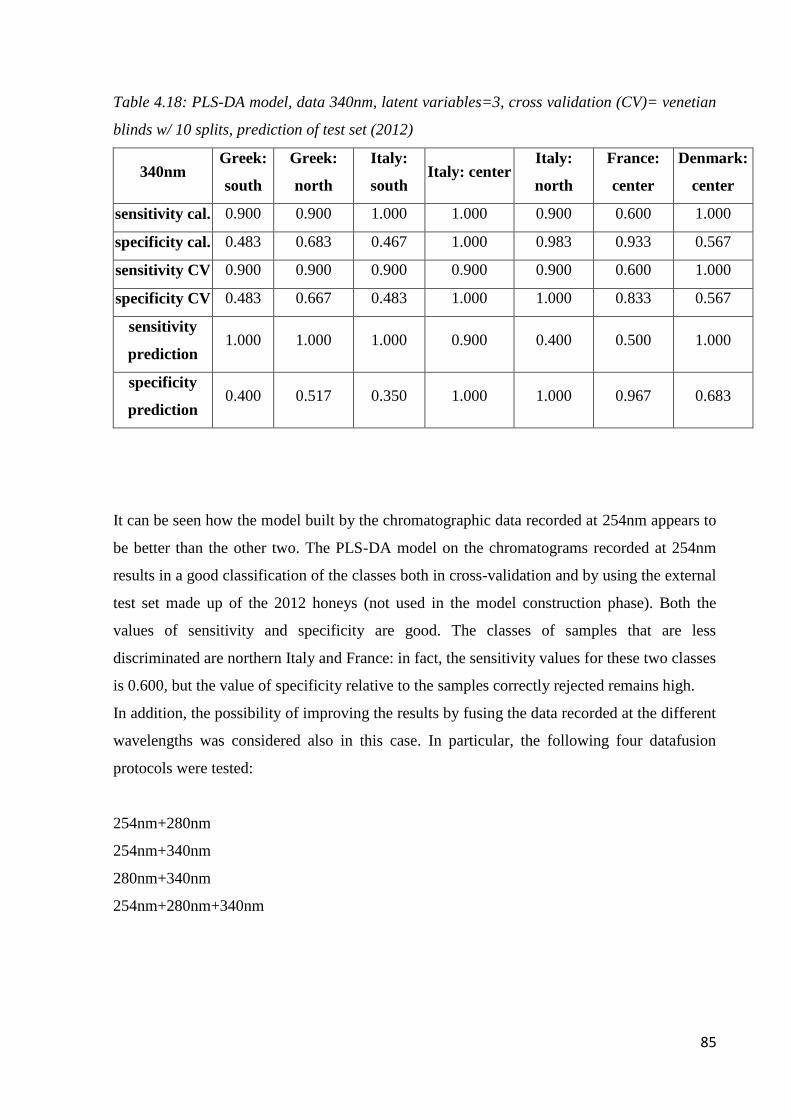
85
Table 4.18: PLS-DA model, data 340nm, latent variables=3, cross validation (CV)= venetian
blinds w/ 10 splits, prediction of test set (2012)
340nm Greek:
south
Greek:
north
Italy:
south Italy: center
Italy:
north
France:
center
Denmark:
center
sensitivity cal. 0.900 0.900 1.000 1.000 0.900 0.600 1.000
specificity cal. 0.483 0.683 0.467 1.000 0.983 0.933 0.567
sensitivity CV 0.900 0.900 0.900 0.900 0.900 0.600 1.000
specificity CV 0.483 0.667 0.483 1.000 1.000 0.833 0.567
sensitivity
prediction 1.000 1.000 1.000 0.900 0.400 0.500 1.000
specificity
prediction 0.400 0.517 0.350 1.000 1.000 0.967 0.683
It can be seen how the model built by the chromatographic data recorded at 254nm appears to
be better than the other two. The PLS-DA model on the chromatograms recorded at 254nm
results in a good classification of the classes both in cross-validation and by using the external
test set made up of the 2012 honeys (not used in the model construction phase). Both the
values of sensitivity and specificity are good. The classes of samples that are less
discriminated are northern Italy and France: in fact, the sensitivity values for these two classes
is 0.600, but the value of specificity relative to the samples correctly rejected remains high.
In addition, the possibility of improving the results by fusing the data recorded at the different
wavelengths was considered also in this case. In particular, the following four datafusion
protocols were tested:
254nm+280nm
254nm+340nm
280nm+340nm
254nm+280nm+340nm
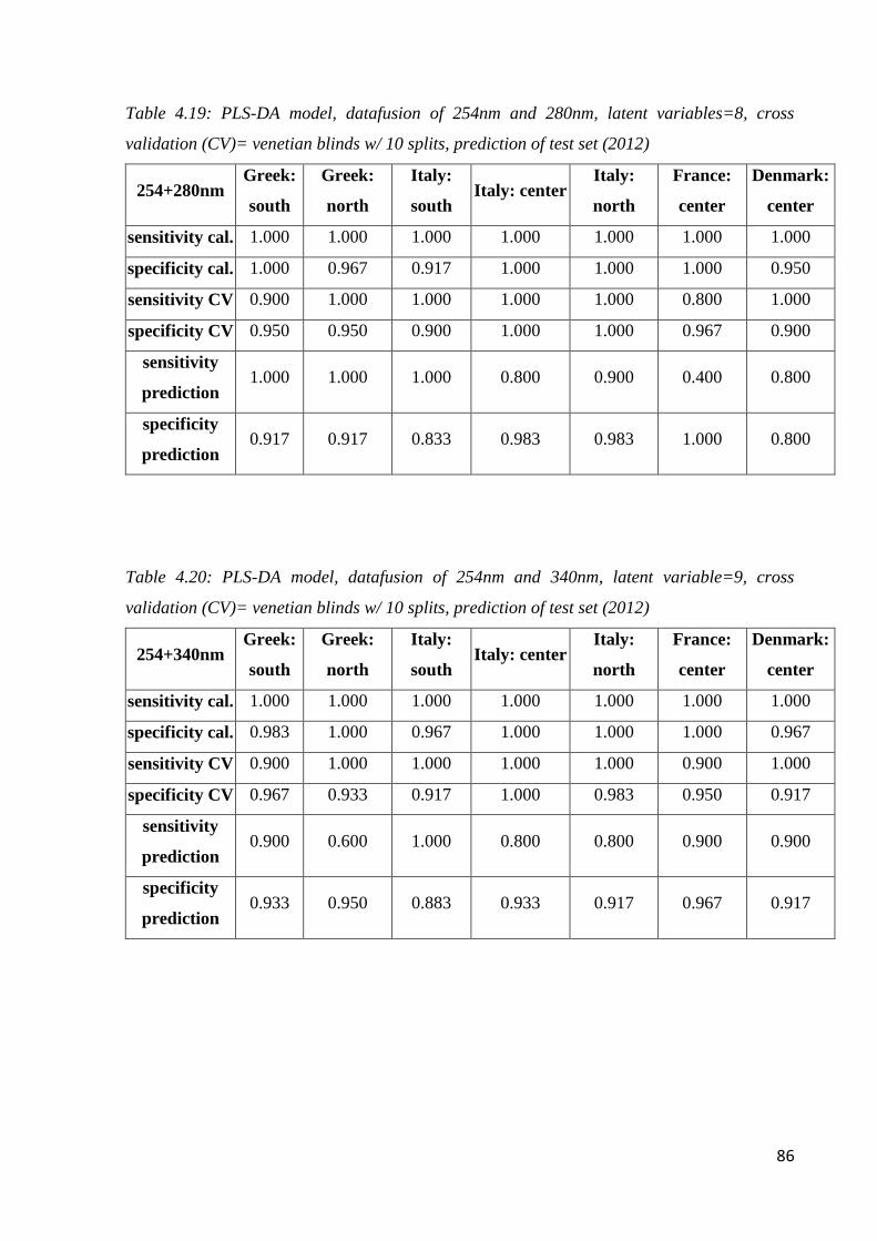
86
Table 4.19: PLS-DA model, datafusion of 254nm and 280nm, latent variables=8, cross
validation (CV)= venetian blinds w/ 10 splits, prediction of test set (2012)
254+280nm Greek:
south
Greek:
north
Italy:
south Italy: center
Italy:
north
France:
center
Denmark:
center
sensitivity cal. 1.000 1.000 1.000 1.000 1.000 1.000 1.000
specificity cal. 1.000 0.967 0.917 1.000 1.000 1.000 0.950
sensitivity CV 0.900 1.000 1.000 1.000 1.000 0.800 1.000
specificity CV 0.950 0.950 0.900 1.000 1.000 0.967 0.900
sensitivity
prediction 1.000 1.000 1.000 0.800 0.900 0.400 0.800
specificity
prediction 0.917 0.917 0.833 0.983 0.983 1.000 0.800
Table 4.20: PLS-DA model, datafusion of 254nm and 340nm, latent variable=9, cross
validation (CV)= venetian blinds w/ 10 splits, prediction of test set (2012)
254+340nm Greek:
south
Greek:
north
Italy:
south Italy: center
Italy:
north
France:
center
Denmark:
center
sensitivity cal. 1.000 1.000 1.000 1.000 1.000 1.000 1.000
specificity cal. 0.983 1.000 0.967 1.000 1.000 1.000 0.967
sensitivity CV 0.900 1.000 1.000 1.000 1.000 0.900 1.000
specificity CV 0.967 0.933 0.917 1.000 0.983 0.950 0.917
sensitivity
prediction 0.900 0.600 1.000 0.800 0.800 0.900 0.900
specificity
prediction 0.933 0.950 0.883 0.933 0.917 0.967 0.917
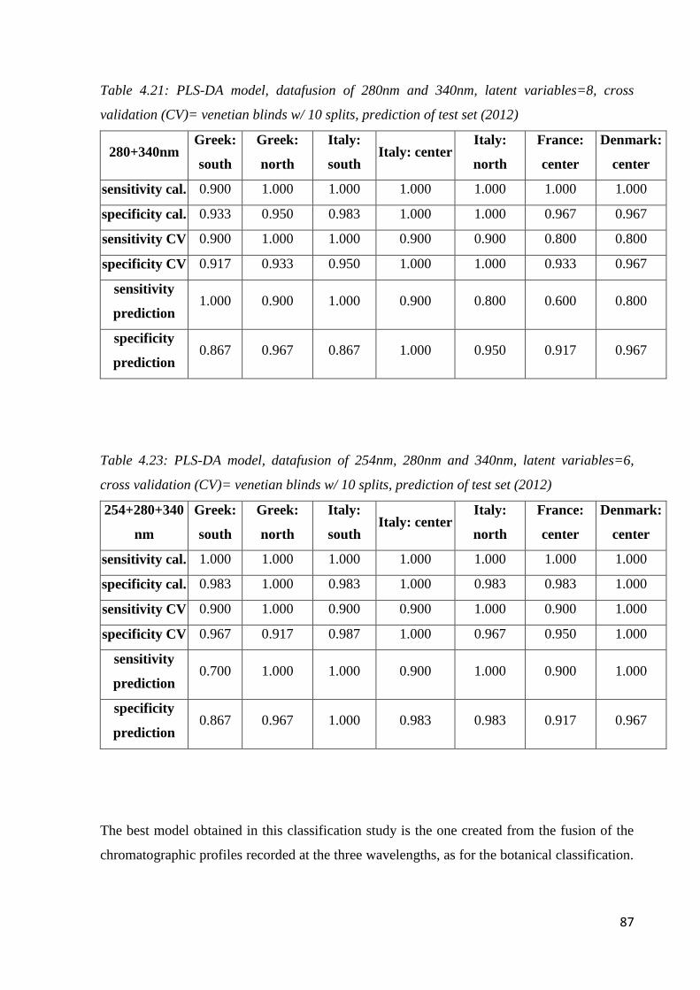
87
Table 4.21: PLS-DA model, datafusion of 280nm and 340nm, latent variables=8, cross
validation (CV)= venetian blinds w/ 10 splits, prediction of test set (2012)
280+340nm Greek:
south
Greek:
north
Italy:
south Italy: center
Italy:
north
France:
center
Denmark:
center
sensitivity cal. 0.900 1.000 1.000 1.000 1.000 1.000 1.000
specificity cal. 0.933 0.950 0.983 1.000 1.000 0.967 0.967
sensitivity CV 0.900 1.000 1.000 0.900 0.900 0.800 0.800
specificity CV 0.917 0.933 0.950 1.000 1.000 0.933 0.967
sensitivity
prediction 1.000 0.900 1.000 0.900 0.800 0.600 0.800
specificity
prediction 0.867 0.967 0.867 1.000 0.950 0.917 0.967
Table 4.23: PLS-DA model, datafusion of 254nm, 280nm and 340nm, latent variables=6,
cross validation (CV)= venetian blinds w/ 10 splits, prediction of test set (2012)
254+280+340
nm
Greek:
south
Greek:
north
Italy:
south Italy: center
Italy:
north
France:
center
Denmark:
center
sensitivity cal. 1.000 1.000 1.000 1.000 1.000 1.000 1.000
specificity cal. 0.983 1.000 0.983 1.000 0.983 0.983 1.000
sensitivity CV 0.900 1.000 0.900 0.900 1.000 0.900 1.000
specificity CV 0.967 0.917 0.987 1.000 0.967 0.950 1.000
sensitivity
prediction 0.700 1.000 1.000 0.900 1.000 0.900 1.000
specificity
prediction 0.867 0.967 1.000 0.983 0.983 0.917 0.967
The best model obtained in this classification study is the one created from the fusion of the
chromatographic profiles recorded at the three wavelengths, as for the botanical classification.
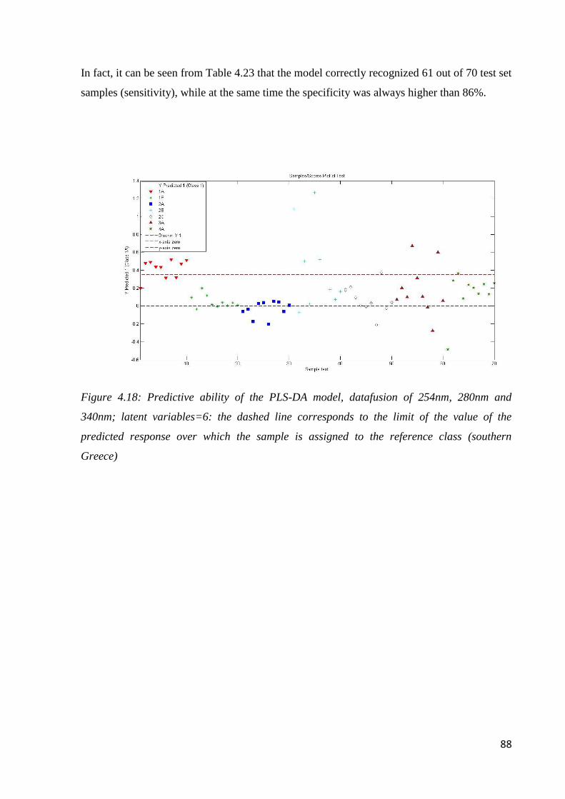
88
In fact, it can be seen from Table 4.23 that the model correctly recognized 61 out of 70 test set
samples (sensitivity), while at the same time the specificity was always higher than 86%.
Figure 4.18: Predictive ability of the PLS-DA model, datafusion of 254nm, 280nm and
340nm; latent variables=6: the dashed line corresponds to the limit of the value of the
predicted response over which the sample is assigned to the reference class (southern
Greece)
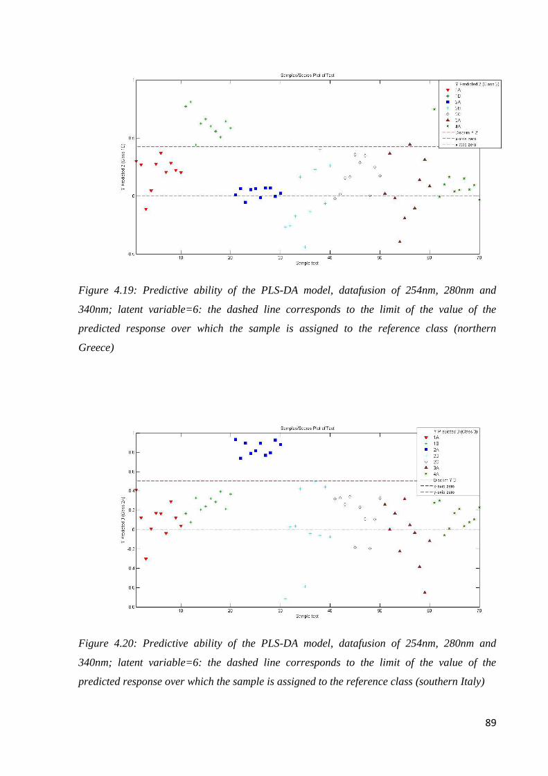
89
Figure 4.19: Predictive ability of the PLS-DA model, datafusion of 254nm, 280nm and
340nm; latent variable=6: the dashed line corresponds to the limit of the value of the
predicted response over which the sample is assigned to the reference class (northern
Greece)
Figure 4.20: Predictive ability of the PLS-DA model, datafusion of 254nm, 280nm and
340nm; latent variable=6: the dashed line corresponds to the limit of the value of the
predicted response over which the sample is assigned to the reference class (southern Italy)
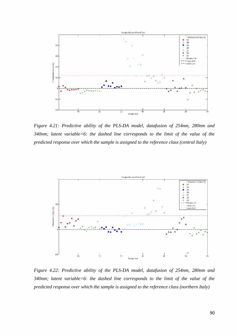
90
Figure 4.21: Predictive ability of the PLS-DA model, datafusion of 254nm, 280nm and
340nm; latent variable=6: the dashed line corresponds to the limit of the value of the
predicted response over which the sample is assigned to the reference class (central Italy)
Figure 4.22: Predictive ability of the PLS-DA model, datafusion of 254nm, 280nm and
340nm; latent variable=6: the dashed line corresponds to the limit of the value of the
predicted response over which the sample is assigned to the reference class (northern Italy)
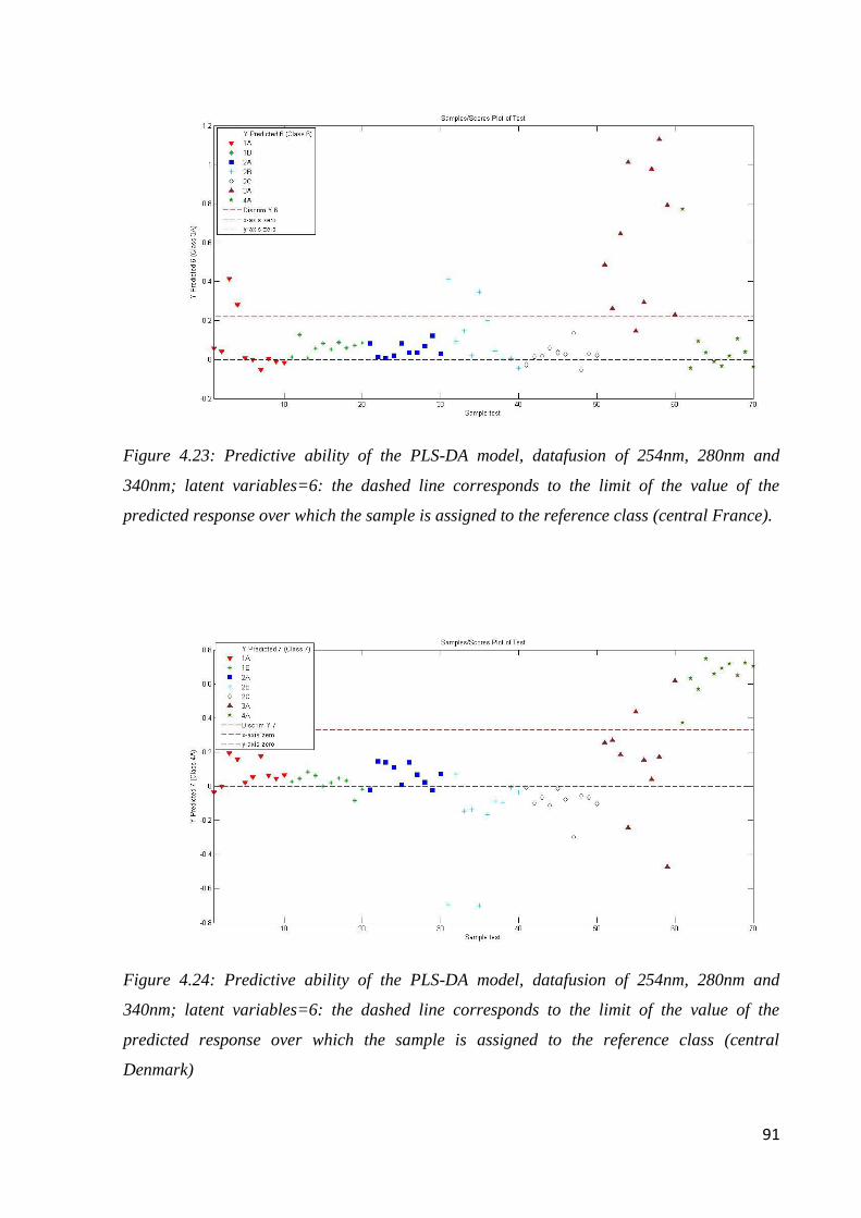
91
Figure 4.23: Predictive ability of the PLS-DA model, datafusion of 254nm, 280nm and
340nm; latent variables=6: the dashed line corresponds to the limit of the value of the
predicted response over which the sample is assigned to the reference class (central France).
Figure 4.24: Predictive ability of the PLS-DA model, datafusion of 254nm, 280nm and
340nm; latent variables=6: the dashed line corresponds to the limit of the value of the
predicted response over which the sample is assigned to the reference class (central
Denmark)
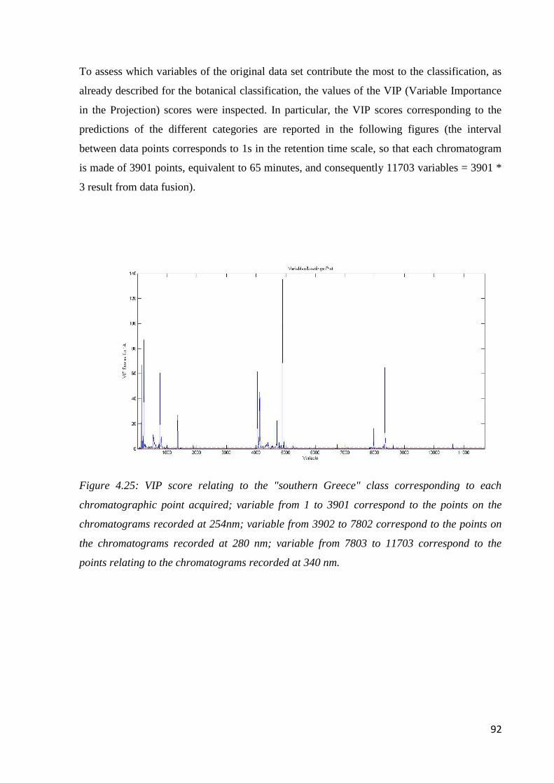
92
To assess which variables of the original data set contribute the most to the classification, as
already described for the botanical classification, the values of the VIP (Variable Importance
in the Projection) scores were inspected. In particular, the VIP scores corresponding to the
predictions of the different categories are reported in the following figures (the interval
between data points corresponds to 1s in the retention time scale, so that each chromatogram
is made of 3901 points, equivalent to 65 minutes, and consequently 11703 variables = 3901 *
3 result from data fusion).
Figure 4.25: VIP score relating to the "southern Greece" class corresponding to each
chromatographic point acquired; variable from 1 to 3901 correspond to the points on the
chromatograms recorded at 254nm; variable from 3902 to 7802 correspond to the points on
the chromatograms recorded at 280 nm; variable from 7803 to 11703 correspond to the
points relating to the chromatograms recorded at 340 nm.
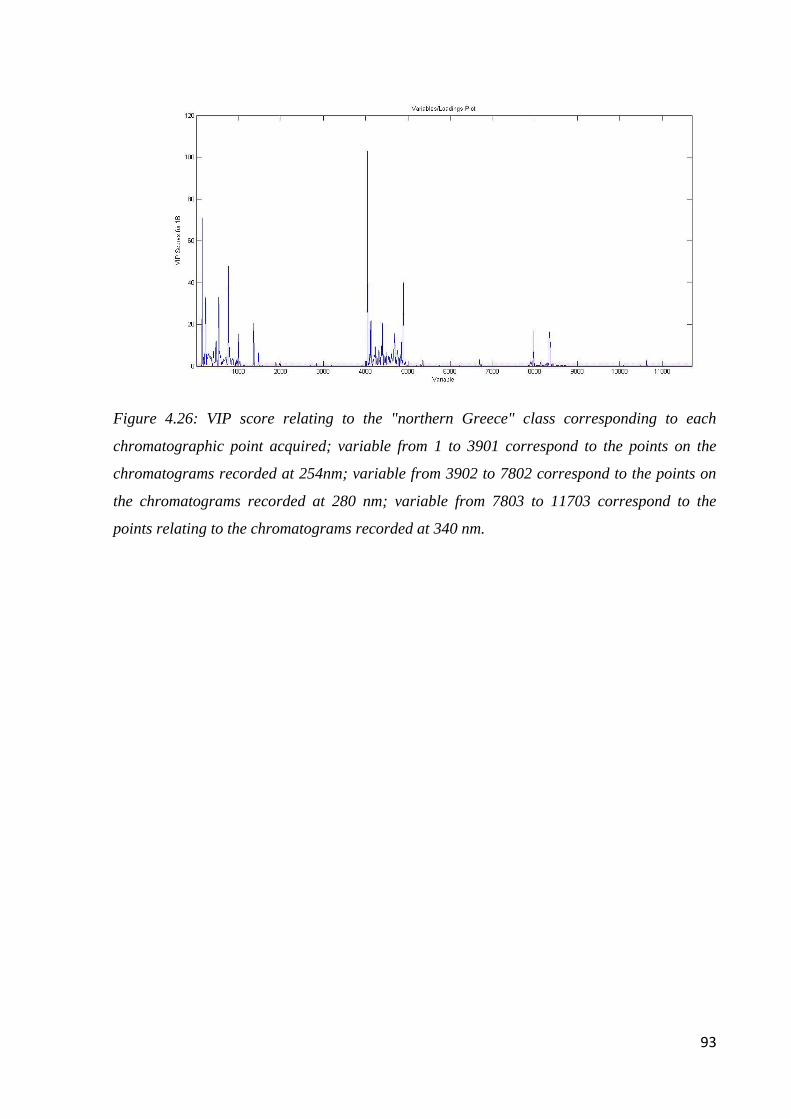
93
Figure 4.26: VIP score relating to the "northern Greece" class corresponding to each
chromatographic point acquired; variable from 1 to 3901 correspond to the points on the
chromatograms recorded at 254nm; variable from 3902 to 7802 correspond to the points on
the chromatograms recorded at 280 nm; variable from 7803 to 11703 correspond to the
points relating to the chromatograms recorded at 340 nm.
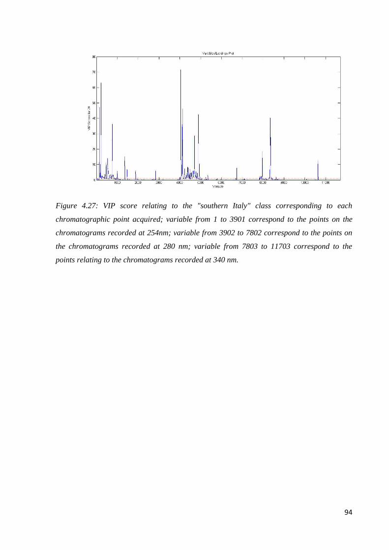
94
Figure 4.27: VIP score relating to the "southern Italy" class corresponding to each
chromatographic point acquired; variable from 1 to 3901 correspond to the points on the
chromatograms recorded at 254nm; variable from 3902 to 7802 correspond to the points on
the chromatograms recorded at 280 nm; variable from 7803 to 11703 correspond to the
points relating to the chromatograms recorded at 340 nm.
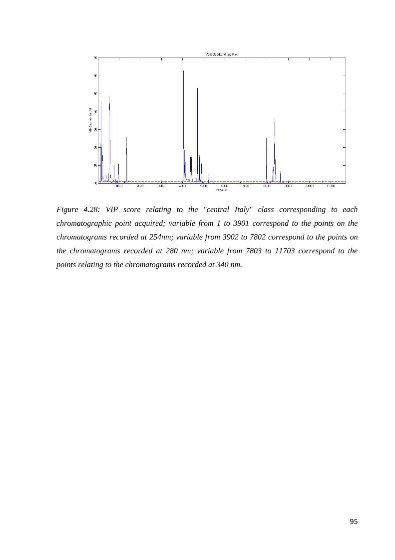
95
Figure 4.28: VIP score relating to the "central Italy" class corresponding to each
chromatographic point acquired; variable from 1 to 3901 correspond to the points on the
chromatograms recorded at 254nm; variable from 3902 to 7802 correspond to the points on
the chromatograms recorded at 280 nm; variable from 7803 to 11703 correspond to the
points relating to the chromatograms recorded at 340 nm.
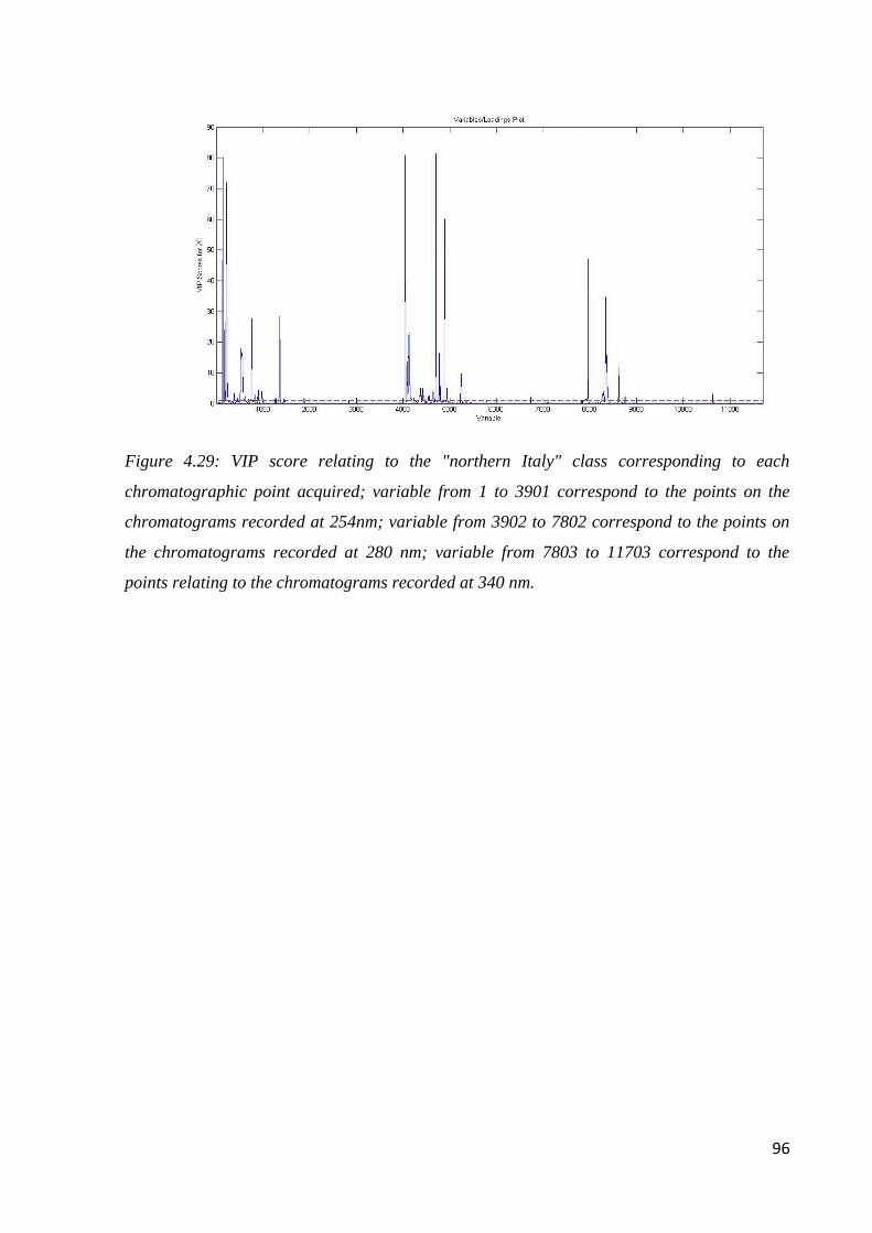
96
Figure 4.29: VIP score relating to the "northern Italy" class corresponding to each
chromatographic point acquired; variable from 1 to 3901 correspond to the points on the
chromatograms recorded at 254nm; variable from 3902 to 7802 correspond to the points on
the chromatograms recorded at 280 nm; variable from 7803 to 11703 correspond to the
points relating to the chromatograms recorded at 340 nm.
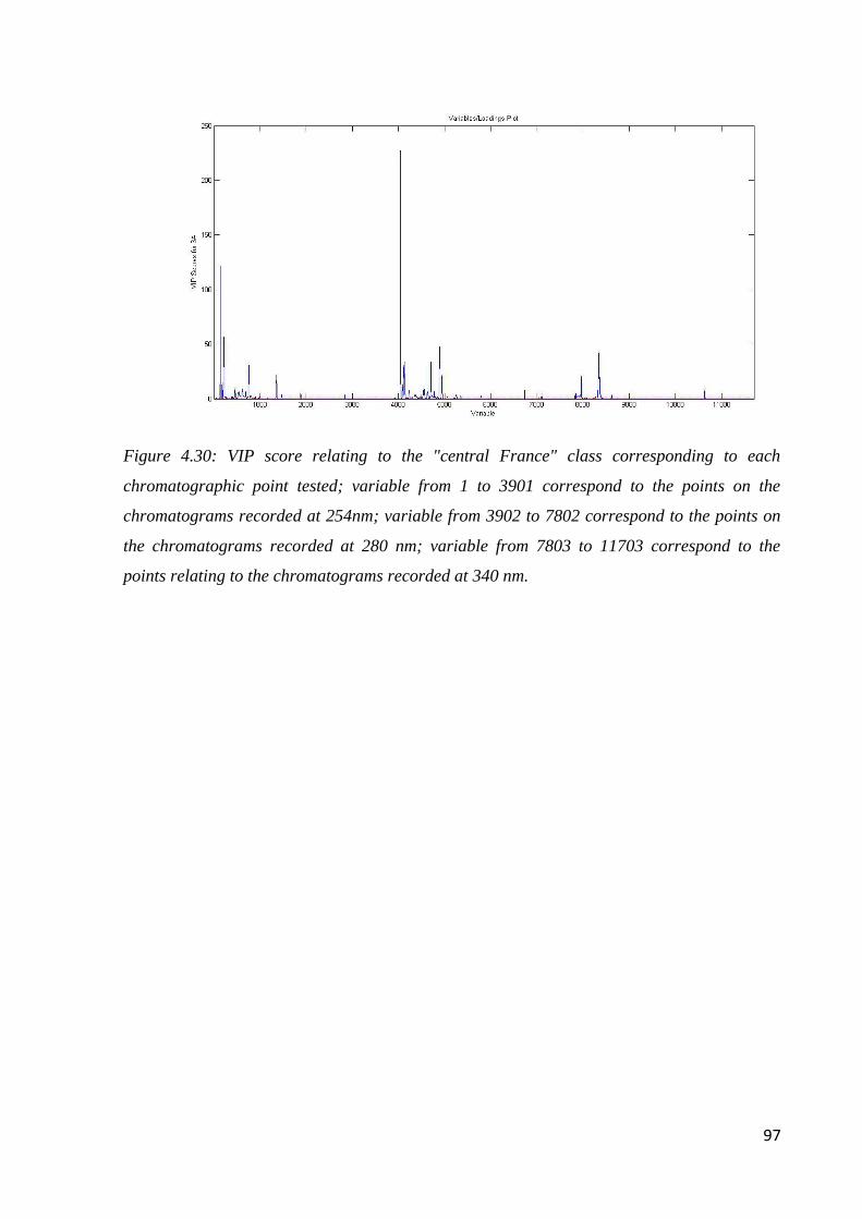
97
Figure 4.30: VIP score relating to the "central France" class corresponding to each
chromatographic point tested; variable from 1 to 3901 correspond to the points on the
chromatograms recorded at 254nm; variable from 3902 to 7802 correspond to the points on
the chromatograms recorded at 280 nm; variable from 7803 to 11703 correspond to the
points relating to the chromatograms recorded at 340 nm.
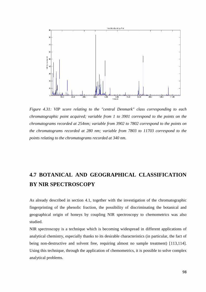
98
Figure 4.31: VIP score relating to the "central Denmark" class corresponding to each
chromatographic point acquired; variable from 1 to 3901 correspond to the points on the
chromatograms recorded at 254nm; variable from 3902 to 7802 correspond to the points on
the chromatograms recorded at 280 nm; variable from 7803 to 11703 correspond to the
points relating to the chromatograms recorded at 340 nm.
4.7 BOTANICAL AND GEOGRAPHICAL CLASSIFICATION
BY NIR SPECTROSCOPY
As already described in section 4.1, together with the investigation of the chromatographic
fingerprinting of the phenolic fraction, the possibility of discriminating the botanical and
geographical origin of honeys by coupling NIR spectroscopy to chemometrics was also
studied.
NIR spectroscopy is a technique which is becoming widespread in different applications of
analytical chemistry, especially thanks to its desirable characteristics (in particular, the fact of
being non-destructive and solvent free, requiring almost no sample treatment) [113,114].
Using this technique, through the application of chemometrics, it is possible to solve complex
analytical problems.
99
NIR spectroscopy is an analytical technique based on the absorption of electromagnetic
radiation in the near infrared region, i.e. in a range of wavenumbers between 12800 and 4000
cm-1
. In this interval, there are harmonics bands (overtones) and combination bands of the
vibrational transitions. The spectrum obtained depends on the behavior of the sample after the
incident radiation strikes: the sample can absorb, reflect or be crossed by the radiation. All
this depends on the chemical and physical characteristics of the sample. The spectrum shows
the intensity as a function of wavenumbers and it is characterized by broad bands, related to
the functional groups that are present in the sample. The NIR spectrum can be acquired in
three modalities:
- Transmittance: the fraction of the incident radiation transmitted by the sample (i.e. which is
not absorbed by the sample itself) is detected.
- Reflectance: the fraction of the incident radiation reflected by the sample is recorded.
- Transflectance: this mode is a combination of the previous two. Indeed, the radiation hits the
sample and passes through it; the beam transmitted by the sample is reflected back by a mirror
placed in a perfectly perpendicular position with respect to it, so that the radiation passes
through it again; Finally, the intensity of the resulting beam is measured.
NIR spectra, however, are very complex. A NIR spectrum alone, in fact, provides almost no
quantitative or qualitative information on the sample and for this reason it is necessary to use
chemometrics.
The acquisition was made through the use of a NIR spectrophotometer in transflectance
mode. For each sample (previously homogenized), a drop of honey between was placed
between two laboratory slides and each sample was analyzed four times, each time repeating
the sampling and analysis. Once recorded through the instrumental software Omnic, the data
were saved and exported to Matlab.
Successively, the NIR spectra of the 264 samples available for the botanical and geographical
classification were used as data for the construction of the PLS-DA models. As already
described, 4 spectra were acquired for each sample and the "standard normal variate" (SNV)
algorithm was applied to preprocess the signals. Indeed, this algorithm is widely used for the
removal of spurious contributions associated with scattering and/or other undesired
phenomena [115]. From the practical point of view the formula for the correction used by
SNV is the following:
(Eq. 4.1)
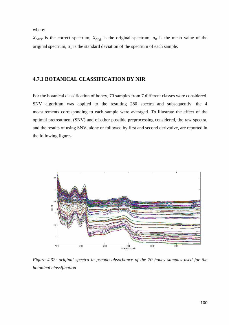
100
where:
is the correct spectrum; is the original spectrum, is the mean value of the
original spectrum, is the standard deviation of the spectrum of each sample.
4.7.1 BOTANICAL CLASSIFICATION BY NIR
For the botanical classification of honey, 70 samples from 7 different classes were considered.
SNV algorithm was applied to the resulting 280 spectra and subsequently, the 4
measurements corresponding to each sample were averaged. To illustrate the effect of the
optimal pretreatment (SNV) and of other possible preprocessing considered, the raw spectra,
and the results of using SNV, alone or followed by first and second derivative, are reported in
the following figures.
Figure 4.32: original spectra in pseudo absorbance of the 70 honey samples used for the
botanical classification
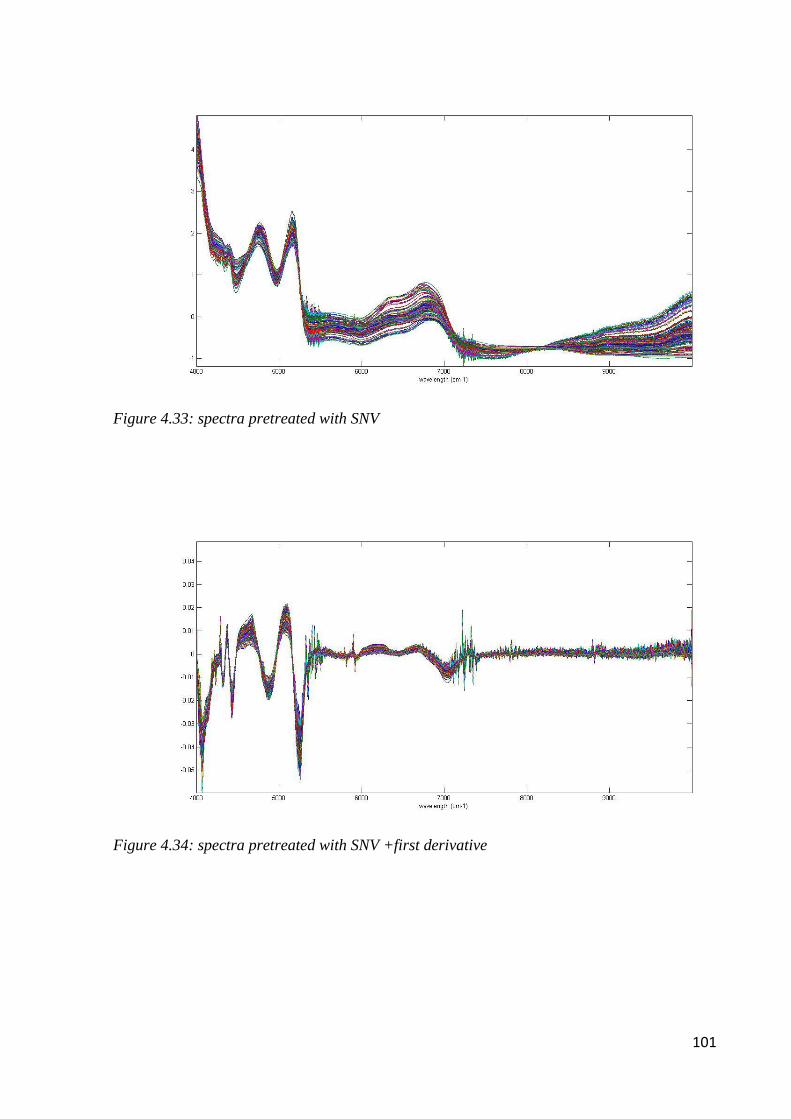
101
Figure 4.33: spectra pretreated with SNV
Figure 4.34: spectra pretreated with SNV +first derivative
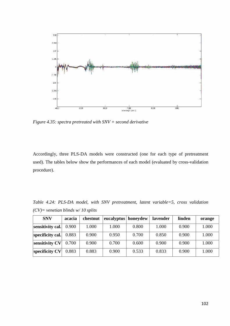
102
Figure 4.35: spectra pretreated with SNV + second derivative
Accordingly, three PLS-DA models were constructed (one for each type of pretreatment
used). The tables below show the performances of each model (evaluated by cross-validation
procedure).
Table 4.24: PLS-DA model, with SNV pretreatment, latent variable=5, cross validation
(CV)= venetian blinds w/ 10 splits
SNV acacia chestnut eucalyptus honeydew lavender linden orange
sensitivity cal. 0.900 1.000 1.000 0.800 1.000 0.900 1.000
specificity cal. 0.883 0.900 0.950 0.700 0.850 0.900 1.000
sensitivity CV 0.700 0.900 0.700 0.600 0.900 0.900 1.000
specificity CV 0.883 0.883 0.900 0.533 0.833 0.900 1.000

103
Table 4.25: PLS-DA model, with SNV+first derivative, latent variable=11, cross validation
(CV)= venetian blinds w/ 10 splits
SNV+der1 acacia chestnut eucalyptus honeydew lavender linden orange
sensitivity cal. 0.900 1.000 1.000 1.000 1.000 1.000 1.000
specificity cal. 0.933 1.000 0.950 0.933 0.983 0.933 1.000
sensitivity CV 0.600 0.800 0.800 0.300 0.700 0.800 1.000
specificity CV 0.867 0.900 0.883 0.883 0.850 0.933 1.000
Table 4.26: PLS-DA model, with SNV+second derivative, latent variable=5, cross validation
(CV)= venetian blinds w/ 10 splits
SNV+der2 acacia chestnut eucalyptus honeydew lavender linden orange
sensitivity cal. 0.900 0.900 0.900 0.800 0.900 0.900 1.000
specificity cal. 0.683 0.867 0.900 0.683 0.750 0.800 1.000
sensitivity CV 0.800 0.800 0.800 0.300 0.800 0.700 1.000
specificity CV 0.667 0.850 0.867 0.717 0.733 0.800 1.000
All the three PLS-DA models perfectly discriminate the orange honey, while for the other
classes the best classification is obtained by SNV correction without any further
differentiation. For the interpretation of the results, the VIP scores corresponding to the PLS-
DA model built on the data pretreated with SNV, is reported in the following figure. The VIP
plot indicates that there are different bands having a relevant impact on the construction of the
model and hence on the discrimination between different botanical classes. The largest
variation among the spectra of considered honey were observed in the regions corresponding
to the combination bands of the C-O and C-H stretching of the saccharides between 4200 and
5200-5300 cm-1
and to the first overtone of O-H at 7100cm-1
.
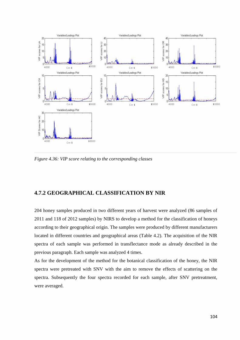
104
Figure 4.36: VIP score relating to the corresponding classes
4.7.2 GEOGRAPHICAL CLASSIFICATION BY NIR
204 honey samples produced in two different years of harvest were analyzed (86 samples of
2011 and 118 of 2012 samples) by NIRS to develop a method for the classification of honeys
according to their geographical origin. The samples were produced by different manufacturers
located in different countries and geographical areas (Table 4.2). The acquisition of the NIR
spectra of each sample was performed in transflectance mode as already described in the
previous paragraph. Each sample was analyzed 4 times.
As for the development of the method for the botanical classification of the honey, the NIR
spectra were pretreated with SNV with the aim to remove the effects of scattering on the
spectra. Subsequently the four spectra recorded for each sample, after SNV pretreatment,
were averaged.
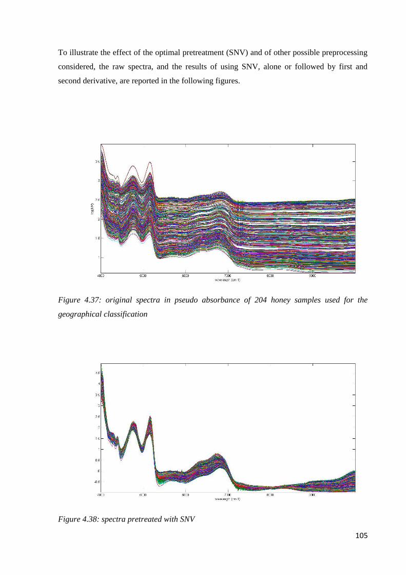
105
To illustrate the effect of the optimal pretreatment (SNV) and of other possible preprocessing
considered, the raw spectra, and the results of using SNV, alone or followed by first and
second derivative, are reported in the following figures.
Figure 4.37: original spectra in pseudo absorbance of 204 honey samples used for the
geographical classification
Figure 4.38: spectra pretreated with SNV
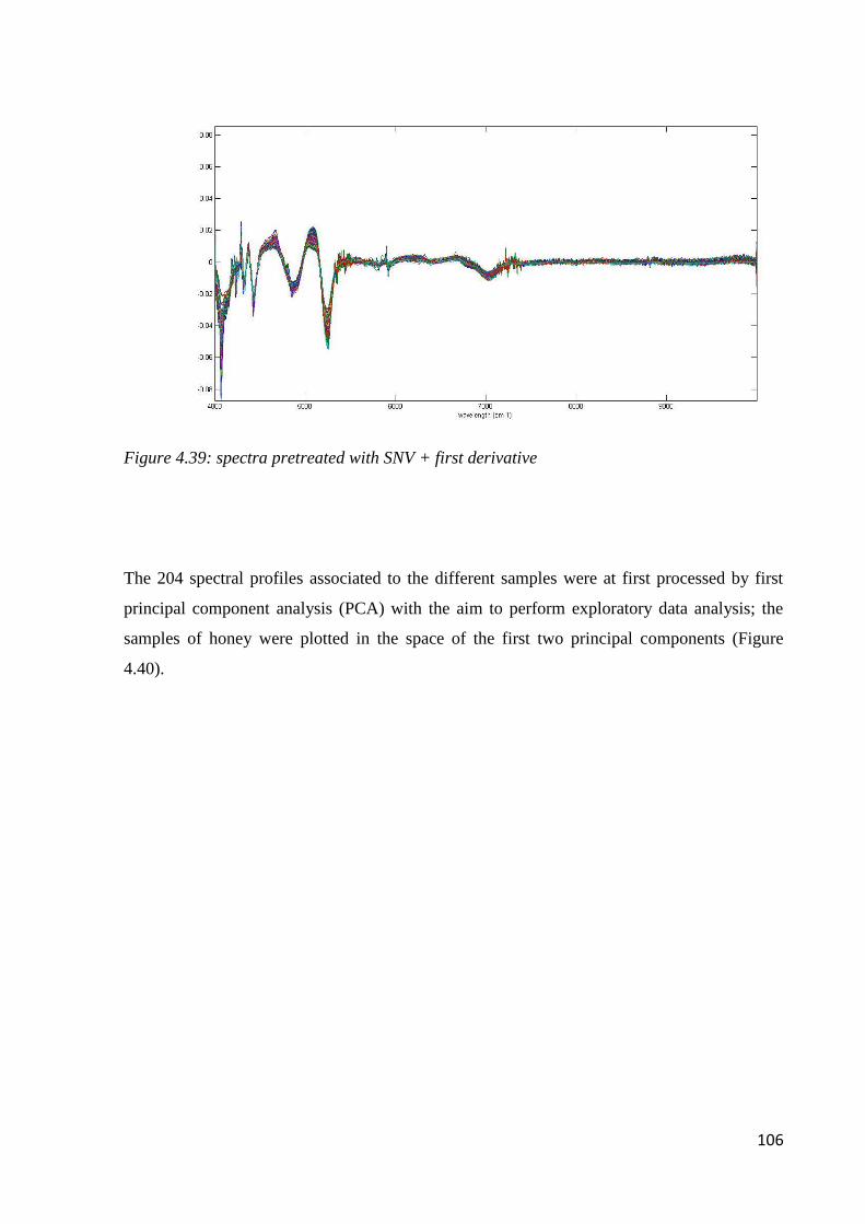
106
Figure 4.39: spectra pretreated with SNV + first derivative
The 204 spectral profiles associated to the different samples were at first processed by first
principal component analysis (PCA) with the aim to perform exploratory data analysis; the
samples of honey were plotted in the space of the first two principal components (Figure
4.40).

107
Figure 4.40: PCA scores of analyzed honey samples: 1A means southern Greece; 1B means
northern Greece; 2A means southern Italy; 2B means center Italy; 2C means northern Italy;
3A means center France; 4A means center Denmark
Exploratory analysis shows the presence of evident clusters, corresponding to the different
categories investigated. As done for the corresponding analysis based on HPLC-DAD, the
data set was split in two sets before building the classification model: a set for the
construction of the model (training set) and a set for the validation of the model built (test
set). Here, it was chosen to build the model using honey samples of 2012 and to test the
predictive ability of the model with samples of 2011.
Together with SNV alone, also the possibility of using first and second derivative as spectral
pretreatment was tested. Three PLS-DA models were constructed, one for each type of
pretreatment used (SNV, SNV + first derivative, second derivative SNV +) and the tables
summarizing the performances of the corresponding models are reported below. The choice of
the number of latent variables was performed based on cross validation, and each model was
validated with the test set not used for the construction of the models (samples of the year
2011).
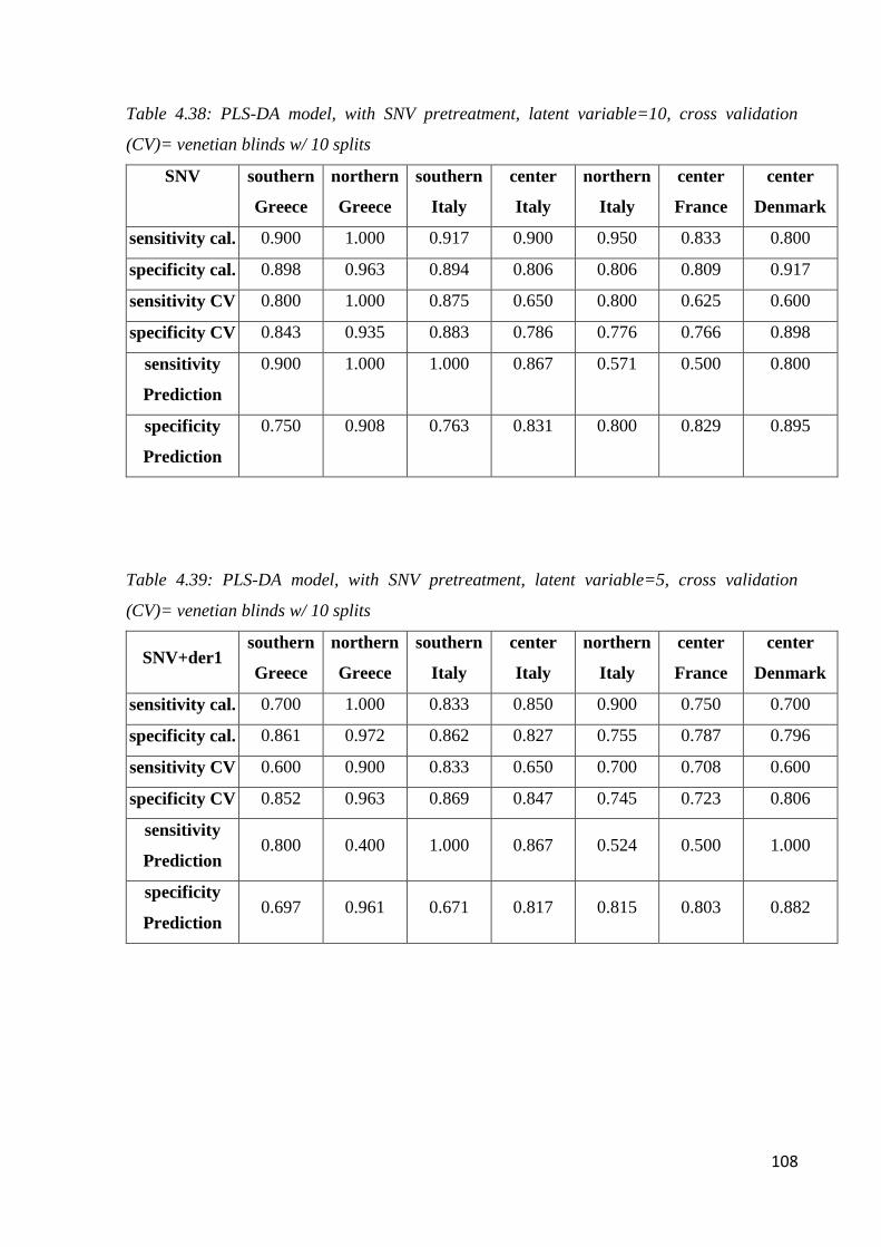
108
Table 4.38: PLS-DA model, with SNV pretreatment, latent variable=10, cross validation
(CV)= venetian blinds w/ 10 splits
SNV southern
Greece
northern
Greece
southern
Italy
center
Italy
northern
Italy
center
France
center
Denmark
sensitivity cal. 0.900 1.000 0.917 0.900 0.950 0.833 0.800
specificity cal. 0.898 0.963 0.894 0.806 0.806 0.809 0.917
sensitivity CV 0.800 1.000 0.875 0.650 0.800 0.625 0.600
specificity CV 0.843 0.935 0.883 0.786 0.776 0.766 0.898
sensitivity
Prediction
0.900 1.000 1.000 0.867 0.571 0.500 0.800
specificity
Prediction
0.750 0.908 0.763 0.831 0.800 0.829 0.895
Table 4.39: PLS-DA model, with SNV pretreatment, latent variable=5, cross validation
(CV)= venetian blinds w/ 10 splits
SNV+der1 southern
Greece
northern
Greece
southern
Italy
center
Italy
northern
Italy
center
France
center
Denmark
sensitivity cal. 0.700 1.000 0.833 0.850 0.900 0.750 0.700
specificity cal. 0.861 0.972 0.862 0.827 0.755 0.787 0.796
sensitivity CV 0.600 0.900 0.833 0.650 0.700 0.708 0.600
specificity CV 0.852 0.963 0.869 0.847 0.745 0.723 0.806
sensitivity
Prediction 0.800 0.400 1.000 0.867 0.524 0.500 1.000
specificity
Prediction 0.697 0.961 0.671 0.817 0.815 0.803 0.882
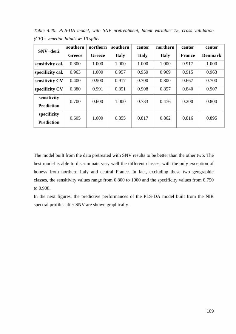
109
Table 4.40: PLS-DA model, with SNV pretreatment, latent variable=15, cross validation
(CV)= venetian blinds w/ 10 splits
SNV+der2 southern
Greece
northern
Greece
southern
Italy
center
Italy
northern
Italy
center
France
center
Denmark
sensitivity cal. 0.800 1.000 1.000 1.000 1.000 0.917 1.000
specificity cal. 0.963 1.000 0.957 0.959 0.969 0.915 0.963
sensitivity CV 0.400 0.900 0.917 0.700 0.800 0.667 0.700
specificity CV 0.880 0.991 0.851 0.908 0.857 0.840 0.907
sensitivity
Prediction 0.700 0.600 1.000 0.733 0.476 0.200 0.800
specificity
Prediction 0.605 1.000 0.855 0.817 0.862 0.816 0.895
The model built from the data pretreated with SNV results to be better than the other two. The
best model is able to discriminate very well the different classes, with the only exception of
honeys from northern Italy and central France. In fact, excluding these two geographic
classes, the sensitivity values range from 0.800 to 1000 and the specificity values from 0.750
to 0.908.
In the next figures, the predictive performances of the PLS-DA model built from the NIR
spectral profiles after SNV are shown graphically.
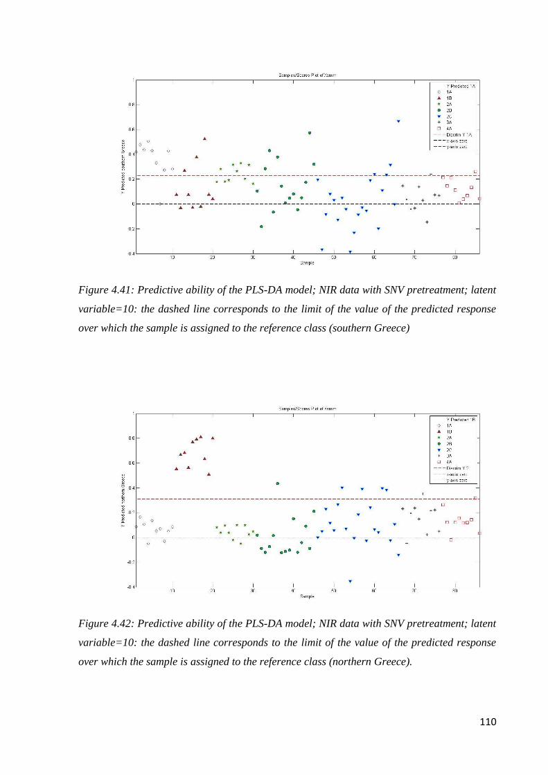
110
Figure 4.41: Predictive ability of the PLS-DA model; NIR data with SNV pretreatment; latent
variable=10: the dashed line corresponds to the limit of the value of the predicted response
over which the sample is assigned to the reference class (southern Greece)
Figure 4.42: Predictive ability of the PLS-DA model; NIR data with SNV pretreatment; latent
variable=10: the dashed line corresponds to the limit of the value of the predicted response
over which the sample is assigned to the reference class (northern Greece).
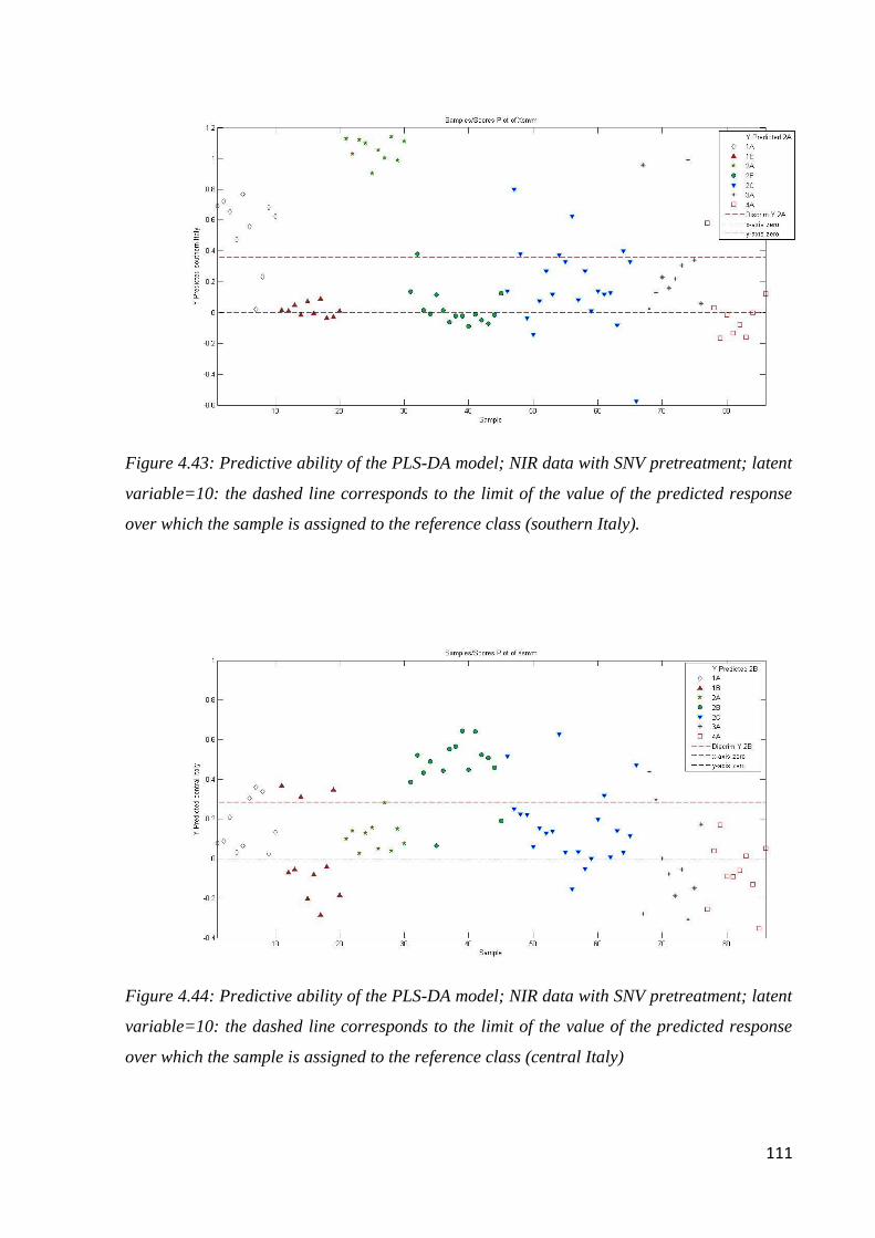
111
Figure 4.43: Predictive ability of the PLS-DA model; NIR data with SNV pretreatment; latent
variable=10: the dashed line corresponds to the limit of the value of the predicted response
over which the sample is assigned to the reference class (southern Italy).
Figure 4.44: Predictive ability of the PLS-DA model; NIR data with SNV pretreatment; latent
variable=10: the dashed line corresponds to the limit of the value of the predicted response
over which the sample is assigned to the reference class (central Italy)
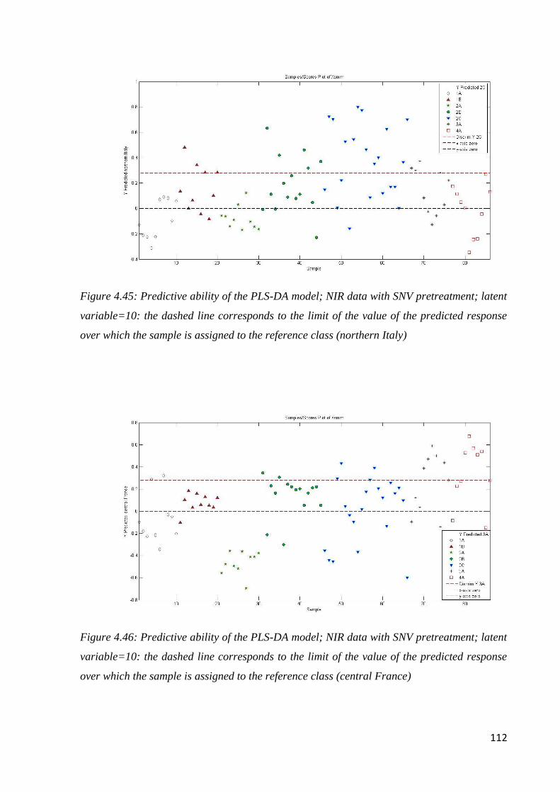
112
Figure 4.45: Predictive ability of the PLS-DA model; NIR data with SNV pretreatment; latent
variable=10: the dashed line corresponds to the limit of the value of the predicted response
over which the sample is assigned to the reference class (northern Italy)
Figure 4.46: Predictive ability of the PLS-DA model; NIR data with SNV pretreatment; latent
variable=10: the dashed line corresponds to the limit of the value of the predicted response
over which the sample is assigned to the reference class (central France)
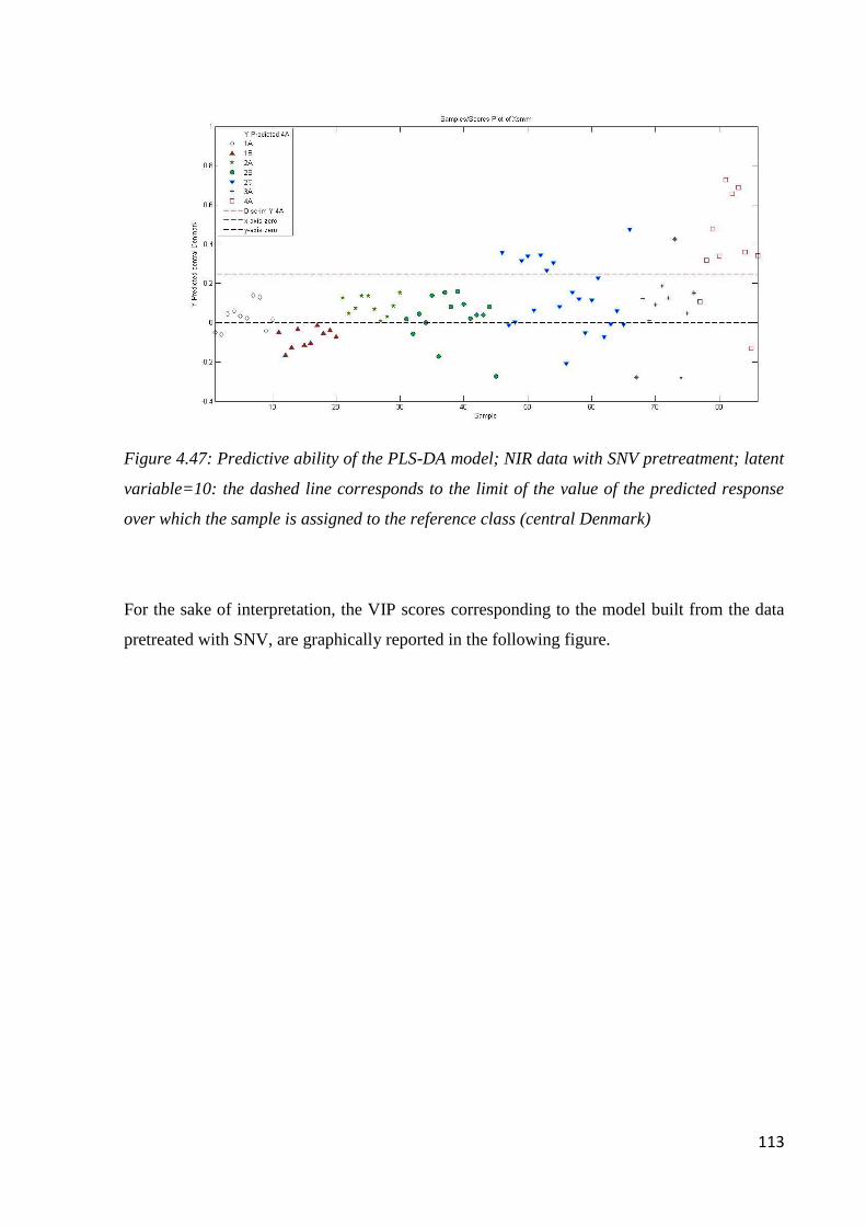
113
Figure 4.47: Predictive ability of the PLS-DA model; NIR data with SNV pretreatment; latent
variable=10: the dashed line corresponds to the limit of the value of the predicted response
over which the sample is assigned to the reference class (central Denmark)
For the sake of interpretation, the VIP scores corresponding to the model built from the data
pretreated with SNV, are graphically reported in the following figure.
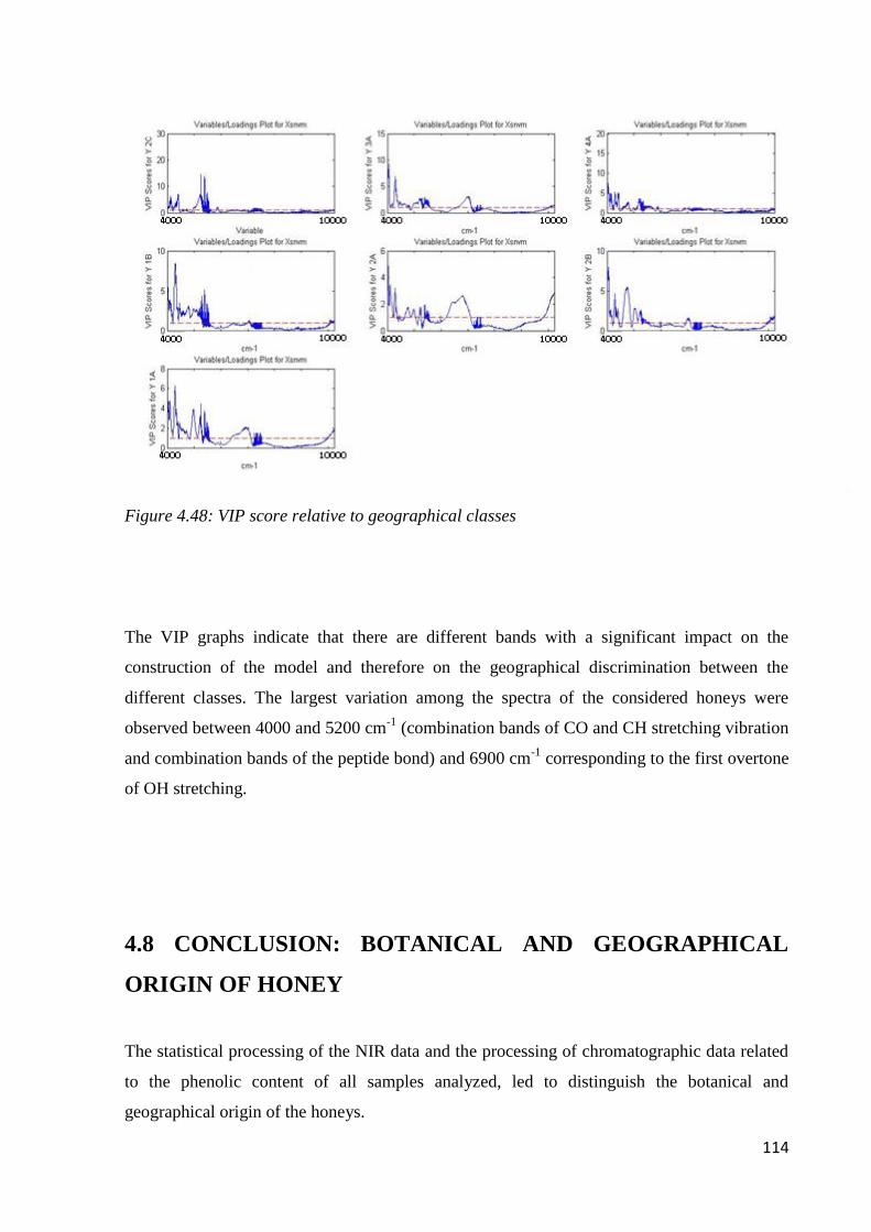
114
Figure 4.48: VIP score relative to geographical classes
The VIP graphs indicate that there are different bands with a significant impact on the
construction of the model and therefore on the geographical discrimination between the
different classes. The largest variation among the spectra of the considered honeys were
observed between 4000 and 5200 cm-1
(combination bands of CO and CH stretching vibration
and combination bands of the peptide bond) and 6900 cm-1
corresponding to the first overtone
of OH stretching.
4.8 CONCLUSION: BOTANICAL AND GEOGRAPHICAL
ORIGIN OF HONEY
The statistical processing of the NIR data and the processing of chromatographic data related
to the phenolic content of all samples analyzed, led to distinguish the botanical and
geographical origin of the honeys.

115
The HPLC-DAD and NIR protocols combined with multivariate statistical analysis, result a
valuable tool for the characterization of botanical and geographical origin of honey samples.
The phenolic fraction present in honey is strongly influenced by floral origin and but also
from the production area. So even honeys belonging to the same botanical species produced in
different geographical regions have differences in level of phenolic composition that make
them different from one other. The phenolic content represents a kind of map for the
recognition of the history of the food in question, including the possibility of tracing its
geographical origin.
For wildflower honey, a differentiation between Italian, Greek, French and Danish samples
was obtained; the statistical models showed very good predictive abilities, being able to
evaluate the geographic origin of external samples (test set).
The results of the project are promising and could be transferred to the honey production
chain, for producers and processors in order to control their products; consumers will benefit
from the project in terms of food safety. Finally, the method can be proposed at the control
authorities for the suppression of fraud.
116
CHAPTER 5
HONEY: DETERMINATION OF
QUALITY PARAMETERS
5.1 INTRODUCTION
One of the aims of the PhD research summarized in this dissertation was to develop an
analytical approach, alternative to the official methods of analysis, based on coupling near-
infrared spectroscopy with chemometric processing of the signal for the determination of
some quality parameters of honey samples, so that it can be rapid, inexpensive and non-
destructive/not invasive. In particular, three of the quality indices whose measured is required
by law, as described in the following paragraphs, were considered: the determination of the
content of reducing sugars, which usually involves the titration of Fehling's solution, the
determination of water content which normally consists of a refractometric analysis, and the
quantification of the 5-hydroxymethylfurfural which, as far as now, is accomplished through
the use of a procedure based on liquid chromatography. At the same time, again in order to
reduce the time and cost of analysis, additional tests were carried out to verify if it was also
possible to determine the water content by thermo-gravimetric analysis, which is the method
required by law for determining ashes, another index of honey quality. In all cases, since the
development of the NIR method required to have samples for which the values of the
properties to be calibrated were known and no certified standards were available, in the first
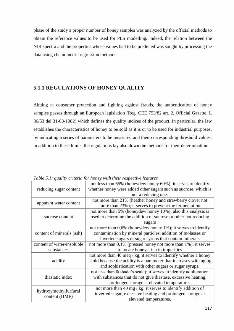
117
phase of the study a proper number of honey samples was analyzed by the official methods to
obtain the reference values to be used for PLS modelling. Indeed, the relation between the
NIR spectra and the properties whose values had to be predicted was sought by processing the
data using chemometric regression methods.
5.1.1 REGULATIONS OF HONEY QUALITY
Aiming at consumer protection and fighting against frauds, the authentication of honey
samples passes through an European legislation (Reg. CEE 753/82 art. 2, Official Gazette. L
86/53 del 31-03-1982) which defines the quality indices of the product. In particular, the law
establishes the characteristics of honey to be sold as it is or to be used for industrial purposes,
by indicating a series of parameters to be measured and their corresponding threshold values;
in addition to these limits, the regulations lay also down the methods for their determination.
Table 5.1: quality criteria for honey with their respective features
reducing sugar content
not less than 65% (honeydew honey 60%); it serves to identify
whether honey were added other sugars such as sucrose, which is
not a reducing one.
apparent water content not more than 21% (heather honey and strawberry clover not
more than 23%); it serves to prevent the fermentation
sucrose content
not more than 5% (honeydew honey 10%); also this analysis is
used to determine the addition of sucrose or other not reducing
sugars
content of minerals (ash)
not more than 0,6% (honeydew honey 1%); it serves to identify
contamination by mineral particles, addition of molasses or
inverted sugars or sugar syrups that contain minerals
content of water-insoluble
substances
not more than 0,1% (pressed honey not more than 1%); it serves
to locate honeys rich in impurities
acidity
not more than 40 meq / kg; it serves to identify whether a honey
is old because the acidity is a parameter that increases with aging
and sophistication with other sugars or sugar syrups.
diastatic index
not less than 8(shade‟s scale); it serves to identify adulteration
with substances that do not give diastase, excessive heating,
prolonged storage at elevated temperatures
hydroxymethylfurfural
content (HMF)
not more than 40 mg / kg; it serves to identify addition of
inverted sugar, excessive heating and prolonged storage at
elevated temperatures.

118
5.2 OFFICIAL METHODS
As previously mentioned, for the determination of each of these parameters, the law provides
official methods, which were selected according to the required analytical accuracy and based
on their characteristics which could allow to have large application in a wide number of
laboratories (Ministry of Health, decree of 20 July 1984, "Methods of analysis for the official
control of the compositional characteristics of honey”).
Reducing sugars
The method is based on the reduction of Fehling's solution by the reducing sugars contained
in a diluted solution of honey, in the presence of methylene blue as indicator [116].
Water content
The determination of the water content in honey is important to verify the conservation and to
define its characteristics; its quantification is performed indirectly by measuring the refractive
index of the honey or by thermogravimetric analysis.
Ashes and water-insoluble substances
Today these informations are obtained from thermogravimetric analysis.
Acidity
It is defined as "acidity of an aqueous solution of honey titratable with a solution of sodium
hydroxide up to pH 8.5" and it‟s determined by a potentiometric titration.
Diastatic Index
Spectrophotometric determination of the amount of residual starch of a solution placed in
incubation under standardized conditions with the solution of honey to be measured.
5-Hidroxymethylfurfural (HMF)
The official methods for International Honey Council (IHC) are the White method, the
Winkler method and the chromatographic method (this latter was used):
CHROMATOGRAPHIC METHOD (HPLC)
This method involves the dissolution of 5g of honey in 50 mL of. After filtration, the solution
is injected into a HPLC equipped with UV detector and an isocratic elution using as mobile
phase a solution of 90% water and 10% methanol at a flow rate of 1 mL / min is carried out.
The hydroxymethylfurfural (HMF) content is then determined, using the internal standard
method, by measuring the areas of the peaks of the analyte and the IS at 285 nm.

119
To obtain an accurate quantification, it is very important not to leave more than an hour and a
half between sample preparation and its injection into the column, since problems can
possibly arise from its degradation: to overcome this drawbacks, it is possible (according to
the method of White) to add the Carrez solution.
The comparison of the three methods [116] pointed out that there is a discordance for low
concentrations of HMF (for a HMF content of about 5mg/kg of the Winkler method gives
higher concentration values than the other two), while for high concentrations (20 to 40 mg
/kg) they are all concordant. From these considerations, it follows that any of the three
methods can be used indiscriminately for the determination of the honey quality, due to their
agreement around the legal limit (if we consider the parameters IHC, in fact, the upper limit is
80mg/kg for all types of honey); the use of the Winkler method is, however, recommended
only in the cases where it is not possible to apply the others, because p-toluidine is
carcinogenic.
5.3 DETERMINATION OF REDUCING SUGARS, WATER
CONTENT AND 5-HMF
For the development of the method for the determination of reducing sugars and water content
14 samples of honey of different botanical origin were analyzed: three of acacia honeys, three
wildflower honeys, one mountain wildflower honey, one orange honey, one linden honey, two
chestnut honey, and two eucalyptus honeys.
On the other hand, for the determination of 5-HMF, 13 samples of uni-and multi-floral honey
of different botanical origin were tested: four wildflower honey, two chestnut honey, two
eucalyptus honey, one of acacia honey, one of linden honey, one of orange honey.
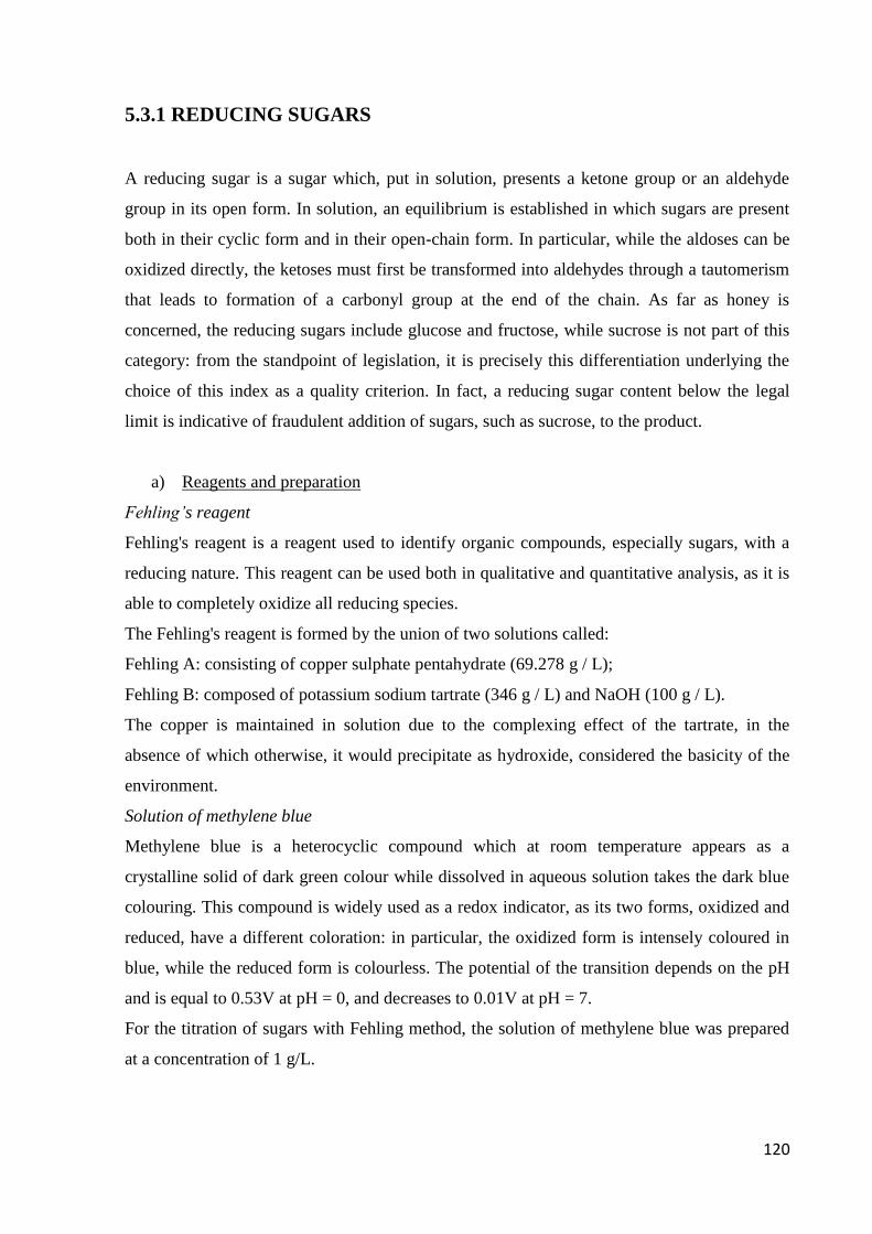
120
5.3.1 REDUCING SUGARS
A reducing sugar is a sugar which, put in solution, presents a ketone group or an aldehyde
group in its open form. In solution, an equilibrium is established in which sugars are present
both in their cyclic form and in their open-chain form. In particular, while the aldoses can be
oxidized directly, the ketoses must first be transformed into aldehydes through a tautomerism
that leads to formation of a carbonyl group at the end of the chain. As far as honey is
concerned, the reducing sugars include glucose and fructose, while sucrose is not part of this
category: from the standpoint of legislation, it is precisely this differentiation underlying the
choice of this index as a quality criterion. In fact, a reducing sugar content below the legal
limit is indicative of fraudulent addition of sugars, such as sucrose, to the product.
a) Reagents and preparation
Fehling’s reagent
Fehling's reagent is a reagent used to identify organic compounds, especially sugars, with a
reducing nature. This reagent can be used both in qualitative and quantitative analysis, as it is
able to completely oxidize all reducing species.
The Fehling's reagent is formed by the union of two solutions called:
Fehling A: consisting of copper sulphate pentahydrate (69.278 g / L);
Fehling B: composed of potassium sodium tartrate (346 g / L) and NaOH (100 g / L).
The copper is maintained in solution due to the complexing effect of the tartrate, in the
absence of which otherwise, it would precipitate as hydroxide, considered the basicity of the
environment.
Solution of methylene blue
Methylene blue is a heterocyclic compound which at room temperature appears as a
crystalline solid of dark green colour while dissolved in aqueous solution takes the dark blue
colouring. This compound is widely used as a redox indicator, as its two forms, oxidized and
reduced, have a different coloration: in particular, the oxidized form is intensely coloured in
blue, while the reduced form is colourless. The potential of the transition depends on the pH
and is equal to 0.53V at pH = 0, and decreases to 0.01V at pH = 7.
For the titration of sugars with Fehling method, the solution of methylene blue was prepared
at a concentration of 1 g/L.
121
Preparation of standard solution of inverted sugar
9.5 g of pure sucrose were weighed and dissolved into 5 mL of concentrated hydrochloric
acid; the resulting solution was then diluted with water to 100 mL. The acidified solution was
then stored for several days at room temperature (about 3 days between 20 °C and 25 °C) and
then diluted to 1000 mL. Immediately before being used, a volume of this solution was
neutralized with a 1 M solution of sodium hydroxide and diluted to the required concentration
(2 g/L) for the standardization.
Preparation of the test sample
About 2 g of homogeneous sample of honey, accurately weighed (W), were collected and
dissolved in distilled water, the resulting solution was diluted to 100 mL in a volumetric flask.
Successively, a further 1:4 dilution was performed, taking 50 mL of this solution and diluting
them to 200 mL.
b) Standardization of Fehling's reagent
This step is the confirmation that the reagent is not altered and titrates exactly the amount of
reducing sugars estimated. To do this, the title of the reagent Fehling solution A was checked,
verifying that 5.0 mL mixed with 5.0 mL of solution B, react completely with 0.050 g of
inverted sugar contained in 25 mL of diluted standard.
c) Preliminary titration
It is appropriate that the total volume of the solution at the equivalence point is 35 mL. For
this purpose, it is normally necessary to add a certain volume of water before the start of the
titration. To determine the volume of water to be added, a preliminary titration was necessary.
In particular, 5 mL of Fehling's solution A, to which 5 mL of solution B were added, were
placed in a flask together with 7 mL of water and a few grains of pumice stone or other
boiling regulator; successively, 15 mL of the diluted solution of honey were added through
the burette. The mixture was heated to boiling point on a plate, maintaining moderate boiling
for 2 minutes. During boiling 3 drops of a solution of methylene blue were added and the
titration was completed using small additions of solution of diluted honey until decolouration
of the indicator in about 3 minutes. Defined as X mL the total volume of diluted solution of
honey used for the preliminary titration, the volume of water to be added is equal to (25 - X)
mL.
d) Determination of reducing sugars
Exactly 5 mL of Fehling's solution A were introduced, with a pipette, in a 250 mL flask, in
which 5 mL of the solution B, (25 - X) mL of water, some grains of pumice and, with a
burette, a volume of diluted honey corresponding to (X - 1.5) mL were added. The mixture

122
was then heated to boiling on plate, maintaining a moderate boiling for 2 minutes. During the
boiling, 1 mL of the solution of methylene blue was added and the titration with the diluted
solution of honey until decolouration of the indicator was completed in a total time not
exceeding 3 minutes. Defined as Y mL the total volume of diluted honey used, the following
formula was used for the calculation of the results, as shown in the Codex Alimentarius
Standard for Honey, Ref No. CL 1993/14-SH:
Eq 5 3
Where:
C = g of inverted sugar per 100 g of honey, W = weight in g of honey sample, Y = volume in
mL of the diluted solution of honey consumed in the determination.
5.3.2 WATER CONTENT THROUGH REFRACTOMETRIC ANALYSIS
By law, the determination of water content in honey is made using refractometric analysis.
This technique is based on measurement of refractive index or the ratio between the speed of
light in vacuum and that the substance to be analyzed, and can be used both in the case of
solid and liquid or gas samples. The measurement was performed by an Abbe refractometer
prism, which is a tool for liquid and solid samples. This type of refractometer is composed of
two prisms, separated by about 0.15 mm. Within this thin layer, a small drop of the liquid to
be examined is placed and the value of the refractive index is measured at the emission
frequency of sodium. The value obtained must always be coupled to temperature [117].
According to the law, the refractive index of homogenized honey was determined at 20 ° C. If
the determination had been made at different temperature, but near to 20 ° C, one would have
to correct the value found using the following thermal coefficients: +0.00023 / ° C for
temperatures above 20 ° C and -0.00023 / ° C for temperatures below 20 ° C. The percentage
of water content was obtained from the following table of correlation.
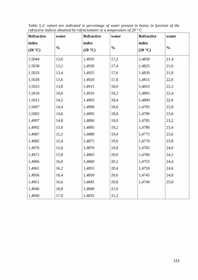
123
Table 5.2: values are indicated in percentage of water present in honey in function of the
refractive indices obtained by refractometer at a temperature of 20 ° C
Refractive
index
(20 °C)
water
%
Refractive
index
(20 °C)
water
%
Refractive
index
(20 °C)
water
%
1,5044 13,0 1,4935 17,2 1,4830 21,4
1,5038 13,2 1,4930 17,4 1,4825 21,6
1,5033 13,4 1,4925 17,6 1,4820 21,8
1,5028 13,6 1,4920 17,8 1,4815 22,0
1,5023 13,8 1,4915 18,0 1,4810 22,2
1,5018 14,0 1,4910 18,2 1,4805 22,4
1,5012 14,2 1,4905 18,4 1,4800 22,6
1,5007 14,4 1,4900 18,6 1,4795 22,8
1,5002 14,6 1,4895 18,8 1,4790 23,0
1,4997 14,8 1,4890 19,0 1,4785 23,2
1,4992 15,0 1,4885 19,2 1,4780 23,4
1,4987 15,2 1,4880 19,4 1,4775 23,6
1,4982 15,4 1,4875 19,6 1,4770 23,8
1,4976 15,6 1,4870 19,8 1,4765 24,0
1,4971 15,8 1,4865 20,0 1,4760 24,2
1,4966 16,0 1,4860 20,2 1,4755 24,4
1,4961 16,2 1,4855 20,4 1,4750 24,6
1,4956 16,4 1,4850 20,6 1,4745 24,8
1,4951 16,6 1,4845 20,8 1,4740 25,0
1,4946 16,8 1,4840 21,0
1,4940 17,0 1,4835 21,2

124
5.3.3 WATER CONTENT THROUGH THERMOGRAVIMETRIC
ANALYSIS
According to the law, the thermo-gravimetric analysis is the technique that must be used to
determine the amount of ashes and water-insoluble substances present in honey. Based on this
consideration, in the present research tests were performed to verify if it was also possible to
determine the water content through this technique. For this purpose, the instrument used was
the thermo-balance.
Balances available for this kind of analysis have an operating range between 1 and 20 mg. In
the thermo balance the sample is placed in the oven, while the rest of the device is thermally
insulated. In thermo-gravimetric analysis, the instrument records the loss in mass of the
sample, subjected to a specific temperature ramp. The instrument is then able to identify all
those thermal processes that result in a loss of mass: because the loss of water due to
volatilization represents just one of these processes detectable, it was decided to study the
possibility of using the thermal analysis for the quantification of water.
For this purpose, three measurements for each sample (5 mg) were made in an inert and
oxidant environment. Also, two different temperature ramps were tested, in order to get as
much information on the components sought:
a) heating at a constant rate of 5 °C/min [118], corresponding to the optimal conditions for the
determination of the ash content and substances insoluble in water;
b) a programmed heating at not constant speed to be able to better appreciate the initial step of
the thermogram (and, in particular, that corresponding to the loss of water).
The obtained thermograms were then exported to ASCII form using the TADS tool software.
5.3.4 HYDROXYMETHYLFURFURAL
In the absence of the standard samples, the quantification of HMF in the samples mentioned
in the previous paragraph was performed through the use of the HPLC method, in order to
obtain the reference values for the construction and validation of the NIR method. In
particular, it was decided to perform the quantitative analysis through the use of the external
standard. For the construction of the calibration curve of the HPLC method a standard of

125
HMF of purity over 99% (Sigma Aldrich, St. Louis, MO) was used. A stock solution was
prepared at a concentration 1 mg/mL by dissolving the appropriate amount of standard in
distilled water. The hydroxymethylfurfural solution of known concentration (in the range of
0.2-10 ng/µL) necessary for the quantitative analysis through the method of the external
standard were prepared by dilution from the stock solution.
In detail, the quantification of hydroxymethylfurfural in honey samples through the HPLC
method was performed using the following procedure. After homogenization of the sample,
about 5 g (with an accuracy of 0.01g) of honey were weighed, and transferred into a 50 mL
volumetric flask. Distilled water was added to the volume expected to completely dissolve the
honey. The obtained solution was filtered on 0.45 µm filters and 20 µL of the filtrate were
then injected into HPLC system. The chromatographic analysis was performed using a HPLC
system interfaced with a photodiode array detector (ThermoFisher, Waltham, MA) and
equipped with a C18 reverse phase column (length 15 cm and internal diameter 4.6 mm),
packed with 5 µm particles. The elution was conducted using an isocratic mobile phase
composed of 90% of ultra-pure water (MilliQ) and 10% methanol (HPLC grade, Carlo Erba,
Milan, Italy); both of the phases were acidified with 0.1% formic acid (Sigma Aldrich, St.
Louis, MO). For detection and quantification, the wavelength of 285 nm, the value at which it
is possible to appreciate a detectable signal of the analyte even at very low concentrations and
without interference, was chosen.
In a second phase of the study, to expand the range of concentration for the calibration and
validation of the NIR method, since the real samples showed a small range of values,
additional samples of honey were then prepared at known concentration of analyte, adding an
appropriate amount of standard of HMF.
5.4 ACQUISITION OF NIR SPECTRA
The acquisition was made through the use of a NIR spectrophotometer. A drop of each
sample was put between two laboratory glass slides. Before this step, each sample was mixed
to obtain homogeneity. The spectra were acquired in transflectance mode [119]. Each honey
was sampled and analyzed 4 times. All acquisitions were performed with 82 scans. Once
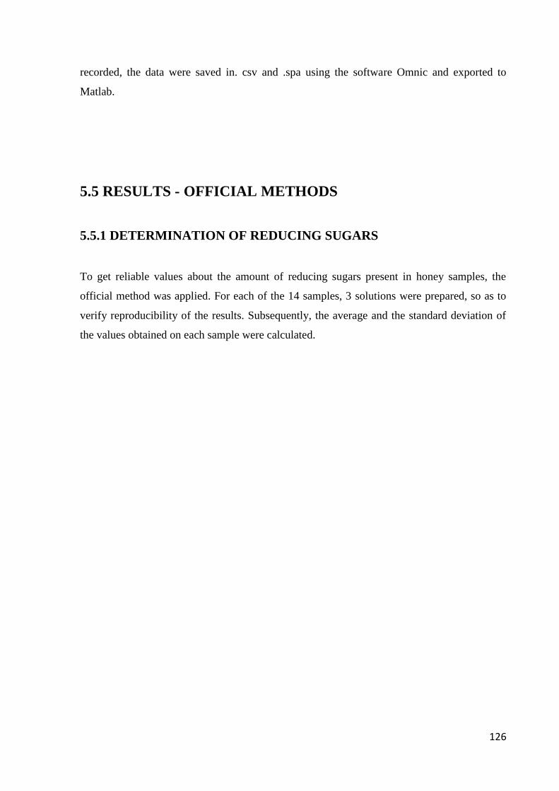
126
recorded, the data were saved in. csv and .spa using the software Omnic and exported to
Matlab.
5.5 RESULTS - OFFICIAL METHODS
5.5.1 DETERMINATION OF REDUCING SUGARS
To get reliable values about the amount of reducing sugars present in honey samples, the
official method was applied. For each of the 14 samples, 3 solutions were prepared, so as to
verify reproducibility of the results. Subsequently, the average and the standard deviation of
the values obtained on each sample were calculated.
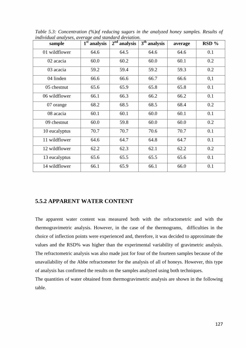
127
Table 5.3: Concentration (%)of reducing sugars in the analyzed honey samples. Results of
individual analyses, average and standard deviation.
sample 1st analysis 2
nd analysis 3
th analysis average RSD %
01 wildflower 64.6 64.5 64.6 64.6 0.1
02 acacia 60.0 60.2 60.0 60.1 0.2
03 acacia 59.2 59.4 59.2 59.3 0.2
04 linden 66.6 66.6 66.7 66.6 0,1
05 chestnut 65.6 65.9 65.8 65.8 0.1
06 wildflower 66.1 66.3 66.2 66.2 0.1
07 orange 68.2 68.5 68.5 68.4 0.2
08 acacia 60.1 60.1 60.0 60.1 0.1
09 chestnut 60.0 59.8 60.0 60.0 0.2
10 eucalyptus 70.7 70.7 70.6 70.7 0.1
11 wildflower 64.6 64.7 64.8 64.7 0.1
12 wildflower 62.2 62.3 62.1 62.2 0.2
13 eucalyptus 65.6 65.5 65.5 65.6 0.1
14 wildflower 66.1 65.9 66.1 66.0 0.1
5.5.2 APPARENT WATER CONTENT
The apparent water content was measured both with the refractometric and with the
thermogravimetric analysis. However, in the case of the thermograms, difficulties in the
choice of inflection points were experienced and, therefore, it was decided to approximate the
values and the RSD% was higher than the experimental variability of gravimetric analysis.
The refractometric analysis was also made just for four of the fourteen samples because of the
unavailability of the Abbe refractometer for the analysis of all of honeys. However, this type
of analysis has confirmed the results on the samples analyzed using both techniques.
The quantities of water obtained from thermogravimetric analysis are shown in the following
table.
128
Table 5.4: Water content (%) obtained by the thermogravimetric analysis and its
corresponding relative standard deviation
sample % of water RSD
01 wildflower 15.0 1.0
02 acacia 15.0 2.0
03 acacia 16.0 2.0
04 linden 16.5 2.0
05 chestnut 17.0 1.0
06 wildflower 17.0 1.0
07 orange 16.0 2.0
08 acacia 17.5 1.0
09 chestnut 16.0 1.0
10 eucalyptus 15.0 1.0
11 wildflower 14.5 2.0
12 wildflower 15.0 1.0
13 eucalyptus 15.5 2.0
14 wildflower 15.0 2.0
5.5.3 DETERMINATION OF 5-HMF
The results obtained are reported in Table 5.5 (for each sample, three replicate measurements
were performed and the values shown are the average and the relative standard deviation,
respectively).
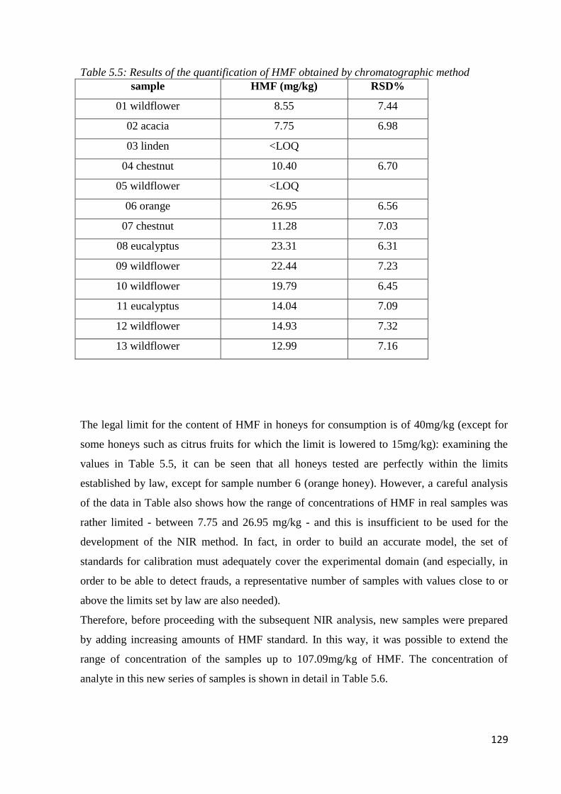
129
Table 5.5: Results of the quantification of HMF obtained by chromatographic method
sample HMF (mg/kg) RSD%
01 wildflower 8.55 7.44
02 acacia 7.75 6.98
03 linden <LOQ
04 chestnut 10.40 6.70
05 wildflower <LOQ
06 orange 26.95 6.56
07 chestnut 11.28 7.03
08 eucalyptus 23.31 6.31
09 wildflower 22.44 7.23
10 wildflower 19.79 6.45
11 eucalyptus 14.04 7.09
12 wildflower 14.93 7.32
13 wildflower 12.99 7.16
The legal limit for the content of HMF in honeys for consumption is of 40mg/kg (except for
some honeys such as citrus fruits for which the limit is lowered to 15mg/kg): examining the
values in Table 5.5, it can be seen that all honeys tested are perfectly within the limits
established by law, except for sample number 6 (orange honey). However, a careful analysis
of the data in Table also shows how the range of concentrations of HMF in real samples was
rather limited - between 7.75 and 26.95 mg/kg - and this is insufficient to be used for the
development of the NIR method. In fact, in order to build an accurate model, the set of
standards for calibration must adequately cover the experimental domain (and especially, in
order to be able to detect frauds, a representative number of samples with values close to or
above the limits set by law are also needed).
Therefore, before proceeding with the subsequent NIR analysis, new samples were prepared
by adding increasing amounts of HMF standard. In this way, it was possible to extend the
range of concentration of the samples up to 107.09mg/kg of HMF. The concentration of
analyte in this new series of samples is shown in detail in Table 5.6.
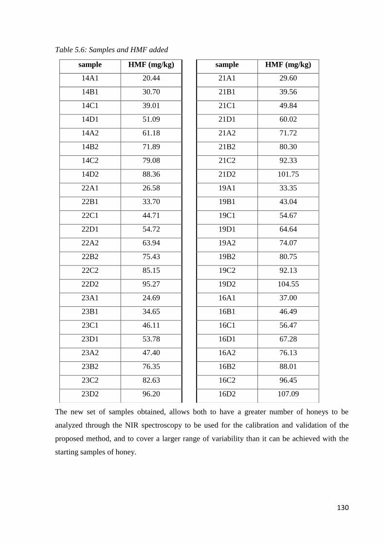
130
Table 5.6: Samples and HMF added
The new set of samples obtained, allows both to have a greater number of honeys to be
analyzed through the NIR spectroscopy to be used for the calibration and validation of the
proposed method, and to cover a larger range of variability than it can be achieved with the
starting samples of honey.
sample HMF (mg/kg) sample HMF (mg/kg)
14A1 20.44 21A1 29.60
14B1 30.70 21B1 39.56
14C1 39.01 21C1 49.84
14D1 51.09 21D1 60.02
14A2 61.18 21A2 71.72
14B2 71.89 21B2 80.30
14C2 79.08 21C2 92.33
14D2 88.36 21D2 101.75
22A1 26.58 19A1 33.35
22B1 33.70 19B1 43.04
22C1 44.71 19C1 54.67
22D1 54.72 19D1 64.64
22A2 63.94 19A2 74.07
22B2 75.43 19B2 80.75
22C2 85.15 19C2 92.13
22D2 95.27 19D2 104.55
23A1 24.69 16A1 37.00
23B1 34.65 16B1 46.49
23C1 46.11 16C1 56.47
23D1 53.78 16D1 67.28
23A2 47.40 16A2 76.13
23B2 76.35 16B2 88.01
23C2 82.63 16C2 96.45
23D2 96.20 16D2 107.09

131
5.6 RESULTS – CHEMOMETRIC ANALYSIS
As already mentioned, one of the aims of this thesis was to study the possibility of developing
alternative methods based on near-infrared spectroscopy for the determination of three
important parameters of honey quality: water content, the amount of reducing sugars and the
amount of idroxymethylfurfural.
For this purpose, the spectra of the samples were recorded in the range 4000-10000 cm-1
,
according to the methods described in Section 5.4.
The "raw" spectral signals obtained are affected by various undesirable phenomena such as
the presence of shift of the baseline, or multiplicative effects, probably due to scattering.
These contributions to the signal constitute sources of undesirable variability (i.e., not bound
to the analyte that is to be determined), so before chemometric analysis, a signal pre-treatment
step was necessary.
The spectral data, after being exported, were converted into pseudo-absorbance units and pre-
treated with the algorithm SNV (Standard Normal Variate) [115] to eliminate contributions to
the variability of the signal, related to sources of spurious variability.
The set of NIR spectra measured, after SNV pretreatment, is shown in Figure 5.1.
Figure 5.1: NIR spectra recorded, after pretreatment with SNV
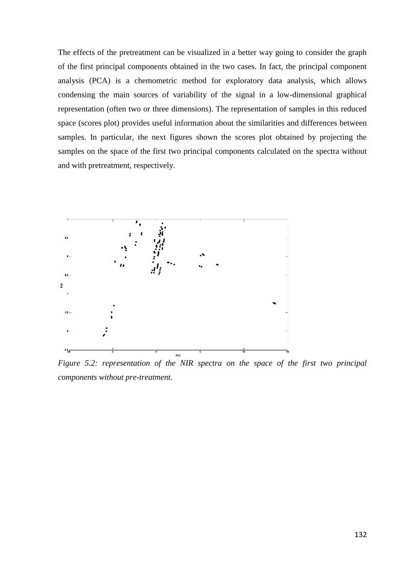
132
The effects of the pretreatment can be visualized in a better way going to consider the graph
of the first principal components obtained in the two cases. In fact, the principal component
analysis (PCA) is a chemometric method for exploratory data analysis, which allows
condensing the main sources of variability of the signal in a low-dimensional graphical
representation (often two or three dimensions). The representation of samples in this reduced
space (scores plot) provides useful information about the similarities and differences between
samples. In particular, the next figures shown the scores plot obtained by projecting the
samples on the space of the first two principal components calculated on the spectra without
and with pretreatment, respectively.
Figure 5.2: representation of the NIR spectra on the space of the first two principal
components without pre-treatment.
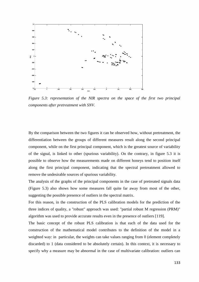
133
Figure 5.3: representation of the NIR spectra on the space of the first two principal
components after pretreatment with SNV.
By the comparison between the two figures it can be observed how, without pretreatment, the
differentiation between the groups of different measures result along the second principal
component, while on the first principal component, which is the greatest source of variability
of the signal, is linked to other (spurious variability). On the contrary, in figure 5.3 it is
possible to observe how the measurements made on different honeys tend to position itself
along the first principal component, indicating that the spectral pretreatment allowed to
remove the undesirable sources of spurious variability.
The analysis of the graphs of the principal components in the case of pretreated signals data
(Figure 5.3) also shows how some measures fall quite far away from most of the other,
suggesting the possible presence of outliers in the spectral matrix.
For this reason, in the construction of the PLS calibration models for the prediction of the
three indices of quality, a "robust" approach was used: "partial robust M regression (PRM)"
algorithm was used to provide accurate results even in the presence of outliers [119].
The basic concept of the robust PLS calibration is that each of the data used for the
construction of the mathematical model contributes to the definition of the model in a
weighted way: in particular, the weights can take values ranging from 0 (element completely
discarded) to 1 (data considered to be absolutely certain). In this context, it is necessary to
specify why a measure may be abnormal in the case of multivariate calibration: outliers can
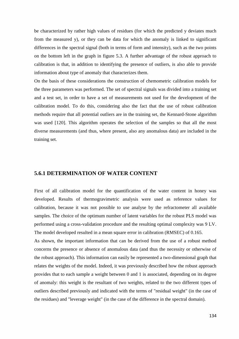
134
be characterized by rather high values of residues (for which the predicted y deviates much
from the measured y), or they can be data for which the anomaly is linked to significant
differences in the spectral signal (both in terms of form and intensity), such as the two points
on the bottom left in the graph in figure 5.3. A further advantage of the robust approach to
calibration is that, in addition to identifying the presence of outliers, is also able to provide
information about type of anomaly that characterizes them.
On the basis of these considerations the construction of chemometric calibration models for
the three parameters was performed. The set of spectral signals was divided into a training set
and a test set, in order to have a set of measurements not used for the development of the
calibration model. To do this, considering also the fact that the use of robust calibration
methods require that all potential outliers are in the training set, the Kennard-Stone algorithm
was used [120]. This algorithm operates the selection of the samples so that all the most
diverse measurements (and thus, where present, also any anomalous data) are included in the
training set.
5.6.1 DETERMINATION OF WATER CONTENT
First of all calibration model for the quantification of the water content in honey was
developed. Results of thermogravimetric analysis were used as reference values for
calibration, because it was not possible to use analyse by the refractometer all available
samples. The choice of the optimum number of latent variables for the robust PLS model was
performed using a cross-validation procedure and the resulting optimal complexity was 9 LV.
The model developed resulted in a mean square error in calibration (RMSEC) of 0.165.
As shown, the important information that can be derived from the use of a robust method
concerns the presence or absence of anomalous data (and thus the necessity or otherwise of
the robust approach). This information can easily be represented a two-dimensional graph that
relates the weights of the model. Indeed, it was previously described how the robust approach
provides that to each sample a weight between 0 and 1 is associated, depending on its degree
of anomaly: this weight is the resultant of two weights, related to the two different types of
outliers described previously and indicated with the terms of "residual weight" (in the case of
the residues) and "leverage weight" (in the case of the difference in the spectral domain).
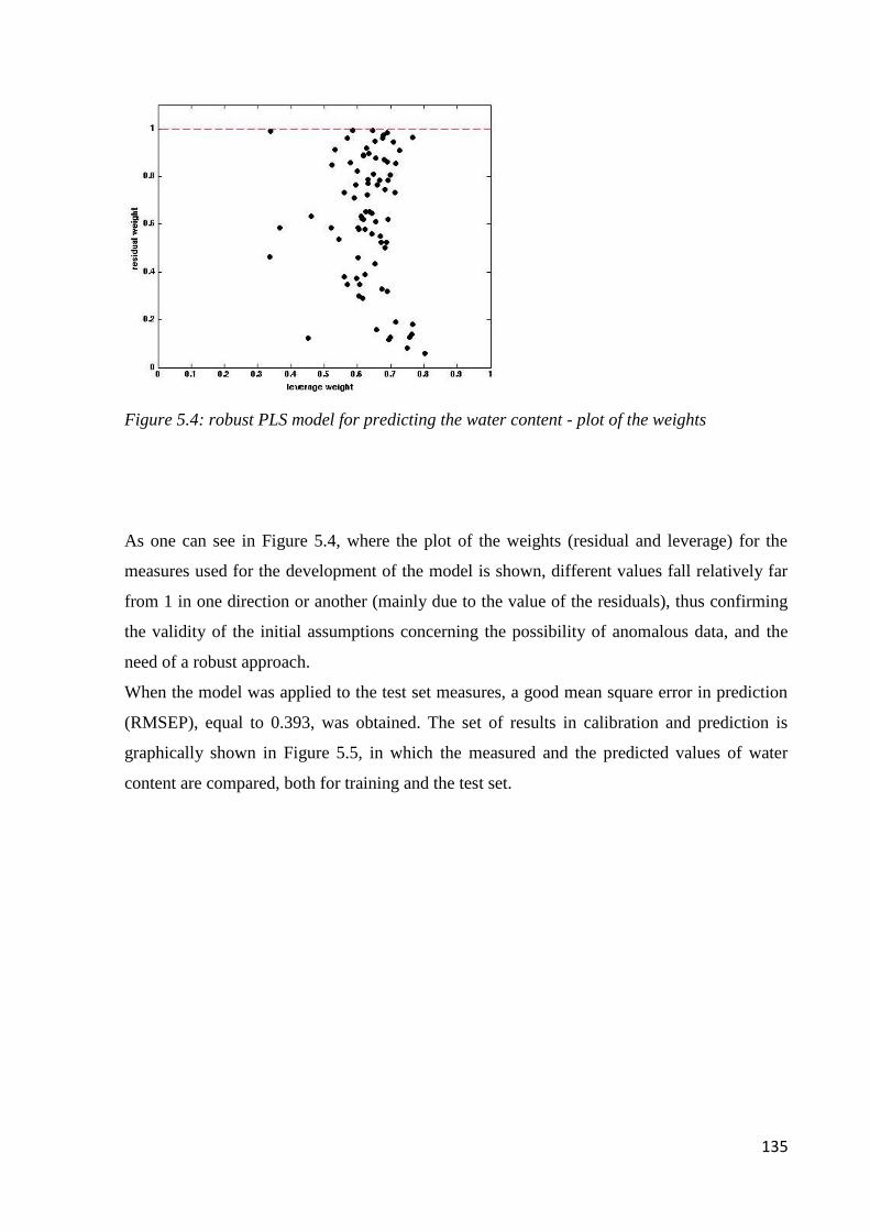
135
Figure 5.4: robust PLS model for predicting the water content - plot of the weights
As one can see in Figure 5.4, where the plot of the weights (residual and leverage) for the
measures used for the development of the model is shown, different values fall relatively far
from 1 in one direction or another (mainly due to the value of the residuals), thus confirming
the validity of the initial assumptions concerning the possibility of anomalous data, and the
need of a robust approach.
When the model was applied to the test set measures, a good mean square error in prediction
(RMSEP), equal to 0.393, was obtained. The set of results in calibration and prediction is
graphically shown in Figure 5.5, in which the measured and the predicted values of water
content are compared, both for training and the test set.
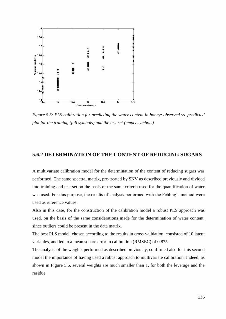
136
Figure 5.5: PLS calibration for predicting the water content in honey: observed vs. predicted
plot for the training (full symbols) and the test set (empty symbols).
5.6.2 DETERMINATION OF THE CONTENT OF REDUCING SUGARS
A multivariate calibration model for the determination of the content of reducing sugars was
performed. The same spectral matrix, pre-treated by SNV as described previously and divided
into training and test set on the basis of the same criteria used for the quantification of water
was used. For this purpose, the results of analysis performed with the Fehling‟s method were
used as reference values.
Also in this case, for the construction of the calibration model a robust PLS approach was
used, on the basis of the same considerations made for the determination of water content,
since outliers could be present in the data matrix.
The best PLS model, chosen according to the results in cross-validation, consisted of 10 latent
variables, and led to a mean square error in calibration (RMSEC) of 0.875.
The analysis of the weights performed as described previously, confirmed also for this second
model the importance of having used a robust approach to multivariate calibration. Indeed, as
shown in Figure 5.6, several weights are much smaller than 1, for both the leverage and the
residue.
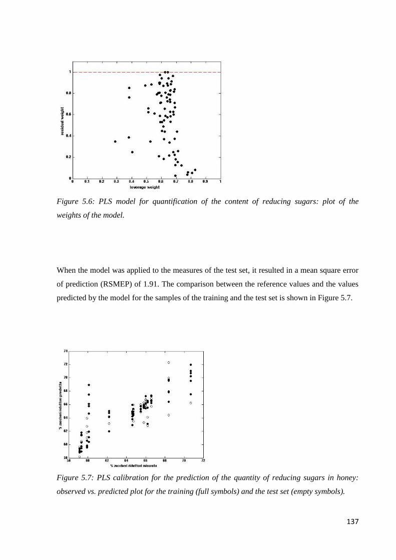
137
Figure 5.6: PLS model for quantification of the content of reducing sugars: plot of the
weights of the model.
When the model was applied to the measures of the test set, it resulted in a mean square error
of prediction (RSMEP) of 1.91. The comparison between the reference values and the values
predicted by the model for the samples of the training and the test set is shown in Figure 5.7.
Figure 5.7: PLS calibration for the prediction of the quantity of reducing sugars in honey:
observed vs. predicted plot for the training (full symbols) and the test set (empty symbols).
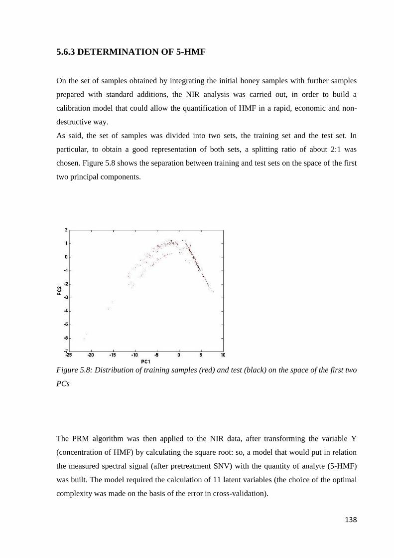
138
5.6.3 DETERMINATION OF 5-HMF
On the set of samples obtained by integrating the initial honey samples with further samples
prepared with standard additions, the NIR analysis was carried out, in order to build a
calibration model that could allow the quantification of HMF in a rapid, economic and non-
destructive way.
As said, the set of samples was divided into two sets, the training set and the test set. In
particular, to obtain a good representation of both sets, a splitting ratio of about 2:1 was
chosen. Figure 5.8 shows the separation between training and test sets on the space of the first
two principal components.
Figure 5.8: Distribution of training samples (red) and test (black) on the space of the first two
PCs
The PRM algorithm was then applied to the NIR data, after transforming the variable Y
(concentration of HMF) by calculating the square root: so, a model that would put in relation
the measured spectral signal (after pretreatment SNV) with the quantity of analyte (5-HMF)
was built. The model required the calculation of 11 latent variables (the choice of the optimal
complexity was made on the basis of the error in cross-validation).
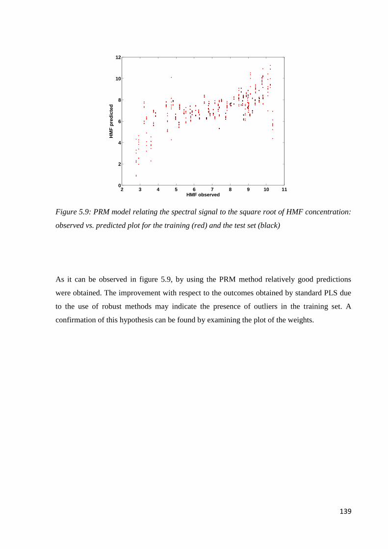
139
Figure 5.9: PRM model relating the spectral signal to the square root of HMF concentration:
observed vs. predicted plot for the training (red) and the test set (black)
As it can be observed in figure 5.9, by using the PRM method relatively good predictions
were obtained. The improvement with respect to the outcomes obtained by standard PLS due
to the use of robust methods may indicate the presence of outliers in the training set. A
confirmation of this hypothesis can be found by examining the plot of the weights.
2 3 4 5 6 7 8 9 10 110
2
4
6
8
10
12
HMF observed
HM
F p
red
icte
d
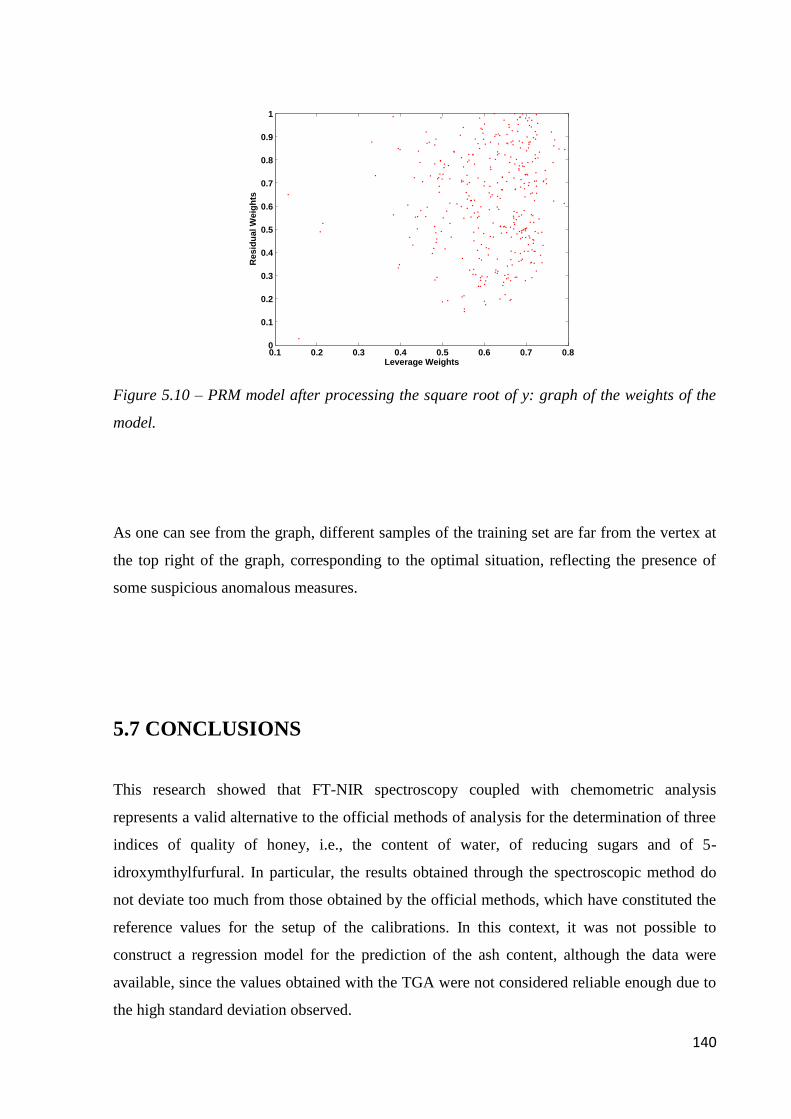
140
Figure 5.10 – PRM model after processing the square root of y: graph of the weights of the
model.
As one can see from the graph, different samples of the training set are far from the vertex at
the top right of the graph, corresponding to the optimal situation, reflecting the presence of
some suspicious anomalous measures.
5.7 CONCLUSIONS
This research showed that FT-NIR spectroscopy coupled with chemometric analysis
represents a valid alternative to the official methods of analysis for the determination of three
indices of quality of honey, i.e., the content of water, of reducing sugars and of 5-
idroxymthylfurfural. In particular, the results obtained through the spectroscopic method do
not deviate too much from those obtained by the official methods, which have constituted the
reference values for the setup of the calibrations. In this context, it was not possible to
construct a regression model for the prediction of the ash content, although the data were
available, since the values obtained with the TGA were not considered reliable enough due to
the high standard deviation observed.
0.1 0.2 0.3 0.4 0.5 0.6 0.7 0.80
0.1
0.2
0.3
0.4
0.5
0.6
0.7
0.8
0.9
1
Leverage Weights
Resid
ua
l W
eig
hts
141
From the experimental point of view the spectroscopic method has proved to be advantageous
compared to the titrimetric method and the thermo-gravimetric method, since the analysis
time were much shorter. The method based on NIR spectroscopy is non-invasive, is more
economic and, from an environmental point of view, zero impact (since it does not require the
use of reagents), according to the guidelines of green chemistry. The time, cost and
environmental impact of refractometer analysis, however, were found to be in line with those
of spectroscopic analysis.
Comparing the thermogravimetric analysis with the refractometric one, the results obtained
showed that the former can achieve performances comparable to those of the latter
considering, on the one hand, that the analysis times are much longer and, on the other hand,
that this technique is required to find the ash content present in honeys and therefore it is an
analysis that still has to be performed.
The results, however, were obtained on a reduced number of samples, and this didn‟t allow to
build a general model for the analysis of honeys. The work showed, however, the existence of
the possibility to realize a model for this type of analysis having a sufficient number of
samples available.
Moreover, the possibility of quantifying the hydroxymethylfurfural in honey samples through
the coupling of NIR spectroscopy and multivariate calibration method was studied. In this
context, best results were obtained by replacing the concentration of HMF with its square
root, suggesting that there are sources of interference in the spectral signal that make the
quantitative relationship not linear. However, this model was not accurate enough to be
adopted. On the other hand, the use of robust methods of calibration, limiting the impact of
any anomalous data on the results, allowed to significantly improve the predictive ability of
the models developed, reducing, at the same time, the error in the prediction of validation
samples.
In conclusion, these results, in general, suggest that it is possible to develop a method that
allows the quantification of HMF in honey samples in a rapid, non-destructive and economic
way by using NIR spectroscopy. However, the fact that the method proposed does not possess
yet the accuracy and precision required for its use in official contexts, shows how this study
represents only a preliminary investigation which necessarily should be examined further:
processing more samples and, in parallel, checking chemometric models of increasing
complexity.
142
CHAPTER 6
SAFFRON: MAE-HPLC-DAD FOR
THE DETERMINATION OF
QUALITY
6.1 QUALITY OF SAFFRON
Saffron is also called "red gold of the East" and it is the most expensive spice in the world
[121, 122], being already known by ancient people who appreciated it for its characteristic
aroma, flavor and taste [123]. Saffron is produced from the dried dark-red colored stigmas of
the flowers of Crocus sativus L. grown in many countries of the Mediterranean basin and
southern Asia [124]. The determination of the geographical origin plays an important role for
this product, since some producing countries, such as Spain, have an export volume which
appears to be too big if it is compared with their production. The original Spanish saffron is a
product of high quality, but its costs have forced many farmers to move in countries such as
Turkey where labor is cheaper [125]. The other producers of saffron are Arzebaijan, Iraq,
Syria, Jordan, Egypt (the latter three are still following the traditional crop), Kashmir, China,
Lebanon (one of the oldest manufacturers), Morocco, Italy, France, Greece, Switzerland.

143
As mentioned, saffron is known to be the most expensive spice in the world due to the limited
cultivation and low harvesting yield. Its high price gives rise to several problems of
sophistication [126].
In order to contrast sophistications and adulterations, the importance of quality control of
saffron is clear.
The chemical composition of saffron is the most important indicator of its quality and of its
commercial value in accordance with ISO 3632-1 and 3632-2 (2003). In fact, ISO 3632 norm
was specifically designed to prevent and combat frauds, this precious spice could be subjected
to. The growing number of frauds of this product, and economic speculation on market prices
reflects an increasing interest from international research institutes.
The International Organization for Standardization (ISO) has defined the quality of saffron
establishing three different categories (I, II and III) defined by specific parameters and ISO
normative establishes also the procedures for their assessment.

144
Table 6.1: Specific parameters for the quality of saffron
Characteristics
Specs
Test methods
Category
I II III
Moisture and volatile substances (% max.)
Saffron in filaments
Ground saffron
12 10
12 10
12 10
ISO/TS 3632-2:2003, Clause 7
Total ash (% max.)
8
8
8
ISO 928:1997. Clause 8, and ISO/TS 3632-2:2003,
Clause 12
Soluble ash in acid solution (%, max.) 1,0 1,0 1,5 ISO 930:1997. Clause 7,
and ISO/TS 3632-2:2003, Clause 13
Soluble extract in cold water (max.)
65 65 65 ISO 941:1980, Clause 7
1% E 1cm 257nm, dried basis:
min.
(maximum absorbance of the picrocrocin)
70 55 40 ISO/TS 3632-2:2003,
Clause 14
1% E 1cm 330nm, dried basis:
min. max.
(maximum absorbance of the safranal)
20 50
20 50
20 50
ISO/TS 3632-2:2003, Clause 14
1% Dyeing power, E 1cm 440nm,
dried basis.
(maximum absorbance of the crocins)
190 150 100 ISO/TS 3632-2:2003,
Clause 14
Soluble artificial colorants in acid solution
No No No ISO/TS 3632-2:2003,
Clause 16 and/or Clasue17
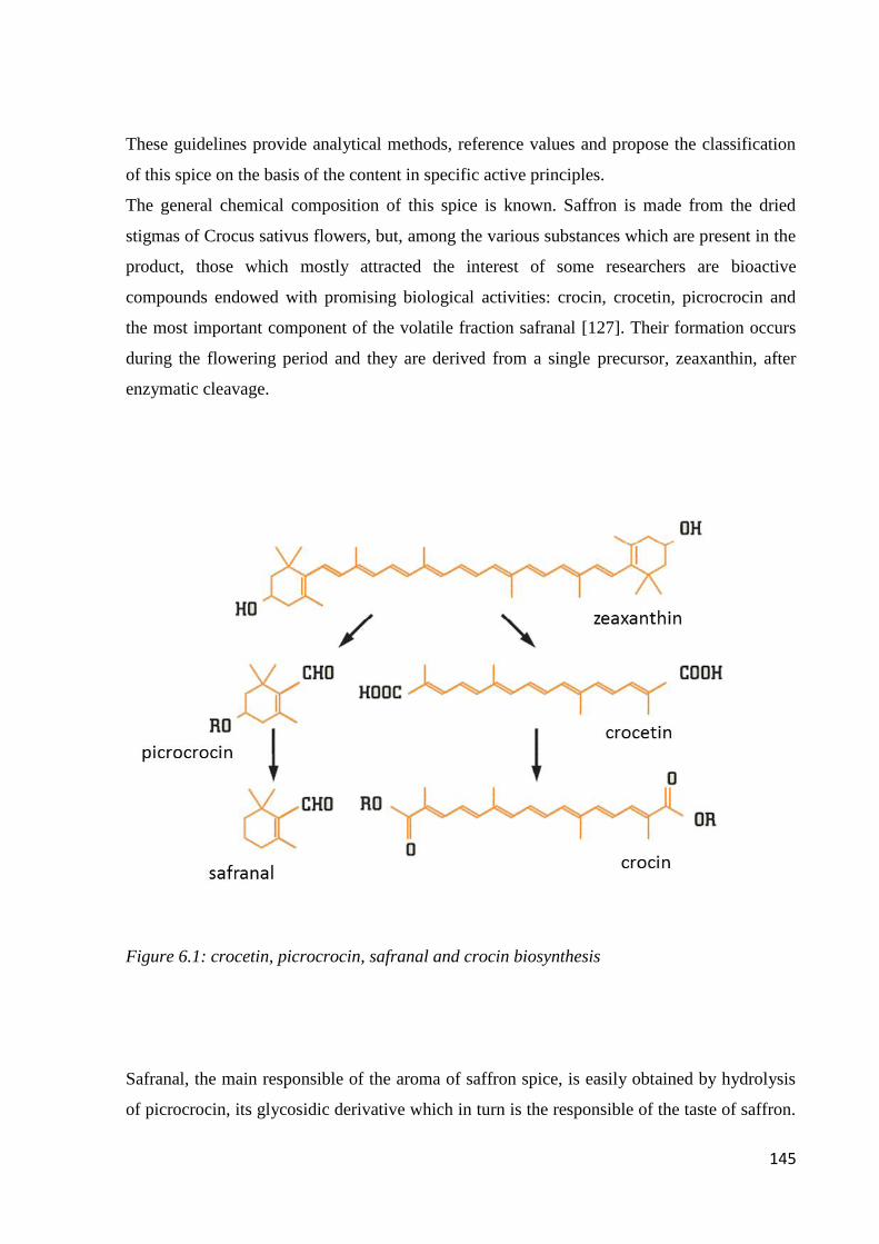
145
These guidelines provide analytical methods, reference values and propose the classification
of this spice on the basis of the content in specific active principles.
The general chemical composition of this spice is known. Saffron is made from the dried
stigmas of Crocus sativus flowers, but, among the various substances which are present in the
product, those which mostly attracted the interest of some researchers are bioactive
compounds endowed with promising biological activities: crocin, crocetin, picrocrocin and
the most important component of the volatile fraction safranal [127]. Their formation occurs
during the flowering period and they are derived from a single precursor, zeaxanthin, after
enzymatic cleavage.
Figure 6.1: crocetin, picrocrocin, safranal and crocin biosynthesis
Safranal, the main responsible of the aroma of saffron spice, is easily obtained by hydrolysis
of picrocrocin, its glycosidic derivative which in turn is the responsible of the taste of saffron.
146
The color of this spice is mainly due to glycosidic esters of crocetin, and in particular to
crocin. All these components and their content determine the quality and the commercial
category of legally traded saffron.
The quality of saffron depends on many factors, such as climate and soil of the area of
production, and also by the mode of cultivation and drying.
Saffron production is constituted by four main phases. The first one is naturally the
cultivation in specific conditions, the second and characteristic one is the manual harvest of
the stigmas. The drying process represents the most critical phase of its production due to the
registered differences among the producing countries. India, Iran and Morocco usually expose
Saffron stigmas to direct sunlight, whereas Greece, Italy and Spain prefer drying processes
indoor at higher temperature than ambient one. That‟s what has the strong impact on the
amount of active principles and then on the quality of Saffron, due to the volatility and
photodegradation processes. Lastly, the product could be marketed as dried filaments or
ground as a powder.
Among the factors related to the quality of saffron, the determination of crocin, picrocrocin
and safranal are the most important parameters, since these three compounds are analytes that
most characterize the saffron. In the literature, different extraction techniques have been
reported, on the basis of the component to be extracted.
The classical extraction method, described by ISO 2003, provides for the extraction of crocin,
picrocrocin, safranal present in 0.5g of saffron using H2O (1 L) and stirring the solution for 1
hour at room temperature. In the literature, there are also articles reporting ultrasonic
extraction [128, 129].
As mentioned in the first chapter, a part of the thesis is focused on the development of an
analytical method which could allow a fast, cheap and reliable analysis of the saffron
permitting to control and to guarantee the quality of the product. Therefore a procedure for the
determination of crocin, picrocrocin and safranal, based on the microwave assisted extraction
(MAE) of the substances followed by HPLC analysis has been developed and optimized. In
order to determine the quality of saffron, the method then has been applied for the analysis of
samples coming from different manufacturers and from different geographical origins.
Microwave-assisted extraction has never been applied to saffron for the recovery of its most
important bioactive compounds and this technique provides in general a better isolation of the
secondary metabolites after the complete swelling of the subcellular structures, faster times of
extraction, reduced solvent waste and an accurate control of different parameter.
147
6.2 MICROWAVE-ASSISTED EXTRACTION OF CROCIN,
PICROCROCIN AND SAFRANAL
For the microwave-assisted extraction of crocin, picrocrocin and safranal different solvents
and mixtures of extractants were tested; instrumental parameters and time of extraction were
also optimized.
6.2.1 SAMPLES AND CHEMICALS
Commercial standards of all trans-crocin (crocin-1, crocetin digentiobiose ester, 98%) and
safranal (>88%) were purchased from Sigma-Aldrich (Italy), and picrocrocin (>98%) from
Biotain PHARMA CO.LTD (China). Safranal was purified by column chromatography on
silica gel (230-400 mesh, G60 Merck) using ethyl acetate:hexane (1:3) as the eluent. 1H
NMR, 13
C NMR and IR spectra of the purified product were in agreement with those reported
in the literature. 4-Nitroaniline, used as internal standard (IS), was purchased from Sigma-
Aldrich (Riedel-de Haën, Seelze, Germany). Methanol and Ethanol HPLC grade (<99.9%)
were purchased from Carlo Erba. Ultrapure water generated by the MilliQ system (Millipore,
Bedford, MA) was used.
One hundred six samples were collected from the best representative leading producers with
particular interest towards Italian saffron from Sardinia and Latium. In particular, 20 samples
from Greece, 25 samples from Turkey, 19 samples from Latium (Italy), 10 samples from
Sardinia (Italy), 23 samples from Spain were collected. They were obtained under the
guarantee of their quality in according to ISO 3632 guidelines. They were ground manually
and sieved to obtain a uniform granulometry before performing the extraction/HPLC and the
NIR spectroscopic analyses.
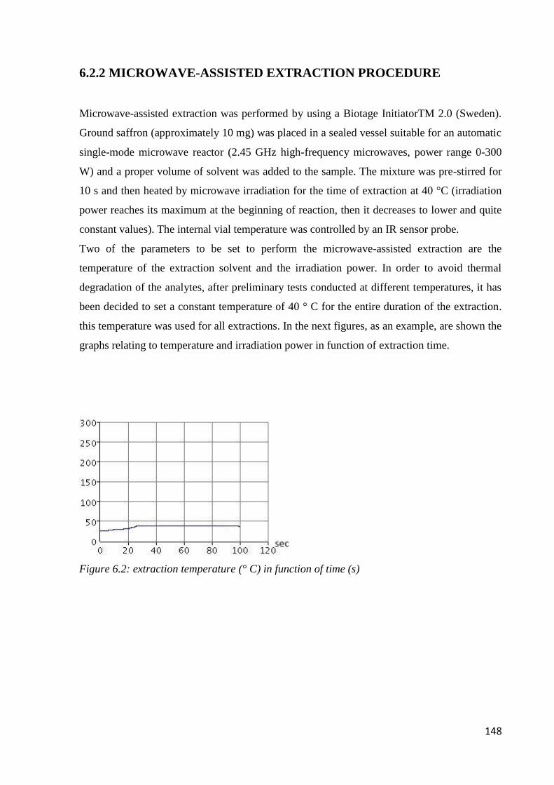
148
6.2.2 MICROWAVE-ASSISTED EXTRACTION PROCEDURE
Microwave-assisted extraction was performed by using a Biotage InitiatorTM 2.0 (Sweden).
Ground saffron (approximately 10 mg) was placed in a sealed vessel suitable for an automatic
single-mode microwave reactor (2.45 GHz high-frequency microwaves, power range 0-300
W) and a proper volume of solvent was added to the sample. The mixture was pre-stirred for
10 s and then heated by microwave irradiation for the time of extraction at 40 °C (irradiation
power reaches its maximum at the beginning of reaction, then it decreases to lower and quite
constant values). The internal vial temperature was controlled by an IR sensor probe.
Two of the parameters to be set to perform the microwave-assisted extraction are the
temperature of the extraction solvent and the irradiation power. In order to avoid thermal
degradation of the analytes, after preliminary tests conducted at different temperatures, it has
been decided to set a constant temperature of 40 ° C for the entire duration of the extraction.
this temperature was used for all extractions. In the next figures, as an example, are shown the
graphs relating to temperature and irradiation power in function of extraction time.
Figure 6.2: extraction temperature (° C) in function of time (s)
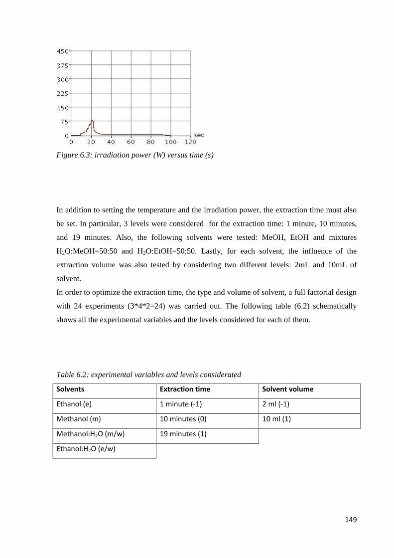
149
Figure 6.3: irradiation power (W) versus time (s)
In addition to setting the temperature and the irradiation power, the extraction time must also
be set. In particular, 3 levels were considered for the extraction time: 1 minute, 10 minutes,
and 19 minutes. Also, the following solvents were tested: MeOH, EtOH and mixtures
H2O:MeOH=50:50 and H2O:EtOH=50:50. Lastly, for each solvent, the influence of the
extraction volume was also tested by considering two different levels: 2mL and 10mL of
solvent.
In order to optimize the extraction time, the type and volume of solvent, a full factorial design
with 24 experiments (3*4*2=24) was carried out. The following table (6.2) schematically
shows all the experimental variables and the levels considered for each of them.
Table 6.2: experimental variables and levels considerated
Solvents Extraction time Solvent volume
Ethanol (e) 1 minute (-1) 2 ml (-1)
Methanol (m) 10 minutes (0) 10 ml (1)
Methanol:H2O (m/w) 19 minutes (1)
Ethanol:H2O (e/w)

150
After the extraction of bioactive compounds, each extract was filtered through a PTFE filter
(0.45 mm; Whatman-Merck, Darmstadt, Germany) and subsequently analyzed by HPLC-
DAD.
6.2.3 HPLC-DAD ANALYSIS
Crocin, picrocrocin and safranal were determined by high performance liquid
chromatography.
The extracts prepared according to what described in section 6.2.2 were analyzed by HPLC-
DAD with a Thermo Quest Spectrasystem LC (Thermo Fisher Scientific, Waltham, MA)
equipped with a P4000 pump, a UV6000 UV-Vis Diode Array Detector, and a SN4000
interface to be operated via a personal computer. Extracted compounds were separated using
an Eclipse XDB-C18 analytical column (4.6x250mm, 5µm particle size; Agilent
Technologies, Santa Clara, CA) protected by a guard cartridge of the same packing, operating
at 25° C. Separation was carried out using gradient elution with a mixture of water
(A):acetonitrile (B) (30–70% B in 20 min) at a flow rate of 0.9 mL min−1. Injection volumes
were 10 µL for all samples and standards. Multiwavelength detection was in the range of
200–550 nm and quantification was carried out by integration of the peak areas at 250 nm
(picrocrocin), 310nm (safranal) and 440 nm (crocin).
6.2.4 OPTIMIZATION OF THE MICROWAVE-ASSISTED
EXTRACTION
As anticipated in section 6.2.4, the operating conditions for the microwave-assisted extraction
of the analytes from saffron samples were optimized using an experimental design. In
particular, for each of the 24 designed experiments (for all extraction tests was used the same
saffron sample), the extracts were subjected to HPLC analysis and the area of safranal, crocin
and picrocrocin were integrated. Obviously, each area was normalized according to the area
of the internal standard added (10µg) before each extraction. The conditions were optimized
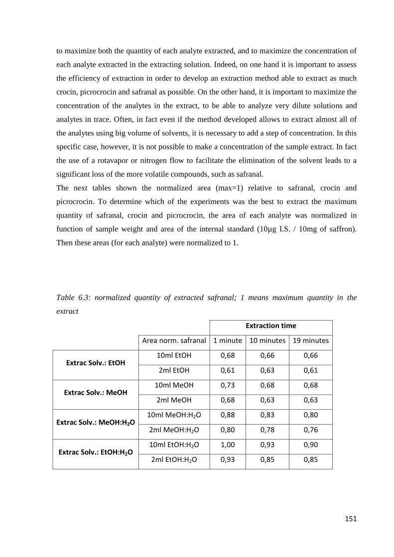
151
to maximize both the quantity of each analyte extracted, and to maximize the concentration of
each analyte extracted in the extracting solution. Indeed, on one hand it is important to assess
the efficiency of extraction in order to develop an extraction method able to extract as much
crocin, picrocrocin and safranal as possible. On the other hand, it is important to maximize the
concentration of the analytes in the extract, to be able to analyze very dilute solutions and
analytes in trace. Often, in fact even if the method developed allows to extract almost all of
the analytes using big volume of solvents, it is necessary to add a step of concentration. In this
specific case, however, it is not possible to make a concentration of the sample extract. In fact
the use of a rotavapor or nitrogen flow to facilitate the elimination of the solvent leads to a
significant loss of the more volatile compounds, such as safranal.
The next tables shown the normalized area (max=1) relative to safranal, crocin and
picrocrocin. To determine which of the experiments was the best to extract the maximum
quantity of safranal, crocin and picrocrocin, the area of each analyte was normalized in
function of sample weight and area of the internal standard (10µg I.S. / 10mg of saffron).
Then these areas (for each analyte) were normalized to 1.
Table 6.3: normalized quantity of extracted safranal; 1 means maximum quantity in the
extract
Extraction time
Area norm. safranal 1 minute 10 minutes 19 minutes
Extrac Solv.: EtOH 10ml EtOH 0,68 0,66 0,66
2ml EtOH 0,61 0,63 0,61
Extrac Solv.: MeOH 10ml MeOH 0,73 0,68 0,68
2ml MeOH 0,68 0,63 0,63
Extrac Solv.: MeOH:H2O 10ml MeOH:H2O 0,88 0,83 0,80
2ml MeOH:H2O 0,80 0,78 0,76
Extrac Solv.: EtOH:H2O 10ml EtOH:H2O 1,00 0,93 0,90
2ml EtOH:H2O 0,93 0,85 0,85
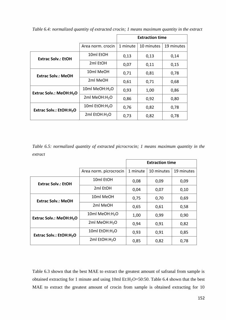
152
Table 6.4: normalized quantity of extracted crocin; 1 means maximum quantity in the extract
Extraction time
Area norm. crocin 1 minute 10 minutes 19 minutes
Extrac Solv.: EtOH 10ml EtOH 0,13 0,13 0,14
2ml EtOH 0,07 0,11 0,15
Extrac Solv.: MeOH 10ml MeOH 0,71 0,81 0,78
2ml MeOH 0,61 0,71 0,68
Extrac Solv.: MeOH:H2O 10ml MeOH:H2O 0,93 1,00 0,86
2ml MeOH:H2O 0,86 0,92 0,80
Extrac Solv.: EtOH:H2O 10ml EtOH:H2O 0,76 0,82 0,78
2ml EtOH:H2O 0,73 0,82 0,78
Table 6.5: normalized quantity of extracted picrocrocin; 1 means maximum quantity in the
extract
Extraction time
Area norm. picrocrocin 1 minute 10 minutes 19 minutes
Extrac Solv.: EtOH 10ml EtOH 0,08 0,09 0,09
2ml EtOH 0,04 0,07 0,10
Extrac Solv.: MeOH 10ml MeOH 0,75 0,70 0,69
2ml MeOH 0,65 0,61 0,58
Extrac Solv.: MeOH:H2O 10ml MeOH:H2O 1,00 0,99 0,90
2ml MeOH:H2O 0,94 0,91 0,82
Extrac Solv.: EtOH:H2O 10ml EtOH:H2O 0,93 0,91 0,85
2ml EtOH:H2O 0,85 0,82 0,78
Table 6.3 shown that the best MAE to extract the greatest amount of safranal from sample is
obtained extracting for 1 minute and using 10ml Et:H2O=50:50. Table 6.4 shown that the best
MAE to extract the greatest amount of crocin from sample is obtained extracting for 10
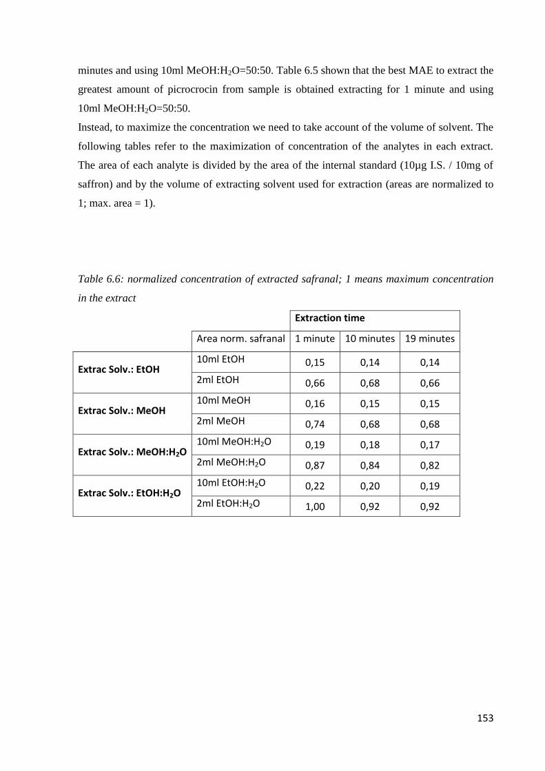
153
minutes and using 10ml MeOH:H2O=50:50. Table 6.5 shown that the best MAE to extract the
greatest amount of picrocrocin from sample is obtained extracting for 1 minute and using
10ml MeOH:H2O=50:50.
Instead, to maximize the concentration we need to take account of the volume of solvent. The
following tables refer to the maximization of concentration of the analytes in each extract.
The area of each analyte is divided by the area of the internal standard (10µg I.S. / 10mg of
saffron) and by the volume of extracting solvent used for extraction (areas are normalized to
1; max. area = 1).
Table 6.6: normalized concentration of extracted safranal; 1 means maximum concentration
in the extract
Extraction time
Area norm. safranal 1 minute 10 minutes 19 minutes
Extrac Solv.: EtOH 10ml EtOH 0,15 0,14 0,14
2ml EtOH 0,66 0,68 0,66
Extrac Solv.: MeOH 10ml MeOH 0,16 0,15 0,15
2ml MeOH 0,74 0,68 0,68
Extrac Solv.: MeOH:H2O 10ml MeOH:H2O 0,19 0,18 0,17
2ml MeOH:H2O 0,87 0,84 0,82
Extrac Solv.: EtOH:H2O 10ml EtOH:H2O 0,22 0,20 0,19
2ml EtOH:H2O 1,00 0,92 0,92
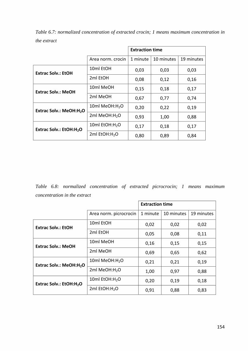
154
Table 6.7: normalized concentration of extracted crocin; 1 means maximum concentration in
the extract
Extraction time
Area norm. crocin 1 minute 10 minutes 19 minutes
Extrac Solv.: EtOH 10ml EtOH 0,03 0,03 0,03
2ml EtOH 0,08 0,12 0,16
Extrac Solv.: MeOH 10ml MeOH 0,15 0,18 0,17
2ml MeOH 0,67 0,77 0,74
Extrac Solv.: MeOH:H2O 10ml MeOH:H2O 0,20 0,22 0,19
2ml MeOH:H2O 0,93 1,00 0,88
Extrac Solv.: EtOH:H2O 10ml EtOH:H2O 0,17 0,18 0,17
2ml EtOH:H2O 0,80 0,89 0,84
Table 6.8: normalized concentration of extracted picrocrocin; 1 means maximum
concentration in the extract
Extraction time
Area norm. picrocrocin 1 minute 10 minutes 19 minutes
Extrac Solv.: EtOH 10ml EtOH 0,02 0,02 0,02
2ml EtOH 0,05 0,08 0,11
Extrac Solv.: MeOH 10ml MeOH 0,16 0,15 0,15
2ml MeOH 0,69 0,65 0,62
Extrac Solv.: MeOH:H2O 10ml MeOH:H2O 0,21 0,21 0,19
2ml MeOH:H2O 1,00 0,97 0,88
Extrac Solv.: EtOH:H2O 10ml EtOH:H2O 0,20 0,19 0,18
2ml EtOH:H2O 0,91 0,88 0,83
155
The MAE procedure which allows obtaining the highest concentration of safranal in the
extract (table 6.6) corresponds to extracting for 1 minute and using 2mL of EtOH: H2O. The
MAE procedure which allows to obtain the highest concentration of crocin in the extract
(table 6.7) corresponds to extracting for 10 minutes and using 2 mL MeOH:H2O=50:50. The
MAE procedure which allows obtaining the highest concentration of picrocrocin in the extract
(table 6.8) corresponds to extracting for 1 minute and using 2 mL MeOH:H2O=50:50.
As can be noted from previous tables we must use different mixtures of solvents (MeOH:H2O
for crocin and picrocrocin, EtOH:H2O for safranal) and different extraction time (1 minute for
safranal and picrocrocin, 10minutes for crocin) depending on which compound we want to
optimize.
Regarding the volume of extracting solvent, the use of 2mL of solvent allows to obtain much
higher concentrations of the analytes than using 10mL. Indeed the use of 10mL, even if the
volume is 5 times greater than 2mL, does not lead to a comparable increase in the amount of
analytes extracted.
On the basis of these results, for the analysis of safranal, crocin and picrocrocin in available
saffron samples, it was decided to use the best conditions for the extraction of safranal (2mL
EtOH:H2O and 1 minute of extraction) because they provided a limited solvent waste
balanced by a suitable extract concentration, reduced extraction times limiting the degradation
of the active principles and the best recovery of safranal which is normally present in very
low concentrations.
6.2.5 VALIDATION OF MAE-HPLC-DAD METHOD
The method developed, based on the microwave-assisted extraction was validated in terms of
linearity, limit of detection (LOD), limit of quantification (LOQ), reproducibility and
recovery (table 6.9).
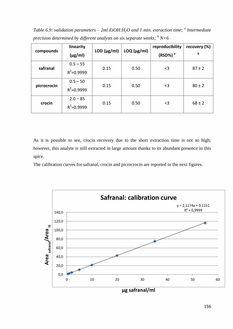
156
Table 6.9: validation parameters – 2ml EtOH:H2O and 1 min. extraction time; a Intermediate
precision determined by different analysts on six separate weeks; b N=6
compounds linearity
(µg/ml) LOD (µg/ml) LOQ (µg/ml)
reproducibility
(RSD%) a
recovery (%)
b
safranal 0.5 – 55
R2=0.9999 0.15 0.50 <3 87 ± 2
picrocrocin 0.5 – 50
R2=0.9999 0.15 0.50 <3 80 ± 2
crocin 2.0 – 85
R2=0.9999 0.15 0.50 <3 68 ± 2
As it is possible to see, crocin recovery due to the short extraction time is not so high;
however, this analyte is still extracted in large amount thanks to its abundant presence in this
spice.
The calibration curves for safranal, crocin and picrocrocin are reported in the next figures.
y = 2,1174x + 0,1151 R² = 0,9999
0,0
20,0
40,0
60,0
80,0
100,0
120,0
140,0
0 10 20 30 40 50 60
Safranal: calibration curve
µg safranal/ml
Are
a sa
fran
al/A
rea
IS
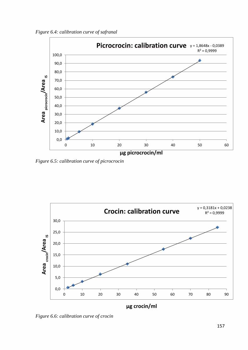
157
Figure 6.4: calibration curve of safranal
Figure 6.5: calibration curve of picrocrocin
Figure 6.6: calibration curve of crocin
y = 1,8648x - 0,0389 R² = 0,9999
0,0
10,0
20,0
30,0
40,0
50,0
60,0
70,0
80,0
90,0
100,0
0 10 20 30 40 50 60
Picrocrocin: calibration curve
µg picrocrocin/ml
Are
a p
icro
cro
cin/A
rea
IS
y = 0,3181x + 0,0238 R² = 0,9999
0,0
5,0
10,0
15,0
20,0
25,0
30,0
0 10 20 30 40 50 60 70 80 90
Crocin: calibration curve
µg crocin/ml
Are
a cr
oci
n/A
rea
IS
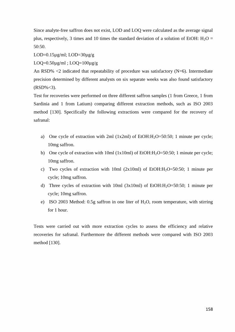
158
Since analyte-free saffron does not exist, LOD and LOQ were calculated as the average signal
plus, respectively, 3 times and 10 times the standard deviation of a solution of EtOH: H2O =
50:50.
LOD=0.15µg/ml; LOD=30µg/g
LOQ=0.50µg/ml ; LOQ=100µg/g
An RSD% <2 indicated that repeatability of procedure was satisfactory (N=6). Intermediate
precision determined by different analysts on six separate weeks was also found satisfactory
(RSD%<3).
Test for recoveries were performed on three different saffron samples (1 from Greece, 1 from
Sardinia and 1 from Latium) comparing different extraction methods, such as ISO 2003
method [130]. Specifically the following extractions were compared for the recovery of
safranal:
a) One cycle of extraction with 2ml (1x2ml) of EtOH:H2O=50:50; 1 minute per cycle;
10mg saffron.
b) One cycle of extraction with 10ml (1x10ml) of EtOH:H2O=50:50; 1 minute per cycle;
10mg saffron.
c) Two cycles of extraction with 10ml (2x10ml) of EtOH:H2O=50:50; 1 minute per
cycle; 10mg saffron.
d) Three cycles of extraction with 10ml (3x10ml) of EtOH:H2O=50:50; 1 minute per
cycle; 10mg saffron.
e) ISO 2003 Method: 0.5g saffron in one liter of H2O, room temperature, with stirring
for 1 hour.
Tests were carried out with more extraction cycles to assess the efficiency and relative
recoveries for safranal. Furthermore the different methods were compared with ISO 2003
method [130].
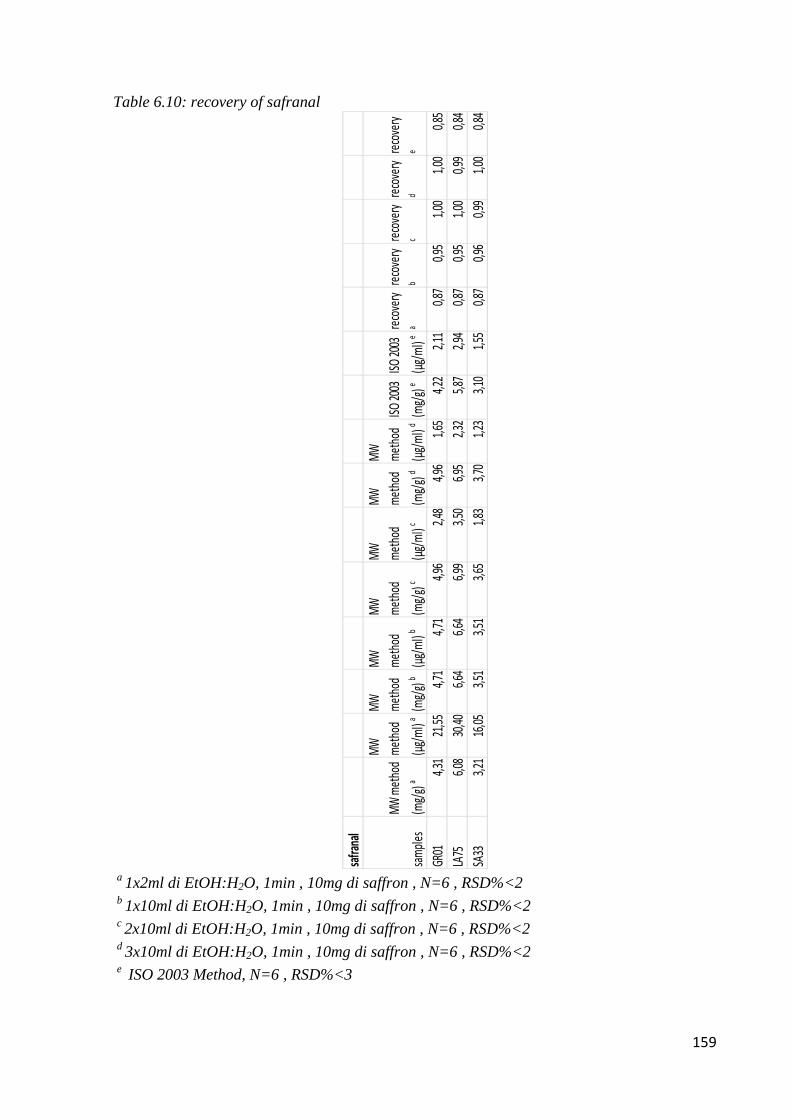
159
Table 6.10: recovery of safranal
a
1x2ml di EtOH:H2O, 1min , 10mg di saffron , N=6 , RSD%<2 b
1x10ml di EtOH:H2O, 1min , 10mg di saffron , N=6 , RSD%<2 c 2x10ml di EtOH:H2O, 1min , 10mg di saffron , N=6 , RSD%<2
d 3x10ml di EtOH:H2O, 1min , 10mg di saffron , N=6 , RSD%<2
e ISO 2003 Method, N=6 , RSD%<3
safra
nal
sam
ples
MW
met
hod
(mg/
g) a
MW
met
hod
(µg/
ml)
a
MW
met
hod
(mg/
g) b
MW
met
hod
(µg/
ml)
b
MW
met
hod
(mg/
g) c
MW
met
hod
(µg/
ml)
c
MW
met
hod
(mg/
g) d
MW
met
hod
(µg/
ml)
d
ISO 20
03
(mg/
g) e
ISO 20
03
(µg/
ml)
e
reco
very
a
reco
very
b
reco
very
c
reco
very
d
reco
very
e
GR01
4,31
21,55
4,71
4,71
4,96
2,48
4,96
1,65
4,22
2,11
0,87
0,95
1,00
1,00
0,85
LA75
6,08
30,40
6,64
6,64
6,99
3,50
6,95
2,32
5,87
2,94
0,87
0,95
1,00
0,99
0,84
SA33
3,21
16,05
3,51
3,51
3,65
1,83
3,70
1,23
3,10
1,55
0,87
0,96
0,99
1,00
0,84
160
The following extractions were compared for the recovery of picrocrocin:
a) One cycle of extraction with 2ml (1x2ml) of MeOH:H2O=50:50; 1 minute per cycle;
10mg saffron.
b) One cycle of extraction with 10ml (1x10ml) of MeOH:H2O=50:50; 1 minute per
cycle; 10mg saffron.
c) Two cycles of extraction with 10ml (2x10ml) of MeOH:H2O=50:50; 1 minute per
cycle; 10mg saffron.
d) Three cycles of extraction with 10ml (3x10ml) of MeOH:H2O=50:50; 1 minute per
cycle; 10mg saffron.
e) ISO 2003 Method: 0.5g saffron in one liter of H2O, room temperature, with stirring
for 1 hour.
f) One cycle of extraction with 2ml (1x2ml) of EtOH:H2O=50:50; 1 minute per cycle;
10mg saffron.
Tests were carried out with more extraction cycles to assess the efficiency and relative
recoveries for picrocrocin. Furthermore the different methods were compared with ISO 2003
method [130].

161
Table 6.11: recovery of picrocrocin
a 1x2ml di MeOH/water , 1min , 10mg di saffron , N=6 , RSD%<2
b 1x10ml di MeOH/water , 1min , 10mg di saffron , N=6 , RSD%<2
c 2x10ml di MeOH/water , 1min , 10mg di saffron , N=6 , RSD%<2
d 3x10ml di MeOH/water , 1min , 10mg di saffron , N=6 , RSD%<2
e ISO 2003 Method, N=6 , RSD%<3
f 1x2ml di EtOH:H2O, 1min , 10mg di saffron , N=6 , RSD%<2
picro
crocin
samp
les
MW m
etho
d
(mg/
g) a
MW
meth
od
(µg/
ml) a
MW
meth
od
(mg/
g) b
MW
meth
od
(µg/
ml) b
MW
meth
od
(mg/
g) c
MW
meth
od
(µg/
ml) c
MW
meth
od
(mg/
g) d
MW
meth
od
(µg/
ml) d
ISO 20
03
(mg/
g) e
ISO 20
03
(µg/
ml) e
MW
meth
od
(mg/
g) f
MW
meth
od
(µg/
ml) f
reco
very
a
reco
very
b
reco
very
c
reco
very
d
reco
very
e
reco
very
f
GR01
4,66
23,32
5,09
5,09
5,36
2,68
5,39
1,80
4,45
2,22
4,31
21,56
0,87
0,94
0,99
1,00
0,83
0,80
LA75
6,07
30,36
6,56
6,56
6,90
3,45
6,93
2,31
5,73
2,86
5,54
27,72
0,88
0,95
1,00
1,00
0,83
0,80
SA33
3,89
19,45
4,20
4,20
4,42
2,21
4,39
1,46
3,62
1,81
3,54
17,68
0,88
0,96
1,00
0,99
0,82
0,80

162
The following extractions were compared for the recovery of crocin:
a) One cycle of extraction with 2ml (1x2ml) of MeOH:H2O=50:50; 10 minutes per
cycle; 10mg saffron.
b) One cycle of extraction with 10ml (1x10ml) of MeOH:H2O=50:50; 10 minutes per
cycle; 10mg saffron.
c) Two cycles of extraction with 10ml (2x10ml) of MeOH:H2O=50:50; 10 minutes per
cycle; 10mg saffron.
d) Three cycles of extraction with 10ml (3x10ml) of MeOH:H2O=50:50; 10 minutes per
cycle; 10mg saffron.
e) ISO 2003 Method: 0.5g saffron in one liter of H2O, room temperature, with stirring
for 1 hour.
f) One cycle of extraction with 2ml (1x2ml) of EtOH:H2O=50:50; 10 minutes per cycle;
10mg saffron.
Tests were carried out with more extraction cycles to assess the efficiency and relative
recoveries for crocin. Furthermore the different methods were compared with ISO 2003
method [130].
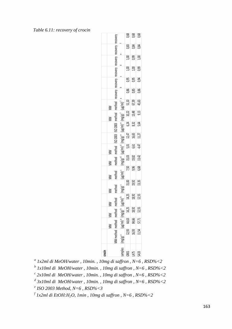
163
Table 6.11: recovery of crocin
a 1x2ml di MeOH/water , 10min. , 10mg di saffron , N=6 , RSD%<2
b 1x10ml di MeOH/water , 10min. , 10mg di saffron , N=6 , RSD%<2
c 2x10ml di MeOH/water , 10min. , 10mg di saffron , N=6 , RSD%<2
d 3x10ml di MeOH/water , 10min. , 10mg di saffron , N=6 , RSD%<2
e ISO 2003 Method, N=6 , RSD%<3
f 1x2ml di EtOH:H2O, 1min , 10mg di saffron , N=6 , RSD%<2
crocin
samp
les
MW m
etho
d
(mg/
g) a
MW
meth
od
(µg/
ml) a
MW
meth
od
(mg/
g) b
MW
meth
od
(µg/
ml) b
MW
meth
od
(mg/
g) c
MW
meth
od
(µg/
ml) c
MW
meth
od
(mg/
g) d
MW
meth
od
(µg/
ml) d
ISO 20
03
(mg/
g) e
ISO 20
03
(µg/
ml) e
MW
meth
od
(mg/
g) f
MW
meth
od
(µg/
ml) f
reco
very
a
reco
very
b
reco
very
c
reco
very
d
reco
very
e
reco
very
f
GR01
12,93
64,63
14,25
14,25
15,00
7,50
15,03
5,01
12,47
6,24
10,22
51,10
0,86
0,95
1,00
1,00
0,83
0,68
LA75
16,93
84,66
18,92
18,92
19,92
9,96
19,82
6,61
16,65
8,32
13,48
67,39
0,85
0,95
1,00
0,99
0,84
0,68
SA33
11,54
57,71
12,55
12,55
13,35
6,68
13,42
4,47
11,27
5,64
9,13
45,63
0,86
0,94
0,99
1,00
0,84
0,68
164
6.3 DETERMINATION OF SAFRANAL, CROCIN,
PICROCROCIN IN SAFFRON
The method (previously described and validated), which allows to obtain the maximum
concentration of safranal in the extract, was then applied for the determination of constituents
related to the quality of the saffron (safranal, picrocrocin and crocin) in all the available
samples.
10 mg of ground saffron were placed in a 10 mL sealed vessel suitable for an automatic
single-mode microwave reactor and 2mL of EtOH:H2O were added to the sample. The
extraction temperature was set at 40 ° C and the extraction time to 1 minute. The extract
containing the analytes extracted was then filtered through a PTFE filter and 10µL were
injected into the HPLC system. With the use of EtOH: H2O and 1 minute of extraction, we
obtained high recovery for safranal which is normally present in very low concentrations.
The following table shows the results obtained on 106 samples of saffron analyzed by MAE-
HPLC-DAD.

165
Table 6.12: determination of crocin, picrocrocin and safranal in different saffron samples –
GR means Greece, LA means Latium, SA means Sardinia, SP means Spain, TK means Turkey
sample crocin (mg/g)
picrocrocin (mg/g)
safranal (mg/g)
sample crocin (mg/g)
picrocrocin (mg/g)
safranal (mg/g)
GR01 15,03 5,39 4,96 SA101 18,93 5,32 2,38
GR02 14,03 5,11 5,45 SA102 16,91 4,52 2,07
GR03 14,48 5,31 4,81 SA103 15,27 4,22 2,06
GR04 12,60 4,45 4,30 SA104 15,08 4,05 1,80
GR05 13,02 4,83 4,37 SA105 16,56 4,71 2,19
GR06 13,47 4,88 4,35 SP21 15,05 4,59 2,99
GR07 12,31 4,35 4,38 SP22 15,03 4,66 2,96
GR08 12,96 4,66 4,27 SP23 10,00 3,12 0,94
GR09 11,08 3,75 3,72 SP24 11,57 3,65 1,02
GR10 13,45 4,60 4,73 SP25 16,19 5,20 2,09
GR11 15,32 5,54 5,21 SP26 16,17 5,21 2,18
GR12 12,44 4,65 3,92 SP27 17,51 5,61 1,91
GR13 17,04 5,99 6,48 SP28 16,80 5,48 1,91
GR14 14,26 5,16 3,89 SP29 17,23 5,81 2,02
GR15 14,56 5,18 4,81 SP30 18,33 6,69 1,86
GR16 14,10 4,91 3,90 SP31 17,80 5,59 2,37
GR17 15,41 5,45 4,81 SP32 17,16 5,75 2,46
GR18 13,83 4,74 4,49 SP40 5,37 1,37 1,86
GR19 14,04 4,87 4,26 SP41 12,81 4,10 1,85
GR20 15,26 5,41 4,15 SP42 15,80 5,17 2,43
LA75 19,02 6,93 6,99 SP43 14,87 4,80 2,22
LA76 16,24 6,05 6,10 SP44 13,40 4,26 1,40
LA77 17,82 6,41 5,55 SP45 14,36 4,90 1,59
LA78 18,17 7,97 5,71 SP46 14,20 4,28 1,56
LA79 17,41 7,29 6,24 SP47 14,73 4,49 2,06
LA80 14,24 5,12 4,58 SP48 13,05 4,45 1,78
LA81 16,23 5,86 5,76 SP49 13,90 5,25 1,93
LA82 7,98 2,75 2,73 SP106 7,16 2,08 1,55
LA83 19,69 7,94 4,33 TK50 3,98 0,62 0,30
LA84 14,22 5,02 3,06 TK51 3,94 0,59 0,24
LA85 15,28 5,56 3,24 TK52 3,99 0,66 0,33
LA86 14,04 5,19 3,29 TK53 3,80 0,58 0,24
LA87 17,90 6,61 2,56 TK54 3,61 0,52 0,18
LA88 13,54 4,77 2,97 TK55 3,68 0,57 0,24
LA89 17,08 7,32 2,73 TK56 4,71 0,82 0,36
LA90 15,13 5,45 2,57 TK57 3,52 0,53 0,19
LA91 15,72 13,00 3,26 TK58 3,60 0,54 0,20
LA92 14,66 5,12 2,80 TK59 3,43 0,54 0,19
LA93 14,62 5,21 3,20 TK60 3,62 0,52 0,18
SA33 13,42 4,42 3,70 TK61 4,69 0,64 0,32
SA34 13,31 4,62 3,84 TK62 3,49 0,55 0,20
SA35 14,25 4,27 2,53 TK63 3,60 0,56 0,22
SA36 14,42 4,45 4,44 TK64 3,61 0,55 0,21
SA37 5,15 1,46 2,75 TK65 3,78 0,56 0,22
SA38 14,92 4,61 3,77 TK66 3,57 0,53 0,19
SA39 5,08 1,39 3,54 TK67 3,68 0,58 0,24
SA94 3,62 0,83 2,36 TK68 3,40 0,55 0,20
SA95 3,79 0,80 1,15 TK69 3,78 0,55 0,23
SA96 3,59 0,84 2,24 TK70 3,45 0,51 0,17
SA97 3,55 0,81 2,52 TK71 3,62 0,54 0,21
SA98 16,97 4,74 2,11 TK72 3,50 0,55 0,21
SA99 18,41 5,33 2,36 TK73 3,70 0,55 0,21
SA100 18,77 5,03 2,29 TK74 3,51 0,54 0,21
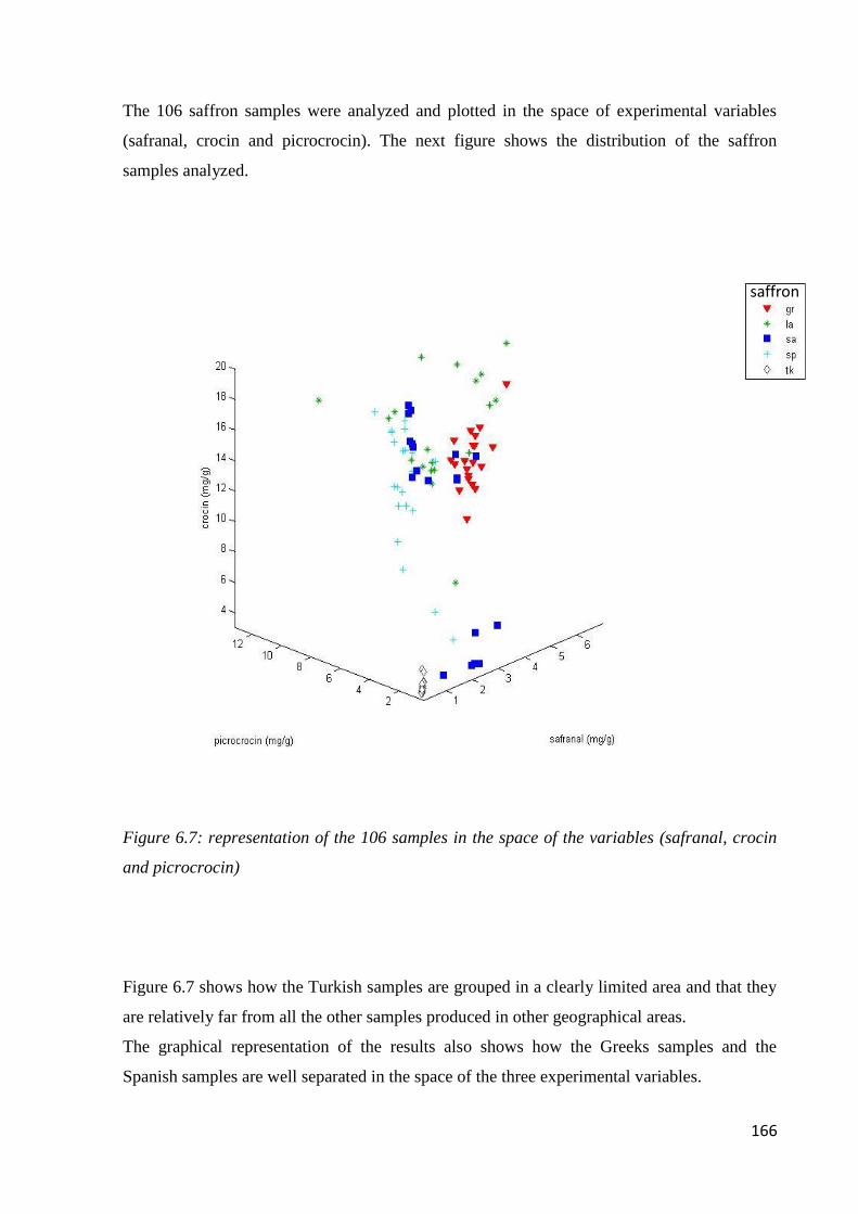
166
The 106 saffron samples were analyzed and plotted in the space of experimental variables
(safranal, crocin and picrocrocin). The next figure shows the distribution of the saffron
samples analyzed.
Figure 6.7: representation of the 106 samples in the space of the variables (safranal, crocin
and picrocrocin)
Figure 6.7 shows how the Turkish samples are grouped in a clearly limited area and that they
are relatively far from all the other samples produced in other geographical areas.
The graphical representation of the results also shows how the Greeks samples and the
Spanish samples are well separated in the space of the three experimental variables.
saffron
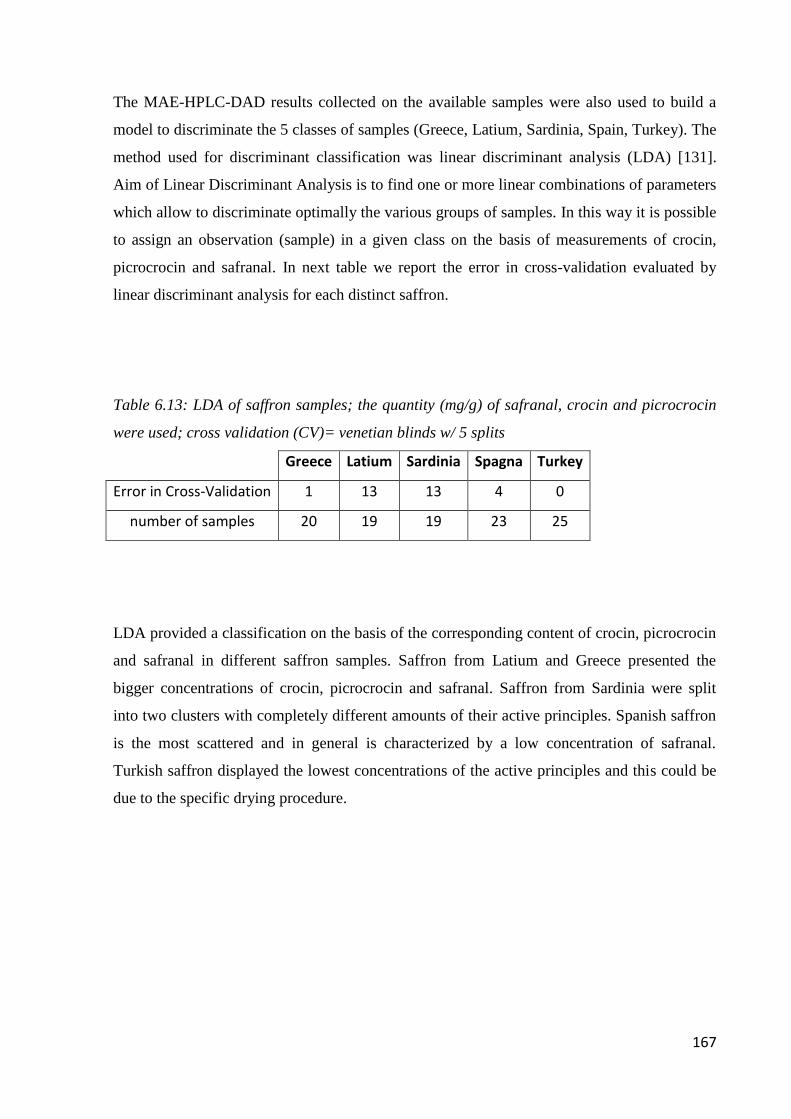
167
The MAE-HPLC-DAD results collected on the available samples were also used to build a
model to discriminate the 5 classes of samples (Greece, Latium, Sardinia, Spain, Turkey). The
method used for discriminant classification was linear discriminant analysis (LDA) [131].
Aim of Linear Discriminant Analysis is to find one or more linear combinations of parameters
which allow to discriminate optimally the various groups of samples. In this way it is possible
to assign an observation (sample) in a given class on the basis of measurements of crocin,
picrocrocin and safranal. In next table we report the error in cross-validation evaluated by
linear discriminant analysis for each distinct saffron.
Table 6.13: LDA of saffron samples; the quantity (mg/g) of safranal, crocin and picrocrocin
were used; cross validation (CV)= venetian blinds w/ 5 splits
Greece Latium Sardinia Spagna Turkey
Error in Cross-Validation 1 13 13 4 0
number of samples 20 19 19 23 25
LDA provided a classification on the basis of the corresponding content of crocin, picrocrocin
and safranal in different saffron samples. Saffron from Latium and Greece presented the
bigger concentrations of crocin, picrocrocin and safranal. Saffron from Sardinia were split
into two clusters with completely different amounts of their active principles. Spanish saffron
is the most scattered and in general is characterized by a low concentration of safranal.
Turkish saffron displayed the lowest concentrations of the active principles and this could be
due to the specific drying procedure.
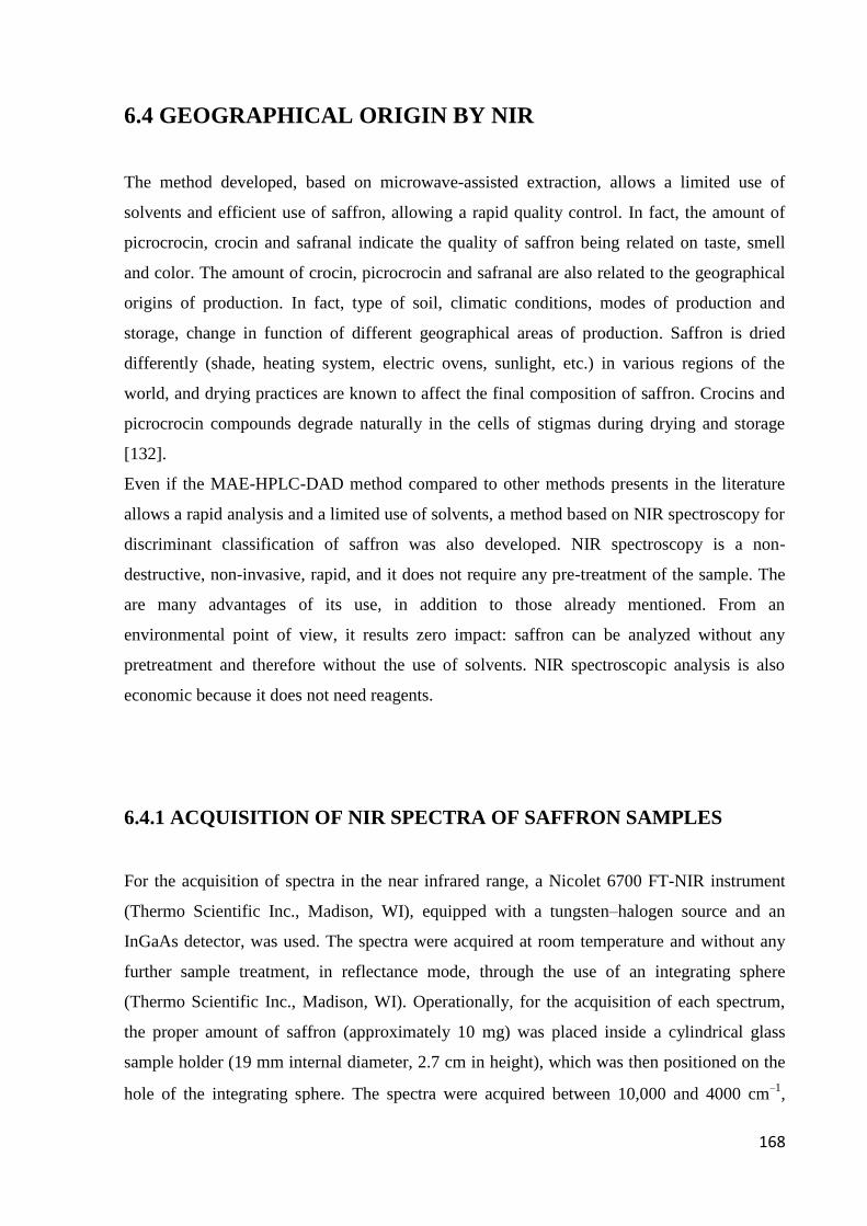
168
6.4 GEOGRAPHICAL ORIGIN BY NIR
The method developed, based on microwave-assisted extraction, allows a limited use of
solvents and efficient use of saffron, allowing a rapid quality control. In fact, the amount of
picrocrocin, crocin and safranal indicate the quality of saffron being related on taste, smell
and color. The amount of crocin, picrocrocin and safranal are also related to the geographical
origins of production. In fact, type of soil, climatic conditions, modes of production and
storage, change in function of different geographical areas of production. Saffron is dried
differently (shade, heating system, electric ovens, sunlight, etc.) in various regions of the
world, and drying practices are known to affect the final composition of saffron. Crocins and
picrocrocin compounds degrade naturally in the cells of stigmas during drying and storage
[132].
Even if the MAE-HPLC-DAD method compared to other methods presents in the literature
allows a rapid analysis and a limited use of solvents, a method based on NIR spectroscopy for
discriminant classification of saffron was also developed. NIR spectroscopy is a non-
destructive, non-invasive, rapid, and it does not require any pre-treatment of the sample. The
are many advantages of its use, in addition to those already mentioned. From an
environmental point of view, it results zero impact: saffron can be analyzed without any
pretreatment and therefore without the use of solvents. NIR spectroscopic analysis is also
economic because it does not need reagents.
6.4.1 ACQUISITION OF NIR SPECTRA OF SAFFRON SAMPLES
For the acquisition of spectra in the near infrared range, a Nicolet 6700 FT-NIR instrument
(Thermo Scientific Inc., Madison, WI), equipped with a tungsten–halogen source and an
InGaAs detector, was used. The spectra were acquired at room temperature and without any
further sample treatment, in reflectance mode, through the use of an integrating sphere
(Thermo Scientific Inc., Madison, WI). Operationally, for the acquisition of each spectrum,
the proper amount of saffron (approximately 10 mg) was placed inside a cylindrical glass
sample holder (19 mm internal diameter, 2.7 cm in height), which was then positioned on the
hole of the integrating sphere. The spectra were acquired between 10,000 and 4000 cm−1,
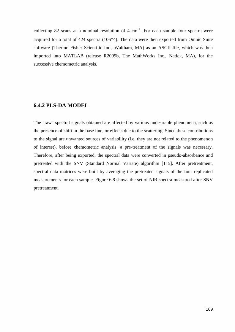
169
collecting 82 scans at a nominal resolution of 4 cm−1. For each sample four spectra were
acquired for a total of 424 spectra (106*4). The data were then exported from Omnic Suite
software (Thermo Fisher Scientific Inc., Waltham, MA) as an ASCII file, which was then
imported into MATLAB (release R2009b, The MathWorks Inc., Natick, MA), for the
successive chemometric analysis.
6.4.2 PLS-DA MODEL
The "raw" spectral signals obtained are affected by various undesirable phenomena, such as
the presence of shift in the base line, or effects due to the scattering. Since these contributions
to the signal are unwanted sources of variability (i.e. they are not related to the phenomenon
of interest), before chemometric analysis, a pre-treatment of the signals was necessary.
Therefore, after being exported, the spectral data were converted in pseudo-absorbance and
pretreated with the SNV (Standard Normal Variate) algorithm [115]. After pretreatment,
spectral data matrices were built by averaging the pretreated signals of the four replicated
measurements for each sample. Figure 6.8 shows the set of NIR spectra measured after SNV
pretreatment.
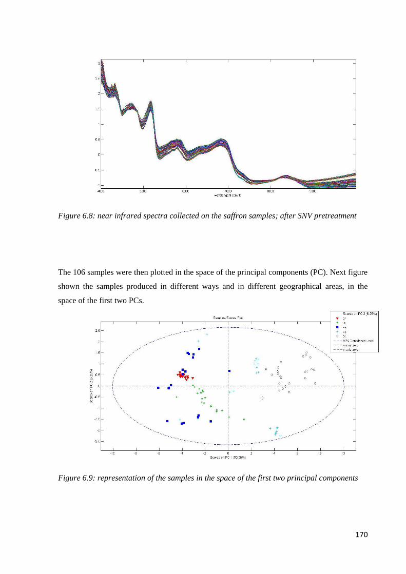
170
Figure 6.8: near infrared spectra collected on the saffron samples; after SNV pretreatment
The 106 samples were then plotted in the space of the principal components (PC). Next figure
shown the samples produced in different ways and in different geographical areas, in the
space of the first two PCs.
Figure 6.9: representation of the samples in the space of the first two principal components
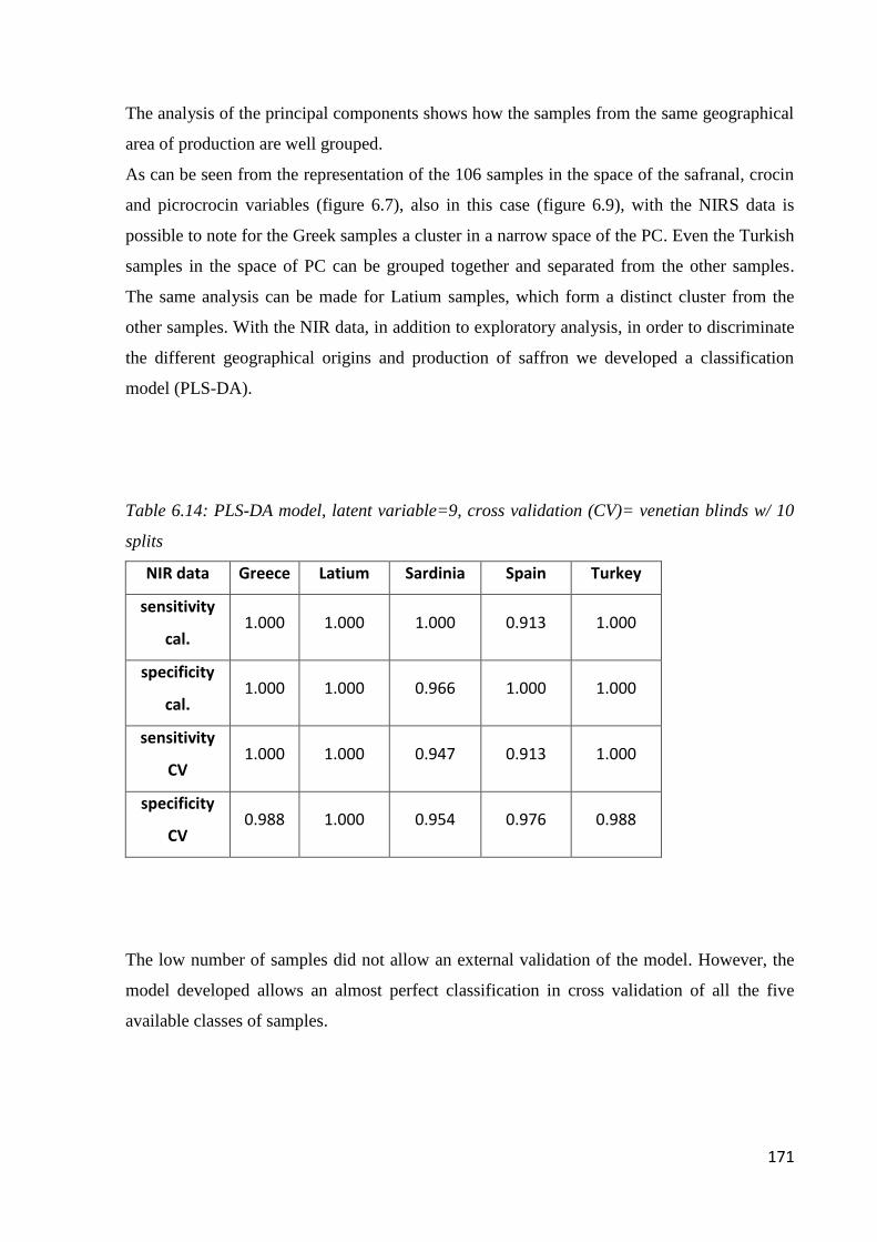
171
The analysis of the principal components shows how the samples from the same geographical
area of production are well grouped.
As can be seen from the representation of the 106 samples in the space of the safranal, crocin
and picrocrocin variables (figure 6.7), also in this case (figure 6.9), with the NIRS data is
possible to note for the Greek samples a cluster in a narrow space of the PC. Even the Turkish
samples in the space of PC can be grouped together and separated from the other samples.
The same analysis can be made for Latium samples, which form a distinct cluster from the
other samples. With the NIR data, in addition to exploratory analysis, in order to discriminate
the different geographical origins and production of saffron we developed a classification
model (PLS-DA).
Table 6.14: PLS-DA model, latent variable=9, cross validation (CV)= venetian blinds w/ 10
splits
NIR data Greece Latium Sardinia Spain Turkey
sensitivity
cal. 1.000 1.000 1.000 0.913 1.000
specificity
cal. 1.000 1.000 0.966 1.000 1.000
sensitivity
CV 1.000 1.000 0.947 0.913 1.000
specificity
CV 0.988 1.000 0.954 0.976 0.988
The low number of samples did not allow an external validation of the model. However, the
model developed allows an almost perfect classification in cross validation of all the five
available classes of samples.
172
6.5 CONCLUSION
A microwave-assisted extraction system for biologically active compounds has many
advantages over other conventional extraction methods. Microwave-assisted extraction
methods required shorter time, less solvents, provide higher extraction rates and better
products with lower costs.
It can be concluded that microwave-assisted extractions provide significant advantages in
terms of extraction efficiency and time savings.
The method developed allows high recovery, it is very reproducible and allows to analyze
samples with very low concentration of safranal, crocin and picrocrocin. This method, thanks
to the high concentration factor (only 2 mL of solvent are used), can be used for the analysis
of compounds and derivatives with similar characteristics to safranal, crocin and picrocrocin
even if they are present in very low concentrations. It may be used also for the analysis of
other spices in which the amount of safranal, crocin and picrocrocin are very low. We
obtained, with the use of microwave-assisted extraction, concentrations of extracts
approximately 10 times higher compared to the ISO 2003 method and to methods which use
ultrasounds for the extraction [129,133,134]. Moreover, with the method developed, it is
possible to simultaneously analyze both safranal, and crocin/picrocrocin, while the works
reported in the literature are focused on the determination of either safranal or crocin and
picrocrocin [123,128].
Although a perfect geographical classification could not be performed only with the
quantitative analysis of crocin, picrocrocin and safranal, we can assert by graphical analysis of
the samples in the space of these three parameters (figure 6.7) and by the results of the linear
discriminant analysis in cross validation (table 6.12), that the content of these bioactive
compounds is strongly linked to the production area.
A discriminant method of classification faster than HPLC-DAD analysis was developed. The
analysis of the NIR spectra of the saffron samples allowed to discriminate in a rapid, non-
destructive and zero impact way, samples from the different production areas such as Turkey,
Greece, Spain and Italy (Latium and Sardinia).
In the future, the method based on NIR spectroscopy will be validated with samples which
will be harvested in 2014: doing so it will be possible to validate the PLS-DA model
developed with a test set does not used to build the model.
173
CHAPTER 7
WATER: DETERMINATION OF BENZOTRIAZOLES IN WATER SAMPLES
7.1 INTRODUCTION
Benzotriazole derivatives are categorized as high production volume chemicals, being
complexing agents widely used as anticorrosives (e. g. in engine coolants, aircraft deicers and
antifreeze liquids) and for silver protection in dish washing liquids [135,136]. Toxicological
studies have demonstrated that they might be hazardous to plants [137,138], mutagenic in
bacteria cell systems [138] and toxic to some microorganisms [139]. Moreover, 1H-
benzotriazole (BTri) has been classified as a suspected human carcinogen by the Dutch Expert
Committee on Occupational Standards [138]. In the environment, benzotriazoles are
considered as emerging pollutants [135,136], with sewage treatment plants (STPs)
representing one of the most important discharge sources of these compounds into the aquatic
media [140-142].Thus, they have been detected in different aquatic compartments, such as
surface, ground or wastewater [135,136], sludge [143,144] and sediments [144]. Also,
benzotriazoles appear in indoor environments (indoor dust) [145], and even in human urine
[146].
Due to their polar character (log Kow values from 1.44 to 2.25), high water solubility and low
volatility, liquid chromatography (LC), usually coupled to mass spectrometry (MS), has been
174
the preferred technique for their sensitive determination in environmental samples during last
years [136]. Most water samples analysis have been carried out using triple quadrupole LC-
MS/MS instruments, achieving methodological LOQs in the low ng L-1
[140,147-150];
furthermore, other types of mass analyzers, such as LTQ FT Orbitrap MS [151], HRMS [152]
and QTOF MS [153], have also demonstrated their suitability for benzotriazole determination
in combination with LC as separation technique. Limited performance of gas chromatography
(GC) methods for benzotriazole compounds has been overcome by the use of ionic liquid
stationary phases coated columns [154], derivatization processes, such as methylation
[155,156] or acetylation [157], and the use of two-dimensional gas chromatography
[156,158]. But for now, no simple analytical methodologies, based on the use of a routine
laboratory affordable GC-single quadrupole MS instrument, have been developed, able to
reach LOQs comparable to those provided by LC-MS/MS methods and an improved isomer
resolution.
Regarding sample preparation, solid-phase extraction (SPE), using conventional hydrophilic-
lipophilic balanced polymeric materials such as OASIS HLB [140,146-148,151] or Strata X
[154,156], remains as the most popular concentration technique for benzotriazoles
determination in water samples. SPE, based on reversed-phase polymers, is also the preferred
approach to carry out multiresidue water sampling campaigns in which these emerging
pollutants are often included [159-162].
Despite microextraction techniques potential advantages, such as miniaturization, low solvent
consumption and high selectivity [163, 164], they have just been scarcely investigated for the
extraction and preconcentration of benzotriazoles. As regards solid-phase methodologies, stir-
bar sorptive extraction (SBSE) has been tested for the determination of BTri in ultrapure
water using coating materials with different polarities, such as polydimethylsiloxane (PDMS),
polyacrylate (PA) with a proportion of poly(ethylene) glycol (PEG) and a PEG modified
silicone. In all cases, the extraction efficiency for BTri remained below 1%, for 50 mL of
ultrapure water, after sampling during 4 hours [165]. Benzotriazoles have also been
successfully concentrated from water samples using a disposable polar membrane of
polyethersulfone [153]. However, the sample preparation method required 6 hours to achieve
equilibrium conditions. Slow extraction kinetics, which are characteristic of solid-phase
microextraction techniques, can be overcome by some liquid-liquid microextraction
methodologies, such as dispersive liquid-liquid microextraction (DLLME) [163]. Following
the first report by Assadi and coworkers [166] in 2006, a high number of DLLME
applications have been published. Some of them, as well as the most outstanding trends in
175
DLLME, have been revised in a recent review [167]. To the best of our knowledge, the only
application of DLLME to benzotriazoles analysis considered tri-n-butylphosphate as
extractant, with concentrated species determined by LC with fluorescence detection and LC-
MS/MS [168]. Obviously, the above extractant was unsuitable to be used in combination with
GC-MS determination.
Therefore, main aims of this work are (1) the development of a simple, easy, highly efficient,
environmental friendly and low cost sample preparation proposal, based on a concurrent
derivatization-DLLME extraction, and (2) the combination with a relatively inexpensive
determination technique, as GC-MS, for the sensitive and selective determination of trace
levels of benzotriazolic compounds in complex aqueous matrices. The performance of the
developed method, particularly the achieved limits of quantification (LOQs) and the
possibility to individually quantify isomeric benzotriazoles, is compared to that corresponding
to previously published approaches, most of them using more sophisticated determination
techniques.
7.2 EXPERIMENTAL
7.2.1 STANDARD, SOLVENT AND MATERIAL
Standards of BTri (98%), 4-methyl-1H-benzotriazole (4-TTri; 100%), 5-methyl-1H-
benzotriazole (5-TTri; 98%), 5,6-dimethyl-1H-benzotriazole (XTri; 99%) and 1H-
benzotriazole-(ring-d4) solution (BTri-d4), 10 g mL-1
in acetone used as internal surrogate
(IS) through derivatization and liquid microextraction steps, were purchased from Sigma-
Aldrich (Milwaukee, WI, USA). Two different standards of 5-chloro-1H-benzotriazole, with
nominal purities of 98% and 99% were acquired from TCI (Zwijndrecht, Belgium) and
Sigma-Aldrich, respectively. Stock solutions of the above compounds and diluted mixtures,
used to spike water samples employed during optimization of extraction conditions, were
prepared in acetonitrile and stored at 4ºC for a maximum of 2 weeks. A standard of 1-acetyl-
1H-benzotriazole (97%) was also provided by Sigma-Aldrich.
176
Methanol and acetonitrile (HPLC-grade) were from Merck (Darmstadt, Germany). Acetone,
toluene, chlorobenzene, carbon tetrachloride and 1,1,1-trichloroethane (trace analysis grade)
were provided by Sigma-Aldrich. Ultrapure water was obtained from a Milli-Q system
(Millipore, Billerica, MA, USA). Sodium acetate, acetic acid, sodium bicarbonate (NaHCO3),
disodium hydrogen phosphate (Na2HPO4) and acetic anhydride were also obtained from
Sigma-Aldrich. Cellulose acetate membrane filters (0.45 m pore size) were purchased from
Millipore (Bedford, MA, USA).
Acetylated derivatives of target compounds, used during optimization of GC-MS
determination conditions, were prepared as described elsewhere [157]. In brief, 10 mL of
ultrapure water, containing a 0.8% (w/v) of Na2HPO4, were spiked with benzotriazole
standards prepared in acetonitrile. Thereafter, 150 L of acetic anhydride were poured into
the same vessel, 5 mL of toluene were added and vials were manually shaken for 2 min.
Derivatized species were concentrated in the upper organic phase (toluene), which was
recovered using a Pasteur pipette before GC-MS analysis. In the particular case of BTri, the
commercially available acetylated standard was also used.
7.2.2 SAMPLES AND SAMPLE PREPARATION
Grab samples of treated wastewater were obtained from different STPs located in Galicia
(Northwest Spain); moreover, time-proportional 24-hour composite samples were received
from the inlet stream of a STP serving a 100000 inhabitants city, in the same region. River
water was obtained from two pristine creeks and the river receiving the discharge of the above
STP.
Optimization of acetylation and DLLME conditions was performed with spiked (0.050 to 20
ng mL-1
) aliquots of ultrapure water, adjusted at different pHs, considering also different
volumes of derivatization reagent (acetic anhydride) dispersant and extractant solvents.
Extractions were performed in conical bottom glass tubes (nominal volume 12 mL), which
were manually shaken during derivatization and microextraction steps. Thereafter, tubes were
centrifuged and the settled drop of extractant (case of chlorinated solvents) recovered after
removal of the upper aqueous phase. When using toluene as extraction solvent, the floating
organic phase, together with some water, was transferred to a conical insert (0.3 mL volume)
177
to improve phase separation, recovering enough volume of toluene to be handled with the
autosampler of the GC-MS instrument. Sample preparation conditions were optimized
following uni- and multi-variate strategies based on the use of experimental factorial designs.
In the latter case, the Statgraphics software (Statpoint Technologies, Warrenton, VA, USA)
was used for experimental design creation and analysis.
Under optimal conditions, samples (10 mL) were first mixed with 1 mL of Na2HPO4 (8%,
w/v) in the DLLME tube. Acetylation and microextraction of target compounds were
simultaneously carried out by addition of a ternary mixture, consisting of 100 L of acetic
anhydride, 1.5 mL of acetonitrile and 60 L of toluene. Reaction and centrifugation (3000
rpm) times were set at 1 and 5 min, respectively. After phase separation, as described above,
around 30 L of toluene could be recovered for GC-MS analysis.
7.2.3 GC-MS CONDITION
Acetylated compounds were determined by GC-MS. The gas chromatograph was an Agilent
(Wilmington, DE, USA) 7890A model, equipped with a split/splitless injector and connected
to a quadrupole MS spectrometer (Agilent MSD5975C), which was furnished with an
electron impact (EI) ionization source. Compounds were separated with an Agilent HP-5MS
capillary column (30 m x 0.25 mm i.d., df: 0.25 m) using helium (99.999%) as carried gas, at
a constant flow of 1.2 mL min-1
. The GC oven was programmed as follows: 80 ºC (held for 2
min), rate at 10 ºC min-1
to 280 ºC (held for 6 min). Injections (2 µL) were done in the
splitless mode, with the solenoid valve switching to the split mode after 1 min. EI source,
quadrupole and transfer line temperatures were maintained at 230 ºC, 150 ºC and 280 ºC,
respectively. GC-MS chromatograms were recorded in the SIM mode, selecting two different
ions per compound, Table 7.1.
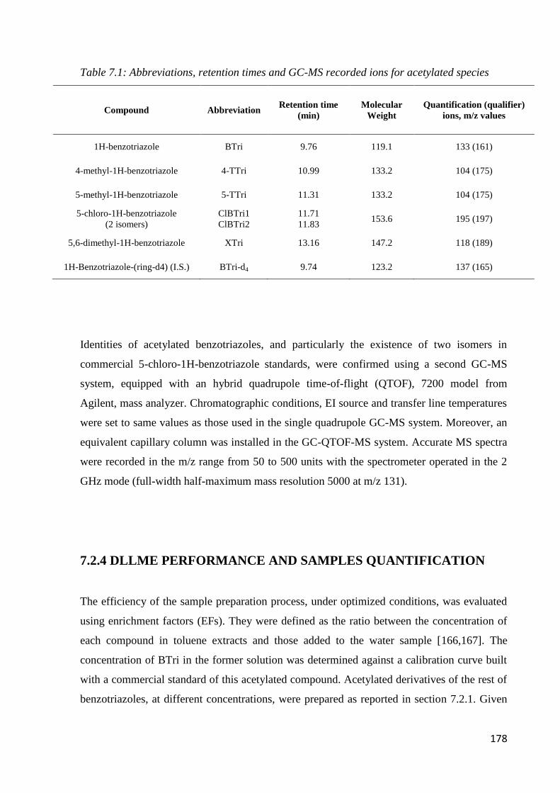
178
Table 7.1: Abbreviations, retention times and GC-MS recorded ions for acetylated species
Compound Abbreviation Retention time
(min)
Molecular
Weight
Quantification (qualifier)
ions, m/z values
1H-benzotriazole BTri 9.76 119.1 133 (161)
4-methyl-1H-benzotriazole 4-TTri 10.99 133.2 104 (175)
5-methyl-1H-benzotriazole 5-TTri 11.31 133.2 104 (175)
5-chloro-1H-benzotriazole
(2 isomers)
ClBTri1
ClBTri2
11.71
11.83 153.6 195 (197)
5,6-dimethyl-1H-benzotriazole XTri 13.16 147.2 118 (189)
1H-Benzotriazole-(ring-d4) (I.S.) BTri-d4 9.74 123.2 137 (165)
Identities of acetylated benzotriazoles, and particularly the existence of two isomers in
commercial 5-chloro-1H-benzotriazole standards, were confirmed using a second GC-MS
system, equipped with an hybrid quadrupole time-of-flight (QTOF), 7200 model from
Agilent, mass analyzer. Chromatographic conditions, EI source and transfer line temperatures
were set to same values as those used in the single quadrupole GC-MS system. Moreover, an
equivalent capillary column was installed in the GC-QTOF-MS system. Accurate MS spectra
were recorded in the m/z range from 50 to 500 units with the spectrometer operated in the 2
GHz mode (full-width half-maximum mass resolution 5000 at m/z 131).
7.2.4 DLLME PERFORMANCE AND SAMPLES QUANTIFICATION
The efficiency of the sample preparation process, under optimized conditions, was evaluated
using enrichment factors (EFs). They were defined as the ratio between the concentration of
each compound in toluene extracts and those added to the water sample [166,167]. The
concentration of BTri in the former solution was determined against a calibration curve built
with a commercial standard of this acetylated compound. Acetylated derivatives of the rest of
benzotriazoles, at different concentrations, were prepared as reported in section 7.2.1. Given
179
that the exact volume of the floating toluene phase is hard to establish, the absolute extraction
efficiencies of the DLLME method were not calculated.
Potential variations of extraction efficiencies among ultrapure, surface and wastewater
samples were evaluated using relative recoveries (%R) defined as follows:
%R = [(As-Ab)/Ar] x 100.
As is the response (analyte/IS peak areas) measured in the extract from a spiked sample, Ab is
the response of the extract from a non-spiked fraction of the same sample, and Ar is the
response measured in the extract from an aliquot of ultrapure water spiked at the same
concentration level. The calculated %R values remained around 100%, a fact that indicates
small variations in the efficiency of the acetylation-DLLME process for different matrices.
Therefore, concentrations of benzotriazoles in environmental water samples were established
by comparison with aliquots of ultrapure water, spiked with target species at different
concentration levels (from 0.05 to 20 ng mL-1
) and containing the same level of IS (1 ng mL-
1).
7.3 RESULTS AND DISCUSSION
7.3.1 PRELIMINARY EXPERIMENTS
Pervova and co-workers [157] reported, for the first time, the acetylation of BTri with the aim
of improving the performance of its GC-MS determination. Thereafter, the same procedure
was applied to 4-TTri and 5-TTri [169]. In both cases, acetylation was performed in aqueous
media, in presence of a basic catalyzer and analytes were further extracted, by conventional
LLE, with toluene. This strategy was extrapolated to the rest of compounds involved in this
study, introducing some changes regarding the type of base and volumes of acetic anhydride
and toluene. Whatever the tested derivatization parameters, under chromatographic conditions
reported in the experimental section, all compounds rendered a single, well-defined peak
corresponding to the acetylated derivative, whose identity was verified on the basis of low and
high resolution MS scan spectra and, in case of BTri, by injection of a commercially available
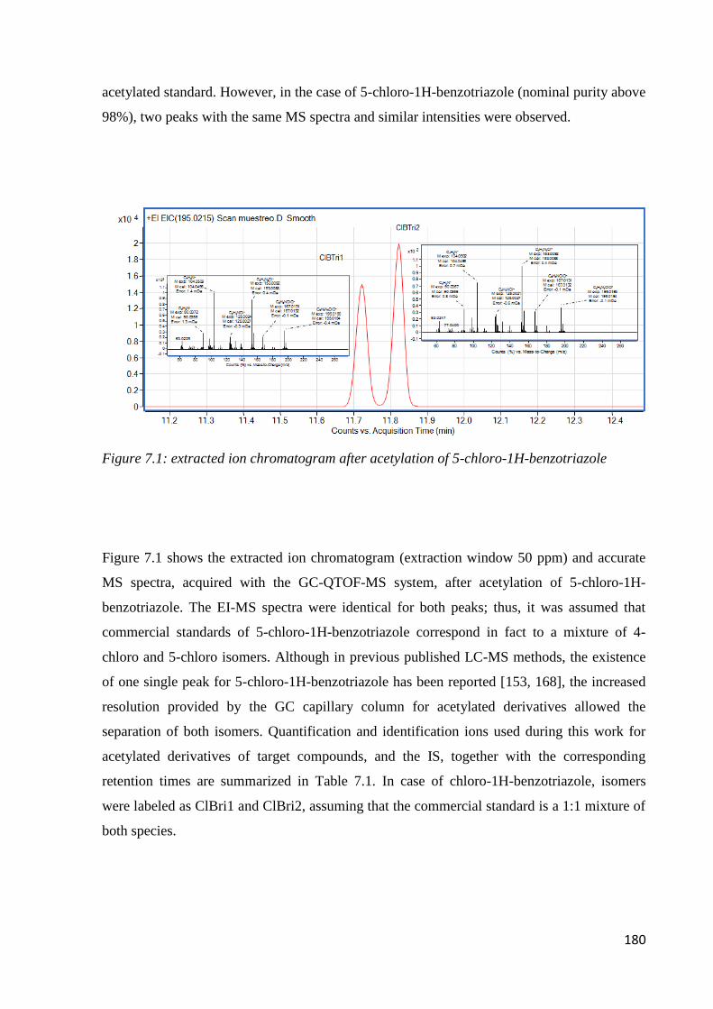
180
acetylated standard. However, in the case of 5-chloro-1H-benzotriazole (nominal purity above
98%), two peaks with the same MS spectra and similar intensities were observed.
Figure 7.1: extracted ion chromatogram after acetylation of 5-chloro-1H-benzotriazole
Figure 7.1 shows the extracted ion chromatogram (extraction window 50 ppm) and accurate
MS spectra, acquired with the GC-QTOF-MS system, after acetylation of 5-chloro-1H-
benzotriazole. The EI-MS spectra were identical for both peaks; thus, it was assumed that
commercial standards of 5-chloro-1H-benzotriazole correspond in fact to a mixture of 4-
chloro and 5-chloro isomers. Although in previous published LC-MS methods, the existence
of one single peak for 5-chloro-1H-benzotriazole has been reported [153, 168], the increased
resolution provided by the GC capillary column for acetylated derivatives allowed the
separation of both isomers. Quantification and identification ions used during this work for
acetylated derivatives of target compounds, and the IS, together with the corresponding
retention times are summarized in Table 7.1. In case of chloro-1H-benzotriazole, isomers
were labeled as ClBri1 and ClBri2, assuming that the commercial standard is a 1:1 mixture of
both species.
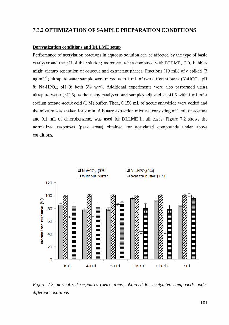
181
7.3.2 OPTIMIZATION OF SAMPLE PREPARATION CONDITIONS
Derivatization conditions and DLLME setup
Performance of acetylation reactions in aqueous solution can be affected by the type of basic
catalyzer and the pH of the solution; moreover, when combined with DLLME, CO2 bubbles
might disturb separation of aqueous and extractant phases. Fractions (10 mL) of a spiked (3
ng mL-1
) ultrapure water sample were mixed with 1 mL of two different bases (NaHCO3, pH
8; Na2HPO4, pH 9; both 5% w:v). Additional experiments were also performed using
ultrapure water (pH 6), without any catalyzer, and samples adjusted at pH 5 with 1 mL of a
sodium acetate-acetic acid (1 M) buffer. Then, 0.150 mL of acetic anhydride were added and
the mixture was shaken for 2 min. A binary extraction mixture, consisting of 1 mL of acetone
and 0.1 mL of chlorobenzene, was used for DLLME in all cases. Figure 7.2 shows the
normalized responses (peak areas) obtained for acetylated compounds under above
conditions.
Figure 7.2: normalized responses (peak areas) obtained for acetylated compounds under
different conditions
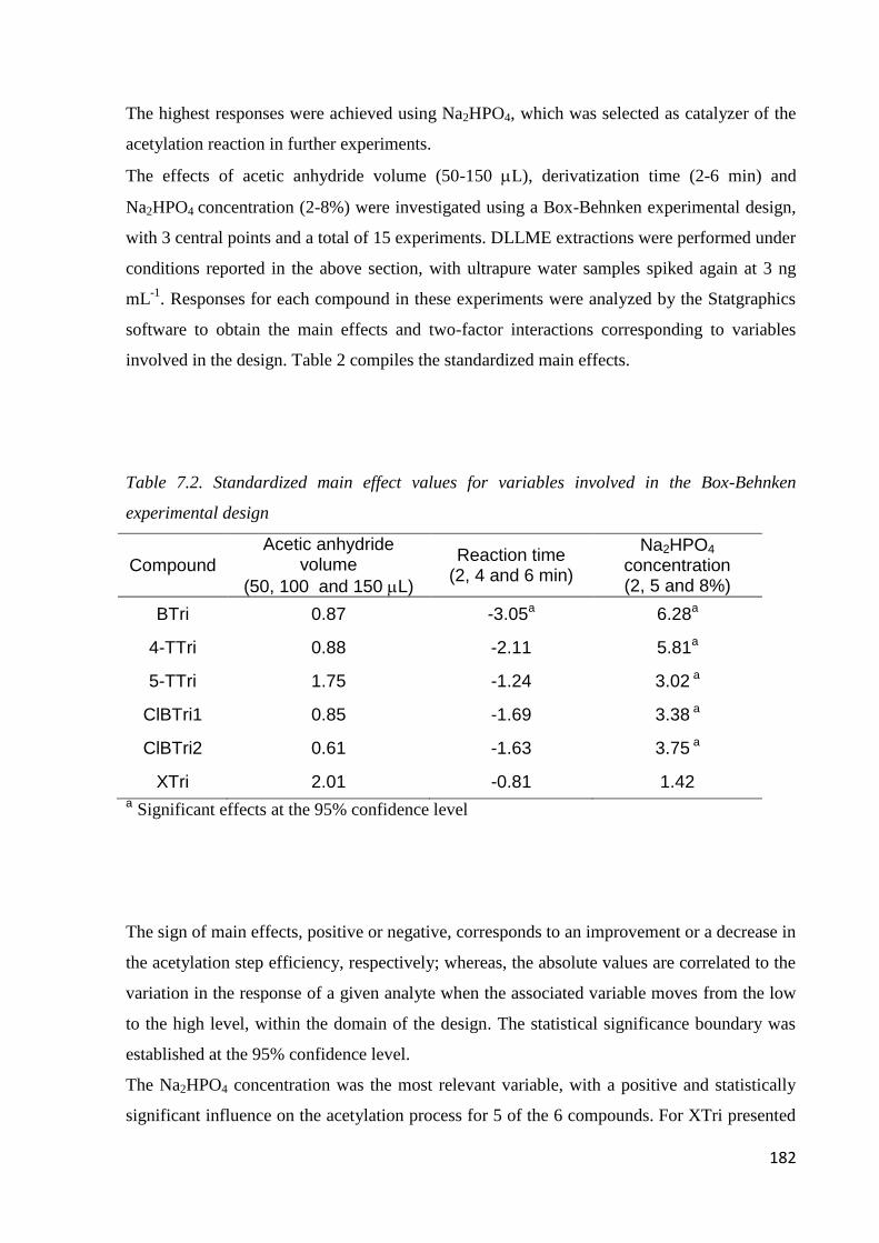
182
The highest responses were achieved using Na2HPO4, which was selected as catalyzer of the
acetylation reaction in further experiments.
The effects of acetic anhydride volume (50-150 L), derivatization time (2-6 min) and
Na2HPO4 concentration (2-8%) were investigated using a Box-Behnken experimental design,
with 3 central points and a total of 15 experiments. DLLME extractions were performed under
conditions reported in the above section, with ultrapure water samples spiked again at 3 ng
mL-1
. Responses for each compound in these experiments were analyzed by the Statgraphics
software to obtain the main effects and two-factor interactions corresponding to variables
involved in the design. Table 2 compiles the standardized main effects.
Table 7.2. Standardized main effect values for variables involved in the Box-Behnken
experimental design
Compound
Acetic anhydride volume
(50, 100 and 150 L)
Reaction time (2, 4 and 6 min)
Na2HPO4
concentration (2, 5 and 8%)
BTri 0.87 -3.05a 6.28a
4-TTri 0.88 -2.11 5.81a
5-TTri 1.75 -1.24 3.02 a
ClBTri1 0.85 -1.69 3.38 a
ClBTri2 0.61 -1.63 3.75 a
XTri 2.01 -0.81 1.42 a Significant effects at the 95% confidence level
The sign of main effects, positive or negative, corresponds to an improvement or a decrease in
the acetylation step efficiency, respectively; whereas, the absolute values are correlated to the
variation in the response of a given analyte when the associated variable moves from the low
to the high level, within the domain of the design. The statistical significance boundary was
established at the 95% confidence level.
The Na2HPO4 concentration was the most relevant variable, with a positive and statistically
significant influence on the acetylation process for 5 of the 6 compounds. For XTri presented
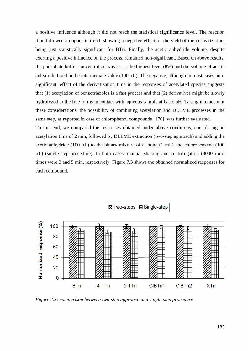
183
a positive influence although it did not reach the statistical significance level. The reaction
time followed an opposite trend, showing a negative effect on the yield of the derivatization,
being just statistically significant for BTri. Finally, the acetic anhydride volume, despite
exerting a positive influence on the process, remained non-significant. Based on above results,
the phosphate buffer concentration was set at the highest level (8%) and the volume of acetic
anhydride fixed in the intermediate value (100 L). The negative, although in most cases non-
significant, effect of the derivatization time in the responses of acetylated species suggests
that (1) acetylation of benzotriazoles is a fast process and that (2) derivatives might be slowly
hydrolyzed to the free forms in contact with aqueous sample at basic pH. Taking into account
these considerations, the possibility of combining acetylation and DLLME processes in the
same step, as reported in case of chlorophenol compounds [170], was further evaluated.
To this end, we compared the responses obtained under above conditions, considering an
acetylation time of 2 min, followed by DLLME extraction (two-step approach) and adding the
acetic anhydride (100 µL) to the binary mixture of acetone (1 mL) and chlorobenzene (100
µL) (single-step procedure). In both cases, manual shaking and centrifugation (3000 rpm)
times were 2 and 5 min, respectively. Figure 7.3 shows the obtained normalized responses for
each compound.
Figure 7.3: comparison between two-step approach and single-step procedure
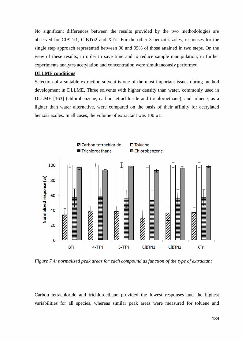
184
No significant differences between the results provided by the two methodologies are
observed for ClBTri1, ClBTri2 and XTri. For the other 3 benzotriazoles, responses for the
single step approach represented between 90 and 95% of those attained in two steps. On the
view of these results, in order to save time and to reduce sample manipulation, in further
experiments analytes acetylation and concentration were simultaneously performed.
DLLME conditions
Selection of a suitable extraction solvent is one of the most important issues during method
development in DLLME. Three solvents with higher density than water, commonly used in
DLLME [163] (chlorobenzene, carbon tetrachloride and trichloroethane), and toluene, as a
lighter than water alternative, were compared on the basis of their affinity for acetylated
benzotriazoles. In all cases, the volume of extractant was 100 µL.
Figure 7.4: normalized peak areas for each compound as function of the type of extractant
Carbon tetrachloride and trichloroethane provided the lowest responses and the highest
variabilities for all species, whereas similar peak areas were measured for toluene and
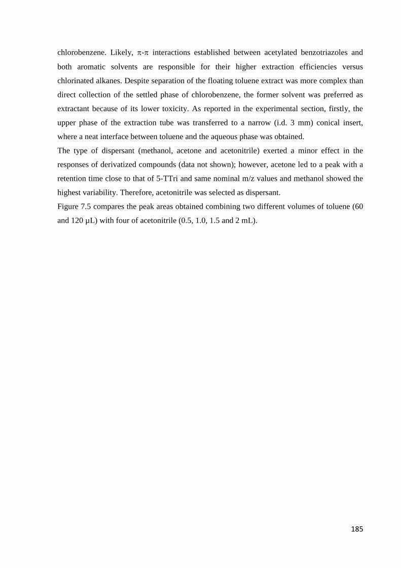
185
chlorobenzene. Likely, - interactions established between acetylated benzotriazoles and
both aromatic solvents are responsible for their higher extraction efficiencies versus
chlorinated alkanes. Despite separation of the floating toluene extract was more complex than
direct collection of the settled phase of chlorobenzene, the former solvent was preferred as
extractant because of its lower toxicity. As reported in the experimental section, firstly, the
upper phase of the extraction tube was transferred to a narrow (i.d. 3 mm) conical insert,
where a neat interface between toluene and the aqueous phase was obtained.
The type of dispersant (methanol, acetone and acetonitrile) exerted a minor effect in the
responses of derivatized compounds (data not shown); however, acetone led to a peak with a
retention time close to that of 5-TTri and same nominal m/z values and methanol showed the
highest variability. Therefore, acetonitrile was selected as dispersant.
Figure 7.5 compares the peak areas obtained combining two different volumes of toluene (60
and 120 µL) with four of acetonitrile (0.5, 1.0, 1.5 and 2 mL).
186
Figure 7.5: peak area in function of extractant and dispersant volume
In all cases, 100 µL of acetic anhydride were incorporated, as derivatization reagent, in the
ternary extraction mixture. With the only exception of the lowest dispersant volume, higher
responses were achieved using 60 µL of toluene than with 120 µL. For the former extractant
volume, the increase in the responses of the analytes with the volume of acetonitrile can be
explained since a more efficient dispersion of toluene droplets in the aqueous sample is
achieved. At 2 mL of acetonitrile, the increased solubility of acetylated analytes in the
aqueous phase led to a small reduction in the efficiency of their extraction. Thus, 60 µL and
1.5 mL were adopted as toluene and acetonitrile optimal volumes. Under these conditions, 25-
30 µL of toluene could be recovered at the end of phase separation process.
187
The influence of the ionic strength on the efficiency of the DLLME was evaluated comparing
the responses obtained without and with addition of 1 g of NaCl to water samples. No
significant variations were noticed in the responses measured for acetylated compounds; thus,
no salt was used in further extractions. The extraction time, after addition of the ternary
acetylation-extraction mixture, was varied between 1 and 5 min, whereas centrifugation (3000
rpm) times of 5, 10 and 15 min were tested. None of these factors modified the performance
of the extraction; thus, extraction and centrifugation steps were limited to 1 and 5 min,
respectively.
7.3.3 PERFORMANCE OF THE METHOD
Linearity of the proposed methodology was investigated with ultrapure water aliquots
fortified with increasing concentrations of target benzotriazoles (from 0.050 to 20 ng mL-1
,
n=7 levels), maintaining the IS at 1ng mL-1
. The corrected responses (peak area/IS peak area)
for each compound were plotted against their concentrations in the water samples and fitted to
a linear model. Determination coefficients (R2) values for the obtained graphs varied from
0.995 up to 0.9997. Regarding reproducibility, nine extractions were carried out in three
different days with samples spiked at two concentration levels, 0.2 ng mL-1
and 2 ng mL-1
.
Relative standard deviation (RSDs, %) of corrected responses remained between 2 and 10%.
Efficiency of the proposed method was evaluated with EFs, calculated as defined in the
experimental section, for a sample spiked at the 10 ng mL-1
level. Analytes were concentrated
between 93 times (BTri) and 172 times (XTri), Table 7.3.
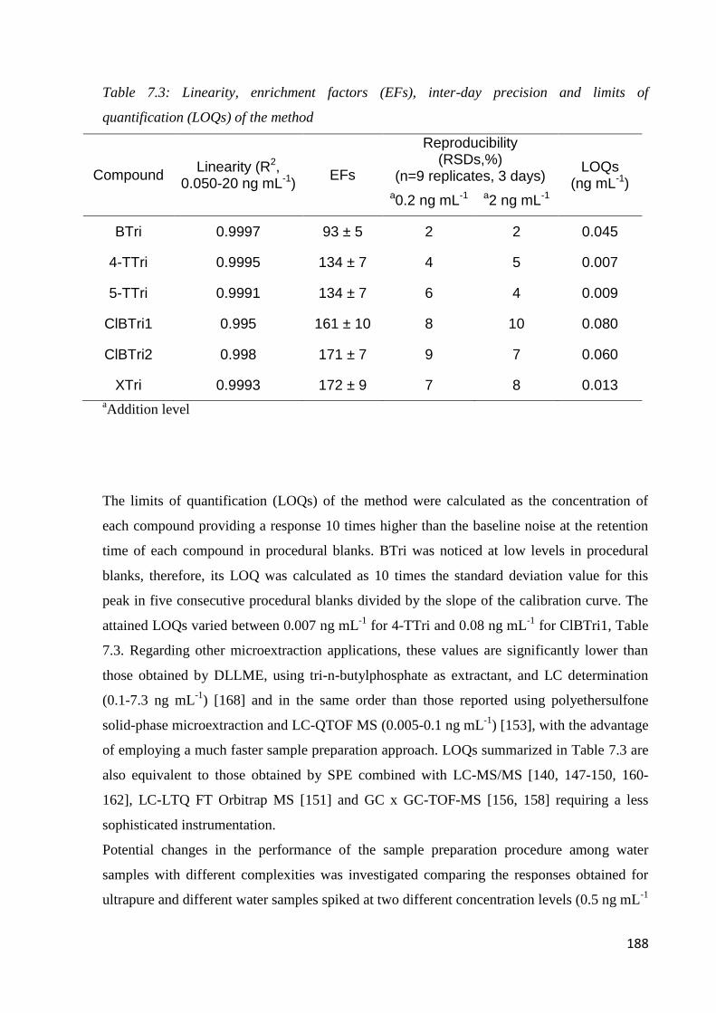
188
Table 7.3: Linearity, enrichment factors (EFs), inter-day precision and limits of
quantification (LOQs) of the method
Compound Linearity (R2,
0.050-20 ng mL-1) EFs
Reproducibility (RSDs,%)
(n=9 replicates, 3 days) LOQs
(ng mL-1) a0.2 ng mL-1 a2 ng mL-1
BTri 0.9997 93 ± 5 2 2 0.045
4-TTri 0.9995 134 ± 7 4 5 0.007
5-TTri 0.9991 134 ± 7 6 4 0.009
ClBTri1 0.995 161 ± 10 8 10 0.080
ClBTri2 0.998 171 ± 7 9 7 0.060
XTri 0.9993 172 ± 9 7 8 0.013
aAddition level
The limits of quantification (LOQs) of the method were calculated as the concentration of
each compound providing a response 10 times higher than the baseline noise at the retention
time of each compound in procedural blanks. BTri was noticed at low levels in procedural
blanks, therefore, its LOQ was calculated as 10 times the standard deviation value for this
peak in five consecutive procedural blanks divided by the slope of the calibration curve. The
attained LOQs varied between 0.007 ng mL-1
for 4-TTri and 0.08 ng mL-1
for ClBTri1, Table
7.3. Regarding other microextraction applications, these values are significantly lower than
those obtained by DLLME, using tri-n-butylphosphate as extractant, and LC determination
(0.1-7.3 ng mL-1
) [168] and in the same order than those reported using polyethersulfone
solid-phase microextraction and LC-QTOF MS (0.005-0.1 ng mL-1
) [153], with the advantage
of employing a much faster sample preparation approach. LOQs summarized in Table 7.3 are
also equivalent to those obtained by SPE combined with LC-MS/MS [140, 147-150, 160-
162], LC-LTQ FT Orbitrap MS [151] and GC x GC-TOF-MS [156, 158] requiring a less
sophisticated instrumentation.
Potential changes in the performance of the sample preparation procedure among water
samples with different complexities was investigated comparing the responses obtained for
ultrapure and different water samples spiked at two different concentration levels (0.5 ng mL-1
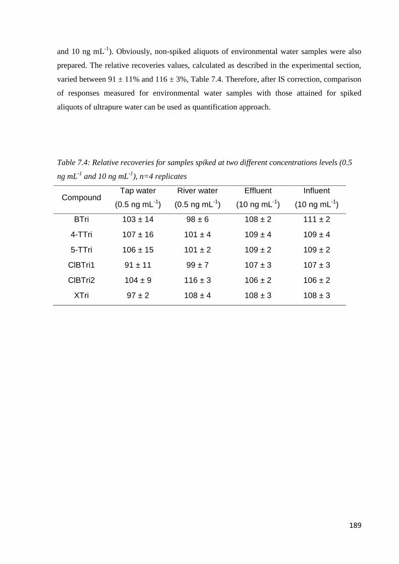
189
and 10 ng mL-1
). Obviously, non-spiked aliquots of environmental water samples were also
prepared. The relative recoveries values, calculated as described in the experimental section,
varied between 91 ± 11% and 116 ± 3%, Table 7.4. Therefore, after IS correction, comparison
of responses measured for environmental water samples with those attained for spiked
aliquots of ultrapure water can be used as quantification approach.
Table 7.4: Relative recoveries for samples spiked at two different concentrations levels (0.5
ng mL-1
and 10 ng mL-1
), n=4 replicates
Compound Tap water
(0.5 ng mL-1)
River water
(0.5 ng mL-1)
Effluent
(10 ng mL-1)
Influent
(10 ng mL-1)
BTri 103 ± 14 98 ± 6 108 ± 2 111 ± 2
4-TTri 107 ± 16 101 ± 4 109 ± 4 109 ± 4
5-TTri 106 ± 15 101 ± 2 109 ± 2 109 ± 2
ClBTri1 91 ± 11 99 ± 7 107 ± 3 107 ± 3
ClBTri2 104 ± 9 116 ± 3 106 ± 2 106 ± 2
XTri 97 ± 2 108 ± 4 108 ± 3 108 ± 3
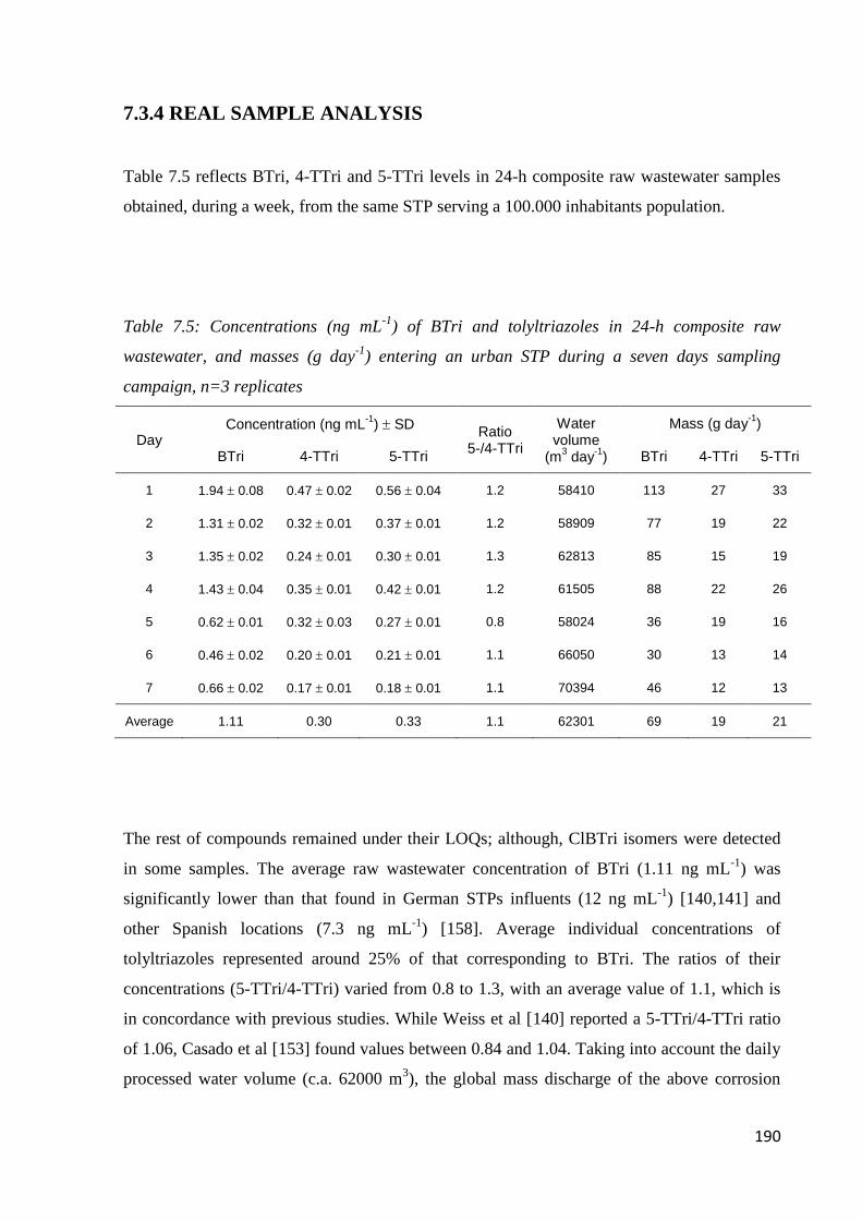
190
7.3.4 REAL SAMPLE ANALYSIS
Table 7.5 reflects BTri, 4-TTri and 5-TTri levels in 24-h composite raw wastewater samples
obtained, during a week, from the same STP serving a 100.000 inhabitants population.
Table 7.5: Concentrations (ng mL-1
) of BTri and tolyltriazoles in 24-h composite raw
wastewater, and masses (g day-1
) entering an urban STP during a seven days sampling
campaign, n=3 replicates
Day Concentration (ng mL
-1) SD
Ratio 5-/4-TTri
Water volume
(m3 day
-1)
Mass (g day-1
)
BTri 4-TTri 5-TTri BTri 4-TTri 5-TTri
1 1.94 0.08 0.47 0.02 0.56 0.04 1.2 58410 113 27 33
2 1.31 0.02 0.32 0.01 0.37 0.01 1.2 58909 77 19 22
3 1.35 0.02 0.24 0.01 0.30 0.01 1.3 62813 85 15 19
4 1.43 0.04 0.35 0.01 0.42 0.01 1.2 61505 88 22 26
5 0.62 0.01 0.32 0.03 0.27 0.01 0.8 58024 36 19 16
6 0.46 0.02 0.20 0.01 0.21 0.01 1.1 66050 30 13 14
7 0.66 0.02 0.17 0.01 0.18 0.01 1.1 70394 46 12 13
Average 1.11 0.30 0.33 1.1 62301 69 19 21
The rest of compounds remained under their LOQs; although, ClBTri isomers were detected
in some samples. The average raw wastewater concentration of BTri (1.11 ng mL-1
) was
significantly lower than that found in German STPs influents (12 ng mL-1
) [140,141] and
other Spanish locations (7.3 ng mL-1
) [158]. Average individual concentrations of
tolyltriazoles represented around 25% of that corresponding to BTri. The ratios of their
concentrations (5-TTri/4-TTri) varied from 0.8 to 1.3, with an average value of 1.1, which is
in concordance with previous studies. While Weiss et al [140] reported a 5-TTri/4-TTri ratio
of 1.06, Casado et al [153] found values between 0.84 and 1.04. Taking into account the daily
processed water volume (c.a. 62000 m3), the global mass discharge of the above corrosion
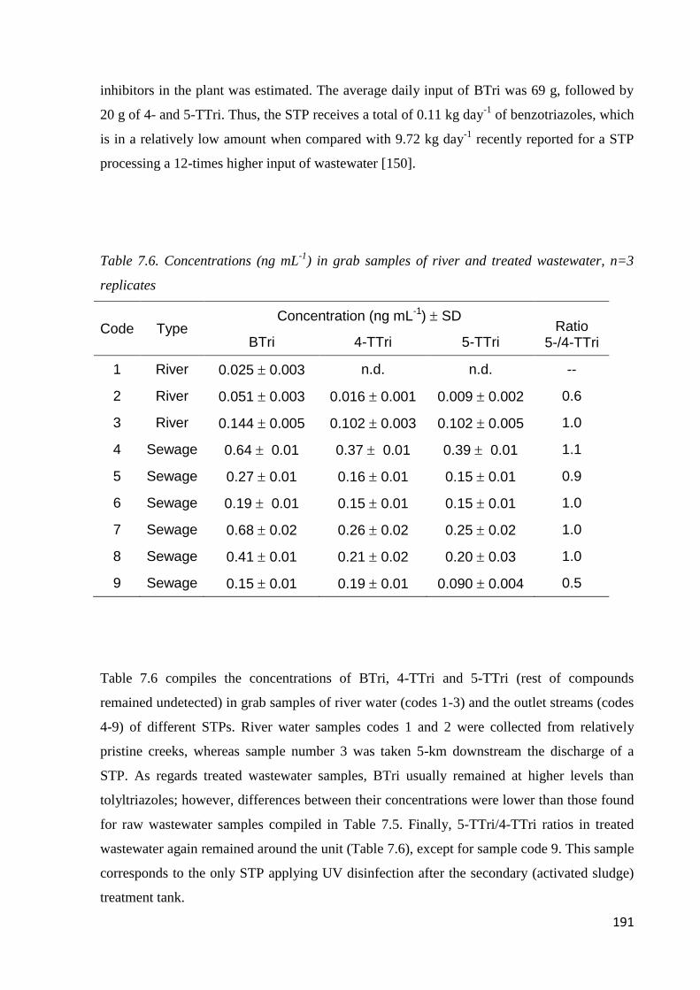
191
inhibitors in the plant was estimated. The average daily input of BTri was 69 g, followed by
20 g of 4- and 5-TTri. Thus, the STP receives a total of 0.11 kg day-1
of benzotriazoles, which
is in a relatively low amount when compared with 9.72 kg day-1
recently reported for a STP
processing a 12-times higher input of wastewater [150].
Table 7.6. Concentrations (ng mL-1
) in grab samples of river and treated wastewater, n=3
replicates
Code Type Concentration (ng mL-1) SD
Ratio 5-/4-TTri BTri 4-TTri 5-TTri
1 River 0.025 0.003 n.d. n.d. --
2 River 0.051 0.003 0.016 0.001 0.009 0.002 0.6
3 River 0.144 0.005 0.102 0.003 0.102 0.005 1.0
4 Sewage 0.64 0.01 0.37 0.01 0.39 0.01 1.1
5 Sewage 0.27 0.01 0.16 0.01 0.15 0.01 0.9
6 Sewage 0.19 0.01 0.15 0.01 0.15 0.01 1.0
7 Sewage 0.68 0.02 0.26 0.02 0.25 0.02 1.0
8 Sewage 0.41 0.01 0.21 0.02 0.20 0.03 1.0
9 Sewage 0.15 0.01 0.19 0.01 0.090 0.004 0.5
Table 7.6 compiles the concentrations of BTri, 4-TTri and 5-TTri (rest of compounds
remained undetected) in grab samples of river water (codes 1-3) and the outlet streams (codes
4-9) of different STPs. River water samples codes 1 and 2 were collected from relatively
pristine creeks, whereas sample number 3 was taken 5-km downstream the discharge of a
STP. As regards treated wastewater samples, BTri usually remained at higher levels than
tolyltriazoles; however, differences between their concentrations were lower than those found
for raw wastewater samples compiled in Table 7.5. Finally, 5-TTri/4-TTri ratios in treated
wastewater again remained around the unit (Table 7.6), except for sample code 9. This sample
corresponds to the only STP applying UV disinfection after the secondary (activated sludge)
treatment tank.
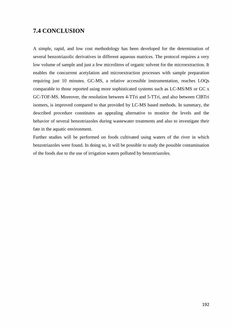
192
7.4 CONCLUSION
A simple, rapid, and low cost methodology has been developed for the determination of
several benzotriazolic derivatives in different aqueous matrices. The protocol requires a very
low volume of sample and just a few microlitres of organic solvent for the microextraction. It
enables the concurrent acetylation and microextraction processes with sample preparation
requiring just 10 minutes. GC-MS, a relative accessible instrumentation, reaches LOQs
comparable to those reported using more sophisticated systems such as LC-MS/MS or GC x
GC-TOF-MS. Moreover, the resolution between 4-TTri and 5-TTri, and also between ClBTri
isomers, is improved compared to that provided by LC-MS based methods. In summary, the
described procedure constitutes an appealing alternative to monitor the levels and the
behavior of several benzotriazoles during wastewater treatments and also to investigate their
fate in the aquatic environment.
Further studies will be performed on foods cultivated using waters of the river in which
benzotriazoles were found. In doing so, it will be possible to study the possible contamination
of the foods due to the use of irrigation waters polluted by benzotriazoles.
193
CHAPTER 8
OVERALL CONCLUSION
In conclusion, new methods for analysis of foods were developed, based on the fruitful
coupling of different instrumental profiling methods to chemometric data processing
techniques, which allow reliable quality control and traceability of the origin of the product.
In this respect, on one hand, chromatographic fingerprinting of the phenolic fraction proved to
be a valid secondary traceability indicator for oil and honey samples.
On the other hand, thanks to the many benefits provided by NIR spectroscopy coupled with
chemometric techniques, it was possible to build models of classification and regression
which allowed to discriminate different samples, providing an additional tool to combat fraud.
In this framework, particular attention was posed to the respect of the principles of "Green
Chemistry", which has now become the focus of the chemistry of the new millennium.
Indeed, the use of NIR spectroscopy allowed developing methods with less impact on the
environment, humans and higher performance compared to existing methods for analysis of
foods. But it is necessary to point out that, in all the examined cases, a key role is played by
chemometrics. Indeed, the possibility of using a not selective fingerprinting technique such as
NIR for calibration and classification, without needing any separation step or sample
pretreatment is only made possible by the use of chemometric data processing which allow to
mathematically manage the presence of interferents and other sources of unwanted variability
in the signals. Furthermore, chemometric proved to be essential also for all the other studies
presented in this PhD research, and ubiquitous in all the stages of the analytical process,
starting from sampling strategies and experimental design to the final validation of the results
obtained.
194
BIBLIOGRAPHY
1) How the European Union works, booklet made by the European Commission, 2012
2) Regulation (EC) No 178/2002 of the European Parliament
3) http://www.eurofoodlaw.com. Last accessed September 1st 2013
4) Potter Norman N. et al. Food Science. 1995, V edition. New York: Chapman Hall
5) ISO 9000:2005
6) ISO 9001:200
7) ISO 9004:2009
8) Report of FAO/WTO. Food consumption and exposure assessment to chemicals in
food. 1997
9) Scot P. M., et al. Officials methods of analysis of AOAC international. 1994, XVI
edition. Arlington, VA: AOAC International Press
10) Sikorski Z. E., Chemical and functional properties of food components. 1996,
Lancaster, PA: Technomic Publishing Co
11) Springett M. B., Raw ingredient quality in processed foods: the influence of
agricultural principles and practices. 2000, Gaithersburg, MA: Aspen Publishers
12) Francis F. J., et al. Encyclopedia of food science and technology. 1999, vol 1-4. new
york: Wiley
13) HACCP. Regulatory Assessment of HACCP. Special issue of Food Control. 2000, 5:
341-422
14) Singhal R. S., et al. Handbook of indices of food quality and authenticity. 1997,
Cambridge, UK: Woodhead Publ., Ltd
15) Ranganna S., Handbook of analysis and quality control for fruit and vegetable
products. 2008, New Delhi, Ind: McGraw-Hill Publ., Ltd
16) Camin F., et al. Characterization of authentic Italian extra-virgin olive oils by stable
isotope ratios of C, O and H and mineral composition. Food Chem. 2010, 118: 901–
909
17) Camin F., et al. Isotopic and elemental data for tracing the origin of European olive
oils. J. Agric. Food Chem. 2010, 58: 570–577
18) Piasentier E., et al. Stable isotope ratio analysis for authentication of lamb meat. Meat
Science, 2003, 64(3): 239-247
195
19) Podio N. S., et al. Elemental and isotopic fingerprint of Argentinean wheat. Matching
soil, water, and crop composition to differentiate provenance. J. Agric. Food Chem.
2013, 61: 3763-3773
20) Manca M., et al. Characterization of the geographical origin of pecorino Sardo cheese
by casein stable isotope (13C/12C and 15N/14N) ratios and free amino acid ratios. J.
Agric. Food Chem. 2001, 49: 1404-1409
21) Pizarro C., et al. Classification of Spanish extra virgin olive oils by data fusion of
visible spectroscopic fingerprints and chemical descriptors. Food Chem. 2013, 138:
915-922
22) Bevilacqua M., et al. Tracing the origin of extra virgin olive oils by infrared
spectroscopy and chemometrics: a case study. Anal. Chim. Acta. 2012, 717: 39-51
23) Gutiérrez J., et al. Enhanced chromatographic fingerprinting of herb materials by
multi-wavelength selection and chemometrics. Chim. Anal. Acta. 2012, 710: 40-49
24) Gao W., et al. Unbiased metabolite profiling by liquid chromatography-quadrupole
time-of-flight mass spectrometry and multivariate data analysis for herbal
authentication: classification of seven lonicera species flower buds. J. Chrom. A.
2012, 1245: 109-116
25) Sforza S. Food analysis and food authentication by peptide nucleic acid (PNA)-based
technologies. Chem. Soc. Rev. 2011, 40: 221–232
26) Mayer R., et al. PCR-based DNA Analysis for the identification and characterization
of food components. LWT Food Sci. Tech. 1996, 29: 1-9
27) Rock L. The use of stable isotope techniques in egg authentication schemes: a review.
Trends Food Sci. Tech. 2012, 28: 62-68
28) Cazzolino D. The use of infrared spectroscopy to trace and authenticate natural and
agricultural food products. Appl. Spectrosc. Rev. 2012, 47: 518-530
29) Vermuelen P., et al. Authentication and traceability of agricultural and food products
using vibrational spectroscopy. Handbook of Vibrational Spectroscopy. 2010, John
Wiley & Sons, Ltd
30) Anastas, P. T.; et al. Green Chemistry: theory and practice. 2000, Oxford University
Press
31) Anastas, P. T. Green chemistry and the role of analytical methodology development.
Crit. Rev. Anal. Chem, 1999, 29 (3): 167-175
32) Namiesnik J. Green analytical chemistry - some remarks. J. Sep. Sci. 2001, 24 (2):
151-153
196
33) Keith L., et al. Green analytical methodologies. Chem. Rev. 2007, 107: 2695-2708
34) Munck L, et al. Chemometrics in food science - a demonstration of the feasibility of a
highly exploratory, inductive evaluation strategy of fundamental scientific
significance. Chemometr. Intell. Lab. Syst. 1998; 44: 31–60
35) Reid L. M., et al. Recent technological advances for the determination of food
authenticity. Trends Food Sci. Technol. 2006, 17: 344–53
36) Pereira A. C., et al. Quality control of food products using image analysis and
multivariate statistical tools. Ind. Eng. Chem. Res. 2009, 48: 988–998
37) Brereton P. Preface to the special issue “Food authenticity and traceability”. Food
Chem. 2010, 118: 887
38) Guillou C. Preface to the special issue “Food authenticity and traceability” Food
Chem. 2010, 118:888–889
39) Bro R., et al. Multivariate data analysis as a tool in advanced quality monitoring in the
food production chain. Trends Food Sci. Technol. 2002, 13: 235–244
40) Kourti T. Process analysis and abnormal situation detection: from theory to practice.
Control Systems, IEEE, 2002, 22: 10-25
41) Boelens, H. F. M., et al. Performance optimization of spectroscopic process analyzers.
Anal. Chem. 2004, 76: 2656-2663
42) Tomasi G., et al. Correlation optimized warping and dynamic time warping as
preprocessing methods for chromatographic data. J. Chemometrics 2004, 18: 231–241
43) European Commission, Regulation (EC) no. 178/2002, Off. J. Eur. Commun. L31
(2002) 1–24
44) European Web site: http://ec.europa.eu/agriculture/quality/index_en.htm. Last
accessed September 1st 2013
45) Trace Project: http://www.trace.eu.org/. Last accessed September 1st 2013
46) Ellekjaer M. R., et al. A case study of the use of experimental design and multivariate
analysis in product improvement. Food Qual. Prefer. 1996, 7: 29-36
47) Jorgensen K. et al. A design and analysis strategy for situations with uncontrolled raw
material variation. J. Chemometrics. 2004, 18: 45-52
48) Lundstedt T. et al. Experimental design and optimization. Chemometr. Intell. Lab.
Syst. 1998, 42: 3-40
49) Leardi R. Experimental design in chemistry: A tutorial. Anal. Chim. Acta. 2009, 652:
161-172
197
50) Plackett R. L., et al. The design of optimum multifactorial experiments. Biometrika.
1946, 33: 305-325
51) Rune Flaten G. et al. A design of experiment approach incorporating layered designs
for choosing the right calibration model. Chemometr. Intell. Lab. Syst. 2004, 73: 55-
66
52) Teixeira Tarley C. R., et al. Chemometric tools in electroanalytical chemistry:
methods for optimization based on factorial design and response surface methodology.
Microchem. J. 2009, 92: 58-67
53) Box G. E. P., et al. Statistics for experimenters: design, innovation, and discovery. II
edition, 2005, Wiley
54) Hamanda M., et al. Analysis of designed experiments with complex aliasing. J. Qual.
Technol. 1992, 24: 130-137
55) Box G. E. P, et al. Some new three level designs for the study of quantitative
variables. Technometrics. 1960, 2: 455-475.
56) Ferreira S. L. C., et al. Box Behnken design: An alternative for the optimization of
analytical methods. Anal. Chim Acta. 2007, 597: 179-186
57) Wold S., et al. PLS-regression: a basic tool of chemometrics. Chemometr. Intell. Lab.
Syst. 2001, 58: 109-130
58) Smilde A.; et al. Two way component and regression models. In: Multi-way analysis.
2005, Wiley
59) Forina, M., et al. Class-modeling techniques, classic and new, for old and new
problems. Chemom. Intell. Lab. Syst. 2008, 93: 132-148
60) Geladi P., et al. Partial least squares regression: a tutorial, Anal. Chim. Acta. 1986
185: 1-17
61) Wold S., et al. Partial least squares projections to latent structures (PLS) in chemistry.
Encyclopedia of computational chemistry. 1998
62) Brereton R. G. Chemometrics for Pattern Recognition. 2010, Wiley
63) Duda R. O., et al. Pattern Classification. 2001, II edition, Wiley
64) Marini F. Classification Methods in chemometrics. Curr. Anal. Chem. 2010, 6: 72-79
65) Barker M., et al. Partial least squares for discrimination, J. Chemometr. 2003, 17: 166-
173
66) Eilers P. H. C. Parametric time warping. Anal. Chem. 2004, 76: 404–411
67) Tomasi G., et al. Correlation optimized warping and dynamic time warping as
preprocessing methods for chromatographic data. J. Chemometr. 2004, 18: 231-241
198
68) Tomasi G., et al. iCoshift: an effective tools for the alignment of chromatographic
data. J. Chromatogr. A. 2011, 1218: 7832-7840
69) Leardi R., et al. Sequential application of backward interval partial least squares and
genetic algorithms for the selection of relevant spectral regions. J. Chemometr. 2004,
18: 486-497
70) Leardi R., et al. Genetic algorithms as a tool for wavelength selection in multivariate
calibration. Anal. Chem. 1995 67: 4295- 4301
71) Leardi R. Genetic algorithms in chemistry. J. Chrom. A. 2007, 1158: 226-233
72) Martens H., et al. Validation and verification of regression in small data sets.
Chemometr. Intell. Lab. Syst. 1998, 44: 99-121
73) Snee R. D. Validation of regression models: methods and examples. Technometrics.
1977, 19: 415-428
74) Janssen M., et al. Product labelling in the market for organic food: consumer
preferences and willingness-to-pay for different organic certification logos. Food
Qual. Prefer. 2012, 25: 259-22
75) Kilcast D. Instrumental assessment of food sensory quality. A practical guide. 2013,
Woodhead Publishing Ltd
76) World Health Organization, Five keys to safer food manual, WHO Press, Geneva,
Switzerland, 2006
77) Erickson M. C. Internalization of fresh produce by foodborne pathogens. Ann. Rev.
Food Sci. Technol. 2012, 3: 283–310
78) Dennis J. Recent developments in food authentication. Analyst 1998, 123: 151–156.
79) Lees M. Food authenticity and traceability. 2003, Woodhead Publishing Ltd
80) Van Rijswijk W., et al. Consumer perceptions of traceability: A cross-national
comparison of the associated benefits. Food Qual. Prefer. 2008 19: 452-464
81) European Commission, Regulation (EC) no. 2081/1992 of 14 July 1992, Off. J. Eur.
Union L208, 1992, 1–8
82) European Commission, Regulation (EC) no. 2082/1992 of 14 July 1992, Off. J. Eur.
Union L208, 1992, 9
83) European Commission, Regulation (EC) no. 510/2006 of 20 March 2006, Off. J. Eur.
Union L93, 2006, 12–25
84) Caramia G., et al. Virgin olive oil in preventive medicine: from legend to epigenetic.
Eur. J. Lipid Sci. Technol. 2012, 114: 375-388
199
85) Frankel E., et al. Nutritional and biological properties of extra virgin olive oil. J.
Agric. Food Chem. 2011, 59: 785-792
86) Trubek A. B., The taste of place: a cultural journey into terroir. 2008, University of
California Press Ltd
87) European Commission, Regulation (EC) no. 1263/96 of 1 July 1996, Off. J. Eur.
Union L163, 1996, 19–21
88) European Commission, Dossier no. IT/PDO/0017/1511 of 2 July 1996, available
online at
http://ec.europa.eu/agriculture/quality/door/registeredName.html?denominationId=628
&locale=en (last accessed November 6th
2013)
89) Marini F., et al. Class-modeling techniques in the authentication of Italian oils from
Sicily with a protected denomination of origin (PDO), Chemometr. Intell. Lab. Syst.
2006, 80: 140-149
90) Cosio M. S., et al. Geographical origin and authentication of extra virgin olive oils by
an electronic nose in combination with artificial neural networks. Anal. Chim. Acta.
2006, 567: 202-210
91) Casale M., et al. The potential of coupling information using three analytical
techniques for identifying the geographical origin of Liguria extra virgin olive oil.
Food Chem. 2010, 118: 163-170
92) Casale M., et al. Characterization of PDO olive oil Chianti Classico by non-selective
(UV–visible, NIR and MIR spectroscopy) and selective (fatty acid composition)
analytical techniques. Anal. Chim. Acta. 2012, 712: 56-63
93) Bevilacqua M., et al. Tracing the origin of extra virgin olive oils by infrared
spectroscopy and chemometrics: a case study. Anal. Chim. Acta. 2012, 71: 739-51
94) Bertacchini L., et al. The impact of chemometrics on food traceability. In: Marini F.
(ed), Chemometrics in Food Chemistry, Elsevier, Oxford, UK, 2013, pp. 371-410
95) Franconi F., et al. Antioxidant effect of two olive oils depends on the concentration
and composition of minor polar compounds, J. Agric. Food Chem. 2006 54: 3121-
3125
96) Gómez-Rico A., et al. Phenolic and volatile compounds of extra virgin olive oil (olea
europea l. Cv. Cornicaba) with regard to fruit ripening and irrigation management. J.
Agric. Food Chem. 2006, 547130-7136
200
97) Kalua C. M., et al. Discrimination of olive oils and fruits into cultivars and maturity
stages based on phenolic and volatile compounds. J. Agric. Food Chem. 2005, 53:
8054-8062
98) Koshihara Y., et al. Caffeic acid is a selective inhibitor for leukotriene biosynthesis.
Biochim. Biophys. Acta. 1984, 792: 92–97
99) Rao C. V., et al. Inhibitory effect of caffeic acid esters on azoxymethane-induced
biochemical changes and aberrant crypt foci formation in rat colon. Cancer Res. 1993
53: 4182–4188
100) Olthof M. R., et al. Chlorogenic acid and caffeic acid are absorbed in humans.
Hum. Nutr. Metabol. 2001, 131: 66–71
101) Leardi R. Genetic algorithms-PLS as a tool for wavelength selection in spectral
data sets. In: R. Leardi (ed), Nature-inspired methods in chemometrics, Elsevier,
Amsterdam, The Netherlands, 2003, pp. 169-196.
102) Bertoncelj J., et al. LC-DAD-ESI/MS analysis of flavonoids and abscisic acid
with chemometric approach for the classification of Slovenian honey. Food Chem.
2011, 127: 296-302
103) Jasicka-Misiak I., et al. Phenolic compounds and abscisic acid as potential
markers for the floral origin of two Polish unifloral honeys. Food Chem. 2012, 131:
1149-1156
104) Iurlina M. O., et al. Major flavonoids of Argentinean honeys. Optimization of
the extraction method and analysis of their content in relationship to the geographical
source of honeys. Food Chem. 2009, 115: 1141-1149
105) Escriche I., et al. Using flavonoids, phenolic compounds and headspace
volatile profile for botanical authentication of lemon and orange honeys. Food Res.
Int. 2011, 44: 1504–1513
106) Woodcock T., et al. Near infrared spectral fingerprinting for confirmation of
claimed PDO provenance of honey. Food Chem. 2009, 114 (2): 742-746
107) Anklam E. A review of the analytical methods to determine the geographical
and botanical origin of honey. Food Chem. 1998, 63: 549-562
108) Woodcock T., et al. Geographical classification of honey samples by near-
infrared spectroscopy: a feasibility study. J. Agric. Food Chem. 2007, 55: 9128-9134
109) Pyrzynska K., et al. Analysis of phenolic acids and flavonoids in honey. Trends
Anal. Chem. 2009, 28(7): 893-902
201
110) Pulcini P., et al. Fast SPE extraction and LC-ESI-MS-MS analysis of
flavonoids and phenolic acids in honey. Apiacta. 2006 41: 21-27
111) Michalkiewicz A., et al. Solid-phase extraction procedures for determination of
phenolic acids and some flavonols in honey. J. Chrom. A. 2008, 118: 718-724
112) Wold, S., Johansson, E., Cocchi, M. PLS: Partial Least Squares Projections To
Latent Structures. In: Kubinyi, H. (Ed) 3D QSAR in Drug Design: Theory, Methods
And Applications. Escom Science Publishers: Leiden, The Netherlands, 1993, 523-
550
113) Toher D., et al. A comparison of model-based and regression classification
techniques applied to near infrared spectroscopic data in food authentication studies.
Chemometr. Intell. Lab. Syst. 2007, 89(2): 102-115
114) Downey G., et al. Food authentication - Has near infrared spectroscopy a role?
Spectrosc. Eur. 2006, 18: 10–14
115) Barnes R. J., et al. Standard normal variate transformation and detrending of
near-infrared diffuse reflectance spectra. Appl. Spectrosc. 1989, 43: 772-777
116) Bogdanov S., et al. Harmonised methods of the international honey
commission. Apidologie, Extra Issue. 2007, 1-59
117) Räty J., et al. Measurement of refractive index of liquids using s-and p-
polarized light. Meas. Sci. Technol. 2000, 11: 74-76
118) Felsner M. L., et al. Optimization of thermogravimetric analysis of ash content
in honey. J. Brazil. Chem. Soc.2004, 15(6): 797-802
119) Serneels S., et al. Partial robust M-regression. Chemom. Intell. Lab. Syst. 2005,
79: 55-64
120) Kennard R. W., et al. Computer aided design of experiments. Technometrics.
1969, 11(1): 137-148
121) Verma R., et al. Analysis of saffron (Crocus sativus L. stigma) components by
LC–MS–MS. Chromatographia. 2010, 71: 117–123
122) Kadkhodaee R., et al. Ultrasonic extraction of active compounds from saffron.
Acta Hort. (ISHS). 2007, 739: 417-425
123) Kyriakoudi A., et al. Revisiting extraction of bioactive apocarotenoids from
Crocus sativus L. dry stigmas (saffron). Anal. Chim. Acta. 2012, 755: 77-85
124) Heravi M. J., et al. Characterization of volatile components of Iranian saffron
using factorial-based response surface modeling of ultrasonic extraction combined
202
with gas chromatography–mass spectrometry analysis. J. Chromatogr. A. 2009,
1216(33): 6088-6097
125) Betti G., et al. Valorization of saffron (crocus sativus). Acta Hort. (ISHS).
2007, 739: 397-403
126) De Los Mozos P. M., et al. Preserving biodiversity in saffron: the crocus bank
project and the world saffron and crocus collection. Acta Hort. (ISHS). 2010, 850: 23-
28
127) Montalvo Hernández B., et al. Recovery of crocins from saffron stigmas
(Crocus sativus) in aqueous two-phase systems. J. Chromatogr. A. 2012, 1236: 7-15
128) Maggi M., et al. Rapid determination of safranal in the quality control of
saffron spice (Crocus sativus L.). Food Chem. 2011, 127: 369-373
129) Kanakis C. D., et al. Qualitative determination of volatile compounds and
quantitative evaluation of safranal and 4-hydroxy-2,6,6-trimethyl-1-cyclohexene-1-
carboxaldehyde (HTCC) in greek saffron. J. Agric. Food Chem. 2004, 52: 4515-4521
130) ISO/TS 3632-1, 2 (2003). Saffron (Crocus sativus L.) Part 1: Specifications,
Part 2: Test Methods. Geneva: ISO
131) Fisher R. A. The use of multiple measurements in taxonomic problems. Ann.
Eugen. 1936, 7: 179 188
132) Straubinger M., et al. Identification of novel glycosidic precursors in saffron. J.
Agric. Food Chem. 1998, 46: 3238–3243
133) Koulakiotis N. S., et al. Comparison of different tandem mass spectrometric
techniques (ESI-IT, ESI- and IP-MALDI-QRTOF and vMALDI-TOF/RTOF) for the
analysis of crocins and picrocrocin from the stigmas of Crocus sativus L. Rapid
Commun. Mass Spectrom. 2012, 26: 670–678
134) Caballero Ortega H., et al. HPLC quantification of major active components
from 11 different saffron (Crocus sativus L.) sources. Food Chem. 2007, 100: 1126–
1131
135) Richardson S. D., et al. Water analysis: emerging contaminants and current
issues. Anal. Chem. 2011, 83: 4614-4648
136) Richardson S. D., et al. Environmental mass spectrometry: emerging
contaminants and current issues. Anal. Chem. 2011, 84(2): 747-778
137) Castro S., et al. Phytotransformation of benzotriazoles. Int. J. Phytorem. 2003,
5: 245-265
203
138) Health Council of the Netherlands: Dutch expert committee on occupational
standards (DECOS). 1,2,3-Benzotriazole; publication no. 2000/14OSH; Health
Council of the Netherlands: The Hague, 2000
139) Cornell J. S., et al. Comparative measures of the toxicity of component
chemicals in aircraft deicing fluid. Environ. Toxicol. Chem. 2000, 19: 1465-1472
140) Weiss S., et al. Determination of benzotriazole corrosion inhibitors from
aqueous environmental samples by liquid chromatography-electrospray ionization-
tandem mass spectrometry. Anal. Chem. 77.22 (2005): 7415-7420
141) Weiss S., et al. Discharge of three benzotriazole corrosion inhibitors with
municipal wastewater and improvements by membrane bioreactor treatment and
ozonation. Environ. Sci. Technol. 2006, 40(23): 7193-7199
142) Reemtsma T., et al. Polar pollutants entry into the water cycle by municipal
wastewater: a European perspective. Environ. Sci. Technol. 2006, 40: 5451-5458
143) Liu Y. S., et al. Simultaneous determination of benzotriazoles and ultraviolet
filters in ground water, effluent and biosolid samples using gas chromatography–
tandem mass spectrometry. J. Chrom. A. 2011, 1218(31): 5328-5335
144) Zhang Z., et al. Determination of benzotriazole and benzophenone UV filters in
sediment and sewage sludge. Environ. Sci. Technol. 2011, 45: 3909-3916
145) Wang L., et al. Benzotriazole, benzothiazole, and benzophenone compounds in
indoor dust from the United States and east Asian countries. Environ. Sci. Technol.
2013, 47: 4752-4759
146) Asimakopoulos A. G., et al. Benzotriazoles and benzothiazoles in human urine
from several countries: A perspective on occurrence, biotransformation, and human
exposure. Anal. Chem. 2013, 85: 441-448
147) Giger W., et al. Benzotriazole and tolyltriazole as aquatic contaminants. 1.
Input and occurrence in rivers and lakes. Environ. Sci. Technol. 2006, 40: 7186-7192
148) Voutsa D., et al. Benzotriazoles, alkylphenols and bisphenol A in municipal
wastewaters and in the Glatt River, Switzerland. Environ. Sci. Pollut. Res. 2006, 13:
333-341
149) Carpinteiro I., et al. Simultaneous determination of benzotriazole and
benzothiazole derivatives in aqueous matrices by mixed-mode solid-phase extraction
followed by liquid chromatography–tandem mass spectrometry. Anal. Bioanal. Chem.
2012, 402: 2471-2478
204
150) Asimakopoulos A. G., et al. Occurrence and removal efficiencies of
benzotriazoles and benzothiazoles in a wastewater treatment plant in Greece. Sci. Tot.
Environ. 2013, 452: 163-171
151) Van Leerdam J. A., et al. Determination of polar 1H-benzotriazoles and
benzothiazoles in water by solid-phase extraction and liquid chromatography LTQ FT
Orbitrap mass spectrometry. Int. J. Mass Spec. 2009, 282: 99-107
152) Wode F., et al. Multiresidue analytical method for the simultaneous
determination of 72 micropollutants in aqueous samples with ultra high performance
liquid chromatography-high resolution mass spectrometry. J. Chromatogr. A. 2012,
1270: 118-126
153) Casado J., et al. Polyethersulfone solid-phase microextraction followed by
liquid chromatography quadrupole time-of-flight mass spectrometry for benzotriazoles
determination in water samples. J. Chromatogr. A. 2013, 1299: 40-47
154) Domínguez C., et al. Determination of benzothiazoles and benzotriazoles by
using ionic liquid stationary phases in gas chromatography mass spectrometry.
Application to their characterization in wastewaters. J. Chromatogr. A. 2012, 1230:
117-122
155) Corsi S. R., et al. Aquatic toxicity of nine aircraft deicer and anti-icer
formulations and relative toxicity of additive package ingredients alkylphenol
ethoxylates and 4, 5-methyl-1H-benzotriazoles. Environ. Sci. Technol. 2006, 40:
3195-3202
156) Matamoros V., et al. Part-per-trillion determination of pharmaceuticals,
pesticides, and related organic contaminants in river water by solid-phase extraction
followed by comprehensive two-dimensional gas chromatography time-of-flight mass
spectrometry. Anal. Chem. 2010, 82: 699-706
157) Pervova M. G., et al. Determination of 1, 2, 3-benzotriazole in aqueous
solutions and air by reaction-gas-liquid chromatography. J. Anal. Chem. 2010, 65:
276-279
158) Jover E., et al. Characterization of benzothiazoles, benzotriazoles and
benzosulfonamides in aqueous matrixes by solid-phase extraction followed by
comprehensive two-dimensional gas chromatography coupled to time-of-flight mass
spectrometry. J. Chromatogr. A. 2009, 1216: 4013-4019
159) Loos R., et al. EU-wide survey of polar organic persistent pollutants in
European river waters. Environ. Poll. 2009, 157: 561-568
205
160) Loos R., et al. Pan-European survey on the occurrence of selected polar
organic persistent pollutants in ground water. Wat. Res. 2010, 44: 4115-4126
161) Nödler K., et al. Development of a multi-residue analytical method, based on
liquid chromatography–tandem mass spectrometry, for the simultaneous determination
of 46 micro-contaminants in aqueous samples. J. Chromatogr. A. 2010, 1217: 6511-
6521
162) Huntscha S., et al. Multiresidue analysis of 88 polar organic micropollutants in
ground, surface and wastewater using online mixed-bed multilayer solid-phase
extraction coupled to high performance liquid chromatography-tandem mass
spectrometry. J. Chromatogr. A. 2012, 1268: 74-83
163) Kokosa J. M., et al. Solvent Microextraction. Theory and Practice. John Wiley
& Sons, Inc. Hoboken, New Jersey, 2009
164) Souza Silva E. A., et al. Recent trends in SPME concerning sorbent materials,
configurations and in vivo applications. Trends Anal. Chem. 2013, 43: 24-36
165) Gilart N., et al. Novel coatings for stir bar sorptive extraction to determine
pharmaceuticals and personal care products in environmental waters by liquid
chromatography and tandem mass spectrometry. Anal. Chim. Acta. 2013, 774: 51-60
166) Rezaee M., et al. Determination of organic compounds in water using
dispersive liquid–liquid microextraction. J. Chromatogr. A. 2006, 1116: 1-9
167) Yan H., et al. Recent development and applications of dispersive liquid–liquid
microextraction. J. Chromatogr. A. 2013, 1295: 1-15
168) Pena M. T., et al. Optimization of a dispersive liquid–liquid microextraction
method for the analysis of benzotriazoles and benzothiazoles in water samples. Anal.
Bioanal. Chem. 2012, 402: 1679-1695
169) Vetter W., et al. Determination of benzotriazoles in dishwasher tabs from
Germany and estimation of the discharge into German waters. Environ. Sci. Pollut.
Res. 2013, 20: 4435-4440
170) Fattahi N., et al. Solid-phase extraction combined with dispersive liquid–liquid
microextraction-ultra preconcentration of chlorophenols in aqueous samples. J.
Chromatogr. A. 2007, 1169: 63-69