A 2-DIMENSIONAL COMPUTATIONAL MODEL TO ANALYZE … · In seguito le fibre intra-nodali conducono...
106
ALMA MATER STUDIORUM – UNIVERSITÀ DI BOLOGNA CAMPUS DI CESENA SCUOLA DI INGEGNERIA E ARCHITETTURA CORSO DI LAUREA MAGISTRALE IN INGEGNERIA BIOMEDICA A 2-DIMENSIONAL COMPUTATIONAL MODEL TO ANALYZE THE EFFECTS OF CELLULAR HETEROGEINITY ON CARDIAC PACEMAKING Tesi in: Bioingegneria molecolare e cellulare LM Relatore: Presentata da: Prof. STEFANO SEVERI CHIARA CAMPANA Correlatore: Prof. ERIC SOBIE Sessione III Anno Accademico 2013 - 2014
Transcript of A 2-DIMENSIONAL COMPUTATIONAL MODEL TO ANALYZE … · In seguito le fibre intra-nodali conducono...
ALMA MATER STUDIORUM – UNIVERSITÀ DI BOLOGNA
CAMPUS DI CESENA
SCUOLA DI INGEGNERIA E ARCHITETTURA
CORSO DI LAUREA MAGISTRALE IN INGEGNERIA BIOMEDICA
A 2-DIMENSIONAL COMPUTATIONAL MODEL
TO ANALYZE THE EFFECTS OF CELLULAR
HETEROGEINITY ON CARDIAC PACEMAKING
Tesi in:
Bioingegneria molecolare e cellulare LM
Relatore: Presentata da:
Prof. STEFANO SEVERI CHIARA CAMPANA
Correlatore:
Prof. ERIC SOBIE
Sessione III
Anno Accademico 2013 - 2014

ii

Alla mia famiglia

Contents
Abstract vii
Introduction xi
1 Sinoatrial node: physiology and mathematical modeling 1
1.1 The cardiac conduction system . . . . . . . . . . . . . . . . 21.1.1 Anatomy and functions of the SAN . . . . . . . . . . 41.1.2 The cardiac action potential . . . . . . . . . . . . . . 71.1.3 Pacemaker action potential . . . . . . . . . . . . . . 101.1.4 Heart rhythm and cardiac arrhythmias . . . . . . . . 12
1.2 Mathematical modeling of cardiac AP . . . . . . . . . . . . . 131.2.1 Single cell model of the rabbit sinoatrial node . . . . 161.2.2 Maltsev model . . . . . . . . . . . . . . . . . . . . . 181.2.3 Severi model . . . . . . . . . . . . . . . . . . . . . . . 191.2.4 Electrical propagation and cable theory . . . . . . . . 20
1.3 Heterogeneity in the SAN . . . . . . . . . . . . . . . . . . . 21
2 Materials and Methods 23
2.1 1-dimensional model implementation in MATLAB . . . . . . 242.2 Implementation of the models in CUDA . . . . . . . . . . . 28
2.2.1 A look inside the CUDA Programming Model . . . . 282.2.2 Maltsev tissue model . . . . . . . . . . . . . . . . . . 322.2.3 Parameter randomization . . . . . . . . . . . . . . . 37
2.3 Simulations . . . . . . . . . . . . . . . . . . . . . . . . . . . 42
3 Results 45
3.1 1-D model results . . . . . . . . . . . . . . . . . . . . . . . . 463.1.1 Conduction velocity and gap junctions . . . . . . . . 46
v
3.1.2 Execution Time in MATLAB and CUDA . . . . . . . 493.2 2-D model results . . . . . . . . . . . . . . . . . . . . . . . . 50
3.2.1 Effect of heterogenity on Cycle Length and ActionPotential Amplitude . . . . . . . . . . . . . . . . . . 50
3.2.2 Control + non-excitable cells model . . . . . . . . . . 59
Conclusions 67
Appendix A 69
Appendix B 81
Acknowledgments 87
Bibliography 89
vi
Abstract
L’azione meccanica del cuore e possibile grazie al verificarsi di eventi elet-trici che interessano le cellule cardiache, proprieta che classifica il tessutocardiaco tra i tessuti eccitabili. L’evento elettrico e il segnale che scatenala contrazione meccanica, inducendo un temporaneo incremento di cal-cio intracellulare, che, a sua volta, reca un messaggio di contrazione alleproteine contrattili della cellula. Per queste ragioni il processo che com-bina l’eccitazione elettrica alla funzione meccanica e definito accoppiamentoeccitazione-contrazione. Il sistema di conduzione atriale comprende il nodoseno-atriale (SAN) posizionato nel lato superiore destro del cuore e in gradodi generare spontaneamente un segnale elettrico periodico ad una frequenzadi 60-100 battiti al minuto. In seguito le fibre intra-nodali conduconol’impulso al nodo atrioventricolare, che rappresenta l’unica connessione elet-trica tra atri e ventricoli. Il segnale elettrico si propaga attraverso il tessutocardiaco via gap junctions tra cardiomiociti e in ciascuno di questi induceun processo denominato potenziale d’azione (AP). La morfologia del poten-ziale d’azione cardiaco mostra un’elevata variabilita all’interno del cuore.Le cellule del SAN non possiedono un vero e proprio potenziale di riposo,bensi generano regolarmente potenziali d’azione spontanei. A differenzadei potenziali d’azione non-pacemaker nel cuore, la corrente depolarizzanteproviene principalmente da ioni Ca2+ piuttosto che da correnti di Na+. Nonvi sono infatti canali veloci di Na+ e relative correnti operanti nelle cellulenodali SA. Cio si traduce in un piu lento potenziale d’azione in termini dirapidita con cui le cellule si depolarizzano.I meccanismi citati possono essere descritti e studiati sfruttando i principidella modellazione matematica, introdotta in ambito cardiaco in seguito allavoro di Hodgkin e Huxley, i quali hanno presentato la descrizione matem-atica di correnti ioniche generanti AP nell’assone gigante di calamaro. Leequazioni di Hodgkin-Huxley (HH) costituiscono ancora oggi parte della
vii
modellazione di AP cardiaci. Seguendo questo formalismo, la cellula e rap-presentata come un circuito elettrico, in cui la membrana e descritta comeuna capacita e i canali ionici voltaggio-dipendenti come conduttanze elet-triche. Da allora, il numero di modelli formulati e cresciuto rapidamente. Inquesta tesi sono presi in considerazione i due piu recenti modelli di singolacellula del nodo seno-atriale di coniglio (modello Severi (2012) e modelloMaltsev (2009)).Nella formulazione di modelli di singola cellula si considerano solamentele proprieta medie del tessuto studiato, invece, per fornire una descrizionepiu realistica, sarebbe utile considerare la variabilita normalmente presenteall’interno del tessuto. Questo e particolarmente vero nel caso del SAN, cheha una struttura molto complessa che mostra eterogeneita anatomica e fun-zionale. Come sara discusso piu avanti, questa variabilita puo dipendere damolteplici cause. E possibile allora considerare modelli di cellule accoppiateutilizzando un array o una matrice e introducendo differenze nel compor-tamento di ogni singola cellula. In tal caso il comportamento di ciascunacellula e influenzato da quella vicina, in particolare ogni cellula riceveraun contributo in corrente dalle cellule adiacenti, che dipende dalla loro dif-ferenza di tensione e dalla resistenza di accoppiamento attraverso la leggedi Ohm. Tale ragionamento e noto come cable theory e puo essere estesoad una propagazione multidimensionale, considerando un modello tissutale.Obiettivo principale del mio progetto e stato l’implementazione in CUDA(acronimo di Compute Unified Device Architecture, un’architettura hard-ware per l’elaborazione parallela creata da NVIDIA) di un modello tissutaledel nodo seno-atriale di coniglio attraverso il quale valutare l’eterogeneitadella sua struttura e come tale variabilita influenzi il comportamento dellecellule. In particolare ogni cellula possiede una frequenza di scarica intrin-seca, dunque diversa da quella di ogni altra cellula del tessuto ed e quindiinteressante studiare il processo di sincronizzazione delle cellule e quale siala frequenza ultima di scarica qualora queste risultino sincronizzate.
• Il primo passo e stato realizzato utilizzando MATLAB per imple-mentare un modello monodimensionale del SAN di coniglio, descrivendoogni cellula attraverso il modello Maltsev o Severi. Considerando ungruppo di cellule in fila, se ciascuna cellula e regolata dalle stesseequazioni differenziali ed ha gli stessi valori per tutti i parametri, inogni momento le cellule possiedono lo stesso potenziale di membranae quindi hanno tutte la stessa frequenza di scarica. Cio si traduce in
viii

un comportamento identico a quello della singola cellula.
• Assegnare ad ogni cellula diverse condizioni iniziali ha in seguito per-messo di valutare l’effetto dell’accoppiamento tra cellule sulla velocitadi conduzione.
• Il resto del lavoro e stato effettuato utilizzando CUDA e visualizzandopoi i risultati in MATLAB. Grazie ai vantaggi introdotti dallo sfrutta-mento di unita di elaborazione grafiche (GPU) in termini di tempo diesecuzione, e stato possibile creare un modello 2D del SAN di coniglio.
• Tale modello e stato infine utilizzato per esaminare la sincronizzazionee l’influenza reciproca tra le cellule. Dopo aver eseguito la random-izzazione di tutte le conduttanze massime presenti nel modello, sonostati valutati gli effetti sulla lunghezza del ciclo e l’ampiezza dei poten-ziali d’azione. Diversi livelli di accoppiamento resistivo tra cellule e divariabilita intercellulare delle conduttanze sono stati testati.
Le simulazioni effettuate utilizzando il modello realizzato suggeriscono chele cellule sincronizzano la loro frequenza di scarica. In particolare il valoreultimo della frequenza di scarica cresce al crescere della resistenza di accop-piamento e della variabilita intercellulare testate. L’ampiezza dei poten-ziali d’azione presenta un comportamento simile a quello della lunghezzadel ciclo, diminuendo nel caso di aumento di resistenza di accoppiamentoe variabilita intercellulare, anche se in maniera meno marcata nell’ultimocaso.Il primo capitolo tratta il sistema di conduzione cardiaco, le caratteristichedel nodo seno-atriale e il potenziale d’azione delle cellule che lo costituis-cono per poi riportare i principi della modellazione cardiaca, con particolareriferimento alla descrizione della propagazione elettrica intercellulare. Nelsecondo capitolo si discute l’implementazione dei modelli utilizzati in questolavoro di tesi e sono descritte in dettaglio le simulazioni effettuate. L’ultimocapitolo riporta infine i risultati ottenuti dalle simulazioni, dedicando par-ticolare attenzione agli esiti delle simulazioni 2D, obiettivo primario dellavoro.
ix

x
Introduction
The mechanical action of the heart is made possible in response to electricalevents that involve the cardiac cells, a property that classifies the heart tis-sue between the excitable tissues. At the cellular level, the electrical eventis the signal that triggers the mechanical contraction, inducing a transientincrease in intracellular calcium which, in turn, carries the message of con-traction to the contractile proteins of the cell. For these reasons, the processthat combines the electrical excitation to the mechanical function is calledexcitation-contraction coupling. The atrial conduction system includes thesinoatrial node (SAN) placed in the upper right corner of the heart able tospontaneously generate a periodic electrical signal at a frequency of 60-100bpm; then intra-nodal pathways lead the impulse to the atrioventricularnode, which is the only electrical connection between atria and ventricles.The electrical signal propagates in the cardiac tissue via gap junctions be-tween cardiac myocytes and in each myocyte it initiates a process namedaction potential (AP). The morphology of the cardiac action potential showsa high variability within of the heart. SAN cells are characterized as havingno true resting potential, but instead generate regular, spontaneous actionpotentials. Unlike non-pacemaker action potentials in the heart, the de-polarizing current is carried into the cell primarily by relatively slow Ca2+
currents instead of by fast Na+ currents. There are, in fact, no fast Na+
channels and currents operating in SA nodal cells. This results in a sloweraction potentials in terms of how rapidly they depolarize.
The mentioned mechanisms can be usefully treated within the mathe-matical modeling. The first step towards mathematical modeling of car-diac cells was made after Hodgkin and Huxley presented the mathematicaldescription of ion currents generating APs in the squid giant axon. TheHodgkin-Huxley (H-H) equations were later introduced to the field of car-diac APs, and the H-H formalism is still used as a part of nowadays cardiac
xi
AP modeling. Following this formalism, the cell is represented as an electri-cal circuit, where the membrane is represented as a capacitance and voltagegated ion channel are represented as electrical conductances. Since thattime, the number of different cell models has grown rapidly. In this thesisthe two most recent rabbit SAN cell models (Severi model (2012), Maltsevmodel (2009)) are taken into account.In formulating models of single cell, only the average properties of the tis-sue under inspection can be considered, instead to have a more realisticdescription it would be helpful to consider the variability normally presentwithin the tissue. This is especially true in the case of the SAN, that hasa very complex structure showing anatomical and functional heterogeneity.As discussed later, this variability may depend on multiple causes. It is pos-sible to consider models of coupled cells using an array or a matrix of cellsand introducing differences in the behavior of each single cell. In that casethe behavior of each cell is influenced by her neighboring, in particular eachcell will receive a contribution in current from its neighbors, which dependsfrom their voltage difference and from the coupling resistance through theOhm’s law. This is known as the cable theory and it can be extended to amultidimensional propagation, considering a tissue model.
The primary goal of my project was to implement in CUDA (ComputeUnified Device Architecture, an hardware architecture for parallel processingcreated by NVIDIA) a tissue model of the rabbit sinoatrial node to evaluatethe heterogeneity of its structure and how that variability influences thebehavior of the cells. In particular, each cell has an intrinsic dischargefrequency, thus different from that of every other cell of the tissue and it isinteresting to study the process of synchronization of the cells and look atthe value of the last discharge frequency if they synchronized.
• The first step has been made using MATLAB to implement a 1-dimensional model of the rabbit sinoatrial node, describing each cellthrough the Maltsev or Severi model. Considering a cable of cells, ifeach cell is governed by the same differential equations and has thesame values for all the parameters, at any moment the cells will be atthe same potential and therefore have all the same rate. This resultsin a behavior of the cable which is identical to the behavior of thesingle cell.
• Giving each cell different initial conditions has made it possible to
xii
evaluate the effect of the inter-cellular coupling on the conductionvelocity.
• The rest of the work was carried out using CUDA and then displayingthe results in MATLAB. Thanks to the advantages of CUDA in termsof execution time it was possible to create a 2-dimensional model ofthe rabbit SAN.
• This model was finally used to evaluate the synchronization and themutual influence between cells. After having performed the random-ization of all maximal conductances, we evaluated the effects on cyclelength and action potential amplitude. Different levels of resistivecoupling between cells and inter-cellular variability of conductanceswere tested.
The simulations made using the tissue model show how cells synchronizetheir discharge frequency, and in particular the ultimate value of dischargefrequency increases with the coupling resistance and the inter-cellular vari-ability. The action potential amplitude has a behavior similar to that of thecycle length, decreasing as coupling resistance and inter-cellular variabilityincrease, although less markedly in the last case.
The first chapter describes the cardiac conduction system, the propertiesof the sinoatrial node and the action potential of his cells and then theprinciples of the cardiac modeling, with particular reference to the inter-cellular electrical propagation, are explained. The second chapter discussesthe implementation of the models used in this thesis and the performedsimulations. The last chapter finally outlines the results obtained from thesimulations with particular attention to 2D simulations, primary goal of thiswork.
xiii

xiv
Chapter 1
Sinoatrial node: physiology
and mathematical modeling
In this first chapter we introduce the background knowledge which has beennecessary to carrying out the work of thesis. We start with a brief descrip-tion of the cardiac conduction system, focusing on the sinoatrial node, itsphysiological role and its anatomy. Then, talking about the cardiac elec-trical activity, we describe the cardiac action potential, making distinctionbetween different cell types and focusing on the pacemaking activity andon the relation between action potential features and heart rhythm and theproblem of cardiac arrhythmias. The second part explains the bases of themathematical modeling in cardiac field, giving particular attention to themodels studied for our project and to the mathematical representation ofthe anisotropic electrical propagation in cardiac physiology.
1
2
CHAPTER 1. SINOATRIAL NODE: PHYSIOLOGY AND
MATHEMATICAL MODELING
1.1 The cardiac conduction system
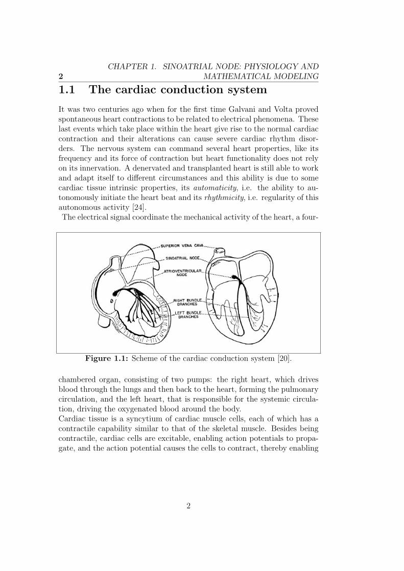
It was two centuries ago when for the first time Galvani and Volta provedspontaneous heart contractions to be related to electrical phenomena. Theselast events which take place within the heart give rise to the normal cardiaccontraction and their alterations can cause severe cardiac rhythm disor-ders. The nervous system can command several heart properties, like itsfrequency and its force of contraction but heart functionality does not relyon its innervation. A denervated and transplanted heart is still able to workand adapt itself to different circumstances and this ability is due to somecardiac tissue intrinsic properties, its automaticity, i.e. the ability to au-tonomously initiate the heart beat and its rhythmicity, i.e. regularity of thisautonomous activity [24].The electrical signal coordinate the mechanical activity of the heart, a four-
Figure 1.1: Scheme of the cardiac conduction system [20].
chambered organ, consisting of two pumps: the right heart, which drivesblood through the lungs and then back to the heart, forming the pulmonarycirculation, and the left heart, that is responsible for the systemic circula-tion, driving the oxygenated blood around the body.Cardiac tissue is a syncytium of cardiac muscle cells, each of which has acontractile capability similar to that of the skeletal muscle. Besides beingcontractile, cardiac cells are excitable, enabling action potentials to propa-gate, and the action potential causes the cells to contract, thereby enabling
2
CHAPTER 1. SINOATRIAL NODE: PHYSIOLOGY AND
MATHEMATICAL MODELING 3
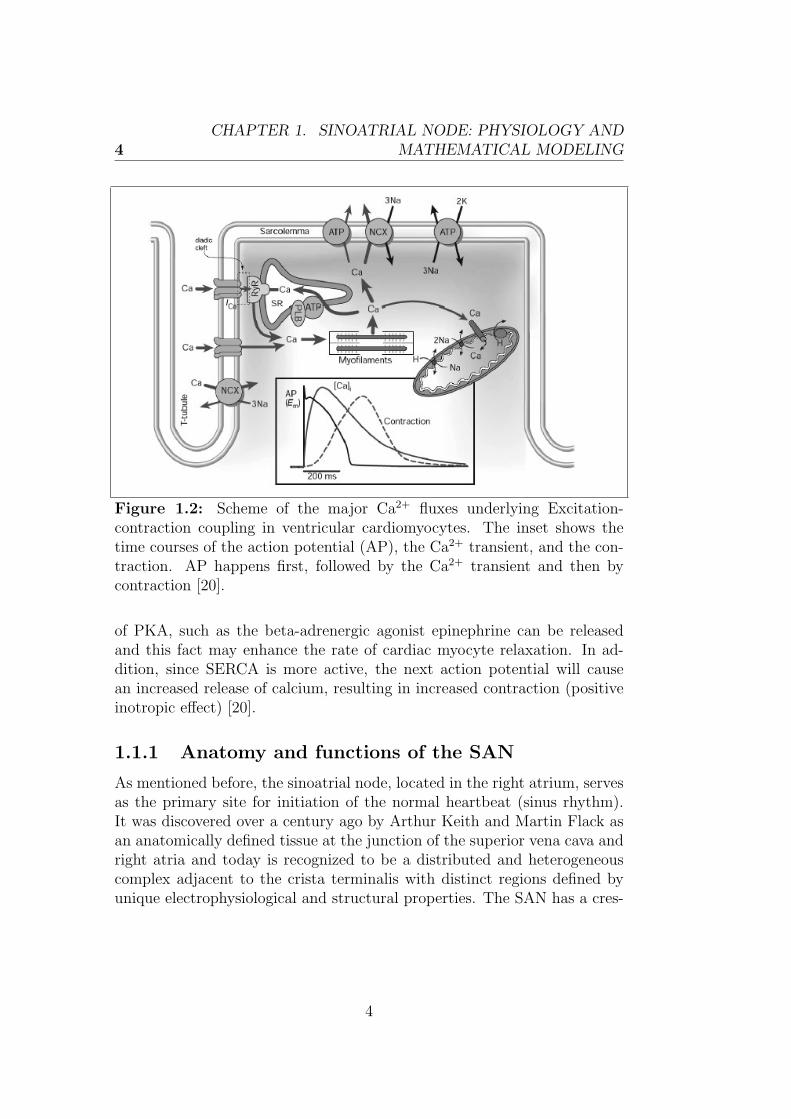
the pumping of blood. We will discuss in detail later the features of cardiacaction potential while for now we focus on the pathway of propagation ofthe electrical activity of the heart, shown in Fig. 1.1. It is initiated in acollection of cells known as the sinoatrial node (SAN) located just belowthe superior vena cava on the right atrium. The cells in the SAN are au-tonomous oscillators and the action potential generated by these cells ispropagated through the atria by the atrial cells. The conduction of actionpotentials between atria and ventricles is normally prevented by a septumcomposed of non excitable cells and the action potential can continue itspropagation only through a group of cells, known as the atrioventricularnode (AVN) and located at the base of the atria. After having passed quiteslowly through the AVN, the action potential propagates through the bundleof HIS composed by a specialized collection of fibers, named Purkinje fiberswhich spread via tree-like branching into the left and right bundle branchesthroughout the interior of the ventricles, ending on the endocardial surfaceof the ventricles. At this point the action potentials activate the ventricularmuscle and propagate through the ventricular wall outward to the epicardialsurface. The process whereby an electrical stimulus is converted into musclecontraction in ventricular cardiomyocytes is called Excitation-contraction(EC) coupling and its fundamental steps are shown in Fig. 1.2. L-typeCa2+ channels open as a result of the depolarization of the T-tubule by theaction potential and they lead to an inward flow of Ca2+ ions (ICa). Theamount of Ca2+ entered the cell induces the sarcoplasmic reticulum (SR)to release additional Ca2+ through ryanodine receptors (RyR). This pro-cess is named Ca2+-induced Ca2+ release (CICR). The released amount ofCa2+ diffuses through the myoplasm, binds to the myofilaments and causescontraction. It is then eventually removed from the myoplasm by ATPases,which pump the Ca2+ into the SR (sarcoplasmic reticulum Ca++-ATPase(SERCA)) or out of the cell, or by the Na+-Ca2+ exchanger (NCX), whichtransfers Ca2+ to the outside of the cell. Phospholamban (PLB) is a proteinand the major substrate for the cAMP-dependent protein kinase (PKA) incardiac muscle. In the unphosphorylated state it works as an inhibitor ofthe sarcoplasmatic calcium pump SERCA, while when phosphorylated byPKA its ability to inhibit SERCA is lost. When phospholamban is notphosphorylated, contractility and rate of muscle relaxation are decreasedand this lead to decreasing stroke volume and heart rate, respectively. Onthe contrary, in case of sympathetic stimulation, for example, activators
3
4
CHAPTER 1. SINOATRIAL NODE: PHYSIOLOGY AND
MATHEMATICAL MODELING
Figure 1.2: Scheme of the major Ca2+ fluxes underlying Excitation-contraction coupling in ventricular cardiomyocytes. The inset shows thetime courses of the action potential (AP), the Ca2+ transient, and the con-traction. AP happens first, followed by the Ca2+ transient and then bycontraction [20].
of PKA, such as the beta-adrenergic agonist epinephrine can be releasedand this fact may enhance the rate of cardiac myocyte relaxation. In ad-dition, since SERCA is more active, the next action potential will causean increased release of calcium, resulting in increased contraction (positiveinotropic effect) [20].
1.1.1 Anatomy and functions of the SAN
As mentioned before, the sinoatrial node, located in the right atrium, servesas the primary site for initiation of the normal heartbeat (sinus rhythm).It was discovered over a century ago by Arthur Keith and Martin Flack asan anatomically defined tissue at the junction of the superior vena cava andright atria and today is recognized to be a distributed and heterogeneouscomplex adjacent to the crista terminalis with distinct regions defined byunique electrophysiological and structural properties. The SAN has a cres-
4
CHAPTER 1. SINOATRIAL NODE: PHYSIOLOGY AND
MATHEMATICAL MODELING 5
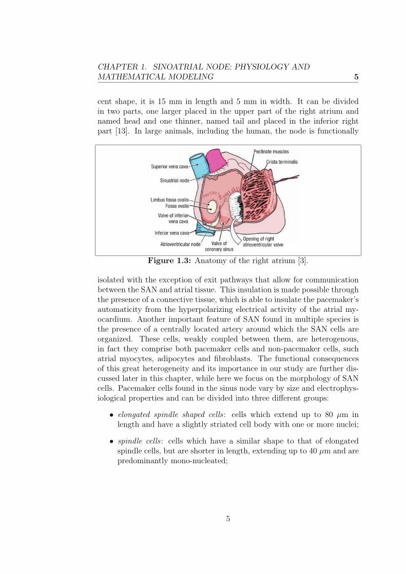
cent shape, it is 15 mm in length and 5 mm in width. It can be dividedin two parts, one larger placed in the upper part of the right atrium andnamed head and one thinner, named tail and placed in the inferior rightpart [13]. In large animals, including the human, the node is functionally
Figure 1.3: Anatomy of the right atrium [3].
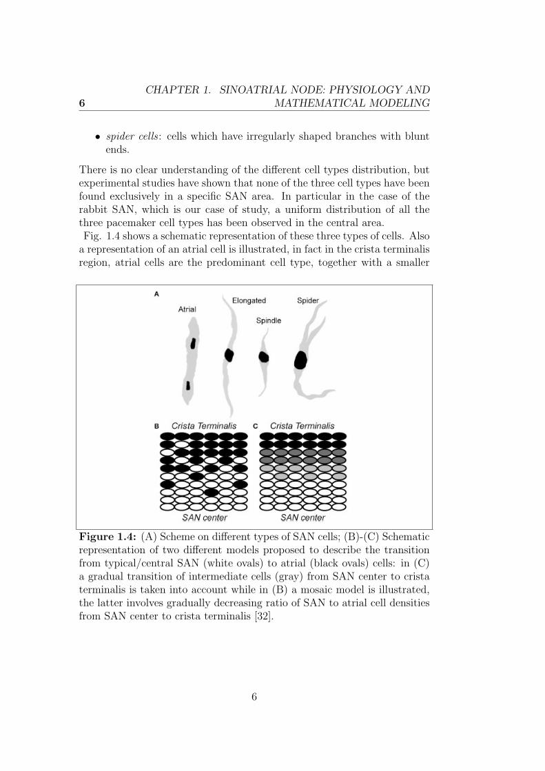
isolated with the exception of exit pathways that allow for communicationbetween the SAN and atrial tissue. This insulation is made possible throughthe presence of a connective tissue, which is able to insulate the pacemaker’sautomaticity from the hyperpolarizing electrical activity of the atrial my-ocardium. Another important feature of SAN found in multiple species isthe presence of a centrally located artery around which the SAN cells areorganized. These cells, weakly coupled between them, are heterogenous,in fact they comprise both pacemaker cells and non-pacemaker cells, suchatrial myocytes, adipocytes and fibroblasts. The functional consequencesof this great heterogeneity and its importance in our study are further dis-cussed later in this chapter, while here we focus on the morphology of SANcells. Pacemaker cells found in the sinus node vary by size and electrophys-iological properties and can be divided into three different groups:
• elongated spindle shaped cells : cells which extend up to 80 µm inlength and have a slightly striated cell body with one or more nuclei;
• spindle cells : cells which have a similar shape to that of elongatedspindle cells, but are shorter in length, extending up to 40 µm and arepredominantly mono-nucleated;
5
6
CHAPTER 1. SINOATRIAL NODE: PHYSIOLOGY AND
MATHEMATICAL MODELING
• spider cells : cells which have irregularly shaped branches with bluntends.
There is no clear understanding of the different cell types distribution, butexperimental studies have shown that none of the three cell types have beenfound exclusively in a specific SAN area. In particular in the case of therabbit SAN, which is our case of study, a uniform distribution of all thethree pacemaker cell types has been observed in the central area.Fig. 1.4 shows a schematic representation of these three types of cells. Alsoa representation of an atrial cell is illustrated, in fact in the crista terminalisregion, atrial cells are the predominant cell type, together with a smaller
Figure 1.4: (A) Scheme on different types of SAN cells; (B)-(C) Schematicrepresentation of two different models proposed to describe the transitionfrom typical/central SAN (white ovals) to atrial (black ovals) cells: in (C)a gradual transition of intermediate cells (gray) from SAN center to cristaterminalis is taken into account while in (B) a mosaic model is illustrated,the latter involves gradually decreasing ratio of SAN to atrial cell densitiesfrom SAN center to crista terminalis [32].
6
CHAPTER 1. SINOATRIAL NODE: PHYSIOLOGY AND
MATHEMATICAL MODELING 7
percentage of spindle nodal cells. Indeed the septal area of SAN is mostlycomposed of atrial cells and an almost uniform amount of the other threetypes of cells is interspersed between them. In the figure we can also seetwo different models proposed to describe the distribution of these differenttypes of cells within the SAN. We will further discuss these two models laterin this chapter [32].
1.1.2 The cardiac action potential
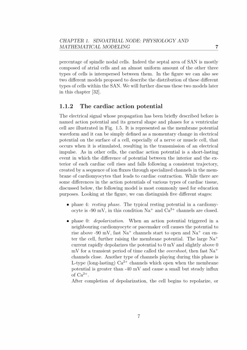
The electrical signal whose propagation has been briefly described before isnamed action potential and its general shape and phases for a ventricularcell are illustrated in Fig. 1.5. It is represented as the membrane potentialwaveform and it can be simply defined as a momentary change in electricalpotential on the surface of a cell, especially of a nerve or muscle cell, thatoccurs when it is stimulated, resulting in the transmission of an electricalimpulse. As in other cells, the cardiac action potential is a short-lastingevent in which the difference of potential between the interior and the ex-terior of each cardiac cell rises and falls following a consistent trajectory,created by a sequence of ion fluxes through specialized channels in the mem-brane of cardiomyocytes that leads to cardiac contraction. While there aresome differences in the action potentials of various types of cardiac tissue,discussed below, the following model is most commonly used for educationpurposes. Looking at the figure, we can distinguish five different stages:
• phase 4: resting phase. The typical resting potential in a cardiomy-ocyte is -90 mV, in this condition Na+ and Ca2+ channels are closed.
• phase 0: depolarization. When an action potential triggered in aneighbouring cardiomyocyte or pacemaker cell causes the potential torise above -90 mV, fast Na+ channels start to open and Na+ can en-ter the cell, further raising the membrane potential. The large Na+
current rapidly depolarizes the potential to 0 mV and slightly above 0mV for a transient period of time called the overshoot, then fast Na+
channels close. Another type of channels playing during this phase isL-type (long-lasting) Ca2+ channels which open when the membranepotential is greater than -40 mV and cause a small but steady influxof Ca2+.After completion of depolarization, the cell begins to repolarize, or
7

8
CHAPTER 1. SINOATRIAL NODE: PHYSIOLOGY AND
MATHEMATICAL MODELING
Figure 1.5: Action potential waveform in a ventricular cell,(TMP=transmembrane potential) [18].
return to its original resting state. The cell can not depolarize againuntil this happens. Phases 1-3 are the repolarization phases and co-incide with the time that the cell is refractory and can not respond toa new stimulus.
• phase 1: early repolarization. At the beginning of this phase the mem-brane potential is slightly positive, then some K+ channels open brieflyand an outward flow of K+ returns the potential to approximately 0mV.
• phase 2: plateau phase. This is the distinguishing phase of the cardiacAP and it is cause of its long lasting. During this stage there is anequilibrium between inward and outward currents, in fact L-type Ca2+
channels are still open and there is a small, constant inward currentof Ca2+, and different types of K+ outward currents. The inwardand outward currents are electrically balanced, so that the membranepotential is maintained at a plateau just below 0 mV throughout phase2.
• phase 3: repolarization. This phase starts with the gradual inacti-vation of Ca2+. The outflow of K+ instead is still present and now,exceeding Ca2+ inflow, brings the membrane potential back towards
8
CHAPTER 1. SINOATRIAL NODE: PHYSIOLOGY AND
MATHEMATICAL MODELING 9
resting potential of -90 mV to prepare the cell for a new cycle ofdepolarization.
The described ionic flows change the normal transmembrane ionic con-centration gradients, that must be restored, especially by returning Na+
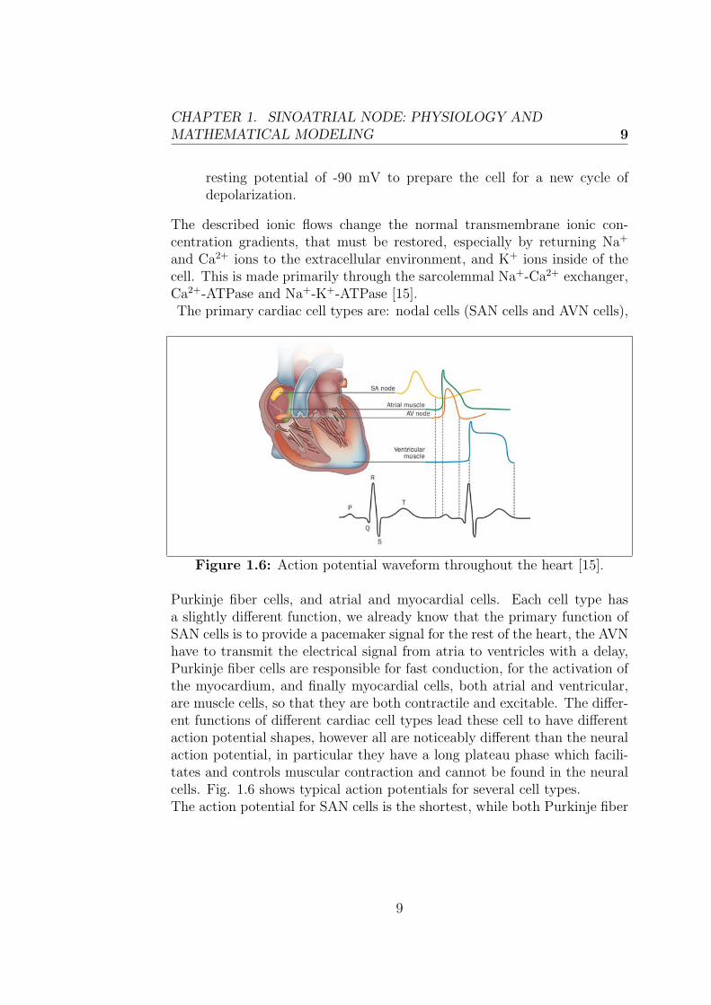
and Ca2+ ions to the extracellular environment, and K+ ions inside of thecell. This is made primarily through the sarcolemmal Na+-Ca2+ exchanger,Ca2+-ATPase and Na+-K+-ATPase [15].The primary cardiac cell types are: nodal cells (SAN cells and AVN cells),
Figure 1.6: Action potential waveform throughout the heart [15].
Purkinje fiber cells, and atrial and myocardial cells. Each cell type hasa slightly different function, we already know that the primary function ofSAN cells is to provide a pacemaker signal for the rest of the heart, the AVNhave to transmit the electrical signal from atria to ventricles with a delay,Purkinje fiber cells are responsible for fast conduction, for the activation ofthe myocardium, and finally myocardial cells, both atrial and ventricular,are muscle cells, so that they are both contractile and excitable. The differ-ent functions of different cardiac cell types lead these cell to have differentaction potential shapes, however all are noticeably different than the neuralaction potential, in particular they have a long plateau phase which facili-tates and controls muscular contraction and cannot be found in the neuralcells. Fig. 1.6 shows typical action potentials for several cell types.The action potential for SAN cells is the shortest, while both Purkinje fiber
9
10
CHAPTER 1. SINOATRIAL NODE: PHYSIOLOGY AND
MATHEMATICAL MODELING
cells and myocardial cells have substantially prolonged action potentials(300 - 400 ms compared to 3 ms for the squid axon). Even within a singlecell type, there can be substantial variation. For example, in the ventricles,epicardial, midmyocardial, and endocardial cells have noticeable differencesin action potential duration [20].
1.1.3 Pacemaker action potential
Cells of the sinoatrial node, on which we focus, have the property of auto-maticity thanks to their unique electrophysiological profile, that is distinctfrom that in atrial or ventricular cells. These latter are characterized ashaving a stable rest potential, while the SAN AP lacks a true resting po-tential due in large part to lack of the inward rectifier K+ channel IK1. TheSAN AP reaches a maximum diastolic potential (MDP) of about -60 mV,followed by a spontaneous depolarization that eventually reaches thresh-old to generate another AP, therefore the SAN is able to generate regular,spontaneous action potentials. Unlike most other cells that elicit actionpotentials (e.g., nerve cells, muscle cells), the depolarizing current is carriedprimarily by a relatively slow, inward Ca2+ current instead of by fast Na+
currents. In fact pacemaker cells have fewer inward rectifier K+ channelsthan do other cardiomyocytes, so their membrane potential is never lowerthan -60 mV. As fast Na+ channels need a transmembrane potential of -90mV to reconfigure into an active state, they are permanently inactivatedin pacemaker cells so there is no rapid depolarization phase. Pacemakercells have an unstable membrane potential and their action potential is notusually divided into the same defined phases seen before.Fig. 1.7 shows a typical AP of a SAN cell, the different phases and the in-volved currents are indicated. The sequence of events for pacemaker actionpotential are:
• phase 4: spontaneous depolarization, which leads the membrane po-tential to overcome the threshold level. At the end of the repolar-ization, when the membrane potential is really negative, i.e. themaximum diastolic potential (MDP=the lowest membrane potentialreached by the cell)) is about -60 mV, the funny current (If ) is ac-tivated. The latter is a distinguishing current of the nodal tissue, itis carried both by Na+ and K+ ions and it is activated by repolar-ization/iperpolarization, which starts at about -50 mV. The reversal
10
CHAPTER 1. SINOATRIAL NODE: PHYSIOLOGY AND
MATHEMATICAL MODELING 11
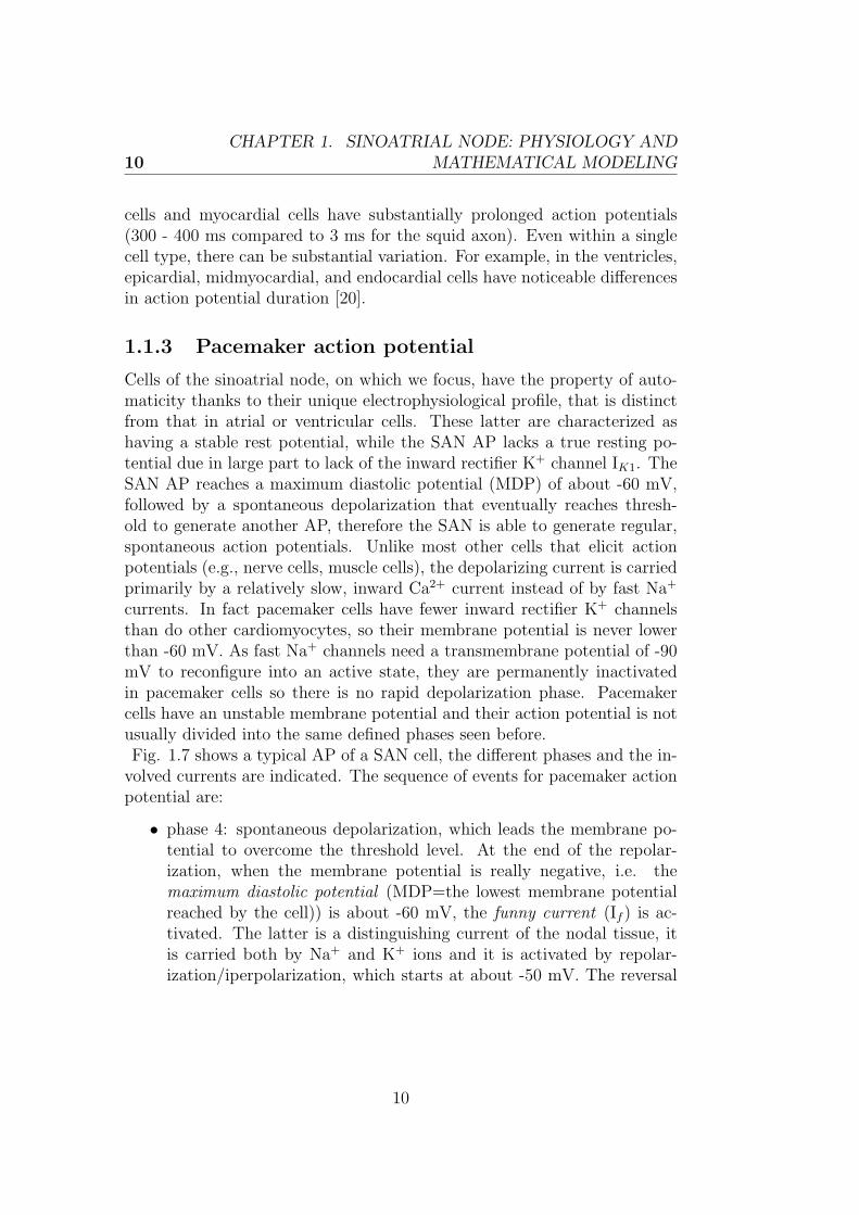
Figure 1.7: SAN cell Action Potential and currents involved in the differentphases [21].
potential of the involved ionic channels is -10/20 mV, due to the theirmixed permeability. The activation of this current, together withthe increased activity of the sodium-calcium exchanger is responsibleof the diastolic depolarization (DD). In particular this phase can bedivided into two stages, the first one, called early diastolic depolar-ization primarily relies on the presence of the funny current, whilethe exchanger is more active in the second part, late diastolic depo-larization, immediately before systole. At the end of this phase themembrane potential is closer to the threshold, so almost ready for theupstroke;
• phase 0: depolarization of the AP (upstroke). Once the membranepotential has reached the threshold level (about -50/-40 mV), a rapiddepolarization can start and move the membrane potential to a peakof about +20 mV. During this phase the conductivity of calcium chan-nels increases and we have two different types of inward currents, ICaL,which is the largest contributor to the upstroke, and ICaT , which isthe first one to be activated (already at the end of phase 4). So theprimary current during this stage is carried by Ca2+ flowing throughL-type channels, for this reason the slope of phase 0, and so the speedof depolarization, is lower than the one found in the other cardiomy-ocytes;
• phase 3: repolarization. Once the membrane potential has reachedpositive values, K+ channels start to open and we have two types of
11
12
CHAPTER 1. SINOATRIAL NODE: PHYSIOLOGY AND
MATHEMATICAL MODELING
currents: IKr and IKs, which, together with the inactivation of ICaL,return the membrane potential to negative values.
1.1.4 Heart rhythm and cardiac arrhythmias
Cardiac arrhythmias are disruptions of the normal cardiac electrical cycleand they are generally of two types. There are temporal disruptions, whichoccur when cells act out of sequence, either by firing autonomously or byrefusing to respond to a stimulus from other cells, as in AVN block or abundle branch block. A collection of cells that fires autonomously is calledan ectopic focus. These arrhythmias cause little disruption to the ability ofthe heart muscle to pump blood, and so if they do not initiate some otherkind of arrhythmia, are generally not life-threatening.The second class of arrhythmias are those that are reentrant in nature andcan occur only because of the spatial distribution of cardiac tissue. If theyoccur in the ventricles, reentrant arrhythmias are of serious concern andlife-threatening, as the ability of the heart to pump blood is greatly di-minished. Reentrant arrhythmias on the atria are less dangerous, since thepumping activity of the atrial muscle is not necessary to normal functionwith minimal physical activity, although long-lived atrial reentrant arrhyth-mias are known to increase the chance of strokes. A reentrant arrhythmiais a self-sustained pattern of action potential propagation that circulatesaround a closed path, reentering and reexiting tissue as it goes. A classicexample of a one-dimensional reentrant rhythm of clinical relevance is onein which an action potential circulates continuously between the atria andthe ventricles through a loop, exiting the atria through the AV node andreentering the atria through an accessory pathway (or vice versa). Reen-trant patterns which are not constrained to a one-dimensional pathway aremuch more problematic. The two primary reentrant arrhythmias of thistype are tachycardia and fibrillation. Both of these can occur on the atria(atrial tachycardia and atrial fibrillation) or in the ventricles (ventriculartachycardia and ventricular fibrillation). When they occur on the atria, forthe reasons mentioned before, they are not immediately life-threatening,while when they occur on the ventricles, they are life-threatening. Ven-tricular fibrillation is fatal if it is not terminated quickly. Tachycardia isoften classified as being either monomorphic or polymorphic, depending onthe assumed morphology of the activation pattern. Monomorphic tachy-
12
CHAPTER 1. SINOATRIAL NODE: PHYSIOLOGY AND
MATHEMATICAL MODELING 13
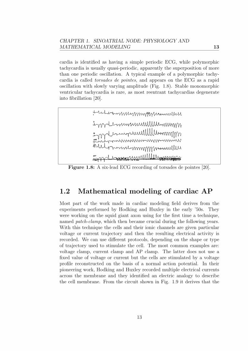
cardia is identified as having a simple periodic ECG, while polymorphictachycardia is usually quasi-periodic, apparently the superposition of morethan one periodic oscillation. A typical example of a polymorphic tachy-cardia is called torsades de pointes, and appears on the ECG as a rapidoscillation with slowly varying amplitude (Fig. 1.8). Stable monomorphicventricular tachycardia is rare, as most reentrant tachycardias degenerateinto fibrillation [20].
Figure 1.8: A six-lead ECG recording of torsades de pointes [20].
1.2 Mathematical modeling of cardiac AP
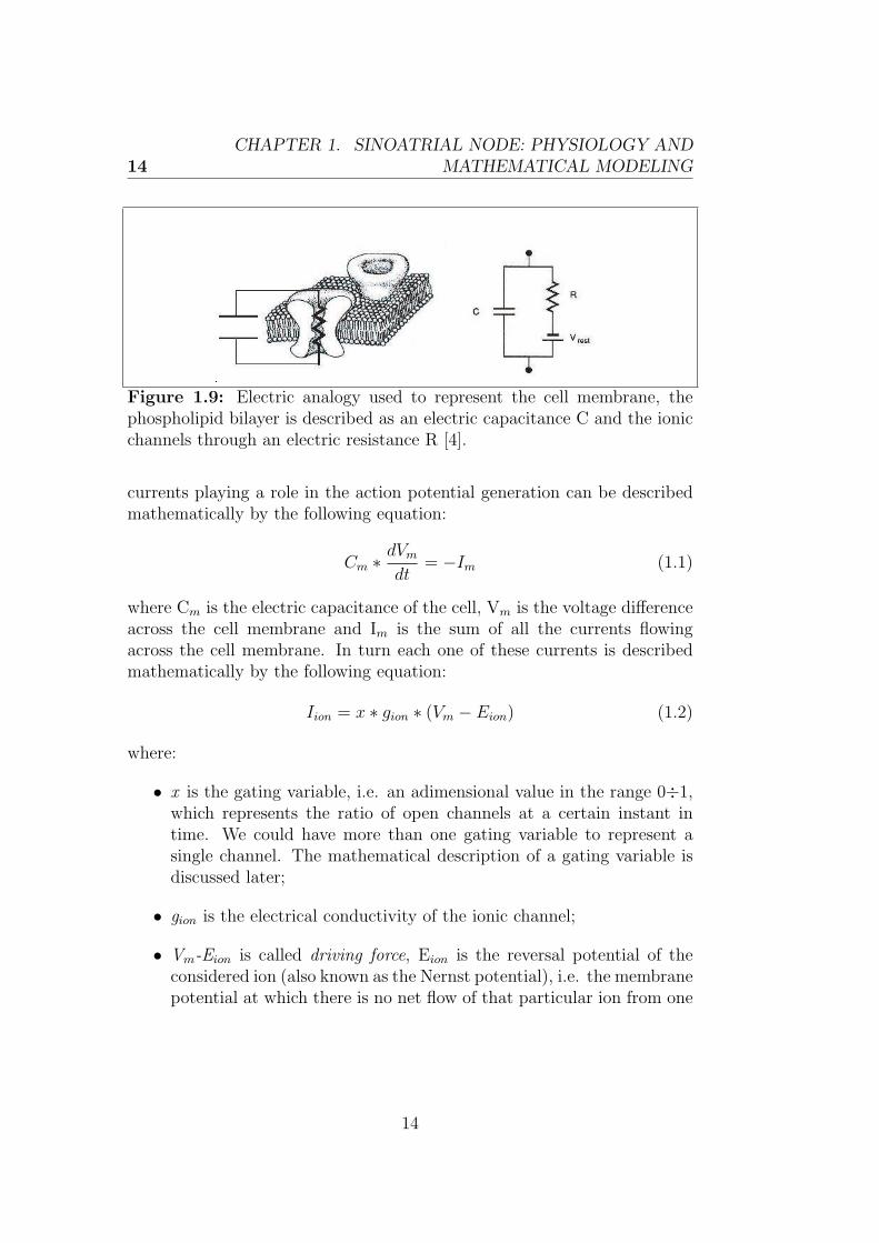
Most part of the work made in cardiac modeling field derives from theexperiments performed by Hodking and Huxley in the early ’50s. Theywere working on the squid giant axon using for the first time a technique,named patch-clamp, which then became crucial during the following years.With this technique the cells and their ionic channels are given particularvoltage or current trajectory and then the resulting electrical activity isrecorded. We can use different protocols, depending on the shape or typeof trajectory used to stimulate the cell. The most common examples are:voltage clamp, current clamp and AP clamp. The latter does not use afixed value of voltage or current but the cells are stimulated by a voltageprofile reconstructed on the basis of a normal action potential. In theirpioneering work, Hodking and Huxley recorded multiple electrical currentsacross the membrane and they identified an electric analogy to describethe cell membrane. From the circuit shown in Fig. 1.9 it derives that the
13
14
CHAPTER 1. SINOATRIAL NODE: PHYSIOLOGY AND
MATHEMATICAL MODELING
Figure 1.9: Electric analogy used to represent the cell membrane, thephospholipid bilayer is described as an electric capacitance C and the ionicchannels through an electric resistance R [4].
currents playing a role in the action potential generation can be describedmathematically by the following equation:
Cm ∗ dVm
dt= −Im (1.1)
where Cm is the electric capacitance of the cell, Vm is the voltage differenceacross the cell membrane and Im is the sum of all the currents flowingacross the cell membrane. In turn each one of these currents is describedmathematically by the following equation:
Iion = x ∗ gion ∗ (Vm − Eion) (1.2)
where:
• x is the gating variable, i.e. an adimensional value in the range 0÷1,which represents the ratio of open channels at a certain instant intime. We could have more than one gating variable to represent asingle channel. The mathematical description of a gating variable isdiscussed later;
• gion is the electrical conductivity of the ionic channel;
• Vm-Eion is called driving force, Eion is the reversal potential of theconsidered ion (also known as the Nernst potential), i.e. the membranepotential at which there is no net flow of that particular ion from one
14
CHAPTER 1. SINOATRIAL NODE: PHYSIOLOGY AND
MATHEMATICAL MODELING 15
side of the membrane to the other. Eion is determined by the Nernstequation:
Eion =R ∗ TZ ∗ F ∗ log [ion]i
[ion]o(1.3)
where:
– ion is the considered specific ion;
– R=8.314472 J K−1 mol−1, universal gas constant;
– T temperature in Kelvin;
– Z valency of the element;
– F=96485.3399 C mol−1, Faraday constant;
– [ion]i intracellular ion concentration;
– [ion]e extracellular ion concentration.
Gating variables are described by differential equations. Conductivity val-ues reached by some channels at fixed potential values are determined byperforming clamp experiments, until the maximal conductivity is reached.These found values are then expressed in relative terms, giving a value tothe gating variable for each one of the tested potentials. The resulting pa-rameter is named x∞ and it is defined by a voltage dependent equation.The ionic channels require a certain amount of time to reach the x∞ value(steady state value), so that we can define a time constant τx, which isstill voltage dependent. The equations for both parameters come from aninterpolation of experimental data and they are the following:
x∞ =α
α + β(1.4)
τx =1
α + β(1.5)
where α and β decribe the relationship with voltage, usually in an expo-nential form. Finally the expression for the voltage gating is the following:
dx
dt= α ∗ (1− x)− β ∗ x (1.6)
15

16
CHAPTER 1. SINOATRIAL NODE: PHYSIOLOGY AND
MATHEMATICAL MODELING
An equal alternative way is:
dx
dt=
x∞ − x
τx(1.7)
During the years a great number of cardiac cell models have been formu-lated, in this work we focus upon rabbit SAN cell models.
1.2.1 Single cell model of the rabbit sinoatrial node
The first sinoatrial node cell model was published in 1980 by Yanagihara,Noma and Irisawa. The model uses a Hodgkin-Huxley formulation and in-cludes five trans-membrane currents: the Na+, slow inward (Ca2+), delayedrectifier K+, hyperpolarization-activated, and time-independent leak (back-ground) currents. In this model, the slow inward current is responsible forthe rising phase of the action potential and the plateau, determined by bothslow inward current inactivation and activation of the dynamic K+ current[19].After this first one, many other models have been proposed with the aimof including always more details. We carefully describe two of the mostrecent rabbit SAN cell models: Maltsev and Severi models, because theyare the ones from which we start the implementation of our models andalso because they describe the diastolic depolarization phase through twodifferent hypotheses: membrane clock and calcium clock.The properties of funny channel seem specifically apt to generate the di-astolic depolarization phase of the action potential, which is the phase re-sponsible for normal spontaneous activity. Because the membrane ionicchannels open and close according to the membrane potential, this processis referred to as a membrane voltage clock. As mentioned before, If acti-vates upon hyperpolarization, one of the unusual features which at the timeof its discovery made the current deserve the attribute funny, at a thresholdof about -40/-50 mV, and is fully activated at about -100 mV. In its rangeof activation, which quite properly comprises the voltage range of diastolicdepolarization, the current is inward, its reversal occurring at about -10/-20 mV. This is due to the mixed Na+/K+ permeability. The channels areencoded by the hyperpolarization-activated, cyclic nucleotide-gated (HCN)channel gene family. Of the four known HCN subunits, HCN4 is the mosthighly expressed in the mammalian SAN. The major role of If has been
16

CHAPTER 1. SINOATRIAL NODE: PHYSIOLOGY AND
MATHEMATICAL MODELING 17
reinforced by the fact that mutations in the If channel are associated witha reduced baseline heart rate, and drugs, which block If (such as ivabra-dine) do the same. Funny channels are so a successful target of specificheart-rate-reducing agents like ivabradine, and is known that funny currentplays a key role on the pacemaking activity of heart cells.The second hypothesis relies on the recent finding of spontaneous Ca2+
Figure 1.10: In the left part of the figure: membrane clock (If ) hypothe-sis: Simulated AP using the Severi model. In the right part of the figure:calcium clock hypothesis: Simulated AP using the Maltsev model [29].
release from the sarcoplasmic reticulum (SR), which has been suggested tobe the mechanism for sinus rhythm generation. When the SR is full, theprobability of spontaneous Ca2+ release increases. On the other hand, whenthe SR is empty, the chances for spontaneous Ca2+ release decrease. Therhythmic alteration of SR Ca2+ release is referred to as the Ca2+ clock.Because the SR Ca2+ content is controlled in part by the membrane volt-age, it is important to recognize that the activation of the Ca2+ clock andthe membrane ionic clock are interdependent. Based on evidence from iso-lated SAN myocytes, late diastolic Cai elevation (LDCAE) relative to theaction potential upstroke is a key signature of pacemaking by the Ca2+
clock. On these bases a new modeling approach starts to be considered,in which rate regulation is governed by intracellular Ca2+ cycling and itscoupling to the surface membrane. These new models differ from classicalpacemaker models, which attribute the rate regulation of SAN cells mainlyto the If activation state and its relation to the early DD slope. The rateand amplitude of SR Ca2+ cycling of the most recent models is controlled
17
18
CHAPTER 1. SINOATRIAL NODE: PHYSIOLOGY AND
MATHEMATICAL MODELING
by the amount of free Ca2+ in the system, the SR Ca2+ pumping rate andthe numbers of activated Ryanodine Receptors (RyR) [14].
1.2.2 Maltsev model
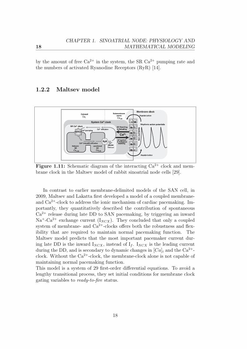
Figure 1.11: Schematic diagram of the interacting Ca2+ clock and mem-brane clock in the Maltsev model of rabbit sinoatrial node cells [29].
In contrast to earlier membrane-delimited models of the SAN cell, in2009, Maltsev and Lakatta first developed a model of a coupled membrane-and Ca2+-clock to address the ionic mechanism of cardiac pacemaking. Im-portantly, they quantitatively described the contribution of spontaneousCa2+ release during late DD to SAN pacemaking, by triggering an inwardNa+-Ca2+ exchange current (INCX). They concluded that only a coupledsystem of membrane- and Ca2+-clocks offers both the robustness and flex-ibility that are required to maintain normal pacemaking function. TheMaltsev model predicts that the most important pacemaker current dur-ing late DD is the inward INCX , instead of If . INCX is the leading currentduring the DD, and is secondary to dynamic changes in [Ca]i and the Ca2+-clock. Without the Ca2+-clock, the membrane-clock alone is not capable ofmaintaining normal pacemaking function.This model is a system of 29 first-order differential equations. To avoid alengthy transitional process, they set initial conditions for membrane clockgating variables to ready-to-fire status.
18
CHAPTER 1. SINOATRIAL NODE: PHYSIOLOGY AND
MATHEMATICAL MODELING 19
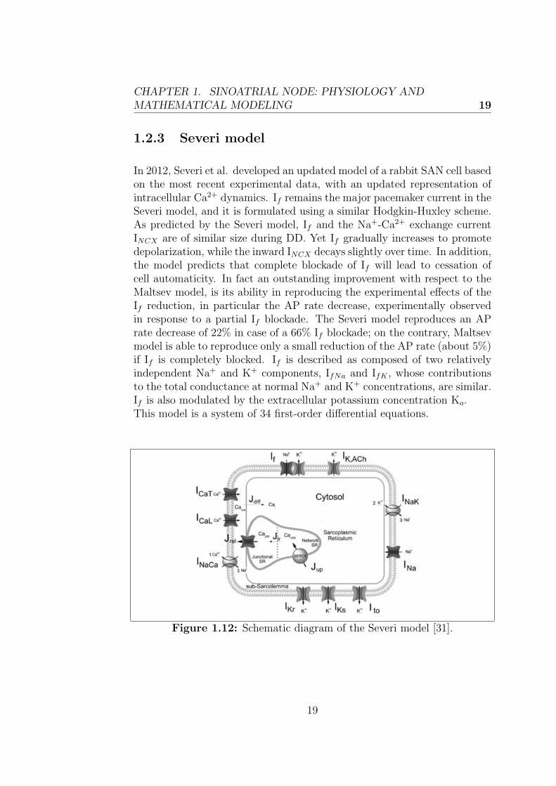
1.2.3 Severi model
In 2012, Severi et al. developed an updated model of a rabbit SAN cell basedon the most recent experimental data, with an updated representation ofintracellular Ca2+ dynamics. If remains the major pacemaker current in theSeveri model, and it is formulated using a similar Hodgkin-Huxley scheme.As predicted by the Severi model, If and the Na+-Ca2+ exchange currentINCX are of similar size during DD. Yet If gradually increases to promotedepolarization, while the inward INCX decays slightly over time. In addition,the model predicts that complete blockade of If will lead to cessation ofcell automaticity. In fact an outstanding improvement with respect to theMaltsev model, is its ability in reproducing the experimental effects of theIf reduction, in particular the AP rate decrease, experimentally observedin response to a partial If blockade. The Severi model reproduces an APrate decrease of 22% in case of a 66% If blockade; on the contrary, Maltsevmodel is able to reproduce only a small reduction of the AP rate (about 5%)if If is completely blocked. If is described as composed of two relativelyindependent Na+ and K+ components, IfNa and IfK , whose contributionsto the total conductance at normal Na+ and K+ concentrations, are similar.If is also modulated by the extracellular potassium concentration Ko.This model is a system of 34 first-order differential equations.
Figure 1.12: Schematic diagram of the Severi model [31].
19
20
CHAPTER 1. SINOATRIAL NODE: PHYSIOLOGY AND
MATHEMATICAL MODELING
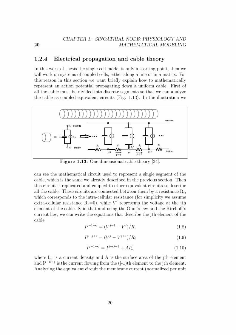
1.2.4 Electrical propagation and cable theory
In this work of thesis the single cell model is only a starting point, then wewill work on systems of coupled cells, either along a line or in a matrix. Forthis reason in this section we want briefly explain how to mathematicallyrepresent an action potential propagating down a uniform cable. First ofall the cable must be divided into discrete segments so that we can analyzethe cable as coupled equivalent circuits (Fig. 1.13). In the illustration we
Figure 1.13: One dimensional cable theory [34].
can see the mathematical circuit used to represent a single segment of thecable, which is the same we already described in the previous section. Thenthis circuit is replicated and coupled to other equivalent circuits to describeall the cable. These circuits are connected between them by a resistance Ri,which corresponds to the intra-cellular resistance (for simplicity we assumeextra-cellular resistance Re=0), while Vj represents the voltage at the jthelement of the cable. Said that and using the Ohm’s law and the Kirchoff’scurrent law, we can write the equations that describe the jth element of thecable:
Ij−1 7→j = (V j−1 − V j)/Ri (1.8)
Ij 7→j+1 = (V j − V j+1)/Ri (1.9)
Ij−1 7→j = Ij 7→j+1 + AIjm (1.10)
where Im is a current density and A is the surface area of the jth elementand Ij−1 7→j is the current flowing from the (j-1)th element to the jth element.Analyzing the equivalent circuit the membrane current (normalized per unit
20
CHAPTER 1. SINOATRIAL NODE: PHYSIOLOGY AND
MATHEMATICAL MODELING 21
area) can be written as follows:
Ijm = Cm
dV j
dt+ Ijion (1.11)
Now, putting the equations together, we obtain:
(V j−1 − V j)/Ri = (V j − V j+1)/Ri + A[CmdV j
dt+ Ijion] (1.12)
and, rearranging the fields:
Cm
dV j
dt= (V j−1 − 2V j) + V j+1/ARi − Ijion (1.13)
The parameter Ri can be also related to cable geometry, in fact defined ρithe intracellular resistivity, a the radius of the transversal section and ∆x
the length of each segment of the cable, we have: Ri=ρi∆x/πa2.
The approach of the cable theory to describe AP propagation can be easilyextended to a multidimensional propagation. In this last case we should con-sider that transverse propagation means encountering more gap junctionsper unit length and thus the resistance in this direction should be greaterthan the longitudinal one. The resistance value in fact is determined bothby cardiac structure and gap junctions, although the cytoplasmic resistanceis relatively low compared with the resistance encountered at gap junctions[34].
1.3 Heterogeneity in the SAN
A fundamental limit of single cell models is that they are unable to describethe interaction between cells and the variability normally existent betweencells of they same organ. In fact each parameter present in the model isgiven an average value, which cannot take into account slight differenceswithin the tissue. In this section we describe the great morphological andfunctional heterogeneity of the rabbit sinoatrial node, pointing out the mostrelevant aspects to this work of thesis.Measurements from intact rabbit SAN have shown heterogeneity of electro-physiological properties from the center to the border of the atrium includ-ing gradual morphological changes in action potential, a decrease in maxi-mum diastolic potential, an increase in peak overshoot potential (POP), an
21

22
CHAPTER 1. SINOATRIAL NODE: PHYSIOLOGY AND
MATHEMATICAL MODELING
increase in upstroke velocity (UV) and a decrease in pacemaker potentialslope. On the basis of these results, as described in the work of Oren etal. [28], two distinct hypotheses have arisen to explain intact SAN hetero-geneity. The first is that the SAN has two specific cell types, central cellsand peripheral cells, each with distinct electrophysiological characteristics.The second hypothesis suggests that all observed heterogeneity in the intactSAN results from electrotonic coupling effects, i.e. cells in the SAN near theatria will be strongly affected and modified by the atrium. However whatOren et al. concluded from their tissue model simulations is that atrialelectrotonic effects is plausible to account for SAN heterogeneity, sequence,and rate of propagation. They also have studied the effect of fibroblasts,concluding that they can act as obstacles, current sinks or shunts to con-duction in the SAN depending on their orientation, density, and coupling.Some of the most important hypotheses proposed to explain the observedheterogeneity of the rabbit sinoatrial node are summarised below:
• SAN tissue has fibroblasts interspersed in islands that occupy about50% of SAN volume and they can act as obstacles, current sinks orshunts to conduction in the SAN depending on their orientation, den-sity and coupling;
• Verheijck et al. [11] have observed atrial cells interspersed in theSAN and suggested a mosaic model of SAN and atrial cells for SANorganization;
• Gap junction density and conductance increase moving from the cen-ter to the pheriphery of the SAN;
• SAN has two specific cell types, central cells and peripheral cells, eachwith distinct electrophysiological characteristics;
• All observed heterogeneity in the intact SAN results from electrotoniccoupling effects, cells in the SAN near the atria will be strongly af-fected and modified by the atrium.
22
Chapter 2
Materials and Methods
Starting from the single cell models for the rabbit sinoatrial node: Severimodel and Maltsev model, first a 1D model both in MATLAB and CUDAand after a 2D model in CUDA were implemented. The 1D model, or ca-ble model consists of an array of cells placed along a line and connectedbetween them and it was used to perform a comparison between the exe-cution time in MATLAB and CUDA, running the same simulations withboth softwares. It was also handled to study and better understand therelationship between the cells coupling and the conduction velocity withina cable of cells. The 2D model, or tissue model consists instead of a matrixof cells and each one, except the ones on the boundary, is connected to fourother cells. This last model has been useful in introducing in this study theheterogeneity of the SAN through a randomization of all the conductancesexistent in the Maltsev model, so that each cell had a different behavior andit was possible to evaluate how each one influences the others.Therefore in this chapter we expose the steps taken for the implementa-tion of the instruments and the last section briefly describes the performedsimulations.
23
24 CHAPTER 2. MATERIALS AND METHODS
2.1 1-dimensional model implementation in
MATLAB
The Maltsev and Severi single cell models for the rabbit sinoatrial node,described in details in the previous chapter, were the starting point of mywork. In the cable model we consider a group of cells placed along a lineand connected between them through gap junctions, therefore, to pass froma single cell model to a cable model, each differential equation existent inthe model and describing the evolution in time of a state variable must bereplicated for each cell of the cable. In this thesis we have looked at cablesof both 25 and 50 cells. The differential equation describing the evolutionof the cell’s membrane potential was modified according to the cable theoryto include the contribution in current each cell gives to the two neighboringcells. No-flux boundary conditions were considered.
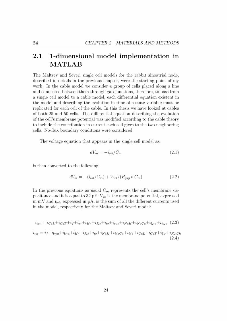
The voltage equation that appears in the single cell model as:
dVm = −itot/Cm (2.1)
is then converted to the following:
dVm = −(itot/Cm) + Vnet/(Rgap ∗ Cm) (2.2)
In the previous equations as usual Cm represents the cell’s membrane ca-pacitance and it is equal to 32 pF, Vm is the membrane potential, expressedin mV and itot, expressed in pA, is the sum of all the different currents usedin the model, respectively for the Maltsev and Severi model:
itot = iCaL+iCaT+if+ist+iKr+iKs+ito+isus+iNaK+iNaCa+ibCa+ibNa (2.3)
itot = if+ibNa+ibCa+iKr+iKs+ito+iNaK+iNaCa+iNa+iCaL+iCaT+ibK+iKACh
(2.4)
24
CHAPTER 2. MATERIALS AND METHODS 25
The new terms introduced with the cable model are:
• Rgap: this parameter takes into account the coupling strength betweenthe cells. It has the units of measurements of an electrical resistance,increasing its value the current contribution between the cells is de-creased according to the Ohm’s law. Its importance in this study willbe further discussed later in this chapter and in the next one;
• Vnet: this parameter takes into account the difference in voltage be-tween the cells, therefore it is expressed in mV and it is obtained asfollows:
Vnet = Vm([2 : end, end])− 2 ∗ Vm + Vm([1, 1 : end− 1]) (2.5)
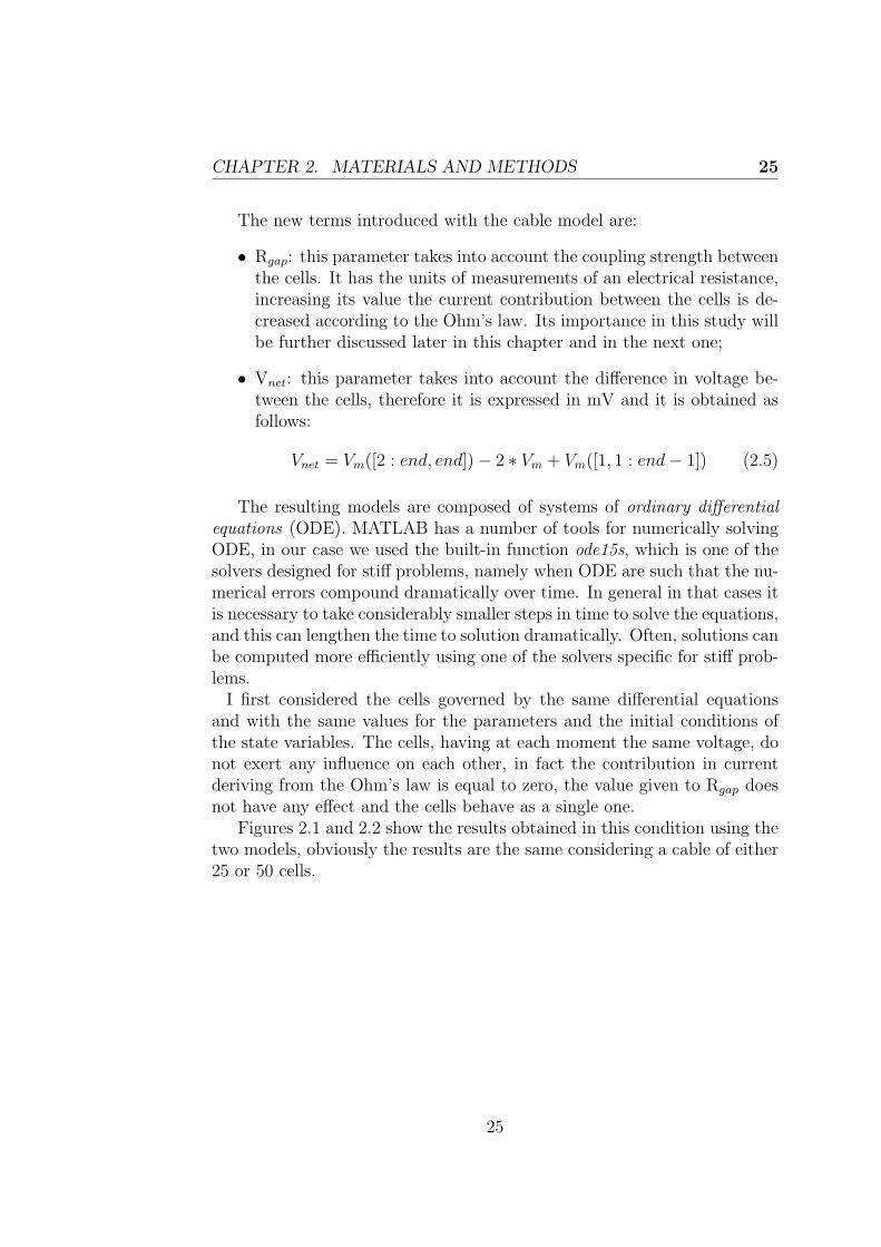
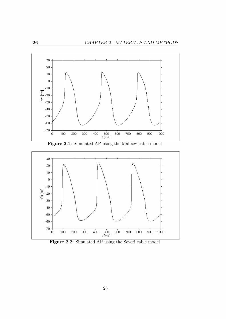
The resulting models are composed of systems of ordinary differentialequations (ODE). MATLAB has a number of tools for numerically solvingODE, in our case we used the built-in function ode15s, which is one of thesolvers designed for stiff problems, namely when ODE are such that the nu-merical errors compound dramatically over time. In general in that cases itis necessary to take considerably smaller steps in time to solve the equations,and this can lengthen the time to solution dramatically. Often, solutions canbe computed more efficiently using one of the solvers specific for stiff prob-lems.I first considered the cells governed by the same differential equations
and with the same values for the parameters and the initial conditions ofthe state variables. The cells, having at each moment the same voltage, donot exert any influence on each other, in fact the contribution in currentderiving from the Ohm’s law is equal to zero, the value given to Rgap doesnot have any effect and the cells behave as a single one.
Figures 2.1 and 2.2 show the results obtained in this condition using thetwo models, obviously the results are the same considering a cable of either25 or 50 cells.
25
26 CHAPTER 2. MATERIALS AND METHODS
Figure 2.1: Simulated AP using the Maltsev cable model
Figure 2.2: Simulated AP using the Severi cable model
26
CHAPTER 2. MATERIALS AND METHODS 27
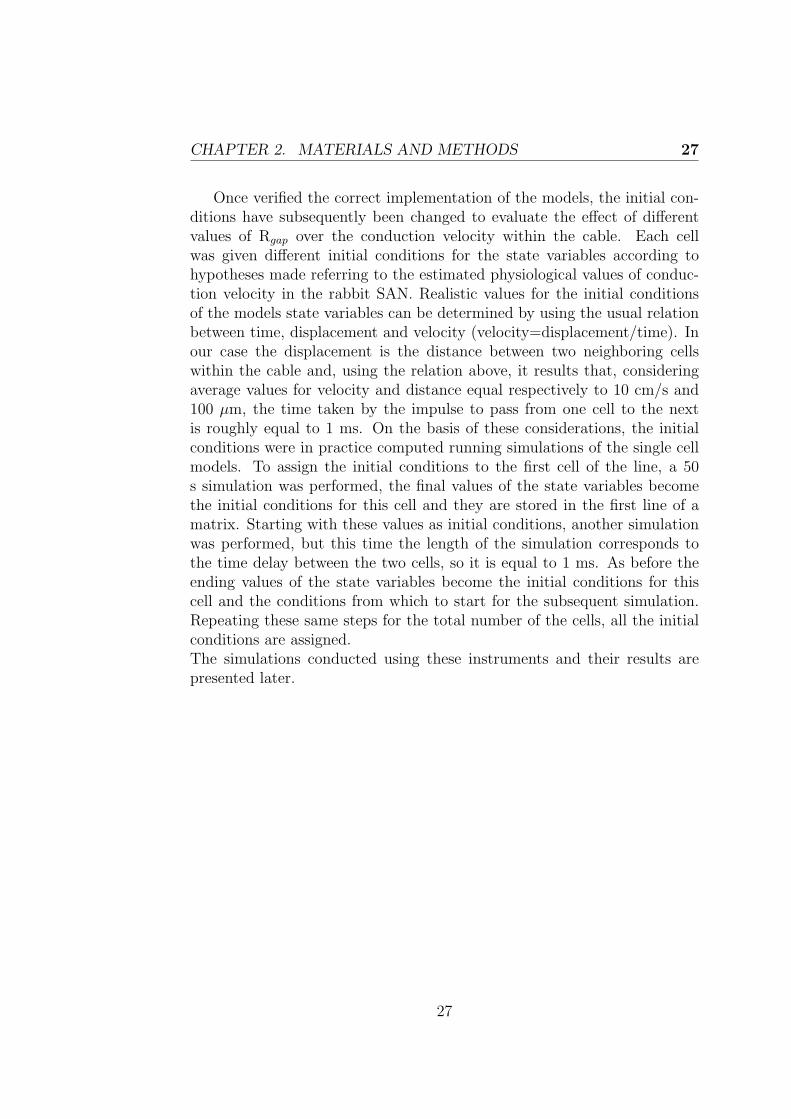
Once verified the correct implementation of the models, the initial con-ditions have subsequently been changed to evaluate the effect of differentvalues of Rgap over the conduction velocity within the cable. Each cellwas given different initial conditions for the state variables according tohypotheses made referring to the estimated physiological values of conduc-tion velocity in the rabbit SAN. Realistic values for the initial conditionsof the models state variables can be determined by using the usual relationbetween time, displacement and velocity (velocity=displacement/time). Inour case the displacement is the distance between two neighboring cellswithin the cable and, using the relation above, it results that, consideringaverage values for velocity and distance equal respectively to 10 cm/s and100 µm, the time taken by the impulse to pass from one cell to the nextis roughly equal to 1 ms. On the basis of these considerations, the initialconditions were in practice computed running simulations of the single cellmodels. To assign the initial conditions to the first cell of the line, a 50s simulation was performed, the final values of the state variables becomethe initial conditions for this cell and they are stored in the first line of amatrix. Starting with these values as initial conditions, another simulationwas performed, but this time the length of the simulation corresponds tothe time delay between the two cells, so it is equal to 1 ms. As before theending values of the state variables become the initial conditions for thiscell and the conditions from which to start for the subsequent simulation.Repeating these same steps for the total number of the cells, all the initialconditions are assigned.The simulations conducted using these instruments and their results arepresented later.
27
28 CHAPTER 2. MATERIALS AND METHODS
2.2 Implementation of the models in CUDA
Although the implementation of the cable model has been an importanttool for learning the mechanism of connection between cells and the nec-essary steps to take to pass from single cell models to models of coupledcells, the primary purpose of my project was the implementation of a tissuemodel of the SAN. In order to do that we made use of CUDA, that enableshuge improvements in computing performances thanks to the power of thegraphic processing units (GPU). GPU’s parallel structure allows a very ef-fective manipulation of many parallel tasks rather than serial tasks. Thecode written in CUDA implements both a cable and a tissue model of theSAN, even if the 1D model has only been used to evaluate the advantagesintroduced in term of execution time comparing to MATLAB. The tissuemodel in CUDA has been realized considering only the Maltsev model todescribe the cells, this choice has been supported by practical time reasons,but the same study could be made considering the Severi model, indeed itwould be interesting to compare the results obtained in the two situations.
2.2.1 A look inside the CUDA Programming Model
First of all the program is divided into several phases that are executed oneither the host (CPU) or the device (GPU) depending on the amount ofdata parallelism that they exhibit. Both host and device code are enclosedby the same source code, which is then compiled using the NVIDIA CCompiler (NVCC). At this point the two codes are separated, the host codeis compiled with the host’s standard C compilers while the device code isfurther compiled by the NVCC and executed on a GPU device.Therefore in our case the code, named Maltsev.cu, will be compiled fromthe command line by typing the following sequence:
nvcc -arch=sm 13 -o a Maltsev.cu
The executable file is then executed through the line:
a.exe
The device code uses keywords for labeling data-parallel functions, calledkernels, and their associated data structures. In particular a kernel, defined
28
CHAPTER 2. MATERIALS AND METHODS 29
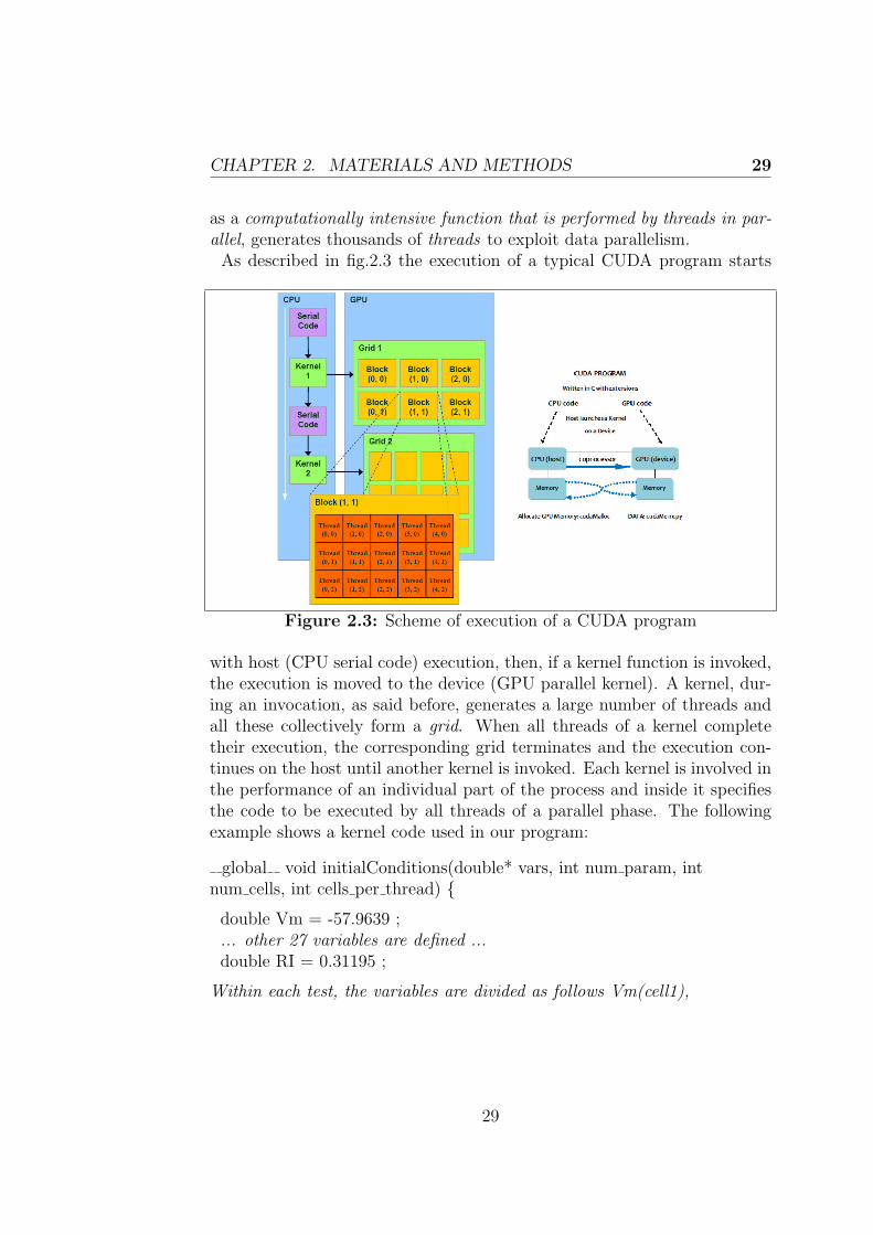
as a computationally intensive function that is performed by threads in par-allel, generates thousands of threads to exploit data parallelism.As described in fig.2.3 the execution of a typical CUDA program starts
Figure 2.3: Scheme of execution of a CUDA program
with host (CPU serial code) execution, then, if a kernel function is invoked,the execution is moved to the device (GPU parallel kernel). A kernel, dur-ing an invocation, as said before, generates a large number of threads andall these collectively form a grid. When all threads of a kernel completetheir execution, the corresponding grid terminates and the execution con-tinues on the host until another kernel is invoked. Each kernel is involved inthe performance of an individual part of the process and inside it specifiesthe code to be executed by all threads of a parallel phase. The followingexample shows a kernel code used in our program:
global void initialConditions(double* vars, int num param, intnum cells, int cells per thread) double Vm = -57.9639 ;... other 27 variables are defined ...double RI = 0.31195 ;
Within each test, the variables are divided as follows Vm(cell1),
29
30 CHAPTER 2. MATERIALS AND METHODS
Vm(cell2), Vm(cell3) ... Vm(cellLast), m(cell1), m(cell2), ... m(cellLast)... for all 29 parameters
int idx = threadIdx.x*cells per thread;int simulations = blockIdx.x;int limit = idx+cells per thread;for (;idx<limit;idx++) vars[(simulations*num param*num cells) + idx +(0*num cells)] = Vm;... other 27 values are assigned ...vars[(simulations*num param*num cells) + idx +(28*num cells)] = RI;
The syntax is ANSI C with some extensions, in fact there is a CUDA spe-cific keyword global , which starts the code and the declaration of eachkernel in general and it indicates that that particular function is a kerneland so it can be called from a host function to generate a grid of threads.Other extensions used in CUDA and shown in the example are the key-words threadIdx.x and blockIdx.x, that refer, respectively, to the indices of athread and of a block in which threads are grouped together. These subdi-visions and indices allow each thread to work only on the particular part ofthe data structure for which it is designated. After calculating the startingposition in the input vector based on unique block and thread coordinatesthe computation is then iterated through a loop, in which the indices aregiven by the thread’s coordinate and each element of the vector can becomputed in a separate thread. Although in the examined code only onedimension (x) is considered, the threads have a multi-dimensional organi-zation. Briefly threads in a grid are organized into a two-level hierarchy,each grid is formed by one or more thread blocks and all blocks have thesame number of threads and are identified through a two dimensional co-ordinate given by the CUDA specific keywords blockIdx.x and blockIdx.y.Each thread block is in turn structured as a three dimensional array ofthreads (maximum 512 threads per block), whose coordinates are given bythe following indices: threadIdx.x, threadIdx.y, and threadIdx.z.The following line describes how the kernel function of the previous exampleis invoked or called in the host code:
initialConditions<<<simulations,(num cells/cells per thread)>>>
30
CHAPTER 2. MATERIALS AND METHODS 31
(dev vars,num param,num cells, cells per thread);
The two parameters: simulations and num cells/cells per thread, betweenthe CUDA symbols for the syntax of the call function, set, respectively,the dimensions of grids in terms of number of blocks and the dimensions ofblocks in terms of number of threads. In this particular case the number ofthreads is related to the number of SAN cells in the model. The structureof the kernel functions implemented in the code used in this study and theirexecution will be discussed in detail in the following section.
Fig. 2.3 also indicates that host and device have separate memory spaces,therefore, in order to execute a kernel on a device, it is necessary to allocatememory on the device and transfer the pertinent data from the host mem-ory to the allocated device memory. Similarly, after device execution, theresult data can be transferred from device back to the host and the devicememory, no longer needed, can be freed up. The CUDA device memorymodel comprises Global Memory and Constant Memory, that the host codecan write to and read from. The activities of allocating and de-allocatingdevice Global Memory can be performed using the Application Program-ming Interface (API) functions provided by the CUDA runtime system,between whom the most important are: cudaMalloc() and cudaFree(). Thefirst one can be called from the host code to allocate a block of memory onthe GPU for an array or any other object. In order to use this function,two parameters must be specified: the address of a pointer to the allocatedobject and the size of the object to be allocated:
cudaMalloc(&dev vars, sizeof(double)*size);
The function cudaFree() is called after the computation is terminated tofree the storage space for the allocated object from the Global Memory andit uses as parameter in input the same pointer used before in cudaMalloc():
cudaFree(dev vars);
Thanks to one of the API functions provided by CUDA for data transferbetween memories, called cudaMemcpy(), it is then possible to transfer thedesired data from the host to the block of memory allocated on the GPU. Inorder to use this function, two pointers must be declared: one points to thesource data object to be copied and the other one points to the destination
31
32 CHAPTER 2. MATERIALS AND METHODS
location for the copied object. The other two required parameters state,respectively, the number of bytes to be copied and the types of memoryinvolved in the copy operation, in fact cudaMemcpy() can be utilized bothto copy data from a location of the device (or host) memory to anotherone in the same memory and to transfer data from host memory to devicememory and vice versa. We report an example of this function used inour code, in which host conductances represents a vector of conductancesobtained by simulations performed in MATLAB:
cudaMemcpy(dev conductances, host conductances, size*sizeof(double),cudaMemcpyHostToDevice);
The fourth parameter is specified through a symbolic constant prede-fined in the CUDA environment. In this example the host code calls thefunction to copy the vector of conductances from the host memory to thedevice memory, but simply reversing the order of the pointers and usingas fourth parameter the symbolic constant: cudaMemcpyDeviceToHost, theconsidered data can be copied from the device memory to the host memory.The latter modality is useful when the outputs of interest must be read fromthe GPU to the CPU so they can be available to main() (host code) to beprinted or to be exported and then visualized and analyzed.The code has been written using Visual Studio 2010 and working on DellPrecision T5500 8 Core Workstation, whose features are: Software: Mi-crosoft Windows 7 Professional 64 Bit; Processor: Intel Quad Core XeonE5504 2.00 GHz CPU Processor - Qty 2 - Total of 8 Cores; Graphics: NvidiaQuadro FX 1800 768MB Video Memory.
2.2.2 Maltsev tissue model
After having discussed the general structure of a CUDA program we wantto describe in detail the kernel functions used in our program Maltsev.cu,whose complete code is shown in Appendix A. As said, a kernel functionspecifies the statements that are executed by each individual thread cre-ated when the kernel is launched at run-time. In our case each threadcorresponds to a single cell in the model, so that all computations are eval-uated in parallel for each cell. When the execution of a kernel is terminatedthe results computed launching that kernel are updated for each cell andthe execution of the following kernel can start.
32
CHAPTER 2. MATERIALS AND METHODS 33
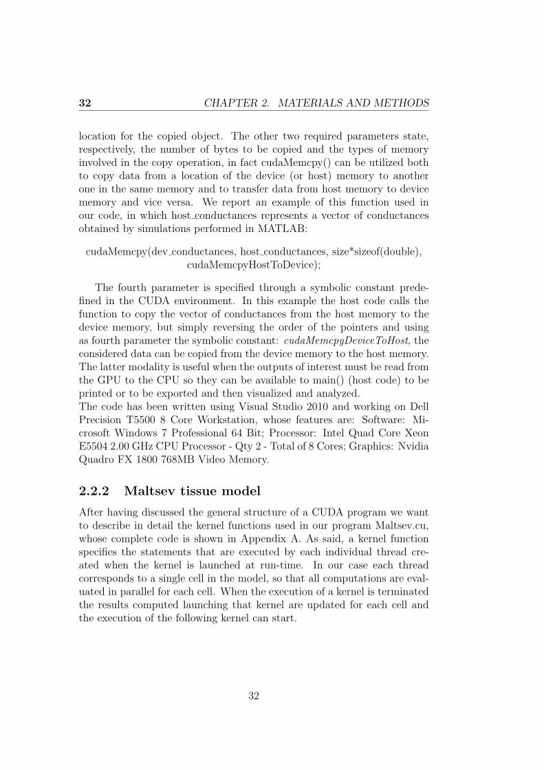
In the first kernel, that we can find in the code, initialConditions, an arrayof dimension num cells*num param is assigned to the initial conditions ofthe state variables. Once executed this kernel, the array, named vars, isstructured as illustrated in fig. 2.4 and contains in sequence the values ofthe initial conditions of each state variable for all the cells.After having initialized the array of the state variables, these latter must be
Figure 2.4: Structure of the array initialized with the Initial Conditions
updated for every time step and this is made possible through the executionof the next kernels. The second kernel computeState, as the name suggests,calculates the updated values for each of the 28 parameters, while the mem-brane voltage will be managed by a separate kernel. Through this kernelfirst the variables are indexed within the array, then all the constant valuesused in the model are specified and finally the differential equations describ-ing the state variables are integrated using the Euler Forward Method. Thislatter is a first-order numerical procedure for solving ODEs with a given
initial value. The following differential equationdy
dt=f(t,y) is satisfied by
a group of functions, a unique initial condition y(t=0)=y0 identifies onlyone of these functions, which is the Initial Value Problem (IVP) solution.Then we assume that a unique solution exists and denote that solution byye(t), while y(t) refers to the numerically computed solution, which canonly be an approximation of the exact one. Denoted the time at the nthtime-step by tn and the computed solution at the nth time-step by yn, i.e.,yn ≡y(t=tn), the constant step size h is then given by h=tn-tn−1. Given(tn,yn), the forward Euler method computes yn+1 as:
yn+1 = yn + hf(tn, yn) (2.6)
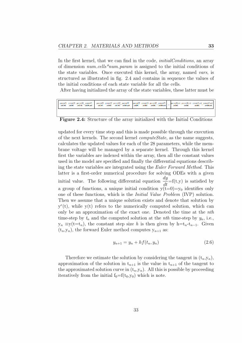
Therefore we estimate the solution by considering the tangent in (tn,yn),approximation of the solution in tn+1 is the value in tn+1 of the tangent tothe approximated solution curve in (tn,yn). All this is possible by proceedingiteratively from the initial f0=f(t0,y0) which is note.
33
34 CHAPTER 2. MATERIALS AND METHODS
Figure 2.5: Scheme of forward Euler integration
At the end of this function, all the state variables are updated into atemporary array and the next step is to copy the updated variables at thistime step in another array, which at the end of the simulation will containall the values for the state variables along all the time of simulation (kernelupdateState).The subsequent kernel computes the new values for the membrane voltage.While the value of each of the other state variables at a certain instant oftime and for a certain cell is not affected by the value assumed by the statevariables in the other cells, the value of one cell’s potential, as we know,is affected by that of neighboring cells. For this reason it is necessary tohave a separate kernel for handling the membrane potentials. Within thekernel compute voltage two different implementations are shown, first thecase of a cable of cells and then the case of a tissue. As usual the cells areconnected between them through gap junctions, but this time the resistanceis expressed referring to geometrical parameters of the cells, and so using aresistivity and the dimensions of the cell. The relation between ρ and Rgap
is given by the second Ohm’s law: R=ρ*l/S, i.e. the resistance R of a homo-geneous conductor of constant transversal section is directly proportionalto its length (l) and is inversely proportional to the area of its transversalsection (S). As it was for the resistance, also for the resistivity there is nota fixed value in literature, in our simulations different values within a widerange have been tested. In the cable model the equation used to updatethe voltage is the same shown before while describing the implementationin one dimension in MATLAB, the only difference is the method of inte-gration. The following illustration and the lines below describe how the
34
CHAPTER 2. MATERIALS AND METHODS 35
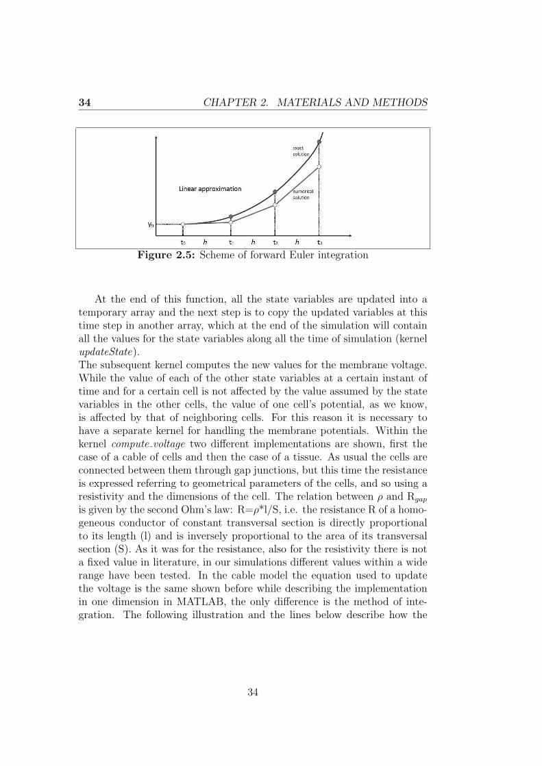
voltage is updated in the case of the tissue model, where no more only twoneighboring cells must be considered when calculating one cell’s potential,but 4 neighboring cells must be taken into account, as the cells are placedas in a matrix and no more along a line.
Figure 2.6: Scheme of connection between cells in the tissue model
Vm[m] = (x[n])+(step)∗((rad2∗ π
(ρ ∗ Cm ∗ deltx))∗(Vnet)−(Iion[n] + stim)
Cm
);
(2.7)
where the following parameters are utilized:
• Vm[m] is the updated membrane potential of the cell whose positionin the voltage array is denoted by the index m (m=0,1...num cell).After having written into Vm the updated values for each cell, theseare copied into another array x, so that Vm is only a temporary vector;
• x is the state variable array, which contains the updated values ofall the state variables. At the first time step, it is filled with theinitial conditions, then the updated values of the state variables arecopied from two temporary arrays into it. In particular voltage valuesoccupy the first num cells positions of the array and n, like m, is anindex which denotes the number of the cell (n=0,1...num cell). Foreach step, m and n denote the same cell, just in two different vectorsand x[n] represents the value assumed by Vm[m] at the previous timestep;
• Vnet is the sum of the contributions in voltage deriving from the fourneighbornig cells: Vnet=Vnet R+Vnet L+Vnet U+Vnet D;
35
36 CHAPTER 2. MATERIALS AND METHODS
• step is the time step, imposed equal to 0.005 ms after having verifiedthat it returns no appreciable difference in results compared to whatobtained with a 0.002 ms step;
• rad is the cell radius imposed equal to 4 µm;
• ρ is the resistivity and its value, as discussed in details later, is changedwithin a range of 104;
• Cm as usual is the membrane capacitance, whose value is equal to 32pF;
• deltx is the cell length imposed equal to 70 µm;
• Iion is the sum of all the different ionic currents;
• stim is an eventual stimulus current, not normally present in a modelof SAN cells, but it could be useful in our simulations as a tool toimpose different initial conditions to the cells, giving the stimulusonly to few of them.
As before another kernel (update voltage) is implicated in the storing ofthe updated values for the voltage. These are saved in the first cell numpositions of the vector used previously to save the other updated statevariables.Once terminated the execution of each kernel, the updated values for everytime step of the simulation are available to be exported and then visualizedand further used to measure outputs of interest, such as cycle length andaction potential amplitude. In order to be able to do that in MATLAB, cellmembrane voltage values for all time points are written into a file namedMaltsev GPU Voltage using the fopen() function in the write mode. Thesedata are structured such that each row of the matrix contains the values ofeach cell’s voltage at the same time point. Therefore the file can be openedin MATLAB environment through the built in function dlmread(), similarlythe function dlmwrite() is used when it is necessary to import in CUDA anarray created in MATLAB and then saved as a file.txt and opened in theprogram using the fopen() function in the read mode.
36
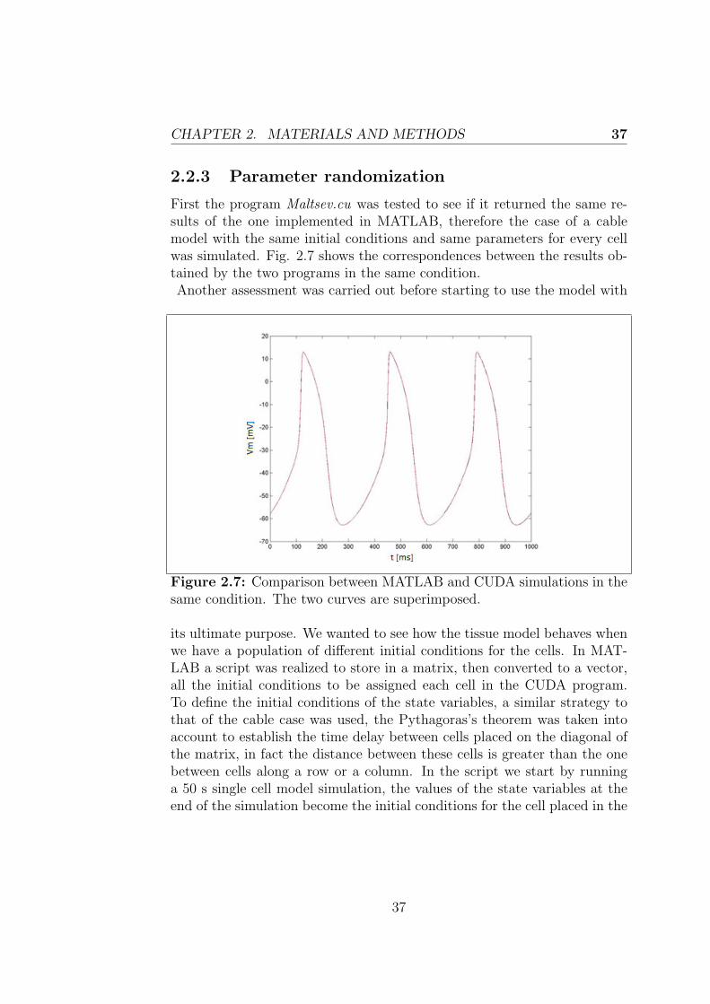
CHAPTER 2. MATERIALS AND METHODS 37
2.2.3 Parameter randomization
First the program Maltsev.cu was tested to see if it returned the same re-sults of the one implemented in MATLAB, therefore the case of a cablemodel with the same initial conditions and same parameters for every cellwas simulated. Fig. 2.7 shows the correspondences between the results ob-tained by the two programs in the same condition.Another assessment was carried out before starting to use the model with
Figure 2.7: Comparison between MATLAB and CUDA simulations in thesame condition. The two curves are superimposed.
its ultimate purpose. We wanted to see how the tissue model behaves whenwe have a population of different initial conditions for the cells. In MAT-LAB a script was realized to store in a matrix, then converted to a vector,all the initial conditions to be assigned each cell in the CUDA program.To define the initial conditions of the state variables, a similar strategy tothat of the cable case was used, the Pythagoras’s theorem was taken intoaccount to establish the time delay between cells placed on the diagonal ofthe matrix, in fact the distance between these cells is greater than the onebetween cells along a row or a column. In the script we start by runninga 50 s single cell model simulation, the values of the state variables at theend of the simulation become the initial conditions for the cell placed in the
37
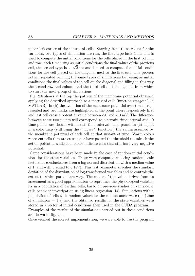
38 CHAPTER 2. MATERIALS AND METHODS
upper left corner of the matrix of cells. Starting from these values for thevariables, two types of simulation are run, the first type lasts 1 ms and isused to compute the initial conditions for the cells placed in the first columnand row, each time using as initial conditions the final values of the previouscell, the second type lasts
√2 ms and is used to compute the initial condi-
tions for the cell placed on the diagonal next to the first cell. The processis then repeated running the same types of simulations but using as initialconditions the final values of the cell on the diagonal and filling in this waythe second row and column and the third cell on the diagonal, from whichto start the next group of simulations.Fig. 2.8 shows at the top the pattern of the membrane potential obtainedapplying the described approach to a matrix of cells (function imagesc() inMATLAB). In (b) the evolution of the membrane potential over time is rep-resented and two marks are highlighted at the point where respectively firstand last cell cross a potential value between -20 and -10 mV. The differencebetween these two points will correspond to a certain time interval and 10time points are chosen within this time interval. The panels in (c) depictin a color map (still using the imagesc() function ) the values assumed bythe membrane potential of each cell at that instant of time. Warm colorsrepresent cells that are crossing or have passed the threshold to unleash theaction potential while cool colors indicate cells that still have very negativepotential.Same considerations have been made in the case of random initial condi-
tions for the state variables. These were computed choosing random scalefactors for conductances from a log-normal distribution with a median valueof 1, and with σ equal to 0.1873. This last parameter specifies the standarddeviation of the distribution of log-transformed variables and so controls theextent to which parameters vary. The choice of this value derives from itsassessment as a good approximation to reproduce the physiological variabil-ity in a population of cardiac cells, based on previous studies on ventricularcells behavior investigation using linear regression [14]. Simulations with apopulation of cells with random values for the conductances were run (timeof simulation = 1 s) and the obtained results for the state variables werestored in a vector of initial conditions then used in the CUDA program.Examples of the results of the simulations carried out in these conditionsare shown in fig. 2.9.Once verified the correct implementation, we were able to use the program
38
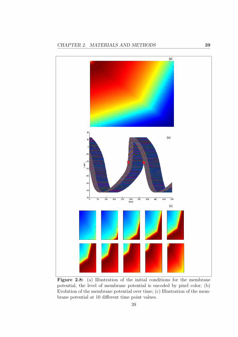
CHAPTER 2. MATERIALS AND METHODS 39
Figure 2.8: (a) Illustration of the initial conditions for the membranepotential, the level of membrane potential is encoded by pixel color; (b)Evolution of the membrane potential over time; (c) Illustration of the mem-brane potential at 10 different time point values.
39

40 CHAPTER 2. MATERIALS AND METHODS
Figure 2.9: Examples of color maps of voltage membrane obtained runningMaltsev.cu with random initial conditions for the SAN cells in the tissue:(a)-(b) tissue 15x15 cells at different intervals of time during the simulations;(c) tissue 8x8 cells; (d) tissue 12x12 cells
with its main scope, that is, to evaluate the effect of heterogeneity withinthe tissue. For this purpose a script in MATLAB was formulated to ran-domly vary the values of the maximal conductances used in the model, sothat each cell has a different value for each of the conductances.The parameters concerned and their base values are the following:
• double gsus = 0.02 nS/pF (in AP sensitive currents);
• double gto = 0.252 nS/pF (in AP sensitive currents);
• double gCaT = 0.1832 nS/pF (in iCaT );
• double gKr = 0.08113973 nS/pF (in iKr);
• double gKs = 0.0259 nS/pF (in iKs);
• double gCaL = 0.464 nS/pF (in iCaL);
• double gb Ca = 0.0006 nS/pF (in ib Ca);
40
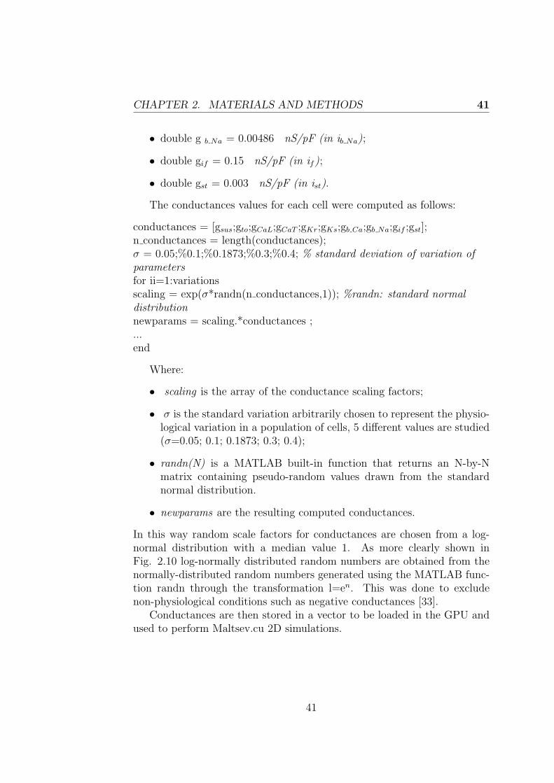
CHAPTER 2. MATERIALS AND METHODS 41
• double g b Na = 0.00486 nS/pF (in ib Na);
• double gif = 0.15 nS/pF (in if);
• double gst = 0.003 nS/pF (in ist).
The conductances values for each cell were computed as follows:
conductances = [gsus;gto;gCaL;gCaT ;gKr;gKs;gb Ca;gb Na;gif ;gst];n conductances = length(conductances);σ = 0.05;%0.1;%0.1873;%0.3;%0.4; % standard deviation of variation ofparametersfor ii=1:variationsscaling = exp(σ*randn(n conductances,1)); %randn: standard normaldistributionnewparams = scaling.*conductances ;...end
Where:
• scaling is the array of the conductance scaling factors;
• σ is the standard variation arbitrarily chosen to represent the physio-logical variation in a population of cells, 5 different values are studied(σ=0.05; 0.1; 0.1873; 0.3; 0.4);
• randn(N) is a MATLAB built-in function that returns an N-by-Nmatrix containing pseudo-random values drawn from the standardnormal distribution.
• newparams are the resulting computed conductances.
In this way random scale factors for conductances are chosen from a log-normal distribution with a median value 1. As more clearly shown inFig. 2.10 log-normally distributed random numbers are obtained from thenormally-distributed random numbers generated using the MATLAB func-tion randn through the transformation l=en. This was done to excludenon-physiological conditions such as negative conductances [33].
Conductances are then stored in a vector to be loaded in the GPU andused to perform Maltsev.cu 2D simulations.
41
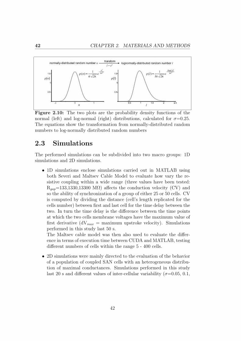
42 CHAPTER 2. MATERIALS AND METHODS
Figure 2.10: The two plots are the probability density functions of thenormal (left) and log-normal (right) distributions, calculated for σ=0.25.The equations show the transformation from normally-distributed randomnumbers to log-normally distributed random numbers
2.3 Simulations
The performed simulations can be subdivided into two macro groups: 1Dsimulations and 2D simulations.
• 1D simulations enclose simulations carried out in MATLAB usingboth Severi and Maltsev Cable Model to evaluate how vary the re-sistive coupling within a wide range (three values have been tested:Rgap=133,1330,13300 MΩ) affects the conduction velocity (CV) andso the ability of synchronization of a group of either 25 or 50 cells. CVis computed by dividing the distance (cell’s length replicated for thecells number) between first and last cell for the time delay between thetwo. In turn the time delay is the difference between the time pointsat which the two cells membrane voltages have the maximum value offirst derivative (dVmax = maximum upstroke velocity). Simulationsperformed in this study last 50 s.The Maltsev cable model was then also used to evaluate the differ-ence in terms of execution time between CUDA and MATLAB, testingdifferent numbers of cells within the range 5 - 400 cells.
• 2D simulations were mainly directed to the evaluation of the behaviorof a population of coupled SAN cells with an heterogeneous distribu-tion of maximal conductances. Simulations performed in this studylast 20 s and different values of inter-cellular variability (σ=0.05, 0.1,
42

CHAPTER 2. MATERIALS AND METHODS 43
0.1873, 0.3, 0.4) and resistive coupling (ρ=1, 10, 102, 103, 104 MΩ m)have been tested. In particular the effects over cycle length (CL) andaction potential amplitude (APA) were evaluated.The two outputs were computed as follows:
– CL: time between two consecutive crossings of 0 mV on the up-stroke of the AP;
– APA: difference between the most positive voltage recorded dur-ing the AP (OS, peak voltage) and the most negative one (MDP,maximum diastolic potential).
Figure 2.11: Scheme of an AP and its outputs of interest
The main question to be addressed through this group of simulationswas if the cells synchronize their spontaneous beating and at whatrate. In order to do that the behavior of the isolated cells was com-pared with the behavior of the same cells put together and connectedbetween them in the Maltsev Tissue Model.
The results of these simulations are discussed in the next chapter.
43

44 CHAPTER 2. MATERIALS AND METHODS
44
Chapter 3
Results
In this chapter we discuss the results of the simulations carried out withthe models implemented in this work. The results, as done previously withthe description of the simulations, have been subdivided into two groups.Through the first section we briefly explore the effects of the resistive cou-pling over the synchronization of a cable of cells. We also include a demon-stration of the clear benefits observed in terms of speed of execution whileconducting simulations in CUDA rather than in MATLAB. In the secondpart of the chapter, where 2D results are described, we finally answer themain question to be addressed with this work. Results of comparisons be-tween isolated heterogeneous cells and the same cells connected to form atissue are reported, so that in this way the ability and manner of synchro-nization of said cells are evaluated.
45
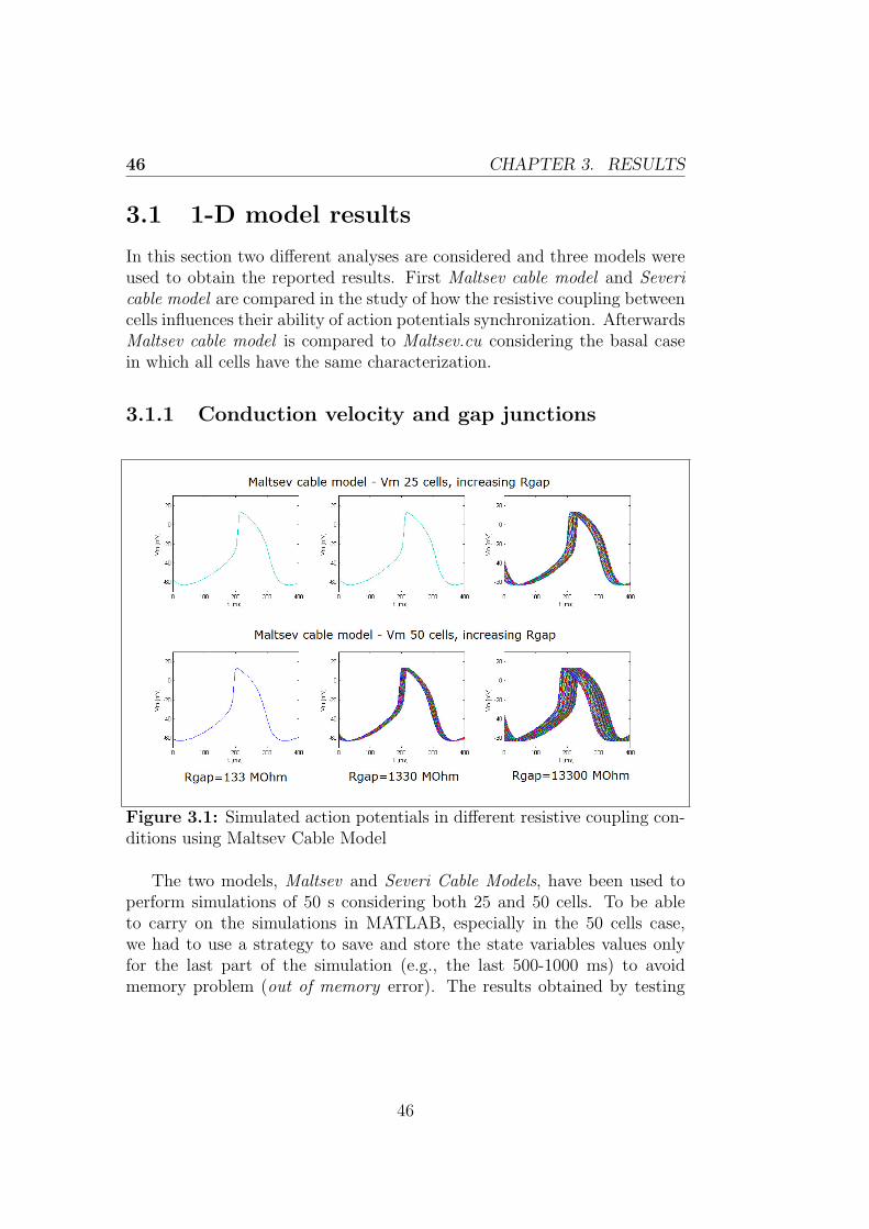
46 CHAPTER 3. RESULTS
3.1 1-D model results
In this section two different analyses are considered and three models wereused to obtain the reported results. First Maltsev cable model and Severicable model are compared in the study of how the resistive coupling betweencells influences their ability of action potentials synchronization. AfterwardsMaltsev cable model is compared to Maltsev.cu considering the basal casein which all cells have the same characterization.
3.1.1 Conduction velocity and gap junctions
Figure 3.1: Simulated action potentials in different resistive coupling con-ditions using Maltsev Cable Model
The two models, Maltsev and Severi Cable Models, have been used toperform simulations of 50 s considering both 25 and 50 cells. To be ableto carry on the simulations in MATLAB, especially in the 50 cells case,we had to use a strategy to save and store the state variables values onlyfor the last part of the simulation (e.g., the last 500-1000 ms) to avoidmemory problem (out of memory error). The results obtained by testing
46
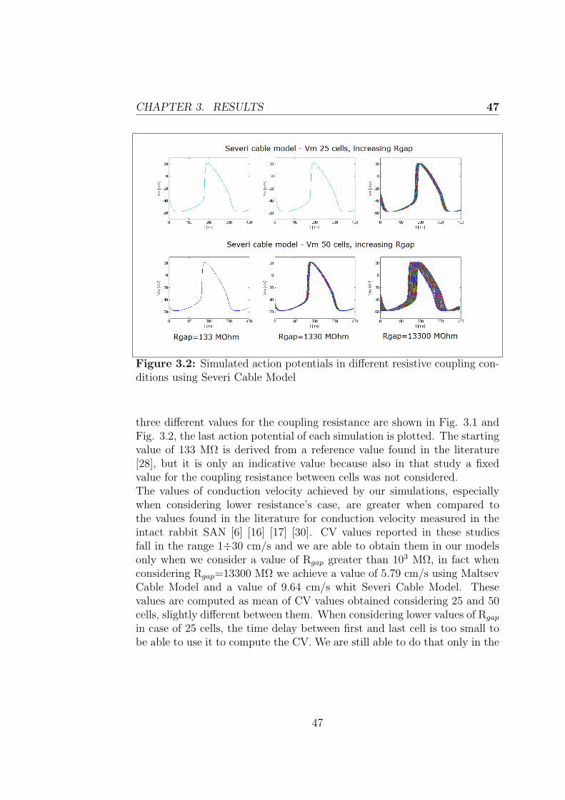
CHAPTER 3. RESULTS 47
Figure 3.2: Simulated action potentials in different resistive coupling con-ditions using Severi Cable Model
three different values for the coupling resistance are shown in Fig. 3.1 andFig. 3.2, the last action potential of each simulation is plotted. The startingvalue of 133 MΩ is derived from a reference value found in the literature[28], but it is only an indicative value because also in that study a fixedvalue for the coupling resistance between cells was not considered.The values of conduction velocity achieved by our simulations, especiallywhen considering lower resistance’s case, are greater when compared tothe values found in the literature for conduction velocity measured in theintact rabbit SAN [6] [16] [17] [30]. CV values reported in these studiesfall in the range 1÷30 cm/s and we are able to obtain them in our modelsonly when we consider a value of Rgap greater than 103 MΩ, in fact whenconsidering Rgap=13300 MΩ we achieve a value of 5.79 cm/s using MaltsevCable Model and a value of 9.64 cm/s whit Severi Cable Model. Thesevalues are computed as mean of CV values obtained considering 25 and 50cells, slightly different between them. When considering lower values of Rgap
in case of 25 cells, the time delay between first and last cell is too small tobe able to use it to compute the CV. We are still able to do that only in the
47
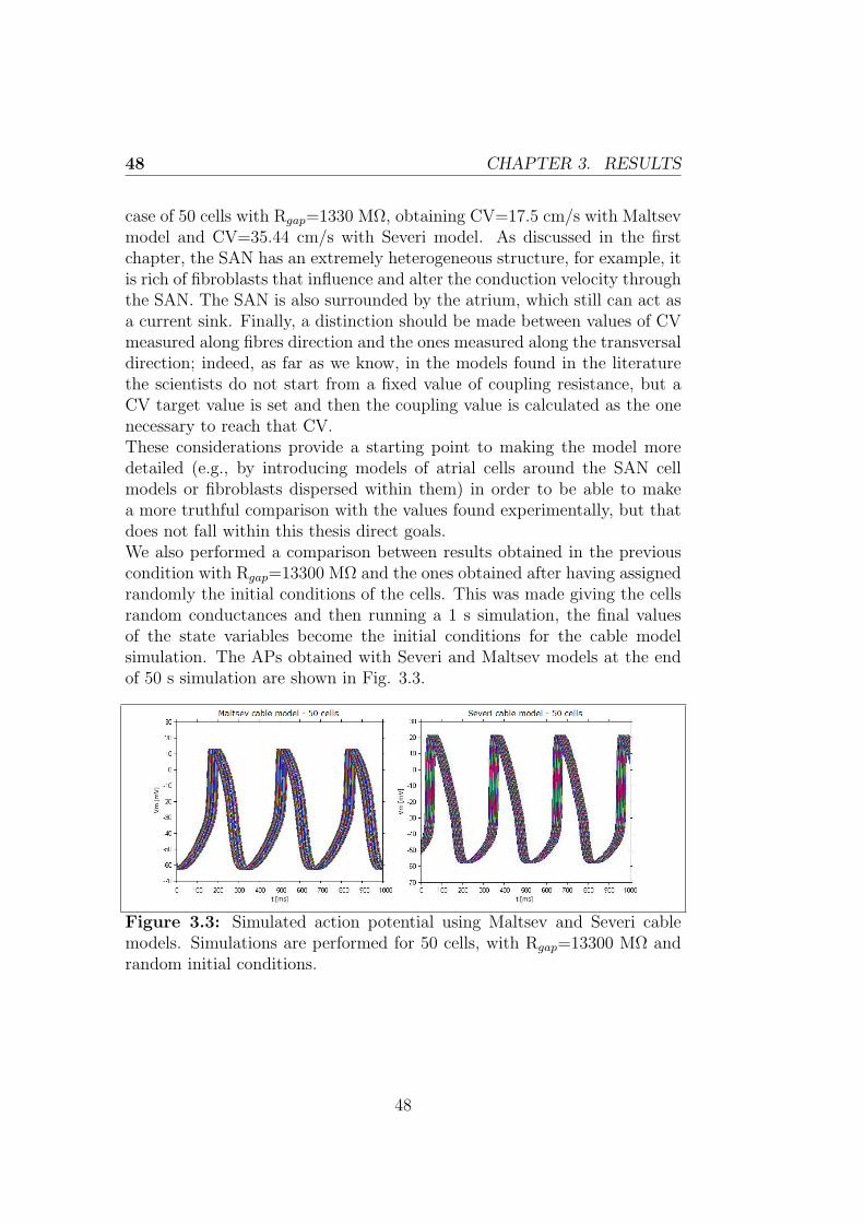
48 CHAPTER 3. RESULTS
case of 50 cells with Rgap=1330 MΩ, obtaining CV=17.5 cm/s with Maltsevmodel and CV=35.44 cm/s with Severi model. As discussed in the firstchapter, the SAN has an extremely heterogeneous structure, for example, itis rich of fibroblasts that influence and alter the conduction velocity throughthe SAN. The SAN is also surrounded by the atrium, which still can act asa current sink. Finally, a distinction should be made between values of CVmeasured along fibres direction and the ones measured along the transversaldirection; indeed, as far as we know, in the models found in the literaturethe scientists do not start from a fixed value of coupling resistance, but aCV target value is set and then the coupling value is calculated as the onenecessary to reach that CV.These considerations provide a starting point to making the model moredetailed (e.g., by introducing models of atrial cells around the SAN cellmodels or fibroblasts dispersed within them) in order to be able to makea more truthful comparison with the values found experimentally, but thatdoes not fall within this thesis direct goals.We also performed a comparison between results obtained in the previouscondition with Rgap=13300 MΩ and the ones obtained after having assignedrandomly the initial conditions of the cells. This was made giving the cellsrandom conductances and then running a 1 s simulation, the final valuesof the state variables become the initial conditions for the cable modelsimulation. The APs obtained with Severi and Maltsev models at the endof 50 s simulation are shown in Fig. 3.3.
Figure 3.3: Simulated action potential using Maltsev and Severi cablemodels. Simulations are performed for 50 cells, with Rgap=13300 MΩ andrandom initial conditions.
48
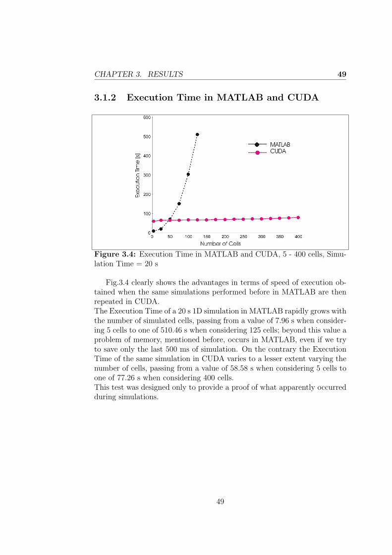
CHAPTER 3. RESULTS 49
3.1.2 Execution Time in MATLAB and CUDA
Figure 3.4: Execution Time in MATLAB and CUDA, 5 - 400 cells, Simu-lation Time = 20 s
Fig.3.4 clearly shows the advantages in terms of speed of execution ob-tained when the same simulations performed before in MATLAB are thenrepeated in CUDA.The Execution Time of a 20 s 1D simulation in MATLAB rapidly grows withthe number of simulated cells, passing from a value of 7.96 s when consider-ing 5 cells to one of 510.46 s when considering 125 cells; beyond this value aproblem of memory, mentioned before, occurs in MATLAB, even if we tryto save only the last 500 ms of simulation. On the contrary the ExecutionTime of the same simulation in CUDA varies to a lesser extent varying thenumber of cells, passing from a value of 58.58 s when considering 5 cells toone of 77.26 s when considering 400 cells.This test was designed only to provide a proof of what apparently occurredduring simulations.
49

50 CHAPTER 3. RESULTS
3.2 2-D model results
This section presents the results obtained by simulating a heterogeneouspopulation of cells in the sinoatrial node. The heterogeneity is achievedin practice through a randomization of the maximal conductances in thecurrents expressions of the Maltsev model. The purpose of this analysis isto evaluate the difference in behavior between a population of isolated cellsand the same cells connected together to form a matrix.
3.2.1 Effect of heterogenity on Cycle Length and Ac-
tion Potential Amplitude
Fig. 3.5 to Fig. 3.9 show the conductances distributions for each testedvalue of σ. These results come from a simulation of the Maltsev single cellmodel considering 400 different combinations of conductances, whose scalingfactors were picked, as described before, from a log-normal distribution.Therefore we have 400 cells still not connected between them and each onedescribed by a unique model characterized by having a unique combinationof conductances values. Together with the conductances distributions, alsoCycle Length and Action Potential Amplitude distributions, computed foreach cell as previously explained, are displayed.Since the standard deviation σ of log-transformed variables controls theextent to which parameters vary, the smaller the σ value, the narrower arethe parameters distributions. In particular we can notice that, for sigmavalues of 0.1873 and above, a large number of cells have CL and APA equalto zero, reaching a percentage of 40% in the case of σ=0.4. This meansthat with particular conductances combinations, cells are not excitable, sothat they do not exhibit any action potential and it is reasonable thatthis happens more easily in case of great values of σ, when the values ofconductances most different from the basal ones are taken into account.
Fig. 3.10 should better point out the difference in the amplitude of pa-rameters distributions when considering different values of σ. All cases plotsare superposed, so that we use the same scale for the parameters values andit is easier to appreciate the difference between distributions amplitude inthe five cases.Fig. 3.11 to Fig. 3.15 show the results obtained after having loaded inthe CUDA program the conductances vector and having run 20 s simula-
50
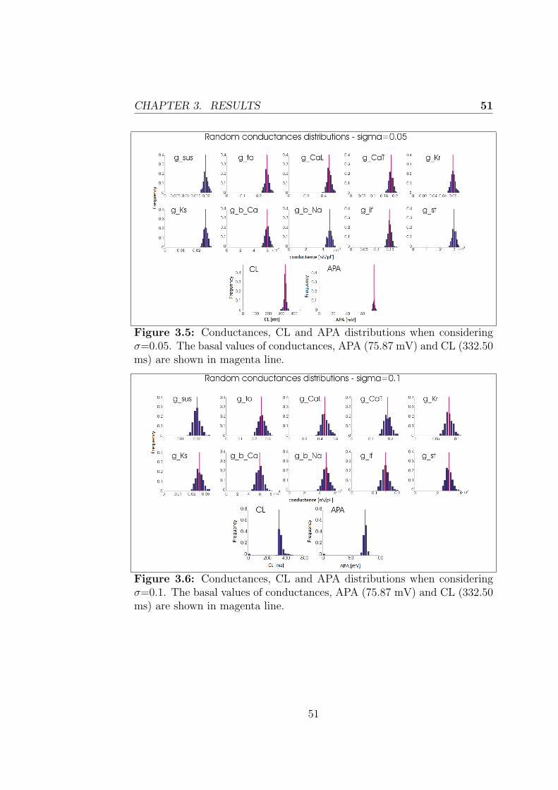
CHAPTER 3. RESULTS 51
Figure 3.5: Conductances, CL and APA distributions when consideringσ=0.05. The basal values of conductances, APA (75.87 mV) and CL (332.50ms) are shown in magenta line.
Figure 3.6: Conductances, CL and APA distributions when consideringσ=0.1. The basal values of conductances, APA (75.87 mV) and CL (332.50ms) are shown in magenta line.
51

52 CHAPTER 3. RESULTS
Figure 3.7: Conductances, CL and APA distributions when consideringσ=0.1873. The basal values of conductances, APA (75.87 mV) and CL(332.50 ms) are shown in magenta line.
Figure 3.8: Conductances, CL and APA distributions when consideringσ=0.3. The basal values of conductances, APA (75.87 mV) and CL (332.50ms) are shown in magenta line.
52
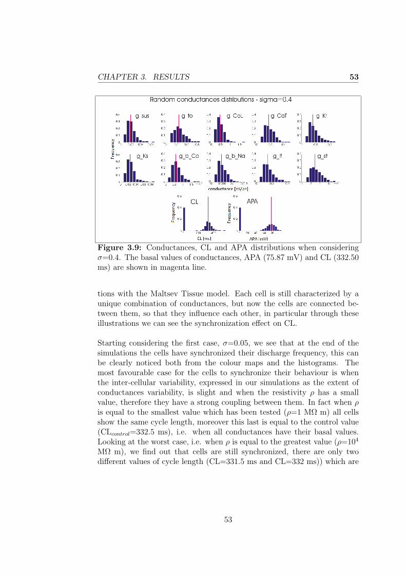
CHAPTER 3. RESULTS 53
Figure 3.9: Conductances, CL and APA distributions when consideringσ=0.4. The basal values of conductances, APA (75.87 mV) and CL (332.50ms) are shown in magenta line.
tions with the Maltsev Tissue model. Each cell is still characterized by aunique combination of conductances, but now the cells are connected be-tween them, so that they influence each other, in particular through theseillustrations we can see the synchronization effect on CL.
Starting considering the first case, σ=0.05, we see that at the end of thesimulations the cells have synchronized their discharge frequency, this canbe clearly noticed both from the colour maps and the histograms. Themost favourable case for the cells to synchronize their behaviour is whenthe inter-cellular variability, expressed in our simulations as the extent ofconductances variability, is slight and when the resistivity ρ has a smallvalue, therefore they have a strong coupling between them. In fact when ρis equal to the smallest value which has been tested (ρ=1 MΩ m) all cellsshow the same cycle length, moreover this last is equal to the control value(CLcontrol=332.5 ms), i.e. when all conductances have their basal values.Looking at the worst case, i.e. when ρ is equal to the greatest value (ρ=104
MΩ m), we find out that cells are still synchronized, there are only twodifferent values of cycle length (CL=331.5 ms and CL=332 ms)) which are
53

54 CHAPTER 3. RESULTS
Figure 3.10: Conductances, CL and APA distributions are shown usingdifferent colours for each value of σ to point out the different extent ofvariation of parameters
really close to the control value, even if slightly lower. This result is inaccordance with the fact that we were evaluating a low degree of variability.
When σ=0.1 and ρ has the minimum value, the cells have a final uni-form value of CL equal to 332 ms. As anticipated, increasing the value ofresistivity and thus resistance, the ability of the cells to synchronize towarda unique value of CL should decrease, in fact in the case of ρ maximum CLvaries within a range of 3.5 ms (CLmin=327.5 ms, CLmax=331 ms).
54
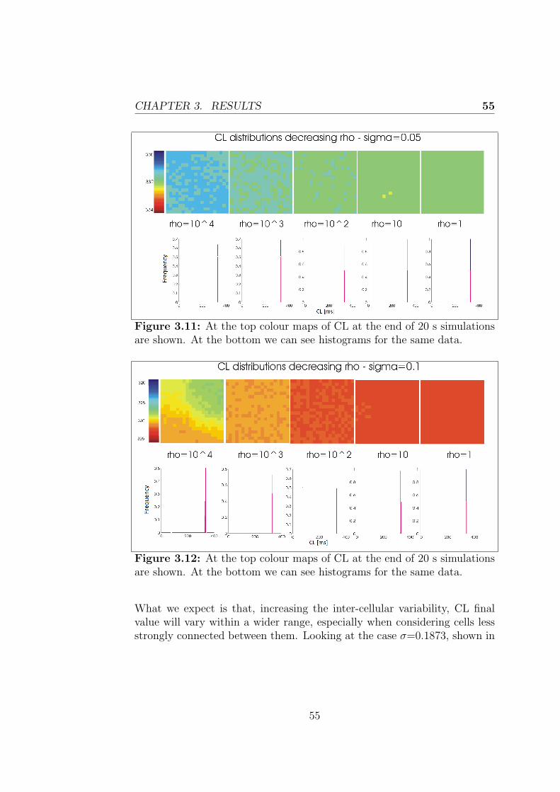
CHAPTER 3. RESULTS 55
Figure 3.11: At the top colour maps of CL at the end of 20 s simulationsare shown. At the bottom we can see histograms for the same data.
Figure 3.12: At the top colour maps of CL at the end of 20 s simulationsare shown. At the bottom we can see histograms for the same data.
What we expect is that, increasing the inter-cellular variability, CL finalvalue will vary within a wider range, especially when considering cells lessstrongly connected between them. Looking at the case σ=0.1873, shown in
55
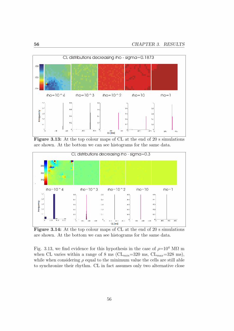
56 CHAPTER 3. RESULTS
Figure 3.13: At the top colour maps of CL at the end of 20 s simulationsare shown. At the bottom we can see histograms for the same data.
Figure 3.14: At the top colour maps of CL at the end of 20 s simulationsare shown. At the bottom we can see histograms for the same data.
Fig. 3.13, we find evidence for this hypothesis in the case of ρ=104 MΩ mwhen CL varies within a range of 8 ms (CLmin=320 ms, CLmax=328 ms),while when considering ρ equal to the minimum value the cells are still ableto synchronize their rhythm. CL in fact assumes only two alternative close
56
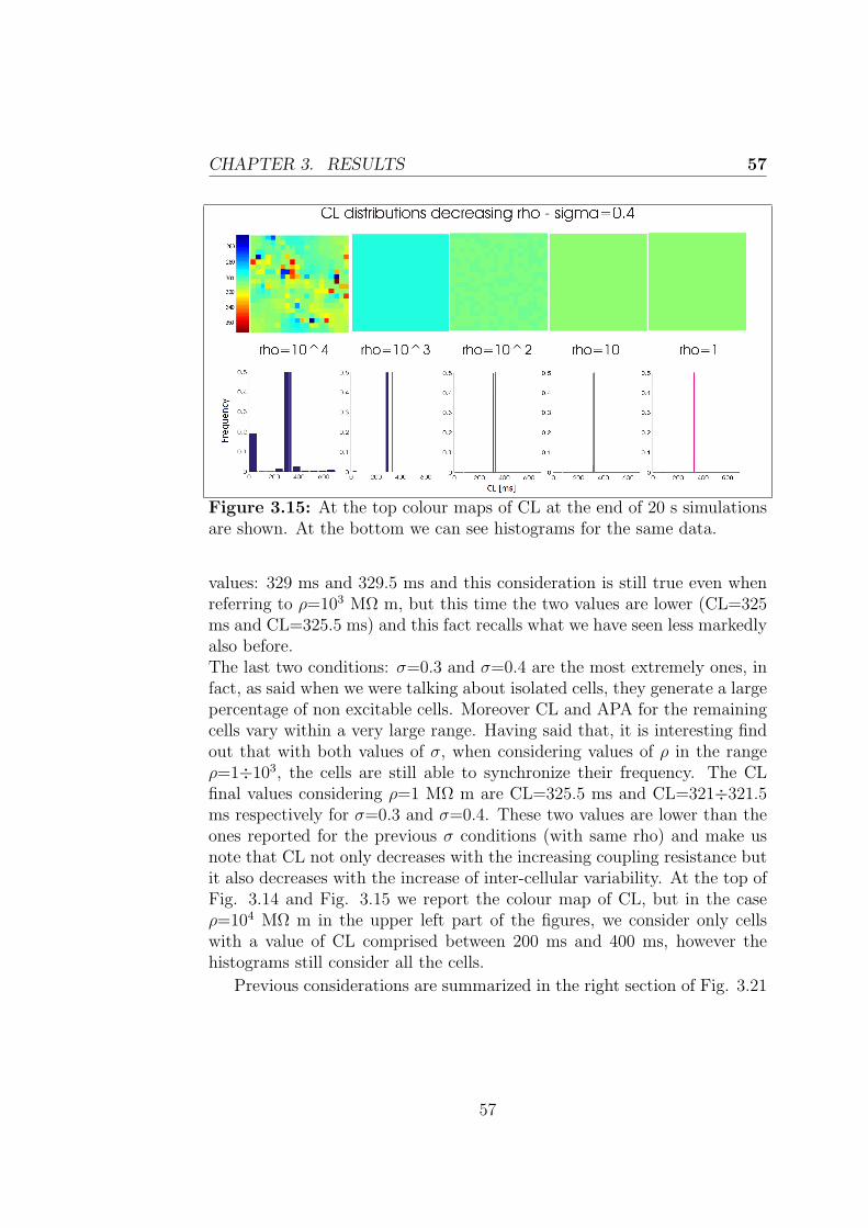
CHAPTER 3. RESULTS 57
Figure 3.15: At the top colour maps of CL at the end of 20 s simulationsare shown. At the bottom we can see histograms for the same data.
values: 329 ms and 329.5 ms and this consideration is still true even whenreferring to ρ=103 MΩ m, but this time the two values are lower (CL=325ms and CL=325.5 ms) and this fact recalls what we have seen less markedlyalso before.The last two conditions: σ=0.3 and σ=0.4 are the most extremely ones, infact, as said when we were talking about isolated cells, they generate a largepercentage of non excitable cells. Moreover CL and APA for the remainingcells vary within a very large range. Having said that, it is interesting findout that with both values of σ, when considering values of ρ in the rangeρ=1÷103, the cells are still able to synchronize their frequency. The CLfinal values considering ρ=1 MΩ m are CL=325.5 ms and CL=321÷321.5ms respectively for σ=0.3 and σ=0.4. These two values are lower than theones reported for the previous σ conditions (with same rho) and make usnote that CL not only decreases with the increasing coupling resistance butit also decreases with the increase of inter-cellular variability. At the top ofFig. 3.14 and Fig. 3.15 we report the colour map of CL, but in the caseρ=104 MΩ m in the upper left part of the figures, we consider only cellswith a value of CL comprised between 200 ms and 400 ms, however thehistograms still consider all the cells.
Previous considerations are summarized in the right section of Fig. 3.21
57
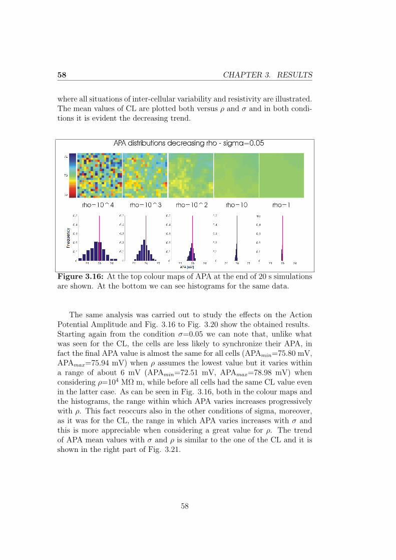
58 CHAPTER 3. RESULTS
where all situations of inter-cellular variability and resistivity are illustrated.The mean values of CL are plotted both versus ρ and σ and in both condi-tions it is evident the decreasing trend.
Figure 3.16: At the top colour maps of APA at the end of 20 s simulationsare shown. At the bottom we can see histograms for the same data.
The same analysis was carried out to study the effects on the ActionPotential Amplitude and Fig. 3.16 to Fig. 3.20 show the obtained results.Starting again from the condition σ=0.05 we can note that, unlike whatwas seen for the CL, the cells are less likely to synchronize their APA, infact the final APA value is almost the same for all cells (APAmin=75.80 mV,APAmax=75.94 mV) when ρ assumes the lowest value but it varies withina range of about 6 mV (APAmin=72.51 mV, APAmax=78.98 mV) whenconsidering ρ=104 MΩ m, while before all cells had the same CL value evenin the latter case. As can be seen in Fig. 3.16, both in the colour maps andthe histograms, the range within which APA varies increases progressivelywith ρ. This fact reoccurs also in the other conditions of sigma, moreover,as it was for the CL, the range in which APA varies increases with σ andthis is more appreciable when considering a great value for ρ. The trendof APA mean values with σ and ρ is similar to the one of the CL and it isshown in the right part of Fig. 3.21.
58
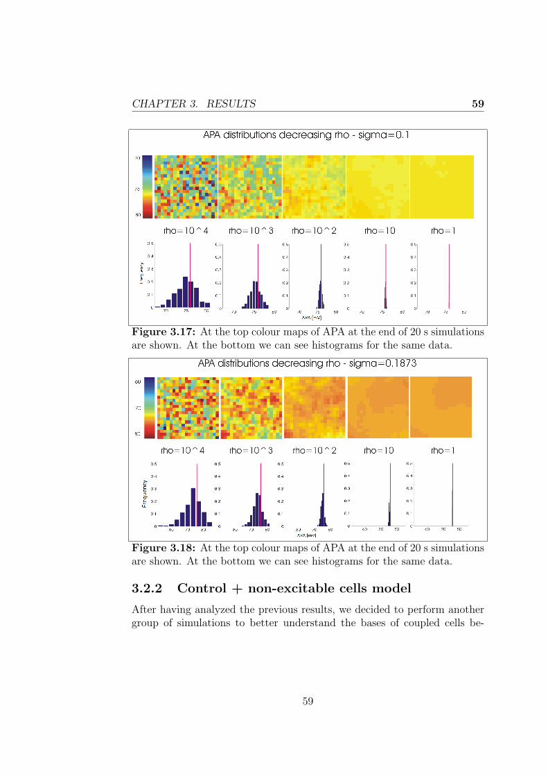
CHAPTER 3. RESULTS 59
Figure 3.17: At the top colour maps of APA at the end of 20 s simulationsare shown. At the bottom we can see histograms for the same data.
Figure 3.18: At the top colour maps of APA at the end of 20 s simulationsare shown. At the bottom we can see histograms for the same data.
3.2.2 Control + non-excitable cells model
After having analyzed the previous results, we decided to perform anothergroup of simulations to better understand the bases of coupled cells be-
59
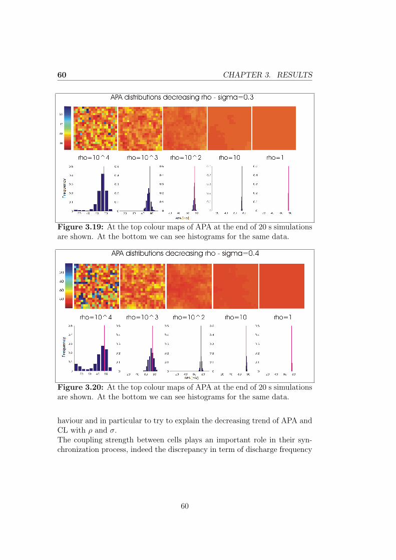
60 CHAPTER 3. RESULTS
Figure 3.19: At the top colour maps of APA at the end of 20 s simulationsare shown. At the bottom we can see histograms for the same data.
Figure 3.20: At the top colour maps of APA at the end of 20 s simulationsare shown. At the bottom we can see histograms for the same data.
haviour and in particular to try to explain the decreasing trend of APA andCL with ρ and σ.The coupling strength between cells plays an important role in their syn-chronization process, indeed the discrepancy in term of discharge frequency
60
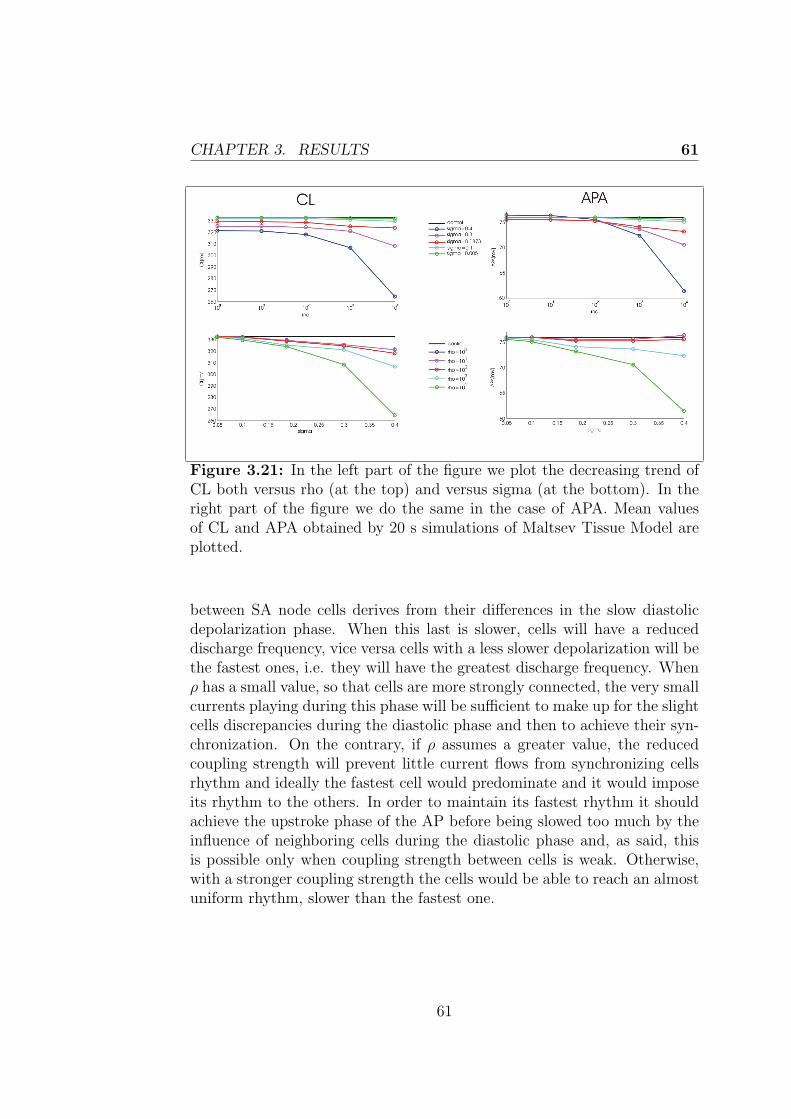
CHAPTER 3. RESULTS 61
Figure 3.21: In the left part of the figure we plot the decreasing trend ofCL both versus rho (at the top) and versus sigma (at the bottom). In theright part of the figure we do the same in the case of APA. Mean valuesof CL and APA obtained by 20 s simulations of Maltsev Tissue Model areplotted.
between SA node cells derives from their differences in the slow diastolicdepolarization phase. When this last is slower, cells will have a reduceddischarge frequency, vice versa cells with a less slower depolarization will bethe fastest ones, i.e. they will have the greatest discharge frequency. Whenρ has a small value, so that cells are more strongly connected, the very smallcurrents playing during this phase will be sufficient to make up for the slightcells discrepancies during the diastolic phase and then to achieve their syn-chronization. On the contrary, if ρ assumes a greater value, the reducedcoupling strength will prevent little current flows from synchronizing cellsrhythm and ideally the fastest cell would predominate and it would imposeits rhythm to the others. In order to maintain its fastest rhythm it shouldachieve the upstroke phase of the AP before being slowed too much by theinfluence of neighboring cells during the diastolic phase and, as said, thisis possible only when coupling strength between cells is weak. Otherwise,with a stronger coupling strength the cells would be able to reach an almostuniform rhythm, slower than the fastest one.
61

62 CHAPTER 3. RESULTS
This decreasing trend with ρ, however, is more significant when consideringsituations of great values for σ and so great inter-cellular variability. Asalready emphasised, in these cases we are handling borderline situationswhere conductances can assume values within a wide range and so cellsbehaviour is really different from the basal one. Moreover this decreasingtrend of CL is shown also with σ and APA mean values show the sametrend both with ρ and σ.All these considerations could make us wonder if this decreasing trend isonly due to the heterogeneity within cells or the large number of cells hav-ing no true pacemaking activity (and so resulting in a large number ofCL and APA equal to zero) could play an important role too. In orderto address this question we decided to carry out simulations using a newmodel, obtained combining a control model, in which cells are described us-ing the basal conductances in the current’s equations, and a non-excitablecell model. We started considering the array of conductances obtained incondition of σ=0.4, because it is in this condition that we can see thegreatest percentage of non excitable-cells and we kept all the combinationsof conductances causing non-excitable isolated cells while we replaced theother ones with the basal conductances. In this way we came up with a vec-tor of conductances which generates the same percentage of non-excitablecells as before, but the remaining cells are described by the control modeland so they exhibit a basal behaviour.The following illustrations describe the results obtained by a comparisonbetween simulations performed using this last model and simulations car-ried out before in the condition σ=0.4 with Maltsev Tissue Model.In our analyses we have always computed both CL and APA, yet that
which, for the most part concerns us is the study of the cycle length whichhas a greater value as a clinical parameter rather than the amplitude of theAP. Looking at Fig. 3.22 we can notice that in both cases, control model+ non-excitable cells model and sigma=0.4 model, with ρ varying in therange 1÷103, cells have synchronized their discharge frequency when thesimulation is completed. What is more interesting is that in case of ρ equalto 104 MOhm m the percentage of non excitable cells is approximately 20%in the case σ=0.4 model while is only 10% considering the other model.Moreover when we look at the upper part of Fig. 3.24 we can see that forall values of ρ the mean values of CL in the pure σ=0.4 model are alwayssmaller than the ones obtained with the new model. Since in the two mod-
62
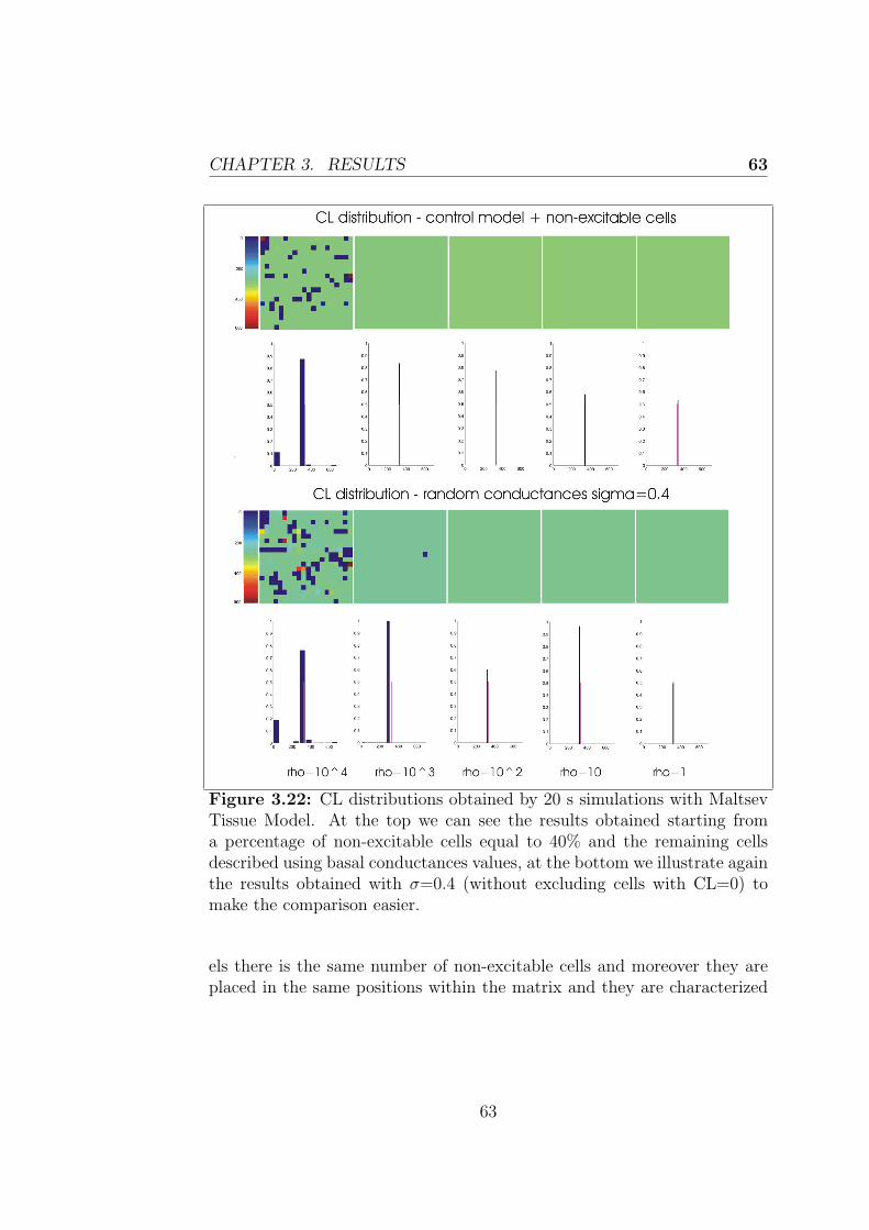
CHAPTER 3. RESULTS 63
Figure 3.22: CL distributions obtained by 20 s simulations with MaltsevTissue Model. At the top we can see the results obtained starting froma percentage of non-excitable cells equal to 40% and the remaining cellsdescribed using basal conductances values, at the bottom we illustrate againthe results obtained with σ=0.4 (without excluding cells with CL=0) tomake the comparison easier.
els there is the same number of non-excitable cells and moreover they areplaced in the same positions within the matrix and they are characterized
63
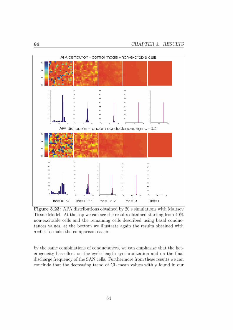
64 CHAPTER 3. RESULTS
Figure 3.23: APA distributions obtained by 20 s simulations with MaltsevTissue Model. At the top we can see the results obtained starting from 40%non-excitable cells and the remaining cells described using basal conduc-tances values, at the bottom we illustrate again the results obtained withσ=0.4 to make the comparison easier.
by the same combinations of conductances, we can emphasize that the het-erogeneity has effect on the cycle length synchronization and on the finaldischarge frequency of the SAN cells. Furthermore from these results we canconclude that the decreasing trend of CL mean values with ρ found in our
64
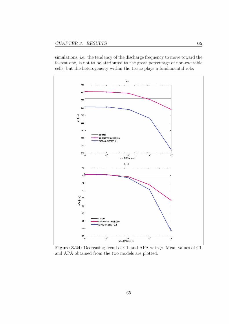
CHAPTER 3. RESULTS 65
simulations, i.e. the tendency of the discharge frequency to move toward thefastest one, is not to be attributed to the great percentage of non-excitablecells, but the heterogeneity within the tissue plays a fundamental role.
Figure 3.24: Decreasing trend of CL and APA with ρ. Mean values of CLand APA obtained from the two models are plotted.
65

66 CHAPTER 3. RESULTS
66
Conclusions
Cardiac diseases remain the number one cause of death in the Westernworld, this is probably one of the reasons why the heart is one of the moststudied organs of the body. Computational modeling, combined with state-of-the-art experimental techniques helps to gaining deeper insights into theregulation of normal heart function as well as how this regulation may bealtered in pathological states. During the years many mathematical modelsof myocardial cells have been proposed, each one trying to better representthe real behaviour of the cells. Even if we can increase a lot the level ofdetails in these models, they will never give an understanding of the mecha-nisms of interactions between cells and since they use a unique value for theparameters they cannot take into account the variability normally presentwithin a population of cells of the same organ. Since the heart is struc-tured as a syncytium of cells which can interact and influence each other toan extent that could completely change the behaviour of the same isolatedcells, single cell model could predict a behaviour completely different fromthe real one.In our study we are primarily interested in the understanding of how tissueheterogeneity can act on a specific cardiac physiological process, that is thegenesis of the cardiac rhythm within the specialized tissue of the sinoatrialnode. Since the morphological and functional heterogeneity of the SANcells is a well known fact, during the years several hypotheses have beenformulated to achieve a better comprehension of the SAN structure and soto be able to realize more detailed and realistic models of the SAN. Some ofthese models consider two types of SAN cells or they introduce an increaseof gap junction density and conductance from the center to the pheripheryof the SAN. We have implemented a 2-dimensional computational modelof the sinoatrial node starting from a single cell model and we have per-formed a randomization of the maximal values of conductances used in the
67
68 CONCLUSIONS
model. Each cell in our case has a different discharge frequency and wecan compare the behaviour of isolated cells to the one of the same cells puttogether to form a tissue. The fundamental question we wanted to addressthrough this study was how the cells influence each other’s spontaneousbeating. In particular, we wanted to find out if the cells synchronize theirbeating and if they do so, if the fastest cell predominates, becoming theleading pacemaker and imposing its frequency to the other cells or if theultimate frequency is fairly equal to the average rate of the isolated cells.What we have concluded from our simulations, testing different conditionsof inter-cellular variability and coupling resistance is that the populationsynchronizes on a rate slightly higher than the one of the isolated cells withthe basal values of conductances, moreover the rate moderately increaseswith resistive coupling and with inter-cellular variability, but it does notequal the rate of the fastest cell.Other questions could be addressed in the future by utilising our model,we could in fact consider the variations of other parameters and not onlyof the conductances, for example we could study the effect of variability inonly one parameter (e.g. in funny current conductance or in calcium clockfluxes) on the heart rate. Moreover, to better describe the SAN heterogene-ity we could add details in our model, for example by introducing atrial cellor fibroblast models interspersed within the matrix of SAN cells.In conclusion, this work provides the starting point for a more compre-hensive and realistic approach to the computational analysis of the cardiacpacemaking. This will likely help in addressing several open questions aboutheart rate and its modulation in physiological and pathological conditions.
68
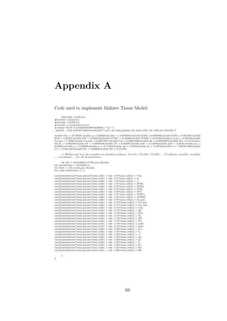
Appendix A
Code used to implement Maltsev Tissue Model:
#include <stdio.h>#include <math.h>#include <stdlib.h>#include <curand kernel.h># define M PI 3.14159265358979323846 /* pi */global void initialConditions(double* vars, int num param, int num cells, int cells per thread)
double Vm = -57.9639; double q = 0.69424;double r = 0.0055813;double fCMi = 0.059488;double fCMs = 0.054381;doublefCQ = 0.27321;double fTC = 0.029132;double fTMC = 0.43269;double fTMM = 0.50105;double Ca jsr = 0.31676;doubleCa nsr = 1.4935;double Ca sub = 0.00013811;double Cai = 0.00015002;double dL = 0.00058455;double fCa = 0.7114;dou-ble fL = 0.86238;double dT = 0.0050439;double fT = 0.42076;double paF = 0.14476;double paS = 0.4531;double pi =0.84941;double n = 0.02646;double y = 0.11364;double qa = 0.4238;double qi = 0.44729;double I = 7.8618e-008;doubleO = 1.734e-007;double R1 = 0.68805;double RI = 0.31195;
// Within each test, the variables are divided as follows: V(cell1), V(cell2), V(cell3) ... V(cellLast), m(cell1), m(cell2),... m(cellLast) ... for all 29 parameters
int idx = threadIdx.x*cells per thread;int simulations = blockIdx.x;int limit = idx+cells per thread;for (;idx<limit;idx++)
vars[(simulations*num param*num cells) + idx +(0*num cells)] = Vm;vars[(simulations*num param*num cells) + idx +(1*num cells)] = q;vars[(simulations*num param*num cells) + idx +(2*num cells)] = r;vars[(simulations*num param*num cells) + idx +(3*num cells)] = fCMi;vars[(simulations*num param*num cells) + idx +(4*num cells)] = fCMs;vars[(simulations*num param*num cells) + idx +(5*num cells)] = fCQ;vars[(simulations*num param*num cells) + idx +(6*num cells)] = fTC;vars[(simulations*num param*num cells) + idx +(7*num cells)] = fTMC;vars[(simulations*num param*num cells) + idx +(8*num cells)] = fTMM;vars[(simulations*num param*num cells) + idx +(9*num cells)] = Ca jsr;vars[(simulations*num param*num cells) + idx +(10*num cells)] = Ca nsr;vars[(simulations*num param*num cells) + idx +(11*num cells)] = Ca sub;vars[(simulations*num param*num cells) + idx +(12*num cells)] = Cai;vars[(simulations*num param*num cells) + idx +(13*num cells)] = dL;vars[(simulations*num param*num cells) + idx +(14*num cells)] = fCa;vars[(simulations*num param*num cells) + idx +(15*num cells)] = fL;vars[(simulations*num param*num cells) + idx +(16*num cells)] = dT;vars[(simulations*num param*num cells) + idx +(17*num cells)] = fT;vars[(simulations*num param*num cells) + idx +(18*num cells)] = paF;vars[(simulations*num param*num cells) + idx +(19*num cells)] = paS;vars[(simulations*num param*num cells) + idx +(20*num cells)] = pi ;vars[(simulations*num param*num cells) + idx +(21*num cells)] = n;vars[(simulations*num param*num cells) + idx +(22*num cells)] = y;vars[(simulations*num param*num cells) + idx +(23*num cells)] = qa;vars[(simulations*num param*num cells) + idx +(24*num cells)] = qi;vars[(simulations*num param*num cells) + idx +(25*num cells)] = I;vars[(simulations*num param*num cells) + idx +(26*num cells)] = O;vars[(simulations*num param*num cells) + idx +(27*num cells)] = R1;vars[(simulations*num param*num cells) + idx +(28*num cells)] = RI;
69
70 APPENDIX A
global void computeState(double* x, float* conductances, double* ion current, int total cells, double step, double*randNums, int variations, double* x temp, int num changing vars, int cells per thread)
int idx = cells per thread*threadIdx.x;int cell num;int limit = idx+cells per thread;for (;idx¡limit;idx++)
cell num = (blockIdx.x*total cells*29) + idx;
//Index Variables to make life easier: Array is categorized by blocks of size=total cells, each block contains the Vmsof one parameter across the cells
int Vm i = 0*total cells ;int q i = 1*total cells ;int r i = 2*total cells ;int fCMi i = 3*total cells ;int fCMs i = 4*total cells ;int fCQ i = 5*total cells ;int fTC i = 6*total cells ;int fTMC i = 7*total cells ;int fTMM i = 8*total cells ;int Ca jsr i = 9*total cells ;int Ca nsr i = 10*total cells ;int Ca sub i = 11*total cells ;int Cai i = 12*total cells ;int dL i = 13*total cells ;int fCa i = 14*total cells ;int fL i = 15*total cells ;int dT i = 16*total cells ;int fT i = 17*total cells ;int paF i = 18*total cells ;int paS i = 19*total cells ;int pi i = 20*total cells ;int n i = 21*total cells ;int y i = 22*total cells ;int qa i = 23*total cells ;int qi i = 24*total cells ;int I i = 25*total cells ;int O i = 26*total cells ;int R1 i = 27*total cells ;int RI i = 28*total cells ;
double E K, i to, i sus, q infinity, tau q; double r infinity, tau r, i CaL, i CaT, E Na, i f Na, i f K, i f;double i st, i Kr, E Ks, i Ks, i NaK ;double RTOnF, k32, k43, di, k14, k12, k41, k34, x2, Do, k21, k23, x1, x3, x4, i NaCa;double i b Ca, i b Na, delta fTC, delta fTMC, delta fTMM, delta fCMi;double delta fCMs, delta fCQ, j Ca dif;double V sub, j up, V cell, V nsr, V in, j SRCarel, V jsr, j tr, dL infinity;double adVm, alpha dL, bdVm, beta dL, tau dL, fCa infinity, tau fCa;double fL infinity, tau fL, dT infinity, tau dT, fT infinity, tau fT;double pa infinity, tau paS, tau paF, pi infinity, tau pi;double alpha n, beta n, n infinity, tau n;double y infinity, tau y, qa infinity, alpha qa, beta qa, tau qa;double alpha qi, beta qi, qi infinity, tau qi;double kCaSR, koSRCa, kiSRCa, Iion;
// conductances control values /*double g sus = 0.02;double g to = 0.252;double g CaT = 0.1832;double g Kr = 0.08113973;double g Ks = 0.0259;double g CaL = 0.464;double g b Ca = 0.0006;double g b Na = 0.00486;double g if = 0.15;double g st = 0.003; */double g sus = conductances[cell num+0*total cells] ;double g to = conductances[cell num+1*total cells] ;double g CaL = conductances[cell num+2*total cells] ;double g CaT = conductances[cell num+3*total cells] ;double g Kr = conductances[cell num+4*total cells] ;double g Ks =conductances[cell num+5*total cells] ;double g b Ca = conductances[cell num+6*total cells] ;double g b Na = conductances[cell num+7*total cells] ;
70
APPENDIX A 71
double g if = conductances[cell num+8*total cells] ;double g st = conductances[cell num+9*total cells] ;
double Cm=32;double CM tot = 0.045;double CQ tot = 10.0;double TC tot = 0.031;double TMC tot = 0.062;doublekb CM = 0.542;double kb CQ = 0.445;double kb TC = 0.446;double kb TMC = 0.00751;double kb TMM = 0.751;dou-ble kf CM = 227.7;double kf CQ = 0.534;double kf TC = 88.8;double kf TMC = 227.7; double kf TMM = 2.277;doubleKm fCa = 0.00035;double alpha fCa = 0.021;double E CaL = 45.0;double E CaT = 45.0;double K1ni = 395.3;doubleK1no = 1628.0;double K2ni = 2.289;double K2no = 561.4;double K3ni = 26.44; double K3no = 4.663;double Kci =0.0207;double Kcni = 26.44;double Kco = 3.663;double Qci = 0.1369;double Qco = 0.0;double Qn = 0.4315;doublekNaCa = 187.5;double Km Kp = 1.4;double Km Nap = 14.0;double i NaK max = 2.88;double VIf half = -64.0;doubleE st = 37.4;
double K up = 0.0006;double P up = 0.012;double tau dif Ca = 0.04;double tau tr = 40.0;double EC50 SR = 0.45;doubleHSR = 2.5;double MaxSR = 15.0;double MinSR = 1.0;double kiCa = 0.5;double kim = 0.005;double koCa = 10.0;doublekom = 0.06;double ks = 250000.0;double Cao = 2.0;double F = 96485.0;double Ki = 140.0;double Ko = 5.4;double L cell= 70.0;double L sub = 0.02;double Mgi = 2.5;double Nai = 10.0;double Nao = 140.0;double R2 = 8314.4;double R cell= 4.0;double T = 310.15;double V in part = 0.46;double V jsr part = 0.0012;double V nsr part = 0.0116;
/*statevar i = [q ,r ,Vm ,fCMi ,fCMs ,fCQ ,fTC ,fTMC ,fTMM ,Ca jsr ,Ca nsr ,Ca sub ,Cai , dL ,fCa ,fL ,dT ,fT ,paF,paS ,pi ,n ,y ,qa ,qi ,I ,O ,R1 ,RI ];*/
E K = R2*T/F*log(Ko/Ki) ;i to = Cm*g to*(x[cell num+Vm i]-E K)*(x[cell num+q i])*(x[cell num+r i]);i sus = Cm*g sus*(x[cell num+Vm i]-E K)*(x[cell num+r i]);
q infinity = 1/(1+exp((x[cell num+Vm i]+49)/13));tau q=6.06+39.102/(0.57*exp(-0.08*(x[cell num+Vm i]+44))+0.065*exp(0.1*(x[cell num+Vm i]+45.93)));
r infinity = 1/(1+exp(-(x[cell num+Vm i]-19.3)/15));tau r = 2.75352+14.40516/(1.037*exp(0.09*(x[cell num+Vm i]+30.61))+0.369*exp(-0.12*( x[cell num+Vm i]+23.84)));
i CaL = Cm*g CaL*(x[cell num+Vm i]-E CaL)*x[cell num+dL i]* x[cell num+fL i]* x[cell num+fCa i];i CaT = Cm*g CaT*(x[cell num+Vm i]-E CaT)* x[cell num+dT i]* x[cell num+fT i];
E Na = R2*T/F*log(Nao/Nai);i f Na = Cm*0.3833*g if*( x[cell num+Vm i]-E Na)*pow(x[cell num+y i],2);i f K = Cm*0.6167*g if*( x[cell num+Vm i]-E K)* pow(x[cell num+y i],2);i f = i f Na+i f K;
i st = Cm*g st*( x[cell num+Vm i]-E st) *x[cell num+qa i] * x[cell num+qi i];
i Kr = Cm*g Kr*( x[cell num+Vm i]-E K) *(0.6* x[cell num+paF i]+0.4* x[cell num+paS i]) * x[cell num+pi i];
E Ks = R2*T/F*log((Ko+0.12*Nao)/(Ki+0.12*Nai));i Ks = Cm*g Ks*( x[cell num+Vm i]-E Ks) *pow(x[cell num+n i],2);
i NaK = Cm*i NaK max/((1+pow((Km Kp/Ko),1.2))*(1+pow((Km Nap/Nai),1.3))*(1+exp(-(x[cell num+Vm i]-E Na+120.0) /30.0)));
RTOnF = R2*T/F;k32 = exp(Qn* x[cell num+Vm i]/(2*RTOnF));k43 = Nai/(K3ni+Nai);di=1+x[cell num+Ca sub i]/Kci*(1+exp(-Qci*x[cell num+Vm i]/RTOnF)+Nai/Kcni)+Nai/K1ni*(1+Nai/K2ni*(1+Nai/K3ni));k14 = Nai/K1ni*Nai/K2ni*(1+Nai/K3ni) *exp(Qn* x[cell num+Vm i]/(2*RTOnF)) /di;k12 = x[cell num+Ca sub i] /Kci*exp(-Qci* x[cell num+Vm i]/RTOnF) /di;k41 = exp(-Qn* x[cell num+Vm i]/(2*RTOnF));k34 = Nao/(K3no+Nao);x2 = k32*k43*(k14+k12)+k41*k12*(k34+k32);Do = 1+Cao/Kco*(1+exp(Qco* x[cell num+Vm i]/RTOnF))+Nao/K1no*(1+Nao/K2no*(1+Nao/K3no));k21 = Cao/Kco*exp(Qco* x[cell num+Vm i]/RTOnF) /Do;k23 = Nao/K1no*Nao/K2no*(1+Nao/K3no) *exp(-Qn* x[cell num+Vm i]/(2*RTOnF))/Do;x1 = k41*k34*(k23+k21)+k21*k32*(k43+k41);x3 = k14*k43*(k23+k21)+k12*k23*(k43+k41);x4 = k23*k34*(k14+k12)+k14*k21*(k34+k32);i NaCa = Cm*kNaCa*(x2*k21-x1*k12)/(x1+x2+x3+x4);
i b Ca = Cm*g b Ca*( x[cell num+Vm i]-E CaL);i b Na = Cm*g b Na*( x[cell num+Vm i]-E Na);
delta fTC = kf TC* x[cell num+Cai i] *(1- x[cell num+fTC i])-kb TC* x[cell num+fTC i];delta fTMC = kf TMC* x[cell num+Cai i] *(1-( x[cell num+fTMC i] + x[cell num+fTMM i]))-kb TMC*x[cell num+fTMC i];delta fTMM = kf TMM*Mgi*(1-( x[cell num+fTMC i]+ x[cell num+fTMM i]))-kb TMM*x[cell num+fTMM i];delta fCMi = kf CM* x[cell num+Cai i] *(1- x[cell num+fCMi i])-kb CM*x[cell num+fCMi i];delta fCMs = kf CM* x[cell num+Ca sub i]*(1- x[cell num+fCMs i])-kb CM* x[cell num+fCMs i];
71

72 APPENDIX A
delta fCQ = kf CQ* x[cell num+Ca jsr i]*(1- x[cell num+fCQ i])-kb CQ* x[cell num+fCQ i];
j Ca dif = (x[cell num+Ca sub i]- x[cell num+ Cai i])/tau dif Ca;
V sub = 0.001*2*M PI *L sub*(R cell-L sub/2)*L cell;//pi=M PIj up = P up/(1+K up/ x[cell num+ Cai i]);V cell = 0.001*M PI *pow(R cell,2)*L cell;V nsr = V nsr part*V cell;V in = V in part*V cell-V sub;
j SRCarel = ks* x[cell num+O i]*( x[cell num+Ca jsr i]- x[cell num+Ca sub i]);V jsr = V jsr part*V cell;j tr = (x[cell num+Ca nsr i] - x[cell num+Ca jsr i])/tau tr;dL infinity = 1/(1+exp(-(x[cell num+Vm i] +13.5)/6));
if (x[cell num+Vm i] == -35) adVm = -35.00001;else if (x[cell num+Vm i] == 0) adVm = 0.00001;else adVm = x[cell num+Vm i];
alpha dL = -0.02839*(adVm+35)/(exp(-(adVm+35)/2.5)-1)-0.0849*adVm/(exp(-adVm/4.8)-1);if (x[cell num+Vm i] == 5) bdVm = 5.00001;else bdVm = x[cell num+Vm i];beta dL = 0.01143*(bdVm-5)/(exp((bdVm-5)/2.5)-1);tau dL = 1/(alpha dL+beta dL);fCa infinity = Km fCa/(Km fCa+ x[cell num+Ca sub i]);tau fCa = fCa infinity/alpha fCa;fL infinity = 1/(1+exp((x[cell num+Vm i]+35)/7.3));tau fL = 44.3+257.1*exp(-pow(((x[cell num+Vm i]+32.5)/13.9),2));
dT infinity = 1.0/(1+exp(-(x[cell num+Vm i]+26.3)/6));tau dT = 1/(1.068*exp((x[cell1 num+Vm i]+26.3)/30)+1.068*exp(-(x[cell num+Vm i]+26.3)/30));fT infinity = 1/(1+exp((x[cell num+Vm i]+61.7)/5.6));tau fT = 1/(0.0153*exp(-(x[cell num+Vm i]+61.7)/83.3)+0.015*exp((x[cell num+Vm i]+61.7)/15.38));
pa infinity = 1/(1+exp(-(x[cell num+Vm i]+23.2)/10.6));tau paS = 0.84655354/(0.0042*exp(x[cell num+Vm i]/17)+0.00015*exp(-x[cell num+Vm i]/21.6));tau paF = 0.84655354/(0.0372*exp(x[cell num+Vm i]/15.9)+0.00096*exp(-x[cell num+Vm i]/22.5));pi infinity = 1/(1+exp((x[cell num+Vm i]+28.6)/17.1));tau pi = 1/(0.1*exp(-x[cell num+Vm i]/54.645)+0.656*exp(x[cell num+Vm i]/106.157));
alpha n = 0.014/(1+exp(-(x[cell num+Vm i]-40)/9));beta n = 0.001*exp(-x[cell num+Vm i]/45);n infinity = alpha n/(alpha n+beta n);tau n = 1/(alpha n+beta n);
y infinity = 1/(1+exp((x[cell num+Vm i]-VIf half)/13.5));tau y = 0.7166529/(exp(-(x[cell num+Vm i]+386.9)/45.302)+exp((x[cell num+Vm i]-73.08)/19.231));
qa infinity = 1/(1+exp(-(x[cell num+Vm i]+57)/5));alpha qa = 1/(0.15*exp(-x[cell num+Vm i]/11)+0.2*exp(-x[cell num+Vm i]/700));beta qa = 1/(16*exp(x[cell num+Vm i]/8)+15*exp(x[cell num+Vm i]/50));tau qa = 1/(alpha qa+beta qa);alpha qi = 1/(3100*exp(x[cell num+Vm i]/13)+700*exp(x[cell num+Vm i]/70));beta qi = 1/(95*exp(-x[cell num+Vm i]/10)+50*exp(-x[cell num+Vm i]/700))+0.000229/(1+exp(-x[cell num+Vm i]/5));qi infinity = alpha qi/(alpha qi+beta qi);tau qi = 6.65/(alpha qi+beta qi);kCaSR = MaxSR-(MaxSR-MinSR)/(1+pow((EC50 SR/x[cell num+Ca jsr i]),HSR));koSRCa = koCa/kCaSR;kiSRCa = kiCa*kCaSR;
Iion=i CaL+i CaT+i f+i st+i Kr+i Ks+i to+i sus+i NaK+i NaCa+i b Ca+i b Na; ion current[cell num] = Iion;
// differential equations
if ( !isinf(x[cell num+q i] + step*((q infinity-x[cell num+q i])/tau q)) && !isnan(x[cell num+q i] +step*((q infinity-x[cell num+q i])/tau q)))
72
APPENDIX A 73
x temp[cell num+q i] = x[cell num+q i] + step*((q infinity-x[cell num+q i])/tau q);else x temp[cell num+q i] = x[cell num+q i];
if ( !isinf(x[cell num+r i] + step*( (r infinity-x[cell num+r i])/tau r)) && !isnan(x[cell num+r i]+ step*( (r infinity-x[cell num+r i])/tau r))) x temp[cell num+r i] = x[cell num+r i] + step*( (r infinity-x[cell num+r i])/tau r);else x temp[cell num+r i] = x[cell num+r i];
if ( !isinf( x[cell num+fCMi i] + step*(delta fCMi) ) && !isnan( x[cell num+fCMi i] + step*(delta fCMi))) x temp[cell num+fCMi i] = x[cell num+fCMi i] + step*(delta fCMi) ;else x temp[cell num+fCMi i] = x[cell num+fCMi i];
if ( !isinf( x[cell num+fCMs i] + step*(delta fCMs) ) && !isnan( x[cell num+fCMs i] +step*(delta fCMs))) x temp[cell num+fCMs i] = x[cell num+fCMs i] + step*(delta fCMs);else x temp[cell num+fCMs i] = x[cell num+fCMs i];
if ( !isinf( x[cell num+fCQ i] + step*(delta fCQ) ) && !isnan( x[cell num+fCQ i] + step*(delta fCQ))) x temp[cell num+fCQ i] = x[cell num+fCQ i] + step*( delta fCQ ) ;else x temp[cell num+fCQ i] = x[cell num+fCQ i];
if ( !isinf( x[cell num+fTC i] + step*( (delta fTC))) && !isnan( x[cell num+dL i] + step*( (delta fTC)))) x temp[cell num+fTC i] = x[cell num+fTC i] + step*( delta fTC) ;else x temp[cell num+fTC i] = x[cell num+fTC i];
if ( !isinf( x[cell num+fTMC i] + step*(delta fTMC) )&& !isnan( x[cell num+fTMC i] +step*(delta fTMC)) ) x temp[cell num+fTMC i] = x[cell num+fTMC i] + step*( delta fTMC );else x temp[cell num+fTMC i] = x[cell num+fTMC i];
if ( !isinf( x[cell num+fTMM i] + step*(delta fTMM) ) && !isnan( x[cell num+fTMM i] +step*(delta fTMM) )) x temp[cell num+fTMM i] = x[cell num+fTMM i] + step*( delta fTMM) ;else x temp[cell num+fTMM i] = x[cell num+fTMM i];
if ( !isinf(x[cell num+Ca jsr i] + step*( j tr-(j SRCarel+CQ tot*delta fCQ) )) &&!isnan(x[cell num+Ca jsr i] + step*( j tr-(j SRCarel+CQ tot*delta fCQ) )))x temp[cell num+Ca jsr i] = x[cell num+Ca jsr i] + step*( j tr-(j SRCarel+CQ tot*delta fCQ) );else x temp[cell num+Ca jsr i] = x[cell num+Ca jsr i];
if ( !isinf(x[cell num+Ca nsr i] + step*( j up-j tr*V jsr/V nsr )) && !isnan( x[cell num+Ca nsr i] + step*( j up-j tr*V jsr/V nsr )))x temp[cell num+Ca nsr i] = x[cell num+Ca nsr i] + step*( j up-j tr*V jsr/V nsr );else x temp[cell num+Ca nsr i] = x[cell num+Ca nsr i];
if ( !isinf( x[cell num+Ca sub i] + step*( (j SRCarel*V jsr/V sub-((i CaL+i CaT+i b Ca-2*i NaCa)/(2*F*V sub)+j Ca dif+CM tot*delta fCMs)) ))&& !isnan( x[cell num+Ca sub i] + step*((j SRCarel*V jsr/V sub-((i CaL+i CaT+i b Ca-2*i NaCa)/(2*F*V sub)+j Ca dif+CM tot*delta fCMs)) )))x temp[cell num+Ca sub i] = x[cell num+Ca sub i] + step*( (j SRCarel*V jsr/V sub-((i CaL+i CaT+i b Ca-2*i NaCa)/(2*F*V sub)+j Ca dif+CM tot*delta fCMs)) ) ; else x temp[cell num+Ca sub i] = x[cell num+Ca sub i];
if ( !isinf( x[cell num+Cai i] + step*( (j Ca dif*V sub-j up*V nsr)/V in-(CM tot*delta fCMi+TC tot*delta fTC+TMC tot*delta fTMC) )) && !isnan( x[cell num+Cai i] + step*( (j Ca dif*V sub-j up*V nsr)/V in-(CM tot*delta fCMi+TC tot*delta fTC+TMC tot*delta fTMC) ))) x temp[cell num+Cai i] = x[cell num+Cai i] + step*( (j Ca dif*V sub-j up*V nsr)/V in-(CM tot*delta fCMi+TC tot*delta fTC+TMC tot*delta fTMC) ) ; else x temp[cell num+Cai i] = x[cell num+Cai i];
if ( !isinf(x[cell num+dL i] + step*( (dL infinity-x[cell num+dL i])/tau dL )) && !isnan(
73
74 APPENDIX A
x[cell num+dL i] + step*( (dL infinity-x[cell num+dL i])/tau dL ))) x temp[cell num+dL i] = x[cell num+dL i] + step*( (dL infinity-x[cell num+dL i])/tau dL ) ;else x temp[cell num+dL i] = x[cell num+dL i];
if ( !isinf( x[cell num+fCa i] + step*( (fCa infinity-x[cell num+fCa i])/tau fCa )) && !isnan( x[cell num+fCa i] + step*((fCa infinity-x[cell num+fCa i])/tau fCa ))) x temp[cell num+fCa i] = x[cell num+fCa i] + step*( (fCa infinity-x[cell num+fCa i])/tau fCa ) ; else x temp[cell num+fCa i] = x[cell num+fCa i]; if ( !isinf( x[cell num+fL i] + step*( (fL infinity-x[cell num+fL i])/tau fL )) && !isnan( x[cell num+fL i] + step*((fL infinity-x[cell num+fL i])/tau fL ))) x temp[cell num+fL i] = x[cell num+fL i] + step*( (fL infinity-x[cell num+fL i])/tau fL ) ; else x temp[cell num+fL i] = x[cell num+fL i];
if ( !isinf( x[cell num+dT i] + step*( (dT infinity-x[cell num+dT i])/tau dT )) && !isnan( x[cell num+dT i] + step*((dT infinity-x[cell num+dT i])/tau dT))) x temp[cell num+dT i] = x[cell num+dT i] + step*( (dT infinity-x[cell num+dT i])/tau dT) ; else x temp[cell num+dT i] = x[cell num+dT i];
if ( !isinf( x[cell num+fT i] + step*( (fT infinity-x[cell num+fT i])/tau fT)) && !isnan( x[cell num+fT i] + step*((fT infinity-x[cell num+fT i])/tau fT))) x temp[cell num+fT i] = x[cell num+fT i] + step*( (fT infinity-x[cell num+fT i])/tau fT) ; else x temp[cell num+fT i] = x[cell num+fT i];
if ( !isinf( x[cell num+paF i] + step*( (pa infinity-x[cell num+paF i])/tau paF)) && !isnan( x[cell num+paF i] + step*((pa infinity-x[cell num+paF i])/tau paF))) x temp[cell num+paF i] = x[cell num+paF i] + step*( (pa infinity-x[cell num+paF i])/tau paF) ;else x temp[cell num+paF i] = x[cell num+paF i];
if ( !isinf( x[cell num+paS i] + step*( (pa infinity-x[cell num+paS i])/tau paS)) && !isnan( x[cell num+paS i] + step*((pa infinity-x[cell num+paS i])/tau paS))) x temp[cell num+paS i] = x[cell num+paS i] + step*( (pa infinity-x[cell num+paS i])/tau paS);else x temp[cell num+paS i] = x[cell num+paS i];
if ( !isinf( x[cell num+pi i] + step*( (pi infinity-x[cell num+pi i])/tau pi)) && !isnan( x[cell num+pi i] + step*((pi infinity-x[cell num+pi i])/tau pi))) x temp[cell num+pi i] = x[cell num+pi i] + step*( (pi infinity-x[cell num+pi i])/tau pi) ;else x temp[cell num+pi i] = x[cell num+pi i];
if ( !isinf( x[cell num+n i] + step*( (n infinity-x[cell num+n i])/tau n)) && !isnan( x[cell num+n i] + step*( (n infinity-x[cell num+n i])/tau n))) x temp[cell num+n i] = x[cell num+n i] + step*( (n infinity-x[cell num+n i])/tau n) ;else x temp[cell num+n i] = x[cell num+n i];
if ( !isinf( x[cell num+y i] + step*( (y infinity-x[cell num+y i])/tau y )) && !isnan( x[cell num+y i] + step*( (y infinity-x[cell num+y i])/tau y ))) x temp[cell num+y i] = x[cell num+y i] + step*( (y infinity-x[cell num+y i])/tau y) ;else x temp[cell num+y i] = x[cell num+y i];
if ( !isinf( x[cell num+qa i] + step*( (qa infinity-x[cell num+qa i])/tau qa )) && !isnan(x[cell num+qa i] + step*( (qa infinity-x[cell num+qa i])/tau qa ))) x temp[cell num+qa i] = x[cell num+qa i] + step*( (qa infinity-x[cell num+qa i])/tau qa ) ;else x temp[cell num+qa i] = x[cell num+qa i];
if ( !isinf( x[cell num+qi i] + step*( (qi infinity-x[cell num+qi i])/tau qi )) && !isnan(x[cell num+qi i] + step*( (qi infinity-x[cell num+qi i])/tau qi ))) x temp[cell num+qi i] = x[cell num+qi i] + step*( (qi infinity-x[cell num+qi i])/tau qi) ;else x temp[cell num+qi i] = x[cell num+qi i];
if ( !isinf(x[cell num+I i] + step*( kiSRCa*x[cell num+Ca sub i]*x[cell num+O i]-kim*x[cell num+I i]-(kom*x[cell num+I i]-koSRCa*pow(x[cell num+Ca sub i],2)*x[cell num+RI i]) )) && !isnan(x[cell num+I i] + step*( kiSRCa*x[cell num+Ca sub i]x[cell num+O i]-kim*x[cell num+I i]-(kom*x[cell num+I i]-koSRCa*pow(x[cell num+Ca sub i],2)*x[cell num+RI i]) )))x temp[cell num+I i] = x[cell num+I i] + step*( kiSRCa*x[cell num+Ca sub i]*x[cell num+O i]-kim*x[cell num+I i]-(kom*x[cell num+I i]-koSRCa*pow(x[cell num+Ca sub i],2)*x[cell num+RI i]) );else x temp[cell num+I i] = x[cell num+I i];
if ( !isinf(x[cell num+O i] + step*( koSRCa*pow(x[cell num+Ca sub i],2)*x[cell num+R1 i]-
74
APPENDIX A 75
kom*x[cell num+O i]-(kiSRCa*x[cell num+Ca sub i]*x[cell num+O i]-kim*x[cell num+I i]) )) && !isnan(x[cell num+O i]+step*( koSRCa*pow(x[cell num+Ca sub i],2)x[cell num+R1 i]-kom*x[cell num+O i]-(kiSRCax[cell num+Ca sub i]*x[cell num+O i]-kim*x[cell num+I i]))) )x temp[cell num+O i] = x[cell num+O i] + step*( koSRCa*pow(x[cell num+Ca sub i],2)*x[cell num+R1 i]-kom*x[cell num+O i]-(kiSRCa*x[cell num+Ca sub i]*x[cell num+O i]-kim*x[cell num+I i]) );else x temp[cell num+O i] = x[cell num+O i];
if ( !isinf(x[cell num+R1 i] + step*(kim*x[cell num+RI i]-kiSRCa*x[cell num+Ca sub i]*x[cell num+R1 i]-(koSRCa*pow(x[cell num+Ca sub i],2)*x[cell num+R1 i]-kom*x[cell num+O i]) )) && !isnan(x[cell num+R1 i] + step*( kim*x[cell num+RI i]-kiSRCa*x[cell num+Ca sub i]*x[cell num+R1 i]-(koSRCa*pow(x[cell num+Ca sub i],2)*x[cell num+R1 i]-kom*x[cell num+O i]) )))x temp[cell num+R1 i] = x[cell num+R1 i] + step*(kim*x[cell num+RI i]-kiSRCa*x[cell num+Ca sub i]*x[cell num+R1 i]-(koSRCa*pow(x[cell num+Ca sub i],2)*x[cell num+R1 i]-kom*x[cell num+O i]) );else x temp[cell num+R1 i] = x[cell num+R1 i];
if ( !isinf(x[cell num+RI i] + step*( kom*x[cell num+I i]-koSRCa*pow(x[cell num+Ca sub i],2)*x[cell num+RI i]-(kim*x[cell num+RI i]-kiSRCa*x[cell num+Ca sub i]*x[cell num+R1 i])))&& !isnan(x[cell num+RI i] + step*( kom*x[cell num+I i]-koSRCa*pow(x[cell num+Ca sub i],2)*x[cell num+RI i]-(kim*x[cell num+RI i]-kiSRCa*x[cell num+Ca sub i]*x[cell num+R1 i]))))x temp[cell num+RI i] = x[cell num+RI i] + step*( kom*x[cell num+I i]-koSRCa*pow(x[cell num+Ca sub i],2)*x[cell num+RI i]-(kim*x[cell num+RI i]-kiSRCa*x[cell num+Ca sub i]*x[cell num+R1 i]) ); else x temp[cell num+RI i] = x[cell num+RI i];
global void updateState(double* x, double* x temp, int num cells, int cells per thread) int i;int idx = cells per thread*threadIdx.x;int variations = blockIdx.x;
int limit = idx+cells per thread;for (;idx<limit;idx++)
for (i=1;i<29;i++) x[(variations*29*num cells) + idx +(i*num cells)] = x temp[(variations*29*num cells) + idx+(i*num cells)];
global void compute voltage(double* x, double* Vm, double* Iion, double step, double* randNums, int variations,int length, int width, int num changing vars, int time, double stimDur, double stimAmp, int tstim, double* s2time, intcells per thread, bool s2 analysis, int s2 loc)
int num cells = length*width;int m;int n;double stim = 0.0;double Istim1 = 0.0;double Istim2 = 0.0;double Vnet R, Vnet L, Vnet U, Vnet D;double rad = 4 ;double deltx = 70 ;double rho;double Cm=32;double Rmyo;double gj;int tstim2;
int idx = cells per thread*threadIdx.x;int limit = idx+cells per thread;
for (;idx<limit;idx++) m = (blockIdx.x * num cells) + idx;n = (blockIdx.x * num cells*29) + idx;if (num changing vars==0) gj = 1.27 ;Rmyo = 526;
75
76 APPENDIX A
else gj = 1.27*randNums[(blockIdx.x*num changing vars)+15] ;Rmyo = 526*randNums[(blockIdx.x*num changing vars)+16];
rho = 10000; // total resistivity
if (s2 analysis) tstim2 = s2time[blockIdx.x]/step;
if ( time%tstim > (stimDur/step)) Istim1 = 0.0;else Istim1 = stimAmp;
if (s2 analysis) if ( time>=tstim2 && time<=(stimDur/step)+tstim2) Istim2 = -150;else Istim2 = 0.0;
// Cable Model
if (width==1) if(idx==0) if ( !isinf( (x[n]) + (step)*( (1e3*pow(rad,2)*M PI/(rho*Cm*deltx))*((x[n+1]-x[n])) -(Iion[n]+Istim1) /Cm )) && !isnan( (x[n]) + (step)*((1e3*pow(rad,2)*M PI/(rho*Cm*deltx))*((x[n+1]-x[n])) - (Iion[n]+Istim1) /Cm )) ) Vm[m] = (x[n]) + (step)*( (1e3*pow(rad,2)*M PI/(rho*Cm*deltx))*((x[n+1]-x[n])) -(Iion[n]+Istim1) /Cm ) ;//V[m] = (x[n]) + (step)*( rad/(2*rho*Cm*deltx*deltx)*(x[n+1]-2*x[n] + x[n+length-1]) -(Iion[n]+Istim1) /Cm ) ; // loopelse Vm[m] = x[n];else if(idx==num cells-1) //last if ( !isinf( (x[n]) + (step)*( (1e3*pow(rad,2)*M PI/(rho*Cm*deltx))*(-x[n] + x[n-1])- (Iion[n]) /Cm)) && !isnan( (x[n]) + (step)*( (1e3*pow(rad,2)*M PI/(rho*Cm*deltx))*(-x[n] + x[n-1]) -(Iion[n]) /Cm )) ) Vm[m] = (x[n]) + (step)*( (1e3*pow(rad,2)*M PI/(rho*Cm*deltx))*(-x[n] + x[n-1]) - (Iion[n]) /Cm); //V[m] = (x[n]) + (step)*( rad/(2*rho*Cm*deltx*deltx)*(x[n+1-length] - 2*x[n] + x[n-1]) - (Iion[n]) /Cm ); // loopelse Vm[m] = x[n]; else if(idx==1) if ( !isinf( (x[n]) + (step)*( (1e3*pow(rad,2)*M PI/(rho*Cm*deltx))*(x[n+1]-2*x[n]+x[n-1]) -(Iion[n]+Istim1)/ Cm)) && !isnan( (x[n]) + (step)*((1e3*pow(rad,2)*M PI/(rho*Cm*deltx))*(x[n+1]-2*x[n]+x[n-1]) - (Iion[n]+Istim1)/ Cm)) ) Vm[m] = (x[n]) + (step)*( (1e3*pow(rad,2)*M PI/(rho*Cm*deltx))*(x[n+1]-2*x[n]+x[n-1]) -(Iion[n]+Istim1)/ Cm);else Vm[m] = x[n]; else if(idx==2) if ( !isinf( (x[n]) + (step)*( (1e3*pow(rad,2)*M PI/(rho*Cm*deltx))*(x[n+1]-2*x[n]+x[n-1]) -(Iion[n]+Istim1)/ Cm)) && !isnan( (x[n]) + (step)*((1e3*pow(rad,2)*M PI/(rho*Cm*deltx))*(x[n+1]-2*x[n]+x[n-1]) - (Iion[n]+Istim1)/ Cm)) ) Vm[m] = (x[n]) + (step)*( (1e3*pow(rad,2)*M PI/(rho*Cm*deltx))*(x[n+1]-2*x[n]+x[n-1]) -(Iion[n]+Istim1)/ Cm);else Vm[m] = x[n]; //stim2 else if (s2 analysis && s2 loc == idx) if ( !isinf( (x[n]) + (step)*( (1e3*pow(rad,2)*M PI/(rho*Cm*deltx))*(x[n+1]-2*x[n]+x[n-1]) -(Iion[n]+Istim2)/ Cm)) && !isnan( (x[n]) + (step)*((1e3*pow(rad,2)*M PI/(rho*Cm*deltx))*(x[n+1]-2*x[n]+x[n-1]) - (Iion[n]+Istim2)/ Cm)) ) Vm[m] = (x[n]) + (step)*( (1e3*pow(rad,2)*M PI/(rho*Cm*deltx))*(x[n+1]-2*x[n]+x[n-1]) -(Iion[n]+Istim2)/ Cm);else Vm[m] = x[n]; else if (s2 analysis && s2 loc+1 == idx) if ( !isinf( (x[n]) + (step)*( (1e3*pow(rad,2)*M PI/(rho*Cm*deltx))*(x[n+1]-2*x[n]+x[n-1]) -(Iion[n]+Istim2)/ Cm)) && !isnan( (x[n]) + (step)*((1e3*pow(rad,2)*M PI/(rho*Cm*deltx))*(x[n+1]-2*x[n]+x[n-1]) - (Iion[n]+Istim2)/ Cm)) ) Vm[m] = (x[n]) + (step)*( (1e3*pow(rad,2)*M PI/(rho*Cm*deltx))*(x[n+1]-2*x[n]+x[n-1]) -(Iion[n]+Istim2)/ Cm);
76
APPENDIX A 77
else Vm[m] = x[n]; else if (s2 analysis && s2 loc-1 == idx) if ( !isinf( (x[n]) + (step)*( (1e3*pow(rad,2)*M PI/(rho*Cm*deltx))*(x[n+1]-2*x[n]+x[n-1]) -(Iion[n]+Istim2)/ Cm)) && !isnan( (x[n]) + (step)*((1e3*pow(rad,2)*M PI/(rho*Cm*deltx))*(x[n+1]-2*x[n]+x[n-1]) - (Iion[n]+Istim2)/ Cm)) ) Vm[m] = (x[n]) + (step)*( (1e3*pow(rad,2)*M PI/(rho*Cm*deltx))*(x[n+1]-2*x[n]+x[n-1]) -(Iion[n]+Istim2)/ Cm);else Vm[m] = x[n]; else if ( !isinf( (x[n]) + (step)*( (1e3*pow(rad,2)*M PI/(rho*Cm*deltx))*( (x[n-1]-x[n]) + (x[n+1]-x[n]) )- (Iion[n]) /Cm ) ) && !isnan ((x[n]) + (step)*( (1e3*pow(rad,2)*M PI/(rho*Cm*deltx))*( (x[n-1]-x[n]) +(x[n+1]-x[n]) ) - (Iion[n]) /Cm )) ) Vm[m] = (x[n]) + (step)*( (1e3*pow(rad,2)*M PI/(rho*Cm*deltx))*( (x[n-1]-x[n]) + (x[n+1]-x[n]) ) - (Iion[n]) /Cm );else Vm[m] = x[n];
//Tissue Model
else // set which cells will get a stimulusif (idx==0 —— idx==1) stim=Istim1; if (idx==2 —— idx==0+length) stim=Istim1; if (idx==1+length —— idx==2+length) stim=Istim1; if (idx==0+2*length —— idx==1+2*length) stim=Istim1; if (idx==2+2*length) stim=Istim1;
if ( threadIdx.x¿=0 && threadIdx.x<=length-1 ) // Top EdgeVnet U = 0.0;else Vnet U = x[n-length] - x[n];
if ( threadIdx.x>=((width*length)-length) && threadIdx.x<=((width*length)-1) ) // Bottom EdgeVnet D = 0.0;else Vnet D = x[n+length] - x[n];
if ( threadIdx.x%length==0 ) // Left EdgeVnet L = 0.0;//Vnet L = x[n+length-1] - x[n]; // tissue loopelse Vnet L = x[n-1] - x[n];
if ( threadIdx.x%length==(length-1) ) // Right EdgeVnet R = 0.0;//Vnet R = x[n+1-length] - x[n]; // tissue loopelse Vnet R = x[n+1] - x[n];
if ( !isinf( (x[n]) + (step)*( (1e3*pow(rad,2)*M PI/(rho*Cm*deltx))*(Vnet R+Vnet L+Vnet U+Vnet D) -(Iion[n]+stim) /Cm )) && !isnan( (x[n]) + (step)*((1e3*pow(rad,2)*M PI/(rho*Cm*deltx))*(Vnet R+Vnet L+Vnet U+Vnet D) - (Iion[n]+stim) /Cm )) ) Vm[m] = (x[n]) + (step)*( (1e3*pow(rad,2)*M PI/(rho*Cm*deltx))*(Vnet R+Vnet L+Vnet U+Vnet D) -(Iion[n]+stim) /Cm ) ;else Vm[m] = x[n];
77
78 APPENDIX A
global void update voltage(double* x, double* Vm, int total cells, int cells per thread)
int idx = cells per thread*threadIdx.x;
int limit = idx+cells per thread;for (;idx¡limit;idx++) int m = (blockIdx.x * total cells) + idx;int n = (blockIdx.x * total cells*29) + idx;x[n] = Vm[m];...
int main( int argc, const char* argv[] )
int i, ii;int time = 0;FILE *fV = fopen(”Maltsev GPU Voltage”, ”w”);FILE *ft = fopen(”Maltsev GPU Time”, ”w”);FILE *output = fopen(”Maltsev GPU Sensitivity Analysis”, ”w”);FILE *s2output = fopen(”Maltsev GPU s2 Analysis”, ”w”);int index=0;double* host vars;double* dev vars;double* dev ion currents;double* dev x temp;double* host Vtemp;double* dev Vtemp;double* V array;double* t array;double* dev V array;double* dev vel;double* vel;double* s2 times;double* s2 times dev;double* percent excited;double* dev percent excited;cudaEvent t start,stop;float elapsedTime;curandState *rndState;int size;double begin time;double end time;double test interval;//Number of Parameters in the Modelint num param = 29;// Assume only running 1 simulation initiallyint simulations = 1;
// Time Step Variablesdouble step = 0.005;double tend = 20000;int iterations = tend/step;double skip time value = 0.5; //msint skip timept = skip time value/step; // skipping time points in voltage array & time arrayint total timepts = iterations/skip timept;
// Number of Cellsint length = 20;int width = 20;int num cells = length*width;int cells per thread =1; // for cell numbers > 500, one thread may need to work on more than one cell
//Stimulus Variablesdouble stimDur = 0.0;double stimAmp = 0.0;double stimInterval = 0.0;int tstim = stimInterval/step;
// Sensitivity Analysis?int num changing vars = 0;
// S2 Analysis?bool s2 analysis = false;
float* host conductances;
78

APPENDIX A 79
float* conductances;
host conductances = (float *)malloc(sizeof(float)*num cells*10);
int j;FILE *f3=fopen(”conductances vector01873 2.txt”,”r”);//FILE *f3=fopen(”conductances vector.txt”,”r”);if((f3=fopen(”conductances vector01873 2.txt”,”r”))==NULL)//if((f3=fopen(”conductances vector.txt”,”r”))==NULL) printf(”\nfailed to open\n”);
for(j=0;j<num cells*10;j++)fscanf(f3,”%f \n ”,&host conductances[j]);printf(”%f \n”, host conductances[j]);//fprintf(prova2, ”%f \n”,host conductances[j]);
cudaMalloc( &conductances, sizeof(float)*num cells*10);cudaMemcpy(conductances,host conductances,num cells*10*sizeof(float), cudaMemcpyHostToDevice);
cudaEventCreate(&start);cudaEventCreate(&stop);cudaEventRecord(start,0);...// vars array contains voltage&state vartiables for all cells across all simulationshost vars = (double *)malloc(sizeof(double)*size);cudaMalloc( &dev vars, sizeof(double)*size);
// results of the computeState kernel cudaMalloc( &dev ion currents, sizeof(double)*num cells*simulations);cudaMalloc( &dev x temp, sizeof(double)*size);
// result of the computeVoltage kernelhost Vtemp = (double*)malloc(sizeof(double)*num cells*simulations);cudaMalloc( &dev Vtemp, sizeof(double)*num cells*simulations);
V array = (double*)malloc(sizeof(double)*(total timepts*num cells*simulations));t array = (double*)malloc(sizeof(double)*(total timepts*simulations));
//fprintf(fV, ”V = [ \n”); to be able to open Maltsev GPU Voltage in Matlab through dlmread
// Initialize vars array with initial conditionsinitialConditions<<<simulations,(num cells/cells per thread)>>>(dev vars,num param,num cells,cells per thread);
cudaMemcpy(host vars, dev vars, size*sizeof(double), cudaMemcpyDeviceToHost);for(i=0;i<num cells*num param*simulations;i++)printf(”%f\n”,host vars[i]);
while (time<iterations) linebreak computeState<<<simulations,(num cells/cells per thread)>>>(dev vars, conductances, dev ion currents, num cells,step, dev randNums, simulations, dev x temp, num changing vars, cells per thread); updateState <<<simulations,(num cells/cells per thread)>>>(dev vars, dev x temp, num cells, cells per thread);
compute voltage<<<simulations,(num cells/cells per thread)>>>(dev vars, dev Vtemp,dev ion currents, step, dev randNums, simulations, length, width, num changing vars, time, stimDur, stimAmp,tstim, s2 times dev, cells per thread, s2 analysis, s2 loc);update voltage<<<simulations,(num cells/cells per thread)>>>(dev vars, dev Vtemp,num cells, cells per thread);
//update Voltage and time arrays and write data to filecudaMemcpy(host Vtemp, dev Vtemp, num cells*simulations*sizeof(double), cudaMemcpyDeviceToHost);if (time%skip timept == 0) for (i=0;i<num cells*simulations;i++) V array[ (i*(iterations/skip timept)) +index] = host Vtemp[i];
fprintf(fV, ”%f⁀”, host Vtemp[i]);fprintf(fV, ”\n”);fprintf(ft, ”%f \n”, time*step);for (i=0;i<simulations;i++) t array[(index*simulations)+i] = time*step;index++;
79
80 APPENDIX A
time++;
//fprintf(fV, ”]; \n”); to be able to open Maltsev GPU Voltage in Matlab through dlmread
/* The Model Computations are Finished – This last section of code is only writing data to file(s) andcleaning up the memory*/
cudaEventRecord(stop,0);cudaEventSynchronize(stop);cudaEventElapsedTime(&elapsedTime,start,stop);
free(host vars);cudaFree(dev vars);cudaFree(dev ion currents);cudaFree(dev x temp);free(host Vtemp);cudaFree(dev Vtemp);
printf(”Elapsed Time = %f s \n”,elapsedTime/1000);printf(”\n”);printf(”Calculating Simulation outputs...\n”);printf(”\n”);
...
free(V array);cudaFree(dev V array);
printf(”Program is Done\n”);
80
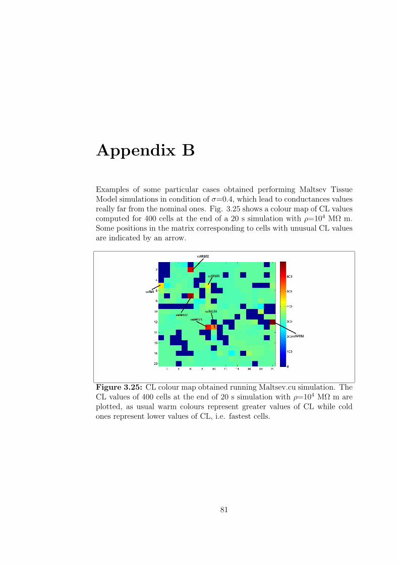
Appendix B
Examples of some particular cases obtained performing Maltsev TissueModel simulations in condition of σ=0.4, which lead to conductances valuesreally far from the nominal ones. Fig. 3.25 shows a colour map of CL valuescomputed for 400 cells at the end of a 20 s simulation with ρ=104 MΩ m.Some positions in the matrix corresponding to cells with unusual CL valuesare indicated by an arrow.
Figure 3.25: CL colour map obtained running Maltsev.cu simulation. TheCL values of 400 cells at the end of 20 s simulation with ρ=104 MΩ m areplotted, as usual warm colours represent greater values of CL while coldones represent lower values of CL, i.e. fastest cells.
81
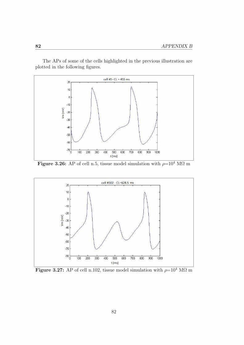
82 APPENDIX B
The APs of some of the cells highlighted in the previous illustration areplotted in the following figures.
Figure 3.26: AP of cell n.5, tissue model simulation with ρ=104 MΩ m
Figure 3.27: AP of cell n.102, tissue model simulation with ρ=104 MΩ m
82
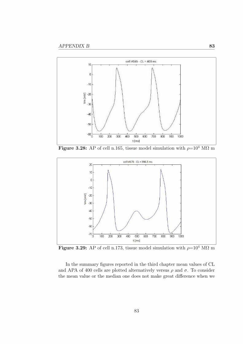
APPENDIX B 83
Figure 3.28: AP of cell n.165, tissue model simulation with ρ=104 MΩ m
Figure 3.29: AP of cell n.173, tissue model simulation with ρ=104 MΩ m
In the summary figures reported in the third chapter mean values of CLand APA of 400 cells are plotted alternatively versus ρ and σ. To considerthe mean value or the median one does not make great difference when we
83

84 APPENDIX B
Figure 3.30: AP of cell n.193, tissue model simulation with ρ=104 MΩ m
Figure 3.31: Mean, median and post-processing values of CL versus ρ.The condition σ=0.4 is considered. In the condition ρ=104 MΩ m, beforemodifying the CL array, it contained 75 CL values equal to 0 ms and 7CL values greater than 400 ms. The CL mean and median value (withoutpost-precessing) with ρ=104 MΩ m are respectively 264.32 ms and 317 ms.
84
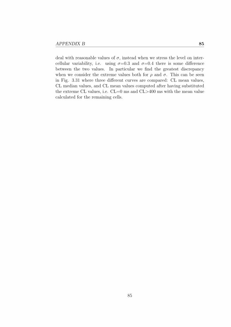
APPENDIX B 85
deal with reasonable values of σ, instead when we stress the level on inter-cellular variability, i.e. using σ=0.3 and σ=0.4 there is some differencebetween the two values. In particular we find the greatest discrepancywhen we consider the extreme values both for ρ and σ. This can be seenin Fig. 3.31 where three different curves are compared: CL mean values,CL median values, and CL mean values computed after having substitutedthe extreme CL values, i.e. CL=0 ms and CL>400 ms with the mean valuecalculated for the remaining cells.
85
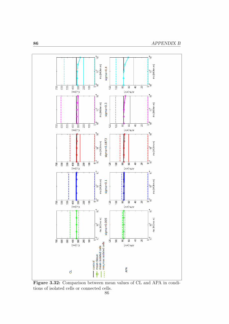
86 APPENDIX B
Figure 3.32: Comparison between mean values of CL and APA in condi-tions of isolated cells or connected cells.
86

Acknowledgments
I would like to express my sincere gratitude to Prof. Stefano Severi andProf. Eric Sobie for having offered me this exciting opportunity, for havingencouraged me during my work and most of all for having transmitted tome enthusiasm for research and for what I have been doing for my project.Thanks to Alan for his advices and for having lightened the worries of thelast days.
Thanks to my family for being always with me even when they have towait until 3 pm to wish me a good day.
Finally thanks to everyone I met in these six months, in particular Martaand Yasi, my favorite New Yorkers!
87

88 ACKNOWLEDGMENTS
88
Bibliography
[1] The cellml project. http://www.cellml.org/.
[2] Cuda programming guide. https://developer.nvidia.com/cuda-zone.
[3] Right atrium. http://successimg.com/right-atrial-anatomy/.
[4] Ionic Channels of Excitable Menbranes. Sinauer Associetes, 1992.
[5] CUDA by Example -An Introduction to General-Purpose GPU Pro-gramming. Addison - Wesley, 2010.
[6] N. H. Lovell A. A. Abed, T. Guo and S. Dokos. Optimisation of ionicmodels to fit tissue action potentials: Application to 3d atrial mod-elling. Computational and Mathematical Methods in Medicine, 2013.
[7] T. Guo N.H. Lovell S. Dokos A.D. Bradd, A.A. Abed. Study of cardiacpacemaker excitation using generic ionic models and realistic cell dis-tribution. In 34th Annual International Conference of the IEEE EMBSSan Diego, California USA.
[8] NVIDIA Corporation. Cuda c/c++ basics.
[9] E.P Matyas D.C Michaels and J. Jalife. Dynamic interactions and mu-tual synchronization of sinoatrial node pacemaker cells. a mathematicalmodel. Circulation Research, 1986.
[10] E.P Matyas D.C Michaels and J.Jalife. Mechanisms of sinoatrial pace-maker synchronization: a new hypothesis. Circulation Research, 1987.
[11] A.C. van Ginneken J. Bourier M.W. Markman et al. E.E. Verheijck,A. Wessels. Distribution of atrial and nodal cells within the rabbitsinoatrial node: models of sinoatrial transition. Circulation, 1998.
89
90 BIBLIOGRAPHY
[12] A.C. van Ginneken J. Bourier W.M. Markman L.M. Vermeulen J.M. deBakker W.H. Lamers T. Opthof L.N. Bouman E.E. Verheijck, A. Wes-sels. Distribution of atrial and nodal cells within the rabbit sinoatrialnode. Circulation, 1998.
[13] M. Fantini. Un nuovo modello di potenziale d’azione del nodo senoa-triale. Bachelor’s thesis, Biomedical Engineering, 2009.
[14] A. Giovannini. Parametric sensitivity analysis of the most recent com-putational models of rabbit cardiac pacemaking. Bachelor’s thesis,Biomedical Engineering, 2012.
[15] J.R. Giudicessi and M.J. Ackerman. Potassium channel mutations andcardiac arrhythmias diagnosis and therapy. Nature Reviews Cardiology,2012.
[16] Y. Okada H. Masumiya, Y. Oku. Inhomogeneous distribution of ac-tion potential characteristics in the rabbit sino-atrial node revealed byvoltage imaging. Journal of Physiological Sciences, 59:227–241, March2009.
[17] I. Kodama H. Honjo M. Lei T. Varghese H. Zhang, A. V. Holden andM. R. Boyett. Mathematical models of action potentials in the periph-ery and center of the rabbit sinoatrial node. Am J Physiol Heart CircPhysiol, 279:397–421, 2000.
[18] R.S. Kass J.M. Nerbonne. Molecular physiology of cardiac repolariza-tion. Physiological Reviews, 2005.
[19] H. Irisawa K. Yanagihara, A. Noma. Reconstruction of sino-atrial nodepacemaker potential based on the voltage clamp experiments. Jpn JPhysiol, 1980.
[20] J. Keener and J. Sneyd. Mathematical Physiology. Springer, ii edition,2009.
[21] R.E. Klabunde. Cardiovascular physiology concepts,2011.
[22] E.G. Lakatta and D. DiFrancesco. What keeps us ticking: a funnycurrent, a calcium clock, or both? Journal of Molecular and CellularCardiology., 2009.
90
BIBLIOGRAPHY 91
[23] D. Difrancesco M. Baruscotti, A. Bucchi. Physiology and pharmacol-ogy of the cardiac pacemaker (”funny”) current. Pharmacology andTherapeutics, 2005.
[24] Robert M.Berne, Matthew N.Levy, Bruce M.Kocppen, and BruceA.Stanton. Fisiologia. Casa Editrice Ambrosiana, iv edition, 2010.
[25] W. Ying M.L. Hubbard and C.S. Henriquez. Effect of gap junctiondistribution on impulse propagation in a monolayer of myocytes: amodel study. Europace, 2007.
[26] I. Kodamab M.R. Boyetta, H. Honjob. The sinoatrial node, a hetero-geneous pacemaker structure. Cardiovascular Research, 2000.
[27] M.D. Munther Homoud. Introduction to cardiovascular pathophysiol-ogy. lectures,.
[28] R. Oren and C. Clancy. Determinants of heterogeneity, excitation andconduction in the sinoatrial node: A model study. PLoS ComputationalBiology, 6, December 2010.
[29] M.M. Maleckar P. Li, T.G. Lines and A. Tveito. Mathematical modelsof cardiac pacemaking function. Frontiers in Physics, 2013.
[30] N. H. Lovell S. L. Cloherty, S. Dokos. A comparison of 1-d mod-els of cardiac pacemaker heterogeneity. IEEE TRANSACTIONS ONBIOMEDICAL ENGINEERING, 53(2), February 2006.
[31] L.A. Charawi S. Severi, M. Fantini and D. DiFrancesco. An updatedcomputational model of rabbit sinoatrial action potential to investigatethe mechanisms of heart rate modulation. The Journal of Physiology,2012.
[32] R.M. Wolf S.D. Unudurthi1 and T.J. Hund. Role of sinoatrial node ar-chitecture in maintaining a balanced source-sink relationship and syn-chronous cardiac pacemaking. Frontiers in Physiology, November 2014.
[33] E. A. Sobie. Parameter sensitivity analysis in electrophysiological mod-els using multivariable regression. Biophysical Journal, 96:1264–1274,February 2009.
91
92 BIBLIOGRAPHY
[34] E.A. Sobie. Anisotropic electrical propagation in heart.
[35] E.G. Lakatta V.A. Maltsev. Synergism of coupled subsarcolemmalca2+ clocks and sarcolemmal voltage clocks confers robust and flexiblepacemaker function in a novel pacemaker cell model. Am J PhysiolHeart Circ Physiol., 2009.
92