
UNIVERSITÀ DEGLI STUDI DI NAPOLI FEDERICO II … · knowledge on the dynamic behaviour of the...
203
UNIVERSITÀ DEGLI STUDI DI NAPOLI FEDERICO II POLO DELLE SCIENZE E DELLE TECNOLOGIE DOTTORATO DI RICERCA IN RISCHIO SISMICO XXI CICLO PERFORMANCE-BASED APPROACH IN SEISMIC DESIGN OF EMBEDDED RETAINING WALLS TESI PER IL CONSEGUIMENTO DEL TITOLO CIRO VISONE NAPOLI, NOVEMBRE 2008 RELATORE PROF. FILIPPO SANTUCCI DE MAGISTRIS COORDINATORE DEL DOTTORATO PROF. PAOLO GASPARINI
Transcript of UNIVERSITÀ DEGLI STUDI DI NAPOLI FEDERICO II … · knowledge on the dynamic behaviour of the...
UNIVERSITÀ DEGLI STUDI DI NAPOLI FEDERICO II POLO DELLE SCIENZE E DELLE TECNOLOGIE DOTTORATO DI RICERCA IN RISCHIO SISMICO XXI CICLO
PERFORMANCE-BASED APPROACH IN SEISMIC DESIGN OF
EMBEDDED RETAINING WALLS
TESI PER IL CONSEGUIMENTO DEL TITOLO
CIRO VISONE
NAPOLI, NOVEMBRE 2008
RELATORE
PROF. FILIPPO SANTUCCI DE MAGISTRIS COORDINATORE DEL DOTTORATO
PROF. PAOLO GASPARINI
UNIVERSITÀ DEGLI STUDI DI NAPOLI FEDERICO II
PERFORMANCE-BASED APPROACH IN SEISMIC DESIGN OF
EMBEDDED RETAINING WALLS
CIRO VISONE
A dissertation submitted for the Degree of Doctor of Philosophy
at University of Napoli Federico II, Italy Napoli, November 2008

To my wife
ABSTRACT
The increasing use of the underground spaces and the last seismic events in the
urban areas have driven many researchers of different countries to deepen the
knowledge on the dynamic behaviour of the structure embedded in the subsoil.
This thesis attempts to give some contributes on the application of the performance
based approach for the seismic design of the embedded retaining walls.
After an overview on the earth pressure theories proposed by different authors, the
static and seismic design methods commonly adopted in the current practice and
based on pseudostatic approaches are recalled.
Several limitations on these procedures can be recognized: the difficulties on the
definition of the seismic coefficient; the calculation of the expected earthquake-
induced displacements around the construction. Moreover, in the framework of the
Performance-Based Design, these methods do not able to describe the response of
the retaining systems to a given earthquake. The seismic displacements of the
flexible walls are evaluated by means of Newmark sliding block procedures, that
were developed for rigid structures, and the yield sequence of the different structural
components can not be predicted. Then, the application of the hierarchical resistance
criteria in the dimensioning of the various parts can not be applied.
In this thesis, different level of analysis are highlighted in relation to the importance of
the structure and to the design phase.
An innovative procedure that can be included in the framework of the "pushover
analyses" is also proposed for the seismic design of the embedded retaining walls.
Finally, the results obtained by the application of the different methods for the ideal
case study of cantilever diaphragms embedded in dry loose and dense sand are
presented. The material properties used in the analyses are referred to the Fraction
E (BS 100/170) of the Leighton Buzzard sand, for which a series of triaxial and
torsional tests on reconstituted samples was conducted.
Ciro Visone – Performance-Based approach in seismic design of embedded retaining walls 1
INDEX
1 INTRODUCTION. ....................................................................................................................1-1 2 GENERALITIES OF RETAINING WALLS...............................................................................2-1
2.1 TYPES OF RETAINING WALLS................................................................................................... 2-1 2.2 TYPES OF RETAINING WALL FAILURES. ................................................................................. 2-2 2.3 ULTIMATE LIMIT STATES FOR RETAINING WALLS. ................................................................ 2-3 2.4 EMBEDDED WALLS: TYPES AND USES. .................................................................................. 2-6
2.4.1 Sheet pile walls. ........................................................................................................................................... 2-6 2.4.2 Bulkheads. ................................................................................................................................................... 2-9 2.4.3 Walls with many anchor levels and props. ................................................................................................. 2-11
3 EARTH PRESSURE THEORY................................................................................................3-1 3.1 STATIC PRESSURES ON RETAINING WALLS. ......................................................................... 3-1
3.1.1 Rankine theory. ............................................................................................................................................ 3-2 3.1.2 Coulomb theory............................................................................................................................................ 3-4 3.1.3 Logarithmic spiral method. ........................................................................................................................... 3-6 3.1.4 Slip line method............................................................................................................................................ 3-8 3.1.5 Limit analysis methods............................................................................................................................... 3-10 3.1.6 Comparisons between the different static methods. .................................................................................. 3-14
3.2 SEISMIC PRESSURES ON RETAINING WALLS. ..................................................................... 3-18 3.2.1 Mononobe-Okabe theory. .......................................................................................................................... 3-18 3.2.2 Limit analysis methods............................................................................................................................... 3-25 3.2.3 Comparisons between the different seismic methods. .............................................................................. 3-31
3.3 EFFECTS OF WATER ON WALL PRESSURES........................................................................ 3-34 3.3.1 Water outboard of wall. .............................................................................................................................. 3-34 3.3.2 Water in backfill.......................................................................................................................................... 3-35
4 STATIC DESIGN OF EMBEDDED RETAINING WALLS........................................................4-1 4.1 FREE CANTILEVER WALLS........................................................................................................ 4-1 4.2 ANCHORED SHEET-PILE WALLS. ............................................................................................. 4-7
4.2.1 Free earth support method........................................................................................................................... 4-8 4.2.2 Fixed earth support method. ...................................................................................................................... 4-10
5 SEISMIC DESIGN OF EMBEDDED RETAINING WALLS......................................................5-1 5.1 EARTHQUAKE PROVISIONS DESCRIBED IN EUROPEAN AND ITALIAN BUILDING CODES.5-1 5.2 PERFORMANCE-BASED DESIGN METHODOLOGY AND DAMAGE CRITERIA. ..................... 5-5 5.3 SEISMIC ANALYSIS OF EMBEDDED RETAINING WALLS........................................................ 5-9
5.3.1 Type of analysis. .......................................................................................................................................... 5-9 5.3.2 Simplified analysis...................................................................................................................................... 5-10 5.3.3 Simplified dynamic analysis. ...................................................................................................................... 5-20 5.3.4 Pushover analysis. ..................................................................................................................................... 5-22 5.3.5 Dynamic analysis. ...................................................................................................................................... 5-23
6 CASE STUDY: CANTILEVER DIAPHRAGMS EMBEDDED IN DRY LOOSE AND DENSE SAND
LAYERS. ..........................................................................................................................................6-1 6.1 DESCRIPTION OF THE EXAMINED PROBLEMS....................................................................... 6-1
6.1.1 Geometries................................................................................................................................................... 6-1 6.1.2 Soil properties. ............................................................................................................................................. 6-2 6.1.3 Diaphragms properties................................................................................................................................. 6-3
Ciro Visone – Performance-Based approach in seismic design of embedded retaining walls 2
6.1.4 Seismic input motions. ................................................................................................................................. 6-4 6.1.5 Analyses program. ....................................................................................................................................... 6-5
6.2 SIMPLIFIED ANALYSES. ............................................................................................................. 6-6 6.3 SIMPLIFIED DYNAMIC ANALYSES............................................................................................. 6-7
6.3.1 Pseudostatic analyses. ................................................................................................................................ 6-7 6.3.2 Free field motions......................................................................................................................................... 6-8 6.3.3 Pseudodynamic analyses: Newmark sliding block analyses. .................................................................... 6-16
6.4 PUSHOVER ANALYSES............................................................................................................ 6-17 6.4.1 Finite element modelling. ........................................................................................................................... 6-17 6.4.2 Configurations at the end of excavation..................................................................................................... 6-19 6.4.3 Pseudostatic loadings. ............................................................................................................................... 6-22
6.5 DYNAMIC ANALYSES. .............................................................................................................. 6-28 6.5.1 Maximum acceleration profiles................................................................................................................... 6-29 6.5.2 Displacement time histories. ...................................................................................................................... 6-29 6.5.3 Configurations at the end of the earthquakes. ........................................................................................... 6-34 6.5.4 Configurations at the instants of maximum bending moment. ................................................................... 6-38
6.6 COMPARISONS BETWEEN THE RESULTS OF DIFFERENT ANALYSES.............................. 6-44 7 CONCLUSIONS AND FUTURE DEVELOPMENTS. ..............................................................7-1 REFERENCES...................................................................................................................................... ANNEX A - MECHANICAL BEHAVIOUR OF LEIGHTON BUZZARD SAND 100/170 BY MEANS
OF LABORATORY TESTS. .................................................................................................................. ANNEX B - CALIBRATION OF FE MODELS FOR DYNAMIC ANALYSES IN GEOTECHNICAL
EARTHQUAKE ENGINEERING. ..........................................................................................................

Ciro Visone – Performance-Based approach in seismic design of embedded retaining walls 3
LIST OF FIGURES
Figure 1-1. Geometry and equipments of the dynamic centrifuge tests in ReLUIS experimental
program: a) cantilever diaphragms; b) propped diaphragms. .............................................................. 1-2 Figure 1-2. Plan view of the monitored piles of "Casa dello Studente" (CB – Italy)............................. 1-4 Figure 1-3. Plan view of “Casa dello Studente” building foundations and monitored sheet pile wall. 1-4 Figure 1-4. Sketch of piles instrumentation: a) vertical position of the sensors; b) and c) details of piles
head and sensor housing; d) layout of intermediate enclosures.......................................................... 1-5 Figure 2-1. Common types of earth retaining structures...................................................................... 2-1 Figure 2-2. Examples of limit modes for overall stability of retaining structures. ................................. 2-4 Figure 2-3. Examples of limit modes for foundation failures of gravity walls. ...................................... 2-4 Figure 2-4. Examples of limit modes for vertical failure of embedded walls. ....................................... 2-4 Figure 2-5. Examples of limit modes for rotational failures of embedded walls. .................................. 2-5 Figure 2-6. Examples of limit modes for structural failure of retaining structures. ............................... 2-5 Figure 2-7. Examples of limit modes for failure by pullout of anchors. ................................................ 2-6 Figure 2-8. Elements for sheet piles walls: a) reinforced concrete; b) steel. ....................................... 2-7 Figure 2-9. Examples of anchored sheet walls: a) quay wall with a single level of anchors; b) sheet
walls with multiple anchors levels; c) injected bulb anchor; d) raking anchor; e) anchor with stand piles.
.............................................................................................................................................................. 2-9 Figure 2-10. Realization of a reinforced concrete diaphragm (Leiper, 1984). ................................... 2-10 Figure 3-1. Utilized symbols for the geometry of the problem. ............................................................ 3-1 Figure 3-2. Rankine active and passive earth pressure coefficients for a horizontal backfill. ............. 3-3 Figure 3-3. Coulomb active and passive earth pressure coefficients for a horizontal backfill sustained
by a vertical wall. .................................................................................................................................. 3-5 Figure 3-4. Critical planar failure surface for a horizontal backfill sustained by a vertical wall. ........... 3-6 Figure 3-5. Logarithmic spiral representation of the critical failure surface for: a) minimum active
pressure conditions; b) maximum passive pressure conditions........................................................... 3-7 Figure 3-6. Active and passive earth pressure coefficients for a horizontal backfill sustained by a
vertical wall (after Caquot & Kerisel, 1948). ......................................................................................... 3-8 Figure 3-7. Active and passive earth pressure coefficients for a horizontal backfill sustained by a
vertical wall using slip line method (Sokolovskii, 1965). ...................................................................... 3-9 Figure 3-8. Log-sandwich failure mechanisms for lateral earth pressure limit analysis (modified after
Chen & Rosenfarb, 1973)................................................................................................................... 3-11 Figure 3-9. Active and passive earth pressure coefficients for a horizontal backfill sustained by a
vertical wall (Chen & Liu, 1990).......................................................................................................... 3-13 Figure 3-10. Active and passive earth pressure coefficients for a horizontal backfill sustained by a
vertical wall (Lancellotta, 2002). ......................................................................................................... 3-14 Figure 3-11. Comparisons between the normal components of the active earth pressure coefficient
given by the various methods for a horizontal backfill sustained by a smooth vertical wall (δ=0). .... 3-15 Figure 3-12. Comparisons between the normal components of the active earth pressure coefficient
given by the various methods for a horizontal backfill sustained by a rough vertical wall (δ=φ)........ 3-16
Ciro Visone – Performance-Based approach in seismic design of embedded retaining walls 4
Figure 3-13. Comparisons between the normal components of the passive earth pressure coefficient
given by the various methods for a horizontal backfill sustained by a smooth vertical wall (δ=0). .... 3-16 Figure 3-14. Comparisons between the normal components of the passive earth pressure coefficient
given by the various methods for a horizontal backfill sustained by a rough vertical wall (δ=φ)........ 3-17 Figure 3-15. Seismic active earth pressure coefficients for a horizontal backfill sustained by vertical
walls (Mononobe-Okabe method): a) δ=0; b) δ=φ/2; c) δ=φ............................................................... 3-21 Figure 3-16. Critical failure surfaces in seismic active conditions for a horizontal backfill sustained by
vertical walls (Mononobe-Okabe method): a) δ=0; b) δ=φ/2; c) δ=φ. ................................................. 3-22 Figure 3-17. Seismic passive earth pressure coefficients for a horizontal backfill sustained by vertical
walls (Mononobe-Okabe method): a) δ=0; b) δ=φ/2; c) δ=φ............................................................... 3-23 Figure 3-18. Critical failure surfaces in seismic passive conditions for a horizontal backfill sustained by
vertical walls (Mononobe-Okabe method): a) δ=0; b) δ=φ/2; c) δ=φ. ................................................. 3-24 Figure 3-19. Seismic active earth pressure coefficients for a horizontal backfill sustained by vertical
walls (Chang, 1981, as quoted by Chen & Liu, 1990): a) δ=0; b) δ=φ/2; c) δ=φ. ............................... 3-27 Figure 3-20. Seismic passive earth pressure coefficients for a horizontal backfill sustained by vertical
walls (Chang, 1981, as quoted by Chen & Liu, 1990): a) δ=0; b) δ=φ/2; c) δ=φ. ............................... 3-28 Figure 3-21. Seismic passive earth pressure coefficients for a horizontal backfill sustained by vertical
walls (Lancellotta, 2007): a) δ=0; b) δ=φ/2; c) δ=φ. ............................................................................ 3-30 Figure 3-22. Comparisons between the normal components of the active earth pressure coefficients
given by the various methods for horizontal backfills sustained by vertical walls: a) δ=0; b) δ=φ/2; c)
δ=φ...................................................................................................................................................... 3-32 Figure 3-23. Comparisons between the normal components of the passive earth pressure coefficients
given by the various methods for horizontal backfills sustained by vertical walls: a) δ=0; b) δ=φ/2; c)
δ=φ...................................................................................................................................................... 3-33 Figure 3-24. Geometry and notation for partially submerged backfill. ............................................... 3-36 Figure 4-1. Soil pressure distributions on an embedded cantilever wall: a) pressure distributions; b) net
pressure distribution. ............................................................................................................................ 4-2 Figure 4-2. Theoretical earth pressures distributions assumed in limit equilibrium methods. ............. 4-2 Figure 4-3. Simplified earth pressures distributions: a) Full Method; b) Blum Method. ....................... 4-3 Figure 4-4. Experimental and numerical limit depth ratios of embedment at collapse for free embedded
walls...................................................................................................................................................... 4-4 Figure 4-5. Limit depth ratios of embedment at collapse for free embedded walls computed with limit
equilibrium methods. ............................................................................................................................ 4-5 Figure 4-6. Experimental and numerical normalized maximum bending moment for free embedded
walls...................................................................................................................................................... 4-6 Figure 4-7. Normalized maximum bending moment for free embedded walls at collapse computed with
limit equilibrium method........................................................................................................................ 4-7 Figure 4-8. General layout and limit earth pressure distributions for anchored sheet pile wall. .......... 4-8 Figure 4-9. Moment reduction factors proposed by Rowe (1952)...................................................... 4-10 Figure 4-10. Design of anchored sheet pile by the fixed earth support method. ............................... 4-11
Ciro Visone – Performance-Based approach in seismic design of embedded retaining walls 5
Figure 5-1. Mononobe-Okabe wedge interacting with harmonic wave characterized by: a) large
wavelength; b) small wavelength. ........................................................................................................ 5-3 Figure 5-2. Influence of the ratio between the height of the wall H and the wavelength λ of a harmonic
wave on the seismic active earth pressure coefficient (Steedman & Zeng, 1990). ............................. 5-3 Figure 5-3. Diagram for the evaluation of the deformability factor α (NTC, 2008). .............................. 5-4 Figure 5-4. Diagram for the evaluation of displacements factor β (NTC, 2008). ................................. 5-5 Figure 5-5. Parameters for specifying damage criteria: a) respect to displacements; b) respect to
stresses (PIANC, 2001)........................................................................................................................ 5-6 Figure 5-6. Preferred sequence for yield of sheet pile wall (PIANC, 2001). ........................................ 5-7 Figure 5-7. Seismic earth pressures acting on a free embedded wall according to Italian Building code
(NTC, 2008) for a pseudo-static analysis adopting the Blum method................................................ 5-12 Figure 5-8. Limit depth ratio of embedment computed by the Blum method in seismic conditions of a
free embedded wall. ........................................................................................................................... 5-13 Figure 5-9. Normalized maximum bending moment computed by the Blum method in seismic
conditions of a free embedded wall.................................................................................................... 5-13 Figure 5-10. a) Geometry and notation for evaluation of anchored bulkhead design; b) Correlation
between damage levels and dimensionless anchored bulkhead indices. After Gazetas et al. (1990).
Empirical design method for waterfront anchored sheet pile walls, Design and Performance of Earth
Retaining Structures (ASCE).............................................................................................................. 5-17 Figure 5-11. Normalized horizontal displacements correlated with thickness of loose soil deposit below
the wall (after Iai et al., 1998). ............................................................................................................ 5-20 Figure 5-12. Sketch of numerical models able to minimize the reflected waves on lateral boundaries. 5-
32 Figure 6-1. Geometry of the examined problem. ................................................................................. 6-1 Figure 6-2. Shear wave velocity (a) and damping ratio (b) profiles for loose (Dr = 20%) and dense (Dr
= 80%) LB sand layers. ........................................................................................................................ 6-2 Figure 6-3. Assumed decay curves of the LB sandy layers, both for loose and dense state. ............. 6-3 Figure 6-4. TMZ-270 Seismic input signal: a) acceleration time-history; b) Fourier spectrum. ........... 6-5 Figure 6-5. STU-270 Seismic input signal: a) acceleration time-history; b) Fourier spectrum............. 6-5 Figure 6-6. Shear wave velocity (a) and damping ratio (b) profiles for loose (Dr = 20%) and dense (Dr
= 80%) LB sand layers adopted in the linear frequency domain analyses. ....................................... 6-10 Figure 6-7. Rayleigh α (a) and β (b) damping parameters profiles for loose (Dr = 20%) and dense (Dr =
80%) LB sand layers adopted in the time domain analyses. ............................................................. 6-10 Figure 6-8. Comparisons between the linear time (TDA) and frequency (FDA) domain analyses in
terms of amplification functions of the loose (a) and the dense (b) sand layers................................ 6-11 Figure 6-9. Maximum acceleration profiles computed by the linear analyses for loose sand layer: a)
TMZ-270 input motion; b) STU-270 input motion............................................................................... 6-12 Figure 6-10. Maximum acceleration profiles computed by the linear analyses for dense sand layer: a)
TMZ-270 input motion; b) STU-270 input motion............................................................................... 6-12 Figure 6-11. Decay curves of loose and dense sand adopted in the site response analyses. .......... 6-13
Ciro Visone – Performance-Based approach in seismic design of embedded retaining walls 6
Figure 6-12. Comparisons between the calculated free field motions for loose sand layer: a) response
spectrum at surface for TMZ-270; b) response spectra at surface for STU-270; c) maximum
acceleration profiles for TMZ-270; d) maximum acceleration profiles for STU-270........................... 6-14 Figure 6-13. Comparisons between the calculated free field motions for dense sand layer: a) response
spectrum at surface for TMZ-270; b) response spectra at surface for STU-270; c) maximum
acceleration profiles for TMZ-270; d) maximum acceleration profiles for STU-270........................... 6-15 Figure 6-14. Sketch of the FE models used in the pushover analyses.............................................. 6-19 Figure 6-15. Interface stresses (a) and bending moment (b) on walls in loose sand at the end of
excavation. ......................................................................................................................................... 6-20 Figure 6-16. Interface stresses (a) and bending moment (b) on walls in dense sand at the end of
excavation. ......................................................................................................................................... 6-20 Figure 6-17. Horizontal displacements of the walls at the end of excavation: a) loose sand, s = 0.60m;
b) loose sand, s = 1.00m; c) dense sand, s = 0.60m; d) dense sand, s = 1.00m .............................. 6-21 Figure 6-18. Shading of horizontal displacements at the end of excavation (loose sand, s = 0.60m). . 6-
22 Figure 6-19. Sketch of the FE models used in the pushover analyses: a) triangular loading distribution,
TRD; b) rectangular loading distribution, RTD. .................................................................................. 6-22 Figure 6-20. Seismic capacities of the diaphragms in terms of normalized horizontal displacements: a)
loose sand, s = 0.60m; b) loose sand, s = 1.00m; c) dense sand, s = 0.60m; d) dense sand, s = 1.00m
............................................................................................................................................................ 6-24 Figure 6-21. Seismic capacities of the diaphragms in terms of normalized vertical displacements: a)
loose sand, s = 0.60m; b) loose sand, s = 1.00m; c) dense sand, s = 0.60m; d) dense sand, s = 1.00m
............................................................................................................................................................ 6-25 Figure 6-22. Seismic capacities of the diaphragms in terms of normalized maximum bending moment:
a) loose sand, s = 0.60m; b) loose sand, s = 1.00m; c) dense sand, s = 0.60m; d) dense sand, s =
1.00m.................................................................................................................................................. 6-26 Figure 6-23. Development of the maximum bending moments with the horizontal displacements: a)
loose sand, s = 0.60m; b) loose sand, s = 1.00m; c) dense sand, s = 0.60m; d) dense sand, s = 1.00m
............................................................................................................................................................ 6-27 Figure 6-24. Comparisons between the seismic behaviours of the two walls predicted by the pushover
analyses: a) HAIP; b) TRD; c) RTD. .................................................................................................. 6-28 Figure 6-25. Sketch of the FE models used in the dynamic analyses. .............................................. 6-29 Figure 6-26. Comparisons between the maximum acceleration profiles of the free field motions and
the dynamic interactions with the walls: a) Loose sand, TMZ-270; b) Loose sand STU-270; c) Dense
sand, TMZ-270; d) Dense sand, STU-270. ........................................................................................ 6-30 Figure 6-27. Time histories of the normalized horizontal displacements at the top of the walls: a)
Loose sand, TMZ—270; b) Loose sand, STU-270; c) Dense sand, TMZ-270; Dense sand, STU-270. 6-
31 Figure 6-28. Comparisons between the normalized horizontal displacements at the top of the walls in
loose sand predicted by Newmark and dynamic interaction analyses: a) L060TMZ; b) L060STU; c)
L100TMZ; L100STU. .......................................................................................................................... 6-32

Ciro Visone – Performance-Based approach in seismic design of embedded retaining walls 7
Figure 6-29. Comparisons between the normalized horizontal displacements at the top of the walls in
dense sand predicted by Newmark and dynamic interaction analyses: a) D060TMZ; b) D060STU; c)
D100TMZ; D100STU.......................................................................................................................... 6-33 Figure 6-30. Normal and net interface stresses acting on the walls in loose (a, b) and dense (c, d) at
the end of earthquakes....................................................................................................................... 6-34 Figure 6-31. Numerical active and passive earth pressure coefficients for walls in loose (a, b) and
dense (c, d) sand at the end of earthquakes...................................................................................... 6-35 Figure 6-32. Shear forces and bending moments acting on walls in loose (a, b) and dense (c, d) sand
at the end of earthquakes................................................................................................................... 6-36 Figure 6-33. Horizontal displacements of the walls in loose (a) and dense (b) sand at the end of
earthquakes........................................................................................................................................ 6-37 Figure 6-34. Normal and net interface stresses acting on the walls in loose (a, b) and dense (c, d) at
the instants of maximum bending moment. ....................................................................................... 6-38 Figure 6-35. Numerical active and passive earth pressure coefficients for walls in loose (a, b) and
dense (c, d) sand at the instants of maximum bending moment. ...................................................... 6-39 Figure 6-36. Shear forces and bending moments acting on walls in loose (a, b) and dense (c, d) sand
at the instants of maximum bending moment. ................................................................................... 6-40 Figure 6-37. Horizontal displacements of the walls in loose (a) and dense (b) sand at the instants of
maximum bending moment. ............................................................................................................... 6-41 Figure 6-38. Instants of maximum bending moment in relation to the earthquake-induced
displacements of walls in loose sand: a) L060TMZ; b) L060STU; c) L100TMZ; L100STU. .............. 6-42 Figure 6-39. Instants of maximum bending moment in relation to the earthquake-induced
displacements of walls in dense sand: a) D060TMZ; b) D060STU; c) D100TMZ; D100STU. .......... 6-43
Ciro Visone – Performance-Based approach in seismic design of embedded retaining walls 8
LIST OF TABLES
Table 3-1. Values of the active earth pressure coefficient for log-spiral failure surface (after Caquot &
Kerisel, 1948). ...................................................................................................................................... 3-7 Table 3-2. Values of the passive earth pressure coefficient for log-spiral failure surface (after Caquot &
Kerisel, 1948). ...................................................................................................................................... 3-8 Table 3-3. Values of the active earth pressure coefficient calculated by Sokolovskii (1965) with the slip
line method. .......................................................................................................................................... 3-9 Table 3-4. Values of the passive earth pressure coefficient calculated by Sokolovskii (1965) with the
slip line method. ................................................................................................................................... 3-9 Table 3-5. Values of the active earth pressure coefficient given by the upper-bound method for log-
sandwich failure mechanisms (Chen & Liu, 1990). ............................................................................ 3-12 Table 3-6. Values of the passive earth pressure coefficient given by the upper-bound method for log-
sandwich failure mechanisms (Chen & Liu, 1990). ............................................................................ 3-12 Table 3-7. Values of the seismic active earth pressure coefficient given by the upper-bound method for
log-sandwich failure mechanisms (Chang, 1981 as quoted by Chen & Liu, 1990). .......................... 3-26 Table 3-8. Values of the seismic passive earth pressure coefficient given by the upper-bound method
for log-sandwich failure mechanisms (Chang, 1981 as quoted by Chen & Liu, 1990). ..................... 3-26 Table 4-1. Relationship between the depth to the point of the sheet pile contraflexure (y) and the free
height of the wall (h) (Blum, 1931, as quoted in Clayton et al. 1993). ............................................... 4-11 Table 5-1. Damage criteria for sheet pile wall (adapted from PIANC, 2001). ...................................... 5-8 Table 5-2. Inputs and outputs of analyses (adapted from PIANC, 2001). ......................................... 5-10 Table 5-3. Mean and standard deviation values for gravity walls displacement analysis (after Whitman
& Liao, 1985). ..................................................................................................................................... 5-15 Table 5-4. Qualitative and quantitative descriptions of reported degrees of damage to anchored
bulkhead during earthquakes (Gazetas et al., 1990). ........................................................................ 5-18 Table 5-5. Case histories of seismic performance of retaining walls at liquefied sites (PIANC, 2001). 5-
19 Table 5-6. Normalized horizontal displacements of anchored sheet pile walls at liquefied sites during
design level earthquake motion (PIANC, 2001). ................................................................................ 5-20 Table 5-7. Summary of Newmark's family integration methods......................................................... 5-28 Table 6-1. Physical and mechanical parameters of LB sand layers. ................................................... 6-2 Table 6-2. Analyses program. .............................................................................................................. 6-5 Table 6-3. Seismic capacities of the retaining walls predicted by the pseudostatic limit equilibrium
method.................................................................................................................................................. 6-6 Table 6-4. Seismic performances of the retaining walls predicted by the simplified analyses. ........... 6-7 Table 6-5. Seismic capacities of the retaining walls predicted by the pseudostatic limit equilibrium
method considering the inertia forces due to the wall masses. ........................................................... 6-8 Table 6-6. Seismic performances of the retaining walls predicted by the simplified analyses accounting
for the wall weight................................................................................................................................. 6-8
Ciro Visone – Performance-Based approach in seismic design of embedded retaining walls 9
Table 6-7. Natural frequencies of the LB sandy layers obtained by means of linear frequency domain
analyses. ............................................................................................................................................ 6-10 Table 6-8. Seismic performances of the retaining walls predicted by the simplified dynamic analyses.6-
16 Table 6-9. Seismic performances of the retaining walls predicted by the simplified dynamic analyses
accounting for the wall weight. ........................................................................................................... 6-16 Table 6-10. MC model parameters of loose sand layers. .................................................................. 6-18 Table 6-11. MC model parameters of dense sand layers. ................................................................. 6-18 Table 6-12. Elastic properties of plates. ............................................................................................. 6-19 Table 6-13. Seismic performances of the walls predicted by the dynamic interaction analyses. ...... 6-37 Table 6-14. Comparisons between the seismic performances of the walls predicted by the different
analyses. ............................................................................................................................................ 6-45
Chapter 1 – Introduction
Ciro Visone – Performance-Based approach in seismic design of embedded retaining walls 1-1
1 INTRODUCTION.
In the last decades, for the shortage of shallow spaces and for the difficulties connected to the tyre
transportation, it is attended to an increasing utilization of the urban subsoils for the realization of
transport infrastructures and many others civil engineering constructions. Underground lines have
been realized and are in construction in many important Italian cities, such as Milano, Roma, Napoli,
Torino. The train crossings of the High Velocity Train lines (TAV) are also under construction in the
cities of Bologna, Firenze, etc.. All of the Italian cities are interested to the realization of subway
parking and underpasses. The major part of these constructions have required or will require deep
excavations and tunnels that are often placed close to existing buildings. In many cases, the
structures pass near to the historical centres of the cities, where poor safety conditions for the existing
constructions can be recognized.
The availability of commercial codes, advanced constitutive models to describe the soil behaviour
when subjected to stress paths similar to those induced by the excavations, and the spread of suitable
laboratory ed in situ techniques have allowed more reliable the evaluation of the safety conditions and
the prediction of the behaviour of these types of structures during both the construction and the
serviceability phases. Furthermore, the monitoring of full scale constructions has permitted to evaluate
the reliability degree of simplified design methods, such as those based on the limit equilibrium, and to
develop empirical methods to predict the effects of excavations on the adjacent structures. Finally, the
introduction of the limit states design methods by using the partial factor of safety (EN1997-1), allows
evaluating the safety of the constructions for which can not be defined a single global factor of safety.
These progresses concern particularly the earth retaining structures in absence of seismic loadings.
The evaluation of the safety conditions of these structures in seismic areas has not reached the same
improvements. In these cases, the complex dynamic soil-structure interaction render the simplified
methods very difficult and unrealistic. The examinations can be performed by means of the
pseudostatic approaches based on the limit equilibrium only for simple cases, such as cantilever or
single-anchor retaining walls, and adopting conventional seismic coefficients that suffer to some
limitations for the fact that they were defined for structures over the ground. The recent European
codes (EN 1998-5) have tackled in a marginal manner the check of safety conditions of embedded
structures suggesting for the flexible retaining walls the use of seismic coefficients equal to the ratio
between the expected maximum acceleration in the site of interest and the gravity acceleration.
In this context, it becomes clear the necessity to improve the knowledge on the seismic behaviour of
the embedded retaining walls, especially to develop innovative seismic design methods able to give
good predictions in the practical applications.
On these basis, a research line (Linea 6 "Metodi Innovativi per il progetto delle opere geotecniche e la
valutazione della stabilità dei pendii") of the Consortium of the University Network of Seismic
Engineering Laboratories (ReLUIS, www.reluis.it) was devoted to develop and validate innovative
design methods for the earth retaining structures and tunnels placed in seismic areas.
The main activities of the ReLUIS research line are based on:
• physical modelling, by performing centrifuge tests on simplified scheme models;
Chapter 1 – Introduction
Ciro Visone - Performance-Based approach in seismic design of embedded retaining walls 1-2
• reference numerical modelling, by carrying out a series of indications on how to conduct
reliable dynamic analyses by using commercial codes;
• dynamic analyses on calibrated numerical models to highlight the main aspects of the seismic
soil-structure interaction;
• simplified analyses, that should be validated on the basis of the results of the physical
modelling and of the advanced dynamic analyses.
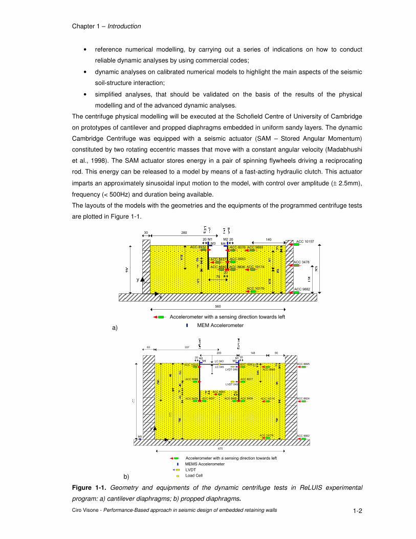
The centrifuge physical modelling will be executed at the Schofield Centre of University of Cambridge
on prototypes of cantilever and propped diaphragms embedded in uniform sandy layers. The dynamic
Cambridge Centrifuge was equipped with a seismic actuator (SAM – Stored Angular Momentum)
constituted by two rotating eccentric masses that move with a constant angular velocity (Madabhushi
et al., 1998). The SAM actuator stores energy in a pair of spinning flywheels driving a reciprocating
rod. This energy can be released to a model by means of a fast-acting hydraulic clutch. This actuator
imparts an approximately sinusoidal input motion to the model, with control over amplitude (± 2.5mm),
frequency (< 500Hz) and duration being available.
The layouts of the models with the geometries and the equipments of the programmed centrifuge tests
are plotted in Figure 1-1.
a)
b)
Figure 1-1. Geometry and equipments of the dynamic centrifuge tests in ReLUIS experimental
program: a) cantilever diaphragms; b) propped diaphragms.
90
20 20
675
ACC 10176
ACC 10174ACC 8836ACC 8880
ACC 8077
ACC 9889
ACC 1926
ACC 8883
ACC 8076
ACC 9882
ACC 8824
ACC 8895
M1M3M4
M2
200
337
ACC 10223
ACC 8837
ACC 8888
148
20
Accelerometer with a sensing direction towards left
MEMS Accelerometer
LVDT
LVDT 046
LVDT 049
M5
x
y
63
LC 045
LC 043
Load Cell
75
280
14020 20
20
560
ACC 10176
ACC 10174ACC 8836ACC 8880
ACC 8883
ACC 9889ACC 8076
ACC 8837
ACC 8932
ACC 9882
ACC 3478
ACC 10157M2
M4M3
M1
Accelerometer with a sensing direction towards left
MEM Accelerometer
30
x
y
Chapter 1 – Introduction
Ciro Visone – Performance-Based approach in seismic design of embedded retaining walls 1-3
The models will be prepared air-pluviating dry sand into the box till to reach the level of the wall base.
After the positioning of sensors and diaphragms, the sand will be also deposited to create the desired
geometry.
The tests on the cantilever walls will be conducted to an acceleration of 80g. At the prototype scale,
the centrifuge models will simulate a 4 meters high excavation retained by a vertical wall of 8m
embedded in dry sandy layers with a thick of 16m. The prototypes of the propped diaphragms are
constituted by a retained height of 5.60m with a depth of embedment of 2.40m into the sand. The
thickness of the soil layer is the same of cantilever prototypes. The tests will be performed to an
acceleration of 40g.
The material adopted for the centrifuge tests at the Schofield Centre is the Fraction E of the Leighton
Buzzard Sand for which an advanced characterization of the mechanical behaviour can not be found
in the literature.
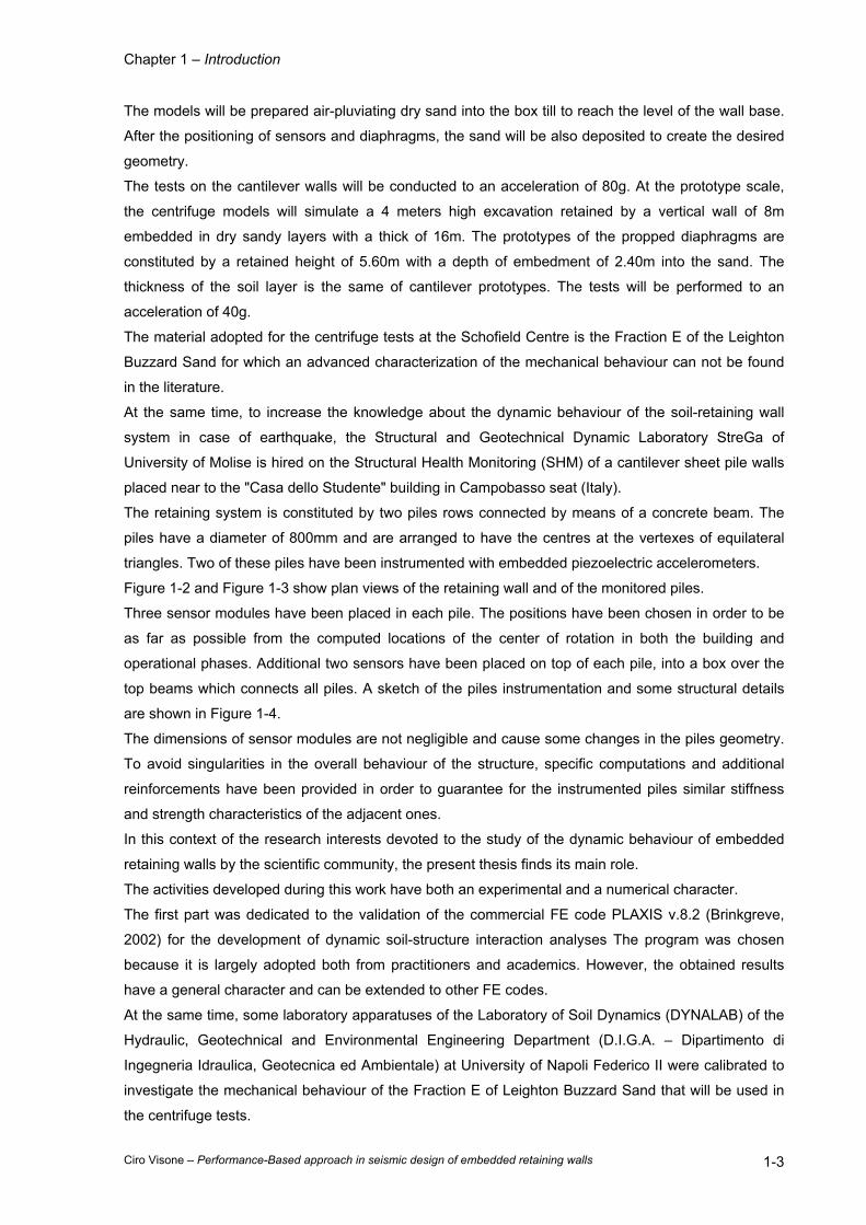
At the same time, to increase the knowledge about the dynamic behaviour of the soil-retaining wall
system in case of earthquake, the Structural and Geotechnical Dynamic Laboratory StreGa of
University of Molise is hired on the Structural Health Monitoring (SHM) of a cantilever sheet pile walls
placed near to the "Casa dello Studente" building in Campobasso seat (Italy).
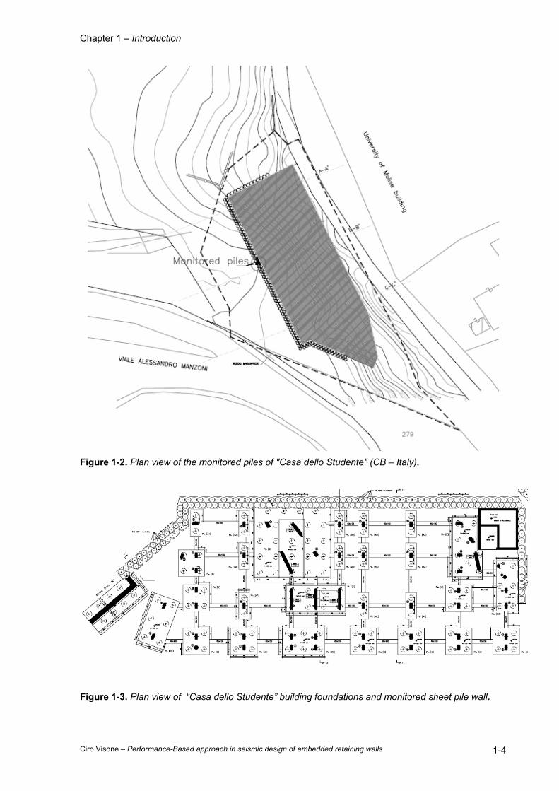
The retaining system is constituted by two piles rows connected by means of a concrete beam. The
piles have a diameter of 800mm and are arranged to have the centres at the vertexes of equilateral
triangles. Two of these piles have been instrumented with embedded piezoelectric accelerometers.
Figure 1-2 and Figure 1-3 show plan views of the retaining wall and of the monitored piles.
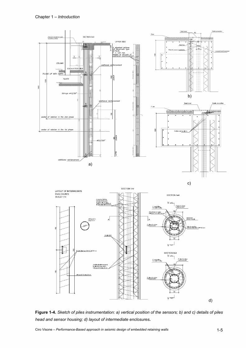
Three sensor modules have been placed in each pile. The positions have been chosen in order to be
as far as possible from the computed locations of the center of rotation in both the building and
operational phases. Additional two sensors have been placed on top of each pile, into a box over the
top beams which connects all piles. A sketch of the piles instrumentation and some structural details
are shown in Figure 1-4.
The dimensions of sensor modules are not negligible and cause some changes in the piles geometry.
To avoid singularities in the overall behaviour of the structure, specific computations and additional
reinforcements have been provided in order to guarantee for the instrumented piles similar stiffness
and strength characteristics of the adjacent ones.
In this context of the research interests devoted to the study of the dynamic behaviour of embedded
retaining walls by the scientific community, the present thesis finds its main role.
The activities developed during this work have both an experimental and a numerical character.
The first part was dedicated to the validation of the commercial FE code PLAXIS v.8.2 (Brinkgreve,
2002) for the development of dynamic soil-structure interaction analyses The program was chosen
because it is largely adopted both from practitioners and academics. However, the obtained results
have a general character and can be extended to other FE codes.
At the same time, some laboratory apparatuses of the Laboratory of Soil Dynamics (DYNALAB) of the
Hydraulic, Geotechnical and Environmental Engineering Department (D.I.G.A. – Dipartimento di
Ingegneria Idraulica, Geotecnica ed Ambientale) at University of Napoli Federico II were calibrated to
investigate the mechanical behaviour of the Fraction E of Leighton Buzzard Sand that will be used in
the centrifuge tests.
Chapter 1 – Introduction
Ciro Visone – Performance-Based approach in seismic design of embedded retaining walls 1-4
Figure 1-2. Plan view of the monitored piles of "Casa dello Studente" (CB – Italy).
Figure 1-3. Plan view of “Casa dello Studente” building foundations and monitored sheet pile wall.
Chapter 1 – Introduction
Ciro Visone – Performance-Based approach in seismic design of embedded retaining walls 1-5
b)
a)
c)
d)
Figure 1-4. Sketch of piles instrumentation: a) vertical position of the sensors; b) and c) details of piles
head and sensor housing; d) layout of intermediate enclosures.
Chapter 1 – Introduction
Ciro Visone – Performance-Based approach in seismic design of embedded retaining walls 1-6
An experimental campaign was then developed on the LB sand by means of triaxial compressions and
extensions, resonant column and torsional shear tests. The results are presented in the Annex A of
this thesis.
The calibration of the Dynamic Module of PLAXIS code was carried out by simulating numerically the
one-dimensional shear waves vertical propagation into ideal visco-elastic layers. The main aspects of
the research are described in the Annex B. The performed parametric study have been allowed
recognizing the various sources of damping existing in dynamic time-domain analyses and correctly
defining the numerical parameters to assume in the numerical calculations. In particular, the use of the
Rayleigh damping formulation to model the soil viscous damping was extended to account for the
numerical damping introduced in the analyses by the time integration scheme. Interesting indications
and suggestions were also given on how to reduce the spurious effects of the reflected waves on the
lateral boundaries of the discrete models and to rightly simulate the free field conditions.
Before to deal the seismic behaviour of the embedded retaining walls, an extensive bibliographic study
on the earth pressure theories, both in static and seismic conditions, on the typologies of retaining
walls and on the static design methods of them was done. A brief review of the literature on these
topics can be found in the Chapters 2, 3 and 4.
The Chapter 5 was entirely devoted to the application of the Performance-Based Design (PBD)
philosophy to the embedded retaining walls. Three types of analysis, depending on the accuracy
degree required by the structure to design, were presented. Simplified analyses can be simply
conducted by adopting the limit equilibrium methods and modelling the seismic actions on the walls as
pseudostatic forces. For cantilever RC diaphragms embedded in cohesionless materials, two charts
for the preliminary design of the needed depth of embedment and for the prediction of the maximum
bending moment were shown. The earthquake-induced displacements can be roughly estimated by
means of empirical formulas proposed in the literature or, having defined an appropriate seismic input
motion, recurring to Newmark type analyses. A more advanced design method can be performed by
using a FE model of the problem in which the seismic performances of the retaining system, in terms
of displacements or forces in structural elements, are described by capacity curves. The methodology
can be included in the framework of the "pushover analyses" and was proposed for the first time in
Visone & Santucci de Magistris (2007). Dynamic analyses represent the most accurate instrument to
predict the seismic behaviour of the geotechnical systems but they require an adequate subsoil
characterization and advanced knowledge in numerical modelling and earthquake engineering.
Finally, the performance based design presented here was applied to the seismic design of cantilever
RC diaphragm walls embedded in dry loose and dense sandy layers. The geometry of the free walls
centrifuge models and the LB sand properties were assumed. The analyses, performed following the
different level of accuracy provided by the PBD, have the main scope to supply preliminary predictions
on the seismic response of the centrifuge models. The results of the study were presented in the
Chapter 6.
At the end, the reached objectives and the future developments of the research were summarized in
the last Chapter 7.
Chapter 2 – Generalities of retaining walls
Ciro Visone – Performance-Based approach in seismic design of embedded retaining walls 2-1
2 GENERALITIES OF RETAINING WALLS.
Retaining walls can be defined as structures which retain ground, comprising soil, rock or backfill and
water. The material is retained at a slope steeper than it would eventually adopt if no structure was
present. Retaining structures include all types of walls and support systems in which structural elements
have forces imposed by the retained material.
They are used throughout seismically active areas and frequently represent key elements of ports and
harbors, transportation systems, lifelines, and other constructed facilities. Earthquakes have caused
permanent deformation of retaining structures in many historical earthquakes. In some cases, these
deformations were negligibly small; in others they caused significant damage. In some cases, retaining
structures have collapsed during earthquakes, with disastrous physical and economic consequences.
In this chapter, the generalities of the retaining structures, with a particular attention to the embedded
walls, are recalled.
2.1 TYPES OF RETAINING WALLS.
The problem of retaining soil is one of the oldest in geotechnical engineering; some of the earliest and
most fundamental principles of soil mechanics were developed to allow rational design of retaining
walls. Many different approaches to soil retention have been developed and used successfully. In
recent years, the development of metallic, polymer and geotextile reinforcement leds to the
development of many innovative types of mechanically stabilized earth retention systems.
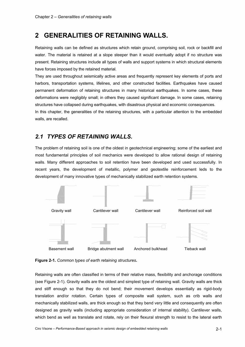
Gravity wall Cantilever wall Cantilever wall Reinforced soil wall
Basement wall Bridge abutment wall Anchored bulkhead Tieback wall
Figure 2-1. Common types of earth retaining structures.
Retaining walls are often classified in terms of their relative mass, flexibility and anchorage conditions
(see Figure 2-1). Gravity walls are the oldest and simplest type of retaining wall. Gravity walls are thick
and stiff enough so that they do not bend; their movement develops essentially as rigid-body
translation and/or rotation. Certain types of composite wall system, such as crib walls and
mechanically stabilized walls, are thick enough so that they bend very little and consequently are often
designed as gravity walls (including appropriate consideration of internal stability). Cantilever walls,
which bend as well as translate and rotate, rely on their flexural strength to resist to the lateral earth
Chapter 2 – Generalities of retaining walls
Ciro Visone – Performance-Based approach in seismic design of embedded retaining walls 2-2
pressures. The actual distribution of lateral earth pressure on a cantilever wall is influenced by the
relative stiffness and deformation of both the wall and the soil. Braced walls are constrained against
certain types of movement by the presence of external bracing elements. In the cases of basement
walls and bridge abutment walls, lateral movements of the tops of the walls may be restrained by the
structures they support. Tieback walls and anchored bulkheads are restrained against lateral
movement by anchors embedded in the soil behind the walls. The provision of lateral support at
different locations along a braced wall may keep bending moments so low that relatively flexible
structural sections can be used.
2.2 TYPES OF RETAINING WALL FAILURES.
To design retaining walls, it is necessary to define failure and to know how walls can fail. Under static
conditions, retaining walls are subjected to the body forces related to the mass of the wall, to the soil
pressures and to the external forces such as those transmitted by braces. A properly designed
retaining wall will achieve equilibrium of these forces without introducing shear stresses that approach
the shear strength of the soil or the failure of the wall material. During an earthquake, however, inertial
forces and changes in soil strength may violate equilibrium and cause permanent deformation of the
wall. Failure, whether by sliding, tilting and bending, or some other mechanism, occurs when these
permanent deformations become excessive. The question of what level of deformation is excessive
depends on many factors and is best addressed on a site specific basis.
Gravity walls usually fail by rigid body mechanisms such as sliding and/or overturning or by gross
instability. Sliding occurs when horizontal force equilibrium is not maintained (i.e., when the lateral
pressures on the back of the wall produce a thrust that exceeds the available sliding resistance on the
base of the wall). Overturning failures occur when moment equilibrium is not satisfied; bearing failures
at the base of the wall are often involved. Gravity walls may also be damaged by gross instability of
the soils behind and beneath them. Such failures may be treated as slope stability failures that
encompass the wall. Composite wall systems, such as crib walls, bin walls and mechanically stabilized
walls, can fail in the same ways or by a number of internal mechanisms that might involve shearing,
pullout or tensile failure of various wall elements.
Cantilever walls are subject to the same failure mechanisms. Soil pressures and bending moments in
cantilever walls depend on the geometry, stiffness and strength of the wall-soil system. If the bending
moments required for equilibrium exceed the flexural strength of the wall, flexural failure may occur.
The structural ductility of the wall itself may influence the level of deformation produced by flexural
failure.
Braced walls usually fail by gross instability, tilting, flexural failure and/or failure of bracing elements.
Tilting of braced walls typically involves rotation about the point at which the brace acts on the wall,
often the top of the wall as in the cases of basement and bridge abutment walls. Anchored walls with
inadequate penetration may tilting by kicking out at their toes. As in the case of cantilever walls,
anchored walls may fail in flexure, although the point of failure (maximum bending moment) is likely to
be different. Failure of bracing elements can include anchor pullout, tie-rod failure or bridge buckling.

Chapter 2 – Generalities of retaining walls
Ciro Visone – Performance-Based approach in seismic design of embedded retaining walls 2-3
Backfill settlements can also impose additional axial and transverse loading on bracing elements such
as tierods and tiebacks.
2.3 ULTIMATE LIMIT STATES FOR RETAINING WALLS.
A limit state is a set of performance criteria (e.g. vibration levels, deflection, strength), or stability
criteria (buckling, twisting, collapse) that must be met when the structure is subject to loads.
In accordance with the most recent construction codes, the design of a structure must satisfy the
following requirements:
• safety towards the ultimate limit states: capability to avoid collapse, loss of equilibrium and
heavy instability, total or partial, which might endanger the safety of the people or involve loss
of goods or to cause heavy environmental and social damages or make the structure out of
order;
• safety towards the serviceability limit states: capability to guarantee the expected performances
for serviceability conditions;
• robustness towards the exceptional actions: capability to avoid damages out of proportion
respect to the causes as fires, explosions, impacts.
For all types of retaining structures, the following limit states should be considered:
• loss of overall stability;
• failure of a structural element such as a wall, anchorage, wale or strut or failure of the
connection between such elements;
• combined failure in ground and in structural element;
• failure by hydraulic heave and piping;
• movement of the retaining structure which may cause collapse or affect the appearance or
efficient use of the structure or nearby structures or services which rely on it;
• unacceptable leakage through or beneath the wall;
• unacceptable transport of soil particles through or beneath the wall
• unacceptable change in groundwater regime.
In addition, the following limit states should be considered for gravity walls and for composite retaining
structures:
• bearing resistance failure of the soil below the base;
• failure by sliding at the base;
• failure by toppling;
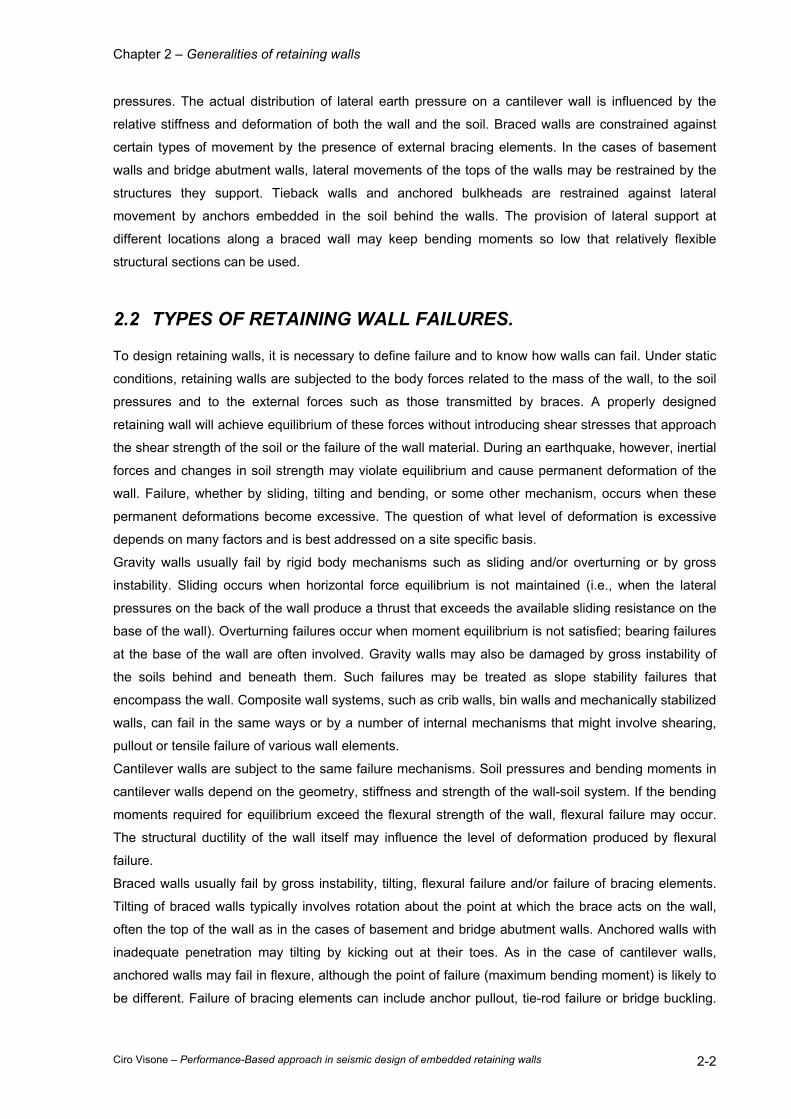
and for embedded walls:
• failure by rotation or translation of the wall or parts thereof;
• failure by lack of vertical equilibrium.
When they are relevant, combinations of the above mentioned limit states should be taken into
account.
Examples of limit modes for the most commonly used retaining structures are plotted in the next
figures (EN1997-1).
Chapter 3 – Earth pressure theory
Ciro Visone – Performance-Based approach in seismic design of embedded retaining walls 2-4
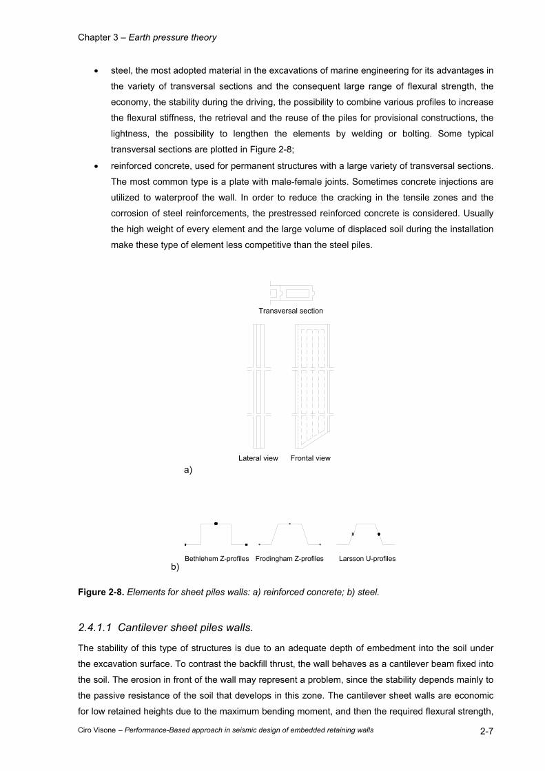
Figure 2-2. Examples of limit modes for overall stability of retaining structures.
Figure 2-3. Examples of limit modes for foundation failures of gravity walls.
Figure 2-4. Examples of limit modes for vertical failure of embedded walls.

Chapter 3 – Earth pressure theory
Ciro Visone – Performance-Based approach in seismic design of embedded retaining walls 2-5
Figure 2-5. Examples of limit modes for rotational failures of embedded walls.
Figure 2-6. Examples of limit modes for structural failure of retaining structures.

Chapter 3 – Earth pressure theory
Ciro Visone – Performance-Based approach in seismic design of embedded retaining walls 2-6
Figure 2-7. Examples of limit modes for failure by pullout of anchors.
2.4 EMBEDDED WALLS: TYPES AND USES.
The preliminary design of a retaining structure is complicated to the various available typologies and to
the design constraints. The problem derive from the necessity to sustain a backfill or loads transmitted
from adjacent constructions. The structure geometry, the limitations imposed from the nature of the
soil and the ground water table conditions, the available construction methodologies and the local
experiences play a fundamental role for the choice of the more appropriate type of retaining system.
Here, only the embedded retaining walls are considered. The main technologies employed for the
realization of them are recalled.
The first classification of the embedded walls is done on the basis of their constraints scheme. Thus,
the walls can be distinguished as:
• cantilever walls, used to sustain backfills lower than 5-6 m;
• embedded walls with a single constraint, for backfills till to 10 m;
• embedded walls with various constraint levels, to retain heights higher than 10 m.
The embedded walls can be realized with wood, steel and reinforced concrete piles driven into the
ground (sheet piles walls, without removing the soil) or with the cast of RC piles or diaphragm into
previously formed holes (bulkheads, with the removal of the soil). The execution modes influence the
mechanical behaviour of the soil interacting with the wall.
2.4.1 Sheet pile walls.
The sheet piles walls are flexible earth retaining structures mainly used in the marine engineering and
for provisional constructions. They can be employed in unfavourable soils conditions (for example, in
soft clays) because they do not require foundations. The poor mechanical soil properties permit to
drive the piles directly from the ground surface. The constructive technique is suitable for the presence
of water, where other types of retaining systems can not be utilized. As mentioned before, the piles
can be constituted by:
• wood, typically used for provisional structures with low heights of excavation. For definitive
retaining systems, protection treatments of the wood are needed
Chapter 3 – Earth pressure theory
Ciro Visone – Performance-Based approach in seismic design of embedded retaining walls 2-7
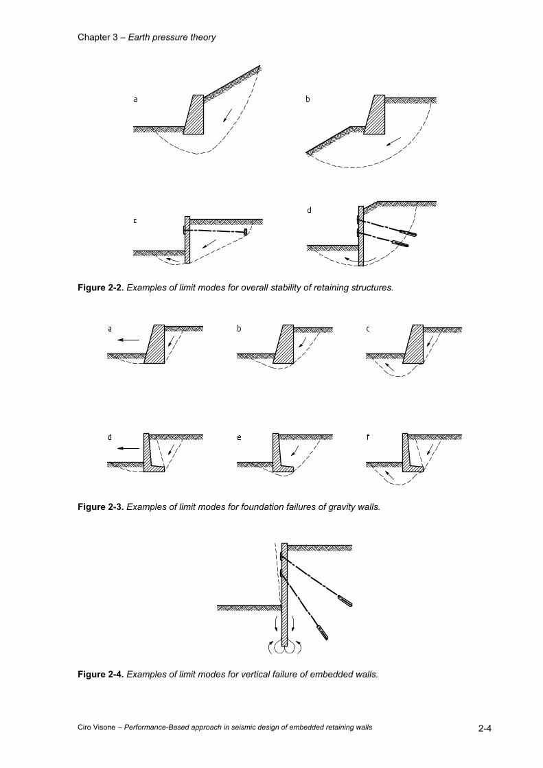
• steel, the most adopted material in the excavations of marine engineering for its advantages in
the variety of transversal sections and the consequent large range of flexural strength, the
economy, the stability during the driving, the possibility to combine various profiles to increase
the flexural stiffness, the retrieval and the reuse of the piles for provisional constructions, the
lightness, the possibility to lengthen the elements by welding or bolting. Some typical
transversal sections are plotted in Figure 2-8;
• reinforced concrete, used for permanent structures with a large variety of transversal sections.
The most common type is a plate with male-female joints. Sometimes concrete injections are
utilized to waterproof the wall. In order to reduce the cracking in the tensile zones and the
corrosion of steel reinforcements, the prestressed reinforced concrete is considered. Usually
the high weight of every element and the large volume of displaced soil during the installation
make these type of element less competitive than the steel piles.
a) Lateral view Frontal view
Transversal section
b) Bethlehem Z-profiles Frodingham Z-profiles Larsson U-profiles
Figure 2-8. Elements for sheet piles walls: a) reinforced concrete; b) steel.
2.4.1.1 Cantilever sheet piles walls.
The stability of this type of structures is due to an adequate depth of embedment into the soil under
the excavation surface. To contrast the backfill thrust, the wall behaves as a cantilever beam fixed into
the soil. The erosion in front of the wall may represent a problem, since the stability depends mainly to
the passive resistance of the soil that develops in this zone. The cantilever sheet walls are economic
for low retained heights due to the maximum bending moment, and then the required flexural strength,
Chapter 3 – Earth pressure theory
Ciro Visone – Performance-Based approach in seismic design of embedded retaining walls 2-8
increases with the cube of the excavation height. The lateral displacements due to the structural
deflection are significant. Free sheet walls are more suitable for provisional constructions.
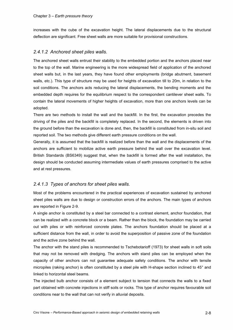
2.4.1.2 Anchored sheet piles walls.
The anchored sheet walls entrust their stability to the embedded portion and the anchors placed near
to the top of the wall. Marine engineering is the more widespread field of application of the anchored
sheet walls but, in the last years, they have found other employments (bridge abutment, basement
walls, etc.). This type of structure may be used for heights of excavation till to 20m, in relation to the
soil conditions. The anchors acts reducing the lateral displacements, the bending moments and the
embedded depth requires for the equilibrium respect to the correspondent cantilever sheet walls. To
contain the lateral movements of higher heights of excavation, more than one anchors levels can be
adopted.
There are two methods to install the wall and the backfill. In the first, the excavation precedes the
driving of the piles and the backfill is completely replaced. In the second, the elements is driven into
the ground before than the excavation is done and, then, the backfill is constituted from in-situ soil and
reported soil. The two methods give different earth pressure conditions on the wall.
Generally, it is assumed that the backfill is realized before than the wall and the displacements of the
anchors are sufficient to mobilize active earth pressure behind the wall over the excavation level.
British Standards (BS6349) suggest that, when the backfill is formed after the wall installation, the
design should be conducted assuming intermediate values of earth pressures comprised to the active
and at rest pressures.
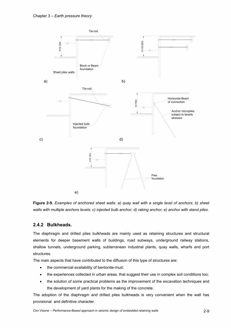
2.4.1.3 Types of anchors for sheet piles walls.
Most of the problems encountered in the practical experiences of excavation sustained by anchored
sheet piles walls are due to design or construction errors of the anchors. The main types of anchors
are reported in Figure 2-9.
A single anchor is constituted by a steel bar connected to a contrast element, anchor foundation, that
can be realized with a concrete block or a beam. Rather than the block, the foundation may be carried
out with piles or with reinforced concrete plates. The anchors foundation should be placed at a
sufficient distance from the wall, in order to avoid the superposition of passive zone of the foundation
and the active zone behind the wall.
The anchor with the stand piles is recommended to Tschebotarioff (1973) for sheet walls in soft soils
that may not be removed with dredging. The anchors with stand piles can be employed when the
capacity of other anchors can not guarantee adequate safety conditions. The anchor with tensile
micropiles (raking anchor) is often constituted by a steel pile with H-shape section inclined to 45° and
linked to horizontal steel beams.
The injected bulb anchor consists of a element subject to tension that connects the walls to a fixed
part obtained with concrete injections in stiff soils or rocks. This type of anchor requires favourable soil
conditions near to the wall that can not verify in alluvial deposits.
Chapter 3 – Earth pressure theory
Ciro Visone – Performance-Based approach in seismic design of embedded retaining walls 2-9
a)
h=5-
12m
Sheet piles walls
Tie-rod
Block or Beam foundation
b)
h=15
-20m
c)
Tie-rod
Injected bulb foundation
d) h<
10m
Horizontal Beam of connection
Anchor micropiles subject to tensile stresses
e)
h=5-
12m
Piles foundation
Figure 2-9. Examples of anchored sheet walls: a) quay wall with a single level of anchors; b) sheet
walls with multiple anchors levels; c) injected bulb anchor; d) raking anchor; e) anchor with stand piles.
2.4.2 Bulkheads.
The diaphragm and drilled piles bulkheads are mainly used as retaining structures and structural
elements for deeper basement walls of buildings, road subways, underground railway stations,
shallow tunnels, underground parking, subterranean industrial plants, quay walls, wharfs and port
structures.
The main aspects that have contributed to the diffusion of this type of structures are:
• the commercial availability of bentonite-mud;
• the experiences collected in urban areas, that suggest their use in complex soil conditions too;
• the solution of some practical problems as the improvement of the excavation techniques and
the development of yard plants for the making of the concrete.
The adoption of the diaphragm and drilled piles bulkheads is very convenient when the wall has
provisional and definitive character.
Chapter 3 – Earth pressure theory
Ciro Visone – Performance-Based approach in seismic design of embedded retaining walls 2-10
The cost of the structure is affected from the depth of embedment required to the stability and
hydraulic conditions above the dredge level, the presence of rock blocks and other constructions, the
necessity of anchors, props and struts, and from some yard factors as the availability of the services,
the time and the space constraints.
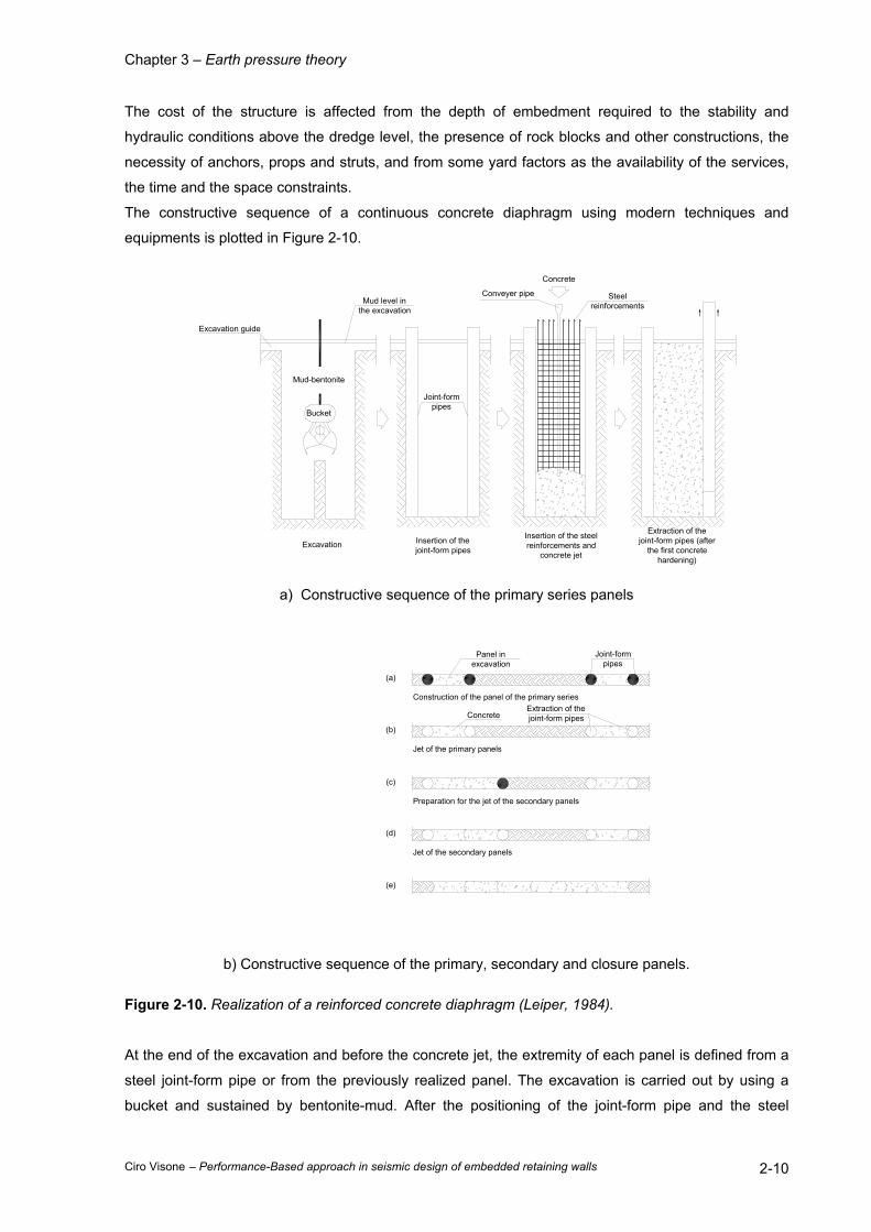
The constructive sequence of a continuous concrete diaphragm using modern techniques and
equipments is plotted in Figure 2-10.
Excavation guide
Mud level in the excavation
Mud-bentonite
Bucket
Joint-form pipes
Concrete
Steel reinforcements
Conveyer pipe
Excavation Insertion of the joint-form pipes
Insertion of the steel reinforcements and
concrete jet
Extraction of the joint-form pipes (after
the first concrete hardening)
a) Constructive sequence of the primary series panels
(a)
Panel in excavation
Joint-form pipes
Construction of the panel of the primary series
ConcreteExtraction of the joint-form pipes
(b)
Jet of the primary panels
(c)
Preparation for the jet of the secondary panels
(d)
Jet of the secondary panels
(e)
b) Constructive sequence of the primary, secondary and closure panels.
Figure 2-10. Realization of a reinforced concrete diaphragm (Leiper, 1984).
At the end of the excavation and before the concrete jet, the extremity of each panel is defined from a
steel joint-form pipe or from the previously realized panel. The excavation is carried out by using a
bucket and sustained by bentonite-mud. After the positioning of the joint-form pipe and the steel

Chapter 3 – Earth pressure theory
Ciro Visone – Performance-Based approach in seismic design of embedded retaining walls 2-11
reinforcements into the trench, the concrete jet is performed by using a conveyer pipe from the bottom
of the hole. The joint-form pipes allows having a good level of joint between the panels.
The diaphragms can be realized with prefabricated reinforced concrete panels. Their main
disadvantage is the high weight of each panel.
The reinforced concrete sheet piles may be adopted in every type of subsoil condition. The piles can
be placed side by side, tangent and secant, in relation to the distance between the piles (larger, equal
or lower than the pile diameter, respectively), according to the required support and the waterproofing
of the excavation. The top of the piles is often connected by a reinforced concrete beam to distribute
the loads.
2.4.3 Walls with many anchor levels and props.
Relatively flexible retaining walls might be designed by adopting anchor levels or multiple props at
small distances. This kind of construction is adopted:
• for provisional excavations;
• to retain relatively resistant soil (fractured rock) for very deep excavation;
• to guarantee a partial sustaining to the jet grouted excavations
• to minimize the losses of soil in critical areas near to deeper excavations.
The anchors can be used for every type of the face covering. In some cases, they are placed to a
small relative distance to form retaining structure in reinforced soils.
Chapter 3 – Earth pressure theory
Ciro Visone – Performance-Based approach in seismic design of embedded retaining walls 3-1
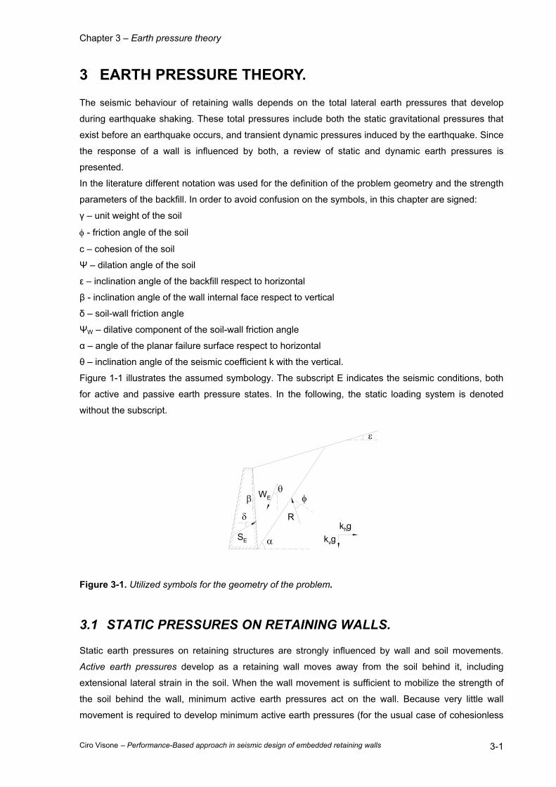
3 EARTH PRESSURE THEORY.
The seismic behaviour of retaining walls depends on the total lateral earth pressures that develop
during earthquake shaking. These total pressures include both the static gravitational pressures that
exist before an earthquake occurs, and transient dynamic pressures induced by the earthquake. Since
the response of a wall is influenced by both, a review of static and dynamic earth pressures is
presented.
In the literature different notation was used for the definition of the problem geometry and the strength
parameters of the backfill. In order to avoid confusion on the symbols, in this chapter are signed:
γ – unit weight of the soil
φ - friction angle of the soil
c – cohesion of the soil
Ψ – dilation angle of the soil
ε – inclination angle of the backfill respect to horizontal
β - inclination angle of the wall internal face respect to vertical
δ – soil-wall friction angle
ΨW – dilative component of the soil-wall friction angle
α – angle of the planar failure surface respect to horizontal
θ – inclination angle of the seismic coefficient k with the vertical.
Figure 1-1 illustrates the assumed symbology. The subscript E indicates the seismic conditions, both
for active and passive earth pressure states. In the following, the static loading system is denoted
without the subscript.
ε
α
βθ
φW
k gh
E
k gv
Rδ
SE
Figure 3-1. Utilized symbols for the geometry of the problem.
3.1 STATIC PRESSURES ON RETAINING WALLS.
Static earth pressures on retaining structures are strongly influenced by wall and soil movements.
Active earth pressures develop as a retaining wall moves away from the soil behind it, including
extensional lateral strain in the soil. When the wall movement is sufficient to mobilize the strength of
the soil behind the wall, minimum active earth pressures act on the wall. Because very little wall
movement is required to develop minimum active earth pressures (for the usual case of cohesionless

Chapter 3 – Earth pressure theory
Ciro Visone – Performance-Based approach in seismic design of embedded retaining walls 3-2
backfill materials), free-standing retaining walls are usually designed on the basis of minimum active
earth pressures. Where lateral wall movements are restrained, such as in the cases of tieback walls,
anchored bulkheads, basement walls, and bridge abutments, static earth pressures may be greater
than minimum active. Passive earth pressures develop as a retaining wall moves toward the soil,
thereby producing compressive lateral strain in the soil. When the strength of the soil is fully mobilized,
maximum passive earth pressures act on the wall. The stability of many free-standing retaining walls
depends on the balance between active pressures acting predominantly on one side of the wall and
passive pressures acting on the other.
Even under static conditions, prediction of actual retaining walls forces and deformations is a
complicated soil-structure interaction problem. Deformations are rarely considered explicitly in design
– the typical approach is to estimate the forces acting on a wall and then to design the wall to resist
those forces with a factor of safety high enough to produce acceptably small deformations. A number
of simplified approaches are available to evaluate static loads on retaining walls. The most commonly
used are described in the following sections.
3.1.1 Rankine theory.
Rankine (1857) developed the simplest procedure for computing minimum active and maximum
passive earth pressures. By making assumptions about the stress conditions and strength envelope of
the soil behind a retaining wall (the backfill soil), Rankine was able to render the lateral earth pressure
problem determinate and directly compute the static pressures acting on retaining walls.
For minimum active conditions, Rankine expressed the pressure at a point on the back of a retaining
wall as:
AVAA KcKp 2' −σ⋅= ( 3-1 )
where KA is the coefficient of minimum active earth pressure, σ’V is the vertical effective stress at the
point of interest, and c is the cohesive strength of the soil. When the principal stress planes are
vertical and horizontal (as in the case of a smooth vertical wall retaining a horizontal backfill), the
coefficient of minimum active earth pressure is given by:
φ−=
φ+φ−
=2
4511 2tan
sinsin
AK ( 3-2 )
For the case of a cohesionless backfill inclined at an angle ε with the horizontal, infinite slope solutions
can be used (Terzaghi, 1943; Taylor, 1948) to compute KA as:
φ−ε+ε
φ−ε−εε=
22
22
coscoscos
coscoscoscosAK ( 3-3 )
for ε≤φ. The pressure distribution on the back of the wall, as indicated by equation ( 3-1 ), depends on
the relative magnitudes of the frictional and cohesive components of the backfill soil strength. Although
the presence of the cohesion indicates that tensile stresses will develop between the upper portion of
the wall and the backfill, tensile stresses do not actually develop in the field. The creep, stress
relaxation, and low permeability characteristics of cohesive soils render them undesirable as backfill

Chapter 3 – Earth pressure theory
Ciro Visone – Performance-Based approach in seismic design of embedded retaining walls 3-3
material for retaining structures, and their use for this purpose is generally avoided whenever possible.
For dry homogeneous cohesionless backfill, Rankine theory predicts a triangular active pressure
distribution oriented parallel to the backfill surface. The active earth pressure resultant, or active thrust
SA, acts at a point located H/3 above the base of a wall of height H, with magnitude:
2
21 HKS AA γ= ( 3-4 )
Under maximum passive conditions, Rankine theory predicts wall pressures given by:
PVPP KcKp 2' +σ⋅= ( 3-5 )
where KP is the coefficient of maximum passive earth pressure. For smooth, vertical walls retaining
horizontal backfills:
φ
+=φ−φ+
=2
4511 2tan
sinsin
PK ( 3-6 )
and:
φ−ε−ε
φ−ε+εε=
22
22
coscoscos
coscoscoscosPK ( 3-7 )
for backfills inclined at ε to the horizontal. For a dry homogeneous backfill, Rankine theory predicts a
triangular passive pressure distribution oriented parallel to the backfill surface.
The passive earth pressure resultant, or passive thrust SP, acts at a point located H/3 above the base
of a wall of height H, with magnitude:
2
21 HKS PP γ= ( 3-8 )
In Figure 3-2 are plotted the graphical representations of the equations ( 3-2 ) and ( 3-6 ).
0.1
1
10
0 5 10 15 20 25 30 35 40 45 50
Friction angle, φ (°)
Ear
th p
ress
ure
coef
ficie
nt, K
A a
nd K
P Active conditions
Passive conditions
Figure 3-2. Rankine active and passive earth pressure coefficients for a horizontal backfill.

Chapter 3 – Earth pressure theory
Ciro Visone – Performance-Based approach in seismic design of embedded retaining walls 3-4
The presence of water in the backfill behind a retaining wall influences the effective stresses and
hence the lateral earth pressure that acts on the wall. For wall design the hydrostatic pressure due to
the water must be added to the lateral earth pressure. Because the total lateral thrust on a wall
retaining a saturated backfill is considerably greater than that on a wall retaining dry backfill, the
provision of backfill drainage is an important part of retaining wall design.
3.1.2 Coulomb theory.
Coulomb (1776) was the first to study the problem of lateral earth pressures on retaining structures. By
assuming that the force acting on the back of a retaining wall resulted from the weight of a wedge of
soil above a planar failure surface, Coulomb used force equilibrium to determine the magnitude of the
soil thrust acting on the wall for both minimum active and maximum passive conditions. Since the
problem is indeterminate, a number of potential failure surfaces must be analyzed to identify the
critical failure surface (i.e., the surface that produces the greatest active thrust or the smallest passive
thrust).
Under minimum active earth pressure conditions, the active thrust on a wall with the geometry shown
in Figure 1-1 is obtained from the force equilibrium. For the critical failure surface, the active thrust on
a wall retaining a cohesionless soil can be expressed as:
2
21 HKS AA γ= ( 3-9 )
where
( )
( ) ( ) ( )( ) ( )
22
2
1
β−εβ+δε−φφ+δ
+β+δβ
β−φ=
coscossinsincoscos
cosAK
( 3-10 )
δ is the angle of interface friction between the wall and the soil, while ε and β are shown in Figure 1-1.
The critical failure surface is inclined at an angle:
( )
+ε−φ+φ=α
2
1
CC
Atan
arctan ( 3-11 )
to the horizontal where
( ) ( ) ( )[ ] ( ) ( )[ ]( ) ( ) ( )[ ]{ }β−φ+ε−φβ+δ+=
β−φβ+δ+β−φ+ε−φε−φ=
cottantancottancottantan
11
2
1
CC
Coulomb theory does not explicitly predict the distribution of active pressure, but it can be shown to be
triangular for linear backfill surfaces with no surface loads. In such cases, SA acts at a point located
H/3 above the base of a wall of height H.
For maximum passive conditions in cohesionless backfills, Coulomb theory predicts a passive thrust:
2
21 HKS PP γ= ( 3-12 )
where:
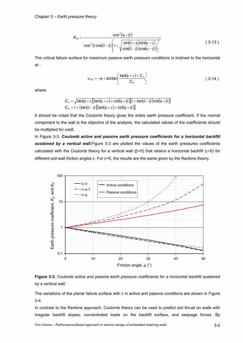
Chapter 3 – Earth pressure theory
Ciro Visone – Performance-Based approach in seismic design of embedded retaining walls 3-5
( )
( ) ( ) ( )( ) ( )
22
2
1
β−εβ−δε−φφ+δ
+β−δβ
β+φ=
coscossinsincoscos
cosPK
( 3-13 )
The critical failure surface for maximum passive earth pressure conditions is inclined to the horizontal
at :
( )
+ε+φ+φ−=α
4
3
CC
Ptan
arctan ( 3-14 )
where:
( ) ( ) ( )[ ] ( ) ( )[ ]( ) ( ) ( )[ ]{ }β+φ+ε+φβ−δ+=
β+φβ−δ+β+φ+ε+φε+φ=
cottantancottancottantan
11
4
3
CC
It should be noted that the Coulomb theory gives the entire earth pressure coefficient. If the normal
component to the wall is the objective of the analysis, the calculated values of the coefficients should
be multiplied for cosδ.
In Figure 3-3. Coulomb active and passive earth pressure coefficients for a horizontal backfill sustained by a vertical wall.Figure 3-3 are plotted the values of the earth pressures coefficients
calculated with the Coulomb theory for a vertical wall (β=0) that retains a horizontal backfill (ε=0) for
different soil-wall friction angles δ. For δ=0, the results are the same given by the Rankine theory.
0.1
1
10
100
0 10 20 30 40 50
Friction angle, φ (°)
Ear
th p
ress
ure
coef
ficie
nt, K
A a
nd K
P δ=0
δ=φ/2
δ=φ
Active conditions
Passive conditions
Figure 3-3. Coulomb active and passive earth pressure coefficients for a horizontal backfill sustained
by a vertical wall.
The variations of the planar failure surface with δ in active and passive conditions are shown in Figure
3-4.
In contrast to the Rankine approach, Coulomb theory can be used to predict soil thrust on walls with
irregular backfill slopes, concentrated loads on the backfill surface, and seepage forces. By
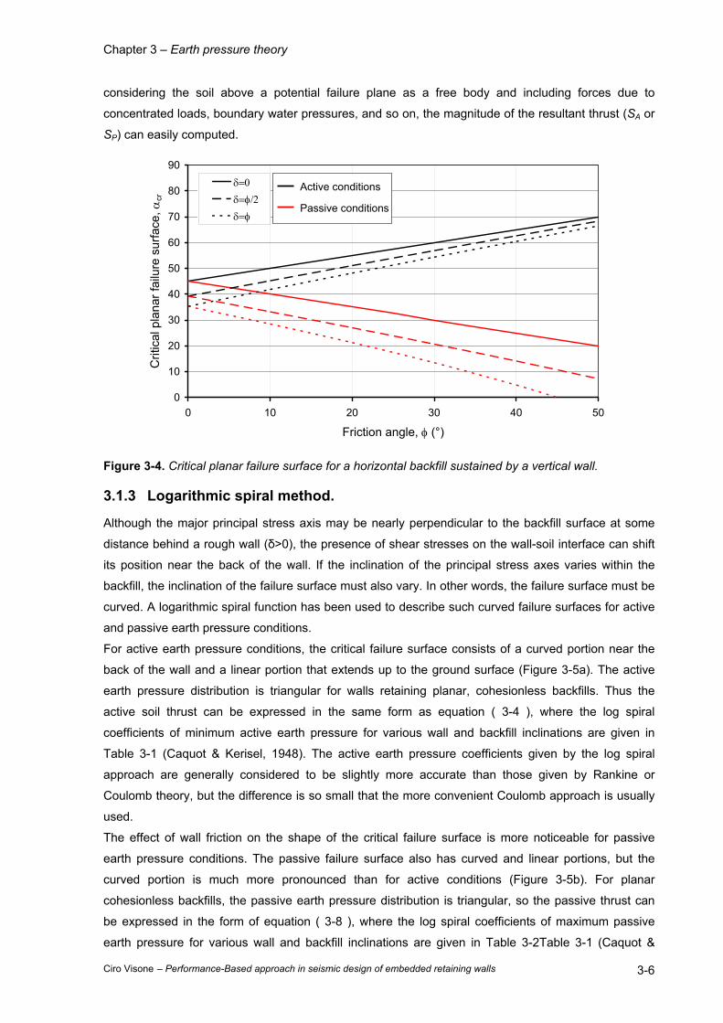
Chapter 3 – Earth pressure theory
Ciro Visone – Performance-Based approach in seismic design of embedded retaining walls 3-6
considering the soil above a potential failure plane as a free body and including forces due to
concentrated loads, boundary water pressures, and so on, the magnitude of the resultant thrust (SA or
SP) can easily computed.
0
10
20
30
40
50
60
70
80
90
0 10 20 30 40 50
Friction angle, φ (°)
Crit
ical
pla
nar f
ailu
re s
urfa
ce, α
cr
δ=0
δ=φ/2
δ=φ
Active conditions
Passive conditions
Figure 3-4. Critical planar failure surface for a horizontal backfill sustained by a vertical wall.
3.1.3 Logarithmic spiral method.
Although the major principal stress axis may be nearly perpendicular to the backfill surface at some
distance behind a rough wall (δ>0), the presence of shear stresses on the wall-soil interface can shift
its position near the back of the wall. If the inclination of the principal stress axes varies within the
backfill, the inclination of the failure surface must also vary. In other words, the failure surface must be
curved. A logarithmic spiral function has been used to describe such curved failure surfaces for active
and passive earth pressure conditions.
For active earth pressure conditions, the critical failure surface consists of a curved portion near the
back of the wall and a linear portion that extends up to the ground surface (Figure 3-5a). The active
earth pressure distribution is triangular for walls retaining planar, cohesionless backfills. Thus the
active soil thrust can be expressed in the same form as equation ( 3-4 ), where the log spiral
coefficients of minimum active earth pressure for various wall and backfill inclinations are given in
Table 3-1 (Caquot & Kerisel, 1948). The active earth pressure coefficients given by the log spiral
approach are generally considered to be slightly more accurate than those given by Rankine or
Coulomb theory, but the difference is so small that the more convenient Coulomb approach is usually
used.
The effect of wall friction on the shape of the critical failure surface is more noticeable for passive
earth pressure conditions. The passive failure surface also has curved and linear portions, but the
curved portion is much more pronounced than for active conditions (Figure 3-5b). For planar
cohesionless backfills, the passive earth pressure distribution is triangular, so the passive thrust can
be expressed in the form of equation ( 3-8 ), where the log spiral coefficients of maximum passive
earth pressure for various wall and backfill inclinations are given in Table 3-2Table 3-1 (Caquot &
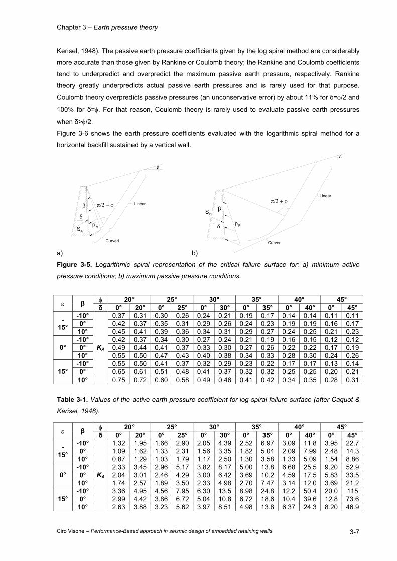
Chapter 3 – Earth pressure theory
Ciro Visone – Performance-Based approach in seismic design of embedded retaining walls 3-7
Kerisel, 1948). The passive earth pressure coefficients given by the log spiral method are considerably
more accurate than those given by Rankine or Coulomb theory; the Rankine and Coulomb coefficients
tend to underpredict and overpredict the maximum passive earth pressure, respectively. Rankine
theory greatly underpredicts actual passive earth pressures and is rarely used for that purpose.
Coulomb theory overpredicts passive pressures (an unconservative error) by about 11% for δ=φ/2 and
100% for δ=φ. For that reason, Coulomb theory is rarely used to evaluate passive earth pressures
when δ>φ/2.
Figure 3-6 shows the earth pressure coefficients evaluated with the logarithmic spiral method for a
horizontal backfill sustained by a vertical wall.
a)
ε
β
δ
SA
Curved
Linearπ/2 − φ
pA
b)
ε
β
δ
SP
Curved
Linearπ/2 + φ
pP
Figure 3-5. Logarithmic spiral representation of the critical failure surface for: a) minimum active
pressure conditions; b) maximum passive pressure conditions.
φ 20° 25° 30° 35° 40° 45° ε β δ 0° 20° 0° 25° 0° 30° 0° 35° 0° 40° 0° 45°
-10° 0.37 0.31 0.30 0.26 0.24 0.21 0.19 0.17 0.14 0.14 0.11 0.11 0° 0.42 0.37 0.35 0.31 0.29 0.26 0.24 0.23 0.19 0.19 0.16 0.17 -
15° 10° 0.45 0.41 0.39 0.36 0.34 0.31 0.29 0.27 0.24 0.25 0.21 0.23 -10° 0.42 0.37 0.34 0.30 0.27 0.24 0.21 0.19 0.16 0.15 0.12 0.12 0° 0.49 0.44 0.41 0.37 0.33 0.30 0.27 0.26 0.22 0.22 0.17 0.19 0° 10° 0.55 0.50 0.47 0.43 0.40 0.38 0.34 0.33 0.28 0.30 0.24 0.26 -10° 0.55 0.50 0.41 0.37 0.32 0.29 0.23 0.22 0.17 0.17 0.13 0.14 0° 0.65 0.61 0.51 0.48 0.41 0.37 0.32 0.32 0.25 0.25 0.20 0.21 15° 10°
KA
0.75 0.72 0.60 0.58 0.49 0.46 0.41 0.42 0.34 0.35 0.28 0.31
Table 3-1. Values of the active earth pressure coefficient for log-spiral failure surface (after Caquot &
Kerisel, 1948).
φ 20° 25° 30° 35° 40° 45° ε β δ 0° 20° 0° 25° 0° 30° 0° 35° 0° 40° 0° 45°
-10° 1.32 1.95 1.66 2.90 2.05 4.39 2.52 6.97 3.09 11.8 3.95 22.7 0° 1.09 1.62 1.33 2.31 1.56 3.35 1.82 5.04 2.09 7.99 2.48 14.3 -
15° 10° 0.87 1.29 1.03 1.79 1.17 2.50 1.30 3.58 1.33 5.09 1.54 8.86 -10° 2.33 3.45 2.96 5.17 3.82 8.17 5.00 13.8 6.68 25.5 9.20 52.9 0° 2.04 3.01 2.46 4.29 3.00 6.42 3.69 10.2 4.59 17.5 5.83 33.5 0° 10° 1.74 2.57 1.89 3.50 2.33 4.98 2.70 7.47 3.14 12.0 3.69 21.2 -10° 3.36 4.95 4.56 7.95 6.30 13.5 8.98 24.8 12.2 50.4 20.0 115 0° 2.99 4.42 3.86 6.72 5.04 10.8 6.72 18.6 10.4 39.6 12.8 73.6 15° 10°
KA
2.63 3.88 3.23 5.62 3.97 8.51 4.98 13.8 6.37 24.3 8.20 46.9

Chapter 3 – Earth pressure theory
Ciro Visone – Performance-Based approach in seismic design of embedded retaining walls 3-8
Table 3-2. Values of the passive earth pressure coefficient for log-spiral failure surface (after Caquot &
Kerisel, 1948).
0.1
1
10
100
0 10 20 30 40 50
Friction angle, φ (°)
Ear
th p
ress
ure
coef
ficie
nt, K
A a
nd K
P
δ=0
δ=φ
Active conditions
Passive conditions
Figure 3-6. Active and passive earth pressure coefficients for a horizontal backfill sustained by a
vertical wall (after Caquot & Kerisel, 1948).
3.1.4 Slip line method.
Sokolovskii (1965) introduced a theory termed the “Slip-Line Field Theory”. In this analysis, it is
assumed that failure occurs at constant volumes of soil along slip lines that meet the Mohr-Coulomb
failure criterion. This method has the advantage of providing a statistically admissible stress state that
satisfy the following equations of the plane equilibrium involving the normal, σ, and shear, τ, stresses
and using a system of rectangular coordinates x, y with x-axis oriented in the vertical direction:
0=∂
σ∂+
∂
τ∂
γ=∂
τ∂+
∂σ∂
yx
yx
yxy
yxx
( 3-15 )
The Mohr-Coulomb criteria states that at yield the following formula must apply everywhere in the soil
mass:
( ) ( ) φσ+σ=τ+σ−σ 2222 4 sinyxxyyx ( 3-16 )
The solution of these equations is called Kotter’s equation and gives the orientation of the slip lines
together with the stresses on the failure surface.
Sokolovoskii accomplished the solution for the active and the passive lateral earth pressure through
the use of the finite difference method for a horizontal backfill. The results are resumed in the Table
3-3 and Table 3-4, while, in Figure 3-7 are plotted the values related to a vertical wall.
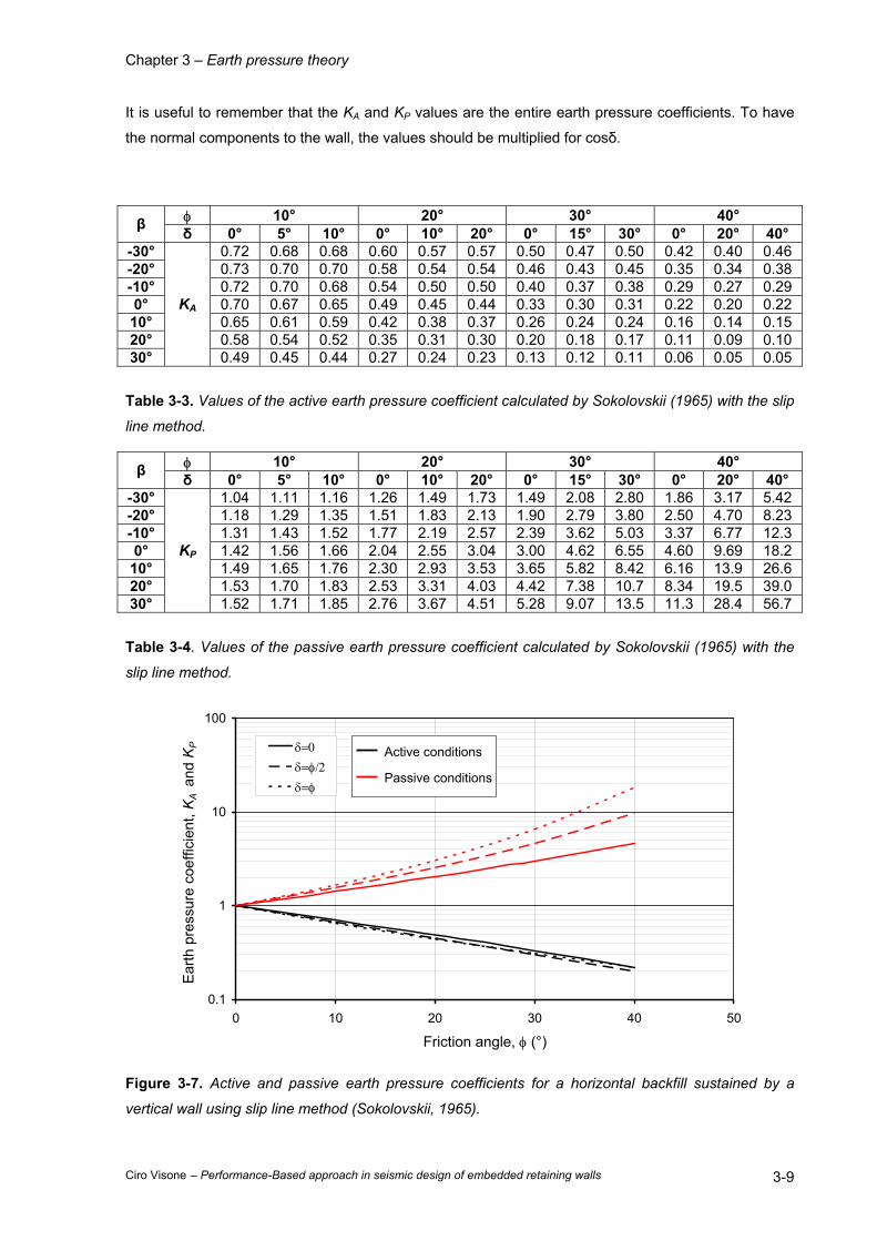
Chapter 3 – Earth pressure theory
Ciro Visone – Performance-Based approach in seismic design of embedded retaining walls 3-9
It is useful to remember that the KA and KP values are the entire earth pressure coefficients. To have
the normal components to the wall, the values should be multiplied for cosδ.
φ 10° 20° 30° 40° β δ 0° 5° 10° 0° 10° 20° 0° 15° 30° 0° 20° 40° -30° 0.72 0.68 0.68 0.60 0.57 0.57 0.50 0.47 0.50 0.42 0.40 0.46 -20° 0.73 0.70 0.70 0.58 0.54 0.54 0.46 0.43 0.45 0.35 0.34 0.38 -10° 0.72 0.70 0.68 0.54 0.50 0.50 0.40 0.37 0.38 0.29 0.27 0.29 0° 0.70 0.67 0.65 0.49 0.45 0.44 0.33 0.30 0.31 0.22 0.20 0.22 10° 0.65 0.61 0.59 0.42 0.38 0.37 0.26 0.24 0.24 0.16 0.14 0.15 20° 0.58 0.54 0.52 0.35 0.31 0.30 0.20 0.18 0.17 0.11 0.09 0.10 30°
KA
0.49 0.45 0.44 0.27 0.24 0.23 0.13 0.12 0.11 0.06 0.05 0.05
Table 3-3. Values of the active earth pressure coefficient calculated by Sokolovskii (1965) with the slip
line method.
φ 10° 20° 30° 40° β δ 0° 5° 10° 0° 10° 20° 0° 15° 30° 0° 20° 40° -30° 1.04 1.11 1.16 1.26 1.49 1.73 1.49 2.08 2.80 1.86 3.17 5.42 -20° 1.18 1.29 1.35 1.51 1.83 2.13 1.90 2.79 3.80 2.50 4.70 8.23 -10° 1.31 1.43 1.52 1.77 2.19 2.57 2.39 3.62 5.03 3.37 6.77 12.3 0° 1.42 1.56 1.66 2.04 2.55 3.04 3.00 4.62 6.55 4.60 9.69 18.2
10° 1.49 1.65 1.76 2.30 2.93 3.53 3.65 5.82 8.42 6.16 13.9 26.6 20° 1.53 1.70 1.83 2.53 3.31 4.03 4.42 7.38 10.7 8.34 19.5 39.0 30°
KP
1.52 1.71 1.85 2.76 3.67 4.51 5.28 9.07 13.5 11.3 28.4 56.7
Table 3-4. Values of the passive earth pressure coefficient calculated by Sokolovskii (1965) with the
slip line method.
0.1
1
10
100
0 10 20 30 40 50
Friction angle, φ (°)
Ear
th p
ress
ure
coef
ficie
nt, K
A a
nd K
P δ=0
δ=φ/2
δ=φ
Active conditions
Passive conditions
Figure 3-7. Active and passive earth pressure coefficients for a horizontal backfill sustained by a
vertical wall using slip line method (Sokolovskii, 1965).
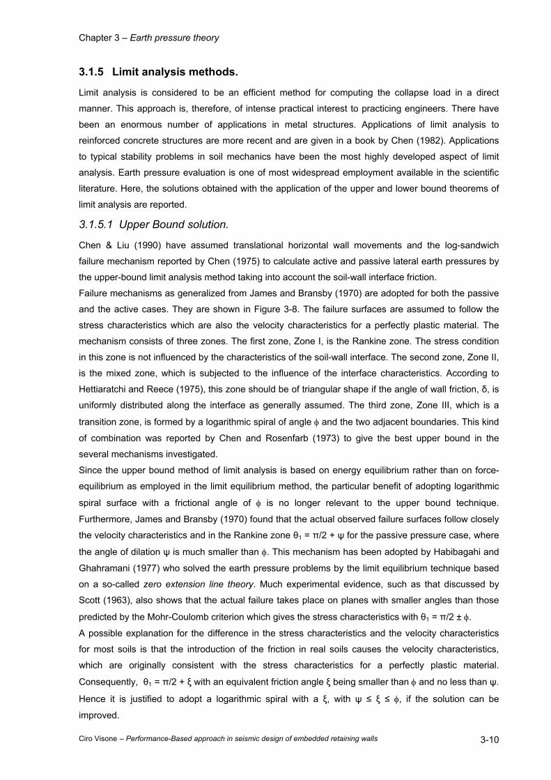
Chapter 3 – Earth pressure theory
Ciro Visone – Performance-Based approach in seismic design of embedded retaining walls 3-10
3.1.5 Limit analysis methods.
Limit analysis is considered to be an efficient method for computing the collapse load in a direct
manner. This approach is, therefore, of intense practical interest to practicing engineers. There have
been an enormous number of applications in metal structures. Applications of limit analysis to
reinforced concrete structures are more recent and are given in a book by Chen (1982). Applications
to typical stability problems in soil mechanics have been the most highly developed aspect of limit
analysis. Earth pressure evaluation is one of most widespread employment available in the scientific
literature. Here, the solutions obtained with the application of the upper and lower bound theorems of
limit analysis are reported.
3.1.5.1 Upper Bound solution.
Chen & Liu (1990) have assumed translational horizontal wall movements and the log-sandwich
failure mechanism reported by Chen (1975) to calculate active and passive lateral earth pressures by
the upper-bound limit analysis method taking into account the soil-wall interface friction.
Failure mechanisms as generalized from James and Bransby (1970) are adopted for both the passive
and the active cases. They are shown in Figure 3-8. The failure surfaces are assumed to follow the
stress characteristics which are also the velocity characteristics for a perfectly plastic material. The
mechanism consists of three zones. The first zone, Zone I, is the Rankine zone. The stress condition
in this zone is not influenced by the characteristics of the soil-wall interface. The second zone, Zone II,
is the mixed zone, which is subjected to the influence of the interface characteristics. According to
Hettiaratchi and Reece (1975), this zone should be of triangular shape if the angle of wall friction, δ, is
uniformly distributed along the interface as generally assumed. The third zone, Zone III, which is a
transition zone, is formed by a logarithmic spiral of angle φ and the two adjacent boundaries. This kind
of combination was reported by Chen and Rosenfarb (1973) to give the best upper bound in the
several mechanisms investigated.
Since the upper bound method of limit analysis is based on energy equilibrium rather than on force-
equilibrium as employed in the limit equilibrium method, the particular benefit of adopting logarithmic
spiral surface with a frictional angle of φ is no longer relevant to the upper bound technique.
Furthermore, James and Bransby (1970) found that the actual observed failure surfaces follow closely
the velocity characteristics and in the Rankine zone θ1 = π/2 + ψ for the passive pressure case, where
the angle of dilation ψ is much smaller than φ. This mechanism has been adopted by Habibagahi and
Ghahramani (1977) who solved the earth pressure problems by the limit equilibrium technique based
on a so-called zero extension line theory. Much experimental evidence, such as that discussed by
Scott (1963), also shows that the actual failure takes place on planes with smaller angles than those
predicted by the Mohr-Coulomb criterion which gives the stress characteristics with θ1 = π/2 ± φ.
A possible explanation for the difference in the stress characteristics and the velocity characteristics
for most soils is that the introduction of the friction in real soils causes the velocity characteristics,
which are originally consistent with the stress characteristics for a perfectly plastic material.
Consequently, θ1 = π/2 + ξ with an equivalent friction angle ξ being smaller than φ and no less than ψ.
Hence it is justified to adopt a logarithmic spiral with a ξ, with ψ ≤ ξ ≤ φ, if the solution can be
improved.
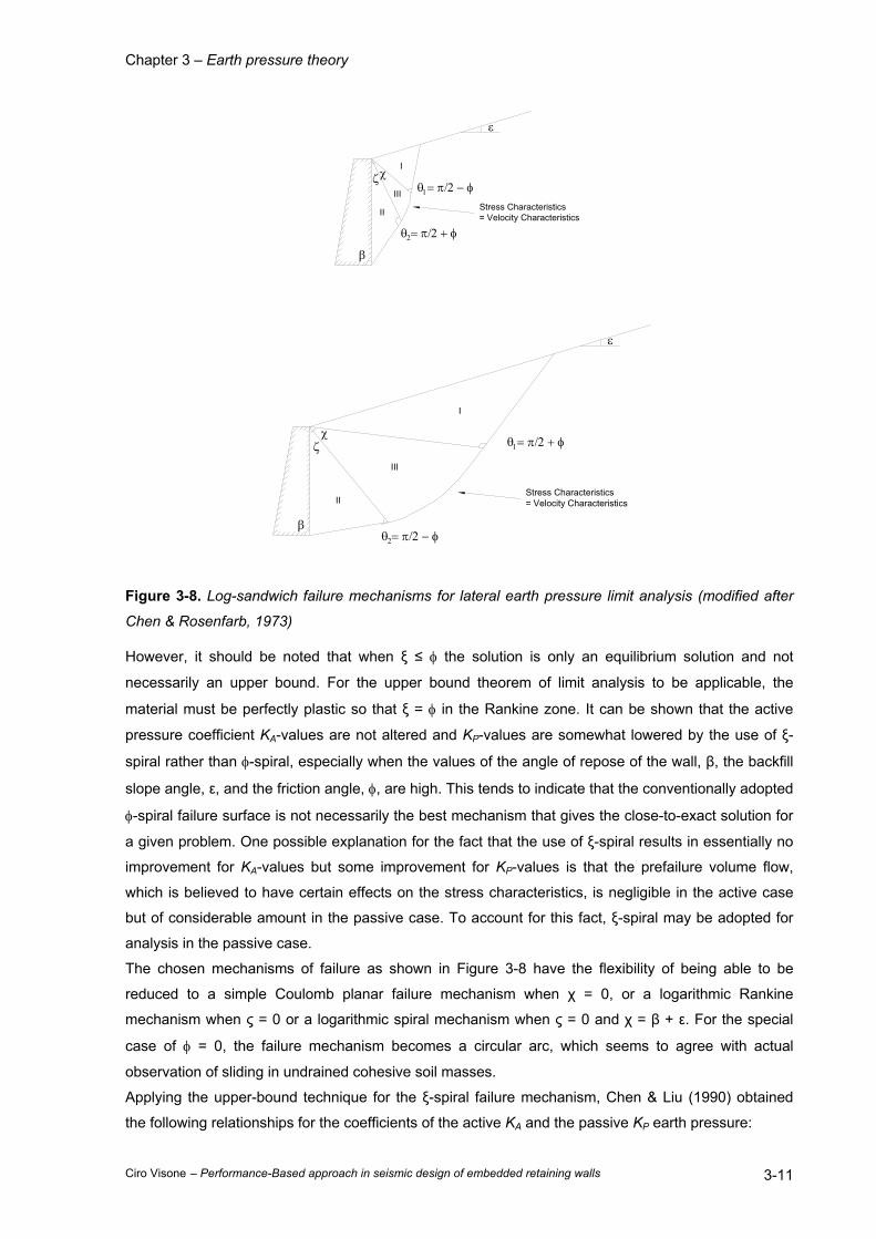
Chapter 3 – Earth pressure theory
Ciro Visone – Performance-Based approach in seismic design of embedded retaining walls 3-11
ε
θ = π/2 − φ1
β
χζ
θ = π/2 + φ2
Stress Characteristics= Velocity Characteristics
I
II
III
ε
θ = π/2 + φ1
β
χζ
θ = π/2 − φ2
Stress Characteristics= Velocity Characteristics
I
II
III
Figure 3-8. Log-sandwich failure mechanisms for lateral earth pressure limit analysis (modified after
Chen & Rosenfarb, 1973)
However, it should be noted that when ξ ≤ φ the solution is only an equilibrium solution and not
necessarily an upper bound. For the upper bound theorem of limit analysis to be applicable, the
material must be perfectly plastic so that ξ = φ in the Rankine zone. It can be shown that the active
pressure coefficient KA-values are not altered and KP-values are somewhat lowered by the use of ξ-
spiral rather than φ-spiral, especially when the values of the angle of repose of the wall, β, the backfill
slope angle, ε, and the friction angle, φ, are high. This tends to indicate that the conventionally adopted
φ-spiral failure surface is not necessarily the best mechanism that gives the close-to-exact solution for
a given problem. One possible explanation for the fact that the use of ξ-spiral results in essentially no
improvement for KA-values but some improvement for KP-values is that the prefailure volume flow,
which is believed to have certain effects on the stress characteristics, is negligible in the active case
but of considerable amount in the passive case. To account for this fact, ξ-spiral may be adopted for
analysis in the passive case.
The chosen mechanisms of failure as shown in Figure 3-8 have the flexibility of being able to be
reduced to a simple Coulomb planar failure mechanism when χ = 0, or a logarithmic Rankine
mechanism when ς = 0 or a logarithmic spiral mechanism when ς = 0 and χ = β + ε. For the special
case of φ = 0, the failure mechanism becomes a circular arc, which seems to agree with actual
observation of sliding in undrained cohesive soil masses.
Applying the upper-bound technique for the ξ-spiral failure mechanism, Chen & Liu (1990) obtained
the following relationships for the coefficients of the active KA and the passive KP earth pressure:
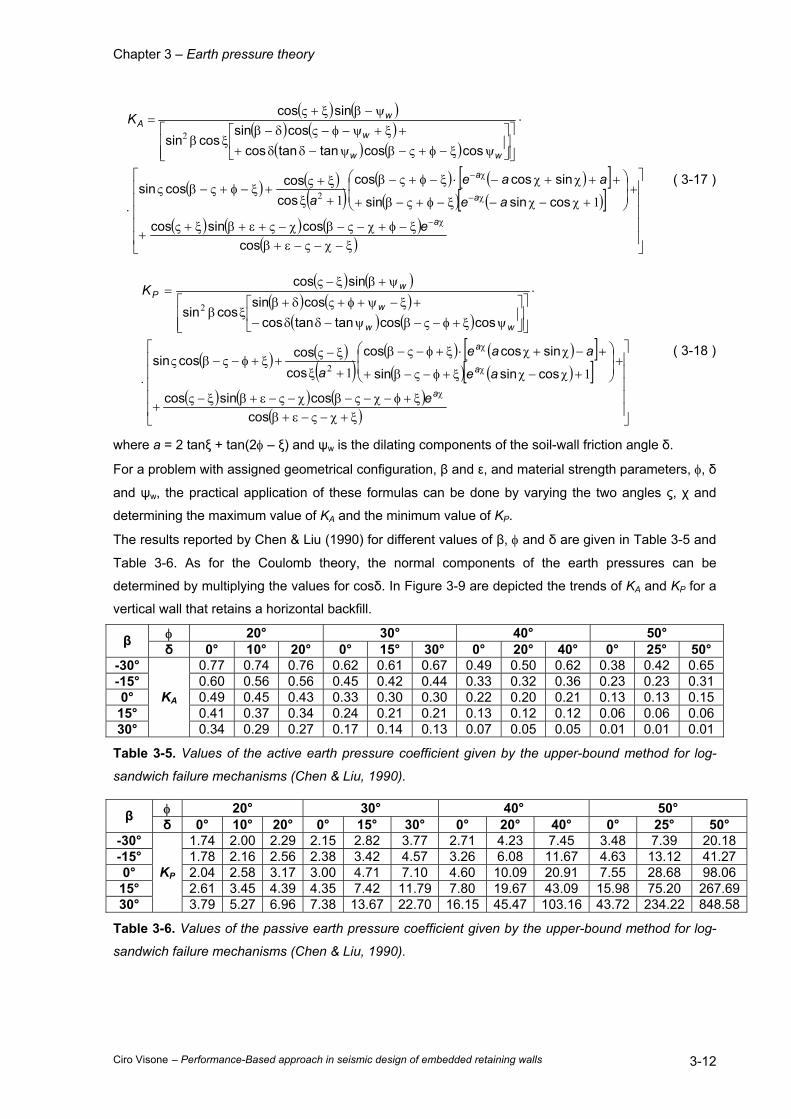
Chapter 3 – Earth pressure theory
Ciro Visone – Performance-Based approach in seismic design of embedded retaining walls 3-12
( ) ( )( ) ( )
( ) ( )
( ) ( )( )
( ) ( )[ ]( ) ( )[ ]
( ) ( ) ( )( )
ξ−χ−ς−ε+βξ−φ+χ−ς−βχ−ς+ε+βξ+ς
+
+
+χ−χ−ξ−φ+ς−β+
++χ+χ−⋅ξ−φ+ς−β
+ξξ+ς
+ξ−φ+ς−βς
⋅
⋅
ψξ−φ+ς−βψ−δδ+
+ξ+ψ−φ−ςδ−βξβ
ψ−βξ+ς=
χ−
χ−
χ−
coscossincos
cossinsin
sincoscoscoscoscossin
coscostantancoscossin
cossin
sincos
a
a
a
ww
w
wA
e
ae
aaea
K
112
2
( 3-17 )
( ) ( )( ) ( )
( ) ( )
( ) ( )( )
( ) ( )[ ]( ) ( )[ ]
( ) ( ) ( )( )
ξ+χ−ς−ε+βξ+φ−χ−ς−βχ−ς−ε+βξ−ς
+
+
+χ−χξ+φ−ς−β+
+−χ+χ⋅ξ+φ−ς−β
+ξ
ξ−ς+ξ+φ−ς−βς
⋅
⋅
ψξ+φ−ς−βψ−δδ−
+ξ−ψ+φ+ςδ+βξβ
ψ+βξ−ς=
χ
χ
χ
coscossincos
cossinsin
sincoscoscoscoscossin
coscostantancoscossin
cossin
sincos
a
a
a
ww
w
wP
e
ae
aaea
K
112
2
( 3-18 )
where a = 2 tanξ + tan(2φ – ξ) and ψw is the dilating components of the soil-wall friction angle δ.
For a problem with assigned geometrical configuration, β and ε, and material strength parameters, φ, δ
and ψw, the practical application of these formulas can be done by varying the two angles ς, χ and
determining the maximum value of KA and the minimum value of KP.
The results reported by Chen & Liu (1990) for different values of β, φ and δ are given in Table 3-5 and
Table 3-6. As for the Coulomb theory, the normal components of the earth pressures can be
determined by multiplying the values for cosδ. In Figure 3-9 are depicted the trends of KA and KP for a
vertical wall that retains a horizontal backfill.
φ 20° 30° 40° 50° β δ 0° 10° 20° 0° 15° 30° 0° 20° 40° 0° 25° 50° -30° 0.77 0.74 0.76 0.62 0.61 0.67 0.49 0.50 0.62 0.38 0.42 0.65 -15° 0.60 0.56 0.56 0.45 0.42 0.44 0.33 0.32 0.36 0.23 0.23 0.31 0° 0.49 0.45 0.43 0.33 0.30 0.30 0.22 0.20 0.21 0.13 0.13 0.15 15° 0.41 0.37 0.34 0.24 0.21 0.21 0.13 0.12 0.12 0.06 0.06 0.06 30°
KA
0.34 0.29 0.27 0.17 0.14 0.13 0.07 0.05 0.05 0.01 0.01 0.01
Table 3-5. Values of the active earth pressure coefficient given by the upper-bound method for log-
sandwich failure mechanisms (Chen & Liu, 1990).
φ 20° 30° 40° 50° β δ 0° 10° 20° 0° 15° 30° 0° 20° 40° 0° 25° 50° -30° 1.74 2.00 2.29 2.15 2.82 3.77 2.71 4.23 7.45 3.48 7.39 20.18 -15° 1.78 2.16 2.56 2.38 3.42 4.57 3.26 6.08 11.67 4.63 13.12 41.27 0° 2.04 2.58 3.17 3.00 4.71 7.10 4.60 10.09 20.91 7.55 28.68 98.06 15° 2.61 3.45 4.39 4.35 7.42 11.79 7.80 19.67 43.09 15.98 75.20 267.6930°
KP
3.79 5.27 6.96 7.38 13.67 22.70 16.15 45.47 103.16 43.72 234.22 848.58
Table 3-6. Values of the passive earth pressure coefficient given by the upper-bound method for log-
sandwich failure mechanisms (Chen & Liu, 1990).
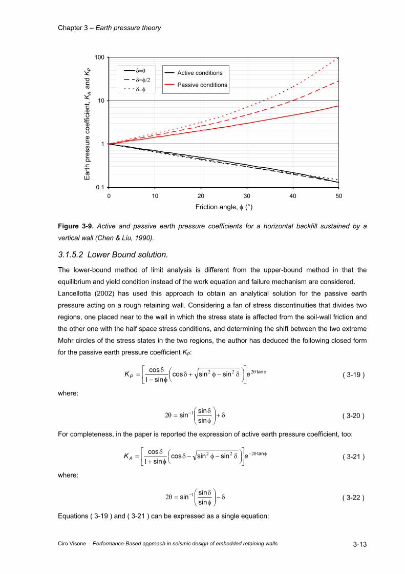
Chapter 3 – Earth pressure theory
Ciro Visone – Performance-Based approach in seismic design of embedded retaining walls 3-13
0.1
1
10
100
0 10 20 30 40 50
Friction angle, φ (°)
Ear
th p
ress
ure
coef
ficie
nt, K
A a
nd K
P δ=0
δ=φ/2
δ=φ
Active conditions
Passive conditions
Figure 3-9. Active and passive earth pressure coefficients for a horizontal backfill sustained by a
vertical wall (Chen & Liu, 1990).
3.1.5.2 Lower Bound solution.
The lower-bound method of limit analysis is different from the upper-bound method in that the
equilibrium and yield condition instead of the work equation and failure mechanism are considered.
Lancellotta (2002) has used this approach to obtain an analytical solution for the passive earth
pressure acting on a rough retaining wall. Considering a fan of stress discontinuities that divides two
regions, one placed near to the wall in which the stress state is affected from the soil-wall friction and
the other one with the half space stress conditions, and determining the shift between the two extreme
Mohr circles of the stress states in the two regions, the author has deduced the following closed form
for the passive earth pressure coefficient KP:
φθ
δ−φ+δ
φ−δ
= tansinsincossin
cos 222
1eKP ( 3-19 )
where:
δ+
φδ
=θ −
sinsinsin 12 ( 3-20 )
For completeness, in the paper is reported the expression of active earth pressure coefficient, too:
φθ−
δ−φ−δ
φ+δ
= tansinsincossin
cos 222
1eK A ( 3-21 )
where:
δ−
φδ
=θ −
sinsinsin 12 ( 3-22 )
Equations ( 3-19 ) and ( 3-21 ) can be expressed as a single equation:
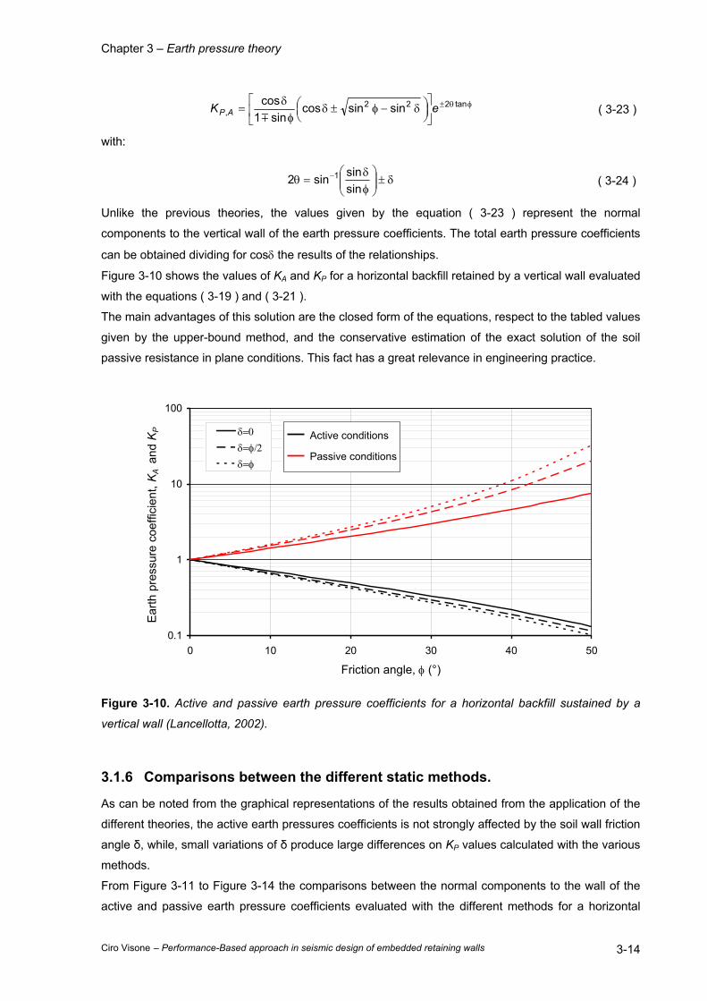
Chapter 3 – Earth pressure theory
Ciro Visone – Performance-Based approach in seismic design of embedded retaining walls 3-14
φθ±
δ−φ±δ
φδ
= tan222, sinsincos
sin1cos eK APm
( 3-23 )
with:
δ±
φδ
=θ −
sinsinsin2 1 ( 3-24 )
Unlike the previous theories, the values given by the equation ( 3-23 ) represent the normal
components to the vertical wall of the earth pressure coefficients. The total earth pressure coefficients
can be obtained dividing for cosδ the results of the relationships.
Figure 3-10 shows the values of KA and KP for a horizontal backfill retained by a vertical wall evaluated
with the equations ( 3-19 ) and ( 3-21 ).
The main advantages of this solution are the closed form of the equations, respect to the tabled values
given by the upper-bound method, and the conservative estimation of the exact solution of the soil
passive resistance in plane conditions. This fact has a great relevance in engineering practice.
0.1
1
10
100
0 10 20 30 40 50
Friction angle, φ (°)
Ear
th p
ress
ure
coef
ficie
nt, K
A a
nd K
P δ=0
δ=φ/2
δ=φ
Active conditions
Passive conditions
Figure 3-10. Active and passive earth pressure coefficients for a horizontal backfill sustained by a
vertical wall (Lancellotta, 2002).
3.1.6 Comparisons between the different static methods.
As can be noted from the graphical representations of the results obtained from the application of the
different theories, the active earth pressures coefficients is not strongly affected by the soil wall friction
angle δ, while, small variations of δ produce large differences on KP values calculated with the various
methods.
From Figure 3-11 to Figure 3-14 the comparisons between the normal components to the wall of the
active and passive earth pressure coefficients evaluated with the different methods for a horizontal
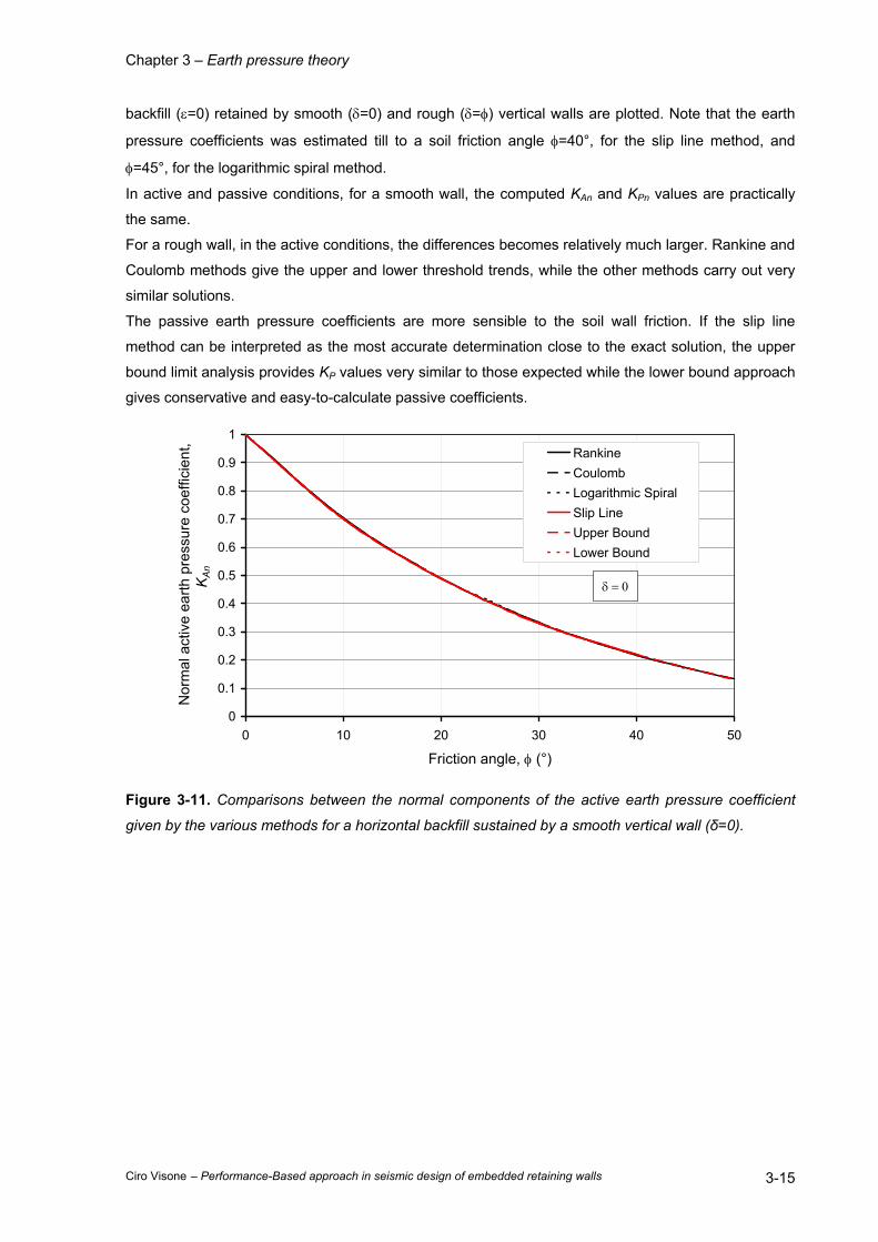
Chapter 3 – Earth pressure theory
Ciro Visone – Performance-Based approach in seismic design of embedded retaining walls 3-15
backfill (ε=0) retained by smooth (δ=0) and rough (δ=φ) vertical walls are plotted. Note that the earth
pressure coefficients was estimated till to a soil friction angle φ=40°, for the slip line method, and
φ=45°, for the logarithmic spiral method.
In active and passive conditions, for a smooth wall, the computed KAn and KPn values are practically
the same.
For a rough wall, in the active conditions, the differences becomes relatively much larger. Rankine and
Coulomb methods give the upper and lower threshold trends, while the other methods carry out very
similar solutions.
The passive earth pressure coefficients are more sensible to the soil wall friction. If the slip line
method can be interpreted as the most accurate determination close to the exact solution, the upper
bound limit analysis provides KP values very similar to those expected while the lower bound approach
gives conservative and easy-to-calculate passive coefficients.
0
0.1
0.2
0.3
0.4
0.5
0.6
0.7
0.8
0.9
1
0 10 20 30 40 50
Friction angle, φ (°)
Nor
mal
act
ive
earth
pre
ssur
e co
effic
ient
, K
An
RankineCoulombLogarithmic SpiralSlip LineUpper BoundLower Bound
δ = 0
Figure 3-11. Comparisons between the normal components of the active earth pressure coefficient
given by the various methods for a horizontal backfill sustained by a smooth vertical wall (δ=0).

Chapter 3 – Earth pressure theory
Ciro Visone – Performance-Based approach in seismic design of embedded retaining walls 3-16
0
0.1
0.2
0.3
0.4
0.5
0.6
0.7
0.8
0.9
1
0 10 20 30 40 50
Friction angle, φ (°)
Nor
mal
act
ive
earth
pre
ssur
e co
effic
ient
, K
An
RankineCoulombLogarithmic SpiralSlip LineUpper BoundLower Bound
δ = φ
Figure 3-12. Comparisons between the normal components of the active earth pressure coefficient
given by the various methods for a horizontal backfill sustained by a rough vertical wall (δ=φ).
0
2
4
6
8
10
12
14
16
18
20
0 10 20 30 40 50
Friction angle, φ (°)
Nor
mal
pas
sive
ear
th p
ress
ure
coef
ficie
nt,
KP
n
RankineCoulombLogarithmic SpiralSlip LineUpper BoundLower Bound
δ = 0
Figure 3-13. Comparisons between the normal components of the passive earth pressure coefficient
given by the various methods for a horizontal backfill sustained by a smooth vertical wall (δ=0).
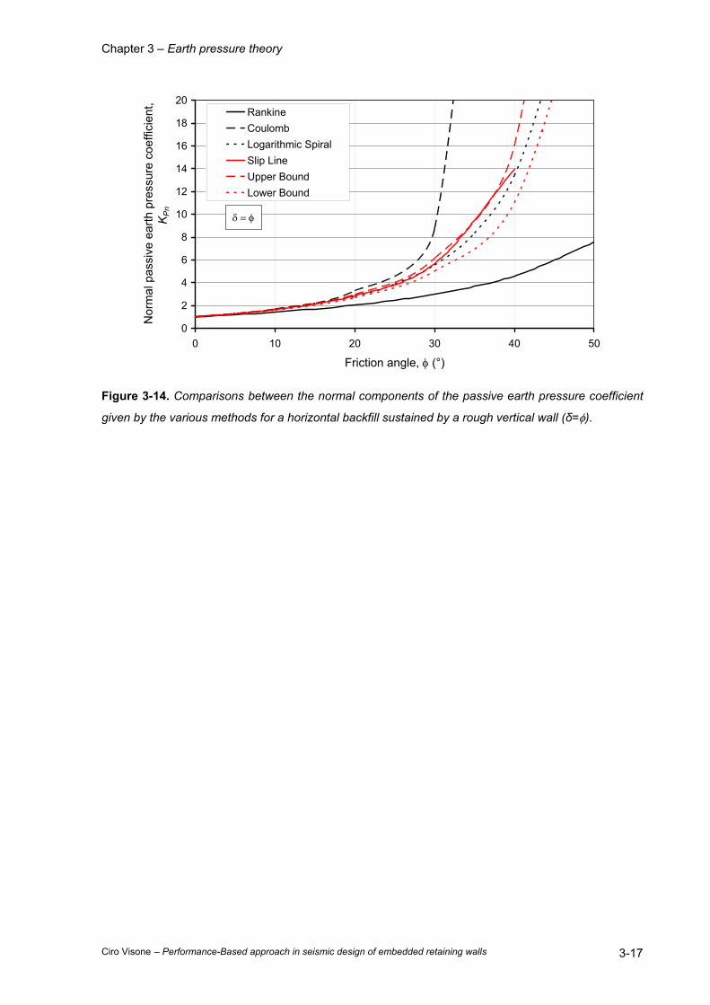
Chapter 3 – Earth pressure theory
Ciro Visone – Performance-Based approach in seismic design of embedded retaining walls 3-17
0
2
4
6
8
10
12
14
16
18
20
0 10 20 30 40 50
Friction angle, φ (°)
Nor
mal
pas
sive
ear
th p
ress
ure
coef
ficie
nt,
KP
n
RankineCoulombLogarithmic SpiralSlip LineUpper BoundLower Bound
δ = φ
Figure 3-14. Comparisons between the normal components of the passive earth pressure coefficient
given by the various methods for a horizontal backfill sustained by a rough vertical wall (δ=φ).
Chapter 3 – Earth pressure theory
Ciro Visone – Performance-Based approach in seismic design of embedded retaining walls 3-18
3.2 SEISMIC PRESSURES ON RETAINING WALLS.
A common approach to the seismic design of retaining walls involves estimating the loads imposed on
the wall during earthquake shaking and then ensuring that the wall can resist those loads. Because
the actual loading on retaining walls during the earthquakes is extremely complicated, seismic
pressures on retaining walls are usually estimated using simplified methods.
Retaining walls that can move sufficiently to develop minimum active and/or maximum passive earth
pressures are referred to as yielding walls. The dynamic pressures acting on yielding walls are usually
estimated by pseudostatic procedures in which the effects of an earthquake are represented by
constant horizontal and/or vertical accelerations.
Some retaining structures, such as massive gravity walls founded on rock or basement walls braced at
both top and bottom, do not move sufficiently to mobilize shear strength of the backfill soil. As a result,
the limiting conditions of minimum active or maximum passive earth pressures can not be developed.
This type of walls are denoted as nonyielding walls.
An earthquake has two possible effects on a soil-wall system. One is to increase the driving force. The
other is to decrease the shearing resistance of the soil. The reduction in the shearing resistance of a
soil during an earthquake appears only when the magnitude of the earthquake exceeds a certain limit
and the ground conditions are favourable for such a reduction. The evaluation of such a reduction
requires considerable knowledge in earthquake engineering and soil dynamics.
Research conducted by Okamoto (1956) indicated that when the average ground acceleration is
larger than 0.3g, there is a considerable reduction in strength for most soils. However, he claimed that
in many cases, the ground acceleration is less than 0.3g and the mechanical properties of mostly of
the soils do not change significantly in these cases. Here, only the increase in driving forces is to be
considered. The shear strength of the soil is assumed unaffected by the influence of the seismic
loading.
In the quasi-static analysis of seismic lateral earth pressures, a constant seismic coefficient, k, is
assumed for the entire soil mass involved. A seismic force, which is equal to k times the weight of a
soil mass, is assumed to act at the center of gravity of the sliding soil mass. The seismic force is
assumed to act in a direction at an angle θ from the vertical as shown in Figure 1-1.
In the following, the main theories developed for the study of the earth pressure on yielding walls in
seismic conditions with a pseudostatic approach and on nonyielding walls are presented.
3.2.1 Mononobe-Okabe theory.
Okabe (1926) and Mononobe & Matsuo (1929) developed the basis of a pseudostatic analysis of
seismic earth pressures on retaining structures that has become popularly known as the Mononobe-
Okabe (M-O) method. The M-O method is a direct extension of the static Coulomb theory to
pseudostatic conditions. In a M-O analysis, pseudostatic accelerations are applied to a Coulomb
active (or passive) wedge. The pseudostatic soil thrust is then obtained from the force equilibrium of
the wedge.
In addition to those under static conditions, the forces acting on an active wedge in a dry cohesionless
backfill wedge are constituted by horizontal and vertical pseudostatic forces whose magnitudes are
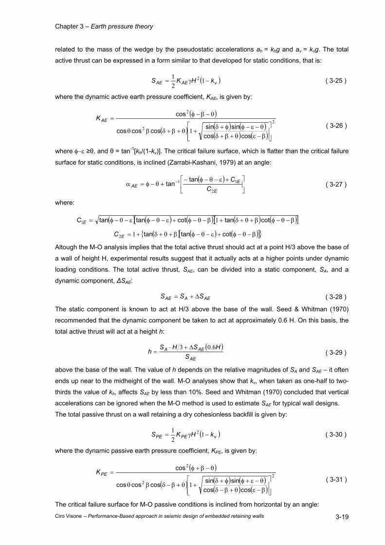
Chapter 3 – Earth pressure theory
Ciro Visone – Performance-Based approach in seismic design of embedded retaining walls 3-19
related to the mass of the wedge by the pseudostatic accelerations ah = khg and av = kvg. The total
active thrust can be expressed in a form similar to that developed for static conditions, that is:
( )vAEAE kHKS −γ= 121 2 ( 3-25 )
where the dynamic active earth pressure coefficient, KAE, is given by:
( )
( ) ( ) ( )( ) ( )
22
2
1
β−εθ+β+δθ−ε−φφ+δ
+θ+β+δβθ
θ−β−φ=
coscossinsincoscoscos
cosAEK
( 3-26 )
where φ−ε ≥θ, and θ = tan-1[kh/(1-kv)]. The critical failure surface, which is flatter than the critical failure
surface for static conditions, is inclined (Zarrabi-Kashani, 1979) at an angle:
( )
+ε−θ−φ−+θ−φ=α −
E
EAE C
C
2
11 tantan ( 3-27 )
where:
( ) ( ) ( )[ ] ( ) ( )[ ]β−θ−φβ+θ+δ+β−θ−φ+ε−θ−φε−θ−φ= cottancottantan 11EC
( ) ( ) ( )[ ]{ }β−θ−φ+ε−θ−φβ+θ+δ+= cottantan12EC
Altough the M-O analysis implies that the total active thrust should act at a point H/3 above the base of
a wall of height H, experimental results suggest that it actually acts at a higher points under dynamic
loading conditions. The total active thrust, SAE, can be divided into a static component, SA, and a
dynamic component, ∆SAE:
AEAAE SSS ∆+= ( 3-28 )
The static component is known to act at H/3 above the base of the wall. Seed & Whitman (1970)
recommended that the dynamic component be taken to act at approximately 0.6 H. On this basis, the
total active thrust will act at a height h:
( )AE
AEA
SHSHS
h603 .∆+⋅
= ( 3-29 )
above the base of the wall. The value of h depends on the relative magnitudes of SA and SAE – it often
ends up near to the midheight of the wall. M-O analyses show that kv, when taken as one-half to two-
thirds the value of kh, affects SAE by less than 10%. Seed and Whitman (1970) concluded that vertical
accelerations can be ignored when the M-O method is used to estimate SAE for typical wall designs.
The total passive thrust on a wall retaining a dry cohesionless backfill is given by:
( )vPEPE kHKS −γ= 121 2 ( 3-30 )
where the dynamic passive earth pressure coefficient, KPE, is given by:
( )
( ) ( ) ( )( ) ( )
22
2
1
β−εθ+β−δθ−ε+φφ+δ
+θ+β−δβθ
θ−β+φ=
coscossinsincoscoscos
cosPEK
( 3-31 )
The critical failure surface for M-O passive conditions is inclined from horizontal by an angle:

Chapter 3 – Earth pressure theory
Ciro Visone – Performance-Based approach in seismic design of embedded retaining walls 3-20
( )
+ε+θ+φ−+φ−θ=α −
E
EPE C
C
4
31 tantan ( 3-32 )
where:
( ) ( ) ( )[ ] ( ) ( )[ ]β+θ−φβ+θ−δ+β+θ−φ+ε+θ−φε+θ−φ= cottancottantan 13EC
( ) ( ) ( )[ ]{ }β+θ−φ+ε+θ−φβ−θ+δ+= cottantan14EC
The total passive thrust can also be divided (Towhata and Islam, 1987) into static and dynamic
components:
PEPPE SSS ∆+= ( 3-33 )
where SPE and SP are computed from equations ( 3-30 ) and ( 3-12 ), respectively. Note that the
dynamic component acts in the opposite direction of the static component, thus reducing the available
passive resistance.
From Figure 3-15 to Figure 3-18 the graphical representations of the seismic earth pressure
coefficients and the critical failure surfaces in active and passive conditions evaluated with the M-O
method for vertical walls retaining a horizontal backfill are plotted. The figures denote a slight influence
of the soil-wall friction on the seismic active conditions while, as in the Coulomb method, strong
differences exist in the passive case.
Although conceptually quite simple, the M-O analysis provides a useful means of estimating
earthquake-induced loads on retaining walls. A positive horizontal acceleration coefficient causes the
total active thrust to exceed the static active thrust and the total passive thrust to be less than the
static passive thrust. Since the stability of a particular wall is generally reduced by an increase in
active thrust and/or a decrease in passive thrust, the M-O method produces seismic loads that are
more critical than the static loads that act prior an earthquake. The effects of distributed load and
discrete surface loads and irregular backfill surfaces are easily considered by modifying the free-body
diagram of the active or passive wedge. In such cases, equations ( 3-26 ) and ( 3-31 ) no longer apply.
The total thrusts must be obtained from the analysis of a number of potential failure planes.
As a pseudostatic extension of the Coulomb analysis, however, the M-O analysis is subject to all of
the limitations of pseudostatic analyses as well as the limitations of Coulomb theory. The
determination of the appropriate pseudostatic coefficient is difficult and the analysis is not appropriate
for soils that experience significant loss of strength during earthquakes (e.g. liquefiable soils). Just as
Coulomb theory does under static conditions, the M-O analysis will overpredict the actual total passive
thrust, particularly for δ > φ/2. For these reasons the M-O method should be used and interpreted
carefully.
Note that, in Figure 3-17c, the seismic passive earth pressure coefficient is larger than 20 when the
yellow horizontal plateau appears.
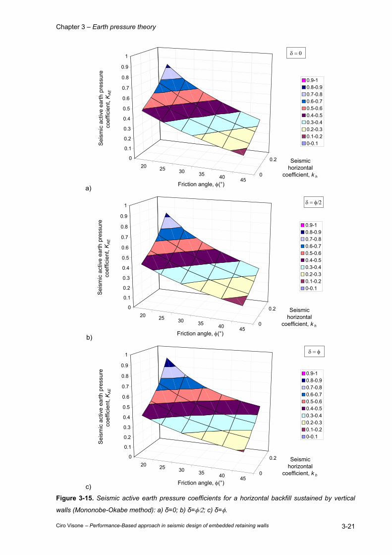
Chapter 3 – Earth pressure theory
Ciro Visone – Performance-Based approach in seismic design of embedded retaining walls 3-21
a)
20 25 30 35 40 450
0.20
0.1
0.2
0.3
0.4
0.5
0.6
0.7
0.8
0.9
1
Sei
smic
act
ive
earth
pre
ssur
e co
effic
ient
, KA
E
Friction angle, φ(°)
Seismic horizontal
coefficient, k h
0.9-10.8-0.90.7-0.80.6-0.70.5-0.60.4-0.50.3-0.40.2-0.30.1-0.20-0.1
δ = 0
b)
20 25 30 35 40 450
0.20
0.1
0.2
0.3
0.4
0.5
0.6
0.7
0.8
0.9
1
Sei
smic
act
ive
earth
pre
ssur
e co
effic
ient
, KA
E
Friction angle, φ(°)
Seismic horizontal
coefficient, k h
0.9-10.8-0.90.7-0.80.6-0.70.5-0.60.4-0.50.3-0.40.2-0.30.1-0.20-0.1
δ = φ/2
c)
20 25 30 35 40 450
0.20
0.1
0.2
0.3
0.4
0.5
0.6
0.7
0.8
0.9
1
Seis
mic
act
ive
earth
pre
ssur
e co
effic
ient
, KA
E
Friction angle, φ(°)
Seismic horizontal
coefficient, k h
0.9-10.8-0.90.7-0.80.6-0.70.5-0.60.4-0.50.3-0.40.2-0.30.1-0.20-0.1
δ = φ
Figure 3-15. Seismic active earth pressure coefficients for a horizontal backfill sustained by vertical
walls (Mononobe-Okabe method): a) δ=0; b) δ=φ/2; c) δ=φ.
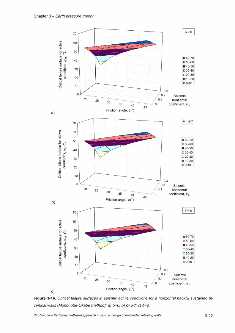
Chapter 3 – Earth pressure theory
Ciro Visone – Performance-Based approach in seismic design of embedded retaining walls 3-22
a)
20 25 30 35 40 450
0.10.2
0.30
10
20
30
40
50
60
70
Crit
ical
failu
re s
urfa
ce fo
r act
ive
cond
ition
s, α
AE (°
)
Friction angle, φ(°)
Seismic horizontal
coefficient, k h
60-7050-6040-5030-4020-3010-200-10
δ = 0
b)
20 25 30 35 40 450
0.10.2
0.30
10
20
30
40
50
60
70
Crit
ical
failu
re s
urfa
ce fo
r act
ive
cond
ition
s, α
AE
(°)
Friction angle, φ(°)
Seismic horizontal
coefficient, k h
60-7050-6040-5030-4020-3010-200-10
δ = φ/2
c)
20 25 30 35 40 450
0.10.2
0.30
10
20
30
40
50
60
70
Crit
ical
failu
re s
urfa
ce fo
r act
ive
cond
ition
s, α
AE (
°)
Friction angle, φ(°)
Seismic horizontal
coefficient, k h
60-7050-6040-5030-4020-3010-200-10
δ = φ
Figure 3-16. Critical failure surfaces in seismic active conditions for a horizontal backfill sustained by
vertical walls (Mononobe-Okabe method): a) δ=0; b) δ=φ/2; c) δ=φ.
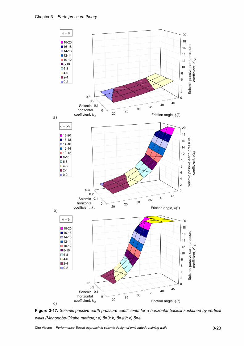
Chapter 3 – Earth pressure theory
Ciro Visone – Performance-Based approach in seismic design of embedded retaining walls 3-23
a) 20
2530
35 40 45
00.1
0.20.3 0
2
4
6
8
10
12
14
16
18
20
Sei
smic
pas
sive
ear
th p
ress
ure
coef
ficie
nt, K
PE
Friction angle, φ(°)
Seismic horizontal
coefficient, k h
18-2016-1814-1612-1410-128-106-84-62-40-2
δ = 0
b) 20
2530
35 40 45
00.1
0.20.3 0
2
4
6
8
10
12
14
16
18
20
Sei
smic
pas
sive
ear
th p
ress
ure
coef
ficie
nt, K
PE
Friction angle, φ(°)
Seismic horizontal
coefficient, k h
18-2016-1814-1612-1410-128-106-84-62-40-2
δ = φ/2
c) 20
2530
35 40 45
00.1
0.20.3 0
2
4
6
8
10
12
14
16
18
20
Sei
smic
pas
sive
ear
th p
ress
ure
coef
ficie
nt, K
PE
Friction angle, φ(°)
Seismic horizontal
coefficient, k h
18-2016-1814-1612-1410-128-106-84-62-40-2
δ = φ
Figure 3-17. Seismic passive earth pressure coefficients for a horizontal backfill sustained by vertical
walls (Mononobe-Okabe method): a) δ=0; b) δ=φ/2; c) δ=φ.
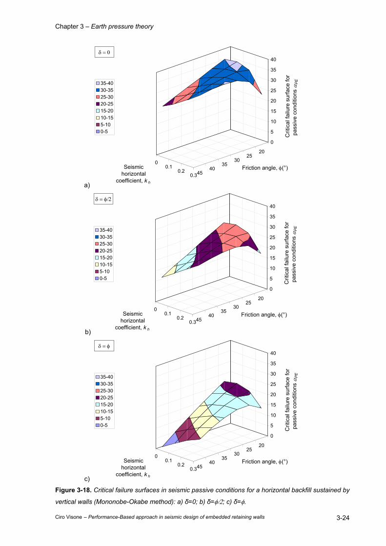
Chapter 3 – Earth pressure theory
Ciro Visone – Performance-Based approach in seismic design of embedded retaining walls 3-24
a)
2025
3035
4045
00.1
0.20.3
0
5
10
15
20
25
30
35
40
Crit
ical
failu
re s
urfa
ce fo
r pa
ssiv
e co
nditi
ons
α PE
Friction angle, φ(°)Seismic horizontal
coefficient, k h
35-4030-3525-3020-2515-2010-155-100-5
δ = 0
b)
2025
3035
4045
00.1
0.20.3
0
5
10
15
20
25
30
35
40
Crit
ical
failu
re s
urfa
ce fo
r pa
ssiv
e co
nditi
ons
α PE
Friction angle, φ(°)Seismic horizontal
coefficient, k h
35-4030-3525-3020-2515-2010-155-100-5
δ = φ/2
c)
2025
3035
4045
00.1
0.20.3
0
5
10
15
20
25
30
35
40
Crit
ical
failu
re s
urfa
ce fo
r pa
ssiv
e co
nditi
ons
α PE
Friction angle, φ(°)Seismic horizontal
coefficient, k h
35-4030-3525-3020-2515-2010-155-100-5
δ = φ
Figure 3-18. Critical failure surfaces in seismic passive conditions for a horizontal backfill sustained by
vertical walls (Mononobe-Okabe method): a) δ=0; b) δ=φ/2; c) δ=φ.
Chapter 3 – Earth pressure theory
Ciro Visone – Performance-Based approach in seismic design of embedded retaining walls 3-25
3.2.2 Limit analysis methods.
3.2.2.1 Upper bound solution.
By equating the incremental external work to the incremental internal energy dissipation associated to
a translational wall movement and a φ-spiral log-sandwich mechanism of failure proposed by Chen
and Rosenfarb (1973), Chang (1981) has deduced seismic active and passive earth pressure
formulations in which the soil thrust can be expressed in terms of equivalent coefficients of seismic
earth pressure, KAE and KPE, as:
2
21 HKS EE γ= ( 3-34 )
The seismic active earth pressure coefficient KAE is:
AcAqAAE NHcN
HqNK
γ+
γ+= γ
22 ( 3-35 )
where γ is the unit weight of the backfill material, H the vertical height of the wall, q is the uniform
surcharge acting on the surface of the backfill, c is the soil cohesion. NAγ, NAq and NAc are three
coefficients for which closed form expressions can be found in Chen & Liu (1990). The most critical
KAE-value can be obtained by maximization with respect to ς and χ shown in Figure 3-8.
At the same manner, the seismic passive earth pressure coefficient KPE is given by the following
relationship:
PcPqPPE NHcN
HqNK
γ+
γ+= γ
22 ( 3-36 )
Expressions of the three coefficients NAγ, NAq and NAc can be found in Chen & Liu (1990). The most
critical KPE-value can be obtained by minimization with respect to ς and χ shown in Figure 3-8.
For practical purposes, the author has calculated some values of the seismic earth pressure
coefficients reported in tables (Chang, 1981, as quoted by Chen & Liu, 1990).
In the next Table 3-7 and Table 3-8 some of them are summarized.
Figure 3-19 and Figure 3-20 show the graphical representations of the seismic earth pressure
coefficients in active and passive conditions given by the upper bound method for vertical walls
retaining a horizontal backfill. As M-O method, the soil-wall friction has a slight influence on the
seismic active conditions. For high values of the friction angle φ, the differences might become larger
in the passive conditions.
The dependence of the seismic coefficient kh on KAE and KPE is more clear considering the variations
of earth pressure coefficients respect to the corresponding static values. For the active case, the
increase of KAE is more obvious for denser soils with higher φ-values than for the looser soils with
lower φ-values. The decrease of KPE is more obvious for looser soils than for denser soils in the
passive case.
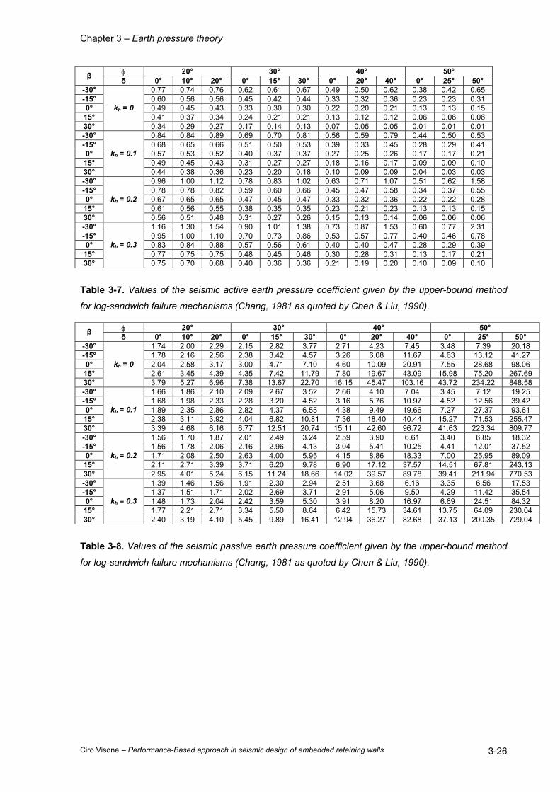
Chapter 3 – Earth pressure theory
Ciro Visone – Performance-Based approach in seismic design of embedded retaining walls 3-26
φ 20° 30° 40° 50° β δ 0° 10° 20° 0° 15° 30° 0° 20° 40° 0° 25° 50° -30° 0.77 0.74 0.76 0.62 0.61 0.67 0.49 0.50 0.62 0.38 0.42 0.65 -15° 0.60 0.56 0.56 0.45 0.42 0.44 0.33 0.32 0.36 0.23 0.23 0.31 0° 0.49 0.45 0.43 0.33 0.30 0.30 0.22 0.20 0.21 0.13 0.13 0.15
15° 0.41 0.37 0.34 0.24 0.21 0.21 0.13 0.12 0.12 0.06 0.06 0.06 30°
kh = 0
0.34 0.29 0.27 0.17 0.14 0.13 0.07 0.05 0.05 0.01 0.01 0.01 -30° 0.84 0.84 0.89 0.69 0.70 0.81 0.56 0.59 0.79 0.44 0.50 0.53 -15° 0.68 0.65 0.66 0.51 0.50 0.53 0.39 0.33 0.45 0.28 0.29 0.41 0° 0.57 0.53 0.52 0.40 0.37 0.37 0.27 0.25 0.26 0.17 0.17 0.21
15° 0.49 0.45 0.43 0.31 0.27 0.27 0.18 0.16 0.17 0.09 0.09 0.10 30°
kh = 0.1
0.44 0.38 0.36 0.23 0.20 0.18 0.10 0.09 0.09 0.04 0.03 0.03 -30° 0.96 1.00 1.12 0.78 0.83 1.02 0.63 0.71 1.07 0.51 0.62 1.58 -15° 0.78 0.78 0.82 0.59 0.60 0.66 0.45 0.47 0.58 0.34 0.37 0.55 0° 0.67 0.65 0.65 0.47 0.45 0.47 0.33 0.32 0.36 0.22 0.22 0.28
15° 0.61 0.56 0.55 0.38 0.35 0.35 0.23 0.21 0.23 0.13 0.13 0.15 30°
kh = 0.2
0.56 0.51 0.48 0.31 0.27 0.26 0.15 0.13 0.14 0.06 0.06 0.06 -30° 1.16 1.30 1.54 0.90 1.01 1.38 0.73 0.87 1.53 0.60 0.77 2.31 -15° 0.95 1.00 1.10 0.70 0.73 0.86 0.53 0.57 0.77 0.40 0.46 0.78 0° 0.83 0.84 0.88 0.57 0.56 0.61 0.40 0.40 0.47 0.28 0.29 0.39
15° 0.77 0.75 0.75 0.48 0.45 0.46 0.30 0.28 0.31 0.13 0.17 0.21 30°
kh = 0.3
0.75 0.70 0.68 0.40 0.36 0.36 0.21 0.19 0.20 0.10 0.09 0.10
Table 3-7. Values of the seismic active earth pressure coefficient given by the upper-bound method
for log-sandwich failure mechanisms (Chang, 1981 as quoted by Chen & Liu, 1990).
φ 20° 30° 40° 50° β δ 0° 10° 20° 0° 15° 30° 0° 20° 40° 0° 25° 50° -30° 1.74 2.00 2.29 2.15 2.82 3.77 2.71 4.23 7.45 3.48 7.39 20.18 -15° 1.78 2.16 2.56 2.38 3.42 4.57 3.26 6.08 11.67 4.63 13.12 41.27 0° 2.04 2.58 3.17 3.00 4.71 7.10 4.60 10.09 20.91 7.55 28.68 98.06
15° 2.61 3.45 4.39 4.35 7.42 11.79 7.80 19.67 43.09 15.98 75.20 267.69 30°
kh = 0
3.79 5.27 6.96 7.38 13.67 22.70 16.15 45.47 103.16 43.72 234.22 848.58 -30° 1.66 1.86 2.10 2.09 2.67 3.52 2.66 4.10 7.04 3.45 7.12 19.25 -15° 1.68 1.98 2.33 2.28 3.20 4.52 3.16 5.76 10.97 4.52 12.56 39.42 0° 1.89 2.35 2.86 2.82 4.37 6.55 4.38 9.49 19.66 7.27 27.37 93.61
15° 2.38 3.11 3.92 4.04 6.82 10.81 7.36 18.40 40.44 15.27 71.53 255.47 30°
kh = 0.1
3.39 4.68 6.16 6.77 12.51 20.74 15.11 42.60 96.72 41.63 223.34 809.77 -30° 1.56 1.70 1.87 2.01 2.49 3.24 2.59 3.90 6.61 3.40 6.85 18.32 -15° 1.56 1.78 2.06 2.16 2.96 4.13 3.04 5.41 10.25 4.41 12.01 37.52 0° 1.71 2.08 2.50 2.63 4.00 5.95 4.15 8.86 18.33 7.00 25.95 89.09
15° 2.11 2.71 3.39 3.71 6.20 9.78 6.90 17.12 37.57 14.51 67.81 243.13 30°
kh = 0.2
2.95 4.01 5.24 6.15 11.24 18.66 14.02 39.57 89.78 39.41 211.94 770.53 -30° 1.39 1.46 1.56 1.91 2.30 2.94 2.51 3.68 6.16 3.35 6.56 17.53 -15° 1.37 1.51 1.71 2.02 2.69 3.71 2.91 5.06 9.50 4.29 11.42 35.54 0° 1.48 1.73 2.04 2.42 3.59 5.30 3.91 8.20 16.97 6.69 24.51 84.32
15° 1.77 2.21 2.71 3.34 5.50 8.64 6.42 15.73 34.61 13.75 64.09 230.04 30°
kh = 0.3
2.40 3.19 4.10 5.45 9.89 16.41 12.94 36.27 82.68 37.13 200.35 729.04
Table 3-8. Values of the seismic passive earth pressure coefficient given by the upper-bound method
for log-sandwich failure mechanisms (Chang, 1981 as quoted by Chen & Liu, 1990).
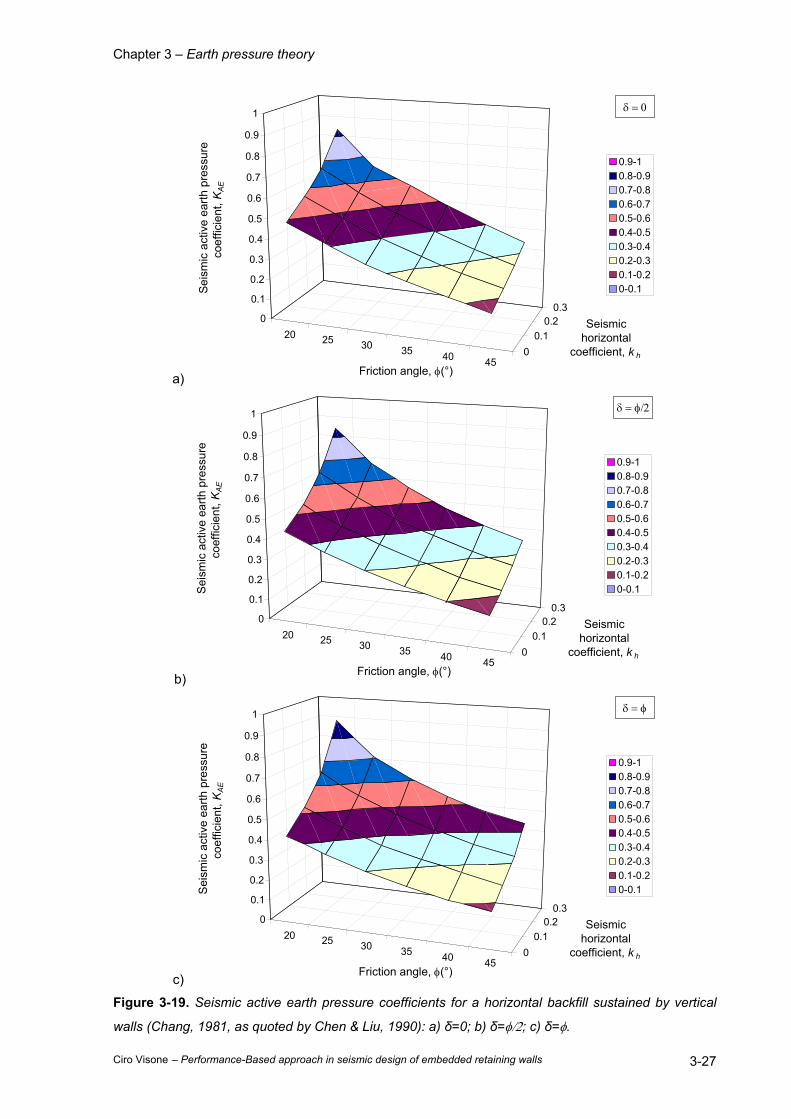
Chapter 3 – Earth pressure theory
Ciro Visone – Performance-Based approach in seismic design of embedded retaining walls 3-27
a)
20 25 30 35 40 450
0.10.2
0.30
0.1
0.2
0.3
0.4
0.5
0.6
0.7
0.8
0.9
1
Seis
mic
act
ive
earth
pre
ssur
e co
effic
ient
, KA
E
Friction angle, φ(°)
Seismic horizontal
coefficient, k h
0.9-10.8-0.90.7-0.80.6-0.70.5-0.60.4-0.50.3-0.40.2-0.30.1-0.20-0.1
δ = 0
b)
20 25 30 35 40 450
0.10.2
0.30
0.1
0.2
0.3
0.4
0.5
0.6
0.7
0.8
0.9
1
Sei
smic
act
ive
earth
pre
ssur
e co
effic
ient
, KA
E
Friction angle, φ(°)
Seismic horizontal
coefficient, k h
0.9-10.8-0.90.7-0.80.6-0.70.5-0.60.4-0.50.3-0.40.2-0.30.1-0.20-0.1
δ = φ/2
c)
20 25 30 35 40 450
0.10.2
0.30
0.1
0.2
0.3
0.4
0.5
0.6
0.7
0.8
0.9
1
Sei
smic
act
ive
earth
pre
ssur
e co
effic
ient
, KA
E
Friction angle, φ(°)
Seismic horizontal
coefficient, k h
0.9-10.8-0.90.7-0.80.6-0.70.5-0.60.4-0.50.3-0.40.2-0.30.1-0.20-0.1
δ = φ
Figure 3-19. Seismic active earth pressure coefficients for a horizontal backfill sustained by vertical
walls (Chang, 1981, as quoted by Chen & Liu, 1990): a) δ=0; b) δ=φ/2; c) δ=φ.

Chapter 3 – Earth pressure theory
Ciro Visone – Performance-Based approach in seismic design of embedded retaining walls 3-28
a) 20
2530 35 40 45
00.1
0.20.3 0
2
4
6
8
10
12
14
16
18
20
Sei
smic
pas
sive
ear
th p
ress
ure
coef
ficie
nt, K
PE
Friction angle, φ(°)
Seismic horizontal
coefficient, k h
18-2016-1814-1612-1410-128-106-84-62-40-2
δ = 0
b) 20
2530 35 40 45
00.1
0.20.3 0
2
4
6
8
10
12
14
16
18
20
Sei
smic
pas
sive
ear
th p
ress
ure
coef
ficie
nt, K
PE
Friction angle, φ(°)
Seismic horizontal
coefficient, k h
18-2016-1814-1612-1410-128-106-84-62-40-2
δ = φ/2
c) 20
2530 35 40 45
00.1
0.20.3 0
2
4
6
8
10
12
14
16
18
20
Sei
smic
pas
sive
ear
th p
ress
ure
coef
ficie
nt, K
PE
Friction angle, φ(°)
Seismic horizontal
coefficient, k h
18-2016-1814-1612-1410-128-106-84-62-40-2
δ = φ
Figure 3-20. Seismic passive earth pressure coefficients for a horizontal backfill sustained by vertical
walls (Chang, 1981, as quoted by Chen & Liu, 1990): a) δ=0; b) δ=φ/2; c) δ=φ.
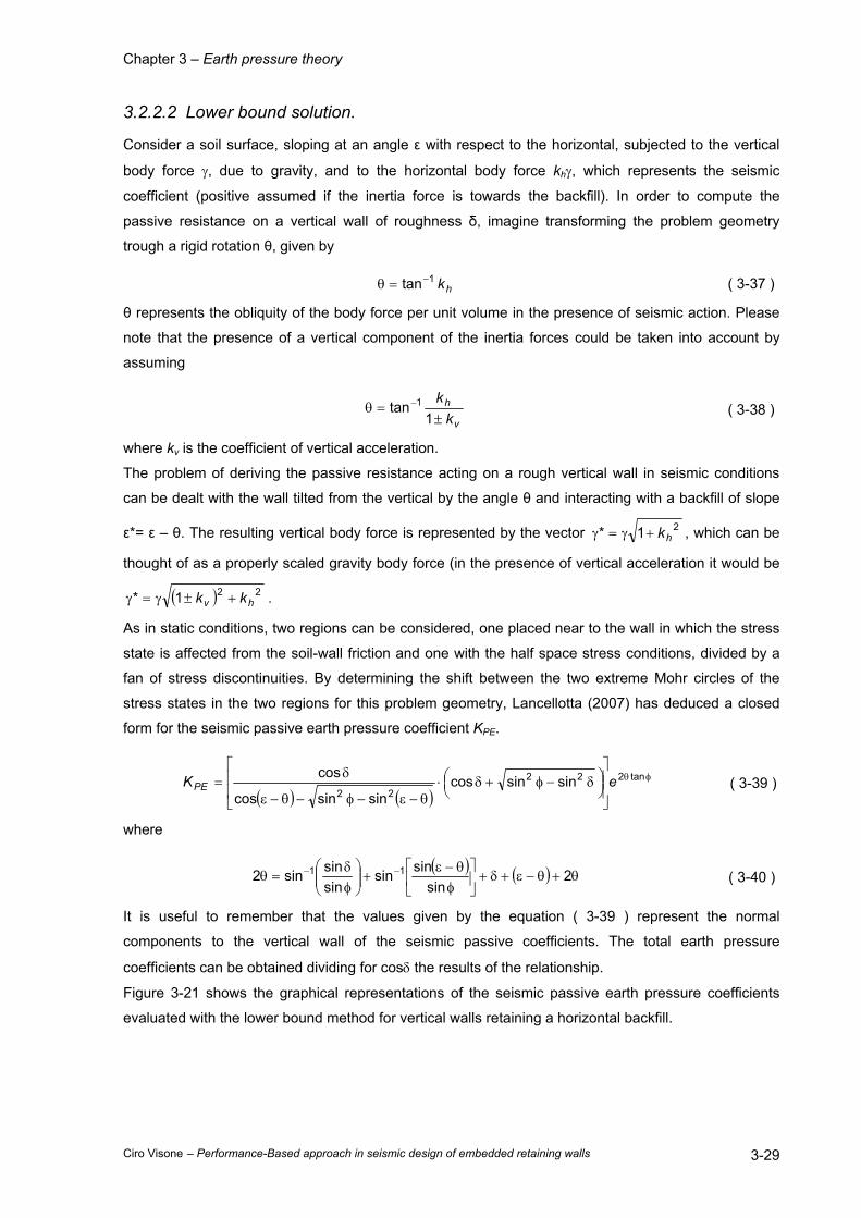
Chapter 3 – Earth pressure theory
Ciro Visone – Performance-Based approach in seismic design of embedded retaining walls 3-29
3.2.2.2 Lower bound solution.
Consider a soil surface, sloping at an angle ε with respect to the horizontal, subjected to the vertical
body force γ, due to gravity, and to the horizontal body force khγ, which represents the seismic
coefficient (positive assumed if the inertia force is towards the backfill). In order to compute the
passive resistance on a vertical wall of roughness δ, imagine transforming the problem geometry
trough a rigid rotation θ, given by
hk1tan−=θ ( 3-37 )
θ represents the obliquity of the body force per unit volume in the presence of seismic action. Please
note that the presence of a vertical component of the inertia forces could be taken into account by
assuming
v
h
kk±
=θ −
1tan 1 ( 3-38 )
where kv is the coefficient of vertical acceleration.
The problem of deriving the passive resistance acting on a rough vertical wall in seismic conditions
can be dealt with the wall tilted from the vertical by the angle θ and interacting with a backfill of slope
ε*= ε – θ. The resulting vertical body force is represented by the vector 21* hk+γ=γ , which can be
thought of as a properly scaled gravity body force (in the presence of vertical acceleration it would be
( ) 221* hv kk +±γ=γ .
As in static conditions, two regions can be considered, one placed near to the wall in which the stress
state is affected from the soil-wall friction and one with the half space stress conditions, divided by a
fan of stress discontinuities. By determining the shift between the two extreme Mohr circles of the
stress states in the two regions for this problem geometry, Lancellotta (2007) has deduced a closed
form for the seismic passive earth pressure coefficient KPE.
( ) ( )φθ
δ−φ+δ⋅
θ−ε−φ−θ−ε
δ= tan222
22sinsincos
sinsincos
cos eKPE ( 3-39 )
where
( ) ( ) θ+θ−ε+δ+
φ
θ−ε+
φδ
=θ −− 2sin
sinsinsinsinsin2 11 ( 3-40 )
It is useful to remember that the values given by the equation ( 3-39 ) represent the normal
components to the vertical wall of the seismic passive coefficients. The total earth pressure
coefficients can be obtained dividing for cosδ the results of the relationship.
Figure 3-21 shows the graphical representations of the seismic passive earth pressure coefficients
evaluated with the lower bound method for vertical walls retaining a horizontal backfill.

Chapter 3 – Earth pressure theory
Ciro Visone – Performance-Based approach in seismic design of embedded retaining walls 3-30
a) 20
2530 35 40 45
0
0.20
2
4
6
8
10
12
14
16
18
20
Seis
mic
pas
sive
ear
th p
ress
ure
coef
ficie
nt, K
PE
Friction angle, φ(°)
Seismic horizontal
coefficient, k h
18-2016-1814-1612-1410-128-106-84-62-40-2
δ = 0
b) 20
2530 35 40 45
0
0.20
2
4
6
8
10
12
14
16
18
20
Seis
mic
pas
sive
ear
th p
ress
ure
coef
ficie
nt, K
PE
Friction angle, φ(°)
Seismic horizontal
coefficient, k h
18-2016-1814-1612-1410-128-106-84-62-40-2
δ = φ/2
c) 20
2530 35 40 45
0
0.20
2
4
6
8
10
12
14
16
18
20
Sei
smic
pas
sive
ear
th p
ress
ure
coef
ficie
nt, K
PE
Friction angle, φ(°)
Seismic horizontal
coefficient, k h
18-2016-1814-1612-1410-128-106-84-62-40-2
δ = φ
Figure 3-21. Seismic passive earth pressure coefficients for a horizontal backfill sustained by vertical
walls (Lancellotta, 2007): a) δ=0; b) δ=φ/2; c) δ=φ.

Chapter 3 – Earth pressure theory
Ciro Visone – Performance-Based approach in seismic design of embedded retaining walls 3-31
3.2.3 Comparisons between the different seismic methods.
In Figure 3-22 and Figure 3-23 the values calculated with the different methods previously recalled of
the normal components of the seismic active and passive earth pressure coefficients exerted on
vertical walls by horizontal backfills are compared.
For the active case, the KAEn values obtained by limit equilibrium and the limit analysis methods are
practically identical. This is due to the fact that, when the wall is approximately vertical and the slope
angle of the backfill is larger than zero, the most critical failure is practically planar.
For the passive case, the most critical sliding surface is much different from a planar surface as is
assumed in the M-O analysis. The KPEn values are seriously overestimated by the M-O method. They
are, in most cases, higher than those obtained by the limit analysis. This is especially the case when
the wall is rough and the angle of wall repose is large. The condition φ = δ = 40° carries out very high
KPEn values larger than 20, unreported in Figure 3-23c. For smooth walls, the potential sliding surface
is practically planar and the different methods give almost identical results.
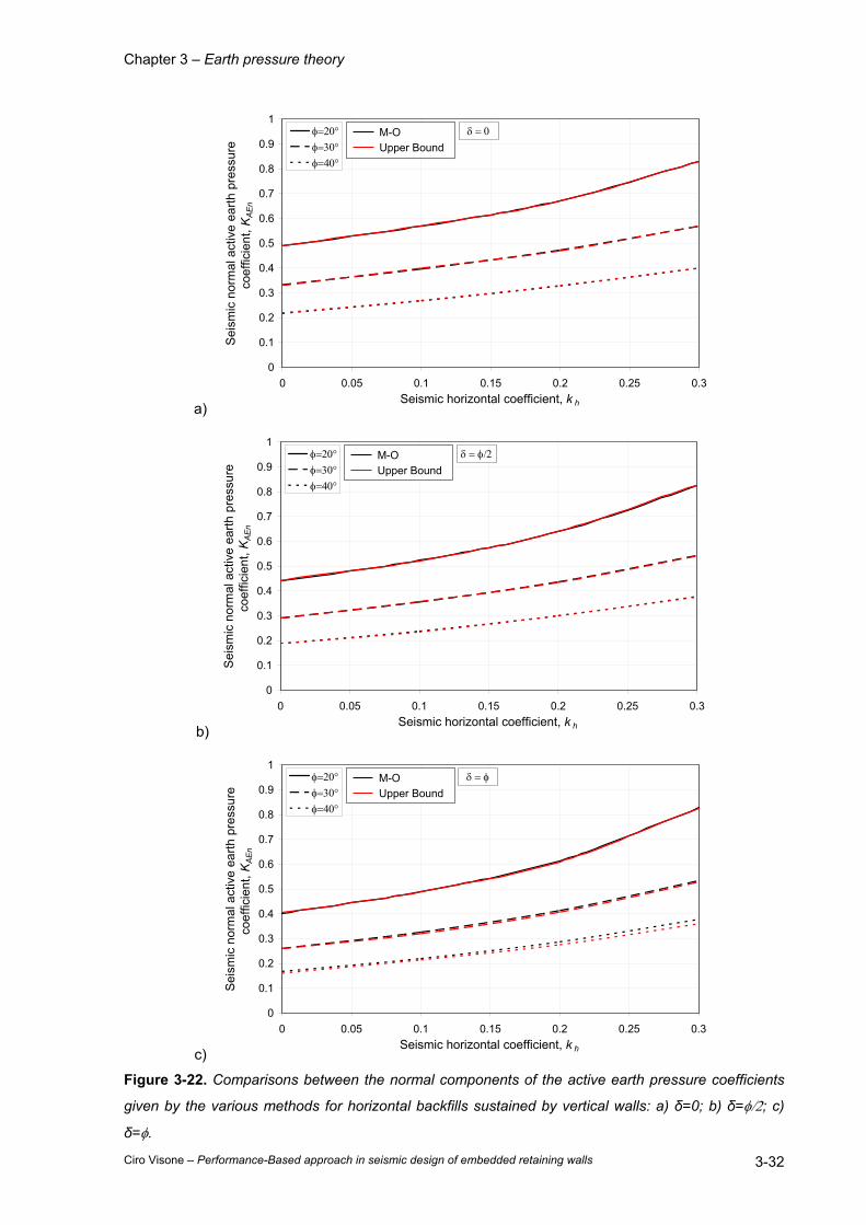
Chapter 3 – Earth pressure theory
Ciro Visone – Performance-Based approach in seismic design of embedded retaining walls 3-32
a)
0
0.1
0.2
0.3
0.4
0.5
0.6
0.7
0.8
0.9
1
0 0.05 0.1 0.15 0.2 0.25 0.3Seismic horizontal coefficient, k h
Sei
smic
nor
mal
act
ive
earth
pre
ssur
e co
effic
ient
, KA
En
φ=20°φ=30°φ=40°
M-OUpper Bound
δ = 0
b)
0
0.1
0.2
0.3
0.4
0.5
0.6
0.7
0.8
0.9
1
0 0.05 0.1 0.15 0.2 0.25 0.3Seismic horizontal coefficient, k h
Sei
smic
nor
mal
act
ive
earth
pre
ssur
e co
effic
ient
, KA
En
φ=20°φ=30°φ=40°
M-OUpper Bound
δ = φ/2
c)
0
0.1
0.2
0.3
0.4
0.5
0.6
0.7
0.8
0.9
1
0 0.05 0.1 0.15 0.2 0.25 0.3Seismic horizontal coefficient, k h
Sei
smic
nor
mal
act
ive
earth
pre
ssur
e co
effic
ient
, KA
En
φ=20°φ=30°φ=40°
M-OUpper Bound
δ = φ
Figure 3-22. Comparisons between the normal components of the active earth pressure coefficients
given by the various methods for horizontal backfills sustained by vertical walls: a) δ=0; b) δ=φ/2; c)
δ=φ.

Chapter 3 – Earth pressure theory
Ciro Visone – Performance-Based approach in seismic design of embedded retaining walls 3-33
a)
0
2
4
6
8
10
12
14
16
18
20
0 0.05 0.1 0.15 0.2 0.25 0.3Seismic horizontal coefficient, k h
Sei
smic
nor
mal
pas
sive
ear
th p
ress
ure
coef
ficie
nt, K
PE
n
φ=20°φ=30°φ=40°
δ = 0M-OUpper BoundLower Bound
b)
0
2
4
6
8
10
12
14
16
18
20
0 0.05 0.1 0.15 0.2 0.25 0.3Seismic horizontal coefficient, k h
Sei
smic
nor
mal
pas
sive
ear
th p
ress
ure
coef
ficie
nt, K
PE
n
φ=20°φ=30°φ=40°
δ = φ/2M-OUpper BoundLower Bound
c)
0
2
4
6
8
10
12
14
16
18
20
0 0.05 0.1 0.15 0.2 0.25 0.3Seismic horizontal coefficient, k h
Sei
smic
nor
mal
pas
sive
ear
th p
ress
ure
coef
ficie
nt, K
PE
n
φ=20°φ=30°φ=40°
δ = φM-OUpper BoundLower Bound
Figure 3-23. Comparisons between the normal components of the passive earth pressure coefficients
given by the various methods for horizontal backfills sustained by vertical walls: a) δ=0; b) δ=φ/2; c)
δ=φ.
Chapter 3 – Earth pressure theory
Ciro Visone – Performance-Based approach in seismic design of embedded retaining walls 3-34
3.3 EFFECTS OF WATER ON WALL PRESSURES.
The procedures for estimation of seismic loads on retaining walls described in the preceding sections
have been limited to cases of dry backfills. Most retaining walls are designed with drains to prevent
water from building up within the backfill. This is not possible for instance for retaining walls in
waterfront areas, where most earthquake-induced wall failures have been observed.
The presence of water plays a strong role in determining the loads on waterfront retaining walls both
during and after earthquakes. Water outboard of a retaining wall can exert dynamic pressures on the
face of the wall. Water within a backfill can also affect the dynamic pressures that act on the back of
the wall. Proper consideration of the effects of water is essential for the seismic design of retaining
structures, particularly in waterfront areas. Since few waterfront retaining structures are completely
impermeable, the water level in the backfill is usually at approximately the same level as the free water
outboard of the wall. Backfill water levels generally lag behind changes in outboard water level – the
difference in water level depends on the permeability of the wall and the backfill and on the rate at
which the outboard water level changes.
The total water pressures that act on retaining walls in the absence of seepage within the backfill can
be divided in two components: hydrostatic pressure, which increases linearly with the depth and acts
on the wall before, during and after the earthquake shaking, and hydrodynamic pressure, which
results from the dynamic response of the water itself.
3.3.1 Water outboard of wall.
Hydrodynamic water pressure results from the dynamic response of a body of water. For retaining
walls, hydrodynamic pressures are usually estimated from Westergaard’s solution (Westergaard,
1931) for the case of a vertical, rigid dam retaining a semi-infinite reservoir of water that is excited by
harmonic, horizontal motion of its rigid base. Westergaard showed that the hydrodynamic pressure
amplitude increased with the square root of water depth when the motion is applied at a frequency
lower than the fundamental frequency of the reservoir, f0 = VP/4H, where VP is the P-wave velocity of
water (about 1400 m/sec) and H is the depth of water in the reservoir (the natural frequency of a 10m-
deep reservoir, for example, would be over 35 Hz, well above the frequencies of interest for
earthquakes). Westergaard computed the amplitude of the hydrodynamic pressure as:
Hzgap ww
hw γ=
87 ( 3-41 )
The resultant hydrodynamic thrust is given by:
2
127 H
gaP w
hw γ= ( 3-42 )
The total water pressure on the face of the wall is the sum of the hydrostatic and hydrodynamic water
pressures. Similarly, the total lateral thrust due to the water is equal to the sum of hydrostatic and
hydrodynamic thrusts.
Another important consideration in the design of a waterfront retaining wall is the potential for rapid
drawdown of the water outboard of the wall. Earthquakes occurring near large bodies of water often
Chapter 3 – Earth pressure theory
Ciro Visone – Performance-Based approach in seismic design of embedded retaining walls 3-35
induce long-period motion of the water, such as tsunamis or seiches, that cause the water surface to
move up and down. While the upward movements of water outboard of a retaining wall will generally
tend to stabilize the wall (assuming that it does not rise above the level of the top of the wall),
downward movements can create a destabilizing rapid drawdown condtions. When liquefiable soils
exist under relatively high levels of initial shear stress, failures can be triggered by very small changes
in water level. Such failures, can originate in the soils adjacent to or beneath the retaining structure
rather than in the backfill.
3.3.2 Water in backfill.
The presence of water in the backfill behind a retaining wall can influence the seismic loads that act on
the wall in three ways:
1. by altering the inertial forces within the backfill
2. by developing hydrodynamic pressures within the backfill
3. by allowing excess pore water pressure generation due to cyclic straining of the backfill soils.
The inertial forces in saturated soils depend on the relative movement between the backfill soil
particles and the pore water that surrounds them. If, as is usually the case, the permeability of the soil
is small enough (typically k ≤ 10-5 m/sec or so) that the pore water moves with the soil during the
earthquake shaking (no relative movement of soil and water, or restrained pore water conditions), the
inertial forces will be proportional to the total unit weight of the soil. If the permeability of the backfill
soil is very high, however, the pore water may remain essentially stationary while the soil skeleton
moves back and forth (the soil particles move through the pore water in free pore water conditions). In
such cases, inertial forces will be proportional to the buoyant (or submerged) unit weight of the soil.
Hydrodynamic water pressures can also develop under free pore water conditions and must be added
to the computed soil and hydrostatic pressures to obtain the total loading on the wall.
For restrained pore water conditions, the M-O method can be modified to account for the presence of
pore water within the backfill (Matsuzawa et al., 1985). Representing the excess of pore water
pressure in the backfill by the pore pressure ratio, ru = ∆u/p’0, the active soil thrust acting on a yielding
wall can be computed from equation ( 3-25 ) using:
( )ub r−γ=γ 1 ( 3-43 )
( )( )
−−γ
γ=θ −
vub
hsat
krk11
tan 1 ( 3-44 )
An equivalent hydrostatic thrust based on a fluid of unit weight γeq = γw + ru γb must be added to the soil
thrust. Note that as ru approaches 1 (as it could in liquefiable backfill), the wall thrust approaches that
imposed by a fluid of equivalent unit weight γeq = γsat. Subsequent unidirectional movement of a soil
that develops high excess pore water pressures may, depending on its residual (or steady state)
strength, cause dilation with accompanying pore water pressure reduction and strength gain.
Soil thrusts from partially submerged backfills may be computed using an average unit weight based
on the relative volumes of soil within the active wedge that are above and below the phreatic surface
(Figure 3-24):

Chapter 3 – Earth pressure theory
Ciro Visone – Performance-Based approach in seismic design of embedded retaining walls 3-36
( ) dsat γλ−+γλ=γ 22 1 ( 3-45 )
Again, the hydrostatic thrust (and hydrodynamic thrust, if present) must be added to the soil thrust.
H
Hλ
γ = γd
γ = γsat
Figure 3-24. Geometry and notation for partially submerged backfill.

Chapter 3 – Earth pressure theory
Ciro Visone – Performance-Based approach in seismic design of embedded retaining walls 4-1
4 STATIC DESIGN OF EMBEDDED RETAINING WALLS.
Embedded walls are relatively thin walls of steel, reinforced concrete or timber, eventually supported
by anchorages, struts and/or passive earth pressure (EN1997-1). The bending capacity of such walls
plays a significant role in the support of the retained material while the role of the weight of the wall is
usually considered to be insignificant. Examples of such walls include: cantilever steel sheet pile walls,
anchored or strutted steel or concrete sheet pile walls, diaphragm walls, etc., as described in Chapter 2.
Limit equilibrium is one of most widespread design method for the analysis of embedded retaining
structures. In this procedure, the wall is assumed rigid, the soil has a rigid-perfectly plastic behaviour
and the pressures deriving form the interaction depend on the expected movements of the wall. The
kinematical mechanism is affected from the constraints applied on the wall. In this section, the various
type of embedded retaining walls in relation to the kinematical restraints are separately treated
4.1 FREE CANTILEVER WALLS.
A cantilever sheet pile retaining wall consists of a vertical structural element embedded in the ground
below the retained material. The upper part of the wall provides a retaining force due to the wall
stiffness and the embedment of the lower part. The embedded cantilever wall obtains its ability to
resist the pressure of the retained soil by developing resisting earth pressures on the embedded
portion of the wall. Embedded cantilever sheet pile retaining walls are frequently used for temporary
and permanent support of excavations up to about 4-5 m high.
The distribution of earth pressure on the embedded part of the wall is dependent on the complex
interaction between the wall movement and the ground. Many methods for analysis and design of
embedded cantilever walls have been proposed and these have been reviewed by Bica & Clayton
(1989). Each method makes various assumptions concerning the distribution of earth pressure on the
wall and the deflection or wall movement. Most of the methods follows the limit equilibrium approach
based on the classical limiting earth pressure distributions. Model studies on embedded walls have
been performed by Rowe (1951), Bransby & Milligan (1975) and Lyndon & Pearson (1984). Bica &
Clayton (1992) have produced some empirical charts for the design of cantilever walls.
King (1995) suggested an analytical limit equilibrium approach for dry cohesionless soil, involving
different assumptions from the previous methods. One of the assumptions involves the location of the
point, near the bottom of the wall, of zero net pressure by means of an empirically determined
parameter. Based on the results of centrifuge tests, the author makes a recommendation for an
appropriate value of this empirical parameter that, referring to the notation introduced in Figure 4-3, is
assumed z' = 0.35 d.
The basis of the limit equilibrium methods is the prediction of the maximum height of excavation for
which static equilibrium is maintained. This is known as the limiting equilibrium situation. It is therefore
important to be able to accurately evaluate the earth pressure acting on each side of the wall in the
limiting equilibrium condition.
The actual distribution and magnitude of earth pressure on an embedded retaining wall is dependent
on the complex interaction of the wall and the soil. The general shape of the earth pressure

Chapter 3 – Earth pressure theory
Ciro Visone – Performance-Based approach in seismic design of embedded retaining walls 4-2
distribution is shown in Figure 4-1. The common limit equilibrium design and analysis methods are all
based on this general shape. Each method makes different simplifications and assumptions that
modify the general shape of the pressure distribution to enable a solution to be found.
a)
hd
b)
hd
Figure 4-1. Soil pressure distributions on an embedded cantilever wall: a) pressure distributions; b)
net pressure distribution.
The stability of the cantilever wall is guaranteed from the passive resistance of the soil in which the
wall is embedded. In the limit equilibrium methods the wall movement that conducts to limit conditions
is constituted by a rigid rotation around a point O placed near to the bottom of the wall. The theoretical
earth pressures distributions on the wall are plotted in Figure 4-2.
hd
H
AK γ
PK γ
PK γAK γ
AK γ d K γ (h+d)P
d'z'
O
Figure 4-2. Theoretical earth pressures distributions assumed in limit equilibrium methods.

Chapter 3 – Earth pressure theory
Ciro Visone – Performance-Based approach in seismic design of embedded retaining walls 4-3
To eliminate stresses discontinuities in correspondence of the rotation point and to obtain a simplified
shape of the pressures distributions, different simplifications and assumptions were proposed in
literature. The main of which are reported in Figure 4-3.
In the first, the net pressure distribution is simplified by a rectilinear shape. It is assumed that the
passive resistance below the dredge level is fully mobilized. The rotation point coincides with the zero
net pressure point. At the bottom of the wall the soil strengths, active and passive, are mobilized and
the net pressure assumes the values reported in Figure 4-3a.
a)
AK γ
P(K - K ) γA
[K (h+d) - K d] γP A
hd
d'z'
b)
hd
AK γ
PK γ
d'
R
0.2
d'
Figure 4-3. Simplified earth pressures distributions: a) Full Method; b) Blum Method.
The limit depth d can be evaluated imposing translation and moment equilibrium. In this manner, a
system of two equations of second and third degree is obtained and the two unknowns, the depth of
the point of the inversion of pressures z’ and the limit depth of embedment d, may be calculated using:
+
−
+−
=
hd
KK
hd
hd
KK
hz
A
P
A
P
211
1'
22
( 4-1 )
+
−
+−
=
hd
KK
hd
hd
KK
hz
A
P
A
P
211
1'
33
( 4-2 )
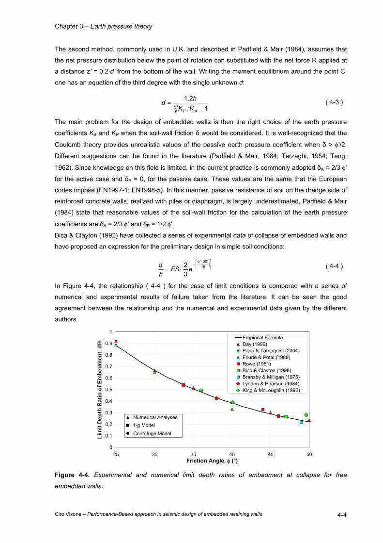
Chapter 3 – Earth pressure theory
Ciro Visone – Performance-Based approach in seismic design of embedded retaining walls 4-4
The second method, commonly used in U.K. and described in Padfield & Mair (1984), assumes that
the net pressure distribution below the point of rotation can substituted with the net force R applied at
a distance z’ = 0.2·d’ from the bottom of the wall. Writing the moment equilibrium around the point C,
one has an equation of the third degree with the single unknown d:
12.1
3 −=
AP KKhd ( 4-3 )
The main problem for the design of embedded walls is then the right choice of the earth pressure
coefficients KA and KP when the soil-wall friction δ would be considered. It is well-recognized that the
Coulomb theory provides unrealistic values of the passive earth pressure coefficient when δ > φ'/2.
Different suggestions can be found in the literature (Padfield & Mair, 1984; Terzaghi, 1954; Teng,
1962). Since knowledge on this field is limited, in the current practice is commonly adopted δA = 2/3 φ'
for the active case and δP = 0, for the passive case. These values are the same that the European
codes impose (EN1997-1; EN1998-5). In this manner, passive resistance of soil on the dredge side of
reinforced concrete walls, realized with piles or diaphragm, is largely underestimated. Padfield & Mair
(1984) state that reasonable values of the soil-wall friction for the calculation of the earth pressure
coefficients are δA = 2/3 φ' and δP = 1/2 φ'.
Bica & Clayton (1992) have collected a series of experimental data of collapse of embedded walls and
have proposed an expression for the preliminary design in simple soil conditions:
°−φ−
⋅= 1830'
32 eFS
hd ( 4-4 )
In Figure 4-4, the relationship ( 4-4 ) for the case of limit conditions is compared with a series of
numerical and experimental results of failure taken from the literature. It can be seen the good
agreement between the relationship and the numerical and experimental data given by the different
authors.
0
0.1
0.2
0.3
0.4
0.5
0.6
0.7
0.8
0.9
1
25 30 35 40 45 50Friction Angle, φ (°)
Lim
it D
epth
Rat
io o
f Em
bedm
ent,
d/h
Empirical FormulaDay (1999)Pane & Tamagnini (2004)Fourie & Potts (1989)Rowe (1951)Bica & Clayton (1998)Bransby & Milligan (1975)Lyndon & Pearson (1984)King & McLoughlin (1992)
▲ Numerical Analyses■ 1-g Model
● Centrifuge Model
Figure 4-4. Experimental and numerical limit depth ratios of embedment at collapse for free
embedded walls.
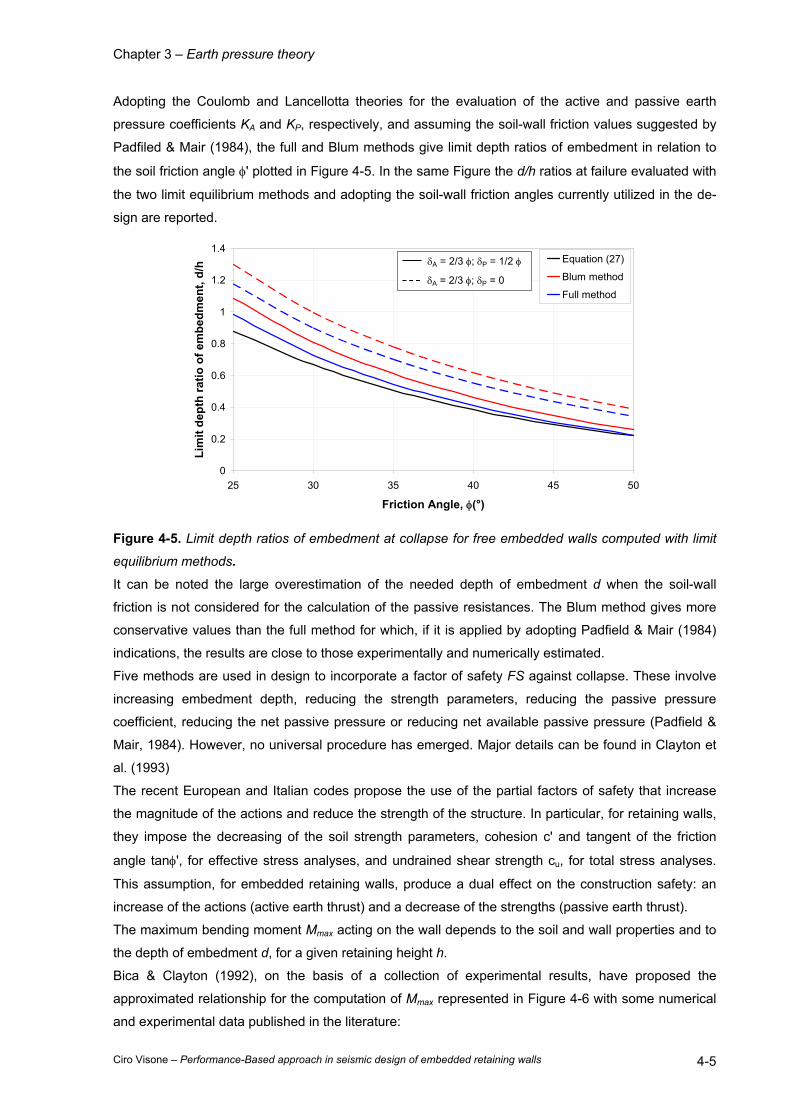
Chapter 3 – Earth pressure theory
Ciro Visone – Performance-Based approach in seismic design of embedded retaining walls 4-5
Adopting the Coulomb and Lancellotta theories for the evaluation of the active and passive earth
pressure coefficients KA and KP, respectively, and assuming the soil-wall friction values suggested by
Padfiled & Mair (1984), the full and Blum methods give limit depth ratios of embedment in relation to
the soil friction angle φ' plotted in Figure 4-5. In the same Figure the d/h ratios at failure evaluated with
the two limit equilibrium methods and adopting the soil-wall friction angles currently utilized in the de-
sign are reported.
0
0.2
0.4
0.6
0.8
1
1.2
1.4
25 30 35 40 45 50
Friction Angle, φ(°)
Lim
it de
pth
ratio
of e
mbe
dmen
t, d/
h Equation (27)
Blum method
Full method
δA = 2/3 φ; δP = 1/2 φ
δA = 2/3 φ; δP = 0
Figure 4-5. Limit depth ratios of embedment at collapse for free embedded walls computed with limit
equilibrium methods. It can be noted the large overestimation of the needed depth of embedment d when the soil-wall
friction is not considered for the calculation of the passive resistances. The Blum method gives more
conservative values than the full method for which, if it is applied by adopting Padfield & Mair (1984)
indications, the results are close to those experimentally and numerically estimated.
Five methods are used in design to incorporate a factor of safety FS against collapse. These involve
increasing embedment depth, reducing the strength parameters, reducing the passive pressure
coefficient, reducing the net passive pressure or reducing net available passive pressure (Padfield &
Mair, 1984). However, no universal procedure has emerged. Major details can be found in Clayton et
al. (1993)
The recent European and Italian codes propose the use of the partial factors of safety that increase
the magnitude of the actions and reduce the strength of the structure. In particular, for retaining walls,
they impose the decreasing of the soil strength parameters, cohesion c' and tangent of the friction
angle tanφ', for effective stress analyses, and undrained shear strength cu, for total stress analyses.
This assumption, for embedded retaining walls, produce a dual effect on the construction safety: an
increase of the actions (active earth thrust) and a decrease of the strengths (passive earth thrust).
The maximum bending moment Mmax acting on the wall depends to the soil and wall properties and to
the depth of embedment d, for a given retaining height h.
Bica & Clayton (1992), on the basis of a collection of experimental results, have proposed the
approximated relationship for the computation of Mmax represented in Figure 4-6 with some numerical
and experimental data published in the literature:
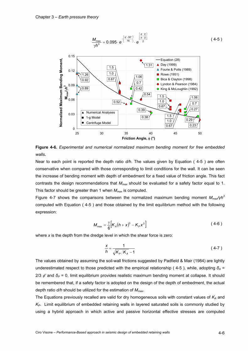
Chapter 3 – Earth pressure theory
Ciro Visone – Performance-Based approach in seismic design of embedded retaining walls 4-6
232
1630'
3max 095.0
−
°−φ−
⋅⋅=γ
hd
eeh
M ( 4-5 )
0
0.03
0.06
0.09
0.12
0.15
25 30 35 40 45 50Friction Angle, φ (°)
Nor
mal
ized
Max
imum
Ben
ding
Mom
ent,
Mm
ax/ γ
h3
Equation (28)Day (1999)Fourie & Potts (1989)Rowe (1951)Bica & Clayton (1998)Lyndon & Pearson (1984)King & McLoughlin (1992)
▲ Numerical Analyses■ 1-g Model
● Centrifuge Model
1.26
0.89
1.0
1.5
0.670.920.7
1.06
0.42
0.52
1.31
0.54
0.39
0.38
0.7
1.06
0.27
1.01.5
0.67
1.01.5
0.67 0.23
0.29
Figure 4-6. Experimental and numerical normalized maximum bending moment for free embedded
walls. Near to each point is reported the depth ratio d/h. The values given by Equation ( 4-5 ) are often
conservative when compared with those corresponding to limit conditions for the wall. It can be seen
the increase of bending moment with depth of embedment for a fixed value of friction angle. This fact
contrasts the design recommendations that Mmax should be evaluated for a safety factor equal to 1.
This factor should be greater than 1 when Mmax is computed.
Figure 4-7 shows the comparisons between the normalized maximum bending moment Mmax/γh3
computed with Equation ( 4-5 ) and those obtained by the limit equilibrium method with the following
expression:
( )[ ]33max 6
xKxhKM PA −+γ
= ( 4-6 )
where x is the depth from the dredge level in which the shear force is zero:
11
−=
AP KKhx ( 4-7 )
The values obtained by assuming the soil-wall frictions suggested by Padfield & Mair (1984) are lightly
underestimated respect to those predicted with the empirical relationship ( 4-5 ), while, adopting δA =
2/3 φ' and δP = 0, limit equilibrium provides realistic maximum bending moment at collapse. It should
be remembered that, if a safety factor is adopted on the design of the depth of embedment, the actual
depth ratio d/h should be utilized for the estimation of Mmax.
The Equations previously recalled are valid for dry homogeneous soils with constant values of KA and
KP. Limit equilibrium of embedded retaining walls in layered saturated soils is commonly studied by
using a hybrid approach in which active and passive horizontal effective stresses are computed

Chapter 3 – Earth pressure theory
Ciro Visone – Performance-Based approach in seismic design of embedded retaining walls 4-7
multiplying vertical effective stresses by active and passive earth pressure coefficients given by the
theories.
0
0.02
0.04
0.06
0.08
0.1
0.12
0.14
0.16
25 30 35 40 45 50
Friction Angle, φ(°)
Nor
mal
ized
max
imum
ben
ding
mom
ent,
Mm
ax/ γ
h3
Equation (28)
Limit equilibrium
δA = 2/3 φ; δP = 1/2 φ
δA = 2/3 φ; δP = 0
Figure 4-7. Normalized maximum bending moment for free embedded walls at collapse computed
with limit equilibrium method.
4.2 ANCHORED SHEET-PILE WALLS.
The possible failure modes for anchored sheet-pile walls are:
• rotation about the point at which the anchor tendon joins the sheet piling;
• failure of the wall by bending, between a relatively rigid anchor and a deeply-embedded sheet
pile toe;
• failure of the anchor tendon, or of the anchor itself;
• overall rotational failure, involving not only the mass of soil which the sheeting is embedded,
but also the soil around the anchor.
In practice, the point on the sheet pile wall at which the anchor is attached will normally move forward
sufficiently to ensure the development of the active pressures over much of the back of the wall. Rowe
(1952) has estimated that, for typical anchored sheet pile walls, the elastic yield of the anchor coble is
of the order of H/1600, while the yield of the anchor block will be about H/800, where H is the height of
the wall. All but the softest materials would be expected to achieve active conditions at these
displacements.
A large number of methods have been proposed for the design of anchored sheet-pile walls, or
"anchored bulkheads" as they are sometimes known. Many of them have fallen into disuse, either
because their fundamental principles have been questioned or because their complexity has made
them unpopular. Examples of methods commonly in use, in the follow are summarized.
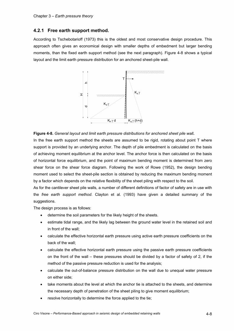
Chapter 3 – Earth pressure theory
Ciro Visone – Performance-Based approach in seismic design of embedded retaining walls 4-8
4.2.1 Free earth support method.
According to Tschebotarioff (1973) this is the oldest and most conservative design procedure. This
approach often gives an economical design with smaller depths of embedment but larger bending
moments, than the fixed earth support method (see the next paragraph). Figure 4-8 shows a typical
layout and the limit earth pressure distribution for an anchored sheet-pile wall.
hd
H AK γ
PK γ
PK γ d K γ (h+d)A
T
Figure 4-8. General layout and limit earth pressure distributions for anchored sheet pile wall. In the free earth support method the sheets are assumed to be rigid, rotating about point T where
support is provided by an underlying anchor. The depth of pile embedment is calculated on the basis
of achieving moment equilibrium at the anchor level. The anchor force is then calculated on the basis
of horizontal force equilibrium, and the point of maximum bending moment is determined from zero
shear force on the shear force diagram. Following the work of Rowe (1952), the design bending
moment used to select the sheet-pile section is obtained by reducing the maximum bending moment
by a factor which depends on the relative flexibility of the sheet piling with respect to the soil.
As for the cantilever sheet pile walls, a number of different definitions of factor of safety are in use with
the free earth support method. Clayton et al. (1993) have given a detailed summary of the
suggestions.
The design process is as follows:
• determine the soil parameters for the likely height of the sheets.
• estimate tidal range, and the likely lag between the ground water level in the retained soil and
in front of the wall;
• calculate the effective horizontal earth pressure using active earth pressure coefficients on the
back of the wall;
• calculate the effective horizontal earth pressure using the passive earth pressure coefficients
on the front of the wall – these pressures should be divided by a factor of safety of 2, if the
method of the passive pressure reduction is used for the analysis;
• calculate the out-of-balance pressure distribution on the wall due to unequal water pressure
on either side;
• take moments about the level at which the anchor tie is attached to the sheets, and determine
the necessary depth of penetration of the sheet piling to give moment equilibrium;
• resolve horizontally to determine the force applied to the tie;
Chapter 3 – Earth pressure theory
Ciro Visone – Performance-Based approach in seismic design of embedded retaining walls 4-9
• calculate the shear force diagram for the sheets, in order to find the position of maximum
bending moment – starting from the top of the wall;
• calculate the maximum bending moment at the point of zero shear force;
• in sands or gravels, calculate the relative flexibility of the sheets and the soil, and reduce the
bending moment according to the Rowe formulation as presented in the following;
• increase the depth of penetration by 20% to allow for the effects of unintentional excess
dredging, unanticipated local scour, and the presence of pockets of exceptionally weak
material (Terzaghi, 1954);
• increase the tie force by 10% to allow for horizontal arching;
• design anchors and select tie section.
Since at the outset, the depth of penetration of the sheeting is unknown, the calculations for moment
equilibrium about the anchor tie level can be only completed if a depth is assumed or the pressure
distributions are expressed in terms of the unknown depth, d.
In practice it is normally easier to adopt the second approach. The condition of moment equilibrium
then leads to a cubic equation. The simplest way to determine the correct value of d is by trial and
error substitution, starting with a likely value.
The magnitude and the distribution of the bending moment in a sheet pile wall is affected to the its
flexibility with respect to the deformability of the retained soil. Rowe (1952, 1957) carried out model
tests and provided charts to allow the maximum bending moment calculated from the free earth
support method to be reduced in line with his experimental findings. In theory, Rowe's reduction
factors can be used for any type of soil, but Skempton (1953), mindful of the fact that they result from
model tests, suggested that the amount of the reduction should be as follows:
• Sands: use 1/2 moment reduction from Rowe;
• Silts: use 1/4 moment reduction from Rowe;
• Clays: use no moment reduction.
Rowe identified the stiffness of the sheet piling as:
EIH 4
=ρ ( 4-8 )
where H is the full length of sheet piling (i.e. retained height plus depth of embedment), E is the Young
modulus and I the moment of inertia of the sheet piling.
Figure 4-9 shows the Rowe's moment reduction curves for sand. To use these curves, select the
relevant soil condition and the wall height, plot a curve of bending moment vs. log (ρ) by multiplying
the maximum free earth support bending moment for the particular wall by the values of M/Mmax for
different ρ in Figure 4-9. Next select various possible sheet pile sections and calculate log (ρ) and Mmax
= f I / y for each, where f is the permitted maximum stress of the pile material, and y is the distance
from the neutral axis to the edge of the section.
Plot the position of each of these sections on the curve. Sections giving points above the operating
curve are wasteful, while those below the curve will be overstressed. Ideal sections will fall directly on
the curve.

Chapter 3 – Earth pressure theory
Ciro Visone – Performance-Based approach in seismic design of embedded retaining walls 4-10
αH
H
log (ρ) (m³/kN)-1.0 -0.5 0 0.5 1.0 1.50
0.1
0.2
0.3
0.4
0.5
0.6
0.7
0.8
0.9
M/M
max
Loos
e
Dense
α=0.8α=0.7α=0.6
α=0.8α=0.7α=0.6
EIH 4
=ρ
Figure 4-9. Moment reduction factors proposed by Rowe (1952).
4.2.2 Fixed earth support method.
This method is derived from the work of Blum (1931). The sheet piling is considered flexible, but driven
to sufficient depth that it may be considered fixed at its toe. Blum's general method deals with rigidly
and flexibly anchored walls, and with cantilever walls, as it is previously shown. In these methods the
stresses on the wall immediately above the toe are replaced by a single force some distance up the
wall and the sheet piling is considered to be held vertical at this point. The depth of penetration of the
sheeting is found by repetitive calculation until the displacement at the anchor level is correct relative
to the point of fixity (at the toe). For routine design the anchor is assumed to be unyielding, and this
relative displacement must therefore be zero. Unless carried out by computer, this technique is
tedious; therefore a number of simplifications are in common use.
The general method used for fixed earth support design is the "elastic line method". In this method the
position of the point C, below of which the sheet pile wall is fixed, is assumed, and the deformation of
the sheet pile is assumed to become tangential to the vertical at this point .Successive integration with
respect to the depth of the net total pressure diagram leads to the shear force diagram, the bending
moment diagram, the slope diagram and the deflection diagram. The position of point C is adjusted
until the deflection of the anchor (point T) relative to point C is zero.

Chapter 3 – Earth pressure theory
Ciro Visone – Performance-Based approach in seismic design of embedded retaining walls 4-11
ux
C
B
FC
N
h L
y
A
d'h
dH
T
Figure 4-10. Design of anchored sheet pile by the fixed earth support method. From this necessary depth of sheeting may be obtained, since Blum demonstrated that the total
required depth of penetration is:
( )xud 20.1to05.1+= ( 4-9 )
Typically, for convenience, the total required depth of penetration is taken as:
( )xud += 20.1 ( 4-10 )
As in Tschebotarioff (1973), for the simplified equivalent beam method to be described below, but the
actual required depth can be found from:
( )AAPPL
C
KKhFxud
δ−δγ++=
coscos'2 ( 4-11 )
where u and x are defined in Figure 4-10, γ' is the average buoyant density (γ – γW) between the top of
the sheet-pile wall and the point C, FC is the replacement force at C, KPcosδP and KAcosδA represent
the components of earth pressure normal to the wall, hL is the height of the wall (including embedment
of the point C), plus an allowance of q/KA γ for any surcharge q imposed at the top of the wall.
Although in the past the elastic line method has been solved by hand calculation, or graphically, it is
now considered too time-consuming for routine use. It is, however, a relatively simple task to program
a desktop computer to provide these solutions.
"Blum's equivalent beam method" (Blum, 1931) uses the same simplifying assumptions with regard to
the stresses at the toe of the pile as were used for the elastic line method above – the stresses at the
pile toe are replaced by a single force some distance above the toe. By carrying out example
calculations on uniform soil profiles, Blum was able to establish the relationship between the depth to
the point of sheet pile contraflexure (y) (where the bending moment is zero – point B in Figure 4-10)
and the free height of the wall (h, from the dredge level to the top of the wall), as follows
Effective angle of friction of soil, φ' Ratio (depth to point of contraflexure)/(free height of wall) (y/h) 20° 0.23 25° 0.15 30° 0.08 35° 0.03 40° -0.007
Table 4-1. Relationship between the depth to the point of the sheet pile contraflexure (y) and the free
height of the wall (h) (Blum, 1931, as quoted in Clayton et al. 1993).
Chapter 3 – Earth pressure theory
Ciro Visone – Performance-Based approach in seismic design of embedded retaining walls 4-12
It is reported by Tschebotarioff (1973) that these values were based on the use of Rankine value for
KA (δA = 0) and KP = 2/KA. Blum is supposed to have used this value for the passive earth pressure
coefficient, not because he allowed for the influence of wall friction, but because tests by Franzius
(1924) using a hinged wall in a relatively narrow box) had given similar results.
Once the point of contraflexure is known, an imaginary hinge can be inserted at that point on the sheet
pile wall, and analysis becomes trivial.
The procedure is:
• by horizontal resolution of forces on span AB, and by taking moments about B, determine the
magnitude of the anchor force T, and the force at the hinge FB;
• Take moments about C, to determine the correct length BC for which the moments about C
are zero. Stresses below C are ignored.
For a uniform soil, with γ' = γ – γW:
( ) ( ) ( ) ( ) ( )[ ]hKyKKydKKydydF AAPAPB −−γ−
+γ−−
=− '2
''6
''23
For moment equilibrium:
( ) ( ) '6'
γ−=−
AP
B
KKFyd
• Determine the final depth of embedment (which will also give a factor of safety against failure
by forward movement of the piling), approximately:
'2.1 dd =
• Determine the point of maximum bending moment from the position of zero shear force, by
drawing the shear force diagram for span AB;
• Determine the maximum bending moment.
The main problem with this method is the determination of a correct point of contraflexure when soil
conditions are non-uniform. For uniform ground conditions B lies approximately level with the point of
zero net pressure, N.

Chapter 5 – Seismic design of embedded retaining walls
Ciro Visone – Performance-Based approach in seismic design of embedded retaining walls 5-1
5 SEISMIC DESIGN OF EMBEDDED RETAINING WALLS.
The design of retaining walls for seismic conditions is similar, in many aspects, to designing for static
conditions. In both cases, potential modes of failure are identified and the wall designed to avoid
initiating them. Although the response of retaining walls under seismic loading conditions is much
more complex, conventional design procedures make use of simplifying assumptions that render the
problem tractable. Several design approaches for embedded retaining walls depending by the analysis
type for the desired level of the seismic performance evaluation are described in the following
sections. The methods are those obtained by extending the static procedure to the seismic conditions
and developed during this work.
5.1 EARTHQUAKE PROVISIONS DESCRIBED IN EUROPEAN AND
ITALIAN BUILDING CODES.
Eurocode 8 part 5 (EN 1998-5) states that earth retaining structures must design to fulfil their function
during and after an earthquake, without suffering significant structural damages. Permanent
displacements, in the form of combined sliding and tilting, the latter due to irreversible deformations of
the foundation soil, may be acceptable if it is shown that they are compatible with functional and/or
aesthetic requirements. Any established method based on the procedures of structural and soil
dynamics, and supported by experience and observations, is in principle acceptable for assessing the
safety of an earth retaining structure. The following aspects should be considered in the analyses:
• the generally non-linear behaviour of the soil in the course of its dynamic interaction with the
retaining structure;
• the inertial effects associated with the masses of the soil, of the structure, and of all other
gravity loads which might participate in the interaction process;
• the hydrodynamic effects generated by the presence of water in the soil behind the wall and/or
by the water on the outer face of the wall;
• the compatibility between the deformations of the soil, the wall, and the tiebacks, when
present.
It should be underlined that no indications on representative parameters for specifying damage criteria
and no limitations on values of the displacements are given.
The basic components that should be included in a pseudo-static analysis consist of the retaining
structure and its foundation, of a soil wedge behind the structure supposed to be in a state of active
limit equilibrium (if the structure is flexible enough), of any surcharge loading acting on the soil wedge,
and, possibly, of a soil mass at the foot of the wall, supposed to be in a state of passive equilibrium.
In the EC8 Part 5, a simplified pseudostatic approach to analyze the safety conditions of retaining
walls is described. The seismic increments of earth pressures may be computed with the M-O method.
Its application for rigid structures is more prompt than for embedded walls for which the stability is
mainly due to the soil passive resistance into the embedded portion. As for the Coulomb theory in
static conditions, the M-O theory gives very high values for passive earth pressure coefficient when
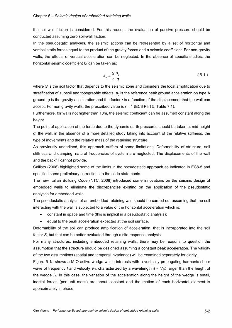
Chapter 5 – Seismic design of embedded retaining walls
Ciro Visone – Performance-Based approach in seismic design of embedded retaining walls 5-2
the soil-wall friction is considered. For this reason, the evaluation of passive pressure should be
conducted assuming zero soil-wall friction.
In the pseudostatic analyses, the seismic actions can be represented by a set of horizontal and
vertical static forces equal to the product of the gravity forces and a seismic coefficient. For non-gravity
walls, the effects of vertical acceleration can be neglected. In the absence of specific studies, the
horizontal seismic coefficient kh can be taken as:
ga
rSk g
h = ( 5-1 )
where S is the soil factor that depends to the seismic zone and considers the local amplification due to
stratification of subsoil and topographic effects, ag is the reference peak ground acceleration on type A
ground, g is the gravity acceleration and the factor r is a function of the displacement that the wall can
accept. For non gravity walls, the prescribed value is r = 1 (EC8 Part 5, Table 7.1).
Furthermore, for walls not higher than 10m, the seismic coefficient can be assumed constant along the
height.
The point of application of the force due to the dynamic earth pressures should be taken at mid-height
of the wall, in the absence of a more detailed study taking into account of the relative stiffness, the
type of movements and the relative mass of the retaining structure.
As previously underlined, this approach suffers of some limitations. Deformability of structure, soil
stiffness and damping, natural frequencies of system are neglected. The displacements of the wall
and the backfill cannot provide.
Callisto (2006) highlighted some of the limits in the pseudostatic approach as indicated in EC8-5 and
specified some preliminary corrections to the code statements.
The new Italian Building Code (NTC, 2008) introduced some innovations on the seismic design of
embedded walls to eliminate the discrepancies existing on the application of the pseudostatic
analyses for embedded walls.
The pseudostatic analysis of an embedded retaining wall should be carried out assuming that the soil
interacting with the wall is subjected to a value of the horizontal acceleration which is:
• constant in space and time (this is implicit in a pseudostatic analysis);
• equal to the peak acceleration expected at the soil surface.
Deformability of the soil can produce amplification of acceleration, that is incorporated into the soil
factor S, but that can be better evaluated through a site response analysis.
For many structures, including embedded retaining walls, there may be reasons to question the
assumption that the structure should be designed assuming a constant peak acceleration. The validity
of the two assumptions (spatial and temporal invariance) will be examined separately for clarity.
Figure 5-1a shows a M-O active wedge which interacts with a vertically propagating harmonic shear
wave of frequency f and velocity VS, characterized by a wavelength λ = VS/f larger than the height of
the wedge H. In this case, the variation of the acceleration along the height of the wedge is small,
inertial forces (per unit mass) are about constant and the motion of each horizontal element is
approximately in phase.
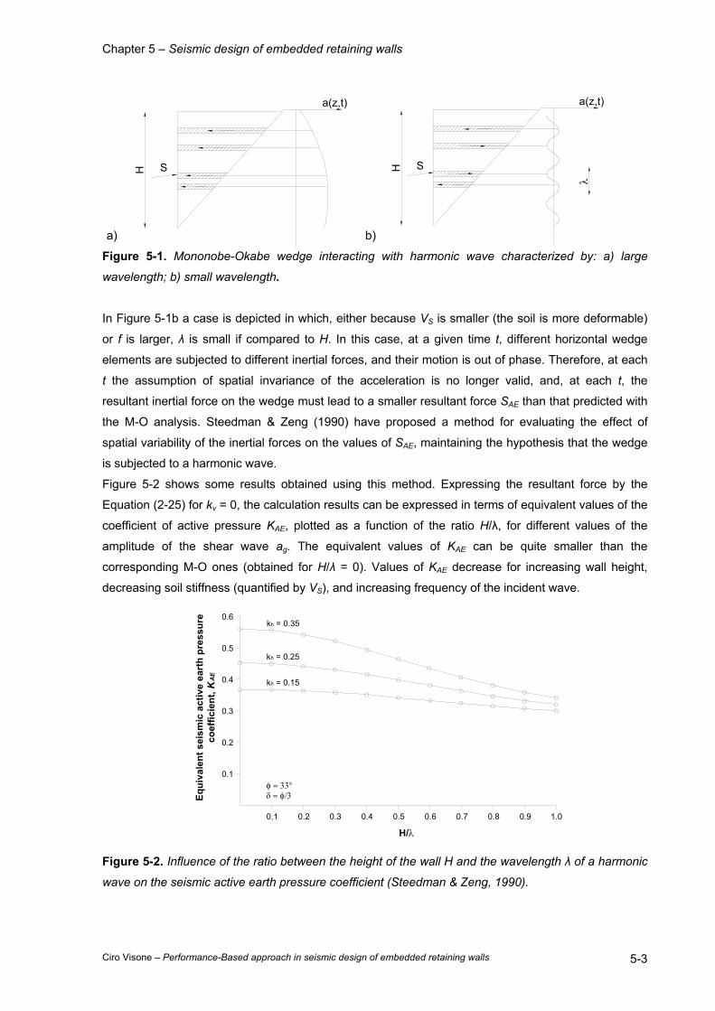
Chapter 5 – Seismic design of embedded retaining walls
Ciro Visone – Performance-Based approach in seismic design of embedded retaining walls 5-3
a)
SH
a(z,t)
b)
SH
a(z,t)
λ
Figure 5-1. Mononobe-Okabe wedge interacting with harmonic wave characterized by: a) large
wavelength; b) small wavelength.
In Figure 5-1b a case is depicted in which, either because VS is smaller (the soil is more deformable)
or f is larger, λ is small if compared to H. In this case, at a given time t, different horizontal wedge
elements are subjected to different inertial forces, and their motion is out of phase. Therefore, at each
t the assumption of spatial invariance of the acceleration is no longer valid, and, at each t, the
resultant inertial force on the wedge must lead to a smaller resultant force SAE than that predicted with
the M-O analysis. Steedman & Zeng (1990) have proposed a method for evaluating the effect of
spatial variability of the inertial forces on the values of SAE, maintaining the hypothesis that the wedge
is subjected to a harmonic wave.
Figure 5-2 shows some results obtained using this method. Expressing the resultant force by the
Equation (2-25) for kv = 0, the calculation results can be expressed in terms of equivalent values of the
coefficient of active pressure KAE, plotted as a function of the ratio H/λ, for different values of the
amplitude of the shear wave ag. The equivalent values of KAE can be quite smaller than the
corresponding M-O ones (obtained for H/λ = 0). Values of KAE decrease for increasing wall height,
decreasing soil stiffness (quantified by VS), and increasing frequency of the incident wave.
0.1
0.2
0.3
0.6
0.5
0.4
0.1 0.2 0.4 0.5 0.6 0.7 0.8 0.9 1.00.3
H/λ
Equi
vale
nt s
eism
ic a
ctiv
e ea
rth
pres
sure
co
effic
ient
, KA
E
kh = 0.15
kh = 0.25
kh = 0.35
φ = 33°δ = φ/3
Figure 5-2. Influence of the ratio between the height of the wall H and the wavelength λ of a harmonic
wave on the seismic active earth pressure coefficient (Steedman & Zeng, 1990).
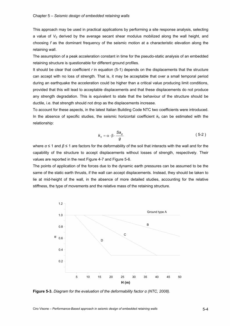
Chapter 5 – Seismic design of embedded retaining walls
Ciro Visone – Performance-Based approach in seismic design of embedded retaining walls 5-4
This approach may be used in practical applications by performing a site response analysis, selecting
a value of VS derived by the average secant shear modulus mobilized along the wall height, and
choosing f as the dominant frequency of the seismic motion at a characteristic elevation along the
retaining wall.
The assumption of a peak acceleration constant in time for the pseudo-static analysis of an embedded
retaining structure is questionable for different ground profiles.
It should be clear that coefficient r in equation (5-1) depends on the displacements that the structure
can accept with no loss of strength. That is, it may be acceptable that over a small temporal period
during an earthquake the acceleration could be higher than a critical value producing limit conditions,
provided that this will lead to acceptable displacements and that these displacements do not produce
any strength degradation. This is equivalent to state that the behaviour of the structure should be
ductile, i.e. that strength should not drop as the displacements increase.
To account for these aspects, in the latest Italian Building Code NTC two coefficients were introduced.
In the absence of specific studies, the seismic horizontal coefficient kh can be estimated with the
relationship:
gSa
k gh ⋅β⋅α= ( 5-2 )
where α ≤ 1 and β ≤ 1 are factors for the deformability of the soil that interacts with the wall and for the
capability of the structure to accept displacements without losses of strength, respectively. Their
values are reported in the next Figure 4-7 and Figure 5-6.
The points of application of the forces due to the dynamic earth pressures can be assumed to be the
same of the static earth thrusts, if the wall can accept displacements. Instead, they should be taken to
lie at mid-height of the wall, in the absence of more detailed studies, accounting for the relative
stiffness, the type of movements and the relative mass of the retaining structure.
0.2
0.4
0.6
1.2
1.0
0.8
5
H (m)
α
10 15 20 25 30 35 40 45 50
D
C
B
Ground type A
Figure 5-3. Diagram for the evaluation of the deformability factor α (NTC, 2008).
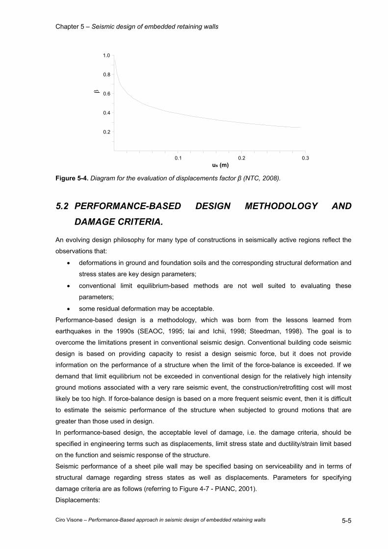
Chapter 5 – Seismic design of embedded retaining walls
Ciro Visone – Performance-Based approach in seismic design of embedded retaining walls 5-5
0.2
0.4
0.6
1.0
0.8
us (m)
β
0.1 0.2 0.3
Figure 5-4. Diagram for the evaluation of displacements factor β (NTC, 2008).
5.2 PERFORMANCE-BASED DESIGN METHODOLOGY AND
DAMAGE CRITERIA.
An evolving design philosophy for many type of constructions in seismically active regions reflect the
observations that:
• deformations in ground and foundation soils and the corresponding structural deformation and
stress states are key design parameters;
• conventional limit equilibrium-based methods are not well suited to evaluating these
parameters;
• some residual deformation may be acceptable.
Performance-based design is a methodology, which was born from the lessons learned from
earthquakes in the 1990s (SEAOC, 1995; Iai and Ichii, 1998; Steedman, 1998). The goal is to
overcome the limitations present in conventional seismic design. Conventional building code seismic
design is based on providing capacity to resist a design seismic force, but it does not provide
information on the performance of a structure when the limit of the force-balance is exceeded. If we
demand that limit equilibrium not be exceeded in conventional design for the relatively high intensity
ground motions associated with a very rare seismic event, the construction/retrofitting cost will most
likely be too high. If force-balance design is based on a more frequent seismic event, then it is difficult
to estimate the seismic performance of the structure when subjected to ground motions that are
greater than those used in design.
In performance-based design, the acceptable level of damage, i.e. the damage criteria, should be
specified in engineering terms such as displacements, limit stress state and ductility/strain limit based
on the function and seismic response of the structure.
Seismic performance of a sheet pile wall may be specified basing on serviceability and in terms of
structural damage regarding stress states as well as displacements. Parameters for specifying
damage criteria are as follows (referring to Figure 4-7 - PIANC, 2001).
Displacements:
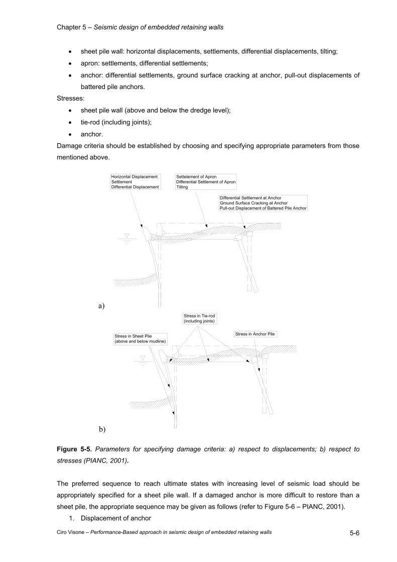
Chapter 5 – Seismic design of embedded retaining walls
Ciro Visone – Performance-Based approach in seismic design of embedded retaining walls 5-6
• sheet pile wall: horizontal displacements, settlements, differential displacements, tilting;
• apron: settlements, differential settlements;
• anchor: differential settlements, ground surface cracking at anchor, pull-out displacements of
battered pile anchors.
Stresses:
• sheet pile wall (above and below the dredge level);
• tie-rod (including joints);
• anchor.
Damage criteria should be established by choosing and specifying appropriate parameters from those
mentioned above.
a)
Settelement of ApronDifferential Settlement of ApronTilting
Differential Settlement at AnchorGround Surface Cracking at AnchorPull-out Displacement of Battered Pile Anchor
Horizontal DisplacementSettlementDifferential Displacement
b)
Stress in Tie-rod(including joints)
Stress in Anchor PileStress in Sheet Pile (above and below mudline)
Figure 5-5. Parameters for specifying damage criteria: a) respect to displacements; b) respect to
stresses (PIANC, 2001).
The preferred sequence to reach ultimate states with increasing level of seismic load should be
appropriately specified for a sheet pile wall. If a damaged anchor is more difficult to restore than a
sheet pile, the appropriate sequence may be given as follows (refer to Figure 5-6 – PIANC, 2001).
1. Displacement of anchor

Chapter 5 – Seismic design of embedded retaining walls
Ciro Visone – Performance-Based approach in seismic design of embedded retaining walls 5-7
2. Yield at sheet pile wall (above the dredge level)
3. Yield at sheet pile wall (below the dredge level)
4. Yield at anchor
5. Yield at tie-rod
If a damaged sheet pile wall is more difficult to restore than an anchor, the yield at anchor should
precede the yield at sheet pile wall. 1) Displacement of Anchor
4) Yield at Anchor5) Yield at Tie-rod2) Yield at Sheet Pile Wall(above mudline)
3) Yield at Sheet Pile Wall(below mudline)
Figure 5-6. Preferred sequence for yield of sheet pile wall (PIANC, 2001).
It could be noted that the yield of soil for passive state is not considered in the sequence and maybe
might be included in the list. However, different and unclear opinions on this point exist in scientific
community.
On the basis of these concepts, the damage criteria for a sheet pile wall can be established by
referring to Table 3-1. The most restrictive conditions among displacements and stresses should
define the damage criteria. Structural damage to the embedded portion of a sheet pile is generally
difficult to restore, and thud necessitates higher seismic resistance. Brittle fracture of a sheet pile wall,
rupture of a tie-rod, and the collapse of anchor should be avoided.
Other damage and serviceability criteria can be found in some seismic codes (e.g., Port and Harbour
Research Institute, 1997; Ministry of Transport, Japan, 1999; ASCE-TCLEE, Werner, 1998).

Chapter 5 – Seismic design of embedded retaining walls
Ciro Visone – Performance-Based approach in seismic design of embedded retaining walls 5-8
Level of damage Serviceable Repairable Near Collapse Collapse Damage criteria Component
Damage Parameters
Normalized residual horizontal displacement (ux/h) Less than 1.5% N/A N/A N/A
Sheet pile wall Residual tilting towards the
excavation side Less than 3° N/A N/A N/A
Apron Differential settlement on apron
Less than 0.03÷0.1m
N/A N/A N/A
Differential settlement
between apron and non-apron areas
Less than 0.3÷0.7m
N/A N/A N/A
Residual displacements
Residual tilting towards the excavation side Less than 2÷3° N/A N/A N/A
Sheet pile wall Above the dredge level Elastic
Plastic (less than the ductility factor/strain limit
above the dredge level)
Plastic (less than the ductility factor/strain limit
above the dredge level)
Plastic (beyond the ductility factor/strain
limit above the dredge level)
Below the dredge level Elastic Elastic
Plastic (less than the ductility factor/strain limit
below the dredge level)
Plastic (beyond the ductility factor/strain
limit below the dredge level)
Tie-rod Elastic Elastic
Plastic (less than the ductility factor/strain limit
for tie-rod)
Plastic (beyond the ductility factor/strain
limit for tie-rod)
Peak response stresses/strains
Anchor Elastic Elastic
Plastic (less than the ductility factor/strain limit
for anchor)
Plastic (beyond the ductility factor/strain
limit for anchor)
Table 5-1. Damage criteria for sheet pile wall (adapted from PIANC, 2001).
Chapter 5 – Seismic design of embedded retaining walls
Ciro Visone – Performance-Based approach in seismic design of embedded retaining walls 5-9
5.3 SEISMIC ANALYSIS OF EMBEDDED RETAINING WALLS.
Seismic analysis of many type of constructions is accomplished in three steps that include assessment
of the regional seismicity, the geotechnical hazards and soil structure interaction analysis. The first
step is to define the earthquake motions at the bedrock. This is typically accomplished by seismic
hazard analysis based on geologic, tectonic and historical seismicity data available for the region of
interest. The second step involves the following two interrelated aspects of dynamic soil response: 1)
an evaluation of local site effects for obtaining the earthquake motions at or near the ground surface;
2) an assessment of the liquefaction resistance of the near surface sandy soils and the associated
potential for ground failures. Once the ground motion and geotechnical parameters have been
established, then seismic analysis of the construction can proceed.
As in all engineering disciplines, reasonable judgement is required in specifying appropriate methods
of analysis and design, as well as in the interpretation of the results of the analysis procedures. This is
particularly important in seismic design, given the multidisciplinary input that is required for these
evaluations, and the influence of this input on the final design recommendations.
5.3.1 Type of analysis.
The objective of analysis in performance-based design is to evaluate the seismic response of the
embedded retaining walls with respect to allowable limits (e.g. displacements, stress, ductility/strain).
Higher capability in analysis is generally required for a higher performance grade facility. The selected
analysis methods should reflect the analytical capability required in the seismic performance
evaluation.
A variety of analysis methods are available for evaluating the local site effects, liquefaction potential
and the seismic response of retaining walls. These analysis methods are broadly categorized based
on a level of sophistication and capability as follows (PIANC, 2001):
1. Simplified analysis: appropriate for evaluating approximate threshold limit for displacements
and/or elastic response limit and an order-of-magnitude estimate for permanent displacements
due to seismic loading.
2. Simplified dynamic analysis: possible to evaluate extent of displacement/stress/ductility/strain
based on assumed failure modes.
3. Dynamic analysis: possible to evaluate both of failure modes and the extent of
displacement/stress/ductility/strain.
In principle, the structures characterized by a higher performance grade should be studied using more
sophisticated methods. Less sophisticated methods may be allowed for preliminary design, screening
purposes or response analysis for low levels of excitation.
Table 5-2 shows the input parameters and the outputs of the various type of seismic analysis of
embedded walls. It should be noted that the reliability of the results depends not only on the type of
analysis, but also on the reliability of the input parameters. It is ideal to use input data based on
through geotechnical investigations for more sophisticated analysis.

Chapter 5 – Seismic design of embedded retaining walls
Ciro Visone – Performance-Based approach in seismic design of embedded retaining walls 5-10
Type of Analysis
Simplified Analysis Simplified Dynamic Analysis Dynamic Analysis
Method Pseudo-
static/empirical methods
Newmark type method
Simplified chart based on
parametric studies
FEM/FDM
Design Parameters
kh: equivalent seismic coefficient kcrit: threshold seismic coefficient
Empirical equations: amax: peak acceleration Vmax: peak velocity Time history analysis: time histories of earthquake motions acrit: threshold acceleration
ag: peak acceleration at the bedrock Cross section of wall Index properties of soil including SPT N-values
Input Parameters
Results of site response analysis, including amax and liquefaction potential assessment Cross section of wall Geotechnical parameters, including cohesion c, friction angle φ and soil-wall friction angle; ground water level
Time histories of earthquake mations at the bottom of analysis domain Cross section of wall For equivalent linear geotechnical analysis: G/G0(γ) and D(γ) curves For nonlinear geotechnical analysis: undrained cyclic properties and G, K: shear and bulk modulus, in addition to the geotechnical parameters for pseudo-static and simplified analyses
Analysis Output
Threshold limit Order-of-magnitude displacement
Wall displacement Stress/ductility
Response/failure modes Peak and residual displacements, stress/ductility
Table 5-2. Inputs and outputs of analyses (adapted from PIANC, 2001).
5.3.2 Simplified analysis.
Simplified analysis of retaining structures is based on the conventional force-balance approach,
sometimes combined with statistical analysis of case history data. The methods in this category are
often those adopted in conventional seismic design codes and standards. In simplified analysis,
retaining walls can be idealized as rigid blocks of soil and structural masses. The rigid block analysis is
typically applied for gravity and sheet pile walls.
Effects of earthquake motions in simplified analysis are represented by a peak ground acceleration
amax or an equivalent seismic coefficient kh for use in conventional pseudo-static design procedures.
These parameters are obtained from the simplified analysis of local site effects. A capacity to resist the
seismic force is evaluated based on structural and geotechnical conditions, often in terms of a
threshold acceleration acrit or a threshold seismic coefficient kcrit, beyond which the rigid blocks of soil
and structural masses begin to move. When soil liquefaction is an issue, the geometric extent of
liquefaction must also be considered in the analysis.
Results of the simplified analysis are appropriate for evaluating the approximate threshold level of
damage, which ensures at least the repairable state of structural performance for the earthquake
related to serviceability criteria. Whether or not the approximate threshold level ensures the
serviceable state of structural performance depends on the details in evaluating the design
parameters for the pseudo-static method. Order-of-magnitude displacement is also obtained by the
pseudo-static method combined with statistical analysis of case history data. This, however is a crude
approximation and should be used only for the preliminary design stage or low levels of excitation.
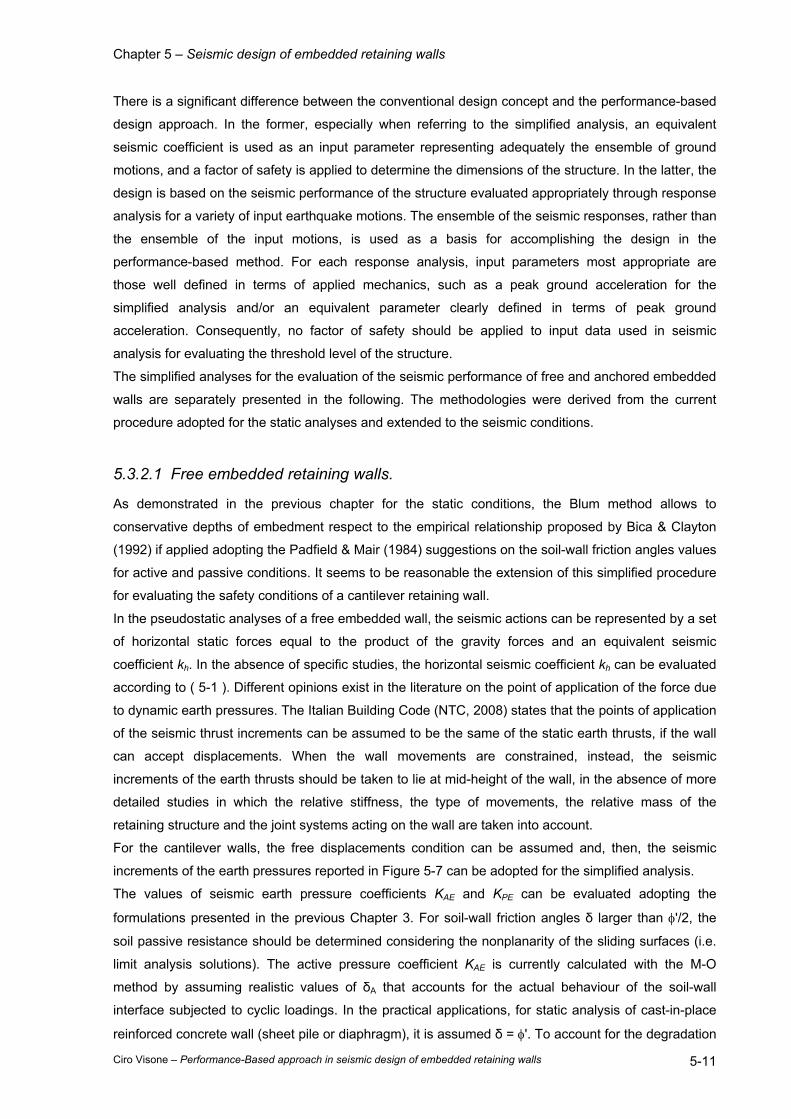
Chapter 5 – Seismic design of embedded retaining walls
Ciro Visone – Performance-Based approach in seismic design of embedded retaining walls 5-11
There is a significant difference between the conventional design concept and the performance-based
design approach. In the former, especially when referring to the simplified analysis, an equivalent
seismic coefficient is used as an input parameter representing adequately the ensemble of ground
motions, and a factor of safety is applied to determine the dimensions of the structure. In the latter, the
design is based on the seismic performance of the structure evaluated appropriately through response
analysis for a variety of input earthquake motions. The ensemble of the seismic responses, rather than
the ensemble of the input motions, is used as a basis for accomplishing the design in the
performance-based method. For each response analysis, input parameters most appropriate are
those well defined in terms of applied mechanics, such as a peak ground acceleration for the
simplified analysis and/or an equivalent parameter clearly defined in terms of peak ground
acceleration. Consequently, no factor of safety should be applied to input data used in seismic
analysis for evaluating the threshold level of the structure.
The simplified analyses for the evaluation of the seismic performance of free and anchored embedded
walls are separately presented in the following. The methodologies were derived from the current
procedure adopted for the static analyses and extended to the seismic conditions.
5.3.2.1 Free embedded retaining walls.
As demonstrated in the previous chapter for the static conditions, the Blum method allows to
conservative depths of embedment respect to the empirical relationship proposed by Bica & Clayton
(1992) if applied adopting the Padfield & Mair (1984) suggestions on the soil-wall friction angles values
for active and passive conditions. It seems to be reasonable the extension of this simplified procedure
for evaluating the safety conditions of a cantilever retaining wall.
In the pseudostatic analyses of a free embedded wall, the seismic actions can be represented by a set
of horizontal static forces equal to the product of the gravity forces and an equivalent seismic
coefficient kh. In the absence of specific studies, the horizontal seismic coefficient kh can be evaluated
according to ( 5-1 ). Different opinions exist in the literature on the point of application of the force due
to dynamic earth pressures. The Italian Building Code (NTC, 2008) states that the points of application
of the seismic thrust increments can be assumed to be the same of the static earth thrusts, if the wall
can accept displacements. When the wall movements are constrained, instead, the seismic
increments of the earth thrusts should be taken to lie at mid-height of the wall, in the absence of more
detailed studies in which the relative stiffness, the type of movements, the relative mass of the
retaining structure and the joint systems acting on the wall are taken into account.
For the cantilever walls, the free displacements condition can be assumed and, then, the seismic
increments of the earth pressures reported in Figure 5-7 can be adopted for the simplified analysis.
The values of seismic earth pressure coefficients KAE and KPE can be evaluated adopting the
formulations presented in the previous Chapter 3. For soil-wall friction angles δ larger than φ'/2, the
soil passive resistance should be determined considering the nonplanarity of the sliding surfaces (i.e.
limit analysis solutions). The active pressure coefficient KAE is currently calculated with the M-O
method by assuming realistic values of δA that accounts for the actual behaviour of the soil-wall
interface subjected to cyclic loadings. In the practical applications, for static analysis of cast-in-place
reinforced concrete wall (sheet pile or diaphragm), it is assumed δ = φ'. To account for the degradation
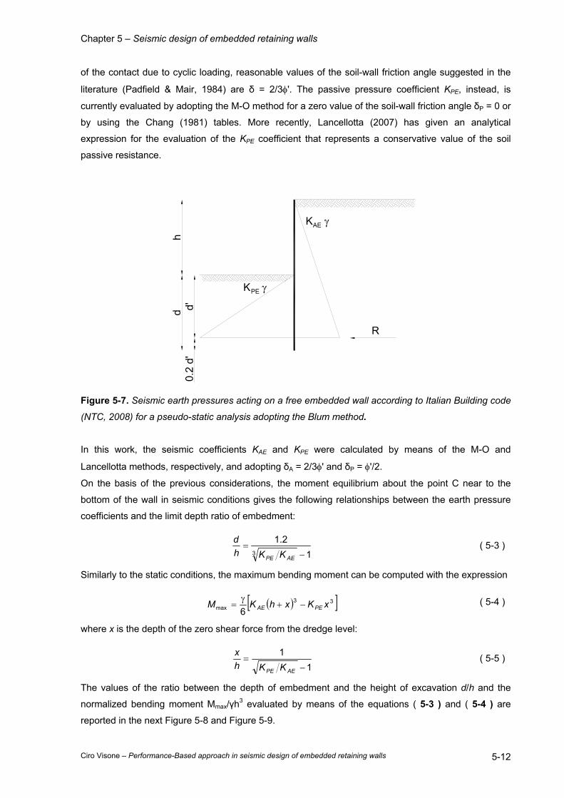
Chapter 5 – Seismic design of embedded retaining walls
Ciro Visone – Performance-Based approach in seismic design of embedded retaining walls 5-12
of the contact due to cyclic loading, reasonable values of the soil-wall friction angle suggested in the
literature (Padfield & Mair, 1984) are δ = 2/3φ'. The passive pressure coefficient KPE, instead, is
currently evaluated by adopting the M-O method for a zero value of the soil-wall friction angle δP = 0 or
by using the Chang (1981) tables. More recently, Lancellotta (2007) has given an analytical
expression for the evaluation of the KPE coefficient that represents a conservative value of the soil
passive resistance.
hd
AEK γ
PEK γ
d'
R
0.2
d'
Figure 5-7. Seismic earth pressures acting on a free embedded wall according to Italian Building code
(NTC, 2008) for a pseudo-static analysis adopting the Blum method.
In this work, the seismic coefficients KAE and KPE were calculated by means of the M-O and
Lancellotta methods, respectively, and adopting δA = 2/3φ' and δP = φ'/2.
On the basis of the previous considerations, the moment equilibrium about the point C near to the
bottom of the wall in seismic conditions gives the following relationships between the earth pressure
coefficients and the limit depth ratio of embedment:
12.1
3 −=
AEPE KKhd ( 5-3 )
Similarly to the static conditions, the maximum bending moment can be computed with the expression
( )[ ]33max 6
xKxhKM PEAE −+γ
= ( 5-4 )
where x is the depth of the zero shear force from the dredge level:
11
−=
AEPE KKhx ( 5-5 )
The values of the ratio between the depth of embedment and the height of excavation d/h and the
normalized bending moment Mmax/γh3 evaluated by means of the equations ( 5-3 ) and ( 5-4 ) are
reported in the next Figure 5-8 and Figure 5-9.
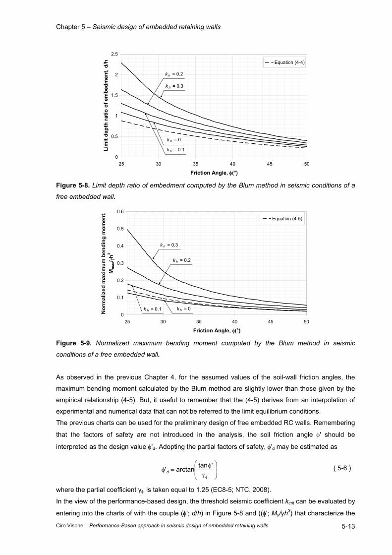
Chapter 5 – Seismic design of embedded retaining walls
Ciro Visone – Performance-Based approach in seismic design of embedded retaining walls 5-13
0
0.5
1
1.5
2
2.5
25 30 35 40 45 50
Friction Angle, φ(°)
Lim
it de
pth
ratio
of e
mbe
dmen
t, d/
h Equation (4-4)
k h = 0
k h = 0.1
k h = 0.3
k h = 0.2
Figure 5-8. Limit depth ratio of embedment computed by the Blum method in seismic conditions of a
free embedded wall.
0
0.1
0.2
0.3
0.4
0.5
0.6
25 30 35 40 45 50
Friction Angle, φ(°)
Nor
mal
ized
max
imum
ben
ding
mom
ent,
Mm
ax/ γ
h3
Equation (4-5)
k h = 0k h = 0.1
k h = 0.3
k h = 0.2
Figure 5-9. Normalized maximum bending moment computed by the Blum method in seismic
conditions of a free embedded wall.
As observed in the previous Chapter 4, for the assumed values of the soil-wall friction angles, the
maximum bending moment calculated by the Blum method are slightly lower than those given by the
empirical relationship (4-5). But, it useful to remember that the (4-5) derives from an interpolation of
experimental and numerical data that can not be referred to the limit equilibrium conditions.
The previous charts can be used for the preliminary design of free embedded RC walls. Remembering
that the factors of safety are not introduced in the analysis, the soil friction angle φ' should be
interpreted as the design value φ'd. Adopting the partial factors of safety, φ'd may be estimated as
γφ
=φφ'
'tanarctan'd ( 5-6 )
where the partial coefficient γφ' is taken equal to 1.25 (EC8-5; NTC, 2008).
In the view of the performance-based design, the threshold seismic coefficient kcrit can be evaluated by
entering into the charts of with the couple (φ'; d/h) in Figure 5-8 and ((φ'; My/γh3) that characterize the
Chapter 5 – Seismic design of embedded retaining walls
Ciro Visone – Performance-Based approach in seismic design of embedded retaining walls 5-14
problem of interest (My is the yielding moment of the wall with respect to the examined limit state) and
estimating the reference curves with constant value of kh.
The factors of safety FS against the earthquake for rotational and structural failure modes are defined
by (PIANC, 2001):
h
crit
kkFS = ( 5-7 )
The displacements of the wall can be then estimated by using empirical relationships and charts.
Richards & Elms (1979) proposed a method for the seismic design of gravity walls based on allowable
permanent wall displacements. Using the results of sliding block analyses in the same manner as
Newmark (1965) and Franklin and Chang (1977), the authors proposed the following expression for
permanent block displacement:
4
3max
2max087.0
critx a
avu =
3.0max ≥aacrit ( 5-8 )
where vmax is the peak ground velocity, amax is the peak ground acceleration and acrit = khcrit·g is the
yield acceleration for the wall-backfill system.
Whitman & Liao (1985) identified several modelling errors that result from the simplifying assumptions
of the Richards & Elms procedure. The most important of these are neglect of the backfill dynamic
response, the kinematic factors, the tilting mechanisms and the vertical accelerations. Finite element
analyses of the effects of the dynamic response of the backfill on wall displacements (Nadim, 1982),
for example, show that amplification occurs when input motions coincide with the natural period of the
backfill and produce considerably greater permanent displacement than the rigid-block model used by
Richards & Elms. Analyses in which the backfill wedge and wall were treated as separate blocks
(Zarrabi-Kashani, 1979) show that the kinematic requirements of horizontal and vertical displacement
of the backfill wedge cause systematically smaller displacements than the single-block model of
Richards and Elms. Studies of combined tilting and sliding (Nadim, 1980; Siddharthan et al., 1992)
indicate that tilting mechanisms generally increase wall displacements over those produced by sliding-
only models such as that of Richards & Elms. Consideration of vertical accelerations produces slightly
larger displacements than when they are neglected, at least for motions with high peak horizontal
acceleration (amax greater than about 0.5g) and acrit/amax ≥ 0.4 (Whitman & Liao, 1985). Whitman &
Liao quantified and combined the effects of each of these sources of modelling error to describe the
total modelling error by a lognormally distributed random variable with mean value, M , and standard
deviation, σln M.
Using the results of sliding block analyses of 14 ground motions by Wong (1982), Whitman & Liao
found that the permanent displacements were lognormally distributed with mean value
−=
maxmax
2max 4.9
exp37
aa
av
u critx ( 5-9 )
Uncertainty due to statistical variability of ground motions was characterized by a lognormally
distributed random variable, Q, with a mean value of Q and standard deviation, σln Q.

Chapter 5 – Seismic design of embedded retaining walls
Ciro Visone – Performance-Based approach in seismic design of embedded retaining walls 5-15
The effects of uncertainty in soil properties, specifically the friction angles, on permanent displacement
were also investigated. Using standard deviations of σφ = 2 to 3° for soil friction angles and σδ = 5° for
wall-soil interface friction angles, the computed yield acceleration was defined as a random variable
with mean value crita and standard deviation critaσ . The mean value crita is the yield acceleration
computed using the mean values of φ and δ.
Combining all the sources of uncertainty, the permanent displacement can be characterized as a
lognormally distributed random variable with mean value
MQa
aav
u critx
−=
maxmax
2max 4.9exp
37 ( 5-10 )
and variance
2ln
2ln
22
max
2ln
4.9QMau critx a
gσ+σ+σ
=σ ( 5-11 )
Suggested values of the means and standard deviations of the ground motion, soil resistance and
model error factors are shown in Table 5-3.
Factor Mean Standard Deviation
Model error 5.3=M 84.0ln =σ M
Soil resistance ( )δφ= ;critcrit aa 065.0to04.0=σcrita
Ground motion 1=Q 05.1to58.0ln =σ Q
Table 5-3. Mean and standard deviation values for gravity walls displacement analysis (after Whitman
& Liao, 1985).
5.3.2.2 Anchored sheet pile walls.
The design of anchored bulkheads in waterfront areas is strongly influenced by liquefaction hazards.
If widespread liquefaction occurs, experience indicates that bulkhead failures are very likely.
Consequently, steps should be taken prior to construction to ensure that such liquefaction will not
occur. Permanent seaward movements of anchored bulkheads in the absence of widespread
liquefaction, however, has also been observed. Conventional design procedures seek to minimize this
type of damage using pseudostatically determined design pressures.
A widespread design procedure uses the free earth support method and Rowe's moment reduction
method, with earthquake effects represented by pseudostatic inertial forces. A brief summary of the
procedure is presented below; a detailed description with a worked example may be found in Ebeling
& Morrison (1993).
• Design the anchored bulkhead for static loading conditions.
• Select pseudostatic accelerations ah and av.
• Compute the active soil thrust on the back of the wall using the M-O method. The active
wedge is assumed to originate at the bottom of the wall.
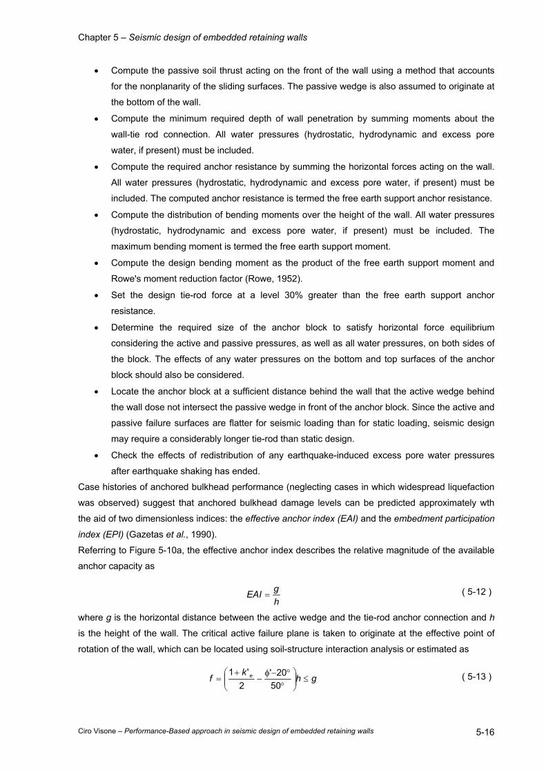
Chapter 5 – Seismic design of embedded retaining walls
Ciro Visone – Performance-Based approach in seismic design of embedded retaining walls 5-16
• Compute the passive soil thrust acting on the front of the wall using a method that accounts
for the nonplanarity of the sliding surfaces. The passive wedge is also assumed to originate at
the bottom of the wall.
• Compute the minimum required depth of wall penetration by summing moments about the
wall-tie rod connection. All water pressures (hydrostatic, hydrodynamic and excess pore
water, if present) must be included.
• Compute the required anchor resistance by summing the horizontal forces acting on the wall.
All water pressures (hydrostatic, hydrodynamic and excess pore water, if present) must be
included. The computed anchor resistance is termed the free earth support anchor resistance.
• Compute the distribution of bending moments over the height of the wall. All water pressures
(hydrostatic, hydrodynamic and excess pore water, if present) must be included. The
maximum bending moment is termed the free earth support moment.
• Compute the design bending moment as the product of the free earth support moment and
Rowe's moment reduction factor (Rowe, 1952).
• Set the design tie-rod force at a level 30% greater than the free earth support anchor
resistance.
• Determine the required size of the anchor block to satisfy horizontal force equilibrium
considering the active and passive pressures, as well as all water pressures, on both sides of
the block. The effects of any water pressures on the bottom and top surfaces of the anchor
block should also be considered.
• Locate the anchor block at a sufficient distance behind the wall that the active wedge behind
the wall dose not intersect the passive wedge in front of the anchor block. Since the active and
passive failure surfaces are flatter for seismic loading than for static loading, seismic design
may require a considerably longer tie-rod than static design.
• Check the effects of redistribution of any earthquake-induced excess pore water pressures
after earthquake shaking has ended.
Case histories of anchored bulkhead performance (neglecting cases in which widespread liquefaction
was observed) suggest that anchored bulkhead damage levels can be predicted approximately wth
the aid of two dimensionless indices: the effective anchor index (EAI) and the embedment participation
index (EPI) (Gazetas et al., 1990).
Referring to Figure 5-10a, the effective anchor index describes the relative magnitude of the available
anchor capacity as
hgEAI = ( 5-12 )
where g is the horizontal distance between the active wedge and the tie-rod anchor connection and h
is the height of the wall. The critical active failure plane is taken to originate at the effective point of
rotation of the wall, which can be located using soil-structure interaction analysis or estimated as
ghk
f e ≤
°
°−φ−
+=
5020'
2'1 ( 5-13 )
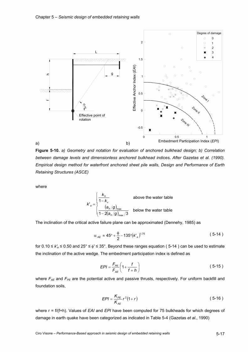
Chapter 5 – Seismic design of embedded retaining walls
Ciro Visone – Performance-Based approach in seismic design of embedded retaining walls 5-17
a)
h
Effective point of rotation
f
α
L
g
AE
b)
Degree of damage
0
123
4
0 0.5 1
-0.5
0
0.5
1
1.5
2
Zone I
Zone II
Zone III
Embedment Participation Index (EPI)
Effe
ctiv
e A
ncho
r Ind
ex (E
AI)
Figure 5-10. a) Geometry and notation for evaluation of anchored bulkhead design; b) Correlation
between damage levels and dimensionless anchored bulkhead indices. After Gazetas et al. (1990).
Empirical design method for waterfront anchored sheet pile walls, Design and Performance of Earth
Retaining Structures (ASCE)
where
( )( )
−
−=
table waterthebelow 321
table waterthe above1
'
max
max
gaga
kk
k
h
h
v
h
e
The inclination of the critical active failure plane can be approximated (Dennehy, 1985) as
( ) 75.1'1352
45 eAE k°−φ
+°≈α ( 5-14 )
for 0.10 ≤ k'e ≤ 0.50 and 25° ≤ φ' ≤ 35°. Beyond these ranges equation ( 5-14 ) can be used to estimate
the inclination of the active wedge. The embedment participation index is defined as
++=
hff
FF
EPIAE
PE 1 ( 5-15 )
where FAE and FPE are the potential active and passive thrusts, respectively. For uniform backfill and
foundation soils,
( )rrKK
EPIAE
PE += 12 ( 5-16 )
where r = f/(f+h). Values of EAI and EPI have been computed for 75 bulkheads for which degrees of
damage in earth quake have been categorized as indicated in Table 5-4 (Gazetas et al., 1990)
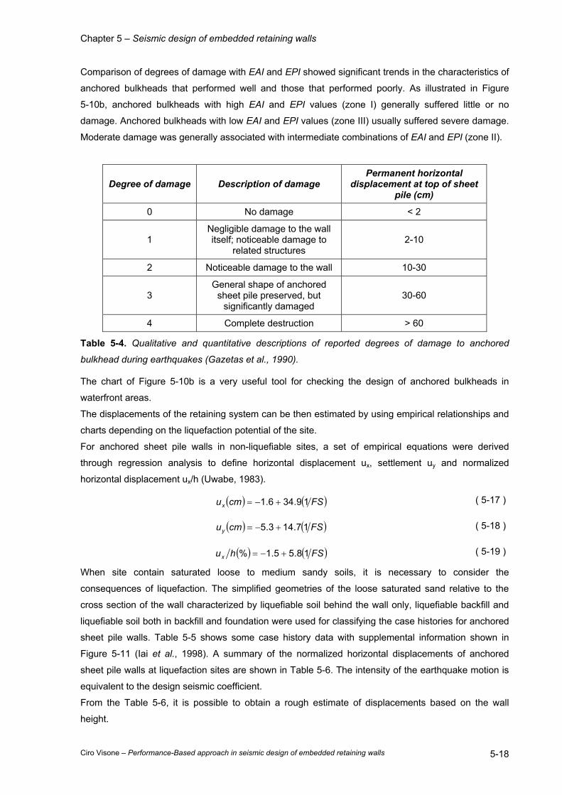
Chapter 5 – Seismic design of embedded retaining walls
Ciro Visone – Performance-Based approach in seismic design of embedded retaining walls 5-18
Comparison of degrees of damage with EAI and EPI showed significant trends in the characteristics of
anchored bulkheads that performed well and those that performed poorly. As illustrated in Figure
5-10b, anchored bulkheads with high EAI and EPI values (zone I) generally suffered little or no
damage. Anchored bulkheads with low EAI and EPI values (zone III) usually suffered severe damage.
Moderate damage was generally associated with intermediate combinations of EAI and EPI (zone II).
Degree of damage Description of damage Permanent horizontal
displacement at top of sheet pile (cm)
0 No damage < 2
1 Negligible damage to the wall itself; noticeable damage to
related structures 2-10
2 Noticeable damage to the wall 10-30
3 General shape of anchored
sheet pile preserved, but significantly damaged
30-60
4 Complete destruction > 60
Table 5-4. Qualitative and quantitative descriptions of reported degrees of damage to anchored
bulkhead during earthquakes (Gazetas et al., 1990).
The chart of Figure 5-10b is a very useful tool for checking the design of anchored bulkheads in
waterfront areas.
The displacements of the retaining system can be then estimated by using empirical relationships and
charts depending on the liquefaction potential of the site.
For anchored sheet pile walls in non-liquefiable sites, a set of empirical equations were derived
through regression analysis to define horizontal displacement ux, settlement uy and normalized
horizontal displacement ux/h (Uwabe, 1983).
( ) ( )FScmux 19.346.1 +−= ( 5-17 )
( ) ( )FScmuy 17.143.5 +−= ( 5-18 )
( ) ( )FShux 18.55.1% +−= ( 5-19 )
When site contain saturated loose to medium sandy soils, it is necessary to consider the
consequences of liquefaction. The simplified geometries of the loose saturated sand relative to the
cross section of the wall characterized by liquefiable soil behind the wall only, liquefiable backfill and
liquefiable soil both in backfill and foundation were used for classifying the case histories for anchored
sheet pile walls. Table 5-5 shows some case history data with supplemental information shown in
Figure 5-11 (Iai et al., 1998). A summary of the normalized horizontal displacements of anchored
sheet pile walls at liquefaction sites are shown in Table 5-6. The intensity of the earthquake motion is
equivalent to the design seismic coefficient.
From the Table 5-6, it is possible to obtain a rough estimate of displacements based on the wall
height.
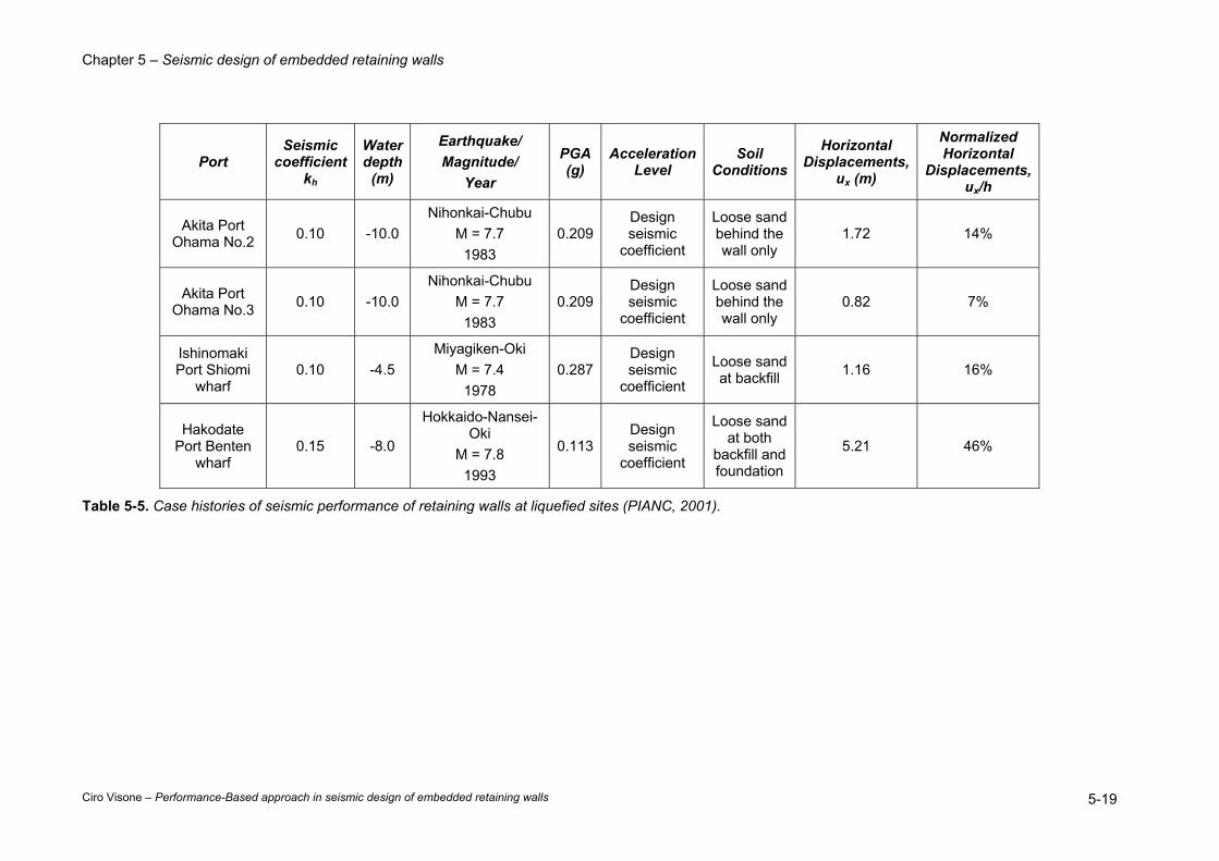
Chapter 5 – Seismic design of embedded retaining walls
Ciro Visone – Performance-Based approach in seismic design of embedded retaining walls 5-19
Port Seismic
coefficient kh
Water depth
(m)
Earthquake/ Magnitude/
Year
PGA (g)
Acceleration Level
Soil Conditions
Horizontal Displacements,
ux (m)
Normalized Horizontal
Displacements, ux/h
Akita Port Ohama No.2 0.10 -10.0
Nihonkai-Chubu M = 7.7
1983 0.209
Design seismic
coefficient
Loose sand behind the wall only
1.72 14%
Akita Port Ohama No.3 0.10 -10.0
Nihonkai-Chubu M = 7.7
1983 0.209
Design seismic
coefficient
Loose sand behind the wall only
0.82 7%
Ishinomaki Port Shiomi
wharf 0.10 -4.5
Miyagiken-Oki M = 7.4
1978 0.287
Design seismic
coefficient
Loose sand at backfill 1.16 16%
Hakodate Port Benten
wharf 0.15 -8.0
Hokkaido-Nansei-Oki
M = 7.8 1993
0.113Design seismic
coefficient
Loose sand at both
backfill and foundation
5.21 46%
Table 5-5. Case histories of seismic performance of retaining walls at liquefied sites (PIANC, 2001).
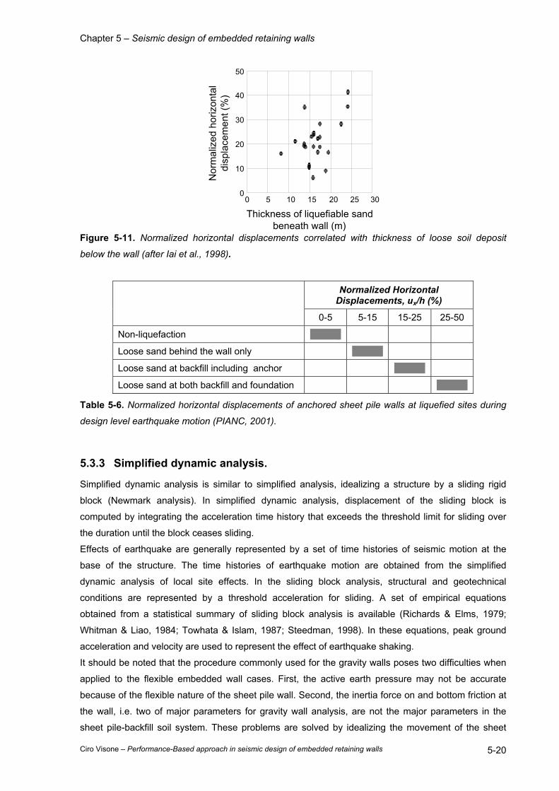
Chapter 5 – Seismic design of embedded retaining walls
Ciro Visone – Performance-Based approach in seismic design of embedded retaining walls 5-20
0 5 10 15 20 25 300
10
20
30
40
50
Nor
mal
ized
hor
izon
tal
disp
lace
men
t (%
)Thickness of liquefiable sand
beneath wall (m) Figure 5-11. Normalized horizontal displacements correlated with thickness of loose soil deposit
below the wall (after Iai et al., 1998).
Normalized Horizontal Displacements, ux/h (%)
0-5 5-15 15-25 25-50
Non-liquefaction G g
Loose sand behind the wall only G g
Loose sand at backfill including anchor G g
Loose sand at both backfill and foundation G g
Table 5-6. Normalized horizontal displacements of anchored sheet pile walls at liquefied sites during
design level earthquake motion (PIANC, 2001).
5.3.3 Simplified dynamic analysis.
Simplified dynamic analysis is similar to simplified analysis, idealizing a structure by a sliding rigid
block (Newmark analysis). In simplified dynamic analysis, displacement of the sliding block is
computed by integrating the acceleration time history that exceeds the threshold limit for sliding over
the duration until the block ceases sliding.
Effects of earthquake are generally represented by a set of time histories of seismic motion at the
base of the structure. The time histories of earthquake motion are obtained from the simplified
dynamic analysis of local site effects. In the sliding block analysis, structural and geotechnical
conditions are represented by a threshold acceleration for sliding. A set of empirical equations
obtained from a statistical summary of sliding block analysis is available (Richards & Elms, 1979;
Whitman & Liao, 1984; Towhata & Islam, 1987; Steedman, 1998). In these equations, peak ground
acceleration and velocity are used to represent the effect of earthquake shaking.
It should be noted that the procedure commonly used for the gravity walls poses two difficulties when
applied to the flexible embedded wall cases. First, the active earth pressure may not be accurate
because of the flexible nature of the sheet pile wall. Second, the inertia force on and bottom friction at
the wall, i.e. two of major parameters for gravity wall analysis, are not the major parameters in the
sheet pile-backfill soil system. These problems are solved by idealizing the movement of the sheet

Chapter 5 – Seismic design of embedded retaining walls
Ciro Visone – Performance-Based approach in seismic design of embedded retaining walls 5-21
pile-backfill system, assuming united rigid block motion of the wall and backfill (Towhata & Islam,
1987). The driving force is the inertia force acting on the soil wedge and the resistance force includes
the passive earth pressures in front of the wall and the shear resistance along the failure surface of
the soil wedge.
By expressing the dynamic earth pressure coefficients KAE and KPE and the ultimate anchor resistance
TE as functions of KA, KP and TS before the earthquake (Seed and Whitman, 1970)
hAAEAAE kKKKK43
+=∆+= ( 5-20 )
hPPEPPE kKKKK8
17−=∆+= ( 5-21 )
AP
AEPESE KK
KKTT−−
+= ( 5-22 )
the threshold horizontal seismic coefficient is obtained as (Towhata and Islam, 1987)
( )( )AE
AEAEAEcrit c
bbakα+
α+α−φ+−α=
tan1tan1tantan ( 5-23 )
where
( )m
PwwPS
WUdhPmT
a∆++γ++
=221 ( 5-24 )
( )θ
α∆+φ+γ= tansintan21 2
m
AEAww
WUdhb ( 5-25 )
( )
γ+
γγ
+−
= 2
127
'817
8231
wwP
satP
AP
S
m
hKP
KKmnT
Wc ( 5-26 )
( ) ( )( )[ ]wwwsatm hdhhhdhW ++−γ++γ= 221 2 ( 5-27 )
and
m = 0 for no anchor capacity, 1 for full anchor capacity (dependant on the amount of excess pore
pressure generation around the anchor)
PP = static passive earth thrust
∆U = excess pore water pressure due to cyclic shearing; subscripts A and P denote pressures within
the active and passive soil wedges
n = 1 when the anchor block is above the water table, and γ/γ' when the anchor is completely
submerged.
The ground water table behind the wall is the same as that of the excavation side.
Using the threshold seismic coefficient kcrit defined for the sheet pile-backfill system, displacement of
the wall is computed based on Newmark's sliding block approach.

Chapter 5 – Seismic design of embedded retaining walls
Ciro Visone – Performance-Based approach in seismic design of embedded retaining walls 5-22
5.3.4 Pushover analysis.
A more sophisticated method for the evaluation of kcrit for an embedded retaining wall is based on
nonlinear FEM/FDM pseudostatic analysis. The procedure can be included in the framework of the
"pushover analyses". The first application was proposed by Visone & Santucci de Magistris (2007).
Pushover analysis is a static nonlinear procedure in which the magnitude of the structural loading is
incrementally increased in accordance with a certain predefined pattern. With the increase of the
loading magnitude, weak links and failure modes of the structure can be found. The sequence of
yields in the structure and the transition from elastic to the ultimate state response may also be
identified. Static pushover analysis is a consolidated methodology in the structural engineering for
evaluation of the real strength of the structures and it promises to be a useful and effective tool in the
view of the performance-based design philosophy.
In geotechnical engineering, only few applications of pushover analyses can be found in the literature
(e.g. Pile-supported wharves – PIANC, 2001). This is maybe due to the difficulties to recognize the
vibration modes of the geotechnical system.
The methodology requires the numerical modelling of the problem by means of FE or FD simulations.
For this scope, the soil can be modelled adopting subgrade reaction method (FE1D analysis) or as an
elasto-plastic continuum.
The static conditions of the soil-wall system should be studied to take into account the nonlinearities of
the soil and wall behaviours. Then, starting from the deformed configuration, the seismic loadings are
applied to the structure through pressure distributions on the wall towards the excavation.
The aspects that should be considered in this type of analysis are:
• geometrical nonlinearities: when the system reach the collapse the small deformations
hypothesis is violated, hence, the calculation need continuous updating of the configuration;
• material nonlinearities: the stress-strain behaviour of the soil, the structural element, the soil-
structure interface and of the other elements (anchors, props, etc.) should be represented with
suitable constitutive models that implement plasticity;
• load advancement to the ultimate level: the external load should be applied incrementally in
order to obtain a load-displacement relationship that permits to detect the displacements of
the system when it is subjected to design actions (seismic demand).
The main results of the analysis are load-displacements curves that represent the capacity of the
system to resist seismic actions (seismic capacity).
In the present research, two different linear pressures distributions are considered.
1. Triangular (TRD), with a maximum pmax at the base of the wall, suitable for low frequencies
motions, as shown for instance by Steedman & Zeng (1990). This distribution agrees with
the provisions given by the Italian Building code (NTC, 2008).
2. Rectangular (RTD), following the indications found in EC8-5.
Thus, dynamic thrust increments are equal to:
HpSE max21
= TRD ( 5-28 )
HpSE max= RTD ( 5-29 )

Chapter 5 – Seismic design of embedded retaining walls
Ciro Visone – Performance-Based approach in seismic design of embedded retaining walls 5-23
acting at H/3, H/2 and 0.6 H from the base of the wall having a total height H = h +d.
These values can be normalized with respect to the weight W of the active soil wedge and the weight
Ww of the wall, in order to obtain the seismic horizontal coefficient kcrit
w
Ecritcrit WW
Sg
ak
+== ( 5-30 )
beyond which the rigid block of soil-wall system begin to move.
For a uniform subsoil, assuming a critical planar surface inclined of an angle αcrit respect to the
horizontal plane, W can be evaluated by the following expression
( )critHW α−°γ= 90tan21 2 ( 5-31 )
while, for a rectangular diaphragm with a thickness s, Ww is
HsW RCw ⋅⋅γ= ( 5-32 )
having indicated with γRC the unit weight of the wall.
Hence, the expressions of kcrit are
( ) sHp
kRCcrit
crit γ+α−°γ=
290tanmax TRD ( 5-33 )
( ) sHp
kRCcrit
crit γ+α−°γ=
290tan2 max RTD ( 5-34 )
For a given geometry of a retaining wall, the value of kcrit can be obtained by a pseudostatic numerical
analysis in which, starting from the static deformed configuration after the excavation, an incremental
load is applied on the structure until the failure is reached. As illustrated in the Chapter 3, the αcrit value
depends on the seismic coefficient kh. A simple trial and error procedure is sufficient to determine step
by step kh and αcrit.
Another possible strategy to evaluate the threshold seismic acceleration acrit with FE or FD methods is
that to apply on the mesh nodes of the 2D numerical model an incremental horizontal acceleration ah.
The critical value acrit of the soil-wall system can be defined as the value that corresponds to the
condition for which the pseudostatic equilibrium is not satisfied. This type of analysis requires some
precautions when the numerical model is defined.
In the next Chapter, examples of application of the procedure to free embedded walls by using a 2D
finite element code will be presented.
5.3.5 Dynamic analysis.
Dynamic analysis is based on soil-structure interaction, generally using FE or FD methods. In this
category of analysis, effects of earthquake are represented by a set of time histories of seismic motion
at the base of the analysis domain chosen for the soil-structure system. A structure is idealized either
as linear or as nonlinear, depending on the level of earthquake motion relative to the elastic limit of the
structure. Soil is idealized either by equivalent linear or by an effective stress model, depending on the
expected strain level in the soil deposit during the design earthquake.
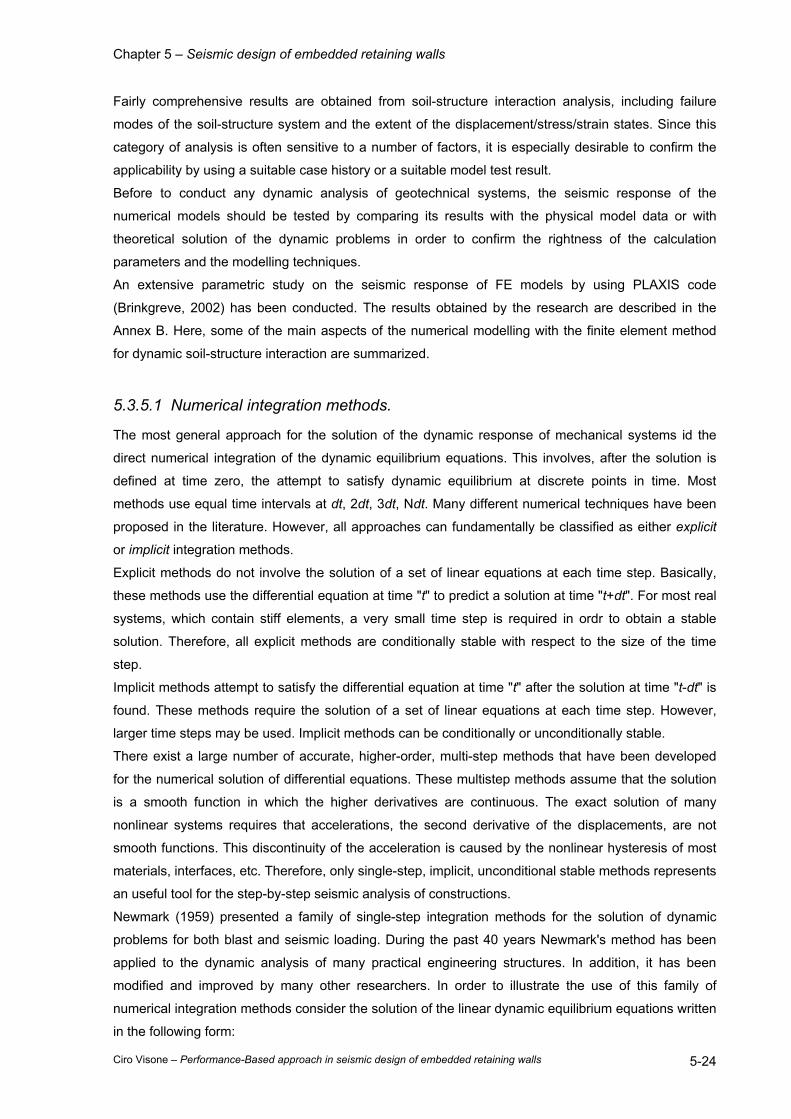
Chapter 5 – Seismic design of embedded retaining walls
Ciro Visone – Performance-Based approach in seismic design of embedded retaining walls 5-24
Fairly comprehensive results are obtained from soil-structure interaction analysis, including failure
modes of the soil-structure system and the extent of the displacement/stress/strain states. Since this
category of analysis is often sensitive to a number of factors, it is especially desirable to confirm the
applicability by using a suitable case history or a suitable model test result.
Before to conduct any dynamic analysis of geotechnical systems, the seismic response of the
numerical models should be tested by comparing its results with the physical model data or with
theoretical solution of the dynamic problems in order to confirm the rightness of the calculation
parameters and the modelling techniques.
An extensive parametric study on the seismic response of FE models by using PLAXIS code
(Brinkgreve, 2002) has been conducted. The results obtained by the research are described in the
Annex B. Here, some of the main aspects of the numerical modelling with the finite element method
for dynamic soil-structure interaction are summarized.
5.3.5.1 Numerical integration methods.
The most general approach for the solution of the dynamic response of mechanical systems id the
direct numerical integration of the dynamic equilibrium equations. This involves, after the solution is
defined at time zero, the attempt to satisfy dynamic equilibrium at discrete points in time. Most
methods use equal time intervals at dt, 2dt, 3dt, Ndt. Many different numerical techniques have been
proposed in the literature. However, all approaches can fundamentally be classified as either explicit
or implicit integration methods.
Explicit methods do not involve the solution of a set of linear equations at each time step. Basically,
these methods use the differential equation at time "t" to predict a solution at time "t+dt". For most real
systems, which contain stiff elements, a very small time step is required in ordr to obtain a stable
solution. Therefore, all explicit methods are conditionally stable with respect to the size of the time
step.
Implicit methods attempt to satisfy the differential equation at time "t" after the solution at time "t-dt" is
found. These methods require the solution of a set of linear equations at each time step. However,
larger time steps may be used. Implicit methods can be conditionally or unconditionally stable.
There exist a large number of accurate, higher-order, multi-step methods that have been developed
for the numerical solution of differential equations. These multistep methods assume that the solution
is a smooth function in which the higher derivatives are continuous. The exact solution of many
nonlinear systems requires that accelerations, the second derivative of the displacements, are not
smooth functions. This discontinuity of the acceleration is caused by the nonlinear hysteresis of most
materials, interfaces, etc. Therefore, only single-step, implicit, unconditional stable methods represents
an useful tool for the step-by-step seismic analysis of constructions.
Newmark (1959) presented a family of single-step integration methods for the solution of dynamic
problems for both blast and seismic loading. During the past 40 years Newmark's method has been
applied to the dynamic analysis of many practical engineering structures. In addition, it has been
modified and improved by many other researchers. In order to illustrate the use of this family of
numerical integration methods consider the solution of the linear dynamic equilibrium equations written
in the following form:
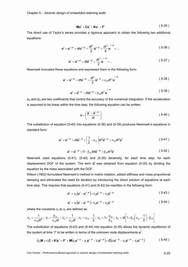
Chapter 5 – Seismic design of embedded retaining walls
Ciro Visone – Performance-Based approach in seismic design of embedded retaining walls 5-25
tttt FKuuCuM =++ &&& ( 5-35 )
The direct use of Taylor’s series provides a rigorous approach to obtain the following two additional
equations:
…++++=−…
−−−dtt
dttdttdttt dtdtdt uuuuu62
32&&& ( 5-36 )
…+++=−…
−−dtt
dttdttt dtdt uuuu2
2&&&& ( 5-37 )
Newmark truncated these equations and expressed them in the following form:
dtt
Ndttdttdttt dtdtdt
−…−−− α+++= uuuuu 3
2
2&&& ( 5-38 )
dtt
Ndttdttt dtdt
−…−− β++= uuuu 2&&&& ( 5-39 )
αN and βN are two coefficients that control the accuracy of the numerical integration. If the acceleration
is assumed to be linear within the time step, the following equation can be written:
−=
−…
dt
dttt uuu&&&&
( 5-40 )
The substitution of equation (5-40) into equations (5-38) and (5-39) produces Newmark’s equations in
standard form:
tN
dttN
dttdttt dtdtdt uuuuu &&&&& 22
21
α+
α−++= −−− ( 5-41 )
( ) tN
dttN
dttt dtdt uuuu &&&&&& 21 β+β−+= −− ( 5-42 )
Newmark used equations (5-41), (5-42) and (5-35) iteratively, for each time step, for each
displacement DOF of the system. The term üt was obtained from equation (5-35) by dividing the
equation by the mass associated with the DOF.
Wilson (1962) formulated Newmark’s method in matrix notation, added stiffness and mass proportional
damping and eliminated the need for iteration by introducing the direct solution of equations at each
time step. This requires that equations (5-41) and (5-42) be rewritten in the following form:
( ) dttdttdtttt ccc −−− ++−= uuuuu &&&&& 320 ( 5-43 )
( ) dttdttdtttt ccc −−− ++−= uuuuu &&&& 541 ( 5-44 )
where the constants c0 to c5 are defined as:
201dt
cNα
= ; dt
cN
N
αβ
=1 ; dt
cNα
=1
2 ; 21
3 −α= Nc ; N
Ncβα
+= 14 ;
β−
−αβ+= NNNdtc
2115
The substitution of equations (5-43) and (5-44) into equation (5-35) allows the dynamic equilibrium of
the system at time “t” to be written in terms of the unknown node displacements ut.
( ) ( ) ( )dttdttdttdttdttdtttt cccccccc −−−−−− −−+−−+=++ uuuCuuuMFuKCM &&&&&& 54113210 ( 5-45 )

Chapter 5 – Seismic design of embedded retaining walls
Ciro Visone – Performance-Based approach in seismic design of embedded retaining walls 5-26
The Newmark direct integration algorithm can be summarized as follows:
I. INITIAL CALCULATION
1. Form static stiffness matrix K, mass matrix M and damping matrix C
2. Specify integration parameters αN and βN
3. Calculate integration constants c0 to c5
4. Form effective stiffness matrix CMKK 10 cc ++=
5. Triangularize effective stiffness matrix TLDLK =
6. Specify initial conditions u0, 0u& 0u&&
II. FOR EACH TIME STEP
1. Calculate effective load vector
( ) ( )dttdttdttdttdttdttttcccccc −−−−−− −−+−−+= uuuCuuuMFF &&&&&& 541132
2. Solve for node displacement vector at time t ttT FuLDL = forward and back-substitution only
3. Calculate node velocities and accelerations at time t
( ) dttdttdtttt ccc −−− ++−= uuuuu &&&&541
( ) dttdttdtttt ccc −−− ++−= uuuuu &&&&&320
4. Go to Step II.1 with t = t+dt
Note that the constants c0 need to be calculated only once. Also, for linear systems, the effective
dynamic stiffness matrix K is formed and triangularized only once.
For zero damping Newmark’s method is conditionally stable if
21
≥βN , 21
≤αN ,
NN
dtα−
βω
≤
2
1
max
( 5-46 )
where ωmax is the maximum circular frequency of interest.
Newmark’s method is unconditionally stable if
212 ≥β≥α NN ( 5-47 )
However, if βN is greater than 1/2 , errors are introduced. These errors are associated with “numerical
damping” and “period elongation”.
If αN = 1/4 and βN = 1/2 the Newmark’s method becomes the so-called constant average acceleration
method. It is identical to the trapezoidal rule that has been used to numerically evaluate the second
order differential equations for approximately 100 years. It can easily be shown that this method
conserves energy for free vibration problem, Mü + Ku = 0, for all possible time steps. Therefore, the
sum of the kinematic and strain energy is constant.
dttTdttdttTdtttTttTt KMKME −−−− +=+= uuuuuuuu &&&&2 ( 5-48 )
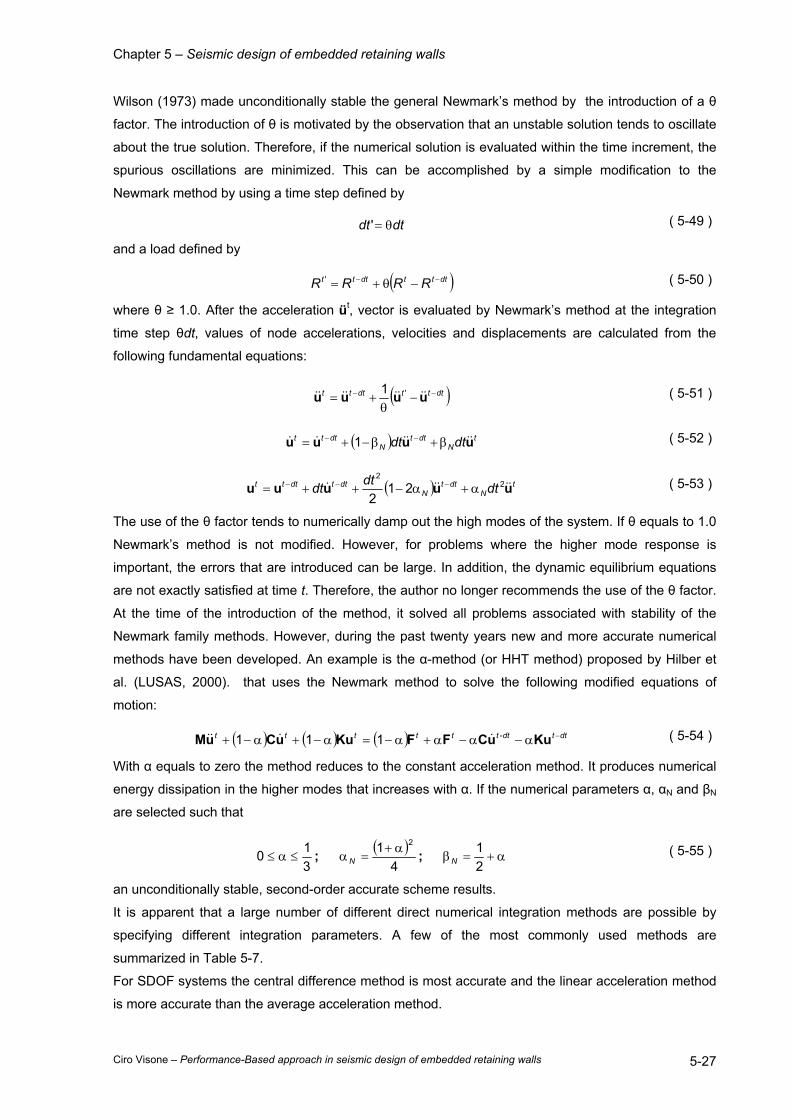
Chapter 5 – Seismic design of embedded retaining walls
Ciro Visone – Performance-Based approach in seismic design of embedded retaining walls 5-27
Wilson (1973) made unconditionally stable the general Newmark’s method by the introduction of a θ
factor. The introduction of θ is motivated by the observation that an unstable solution tends to oscillate
about the true solution. Therefore, if the numerical solution is evaluated within the time increment, the
spurious oscillations are minimized. This can be accomplished by a simple modification to the
Newmark method by using a time step defined by
dtdt θ=' ( 5-49 )
and a load defined by
( )dtttdttt RRRR −− −θ+=' ( 5-50 )
where θ ≥ 1.0. After the acceleration üt, vector is evaluated by Newmark’s method at the integration
time step θdt, values of node accelerations, velocities and displacements are calculated from the
following fundamental equations:
( )dtttdttt −− −θ
+= uuuu &&&&&&&& '1 ( 5-51 )
( ) tN
dttN
dttt dtdt uuuu &&&&&& β+β−+= −− 1 ( 5-52 )
( ) tN
dttN
dttdttt dtdtdt uuuuu &&&&& 22
212
α+α−++= −−− ( 5-53 )
The use of the θ factor tends to numerically damp out the high modes of the system. If θ equals to 1.0
Newmark’s method is not modified. However, for problems where the higher mode response is
important, the errors that are introduced can be large. In addition, the dynamic equilibrium equations
are not exactly satisfied at time t. Therefore, the author no longer recommends the use of the θ factor.
At the time of the introduction of the method, it solved all problems associated with stability of the
Newmark family methods. However, during the past twenty years new and more accurate numerical
methods have been developed. An example is the α-method (or HHT method) proposed by Hilber et
al. (LUSAS, 2000). that uses the Newmark method to solve the following modified equations of
motion:
( ) ( ) ( ) dttdt-tttttt −α−α−α+α−=α−+α−+ KuuCFFKuuCuM &&&& 111 ( 5-54 )
With α equals to zero the method reduces to the constant acceleration method. It produces numerical
energy dissipation in the higher modes that increases with α. If the numerical parameters α, αN and βN
are selected such that
310 ≤α≤ ; ( )
41 2α+
=αN ; α+=β21
N ( 5-55 )
an unconditionally stable, second-order accurate scheme results.
It is apparent that a large number of different direct numerical integration methods are possible by
specifying different integration parameters. A few of the most commonly used methods are
summarized in Table 5-7.
For SDOF systems the central difference method is most accurate and the linear acceleration method
is more accurate than the average acceleration method.
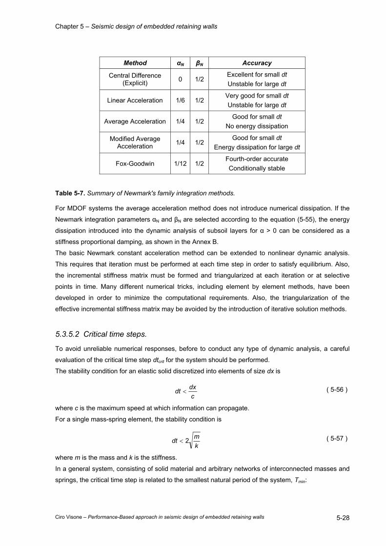
Chapter 5 – Seismic design of embedded retaining walls
Ciro Visone – Performance-Based approach in seismic design of embedded retaining walls 5-28
Method αN βN Accuracy
Central Difference (Explicit) 0 1/2
Excellent for small dt Unstable for large dt
Linear Acceleration 1/6 1/2 Very good for small dt Unstable for large dt
Average Acceleration 1/4 1/2 Good for small dt
No energy dissipation
Modified Average Acceleration 1/4 1/2
Good for small dt Energy dissipation for large dt
Fox-Goodwin 1/12 1/2 Fourth-order accurate Conditionally stable
Table 5-7. Summary of Newmark's family integration methods.
For MDOF systems the average acceleration method does not introduce numerical dissipation. If the
Newmark integration parameters αN and βN are selected according to the equation (5-55), the energy
dissipation introduced into the dynamic analysis of subsoil layers for α > 0 can be considered as a
stiffness proportional damping, as shown in the Annex B.
The basic Newmark constant acceleration method can be extended to nonlinear dynamic analysis.
This requires that iteration must be performed at each time step in order to satisfy equilibrium. Also,
the incremental stiffness matrix must be formed and triangularized at each iteration or at selective
points in time. Many different numerical tricks, including element by element methods, have been
developed in order to minimize the computational requirements. Also, the triangularization of the
effective incremental stiffness matrix may be avoided by the introduction of iterative solution methods.
5.3.5.2 Critical time steps.
To avoid unreliable numerical responses, before to conduct any type of dynamic analysis, a careful
evaluation of the critical time step dtcrit for the system should be performed.
The stability condition for an elastic solid discretized into elements of size dx is
cdxdt < ( 5-56 )
where c is the maximum speed at which information can propagate.
For a single mass-spring element, the stability condition is
kmdt 2< ( 5-57 )
where m is the mass and k is the stiffness.
In a general system, consisting of solid material and arbitrary networks of interconnected masses and
springs, the critical time step is related to the smallest natural period of the system, Tmin:
Chapter 5 – Seismic design of embedded retaining walls
Ciro Visone – Performance-Based approach in seismic design of embedded retaining walls 5-29
π< minT
dt ( 5-58 )
For a finite element mesh, the critical time step depends on the maximum frequency and on the
refinement degree of the discretization. In general, the following expression can be used for a single
element (Pal, 1998 as quoted by Brinkgreve, 2002):
ν−+−+α
=
2
2
2
4 24211
241
BS
SB
SBV
Bdt
P
crit ( 5-59 )
The factor α depends on the element type. For a 6-node-element ( )66/1 c=α , with c6 = 5.1282 and
for a 15 node-element ( )1519/1 c=α , with c15 ≈ 4.9479 (Zienkiewicz and Taylor, 1991). VP and ν are
the compression waves velocity and the Poisson ratio of the element. B and S are the average length
and the surface of the element. In a finite element model the critical time step is equal to the minimum
value of dtcrit according to ( 5-59 ) all over the elements. This time step is chosen to ensure that a wave
during a single step does not move a distance larger than the minimum dimension of an element.
5.3.5.3 Numerical modelling of soil damping.
In nonlinear time-domain response models, there are generally two sources of damping. One source
is hysteretic damping (frequency independent) associated with the area bounded by hysteretic stress-
strain loops. When Masing (1926) and extended Masing rules (Pyke, 1979; Wang et al., 1980; Vucetic
1990) are used to represent the unload-reload behaviour of soil, zero damping is encountered at small
strains, where the backbone curve is linear. The zero damping condition is incompatible with soil
behaviour measured in the laboratory at small strains (e.g. Hardin & Drnevich, 1972; Tatsuoka et al.
1978) and can result in overestimation of propagated ground motion. One solution to this problem is to
add velocity-proportional viscous damping in the form of dashpots embedded within the material
elements. It should be noted that the nature of soil damping at small strains is neither perfectly
hysteretic nor perfectly viscous (Vucetic & Dobry 1986; Lanzo & Vucetic 1999). The incorporation of
hysteretic or viscous damping schemes into nonlinear codes is merely a convenient approximation for
simulation purposes, and is required to ensure numerical stability of lumped mass solutions.
A very common type of damping used in the nonlinear time domain analysis is to assume that the
damping matrix C is proportional to the mass M and stiffness K matrices by means of two coefficients,
αR and βR.
KMC RR β+α= ( 5-60 )
This type of damping is normally referred to as Rayleigh damping. In mode superposition analysis the
damping matrix must have the following properties in order for the modal equations to be uncoupled:
nTnnn φφ=ζω C2 ( 5-61 )
Due to the orthogonality properties of the mass and stiffness matrices, this equation can be rewritten
as
Chapter 5 – Seismic design of embedded retaining walls
Ciro Visone – Performance-Based approach in seismic design of embedded retaining walls 5-30
22 nRRnn ωβ+α=ζω or
ωβ+
ωα
=ζ nRn
Rn 2
1 ( 5-62 )
It is apparent that modal damping can be specified exactly at only two frequencies in order to solve for
αR and βR in the above equation. The use of stiffness proportional damping has the effect of increasing
the damping in the higher modes of the system for which there is no physical justification and can
result in significant errors for impact type of problems. Therefore, the use of Rayleigh type of damping
is not the best way to simulate damping in the soil but it is often introduced in numerical codes as it is
straightforward to implement.
Different procedures were proposed for the evaluation of the Rayleigh damping coefficients (Park &
Hashash, 2004; Lanzo et al., 2004). On the base of the parametric study described in detail in the
Annex B, it may be concluded that, for geotechnical earthquake engineering problems, the full
Rayleigh damping formulation is more accurate than the simplified forms to model the soil viscous
damping. In this procedure, the choice of αR and βR is based on the solution of the following linear
system
ωωω+ω
ζ=
βα
12 mn
mnR
R ( 5-63 )
where ζ, the modal damping ratio, can be identified as the soil damping ratio at low strain level, D0, ωn
and ωm are two significant circular natural frequencies of the system that can be fixed as two of the
first three natural frequencies, in most of cases.
5.3.5.4 Boundary conditions for dynamic soil-structure interaction analyses.
The modelling of geomechanics problems involves media which, at the scale of the analysis, are
better represented as unbounded. Deep underground excavations are normally assumed to be
surrounded by an infinite medium, while surface and near-surface structures are assumed to lie on a
half-space. Numerical methods relying on the discretization of a finite region of space require that
appropriate conditions be enforced at the artificial numerical boundaries. In static analyses, fixed or
elastic boundaries (e.g., represented by boundary-element techniques) can be realistically placed at
some distance from the region of interest. In dynamic problems, however, such boundary conditions
cause the reflection of outward propagating waves back into the model and do not allow the necessary
energy radiation. The use of a larger model can minimize the problem, since material damping will
absorb most of the energy in the waves reflected from distant boundaries. However, this solution leads
to a large computational burden. The alternative is to use quiet (or absorbing) boundaries. Several
formulations have been proposed. One of most widespread is the use of viscous boundaries
developed by Lysmer and Kuhlemeyer (1969). It is based on the use of independent dashpots in the
normal and shear directions at the model boundaries. The method is almost completely effective at
absorbing body waves approaching the boundary at angles of incidence greater than 30°. For lower
angles of incidence, or for surface waves, there is still energy absorption, but it is not perfect.
However, the scheme has the advantage that it operates in the time domain. Its effectiveness has
been demonstrated in both finite-element and finite-difference models (Kunar et al., 1977). A variation
of the technique proposed by White et al. (1977) is also widely used. More efficient energy absorption
Chapter 5 – Seismic design of embedded retaining walls
Ciro Visone – Performance-Based approach in seismic design of embedded retaining walls 5-31
(particularly in the case of Rayleigh waves) requires the use of frequency-dependent elements, which
can only be used in frequency-domain analyses (e.g., Lysmer and Waas 1972). These are usually
termed “consistent boundaries,” and involve the calculation of dynamic stiffness matrices coupling all
the boundary degrees-of-freedom. Boundary element methods may be used to derive these matrices
(e.g., Wolf 1985). A comparative study of the performance of different types of elementary, viscous
and consistent boundaries was documented by Roesset and Ettouney (1977).
The quiet-boundary scheme proposed by Lysmer and Kuhlemeyer (1969) involves dashpots attached
independently to the boundary in the normal and shear directions. The dashpots provide viscous
normal and shear tractions given by:
xPn uVc &ρ−=σ 1 ( 5-64 )
ySuVc &ρ−=τ 2 ( 5-65 )
where ρ is the mass density of the material, VP and VS are the compression and shear wave velocities,
xu& and yu& are the normal and shear components of the velocity at the boundary, c1 and c2 are
relaxation coefficients.
Only few suggestions exist in literature for the choice of these parameters (e.g., Lysmer and
Kuhlemeyer, 1969). Such constraints are introduced in the model simply by adding frequency-
independent terms to the damping matrix of the system.
Dynamic analysis starts from some in-situ condition. If a velocity boundary is used to provide the static
stress state, this boundary condition can be replaced by a quiet boundary; the boundary reaction
forces will be automatically calculated and maintained throughout the dynamic loading phase. Note
that the boundaries must not be freed before applying the quiet boundary condition, otherwise the
reaction forces will be lost.
Quiet boundaries are best-suited when the dynamic source is within a mesh while should not be used
alongside boundaries of a calculation domain when the dynamic source is applied as a boundary
condition at the top or base, because the wave energy will “leak out” of the sides. In this situation,
other types of boundary conditions should be adopted such as perfectly matched layers (Berenger,
1994), infinite elements (Kramer, 1996; Ross, 2004), free-field boundaries (Cundall et al., 1980).
The numerical study described in the Annex B by using the FE code PLAXIS on homogeneous linear
visco-elastic layers crossed by vertical shear waves has shown that the simple assumption of the
lateral adsorbent boundaries is not able to reproduce the expected seismic response of the subsoil.
The more accurate solutions were found by adopting the finite element models sketched in Figure
5-12. These models are characterized by a central domain with a refined mesh, in which the interest of
the study is concentrated, and two lateral domains with a coarse mesh, that have the only aim to
minimize the effects of spurious waves reflected on the boundaries. The boundary conditions are the
following:
1. LOWER BOUNDARY: fixed nodes with a prescribed acceleration (for rigid bedrock) or shear
stress (for elastic bedrock) time history, that is decreased linearly from the central part to the
vertical boundaries until zero
2. LATERAL BOUNDARIES: fixed nodes
3. UPPER BOUNDARY: free surface conditions.

Chapter 5 – Seismic design of embedded retaining walls
Ciro Visone – Performance-Based approach in seismic design of embedded retaining walls 5-32
ax = 1.00 ax = 0.00ax = 0.00
H
B/2 B/2
B
Region of interestRefined Mesh
Lateral DomainCoarse Mesh
Lateral DomainCoarse Mesh
Figure 5-12. Sketch of numerical models able to minimize the reflected waves on lateral boundaries.
Mesh dimension ratios B/2H between the half-width, B/2, and the height, H, of the model of order of 15
allow numerically simulating the free field conditions.
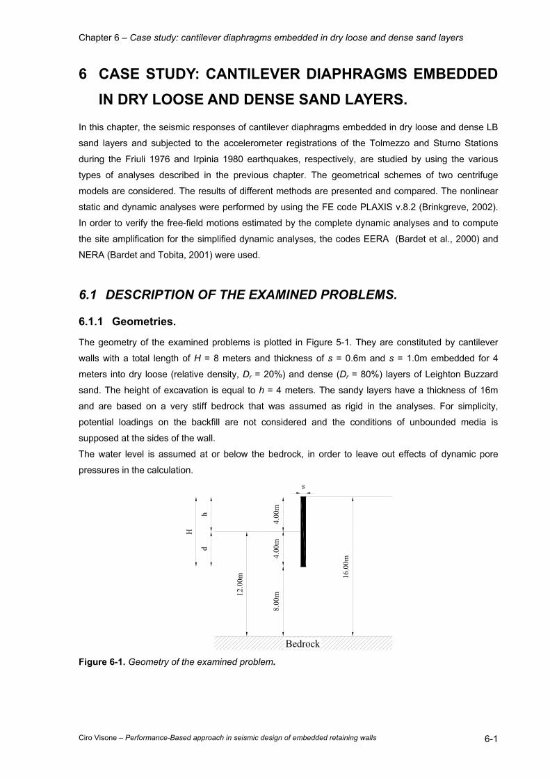
Chapter 6 – Case study: cantilever diaphragms embedded in dry loose and dense sand layers
Ciro Visone – Performance-Based approach in seismic design of embedded retaining walls 6-1
6 CASE STUDY: CANTILEVER DIAPHRAGMS EMBEDDED IN DRY LOOSE AND DENSE SAND LAYERS.
In this chapter, the seismic responses of cantilever diaphragms embedded in dry loose and dense LB
sand layers and subjected to the accelerometer registrations of the Tolmezzo and Sturno Stations
during the Friuli 1976 and Irpinia 1980 earthquakes, respectively, are studied by using the various
types of analyses described in the previous chapter. The geometrical schemes of two centrifuge
models are considered. The results of different methods are presented and compared. The nonlinear
static and dynamic analyses were performed by using the FE code PLAXIS v.8.2 (Brinkgreve, 2002).
In order to verify the free-field motions estimated by the complete dynamic analyses and to compute
the site amplification for the simplified dynamic analyses, the codes EERA (Bardet et al., 2000) and
NERA (Bardet and Tobita, 2001) were used.
6.1 DESCRIPTION OF THE EXAMINED PROBLEMS.
6.1.1 Geometries.
The geometry of the examined problems is plotted in Figure 5-1. They are constituted by cantilever
walls with a total length of H = 8 meters and thickness of s = 0.6m and s = 1.0m embedded for 4
meters into dry loose (relative density, Dr = 20%) and dense (Dr = 80%) layers of Leighton Buzzard
sand. The height of excavation is equal to h = 4 meters. The sandy layers have a thickness of 16m
and are based on a very stiff bedrock that was assumed as rigid in the analyses. For simplicity,
potential loadings on the backfill are not considered and the conditions of unbounded media is
supposed at the sides of the wall.
The water level is assumed at or below the bedrock, in order to leave out effects of dynamic pore
pressures in the calculation.
Bedrock
4.00
m4.
00m
8.00
m
hd
H
12.0
0m 16.0
0m
s
Figure 6-1. Geometry of the examined problem.
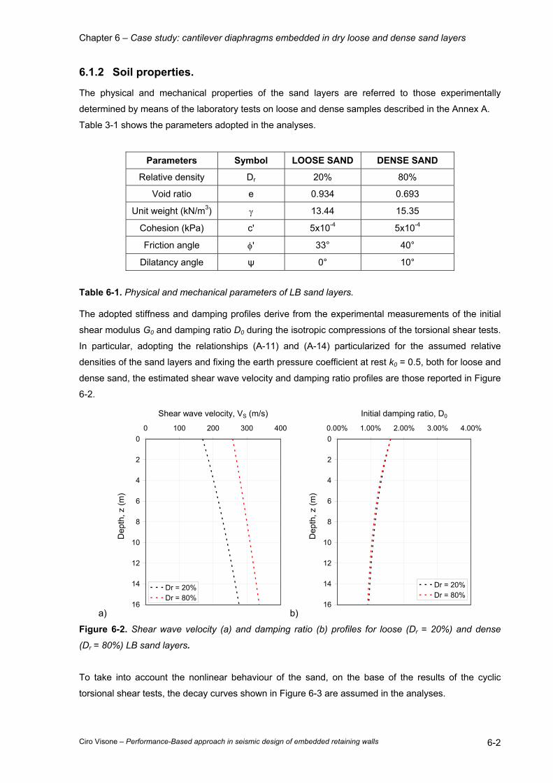
Chapter 6 – Case study: cantilever diaphragms embedded in dry loose and dense sand layers
Ciro Visone – Performance-Based approach in seismic design of embedded retaining walls 6-2
6.1.2 Soil properties.
The physical and mechanical properties of the sand layers are referred to those experimentally
determined by means of the laboratory tests on loose and dense samples described in the Annex A.
Table 3-1 shows the parameters adopted in the analyses.
Parameters Symbol LOOSE SAND DENSE SAND
Relative density Dr 20% 80%
Void ratio e 0.934 0.693
Unit weight (kN/m3) γ 13.44 15.35
Cohesion (kPa) c' 5x10⁻⁴ 5x10⁻⁴
Friction angle φ' 33° 40°
Dilatancy angle ψ 0° 10°
Table 6-1. Physical and mechanical parameters of LB sand layers.
The adopted stiffness and damping profiles derive from the experimental measurements of the initial
shear modulus G0 and damping ratio D0 during the isotropic compressions of the torsional shear tests.
In particular, adopting the relationships (A-11) and (A-14) particularized for the assumed relative
densities of the sand layers and fixing the earth pressure coefficient at rest k0 = 0.5, both for loose and
dense sand, the estimated shear wave velocity and damping ratio profiles are those reported in Figure
6-2.
a)
0
2
4
6
8
10
12
14
16
0 100 200 300 400
Shear wave velocity, VS (m/s)
Dep
th, z
(m)
Dr = 20%Dr = 80%
b)
0
2
4
6
8
10
12
14
16
0.00% 1.00% 2.00% 3.00% 4.00%
Initial damping ratio, D0
Dep
th, z
(m)
Dr = 20%Dr = 80%
Figure 6-2. Shear wave velocity (a) and damping ratio (b) profiles for loose (Dr = 20%) and dense
(Dr = 80%) LB sand layers.
To take into account the nonlinear behaviour of the sand, on the base of the results of the cyclic
torsional shear tests, the decay curves shown in Figure 6-3 are assumed in the analyses.
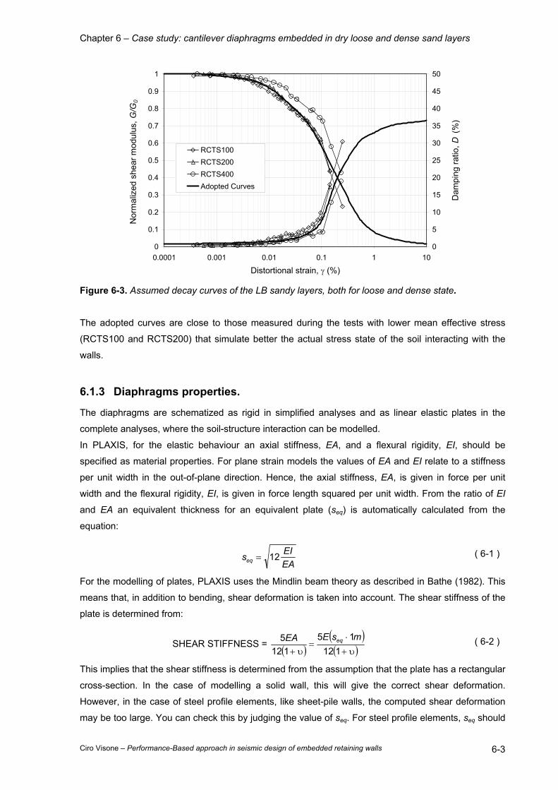
Chapter 6 – Case study: cantilever diaphragms embedded in dry loose and dense sand layers
Ciro Visone – Performance-Based approach in seismic design of embedded retaining walls 6-3
0
0.1
0.2
0.3
0.4
0.5
0.6
0.7
0.8
0.9
1
0.0001 0.001 0.01 0.1 1 10
Distortional strain, γ (%)
Nor
mal
ized
she
ar m
odul
us, G
/G0
0
5
10
15
20
25
30
35
40
45
50
Dam
ping
ratio
, D (%
)
RCTS100RCTS200RCTS400Adopted Curves
Figure 6-3. Assumed decay curves of the LB sandy layers, both for loose and dense state.
The adopted curves are close to those measured during the tests with lower mean effective stress
(RCTS100 and RCTS200) that simulate better the actual stress state of the soil interacting with the
walls.
6.1.3 Diaphragms properties.
The diaphragms are schematized as rigid in simplified analyses and as linear elastic plates in the
complete analyses, where the soil-structure interaction can be modelled.
In PLAXIS, for the elastic behaviour an axial stiffness, EA, and a flexural rigidity, EI, should be
specified as material properties. For plane strain models the values of EA and EI relate to a stiffness
per unit width in the out-of-plane direction. Hence, the axial stiffness, EA, is given in force per unit
width and the flexural rigidity, EI, is given in force length squared per unit width. From the ratio of EI
and EA an equivalent thickness for an equivalent plate (seq) is automatically calculated from the
equation:
EAEIseq 12= ( 6-1 )
For the modelling of plates, PLAXIS uses the Mindlin beam theory as described in Bathe (1982). This
means that, in addition to bending, shear deformation is taken into account. The shear stiffness of the
plate is determined from:
SHEAR STIFFNESS = ( )( )( )υ+
⋅=
υ+ 11215
1125 msEEA eq ( 6-2 )
This implies that the shear stiffness is determined from the assumption that the plate has a rectangular
cross-section. In the case of modelling a solid wall, this will give the correct shear deformation.
However, in the case of steel profile elements, like sheet-pile walls, the computed shear deformation
may be too large. You can check this by judging the value of seq. For steel profile elements, seq should

Chapter 6 – Case study: cantilever diaphragms embedded in dry loose and dense sand layers
Ciro Visone – Performance-Based approach in seismic design of embedded retaining walls 6-4
be at least of the order of a factor 10 times smaller than the length of the plate to ensure negligible
shear deformations.
In addition to the above stiffness parameters, a Poisson's ratio, ν, is required. For thin structures with a
certain profile or structures that are relatively flexible in the out-of-plane direction (like sheet-pile walls),
it is advisable to set Poisson's ratio to zero. For real massive structures (like concrete walls) it is more
realistic to enter a true Poisson's ratio of the order of 0.15. Since PLAXIS considers plates (extending
in the out-of-plane direction) rather than beams (one-dimensional structures), the value of Poisson's
ratio will influence the flexural rigidity of the plate as follows:
Input value of flexural rigidity EI ( 6-3 )
Observed value of flexural rigidity 21 υ−EI ( 6-4 )
The stiffening effect of Poisson's ratio is caused by the stresses in the out-of-plane direction (σzz) and
the fact that strains are prevented in this direction.
Furthermore, in a material set for plates a specific weight w can be specified, which is entered as a
force per unit area. For relatively massive structures this force is, in principle, obtained by multiplying
the unit weight of the plate material by the thickness of the plate. Note that in a finite element model,
plates are superimposed on a continuum and therefore 'overlap' the soil. To calculate accurately the
total weight of soil and structures in the model, the unit weight of the soil should be subtracted from
the unit weight of the plate material. For sheet-pile walls the weight (force per unit area) is generally
provided by the manufacturer. This value can be adopted directly since sheet-pile walls usually occupy
relatively little volume.
6.1.4 Seismic input motions.
To highlight the influence of the input motion on nonlinear seismic responses of the examined
problems, two earthquake signals were considered.
The first is the WE component of the accelerometer registration at Tolmezzo Station for the main
shock of the earthquake of Friuli (Italy) on May 6th, 1976, denoted as TMZ-270. The data were
sampled at 200 Hz for a total number of 7279 registration points. The horizontal peak acceleration,
equal to 0.315 g, was reached at the time t=3.935 s. Most of the energy is included into a frequency
range between 0.8 and 5 Hz, with a predominant frequency of 1.5 Hz. The Arias intensity is 1.20 m/s
and the significant duration (Trifunac and Brady, 1975) is 4.92 s. The time-history of acceleration and
the Fourier spectrum of amplitude are reported in Figure 6-4.
The second is the WE component of the accelerometer registration at Sturno Station for the main
shock of the earthquake of Irpinia (Italy) on November 23rd, 1980, denoted as STU-270. The sampling
frequency is 400 Hz for a total number of 15737 registration points. The horizontal peak acceleration,
equal to 0.321g, was reached at the time t = 5.2375 s. The predominant frequency is 0.44 Hz. The
Arias intensity and the significant duration are 1.39 m/s and 15.2 s, respectively. The acceleration
time-history and the Fourier spectrum of amplitude are plotted in Figure 6-5.
Even if the two considered seismic motions have similar maximum acceleration, they are
characterized by different frequency contents.
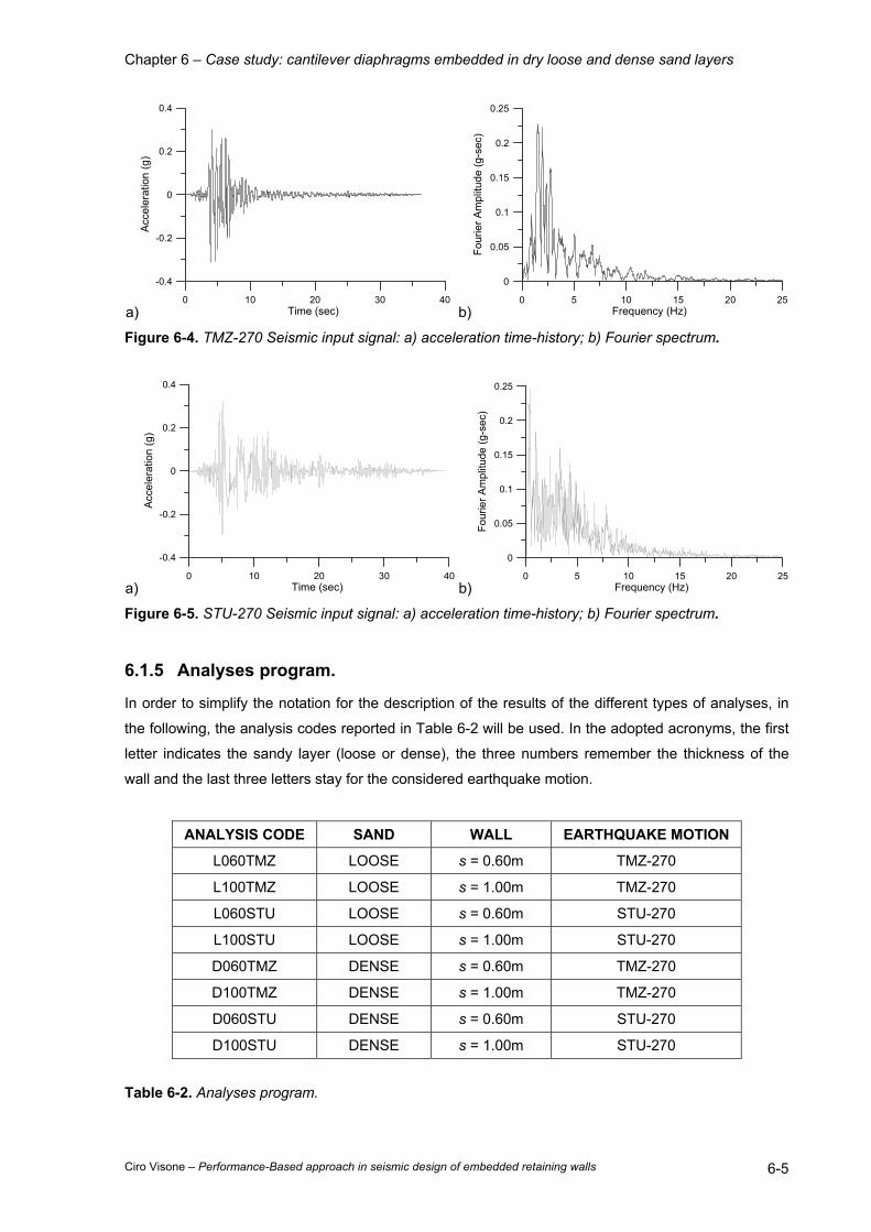
Chapter 6 – Case study: cantilever diaphragms embedded in dry loose and dense sand layers
Ciro Visone – Performance-Based approach in seismic design of embedded retaining walls 6-5
a)
0 10 20 30 40Time (sec)
-0.4
-0.2
0
0.2
0.4
Acc
eler
atio
n (g
)
b)
0 5 10 15 20 25Frequency (Hz)
0
0.05
0.1
0.15
0.2
0.25
Four
ier A
mpl
itude
(g-s
ec)
Figure 6-4. TMZ-270 Seismic input signal: a) acceleration time-history; b) Fourier spectrum.
a)
0 10 20 30 40Time (sec)
-0.4
-0.2
0
0.2
0.4
Acc
eler
atio
n (g
)
b)
0 5 10 15 20 25Frequency (Hz)
0
0.05
0.1
0.15
0.2
0.25
Four
ier A
mpl
itude
(g-s
ec)
Figure 6-5. STU-270 Seismic input signal: a) acceleration time-history; b) Fourier spectrum.
6.1.5 Analyses program.
In order to simplify the notation for the description of the results of the different types of analyses, in
the following, the analysis codes reported in Table 6-2 will be used. In the adopted acronyms, the first
letter indicates the sandy layer (loose or dense), the three numbers remember the thickness of the
wall and the last three letters stay for the considered earthquake motion.
ANALYSIS CODE SAND WALL EARTHQUAKE MOTION
L060TMZ LOOSE s = 0.60m TMZ-270
L100TMZ LOOSE s = 1.00m TMZ-270
L060STU LOOSE s = 0.60m STU-270
L100STU LOOSE s = 1.00m STU-270
D060TMZ DENSE s = 0.60m TMZ-270
D100TMZ DENSE s = 1.00m TMZ-270
D060STU DENSE s = 0.60m STU-270
D100STU DENSE s = 1.00m STU-270
Table 6-2. Analyses program.
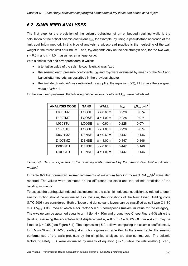
Chapter 6 – Case study: cantilever diaphragms embedded in dry loose and dense sand layers
Ciro Visone – Performance-Based approach in seismic design of embedded retaining walls 6-6
6.2 SIMPLIFIED ANALYSES.
The first step for the prediction of the seismic behaviour of an embedded retaining walls is the
calculation of the critical seismic coefficient kcrit, for example, by using a pseudostatic approach of the
limit equilibrium method. In this type of analysis, a widespread practice is the neglecting of the wall
weight in the forces limit equilibrium. Then, kcrit depends only on the soil strength and, for the two wall,
s = 0.6m and s = 1.0m, assumes an unique value.
With a simple trial and error procedure in which:
• a tentative value of the seismic coefficient kh was fixed
• the seismic earth pressure coefficients KAE and KPE were evaluated by means of the M-O and
Lancellotta methods, as described in the previous chapter
• the limit depth ratio d/h was estimated by adopting the equation (5-3), till to have the assigned
value of d/h = 1
for the examined problems, the following critical seismic coefficient kcrit were calculated:
ANALYSIS CODE SAND WALL kcrit ∆Mmax/γh3
L060TMZ LOOSE s = 0.60m 0.228 0.074
L100TMZ LOOSE s = 1.00m 0.228 0.074
L060STU LOOSE s = 0.60m 0.228 0.074
L100STU LOOSE s = 1.00m 0.228 0.074
D060TMZ DENSE s = 0.60m 0.447 0.146
D100TMZ DENSE s = 1.00m 0.447 0.146
D060STU DENSE s = 0.60m 0.447 0.146
D100STU DENSE s = 1.00m 0.447 0.146
Table 6-3. Seismic capacities of the retaining walls predicted by the pseudostatic limit equilibrium
method.
In Table 6-3 the normalized seismic increments of maximum bending moment ∆Mmax/γh3 were also
reported. The values were estimated as the difference the static and the seismic prediction of the
bending moments.
To assess the earthquake-induced displacements, the seismic horizontal coefficient kh related to each
seismic motion should be estimated. For this aim, the indications of the New Italian Building code
(NTC-2008) are considered. Both of loose and dense sand layers can be classified as soil type C (180
m/s < VS16 < 360 m/s) at which a soil factor S = 1.5 corresponds (maximum value for the category).
The α-value can be assumed equal to α = 1 (for H < 10m and ground type C, see Figure 5-3) while the
β-value, assuming the acceptable limit displacement ux = 0.005 H = 0.005 ⋅ 8.00m = 4 cm, may be
fixed as β = 0.55 (see Figure 5-4). The expression ( 5-2 ) allows computing the seismic coefficients kh
for TMZ-270 and STU-270 earthquake motions given in Table 6-4. In the same Table, the seismic
performances of the walls predicted by the simplified analyses are also summarized. The seismic
factors of safety, FS, were estimated by means of equation ( 5-7 ) while the relationship ( 5-17 )
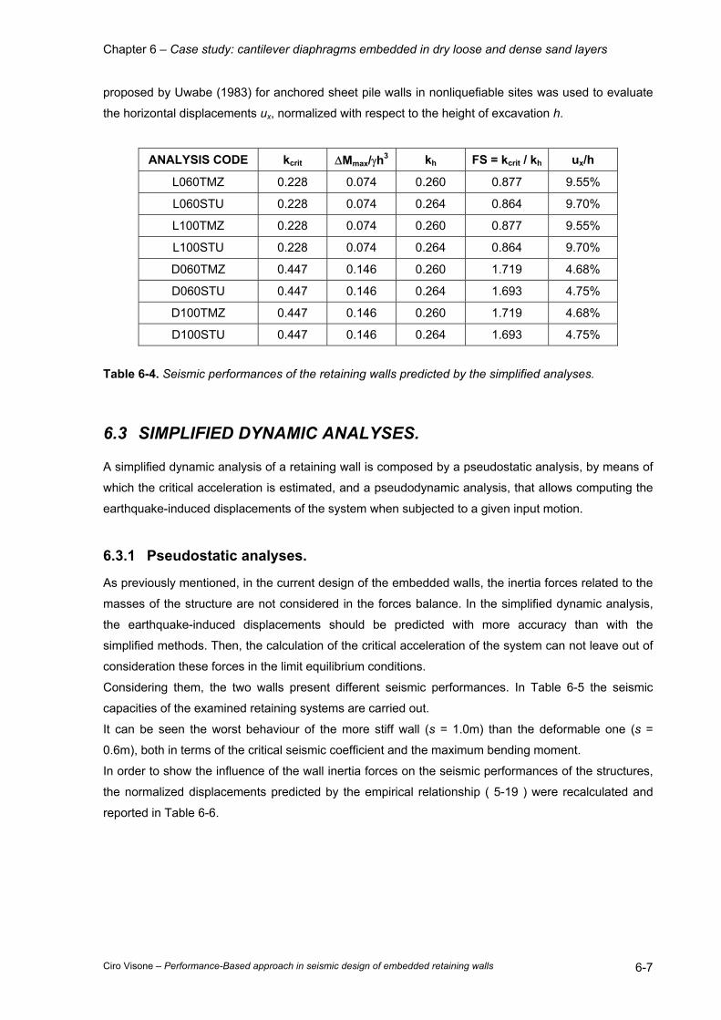
Chapter 6 – Case study: cantilever diaphragms embedded in dry loose and dense sand layers
Ciro Visone – Performance-Based approach in seismic design of embedded retaining walls 6-7
proposed by Uwabe (1983) for anchored sheet pile walls in nonliquefiable sites was used to evaluate
the horizontal displacements ux, normalized with respect to the height of excavation h.
ANALYSIS CODE kcrit ∆Mmax/γh3 kh FS = kcrit / kh ux/h
L060TMZ 0.228 0.074 0.260 0.877 9.55%
L060STU 0.228 0.074 0.264 0.864 9.70%
L100TMZ 0.228 0.074 0.260 0.877 9.55%
L100STU 0.228 0.074 0.264 0.864 9.70%
D060TMZ 0.447 0.146 0.260 1.719 4.68%
D060STU 0.447 0.146 0.264 1.693 4.75%
D100TMZ 0.447 0.146 0.260 1.719 4.68%
D100STU 0.447 0.146 0.264 1.693 4.75%
Table 6-4. Seismic performances of the retaining walls predicted by the simplified analyses.
6.3 SIMPLIFIED DYNAMIC ANALYSES.
A simplified dynamic analysis of a retaining wall is composed by a pseudostatic analysis, by means of
which the critical acceleration is estimated, and a pseudodynamic analysis, that allows computing the
earthquake-induced displacements of the system when subjected to a given input motion.
6.3.1 Pseudostatic analyses.
As previously mentioned, in the current design of the embedded walls, the inertia forces related to the
masses of the structure are not considered in the forces balance. In the simplified dynamic analysis,
the earthquake-induced displacements should be predicted with more accuracy than with the
simplified methods. Then, the calculation of the critical acceleration of the system can not leave out of
consideration these forces in the limit equilibrium conditions.
Considering them, the two walls present different seismic performances. In Table 6-5 the seismic
capacities of the examined retaining systems are carried out.
It can be seen the worst behaviour of the more stiff wall (s = 1.0m) than the deformable one (s =
0.6m), both in terms of the critical seismic coefficient and the maximum bending moment.
In order to show the influence of the wall inertia forces on the seismic performances of the structures,
the normalized displacements predicted by the empirical relationship ( 5-19 ) were recalculated and
reported in Table 6-6.

Chapter 6 – Case study: cantilever diaphragms embedded in dry loose and dense sand layers
Ciro Visone – Performance-Based approach in seismic design of embedded retaining walls 6-8
ANALYSIS CODE SAND WALL kcrit ∆Mmax/γh3
L060TMZ LOOSE s = 0.60m 0.167 0.093
L100TMZ LOOSE s = 1.00m 0.140 0.100
L060STU LOOSE s = 0.60m 0.167 0.093
L100STU LOOSE s = 1.00m 0.140 0.100
D060TMZ DENSE s = 0.60m 0.370 0.159
D100TMZ DENSE s = 1.00m 0.328 0.178
D060STU DENSE s = 0.60m 0.370 0.159
D100STU DENSE s = 1.00m 0.328 0.178
Table 6-5. Seismic capacities of the retaining walls predicted by the pseudostatic limit equilibrium
method considering the inertia forces due to the wall masses.
ANALYSIS CODE kcrit ∆Mmax/γh3 kh FS = kcrit / kh ux/h
L060TMZ 0.167 0.093 0.260 0.642 13.19%
L100TMZ 0.140 0.100 0.260 0.538 15.82%
L060STU 0.167 0.093 0.264 0.633 13.38%
L100STU 0.140 0.100 0.264 0.530 16.06%
D060TMZ 0.370 0.159 0.260 1.423 5.73%
D100TMZ 0.328 0.178 0.260 1.262 6.51%
D060STU 0.370 0.159 0.264 1.402 5.82%
D100STU 0.328 0.178 0.264 1.242 6.62%
Table 6-6. Seismic performances of the retaining walls predicted by the simplified analyses
accounting for the wall weight.
6.3.2 Free field motions.
Before to conduct any type of dynamic analysis, a good practice is to perform local site response
analyses in order to highlight the amplification of the seismic motion due to the stratigraphic
conditions. In this study, various type of ground response analyses were carried out by assuming
different soil constitutive models and integration techniques. The results are presented and compared
in this subsection.
The computer codes used in the analyses are the following:
• EERA (Bardet et al., 2000), that stands for Equivalent-linear Earthquake site Response
Analysis. It is a modern implementation of the well-known concepts of the equivalent linear
site response analysis that was first implemented in the SHAKE code (Schnabel et al., 1972).
The input and output are fully integrated with the spreadsheet program MS-Excel. This code
permits to perform frequency domain analyses for linear and equivalent linear stratified
subsoils. The bedrock can be modelled as rigid, if the option “inside” is selected in the Profile
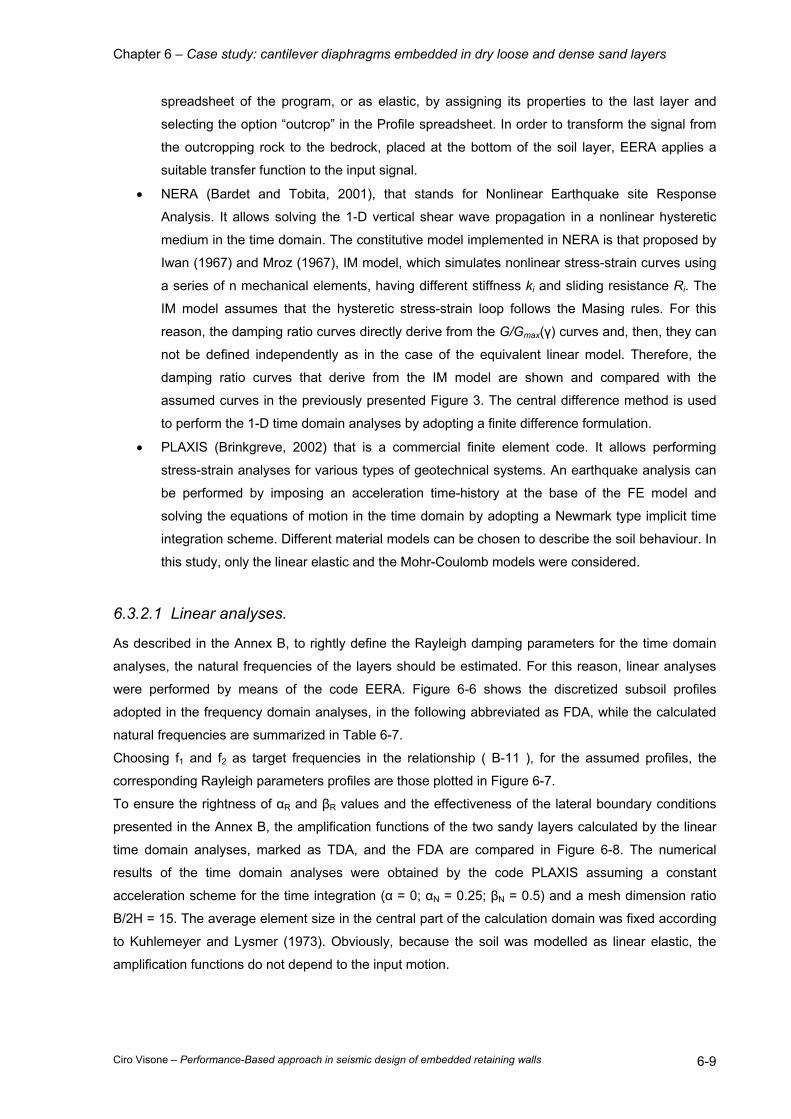
Chapter 6 – Case study: cantilever diaphragms embedded in dry loose and dense sand layers
Ciro Visone – Performance-Based approach in seismic design of embedded retaining walls 6-9
spreadsheet of the program, or as elastic, by assigning its properties to the last layer and
selecting the option “outcrop” in the Profile spreadsheet. In order to transform the signal from
the outcropping rock to the bedrock, placed at the bottom of the soil layer, EERA applies a
suitable transfer function to the input signal.
• NERA (Bardet and Tobita, 2001), that stands for Nonlinear Earthquake site Response
Analysis. It allows solving the 1-D vertical shear wave propagation in a nonlinear hysteretic
medium in the time domain. The constitutive model implemented in NERA is that proposed by
Iwan (1967) and Mroz (1967), IM model, which simulates nonlinear stress-strain curves using
a series of n mechanical elements, having different stiffness ki and sliding resistance Ri. The
IM model assumes that the hysteretic stress-strain loop follows the Masing rules. For this
reason, the damping ratio curves directly derive from the G/Gmax(γ) curves and, then, they can
not be defined independently as in the case of the equivalent linear model. Therefore, the
damping ratio curves that derive from the IM model are shown and compared with the
assumed curves in the previously presented Figure 3. The central difference method is used
to perform the 1-D time domain analyses by adopting a finite difference formulation.
• PLAXIS (Brinkgreve, 2002) that is a commercial finite element code. It allows performing
stress-strain analyses for various types of geotechnical systems. An earthquake analysis can
be performed by imposing an acceleration time-history at the base of the FE model and
solving the equations of motion in the time domain by adopting a Newmark type implicit time
integration scheme. Different material models can be chosen to describe the soil behaviour. In
this study, only the linear elastic and the Mohr-Coulomb models were considered.
6.3.2.1 Linear analyses.
As described in the Annex B, to rightly define the Rayleigh damping parameters for the time domain
analyses, the natural frequencies of the layers should be estimated. For this reason, linear analyses
were performed by means of the code EERA. Figure 6-6 shows the discretized subsoil profiles
adopted in the frequency domain analyses, in the following abbreviated as FDA, while the calculated
natural frequencies are summarized in Table 6-7.
Choosing f1 and f2 as target frequencies in the relationship ( B-11 ), for the assumed profiles, the
corresponding Rayleigh parameters profiles are those plotted in Figure 6-7.
To ensure the rightness of αR and βR values and the effectiveness of the lateral boundary conditions
presented in the Annex B, the amplification functions of the two sandy layers calculated by the linear
time domain analyses, marked as TDA, and the FDA are compared in Figure 6-8. The numerical
results of the time domain analyses were obtained by the code PLAXIS assuming a constant
acceleration scheme for the time integration (α = 0; αN = 0.25; βN = 0.5) and a mesh dimension ratio
B/2H = 15. The average element size in the central part of the calculation domain was fixed according
to Kuhlemeyer and Lysmer (1973). Obviously, because the soil was modelled as linear elastic, the
amplification functions do not depend to the input motion.
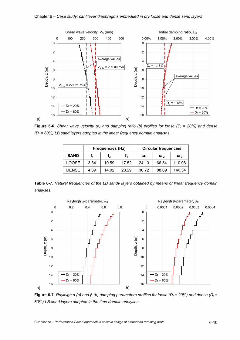
Chapter 6 – Case study: cantilever diaphragms embedded in dry loose and dense sand layers
Ciro Visone – Performance-Based approach in seismic design of embedded retaining walls 6-10
a)
0
2
4
6
8
10
12
14
16
0 100 200 300 400 500
Shear wave velocity, VS (m/s)
Dep
th, z
(m)
Dr = 20%
Dr = 80%
Average values
VS av = 227.21 m/s
VS av = 299.00 m/s
b)
0
2
4
6
8
10
12
14
16
0.00% 1.00% 2.00% 3.00% 4.00%
Initial damping ratio, D0
Dep
th, z
(m)
Dr = 20%Dr = 80%
Average values
D0 = 1.15%
D0 = 1.18%
Figure 6-6. Shear wave velocity (a) and damping ratio (b) profiles for loose (Dr = 20%) and dense
(Dr = 80%) LB sand layers adopted in the linear frequency domain analyses.
Frequencies (Hz) Circular frequencies
SAND f1 f2 f3 ω1 ω 2 ω 3
LOOSE 3.84 10.59 17.52 24.13 66.54 110.08
DENSE 4.89 14.02 23.29 30.72 88.09 146.34
Table 6-7. Natural frequencies of the LB sandy layers obtained by means of linear frequency domain
analyses.
a)
0
2
4
6
8
10
12
14
16
0 0.2 0.4 0.6 0.8
Rayleigh α-parameter, αR
Dep
th, z
(m)
Dr = 20%
Dr = 80%
b)
0
2
4
6
8
10
12
14
16
0 0.0001 0.0002 0.0003 0.0004
Rayleigh β-parameter, βR
Dep
th, z
(m)
Dr = 20%
Dr = 80%
Figure 6-7. Rayleigh α (a) and β (b) damping parameters profiles for loose (Dr = 20%) and dense (Dr =
80%) LB sand layers adopted in the time domain analyses.
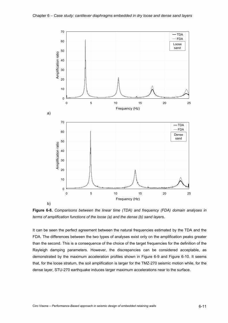
Chapter 6 – Case study: cantilever diaphragms embedded in dry loose and dense sand layers
Ciro Visone – Performance-Based approach in seismic design of embedded retaining walls 6-11
a)
0
10
20
30
40
50
60
70
0 5 10 15 20 25
Frequency (Hz)
Am
plifi
catio
n ra
tio
TDAFDA
Loose sand
b)
0
10
20
30
40
50
60
70
0 5 10 15 20 25
Frequency (Hz)
Am
plifi
catio
n ra
tio
TDAFDA
Dense sand
Figure 6-8. Comparisons between the linear time (TDA) and frequency (FDA) domain analyses in
terms of amplification functions of the loose (a) and the dense (b) sand layers.
It can be seen the perfect agreement between the natural frequencies estimated by the TDA and the
FDA. The differences between the two types of analyses exist only on the amplification peaks greater
than the second. This is a consequence of the choice of the target frequencies for the definition of the
Rayleigh damping parameters. However, the discrepancies can be considered acceptable, as
demonstrated by the maximum acceleration profiles shown in Figure 6-9 and Figure 6-10. It seems
that, for the loose stratum, the soil amplification is larger for the TMZ-270 seismic motion while, for the
dense layer, STU-270 earthquake induces larger maximum accelerations near to the surface.
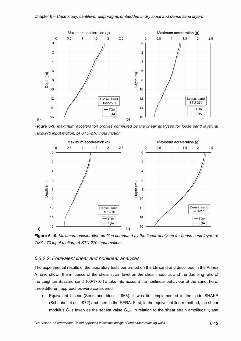
Chapter 6 – Case study: cantilever diaphragms embedded in dry loose and dense sand layers
Ciro Visone – Performance-Based approach in seismic design of embedded retaining walls 6-12
a)
0
2
4
6
8
10
12
14
16
0 0.5 1 1.5 2 2.5
Maximum acceleration (g)
Dep
th (m
)
TDAFDA
Loose sandTMZ-270
b)
0
2
4
6
8
10
12
14
16
0 0.5 1 1.5 2 2.5
Maximum acceleration (g)
Dep
th (m
)
TDAFDA
Loose sandSTU-270
Figure 6-9. Maximum acceleration profiles computed by the linear analyses for loose sand layer: a)
TMZ-270 input motion; b) STU-270 input motion.
a)
0
2
4
6
8
10
12
14
16
0 0.5 1 1.5 2 2.5
Maximum acceleration (g)
Dep
th (m
)
TDAFDA
Dense sandTMZ-270
b)
0
2
4
6
8
10
12
14
16
0 0.5 1 1.5 2 2.5
Maximum acceleration (g)
Dep
th (m
)
TDAFDA
Dense sandSTU-270
Figure 6-10. Maximum acceleration profiles computed by the linear analyses for dense sand layer: a)
TMZ-270 input motion; b) STU-270 input motion.
6.3.2.2 Equivalent linear and nonlinear analyses.
The experimental results of the laboratory tests performed on the LB sand and described in the Annex
A have shown the influence of the shear strain level on the shear modulus and the damping ratio of
the Leighton Buzzard sand 100/170. To take into account the nonlinear behaviour of the sand, here,
three different approaches were considered:
• Equivalent Linear (Seed and Idriss, 1968): it was first implemented in the code SHAKE
(Schnabel et al., 1972) and then in the EERA. First, in the equivalent linear method, the shear
modulus G is taken as the secant value Gsec, in relation to the shear strain amplitude γ, and
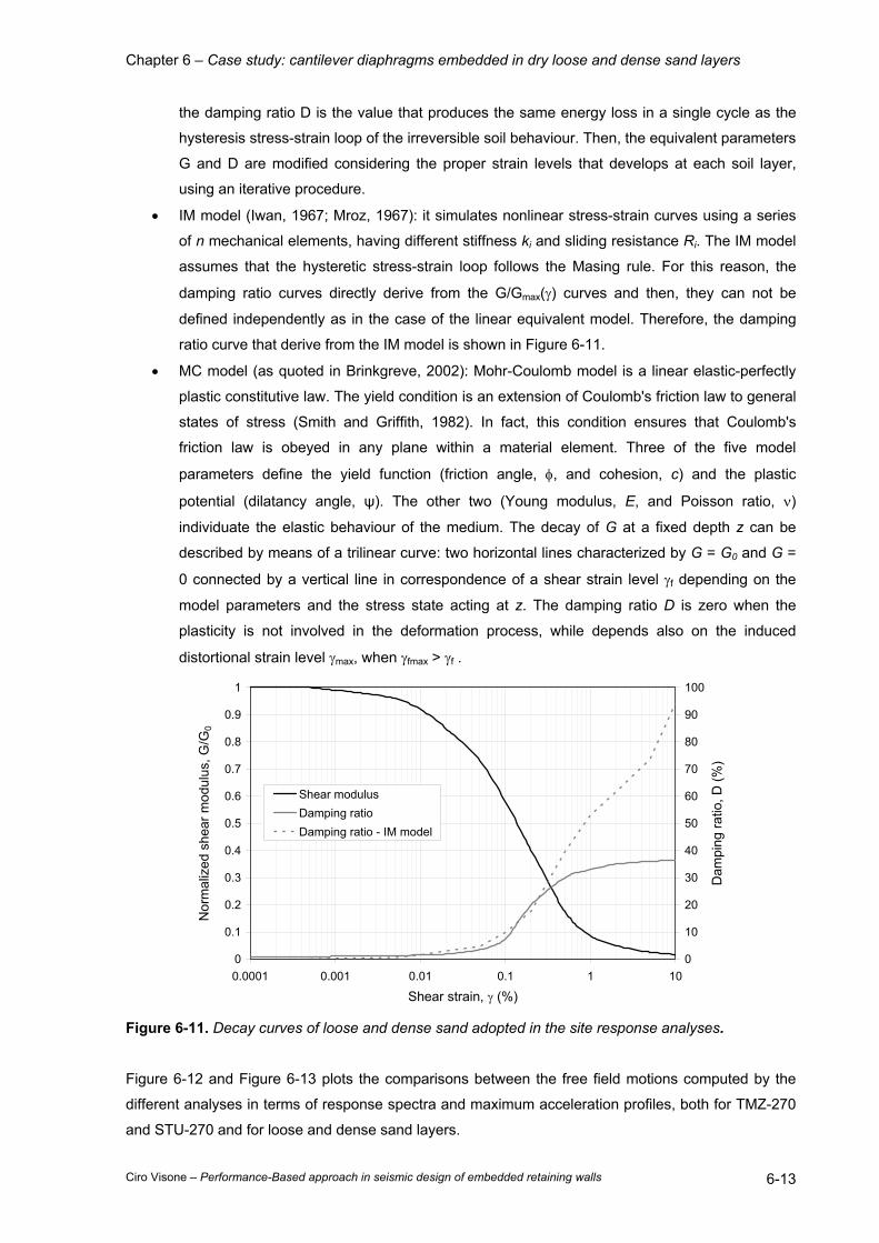
Chapter 6 – Case study: cantilever diaphragms embedded in dry loose and dense sand layers
Ciro Visone – Performance-Based approach in seismic design of embedded retaining walls 6-13
the damping ratio D is the value that produces the same energy loss in a single cycle as the
hysteresis stress-strain loop of the irreversible soil behaviour. Then, the equivalent parameters
G and D are modified considering the proper strain levels that develops at each soil layer,
using an iterative procedure.
• IM model (Iwan, 1967; Mroz, 1967): it simulates nonlinear stress-strain curves using a series
of n mechanical elements, having different stiffness ki and sliding resistance Ri. The IM model
assumes that the hysteretic stress-strain loop follows the Masing rule. For this reason, the
damping ratio curves directly derive from the G/Gmax(γ) curves and then, they can not be
defined independently as in the case of the linear equivalent model. Therefore, the damping
ratio curve that derive from the IM model is shown in Figure 6-11.
• MC model (as quoted in Brinkgreve, 2002): Mohr-Coulomb model is a linear elastic-perfectly
plastic constitutive law. The yield condition is an extension of Coulomb's friction law to general
states of stress (Smith and Griffith, 1982). In fact, this condition ensures that Coulomb's
friction law is obeyed in any plane within a material element. Three of the five model
parameters define the yield function (friction angle, φ, and cohesion, c) and the plastic
potential (dilatancy angle, ψ). The other two (Young modulus, E, and Poisson ratio, ν)
individuate the elastic behaviour of the medium. The decay of G at a fixed depth z can be
described by means of a trilinear curve: two horizontal lines characterized by G = G0 and G =
0 connected by a vertical line in correspondence of a shear strain level γf depending on the
model parameters and the stress state acting at z. The damping ratio D is zero when the
plasticity is not involved in the deformation process, while depends also on the induced
distortional strain level γmax, when γfmax > γf .
0
0.1
0.2
0.3
0.4
0.5
0.6
0.7
0.8
0.9
1
0.0001 0.001 0.01 0.1 1 10
Shear strain, γ (%)
Nor
mal
ized
she
ar m
odul
us, G
/G0
0
10
20
30
40
50
60
70
80
90
100
Dam
ping
ratio
, D (%
)
Shear modulusDamping ratioDamping ratio - IM model
Figure 6-11. Decay curves of loose and dense sand adopted in the site response analyses.
Figure 6-12 and Figure 6-13 plots the comparisons between the free field motions computed by the
different analyses in terms of response spectra and maximum acceleration profiles, both for TMZ-270
and STU-270 and for loose and dense sand layers.
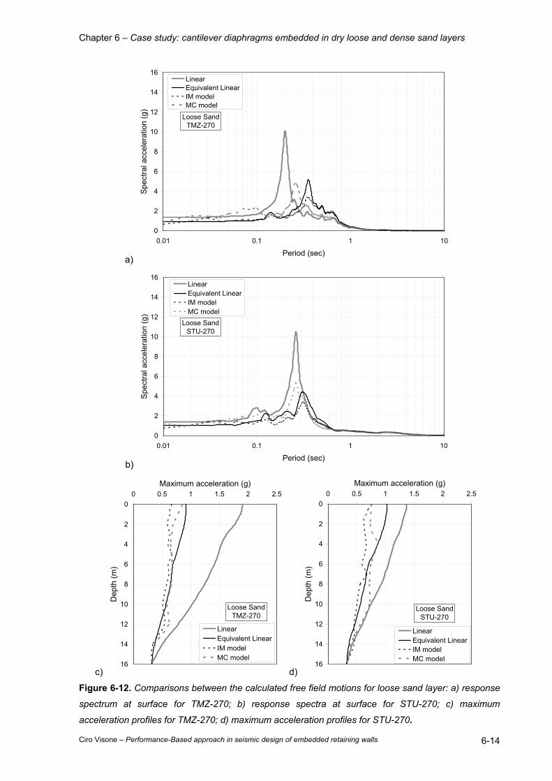
Chapter 6 – Case study: cantilever diaphragms embedded in dry loose and dense sand layers
Ciro Visone – Performance-Based approach in seismic design of embedded retaining walls 6-14
a)
0
2
4
6
8
10
12
14
16
0.01 0.1 1 10
Period (sec)
Spec
tral a
ccel
erat
ion
(g)
LinearEquivalent LinearIM modelMC model
Loose Sand TMZ-270
b)
0
2
4
6
8
10
12
14
16
0.01 0.1 1 10
Period (sec)
Spec
tral a
ccel
erat
ion
(g)
LinearEquivalent LinearIM modelMC model
Loose Sand STU-270
c)
0
2
4
6
8
10
12
14
16
0 0.5 1 1.5 2 2.5Maximum acceleration (g)
Dep
th (m
)
LinearEquivalent LinearIM modelMC model
Loose Sand TMZ-270
d)
0
2
4
6
8
10
12
14
16
0 0.5 1 1.5 2 2.5Maximum acceleration (g)
Dep
th (m
)
LinearEquivalent LinearIM modelMC model
Loose SandSTU-270
Figure 6-12. Comparisons between the calculated free field motions for loose sand layer: a) response
spectrum at surface for TMZ-270; b) response spectra at surface for STU-270; c) maximum
acceleration profiles for TMZ-270; d) maximum acceleration profiles for STU-270.
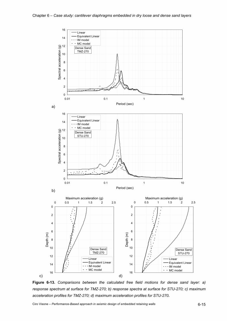
Chapter 6 – Case study: cantilever diaphragms embedded in dry loose and dense sand layers
Ciro Visone – Performance-Based approach in seismic design of embedded retaining walls 6-15
a)
0
2
4
6
8
10
12
14
16
0.01 0.1 1 10
Period (sec)
Spec
tral a
ccel
erat
ion
(g)
LinearEquivalent LinearIM modelMC model
Dense Sand TMZ-270
b)
0
2
4
6
8
10
12
14
16
0.01 0.1 1 10
Period (sec)
Spec
tral a
ccel
erat
ion
(g)
LinearEquivalent LinearIM modelMC model
Dense Sand STU-270
c)
0
2
4
6
8
10
12
14
16
0 0.5 1 1.5 2 2.5Maximum acceleration (g)
Dep
th (m
)
LinearEquivalent LinearIM modelMC model
Dense SandTMZ-270
d)
0
2
4
6
8
10
12
14
16
0 0.5 1 1.5 2 2.5Maximum acceleration (g)
Dep
th (m
)
LinearEquivalent LinearIM modelMC model
Dense SandSTU-270
Figure 6-13. Comparisons between the calculated free field motions for dense sand layer: a)
response spectrum at surface for TMZ-270; b) response spectra at surface for STU-270; c) maximum
acceleration profiles for TMZ-270; d) maximum acceleration profiles for STU-270.
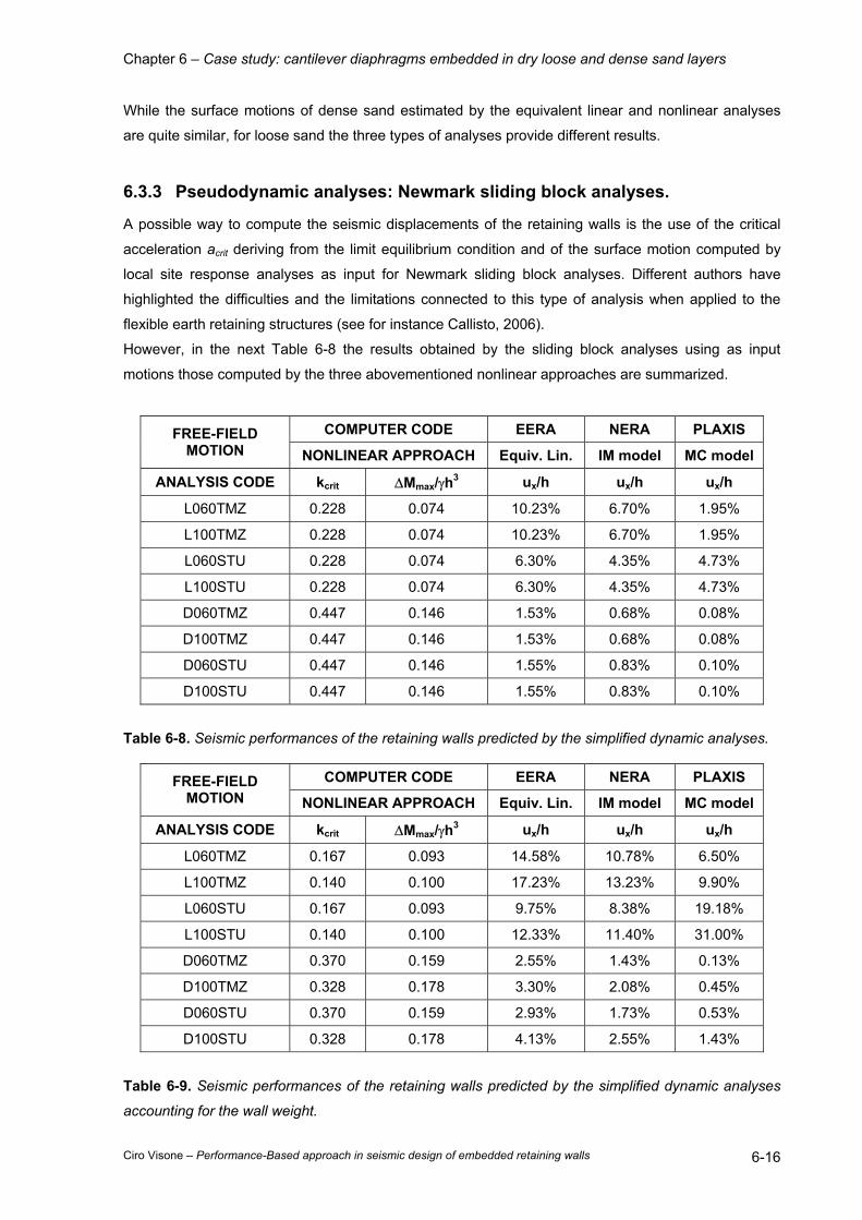
Chapter 6 – Case study: cantilever diaphragms embedded in dry loose and dense sand layers
Ciro Visone – Performance-Based approach in seismic design of embedded retaining walls 6-16
While the surface motions of dense sand estimated by the equivalent linear and nonlinear analyses
are quite similar, for loose sand the three types of analyses provide different results.
6.3.3 Pseudodynamic analyses: Newmark sliding block analyses.
A possible way to compute the seismic displacements of the retaining walls is the use of the critical
acceleration acrit deriving from the limit equilibrium condition and of the surface motion computed by
local site response analyses as input for Newmark sliding block analyses. Different authors have
highlighted the difficulties and the limitations connected to this type of analysis when applied to the
flexible earth retaining structures (see for instance Callisto, 2006).
However, in the next Table 6-8 the results obtained by the sliding block analyses using as input
motions those computed by the three abovementioned nonlinear approaches are summarized.
COMPUTER CODE EERA NERA PLAXIS FREE-FIELD MOTION NONLINEAR APPROACH Equiv. Lin. IM model MC model
ANALYSIS CODE kcrit ∆Mmax/γh3 ux/h ux/h ux/h
L060TMZ 0.228 0.074 10.23% 6.70% 1.95%
L100TMZ 0.228 0.074 10.23% 6.70% 1.95%
L060STU 0.228 0.074 6.30% 4.35% 4.73%
L100STU 0.228 0.074 6.30% 4.35% 4.73%
D060TMZ 0.447 0.146 1.53% 0.68% 0.08%
D100TMZ 0.447 0.146 1.53% 0.68% 0.08%
D060STU 0.447 0.146 1.55% 0.83% 0.10%
D100STU 0.447 0.146 1.55% 0.83% 0.10%
Table 6-8. Seismic performances of the retaining walls predicted by the simplified dynamic analyses.
COMPUTER CODE EERA NERA PLAXIS FREE-FIELD MOTION NONLINEAR APPROACH Equiv. Lin. IM model MC model
ANALYSIS CODE kcrit ∆Mmax/γh3 ux/h ux/h ux/h
L060TMZ 0.167 0.093 14.58% 10.78% 6.50%
L100TMZ 0.140 0.100 17.23% 13.23% 9.90%
L060STU 0.167 0.093 9.75% 8.38% 19.18%
L100STU 0.140 0.100 12.33% 11.40% 31.00%
D060TMZ 0.370 0.159 2.55% 1.43% 0.13%
D100TMZ 0.328 0.178 3.30% 2.08% 0.45%
D060STU 0.370 0.159 2.93% 1.73% 0.53%
D100STU 0.328 0.178 4.13% 2.55% 1.43%
Table 6-9. Seismic performances of the retaining walls predicted by the simplified dynamic analyses
accounting for the wall weight.
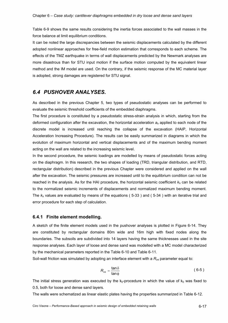
Chapter 6 – Case study: cantilever diaphragms embedded in dry loose and dense sand layers
Ciro Visone – Performance-Based approach in seismic design of embedded retaining walls 6-17
Table 6-9 shows the same results considering the inertia forces associated to the wall masses in the
force balance at limit equilibrium conditions.
It can be noted the large discrepancies between the seismic displacements calculated by the different
adopted nonlinear approaches for free-field motion estimation that corresponds to each scheme. The
effects of the TMZ earthquake in terms of wall displacements predicted by the Newmark analyses are
more disastrous than for STU input motion if the surface motion computed by the equivalent linear
method and the IM model are used. On the contrary, if the seismic response of the MC material layer
is adopted, strong damages are registered for STU signal.
6.4 PUSHOVER ANALYSES.
As described in the previous Chapter 5, two types of pseudostatic analyses can be performed to
evaluate the seismic threshold coefficients of the embedded diaphragms.
The first procedure is constituted by a pseudostatic stress-strain analysis in which, starting from the
deformed configuration after the excavation, the horizontal acceleration ah applied to each node of the
discrete model is increased until reaching the collapse of the excavation (HAIP, Horizontal
Acceleration Increasing Procedure). The results can be easily summarized in diagrams in which the
evolution of maximum horizontal and vertical displacements and of the maximum bending moment
acting on the wall are related to the increasing seismic level.
In the second procedure, the seismic loadings are modelled by means of pseudostatic forces acting
on the diaphragm. In this research, the two shapes of loading (TRD, triangular distribution, and RTD,
rectangular distribution) described in the previous Chapter were considered and applied on the wall
after the excavation. The seismic pressures are increased until to the equilibrium condition can not be
reached in the analysis. As for the HAI procedure, the horizontal seismic coefficient kh can be related
to the normalized seismic increments of displacements and normalized maximum bending moment.
The kh values are evaluated by means of the equations ( 5-33 ) and ( 5-34 ) with an iterative trial and
error procedure for each step of calculation.
6.4.1 Finite element modelling.
A sketch of the finite element models used in the pushover analyses is plotted in Figure 6-14. They
are constituted by rectangular domains 80m wide and 16m high with fixed nodes along the
boundaries. The subsoils are subdivided into 14 layers having the same thicknesses used in the site
response analyses. Each layer of loose and dense sand was modelled with a MC model characterized
by the mechanical parameters reported in the Table 6-10 and Table 6-11.
Soil-wall friction was simulated by adopting an interface element with a Rint parameter equal to:
φδ
=tantan
intR ( 6-5 )
The initial stress generation was executed by the k0-procedure in which the value of k0 was fixed to
0.5, both for loose and dense sand layers.
The walls were schematized as linear elastic plates having the properties summarized in Table 6-12.
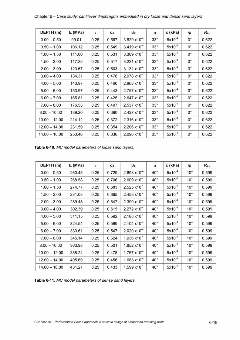
Chapter 6 – Case study: cantilever diaphragms embedded in dry loose and dense sand layers
Ciro Visone – Performance-Based approach in seismic design of embedded retaining walls 6-18
DEPTH (m) E (MPa) ν αR βR φ c (kPa) ψ Rint
0.00 – 0.50 99.01 0.25 0.567 3.529 x10⁻⁴ 33° 5x10⁻⁴ 0° 0.622
0.50 – 1.00 106.12 0.25 0.549 3.419 x10⁻⁴ 33° 5x10⁻⁴ 0° 0.622
1.00 – 1.50 111.00 0.25 0.531 3.309 x10⁻⁴ 33° 5x10⁻⁴ 0° 0.622
1.50 – 2.00 117.25 0.25 0.517 3.221 x10⁻⁴ 33° 5x10⁻⁴ 0° 0.622
2.00 – 3.00 123.67 0.25 0.503 3.132 x10⁻⁴ 33° 5x10⁻⁴ 0° 0.622
3.00 – 4.00 134.31 0.25 0.478 2.978 x10⁻⁴ 33° 5x10⁻⁴ 0° 0.622
4.00 – 5.00 143.97 0.25 0.460 2.868 x10⁻⁴ 33° 5x10⁻⁴ 0° 0.622
5.00 – 6.00 153.97 0.25 0.443 2.757 x10⁻⁴ 33° 5x10⁻⁴ 0° 0.622
6.00 – 7.00 165.81 0.25 0.425 2.647 x10⁻⁴ 33° 5x10⁻⁴ 0° 0.622
7.00 – 8.00 176.53 0.25 0.407 2.537 x10⁻⁴ 33° 5x10⁻⁴ 0° 0.622
8.00 – 10.00 189.20 0.25 0.390 2.427 x10⁻⁴ 33° 5x10⁻⁴ 0° 0.622
10.00 – 12.00 214.12 0.25 0.372 2.316 x10⁻⁴ 33° 5x10⁻⁴ 0° 0.622
12.00 – 14.00 231.59 0.25 0.354 2.206 x10⁻⁴ 33° 5x10⁻⁴ 0° 0.622
14.00 – 16.00 253.46 0.25 0.336 2.096 x10⁻⁴ 33° 5x10⁻⁴ 0° 0.622
Table 6-10. MC model parameters of loose sand layers.
DEPTH (m) E (MPa) ν αR βR φ c (kPa) ψ Rint
0.00 – 0.50 260.45 0.25 0.729 2.693 x10⁻⁴ 40° 5x10⁻⁴ 10° 0.599
0.50 – 1.00 268.58 0.25 0.706 2.609 x10⁻⁴ 40° 5x10⁻⁴ 10° 0.599
1.00 – 1.50 274.77 0.25 0.683 2.525 x10⁻⁴ 40° 5x10⁻⁴ 10° 0.599
1.50 – 2.00 281.03 0.25 0.665 2.458 x10⁻⁴ 40° 5x10⁻⁴ 10° 0.599
2.00 – 3.00 289.48 0.25 0.647 2.390 x10⁻⁴ 40° 5x10⁻⁴ 10° 0.599
3.00 – 4.00 302.39 0.25 0.615 2.272 x10⁻⁴ 40° 5x10⁻⁴ 10° 0.599
4.00 – 5.00 311.15 0.25 0.592 2.188 x10⁻⁴ 40° 5x10⁻⁴ 10° 0.599
5.00 – 6.00 324.54 0.25 0.569 2.104 x10⁻⁴ 40° 5x10⁻⁴ 10° 0.599
6.00 – 7.00 333.61 0.25 0.547 2.020 x10⁻⁴ 40° 5x10⁻⁴ 10° 0.599
7.00 – 8.00 345.14 0.25 0.524 1.936 x10⁻⁴ 40° 5x10⁻⁴ 10° 0.599
8.00 – 10.00 363.98 0.25 0.501 1.852 x10⁻⁴ 40° 5x10⁻⁴ 10° 0.599
10.00 – 12.00 388.24 0.25 0.478 1.767 x10⁻⁴ 40° 5x10⁻⁴ 10° 0.599
12.00 – 14.00 405.69 0.25 0.456 1.683 x10⁻⁴ 40° 5x10⁻⁴ 10° 0.599
14.00 – 16.00 431.27 0.25 0.433 1.599 x10⁻⁴ 40° 5x10⁻⁴ 10° 0.599
Table 6-11. MC model parameters of dense sand layers.
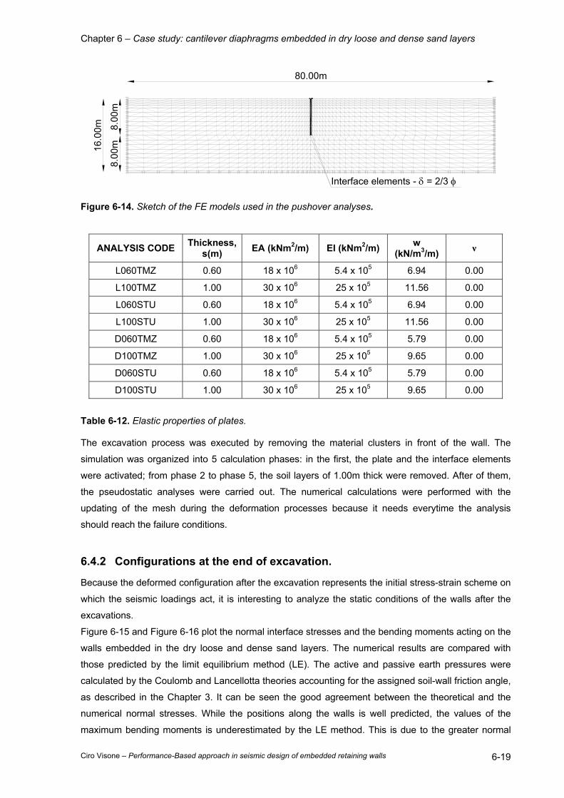
Chapter 6 – Case study: cantilever diaphragms embedded in dry loose and dense sand layers
Ciro Visone – Performance-Based approach in seismic design of embedded retaining walls 6-19
80.00m
16.0
0m 8.00
m8.
00m
Interface elements - δ = 2/3 φ
Figure 6-14. Sketch of the FE models used in the pushover analyses.
ANALYSIS CODE Thickness, s(m) EA (kNm2/m) EI (kNm2/m) w
(kN/m3/m) ν
L060TMZ 0.60 18 x 106 5.4 x 10⁵ 6.94 0.00
L100TMZ 1.00 30 x 106 25 x 105 11.56 0.00
L060STU 0.60 18 x 106 5.4 x 10⁵ 6.94 0.00
L100STU 1.00 30 x 106 25 x 105 11.56 0.00
D060TMZ 0.60 18 x 106 5.4 x 10⁵ 5.79 0.00
D100TMZ 1.00 30 x 106 25 x 105 9.65 0.00
D060STU 0.60 18 x 106 5.4 x 10⁵ 5.79 0.00
D100STU 1.00 30 x 106 25 x 105 9.65 0.00
Table 6-12. Elastic properties of plates.
The excavation process was executed by removing the material clusters in front of the wall. The
simulation was organized into 5 calculation phases: in the first, the plate and the interface elements
were activated; from phase 2 to phase 5, the soil layers of 1.00m thick were removed. After of them,
the pseudostatic analyses were carried out. The numerical calculations were performed with the
updating of the mesh during the deformation processes because it needs everytime the analysis
should reach the failure conditions.
6.4.2 Configurations at the end of excavation.
Because the deformed configuration after the excavation represents the initial stress-strain scheme on
which the seismic loadings act, it is interesting to analyze the static conditions of the walls after the
excavations.
Figure 6-15 and Figure 6-16 plot the normal interface stresses and the bending moments acting on the
walls embedded in the dry loose and dense sand layers. The numerical results are compared with
those predicted by the limit equilibrium method (LE). The active and passive earth pressures were
calculated by the Coulomb and Lancellotta theories accounting for the assigned soil-wall friction angle,
as described in the Chapter 3. It can be seen the good agreement between the theoretical and the
numerical normal stresses. While the positions along the walls is well predicted, the values of the
maximum bending moments is underestimated by the LE method. This is due to the greater normal
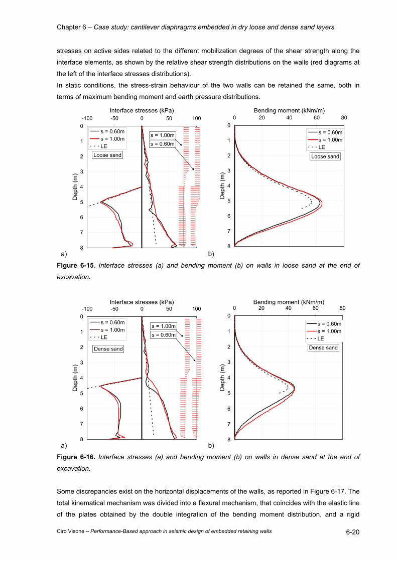
Chapter 6 – Case study: cantilever diaphragms embedded in dry loose and dense sand layers
Ciro Visone – Performance-Based approach in seismic design of embedded retaining walls 6-20
stresses on active sides related to the different mobilization degrees of the shear strength along the
interface elements, as shown by the relative shear strength distributions on the walls (red diagrams at
the left of the interface stresses distributions).
In static conditions, the stress-strain behaviour of the two walls can be retained the same, both in
terms of maximum bending moment and earth pressure distributions.
a)
0
1
2
3
4
5
6
7
8
-100 -50 0 50 100Interface stresses (kPa)
Dep
th (m
)
s = 0.60ms = 1.00mLE
Loose sand
s = 1.00ms = 0.60m
b)
0
1
2
3
4
5
6
7
8
0 20 40 60 80Bending moment (kNm/m)
Dep
th (m
)
s = 0.60ms = 1.00mLE
Loose sand
Figure 6-15. Interface stresses (a) and bending moment (b) on walls in loose sand at the end of
excavation.
a)
0
1
2
3
4
5
6
7
8
-100 -50 0 50 100Interface stresses (kPa)
Dep
th (m
)
s = 0.60ms = 1.00mLE
s = 1.00m
Dense sand
s = 0.60m
b)
0
1
2
3
4
5
6
7
8
0 20 40 60 80Bending moment (kNm/m)
Dep
th (m
)
s = 0.60ms = 1.00mLE
Dense sand
Figure 6-16. Interface stresses (a) and bending moment (b) on walls in dense sand at the end of
excavation.
Some discrepancies exist on the horizontal displacements of the walls, as reported in Figure 6-17. The
total kinematical mechanism was divided into a flexural mechanism, that coincides with the elastic line
of the plates obtained by the double integration of the bending moment distribution, and a rigid
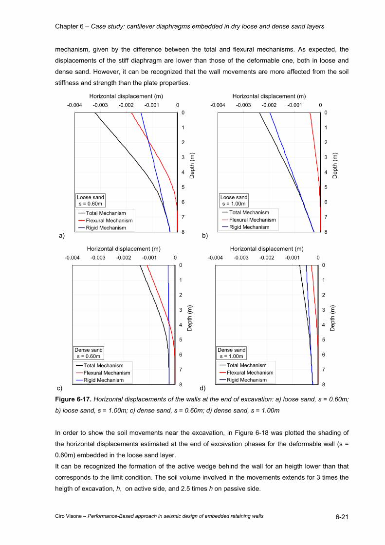
Chapter 6 – Case study: cantilever diaphragms embedded in dry loose and dense sand layers
Ciro Visone – Performance-Based approach in seismic design of embedded retaining walls 6-21
mechanism, given by the difference between the total and flexural mechanisms. As expected, the
displacements of the stiff diaphragm are lower than those of the deformable one, both in loose and
dense sand. However, it can be recognized that the wall movements are more affected from the soil
stiffness and strength than the plate properties.
a)
0
1
2
3
4
5
6
7
8
-0.004 -0.003 -0.002 -0.001 0Horizontal displacement (m)
Dep
th (m
)
Total MechanismFlexural MechanismRigid Mechanism
Loose sands = 0.60m
b)
0
1
2
3
4
5
6
7
8
-0.004 -0.003 -0.002 -0.001 0Horizontal displacement (m)
Dep
th (m
)
Total MechanismFlexural MechanismRigid Mechanism
Loose sands = 1.00m
c)
0
1
2
3
4
5
6
7
8
-0.004 -0.003 -0.002 -0.001 0Horizontal displacement (m)
Dep
th (m
)
Total MechanismFlexural MechanismRigid Mechanism
Dense sands = 0.60m
d)
0
1
2
3
4
5
6
7
8
-0.004 -0.003 -0.002 -0.001 0Horizontal displacement (m)
Dep
th (m
)
Total MechanismFlexural MechanismRigid Mechanism
Dense sands = 1.00m
Figure 6-17. Horizontal displacements of the walls at the end of excavation: a) loose sand, s = 0.60m;
b) loose sand, s = 1.00m; c) dense sand, s = 0.60m; d) dense sand, s = 1.00m
In order to show the soil movements near the excavation, in Figure 6-18 was plotted the shading of
the horizontal displacements estimated at the end of excavation phases for the deformable wall (s =
0.60m) embedded in the loose sand layer.
It can be recognized the formation of the active wedge behind the wall for an heigth lower than that
corresponds to the limit condition. The soil volume involved in the movements extends for 3 times the
heigth of excavation, h, on active side, and 2.5 times h on passive side.
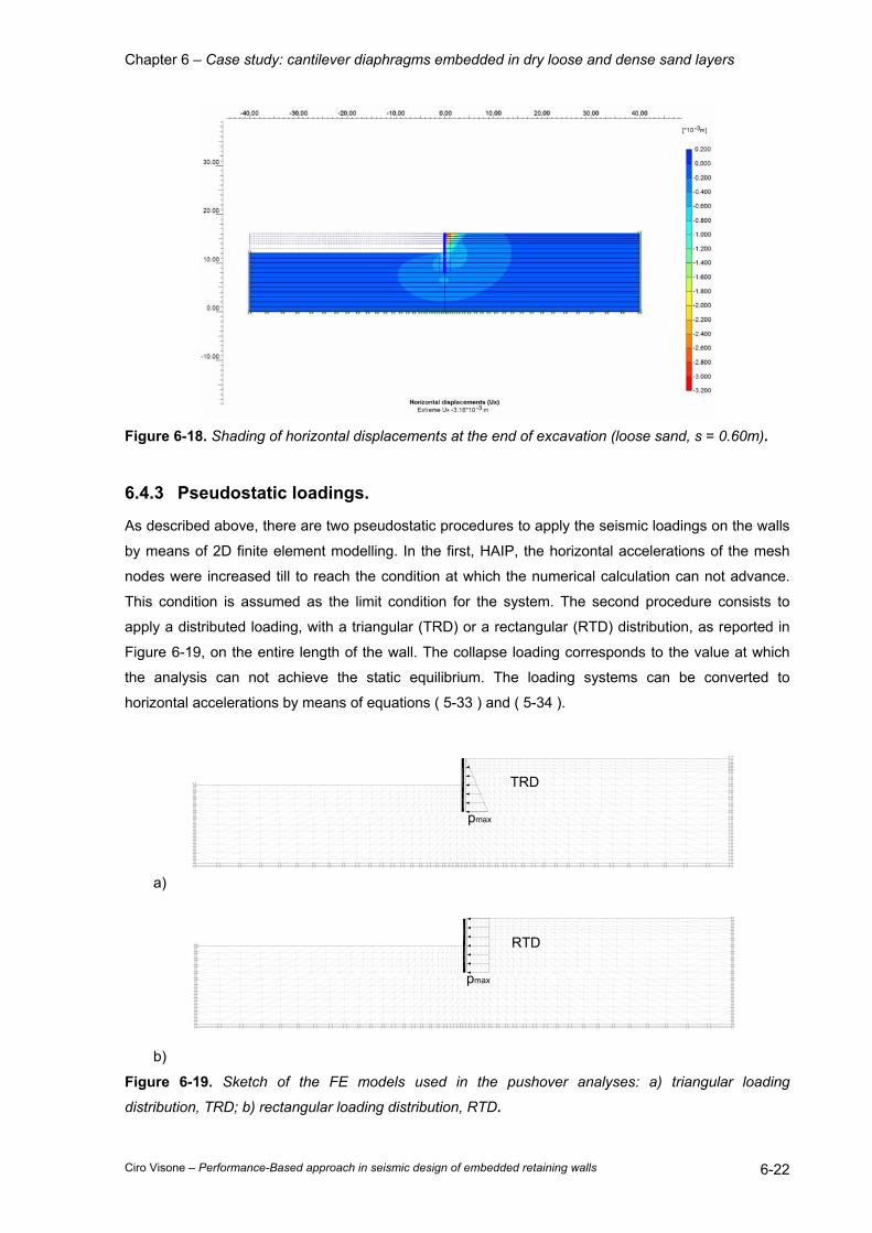
Chapter 6 – Case study: cantilever diaphragms embedded in dry loose and dense sand layers
Ciro Visone – Performance-Based approach in seismic design of embedded retaining walls 6-22
Figure 6-18. Shading of horizontal displacements at the end of excavation (loose sand, s = 0.60m).
6.4.3 Pseudostatic loadings.
As described above, there are two pseudostatic procedures to apply the seismic loadings on the walls
by means of 2D finite element modelling. In the first, HAIP, the horizontal accelerations of the mesh
nodes were increased till to reach the condition at which the numerical calculation can not advance.
This condition is assumed as the limit condition for the system. The second procedure consists to
apply a distributed loading, with a triangular (TRD) or a rectangular (RTD) distribution, as reported in
Figure 6-19, on the entire length of the wall. The collapse loading corresponds to the value at which
the analysis can not achieve the static equilibrium. The loading systems can be converted to
horizontal accelerations by means of equations ( 5-33 ) and ( 5-34 ).
a)
TRD
pmax
b)
RTD
pmax
Figure 6-19. Sketch of the FE models used in the pushover analyses: a) triangular loading
distribution, TRD; b) rectangular loading distribution, RTD.
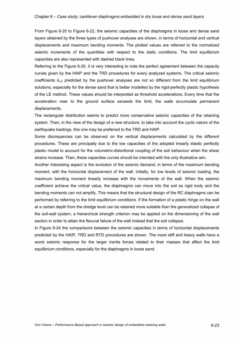
Chapter 6 – Case study: cantilever diaphragms embedded in dry loose and dense sand layers
Ciro Visone – Performance-Based approach in seismic design of embedded retaining walls 6-23
From Figure 6-20 to Figure 6-22, the seismic capacities of the diaphragms in loose and dense sand
layers obtained by the three types of pushover analyses are shown, in terms of horizontal and vertical
displacements and maximum bending moments. The plotted values are referred to the normalized
seismic increments of the quantities with respect to the static conditions. The limit equilibrium
capacities are also represented with dashed black lines.
Referring to the Figure 6-20, it is very interesting to note the perfect agreement between the capacity
curves given by the HAIP and the TRD procedures for every analyzed systems. The critical seismic
coefficients kcrit predicted by the pushover analyses are not so different from the limit equilibrium
solutions, especially for the dense sand that is better modelled by the rigid-perfectly plastic hypothesis
of the LE method. These values should be interpreted as threshold accelerations. Every time that the
acceleration near to the ground surface exceeds the limit, the walls accumulate permanent
displacements.
The rectangular distribution seems to predict more conservative seismic capacities of the retaining
system. Then, in the view of the design of a new structure, to take into account the cyclic nature of the
earthquake loadings, this one may be preferred to the TRD and HAIP.
Some discrepancies can be observed on the vertical displacements calculated by the different
procedures. These are principally due to the low capacities of the adopted linearly elastic perfectly
plastic model to account for the volumetric-distortional coupling of the soil behaviour when the shear
strains increase. Then, these capacities curves should be intended with the only illustrative aim.
Another interesting aspect is the evolution of the seismic demand, in terms of the maximum bending
moment, with the horizontal displacement of the wall. Initially, for low levels of seismic loading, the
maximum bending moment linearly increase with the movements of the wall. When the seismic
coefficient achieve the critical value, the diaphragms can move into the soil as rigid body and the
bending moments can not amplify. This means that the structural design of the RC diaphragms can be
performed by referring to the limit equilibrium conditions. If the formation of a plastic hinge on the wall
at a certain depth from the dredge level can be retained more suitable than the generalized collapse of
the soil-wall system, a hierarchical strength criterion may be applied on the dimensioning of the wall
section in order to attain the flexural failure of the wall instead that the soil collapse.
In Figure 6-24 the comparisons between the seismic capacities in terms of horizontal displacements
predicted by the HAIP, TRD and RTD procedures are shown. The more stiff and heavy walls have a
worst seismic response for the larger inertia forces related to their masses that affect the limit
equilibrium conditions, especially for the diaphragms in loose sand.
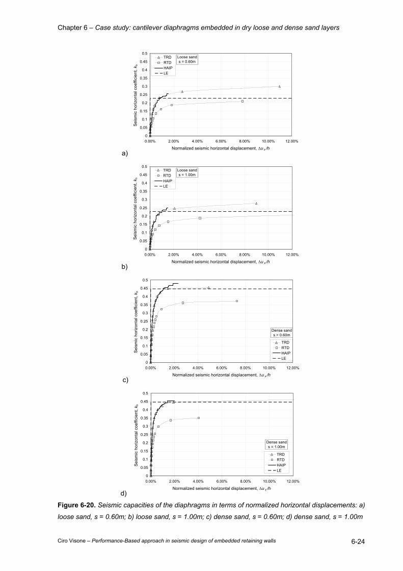
Chapter 6 – Case study: cantilever diaphragms embedded in dry loose and dense sand layers
Ciro Visone – Performance-Based approach in seismic design of embedded retaining walls 6-24
a)
0
0.05
0.1
0.15
0.2
0.25
0.3
0.35
0.4
0.45
0.5
0.00% 2.00% 4.00% 6.00% 8.00% 10.00% 12.00%
Normalized seismic horizontal displacement, ∆u x /h
Seis
mic
hor
izon
tal c
oeffi
cien
t, k h
TRDRTDHAIPLE
Loose sands = 0.60m
b)
0
0.05
0.1
0.15
0.2
0.25
0.3
0.35
0.4
0.45
0.5
0.00% 2.00% 4.00% 6.00% 8.00% 10.00% 12.00%
Normalized seismic horizontal displacement, ∆u x /h
Seis
mic
hor
izon
tal c
oeffi
cien
t, k h
TRDRTDHAIPLE
Loose sands = 1.00m
c)
0
0.05
0.1
0.15
0.2
0.25
0.3
0.35
0.4
0.45
0.5
0.00% 2.00% 4.00% 6.00% 8.00% 10.00% 12.00%
Normalized seismic horizontal displacement, ∆u x /h
Seis
mic
hor
izon
tal c
oeffi
cien
t, k h
TRDRTDHAIPLE
Dense sands = 0.60m
d)
0
0.05
0.1
0.15
0.2
0.25
0.3
0.35
0.4
0.45
0.5
0.00% 2.00% 4.00% 6.00% 8.00% 10.00% 12.00%
Normalized seismic horizontal displacement, ∆u x /h
Seis
mic
hor
izon
tal c
oeffi
cien
t, k h
TRDRTDHAIPLE
Dense sands = 1.00m
Figure 6-20. Seismic capacities of the diaphragms in terms of normalized horizontal displacements: a)
loose sand, s = 0.60m; b) loose sand, s = 1.00m; c) dense sand, s = 0.60m; d) dense sand, s = 1.00m

Chapter 6 – Case study: cantilever diaphragms embedded in dry loose and dense sand layers
Ciro Visone – Performance-Based approach in seismic design of embedded retaining walls 6-25
a)
0
0.05
0.1
0.15
0.2
0.25
0.3
0.35
0.4
0.45
0.5
0.00% 2.00% 4.00% 6.00% 8.00% 10.00% 12.00%
Normalized seismic vertical displacement, ∆u y /h
Sei
smic
hor
izon
tal c
oeffi
cien
t, k h
TRDRTDHAIPLE
Loose sands = 0.60m
b)
0
0.05
0.1
0.15
0.2
0.25
0.3
0.35
0.4
0.45
0.5
0.00% 2.00% 4.00% 6.00% 8.00% 10.00% 12.00%
Normalized seismic vertical displacement, ∆u y /h
Sei
smic
hor
izon
tal c
oeffi
cien
t, k h
TRDRTDHAIPLE
Loose sands = 1.00m
c)
0
0.05
0.1
0.15
0.2
0.25
0.3
0.35
0.4
0.45
0.5
0.00% 2.00% 4.00% 6.00% 8.00% 10.00% 12.00%
Normalized seismic vertical displacement, ∆u y /h
Sei
smic
hor
izon
tal c
oeffi
cien
t, k h
TRDRTDHAIPLE
Dense sands = 0.60m
d)
0
0.05
0.1
0.15
0.2
0.25
0.3
0.35
0.4
0.45
0.5
0.00% 2.00% 4.00% 6.00% 8.00% 10.00% 12.00%
Normalized seismic vertical displacement, ∆u y /h
Seis
mic
hor
izon
tal c
oeffi
cien
t, k h
TRDRTDHAIPLE
Dense sands = 1.00m
Figure 6-21. Seismic capacities of the diaphragms in terms of normalized vertical displacements: a)
loose sand, s = 0.60m; b) loose sand, s = 1.00m; c) dense sand, s = 0.60m; d) dense sand, s = 1.00m
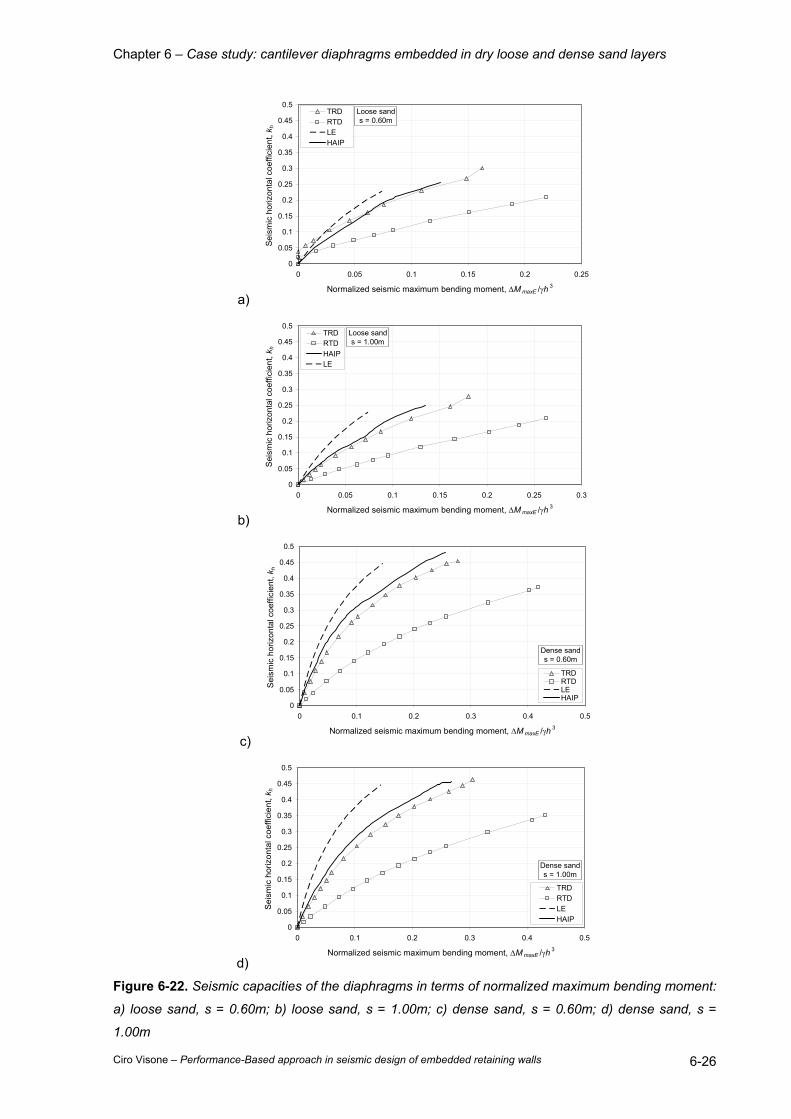
Chapter 6 – Case study: cantilever diaphragms embedded in dry loose and dense sand layers
Ciro Visone – Performance-Based approach in seismic design of embedded retaining walls 6-26
a)
0
0.05
0.1
0.15
0.2
0.25
0.3
0.35
0.4
0.45
0.5
0 0.05 0.1 0.15 0.2 0.25
Normalized seismic maximum bending moment, ∆M maxE /γh 3
Sei
smic
hor
izon
tal c
oeffi
cien
t, k h
TRDRTDLEHAIP
Loose sands = 0.60m
b)
0
0.05
0.1
0.15
0.2
0.25
0.3
0.35
0.4
0.45
0.5
0 0.05 0.1 0.15 0.2 0.25 0.3
Normalized seismic maximum bending moment, ∆M maxE /γh 3
Sei
smic
hor
izon
tal c
oeffi
cien
t, k h
TRDRTDHAIPLE
Loose sands = 1.00m
c)
0
0.05
0.1
0.15
0.2
0.25
0.3
0.35
0.4
0.45
0.5
0 0.1 0.2 0.3 0.4 0.5
Normalized seismic maximum bending moment, ∆M maxE /γh 3
Sei
smic
hor
izon
tal c
oeffi
cien
t, k h
TRDRTDLEHAIP
Dense sands = 0.60m
d)
0
0.05
0.1
0.15
0.2
0.25
0.3
0.35
0.4
0.45
0.5
0 0.1 0.2 0.3 0.4 0.5
Normalized seismic maximum bending moment, ∆M maxE /γh 3
Seis
mic
hor
izon
tal c
oeffi
cien
t, k h
TRDRTDLEHAIP
Dense sands = 1.00m
Figure 6-22. Seismic capacities of the diaphragms in terms of normalized maximum bending moment:
a) loose sand, s = 0.60m; b) loose sand, s = 1.00m; c) dense sand, s = 0.60m; d) dense sand, s =
1.00m
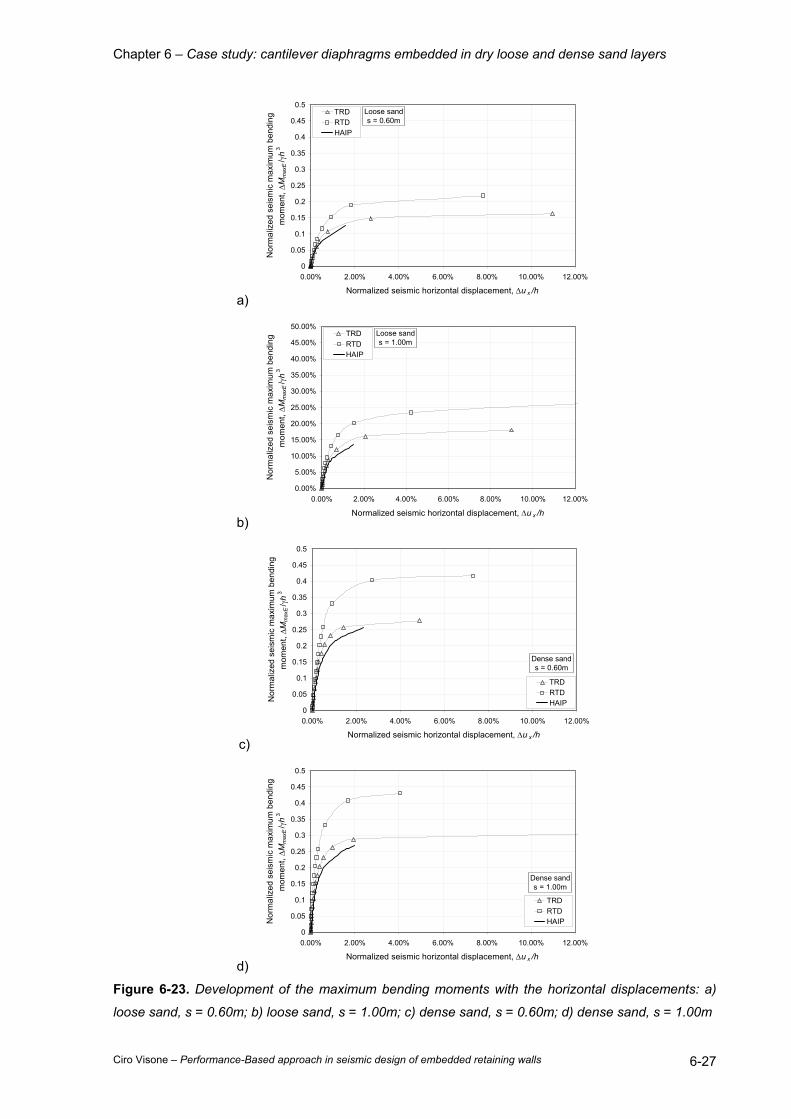
Chapter 6 – Case study: cantilever diaphragms embedded in dry loose and dense sand layers
Ciro Visone – Performance-Based approach in seismic design of embedded retaining walls 6-27
a)
0
0.05
0.1
0.15
0.2
0.25
0.3
0.35
0.4
0.45
0.5
0.00% 2.00% 4.00% 6.00% 8.00% 10.00% 12.00%
Normalized seismic horizontal displacement, ∆u x /h
Nor
mal
ized
sei
smic
max
imum
ben
ding
m
omen
t, ∆M
max
E/ γ
h3
TRDRTDHAIP
Loose sands = 0.60m
b)
0.00%
5.00%
10.00%
15.00%
20.00%
25.00%
30.00%
35.00%
40.00%
45.00%
50.00%
0.00% 2.00% 4.00% 6.00% 8.00% 10.00% 12.00%
Normalized seismic horizontal displacement, ∆u x /h
Nor
mal
ized
sei
smic
max
imum
ben
ding
m
omen
t, ∆
Mm
axE
/ γh
3
TRDRTDHAIP
Loose sands = 1.00m
c)
0
0.05
0.1
0.15
0.2
0.25
0.3
0.35
0.4
0.45
0.5
0.00% 2.00% 4.00% 6.00% 8.00% 10.00% 12.00%
Normalized seismic horizontal displacement, ∆u x /h
Nor
mal
ized
sei
smic
max
imum
ben
ding
m
omen
t, ∆M
max
E/ γ
h3
TRDRTDHAIP
Dense sands = 0.60m
d)
0
0.05
0.1
0.15
0.2
0.25
0.3
0.35
0.4
0.45
0.5
0.00% 2.00% 4.00% 6.00% 8.00% 10.00% 12.00%
Normalized seismic horizontal displacement, ∆u x /h
Nor
mal
ized
sei
smic
max
imum
ben
ding
m
omen
t, ∆M
max
E/ γ
h3
TRDRTDHAIP
Dense sands = 1.00m
Figure 6-23. Development of the maximum bending moments with the horizontal displacements: a)
loose sand, s = 0.60m; b) loose sand, s = 1.00m; c) dense sand, s = 0.60m; d) dense sand, s = 1.00m
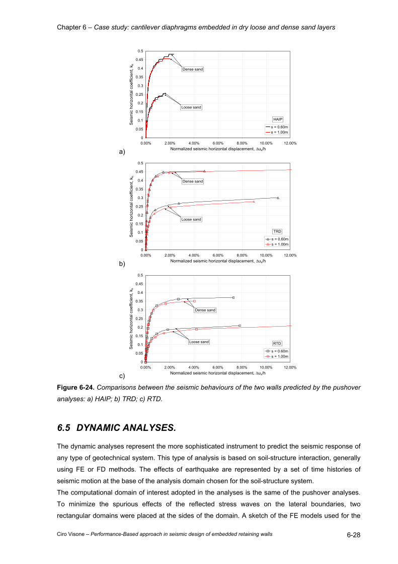
Chapter 6 – Case study: cantilever diaphragms embedded in dry loose and dense sand layers
Ciro Visone – Performance-Based approach in seismic design of embedded retaining walls 6-28
a)
0
0.05
0.1
0.15
0.2
0.25
0.3
0.35
0.4
0.45
0.5
0.00% 2.00% 4.00% 6.00% 8.00% 10.00% 12.00%Normalized seismic horizontal displacement, ∆ux/h
Sei
smic
hor
izon
tal c
oeffi
cien
t, k h
s = 0.60ms = 1.00m
Loose sand
Dense sand
HAIP
b)
0
0.05
0.1
0.15
0.2
0.25
0.3
0.35
0.4
0.45
0.5
0.00% 2.00% 4.00% 6.00% 8.00% 10.00% 12.00%Normalized seismic horizontal displacement, ∆ux/h
Sei
smic
hor
izon
tal c
oeffi
cien
t, k h
s = 0.60ms = 1.00m
Loose sand
Dense sand
TRD
c)
0
0.05
0.1
0.15
0.2
0.25
0.3
0.35
0.4
0.45
0.5
0.00% 2.00% 4.00% 6.00% 8.00% 10.00% 12.00%Normalized seismic horizontal displacement, ∆ux/h
Sei
smic
hor
izon
tal c
oeffi
cien
t, k h
s = 0.60ms = 1.00m
Loose sand
Dense sand
RTD
Figure 6-24. Comparisons between the seismic behaviours of the two walls predicted by the pushover
analyses: a) HAIP; b) TRD; c) RTD.
6.5 DYNAMIC ANALYSES.
The dynamic analyses represent the more sophisticated instrument to predict the seismic response of
any type of geotechnical system. This type of analysis is based on soil-structure interaction, generally
using FE or FD methods. The effects of earthquake are represented by a set of time histories of
seismic motion at the base of the analysis domain chosen for the soil-structure system.
The computational domain of interest adopted in the analyses is the same of the pushover analyses.
To minimize the spurious effects of the reflected stress waves on the lateral boundaries, two
rectangular domains were placed at the sides of the domain. A sketch of the FE models used for the
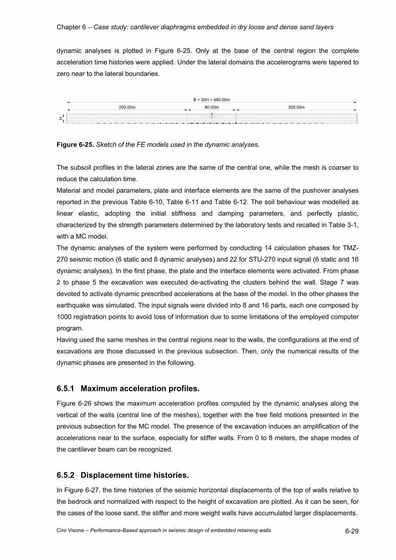
Chapter 6 – Case study: cantilever diaphragms embedded in dry loose and dense sand layers
Ciro Visone – Performance-Based approach in seismic design of embedded retaining walls 6-29
dynamic analyses is plotted in Figure 6-25. Only at the base of the central region the complete
acceleration time histories were applied. Under the lateral domains the accelerograms were tapered to
zero near to the lateral boundaries.
200.00m 200.00m
B = 30H = 480.00m
H
80.00m
Figure 6-25. Sketch of the FE models used in the dynamic analyses.
The subsoil profiles in the lateral zones are the same of the central one, while the mesh is coarser to
reduce the calculation time.
Material and model parameters, plate and interface elements are the same of the pushover analyses
reported in the previous Table 6-10, Table 6-11 and Table 6-12. The soil behaviour was modelled as
linear elastic, adopting the initial stiffness and damping parameters, and perfectly plastic,
characterized by the strength parameters determined by the laboratory tests and recalled in Table 3-1,
with a MC model.
The dynamic analyses of the system were performed by conducting 14 calculation phases for TMZ-
270 seismic motion (6 static and 8 dynamic analyses) and 22 for STU-270 input signal (6 static and 16
dynamic analyses). In the first phase, the plate and the interface elements were activated. From phase
2 to phase 5 the excavation was executed de-activating the clusters behind the wall. Stage 7 was
devoted to activate dynamic prescribed accelerations at the base of the model. In the other phases the
earthquake was simulated. The input signals were divided into 8 and 16 parts, each one composed by
1000 registration points to avoid loss of information due to some limitations of the employed computer
program.
Having used the same meshes in the central regions near to the walls, the configurations at the end of
excavations are those discussed in the previous subsection. Then, only the numerical results of the
dynamic phases are presented in the following.
6.5.1 Maximum acceleration profiles.
Figure 6-26 shows the maximum acceleration profiles computed by the dynamic analyses along the
vertical of the walls (central line of the meshes), together with the free field motions presented in the
previous subsection for the MC model. The presence of the excavation induces an amplification of the
accelerations near to the surface, especially for stiffer walls. From 0 to 8 meters, the shape modes of
the cantilever beam can be recognized.
6.5.2 Displacement time histories.
In Figure 6-27, the time histories of the seismic horizontal displacements of the top of walls relative to
the bedrock and normalized with respect to the height of excavation are plotted. As it can be seen, for
the cases of the loose sand, the stiffer and more weight walls have accumulated larger displacements.
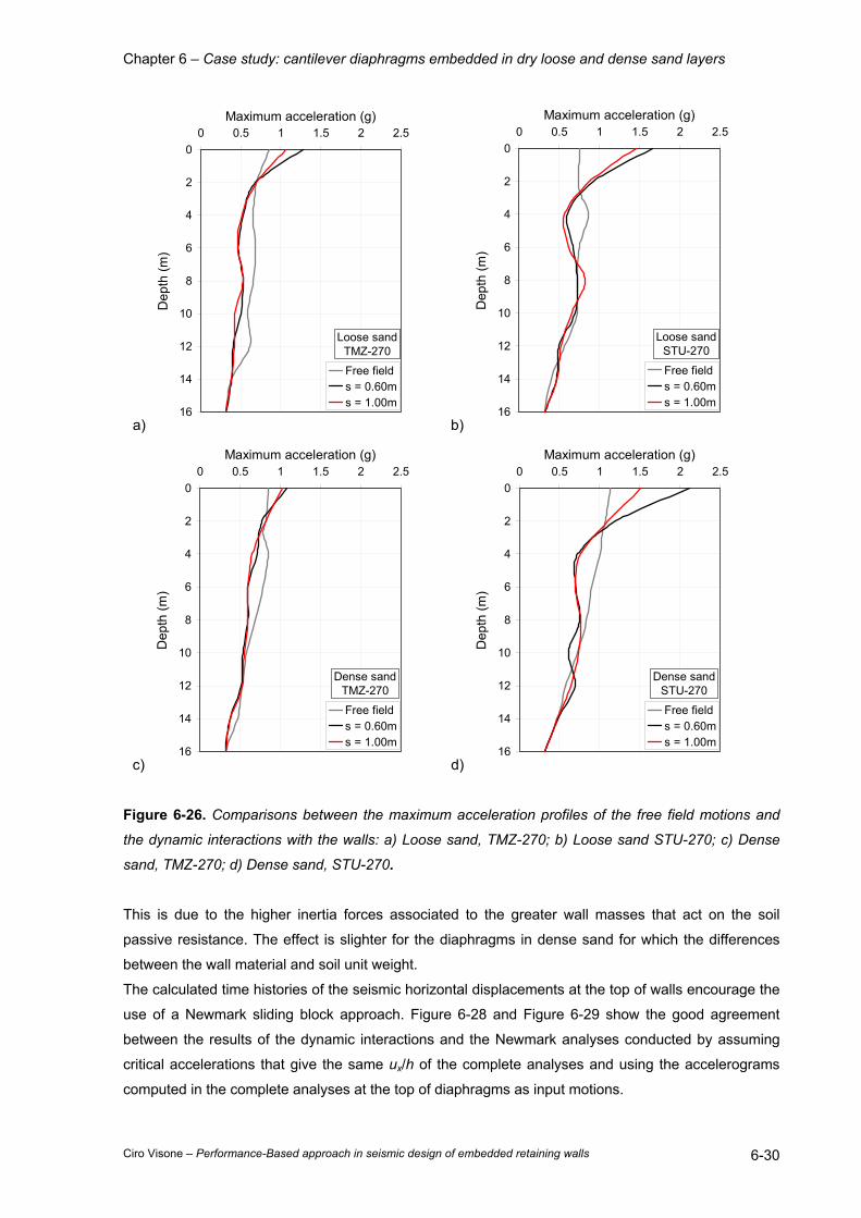
Chapter 6 – Case study: cantilever diaphragms embedded in dry loose and dense sand layers
Ciro Visone – Performance-Based approach in seismic design of embedded retaining walls 6-30
a)
0
2
4
6
8
10
12
14
16
0 0.5 1 1.5 2 2.5Maximum acceleration (g)
Dep
th (m
)
Free fields = 0.60ms = 1.00m
Loose sandTMZ-270
b)
0
2
4
6
8
10
12
14
16
0 0.5 1 1.5 2 2.5Maximum acceleration (g)
Dep
th (m
)
Free fields = 0.60ms = 1.00m
Loose sandSTU-270
c)
0
2
4
6
8
10
12
14
16
0 0.5 1 1.5 2 2.5Maximum acceleration (g)
Dep
th (m
)
Free fields = 0.60ms = 1.00m
Dense sandTMZ-270
d)
0
2
4
6
8
10
12
14
16
0 0.5 1 1.5 2 2.5Maximum acceleration (g)
Dep
th (m
)
Free fields = 0.60ms = 1.00m
Dense sandSTU-270
Figure 6-26. Comparisons between the maximum acceleration profiles of the free field motions and
the dynamic interactions with the walls: a) Loose sand, TMZ-270; b) Loose sand STU-270; c) Dense
sand, TMZ-270; d) Dense sand, STU-270.
This is due to the higher inertia forces associated to the greater wall masses that act on the soil
passive resistance. The effect is slighter for the diaphragms in dense sand for which the differences
between the wall material and soil unit weight.
The calculated time histories of the seismic horizontal displacements at the top of walls encourage the
use of a Newmark sliding block approach. Figure 6-28 and Figure 6-29 show the good agreement
between the results of the dynamic interactions and the Newmark analyses conducted by assuming
critical accelerations that give the same ux/h of the complete analyses and using the accelerograms
computed in the complete analyses at the top of diaphragms as input motions.
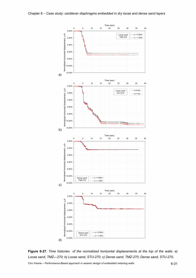
Chapter 6 – Case study: cantilever diaphragms embedded in dry loose and dense sand layers
Ciro Visone – Performance-Based approach in seismic design of embedded retaining walls 6-31
a)
0.00%
2.00%
4.00%
6.00%
8.00%
10.00%
12.00%
0 5 10 15 20 25 30 35 40Time (sec)
Nor
mal
ized
hor
izon
tal d
ispl
acem
ent,
u x/h s = 0.60m
s = 1.00mLoose sand
TMZ-270
b)
0.00%
2.00%
4.00%
6.00%
8.00%
10.00%
12.00%
0 5 10 15 20 25 30 35 40Time (sec)
Nor
mal
ized
hor
izon
tal d
ispl
acem
ent,
u x/h s=0.6m
s=1.0mLoose sand
STU-270
c)
0.00%
2.00%
4.00%
6.00%
8.00%
10.00%
12.00%
0 5 10 15 20 25 30 35 40Time (sec)
Nor
mal
ized
hor
izon
tal d
ispl
acem
ent,
u x/h
s = 0.60ms = 1.00m
Dense sandTMZ-270
d)
0.00%
2.00%
4.00%
6.00%
8.00%
10.00%
12.00%
0 5 10 15 20 25 30 35 40Time (sec)
Nor
mal
ized
hor
izon
tal d
ispl
acem
ent,
u x/h
s = 0.60m
s = 1.00mDense sand
STU-270
Figure 6-27. Time histories of the normalized horizontal displacements at the top of the walls: a)
Loose sand, TMZ—270; b) Loose sand, STU-270; c) Dense sand, TMZ-270; Dense sand, STU-270.
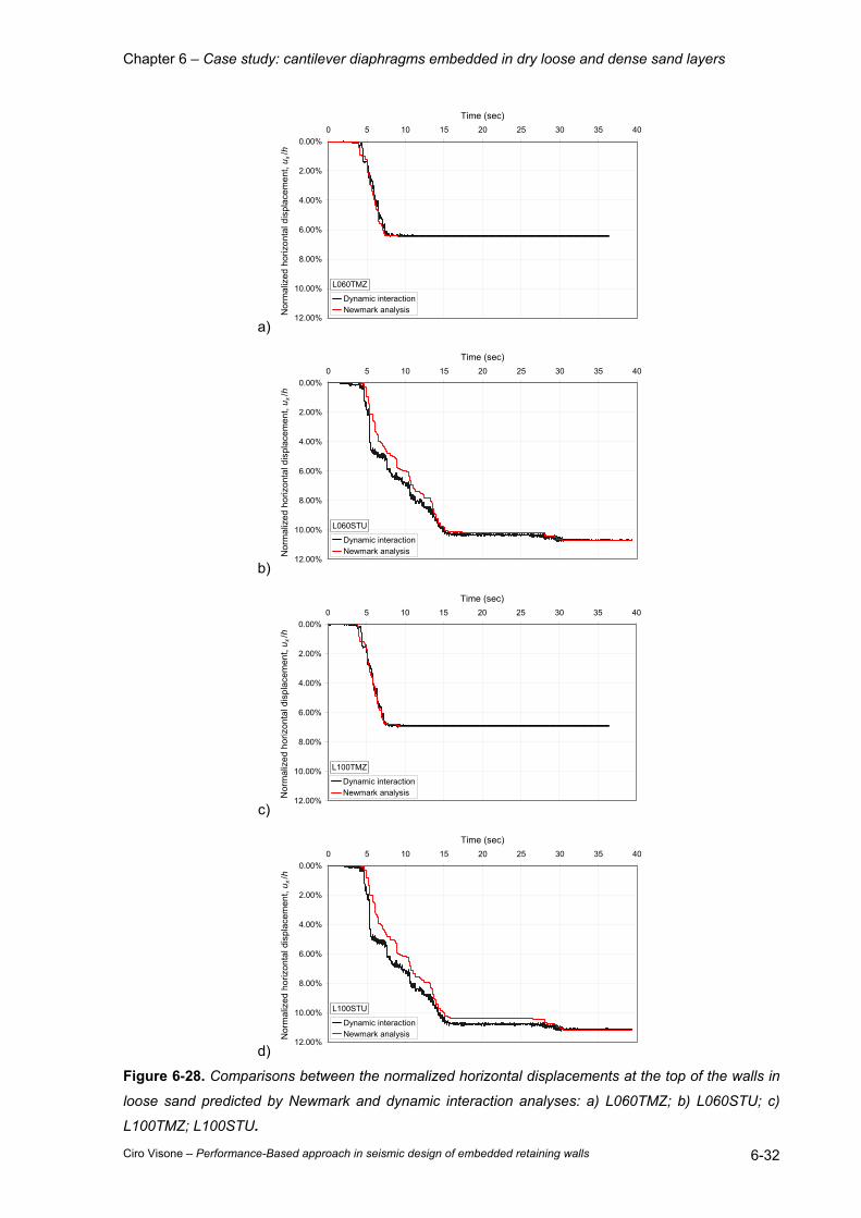
Chapter 6 – Case study: cantilever diaphragms embedded in dry loose and dense sand layers
Ciro Visone – Performance-Based approach in seismic design of embedded retaining walls 6-32
a)
0.00%
2.00%
4.00%
6.00%
8.00%
10.00%
12.00%
0 5 10 15 20 25 30 35 40
Time (sec)
Nor
mal
ized
hor
izon
tal d
ispl
acem
ent,
u x/h
Dynamic interactionNewmark analysis
L060TMZ
b)
0.00%
2.00%
4.00%
6.00%
8.00%
10.00%
12.00%
0 5 10 15 20 25 30 35 40
Time (sec)
Nor
mal
ized
hor
izon
tal d
ispl
acem
ent,
u x/h
Dynamic interactionNewmark analysis
L060STU
c)
0.00%
2.00%
4.00%
6.00%
8.00%
10.00%
12.00%
0 5 10 15 20 25 30 35 40
Time (sec)
Nor
mal
ized
hor
izon
tal d
ispl
acem
ent,
u x/h
Dynamic interactionNewmark analysis
L100TMZ
d)
0.00%
2.00%
4.00%
6.00%
8.00%
10.00%
12.00%
0 5 10 15 20 25 30 35 40
Time (sec)
Nor
mal
ized
hor
izon
tal d
ispl
acem
ent,
u x/h
Dynamic interactionNewmark analysis
L100STU
Figure 6-28. Comparisons between the normalized horizontal displacements at the top of the walls in
loose sand predicted by Newmark and dynamic interaction analyses: a) L060TMZ; b) L060STU; c)
L100TMZ; L100STU.
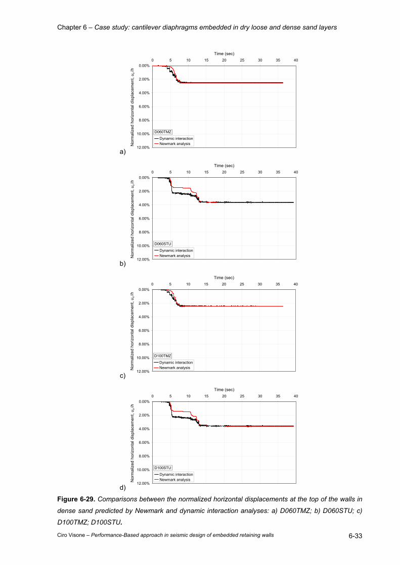
Chapter 6 – Case study: cantilever diaphragms embedded in dry loose and dense sand layers
Ciro Visone – Performance-Based approach in seismic design of embedded retaining walls 6-33
a)
0.00%
2.00%
4.00%
6.00%
8.00%
10.00%
12.00%
0 5 10 15 20 25 30 35 40
Time (sec)
Nor
mal
ized
hor
izon
tal d
ispl
acem
ent,
u x/h
Dynamic interactionNewmark analysis
D060TMZ
b)
0.00%
2.00%
4.00%
6.00%
8.00%
10.00%
12.00%
0 5 10 15 20 25 30 35 40
Time (sec)
Nor
mal
ized
hor
izon
tal d
ispl
acem
ent,
u x/h
Dynamic interactionNewmark analysis
D060STU
c)
0.00%
2.00%
4.00%
6.00%
8.00%
10.00%
12.00%
0 5 10 15 20 25 30 35 40
Time (sec)
Nor
mal
ized
hor
izon
tal d
ispl
acem
ent,
u x/h
Dynamic interactionNewmark analysis
D100TMZ
d)
0.00%
2.00%
4.00%
6.00%
8.00%
10.00%
12.00%
0 5 10 15 20 25 30 35 40
Time (sec)
Nor
mal
ized
hor
izon
tal d
ispl
acem
ent,
u x/h
Dynamic interactionNewmark analysis
D100STU
Figure 6-29. Comparisons between the normalized horizontal displacements at the top of the walls in
dense sand predicted by Newmark and dynamic interaction analyses: a) D060TMZ; b) D060STU; c)
D100TMZ; D100STU.
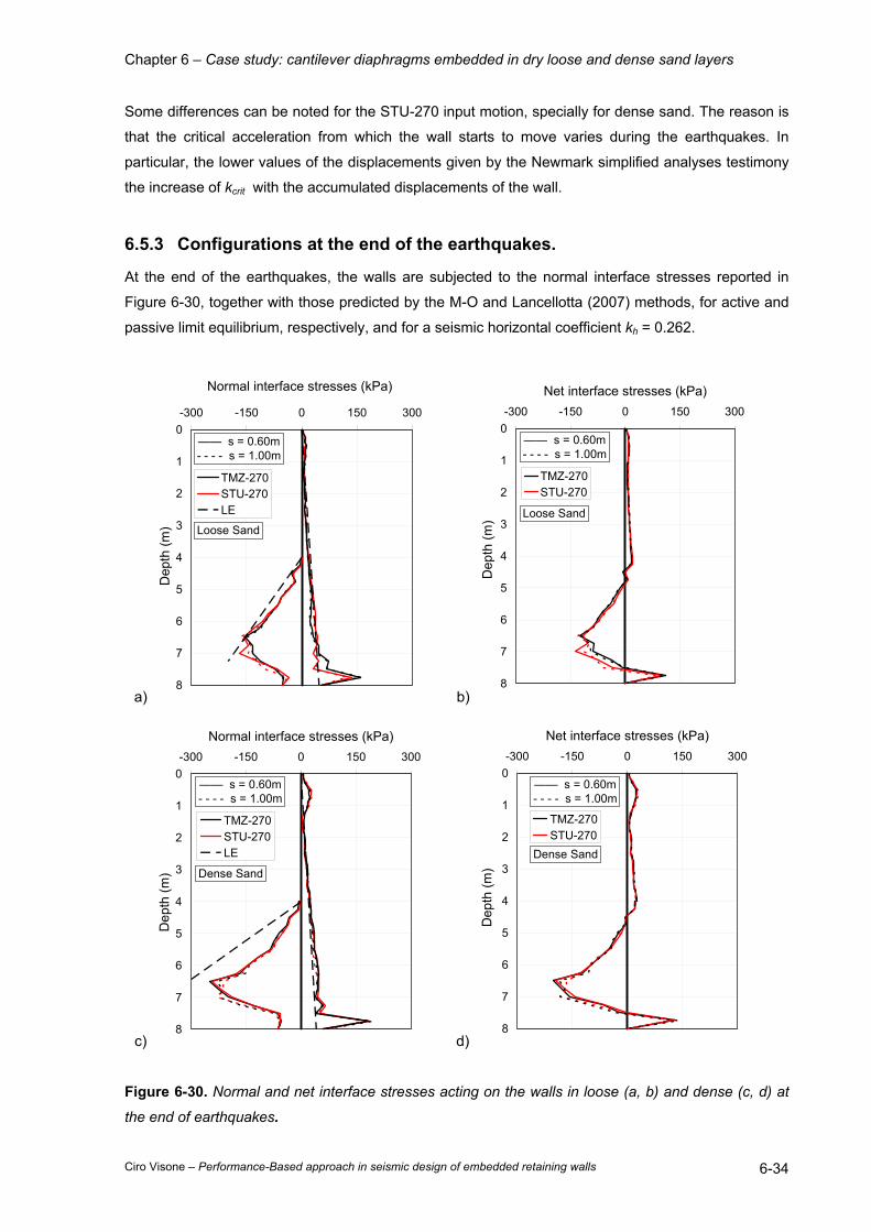
Chapter 6 – Case study: cantilever diaphragms embedded in dry loose and dense sand layers
Ciro Visone – Performance-Based approach in seismic design of embedded retaining walls 6-34
Some differences can be noted for the STU-270 input motion, specially for dense sand. The reason is
that the critical acceleration from which the wall starts to move varies during the earthquakes. In
particular, the lower values of the displacements given by the Newmark simplified analyses testimony
the increase of kcrit with the accumulated displacements of the wall.
6.5.3 Configurations at the end of the earthquakes.
At the end of the earthquakes, the walls are subjected to the normal interface stresses reported in
Figure 6-30, together with those predicted by the M-O and Lancellotta (2007) methods, for active and
passive limit equilibrium, respectively, and for a seismic horizontal coefficient kh = 0.262.
a)
0
1
2
3
4
5
6
7
8
-300 -150 0 150 300
Normal interface stresses (kPa)
Dep
th (m
)
TMZ-270STU-270LE
—— s = 0.60m- - - - s = 1.00m
Loose Sand
b)
0
1
2
3
4
5
6
7
8
-300 -150 0 150 300
Net interface stresses (kPa)
Dep
th (m
)TMZ-270STU-270
—— s = 0.60m- - - - s = 1.00m
Loose Sand
c)
0
1
2
3
4
5
6
7
8
-300 -150 0 150 300
Normal interface stresses (kPa)
Dep
th (m
)
TMZ-270STU-270LE
—— s = 0.60m- - - - s = 1.00m
Dense Sand
d)
0
1
2
3
4
5
6
7
8
-300 -150 0 150 300
Net interface stresses (kPa)
Dep
th (m
)
TMZ-270STU-270
—— s = 0.60m- - - - s = 1.00m
Dense Sand
Figure 6-30. Normal and net interface stresses acting on the walls in loose (a, b) and dense (c, d) at
the end of earthquakes.
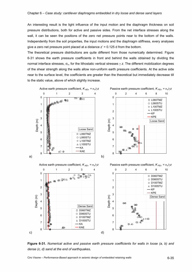
Chapter 6 – Case study: cantilever diaphragms embedded in dry loose and dense sand layers
Ciro Visone – Performance-Based approach in seismic design of embedded retaining walls 6-35
An interesting result is the light influence of the input motion and the diaphragm thickness on soil
pressure distributions, both for active and passive sides. From the net interface stresses along the
wall, it can be seen the positions of the zero net pressure points near to the bottom of the walls.
Independently from the soil properties, the input motions and the diaphragm stiffness, every analyses
give a zero net pressure point placed at a distance z’ = 0.125 d from the bottom.
The theoretical pressure distributions are quite different from those numerically determined. Figure
6-31 shows the earth pressure coefficients in front and behind the walls obtained by dividing the
normal interface stresses, σn, for the lithostatic vertical stresses γ z. The different mobilization degrees
of the shear strength along the walls allow non-uniform earth pressure coefficients. At the active side
near to the surface level, the coefficients are greater than the theoretical but immediately decrease till
to the static value, above of which slightly increase.
a)
0
1
2
3
4
5
6
7
8
0 1 2 3 4
Active earth pressure coefficient, K AEn = σn/γz
Dep
th (m
)
L060TMZL060STUL100TMZL100STUKAKAE
Loose Sand
b)
0
1
2
3
4
5
6
7
8
0 2 4 6 8 10
Passive earth pressure coefficient, K PEn = σn/γz
Dep
th (m
)
L060TMZL060STUL100TMZL100STUKPKPE
Loose Sand
c)
0
1
2
3
4
5
6
7
8
0 1 2 3 4
Active earth pressure coefficient, K AEn = σn/γz
Dep
th (m
)
D060TMZD060STUD100TMZD100STUKAKAE
Dense Sand
d)
0
1
2
3
4
5
6
7
8
0 2 4 6 8 10
Passive earth pressure coefficient, K PEn = σn/γz
Dep
th (m
)
D060TMZD060STUD100TMZD100STUKPKPEDense Sand
Figure 6-31. Numerical active and passive earth pressure coefficients for walls in loose (a, b) and
dense (c, d) sand at the end of earthquakes.
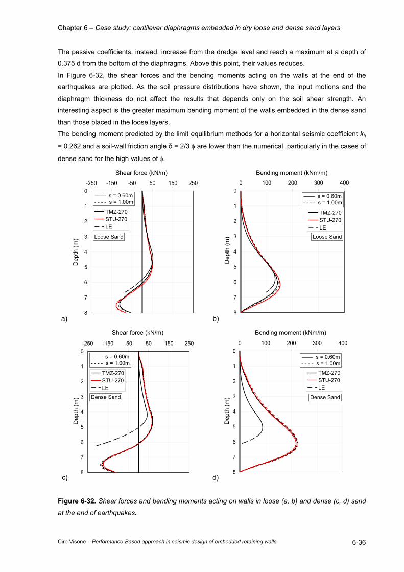
Chapter 6 – Case study: cantilever diaphragms embedded in dry loose and dense sand layers
Ciro Visone – Performance-Based approach in seismic design of embedded retaining walls 6-36
The passive coefficients, instead, increase from the dredge level and reach a maximum at a depth of
0.375 d from the bottom of the diaphragms. Above this point, their values reduces.
In Figure 6-32, the shear forces and the bending moments acting on the walls at the end of the
earthquakes are plotted. As the soil pressure distributions have shown, the input motions and the
diaphragm thickness do not affect the results that depends only on the soil shear strength. An
interesting aspect is the greater maximum bending moment of the walls embedded in the dense sand
than those placed in the loose layers.
The bending moment predicted by the limit equilibrium methods for a horizontal seismic coefficient kh
= 0.262 and a soil-wall friction angle δ = 2/3 φ are lower than the numerical, particularly in the cases of
dense sand for the high values of φ.
a)
0
1
2
3
4
5
6
7
8
-250 -150 -50 50 150 250
Shear force (kN/m)
Dep
th (m
)
TMZ-270STU-270LE
—— s = 0.60m- - - - s = 1.00m
Loose Sand
b)
0
1
2
3
4
5
6
7
8
0 100 200 300 400
Bending moment (kNm/m)
Dep
th (m
)
TMZ-270STU-270LE
—— s = 0.60m- - - - s = 1.00m
Loose Sand
c)
0
1
2
3
4
5
6
7
8
-250 -150 -50 50 150 250
Shear force (kN/m)
Dep
th (m
)
TMZ-270STU-270LE
—— s = 0.60m- - - - s = 1.00m
Dense Sand
d)
0
1
2
3
4
5
6
7
8
0 100 200 300 400
Bending moment (kNm/m)
Dep
th (m
)
TMZ-270STU-270LE
—— s = 0.60m- - - - s = 1.00m
Dense Sand
Figure 6-32. Shear forces and bending moments acting on walls in loose (a, b) and dense (c, d) sand
at the end of earthquakes.
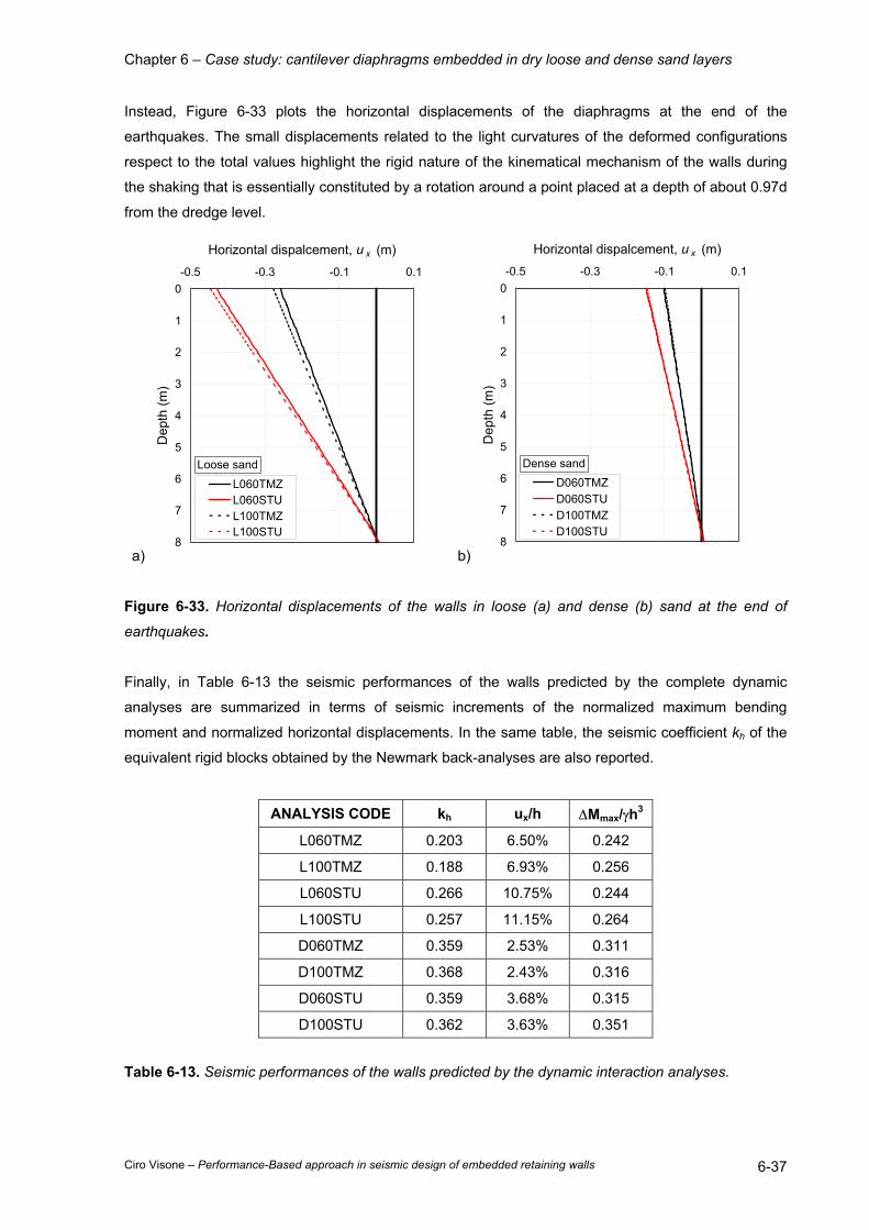
Chapter 6 – Case study: cantilever diaphragms embedded in dry loose and dense sand layers
Ciro Visone – Performance-Based approach in seismic design of embedded retaining walls 6-37
Instead, Figure 6-33 plots the horizontal displacements of the diaphragms at the end of the
earthquakes. The small displacements related to the light curvatures of the deformed configurations
respect to the total values highlight the rigid nature of the kinematical mechanism of the walls during
the shaking that is essentially constituted by a rotation around a point placed at a depth of about 0.97d
from the dredge level.
a)
0
1
2
3
4
5
6
7
8
-0.5 -0.3 -0.1 0.1
Horizontal dispalcement, u x (m)
Dep
th (m
)
L060TMZL060STUL100TMZL100STU
Loose sand
b)
0
1
2
3
4
5
6
7
8
-0.5 -0.3 -0.1 0.1
Horizontal dispalcement, u x (m)
Dep
th (m
)D060TMZD060STUD100TMZD100STU
Dense sand
Figure 6-33. Horizontal displacements of the walls in loose (a) and dense (b) sand at the end of
earthquakes.
Finally, in Table 6-13 the seismic performances of the walls predicted by the complete dynamic
analyses are summarized in terms of seismic increments of the normalized maximum bending
moment and normalized horizontal displacements. In the same table, the seismic coefficient kh of the
equivalent rigid blocks obtained by the Newmark back-analyses are also reported.
ANALYSIS CODE kh ux/h ∆Mmax/γh3
L060TMZ 0.203 6.50% 0.242
L100TMZ 0.188 6.93% 0.256
L060STU 0.266 10.75% 0.244
L100STU 0.257 11.15% 0.264
D060TMZ 0.359 2.53% 0.311
D100TMZ 0.368 2.43% 0.316
D060STU 0.359 3.68% 0.315
D100STU 0.362 3.63% 0.351
Table 6-13. Seismic performances of the walls predicted by the dynamic interaction analyses.
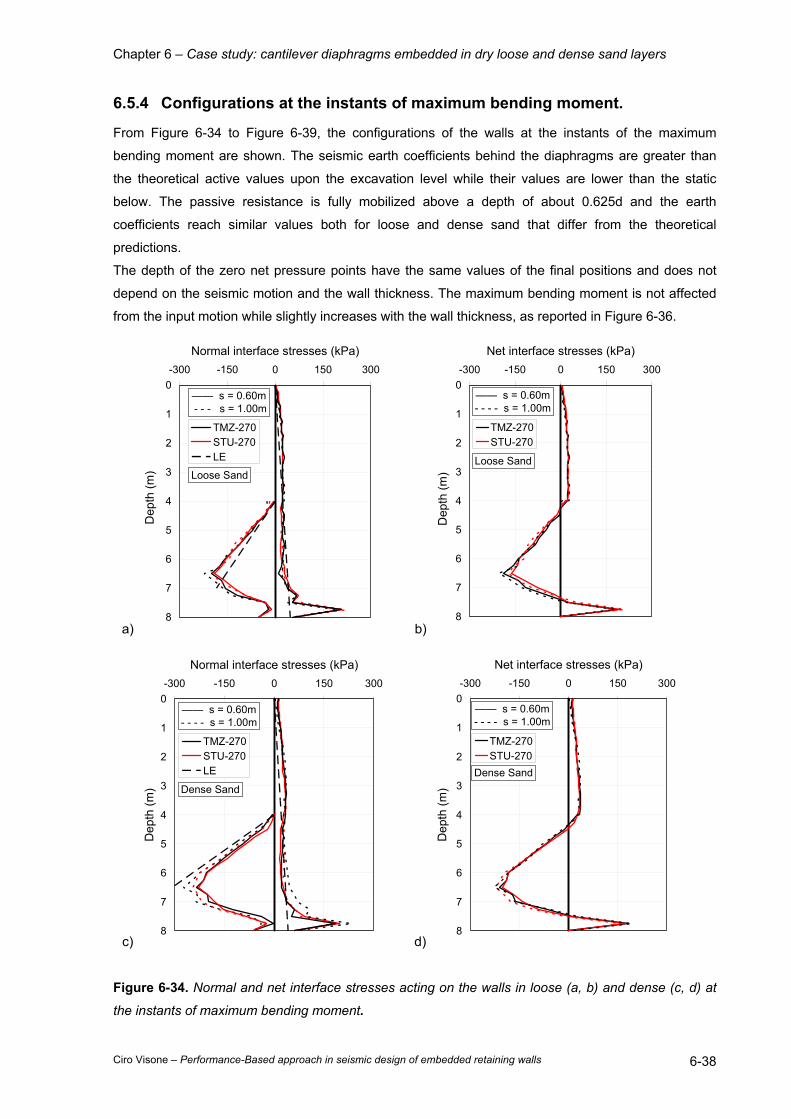
Chapter 6 – Case study: cantilever diaphragms embedded in dry loose and dense sand layers
Ciro Visone – Performance-Based approach in seismic design of embedded retaining walls 6-38
6.5.4 Configurations at the instants of maximum bending moment.
From Figure 6-34 to Figure 6-39, the configurations of the walls at the instants of the maximum
bending moment are shown. The seismic earth coefficients behind the diaphragms are greater than
the theoretical active values upon the excavation level while their values are lower than the static
below. The passive resistance is fully mobilized above a depth of about 0.625d and the earth
coefficients reach similar values both for loose and dense sand that differ from the theoretical
predictions.
The depth of the zero net pressure points have the same values of the final positions and does not
depend on the seismic motion and the wall thickness. The maximum bending moment is not affected
from the input motion while slightly increases with the wall thickness, as reported in Figure 6-36.
a)
0
1
2
3
4
5
6
7
8
-300 -150 0 150 300
Normal interface stresses (kPa)
Dep
th (m
)
TMZ-270STU-270LE
—— s = 0.60m - - - s = 1.00m
Loose Sand
b)
0
1
2
3
4
5
6
7
8
-300 -150 0 150 300
Net interface stresses (kPa)
Dep
th (m
)TMZ-270STU-270
—— s = 0.60m- - - - s = 1.00m
Loose Sand
c)
0
1
2
3
4
5
6
7
8
-300 -150 0 150 300
Normal interface stresses (kPa)
Dep
th (m
)
TMZ-270STU-270LE
—— s = 0.60m- - - - s = 1.00m
Dense Sand
d)
0
1
2
3
4
5
6
7
8
-300 -150 0 150 300
Net interface stresses (kPa)
Dep
th (m
)
TMZ-270STU-270
—— s = 0.60m- - - - s = 1.00m
Dense Sand
Figure 6-34. Normal and net interface stresses acting on the walls in loose (a, b) and dense (c, d) at
the instants of maximum bending moment.

Chapter 6 – Case study: cantilever diaphragms embedded in dry loose and dense sand layers
Ciro Visone – Performance-Based approach in seismic design of embedded retaining walls 6-39
a)
0
1
2
3
4
5
6
7
8
0 1 2 3 4
Active earth pressure coefficient, K AEn = σn/γz
Dep
th (m
)
L060TMZL060STUL100TMZL100STUKAKAE
Loose Sand
b)
0
1
2
3
4
5
6
7
8
0 2 4 6 8 10
Passive earth pressure coefficient, K PEn = σn/γz
Dep
th (m
)
L060TMZL060STUL100TMZL100STUKPKPE
Loose Sand
c)
0
1
2
3
4
5
6
7
8
0 1 2 3 4
Active earth pressure coefficient, K AEn = σn/γz
Dep
th (m
)
D060TMZD060STUD100TMZD100STUKAKAE
Dense Sand
d)
0
1
2
3
4
5
6
7
8
0 2 4 6 8 10
Passive earth pressure coefficient, K PEn = σn/γz
Dep
th (m
)
D060TMZD060STUD100TMZD100STUKPKPE
Dense Sand
Figure 6-35. Numerical active and passive earth pressure coefficients for walls in loose (a, b) and
dense (c, d) sand at the instants of maximum bending moment.

Chapter 6 – Case study: cantilever diaphragms embedded in dry loose and dense sand layers
Ciro Visone – Performance-Based approach in seismic design of embedded retaining walls 6-40
a)
0
1
2
3
4
5
6
7
8
-250 -150 -50 50 150 250Shear force (kN/m)
Dep
th (m
)
TMZ-270STU-270LE
—— s = 0.60m- - - - s = 1.00m
Loose Sand
b)
0
1
2
3
4
5
6
7
8
0 100 200 300 400
Maximum bending moment (kNm/m)
Dep
th (m
)
TMZ-270STU-270LE
—— s = 0.60m- - - - s = 1.00m
Loose Sand
c)
0
1
2
3
4
5
6
7
8
-350 -150 50 250
Shear force (kN/m)
Dep
th (m
)
TMZ-270STU-270LE
—— s = 0.60m- - - - s = 1.00m
Dense Sand
d)
0
1
2
3
4
5
6
7
8
0 100 200 300 400
Maximum bending moment (kNm/m)
Dep
th (m
)
TMZ-270STU-270LE
—— d = 0.60m- - - - d = 1.00m
Dense Sand
Figure 6-36. Shear forces and bending moments acting on walls in loose (a, b) and dense (c, d) sand
at the instants of maximum bending moment.
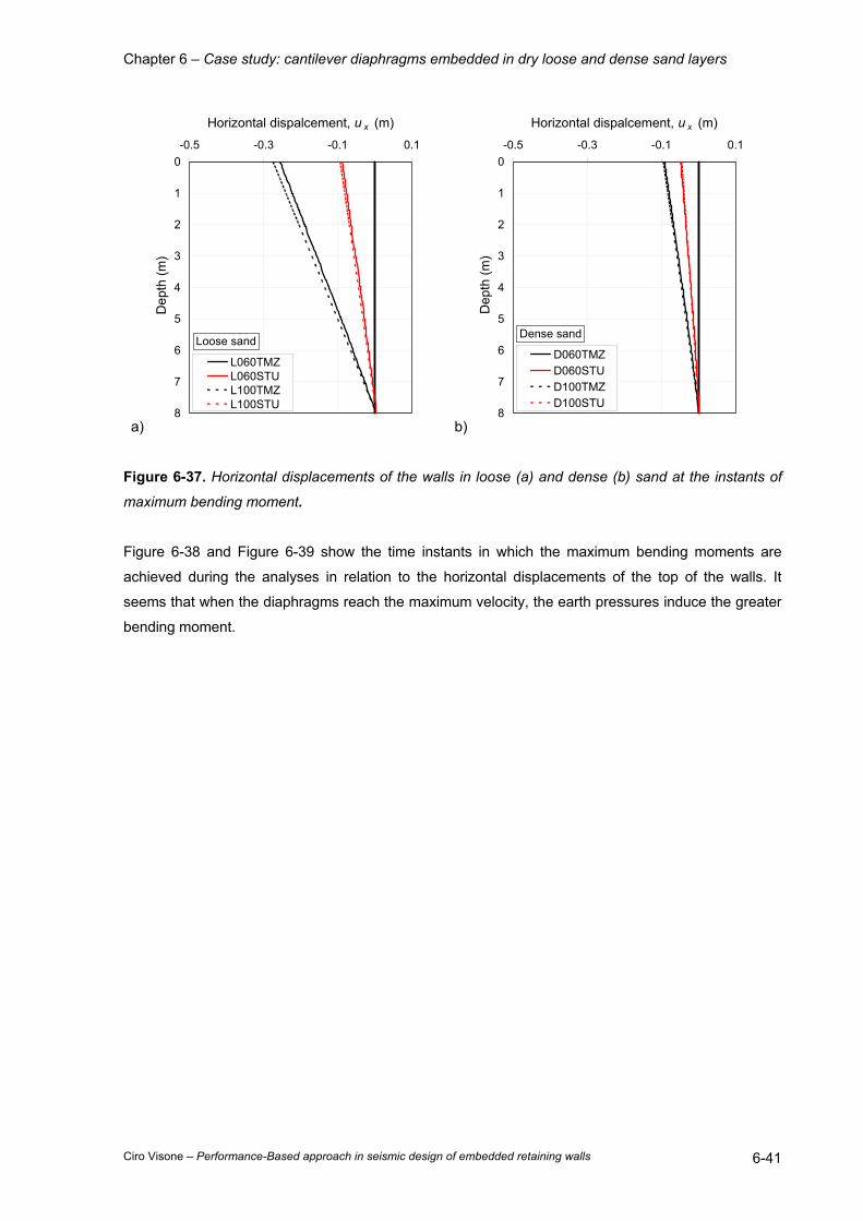
Chapter 6 – Case study: cantilever diaphragms embedded in dry loose and dense sand layers
Ciro Visone – Performance-Based approach in seismic design of embedded retaining walls 6-41
a)
0
1
2
3
4
5
6
7
8
-0.5 -0.3 -0.1 0.1
Horizontal dispalcement, u x (m)
Dep
th (m
)
L060TMZL060STUL100TMZL100STU
Loose sand
b)
0
1
2
3
4
5
6
7
8
-0.5 -0.3 -0.1 0.1
Horizontal dispalcement, u x (m)
Dep
th (m
)
D060TMZD060STUD100TMZD100STU
Dense sand
Figure 6-37. Horizontal displacements of the walls in loose (a) and dense (b) sand at the instants of
maximum bending moment.
Figure 6-38 and Figure 6-39 show the time instants in which the maximum bending moments are
achieved during the analyses in relation to the horizontal displacements of the top of the walls. It
seems that when the diaphragms reach the maximum velocity, the earth pressures induce the greater
bending moment.
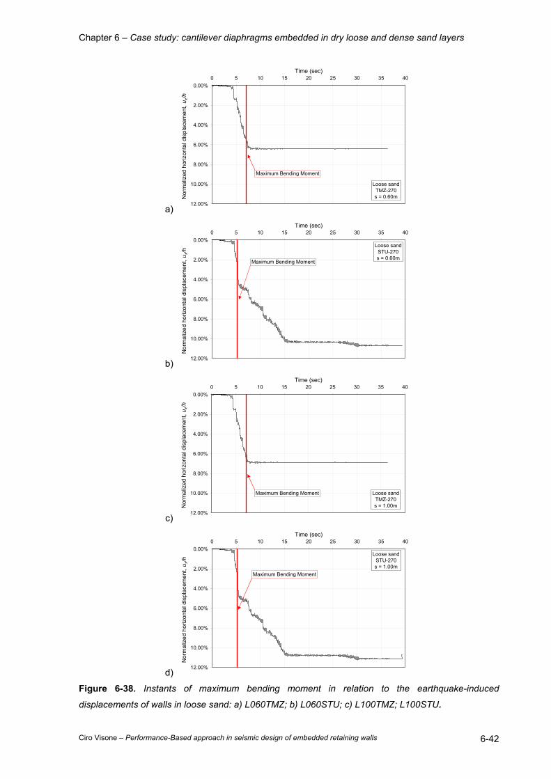
Chapter 6 – Case study: cantilever diaphragms embedded in dry loose and dense sand layers
Ciro Visone – Performance-Based approach in seismic design of embedded retaining walls 6-42
a)
0.00%
2.00%
4.00%
6.00%
8.00%
10.00%
12.00%
0 5 10 15 20 25 30 35 40Time (sec)
Nor
mal
ized
hor
izon
tal d
ispl
acem
ent,
u x/h
Maximum Bending Moment
Loose sandTMZ-270s = 0.60m
b)
0.00%
2.00%
4.00%
6.00%
8.00%
10.00%
12.00%
0 5 10 15 20 25 30 35 40Time (sec)
Nor
mal
ized
hor
izon
tal d
ispl
acem
ent,
u x/h
Maximum Bending Moment
Loose sandSTU-270s = 0.60m
c)
0.00%
2.00%
4.00%
6.00%
8.00%
10.00%
12.00%
0 5 10 15 20 25 30 35 40Time (sec)
Nor
mal
ized
hor
izon
tal d
ispl
acem
ent,
u x/h
Loose sandTMZ-270s = 1.00m
Maximum Bending Moment
d)
0.00%
2.00%
4.00%
6.00%
8.00%
10.00%
12.00%
0 5 10 15 20 25 30 35 40Time (sec)
Nor
mal
ized
hor
izon
tal d
ispl
acem
ent,
u x/h
Maximum Bending Moment
Loose sandSTU-270s = 1.00m
Figure 6-38. Instants of maximum bending moment in relation to the earthquake-induced
displacements of walls in loose sand: a) L060TMZ; b) L060STU; c) L100TMZ; L100STU.

Chapter 6 – Case study: cantilever diaphragms embedded in dry loose and dense sand layers
Ciro Visone – Performance-Based approach in seismic design of embedded retaining walls 6-43
a)
0.00%
2.00%
4.00%
6.00%
8.00%
10.00%
12.00%
0 5 10 15 20 25 30 35 40Time (sec)
Nor
mal
ized
hor
izon
tal d
ispl
acem
ent,
u x/h
Maximum Bending Moment
Dense sandTMZ-270s = 0.60m
b)
0.00%
2.00%
4.00%
6.00%
8.00%
10.00%
12.00%
0 5 10 15 20 25 30 35 40Time (sec)
Nor
mal
ized
hor
izon
tal d
ispl
acem
ent,
u x/h
Maximum Bending Moment
Dense sandSTU-270s = 0.60m
c)
0.00%
2.00%
4.00%
6.00%
8.00%
10.00%
12.00%
0 5 10 15 20 25 30 35 40Time (sec)
Nor
mal
ized
hor
izon
tal d
ispl
acem
ent,
u x/h
Maximum Bending Moment
Dense sandTMZ-270s = 1.00m
d)
0.00%
2.00%
4.00%
6.00%
8.00%
10.00%
12.00%
0 5 10 15 20 25 30 35 40Time (sec)
Nor
mal
ized
hor
izon
tal d
ispl
acem
ent,
u x/h
Maximum Bending Moment
Dense sandSTU-270s = 1.00m
Figure 6-39. Instants of maximum bending moment in relation to the earthquake-induced
displacements of walls in dense sand: a) D060TMZ; b) D060STU; c) D100TMZ; D100STU.
Chapter 6 – Case study: cantilever diaphragms embedded in dry loose and dense sand layers
Ciro Visone – Performance-Based approach in seismic design of embedded retaining walls 6-44
6.6 COMPARISONS BETWEEN THE RESULTS OF DIFFERENT
ANALYSES.
Table 6-14 summarizes the results of the various type of analyses performed on the examined
schemes.
Assuming the dynamic analyses as reference solution, the first difficulty encountered in the simplified
methods is the definition of the seismic horizontal coefficient associated to each earthquake. In fact,
the same signal, applied to the base of the two soil columns of loose and dense sand, belonging to the
same soil category, produces different seismic amplification, both for dynamic interaction and free field
conditions. Furthermore, the effects on walls in terms of displacements and stresses are quite
different.
The common simplified analyses of the pseudostatic limit equilibrium and the use of empirical formulas
do not give very dissimilar displacements but underpredict the maximum bending moments.
Accurate displacements are furnished for diaphragms in dense sand from the simplified dynamic
analyses. For loose sand, instead, the predicted values are too much large.
The pushover analyses allow completely describing the seismic performances of each wall. The
difficulty consists only on the definition of the expected kh for the seismic demand of the site and
subsoil conditions of the structure. This type of analysis is also able to account for the effects of wall
properties on the seismic response.
Remembering the hierarchical resistance concepts exposed in the Chapter 5, the limit equilibrium
approach for the evaluation of the critical acceleration of the retaining system in the simplified
analyses is a good method to control the collapse of the retaining system if the formation of a plastic
hinge in the wall below the excavation level can be preferred to the failure of the structure for
exceeding of the soil passive strength.
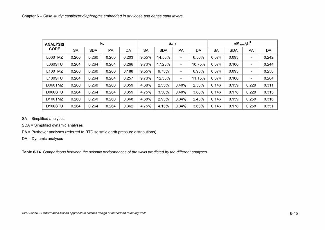
Chapter 6 – Case study: cantilever diaphragms embedded in dry loose and dense sand layers
Ciro Visone – Performance-Based approach in seismic design of embedded retaining walls 6-45
kh ux/h ∆Mmax/γh3 ANALYSIS CODE SA SDA PA DA SA SDA PA DA SA SDA PA DA
L060TMZ 0.260 0.260 0.260 0.203 9.55% 14.58% - 6.50% 0.074 0.093 - 0.242
L060STU 0.264 0.264 0.264 0.266 9.70% 17.23% - 10.75% 0.074 0.100 - 0.244
L100TMZ 0.260 0.260 0.260 0.188 9.55% 9.75% - 6.93% 0.074 0.093 - 0.256
L100STU 0.264 0.264 0.264 0.257 9.70% 12.33% - 11.15% 0.074 0.100 - 0.264
D060TMZ 0.260 0.260 0.260 0.359 4.68% 2.55% 0.40% 2.53% 0.146 0.159 0.228 0.311
D060STU 0.264 0.264 0.264 0.359 4.75% 3.30% 0.40% 3.68% 0.146 0.178 0.228 0.315
D100TMZ 0.260 0.260 0.260 0.368 4.68% 2.93% 0.34% 2.43% 0.146 0.159 0.258 0.316
D100STU 0.264 0.264 0.264 0.362 4.75% 4.13% 0.34% 3.63% 0.146 0.178 0.258 0.351
SA = Simplified analyses
SDA = Simplified dynamic analyses
PA = Pushover analyses (referred to RTD seismic earth pressure distributions)
DA = Dynamic analyses
Table 6-14. Comparisons between the seismic performances of the walls predicted by the different analyses.
Chapter 7 – Conclusions and future developments
Ciro Visone – Performance-Based approach in seismic design of embedded retaining walls 7-1
7 CONCLUSIONS AND FUTURE DEVELOPMENTS.
The increasing use of the underground spaces and the last seismic events in the urban areas have
driven many researchers of different countries to deepen the knowledge on the dynamic behaviour of
the structure embedded in the subsoil.
Different contributes were given by the recent Italian and European building codes on these topics.
The present PhD thesis has found its main role in the application of the performance based approach
in the seismic design of this type of structures.
The most widespread procedure based on the extension of the limit equilibrium method to the
pseudostatic conditions was analyzed and discussed. The effectiveness of the Mononobe (1929) and
Okabe (1926) and Lancellotta (2007) theories for the estimation of the seismic active and passive
earth pressure coefficients was shown. Some charts for the preliminary design of the depth of
embedment and the maximum bending moment for walls in dry homogeneous granular materials were
developed by using the Blum method. To predict the earthquake-induced displacements of the walls,
the empirical relationships proposed by Uwabe (1983) for anchored bulkheads embedded in non-
liquefiable sites were considered also for cantilever walls. However, their capabilities should be tested
on a greater number of data deriving from advanced numerical analyses, model and full scale tests.
Another design method, consisting in a pseudostatic procedure to define the critical acceleration of the
retaining system and Newmark sliding block analyses for the calculation of the seismic displacements,
was highlighted. The approach can be identified such as simplified dynamic analysis but its application
presents some difficulties and uncertainties for flexible walls, as recognized in the literature (Callisto,
2006).
An innovative design method to completely predict the seismic performances of a retaining system
was proposed in this thesis. The procedure can be included in the framework of the "pushover
analyses" and can be accomplished by conducting FE or FD pseudostatic analyses. It consists to
apply the seismic loading as an increasing pressure distribution that can be expressed as a seismic
horizontal coefficient by means of the normalization with respect to the weight of the active soil wedge
and the wall. The performances of the system can be described by capacity curves in terms of
maximum horizontal displacements, maximum settlements of the backfill, maximum bending moment,
etc. The method requires more validations by means of accurate analyses with appropriate soil
constitutive models, seismic in-situ monitoring of full-scale structures and dynamic centrifuge
modelling. However, the good agreement between the predictions of the analyses presented in the
Chapter 6 encourages deepening the application of the pushover analyses to the embedded walls that
is not a consolidated procedures for the seismic design of geotechnical systems.
The most accurate tool for the estimation of the dynamic behaviour of the constructions interacting
with the soil is constituted by the numerical simulations. Their use requires advanced knowledge in
numerical calculations, a proper soil constitutive model, an adequate soil characterization by means of
in situ and laboratory tests, a proper definition of the seismic input when dynamic analyses should be
carried out. In the Annex B, the problem of the calibration of the FE model for dynamic analyses in
geotechnical earthquake engineering by means of a commercial code was illustrated. The various
sources of damping were recognized and the procedure to rightly estimate the damping coefficients,
Chapter 7 – Conclusions and future developments
Ciro Visone – Performance-Based approach in seismic design of embedded retaining walls 7-2
both numerical and material, was presented. In order to minimize the spurious effects of the reflected
stress waves on the lateral boundaries of the discrete models, an useful configuration of the boundary
conditions was accomplished by testing the seismic response of the models crossed by vertical shear
waves.
An example of application of the different procedures for the evaluation of the seismic performances of
free cantilever walls embedded in dry loose and dense sand was shown in the Chapter 6. The
predictions confirm the difficulties related to the application of the simplified methods, especially in the
definition of the equivalent seismic coefficient for a given earthquake.
The material properties for the soils was chosen on the basis of the results of laboratory tests
conducted on samples of Leighton Buzzard sand 100/170 (Fraction E) presented in the Annex A. The
experimental data have allowed defining the mechanical behaviour of the sand under different stress
paths and loading conditions. The future developments of this research line is the use of advanced
constitutive models to simulate the behaviour of the sand in the controlled laboratory tests to catch its
main mechanical aspects. The material was chosen in the contest of the research program ReLUIS
presented in the Chapter 1 for the centrifuge model tests of retaining walls.

References
Ciro Visone – Performance-Based approach in seismic design of embedded retaining walls
REFERENCES.
Ampadu S. I. K, Tatsuoka F.(1989). "The dry versus the wet Methods of setting clay specimens for
triaxial testing", Proc. 28th National Conference of the Japanese Society of Soil Mechanics and
Foundation Engineering, Tokyo, June
Aversa S. and Vinale F. (1985). “Improvement to a stress-path triaxial cell”, Geotechnical Testing
Journal, Vol. 18, Issue 1, pp. 116-120
Bardet J.P., Ichii K. and Lin C.H. (2000). “EERA: a computer program for Equivalent-linear Earthquake
site Response Analyses of layered soil deposits”, University of Southern California, Los Angeles.
Bardet J.P., Tobita T. (2001). “NERA: a computer program for Nonlinear Earthquake site Response
Analyses of layered soil deposits”, University of Southern California, Los Angeles.
Berenger J.P., (1994). “A perfectly matched layer for the absorption of electromagnetic waves”, J. of
Comp. Physics, vol. 114, pp. 185-200
Bica A.V.D., Clayton C.R.I. (1989). "Limit equilibrium design methods for free embedded cantilever
walls", Proc. Inst. Civ. Engrs 86, 879-898.
Bica A.V.D., Clayton C.R.I. (1992). “The preliminary design of free embedded cantilever walls in
granular soils”, Proc. Int. Conf. on Retaining Structures, Cambridge
Bica A.V.D., Clayton C.R.I. (1998). " An experimental study of the behaviour of embedded lengths of
cantilever walls", Geotechnique, Vol. 48, no.6, pp. 731.745
Bishop A.W., Wensley L.D. (1975). "Hydraulic triaxial apparatus for controlled stress path testing",
Geotechnique, Vol. 25, no. 4, pp. 657-670
Blum H. (1931).”Einspannungsverhältnisse bel Bohlwerken”,Wilh.Ernst und Sohn Berlin
Bolton M.D. (1986). "The strength and dilatancy of sands", Geotechnique, Vol. 36, no. 1, pp. 65-78
Bransby, P. L., Milligan, G. W. E. (1975). "Soil deformations near cantilever sheet pile walls",
Geotechnique, Vol. 25, No. 1, 175-195
Brinkgreve R.B.J. (2002). Plaxis 2D version8. A.A. Balkema Publisher, Lisse.
Callisto L. (2006), “Pseudo-static seismic design of embedded retaining structures", Workshop of
ETC12 Evaluation Committee for the Application of EC8, Athens, January 20-21
Caquot A., Kerisel F. (1948). “Tables for the calculation of passive pressure, active pressure and
bearing capacity of foundations”, Gauthier-Villars, Paris
Castro G. (1969). "Liquefaction of sands", Harvard Soil Mechanics Series 87, Harvard University,
Cambridge, Massachusetts
Chang M.F. (1981). “Static and seismic lateral earth pressures on rigid retaining structures”, PhD
Thesis, School of Civil Engineering, Purdue University, West Lafayette, IN, 465 pp.
Chang M.F., Chen W.F. (1982). “Lateral earth pressures on rigid retaining walls subjected to
earthquake forces”, Solid mechanics archives, Vol. 7, Martinus Nijoff Publishers, The Hague, The
Netherlands, pp. 315-362
Chen W.F., Rosenfarb J.L. (1973). “Limit analysis solutions of earth pressure problems”, Soils and
Foundations, Vol. 13, No. 4, pp. 45-60
Chen W.F. (1975). “Limit analysis and soil plasticity”, Elsevier, Amsterdam, 638 pp.

References
Ciro Visone – Performance-Based approach in seismic design of embedded retaining walls
Chen W.F., Chang M.F. (1981). “Limit analysis in soil mechanics and its applications to lateral earth
pressure problems”, Solid mechanics archives, Vol. 6, No. 3, Sijthoff & Noordhoff International
Publishers, Alphen aan den Rijn, The Netherlands, pp. 331-399
Chen W.F. (1982). “Constitutive equations for engineering materials, Vol. 1: Elasticity and modelling”,
Wiley Interscience, New York, NY, 580 pp.
Chen W.F. (1990). “Limit analysis in soil mechanics”, Elsevier, Amsterdam, 477 pp.
Clayton C.R.I., Milititsky J. Woods R.I. (1993). “Earth pressure and earth retaining structures”,
Chapman & Hall
Coulomb C.A. (1776). “Essai sur une application des regles des maximis et minimis a quelques
problemes de statique relatifs a l’architecture”, Memoires de l’Academie Royale pres Divers Savants,
Vol. 7
Cundall, P., Hansteen, E., Lacasse, S., and Selnes, P. B., (1980). “NESSI, soil structure interaction
program for dynamic and static problems”, Norges Geotekniske Institute, Norway
Day R.A.(1999). " Net pressure analysis of cantilever sheet pile walls", Geotechnique, Vol. 49, no.2,
pp. 231-245
Dennehy K.T. (1985). "Seismic vulnerability, analysis and design of anchored bulkheads", PhD.
Dissertation, Renssalaer Polytechnic Institute, Troy, New York
D'Onofrio A. (1996). "Comportamento meccanico dell'argilla di Vallericca in condizioni lontane dalla
rottura", PhD. Thesis, Università degli Studi di Napoli Federico II, Napoli, Italy (in Italian)
Ebeling R.M., Morrison E.E.(1993). "The seismic design of waterfront retaining structures", NCEL
Report R-939, Naval Civil Engineering Laboratory, Port Hueneme, California, 256 pp.
EN 1997-1 (October 2001). Eurocode 7: Geotechnical design – Part 1: General rules. CEN European
Committee for Standardization, Bruxelles, Belgium.
EN 1998-5 (December 2003). Eurocode 8: Design of structures for earthquake resistance – Part 5:
Foundations, retaining structures and geotechnical aspects. CEN European Committee for
Standardization, Bruxelles, Belgium
EPRI, Electric Power Research Institute (1991): “Soil response to earthquake ground motion”, NP-
5747, pp. 293
Fourie A.B., Potts D.M. (1989). “Comparisons of finite element and limiting equilibrium analyses for an
embedded cantilever retaining wall”, Geotechique, Vol. 39, pp. 175-188
Franklin A.G., Chang F.K. (1977). "Permanent displacements of earth embankments by Newmark
sliding block analysis", Report 5, Miscellaneous Paper S-71-17, U.S. Army Corps of Engineers
Waterways Experiment Station, Vicksburg, Mississipi.
Franzius O. (1924): "Versuche mit passiven Druck", Bauingegnieur, Berlin, 314-320
Gazetas G., Dakoulas P., Dennehy K. (1990). "Empirical seismic design method for waterfront
anchored sheet pile walls", Proc. ASCE, Specialty Conf. On Design and Performance of Earth
Retaining Structures, Geotechnical Specialty Publication 25, pp. 232-250
Habibagahi K., Ghahramani A. (1977). “Zero extension theory of earth pressure”, Journal of
Geotechnical Division, ASCE, Vol. 105 (GT7), pp. 881-896
References
Ciro Visone – Performance-Based approach in seismic design of embedded retaining walls
Hardin B.O., Drnevich V.P. (1972). "Shear modulus and damping in soils: Measurement and
parameter effects", Journal of Soil Mechanics and Foundations Division, ASCE, Vol. 98, no. SM6, pp.
603-624
Hettiaratchi R.P., Reece A.R. (1975). “Boundary wedges in two-dimensional passive soil failure”.
Geotechnique, Vol. 25, No. 2, pp. 197-220
Iai S., Ichii K. (1998). “Performance Based design of port structures", U.S./Japan Natural Resources
Development Program (UJNR). Wind and Seismic Effects. Joint Meeting of the U.S./Japan
Cooperative Program in Natural Resources Panel on Wind and Seismic Effects, 30th. May 12-15,
1998, Gaithersburg, MD, Raufaste, N. J., Jr., Editor(s), 84-96 pp, 1998
Iai, S., Ichii, K., Liu, H., Morita, T. (1998). "Effective stress analyses of port structures", Soils and
Foundations, Special Issue on Geotechnical Aspects of the January 17 1995 Hyogoken-Nambu
Earthquake, No.2, pp. 97-114
Iwan W.D. (1967). “On a class of models for the yielding behaviour of continuous and composite
systems”, ASME, Journal of Applied Mechanics, Vol. 34, pp.612-617
Ishihara K. (1993). " Liquefaction and flow failure during earthquakes", geotechnique, Vol. 43, no. 3,
pp. 351-415
James R.G., Bransby P.L. (1970). “Experimental and theoretical investigations of a passive earth
pressure problem”, Geotechnique, Vol. 20, No. 1, pp. 17-37
Jamiolkowski M. et al. (1985). "Laboratory validation of in situ tests", in Geotechnical Engineering in
Italy, ISSMFE, Golden Jubilee Volume, AGI 251-270
Jeyatharan K. (1991). " Partial liquefaction of sand fill in a mobile arctic caisson under dynamic ice-
loading", PhD. Thesis, Cambridge University, Cambridge, U.K.
King G. J. W., McLoughlin J. P. (1992). "Centrifuge model studies of a cantilever retaining wall in
sand", Proceedings of an international conference on Retaining Structures, Cambridge, pp. 711-720.
King G. J. W. (1995). "Analysis of cantilever sheet-pile walls in cohesionless soil", J. Geotech. Engng
Div., ASCE, Vol. 121, No. 9, 629-635
Kramer, S.L. (1996). “Geotechnical Earthquake Engineering”, Prentice Hall, Inc., Upper Saddle River,
New Jersey, 653 pp.
Kuhlmeyer R.L, Lysmer J. (1973). “Finite Element Method Accuracy for Wave Propagation Problems”,
J. of the Soil Mechanics and Foundation Division, vol.99 n.5, pp. 421-427
Kunar R. R., Beresford P. J., Cundall P. A. (1977). “A Tested Soil-Structure Model for Surface
Structures,” in Proceedings of the Symposium on Soil-Structure Interaction (Roorkee University, India,
January, 1977), Vol. 1, pp. 137-144. Meerut, India: Sarita Prakashan
Lancellotta R. (2002). “Analytical solution of passive earth pressure”, Geotechnique, Vol. 52, No. 8,
pp. 617-619
Lancellotta R. (2007). “Lower-Bound approach for seismic passive earth resistance”. Geotechnique,
Vol. 57, No. 3, pp. 319-321
Lanzo G., Vucetic M. (1999). "Effect of Soil Plasticity on Damping Ratio at Small Cyclic Strains", Soils
and Foundations, Vol. 39, No. 4, pp. 131-141

References
Ciro Visone – Performance-Based approach in seismic design of embedded retaining walls
Lanzo G., Pagliaroli A., D’Elia B. (2004). "L’influenza della modellazione di Rayleigh dello
smorzamento viscoso nelle analisi di risposta sismica locale", ANIDIS, XI Congresso Nazionale
“L’Ingegneria Sismica in Italia”, Genova 25-29 Gennaio 2004 (in Italian)
Lanzo G. (2005): “Risposta sismica locale”, Aspetti geotecnici della progettazione in zone sismiche,
Linee Guida AGI (in Italian)
Leiper Q.J. (1984). “Instrumentation of diaphragm walls”, M. Sc. Dissertation, University of Surrey
LUSAS (2000). Theory Manual, FEA Ltd., United Kingdom
Lyndon A., Pearson R. A. (1984). "Pressure distribution on a rigid retaining wall in cohesionless
material", Proceedings of a symposium on the application of centrifuge modelling to geotechnical
design, Manchester, pp. 271-280
Lysmer J., Kuhlmeyer R.L. (1969). "Finite Dynamic Model for Infinite Media", ASCE, Journal of
Engineering and Mechanical Division, pp. 859-877
Lysmer, J., and G.Waas. (1972). “Shear Waves in Plane Infinite Structures”, ASCE J. Eng. Mech., Vol.
98, no. EM1, pp. 85-105
Lysmer J. (1978): “Analytical procedures in soil dynamics”, Report no. UCB EERC-78/29, University of
California, Berkeley
Madabhushi, S.P.G., Schofield, A.N., Lesley, S. (1998). "A new stored angular momentum (SAM)
based earthquake actuator", In Kimura, Kusakabe & Takemura (eds.), Proc. Int. conf. Centrifuge ’98,
Tokyo, 23-25 September 1998, Rotterdam, Balkema
Mak K.W. (1984). "Modelling the effects of a strip load behind rigid retaining walls", PhD. Thesis,
Cambridge University, Cambridge, U.K.
Masing G. (1926). "Eigenspannungen und Verfertigung beim Messing", Proc., 2nd International
Congress on Applied Mechanics, Zurich
Ministry of Transport, Japan, (1999). "Design Standard for Port and Harbour Facilities and
Commentaries", Japan Port and Harbour Association, 1181 pp. (in Japanese)
Mononobe N., Matsuo H. (1929).”On the determination of earth pressures during earthquakes”, Proc.
World Engineering Conference, Vol. 9, pp. 176
Mroz Z. (1967). “On the description of anisotropic work hardening”, Journal of Mechanics and Physics
of Solids, 15, pp. 163-175
Mulilis J.P., Seed H.B., Chan C.K., Mitchell J.K. (1977). "The effects of method of sample preparation
on the cyclic stress-strain behaviour of sands", Report no. EERC 75-18, Earthquake Engineering
Research Center, University of California, Berkeley
Nadim F. (1980). "Tilting and sliding of gravity retaining walls", S.M. Thesis, Department of Civil
Engineering, Massachusetts Institute of Technology, Cambridge, Massachusetts
Nadim F. (1982). “A numerical model for evaluation of seismic behaviour of gravity retaining walls",
Sc. D. thesis, Research Report R82-33, Department of Civil Engineering, Massachusetts Institute of
Technology, Cambridge, Massachusetts
Newmark, N. M. (1959). “A Method of Computation for Structural Dynamics”, ASCE, Journal of the
Engineering Mechanics Division, Vol. 85 No. EM3
Newmark N. (1965). "Effects of earthquakes on dams and embankments", Geotechnique, Vol. 15, no.
2, pp. 139-160
References
Ciro Visone – Performance-Based approach in seismic design of embedded retaining walls
NTC 2008. Approvazione delle nuove norme tecniche per le costruzioni. Gazzetta Ufficiale della
Repubblica Italiana, n. 29 del 4 febbraio 2008 - Suppl. Ordinario n. 30,
http://www.cslp.it/cslp/index.php?option=com_docman&task=doc_download&gid=3269&Itemid=10 (in
Italian).
Okabe S. (1926). “General theory of earth pressure”, Journal of Japanese Society of Civil Engineering,
Vol. 12, No. 1
Okamoto S. (1956). “Bearing capacity of sandy soil and lateral earth pressure during earthquakes”,
Proc. 1st World Conf. on Earthquake Engineering, Tokyo, pp. 231-247
Padfield C.J., Mair R.J. (1984). “Design of retaining walls embedded in stiff clays”, CIRIA, Report no
104, Construction Industry Research and Information Association, London
Pal O. (1998). "Modélisation du comportement dynamique des ouvrages grace à des elements finis de
haute precision”, Thesis, L’université Joseph Fourier – Grenoble I
Pane V., Tamagnini C. (2004). “Analisi di paratie pluriancorate”, Hevelius, Benevento (in Italian)
Park D., Hashash Y.M.A. (2004). "Soil Damping Formulation in Nonlinear Time Domain Site Response
Analysis”, Journal of Earthquake Engineering, Vol.8, no. 2, pp. 249-274
PHRI (1997). “Handbook on liquefaction remediation of reclaimed land", Port and Harbour Research
Institute, A.A. Balkema, Rotterdam, Brookfield
PIANC (2001). “Seismic Design Guidelines for Port Structures”, Working Group n.34 of the Maritime
Navigation Commission, International Navigation Association, Balkema, Lisse, 474 pp.
Rankine W. (1857). “On the stability of loose earth”, Philosophical Transactions of the Royal Society of
London, Vol. 147
Pyke, (1979). "Nonlinear soil models for irregular cyclic loading", Journal of the Geotechnical
Engineering Division, Vol. 105, pp. 715 - 726
Richards R., Elms D. (1979). "Seismic behaviour of gravity retaining walls", Journal of geotechnical
Engineering Division, ASCE, Vol. 105, no. GT4, pp. 449-464
Roesset, J.M. (1970): “Fundamentals of Soil Amplification”, in Seismic Design for Nuclear Power
Plants, ed. R.J. Hansen, The MIT Press, Cambridge, MA, pp. 183-244
Roesset, J. M., Ettouney M. M. (1977). “Transmitting Boundaries: A Comparison”, Int. J. Num. &
Analy. Methods Geomech., Vol. 1, pp. 151-176.
Ross M., (2004). "Modeling Methods for Silent Boundaries in Infinite Media", ASEN 5519-006: Fluid-
Structure Interaction, University of Colorado at Boulder
Rowe P.W. (1951). “Cantilever sheet piling in cohesionless soil", Engineering September 7, pp. 316-
319
Rowe P.W. (1952). “Anchored sheet pile walls”, Proc. ICE, Vol. 1, no.1, pp. 27-70
Rowe P.W. (1957). “Sheet pile walls in clay”, Proc. ICE, Vol. 7, pp. 629-654
Santucci de Magistris F. (1992). "Una cella triassiale a stress path controllato: messa a punto e primi
risultati sperimentali", Sc.M. Thesis, Università degli studi di Napoli Federico II (In Italian)
Santucci de Magistris F., Koseki J., Amaya M., Hamaya S., Sato T., Tatsuoka, F (1999). "Triaxial
testing system to evaluate stress-strain behaviour of soils for wide range of strain and strain rate",
ASTM Geotechnical Testing Journal, Vol. 22, no. 1, pp. 44-60
References
Ciro Visone – Performance-Based approach in seismic design of embedded retaining walls
Schnabel, P. B., Lysmer, J., Seed, H. B. (1972): “SHAKE: a computer program for earthquake
response analysis of horizontally layered sites”, Report n° EERC72-12, University of California at
Berkeley
Scott R.F. (1963). “Principle of soil mechanics”, Addison-Wesley, Reading, MA, 523 pp.
SEAOC (1995). “Vision 2000 - A Framework for Performance Based Earthquake Engineering", Vol. 1,
January
Seed H.B., Idriss I.M. (1970): “Soil moduli and damping factors for dynamic response analyses”,
Report ERC 70-10, Earthquake Engineering Research Center, University of California, Berkeley
Seed H.B., Whitman R.V. (1970). “Design of earth retaining structures for dynamic loads”, Proc. ASCE
Specialty Conference on lateral stresses in the ground and design of earth retaining structures, pp.
103-147
Siddharthan R., Ara S., Norris G.M. (1992). "Simple rigid plastic model for seismic tilting of rigid walls",
Journal of Structural Engineering, ASCE, Vol. 118, no. 2, pp. 469-487
Skempton A.V. (1953). “Earth pressure, retaining walls, tunnels and strutted excavation”, Proc. of 3rd
Int. Conf. Soil Mech. Found. Engin.
Smith, I.M., Griffith, D.V. (1982): “Programming the Finite Element Method”, Second Edition. John
Wiley & Sons, Chisester, U.K.
Sokolovskii V.V. (1965). “Static of granular media”, Pergamon Press, New York, NY, 232 pp.
Steedman R.S., Zeng X. 1990. “The seismic response of waterfront retaining walls”, Proc. ASCE
Specialty Conference on Design and Performance of Earth Retaining Structures, Special Technical
Publication 25, Cornell University, Ithaca, New York, pp.872-886
Steedman R.S. (1998). “Seismic design of retaining walls", Proc. Instn Civ. Engng, Vol. 131, pp. 12-22
Tan F.S.C. (1990). "Centrifuge and theoretical modelling of conical footings on sand", PhD. Thesis,
Cambridge University, Cambridge, U.K.
Tatsuoka F., Iwasaki T., Takagi Y. (1978). “Hysteretic damping of sands and its relation to shear
modulus”, Soils and Foundations, Vol. 18, no. 2, pp. 25-40
Tatsuoka F., Ochi K., Fujii S., Okamoto M. (1986). “Cyclic undrained triaxial and torsional shear
strength of sands for different sample preparation methods”, Soils and Foundations, Vol. 26, no. 3, pp.
11-16
Tatsuoka F., Sato T., Park C.S., Kim Y.S., Mukabi J.N., Kohata Y. (1994). "Measurements of elastic
properties of geomaterials in laboratory compression tests", ASTM Geotechnical Testing Journal, Vol.
17, no. 1, pp. 80-94
Taylor D.W. (1948). “Fundamentals of Soil Mechanics”, Wiley, New York, 700 pp.
Teng W.C. (1962). “Foundation design”, Prentice-Hall, New Jersey
Terzaghi K. (1943). “ Theoretical Soil Mechanics”, Wiley, Inc., New York
Terzaghi K. (1954). “Anchored bulkheads”, Trans. ASCE, Vol. 119, pp. 1243-1280
Towhata I., Islam S. (1987). “Prediction of lateral movement of anchored bulkheads induced by
seismic liquefaction”, Soils and Foundations, Vol. 27, No. 4, pp. 137-147
Trifunac M.D., Brady A.G. (1975): “A study of the duration of strong earthquake ground motion”,
Bulletin of the Seismological Society of America, 65, 581-626
Tschebotarioff G.P. (1973). “Foundations, retaining and earth structures”, MGraw-Hill, New York
References
Ciro Visone – Performance-Based approach in seismic design of embedded retaining walls
Uwabe T. (1983). "Earthquake response and seismic design of composite type breakwater in deep
sea", Proc. Of 1983 Annual Research Presentations of Port and Harbour Research Institute, pp. 103-
165 (in Japanese)
Visone C., Santucci de Magistris F. (2007). “Some aspects of seismic design methods for flexible
earth retaining structures”, ISSMGE – ERTC 12 Workshop – XIV European Conference on Soil
Mechanics and Geotechnical Engineering, 25th September 2007, Madrid
Vucetic M., Dobry R. (1986). "Pore Pressure Build Up and Liquefaction at Level Sandy Sites During
Earthquakes”, Research Report, Department of Civil Engineering, Rensselaer Polytechnic Institute,
Troy
Vucetic M. (1990). "Normalized behaviour of clay under irregular cyclic loading", Canadian
Geotechnical Journal, Vol. 27, no. 1, pp. 29-46
Wang Z.L., Qing-Yu H., Gen-Shou Z. (1980). “Wave Propagation Method of Site Seismic Response
by a Visco-Elastoplastic Model”, Proceedings: Seventh World Conference on Earthquake Engineering,
Vol. 2, p. 279-386
Werner (1998). “Seismic Guidelines for Ports", Technical Council on Lifeline Earthquake Engineering,
Monograph n.12, ASCE
White W., Valliappan S., Lee I. K. (1977). “Unified Boundary for Finite Dynamic Models”, J. Eng.
Mech., Vol. 103, pp. 949-964
Whitman R., Liao S. (1984). ''Seismic Design of Gravity Retaining Walls", Proc., 8th World Conference
on Earthquake Engineering, San Francisco, California, Vol. 3
Whitman R., Liao S. (1984). ''Seismic Design of Gravity Retaining Walls", Miscellaneous Paper GL-85-
1, U.S. Army Engineer Waterways Experiment Station, Vicksburg, Mississipi
Wilson E. L. (1962). “Dynamic Response by Step-By-Step Matrix Analysis”, Proceedings, Symposium
On The Use of Computers in Civil Engineering, Laboratorio Nacional de Engenharia Civil, Lisbon,
Portugal, October 1-5
Wilson E. L., Farhoomand I., Bathe K. J. (1973). “Nonlinear Dynamic Analysis of Complex Structures”,
Earthquake Engineering and Structural Dynamics, Vol. 1, 241-252
Wolf J.P. (1985). "Dynamic soil-structure interaction", Prentice Hall, New Jersey, 466 pp.
Wong C.P. (1982). "Seismic analysis and an improved design procedure for gravity retaining walls",
S.M. Thesis, Department of Civil Engineering, Massachusetts Institute of Technology, Cambridge,
Massachusetts
Yoshimine M., Ishihara K., Vargas W. (1998). "Effects of principal stress direction and intermediate
principal stress on undrained shear behavior of sand", Soils and Foundations, Vol. 38, No. 3, pp. 179-
188
Zarrabi-Kashani K. (1979). "Sliding of gravity retaining wall during earthquakes considering vertical
accelerations and changing inclinations of failure surface”, S.M. Thesis, Department of Civil
Engineering, Massachusetts Institute of Technology, Cambridge, Massachusetts
Zienkiewicz O.C., Taylor R.L. (1991). "The finite element method", 4th edition, Vol. 2, Solid and Fluid
mechanics, Dynamics and Non-Linearity, Mc Graw-Hill, U.K.
Annex A – Mechanical behaviour of Leighton Buzzard sand 100/170 by means of laboratory tests
Ciro Visone – Performance-Based approach in seismic design of embedded retaining walls A- 1
ANNEX A MECHANICAL BEHAVIOUR OF LEIGHTON BUZZARD SAND 100/170 BY MEANS OF LABORATORY TESTS.
The interpretation of the centrifuge data registered during the seismic excitations on embedded wall
models requires an advanced characterization of the sand behaviour. In this section, the results of a
series of triaxial and torsional shear tests on dry and saturated sand specimens prepared by means of
different techniques are described. The experimental study was conducted at the Laboratory of Soil
Dynamics (DYNALAB) of the Hydraulic, Geotechnical and Environmental Engineering Department
(D.I.G.A. – Dipartimento di Ingegneria Idraulica, Geotecnica ed Ambientale) at University of Napoli
Federico II.
A.1 PHYSICAL PROPERTIES OF SAND.
The Leighton Buzzard sand (denoted as LBS in the following) used in the centrifuge modelling is a
commercial sand, and according to the British Standard, the 100/170 sand passes through the No.
100 British Standard sieve (0.15mm) and is retained on the No. 170 sieve (0.09mm), being in the
category of fine sands. Thus, the nominal grain size of the sand can be taken as 0.12mm, which is
simply the average of the maximum and minimum grain sizes. However, these values are merely
estimate and particle size distribution tests are often done in order to establish the distribution of sizes
under more controlled conditions.
The particle size distribution for this sand has been determined using the dry sieve method and is
shown in Figure A-1. The grain size of D50 is 0.14mm, where D50 is the grain size diameter at which
50% of the soil weight is finer. The uniformity of a soil is often expressed by a uniformity coefficient Uc,
which is defined as the ratio of D60 and D10. For LBS, these values are 0.15mm and 0.095mm,
respectively, giving Uc = D60 / D10 = 1.58, thus classifying the sand as a uniform sand.
LBS is a quartz based sand and should therefore have a specific gravity Gs similar to that of a silica
sand, which is known to be 2.65. Mak (1984) also conducted specific gravity tests according to the
British Standard and obtained the same results, thereby confirming the value of Gs = 2.65 for the
specific gravity of LBS.
The minimum void ratio emin was obtained by filling a 4-inches diameter compaction cylinder (Proctor's
type) with dry sand and vibrating it in 3 layers on a vibrating table, at an amplitude of 0.95mm, a
frequency of 50Hz and for a duration of 15 minutes. The density and the voids ratio of the specimen
were then determined from the overall mass and volume resulting in an emin value of 0.613 Tan (1990).
The maximum void ratio emax was obtained using the quick tilt test in which 1 kg of sand was placed in
a 2 litres measuring cylinder with a rubber stopper, shaken several times, turned upside down and
then very quickly over again. The volume was then read and the density and void ratio calculated
giving emax = 1.014 (Tan, 1990).
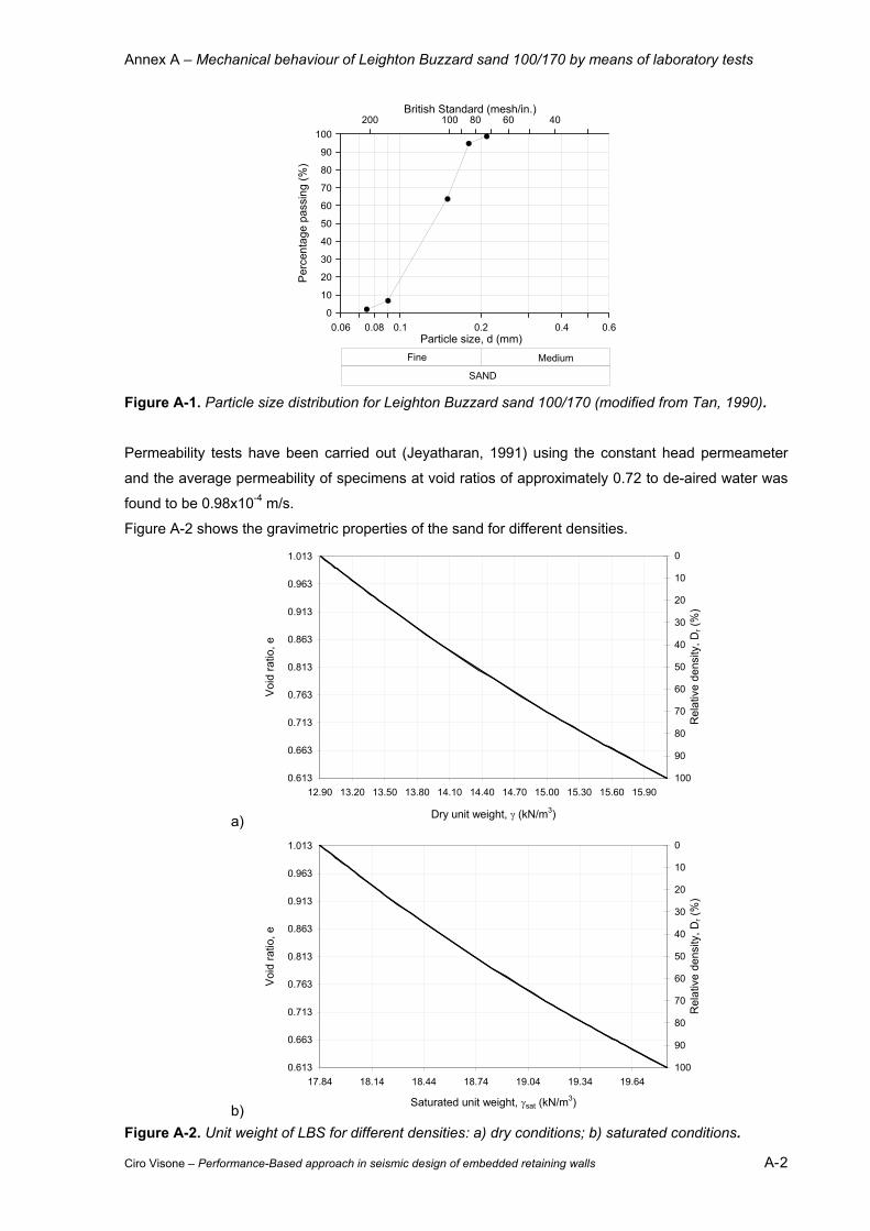
Annex A – Mechanical behaviour of Leighton Buzzard sand 100/170 by means of laboratory tests
Ciro Visone – Performance-Based approach in seismic design of embedded retaining walls A- 2
0.1 0.2 0.4 0.60.080.06Particle size, d (mm)
0
20
40
60
80
100
10
30
50
70
90
Per
cent
age
pass
ing
(%)
100200 80 60 40British Standard (mesh/in.)
Fine Medium
SAND Figure A-1. Particle size distribution for Leighton Buzzard sand 100/170 (modified from Tan, 1990).
Permeability tests have been carried out (Jeyatharan, 1991) using the constant head permeameter
and the average permeability of specimens at void ratios of approximately 0.72 to de-aired water was
found to be 0.98x10⁻⁴ m/s.
Figure A-2 shows the gravimetric properties of the sand for different densities.
a)
0.613
0.663
0.713
0.763
0.813
0.863
0.913
0.963
1.013
12.90 13.20 13.50 13.80 14.10 14.40 14.70 15.00 15.30 15.60 15.90
Dry unit weight, γ (kN/m3)
Voi
d ra
tio, e
0
10
20
30
40
50
60
70
80
90
100
Rel
ativ
e de
nsity
, Dr (
%)
b)
0.613
0.663
0.713
0.763
0.813
0.863
0.913
0.963
1.013
17.84 18.14 18.44 18.74 19.04 19.34 19.64
Saturated unit weight, γsat (kN/m3)
Voi
d ra
tio, e
0
10
20
30
40
50
60
70
80
90
100
Rel
ativ
e de
nsity
, Dr (
%)
Figure A-2. Unit weight of LBS for different densities: a) dry conditions; b) saturated conditions.
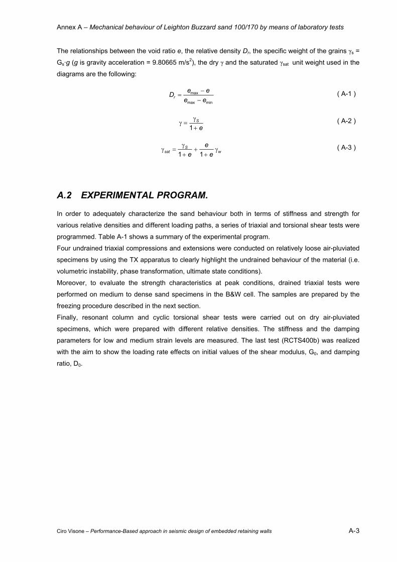
Annex A – Mechanical behaviour of Leighton Buzzard sand 100/170 by means of laboratory tests
Ciro Visone – Performance-Based approach in seismic design of embedded retaining walls A- 3
The relationships between the void ratio e, the relative density Dr, the specific weight of the grains γs =
Gs·g (g is gravity acceleration = 9.80665 m/s2), the dry γ and the saturated γsat unit weight used in the
diagrams are the following:
minmax
max
eeeeDr −
−= ( A-1 )
eS
+γ
=γ1
( A-2 )
wS
sat ee
eγ
++
+γ
=γ11
( A-3 )
A.2 EXPERIMENTAL PROGRAM.
In order to adequately characterize the sand behaviour both in terms of stiffness and strength for
various relative densities and different loading paths, a series of triaxial and torsional shear tests were
programmed. Table A-1 shows a summary of the experimental program.
Four undrained triaxial compressions and extensions were conducted on relatively loose air-pluviated
specimens by using the TX apparatus to clearly highlight the undrained behaviour of the material (i.e.
volumetric instability, phase transformation, ultimate state conditions).
Moreover, to evaluate the strength characteristics at peak conditions, drained triaxial tests were
performed on medium to dense sand specimens in the B&W cell. The samples are prepared by the
freezing procedure described in the next section.
Finally, resonant column and cyclic torsional shear tests were carried out on dry air-pluviated
specimens, which were prepared with different relative densities. The stiffness and the damping
parameters for low and medium strain levels are measured. The last test (RCTS400b) was realized
with the aim to show the loading rate effects on initial values of the shear modulus, G0, and damping
ratio, D0.
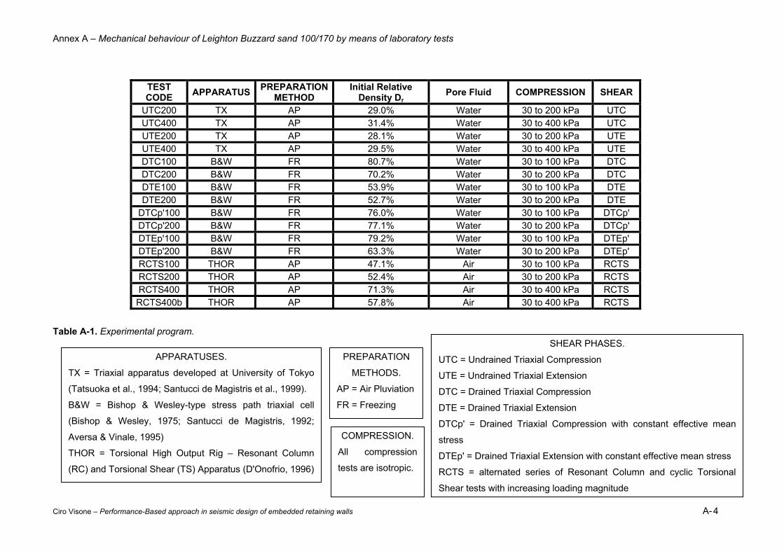
Annex A – Mechanical behaviour of Leighton Buzzard sand 100/170 by means of laboratory tests
Ciro Visone – Performance-Based approach in seismic design of embedded retaining walls A- 4
TEST CODE APPARATUS PREPARATION
METHOD Initial Relative
Density Dr Pore Fluid COMPRESSION SHEAR
UTC200 TX AP 29.0% Water 30 to 200 kPa UTC UTC400 TX AP 31.4% Water 30 to 400 kPa UTC UTE200 TX AP 28.1% Water 30 to 200 kPa UTE UTE400 TX AP 29.5% Water 30 to 400 kPa UTE DTC100 B&W FR 80.7% Water 30 to 100 kPa DTC DTC200 B&W FR 70.2% Water 30 to 200 kPa DTC DTE100 B&W FR 53.9% Water 30 to 100 kPa DTE DTE200 B&W FR 52.7% Water 30 to 200 kPa DTE
DTCp'100 B&W FR 76.0% Water 30 to 100 kPa DTCp' DTCp'200 B&W FR 77.1% Water 30 to 200 kPa DTCp' DTEp'100 B&W FR 79.2% Water 30 to 100 kPa DTEp' DTEp'200 B&W FR 63.3% Water 30 to 200 kPa DTEp' RCTS100 THOR AP 47.1% Air 30 to 100 kPa RCTS RCTS200 THOR AP 52.4% Air 30 to 200 kPa RCTS RCTS400 THOR AP 71.3% Air 30 to 400 kPa RCTS RCTS400b THOR AP 57.8% Air 30 to 400 kPa RCTS
Table A-1. Experimental program.
APPARATUSES.
TX = Triaxial apparatus developed at University of Tokyo
(Tatsuoka et al., 1994; Santucci de Magistris et al., 1999).
B&W = Bishop & Wesley-type stress path triaxial cell
(Bishop & Wesley, 1975; Santucci de Magistris, 1992;
Aversa & Vinale, 1995)
THOR = Torsional High Output Rig – Resonant Column
(RC) and Torsional Shear (TS) Apparatus (D'Onofrio, 1996)
PREPARATION
METHODS.
AP = Air Pluviation
FR = Freezing
SHEAR PHASES.
UTC = Undrained Triaxial Compression
UTE = Undrained Triaxial Extension
DTC = Drained Triaxial Compression
DTE = Drained Triaxial Extension
DTCp' = Drained Triaxial Compression with constant effective mean
stress
DTEp' = Drained Triaxial Extension with constant effective mean stress
RCTS = alternated series of Resonant Column and cyclic Torsional
Shear tests with increasing loading magnitude
COMPRESSION.
All compression
tests are isotropic.
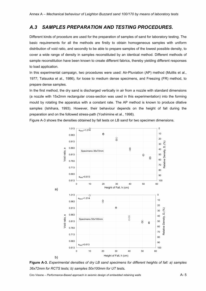
Annex A – Mechanical behaviour of Leighton Buzzard sand 100/170 by means of laboratory tests
Ciro Visone – Performance-Based approach in seismic design of embedded retaining walls A- 5
A.3 SAMPLES PREPARATION AND TESTING PROCEDURES.
Different kinds of procedure are used for the preparation of samples of sand for laboratory testing. The
basic requirements for all the methods are firstly to obtain homogeneous samples with uniform
distribution of void ratio, and secondly to be able to prepare samples of the lowest possible density, to
cover a wide range of density in samples reconstituted by an identical method. Different methods of
sample reconstitution have been known to create different fabrics, thereby yielding different responses
to load application.
In this experimental campaign, two procedures were used: Air-Pluviation (AP) method (Mulilis et al.,
1977; Tatsuoka et al., 1986), for loose to medium dense specimens, and Freezing (FR) method, to
prepare dense samples.
In the first method, the dry sand is discharged vertically in air from a nozzle with standard dimensions
(a nozzle with 15x2mm rectangular cross-section was used in this experimentation) into the forming
mould by rotating the apparatus with a constant rate. The AP method is known to produce dilative
samples (Ishihara, 1993). However, their behaviour depends on the height of fall during the
preparation and on the followed stress-path (Yoshimine et al., 1998).
Figure A-3 shows the densities obtained by fall tests on LB sand for two specimen dimensions.
a)
Specimens 36x72mm
0.613
0.663
0.713
0.763
0.813
0.863
0.913
0.963
1.013
0 10 20 30 40 50 60Height of Fall, h (cm)
Void
ratio
, e
0
10
20
30
40
50
60
70
80
90
100
Rel
ativ
e D
ensi
ty, D
r (%
)
eMIN=0.613
eMAX=1.014
b)
Specimens 50x100mm
0.613
0.663
0.713
0.763
0.813
0.863
0.913
0.963
1.013
0 10 20 30 40 50 60
Height of Fall, h (cm)
Void
ratio
, e
0
10
20
30
40
50
60
70
80
90
100
Rel
ativ
e D
ensi
ty, D
r (%
)
eMIN=0.613
eMAX=1.014
Figure A-3. Experimental densities of dry LB sand specimens for different heights of fall: a) samples
36x72mm for RCTS tests; b) samples 50x100mm for UT tests.
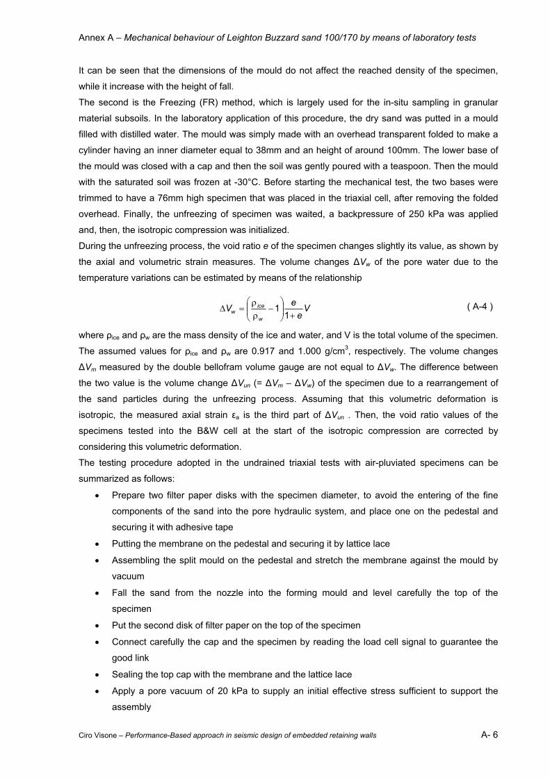
Annex A – Mechanical behaviour of Leighton Buzzard sand 100/170 by means of laboratory tests
Ciro Visone – Performance-Based approach in seismic design of embedded retaining walls A- 6
It can be seen that the dimensions of the mould do not affect the reached density of the specimen,
while it increase with the height of fall.
The second is the Freezing (FR) method, which is largely used for the in-situ sampling in granular
material subsoils. In the laboratory application of this procedure, the dry sand was putted in a mould
filled with distilled water. The mould was simply made with an overhead transparent folded to make a
cylinder having an inner diameter equal to 38mm and an height of around 100mm. The lower base of
the mould was closed with a cap and then the soil was gently poured with a teaspoon. Then the mould
with the saturated soil was frozen at -30°C. Before starting the mechanical test, the two bases were
trimmed to have a 76mm high specimen that was placed in the triaxial cell, after removing the folded
overhead. Finally, the unfreezing of specimen was waited, a backpressure of 250 kPa was applied
and, then, the isotropic compression was initialized.
During the unfreezing process, the void ratio e of the specimen changes slightly its value, as shown by
the axial and volumetric strain measures. The volume changes ∆Vw of the pore water due to the
temperature variations can be estimated by means of the relationship
Ve
eVw
icew +
−
ρρ
=∆1
1 ( A-4 )
where ρice and ρw are the mass density of the ice and water, and V is the total volume of the specimen.
The assumed values for ρice and ρw are 0.917 and 1.000 g/cm3, respectively. The volume changes
∆Vm measured by the double bellofram volume gauge are not equal to ∆Vw. The difference between
the two value is the volume change ∆Vun (= ∆Vm – ∆Vw) of the specimen due to a rearrangement of
the sand particles during the unfreezing process. Assuming that this volumetric deformation is
isotropic, the measured axial strain εa is the third part of ∆Vun . Then, the void ratio values of the
specimens tested into the B&W cell at the start of the isotropic compression are corrected by
considering this volumetric deformation.
The testing procedure adopted in the undrained triaxial tests with air-pluviated specimens can be
summarized as follows:
• Prepare two filter paper disks with the specimen diameter, to avoid the entering of the fine
components of the sand into the pore hydraulic system, and place one on the pedestal and
securing it with adhesive tape
• Putting the membrane on the pedestal and securing it by lattice lace
• Assembling the split mould on the pedestal and stretch the membrane against the mould by
vacuum
• Fall the sand from the nozzle into the forming mould and level carefully the top of the
specimen
• Put the second disk of filter paper on the top of the specimen
• Connect carefully the cap and the specimen by reading the load cell signal to guarantee the
good link
• Sealing the top cap with the membrane and the lattice lace
• Apply a pore vacuum of 20 kPa to supply an initial effective stress sufficient to support the
assembly

Annex A – Mechanical behaviour of Leighton Buzzard sand 100/170 by means of laboratory tests
Ciro Visone – Performance-Based approach in seismic design of embedded retaining walls A- 7
• Remove the mould
• Measure the sample dimensions
• Assemble and fill the cell with water
• Adjust the axial strain transducers (Gap sensor and LVDT)
• Apply a cell pressure of 20 kPa reducing in the same time the pore vacuum to have a constant
effective mean stress acting on the specimen
• Start with the flushing procedure to saturate the specimen.
The saturation procedure used in these experiments is constituted by a combination of vacuuming,
flushing with distilled water, time lag and back pressurization (250 kPa) in a procedure called “Dry
Setting Method” (Ampadu and Tatsuoka, 1989).
For dry specimens tested with the THOR apparatus, the preparation technique is the same of that
previously exposed for undrained tests till to the saturation process.
A.4 STIFFNESS OF SAND.
During the RCTS and UT tests, the stiffness properties of sand were investigated. In this section the
results are shown.
It should be underlined that the configuration of the THOR apparatus for tests on dry sand does not
permit the measurement of the volume changes of specimen. To provide these information, the
volumetric strains during the isotropic compressions were assumed isotropic. The radial strain εr was
taken equal to the axial strain εa measured by means of LVDT. During the torsional shear phases, the
radial strain was fixed to be zero and, then, the volumetric strains are equal to the axial strains.
Another aspect should be highlighted on the elaboration of the experimental measurements deriving
from cyclic torsional shear tests. The measured stress-strain loops at low strain levels (γ < 10-3%)
were reconstructed by interpolating the stress τ(t) and strain γ(t) time histories by means of sinusoidal
laws and taking the data calculated from the elaboration. This allows avoiding the data scattering due
to the electrical noises of the acquired signals. The stiffness parameters at intermediate strain levels
(10-3% < γ < 10-2%) were defined as the mean values registered during the loading cycles and, finally,
at high strain levels (γ > 10-2%), the data were referred to the first cycle.
A.4.1 Evolution of elastic properties with mean effective stress.
During the isotropic compressions of the RCTS specimens, resonant column tests at low strains were
performed to describe the evolution of the elastic stiffness, both in terms of initial shear modulus G0
and the shear wave velocity VS, and damping properties of sand with the mean effective stress p'. The
measured values are plotted in Figure A-4. The damping ratios were evaluated by the resonance
factor method. It can be seen the larger dispersion of the shear modulus data than the shear wave
velocity. This is due to the effect of the different relative densities of the specimens on G0 and VS.
Remembering the following relationship for an elastic medium:
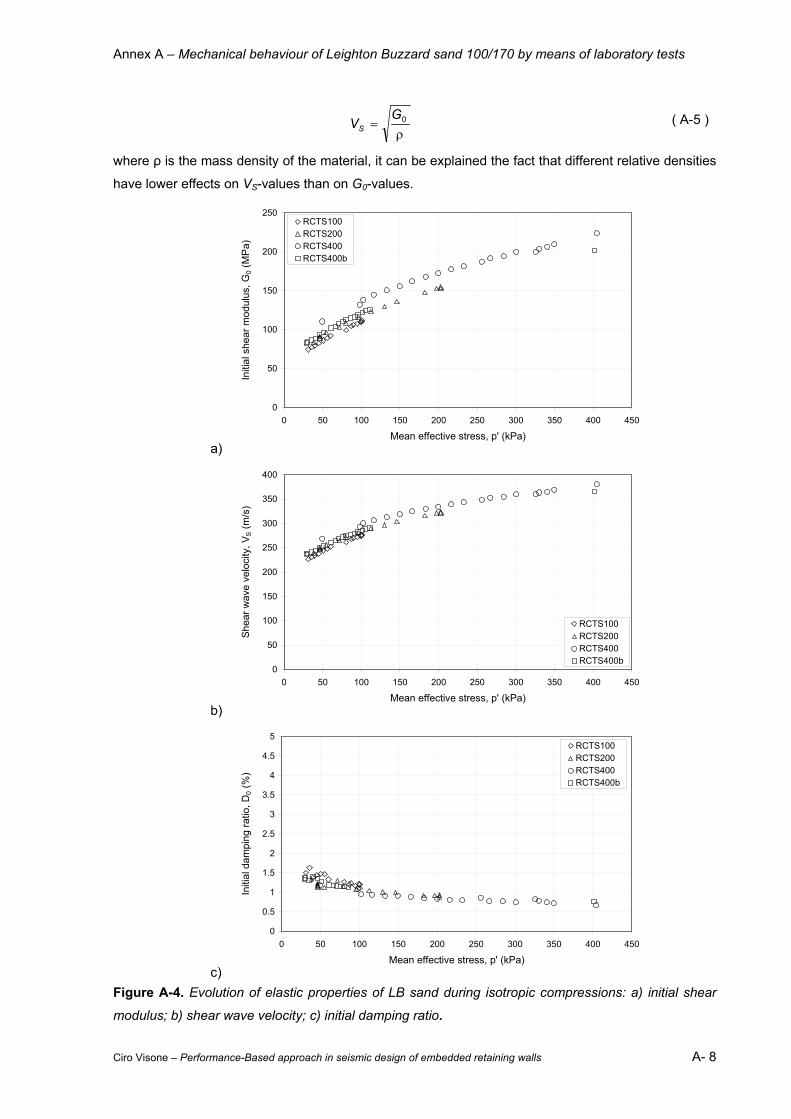
Annex A – Mechanical behaviour of Leighton Buzzard sand 100/170 by means of laboratory tests
Ciro Visone – Performance-Based approach in seismic design of embedded retaining walls A- 8
ρ= 0G
VS ( A-5 )
where ρ is the mass density of the material, it can be explained the fact that different relative densities
have lower effects on VS-values than on G0-values.
a)
0
50
100
150
200
250
0 50 100 150 200 250 300 350 400 450
Mean effective stress, p' (kPa)
Initi
al s
hear
mod
ulus
, G0 (
MP
a)
RCTS100RCTS200RCTS400RCTS400b
b)
0
50
100
150
200
250
300
350
400
0 50 100 150 200 250 300 350 400 450
Mean effective stress, p' (kPa)
Shea
r wav
e ve
loci
ty, V
S (m
/s)
RCTS100RCTS200RCTS400RCTS400b
c)
0
0.5
1
1.5
2
2.5
3
3.5
4
4.5
5
0 50 100 150 200 250 300 350 400 450
Mean effective stress, p' (kPa)
Initi
al d
ampi
ng ra
tio, D
0 (%
)
RCTS100RCTS200RCTS400RCTS400b
Figure A-4. Evolution of elastic properties of LB sand during isotropic compressions: a) initial shear
modulus; b) shear wave velocity; c) initial damping ratio.
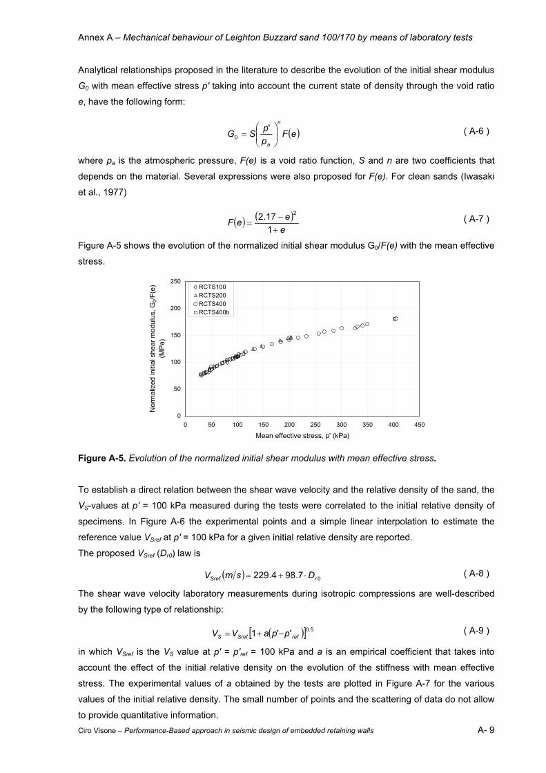
Annex A – Mechanical behaviour of Leighton Buzzard sand 100/170 by means of laboratory tests
Ciro Visone – Performance-Based approach in seismic design of embedded retaining walls A- 9
Analytical relationships proposed in the literature to describe the evolution of the initial shear modulus
G0 with mean effective stress p' taking into account the current state of density through the void ratio
e, have the following form:
( )eFppSG
n
a
=
'0 ( A-6 )
where pa is the atmospheric pressure, F(e) is a void ratio function, S and n are two coefficients that
depends on the material. Several expressions were also proposed for F(e). For clean sands (Iwasaki
et al., 1977)
( ) ( )eeeF
+−
=117.2 2
( A-7 )
Figure A-5 shows the evolution of the normalized initial shear modulus G0/F(e) with the mean effective
stress.
0
50
100
150
200
250
0 50 100 150 200 250 300 350 400 450
Mean effective stress, p' (kPa)
Nor
mal
ized
initi
al s
hear
mod
ulus
, G0/F
(e)
(MP
a)
RCTS100RCTS200RCTS400RCTS400b
Figure A-5. Evolution of the normalized initial shear modulus with mean effective stress.
To establish a direct relation between the shear wave velocity and the relative density of the sand, the
VS-values at p' = 100 kPa measured during the tests were correlated to the initial relative density of
specimens. In Figure A-6 the experimental points and a simple linear interpolation to estimate the
reference value VSref at p' = 100 kPa for a given initial relative density are reported.
The proposed VSref (Dr0) law is
( ) 07.984.229 rSref DsmV ⋅+= ( A-8 )
The shear wave velocity laboratory measurements during isotropic compressions are well-described
by the following type of relationship:
( )[ ] 5.0''1 refSrefS ppaVV −+= ( A-9 )
in which VSref is the VS value at p' = p'ref = 100 kPa and a is an empirical coefficient that takes into
account the effect of the initial relative density on the evolution of the stiffness with mean effective
stress. The experimental values of a obtained by the tests are plotted in Figure A-7 for the various
values of the initial relative density. The small number of points and the scattering of data do not allow
to provide quantitative information.
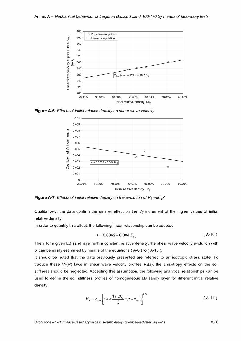
Annex A – Mechanical behaviour of Leighton Buzzard sand 100/170 by means of laboratory tests
Ciro Visone – Performance-Based approach in seismic design of embedded retaining walls A- 10
200
220
240
260
280
300
320
340
360
380
400
20.00% 30.00% 40.00% 50.00% 60.00% 70.00% 80.00%
Initial relative density, Dr0
Shea
r wav
e ve
loci
ty a
t p'=
100
kPa,
VSr
ef
(m/s
)
Experimental pointsLinear interpolation
VSref (m/s) = 229.4 + 98.7 Dr0
Figure A-6. Effects of initial relative density on shear wave velocity.
0
0.001
0.002
0.003
0.004
0.005
0.006
0.007
0.008
0.009
0.01
20.00% 30.00% 40.00% 50.00% 60.00% 70.00% 80.00%
Initial relative density, Dr0
Coe
ffici
ent o
f VS
incr
emen
t, a
a = 0.0062 - 0.004 Dr0
Figure A-7. Effects of initial relative density on the evolution of VS with p'.
Qualitatively, the data confirm the smaller effect on the VS increment of the higher values of initial
relative density.
In order to quantify this effect, the following linear relationship can be adopted:
0004.00062.0 rDa −= ( A-10 )
Then, for a given LB sand layer with a constant relative density, the shear wave velocity evolution with
p' can be easily estimated by means of the equations ( A-8 ) to ( A-10 ).
It should be noted that the data previously presented are referred to an isotropic stress state. To
traduce these VS(p') laws in shear wave velocity profiles VS(z), the anisotropy effects on the soil
stiffness should be neglected. Accepting this assumption, the following analytical relationships can be
used to define the soil stiffness profiles of homogeneous LB sandy layer for different initial relative
density.
( )5.0
0
321
1
−γ
++= refSrefS zz
kaVV ( A-11 )

Annex A – Mechanical behaviour of Leighton Buzzard sand 100/170 by means of laboratory tests
Ciro Visone – Performance-Based approach in seismic design of embedded retaining walls A- 11
where k0 is the earth pressure coefficient at rest, γ is the unit weight of sand, VSref and a can be
estimated by means of equations ( A-8 ) and ( A-10 ), and
0213'
kp
z refref +γ
= ( A-12 )
The dependence of k0 on relative density of sands is not so clear as for the cohesive materials.
Jamiolkowski et al. (1985) report the k0-values of different sand specimens measured in calibration
camera at the end of the consolidation phase. The results are enough scattered but show a slight
reduction of k0 when Dr increases. However, for relative densities comprises between the range
20÷80%, k0 can be assumed equal to 0.5.
The empirical relationships proposed in the literature to describe the evolution of the initial damping
ratio D0 with the mean effective stress p' have the following form:
nref pDD −⋅= '00 ( A-13 )
where D0ref and n are two coefficients that should be determined with advanced laboratory tests (e.g.,
resonant column tests). This analytical forms conduct to high values of initial damping ratio for low
values of p'. In the view to define initial damping ratio profiles D0(z), the laboratory data obtained on
the LB sand, were interpolated with the following expressions:
+=
+=
−−refref zzn
refp
pn
ref eDeDD 11 0'
'
00 ( A-14 )
D0ref represents the half-value of the initial damping ratio near to the surface, n expresses the
heterogeneity of the layer and p'ref = 100 kPa is the reference pressure. This type of relationship allows
predicting more reasonable D0-values for the shallow depths of LB sandy deposits.
The experimental data interpolation and the coefficients D0ref and n are shown Figure A-8
0.00%
0.50%
1.00%
1.50%
2.00%
2.50%
3.00%
3.50%
4.00%
4.50%
5.00%
0 50 100 150 200 250 300 350 400 450
Mean effective stress, p' (kPa)
Initi
al d
ampi
ng ra
tio, D
0
RCTS100RCTS200RCTS400RCTS400bInterpolation
D0 = D0ref (1 + exp(-n p'/p'ref))D0ref = 0.008
n = 1.2
Figure A-8. Analytical interpolation of the evolution of initial damping ratio with mean effective stress.
The initial damping ratio profiles of sandy layer characterized by a uniform relative density can be then
described by means of ( A-14 ) assuming D0ref = 0.008 and n = 1.2.
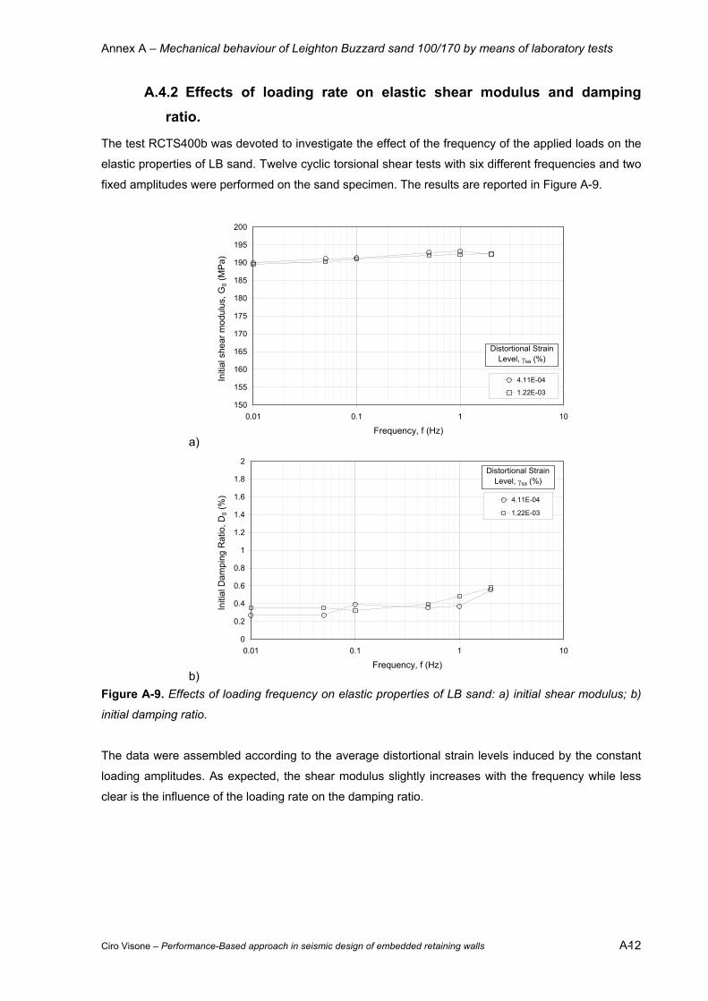
Annex A – Mechanical behaviour of Leighton Buzzard sand 100/170 by means of laboratory tests
Ciro Visone – Performance-Based approach in seismic design of embedded retaining walls A- 12
A.4.2 Effects of loading rate on elastic shear modulus and damping ratio.
The test RCTS400b was devoted to investigate the effect of the frequency of the applied loads on the
elastic properties of LB sand. Twelve cyclic torsional shear tests with six different frequencies and two
fixed amplitudes were performed on the sand specimen. The results are reported in Figure A-9.
a)
150
155
160
165
170
175
180
185
190
195
200
0.01 0.1 1 10
Frequency, f (Hz)
Initi
al s
hear
mod
ulus
, G0 (
MPa
)
4.11E-04
1.22E-03
Distortional Strain Level, γsa (%)
b)
0
0.2
0.4
0.6
0.8
1
1.2
1.4
1.6
1.8
2
0.01 0.1 1 10
Frequency, f (Hz)
Initi
al D
ampi
ng R
atio
, D0 (
%) 4.11E-04
1.22E-03
Distortional Strain Level, γsa (%)
Figure A-9. Effects of loading frequency on elastic properties of LB sand: a) initial shear modulus; b)
initial damping ratio.
The data were assembled according to the average distortional strain levels induced by the constant
loading amplitudes. As expected, the shear modulus slightly increases with the frequency while less
clear is the influence of the loading rate on the damping ratio.
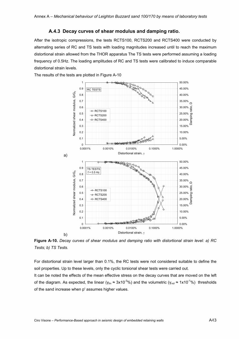
Annex A – Mechanical behaviour of Leighton Buzzard sand 100/170 by means of laboratory tests
Ciro Visone – Performance-Based approach in seismic design of embedded retaining walls A- 13
A.4.3 Decay curves of shear modulus and damping ratio.
After the isotropic compressions, the tests RCTS100, RCTS200 and RCTS400 were conducted by
alternating series of RC and TS tests with loading magnitudes increased until to reach the maximum
distortional strain allowed from the THOR apparatus The TS tests were performed assuming a loading
frequency of 0.5Hz. The loading amplitudes of RC and TS tests were calibrated to induce comparable
distortional strain levels.
The results of the tests are plotted in Figure A-10
a)
0
0.1
0.2
0.3
0.4
0.5
0.6
0.7
0.8
0.9
1
0.0001% 0.0010% 0.0100% 0.1000% 1.0000%
Distortional strain, γ
Nor
mal
ized
she
ar m
odul
us, G
/G0
0.00%
5.00%
10.00%
15.00%
20.00%
25.00%
30.00%
35.00%
40.00%
45.00%
50.00%
Dam
ping
ratio
, D
RCTS100RCTS200RCTS400
RC TESTS
b)
0
0.1
0.2
0.3
0.4
0.5
0.6
0.7
0.8
0.9
1
0.0001% 0.0010% 0.0100% 0.1000% 1.0000%
Distortional strain, γ
Nor
mal
ized
she
ar m
odul
us, G
/G0
0.00%
5.00%
10.00%
15.00%
20.00%
25.00%
30.00%
35.00%
40.00%
45.00%
50.00%
Dam
ping
ratio
, DRCTS100RCTS200RCTS400
TS TESTSf = 0.5 Hz
Figure A-10. Decay curves of shear modulus and damping ratio with distortional strain level: a) RC
Tests; b) TS Tests.
For distortional strain level larger than 0.1%, the RC tests were not considered suitable to define the
soil properties. Up to these levels, only the cyclic torsional shear tests were carried out.
It can be noted the effects of the mean effective stress on the decay curves that are moved on the left
of the diagram. As expected, the linear (γlin ≈ 3x10⁻³%) and the volumetric (γvol ≈ 1x10⁻¹%) thresholds
of the sand increase when p' assumes higher values.

Annex A – Mechanical behaviour of Leighton Buzzard sand 100/170 by means of laboratory tests
Ciro Visone – Performance-Based approach in seismic design of embedded retaining walls A- 14
A.5 STRENGTH OF SAND.
The strength of the sand was also investigated by means of several triaxial tests with two
apparatuses. The tests, both in drained and undrained conditions, were performed following various
stress-paths and starting from different mean effective stress. In this section, the experimental results
are presented.
A.5.1 Undrained triaxial tests (UTC and UTE).
Four triaxial tests, two in compression and two in extension, were carried out on relatively loose air-
pluviated specimens. Before to conduct the undrained shear phases, the samples were isotropically
compressed till to 200 and 400 kPa. During these phases, the volumetric strains can not be measured.
The current states of the specimens are defined by assuming an isotropic deformation (εr = εa).
The tests results are plotted in Figure A-11. By conducting this type of test on loose specimens, it has
been possible to clearly recognize the phase transformation of the sand, in which the behaviour from
contractive becomes dilative (maximum excess pore pressures condition). Greater difficulties have
been encountered for the definition of the critical state conditions (stabilization of the excess of pore
pressures). In fact, for reached distortional strain εq = εa ( ≈ 15÷20%), the steady state conditions are
not observed in the tests. Up to these levels of strains the specimens are not cylindrical and
uncertainties arise on stress and strain evaluations.
An interesting aspects shown by the data is the more contractive behaviour registered during the
triaxial extensions respect to the compressions. In correspondence of the maximum ratio q/p' before
the phase transformation, it can be read the volumetric instability condition (Castro, 1969). These
results agree with those obtained by Yoshimine et al. (1998) that attribute these effects to the direction
of the principal stress relative to the layered structure of soil and to the magnitude of the intermediate
principal stress.
A.5.2 Drained triaxial tests (DTC and UTE, DTCp’ and DTEp’).
To investigate the peak strength of the sand, eight drained triaxial tests were performed by using the
B&W apparatus. The dense samples were prepared with the freezing technique, as previously
described. After the isotropic compressions, the drained shear phases, both in compression and in
extension, were conducted by increasing and decreasing the axial stress, respectively.
Figure A-12 reports the results of all drained tests. As observed in undrained conditions, for similar
values of the relative density, the sand behaviour is more dilative in triaxial compressions than in
extensions.
In these tests, the phase transformation can be identified to the condition at which the dilatancy is
zero. The variations of volumetric strains change the sign becoming negative.
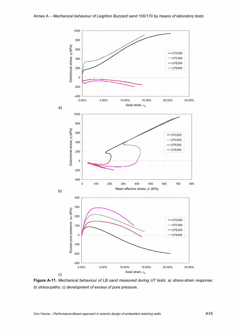
Annex A – Mechanical behaviour of Leighton Buzzard sand 100/170 by means of laboratory tests
Ciro Visone – Performance-Based approach in seismic design of embedded retaining walls A- 15
a)
-400
-200
0
200
400
600
800
1000
0.00% 5.00% 10.00% 15.00% 20.00% 25.00%
Axial strain, εa
Dis
torti
onal
stre
ss, q
(kP
a)
UTC200
UTC400
UTE200
UTE400
b)
-400
-200
0
200
400
600
800
1000
0 100 200 300 400 500 600 700 800
Mean effective stress, p' (kPa)
Dis
torti
onal
stre
ss, q
(kP
a)
UTC200
UTC400
UTE200
UTE400
c)
-300
-200
-100
0
100
200
300
400
0.00% 5.00% 10.00% 15.00% 20.00% 25.00%
Axial strain, εa
Exce
ss p
ore
pres
sure
, ∆u
(kP
a)
UTC200
UTC400
UTE200
UTE400
Figure A-11. Mechanical behaviour of LB sand measured during UT tests: a) stress-strain response;
b) stress-paths; c) development of excess of pore pressure.
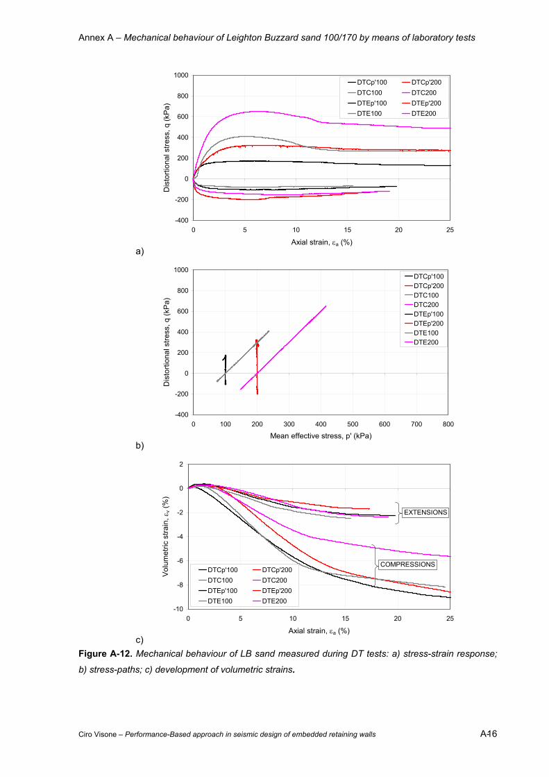
Annex A – Mechanical behaviour of Leighton Buzzard sand 100/170 by means of laboratory tests
Ciro Visone – Performance-Based approach in seismic design of embedded retaining walls A- 16
a)
-400
-200
0
200
400
600
800
1000
0 5 10 15 20 25
Axial strain, εa (%)
Dis
torti
onal
stre
ss, q
(kP
a)
DTCp'100 DTCp'200DTC100 DTC200DTEp'100 DTEp'200DTE100 DTE200
b)
-400
-200
0
200
400
600
800
1000
0 100 200 300 400 500 600 700 800
Mean effective stress, p' (kPa)
Dis
torti
onal
stre
ss, q
(kP
a)
DTCp'100DTCp'200DTC100DTC200DTEp'100DTEp'200DTE100DTE200
c)
-10
-8
-6
-4
-2
0
2
0 5 10 15 20 25
Axial strain, εa (%)
Volu
met
ric s
train
, εv (
%)
DTCp'100 DTCp'200DTC100 DTC200DTEp'100 DTEp'200DTE100 DTE200
EXTENSIONS
COMPRESSIONS
Figure A-12. Mechanical behaviour of LB sand measured during DT tests: a) stress-strain response;
b) stress-paths; c) development of volumetric strains.
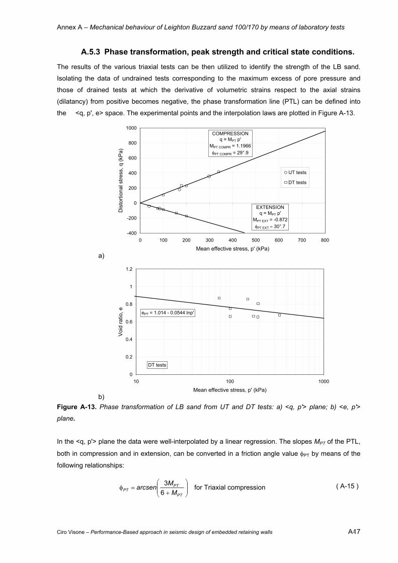
Annex A – Mechanical behaviour of Leighton Buzzard sand 100/170 by means of laboratory tests
Ciro Visone – Performance-Based approach in seismic design of embedded retaining walls A- 17
A.5.3 Phase transformation, peak strength and critical state conditions.
The results of the various triaxial tests can be then utilized to identify the strength of the LB sand.
Isolating the data of undrained tests corresponding to the maximum excess of pore pressure and
those of drained tests at which the derivative of volumetric strains respect to the axial strains
(dilatancy) from positive becomes negative, the phase transformation line (PTL) can be defined into
the <q, p', e> space. The experimental points and the interpolation laws are plotted in Figure A-13.
a)
-400
-200
0
200
400
600
800
1000
0 100 200 300 400 500 600 700 800
Mean effective stress, p' (kPa)
Dis
torti
onal
stre
ss, q
(kP
a)
UT tests
DT tests
COMPRESSIONq = MPT p'
MPT COMPR = 1.1966φPT COMPR = 29°.9
EXTENSIONq = MPT p'
MPT EXT = -0.872φPT EXT = 30°.7
b)
0
0.2
0.4
0.6
0.8
1
1.2
10 100 1000
Mean effective stress, p' (kPa)
Voi
d ra
tio, e ePT = 1.014 - 0.0544 lnp'
DT tests
Figure A-13. Phase transformation of LB sand from UT and DT tests: a) <q, p'> plane; b) <e, p'>
plane.
In the <q, p'> plane the data were well-interpolated by a linear regression. The slopes MPT of the PTL,
both in compression and in extension, can be converted in a friction angle value φPT by means of the
following relationships:
+
=φPT
PTPT M
Marcsen63 for Triaxial compression ( A-15 )

Annex A – Mechanical behaviour of Leighton Buzzard sand 100/170 by means of laboratory tests
Ciro Visone – Performance-Based approach in seismic design of embedded retaining walls A- 18
−
=φPT
PTPT M
Marcsen63 for Triaxial extension ( A-16 )
The values of φPT and MPT for triaxial compression and extension conditions obtained by the linear
regression are given in Figure A-13a.
The data shown in the <e, p'> plane, referred only to the drained tests, are very scattered. This is due
to the difficulties to rightly estimate the void ratio evolution during the tests for the low capacities of the
measurement systems adopted for the volume changes evaluation. However, a logarithmic regression
of data was reported in Figure A-13b. The interpolation was done by fixing the constant value as the
maximum void ratio (emax = 1.014) of LB sand. The slope of the PTL is λPT = 0.0469.
The drained triaxial tests performed on the dense samples of the LB sand have allowed defining the
strength at peak for relative densities varying in the range of 60÷80%.
Figure A-14 shows the experimental data and the interpolations.
a)
-400
-200
0
200
400
600
800
1000
0 100 200 300 400 500 600 700 800
Mean effective stress, p' (kPa)
Dis
torti
onal
stre
ss, q
(kP
a) COMPRESSIONq = MPC COMPR p'
MPC COMPR = 1.6084φPC COMPR = 39°.4
EXTENSIONq = MPC EXT p'
MPC EXT = -1.0188φPC EXT = 37°.8
DT tests
b)
0
0.2
0.4
0.6
0.8
1
1.2
10 100 1000
Mean effective stress, p' (kPa)
Voi
d ra
tio, e ePC = 0.9976 - 0.0489 lnp'
DT tests
Figure A-14. Peak strength of LB sand measured in DT tests on dense samples (Dr = 60÷80%): a)
<q, p'> plane; b) <e, p'> plane.
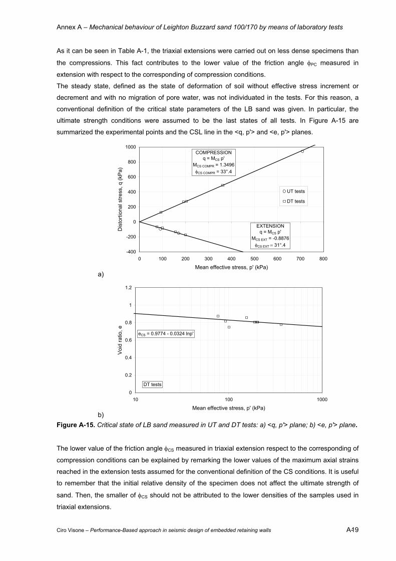
Annex A – Mechanical behaviour of Leighton Buzzard sand 100/170 by means of laboratory tests
Ciro Visone – Performance-Based approach in seismic design of embedded retaining walls A- 19
As it can be seen in Table A-1, the triaxial extensions were carried out on less dense specimens than
the compressions. This fact contributes to the lower value of the friction angle φPC measured in
extension with respect to the corresponding of compression conditions.
The steady state, defined as the state of deformation of soil without effective stress increment or
decrement and with no migration of pore water, was not individuated in the tests. For this reason, a
conventional definition of the critical state parameters of the LB sand was given. In particular, the
ultimate strength conditions were assumed to be the last states of all tests. In Figure A-15 are
summarized the experimental points and the CSL line in the <q, p'> and <e, p'> planes.
a)
-400
-200
0
200
400
600
800
1000
0 100 200 300 400 500 600 700 800
Mean effective stress, p' (kPa)
Dis
torti
onal
stre
ss, q
(kP
a)
UT tests
DT tests
COMPRESSIONq = MCS p'
MCS COMPR = 1.3496φCS COMPR = 33°.4
EXTENSIONq = MCS p'
MCS EXT = -0.8876φCS EXT = 31°.4
b)
0
0.2
0.4
0.6
0.8
1
1.2
10 100 1000
Mean effective stress, p' (kPa)
Voi
d ra
tio, e
eCS = 0.9774 - 0.0324 lnp'
DT tests
Figure A-15. Critical state of LB sand measured in UT and DT tests: a) <q, p'> plane; b) <e, p'> plane.
The lower value of the friction angle φCS measured in triaxial extension respect to the corresponding of
compression conditions can be explained by remarking the lower values of the maximum axial strains
reached in the extension tests assumed for the conventional definition of the CS conditions. It is useful
to remember that the initial relative density of the specimen does not affect the ultimate strength of
sand. Then, the smaller of φCS should not be attributed to the lower densities of the samples used in
triaxial extensions.
Annex A – Mechanical behaviour of Leighton Buzzard sand 100/170 by means of laboratory tests
Ciro Visone – Performance-Based approach in seismic design of embedded retaining walls A- 20
Having identified the critical state (φCS) and the peak strength (φPC) corresponding to relative densities
of about 75% and assuming a linear dependence of the peak friction angle from Dr, the following
relationships can be used to determine the strength parameters of the LB sand in relation to the
relative density.
rCSPC D⋅+φ=φ 10 ( A-17 )
8.0CSPC
PCφ−φ
=ψ ( A-18 )
The ( A-18 ) represents the inverse form of the empirical relationship between the maximum friction
angle (φMAX) exhibited by the soil, the critical friction angle (φCS) and the dilatancy angle ψ proposed by
Bolton (1986).
A conservative value of the critical friction angle is φCS = 32° that agrees with the estimation of Tan
(1990).
In Table A-2 the strength parameters of the LB sand estimated by the triaxial tests for different states
are summarized.
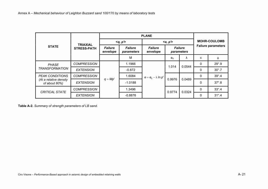
Annex A – Mechanical behaviour of Leighton Buzzard sand 100/170 by means of laboratory tests
Ciro Visone – Performance-Based approach in seismic design of embedded retaining walls A- 21
PLANE
<q, p'> <e, p'>
Failure envelope
Failure parameters
Failure envelope
Failure parameters
MOHR-COULOMB Failure parameters STATE TRIAXIAL
STRESS-PATH
M e0 λ c φ
COMPRESSION 1.1966 0 29°.9 PHASE TRANSFORMATION EXTENSION -0.872
1.014 0.0544 0 30°.7
COMPRESSION 1.6084 0 39°.4 PEAK CONDITIONS (At a relative density
of about 80%) EXTENSION -1.0188 0.9976 0.0489
0 37°.8
COMPRESSION 1.3496 0 33°.4 CRITICAL STATE
EXTENSION
'Mpq =
-0.8876
'ln0 pee λ−=
0.9774 0.0324 0 31°.4
Table A-2. Summary of strength parameters of LB sand.
Annex B – Calibration of FE models for dynamic analyses in geotechnical earthquake engineering
Ciro Visone – Performance-Based approach in seismic design of embedded retaining walls B-1
ANNEX B CALIBRATION OF FE MODELS FOR DYNAMIC ANALYSES IN GEOTECHNICAL EARTHQUAKE ENGINEERING.
Dynamic interaction problems involve the determination of the response of a structure placed in a
seismic environment created by an earthquake or some other source such as vibrating machine
foundation. Such an environment is defined in terms of free field motion prior to placement of the
structure. The spatial and the temporal variation of the free field motion used as input must be such
that they satisfy the equations of motions for the free field. They may be obtained from a site response
analysis. Thus, a free field solution must be available before a true interaction problem can be solved
(Lysmer, 1978).
Numerical methods is often adopted to predict the behaviour of the geotechnical systems (e.g.
retaining walls, pile foundations, embankments, dams) under seismic loadings, both for scientific and
practical applications.
Dynamic finite element analyses can be considered one of the most complete available tools in
geotechnical earthquake engineering for their capabilities to provide indications on the soil stress
distribution and deformation/displacements and on the forces acting on the structural elements that
interact with the ground (PIANC, 2001). However, they require at least a proper soil constitutive
model, an adequate soil characterization by means of in situ and laboratory tests and a proper
definition of the seismic input. The response of a finite element model is also conditioned by the
setting of several parameters influencing the sources of energy dissipation in time-domain analyses.
The amount of damping shown by a discrete numerical system is determined by the choice of the
constitutive model (material damping), the integration scheme of the equations (numerical damping),
and the boundary conditions. Material damping models the effects of viscous and hysteretic energy
dissipations in the soils; numerical damping appears as a consequence of the numerical algorithm of
solution of the dynamic equilibrium in the time domain; boundary conditions affect the way in which the
numerical model transmits the specific energy of the stress waves outside the domain.
Lists of widespread computer codes used to perform 1-D seismic site response analyses are reported
by several authors (EPRI, 1991; Kramer, 1996; Lanzo, 2005).
The influence of the sources of damping on the seismic response of a soil layer has been investigated
in this chapter.
A series of dynamic analyses of the vertical propagation of S-waves in a homogeneous elastic layer
was carried out. This scheme was chosen because a well-known theoretical solution of the problem is
available in literature and some comparisons can be easily done.
The FE code Plaxis 2D v.8.2 (Brinkgreve, 2002), that allows time domain dynamic analyses, was used
in this research as it is largely adopted both from practitioners and academics.
The reference solution in the frequency domain was calculated by means of the well-known EERA
code (Bardet et al., 2000).
A simple calibration procedure of the damping parameters and some suggestions on how to reduce
the spurious lateral boundaries effects on the wave propagation are presented.
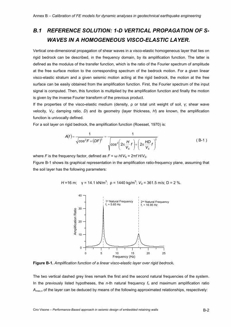
Annex B – Calibration of FE models for dynamic analyses in geotechnical earthquake engineering
Ciro Visone – Performance-Based approach in seismic design of embedded retaining walls B-2
B.1 REFERENCE SOLUTION: 1-D VERTICAL PROPAGATION OF S-
WAVES IN A HOMOGENEOUS VISCO-ELASTIC LAYER.
Vertical one-dimensional propagation of shear waves in a visco-elastic homogeneous layer that lies on
rigid bedrock can be described, in the frequency domain, by its amplification function. The latter is
defined as the modulus of the transfer function, which is the ratio of the Fourier spectrum of amplitude
at the free surface motion to the corresponding spectrum of the bedrock motion. For a given linear
visco-elastic stratum and a given seismic motion acting at the rigid bedrock, the motion at the free
surface can be easily obtained from the amplification function. First, the Fourier spectrum of the input
signal is computed. Then, this function is multiplied by the amplification function and finally the motion
is given by the inverse Fourier transform of the previous product.
If the properties of the visco-elastic medium (density, ρ or total unit weight of soil, γ; shear wave
velocity, VS; damping ratio, D) and its geometry (layer thickness, H) are known, the amplification
function is univocally defined.
For a soil layer on rigid bedrock, the amplification function (Roesset, 1970) is:
( )( ) 2
222
22
11
π+
π
=+
=
fVHDf
VHcos
DFFcosfA
SS
( B-1 )
where F is the frequency factor, defined as F = ω H/VS = 2πf H/VS.
Figure B-1 shows its graphical representation in the amplification ratio-frequency plane, assuming that
the soil layer has the following parameters:
H =16 m; γ = 14.1 kN/m3; ρ = 1440 kg/m3; VS = 361.5 m/s; D = 2 %.
0 5 10 15 20 25Frequency (Hz)
0
10
20
30
40
Ampl
ifica
tion
Rat
io
1st Natural Frequencyf1 = 5.65 Hz
2nd Natural Frequencyf1 = 16.95 Hz
Figure B-1. Amplification function of a linear visco-elastic layer over rigid bedrock.
The two vertical dashed grey lines remark the first and the second natural frequencies of the system.
In the previously listed hypotheses, the n-th natural frequency fn and maximum amplification ratio
Amax,n of the layer can be deduced by means of the following approximated relationships, respectively:
Annex B – Calibration of FE models for dynamic analyses in geotechnical earthquake engineering
Ciro Visone – Performance-Based approach in seismic design of embedded retaining walls B-3
( )1242
−≅π
ω= n
HVf Sn
n ( B-2 )
( ) n
Sn HD
VDn
Aω
=π−
≅12
2max, ( B-3 )
B.2 NUMERICAL MODELING OF THE REFERENCE PROBLEM.
The finite element modelling of the one-dimensional vertical propagation of shear waves into a visco-
elastic layer based on a rigid bedrock can be performed by following the next steps:
1. define the FE model (damping parameters; numerical parameters; boundary conditions)
2. define input motion (in terms of accelerations, velocities, displacements, forces time-
histories and Fourier spectra)
3. conduct the dynamic analysis for the specified seismic motion
4. check the goodness of the model response both in the frequency and in the time domains
(e.g., in terms of maximum acceleration profiles, amplification function, etc.)
B.2.1 Finite element models.
The discretization of a continuum through the use of finite elements or finite differences requires the
existence of a finite domain with well defined boundaries, where conditions are specified for forces
and displacements. If these boundaries do not exist naturally but are created artificially, it is necessary
to determine appropriate boundary conditions that will simulate the physical behaviour of the actual
problem.
For a horizontally stratified soil deposit with shear waves propagating vertically, the existence of an
underlying half-space could be reproduced in a discrete model by placing at the bottom different static
and kinematic conditions depending on the bedrock properties. If the last is rigid, its motion is not
affected by the presence of the overlying soil. It acts as a fixed end boundary. Any downward-
travelling waves in the soil is completely reflected back toward the ground surface by the rigid layer,
thereby trapping all of the elastic wave energy within the soil layer. In a time domain analysis, the rigid
bedrock is simply modelled imposing an acceleration (or velocity or displacement) time-history at the
base of the numerical model. When the rock is elastic, however, downward-travelling stress waves
that reach the soil-rock boundary are reflected only partially; part of their energy is transmitted through
the boundary to continue travelling downward through the rock. If the rock extends to great depth, the
elastic energy of these waves is effectively removed from the soil layer. This is a form of radiation
damping and it causes the free surface motion amplitudes to be smaller than those for the case of
rigid bedrock. In a time domain analysis, the presence of an elastic bedrock can be modelled by
imposing a force time history rather than a base motion at the bottom of the soil layer. The continuity
of the stresses along the rock-soil boundary requires that the shear stress in the rock side is equal to
the shear stress in the soil side. For this reason, the motion of an elastic bedrock is usually specified
by adopting a shear stress time history τ(t). It can be simply obtained by the motion expected at the
outcropping rock in terms of velocity time-history ( )tu& by means of the relationship (Tsai, 1969):

Annex B – Calibration of FE models for dynamic analyses in geotechnical earthquake engineering
Ciro Visone – Performance-Based approach in seismic design of embedded retaining walls B-4
( ) ( )tuVt SRR &ρ=τ ( B-4 )
where ρR and VSR are the mass density and the shear wave velocity of the elastic bedrock.
Another way to specify the motion of an elastic bedrock at the bottom of a FE model is to run a
frequency domain analysis by applying the seismic signal at the outcropping rock and then computing
the time-history of acceleration at the interface between the soil layer and the rock (called “inside” in
the EERA code). Such time history accounts for the shear stress transmission between the bedrock
and the layer and can be directly applied to the lower boundary of the FE mesh.
For the simple cases of SH, SV or P waves travelling into the subsoil at a specified angle, when the
geometry is one-dimensional and only one train of plane waves is considered, appropriate conditions
for the lateral boundaries can also be obtained easily. For example,
• For SH waves with normal incidence the lateral boundary nodes should be left free
• For SV waves with normal incidence, the nodes on the lateral boundary should have free
displacements in the horizontal direction and completely restrained displacements in the
vertical direction
• For P waves with normal incidence, the nodes on the lateral boundary should have free
displacements in the vertical direction and completely restrained displacements in the
horizontal direction
• For SH, SV, or P waves with a specified nonzero angle of incidence, the nodes on the lateral
boundary should have lumped dashpots or consistent damping matrices with properties that
are functions of the angle.
In the case of interest, simple vertical fixities allowing horizontal displacements of nodes placed on the
lateral boundaries are the best solution to reproduce the vertical propagation of S-waves polarized in
the horizontal plane of layered subsoils. In order to equilibrate the horizontal lithostatic stresses acting
on lateral boundaries, it is suitable to introduce load distributions at the left-hand and right-hand
vertical boundaries, as sketched in Figure B-2. In such conditions, the width of the FE model does not
affect its response. The influence of the various sources of dissipation in time domain analyses can be
examined by adopting a simple soil column (for example B = 1m) reducing the required calculation
time.
ax(t)
K0γz
K0γHK0γH
H
B
K0γz
Figure B-2. FE model for 1-D dynamic analysis of visco-elastic layers.
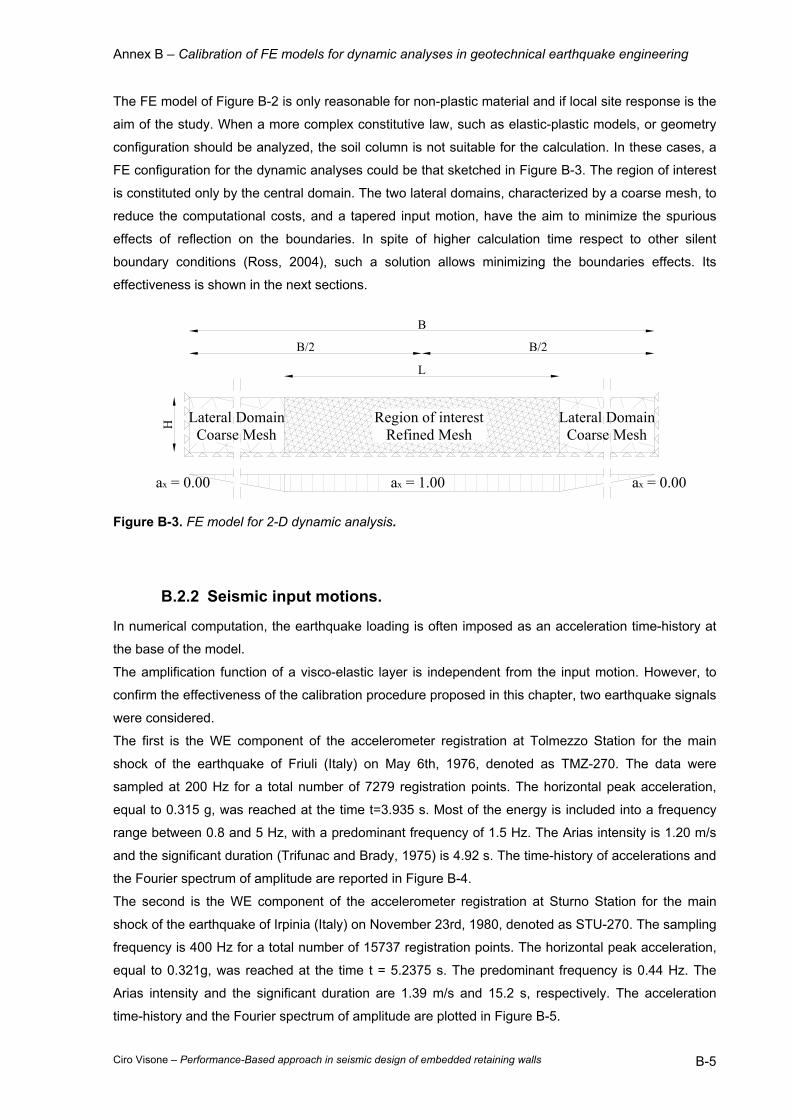
Annex B – Calibration of FE models for dynamic analyses in geotechnical earthquake engineering
Ciro Visone – Performance-Based approach in seismic design of embedded retaining walls B-5
The FE model of Figure B-2 is only reasonable for non-plastic material and if local site response is the
aim of the study. When a more complex constitutive law, such as elastic-plastic models, or geometry
configuration should be analyzed, the soil column is not suitable for the calculation. In these cases, a
FE configuration for the dynamic analyses could be that sketched in Figure B-3. The region of interest
is constituted only by the central domain. The two lateral domains, characterized by a coarse mesh, to
reduce the computational costs, and a tapered input motion, have the aim to minimize the spurious
effects of reflection on the boundaries. In spite of higher calculation time respect to other silent
boundary conditions (Ross, 2004), such a solution allows minimizing the boundaries effects. Its
effectiveness is shown in the next sections.
ax = 1.00 ax = 0.00ax = 0.00
H
B/2 B/2
B
Region of interestRefined Mesh
Lateral DomainCoarse Mesh
Lateral DomainCoarse Mesh
L
Figure B-3. FE model for 2-D dynamic analysis.
B.2.2 Seismic input motions.
In numerical computation, the earthquake loading is often imposed as an acceleration time-history at
the base of the model.
The amplification function of a visco-elastic layer is independent from the input motion. However, to
confirm the effectiveness of the calibration procedure proposed in this chapter, two earthquake signals
were considered.
The first is the WE component of the accelerometer registration at Tolmezzo Station for the main
shock of the earthquake of Friuli (Italy) on May 6th, 1976, denoted as TMZ-270. The data were
sampled at 200 Hz for a total number of 7279 registration points. The horizontal peak acceleration,
equal to 0.315 g, was reached at the time t=3.935 s. Most of the energy is included into a frequency
range between 0.8 and 5 Hz, with a predominant frequency of 1.5 Hz. The Arias intensity is 1.20 m/s
and the significant duration (Trifunac and Brady, 1975) is 4.92 s. The time-history of accelerations and
the Fourier spectrum of amplitude are reported in Figure B-4.
The second is the WE component of the accelerometer registration at Sturno Station for the main
shock of the earthquake of Irpinia (Italy) on November 23rd, 1980, denoted as STU-270. The sampling
frequency is 400 Hz for a total number of 15737 registration points. The horizontal peak acceleration,
equal to 0.321g, was reached at the time t = 5.2375 s. The predominant frequency is 0.44 Hz. The
Arias intensity and the significant duration are 1.39 m/s and 15.2 s, respectively. The acceleration
time-history and the Fourier spectrum of amplitude are plotted in Figure B-5.

Annex B – Calibration of FE models for dynamic analyses in geotechnical earthquake engineering
Ciro Visone – Performance-Based approach in seismic design of embedded retaining walls B-6
a)
0 10 20 30 40Time (sec)
-0.4
-0.2
0
0.2
0.4
Acc
eler
atio
n (g
)
b)0 5 10 15 20 25
Frequency (Hz)
0
0.05
0.1
0.15
0.2
0.25
Four
ier A
mpl
itude
(g-s
ec)
Figure B-4. Seismic input TMZ-270: a) acceleration time-history; b) Fourier spectrum.
a)
0 10 20 30 40Time (sec)
-0.4
-0.2
0
0.2
0.4
Acce
lera
tion
(g)
b)
0 5 10 15 20 25Frequency (Hz)
0
0.05
0.1
0.15
0.2
0.25
Four
ier A
mpl
itude
(g-s
ec)
Figure B-5. Seismic input STU-270: a) acceleration time-history; b) Fourier spectrum.
B.3 ANALYSIS OF THE SOURCES OF ENERGY DISSIPATION IN
TIME DOMAIN ANALYSES.
In time domain seismic analyses different sources of energy dissipation exist: material damping, which
includes viscous and hysteretic soil damping, numerical damping, arising from the adopted time
integration scheme, and energy dissipation at the lateral boundaries. In this section, the various
causes of the motion attenuation are analyzed.
B.3.1 Material damping.
The dissipation of elastic energy due to the intrinsic characteristics of the material can be modelled by
viscous damping, according to the Rayleigh formulation. Figure B-6 shows the different amplification
functions for three values of the Rayleigh damping coefficients αR and βR, respectively. Both sets of
curves were obtained by fixing the numerical damping to zero, as described in the next § B.3.2, and
assuming βR = 0, for the first set (Figure B-6a), and αR = 0, for the second set (Figure B-6b).
The observed effects on the seismic response of the layer can be explained with the theory of a
viscous damped single-degree-of-freedom (SDOF) system subjected to forced vibrations (Kramer,
1996). First, it seems helpful to remind of the distinction between the damping ratio D and the critical
damping ratio ξ: the former is defined as the ratio between the energy dissipated in one cycle of
oscillation of a hysteresis loop and the strain energy stored in the system, the latter is equal to the
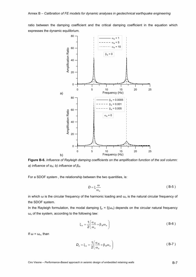
Annex B – Calibration of FE models for dynamic analyses in geotechnical earthquake engineering
Ciro Visone – Performance-Based approach in seismic design of embedded retaining walls B-7
ratio between the damping coefficient and the critical damping coefficient in the equation which
expresses the dynamic equilibrium.
a)
0 5 10 15 20 25Frequency (Hz)
0
20
40
60
80
Am
plifi
catio
n R
atio
αR = 1αR = 5αR = 10
βR = 0
b)
0 5 10 15 20 25Frequency (Hz)
0
20
40
60
80
Ampl
ifica
tion
Rat
io
βR = 0.0005βR = 0.001βR = 0.005
αR = 0
Figure B-6. Influence of Rayleigh damping coefficients on the amplification function of the soil column:
a) influence of αR; b) influence of βR.
For a SDOF system , the relationship between the two quantities, is:
n
Dωω
ξ= ( B-5 )
in which ω is the circular frequency of the harmonic loading and ωn is the natural circular frequency of
the SDOF system.
In the Rayleigh formulation, the modal damping ξn = ξ(ωn) depends on the circular natural frequency
ωn of the system, according to the following law:
ωβ+
ωα
=ξ nRn
Rn 2
1 ( B-6 )
If ω = ωn, than
ωβ+
ωα
=ξ= nRn
RnnD
21 ( B-7 )
Annex B – Calibration of FE models for dynamic analyses in geotechnical earthquake engineering
Ciro Visone – Performance-Based approach in seismic design of embedded retaining walls B-8
Therefore, according to the Rayleigh formulation, the modal damping ratio Dn is affected from the
natural frequency of the examined SDOF system.
A soil layer resting on rigid bedrock is theoretically characterized by an infinite number of natural
frequencies. The amplification factor corresponding to the n-th natural circular frequency ωn of the
system can be expressed as follows, by introducing the equation ( B-7 ) into the ( B-3 ):
ωβ+α=
ω= 2max,
12
nRR
S
nn
Sn H
VHD
VA ( B-8 )
The maximum amplification ratio calculated according to equation ( B-8 ) is consistent with the
amplification functions computed from the results of the analyses and represented in Figure B-6.
For βR = 0 (as in Figure B-6a), Amax does not change with the modal number n while it decreases
hyperbolically with αR . On the contrary, by setting αR = 0 (as in Figure B-6b), the maximum
amplification ratio decreases with the square of the natural frequency, for any given βR.
If no numerical dissipation is introduced in the time integration scheme, the damping of the system can
be modelled by using the Rayleigh parameters only. For a soil layer with a constant value of the
damping ratio D*, the linear system of equations that provides αR and βR is:
*2 2 DniniRR ω=ωβ+α ( B-9 )
in which ωni are two circular natural frequencies of the layer.
Assuming ωni as the first and the second natural frequencies (ωn1 = 35.5 rad/s; ωn2 = 106.5 rad/s), the
numerical calculation gives the results plotted in Figure B-7, in which the comparisons with the
frequency domain analysis solutions were done for TMZ-270 and STU-270 input motions. The
reference maximum acceleration profile was computed with the EERA code. The two types of
analyses agree both in terms of amplification functions and maximum acceleration profile. The
numerical parameters (α and dt) was fixed to have zero numerical dissipation and to respect the
accuracy condition ( 5–60) for a stable solution.
B.3.2 Numerical damping.
The Newmark scheme, which is used in many FE codes for time integration, can be varied adopting
different values of the parameter α, according to the HHT method (LUSAS, 2000). If no damping is
introduced in a dynamic analysis, either material or numerical, the model reaches the resonant
conditions at the natural frequencies of the system with a corresponding theoretically infinite
amplification ratio. Figure B-8 shows the response at a control point on the free-surface obtained for
an undamped analysis (α = 0; αN = 0.25; βN = 0.5; αR = βR = 0) both in terms of the acceleration time-
history and the Fourier spectrum. The estimated natural frequencies of the layer are very close to the
expected theoretical values. The analysis was performed by applying at the base of the model the
TMZ-270 acceleration time history.
The standard setting of the Plaxis code is the damped Newmark scheme with αN = 0.3025 and
βN = 0.6, that corresponds to α = 0.1, according to equations ( 5-56). This assumption introduces a
numerical energy dissipation which should be considered when calibrating the model damping against
the true soil damping.
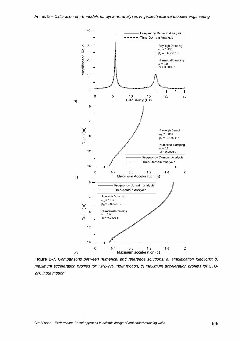
Annex B – Calibration of FE models for dynamic analyses in geotechnical earthquake engineering
Ciro Visone – Performance-Based approach in seismic design of embedded retaining walls B-9
a) 0 5 10 15 20 25
Frequency (Hz)
0
10
20
30
40
Am
plifi
catio
n R
atio
Frequency Domain AnalysisTime Domain Analysis
Rayleigh DampingαR = 1.065βR = 0.0002818
Numerical Dampingα = 0.0dt = 0.0005 s
b) 0 0.4 0.8 1.2 1.6 2
Maximum Acceleration (g)
16
12
8
4
0
Dep
th (m
)
Frequency Domain AnalysisTime Domain Analysis
Rayleigh DampingαR = 1.065βR = 0.0002818
Numerical Dampingα = 0.0dt = 0.0005 s
c) 0 0.4 0.8 1.2 1.6 2
Maximum acceleration (g)
16
12
8
4
0
Dep
th (m
)
Frequency domain analysisTime domain analysis
Rayleigh DampingαR = 1.065βR = 0.0002818
Numerical Dampingα = 0.0dt = 0.0005 s
Figure B-7. Comparisons between numerical and reference solutions: a) amplification functions; b)
maximum acceleration profiles for TMZ-270 input motion; c) maximum acceleration profiles for STU-
270 input motion.
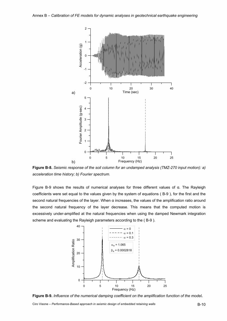
Annex B – Calibration of FE models for dynamic analyses in geotechnical earthquake engineering
Ciro Visone – Performance-Based approach in seismic design of embedded retaining walls B-10
a)
0 10 20 30 40Time (sec)
-2
-1
0
1
2
Acce
lera
tion
(g)
b)
0 5 10 15 20 25Frequency (Hz)
0
1
2
3
4
5
Four
ier A
mpl
itude
(g-s
ec)
Figure B-8. Seismic response of the soil column for an undamped analysis (TMZ-270 input motion): a)
acceleration time history; b) Fourier spectrum.
Figure B-9 shows the results of numerical analyses for three different values of α. The Rayleigh
coefficients were set equal to the values given by the system of equations ( B-9 ), for the first and the
second natural frequencies of the layer. When α increases, the values of the amplification ratio around
the second natural frequency of the layer decrease. This means that the computed motion is
excessively under-amplified at the natural frequencies when using the damped Newmark integration
scheme and evaluating the Rayleigh parameters according to the ( B-9 ).
0 5 10 15 20 25Frequency (Hz)
0
10
20
30
40
Am
plifi
catio
n R
atio
α = 0α = 0.1α = 0.3
αR = 1.065
βR = 0.0002818
Figure B-9. Influence of the numerical damping coefficient on the amplification function of the model.
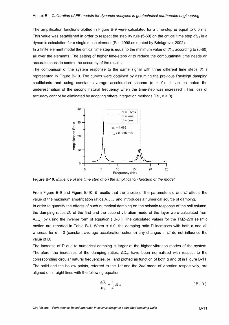
Annex B – Calibration of FE models for dynamic analyses in geotechnical earthquake engineering
Ciro Visone – Performance-Based approach in seismic design of embedded retaining walls B-11
The amplification functions plotted in Figure B-9 were calculated for a time-step dt equal to 0.5 ms.
This value was established in order to respect the stability rule (5-60) on the critical time step dtcrit in a
dynamic calculation for a single mesh element (Pal, 1998 as quoted by Brinkgreve, 2002).
In a finite element model the critical time step is equal to the minimum value of dtcrit according to (5-60)
all over the elements. The setting of higher time-steps dt to reduce the computational time needs an
accurate check to control the accuracy of the results.
The comparison of the system response to the same signal with three different time steps dt is
represented in Figure B-10. The curves were obtained by assuming the previous Rayleigh damping
coefficients and using constant average acceleration scheme (α = 0). It can be noted the
underestimation of the second natural frequency when the time-step was increased . This loss of
accuracy cannot be eliminated by adopting others integration methods (i.e., α > 0).
0 5 10 15 20 25Frequency (Hz)
0
10
20
30
40
Am
plifi
catio
n R
atio
dt = 0.5msdt = 2msdt = 5ms
αR = 1.065
βR = 0.0002818
Figure B-10. Influence of the time step dt on the amplification function of the model.
From Figure B-9 and Figure B-10, it results that the choice of the parameters α and dt affects the
value of the maximum amplification ratios Amax,n and introduces a numerical source of damping.
In order to quantify the effects of such numerical damping on the seismic response of the soil column,
the damping ratios Dn of the first and the second vibration mode of the layer were calculated from
Amax,n by using the inverse form of equation ( B-3 ). The calculated values for the TMZ-270 seismic
motion are reported in Table B-1. When α ≠ 0, the damping ratio D increases with both α and dt,
whereas for α = 0 (constant average acceleration scheme) any changes in dt do not influence the
value of D.
The increase of D due to numerical damping is larger at the higher vibration modes of the system.
Therefore, the increases of the damping ratios, ∆Dn, have been normalized with respect to the
corresponding circular natural frequencies, ωn, and plotted as function of both α and dt in Figure B-11.
The solid and the hollow points, referred to the 1st and the 2nd mode of vibration respectively, are
aligned on straight lines with the following equation:
α=ω∆ dt
21
n
nD ( B-10 )

Annex B – Calibration of FE models for dynamic analyses in geotechnical earthquake engineering
Ciro Visone – Performance-Based approach in seismic design of embedded retaining walls B-12
1st Vibration Mode 2nd Vibration Mode
dt (ms) dt (ms) α
0.25 0.5 1 α
0.25 0.5 1
0.0 2.00% 2.00% 2.00% 0.0 2.00% 2.00% 2.00%
0.1 2.05% 2.10% 2.19% 0.1 2.16% 2.29% 2.56%
0.2 2.10% 2.19% 2.36% 0.2 2.29% 2.56% 3.09%
0.3 2.14% 2.27% 2.54% 0.3 2.42% 2.82% 3.63%
Table B-1. Effects of numerical dissipation (α and dt) on the modal damping ratio Dn of the soil
column.
0 0.1 0.2 0.3Newmark Integration Parameter, α
0
0.004
0.008
0.012
0.016
Nor
mal
ized
Incr
ease
of D
ampi
ng R
atio
, ∆D
n/ωn (
%)
2nd
Mod
e
1st M
ode dt = 0.25ms
dt = 0.5msdt = 1ms
α=ω∆
dt21
n
nD
Figure B-11. Normalized increase of modal damping ratio induced by the Newmark damped
integration schemes.
For the time step dt = 1ms, larger than the limit value given by the accuracy condition (5-60), a small
scattering of data can be noticed.
The relationship ( B-10 ) was validated on other homogeneous layers with various values of thickness,
damping ratio and shear wave velocity.
On the basis of these outcomes, it can be concluded that, if the modified Newmark integration scheme
is used, the entire modal damping ratio, both numerical and material, in a time domain analysis of a
homogenous layer crossed by vertical propagating S-waves is equal to:
( )
ωγ+β+
ωα
=ξ= nRn
RnnD dt
21 ( B-11 )
In other words, the adoption of a damped Newmark integration scheme (α > 0) according to the HHT
method is equivalent to the use of a stiffness proportional damping.
The amplification function and the maximum acceleration profile of the reference layer computed for
the TMZ-270 earthquake by assuming dt = 0.5ms and α = 0.2 are plotted in Figure B-12. The Rayleigh
coefficients were chosen assuming the first and the second natural frequencies of the layer and
reducing βR of the quantity α·dt. Comparing the Figure B-7 and Figure B-12, it appears that the

Annex B – Calibration of FE models for dynamic analyses in geotechnical earthquake engineering
Ciro Visone – Performance-Based approach in seismic design of embedded retaining walls B-13
dynamic analyses performed by using the two sets of parameters, which respect the equation ( B-11 ),
give the same results.
a) 0 5 10 15 20 25
Frequency (Hz)
0
10
20
30
40
Am
plifi
catio
n R
atio
Frequency Domain AnalysisTime Domain Analysis
Rayleigh DampingαR = 1.065βR = 0.0001818
Numerical Dampingα = 0.2dt = 0.0005 s
b) 0 0.4 0.8 1.2 1.6 2
Maximum Acceleration (g)
16
12
8
4
0
Dep
th (m
)
Frequency Domain AnalysisTime Domain Analysis
Rayleigh DampingαR = 1.065βR = 0.0001818
Numerical Dampingα = 0.2dt = 0.0005 s
Figure B-12. Comparisons between the reference and the numerical solutions obtained by adopting a
damped Newmark integration scheme for the TMZ-270 input motion: a) amplification functions; b)
maximum acceleration profiles.
B.3.3 Boundary conditions.
The solution obtained by assuming free horizontal displacements on lateral boundaries is only
reasonable for non-plastic material and when local site response is the aim of the study. In many other
cases, horizontal fixities on the sides of the model should be applied. As underlined in the previous
Chapter 5, viscous dampers are often used to simulate infinite media (Lysmer & Kuhlemeyer, 1969),
but there is a lack of well-established criteria in the literature for the choice of the parameters c1 and
c2; following common suggestions, the values of c1 and c2 have been set in the analyses to 1.0 and
0.25, respectively. However, if the lateral boundaries are sufficiently far from the central zone, their
effects due to the reflection of waves on the boundaries should decrease. In Figure B-13 the results of
analyses performed with two values of the ratio between the half-width, B/2, and the height, H of the
mesh, in terms of amplification functions and maximum acceleration profile, are plotted together with
the frequency domain solution of 1D ground motion. The two computed amplification curves differ from
the theoretical solution for the presence of the lateral boundaries. In general, the viscous dampers
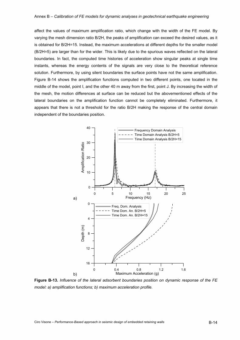
Annex B – Calibration of FE models for dynamic analyses in geotechnical earthquake engineering
Ciro Visone – Performance-Based approach in seismic design of embedded retaining walls B-14
affect the values of maximum amplification ratio, which change with the width of the FE model. By
varying the mesh dimension ratio B/2H, the peaks of amplification can exceed the desired values, as it
is obtained for B/2H=15. Instead, the maximum accelerations at different depths for the smaller model
(B/2H=5) are larger than for the wider. This is likely due to the spurious waves reflected on the lateral
boundaries. In fact, the computed time histories of acceleration show singular peaks at single time
instants, whereas the energy contents of the signals are very close to the theoretical reference
solution. Furthermore, by using silent boundaries the surface points have not the same amplification.
Figure B-14 shows the amplification functions computed in two different points, one located in the
middle of the model, point I, and the other 40 m away from the first, point J. By increasing the width of
the mesh, the motion differences at surface can be reduced but the abovementioned effects of the
lateral boundaries on the amplification function cannot be completely eliminated. Furthermore, it
appears that there is not a threshold for the ratio B/2H making the response of the central domain
independent of the boundaries position.
a)
0 5 10 15 20 25Frequency (Hz)
0
10
20
30
40
Am
plifi
catio
n R
atio
Frequency Domain AnalysisTime Domain Analysis B/2H=5Time Domain Analysis B/2H=15
b)
0 0.4 0.8 1.2 1.6Maximum Acceleration (g)
16
12
8
4
0
Dep
th (m
)
Freq. Dom. AnalysisTime Dom. An. B/2H=5Time Dom. An. B/2H=15
Figure B-13. Influence of the lateral adsorbent boundaries position on dynamic response of the FE
model: a) amplification functions; b) maximum acceleration profile.
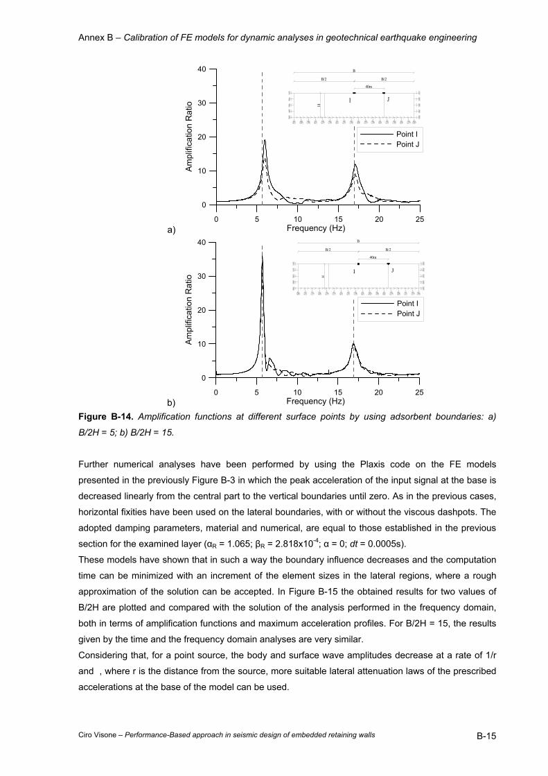
Annex B – Calibration of FE models for dynamic analyses in geotechnical earthquake engineering
Ciro Visone – Performance-Based approach in seismic design of embedded retaining walls B-15
a)
0 5 10 15 20 25Frequency (Hz)
0
10
20
30
40
Am
plifi
catio
n R
atio
Point IPoint J
B/2 B/2
40m
I J
B
H
b)
0 5 10 15 20 25Frequency (Hz)
0
10
20
30
40
Am
plifi
catio
n R
atio
Point IPoint J
B/2 B/2
40m
I J
B
H
Figure B-14. Amplification functions at different surface points by using adsorbent boundaries: a)
B/2H = 5; b) B/2H = 15.
Further numerical analyses have been performed by using the Plaxis code on the FE models
presented in the previously Figure B-3 in which the peak acceleration of the input signal at the base is
decreased linearly from the central part to the vertical boundaries until zero. As in the previous cases,
horizontal fixities have been used on the lateral boundaries, with or without the viscous dashpots. The
adopted damping parameters, material and numerical, are equal to those established in the previous
section for the examined layer (αR = 1.065; βR = 2.818x10⁻⁴; α = 0; dt = 0.0005s).
These models have shown that in such a way the boundary influence decreases and the computation
time can be minimized with an increment of the element sizes in the lateral regions, where a rough
approximation of the solution can be accepted. In Figure B-15 the obtained results for two values of
B/2H are plotted and compared with the solution of the analysis performed in the frequency domain,
both in terms of amplification functions and maximum acceleration profiles. For B/2H = 15, the results
given by the time and the frequency domain analyses are very similar.
Considering that, for a point source, the body and surface wave amplitudes decrease at a rate of 1/r
and , where r is the distance from the source, more suitable lateral attenuation laws of the prescribed
accelerations at the base of the model can be used.
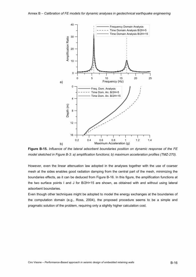
Annex B – Calibration of FE models for dynamic analyses in geotechnical earthquake engineering
Ciro Visone – Performance-Based approach in seismic design of embedded retaining walls B-16
a)
0 5 10 15 20 25Frequency (Hz)
0
10
20
30
40
Am
plifi
catio
n R
atio
Frequency Domain AnalysisTime Domain Analysis B/2H=5Time Domain Analysis B/2H=15
b)
0.2 0.4 0.6 0.8 1 1.2 1.4Maximum Acceleration (g)
16
12
8
4
0
Dep
th (m
)
Freq. Dom. AnalysisTime Dom. An. B/2H=5Time Dom. An. B/2H=15
Figure B-15. Influence of the lateral adsorbent boundaries position on dynamic response of the FE
model sketched in Figure B-3: a) amplification functions; b) maximum acceleration profiles (TMZ-270).
However, even the linear attenuation law adopted in the analyses together with the use of coarser
mesh at the sides enables good radiation damping from the central part of the mesh, minimizing the
boundaries effects, as it can be deduced from Figure B-16. In this figure, the amplification functions at
the two surface points I and J for B/2H=15 are shown, as obtained with and without using lateral
adsorbent boundaries.
Even though other techniques might be adopted to model the energy exchanges at the boundaries of
the computation domain (e.g., Ross, 2004), the proposed procedure seems to be a simple and
pragmatic solution of the problem, requiring only a slightly higher calculation cost.
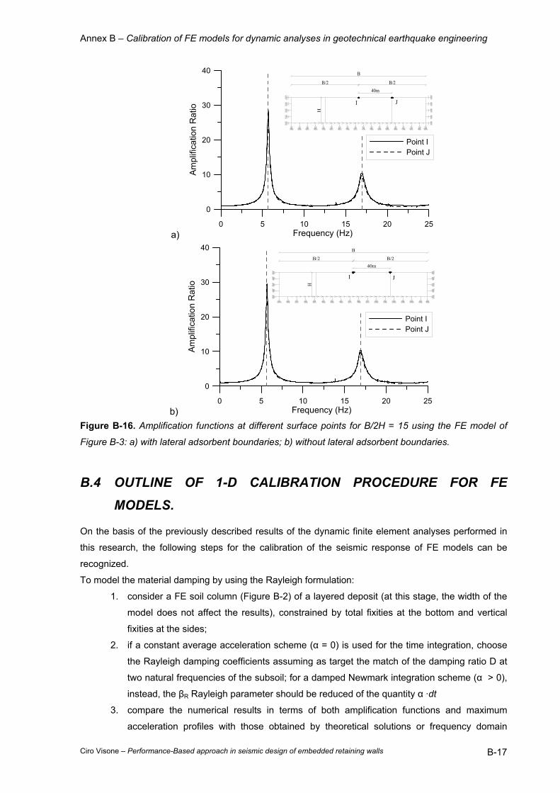
Annex B – Calibration of FE models for dynamic analyses in geotechnical earthquake engineering
Ciro Visone – Performance-Based approach in seismic design of embedded retaining walls B-17
a)
0 5 10 15 20 25Frequency (Hz)
0
10
20
30
40
Ampl
ifica
tion
Rat
io
Point IPoint J
B/2 B/240m
I J
B
H
b)
0 5 10 15 20 25Frequency (Hz)
0
10
20
30
40
Am
plifi
catio
n R
atio
Point IPoint J
B/2 B/240m
I J
B
H
Figure B-16. Amplification functions at different surface points for B/2H = 15 using the FE model of
Figure B-3: a) with lateral adsorbent boundaries; b) without lateral adsorbent boundaries.
B.4 OUTLINE OF 1-D CALIBRATION PROCEDURE FOR FE
MODELS.
On the basis of the previously described results of the dynamic finite element analyses performed in
this research, the following steps for the calibration of the seismic response of FE models can be
recognized.
To model the material damping by using the Rayleigh formulation:
1. consider a FE soil column (Figure B-2) of a layered deposit (at this stage, the width of the
model does not affect the results), constrained by total fixities at the bottom and vertical
fixities at the sides;
2. if a constant average acceleration scheme (α = 0) is used for the time integration, choose
the Rayleigh damping coefficients assuming as target the match of the damping ratio D at
two natural frequencies of the subsoil; for a damped Newmark integration scheme (α > 0),
instead, the βR Rayleigh parameter should be reduced of the quantity α ·dt
3. compare the numerical results in terms of both amplification functions and maximum
acceleration profiles with those obtained by theoretical solutions or frequency domain

Annex B – Calibration of FE models for dynamic analyses in geotechnical earthquake engineering
Ciro Visone – Performance-Based approach in seismic design of embedded retaining walls B-18
analyses, in order to check the accuracy of the mesh discretization and the time step dt.
To reduce the effect of the lateral boundaries (needed for boundary value problems):
4. add two rectangular domains with a coarse mesh at the sides of the region of interest; the
acceleration time-history at the base of the FE model under the region of interest has full
amplitude whereas it is linearly tapered down to zero under the lateral domains. The zero
value is set in correspondence of the lateral boundaries;
5. increase the width of the model (the lateral regions only should be changed at this stage)
and choose the more suitable mesh dimension ratio B/2H to attain a good agreement with
the 1D reference solution both in the frequency domain (amplification function) and in the
time domain (maximum acceleration profile).


![Anno 2011 Numero apporti tecnici - Earth-prints · [Marzorati and Bindi, 2009]. Indeed, this area is characterized by a high density in terms of both population and production activities.](https://static.fdocumenti.com/doc/165x107/5e7e8aa3f10c424fea671f3e/anno-2011-numero-apporti-tecnici-earth-prints-marzorati-and-bindi-2009-indeed.jpg)