
Olivi Davide Tesi
141
Alma Mater Studiorum – University of Bologna FACULTY OF ENGINEERING RESEARCH DOCTORATE Fluid Machines and Ene rgy Systems Cycle XXV Affiliation sector: 09/C1 – FLUID MACHINERY, ENERGY SYSTEMS AND POWER GENERATION Scientific-disciplinary sector: ING-IND/08 – FLUID MACHINES D e ve l opme n t of con tr ol -or i e nte d mode l s of D u al Cl u tch T r ans mi s s i on s ys te ms Davide Olivi Doctorate School Coordinator Supervisor Prof. Ing. Vincenzo Parenti Castel li Prof. Ing. Nicolò Cavina Final exam 2013
-
Upload
socol-mihai -
Category
Documents
-
view
240 -
download
1
Transcript of Olivi Davide Tesi
8/20/2019 Olivi Davide Tesi
http://slidepdf.com/reader/full/olivi-davide-tesi 1/141
Alma Mater Studiorum – University of Bologna
FACULTY OF ENGINEERING
RESEARCH DOCTORATE
Fluid Machines and Energy Systems
Cycle XXV
Affiliation sector:09/C1 – FLUID MACHINERY, ENERGY SYSTEMS AND POWER GENERATION
Scientific-disciplinary sector:ING-IND/08 – FLUID MACHINES
Development of control-or iented models
of Dual Clutch Transmission systems
Davide Olivi
Doctorate School Coordinator Supervisor
Prof. Ing. Vincenzo Parenti Castelli Prof. Ing. Nicolò Cavina
Final exam 2013

8/20/2019 Olivi Davide Tesi
http://slidepdf.com/reader/full/olivi-davide-tesi 2/141

8/20/2019 Olivi Davide Tesi
http://slidepdf.com/reader/full/olivi-davide-tesi 3/141
How many roads must a man walk down
Before you call him a man?

8/20/2019 Olivi Davide Tesi
http://slidepdf.com/reader/full/olivi-davide-tesi 4/141
8/20/2019 Olivi Davide Tesi
http://slidepdf.com/reader/full/olivi-davide-tesi 5/141
Acknowledgments
First of all, I want to thank my family for the support they have always provided during
all my studies, and all my friends, without whom life wouldn’t be so colorful and
interesting.
I want to express my gratitude to my supervisor Prof. Ing. Nicolò Cavina, who gave me
the great opportunity to carry on this interesting research project, for his guidance, his
patience and also for his example in both professional and personal life.
I want to mention here all the people I met in Bologna during my doctoral period: thanks
to Giorgio, Alberto, Roberta, Gaspare, Gherardo, Elisa, Lisa, Marco F., Marco C., Igor,
Giulio, Andrea, Claudio, Bruno, Enrico, Manuel, Davide. Special thanks to Ing. Luca
Solieri for his precious help during the first months of work with the simulator.
I would like to thank Ferrari S.p.A. for financing this research project, and Ing. Luca
Poggio, Ing. Francesco Marcigliano and Ing. Alfonso Tarantini for guidance and support
during the development of this activity.
Thanks to the people who shared with me the office in Maranello: Ivan, Alessandro,
Matteo, Barbara, Daniele, Francesco C., Francesco B., Andrea N., Andrea S., Samuele,
Luca, and all the others that would be too long to mention, for their sympathy andcordiality. A special thank to my flatmates in Maranello, Fabio, Matteo and Simone, who
made my stay not only a working experience but also a joyful life experience.
Last but not least, I would like to thank Eglė for her smile, which gives purpose to life’s
struggles.
Contacts
Davide Olivi
Alma Automotive s.r.l.
Via Terracini 2/c
40131 Bologna (BO)
ITALY
e-mail:

8/20/2019 Olivi Davide Tesi
http://slidepdf.com/reader/full/olivi-davide-tesi 6/141
8/20/2019 Olivi Davide Tesi
http://slidepdf.com/reader/full/olivi-davide-tesi 7/141
Index
I
Index
Abstract 1
Introduction 3
Chapter 1 – The Dual Clutch Transmission 5
1.1
History 5
1.2 Operating principle 7
Chapter 2 – The Ferrari Dual Clutch Transmission 10
2.1 Overview 10
2.2 Hydraulic circuit 132.3 Hardware modifications for electric drive 14
2.4 Electrical connections 15
Chapter 3 – The Dual Clutch Transmission model 18
3.1 Hydraulic actuation circuit 18
3.1.1 Pump model 19
3.1.2 System pressure model 203.1.3 Pressure control valve model 21
3.1.4 Safety valve model 25
3.2 Clutch model 25
3.2.1 Clutch actuation model 25
3.2.2 Clutch longitudinal motion 27
3.2.3 Clutch hysteresis 30
3.2.4 Clutch torque 31
3.2.5 Clutch lubrication 35
8/20/2019 Olivi Davide Tesi
http://slidepdf.com/reader/full/olivi-davide-tesi 8/141
Davide Olivi Development of control-oriented models of DCT systems
II
3.3 Synchronizers model 36
3.3.1 Synchronizers actuation model 36
3.3.2 Synchronizers longitudinal motion 37
3.3.3 Speed synchronization 40
3.4 Parking lock model 43
3.5 Electronic differential model 44
3.6 Driveline and vehicle model 45
3.6.1 No-slip phase 46
3.6.2 Slip phase 48
3.7 Engine model 50
3.7.1 Stop&Start strategy 52
3.7.2 Electric Drive strategy 53
Chapter 4 – Simplified model for HIL application 54
4.1 Model simulation 54
Chapter 5 – DCT model developed in Simulink 61
5.1 Model overview 61
5.2 CCP and clutch model 62
5.3 Sap and synchronizers model 66
5.4 Driveline and vehicle model 69
5.5 Driver model 72
Chapter 6 – Offline simulation results 74
6.1 Clutch pressure 75
6.2 System pressure 77
6.3 Synchronizers 78
Chapter 7 – Hardware In the Loop 81
7.1 Hardware configuration 82
7.2 Input / Output model 86
8/20/2019 Olivi Davide Tesi
http://slidepdf.com/reader/full/olivi-davide-tesi 9/141
Index
III
Chapter 8 – TCU testing 90
8.1 Functional tests 90
8.1.1 Gear shift 90
8.1.2 Drive away 928.2 Failure tests 94
8.2.1 Mechanical failures simulation 94
8.2.2 Hydraulic failures simulation 95
8.2.3 Electrical failures simulation 99
8.3 New engine functionalities 100
8.3.1 Stop&Start 100
8.3.2 Electric Drive 101
8.4 Adaption procedures 103
8.4.1 Rod calibration 103
8.4.2 Detection of clutch valve solenoid characteristic 104
8.5 Safety Level 2 software validation 105
8.5.1 Example: illegal drive direction for reverse gear 107
8.5.2 Example: illegal launch 108
8.5.3 Example: double gear engagement 109
Chapter 9 – Test automation 111
9.1 On-Board Diagnostics (OBD) and software development tools 111
9.2 The automation procedure 112
9.3 Non-regression tests on new TCU software 116
9.3.1 Example: redundant clutch valve not actuated 117
9.3.2 Example: short engine CAN timeout during gear shift request 118
9.3.3 Example: wrong rod management during sensor fault 120
Conclusions 123
Bibliography 125
Appendix i

8/20/2019 Olivi Davide Tesi
http://slidepdf.com/reader/full/olivi-davide-tesi 10/141
8/20/2019 Olivi Davide Tesi
http://slidepdf.com/reader/full/olivi-davide-tesi 11/141
Abstract
1
Abstract
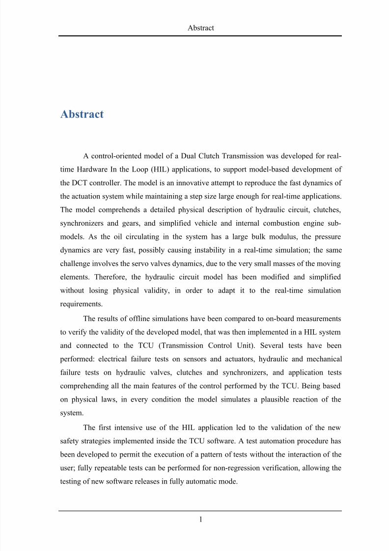
A control-oriented model of a Dual Clutch Transmission was developed for real-
time Hardware In the Loop (HIL) applications, to support model-based development of
the DCT controller. The model is an innovative attempt to reproduce the fast dynamics of
the actuation system while maintaining a step size large enough for real-time applications.
The model comprehends a detailed physical description of hydraulic circuit, clutches,
synchronizers and gears, and simplified vehicle and internal combustion engine sub-
models. As the oil circulating in the system has a large bulk modulus, the pressure
dynamics are very fast, possibly causing instability in a real-time simulation; the same
challenge involves the servo valves dynamics, due to the very small masses of the moving
elements. Therefore, the hydraulic circuit model has been modified and simplified
without losing physical validity, in order to adapt it to the real-time simulation
requirements.
The results of offline simulations have been compared to on-board measurements
to verify the validity of the developed model, that was then implemented in a HIL system
and connected to the TCU (Transmission Control Unit). Several tests have been
performed: electrical failure tests on sensors and actuators, hydraulic and mechanical
failure tests on hydraulic valves, clutches and synchronizers, and application tests
comprehending all the main features of the control performed by the TCU. Being based
on physical laws, in every condition the model simulates a plausible reaction of the
system.
The first intensive use of the HIL application led to the validation of the new
safety strategies implemented inside the TCU software. A test automation procedure has
been developed to permit the execution of a pattern of tests without the interaction of the
user; fully repeatable tests can be performed for non-regression verification, allowing the
testing of new software releases in fully automatic mode.
8/20/2019 Olivi Davide Tesi
http://slidepdf.com/reader/full/olivi-davide-tesi 12/141
Davide Olivi Development of control-oriented models of DCT systems
2
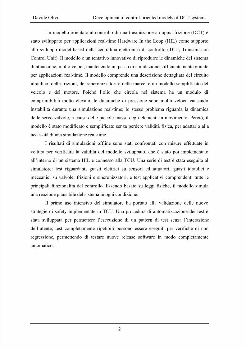
Un modello orientato al controllo di una trasmissione a doppia frizione (DCT) è
stato sviluppato per applicazioni real-time Hardware In the Loop (HIL) come supporto
allo sviluppo model-based della centralina elettronica di controllo (TCU, Transmission
Control Unit). Il modello è un tentativo innovativo di riprodurre le dinamiche del sistema
di attuazione, molto veloci, mantenendo un passo di simulazione sufficientemente grande
per applicazioni real-time. Il modello comprende una descrizione dettagliata del circuito
idraulico, delle frizioni, dei sincronizzatori e delle marce, e un modello semplificato del
veicolo e del motore. Poiché l’olio che circola nel sistema ha un modulo di
comprimibilità molto elevato, le dinamiche di pressione sono molto veloci, causando
instabilità durante una simulazione real-time; lo stesso problema riguarda la dinamica
delle servo valvole, a causa delle piccole masse degli elementi in movimento. Perciò, il
modello è stato modificato e semplificato senza perdere validità fisica, per adattarlo alla
necessità di una simulazione real-time.
I risultati di simulazioni offline sono stati confrontati con misure effettuate in
vettura per verificare la validità del modello sviluppato, che è stato poi implementato
all’interno di un sistema HIL e connesso alla TCU. Una serie di test è stata eseguita al
simulatore: test riguardanti guasti elettrici su sensori ed attuatori, guasti idraulici e
meccanici su valvole, frizioni e sincronizzatori, e test applicativi comprendenti tutte le
principali funzionalità del controllo. Essendo basato su leggi fisiche, il modello simula
una reazione plausibile del sistema in ogni condizione.
Il primo uso intensivo del simulatore ha portato alla validazione delle nuove
strategie di safety implementate in TCU. Una procedura di automatizzazione dei test è
stata sviluppata per permettere l’esecuzione di un pattern di test senza l’interazione
dell’utente; test completamente ripetibili possono essere eseguiti per verifiche di non
regressione, permettendo di testare nuove release software in modo completamente
automatico.
8/20/2019 Olivi Davide Tesi
http://slidepdf.com/reader/full/olivi-davide-tesi 13/141
Introduction
3
Introduction
In recent years the need for increased fuel efficiency, driving performance and
comfort has driven the development of engine and transmission technology in the
automotive industry, and several types of transmissions are currently available in the
market trying to meet these needs. The conventional Automatic Transmission (AT), with
torque converter and planetary gears, was leading the market of non-manual
transmissions, but in recent years it is losing its predominant position, because of the low
efficiency of the converter and the overall structure complexity, in favour of other
technologies: Continuously Variable Transmissions (CVT) permit avoiding the problem
of gear shifting, but are limited in torque capacity and have the disadvantage of a low
transmission efficiency due to the high pump losses caused by the large oil flows and
pressure values needed. Automated Manual Transmissions (AMT) with dry clutches are
the most efficient systems, but they don’t meet customer expectations due to torque
interruption during gear shift [21]. If compared to other transmissions, the DCT
technology has the advantage of being suitable both for low revving and high torque
diesel engines and for high revving engines for sport cars, maintaining a high
transmission efficiency, as well as high gear shift performance and comfort [14].
A Dual Clutch Transmission can be considered as an evolution of the AMT. An
AMT is similar to a manual transmission, but the clutch actuation and the gear selectionare performed by electro-hydraulic valves controlled by a TCU (Transmission Control
Unit). The peculiarity of a DCT system is the removal of torque interruption during gear
shift typical of AMTs through the use of two clutches: each clutch is connected on one
side to the engine, and on the other side to its own primary shaft, carrying odd and even
gears, respectively.
The role of engine and transmission electronic control units is steeply increasing,
and new instruments for their development are needed. Hardware In the Loop (HIL)systems are nowadays largely used in the automotive industry, in which the important
8/20/2019 Olivi Davide Tesi
http://slidepdf.com/reader/full/olivi-davide-tesi 14/141
Davide Olivi Development of control-oriented models of DCT systems
4
role of control systems results in the need of new techniques for software testing and
validation. They are designed for testing control units in a simulation environment,
allowing to perform functional and failure tests on the control unit by connecting it to a
device capable to simulate the behaviour of the controlled system in real-time.
The aim of this thesis is the development of a control-oriented model of a DCT
system that has been designed to support model-based development of the DCT
controller. The most difficult behaviour to reproduce is the fast dynamics of the hydraulic
circuit, with the constraint of a sufficiently large simulation step size, suitable for real-
time simulation.
The developed model [22] has been integrated in a Hardware In the Loop
application for real-time simulation and the testing of different software releases
implemented inside the TCU is being carried out [23].
Test automation permits executing tests at the simulator without the interaction of
the user; the complete repeatability of every test is fundamental for non-regression tests
on new software releases; the possibility to plan in advance the sequence of actions that
have to take place during the test permits to execute tests which wouldn’t be possible with
the manual interaction of the user.
8/20/2019 Olivi Davide Tesi
http://slidepdf.com/reader/full/olivi-davide-tesi 15/141
Chapter 1 – The Dual Clutch Transmission
5
Chapter 1
The Dual Clutch Transmission
1.1 History
The inventor of the Dual Clutch Transmission is the French engineer Adolphe
Kégresse [5]. Also famous for the invention of the half-track (a type of vehicle equipped
with endless rubber treads allowing it to drive off-road over various forms of terrain)
while working in Russia for the Tsar Nicholas II, after WWI he moved back to France
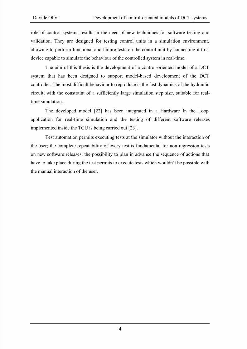
and focused his attention on automotive transmissions [24]. In 1935, he patented his
Autoserve transmission design, that used two clutches; the first engaged even gears, while
the second engaged odd gears. The design was based on a concentric clutch arrangement,
where both clutches shared the same plane. Kégresse installed his system on a 1939
Citroën Traction Avant to test his technology [28]. Unfortunately, the system was never
taken any further because traditional torque converter automatic technology was more
cost effective, and the upcoming WWII stopped the development of transmission
technology.
Figure 1.1 – Fist DCT patent by Adolphe Kégresse, and Citroën Traction Avant with DCT
technology
8/20/2019 Olivi Davide Tesi
http://slidepdf.com/reader/full/olivi-davide-tesi 16/141
Davide Olivi Development of control-oriented models of DCT systems
6
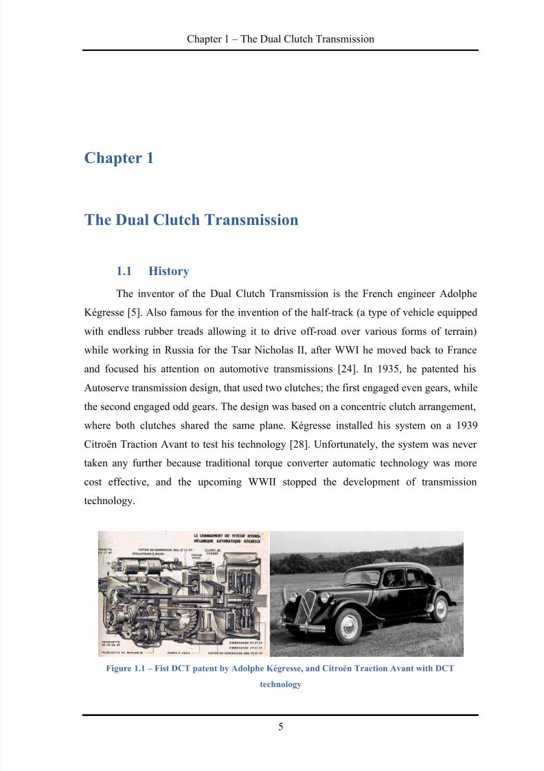
The Dual Clutch Transmission was considered again only in the 1980s, when
Porsche adopted it (called PDK, Porsche Doppelkupplung) for its 956 and 962 Le Mans
racing cars, and Audi installed a transmission with dual clutch technology in its
successful Audi Quattro rally car. In 1985, an Audi Sport Quattro S1 equipped with a
DCT transmission and driven by Michèle Mouton won the Pikes Peak Hill climb rally,
and in 1986 a Porsche 962 driven by Hans-Joachim Stuck and Derek Bell won the Monza
360 Kilometer race, part of the World Sports Prototype Championship.
Figure 1.2 – Porsche 962 and Audi Sport Quattro S1
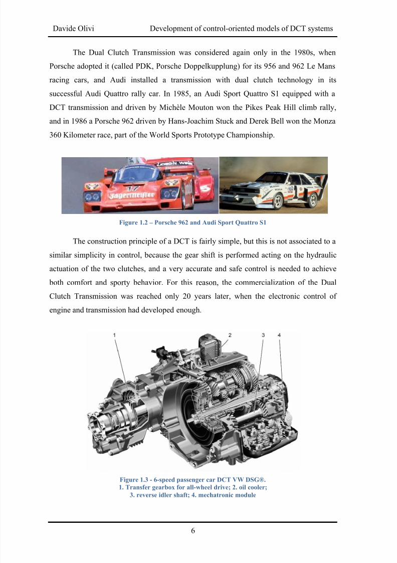
The construction principle of a DCT is fairly simple, but this is not associated to a
similar simplicity in control, because the gear shift is performed acting on the hydraulic
actuation of the two clutches, and a very accurate and safe control is needed to achieve
both comfort and sporty behavior. For this reason, the commercialization of the Dual
Clutch Transmission was reached only 20 years later, when the electronic control of
engine and transmission had developed enough.
Figure 1.3 - 6-speed passenger car DCT VW DSG®.
1. Transfer gearbox for all-wheel drive; 2. oil cooler;
3. reverse idler shaft; 4. mechatronic module
8/20/2019 Olivi Davide Tesi
http://slidepdf.com/reader/full/olivi-davide-tesi 17/141
Chapter 1 – The Dual Clutch Transmission
7
In 2003 Volkswagen licensed BorgWarner's DualTronic technology, becoming the
first to commercialize a car equipped with a DCT transmission (Figure 1.3), adopting it in
the fourth generation VW Golf, at first in the high performance R32 variant. In recent
years most of the automatic transmission suppliers developed their own Dual Clutch
Transmission, supplying it to all the main European automotive constructors [25, 26].
1.2 Operating principle
The DCT technology has been improved since Kégresse’s original concentric
arrangement: many of the latest designs use identically-sized clutches arranged in
parallel, controlling up to seven speeds; clutch types have also improved: wet clutches are
adopted in high performance cars, while dry clutches are developed for B-segmentvehicles which transmit up to 350 Nm, with the advantage of a higher efficiency if
compared to wet clutches.
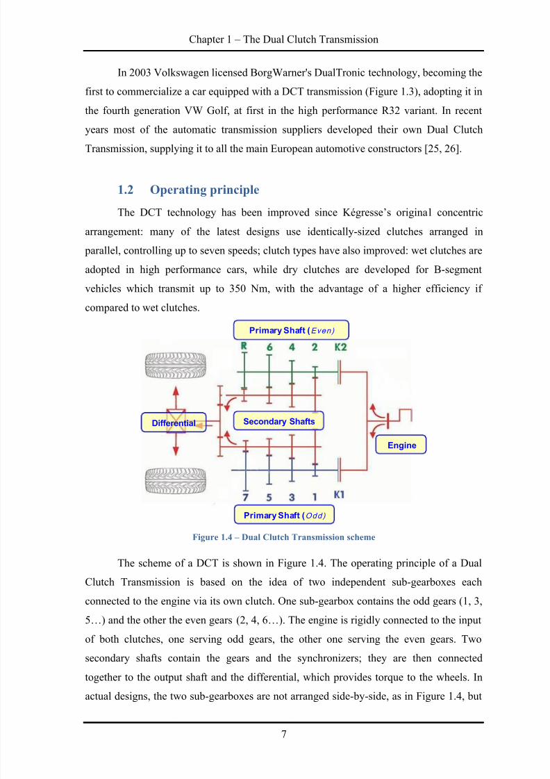
Figure 1.4 – Dual Clutch Transmission scheme
The scheme of a DCT is shown in Figure 1.4. The operating principle of a Dual
Clutch Transmission is based on the idea of two independent sub-gearboxes each
connected to the engine via its own clutch. One sub-gearbox contains the odd gears (1, 3,
5…) and the other the even gears (2, 4, 6…). The engine is rigidly connected to the input
of both clutches, one serving odd gears, the other one serving the even gears. Two
secondary shafts contain the gears and the synchronizers; they are then connected
together to the output shaft and the differential, which provides torque to the wheels. Inactual designs, the two sub-gearboxes are not arranged side-by-side, as in Figure 1.4, but
Primary Shaft (Even)
Primary Shaft (Odd)
Secondary ShaftsDifferential
Engine
8/20/2019 Olivi Davide Tesi
http://slidepdf.com/reader/full/olivi-davide-tesi 18/141
Davide Olivi Development of control-oriented models of DCT systems
8
rather one is nested in the other to save space. For this reason one of the two gearbox
input shafts is a hollow shaft.
In general, a DCT can be considered an evolution of an AMT gearbox, because
the actuation of clutches and synchronizers is electro-hydraulic. Thanks to the
coordinated use of the two clutches, at the moment of gear shift the future gear is already
preselected by the synchronizer on the shaft that is not transmitting torque; the only action
performed during the gear shift is the opening of the currently closed clutch and the
closing of the other one. If a precise control of clutch slipping is performed, the shifting
characteristic is similar to the clutch-to-clutch shift commonly seen in conventional
automatic transmissions [10], but while in a conventional AT the gear shift smoothness is
achieved through the action of the torque converter, which provides a dampening effect
during shift transients, in a DCT transmission the shift comfort depends only on the
control of clutch actuation [12]. Therefore, transmission control plays a key role in the
possibility to install a Dual Clutch Transmission in mass production vehicles. The control
of gearbox actuation is executed by a specific electronic control unit, called Transmission
Control Unit (TCU).
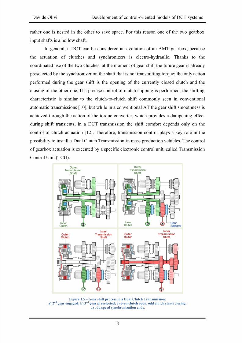
Figure 1.5 –
Gear shift process in a Dual Clutch Transmission:a) 2nd gear engaged; b) 3rd gear preselected; c) even clutch open, odd clutch starts closing;
d) odd speed synchronization ends.
8/20/2019 Olivi Davide Tesi
http://slidepdf.com/reader/full/olivi-davide-tesi 19/141
Chapter 1 – The Dual Clutch Transmission
9
Figure 1.5 shows an example of gear shift [25]. The inner shaft, connected to the
outer clutch, is responsible for odd gears; the outer hollow shaft, connected to the inner
clutch, controls the even gears. At first (Figure 1.5.a) the engine is transmitting torque to
the wheels through the even shaft and clutch, in 2nd gear; while the even clutch is closed,
the 3rd gear is preselected on the odd shaft (Figure 1.5.b) while its relative clutch is open
and consequently not transmitting torque. When a gear shift is requested by the driver (or
by the strategy of the TCU, if the automatic gear shift is selected), the even clutch is open
and, at the same time, the odd clutch is closed (Figure 1.5.c). When the process is over,
i.e. the engine speed and the odd clutch speed are synchronized, the engine transmits
torque through the odd shaft and the 3rd gear (Figure 1.5.d).
8/20/2019 Olivi Davide Tesi
http://slidepdf.com/reader/full/olivi-davide-tesi 20/141
Davide Olivi Development of control-oriented models of DCT systems
10
Chapter 2
The Ferrari Dual Clutch Transmission
2.1 Overview
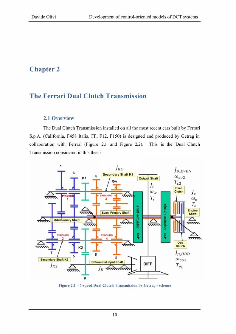
The Dual Clutch Transmission installed on all the most recent cars built by Ferrari
S.p.A. (California, F458 Italia, FF, F12, F150) is designed and produced by Getrag in
collaboration with Ferrari (Figure 2.1 and Figure 2.2). This is the Dual Clutch
Transmission considered in this thesis.
Figure 2.1 – 7-speed Dual Clutch Transmission by Getrag - scheme
8/20/2019 Olivi Davide Tesi
http://slidepdf.com/reader/full/olivi-davide-tesi 21/141
Chapter 2 – The Ferrari Dual Clutch Transmission
11
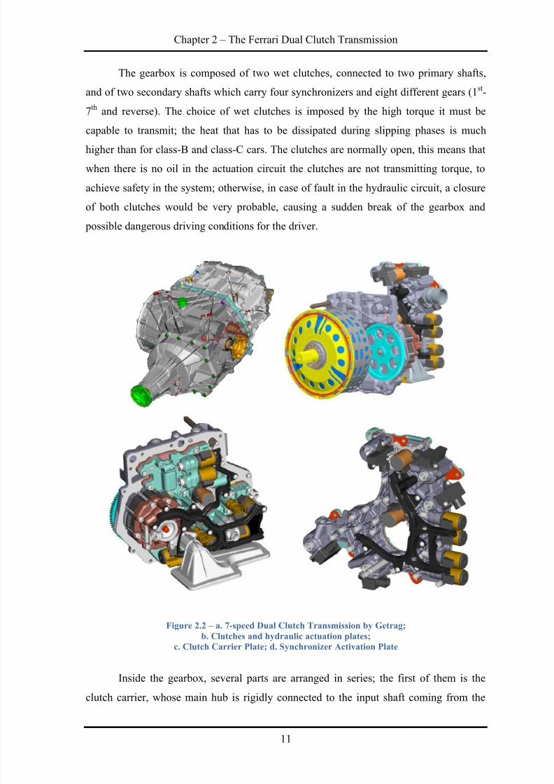
The gearbox is composed of two wet clutches, connected to two primary shafts,
and of two secondary shafts which carry four synchronizers and eight different gears (1st-
7th and reverse). The choice of wet clutches is imposed by the high torque it must be
capable to transmit; the heat that has to be dissipated during slipping phases is much
higher than for class-B and class-C cars. The clutches are normally open, this means that
when there is no oil in the actuation circuit the clutches are not transmitting torque, to
achieve safety in the system; otherwise, in case of fault in the hydraulic circuit, a closure
of both clutches would be very probable, causing a sudden break of the gearbox and
possible dangerous driving conditions for the driver.
Figure 2.2 – a. 7-speed Dual Clutch Transmission by Getrag;
b. Clutches and hydraulic actuation plates;
c. Clutch Carrier Plate; d. Synchronizer Activation Plate
Inside the gearbox, several parts are arranged in series; the first of them is the
clutch carrier, whose main hub is rigidly connected to the input shaft coming from the
8/20/2019 Olivi Davide Tesi
http://slidepdf.com/reader/full/olivi-davide-tesi 22/141
Davide Olivi Development of control-oriented models of DCT systems
12
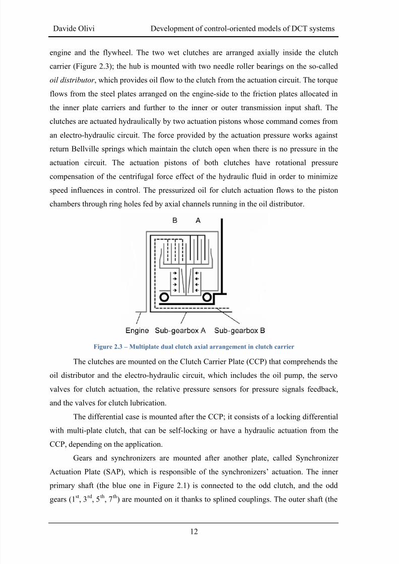
engine and the flywheel. The two wet clutches are arranged axially inside the clutch
carrier (Figure 2.3); the hub is mounted with two needle roller bearings on the so-called
oil distributor , which provides oil flow to the clutch from the actuation circuit. The torque
flows from the steel plates arranged on the engine-side to the friction plates allocated in
the inner plate carriers and further to the inner or outer transmission input shaft. The
clutches are actuated hydraulically by two actuation pistons whose command comes from
an electro-hydraulic circuit. The force provided by the actuation pressure works against
return Bellville springs which maintain the clutch open when there is no pressure in the
actuation circuit. The actuation pistons of both clutches have rotational pressure
compensation of the centrifugal force effect of the hydraulic fluid in order to minimize
speed influences in control. The pressurized oil for clutch actuation flows to the piston
chambers through ring holes fed by axial channels running in the oil distributor.
Figure 2.3 – Multiplate dual clutch axial arrangement in clutch carrier
The clutches are mounted on the Clutch Carrier Plate (CCP) that comprehends the
oil distributor and the electro-hydraulic circuit, which includes the oil pump, the servo
valves for clutch actuation, the relative pressure sensors for pressure signals feedback,
and the valves for clutch lubrication.
The differential case is mounted after the CCP; it consists of a locking differential
with multi-plate clutch, that can be self-locking or have a hydraulic actuation from the
CCP, depending on the application.
Gears and synchronizers are mounted after another plate, called Synchronizer
Actuation Plate (SAP), which is responsible of the synchronizers’ actuation. The inner
primary shaft (the blue one in Figure 2.1) is connected to the odd clutch, and the odd
gears (1st, 3rd, 5th, 7th) are mounted on it thanks to splined couplings. The outer shaft (the
8/20/2019 Olivi Davide Tesi
http://slidepdf.com/reader/full/olivi-davide-tesi 23/141
Chapter 2 – The Ferrari Dual Clutch Transmission
13
orange one) is connected to the even clutch and to the even gears (2nd, 4th, 6th and
Reverse). The 1st gear and the 7th gear have a dedicated gear on the primary shaft, while
the others share a gear in the primary shaft, in couples (2nd – Reverse, 3rd – 5 th, 4th – 6th).
Both K1 and K2 gears, splined on the secondary shafts, engage the gear K splined on the
gearbox output shaft. On K1 secondary shaft 1 st, 3rd, 4th and Reverse gears are mounted,
while 2nd, 5th, 6th and 7th gears are relative to K2 shaft.
The Synchronizers Activation Plate consists of several actuators which controls
the synchronizers’ motion, the odd-even gears selector and the parking lock, i.e. the
mechanical device which locks the output shaft against the transmission housing in order
to maintain the vehicle still when the engine is switched off and the clutches are open, to
avoid unintentional rolling away while parked. The desired gear is selected through the
use of four synchronizers, each serving two gears: 1st – 3rd, 5th – 7th, 2nd – 6th, 4th –
Reverse. The two gears of each synchronizer are always relative to the same sub-gearbox:
in this way, it can never happen that the same selector has to preselect the future gear
while it is already selecting the actual one.
2.2 Hydraulic circuit
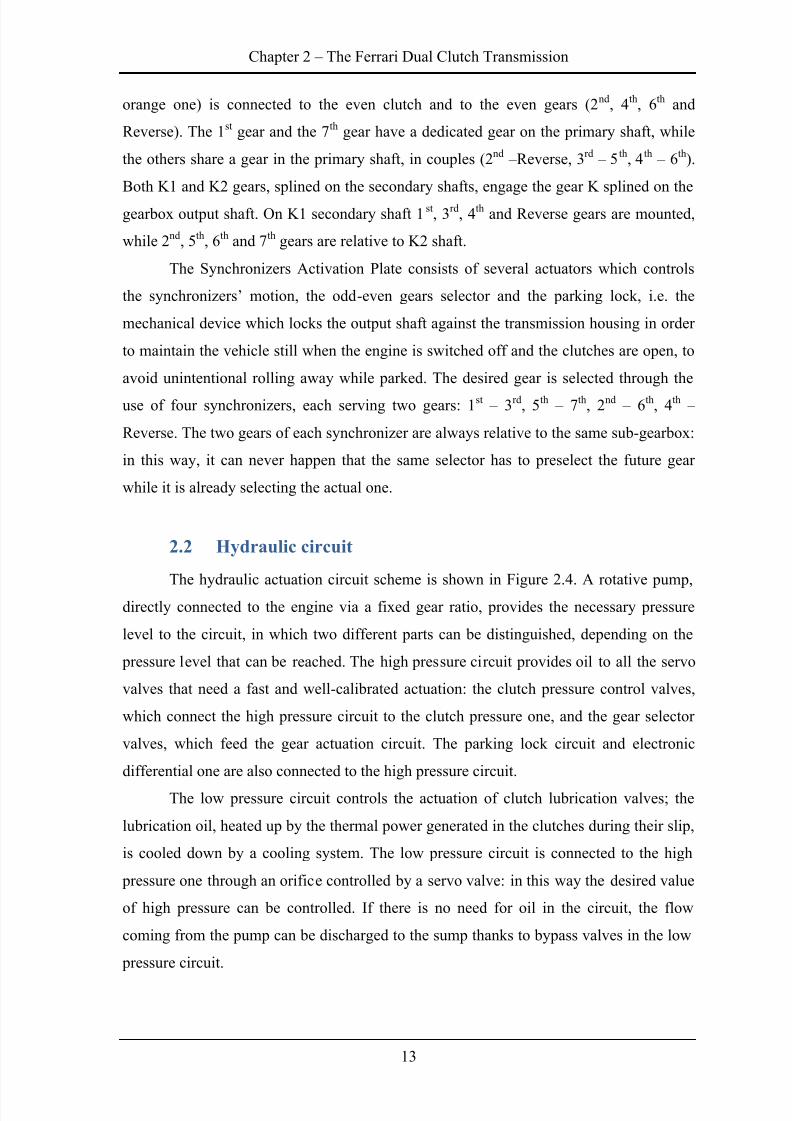
The hydraulic actuation circuit scheme is shown in Figure 2.4. A rotative pump,
directly connected to the engine via a fixed gear ratio, provides the necessary pressure
level to the circuit, in which two different parts can be distinguished, depending on the
pressure level that can be reached. The high pressure circuit provides oil to all the servo
valves that need a fast and well-calibrated actuation: the clutch pressure control valves,
which connect the high pressure circuit to the clutch pressure one, and the gear selector
valves, which feed the gear actuation circuit. The parking lock circuit and electronic
differential one are also connected to the high pressure circuit.
The low pressure circuit controls the actuation of clutch lubrication valves; the
lubrication oil, heated up by the thermal power generated in the clutches during their slip,
is cooled down by a cooling system. The low pressure circuit is connected to the high
pressure one through an orifice controlled by a servo valve: in this way the desired value
of high pressure can be controlled. If there is no need for oil in the circuit, the flow
coming from the pump can be discharged to the sump thanks to bypass valves in the low
pressure circuit.
8/20/2019 Olivi Davide Tesi
http://slidepdf.com/reader/full/olivi-davide-tesi 24/141
Davide Olivi Development of control-oriented models of DCT systems
14
Figure 2.4 – Hydraulic actuation scheme
2.3 Hardware modifications for electric drive
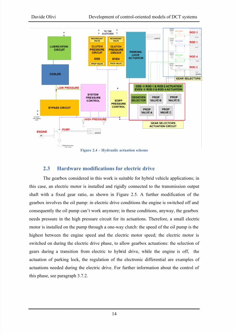
The gearbox considered in this work is suitable for hybrid vehicle applications; in
this case, an electric motor is installed and rigidly connected to the transmission output
shaft with a fixed gear ratio, as shown in Figure 2.5. A further modification of the
gearbox involves the oil pump: in electric drive conditions the engine is switched off and
consequently the oil pump can’t work anymore; in these conditions, anyway, the gearbox
needs pressure in the high pressure circuit for its actuations. Therefore, a small electric
motor is installed on the pump through a one-way clutch: the speed of the oil pump is the
highest between the engine speed and the electric motor speed; the electric motor is
switched on during the electric drive phase, to allow gearbox actuations: the selection of
gears during a transition from electric to hybrid drive, while the engine is off, the
actuation of parking lock, the regulation of the electronic differential are examples of
actuations needed during the electric drive. For further information about the control of
this phase, see paragraph 3.7.2.
8/20/2019 Olivi Davide Tesi
http://slidepdf.com/reader/full/olivi-davide-tesi 25/141
Chapter 2 – The Ferrari Dual Clutch Transmission
15
Figure 2.5 – Installation of the electric motor on gearbox output shaft
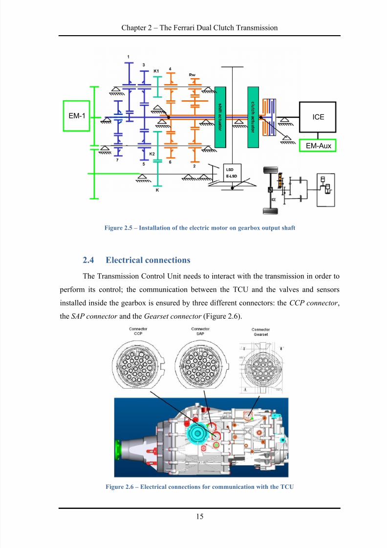
2.4 Electrical connections
The Transmission Control Unit needs to interact with the transmission in order to
perform its control; the communication between the TCU and the valves and sensors
installed inside the gearbox is ensured by three different connectors: the CCP connector ,
the SAP connector and the Gearset connector (Figure 2.6).
Figure 2.6 – Electrical connections for communication with the TCU
EM-1 ICE
EM-Aux
8/20/2019 Olivi Davide Tesi
http://slidepdf.com/reader/full/olivi-davide-tesi 26/141
Davide Olivi Development of control-oriented models of DCT systems
16
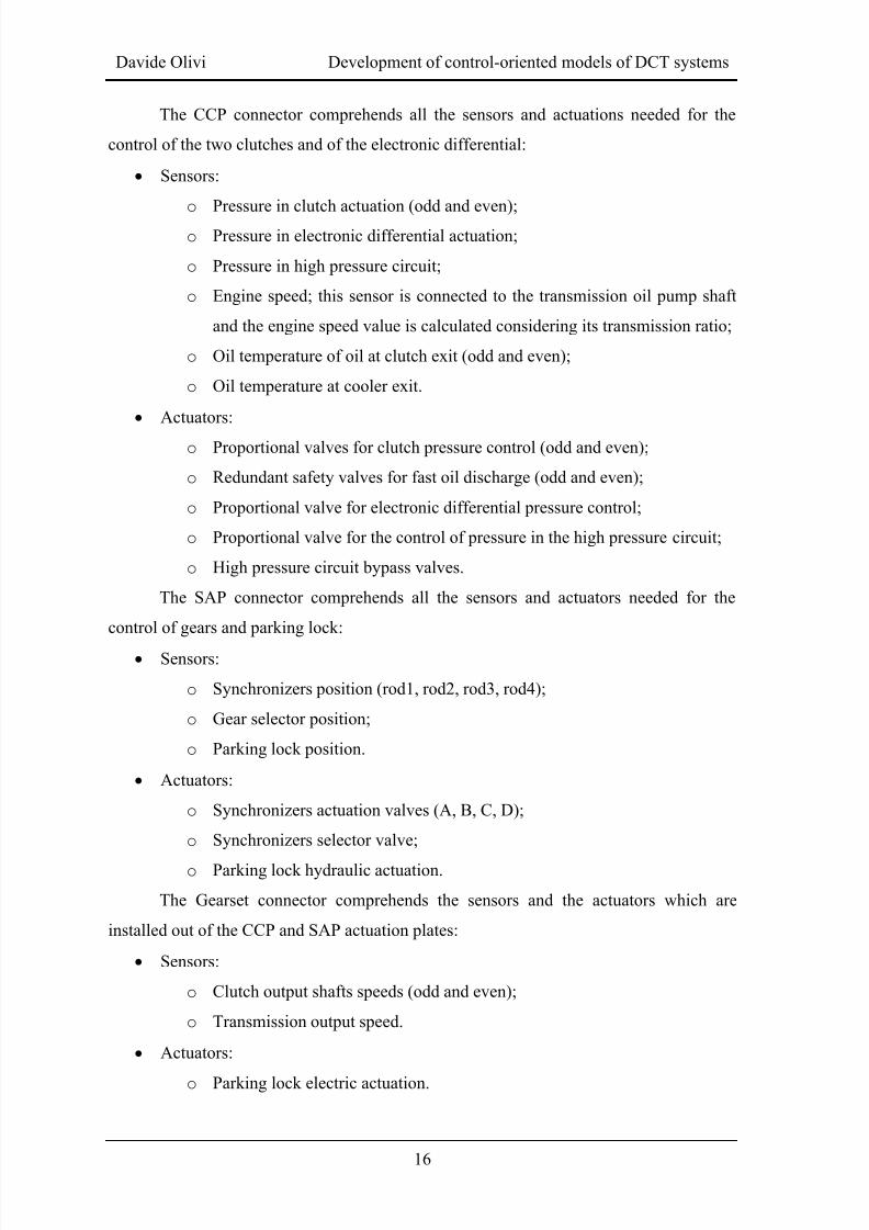
The CCP connector comprehends all the sensors and actuations needed for the
control of the two clutches and of the electronic differential:
Sensors:
o Pressure in clutch actuation (odd and even);
o
Pressure in electronic differential actuation;
o Pressure in high pressure circuit;
o Engine speed; this sensor is connected to the transmission oil pump shaft
and the engine speed value is calculated considering its transmission ratio;
o Oil temperature of oil at clutch exit (odd and even);
o Oil temperature at cooler exit.
Actuators:
o Proportional valves for clutch pressure control (odd and even);
o
Redundant safety valves for fast oil discharge (odd and even);
o Proportional valve for electronic differential pressure control;
o Proportional valve for the control of pressure in the high pressure circuit;
o
High pressure circuit bypass valves.
The SAP connector comprehends all the sensors and actuators needed for the
control of gears and parking lock:
Sensors:
o Synchronizers position (rod1, rod2, rod3, rod4);
o Gear selector position;
o Parking lock position.
Actuators:
o Synchronizers actuation valves (A, B, C, D);
o Synchronizers selector valve;
o
Parking lock hydraulic actuation.
The Gearset connector comprehends the sensors and the actuators which are
installed out of the CCP and SAP actuation plates:
Sensors:
o
Clutch output shafts speeds (odd and even);
o Transmission output speed.
Actuators:
o
Parking lock electric actuation.
8/20/2019 Olivi Davide Tesi
http://slidepdf.com/reader/full/olivi-davide-tesi 27/141
Chapter 2 – The Ferrari Dual Clutch Transmission
17
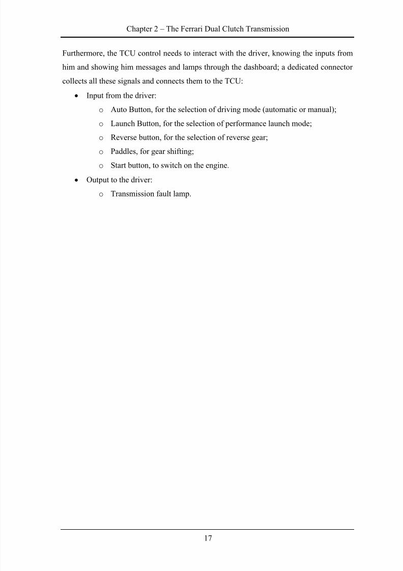
Furthermore, the TCU control needs to interact with the driver, knowing the inputs from
him and showing him messages and lamps through the dashboard; a dedicated connector
collects all these signals and connects them to the TCU:
Input from the driver:
o
Auto Button, for the selection of driving mode (automatic or manual);
o Launch Button, for the selection of performance launch mode;
o Reverse button, for the selection of reverse gear;
o Paddles, for gear shifting;
o Start button, to switch on the engine.
Output to the driver:
o Transmission fault lamp.
8/20/2019 Olivi Davide Tesi
http://slidepdf.com/reader/full/olivi-davide-tesi 28/141
Davide Olivi Development of control-oriented models of DCT systems
18
Chapter 3
The Dual Clutch Transmission model
3.1 Hydraulic actuation circuit
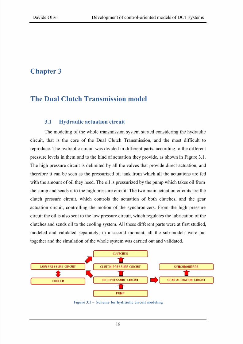
The modeling of the whole transmission system started considering the hydraulic
circuit, that is the core of the Dual Clutch Transmission, and the most difficult to
reproduce. The hydraulic circuit was divided in different parts, according to the different
pressure levels in them and to the kind of actuation they provide, as shown in Figure 3.1.
The high pressure circuit is delimited by all the valves that provide direct actuation, and
therefore it can be seen as the pressurized oil tank from which all the actuations are fed
with the amount of oil they need. The oil is pressurized by the pump which takes oil from
the sump and sends it to the high pressure circuit. The two main actuation circuits are the
clutch pressure circuit, which controls the actuation of both clutches, and the gear
actuation circuit, controlling the motion of the synchronizers. From the high pressure
circuit the oil is also sent to the low pressure circuit, which regulates the lubrication of the
clutches and sends oil to the cooling system. All these different parts were at first studied,
modeled and validated separately; in a second moment, all the sub-models were put
together and the simulation of the whole system was carried out and validated.
Figure 3.1 –
Scheme for hydraulic circuit modeling
8/20/2019 Olivi Davide Tesi
http://slidepdf.com/reader/full/olivi-davide-tesi 29/141
Chapter 3 – The Dual Clutch Transmission model
19
A generic pressure dynamics model was developed by considering the continuity
equation of an incompressible fluid [15], taking into account all input flows and
output flows in the circuit, the total volume change from the initial value caused
by the motion of mechanical parts, and the total bulk modulus
of the oil circulating
in the circuit, as shown in Equation (3.1):
(3.1)
Equation (3.1) can be applied for every part of the circuit: in the high pressure circuit, the
term can be considered negligible, because only the valve spools are moving and
the volume change is very low. Instead, this term is particularly important in the clutch
pressure circuit, because of the clutch motion while closing or opening, and in the
synchr onizers’ actuation circuit, due to the rod motion from a position to another
(depending on the selected gear).
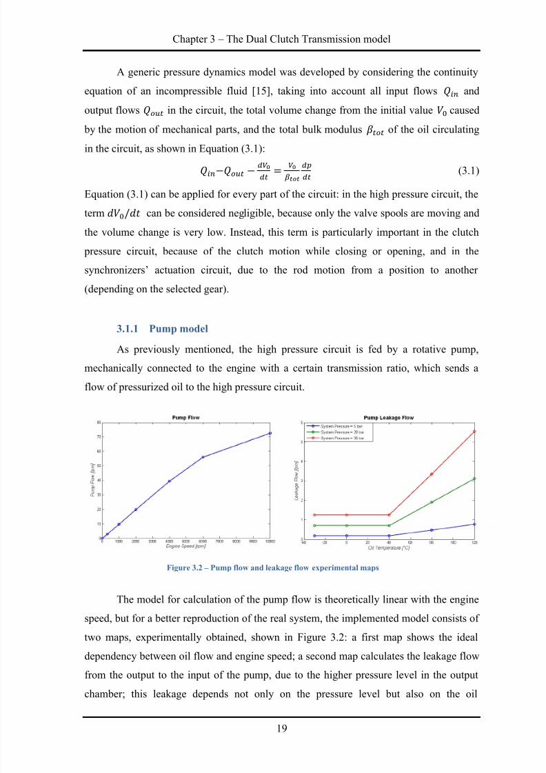
3.1.1 Pump model
As previously mentioned, the high pressure circuit is fed by a rotative pump,
mechanically connected to the engine with a certain transmission ratio, which sends a
flow of pressurized oil to the high pressure circuit.
The model for calculation of the pump flow is theoretically linear with the engine
speed, but for a better reproduction of the real system, the implemented model consists of
two maps, experimentally obtained, shown in Figure 3.2: a first map shows the ideal
dependency between oil flow and engine speed; a second map calculates the leakage flow
from the output to the input of the pump, due to the higher pressure level in the outputchamber; this leakage depends not only on the pressure level but also on the oil
Figure 3.2 – Pump flow and leakage flow experimental maps
8/20/2019 Olivi Davide Tesi
http://slidepdf.com/reader/full/olivi-davide-tesi 30/141
Davide Olivi Development of control-oriented models of DCT systems
20
temperature, which modifies the oil properties (density and viscosity): the lower the
temperature, the more viscous the oil, the lower the leakage flow through the pump.
3.1.2 System pressure modelThe pressure level in the high pressure circuit is called system pressure; it is
usually regulated for values between 15 and 35 bars during the normal transmission
operation; the actual desired value depends on the actuations that are going to happen in
the system (clutch closure, synchronizer motion, etc...). A safety valve automatically
opens the circuit if the internal pressure level reaches 40 bars.
The control of system pressure is performed by regulating the actuation current on
a proportional three-way servo valve; its output flow actuates a hydraulic valve, which
opens the orifice that connects the high pressure circuit to the low pressure one. A first
feed-forward open loop value of current to be applied on the valve is calculated by the
TCU according to the desired pressure value to be reached. The actual system pressure
value is then measured thanks to a pressure sensor, which gives the possibility to correct
the open loop current value with a closed-loop contribution calculated by a PID
considering the difference between the desired pressure value and the actual one.
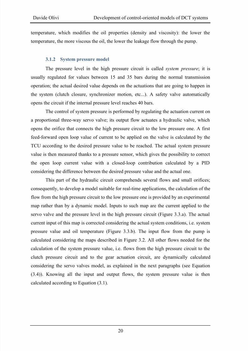
This part of the hydraulic circuit comprehends several flows and small orifices;
consequently, to develop a model suitable for real-time applications, the calculation of the
flow from the high pressure circuit to the low pressure one is provided by an experimental
map rather than by a dynamic model. Inputs to such map are the current applied to the
servo valve and the pressure level in the high pressure circuit (Figure 3.3.a). The actual
current input of this map is corrected considering the actual system conditions, i.e. system
pressure value and oil temperature (Figure 3.3.b). The input flow from the pump is
calculated considering the maps described in Figure 3.2. All other flows needed for the
calculation of the system pressure value, i.e. flows from the high pressure circuit to the
clutch pressure circuit and to the gear actuation circuit, are dynamically calculated
considering the servo valves model, as explained in the next paragraphs (see Equation
(3.4)). Knowing all the input and output flows, the system pressure value is then
calculated according to Equation (3.1).
8/20/2019 Olivi Davide Tesi
http://slidepdf.com/reader/full/olivi-davide-tesi 31/141
Chapter 3 – The Dual Clutch Transmission model
21
Figure 3.3 – a. Experimental map for calculation of flow through the system pressure regulation
valve; b. System pressure correction map
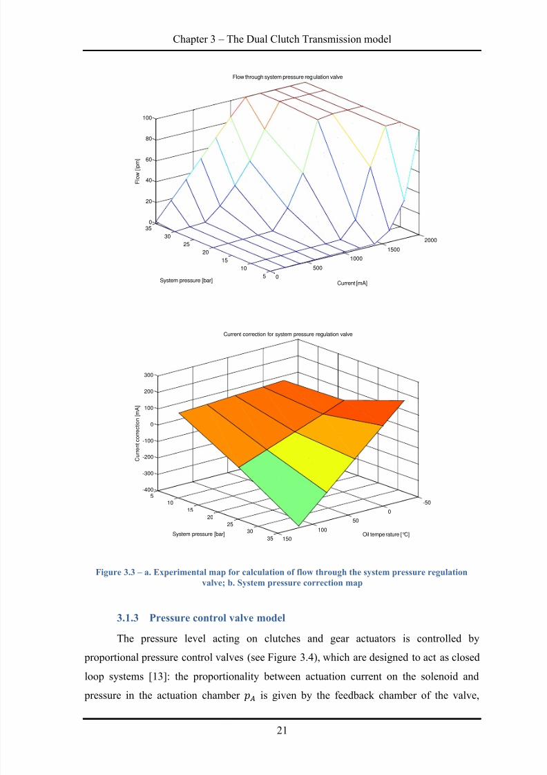
3.1.3 Pressure control valve model
The pressure level acting on clutches and gear actuators is controlled by
proportional pressure control valves (see Figure 3.4), which are designed to act as closed
loop systems [13]: the proportionality between actuation current on the solenoid and pressure in the actuation chamber is given by the feedback chamber of the valve,
0
500
1000
1500
2000
5
10
15
20
25
30
350
20
40
60
80
100
Current [mA]
Flow through system pressure regulation valve
System pressure [bar]
Flow
[lpm]
-50
0
50
100
150
5
10
15
20
25
30
35
-400
-300
-200
-100
0
100
200
300
Oil temperature [°C]
Current correction for system pressure regulation valve
System pressure [bar]
Currentcorrection[mA]
8/20/2019 Olivi Davide Tesi
http://slidepdf.com/reader/full/olivi-davide-tesi 32/141
Davide Olivi Development of control-oriented models of DCT systems
22
which generates a feedback force against the valve opening, whose proportionality
factor is the feedback chamber area of the spool, as shown in Equation (3.2): (3.2)
The dynamics of the spool is given by the mass-spring-damper Equation (3.3): (3.3)
Figure 3.4 – Three way proportional valve
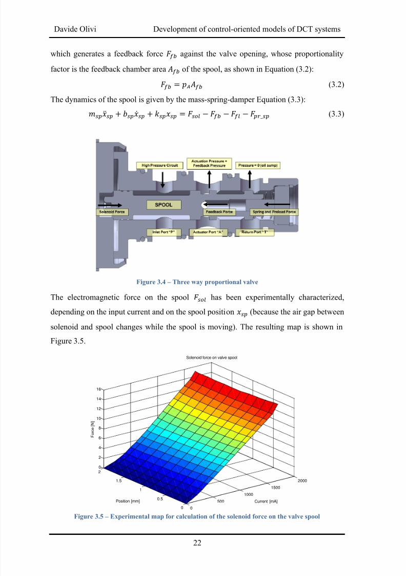
The electromagnetic force on the spool
has been experimentally characterized,
depending on the input current and on the spool position (because the air gap between
solenoid and spool changes while the spool is moving). The resulting map is shown in
Figure 3.5.
Figure 3.5 – Experimental map for calculation of the solenoid force on the valve spool
0
500
1000
1500
2000
0
0.5
1
1.5
20
2
4
6
8
10
12
14
16
Current [mA]
Solenoid force on valve spool
Position [mm]
Force[N]
8/20/2019 Olivi Davide Tesi
http://slidepdf.com/reader/full/olivi-davide-tesi 33/141
Chapter 3 – The Dual Clutch Transmission model
23
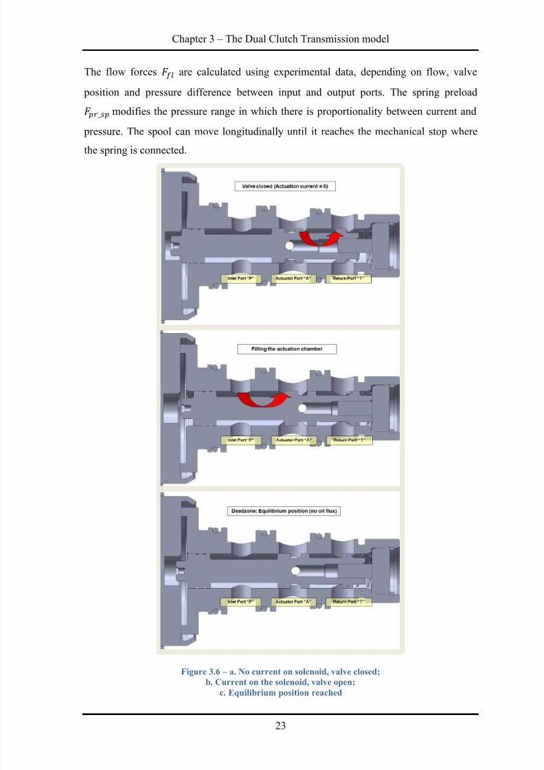
The flow forces are calculated using experimental data, depending on flow, valve
position and pressure difference between input and output ports. The spring preload modifies the pressure range in which there is proportionality between current and
pressure. The spool can move longitudinally until it reaches the mechanical stop wherethe spring is connected.
Figure 3.6 –
a. No current on solenoid, valve closed;b. Current on the solenoid, valve open;
c. Equilibrium position reached
8/20/2019 Olivi Davide Tesi
http://slidepdf.com/reader/full/olivi-davide-tesi 34/141
Davide Olivi Development of control-oriented models of DCT systems
24
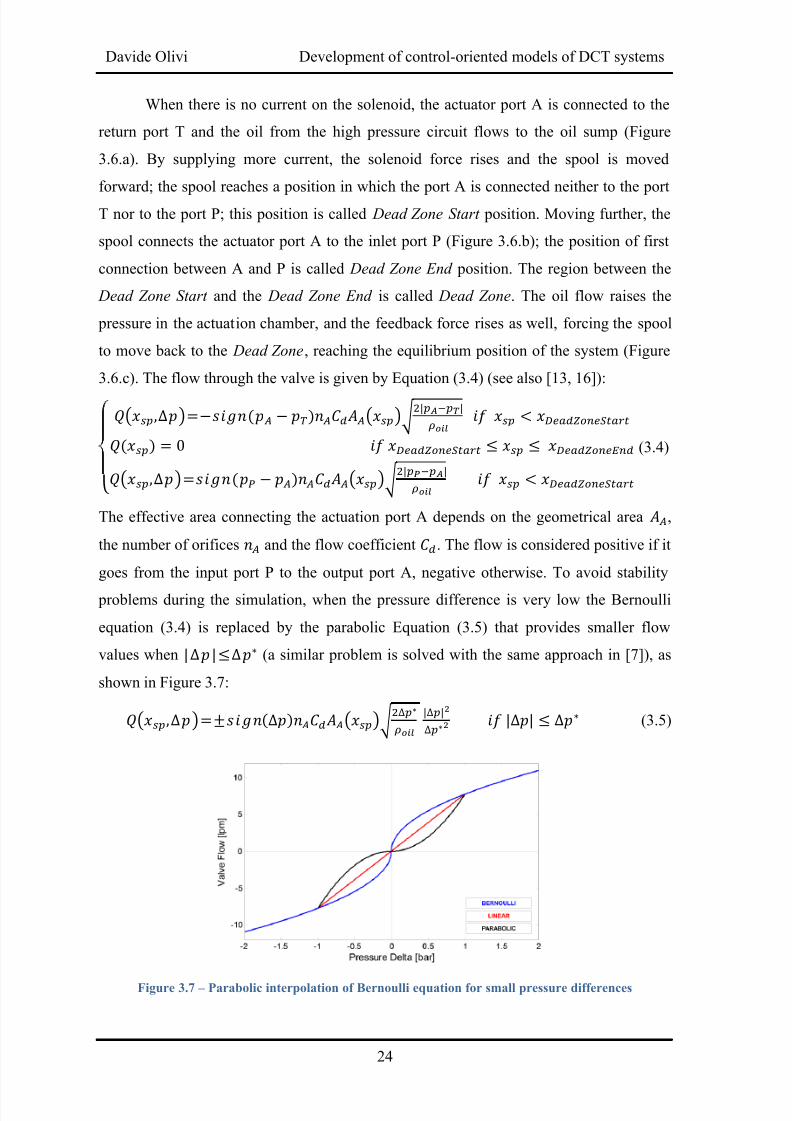
When there is no current on the solenoid, the actuator port A is connected to the
return port T and the oil from the high pressure circuit flows to the oil sump (Figure
3.6.a). By supplying more current, the solenoid force rises and the spool is moved
forward; the spool reaches a position in which the port A is connected neither to the port
T nor to the port P; this position is called Dead Zone Start position. Moving further, the
spool connects the actuator port A to the inlet port P (Figure 3.6.b); the position of first
connection between A and P is called Dead Zone End position. The region between the
Dead Zone Start and the Dead Zone End is called Dead Zone. The oil flow raises the
pressure in the actuation chamber, and the feedback force rises as well, forcing the spool
to move back to the Dead Zone, reaching the equilibrium position of the system (Figure
3.6.c). The flow through the valve is given by Equation (3.4) (see also [13, 16]):
{() ()√ () ()√
(3.4)
The effective area connecting the actuation port A depends on the geometrical area ,
the number of orifices and the flow coefficient . The flow is considered positive if it
goes from the input port P to the output port A, negative otherwise. To avoid stability
problems during the simulation, when the pressure difference is very low the Bernoulli
equation (3.4) is replaced by the parabolic Equation (3.5) that provides smaller flow
values when (a similar problem is solved with the same approach in [7]), as
shown in Figure 3.7:
() ()√ (3.5)
Figure 3.7 –
Parabolic interpolation of Bernoulli equation for small pressure differences
8/20/2019 Olivi Davide Tesi
http://slidepdf.com/reader/full/olivi-davide-tesi 35/141
Chapter 3 – The Dual Clutch Transmission model
25
3.1.4 Safety valve model
A safety valve is installed inside the high pressure circuit to prevent the pressure
level to overtake the value of 40 bars, for safety reasons. The model of the safety valvemust calculate the flow through the valve, because it is needed for the dynamic
calculation of the pressure inside the circuit through Equation (3.1). The spool dynamic
equation is similar to Equation (3.3): (3.6)
The preload force is calibrated so that it can be overtaken only when the pressure
inside the circuit reaches the level of 40 bars; when the spool moves, all the area is
available for the oil to flow out of the circuit; the calculation of the oil flow is executedthough the Bernoulli equation:
√ (3.7)
This term is part of the output flows of Equation (3.1) in the calculation of the pressure in
the high pressure circuit, in case the pressure reaches the level of 40 bars. An example of
simulation of this model is provided in Figure 8.7.
3.2 Clutch model
3.2.1 Clutch actuation model
The clutches of the considered Dual Clutch Transmission are wet clutches; the
lubrication oil removes the heat generated while slipping, and the torque is transmitted by
the contact between the clutch discs, covered with high-friction materials, and the
separator plates. The clutch motion is opposed by Bellville springs between every friction
disc, giving also a preload force. For safety reasons, when no actuation is required, theclutch is open and engine shaft and transmission shaft are separated. The clutch closure is
performed by pumping current in the corresponding proportional valve, in order to raise
the pressure level acting on the clutch actuator.
8/20/2019 Olivi Davide Tesi
http://slidepdf.com/reader/full/olivi-davide-tesi 36/141
Davide Olivi Development of control-oriented models of DCT systems
26
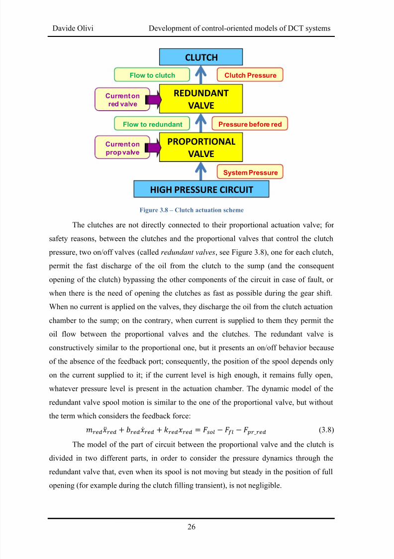
Figure 3.8 – Clutch actuation scheme
The clutches are not directly connected to their proportional actuation valve; for
safety reasons, between the clutches and the proportional valves that control the clutch
pressure, two on/off valves (called redundant valves, see Figure 3.8), one for each clutch,
permit the fast discharge of the oil from the clutch to the sump (and the consequent
opening of the clutch) bypassing the other components of the circuit in case of fault, or
when there is the need of opening the clutches as fast as possible during the gear shift.
When no current is applied on the valves, they discharge the oil from the clutch actuation
chamber to the sump; on the contrary, when current is supplied to them they permit the
oil flow between the proportional valves and the clutches. The redundant valve is
constructively similar to the proportional one, but it presents an on/off behavior because
of the absence of the feedback port; consequently, the position of the spool depends only
on the current supplied to it; if the current level is high enough, it remains fully open,
whatever pressure level is present in the actuation chamber. The dynamic model of theredundant valve spool motion is similar to the one of the proportional valve, but without
the term which considers the feedback force: (3.8)
The model of the part of circuit between the proportional valve and the clutch is
divided in two different parts, in order to consider the pressure dynamics through the
redundant valve that, even when its spool is not moving but steady in the position of full
opening (for example during the clutch filling transient), is not negligible.
REDUNDANT
VALVE
PROPORTIONAL
VALVE
System Pressure
Pressure before red
Clutch Pressure
Currenton
propvalve
Currentonred valve
Flow to redundant
Flow to clutch
HIGH PRESSURE CIRCUIT
CLUTCH
8/20/2019 Olivi Davide Tesi
http://slidepdf.com/reader/full/olivi-davide-tesi 37/141
Chapter 3 – The Dual Clutch Transmission model
27
Calculation of the pressure in the chamber between the proportional valve
and the redundant valve may be performed by applying the mass conservation principle
of Equation (3.1), as shown in Equation (3.9):
(3.9)
Calculation of pressure acting on the clutch may be performed in a similar way:
(3.10)
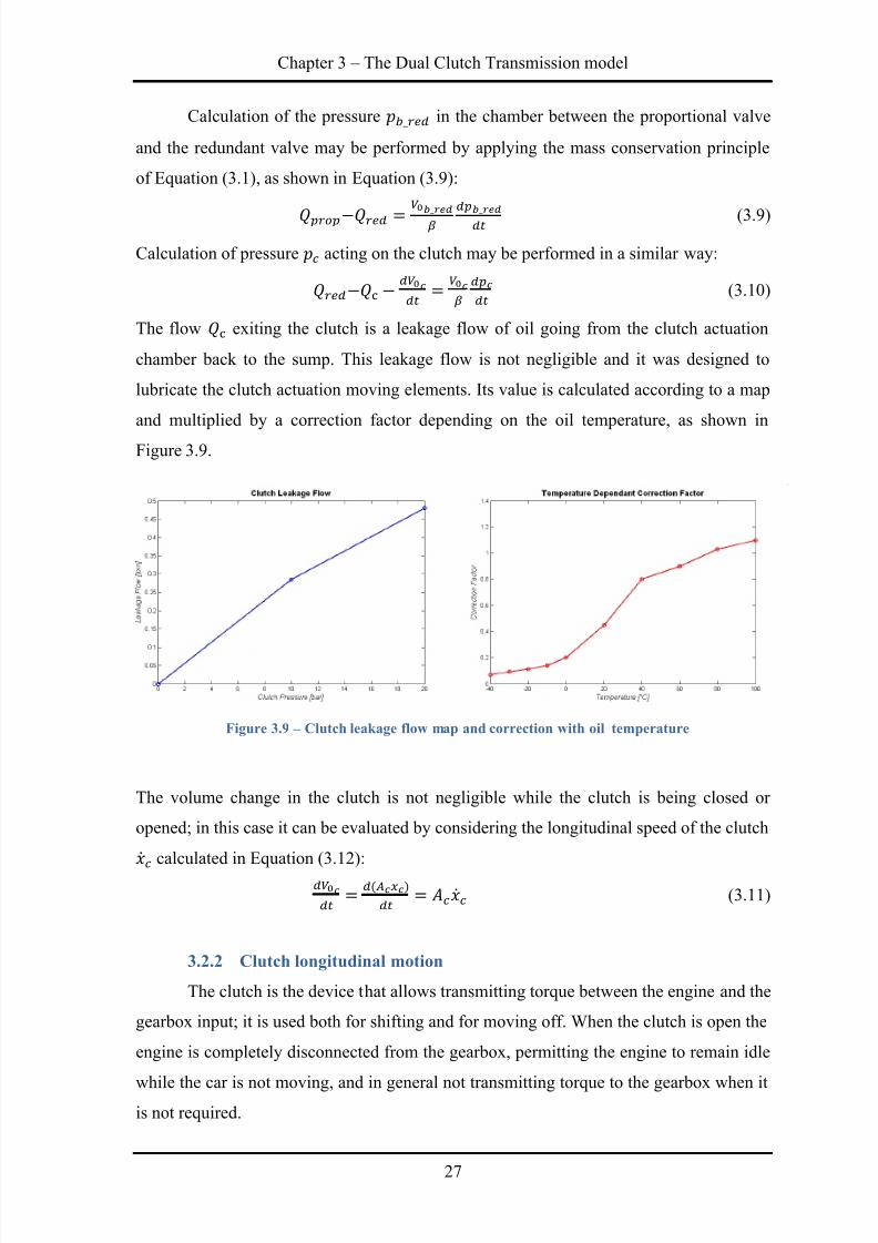
The flow exiting the clutch is a leakage flow of oil going from the clutch actuation
chamber back to the sump. This leakage flow is not negligible and it was designed to
lubricate the clutch actuation moving elements. Its value is calculated according to a map
and multiplied by a correction factor depending on the oil temperature, as shown in
Figure 3.9.
The volume change in the clutch is not negligible while the clutch is being closed or
opened; in this case it can be evaluated by considering the longitudinal speed of the clutch
calculated in Equation (3.12):
(3.11)
3.2.2 Clutch longitudinal motion
The clutch is the device that allows transmitting torque between the engine and the
gearbox input; it is used both for shifting and for moving off. When the clutch is open the
engine is completely disconnected from the gearbox, permitting the engine to remain idle
while the car is not moving, and in general not transmitting torque to the gearbox when itis not required.
Figure 3.9 – Clutch leakage flow map and correction with oil temperature
8/20/2019 Olivi Davide Tesi
http://slidepdf.com/reader/full/olivi-davide-tesi 38/141
Davide Olivi Development of control-oriented models of DCT systems
28
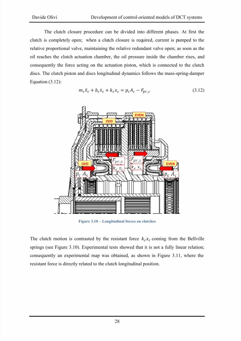
The clutch closure procedure can be divided into different phases. At first the
clutch is completely open; when a clutch closure is required, current is pumped to the
relative proportional valve, maintaining the relative redundant valve open; as soon as the
oil reaches the clutch actuation chamber, the oil pressure inside the chamber rises, and
consequently the force acting on the actuation piston, which is connected to the clutch
discs. The clutch piston and discs longitudinal dynamics follows the mass-spring-damper
Equation (3.12): (3.12)
Figure 3.10 – Longitudinal forces on clutches
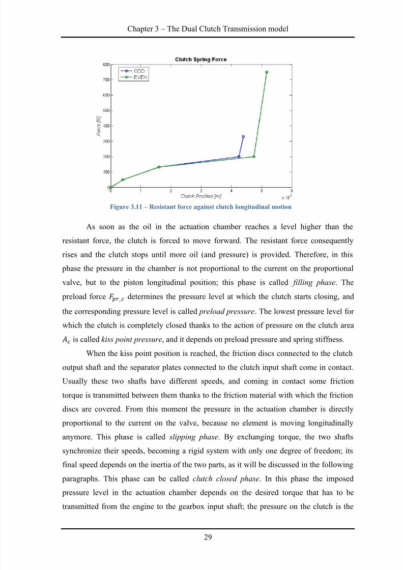
The clutch motion is contrasted by the resistant force coming from the Bellville
springs (see Figure 3.10). Experimental tests showed that it is not a fully linear relation;
consequently an experimental map was obtained, as shown in Figure 3.11, where the
resistant force is directly related to the clutch longitudinal position.
ODD EVEN
ODD
EVEN
8/20/2019 Olivi Davide Tesi
http://slidepdf.com/reader/full/olivi-davide-tesi 39/141
Chapter 3 – The Dual Clutch Transmission model
29
As soon as the oil in the actuation chamber reaches a level higher than the
resistant force, the clutch is forced to move forward. The resistant force consequently
rises and the clutch stops until more oil (and pressure) is provided. Therefore, in this
phase the pressure in the chamber is not proportional to the current on the proportional
valve, but to the piston longitudinal position; this phase is called filling phase. The
preload force determines the pressure level at which the clutch starts closing, andthe corresponding pressure level is called preload pressure. The lowest pressure level for
which the clutch is completely closed thanks to the action of pressure on the clutch area is called kiss point pressure, and it depends on preload pressure and spring stiffness.
When the kiss point position is reached, the friction discs connected to the clutch
output shaft and the separator plates connected to the clutch input shaft come in contact.
Usually these two shafts have different speeds, and coming in contact some friction
torque is transmitted between them thanks to the friction material with which the friction
discs are covered. From this moment the pressure in the actuation chamber is directly
proportional to the current on the valve, because no element is moving longitudinally
anymore. This phase is called slipping phase. By exchanging torque, the two shafts
synchronize their speeds, becoming a rigid system with only one degree of freedom; its
final speed depends on the inertia of the two parts, as it will be discussed in the following
paragraphs. This phase can be called clutch closed phase. In this phase the imposed
pressure level in the actuation chamber depends on the desired torque that has to be
transmitted from the engine to the gearbox input shaft; the pressure on the clutch is the
Figure 3.11 – Resistant force against clutch longitudinal motion
8/20/2019 Olivi Davide Tesi
http://slidepdf.com/reader/full/olivi-davide-tesi 40/141
Davide Olivi Development of control-oriented models of DCT systems
30
lower pressure which ensures that the clutch will remain closed, i.e. the speed
synchronization between the clutch input and output shafts won’t be lost.
The clutch goes back to the slipping phase when the pressure level is not sufficient
to transmit the torque exchanged through the clutch. If the pressure level becomes lower
than the Bellville springs force, the clutch starts opening, discharging oil to the sump; if
the pressure level is low enough, the clutch reaches its preload position and goes back to
the fully open condition.
3.2.3 Clutch hysteresis
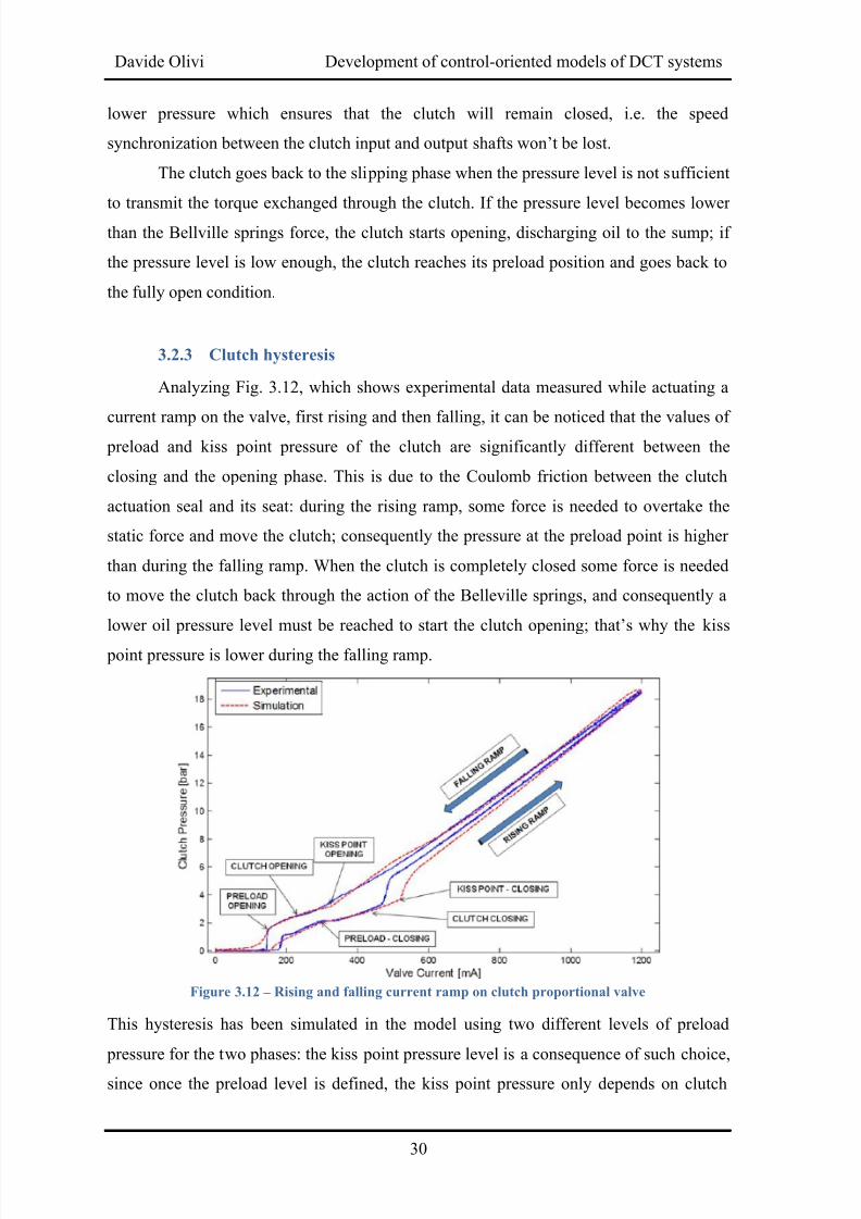
Analyzing Fig. 3.12, which shows experimental data measured while actuating a
current ramp on the valve, first rising and then falling, it can be noticed that the values of
preload and kiss point pressure of the clutch are significantly different between the
closing and the opening phase. This is due to the Coulomb friction between the clutch
actuation seal and its seat: during the rising ramp, some force is needed to overtake the
static force and move the clutch; consequently the pressure at the preload point is higher
than during the falling ramp. When the clutch is completely closed some force is needed
to move the clutch back through the action of the Belleville springs, and consequently a
lower oil pressure level must be reached to start the clutch opening; that’s why the kiss
point pressure is lower during the falling ramp.
Figure 3.12 – Rising and falling current ramp on clutch proportional valve
This hysteresis has been simulated in the model using two different levels of preload
pressure for the two phases: the kiss point pressure level is a consequence of such choice,
since once the preload level is defined, the kiss point pressure only depends on clutch
8/20/2019 Olivi Davide Tesi
http://slidepdf.com/reader/full/olivi-davide-tesi 41/141
Chapter 3 – The Dual Clutch Transmission model
31
spring stiffness. It is a rough simplification of a complex hysteretic behaviour [1, 4], but it
is probably the most suitable, because of the real-time purpose and the lack of more
experimental details about this phenomenon.
It can be also noticed that the relationship between actuation current and clutch
pressure is not unique; it happens not only during the closing and opening phases, in
which the process is ruled by the spring stiffness, but also at higher current values, for
which the clutch is completely closed. This behaviour is due to the fact that during the
ramps the pressure change is achieved by changing the oil volume in the circuit; during a
rising ramp, some oil flow has to enter the circuit, and the valve spool must be in a
position that permits the connection between P and A ports (as in Figure 3.6.b); during a
falling ramp, some oil must be discharged to the sump and the spool must be in a position
which allows oil flow from port A to port T (as in Figure 3.6.a). Consequently, at the
same pressure level, when the valve is filling the circuit with more oil the position of the
spool is after the Dead Zone, while when the valve is discharging the circuit the spool is
before the Dead Zone; in conclusion, during a rising phase more current is needed on the
valve than during a falling phase, at the same pressure level. In a static characterization of
the valve this effect wouldn’t be present.
3.2.4 Clutch torque
The evaluation of the torque transmissible by a wet friction clutch in multi-plate
design could be obtained considering the axial force provided on the actuation piston
by the pressurized oil, the friction coefficient and the number of friction surfaces z,
according to Equation (3.13): (3.13)
Where
and
is the mean friction radius calculated from the outer and inner
friction surface radius and : (3.14)
The calculation of this torque in a realistic way is a very delicate topic to deal with. A
static model for clutch friction torque is adequate only in the case of high energy
engagements, and furthermore, the evaluation of the actual friction coefficient between
the clutch discs and the separator plates is very complex, depending on clutch relative
speed, applied force and oil temperature; for a more detailed modeling of the clutchengagement a dynamic model would be needed [2, 3], considering three different phases
8/20/2019 Olivi Davide Tesi
http://slidepdf.com/reader/full/olivi-davide-tesi 42/141
Davide Olivi Development of control-oriented models of DCT systems
32
of engagement (hydrodynamic lubrication, boundary lubrication, mechanical contact
phase), considering as main parameter the fluid film thickness, and therefore, the
Reynolds Equation in polar coordinates and the Greenwood and Williamson model for
the contact of nominally flat surfaces [6] should be considered. Even with the use of
simplified equations based on the assumption of constant fluid thickness and constant
temperature over the clutch area [3], this modeling approach would be too complicated
for a real-time control oriented model.
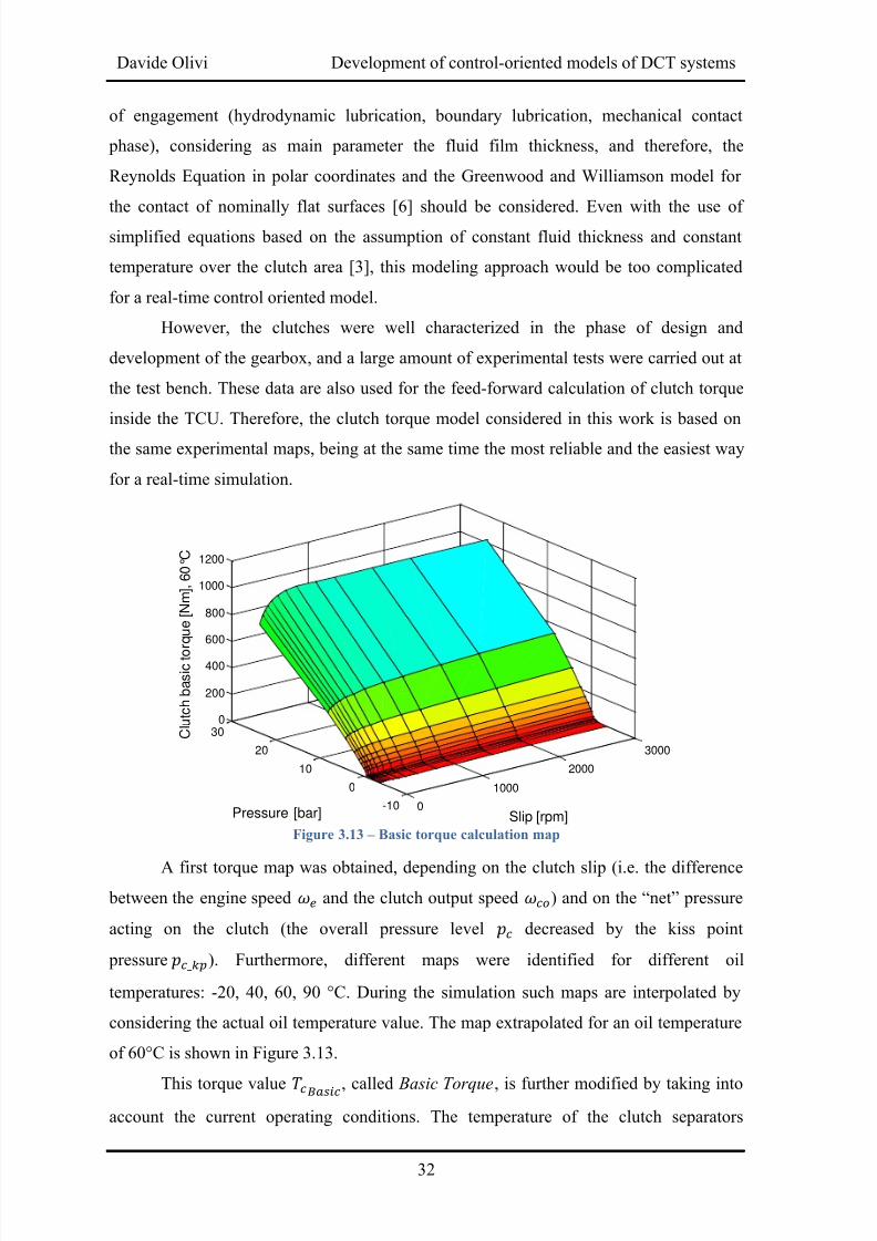
However, the clutches were well characterized in the phase of design and
development of the gearbox, and a large amount of experimental tests were carried out at
the test bench. These data are also used for the feed-forward calculation of clutch torque
inside the TCU. Therefore, the clutch torque model considered in this work is based on
the same experimental maps, being at the same time the most reliable and the easiest way
for a real-time simulation.
Figure 3.13 – Basic torque calculation map
A first torque map was obtained, depending on the clutch slip (i.e. the difference
between the engine speed and the clutch output speed ) and on the “net” pressure
acting on the clutch (the overall pressure level decreased by the kiss point
pressure ). Furthermore, different maps were identified for different oil
temperatures: -20, 40, 60, 90 °C. During the simulation such maps are interpolated by
considering the actual oil temperature value. The map extrapolated for an oil temperature
of 60°C is shown in Figure 3.13.
This torque value , called Basic Torque, is further modified by taking into
account the current operating conditions. The temperature of the clutch separators
0
1000
2000
3000
-10
0
10
20
300
200
400
600
800
1000
1200
Slip [rpm]Pressure [bar]
Clutchbasictorque[Nm],60°C
8/20/2019 Olivi Davide Tesi
http://slidepdf.com/reader/full/olivi-davide-tesi 43/141
Chapter 3 – The Dual Clutch Transmission model
33
strongly influences the friction coefficient of the friction material; a precise calculation of
the temperature inside the clutches would be possible with a finite volume based
numerical method [11], which takes into account the variations of temperature with
position and time, but it wouldn’t meet the requirements of a real-time model. Therefore,
the temperature inside the clutch is calculated through a linear mean value model [20],
and the torque variation caused by this effect is calculated with an experimental map
depending on this temperature.
The separators temperature is calculated by considering the net heat flow
inside the clutches, and the heat capacity of the separators:
;
∫
(3.15)
The heat power generated inside the clutches is a consequence of the clutch discs slip;
the heat power removed from the clutches by the lubrication oil depends on the
amount of lubrication flow : (3.16) (3.17)
An experimentally-derived function permits determining the temperature of
the oil inside the clutches, if the temperature of the separators is known:
( ) (3.18)
The temperature of the oil exiting the cooler depends on the heat exchange inside
the cooler; depending on the project, this heat exchange can happen inside a radiator
cooled down by the air flow, or inside a heat exchanger which is cooled down by the
water which is responsible for the cooling of the engine. The model of the cooling system
was not developed because it is not a core part of the simulation; for simplicity, the
temperature of the oil coming from the cooler is set to a constant value.
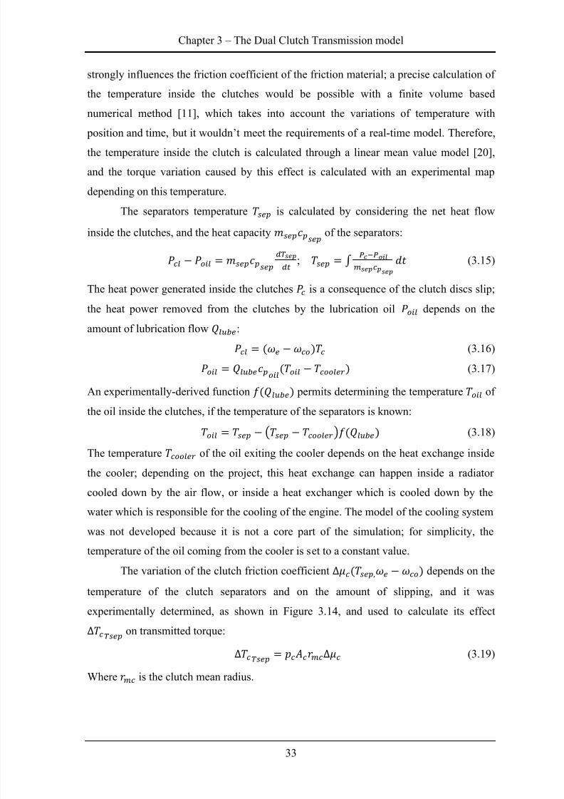
The variation of the clutch friction coefficient depends on the
temperature of the clutch separators and on the amount of slipping, and it was
experimentally determined, as shown in Figure 3.14, and used to calculate its effect on transmitted torque:
(3.19)
Where is the clutch mean radius.
8/20/2019 Olivi Davide Tesi
http://slidepdf.com/reader/full/olivi-davide-tesi 44/141
Davide Olivi Development of control-oriented models of DCT systems
34
Figure 3.14 – Friction coefficient variation on separator plates temperature and clutch slip
The total friction torque , generated by the friction between the clutch discs
can therefore be expressed as: (3.20)
When the pressure on the clutch is lower than the kiss point pressure, the clutch is
still transmitting some torque, due to the viscosity of the lubrication oil inside the clutch
discs, and consequently the drag torque must be taken into account. The value of
this torque has been experimentally determined, depending on engine speed, clutch output
speed, lube flow and oil temperature.
If the clutch is not completely open, i.e. the clutch is over the preload position,
part of frictional torque is also transmitted, depending on how near the clutch is to the
kiss point: that’s why the kiss point torque
is also considered, defined as the output
of the map shown in Figure 3.13 when the “net” pressure is zero (and therefore the
pressure on the clutch is exactly the kiss point pressure).
Another factor to take into account is that the two clutches are not completely
independent, being influenced by their mutual movement: even if a clutch is completely
open and without lubrication, it can still transmit some torque if the other clutch is closed,
due to the proximity layout of the two clutches. An experimentally derived crosstalk
torque
is added to the total torque, depending on both clutch pressures.
Considering all these contributions, the total clutch torque is given by:
0
500
1000
1500
2000
25000
50100
150
200250
300
0
0.01
0.02
0.03
0.04
0.05
0.06
Tsep [°C]Clutch slip [rpm]
Friction
coefficientdelta
8/20/2019 Olivi Davide Tesi
http://slidepdf.com/reader/full/olivi-davide-tesi 45/141
Chapter 3 – The Dual Clutch Transmission model
35
(3.21)
Where
represents the percentage of friction torque that has to be considered
while the clutch is not completely closed, i.e. until the kiss point is not reached ( ). If = 0, then and . When instead , the kiss point is reached, becomes zero, and the two equations in Equation
(3.21) become identical: .
The calculation of clutch torque must be as accurate possible, because the TCU
regulates the gear shift actuation according to the desired torque transmitted. The
calculated clutch torque is the actual torque transmitted between the engine and the
gearbox when the clutch is in slipping, filling or open conditions; when the clutch is
closed, the actual torque is the one coming from the engine, while the torque calculated
with this model is the transmissible torque, i.e. the maximum torque the clutch can
transmit in those conditions; usually while the clutch is closed the TCU regulates the
pressure so that the transmissible torque is higher than the transmitted one. In these
conditions the clutch pressure is not regulated as high as possible because, even if it
wouldn’t compromise the functionality of the clutch, it would require a higher oil flow,
with consequent higher power losses due to the work of the pump.
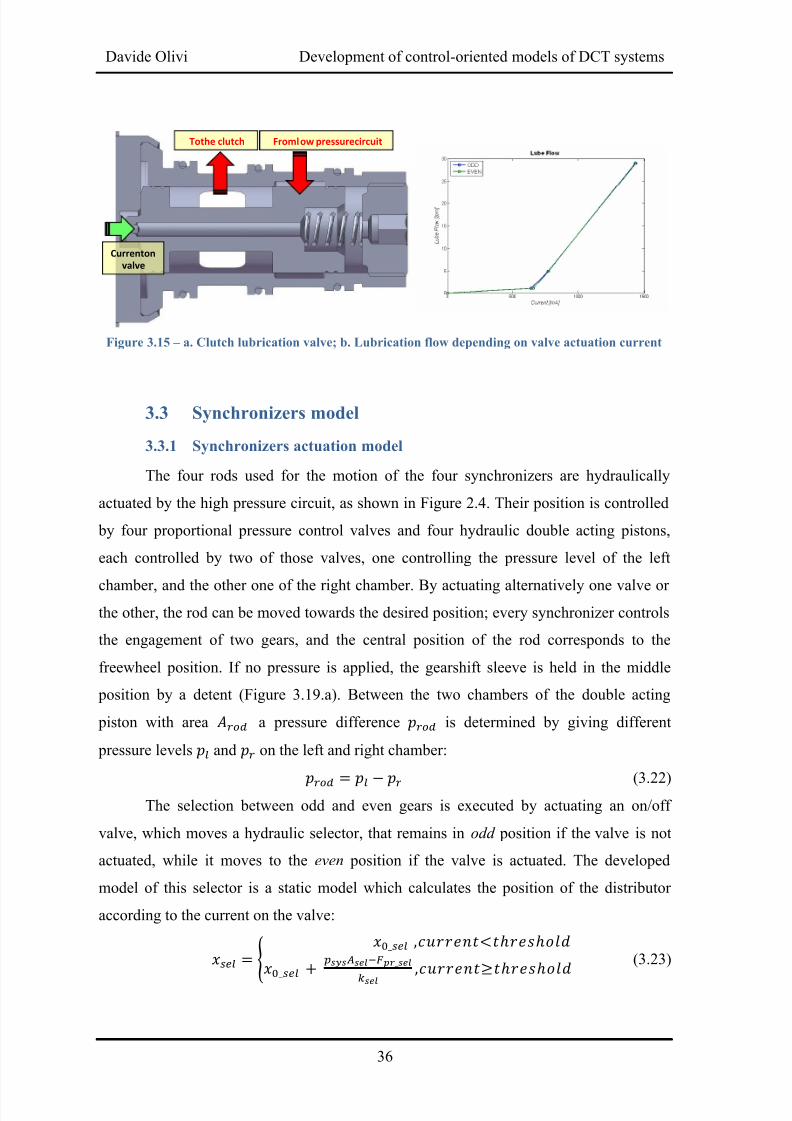
3.2.5 Clutch lubrication
The lubrication of the clutches is provided by an oil flow coming from the low
pressure circuit. The regulation of the flow is made through two valves (one for each
clutch, see Figure 3.15.a) having rectangular sections for the passage of the oil, to
maximize the flow. The amount of oil passing through the valve and reaching the clutches
is regulated through the actuation current on the valve itself.
The low pressure circuit was not modeled in a detailed way, for the low impact it
has in the whole actuation system; however, the calculation of the amount of lubrication
flow is needed for the thermal mean value model of the clutches; therefore, it is calculated
in the model according to an experimental map which considers only the current on the
valve, as shown in Figure 3.15.b. This means that the pressure inside the low pressure
circuit is assumed constant; a plausible pressure level inside it is around 5 bars.
8/20/2019 Olivi Davide Tesi
http://slidepdf.com/reader/full/olivi-davide-tesi 46/141
Davide Olivi Development of control-oriented models of DCT systems
36
Figure 3.15 – a. Clutch lubrication valve; b. Lubrication flow depending on valve actuation current
3.3 Synchronizers model
3.3.1 Synchronizers actuation model
The four rods used for the motion of the four synchronizers are hydraulically
actuated by the high pressure circuit, as shown in Figure 2.4. Their position is controlled
by four proportional pressure control valves and four hydraulic double acting pistons,
each controlled by two of those valves, one controlling the pressure level of the left
chamber, and the other one of the right chamber. By actuating alternatively one valve orthe other, the rod can be moved towards the desired position; every synchronizer controls
the engagement of two gears, and the central position of the rod corresponds to the
freewheel position. If no pressure is applied, the gearshift sleeve is held in the middle
position by a detent (Figure 3.19.a). Between the two chambers of the double acting
piston with area a pressure difference is determined by giving different
pressure levels and on the left and right chamber:
(3.22)The selection between odd and even gears is executed by actuating an on/off
valve, which moves a hydraulic selector, that remains in odd position if the valve is not
actuated, while it moves to the even position if the valve is actuated. The developed
model of this selector is a static model which calculates the position of the distributor
according to the current on the valve:
(3.23)
Fromlow pressurecircuitTothe clutch
Currenton
valve
8/20/2019 Olivi Davide Tesi
http://slidepdf.com/reader/full/olivi-davide-tesi 47/141
Chapter 3 – The Dual Clutch Transmission model
37
The flow through this valve, as all the flows through the on/off valves of the circuit, are
not calculated in the model, because they are considered negligible if compared with the
ones through the proportional valves.
The four proportional valves are 3-way proportional valves constructively similar
to the clutch pressure regulation ones. The valve spool dynamics and the flow through the
valve can be calculated with the relations shown in paragraph 3.1.3. The pressure
dynamics inside the rod chambers can be calculated according to Equation (3.24),
considering as input and output flows the ones coming from the valve model, while the
leakage flow on the rod actuation chambers can be considered negligible:
(3.24)
The variation of volume in the chamber is due to the motion of the rod, consequent to the
change in the pressure value, calculated thanks to the synchronizer model (see next
paragraph):
(3.25)
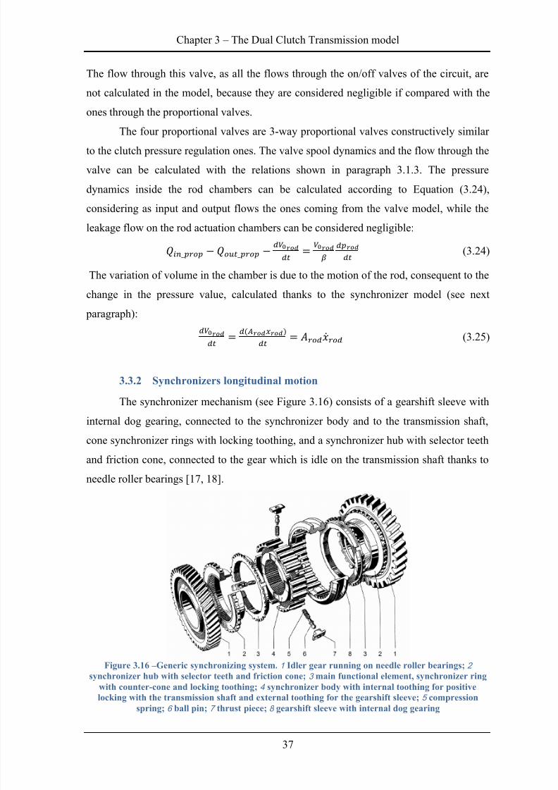
3.3.2 Synchronizers longitudinal motion
The synchronizer mechanism (see Figure 3.16) consists of a gearshift sleeve with
internal dog gearing, connected to the synchronizer body and to the transmission shaft,
cone synchronizer rings with locking toothing, and a synchronizer hub with selector teeth
and friction cone, connected to the gear which is idle on the transmission shaft thanks to
needle roller bearings [17, 18].
Figure 3.16 – Generic synchronizing system. 1 Idler gear running on needle roller bearings; 2
synchronizer hub with selector teeth and friction cone; 3 main functional element, synchronizer ring
with counter-cone and locking toothing; 4 synchronizer body with internal toothing for positive
locking with the transmission shaft and external toothing for the gearshift sleeve; 5 compression
spring; 6 ball pin; 7 thrust piece; 8 gearshift sleeve with internal dog gearing
8/20/2019 Olivi Davide Tesi
http://slidepdf.com/reader/full/olivi-davide-tesi 48/141
Davide Olivi Development of control-oriented models of DCT systems
38
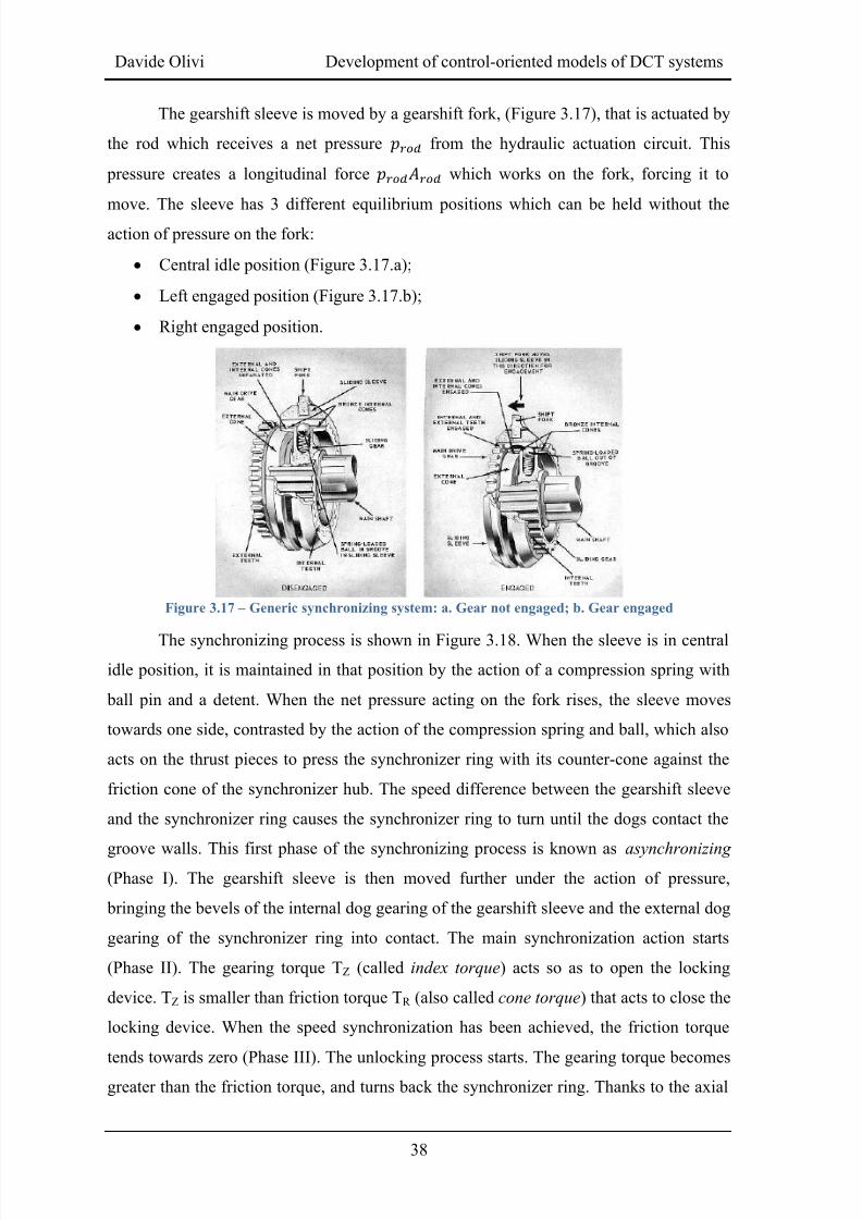
The gearshift sleeve is moved by a gearshift fork, (Figure 3.17), that is actuated by
the rod which receives a net pressure from the hydraulic actuation circuit. This
pressure creates a longitudinal force which works on the fork, forcing it to
move. The sleeve has 3 different equilibrium positions which can be held without the
action of pressure on the fork:
Central idle position (Figure 3.17.a);
Left engaged position (Figure 3.17.b);
Right engaged position.
Figure 3.17 – Generic synchronizing system: a. Gear not engaged; b. Gear engaged
The synchronizing process is shown in Figure 3.18. When the sleeve is in central
idle position, it is maintained in that position by the action of a compression spring with
ball pin and a detent. When the net pressure acting on the fork rises, the sleeve moves
towards one side, contrasted by the action of the compression spring and ball, which also
acts on the thrust pieces to press the synchronizer ring with its counter-cone against the
friction cone of the synchronizer hub. The speed difference between the gearshift sleeve
and the synchronizer ring causes the synchronizer ring to turn until the dogs contact the
groove walls. This first phase of the synchronizing process is known as asynchronizing (Phase I). The gearshift sleeve is then moved further under the action of pressure,
bringing the bevels of the internal dog gearing of the gearshift sleeve and the external dog
gearing of the synchronizer ring into contact. The main synchronization action starts
(Phase II). The gearing torque TZ (called index torque) acts so as to open the locking
device. TZ is smaller than friction torque TR (also called cone torque) that acts to close the
locking device. When the speed synchronization has been achieved, the friction torque
tends towards zero (Phase III). The unlocking process starts. The gearing torque becomes
greater than the friction torque, and turns back the synchronizer ring. Thanks to the axial
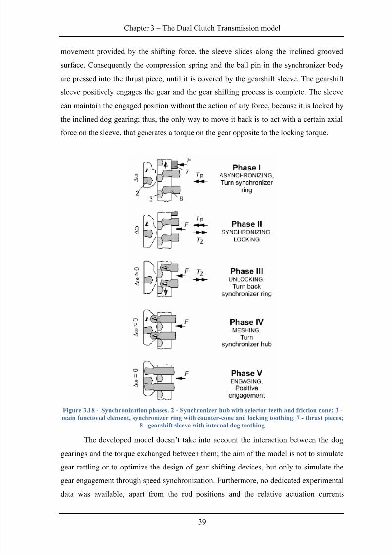
8/20/2019 Olivi Davide Tesi
http://slidepdf.com/reader/full/olivi-davide-tesi 49/141
Chapter 3 – The Dual Clutch Transmission model
39
movement provided by the shifting force, the sleeve slides along the inclined grooved
surface. Consequently the compression spring and the ball pin in the synchronizer body
are pressed into the thrust piece, until it is covered by the gearshift sleeve. The gearshift
sleeve positively engages the gear and the gear shifting process is complete. The sleeve
can maintain the engaged position without the action of any force, because it is locked by
the inclined dog gearing; thus, the only way to move it back is to act with a certain axial
force on the sleeve, that generates a torque on the gear opposite to the locking torque.
Figure 3.18 - Synchronization phases. 2 - Synchronizer hub with selector teeth and friction cone; 3 -
main functional element, synchronizer ring with counter-cone and locking toothing; 7 - thrust pieces;
8 - gearshift sleeve with internal dog toothing
The developed model doesn’t take into account the interaction between the dog
gearings and the torque exchanged between them; the aim of the model is not to simulate
gear rattling or to optimize the design of gear shifting devices, but only to simulate the
gear engagement through speed synchronization. Furthermore, no dedicated experimental
data was available, apart from the rod positions and the relative actuation currents
8/20/2019 Olivi Davide Tesi
http://slidepdf.com/reader/full/olivi-davide-tesi 50/141
Davide Olivi Development of control-oriented models of DCT systems
40
registered during on-board tests; all the study has been carried out analyzing the
bibliography and supposing plausible physical data, calibrated in order to match the
results of the simulation with the measured data.
The motion of the hydraulic piston is described as a spring-mass-damper dynamic
equation. For simplicity, the coordinates taken into account are different depending on the
position of the sleeve of the synchronizer; the position can be considered the
“absolute” position, i.e. the position value as registered by the on-board sensor and that
has to be reproduced by the model, always increasing from the left engaged position to
the right engaged position. The different intervals corresponds to different phases:
when ; in this interval the left
gear is selected:
(3.26)
when ; in this interval no gear is selected: (3.27)
when ; in this interval the right
gear is selected: (3.28)
As mentioned before, there are three equilibrium positions the synchronizer can hold
without any pressure action: maintains the position in the center of the rod, when
no gears are selected, and maintains the position or ,
when the left or the right gear is engaged, respectively. The extreme positions and , corresponding to the positions in which the sleeve comes in contact with the end
stop of the gear, can be reached only when pressure, and the correspondent axial force, is
applied on the sleeve; when the pressure is released, the sleeve goes back to
or , respectively, to avoid contact with the end stop, that
would cause unwanted friction and consequent wear.
3.3.3 Speed synchronization
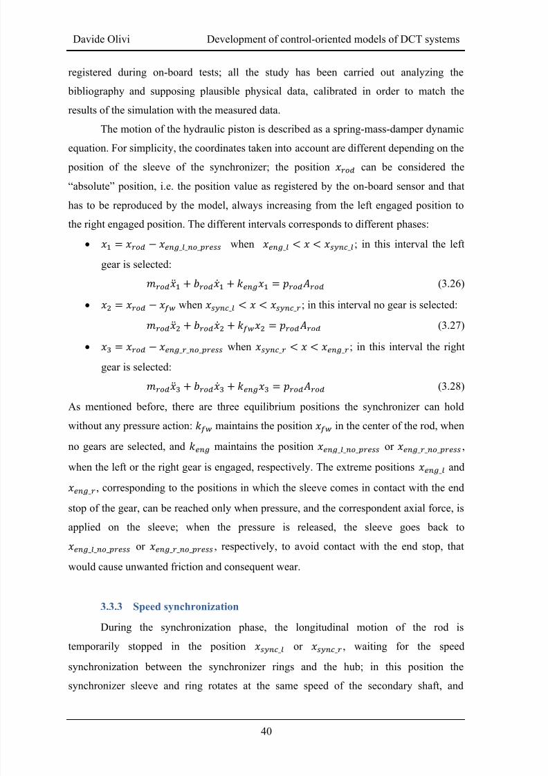
During the synchronization phase, the longitudinal motion of the rod is
temporarily stopped in the position or , waiting for the speed
synchronization between the synchronizer rings and the hub; in this position the
synchronizer sleeve and ring rotates at the same speed of the secondary shaft, and
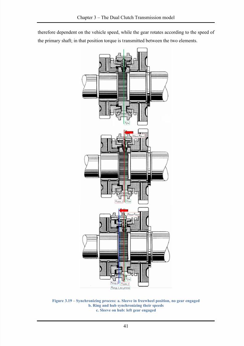
8/20/2019 Olivi Davide Tesi
http://slidepdf.com/reader/full/olivi-davide-tesi 51/141
Chapter 3 – The Dual Clutch Transmission model
41
therefore dependent on the vehicle speed, while the gear rotates according to the speed of
the primary shaft; in that position torque is transmitted between the two elements.
Figure 3.19 – Synchronizing process: a. Sleeve in freewheel position, no gear engaged
b. Ring and hub synchronizing their speeds
c. Sleeve on hub: left gear engaged
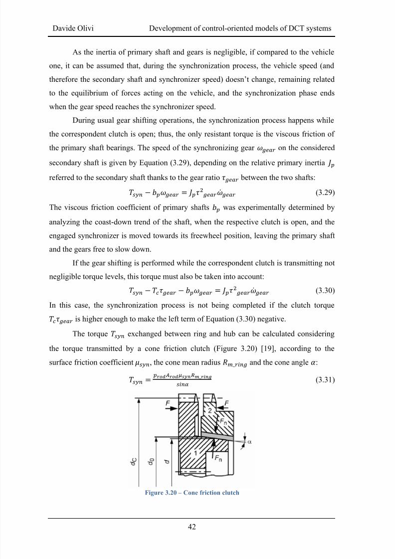
8/20/2019 Olivi Davide Tesi
http://slidepdf.com/reader/full/olivi-davide-tesi 52/141
Davide Olivi Development of control-oriented models of DCT systems
42
As the inertia of primary shaft and gears is negligible, if compared to the vehicle
one, it can be assumed that, during the synchronization process, the vehicle speed (and
therefore the secondary shaft and synchronizer speed) doesn’t change, remaining related
to the equilibrium of forces acting on the vehicle, and the synchronization phase ends
when the gear speed reaches the synchronizer speed.
During usual gear shifting operations, the synchronization process happens while
the correspondent clutch is open; thus, the only resistant torque is the viscous friction of
the primary shaft bearings. The speed of the synchronizing gear on the considered
secondary shaft is given by Equation (3.29), depending on the relative primary inertia
referred to the secondary shaft thanks to the gear ratio between the two shafts:
(3.29)The viscous friction coefficient of primary shafts was experimentally determined by
analyzing the coast-down trend of the shaft, when the respective clutch is open, and the
engaged synchronizer is moved towards its freewheel position, leaving the primary shaft
and the gears free to slow down.
If the gear shifting is performed while the correspondent clutch is transmitting not
negligible torque levels, this torque must also be taken into account:
(3.30)In this case, the synchronization process is not being completed if the clutch torque is higher enough to make the left term of Equation (3.30) negative.
The torque exchanged between ring and hub can be calculated considering
the torque transmitted by a cone friction clutch (Figure 3.20) [19], according to the
surface friction coefficient , the cone mean radius and the cone angle :
(3.31)
Figure 3.20 –
Cone friction clutch
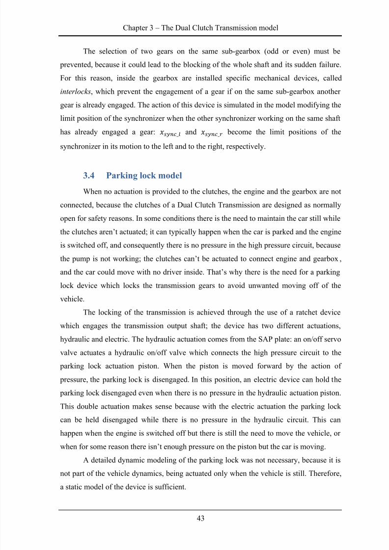
8/20/2019 Olivi Davide Tesi
http://slidepdf.com/reader/full/olivi-davide-tesi 53/141
Chapter 3 – The Dual Clutch Transmission model
43
The selection of two gears on the same sub-gearbox (odd or even) must be
prevented, because it could lead to the blocking of the whole shaft and its sudden failure.
For this reason, inside the gearbox are installed specific mechanical devices, called
interlocks, which prevent the engagement of a gear if on the same sub-gearbox another
gear is already engaged. The action of this device is simulated in the model modifying the
limit position of the synchronizer when the other synchronizer working on the same shaft
has already engaged a gear: and become the limit positions of the
synchronizer in its motion to the left and to the right, respectively.
3.4 Parking lock model
When no actuation is provided to the clutches, the engine and the gearbox are not
connected, because the clutches of a Dual Clutch Transmission are designed as normally
open for safety reasons. In some conditions there is the need to maintain the car still while
the clutches aren’t actuated; it can typically happen when the car is parked and the engine
is switched off, and consequently there is no pressure in the high pressure circuit, because
the pump is not working; the clutches can’t be actuated to connect engine and gearbox ,
and the car could move with no driver inside. That’s why there is the need for a parking
lock device which locks the transmission gears to avoid unwanted moving off of thevehicle.
The locking of the transmission is achieved through the use of a ratchet device
which engages the transmission output shaft; the device has two different actuations,
hydraulic and electric. The hydraulic actuation comes from the SAP plate: an on/off servo
valve actuates a hydraulic on/off valve which connects the high pressure circuit to the
parking lock actuation piston. When the piston is moved forward by the action of
pressure, the parking lock is disengaged. In this position, an electric device can hold the
parking lock disengaged even when there is no pressure in the hydraulic actuation piston.
This double actuation makes sense because with the electric actuation the parking lock
can be held disengaged while there is no pressure in the hydraulic circuit. This can
happen when the engine is switched off but there is still the need to move the vehicle, or
when for some reason there isn’t enough pressure on the piston but the car is moving.
A detailed dynamic modeling of the parking lock was not necessary, because it is
not part of the vehicle dynamics, being actuated only when the vehicle is still. Therefore,
a static model of the device is sufficient.
8/20/2019 Olivi Davide Tesi
http://slidepdf.com/reader/full/olivi-davide-tesi 54/141
Davide Olivi Development of control-oriented models of DCT systems
44
When no current is injected neither in the on/off servo valve nor in the electric
actuation, and the vehicle is not moving, the parking lock is engaged: (3.32)
When current is supplied to the servo valve, the parking lock is lifted by thesystem pressure insisting on its piston, contrasted by a return spring with a certain preload : (3.33)
The two limit positions the parking lock can reach are (low
position) and (high position). If the hydraulic actuation is switched off while the
electric actuation is on, the electric actuation is able to hold the device not permitting the
engagement, but in a position that is intermediate between and : (3.34)
If the control strategy of the parking lock is not correct or there are multiple faults
in the system, the parking lock can try to engage while the vehicle is moving; the force it
can provide against the motion of the vehicle is not enough, and the device starts rattling
over the transmission output shaft. This behavior is simulated adding in the model one
more possible position :
(3.35)
If necessary, the parking lock device can be disengaged manually, working on a
dedicated lever which acts mechanically on the device. This condition is called service
mode; in this case the disengaged position reaches a different value, called .
3.5 Electronic differential model
The Dual Clutch Transmission installed in current Ferrari cars is provided with an
electronic limited slip differential, to maximize the dynamic control of the vehicle and to
guarantee maximum grip while steering and in slippery conditions. The differential is
actuated through a three-way proportional servo valve connected to the high pressure
circuit in the CCP plate; the valve sends pressurized oil to the differential limited slip
clutch actuation chamber according to the desired torque it has to transmit. The clutch is
integrated inside the gearbox and its actuation is controlled by the TCU.
The simulated vehicle model comprehends only longitudinal dynamics, and no
model of wheel slip was implemented: therefore, the four wheels have always identical
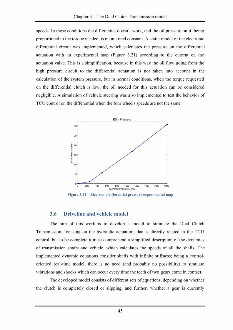
8/20/2019 Olivi Davide Tesi
http://slidepdf.com/reader/full/olivi-davide-tesi 55/141
Chapter 3 – The Dual Clutch Transmission model
45
speeds. In these conditions the differential doesn’t work, and the oil pressure on it, being
proportional to the torque needed, is maintained constant. A static model of the electronic
differential circuit was implemented, which calculates the pressure on the differential
actuation with an experimental map (Figure 3.21) according to the current on the
actuation valve. This is a simplification, because in this way the oil flow going from the
high pressure circuit to the differential actuation is not taken into account in the
calculation of the system pressure, but in normal conditions, when the torque requested
on the differential clutch is low, the oil needed for this actuation can be considered
negligible. A simulation of vehicle steering was also implemented to test the behavior of
TCU control on the differential when the four wheels speeds are not the same.
Figure 3.21 – Electronic differential pressure experimental map
3.6 Driveline and vehicle model
The aim of this work is to develop a model to simulate the Dual Clutch
Transmission, focusing on the hydraulic actuation, that is directly related to the TCU
control, but to be complete it must comprehend a simplified description of the dynamics
of transmission shafts and vehicle, which calculates the speeds of all the shafts. The
implemented dynamic equations consider shafts with infinite stiffness; being a control-
oriented real-time model, there is no need (and probably no possibility) to simulate
vibrations and shocks which can occur every time the teeth of two gears come in contact.
The developed model consists of different sets of equations, depending on whether
the clutch is completely closed or slipping, and further, whether a gear is currently
0 200 400 600 800 1000 1200 1400 1600 18000
5
10
15
20
25
30
Current on valve 210 [mA]
EDiffPressure[bar]
EDiff Pressure
8/20/2019 Olivi Davide Tesi
http://slidepdf.com/reader/full/olivi-davide-tesi 56/141
Davide Olivi Development of control-oriented models of DCT systems
46
selected, or not. The speeds of vehicle, gears and transmission shafts are calculated by
considering inertial effects and the torques acting on them [10, 12].
3.6.1 No-slip phaseWhen the clutch is completely closed and a gear is selected, engine, gearbox and
vehicle are connected and only one differential equation provides the description of the
entire system dynamics (under the hypothesis of infinite stiffness); the transmitted torque
is not the one calculated by the clutch torque model, but is the engine torque calculated by
the engine model; the resistant torque acting on the system is the total resistant torque
which acts on the vehicle. The engine speed is calculated considering the net torque
on engine shaft, i.e. the difference between the engine torque
and the resistant torque
, properly divided by the total gear ratio of the currently selected gear:
(3.36)
For simplicity, the inertia of all the elements before the clutch and the equivalent
inertia of primary shafts are referred to the engine shaft, while the equivalent inertia of shafts K1, K2, K (see Figure 2.1) and of the whole vehicle are referred to the
wheel shaft:
(3.37) (3.38)
The equivalent primary inertia is calculated from the inertia of those shafts
referred to their own axes; the equivalent value referred to the engine axes depends on the
current gear, i.e. the gear whose clutch is closed and therefore transmitting torque to the
wheels; the equivalent inertia is the axes inertia if the clutch of the considered gear is
closed, otherwise a multiple gear ratio must be considered. If the current gear is odd:
(3.39)
Where is the gear ratio between the secondary shaft (K1 or K2, depending on
which odd gear is selected) and K shaft, the same for , while is the total gear
ratio of the currently selected gear and the one of the preselected gear on the other
primary shaft. If the current gear is instead an even gear:
(3.40)
8/20/2019 Olivi Davide Tesi
http://slidepdf.com/reader/full/olivi-davide-tesi 57/141
Chapter 3 – The Dual Clutch Transmission model
47
The equivalent inertia of all the other shafts inside the gearbox (the secondary
shafts and the differential input shaft) and the vehicle inertia are referred to the wheels, so
the transmission ratio between the secondary shaft and the differential input shaft and
and the differential ratio
must be taken into account:
(3.41) (3.42) (3.43)
(3.44)
The total transmission ratio considers the engine speed and the wheel speed:
(3.45)
The vehicle speed is then calculated considering the total gear ratio and the wheel
radius : (3.46)
The resistant torque acting on the vehicle can be calculated following a simple
standard approach [8]; it is due to the aerodynamic force (depending on air density ,
frontal area of the vehicle and vehicle drag coefficient ), the rolling friction
resistance (depending on rolling friction coefficient
and vehicle total mass
) and the
braking torque :
(3.47)
Aerodynamic and rolling resistant torques can also be calculated considering the coast-
down trend of the vehicle, as shown in Equation (3.48), with the use of three curve fitting
parameters , , : (3.48)
The braking torque is proportional to the pressure acting on the brake circuit, according tothe pressure of the brake fluid (proportional to the pressure on the brake pedal), the
actual areas for pressure , , the friction coefficients of the linings , and the
mean radius of front and rear discs , : (3.50)
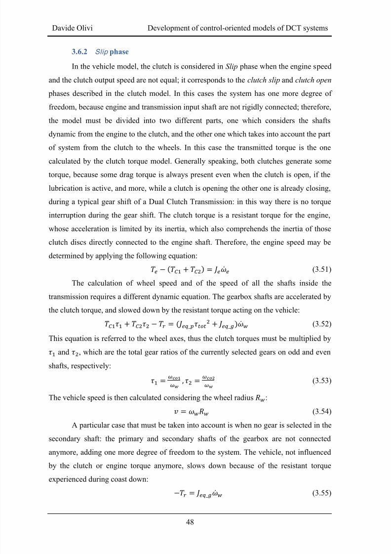
8/20/2019 Olivi Davide Tesi
http://slidepdf.com/reader/full/olivi-davide-tesi 58/141
Davide Olivi Development of control-oriented models of DCT systems
48
3.6.2 Slip phase
In the vehicle model, the clutch is considered in Slip phase when the engine speed
and the clutch output speed are not equal; it corresponds to the clutch slip and clutch open
phases described in the clutch model. In this cases the system has one more degree offreedom, because engine and transmission input shaft are not rigidly connected; therefore,
the model must be divided into two different parts, one which considers the shafts
dynamic from the engine to the clutch, and the other one which takes into account the part
of system from the clutch to the wheels. In this case the transmitted torque is the one
calculated by the clutch torque model. Generally speaking, both clutches generate some
torque, because some drag torque is always present even when the clutch is open, if the
lubrication is active, and more, while a clutch is opening the other one is already closing,
during a typical gear shift of a Dual Clutch Transmission: in this way there is no torque
interruption during the gear shift. The clutch torque is a resistant torque for the engine,
whose acceleration is limited by its inertia, which also comprehends the inertia of those
clutch discs directly connected to the engine shaft. Therefore, the engine speed may be
determined by applying the following equation: (3.51)
The calculation of wheel speed and of the speed of all the shafts inside the
transmission requires a different dynamic equation. The gearbox shafts are accelerated by
the clutch torque, and slowed down by the resistant torque acting on the vehicle: (3.52)
This equation is referred to the wheel axes, thus the clutch torques must be multiplied by and , which are the total gear ratios of the currently selected gears on odd and even
shafts, respectively:
(3.53)
The vehicle speed is then calculated considering the wheel radius : (3.54)
A particular case that must be taken into account is when no gear is selected in the
secondary shaft: the primary and secondary shafts of the gearbox are not connected
anymore, adding one more degree of freedom to the system. The vehicle, not influenced
by the clutch or engine torque anymore, slows down because of the resistant torque
experienced during coast down:
(3.55)
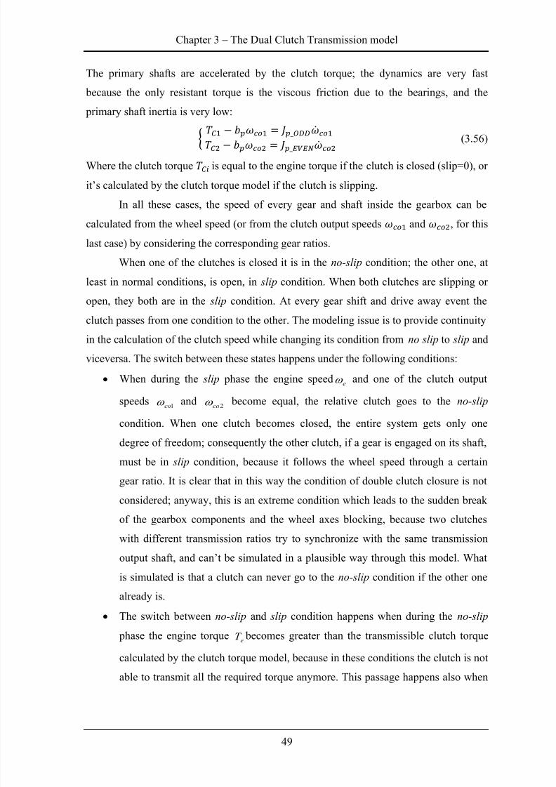
8/20/2019 Olivi Davide Tesi
http://slidepdf.com/reader/full/olivi-davide-tesi 59/141
Chapter 3 – The Dual Clutch Transmission model
49
The primary shafts are accelerated by the clutch torque; the dynamics are very fast
because the only resistant torque is the viscous friction due to the bearings, and the
primary shaft inertia is very low:
(3.56)
Where the clutch torque is equal to the engine torque if the clutch is closed (slip=0), or
it’s calculated by the clutch torque model if the clutch is slipping.
In all these cases, the speed of every gear and shaft inside the gearbox can be
calculated from the wheel speed (or from the clutch output speeds and , for this
last case) by considering the corresponding gear ratios.
When one of the clutches is closed it is in the no-slip condition; the other one, at
least in normal conditions, is open, in slip condition. When both clutches are slipping or
open, they both are in the slip condition. At every gear shift and drive away event the
clutch passes from one condition to the other. The modeling issue is to provide continuity
in the calculation of the clutch speed while changing its condition from no slip to slip and
viceversa. The switch between these states happens under the following conditions:
When during the slip phase the engine speede
and one of the clutch output
speeds1co
and2co
become equal, the relative clutch goes to the no-slip
condition. When one clutch becomes closed, the entire system gets only one
degree of freedom; consequently the other clutch, if a gear is engaged on its shaft,
must be in slip condition, because it follows the wheel speed through a certain
gear ratio. It is clear that in this way the condition of double clutch closure is not
considered; anyway, this is an extreme condition which leads to the sudden break
of the gearbox components and the wheel axes blocking, because two clutches
with different transmission ratios try to synchronize with the same transmission
output shaft, and can’t be simulated in a plausible way through this model. What
is simulated is that a clutch can never go to the no-slip condition if the other one
already is.
The switch between no-slip and slip condition happens when during the no-slip
phase the engine torquee
T becomes greater than the transmissible clutch torque
calculated by the clutch torque model, because in these conditions the clutch is not
able to transmit all the required torque anymore. This passage happens also when
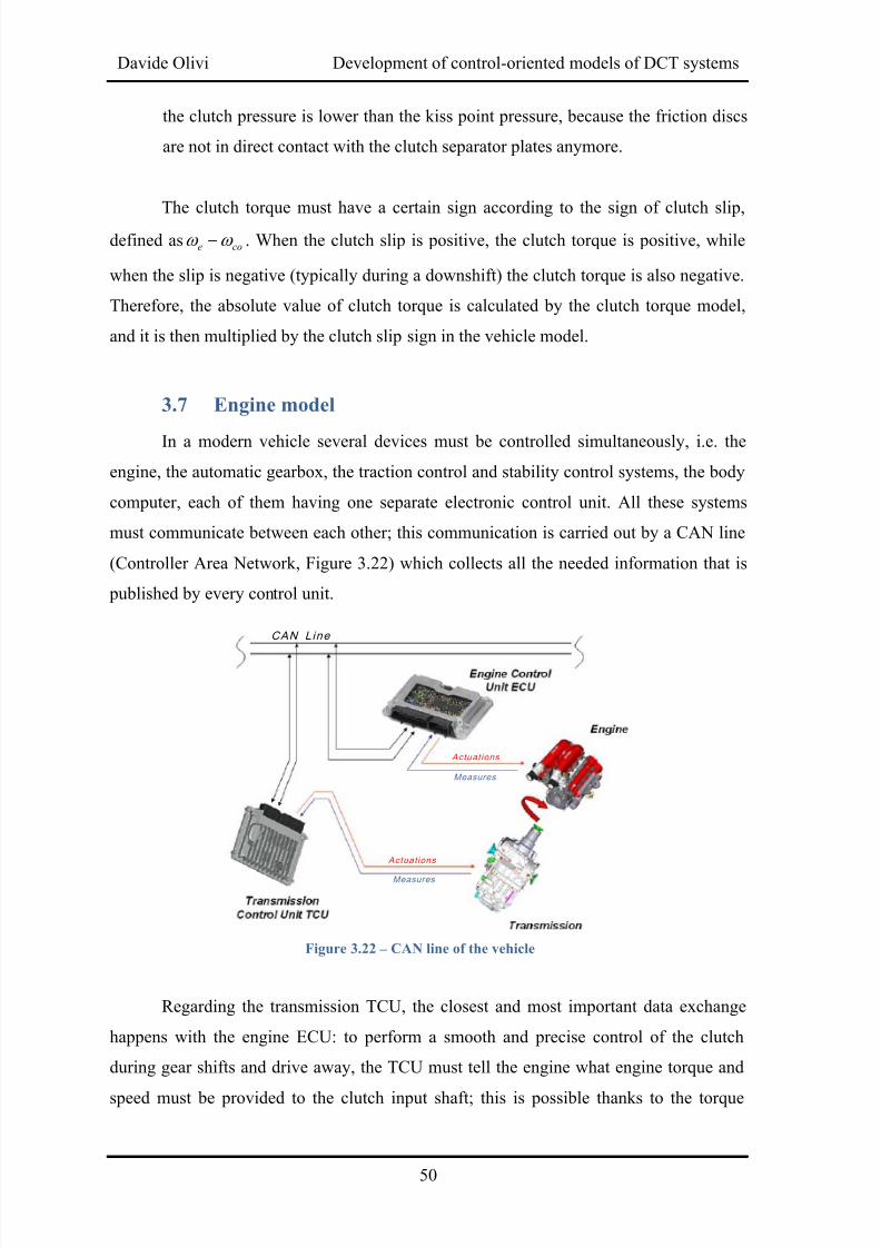
8/20/2019 Olivi Davide Tesi
http://slidepdf.com/reader/full/olivi-davide-tesi 60/141
Davide Olivi Development of control-oriented models of DCT systems
50
the clutch pressure is lower than the kiss point pressure, because the friction discs
are not in direct contact with the clutch separator plates anymore.
The clutch torque must have a certain sign according to the sign of clutch slip,
defined ascoe
. When the clutch slip is positive, the clutch torque is positive, while
when the slip is negative (typically during a downshift) the clutch torque is also negative.
Therefore, the absolute value of clutch torque is calculated by the clutch torque model,
and it is then multiplied by the clutch slip sign in the vehicle model.
3.7 Engine model
In a modern vehicle several devices must be controlled simultaneously, i.e. the
engine, the automatic gearbox, the traction control and stability control systems, the body
computer, each of them having one separate electronic control unit. All these systems
must communicate between each other; this communication is carried out by a CAN line
(Controller Area Network, Figure 3.22) which collects all the needed information that is
published by every control unit.
Regarding the transmission TCU, the closest and most important data exchange
happens with the engine ECU: to perform a smooth and precise control of the clutch
during gear shifts and drive away, the TCU must tell the engine what engine torque and
speed must be provided to the clutch input shaft; this is possible thanks to the torque
Figure 3.22 – CAN line of the vehicle
CAN Line
Actuations
Measures
Actuations
Measures
8/20/2019 Olivi Davide Tesi
http://slidepdf.com/reader/full/olivi-davide-tesi 61/141
Chapter 3 – The Dual Clutch Transmission model
51
based engine control system: every device of the vehicle can interact with the ECU asking
for a desired engine torque, that is fulfilled by the ECU under certain conditions and with
different priorities. The desired torque is sent to the engine via the CAN line; the engine
sends to the TCU the actual torque generated by the engine.
When the clutch is closed, the engine follows a target torque coming from the
driver request; in this phase the engine is master and the TCU (and in general the other
devices) is slave. The TCU maintains a pressure level in the clutch actuation circuit high
enough to transmit all the torque coming from the engine (whose information is sent via
CAN to the TCU). When a gear shift or a drive away request comes from the driver or
from the control logic of the TCU, the TCU becomes master (Figure 3.23) and asks the
engine for the desired torque and speed; the engine controller becomes slave and provides
the desired torque and speed, if possible.
Figure 3.23 – TCU and ECU Master and Slave management
The model presented in the previous paragraphs may be considered complete once
all the vehicle parts generating and transmitting torque are simulated, from the engine to
the wheels. The engine model implemented for real-time application is a real-time zero-
dimensional mean value model [9], and comprehends the control logic of the ECU. It can
therefore maintain the idle speed during idling, and it can correctly respond to torque and
speed requests coming from the TCU. All the CAN messages between the ECU and the
TCU have been reproduced in the simulation environment. The core of the model was
already developed, but other additional functions has been added to match the
requirements of the new applications on which the DCT transmission is being installed.
The most important are the Stop&Start strategy for conventional vehicles and the Electric
Drive for hybrid vehicles. Both of these models have been implemented with StateFlow
charts.
TCU
MASTER
ECU
SLAVE
TARGETS
ACTUATIONS SENSORS ACTUATIONS SENSORS
CAN
TORQUE
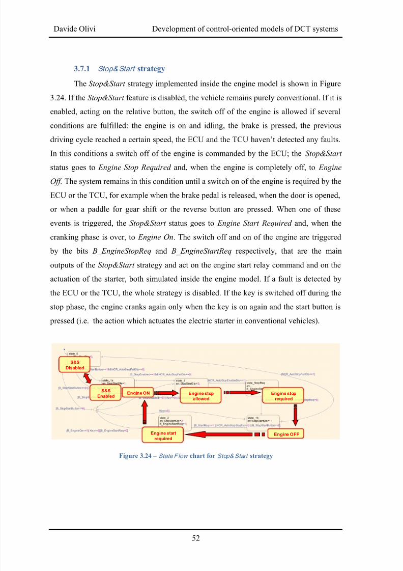
8/20/2019 Olivi Davide Tesi
http://slidepdf.com/reader/full/olivi-davide-tesi 62/141
Davide Olivi Development of control-oriented models of DCT systems
52
3.7.1 Stop&Start strategy
The Stop&Start strategy implemented inside the engine model is shown in Figure
3.24. If the Stop&Start feature is disabled, the vehicle remains purely conventional. If it isenabled, acting on the relative button, the switch off of the engine is allowed if several
conditions are fulfilled: the engine is on and idling, the brake is pressed, the previous
driving cycle reached a certain speed, the ECU and the TCU haven’t detected any faults.
In this conditions a switch off of the engine is commanded by the ECU; the Stop&Start
status goes to Engine Stop Required and, when the engine is completely off, to Engine
Off. The system remains in this condition until a switch on of the engine is required by the
ECU or the TCU, for example when the brake pedal is released, when the door is opened,
or when a paddle for gear shift or the reverse button are pressed. When one of these
events is triggered, the Stop&Start status goes to Engine Start Required and, when the
cranking phase is over, to Engine On. The switch off and on of the engine are triggered
by the bits B_EngineStopReq and B_EngineStartReq respectively, that are the main
outputs of the Stop&Start strategy and act on the engine start relay command and on the
actuation of the starter, both simulated inside the engine model. If a fault is detected by
the ECU or the TCU, the whole strategy is disabled. If the key is switched off during the
stop phase, the engine cranks again only when the key is on again and the start button is
pressed (i.e. the action which actuates the electric starter in conventional vehicles).
Figure 3.24 – State F low chart for Stop&Start strategy
Engine ON Engine stop
required
Engine stop
allowed
Engine OFFEngine start
required
S&S
Disabled
S&S
Enabled
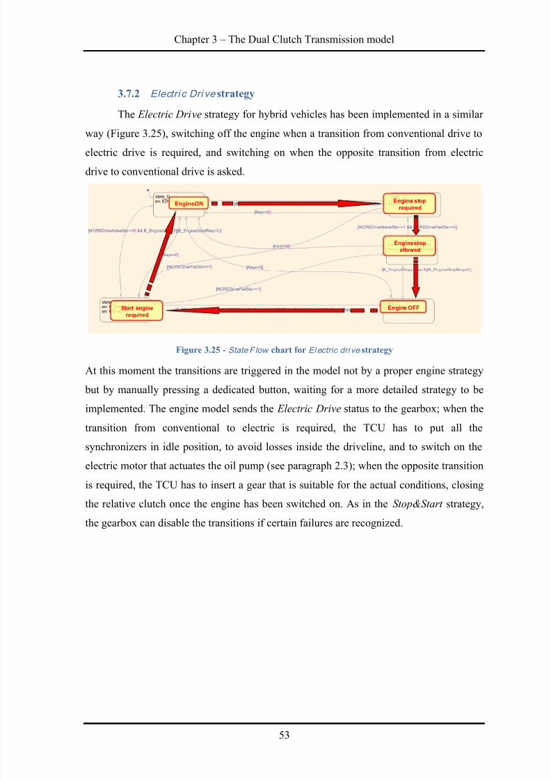
8/20/2019 Olivi Davide Tesi
http://slidepdf.com/reader/full/olivi-davide-tesi 63/141
Chapter 3 – The Dual Clutch Transmission model
53
3.7.2 Electri c Dri ve strategy
The Electric Drive strategy for hybrid vehicles has been implemented in a similar
way (Figure 3.25), switching off the engine when a transition from conventional drive toelectric drive is required, and switching on when the opposite transition from electric
drive to conventional drive is asked.
Figure 3.25 - State F low chart for Electric dri ve strategy
At this moment the transitions are triggered in the model not by a proper engine strategy
but by manually pressing a dedicated button, waiting for a more detailed strategy to be
implemented. The engine model sends the Electric Drive status to the gearbox; when the
transition from conventional to electric is required, the TCU has to put all the
synchronizers in idle position, to avoid losses inside the driveline, and to switch on the
electric motor that actuates the oil pump (see paragraph 2.3); when the opposite transition
is required, the TCU has to insert a gear that is suitable for the actual conditions, closing
the relative clutch once the engine has been switched on. As in the Stop&Start strategy,
the gearbox can disable the transitions if certain failures are recognized.
EngineON Engine stop
required
Enginestop
allowed
Engine OFFStart engine
required
8/20/2019 Olivi Davide Tesi
http://slidepdf.com/reader/full/olivi-davide-tesi 64/141
Davide Olivi Development of control-oriented models of DCT systems
54
Chapter 4
Simplified model for HIL application
4.1 Model simulation
The model described in Chapter 3 comprehends all the parts needed for a
complete simulation of the whole system. It needs as inputs only the electrical currents
from the TCU, the driver inputs (accelerator and brake pedals, and gear shift request) and
environmental data. The single parts of the model were validated and calibrated by trying
to reproduce data taken from on-board measurements, and then integrated in a complete
model. Even if the complete model could provide accurate results it was not suitable for
the HIL application, because in order to achieve a stable simulation it required a step size
too small for a real-time simulation. The step size for a real-time implementation of the
considered model should be set to around 0.5 ms; the simulation of the whole system with
this step size would cause instability and undermine the possibility of plausible results.
The causes of this limitation were investigated, and the problem was found in the
description of some dynamics inside the hydraulic actuation circuit: in more detail, the
pressure dynamics and the mass-spring-damper dynamics are very fast and can’t be
reproduced in a real-time simulation. To ensure stability to the simulation, the model
must be tested under the worst conditions, which in this case are represented by a step
current input on the clutch actuation valve, that forces the fastest pressure and motion
dynamics, related one to each other. Hence, the model was tested by performing a
simulation of the clutch actuation dynamics, having as input on the actuation valve
different current steps and considering progressively smaller step sizes: as shown in
Figure 4.1, to avoid instability the only plausible result could be obtained with a step size
of 1e-6 s, absolutely not feasible for a real-time application, and, in the case of a 700 mAcurrent step, still with some large oscillations.
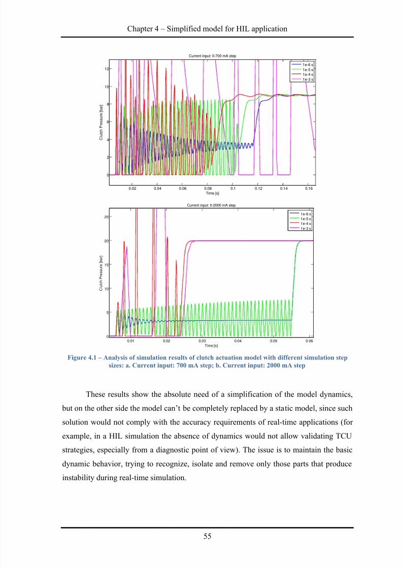
8/20/2019 Olivi Davide Tesi
http://slidepdf.com/reader/full/olivi-davide-tesi 65/141
Chapter 4 – Simplified model for HIL application
55
Figure 4.1 – Analysis of simulation results of clutch actuation model with different simulation step
sizes: a. Current input: 700 mA step; b. Current input: 2000 mA step
These results show the absolute need of a simplification of the model dynamics,
but on the other side the model can’t be completely replaced by a static model, since such
solution would not comply with the accuracy requirements of real-time applications (for
example, in a HIL simulation the absence of dynamics would not allow validating TCU
strategies, especially from a diagnostic point of view). The issue is to maintain the basic
dynamic behavior, trying to recognize, isolate and remove only those parts that produce
instability during real-time simulation.
0.02 0.04 0.06 0.08 0.1 0.12 0.14 0.16
0
2
4
6
8
10
12
Current input: 0-700 mA step
Time [s]
ClutchPressure[bar]
1e-6 s
1e-5 s
1e-4 s
1e-3 s
0.01 0.02 0.03 0.04 0.05 0.060
5
10
15
20
25
Current input: 0-2000 mA step
Time [s]
ClutchPressure[bar]
1e-6 s
1e-5 s
1e-4 s
1e-3 s
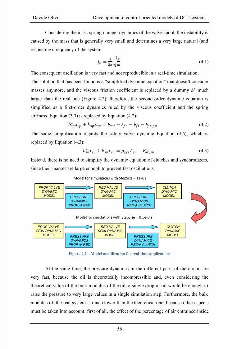
8/20/2019 Olivi Davide Tesi
http://slidepdf.com/reader/full/olivi-davide-tesi 66/141
Davide Olivi Development of control-oriented models of DCT systems
56
Considering the mass-spring-damper dynamics of the valve spool, the instability is
caused by the mass that is generally very small and determines a very large natural (and
resonating) frequency of the system:
√ (4.1)
The consequent oscillation is very fast and not reproducible in a real-time simulation.
The solution that has been found is a “simplified dynamic equation” that doesn’t consider
masses anymore, and the viscous friction coefficient is replaced by a dummy much
larger than the real one (Figure 4.2): therefore, the second-order dynamic equation is
simplified as a first-order dynamics ruled by the viscous coefficient and the spring
stiffness. Equation (3.3) is replaced by Equation (4.2):
(4.2)
The same simplification regards the safety valve dynamic Equation (3.6), which is
replaced by Equation (4.3): (4.3)
Instead, there is no need to simplify the dynamic equation of clutches and synchronizers,
since their masses are large enough to prevent fast oscillations.
Figure 4.2 – Model modification for real-time applications
At the same time, the pressure dynamics in the different parts of the circuit are
very fast, because the oil is theoretically incompressible and, even considering the
theoretical value of the bulk modulus of the oil, a single drop of oil would be enough to
raise the pressure to very large values in a single simulation step. Furthermore, the bulk
modulus of the real system is much lower than the theoretical one, because other aspects
must be taken into account: first of all, the effect of the percentage of air entrained inside
Model for simulations with StepSize = 1e-6 s
PROP VALVE
DYNAMIC
MODELPRESSURE
DYNAMICS
PROP RED
CLUTCH
DYNAMIC
MODEL
RED VALVE
DYNAMIC
MODELPRESSURE
DYNAMICS
RED CLUTCH
Model for simulations with StepSize = 0.5e-3 s
PROP VALVE
SEMI-DYNAMIC
MODELPRESSURE
DYNAMICS
PROP RED
CLUTCH
DYNAMIC
MODEL
RED VALVE
SEMI-DYNAMIC
MODELPRESSURE
DYNAMICS
RED CLUTCH
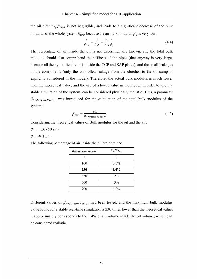
8/20/2019 Olivi Davide Tesi
http://slidepdf.com/reader/full/olivi-davide-tesi 67/141
Chapter 4 – Simplified model for HIL application
57
the oil circuit ⁄ is not negligible, and leads to a significant decrease of the bulk
modulus of the whole system , because the air bulk modulus is very low:
(4.4)
The percentage of air inside the oil is not experimentally known, and the total bulk
modulus should also comprehend the stiffness of the pipes (that anyway is very large,
because all the hydraulic circuit is inside the CCP and SAP plates), and the small leakages
in the components (only the controlled leakage from the clutches to the oil sump is
explicitly considered in the model). Therefore, the actual bulk modulus is much lower
than the theoretical value, and the use of a lower value in the model, in order to allow a
stable simulation of the system, can be considered physically realistic. Thus, a parameter
was introduced for the calculation of the total bulk modulus of the
system:
(4.5)
Considering the theoretical values of Bulk modulus for the oil and the air:
The following percentage of air inside the oil are obtained:
1 0
100 0.6%
230 1.4%
330 2%
500 3%
700 4.2%
Different values of had been tested, and the maximum bulk modulus
value found for a stable real-time simulation is 230 times lower than the theoretical value;
it approximately corresponds to the 1.4% of air volume inside the oil volume, which can
be considered realistic.
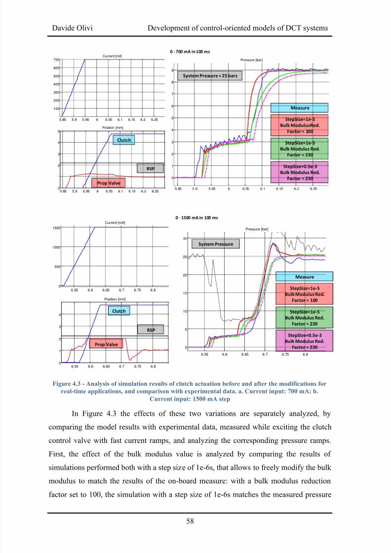
8/20/2019 Olivi Davide Tesi
http://slidepdf.com/reader/full/olivi-davide-tesi 68/141
Davide Olivi Development of control-oriented models of DCT systems
58
Figure 4.3 - Analysis of simulation results of clutch actuation before and after the modifications for
real-time applications, and comparison with experimental data. a. Current input: 700 mA; b.
Current input: 1500 mA step
In Figure 4.3 the effects of these two variations are separately analyzed, by
comparing the model results with experimental data, measured while exciting the clutch
control valve with fast current ramps, and analyzing the corresponding pressure ramps.
First, the effect of the bulk modulus value is analyzed by comparing the results of
simulations performed both with a step size of 1e-6s, that allows to freely modify the bulk
modulus to match the results of the on-board measure: with a bulk modulus reductionfactor set to 100, the simulation with a step size of 1e-6s matches the measured pressure
5.85 5.9 5.95 6 6.05 6.1 6.15 6.2 6.25
100
200
300
400
500
600
700Current [mA]
5.85 5.9 5.95 6 6.05 6.1 6.15 6.2 6.25
0
1
2
3
4
5
6
7
8
9
Pressure [bar]
5.85 5.9 5.95 6 6.05 6.1 6.15 6.2 6.250
1
2
3
4
5Position [mm]
Prop Valve
Clutch
StepSize=0.5e-3
Bulk Modulus Red.
Factor = 230
RSP
Measure
StepSize=1e-5
Bulk ModulusRed.
Factor = 100
StepSize=1e-5
Bulk Modulus Red.
Factor = 230
System Pressure = 25 bars
0 - 700 mA in 100 ms
6.55 6.6 6.65 6.7 6.75 6.8
0
500
1000
1500
Current [mA]
6.55 6.6 6.65 6.7 6.75 6.8
0
5
10
15
20
25
30
Pressure [bar]
6.55 6.6 6.65 6.7 6.75 6.80
1
2
3
4
Position [mm]
Prop Valve
Clutch
StepSize=0.5e-3
Bulk Modulus Red.
Factor = 230
RSP
Measure
StepSize=1e-5Bulk Modulus Red.
Factor = 100
StepSize=1e-5
Bulk Modulus Red.
Factor = 230
0 - 1500 mA in 100 ms
System Pressure
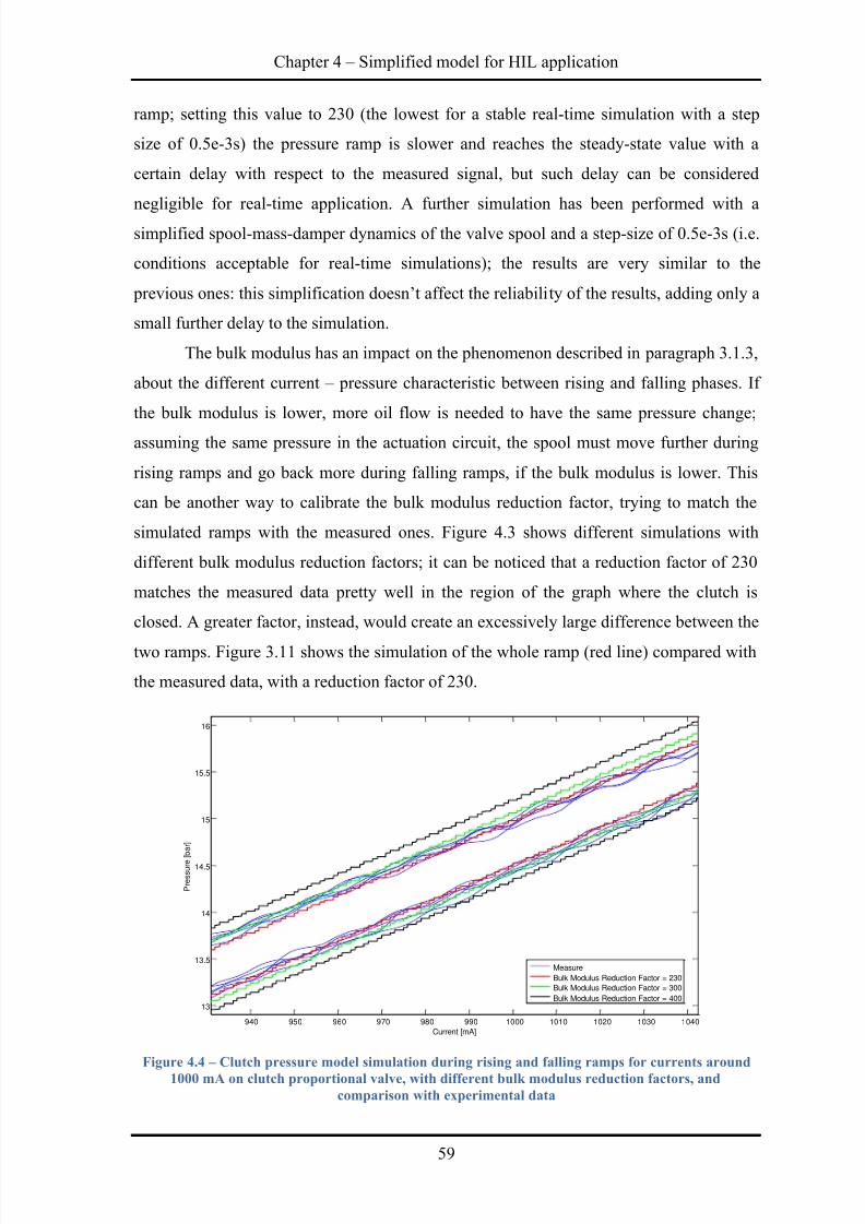
8/20/2019 Olivi Davide Tesi
http://slidepdf.com/reader/full/olivi-davide-tesi 69/141
Chapter 4 – Simplified model for HIL application
59
ramp; setting this value to 230 (the lowest for a stable real-time simulation with a step
size of 0.5e-3s) the pressure ramp is slower and reaches the steady-state value with a
certain delay with respect to the measured signal, but such delay can be considered
negligible for real-time application. A further simulation has been performed with a
simplified spool-mass-damper dynamics of the valve spool and a step-size of 0.5e-3s (i.e.
conditions acceptable for real-time simulations); the results are very similar to the
previous ones: this simplification doesn’t affect the reliability of the results, adding only a
small further delay to the simulation.
The bulk modulus has an impact on the phenomenon described in paragraph 3.1.3,
about the different current – pressure characteristic between rising and falling phases. If
the bulk modulus is lower, more oil flow is needed to have the same pressure change;
assuming the same pressure in the actuation circuit, the spool must move further during
rising ramps and go back more during falling ramps, if the bulk modulus is lower. This
can be another way to calibrate the bulk modulus reduction factor, trying to match the
simulated ramps with the measured ones. Figure 4.3 shows different simulations with
different bulk modulus reduction factors; it can be noticed that a reduction factor of 230
matches the measured data pretty well in the region of the graph where the clutch is
closed. A greater factor, instead, would create an excessively large difference between the
two ramps. Figure 3.11 shows the simulation of the whole ramp (red line) compared with
the measured data, with a reduction factor of 230.
Figure 4.4 – Clutch pressure model simulation during rising and falling ramps for currents around
1000 mA on clutch proportional valve, with different bulk modulus reduction factors, and
comparison with experimental data
940 950 960 970 980 990 1000 1010 1020 1030 1040
13
13.5
14
14.5
15
15.5
16
Current [mA]
Pressure[b
ar]
Measure
Bulk Modulus Reduction Factor = 230
Bulk Modulus Reduction Factor = 300
Bulk Modulus Reduction Factor = 400
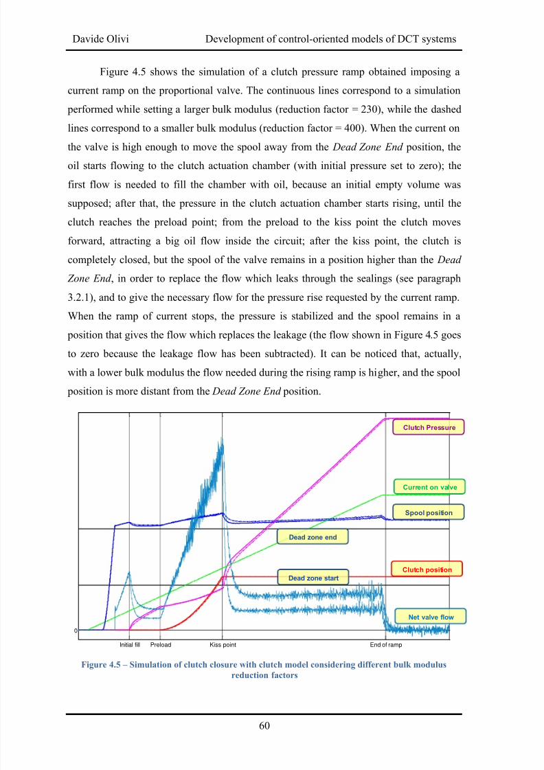
8/20/2019 Olivi Davide Tesi
http://slidepdf.com/reader/full/olivi-davide-tesi 70/141
Davide Olivi Development of control-oriented models of DCT systems
60
Figure 4.5 shows the simulation of a clutch pressure ramp obtained imposing a
current ramp on the proportional valve. The continuous lines correspond to a simulation
performed while setting a larger bulk modulus (reduction factor = 230), while the dashed
lines correspond to a smaller bulk modulus (reduction factor = 400). When the current on
the valve is high enough to move the spool away from the Dead Zone End position, the
oil starts flowing to the clutch actuation chamber (with initial pressure set to zero); the
first flow is needed to fill the chamber with oil, because an initial empty volume was
supposed; after that, the pressure in the clutch actuation chamber starts rising, until the
clutch reaches the preload point; from the preload to the kiss point the clutch moves
forward, attracting a big oil flow inside the circuit; after the kiss point, the clutch is
completely closed, but the spool of the valve remains in a position higher than the Dead
Zone End , in order to replace the flow which leaks through the sealings (see paragraph
3.2.1), and to give the necessary flow for the pressure rise requested by the current ramp.
When the ramp of current stops, the pressure is stabilized and the spool remains in a
position that gives the flow which replaces the leakage (the flow shown in Figure 4.5 goes
to zero because the leakage flow has been subtracted). It can be noticed that, actually,
with a lower bulk modulus the flow needed during the rising ramp is higher, and the spool
position is more distant from the Dead Zone End position.
Figure 4.5 – Simulation of clutch closure with clutch model considering different bulk modulus
reduction factors
End of rampKiss pointPreloadInitial fill
0
Current on valve
Clutch Pressure
Spool position
Net valve flow
Clutch position
Dead zone end
Dead zone start
8/20/2019 Olivi Davide Tesi
http://slidepdf.com/reader/full/olivi-davide-tesi 71/141
Chapter 5 – DCT model developed in Simulink
61
Chapter 5
DCT model developed in Simulink
5.1 Model overview
The model of the Dual Clutch Transmission for the Hardware In the Loop
application has been entirely developed in Matlab Simulink environment. Figure 5.1
shows the whole model, which comprehends the different parts described in the previous
paragraphs:
The CCP model calculates the pressure in the high pressure circuit, and
comprehends the model of clutch longitudinal motion and clutch pressure; the
electronic differential actuation is also simulated in this model;
The Clutch torque model transforms the pressure on clutches in transmissible
torque, also considering the clutch input and output speeds calculated in the
Driveline and vehicle model;
The SAP model calculates the pressure in every chamber of the four actuation
pistons of the synchronizers; it also comprehends the parking lock model, whose
actuation is situated in this plate;
The Synchronizers model transforms the pressure on the actuation pistons in
position of the synchronizers, taking into account all the forces acting on them and
the speeds of primary and secondary shafts calculated in the Driveline and vehicle
model; it comprehends the gear synchronization model and consequently
calculates the speed of every gear inside the gearbox;
The Driveline and vehicle model calculates the speeds of engine, primary and
secondary shafts, transmission output shaft and vehicle speed, considering
different sets of equations according to the slip / no-slip conditions;
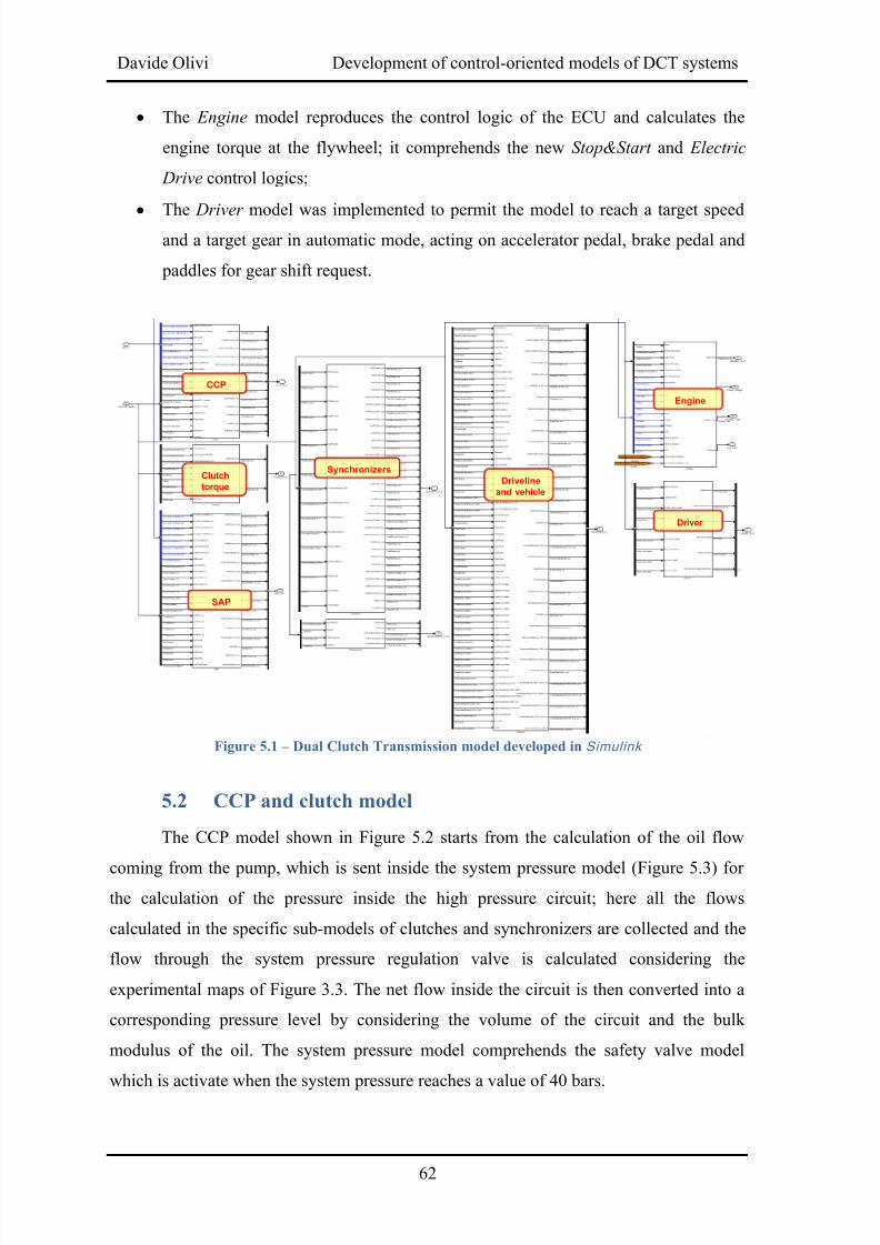
8/20/2019 Olivi Davide Tesi
http://slidepdf.com/reader/full/olivi-davide-tesi 72/141
Davide Olivi Development of control-oriented models of DCT systems
62
The Engine model reproduces the control logic of the ECU and calculates the
engine torque at the flywheel; it comprehends the new Stop&Start and Electric
Drive control logics;
The Driver model was implemented to permit the model to reach a target speedand a target gear in automatic mode, acting on accelerator pedal, brake pedal and
paddles for gear shift request.
Figure 5.1 – Dual Clutch Transmission model developed in Simulink
5.2 CCP and clutch model
The CCP model shown in Figure 5.2 starts from the calculation of the oil flow
coming from the pump, which is sent inside the system pressure model (Figure 5.3) forthe calculation of the pressure inside the high pressure circuit; here all the flows
calculated in the specific sub-models of clutches and synchronizers are collected and the
flow through the system pressure regulation valve is calculated considering the
experimental maps of Figure 3.3. The net flow inside the circuit is then converted into a
corresponding pressure level by considering the volume of the circuit and the bulk
modulus of the oil. The system pressure model comprehends the safety valve model
which is activate when the system pressure reaches a value of 40 bars.
CCP
SAP
Clutch
torque
Synchronizers
Driveline
and vehicle
Driver
Engine
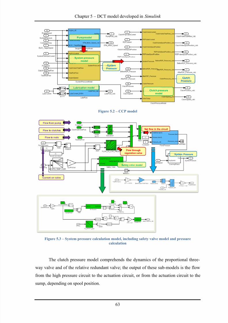
8/20/2019 Olivi Davide Tesi
http://slidepdf.com/reader/full/olivi-davide-tesi 73/141
Chapter 5 – DCT model developed in Simulink
63
Figure 5.2 –
CCP model
Figure 5.3 – System pressure calculation model, including safety valve model and pressure
calculation
The clutch pressure model comprehends the dynamics of the proportional three-
way valve and of the relative redundant valve; the output of these sub-models is the flow
from the high pressure circuit to the actuation circuit, or from the actuation circuit to the
sump, depending on spool position.
Pumpmodel
System pressure
model
Lubrication modelClutch pressure
model
System
Pressure
Clutch
Pressure
Flow to clutches
Flow to rods
Flow from pump
Current on valve
Flow through
regulation valve
Net flow in the circuit
System Pressure
Safety valve model
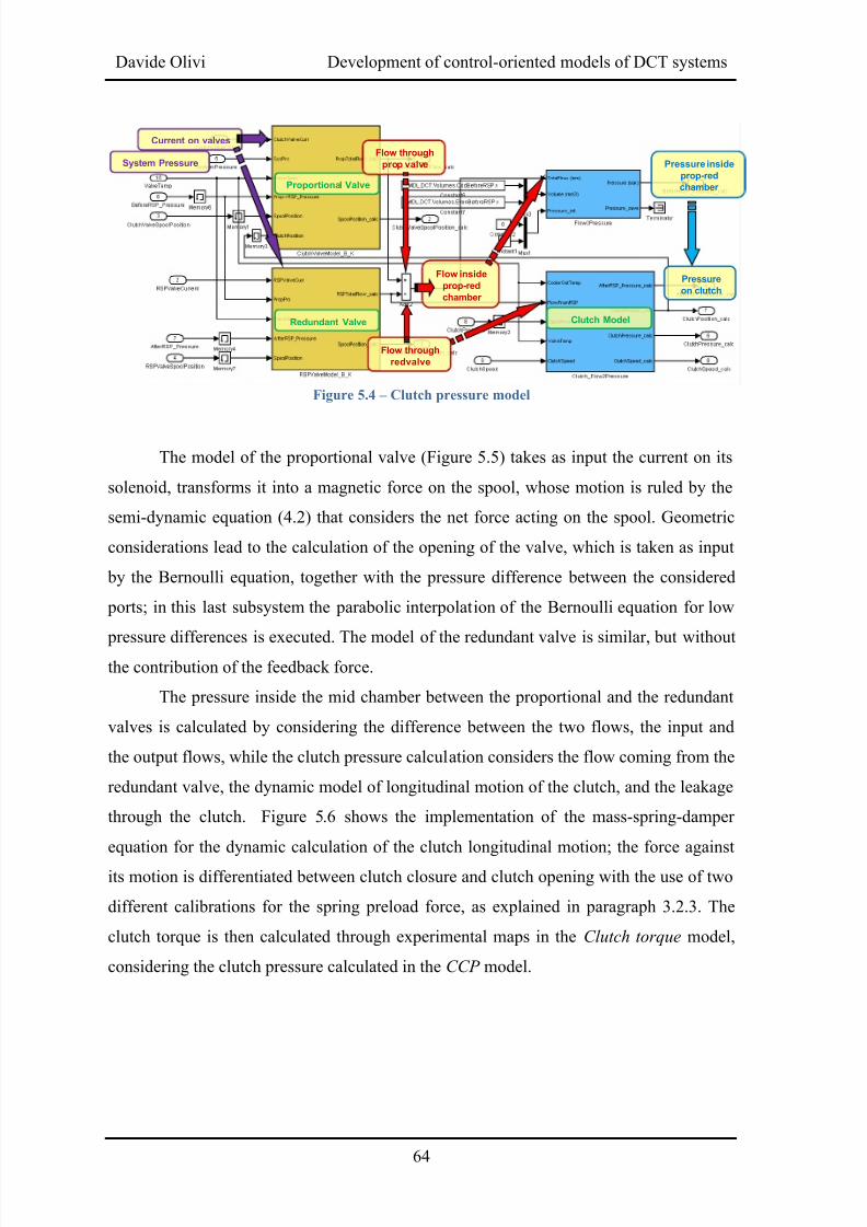
8/20/2019 Olivi Davide Tesi
http://slidepdf.com/reader/full/olivi-davide-tesi 74/141
Davide Olivi Development of control-oriented models of DCT systems
64
Figure 5.4 – Clutch pressure model
The model of the proportional valve (Figure 5.5) takes as input the current on its
solenoid, transforms it into a magnetic force on the spool, whose motion is ruled by the
semi-dynamic equation (4.2) that considers the net force acting on the spool. Geometric
considerations lead to the calculation of the opening of the valve, which is taken as input
by the Bernoulli equation, together with the pressure difference between the considered
ports; in this last subsystem the parabolic interpolation of the Bernoulli equation for low
pressure differences is executed. The model of the redundant valve is similar, but withoutthe contribution of the feedback force.
The pressure inside the mid chamber between the proportional and the redundant
valves is calculated by considering the difference between the two flows, the input and
the output flows, while the clutch pressure calculation considers the flow coming from the
redundant valve, the dynamic model of longitudinal motion of the clutch, and the leakage
through the clutch. Figure 5.6 shows the implementation of the mass-spring-damper
equation for the dynamic calculation of the clutch longitudinal motion; the force against
its motion is differentiated between clutch closure and clutch opening with the use of two
different calibrations for the spring preload force, as explained in paragraph 3.2.3. The
clutch torque is then calculated through experimental maps in the Clutch torque model,
considering the clutch pressure calculated in the CCP model.
Proportional Valve
Flow through
prop valve
Redundant Valve
Flow through
redvalve
Flow inside
prop-red
chamber
Pressure inside
prop-red
chamber
Pressure
on clutch
Current on valves
System Pressure
Clutch Model
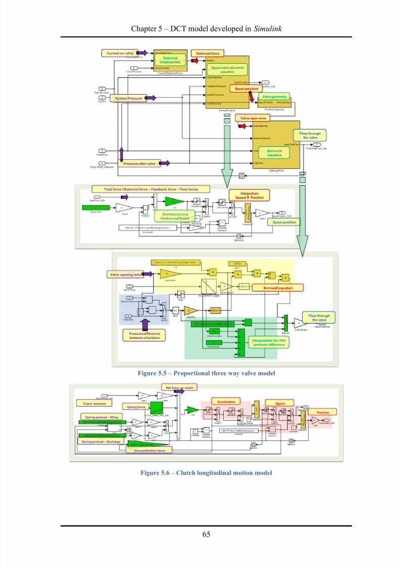
8/20/2019 Olivi Davide Tesi
http://slidepdf.com/reader/full/olivi-davide-tesi 75/141
Chapter 5 – DCT model developed in Simulink
65
Figure 5.5 – Proportional three way valve model
Figure 5.6 – Clutch longitudinal motion model
Solenoid
characteristic
Spool semi-dynamic
equation
Valve geometry
Bernoulli
equation
Current on valve
System Pressure
Pressure after valve
Flow through
the valve
Solenoid force
Spool position
Valve open area
Total force =Solenoid force – Feedback force – Flow forces
Dummyviscous
friction coefficient
Integration:
Speed Posiiton
Spool position
Flow through
the valve
Valve opening area
Pressure difference
between chambersInterpolation for little
pressure difference
Bernoulli equation
AccelerationSpeed
Position
Net force on clutch
Clutch pressureSpring force
Spring preload - filling
Spring preload - discharge
Viscousfriction force
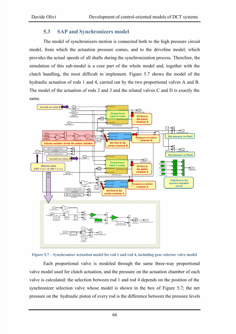
8/20/2019 Olivi Davide Tesi
http://slidepdf.com/reader/full/olivi-davide-tesi 76/141
Davide Olivi Development of control-oriented models of DCT systems
66
5.3 SAP and Synchronizers model
The model of synchronizers motion is connected both to the high pressure circuit
model, from which the actuation pressure comes, and to the driveline model, which
provides the actual speeds of all shafts during the synchronization process. Therefore, the
simulation of this sub-model is a core part of the whole model and, together with the
clutch handling, the most difficult to implement. Figure 5.7 shows the model of the
hydraulic actuation of rods 1 and 4, carried out by the two proportional valves A and B.
The model of the actuation of rods 2 and 3 and the related valves C and D is exactly the
same.
Figure 5.7 – Synchronizer actuation model for rod 1 and rod 4, including gear selector valve model
Each proportional valve is modeled through the same three-way proportional
valve model used for clutch actuation, and the pressure on the actuation chamber of each
valve is calculated; the selection between rod 1 and rod 4 depends on the position of the
synchronizer selection valve whose model is shown in the box of Figure 5.7; the net
pressure on the hydraulic piston of every rod is the difference between the pressure levels
Current on valve B
Current on valve A
Proportional
valve B model
Proportional
valve A model
Oil flow tothe piston
chamber B
Oil flow to
the piston
chamber A
Volume variation inside the piston chamber Net flow in the
piston chamber B
Net flow in the
piston chamber A
Selector state
(OFF = Od d or ON = Even )
Pressure on piston
chamber B
Pressure on piston
chamber A
Net pressure on Rod1
Net pressure on Rod4
Total flow to the
synchro actuation
circuit
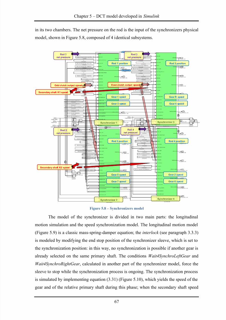
8/20/2019 Olivi Davide Tesi
http://slidepdf.com/reader/full/olivi-davide-tesi 77/141
Chapter 5 – DCT model developed in Simulink
67
in its two chambers. The net pressure on the rod is the input of the synchronizers physical
model, shown in Figure 5.8, composed of 4 identical subsystems.
Figure 5.8 – Synchronizers model
The model of the synchronizer is divided in two main parts: the longitudinal
motion simulation and the speed synchronization model. The longitudinal motion model
(Figure 5.9) is a classic mass-spring-damper equation; the interlock (see paragraph 3.3.3)
is modeled by modifying the end stop position of the synchronizer sleeve, which is set to
the synchronization position: in this way, no synchronization is possible if another gear is
already selected on the same primary shaft. The conditions Wait4SynchroLeftGear and
Wait4SynchroRightGear , calculated in another part of the synchronizer model, force the
sleeve to stop while the synchronization process is ongoing. The synchronization process
is simulated by implementing equation (3.31) (Figure 5.10), which yields the speed of thegear and of the relative primary shaft during this phase; when the secondary shaft speed
Synchronizer 1
Synchronizer 2
Synchronizer 3
Synchronizer 4
Rod 1
net pressure
Rod 2
net pressure
Rod 3
net pressure
Rod 4
net pressure
Secondary shaft K1 speed
Secondary shaft K2 speed
Even clutch output speedOdd clutch output speed
Rod 1 position
Gear 1 speed
Gear 3 speed
Rod 3 position
Gear R speed
Gear 4 speed
Rod 2 position
Gear 5 speed
Gear 7 speed
Rod 4 position
Gear 2 speed
Gear 6 speed
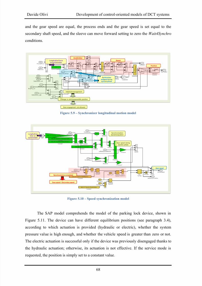
8/20/2019 Olivi Davide Tesi
http://slidepdf.com/reader/full/olivi-davide-tesi 78/141
Davide Olivi Development of control-oriented models of DCT systems
68
and the gear speed are equal, the process ends and the gear speed is set equal to the
secondary shaft speed, and the sleeve can move forward setting to zero the Wait4Synchro
conditions.
Figure 5.9 – Synchronizer longitudinal motion model
Figure 5.10 – Speed synchronization model
The SAP model comprehends the model of the parking lock device, shown in
Figure 5.11. The device can have different equilibrium positions (see paragraph 3.4),
according to which actuation is provided (hydraulic or electric), whether the system
pressure value is high enough, and whether the vehicle speed is greater than zero or not.
The electric actuation is successful only if the device was previously disengaged thanks to
the hydraulic actuation; otherwise, its actuation is not effective. If the service mode is
requested, the position is simply set to a constant value.
Longitudinal force
on synchronizer
Interlock management
Change in min/maxpossible position
Gear engagement not allowed
Acceleration
Speed
Position
Synhronizer
stopped during
synchro phase
Synchronization
dynamicequation
Synchronization completed
Gear speed = Secondary speed
Gear speed during
synchro phase
Gear speed
Longitudinal
force on
synchronizer
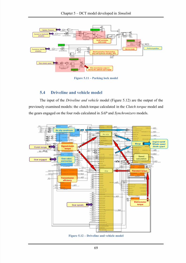
8/20/2019 Olivi Davide Tesi
http://slidepdf.com/reader/full/olivi-davide-tesi 79/141
Chapter 5 – DCT model developed in Simulink
69
Figure 5.11 – Parking lock model
5.4 Driveline and vehicle model
The input of the Driveline and vehicle model (Figure 5.12) are the output of the
previously examined models: the clutch torque calculated in the Clutch torque model and
the gears engaged on the four rods calculated in SAP and Synchronizers models.
Figure 5.12 – Driveline and vehicle model
Current on electric
actuation
Current on hydraulic
actuation
System Pressure
Rear wheels speed
If the transmission output is
moving the parklockcan’t engage
On/off servovalve
static model
Service mode Parklock position
Electricactuation: fixed position
(Ony with hydraulic actuation OFF)
No slip conditions
Gear speeds
Signed clutch
torque
Resistant torque
Eletricmotor
torque
Transmission
efficiency
Gear ratios
and inertias
No sl ip
Sl ip
Speed
calculation
Engine speed
Wheels speed
Shafts speed
Merge
Clutch torque
Gear engaged
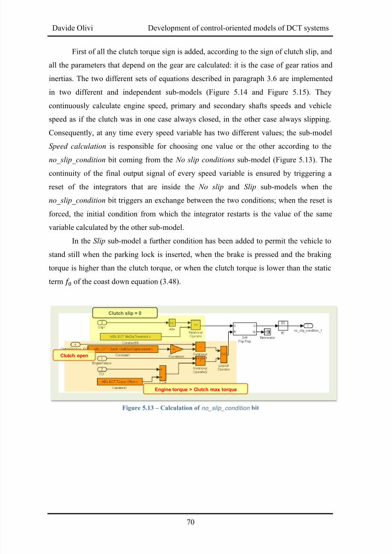
8/20/2019 Olivi Davide Tesi
http://slidepdf.com/reader/full/olivi-davide-tesi 80/141
Davide Olivi Development of control-oriented models of DCT systems
70
First of all the clutch torque sign is added, according to the sign of clutch slip, and
all the parameters that depend on the gear are calculated: it is the case of gear ratios and
inertias. The two different sets of equations described in paragraph 3.6 are implemented
in two different and independent sub-models (Figure 5.14 and Figure 5.15). They
continuously calculate engine speed, primary and secondary shafts speeds and vehicle
speed as if the clutch was in one case always closed, in the other case always slipping.
Consequently, at any time every speed variable has two different values; the sub-model
Speed calculation is responsible for choosing one value or the other according to the
no_slip_condition bit coming from the No slip conditions sub-model (Figure 5.13). The
continuity of the final output signal of every speed variable is ensured by triggering a
reset of the integrators that are inside the No slip and Slip sub-models when the
no_slip_condition bit triggers an exchange between the two conditions; when the reset is
forced, the initial condition from which the integrator restarts is the value of the same
variable calculated by the other sub-model.
In the Slip sub-model a further condition has been added to permit the vehicle to
stand still when the parking lock is inserted, when the brake is pressed and the braking
torque is higher than the clutch torque, or when the clutch torque is lower than the static
term
of the coast down equation (3.48).
Figure 5.13 – Calculation of no_slip_condition bit
Engine torque > Clutch max torque
Clutch open
Clutch slip = 0
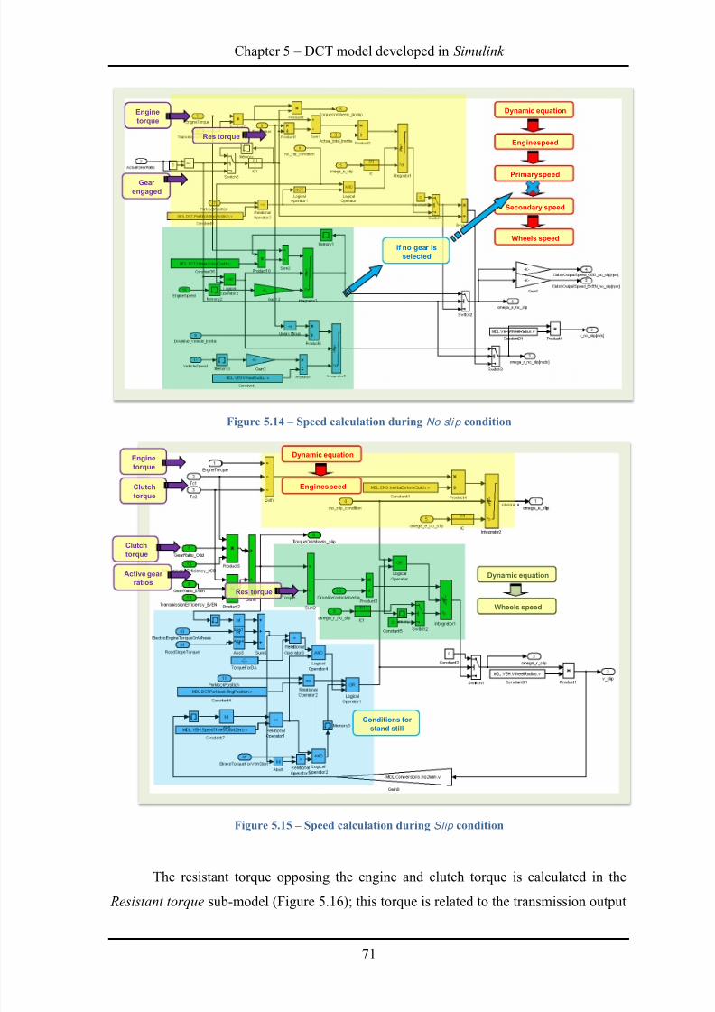
8/20/2019 Olivi Davide Tesi
http://slidepdf.com/reader/full/olivi-davide-tesi 81/141
Chapter 5 – DCT model developed in Simulink
71
Figure 5.14 – Speed calculation during No sli p condition
Figure 5.15 – Speed calculation during Slip condition
The resistant torque opposing the engine and clutch torque is calculated in the
Resistant torque sub-model (Figure 5.16); this torque is related to the transmission output
Dynamic equation
Enginespeed
Wheels speed
If no gear is
selected
Primaryspeed
Secondary speed
Gear
engaged
Engine
torque
Res torque
Engine
torque
Clutch
torque
Dynamic equation
Enginespeed
Dynamic equation
Wheels speed
Clutch
torque
Active gear
ratios
Res torque
Conditions for
stand still
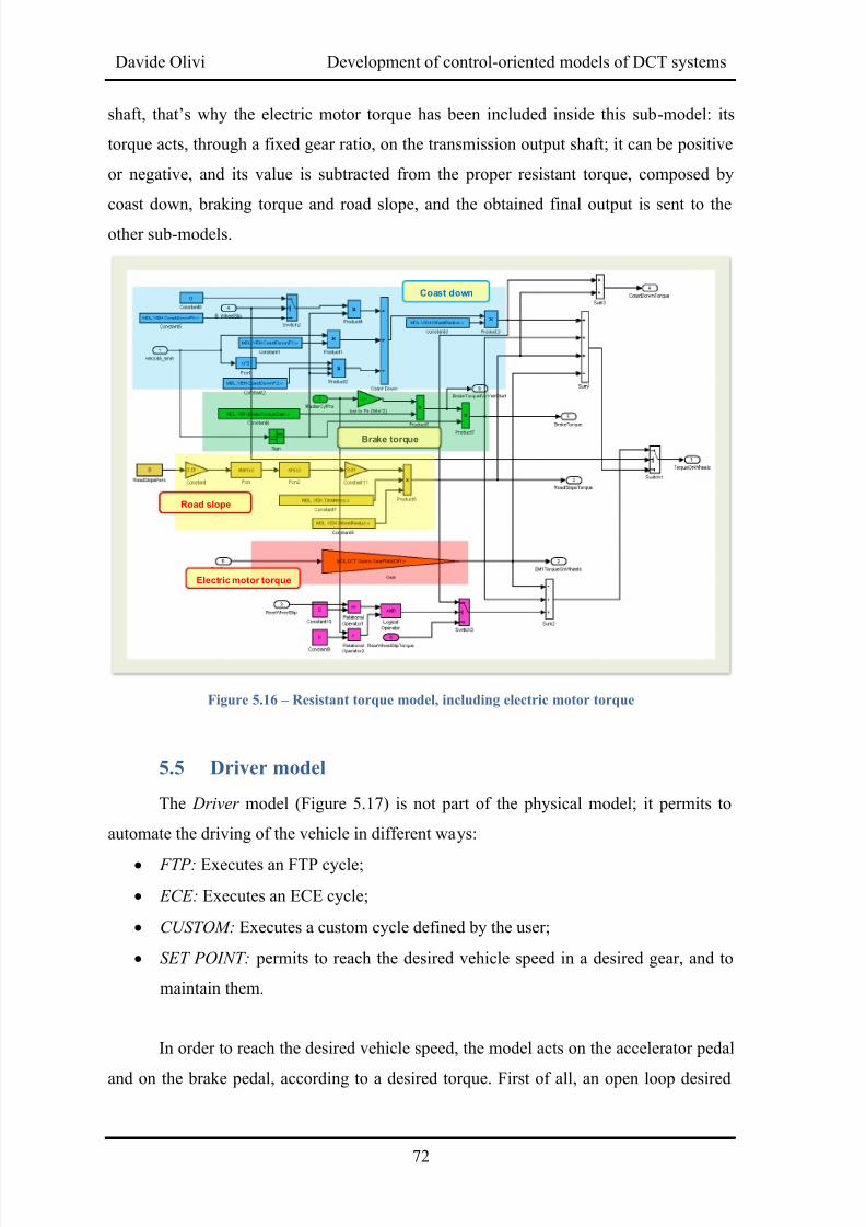
8/20/2019 Olivi Davide Tesi
http://slidepdf.com/reader/full/olivi-davide-tesi 82/141
Davide Olivi Development of control-oriented models of DCT systems
72
shaft, that’s why the electric motor torque has been included inside this sub-model: its
torque acts, through a fixed gear ratio, on the transmission output shaft; it can be positive
or negative, and its value is subtracted from the proper resistant torque, composed by
coast down, braking torque and road slope, and the obtained final output is sent to the
other sub-models.
Figure 5.16 – Resistant torque model, including electric motor torque
5.5 Driver model
The Driver model (Figure 5.17) is not part of the physical model; it permits to
automate the driving of the vehicle in different ways:
FTP: Executes an FTP cycle;
ECE: Executes an ECE cycle;
CUSTOM: Executes a custom cycle defined by the user;
SET POINT: permits to reach the desired vehicle speed in a desired gear, and to
maintain them.
In order to reach the desired vehicle speed, the model acts on the accelerator pedal
and on the brake pedal, according to a desired torque. First of all, an open loop desired
Coast down
Brake torque
Road slope
Electric motor torque
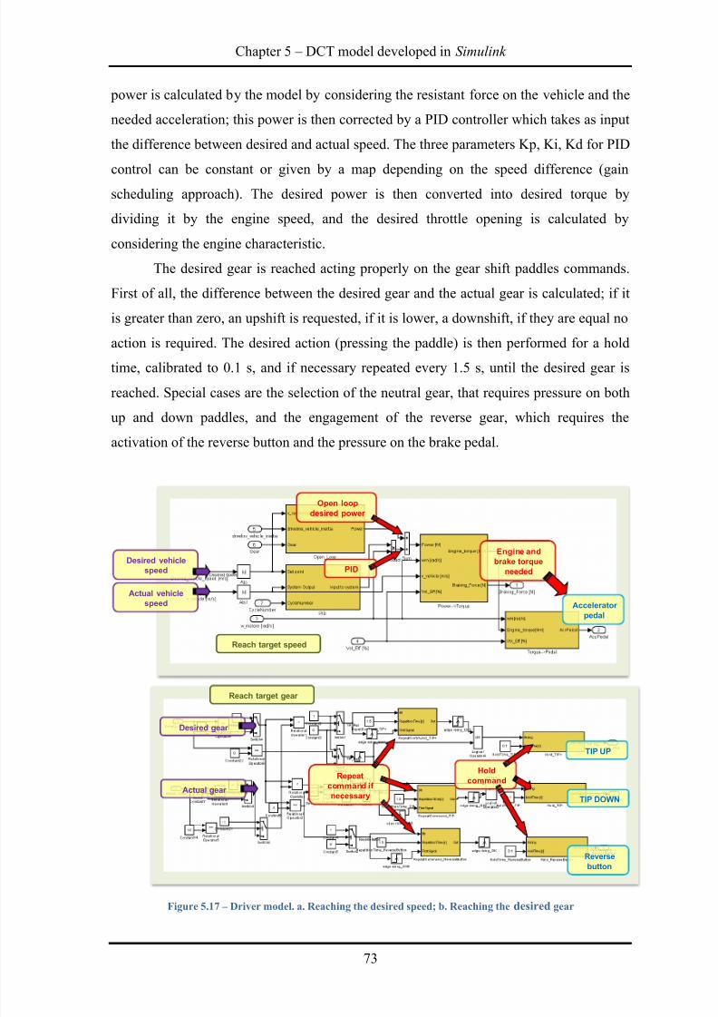
8/20/2019 Olivi Davide Tesi
http://slidepdf.com/reader/full/olivi-davide-tesi 83/141
Chapter 5 – DCT model developed in Simulink
73
power is calculated by the model by considering the resistant force on the vehicle and the
needed acceleration; this power is then corrected by a PID controller which takes as input
the difference between desired and actual speed. The three parameters Kp, Ki, Kd for PID
control can be constant or given by a map depending on the speed difference (gain
scheduling approach). The desired power is then converted into desired torque by
dividing it by the engine speed, and the desired throttle opening is calculated by
considering the engine characteristic.
The desired gear is reached acting properly on the gear shift paddles commands.
First of all, the difference between the desired gear and the actual gear is calculated; if it
is greater than zero, an upshift is requested, if it is lower, a downshift, if they are equal no
action is required. The desired action (pressing the paddle) is then performed for a hold
time, calibrated to 0.1 s, and if necessary repeated every 1.5 s, until the desired gear is
reached. Special cases are the selection of the neutral gear, that requires pressure on both
up and down paddles, and the engagement of the reverse gear, which requires the
activation of the reverse button and the pressure on the brake pedal.
Figure 5.17 – Driver model. a. Reaching the desired speed; b. Reaching the desired gear
Open loop
desired power
PID
Actual vehicle
speed
Desired vehicle
speed
Engine and
brake torque
needed
Accelerator
pedal
Actual gear
Desired gear
Repeat
command if
necessary
Hold
command
TIP UP
TIP DOWN
Reverse
button
Reach target speed
Reach target gear
8/20/2019 Olivi Davide Tesi
http://slidepdf.com/reader/full/olivi-davide-tesi 84/141
Davide Olivi Development of control-oriented models of DCT systems
74
Chapter 6
Offline simulation results
The first analysis of the results obtained with the developed DCT model is made
through an offline simulation, without the connection to the TCU; the input values (i.e.
currents and driver’s requests) are taken from a measurement performed on board the
vehicle. The validation and calibration of the model was carried out trying to match
measured data and simulation results. This validation can’t be considered definitive and
can’t be very accurate, because in this way the TCU control can’t interact with the
simulation, which is performed in fully open loop mode: during a real on-board action,
instead, the actuation currents are calculated and corrected by the TCU according to aclosed loop control, based on the difference between the measured values (coming from
the sensors installed in the gearbox) and the TCU target values. In an offline simulation
these measured currents act on the system without any further correction. The difficulty to
perform a simulation without a closed loop control is summed to the problem that the
input signals are not the nominal ones, but are affected by the on-board closed loop
contribution, which is certainly not the one needed by the simulated system to match the
target value. It is clear that, because of these difficulties, the offline simulation can’t
provide the same results that it could during an online simulation, controlled by the TCU
in a closed loop control. Nevertheless, performing an offline simulation is fundamental
for a first validation of every part of the model, before it can be implemented in the HIL
application. The most important signals that can be checked in an offline simulation are
the signals of the sensors in the actuation circuit; this permits validating the whole high
pressure circuit model, the clutch model and the synchronizers model. The signals coming
from the speed sensors can be also compared to evaluate the simulation results; the match
of these signals allow verifying the driveline and vehicle model, as well as the clutch
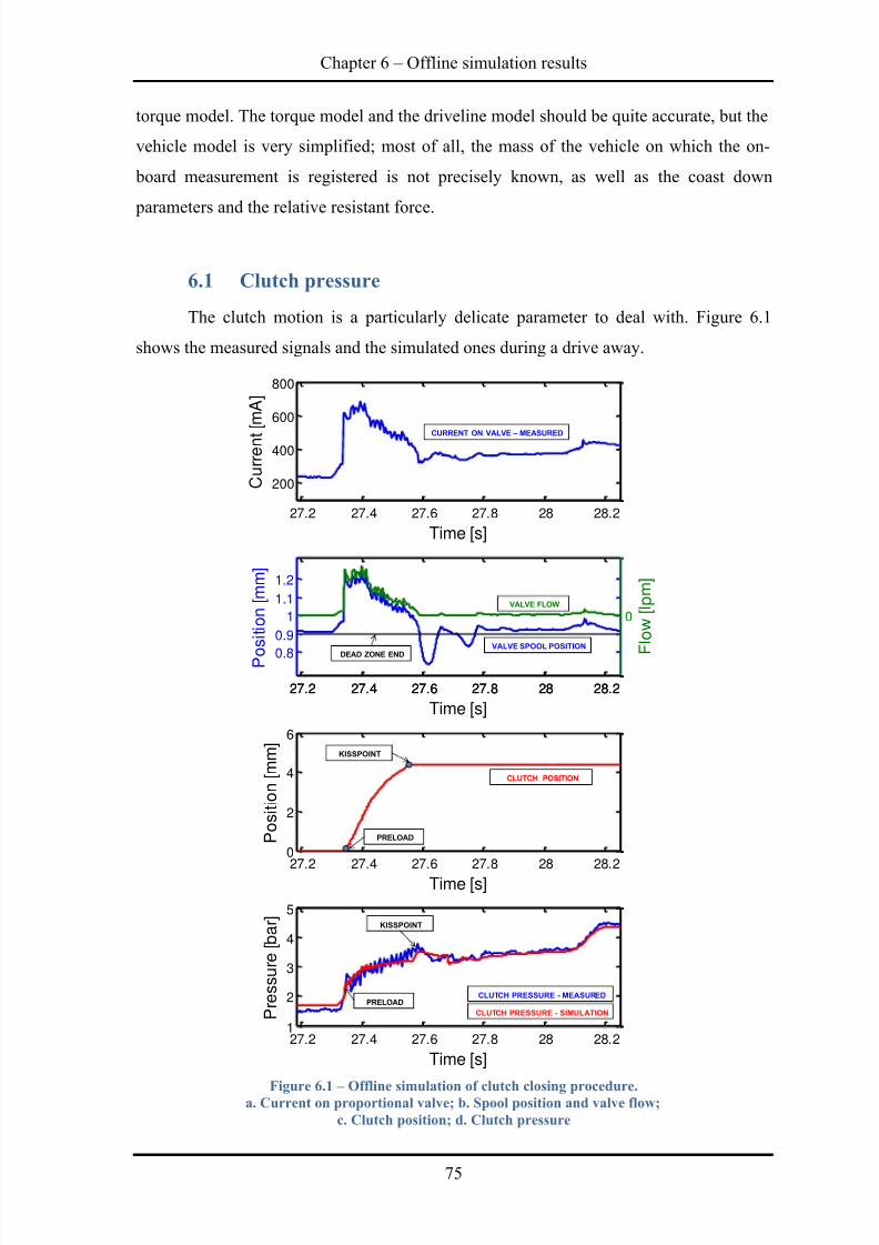
8/20/2019 Olivi Davide Tesi
http://slidepdf.com/reader/full/olivi-davide-tesi 85/141
Chapter 6 – Offline simulation results
75
torque model. The torque model and the driveline model should be quite accurate, but the
vehicle model is very simplified; most of all, the mass of the vehicle on which the on-
board measurement is registered is not precisely known, as well as the coast down
parameters and the relative resistant force.
6.1 Clutch pressure
The clutch motion is a particularly delicate parameter to deal with. Figure 6.1
shows the measured signals and the simulated ones during a drive away.
Figure 6.1 –
Offline simulation of clutch closing procedure.a. Current on proportional valve; b. Spool position and valve flow;
c. Clutch position; d. Clutch pressure
27.2 27.4 27.6 27.8 28 28.2
200
400
600
800
Current
[mA]
Time [s]
27.2 27.4 27.6 27.8 28 28.2
0.8
0.9
1
1.1
1.2
Po
sition[mm]
Time [s]
27.2 27.4 27.6 27.8 28 28.20
2
4
6
Position[mm]
Time [s]
27.2 27.4 27.6 27.8 28 28.21
2
3
4
5
Pressure[bar]
Time [s]
27.2 27.4 27.6 27.8 28 28.2
0
F
low
[lpm]
PRELOAD
KISSPOINT
CLUTCH PRESSURE - MEASURED
CLUTCH PRESSURE - SIMULATION
CLUTCH POSITION
KISSPOINT
PRELOAD
VALVE FLOW
VALVE SPOOL POSITION
DEAD ZONE END
CURRENT ON VALVE – MEASURED
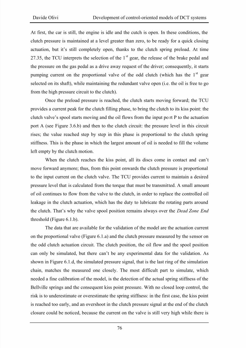
8/20/2019 Olivi Davide Tesi
http://slidepdf.com/reader/full/olivi-davide-tesi 86/141
Davide Olivi Development of control-oriented models of DCT systems
76
At first, the car is still, the engine is idle and the cutch is open. In these conditions, the
clutch pressure is maintained at a level greater than zero, to be ready for a quick closing
actuation, but it’s still completely open, thanks to the clutch spring preload. At time
27.35, the TCU interprets the selection of the 1 st gear, the release of the brake pedal and
the pressure on the gas pedal as a drive away request of the driver; consequently, it starts
pumping current on the proportional valve of the odd clutch (which has the 1st gear
selected on its shaft), while maintaining the redundant valve open (i.e. the oil is free to go
from the high pressure circuit to the clutch).
Once the preload pressure is reached, the clutch starts moving forward; the TCU
provides a current peak for the clutch filling phase, to bring the clutch to its kiss point: the
clutch valve’s spool starts moving and the oil flows from the input po rt P to the actuation
port A (see Figure 3.6.b) and then to the clutch circuit: the pressure level in this circuit
rises; the value reached step by step in this phase is proportional to the clutch spring
stiffness. This is the phase in which the largest amount of oil is needed to fill the volume
left empty by the clutch motion.
When the clutch reaches the kiss point, all its discs come in contact and can’t
move forward anymore; thus, from this point onwards the clutch pressure is proportional
to the input current on the clutch valve. The TCU provides current to maintain a desired
pressure level that is calculated from the torque that must be transmitted. A small amount
of oil continues to flow from the valve to the clutch, in order to replace the controlled oil
leakage in the clutch actuation, which has the duty to lubricate the rotating parts around
the clutch. That’s why the valve spool position remains always over the Dead Zone End
threshold (Figure 6.1.b).
The data that are available for the validation of the model are the actuation current
on the proportional valve (Figure 6.1.a) and the clutch pressure measured by the sensor on
the odd clutch actuation circuit. The clutch position, the oil flow and the spool position
can only be simulated, but there can’t be any experimental data for the validation. As
shown in Figure 6.1.d, the simulated pressure signal, that is the last ring of the simulation
chain, matches the measured one closely. The most difficult part to simulate, which
needed a fine calibration of the model, is the detection of the actual spring stiffness of the
Bellville springs and the consequent kiss point pressure. With no closed loop control, the
risk is to underestimate or overestimate the spring stiffness: in the first case, the kiss point
is reached too early, and an overshoot in the clutch pressure signal at the end of the clutch
closure could be noticed, because the current on the valve is still very high while there is
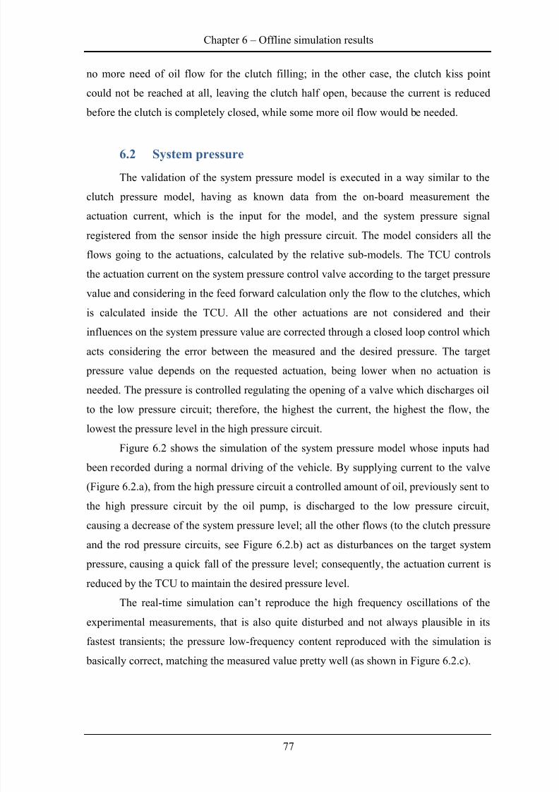
8/20/2019 Olivi Davide Tesi
http://slidepdf.com/reader/full/olivi-davide-tesi 87/141
Chapter 6 – Offline simulation results
77
no more need of oil flow for the clutch filling; in the other case, the clutch kiss point
could not be reached at all, leaving the clutch half open, because the current is reduced
before the clutch is completely closed, while some more oil flow would be needed.
6.2 System pressure
The validation of the system pressure model is executed in a way similar to the
clutch pressure model, having as known data from the on-board measurement the
actuation current, which is the input for the model, and the system pressure signal
registered from the sensor inside the high pressure circuit. The model considers all the
flows going to the actuations, calculated by the relative sub-models. The TCU controls
the actuation current on the system pressure control valve according to the target pressurevalue and considering in the feed forward calculation only the flow to the clutches, which
is calculated inside the TCU. All the other actuations are not considered and their
influences on the system pressure value are corrected through a closed loop control which
acts considering the error between the measured and the desired pressure. The target
pressure value depends on the requested actuation, being lower when no actuation is
needed. The pressure is controlled regulating the opening of a valve which discharges oil
to the low pressure circuit; therefore, the highest the current, the highest the flow, the
lowest the pressure level in the high pressure circuit.
Figure 6.2 shows the simulation of the system pressure model whose inputs had
been recorded during a normal driving of the vehicle. By supplying current to the valve
(Figure 6.2.a), from the high pressure circuit a controlled amount of oil, previously sent to
the high pressure circuit by the oil pump, is discharged to the low pressure circuit,
causing a decrease of the system pressure level; all the other flows (to the clutch pressure
and the rod pressure circuits, see Figure 6.2.b) act as disturbances on the target system
pressure, causing a quick fall of the pressure level; consequently, the actuation current is
reduced by the TCU to maintain the desired pressure level.
The real-time simulation can’t reproduce the high frequency oscillations of the
experimental measurements, that is also quite disturbed and not always plausible in its
fastest transients; the pressure low-frequency content reproduced with the simulation is
basically correct, matching the measured value pretty well (as shown in Figure 6.2.c).
8/20/2019 Olivi Davide Tesi
http://slidepdf.com/reader/full/olivi-davide-tesi 88/141
Davide Olivi Development of control-oriented models of DCT systems
78
Figure 6.2 – Offline simulation of system pressure regulation circuit.
a. Current supplied to the valve; b. flows in the high pressure circuit; c. System pressure
6.3 Synchronizers
The synchronizer model comprehends the model of the actuation circuit, the
model of the synchronizer motion and the model of driveline and vehicle, when the
speeds must synchronize; the challenge is to connect all these sub-models together
without creating instability or discontinuity. In this case the input data are the currents on
the 4 proportional valves that control the rod motion; the data used for the validation are
37.5 38 38.5 39 39.5750
800
850
900
950
1000
1050
Curren
t[mA]
Time [s]
37.5 38 38.5 39 39.50
5
10
15
20
25
Flows[lpm]
Time [s]
37.5 38 38.5 39 39.5
15
20
25
30
Pressure[bar]
Time [s]
SYSTEM PRESSURE - MEASURED
SYSTEM PRESSURE - SIMULATION
FLOW FROM PUMP
FLOW TO
CLUTCHES / RODS
FLOW THROUGH
REGULATION VALVE
ACTUATION CURRENT ON VALVE - MEASURED
8/20/2019 Olivi Davide Tesi
http://slidepdf.com/reader/full/olivi-davide-tesi 89/141
Chapter 6 – Offline simulation results
79
the related signals registered from the position sensors of the rods. These sensors are
located in the rods actuation circuit and measure the position of the piston which controls
the rods motion, rigidly connected to the fork which moves the synchronizer hub. There is
no information about the oil flow through the valve and about the pressure on the
actuation pistons.
In Figure 6.3 the gear selection on the odd shaft of the transmission is shown;
during all this process the engine is transmitting torque through the even shaft in 2nd gear,
while the odd clutch is completely open; therefore, the engine speed and the even shaft
speed are coincident. The pre-selection of gears is controlled by the TCU, which previews
the future gear according mainly to the engine speed trend and to the torque request. At
first, rod 1 is engaging the 1st gear, which corresponds to the low position measured by
the sensor (Figure 6.3.c, until time 29.4); when the TCU triggers the pre-selection of the
3rd gear, it provides on valve A (see Figure 2.4) an actuation current with a very impulsive
shape (Figure 6.3.a, at time 29.4), in order to move the synchronizer from the engaged
position; then the current changes into a ramp profile when the 3rd gear (which
corresponds to the high position measured by the sensor) is synchronizing (Figures 6.3.c
and 6.3.d, from time 29.5 to time 29.7), to prevent the risk of gear rattling. The net
pressure inside the rod (i.e. the difference between the pressure on the left chamber and
the one on the right chamber, Figure 6.3.b), follows the target pressure imposed by the
TCU; the oil flow from the rod pressure circuit to the rod chamber in the phases with a
fast movement of the rod acts as a disturbance on this target pressure, because the
movement determines a volume increase that must be filled by oil, causing a temporary
pressure level decrease (Figure 6.3.b, time 29.6).
When the speed synchronization is completed, the 3rd gear is correctly engaged
and there is no more need for pressure in the rod chambers. At time 30.7 the engine starts
slowing down and at time 31.0 the TCU triggers the pre-selection of 1st gear, sending
current to valve A and following the same procedure.
The simulation output matches the experimental one closely; the most difficult
part to simulate is the synchronization phase; on board the vehicle a closed loop control
works according to the desired and the actual position of the rod, and considering the
shafts speeds: when the speeds are synchronized and the rod position is reached, the TCU
stops pumping current on the relative valves. In the offline simulation this control can’t
happen and the synchronization phase can last less or more then during the on-board
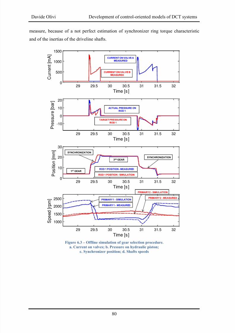
8/20/2019 Olivi Davide Tesi
http://slidepdf.com/reader/full/olivi-davide-tesi 90/141
Davide Olivi Development of control-oriented models of DCT systems
80
measure, because of a not perfect estimation of synchronizer ring torque characteristic
and of the inertias of the driveline shafts.
Figure 6.3 – Offline simulation of gear selection procedure.
a. Current on valves; b. Pressure on hydraulic piston;
c. Synchronizer position; d. Shafts speeds
29 29.5 30 30.5 31 31.5 320
500
1000
1500
Current[mA
]
Time [s]
29 29.5 30 30.5 31 31.5 32
-10
0
10
20
Pressu
re[bar]
Time [s]
29 29.5 30 30.5 31 31.5 320
10
20
30
P
osition[mm]
Time [s]
29 29.5 30 30.5 31 31.5 32
1000
1500
2000
2500
Speed[rpm]
Time [s]
CURRENT ON VALVE AMEASURED
CURRENT ON VALVE B
MEASURED
TARGET PRESSURE ON
ROD 1
ACTUAL PRESSURE ON
ROD 1
ROD 1 POSITION -MEASURED
ROD 1 POSITION - SIMULATION
1ST GEAR
3RD GEAR
SYNCHRONIZATION
SYNCHRONIZATION
PRIMARY 1 - SIMULATION
PRIMARY 1 - MEASURED
PRIMARY 2 - SIMULATION
PRIMARY 2 - MEASURED
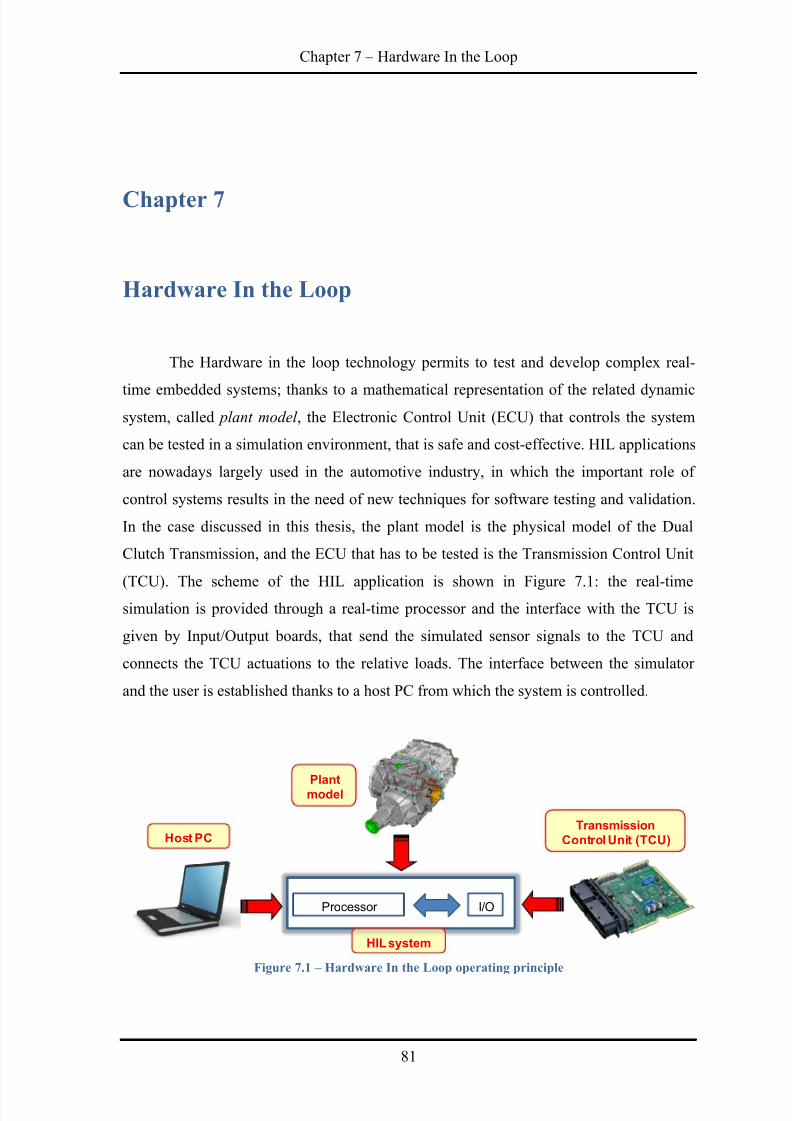
8/20/2019 Olivi Davide Tesi
http://slidepdf.com/reader/full/olivi-davide-tesi 91/141
Chapter 7 – Hardware In the Loop
81
Chapter 7
Hardware In the Loop
The Hardware in the loop technology permits to test and develop complex real-
time embedded systems; thanks to a mathematical representation of the related dynamic
system, called plant model , the Electronic Control Unit (ECU) that controls the system
can be tested in a simulation environment, that is safe and cost-effective. HIL applications
are nowadays largely used in the automotive industry, in which the important role of
control systems results in the need of new techniques for software testing and validation.
In the case discussed in this thesis, the plant model is the physical model of the Dual
Clutch Transmission, and the ECU that has to be tested is the Transmission Control Unit
(TCU). The scheme of the HIL application is shown in Figure 7.1: the real-timesimulation is provided through a real-time processor and the interface with the TCU is
given by Input/Output boards, that send the simulated sensor signals to the TCU and
connects the TCU actuations to the relative loads. The interface between the simulator
and the user is established thanks to a host PC from which the system is controlled.
Figure 7.1 – Hardware In the Loop operating principle
Plantmodel
Host PC
Processor I/O
HIL system
Transmission
Control Unit (TCU)
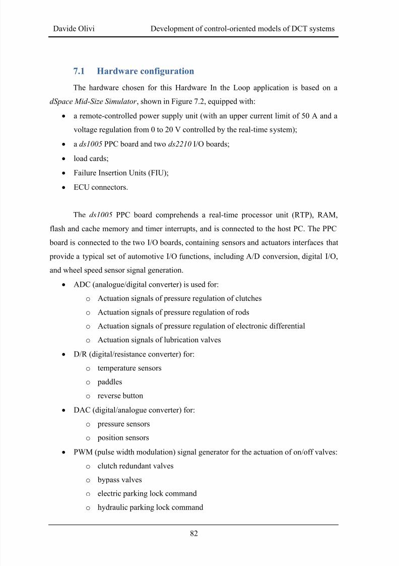
8/20/2019 Olivi Davide Tesi
http://slidepdf.com/reader/full/olivi-davide-tesi 92/141
Davide Olivi Development of control-oriented models of DCT systems
82
7.1 Hardware configuration
The hardware chosen for this Hardware In the Loop application is based on a
dSpace Mid-Size Simulator , shown in Figure 7.2, equipped with:
a remote-controlled power supply unit (with an upper current limit of 50 A and a
voltage regulation from 0 to 20 V controlled by the real-time system);
a ds1005 PPC board and two ds2210 I/O boards;
load cards;
Failure Insertion Units (FIU);
ECU connectors.
The ds1005 PPC board comprehends a real-time processor unit (RTP), RAM,
flash and cache memory and timer interrupts, and is connected to the host PC. The PPC
board is connected to the two I/O boards, containing sensors and actuators interfaces that
provide a typical set of automotive I/O functions, including A/D conversion, digital I/O,
and wheel speed sensor signal generation.
ADC (analogue/digital converter) is used for:
o
Actuation signals of pressure regulation of clutches
o Actuation signals of pressure regulation of rods
o Actuation signals of pressure regulation of electronic differential
o Actuation signals of lubrication valves
D/R (digital/resistance converter) for:
o temperature sensors
o paddles
o
reverse button
DAC (digital/analogue converter) for:
o pressure sensors
o
position sensors
PWM (pulse width modulation) signal generator for the actuation of on/off valves:
o
clutch redundant valves
o bypass valves
o
electric parking lock commando
hydraulic parking lock command
8/20/2019 Olivi Davide Tesi
http://slidepdf.com/reader/full/olivi-davide-tesi 93/141
Chapter 7 – Hardware In the Loop
83
a CAN controller gives the possibility to set two CAN lines per board, for a total
of 4 different CAN lines. At the moment 3 of these lines are used:
o CCAN (Vehicle CAN)
o PWTCAN (Powertrain CAN)
o
CAN3 (Electric pump CAN)
A load card permits the connection of the TCU to the loads it controls and
actuates; the connected loads are the real valves and actuators of the DCT transmission, to
obtain the best possible match with the real system. Each load channel is connected to a
Failure Insertion Unit (FIU), to give the possibility to simulate failures in the TCU wiring.
Three types of failure can be simulated:
TCU output shorted to battery voltage
TCU output shorted to ground
TCU output open circuit.
Figure 7.2 – dSpace Mid-Size Simulator
A Load Plate and a TCU Plate were created; the connections between these plates
and the other parts of the simulator are complete, it means that every I/O channel of the
simulator was wired, so that further modifications of the loads or of the TCU wiring
would require modifications only inside the two plates. The current configuration of the
simulator is shown in Figure 7.3.
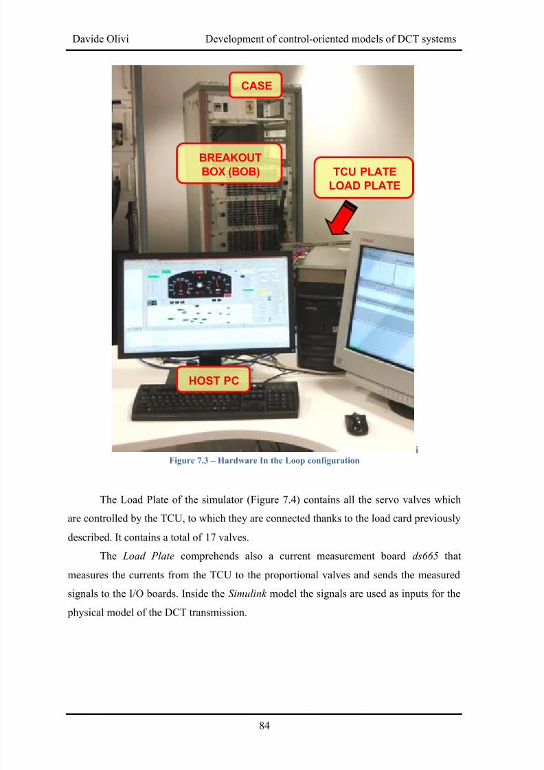
8/20/2019 Olivi Davide Tesi
http://slidepdf.com/reader/full/olivi-davide-tesi 94/141
Davide Olivi Development of control-oriented models of DCT systems
84
ì
Figure 7.3 – Hardware In the Loop configuration
The Load Plate of the simulator (Figure 7.4) contains all the servo valves which
are controlled by the TCU, to which they are connected thanks to the load card previously
described. It contains a total of 17 valves.The Load Plate comprehends also a current measurement board ds665 that
measures the currents from the TCU to the proportional valves and sends the measured
signals to the I/O boards. Inside the Simulink model the signals are used as inputs for the
physical model of the DCT transmission.
TCU PLATE
LOAD PLATE
CASE
BREAKOUT
BOX (BOB)
HOST PC
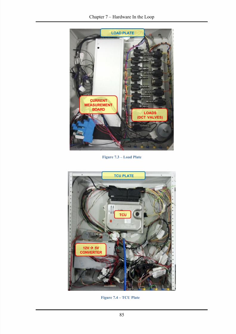
8/20/2019 Olivi Davide Tesi
http://slidepdf.com/reader/full/olivi-davide-tesi 95/141
Chapter 7 – Hardware In the Loop
85
Figure 7.3 – Load Plate
Figure 7.4 – TCU Plate
CURRENT
MEASUREMENT
BOARDLOADS
(DCT VALVES)
LOAD PLATE
TCU
12V 5V
CONVERTER
TCU PLATE
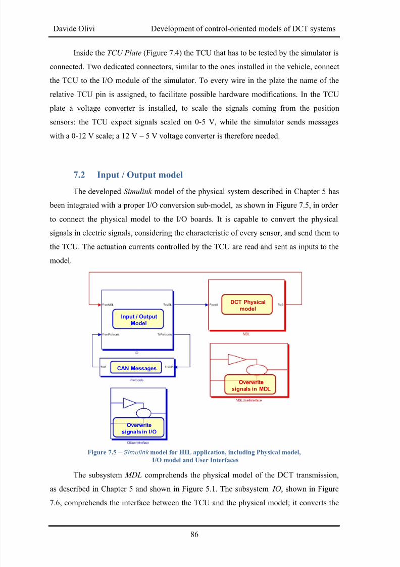
8/20/2019 Olivi Davide Tesi
http://slidepdf.com/reader/full/olivi-davide-tesi 96/141
Davide Olivi Development of control-oriented models of DCT systems
86
Inside the TCU Plate (Figure 7.4) the TCU that has to be tested by the simulator is
connected. Two dedicated connectors, similar to the ones installed in the vehicle, connect
the TCU to the I/O module of the simulator. To every wire in the plate the name of the
relative TCU pin is assigned, to facilitate possible hardware modifications. In the TCU
plate a voltage converter is installed, to scale the signals coming from the position
sensors: the TCU expect signals scaled on 0-5 V, while the simulator sends messages
with a 0-12 V scale; a 12 V – 5 V voltage converter is therefore needed.
7.2 Input / Output model
The developed Simulink model of the physical system described in Chapter 5 has
been integrated with a proper I/O conversion sub-model, as shown in Figure 7.5, in order
to connect the physical model to the I/O boards. It is capable to convert the physical
signals in electric signals, considering the characteristic of every sensor, and send them to
the TCU. The actuation currents controlled by the TCU are read and sent as inputs to the
model.
Figure 7.5 – Simulink model for HIL application, including Physical model,
I/O model and User Interfaces
The subsystem MDL comprehends the physical model of the DCT transmission,
as described in Chapter 5 and shown in Figure 5.1. The subsystem IO, shown in Figure
7.6, comprehends the interface between the TCU and the physical model; it converts the
DCT Physical
model
Input / Output
Model
CAN Messages
Overwrite
signals in I/O
Overwrite
signals in MDL
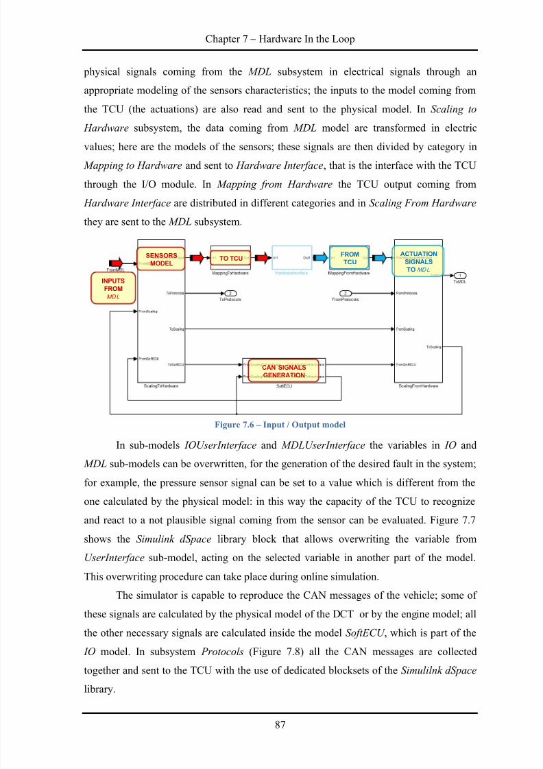
8/20/2019 Olivi Davide Tesi
http://slidepdf.com/reader/full/olivi-davide-tesi 97/141
Chapter 7 – Hardware In the Loop
87
physical signals coming from the MDL subsystem in electrical signals through an
appropriate modeling of the sensors characteristics; the inputs to the model coming from
the TCU (the actuations) are also read and sent to the physical model. In Scaling to
Hardware subsystem, the data coming from MDL model are transformed in electric
values; here are the models of the sensors; these signals are then divided by category in
Mapping to Hardware and sent to Hardware Interface, that is the interface with the TCU
through the I/O module. In Mapping from Hardware the TCU output coming from
Hardware Interface are distributed in different categories and in Scaling From Hardware
they are sent to the MDL subsystem.
Figure 7.6 – Input / Output model
In sub-models IOUserInterface and MDLUserInterface the variables in IO and
MDL sub-models can be overwritten, for the generation of the desired fault in the system;
for example, the pressure sensor signal can be set to a value which is different from the
one calculated by the physical model: in this way the capacity of the TCU to recognize
and react to a not plausible signal coming from the sensor can be evaluated. Figure 7.7
shows the Simulink dSpace library block that allows overwriting the variable from
UserInterface sub-model, acting on the selected variable in another part of the model.
This overwriting procedure can take place during online simulation.
The simulator is capable to reproduce the CAN messages of the vehicle; some of
these signals are calculated by the physical model of the DCT or by the engine model; all
the other necessary signals are calculated inside the model SoftECU , which is part of the
IO model. In subsystem Protocols (Figure 7.8) all the CAN messages are collected
together and sent to the TCU with the use of dedicated blocksets of the Simulilnk dSpace library.
SENSORS
MODEL
INPUTS
FROM
MDL
TO TCUFROM
TCU
ACTUATION
SIGNALS
TOMDL
CAN SIGNALS
GENERATION
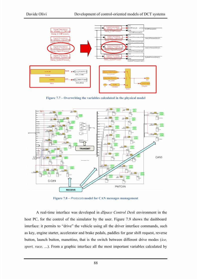
8/20/2019 Olivi Davide Tesi
http://slidepdf.com/reader/full/olivi-davide-tesi 98/141
Davide Olivi Development of control-oriented models of DCT systems
88
Figure 7.7 –
Overwriting the variables calculated in the physical model
Figure 7.8 – Protocols model for CAN messages management
A real-time interface was developed in dSpace Control Desk environment in the
host PC, for the control of the simulator by the user. Figure 7.9 shows the dashboard
interface: it permits to “drive” the vehicle using all the driver interface commands, such
as key, engine starter, accelerator and brake pedals, paddles for gear shift request, reverse
button, launch button, manettino, that is the switch between different drive modes (ice,
sport, race, ...). From a graphic interface all the most important variables calculated by
TRANSMIT
RECEIVE
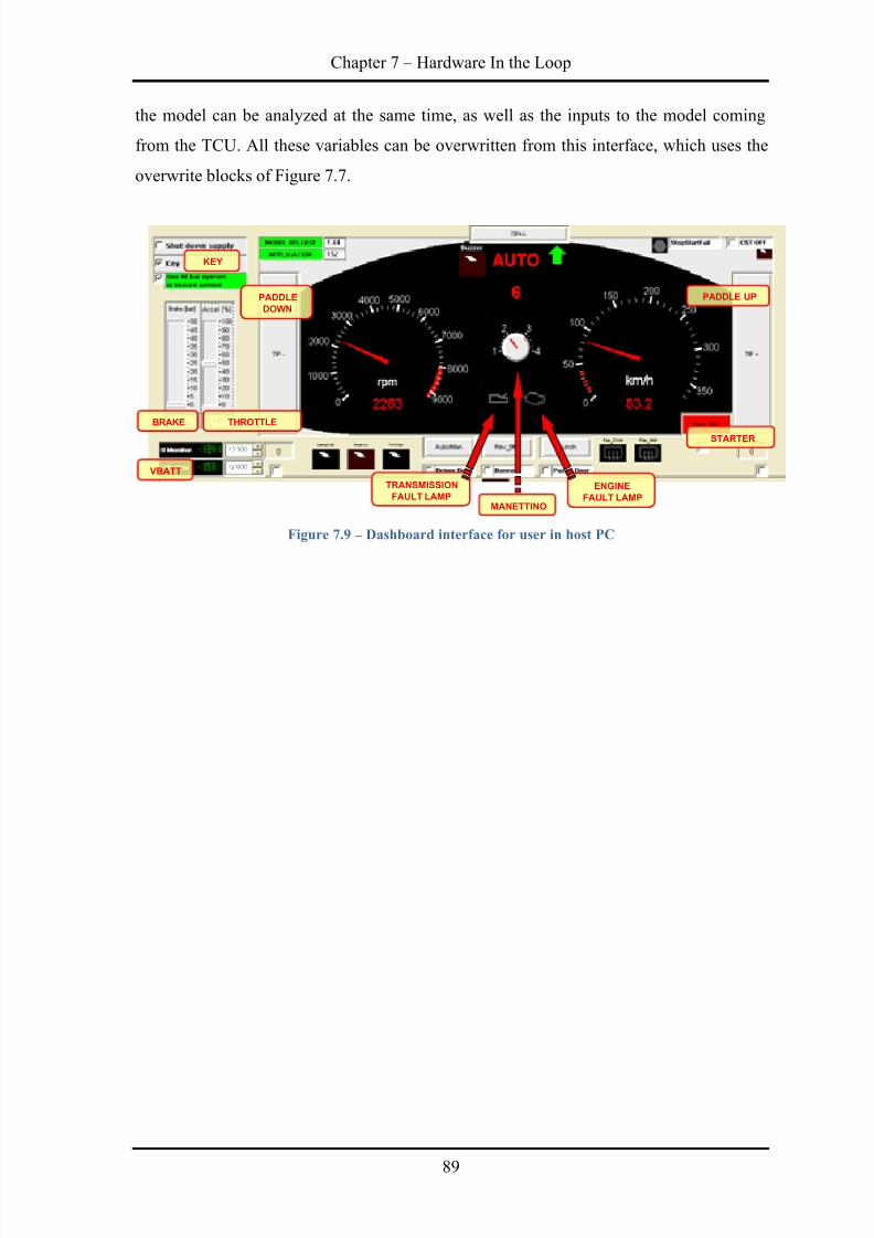
8/20/2019 Olivi Davide Tesi
http://slidepdf.com/reader/full/olivi-davide-tesi 99/141
Chapter 7 – Hardware In the Loop
89
the model can be analyzed at the same time, as well as the inputs to the model coming
from the TCU. All these variables can be overwritten from this interface, which uses the
overwrite blocks of Figure 7.7.
Figure 7.9 – Dashboard interface for user in host PC
PADDLE UP
ENGINE
FAULT LAMP
TRANSMISSION
FAULT LAMP
KEY
THROTTLEBRAKE
VBATT
PADDLE
DOWN
MANETTINO
STARTER
8/20/2019 Olivi Davide Tesi
http://slidepdf.com/reader/full/olivi-davide-tesi 100/141
Davide Olivi Development of control-oriented models of DCT systems
90
Chapter 8
TCU testing
The developed Simulink model is compiled with the use of Real-time Workshop
tool and then flashed inside the HIL real-time processor unit. The HIL application permits
to execute a wide range of tests to check and validate the functionality of the DCT
controller. In general, these tests can be of different kinds: functional tests permit to check
the main functionalities of the TCU, as drive away, gear shift, performance launch and
interaction with the driver through paddles and buttons; the possibility of introducing a
mechanical, hydraulic or electrical fault in the system allows verifying the TCU
capability to recognize the problem and recover to a safe state. The capability of the
controller to adapt to changes in the controlled system during its lifetime can be checked
by analyzing the result of adaption procedures.
The model has been implemented inside the real-time processor and tested
connecting to the HIL a TCU with a production software. The model was calibrated in
order to give plausible results under the control of a TCU software that was already
validated. After this first validation of the model, a new TCU software was connected to
the hardware and the new TCU software testing phase started.
8.1 Functional tests
8.1.1 Gear shift
First of all, the basic functions implemented in the TCU can be tested. In a Dual
Clutch Transmission, the gear shift is performed only opening the offgoing clutch and
closing the ongoing one, thanks to the possibility of preselecting gears on odd and even
shafts before the gear shift. Figure 8.1 considers a gear shift from 3rd to 4th gear.
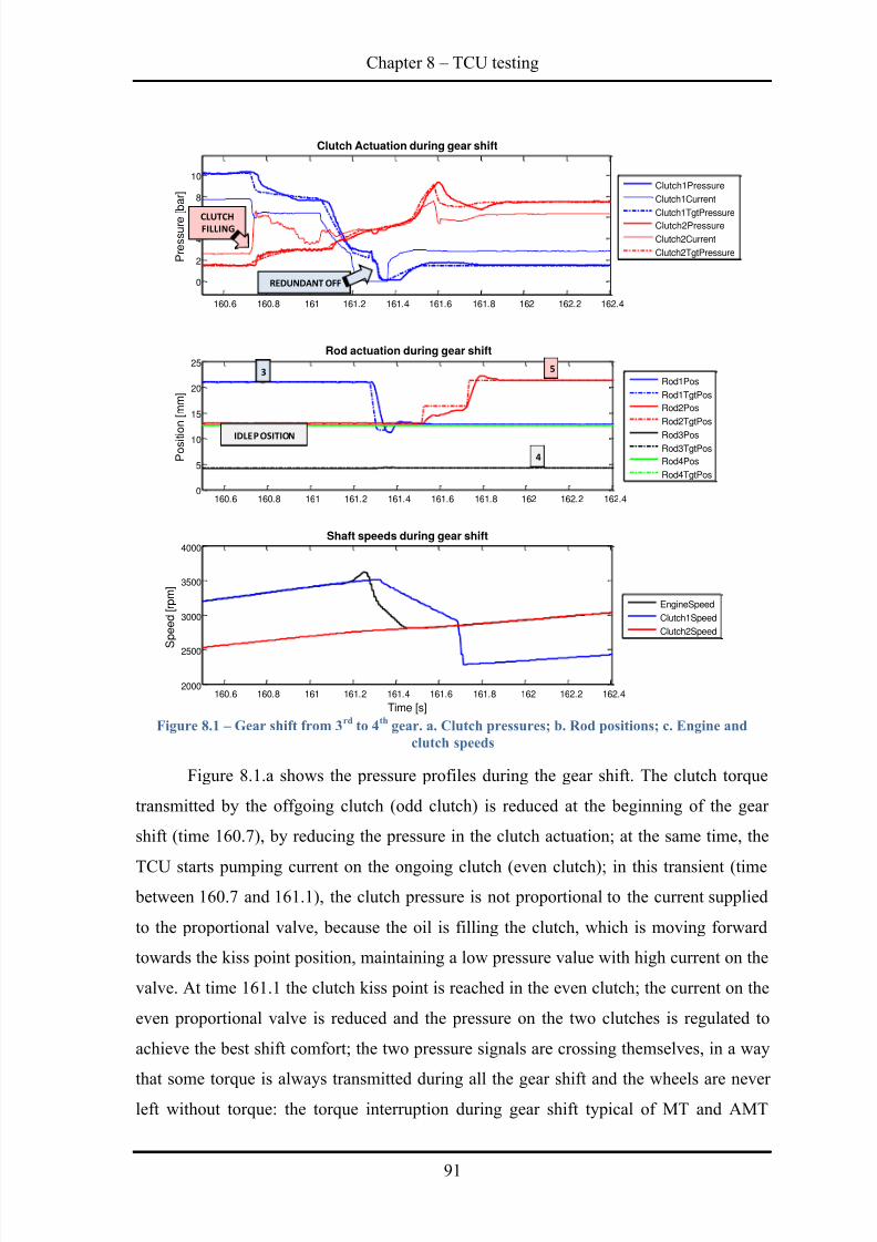
8/20/2019 Olivi Davide Tesi
http://slidepdf.com/reader/full/olivi-davide-tesi 101/141
Chapter 8 – TCU testing
91
Figure 8.1 – Gear shift from 3rd
to 4th
gear. a. Clutch pressures; b. Rod positions; c. Engine and
clutch speeds
Figure 8.1.a shows the pressure profiles during the gear shift. The clutch torque
transmitted by the offgoing clutch (odd clutch) is reduced at the beginning of the gear
shift (time 160.7), by reducing the pressure in the clutch actuation; at the same time, the
TCU starts pumping current on the ongoing clutch (even clutch); in this transient (time between 160.7 and 161.1), the clutch pressure is not proportional to the current supplied
to the proportional valve, because the oil is filling the clutch, which is moving forward
towards the kiss point position, maintaining a low pressure value with high current on the
valve. At time 161.1 the clutch kiss point is reached in the even clutch; the current on the
even proportional valve is reduced and the pressure on the two clutches is regulated to
achieve the best shift comfort; the two pressure signals are crossing themselves, in a way
that some torque is always transmitted during all the gear shift and the wheels are never
left without torque: the torque interruption during gear shift typical of MT and AMT
160.6 160.8 161 161.2 161.4 161.6 161.8 162 162.2 162.4
0
2
4
6
8
10
Clutch Actuation during gear shift
Pressure
[bar]
160.6 160.8 161 161.2 161.4 161.6 161.8 162 162.2 162.40
5
10
15
20
25
Rod actuation during gear shift
Position[mm]
160.6 160.8 161 161.2 161.4 161.6 161.8 162 162.2 162.42000
2500
3000
3500
4000
Shaft speeds during gear shift
Time [s]
Speed[rpm]
Clutch1Pressure
Clutch1Current
Clutch1TgtPressureClutch2Pressure
Clutch2Current
Clutch2TgtPressure
Rod1Pos
Rod1TgtPos
Rod2Pos
Rod2TgtPos
Rod3PosRod3TgtPos
Rod4Pos
Rod4TgtPos
EngineSpeed
Clutch1Speed
Clutch2Speed
REDUNDANT OFF
CLUTCHFILLING
3 5
4
IDLE POSITION
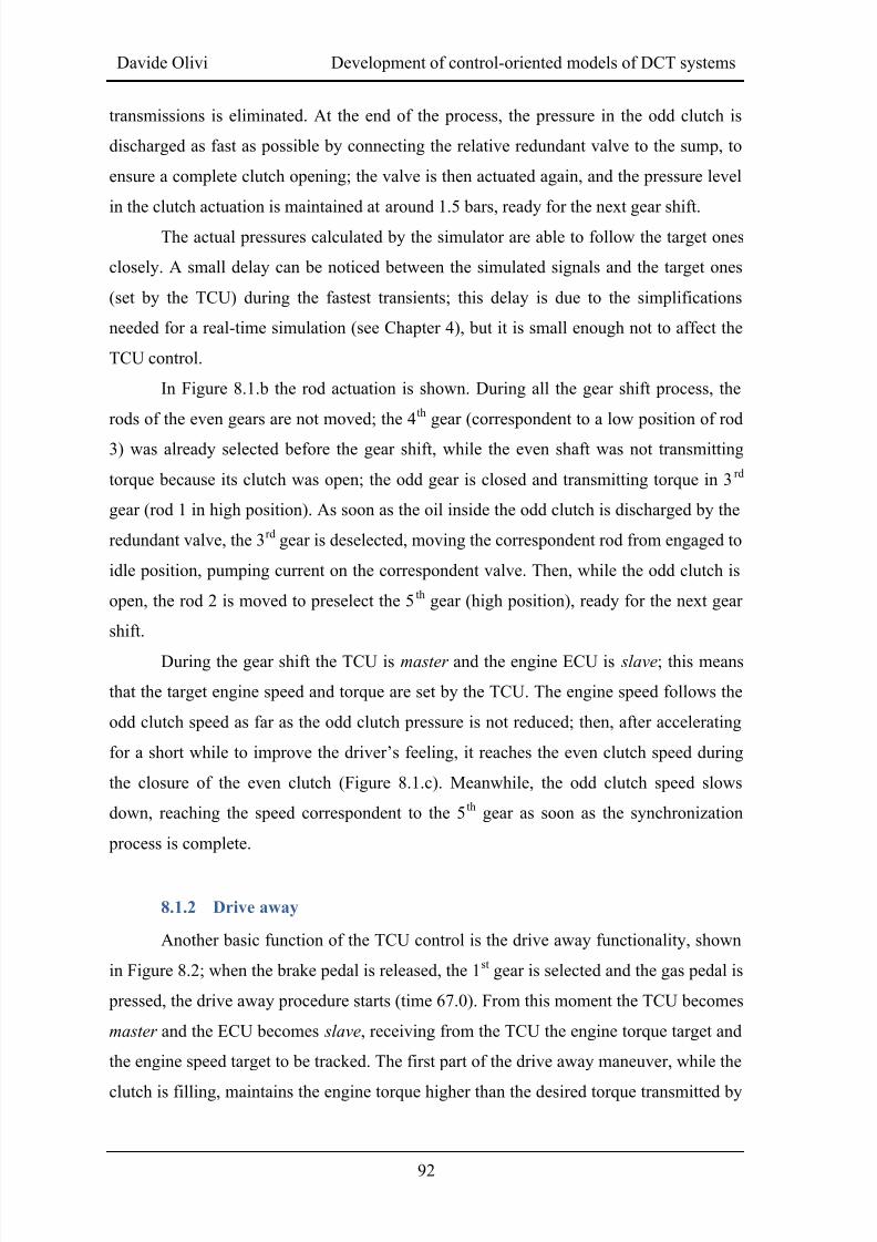
8/20/2019 Olivi Davide Tesi
http://slidepdf.com/reader/full/olivi-davide-tesi 102/141
Davide Olivi Development of control-oriented models of DCT systems
92
transmissions is eliminated. At the end of the process, the pressure in the odd clutch is
discharged as fast as possible by connecting the relative redundant valve to the sump, to
ensure a complete clutch opening; the valve is then actuated again, and the pressure level
in the clutch actuation is maintained at around 1.5 bars, ready for the next gear shift.
The actual pressures calculated by the simulator are able to follow the target ones
closely. A small delay can be noticed between the simulated signals and the target ones
(set by the TCU) during the fastest transients; this delay is due to the simplifications
needed for a real-time simulation (see Chapter 4), but it is small enough not to affect the
TCU control.
In Figure 8.1.b the rod actuation is shown. During all the gear shift process, the
rods of the even gears are not moved; the 4th gear (correspondent to a low position of rod
3) was already selected before the gear shift, while the even shaft was not transmitting
torque because its clutch was open; the odd gear is closed and transmitting torque in 3 rd
gear (rod 1 in high position). As soon as the oil inside the odd clutch is discharged by the
redundant valve, the 3rd gear is deselected, moving the correspondent rod from engaged to
idle position, pumping current on the correspondent valve. Then, while the odd clutch is
open, the rod 2 is moved to preselect the 5 th gear (high position), ready for the next gear
shift.
During the gear shift the TCU is master and the engine ECU is slave; this means
that the target engine speed and torque are set by the TCU. The engine speed follows the
odd clutch speed as far as the odd clutch pressure is not reduced; then, after accelerating
for a short while to improve the driver’s feeling, it reaches the even clutch speed during
the closure of the even clutch (Figure 8.1.c). Meanwhile, the odd clutch speed slows
down, reaching the speed correspondent to the 5th gear as soon as the synchronization
process is complete.
8.1.2 Drive away
Another basic function of the TCU control is the drive away functionality, shown
in Figure 8.2; when the brake pedal is released, the 1st gear is selected and the gas pedal is
pressed, the drive away procedure starts (time 67.0). From this moment the TCU becomes
master and the ECU becomes slave, receiving from the TCU the engine torque target and
the engine speed target to be tracked. The first part of the drive away maneuver, while the
clutch is filling, maintains the engine torque higher than the desired torque transmitted by
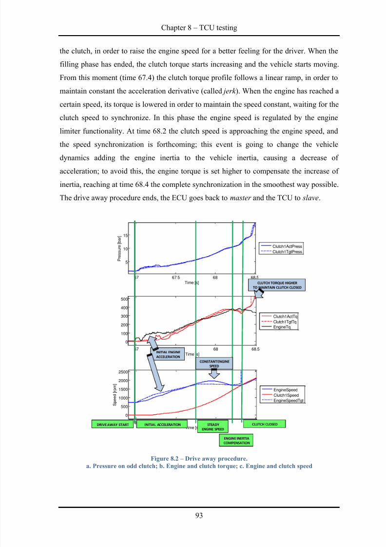
8/20/2019 Olivi Davide Tesi
http://slidepdf.com/reader/full/olivi-davide-tesi 103/141
Chapter 8 – TCU testing
93
the clutch, in order to raise the engine speed for a better feeling for the driver. When the
filling phase has ended, the clutch torque starts increasing and the vehicle starts moving.
From this moment (time 67.4) the clutch torque profile follows a linear ramp, in order to
maintain constant the acceleration derivative (called jerk ). When the engine has reached a
certain speed, its torque is lowered in order to maintain the speed constant, waiting for the
clutch speed to synchronize. In this phase the engine speed is regulated by the engine
limiter functionality. At time 68.2 the clutch speed is approaching the engine speed, and
the speed synchronization is forthcoming; this event is going to change the vehicle
dynamics adding the engine inertia to the vehicle inertia, causing a decrease of
acceleration; to avoid this, the engine torque is set higher to compensate the increase of
inertia, reaching at time 68.4 the complete synchronization in the smoothest way possible.
The drive away procedure ends, the ECU goes back to master and the TCU to slave.
Figure 8.2 – Drive away procedure.
a. Pressure on odd clutch; b. Engine and clutch torque; c. Engine and clutch speed
67 67.5 68 68.5
5
10
15
Time [s]
Pressure[bar]
67 67.5 68 68.5
0
100
200
300
400
500
Time [s]
67 67.5 68 68.5
0
500
1000
1500
2000
2500
Time [s]
Speed[rpm]
EngineSpeed
Clutch1Speed
EngineSpeedTgt
Clutch1ActPress
Clutch1TgtPress
Clutch1ActTq
Clutch1TgtTq
EngineTq
INITIAL ACCELERATION STEADY
ENGINE SPEED
CLUTCH CLOSEDDRIVE AWAY START
INITIAL ENGINE
ACCELERATION
CONSTANT ENGINE
SPEED
CLUTCH TORQUE HIGHER
TO MAINTAIN CLUTCH CLOSED
ENGINE INERTIA
COMPENSATION
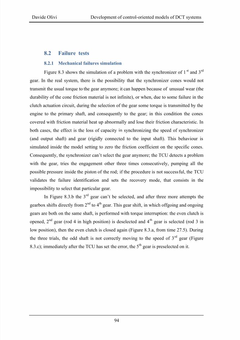
8/20/2019 Olivi Davide Tesi
http://slidepdf.com/reader/full/olivi-davide-tesi 104/141
Davide Olivi Development of control-oriented models of DCT systems
94
8.2 Failure tests
8.2.1 Mechanical failures simulation
Figure 8.3 shows the simulation of a problem with the synchronizer of 1 st and 3rd
gear. In the real system, there is the possibility that the synchronizer cones would not
transmit the usual torque to the gear anymore; it can happen because of unusual wear (the
durability of the cone friction material is not infinite), or when, due to some failure in the
clutch actuation circuit, during the selection of the gear some torque is transmitted by the
engine to the primary shaft, and consequently to the gear; in this condition the cones
covered with friction material heat up abnormally and lose their friction characteristic. In
both cases, the effect is the loss of capacity in synchronizing the speed of synchronizer
(and output shaft) and gear (rigidly connected to the input shaft). This behaviour is
simulated inside the model setting to zero the friction coefficient on the specific cones.
Consequently, the synchronizer can’t select the gear anymore; the TCU detects a problem
with the gear, tries the engagement other three times consecutively, pumping all the
possible pressure inside the piston of the rod; if the procedure is not successful, the TCU
validates the failure identification and sets the recovery mode, that consists in the
impossibility to select that particular gear.
In Figure 8.3.b the 3rd gear can’t be selected, and after three more attempts the
gearbox shifts directly from 2nd to 4th gear. This gear shift, in which offgoing and ongoing
gears are both on the same shaft, is performed with torque interruption: the even clutch is
opened, 2nd gear (rod 4 in high position) is deselected and 4 th gear is selected (rod 3 in
low position), then the even clutch is closed again (Figure 8.3.a, from time 27.5). During
the three trials, the odd shaft is not correctly moving to the speed of 3rd
gear (Figure
8.3.c); immediately after the TCU has set the error, the 5th gear is preselected on it.
8/20/2019 Olivi Davide Tesi
http://slidepdf.com/reader/full/olivi-davide-tesi 105/141
Chapter 8 – TCU testing
95
Figure 8.3 – Failure synchronizing 3rd
gear.
a. Clutch pressures; b. Rod positions; c. Engine and transmission shafts speeds
8.2.2 Hydraulic failures simulation
Figure 8.4 shows a failure due to an anomalous pressure drop in the odd clutch
actuation: it can be caused by an augmented leakage flow from the actuation chamber to
the sump, due to a broken hydraulic seal in the clutch actuation piston, or because the
pressure regulation valves, the proportional one or the redundant one, are stuck and their
spools can’t move properly anymore when actuated with a certain current; all these kinds
of failures can be simulated in the model.
Before the failure injection, a gear shift from 2nd to 3rd gear is performed, and the
odd clutch is being closed, reaching the engine speed. When the failure is inserted in thesystem, the pressure level drops and the clutch can’t transmit to the wheels all the torque
19 20 21 22 23 24 25 26 27 28-2
0
2
4
6
8
10
Clutch Actuation - 3rd gear can't synchronize
Press
ure[bar]
19 20 21 22 23 24 25 26 27 28
0
5
10
15
20
Rod actuation - 3rd gear can't synchronize
Posit
ion[mm]
19 20 21 22 23 24 25 26 27 28-2000
-1000
0
1000
2000
3000
4000
Shaft speeds - 3rd gear can't synchronize
Time [s]
Spe
ed[rpm]
Clutch1Pressure
Clutch1TgtPressure
Clutch2Pressure
Clutch2TgtPressureGear
Error Detection
Rod1Pos
Rod1TgtPos
Rod2Pos
Rod2TgtPos
Rod3Pos
Rod3TgtPos
Rod4Pos
Rod4TgtPos
RodCurrentA
RodCurrentB
EngineSpeed
Clutch1Speed
Clutch2Speed
OutputSpeed
A B C
1
2R
4
5
NO ERROR
ERROR PRESENT
EVEN GEARS
CLUTCH SHIFT
SYNCHRONIZATION
NOT SUCCESSFUL
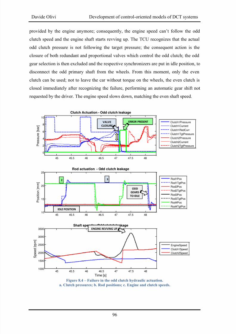
8/20/2019 Olivi Davide Tesi
http://slidepdf.com/reader/full/olivi-davide-tesi 106/141
Davide Olivi Development of control-oriented models of DCT systems
96
provided by the engine anymore; consequently, the engine speed can’t follow the odd
clutch speed and the engine shaft starts revving up. The TCU recognizes that the actual
odd clutch pressure is not following the target pressure; the consequent action is the
closure of both redundant and proportional valves which control the odd clutch; the odd
gear selection is then excluded and the respective synchronizers are put in idle position, to
disconnect the odd primary shaft from the wheels. From this moment, only the even
clutch can be used; not to leave the car without torque on the wheels, the even clutch is
closed immediately after recognizing the failure, performing an automatic gear shift not
requested by the driver. The engine speed slows down, matching the even shaft speed.
Figure 8.4 – Failure in the odd clutch hydraulic actuation.
a. Clutch pressures; b. Rod positions; c. Engine and clutch speeds.
45 45.5 46 46.5 47 47.5 48
0
2
4
6
8
10
Clutch Actuation - Odd clutch leakage
Pressure[bar]
45 45.5 46 46.5 47 47.5 4810
15
20
25
Rod actuation - Odd clutch leakage
Position[mm]
45 45.5 46 46.5 47 47.5 481000
1500
2000
2500
3000
3500
Shaft speeds - Odd clutch leakage
Time [s]
Speed[rpm]
Clutch1Pressure
Clutch1Current
Clutch1RedCurr
Clutch1TgtPressure
Clutch2Pressure
Clutch2Current
Clutch2TgtPressure
Rod1Pos
Rod1TgtPos
Rod2Pos
Rod2TgtPos
Rod3Pos
Rod3TgtPos
Rod4Pos
Rod4TgtPos
EngineSpeed
Clutch1Speed
Clutch2Speed
ERROR PRESENT
2 3
IDLE POSITION
ODD
GEARS
TO IDLE
ENGINE REVVING UP
VALVE
CLOSURE
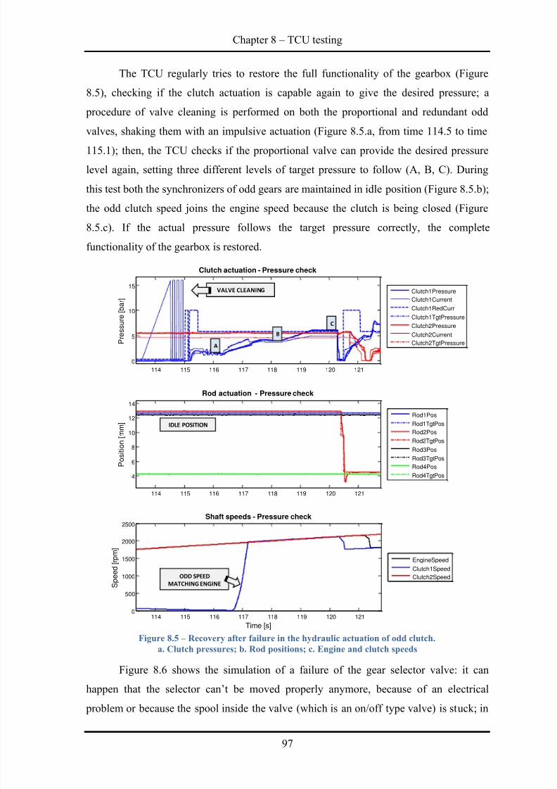
8/20/2019 Olivi Davide Tesi
http://slidepdf.com/reader/full/olivi-davide-tesi 107/141
Chapter 8 – TCU testing
97
The TCU regularly tries to restore the full functionality of the gearbox (Figure
8.5), checking if the clutch actuation is capable again to give the desired pressure; a
procedure of valve cleaning is performed on both the proportional and redundant odd
valves, shaking them with an impulsive actuation (Figure 8.5.a, from time 114.5 to time
115.1); then, the TCU checks if the proportional valve can provide the desired pressure
level again, setting three different levels of target pressure to follow (A, B, C). During
this test both the synchronizers of odd gears are maintained in idle position (Figure 8.5.b);
the odd clutch speed joins the engine speed because the clutch is being closed (Figure
8.5.c). If the actual pressure follows the target pressure correctly, the complete
functionality of the gearbox is restored.
Figure 8.5 – Recovery after failure in the hydraulic actuation of odd clutch.
a. Clutch pressures; b. Rod positions; c. Engine and clutch speeds
Figure 8.6 shows the simulation of a failure of the gear selector valve: it can
happen that the selector can’t be moved properly anymore, because of an electrical
problem or because the spool inside the valve (which is an on/off type valve) is stuck; in
114 115 116 117 118 119 120 121
0
5
10
15
Clutch actuation - Pressure check
Pressure[bar]
114 115 116 117 118 119 120 121
4
6
8
10
12
14
Rod actuation - Pressure check
Position[mm]
114 115 116 117 118 119 120 1210
500
1000
1500
2000
2500
Shaft speeds - Pressure check
Time [s]
Speed[rpm]
Clutch1Pressure
Clutch1Current
Clutch1RedCurr
Clutch1TgtPressure
Clutch2Pressure
Clutch2Current
Clutch2TgtPressure
Rod1PosRod1TgtPos
Rod2Pos
Rod2TgtPos
Rod3Pos
Rod3TgtPos
Rod4Pos
Rod4TgtPos
EngineSpeed
Clutch1Speed
Clutch2Speed
VALVE CLEANING
IDLE POSITION
ODD SPEED
MATCHING ENGINE
A
B
C
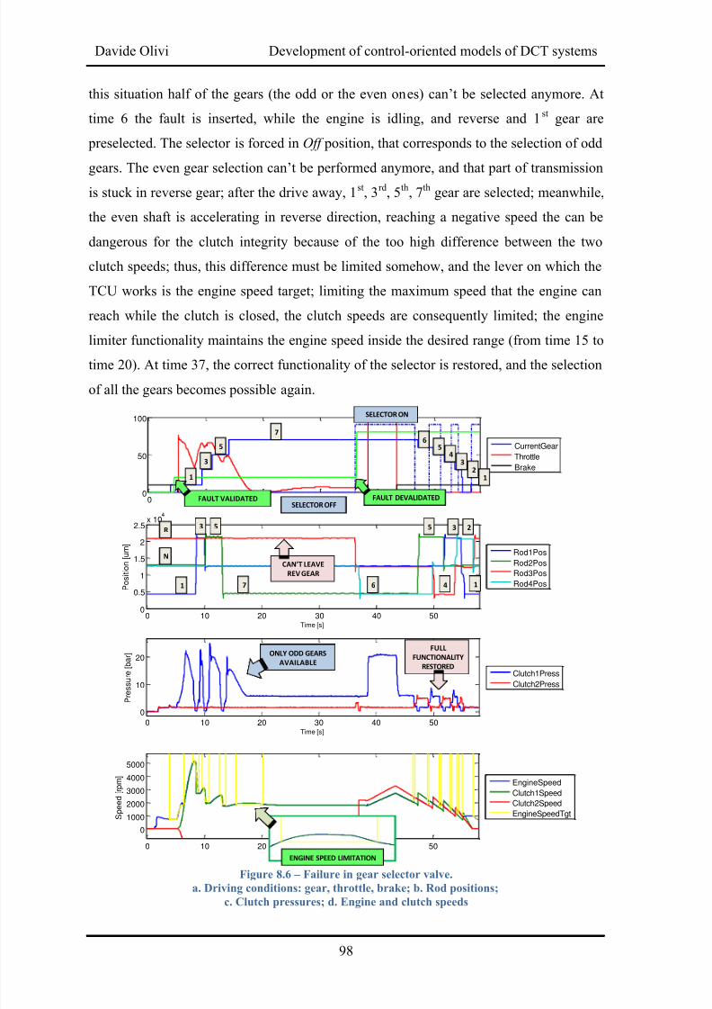
8/20/2019 Olivi Davide Tesi
http://slidepdf.com/reader/full/olivi-davide-tesi 108/141
Davide Olivi Development of control-oriented models of DCT systems
98
this situation half of the gears (the odd or the even ones) can’t be selected anymore. At
time 6 the fault is inserted, while the engine is idling, and reverse and 1 st gear are
preselected. The selector is forced in Off position, that corresponds to the selection of odd
gears. The even gear selection can’t be performed anymore, and that part of transmission
is stuck in reverse gear; after the drive away, 1 st, 3rd, 5th, 7th gear are selected; meanwhile,
the even shaft is accelerating in reverse direction, reaching a negative speed the can be
dangerous for the clutch integrity because of the too high difference between the two
clutch speeds; thus, this difference must be limited somehow, and the lever on which the
TCU works is the engine speed target; limiting the maximum speed that the engine can
reach while the clutch is closed, the clutch speeds are consequently limited; the engine
limiter functionality maintains the engine speed inside the desired range (from time 15 to
time 20). At time 37, the correct functionality of the selector is restored, and the selection
of all the gears becomes possible again.
Figure 8.6 – Failure in gear selector valve.
a. Driving conditions: gear, throttle, brake; b. Rod positions;
c. Clutch pressures; d. Engine and clutch speeds
0 10 20 30 40 500
50
100
Time [s]
0 10 20 30 40 500
0.5
1
1.5
2
2.5x 10
4
Time [s]
Position[um]
0 10 20 30 40 50
0
10
20
Time [s]
Pressure[bar]
0 10 20 30 40 50
0
1000
2000
3000
4000
5000
i
Speed[rpm]
EngineSpeed
Clutch1Speed
Clutch2Speed
EngineSpeedTgt
Clutch1Press
Clutch2Press
CurrentGear
Throttle
Brake
Rod1Pos
Rod2Pos
Rod3Pos
Rod4Pos
1
3
5
7
6
5
4
3
2
1
FAULT VALIDATED FAULT DEVALIDATED
1
3
R
5
7 6
N
5
4
3 2
1
CAN’T LEAVE
REV GEAR
ONLY ODD GEARS
AVAILABLE
FULL
FUNCTIONALITY
RESTORED
SELECTOR OFF
SELECTOR ON
.
.
.
ENGINE SPEED LIMITATION
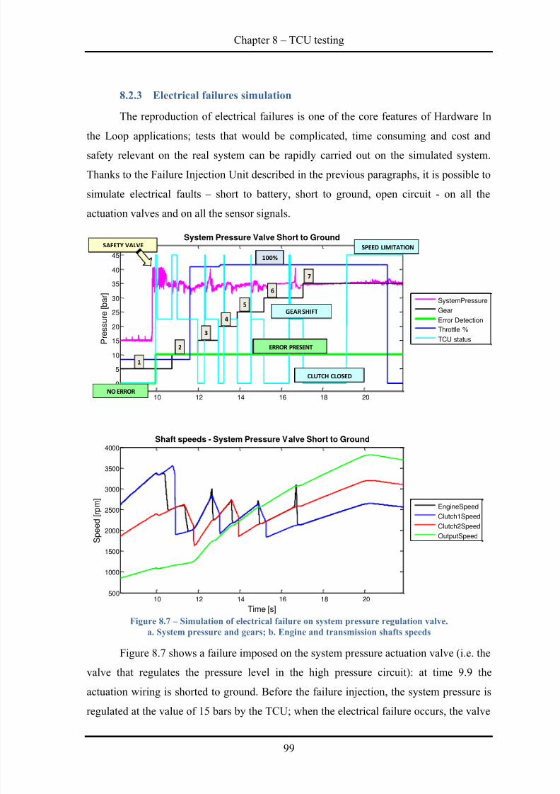
8/20/2019 Olivi Davide Tesi
http://slidepdf.com/reader/full/olivi-davide-tesi 109/141
Chapter 8 – TCU testing
99
8.2.3 Electrical failures simulation
The reproduction of electrical failures is one of the core features of Hardware In
the Loop applications; tests that would be complicated, time consuming and cost andsafety relevant on the real system can be rapidly carried out on the simulated system.
Thanks to the Failure Injection Unit described in the previous paragraphs, it is possible to
simulate electrical faults – short to battery, short to ground, open circuit - on all the
actuation valves and on all the sensor signals.
Figure 8.7 – Simulation of electrical failure on system pressure regulation valve.
a. System pressure and gears; b. Engine and transmission shafts speeds
Figure 8.7 shows a failure imposed on the system pressure actuation valve (i.e. the
valve that regulates the pressure level in the high pressure circuit): at time 9.9 the
actuation wiring is shorted to ground. Before the failure injection, the system pressure isregulated at the value of 15 bars by the TCU; when the electrical failure occurs, the valve
10 12 14 16 18 20
0
5
10
15
20
25
30
35
40
45
System Pressure Valve Short to Ground
Pressure[bar]
10 12 14 16 18 20500
1000
1500
2000
2500
3000
3500
4000
Shaft speeds - System Pressure Valve Short to Ground
Time [s]
Speed[rpm]
SystemPressure
Gear
Error Detection
Throttle %
TCU status
EngineSpeed
Clutch1Speed
Clutch2Speed
OutputSpeed
SAFETY VALVE
NO ERROR
ERROR PRESENT
CLUTCH CLOSED
GEAR SHIFT
SPEED LIMITATION
3
4
5
6
7
2
1
100%
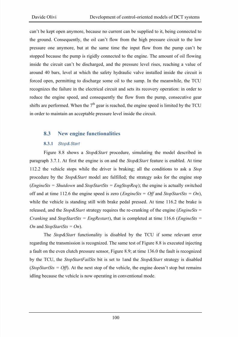
8/20/2019 Olivi Davide Tesi
http://slidepdf.com/reader/full/olivi-davide-tesi 110/141
Davide Olivi Development of control-oriented models of DCT systems
100
can’t be kept open anymore, because no current can be supplied to it, being connected to
the ground. Consequently, the oil can’t flow from the high pressure circuit to the low
pressure one anymore, but at the same time the input flow from the pump can’t be
stopped because the pump is rigidly connected to the engine. The amount of oil flowing
inside the circuit can’t be discharged, and the pressure level rises, reaching a value of
around 40 bars, level at which the safety hydraulic valve installed inside the circuit is
forced open, permitting to discharge some oil to the sump. In the meanwhile, the TCU
recognizes the failure in the electrical circuit and sets its recovery operation: in order to
reduce the engine speed, and consequently the flow from the pump, consecutive gear
shifts are performed. When the 7th gear is reached, the engine speed is limited by the TCU
in order to maintain an acceptable pressure level inside the circuit.
8.3 New engine functionalities
8.3.1 Stop&Start
Figure 8.8 shows a Stop&Start procedure, simulating the model described in
paragraph 3.7.1. At first the engine is on and the Stop&Start feature is enabled. At time
112.2 the vehicle stops while the driver is braking; all the conditions to ask a Stop
procedure by the Stop&Start model are fulfilled; the strategy asks for the engine stop
( EngineSts = Shutdown and StopStartSts = EngStopReq); the engine is actually switched
off and at time 112.6 the engine speed is zero ( EngineSts = Off and StopStartSts = On),
while the vehicle is standing still with brake pedal pressed. At time 116.2 the brake is
released, and the Stop&Start strategy requires the re-cranking of the engine ( EngineSts =
Cranking and StopStartSts = EngRestart ), that is completed at time 116.6 ( EngineSts =
On and StopStartSts = On).
The Stop&Start functionality is disabled by the TCU if some relevant errorregarding the transmission is recognized. The same test of Figure 8.8 is executed injecting
a fault on the even clutch pressure sensor, Figure 8.9; at time 136.0 the fault is recognized
by the TCU, the StopStartFailSts bit is set to 1and the Stop&Start strategy is disabled
(StopStartSts = Off ). At the next stop of the vehicle, the engine doesn’t stop but remains
idling because the vehicle is now operating in conventional mode.
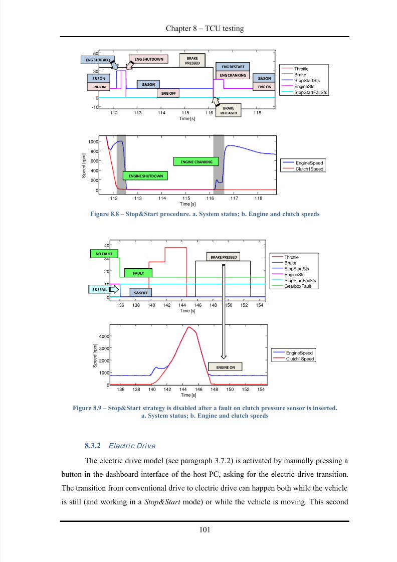
8/20/2019 Olivi Davide Tesi
http://slidepdf.com/reader/full/olivi-davide-tesi 111/141
Chapter 8 – TCU testing
101
Figure 8.8 – Stop&Start procedure. a. System status; b. Engine and clutch speeds
Figure 8.9 – Stop&Start strategy is disabled after a fault on clutch pressure sensor is inserted.
a. System status; b. Engine and clutch speeds
8.3.2 Electri c Dri ve
The electric drive model (see paragraph 3.7.2) is activated by manually pressing a
button in the dashboard interface of the host PC, asking for the electric drive transition.
The transition from conventional drive to electric drive can happen both while the vehicle
is still (and working in a Stop&Start mode) or while the vehicle is moving. This second
112 113 114 115 116 117 118
-10
0
10
20
30
40
50
Time [s]
112 113 114 115 116 117 118
0
200
400
600
800
1000
Time [s]
Speed[rpm]
EngineSpeed
Clutch1Speed
Throttle
Brake
StopStartSts
EngineSts
StopStartFailStsENG ON
S&SON
ENG STOP REQ ENG SHUTDOWN
ENG OFF
S&SON
ENG RESTART
ENG CRANKING
ENG ON
S&SON
BRAKE
PRESSED
BRAKE
RELEASED
ENGINE SHUTDOWN
ENGINE CRANKING
136 138 140 142 144 146 148 150 152 154
0
10
20
30
40
Time [s]
136 138 140 142 144 146 148 150 152 1540
1000
2000
3000
4000
Time [s]
Speed[rpm]
EngineSpeed
Clutch1Speed
Throttle
Brake
StopStartSts
EngineSts
StopStartFailSts
GearboxFault
NO FAULT
FAULT
S&SOFFS&SFAIL
BRAKE PRESSED
ENGINE ON
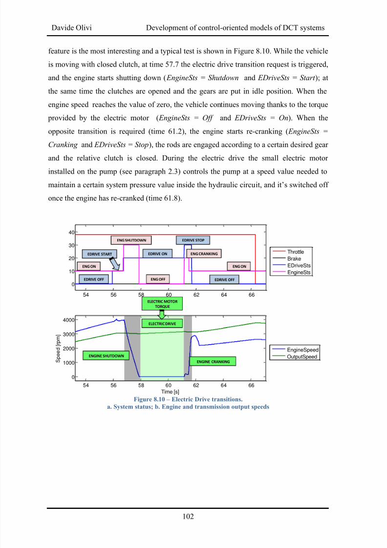
8/20/2019 Olivi Davide Tesi
http://slidepdf.com/reader/full/olivi-davide-tesi 112/141
Davide Olivi Development of control-oriented models of DCT systems
102
feature is the most interesting and a typical test is shown in Figure 8.10. While the vehicle
is moving with closed clutch, at time 57.7 the electric drive transition request is triggered,
and the engine starts shutting down ( EngineSts = Shutdown and EDriveSts = Start ); at
the same time the clutches are opened and the gears are put in idle position. When the
engine speed reaches the value of zero, the vehicle continues moving thanks to the torque
provided by the electric motor ( EngineSts = Off and EDriveSts = On). When the
opposite transition is required (time 61.2), the engine starts re-cranking ( EngineSts =
Cranking and EDriveSts = Stop), the rods are engaged according to a certain desired gear
and the relative clutch is closed. During the electric drive the small electric motor
installed on the pump (see paragraph 2.3) controls the pump at a speed value needed to
maintain a certain system pressure value inside the hydraulic circu it, and it’s switched off
once the engine has re-cranked (time 61.8).
Figure 8.10 – Electric Drive transitions.
a. System status; b. Engine and transmission output speeds
54 56 58 60 62 64 66
0
10
20
30
40
Time [s]
54 56 58 60 62 64 66
0
1000
2000
3000
4000
Time [s]
Speed[rpm]
EngineSpeed
OutputSpeed
Throttle
Brake
EDriveSts
EngineSts
ENG ON
ENG SHUTDOWN
ENG OFF
ENG CRANKING
ENG ON
EDRIVE OFF
EDRIVE START EDRIVE ON
EDRIVE STOP
EDRIVE OFF
ENGINE SHUTDOWN
ENGINE CRANKING
ELECTRIC MOTOR
TORQUE
ELECTRIC DRIVE

8/20/2019 Olivi Davide Tesi
http://slidepdf.com/reader/full/olivi-davide-tesi 113/141
Chapter 8 – TCU testing
103
8.4 Adaption procedures
To perform a precise and comfortable control of the transmission, every TCU
must be adapted to the gearbox it is connected to; that’s why some end of line calibrations
of the TCU are needed after coupling a TCU to a specific gearbox. The adaption
procedures comprehend rod calibration, clutch preload and kiss point detection, clutch
filling procedure, and detection of the solenoid characteristic of proportional clutch
pressure regulation valves. These procedures are regularly performed by the TCU during
its lifetime: the adaptive values can change from the ones identified with a new gearbox,
because of many factors, such as wear, flexion of mechanical parts, augmented leakage in
the hydraulic circuit, and change in oil properties. In the HIL application, the
characteristic of the components inside the model can be changed as desired; it is then
possible to check the capability of the TCU to perform these procedures and to correctly
adapt to the new settings, updating its calibrations to new values.
8.4.1 Rod calibration
Figure 8.11.a shows the adaption procedure on rod number 2. The calibration of a
rod consists in moving the synchronizer from its idle position, forcing it to engage both of
the gears it controls, and checking the 5 characteristic steady-state positions of the rod:
N: idle position;
A2, B2: gear engaged with pressure acting on the synchronizer, on each of the two
gears;
A1, B1: engaged gear without pressure on the synchronizer, on each of the two
gears.
The procedure is performed three times per gear and the mean values of the 3 trials are
memorized in the TCU as the adapted positions. During the gearbox lifetime, the TCU
recognizes a failure in the synchronizer actuation when the position measured from the
sensor doesn’t match the expected one registered during the online self-calibration. The
simulation results show a good capability of the TCU to adapt to the values set in the
model; Figure 8.11.b shows the original values memorized inside the TCU (on the left),
and the new values registered by the TCU during the adaption procedure (on the right).
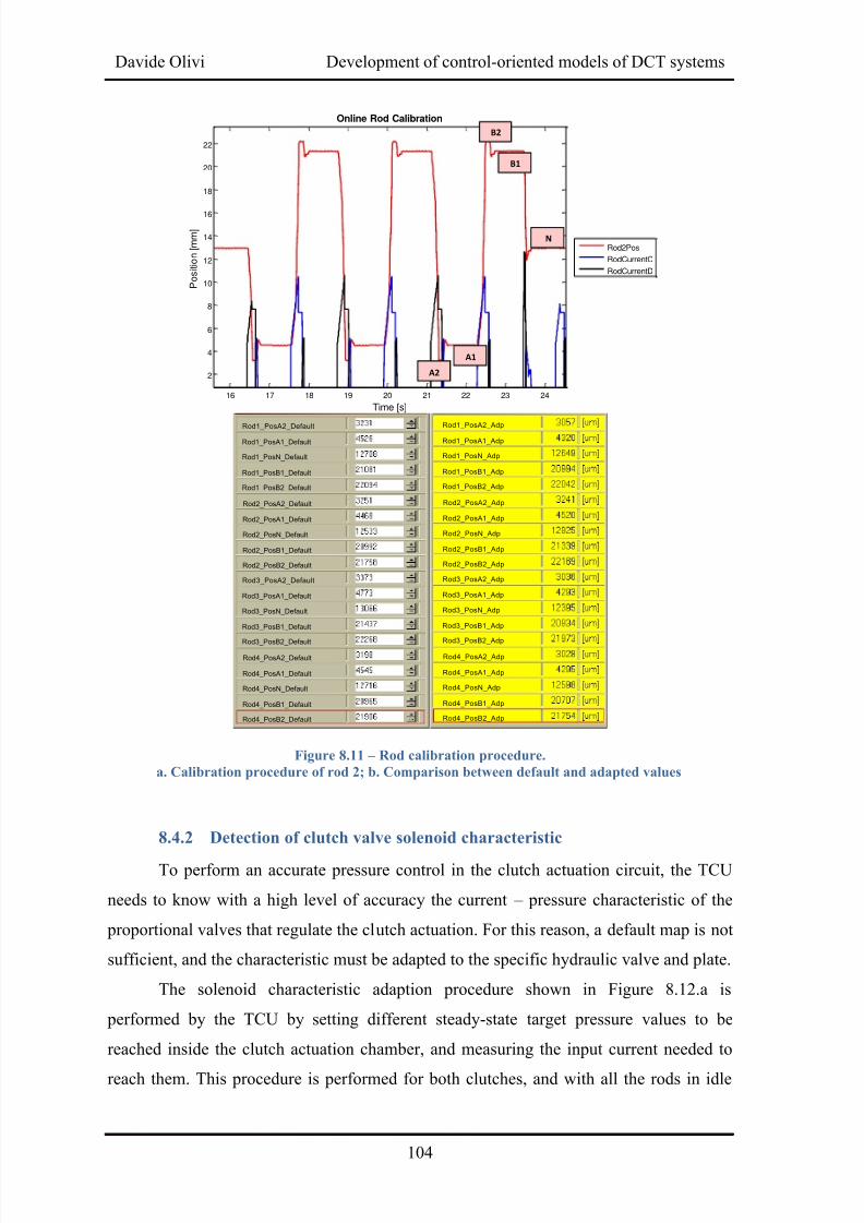
8/20/2019 Olivi Davide Tesi
http://slidepdf.com/reader/full/olivi-davide-tesi 114/141
Davide Olivi Development of control-oriented models of DCT systems
104
Figure 8.11 – Rod calibration procedure.
a. Calibration procedure of rod 2; b. Comparison between default and adapted values
8.4.2 Detection of clutch valve solenoid characteristic
To perform an accurate pressure control in the clutch actuation circuit, the TCU
needs to know with a high level of accuracy the current – pressure characteristic of the
proportional valves that regulate the clutch actuation. For this reason, a default map is not
sufficient, and the characteristic must be adapted to the specific hydraulic valve and plate.
The solenoid characteristic adaption procedure shown in Figure 8.12.a is
performed by the TCU by setting different steady-state target pressure values to be
reached inside the clutch actuation chamber, and measuring the input current needed to
reach them. This procedure is performed for both clutches, and with all the rods in idle
16 17 18 19 20 21 22 23 24
2
4
6
8
10
12
14
16
18
20
22
Online Rod Calibration
Time [s]
Position[mm]
Rod2Pos
RodCurrentC
RodCurrentD
B1
B2
A1
A2
N
Rod1_PosA2_Default
Rod1_PosA1_Default
Rod1_PosN_Default
Rod1_PosB1_Default
Rod1_PosB2_Default
Rod2_PosA2_Default
Rod2_PosA1_Default
Rod2_PosN_Default
Rod2_PosB1_Default
Rod2_PosB2_Default
Rod3_PosA2_Default
Rod3_PosA1_Default
Rod3_PosN_Default
Rod3_PosB1_Default
Rod3_PosB2_Default
Rod4_PosA2_Default
Rod4_PosA1_Default
Rod4_PosN_Default
Rod4_PosB1_Default
Rod4_PosB2_Default
Rod1_PosA2_Adp
Rod1_PosA1_Adp
Rod1_PosN_Adp
Rod1_PosB1_Adp
Rod1_PosB2_Adp
Rod2_PosA2_Adp
Rod2_PosA1_Adp
Rod2_PosN_Adp
Rod2_PosB1_Adp
Rod2_PosB2_Adp
Rod3_PosA2_Adp
Rod3_PosA1_Adp
Rod3_PosN_Adp
Rod3_PosB1_Adp
Rod3_PosB2_Adp
Rod4_PosA2_Adp
Rod4_PosA1_Adp
Rod4_PosN_Adp
Rod4_PosB1_Adp
Rod4_PosB2_Adp
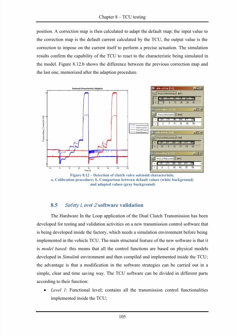
8/20/2019 Olivi Davide Tesi
http://slidepdf.com/reader/full/olivi-davide-tesi 115/141
Chapter 8 – TCU testing
105
position. A correction map is then calculated to adapt the default map; the input value to
the correction map is the default current calculated by the TCU, the output value is the
correction to impose on the current itself to perform a precise actuation. The simulation
results confirm the capability of the TCU to react to the characteristic being simulated in
the model. Figure 8.12.b shows the difference between the previous correction map and
the last one, memorized after the adaption procedure.
Figure 8.12 –
Detection of clutch valve solenoid characteristic.a. Calibration procedure; b. Comparison between default values (white background)
and adapted values (gray background)
8.5 Safety Level 2 software validation
The Hardware In the Loop application of the Dual Clutch Transmission has been
developed for testing and validation activities on a new transmission control software that
is being developed inside the factory, which needs a simulation environment before being
implemented in the vehicle TCU. The main structural feature of the new software is that it
is model based : this means that all the control functions are based on physical models
developed in Simulink environment and then compiled and implemented inside the TCU;
the advantage is that a modification in the software strategies can be carried out in a
simple, clear and time saving way. The TCU software can be divided in different parts
according to their function:
Level 1: Functional level; contains all the transmission control functionalities
implemented inside the TCU;
65 70 75 80 85 90 95 100 105
0
5
10
15
Soelnoid Characteristic Adaption
Time [s]
Pressure[bar],Current[A/100]
Clutch1Pressure
Clutch1Current
Clutch2Pressure
Clutch2Current
PrsCurOffsOddDef
PrsCurOffsOddAdp
PrsCurOffsEvenAdp
PrsCurOffsEvenDef
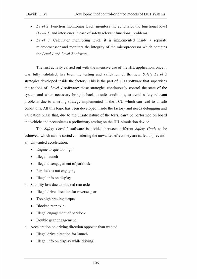
8/20/2019 Olivi Davide Tesi
http://slidepdf.com/reader/full/olivi-davide-tesi 116/141
Davide Olivi Development of control-oriented models of DCT systems
106
Level 2: Function monitoring level; monitors the actions of the functional level
( Level 1) and intervenes in case of safety relevant functional problems;
Level 3: Calculator monitoring level; it is implemented inside a separate
microprocessor and monitors the integrity of the microprocessor which containsthe Level 1 and Level 2 software.
The first activity carried out with the intensive use of the HIL application, once it
was fully validated, has been the testing and validation of the new Safety Level 2
strategies developed inside the factory. This is the part of TCU software that supervises
the actions of Level 1 software: these strategies continuously control the state of the
system and when necessary bring it back to safe conditions, to avoid safety relevant
problems due to a wrong strategy implemented in the TCU which can lead to unsafe
conditions. All this logic has been developed inside the factory and needs debugging and
validation phase that, due to the unsafe nature of the tests, can’t be perfor med on board
the vehicle and necessitates a preliminary testing on the HIL simulation device.
The Safety Level 2 software is divided between different Safety Goals to be
achieved, which can be sorted considering the unwanted effect they are called to prevent:
a. Unwanted acceleration:
Engine torque too high
Illegal launch
Illegal disengagement of parklock
Parklock is not engaging
Illegal info on display.
b. Stability loss due to blocked rear axle
Illegal drive direction for reverse gear
Too high braking torque
Blocked rear axle
Illegal engagement of parklock
Double gear engagement.
c. Acceleration on driving direction opposite than wanted
Illegal drive direction for launch
Illegal info on display while driving.
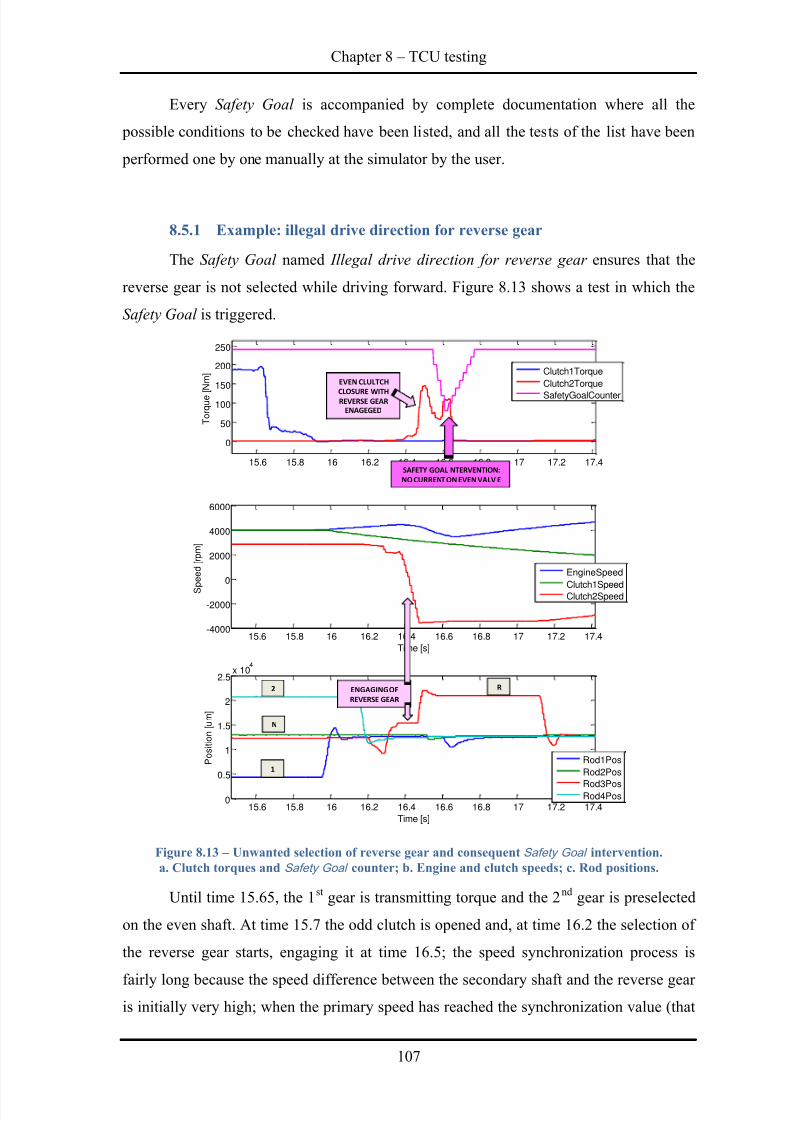
8/20/2019 Olivi Davide Tesi
http://slidepdf.com/reader/full/olivi-davide-tesi 117/141
Chapter 8 – TCU testing
107
Every Safety Goal is accompanied by complete documentation where all the
possible conditions to be checked have been listed, and all the tests of the list have been
performed one by one manually at the simulator by the user.
8.5.1 Example: illegal drive direction for reverse gear
The Safety Goal named Illegal drive direction for reverse gear ensures that the
reverse gear is not selected while driving forward. Figure 8.13 shows a test in which the
Safety Goal is triggered.
Figure 8.13 – Unwanted selection of reverse gear and consequent Safety Goal intervention.
a. Clutch torques and Safety Goal counter; b. Engine and clutch speeds; c. Rod positions.
Until time 15.65, the 1st gear is transmitting torque and the 2nd gear is preselected
on the even shaft. At time 15.7 the odd clutch is opened and, at time 16.2 the selection of
the reverse gear starts, engaging it at time 16.5; the speed synchronization process is
fairly long because the speed difference between the secondary shaft and the reverse gear
is initially very high; when the primary speed has reached the synchronization value (that
15.6 15.8 16 16.2 16.4 16.6 16.8 17 17.2 17.4
0
50
100
150
200
250
Time [s]
Torque[Nm]
15.6 15.8 16 16.2 16.4 16.6 16.8 17 17.2 17.4-4000
-2000
0
2000
4000
6000
Time [s]
Speed[rpm]
15.6 15.8 16 16.2 16.4 16.6 16.8 17 17.2 17.40
0.5
1
1.5
2
2.5x 10
4
Time [s]
Position[um]
EngineSpeed
Clutch1SpeedClutch2Speed
Clutch1Torque
Clutch2Torque
SafetyGoalCounter
Rod1Pos
Rod2Pos
Rod3PosRod4Pos
ENGAGING OF
REVERSE GEAR
EVEN CLULTCH
CLOSURE WITHREVERSE GEAR
ENAGEGED
SAFETY GOAL NTERVENTION:
NO CURRENT ON EVEN VALV E
1
2
N
R
8/20/2019 Olivi Davide Tesi
http://slidepdf.com/reader/full/olivi-davide-tesi 118/141
Davide Olivi Development of control-oriented models of DCT systems
108
is negative), the TCU triggers the closure of the even clutch, pumping current on the
relative valve and thus raising the pressure on the clutch actuation and the relative
transmitted torque. The engine speed starts decreasing because of this torque, trying to
match the speed of the even clutch. As soon as the Safety Level 2 software recognizes that
the filling phase (i.e. the phase in which the clutch is being filled with oil bringing it to
the kiss point) has ended, around time 16.5, the Safety Goal counter starts decreasing,
until it reaches the value for which the opening of the clutch is forced, at time 16.65. This
intervention prevents the closure of the even clutch on the reverse gear, which could be
very dangerous for the driver and for vehicle stability. After the Safety Goal action, the
engine revs up without transmitting torque, until another gearshift is requested by the
driver. In this test the selection of the reverse gear is forced by manually bypassing the
request of reverse gear inside the TCU software, in order to verify the correct intervention
of the Safety Level 2 control.
8.5.2 Example: illegal launch
The Safety Goal named Illegal launch verifies that the vehicle is not moving from
its still position if not wanted, for example when the neutral position of the transmission
is requested. Figure 8.14 shows an unexpected launch while the car is still, displaying N
(neutral gear) on display. At time 7.4 the driver accelerates in order to rev up the engine,maintaining the vehicle still in its position with open clutches. The TCU, on the contrary,
decides that the driver is asking for a drive away and starts pumping current on the odd
clutch valve, on which the 1st gear is selected. As soon as the torque transmitted to the
wheels starts increasing, the Safety Goal starts decreasing its counter and at time 7.8 the
clutch actuation is disabled forcing the relative currents to zero. The engine starts revving
up without transmitting torque and the system is brought back to safe conditions. From
time 7 to time 7.8 the vehicle has started moving, but after the Safety Level 2 intervention
it slows down, and the max vehicle speed reached is only around 1.4 km/h. Of course
these data about the speed are purely indicative, because the vehicle model is very
simplified and the real case can be slightly different, but the rapid intervention of the
Safety Goal is checked. Also in this case the test is performed bypassing the driver’s
request inside the TCU software.
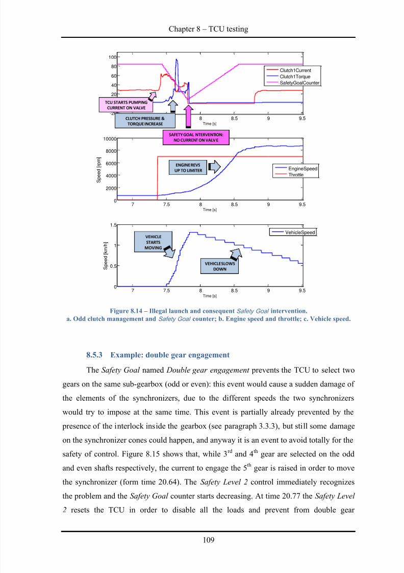
8/20/2019 Olivi Davide Tesi
http://slidepdf.com/reader/full/olivi-davide-tesi 119/141
Chapter 8 – TCU testing
109
Figure 8.14 – Illegal launch and consequent Safety Goal intervention.
a. Odd clutch management and Safety Goal counter; b. Engine speed and throttle; c. Vehicle speed.
8.5.3 Example: double gear engagement
The Safety Goal named Double gear engagement prevents the TCU to select two
gears on the same sub-gearbox (odd or even): this event would cause a sudden damage of
the elements of the synchronizers, due to the different speeds the two synchronizerswould try to impose at the same time. This event is partially already prevented by the
presence of the interlock inside the gearbox (see paragraph 3.3.3), but still some damage
on the synchronizer cones could happen, and anyway it is an event to avoid totally for the
safety of control. Figure 8.15 shows that, while 3rd and 4th gear are selected on the odd
and even shafts respectively, the current to engage the 5th gear is raised in order to move
the synchronizer (form time 20.64). The Safety Level 2 control immediately recognizes
the problem and the Safety Goal counter starts decreasing. At time 20.77 the Safety Level
2 resets the TCU in order to disable all the loads and prevent from double gear
7 7.5 8 8.5 9 9.5-20
0
20
40
60
80
100
Time [s]
7 7.5 8 8.5 9 9.50
2000
4000
6000
8000
10000
Time [s]
Speed[rpm]
7 7.5 8 8.5 9 9.50
0.5
1
1.5
Time [s]
Speed[km/h]
EngineSpeed
Throttle
Clutch1Current
Clutch1Torque
SafetyGoalCounter
VehicleSpeed
TCU STARTS PUMPING
CURRENT ON VALVE
CLUTCH PRESSURE &
TORQUE INCREASE
VEHICLE
STARTS
MOVING
SAFETY GOAL NTERVENTION:
NO CURRENT ON VALVE
ENGINE REVS
UP TO LIMITER
VEHICLE SLOWS
DOWN
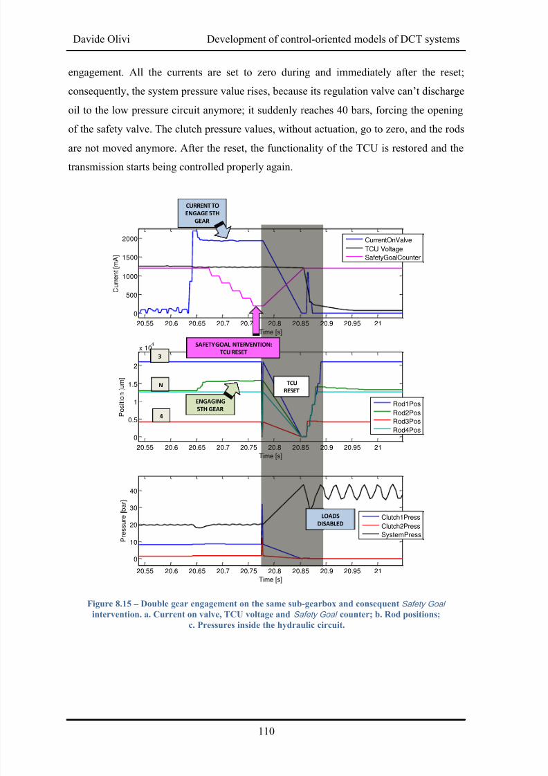
8/20/2019 Olivi Davide Tesi
http://slidepdf.com/reader/full/olivi-davide-tesi 120/141
Davide Olivi Development of control-oriented models of DCT systems
110
engagement. All the currents are set to zero during and immediately after the reset;
consequently, the system pressure value rises, because its regulation valve can’t discharge
oil to the low pressure circuit anymore; it suddenly reaches 40 bars, forcing the opening
of the safety valve. The clutch pressure values, without actuation, go to zero, and the rods
are not moved anymore. After the reset, the functionality of the TCU is restored and the
transmission starts being controlled properly again.
Figure 8.15 – Double gear engagement on the same sub-gearbox and consequent Safety Goal
intervention. a. Current on valve, TCU voltage and Safety Goal counter; b. Rod positions;
c. Pressures inside the hydraulic circuit.
20.55 20.6 20.65 20.7 20.75 20.8 20.85 20.9 20.95 21
0
500
1000
1500
2000
Time [s]
Current
[mA]
20.55 20.6 20.65 20.7 20.75 20.8 20.85 20.9 20.95 21
0
0.5
1
1.5
2
x 104
Time [s]
Pos
ition[um]
20.55 20.6 20.65 20.7 20.75 20.8 20.85 20.9 20.95 21
0
10
20
30
40
Time [s]
Pressure[bar]
Clutch1Press
Clutch2Press
SystemPress
CurrentOnValve
TCU Voltage
SafetyGoalCounter
Rod1Pos
Rod2Pos
Rod3Pos
Rod4Pos
TCU
RESET
CURRENT TO
ENGAGE 5TH
GEAR
ENGAGING
5TH GEAR
N
3
SAFETY GOAL NTERVENTION:
TCU RESET
4
LOADS
DISABLED
8/20/2019 Olivi Davide Tesi
http://slidepdf.com/reader/full/olivi-davide-tesi 121/141
Chapter 9 – Test automation
111
Chapter 9
Test automation
The final aim of a HIL application is to execute automatically a list of tests which
covers all the possible TCU functionalities that have to be checked. Once the pattern of
tests is considered complete, it is possible to validate every new software release in a fully
automatic way.
The main advantage of the automation is the possibility to perform a test, which
remains totally identical, on different applications, repeating it several times; tests can be
performed, that couldn’t be possible in a manual way because of the multiple actions
required at the same time or because of the necessity to space different actions with fixed
time intervals, which can be a few milliseconds. Another advantage is that there is no
need for the interaction of a user while performing the pattern of tests, which can last
several hours or even days.
9.1 On-Board Diagnostics (OBD) and software development tools
On-Board Diagnostics, or OBD, refers to the vehicle's self-diagnostic capability.OBD systems give the vehicle owner or a repair technician access to state of health
information for various vehicle sub-systems. The amount of diagnostic information
available via OBD has varied widely since the introduction in the early 1980s of on-board
vehicle computers, which made OBD possible. Early instances of OBD would simply
illuminate a Malfunction Indicator Light , or MIL, if a problem was detected, but would
not provide any information as to the nature of the problem. Current OBD
implementations, called OBD-II, use a standardized digital communications port to
provide real-time data in addition to a standardized series of Diagnostic Trouble Codes,
8/20/2019 Olivi Davide Tesi
http://slidepdf.com/reader/full/olivi-davide-tesi 122/141
Davide Olivi Development of control-oriented models of DCT systems
112
or DTCs, which allow one to rapidly identify and remedy malfunctions within the
vehicle.
Every electronic control unit inside the vehicle has its own OBD-II system (or
EOBD for the European market), and the TCU is between them. If the TCU recognizes a
problem in the control of the transmission, the relative DTC is published inside the OBD
system, and the Transmission Fault Lamp (TFL) can be illuminated. With an appropriate
tool (OBD interpreter) the DTC can be read and analyzed. The DTCs published by the
TCU are accompanied by a Freeze Frame, i.e. the detailed environmental conditions of
the system at the moment in which the fault is recognized; this helps to recognize the
cause of the fault and the relative actions to take to repair the transmission.
The development of control software of the TCU is helped by the use of INCA
software, which offers flexible tools for the calibration, diagnostics and validation of
automotive electronic systems; it can be used for electronic control units development and
test as well as for validation and calibration of electronically controlled systems in the
vehicle, on the test bench, or in a virtual environment on the PC. In the case of the Dual
Clutch Transmission, it permits to calibrate the transmission control functions, and
display online and measure the variables inside the TCU software, that can be analyzed
offline after the end of the test.
9.2 The automation procedure
Both the OBD tools and the software development tools can support the
automation of tests, which was developed with the coordinated use of different software
packages: Python, INCA, Matlab, Excel .
In Python environment, a code that permits to communicate with the simulator
was developed: it is capable to read and modify the variables of the Simulink model
which has been downloaded inside the simulator. The connection of the OBD interface of
the simulator to an OBD – USB device ( ELM327 ) represents the diagnostic interface of
the system: the Python code reads the information sent by the TCU via the OBD interface
and translates it in readable information. An interface between Python code and INCA
allows opening a INCA experiment, starting, stopping and saving a measurement, and
reading variables and modifying calibrations inside the TCU if necessary. The pattern of
tests is defined in the Python code; when the online procedure ends, i.e. all the tests have been carried out and recorded, a Matlab function is automatically opened; it reads an
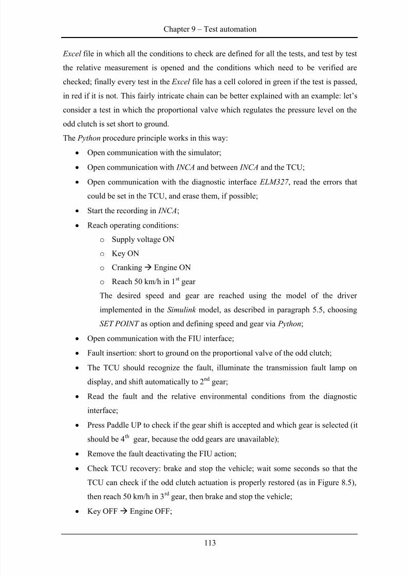
8/20/2019 Olivi Davide Tesi
http://slidepdf.com/reader/full/olivi-davide-tesi 123/141
Chapter 9 – Test automation
113
Excel file in which all the conditions to check are defined for all the tests, and test by test
the relative measurement is opened and the conditions which need to be verified are
checked; finally every test in the Excel file has a cell colored in green if the test is passed,
in red if it is not. This fairly intricate chain can be better explained with an example: let’s
consider a test in which the proportional valve which regulates the pressure level on the
odd clutch is set short to ground.
The Python procedure principle works in this way:
Open communication with the simulator;
Open communication with INCA and between INCA and the TCU;
Open communication with the diagnostic interface ELM327 , read the errors that
could be set in the TCU, and erase them, if possible;
Start the recording in INCA;
Reach operating conditions:
o Supply voltage ON
o Key ON
o
Cranking Engine ON
o Reach 50 km/h in 1st gear
The desired speed and gear are reached using the model of the driver
implemented in the Simulink model, as described in paragraph 5.5, choosing
SET POINT as option and defining speed and gear via Python;
Open communication with the FIU interface;
Fault insertion: short to ground on the proportional valve of the odd clutch;
The TCU should recognize the fault, illuminate the transmission fault lamp on
display, and shift automatically to 2nd gear;
Read the fault and the relative environmental conditions from the diagnostic
interface;
Press Paddle UP to check if the gear shift is accepted and which gear is selected (it
should be 4th gear, because the odd gears are unavailable);
Remove the fault deactivating the FIU action;
Check TCU recovery: brake and stop the vehicle; wait some seconds so that the
TCU can check if the odd clutch actuation is properly restored (as in Figure 8.5),
then reach 50 km/h in 3rd gear, then brake and stop the vehicle;
Key OFF Engine OFF;
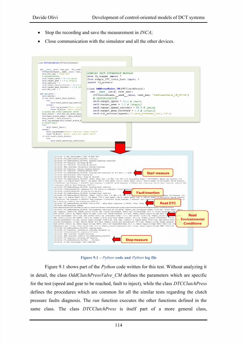
8/20/2019 Olivi Davide Tesi
http://slidepdf.com/reader/full/olivi-davide-tesi 124/141
Davide Olivi Development of control-oriented models of DCT systems
114
Stop the recording and save the measurement in INCA;
Close communication with the simulator and all the other devices.
Figure 9.1 – Python code and Python log file
Figure 9.1 shows part of the Python code written for this test. Without analyzing it
in detail, the class OddClutchPressValve_CM defines the parameters which are specific
for the test (speed and gear to be reached, fault to inject), while the class DTCClutchPress
defines the procedures which are common for all the similar tests regarding the clutch
pressure faults diagnosis. The run function executes the other functions defined in thesame class. The class DTCClutchPress is itself part of a more general class,
Fault insertion
Read DTC
Read
Environmental
Conditions
Stop measure
Start measure
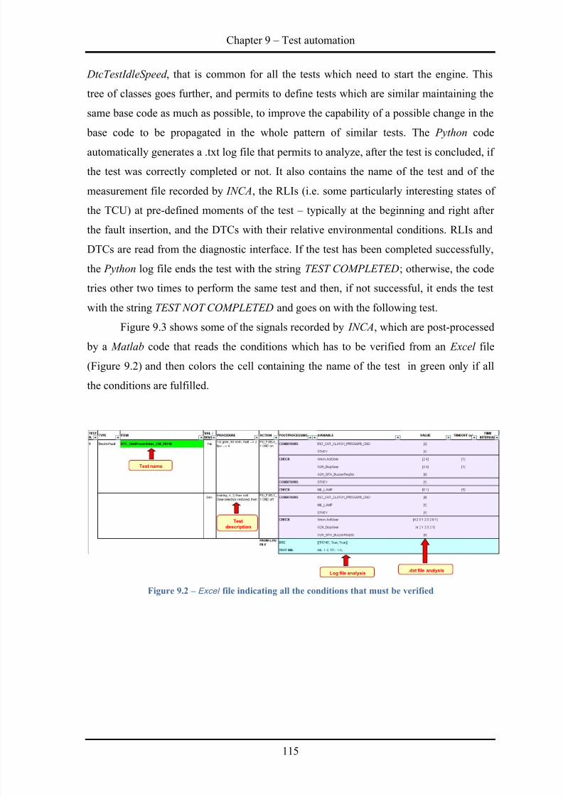
8/20/2019 Olivi Davide Tesi
http://slidepdf.com/reader/full/olivi-davide-tesi 125/141
Chapter 9 – Test automation
115
DtcTestIdleSpeed , that is common for all the tests which need to start the engine. This
tree of classes goes further, and permits to define tests which are similar maintaining the
same base code as much as possible, to improve the capability of a possible change in the
base code to be propagated in the whole pattern of similar tests. The Python code
automatically generates a .txt log file that permits to analyze, after the test is concluded, if
the test was correctly completed or not. It also contains the name of the test and of the
measurement file recorded by INCA, the RLIs (i.e. some particularly interesting states of
the TCU) at pre-defined moments of the test – typically at the beginning and right after
the fault insertion, and the DTCs with their relative environmental conditions. RLIs and
DTCs are read from the diagnostic interface. If the test has been completed successfully,
the Python log file ends the test with the string TEST COMPLETED; otherwise, the code
tries other two times to perform the same test and then, if not successful, it ends the test
with the string TEST NOT COMPLETED and goes on with the following test.
Figure 9.3 shows some of the signals recorded by INCA, which are post-processed
by a Matlab code that reads the conditions which has to be verified from an Excel file
(Figure 9.2) and then colors the cell containing the name of the test in green only if all
the conditions are fulfilled.
Figure 9.2 – Excel file indicating all the conditions that must be verified
Test name
Test
description
.dat file analysisLog file analysis
8/20/2019 Olivi Davide Tesi
http://slidepdf.com/reader/full/olivi-davide-tesi 126/141
Davide Olivi Development of control-oriented models of DCT systems
116
Figure 9.3 – INCA measurement and Matlab postprocessing script
9.3 Non-regression tests on new TCU software
The test automation permits executing non-regression tests on every new software
release; a test which gives a certain expected result on the current production TCU
software is performed on the new TCU software; in the majority of cases, the expected
TCU behavior is the same for both, as defined in the Excel file of Figure 9.3. When the
result of the test on the new software is negative, the non regression test is not successful;
the cell with the name of the test in the Excel file is colored in red; this means that the
modifications introduced in the new software had an unexpected impact on the strategies
checked during that particular test, that must be analyzed to understand and solve the
FAULT
VALIDATION
FAULT
DEVALIDATION
AUTOMATIC
GEAR SHIT 1 2
TIP UP:
2 4 SHIFT
ONLY EVEN
GEARS
AVAILABLE
CHECK ODD CLUTCH
FUNCTIONALITY
FULL
FUNCTIONALITY
RESTORED
ALL GEARS
AVAILABLE:
1 2 3 2 1
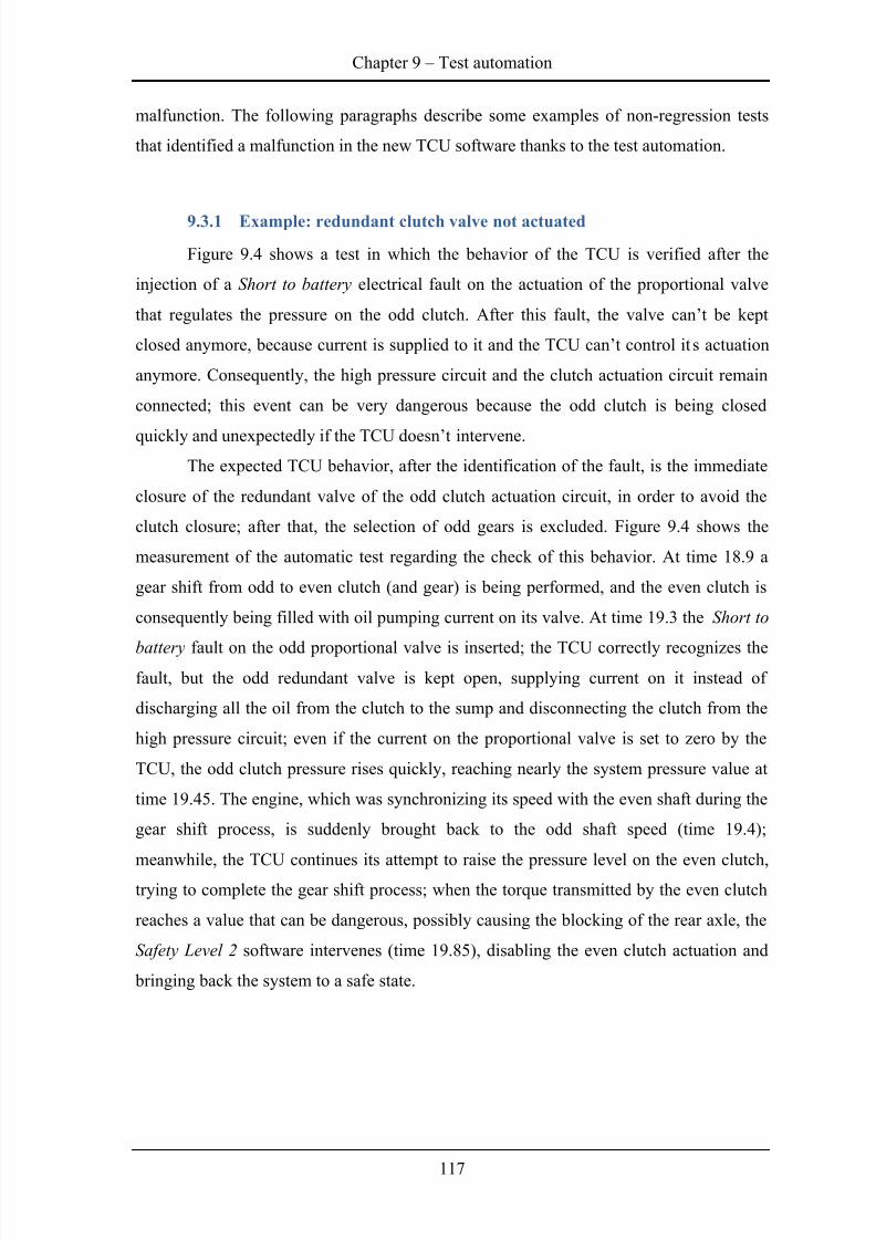
8/20/2019 Olivi Davide Tesi
http://slidepdf.com/reader/full/olivi-davide-tesi 127/141
Chapter 9 – Test automation
117
malfunction. The following paragraphs describe some examples of non-regression tests
that identified a malfunction in the new TCU software thanks to the test automation.
9.3.1 Example: redundant clutch valve not actuated
Figure 9.4 shows a test in which the behavior of the TCU is verified after the
injection of a Short to battery electrical fault on the actuation of the proportional valve
that regulates the pressure on the odd clutch. After this fault, the valve can’t be kept
closed anymore, because current is supplied to it and the TCU can’t control it s actuation
anymore. Consequently, the high pressure circuit and the clutch actuation circuit remain
connected; this event can be very dangerous because the odd clutch is being closed
quickly and unexpectedly if the TCU doesn’t intervene.
The expected TCU behavior, after the identification of the fault, is the immediate
closure of the redundant valve of the odd clutch actuation circuit, in order to avoid the
clutch closure; after that, the selection of odd gears is excluded. Figure 9.4 shows the
measurement of the automatic test regarding the check of this behavior. At time 18.9 a
gear shift from odd to even clutch (and gear) is being performed, and the even clutch is
consequently being filled with oil pumping current on its valve. At time 19.3 the Short to
battery fault on the odd proportional valve is inserted; the TCU correctly recognizes thefault, but the odd redundant valve is kept open, supplying current on it instead of
discharging all the oil from the clutch to the sump and disconnecting the clutch from the
high pressure circuit; even if the current on the proportional valve is set to zero by the
TCU, the odd clutch pressure rises quickly, reaching nearly the system pressure value at
time 19.45. The engine, which was synchronizing its speed with the even shaft during the
gear shift process, is suddenly brought back to the odd shaft speed (time 19.4);
meanwhile, the TCU continues its attempt to raise the pressure level on the even clutch,
trying to complete the gear shift process; when the torque transmitted by the even clutch
reaches a value that can be dangerous, possibly causing the blocking of the rear axle, the
Safety Level 2 software intervenes (time 19.85), disabling the even clutch actuation and
bringing back the system to a safe state.
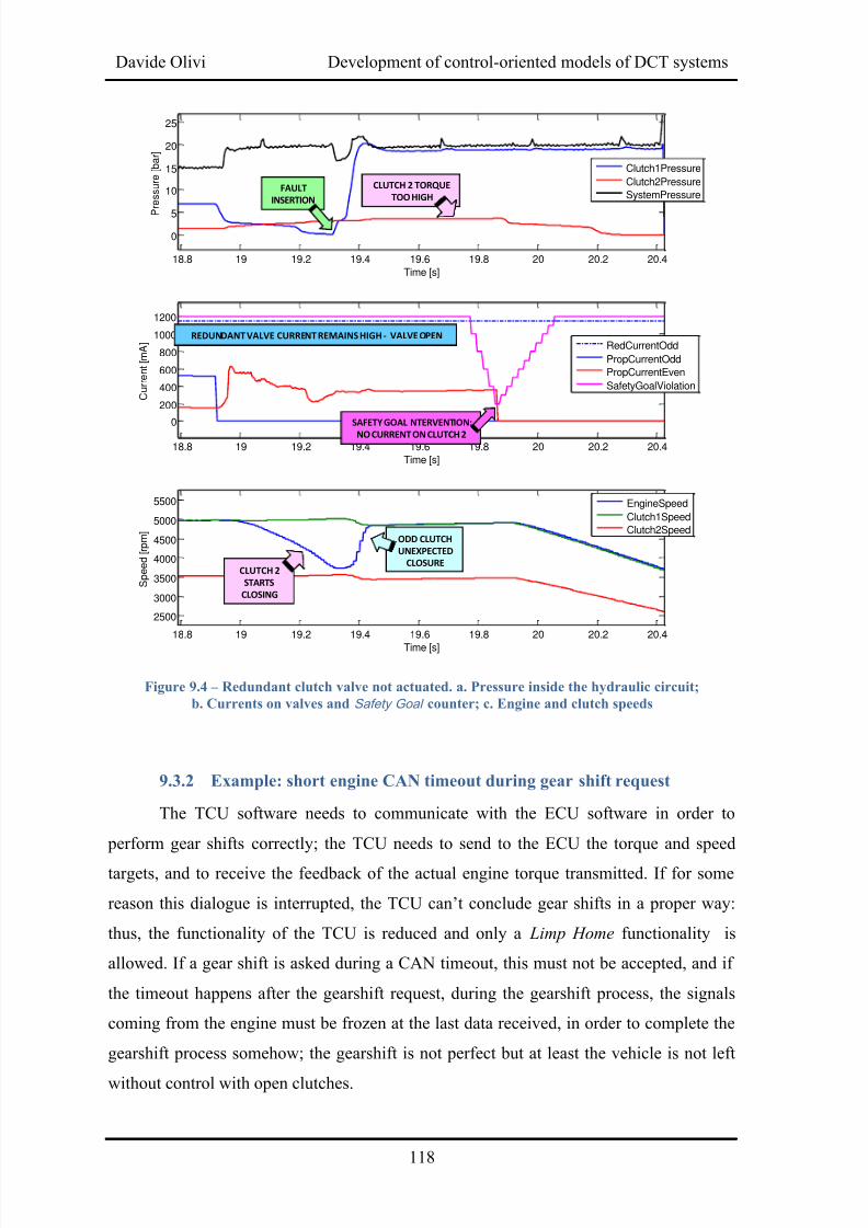
8/20/2019 Olivi Davide Tesi
http://slidepdf.com/reader/full/olivi-davide-tesi 128/141
Davide Olivi Development of control-oriented models of DCT systems
118
Figure 9.4 – Redundant clutch valve not actuated. a. Pressure inside the hydraulic circuit;
b. Currents on valves and Safety Goal counter; c. Engine and clutch speeds
9.3.2 Example: short engine CAN timeout during gear shift request
The TCU software needs to communicate with the ECU software in order to
perform gear shifts correctly; the TCU needs to send to the ECU the torque and speed
targets, and to receive the feedback of the actual engine torque transmitted. If for some
reason this dialogue is interrupted, the TCU can’t conclude gear shifts in a proper way:
thus, the functionality of the TCU is reduced and only a Limp Home functionality is
allowed. If a gear shift is asked during a CAN timeout, this must not be accepted, and if
the timeout happens after the gearshift request, during the gearshift process, the signals
coming from the engine must be frozen at the last data received, in order to complete the
gearshift process somehow; the gearshift is not perfect but at least the vehicle is not left
without control with open clutches.
18.8 19 19.2 19.4 19.6 19.8 20 20.2 20.4
0
5
10
15
20
25
Time [s]
P
ressure[bar]
18.8 19 19.2 19.4 19.6 19.8 20 20.2 20.4
0
200
400
600
800
1000
1200
Time [s]
Current[mA]
18.8 19 19.2 19.4 19.6 19.8 20 20.2 20.4
2500
3000
3500
4000
4500
5000
5500
Time [s]
Speed[rpm]
Clutch1Pressure
Clutch2Pressure
SystemPressure
EngineSpeed
Clutch1Speed
Clutch2Speed
RedCurrentOdd
PropCurrentOdd
PropCurrentEven
SafetyGoalViolation
FAULT
INSERTION
ODD CLUTCH
UNEXPECTED
CLOSURE
CLUTCH 2 TORQUE
TOO HIGH
SAFETY GOAL NTERVENTION:
NO CURRENT ON CLUTCH 2
CLUTCH 2
STARTS
CLOSING
REDUNDANT VALVE CURRENT REMAINS HIGH - VALVE OPEN
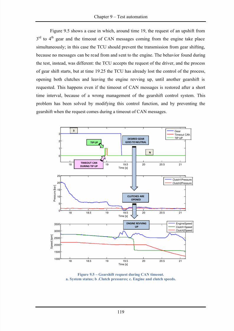
8/20/2019 Olivi Davide Tesi
http://slidepdf.com/reader/full/olivi-davide-tesi 129/141
Chapter 9 – Test automation
119
Figure 9.5 shows a case in which, around time 19, the request of an upshift from
3rd to 4th gear and the timeout of CAN messages coming from the engine take place
simultaneously; in this case the TCU should prevent the transmission from gear shifting,
because no messages can be read from and sent to the engine. The behavior found during
the test, instead, was different: the TCU accepts the request of the driver, and the process
of gear shift starts, but at time 19.25 the TCU has already lost the control of the process,
opening both clutches and leaving the engine revving up, until another gearshift is
requested. This happens even if the timeout of CAN messages is restored after a short
time interval, because of a wrong management of the gearshift control system. This
problem has been solved by modifying this control function, and by preventing the
gearshift when the request comes during a timeout of CAN messages.
Figure 9.5 – Gearshift request during CAN timeout.
a. System status; b .Clutch pressures; c. Engine and clutch speeds.
18 18.5 19 19.5 20 20.5 21
0
1
2
3
Time [s]
18 18.5 19 19.5 20 20.5 210
5
10
15
20
25
Time [s]
Pressure[bar]
18 18.5 19 19.5 20 20.5 211000
1500
2000
2500
3000
3500
Time [s]
Speed[rpm]
Clutch1Pressure
Clutch2Pressure
Gear
Timeout CAN
TIP UP
EngineSpeed
Clutch1Speed
Clutch2Speed
TIP UP
TIMEOUT CAN
DURING TIP UP
3
N
DESIRED GEAR
GOES TO NEUTRAL
CLUTCHES ARE
OPENED
ENGINE REVVING
UP
8/20/2019 Olivi Davide Tesi
http://slidepdf.com/reader/full/olivi-davide-tesi 130/141
Davide Olivi Development of control-oriented models of DCT systems
120
9.3.3 Example: wrong rod management during sensor fault
Figure 9.6 shows the correct behavior of the TCU when a fault regarding the
position sensor of rod 1 is recognized. If a Short to ground is injected on the sensor wires,
the TCU can’t have a feedback about the rod position and the gear engaged. Thus, theother rod relative to the odd gears (rod 2) is maintained in idle position, to avoid double
gear selection on the odd shaft. Anyway, the gear engaged by rod 1 can be reconstructed
by considering the odd clutch speed, and comparing it to the speed it would have if the
gear was engaged.
Figure 9.6 – Expected behaviour during fault on rod 1 sensor. a. System status; b. Clutch pressures;
c. Engine and clutch speeds; d. Rod positions
Until time 28.8, the 1st gear is transmitting torque to the wheels; after the upshift
request, the transmission shifts to 2nd gear. The vehicle is accelerating, and in full
functionality mode the TCU would preselect the 3rd gear on the odd shaft. In this case, the
28.5 29 29.5 30 30.5 31 31.5
0
1
2
3
Time [s]
28.5 29 29.5 30 30.5 31 31.5
0
10
20
Time [s]
Pressure[bar]
28.5 29 29.5 30 30.5 31 31.53000
4000
5000
6000
7000
Time [s]
Speed[rpm]
28.5 29 29.5 30 30.5 31 31.50
1
2
x 104
Time [s]
Positi
on[um]
Clutch1Pressure
Clutch2Pressure
Gear
TIP UP
EngineSpeed
Clutch1Speed
Clutch2Speed
Rod1Pos
Rod2Pos
Rod3Pos
Rod4Pos
Curr 3rd gear
1
2
3
2
N
ELECTRICAL FAILURE ON
ROD1 SENSOR: NO
POSITION FEEDBACK
OPEN LOOP CURRENT TO
ENGAGE 3RD GEAR
3RD GEAR CORRECTLY
ENGAGING ON ROD1
ASK FOR 2ND GEAR ASK FOR 3RD GEAR
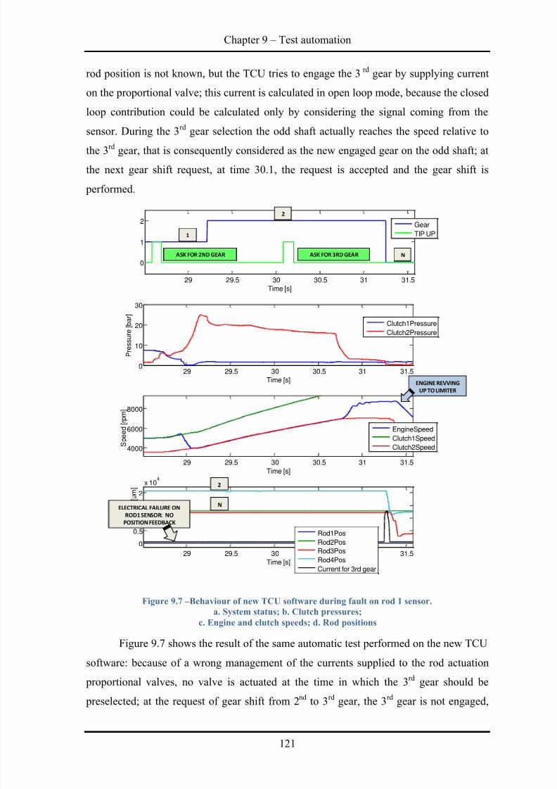
8/20/2019 Olivi Davide Tesi
http://slidepdf.com/reader/full/olivi-davide-tesi 131/141
Chapter 9 – Test automation
121
rod position is not known, but the TCU tries to engage the 3 rd gear by supplying current
on the proportional valve; this current is calculated in open loop mode, because the closed
loop contribution could be calculated only by considering the signal coming from the
sensor. During the 3rd gear selection the odd shaft actually reaches the speed relative to
the 3rd gear, that is consequently considered as the new engaged gear on the odd shaft; at
the next gear shift request, at time 30.1, the request is accepted and the gear shift is
performed.
Figure 9.7 – Behaviour of new TCU software during fault on rod 1 sensor.
a. System status; b. Clutch pressures;
c. Engine and clutch speeds; d. Rod positions
Figure 9.7 shows the result of the same automatic test performed on the new TCU
software: because of a wrong management of the currents supplied to the rod actuation
proportional valves, no valve is actuated at the time in which the 3rd gear should be
preselected; at the request of gear shift from 2nd to 3rd gear, the 3rd gear is not engaged,
29 29.5 30 30.5 31 31.5
0
1
2
Time [s]
29 29.5 30 30.5 31 31.50
10
20
30
Time [s]
Pressure[bar]
29 29.5 30 30.5 31 31.5
4000
6000
8000
Time [s]
Speed[rpm
]
29 29.5 30 30.5 31 31.5
0
0.5
1
1.5
2
x 104
Time [s]
Position[um]
Clutch1Pressure
Clutch2Pressure
Gear
TIP UP
EngineSpeed
Clutch1Speed
Clutch2Speed
Rod1Pos
Rod2Pos
Rod3PosRod4Pos
Current for 3rd gear
1
2
ASK FOR 2ND GEAR ASK FOR 3RD GEAR N
2
NELECTRICAL FAILURE ON
ROD1 SENSOR: NO
POSITION FEEDBACK
ENGINE REVVING
UP TO LIMITER
8/20/2019 Olivi Davide Tesi
http://slidepdf.com/reader/full/olivi-davide-tesi 132/141
Davide Olivi Development of control-oriented models of DCT systems
122
but the gearshift is accepted: the result is that the engine revs up unexpectedly (from time
30.8) with both clutches opened, N is displayed to the driver, and the control of the
vehicle is restored only if a new gearshift is required.
Thanks to the test automation, several bugs were found in the TCU software under
test; these problems can be analyzed one by one thanks to the measurements recorded
during each automatic test, and the same test can be reproduced indetically several times
to analyze different variables that had not initially been considered. When the pattern of
non-regression tests can be considered complete, the validation of every new TCU
software can be performed in fully automatic mode in a safe, time-saving and cost-
effective simulation environment.
8/20/2019 Olivi Davide Tesi
http://slidepdf.com/reader/full/olivi-davide-tesi 133/141
Conclusions
123
Conclusions
During this PhD thesis a control oriented model of the Dual Clutch Transmission
has been developed, by considering the dynamic physical equations of hydraulic circuit,
clutches and synchronizers, of all the shafts inside the gearbox (considered with infinite
stiffness), and a vehicle model that takes into account the resistant force on the vehicle
and its own inertia. The different parts of the model were at first tested and validated
separately; a simplification of some dynamics was carried out to adapt the model to real-
time applications, in order to reproduce the fast dynamics of the hydraulic circuit while
maintaining a sufficiently large simulation step size.
The results of offline simulation of clutch pressure, system pressure, rod motion
and shafts speeds have been compared to on-board measurements, and the model was
consequently calibrated to match them. After the validation of the physical model, a
model of input/output signal scaling was added, and the complete model was then
implemented in a Hardware In the Loop simulator, composed of a real-time processor,
input / output boards, a TCU plate and a load plate.
Several tests have been performed on the HIL simulator: functional tests, as well
as mechanical, hydraulic and electrical failure tests have been executed, analyzing the
behaviour of the model and the transmission control unit reaction. Adaption procedures
were performed to adapt the TCU to the specific gearbox simulated by the HILapplication. The results demonstrate the capability of the HIL model to correctly simulate
the behaviour of the real system, and to respond to the requests coming from the TCU
both during functional tests and during failure recovery procedures.
The first intensive use of the simulator aimed at a complete validation of the new
safety level software implemented inside the TCU, performing manually a pattern of
tests, previously defined, which covered all the possible functionalities of the software.
A test automation procedure has then been developed to meet the requirement of
performing a pattern of tests without the direct interaction of the user; the tests
8/20/2019 Olivi Davide Tesi
http://slidepdf.com/reader/full/olivi-davide-tesi 134/141
Davide Olivi Development of control-oriented models of DCT systems
124
automation allows saving time, reproducing identical tests on different software releases,
and designing tests with a tight actions timing – sometimes with just a few milliseconds
between them – that wouldn’t be possible to be executed manually by the user.
The HIL simulator is now being used for the testing, debug and validation ofevery new software release of the specific TCU it was developed for. The tests are
performed both in manual mode, for the verification of the new features implemented in
the software, and in fully automatic mode, for non-regression tests and comparison
between different software releases. When the pattern of automatic tests will be
considered complete, i.e. it will cover all the functionalities of the TCU, a fully automatic
non-.regression validation will be possible with the use of the simulator.
Considering that new features are being implemented inside the software almost
everyday, concerning new gearshift management, new diagnosis requests, new fuel
saving strategies (such as Stop&Start and Electric Drive), the simulator is a fundamental
tool to assist the development of all these new strategies and the debugging and validation
of a software that can then be installed in production vehicles, all this in a safe, time-
saving and cost-effective simulation environment.
8/20/2019 Olivi Davide Tesi
http://slidepdf.com/reader/full/olivi-davide-tesi 135/141
Bibliography
125
Bibliography
[1] Bertotti, G., Mayergoyz, I.D. (2006). The Science of Hysteresis: Mathematical
modeling and applications. Academic Press.
[2] Davis, C.L., Sadeghi, F., Krousgrill, C.M. (2000). A Simplified Approach to
Modeling Thermal Effects in Wet Clutch Engagement: Analytical and ExperimentalComparison. ASME Journal of Mechanical Design, Vol. 122, p. 110-118.
[3] Deur, J., Petric, J., Asgari, J., Hrovat, D. (2005). Modeling of Wet Clutch
Engagement Including a Thorough Experimental Validation. SAE Technical Paper
2005-01-0877 .
[4] Eyabi, P., Washington, G. (2006). Nonlinear Modeling of an Electromagnetic Valve
Actuator. SAE Technical Paper 2006-01-0043.
[5] Goetz, M., Levesley, M.C., Crolla, D.A. (2005). Dynamics and control of gearshifts
on twin-clutch transmissions. Proc. of the IMECHE, Aug. 2005; 219, 8.
[6] Greenwood, J.A., Williamson, J.B.P. (1966). Contact of nominally flat surfaces.
Proceedings of the Royal Society of London. Series A, Mathematical and Physical
Sciences, Vol. 295, No. 1442, 300-319.
[7] Guzzella, L., Onder, C. H. (2004). Introduction to Modeling and Control of Internal
Combustion Engine Systems. Springer.
[8] Guzzella, L. Sciarretta, A. (2008). Vehicle Propulsion Systems. Springer.
[9] He, Y., Lin, C., (2007). Development and Validation of a Mean Value EngineModel for Integrated Engine and Control System Simulation. SAE Technical Paper
2007-01-1304.
[10] Kulkarni, M., Shim, T., Zhang, Y. (2007). Shift dynamics and control of dual-clutch
transmissions. Mechanism and Machine Theory 42, 168-182.
[11] Lai, G.Y. (2007). Simulation of heat-transfer characteristics of wet clutch
engagement processes. Numerical Heat Transfer, Part A: Applications, 33: 6, 583-
597.
8/20/2019 Olivi Davide Tesi
http://slidepdf.com/reader/full/olivi-davide-tesi 136/141
Davide Olivi Development of control-oriented models of DCT systems
126
[12] Liu, Y., Qin, D., Jiang, H., Zhang, Y. (2009). A Systematic Model for Dynamics
and Control of Dual Clutch Transmissions. Journal of Mechanical Design, Vol.
131, 061012.
[13] Lucente, G., Montanari, M., Rossi, C. (2007). Modelling of an automated manual
transmission system. Mechatronics 17, 73 – 91.
[14] Matthes, B. (2005). Dual Clutch Transmissions – Lessons learned and future
potential. SAE Technical Paper 2005-01-1021.
[15] Merritt, H.E. (1967). Hydraulic Control Systems. John Wiley & Sons Inc.
[16] Montanari, M., Ronchi, F., Rossi, C., Tilli, A., Tonielli, A. (2004). Control and
performance evaluation of a clutch servo system with hydraulic actuation. Control
Engineering Practice 21,1369-1379.
[17] Naunheimer, H., Bertsche, B., Ryborz, J., Novak, W. (2011). AutomotiveTransmissions: Fundamentals, Selection, Design and Application. Springer.
[18] Neto, D.V., Florencio, D.G., Fernandez, J., Rodriguez, P. (2006). Manual
Transmission: Synchronization Main Aspects. SAE Technical Paper 2006-01-2519.
[19] Razzacki, S.T. (2004). Synchronizer Design: A Mathematical and Dimensional
Treatise, SAE Technical Paper 2004-01-1230.
[20] Velardocchia, M. Amisano, F, Flora, R. (2000). A Linear Thermal Model for an
Automotive Clutch. SAE Technical Paper 2000-01-0834.
[21] Zhang, Y., Chen, X., Zhang, X., Jiang, H., Tobler, W. (2005). Dynamic Modeling
and Simulation of a Dual Clutch Automated Lay-Shaft Transmission. ASME
Journal of Mechanical Design, Vol. 127, 302-307.
[22] Olivi, D., Cavina, N., Corti, E., Poggio, L., Marcigliano, F. (2012). Development of
a Dual Clutch Transmission Model for Real-Time Applications, Proc. of ECOSM
2012, Oct. 2012.
[23] Olivi, D., Cavina, N., Mancini G., Moro D., Poggio, L., Marcigliano, F. (2013).
Development and implementation of Hardware In the Loop simulation for DualClutch Transmission Control Units, Proc. of SAE World Congress 2013, Apr. 2013.
[24] www.wikipedia.org
[25] www.howstuffworks.com
[26] www.dctfacts.com
[27] www.drivelinenews.com
[28] www.ae-plus.com
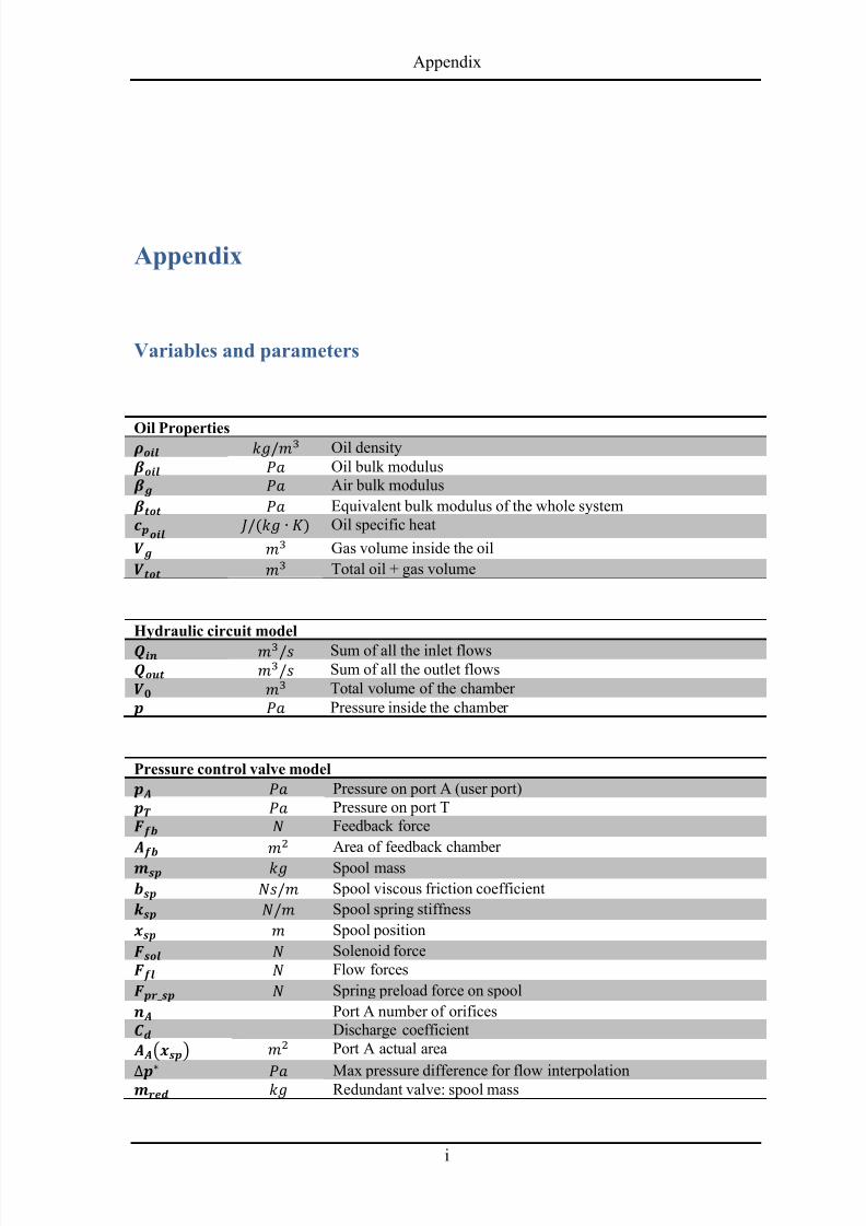
8/20/2019 Olivi Davide Tesi
http://slidepdf.com/reader/full/olivi-davide-tesi 137/141
Appendix
i
Appendix
Variables and parameters
Oil Properties Oil density Oil bulk modulus Air bulk modulus Equivalent bulk modulus of the whole system Oil specific heat Gas volume inside the oil Total oil + gas volume
Hydraulic circuit model
Sum of all the inlet flows Sum of all the outlet flows Total volume of the chamber Pressure inside the chamber
Pressure control valve model Pressure on port A (user port) Pressure on port T Feedback force
Area of feedback chamber
Spool mass Spool viscous friction coefficient Spool spring stiffness Spool position Solenoid force Flow forces Spring preload force on spool Port A number of orifices Discharge coefficient
()
Port A actual area
Max pressure difference for flow interpolation Redundant valve: spool mass
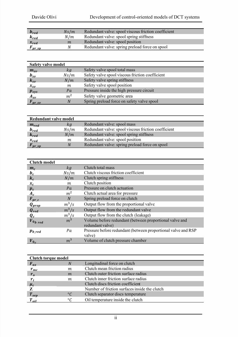
8/20/2019 Olivi Davide Tesi
http://slidepdf.com/reader/full/olivi-davide-tesi 138/141
Davide Olivi Development of control-oriented models of DCT systems
ii
Redundant valve: spool viscous friction coefficient Redundant valve: spool spring stiffness Redundant valve: spool position Redundant valve: spring preload force on spool
Safety valve model Safety valve spool total mass Safety valve spool viscous friction coefficient Safety valve spring stiffness Safety valve spool position Pressure inside the high pressure circuit Safety valve geometric area Spring preload force on safety valve spool
Redundant valve model Redundant valve: spool mass Redundant valve: spool viscous friction coefficient Redundant valve: spool spring stiffness Redundant valve: spool position Redundant valve: spring preload force on spool
Clutch model Clutch total mass
Clutch viscous friction coefficient
Clutch spring stiffness Clutch position Pressure on clutch actuation Clutch actual area for pressure Spring preload force on clutch Output flow from the proportional valve Output flow from the redundant valve Output flow from the clutch (leakage) Volume before redundant (between proportional valve and
redundant valve)
Pressure before redundant (between proportional valve and RSP
valve) Volume of clutch pressure chamber
Clutch torque model Longitudinal force on clutch Clutch mean friction radius Clutch outer friction surface radius Clutch inner friction surface radius Clutch discs friction coefficient
Z Number of friction surfaces inside the clutch
Clutch separator discs temperature Oil temperature inside the clutch
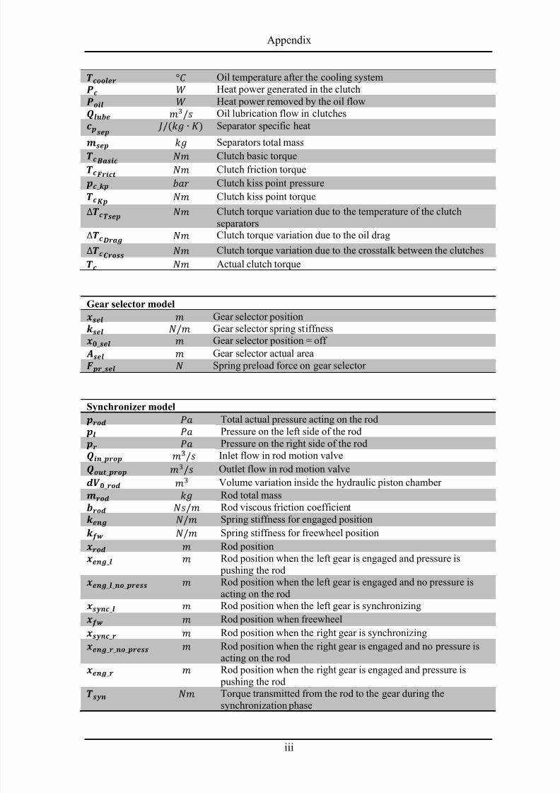
8/20/2019 Olivi Davide Tesi
http://slidepdf.com/reader/full/olivi-davide-tesi 139/141
Appendix
iii
Oil temperature after the cooling system Heat power generated in the clutch Heat power removed by the oil flow Oil lubrication flow in clutches
Separator specific heat
Separators total mass Clutch basic torque Clutch friction torque Clutch kiss point pressure Clutch kiss point torque Clutch torque variation due to the temperature of the clutch
separators Clutch torque variation due to the oil drag Clutch torque variation due to the crosstalk between the clutches
Actual clutch torque
Gear selector model Gear selector position Gear selector spring stiffness Gear selector position = off Gear selector actual area Spring preload force on gear selector
Synchronizer model
Total actual pressure acting on the rod Pressure on the left side of the rod Pressure on the right side of the rod Inlet flow in rod motion valve Outlet flow in rod motion valve Volume variation inside the hydraulic piston chamber Rod total mass Rod viscous friction coefficient Spring stiffness for engaged position Spring stiffness for freewheel position
Rod position
Rod position when the left gear is engaged and pressure is pushing the rod Rod position when the left gear is engaged and no pressure isacting on the rod Rod position when the left gear is synchronizing Rod position when freewheel Rod position when the right gear is synchronizing Rod position when the right gear is engaged and no pressure isacting on the rod Rod position when the right gear is engaged and pressure is pushing the rod
Torque transmitted from the rod to the gear during thesynchronization phase
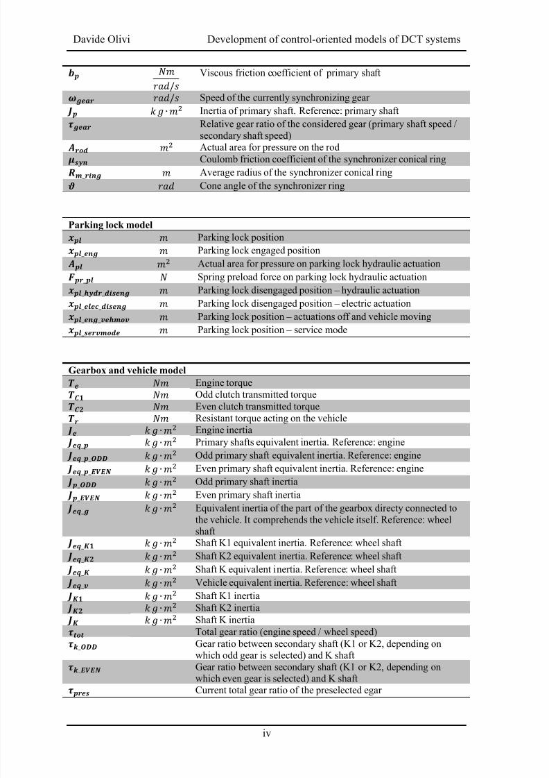
8/20/2019 Olivi Davide Tesi
http://slidepdf.com/reader/full/olivi-davide-tesi 140/141
Davide Olivi Development of control-oriented models of DCT systems
iv
Viscous friction coefficient of primary shaft
Speed of the currently synchronizing gear Inertia of primary shaft. Reference: primary shaft
Relative gear ratio of the considered gear (primary shaft speed /
secondary shaft speed) Actual area for pressure on the rod Coulomb friction coefficient of the synchronizer conical ring Average radius of the synchronizer conical ring Cone angle of the synchronizer ring
Parking lock model Parking lock position Parking lock engaged position
Actual area for pressure on parking lock hydraulic actuation
Spring preload force on parking lock hydraulic actuation Parking lock disengaged position – hydraulic actuation Parking lock disengaged position – electric actuation Parking lock position – actuations off and vehicle moving Parking lock position – service mode
Gearbox and vehicle model Engine torque
Odd clutch transmitted torque
Even clutch transmitted torque Resistant torque acting on the vehicle Engine inertia Primary shafts equivalent inertia. Reference: engine Odd primary shaft equivalent inertia. Reference: engine Even primary shaft equivalent inertia. Reference: engine Odd primary shaft inertia Even primary shaft inertia Equivalent inertia of the part of the gearbox directy connected tothe vehicle. It comprehends the vehicle itself. Reference: wheelshaft
Shaft K1 equivalent inertia. Reference: wheel shaft Shaft K2 equivalent inertia. Reference: wheel shaft Shaft K equivalent inertia. Reference: wheel shaft Vehicle equivalent inertia. Reference: wheel shaft Shaft K1 inertia Shaft K2 inertia Shaft K inertia Total gear ratio (engine speed / wheel speed) Gear ratio between secondary shaft (K1 or K2, depending onwhich odd gear is selected) and K shaft
Gear ratio between secondary shaft (K1 or K2, depending on
which even gear is selected) and K shaft Current total gear ratio of the preselected egar
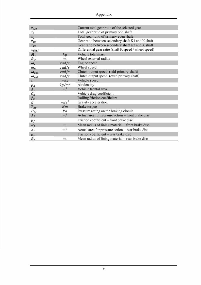
8/20/2019 Olivi Davide Tesi
http://slidepdf.com/reader/full/olivi-davide-tesi 141/141
Appendix
Current total gear ratio of the selected gear Total gear ratio of primary odd shaft Total gear ratio of primary even shaft Gear ratio between secondary shaft K1 and K shaft
Gear ratio between secondary shaft K2 and K shaft
Differential gear ratio (shaft K speed / wheel speed) Vehicle total mass Wheel external radius Engine speed Wheel speed Clutch output speed (odd primary shaft) Clutch output speed (even primary shaft) Vehicle speed Air density Vehicle frontal area
Vehicle drag coefficient
Rolling friction coefficient
Gravity acceleration Brake torque Pressure acting on the braking circuit Actual area for pressure action – front brake disc Friction coefficient – front brake disc Mean radius of lining material – front brake disc Actual area for pressure action – rear brake disc Friction coefficient – rear brake disc Mean radius of lining material – rear brake disc


![Pietro di Giovanni Olivi Pietro di Giovanni Olivi (+1291) [Petrus Johannis Olivi; Pierre Jean Olieu] Pietro di Giovanni Olivi nacque a Sérignan, vicino.](https://static.fdocumenti.com/doc/165x107/5542eb5c497959361e8ca4a4/pietro-di-giovanni-olivi-pietro-di-giovanni-olivi-1291-petrus-johannis-olivi-pierre-jean-olieu-pietro-di-giovanni-olivi-nacque-a-serignan-vicino.jpg)