
Hyperon polarisation at BESIII - Istituto Nazionale di ... Hyperon polarisation at BESIII Candidato:...
82
Universit` a degli Studi di Torino DIPARTIMENTO DI FISICA Corso di Laurea Magistrale in Fisica Tesi di laurea magistrale Hyperon polarisation at BESIII Candidato: Giulio Mezzadri Relatore: Prof. Marco Maggiora Co-Relatore: Dott. Marco Destefanis Contro-Relatore: Prof. Mauro Anselmino Anno Accademico 2012-2013
Transcript of Hyperon polarisation at BESIII - Istituto Nazionale di ... Hyperon polarisation at BESIII Candidato:...
Universita degli Studi di Torino
DIPARTIMENTO DI FISICA
Corso di Laurea Magistrale in Fisica
Tesi di laurea magistrale
Hyperon polarisation at BESIII
Candidato:
Giulio MezzadriRelatore:
Prof. Marco Maggiora
Co-Relatore:
Dott. Marco Destefanis
Contro-Relatore:
Prof. Mauro Anselmino
Anno Accademico 2012-2013

Alla mia famiglia, il mio incrollabile sostegno

Because maybe,
you’re gonna be the one that saves me...
And after all, you’re my wonderwall..
Oasis
Contents
I Introduction 7
1 Physics 8
1.1 Introduction . . . . . . . . . . . . . . . . . . . . . . . . . . . . . . . . . . . 8
1.2 Particles and Forces in the Standard Model . . . . . . . . . . . . . . . . . 8
1.3 e+e− Annihilation Process . . . . . . . . . . . . . . . . . . . . . . . . . . . 10
1.3.1 Feynmann Diagramm and Cross Section Calculation . . . . . . . . 10
1.3.2 Synchrotron radiation . . . . . . . . . . . . . . . . . . . . . . . . . 12
1.3.3 Beamstrahlung and Initial State Radiation . . . . . . . . . . . . . . 12
1.4 Charmonium . . . . . . . . . . . . . . . . . . . . . . . . . . . . . . . . . . 13
1.5 Hyperons and Strangeness . . . . . . . . . . . . . . . . . . . . . . . . . . . 16
1.5.1 Strange Quark Physics - The SU(3)F Model . . . . . . . . . . . . . 17
1.5.2 Λ description . . . . . . . . . . . . . . . . . . . . . . . . . . . . . . 19
1.6 Hyperon Polarisation . . . . . . . . . . . . . . . . . . . . . . . . . . . . . . 19
2 BESIII Spectrometer 21
2.1 Introduction . . . . . . . . . . . . . . . . . . . . . . . . . . . . . . . . . . . 21
2.1.1 BEPCII . . . . . . . . . . . . . . . . . . . . . . . . . . . . . . . . . 23
2.2 BESIII Spectrometer . . . . . . . . . . . . . . . . . . . . . . . . . . . . . . 23
2.2.1 Multilayer Drift Chamber . . . . . . . . . . . . . . . . . . . . . . . 24
2.2.2 Time of Flight System . . . . . . . . . . . . . . . . . . . . . . . . . 26
2.2.3 Electromagnetic Calorimeter . . . . . . . . . . . . . . . . . . . . . . 27
2.2.4 Muon Counter . . . . . . . . . . . . . . . . . . . . . . . . . . . . . . 28
II Data Analysis 31
3 Analysis e+e− → ΛΛ 32
3.1 Event Simulation . . . . . . . . . . . . . . . . . . . . . . . . . . . . . . . . 32
3.2 Event Selection . . . . . . . . . . . . . . . . . . . . . . . . . . . . . . . . . 35
3.3 Armenteros-Podalansky Plot . . . . . . . . . . . . . . . . . . . . . . . . . . 42
3.4 Efficiency and acceptance . . . . . . . . . . . . . . . . . . . . . . . . . . . 44
3
CONTENTS 4
3.5 Hyperon Polarisation . . . . . . . . . . . . . . . . . . . . . . . . . . . . . . 45
4 Analysis e+e− → J/ψ → ΛX 54
4.1 Event Simulation . . . . . . . . . . . . . . . . . . . . . . . . . . . . . . . . 54
4.2 Event Selection . . . . . . . . . . . . . . . . . . . . . . . . . . . . . . . . . 55
4.3 Efficiency and Acceptance . . . . . . . . . . . . . . . . . . . . . . . . . . . 56
4.4 Hyperon Polarisation . . . . . . . . . . . . . . . . . . . . . . . . . . . . . . 57
5 Analysis e+e− → J/ψ → ΛX 63
5.1 Event simulation . . . . . . . . . . . . . . . . . . . . . . . . . . . . . . . . 63
5.2 Event Selection . . . . . . . . . . . . . . . . . . . . . . . . . . . . . . . . . 64
5.3 Efficiency and Acceptance . . . . . . . . . . . . . . . . . . . . . . . . . . . 65
5.4 Hyperon Polarisation . . . . . . . . . . . . . . . . . . . . . . . . . . . . . . 66
6 Relative Phase 71
6.1 Introduction . . . . . . . . . . . . . . . . . . . . . . . . . . . . . . . . . . . 71
6.1.1 Measuring the Phase . . . . . . . . . . . . . . . . . . . . . . . . . . 72
6.2 Event Simulation and Selection . . . . . . . . . . . . . . . . . . . . . . . . 73
6.3 Data Analysis . . . . . . . . . . . . . . . . . . . . . . . . . . . . . . . . . . 74
III Conclusion 78

Abstract
The investigation of the hyperons structure could shed new light on many different
open questions in particle physics; probing the spin degrees of freedom is an usual and
effective approach to experimentally evaluate such a structure. Hyperon polarisation
has been already investigated at low energy (among others at DISTO and CLEOc); to
evaluate it in the yet relatively unexplored threshold sector in electron-positron collision,
eventually up to the J/ψ resonance, could allow to extend the investigation of the energy
dependence of the hyperon polarisation itself and of the underlying elementary processess
at quark level.
After an initial focus on the related theoretical issues, the experimental scenario and
those detectors relevant for the event selection and reconstruction will be described in
details.
Afterwards the complete procedure adopted to extract the spin polarisation for both
the exclusive (e+e− → ΛΛ) and inclusive (e+e− → J/ψ → ΛX and e+e− → J/ψ → ΛX)
hyperon production will be reported, from the event selection to its final results.
Finally, one more observable, the relative phase between electromagnetic and strong
J/ψ production amplitudes, has been extracted considering the ΛΛ final state.
The present analysis has been performed on the full set of events collected up to now
with the BESIII spectrometer at different center of mass energies, to perform both the
J/ψ lineshape scan and a detailed investigation of the off-resonance interference pattern.

Part I
Introduction
7
Chapter 1
Physics
1.1 Introduction
The first hypothesis of quark’s existence is found in Gell-Mann’s work [1] as explana-
tion for similar behavior of different particles: Gell-Mann proposed that these elementary
particles group together to form all the known hadrons. In the same period, Feynmann
proposed the idea of partons, point-like elementary particles which brings part of the
momentum of the hadrons. In the following years, many others compontents of the sub-
atomic world were found: the quark c (with the discovery of J/ψ), the quark b and quark
t and the differences between valence and sea quarks were finally pointed out. Those
studies lead to the full definition the Weinberg and Salam’s Standard Model of Particles.
Althought many questions were answered, many others were brought to a new light,
such as hadronization process, quark extraction from the vacuum, and the neutrino mass,
that are still under investigation. Thus, high energy physics remains a very rich field to
probe our understanding of the subatomic world.
1.2 Particles and Forces in the Standard Model
We need to clarify that there are two different types of elementary particles. The
distinction is based on their spin quantum number: bosons, which have integer spin and
follow the Bose-Einstein statistics, and fermions, which have half integer spin and are
described by the Fermi-Dirac statistics.
Bosons are the particles carrying the elementary forces the particles interact with.
There are five type of bosons: photons, mediators of the electromagnetic force, W’s and
Z’s, of the weak force, gluons, mediators of the strong interaction, and gravitons, of the
gravitational force.
Fermions can be divided in two different groups:
8
CHAPTER 1. PHYSICS 9
• leptons, which are pointlike particles interacting by electromagnetic (EM) and weak
interaction
• quarks, interacting by strong force as well.
Quarks bind together to form not-elementary particle called hadrons.
Hadrons can be divided in two different group:
• mesons, which are composed of a quark-antiquark pair;
• baryons, which are composed of three quarks.
Both leptons and quarks are divided in three families, as shown in the tab. 1.1 and
tab 1.2 respectively.
(ud
) (cs
) (tb
)Table 1.1: The three families of quarks.
(νee
) (νµµ
) (νττ
)Table 1.2: The three families of leptons.
The five lighter quark (up (u), down (d), strange (s), charm (c), and bottom (b), from
the lightest to the heaviest) bind together to form hadrons, while the top quark (t) is too
heavy, and it has too many open decay channels so that it cannot form a tt bound state.
The electromagnetic (EM) interaction is well interpred in a quantum field theory called
Quantum Electrodynamics (QED). Also the weak interaction is today well understood.
Both are unified in the Electroweak interaction theory.
The situation is different once the strong interaction is considered. Two regimes may
apply: the hard regime, explained by the Quantum Cromodynamics, in which processes
with large transverse momentum are described in a similar way as by QED, and the soft
regime, in which processes are no more perturbative; the latter regime still has to be
completely understood. Usually a perturbative approach is considered safe only if the
energy scale of the considered processes is larger than 1 GeV.
CHAPTER 1. PHYSICS 10
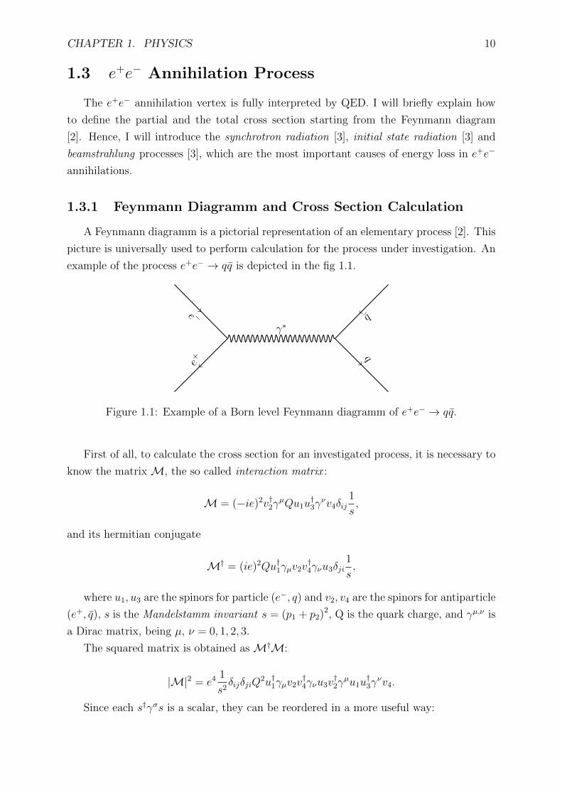
1.3 e+e− Annihilation Process
The e+e− annihilation vertex is fully interpreted by QED. I will briefly explain how
to define the partial and the total cross section starting from the Feynmann diagram
[2]. Hence, I will introduce the synchrotron radiation [3], initial state radiation [3] and
beamstrahlung processes [3], which are the most important causes of energy loss in e+e−
annihilations.
1.3.1 Feynmann Diagramm and Cross Section Calculation
A Feynmann diagramm is a pictorial representation of an elementary process [2]. This
picture is universally used to perform calculation for the process under investigation. An
example of the process e+e− → qq is depicted in the fig 1.1.
e −
e+
γ∗
q
q
Figure 1.1: Example of a Born level Feynmann diagramm of e+e− → qq.
First of all, to calculate the cross section for an investigated process, it is necessary to
know the matrix M, the so called interaction matrix :
M = (−ie)2v†2γµQu1u
†3γ
νv4δij1
s,
and its hermitian conjugate
M† = (ie)2Qu†1γµv2v†4γνu3δji
1
s,
where u1, u3 are the spinors for particle (e−, q) and v2, v4 are the spinors for antiparticle
(e+, q), s is the Mandelstamm invariant s = (p1 + p2)2, Q is the quark charge, and γµ,ν is
a Dirac matrix, being µ, ν = 0, 1, 2, 3.
The squared matrix is obtained as M†M:
|M|2 = e4 1
s2δijδjiQ
2u†1γµv2v†4γνu3v
†2γ
µu1u†3γ
νv4.
Since each s†γσs is a scalar, they can be reordered in a more useful way:
CHAPTER 1. PHYSICS 11
|M|2 = e4 1
s2δijδjiQ
2u†1γµv2v†2γ
µu1v†4γνu3u
†3γ
νv4.
Two traces can be defined: u†1γµv2v†2γ
µu1 and v†4γνu3u†3γ
νv4.
Both the beam and the target polarisations have now to be considered. One has to
sum over final spin state and to average on the initial spin state, using the 12S+1
relation,
where S is the spin of the incoming particle. Since quarks populates the final state, a
color factor 13
has to be introduced for each quark line:
1
4
1
9Σf |M|2 =
1
4
1
9δijδjiQ
2Σf tr[u†1γµv2v
†2γ
µu1
]tr[v†4γνu3u
†3γ
νv4
].
By using the trace cyclicity properties Σuu† = (γσpσ + m) and Σvv† = (γσpσ − m)
pairs can be formed, where p is the momentum of the fermion, m is its mass, and σ is a
generic 4-vector index σ = 0, 1, 2, 3. Since the masses of e−, e+, q, q are smaller than√s,
leptons and quark masses can be neglected in this calculation.
1
4
1
9Σf |M|2 =
1
4
1
93Q2 tr [6p1γ
µ 6p2γν ] tr [6p4γµ 6p3γν ] .
Thanks to the trace properties, the solution of the latter equation is:
|M|2 ∝ 2 (p1 · p3p2 · p4 + p1 · p4p2 · p3) .
Introducing the other Mandelstamm variables t = (p1 − p4)2 = (p2 − p3)2 and u =
(p1 − p3)2 = (p2 − p4)2, one obtains:
|M|2 =1
4
1
3
1
2
1
s2e4[u2 + t2
].
In order to correctly evaluate the cross section predictions of the considered process,
a flux factor 12s
, and a factor, 1(2π)3n−4 , accounting for all the π in the vertex and in the
photon propagator, have to be introduced. More over a phase space factor has to be
added as well.
The total cross section of the process:
σ(e+e− → ss) =4πe4
9s
can be evaluated considering the factor Q2 = 19, as for the annihilation to a dd couple,
while for the cross section of the process e+e− → uu the different charge Qu = 23
has to
be considered.
It has to be stressed how all the calculations reported above have been performed
within a pure QED framework, and no effect related to QCD is involved. This is one
more reason to favour those experimental scenarios involving annihilating positron and
electron beams.
CHAPTER 1. PHYSICS 12
1.3.2 Synchrotron radiation
Since both electrons and positron are accelerated charged particles, they emit photons:
such an emission is called synchrotron radiation. This effect causes an energy loss in the
beam energy: the annihilation has hence a lower center of mass energy with respect to
the nominal one.
The Larmor equation [3] rules the synchrotron radiation emission:
P =2
3
e2
m20c
3
∣∣∣∣d−→pdt∣∣∣∣2 ,
where P is the power emitted by a non relativistic charged particle of charge e and
mass m0. Since both electrons and positron are relativistic, a modified version of the
Larmor formula applies:
P =2
3
e4c2
(m0c2)4E2B2,
where B is the magnetic field, E is the energy of the particle. This formula was derived
by Iwanenko and Pomeranchuk in 1944 [4]. The power emitted (or, in the case of an
accelerator, lost) by the accelerated particle depends on the square of the energy but it
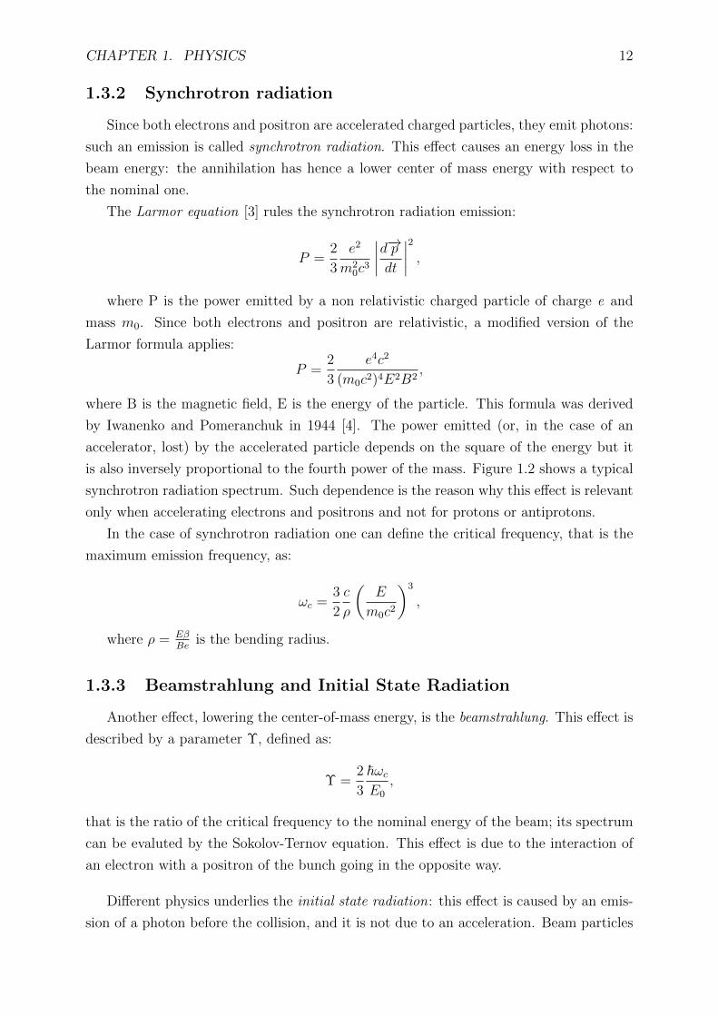
is also inversely proportional to the fourth power of the mass. Figure 1.2 shows a typical
synchrotron radiation spectrum. Such dependence is the reason why this effect is relevant
only when accelerating electrons and positrons and not for protons or antiprotons.
In the case of synchrotron radiation one can define the critical frequency, that is the
maximum emission frequency, as:
ωc =3
2
c
ρ
(E
m0c2
)3
,
where ρ = EβBe
is the bending radius.
1.3.3 Beamstrahlung and Initial State Radiation
Another effect, lowering the center-of-mass energy, is the beamstrahlung. This effect is
described by a parameter Υ, defined as:
Υ =2
3
~ωcE0
,
that is the ratio of the critical frequency to the nominal energy of the beam; its spectrum
can be evaluted by the Sokolov-Ternov equation. This effect is due to the interaction of
an electron with a positron of the bunch going in the opposite way.
Different physics underlies the initial state radiation: this effect is caused by an emis-
sion of a photon before the collision, and it is not due to an acceleration. Beam particles
CHAPTER 1. PHYSICS 13
Figure 1.2: Emission spectrum of synchrotron radiation.
can be represented by f ee (x,Q2), which describes the probability of a particle to collide
with a fraction x of its energy at the scale Q2, and is defined as:
f ee =β
2(1− x)(
β2−1)(
1 +3
8β
)− β
4(1 + x),
where
β =2α
π
(lnQ2
m2− 1
).
The scale Q2 depends on the actual interaction process, and, for central production
processes, it can be defined as Q2 = s = 4E2cm.
1.4 Charmonium
Some sharp resonances were observed in high energy e+e. annihilation processes in
the 70’s. These resonances where interpreted with an approach similar to that adopted
to interprete the positronium, i.e. as heavy hadronic bound states composed of a fermion
and an antifermion.
These bound states were first observed in 1974 at SLAC(Stanford Linear Accelera-
tor Centre), in e+e− collisions at SPEAR [5], and simultaneously at Brookhaven AGS
(Alternate Gradient Synchroton) [6] in proton scattering on a Beryllium target. The
first observed state, the so called J/ψ, was interpreted as a cc bound state, c being the
charm quark, a scheme proposed by Glashow, Iliopoulos and Maiani to explain the flavour
changing neutral currents [2]. The cc bound state are addressed as charmonium.
CHAPTER 1. PHYSICS 14
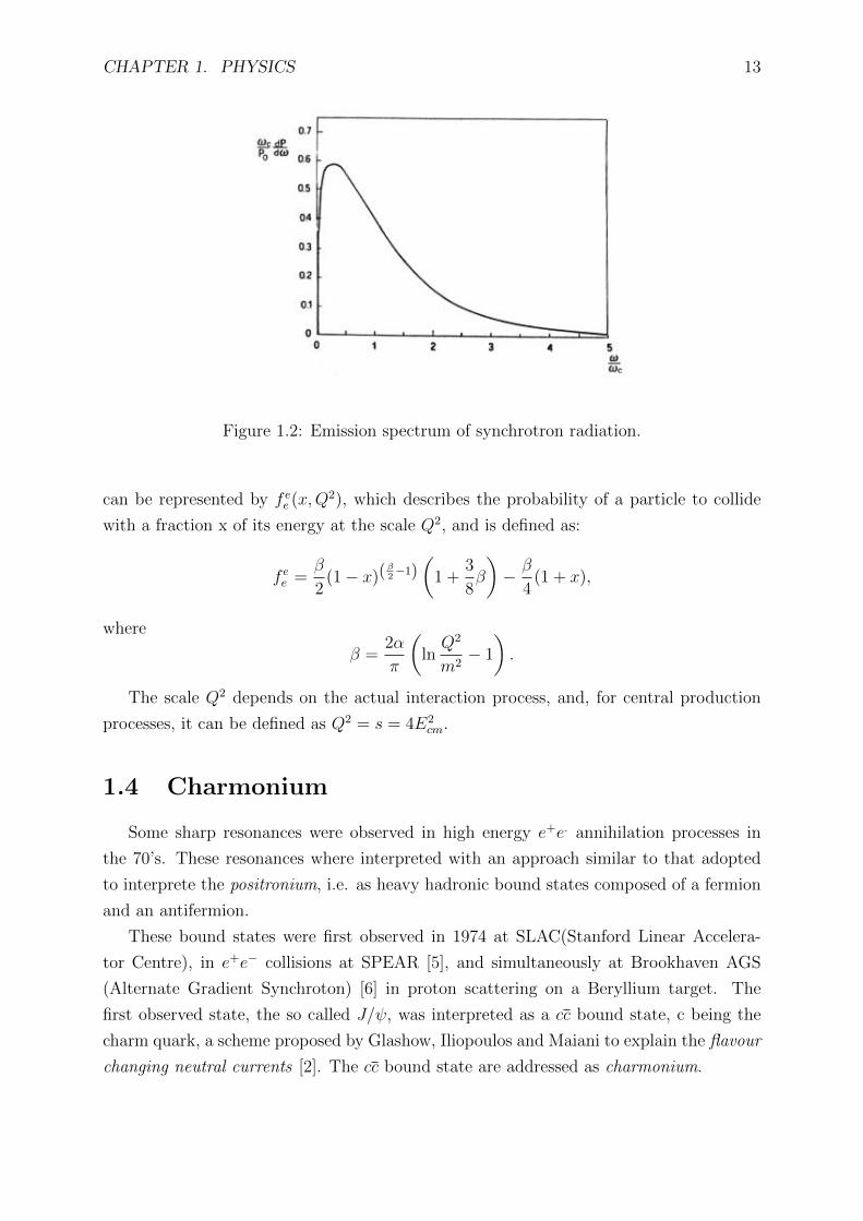
Figure 1.3: Decay of J/ψ → π+π− can explain the characteristic name ψ [2].
Properties of J/ψ
The first measurement of the J/ψ resonance width was dominated by the experimental
resolution. The true width can be calculated starting from the Breit-Wigner formula: for
a resonance of spin J from two particle of spin s1 and s2, we can write:
σ(E)e+e−→J/ψ→e+e− =4πλ2 (2J + 1) Γ2
e+e−/4
(2s1 + 1) (2s2 + 1)[(E − ER)2 + Γ2/4
] ,where λ is the de Broglie wavelength of the e+ and e− in the center of mass (cms), E
is the energy of cms, ER is the energy of the resonance, Γ is the total width, and Γe+e− is
the partial width of J/ψ → e+e−. Assuming that s1 = s2 = 12
and J = 1, the integrated
cross section is found to be:∫ ∞0
σ(E)dE =3π2
2λ2
(Γe+e−
Γ
)2
Γ.
The parameters necessary to describe the J/ψ resonance are listed in tab 1.3. The
quite small width of the charmonium is related to the large number of channels in which
it can decay. In table 1.4, 1.5 a list of J/ψ decays is given. The decay BR referred to the
exclusive J/ψ → ΛΛ decay, object of the investigation performed in this thesis, is:
BR(J/ψ → ΛΛ) = (1.61± 0.15)× 10−3
[7].
Charmonium energy levels
As it happend for the positronium, the bounds that let a cc couple forming a meson
can be parametrized by potential models.
CHAPTER 1. PHYSICS 15
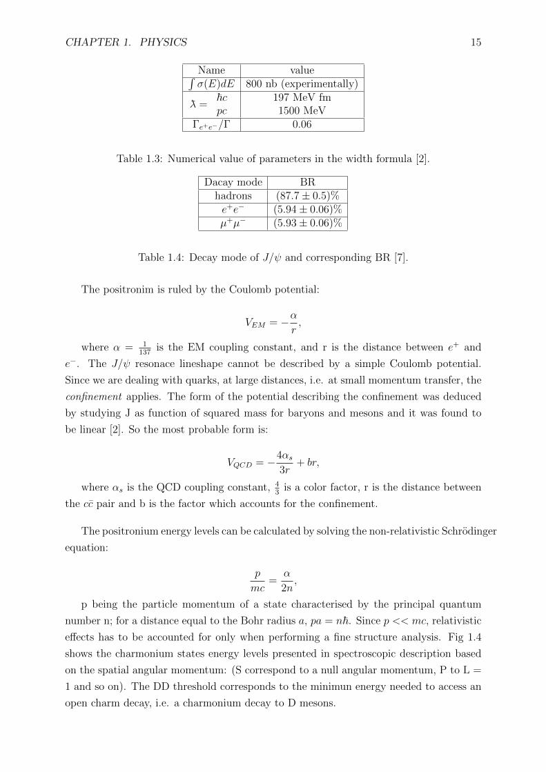
Name value∫σ(E)dE 800 nb (experimentally)
λ =~cpc
197 MeV fm1500 MeV
Γe+e−/Γ 0.06
Table 1.3: Numerical value of parameters in the width formula [2].
Dacay mode BRhadrons (87.7± 0.5)%e+e− (5.94± 0.06)%µ+µ− (5.93± 0.06)%
Table 1.4: Decay mode of J/ψ and corresponding BR [7].
The positronim is ruled by the Coulomb potential:
VEM = −αr,
where α = 1137
is the EM coupling constant, and r is the distance between e+ and
e−. The J/ψ resonace lineshape cannot be described by a simple Coulomb potential.
Since we are dealing with quarks, at large distances, i.e. at small momentum transfer, the
confinement applies. The form of the potential describing the confinement was deduced
by studying J as function of squared mass for baryons and mesons and it was found to
be linear [2]. So the most probable form is:
VQCD = −4αs3r
+ br,
where αs is the QCD coupling constant, 43
is a color factor, r is the distance between
the cc pair and b is the factor which accounts for the confinement.
The positronium energy levels can be calculated by solving the non-relativistic Schrodinger
equation:
p
mc=
α
2n,
p being the particle momentum of a state characterised by the principal quantum
number n; for a distance equal to the Bohr radius a, pa = n~. Since p << mc, relativistic
effects has to be accounted for only when performing a fine structure analysis. Fig 1.4
shows the charmonium states energy levels presented in spectroscopic description based
on the spatial angular momentum: (S correspond to a null angular momentum, P to L =
1 and so on). The DD threshold corresponds to the minimun energy needed to access an
open charm decay, i.e. a charmonium decay to D mesons.
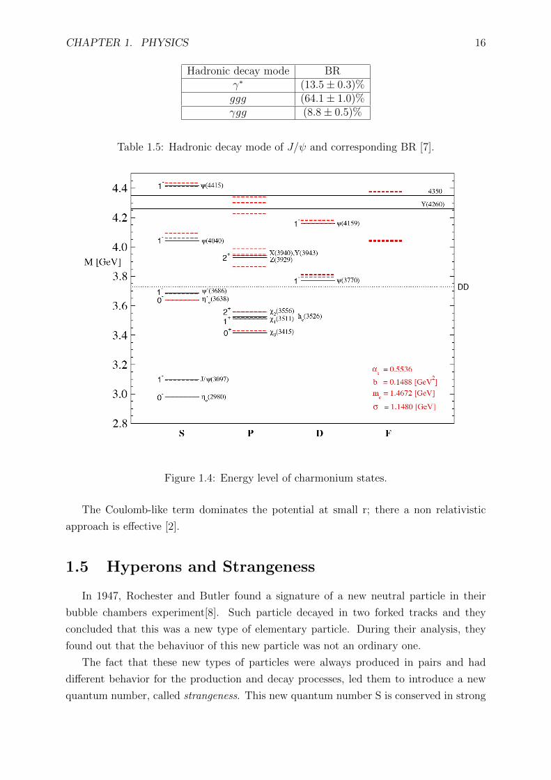
CHAPTER 1. PHYSICS 16
Hadronic decay mode BRγ∗ (13.5± 0.3)%ggg (64.1± 1.0)%γgg (8.8± 0.5)%
Table 1.5: Hadronic decay mode of J/ψ and corresponding BR [7].
Figure 1.4: Energy level of charmonium states.
The Coulomb-like term dominates the potential at small r; there a non relativistic
approach is effective [2].
1.5 Hyperons and Strangeness
In 1947, Rochester and Butler found a signature of a new neutral particle in their
bubble chambers experiment[8]. Such particle decayed in two forked tracks and they
concluded that this was a new type of elementary particle. During their analysis, they
found out that the behaviuor of this new particle was not an ordinary one.
The fact that these new types of particles were always produced in pairs and had
different behavior for the production and decay processes, led them to introduce a new
quantum number, called strangeness. This new quantum number S is conserved in strong
CHAPTER 1. PHYSICS 17
interactions but can be violated by weak interactions. They also defined hyperon a particle
carrying strangeness.
1.5.1 Strange Quark Physics - The SU(3)F Model
In a quark approach their experiments led to the introduction of a new type of quark,
and static quark model was proposed to describe the properties of hadrons. A symmetry
group SU(3)F under the hypotesis of three quark flavours, was the mathematical ground
on which such a model was introduced.
The wave function of an hyperon can be written as:
Ψ = ψ(space)φ(flavour)χ(spin)ε(color)
and must be antisymmetric, since hyperons are fermions. The colour part can only
be antisymmetric while the space part can be symmetric. The total wave function
φ(flavour) × χ(spin) should be symmetric. The SU(3)F wave functions can be decom-
posed as:
3⊗ 3⊗ 3 = 10S ⊕ 8MS⊕ 8MA
⊕ 1A,
the SU(2) wave functions as:
2⊗ 2⊗ 2 = 4S ⊕ 2MS⊕ 2MA
,
the subscripts meaning:
• S → simmetric wave function with respect to the exchange of two quarks;
• A → antisymmetric wave function with respect to the exchange of two quarks;
• MS(MA) are symmetric (antisymmetric) wave functions with respect to the ex-
change of the first two quarks.
To obtain a globally symmetric wave functions, only the (10,4) and (8,2) combinations
are possible, the numbers being the SU(3)F and SU(2) dimensions.
The introduction of a new quantum number affects also the Gell-Mann-Nishijima
formula [2], that provides the relation between electric charge and quantum numbers. Its
new form becomes:Q
e= I3 +
B + S
2= I3 +
Y
2,
where B represents the baryon number and Y is called hypercharge, and contains the sum
of all additive quantum number of the particle. [9]
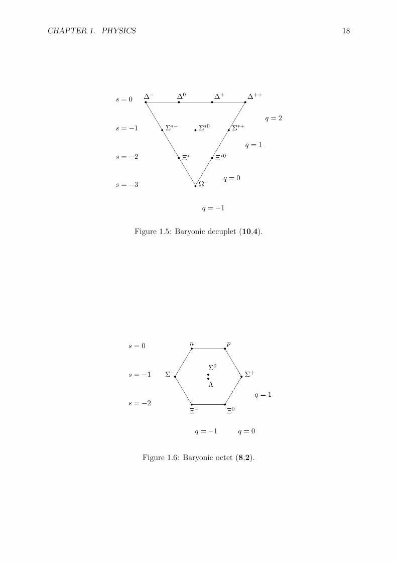
Using the hypercharge Y and the third component of the isospin I3 as coordinate axes,
the multiplets can be graphically represented, as shown in fig. 1.5 and in fig. 1.6 for the
baryons with spin S = 32
and S = 12
respectively [1].
CHAPTER 1. PHYSICS 18
Figure 1.5: Baryonic decuplet (10,4).
Figure 1.6: Baryonic octet (8,2).
CHAPTER 1. PHYSICS 19
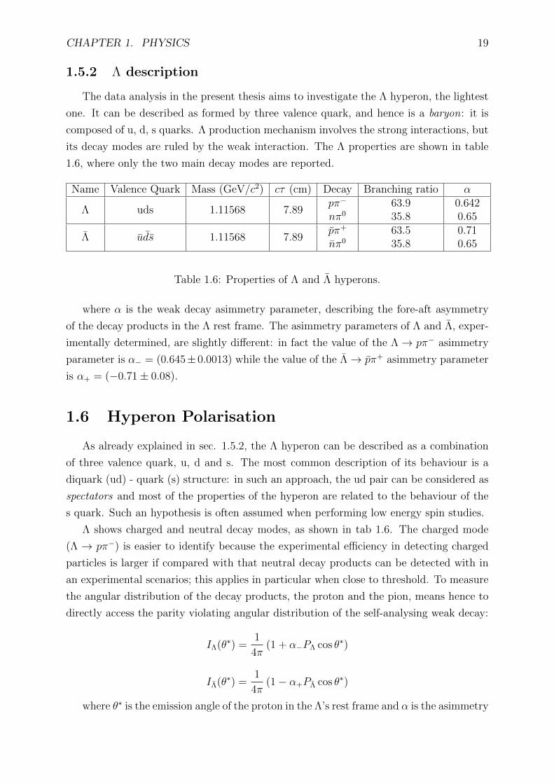
1.5.2 Λ description
The data analysis in the present thesis aims to investigate the Λ hyperon, the lightest
one. It can be described as formed by three valence quark, and hence is a baryon: it is
composed of u, d, s quarks. Λ production mechanism involves the strong interactions, but
its decay modes are ruled by the weak interaction. The Λ properties are shown in table
1.6, where only the two main decay modes are reported.
Name Valence Quark Mass (GeV/c2) cτ (cm) Decay Branching ratio α
Λ uds 1.11568 7.89pπ−
nπ0
63.935.8
0.6420.65
Λ uds 1.11568 7.89pπ+
nπ0
63.535.8
0.710.65
Table 1.6: Properties of Λ and Λ hyperons.
where α is the weak decay asimmetry parameter, describing the fore-aft asymmetry
of the decay products in the Λ rest frame. The asimmetry parameters of Λ and Λ, exper-
imentally determined, are slightly different: in fact the value of the Λ→ pπ− asimmetry
parameter is α− = (0.645± 0.0013) while the value of the Λ→ pπ+ asimmetry parameter
is α+ = (−0.71± 0.08).
1.6 Hyperon Polarisation
As already explained in sec. 1.5.2, the Λ hyperon can be described as a combination
of three valence quark, u, d and s. The most common description of its behaviour is a
diquark (ud) - quark (s) structure: in such an approach, the ud pair can be considered as
spectators and most of the properties of the hyperon are related to the behaviour of the
s quark. Such an hypothesis is often assumed when performing low energy spin studies.
Λ shows charged and neutral decay modes, as shown in tab 1.6. The charged mode
(Λ → pπ−) is easier to identify because the experimental efficiency in detecting charged
particles is larger if compared with that neutral decay products can be detected with in
an experimental scenarios; this applies in particular when close to threshold. To measure
the angular distribution of the decay products, the proton and the pion, means hence to
directly access the parity violating angular distribution of the self-analysing weak decay:
IΛ(θ∗) =1
4π(1 + α−PΛ cos θ∗)
IΛ(θ∗) =1
4π(1− α+PΛ cos θ∗)
where θ∗ is the emission angle of the proton in the Λ’s rest frame and α is the asimmetry
CHAPTER 1. PHYSICS 20
parameter. The hyperon polarization can be measured by determining the asimmetry of
the decay angular distributions, since the decay proton is emitted preferentially along the
Λ spin direction in the hyperon rest frame. When considering unpolarised lepton beams,
only the transverse polarisation can be non zero; the transverse polarisation is defined
with respect to a quantisation axis normal to the production plane.
To investigate the dependence of the Λ polarisation on the transverse momentum (pt)
means to investigate the hyperon polarisation dependence on the Λ emission angle. The
pt dependence is relevant bacause it usually allow to select between different reaction
mechanisms.
Hyperons polarisation has been recently investigated at COSY in Julich and at SA-
TURNE II in Saclay, respectively by the COSY-11 [10] and by the DISTO [11] collabo-
rations, making use of the scattering of polarised proton beams on hydrogen target.
Chapter 2
BESIII Spectrometer
In this chapter the BEPCII collider and to the BESIII spectrometer will be discussed.
More emphasis will be given to those detector parts involved in the performed analysis.
2.1 Introduction
The BESIII Collaboration is an international collaboration, which involves 31 Univer-
sities from China, 13 from Europe, 5 from USA and 4 more from other Asian countries.
The spectrometer is hosted at the BEPCII collider, placed at the IHEP, Beijing, People’s
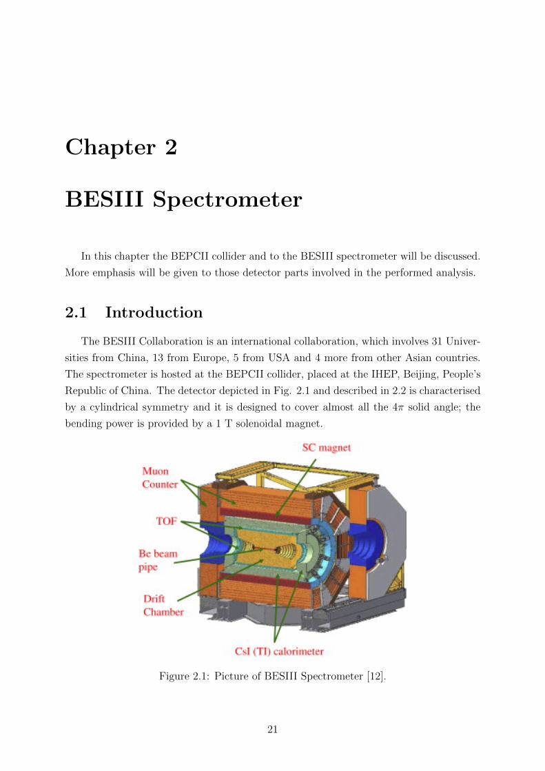
Republic of China. The detector depicted in Fig. 2.1 and described in 2.2 is characterised
by a cylindrical symmetry and it is designed to cover almost all the 4π solid angle; the
bending power is provided by a 1 T solenoidal magnet.
Figure 2.1: Picture of BESIII Spectrometer [12].
21
CHAPTER 2. BESIII SPECTROMETER 22
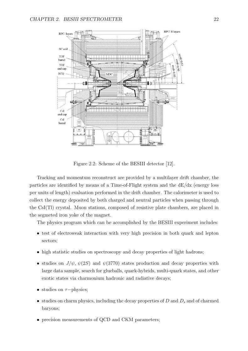
Figure 2.2: Scheme of the BESIII detector [12].
Tracking and momentum reconstruct are provided by a multilayer drift chamber, the
particles are identified by means of a Time-of-Flight system and the dE/dx (energy loss
per units of length) evaluation performed in the drift chamber. The calorimeter is used to
collect the energy deposited by both charged and neutral particles when passing through
the CsI(Tl) crystal. Muon stations, composed of resistive plate chambers, are placed in
the segmeted iron yoke of the magnet.
The physics program which can be accomplished by the BESIII experiment includes:
• test of electroweak interaction with very high precision in both quark and lepton
sectors;
• high statistic studies on spectroscopy and decay properties of light hadrons;
• studies on J/ψ, ψ(2S) and ψ(3770) states production and decay properties with
large data sample, search for glueballs, quark-hybrids, multi-quark states, and other
exotic states via charmonium hadronic and radiative decays;
• studies on τ−physics;
• studies on charm physics, including the decay properties of D and Ds and of charmed
baryons;
• precision measurements of QCD and CKM parameters;
CHAPTER 2. BESIII SPECTROMETER 23
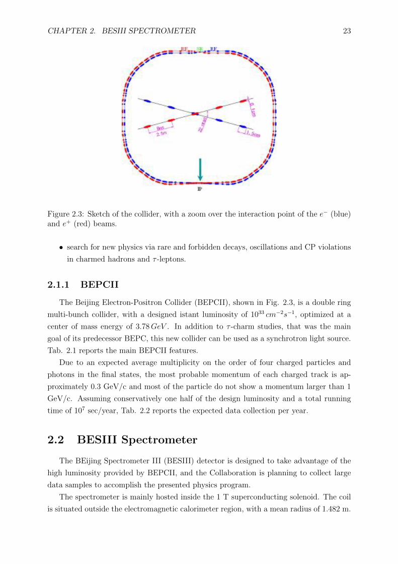
Figure 2.3: Sketch of the collider, with a zoom over the interaction point of the e− (blue)and e+ (red) beams.
• search for new physics via rare and forbidden decays, oscillations and CP violations
in charmed hadrons and τ -leptons.
2.1.1 BEPCII
The Beijing Electron-Positron Collider (BEPCII), shown in Fig. 2.3, is a double ring
multi-bunch collider, with a designed istant luminosity of 1033 cm−2s−1, optimized at a
center of mass energy of 3.78GeV . In addition to τ -charm studies, that was the main
goal of its predecessor BEPC, this new collider can be used as a synchrotron light source.
Tab. 2.1 reports the main BEPCII features.
Due to an expected average multiplicity on the order of four charged particles and
photons in the final states, the most probable momentum of each charged track is ap-
proximately 0.3 GeV/c and most of the particle do not show a momentum larger than 1
GeV/c. Assuming conservatively one half of the design luminosity and a total running
time of 107 sec/year, Tab. 2.2 reports the expected data collection per year.
2.2 BESIII Spectrometer
The BEijing Spectrometer III (BESIII) detector is designed to take advantage of the
high luminosity provided by BEPCII, and the Collaboration is planning to collect large
data samples to accomplish the presented physics program.
The spectrometer is mainly hosted inside the 1 T superconducting solenoid. The coil
is situated outside the electromagnetic calorimeter region, with a mean radius of 1.482 m.
CHAPTER 2. BESIII SPECTROMETER 24
Parameters BEPCIICenter of mass energy (GeV) 2 - 4.6
Circumference (m) 237.5Number of rings 2
RF frequency (MHz) 499.8Peak Luminosity (cm−2s−1) ∼ 1033
Number of bunches 2× 93Beam current (A) 2× 0.91
Bunch spacing (m - ns) 2.4 - 8Bunch length (σz cm) 1.5Bunch width (σx µm) ∼ 380Bunch height (σy µm) ∼ 5.7Relative energy spread 5× 10⁻⁴
Crossing angle (mrad) ±22
Table 2.1: Table of parameters of BEPCII [12].
States Energy (GeV) Peak Luminosity (1033cm−2s−1) Physics cross-section (nb) Events/year
J/ψ 3.097 0.6 3400 1× 10¹⁰
ψ(2S) 3.686 1.0 640 3× 10⁹
τ+τ− 3.670 1.0 2.4 1.2× 10⁷
D0D0 3.770 1.0 3.6 1.8× 10⁶
D+D− 3.770 1.0 2.8 1.4× 10⁶
DsDs 4.030 0.6 0.32 1× 10⁶
DsDs 4.170 0.6 1.0 2× 10⁶
Table 2.2: Expected data collection per year [12].
The polar angle coverage of the spectrometer is 21 < θ < 159, leading to the geometrical
acceptance ∆Ω/4π = 0.93.
In the next sections, the main characteristics of each detector system will be briefly
described, moving from the interaction point to the most peripheral areas.
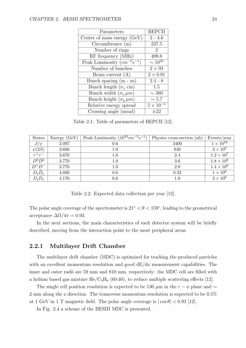
2.2.1 Multilayer Drift Chamber
The multilayer drift chamber (MDC) is optimized for tracking the produced particles
with an excellent momentum resolution and good dE/dx measurement capabilities. The
inner and outer radii are 59 mm and 810 mm, respectively: the MDC cell are filled with
a helium based gas mixture He/C3H8 (60:40), to reduce multiple scattering effects [12].
The single cell position resolution is expected to be 130 µm in the r − φ plane and ∼2 mm along the z direction. The transverse momentum resolution is expected to be 0.5%
at 1 GeV in 1 T magnetic field. The polar angle coverage is | cos θ| < 0.93 [12].
In Fig. 2.4 a scheme of the BESIII MDC is presented.
CHAPTER 2. BESIII SPECTROMETER 25
Figure 2.4: Scheme of the BESIII MDC [12].
Performance
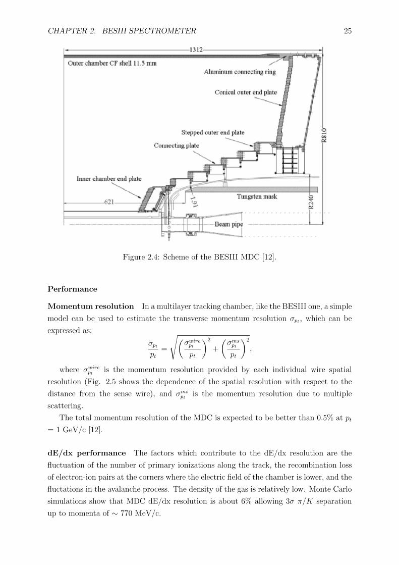
Momentum resolution In a multilayer tracking chamber, like the BESIII one, a simple
model can be used to estimate the transverse momentum resolution σpt , which can be
expressed as:
σptpt
=
√(σwirept
pt
)2
+
(σmsptpt
)2
,
where σwirept is the momentum resolution provided by each individual wire spatial
resolution (Fig. 2.5 shows the dependence of the spatial resolution with respect to the
distance from the sense wire), and σmspt is the momentum resolution due to multiple
scattering.
The total momentum resolution of the MDC is expected to be better than 0.5% at pt
= 1 GeV/c [12].
dE/dx performance The factors which contribute to the dE/dx resolution are the
fluctuation of the number of primary ionizations along the track, the recombination loss
of electron-ion pairs at the corners where the electric field of the chamber is lower, and the
fluctations in the avalanche process. The density of the gas is relatively low. Monte Carlo
simulations show that MDC dE/dx resolution is about 6% allowing 3σ π/K separation
up to momenta of ∼ 770 MeV/c.
CHAPTER 2. BESIII SPECTROMETER 26
Figure 2.5: Spatial resolution wrt the distance from the sense wire [12].
2.2.2 Time of Flight System
The Time Of Flight (TOF) system, which consists of a barrel and two end caps, is
composed of plastic scintillator bars read out by fine mesh photomultiplier tubes attached
at the two end faces of the bar. The expected time resolution (∼ 100 ps) allows for a 3σ
π/K separation.
The position of the TOF layers is constrained by the compact design of BESIII: in the
barrel region, the inner radius of the first layer is 810 mm and the second one is 860 mm,
while one layer is placed in the end caps region. The relatively short particle flight path
makes the design of the TOF system challenging.
A cross section view of the TOF system inside the calorimeter is shown in fig. 2.2.
Performance
Time resolution The overall time resolution σ of the spectrometer can be expressed
as
σ =√σ2i + σ2
b + σ2l + σ2
z + σ2e + σ2
t + σ2w
.
The value of each term is reported in Tab. 2.3. The σz depends on the time needed
to collect the signal and is estimated to be around 30 ps and 50 ps for the barrel and end
caps region, respectively.
Excluding σi and σw, the total contribution from those terms not directly related to
the counters (the other five) to the uncertainty of the TOF system is about 66 ps for
the barrel and 87 ps for the end caps region. Using two layer in the barrel improves the
resolution of the intrinsic factor of the TOF system, i.e. σi and σw, by a factor of√
2.
CHAPTER 2. BESIII SPECTROMETER 27
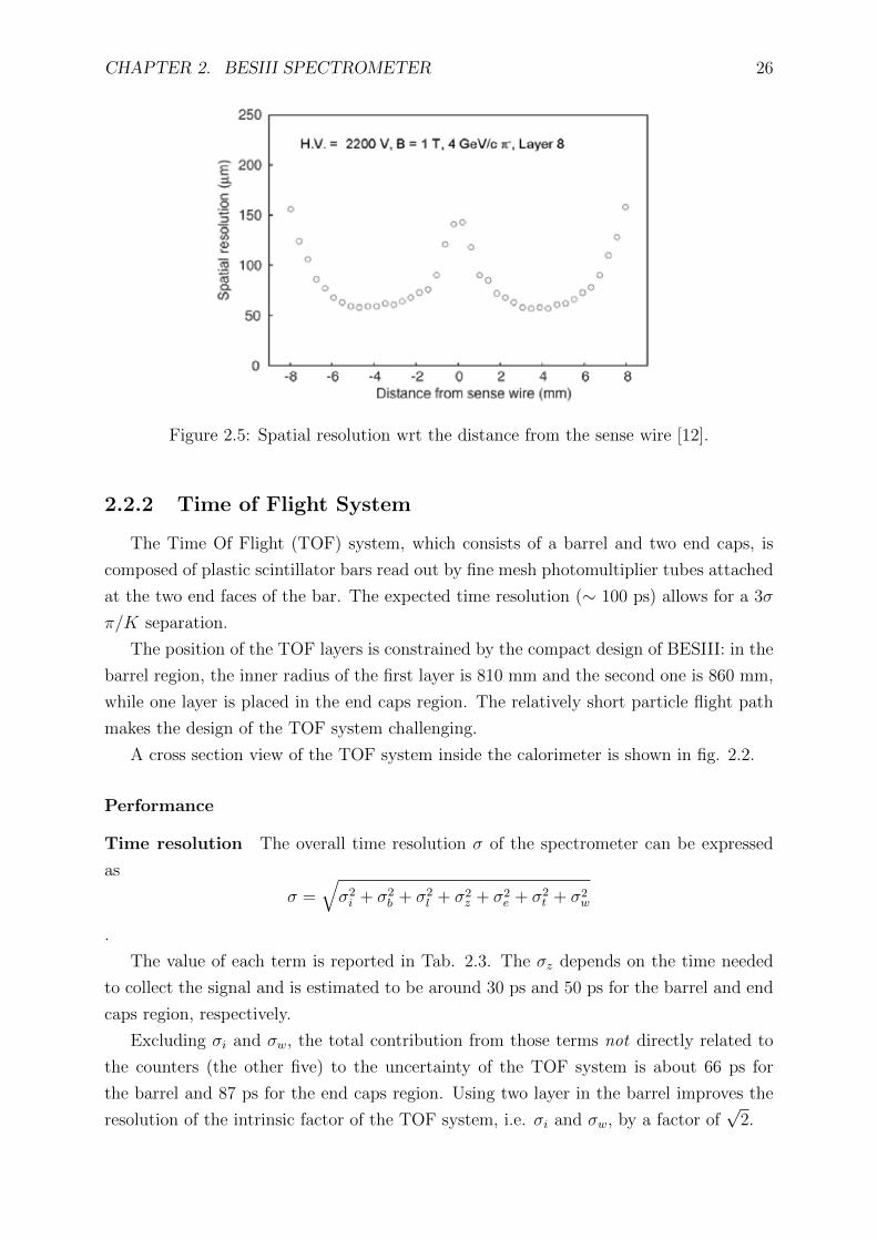
σ Barrel (ps) EndCap (ps)σi: counter intrinsic time resolution 80 ∼ 90 80
σl: uncertainty from 15 mm bunch length 35 35σb: uncertainty from clock system ∼ 20 ∼ 20σθ : uncertainty from θ-angle 25 50σe: uncertainty from electronics 25 25
σt: uncertainty in expected flight time 30 30σw: uncertainty from time walk 10 10
σ1: total time resolution, one layer 100 - 110 110combined time resolution, two layes 80 - 90 -
Table 2.3: TOF time resolution performance for 1 GeV/c muons [12].
Figure 2.6: Kaon identification (up K → K ) and misidentification (down K → πefficiency. [12])
Particle ID Figure 2.6 shows the simulated separation capability of the BESIII barrel
TOF system.
A K/π separation efficiency of 95% and a contamination level of about 5% can be
achieved up to a momentum of 0.9 GeV/c [12].
2.2.3 Electromagnetic Calorimeter
The electromagnetic calorimeter (EMC), composed of CsI(Tl) crystals, is designed to
precisely measure the energies of photons above 20 MeV, and to provide trigger signals.
It has good e/π discrimination capabilities for momenta above 200 MeV.
It is composed of 6240 CsI(Tl) crystals placed outside the TOF counters. The inner
CHAPTER 2. BESIII SPECTROMETER 28
radius of the BESIII EMC is 940 mm. The length of the crystals, 28 cm, corresponds to
15 radiation lengths (X0) and their section varies from the front face (5.2 cm × 5.2 cm)
to the rear face (6.4 cm × 6.4 cm). The design energy resolution of the EM showers is
σE/E = 2.5%√E and the design position resolution is σ = 0.6cm/
√E at an energy of 1
GeV.
The properties of CsI(Tl) scintillating crystals are listed in Tab. 2.4.
Parameter ValuesRadiation length X0 1.85 cm
Moliere radius 3.8 cmDensity 4.53 g/cm3
Light yield (photodiode) 56000 γ’s/MeVPeak emission wavelength 560 nm
Signal decay time 680 ns (64%)3.34 ms (36%)
Light yield temp coefficient 0.3 %/CdE/dx (per mip) 5.6 MeV/cm
Hygroscopic sensivity slight
Table 2.4: Properties of thallium doped CsI(Tl) crystal [12].
Performance
Position and Energy Resolution The energy resolution is affected by many factors
(dead materials, crystal quality, etc.). The photon position resolution is mainly deter-
mined by the cristal segmentation [12]. The EMC composed of 28 cm long CsI crystals
can reach the desired energy resolution of ≤ 2.5% at 1 GeV photon energy.
2.2.4 Muon Counter
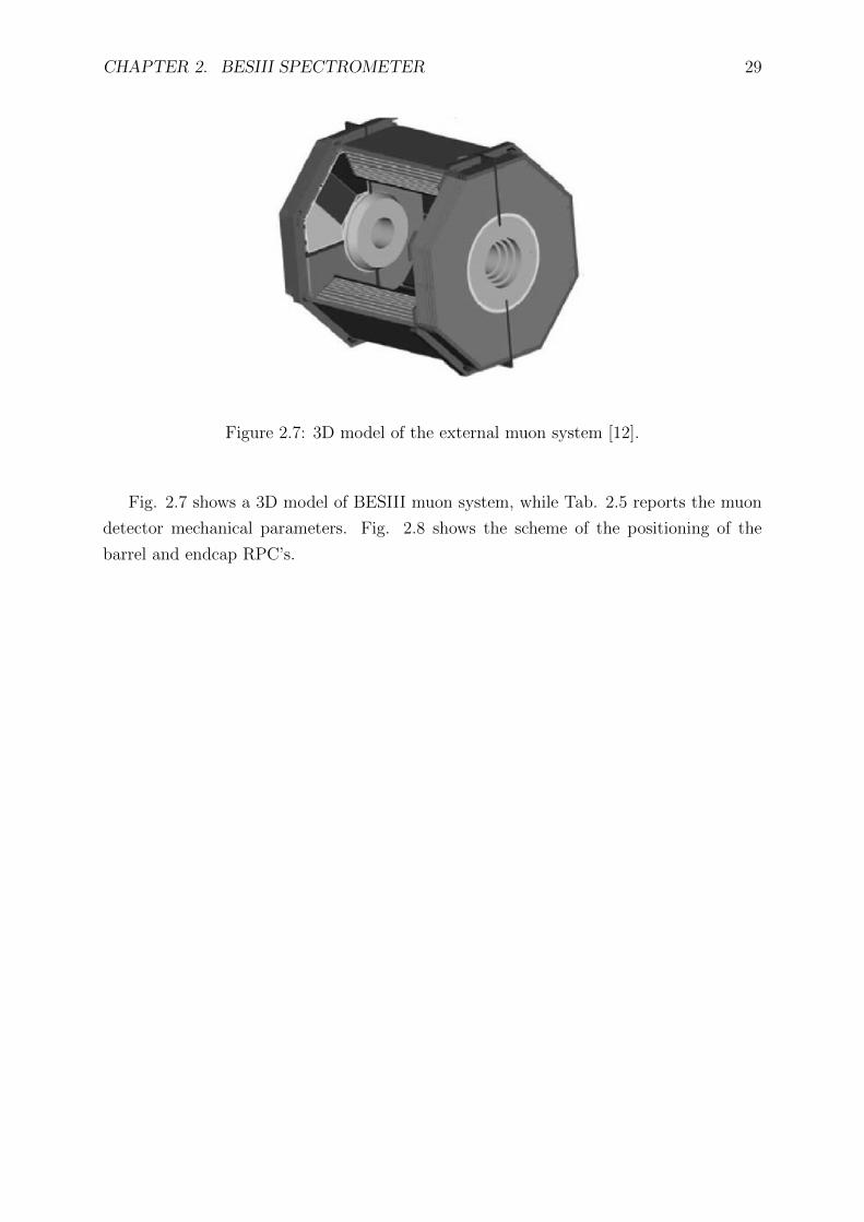
The muon detector consists of resistive plate chambers (RPC) hosted in the steel plates
of the magnetic flux return yoke of the solenoidal magnet. Its main functions is to detect
and separate muons from charged pions, expecially at lower momenta. There are nine
layers of RPC in the barrel and eight in the end caps.
By associating hits in muon counters with tracks reconstructed in the MDC and energy
measured in the EMC, the muons can be identified with a low cut-off momentum. The
requirements for the position resolution of the RPC are modest due to multiple scattering
which can occur in the EMC, in the magnet coil, and in the steel layers. The typical
width of the readout strips in the RPC is about 4 cm.
The active part of the muon detectors must be highly reliable and relatively cheap,
since the area to be covered is quite large and almost inaccessible once the detectors are
installed. Muon detectors are fluxed with an Ar/C2F4H2/C4H10 (50:42:8) gas mixture.
CHAPTER 2. BESIII SPECTROMETER 29
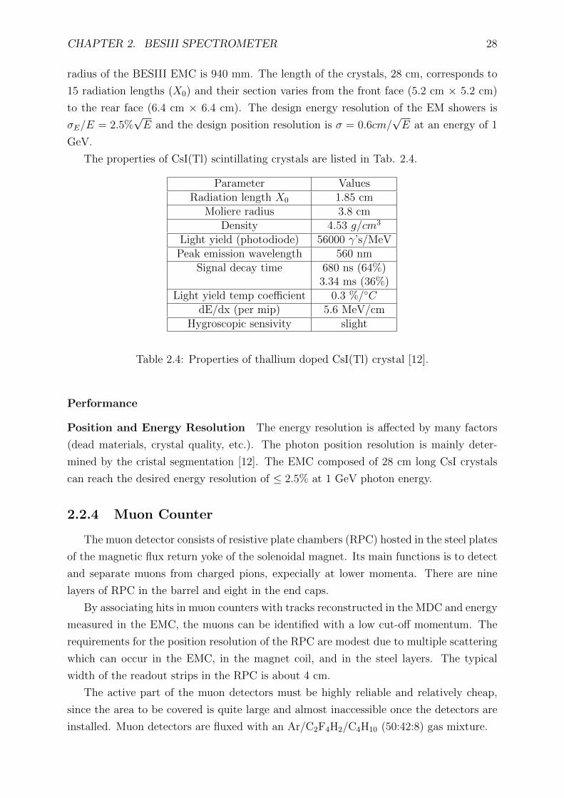
Figure 2.7: 3D model of the external muon system [12].
Fig. 2.7 shows a 3D model of BESIII muon system, while Tab. 2.5 reports the muon
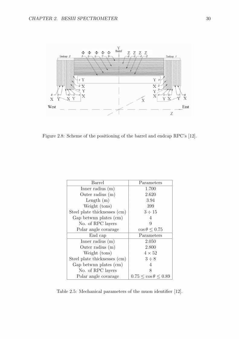
detector mechanical parameters. Fig. 2.8 shows the scheme of the positioning of the
barrel and endcap RPC’s.
CHAPTER 2. BESIII SPECTROMETER 30
Figure 2.8: Scheme of the positioning of the barrel and endcap RPC’s [12].
Barrel ParametersInner radius (m) 1.700Outer radius (m) 2.620
Length (m) 3.94Weight (tons) 399
Steel plate thicknesses (cm) 3÷ 15Gap betwnn plates (cm) 4
No. of RPC layers 9Polar angle covarage cos θ ≤ 0.75
End cap ParametersInner radius (m) 2.050Outer radius (m) 2.800
Weight (tons) 4× 52Steel plate thicknesses (cm) 3÷ 8
Gap betwnn plates (cm) 4No. of RPC layers 8
Polar angle covarage 0.75 ≤ cos θ ≤ 0.89
Table 2.5: Mechanical parameters of the muon identifier [12].
Part II
Data Analysis
31
Chapter 3
Analysis e+e−→ ΛΛ
The inclusive process e+e− → ΛΛ is first investigated process. Only their charged
decay channels Λ→ pπ− (Λ→ pπ+) are used to recontruct hyperons, since characterised
by an higher branching ratio and since the experimental efficiency in detecting charged
particles is expected to be larger if compared to that of neutral particles.
For this process, two track candidates selection method were implemented: the clas-
sical particle identification and the kinematic fit, a quite commonly used technique. The
phsyical observables of the ΛΛ process are hence investigated once the events selection
has been performed.
For this analysis, two data samples were used: a first one collected during the 2009
data taking run and a second one collected during the 2012 run. First I have analysed,
using BOSS version 6.6.2, the data collected in 2012: these data were collected to perform
a J/ψ lineshape scan and will also be used to evaluate the relative phase between strong
and electromagnetic J/ψ decay amplitudes. The nominal energies and the integrated
luminosities of each collected center of mass energy are shown in Tab. 3.1. Afterwards, I
have analysed the 79pb−1 J/ψ peak data collected at the J/ψ peak in 2009 using BOSS
version 6.5.5.
To perform efficiency corrections, I have also used the 225M Monte-Carlo J/ψ inclusive
sample, provided by the Collaboration and analysed with the BOSS version 6.5.5. In this
inclusive sample, all the J/ψ decays are simulated with their respective branching ratios
(BR). ROOT [13] version 5.24 has been used for all the analyses.
3.1 Event Simulation
In order to understand the real data scenario, it is necessary to evaluate the behaviour
of Monte Carlo signals produced with the generator BesEvtGen [14] implemented in
BOSS version 6.6.2, the official collaboration software framework. This software allows to
generate events for the final states under investigation, which are then propagated inside
the detector by means of GEANT4.
32
CHAPTER 3. ANALYSIS E+E− → ΛΛ 33
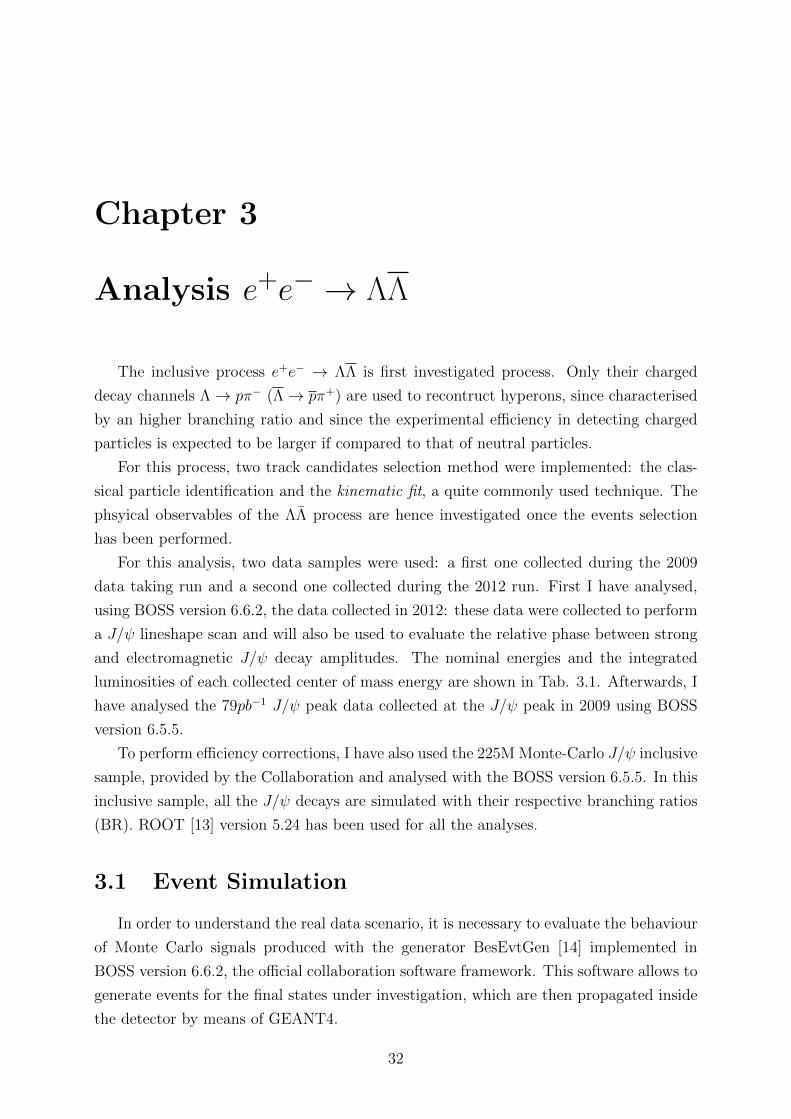
Ecm (GeV) L(pb−1)3.05 14.895± 0.0293.06 15.056± 0.033.083 4.759± 0.0173.0856 17.507± 0.0323.09 15.552± 0.033.093 15.249± 0.033.0943 2.145± 0.0113.0952 1.819± 0.013.0958 2.161± 0.0113.0969 2.097± 0.0113.0982 2.210± 0.0113.099 0.759± 0.0073.1015 1.164± 0.0103.1055 2.106± 0.0113.112 1.719± 0.013.12 1.261± 0.009
Table 3.1: Center of mass energies and luminosity measurements [15].
A typical BesEvtGen simulation card looks like:
Decay J/psi ← set the mother particle (its properties are taken from [7])
1.0000 Lambda0 Anti-Lambda0 PHSP ← PHSP (stays for PHase SPace), indicates the
probability of a certain decay mode and its angular distribution
Enddecay
Decay Lambda0
1.0000 p+ pi- PHSP
Enddecay
Decay Anti-Lambda0
1.0000 anti-p- pi+ PHSP
Enddecay
This generator card was used to produce 104 ΛΛ events and the subsequent decays
into their charged decay channels with a PHSP angular distribution for the 16 center of
mass energies collected, enlisted in Tab. 3.1.
To be sure that we are dealing with a reliable Monte Carlo simulation, the agree-
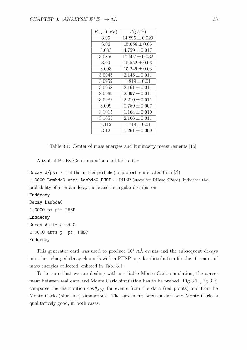
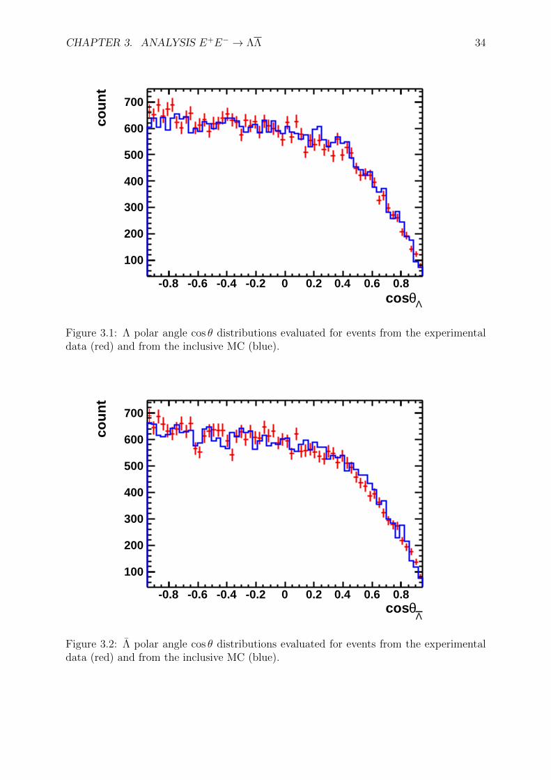
ment between real data and Monte Carlo simulation has to be probed. Fig 3.1 (Fig 3.2)
compares the distribution cos θΛ(Λ) for events from the data (red points) and from he
Monte Carlo (blue line) simulations. The agreement between data and Monte Carlo is
qualitatively good, in both cases.
CHAPTER 3. ANALYSIS E+E− → ΛΛ 34
Λθcos-0.8 -0.6 -0.4 -0.2 0 0.2 0.4 0.6 0.8
cou
nt
100
200
300
400
500
600
700
Figure 3.1: Λ polar angle cos θ distributions evaluated for events from the experimentaldata (red) and from the inclusive MC (blue).
Λθcos
-0.8 -0.6 -0.4 -0.2 0 0.2 0.4 0.6 0.8
cou
nt
100
200
300
400
500
600
700
Figure 3.2: Λ polar angle cos θ distributions evaluated for events from the experimentaldata (red) and from the inclusive MC (blue).
CHAPTER 3. ANALYSIS E+E− → ΛΛ 35
3.2 Event Selection
The choice of reconstructing hyperons through their charged decays only implies that
I need to perform the event selection asking for four reconstructed charged tracks and
zero net charge. Moreover I impose additional kinematic cuts: the selected events are
only those ones for which the vertex of all four charged tracks is inside a cylinder with
a radius of 10 cm and a lenght along the z direction of 20 cm; charged tracks must have
a | cos θ| < 0.92 in the LAB frame, i.e. 21 < θ < 153; finally each charged track’s
momentum should be < 2.GeV, since in a four particle decay no candidate can bring
more than half of the total energy of the event.
PID
I use the PID system information (dE/dx and TOF of the particle) in order to identify
the tracks with the probability density function method. For example, to be identified
as proton, a track candidate must have a probability > 0.001 to be a proton, and this
probability has to be higher than the one to be a kaon or a pion. Once obtained this
information, I select those events in which two tracks are identified as proton (p and p)
and two tracks as pion (π+ and π−).
Afterwards, I require that the constructed pπ− and pπ+ pairs survive a vertex fit
algorithm: this selection is operated in order to verify that p(p) and π−(+) come from
a common vertex, that is then tagged as the Λ(Λ) decay vertex. The same algorithm
perform a fit on the parameters of the tracks, tuning the 4-momenta of protons and
pions. To evalutate thr Λ(Λ)’s 4-momentum, I sum over the 4-momenta of the decay
particles.
In order to reduce the possible background, expecially in the energy region under the
J/ψ resonance, I considered the fact that this process can be described as a two-body
decay: as it is known, in a two-body decay daughter particles go back-to-back in the
parent particle’s rest frame. Although the boost of the event center of mass (CM) in the
Laboratory frame (LAB) slightly differs from zero, one can consider the two reference
frames to be almost coincident, so the angle between the reconstructed Λ and Λ should
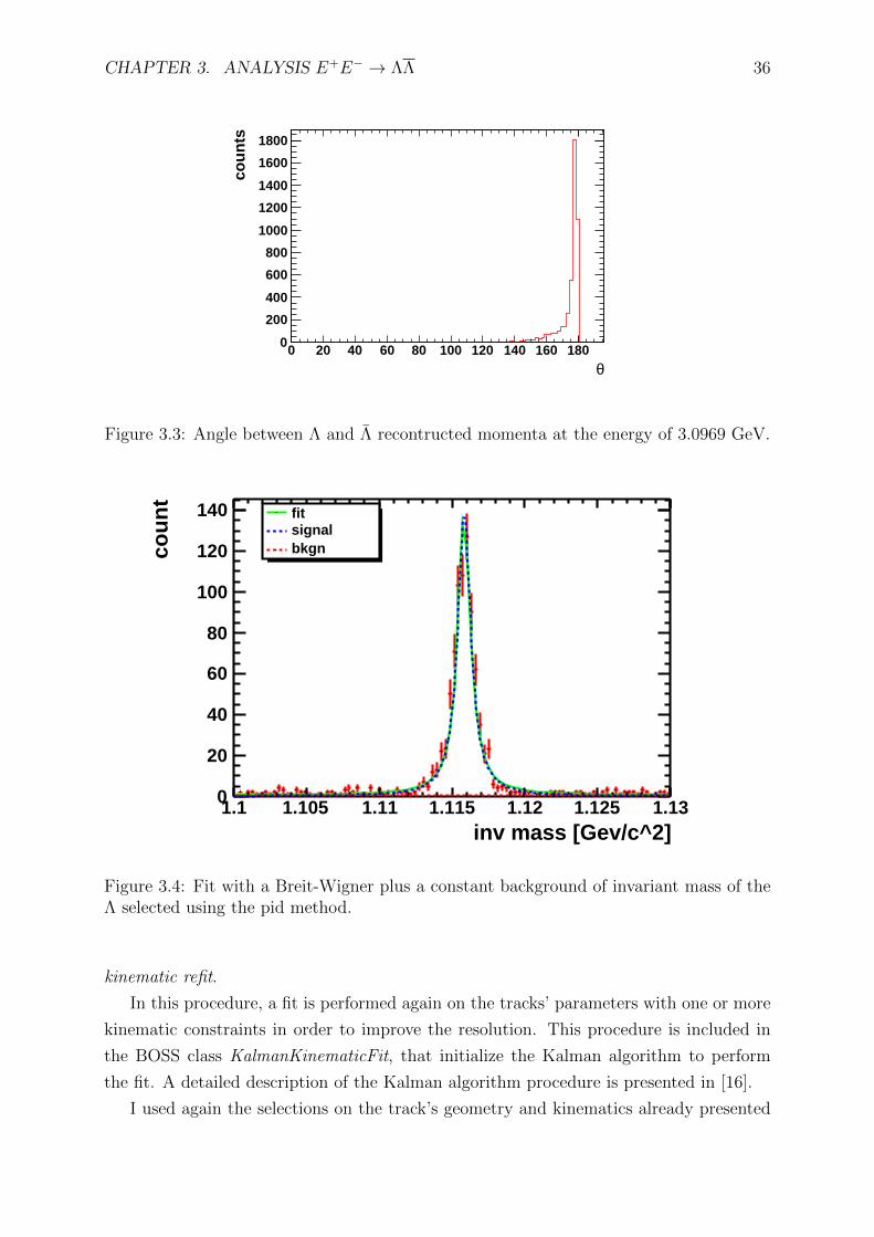
be 180M; due to the detector finite resolution, a cut on ΛΛ > 178 was imposed (Fig.
3.3 shows the distribution of the angle between the tracks).
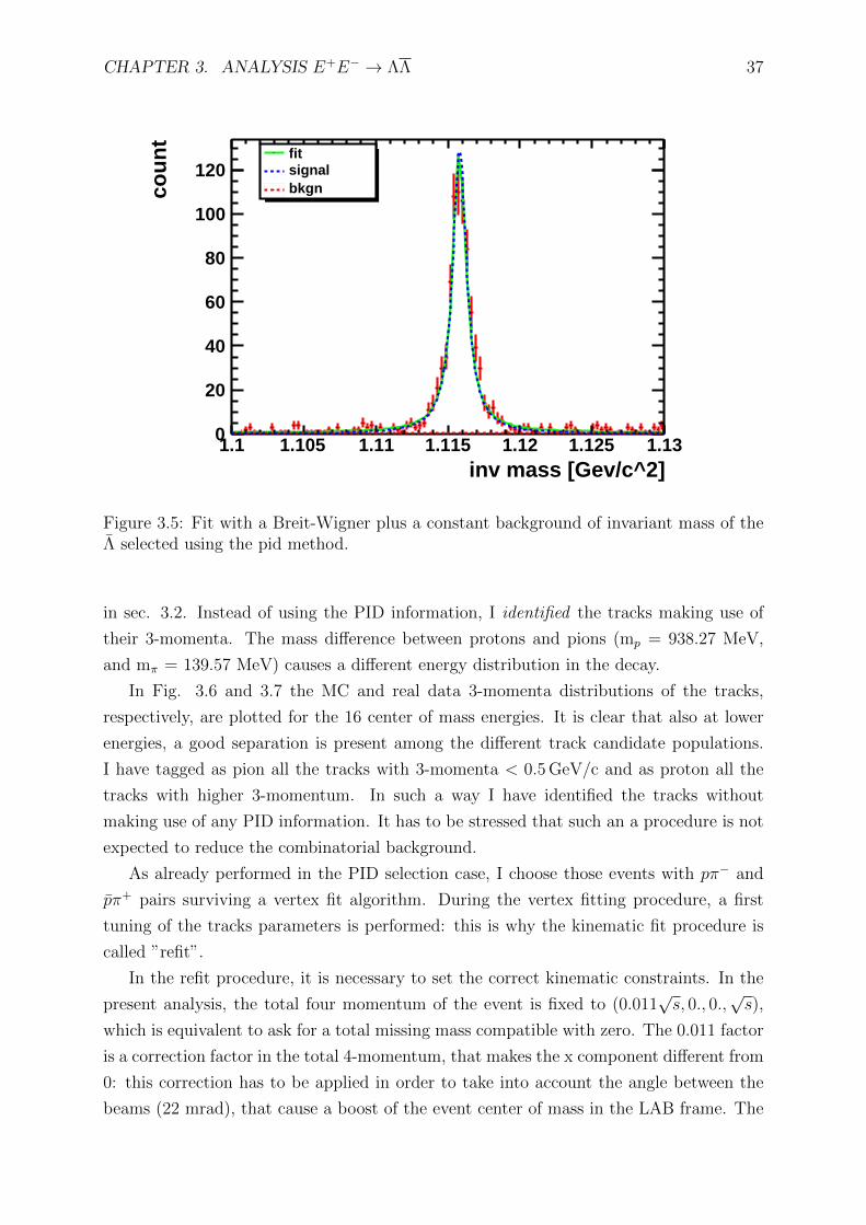
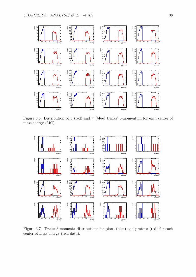
The invariant mass distributions of the reconstructed Λ, Λ, fitted with a Breit-Wigner
function plus a flat background, are presented in Fig. 3.4 and 3.5, respectively.
Kinematic Refitting
Once I have verified that a classical PID approach is possible, I want to explore another
well-known procedure that should have, in principle, a better event rejection factor: the
CHAPTER 3. ANALYSIS E+E− → ΛΛ 36
θ0 20 40 60 80 100 120 140 160 180
cou
nts
0
200
400
600
800
1000
1200
1400
1600
1800
Figure 3.3: Angle between Λ and Λ recontructed momenta at the energy of 3.0969 GeV.
inv mass [Gev/c^2]1.1 1.105 1.11 1.115 1.12 1.125 1.13
cou
nt
0
20
40
60
80
100
120
140 fitsignalbkgn
Figure 3.4: Fit with a Breit-Wigner plus a constant background of invariant mass of theΛ selected using the pid method.
kinematic refit.
In this procedure, a fit is performed again on the tracks’ parameters with one or more
kinematic constraints in order to improve the resolution. This procedure is included in
the BOSS class KalmanKinematicFit, that initialize the Kalman algorithm to perform
the fit. A detailed description of the Kalman algorithm procedure is presented in [16].
I used again the selections on the track’s geometry and kinematics already presented
CHAPTER 3. ANALYSIS E+E− → ΛΛ 37
inv mass [Gev/c^2]1.1 1.105 1.11 1.115 1.12 1.125 1.13
cou
nt
0
20
40
60
80
100
120fitsignalbkgn
Figure 3.5: Fit with a Breit-Wigner plus a constant background of invariant mass of theΛ selected using the pid method.
in sec. 3.2. Instead of using the PID information, I identified the tracks making use of
their 3-momenta. The mass difference between protons and pions (mp = 938.27 MeV,
and mπ = 139.57 MeV) causes a different energy distribution in the decay.
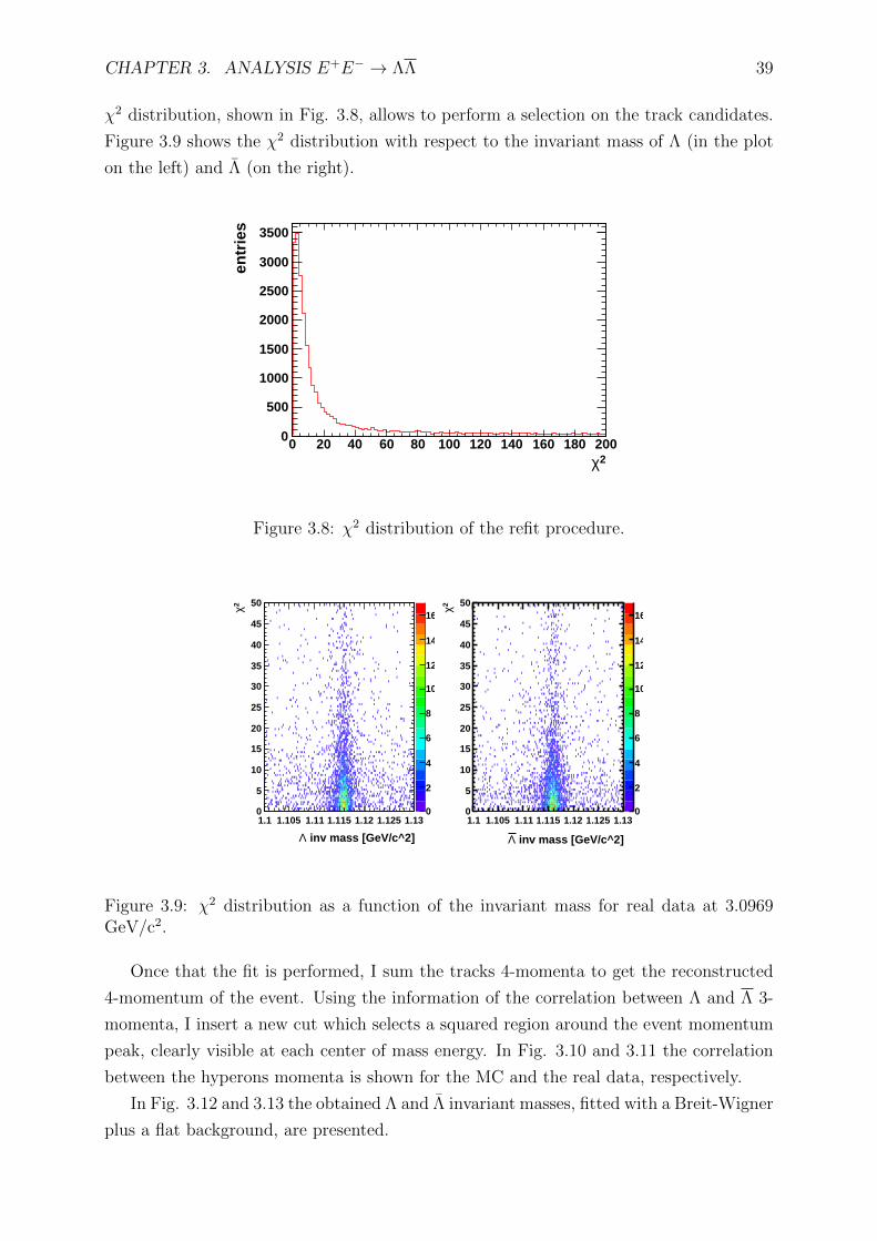
In Fig. 3.6 and 3.7 the MC and real data 3-momenta distributions of the tracks,
respectively, are plotted for the 16 center of mass energies. It is clear that also at lower
energies, a good separation is present among the different track candidate populations.
I have tagged as pion all the tracks with 3-momenta < 0.5 GeV/c and as proton all the
tracks with higher 3-momentum. In such a way I have identified the tracks without
making use of any PID information. It has to be stressed that such an a procedure is not
expected to reduce the combinatorial background.
As already performed in the PID selection case, I choose those events with pπ− and
pπ+ pairs surviving a vertex fit algorithm. During the vertex fitting procedure, a first
tuning of the tracks parameters is performed: this is why the kinematic fit procedure is
called ”refit”.
In the refit procedure, it is necessary to set the correct kinematic constraints. In the
present analysis, the total four momentum of the event is fixed to (0.011√s, 0., 0.,
√s),
which is equivalent to ask for a total missing mass compatible with zero. The 0.011 factor
is a correction factor in the total 4-momentum, that makes the x component different from
0: this correction has to be applied in order to take into account the angle between the
beams (22 mrad), that cause a boost of the event center of mass in the LAB frame. The
CHAPTER 3. ANALYSIS E+E− → ΛΛ 38
p (GeV/c)0 0.2 0.4 0.6 0.8 1 1.2
cou
nts
020
40
60
80
100
120
140
160
180
200
p (GeV/c)0 0.2 0.4 0.6 0.8 1 1.2
cou
nts
0
20
40
60
80
100
120
140
160
180
200
p (GeV/c)0 0.2 0.4 0.6 0.8 1 1.2
cou
nts
0
50
100
150
200
250
300
p (GeV/c)0 0.2 0.4 0.6 0.8 1 1.2
cou
nts
0
50
100
150
200
250
300
p (GeV/c)0 0.2 0.4 0.6 0.8 1 1.2
cou
nts
0
50
100
150
200
250
300
p (GeV/c)0 0.2 0.4 0.6 0.8 1 1.2
cou
nts
0
50
100
150
200
250
300
p (GeV/c)0 0.2 0.4 0.6 0.8 1 1.2
cou
nts
0
50
100
150
200
250
300
p (GeV/c)0 0.2 0.4 0.6 0.8 1 1.2
cou
nts
0
50
100
150
200
250
300
p (GeV/c)0 0.2 0.4 0.6 0.8 1 1.2
cou
nts
0
50
100
150
200
250
300
p (GeV/c)0 0.2 0.4 0.6 0.8 1 1.2
cou
nts
0
50
100
150
200
250
300
p (GeV/c)0 0.2 0.4 0.6 0.8 1 1.2
cou
nts
0
50
100
150
200
250
300
p (GeV/c)0 0.2 0.4 0.6 0.8 1 1.2
cou
nts
0
50
100
150
200
250
300
p (GeV/c)0 0.2 0.4 0.6 0.8 1 1.2
cou
nts
0
50
100
150
200
250
300
p (GeV/c)0 0.2 0.4 0.6 0.8 1 1.2
cou
nts
0
50
100
150
200
250
300
p (GeV/c)0 0.2 0.4 0.6 0.8 1 1.2
cou
nts
0
50
100
150
200
250
300
p (GeV/c)0 0.2 0.4 0.6 0.8 1 1.2
cou
nts
0
50
100
150
200
250
300
Figure 3.6: Distribution of p (red) and π (blue) tracks’ 3-momentum for each center ofmass energy (MC).
p (GeV/c)0 0.2 0.4 0.6 0.8 1 1.2
cou
nts
0
0.5
1
1.5
2
2.5
3
3.5
4
p (GeV/c)0 0.2 0.4 0.6 0.8 1 1.2
cou
nts
0
0.5
1
1.5
2
2.5
3
3.5
4
p (GeV/c)0 0.2 0.4 0.6 0.8 1 1.2
cou
nts
00.2
0.4
0.6
0.81
1.2
1.4
1.61.8
2
p (GeV/c)0 0.2 0.4 0.6 0.8 1 1.2
cou
nts
00.2
0.4
0.6
0.81
1.2
1.4
1.61.8
2
p (GeV/c)0 0.2 0.4 0.6 0.8 1 1.2
cou
nts
0
0.5
1
1.5
2
2.5
3
p (GeV/c)0 0.2 0.4 0.6 0.8 1 1.2
cou
nts
0
1
2
3
4
5
6
7
8
p (GeV/c)0 0.2 0.4 0.6 0.8 1 1.2
cou
nts
02
4
6
81012
14
1618
20
p (GeV/c)0 0.2 0.4 0.6 0.8 1 1.2
cou
nts
0
5
10
15
20
25
30
35
40
45
p (GeV/c)0 0.2 0.4 0.6 0.8 1 1.2
cou
nts
0
20
40
60
80
100
120
p (GeV/c)0 0.2 0.4 0.6 0.8 1 1.2
cou
nts
0
20
40
60
80
100
120
140
160
180
200
p (GeV/c)0 0.2 0.4 0.6 0.8 1 1.2
cou
nts
0
10
20
30
40
50
60
70
80
90
p (GeV/c)0 0.2 0.4 0.6 0.8 1 1.2
cou
nts
0
2
4
6
8
10
12
14
16
p (GeV/c)0 0.2 0.4 0.6 0.8 1 1.2
cou
nts
0
2
4
6
8
10
p (GeV/c)0 0.2 0.4 0.6 0.8 1 1.2
cou
nts
01
2
3
4
5
6
7
8
9
p (GeV/c)0 0.2 0.4 0.6 0.8 1 1.2
cou
nts
0
1
2
3
4
5
p (GeV/c)0 0.2 0.4 0.6 0.8 1 1.2
cou
nts
0
0.5
1
1.5
2
2.5
3
Figure 3.7: Tracks 3-momenta distributions for pions (blue) and protons (red) for eachcenter of mass energy (real data).
CHAPTER 3. ANALYSIS E+E− → ΛΛ 39
χ2 distribution, shown in Fig. 3.8, allows to perform a selection on the track candidates.
Figure 3.9 shows the χ2 distribution with respect to the invariant mass of Λ (in the plot
on the left) and Λ (on the right).
2χ0 20 40 60 80 100 120 140 160 180 200
entr
ies
0
500
1000
1500
2000
2500
3000
3500
Figure 3.8: χ2 distribution of the refit procedure.
inv mass [GeV/c^2]Λ1.1 1.105 1.11 1.115 1.12 1.125 1.13
2 χ
0
5
10
15
20
25
30
35
40
45
50
0
2
4
6
8
10
12
14
16
inv mass [GeV/c^2]Λ
1.1 1.105 1.11 1.115 1.12 1.125 1.13
2 χ
0
5
10
15
20
25
30
35
40
45
50
0
2
4
6
8
10
12
14
16
Figure 3.9: χ2 distribution as a function of the invariant mass for real data at 3.0969GeV/c2.
Once that the fit is performed, I sum the tracks 4-momenta to get the reconstructed
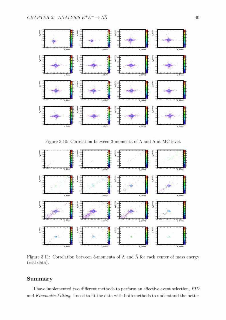
4-momentum of the event. Using the information of the correlation between Λ and Λ 3-
momenta, I insert a new cut which selects a squared region around the event momentum
peak, clearly visible at each center of mass energy. In Fig. 3.10 and 3.11 the correlation
between the hyperons momenta is shown for the MC and the real data, respectively.
In Fig. 3.12 and 3.13 the obtained Λ and Λ invariant masses, fitted with a Breit-Wigner
plus a flat background, are presented.
CHAPTER 3. ANALYSIS E+E− → ΛΛ 40
(GeV/c)Λ
p0.9 0.95 1 1.05 1.1 1.15 1.2 1.25 1.3
(G
eV/c
)Λ
p
0.9
0.95
1
1.05
1.1
1.15
1.2
1.25
1.3
0
20
40
60
80
100
120
140
160
(GeV/c)Λ
p0.9 0.95 1 1.05 1.1 1.15 1.2 1.25 1.3
(G
eV/c
)Λ
p
0.9
0.95
1
1.05
1.1
1.15
1.2
1.25
1.3
0
20
40
60
80
100
120
140
(GeV/c)Λ
p0.9 0.95 1 1.05 1.1 1.15 1.2 1.25 1.3
(G
eV/c
)Λ
p
0.9
0.95
1
1.05
1.1
1.15
1.2
1.25
1.3
0
50
100
150
200
250
(GeV/c)Λ
p0.9 0.95 1 1.05 1.1 1.15 1.2 1.25 1.3
(G
eV/c
)Λ
p
0.9
0.95
1
1.05
1.1
1.15
1.2
1.25
1.3
0
50
100
150
200
250
(GeV/c)Λ
p0.9 0.95 1 1.05 1.1 1.15 1.2 1.25 1.3
(G
eV/c
)Λ
p
0.9
0.95
1
1.05
1.1
1.15
1.2
1.25
1.3
0
50
100
150
200
250
(GeV/c)Λ
p0.9 0.95 1 1.05 1.1 1.15 1.2 1.25 1.3
(G
eV/c
)Λ
p
0.9
0.95
1
1.05
1.1
1.15
1.2
1.25
1.3
0
50
100
150
200
250
(GeV/c)Λ
p0.9 0.95 1 1.05 1.1 1.15 1.2 1.25 1.3
(G
eV/c
)Λ
p
0.9
0.95
1
1.05
1.1
1.15
1.2
1.25
1.3
0
50
100
150
200
250
300
(GeV/c)Λ
p0.9 0.95 1 1.05 1.1 1.15 1.2 1.25 1.3
(G
eV/c
)Λ
p
0.9
0.95
1
1.05
1.1
1.15
1.2
1.25
1.3
0
50
100
150
200
250
(GeV/c)Λ
p0.9 0.95 1 1.05 1.1 1.15 1.2 1.25 1.3
(G
eV/c
)Λ
p
0.9
0.95
1
1.05
1.1
1.15
1.2
1.25
1.3
0
50
100
150
200
250
(GeV/c)Λ
p0.9 0.95 1 1.05 1.1 1.15 1.2 1.25 1.3
(G
eV/c
)Λ
p
0.9
0.95
1
1.05
1.1
1.15
1.2
1.25
1.3
0
50
100
150
200
250
(GeV/c)Λ
p0.9 0.95 1 1.05 1.1 1.15 1.2 1.25 1.3
(G
eV/c
)Λ
p
0.9
0.95
1
1.05
1.1
1.15
1.2
1.25
1.3
0
50
100
150
200
250
(GeV/c)Λ
p0.9 0.95 1 1.05 1.1 1.15 1.2 1.25 1.3
(G
eV/c
)Λ
p
0.9
0.95
1
1.05
1.1
1.15
1.2
1.25
1.3
0
50
100
150
200
250
(GeV/c)Λ
p0.9 0.95 1 1.05 1.1 1.15 1.2 1.25 1.3
(G
eV/c
)Λ
p
0.9
0.95
1
1.05
1.1
1.15
1.2
1.25
1.3
020406080100120140160180200220240
(GeV/c)Λ
p0.9 0.95 1 1.05 1.1 1.15 1.2 1.25 1.3
(G
eV/c
)Λ
p
0.9
0.95
1
1.05
1.1
1.15
1.2
1.25
1.3
0
50
100
150
200
250
(GeV/c)Λ
p0.9 0.95 1 1.05 1.1 1.15 1.2 1.25 1.3
(G
eV/c
)Λ
p
0.9
0.95
1
1.05
1.1
1.15
1.2
1.25
1.3
0
50
100
150
200
250
(GeV/c)Λ
p0.9 0.95 1 1.05 1.1 1.15 1.2 1.25 1.3
(G
eV/c
)Λ
p
0.9
0.95
1
1.05
1.1
1.15
1.2
1.25
1.3
0
50
100
150
200
250
Figure 3.10: Correlation between 3-momenta of Λ and Λ at MC level.
(GeV/c)Λ
p0.9 0.95 1 1.05 1.1 1.15 1.2 1.25 1.3
(G
eV/c
)Λ
p
0.9
0.95
1
1.05
1.1
1.15
1.2
1.25
1.3
0
0.1
0.2
0.3
0.4
0.5
0.6
0.7
0.8
0.91
(GeV/c)Λ
p0.9 0.95 1 1.05 1.1 1.15 1.2 1.25 1.3
(G
eV/c
)Λ
p
0.9
0.95
1
1.05
1.1
1.15
1.2
1.25
1.3
0
0.1
0.2
0.3
0.4
0.5
0.6
0.7
0.8
0.91
(GeV/c)Λ
p0.9 0.95 1 1.05 1.1 1.15 1.2 1.25 1.3
(G
eV/c
)Λ
p
0.9
0.95
1
1.05
1.1
1.15
1.2
1.25
1.3
0
0.1
0.2
0.3
0.4
0.5
0.6
0.7
0.8
0.91
(GeV/c)Λ
p0.9 0.95 1 1.05 1.1 1.15 1.2 1.25 1.3
(G
eV/c
)Λ
p
0.9
0.95
1
1.05
1.1
1.15
1.2
1.25
1.3
0
0.2
0.4
0.6
0.81
1.2
1.4
1.6
1.82
(GeV/c)Λ
p0.9 0.95 1 1.05 1.1 1.15 1.2 1.25 1.3
(G
eV/c
)Λ
p
0.9
0.95
1
1.05
1.1
1.15
1.2
1.25
1.3
0
0.2
0.4
0.6
0.81
1.2
1.4
1.6
1.82
(GeV/c)Λ
p0.9 0.95 1 1.05 1.1 1.15 1.2 1.25 1.3
(G
eV/c
)Λ
p
0.9
0.95
1
1.05
1.1
1.15
1.2
1.25
1.3
0
0.5
1
1.5
2
2.5
3
3.5
4
(GeV/c)Λ
p0.9 0.95 1 1.05 1.1 1.15 1.2 1.25 1.3
(G
eV/c
)Λ
p
0.9
0.95
1
1.05
1.1
1.15
1.2
1.25
1.3
0
2
4
6
8
10
(GeV/c)Λ
p0.9 0.95 1 1.05 1.1 1.15 1.2 1.25 1.3
(G
eV/c
)Λ
p
0.9
0.95
1
1.05
1.1
1.15
1.2
1.25
1.3
0
5
10
15
20
25
30
(GeV/c)Λ
p0.9 0.95 1 1.05 1.1 1.15 1.2 1.25 1.3
(G
eV/c
)Λ
p
0.9
0.95
1
1.05
1.1
1.15
1.2
1.25
1.3
0
10
20
30
40
50
60
70
(GeV/c)Λ
p0.9 0.95 1 1.05 1.1 1.15 1.2 1.25 1.3
(G
eV/c
)Λ
p
0.9
0.95
1
1.05
1.1
1.15
1.2
1.25
1.3
0
20
40
60
80
100
120
(GeV/c)Λ
p0.9 0.95 1 1.05 1.1 1.15 1.2 1.25 1.3
(G
eV/c
)Λ
p
0.9
0.95
1
1.05
1.1
1.15
1.2
1.25
1.3
0
10
20
30
40
50
60
(GeV/c)Λ
p0.9 0.95 1 1.05 1.1 1.15 1.2 1.25 1.3
(G
eV/c
)Λ
p
0.9
0.95
1
1.05
1.1
1.15
1.2
1.25
1.3
01
2
34
5
67
8
9
10
(GeV/c)Λ
p0.9 0.95 1 1.05 1.1 1.15 1.2 1.25 1.3
(G
eV/c
)Λ
p
0.9
0.95
1
1.05
1.1
1.15
1.2
1.25
1.3
0
1
2
3
4
5
6
7
8
9
(GeV/c)Λ
p0.9 0.95 1 1.05 1.1 1.15 1.2 1.25 1.3
(G
eV/c
)Λ
p
0.9
0.95
1
1.05
1.1
1.15
1.2
1.25
1.3
0
1
2
3
4
5
6
(GeV/c)Λ
p0.9 0.95 1 1.05 1.1 1.15 1.2 1.25 1.3
(G
eV/c
)Λ
p
0.9
0.95
1
1.05
1.1
1.15
1.2
1.25
1.3
0
0.2
0.4
0.6
0.81
1.2
1.4
1.6
1.82
(GeV/c)Λ
p0.9 0.95 1 1.05 1.1 1.15 1.2 1.25 1.3
(G
eV/c
)Λ
p
0.9
0.95
1
1.05
1.1
1.15
1.2
1.25
1.3
0
0.5
1
1.5
2
2.5
3
3.5
4
Figure 3.11: Correlation between 3-momenta of Λ and Λ for each center of mass energy(real data).
Summary
I have implemented two different methods to perform an effective event selection, PID
and Kinematic Fitting. I need to fit the data with both methods to understand the better
CHAPTER 3. ANALYSIS E+E− → ΛΛ 41
selection criteria: the aim is to achieve the best signal over background ratio and the
largest statistics.
inv mass [Gev/c^2]1.1 1.105 1.11 1.115 1.12 1.125 1.13
cou
nt
0
50
100
150
200
250
300
350 fitsignalbkgn
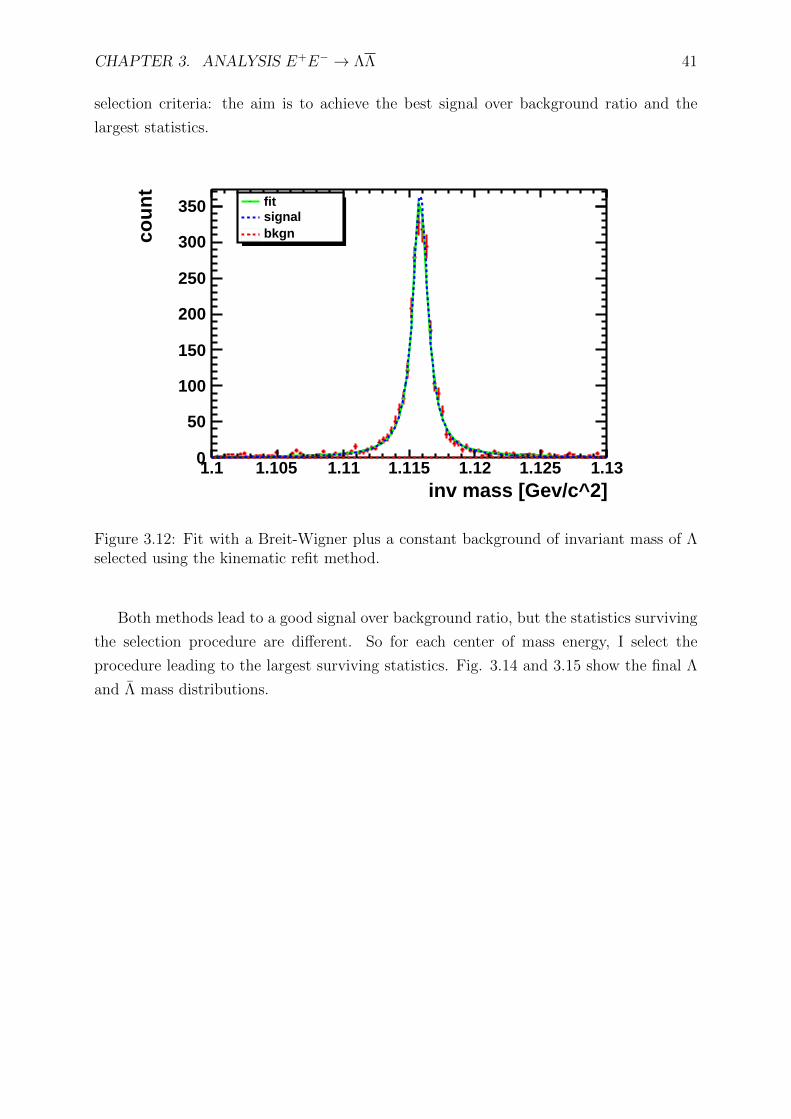
Figure 3.12: Fit with a Breit-Wigner plus a constant background of invariant mass of Λselected using the kinematic refit method.
Both methods lead to a good signal over background ratio, but the statistics surviving
the selection procedure are different. So for each center of mass energy, I select the
procedure leading to the largest surviving statistics. Fig. 3.14 and 3.15 show the final Λ
and Λ mass distributions.
CHAPTER 3. ANALYSIS E+E− → ΛΛ 42
inv mass [Gev/c^2]1.1 1.105 1.11 1.115 1.12 1.125 1.13
cou
nt
0
50
100
150
200
250
300
350fitsignalbkgn
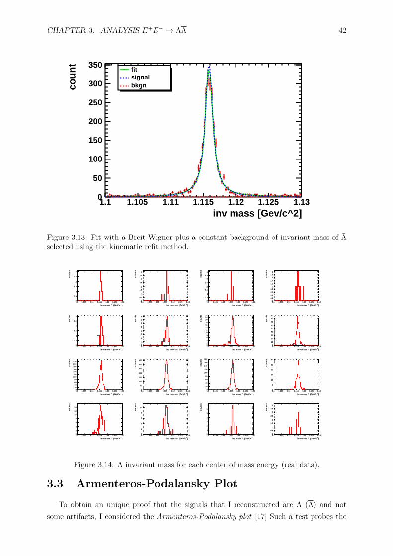
Figure 3.13: Fit with a Breit-Wigner plus a constant background of invariant mass of Λselected using the kinematic refit method.
)2 (GeV/cΛinv mass
1.1 1.105 1.11 1.115 1.12 1.125 1.13
cou
nts
0
0.5
1
1.5
2
2.5
3
)2 (GeV/cΛinv mass
1.1 1.105 1.11 1.115 1.12 1.125 1.13
cou
nts
0
0.5
1
1.5
2
2.5
3
3.5
4
)2 (GeV/cΛinv mass
1.1 1.105 1.11 1.115 1.12 1.125 1.13
cou
nts
0
0.5
1
1.5
2
2.5
3
3.5
4
)2 (GeV/cΛinv mass
1.1 1.105 1.11 1.115 1.12 1.125 1.13
cou
nts
00.2
0.4
0.6
0.81
1.2
1.4
1.61.8
2
)2 (GeV/cΛinv mass
1.1 1.105 1.11 1.115 1.12 1.125 1.13
cou
nts
0
0.5
1
1.5
2
2.5
3
)2 (GeV/cΛinv mass
1.1 1.105 1.11 1.115 1.12 1.125 1.13
cou
nts
0
1
2
3
4
5
6
7
8
)2 (GeV/cΛinv mass
1.1 1.105 1.11 1.115 1.12 1.125 1.13
cou
nts
024
68
1012141618202224
)2 (GeV/cΛinv mass
1.1 1.105 1.11 1.115 1.12 1.125 1.13
cou
nts
0
10
20
30
40
50
60
70
80
90
)2 (GeV/cΛinv mass
1.1 1.105 1.11 1.115 1.12 1.125 1.13
cou
nts
020406080
100120140160180200220
)2 (GeV/cΛinv mass
1.1 1.105 1.11 1.115 1.12 1.125 1.13
cou
nts
0
50
100
150
200
250
300
350
)2 (GeV/cΛinv mass
1.1 1.105 1.11 1.115 1.12 1.125 1.13
cou
nts
0
20
40
60
80
100
120
140
160
180
)2 (GeV/cΛinv mass
1.1 1.105 1.11 1.115 1.12 1.125 1.13
cou
nts
0
5
10
15
20
25
30
)2 (GeV/cΛinv mass
1.1 1.105 1.11 1.115 1.12 1.125 1.13
cou
nts
0
2
4
6
8
10
12
14
)2 (GeV/cΛinv mass
1.1 1.105 1.11 1.115 1.12 1.125 1.13
cou
nts
0
2
4
6
8
10
)2 (GeV/cΛinv mass
1.1 1.105 1.11 1.115 1.12 1.125 1.13
cou
nts
0
1
2
3
4
5
6
7
)2 (GeV/cΛinv mass
1.1 1.105 1.11 1.115 1.12 1.125 1.13
cou
nts
0
0.5
1
1.5
2
2.5
3
3.5
4
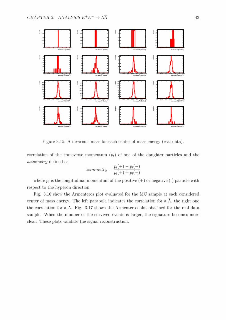
Figure 3.14: Λ invariant mass for each center of mass energy (real data).
3.3 Armenteros-Podalansky Plot
To obtain an unique proof that the signals that I reconstructed are Λ (Λ) and not
some artifacts, I considered the Armenteros-Podalansky plot [17] Such a test probes the
CHAPTER 3. ANALYSIS E+E− → ΛΛ 43
)2 (GeV/cΛinv mass
1.1 1.105 1.11 1.115 1.12 1.125 1.13
cou
nts
0
0.2
0.4
0.6
0.8
1
)2 (GeV/cΛinv mass
1.1 1.105 1.11 1.115 1.12 1.125 1.13
cou
nts
0
0.2
0.4
0.6
0.8
1
)2 (GeV/cΛinv mass
1.1 1.105 1.11 1.115 1.12 1.125 1.13
cou
nts
0
0.2
0.4
0.6
0.8
1
)2 (GeV/cΛinv mass
1.1 1.105 1.11 1.115 1.12 1.125 1.13
cou
nts
00.2
0.4
0.6
0.81
1.2
1.4
1.61.8
2
)2 (GeV/cΛinv mass
1.1 1.105 1.11 1.115 1.12 1.125 1.13
cou
nts
0
0.5
1
1.5
2
2.5
3
3.5
4
)2 (GeV/cΛinv mass
1.1 1.105 1.11 1.115 1.12 1.125 1.13
cou
nts
0
1
2
3
4
5
6
7
)2 (GeV/cΛinv mass
1.1 1.105 1.11 1.115 1.12 1.125 1.13
cou
nts
0
5
10
15
20
25
)2 (GeV/cΛinv mass
1.1 1.105 1.11 1.115 1.12 1.125 1.13
cou
nts
0
10
20
30
40
50
60
70
)2 (GeV/cΛinv mass
1.1 1.105 1.11 1.115 1.12 1.125 1.13
cou
nts
0
20
40
60
80
100
120
140
160
180
)2 (GeV/cΛinv mass
1.1 1.105 1.11 1.115 1.12 1.125 1.13
cou
nts
0
50
100
150
200
250
300
)2 (GeV/cΛinv mass
1.1 1.105 1.11 1.115 1.12 1.125 1.13
cou
nts
0
20
40
60
80
100
120
140
160
)2 (GeV/cΛinv mass
1.1 1.105 1.11 1.115 1.12 1.125 1.13
cou
nts
0
5
10
15
20
25
)2 (GeV/cΛinv mass
1.1 1.105 1.11 1.115 1.12 1.125 1.13
cou
nts
02
4
6
8
1012
14
16
18
)2 (GeV/cΛinv mass
1.1 1.105 1.11 1.115 1.12 1.125 1.13
cou
nts
0
2
4
6
8
10
12
)2 (GeV/cΛinv mass
1.1 1.105 1.11 1.115 1.12 1.125 1.13
cou
nts
0
1
2
3
4
5
6
7
)2 (GeV/cΛinv mass
1.1 1.105 1.11 1.115 1.12 1.125 1.13
cou
nts
0
1
2
3
4
5
6
7
Figure 3.15: Λ invariant mass for each center of mass energy (real data).
correlation of the transverse momentum (pt) of one of the daughter particles and the
asimmetry defined as
asimmetry =pl(+)− pl(−)
pl(+) + pl(−)
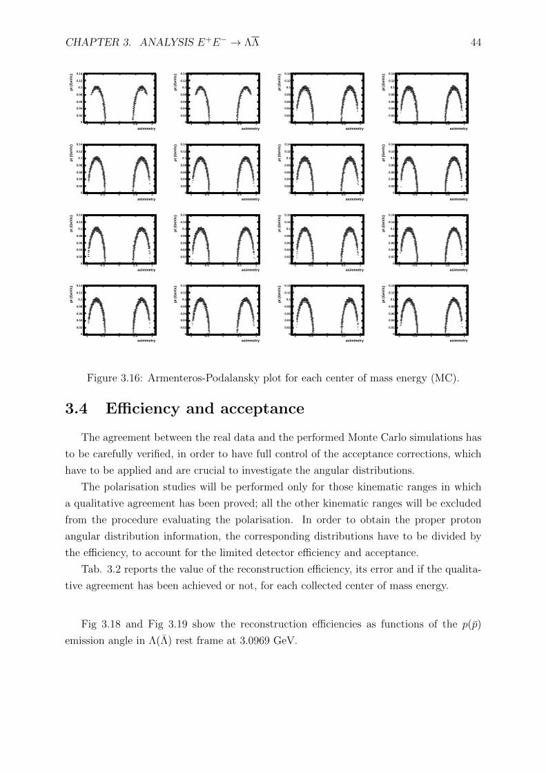
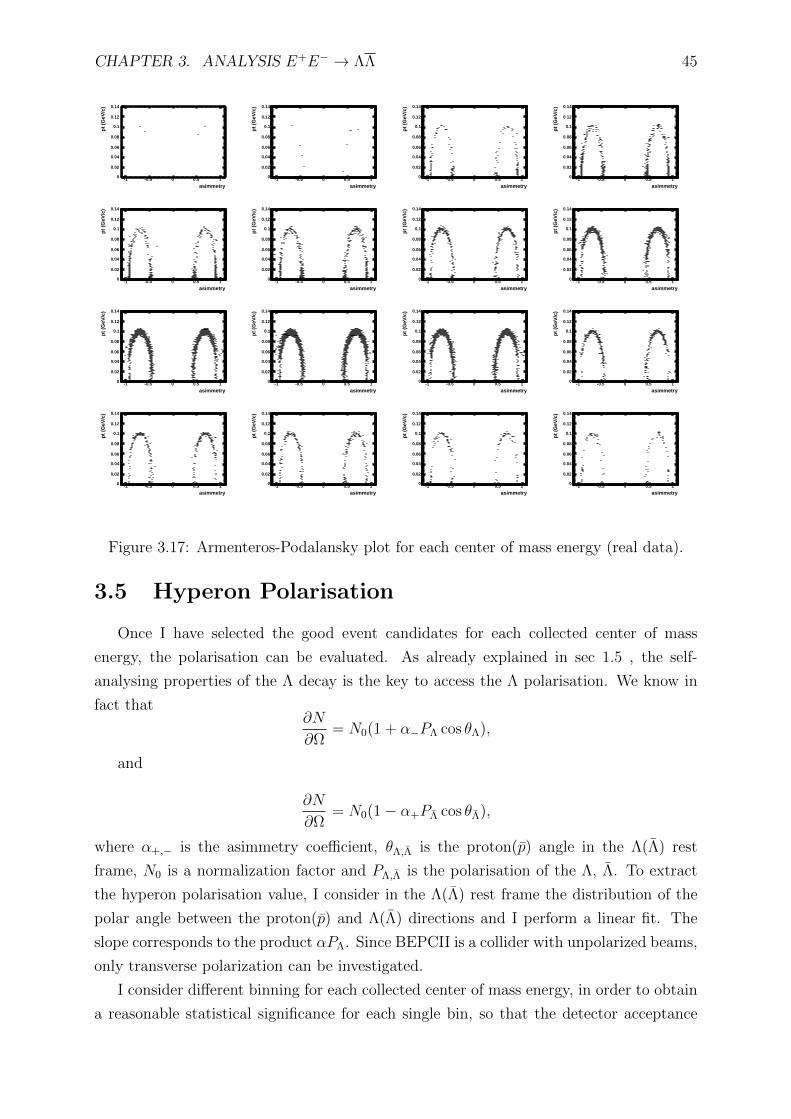
where pl is the longitudinal momentum of the positive (+) or negative (-) particle with
respect to the hyperon direction.
Fig. 3.16 show the Armenteros plot evaluated for the MC sample at each considered
center of mass energy. The left parabola indicates the correlation for a Λ, the right one
the correlation for a Λ. Fig. 3.17 shows the Armenteros plot obatined for the real data
sample. When the number of the survived events is larger, the signature becomes more
clear. These plots validate the signal reconstruction.
CHAPTER 3. ANALYSIS E+E− → ΛΛ 44
asimmetry-1 -0.5 0 0.5 1
pt
(GeV
/c)
0
0.02
0.04
0.06
0.08
0.1
0.12
0.14
asimmetry-1 -0.5 0 0.5 1
pt
(GeV
/c)
0
0.02
0.04
0.06
0.08
0.1
0.12
0.14
asimmetry-1 -0.5 0 0.5 1
pt
(GeV
/c)
0
0.02
0.04
0.06
0.08
0.1
0.12
0.14
asimmetry-1 -0.5 0 0.5 1
pt
(GeV
/c)
0
0.02
0.04
0.06
0.08
0.1
0.12
0.14
asimmetry-1 -0.5 0 0.5 1
pt
(GeV
/c)
0
0.02
0.04
0.06
0.08
0.1
0.12
0.14
asimmetry-1 -0.5 0 0.5 1
pt
(GeV
/c)
0
0.02
0.04
0.06
0.08
0.1
0.12
0.14
asimmetry-1 -0.5 0 0.5 1
pt
(GeV
/c)
0
0.02
0.04
0.06
0.08
0.1
0.12
0.14
asimmetry-1 -0.5 0 0.5 1
pt
(GeV
/c)
0
0.02
0.04
0.06
0.08
0.1
0.12
0.14
asimmetry-1 -0.5 0 0.5 1
pt
(GeV
/c)
0
0.02
0.04
0.06
0.08
0.1
0.12
0.14
asimmetry-1 -0.5 0 0.5 1
pt
(GeV
/c)
0
0.02
0.04
0.06
0.08
0.1
0.12
0.14
asimmetry-1 -0.5 0 0.5 1
pt
(GeV
/c)
0
0.02
0.04
0.06
0.08
0.1
0.12
0.14
asimmetry-1 -0.5 0 0.5 1
pt
(GeV
/c)
0
0.02
0.04
0.06
0.08
0.1
0.12
0.14
asimmetry-1 -0.5 0 0.5 1
pt
(GeV
/c)
0
0.02
0.04
0.06
0.08
0.1
0.12
0.14
asimmetry-1 -0.5 0 0.5 1
pt
(GeV
/c)
0
0.02
0.04
0.06
0.08
0.1
0.12
0.14
asimmetry-1 -0.5 0 0.5 1
pt
(GeV
/c)
0
0.02
0.04
0.06
0.08
0.1
0.12
0.14
asimmetry-1 -0.5 0 0.5 1
pt
(GeV
/c)
0
0.02
0.04
0.06
0.08
0.1
0.12
0.14
Figure 3.16: Armenteros-Podalansky plot for each center of mass energy (MC).
3.4 Efficiency and acceptance
The agreement between the real data and the performed Monte Carlo simulations has
to be carefully verified, in order to have full control of the acceptance corrections, which
have to be applied and are crucial to investigate the angular distributions.
The polarisation studies will be performed only for those kinematic ranges in which
a qualitative agreement has been proved; all the other kinematic ranges will be excluded
from the procedure evaluating the polarisation. In order to obtain the proper proton
angular distribution information, the corresponding distributions have to be divided by
the efficiency, to account for the limited detector efficiency and acceptance.
Tab. 3.2 reports the value of the reconstruction efficiency, its error and if the qualita-
tive agreement has been achieved or not, for each collected center of mass energy.
Fig 3.18 and Fig 3.19 show the reconstruction efficiencies as functions of the p(p)
emission angle in Λ(Λ) rest frame at 3.0969 GeV.
CHAPTER 3. ANALYSIS E+E− → ΛΛ 45
asimmetry-1 -0.5 0 0.5 1
pt
(GeV
/c)
0
0.02
0.04
0.06
0.08
0.1
0.12
0.14
asimmetry-1 -0.5 0 0.5 1
pt
(GeV
/c)
0
0.02
0.04
0.06
0.08
0.1
0.12
0.14
asimmetry-1 -0.5 0 0.5 1
pt
(GeV
/c)
0
0.02
0.04
0.06
0.08
0.1
0.12
0.14
asimmetry-1 -0.5 0 0.5 1
pt
(GeV
/c)
0
0.02
0.04
0.06
0.08
0.1
0.12
0.14
asimmetry-1 -0.5 0 0.5 1
pt
(GeV
/c)
0
0.02
0.04
0.06
0.08
0.1
0.12
0.14
asimmetry-1 -0.5 0 0.5 1
pt
(GeV
/c)
0
0.02
0.04
0.06
0.08
0.1
0.12
0.14
asimmetry-1 -0.5 0 0.5 1
pt
(GeV
/c)
0
0.02
0.04
0.06
0.08
0.1
0.12
0.14
asimmetry-1 -0.5 0 0.5 1
pt
(GeV
/c)
0
0.02
0.04
0.06
0.08
0.1
0.12
0.14
asimmetry-1 -0.5 0 0.5 1
pt
(GeV
/c)
0
0.02
0.04
0.06
0.08
0.1
0.12
0.14
asimmetry-1 -0.5 0 0.5 1
pt
(GeV
/c)
0
0.02
0.04
0.06
0.08
0.1
0.12
0.14
asimmetry-1 -0.5 0 0.5 1
pt
(GeV
/c)
0
0.02
0.04
0.06
0.08
0.1
0.12
0.14
asimmetry-1 -0.5 0 0.5 1
pt
(GeV
/c)
0
0.02
0.04
0.06
0.08
0.1
0.12
0.14
asimmetry-1 -0.5 0 0.5 1
pt
(GeV
/c)
0
0.02
0.04
0.06
0.08
0.1
0.12
0.14
asimmetry-1 -0.5 0 0.5 1
pt
(GeV
/c)
0
0.02
0.04
0.06
0.08
0.1
0.12
0.14
asimmetry-1 -0.5 0 0.5 1
pt
(GeV
/c)
0
0.02
0.04
0.06
0.08
0.1
0.12
0.14
asimmetry-1 -0.5 0 0.5 1
pt
(GeV
/c)
0
0.02
0.04
0.06
0.08
0.1
0.12
0.14
Figure 3.17: Armenteros-Podalansky plot for each center of mass energy (real data).
3.5 Hyperon Polarisation
Once I have selected the good event candidates for each collected center of mass
energy, the polarisation can be evaluated. As already explained in sec 1.5 , the self-
analysing properties of the Λ decay is the key to access the Λ polarisation. We know in
fact that∂N
∂Ω= N0(1 + α−PΛ cos θΛ),
and
∂N
∂Ω= N0(1− α+PΛ cos θΛ),
where α+,− is the asimmetry coefficient, θΛ,Λ is the proton(p) angle in the Λ(Λ) rest
frame, N0 is a normalization factor and PΛ,Λ is the polarisation of the Λ, Λ. To extract
the hyperon polarisation value, I consider in the Λ(Λ) rest frame the distribution of the
polar angle between the proton(p) and Λ(Λ) directions and I perform a linear fit. The
slope corresponds to the product αPΛ. Since BEPCII is a collider with unpolarized beams,
only transverse polarization can be investigated.
I consider different binning for each collected center of mass energy, in order to obtain
a reasonable statistical significance for each single bin, so that the detector acceptance
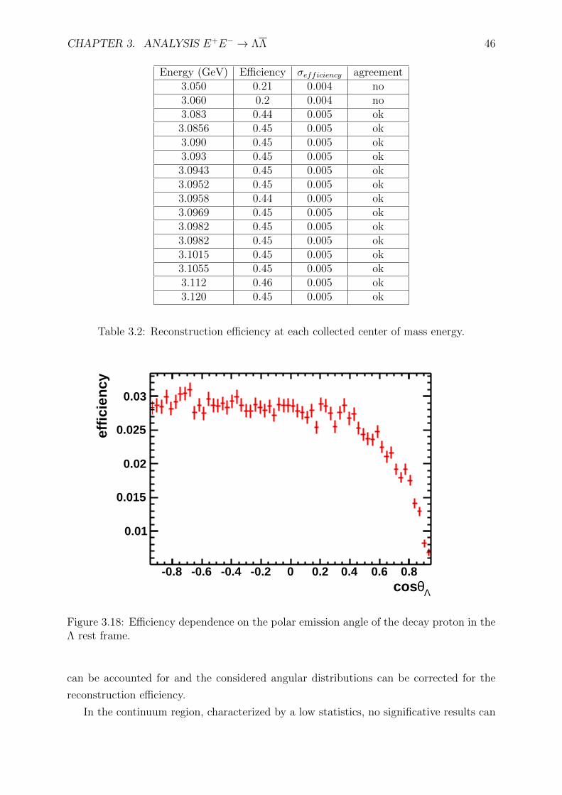
CHAPTER 3. ANALYSIS E+E− → ΛΛ 46
Energy (GeV) Efficiency σefficiency agreement3.050 0.21 0.004 no3.060 0.2 0.004 no3.083 0.44 0.005 ok3.0856 0.45 0.005 ok3.090 0.45 0.005 ok3.093 0.45 0.005 ok3.0943 0.45 0.005 ok3.0952 0.45 0.005 ok3.0958 0.44 0.005 ok3.0969 0.45 0.005 ok3.0982 0.45 0.005 ok3.0982 0.45 0.005 ok3.1015 0.45 0.005 ok3.1055 0.45 0.005 ok3.112 0.46 0.005 ok3.120 0.45 0.005 ok
Table 3.2: Reconstruction efficiency at each collected center of mass energy.
Λθcos-0.8 -0.6 -0.4 -0.2 0 0.2 0.4 0.6 0.8
effi
cien
cy
0.01
0.015
0.02
0.025
0.03
Figure 3.18: Efficiency dependence on the polar emission angle of the decay proton in theΛ rest frame.
can be accounted for and the considered angular distributions can be corrected for the
reconstruction efficiency.
In the continuum region, characterized by a low statistics, no significative results can
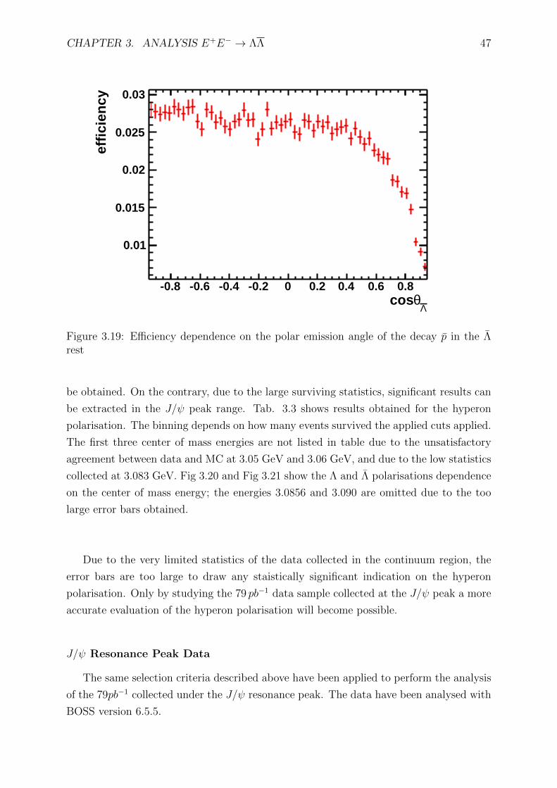
CHAPTER 3. ANALYSIS E+E− → ΛΛ 47
Λθcos
-0.8 -0.6 -0.4 -0.2 0 0.2 0.4 0.6 0.8
effi
cien
cy
0.01
0.015
0.02
0.025
0.03
Figure 3.19: Efficiency dependence on the polar emission angle of the decay p in the Λrest
be obtained. On the contrary, due to the large surviving statistics, significant results can
be extracted in the J/ψ peak range. Tab. 3.3 shows results obtained for the hyperon
polarisation. The binning depends on how many events survived the applied cuts applied.
The first three center of mass energies are not listed in table due to the unsatisfactory
agreement between data and MC at 3.05 GeV and 3.06 GeV, and due to the low statistics
collected at 3.083 GeV. Fig 3.20 and Fig 3.21 show the Λ and Λ polarisations dependence
on the center of mass energy; the energies 3.0856 and 3.090 are omitted due to the too
large error bars obtained.
Due to the very limited statistics of the data collected in the continuum region, the
error bars are too large to draw any staistically significant indication on the hyperon
polarisation. Only by studying the 79 pb−1 data sample collected at the J/ψ peak a more
accurate evaluation of the hyperon polarisation will become possible.
J/ψ Resonance Peak Data
The same selection criteria described above have been applied to perform the analysis
of the 79pb−1 collected under the J/ψ resonance peak. The data have been analysed with
BOSS version 6.5.5.
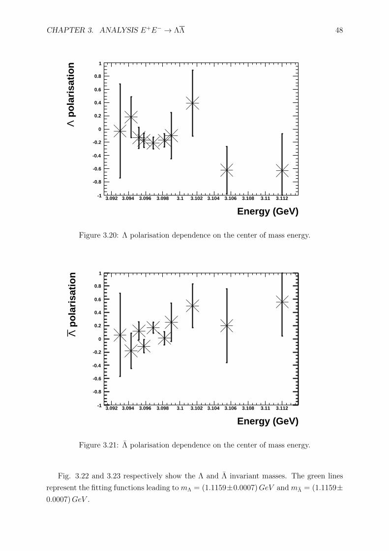
CHAPTER 3. ANALYSIS E+E− → ΛΛ 48
Energy (GeV)
3.092 3.094 3.096 3.098 3.1 3.102 3.104 3.106 3.108 3.11 3.112
po
lari
sati
on
Λ
-1
-0.8
-0.6
-0.4
-0.2
0
0.2
0.4
0.6
0.8
1
Figure 3.20: Λ polarisation dependence on the center of mass energy.
Energy (GeV)
3.092 3.094 3.096 3.098 3.1 3.102 3.104 3.106 3.108 3.11 3.112
po
lari
sati
on
Λ
-1
-0.8
-0.6
-0.4
-0.2
0
0.2
0.4
0.6
0.8
1
Figure 3.21: Λ polarisation dependence on the center of mass energy.
Fig. 3.22 and 3.23 respectively show the Λ and Λ invariant masses. The green lines
represent the fitting functions leading to mΛ = (1.1159±0.0007)GeV and mΛ = (1.1159±0.0007)GeV .
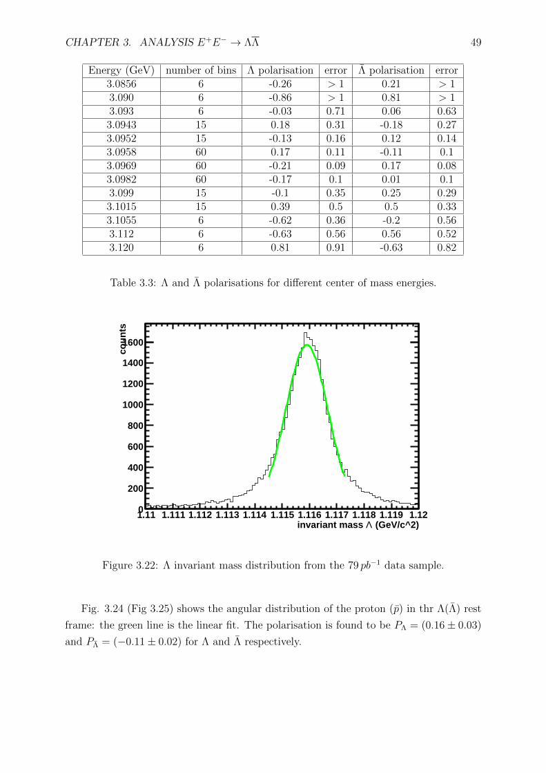
CHAPTER 3. ANALYSIS E+E− → ΛΛ 49
Energy (GeV) number of bins Λ polarisation error Λ polarisation error3.0856 6 -0.26 > 1 0.21 > 13.090 6 -0.86 > 1 0.81 > 13.093 6 -0.03 0.71 0.06 0.633.0943 15 0.18 0.31 -0.18 0.273.0952 15 -0.13 0.16 0.12 0.143.0958 60 0.17 0.11 -0.11 0.13.0969 60 -0.21 0.09 0.17 0.083.0982 60 -0.17 0.1 0.01 0.13.099 15 -0.1 0.35 0.25 0.293.1015 15 0.39 0.5 0.5 0.333.1055 6 -0.62 0.36 -0.2 0.563.112 6 -0.63 0.56 0.56 0.523.120 6 0.81 0.91 -0.63 0.82
Table 3.3: Λ and Λ polarisations for different center of mass energies.
(GeV/c^2)Λinvariant mass 1.11 1.111 1.112 1.113 1.114 1.115 1.116 1.117 1.118 1.119 1.12
cou
nts
0
200
400
600
800
1000
1200
1400
1600
Figure 3.22: Λ invariant mass distribution from the 79 pb−1 data sample.
Fig. 3.24 (Fig 3.25) shows the angular distribution of the proton (p) in thr Λ(Λ) rest
frame: the green line is the linear fit. The polarisation is found to be PΛ = (0.16± 0.03)
and PΛ = (−0.11± 0.02) for Λ and Λ respectively.
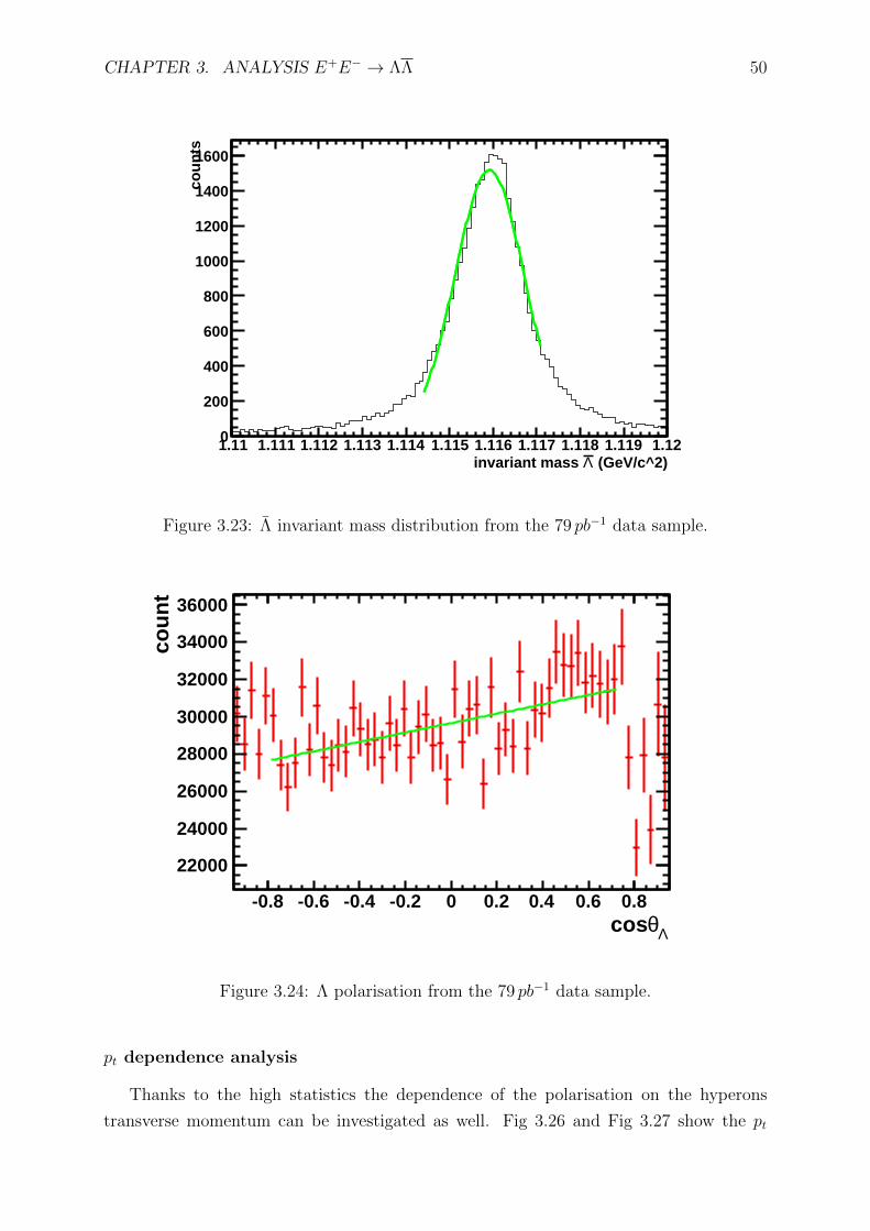
CHAPTER 3. ANALYSIS E+E− → ΛΛ 50
(GeV/c^2)Λinvariant mass 1.11 1.111 1.112 1.113 1.114 1.115 1.116 1.117 1.118 1.119 1.12
cou
nts
0
200
400
600
800
1000
1200
1400
1600
Figure 3.23: Λ invariant mass distribution from the 79 pb−1 data sample.
Λθcos-0.8 -0.6 -0.4 -0.2 0 0.2 0.4 0.6 0.8
cou
nt
22000
24000
26000
28000
30000
32000
34000
36000
Figure 3.24: Λ polarisation from the 79 pb−1 data sample.
pt dependence analysis
Thanks to the high statistics the dependence of the polarisation on the hyperons
transverse momentum can be investigated as well. Fig 3.26 and Fig 3.27 show the pt
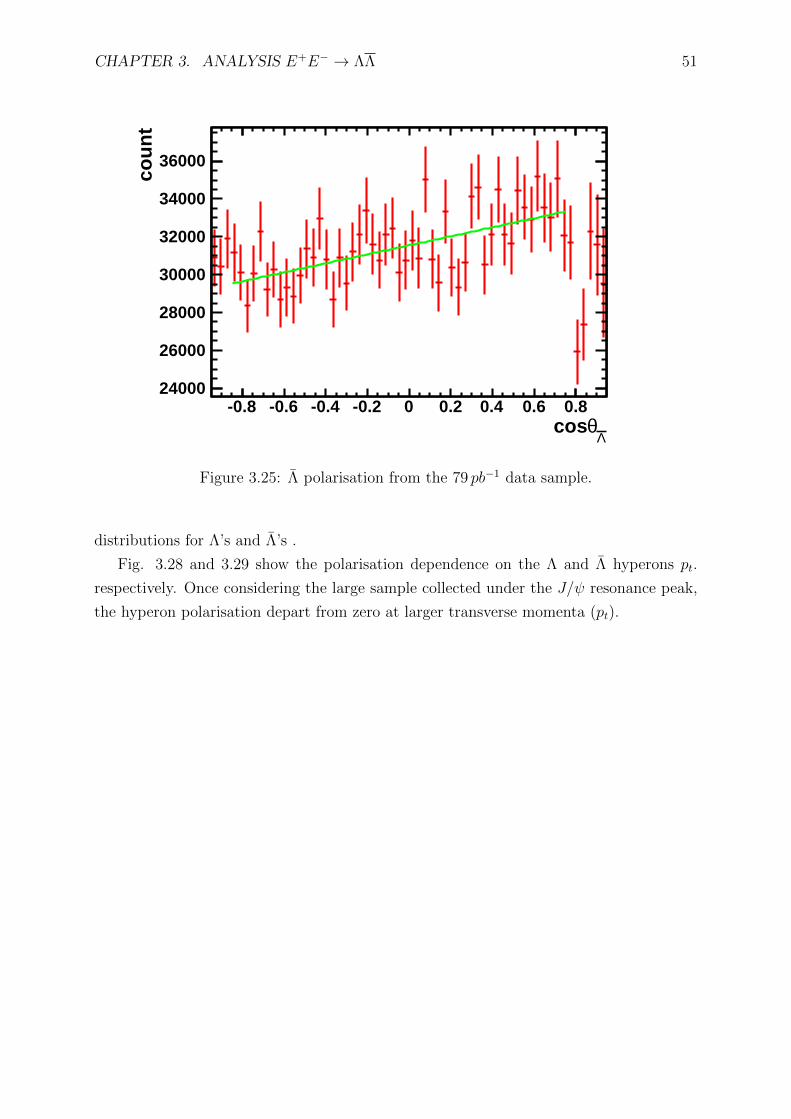
CHAPTER 3. ANALYSIS E+E− → ΛΛ 51
Λθcos
-0.8 -0.6 -0.4 -0.2 0 0.2 0.4 0.6 0.8
cou
nt
24000
26000
28000
30000
32000
34000
36000
Figure 3.25: Λ polarisation from the 79 pb−1 data sample.
distributions for Λ’s and Λ’s .
Fig. 3.28 and 3.29 show the polarisation dependence on the Λ and Λ hyperons pt.
respectively. Once considering the large sample collected under the J/ψ resonance peak,
the hyperon polarisation depart from zero at larger transverse momenta (pt).
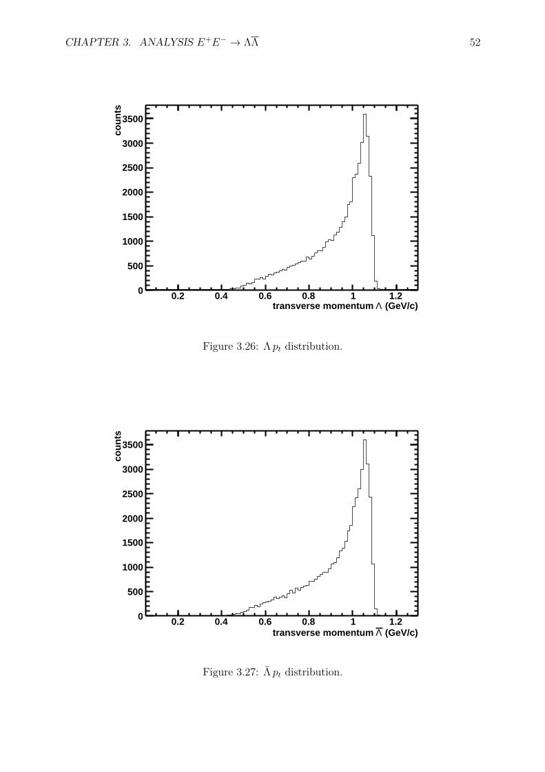
CHAPTER 3. ANALYSIS E+E− → ΛΛ 52
(GeV/c)Λtransverse momentum 0.2 0.4 0.6 0.8 1 1.2
cou
nts
0
500
1000
1500
2000
2500
3000
3500
Figure 3.26: Λ pt distribution.
(GeV/c)Λtransverse momentum 0.2 0.4 0.6 0.8 1 1.2
cou
nts
0
500
1000
1500
2000
2500
3000
3500
Figure 3.27: Λ pt distribution.
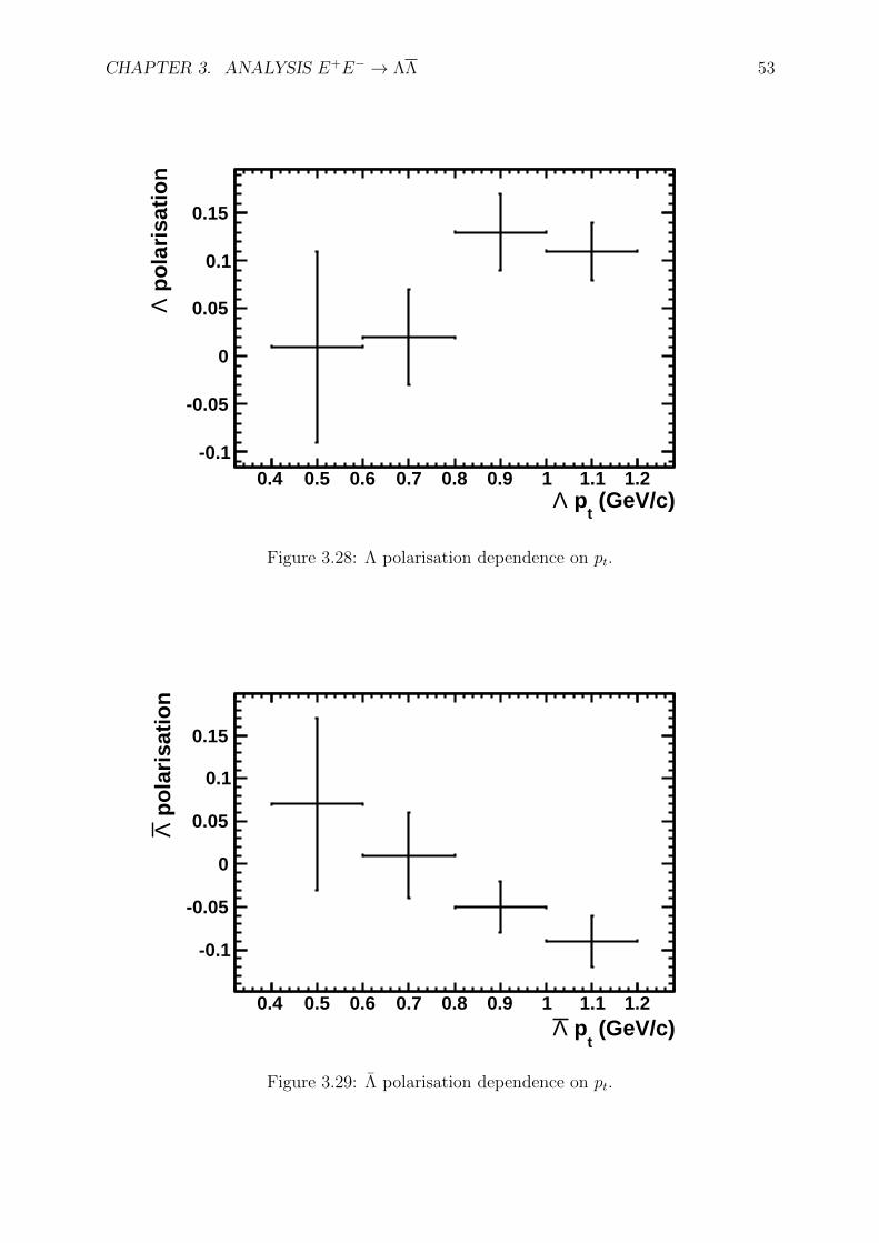
CHAPTER 3. ANALYSIS E+E− → ΛΛ 53
(GeV/c)t
pΛ0.4 0.5 0.6 0.7 0.8 0.9 1 1.1 1.2
po
lari
sati
on
Λ
-0.1
-0.05
0
0.05
0.1
0.15
Figure 3.28: Λ polarisation dependence on pt.
(GeV/c)t
pΛ0.4 0.5 0.6 0.7 0.8 0.9 1 1.1 1.2
po
lari
sati
on
Λ
-0.1
-0.05
0
0.05
0.1
0.15
Figure 3.29: Λ polarisation dependence on pt.
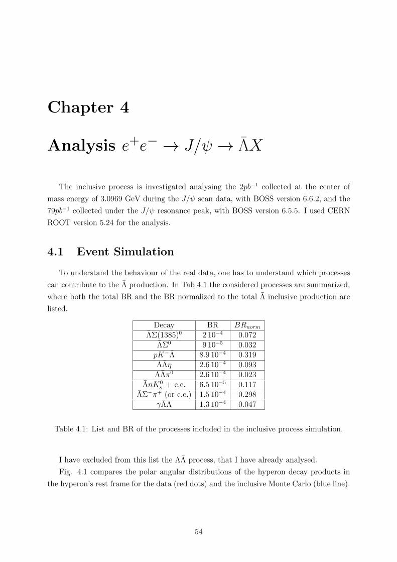
Chapter 4
Analysis e+e−→ J/ψ → ΛX
The inclusive process is investigated analysing the 2pb−1 collected at the center of
mass energy of 3.0969 GeV during the J/ψ scan data, with BOSS version 6.6.2, and the
79pb−1 collected under the J/ψ resonance peak, with BOSS version 6.5.5. I used CERN
ROOT version 5.24 for the analysis.
4.1 Event Simulation
To understand the behaviour of the real data, one has to understand which processes
can contribute to the Λ production. In Tab 4.1 the considered processes are summarized,
where both the total BR and the BR normalized to the total Λ inclusive production are
listed.
Decay BR BRnorm
ΛΣ(1385)0 2 10−4 0.072ΛΣ0 9 10−5 0.032pK−Λ 8.9 10−4 0.319ΛΛη 2.6 10−4 0.093ΛΛπ0 2.6 10−4 0.023
ΛnK0s + c.c. 6.5 10−5 0.117
ΛΣ−π+ (or c.c.) 1.5 10−4 0.298γΛΛ 1.3 10−4 0.047
Table 4.1: List and BR of the processes included in the inclusive process simulation.
I have excluded from this list the ΛΛ process, that I have already analysed.
Fig. 4.1 compares the polar angular distributions of the hyperon decay products in
the hyperon’s rest frame for the data (red dots) and the inclusive Monte Carlo (blue line).
54
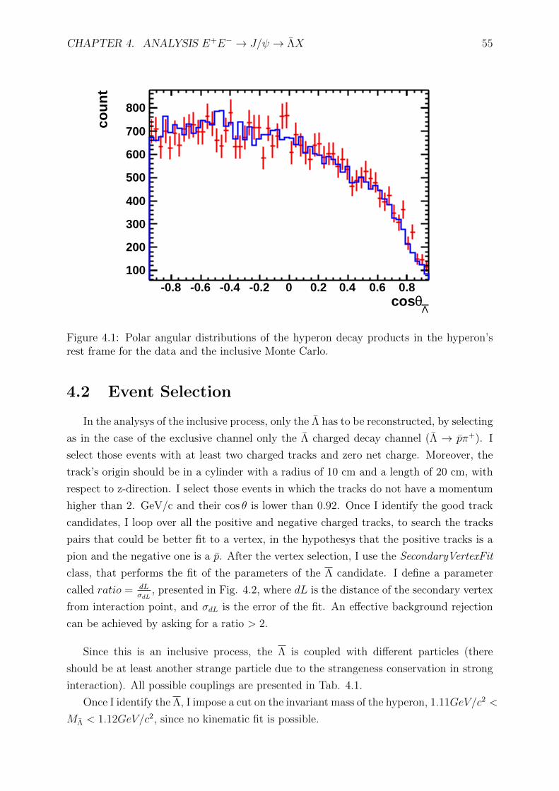
CHAPTER 4. ANALYSIS E+E− → J/ψ → ΛX 55
Λθcos
-0.8 -0.6 -0.4 -0.2 0 0.2 0.4 0.6 0.8
cou
nt
100
200
300
400
500
600
700
800
Figure 4.1: Polar angular distributions of the hyperon decay products in the hyperon’srest frame for the data and the inclusive Monte Carlo.
4.2 Event Selection
In the analysys of the inclusive process, only the Λ has to be reconstructed, by selecting
as in the case of the exclusive channel only the Λ charged decay channel (Λ → pπ+). I
select those events with at least two charged tracks and zero net charge. Moreover, the
track’s origin should be in a cylinder with a radius of 10 cm and a length of 20 cm, with
respect to z-direction. I select those events in which the tracks do not have a momentum
higher than 2. GeV/c and their cos θ is lower than 0.92. Once I identify the good track
candidates, I loop over all the positive and negative charged tracks, to search the tracks
pairs that could be better fit to a vertex, in the hypothesys that the positive tracks is a
pion and the negative one is a p. After the vertex selection, I use the SecondaryVertexFit
class, that performs the fit of the parameters of the Λ candidate. I define a parameter
called ratio = dLσdL
, presented in Fig. 4.2, where dL is the distance of the secondary vertex
from interaction point, and σdL is the error of the fit. An effective background rejection
can be achieved by asking for a ratio > 2.
Since this is an inclusive process, the Λ is coupled with different particles (there
should be at least another strange particle due to the strangeness conservation in strong
interaction). All possible couplings are presented in Tab. 4.1.
Once I identify the Λ, I impose a cut on the invariant mass of the hyperon, 1.11GeV/c2 <
MΛ < 1.12GeV/c2, since no kinematic fit is possible.
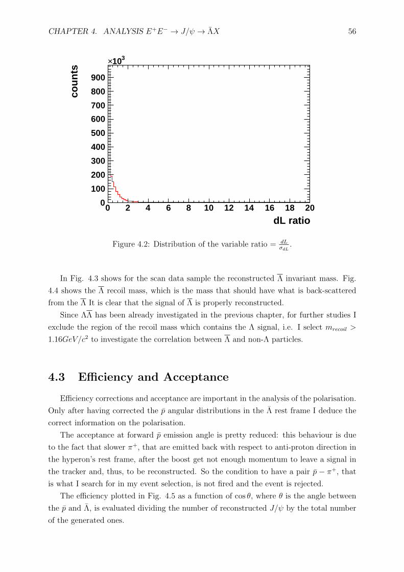
CHAPTER 4. ANALYSIS E+E− → J/ψ → ΛX 56
dL ratio0 2 4 6 8 10 12 14 16 18 20
cou
nts
0
100
200
300
400
500
600
700
800
900
310×
Figure 4.2: Distribution of the variable ratio = dLσdL
.
In Fig. 4.3 shows for the scan data sample the reconstructed Λ invariant mass. Fig.
4.4 shows the Λ recoil mass, which is the mass that should have what is back-scattered
from the Λ It is clear that the signal of Λ is properly reconstructed.
Since ΛΛ has been already investigated in the previous chapter, for further studies I
exclude the region of the recoil mass which contains the Λ signal, i.e. I select mrecoil >
1.16GeV/c2 to investigate the correlation between Λ and non-Λ particles.
4.3 Efficiency and Acceptance
Efficiency corrections and acceptance are important in the analysis of the polarisation.
Only after having corrected the p angular distributions in the Λ rest frame I deduce the
correct information on the polarisation.
The acceptance at forward p emission angle is pretty reduced: this behaviour is due
to the fact that slower π+, that are emitted back with respect to anti-proton direction in
the hyperon’s rest frame, after the boost get not enough momentum to leave a signal in
the tracker and, thus, to be reconstructed. So the condition to have a pair p − π+, that
is what I search for in my event selection, is not fired and the event is rejected.
The efficiency plotted in Fig. 4.5 as a function of cos θ, where θ is the angle between
the p and Λ, is evaluated dividing the number of reconstructed J/ψ by the total number
of the generated ones.
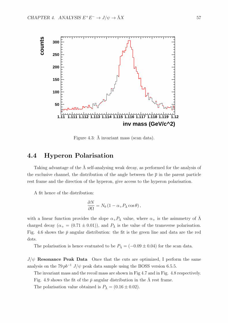
CHAPTER 4. ANALYSIS E+E− → J/ψ → ΛX 57
inv mass (GeV/c^2)1.11 1.111 1.112 1.113 1.114 1.115 1.116 1.117 1.118 1.119 1.12
cou
nts
50
100
150
200
250
300
Figure 4.3: Λ invariant mass (scan data).
4.4 Hyperon Polarisation
Taking advantage of the Λ self-analysing weak decay, as performed for the analysis of
the exclusive channel, the distribution of the angle between the p in the parent particle
rest frame and the direction of the hyperon, give access to the hyperon polarisation.
A fit hence of the distribution:
∂N
∂Ω= N0 (1− α+PΛ cos θ) ,
with a linear function provides the slope α+PΛ value, where α+ is the asimmetry of Λ
charged decay (α+ = (0.71 ± 0.01)), and PΛ is the value of the transverse polarisation.
Fig. 4.6 shows the p angular distribution: the fit is the green line and data are the red
dots.
The polarisation is hence evatuated to be PΛ = (−0.09± 0.04) for the scan data.
J/ψ Resonance Peak Data Once that the cuts are optimized, I perform the same
analysis on the 79 pb−1 J/ψ peak data sample using the BOSS version 6.5.5.
The invariant mass and the recoil mass are shown in Fig 4.7 and in Fig. 4.8 respectively.
Fig. 4.9 shows the fit of the p angular distribution in the Λ rest frame.
The polarisation value obtained is PΛ = (0.16± 0.02).
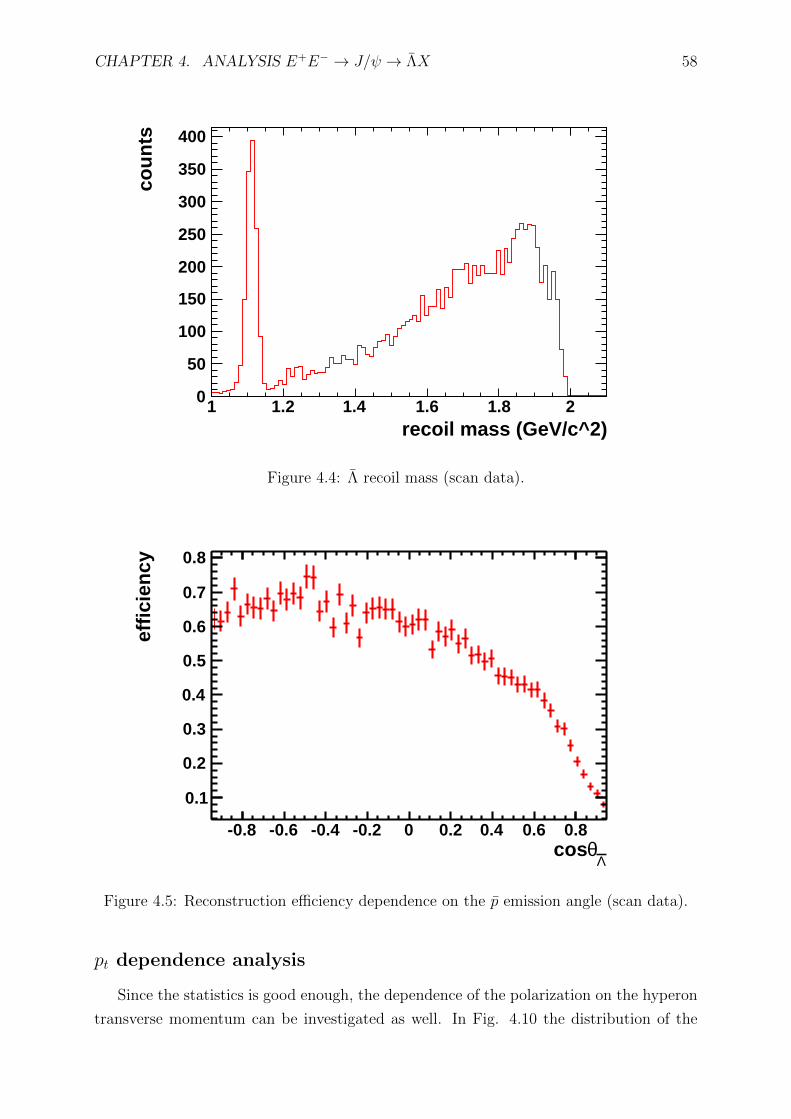
CHAPTER 4. ANALYSIS E+E− → J/ψ → ΛX 58
recoil mass (GeV/c^2)1 1.2 1.4 1.6 1.8 2
cou
nts
0
50
100
150
200
250
300
350
400
Figure 4.4: Λ recoil mass (scan data).
Λθcos
-0.8 -0.6 -0.4 -0.2 0 0.2 0.4 0.6 0.8
effi
cien
cy
0.1
0.2
0.3
0.4
0.5
0.6
0.7
0.8
Figure 4.5: Reconstruction efficiency dependence on the p emission angle (scan data).
pt dependence analysis
Since the statistics is good enough, the dependence of the polarization on the hyperon
transverse momentum can be investigated as well. In Fig. 4.10 the distribution of the
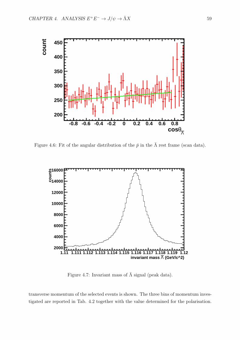
CHAPTER 4. ANALYSIS E+E− → J/ψ → ΛX 59
Λθcos
-0.8 -0.6 -0.4 -0.2 0 0.2 0.4 0.6 0.8
cou
nt
200
250
300
350
400
450
Figure 4.6: Fit of the angular distribution of the p in the Λ rest frame (scan data).
(GeV/c^2)Λinvariant mass 1.11 1.111 1.112 1.113 1.114 1.115 1.116 1.117 1.118 1.119 1.12
cou
nts
2000
4000
6000
8000
10000
12000
14000
16000
Figure 4.7: Invariant mass of Λ signal (peak data).
transverse momentum of the selected events is shown. The three bins of momentum inves-
tigated are reported in Tab. 4.2 together with the value determined for the polarisation.
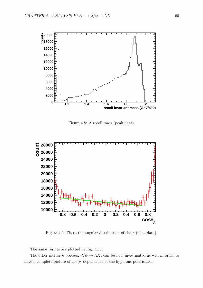
CHAPTER 4. ANALYSIS E+E− → J/ψ → ΛX 60
recoil invariant mass (GeV/c^2)1.2 1.4 1.6 1.8 2
cou
nts
0
2000
4000
6000
8000
10000
12000
14000
16000
18000
20000
Figure 4.8: Λ recoil mass (peak data).
Λθcos
-0.8 -0.6 -0.4 -0.2 0 0.2 0.4 0.6 0.8
cou
nt
10000
12000
14000
16000
18000
20000
22000
24000
26000
28000
Figure 4.9: Fit to the angular distribution of the p (peak data).
The same results are plotted in Fig. 4.11.
The other inclusive process, J/ψ → ΛX, can be now investigated as well in order to
have a complete picture of the pt dependence of the hyperons polarisation.
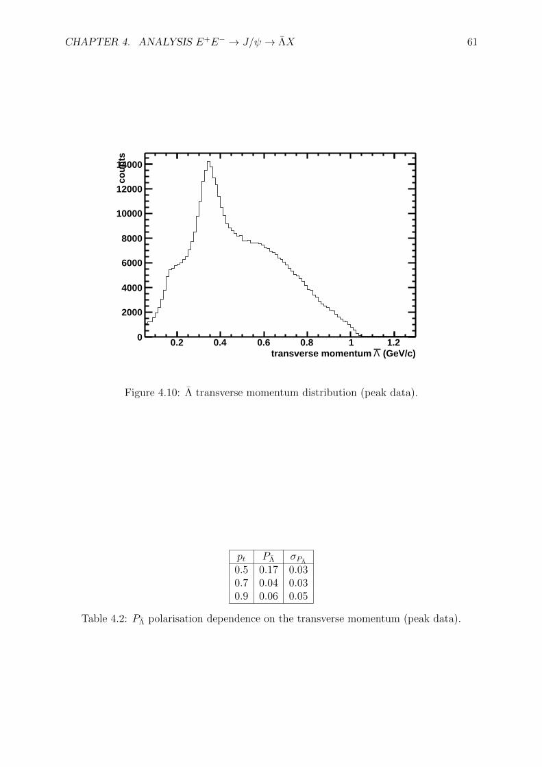
CHAPTER 4. ANALYSIS E+E− → J/ψ → ΛX 61
(GeV/c)Λtransverse momentum 0.2 0.4 0.6 0.8 1 1.2
cou
nts
0
2000
4000
6000
8000
10000
12000
14000
Figure 4.10: Λ transverse momentum distribution (peak data).
pt PΛ σPΛ
0.5 0.17 0.030.7 0.04 0.030.9 0.06 0.05
Table 4.2: PΛ polarisation dependence on the transverse momentum (peak data).
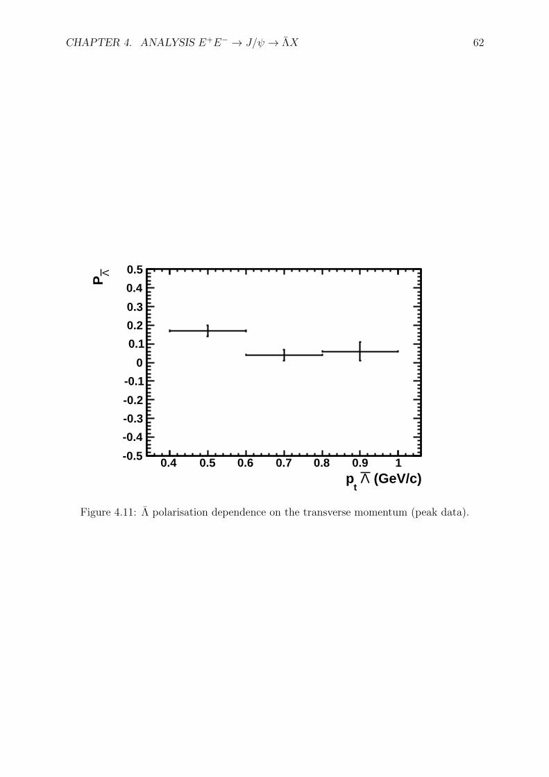
CHAPTER 4. ANALYSIS E+E− → J/ψ → ΛX 62
(GeV/c)Λ t
p0.4 0.5 0.6 0.7 0.8 0.9 1
ΛP
-0.5
-0.4
-0.3
-0.2
-0.1
0
0.1
0.2
0.3
0.4
0.5
Figure 4.11: Λ polarisation dependence on the transverse momentum (peak data).
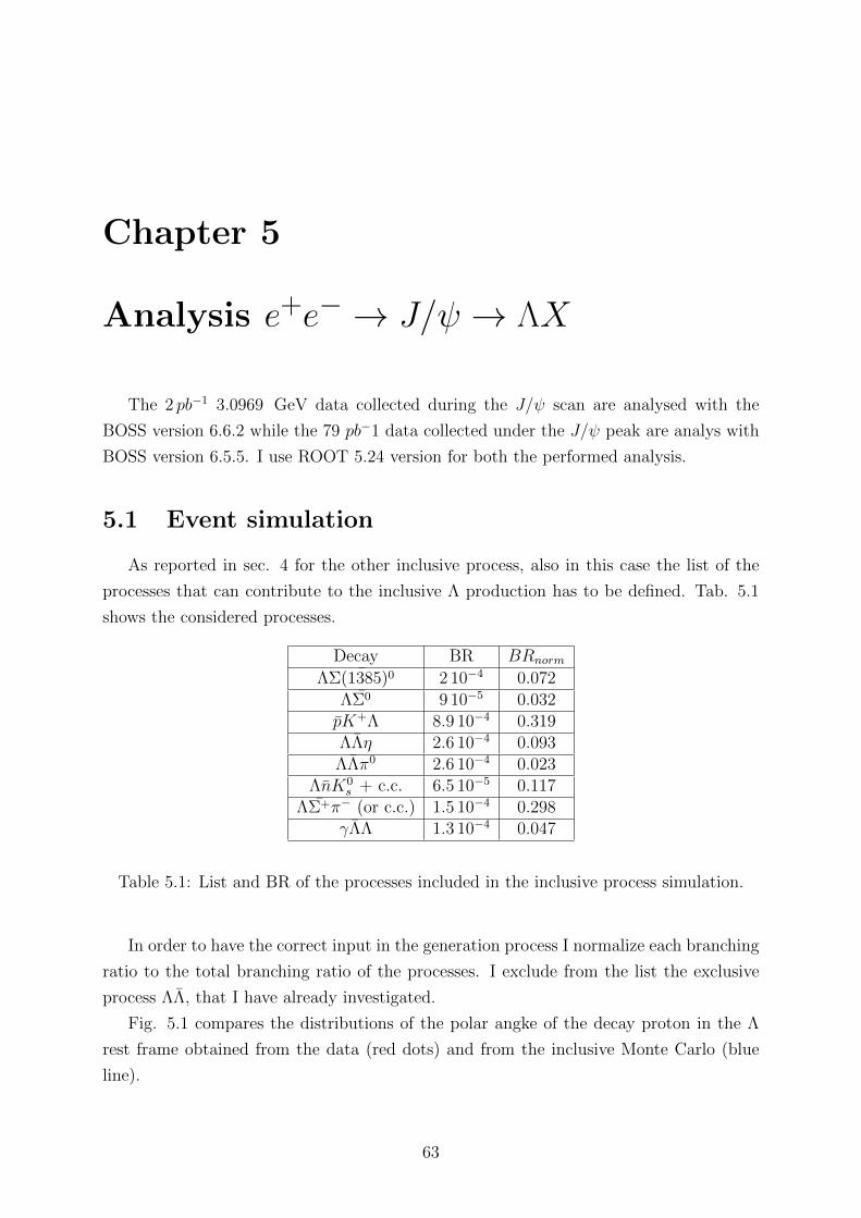
Chapter 5
Analysis e+e−→ J/ψ → ΛX
The 2 pb−1 3.0969 GeV data collected during the J/ψ scan are analysed with the
BOSS version 6.6.2 while the 79 pb−1 data collected under the J/ψ peak are analys with
BOSS version 6.5.5. I use ROOT 5.24 version for both the performed analysis.
5.1 Event simulation
As reported in sec. 4 for the other inclusive process, also in this case the list of the
processes that can contribute to the inclusive Λ production has to be defined. Tab. 5.1
shows the considered processes.
Decay BR BRnorm
Λ ¯Σ(1385)0 2 10−4 0.072ΛΣ0 9 10−5 0.032pK+Λ 8.9 10−4 0.319ΛΛη 2.6 10−4 0.093ΛΛπ0 2.6 10−4 0.023
ΛnK0s + c.c. 6.5 10−5 0.117
ΛΣ+π− (or c.c.) 1.5 10−4 0.298γΛΛ 1.3 10−4 0.047
Table 5.1: List and BR of the processes included in the inclusive process simulation.
In order to have the correct input in the generation process I normalize each branching
ratio to the total branching ratio of the processes. I exclude from the list the exclusive
process ΛΛ, that I have already investigated.
Fig. 5.1 compares the distributions of the polar angke of the decay proton in the Λ
rest frame obtained from the data (red dots) and from the inclusive Monte Carlo (blue
line).
63
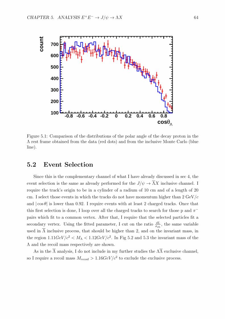
CHAPTER 5. ANALYSIS E+E− → J/ψ → ΛX 64
Λθcos-0.8 -0.6 -0.4 -0.2 0 0.2 0.4 0.6 0.8
cou
nt
100
200
300
400
500
600
700
Figure 5.1: Comparison of the distributions of the polar angle of the decay proton in theΛ rest frame obtained from the data (red dots) and from the inclusive Monte Carlo (blueline).
5.2 Event Selection
Since this is the complementary channel of what I have already discussed in sec 4, the
event selection is the same as already performed for the J/ψ → ΛX inclusive channel. I
require the track’s origin to be in a cylinder of a radium of 10 cm and of a length of 20
cm. I select those events in which the tracks do not have momentum higher than 2 GeV/c
and | cos θ| is lower than 0.92. I require events with at least 2 charged tracks. Once that
this first selection is done, I loop over all the charged tracks to search for those p and π−
pairs which fit to a common vertex. After that, I require that the selected particles fit a
secondary vertex. Using the fitted parameter, I cut on the ratio dLσdL
, the same variable
used in Λ inclusive process, that should be higher than 2, and on the invariant mass, in
the region 1.11GeV/c2 < MΛ < 1.12GeV/c2. In Fig 5.2 and 5.3 the invariant mass of the
Λ and the recoil mass respectively are shown.
As in the Λ analysis, I do not include in my further studies the ΛΛ exclusive channel,
so I require a recoil mass Mrecoil > 1.16GeV/c2 to exclude the exclusive process.
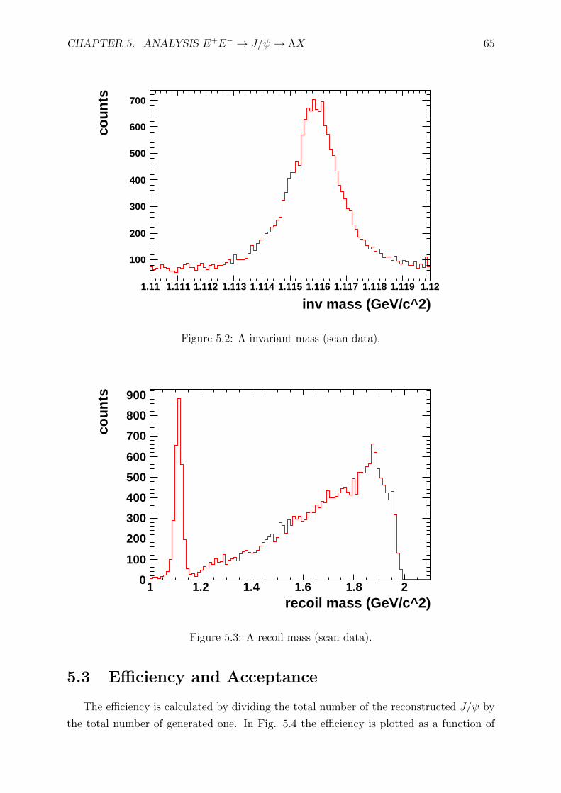
CHAPTER 5. ANALYSIS E+E− → J/ψ → ΛX 65
inv mass (GeV/c^2)1.11 1.111 1.112 1.113 1.114 1.115 1.116 1.117 1.118 1.119 1.12
cou
nts
100
200
300
400
500
600
700
Figure 5.2: Λ invariant mass (scan data).
recoil mass (GeV/c^2)1 1.2 1.4 1.6 1.8 2
cou
nts
0
100
200
300
400
500
600
700
800
900
Figure 5.3: Λ recoil mass (scan data).
5.3 Efficiency and Acceptance
The efficiency is calculated by dividing the total number of the reconstructed J/ψ by
the total number of generated one. In Fig. 5.4 the efficiency is plotted as a function of
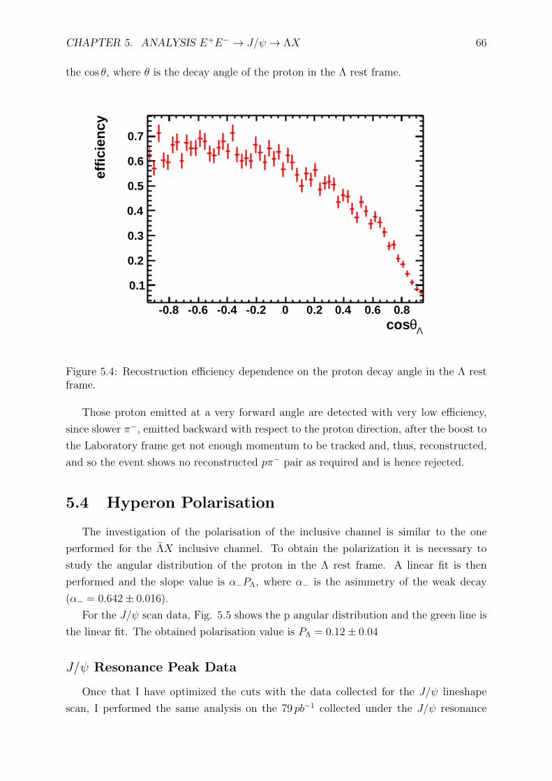
CHAPTER 5. ANALYSIS E+E− → J/ψ → ΛX 66
the cos θ, where θ is the decay angle of the proton in the Λ rest frame.
Λθcos-0.8 -0.6 -0.4 -0.2 0 0.2 0.4 0.6 0.8
effi
cien
cy
0.1
0.2
0.3
0.4
0.5
0.6
0.7
Figure 5.4: Recostruction efficiency dependence on the proton decay angle in the Λ restframe.
Those proton emitted at a very forward angle are detected with very low efficiency,
since slower π−, emitted backward with respect to the proton direction, after the boost to
the Laboratory frame get not enough momentum to be tracked and, thus, reconstructed,
and so the event shows no reconstructed pπ− pair as required and is hence rejected.
5.4 Hyperon Polarisation
The investigation of the polarisation of the inclusive channel is similar to the one
performed for the ΛX inclusive channel. To obtain the polarization it is necessary to
study the angular distribution of the proton in the Λ rest frame. A linear fit is then
performed and the slope value is α−PΛ, where α− is the asimmetry of the weak decay
(α− = 0.642± 0.016).
For the J/ψ scan data, Fig. 5.5 shows the p angular distribution and the green line is
the linear fit. The obtained polarisation value is PΛ = 0.12± 0.04
J/ψ Resonance Peak Data
Once that I have optimized the cuts with the data collected for the J/ψ lineshape
scan, I performed the same analysis on the 79 pb−1 collected under the J/ψ resonance
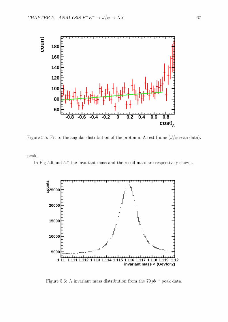
CHAPTER 5. ANALYSIS E+E− → J/ψ → ΛX 67
Λθcos-0.8 -0.6 -0.4 -0.2 0 0.2 0.4 0.6 0.8
cou
nt
60
80
100
120
140
160
180
Figure 5.5: Fit to the angular distribution of the proton in Λ rest frame (J/ψ scan data).
peak.
In Fig 5.6 and 5.7 the invariant mass and the recoil mass are respectively shown.
(GeV/c^2)Λinvariant mass 1.11 1.111 1.112 1.113 1.114 1.115 1.116 1.117 1.118 1.119 1.12
cou
nts
5000
10000
15000
20000
25000
Figure 5.6: Λ invariant mass distribution from the 79 pb−1 peak data.
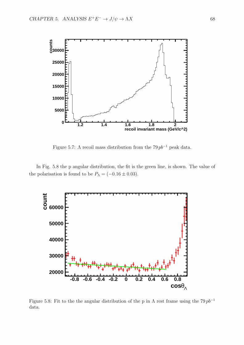
CHAPTER 5. ANALYSIS E+E− → J/ψ → ΛX 68
recoil invariant mass (GeV/c^2)1.2 1.4 1.6 1.8 2
cou
nts
0
5000
10000
15000
20000
25000
30000
Figure 5.7: Λ recoil mass distribution from the 79 pb−1 peak data.
In Fig. 5.8 the p angular distribution, the fit is the green line, is shown. The value of
the polarisation is found to be PΛ = (−0.16± 0.03).
Λθcos-0.8 -0.6 -0.4 -0.2 0 0.2 0.4 0.6 0.8
cou
nt
20000
30000
40000
50000
60000
Figure 5.8: Fit to the the angular distribution of the p in Λ rest frame using the 79 pb−1
data.
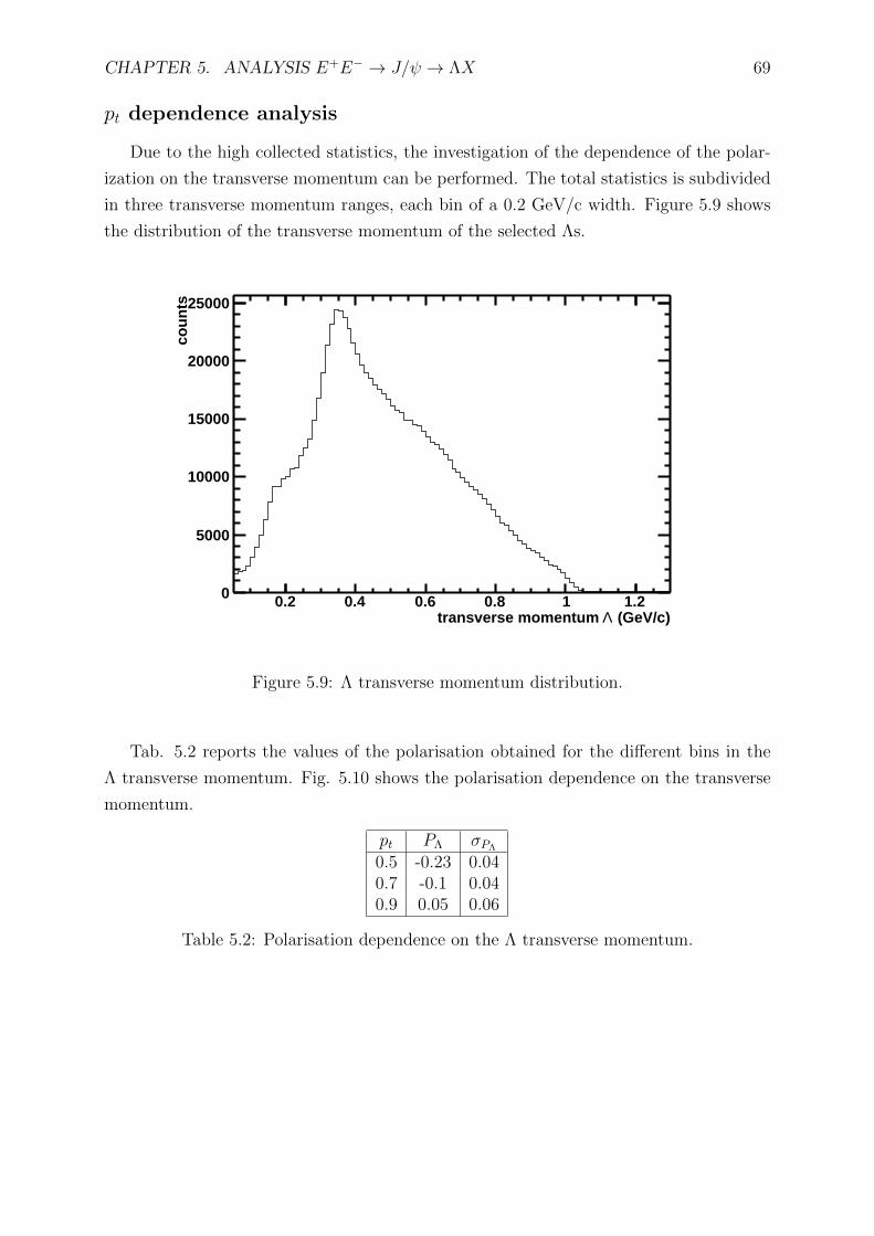
CHAPTER 5. ANALYSIS E+E− → J/ψ → ΛX 69
pt dependence analysis
Due to the high collected statistics, the investigation of the dependence of the polar-
ization on the transverse momentum can be performed. The total statistics is subdivided
in three transverse momentum ranges, each bin of a 0.2 GeV/c width. Figure 5.9 shows
the distribution of the transverse momentum of the selected Λs.
(GeV/c)Λtransverse momentum 0.2 0.4 0.6 0.8 1 1.2
cou
nts
0
5000
10000
15000
20000
25000
Figure 5.9: Λ transverse momentum distribution.
Tab. 5.2 reports the values of the polarisation obtained for the different bins in the
Λ transverse momentum. Fig. 5.10 shows the polarisation dependence on the transverse
momentum.
pt PΛ σPΛ
0.5 -0.23 0.040.7 -0.1 0.040.9 0.05 0.06
Table 5.2: Polarisation dependence on the Λ transverse momentum.
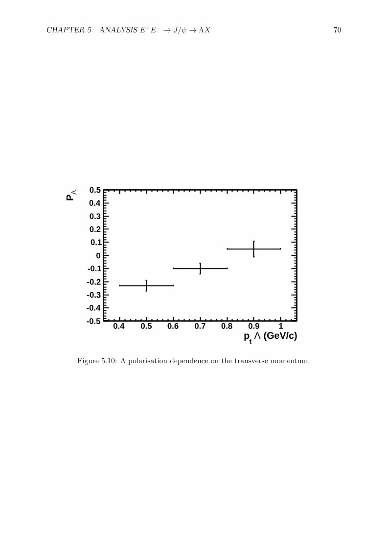
CHAPTER 5. ANALYSIS E+E− → J/ψ → ΛX 70
(GeV/c)Λ t
p0.4 0.5 0.6 0.7 0.8 0.9 1
ΛP
-0.5
-0.4
-0.3
-0.2
-0.1
0
0.1
0.2
0.3
0.4
0.5
Figure 5.10: Λ polarisation dependence on the transverse momentum.
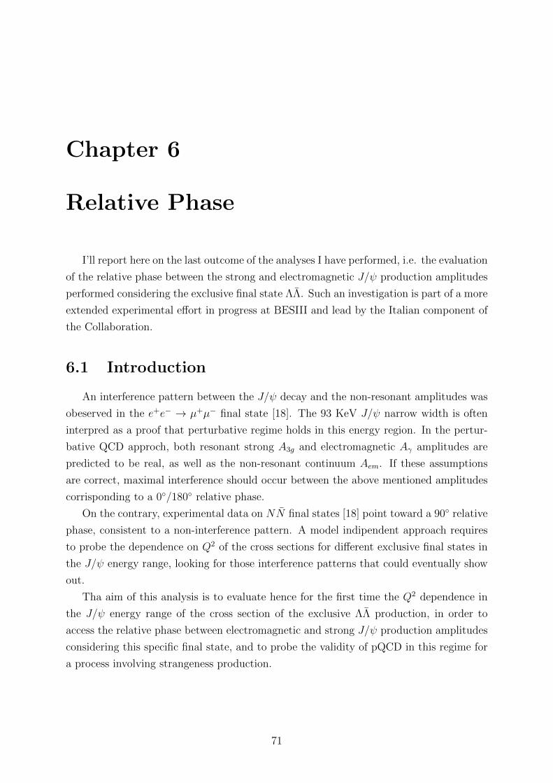
Chapter 6
Relative Phase
I’ll report here on the last outcome of the analyses I have performed, i.e. the evaluation
of the relative phase between the strong and electromagnetic J/ψ production amplitudes
performed considering the exclusive final state ΛΛ. Such an investigation is part of a more
extended experimental effort in progress at BESIII and lead by the Italian component of
the Collaboration.
6.1 Introduction
An interference pattern between the J/ψ decay and the non-resonant amplitudes was
obeserved in the e+e− → µ+µ− final state [18]. The 93 KeV J/ψ narrow width is often
interpred as a proof that perturbative regime holds in this energy region. In the pertur-
bative QCD approch, both resonant strong A3g and electromagnetic Aγ amplitudes are
predicted to be real, as well as the non-resonant continuum Aem. If these assumptions
are correct, maximal interference should occur between the above mentioned amplitudes
corrisponding to a 0/180 relative phase.
On the contrary, experimental data on NN final states [18] point toward a 90 relative
phase, consistent to a non-interference pattern. A model indipendent approach requires
to probe the dependence on Q2 of the cross sections for different exclusive final states in
the J/ψ energy range, looking for those interference patterns that could eventually show
out.
Tha aim of this analysis is to evaluate hence for the first time the Q2 dependence in
the J/ψ energy range of the cross section of the exclusive ΛΛ production, in order to
access the relative phase between electromagnetic and strong J/ψ production amplitudes
considering this specific final state, and to probe the validity of pQCD in this regime for
a process involving strangeness production.
71
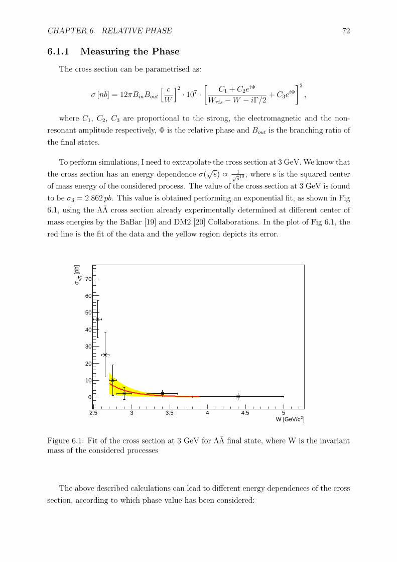
CHAPTER 6. RELATIVE PHASE 72
6.1.1 Measuring the Phase
The cross section can be parametrised as:
σ [nb] = 12πBinBout
[ cW
]2
· 107 ·[
C1 + C2eiΦ
Wris −W − iΓ/2+ C3e
iΦ
]2
,
where C1, C2, C3 are proportional to the strong, the electromagnetic and the non-
resonant amplitude respectively, Φ is the relative phase and Bout is the branching ratio of
the final states.
To perform simulations, I need to extrapolate the cross section at 3 GeV. We know that
the cross section has an energy dependence σ(√s) ∝ 1√
s10 , where s is the squared center
of mass energy of the considered process. The value of the cross section at 3 GeV is found
to be σ3 = 2.862 pb. This value is obtained performing an exponential fit, as shown in Fig
6.1, using the ΛΛ cross section already experimentally determined at different center of
mass energies by the BaBar [19] and DM2 [20] Collaborations. In the plot of Fig 6.1, the
red line is the fit of the data and the yellow region depicts its error.
]2W [GeV/c2.5 3 3.5 4 4.5 5
[pb]
ΛΛσ
0
10
20
30
40
50
60
70
Figure 6.1: Fit of the cross section at 3 GeV for ΛΛ final state, where W is the invariantmass of the considered processes
The above described calculations can lead to different energy dependences of the cross
section, according to which phase value has been considered:
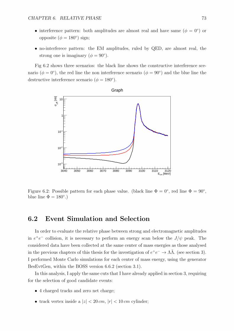
CHAPTER 6. RELATIVE PHASE 73
• interference pattern: both amplitudes are almost real and have same (φ = 0) or
opposite (φ = 180) sign;
• no-interferece pattern: the EM amplitudes, ruled by QED, are almost real, the
strong one is imaginary (φ = 90).
Fig 6.2 shows three scenarios: the black line shows the constructive interference sce-
nario (φ = 0), the red line the non interference scenario (φ = 90) and the blue line the
destructive interference scenario (φ = 180).
[MeV]cmE3040 3050 3060 3070 3080 3090 3100 3110 3120
[nb]
ΛΛσ
-310
-210
-110
1
10
Graph
Figure 6.2: Possible pattern for each phase value. (black line Φ = 0, red line Φ = 90,blue line Φ = 180.)
6.2 Event Simulation and Selection
In order to evaluate the relative phase between strong and electromagnetic amplitudes
in e+e− collision, it is necessary to perform an energy scan below the J/ψ peak. The
considered data have been collected at the same center of mass energies as those analysed
in the previous chapters of this thesis for the investigation of e+e− → ΛΛ. (see section 3).
I performed Monte Carlo simulations for each center of mass energy, using the generator
BesEvtGen, within the BOSS version 6.6.2 (section 3.1).
In this analysis, I apply the same cuts that I have already applied in section 3, requiring
for the selection of good candidate events:
• 4 charged tracks and zero net charge;
• track vertex inside a |z| < 20 cm, |r| < 10 cm cylinder;
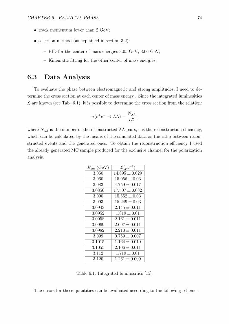
CHAPTER 6. RELATIVE PHASE 74
• track momentum lower than 2 GeV;
• selection method (as explained in section 3.2):
– PID for the center of mass energies 3.05 GeV, 3.06 GeV;
– Kinematic fitting for the other center of mass energies.
6.3 Data Analysis
To evaluate the phase between electromagnetic and strong amplitudes, I need to de-
termine the cross section at each center of mass energy . Since the integrated luminosities
L are known (see Tab. 6.1), it is possible to determine the cross section from the relation:
σ(e+e− → ΛΛ) =NΛΛ
εL,
where NΛΛ is the number of the reconstructed ΛΛ pairs, ε is the reconstruction efficiency,
which can be calculated by the means of the simulated data as the ratio between recon-
structed events and the generated ones. To obtain the reconstruction efficiency I used
the already generated MC sample produced for the exclusive channel for the polarization
analysis.
Ecm (GeV) L(pb−1)3.050 14.895± 0.0293.060 15.056± 0.033.083 4.759± 0.0173.0856 17.507± 0.0323.090 15.552± 0.033.093 15.249± 0.033.0943 2.145± 0.0113.0952 1.819± 0.013.0958 2.161± 0.0113.0969 2.097± 0.0113.0982 2.210± 0.0113.099 0.759± 0.0073.1015 1.164± 0.0103.1055 2.106± 0.0113.112 1.719± 0.013.120 1.261± 0.009
Table 6.1: Integrated luminosities [15].
The errors for these quantities can be evaluated according to the following scheme:
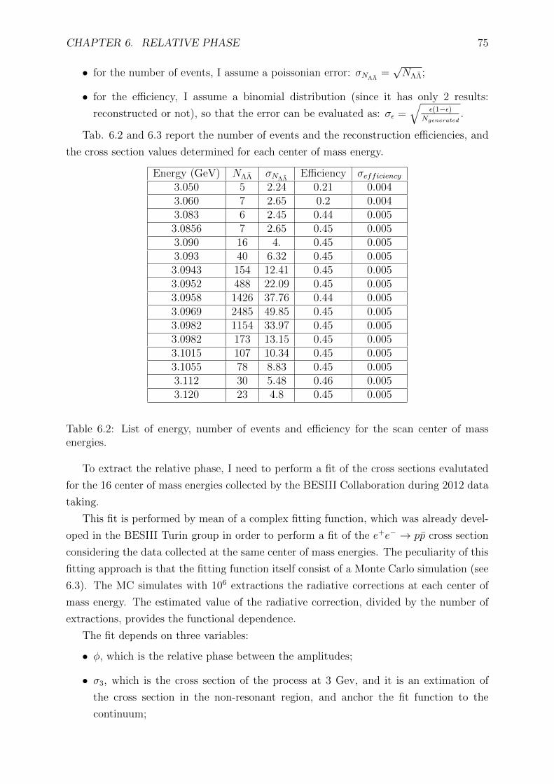
CHAPTER 6. RELATIVE PHASE 75
• for the number of events, I assume a poissonian error: σNΛΛ=√NΛΛ;
• for the efficiency, I assume a binomial distribution (since it has only 2 results:
reconstructed or not), so that the error can be evaluated as: σε =√
ε(1−ε)Ngenerated
.
Tab. 6.2 and 6.3 report the number of events and the reconstruction efficiencies, and
the cross section values determined for each center of mass energy.
Energy (GeV) NΛΛ σNΛΛEfficiency σefficiency
3.050 5 2.24 0.21 0.0043.060 7 2.65 0.2 0.0043.083 6 2.45 0.44 0.0053.0856 7 2.65 0.45 0.0053.090 16 4. 0.45 0.0053.093 40 6.32 0.45 0.0053.0943 154 12.41 0.45 0.0053.0952 488 22.09 0.45 0.0053.0958 1426 37.76 0.44 0.0053.0969 2485 49.85 0.45 0.0053.0982 1154 33.97 0.45 0.0053.0982 173 13.15 0.45 0.0053.1015 107 10.34 0.45 0.0053.1055 78 8.83 0.45 0.0053.112 30 5.48 0.46 0.0053.120 23 4.8 0.45 0.005
Table 6.2: List of energy, number of events and efficiency for the scan center of massenergies.
To extract the relative phase, I need to perform a fit of the cross sections evalutated
for the 16 center of mass energies collected by the BESIII Collaboration during 2012 data
taking.
This fit is performed by mean of a complex fitting function, which was already devel-
oped in the BESIII Turin group in order to perform a fit of the e+e− → pp cross section
considering the data collected at the same center of mass energies. The peculiarity of this
fitting approach is that the fitting function itself consist of a Monte Carlo simulation (see
6.3). The MC simulates with 106 extractions the radiative corrections at each center of
mass energy. The estimated value of the radiative correction, divided by the number of
extractions, provides the functional dependence.
The fit depends on three variables:
• φ, which is the relative phase between the amplitudes;
• σ3, which is the cross section of the process at 3 Gev, and it is an extimation of
the cross section in the non-resonant region, and anchor the fit function to the
continuum;
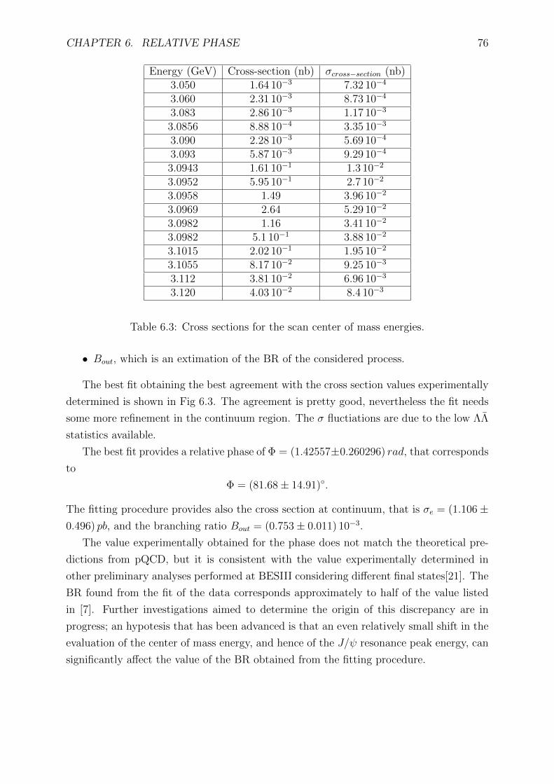
CHAPTER 6. RELATIVE PHASE 76
Energy (GeV) Cross-section (nb) σcross−section (nb)3.050 1.64 10−3 7.32 10−4
3.060 2.31 10−3 8.73 10−4
3.083 2.86 10−3 1.17 10−3
3.0856 8.88 10−4 3.35 10−3
3.090 2.28 10−3 5.69 10−4
3.093 5.87 10−3 9.29 10−4
3.0943 1.61 10−1 1.3 10−2
3.0952 5.95 10−1 2.7 10−2
3.0958 1.49 3.96 10−2
3.0969 2.64 5.29 10−2
3.0982 1.16 3.41 10−2
3.0982 5.1 10−1 3.88 10−2
3.1015 2.02 10−1 1.95 10−2
3.1055 8.17 10−2 9.25 10−3
3.112 3.81 10−2 6.96 10−3
3.120 4.03 10−2 8.4 10−3
Table 6.3: Cross sections for the scan center of mass energies.
• Bout, which is an extimation of the BR of the considered process.
The best fit obtaining the best agreement with the cross section values experimentally
determined is shown in Fig 6.3. The agreement is pretty good, nevertheless the fit needs
some more refinement in the continuum region. The σ fluctiations are due to the low ΛΛ
statistics available.
The best fit provides a relative phase of Φ = (1.42557±0.260296) rad, that corresponds
to
Φ = (81.68± 14.91).
The fitting procedure provides also the cross section at continuum, that is σe = (1.106±0.496) pb, and the branching ratio Bout = (0.753± 0.011) 10−3.
The value experimentally obtained for the phase does not match the theoretical pre-
dictions from pQCD, but it is consistent with the value experimentally determined in
other preliminary analyses performed at BESIII considering different final states[21]. The
BR found from the fit of the data corresponds approximately to half of the value listed
in [7]. Further investigations aimed to determine the origin of this discrepancy are in
progress; an hypotesis that has been advanced is that an even relatively small shift in the
evaluation of the center of mass energy, and hence of the J/ψ resonance peak energy, can
significantly affect the value of the BR obtained from the fitting procedure.
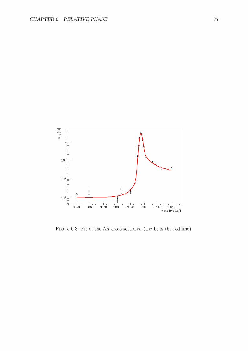
CHAPTER 6. RELATIVE PHASE 77
]2Mass [MeV/c3050 3060 3070 3080 3090 3100 3110 3120
[nb]
ΛΛσ
-310
-210
-110
1
Figure 6.3: Fit of the ΛΛ cross sections. (the fit is the red line).

Part III
Conclusion
78
79
Hyperon Polarisation
Two different event selection approches has been tested, and then separately for each
center of mass energy I have selected the most suitable, i.e. that providing the largest
number of surviving events and the better signal over background ratio. The Λ and the Λ
polarisations have been determined for the exclusive production of the ΛΛ pairs, for the
first time with e+e− beams in the J/ψ sector and in the lower energy continuum. The
hyperon polarisation is compatible with zero in the continuum region and is statistically
uncompatible with zero in the J/ψ resonance region: PΛ = 0.16± 0.03 and PΛ = −0.11±0.02. A precise evaluation of the hyperon polarisation could also allow to access the
relative phase between the hyperon electric and magnetic form factors [22].
The polarisation has been evaluated as well for the inclusive J/ψ → ΛX production,
and is also statistically non compatible with zero: PΛ = 0.16± 0.02.
A similar result has been determined for the charge conjugate process J/ψ → Λ:
PΛ = −0.16± 0.03.
The polarisation evaluated experimentally both in the inclusive both in the exclusive
processes shows a clear dependence on the hypeon transverse momentum: in the case
of the exclusive process, the polarisation is more sizeable at larger transverse momen-
tum, while in the inclusive processes the polarisation is more sizeable at lower transverse
momentum.
The present analysis has shown as the polarisation has opposite signs in the considered
exclusive and inclusive hyperon production processes.
Relative phase
The relative phase between strong and electromagnetic J/ψ production amplitudes
has been determined for the first time: φ = (81.68± 14.91), and found to be compatible
with 90 degrees. A similar picture has been recently reported by BESIII considering other
final states. A 90 relatice phase between amplitudes ruled by QED and QCD implies that
at least one of these amplitudes should be imaginary, and such a possibility is excluded
by QED and QCD.
Bibliography
[1] M. Gell-Mann, The interpretation of the New Particels as Displaced Charged Multi-
plets, Il Nuovo Cimento 4 (S2): 848 (1956)
[2] D.H. Perkins, Introduction to High Energy physics, Cambridge Press.
[3] D. Schulte, Beam-Beam Interaction, CERN.
[4] Iwanenko D., Pomeranchuk I., On the maximal energy attainable in betatron, Physical
Review 65 (1944) 343.
[5] J. Aubert et al., Experimental observation of a Heavy Particle J, Physical Review
Letters 33 (1974).
[6] J. Augustin et al.,Discovery of a Narrow Resonance in e+e− Annihilation., Physical
Review Letters 33 (1974).
[7] J. Beringer et al. (Particle Data Group), The Review of Particle Physics, Phys. Rev.
D86,010001 (2012)
[8] G. D. Rochester and C. C. Butler, Evidence for the Existence of New Un- stable
Elementary Particles, Nature, 92:855 (1947).
[9] K. Nishijima (1955), Charge Indipendence Theory of V Particles, Progress of Theo-
retical Physics 13(3): 285.
[10] S. Brauksiepe, et al., COSY-11 an Internal Experimental Facility for Threshold Mea-
surements, Nucl. Instr. Meth. A 376, 3 (1996)
[11] F. Balestra et al., Spin Transfer in Exclusive Λ Production from pp Collisions at 3.67
GeV/c, Phys. Rev. Lett. 83, 1534-1537 (1999)
[12] M. Ablikim et al. (BESIII collaboration), Design and Construction of BESIII.
[13] http://root.cern.ch/drupal/
[14] R.G. Ping, C.Y. Pang, Monte Carlo Generators for Tau-Charm-Physics at BESIII
80
BIBLIOGRAPHY 81
[15] B.X. Zhang, Luminosity measurement for J/ψ phase and lineshape study, private
communication.
[16] R. E. Kalman, A New Approach to Linear Filtering and Prediction Problems, Trans-
action of the ASME Journal of Basic Engineering 82D (1960)
[17] J. Podolansky and R. Armenteros, Phil. Mag., 45(13), 1954
[18] J. Augustin et al., PRL 33, 1076 (1974)
[19] B. Aubert et al. (BABAR Collaboration), Phys. Rev. D 76, 092006 (2007)
[arXiv:0709.1988[hep-ex]])
[20] D. Bisello et al. (DM2 Collaboration), Z. Phys. C 48, 23 (1990)
[21] M. Destefanis, Measurement of the Phase between Strong and Electromagnatic J/ψ →pp Decay Amplitudes, BAM-106 on Hypernews.
[22] B. Aubert et al. (BABAR collaboration), Study of e+e− → ΛΛ,ΛΣ0,Σ0Σ0 using
initial state radiation with BABAR, Physical Rewiew D 76, 092006(2007).
And without any reference in the text:
[-] M. Ablikim et al. (BESIII collaboration), Physics at BESIII.
[-] M. Ablikim et al. (BESIII collaboration), Study of the J/ψ decays to ΛΛ and Σ0Σ0.,
hep-ex/050602v1 (2005)
[-] M. Destefanis, Hyperon Studies at GSI: Λ reconstruction in p-p Collision at 2.2 GeV
with Hades and in p-p Interaction for the Future PANDA Experiment. Ph.D thesis
(2008),
[-] M. Gell-Mann , Phys. Lett. 16(1964), pag 214-215
[-] M. Maggiora, Measuring the phase between strong and EM J/ψ decay amplitude.