1

SCUOLA NAZIONALE

DI RISONANZA MAGNETICA NUCLEARE

Torino 23-27 Settembre 2013

Stefano MammiDipartimento di Scienze Chimiche

Università di Padovastefano.mammi@unipd.it

Concetti di baseParametri NMR

Esperimento 1D-FT NMR

RIFERIMENTI BIBLIOGRAFICI

M. Levitt “Spin Dynamics” ”, 2nd ed., John Wiley & Sons, 2008.

J. Keeler, “Understanding NMR Spectroscopy”, 2nd ed., John Wiley & Sons, 2010.

T. D. W. Claridge, “High-Resolution NMR Techniques in Organic Chemistry”, Pergamon Press, 1999.

J. Cavanagh, “Protein NMR spectroscopy: principles and practice”, 2nd ed., Elsevier, 2007.

http://www.cis.rit.edu/htbooks/nmrhttp://www.chem.queensu.ca/FACILITIES/NMR/nmr/webcourse

http://www-keeler.ch.cam.ac.uk/lectures/index.html

2

RIFERIMENTI BIBLIOGRAFICI

H. Günther, "NMR Spectroscopy", 2nd ed., John Wiley & Sons, 1995.

J. K. M. Sanders and B. K. Hunter, "Modern NMR Spectroscopy", 2nd

ed., Oxford University Press, 1994.

H. Friebolin, "Basic One- and Two-Dimensional NMR Spectroscopy", VCH, 1991.

R. M. Silverstein and F. X. Webster, "Identificazione Spettroscopica di Composti Organici", Casa Editrice Ambrosiana, 1999.

A. E. Derome, "Modern NMR Techniques for Chemistry Research", Pergamon Press, 1987.

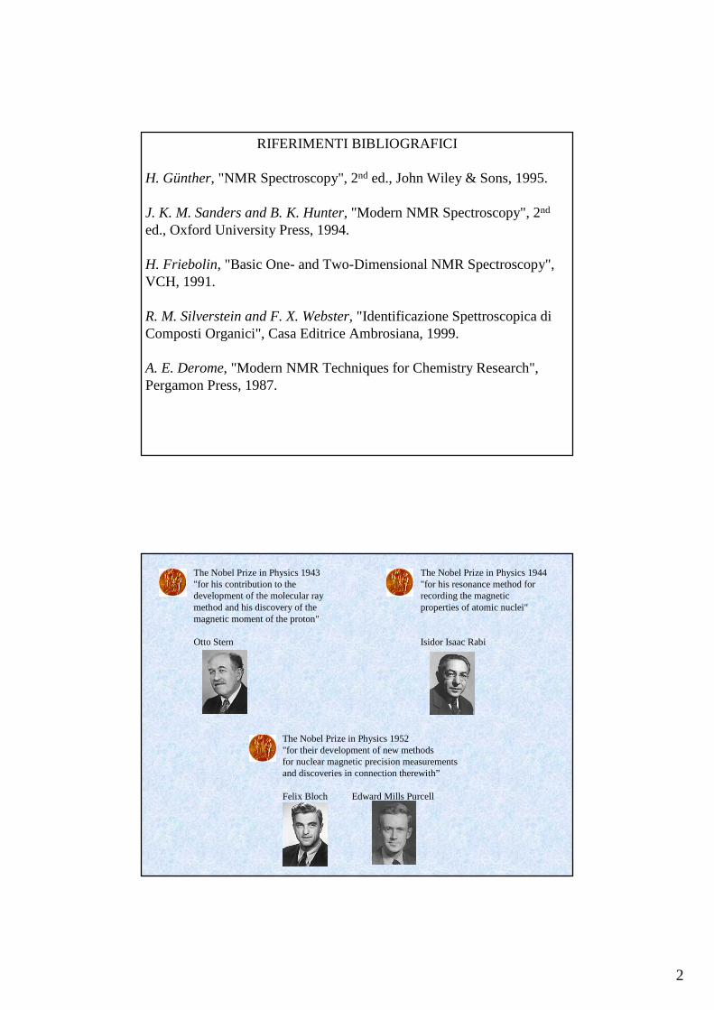
The Nobel Prize in Physics 1952"for their development of new methodsfor nuclear magnetic precision measurements and discoveries in connection therewith”

Felix Bloch Edward Mills Purcell

The Nobel Prize in Physics 1944"for his resonance method for recording the magneticproperties of atomic nuclei"

Isidor Isaac Rabi

The Nobel Prize in Physics 1943"for his contribution to the development of the molecular ray method and his discovery of the magnetic moment of the proton"

Otto Stern

3

The Nobel Prize in Chemistry 1991"for his contributions to the development of the methodology of high resolution nuclear magnetic resonance (NMR) spectroscopy"

Richard R. Ernst

The Nobel Prize in Chemistry 2002"for his development of nuclear magnetic resonance spectroscopy for determining the three-dimensional structure of biological macromolecules in solution”

Kurt Wüthrich 1/2 of the prize

The Nobel Prize in Physics 2003”for pioneering contributions to the theory of superconductors”

Alexei A. Abrikosov Vitaly L. Ginzburg1/3 of the prize 1/3 of the prize

The Nobel Prize in Physiology or Medicine 2003"for their discoveries concerning magnetic resonance imaging”

Paul C. Lauterbur Sir Peter Mansfield

4

B0

I

µ

ω0

dIdt

z

mIz

hγ=γ= µµ

mI

ImI- 1)I(II

zh

h

=

+≤≤+=

000 B- BdtId γ=ω×= µ

B0

M0

I=1/2 E = −µB0

E = −γhmB0

α: m = +½

µα = +½γhEα = −½γhB0

β: m = −½

µβ = −½γhEβ = +½γhB0

kT

E

eP

P ∆−

α

β =

M0 = Σµ = Mz

Mx = My = 0

∆E = γhB0 = hω0 = hν0

5

∆E = γhB0 = hω0 = hν0

kT

E

eP

P ∆−

α

β =

M0 = Σµ = Mz

the new arrival!

CERM, University of FlorenceSeason greetings - 2003

6

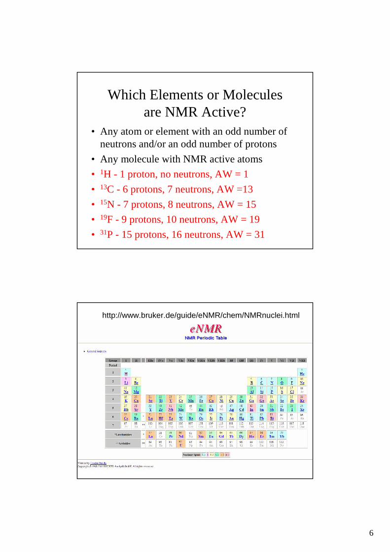
Which Elements or Molecules are NMR Active?

• Any atom or element with an odd number of neutrons and/or an odd number of protons

• Any molecule with NMR active atoms

• 1H - 1 proton, no neutrons, AW = 1

• 13C - 6 protons, 7 neutrons, AW =13

• 15N - 7 protons, 8 neutrons, AW = 15

• 19F - 9 protons, 10 neutrons, AW = 19

• 31P - 15 protons, 16 neutrons, AW = 31

http://www.bruker.de/guide/eNMR/chem/NMRnuclei.html

7

Different Isotopes Absorb at Different Frequencies

low frequency high frequency

15N 2H 13C 19F 1H

50 MHz 77 MHz 125 MHz 200 MHz 470 MHz 500 MHz

31P

Isotope Spin Nat. Ab. %Relative Absolute

4.6975 9.395 14.09261H 1/2 99.98 1 1 200 400 6002H 1 1.50E-029.65E-031.45E-06 30.701 61.402 92.10213C 1/2 1.1081.59E-021.76E-04 50.288 100.577 150.86415N 1/2 0.371.04E-033.85E-06 20.265 40.531 60.79619F 1/2 100 0.83 0.83 188.154 376.308 564.46231P 1/2 1006.63E-026.63E-02 80.961 161.923 242.884

Relative Sensitivity = at the same field and for the same number of nucleiAbsolute Sensitivity = (relative sensitivity * natural abundance)

Sensitivity NMR Resonance Frequencies (MHz) at a field of (T):

NMR Parameters for some nuclei

8

Bx(t) = B x * cos ( ωωωωot)

x

y

z

MB0 B0

x

y

z

M

B1

x

y

time

1( ) cosx rfB t B tω=

1( ) / 2( cos sin )R rf rfB t B t tω ω= +i j

1( ) / 2( cos sin )L rf rfB t B t tω ω= −i j

9

So how does that help?

Lωω =0

z, B0

)( 1Brfω−

)( 1Brfω

x

Lωω =0

z, B0

)( 1Brfω

10

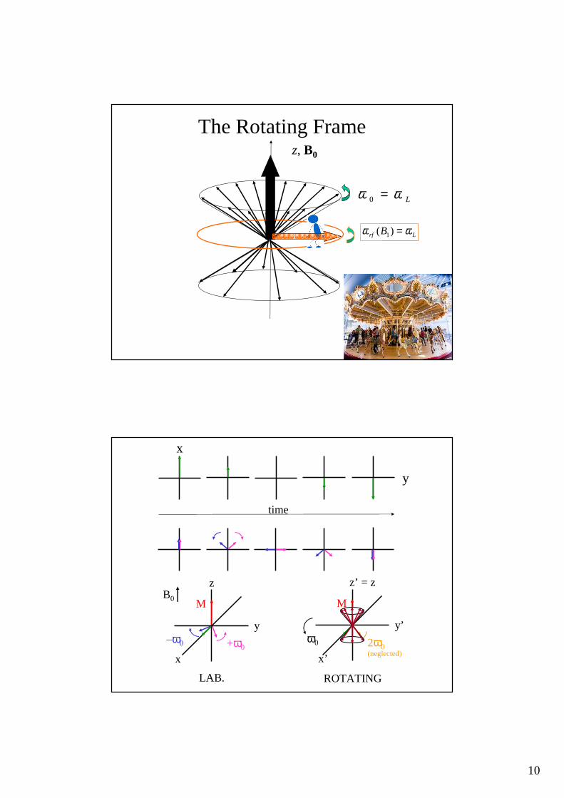
Lωω =0

z, B0

The Rotating Frame

)( 1Brfω Lrf B ωω =)( 1

x

y

time

+ω0–ω0

M

x

y

zB0

LAB.

2ω0(neglected)x’

y’

M

z’ = z

ω0

ROTATING

11

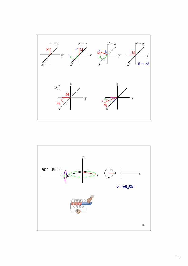
x

y

z

M

B0

ω0

x’

y’

z’ = z

M

x’

y’

z’ = z

M

B1

x’

y’

z’ = z

B1

M θ

x’

y’

z’ = z

M

θ = π/2

x

y

z

ω0

ω0t

22

νννν = γγγγBo/2ππππ

90° Pulse

12

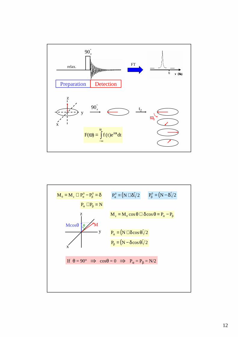
FTrelax.

°x90

Preparation Detection

x

y

z

°x90 t2

ω0

∫+∞

∞−

ω=ω dte)t(f)(F ti

x

y

z

MθMcosθ

δ=−∝= βα00

z0 PPMM ( ) 2NP0 δ+=α ( ) 2NP0 δ−=β

βα −=θδ∝θ= PPcoscosMM 0z

NPP =+ βα

( ) 2cosNP θδ+=α

( ) 2cosNP θδ−=β

If θ = 90° ⇒ cosθ = 0 ⇒ Pα = Pβ = N/2

13

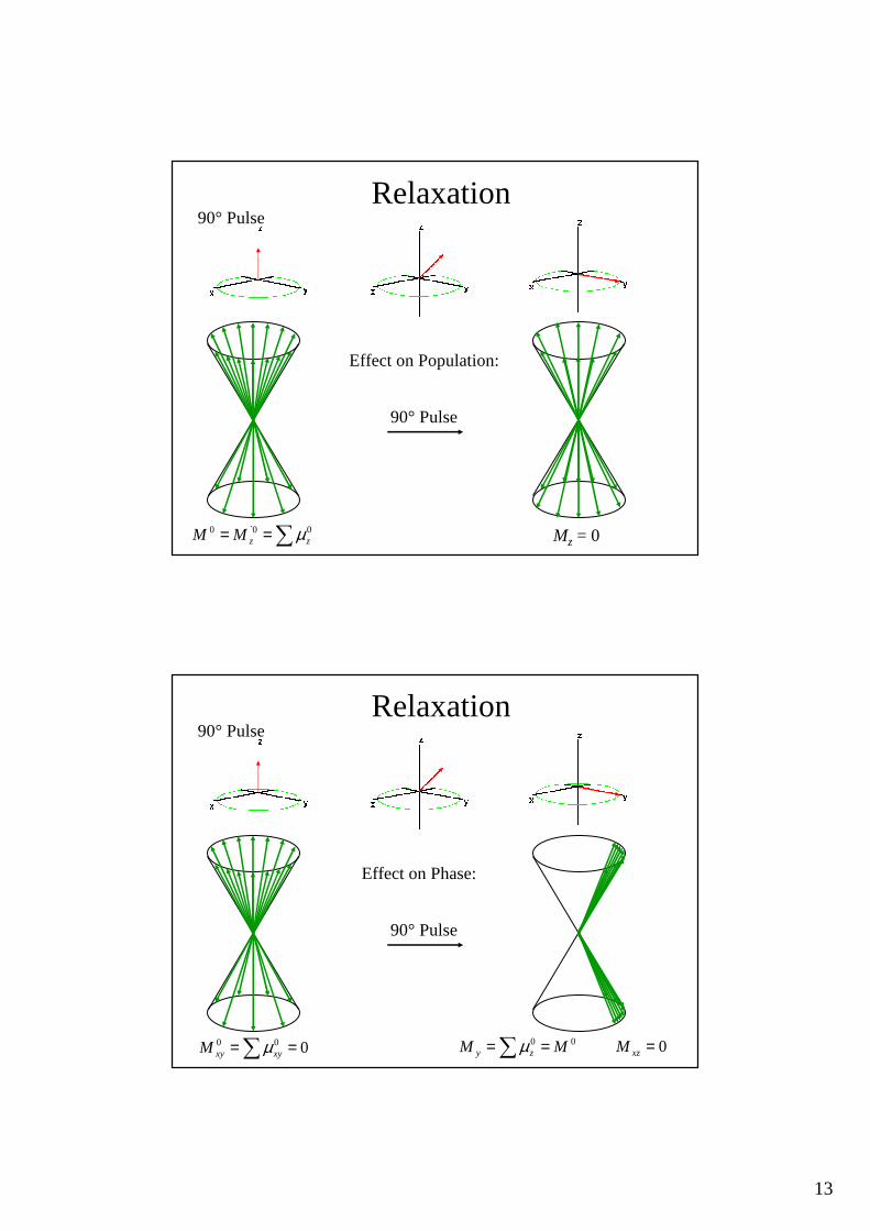
Relaxation 90° Pulse

Effect on Population:

90° Pulse

Mz = 0∑== 000zzMM µ

Relaxation 90° Pulse

Effect on Phase:

90° Pulse

000 ==∑ xyxyM µ 00 MM zy ==∑µ 0=xzM

14

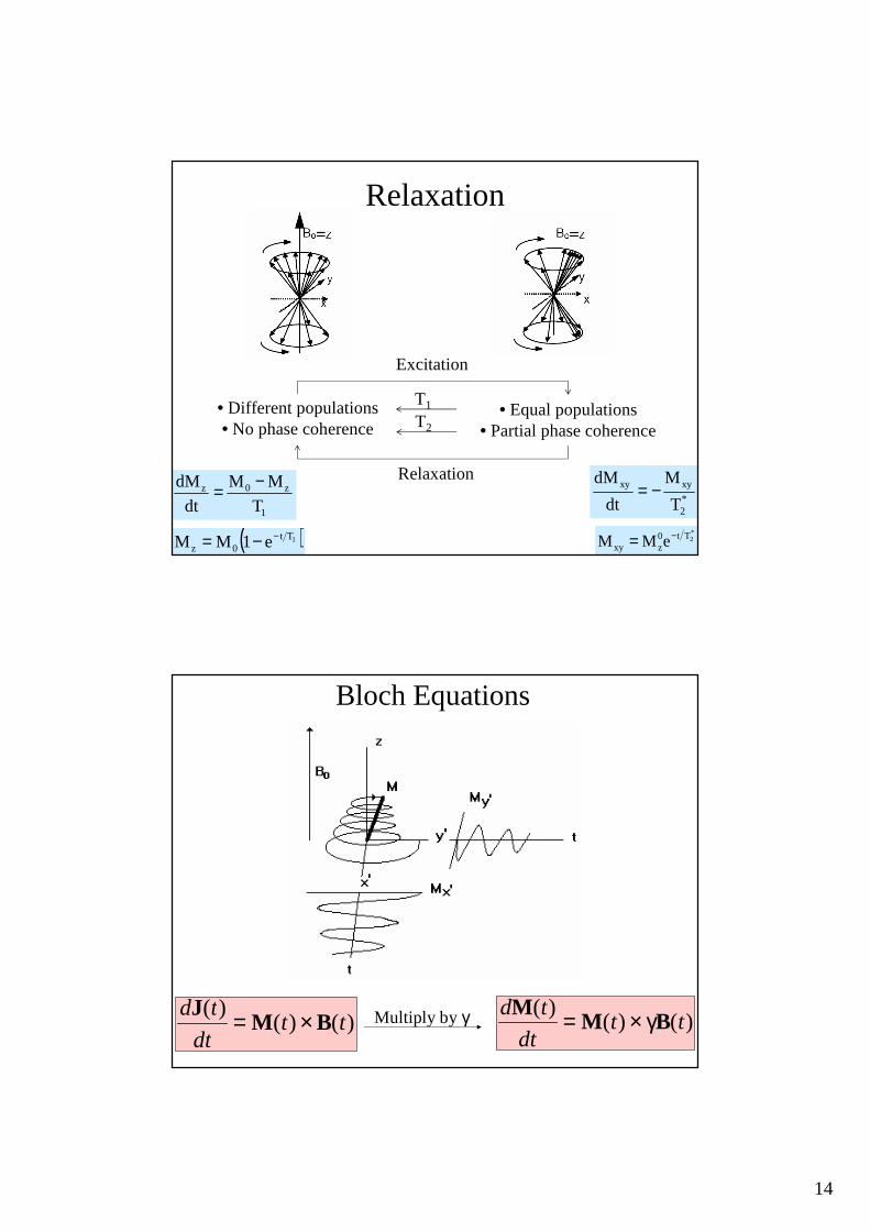
Relaxation

• Different populations• No phase coherence

• Equal populations• Partial phase coherence

Excitation

Relaxation

T1

T2

*2Tt0

zxy eMM −=

*2

xyxy

T

M

dt

dM−=

1

z0z

T

MM

dt

dM −=

( )1Tt0z e1MM −−=

Bloch Equations

d t

dtt t

JM B

( )( ) ( )= ×

d t

dtt t

MM B

( )( ) ( )= × γMultiply by γ

15

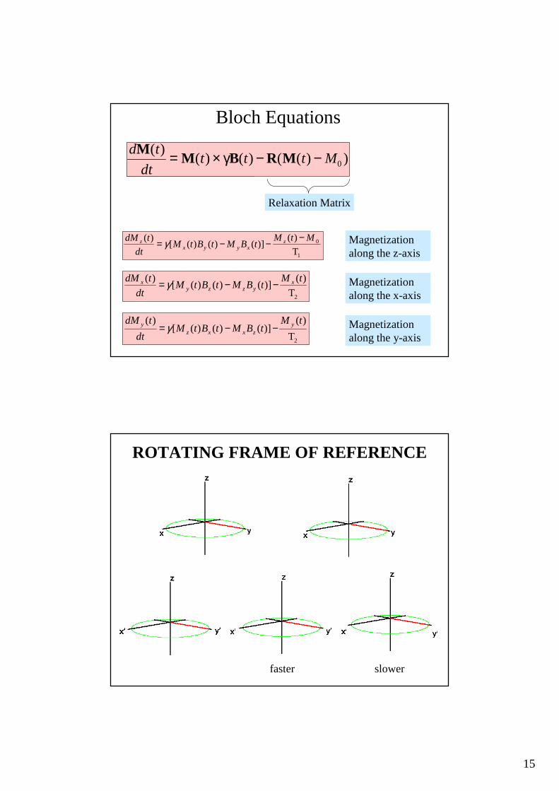
Bloch Equations

d t

dtt t

MM B

( )( ) ( )= × γ

1

0

T

)()]()()([

)( MtMtBMtBtM

dt

tdM zxyyx

z −−−= γ Magnetization

along the z-axis

2T

)()]()()([

)( tMtBMtBtM

dt

tdM xyzzy

x −−= γ Magnetization along the x-axis

2T

)()]()()([

)( tMtBMtBtM

dt

tdM yzxxz

y −−= γ Magnetization along the y-axis

d t

dtt t t M

MM B R M

( )( ) ( ) ( ( ) )= × − −γ 0

Relaxation Matrix

ROTATING FRAME OF REFERENCE

faster slower

16

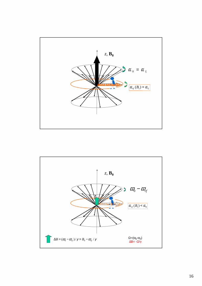
Lωω =0

z, B0

)( 1Brfω Lrf B ωω =)( 1

01)( ωω <Brf

z, B0

γωγωω //)( 00 rfrf BB −=−=∆

rfωω −0

Ω=(ω0-ωrf) ∆B= -Ω/γ

17

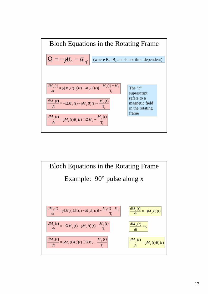
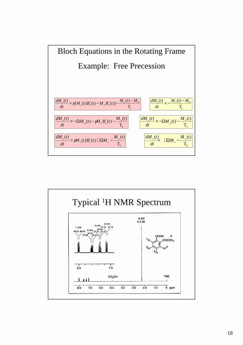
Bloch Equations in the Rotating Frame

rfB ωγ −−=Ω 0

1

0

T

)()]()()([

)( MtMtBMtBtM

dt

tdM zrxy

ryx

z −−−= γ The “r” superscript refers to a magnetic field in the rotating frame

2T

)()()(

)( tMtBMtM

dt

tdM xryzy

x −−Ω−= γ

2T

)()()(

)( tMMtBtM

dt

tdM yx

rxz

y −Ω+= γ

(where B0=Bz and is not time-dependent)

Bloch Equations in the Rotating Frame

Example: 90° pulse along x

)()(

tBMdt

tdM rxy

z γ−=

0)( =

dt

tdM x

)()()(

tBtMdt

tdM rxz

y γ=

1

0

T

)()]()()([

)( MtMtBMtBtM

dt

tdM zrxy

ryx

z −−−= γ

2T

)()()(

)( tMtBMtM

dt

tdM xryzy

x −−Ω−= γ

2T

)()()(

)( tMMtBtM

dt

tdM yx

rxz

y −Ω+= γ

18

Bloch Equations in the Rotating Frame

Example: Free Precession

1

0

T

)()]()()([

)( MtMtBMtBtM

dt

tdM zrxy

ryx

z −−−= γ

2T

)()()(

)( tMtBMtM

dt

tdM xryzy

x −−Ω−= γ

2T

)()()(

)( tMMtBtM

dt

tdM yx

rxz

y −Ω+= γ

1

0

T

)()( MtM

dt

tdM zz −−=

2T

)()(

)( tMtM

dt

tdM xy

x −Ω−=

2T

)()( tMM

dt

tdM yx

y −Ω+=

Typical 1H NMR Spectrum

Abs

orba

nce

19

8 7 6 5 4 3 2 1 0

Chemical ShiftO

C6H5−CH2−O−C−CH3

H H

H

H

H

H|

— C —|H

H|

— C —H|H

TMS

6

0

TMS 10)ppm( ×ωω−ω=δ

N

eBo

σBo

“Chemical” Shift

1951

20

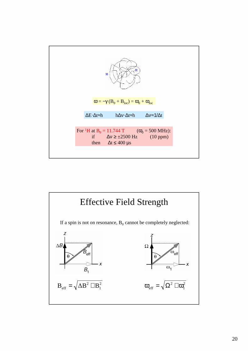
ω = −γ (B0 + Bloc) = ω0 + ωloc

∆E·∆t≈h h∆ν·∆t≈h ∆ν≈1/∆t

For 1H at B0 = 11.744 T (ω0 = 500 MHz):if ∆ν ≥ ±2500 Hz (10 ppm)then ∆t ≤ 400 µs

Effective Field Strength

If a spin is not on resonance, B0 cannot be completely neglected:

21

2eff B∆BB += 2

12

eff ω+Ω=ω

21

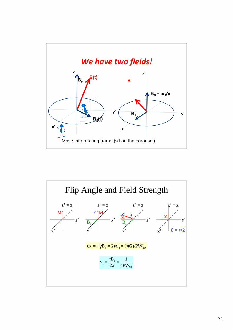
x’

y’

z

B0

B1(t)

B(t)

x

y

z

B1

B

We have two fields!

Move into rotating frame (sit on the carousel)

B0 – ωωωωrf/γγγγ

x’

y’

z’ = z

M

x’

y’

z’ = z

M

B1

x’

y’

z’ = z

B1

M θ

x’

y’

z’ = z

M

θ = π/2

Flip Angle and Field Strength

ω1 = −γB1 = 2πν1 = (π/2)/PW90

90

11 4PW

1

2π

γBν ==

22

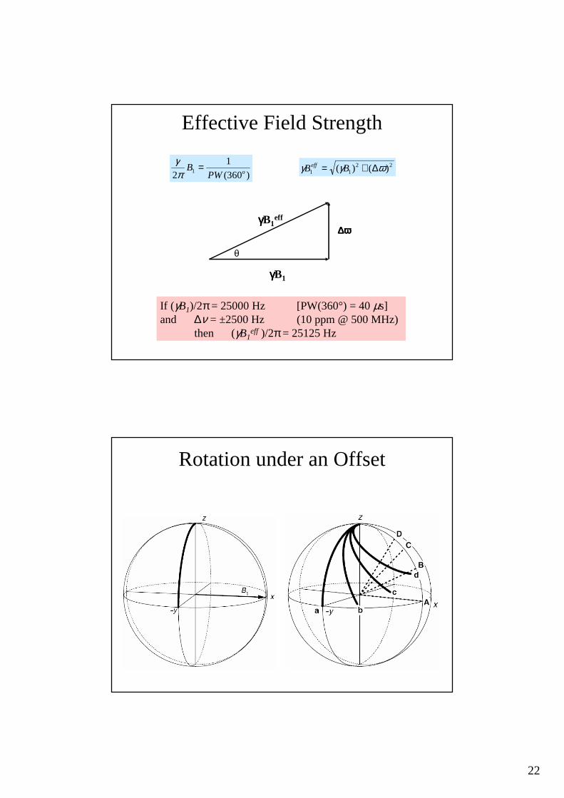
)360(

1

2 1 oPWB =

πγ 22

11 )()( ωγγ ∆+= BBeff

γγγγB1

∆ω∆ω∆ω∆ωγγγγB1

eff

θ

If (γB1)/2π = 25000 Hz [PW(360°) = 40 µs]and ∆ν = ±2500 Hz (10 ppm @ 500 MHz)

then (γB1eff )/2π = 25125 Hz

Effective Field Strength

Rotation under an Offset

23

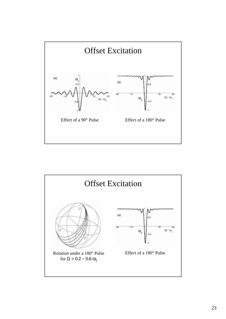
Offset Excitation

Effect of a 90° Pulse Effect of a 180° Pulse

Offset Excitation

Effect of a 180° PulseRotation under a 180° Pulse for Ω = 0.2 − 0.6 ω1

24

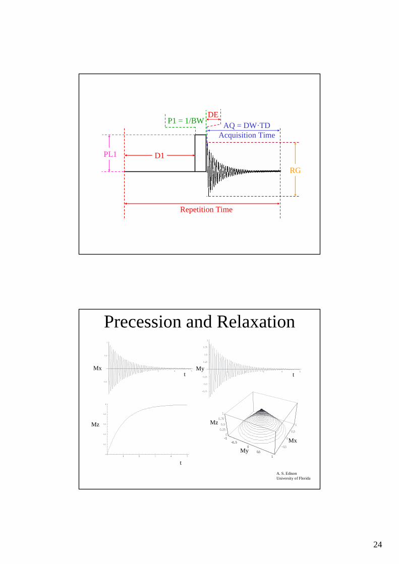
D1

Repetition Time

DEP1 = 1/BW

PL1

AQ = DW·TDAcquisition Time

RG

Precession and Relaxation

A. S. EdisonUniversity of Florida

1 2 3 4 5

-0.5

0.5

1

1 2 3 4 5

-0.75

-0.5

-0.25

0.25

0.5

0.75

1

Mx My

0.2

0.4

0.6

0.8

Mz

-1-0.5

0

0.5

1

-0.5

0

0.5

1

0

0.25

0.5

0.75

1

-1-0.5

0

0.5

1

Mz

Mx

My

t

t t

25

Detection

A. S. EdisonUniversity of Florida

0.2 0.4 0.6 0.8 1

-1

-0.5

0.5

1

0.2 0.4 0.6 0.8 1

-1

-0.5

0.5

1

analog

20 40 60 80 100

-1

-0.5

0.5

1

digital

∆t = 1/(2·νmax)Nyquist:

A B C

°−x90 t2

x

y

z

ω ≈ 108 Hz

Static:

Rotating (ω0 = ωB):

x

y

z

x

y

z

°−x90 t2

x’

y’

z

ω ≈ 103 Hzx’

y’

z

x’

y’

z

ω0 = ωB

26

Det. ADCNMRSignal

ω0 (reference)

ComputerMemory

500 MHz ± 2500 Hz

500 MHz

± 2500 Hz

∆t = 1/(2·νmax) DW = 1/SW

1/2· νmax = 10-4 s νmax = 5.0 kHz

ν = 2.0 kHz

ν = 4.5 kHz

ν = 2.0 kHz

ν = 8.0 kHz

100 µs

Nyquist:

27

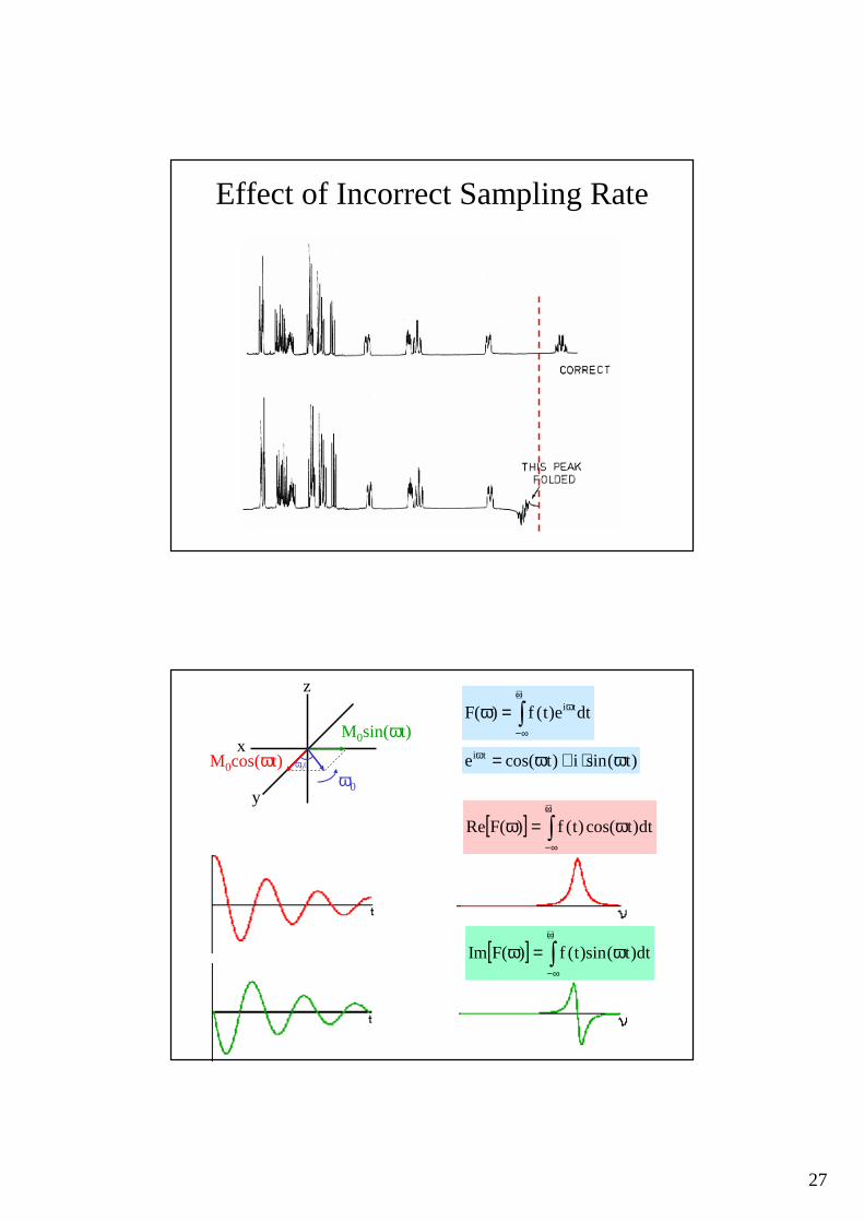
Effect of Incorrect Sampling Rate

∫+∞

∞−

ω=ω dte)t(f)(F ti

[ ] ∫+∞

∞−

ω=ω dt)tcos()t(f)(FRe

[ ] ∫+∞

∞−

ω=ω dt)t(sin)t(f)(FIm

)t(sini)tcos(e ti ω⋅+ω=ω

z

x

yω0

ω0t

M0sin(ωt)

M0cos(ωt)

28

∫+∞

∞−

ω=ω dte)t(f)(F ti

[ ] ∫+∞

∞−

ω=ω dt)tcos()t(f)(FRe

[ ] ∫+∞

∞−

ω=ω dt)t(sin)t(f)(FIm

)t(sini)tcos(e ti ω⋅+ω=ω

1

12

22 +Ω−ω

=ωT

A)(

)(

122

22

+Ω−ωΩ−ω=ωT

TD

)()(

)(

)()()( ω+ω=ω iDAF

z

x

yω0

ω0t

M0sin(ωt)

M0cos(ωt)

Phase Correction

)()()( ω+ω=ω iDAF ( ) )()(exp)( ωωφω iDAiF instr +=

[ ] )()(Re ωω AF =

[ ] ( ) ( ) )(sin)(cos)(Im ωφωφω ADF instrinstr +=

[ ] ( ) ( ) )(sin)(cos)(Re ωφωφω DAF instrinstr −=

[ ] )()(Im ωω DF =

29

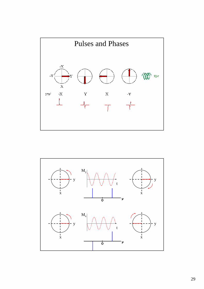
Pulses and Phases

x

yt

My

x

y

x

yt

Mx

x

y

30

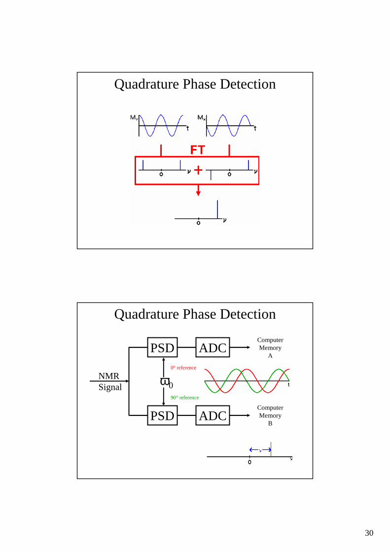
Quadrature Phase Detection

Quadrature Phase Detection

PSD ADC

PSD ADC

NMRSignal ω0

0° reference

90° reference

ComputerMemory

A

ComputerMemory

B

31

The Redfield Trick

PSD

PSD

ADCNMRSignal ω0

0° reference

90° reference

ComputerMemory(+ + − −)

∆t = DW/2 = 1/2·SW

Each subsequent point is phase-shifted by 90°The period of this added frequency is 4·∆tThe added frequency is therefore SW/2

The Redfield Trick

Original SW: −νmax ↔ +νmax

Added frequency: SW/2 = νmax

Final SW: 0 ↔ +2νmax

32

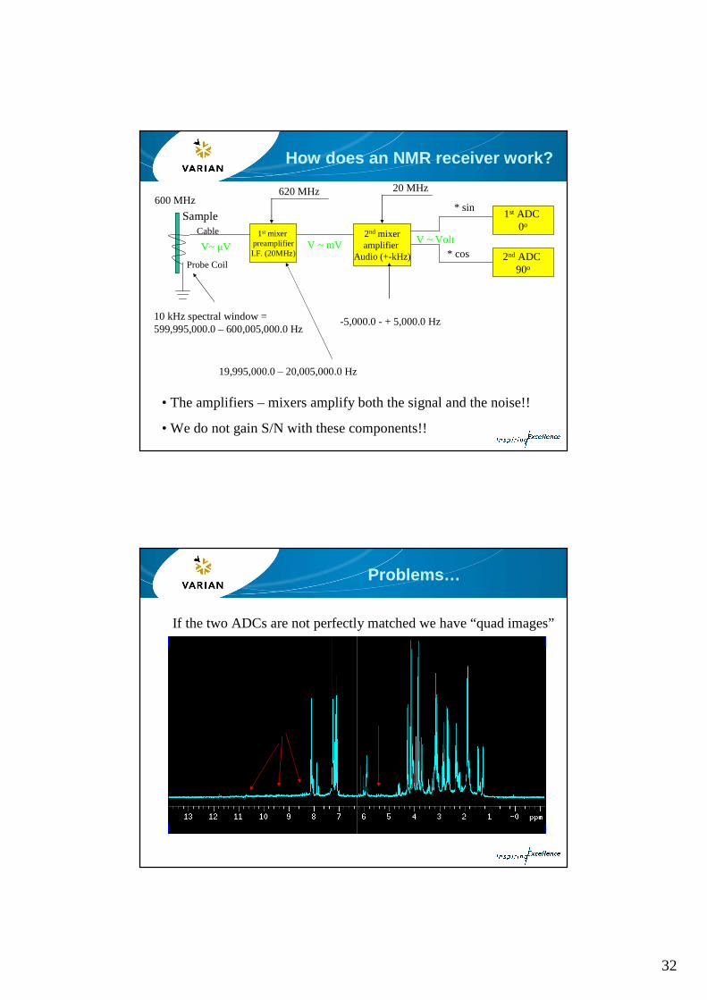
1st mixer preamplifierI.F. (20MHz)

2nd mixeramplifier

Audio (+-kHz)

1st ADC 0o

Sample

Probe Coil

Cable

2nd ADC 90o

600 MHz

10 kHz spectral window =599,995,000.0 – 600,005,000.0 Hz

19,995,000.0 – 20,005,000.0 Hz

-5,000.0 - + 5,000.0 Hz

620 MHz 20 MHz

* sin

* cosV~ µV V ~ mV V ~ Volt

• The amplifiers – mixers amplify both the signal and the noise!!

• We do not gain S/N with these components!!

How does an NMR receiver work?

Problems…

If the two ADCs are not perfectly matched we have “quad images”

33

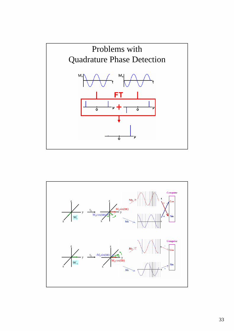
Problems with Quadrature Phase Detection

x

y°y90

t2

z

x

yωt

M0sin(ωt)

M0cos(ωt)

z

z

x

y°−x90

t2

z

x

yωt

M0cos(ωt)

-M0sin(ωt)

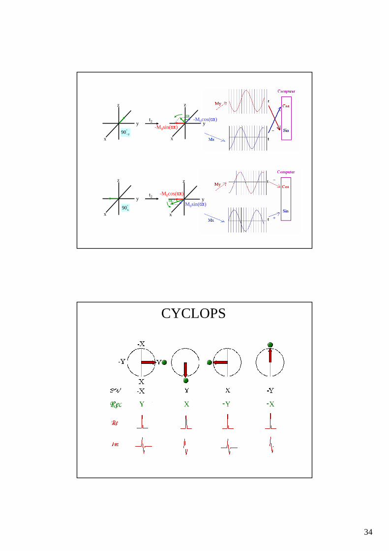
34

z

x

y°−y90

t2

z

x

y

ωt

-M0sin(ωt)

-M0cos(ωt)

z

x

y°x90

t2

x

yωt

-M0cos(ωt)

M0sin(ωt)

z

CYCLOPS

35

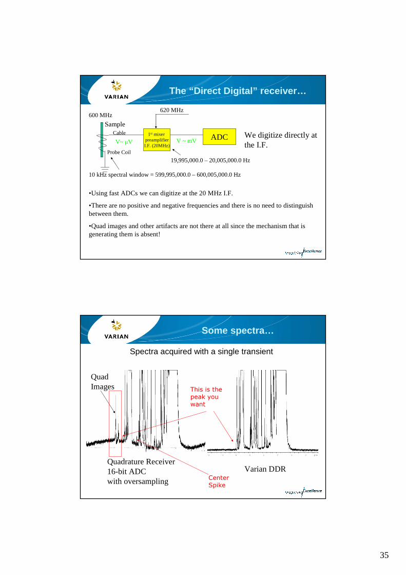
The “Direct Digital” receiver…

1st mixer preamplifierI.F. (20MHz)

Sample

Probe Coil

Cable

600 MHz

10 kHz spectral window = 599,995,000.0 – 600,005,000.0 Hz

19,995,000.0 – 20,005,000.0 Hz

620 MHz

V~ µV V ~ mV ADC We digitize directly at the I.F.

•Using fast ADCs we can digitize at the 20 MHz I.F.

•There are no positive and negative frequencies and there is no need to distinguish between them.

•Quad images and other artifacts are not there at all since the mechanism that is generating them is absent!

Some spectra…

Quadrature Receiver16-bit ADC with oversampling

Varian DDR

Quad Images

Spectra acquired with a single transient

This is the

peak you

want

Center

Spike

36

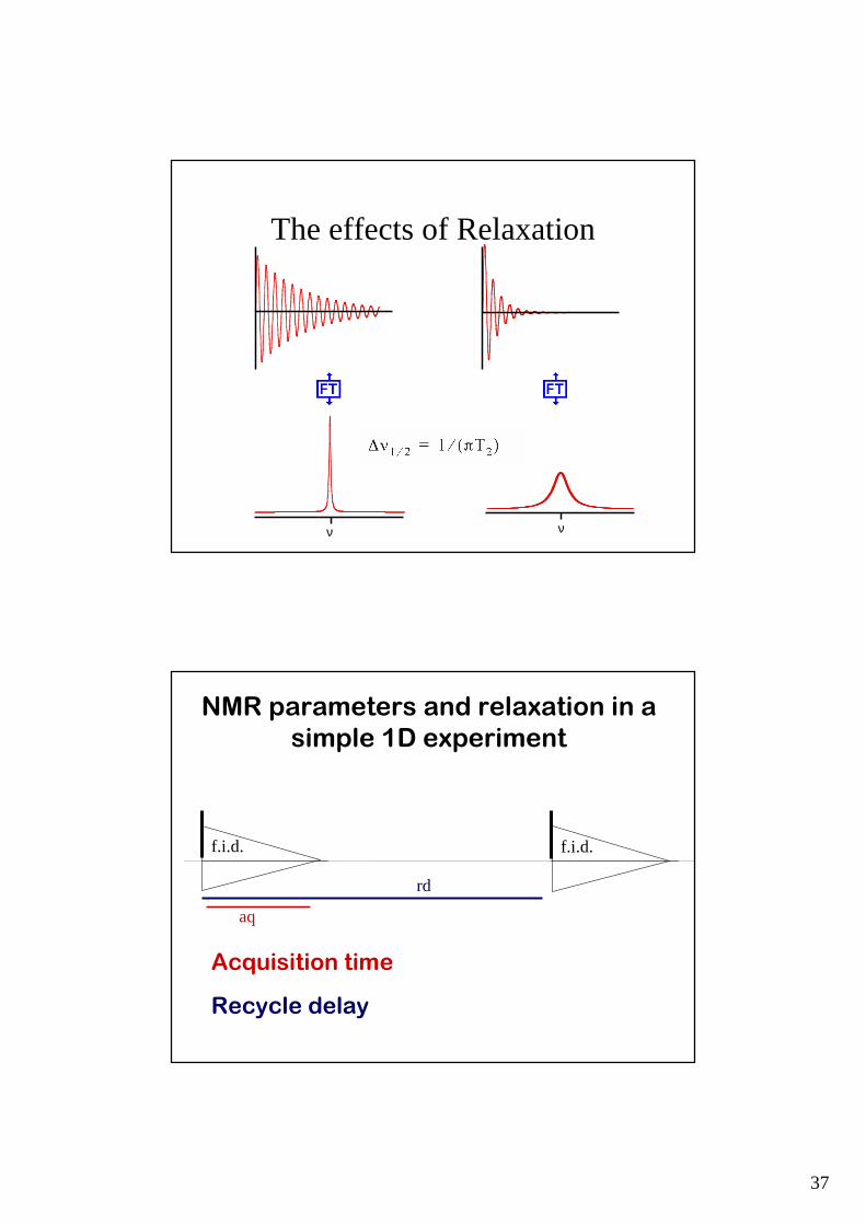
FID Clipping

FT

FT

The effects of Relaxation

37

ν ν

The effects of Relaxation

NMR parameters and relaxation in a

simple 1D experiment

f.i.d. f.i.d.

aq

rd

Acquisition time

Recycle delay

38

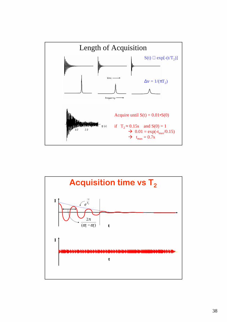
Length of AcquisitionS(t) ∝ exp[-(t/T2)]

∆ν = 1/(πT2)

Acquire until S(t) = 0.01•S(0)

if T2 ≈ 0.15s and S(0) = 1 0.01 = exp(-tmax/0.15) tmax = 0.7s

I

tt

I

tt

Acquisition time vs T2

2T

t

e−

)(

2

1ωωπ−I

39

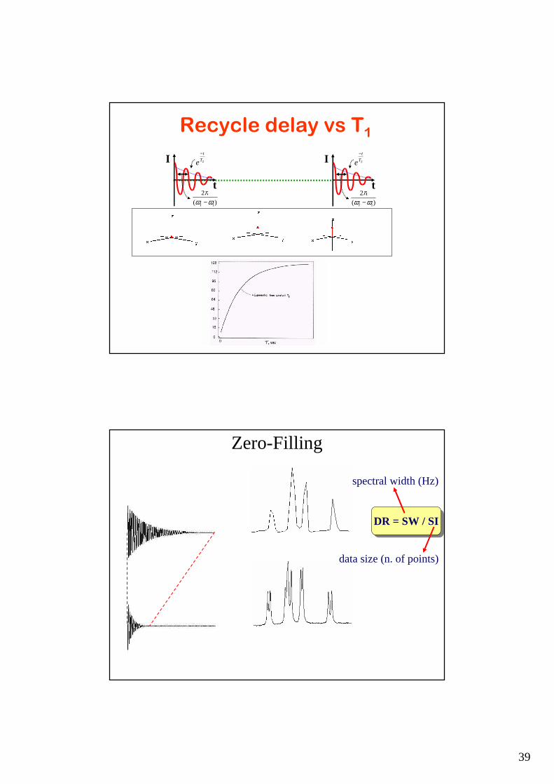
Recycle delay vs T1

I

t

2T

t

e−

)(

2

1ωωπ−I

I

t

2T

t

e−

)(

2

1ωωπ−I

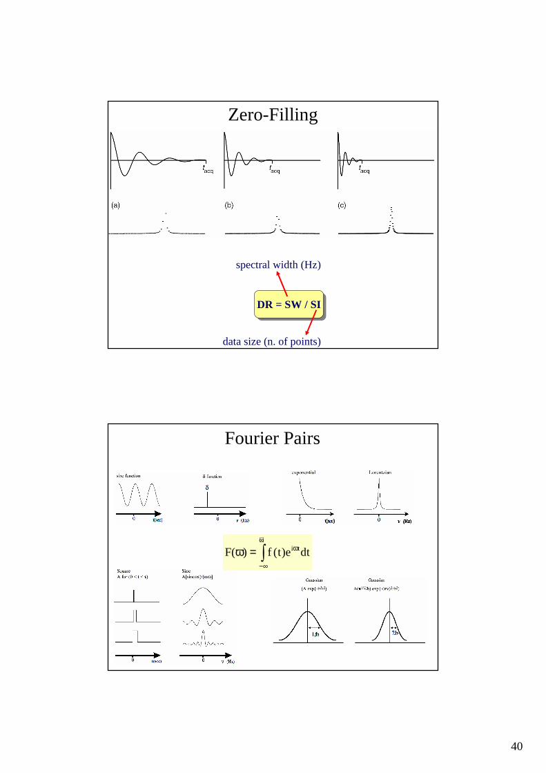
Zero-Filling

DR = SW / SIDR = SW / SI

spectral width (Hz)

data size (n. of points)

40

Zero-Filling

DR = SW / SIDR = SW / SI

spectral width (Hz)

data size (n. of points)

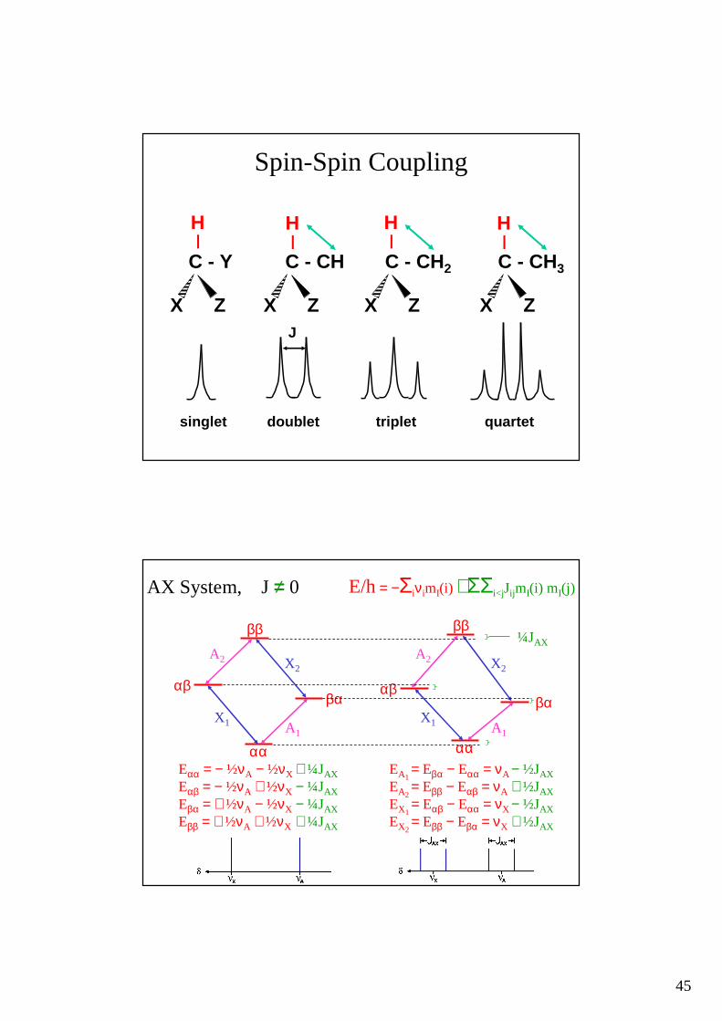
Fourier Pairs

∫+∞

∞−

ω=ω dte)t(f)(F ti

41

Truncation and Apodization

Truncation and Apodization

42

Window Functions:Sensitivity Enhancement

S = A exp-t/T2 exp-at = A exp-t (a+ 1/T2)a = 1/T2 (matched filter)

RESOLUTION

Resolution is the ability to distinguish between two frequencies

AQ = DW*TD No resolution

AQ = DW*TD’ Resolution

DIGITALRESOLUTION

43

Window Functions:Resolution Enhancement

S = A*exp-t/T2 exp-atexp-bt2a = -1/T2 ; b>0

Other Window Functions:Sine Bell and Sine Bell Squared

S = A*exp-t/T2 sin( π-φ)t/tmax +φ

AS=

S = A*exp-t/T2 sin2( π-φ)t/tmax +φ

44

Linear Prediction

8 7 6 5 4 3 2 1 08 7 6 5 4 3 2 1 0

Integration

O

C6H5−CH2−O−C−CH3

TMS

52

2132

45

Spin-Spin Coupling

C - Y C - CH C - CH2 C - CH3

H|

H|

H|

H|

singlet doublet triplet quartet

X ZX Z X Z X ZJ

AX System, J = 0 E/h= −ΣiνimI(i)

A2

X1

X2

A1

αα

ββ

βααβ

Eαα = − ½νA − ½νX

Eαβ = − ½νA + ½νX

Eβα = + ½νA − ½νX

Eββ = + ½νA + ½νX

EA1 = Eβα − Eαα = νA

EA2 = Eββ − Eαβ = νA

EX1 = Eαβ − Eαα = νX

EX2 = Eββ − Eβα = νX

A2

X1

X2

A1

αα

ββ

βααβ

+ΣΣi<jJijmI(i) mI(j)

+ ¼JAX

− ¼JAX

− ¼JAX

+ ¼JAX

− ½JAX

+ ½JAX

− ½JAX

+ ½JAX

≠

¼JAX

46

αβ (andβα) levels arestabilized

αα (andββ) levels aredestabilized

Origin of Scalar Coupling

J > 0

H H

HH

C C

CC

αβ (andβα) levels arestabilized

αα (andββ) levels aredestabilized

Origin of Scalar Coupling

J > 0