
CLUSTERING AND LENSING PROPERTIES OF DARK...
130
Sede amministrativa: Universit` a degli Studi di Padova Dipartimento di Fisica e Astronomia SCUOLA DI DOTTORATO DI RICERCA IN: ASTRONOMIA CICLO XXVIII CLUSTERING AND LENSING PROPERTIES OF DARK MATTER HALOES IN EUCLID ERA Direttore della scuola: Ch.mo Prof. Giampaolo Piotto Supervisore: Ch.mo Prof. Giuseppe Tormen Co-Supervisore: Dott. Massimo Meneghetti Dottorando: Michele Boldrin
Transcript of CLUSTERING AND LENSING PROPERTIES OF DARK...

Sede amministrativa: Universita degli Studi di PadovaDipartimento di Fisica e Astronomia
SCUOLA DI DOTTORATO DI RICERCA IN: ASTRONOMIACICLO XXVIII
CLUSTERING AND LENSINGPROPERTIES OF DARK MATTER
HALOES IN EUCLID ERA
Direttore della scuola: Ch.mo Prof. Giampaolo PiottoSupervisore: Ch.mo Prof. Giuseppe TormenCo-Supervisore: Dott. Massimo Meneghetti
Dottorando: Michele Boldrin

Contents
Abstract 2
Sommario 4
1 The Smooth Universe 5
1.1 The Robertson-Walker Metric . . . . . . . . . . . . . . . . . . . . . . . . 5
1.2 Redshift . . . . . . . . . . . . . . . . . . . . . . . . . . . . . . . . . . . . 6
1.3 The Friedmann Equations . . . . . . . . . . . . . . . . . . . . . . . . . . 6
1.4 Cosmological Distances . . . . . . . . . . . . . . . . . . . . . . . . . . . . 7
1.5 The Friedmann Models . . . . . . . . . . . . . . . . . . . . . . . . . . . . 9
1.6 Cosmological Horizons . . . . . . . . . . . . . . . . . . . . . . . . . . . . 12
1.7 Models With Cosmological Constant . . . . . . . . . . . . . . . . . . . . 13
1.8 Energetic Balance Of The universe . . . . . . . . . . . . . . . . . . . . . 14
1.9 Relevant Moments Of The Thermical History Of The Universe . . . . . 14
1.10 Problems Of The Big Bang Theory And The Inationary Model . . . . . 16
2 Structure Formation 19
2.1 The Linear Theory . . . . . . . . . . . . . . . . . . . . . . . . . . . . . . 20
2.2 Values Of The Jeans Scale . . . . . . . . . . . . . . . . . . . . . . . . . . 25
2.3 Statistical Aspects Of Structure Formation . . . . . . . . . . . . . . . . . 26
2.3.1 Power Spectrum And Variance . . . . . . . . . . . . . . . . . . . 27
2.4 Non-Linear Regime . . . . . . . . . . . . . . . . . . . . . . . . . . . . . . 28
2.4.1 Mass Function From The Spherical Collapse Model . . . . . . . . 28
2.5 Galaxy Clusters . . . . . . . . . . . . . . . . . . . . . . . . . . . . . . . . 32
3 N-Body Simulations 35
3.1 N -Body Methods . . . . . . . . . . . . . . . . . . . . . . . . . . . . . . . 35
3.2 Numerical simulations . . . . . . . . . . . . . . . . . . . . . . . . . . . . 37
3.2.1 GIF2 . . . . . . . . . . . . . . . . . . . . . . . . . . . . . . . . . . 37
3.2.2 LE SBARBINE . . . . . . . . . . . . . . . . . . . . . . . . . . . . . 37
3.3 Halo Finder Technique . . . . . . . . . . . . . . . . . . . . . . . . . . . . 38
3.4 Merger Trees . . . . . . . . . . . . . . . . . . . . . . . . . . . . . . . . . 38
4 Statistical Properties Of Dark Matter Haloes From N-Body Simula-tions LE SBARBINE 41
4.1 Data Analysis . . . . . . . . . . . . . . . . . . . . . . . . . . . . . . . . . 42
4.2 Subhalo Mass Functions . . . . . . . . . . . . . . . . . . . . . . . . . . . 44
4.2.1 Unevolved Subhalo Mass Function . . . . . . . . . . . . . . . . . 44
i

ii CONTENTS
4.2.2 Evolved Subhalo Mass Function . . . . . . . . . . . . . . . . . . . 464.3 Statistics Of The Satellite Mass Evolution . . . . . . . . . . . . . . . . . 48
4.3.1 The Role Of Merging Time . . . . . . . . . . . . . . . . . . . . . 484.3.2 Average Satellite Mass At z0 . . . . . . . . . . . . . . . . . . . . 484.3.3 Average Satellite Mass At zm . . . . . . . . . . . . . . . . . . . . 514.3.4 The Heavily-Consumed Satellite Population . . . . . . . . . . . . 52
4.4 Conclusions . . . . . . . . . . . . . . . . . . . . . . . . . . . . . . . . . . 58
5 Gravitational Lensing 615.1 The Lens Equation . . . . . . . . . . . . . . . . . . . . . . . . . . . . . . 645.2 Convergence And Lensing Potential . . . . . . . . . . . . . . . . . . . . . 645.3 Distortion, Magnication And Multiple Images . . . . . . . . . . . . . . 65
5.3.1 Time Delay Surface . . . . . . . . . . . . . . . . . . . . . . . . . 725.4 Analytical Lens Models . . . . . . . . . . . . . . . . . . . . . . . . . . . 73
5.4.1 Singular Isotermal Sphere (SIS) . . . . . . . . . . . . . . . . . . . 735.4.2 Non-singular Isothermal Sphere (NIS) . . . . . . . . . . . . . . . 765.4.3 Elliptical Lenses . . . . . . . . . . . . . . . . . . . . . . . . . . . 79
5.5 Modeling Strong Gravitational Lensing From Galaxy Clusters . . . . . . 815.5.1 Asymmetry, Substructure And Mergers . . . . . . . . . . . . . . 825.5.2 The Baryonic Component . . . . . . . . . . . . . . . . . . . . . . 82
5.6 MOKA: A Semi-Analytical Tool For Gravitational Lensing . . . . . . . . . 83
6 Arc Statistics In New Technology Era 856.1 The Number Of Gravitational Arcs As A Cosmological Tool . . . . . . . 856.2 Realistic Arc Statistics Forecasts In A ΛCDM Cosmology . . . . . . . . 86
6.2.1 The Euclid Mission . . . . . . . . . . . . . . . . . . . . . . . . . . 866.2.2 Synthetic Haloes . . . . . . . . . . . . . . . . . . . . . . . . . . . 896.2.3 Ray-Tracing Simulations And Cross Sections . . . . . . . . . . . 906.2.4 Redshift Evolution Of The Cross Section . . . . . . . . . . . . . . 906.2.5 Source Number Density . . . . . . . . . . . . . . . . . . . . . . . 956.2.6 Construction Of The Light-Cones . . . . . . . . . . . . . . . . . . 966.2.7 The Total Number Of Arcs . . . . . . . . . . . . . . . . . . . . . 976.2.8 Arc production as a function of the lens redshift . . . . . . . . . 98
6.3 Sensitivity To Ωm And σ8 . . . . . . . . . . . . . . . . . . . . . . . . . . 1006.3.1 Number Of Arcs As A Function Of Redshift . . . . . . . . . . . . 1006.3.2 The Total Number Of Arcs In The Light Cone . . . . . . . . . . 1036.3.3 Inuence Of The Cosmological Parameters On Arc Statistics . . 1066.3.4 Eects Of Completeness And Cluster Selection Function . . . . . 1106.3.5 A Test-Bed For The Method: The CLASH Survey . . . . . . . . 1146.3.6 Conclusions . . . . . . . . . . . . . . . . . . . . . . . . . . . . . . 114
List of Figures 117
List of Tables 122
Bibliography 124

Abstract
Following the most accredited cosmological model, the ΛCDM model, only 4% of theUniverse is formed by baryonic matter, while about 26% is made up of Cold DarkMatter (CDM) and the remaining 70% is given by the component responsable of thecosmic accelerated expansion, called dark energy or Λ. Primordial perturbations in theCDM distribution that oppose to cosmic expansion and begin to collapse origin thepotential wells where baryonic matter condense to form galaxies and stars. Observedon scales minor than some Mpc, the Universe is far from being homogeneous: galaxiesare embedded by collapsed dark matter haloes. Therefore, the study of the substratumof dark matter in which the baryonic matter lies is fundamental to understand theformation and evolution of cosmic structures.
Every object we observe come from an aggregation history of dark matter haloes,which generally enter in a host halo and orbit around the center of mass, becomingsatellites. During this motion, several dynamical phenomenons may cause partial ortotal satellite mass-loss, or they can brake it through loss of angular momentum, so thesatellite fall in the center of the host halo. In any case, the evolution of the satellitemass is very dierent from the evolution of a single halo. In this work we analyse theaverage relations between the satellite mass at the time of accretion and the mass ata given later observation moment. In particular, we wonder how can we estimate theformer by the latter and viceversa. Using the new set of cosmological simulations LE
SBARBINE, developed in the Physics and Astronomy Department of the University ofPadova, we test the law that regulates the average mass-loss rate of satellites and wedevelop a new relation between the mass observed at a certain redshift and the averagemass it could have at the accretion time. Furthermore, we discuss some factors thatoriginate anomallies in the satellite mass evolution with respect to the average law wefound, with particular attention to major mergers.
In the context of the structure formation, galaxy clusters rapresent the last phaseof the aggregation process of dark matter haloes. Being the largest and more recentobjects in the Universe, every their feature or behaviour is a probe for the referencecosmological model. This is even more important in this epoch of technological progress,as the statistical study of these objects requires large and deep observations. An optimalexample of those future innovative instruments is given by the spatial telescope Euclid(ESO), which will be launched in 2019 − 2020 and will observe a main 15000 deg2 ofextragalactic sky, collecting images and spectra with excellent resolution and quality inoptical and NIR bands. One of the research eld that will be mostly improved by futureobservations is arc statistics, that is the cosmological research through the observation ofgiant gravitational arcs, the most magnicent eects of strong gravitational lensing. Inthe last decades, the study and the observations of gravitational lensing phenomenonshas increased, following the rate of technological development. In particular, giant
1

2 CONTENTS
gravitational arcs, which are mainly created by galaxy clusters, need detailed and deepobservations to be identied and used in statistical inventigations. Because of the strongdependence of the number of those objects in the sky on the cosmology, we study as thenumber of arcs visible in the main survey of Euclid is dependent on the cosmologicalparameters Ωm and σ8, the two that mostly determine the structure formation process.Moreover, we analise the eect of the survey size and of the application of a selectionfunction on our estimates.
The thesis is structured as follows:
• in Chapters 1 and 2 we introduce the cosmological ΛCDM model;
• in Chapter 3 we briey describe the methods for numerical simulations, we givesome features of the two simulations we will deal with, namely GIF2 and LE
SBARBINE and we describe the methods usedin both of them to identify haloesand to dene their accretion history;
• in Chapter 4, after a description of the code we developed and the consistencytests with previous works, we present the results obtained in the frame of satellitestatistics;
• in Chapter 5 we briey introduce the formalism of gravitational lensing;
• in Chapter 6 we present the spatial telescope Euclid and the method adoptedto estimate the theoretica number of arcs visible in the sky, then we describe thestudy of the inuence on this number of cosmological parameters Ωm and σ8, witha discussion about the eect given by the survey size and the selection function.

Sommario
Secondo il più accreditato modello cosmologico oggigiorno, il modello ΛCDM, solamenteil 4% dell'Universo sarebbe composto da materia barionica, mentre circa il 26% sarebbeformato da materia oscura fredda (CDM) e il restante 70% da una componente ritenutaresponsabile dell'espansione cosmica accelerata, chiamata energia oscura o Λ. Le per-turbazioni primordiali nella distribuzione di CDM che vincono l'espansione cosmica eriescono a contrarsi, formano le buche di potenziale nelle quali la materia barionica con-densa formando galassie e stelle. Osservato su scale minori di circa 1 Mpc, l'Universo èquindi tutt'altro che omogeneo: la materia oscura collassata in aloni ospita le galassieche noi osserviamo. Lo studio della formazione del substrato di materia oscura nel qualeè ospitata la materia barionica condensata risulta perciò di fondamentale importanzaper capire la formazione e l'evoluzione delle strutture cosmiche.
Ogni oggetto che osserviamo deriva da una storia di aggregazione di aloni di ma-teria oscura, i quali generalmente entrano in un alone ospite e orbitano attorno al suocentro di massa, divenendo suoi satelliti. Durante questo moto, vari fenomeni dinamicipossono causare perdita di massa parziale o totale del satellite, oppure possono frenarlofacendogli perdere momento angolare e quindi spiraleggiare verso il centro dell'ospite.In ogni caso, l'evoluzione della massa del satellite risulta molto diversa dall'evoluzionedi un alone singolo. In questo lavoro analizziamo le relazioni medie fra la massa deisatelliti al momento dell'accrescimento e la massa ad un certo momento di osservazione.In particolare, ci domandiamo come stimare la prima dalla seconda e viceversa. Facendouso del nuovo set di simulazioni cosmologiche LE SBARBINE, sviluppato nel dipartimentodi Fisica e Astronomia dell'Università di Padova, testeremo la legge precedentementetrovata per il tasso medio di perdita di massa dei satelliti e svilupperemo una relazionefra la massa osservata di un satellite ad un certo redshift e la massa media che avevaal momento dell'accrescimento. Inoltre commenteremo i fattori che determinano delleanomalie nell'evoluzione della massa dei satelliti rispetto alla legge trovata, con parti-colare attenzione ai major mergers.
Nel contesto della formazione delle strutture, gli ammassi di galassie rappresen-tano l'ultimo stadio del processo di aggregazione di aloni di materia oscura. Essendogli oggetti più grandi e più giovani dell'Universo, ogni loro caratteristica o comporta-mento funziona da test per il modello cosmologico di riferimento. Questo è ancora piùimportante in questa epoca di forte progresso tecnologico, poiché lo studio statisticodi tali oggetti richiede osservazioni di porzioni di cielo più estese possibili e con ottimarisoluzione. Un ottimo esempio di futuri strumenti innovativi è il telescopio spazialeEuclid, dell'European Spatial Observatory, che verrà lanciato nel 2019 − 2020 e os-serverà 15000 gradi quadri di cielo extragalattico raccogliendo immagini e spettri dieccellente qualità in ottico e vicino infrarosso. Uno dei campi di ricerca che verrannomaggiormente rivoluzionati dalle future osservazioni è quello della statistica degli archi,
3

4 CONTENTS
ovvero la ricerca cosmologica attraverso l'osservazione di archi gravitazionali giganti, ipiù eclatanti eetti di lensing gravitazionale forte. Negli ultimi decenni, infatti, lo studioe le osservazioni dei fenomeni di lensing gravitazionale è andato via via aumentando, dipari passo con lo sviluppo tecnologico. In particolare, gli archi gravitazionali giganti,prodotti dagli ammassi di galassie, necessitano di osservazioni dettagliate e profonde peressere identicati e utilizzati in studi di tipo statistico. Data la forte dipendenza cos-mologica del numero di questi oggetti visibili nel cielo, ci proponiamo di studiare comeil numero di archi visibili nella survey principale di Euclid è dipendente dai parametricosmologici Ωm e σ8, i due che maggiormente inuenzano la formazione delle strutture.Inoltre, abbiamo analizzato l'eetto della dimensione della survey e dell'applicazione diuna funzione di selezione sulle nostre previsioni.
La tesi è strutturata come segue:
• nei Capitoli 1 e 2 introduciamo il modello cosmologico ΛCDM;
• nel Capitolo 3 descriviamo brevemente le tecniche di simulazione numeriche, di-amo le caratteristiche delle due simulazioni cosmologiche che tratteremo nel la-voro, ovvero le GIF2 e LE SBARBINE e descriviamo i metodi utilizzati in entrambele simulazioni per l'denticazione degli aloni e la denizione della loro storia diaccrescimento;
• nel Capitolo 4, dopo aver descritto il codice usato per il nostro lavoro e i testdi consistenza con i lavori precedenti, presentiamo i risultati ottenuti nell'ambitodella statistica dei satelliti di materia oscura;
• nel Capitolo 5 introduciamo brevemente il formalismo del lensing gravitazionale;
• nel Capitolo 6 presentiamo il telescopio spaziale Euclid e il metodo utilizzatoper dare una stima teorica del numero di archi nel cielo osservati da Euclid, poiillustriamo lo studio dell'inuenza su tale numero dei parametri cosmologici Ωm
e σ8, accompagnato da una discussione sull'eetto della dimensione della surveye della funzione di selezione.

Chapter 1
The Smooth Universe
The rst step toward a description of the Universe is the construction of a robust thoreti-cal model which describes what we observe. Such a model must lie on the known physicsand it must depend on the minimum number of assumptions as possible. Nowadays,the most accredited cosmological model is given by the Big Bang theory, together withthe ination theory.
1.1 The Robertson-Walker Metric
The starting point of the Big Bang model is the cosmological principle: on large scale,namely on scales of about hundred Mpc, the Universe appears isotropic and homo-geneous, that is the density of cosmic structures is the same in every point, so thereis no special positions or direction. Before the descovering of the Cosmic MicrowaveBackground (CMB) and the expansion of the Universe, the cosmological principle wasalso said perfect, so there were no preferred times (the Universe was supposed to bestatic) and the creation of matter from nothing was an allowed thought. The discoverof the CMB put some new problems such as the creation of photons from nothing andthe expansion of the Universe, and it was clear the Universe was not static and theadjective perfetto was not used anymore. Nevertheless, the CMB proves the Universehomogeneity, because the average observed temperature uctuation is in the order of10−5.
The second assumption we take to build our cosmological model is that the gravita-tional force dominates on the other fundamental forces on large scale. Gravity behaviouris well described by Einstein's General Relativity, which states that the geometricalproperties of space-time are dened by its energetic content.
The general metric in space-time which established a relation between two pointswith dierent t, x, y and z coordinates has the followin form:
ds2 = gαβdxαdxβ = g00dt
2 − 2g0idtdxi − gijdx2, (1.1)
where gαβ is the metric tensor and α, β = 0, 1, 2, 3 are the space-time coordinates(i, j = 1, 2, 3 identify the spatial ones).
Assuming isotropy and homogeneity, we obtain the Robertson-Walker metric:
ds2 = c2dt2 − a2(t)[dr2
1−Kr2+ r2(dθ2 + sin2 θdφ2)], (1.2)
5

6 Chapter 1. The Smooth Universe
where r, θ e φ are the comoving sferic coordinates, t is the cosmic time, a(t) is the scalefactor, which contains the dependence on time of the spatial part of the metric, and kis the curve parameter. the space can be thought as a sum of iper-surveys at dierenttimes, and their shape depends on the cosmic geometry, we may be at, spherical orhyperbolic depending on the value of k, 0, 1 or -1.
1.2 Redshift
An important quantity related to the scale factor is the redshift, which is dened as
z ≡ ∆λ
λ=λobs − λth
λth, (1.3)
that is the dierence between the observed and the theoretical wavelenghts λ of aradiation. The wavelenght of a radiation emitted by a far source is connected to thescale factor through the relation
a0
λ0=aEλE
,
where subscripts 0 and E indicate the time of observation and the time of emission,respectively. Using eq. (1.3), the relation could be written as
1 + zE =a0
aE. (1.4)
Hence, since the scale factor a is a monotonically increasing function of time, its variationfrom tE to t0 causes a net shift of the observed wavelenght toward the redder regionsof the spectrum. If we dene today as t0 and a(t0) = 1, we can write
1 + z =1
a(t).
Thus, the redshift tells how much far from us is a source along the space-time, relatingan observable, λ, to a cosmological factor, a(t).
1.3 The Friedmann Equations
In order to know how the scale factor evolves with time, we need to solve Einstein'seld equation:
Rij −1
2gijR− Λgij =
8πG
c4Tij , (1.5)
where R is the Ricci's tensor, g is the metric tensor and T is the energy-impulse tensor.The term Λgij was added my Einstein to obtain a model of a static Universe, but itwas removed after the discover of the cosmic expansion. During the last decades theterm Λ has been reconsidered to explain the accelerated expansion of the Universe, andit represents the contribute of the Dark Energy on the eld equation.
Friedmann solved the led equation through the following two assumptions:
• the cosmological principle, thus g is given by the Robertson-Walker metric;
• the matter that lls the Universe is thgouth as a perfect uid, so the energy-impulse tensor has the shape Tij = −Pgij+(P+ρc2)uiuj , where P is the pression,ρ the mean density and ui is the velocity quadrivector.

1.4. Cosmological Distances 7
Friedmann's solutions are therefore:(a
a
)= −4πG
3
(ρ+
3P
c2
)(1.6)
(a
a
)2
=8πG
3ρ− Kc2
a2+
Λc2
3, (1.7)
both linked to the condition of an adiabatic expansion of the Universe
d
dt
(a3ρc2
)− P da3
dt= 0. (1.8)
In order to solve this system, we need a state equation that connect the pression to thedensity. The most general form is
P = wρc2, (1.9)
where the value of w depends on the considered component of the Universe, since it isgiven by the medium sound velocity (dealing with Dark Matter, which is non-collisional,we will talk about velocity dispersion instead of sound velocity). Typically, matter hasthermal velocities much smaller than c2, so P ρc2; photons and relativistic particles
have the state equation PR =1
3ρRc
2; in order to get the state equaion of Dark Energy,
we recover the energy-impulse tensor from the eld equation in empty space
Λgij =8πG
c4Tij → Tij =
Λc4
8πGgij
given that Tij = −Pgij + (P + ρc2)uiuj , hence we obtain
PΛ = − Λc4
8πGe Pρc2 = 0→ P = −ρc2. (1.10)
Therefore, the parameter w in the state equation may have the following values:
w =
0 matter
1/3 radiation
−1 cosmological constant
(1.11)
From equations (1.8) and (1.9) we can express the density ρ in term of a(t) and w:
ρ0,w ∝ a−3(1+w). (1.12)
1.4 Cosmological Distances
In the contest of General Relativity, where the metric contains a dependece on time,distance is an ambiguous concept. There are many denitions of distance, dependingon the way it is measured. Here we list the main ones.
Proper distance: iti s given taking dt2 = 0 e aligning θ and φ along the observeddirection, thus dθ = dφ = 0
dP =
∫ds =
∫ r
0
adr′√1−Kr2
= a(t)f(r) with f(r) =
arcsin r K = 1
r K = 0
arcsinh r K = −1

8 Chapter 1. The Smooth Universe
Comoving Distance
It is dened as the proper distance computed today, at time t = t0:
dC = dP (t = t0) = a0f(r) =a0
a(t)dP .
The relation between the proper distance at time t0 and at an arbitrary t implies a timevariation of dP , so we can derive it and get the recession velocity of objects from theobserver:
vR =d
dtdP = f(r)
da(t)
dt= f(r)a =
a(t)
a(t)dP = (1 + z)dP .
This relation is known as the Hubble law : objects move away from the observer witha velocity which is proportional to the proper distance and it is normalized with thequantity
H(t) ≡ a(t)
a(t), (1.13)
called Hubble constant. Since measurements of H(t0) ≡ H0 have still large uncertainty,the parameter h is used instead of H0, such that
H0 = 100× h Km/s/Mpc,
so h lie in the range ∼ [0.5 − 1]. Recent observations state1 that H0 ≈ 70 km/s/Mpc,so h ≈ 0.7. Another important parameter for the Universe dynamic is the so-calleddeceleration parameter, dened as
q = − aaa2,
which express the amount of deceleration of the Universe at a given z.
Luminosity Distance
The ux we get from a distant source decreases with the distance following the law
F =L
4πd2, where L is the absolute luminosity. Through this relation, astrophysicians
get the distance d of standard candles, that is objects with known absolute luminosity.In dealing with cosmological distances, one must cosider the eects of the Universe ex-pansion and the time dilation, both predicted by the General Relativity, which togethergive a contribute (a(t)/a0)2, so we the relation between ux and distance is rescaled inthe following way:
F = L
(dt′
t0
a(t′)
a0
1
4πa20r
2
)=
L
4πa20r
2
1
(1 + z)2≡ L
4πdL. (1.14)
The luminosity distance is dened as dL(z) ≡ a0r(1 + z), and it satisfy the relation(1.14).
1A large amount of method to estimate h0 exist; the most established one is based on the derivation ofthe luminosity distance of objects with known average absolute magnitude and spectroscopic redshift,knwon as distance indicators (some examples are Cepheids variable stars, supernovae, HII regions,globular clusters and very luminous galaxy clusters). More recent methods make use of the Sunyaev-
Zel'dovich eect, that is the inverse Compton interaction between CMB photons and very energeticparticles which form the hot gas halo in galaxy clusters. The variation of the CMB ux in such regions,together with the X ux from the hot gas, allows the estimation of the cluster distance, that is afunction of h0. An even more recent method goes through the gravitational lensing eect, but it is stillvery rough.

1.5. The Friedmann Models 9
Angular Diameter Distance
The intrinsic and apparent sizes of objects are linked each other by the object distance.We dene the apparent size as the angle covered in the sky by the object δθ and theproper size as DPR, the angular diameter distance is
dA =DPR
δθ. (1.15)
An expression for DPR is given by the Robertson-Walker metric just xing dt = dφ = 0,
D2PR = ds2 = a2(t)r2dθ2 → DPR = arδθ,
thus the equation (1.15) becomes
dA = a(t)r =dL
(1 + z)2. (1.16)
The equation (1.16) tells that dL 6= dA, as they are two operative distance denitionsthat can be used if there are standard candles available or if the proper size of the objectare known.
1.5 The Friedmann Models
We use equation (1.13) to expand the second Friedmann equation (1.7):
H2 =8πG
3ρ− Kc2
a2→ t = t0 → H2
0 =8πG
3ρ0 −
Kc2
a20
. (1.17)
From the equation above we derive an expression for the curvature parameter K =1
c2
[H2
0 −8πG
3ρ0
]and dene the critical density, that is the average density for the
Universe to be at, in other words the density in order to get K = 0:
ρ0,cr ≡3H2
0
8πG= 2.775× 10¹¹h2 M/Mpc3. (1.18)
Measuring the density of the Universe in terms of ρ0,cr, we dene the density parameterΩ ≡ ρ0/ρ0,cr and relate it with the curvature parameter, so that the geometry of theUniverse is given by its the matter content:
K = 0 → ρ0 = ρ0,cr → Ω0 = 1 piatta
K = 1 → ρ0 > ρ0,cr → Ω0 > 1 sferica
K = −1 → ρ0 < ρ0,cr → Ω0 < 1 iperbolica
(1.19)
Thus, it is clear how much important is the precise measurement of the parameter Ω0.To date, the best estimate of Ω0 is given by CMB Planck observations by the Planckmission (Planck Collaboration et al. 2011), and it is very close to 1. If we put the exactvalue of w in equation (1.12), we obtain the density trend for every component:
• if w = 0 → ρM ∝ a−3, matter density is inversely proportional to the volume,as expected;

10 Chapter 1. The Smooth Universe
• if w = 1/3 → ρR ∝ a−4, the radiation density is diluted in space, as matter,so we nd a factor a−3, but another factor a−1 accounts for the eect of redshifton the wavelenght;
• if w = −1 → ρΛ ∝ a0 = const, Λ gives a constant energetic contribute2.
Altought every component has always existed, those dierent dependences on timeimply that at dierent ages of the Universe only one component (with the largest en-ergetic contribute) dominated. We write the equation that regulates the dynamics ofthe Universe combining the second Friedmann equation (1.7), equation (1.12) and thedenitions of Hubble constant and density parameter
H(t)2 = H20
(a0
a
)2[(
1−∑i
Ω0,wi
)+∑i
Ω0,wi
(a0
a
)1+3wi
]. (1.20)
The rst term we nd inside the square brackets is the so-called curvature density
parameter, as the dierence among∑
i Ω0,wi and 1 returns the cosmic geometry, whilethe second one is the sum of contributes from all components. From the Hubble lawit is clear that today a0 > 0, thus now the Universe is expanding. In order to test ifa(t) > 0 for every t, we study a by combining the equation (1.9) to the rst Friedmannequation (1.6), and obtaining:
a = −4πG
3ρ (1 + 3w) a. (1.21)
The sign of a is given only by the term inside the brackets:
• if 1 + 3w < 0→ w < −1/3 then a > 0, the expansion is accelerated;
• if 1 + 3w > 0→ w > −1/3 then a < 0, the expansion is decelerated.
The only component who could satisfy the condition of accelerated expansion is Λ.Hence a is a monotonically increasing function of time with the concavity downward,so walking back the timeline we will necessarily nd the point when t ≡ 0 and a = 0,that is the Big Bang, which is predicted by all Friedmann models. We still have not theinstruments to study this particular moment yet, when ρ, T,E →∞, but theorists areworking to develop a quantistic gravitation theory which described the big unicationthat occurred close to the Big Bang. The only two ways we have to reject the Big Bangtheory are
1. violating one of hypotesis of the Friedmann models;
2. presuming that near to the Big Bang Λ was the dominant component.
Let's neglect Λ for a while and continue with the analysis of Friedmann models.
2Cosmological models with the Dark Energy parameter of state w = w(z) have been recentlydeveloped, and they are known as quintessence models.

1.5. The Friedmann Models 11
Analytical Solutions In A Flat Universe: The Einstein-de Sitter Model
We consider a at Universe, so Ω0 = 1, and we solve the equation (1.20), which becomes:(a
a0
)2
= H20
(a0
a
)1+3w.
The integration leads to
a(t) = a0
(t
t0
) 2
3(1 + w) =
t2/3 matter
t1/2 radiation(1.22)
The expansion is slower when radiation dominates, even if the radiation pressure is
larger, because from the rst Friedmann equation (1.6) a = −4πG
3(ρ + 3P/c2)a we
see that the larger P , the smaller a, so the pression brakes the expansion. This mod-els is called Einstein-de Sitter model, hereafter Eds. In a Eds model the decelerationparameter is given by the following
q =4πG
3H2ρM =
1
2ΩM , (1.23)
and we note that in such an Universe it is not possible to have an accelerated expansion,as q > 0 always.
Solutions In Curve Universes
The rst thing we wonder is in which moment in the history of the Universe the curva-ture became non-negligible. Equation (1.20) presents two contributes, one for curvatureand the other one for density, so one may dominate the other one, depending on time.Comparing those two factors, we nd z∗ so that for every z > z∗ we neglect the curva-ture, and z∗ ≈ 1/Ω0. Since from observations we know that Ω0 is surely greater than0.1, the curvature factor becomes important only at low redshifts. Hence, almost allthe history of the Universe can be studied with the Eds model equation.
What happens when z < z∗? If we assume an open Universe, so Ω0,w < 1, and anegligible density factor with respect to the curvature term, equation (1.20) becomes:(
a
a0
)2
= H20 (1− Ω0,w)
that is constant in time. Therefore, the integration returns
a = a0H0
√1− Ω0,w t. (1.24)
The expansion is free and linear with time, and since a = costante, a = 0, it is neitherdecelerated nor accelerated.
Assuming a closed Universe, so Ω0,w > 1, the curvature factor of equation (1.20)is negative, so for a given value of a we have a = 0, which corresponds to the moment
when Ω0,w
(a0
a
)1+3w= Ω0,w − 1. When the scale factor reaches that given value, the
Universe reaches the maximum expansion (and the minimum density at the same time)and later it starts to collapse until it returns to the singolar point when a = 0. As

12 Chapter 1. The Smooth Universe
equation (1.20) is a quadratic, the decreasing solution is equal to the increasing one,hence the collapse is equal and opposite to the expansion. This scenario is called Big
Crunch (Figure 1.1).Therefore, we learnt that the curvature is not relevant for the past history, while
it is fundamental to know the future.
Figure 1.1: Density parameter as a function of time for the three geometries (Coles P.& Lucchin F., Cosmology).
Density Parameter Evolution With Time
Starting from the denition of density parameter Ωw ≡ ρw/ρcr, we can write it usingequation (1.12) and expanding the expression of the critical density ρcr:
Ω−1w (z)− 1 =
Ω0,w−1−1
(1 + z)1+3w. (1.25)
Note that 1 + 3w is always positive for radiation and matter. Moreover, if z → +∞then Ωw(z) → 1, in other words the very young Universe is at in every case. Whenz→ 0, the sign of Ωw is uniquely given by the numerator in the right-hand term, andin particular by the value of Ω0, which does not depend on w. This means that:
• if Ω0 > 1 then Ω(z)−1 − 1 < 0→ Ω(z) > 1 always;
• if Ω0 = 1 then Ω(z)−1 − 1 = 0→ Ω(z) = 1 always;
• if Ω0 < 1 then Ω(z)−1 − 1 > 0→ Ω(z) < 1 always;
so the dynamical evolution of the Universe does not inuence the geometry, whatevercomponent is considered.
1.6 Cosmological Horizons
Horizon Radius
The horizon radius Rhor is dened as the radius of the region in causal connection withthe observer. Its value is nite because the speed of light is nite, and intuitively onecould state that Rhor = tc, but light travels on proper distances, so it becomes
Rhor = a(t)
∫ a(t)
0
c da′
a(t)a(t),

1.7. Models With Cosmological Constant 13
but if t → 0, then a(t) → 0 and Rhor → ∞. Using the second Friedmann equation(1.7) close to Big Bang (when the curvature is negligible) and the equation of an EdSUniverse, we obtain the following:
Rhor =3(1 + w)
1 + 3wct =
3ct matter
2ct radiation(1.26)
The horizon radius is a linear function of time and it is nite for any curvature. Ordinaryphysics is valid only inside Rhor and the thermical equilibrium is not possible betweentwo regions that are not causally connected.
Hubble Sphere Radius
It is the distance of an object that travels with speed c in a reference system integralwith the expansion of the Universe, so
Rh =c
H=
3(1 + w)
2ct.
The dependences are the same of Rhor, but the physical meaning is quite dierent:Rh is an istantaneous measurement, while Rhor includes information about the past,so if two regions are causally connected, they will be forever. If something happenedin the history of the Universe that inverted the trend of a, Rhor would conserve thatinformation of the maximum value reached by the scale factor, whereas Rh would not.
1.7 Models With Cosmological Constant
We now insert Λ in the Fredmann equations and, at the same time, we ignore Ω0,R,as the radiation dominates only in the very early history of the Universe, therefore thedensity of the Universe assumes the form ρ = ρ + Λc2/(8πG) and, consequently, thepression becomes P = P − Λc4/(8πG). We can write the rst Friedmann equation as:
a = −4πG
3aρM +
Λc2
3a, (1.27)
and the second one
a2 +Kc2 = −4πG
3
(ρ+
3P
c2
)a =
[8πG
3ρM +
Λc2
3
]a2. (1.28)
From the equation (1.27) we note that for some values of Λ we could have a > 0, and
from the equation (1.28) it is clear that the termΛc2
3a2 enhances the expansion velocity.
If we dene Ω0,Λ ≡ ρ0,Λ/ρ0,cr and we rewrite the equation (1.28), we obtain a relationsimilar to equation (1.17), which is useful to determine how Λ inuences the curvatureof the Universe:
H20 (1− Ω0,M − Ω0,Λ) = −Kc
2
a20
. (1.29)
Thus Λ plays a crucial role in determining the curvature, so K = 0 does not meanΩ0,M = 1 anymore, but Ω0,M + Ω0,Λ = 1. Therefore, it is possible to have a at

14 Chapter 1. The Smooth Universe
Universe with Ω0,M < 1 and Ω0,Λ which balances the value. From equations (1.27) and(1.28) we can dene the deceleration parameter with Λ as
q =4πG
3H2ρM −
Λc2
3H2=
1
2ΩM − ΩΛ. (1.30)
The equation (1.30) demonstrates that Λ is necessary to have an accelerated expansion
of the Universe, and that the condition for this acceleration is ΩΛ >1
2ΩM . By means of
measurements of SNIa, q0 has been estimated as −0.6, in fact SNIa are standard candlessince they have the same absolute magnitude M at the moment of the explosion andfrom the distance module, dened as
m−M = 25 + 5 log(cz)− 5 logH0 + 1.086z(1− q0),
knowing the redshift z and measuring the apparent magnitude m, we can estimate q0.
1.8 Energetic Balance Of The universe
We now draw a picture of what we know about the energetic contribute of the variouscomponents of the Universe.
• Ω0,R ≈ 10−5 is the contribute we know best, estimated from observation of theCosmic Microwave Background radiation (CMB), which is an almost perfect blackbody with temperature equal to 2.726 K;
• Ω0,M ≈ 0.3, which includes baryonic matter and dark matter, estimated by meansof dynamical events or gravitational lensing. The constribute of the baryonicmatter alone is Ω0,b ≈ 0.04, given by the acoustic peak analysis of the CMB;
• ΩTOT = Ω0,R+Ω0,M +Ω0,Λ ≈ 1 estimated by observations of the CMB radiation,in particular by the position of the rst acoustic peak of the angulat spectrum ofthe CMB;
• Ω0,Λ ≈ 0.7 derived by subtraction from the value of Ω0 or by the equation (1.30).
We conclude that we live in a at Universe and that the radiative contribute is nowadaysnegligible, but it was not in the rst epoch of the history of the Universe. Moreover,we are in a trantitional phase, from the matter domain to the dark energy domain, asthe respective contributes state. Thus, the Universe is in a inection point where thefunction a(t) passes from a < 0 to a > 0, hence to an accelerated expansion. If we set
q(z) =ΩM (zinfl)
2− ΩΛ(zinfl) = 0, this is the condition to nd the precise moment of
the change of curvature and it is satised for zflesso ≈ 0.8. The fact that the inectionis so close to z0 seems a too big coincidence to many; in fact, this is known as thecoincidence problem of the big Bang theory.
1.9 Relevant Moments Of The Thermical History Of The
Universe
So far we treated the Universe as an adiabatic system, and we made use of the adia-batic condition. An adiabatic expanding system inevitably cools, so the history of the

1.9. Relevant Moments Of The Thermical History Of The Universe 15
Universe, from the Big Bang to now, is basically the history of a cooling. From theBig Bang, when ideally T, ρ→∞ and Rhor → 0, the expansion process have enhancedRhor, so the Universe content dilutes, and T and ρ have decreased.
We dene the Planck epoch as the time range after the Big Bang in which we mustconsider quantum mechanics. The Planck time comes from the Uncertainty Principle∆E∆t ≈ ~, with thecrelativistic energy ∆E = mpc
2 and ∆t = tp, where tp is the time
scale of perturbations lp = tpc, which have mass mp = ρpl3p with ρp = 1/
√Gt2p, so that
tp =
√~Gc5≈ 10−43s.
From now to tp after the Big Bang the relativistic theory is valid, while for t < tp aquantum thoery of gravitation is needed. Since no quantum theory of gravitation hasbeen conrmed so far, we usually let start the Universe history from tp.
Let's see, very briey, the most important moments in the history of this coolingprocess, neglecting for the moment Λ and focussing on the relation between matter andradiation. Baryonic matter and radiation can be either coupled or decoupled, dependingon whether they are in thermal equilibrium, that means TR = TM,b, which is satisedif the time scale of collions among matter and radiative particles τcoll = mp/(cσρM )is shorter than the time scale of the expansion of the Universe τh = 1/H. Nowadaysbaryons and radiation are decoupled, because τcoll τh and the relative temperatureshave dierent trends with time, which can be recovered from the adiabaticity condition:
TR ∝ a−1
TM,b ∝ a−2.
From the denitions of tempo-
Figure 1.2: Temperature trends with the expan-sion parameter before and after the decoupling be-tween matter and radiation.
ral scales τcoll and τh, it is clear thatthey have dierent dependences ontime. This means that a time of
decoupling zdec between matter andradiation exists, at which τcoll = τhwas satised, and for z > zdec →τcoll < τh matter and radiation weredecoupled. From the equivalenceτcoll = τh, using the EdS equations,we obtain that zdec ≈ 103. Hence,for z > zdec baryons and radiationinteract with an enough high rateto be considered as one componentwith temperature TR+M,b, as it isshown in Figure 1.2.
Another important moment is the equivalence time, that is the transition betweenthe radiative domination and matter domination, happened at zeq satisfying ρM (zeq) =ρR(zeq). Assuming, for example, Ω0,M = 0.25 and h = 0.7, we obtain zeq ≈ 5 × 10³.Hence, we have to consider both components only close to zeq, while for z > zeq → w =1/3 and z < zeq → w = 0.
As the temperature decreses with time from the Big Bang, at a given time T dropsthe hydrogen ionization temperature T ≈ 4 − 5 × 10³ K, so athoms start to combine.

16 Chapter 1. The Smooth Universe
This time is called recombination time,about at zrec ≈ 1500, and after the Universebecomes neutral.
The application of the EdS equations, without considering Λ, is consistent becausethe curvature becomes relevant only at z ≈ 10−20 and the contribute of Λ is signicantonly at z ≈ 1. We can conclude that in the rst moments of its history, the Universe islle with ionized plasma composed by matter and radiation in thermal equilibrium (seeFigure 1.3). At zeq ≈ 5000 matter starts to dominate. As the temperature decreases,at zrec ≈ 1500 protons and electrons in the plasma begin to combine. Due to the
Figure 1.3: Schematic portrayal of the important moment in the history of the Universe,from the Big Bang to the decoupling.
recombination of athoms, radiation and matter interact less and less, until the momentof decoupling, at zdec ≈ 1000, is reached. From the Big Bang to this moment, photonshave been continuously deected by interactions with protons and electrons, so they lostthe memory of the information they brought; from the decoupling, photons have beenfree to travel through space-time without being scattered by interactions with matter,so they could bring us the rst signal we can see of the Universe, the CMB radiation.This sequence of events, and the dierence between zeq and zdec, is very important tounderstand the hierarchical model, on which the dynamics of the structure formationis based.
1.10 Problems Of The Big Bang Theory And The Ina-
tionary Model
The main successes of the Big Bang theory are: I principali successi del modello del BigBang sono:
1. the primordial nucleusynthesis, largely explained by the model;
2. the origin of cosmic structure from the growth of mall matter density uctuationsfor gravity;
3. the expansion of the Universe.
On the other hand, if we assume the new physics3, the Big Bang theory takes variousproblems:
3The new physics is the totality of the force unication theories: the QED (Quantum Electro-Dynamics) and the GUT (Great Unication Theory).

1.10. Problems Of The Big Bang Theory And The Inationary Model 17
Figure 1.4: Schamatic visualisation of the inationary period: ti marks the beginningof the ination period, tf the end and t0 today; Rh,c is the comoving horizon radius, soRh,c(tdec) is the comoving horizon radius at the time of decoupling. The shaded regionrepresents the scale causally connected at time ti. Scales among Rh,c(t0) and Rh,c(ti),although in causally equilibrium, are larger than the horizon radius today.
Di contro, se si assume come buona la new physics4, il Big Bang porta con sè iseguenti diversi problemi:
1. the origin of the Universe at t = 0;
2. the atness problem: from equation 1.25 comes that a very small variation of Ω(tp)determines a huge dierence in the value of Ω0. Hence, a ne tuning problemarises, in other words only with a very precise regolation of parameters we canobtain Ω0 ≈ 1, as recents measurements conrm;
3. the horizon problem: the radius that encloses the CMB radiation, event thoughthe latter is in thermal equilibrium, is larger than the cosmological horizon at thatepoch;
4. what happens close to the Big Bang, at high energies, namely T > 1019 GeV: withthe new physics we can explain the phenomenons occurred at that temperatures;
5. the homogeneous and isotropic distribution on large scale;
6. the prediction of the existence of magnetic monopoles, but never detected.
The cosmic ination solves the problems 3, 5 and 6, but it introduces Λ, so the openproblems to date are the cosmic origin at t = 0 and the cosmological constant Λ.

18 Chapter 1. The Smooth Universe
Cosmic Ination
The cosmic ination model considers a period in the history of the Universe throughoutwhich a, from being negative, becomes positive, with a consequent change of the sign ofRhor,c, where c means comoving. As Figure 1.4 shows, this is the only way to observetoday two regions in thermal equilibrium though lieing outside the cosmic horizon. Inorder to have the results we can observe, the ination must last a precise time, expressed
by the e-folding number NeF ≡ lnafai 60, where ai and af are the scale factors at
the beginning and at the end of the ination period, respectively. The particle thatmediates the scalar eld which caused the pricordial acceleration is known with thegeneral name of inaton, and it is characterised by an enough high energy to allowa large e-folding number. Energies which satisfy this request are possible only in theradiation dominated era, and people uses to place the ination period during the GUTphase transition.
Lots of ination models exists, but here none of those will be studied in details,since this work does not concern that issue. Anyway, all ination models end with anequation of state relative to matter, but we said that ination must be placed during theradiation era, because only in that period a so high energy particle can exist. Moreover,it is necessary that some process removed all ination and lled the Universe of ordinarymatter. This double result is given by the inaton decay, a process that heats up theUniverse until it reaches temperatures close to the GUT transition temperature. Quicklyall inations decay in scalar particles which ll the Universe. In this moment densityperturbations, the seeds of cosmic structure formation, originate.
4La new physics è l'insieme delle teorie di unicazione delle forze: la QED (Quantum Electro-Dynamics) e la GUT (Great Unication Theory).

Chapter 2
Structure Formation
The inationary period produces the density uctuations which, from a certain moment,will grow for gravity leading to the formation of cosmic objects. To date, the mostaccredited cosmological model identies Dark Matter (DM) and baryons as the twocomponents of matter, which have very dierent behaviours and roles in the structureformation process. DM interacts only throught gravity, while baryons also throughelectromagnetism, so the growth of matter perturbations will follows dierent pathsdepending on the considered matter component. Very briey, we have the followingevents:
• at z ∼ ∞, at the end of inationary period, matter perturbations originate;
• until z > zeq ≈ 5 × 10³ radiation dominates and its pressure inhibits the growthof perturbations (relatively to DM, this phenomenon is called stagnation, whichwill be illustred below);
• at zdec < z < zeq the domination of matter starts, DM perturbations are freeto grow, while baryons are still coupled with photons through electromagneticinteractions;
• at z ≈ zdec baryonic matter and radiation decouple: photons of the CMB radiationtake information about this moment. The CMB radiation shows the structure ofthe last scattering surface and it traces the small baryonic matter density uctu-ations which are free to grow from this moment.
In this model, Dark Energy (DE) does not collapse and is considered as a backgroundcomponent to better dene the mean density the expansion rate of the Universe. Wedened zrec ≈ 1500 as the beginning of recombination of protons and electrons to formhydrogen atoms. Until this moment, electrons and photons contiuously interacts andmakes the Universe opaque to any observation. From z = zrec, the number of scattersamong electrons and photons decreases until the moment of decoupling, at zdec ∼ 1000.From the probability density function of the last scattering we found that it reaches themaximum at z ≈ 1100 ≡ zls, where ls stays for last scatterins.
Assuming adiabatic perturbations (hence ρM ∝ a−3) the uctuations of tempera-ture and matter density are related in this way
δ ≡ δT
T∝ 1
3
δρ
ρ(zls) ≈ 10−5,
19

20 Chapter 2. Structure Formation
so at the beginning the growth of structure can be considered as linear. However,the observed cosmic objects are characterised by a density contrast δ ≈ 102, in highlynon-linear regime, which can be faced onyl through numerical techniques.
2.1 The Linear Theory
In order to deal with the intial linear growth of structure, when δ 1, we must denesome spatial and temporal fundamental scales.
The Jeans Scale
Let's conside the Universe as a static uid embedded in a gravitational eld, thus wecan consider the uid dynamics equations
∂ρ
∂t+ ~∇(ρ~v) = 0 continuity
∂~v
∂t+ (~v × ~∇)~v = −1
ρ~∇P − ~∇Φ Euler
∇2Φ = 4πGρ Poisson
(2.1)
and we can insert on them a solution perturbed by small and adiabatic uctuations(dS/dT = 0, where S is entropy, thus the equation of state has the form P = P (ρ))
ρ = ρb = const → ρ = ρb + δρ
P = Pb = const → P = Pb + δP
~v = 0 ~v = δ~v
Φ = Φb = const → Φ = Φb + δΦ
(2.2)
where the subscript bmeans background, and δρ, δ~v, and δΦ are the density, velocity andpotential perturbations, respectively. We assume that the perturbation is a solution ofthe system and we linearize it, coming to the iud dynamic equations for perturbationsin a static Universe:
∂δρ
∂t+ ρb~∇δ~v = 0
∂δ~v
∂t= −v
2s
ρb~∇δρ− ~∇δΦ
∇2δΦ = 4πGδρρb
(2.3)
where vs, which satises δP = v2sδρ is the sound velocity under adiabatic condition.
Since dierential operators are much easier to deal with in the Fourier space, we assumethat solutions are plane waves and we move to the Fourier space. Thus, perturbationsbecome
δρ(~r, t) = δρk exp(i~k × ~r + i~ωt)
δ~v(~r, t) = δvk exp(i~k × ~r + i~ωt)
δΦ(~r, t) = δΦk exp(i~k × ~r + i~ωt)
(2.4)

2.1. The Linear Theory 21
with ~ω being the wave pulsation and ~k = 2π/~λ is the inverse of the lenght scale.
Equations (2.3) therefore become
(δρkρb≡ δk
)~ωδk + ~kδ~vk = 0
~ωδ~vk = −~k(v2sδk − δΦk).
δΦk = −4πGρbk2
δk
(2.5)
We nally have a system of three linear equations with three variables, which canbe solved using the role of the determinant, through which we obtain the dispersion
relation:ω2 = v2
sk2 − 4πGρb (2.6)
which relates the fundamental quantities ~ω, ~k, ~vs and ρb.The pulsation ~ω governs the waves dependence on time, as expresses by equations
(2.4); from equation (2.6) we note that ω2 can by positive or negative, so ~ω may be eitherimaginary or real, if ω2 < 0 or ω2 > 0, respectively. In the rst case, the dependence ontime is real, so the amplitude changes with time and there is not free propagation. Inthe second case, the dependence on time is imaginary, thus the wave propagates withconstatn amplitude. These two regimes are divided by the condition ω2 = 0 and, fromequation (2.6) and from the denition of ~k, we obtain a lenght scale known as the Jeansscale:
λJ = vs
√π
Gρb(2.7)
which marks the limit over which a wave changes its amplitude with time; to the Jeanslenght, the Jeans mass is connected:
MJ =4
3πρbλ
3J . (2.8)
Let's see the two cases in detail:
1. λ < λJ : small waves w.r.t. the Jeans scale, ω2 > 0 thus the pulsation is realand solutions are formed by a couple of sonic waves with amplitude δρk, whichpropagates in time with constant phase velocity;
2. λ > λJ : waves with amplitude greater than the Jeans scale, ω2 < 0 thush thepulsation is imaginaru and solutions are given by δρ(~r, t) = δρk exp(±ωt) exp(i~k×~r), one increasing (the one we are interested in) and the other one decreasing.
Horizon Scale
Another important scale is the horizon radius Rhor, already dened in 1.6, which dividesthe region causally connected, so where micrphysics is relevant, from the region whereonly gravity interactions are relevant. As outside the horizon radius there is not radiativepressure which balance the gravitational pull, perturbations on scales R > Rhor(t)always grow, following the law
δ(t) =3c2
8πGa2ρb, (2.9)
obtained considering the uctuation as a closed Universe embedded in a backgroundEdS Universe and using Friedmann equations. The dependence of δ(t) on ρb tells that

22 Chapter 2. Structure Formation
the temporal trend depends on the dominant componente (see equation 1.12), so wecan divide the two hypotesis:
• if t < teq → ρb ∝ a−4 thus δR ∝ a2;
• if t > teq → ρb ∝ a−3 thus δM ∝ a.The other components follow the same dependences of the dominant one, since outsidethe horizon all of them interact only through gravity.
Evolution Of Perturbations In A Flat Expanding Universe
We analyse now the case of scales smaller than the horizon, recovering the solutionswith an approach analogous to that one we used in the previous section for a staticUniverse.
We perturbate the uid statics equations considering the expansion by means ofthe Hubble law, which dens the background velocity ~u:
ρ = ρb → ρ = ρb + δρ
P = Pb → P = Pb + δP
~u = H~r → ~u = H~r + ~v.
Φ = Φb → Φ = Φb + δΦ
(2.10)
In an at radiation dominated Universe, thus for times t < teq, the perturbed andlinearized system leads to the following equation which regulates the evolutions of uc-tuations:
δk + 2a
aδk +
(k2v2
s −32
3πGρb
)δk = 0 (2.11)
where the term 2a
a= 2H is called Hubble friction, that slows down the growth of
perturbations. By means of the dispersion relation we nd that before the equivalence
λJ(t) > Rhor(t),
that it inside the horizon there is no gravitational instability, since the sound velocity isvery close to c and the pressure is strong enough to erase the matter density uctuations.
After the equivalence, so when t > teq, the equation that regulates the evolution ofperturbations in a matter dominated Universe is almost equivalent to equation (2.11):
δk + 2a
aδk +
(K2v2
s − 4πGρb)δk = 0, (2.12)
there is only a dierent numerical factor because of the negligible contribute of matterpressure to gravity w.r.t. the radiative pressure. The Jeans scale we obtain in this case,solving equation (2.12) is
λJ =vs5
√6
πGρb, (2.13)
that, like in the static case, separates the lenght scale into two regimes, so that pertur-bation on scales λ < λJ propagates as acoustic waves with constant amplitude, while forperturbations on scales λ > λJ two solutions exist, one increasing and the other one de-creasing. The scale λJ is valid for both baryons and DM. The term vs, which presumesthe existence of a uid, is nonsense when dealing with DM, as it is non-collisional, butthe velocity dispersion of particles is used instead, which has the same meaning of thesound velocity in a collisional uid.

2.1. The Linear Theory 23
Evolution Of Perturbations In A Matter Warped Universe
Let's see now how matter perturbation evolve at times t < teq, on scales λJ < λ < Rhor.We use the similarity between equation (2.12) with the equation that describes theevolution of the hubble parameter H in case of negligible pressure:
H + 2HH − 4πGρb = 0, (2.14)
which means that the two equations have the same solutions. In Friedmann models,H(t) is an increasing monotonic function, thus relates to the decreasing solution δ−(t).In order to obtain δ+(z), we use the relation between increasing and decreasing solutionsdened by the wronskian W = δ− ˙δ+ − δ+
˙δ−, and we can recover
δ+(z) = H(z)
∫dz
dt
(dz)
1
(aH)2. (2.15)
Figure 2.1: The growth of perturbations in function of redshift. Solid, dashed anddottet lines depict at, open and close Universes, respectively. The relative values ofΩ0 are labeled on the plot.
The dependence on H(z) makes the growth factor very sensitive to the cosmicgeometry and to the expansion rate. In open Universes perturbations grow less, since theHubble friction is stronger, while in closed Universe the expansion rate is less important,hence the growth is much more signicative.
Dissipation Scales
Since the uid we are considering is not perfect, some dissipative phenomenons mayoccur on small scales. From the time of decoupling from the plasma of baryons andphotons, the uctuations of DM freely propagate following geodetics xed by the global,not local, gravitational eld of perturbation, so they ll the underdense regions and at-ten the overdense ones. This phenomenon is called free streaming, and it is associated

24 Chapter 2. Structure Formation
Figure 2.2: Left panel : Jeans and free streaming masses (in black and dashed red,respectively) trends with time for Cold Dark Matter (CDM); NR and DX stands forde-relativization and decoupling of particle X, DM candidate. In Section 2.2 thosetwo moments will be described in details. Right panel : Jeans ans Silk masses (blackand red line, respectively) trends with time for baryonic matter.
with the free streaming mass, which denes the dissipation scale. Free streaming massand Jeans mass have the same trend (Figure 2.2, left-panel), because they are based onthe same physics: the Jeans mass is the scale under which the pressure inhibits the col-lapse, while the free streaming mass represents the scale of the oscillating phenomenonsthat soften it. In Figure 2.2, Mmin is the minimum mass of a perturbation that growswithout undergoing free streaming; we will see in Section 2.2 that its value dependson the characteristics of the candidate DM particles. Perturbations less massive thanMmin are deleted.
Baryonic matter undergo a dissipative phenomenon, actually very similar to thefree streaming: photons and baryons are coupled by continuous Thomson collisions,nonetheless photons have a mean free path with respect to baryons, which tends toatten existing perturbations. Although the mean free path of photons is short, onaverage there is a signicative eect. The scale under which photons delete the baryonicperturbations is called Silk scale, which is associated with the Silk mass. Contrary toDM, the Silk mass has not the same trend of the Jeans mass (Figure 2.2, right-handpanel), but at xed a it is lower, thus some perturbations oscillate until zdec, when theystart again to collapse. Baryonic perturbations with M > 1016h−1M always grow,while those ones with 1012 < M < 1016h−1M collapse as long asM > MJ , then theyoscillate until they restart to grow at adec. Perturbations withM < 1012h−1M grow,then oscillate when M < MJ , and nally, when the Silk scale exceeds their scale, areerased.
Summary Of Solutions
• t < teq
perturbations of scale λ > Rhor always grow, radiation xes the grow ratefor all other components δR ∝ δbar ∝ δDM ∝ a2;
perturbations of scale λ < Rhor do not grow, since λJ > Rhor, hence alsobaryonic perturbations do not grow, because they are coupled with radiation.

2.2. Values Of The Jeans Scale 25
DM is not coupled, so DM uctuations can grow, but they undergo stagna-
tion: Hubble friction inhibits the perturbation collapse, soδDM (teq)
δDM (thor)≤ 5
2if
the entrance of the perturbation is at ahor = 01.
• teq < t < tdec
at scales λ > Rhor the rate of growth of perturbations is determined bymatter, which dominate, depending also on the geometry of the Universe;
at scales λJ < λ < Rhor DM perturbations grow, while baryonic uctuationsoscillate, as they are still coupled with radiation;
at scales λ < λJ DM perturbations are erased by free streaming; baryonicuctuations that are smaller than the Silk lenght are deleted, while those onewith size included in the range between the Silk scale and the Jeans lenght,oscillate;
• t > tdec
at scales λ > Rhor same as teq < t < tdec;
at scales λJ < λ < Rhor DM uctuations grow and perturbations of baryonicmatter start to collapse. It is possible to express the baryonic perturbationgrowth in relation with the DM perturbation growth in this way δbar(a) =δDM (1 − adec/a), for a adec we have δbar ∝ δDM , so baryonic matterperturbations, once baryons and photons are decoupled, quickly grow in thepotential wells created by the earlier DM collapse, reaching the same growthrate. This phenomenon is called baryon catch up and it explains the existenceof collapsed strucutre2. Radiative perturbations oscillate.
at scales λ < λJ DM and baryonic perturbation oscilalte; the Jeans scalefor baryons falls down after the decoupling, since radiative pressure does notgive anymore its contribute to contrast the gravitational push.
2.2 Values Of The Jeans Scale
We saw that the Jeans lenght discriminates growing uctuations from those one thatpropagate with constant amplitude. Consequently, we dened the Jeans mass as themass of earlier collapsed objects, described by equation (2.8). The dependence of theJeans mass on the sound velocity, through λJ , plays a fundamental role on the determi-nation of the values of the Jeans masses for the matter components. It is dened anr asthe de-relativization time3 relatively to one component, and it is placed at the equi-librium between thermial energy and mass-energy at rest, thus when KT = mXc
2, with
1We dene The time of entrance of a uctuation in the horizon scale thor. Since the horizon scaleincreases with time, then also the scales of perturbations inside the horizon are increasing functions oftime.
2From the CMB radiation we measureδT
T=δρ
ρ≈ 10−5 so, for a at Universe at z = 0 we should
have a mean perturbation contrastδρ
ρ= 10−5(1 + zdec) ≈ 10−2, a too small value to explain the
collapsed structures, highly non-linear which can be observed today.3The time needed by a particle to cool until non-relativistic velocities.

26 Chapter 2. Structure Formation
K being the Boltzmann constant and mX the rest mass of particle x. Two situations,which dene the two kinds of DM, are distinguished:
1. anr < adec: at the decoupling time the DM particle is already non-relativistic →Cold Dark Matter (CDM);
2. anr < adec: at the decoupling time the DM particle is still relativistic→ Hot DarkMatter (HDM);
The Jeams mass trends with time for HDM and CDM are strictly related to the valueof the velocity dispersion, which is c/
√3 for a < anr. Since the HDM becomes non-
relativistic later than CDM, the maximum value of MJ at the equivalence is larger, onthe order of 1015−1016M, while for CDM we have 105−106M. All values given hereare computed assuming an EdS Universe. On the other hand, MJ for baryons reachesthe maximum at the decoupling, namely 3× 10¹⁶M.
If the DM that triggered the structure formation were HDM, the rst collapsedstructures would be the largest ones, that is galaxy clusters, and smaller ones would beformed by fragmentation, in the so-called top-down scenario. If it were CDM instead,the oldes structure should be massive as a big globular cluster, and the larger structuressould have formed by merging of small ones. The latter is called bottom-up scenario,and it is the favourite, since oldest observed structures are the smalles ones, while moremassive objects, like galaxy clusters, seems to have recently formed, some do not evenappear virilized.
The scenario depicted by the baryonic behaviour is similar to the top-down sce-nario, and it is conrmed by observations, which show that more massive galaxies arethe oldest ones. This is explaind assuming that the formation of baryonic structuresfollows a dierent physics w.r.t. Dark Matter.
2.3 Statistical Aspects Of Structure Formation
We consider the density perturbations δ ≡ δρ/ρ, stochastically generated at the endof the inationary epoch. We try to describe in a statistical way this stochastic eld,which can be dened in every point of the Universe ~x, so δ = δ(~x). Which is theprobability p(δ) that, in a point ~x, δ assumes a given value? The ergodic principlesays that the mean of dierent realisations of a stochastic eld can be substituted bylocal means. This principle helps to study the statistical properties of the Universe,since have only one realization; furthermore, the principle becomes a theorem (knownas the fair sample theorem) when the probability p(δ) is described by a Gaussian. Thedistribution of perturbations predicted by ination is extremely close to a Gaussian,thus we expect that the perturbation eld can be described by mean (that is 0) andvariance.
During linear and non-linear regimes of density uctuation growth, the distributionof perturbations changes in dierent ways: the linear evolution depends on time but doenot depende on the spatial scale, so δfin = δiniδ+(t), with δ+(t) known as growth factor,therefore the distribution remains Gaussian even if it changes shape; on the other hand,during the non-linear phase the eld is deeply altered, becoming non Gaussian.

2.3. Statistical Aspects Of Structure Formation 27
2.3.1 Power Spectrum And Variance
The correlation function is dened as
ξ(~r) ≡< δ(~x)δ(~x+ ~r) >, (2.16)
and indicates how much the value of the density uctuation δ in the point ~x is correlatedwith the value of the uctuations ~x+~r. Passing in the Fourier space through the Wiener-Khintchine theorem, the denition (2.16) becomes
ξ(~r) =1
(2π)6
∫d3k
∫d3k′ < δ(k)δ(k′) > exp(i~k×(~x+~r)) exp(i~k′~x) =
1
(2π)3
∫d3kP (~k) exp(i~k~r)
(2.17)where P (~k) is the power spectrum, which satises
< δ(k)δ(k′) >= (2π)3P (~k)δD(~k + ~k′). (2.18)
The correlation function and the power spectrum represent the same concept, the formerin the real space, while the latter in the space of congurations. The meaning of P (k)is better understood if we consider the case k′ = −k, since we have
P (k) ∝< δ(k)δ∗(k′) >∝< |δ2k| >, (2.19)
where a properties of Fourier trasfmors has been used, namely if δ is real, then δ∗(k) =δ(−k). Therefore, the power spectrum is related to the mean quadratic amplitude ofthe perturbation in the space k, that is it indicates how much is relevant the contributeof uctuations in scale k on the whole spectrum.
The intial power spectrum predicted by ination is a Zel'dovich spectrum, thatis Pi(k) ∝ k. If we consider a perturbation of scale k khor, where khor is thehorizon scale at the equivalence, when the perturbation enters the horizon we have thatPenter(k) ∝ k−4Pi(k) ∝ k−3, due to stagnation; a perturbation with size k khordoes not undergo stagnation, so its spectrum remains unchanged P (k khor) ∝ k.Therefore, the slope of the power spectrum invert at large value of k and the peakcorresponds to the horizon scale at the moment of equivalence.
The power spectrum is also related to the variance σ2 (cosmologists use σ), thefundamental parameter to characterise the Gaussian eld δ. Using the Perceval theoremand applying isotropy, we derive the following denition of punctual variance:
σ2 =1
2π2
∫P (k)k2dk, (2.20)
which is useless from a practical point of view, thus the mass variance is introduced:
σ2M ≡<
(δM
M
)2
>=< δ2M > (2.21)
whereδM (~x) ≡ δ(~x) ∗W (R),
that is a smoothed version of the eld δ by means of the lter function W with sizeR, usually a Gaussian or a top-hat function; M is the mass included inside the lterof radius R. The convolution of the punctual eld δ(~x) with the lter W (R) is stilla Gaussian, since δM is a mean among volumes (see equation (2.21)). In the Fourierspace, using the convolution theorem, the following expression for the mass variance isobtained:
σ2M =
1
(2π)3
∫d3kP (k)W 2(k,R). (2.22)

28 Chapter 2. Structure Formation
2.4 Non-Linear Regime
The non-linear regime starts when δ ∼ 1 and it is reached rstly by small densityperturbations of DM, as the hierarchical model states. The only ecient way to face thenon-linear regime is by means of numerical simulations, which are illustrated in Section3, but a solution for the case of spherical collapse exists, in which the perturbation isconsidered as a closed Universe embedded in a at background Universe.
2.4.1 Mass Function From The Spherical Collapse Model
Considering the background Universe as an EdS Universe, the overdense region initiallyexpands with rate minor than the expansion rate of the Universe, until it stops andit begin to collapse, followed by violent relaxation process that leads the overdensityto the virialization. During the collapse the density of the perturbation is about 180times greater than the background density; baryons inside the perturbation lose energy,due to the dissipative processes, and they fall in the DM potential well. When thestructure reaches the equilibrium, it will have a virial radius Rvir, which will enclose aregion where the density is about δρ/ρ ≈ 400 times larger than the background density,independently on the considered scale.
The predicted value of δρ/ρ the nal overdensity by the linear theory is 1.676.This number is related to the statistics of collapsed objects, since it tells us which isthe value of a collapsed perturbation in the linear regime. Therefore, if we let evolve amatter distribution in linear regime, we can individiate a collapsed structure in everyperturbation that reaches the critical value δc ≡ (δρ/ρ) |lin = 1.676. Eke et al. (1996)computed virial overdensities of virialized haloes in at ΛCDM Universes, with Ωm
spanning from 0 to 1, and found that, at the present time, the contrast of density ofvirialized object is ρvir/ρ = 324 for Ωm = 0.3.
The mass function is a theoretical quantity that tells how many objects with massM are inside a give cosmic volume V . There are two main approaches to recover it,the rst one is through the analysis of the distribution of perturbations δM , while thesecond one is based on the Brownian analysis of trajectories in the (s = σ2
M ,δ) plane,following the so-called excursion set approach.
Considering the Gaussian distribution of δM , the probability that the latter had agiven value can be expressed in the following way:
P (δM )dδM =1√
2πσ2M
exp
(−δ2
M
2σ2M
)dδM , (2.23)
but collapsing objects lie in the high density tail of the distribution of δ, and preciselythey have δ > δc, where δc ≡ (δρ/ρ) |lin = 1.676, as obtained by the linear theory ofspherical collapse. Moreover, the eld is ltered with radius R, which is related to themass M , therefore the probability that δ > δc is given by
P (δM > δc, R→M) =
∫ ∞δc
P (δM )dδM =1
2
[1− erf
(δc√2σM
)](2.24)
with erf(x) =2√π
∫ x0 e−t2dt known as error function. Cosmology is crucial for the
mass function, as it enters in σM , that depends on Ω0,M , Ω0,Λ, z, P (k). The number of

2.4. Non-Linear Regime 29
collapsed objects can be recovered from
n(M)MdM = 2[P>δc(M)− P>δc(M + ∆M)]ρM = 2ρ
∣∣∣∣ d
dσMP>δc
∣∣∣∣ ∣∣∣∣dσMdM∣∣∣∣ dM.
From the above expression, Press and Schechter found the following general way, goodfor any assumed power spectrum, to express the mass function:
n(M, z) =
√2
π
δcσM (M, z)
ρM (z)
M2
∣∣∣∣d lnσMd lnM
∣∣∣∣ exp
[− δ2
c
2σ2M (M, z)
],
in which the cosmology enters through ρM = ΩMρcrit and σ2M . Assuming a power-law
power spectrum, P (k) ∝ kn, we obtain the following form for the mass function
n(M) =2
π
ρM × αM2∗
(M
M∗
)α−2
exp
[−(M
M∗
)2α], (2.25)
with α = (n+ 3)/6.
Figure 2.3: Left-panel : eect of redshift on the Press-Schechter mass function, for aΛCDM cosmology (Ω0,M = 0.3, ΩΛ,0 = 0.7); at higher z the cut-o shifts towards lowermasses. Right-panel : eect of cosmology, xed z = 0; red line traces the mass functionfor a SCDM model (Ω0,M = 1, ΩΛ,0 = 0), while black line traces the ΛCDM. In bothmodels h0 = 0.7, σ8 = 0.9 are taken and the considered volume is 100 (Mpc/h)−3.
From equation (2.25) is clear that there are two dierent regimes of the massfunction, divided by M∗: for M M∗ the factor M
α−2 domnates, while for M M∗the exponential cut-o dominates. As we can see in Figure 2.3, the position of thecut-o depends on z, since typical collapsed objects are more massive at low z, and onthe cosmological model: xed z, perturbations grow faster in an EdS Universe ratherthan in a ΛCDM model, thus the amplitude of the mass function in EdS model is largerthan in ΛCDM model.
The mass function is not so sensitive to the shape of power spectrum, since P (k) =AknT 2(k) (with kn dened by ination, T 2(k) by microphysics, A amplitude), and inthe integral in equation (2.20) details of parameters dependent on k are lost. What isreally relevant is the amplitude A, which get o the integral, but it is totally free inination models and it is not directly related to P (k). For this reason we use
σ2R =
1
2π2
∫k2AknT 2(k)W 2(kR)dk (2.26)

30 Chapter 2. Structure Formation
which, contrary to A, is an adimensional constant. Historically, σ8 is used, that is√σ2R
with R = 8 h−1 Mpc .
Figure 2.4: Comparison among Press-SChechter mass function (in black) and the Sheth-Tormen mass function (in red), at z = 0 in the ΛCDM model. The other parametersare dened as in Figure 2.3.
From the analysis of GIF N-body simulations in dierent cosmological models,Sheth & Tormen (1999) recovered a mass function which represents data better thanthe Press-Schetcher mass function. The main dierence in the approach they adoptedwas to consider the ellipsoidal collapse of DM haloes rather than spherical. We will notenter in details of the ellipsoidal collapse, but we just show it since the Sheth-Tormenmass function has been used in this work. In Figure 2.4 both mass functions are shown,the Press-Schechter in black, the Sheth-Tormen in red. The dierence between the twopower-law regimes is negligible, but it becomes relevant at high masses: the numberof collapsed objects with M M∗ is greater than the number predicted by the Press-Schechter function, so it gives a better description of the population of galaxy clusters.
Excursion Set Approach
As we said, the fraction of smoothed density perturbations bigger than δc = δc(z), ona scale R and at redshift z, gives the mass function of virialized haloes. This kind ofapproach proposes to re-formulate the Press & Schechter (1974) model using Brownianwalks in the plane (s, δ) (Bond et al. 1991): trajectories that, starting from the origin,up-cross for the rst time δc(z), at the abscissa s, correspond to virialized DM haloes ofmass M . The mass fraction in virialized haloes will thus be dened by the trajectoriesthat cross for the rst time the critical overdensity δc(z), for xed z (Bond et al. 1991).
The Brownian motion of a trajectory is mathematically described by the followingdiusion equation:
∂Q(s, δ)
∂s=
1
2
∂2Q(s, δ)
∂δ2(2.27)

2.4. Non-Linear Regime 31
Figure 2.5: Random walks associated with the three probability (a), (b) and (c). Seethe main text for more details.
where Q(s, δ) represents the probability distribution that a trajectory in s has value δ.For Brownian walks, the solution of the diusion equation, and so the distribution in Sfor walks that have δ = δc , is a Gaussian function, which has the form:
Q(s, δc) =1√2πs
exp
(− δ
2c
2s
). (2.28)
Computing the mass function means counting, at a xed redshift z, the fraction of tra-jectories that went over δc. It is necessary to remember that given the power spectrum,s does not correspond only to a mass M , but also to a scale k. Fixing the redshift z, ina given s we could have three dierent kinds of trajectories:
• (a) those that have crossed δc and that are still over the barrier;
• (b) those that are under δc but have crossed the barrier at s < s;
• (c) those that have been always under the barrier.
As rst step, let compute the fraction of trajectories that are still under the barrier,case (c): to all trajectories that are under the barrier we must subtract the (b)-kindones. Considering that for a given (b)-kind walk there is another virtual trajectory thatstarting from (0, 2δc) intersects the barrier at the same point (see Figure 2.5, for aschematic representation of the three kinds of barriers), always satisfying the equation(2.27), the probability associated with (b)-kind walks is:
Qb(δ, s, δc)dδ =1√2πs
exp
[−(δ − 2δc)
2
2s
]dδ. (2.29)
Hence, the probability for (c)-kind walks will be:
Qc(δ, s, δc)dδ =1√2πs
exp
(δ2
2s2
)− exp
[(δ − 2δc)
2
2s
]dδ.f (2.30)

32 Chapter 2. Structure Formation
From equation (2.30) we can write the cumulative fraction of trajectories that nevercrossed the barrier δc as:
Pc(s, δc) =
∫ δc
−∞Qc(δ, s, δc)dδ. (2.31)
The complementary of this will represent the walks that intersected the barrier (thatcosmologically represents the fraction of elements in collapsed objects with mass vari-ance minor than s), that is
Pa,b(δ, s) = 1− Pc(s, δc) = P (< s), (2.32)
and the relative dierential distribution:
p(s, δc) =∂P (< s)
∂s= − ∂
∂s
∫ δc
−∞Qc(δ, s, δc)dδ, (2.33)
that, considering the diusion equation (2.27) for (c)-kind trajectories, becomes
p(s, δc) = − 1
2
∂Qc∂δ
∣∣∣∣δc−∞
= − δc√2πs3/2
exp
(− δ
2c
2s
). (2.34)
Using the rescaled variable ν = δ2c/s, equation (2.34) can be rewritten in the following
way:
νf(ν) =
√ν
2πexp
(−ν
2
)(2.35)
that is the same equation recovered by Press & Schechter (1974) studying the formationof self gravitating masses and their evolution during the cosmic time in order to formgalaxies and clusters of galaxies at the present time. The mass function can also bewritten in terms of m:
m2n(m, z)
ρ= νf(ν)
d ln(ν)
d ln(m). (2.36)
2.5 Galaxy Clusters
Galaxy clusters are the largest collapsed objects in the Universe, thus, following thehierarchical model, they are also the youngest. On average, the size of galaxy clustersis on the scale of Mpc, they contains from 100 to 1000 galaxies with average velocityvgal ∼ 103 km s−1, and they have a virial mass of Mvir = 1014 − 1015 M, assumingthe virial equilibrium, which is composed of DM (85 − 90%) and baryons (10 − 15%),one third in form of galaxies and two thirds as hot intracluster gas. Gravitational tidalinteraction between DM and baryons inuences the spherical collapse of DM haloes,leading to triaxial virialized structures (Sheth & Tormen 1999).
The DM component formed through hierarchical aggregation of small haloes inmore massive haloes. Baryons in haloes are compressed by shocks occurred during theformation process, thus they heat and completely ionize, forming a cloud of hot low-density intracluster gas (about T = 107 K and n ≈ 10−3 atoms cm−3), trappend in thetotal potential well. This hot gas emits in X-ray for bremmstrahlung with luminositiesreaching LX ≈ 1045 erg s−1, that makes galaxy clusters some of the most luminous X-raysources in the Universe. The brayon fraction of the cluster mass remains in cold phase

2.5. Galaxy Clusters 33
in stellar systems, mostly old and red elliptical galaxies, therefore colour is one of thebest instrument to recognize cluster galaxies. Usually, one or two giant galaxies occupythe central position, with masses about 1012 − 1013 M, known as Central Dominant(CD) galaxies or Bright Central Galaxy (BCG). The most likely formation mechanismof those galaxues is galactic cannibalism: orbiting galaxies fall towards the central onedue to dynamical friction.
The formation process of DM halo and CD galaxy suggest that galaxy clusters areplenty of substructures, which undergo an intense dynamical activity, as conrmed bynumerical simulations; hence, observations of galaxy clusters are very useful to under-stand the interactions between DM and baryons. Substructures are the marks of theevolotions of DM haloes, as they are the nuclei of progenitor haloes, which formed thegalaxy cluster by merging events.
The Navarro, Frenk & White Prole
The Navarro, Frenk & White (NFW) prole, recovered by N-body simulation analysis,reproduces the distribution of collapsed DM in haloes in virial equilibrium. The proleof haloes with mass in the range [1011− 1015] Mis well described by the following law:
ρ(r) =4ρs(
r
rs
)(1 +
r
rs
)2 (2.37)
where rs and ρs are the radius and density scales: if r rs then ρ(r) ∝ 1/r−3, otherwiseif r rs then ρ ∝ 1/r. Thanks to the normalisation scales, the prole expressed bythe relation (2.37) is good for any DM halo, independently on mass, on the spectrumof intial uctuations and on cosmological parameters. It diers from the isothermalsphere prole, namely ρ(r) ∝ 1/r2, for the fact that the NFW prole is steeper in outerregions and shallower in inner ones.
An useful parameter introduced by the NFW prole is the concentration, denedas c ≡ r/rs and linked to the halo mass, independently on cosmology. Since the time ofcollapse depends on the halo mass and, thus, small systems form earlier than massiveones (Sheth & Tormen 2004; Giocoli et al. 2007), the concentration parameter is relatedto the halo mass: at xed z, small haloes have higher values of c with respect tomassive haloes. Hence, the goemetry of the Universe plays an important role, as inopen Universes the structure formation occurs more slowly than in closed ones, due tothe Hubble friction; so, if we x the formation redshift of an object, at a given z inan open Universe the concentration is smaller than what we would have in a closedUniverse; vice-versa, xed c, the formation time of a halo occurs early in an openUniverse, since the collapse time si longer. Generally, for a given cosmology, haloeswhich formed at higher redshifts are more concentrated and contain less substructuresthan early formed haloes, because the assembly time is related to the concentrationand the evolution time is related to the abundance of substructures. Thus, cosmologydetermines the trend of the mass-concentration relation with time for galaxy clusters;the relation we will use in this work has been recovered by Zhao et al. (2003) throughN-body simulations analysis.


Chapter 3
N-Body Simulations
The non-linear evolution of structure is too much complex to be investigated by analyt-ical approaches. The best way to do it is by means of cosmological N-body simulations.In numerical simulations, the mass distribution of the Universe is sampled by virtualparticles which ll a cube of arbitrary comoving volume. The initially homogeneousdistribution of particles is then perturbed and left evolve under the interaction withthe Newtonian gravitational eld in an expanding metric. Time in simulations owsin a non-continuous way and the history of cosmic structure is made up of a series ofphotographs of the simulated volume, called snapshots, for each of which the positionand velocity of all particles are recorded.
In this chapter we will briey describe the methods to perform Dark Matter N-body simulations, so we will ignore the methods used to simulate any interaction butthe gravitational, and nally we will introduce the two numerical simulations we usedand we will present the adopted post-processing method.
3.1 N-Body Methods
In few words, the idea behind Dark Matter numerical simulations is to compute the forcethat acts on each particle due to the presence of all the other ones, and, consequently,integrate the equations of motion to get the new position and velocity of particle. Thetime step is therefore updated. This simple idea hides a problem: the larger is thenumber of particles, the longer is the computational time to complete the process.Therefore, the main challenge of N -body methods is to reduce the computational timewithout losing information of particles. We will present the most common methods,each of them nding a compromise between precision and computational time.
PP: Particle-Particle
The Particle-Particle method is the simplest and the more precise method to performnumerical simulations. The force acting on the particle i is given by the sum of forcesdue to every particle j:
~Fi =
N∑j 6=i
mimjG
(rij + ε)2~uij (3.1)
where rij is the distance between the two particles and ε is the gravitational soften-
ing, the minimum distance particles can get close, which avoid a diverging force when
35

36 Chapter 3. N -Body Simulations
distance between particles is close to zero. Subsequently, the motion equation are inte-grated to update positions and velocities for the next time step.
This method is the more precise but also the more demanding, as the requiredcomputational time is of the order of O(N(N − 1)).
PM: Particle-Mesh
The idea of this method stays in approximating the particle distribution with a massdensity grid (with arbitrary size) which is then used to compute the force eld. Insidethe cosmic volume, a mesh with M knots is dened. At every snapshot, to every gridpoint xi,j,k is then related the mass density ρ(xi,j,k) given by the following:
ρ(xi,j,k) = mpM3N∑l
Π(δ~xl), (3.2)
where δ~xl is the distance of the particle l from the grid point xi,j,k and Π is an interpo-lation function. Therefore, from the Poissonian equation, the force is computed in everygrid point and then in every particle by interpolation. Finally, positions and velocitiesare computed by integration of the equations of motion.
This method is very fast, as it presents a computational time of the order ofO(N + Ng log(Ng)) where Ng is the number of grid points. However, the resolutionof the eld undergoes a signicant worsening, so this method is not suitable to studyclose encounters or highly non-uniform mass distributions. An usually adopted solutionfor the latter is the use of adaptive grids, in order to improve the resolution only in highdensity regions.
P3M: Particle-Particle/Particle-Mesh
This method joins the advantages of the two previously described methods: the force dueto far particles is computed with the PM method, while the force due to close particlesis computed by direct sum of PP method. In this way, the total force is divided intotwo parts: the slowly-varying long-range part and the rapidly-varying short-range part,the former at high and the latter at low resolutions. The threshold lenght among thetwo regimes is about 3 times the grid spacing.
If the separation among the two regimes is easy or there is no need of an optimalforce resolution, the method is appropriate and the order of magnitude of computationaltime scales with N+Ng. The main disadvantage is that this method could be dominatedby the direct summation part, especially in high density regions. Again, one possiblesolution is the use of spatially adaptive mesh.
TC: Tree-Code
The cosmic volume is divided in smaller and smaller cubes until in every cube is presentat most one particle. In this way, a sort of tree, a hierarchical structure with the nodesbeing the cubes, is built. Starting from the largest cubes, the force is computed bywalking the tree and summing up the contributes from tree nodes. If the cube is farenough (also depending on the force precision one wants to get) from the position wherethe force must be computed, the walk along that branch is termined. Thus, the forceexerted by distant groups is approximated by their lowest multipole moments, while

3.2. Numerical simulations 37
name box [Mpc h−1] zi mp[Mh−1] soft [kpc h−1] Nh>1000 (z = 0)
GIF2 110 49 1.73× 10⁹ 7 14928
Ada 62.5 124 1.94× 10⁷ 1.5 36561Bice 125 99 1.55× 10⁸ 3 44883Cloe 250 99 1.24× 10⁹ 6 54467Dora 500 99 9.92× 10⁹ 12 58237Emma 1000 99 7.94× 10¹⁰ 24 38632Flora 2000 99 6.35× 10¹¹ 48 5298
Table 3.1: Mean features of the simulations we consider. The last column is the numberof haloes with more than 1000 particles identied at z = 0 by means of sphericaloverdensity criterion.
the force contribution of close particles is computed directly. This procedure is justiedby the barycenter theorem: a system of distant particles can be considered as a singleparticle at the barycenter position, whose mass is the sum of all the particle masses.
The computational time of this method scales with N logN . If the multipoleexpansion is carried out to higher orders (i.e. the trees are walked deeper), the forcecomputation becomes more accurate.
3.2 Numerical simulations
In this section we describe the two cosmological numerical simulations (actually thesecond one is a set of 6 simulations) we analysed in this work. Both simulations followonly Dark Matter particles and are based on ΛCDM cosmological models. The mainfeatures of simulations are summarized in the Table 3.1.
3.2.1 GIF2
The GIF2 simulation (Gao et al. 2004) adopts a ΛCDM cosmology with the followingparameters Ωm = 0.3, ΩΛ = 0.7, σ8 = 0.9 and h0 = 0.7. A periodic cube of side110 Mpc h−1 is lled with 4003 Dark Matter particles with individual mass mp =1.73× 10⁹ Mh
−1. Initial conditions were produced by perturbing an initially uniformconguration represented by a glass distribution of particles. Based on the Zel'dovichapproximation (Zel'Dovich 1970), a Gaussian random eld is set up by perturbing thepositions of particles and assigning velocities according to the growing model solutionof linear theory. The critical value of the linear theory overdensity that is required forspherical collapse at the present time is δc = 1.676. In order to reduce the computationaltime, the simulation was performed in two steps: until z = 2.2 with the parallel SHMEMversion of HYDRA (Couchman et al. 1995) and then it has been completed with GADGET
(Springel et al. 2001a), which has better performance on the heavily clustered regime(for more details on GIF2 simulation, see Gao et al. 2004).
3.2.2 LE SBARBINE
LE SBARBINE is a set of 6 cosmological simulations which were run in the Physics andAstrophysics department of the University of Padova in 2013-2014 (Despali et al. 2016),embedded in a ΛCDM cosmology with parameters Ωm = 0.30711, ΩΛ = 0.69289,

38 Chapter 3. N -Body Simulations
σ8 = 0.8288 and h0 = 0.6777, consistently with the recent results from Planck (PlanckCollaboration et al. 2014).
All cubes were lled with 10283 particles and the boxes have increasing sizes,following the alphabetical order of names: from Ada to Flora, the box size doubles inevery simulation, starting from 62.5 Mpc h−1 and reaching 2000 Mpch−1. Since thenumber of particles remains always the same, increasing the box size makes the mass ofparticles increase from 1.94× 10⁷ Mh
−1 to 6.35× 10¹¹ Mh−1. In Table 3.1 the main
characteristics of all simulations are listed. The whole new set includes about 250000haloes identied at z0 with more than 1000 particles; this number increases to about22 millions if the mass threshold decreases to 10 particles.
The large range of mass covered by LE SBARBINE guarantees that haloes of allmasses are formed by many particles, reducing the prolems due to resolution eects;moreover, since each mass range partially overlaps the two closest ones, one can isolateand check resolution eects.
3.3 Halo Finder Technique
Haloes in simulations are identied in every snapshot through the spherical overdensity(SO) criterion, applied by a code developed by Giuseppe Tormen. A local densityρi ∝ d3
i,10 is assigned to each particle i by calculating the distance to the tenth closestneighbour particles. Local densities are then sorted in deacreasing order and the positionrelative to the rst one is taken as the center of the rst halo. Then, a sphere around thispoint is grown until the mean density within it falls below the virial value appropriatefor the cosmological model at that redshift. The radius of the resulting sphere is thevirial radius Rvir of the halo. For the denition of virial density, the model of Eke et al.(1996) is taken. All particles inside the sphere are assigned to the halo and they areremoved from the whole list. The center of the next halo is taken as the position of theparticle relative to the following density in the sorted list and the process is repeateduntil all particles are scanned.
The minum number of particles a group must have inside the virial radius in orderto be identied as a halo is 10. Particles that do not belong to any halo are identiedas eld particles.
3.4 Merger Trees
Before we start to describe our work, we introduce the elements that we are goingto talk about. As we already said, cosmic structures come from mergers of Dark Matterhaloes in a hierarchical way. If we take a halo, called the host halo, which has beenidentied at, let's say, z = 0 and we know the particles that are in it, we can trace backparticles to the previous snapshot identifying all haloes which particles come from. Wecall progenitors all those haloes which contribute with at least 50% of their particles tothe initial system. Tracing backwards the particles of all progenitors again and againuntil no more haloes are nd, we nally get the merger tree relative to the intial haloidentied at z = 0.
Among all progenitors, at each redshift we dene the main progenitor (MP) asthe halo that provides the largest mass contribute to the initially identied halo at z0.Every progenitor which at any redshift directly merges with the MP, that is gives at

3.4. Merger Trees 39
least 50% of its mass at the moment of merging, is called satellite. Linking all the MPsand satellites of a given halo means to follow the main branch of the halo.
In Fig. 3.1 a schematic view of az
z
z
z
z
4
3
2
1
0
A
A
A
A
B
B
B
A
C
B
C
C
D
D
D
D
D
a
a
a
b
b
c
b
c
b
c
Figure 3.1: Schematic partial visualisationof a merger tree (taken from Giocoli et al.2008).
merger tree is shown. Blue haloes rep-resent the main progenitors, which formthe main branch, while the pink ones aresatellites. In our investigation, we willnot consider secondary branches, i.e. branchesobtained following the merger history ofa satellite. In Fig. 3.1, the branch iden-tied by linking the main progenitors ofsatellite D represents a secondary branchof the merger tree of the blue halo. More-over, satellites of satellites (haloes a, band c in Fig. 3.1) are not considered.
When referring to satellites, all fea-tures taken at the redshift of merging willbe meant as taken at the last snapshot inwhich the satellite is identied as a singlehalo. Hence, for example, the redshift ofmerging of satellites A, B, C and D arez4, z3, z2 and z1, respectively.


Chapter 4
Statistical Properties Of Dark
Matter Haloes From N-Body
Simulations LE SBARBINE
The clumpy nature of Dark Matter (DM) structure in the Universe is a well-establishedfact. Primordial uctuations originated after the inationary period in the DM massdistribution grow for the interaction with the general gravitational eld. The collapseof such uctuations into haloes has been investigated by several previous works. Thegravitational eld modies consistently with the formation of haloes, thus they formbigger haloes by merging together, following a hierarchical way. We saw in the previouschapter that we can visualize this process as a merger tree. On average, a DM halolives as an isolated halo until it falls inside a host and starts to orbit around its centerof mass, as a satellite. This moment represents a crucial change in the evolution ofthe halo. While orbiting around the host center of mass, several dynamical eects mayliterally consume the halo even until its total destruction:
• tidal stripping: the tidal attraction of massive satellites can strip particles away;
• gravitational evaporation: close encounters may heat particles that form the satel-lite and give them kinetic energy. Particles which get enough kinetic energy canescape from the satellite potential well;
• dinamical friction: while orbiting into the dense host environment, the satellitecatches a tail of particles from the host halo that acts as a brake for the satellitemotion, so it loses angular momentum and falls towards the center of the hosthalo.
Two kinds of mass functions relative to subhaloes have been developed by studying nu-merical simulations, and they reect these dierent evolutions they undergo as isolatedhaloes and as satellites. The rst one, called unevolved subhalo mass function, modelsthe number of satellites of given mass that entered in any host halo at any redshift.In other words, it expresses the average merger rate of haloes with satellites of givenmass. The second one describes the number of satellites of given mass that are orbitinginside host haloes at a given z0. This is called evolved subhalo mass function, sinceit is an istantaneous recording satellites which, orbiting inside host haloes, underwent
41

42Chapter 4. Statistical Properties Of Dark Matter Haloes From N-Body Simulations LE
SBARBINE
particular evolutions given by the above described dynamical events (van den Boschet al. 2005; Giocoli et al. 2008, 2010).
Hereafter we will refer to the subhalo features with lowercase letters and to hosthalo features with uppercase letters. The pedices m and 0 we will indicate that featureat the redshift of merging zm and at the observation redshift z0, respectively. So M0 isthe host halo mass at z0, while mm is the satellite mass at zm.
Our intent here is to derive an average relation between the mass a satellite hasat a given moment inside the host halo and the mass it had when it fell in the host,namely between m0 and mm. In order to avoid dipendences on the host mass, we willconsider the satellite masses per unit host halo mass, the latter at z0, thus we will usex0 ≡ m0/M0 and xm ≡ mm/M0, rather than m0 and mm.
In Section 4.1 we will describe and test the pipeline we adopt to collect data fromsimulations; in Section 4.2 we the obtained subhalo mass functions in LE SBARBINE
simulations are illustred; in 4.3.3 we show the relation between x0 and xm, while in4.3.4 we will discuss the relation we found in relation of major mergers; nally inSection 4.4 we will draw some conclusions.
4.1 Data Analysis
We analize the merger trees of haloes identied at 4 dierent values of z0, namely z0 = 0,0.5, 1 and 2 which are more massive than 1000 particles. Since we are interested inaverage features of merger trees, we avoid those host haloes which accreted more than10% of their nal mass during the merger history, i.e. those host haloes which had,at any redshift, Mm larger of 10% than M0. The occurance of those kind of peculiarevents is larger for low mass haloes identied at low redshift: the maximum abundance is22% in Ada among haloes identied at z0 = 0, while it decreases to 13% among haloesidentied at z0 = 2; in Flora they represent the 2% of haloes identied at z0 = 0.Since it is not part of this work, we will simply ignore those haloes, but these numbersindicate that in certain samples of haloes these events may be signicant, thus we stressthe importance of further investigation in that direction.
We underline that, as we can see from Table 3.1, Emma and Flora simulations arenot suitable for our aims, as they do not provide for a complete sample of neither hosthaloes and satellites. Therefore, we avoid Emma and Flora simulation from our work,and we focus only on Ada, Bice, Cloe and Dora.
The pipeline we wrote to analyse data follows the above steps:
1. all satellites of all identied haloes are collected. We remind that a satellite, inorder to be considered a satellite, is supposed to cede at least 50% of its mass tothe MP at the redshift of merging zm and to contribute with at least 50% of itsmass to the initial system at z0, independently on whether the satellite is still abound structure at z0.
2. In order to avoid double counts, caused by, for example, satellites that enteredin the MP then exit and then enter again at a further time, or by satellitesthat enter in a MP and they exit and enter inside a dierent host, everytimewe identify a satellite we check if at least 30% of its particles have already beenconsidered during the whole analysis. If it is true, we neglect that satellite. The30% threshold is justied by the possible exchange of particles among satellitesdue to close encounters.

4.1. Data Analysis 43
Figure 4.1: Top: unevolved subhalo mass functions in simulation GIF2 of satellitesaccreted at higher and lower redshift than the host halo formation redshift zf (top andmiddle panels, respectively), and at any redshift, in the bottom panel. Bottom: evolvedsubhalo mass functions in simulation GIF2. Both unevolved and evolved mass functionsare recovered using the new pipeline adopted for this work. Line and point styles referto logM0/h bins, as labeled on the plots, where M0 is in unit of solar masses. Dataare recovered using the new pipeline developed for this work, while black solid linesrepresent the best t models for the unevolved mass functions as found by Giocoli et al.(2008).
3. Once we have the catalog of all satellites, we collect those which survived bycalculating the binding energy of particles at z0. Given a satellite, we cycle all itsparticles and compute their potential energy and kinetic energy with respect tothe center of mass. At the end of each cycle, particles with positive net energy areneglected and the new position of the center of mass is derived with the remainedparticles. The process is repeated until no particles are neglected, so we have asurvived satellite, or until the mass falls below 10 particles, thus the satellite isclassied as destructed.
4. It is possible that a satellite completely loses its angular momentum while orbitingaround the host center of mass and goes to increment the host nucleus. In thiscase, the satellite would result bound only because it is part of the bound nucleus,but it is no more a particular clump in the host structure. We therefore avoidthose survived satellites that are closer to the host center of mass less than 5% ofthe host virial radius.
Our code is based on the procedure illustrated above, and it allows to derive the un-evolved and the evovled subhalo mass functions in a given numerical simulation. Inorder to test the consistency of our pipeline with results from previous works, we runit on GIF2 simulations and we compare them with results by Giocoli et al. (2008). Theunevolved and the evolved subhalo mass functions are shown for z0 = 0, in left andright panels of Figure 4.1, respectively. In both panels the mass functions are shownfor dierent bins of M0, the host halo mass at z0, as labeled in the graphics. The black

44Chapter 4. Statistical Properties Of Dark Matter Haloes From N-Body Simulations LE
SBARBINE
name Nsat(z0 = 0) Nsat(z0 = 0.5) Nsat(z0 = 1) Nsat(z0 = 2)
GIF2 122148 (23%) 112311 (25%) 92958 (26%) 56976 (30%)
Ada 1249317 (28%) 1208021 (28%) 1101518 (30%) 811495 (35%)Bice 1275783 (30%) 1172337 (31%) 995836 (34%) 603371 (40%)Cloe 1204735 (35%) 1013700 (37%) 758531 (40%) 318148 (47%)Dora 963082 (41%) 669002 (42%) 375164 (46%) 66184 (52%)
Table 4.1: Total number of satellites found following the main branch of haloes identiedat z0 = 0, 0.5, 1 and 2, in the rst, second, third and fourth comlumn, respectively. Per-centages inside brackets refer to the amount of survived satellites at the four consideredz0.
solid lines represent the analytical form of the unevolved subhalo mass function, asfound by Giocoli et al. (2008). The unevolved subhalo mass functions has been derivedfor satellites accreted at any redshift (bottom panel), at redshift lower and higher thanthe host formation redshift (middle and top panel, respectively).
The agreement with Giocoli et al. (2008) is excellent. The unevolved subhalo massfunction is independent on the host halo mass and on the considered redshift of merging,while the evolved shows a dependence on the host halo mass. We will describe in detailsthe mass functions right above, as we found in LE SBARBINE. Nevertheless, we will referto those results from GIF2 to do some comparisons.
4.2 Subhalo Mass Functions
The total numbers of satellites accreted at any redshift by all haloes more massivethan 1000 particles identied in the 4 considered z0, are shown in Table 4.1 for all theconsidered simulations. Percentages inside the brackets indicate the amount of survivedsatellites at the four observational redshifts. In the following paragraphs we will describeand comment the subhalo mass functions we found in LE SBARBINE simulations.
4.2.1 Unevolved Subhalo Mass Function
Recent works studied the unevolved subhalo mass function of haloes identied at redshiftz0 = 0 from GIF2 simulations and found that it is well described by the following power-law:
dN
d ln(mm/M0)= N0x
−αe−6.283x3 , x ≡ mm
αM0. (4.1)
with α = 0.8 and N0 = 0.21 for z0 = 0, independently on the value of M0 (van denBosch et al. 2005; Giocoli et al. 2008).
In Figure 4.2 unevolved subhalo mass functions found in LE SBARBINE are shownfor haloes identied at 4 dierent observational redshift z0: 0, 0.5, 1 and 2. Line andpoint styles in each plot refer to the same mass bin of the host halo massM0, as labeledin the upper-left panel, in units of logM/M. As previously found, we conrm thatthere is no signicant dependence on the host halo mass M0, so the assembly historyof dark matter haloes is scale invariant, independently on z0. Black solid lines depictthe best tting functions given by equation 4.1 with best t parameters α = 0.8 andN0 = 0.19, in good agreement with previous results, not depending on z0. We ascribethe small dierence obtained in the value of the normalization N0 to the dierent values

4.2. Subhalo Mass Functions 45
Figure 4.2: Unevolved subhalo mass functions in LE SBARBINE, for 4 dierent values ofz0, as labeled on the plots. Line and point styles refer to logM0/h bins, as labeled onthe top-left panel, where M0 is in unit of solar masses. Black solid lines represent thebest t models (see text for more details).
Figure 4.3: Unevolved subhalo mass functions in LE SBARBINE, for 4 values of z0. Lineand point styles are the same of Figure 4.2. On the left-hand panel: unevolved massfunctions of subhaloes accreted at redshift higher than the host formation redshift. Onthe right-hand panel: unevolved mass functions of subhaloes accreted at lower redshift.
of cosmological parameters in GIF2, in particular to the higher value of σ8, namely 0.9rather than 0.8288 as in LE SBARBINE.

46Chapter 4. Statistical Properties Of Dark Matter Haloes From N-Body Simulations LE
SBARBINE
Figure 4.4: Distributions of the mass ratio µ ≡ M(zf )/M0 measured in LE SBARBINE
simulations. Various line type histogram refer to dierent nal host halo mass bins.We also plot all halo more massive than 1011 Mh
−1, assuming poissonian errors. Forµ ≤ 1/2 we take the distribution of µ just before the formation redshift. Pink linesdescribe the theoretical form as found by Sheth & Tormen (2004).
In left and right-hand panels of Figure 4.3 we show the mass functions relative tosatellites accreted at redshifts larger and smaller than the formation redshift zf , respec-tively, where zf is dened as the highest redshift at which the MP mass exceeds thehalf mass of the inital halo, M(z) > M0/2. Although the slope of the tting functionsremains unmodied, the normalizations of the unevolved subhalo mass functions forsatellites accreted before and after the formation redshift, namely N0,b and N0,a, respec-tively, are dierent. Of course we have that N0,a +N0,b = N0, but N0,a 6= N0,b 6= N0/2,since in numerical simulations time is descretized in snapshots. The values of N0,a andN0,b are linked to the value of N0 through the parameter µ ≡M(zf )/M0, such that
N0,b = µN0 and N0,a = (1− µ)N0, (4.2)
where µ is the mean mass ratio among all haloes in the sample. From the analysis ofthe large sample of haloes provided in the set LE SBARBINE, we found the distributionof µ showed in Figure 4.4, for all considered z0. We found the following values of µ:µ0 = 0.58 ± 0.09, µ0.5 = 0.59 ± 0.09, µ1 = 0.59 ± 0.1 and µ2 = 0.6 ± 0.1, where thesubscript indicates the relative z0. We use these numbers and the relations (4.2) to xthe normalizations of tting functions in Figure 4.3.
4.2.2 Evolved Subhalo Mass Function
Once satellites enter in the host halo, they start to orbit around the host center of mass.From this moment they may undergo to some dynamical phenomenons which cause the

4.2. Subhalo Mass Functions 47
Figure 4.5: Evolved subhalo mass functions as found in simulations LE SBARBINE atz0 = 0, 0.5, 1 and 2, from left to right. Point and line style refer to dierent M0bins, as in previous gures. Residuals with the unevolved mass function (shown withblack lines) are shown in bottom panels. Dashed red lines are the best t functions,which have power-law form as eq. 4.1 with parameters α = 0.86, 0.84, 0.81, 0.79 andN0 = 0.03, 0.04, 0.05, 0.07 for z0 = 0, 0.5, 1 and 2, respectively.
partial consuming or even the total destruction of their structure, depending on severalfactors like satellite orbital parameters and both host and satellite structures. If we takea picture of every host haloes at z0 and we count all hosted satellites with given massratio x0 ≡ m0/M0, we are dealing with the so-called evolved subhalo mass function.
In Figure 4.5 evolved subhalo mass functions, as found in LE SBARBINE simulations,are shown. From left to right, we show results for z0 = 0, 0.5, 1 and 2. Again, thewhole sample is divided in 8 subsamples depending on the value of M0, as labeled onthe left-hand panel. On bottom frames we show residuals from the unevolved massfunction, which is traced with black solid lines. With dashed red lines lines we t allpoints of evolved mass functions using equation (4.1) to have an idea of the averagebehaviour in function of redshift. We nd the slopes α0 = 0.86, α0.5 = 0.84, α1 = 0.81and α2 = 0.79, while we nd the following normalizations: N0,0 = 0.03, N0,0.5 = 0.04,N0,1 = 0.05 and N0,2 = 0.07.
We do two main considerations: rstly, we note that the normalization and theslope change with the redshift: as the redshift decreases, the average slope of evolvedmass functions dier from the slope of the unevolved, so proportions among small andmassive haloes change. This can be explained by a slight dependence of the comsump-tion process on the satellite mass. If satellites would undergo the same average evolutiononce they enter inside the host halo, we should expect that the average number of satel-lites in the hosts decreases independent on satellite masses, and therefore we shouldexpect no signicant variation in the slope of evolved mass functions.
Secondly, as already found in previous works, while the unevolved mass functiondoes not depend onM0, evolved subhalo mass functions do: at every considered redshift,in low mass haloes the average satellite consumption seems to be more advanced withrespect to more massive hosts. This is due to the anticipated formation of less massivehaloes, so satellites spend more time inside those haloes than inside massive ones and,thus, they get more consumed. In the next paragraph we will use data from LE SBARBINE
to test those hypotesis.

48Chapter 4. Statistical Properties Of Dark Matter Haloes From N-Body Simulations LE
SBARBINE
4.3 Statistics Of The Satellite Mass Evolution
As we already told, satellites orbiting inside the host haloes undergo some dynamicalevents that result in satellite mass loss. The individual histories of satellite accretionand, consequently, their fate may be very dierent, but the average mass loss of thesatellite population has been studied by previous works (e.g. Gao et al. 2004; van denBosch et al. 2005; Giocoli et al. 2008). We will focus on how the masses of satellites m0
and mm, namely being the masses at z0 and zm respectively, can be inferred the formerfrom the latter and vice-versa (paragraphs 4.3.2 and 4.3.3, respectively). We remindthat we will consider the masses in units of the host halo mass at z0, that is M0, so wewill deal with x0 ≡ m0/M0 and xm ≡ mm/M0.
4.3.1 The Role Of Merging Time
In our attempt to analyse the average mass loss of satellites, it is fundamental to discussthe role of the time spent by satellites orbiting inside the host halo. Whichever orbitalparameters regulate the satellite trajectory and whichever structural properties the hostmay have, it is evident that, on average, the longer the time spent inside the host halo,the bigger the satellite mass loss.
In the left-hand panel of Figure 4.6 we show the distribution of mass loss, i.e. theratio m0/mm, for three subsamples of satellites taken from LE SBARBINE simulations,depending on their time spent in the host, namely tin, expressed in Giga years: distri-butions for satellites identied at z0 = 0, that spent less than 3, from 3 to 8 and over8 Gyr are shown with solid, dashed and dotted lines, respectively. In terms of redshift,the three distributions refer to satellites accreted at zm < 0.3, 0.3 ≥ zm < 1 and z ≥ 1.Percentages inside brackets refer to the size of the three subsamples w.r.t. the wholesample. As expected, the amount of mass loss is directly related to the time spent insidethe host. On the right-hand panel we show distributions of the mass loss of satellitesinside hosts with three dierent masses at z0, namely logM0 = 11 ± 0.25, 13 ± 0.25and 15 ± 0.25 h−1M. On average, satellites inside low-mass hosts undergo a deeperconsumption than satellites accreted by massive hosts. This is directly connected tothe model of hierarchical formation of structures, as low-mass haloes formed earlierthan massive one, therefore accrete satellites earlier, so at a given z0 they contain moreconsumed satellite populations w.r.t. massive haloes. The bottom panel of Figure 4.6,where cumulative distribution of zm for the same three sub-samples of host haloes exam-ined in right-hand panel are shown, proves this last claim: the median accretion redshiftzm of satellites is higher for low-mass haloes. In particular, we nd zm ≈ 0.8 ± −0.6,0.5+0.5−0.3 and 0.2+0.3
−0.1 for hosts with logarithmic mass in the bins 11± 0.25, 13± 0.25 and15± 0.25 h−1M, respectively. Errors are given by interquartile ranges.
Hence, here we demonstrated the statements we did in the end of the previousparagraph, where we discussed the reasons of the dependence of the evolved subhalomass functions on the host halo mass.
4.3.2 Average Satellite Mass At z0
Let's say that we know the redshift of merging zm and the mass of a subhalo entering ina host, namely mm ≡ m(zm). Is there a way to estimate the average mass the satellitewill have at a given z0, namely m0 ≡ m(z0)? van den Bosch et al. (2005) answered this

4.3. Statistics Of The Satellite Mass Evolution 49
Figure 4.6: Left-hand panel : distribution of mass loss experienced by satellites spendinga given amount of time inside the hosts: less than 3 Gyr (solid histogram), from 3to 8 Gyr (dashed histogram) and over 8 Gyr (dotted histogram). Right-hand panel :distribution of mass loss experienced by satellites accreted by haloes with the followinglogarithmic masses at z0: 11±0.25, 13±0.25 and 15±0.25 h−1M, depicted with dotted,dashed and solid histograms, respectively. Bottom panel : cumulative distribution of theredshift of merging zm of satellites accreted by the host sub-sample examined in theright-hand panel.
question proposing the following equation for the mass loss:
m0 = mm exp
[t0 − t(zm)
τ(zm)
], (4.3)
where times are cosmic times expressed in Gyr and masses in h−1Mpc. The quantityτ(zm) is the characteristic time scale of the mass-loss rate and it quantify the timedependence we qualitatively illustred in the previous paragraph. Very briey, they
assume that τ is proportional to the dynamical time tdyn ∝ ρ−1/2V (z), where ρV is the
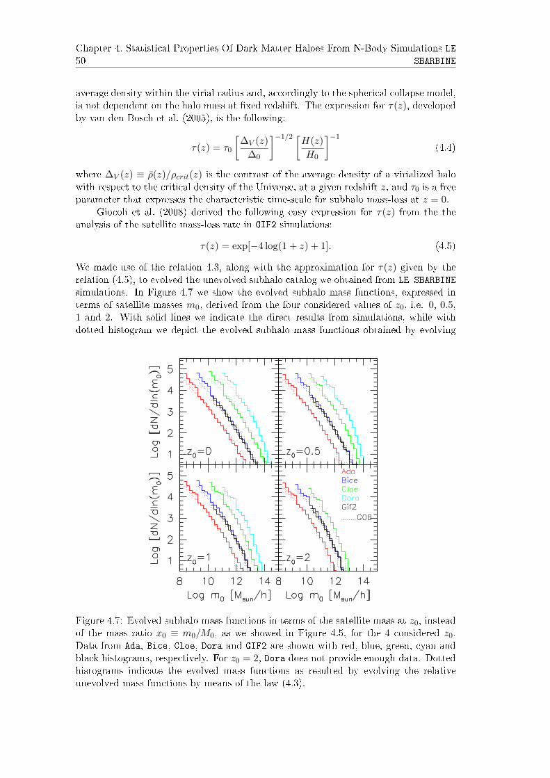
50Chapter 4. Statistical Properties Of Dark Matter Haloes From N-Body Simulations LE
SBARBINE
average density within the virial radius and, accordingly to the spherical collapse model,is not dependent on the halo mass at xed redshift. The expression for τ(z), developedby van den Bosch et al. (2005), is the following:
τ(z) = τ0
[∆V (z)
∆0
]−1/2 [H(z)
H0
]−1
(4.4)
where ∆V (z) ≡ ρ(z)/ρcrit(z) is the contrast of the average density of a virialized halowith respect to the critical density of the Universe, at a given redshift z, and τ0 is a freeparameter that expresses the characteristic time-scale for subhalo mass-loss at z = 0.
Giocoli et al. (2008) derived the following easy expression for τ(z) from the theanalysis of the satellite mass-loss rate in GIF2 simulations:
τ(z) = exp[−4 log(1 + z) + 1]. (4.5)
We made use of the relation 4.3, along with the approximation for τ(z) given by therelation (4.5), to evolved the unevolved subhalo catalog we obtained from LE SBARBINE
simulations. In Figure 4.7 we show the evolved subhalo mass functions, expressed interms of satellite masses m0, derived from the four considered values of z0, i.e. 0, 0.5,1 and 2. With solid lines we indicate the direct results from simulations, while withdotted histogram we depict the evolved subhalo mass functions obtained by evolving
Figure 4.7: Evolved subhalo mass functions in terms of the satellite mass at z0, insteadof the mass ratio x0 ≡ m0/M0, as we showed in Figure 4.5, for the 4 considered z0.Data from Ada, Bice, Cloe, Dora and GIF2 are shown with red, blue, green, cyan andblack histograms, respectively. For z0 = 2, Dora does not provide enough data. Dottedhistograms indicate the evolved mass functions as resulted by evolving the relativeunevolved mass functions by means of the law (4.3).

4.3. Statistics Of The Satellite Mass Evolution 51
the unevolved subhalo catalog using equation (4.3). The same color refers to the samesimulation: red for Ada, blue for Bice, green for Cloe, cyan for Dora and black forGIF2. The results from GIF2 simulations are shown to certify the consistency of ourresults with previous works. As we can see, the evolution expressed by the power-law(4.3), combined with the approximation for τ(z) given by equation (4.5), is in excellentagreement with data results from LE SBARBINE simulations.
4.3.3 Average Satellite Mass At zm
In this section we try to answer the following simple question: if we know the massratio x0 ≡ m0/M0 of a satellite at a given observation redshift z0, can we infer the massratio at the redshift of merging zm, namely xm ≡ mm/M0 ?
In order to answer this question, we examinate how data from LE SBARBINE sim-ulations populate the log x0-log xm plane. In Figure 4.8 we show the plane for everyconsidered simulation (for z0 = 2 we do not use data from DORA, because of lack of data)and observational redshift. Colours depict which simulation data come from, while forclarity we mark the bisectors with black solid lines. Of course data occupy only the half-plane above the bisector, since haloes inside hosts can only lose mass. Given a value ofxm, the more distant from the bisector is the relative value of x0, the more the satellitehas lost mass. We immediately note an overpopulated region in the plan, correspondingto log xm approximately larger than −2.5, where satellites seem to have undergone amore heavier consumption. We will discuss later this population of satellites.
For every simulation, we divide the log x0 range [−5.5,−1] in 9 bins with width∆ log x0 = 0.5 and nd the median xm inside each bin, which is marked with dierentpoint styles and colours relatively to the dierent simulations. Error bars refer tointerquartile ranges. We see that medians from dierent simulations perfectly overlap,so we t them with the line log xm = A log x0 + B and we nd that A ∼ 1 ± 0.01, sowe x A = 1 and minimimize the last squares adjusting only the value of B. Hence, wend that the relation between x0 and xm have the following easy form:
log xm = log x0 +B (4.6)
with B = 0.249± 0.021, 0.245± 0.017, 0.243± 0.013 and 0.239± 0.014 for z0 = 0, 0.5,1 and 2, respectively.
Equation (4.6) gives the average mass ratio at zm of a satellite with given massratio at z0 and it seems to be independent on the value of x0 and very slightly dependenton the observational redshift, so that satellites observed at low z0 generally undewenta slightly heavier mass loss. However, we can state that satellites were on average 1.75times (precisely from 1.77 for z0 = 0 to 1.73 for z0 = 2) more massive when they enteredinside the host halo.
We then study residuals around the median value xm averaging the residuals aroundthe relative median value found in every x0 bin. We precise that we consider residualsaround log xm + 1 instead of log xm to better perform the t. In Figure 4.9 probabilitydensity functions for satellites to have a given residual from the median best t expressedby of equation (4.6) are shown for the 4 considered z0. Squares indicate the meanabundances of data around the median values among the nine considered x0 bins anderror bars are the standard deviations. Red curves depict the lognormal best ts, forwhich we leave free only the parameter σ, since the resulting best t values of the mean

52Chapter 4. Statistical Properties Of Dark Matter Haloes From N-Body Simulations LE
SBARBINE
Figure 4.8: Median log xm for dierent bins of log x0 in LE SBARBINE simulations andfor z0 = 0, 0.5, 1 and 2. Coloured regions show the data in every simulation. We showwith black dashed lines the best t of the median points for every z0. For semplication,we keep the angular coecient xed to 1 and adjust only the value of the zero pointwith the last squares technique.
µ deviate from zero only for some thousandths. Thus, xing µ = 0, lognormal ts havethe form:
P (y)dy = C1√2π
e−(
ln2 y
2σ2
)σy
dy, (4.7)
where we remind that
y ≡ 1 + log xm − log xm = 1 + logxmxm
(4.8)
and that C is the normalization constant, so that the whole integral of equation (4.7)is equal to unity. Best t parameters are C = 4.34× 10⁻³, independently on the valueof z0, and σ = 0.131, 0.127, 0.122 and 0.118 for z0 = 0, 0.5, 1 and 2, respectively.
We underline that equation (4.7), which represents the best t for residuals aroundthe median expected xm, has no specic physical meaning, but it just gives a qualitativedescription of how data are, on average, spread around the median value, given byequation (4.6).
4.3.4 The Heavily-Consumed Satellite Population
In this section we examine the log x0-log xm plane at various values of redshift of mergingzm, considering dierent values of the host mass M0. We consider six minimum values

4.3. Statistics Of The Satellite Mass Evolution 53
Figure 4.9: Residuals around the median value xm for the four considered z0. In orderto perform the lognormal t, we shift the curve around 1 instead of 0.
of zm, namely 0, 0.5, 1, 2, 3 and 5, and four inferior limits of logM0: 10.5, 11.5, 12.5and 13.5, and we populate the plane with satellites which have survived until z0 andwere accreted at redshift higher or equal than zm by hosts more or equally massivethan M0. In Figure 4.10 we show the results. In each line the minimum mass is keptxed (we indicate it on the plot, where M0 ≡ log[M0/M]), while each column ischaracterized by the same value of z0. In each panel we use dierent colors to identifythe various minimum merging redshift we consider, as labeled, and we also draw thenormalized projected histograms along the two axis. Data from Ada, Bice, Cloe andDora simulations are used. The whole set of data is shown in the top-left panel andmoving downward host haloes withM0 lower than the relative mass limits are removed,whereas moving rightward z0 enhances.
As we expect from the above considerations about the subhalo mass functions,the shape of distributions of x0 and xm do not show signicant dependences on theobservational redshift or on the host halo mass at z0 (excluding statistically poor bins).Scanning the panels from the top to the bottom, that is excluding less massive hosthaloes, the shape of the data cloud remains the same but the number of satellitesaccreted at high redshift reduces. This is due the higher merger rate of massive haloeswith respect to less massive. The higher number of dynamical events during their longerassembly history is responsible of the stronger satellite consumtion, therefore it is morelikely that satellites accreted in past epochs by massive hosts undergo to a completedestruction.
It is useful to comment the evolution of satellites accreted at dierent epochs, thatis done by scanning panels from the right to the left for a xed threshold of M0. Thenumber of early accreted satellites decreases beacuse they have been totally demolished

54Chapter 4. Statistical Properties Of Dark Matter Haloes From N-Body Simulations LE
SBARBINE
Figure 4.10: The log x0-log xm planes including data from host haloes with mass largerthan M0 = 10.5, 11.5, 12.5 and 13.5, from the top to the bottom rows, respectively,at all considered simulations at the four observational redshift z0 = 0, 0.5, 1 and 2,respectively, from left to right columns. Satellites accreted at zm ≥ 0, 1, 2, 3 and 5 aredepicted by dierent colours: black, red, orange, green, yellow and blue, respectively.On the small panel we show the projected histograms on the two axis.
or simply their mass fell below the simulation resolution. We remind that all the halfplane above the bisector could potentially be populated. From a quite well deneddistribution at high z0, we see that the evolution to recent epochs brings to a bimodalsituation at low observational redshifts. There is a region on the top of the planes,corresponding to values of log xm approximately larger than −2.5, which seems to bemore dispersed along the values of log x0, like if satellites in this region were on averagemore consumed. Moreover, the shape of this region suggests that the evolution of somesatellites is dierent from what we found above. We will refer to this kind of satellites,which represent about 10% of the total population, as the Heavily-Consumed (hereafterHC) satellites.

4.3. Statistics Of The Satellite Mass Evolution 55
Figure 4.11: Median log xm for dierent bins of log x0 in LE SBARBINE simulations andfor z0 = 0, 0.5, 1 and 2. Here only the major mergers population has been considered.Colours are the same of Figure 4.8.
For a rst characterization of the HC satellites, we wonder in which case a satelliteundergoes more disruptive events, and the simplest answer is during a major merger.With major merger we mean the assembly of a satellite with mass ratio xm,m ≡ mm
Mm
greater or equal than 1/10. We underline that in this case both masses of satellitesand hosts are measured at the time of merging, as the pedices m indicate. Thus,the parameter xm,m should discriminate two populations and two dierent evolutionpaths for subhaloes: the rst one, the most common, for satellites relatively small (lessthan one tenth) with respect to the host at the moment of merging, so they undergothe standard consumption process we described in above sections; the second one, forsatellites with xm,m ≥ 0.1, which provide a more rapid mass loss.
In Figure 4.11 we propose again the same plots of Figure 4.8 including only majormergers. We t again the clouds just to have an estimate of the law relating x0 and xmin such kind of mergers. The resulting laws, averaged over the simulations, have thefollowing form, good for −4 < log x0 < 0:
log xm,maj = Amaj log x0 +Bmaj (4.9)
where Amaj = 0.28 ± 0.02, 0.27 ± 0.02, 0.29 ± 0.03 and 0.32 ± 0.02, and Bmaj =−0.56 ± 0.04, −0.58 ± 0.05, −0.61 ± 0.06 and 0.59 ± 0.06, for z0 = 0, 0.5, 1 and 2,respectively.
In top-left panel of Figure 4.12 we show again the log x0-log xm plane for z0 = 0and all considered simulations, where we trace in black the region that encloses datathat satisfy the condition log xm,m ≥ −1, while in red those data that do not. Curvesenclose the 99, 68.7 and 50% of data, from the thinnest to the thickest, respectively.

56Chapter 4. Statistical Properties Of Dark Matter Haloes From N-Body Simulations LE
SBARBINE
Figure 4.12: Top-left : regions containing major and minor mergers, in black and red,respectively, for z0 = 0 and all considered simulations. Top-right : same as the left-handpanel, but we add the condition Mm ≥ 500 particles for major mergers in black, whilein green we show major mergers for which Mm < 500 and in red all data which are notenclosed in the black region. Bottom-left : same of top-right panel but in a sub-sampleof massive host haloes, namely more massive than 104 particles. Bottom-right : blacklines enclose major mergers occurred more than 5 Gyr before z0, green lines enclosemajor mergers occurred at any time, while red lines enclose all minor mergers. Again,only host haloes more massive than 104 particles were considered. In each plot, lines ofthe same colour enclose the 99, 68.3 and 50% of data, from the thinnest to the thickest,respectively.
We see that the black region still shows bimodality, as if the mass ratio xm,m were notthe only condition that characterize HC satellites. After some experimenting, we ndthat the best discrimination parameter of those two populations that form the wholeset of major mergers is the mass of the host halo at the time of merging Mm.
Nevertheless, the amount of survived satellites (self-bound structures more massivethan 10 particles at z0) is larger among major mergers than among minor mergers: if weconsider all the simulations we have, for example at z0 = 0, the 62% of major mergers wenf a survived satellite, against the 33% among minor mergers. The possible explanationis that major mergers are more likely to occur at high redshift, thus among early formedhaloes, which we remind to have, on average, larger concentration, so they get hardlydestructed.
We note from the top-left panel of Figure 4.12 that the shape the region containingthe HC population (black lines) suggests the overlapping of two further populations. Intop-right panel of Figure 4.12 we isolate with green line the major mergers with hostshaving maximum mass at merging Mm equal to 500 particles (for z0 = 0) from majormergers with hosts more massive than 500 particles (included in black contours). The

4.3. Statistics Of The Satellite Mass Evolution 57
less massive major mergers seem to follow the same evolution of minor mergers, sincethe shape of the green cloud does not match the trend of the massive major mergers.Nevertheless, we must consider the inuence of resolution: the green cloud contains datarelative to satellites which have, at zm, a mass 50 ≤ mm < 500 particles, as we denedmajor mergers when log xm,m ≥ −1, thus, those satellites are already small when theyfall inside the host and their mass easily falls below the 10 particles resolution limit.In this perspective, if we ideally had not resolution problems, we should see the greencloud extented leftward, in other words toward low values of log x0. But if that were nota resolution problem, in the ideal simulation we would expect to nd the green cloudplaced exactly where it is on the top-right panel of Figure 4.12.
A straightforward way to simulate
Figure 4.13: Probability density functionsto have a minor (major) merger in d log(1+zm), traced by red (black) lines, at z0 =0. With dashed (solid) lines we show dis-tributions relative to satellites which havelog x0 ≥ −2 (log x0 < −2). Distributionsrefer to the sub-sample of host haloes moremassive than 104 particles.
an ideal simulation is to consider a sub-sample of very massive host haloes at z0,so a larger portion of the log x0 − log xmplane can be populated, especially alongthe log x0 axis. In bottom-left panel ofFigure 4.12 we show the same plot of top-right panel for a sub-sample of host haloeswith M0 ≥ 104 particles. Again, blackcontours enclose data from major merg-ers, that is log xm,m ≥ −1 where we re-mind that xm,m ≡ mm
Mmis the mass ra-
tio at the redshift of merging, with hosthaloes with mass Mm ≥ 500 particles,while green contours refer to major merg-ers with hosts having mass at mergingMm < 500 particles. Red lines encloseall data which are not contained in theblack cloud. Lines of the same colour en-close the 99, 68.3 and 50% of data, fromthe thinnest to the thickest, respectively.We see that the green cloud occupies amore central position with respect to theabove case, so we can conclude that if theresolution ideally were deeper of two or
three orders of magnitude, we would probably see this kind of conguration being theaverage. Another relevant notation is the presence of two distinct peaks in the distri-bution of massive major mergers, completely invisible in the top-right panel, thus thereis a further discriminating factor which regulates the shape of the HC population. Weidentify this further discriminating factor with a critical value of the redshift of merg-ing, that we call zm,cr, which depends on z0. The left-hand peak of the black cloud inbottom left panel of Figure 4.12 refers to satellites accreted at zm < zm,cr, while theright-hand peak refers to satellites accreted at zm ≥ zm,cr. After some experiments,we nd that for satellites identied at z0 = 0, 0.5, 1 and 2, zm,cr ≈ 0.5, 1, 1.8 and3, respectively, which correspond to the following times spent inside the host halo (inGyr): 5, 3, 2 and 1, respectively.
In Figure 4.13 we show the distributions of the redshift of merging in the sub-sampleof hosts more massive than 104 particles at z0 = 0. Solid lines refer to satellites charac-

58Chapter 4. Statistical Properties Of Dark Matter Haloes From N-Body Simulations LE
SBARBINE
terized by low values of x0, namely lower than −2, while dashed lines refer to satelliteswith x0 ≥ −2. Red and black lines depict minor and major mergers, respectively. Fo-cusing on red lines, i.e. minor mergers, we do not see a signicant dierence betweenhigh and low values of log x0, except for the more extended tail for low mass-ratio minormergers, due to the higher abundance of small haloes in early epochs. On the otherhand, the behaviour of major mergers in the two cases appears very dierent: satelliteswith low and high mass-ratio have very dierent distributions of zm. We can roughlysay that the low mass-ratio major mergers are, on average, accreted at zm < 0.5 whilethe high mass-ratio major mergers at zm > 0.5 This is conrmed from the bottom-rightpanel of Figure 4.12, where we show the bidimensional distributions for the followingthree populations: major mergers (either massive or not) occurred at zm > zm,cr withblack lines, major mergers at zm < zm,cr with green lines and any mergers which is notincluded in the black cloud, with red lines. The green and the black populations formtwo well separate bulks in the total sample of major mergers. The cases of z0 = 0.5, 1and 2 give the same results.
4.4 Conclusions
We analysed merger trees from the new set of Dark Matter simulations run in theUniversity of Padova called LE SBARBINE (Despali et al. 2016). The whole set is com-posed by six dierent realizations of cosmic cubes with the following comoving edges,in units of Mpc/h: 62.5 (Ada), 125 (Bice), 250 (Cloe), 500 (Dora), 1000 (Emma) and2000 (Flora), each lled by 10243 Dark Matter particles, hence having incresing massresolution from Flora to Ada. Our aim is to study the relations between the mass asatellite has just before merging with the host halo, i.e. at the redshift of merging zm,and the mass it has once inside the host, at a given z0. We consider 4 values for z0,namely 0, 0.5, 1 and 2. Since the two largest simulations (Emma and Flora) have toolow mass resolutions, we focus only on the rst four simulations.
In order to deal only with direct interactions, without including oblique mergers,we only consider subhaloes that give to the host halo at least 50% of their mass at zm.Furthermore, we check if at least a half of the particles of the initial subhaloes is stillinside the host halo at z0.
We derive the unevolved and evolved subhalo mass functions and we conrm pre-vious results from early works: the unevolved subhalo mass function is not dependenton either the host halo mass at z0 or the merging redshift zm. On the other hand, wend the evolved subhalo mass function being dependent on the host halo mass: satellitepopulations in less massive haloes seem to have undergone a deeper mass-loss. Theaverage characteristics of evolved populations, such as slope and normalisation, are inagreement with previous ndings. We also show evidences from data that the timespent in the host halo is determinant for the mass-loss of satellites: low-mass hostshaloes accrete satellites earlier, so those spend a longer time orbiting around the hostcenter of mass and get more consumed.
Using our data from the new set of simulations LE SBARBINE, we test the lawdeveloped by van den Bosch et al. (2005) and Giocoli et al. (2008) for the satellite mass-loss, expressed by equations (4.3) and (4.5). We nd an excellent agreement betweenthe theoretical law and data from LE SBARBINE. Thus, the theoretical law gives a wayto predict which is the mass of a satellite at z0, being accreted at redshift zm and havingmass mm at that moment.

4.4. Conclusions 59
We then give a form to recover the average mass-ratio (where with mass ratio wemean) one satellite had at the moment of merging, given its mass at z0. We denethe quantities x0 ≡ m0/M0 and xm ≡ mm/M0 as the satellite masses at redshift z0
and at the redshift of merging zm, respectively, in units of the host halo mass at z0.In this way, we avoid possible dependences on the host halo mass. We analyze thelog x0 − log xm plane and nd that the average xm, that we call xm is related to x0
through a simple linear equation, namely log xm = log x0 +B, where the parameter Bis slightly dependent on z0. In particular we nd B = 0.249 ± 0.021, 0.245 ± 0.017,0.243 ± 0.013 and 0.239 ± 0.014 for z0 = 0, 0.5, 1 and 2, respectively, that means anaverage mass at merging greater a factor ∼ 1.75 than the mass at z0. We then derive aform for the residuals around 1 + xm, having a lognormal distribution with mean µ = 0and the variance slightly dependent on z0, that is σ = 0.131, 0.127, 0.122 and 0.118 forz0 = 0, 0.5, 1 and 2, respectively. We stress that the lognormal expression for residualsaround xm has not a physical meaning, it just gives a good average description of data.Hence, we found a form for the average satellite mass at the accretion time, withoutknowing the redshift of merging, in terms of its mass and the mass of the host at z0.
The analysis of the log x0 − log xm plane allows a further comment about a sub-population of satellites whose evolution presents a peculiar behaviour. Besides themajority of data, which place into a cloud roughly parallel to the bisector, we also see asecondary cloud (including about 10% of the total data) placed about at log xm > −2.5with dierent average slope, and it is more evident at low values of z0, as the evolutionoccurred for longer time. Because of the elongated tail of this cloud toward low values oflog x0, we call this population as the Heavily-Consumed (HC) population. We identifythe HC satellite population as the results of early major mergers, where with majormergers we mean log xm,m ≡ mm/Mm < −1. We found that the the shape of the HCpopulations appears to be dened by some features. Firstly, we nd a slight dierencein position and shape between major mergers with massive and low-mass hosts, wherethe mass threshold is given by 500 particles at z0 = 0, as if the low-mass major mergersfollowed the law described by minor mergers. However, we tested by checking a sub-sample of very massive hosts at z0 = 0 (so we should avoid resolution problems), thatthis dierence is due only by lack of resolution, since for the very massive host sub-sample the low-mass major mergers appear to follow the behaviour of the whole sampleof major mergers. Secondly, we found that, for every considered z0, a critical valuefor zm (zm,cr), which discriminates two separate populations of major mergers, can beidentied. For z0 = 0, 0.5, 1 and 2 we nd that major mergers occurred at redshiftlower than 0.5, 1, 1.8 and 3, provide higher mass ratios x0 at z0, accordingly to the factthat satellites that spent longer time in hosts get more consumed, but in major mergersthis phenomenon appears to have a bimodal behaviour.


Chapter 5
Gravitational Lensing
Gravitational lensing is one of the most spectacular events observed in the Universe.Althought the physical phenomenon is always the same, its display is dierent depensingon the considered scale:
• on the stellar scale, it expresses as variations on the stellar light curve1, moreprecisely as temporary enhancements of the stellar ux. This regime is known asmicrolensing.
• on the scale of galaxies and clusters of galaxies it is possible to observe, in theinner region of an object, multiple images or very deformed images coming fromanother galaxy, sometimes assuming the form of an arc and, therefore, calledgravitational arcs (see Fig. 5.1). This regime, characterized by strong distorsionand multiple images is called strong gravitational lensing (hereafter SL), and wedene as strong lensing clusters every cluster of galaxy that produce SL eects;
• in the outer regions of cluster of galaxies or very massive galaxies, backgroundgalaxies appear very slightly deformed in the tangential direction w.r.t. the dis-tance with the lensing object, in the regime known as weak lensing (hereafterWL).
The common explanation for these events lies on the General Relativity: from Einsteineld equation we know that the gravitational eld preoduced by an arbitrary mass-energy distribution deforms the space-time around, with the consequent deformationof the near geodetic paths (see Fig. 5.2). Thus, the light emitted by a far source andpassing through a perturbed region, follows a deformed null geodetic and, therefore,changes direction. This event may lead to three consequences:
1. since more than one null geodetic may exist, dierent paths are possible arounda mass distribution, so from a single source could generate multiple images;
2. considering extended sources, since the number of photons and the surface bright-ness are conserved, the deformation of the image carries a change in the sourceux, being magnied or de-magnied;
3. dierent paths are covered in dierent times, so it is possible to observe a timedelay among the multiple images of a source.
1Flux diagram in function of time.
61

62 Chapter 5. Gravitational Lensing
Figure 5.1: Galaxy cluster Abell 1689, one of the most magnicent examples of stronglensing cluster, observed by HST. Gravitational arcs are clear.
Because of the similarity with optics, every object that acts in this way is called gravi-tational lens.
Figure 5.2: Right-hand panel : a very simple visualisation of the space-time deformationdue to the presence of a mass. Left-hand panel : a scheme with the deection of a lightray due to the sun (Narayan & Bartelmann 1996).
A photon of arbitrary frequency chooses the shortest path to travel from one pointto one another, as stated by the Fermat principle. Just applying this principle, onecan derive a relation between the deection angle ~α and lens gravitational potential φmaking two assumptions:
1. the gravitational eld is weak, that is φ/c2 1, which is true in every astrophys-ical situation (for a cluster of galaxies |φ| < 10−4c2);
2. as a consequence of the previous assumption, the deection angle is small, so wecan apply the Born approximation (visualised in left panel of Figure 5.3), in otherwords we can think of the deection as it were istantaneous in the plane thatcontains the lens.

63
Observer
Lens plane
Source plane
θ
β
ξ
α^
η
Dds
Dd
Ds
Figure 5.3: Left panel : Born approximation (Narayan & Bartelmann 1996). Right panel :A schematic view of a lensing system (Bartelmann & Schneider 2001).
Having dene with b the impact parameter (the minimum distance between the lightpath and the lens), the relation between ~α and φ is expresses by the following:
~α(b) =2
c2
∫ +∞
−∞∇⊥φdz, (5.1)
good for any considered potential. Generally, the thin screen approximation is applied:in any case, the size of a lens is always innitesimal compared to the whole lensingsystem (source-lens-observer), even if the lens is a cluster of galaxies. Therefore, everylens can be thought as a bidimensional matter distribution that occupies the lens plane;the same for sources, which lie on the source plane.
Point lens
We consider a point source with mass M , so φ = −GMr
, with r =√x2 + y2 + z2 =
√b2 + z2. Inside the integral of equation (5.1) we then nd∇⊥φ =
GM
r3
∣∣∣∣xy∣∣∣∣ =
GM
r3b
∣∣∣∣cosφsinφ
∣∣∣∣.Therefore, the deection angle for a point source is
~α =4GM
c2b
∣∣∣∣cosφsinφ
∣∣∣∣ ,which is
|~α| = 4GM
c2b. (5.2)
Continuous Distribution
The equation (5.2) tells that |~α| is linear function of mass, then the deection angle ofa planar distribution of N point sources with positions ~ξi and masses Mi (1≤ i ≤ N) is
~α(~ξ) =∑i
~αi(~ξ − ~ξi) =4G
c2
∑i
Mi
~ξ − ~ξi|~ξ − ~ξi|2
. (5.3)

64 Chapter 5. Gravitational Lensing
Considering a tridimensional distribution and applying the thin screen approximation,the lens mass density ρ(~ξ, z) is projected on the lens plane to obtain the lens bidimen-sional mass distribution Σ(~ξ) =
∫ρ(~ξ, z)dz. The deection angle is given summing the
constributes from all elements with mass Σ(~ξ)d2~ξ = dM ,
~α(~ξ) =4G
c2
∫(~ξ − ~ξ′)Σ(~ξ′)
|~ξ − ~ξ′|2d2~ξ, (5.4)
where ~ξ′ is the position of the element of mass and ~ξ is the position of the light beam.
5.1 The Lens Equation
Every lensing system is characterized by a simply relation that connects the real positionof a source to the apparent one and to the deection angle. We call β the angle whichsubtends the source real position, θ the angle which subtends the image, and DS , DL
and DLS the angual diameter distances of the source plane, the lens plane and betweenlens and source planes (see right-hand panel of Figure 5.3). As we are considering smallangles, the virtual position of the source is given by the real one plus the distance causedby the deection:
~βDS + ~αDLS = ~θDS ,
which can be written as~β = ~θ − ~α(~θ), (5.5)
where ~α(~θ) ≡ ~αDLS
DSis the reduced deection angle.
It is worth to dene an adimensional form of the lens equation mutiplying bothmembers per DL and multiplying and dividing the rst member per DS . We obtain thefollowing:
~ηDL
DS= ~ξ − ~α(~θ)DL, (5.6)
where ~η = ~βDS and ~ξ = ~θDL. We also rescale all lenghts with a reference one on the
lens plane, namely ~ξ0 ≡ ~η0DL
DS, and we obtain
~y = ~x− ~α(~x), (5.7)
where ~y =~η
~η0, ~x =
~ξ
~ξ0
and ~α(~x) = ~α(~ξ)DL
~ξ0
.
5.2 Convergence And Lensing Potential
In this thesis we will deal with SL eects by galaxy clusters, in particular gravitationalarcs, therefore we now illustrate which are the conditions for these special featuresto form. We need to dene some important properties of the lens that determine itseciency in producing strong lensing eects.

5.3. Distortion, Magnication And Multiple Images 65
We start with the convergence, dened as the adimensional projected mass density
κ(~x) ≡ Σ(~x)
Σcrit, where the quantity Σcrit ≡
c2
4πG
DS
DLDLSseparate weak from strong
lensing regime. A lens with projected mass distribution Σ so that in some point of thelens plane Σ > Σcrit, thus κ > 1, is said to have a supercritical behaviour.
The lensing potential is dened as the projected gravitational potential of the lenson the lens plane. Given the projection of the potential along the z axis φ(DL
~θ, z), thelensing potential is dened as:
ψ(~θ) =DLS
DLDS
2
c2
∫φ(DL
~θ, z)dz, (5.8)
while its adimensional counterpart is ψ =D2L
ξ20
ψ. The lensing potential is linked to the
deection angle and to the convergence through two simple relations:
1.~∇xψ(~x) = ~α(~x), (5.9)
in fact, given ~∇x = ξ0~∇⊥, it is demonstrate that
~∇xψ(~x) = ξ0~∇⊥
DLSDL
ξ20DS
2
c2
∫φ(~x, ~z)dz =
DLSDL
ξ0DS
2
c2
∫~∇⊥φ(~x, ~z)dz = ~α(~x).
2.
∆xψ(~x) = 2κ(~x), (5.10)
which is similar to the Poisson equation ∆φ = 4πGρ.
Using the bidimensional notation, we express the deection angle through κ as
α(~ξ) =4G
c2
∫Σ(~ξ′)
~ξ − ~ξ′
|~ξ − ~ξ′|2d2~ξ′
π
π
DLDLS
DS
DS
DLDLS=
1
π
DS
DLDLS
∫κ(~ξ′)
~ξ − ~ξ′
|~ξ − ~ξ′|2d2~ξ′.
(5.11)
From the adimensional distance x ≡~ξ
~ξ0
we obtain
α(~x) =1
π
∫κ(~x)
~x− ~x′
|~x− ~x′|2d2~x′.
Finally, from ~∇ ln |~x| = ~x
|~x|2, we relate the convergence to the lensing potential:
ψ =1
π
∫κ(~x′) ln |~x− ~x′|d2~x′ (5.12)
5.3 Distortion, Magnication And Multiple Images
From equation (5.7) we deduce that the deection of light beams is dierential, thatis the deection angle depends on the projected distance between the source and thecenter of the lens. Considering extended sources, this implicates the deformation of the

66 Chapter 5. Gravitational Lensing
image and the source magnication. The deformation is described at the rst order bythe Jacobian matrix A:
A ≡ ∂~y
∂~x= δij −
∂αi(~x)
∂xj= δij −
∂2ψ
∂xi∂xj= δij − ψij ,
having dened ψij ≡∂2ψ
∂xi∂xj.
The anisotropic part of the tensor A is dened as(A− 1
2TrA× I
)= δij − ψij −
1
2(2− ψ11 − ψ22) δij = −ψij +
1
2(ψ11 + ψ22) δij =
=
∣∣∣∣∣∣∣−1
2(ψ11 − ψ22) −ψ12
−ψ211
2(ψ11 − ψ22)
∣∣∣∣∣∣∣and since the matrix is symmetrical and with null trace, we dene the shear as thepseudo-vector ~γ = (~γ1, ~γ2) with components
γ1 =1
2(ψ11 − ψ22) e γ2 = ψ12 = ψ21. (5.13)
On the other hand, the isotropic part is(1
2TrA× I
)ij
=
[1− 1
2(ψ11 + ψ22)
]δij = (1− κ)δij
since, as we already saw,1
2∆ψ = κ.
The tensor A can be then written as
A =
∣∣∣∣1− κ− γ1 −γ2
−γ2 1− κ+ γ1
∣∣∣∣ ,which has the following determinant detA = (1 − κ)2 − γ2 = (1 − κ − γ)(1 − κ + γ).The diagonalisation leads to
A =
∣∣∣∣λt 00 λr
∣∣∣∣ , (5.14)
where λt ≡ 1 − κ − γ and λr ≡ 1 − κ + γ are the tangential and radial eigenvalues,respectively. The relation (5.14) is very useful to understand the meaning of convergenceand shear. Considering a circular source, described on the source plane by the equationy1 + y2 = R2, and neglecting the shear (γ = 0), we have that the lens equation is∣∣∣∣y1
y2
∣∣∣∣ = A
∣∣∣∣x1
x2
∣∣∣∣ = (1− κ)δij
∣∣∣∣x1
x2
∣∣∣∣ ,that is equivalent to the system
y1 = (1− κ)x1
y2 = (1− κ)x2
.

5.3. Distortion, Magnication And Multiple Images 67
Figure 5.4: The eect of convergence and shear on a circular source (Narayan & Bartel-mann 1996).
Adding the squares of the rwo equations we obtain
R2 = (1− κ)2(x21 + x2
2).
Hence, a circular source with radius R is mapped on the lens plan with circular im-
age with scaled radiusR
(1− κ). Therefore the convergence represents the eect of the
isotropic component of the Jacobian and modies the size of the image without changingthe shape.
Including also the shear in the example, we have that∣∣∣∣y1
y2
∣∣∣∣ = (1− κ)δij
∣∣∣∣x1
x2
∣∣∣∣− ∣∣∣∣γ1 γ2
γ2 −γ1
∣∣∣∣ ∣∣∣∣x1
x2
∣∣∣∣ ,so the system becomes
y1 = (1− κ− γ)x1
y2 = (1− κ+ γ)x2
,
and adding the squares we obtain
R2 = (1− κ− γ)2x21 + (1− κ+ γ)2x2
2.
In this case, a circular source is mapped in the lens plane with an elliptical image with
dimensions a =R
1− κ− γand b =
R
1− κ+ γ. The shear quantify the eect of the
anisotropic component of the tensor A and the deformation of the image, which fromcircular becomes elliptical (Figure 5.4).
The lens equation maps a surface element in the source plane δy2 in a surfaceelement in the lens plane δx2. The Liouville theorem and the absence of photon emissionor absorption during the lensing event guarantee the the photon density in the phasespace is conserved, so the source ux must change. The ratio of source and image uxesis reects the ratio of the surfaces in source and lens planes occupied by the source andby the image. The magnication µ is therefore the ratio of the solid angle sottended

68 Chapter 5. Gravitational Lensing
by the image and the solid angle sottended by the source, and it is dened as thedeterminant of the magnication tensor M , that is the inverted A tensor:
µ ≡ detM =1
detA=
1
(1− κ)2 − γ2.
Since M is a second order tensor, it admit two eigenvalues, linked to the eigenvalues ofA:
µt =1
λt=
1
1− κ− γµr =
1
λr=
1
1− κ+ γ
,
where µt and µr are the tangential and radial components of µ, respectively.The eigenvalues of A, namely λt(~x) and λr(~x), are functions of the coordinates on
the lens plane. In the points on the the lens plane ~x where λt(~x) or λr(~x) are null,called critical points, the magnication diverges in the tangential or radial direction,respectively. Critical points form two separate curves on the lens plane: from thecondition λr(~x) = 0 the radial critical line is generated in the inner region of the lens,while from λt(~x) = 0 the tangential critical line is dened, which lies more externallyon the lens plane. Using the lens equation, one can map the critical lines from the lensplane to the source plane, nding the radial or tangential caustic lines. The divergenceof the magnication on the critical lines suggests that in those regions of the lens planeimages from background galaxies appear very deformed, as we will see just below.
Image Distortion Near Critical Lines
We now analyse how images get deformed near critical lines. We consider a genericaxially symmetrical lens, so that Σ(~ξ) = Σ(|~ξ|), and we let the lens center correspondto the optical axis. In order to know how is the deformation near the critical lines, wecompute the Jacobian and we apply it to a point close to the critical line. The deectionangle of an axially symmetrical lens is
α(ξ) =4GM(ξ)
c2ξ,
which has the following adimensional form:
α(x) =m(x)
x,
wherem(x) =M(x)
πξ20Σcr
is the adimensional mass included in x, whileM(x) is its physical
counterpart. The adimensional lens equation is therefore
y = x− m(x)
x. (5.15)
Since we know that ~α(x) =m(x)
x2~x and that ∇ψ = ~α, we derive the following form for
the convergence
κ =1
2(ψ11 + ψ22) =
1
2
(∂α1
∂x1+∂α2
∂x2
)=
1
2x
dm
dx(5.16)

5.3. Distortion, Magnication And Multiple Images 69
and the following for the rst component of shear
γ1 =1
2(ψ11 − ψ22) =
1
2(x2
2 − x21)
(2m
x4− dm
dx
1
x3
), (5.17)
and for the second one
γ2 = ψ12 = x1x2
(dm
dx
1
x3− 2m
x4
). (5.18)
Therefore, the Jacobian matrix is given by Aij = δij − ψij = δij −∂αi∂xj
and
A = 1− m
x4
∣∣∣∣x22 − x2
1 −2x1x2
−2x1x2 x21 − x2
2
∣∣∣∣− dm
dx
1
x3
∣∣∣∣ x21 x1x2
x1x2 x22
∣∣∣∣ . (5.19)
With equations (5.16), (5.17) and (5.18) we derive that, for axially simmetrical lenses,shear and convergence are related in this way:
~γ2 =
(m(x)
x2− κ)2
,
where κ(x) =m
x2represents the mean value of κ in the region delimited by x. Conse-
quently, we haveγ(x) = κ(x)− κ(x).
Since the tangential critical line was dened as the location of points that satisfy thecondition 1− κ(x)− γ(x) = 0, then inside the region enclosed by the tangential criticalline we have that κ = 1.
For this kind of lens the determinant of the Jacobian is given by
detA =y
x
dy
dx= (1− κ)(1− 2κ+ κ) = λtλr
and it gives the equations that dene the critical lines: 1 − κ = 0 for the tangentialcritical line, while 1 − 2κ + κ = 0 describe the radial one. These equations representtwo circumferences on the lens plane, the rst one inner (radial) and the second oneouter (tangential). From the equation (5.15) we see that the tangential critical line ismapped in the point y = 0 in the source plane, so the tangential caustic line of anaxially symmetrical lens is a point. On the other hand, the radial caustic has a circularshape. We will see that when the source lies inside the caustic radial line, multipleimages form in the lens plane.
Now we consider the point (xc, 0), very close to the tangential critical line, thus it
satisesm
x2= 1− δ, with |δ| 1. The Jacobian matrix in the point (xc, 0) is given by
equation (5.19) (where m′ ≡ dm
dx):
A(xc, 0) = 1− m(xc)
x2c
∣∣∣∣−1 00 1
∣∣∣∣− m′(xc)
xc
∣∣∣∣1 00 0
∣∣∣∣ =
=
∣∣∣∣∣∣∣1 +
m
x2c
− m′
xc0
0 1− m
x2c
∣∣∣∣∣∣∣ =
∣∣∣∣∣∣2−m′
xc0
0 δ
∣∣∣∣∣∣ .

70 Chapter 5. Gravitational Lensing
Let's suppose that the image in (xc, 0) of a circular source were elliptical, thus describedby the equation
~c(φ) = ~xc +
∣∣∣∣ρ1 cosφρ2 sinφ
∣∣∣∣ , (5.20)
where ρ2 and ρ1 are the tangential and radial semiaxis, respectively. Using the lensequation we derive the equation that describes the source:
~d(φ) = A(xc, 0)~c(φ) = ~yc +
∣∣∣∣∣∣2−m′
xc0
0 δ
∣∣∣∣∣∣∣∣∣∣ρ1 cosφρ2 sinφ
∣∣∣∣ = ~yc +
∣∣∣∣∣∣(
2− m′
xc
)ρ1 cosφ
δρ2 sinφ
∣∣∣∣∣∣ .Having assumed a circular source, the terms
(2− m′
xc
)ρ1 e δρ2 must be equivalent, so
(2− m′
xc
)= δρ2,
from which we have the ratio between the tangential and the radial semiaxis of theimage:
ρ2
ρ1=
2−m′/xcδ
1.
Hence, the elliptical image near the tangential critical line has the semiaxis ρ2 muchlarger than ρ1: here a tangential arc is formed.
If an elliptical image forms on a point (xc, 0) close to the radial critical line, so that
1 +m2− m′
x= δ, the Jacobian will be
A(xc, 0) =
∣∣∣∣∣∣∣1 +
m
x2c
− m′
xc0
0 1− m
x2c
∣∣∣∣∣∣∣ =
∣∣∣∣∣∣δ 0
0 1− m
x2C
∣∣∣∣∣∣ .The ellipse (equation (5.20) is mapped on the source plane as
~d(φ) = ~y +
∣∣∣∣∣∣δρ1 cosφ(
1− m
x2c
)ρ2 sinφ
∣∣∣∣∣∣ .As we supposed a circular source, we have
δρ1 =
(1− m
x2c
)ρ2,
so the ratio between tangential and radial semiaxis is
ρ2
ρ1=
δ
1−m/x2c
1.
In this case, the radial semiaxis is much larger than the tangential one, so we get aradial arc.

5.3. Distortion, Magnication And Multiple Images 71
Figure 5.5: The only way to get multiple images is that at least for one y the functiony(x) inverted the monotonicity, so dy/dx=0. If this condition is satised, thus exists atleast one point ys corresponding to more values of x.
The Generation Of Multiple Images
Axially symmetrical lenses produce mupltiple images from the same source if at leastin one point the following condition is satised:
dy
dx= 1− 2κ+ κ < 0, (5.21)
because if in any point y(x) is decreasing, hence a certain value ys on the source planewill be mapped in more points x on the lens plane (see Fig. 5.5). The change in the
sign ofdy
dximplies that in one point we have
dy
dx= 0: for an axially symmetrical lens
this condition correspond to the equation of the critical radial line.
Figure 5.6: The red curve represents a generical function α(x). If |y| < |ya| lines y − xintercept the curve more than once, while if |y| > |ya| there is only one intersection.

72 Chapter 5. Gravitational Lensing
Projecting on a plane the function α(x) =m(x)
xand observing where x−y = α(x),
one den themultiple image diagram. The number of intersections between the line x−yand the curve α(x) is equal to the number of multiple images (the latter being dependenton the source position y) originated by the lensing system (see Fig. 5.6). The conditiondα
dx= 1 denes the radial critical line, as
dα(x)
dx=
d
dx(x − y) = 1 is satised only if
dy
dx= 0. Like in Fig. 5.6, the values ya that satisfy
dyadx
= 0 identify lines which are
tangent to the curve α(x): if |y| > |ya| (the source is outside the radial caustic line) wehave one image, while if |y| < |ya| (the source is inside the radial caustic line) we ndmore than one image.
5.3.1 Time Delay Surface
A way to study the number and position of multiple images is given my the time delaysurface analysis. However, before starting this issue, we must introduce the time delay.Gravitational lensing is essentially given by a change in the light path from a source toan observer, caused by local space-time distortion due to the presence of a gravitationaleld. This change implies a dierence between times that light takes to travel alongstraight and bended paths, called geometrical delay, ∆tgeom. Moreover, the presence of
a weak gravitational eld acts as an eective refraction index n ≈ 1− 2φ
c2which delays
the light beam, causing the so-called Shapiro delay, ∆tgrav. Both those two delays hencecontribute to the total time delay ∆t = ∆tgrav + ∆tgeom.
The Shapiro delay is given by the dierence among travel times with and withoutgravitational perturbations:
∆tgrav =
∫dl
c′−∫
dl
c=
1
c
∫(n− 1)dl = − 2
c3
∫φdl, (5.22)
where c′ = c/n is the eective speed of light in presence of gravitational eld. On theother hand, the geometrical time delay is given by
∆tgeom =∆l
c=
1
2c(θ − β)2DLDS
DLS. (5.23)
Adding equations (5.22) and (5.23) we get the total time delay:
∆t(~θ) = ∆grav + ∆geom =DLDS
DLS
1
c
[1
2(~θ − ~β)2 − ψ(~θ)
](1 + zl), (5.24)
where the denition of lensing potential has been used (equation 5.8). Using the scalelenght ξ0, we have the following adimensional form for the time delay
∆t(~x) =DS
DLDLS
ξ20
c
[1
2(~x− ~y)2 − ψ(~x)
](1 + zl),
, which denes the time delay surface. The gradient of the time delay surface is givenby
∇(∆t) =DS
DLDLS
ξ20
c[(~x− ~y)− α(~x)] (1 + zl), (5.25)

5.4. Analytical Lens Models 73
since ∇ψ(~x) = α(~x) for the property of the lensing potential. Inside the square bracketsof equation (5.25) we note the lens equation, therefore images form where ∇(∆t) = 0,as requested by the Fermat principle.
Fixed the source position, the time delay is characterise by the paraboloid f(~x) =(~x−~y)2 and the function g(~x) = ψ(~x), the latter being determined by the lens potential.The Hessian matrix of the time delay surface is related to the magnication throughthe following relation:
Tij =∂2(∇t)∂xi∂xj
∝ δij − ψij = Aij =1
µij(5.26)
that is telling us that the more bended the surface where image forms, the less magniedthe image; on the ather hand, the less curve the surface, the more magnied the image.
From the time delay surface analysis is clear that the density prole of the lens isessential to determine how many multiple images form and where these are located inthe lens plane. In the next section we will examine the image congurations for thesimplest analytical models of lens.
5.4 Analytical Lens Models
Since the eciency of a given object in producing gravitational lensing eects is givenby its mass distribution, let's see how we can analytically derive the lensing propertiesof objects with given known mass distributions. This is also useful to understand howmuch dierent realistic lenses and ideal situations are. Nevertheless, the modeling ofrealistic lenses can take advantage of ideal cases, as we will see.
5.4.1 Singular Isotermal Sphere (SIS)
The SIS has a projected density prole described by
Σ(~ξ) =σ2v
2G|~ξ|∝ |ξ−1|,
since Σ(~ξ) = 2∫∞
0 ρ(r, z)dz, with ρ(~r) =σ2v
2πGr2, where σv is the velocity dispersion of
particles. We rescale the projected density prole with ~ξ0 = 4πσ2v
c2
DLDLS
DSand we use
the critical density to write the folling:
Σ(~ξ) =σ2v
2G
~ξ0
~ξ
1
~ξ0
=1
2xΣcrit. (5.27)
From the denition of convergence κ ≡ Σ
Σcritand equation (5.27) we derive the following
expression of κ(x):
κ(x) =1
2|x|, (5.28)
where the absolute value is used, as the convergence is dened positive. We derive thelensing potential from its general relation with κ - equation (5.9) - and we nd
ψ = |x|. (5.29)

74 Chapter 5. Gravitational Lensing
The deection anglge is given by the gradient of the potential, as stated by the relation(5.10), so we have:
~α =~x
|~x|(5.30)
with which we write the lens equation in the following way
y = x− x
|x|. (5.31)
Positions and multiplicity of images are given by the solutions of the equation (5.31):if |y| < 1 two solutions (therefore two images) exist, one positive x+ = y + 1 and onenegative x− = y− 1, xed separation x+−x− = 2; if |y| > 1 we have only one solution.
Fig. 5.7 illustrates the multiple image diagram for a SIS lens. The interceptionbetween ~α(~x) and lines x− y occurs two times only for source positions |y| < 1. Hence,if the source lie inside a certain scale, there will be two images on the lens plane. In
Figure 5.7: Multiple images diagram for a SIS lens. Lines x − y intercept the lines~α = ~x/|~x| in two points only for those |y| < 1; if |y| > 1 there is only one interceptionand, therefore, one image.
order to dene the scale the denes the region where the source has to be to form two
images, we consider the normalisation lenght ~ξ0 = 4πσ2v
c2
DLDLS
DS, minding that, for a
isothermal sphere, we have
M(ξ) = 2π
∫ ξ
0Σ(ξ′)ξ′dξ′ = 2π
∫ ξ
0
σ2v
2Gdξ′ =
πσ2v
Gξ.
From the latter equation we derive σ2v and we insert it in the denition of ξ0, getting
the following expression for θ0:
θ0 =
√4GM(θ0)
c2
DLS
DLDS= θE , (5.32)
where θE denes the Einstein radius. If y = 0 the image is a ring with radius thatsubtend θE , while if y 6= 0 we must distinguish two cases, depending on β:

5.4. Analytical Lens Models 75
1. if |β| < θE then |y| < 1, two images are generated;
2. if |β| > θE then |y| > 1, only one image is produced.
Genrally speaking, the Einstein radius separate the strong lensing regime from the weakone and it denes the eciency of a lens in generating multiple images.
The SIS model is characterised by a prticular relation among shear and convergence:from equations (5.13) we get the component of shear γ1 and γ2, so that we can write itas
γ =√γ2
1 + γ22 =
1
2|x|= κ, (5.33)
so, for a SIS lens, the measurement of γ gives an estimate of the convergence prole.From this relation, critical lines, dened as the eigenvalues of the Jacobian matrix, arefound. The tangential critical line is given by
λt = 1 + κ+ γ = 0
and, thanks to the relation (5.33) we obtain
x = 1,
that is, again, the Einstein radius. The radial critical line is given by
λr = 1 + κ− γ = 0,
but γ = κ, then
λr = 1
and it is never null. Thus, this lens model does not originate radial critical lines.
Let's see now the image magnication. Since the radial magnication is µr =1
λr=
1, the image is not magnied in the radial direction, but only in the tangential direction,so
µ = µt =1
λt=
|x||x| − 1
.
Assuming that the source lies inside the Einstein radius, so |y| < 1, and considering
the positive solution |x+| = x+ = y+1, the magnication will be µ+ = 1+1
y; if y →∞
then µ+ = 1, while if y → 0 then µ → ∞, as expected: if the source is far from thecenter of the lens the image does not undergo magnication, while if it is exactly behindthe center, the Einstein ring is formed on the tangential critical line, that is the placeon the lens plane where µ→∞.
In this case, the time delay surface is given by the sum of (x−y)2 with the oppositeof the potential ψSIS(x), where ψSIS is dened by equation 5.29, and it is characterisedby a central cusp (dashed line in Fig. 5.8 ). If the source is perfectly aligned with thelens, so β = 0, then the paraboloid is centered in the origin (black line in Fig. 5.8). Thetime delay surface is shaown in Fig. 5.8 as a red curve, while the points indicate whereimages form, that is where the Hessian matrix of the surface is null. We nd the twosymmetrical lateral points, corresponding to the solutions x+, x− of the lens equationand to the Einstein radius. Here the curvature is zero and the magnication is innite,as described by the relation (5.26) between Hessian matrix and magnication. In the

76 Chapter 5. Gravitational Lensing
Figure 5.8: The red line represents the bidimensional section of the time delay surface,given adding the palabola (x−y)2 (solid line) with the opposite of the potential (dashedline). We show the case with β = 0, that is when the source is exactly behind the lens.Points indicate the image positions: the lateral ones correspond to the solutions x+
and x−; in the central point the curvature diverges, so the central image is innitelydemagnied and, therefore, invisible.
central cusp, though there is a relative maximum, there is no image since the curvaturediverges and the magnication is zero.
We saw that singular spherical lenses produce two images is the sources is closerthan the Einstein radius to the lens center. Both images form along the tangentialcritical line, so they form two tangential arcs, one long and one short, known as counter-arc; if the source is exactly behind the lens, the two arcs merge to form the Einsteinring. Moreover, the central singularity of this model does not allow the formation ofthe radial critical line, so no radial arc is produced.
This kind of image conguration is often observed in strong lensing from galaxies(Bolton et al. 2008), hence it seems they are consistent with a spherical singular prole.It is not clear how the Dark Matter halo (which is supposed to have a NFW prole)combines with baryons to generate this kind of prole. On the other hand, galaxyclusters usually show much complex congurations: radial arcs are found, no counter-arcs are observed and multiple images are much more than two. Thus, it is clear thatthe most suitable model to describe galaxy cluster must be much more complex than asingular isothermal sphere.
5.4.2 Non-singular Isothermal Sphere (NIS)
We now remove the central singularity from the SIS model adding a core inside a certainradius xc and we obtain a non-singular isothermal sphere (NIS). The lensing potentialis given by the following
ψ =√x2 + x2
c .

5.4. Analytical Lens Models 77
We note that, in this case, the time delay surface has no central cusp and, then itproduces even the central image. From the potential, the deection angle is derived:
~α = ~∇φ =~x√
x2 + x2c
and therefore the lens equation
~y = ~x− ~x√x2 + x2
c
.
Convergence and shear are derived from the rst derivatives of the components of ~α,obtaining
κ =1
2
[x2 + 2x2
c
(x2 + x2c)
3/2
]γ =
1
2
x2
(x2 + x2c)
3/2. (5.34)
Like the SIS model, the NIS model shows a simple relation between γ and κ prolestoo, which is
κ =1
2
x2 + 2x2c
(x2 + x2c)
3/2=
1
2
x2
(x2 + x2c)
3/2
(1 +
2x2c
x2
)= γ
(1 +
2x2c
x2
). (5.35)
The tangential critical line is dened by relation (5.35), so the condition λt = 0, that is1− κ− γ = 0, becomes
1− γ(
1 +2x2
c
x2
)− γ = 0.
Using the expression (5.34) we dene the tangential critical line as points that satisfy
xt =√
1− x2c ,
so the line exists if the condition |xc| < 1 on the core radius is satised.The same for the radial critical line, dene by points where 1 − κ + γ = 0, that
becomes
1− γ(
1 +2x2
c
x2
)+ γ = 0.
Again, from this equation we derive the following formulation for points on the radial
critical line x2r = x
4/3c (1 − x
3/2c ). We see that both critical lines have the condition
|xc| < 1 to exist, so the core radius must be smaller than the Einstein radius.As we saw in Section 5.3, the condition for critical lines to exist transform in the
condition for multiple images to exist. Note in Fig. 5.9 (right-hand panel) that if xc = 0,the multiple images diagram becomes equivalent to the typical step diagram of the SIScase; enhancing xc, the step gets less steep and the intersection points between curveand x−y the line (so where the curvature of the time delay surface is null and thereforethe multiple images) are three. If xc = 1 the curve is tangent to the line, so if xc ≥ 1a single image is generated. In Fig. 5.9 the time delay surface for a NIS lens is shown(left-hand bottom panel), with a source o-axis w.r.t. the lens center (in the top panelβ is the source position while the dotted line indicate the center of the lens). Besidesthe tangential arcs represented by the two lateral points, as in the SIS case, but the

78 Chapter 5. Gravitational Lensing
Figure 5.9: Left-hand panel : bidimensional representation of geometrical, gravitationaland total time delays, top, middle and bottom panels, respectively; β indicates thesource position, while black points indicate the image positions; the dotted line depictsthe center of the lens (Narayan & Bartelmann 1996). Right-hand panel : multiple imagediagram for a NIS lens. If the core radius xc is zero, we nd the SIS case (solid line);if the core radius is smaller than the Einstein radius, 0 < xc < 1, the line x − y = 0intercept the diagram in three points, where multiple images form; if the core radius islarger than the Einstein radius, xc ≥ 1, the intersection is one and no multiple imagesare formed.
Figure 5.10: Lens and source planes (left-hand and right-hand panel, respectively) ofa lensing system with NIS lens. On the lens plane we see the tangential and radialcritical lines (outer and inner circle, respectively), while on the source plane we see thetangential caustic line (the central point) and the radial caustic line (the outer circle).
central image has now nite magnication because the time delay surface is continually

5.4. Analytical Lens Models 79
deformed in the central point, without any singularity. Therefore, the central image isvisible. Fig. 5.10 reports a visulisation of what we described in this section. The lensingconguration with an axially symmetrical lens is shown in the lens and the source plane,left-hand and right-hand panels, respectively. Note critical lines on the left and causticlines on the right. Also note that critical lines are both circles (the outer one beingthe tangential critical, while the inner one the radial), and that caustic tangential andradial lines are given by a central point and a circle, respectively. We consider twosource positions, depicted in red and black. In red we consider the source lying on thecaustic radial line and, consequentely, the formation on the lens plane of three multipleimages, two of them deformed in the radial direction and merged in a radial arc. Thenwe put the source very close to the tangential caustic curve, shown in black on Fig. 5.10.Images on the lens plane are still three, the central one being very demagnied, whilethe other two are elongated along the tangential direction.
Let's suppose to follow the movement of the source rightward from the center of thelens. The paraboloid of Fig. 5.9 moves rightward and the time delay surface changes:the minimum at the left and the central maximum get closer. between the two pointsis the radial critical line, more precisely on the point where the curvature changes andwhere there is the maximum radial magnication. This means that the tangential arcsat the left in Fig. 5.10 moves rightward and get closer to the radial critical line, whilethe central image moves leftward approaching the tangential arc. The arc tangentialmagnication decreases and its radial magnication increases. When the source is verynear to the radial caustic, the two images higly deform in the radial direction and mergeforming a radial arcs. This moment corresponds to the formation of a saddle point inthe time delay surface.
Once the source get out the radial caustic, the two images vanish and only the rightimage remains, in the meanwhile tangetially demagnied. In this moment, the timedelay surface has only one stationary point. We now are in the weak lensing regime,where images are single and deformations are very weak in the tangential direction.
5.4.3 Elliptical Lenses
We examined the deformation of images near critical lines for simple spherical modelsof lens, and we saw that those models are characterised by circular critical and causticlines and more precisely that the tangential caustic line is a point. The ellipticity of thelens radically changes this conguration, as it is shown in Fig. 5.11, where caustic linesfor three dierent values of ellipticity (from 0 to 4, from the left to the right) are plotted.The tangential caustic, from being a point on the left, get a diamond shape, while theradial caustic becomes an ellipse. Cusps are the points of maximum magnication andthe conguration of images depends on whether the source lies near a cusp or near afold.
In Fig. 5.12 image congurations from a source passing through a fold (on the toppanel) and through a cusp (on the bottom) are shown. In the left-hand panel we showthe lens plane, while in the right-hand panel the source plane is shown. Every sourceposition and the relative image on the lens plane is marked with dierent colours.
When the source is perfectly aligned with the lens center, we have ve images: thecentral one and four other ones forming a cross (marked in red in Fig. 5.12). If thesource gets close to a fold of the tangential caustic, two of the four images deform inthe tangential direction and merge, forming a tangential arc, as it is shown in Fig. 5.12

80 Chapter 5. Gravitational Lensing
Figure 5.11: From left to right, caustic lines for lenses with dierent ellipticity, namely0, 0.2 and 0.4 (Meneghetti et al. 2003a).
Figure 5.12: Image conguration relative to a source that lies close to a fold (on toppanel) or a cusp (on bottom panel); in left-hand panels the lens planes are shown, whilein right-panels the source planes are shown. Coloured points indicates the source posi-tions on the source planes and the relative image positions on the lens planes (Narayan& Bartelmann 1996).

5.5. Modeling Strong Gravitational Lensing From Galaxy Clusters 81
with yellow.
When the source passes through a cusp, deformed and merging images are threerather than two (see the bottom panel of Fig. 5.12). The gravitational arc formed thisway has larger lenght-to-width (l/w) ratio. When the l/w ratio becomes larger than10, we dene the arc as a giant gravitational arc. Going on on following the sourcetoward the outer regions, when it source gets o the tangential caustic, the multeplicityof images decrease of two units; when the source approaches the radial caustic line,the central image and the image outside the radial critical line get closer until theymerge to form a radial arc, when the source touches the radial caustic line (see thegreen conguration in the top panel of Fig. 5.12). When the source is outside the radialcustic line, in the lens plane only a weakly tangentially deformed image remains, in theweak lensing regime.
We therefore saw that the formation of gravitational arcs occurs when the sourceis close to caustic lines. Larger arcs, that means with large lenght-to-width ratio,originate when three images merge, in other words when the source lie on one cuspof the tangential caustic line. Moreover, if the lens is elliptical, the presence of agravitational arc does not presuppose the existence of any counter-arc, like we notedfor spherical lenses.
5.5 Modeling Strong Gravitational Lensing From Galaxy
Clusters
We dene the Strong Lensing Cross Section (SLCS or σl/w) as the area on the sourceplane where the source must lie to produce arcs with given l/w. Every strong lens ischaracterised by a σl/W , which is a complex function of the geometry of the lensingsystem, which denes the Σcr, and the lens structural properties, which determine theprojected mass density.
Since one of the aims of this thesis is to do realistic predictions of the number ofvisible arcs in the sky, we need to model as much realistic strong lenses as possible. Thecomplexity of systems like galaxy clusters makes this task very challenging, even becauseit is a well established fact that they usually are elliptical, asymmetric, clumpy systemswhich may contain on-going merger events or an Active Galactic Nucleus (AGN). Sincewe are interested on the strong lensing eciency of such systems, quantied by theSLCS, the rst thing we must considerate is to identify those structural features thathave signicant role in the SLCS denition.
In the end of the previous section we concluded observing that lenns ellipticityallows the formation of giant gravitational arcs by merging two or three multiple images,when the source lies on a fold or a cusp of caustic lines. Recently, theoretical studiesbased on N-body simulations found that the cosmic structures are triaxial and collapsedby elliptical collapse rather than spherical (Sheth & Tormen 1999; Despali et al. 2014;Bonamigo et al. 2014). Moreover, from observations we know that giant gravitationalarcs very rarely present counter-arcs, so we deduce that galaxy clusters, which presentgiant arcs, have elliptical geometry rather than spherical (Grossman & Narayan 1988).Comparing shperical and elliptical models, Meneghetti et al. (2007) and conclude that,for elliptical lenses, triaxiality is responsable of 40% of the SUSL of the lens. Therefore,we conclude the triaxiality is the rst feature we must keep in consideration to performrealistic models of strong lenses, especially in dealing with strong lensing galaxy clusters.

82 Chapter 5. Gravitational Lensing
5.5.1 Asymmetry, Substructure And Mergers
We saw in section 5.4.3 that giant gravitational arcs form when the source is close toa cusp of the tangential caustic line. The large abundance of giant arcs with respectto small arcs can be interpreted as largely cuspy tangential caustics. Bartelmann et al.(1995) compared numerical models with spherical models of galaxy clusetr with thesame observational properties (radius of the nucleus and velocity dispersion) and foundthat the likelihood of giant arc formation with numerical models is, on average, twoorder of magnitude larger.
The presence of asymmetry and substructure of a galaxy cluster, as well as en-hancing the convergence eld, enhances the shear eld and heavely contributes to theformation of cusps in the caustic line (Bartelmann et al. 1995); furthermore, asym-metry and substructure are responsable of 40% of the total SUSL of a galaxy cluster(Meneghetti et al. 2007).
In the hierarchical scenario, the evolution of a cluster of galaxies is full of dynamicalevents among the subhaloes that lie inside the main halo. These mergers modify both theconvergence and sehar maps, so it is more likely that in some regions the convergencebecomes supercritical and the caustic lenght enhances. This merging phoenomenonsmay enlarge the SUSL of even one order of magnitude (Torri et al. 2004).
5.5.2 The Baryonic Component
The baryonic content of clusters is mainly in form of:
1. cluster galaxies which occupy the underlying substructure;
2. bright central galaxy (BCG);
3. hot gas;
4. Active Galactic Nucleus (AGN.)
Every of these features may change the convergence and shear maps leading to anenlargement of the SUSL and in the last 15 years a large amount of works investigatedon their weight on the enlargement.
The impact of cluster galaxies was discussed by Meneghetti et al. (2000) comparingthe SUSL of ismulated clusters with and without cluster galaxies. They found nosignicative dierence among the two options, but a very slight thinning and, rarely,breaks of arcs in the case of clusters with galaxies. A dierent role is played by the BCG.Meneghetti et al. (2003c) inserted a BCG in simulated galaxy clusters and studied howmuch the SUSL size modied. The presence of the BCG leads to an enhancement of theSUSL of 50-100%, depending on the BCG mass, prole and orientation. Moreover, fromsimulations Dalal et al. (2004) found that the BCG inuences the angular distributionof arcs. In particular, they distribute more uniformely around the lens center when theBCG is inserted.
The most important eect related to the hot gas which may inuence the SUSLsize is the cooling ow with star formation, as it steeps the central galaxy cluster densityprole. It has been studied that this event could enlarge the SUSL of 100% (Puchweinet al. 2005). However, the presence of an AGN in the center of the galaxy cluster hasthe opposite eect on the mass prole, since it warms the environment and inhibites

5.6. MOKA: A Semi-Analytical Tool For Gravitational Lensing 83
the star formation. (Mead et al. 2010) found that the net combined eect of coolingows and AGNs is not relevant, as they avoid each other .
Therefore, we conclude that the only baryonic component which must to be con-sidered in modeling strong lensing galaxy clusters is given by the BCG.
5.6 MOKA: A Semi-Analytical Tool For Gravitational Lensing
When dealing with galaxy clusters as gravitational lenses and, in particular, with themodeling of galaxy clusters as strong lenses, there are some structural properties thatcannot be ignored. We can summerise them into:
• mass prole,
• triaxiality,
• asymmetry,
• substructure,
• BCG.
Any simulation of galaxy clusters as strong gravitational lenses that does not take intoaccount one or some of those features, could lead to an underestimate of the SUSLsize. Of course, including all those characteristics in a model means making use ofnumerical simulations, which is not always possible or just easy to do. In this context,semi-analytical tools become very important and allow a quick and precise modeling,sometimes reaching the same level of precision given by N-body simulations.
One of those semi-analytical tools is the MOKA code (Giocoli et al. 2012a). MOKA
collects simulation-calibrated analytical relations to describe the shape and the contentof clusters and creates bidimensional maps of any desired lensing features of the createdobject, the most important for us being the convergence map. In fact, using the latterone can derive the relative SUSL via ray-tracing technique.
In Giocoli et al. (2012a) is tested that all characteristics listed above are essentialfor an optimal reproducing of simulated galaxy clusters strong lensing behavior. Finally,it is also very important to note that MOKA is very ecient and allows to quickly generatea lens model within a few seconds of CPU time on a powerful personal computer. Sincewe aim at simulating a (almost) full-sky survey of strong lensing clusters and at samplinga large number of lines of sight, which requires generating a large number of lenses, inthis work we use MOKA to produce the mass distributions which are then analyzed bymeans of ray-tracing methods.


Chapter 6
Arc Statistics In New Technology
Era
6.1 The Number Of Gravitational Arcs As A Cosmological
Tool
In the previous chapter we stated that every galaxy cluster has a given eciency inproducing SL features, depending on its structure properties and on the lensing systemgeometry. We saw that this eciency is quantied with the Strong Lensing CrossSection (SLCS), the area on the source plane where a source must be in order to beosberved as an arc with given l/w ratio. Once the SLCS is known, the number of arcsproduced by an arbitrary strong lens cluster with mass M at redshift zl is obtained bythe following
Nl/w(M, zl) =
∫ ∞zl
σl/w(M, zl, zs)nS(zs)dzs, (6.1)
where nS(zs) is the number density at redshift zs of sources with surface brightnesshigher than S. The number of visible arcs in a given survey is therefore given by
Nl/w =
∫ ∞0
∫ Mmax
Mmin
dN(zl)
dM
∫ ∞zl
σl/w(M, zl, zs)nS(zs)dzsdzldM, (6.2)
where dN/dM is the number of strong lenses of given mass M at redshift zl. It isevident from equation (6.2) thatNl/w is strongly aected by the cosmological parametersthrough the following factors:
• the lens structure: since galaxy clusters are the last results of the cosmic structureevolution, their structure is very sensitive to cosmological parameters;
• the lens spatial abundance, in other words the mass function;
• the lensing system geometry.
The number of observed arcs in the sky, therefore, can be used to constrain the cos-mological parameters. This kind of approach to the cosmological research is called arc
statistics. Since giant gravitational arcs are relatively rare events, their cosmologicalpurpose makes sense only if very large, highly resolved and deep catalogs are available.
85

86 Chapter 6. Arc Statistics In New Technology Era
Actually there is no catalog that allowed such an application, but it is very likely thatin the near future we will have appropriate instruments to get it.
It is worth to mention an almost twenty-year old study by Bartelmann et al. (1998)(hereafter B98), which was determinant for the development of strong gravitational lens-ing research, in particular of strong lensing from galaxy clusters. Comparing the numberof arcs produced by simulated spherical dark matter haloes with the extrapolated num-ber from observations by Luppino et al. (1999), B98 found that in a at ΛCDM modelthe expected number of arcs in the whole sky is about one order of magnitude less thanthe extrapolated observed number. The so-called arc statistics problem was source ofanimated debate in the scientic community, and it led to a strong intensication of thestudy of cosmic structure features which may increase the SLCS. Though it is evidentthat a possible origin of the problem lies on the semplicity of B98 lens models, nobodyhas still solved it and the issue remains open.
6.2 Realistic Arc Statistics Forecasts In A ΛCDM Cosmol-
ogy
We are living days of strong and quick technological advancement that is conditioningall aspects of our lives, either trivial or important. In the astrophysical and cosmologicalcontexts this is true more then ever. Recent progresses permit both higher resolutionpower and larger storing space, thus the very recent and the next future observationalcampaigns are characterized by larger and larger amounts of excellent quality data.From the astronomical point of view, this is the most important feature of the historicalmoment we are living: the possibility to have access to huge amounts of data, hencethe possibility to conduct some kind of investigations which need good statistics. Arcstatistics is one of these.
The advent of such large surveys is combined with the need to know the quality ofthe science that will be possible with the next arc statistics measurements. Therefore,the rst thing we wonder is how many arcs will be visible in a next-future wide survey.We refer to the wide eld survey performed by the future European Space Agency (ESA)Euclid mission (Laureijs et al. 2011), since it has all characteristics (size, depth) thatpresume the creation of the largest gravitational arc catalog ever collected.
6.2.1 The Euclid Mission
The Euclid project is part of the ESA program Cosmic vision 2015-2025, that involvesscientits from all ESA member countries. The aim of the program is to x the most openissues and the necessary technology needed to study them. The main four questionsthat structure the ESA research plan include all the astrophysical research elds:
1. what are the conditions for planets and life on them to form?
2. how does it works the solar system?
3. which are the fundamental law of the Universe?
4. how was the Universe born and what are its constituents?
Every question includes a set of research themes and the projects for the relative nec-essary instruments, elaborated by scientists and aerospatial engineers. The need of a

6.2. Realistic Arc Statistics Forecasts In A ΛCDM Cosmology 87
long-term plan comes from the need for aerospatial missions of, on average, 15 years fromthe proposal to the realization of a given project. Previous successes like the Cassini-Huygens probe, which took 17 years of work, would not have been possible without asolid plan, thus ESA members convinced theirselves to continue to scrupulously planthe missions.
Euclid Main Goals
Euclid is one of the proposed missions answering the Cosmic Vision announcement,that enters in the above fourth issue, and it is aimed at the study of the Dark Universe.The expression Dark Universe involves all components of the Unvierse that still havea misterious nature or behaviour, namely:
• the Dark Energy: it is the presumed responsible of the accelerated expansion ofthe Universe, the study of its nature passes through the denition of the valueof w with the accuracy of 1%, in order to understand whether it is a constantdensity eld (so w = −1 and we are dealing with the cosmological constant Λ) ordepending on time;
• Dark Matter: its nature is investigated through the parameter mν , that is thesum of the three known kind of neutrinos. The larger mν , the larger the minimummass allowed in the structure formation, so its footprint should be visible in theobserved power spectrum;
• gravity: the validity of General Relativity can be tested through the measurementof the growth factor γ, related to the growth rate of structures f(z) = ΩM (z)γ . Ifmeasurements led to γ 6= 0.55, General Relativity should be rejected in favor ofanother gravity theory. Euclid is supposed to measure γ with a precision of 0.02;
• the initial condition of the Universe: Euclid will measure the power spectrum indexof initial uctuations which, following the simplest inationary models, should notbe dependent on the scale. Combined with Planck1 results, these mesurementswill constraint the promirdial power spectrum and inform about the Gaussianitylevel of primordial uctuations, improving Planck results.
The rst Euclid main probe is cosmic shear, that is the weak lensing eect originatedfrom the entire cosmic matter content and undergone by all galaxies, through whichthe matter (either dark and visible) distribution can be determined. The second isbaryonic acoustic oscillations (BAO), oscillations in the primordial plasma detectableeither at very high z in the angular power spectrum of CMB or at low z in the spatialdistribution of galaxies, since a comoving cyclic separation among galaxies has beenobserved (Eisenstein et al. 2005).
Weak lensing measurements require a resolution better than 1 arcsecond to opti-mally get the shape of galaxies and to perform photometry in visible and NIR bandsto evaluate redshifts of galaxies at z ≥ 2. Clustering observations require precise spec-troscopic measurements in NIR band for galaxies at redshift 0.7 < z < 2.1, when DarkEnergy begain to dominate (Refregier et al. 2010; Laureijs et al. 2011).
1The Planck probe, launched by ESA in 2009, maps the CMB on the whole sky with unprecedentprecision and angular resolution. Its measurements are signicatively contributing to the investigationon the primordial Universe and on the origin of cosmic structures.

88 Chapter 6. Arc Statistics In New Technology Era
Telescope Description
Euclid will detect a main wide survey of about 15000 deg2 of extragalactic sky and twodeeeper (2 magnitudes w.r.t. the main survey) 40 deg2 secondary survey, which test theslitless spectroscope and control the teloscope stability, focussing more than once thesame sky region; nevertheless, even those smaller surveys will play an important role indeep data collecting.
Such measurements can be done only
Figure 6.1: A preview of how the spatialtelescope Euclid will appear when oatingin the sky.
by a stable instrument which suers ofsystematics as little as possible and fo-cus on a wide portion of extragalactic sky.The best way to minimize the PSF andto optimize the instrument stability, and,consequently, to get excellent and deepimaging, is to build the telescope in space.Furthermore, atmospheric absorption andemission lines may interfer with spectro-scopic measurements which have the tar-get in the near infrared, where the Hα linecoming from galaxies at redshift 0.7 <z < 2.1 should be shifted.
Euclid will be equipped with a 1.2 m Korsch telescope which directs the lightthrough a dicroic lter to the two collecting instruments, both covering the same eldof view of 0.54 deg2: VIS, the visual band instrument, and NISP, that contains a channelfor spectroscopy and a channel for the NIR photometry.
The VIS camera is made up of 36 CCD. It will be used to measure galaxy shapeswith a 0.1 arcsec resolution in the wide optical band (R+I+Z), from 550 to 950 nm,with sensitivity of 24.5 AB magnitude. The PSF Full Width Half Maximum will beless than 0.2. The NISP spectroscopic channel works in slitless modality in the range
1.1-2.0 micrón, with an average spatial resolution of l =λ
∆λ∼ 250; every pixel covers
0.3 arcseconds. The NIR photometry will be in three bands (Y, J, H) with an ABmagnitude limit of 24. Therefore, the total covered band by VIS and NISP goes from550 nm to 2000 nm. While VIS and NISP works in parallel and frame up the same eldof view, the two NISP channels works serially through a grism wheel for the spectroscopyand a lter wheel for the photometry (Refregier et al. 2010; Laureijs et al. 2011).
Strong Lensing With Euclid
It has been estimated that in the main survey Euclid will reveal about 60000 galaxyclusters in the redshift range 0.2 < z < 2, 10000 of them at z > 1. We expect that themajority of them will be strong gravitational lenses. The excellent quality imaging andthe high magnitude limit will allow an accurate observation of gravitational arcs, adnit will be useful for arc statistics studies.
Since galaxy clusters are the nal results of non-linear growth of structure and sinceSL events trace regions with higher projected density, the identication of SL events athigh redshift is useful to constrain the non-linear growth of structures.
Gravitational arcs put constraints on the lens structure, in particular radial arcsconstrain the lens inner density prole, while tangential arcs contrain the mass inside

6.2. Realistic Arc Statistics Forecasts In A ΛCDM Cosmology 89
their curvature radius. Moreover, from arc morphology the abundance and distributionof substructures in the main halo can be estimated. Finally, the combination of SLand WL measurements give a precise estimate of the density proles until large lensradii, from which one can test the ΛCDM model predictions through the concentrationparameter. The mass estimated with gravitational lensing measurements is totallyindependent on assumptions as hydrostatic or virial equilibrium, which are necessaryto infer the mass with other known methods.
Finally, gravitational arcs originated from sources at various redshifts are usefulto constrain the cosmic geometry. In fact, the dierence of the lensing power fromthe same mass distribution is only due to the system geometry. (Refregier et al. 2010;Laureijs et al. 2011).
6.2.2 Synthetic Haloes
We already said that MOKA allows to create mock lenses using a fast semi-analytic ap-proach, through which all the cluster properties that are relevant for strong lensing areincorporated in the lenses. Since we want our modeled strong lensing halos to be assimilar as possible to numerically simulated galaxy clusters, we include all features thatsignicantly inuence the strong lensing behavior in our computation. In Boldrin et al.(2012) we decided to adopt, among all prescriptions available in the code, the followingrecipes to model our strong lensing galaxy clusters:
• clusters are assumed to possess a triaxial dark matter halo. The axial-ratiosdescribing the elongation of these halos are drawn following the prescriptions ofJing & Suto (2002). To each halo, a random orientation is assigned;
• dark matter is distributed in the halos such that the averaged azimuthal densityprole resembles the Navarro-Frenk-White (NFW) density prole (Navarro et al.1997). The halo concentration and its dependence on mass and redshift is mod-eled using the c −M relation of Zhao et al. (2009). A concentration scatter isassumed, which is also based on the analysis of numerically simulated dark matterhalos. These typically show that concentrations at xed mass are log-normallydistributed with a rms ∼ 0.25, almost independent of redshift;
• dark matter substructures are added to the lens models according to the substruc-ture mass function found by Giocoli et al. (2010). Their spatial distribution ismodeled following the cumulative density distribution by Gao et al. (2004). Eachsubstructure is approximated with a truncated Singular-Isothermal-Sphere;
• a central Brightest-Cluster-Galaxy (BCG) is added at the center of the dark mat-ter halos. The stellar content of the BCG is approximated by a Hernquist (1990)density prole. We take into account the inuence of the presence of the BCG onthe dark matter distribution near the halo center using the recipe by Blumenthalet al. (1986), which analytically describes the adiabatic contraction. The inuenceof baryons settled on the halo center on the surrounding dark matter distributionhas been studied both using analytical calculations and numerical simulations,and during the last years the problem has also been addressed from an observa-tional point of view (Schulz et al. 2010). However recently Newman et al. (2011),modeling the triaxiality of Abell 383, have ruled out baryonic physics which serveto steepen the central dark matter prole. Nowadays this phenomenology is still

90 Chapter 6. Arc Statistics In New Technology Era
an open debate both from a theoretical where the dark matter behavior seemsto strongly depend on the gas physics and treatment of the simulations and anobservational point of view, and further investigations are out of the purposes ofthis paper. However we want to stress that in the light of what has been shownby Giocoli et al. (2012a) in comparing the strong lensing cross sections of triaxialhaloes without and with BCG plus adiabatic contraction, we expect to nd adierence of the order of 5 − 10% between clusters with and without adiabaticcontraction.
6.2.3 Ray-Tracing Simulations And Cross Sections
By using MOKA, we generate three-dimensional cluster models, which we project alongarbitrary lines-of-sight. The usage of a semi-analytic formalism allows to quickly com-pute for each projected mass distribution its deection angle eld on the lens plane.This is used to distort the images of a large number of background sources in order tocompute the lens cross sections for giant arcs. The methods employed to measure thecross sections are explained in details elsewhere (see e.g. Meneghetti et al. 2000). Here,we only summarized briey the procedure.
We use the lens deection angle maps to trace bundles of light rays from theobserver position back to a source plane at redshift zs = 2. This is populated withan adaptive grid of elliptical sources, whose spatial resolution increases toward thecaustics of the lens. The caustics are lines on the source plane along which the lensingmagnication diverges. Therefore, those sources which will be placed near the causticswill be characterized by large magnications. The magnications induced by lensingcan either be tangential (near the tangential caustic) or radial (near the radial caustic).The adaptive source renement articially increases the number of highly magniedand distorted images. In the following analysis, a statistical weight, wi, which is relatedto the spatial resolution of the source grid at the source position, is assigned to eachsource. If a is the area of one pixel of the highest resolution source grid, then the areaon the source plane of which the i-th source is representative is given by Ai = awi. Bycollecting the rays hitting each source on the source plane, we produce distorted imagesof these sources on the lens plane. The images are analyzed individually by measuringtheir lengths and widths using the method outlined in Meneghetti et al. (2000).
We dene the lensing cross section for giant arcs, σl/w, as
σl/w =∑
Ai , (6.3)
where the sum is extended to all sources that produce at least one image with (l/w) ≥(l/w)min.
6.2.4 Redshift Evolution Of The Cross Section
The cross section is sensitive to several lens properties and it depends on the cosmo-logical parameters and the redshifts of the lens and of the sources. If we pack all therelevant lens properties into the vector of parameters ~p and the cosmological parametersinto the vector ~c, then the expected number of arcs with (l/w) ≥ (l/w)min and surfacebrightness larger than S that the lens can produce is given by
Nl/w(~p,~c, zl, S) =
∫ ∞zl
σl/w(~p,~c, zl, zs)n(zs, S)dzs , (6.4)

6.2. Realistic Arc Statistics Forecasts In A ΛCDM Cosmology 91
Figure 6.2: Minimal mass for producing giant arcs as a function of redshift, as derivedfrom the simulations by Meneghetti et al. (2010a).
where zl and zs are the lens and the source redshifts, respectively, and n(zs, S) is thenumber density of sources with surface brightness larger than S at redshift zs.
As explained above, we measure the lens cross sections for a xed source redshift,zs = 2. The previous formula shows that the cross sections need to be measured at allredshifts above zl in order to calculate the number of arcs expected from a single lens.In principle, this would imply running ray-tracing simulations for many source planes,which is computationally very demanding, given the number of lenses we are using inthis work. Following Meneghetti et al. (2010a), we prefer to determine a scaling functionto describe the redshift evolution of the cross section. To construct this scaling functionwe proceed as follows.
Although σl/w depends on a large number of lens properties, ~p, we can identify themass as the primary parameter characterizing the lens. Then, xing the cosmologicalframework, we can write:
σl/w(M, zl, zs) ≡ 〈σl/w(~p,~c, zl, zs)〉~p , (6.5)
where the average is taken over the remaining lens properties, ~p (i.e. substructurecontent, concentration, triaxiality and orientation). We start by producing halos withMOKA spanning three orders of magnitude in mass, in the range [1013−1016], distributedover the redshift interval [0 − 1.5]. Halos are subdivided in 100 logarithmically equi-spaced mass bins and 50 linearly equi-spaced redshift bins. In each (M, zl) cell, wegenerate 100 halos with varying properties, ~p, to be used for ray-tracing simulations asexplained above. Therefore, the number of lenses we should process is 100× 50× 100 =500, 000, which is huge and computationally very demanding. The numerical studyperformed by Meneghetti et al. (2010a) shows that there is a minimal mass Mmin(zl) ateach redshift below which halos are not capable to produce giant arcs. To reduce thecomputational time, we use their results to avoid the computation of the cross sectionof halos with M(zl) < Mmin(zl), for which we assume that σl/w = 0. This allows us tothe reduce the number of halos to be processed using ray-tracing to ∼ 340, 000. Theminimal mass adopted in our study is shown as a function of redshift in Fig. 6.2.
We measure σl/w(M, zl, zs = 2) by averaging the cross sections of all halos in the

92 Chapter 6. Arc Statistics In New Technology Era
(M, zl) cell. This allows us to obtain σl/w(M, zl, zs = 2) on a grid in the (M, zl) plane.Then, we use subsamples of 32 halos randomly chosen in each (M, zl) cell to repeat thecalculation of the cross sections for source planes at 32 dierent redshifts between zl
and zs,max = 6. These source planes are dened such to take into account how rapidlythe strong lensing eciency is expected to to grow with redshift. In particular, for eachlens redshift zl, we use the lensing distance function
Dlens ≡DlsDl
Ds, (6.6)
where Dl ,Ds and Dls are the angular diameter distances between the observer andthe lens plane, between the observer and the source plane, and between the lens andthe source planes, respectively. We normalize these functions such that Dlens(zs =6) = 1, and we determine the redshifts of the source planes by uniformly samplingthe normalized lensing distance at intervals ∆Dlens = 1/32. In Fig. 6.3 we show thenormalized lensing distances as a function of the source redshift for several lens redshift.Our method to dene the redshifts of the source planes ensures that many more sourceplanes are placed in the redshift range where the lensing distance grows rapidly, whileless planes are placed where the Dlens function becomes at.
A critical aspect of the ray-tracing simulations and of the measurement of thecross sections may be given by the assumed size of the source galaxies, which is redshiftdependent. Gao et al. (2009) studied how strongly the lensing cross sections depend onthe source sizes. They found that this dependency is very weak. However, as it doesnot delay the computation time, we include in our simulations the redshift evolution ofthe galaxy sizes, which is modeled as follows. Gao et al. (2009) used COSMOS data(Scoville et al. 2007) to measure the redshift evolution of the galaxy eective diameterup to redshift 3 (see their Fig. 1). The median eective diameter measured by Gaoet al. (2009) as a function of redshift is shown in Fig. 6.4. The curve has been extendedto redshift 6 by assuming no evolution of the galaxy sizes above z = 3. We use thisfunction for setting the size of the sources as a function of redshift in our ray-tracingsimulations.
Figure 6.3: Normalized lensing distance as a function of zs for 5 dierent zl values, asshown in the label.

6.2. Realistic Arc Statistics Forecasts In A ΛCDM Cosmology 93
Figure 6.4: Apparent eective diameter as a function of redshift, as found by Gao et al.(2009).
Figure 6.5: Median scaling functions derived from a sample of 32 lenses with M ≈1015h−1M for ve zl values, as shown in the gure label. The thick (long-dashed)lines refer to functions computed without accounting for the source size dependence onredshift while thin lines are not.
Having measured the cross sections for the dierent source planes, we can constructthe scaling functions
fσ(M, zl, zs) ≡σl/w(M, zl, zs)
σl/w,0(M, zl, zs = 2), (6.7)
where σl/w(M, zl, zs) is estimated by averaging over the 32 halos for each source plane.Some examples of the scaling functions for halos with mass 1015h−1M at several red-shifts are shown in the Fig. 6.5. By construction all scaling functions intercept at zs = 2,where fσ = 1. In Fig. 6.5, the thin lines that almost overlap the curves represent thescaling functions listed above computed without accounting for the source size depen-dence on redshift. As we can see, there is no remarkable dierence among curves, hence

94 Chapter 6. Arc Statistics In New Technology Era
Figure 6.6: Scaling functions at four dierent lens redshifts. Starting from the upper leftpanel and continuing to the bottom right, the results refer to lenses at zl = 0.21, 0.39, 0.6and 0.81, respectively. In each plot we show the curves corresponding to ve dierentmasses, namely 2× 10¹⁴h−1M (black solid line), 4.5× 10¹⁴h−1M (blue dotted line),7.5 × 1014h−1M (cyan dashed line), 1015h−1M (green dot-dashed line) and 3.2 ×10¹⁵ h−1M (red double dot-dashed line).
we can state that source size dependence on redshift does not signicantly aect thenal number of arcs. Anyway, as already said, adding this feature does not change thecomputational time, so we decide to consider it in our implementation.
Note that the scaling functions depend not only on the lens redshift, but also onthe halo mass. This is clear in Fig 6.6, which shows the scaling functions measuredat dierent redshifts and for halos of dierent mass. We see that, at any redshift, thescaling functions for low-mass lenses start to rise at larger zs compared to lenses withhigher mass. They also tend to reach their maxima at signicantly higher redshift. Thisis due to the fact that small lenses are ecient at producing giant arcs only when thesources are distant. Therefore, it is of fundamental importance to evaluate the scalingfunctions in dierent mass and redshift bins, as we do here.
By using the scaling functions, we can re-write Eq. 6.4 as
Nl/w(~p,~c, zl, S) = σl/w(~p,~c, zl, zs = 2)× (6.8)
×∫ ∞zl
fσ(M, zl, zs)n(zs, S)dzs , (6.9)
which allows us to estimate the number of arcs produced by any lens for a given numberdensity of sources just by measuring its cross section at zl = 2.

6.2. Realistic Arc Statistics Forecasts In A ΛCDM Cosmology 95
Figure 6.7: Source density distribution as a function of redshift for galaxies detected at1σ and 3σ above the mean background level. The red histograms show the distributionsderived from the analysis of the Euclid simulated observations. The solid lines show thebest t to the distributions using the functional proposed by Fu et al. (2008). Numbersin the y axis are in unit of arcmin−2.
6.2.5 Source Number Density
The last ingredient needed in Eq. 6.9 to be able to compute the number of giant arcsexpected from a single lens is the number density of sources as a function of redshiftand limiting surface brightness, n(zs, S).
For deriving the source redshift distribution function, we make use of simulatedobservations with the SkyLens software (Meneghetti et al. 2008, 2010b; Bellagamba et al.2012; Rasia et al. 2012). This code uses a set of real galaxies decomposed into shapelets(Refregier 2003) to model the source morphologies on a synthetic sky. In particular,we use here 10,000 galaxies in the B, V,i,z bands from the Hubble-Ultra-Deep-Field(HUDF) archive (Beckwith et al. 2006). Most galaxies have spectral classicationsand photometric redshifts available (Coe et al. 2006), which are used to generate apopulation of sources whose luminosity and redshift distributions resemble those of theHUDF. SkyLens allows us to mimic observations with a variety of telescopes, both fromspace and from the ground. For this work, we simulate wide-eld observations withthe optical camera which will be onboard the Euclid satellite. For setting up thesesimulations, we stick to the Euclid description (throughput, PSF, telescope size, CCDcharacteristics, etc.) contained in the Euclid Red-Book (Laureijs et al. 2011). Moredetails on Euclid simulations carried out with the SkyLens software can be found inBellagamba et al. (2012).
We simulate 400” × 400” elds to the depth which will be reached by Euclid(mriz ∼ 24.5), and we derive the number density and the redshift distribution of allsources detected in the simulated images. To analyze the images, we use the softwareSExtractor (Bertin & Arnouts 1996), which we use also to estimate the backgroundrms. We derive source catalogs imposing dierent detection thresholds, i.e 1 and 3 timesthe background rms.
The redshift distributions obtained for these two detection limits are shown bythe histograms in Fig. 6.7, where we plot the number density of detected sources as afunction of their redshift. We t these distributions with the functional proposed by Fu

96 Chapter 6. Arc Statistics In New Technology Era
et al. (2008), which has the form
n(z) = Aza + zab
zb + c, (6.10)
with
A =
(∫ +∞
0
za + zab
zb + cdz
)−1
and a, b, c free parameters. We nd that the observed distributions are tted by the func-tional with bets-t parameters (a, b, c) = (0.764, 5.998, 0.751) and (a, b, c) = (0.662, 5.502, 0.633)for sources 1σ and 3σ above the mean sky level, respectively. These best ts are shownby the solid lines in Fig. 6.7 from the same gures.
6.2.6 Construction Of The Light-Cones
The procedure outlined above describes how we can calculate the number of arcs with agiven l/w ratio produced by a single lens. By investigating all lenses on our (M, zl) grid,we end up with a list of ∼ 340, 000 cross sections for sources at redshift zs = 2, which wecan transform into cross sections for other source redshifts using the previously denedscaling functions. In particular, for each cell of the grid, we have 100 cross sections ofhalos with similar mass but dierent structural properties.
In this section, we explain how we estimate the number of arcs expected in a givenarea of the sky. To achieve this goal, we obviously need to consider all lenses withinthe light-cone with vertex on the observer, which subtends the surveyed area. Morespecically, aiming at simulating the wide survey which will be operated by Euclid, weconstruct light-cones subtending an area of 15,000 squared degree. The depth of thelight-cones should be such to contain all lenses capable to produce giant arcs. Accordingto the simulations by Meneghetti et al. (2010a), we expect no lenses producing giantarcs from sources at zs = 2 above zl ∼ 1.3. To be more conservative, given that oursimulations use source planes until redshift zs = 6, we extend the light-cones up tozl = 1.5. It is worth mentioning, however, that a giant arc has been recently discoveredbehind the galaxy cluster IDCS J1426.5+3508 at z = 1.75 using deep HST/ACS+WFC3observations (Gonzalez et al. 2012a). On the basis of the arc color, the arc redshift hasbeen constrained to be at z < 6, most likely z ∼ 4. The integrated magnitude in theF814W ACS lter is 24.29±0.31, thus close to the detection limit of Euclid. As we willshow later, in our simulations no giant arcs are produced by lenses at zl > 1.3. Thus,our results conrm the peculiarity of this arc detection, which may have interestingcosmological implications (Gonzalez et al. 2012a).
Once dened the size of the light-cones, we populate them with lenses with dierentmass and redshift. To do so, we divide the cone into 50 redshift slices, equi-spaced inredshift with ∆z = 0.03. This is the same redshift spacing used to construct the grid(M, zl) over which the cross sections were evaluated. Thus, we dene 50 lens planes,with the rst plane at z = 0.03 and the last plane placed at redshift 1.5.
We calculate the number of the lenses with a given mass to be placed on each lensplane by using the Sheth & Tormen mass function (Sheth & Tormen 1999). Masses aredrawn again in the interval [1013, 1016]h−1M. To consider eects of cosmic variance,we produce 128 realizations of the light-cone.
In order to calculate the number of giant arcs expected to be detectable in thesurveyed area, for each halo of mass M and redshift zl, we randomly select one of

6.2. Realistic Arc Statistics Forecasts In A ΛCDM Cosmology 97
Figure 6.8: Median number of halos as a function of redshift in the 128 realizationsof the light cone corresponding to the Euclid wide survey. The error-bars indicatethe minimum and maximum number of halos in each redshift bin, again from the 128light-cone realizations.
Nmed I quartile III quartile Nmin Nmax
l/w ≥ 5 1σ 8912 8839 8991 8623 93083σ 2409 2381 2433 2294 2482
l/w ≥ 7.5 1σ 2914 2889 2952 2810 31003σ 790 779 800 746 819
l/w ≥ 10 1σ 1275 1260 1297 1216 13873σ 346 340 352 323 362
Table 6.1: Nmed is the median number of arcs with l/w ≥ 5, 7.5, and 10, computedfrom the results of 128 dierent 15, 000 deg2 mock light-cone realizations, from sources1σ and 3σ upon the mean sky level. In fourth and fth columns are the 25% and 75%percentiles, while in sixth and seventh columns are the minimum and maximum values.
the 100 cross sections in the corresponding (M, zl) cell. Then, we assign to the halothe scaling function previously measured for halos with its mass and redshift. We useEq. 6.9 to compute the number of arcs expected from each lens. The total number ofarcs expected in the survey is then calculated as
N totl/w =
Nlens∑i=1
Nl/w,i , (6.11)
where Nlens is the total number of arcs in the light-cone and Nl/w,i is the number ofarcs produced by the i-th lens.
6.2.7 The Total Number Of Arcs
The total number of arcs expected in the Euclid wide survey on the basis of our sim-ulations is given in Tab. 6.1 for dierent minimal length-to-width ratios (l/wmin =5, 7.5, 10) and for two detection thresholds, namely 1 and 3 times the background rms

98 Chapter 6. Arc Statistics In New Technology Era
These values represent the threshold above the background for which a group of con-nected pixels are identied by SExtractor (Bertin & Arnouts 1996). We report themedian number of arcs derived from the 128 realizations of the light-cones (Nmed), aswell as the quartiles of the distributions. To allow for better quantication of the cosmicvariance, we also report the minima and the maxima of the distributions.
If we consider the detections above the background rms, the median numbers ofarcs with l/w ≥ 5, 7.5 and 10 are 8912+79
−73, 2914+38−25 and 1275+22
−15 respectively. If weconsider the detections at higher signicance (3 times the background rms) the respec-tive numbers are 2409+24
−28, 790+10−12 and 346 ± 6. The quoted errors correspond to the
inter-quartile ranges of the distributions. We notice that those values are dependentsomehow on the source redshift distribution adopted, which is consistent with the sim-ulations performed with the Euclid telescope equipment. A source redshift distributionwith a pick shifted 10% below or above our ducial one produces a total number of arcswhich is 20% smaller or larger.
We would like to stress that these arcs will be potentially detectable in the futureEuclid wide survey. At this stage, we are not considering several practical dicultieswhich may complicate the recognition of gravitational arcs in real observations. Forexample, arcs can be easily confused with edge-on spiral galaxies or with other elongatedstructures on the CCDs. Additionally, arcs form in dense regions of cluster galaxies.Since these are typically very bright and extended, arcs are frequently hidden behindthem. Aiming at analyzing huge datasets such as the data that will be delivered byEuclid, it will be particularly important to develop softwares for the automatic detectionof gravitational arcs. Few such tools exist already (Alard 2006; Seidel & Bartelmann2007; Cabanac et al. 2007; More et al. 2012) and have been tested extensively. Ina work in progress, we are currently addressing the task of quantifying the degree ofcontamination and completeness of the arc catalogs delivered from these arc ndersthrough the analysis of simulated images.
Nevertheless, these results indicate that Euclid will be able to detect an unprece-dented number of strong lensing features such as giant arcs and arclets. These willrepresent a treasury for any future study focusing not only on arc statistics but alsoaiming at using these features to construct and calibrate lens models and to map themass distribution in galaxy clusters.
6.2.8 Arc production as a function of the lens redshift
It is interesting to study the redshift distribution of the lenses producing giant arcs. Thisis important to assess which lenses will be better constrained by strong lensing data.Moreover, given its sensitivity to the dynamical evolution of clusters, it is important tounderstand up to which redshift gravitational arcs can be used to trace cluster evolution.
In Fig. 6.9 we show the number of arcs produced by lenses at dierent redshifts. Weuse solid red, dashed orange and long-dashed green lines to display the results for arcswith l/w ≥ 5, 7.5, and 10, respectively. Shown are the medians of the 128 realizationsof the Euclid survey (thick lines) and the corresponding ranges among minimum andmaximum values (thin lines). The left and the right panels refer to detections at thelevels of 1 and 3 times the background rms
We note that, independently of the minimal l/w ratio, the number of arcs reachesits maximum at redshift ∼ 0.6. It drops quickly to zero at redshifts z . 0.2 and z & 1.2.Such behavior results from a combination of dierent reasons. First, at low redshift,

6.2. Realistic Arc Statistics Forecasts In A ΛCDM Cosmology 99
Figure 6.9: Number of arcs as a function of the lens redshift. The thick (thin) lines arethe median (quartiles) among the 128 light-cone realizations and they refer to arcs withl/w ≥ 5 (solid red), 7.5 (dashed orange), and 10 (long-dashed green), respectively. Theleft and the right panels refer to detections at the level of 1 and 3 times the backgroundrms.
the cosmic volume contained in the light-cone is small, thus a relatively small numberof lenses are present at these redshifts. This is clear from Fig. 6.8, which shows that thenumber of halos drops by almost two orders-of-magnitude between z = 0.4 and z = 0.2and by an additional order-of-magnitude between z = 0.2 and z = 0.1. Second, thelensing cross section of individual halos is small both at low- and at high-redshift, i.e.when the lens is too close to the observer or to the bulk of sources. To illustrate this,we show in Fig. 6.10 the lensing cross section for arcs with l/w ≥ 7.5 (solid lines) andl/w ≥ 10 (dashed lines) as a function of redshift for a halo with mass 7× 10¹⁴ h−1 M.Given the redshift distribution of the sources expected in the Euclid observations, themedian source redshift in the case of arcs detectable at the level of 1 and 3 times thebackground rms are zs = zmeds,1σ = 1.24 and zs = zmeds,3σ = 1.03, respectively. In theupper and bottom panels of Fig. 6.10, we use these source redshifts to calculate thecross sections. This explains why the curve in the upper panel reaches its maximumat a slightly larger redshift than the curve in the bottom panel. Third, as the redshiftgrows, increasingly less massive halos are expected, which implies that the number ofgravitational arcs produced by these lenses is substantially lower. Fourth, although high-redshift sources can be more eciently distorted, their surface brightness is dimmed,and their images are more dicult to detect.
As we can see from Fig. 6.10, the lensing cross sections of each individual haloexhibit several local maxima at dierent lens redshifts. We remind that MOKA producesmock lenses which include substructures whose mass and positions are drawn fromrecipes calibrated on numerical simulations. In particular, halos may be producedwith mass congurations resembling a merging phase. In fact, the bumps in Fig. 6.10correspond to such events, which are known to boost the lensing cross section and theproduction of arcs, (Torri et al. 2004) signicantly. The same events are responsible forthe irregular behavior of the curves in Fig. 6.9.

100 Chapter 6. Arc Statistics In New Technology Era
Figure 6.10: Lensing cross section as a function of the lens redshift for a halo with mass7× 1014h−1M. The upper and the bottom panels refer to detections at the level of 1and 3 times the background rms, respectively. The solid and the dashed lines indicatethe cross sections for arc with l/w ≥ 7.5 and with l/w ≥ 10, respectively (cross sectionsfor arcs with l/w ≥ 5 have a similar behavior).
6.3 Sensitivity To Ωm And σ8
In the previous paragraph we illustred the method adopted in Boldrin et al. (2012) toforecast the number of visible arcs in the wide survey be detectable by Euclid. A furtherstep is the analysis of the sensitivity of arc statistics on cosmological parameters. Inparticular, we study how arc counts are sensitive to the variation of two cosmologicalparameters: the (total) matter density parameter, Ωm, and the normalisation of theprimordial power spectrum, expressed in terms of σ8. Both these parameters inuencethe abundances of collapsed structures and their internal structure. We compute theexpected number of gravitational arcs with various length-to-width ratios in mock lightcones, by varying these cosmological parameters in the ranges 0.1 ≤ Ωm ≤ 0.5 and0.6 ≤ σ8 ≤ 1. We nd that the arc counts dependence on Ωm and σ8 is similar, but notidentical, to that of the halo counts. We investigate how the precision of the constraintson the cosmological parameters based on arc counts depends on the survey area. Wend that the constraining power of arc statistics degrades critically only for surveyscovering an area smaller than 10% of the whole sky. Finally, we consider the casein which the search for arcs is done only in frames where galaxy clusters have beenpreviously identied. Adopting the selection function for galaxy clusters expected to bedetected from photometric data in future wide surveys, we nd that less than 10% ofthe arcs will be missed, with only a small degradation of the corresponding cosmologicalconstraints.
6.3.1 Number Of Arcs As A Function Of Redshift
For each combination of cosmological parameters, we produce a catalog of cluster-sizedlenses with dierent masses and redshifts, as described in Section 6.2.6. In order tominimize the computational time, we dene 8 redshift bins, having ∆z = 0.03 andcentered at redshifts 0.21, 0.36, 0.54, 0.6, 0.84, 1.02, 1.14, and 1.26. The choice of suchredshift bins is optimised for the expected redshift distribution of the lenses producinggiant arcs, which we derived in Boldrin et al. (2012) for a Euclid-like survey. For each

6.3. Sensitivity To Ωm And σ8 101
Figure 6.11: Number of arcs (normalised to the reference WMAP7 cosmology) as func-tion of Ωm and for dierent values of σ8. Dierent panels refer to dierent redshiftbins between z = 0.21 and z = 1.26, as labeled. The reported counts represent themedian of 128 dierent light-cone realisations for each combination of the cosmologicalparameters. Solid blue, dotted cyan, dashed green, long-dashed brown and dot-dasheddark orange lines indicate the results for σ8 = 0.6, 0.7, 0.8, 0.9 and 1, respectively. Theresults refer to arcs with l/w ≥ 10 and sources 1σ above the mean background noiselevel.
combination of redshift and mass we use MOKA to generate 100 halos with dierentstructural properties and measure their σl/w, from which we can derive the number ofgiant arcs they produce, as discussed above.
The catalog of lenses is then used to generate 128 realisations of lens distributions(light-cones) for every above mentioned redshift bin. In each light-cone, which subtendsan area of 15,000 square degrees, we calculate the number of lenses of mass M andredshift zl according to the Sheth & Tormen (1999) mass function, and estimate thetotal number of arcs by summing up the contributions from each individual lens. Finally,we combine the dierent light-cones to measure the median number of arcs per squaredegree and the relative scatter as a function of the considered cosmological parameters.
In Fig. 6.11 we show the number of arcs, normalized to the reference WMAP7cosmology, as function of Ωm. The dierent panels refer to the eight redshifts wherethe calculations were performed. Dierent colors and line styles are used to displaythe results for several values of σ8: solid blue, dotted cyan, dashed green, long-dashedbrown and dot-dashed dark orange lines refer to σ8=0.6, 0.7, 0.8, 0.9 and 1, respectively.Long-dashed black horizontal lines correspond to unity, i.e. to the reference cosmology.

102 Chapter 6. Arc Statistics In New Technology Era
Figure 6.12: Number density of arcs as a function of Ωm for dierent values of σ8.The right and left columns refer to sources detectable at 1σ and 3σ above the meanbackground noise level, respectively. From top to bottom, the dierent panels show theresults for three choices of minimum l/w, namely 5, 7.5 and 10. Line and color stylesare as in Fig. 6.11. In each panel the horizontal dashed line shows the counts in theconsidered reference model.

6.3. Sensitivity To Ωm And σ8 103
Figure 6.13: The abundances of arcs with l/w ≥ 5 (left panel) and l/w ≥ 7.5 (rightpanel) relative to the abundances of arcs with l/w ≥ 10 as a function of Ωm. Line andcolor styles are as in Fig. 6.11. The results refer to arcs detectable at 1σ above themean background level.
The lack of a blue solid line in the last panel is due to the ineciency of clusters atzl = 1.26 to produce giant arcs in the cosmology with σ8 = 0.6. As expected, at allredshifts, the arc counts grow as a function of Ωm and as a function of σ8, indicatingthat the abundance of giant gravitational arcs is higher in cosmological models withmore matter and higher normalisation of the power spectrum of the primordial densityuctuations.
We also notice that the change of arc counts as a function of cosmology dependson the lens redshift. The dependence on Ωm is stronger at lower redshift, and attenso as zl increases. On the contrary, it appears that the value of σ8 aects the resultsmore signicantly at high redshift.
While the results in Fig. 6.11 refer to arcs with l/w ≥ 10 and sources above the 1σbackground level, the trends remain similar for other l/w ratios and detection limits.
6.3.2 The Total Number Of Arcs In The Light Cone
From the distributions obtained from the 128 dierent light-cone realizations, we mea-sure the median number of arcs per square degree expected in each cosmological model.This has been done by performing a spline interpolation through the above-mentioned8 redshifts up to a maximum lens redshift of zl = 1.5.
In the reference WMAP7 cosmology, the expected number densities of arcs persquare degree with l/w ≥ 5, 7.5, and 10 are 0.594±0.016, 0.194±0.006, and 0.085±0.003,respectively. These are in excellent agreement with our estimates reported in Boldrinet al. (2012), although these were obtained using a larger number of redshift bins andavoiding the interpolation.
In Fig. 6.12, we show the median arc number counts per square degree as a function

104 Chapter 6. Arc Statistics In New Technology Era
C D E F
l/w ≥ 5 1σ 0.424 0.746 -3.118 1.5873σ 0.437 0.731 -3.975 0.952
l/w ≥ 7.5 1σ 0.375 0.831 -3.073 0.9983σ 0.418 0.778 -3.181 0.562
l/w ≥ 10 1σ 0.381 0.853 -3.160 0.7003σ 0.423 0.798 -3.281 0.285
Table 6.2: Best t parameters for equations (6.13) and (6.14), indicating the numberof arcs in function of Ωm, σ8, l/w and the minimum deviation between the sourcebrightness and the mean sky level.
of Ωm. We also show how the counts vary by changing the value of σ8, using the samecolor and line styles used in Fig. 6.11. From top to bottom, we show the results forl/w ≥ 5, 7.5, and 10, respectively. The left and the right panels refer to detectionsat 1- and 3σ above the level of the background. Obviously, the results show the samedependence on Ωm and σ8 reported in Fig. 6.11.
We also see that the ratios between counts of arcs with dierent l/w depend on thecosmological parameters. As shown in Fig. 6.13, for low Ωm, the abundance of arcs withl/w ≥ 5 or l/w ≥ 7.5, relative to that of arcs with l/w ≥ 10, is higher, indicating thathalos in these cosmological models have smaller critical lines and are thus less ecientat producing large distortions. The ratios also depend on σ8; in cosmologies with higherσ8 halos are able to produce a higher abundance of arcs with large l/w. The results(here shown only for sources 1σ above the mean background level) are insensitive to theassumed detection limit. Therefore, in the following discussion we will show the resultsonly for arcs detectable at the 1σ level. We will also focus on arcs with l/w ≥ 10.
We were able to nd an analytical form for density of arcs Narcs(Ωm, σ8, l/w, σ)deg−2. The curves that link data points in Fig. 6.12 have the following form:
log[Narcs(Ωm, σ8, l/w, Smin) deg−2] = A(σ8, l/w, Smin)Ω1/ ln 10m +B(σ8, l/w, Smin),
(6.12)where A and B are given by
A(σ8, l/w, Smin) = exp
(C(l/w, Smin)
σ8+D(l/w, Smin)
)(6.13)
and
B(σ8, l/w, Smin) =E(l/w, Smin)
σ8+ F (l/w, Smin). (6.14)
Parameters C, D, E and F depend on the values of l/w (5, 7.5 or 10) and Smin, theminimum considered source brightness w.r.t. the mean sky level (1σ or 3σ). Best tvalues for C, D, E and F are shown in Table 6.2.
The upper panel in Fig. 6.14 shows the dierence in the arc counts relative to thereference WMAP7 cosmology in the Ωm− σ8 plane. Within the ranges explored in thiswork, we may nd dierences of up to one order of magnitude for the predicted arccounts between cosmological models. We also notice that the cosmological parametersΩm and σ8 are degenerate with respect to the arc counts. Indeed, the same number ofarcs is expected in cosmologies whose combination of Ωm and σ8 lays in a banana-likeregion extending from the upper left to the bottom right corner of the plane. The origin

6.3. Sensitivity To Ωm And σ8 105
of this degeneracy will be better discussed in Section 6.3.3. Interestingly, a Planck-likecosmology with Ωm = 0.3086 and σ8 = 0.8288 (Planck Collaboration et al. 2013)produces 54% more arcs than the reference WMAP7 cosmology.
We nd that in the case of the reference WMAP7 model, the equation describing
l/w >= 10
0.1 0.2 0.3 0.4 0.5
Ωm
0.6
0.7
0.8
0.9
1.0σ
8
-100
-75
-50
-25
0
25
50
75
100
(N-N
WM
AP)/
NW
MA
P [%
]
l/w >= 10l/w >= 10
Figure 6.14: Upper panel: dierence in the arc counts with respect to the referenceWMAP7 cosmology in the Ωm−σ8 plane. The results are shown for arcs with l/w ≥ 10detectable at 1σ above the background level. The white crosses represent the cosmolog-ical models having the same arc counts as the reference WMAP7 model [relation (6.15)].Bottom panel: levels corresponding to 1, 3, and 5σ deviations (from dark to light colors)from the WMAP7 (blue) and the Planck (yellow) cosmologies in the Ωm − σ8 plane,assuming a 15,000 deg2 survey to the expected depth of the Euclid wide survey. Thecrosses indicate the position of the two reference models.

106 Chapter 6. Arc Statistics In New Technology Era
Figure 6.15: The strong lensing selection function (black solid curve), i.e. the minimumgalaxy cluster mass expected to produce critical lines for sources located at zs = 2(Meneghetti et al. 2010a; Boldrin et al. 2012). For comparison, the red dashed curverepresents the minimum mass of galaxy clusters which are expected to be detectedabove three times the rms of the eld galaxy counts in the Euclid photometric survey(Sartoris et al. 2016).
the degeneracy curve between the cosmological parameters has the following form:
Ωm = Aσ28 +Bσ8 + C, (6.15)
where A = 1.771, B = −3.952 and C = 2.31. Such function is given by the white linein the upper panel of Fig. 6.14.
In the attempt to quantify the uncertainty in the arc counts, we dene the 1σuncertainty on the number counts as σ ≡ (σ2
CV + σ2P )1/2, where σCV is the cosmic
variance, which is estimated from the 16th and 84th percentiles of the distributionsderived from the 128 light-cone realisations of each tested cosmological model. Theother term appearing in the equation, σP ≡
√N , is the associated Poisson noise on the
number counts.In the bottom panel of Fig. 6.14, we perform an error analysis showing the levels
corresponding to 1, 3, and 5 σ deviations (from dark to light colors) from the WMAP7and the Planck cosmologies in the Ωm − σ8 plane. The results were obtained assuminga survey covering 15, 000 sq. degrees of the sky to the depth expected for the Euclidmission. It is interesting to notice that a survey with the Euclid characteristics will beable to distinguish these two cosmological models at more than 5σ level.
6.3.3 Inuence Of The Cosmological Parameters On Arc Statistics
In this section we will discuss in more detail some aspects of the inuence of Ωm andσ8 on arc statistics. In general, the cosmological parameters play an important role inarc statistics through the lens mass function and their strong lensing cross section, the

6.3. Sensitivity To Ωm And σ8 107
Figure 6.16: Number density of expected strong lenses as a function of redshift, forcosmologies with dierent Ωm and σ8. Plots from left to right and from up to bottomrefer to increasing values of Ωm. Dierent colors represent counts for various values ofσ8, as labeled on the bottom right. The black line shown in all panels represents theresults for the reference WMAP7 model.
latter depending on the geometry of the Universe and on the structural properties ofthe lens halo.
In particular, the number of arcs is directly related to the number of lenses able toproduce arcs. Following Meneghetti et al. (2010a, 2011), this can be estimated includingin the mass function describing the lens distribution a sharp cut at the minimum masscorresponding to the smallest systems in which we expect to nd critical lines for sourcesat zs = 2. The shape of the adopted selection function as a function of redshift is shownby the black curve in Fig. 6.15 (see also Boldrin et al. 2012).
In Fig. 6.16, we present the number density (given per square degree) of the lensesas a function of redshift. In each panel, we keep xed Ωm as labeled and we varythe value for σ8, using the color code indicated on the bottom right. To facilitate thecomparison, the lens number density in the reference WMAP7 cosmology is shown inblack in all panels. From the gure, the strong eect of the dierent matter densityon the lens abundances and the anticipated structure formation originated by a higherpower spectrum normalization are clear.
In Fig. 6.17, adopting the same color code as in the upper panel of Fig. 6.14, weshow the dierence in the lens counts relative to the reference WMAP7 cosmology in theΩm − σ8 plane. The white solid curve in the gure represents the degeneracy betweenΩm and σ8 for the halo counts, for which we nd the following relation:
σ8(Ωm/0.272)0.304 = 0.809 . (6.16)
Even if with some dierences, this curve is close to the relation (shown by the whitecrosses) representing the degeneracy we found in the Ωm − σ8 plane for the arc counts(see also Fig. 6.14): this is clearly due to the fact that the most important ingredient

108 Chapter 6. Arc Statistics In New Technology Era
Halo Counts
0.1 0.2 0.3 0.4 0.5
Ωm
0.6
0.7
0.8
0.9
1.0
σ8
-100
-75
-50
-25
0
25
50
75
100
(N-N
WM
AP)/
NW
MA
P [%
]
Figure 6.17: Relative dierence of halo counts on the σ8-Ωm plane with respect to thereference WMAP7 model. The white crosses represent the degeneration curve relativeto the arc counts, while the white solid line refers to the degeneracy curve for halocounts.
for arc statistics is the lens mass function. However, if one compares the amplitudeof the count variation by looking at the width of the coloured strips, it is evidentthat the arc density is more sensitive to the cosmological parameters than the simple
Figure 6.18: Lensing distance for dierent values of Ωm. Sources are kept xed atredshift zs = 2.

6.3. Sensitivity To Ωm And σ8 109
halo density: consequently, a wide survey of gravitational arcs could potentially givesignicant constraints.
The larger sensitivity of arc statistics is due to the cosmological dependence of theother main ingredients, such as the angular diameter distances of lenses and sources andthe lens structural properties. We know that the rst condition for an axially symmetriclens to act like a strong lens is that in some points ~x on the lens plane the condition
κ(~x) > 1 (6.17)
occurs, where κ ≡ Σ(~x)/Σcr is the so-called convergence, Σ(~x) is the lens projectedmass density and
Σcr ≡c2
4πGD−1lens (6.18)
represents the critical value of the two-dimensional mass density in order to have stronglensing eects. The quantity Dlens is the so-called lensing distance, dened as
Dlens ≡DLSDL
DS, (6.19)
where DS , DL and DLS are the angular diameter distances of the source, of the lensand between source and lens, respectively. Although for elliptical lenses we have toadd the eect of shear to the condition (6.17), we can infer, to rst approximation,what are the system congurations which are more ecient in producing strong lensingfeatures by investigating how Dlens changes in the dierent cosmological models, oncethe lens properties and the source redshifts are kept xed. We remind the reader thatDlens contains the full dependence on the geometry of the system and does not dependon σ8, but only on Ωm. We x the source position at redshift zs = 2 and we studyDlens(zl), that is we keep xed the length of the lensing system and we move the lensfrom the observer towards the source plane. The results are shown in Fig. 6.18: we seethat increasing the value of Ωm, the strong lensing eciency reaches its maximum atlower lens redshifts. In particular the peak around which the production of gravitationalarcs is expected to be boosted shifts from z ≈ 0.6 to z ≈ 0.4 when the value of Ωm isincreased from 0.1 to 0.5.
The eect of the anticipation of structure formation due to a higher value of σ8
(Giocoli et al. 2007, 2012b) has consequences on several halo structural properties thatmay inuence the size of σl/w. Considering the concentration parameter, at xed σ8,large Ωm values lead to larger concentrations because the structures form and grow indenser environments. At the same time, keeping xed the value of Ωm, in cosmologieswith high σ8 the concentration increases because of both the higher contrast betweenprimordial perturbations and background, and the anticipated formation time (Netoet al. 2007; Giocoli et al. 2012b; Macciò et al. 2008).
Haloes triaxiality is also an important feature that depends on cosmological param-eters (Despali et al. 2014; Bonamigo et al. 2015). In particular, the level of sphericityof a halo, which is directly related to the ratio between its minor and major semi-axesa/c, is an increasing function of σ8 and a decreasing function of Ωm. As an example,if we consider haloes with a mass equal to 7.5 × 10¹⁴ h−1M at redshift z = 0.54 ina cosmological model with Ωm = 0.3, the median ratio among 128 realizations variesfrom a/c = 0.353+0.049
−0.056 in a model with σ8 = 0.6, to a/c = 0.417+0.057−0.066 in a model with
σ8 = 1.0. The quoted uncertaintes correspond to 1σ errors. On the other hand, if wex σ8 = 0.8, the ratio changes from a/c = 0.419+0.058
−0.066 in a model with Ωm = 0.1, to
a/c = 0.388+0.053−0.061 in a model with Ωm = 0.5.

110 Chapter 6. Arc Statistics In New Technology Era
Figure 6.19: The amplitude of the 3σ error bar on Ωm as a function of the surveyarea. The vertical dashed line shows the size of the future Euclid wide survey. The redhorizontal dotted and dashed lines represent a variation of Ωm corresponding to ±10%and ±25%, respectively.
6.3.4 Eects Of Completeness And Cluster Selection Function
In the following subsections we will discuss how our results change when we take intoaccount the lack of completeness and when we introduce a realistic photometric galaxycluster selection function.
The eect of sample completeness and survey area
Let us consider here the case in which a fraction of arcs are missed, independently of theproperties of the lens congurations (l/w, zl, zs). This may happen because some arcsmay escape detection for some particular congurations of the light distribution withinthe cluster, or when the separation between cluster and foreground galaxies is madedicult by the lack of precise color information. The total arc counts may also diminishbecause we are performing our search in a reduced eective area, smaller than the oneof the running survey. In this situation losing 10% of the counts is equivalent to observea portion of sky 10% smaller than the original survey. The obvious consequence of areduction of the number of observed arcs is that the Poissonian uncertainty grows andcan start to dominate with respect to the cosmic variance, when accounting for the totalerror budget. To quantify this eect, in Fig. 6.19 we show, as a function of the fractionof the sky covered by the arc search, the variation of the 3σ error bar on the parameterΩm, when the value of σ8 is a priori xed to its reference value (σ8 = 0.809), as itmay happen if independently measured from other cosmological probes. Dark, mediumand light blue regions refer to the cases of arcs with l/w ≥ 5, 7.5 and 10, respectively,while the horizontal dotted (dashed) lines indicate an accuracy of 10 (25) per cent onΩm. From the gure it is clear that arcs with l/w ≥ 5, being more numerous, give

6.3. Sensitivity To Ωm And σ8 111
Figure 6.20: Percentage of arcs eectively detected by considering only lenses having amass larger than the Euclid cluster photometric selection function. Dierent color referto dierent values of σ8, as labeled; solid and dotted lines are for arcs with l/w ≥ 5 and10.
stronger contraints and are less aected by possible incompleteness problems. However,there is a diculty when dealing with them because they can look like simple edge-ongalaxies. For this reason the loss and misidentication of arcs are expected to dependon l/w, being stronger for low-l/w ratios. From this point of view, Fig. 6.19 is quiteencouraging: if the survey area is suciently wide (larger than 10% of the whole sky),or equivalently if the arc nders are suciently ecient, the error budget is dominatedby cosmic variance and there is not a signicant dierence in the constraining powerbetween using arcs with l/w ≥ 5 or with l/w ≥ 10. We remind that the SDSS (Yorket al. 2000) has an area of about 10,000 deg2, while the Euclid wide survey is expectedto cover 15,000 deg2 (Laureijs et al. 2011).
The Eect Of The Cluster Selection Function
Due to the high computational cost of the algorithms for arc detection, a possiblestrategy in future wide surveys is to run these codes only on small-size frames wheregalaxy clusters have been previously identied. Obviously, this originates a reduction ofthe eective number of arcs, which is strongly dependent on the specic cluster selectionfunction of the survey.
As a worked example, here we consider again the future ESA Euclid mission.Given the amount and quality of its data covering an area of 15,000 deg2, there willbe at least three main ways to identify galaxy clusters: (i) from photometric data, (ii)from spectroscopic data, and (iii) from cosmic shear maps. As shown in Sartoris et al.(2016) , the one based on photometric data (see, for example, Bellagamba et al. 2011,and references therein) is expected to be largely the most ecient one. In this case,the minimum mass of galaxy clusters having a number of members larger than 3 times

112 Chapter 6. Arc Statistics In New Technology Era
l/w >= 10
0.1 0.2 0.3 0.4 0.5
Ωm
0.6
0.7
0.8
0.9
1.0
σ8
-100
-75
-50
-25
0
25
50
75
100
(N-N
WM
AP)/
NW
MA
P [%
]
l/w >= 10l/w >= 10
Figure 6.21: As the upper plot of Fig. 6.14, but for arcs produced by lenses having amass larger than the Euclid cluster photometric selection function (Sartoris et al. 2016).The crossed line represents the degeneracy curve obtained when no selection functionis applied.
the r.m.s. of the eld galaxy counts is expected to be between 5 × 10¹³M/h and8×1013M/h in the redshift range here considered (Sartoris et al. 2016). Compared tothe minimum mass needed to produce critical lines for sources located at redshift zs = 2(see Fig. 6.15), the Euclid cluster selection is then slighly higher on a limited redshiftrange only, namely between z = 0.2 and z = 0.5. This means that limiting the searchfor arcs to frames where galaxy clusters have been already identied is expected to notreduce dramatically the number of detected arcs. This is conrmed in Fig. 6.20, wherewe show the fraction of arcs that can be eectively detected following this strategy.Same colors indicate same values of σ8, as labeled in the gure, while solid and dottedlines refer to arcs with l/w ≥ 5 and 10, respectively. For the cosmological models hereconsidered, the reduction varies between 2 and 10 per cent and is almost independentof l/w. For the reference WMAP7 model, the percentage of eectively detected arcsremains about 95 per cent.
In Fig. 6.21 we show the relative dierences in the arc counts between each cosmo-logical model and the reference WMAP7 cosmology, considering only arcs produced bygalaxy clusters above the Euclid photometric selection function. In the gure, the colorscale is identical to that adopted in the upper panel of Fig. 6.14. The white crossesrepresent the degeneration curve we found considering the total number of arcs, i.e.without applying the cluster selection function. Although similar, the curve changesin a non negligible way, especially considering extreme values of the parameters. Thisunderlines the importance of taking into account every kind of selection function whencombining theory and observations in arc statistic studies, avoiding possible systematics.
The presence of strong lensing features like arcs can represent a complementaryway to conrm the presence of a galaxy cluster. Moreover arcs can be used to improvethe estimates of the mass of galaxy clusters, a fundamental ingredient to fully exploit theevolution of their abundance as cosmological probe. For this reason it is important to

6.3. Sensitivity To Ωm And σ8 113
Figure 6.22: Fraction of galaxy clusters having a mass larger than the Euclid clusterphotometric selection function producing at least one giant arc. Results are shown forthe reference WMAP7 model. Dierent line styles refer to dierent length-to-widthratios, as labeled.
compute what is the fraction of the galaxy clusters identied in the Euclid photometricsurvey, which are able to produce at least one giant arc. The result for the referenceWMAP7 cosmology as a function of redshift is shown in Fig. 6.22 for arcs with l/w ≥ 5,7.5 and 10 (black solid, red dashed and green long-dashed lines, respectively). Typicalmean values are around 1 per cent, 0.33 per cent and 0.15 per cent for l/w ≥ 5, 7.5and 10, respectively. From the gure we notice that the strong lens fraction peaksaround z = 0.5: this behaviour is a combined eect between the well of the photometricselection function around redshift z = 0.75 and the peak around the same redshifts of the strong lens counts. Interestingly, for redshift z ≥ 1.3 the percentage tends tovanish. Finally we notice that the fact that the strong lensing selection function can besmaller than the photometric cluster one would allow in principle to add extra objectsto the Euclid cluster sample by looking for strong lensing features only. However thiswould require to run the algorithms for arc detection blindly in dierent areas of thesurvey. Considering the reference WMAP7 model and arcs with l/w ≥ 5, the gainwould correspond to approximately 300 extra objects only, all having a relatively lowredshift (0.2 ≤ z ≤ 0.5).
Therefore, we can conclude that arc statistics represents a complementary tool toidentify galaxy clusters or eventually to prove their presence. In particular, arcs witha small l/w ratio are the best tracers, since they are more numerous, but, at the sametime, they are the more dicult to identify because of their similarity with non-lensedgalaxies. Finally, our results underline that the codes for arc identication can be runon single frames where galaxy clusters have been already detected with no consequenceson the cosmological predictive power of arc statistics.

114 Chapter 6. Arc Statistics In New Technology Era
6.3.5 A Test-Bed For The Method: The CLASH Survey
While this paper focuses on the sensitivity of arc statistics to cosmological parameterslike Ωm and σ8, it is worth mentioning that another paper has been recently submittedby our collaborators Xu et al. (2015) to compare theoretical predictions of arc abun-dances in a ΛCDM cosmological model and observations. More precisely, in this otherwork MOKA has been used to build up halos reproducing the properties of the X-rayselected galaxy clusters belonging to the CLASH sample (Postman et al. 2012). Numer-ical hydro-dynamical simulations tailored to reproduce the CLASH selection function(Meneghetti et al. 2014) are also used to derive theoretical predictions. Thus, the workof Xu et al. (2015) provides the best opportunity for validating our methodology againstmore complex models of the cluster mass distribution and against observed clusters witha known selection function.
The results of this study show that there is an excellent agreement between ex-pectations based on MOKA halos and numerical simulations and the arc counts inthe CLASH clusters. More specically, the lensing eciency measured in the CLASHsample is 4± 1 arcs (with l > 6” and l/w > 7) per cluster. MOKA simulations returnexactly the same number (4±1), while numerical simulations give 3±1 arcs per cluster.Therefore, according to Xu et al. (2015), in terms of eciency to produce long and thinarcs, observations and simulations based on MOKA and numerical hydro-dynamicaltechniques come into full agreement. It is particularly signicant that the methodologywe have developed for modeling cluster lenses for arc-statistics calculations is fully cap-turing the complexity of numerically simulated halos, as evinced from the fact that thecross sections for giant arcs of MOKA generated halos are well matching those of thehalos described in Meneghetti et al. (2014).
6.3.6 Conclusions
In this work we have investigated how the number of gravitational arcs depends oncosmology, focusing our attention on the (total) matter density parameter Ωm andon the initial normalisation power spectrum parameter σ8. In more detail we haveconsidered the ranges Ωm = [0.1 − 0.5] and σ8 = [0.6 − 1.0]. Our main results can besummarised as follows.
• We conrm that arc statistics is very sensitive to the couple of parameters Ωm−σ8.In particular we nd that the expected number of arcs is an increasing function ofboth parameters: this is mostly due to the fact that increasing these parametersboosts the number of lenses.
• The eciency in producing arcs in cosmologies with high values of σ8 is larger,since it has an eect also on the structure formation time, that in turn aectssome lens structural properties (mainly concentration and triaxiality) relevant forstrong lensing.
• A strong degeneracy exists between the two considered cosmological parametersfor the number of arcs Narcs; for the reference WMAP7 model this is expressedby the relation (6.15), that is similar, but not equal, in shape to the degeneracyderived from galaxy cluster counts (see eq. 6.16). The dierences between thetwo arise from the non negligible contribution to σl/w given by the lens structural

6.3. Sensitivity To Ωm And σ8 115
properties triaxiality, asymmetries, concentration, substructures and the BCG and the lensing distance relation.
• Arcs with small l/w ratio are more suitable to constrain cosmological parameters,since they are more numerous. On the other hand, they could be more dicultlyidentied in the surveys because of their similarity with non-lensed galaxies. Wend that if the survey area is suciently larger (more than 10% of the full sky)the error budget is dominated by cosmic variance, and the constraining powerof arc counts becomes almost independent of the value of l/w. In particular asurvey covering 15,000 deg2 will be able to distinguish at more than 5σ level thetwo cosmological models supported by WMAP7 and Planck CMB data.
• Considering future wide surveys, like the ESA Euclid mission, we nd that search-ing for arcs only in frames where galaxy clusters have been previously detectedwill produce a loss of 2-10% of arcs only (depending on the cosmological model)and a consequent limited degradation of the constraining power of arc counts.This suggests that it will be not necessary to run the computationally expensivealgorithms for arc detection on whole wide surveys.


List of Figures
1.1 Density parameter as a function of time for the three geometries (ColesP. & Lucchin F., Cosmology). . . . . . . . . . . . . . . . . . . . . . . . 12
1.2 Temperature trends with the expansion parameter before and after thedecoupling between matter and radiation. . . . . . . . . . . . . . . . . . 15
1.3 Schematic portrayal of the important moment in the history of the Uni-verse, from the Big Bang to the decoupling. . . . . . . . . . . . . . . . . 16
1.4 Schamatic visualisation of the inationary period: ti marks the beginningof the ination period, tf the end and t0 today; Rh,c is the comoving hori-zon radius, so Rh,c(tdec) is the comoving horizon radius at the time ofdecoupling. The shaded region represents the scale causally connected attime ti. Scales among Rh,c(t0) and Rh,c(ti), although in causally equilib-rium, are larger than the horizon radius today. . . . . . . . . . . . . . . 17
2.1 The growth of perturbations in function of redshift. Solid, dashed anddottet lines depict at, open and close Universes, respectively. The rela-tive values of Ω0 are labeled on the plot. . . . . . . . . . . . . . . . . . . 23
2.2 Left panel : Jeans and free streaming masses (in black and dashed red,respectively) trends with time for Cold Dark Matter (CDM); NR andDX stands for de-relativization and decoupling of particle X, DMcandidate. In Section 2.2 those two moments will be described in details.Right panel : Jeans ans Silk masses (black and red line, respectively)trends with time for baryonic matter. . . . . . . . . . . . . . . . . . . . . 24
2.3 Left-panel : eect of redshift on the Press-Schechter mass function, for aΛCDM cosmology (Ω0,M = 0.3, ΩΛ,0 = 0.7); at higher z the cut-o shiftstowards lower masses. Right-panel : eect of cosmology, xed z = 0; redline traces the mass function for a SCDM model (Ω0,M = 1, ΩΛ,0 = 0),while black line traces the ΛCDM. In both models h0 = 0.7, σ8 = 0.9 aretaken and the considered volume is 100 (Mpc/h)−3. . . . . . . . . . . . . 29
2.4 Comparison among Press-SChechter mass function (in black) and theSheth-Tormen mass function (in red), at z = 0 in the ΛCDM model.The other parameters are dened as in Figure 2.3. . . . . . . . . . . . . 30
2.5 Random walks associated with the three probability (a), (b) and (c). Seethe main text for more details. . . . . . . . . . . . . . . . . . . . . . . . 31
3.1 Schematic partial visualisation of a merger tree (taken from Giocoli et al.2008). . . . . . . . . . . . . . . . . . . . . . . . . . . . . . . . . . . . . . 39
117

118 LIST OF FIGURES
4.1 Top: unevolved subhalo mass functions in simulation GIF2 of satellitesaccreted at higher and lower redshift than the host halo formation redshiftzf (top and middle panels, respectively), and at any redshift, in thebottom panel. Bottom: evolved subhalo mass functions in simulationGIF2. Both unevolved and evolved mass functions are recovered usingthe new pipeline adopted for this work. Line and point styles refer tologM0/h bins, as labeled on the plots, whereM0 is in unit of solar masses.Data are recovered using the new pipeline developed for this work, whileblack solid lines represent the best t models for the unevolved massfunctions as found by Giocoli et al. (2008). . . . . . . . . . . . . . . . . . 43
4.2 Unevolved subhalo mass functions in LE SBARBINE, for 4 dierent valuesof z0, as labeled on the plots. Line and point styles refer to logM0/h bins,as labeled on the top-left panel, whereM0 is in unit of solar masses. Blacksolid lines represent the best t models (see text for more details). . . . 45
4.3 Unevolved subhalo mass functions in LE SBARBINE, for 4 values of z0.Line and point styles are the same of Figure 4.2. On the left-hand panel:unevolved mass functions of subhaloes accreted at redshift higher thanthe host formation redshift. On the right-hand panel: unevolved massfunctions of subhaloes accreted at lower redshift. . . . . . . . . . . . . . 45
4.4 Distributions of the mass ratio µ ≡M(zf )/M0 measured in LE SBARBINE
simulations. Various line type histogram refer to dierent nal host halomass bins. We also plot all halo more massive than 1011 Mh
−1, assumingpoissonian errors. For µ ≤ 1/2 we take the distribution of µ just beforethe formation redshift. Pink lines describe the theoretical form as foundby Sheth & Tormen (2004). . . . . . . . . . . . . . . . . . . . . . . . . . 46
4.5 Evolved subhalo mass functions as found in simulations LE SBARBINE atz0 = 0, 0.5, 1 and 2, from left to right. Point and line style refer to dier-ent M0 bins, as in previous gures. Residuals with the unevolved massfunction (shown with black lines) are shown in bottom panels. Dashedred lines are the best t functions, which have power-law form as eq. 4.1with parameters α = 0.86, 0.84, 0.81, 0.79 and N0 = 0.03, 0.04, 0.05,0.07 for z0 = 0, 0.5, 1 and 2, respectively. . . . . . . . . . . . . . . . . . 47
4.6 Left-hand panel : distribution of mass loss experienced by satellites spend-ing a given amount of time inside the hosts: less than 3 Gyr (solid his-togram), from 3 to 8 Gyr (dashed histogram) and over 8 Gyr (dottedhistogram). Right-hand panel : distribution of mass loss experienced bysatellites accreted by haloes with the following logarithmic masses at z0:11±0.25, 13±0.25 and 15±0.25 h−1M, depicted with dotted, dashed andsolid histograms, respectively. Bottom panel : cumulative distribution ofthe redshift of merging zm of satellites accreted by the host sub-sampleexamined in the right-hand panel. . . . . . . . . . . . . . . . . . . . . . . 49
4.7 Evolved subhalo mass functions in terms of the satellite mass at z0, in-stead of the mass ratio x0 ≡ m0/M0, as we showed in Figure 4.5, forthe 4 considered z0. Data from Ada, Bice, Cloe, Dora and GIF2 areshown with red, blue, green, cyan and black histograms, respectively.For z0 = 2, Dora does not provide enough data. Dotted histograms in-dicate the evolved mass functions as resulted by evolving the relativeunevolved mass functions by means of the law (4.3). . . . . . . . . . . . 50

LIST OF FIGURES 119
4.8 Median log xm for dierent bins of log x0 in LE SBARBINE simulationsand for z0 = 0, 0.5, 1 and 2. Coloured regions show the data in everysimulation. We show with black dashed lines the best t of the medianpoints for every z0. For semplication, we keep the angular coecientxed to 1 and adjust only the value of the zero point with the last squarestechnique. . . . . . . . . . . . . . . . . . . . . . . . . . . . . . . . . . . . 52
4.9 Residuals around the median value xm for the four considered z0. Inorder to perform the lognormal t, we shift the curve around 1 insteadof 0. . . . . . . . . . . . . . . . . . . . . . . . . . . . . . . . . . . . . . . 53
4.10 The log x0-log xm planes including data from host haloes with mass largerthanM0 = 10.5, 11.5, 12.5 and 13.5, from the top to the bottom rows, re-spectively, at all considered simulations at the four observational redshiftz0 = 0, 0.5, 1 and 2, respectively, from left to right columns. Satellitesaccreted at zm ≥ 0, 1, 2, 3 and 5 are depicted by dierent colours: black,red, orange, green, yellow and blue, respectively. On the small panel weshow the projected histograms on the two axis. . . . . . . . . . . . . . . 54
4.11 Median log xm for dierent bins of log x0 in LE SBARBINE simulations andfor z0 = 0, 0.5, 1 and 2. Here only the major mergers population has beenconsidered. Colours are the same of Figure 4.8. . . . . . . . . . . . . . . 55
4.12 Top-left : regions containing major and minor mergers, in black and red,respectively, for z0 = 0 and all considered simulations. Top-right : sameas the left-hand panel, but we add the condition Mm ≥ 500 particlesfor major mergers in black, while in green we show major mergers forwhich Mm < 500 and in red all data which are not enclosed in the blackregion. Bottom-left : same of top-right panel but in a sub-sample ofmassive host haloes, namely more massive than 104 particles. Bottom-
right : black lines enclose major mergers occurred more than 5 Gyr beforez0, green lines enclose major mergers occurred at any time, while red linesenclose all minor mergers. Again, only host haloes more massive than 104
particles were considered. In each plot, lines of the same colour enclosethe 99, 68.3 and 50% of data, from the thinnest to the thickest, respectively. 56
4.13 Probability density functions to have a minor (major) merger in d log(1+zm), traced by red (black) lines, at z0 = 0. With dashed (solid) lines weshow distributions relative to satellites which have log x0 ≥ −2 (log x0 <−2). Distributions refer to the sub-sample of host haloes more massivethan 104 particles. . . . . . . . . . . . . . . . . . . . . . . . . . . . . . . 57
5.1 Galaxy cluster Abell 1689, one of the most magnicent examples of stronglensing cluster, observed by HST. Gravitational arcs are clear. . . . . . . 62
5.2 Right-hand panel : a very simple visualisation of the space-time deforma-tion due to the presence of a mass. Left-hand panel : a scheme with thedeection of a light ray due to the sun (Narayan & Bartelmann 1996). . 62
5.3 Left panel : Born approximation (Narayan & Bartelmann 1996). Right
panel : A schematic view of a lensing system (Bartelmann & Schneider2001). . . . . . . . . . . . . . . . . . . . . . . . . . . . . . . . . . . . . . 63
5.4 The eect of convergence and shear on a circular source (Narayan &Bartelmann 1996). . . . . . . . . . . . . . . . . . . . . . . . . . . . . . . 67

120 LIST OF FIGURES
5.5 The only way to get multiple images is that at least for one y the functiony(x) inverted the monotonicity, so dy/dx=0. If this condition is satised,thus exists at least one point ys corresponding to more values of x. . . . 71
5.6 The red curve represents a generical function α(x). If |y| < |ya| linesy− x intercept the curve more than once, while if |y| > |ya| there is onlyone intersection. . . . . . . . . . . . . . . . . . . . . . . . . . . . . . . . 71
5.7 Multiple images diagram for a SIS lens. Lines x − y intercept the lines~α = ~x/|~x| in two points only for those |y| < 1; if |y| > 1 there is only oneinterception and, therefore, one image. . . . . . . . . . . . . . . . . . . . 74
5.8 The red line represents the bidimensional section of the time delay sur-face, given adding the palabola (x − y)2 (solid line) with the oppositeof the potential (dashed line). We show the case with β = 0, that iswhen the source is exactly behind the lens. Points indicate the imagepositions: the lateral ones correspond to the solutions x+ and x−; inthe central point the curvature diverges, so the central image is innitelydemagnied and, therefore, invisible. . . . . . . . . . . . . . . . . . . . . 76
5.9 Left-hand panel : bidimensional representation of geometrical, gravita-tional and total time delays, top, middle and bottom panels, respec-tively; β indicates the source position, while black points indicate theimage positions; the dotted line depicts the center of the lens (Narayan& Bartelmann 1996). Right-hand panel : multiple image diagram for aNIS lens. If the core radius xc is zero, we nd the SIS case (solid line); ifthe core radius is smaller than the Einstein radius, 0 < xc < 1, the linex − y = 0 intercept the diagram in three points, where multiple imagesform; if the core radius is larger than the Einstein radius, xc ≥ 1, theintersection is one and no multiple images are formed. . . . . . . . . . . 78
5.10 Lens and source planes (left-hand and right-hand panel, respectively) ofa lensing system with NIS lens. On the lens plane we see the tangentialand radial critical lines (outer and inner circle, respectively), while on thesource plane we see the tangential caustic line (the central point) and theradial caustic line (the outer circle). . . . . . . . . . . . . . . . . . . . . 78
5.11 From left to right, caustic lines for lenses with dierent ellipticity, namely0, 0.2 and 0.4 (Meneghetti et al. 2003a). . . . . . . . . . . . . . . . . . . 80
5.12 Image conguration relative to a source that lies close to a fold (on toppanel) or a cusp (on bottom panel); in left-hand panels the lens planesare shown, while in right-panels the source planes are shown. Colouredpoints indicates the source positions on the source planes and the relativeimage positions on the lens planes (Narayan & Bartelmann 1996). . . . . 80
6.1 A preview of how the spatial telescope Euclid will appear when oatingin the sky. . . . . . . . . . . . . . . . . . . . . . . . . . . . . . . . . . . . 88
6.2 Minimal mass for producing giant arcs as a function of redshift, as derivedfrom the simulations by Meneghetti et al. (2010a). . . . . . . . . . . . . 91
6.3 Normalized lensing distance as a function of zs for 5 dierent zl values,as shown in the label. . . . . . . . . . . . . . . . . . . . . . . . . . . . . 92
6.4 Apparent eective diameter as a function of redshift, as found by Gaoet al. (2009). . . . . . . . . . . . . . . . . . . . . . . . . . . . . . . . . . 93

LIST OF FIGURES 121
6.5 Median scaling functions derived from a sample of 32 lenses with M ≈1015h−1M for ve zl values, as shown in the gure label. The thick(long-dashed) lines refer to functions computed without accounting forthe source size dependence on redshift while thin lines are not. . . . . . 93
6.6 Scaling functions at four dierent lens redshifts. Starting from the upperleft panel and continuing to the bottom right, the results refer to lenses atzl = 0.21, 0.39, 0.6 and 0.81, respectively. In each plot we show the curvescorresponding to ve dierent masses, namely 2 × 10¹⁴h−1M (blacksolid line), 4.5× 10¹⁴h−1M (blue dotted line), 7.5× 10¹⁴h−1M (cyandashed line), 1015h−1M (green dot-dashed line) and 3.2× 10¹⁵ h−1M(red double dot-dashed line). . . . . . . . . . . . . . . . . . . . . . . . . 94
6.7 Source density distribution as a function of redshift for galaxies detectedat 1σ and 3σ above the mean background level. The red histogramsshow the distributions derived from the analysis of the Euclid simulatedobservations. The solid lines show the best t to the distributions usingthe functional proposed by Fu et al. (2008). Numbers in the y axis arein unit of arcmin−2. . . . . . . . . . . . . . . . . . . . . . . . . . . . . . 95
6.8 Median number of halos as a function of redshift in the 128 realizationsof the light cone corresponding to the Euclid wide survey. The error-barsindicate the minimum and maximum number of halos in each redshiftbin, again from the 128 light-cone realizations. . . . . . . . . . . . . . . . 97
6.9 Number of arcs as a function of the lens redshift. The thick (thin) linesare the median (quartiles) among the 128 light-cone realizations and theyrefer to arcs with l/w ≥ 5 (solid red), 7.5 (dashed orange), and 10 (long-dashed green), respectively. The left and the right panels refer to detec-tions at the level of 1 and 3 times the background rms. . . . . . . . . . . 99
6.10 Lensing cross section as a function of the lens redshift for a halo with mass7× 1014h−1M. The upper and the bottom panels refer to detections atthe level of 1 and 3 times the background rms, respectively. The solidand the dashed lines indicate the cross sections for arc with l/w ≥ 7.5and with l/w ≥ 10, respectively (cross sections for arcs with l/w ≥ 5have a similar behavior). . . . . . . . . . . . . . . . . . . . . . . . . . . . 100
6.11 Number of arcs (normalised to the reference WMAP7 cosmology) as func-tion of Ωm and for dierent values of σ8. Dierent panels refer to dierentredshift bins between z = 0.21 and z = 1.26, as labeled. The reportedcounts represent the median of 128 dierent light-cone realisations foreach combination of the cosmological parameters. Solid blue, dottedcyan, dashed green, long-dashed brown and dot-dashed dark orange linesindicate the results for σ8 = 0.6, 0.7, 0.8, 0.9 and 1, respectively. Theresults refer to arcs with l/w ≥ 10 and sources 1σ above the mean back-ground noise level. . . . . . . . . . . . . . . . . . . . . . . . . . . . . . . 101
6.12 Number density of arcs as a function of Ωm for dierent values of σ8. Theright and left columns refer to sources detectable at 1σ and 3σ abovethe mean background noise level, respectively. From top to bottom,the dierent panels show the results for three choices of minimum l/w,namely 5, 7.5 and 10. Line and color styles are as in Fig. 6.11. Ineach panel the horizontal dashed line shows the counts in the consideredreference model. . . . . . . . . . . . . . . . . . . . . . . . . . . . . . . . . 102

122 LIST OF FIGURES
6.13 The abundances of arcs with l/w ≥ 5 (left panel) and l/w ≥ 7.5 (rightpanel) relative to the abundances of arcs with l/w ≥ 10 as a function ofΩm. Line and color styles are as in Fig. 6.11. The results refer to arcsdetectable at 1σ above the mean background level. . . . . . . . . . . . . 103
6.14 Upper panel: dierence in the arc counts with respect to the referenceWMAP7 cosmology in the Ωm−σ8 plane. The results are shown for arcswith l/w ≥ 10 detectable at 1σ above the background level. The whitecrosses represent the cosmological models having the same arc countsas the reference WMAP7 model [relation (6.15)]. Bottom panel: levelscorresponding to 1, 3, and 5σ deviations (from dark to light colors) fromthe WMAP7 (blue) and the Planck (yellow) cosmologies in the Ωm − σ8
plane, assuming a 15,000 deg2 survey to the expected depth of the Euclidwide survey. The crosses indicate the position of the two reference models.105
6.15 The strong lensing selection function (black solid curve), i.e. the mini-mum galaxy cluster mass expected to produce critical lines for sourceslocated at zs = 2 (Meneghetti et al. 2010a; Boldrin et al. 2012). Forcomparison, the red dashed curve represents the minimum mass of galaxyclusters which are expected to be detected above three times the rms ofthe eld galaxy counts in the Euclid photometric survey (Sartoris et al.2016). . . . . . . . . . . . . . . . . . . . . . . . . . . . . . . . . . . . . . 106
6.16 Number density of expected strong lenses as a function of redshift, forcosmologies with dierent Ωm and σ8. Plots from left to right and fromup to bottom refer to increasing values of Ωm. Dierent colors representcounts for various values of σ8, as labeled on the bottom right. The blackline shown in all panels represents the results for the reference WMAP7model. . . . . . . . . . . . . . . . . . . . . . . . . . . . . . . . . . . . . . 107
6.17 Relative dierence of halo counts on the σ8-Ωm plane with respect to thereference WMAP7 model. The white crosses represent the degenerationcurve relative to the arc counts, while the white solid line refers to thedegeneracy curve for halo counts. . . . . . . . . . . . . . . . . . . . . . . 108
6.18 Lensing distance for dierent values of Ωm. Sources are kept xed atredshift zs = 2. . . . . . . . . . . . . . . . . . . . . . . . . . . . . . . . . 108
6.19 The amplitude of the 3σ error bar on Ωm as a function of the surveyarea. The vertical dashed line shows the size of the future Euclid widesurvey. The red horizontal dotted and dashed lines represent a variationof Ωm corresponding to ±10% and ±25%, respectively. . . . . . . . . . . 110
6.20 Percentage of arcs eectively detected by considering only lenses havinga mass larger than the Euclid cluster photometric selection function.Dierent color refer to dierent values of σ8, as labeled; solid and dottedlines are for arcs with l/w ≥ 5 and 10. . . . . . . . . . . . . . . . . . . . 111
6.21 As the upper plot of Fig. 6.14, but for arcs produced by lenses hav-ing a mass larger than the Euclid cluster photometric selection function(Sartoris et al. 2016). The crossed line represents the degeneracy curveobtained when no selection function is applied. . . . . . . . . . . . . . . 112
6.22 Fraction of galaxy clusters having a mass larger than the Euclid clusterphotometric selection function producing at least one giant arc. Resultsare shown for the reference WMAP7 model. Dierent line styles refer todierent length-to-width ratios, as labeled. . . . . . . . . . . . . . . . . 113

List of Tables
3.1 Mean features of the simulations we consider. The last column is thenumber of haloes with more than 1000 particles identied at z = 0 bymeans of spherical overdensity criterion. . . . . . . . . . . . . . . . . . . 37
4.1 Total number of satellites found following the main branch of haloesidentied at z0 = 0, 0.5, 1 and 2, in the rst, second, third and fourthcomlumn, respectively. Percentages inside brackets refer to the amountof survived satellites at the four considered z0. . . . . . . . . . . . . . . . 44
6.1 Nmed is the median number of arcs with l/w ≥ 5, 7.5, and 10, computedfrom the results of 128 dierent 15, 000 deg2 mock light-cone realizations,from sources 1σ and 3σ upon the mean sky level. In fourth and fthcolumns are the 25% and 75% percentiles, while in sixth and seventhcolumns are the minimum and maximum values. . . . . . . . . . . . . . 97
6.2 Best t parameters for equations (6.13) and (6.14), indicating the numberof arcs in function of Ωm, σ8, l/w and the minimum deviation betweenthe source brightness and the mean sky level. . . . . . . . . . . . . . . . 104
123

124 LIST OF TABLES

Bibliography
Alard, C. 2006, ArXiv Astrophysics e-prints
Bartelmann, M., Huss, A., Colberg, J. M., Jenkins, A., & Pearce, F. R. 1998, A&A,330, 1
Bartelmann, M. & Schneider, P. 2001, Physics Report, 340, 291
Bartelmann, M., Steinmetz, M., & Weiss, A. 1995, A&A, 297, 1
Beckwith, S. V. W., Stiavelli, M., Koekemoer, A. M., et al. 2006, AJ, 132, 1729
Bellagamba, F., Maturi, M., Hamana, T., et al. 2011, VizieR Online Data Catalog, 741,31145
Bellagamba, F., Meneghetti, M., Moscardini, L., & Bolzonella, M. 2012, MNRAS, 422,553
Bertin, E. & Arnouts, S. 1996, A&AS, 117, 393
Blumenthal, G. R., Faber, S. M., Flores, R., & Primack, J. R. 1986, ApJ, 301, 27
Boldrin, M., Giocoli, C., Meneghetti, M., & Moscardini, L. 2012, MNRAS, 427, 3134
Bolton, A. S., Burles, S., Koopmans, L. V. E., et al. 2008, ApJ, 682, 964
Bonamigo, M., Despali, G., Limousin, M., et al. 2014, ArXiv e-prints
Bonamigo, M., Despali, G., Limousin, M., et al. 2015, MNRAS, 449, 3171
Bond, J. R., Cole, S., Efstathiou, G., & Kaiser, N. 1991, ApJ, 379, 440
Cabanac, R. A., Alard, C., Dantel-Fort, M., et al. 2007, A&A, 461, 813
Coe, D., Benítez, N., Sánchez, S. F., et al. 2006, AJ, 132, 926
Couchman, H. M. P., Thomas, P. A., & Pearce, F. R. 1995, ApJ, 452, 797
Dalal, N., Holder, G., & Hennawi, J. F. 2004, ApJ, 609, 50
Despali, G., Giocoli, C., Angulo, R. E., et al. 2016, MNRAS, 456, 2486
Despali, G., Giocoli, C., & Tormen, G. 2014, ArXiv e-prints
Eisenstein, D. J., Zehavi, I., Hogg, D. W., et al. 2005, ApJ, 633, 560
Eke, V. R., Cole, S., & Frenk, C. S. 1996, MNRAS, 282, 263
125

126 BIBLIOGRAPHY
Fu, L., Semboloni, E., Hoekstra, H., et al. 2008, A&A, 479, 9
Gao, G. J., Jing, Y. P., Mao, S., Li, G. L., & Kong, X. 2009, ApJ, 707, 472
Gao, L., White, S. D. M., Jenkins, A., Stoehr, F., & Springel, V. 2004, MNRAS, 355,819
Giocoli, C., Meneghetti, M., Bartelmann, M., Moscardini, L., & Boldrin, M. 2012a,MNRAS, 421, 3343
Giocoli, C., Meneghetti, M., Ettori, S., & Moscardini, L. 2012b, ArXiv e-prints
Giocoli, C., Moreno, J., Sheth, R. K., & Tormen, G. 2007, MNRAS, 376, 977
Giocoli, C., Tormen, G., Sheth, R. K., & van den Bosch, F. C. 2010, MNRAS, 404, 502
Giocoli, C., Tormen, G., & van den Bosch, F. C. 2008, MNRAS, 386, 2135
Gonzalez, A. H., Stanford, S. A., Brodwin, M., et al. 2012a, ArXiv e-prints
Grossman, S. A. & Narayan, R. 1988, ApJ, 324, L37
Hernquist, L. 1990, ApJ, 356, 359
Jing, Y. P. & Suto, Y. 2002, ApJ, 574, 538
Laureijs, R., Amiaux, J., Arduini, S., et al. 2011, ArXiv e-prints
Luppino, G. A., Gioia, I. M., Hammer, F., Le Fèvre, O., & Annis, J. A. 1999, A&AS,136, 117
Macciò, A. V., Dutton, A. A., & van den Bosch, F. C. 2008, MNRAS, 391, 1940
Mead, J. M. G., King, L. J., Sijacki, D., et al. 2010, MNRAS, 406, 434
Meneghetti, M., Argazzi, R., Pace, F., et al. 2007, A&A, 461, 25
Meneghetti, M., Bartelmann, M., & Moscardini, L. 2003a, MNRAS, 340, 105
Meneghetti, M., Bartelmann, M., & Moscardini, L. 2003c, MNRAS, 346, 67
Meneghetti, M., Bolzonella, M., Bartelmann, M., Moscardini, L., & Tormen, G. 2000,MNRAS, 314, 338
Meneghetti, M., Fedeli, C., Pace, F., Gottlöber, S., & Yepes, G. 2010a, A&A, 519,A90+
Meneghetti, M., Fedeli, C., Zitrin, A., et al. 2011, A&A, 530, A17+
Meneghetti, M., Melchior, P., Grazian, A., et al. 2008, A&A, 482, 403
Meneghetti, M., Rasia, E., Merten, J., et al. 2010b, A&A, 514, A93+
Meneghetti, M., Rasia, E., Vega, J., et al. 2014, ApJ, 797, 34
More, A., Cabanac, R., More, S., et al. 2012, ApJ, 749, 38

BIBLIOGRAPHY 127
Narayan, R. & Bartelmann, M. 1996, ArXiv Astrophysics e-prints
Navarro, J. F., Frenk, C. S., & White, S. D. M. 1997, ApJ, 490, 493
Neto, A. F., Gao, L., Bett, P., et al. 2007, MNRAS, 381, 1450
Newman, A. B., Treu, T., Ellis, R. S., & Sand, D. J. 2011, ApJ, 728, L39+
Planck Collaboration, Ade, P. A. R., Aghanim, N., et al. 2013, ArXiv e-prints
Planck Collaboration, Ade, P. A. R., Aghanim, N., et al. 2014, A&A, 571, A16
Planck Collaboration, Ade, P. A. R., Aghanim, N., et al. 2011, A&A, 536, A1
Postman, M., Coe, D., Benítez, N., et al. 2012, ApJS, 199, 25
Press, W. H. & Schechter, P. 1974, ApJ, 187, 425
Puchwein, E., Bartelmann, M., Dolag, K., & Meneghetti, M. 2005, A&A, 442, 405
Rasia, E., Meneghetti, M., Martino, R., et al. 2012, New Journal of Physics, 14, 055018
Refregier, A. 2003, MNRAS, 338, 35
Refregier, A., Amara, A., Kitching, T. D., et al. 2010, ArXiv e-prints
Sartoris, B., Biviano, A., Fedeli, C., et al. 2016, MNRAS, 459, 1764
Schulz, A. E., Mandelbaum, R., & Padmanabhan, N. 2010, MNRAS, 408, 1463
Scoville, N., Aussel, H., Brusa, M., et al. 2007, ApJS, 172, 1
Seidel, G. & Bartelmann, M. 2007, A&A, 472, 341
Sheth, R. K. & Tormen, G. 1999, MNRAS, 308, 119
Sheth, R. K. & Tormen, G. 2004, MNRAS, 349, 1464
Springel, V., Yoshida, N., & White, S. D. M. 2001a, New Astronomy, 6, 79
Torri, E., Meneghetti, M., Bartelmann, M., et al. 2004, MNRAS, 349, 476
van den Bosch, F. C., Tormen, G., & Giocoli, C. 2005, MNRAS, 359, 1029
Xu, B., Postman, M., Meneghetti, M., Coe, D. A., & Clash Team. 2015, in AmericanAstronomical Society Meeting Abstracts, Vol. 225, American Astronomical SocietyMeeting Abstracts, 418.03
York, D. G., Adelman, J., Anderson, Jr., J. E., Anderson, S. F., & SDSS Collaboration.2000, AJ, 120, 1579
Zel'Dovich, Y. B. 1970, A&A, 5, 84
Zhao, D. H., Jing, Y. P., Mo, H. J., & Bnörner, G. 2009, ApJ, 707, 354
Zhao, D. H., Jing, Y. P., Mo, H. J., & Börner, G. 2003, ApJ, 597, L9


![[Objective-C] - 02 Properties e Costruttori](https://static.fdocumenti.com/doc/165x107/548229e4b4af9fc2488b465e/objective-c-02-properties-e-costruttori.jpg)