
Adaptive Wireless Multimedia
187
Alma Mater Studiorum - Universit` a di Bologna Dipartimento di Elettronica, Informatica e Sistemistica Dottorato di Ricerca in Ingegneria Elettronica, Informatica e delle Telecomunicazioni - XXI Ciclo Settore scientifico-disciplinare: ING-INF/03 - Telecomunicazioni Adaptive wireless multimedia communication systems Tesi di: Ing. Laura Toni Coordinatore: Chiar.mo Prof. Ing. Paola Mello Relatore: Chiar.mo Prof. Ing. Oreste Andrisano Co-relatore: Prof. Ing. Andrea Conti Esame Finale Anno 2009
-
Upload
swarupa-uppuluri -
Category
Documents
-
view
226 -
download
0
Transcript of Adaptive Wireless Multimedia
7/29/2019 Adaptive Wireless Multimedia
http://slidepdf.com/reader/full/adaptive-wireless-multimedia 1/187
Alma Mater Studiorum - Universita di Bologna
Dipartimento di Elettronica, Informatica e Sistemistica
Dottorato di Ricerca in Ingegneria Elettronica, Informaticae delle Telecomunicazioni - XXI Ciclo
Settore scientifico-disciplinare:ING-INF/03 - Telecomunicazioni
Adaptive wireless multimedia
communication systems
Tesi di:Ing. Laura Toni
Coordinatore:Chiar.mo Prof. Ing. Paola Mello
Relatore:Chiar.mo Prof. Ing. Oreste Andrisano
Co-relatore:Prof. Ing. Andrea Conti
Esame Finale Anno 2009

7/29/2019 Adaptive Wireless Multimedia
http://slidepdf.com/reader/full/adaptive-wireless-multimedia 2/187

7/29/2019 Adaptive Wireless Multimedia
http://slidepdf.com/reader/full/adaptive-wireless-multimedia 3/187
Chi non sa sedersi sulla soglia dell’attimo,
dimenticando tutto il passato,chi non sa stare ritto su un punto senza vertigini
e paura come una dea della vittoria,
non sapra mai che cos’e la felicita e ancor peggio,
non fara mai qualcosa che renda felici gli altri.
- F. Nietzsche

7/29/2019 Adaptive Wireless Multimedia
http://slidepdf.com/reader/full/adaptive-wireless-multimedia 4/187

7/29/2019 Adaptive Wireless Multimedia
http://slidepdf.com/reader/full/adaptive-wireless-multimedia 5/187
Contents
Abstract 1
1 Introduction 3
1.1 Introduction . . . . . . . . . . . . . . . . . . . . . . . . . . 4
1.2 Outline of the work . . . . . . . . . . . . . . . . . . . . . . 5
1.3 System modeling . . . . . . . . . . . . . . . . . . . . . . . 7
1.3.1 Wireless channel modeling . . . . . . . . . . . . . . 7
1.3.2 SIMO system - spatial diversity . . . . . . . . . . . 10
1.3.3 Multicarrier systems - OFDM . . . . . . . . . . . . 13
2 Channel coding for progressive images 17
2.1 Motivation and outline of the work . . . . . . . . . . . . . 18
2.2 Progressive image and multiple description . . . . . . . . . 20
2.3 Channel model and time-frequency channel coding . . . . . 24
2.4 ICI and channel estimation errors . . . . . . . . . . . . . . 28
2.5 Problem formulation . . . . . . . . . . . . . . . . . . . . . 31
2.6 Results and discussion . . . . . . . . . . . . . . . . . . . . 33
2.7 Conclusion . . . . . . . . . . . . . . . . . . . . . . . . . . . 49
3 JSCC for MC-FGS Video 53
3.1 Motivation and outline of the work . . . . . . . . . . . . . 54
3.2 Motion-compensated FGS with leaky prediction . . . . . . 57
3.3 System model overview . . . . . . . . . . . . . . . . . . . . 60
3.3.1 Channel model . . . . . . . . . . . . . . . . . . . . 60
3.3.2 Time-frequency MD coding . . . . . . . . . . . . . 60
3.4 Problem formulation . . . . . . . . . . . . . . . . . . . . . 62
3.4.1 Drift management . . . . . . . . . . . . . . . . . . 62
i
7/29/2019 Adaptive Wireless Multimedia
http://slidepdf.com/reader/full/adaptive-wireless-multimedia 6/187
ii Contents
3.4.2 Motion-compensated FEC-MD coding construction 643.4.3 Rate-Distortion curve . . . . . . . . . . . . . . . . . 68
3.5 Results and discussion . . . . . . . . . . . . . . . . . . . . 72
3.6 Conclusion . . . . . . . . . . . . . . . . . . . . . . . . . . . 84
4 Adaptive modulation techniques 85
4.1 Motivation and outline of the work . . . . . . . . . . . . . 86
4.2 System model . . . . . . . . . . . . . . . . . . . . . . . . . 88
4.2.1 Adaptive modulation . . . . . . . . . . . . . . . . . 88
4.2.2 Channel estimation . . . . . . . . . . . . . . . . . . 91
4.3 Imperfect CSI at the transmitter . . . . . . . . . . . . . . 92
4.3.1 Mean throughput . . . . . . . . . . . . . . . . . . . 94
4.3.2 Outage probability . . . . . . . . . . . . . . . . . . 96
4.4 Imperfect CSI at the receiver . . . . . . . . . . . . . . . . 97
4.4.1 Bit error probability . . . . . . . . . . . . . . . . . 98
4.4.2 Mean throughput . . . . . . . . . . . . . . . . . . . 99
4.5 Numerical results . . . . . . . . . . . . . . . . . . . . . . . 101
4.5.1 Imperfect CSI at the transmitter . . . . . . . . . . 1014.5.2 Imperfect CSI at the receiver . . . . . . . . . . . . 105
4.6 Conclusion . . . . . . . . . . . . . . . . . . . . . . . . . . . 112
5 Adaptive modulation in the presence of... 113
5.1 Motivation and outline of the work . . . . . . . . . . . . . 114
5.2 System model . . . . . . . . . . . . . . . . . . . . . . . . . 115
5.3 Imperfect thresholds . . . . . . . . . . . . . . . . . . . . . 117
5.4 Approximated BEP expressions . . . . . . . . . . . . . . . 118
5.5 Co-channel interference . . . . . . . . . . . . . . . . . . . . 120
5.6 Numerical results . . . . . . . . . . . . . . . . . . . . . . . 125
5.7 Conclusion . . . . . . . . . . . . . . . . . . . . . . . . . . . 132
6 Conclusion 135
A Packet loss rate 137
B Canonical expression 141

7/29/2019 Adaptive Wireless Multimedia
http://slidepdf.com/reader/full/adaptive-wireless-multimedia 7/187
Contents iii
C Approximation on BEP expressions 145C.1 Instantaneous BEP . . . . . . . . . . . . . . . . . . . . . . 145
C.2 Mean BEP . . . . . . . . . . . . . . . . . . . . . . . . . . . 146
D Co Channel Interference 151
Bibliography 156
Thanks 169

7/29/2019 Adaptive Wireless Multimedia
http://slidepdf.com/reader/full/adaptive-wireless-multimedia 8/187
7/29/2019 Adaptive Wireless Multimedia
http://slidepdf.com/reader/full/adaptive-wireless-multimedia 9/187
List of Figures
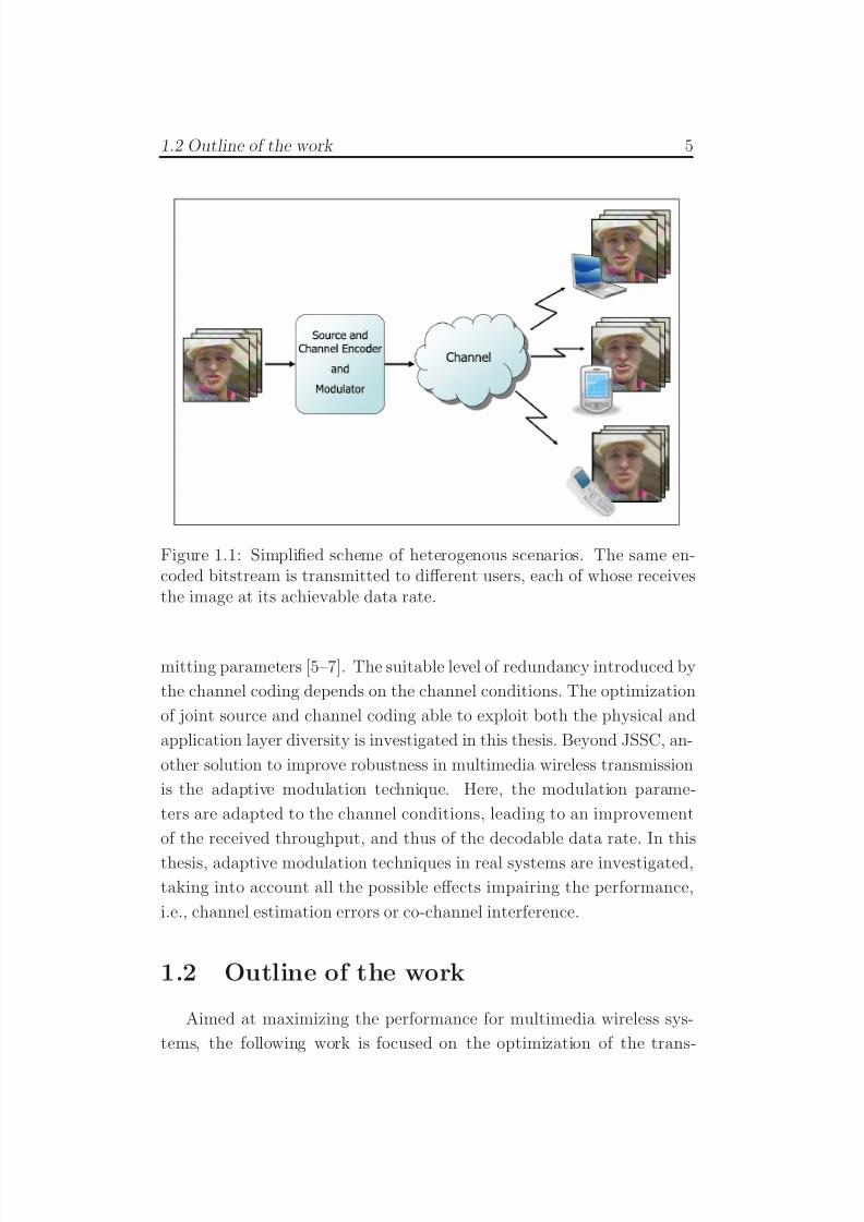
1.1 Simplified scheme of heterogenous scenarios. The sameencoded bitstream is transmitted to different users, each
of whose receives the image at its achievable data rate. . . 5
1.2 Combiner schemes at the receiver. a) A generic scheme, b)
descriptions of a hybrid-selection/maximum ratio combiner. 12
1.3 OFDM implementation scheme at the transmitter and at
the receiver. . . . . . . . . . . . . . . . . . . . . . . . . . 14
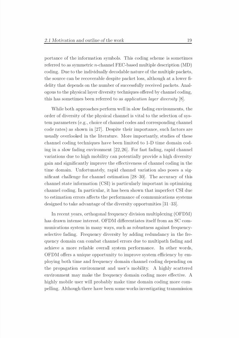
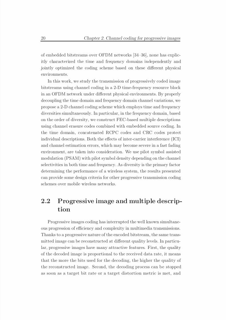
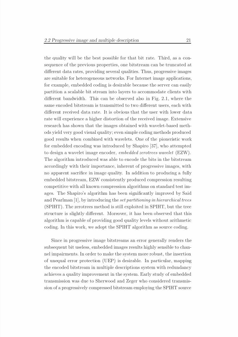
2.1 Scheme of a Lena image transmission to two different users,with different data rates at the receiver, and indeed differ-
ent qualities of the received image. . . . . . . . . . . . . . 22
2.2 Illustration of the FEC-based multiple description coding
technique for an embedded bistream with n = 5 descriptions. 23
2.3 Subcarrier spectrum assignment. . . . . . . . . . . . . . . . 25
2.4 Transmission of the embedded bitstream over OFDM mo-
bile wireless networks. The dark shaded area to the right
of the RCPC coding boundary line represents the bits forCRC and RCPC coding. The lighter shaded area under the
RS coding boundary staircase represents Reed-Solomon
parity symbols. The unshaded area represents informa-
tion symbols. Note that the CRC/RCPC parity symbols
are interleaved with the RS symbols in the actual system.
N t = N × M total subcarriers and LRS Reed-Solomon
symbols are considered. For each (n, k) RS codeword, k
information symbols are encoded into n = N t total symbols. 26
v
7/29/2019 Adaptive Wireless Multimedia
http://slidepdf.com/reader/full/adaptive-wireless-multimedia 10/187
vi Contents
2.5 Pilot insertion scheme for systems with: (a) one correlatedsubcarrier; (b) M correlated subcarriers. . . . . . . . . . . 30
2.6 Profiles showing the optimal allocation of source and chan-
nel symbols for systems with (N, M ) = (4, 32), f nd = 10−3
and SNR = 16.0 dB for different choices of RCPC coding
rates and for both perfect CSI and imperfect CSI. . . . . . 34
2.7 Profiles showing the optimal allocation of source and chan-
nel symbols for systems with Rrcpc = 8/24 and SNR = 16.0
dB and imperfect CSI for systems with frequency diversity
orders N = 1, 4, 32, 128, respectively. . . . . . . . . . . . . 36
2.8 Optimal Rrs vs. Rrcpc for systems with (N, M ) = (4, 32),
f nd = 10−3 SNR = 16.0 and both perfect and imperfect CSI. 37
2.9 Optimized PSNR vs Rrcpc for different Doppler spreads in
systems with (N, M ) = (4, 32), SNR = 16 dB and imper-
fect CSI. . . . . . . . . . . . . . . . . . . . . . . . . . . . . 38
2.10 Optimized PSNR vs. f nd for systems with (N, M ) =
(16, 8), SNR = 16 dB and Rrcpc = 1 for perfect and im-
perfect CSI systems. . . . . . . . . . . . . . . . . . . . . . 40
2.11 Optimized PSNR vs Rrcpc for different coherence band-
widths. . . . . . . . . . . . . . . . . . . . . . . . . . . . . . 41
2.12 Optimized PSRN vs. f nd for systems with (N, M ) =
(16, 8), SNR = 16 dB and different RCPC code rates. . . . 42
2.13 Optimal PSNR performances vs. both N and f nd in sys-
tems with SNR = 16 dB for both perfect CSI systems (a)
and imperfect CSI systems (b). . . . . . . . . . . . . . . . 44
2.14 Optimized PSNR vs. f nd for systems with SNR = 16 dB
and both perfect and imperfect CSI. Two different fre-quency diversity order are considered: (N, M ) = (32, 4)
and (N, M ) = (4, 32). . . . . . . . . . . . . . . . . . . . . . 46
2.15 Image quality for a system with f nd = 10−1, (N,M ) = (32, 4),
SNR = 16 dB, and imperfect CSI. We denote by RTX the
transmitted source rate and by RRX the received source rate. . 51
3.1 Encoder structure of the FGS coding methodology based
on MPEG-4. . . . . . . . . . . . . . . . . . . . . . . . . . . 57
7/29/2019 Adaptive Wireless Multimedia
http://slidepdf.com/reader/full/adaptive-wireless-multimedia 11/187
Contents vii
3.2 Motion-compensated FGS hybrid coder with leaky predic-tion. . . . . . . . . . . . . . . . . . . . . . . . . . . . . . . 59
3.3 Transmission of the embedded bitstream over OFDM mo-
bile wireless networks. (a) FGS embedded bitstream. (b)
Motion-compensated MD coding. The white shaded area
represents the parity symbols (both in time and frequency
domain), the light-grey shaded area represents the EL-
MCP symbols, and the dark-grey shaded area represents
the EL-Extra symbols. Note that the CRC/RCPC sym-
bols are interleaved with RS symbols in real systems. . . . 65
3.4 Rate-Distortion curve evaluation. . . . . . . . . . . . . . . 69
3.5 RD curve evaluation methods. . . . . . . . . . . . . . . . 71
3.6 Rate-Distortion function for the MC-FGS with various
MCP values (β ), without leaky prediction (α = 1), and
with no time coding (Rrcpc = 1). . . . . . . . . . . . . . . . 73
3.7 Comparison of the off-line and on-line method for the
FEC level evaluation. . . . . . . . . . . . . . . . . . . . . 74
3.8 Rate-distortion function and optimal FEC profiles for both
the off-line and the on-line method for systems with f nd =
10−3, Rrcpc = 1, (N, M ) = (2, 64). Note that the frame nr.
10 and nr. 30 are considered in the on-line method. . . . . 76
3.9 Optimal profile of the parity symbols for a system with
f nd = 2.5 × 10⁻⁴, Rrcpc = 8/12, and N variable for the
transmission of sequences encoded with different α and β
parameters. The profile for the 20-th frame is considered. . 77
3.10 Optimal profile of the parity symbols for a system with
f nd = 2 ×10⁻⁴,(N, M ) = (2, 64), and different Rrcpc values
for the transmission of sequences encoded with α = 0.9
and the optimal β parameter. The profile for the 20-th
frame is considered, and the PSNR values are expressed in
dB. . . . . . . . . . . . . . . . . . . . . . . . . . . . . . . . 78
3.11 Optimum β vs. Rrcpc for systems with f nd = 2 × 10⁻⁴,
(N, M ) = (2, 64), and α = 1, 0.9, and 0.7. . . . . . . . . . 80
7/29/2019 Adaptive Wireless Multimedia
http://slidepdf.com/reader/full/adaptive-wireless-multimedia 12/187
viii Contents
3.12 PSNR performance for several orders of diversity availablein the frequency domain in both slow and fast fading systems. 81
3.13 Expected PSNR-Y vs. f nd for systems with (N, M ) =
(4, 32), β = 0.10, and 0.35, α = 1.0. Both optimal Rrcpc
values and constant rates (Rrcpc = 1, and 8/14) are employed. 82
3.14 PSNR-Y vs. number of frame for systems with (N, M ) =
(4, 32), f nd = 10−4, and several β and α values. . . . . . . . 83
4.1 Adaptive modulation technique. Starting from the bit er-
ror probability expression, the SNR thresholds are evalu-ated, and then, the optimal modulation level to be adopted
is chosen. Note that if FAM (SAM) is considered, the
bit error probability, P b, considered is the instantaneous
(mean) BEP, the SNR parameter, χ, is the instantaneous
(mean) SNR, and the observed fluctuations variable with
the time are hte small-scale (large-scale) fading. . . . . . . 89
4.2 Transmitted pilot scheme. . . . . . . . . . . . . . . . . . . 91
4.3 BEO vs. µdB for SAM system with maximum modulationsize 256, N = 4, P ⋆b = 10−2, and σdB = 8. A comparison
between perfect and imperfect CSI is reported. . . . . . . . 102
4.4 BEO vs. N pε for SAM systems with imperfect CSI, max-
imum modulation size 256, N = 2, 4, and 8, P ⋆b = 10−2,
µdB = 35 and σdB = 8. . . . . . . . . . . . . . . . . . . . . 102
4.5 Effective throughput vs. µdB for SAM systems with MRC
(N = 4), maximum constellation size 256, maximum out-
age 5%, P ⋆b = 10−2, and σdB = 8. Results are evaluated for
both perfect and imperfect CSI, considering several chan-
nel estimation quality levels. . . . . . . . . . . . . . . . . . 103
4.6 Comparison between effective throughout in SAM and in
FAM systems with imperfect CSI, maximum modulation
level 256, maximum outage 5%, P ⋆b = 10−2, and σdB = 8. . 104
4.7 BEO vs. µdB for a non adaptive scheme with P ⋆b , σdB = 8,
N = 4 (MRC), different constellation sizes M (M = 4,
M = 64) and both perfect and imperfect CSI systems. . . 105
7/29/2019 Adaptive Wireless Multimedia
http://slidepdf.com/reader/full/adaptive-wireless-multimedia 13/187
Contents ix
4.8 Effective throughput vs. µdB for adaptive and non-adaptivescheme with P ⋆b , σdB = 8, N = 4 (MRC), ε = 1, maximum
modulation M max = 256, and N tot = 180. . . . . . . . . . . 106
4.9 Effective throughput vs. µdB for SAM systems with P ⋆b ,
σdB = 8, H-S/MRC (L/N=2/8) and MRC (L/N=8/8),
ε = 1, maximum modulation M max = 64, and N tot = 180. . 107
4.10 Effective throughput vs. µdB for SAM systems with P ⋆b =
10−2, Nakagami−m channels with m = 0.5 and m = 4,
σdB = 8, MRC (N=8), ε = 1, maximum modulationM max = 64, and N tot = 180. . . . . . . . . . . . . . . . . . 107
4.11 Effective throughput vs. N p for SAM systems with P ⋆b ,
σdB = 8, MRC (N = 8), ε = 1, and maximum modulation
M max = 256. Several median values µdB are considered,
µdB = 25, 30, 40. N tot = 180. . . . . . . . . . . . . . . . . . 109
4.12 Effective throughput vs. N p for SAM systems with P ⋆b =
10−2, σdB = 8, MRC (N=4), maximum modulation M max =
256. Several median values µdB
(µdB
= 25, 30, 40) and ε
values (ε = 0.5, 1, 3) are considered. N tot = 100. . . . . . . 110
4.13 SNR outage penalty and Mean throughput penalty vs. ǫ
for SAM systems with P ⋆b , σdB = 8, MRC (N=4), and
several values of pilot symbols (N p = 1, 2, 4,and 6). In the
throughput penalty plot(b), µdB = 15. . . . . . . . . . . . 111
5.1 Approximated and Exact threshold lines for a system with
N d = 1, N I = 2, and M ranging from 4 to 256. . . . . . . 124
5.2 Outage probability vs. µdB for SAM systems with maxi-
mum modulation size 64, 256, 1024, no diversity at the re-
ceiver, P ⋆b = 10−2, σdB = 8. To evaluate SNR thresholds,
the BEP approximation A3 is adopted. . . . . . . . . . . . 126
5.3 Mean SE vs. µdB for SAM systems with maximum modu-
lation size 64, 256, 1024, MRC with N = 1, 2, 8, maximum
outage 5%, P ⋆b = 10−2, and σdB = 8. The mean SE is
evaluated with both perfect and imperfect BEP expressions.127
7/29/2019 Adaptive Wireless Multimedia
http://slidepdf.com/reader/full/adaptive-wireless-multimedia 14/187
5.4 BEP vs. γ dB for M -QAM systems with modulation sizeM = 16, maximum outage 5%, P ⋆b = 10−2, and σdB = 8.
The bit error probability, conditioned to SIR, is evaluated
for several N and N I values. . . . . . . . . . . . . . . . . 128
5.5 ∆ j,dB vs. γ I,dB for SAM systems with M max = 256, maxi-
mum outage 5%, P ⋆b = 10−2, σdB = 8, and several N and
N I values. The analysis is conditioned to the SIR value. . . 129
5.6 Mean throughput (conditioned to SIR) vs. µdB for SAM
systems with M max = 256, maximum outage 5%, P ⋆b =
10−2, σdB = 8, N I = 6, and number of antennas equals to2 and 4. . . . . . . . . . . . . . . . . . . . . . . . . . . . . 130
5.7 BEP vs. γ dB for M -QAM systems with M = 4, N = 1,
N I = 4. . . . . . . . . . . . . . . . . . . . . . . . . . . . . 131
5.8 SNR thresholds vs. INR thresholds for SAM systems with
M max = 256, N = 1, N I = 2. . . . . . . . . . . . . . . . . 132
5.9 Mean throughput vs. µdB SAM systems with M max = 64,
N = 1, and N I = 2. . . . . . . . . . . . . . . . . . . . . . 133
A.1 Simulation and analytic results for the packet success ratefor an uncoded system with different f nd with SNR(Rth)
= 9 dB. . . . . . . . . . . . . . . . . . . . . . . . . . . . . 139
C.1 Exact and approximated BEP vs. instantaneous SNR for
a 4-QAM and 1024-QAM system. . . . . . . . . . . . . . . 147
C.2 Exact and approximated BEP vs. averaged SNR for 1024-
QAM system. . . . . . . . . . . . . . . . . . . . . . . . . . 148
7/29/2019 Adaptive Wireless Multimedia
http://slidepdf.com/reader/full/adaptive-wireless-multimedia 15/187
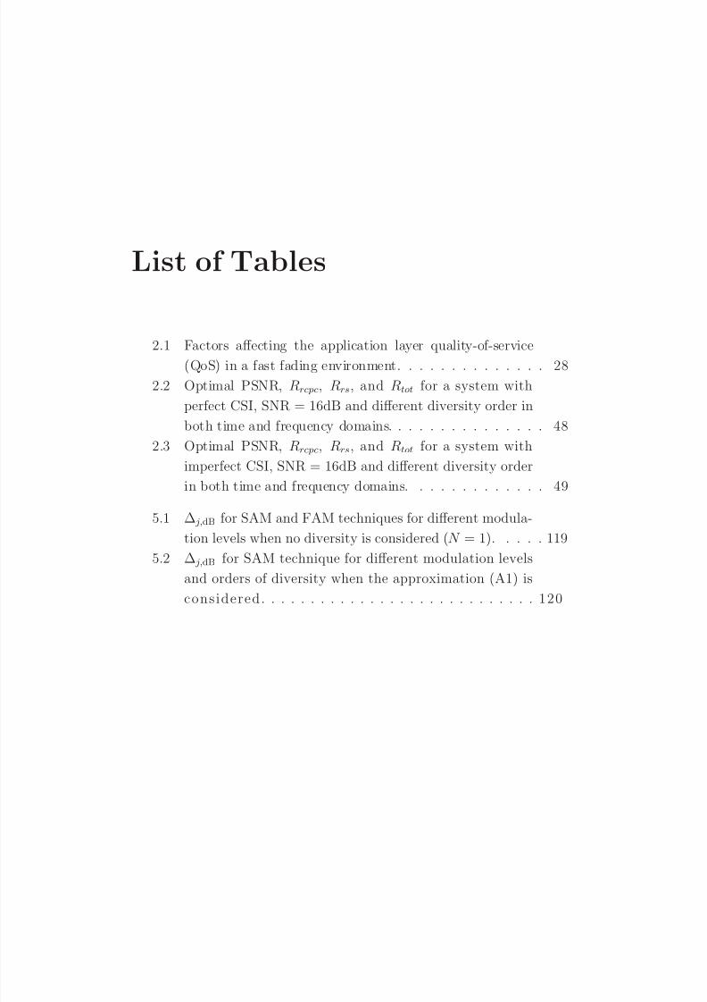
List of Tables
2.1 Factors affecting the application layer quality-of-service(QoS) in a fast fading environment. . . . . . . . . . . . . . 28
2.2 Optimal PSNR, Rrcpc, Rrs, and Rtot for a system with
perfect CSI, SNR = 16dB and different diversity order in
both time and frequency domains. . . . . . . . . . . . . . . 48
2.3 Optimal PSNR, Rrcpc, Rrs, and Rtot for a system with
imperfect CSI, SNR = 16dB and different diversity order
in both time and frequency domains. . . . . . . . . . . . . 49
5.1 ∆ j,dB
for SAM and FAM techniques for different modula-
tion levels when no diversity is considered (N = 1). . . . . 119
5.2 ∆ j,dB for SAM technique for different modulation levels
and orders of diversity when the approximation (A1) is
consi dered. . . . . . . . . . . . . . . . . . . . . . . . . . . . 120

7/29/2019 Adaptive Wireless Multimedia
http://slidepdf.com/reader/full/adaptive-wireless-multimedia 16/187

7/29/2019 Adaptive Wireless Multimedia
http://slidepdf.com/reader/full/adaptive-wireless-multimedia 17/187
Abbreviations
QoS Quality of Service
OFDM Orthogonal Frequency Division Multiplexing
SIMO Single Input Multiple Output
MIMO Multiple Input Multiple Output
PDF Probability Density Function
CDF Cumulative Density Function
MGF Moment-Generating Function
FEC Forward Error Correction
MDS Maximum Distance Separable
RS Reed-Solomon
RCPC Rate-Compatible Punctured Convolutional
CRC Cyclic Redundancy CheckRB Resource Block
AWGN Additive White Gaussian Noise
SNR Signal-to-Noise Ratio
SINR Signal-to-Interference-plus-Noise Ratio
INR Interference-to-Noise Ratio
FFT Fast Fourier Transform
IFFT Inverse Fast Fourier Transform
MMSE Minimum Mean Square Error
MRC Maximum Ratio Combining
H-S/MRC Hybrid- Selection/Maximum Ratio CombiningECG Equal-Gain Combining
SC Selection Combining
OC Optimum Combining
AGC Automatic Gain Control
PSAM Pilot Symbol Assisted Modulation
CSI Channel State Information
ICI Inter-Carrier Interference
ISI Inter-Symbol Interference

7/29/2019 Adaptive Wireless Multimedia
http://slidepdf.com/reader/full/adaptive-wireless-multimedia 18/187
xiv Contents
SPIHT Set Partitioning In Hierarchical TreesEZW Embedded Zerotrees Wavelet
MD Multiple Description
PET Priority Encoding Transmission
UEP Unequal Error Protection
EEP Equal Error Protection
JSSC/D Joint Source and Channel Coding/Decoding
MPEG Moving Pictures Experts Group
BL Base Layer
EL Enhanced Layer
FGS Fine Granularity Scalable
MCP Motion-Compensated Prediction
VLC Variable Length Coding
BSC Binary Symmetric Channel
DCT Discrete Cosine Transform
RD Rate-Distortion
SAM Slow Adaptive Modulation
FAM Fast Adaptive Modulation
SE Spectral Efficiency
SSD Subset Diversity
BEP Bit Error Probability
BEO Bit Error OutageQAM Quadrature Amplitude Modulation
7/29/2019 Adaptive Wireless Multimedia
http://slidepdf.com/reader/full/adaptive-wireless-multimedia 19/187
Abstract
In recent years, due to the rapid convergence of multimedia services,
Internet and wireless communications, there has been a growing trend of
heterogeneity (in terms of channel bandwidths, mobility levels of termi-
nals, end-user quality-of-service (QoS) requirements) for emerging inte-
grated wired/wireless networks. Moreover, in nowadays systems, a mul-
titude of users coexists within the same network, each of them with hisown QoS requirement and bandwidth availability. In this framework,
embedded source coding allowing partial decoding at various resolution
is an appealing technique for multimedia transmissions. This disserta-
tion includes my PhD research, mainly devoted to the study of embedded
multimedia bitstreams in heterogenous networks, developed at the Uni-
versity of Bologna, advised by Prof. O. Andrisano and Prof. A. Conti,
and at the University of California, San Diego (UCSD), where I spent
eighteen months as a visiting scholar, advised by Prof. L. B. Milstein
and Prof. P. C. Cosman. In order to improve the multimedia trans-
mission quality over wireless channels, joint source and channel coding
optimization is investigated in a 2D time-frequency resource block for an
OFDM system. We show that knowing the order of diversity in time
and/or frequency domain can assist image (video) coding in selecting
optimal channel code rates (source and channel code rates). Then, adap-
tive modulation techniques, aimed at maximizing the spectral efficiency,
are investigated as another possible solution for improving multimedia
transmissions. For both slow and fast adaptive modulations, the effectsof imperfect channel estimation errors are evaluated, showing that the
fast technique, optimal in ideal systems, might be outperformed by the
slow adaptive modulation, when a real test case is considered. Finally,
the effects of co-channel interference and approximated bit error proba-
bility (BEP) are evaluated in adaptive modulation techniques, providing
new decision regions concepts, and showing how the widely used BEP
approximations lead to a substantial loss in the overall performance.

7/29/2019 Adaptive Wireless Multimedia
http://slidepdf.com/reader/full/adaptive-wireless-multimedia 20/187
7/29/2019 Adaptive Wireless Multimedia
http://slidepdf.com/reader/full/adaptive-wireless-multimedia 21/187
Chapter 1
Wireless multimedia
transmission overview
Only those who dare may fly.
- Luis Sep´ ulveda
The high demand of high quality multimedia applications has pro-
moted a significant development in multimedia transmissions at high data
rate. In this framework, great interest is reposed in cross-layer optimiza-
tion for joint source and channel coding/decoding (JSCC/D) as well as
in adaptive modulation algorithms, aimed at optimizing the transmitting
parameters taking into account both the physical and the application
layer conditions. Moreover, in multiuser networks, where requirements
from different users must be met at the same time, a multi-rate (i.e.,
multi-quality) transmission is needed. With this aim, an enormous sim-
plification in the transmission overhead is represented by the progressive
image and video bitstreams. The combination of source and channelcoding and modulation parameters optimization in systems transmitting
progressive multimedia bitstreams is therefore an appealing technique,
able to provide a system that is robust enough to the channel impair-
ments, still satisfying the multiusers constraints. In the following thesis,
several optimized multimedia wireless transmissions will be discussed.
In the introductory chapter, we provide an outline of the thesis mainly
focusing on the contributions of this work as compared to existing liter-
ature. Next, we provide a basic overview of the system model adopted
3
7/29/2019 Adaptive Wireless Multimedia
http://slidepdf.com/reader/full/adaptive-wireless-multimedia 22/187
4 Chapter 1. Introduction
in the thesis.
1.1 Introduction
In recent years, due to the rapid convergence of multimedia services,
Internet and wireless communications, there has been a growing trend of
heterogeneity (in terms of channel bandwidths, mobility levels of termi-
nals, end-user quality-of-service (QoS) requirements) for emerging inte-
grated wired/wireless networks. In multi-services multi-users networks,different users need different QoS requirements due to the multitude of
applications and scenario coexisting within the modern networks. The
quality required for a real-time video played on a PAD, for example, is
lower than the one reproduced on a laptop. The heterogeneity comes not
only from different data rates and QoS requirements, but also from dif-
ferent scenarios, as the PAD might be for example connect to a wireless
networks with an high level of mobility, and the latpot to a wired connec-
tion. Embedded source coding [1], allowing partial decoding at various
resolution and quality levels from a single compressed bitstream, is a
promising technology for multimedia communications in heterogeneous
environments. Thanks to the progressive image features, in a multi-user
networks, each user is able to decode the same transmitted bitstream
at the desired data rate. A typical case can be the one represented in
Fig. 1.1, where only one transmitter can provide embedded progressive
bitstream to a multitude of users. Although a single progressive bit-
stream can be decoded at different data rates, providing a multitude of
decoded quality levels, an error in the bitstream would make the subse-quent bit useless. Thus, a single error can cause an unrecoverable loss in
synchronization between encoder and decoder, and produce substantial
quality degradation. It follows that embedded source coders are usually
extremely sensitive to channel impairments which can be severe in mo-
bile wireless links due to multipath signal propagation, delay and Doppler
spreads, and other effects. In order to cope with the channel, it is there-
fore clear the importance of making the signal as reliable as possible,
introducing redundancy in the bitstream [2–4], or optimizing the trans-
7/29/2019 Adaptive Wireless Multimedia
http://slidepdf.com/reader/full/adaptive-wireless-multimedia 23/187
1.2 Outline of the work 5
Figure 1.1: Simplified scheme of heterogenous scenarios. The same en-coded bitstream is transmitted to different users, each of whose receivesthe image at its achievable data rate.
mitting parameters [5–7]. The suitable level of redundancy introduced by
the channel coding depends on the channel conditions. The optimization
of joint source and channel coding able to exploit both the physical and
application layer diversity is investigated in this thesis. Beyond JSSC, an-
other solution to improve robustness in multimedia wireless transmission
is the adaptive modulation technique. Here, the modulation parame-
ters are adapted to the channel conditions, leading to an improvement
of the received throughput, and thus of the decodable data rate. In this
thesis, adaptive modulation techniques in real systems are investigated,
taking into account all the possible effects impairing the performance,
i.e., channel estimation errors or co-channel interference.
1.2 Outline of the work
Aimed at maximizing the performance for multimedia wireless sys-
tems, the following work is focused on the optimization of the trans-
7/29/2019 Adaptive Wireless Multimedia
http://slidepdf.com/reader/full/adaptive-wireless-multimedia 24/187
6 Chapter 1. Introduction
mission parameters (at physical level), such as code rates or modulationlevels. First, the design of channel coding is investigated in image trans-
missions applications. In addiction to the physical layer gain, an applica-
tion layer diversity [8] can be exploited by adopting a multiple description
encoding. Thus a symmetric n-channel forward error correction (FEC)-
based multiple description is investigated, with the FEC level based on
channel conditions. Then, this study has been extended to video trans-
missions. Due to the high complexity of a video bitstream, the channel
coding is optimized in conjunction with the source coding parameters.
It follows that the JSSC design is investigated, aimed at evaluating theoptimal channel code rate together with the suitable compression rate to
be employed for the transmission over a given wireless channel.
Since, in embedded bitstreams, the quality of the decoded image is
proportional to the data-rate to be decoded, adaptive modulation tech-
niques, aimed at maximizing the received throughput, can also be em-
ployed. In perfect systems, adaptive modulation techniques allow a sub-
stantial improvement on the averaged received throughput, without com-
promising the outage probability [5, 6]. In this thesis, adaptive modula-tion techniques are investigated for real systems, i.e., systems experienc-
ing imperfect channel estimations or the presence of interference or other
issues that might compromise the bit error probability performance. The
remainder of the Thesis is organized as follows.
In Chapter 2, channel coding in both time and frequency domain is
optimized for progressive images transmission. The topic is investigated
for OFDM systems and several Doppler values of the channels. It has
been demonstrated that the optimization of the FEC protection in both
the domains provides a system that results to be robust to channel im-
pairments, for channels with both fast and slow variations.
In Chapter 3, the embedded video transmission is investigated. A
JSSC is considered, and the channel coding is optimized in conjunction
with the source coding in OFDM systems experiencing several orders
of diversity in both time and frequency domain. Important results are
reported for the rate distortion curve evaluation. The method we pro-
pose achieves worthy quality transmissions, optimizing the transmitting
7/29/2019 Adaptive Wireless Multimedia
http://slidepdf.com/reader/full/adaptive-wireless-multimedia 25/187
1.3 System modeling 7
scheme, and satisfying the imposed temporal constraints.Chapter 4 investigates adaptive modulation techniques in systems
with imperfect channel estimation. Both the cases of imperfect channel
estimation at the transmitter and at the receiver are considered, for both
slow and fast adaptive modulation techniques. Pilot symbols insertion is
considered for the channel estimation, and the design of the optimal pilot
scheme is optimized, based on the tradeoff estimation quality-throughput
reduction . The results show that the fast technique, optimal in ideal sys-
tems, might be outperformed by the slow adaptive modulation technique.
In Chapter 5, adaptive modulation techniques are investigated formore general systems, experiencing a shift in the SNR thresholds. Some
applicative examples are considered, as systems experiencing co-channel
interference and/or the employment of the bit error probability approxi-
mated expression. Depending on the channel configurations, the median
SNR values that achieve satisfactory performance can be evaluated in all
the applicative examples. Moreover, we highlight the lost of performance
in terms of mean throughput that the system experiences when the widely
used exponential bit error probability approximation is employed.
In Chapter 6, concluding remarks and future directions are reported.
1.3 System modeling
In this section, the system model has been described in details. In par-
ticular, starting from basic concepts on wireless channels, the assumption
employed in the analysis of the thesis are described. The characterization
of the wireless channels, the descriptions of SIMO and OFDM systems
are here presented.
1.3.1 Wireless channel modeling
It is well known that the additive white gaussian noise is not the only
issue affecting the performance in wireless systems [9–12]. Because of
reflection, diffusion and refraction of signals through scattering objects,
a short impulse transmitted over the channel is received as a sum of mul-
tiple impulses, each of whose with its own amplitude and delay. These
7/29/2019 Adaptive Wireless Multimedia
http://slidepdf.com/reader/full/adaptive-wireless-multimedia 26/187
8 Chapter 1. Introduction
amplitude and phase fluctuations, varying with the time, are named fad-ing, and they can be modeled statistically, as described in the following.
Moreover, for long distance communications, the signal suffer of a power
reduction due to the path loss.
The equivalent low-pass response of the channel at time t to an im-
pulse at time t − τ can be represented as
h(t, τ ) =
N (t)
n=1
αn(t)e j2πf 0τ n(t)δ (τ − τ n(t)),
where we denote by αn(t) the possibly time-variant attenuation factor
of the N (t) multipath propagation and by τ n(t) the corresponding time
delays. For stationary channels, the channel response results in a function
of only τ . Knowing the correlation function in the time and frequency
domain, the channel can be characterized as follows.
Frequency-flat or frequency-selective channel . The coherence band-
width ∆f c, defined as the frequency range in which the fading process
results correlated, can be expressed as ∆f c = 1/τ max, where τ max is the
maximum delay spread. When the system bandwidth is smaller thanthe coherence bandwidth (for example, narrow band systems), the chan-
nel is defined a flat-frequency channel, and the frequency components
are affected in similar manner. Conversely, when the system bandwidth
exceeds ∆f c (for example, wide band systems), the channel is frequency-
selective.
Slow or fast fading channel . Defining the coherence time T c as the
period over which the fading process is correlated, it can be related to
the maximum Doppler spread, f D, as T c≃
1/f D.
In general, the multipath fading, characterizing the short-term signal
fluctuation, is usually too complex for an exact physical analysis, thus, it
is considered statistically distributed. Assuming the fading h zero-mean
complex Gaussian distributed, its phase is uniform distributed between
0 and 2π, and the envelope is Rayleigh distributed. It follows that the
channel power has the following probability density function (PDF)
f |h|2(x) =1
Ωexp
− x
Ωx ≥ 0, (1.1)
7/29/2019 Adaptive Wireless Multimedia
http://slidepdf.com/reader/full/adaptive-wireless-multimedia 27/187
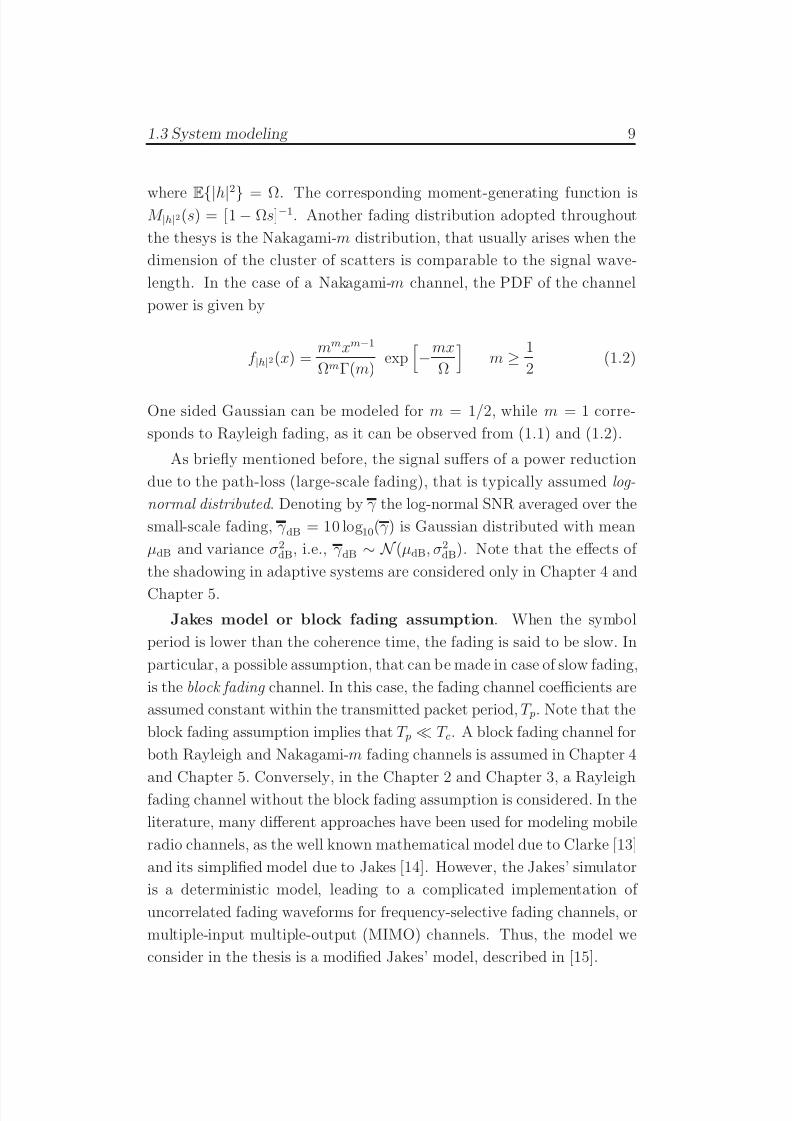
1.3 System modeling 9
where E|h|2
= Ω. The corresponding moment-generating function isM |h|2(s) = [1 − Ωs]−1. Another fading distribution adopted throughout
the thesys is the Nakagami-m distribution, that usually arises when the
dimension of the cluster of scatters is comparable to the signal wave-
length. In the case of a Nakagami-m channel, the PDF of the channel
power is given by
f |h|2(x) =mmxm−1
ΩmΓ(m)exp
−mx
Ω
m ≥ 1
2(1.2)
One sided Gaussian can be modeled for m = 1/2, while m = 1 corre-
sponds to Rayleigh fading, as it can be observed from (1.1) and (1.2).
As briefly mentioned before, the signal suffers of a power reduction
due to the path-loss (large-scale fading), that is typically assumed log-
normal distributed . Denoting by γ the log-normal SNR averaged over the
small-scale fading, γ dB = 10 log10(γ ) is Gaussian distributed with mean
µdB and variance σ2dB, i.e., γ dB ∼ N (µdB, σ2
dB). Note that the effects of
the shadowing in adaptive systems are considered only in Chapter 4 and
Chapter 5.
Jakes model or block fading assumption. When the symbol
period is lower than the coherence time, the fading is said to be slow. In
particular, a possible assumption, that can be made in case of slow fading,
is the block fading channel. In this case, the fading channel coefficients are
assumed constant within the transmitted packet period, T p. Note that the
block fading assumption implies that T p ≪ T c. A block fading channel for
both Rayleigh and Nakagami-m fading channels is assumed in Chapter 4
and Chapter 5. Conversely, in the Chapter 2 and Chapter 3, a Rayleighfading channel without the block fading assumption is considered. In the
literature, many different approaches have been used for modeling mobile
radio channels, as the well known mathematical model due to Clarke [13]
and its simplified model due to Jakes [14]. However, the Jakes’ simulator
is a deterministic model, leading to a complicated implementation of
uncorrelated fading waveforms for frequency-selective fading channels, or
multiple-input multiple-output (MIMO) channels. Thus, the model we
consider in the thesis is a modified Jakes’ model, described in [15].
7/29/2019 Adaptive Wireless Multimedia
http://slidepdf.com/reader/full/adaptive-wireless-multimedia 28/187
10 Chapter 1. Introduction
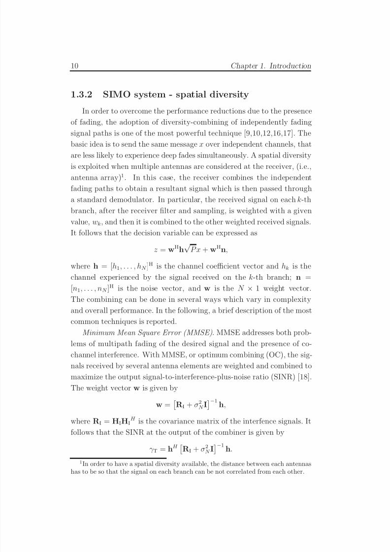
1.3.2 SIMO system - spatial diversityIn order to overcome the performance reductions due to the presence
of fading, the adoption of diversity-combining of independently fading
signal paths is one of the most powerful technique [9,10,12,16,17]. The
basic idea is to send the same message x over independent channels, that
are less likely to experience deep fades simultaneously. A spatial diversity
is exploited when multiple antennas are considered at the receiver, (i.e.,
antenna array)1. In this case, the receiver combines the independent
fading paths to obtain a resultant signal which is then passed through
a standard demodulator. In particular, the received signal on each k-th
branch, after the receiver filter and sampling, is weighted with a given
value, wk, and then it is combined to the other weighted received signals.
It follows that the decision variable can be expressed as
z = wHh√
P x + wHn,
where h = [h1, . . . , hN ]H is the channel coefficient vector and hk is the
channel experienced by the signal received on the k-th branch; n =
[n1, . . . , nN ]H
is the noise vector, and w is the N × 1 weight vector.The combining can be done in several ways which vary in complexity
and overall performance. In the following, a brief description of the most
common techniques is reported.
Minimum Mean Square Error (MMSE). MMSE addresses both prob-
lems of multipath fading of the desired signal and the presence of co-
channel interference. With MMSE, or optimum combining (OC), the sig-
nals received by several antenna elements are weighted and combined to
maximize the output signal-to-interference-plus-noise ratio (SINR) [18].
The weight vector w is given by
w =
RI + σ2N I−1
h,
where RI = HIHIH is the covariance matrix of the interfence signals. It
follows that the SINR at the output of the combiner is given by
γ T = hH
RI + σ2N I−1
h.
1In order to have a spatial diversity available, the distance between each antennashas to be so that the signal on each branch can be not correlated from each other.
7/29/2019 Adaptive Wireless Multimedia
http://slidepdf.com/reader/full/adaptive-wireless-multimedia 29/187
1.3 System modeling 11
Maximum Ratio Combining (MRC). MRC is the optimum linear com-bining technique for coherent reception with independent fading at each
antenna element in the presence of spatially white Gaussian noise. The
complex weight at each element compensates for the phase shift in the
channel and is proportional to the signal strength. The weight vector w
is given by
w =h
||h|| ,
At the cost of the knowledge of channel coefficients, the MRC allows to
maximize the instantaneous SNR at the combiner output, given by
γ T =N i=1
γ i.
It is well known that γ T is a chi-square distributed with 2N degrees
of freedom [9, 10] and its MGF can be easily derived. In particular,
assuming the channel coefficients independent from each other, the MGF
of γ T can be derived as the product of the MGF of the single SNR on
each branch, γ i. Thus, M γ T( jν ) = (1 + jν γ )−N . MRC mitigates fading,
however, it ignores co-channel interference.
Equal-Gain Combining (EGC). To overcome the high complexity of
the MRC, the equal-gain combining technique can be adopted, which is
essentially a maximal-ratio combiner with all of the weight wi = 1. In
practice, EGC is often limited to coherent modulations with equal energy
symbols (M-ary PSK signals). Indeed, for signals with unequal energy
symbols such as M-QAM, estimation of the path amplitudes is needed
anyway for automatic gain control (AGC) purposes, and thus for these
modulations MRC should be used to achieve better performance.Selection Combining (SC). In contradiction with the previous combin-
ers, the SC do not combine all the branches and it does not require the
channel knowledge. In particular, in SC techniques, the branch signal
with the largest amplitude (or signal-to-noise ratio) is selected for de-
modulation. Therefore, the SC scheme can be used in conjunction with
differentially coherent and noncoherent modulation techniques since it
does not require knowledge of the signal phases on each branch as would
be needed to implement MRC or EGC in a coherent system. Clearly, SC
7/29/2019 Adaptive Wireless Multimedia
http://slidepdf.com/reader/full/adaptive-wireless-multimedia 30/187
12 Chapter 1. Introduction
Branches
γ T
.
.
.
wNCombiner
γ Tw2
w1
.
.
.
1
N
.
.
.
1
2
.
.
.
L+1
N−1
N
MRC
H−S/MRC
L
Discarded
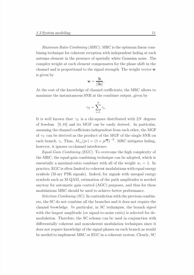
Figure 1.2: Combiner schemes at the receiver. a) A generic scheme, b)descriptions of a hybrid-selection/maximum ratio combiner.
and MRC (or EGC) represent the two extremes in diversity combining
strategy with respect to the number of signals used for demodulation.
Hybrid-Selection/ Maximum Ratio Combining (H-S/MRC). This hy-
brid combining technique processes a subset of the available diversitybranches, reducing the system complexity, but achieving better perfor-
mance than SC. The H-S/MRC selects the L branches (over N ) with
the largest SNR at each instant, and then combines these branches to
maximize the instantaneous output. It means, that the L most powerful
branches are processed by a MRC, as it can be observed from Fig. 1.2.
Here, the model scheme of a hybrid-selection/maximum ratio combiner ,
together with the scheme of a general combiner receiver, is reported. The
main issue in the H-S/MRC, from an analytical point of view, is that af-
ter the reordering, the branches are not independent from each other. Anenormous simplification can be derived by adopting the virtual branches
technique, introduced in [19]. In particular, the instantaneous SNR of
the ordered diversity branches, γ [N ], are transformed into a new set of
virtual branch instantaneous SNRs, V ns, by using the following relation
γ [N ] = T VBV N ,
where T VB is an upper triangular virtual branch transformation matrix,
7/29/2019 Adaptive Wireless Multimedia
http://slidepdf.com/reader/full/adaptive-wireless-multimedia 31/187
1.3 System modeling 13
defined in [19]. The gain in adopting this transformation matrix is thatthe virtual branches SNRs are independent and identically-distributed
random variables, with characteristic function given by ψV n( jν ) = (1 − jν )−1.
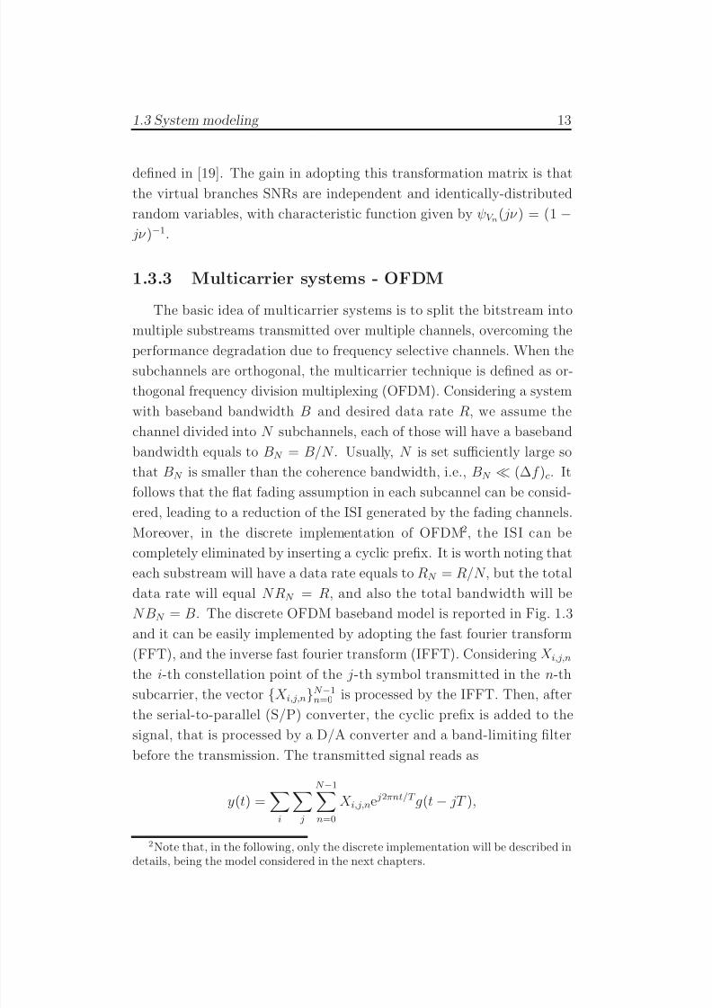
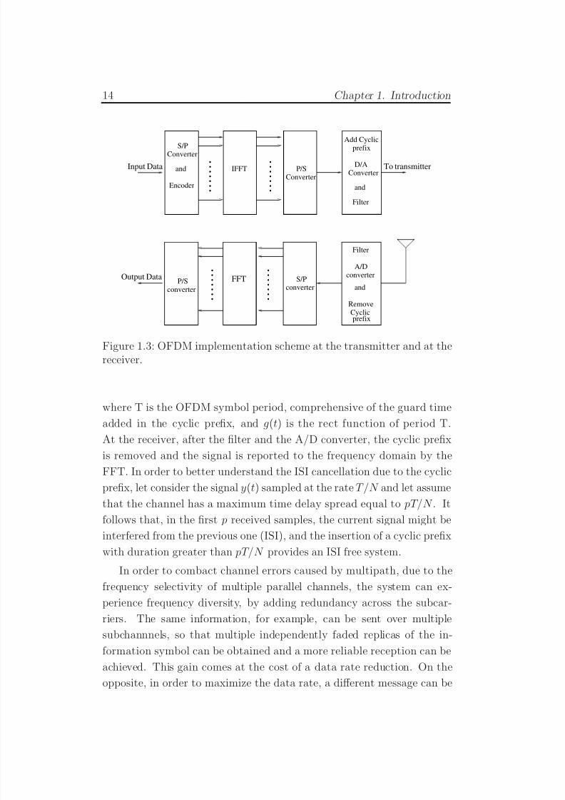
1.3.3 Multicarrier systems - OFDM
The basic idea of multicarrier systems is to split the bitstream into
multiple substreams transmitted over multiple channels, overcoming the
performance degradation due to frequency selective channels. When thesubchannels are orthogonal, the multicarrier technique is defined as or-
thogonal frequency division multiplexing (OFDM). Considering a system
with baseband bandwidth B and desired data rate R, we assume the
channel divided into N subchannels, each of those will have a baseband
bandwidth equals to BN = B/N . Usually, N is set sufficiently large so
that BN is smaller than the coherence bandwidth, i.e., BN ≪ (∆f )c. It
follows that the flat fading assumption in each subcannel can be consid-
ered, leading to a reduction of the ISI generated by the fading channels.
Moreover, in the discrete implementation of OFDM2, the ISI can becompletely eliminated by inserting a cyclic prefix. It is worth noting that
each substream will have a data rate equals to RN = R/N , but the total
data rate will equal N RN = R, and also the total bandwidth will be
N BN = B. The discrete OFDM baseband model is reported in Fig. 1.3
and it can be easily implemented by adopting the fast fourier transform
(FFT), and the inverse fast fourier transform (IFFT). Considering X i,j,n
the i-th constellation point of the j-th symbol transmitted in the n-th
subcarrier, the vector
X i,j,n
N −1n=0 is processed by the IFFT. Then, after
the serial-to-parallel (S/P) converter, the cyclic prefix is added to the
signal, that is processed by a D/A converter and a band-limiting filter
before the transmission. The transmitted signal reads as
y(t) =i
j
N −1n=0
X i,j,ne j2πnt/T g(t − jT ),
2Note that, in the following, only the discrete implementation will be described indetails, being the model considered in the next chapters.
7/29/2019 Adaptive Wireless Multimedia
http://slidepdf.com/reader/full/adaptive-wireless-multimedia 32/187
14 Chapter 1. Introduction
Output Data FFT
To transmitterInput Data
S/PConverter
and
Encoder
IFFT P/SConverter
Add Cyclicprefix
D/AConverter
and
Filter
Filter
A/Dconverter
and
RemoveCyclicprefix
S/Pconverterconverter
P/S
.
.
.
.
.
.
.
.
.
.
.
.
.
.
.
.
.
.
.
.
.
.
.
.
.
.
.
.
Figure 1.3: OFDM implementation scheme at the transmitter and at thereceiver.
where T is the OFDM symbol period, comprehensive of the guard time
added in the cyclic prefix, and g(t) is the rect function of period T.At the receiver, after the filter and the A/D converter, the cyclic prefix
is removed and the signal is reported to the frequency domain by the
FFT. In order to better understand the ISI cancellation due to the cyclic
prefix, let consider the signal y(t) sampled at the rate T /N and let assume
that the channel has a maximum time delay spread equal to pT/N . It
follows that, in the first p received samples, the current signal might be
interfered from the previous one (ISI), and the insertion of a cyclic prefix
with duration greater than pT/N provides an ISI free system.
In order to combact channel errors caused by multipath, due to the
frequency selectivity of multiple parallel channels, the system can ex-
perience frequency diversity, by adding redundancy across the subcar-
riers. The same information, for example, can be sent over multiple
subchannnels, so that multiple independently faded replicas of the in-
formation symbol can be obtained and a more reliable reception can be
achieved. This gain comes at the cost of a data rate reduction. On the
opposite, in order to maximize the data rate, a different message can be

7/29/2019 Adaptive Wireless Multimedia
http://slidepdf.com/reader/full/adaptive-wireless-multimedia 33/187
1.3 System modeling 15
sent over each subchannels, leading to an higher transmitted data rate,but a lower reliability of the information. It is worth noting, therefore,
the tradeoff between diversity gain and information rate in OFDM sys-
tems experiencing frequency selectivity. It will be observed in the next
chapters, for example, that an important parameter in this tradeoff is
the channel coherence bandwidth. In particular, the diversity gain can
be roughly evaluated as (∆f )c/N , and the optimal tradeoff can be found
depending on the diversity naturally offered by the channels.

7/29/2019 Adaptive Wireless Multimedia
http://slidepdf.com/reader/full/adaptive-wireless-multimedia 34/187
7/29/2019 Adaptive Wireless Multimedia
http://slidepdf.com/reader/full/adaptive-wireless-multimedia 35/187
Chapter 2
Channel coding for
progressive images
In this chapter, the optimization of channel encoder for image trans-
missions is addressed. The transmission of progressive image bitstreams
using channel coding in a 2-D time-frequency resource block in an OFDM
network, employing time and frequency diversities simultaneously is in-
vestigated. The physical channel conditions arising from various different
coherence bandwidths and coherence times, leading to various orders of
diversities available in the time and frequency domains, are considered
in the optimization. We investigate the effects of different error patterns
on the delivered image quality due to various fade rates. We also study
the tradeoffs and compare the relative effectiveness associated with the
use of erasure codes in the frequency domain and convolutional codes in
the time domain under different physical environments.
The remainder of this chapter is organized as follows: In Section 2.1
a description of progressive images, together with a brief overview of themultiple description coding are provided. In Section 2.2, progressive im-
age transmissions are deeply explained and further details on MD coding
is reported. In Section 2.3, we give a description of the OFDM system and
the channel model. We also describe the proposed transmission system
and discuss some of the issues associated with the use of channel coding
in a time-frequency block. In Section 2.5, we describe the optimization
problem. In Section 2.6, we provide simulation results and discussion.
Finally, in Section 2.7, we provide a summary and conclusion.
17
7/29/2019 Adaptive Wireless Multimedia
http://slidepdf.com/reader/full/adaptive-wireless-multimedia 36/187
18 Chapter 2. Channel coding for progressive images
2.1 Motivation and outline of the work
In recent years, with the rapid convergence of multimedia, Inter-
net and wireless communications, there is a growing trend of hetero-
geneity (in terms of channel bandwidths, mobility levels of terminals,
enduser quality-of-service (QoS) requirements) for emerging integrated
wired/wireless networks. Embedded source coding, allowing partial de-
coding at various resolution and quality levels from a single compressed
bitstream, is a promising technology for multimedia communications
in heterogeneous environments. Early study of embedded transmissionincludes [20, 21]. Both papers studied the transmission of a progres-
sively compressed bitstream employing the Set Partitioning in Hierar-
chical Trees (SPIHT) source coder combined with rate-compatible punc-
tured convolutional (RCPC) codes. Coding and diversity are very ef-
fective techniques for improving the transmission reliability in a mobile
wireless environment. However, time diversity achieved by channel cod-
ing plus intra-packet interleaving in a single carrier communication sys-
tem becomes less effective in a slow fading environment where correlated
and prolonged deep fades often result in the erasure of the whole packet
or even several contiguous packets. Hence, although improvement could
still be achieved due to the coding gain associated with the use of RCPC
codes, the performance was not satisfactory [21].
To improve the performance against deep fades in a wireless environ-
ment, two approaches have been proposed to exploit diversity in the time
domain at the physical layer for SC communication systems. One was
to add systematic Reed-Solomon (RS) codes across multiple packets [22].
Specifically, channel codes consisted of a concatenation of RCPC and
CRC codes as the row codes and RS codes as the column codes. With
the addition of RS codes across multiple packets, lost packets might still
be recoverable due to independently faded time slots [22].
Another approach [23–26] uses contiguous information symbols from
the progressive bitstreams, which, instead of being packed in the same
packets [20, 22], are spread across multiple packets (descriptions). The
information symbols are protected against channel errors using system-
atic RS codes with the level of protection depending on the relative im-
7/29/2019 Adaptive Wireless Multimedia
http://slidepdf.com/reader/full/adaptive-wireless-multimedia 37/187
2.1 Motivation and outline of the work 19
portance of the information symbols. This coding scheme is sometimesreferred to as symmetric n-channel FEC-based multiple description (MD)
coding. Due to the individually decodable nature of the multiple packets,
the source can be recoverable despite packet loss, although at a lower fi-
delity that depends on the number of successfully received packets. Anal-
ogous to the physical layer diversity techniques offered by channel coding,
this has sometimes been referred to as application layer diversity [8].
While both approaches perform well in slow fading environments, the
order of diversity of the physical channel is vital to the selection of sys-
tem parameters (e.g., choice of channel codes and corresponding channel
code rates) as shown in [27]. Despite their importance, such factors are
usually overlooked in the literature. More importantly, studies of these
channel coding techniques have been limited to 1-D time domain cod-
ing in a slow fading environment [22, 26]. For fast fading, rapid channel
variations due to high mobility can potentially provide a high diversity
gain and significantly improve the effectiveness of channel coding in the
time domain. Unfortunately, rapid channel variation also poses a sig-
nificant challenge for channel estimation [28–30]. The accuracy of thischannel state information (CSI) is particularly important in optimizing
channel coding. In particular, it has been shown that imperfect CSI due
to estimation errors affects the performance of communications systems
designed to take advantage of the diversity opportunities [31–33].
In recent years, orthogonal frequency division multiplexing (OFDM)
has drawn intense interest. OFDM differentiates itself from an SC com-
munications system in many ways, such as robustness against frequency-
selective fading. Frequency diversity by adding redundancy in the fre-quency domain can combat channel errors due to multipath fading and
achieve a more reliable overall system performance. In other words,
OFDM offers a unique opportunity to improve system efficiency by em-
ploying both time and frequency domain channel coding depending on
the propagation environment and user’s mobility. A highly scattered
environment may make the frequency domain coding more effective. A
highly mobile user will probably make time domain coding more com-
pelling. Although there have been some works investigating transmission
7/29/2019 Adaptive Wireless Multimedia
http://slidepdf.com/reader/full/adaptive-wireless-multimedia 38/187
20 Chapter 2. Channel coding for progressive images
of embedded bitstreams over OFDM networks [34–36], none has explic-itly characterized the time and frequency domains independently and
jointly optimized the coding scheme based on these different physical
environments.
In this work, we study the transmission of progressively coded image
bitstreams using channel coding in a 2-D time-frequency resource block
in an OFDM network under different physical environments. By properly
decoupling the time domain and frequency domain channel variations, we
propose a 2-D channel coding scheme which employs time and frequency
diversities simultaneously. In particular, in the frequency domain, basedon the order of diversity, we construct FEC-based multiple descriptions
using channel erasure codes combined with embedded source coding. In
the time domain, concatenated RCPC codes and CRC codes protect
individual descriptions. Both the effects of inter-carrier interference (ICI)
and channel estimation errors, which may become severe in a fast fading
environment, are taken into consideration. We use pilot symbol assisted
modulation (PSAM) with pilot symbol density depending on the channel
selectivities in both time and frequency. As diversity is the primary factor
determining the performance of a wireless system, the results presented
can provide some design criteria for other progressive transmission coding
schemes over mobile wireless networks.
2.2 Progressive image and multiple descrip-
tion
Progressive images coding has interrupted the well known simultane-ous progression of efficiency and complexity in multimedia transmissions.
Thanks to a progressive nature of the encoded bitstream, the same trans-
mitted image can be reconstructed at different quality levels. In particu-
lar, progressive images have many attractive features. First, the quality
of the decoded image is proportional to the received data rate, it means
that the more the bits used for the decoding, the higher the quality of
the reconstructed image. Second, the decoding process can be stopped
as soon as a target bit rate or a target distortion metric is met, and
7/29/2019 Adaptive Wireless Multimedia
http://slidepdf.com/reader/full/adaptive-wireless-multimedia 39/187
2.2 Progressive image and multiple description 21
the quality will be the best possible for that bit rate. Third, as a con-sequence of the previous properties, one bitstream can be truncated at
different data rates, providing several qualities. Thus, progressive images
are suitable for heterogeneous networks. For Internet image applications,
for example, embedded coding is desirable because the server can easily
partition a scalable bit stream into layers to accommodate clients with
different bandwidth. This can be observed also in Fig. 2.1, where the
same encoded bitstream is transmitted to two different users, each with
different received data rate. It is obvious that the user with lower data
rate will experience a higher distortion of the received image. Extensiveresearch has shown that the images obtained with wavelet-based meth-
ods yield very good visual quality; even simple coding methods produced
good results when combined with wavelets. One of the pioneristic work
for embedded encoding was introduced by Shapiro [37], who attempted
to design a wavelet image encoder, embedded zerotrees wavelet (EZW).
The algorithm introduced was able to encode the bits in the bitstream
accordingly with their importance, inherent of progressive images, with
no apparent sacrifice in image quality. In addition to producing a fully
embedded bitstream, EZW consistently produced compression resulting
competitive with all known compression algorithms on standard test im-
ages. The Shapiro’s algorithm has been significantly improved by Said
and Pearlman [1], by introducing the set partitioning in hierarchical trees
(SPIHT). The zerotrees method is still exploited in SPIHT, but the tree
structure is slightly different. Moreover, it has been observed that this
algorithm is capable of providing good quality levels without arithmetic
coding. In this work, we adopt the SPIHT algorithm as source coding.
Since in progressive image bitstreams an error generally renders the
subsequent bit useless, embedded images results highly sensible to chan-
nel impairments. In order to make the system more robust, the insertion
of unequal error protection (UEP) is desirable. In particular, mapping
the encoded bitstream in multiple descriptions system with redundancy
achieves a quality improvement in the system. Early study of embedded
transmission was due to Sherwood and Zeger who considered transmis-
sion of a progressively compressed bitstream employing the SPIHT source
7/29/2019 Adaptive Wireless Multimedia
http://slidepdf.com/reader/full/adaptive-wireless-multimedia 40/187
22 Chapter 2. Channel coding for progressive images
Receiver
SourceEncoder
1 2 20 21 22 ...... To theTransmitter
D1
D1
D <2
SourceDecoder
SourceDecoder 1 2 20 21...
1 2 12...From theReceiver
From the
Figure 2.1: Scheme of a Lena image transmission to two different users,with different data rates at the receiver, and indeed different qualities of the received image.
coder over a binary symmetric channel (BSC) [20]. In particular, the au-
thors considered a concatenation of outer cyclic redundancy check (CRC)
codes for error detection and inner rate-compatible punctured (RCPC)
codes for error correction in the transmission of the SPIHT-coded em-
bedded bistream. The joint source channel image coder was shown to
outperform previously reported techniques at that time. Unfortunately,
the performance of this scheme was not satisfactory for certain physical
channels, commonly observed in a mobile wireless environment. To im-
prove the performance against deep fades in wireless channels, systematic
Reed-Solomon (RS) codes across multiple packets were added [22]. The
main weakness of this algorithm is that contiguous information symbols
from the bitstream are packed in the same packets, leading to substantial
lost in terms of quality if the first packets are not correctly received.
This high sensibility to packet loss was overcame by Sach et al. [26].
Although the authors still considered a CRC/RCPC time encoder and
7/29/2019 Adaptive Wireless Multimedia
http://slidepdf.com/reader/full/adaptive-wireless-multimedia 41/187
2.2 Progressive image and multiple description 23
2
1 2 3 4 5 6 7 8 9 10 11 12 13 14
Description 3
Description 4
Description 5
Description 2
2
3
1
FEC
4
5
6
7
8
9
10
11
12
13
14FECFEC FEC
FEC FECFEC
FEC FEC FEC
FEC Parity Level
Description 1
(R , D )0 0
(R , D3 3
Mapping
(R , D )1 1
(R , D )2
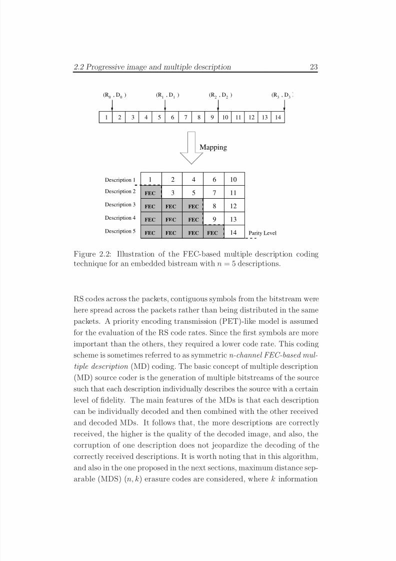
Figure 2.2: Illustration of the FEC-based multiple description codingtechnique for an embedded bistream with n = 5 descriptions.
RS codes across the packets, contiguous symbols from the bitstream were
here spread across the packets rather than being distributed in the same
packets. A priority encoding transmission (PET)-like model is assumed
for the evaluation of the RS code rates. Since the first symbols are more
important than the others, they required a lower code rate. This coding
scheme is sometimes referred to as symmetric n-channel FEC-based mul-
tiple description (MD) coding. The basic concept of multiple description
(MD) source coder is the generation of multiple bitstreams of the source
such that each description individually describes the source with a certainlevel of fidelity. The main features of the MDs is that each description
can be individually decoded and then combined with the other received
and decoded MDs. It follows that, the more descriptions are correctly
received, the higher is the quality of the decoded image, and also, the
corruption of one description does not jeopardize the decoding of the
correctly received descriptions. It is worth noting that in this algorithm,
and also in the one proposed in the next sections, maximum distance sep-
arable (MDS) (n, k) erasure codes are considered, where k information
7/29/2019 Adaptive Wireless Multimedia
http://slidepdf.com/reader/full/adaptive-wireless-multimedia 42/187
24 Chapter 2. Channel coding for progressive images
symbols are encoded into n channel symbols. In MDS codes, the mini-mum distance dmin equals n − k + 1. Knowing that in each (n, k) codes,
the reception of each (n − dmin + 1) channel symbols allows to recover
the k information symbols, in MDS codes, the k information symbols are
recovered if any k channel symbols are correctly received. In Fig. 2.2, a
general mechanism for converting an embedded bitstream from a source
encoder into multiple descriptions is considered. In this example, n = 5
descriptions are considered, and an UEP is assumed. Considering the first
RS codeword, that is a (5, 1) codeword, the single information symbols
can be reconstructed if up to 4 descriptions are lost. Is is worth notingthat assuming all the descriptions equally important is an approxima-
tion, leading to a lower bound of the expected distortion. For example,
receiving the first g out of n descriptions provides a lower distortion than
the reception of the last g descriptions. In the MD scheme in Fig. 2.2,
for example, receiving correctly the first three descriptions rather than
the last three allows to recover up to eight information symbols rather
than up to five. Anyway, since increasing the number of the descriptions
the probability of a particular combination of the received packets is less
likely, the descriptions are usually assumed equally important .
2.3 Channel model and time-frequency chan-
nel coding
As already mentioned in Section 1.3.3, the basic principle of OFDM
is to split a high-rate data stream into a number of lower rate streams
that are transmitted over overlapped but orthogonal subcarriers. Sincethe symbol duration increases for the lower rate parallel subcarriers, the
relative amount of dispersion in time caused by multipath delay spread is
decreased. Depending on the propagation environment and the channel
characteristics, the resource block in an OFDM system can be used to
exploit time and/or frequency diversities through channel coding. For
time diversity, channel coding plus interleaving can be used in the time
domain. However, for the technique to be effective, the time frame has to
be greater than the channel coherence time (∆t)c. The maximum time-
7/29/2019 Adaptive Wireless Multimedia
http://slidepdf.com/reader/full/adaptive-wireless-multimedia 43/187
2.3 Channel model and time-frequency channel coding 25
N Independent Subbands (Bandwidth = W T )
f 1,1 f 1,2 f 1,M f 2,1 f 2,2 f 2,M f N,1 f N,2 f N,M
Subband 1 Subband 2 Subband N
(∆f )cM Correlated Subcarriers
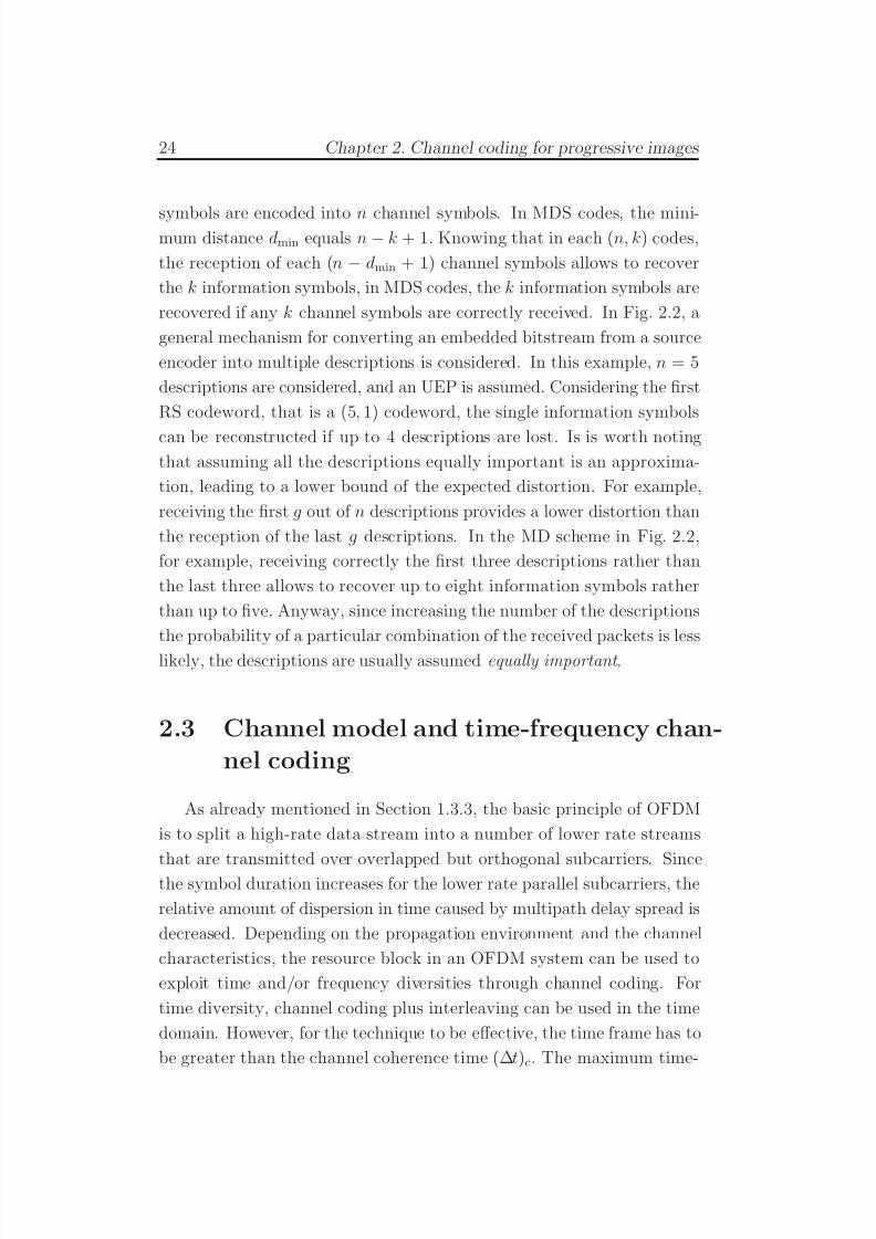
Figure 2.3: Subcarrier spectrum assignment.
diversity gain Dt is given by the ratio between the duration of a time
frame and (∆t)c.
In addition to time diversity, frequency diversity by adding redun-
dancy across the subcarriers can be applied to combat channel errors.
Generally, the maximum achievable frequency diversity Df is given by
the ratio between the overall system bandwidth W T and the coherence
bandwidth (∆f )c.In this chapter, we consider a frequency-selective environment and use
a block fading channel model to simulate the frequency selectivity [38]. In
this model, the spectrum is divided into blocks of size (∆f )c. Subcarriers
in different blocks are considered to fade independently; subcarriers in
the same block experience identical fades. As illustrated in Fig. 2.3, we
assume an OFDM system with an overall system bandwidth W T , such
that we can define N independent subbands. Each subband consists of
M correlated subcarriers spanning a total bandwidth of (∆f )c. The total
number of subcarriers in the OFDM system is NM . In the time domain,
we assume the channel experiences Rayleigh fading. We use the modified
Jakes’ model [39] to simulate different fading rates, resulting in different
time diversity orders.
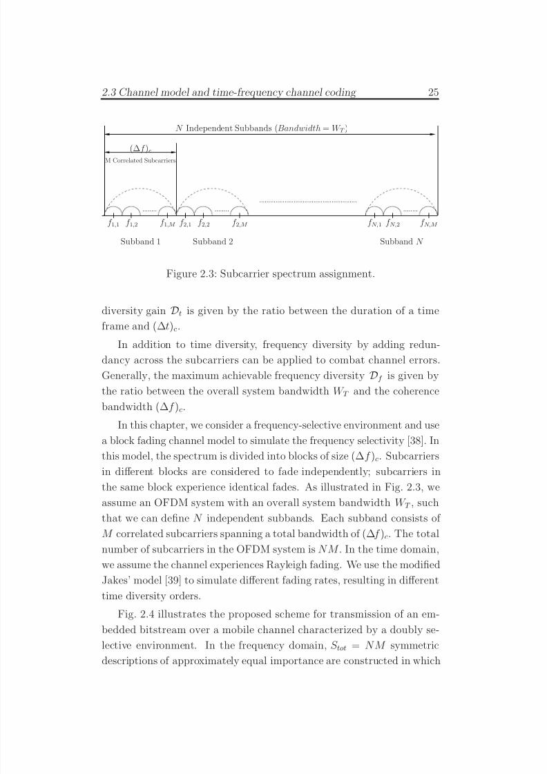
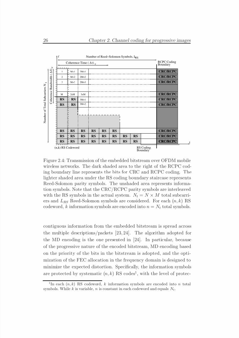
Fig. 2.4 illustrates the proposed scheme for transmission of an em-
bedded bitstream over a mobile channel characterized by a doubly se-
lective environment. In the frequency domain, S tot = NM symmetric
descriptions of approximately equal importance are constructed in which
7/29/2019 Adaptive Wireless Multimedia
http://slidepdf.com/reader/full/adaptive-wireless-multimedia 44/187
26 Chapter 2. Channel coding for progressive images
Number of Reed−Solomon Symbols, L
∆
c
RS
RS
RS
RS
RS
RS
RS
RS
RS
RS
RS
RS
RS
RS
RS
RS
RS
RS
RS RS
RS
RS
RS
2
3
M
M+1
M+2
M+3
2xM 3xM
2M+1
2M+2
2M+3
3M+1
3M+2
1
f
t
(n,k) RS Codeword
RCPC Coding
RS
Boundary
RS CodingBoundary
N u m
b e r o f T o t a l S u b c a r r i e r s N
Coherence Time ( t)∆ c
t
RS
RS
CRC/RCPC
CRC/RCPC
CRC/RCPC
CRC/RCPC
CRC/RCPC
CRC/RCPC
CRC/RCPC
CRC/RCPC
CRC/RCPCCRC/RCPC
RS
C o h e r e n c e B a n d w i d t h (
f )
Figure 2.4: Transmission of the embedded bitstream over OFDM mobilewireless networks. The dark shaded area to the right of the RCPC cod-ing boundary line represents the bits for CRC and RCPC coding. The
lighter shaded area under the RS coding boundary staircase representsReed-Solomon parity symbols. The unshaded area represents informa-tion symbols. Note that the CRC/RCPC parity symbols are interleavedwith the RS symbols in the actual system. N t = N × M total subcarri-ers and LRS Reed-Solomon symbols are considered. For each (n, k) RScodeword, k information symbols are encoded into n = N t total symbols.
contiguous information from the embedded bitstream is spread across
the multiple descriptions/packets [23, 24]. The algorithm adopted for
the MD encoding is the one presented in [24]. In particular, because
of the progressive nature of the encoded bitstream, MD encoding based
on the priority of the bits in the bitstream is adopted, and the opti-
mization of the FEC allocation in the frequency domain is designed to
minimize the expected distortion. Specifically, the information symbols
are protected by systematic (n, k) RS codes1, with the level of protec-
1In each (n, k) RS codeword, k information symbols are encoded into n totalsymbols. While k is variable, n is constant in each codeword and equals N t.
7/29/2019 Adaptive Wireless Multimedia
http://slidepdf.com/reader/full/adaptive-wireless-multimedia 45/187
2.3 Channel model and time-frequency channel coding 27
tion depending on the relative importance of the information symbols,as well as on the order of diversity available in the frequency domain.
Generally, an (n, k) MDS erasure code can correct up to n − k erasures.
Hence, if any g out of n descriptions are received, those codewords with
minimum distance dmin ≥ n − g + 1 can be decoded. As a result, decod-
ing is guaranteed at least up to distortion D(Rg), where D(Rg) refers to
the distortion achieved with Rg information symbols.
The individual descriptions are then mapped to the S tot = NM sub-
carriers. A concatenation of CRC codes and RCPC codes, for possible
diversity and coding gains in the time domain, are applied to each de-
scription. Since the descriptions are approximately equally important,
RCPC codes with the same channel code rate can be applied to protect
each individual description. This results in a vertical boundary (RCPC
coding line), as illustrated in Fig. 2.4. The LRS symbols on the left of the
boundary are the RS symbols, while those on the right are CRC/RCPC
parity symbols. It should be noted that the multiple description RS sym-
bols and RCPC parity symbols would be interleaved in an actual system.
However, for illustration, we show the de-interleaved version throughoutthe paper so that the relative amounts of RCPC parity symbols and RS
symbols can be clearly indicated.
Since both forms of diversity are not necessarily simultaneously avail-
able at any given instant of time, the channel coding scheme should be
designed to synergistically exploit the available diversity. For example,
in a slow fading environment, channel coding plus interleaving is usually
ineffective, especially for delay-sensitive applications such as real-time
multimedia services. Hence, in this case, frequency diversity techniques
may be more effective than time diversity techniques.
As stated previously, traditional studies of progressive transmission
have concentrated on slow fading channels. In fact, in addition to the
performance differences in channel coding efficiencies and channel estima-
tion accuracies, the error patterns for different fade rates also affects the
application layer throughputs and hence the end-user delivered quality.
In particular, in a fast fading environment, the errors are more scattered
among multiple packets due to the higher level crossing rate which mea-
7/29/2019 Adaptive Wireless Multimedia
http://slidepdf.com/reader/full/adaptive-wireless-multimedia 46/187
28 Chapter 2. Channel coding for progressive images
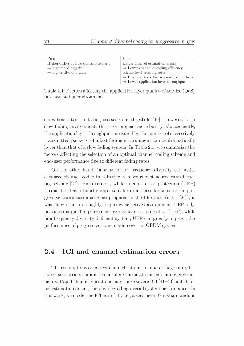
Pros ConsHigher orders of time domain diversity Larger channel estimation errors⇒ higher coding gain ⇒ Lower channel decoding efficiency⇒ higher diversity gain Higher level crossing rates
⇒ Errors scattered across multiple packets⇒ Lower application layer throughput
Table 2.1: Factors affecting the application layer quality-of-service (QoS)in a fast fading environment.
sures how often the fading crosses some threshold [40]. However, for aslow fading environment, the errors appear more bursty. Consequently,
the application layer throughput, measured by the number of successively
transmitted packets, of a fast fading environment can be dramatically
lower than that of a slow fading system. In Table 2.1, we summarize the
factors affecting the selection of an optimal channel coding scheme and
end-user performance due to different fading rates.
On the other hand, information on frequency diversity can assist
a source-channel codec in selecting a more robust source-cannel cod-
ing scheme [27]. For example, while unequal error protection (UEP)
is considered as primarily important for robustness for some of the pro-
gressive transmission schemes proposed in the literature (e.g., [26]), it
was shown that in a highly frequency selective environment, UEP only
provides marginal improvement over equal error protection (EEP), while
in a frequency diversity deficient system, UEP can greatly improve the
performance of progressive transmission over an OFDM system.
2.4 ICI and channel estimation errors
The assumptions of perfect channel estimation and orthogonality be-
tween subcarriers cannot be considered accurate for fast fading environ-
ments. Rapid channel variations may cause severe ICI [41–43] and chan-
nel estimation errors, thereby degrading overall system performance. In
this work, we model the ICI as in [41], i.e., a zero mean Gaussian random
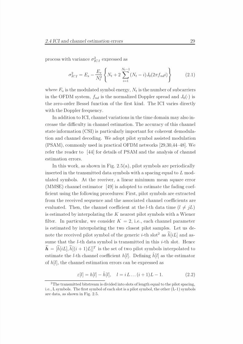
7/29/2019 Adaptive Wireless Multimedia
http://slidepdf.com/reader/full/adaptive-wireless-multimedia 47/187
2.4 ICI and channel estimation errors 29
process with variance σ2ICI expressed as
σ2ICI = E s − E s
N 2t
N t + 2
N t−1i=1
(N t − i)J 0(2πf ndi)
(2.1)
where E s is the modulated symbol energy, N t is the number of subcarriers
in the OFDM system, f nd is the normalized Doppler spread and J 0(·) is
the zero-order Bessel function of the first kind. The ICI varies directly
with the Doppler frequency.
In addition to ICI, channel variations in the time domain may also in-
crease the difficulty in channel estimation. The accuracy of this channel
state information (CSI) is particularly important for coherent demodula-
tion and channel decoding. We adopt pilot symbol assisted modulation
(PSAM), commonly used in practical OFDM networks [29,30,44–48]. We
refer the reader to [44] for details of PSAM and the analysis of channel
estimation errors.
In this work, as shown in Fig. 2.5(a), pilot symbols are periodically
inserted in the transmitted data symbols with a spacing equal to L mod-
ulated symbols. At the receiver, a linear minimum mean square error(MMSE) channel estimator [49] is adopted to estimate the fading coef-
ficient using the following procedures: First, pilot symbols are extracted
from the received sequence and the associated channel coefficients are
evaluated. Then, the channel coefficient at the l-th data time (l = jL)
is estimated by interpolating the K nearest pilot symbols with a Wiener
filter. In particular, we consider K = 2, i.e., each channel parameter
is estimated by interpolating the two closest pilot samples. Let us de-
note the received pilot symbol of the generic i-th slot2 as h[iL] and as-
sume that the l-th data symbol is transmitted in this i-th slot. Henceh = [h[iL],h[(i + 1)L]]T is the set of two pilot symbols interpolated to
estimate the l-th channel coefficient h[l]. Defining h[l] as the estimator
of h[l], the channel estimation errors can be expressed as
ε[l] = h[l] − h[l], l = i L . . . (i + 1)L − 1. (2.2)
2The transmitted bitstream is divided into slots of length equal to the pilot spacing,i.e., L symbols. The first symbol of each slot is a pilot symbol, the other (L-1) symbolsare data, as shown in Fig. 2.5.
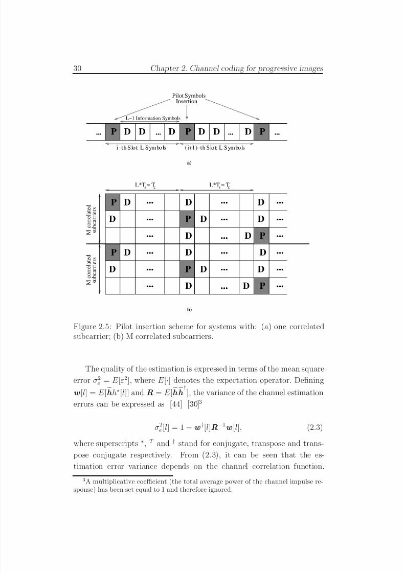
7/29/2019 Adaptive Wireless Multimedia
http://slidepdf.com/reader/full/adaptive-wireless-multimedia 48/187
30 Chapter 2. Channel coding for progressive images
s
s u b c a r r i e r s
M c o
r r e l a t e d
s u b c a r r i e r s
M c
o r r e
l a t e d
L*T = T
D D D D D D... ... ......
i−th Slot: L Symbols (i+1)−th Slot: L Symbols
Pilot Symbols
Insertion
L−1 Information Symbols
P
a)
b)
P
P
D
D
D
D
...
...
...
...
...
......
...
...
P
P
D
D
D
D
...
...
...
...
...
......
...
...
D
D
D
D
D
D
D
D
P P
P
P
c cs L*T = T
Figure 2.5: Pilot insertion scheme for systems with: (a) one correlatedsubcarrier; (b) M correlated subcarriers.
The quality of the estimation is expressed in terms of the mean square
error σ2e = E [ε2], where E [·] denotes the expectation operator. Defining
w [l] = E [h h∗[l]] and R = E [h h
†], the variance of the channel estimation
errors can be expressed as [44] [30]3
σ2e [l] = 1 −w
†[l]R−1w [l], (2.3)
where superscripts ∗, T and † stand for conjugate, transpose and trans-
pose conjugate respectively. From (2.3), it can be seen that the es-
timation error variance depends on the channel correlation function.
3A multiplicative coefficient (the total average power of the channel impulse re-sponse) has been set equal to 1 and therefore ignored.
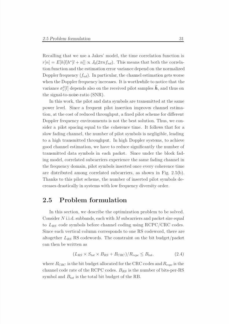
7/29/2019 Adaptive Wireless Multimedia
http://slidepdf.com/reader/full/adaptive-wireless-multimedia 49/187
2.5 Problem formulation 31
Recalling that we use a Jakes’ model, the time correlation function isr[n] = E [h[l]h∗[l + n]] ∝ J 0(2πnf nd). This means that both the correla-
tion function and the estimation error variance depend on the normalized
Doppler frequency (f nd). In particular, the channel estimation gets worse
when the Doppler frequency increases. It is worthwhile to notice that the
variance σ2e [l] depends also on the received pilot samples h , and thus on
the signal-to-noise-ratio (SNR).
In this work, the pilot and data symbols are transmitted at the same
power level. Since a frequent pilot insertion improves channel estima-
tion, at the cost of reduced throughput, a fixed pilot scheme for differentDoppler frequency environments is not the best solution. Thus, we con-
sider a pilot spacing equal to the coherence time. It follows that for a
slow fading channel, the number of pilot symbols is negligible, leading
to a high transmitted throughput. In high Doppler systems, to achieve
good channel estimation, we have to reduce significantly the number of
transmitted data symbols in each packet. Since under the block fad-
ing model, correlated subcarriers experience the same fading channel in
the frequency domain, pilot symbols inserted once every coherence time
are distributed among correlated subcarriers, as shown in Fig. 2.5(b).
Thanks to this pilot scheme, the number of inserted pilot symbols de-
creases drastically in systems with low frequency diversity order.
2.5 Problem formulation
In this section, we describe the optimization problem to be solved.
Consider N i.i.d. subbands, each with M subcarriers and packet size equal
to LRS code symbols before channel coding using RCPC/CRC codes.Since each vertical column corresponds to one RS codeword, there are
altogether LRS RS codewords. The constraint on the bit budget/packet
can then be written as
(LRS × S tot × BRS + BCRC )/Rrcpc ≤ Btot, (2.4)
where BCRC is the bit budget allocated for the CRC codes and Rrcpc is the
channel code rate of the RCPC codes. BRS is the number of bits-per-RS
symbol and Btot is the total bit budget of the RB.
7/29/2019 Adaptive Wireless Multimedia
http://slidepdf.com/reader/full/adaptive-wireless-multimedia 50/187
32 Chapter 2. Channel coding for progressive images
We assume that for RS codeword l, where l ∈ [1, LRS ], cl code symbolsare assigned to information data symbols. Hence, the number of RS
parity symbols assigned to codeword l is
f l = S tot − cl l ∈ [1, LRS ]. (2.5)
Let φth be the minimum number of descriptions that a decoder needs
to reconstruct the source, and g be the number of correctly received
packets. The reception of any number of packets g ≥ φth leads to im-
proving image quality D(Rg), where R
gis the allocated bit budget for
the information symbols,
Rg =
l:cl≤gcl × BRS . (2.6)
Hence, the overall RS channel code rate equals Rrs = RS tot/(S tot×LRS ×BRS ). Given the source code rate-distortion curve D(Rg) and the packet
loss probability mass function P J ( j), where j = S tot − g is the number
of lost packets, we can minimize the expected distortion as follows:
E ∗[D] = mincl,Rrcpc
S tot−φth j=0
P J ( j)D(RS tot− j) +S tot
j=S tot−φth+1
P J ( j)D0
,(2.7)
subject to the constraint on the overall bit budget
RS tot/Rrs + BCRC
Rrcpc≤ Btot (2.8)
where D0 corresponds to the distortion when fewer than φth descriptions
are received and so the decoder must reconstruct the source without being
able to use any of the transmitted information. For a still image, this
typically means reconstructing the entire image at the mean pixel value.
The packet loss probability mass function P J ( j) depends on (∆f )c,
(∆t)c and Rrcpc. Although P J ( j) can be found analytically for uncor-
related fading channels, due to the correlated fading in both time and
frequency domains of the mobile environment considered here, we use
simulations to find P J ( j). We use the iterative procedure described in [24]
to solve the optimization problem (2.7).
7/29/2019 Adaptive Wireless Multimedia
http://slidepdf.com/reader/full/adaptive-wireless-multimedia 51/187
2.6 Results and discussion 33
2.6 Results and discussionWe carried out simulations on the 512 × 512 gray-scale images Lena,
Peppers and Goldhill. Similar results were obtained for all three. Hence,
in this paper, we only present the results using the Lena image. The
image was encoded using the SPIHT [1] algorithm to produce an em-
bedded bitstream. The serial bitstream was converted into 128 parallel
bitstreams using the FEC-based multiple description encoder. The 128
descriptions were mapped to the OFDM system with 128 subcarriers.
We used RS codes in the frequency domain and there were 8 bits perRS symbol. The packet size was set equal to 512 bits. We used QPSK
modulation and considered both perfect and imperfect CSI. It should be
noted that more sophisticated modulation schemes could be used to fur-
ther improve the system performance, such as the one discussed in [50].
However, for the sake of simplicity and better understanding of the funda-
mental impact of the time and frequency diversities on the construction
of the 2-D OFDM block, a fixed modulation scheme using QPSK was
chosen. The RCPC codes of rates Rrcpc = 89
, 810
, . . . , 824
, were obtained by
puncturing an Rc = 1/3 mother code with K = 7, p = 8 and generatorpolynomials (133, 165, 171)octal with the puncturing table given in [51].
In the following figures, we illustrate the proposed channel coding
scheme under different fading environments and study the effects of chan-
nel estimation on the selection by comparing performance of systems with
perfect CSI to systems with imperfect CSI and ICI. From here onwards,
for systems with imperfect CSI and ICI, ICI is omitted from the notation
for sake of brevity, although it is considered as well. We begin by studying
the optimized construction of RS information and parity symbols for
• Different values of RCPC coding rate,
• Both perfect and imperfect CSI, and
• Different frequency diversity orders and different fading rates.
Then we study how the received image PSNR varies for different
Doppler spreads, for perfect and imperfect CSI, and for different fre-
quency diversity orders.
In Fig. 2.6, we show the optimized construction of RS information
symbols, RS parity symbols and RCPC parity symbols for different Rrcpc’s
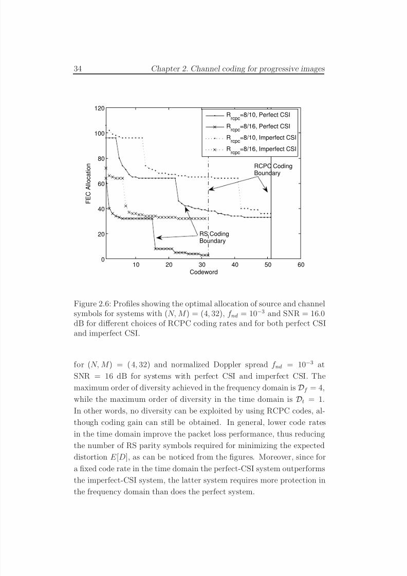
7/29/2019 Adaptive Wireless Multimedia
http://slidepdf.com/reader/full/adaptive-wireless-multimedia 52/187
34 Chapter 2. Channel coding for progressive images
10 20 30 40 50 600
20
40
60
80
100
120
Codeword
F
E C
A l l o c a t i o n
Rrcpc
=8/10, Perfect CSI
Rrcpc
=8/16, Perfect CSI
Rrcpc
=8/10, Imperfect CSI
Rrcpc
=8/16, Imperfect CSI
RCPC CodingBoundary
RS CodingBoundary
Figure 2.6: Profiles showing the optimal allocation of source and channelsymbols for systems with (N, M ) = (4, 32), f nd = 10−3 and SNR = 16.0dB for different choices of RCPC coding rates and for both perfect CSIand imperfect CSI.
for (N, M ) = ( 4, 32) and normalized Doppler spread f nd = 10−3 at
SNR = 16 dB for systems with perfect CSI and imperfect CSI. The
maximum order of diversity achieved in the frequency domain is Df = 4,
while the maximum order of diversity in the time domain is Dt = 1.In other words, no diversity can be exploited by using RCPC codes, al-
though coding gain can still be obtained. In general, lower code rates
in the time domain improve the packet loss performance, thus reducing
the number of RS parity symbols required for minimizing the expected
distortion E [D], as can be noticed from the figures. Moreover, since for
a fixed code rate in the time domain the perfect-CSI system outperforms
the imperfect-CSI system, the latter system requires more protection in
the frequency domain than does the perfect system.
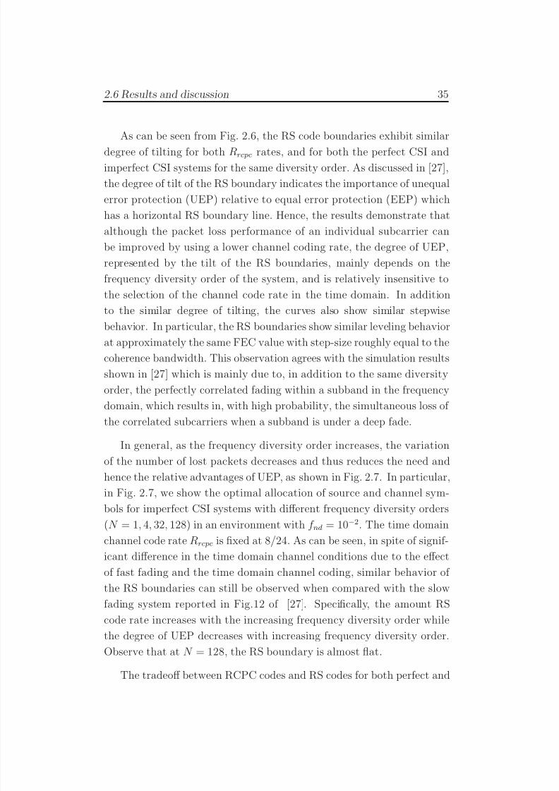
7/29/2019 Adaptive Wireless Multimedia
http://slidepdf.com/reader/full/adaptive-wireless-multimedia 53/187
2.6 Results and discussion 35
As can be seen from Fig. 2.6, the RS code boundaries exhibit similardegree of tilting for both Rrcpc rates, and for both the perfect CSI and
imperfect CSI systems for the same diversity order. As discussed in [27],
the degree of tilt of the RS boundary indicates the importance of unequal
error protection (UEP) relative to equal error protection (EEP) which
has a horizontal RS boundary line. Hence, the results demonstrate that
although the packet loss performance of an individual subcarrier can
be improved by using a lower channel coding rate, the degree of UEP,
represented by the tilt of the RS boundaries, mainly depends on the
frequency diversity order of the system, and is relatively insensitive tothe selection of the channel code rate in the time domain. In addition
to the similar degree of tilting, the curves also show similar stepwise
behavior. In particular, the RS boundaries show similar leveling behavior
at approximately the same FEC value with step-size roughly equal to the
coherence bandwidth. This observation agrees with the simulation results
shown in [27] which is mainly due to, in addition to the same diversity
order, the perfectly correlated fading within a subband in the frequency
domain, which results in, with high probability, the simultaneous loss of
the correlated subcarriers when a subband is under a deep fade.
In general, as the frequency diversity order increases, the variation
of the number of lost packets decreases and thus reduces the need and
hence the relative advantages of UEP, as shown in Fig. 2.7. In particular,
in Fig. 2.7, we show the optimal allocation of source and channel sym-
bols for imperfect CSI systems with different frequency diversity orders
(N = 1, 4, 32, 128) in an environment with f nd = 10−2. The time domain
channel code rate Rrcpc is fixed at 8/24. As can be seen, in spite of signif-
icant difference in the time domain channel conditions due to the effectof fast fading and the time domain channel coding, similar behavior of
the RS boundaries can still be observed when compared with the slow
fading system reported in Fig.12 of [27]. Specifically, the amount RS
code rate increases with the increasing frequency diversity order while
the degree of UEP decreases with increasing frequency diversity order.
Observe that at N = 128, the RS boundary is almost flat.
The tradeoff between RCPC codes and RS codes for both perfect and
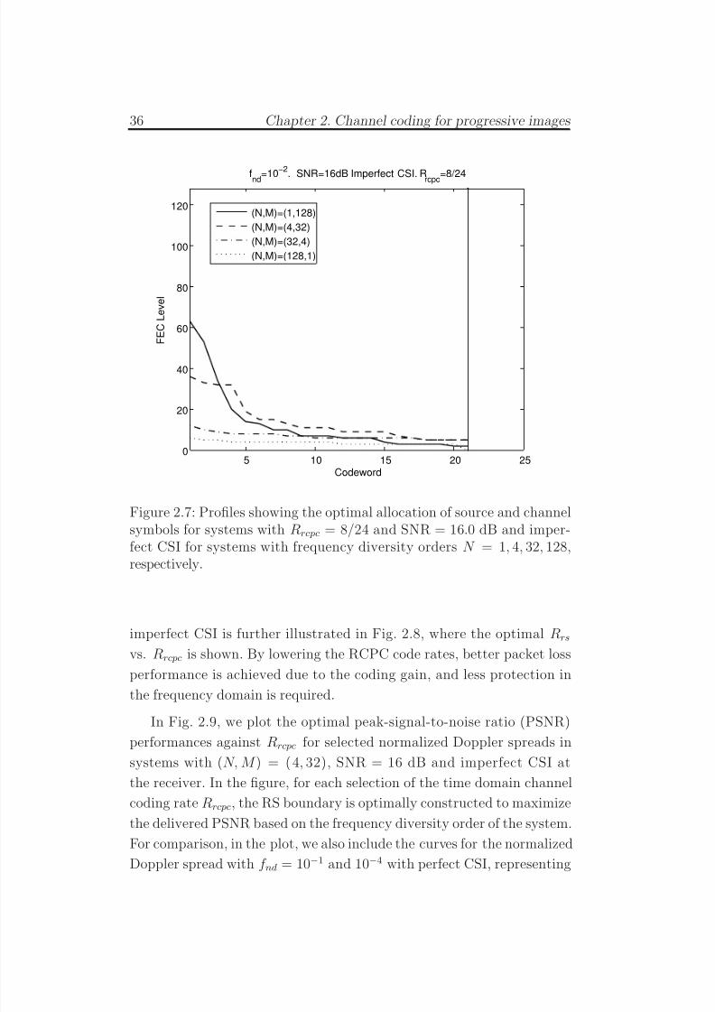
7/29/2019 Adaptive Wireless Multimedia
http://slidepdf.com/reader/full/adaptive-wireless-multimedia 54/187
36 Chapter 2. Channel coding for progressive images
5 10 15 20 250
20
40
60
80
100
120
Codeword
F E C
L e v e l
fnd=10
−2
. SNR=16dB Imperfect CSI. Rrcpc=8/24
(N,M)=(1,128)
(N,M)=(4,32)
(N,M)=(32,4)
(N,M)=(128,1)
Figure 2.7: Profiles showing the optimal allocation of source and channel
symbols for systems with Rrcpc = 8/24 and SNR = 16.0 dB and imper-fect CSI for systems with frequency diversity orders N = 1, 4, 32, 128,respectively.
imperfect CSI is further illustrated in Fig. 2.8, where the optimal Rrs
vs. Rrcpc is shown. By lowering the RCPC code rates, better packet loss
performance is achieved due to the coding gain, and less protection in
the frequency domain is required.
In Fig. 2.9, we plot the optimal peak-signal-to-noise ratio (PSNR)
performances against Rrcpc for selected normalized Doppler spreads in
systems with (N, M ) = ( 4, 32), SNR = 16 dB and imperfect CSI at
the receiver. In the figure, for each selection of the time domain channel
coding rate Rrcpc, the RS boundary is optimally constructed to maximize
the delivered PSNR based on the frequency diversity order of the system.
For comparison, in the plot, we also include the curves for the normalized
Doppler spread with f nd = 10−1 and 10−4 with perfect CSI, representing
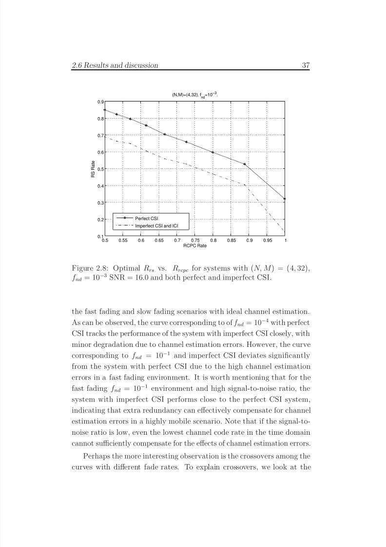
7/29/2019 Adaptive Wireless Multimedia
http://slidepdf.com/reader/full/adaptive-wireless-multimedia 55/187
2.6 Results and discussion 37
0.5 0.55 0.6 0.65 0.7 0.75 0.8 0.85 0.9 0.95 10.1
0.2
0.3
0.4
0.5
0.6
0.7
0.8
0.9
RCPC Rate
R S
R a t e
(N,M)=(4,32). fnd=10−3
.
Perfect CSI
Imperfect CSI and ICI
Figure 2.8: Optimal Rrs vs. Rrcpc for systems with (N, M ) = (4, 32),f nd = 10−3 SNR = 16.0 and both perfect and imperfect CSI.
the fast fading and slow fading scenarios with ideal channel estimation.
As can be observed, the curve corresponding to of f nd = 10−4 with perfect
CSI tracks the performance of the system with imperfect CSI closely, with
minor degradation due to channel estimation errors. However, the curve
corresponding to f nd = 10−1 and imperfect CSI deviates significantly
from the system with perfect CSI due to the high channel estimation
errors in a fast fading environment. It is worth mentioning that for the
fast fading f nd = 10−1 environment and high signal-to-noise ratio, the
system with imperfect CSI performs close to the perfect CSI system,
indicating that extra redundancy can effectively compensate for channel
estimation errors in a highly mobile scenario. Note that if the signal-to-
noise ratio is low, even the lowest channel code rate in the time domain
cannot sufficiently compensate for the effects of channel estimation errors.
Perhaps the more interesting observation is the crossovers among the
curves with different fade rates. To explain crossovers, we look at the
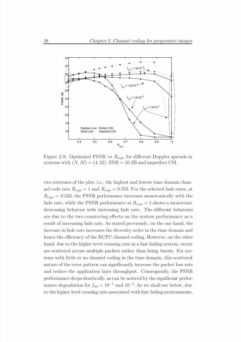
7/29/2019 Adaptive Wireless Multimedia
http://slidepdf.com/reader/full/adaptive-wireless-multimedia 56/187
38 Chapter 2. Channel coding for progressive images
0.4 0.5 0.6 0.7 0.8 0.9 1
16
18
20
22
24
26
28
30
32
34
Rrcpc
P S N R ,
d B
fnd
= 1.0x10⁻⁴
fnd
= 1.0x10⁻³
fnd
= 1.0x10⁻²
fnd
= 1.0x10⁻¹
Dashed Line: Perfect CSISolid Line: Imperfect CSI
Figure 2.9: Optimized PSNR vs Rrcpc for different Doppler spreads insystems with (N, M ) = (4, 32), SNR = 16 dB and imperfect CSI.
two extremes of the plot, i.e., the highest and lowest time domain chan-
nel code rate Rrcpc = 1 and Rrcpc = 0.333. For the selected fade rates, at
Rrcpc = 0.333, the PSNR performance increases monotonically with the
fade rate, while the PSNR performance at Rrcpc = 1 shows a monotonic
decreasing behavior with increasing fade rate. The different behaviors
are due to the two countering effects on the system performance as a
result of increasing fade rate. As stated previously, on the one hand, the
increase in fade rate increases the diversity order in the time domain and
hence the efficiency of the RCPC channel coding. However, on the otherhand, due to the higher level crossing rate in a fast fading system, errors
are scattered across multiple packets rather than being bursty. For sys-
tems with little or no channel coding in the time domain, this scattered
nature of the error pattern can significantly increase the packet loss rate
and reduce the application layer throughput. Consequently, the PSNR
performance drops drastically, as can be noticed by the significant perfor-
mance degradation for f nd = 10−1 and 10−2. As we shall see below, due
to the higher level crossing rate associated with fast fading environments,
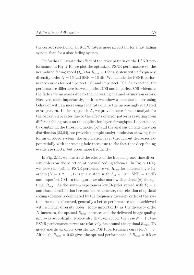
7/29/2019 Adaptive Wireless Multimedia
http://slidepdf.com/reader/full/adaptive-wireless-multimedia 57/187
2.6 Results and discussion 39
the correct selection of an RCPC rate is more important for a fast fadingsystem than for a slow fading system.
To further illustrate the effect of the error pattern on the PSNR per-
formance, in Fig. 2.10, we plot the optimized PSNR performance vs. the
normalized fading speed (f nd) for Rrcpc = 1 for a system with a frequency
diversity order N = 16 and SNR = 16 dB. We include the PSNR perfor-
mance curves for both perfect CSI and imperfect CSI. As expected, the
performance difference between perfect CSI and imperfect CSI widens as
the fade rate increases due to the increasing channel estimation errors.
However, more importantly, both curves show a monotonic decreasing
behavior with an increasing fade rate due to the increasingly scattered
error pattern. In the Appendix A, we provide some further analysis for
the packet error rates due to the effects of error patterns resulting from
different fading rates on the application layer throughput. In particular,
by combining the threshold model [52] and the analysis on fade duration
distribution [53,54], we provide a simple analytic solution showing that
for an uncoded system, the application layer throughput decreases ex-
ponentially with increasing fade rates due to the fact that deep fadingevents are shorter but occur more frequently.
In Fig. 2.11, we illustrate the effects of the frequency and time diver-
sity orders on the selection of optimal coding schemes. In Fig. 2.11(a),
we show the optimal PSNR performance vs. Rrcpc for different diversity
orders (N = 1, 2, . . . , 128) in a system with f nd = 10−3, SNR = 16 dB
and imperfect CSI. In the figure, we also mark with a circle () the op-
timal Rrcpc. As the system experiences low Doppler spread with Dt = 1
and channel estimation becomes more accurate, the selection of optimalcoding schemes is dominated by the frequency diversity order of the sys-
tem. As can be observed, generally a better performance can be achieved
with a higher diversity order. More importantly, as the diversity order
N increases, the optimal Rrcpc increases and the delivered image quality
improves accordingly. Notice also that, except for the case N = 1 , the
PSNR performance curves are relatively flat around the optimal Rrcpc. To
give a specific example, consider the PSNR performance curve for N = 8.
Although Rrcpc = 0.62 gives the optimal performance, if Rrcpc = 0.5 or
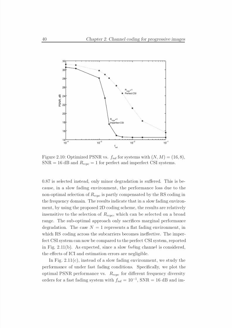
7/29/2019 Adaptive Wireless Multimedia
http://slidepdf.com/reader/full/adaptive-wireless-multimedia 58/187
40 Chapter 2. Channel coding for progressive images
10−4
10−3
10−2
10−1
14
16
18
20
22
24
26
28
30
32
fnd
P S N R ,
d B
Rrcpc
=1
Imperfect CSI
Rrcpc
=1
Perfect CSI
Figure 2.10: Optimized PSNR vs. f nd for systems with (N, M ) = (16, 8),SNR = 16 dB and Rrcpc = 1 for perfect and imperfect CSI systems.
0.87 is selected instead, only minor degradation is suffered. This is be-
cause, in a slow fading environment, the performance loss due to the
non-optimal selection of Rrcpc is partly compensated by the RS coding in
the frequency domain. The results indicate that in a slow fading environ-
ment, by using the proposed 2D coding scheme, the results are relatively
insensitive to the selection of Rrcpc, which can be selected on a broad
range. The sub-optimal approach only sacrifices marginal performance
degradation. The case N = 1 represents a flat fading environment, inwhich RS coding across the subcarriers becomes ineffective. The imper-
fect CSI system can now be compared to the perfect CSI system, reported
in Fig. 2.11(b). As expected, since a slow fading channel is considered,
the effects of ICI and estimation errors are negligible.
In Fig. 2.11(c), instead of a slow fading environment, we study the
performance of under fast fading conditions. Specifically, we plot the
optimal PSNR performance vs. Rrcpc for different frequency diversity
orders for a fast fading system with f nd = 10−1, SNR = 16 dB and im-
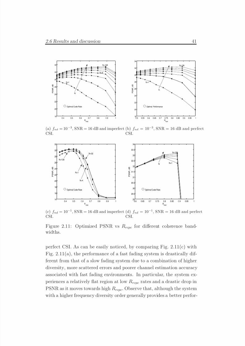
7/29/2019 Adaptive Wireless Multimedia
http://slidepdf.com/reader/full/adaptive-wireless-multimedia 59/187
2.6 Results and discussion 41
0.4 0.5 0.6 0.7 0.8 0.9 118
20
22
24
26
28
30
32
Rrcpc
P S N R ,
d B
N=8
Optimal Code Rate
N=128
N=1
N
(a) f nd = 10−3, SNR = 16 dB and imperfectCSI.
0.5 0.55 0.6 0.65 0.7 0.75 0.8 0.85 0.9 0.95 118
20
22
24
26
28
30
32
34
Rrcpc
P S N R ,
d B
Optimal Performance
N
N=1
N=128
(b) f nd = 10−3, SNR = 16 dB and perfectCSI.
0.4 0.5 0.6 0.7 0.8 0.9 114
16
18
20
22
24
26
28
30
32
Rrcpc
P S N R ,
d B
Optimal Code Rate
N=4
N=1
N=32
N=128
(c) f nd = 10−1, SNR = 16 dB and imperfectCSI.
0.6 0.65 0.7 0.75 0.8 0.85 0.9 0.95 129
29.5
30
30.5
31
31.5
32
32.5
33
33.5
34
Rrcpc
P S N R ,
d B
N N=1
N=128
Optimal Code Rate
(d) f nd = 10−1, SNR = 16 dB and perfectCSI.
Figure 2.11: Optimized PSNR vs Rrcpc for different coherence band-widths.
perfect CSI. As can be easily noticed, by comparing Fig. 2.11(c) with
Fig. 2.11(a), the performance of a fast fading system is drastically dif-
ferent from that of a slow fading system due to a combination of higher
diversity, more scattered errors and poorer channel estimation accuracy
associated with fast fading environments. In particular, the system ex-
periences a relatively flat region at low Rrcpc rates and a drastic drop in
PSNR as it moves towards high Rrcpc. Observe that, although the system
with a higher frequency diversity order generally provides a better perfor-
7/29/2019 Adaptive Wireless Multimedia
http://slidepdf.com/reader/full/adaptive-wireless-multimedia 60/187
42 Chapter 2. Channel coding for progressive images
10−4
10−3
10−2
10−1
14
16
18
20
22
24
26
28
30
32
fnd
P S N R , d B
Rrcpc
=1/3
Rrcpc
=8/10
Rrcpc
=1
Optimal Rrcpc
Figure 2.12: Optimized PSRN vs. f nd for systems with (N, M ) = (16, 8),SNR = 16 dB and different RCPC code rates.
mance, unlike the slow fading systems, the optimal Rrcpc’s are relatively
insensitive to the frequency diversity order. This is because in the time
domain, the performance is dominated by the high time diversity gain,
and thus PSNR depends only slightly on the frequency diversity order.
Moreover, it is worth noting that, due to the high time diversity order,
the time domain channel coding is very effective and the optimal channel
code rate in the time domain is dominated by the channel estimation
errors and ICI.
This can be illustrated by comparing Fig. 2.11(c) with Fig. 2.11(d).
In Fig. 2.11(d), we plot the corresponding system with perfect CSI as op-
posed to the system with imperfect CSI shown in Fig. 2.11(c). Observe
that, generally, high Rrcpc’s are preferred for better system performance.
However, the performance is relatively insensitive to the frequency diver-
sity order. Moreover, both systems exhibit precipitous drops in PSNR
performance due to a more dispersed error pattern, leading to poor ap-
plication layer throughput if the system is under-protected.
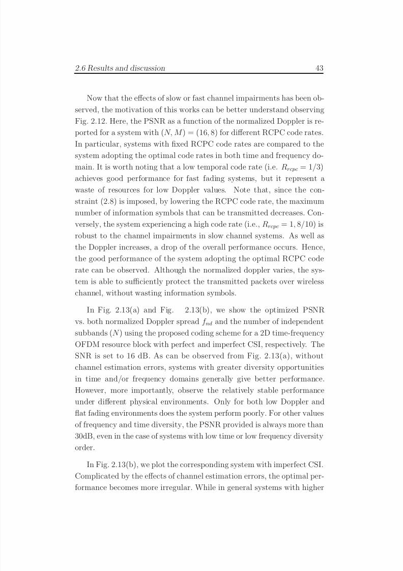
7/29/2019 Adaptive Wireless Multimedia
http://slidepdf.com/reader/full/adaptive-wireless-multimedia 61/187
2.6 Results and discussion 43
Now that the effects of slow or fast channel impairments has been ob-served, the motivation of this works can be better understand observing
Fig. 2.12. Here, the PSNR as a function of the normalized Doppler is re-
ported for a system with (N, M ) = (16, 8) for different RCPC code rates.
In particular, systems with fixed RCPC code rates are compared to the
system adopting the optimal code rates in both time and frequency do-
main. It is worth noting that a low temporal code rate (i.e. Rrcpc = 1/3)
achieves good performance for fast fading systems, but it represent a
waste of resources for low Doppler values. Note that, since the con-
straint (2.8) is imposed, by lowering the RCPC code rate, the maximumnumber of information symbols that can be transmitted decreases. Con-
versely, the system experiencing a high code rate (i.e., Rrcpc = 1, 8/10) is
robust to the channel impairments in slow channel systems. As well as
the Doppler increases, a drop of the overall performance occurs. Hence,
the good performance of the system adopting the optimal RCPC code
rate can be observed. Although the normalized doppler varies, the sys-
tem is able to sufficiently protect the transmitted packets over wireless
channel, without wasting information symbols.
In Fig. 2.13(a) and Fig. 2.13(b), we show the optimized PSNR
vs. both normalized Doppler spread f nd and the number of independent
subbands (N ) using the proposed coding scheme for a 2D time-frequency
OFDM resource block with perfect and imperfect CSI, respectively. The
SNR is set to 16 dB. As can be observed from Fig. 2.13(a), without
channel estimation errors, systems with greater diversity opportunities
in time and/or frequency domains generally give better performance.
However, more importantly, observe the relatively stable performance
under different physical environments. Only for both low Doppler andflat fading environments does the system perform poorly. For other values
of frequency and time diversity, the PSNR provided is always more than
30dB, even in the case of systems with low time or low frequency diversity
order.
In Fig. 2.13(b), we plot the corresponding system with imperfect CSI.
Complicated by the effects of channel estimation errors, the optimal per-
formance becomes more irregular. While in general systems with higher
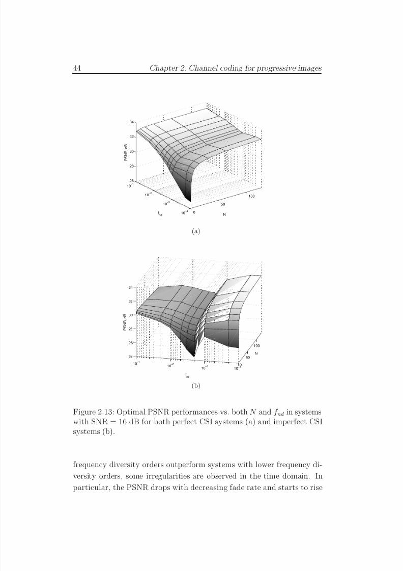
7/29/2019 Adaptive Wireless Multimedia
http://slidepdf.com/reader/full/adaptive-wireless-multimedia 62/187
44 Chapter 2. Channel coding for progressive images
0
50
100
10−4
10−3
10−2
10−1
26
28
30
32
34
Nfnd
P S N R ,
d B
(a)
0
50
100
10−410
−310−210
−1
24
26
28
30
32
34
fnd
P S N R ,
d B
N
10−40
(b)
Figure 2.13: Optimal PSNR performances vs. both N and f nd in systemswith SNR = 16 dB for both perfect CSI systems (a) and imperfect CSIsystems (b).
frequency diversity orders outperform systems with lower frequency di-
versity orders, some irregularities are observed in the time domain. In
particular, the PSNR drops with decreasing fade rate and starts to rise
7/29/2019 Adaptive Wireless Multimedia
http://slidepdf.com/reader/full/adaptive-wireless-multimedia 63/187
2.6 Results and discussion 45
again at fade rates around 10−2
and 10−3
. To have a better understand-ing of the optimal behavior, in Fig. 2.14 we show the optimal PSNR
performance vs. f nd for systems with two different frequency diversity
orders, Df = 4 and Df = 32. The SNR is set to 16 dB. The OFDM
resource block is constructed with optimal RS profiles and RCPC rates
based on the proposed scheme. For comparison, systems with both per-
fect and imperfect CSI are considered. By first looking at the slow fading
section, i.e., the region with f nd < 10−3, it can be observed that the opti-
mal PSNR performances are relatively flat, with some degradation in the
systems with imperfect CSI due to channel estimation errors. The per-formance gap between the perfect CSI and imperfect CSI in this region
is relatively small due to better channel estimation accuracy in a slow
fading environment. At the middle section, i.e., (10−3 < f nd < 10−2), the
drops in PSNR performance are steepened for systems with imperfect
CSI, due to the combined effects of low time diversity gain, increasing
channel estimations errors, and the impact of the more scattered nature
of the error pattern. For f nd > 10−2, the large channel variations provide
significant time diversity gain which improves the efficiency of the RCPC
codes and partly compensate for the performance loss due to the channel
estimation errors.
Finally, results in terms of reconstructed images in Fig. 2.15 for sys-
tems with f nd = 10−1, (N, M ) = (32, 4), and imperfect CSI, provide some
subjective comparisons. Here, the advantage of the proposed scheme and
the effect of channel impairments under a fast fading environment can be
observed by comparing the reconstructed images with the original one.
The five reconstructed images (Fig. 2.15(b)-(f)) represent 5 different sim-ulated results based on 5 different RCPC code rates. In each of the cases,
the corresponding RS boundary is optimally selected based on the chosen
RCPC code rate. Fig. 2.15(c) shows the result for optimal channel coding
for the 2D time-frequency OFDM block. It can be shown that the choice
of the optimal 2D channel coding which includes the proper selections
of RCPC codes in the time domain and RS boundary in the frequency
domain turns out to be critical. As can be observed, RCPC code rates
higher than 0.66 do not provide sufficient protection against the degra-
7/29/2019 Adaptive Wireless Multimedia
http://slidepdf.com/reader/full/adaptive-wireless-multimedia 64/187
46 Chapter 2. Channel coding for progressive images
10−4
10−3
10−2
10−1
27
28
29
30
31
32
33
fnd
P S N R ,
d B
(N,M)=(32,4)
(N,M)=(4,32)
Solid Line : perfect CSIDashdot Line: imperfect CSI
Figure 2.14: Optimized PSNR vs. f nd for systems with SNR = 16 dBand both perfect and imperfect CSI. Two different frequency diversityorder are considered: (N, M ) = (32, 4) and (N, M ) = (4, 32).
dation caused by the imperfect channel estimation and the intercarrier
interference that the system experiences at high Doppler. Conversely,
when an extremely low code rate is chosen, the system might be over
protected, leading to too low a source rate.
In Table 2.2 and Table 2.3, by defining the total/combined channel
code rate as Rtot = Rrcpc · Rrs and the total system diversity order avail-
able as
Dtot =
Df
·Dt, we provide further analysis regarding the proposed
2D channel coding scheme. In particular, in Table 2.2, the optimal PSNR,
Rrcpc, Rrs, and Rtot are presented for a system with SNR = 16dB4, per-
fect CSI and different diversity orders in both the time and frequency
domains. In each row, we keep Dtot fixed and investigate the correspond-
ing performance for different combinations of Df and Dt. To provide a
specific comparison, consider systems with Dtot equal to 4. Obviously,
4Although only SNR = 16dB is reported, we also considered other SNR values andbehavior similar to the one for SNR = 16dB were observed.
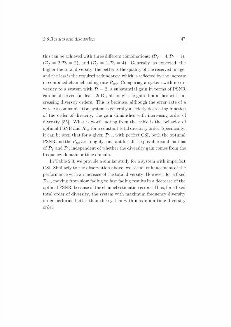
7/29/2019 Adaptive Wireless Multimedia
http://slidepdf.com/reader/full/adaptive-wireless-multimedia 65/187
2.6 Results and discussion 47
this can be achieved with three different combinations: (Df = 4, Dt = 1),(Df = 2, Dt = 2), and (Df = 1, Dt = 4). Generally, as expected, the
higher the total diversity, the better is the quality of the received image,
and the less is the required redundancy, which is reflected by the increase
in combined channel coding rate Rtot. Comparing a system with no di-
versity to a system with D = 2, a substantial gain in terms of PSNR
can be observed (at least 2dB), although the gain diminishes with in-
creasing diversity orders. This is because, although the error rate of a
wireless communication system is generally a strictly decreasing function
of the order of diversity, the gain diminishes with increasing order of diversity [55]. What is worth noting from the table is the behavior of
optimal PSNR and Rtot for a constant total diversity order. Specifically,
it can be seen that for a given Dtot, with perfect CSI, both the optimal
PSNR and the Rtot are roughly constant for all the possible combinations
of Df and Dt, independent of whether the diversity gain comes from the
frequency domain or time domain.
In Table 2.3, we provide a similar study for a system with imperfect
CSI. Similarly to the observation above, we see an enhancement of the
performance with an increase of the total diversity. However, for a fixed
Dtot, moving from slow fading to fast fading results in a decrease of the
optimal PSNR, because of the channel estimation errors. Thus, for a fixed
total order of diversity, the system with maximum frequency diversity
order performs better than the system with maximum time diversity
order.
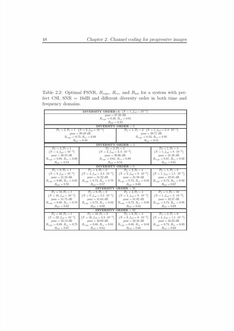
7/29/2019 Adaptive Wireless Multimedia
http://slidepdf.com/reader/full/adaptive-wireless-multimedia 66/187
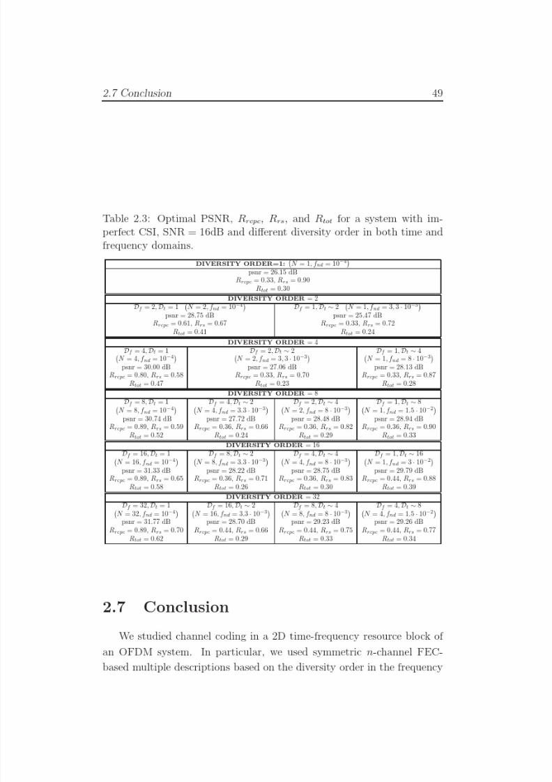
7/29/2019 Adaptive Wireless Multimedia
http://slidepdf.com/reader/full/adaptive-wireless-multimedia 67/187
7/29/2019 Adaptive Wireless Multimedia
http://slidepdf.com/reader/full/adaptive-wireless-multimedia 68/187
50 Chapter 2. Channel coding for progressive images
domain. In the time domain, a concatenation of RCPC codes and CRCcodes was employed to protect individual descriptions. We studied the
performance of the proposed system in a doubly-selective channel with
channel estimation errors. In a slow-fading environment, it was shown as
the frequency diversity order increases, the optimal Rrcpc increases and
the delivered image quality improves accordingly. On the other hand, in a
fast-fading environment, the optimal Rrcpc is relatively insensitive to the
frequency diversity order while the performance is limited by the channel
estimation errors and ICI. It was also illustrated that the advantages of
UEP protection diminishes as the frequency diversity order increases inboth slow and fast fading environment. Thus, since both the optimal
Rrcpc and Rrs vary depending on the channel conditions, a system can
be robust only employing a 2D channel coding adaptable to both time
and frequency diversity orders. Lastly, we illustrated that the bursty
nature of a slow fading environment can lead to a higher application
layer throughput and thereby deliver a better image quality while the
scattered error pattern in a fast fading environment may lead to poor
image quality.
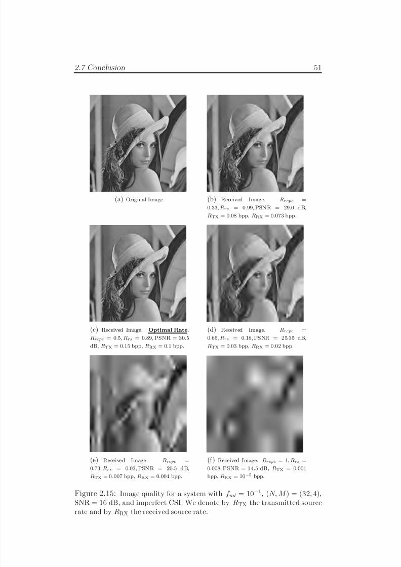
7/29/2019 Adaptive Wireless Multimedia
http://slidepdf.com/reader/full/adaptive-wireless-multimedia 69/187
2.7 Conclusion 51
(a) Original Image. (b) Received Image. Rrcpc =0.33, Rrs = 0.99,PSNR = 29.0 dB,
RTX = 0.08 bpp, RRX = 0.073 bpp.
(c) Received Image. Optimal Rate.
Rrcpc = 0.5, Rrs = 0.89,PSNR = 30.5
dB, RTX = 0.15 bpp, RRX = 0.1 bpp.
(d) Received Image. Rrcpc =
0.66, Rrs = 0.18,PSNR = 25.35 dB,
RTX = 0.03 bpp, RRX = 0.02 bpp.
(e) Received Image. Rrcpc =
0.73, Rrs = 0.03,PSNR = 20.5 dB,
RTX = 0.007 bpp, RRX = 0.004 bpp.
(f) Received Image. Rrcpc = 1,Rrs =
0.008,PSNR = 14.5 dB, RTX = 0.001
bpp, RRX = 10−5 bpp.
Figure 2.15: Image quality for a system with f nd = 10−1
, (N,M ) = (32, 4),SNR = 16 dB, and imperfect CSI. We denote by RTX the transmitted sourcerate and by RRX the received source rate.

7/29/2019 Adaptive Wireless Multimedia
http://slidepdf.com/reader/full/adaptive-wireless-multimedia 70/187
7/29/2019 Adaptive Wireless Multimedia
http://slidepdf.com/reader/full/adaptive-wireless-multimedia 71/187
Chapter 3
Joint source and channelcoding for
motion-compensated fine
granularity scalable video
The previously investigated channel coding optimization is here ex-tended to a joint source and channel coding optimization for video trans-
missions. Cross-layer motion-compensated multiple descriptions coding
for progressive video bitstream is investigated. Based on the diversity
order offered by the channel in both time and frequency domain, the
optimal compression rate and channel code rates are evaluated.
The remainder of the chapter is organized as follows. In Section 3.1, a
description of progressive video bitstreams, together with a brief overview
of the multiple description coding, is reported. In Section 3.2, we providea detailed description of FGS video, considering motion compensation
with leaky prediction. In Section 3.3, we describe OFDM systems and
the channel model considered in our analysis. In Section 3.4, we pro-
vide a framework for the construction of n-channel symmetric motion-
compensated MD coding and we formulate the optimization problem, de-
scribing the rate-distortion evaluation algorithm adopted. In Section 3.5,
we provide simulation results and discussion. Finally, in Section 3.6, we
provide a summary and conclusion.
53
7/29/2019 Adaptive Wireless Multimedia
http://slidepdf.com/reader/full/adaptive-wireless-multimedia 72/187
54 Chapter 3. JSCC for MC-FGS Video
3.1 Motivation and outline of the work
Due to the increasing demand for multimedia services on mobile ter-
minals, and the recent advances in mobile computing, video services are
expected to be widely deployed. Moreover, the rising of Internet and wire-
less communications has widely increased the diffusion of heterogeneity
in multiuser systems, and modern studies are focused on meeting each
user requirement at the same time. To this aim, network-adaptive scal-
able video coding and cross-layer optimization have been under intense
research [56–60]. Note that, in the past, the aim of video coding was theoptimization of the video quality at a given bit rate . The encoder should
compress the video bitstream to a fixed bit rate, less and hopefully close
to the channel capacity, and the decoder should be able to reconstruct
the video source from the received bit rate. However, the channel ca-
pacity is an information not always available, and unknown is also the
bit rate to which optimize the compression. Moreover, due to channel
impairments in wireless transmissions, the received data rate is variable,
resulting to be a function of the channel conditions. Thus, the decoder
has to be able to reconstruct the video from several ranges of received
bit rate. For these reasons, the aim of video coding studies is changed to
optimizing the video quality over a given bit rate range instead of a given
bit rate [61–64], meeting the requirements of heterogenous networks.
Moving Pictures Experts Group (MPEG) has provided scalable video
coding schemes to accommodate the various levels of picture quality de-
pending on the transmission environments and the performances of the
user-level terminals [65], and has also put its considerations in a new ad-
vanced video coding standard with ITU-T for broadcasting and internetmultimedia services [66]. In scalable coding techniques (SNR, temporal
or spatial scalability), adopted in the MPEG-2 for example [67–69], the
compressed bitstream is partitioned into a Base Layer (BL) and an En-
hanced Layer (EL). The main weakness of this layered scalable coding
is that the EL can be either entirely transmitted/received/decoded or
it does not provide any enhancement at all. To address this limitation
of earlier scalable video coding standards, the Fine Granularity Scalable
(FGS) video coding technique was introduced. In addition to the Base
7/29/2019 Adaptive Wireless Multimedia
http://slidepdf.com/reader/full/adaptive-wireless-multimedia 73/187
3.1 Motivation and outline of the work 55
Layer, FGS consists of a single Enhanced Layer encoded in a progressivemanner. Although the BL is encoded at a certain rate RBL, such that the
minimum received bandwidth is higher than RBL (RBL ≤ Rmin), the EL
can be compressed over any desired bit rate range [Rmin, Rmax]. Thanks
to the progressive nature of the enhanced layer, the decoder is able to re-
construct the EL at any received bit rate, i.e., the EL can be truncated at
any arbitrary location. While in scalable video coding the EL is entirely
received or lost, in the FGS, any portion of the EL correctly received im-
proves the quality of the decoded video bitstream. Note that, as deeply
described in the previous chapter, a MD coding improves the robustnessof the system, and so even of the transmitted EL1 [27,70,71]. However,
even considering more reliable transmissions, scalable video standards
still preserve their limit.
Most state-of-the-art video codecs incorporate motion-compensated
prediction (MCP), leading to a higher compression of the source video [58,
60]. With MCP, a single bit error can cause the so called drift prob-
lem, that is the quality degradation due to an error propagation as a
result of predictor mismatch between the encoder and the decoder. In
FGS MPEG-4 coders, the MCP is considered for the BL but not for the
EL, avoiding the drift problem when the EL is lost. The encoded bit-
stream is therefore robust to channel impairments, and the embedded
structure support the adoption of prioritized transport protocol or any
unequal error protection UEP, as in [24, 72]. However, the robustness
of errors propagation is paid by the reduction of compression efficiency.
To overcome this issue, motion compensation was introduced within the
enhanced layer [64,73]. In [73], the authors included the EL layer in the
MCP loop to exploit the remaining (not coded in the base layer) tempo-ral correlation within this layer. The tradeoff between coding gain and
prediction drift is found by varying the portion of the EL included into
the MCP loop. However, MC-FGS suffers from error propagation when
the portion of the EL employed for the prediction is lost. In [64], the
authors proposed a progressive FGS (PFGS) coding scheme by adopting
a separate MCP loop in the embedded EL. To address the drift problem
1We refer the reader to Section 2.3 and Section 2.5 for further details on MDcoding.
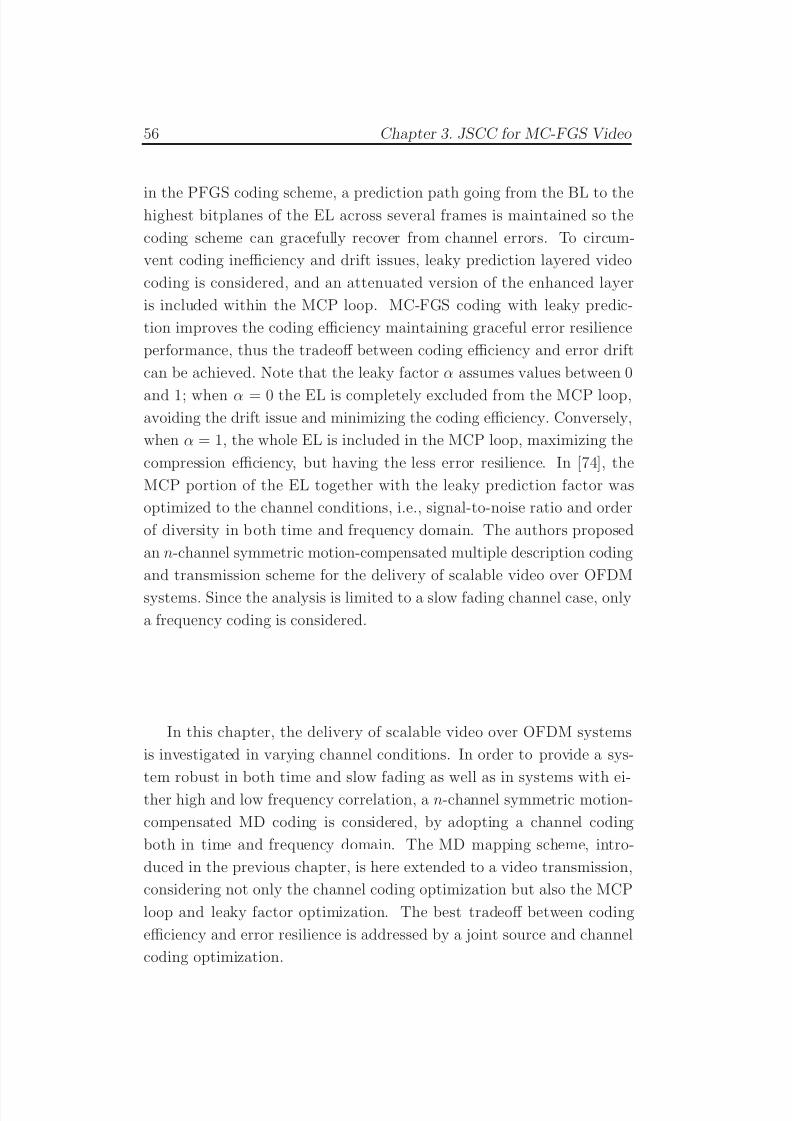
7/29/2019 Adaptive Wireless Multimedia
http://slidepdf.com/reader/full/adaptive-wireless-multimedia 74/187
56 Chapter 3. JSCC for MC-FGS Video
in the PFGS coding scheme, a prediction path going from the BL to thehighest bitplanes of the EL across several frames is maintained so the
coding scheme can gracefully recover from channel errors. To circum-
vent coding inefficiency and drift issues, leaky prediction layered video
coding is considered, and an attenuated version of the enhanced layer
is included within the MCP loop. MC-FGS coding with leaky predic-
tion improves the coding efficiency maintaining graceful error resilience
performance, thus the tradeoff between coding efficiency and error drift
can be achieved. Note that the leaky factor α assumes values between 0
and 1; when α = 0 the EL is completely excluded from the MCP loop,avoiding the drift issue and minimizing the coding efficiency. Conversely,
when α = 1, the whole EL is included in the MCP loop, maximizing the
compression efficiency, but having the less error resilience. In [74], the
MCP portion of the EL together with the leaky prediction factor was
optimized to the channel conditions, i.e., signal-to-noise ratio and order
of diversity in both time and frequency domain. The authors proposed
an n-channel symmetric motion-compensated multiple description coding
and transmission scheme for the delivery of scalable video over OFDM
systems. Since the analysis is limited to a slow fading channel case, only
a frequency coding is considered.
In this chapter, the delivery of scalable video over OFDM systems
is investigated in varying channel conditions. In order to provide a sys-
tem robust in both time and slow fading as well as in systems with ei-ther high and low frequency correlation, a n-channel symmetric motion-
compensated MD coding is considered, by adopting a channel coding
both in time and frequency domain. The MD mapping scheme, intro-
duced in the previous chapter, is here extended to a video transmission,
considering not only the channel coding optimization but also the MCP
loop and leaky factor optimization. The best tradeoff between coding
efficiency and error resilience is addressed by a joint source and channel
coding optimization.
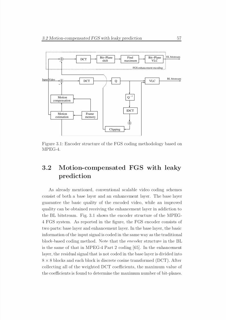
7/29/2019 Adaptive Wireless Multimedia
http://slidepdf.com/reader/full/adaptive-wireless-multimedia 75/187
3.2 Motion-compensated FGS with leaky prediction 57
Input Video
−1
VLC
Clipping
DCT
DCTBit−Plane
shift maximumFind Bit−Plane
VLC
Q
IDCT
estimationFrame
Motioncompensation
Motionmemory
−
−
FGS enhancement encoding
EL bitstream
BL bitstream
Q
Figure 3.1: Encoder structure of the FGS coding methodology based onMPEG-4.
3.2 Motion-compensated FGS with leakyprediction
As already mentioned, conventional scalable video coding schemes
consist of both a base layer and an enhancement layer. The base layer
guarantee the basic quality of the encoded video, while an improved
quality can be obtained receiving the enhancement layer in addiction to
the BL bitstream. Fig. 3.1 shows the encoder structure of the MPEG-
4 FGS system. As reported in the figure, the FGS encoder consists of two parts: base layer and enhancement layer. In the base layer, the basic
information of the input signal is coded in the same way as the traditional
block-based coding method. Note that the encoder structure in the BL
is the same of that in MPEG-4 Part 2 coding [65]. In the enhancement
layer, the residual signal that is not coded in the base layer is divided into
8 × 8 blocks and each block is discrete cosine transformed (DCT). After
collecting all of the weighted DCT coefficients, the maximum value of
the coefficients is found to determine the maximum number of bit-planes.
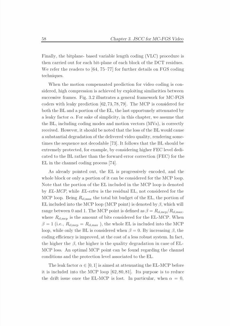
7/29/2019 Adaptive Wireless Multimedia
http://slidepdf.com/reader/full/adaptive-wireless-multimedia 76/187
58 Chapter 3. JSCC for MC-FGS Video
Finally, the bitplane- based variable length coding (VLC) procedure isthen carried out for each bit-plane of each block of the DCT residues.
We refer the readers to [64, 75–77] for further details on FGS coding
techniques.
When the motion compensated prediction for video coding is con-
sidered, high compression is achieved by exploiting similarities between
successive frames. Fig. 3.2 illustrates a general framework for MC-FGS
coders with leaky prediction [62, 73, 78, 79]. The MCP is considered for
both the BL and a portion of the EL, the last opportunely attenuated by
a leaky factor α. For sake of simplicity, in this chapter, we assume that
the BL, including coding modes and motion vectors (MVs), is correctly
received. However, it should be noted that the loss of the BL would cause
a substantial degradation of the delivered video quality, rendering some-
times the sequence not decodable [73]. It follows that the BL should be
extremely protected, for example, by considering higher FEC level dedi-
cated to the BL rather than the forward error correction (FEC) for the
EL in the channel coding process [74].
As already pointed out, the EL is progressively encoded, and thewhole block or only a portion of it can be considered for the MCP loop.
Note that the portion of the EL included in the MCP loop is denoted
by EL-MCP , while EL-extra is the residual EL, not considered for the
MCP loop. Being Rel,max the total bit budget of the EL, the portion of
EL included into the MCP loop (MCP point) is denoted by β , which will
range between 0 and 1. The MCP point is defined as β = Rel,mcp/Rel,max,
where Rel,mcp is the amount of bits considered for the EL-MCP. When
β = 1 (i.e., Rel,mcp = Rel,max ), the whole EL is included into the MCP
loop, while only the BL is considered when β = 0. By increasing β , the
coding efficiency is improved, at the cost of a less robust system. In fact,
the higher the β , the higher is the quality degradation in case of EL-
MCP loss. An optimal MCP point can be found regarding the channel
conditions and the protection level associated to the EL.
The leak factor α ∈ [0, 1] is aimed at attenuating the EL-MCP before
it is included into the MCP loop [62, 80, 81]. Its purpose is to reduce
the drift issue once the EL-MCP is lost. In particular, when α = 0,
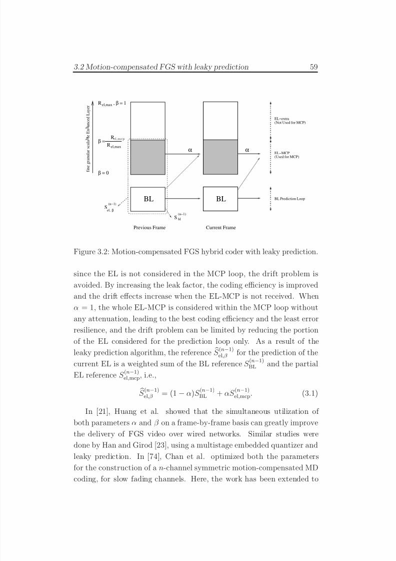
7/29/2019 Adaptive Wireless Multimedia
http://slidepdf.com/reader/full/adaptive-wireless-multimedia 77/187
3.2 Motion-compensated FGS with leaky prediction 59
f i n e g r a n u l a r s c a l a l e E n a n c e d L a y e r
R , β = 1
Rel,max
β =R
S(n−1)
el, β
S(n−1)
bl
EL−extra(Not Used for MCP)
EL−MCP(Used for MCP)
BL Prediction Loop
β = 0
BL
Previous Frame
α α
BL
Current Frame
el,max
el,mcp
Figure 3.2: Motion-compensated FGS hybrid coder with leaky prediction.
since the EL is not considered in the MCP loop, the drift problem is
avoided. By increasing the leak factor, the coding efficiency is improved
and the drift effects increase when the EL-MCP is not received. Whenα = 1, the whole EL-MCP is considered within the MCP loop without
any attenuation, leading to the best coding efficiency and the least error
resilience, and the drift problem can be limited by reducing the portion
of the EL considered for the prediction loop only. As a result of the
leaky prediction algorithm, the reference S (n−1)el,β for the prediction of the
current EL is a weighted sum of the BL reference S (n−1)BL and the partial
EL reference S (n−1)
el,mcp, i.e.,
S (n−
1)el,β = (1 − α)S
(n−
1)BL + αS
(n−
1)el,mcp. (3.1)
In [21], Huang et al. showed that the simultaneous utilization of
both parameters α and β on a frame-by-frame basis can greatly improve
the delivery of FGS video over wired networks. Similar studies were
done by Han and Girod [23], using a multistage embedded quantizer and
leaky prediction. In [74], Chan et al. optimized both the parameters
for the construction of a n-channel symmetric motion-compensated MD
coding, for slow fading channels. Here, the work has been extended to
7/29/2019 Adaptive Wireless Multimedia
http://slidepdf.com/reader/full/adaptive-wireless-multimedia 78/187
60 Chapter 3. JSCC for MC-FGS Video
fast fading channels, providing an optimized scheme robust in severalchannel conditions.
3.3 System model overview
The system model and the channel coding adopted in this chapter
have been already described in the Chapter 2, and they are briefly re-
ported in the following.
3.3.1 Channel model
We assume an OFDM system with an overall bandwidth W T , in which
N independent subchannels can be individuated. Being (∆f )c the coher-
ence bandwith, the number of independent subchannels is evaluated as
N = N t/M , where N t is the number of total subcarriers (spanning a
total bandwidth of W T ) and M is the number of correlated subcarriers
(spanning a total bandwidth of (∆f )c). Frequency diversity by adding
redundancy across the subcarriers can be applied to combat channel er-
rors. Generally, the maximum achievable frequency diversity Df is given
by the ratio between the overall system bandwidth W T and the coherence
bandwidth (∆f )c. In addiction to frequency domain, for time diversity,
channel coding plus interleaving can be used in the time domain. How-
ever, for the technique to be effective, the time frame has to be greater
than the channel coherence time (∆t)c. The maximum time-diversity
gain Dt is given by the ratio between the duration of a time frame and
(∆t)c. In the time domain, a Rayleigh fading is assumed, while in the fre-
quency domain a block fading channel is considered . A modified Jakes’model [39] is considered to simulate different fading rates, resulting in
different time diversity orders.
3.3.2 Time-frequency MD coding
In Section 2.3, the proposed scheme for the transmission of an embed-
ded bitstream over a mobile channel characterized by a doubly selective
environment was described. In the frequency domain, N t = N × M sym-
7/29/2019 Adaptive Wireless Multimedia
http://slidepdf.com/reader/full/adaptive-wireless-multimedia 79/187
3.3 System model overview 61
metric descriptions2
of approximately equal importance are constructedin which contiguous information from the embedded bitstream is spread
across the multiple packets [23, 24]. In the previous chapter the infor-
mation symbols represented the progressively encoded images, now they
represent the progressive EL bits (both the EL-MCP and EL-extra por-
tions). Because of the progressive nature of the encoded bitstream, MD
coding based on the priority of the bits in the bitstream is adopted, and
the optimization of the FEC allocation in the frequency domain is de-
signed to minimize the expected distortion. In the frequency domain,
a (n, k) MDS erasure RS code is adopted, and the code rates are opti-mized based on the importance of the information symbols. In the time
domain, a concatenation of cyclic redundancy check (CRC) codes and
rate-compatible punctured convolutional (RCPC) codes, for possible di-
versity and coding gains, are applied to each description. We recall that
it has been demonstrated the importance of the MD coders optimization
for multimedia transmissions, [59,72–74]. In particular, in [72] (for slow
channels) and in the previous chapter (for both slow and fast channels),
it has been highlighted how the knowledge of the order of diversity of-
fered by the channel greatly improves the system performance for image
transmissions. The FEC profile in the MD coding can be optimized based
on these diversity orders in both time and frequency domain. When the
diversity is available at least in one of the two domains, the system re-
sults to be robust in both slow and fast fading channels. Moreover, in
flat fading conditions, the UEP in the frequency domain is the optimal
FEC allocation, while in highly frequency selective channels, the optimal
FEC staircase merges to an EEP. These considerations were extended to
video source transmissions in [74], for slow fading channels. The FECstaircase in the frequency domain was optimized together with the α
and β parameters for motion-compensated MD coding. In [74], no time
conding was considered, leading to a collapse of the performance with
the increasing of the Doppler. Here, the CRC/RCPC coding is inserted
in the time domain, and both time and frequency coding are optimized
in conjunction to the α and β parameters.
2Note that each description is a single packet, so we shall use the terms “descrip-tion” and “packet” interchangeably throughout the paper.
7/29/2019 Adaptive Wireless Multimedia
http://slidepdf.com/reader/full/adaptive-wireless-multimedia 80/187
62 Chapter 3. JSCC for MC-FGS Video
3.4 Problem formulation
In this section, we describe the optimization problem to be solved, and
we provide some worthy details on methods and parameters useful for the
optimization analysis, as the drift-management and the rate-distortion
curve.
3.4.1 Drift management
As already mentioned, the multiple description stream is insensitive tothe position of losses in the bitstream, and thus it has the desired feature
that the delivery quality is dependent only on the fraction of packets
delivered reliably. Most of the initial works in this area has focused on
the case of N t = 2 descriptions [82, 83]. Then, the case of N t > 2 was
addressed by other authors. In most of these works, one of the main issue
is the error propagation that occurs when there is a mismatch between
encoder and decoder.
Consider a generic 2-channel nonsymmetric MD system which can be
characterized by the quintuple (R1, R2, D(1)1 , D(2)
1 , D2), where R1 and R2
are the bitrates of the two individual descriptions. D(1)1 is the distortion
when description 1 is received, D(2)1 is the distortion when description 2
is received and D2 is the distortion when both descriptions are received.
As a result, there are three possible prediction states at the decoder, cor-
responding to the successful reception of only description 1, only descrip-
tion 2, or both descriptions (decoded by the central decoder). Each of the
three states can form its own prediction loop. Whenever the encoder uses
a predictor that depends on a state not available at the decoder, there willbe a mismatch between the prediction loops at the encoder and decoder.
Similar to single description (SD) MCP coding, this mismatch between
encoder and decoder will trigger error propagation, or drift. To avoid
such mismatch, one can, for example, construct two independent predic-
tion loops, each based on a single-channel reconstruction. At the expense
of decreased compression efficiency, this can completely avoid the mis-
matches for the side decoders, even when one of the two descriptions is
lost [82,84]. For the symmetric counterpart, since the video quality only
7/29/2019 Adaptive Wireless Multimedia
http://slidepdf.com/reader/full/adaptive-wireless-multimedia 81/187
3.4 Problem formulation 63
depends on the number of descriptions received, the two independentprediction loops can be reduced to one. Hence, the symmetric property
significantly reduces the complexity of encoding and decoding. In general,
there are as many as (2n − 1) possible prediction states, while there are
n prediction states for the corresponding symmetric counterpart. How-
ever, when n is large, aside from the complexity issue, the probability
of simultaneous failure of all but one of them is typically small. Hence,
although this approach completely eliminates mismatches, it is not useful
in practice. More importantly, as stated above, mismatch-free or drift-
free approaches generally suffer from poorer compression efficiency [85].Hence, as opposed to the traditional predictive coding paradigm that sys-
tems should not be designed to allow drift/mismatch, there is a growing
interest in predictive coding schemes (both SD and MD) that attempt
to allow some drift/mismatch so as to improve the overall compression
efficiency. This is called the drift-managed approach [58, 62, 86–89]. A
drift-managed approach does not preclude drift in the prediction strat-
egy. Instead, it allows drift/mismatch to be introduced incrementally,
and encompasses drift-free as a special case. In other words, a drift-
managed approach optimizes the system performance by trading off the
compression efficiency and the amount of mismatch, allowing the drift-
free solution to emerge when it is optimal.
The design paradigm can be applied to the construction of n-channel
symmetric motion-compensated MD codes. One can, for example, assign
m ∈ [0, n] descriptions as a reference for the temporal prediction, where
m = 0 corresponds to the drift-free case. Note that if the number of re-
ceived descriptions m′ < m, there will be a mismatch. Generally, a higherprediction efficiency can be achieved by using a larger m. However, this
comes at a price of greater probability of mismatch. More importantly,
although the number of descriptions to be included for the MCP has
often been thought as a fine-tuning method for trading off compression
and error resilience, and allowing drift to be introduced incrementally
(see [87], Section III-G]), the correlation among the subcarriers/channels
may make this less effective. For instance, if M out of n descriptions are
delivered through M highly correlated channels, i.e., systems with low
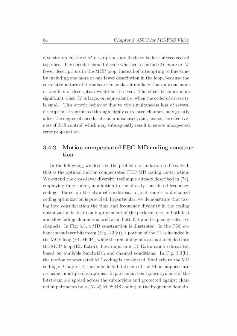
7/29/2019 Adaptive Wireless Multimedia
http://slidepdf.com/reader/full/adaptive-wireless-multimedia 82/187
64 Chapter 3. JSCC for MC-FGS Video
diversity order, these M descriptions are likely to be lost or received alltogether. The encoder should decide whether to include M more or M
fewer descriptions in the MCP loop, instead of attempting to fine-tune
by including one more or one fewer description in the loop, because the
correlated nature of the subcarriers makes it unlikely that only one more
or one less of description would be received. The effect becomes more
significant when M is large, or, equivalently, when the order of diversity
is small. This erratic behavior due to the simultaneous loss of several
descriptions transmitted through highly correlated channels may greatly
affect the degree of encoder-decoder mismatch, and, hence, the effective-ness of drift control, which may subsequently result in severe unexpected
error propagation.
3.4.2 Motion-compensated FEC-MD coding construc-
tion
In the following, we describe the problem formulation to be solved,
that is the optimal motion compensated FEC-MD coding construction.
We extend the cross-layer diversity technique already described in [74],
employing time coding in addition to the already considered frequency
coding. Based on the channel conditions, a joint source and channel
coding optimization is provided. In particular, we demonstrate that tak-
ing into consideration the time and frequency diversity in the coding
optimization leads to an improvement of the performance, in both fast
and slow fading channels as well as in both flat and frequency selective
channels. In Fig. 3.3, a MD construction is illustrated. In the FGS en-
hancement layer bitstream (Fig. 3.3(a)), a portion of the EL is included inthe MCP loop (EL-MCP), while the remaining bits are not included into
the MCP loop (EL-Extra). Less important EL-Extra can be discarded,
based on available bandwidth and channel conditions. In Fig. 3.3(b),
the motion compensated MD coding is considered. Similarly to the MD
coding of Chapter 2, the embedded bitstream of the EL is mapped into
n-channel multiple descriptions. In particular, contiguous symbols of the
bitstream are spread across the subcarriers and protected against chan-
nel impairments by a (N t, k) MDS RS coding in the frequency domain,
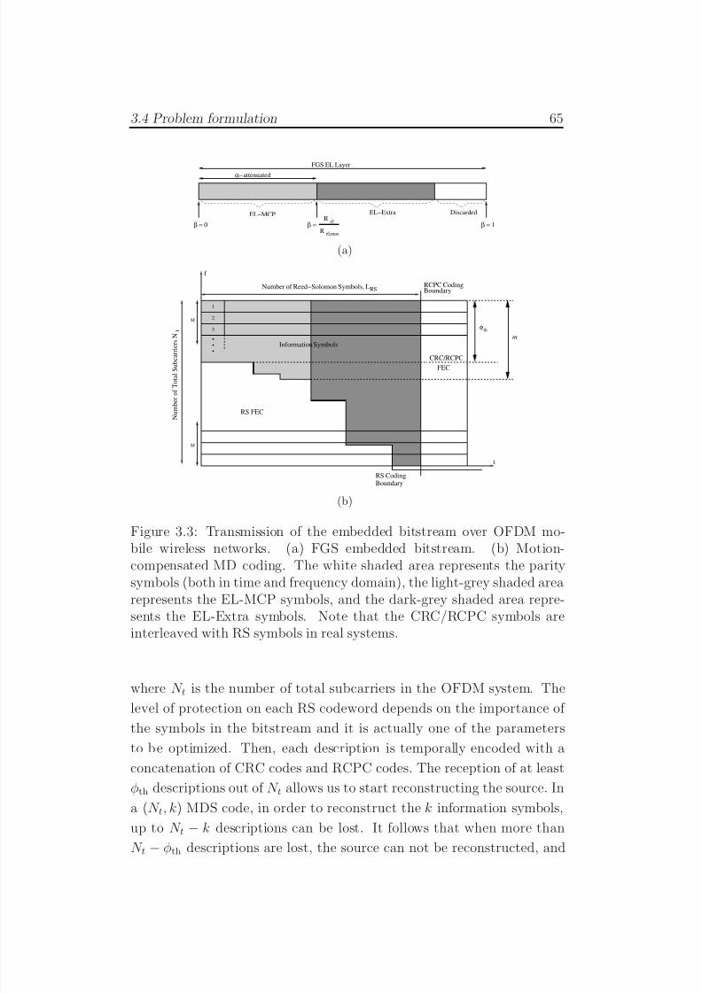
7/29/2019 Adaptive Wireless Multimedia
http://slidepdf.com/reader/full/adaptive-wireless-multimedia 83/187
3.4 Problem formulation 65
EL−MCPel
R el,max
β =
α−attenuated
β = 0 β = 1
FGS EL Layer
EL−Extra DiscardedR
(a)
Number of Reed−Solomon Symbols, L
f
t
RCPC CodingBoundary
N u m b e r o f T o t a l S u b c a r r i e
r s N t
. . .
CRC/RCPC
FEC
M
M
RS CodingBoundary
. . .3
2
1
RS FEC
φ th
m
RS
Information Symbols
(b)
Figure 3.3: Transmission of the embedded bitstream over OFDM mo-bile wireless networks. (a) FGS embedded bitstream. (b) Motion-compensated MD coding. The white shaded area represents the paritysymbols (both in time and frequency domain), the light-grey shaded arearepresents the EL-MCP symbols, and the dark-grey shaded area repre-sents the EL-Extra symbols. Note that the CRC/RCPC symbols areinterleaved with RS symbols in real systems.
where N t is the number of total subcarriers in the OFDM system. Thelevel of protection on each RS codeword depends on the importance of
the symbols in the bitstream and it is actually one of the parameters
to be optimized. Then, each description is temporally encoded with a
concatenation of CRC codes and RCPC codes. The reception of at least
φth descriptions out of N t allows us to start reconstructing the source. In
a (N t, k) MDS code, in order to reconstruct the k information symbols,
up to N t − k descriptions can be lost. It follows that when more than
N t − φth descriptions are lost, the source can not be reconstructed, and
7/29/2019 Adaptive Wireless Multimedia
http://slidepdf.com/reader/full/adaptive-wireless-multimedia 84/187
66 Chapter 3. JSCC for MC-FGS Video
all the EL of the transmitted frame is discarded. In Fig. 3.3(b), M is thenumber of highly correlated subcarriers3, and N is the number of inde-
pendent subbands in the frequency domain such that N t = N × M . The
white area represents the parity symbols for both CRC/RCPC codes and
RS codes. It should be noted that, in actual systems, RS symbols and
RCPC parity symbols of each description would be interleaved. How-
ever, for illustration, we show the de-interleaved version throughout the
chapter so that the relative amounts of RCPC parity symbols and RS
symbols can be clearly indicated. Unlike the MD coding with no motion
compensation, the information symbols are here classified into EL-MCP(light-grey shaded area), used for the MCP loop at the decoder, and EL-
Extra (dark-grey shaded area) carrying information for enhancing the
video without being included into the MCP loop. Note that, since the
leaky prediction is considered, the EL-MCP symbols are α-attenuated
before being included into the MCP loop. Denoting by m the minimum
number of descriptions to be received for reconstructing the EL-MCP, the
reception of m′ < m descriptions leads to an encoder-decoder mismatch.
The quality degradation caused by the mismatch depends on the number
of EL-MCP descriptions missed, as well as the leaky factor considered
in the coding. Intuitively, the mismatch is proportional to α( S m − S m′),
where S m and S m′ are the reconstructed frame using m and m′ received
descriptions.
Mathematically, the optimization for the construction of n-channel
symmetric motion-compensated MDs is formulated as follows. Consider
N i.i.d. subbands, each with M subcarriers and packet size equal to
LRS code symbols before channel coding in the time domain. Since each
vertical column corresponds to one RS codeword, before the time cod-ing there are altogether LRS RS codewords. The constraint on the bit
budget/packet can then be written as
(LRS × N tot × BRS + BCRC )/Rrcpc ≤ Btot, (3.2)
where BCRC is the bit budget allocated for the CRC codes and Rrcpc is
the channel code rate of the RCPC codes. BRS is the number of bits-per-
3We recall that a block fading model is considered for the channel in the frequencydomain.
7/29/2019 Adaptive Wireless Multimedia
http://slidepdf.com/reader/full/adaptive-wireless-multimedia 85/187
3.4 Problem formulation 67
RS symbol and Btot is the total bit budget of the OFDM resource block(RB).
We assume that for the RS codeword l, where l ∈ [1, LRS ], cl code
symbols are assigned to information data symbols, therefore, f l = N t− cl
are the FEC symbols. The reception of m′ > φth descriptions leads
to a reconstruction of the source with distortion D(Rm′), where Rm′
is the allocated bit budget for the information symbols in the first m′
descriptions,
Rm′ = l:cl≤m′
cl
×BRS . (3.3)
Hence, the overall RS channel code rate equals Rrs = RN t/(N t × LRS ×BRS ). Given the source code rate-distortion curve D(•) and the packet
loss probability mass function P J ( j), where j = N t − m′ is the number
of lost packets, we can minimize the expected distortion as follows
E ∗[D] = mincl,Rrcpc,β,α
N t−φth j=0
P J ( j)D(RN t− j , β , α) +N t
j=N t−φth+1
P J ( j)DBL
,
(3.4)
subject to the constraint on the overall bit budget
RN t/Rrs + BCRC
Rrcpc
≤ Btot (3.5)
where DBL corresponds to the distortion when fewer than φth descrip-
tions are received and only the BL is decoded in the current frame. It is
worth noting the tradeoff between reliability and throughput. Given the
constraint (3.5), lowering Rrs and/or Rrcpc will cope with channel impair-
ments, but it will lead to a reduction of RN t, that is the number of totalinformation symbols transmitted within the resource block (RB). The
packet loss probability mass function P J ( j) depends on (∆f )c, (∆t)c
and Rrcpc. Although P J ( j) can be found analytically for uncorrelated
fading channels, due to the correlated fading in both time and frequency
domains of the mobile environment considered here, we use simulations
to find P J ( j). Different algorithms can be considered for solving the opti-
mization problem [90–93], here, we use the iterative procedure described
in [24] due to its simplicity. We set the parameter Q = N t for a full
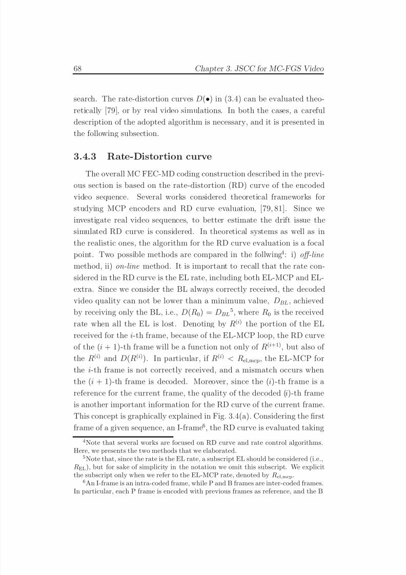
7/29/2019 Adaptive Wireless Multimedia
http://slidepdf.com/reader/full/adaptive-wireless-multimedia 86/187
68 Chapter 3. JSCC for MC-FGS Video
search. The rate-distortion curves D(•) in (3.4) can be evaluated theo-retically [79], or by real video simulations. In both the cases, a careful
description of the adopted algorithm is necessary, and it is presented in
the following subsection.
3.4.3 Rate-Distortion curve
The overall MC FEC-MD coding construction described in the previ-
ous section is based on the rate-distortion (RD) curve of the encoded
video sequence. Several works considered theoretical frameworks for
studying MCP encoders and RD curve evaluation, [79, 81]. Since we
investigate real video sequences, to better estimate the drift issue the
simulated RD curve is considered. In theoretical systems as well as in
the realistic ones, the algorithm for the RD curve evaluation is a focal
point. Two possible methods are compared in the follwing4: i) off-line
method, ii) on-line method. It is important to recall that the rate con-
sidered in the RD curve is the EL rate, including both EL-MCP and EL-
extra. Since we consider the BL always correctly received, the decoded
video quality can not be lower than a minimum value, DBL, achievedby receiving only the BL, i.e., D(R0) = DBL
5, where R0 is the received
rate when all the EL is lost. Denoting by R(i) the portion of the EL
received for the i-th frame, because of the EL-MCP loop, the RD curve
of the (i + 1)-th frame will be a function not only of R(i+1), but also of
the R(i) and D(R(i)). In particular, if R(i) < Rel,mcp, the EL-MCP for
the i-th frame is not correctly received, and a mismatch occurs when
the (i + 1)-th frame is decoded. Moreover, since the (i)-th frame is a
reference for the current frame, the quality of the decoded (i)-th frame
is another important information for the RD curve of the current frame.This concept is graphically explained in Fig. 3.4(a). Considering the first
frame of a given sequence, an I-frame6, the RD curve is evaluated taking
4Note that several works are focused on RD curve and rate control algorithms.Here, we presents the two methods that we elaborated.
5Note that, since the rate is the EL rate, a subscript EL should be considered (i.e.,REL), but for sake of simplicity in the notation we omit this subscript. We explicitthe subscript only when we refer to the EL-MCP rate, denoted by Rel,mcp.
6An I-frame is an intra-coded frame, while P and B frames are inter-coded frames.In particular, each P frame is encoded with previous frames as reference, and the B
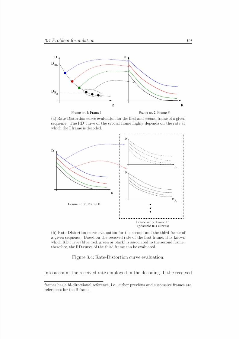
7/29/2019 Adaptive Wireless Multimedia
http://slidepdf.com/reader/full/adaptive-wireless-multimedia 87/187
3.4 Problem formulation 69
Frame nr. 1: Frame I
BL
DRel
D
R
D
R
Frame nr. 2: Frame P
D
(a) Rate-Distortion curve evaluation for the first and second frame of a givensequence. The RD curve of the second frame highly depends on the rate atwhich the I frame is decoded.
(possible RD curves)
D
R
D
R
D
R
.
.
.
Frame nr. 2: Frame P
Frame nr. 3: Frame P
(b) Rate-Distortion curve evaluation for the second and the third frame of
a given sequence. Based on the received rate of the first frame, it is knownwhich RD curve (blue, red, green or black) is associated to the second frame,therefore, the RD curve of the third frame can be evaluated.
Figure 3.4: Rate-Distortion curve evaluation.
into account the received rate employed in the decoding. If the received
frames has a bi-directional reference, i.e., either previous and successive frames arereferences for the B frame.
7/29/2019 Adaptive Wireless Multimedia
http://slidepdf.com/reader/full/adaptive-wireless-multimedia 88/187
70 Chapter 3. JSCC for MC-FGS Video
rate is greater than the EL-MCP rate (R(1)
≥ Rel,mcp), no mismatch willoccur during the decoding of the second frame. In this case, the amount
of bits received for the first frame does not influence the evaluation of the
RD of the second one (black RD curve). Conversely, when R(1) < Rel,mcp,
the bit budget received for the first frame is a required information for
the evaluation of the RD curve of the second frame. It is important to
know how much drift occurs during decoding process (blue, red or orange
curve). When the third frame is considered (Fig. 3.4(b)), the RD curve
evaluation depends on R(3), R(2), and R(1), or analogously, on R(3), R(2),
and D(R(2)). In fact, it is important to know if the second frame, used asreference for the third one, is drift-free. It follows that, for the evaluation
of the D(R(3)), it is important to know if a mismatch occurs during the
third frame decoding, but also if one was experienced in the past frames.
More generally, the rate distortion curve for the (i + 1)-th frame de-
pends on the rate vector [R1, R2, . . . , R(i+1)], or equivalently, it depends
on (R(i+1), R(i), D(R(i))), since the distortion of the i-th frame has an
implicit dependency on the rates of the previous frames.
Therefore, it is understandable that the RD curve evaluation of an
entire sequence is extremely complex and onerous from a computational
point of view, and a simplification has to be considered. In [74], the
authors based the FEC staircase on an average rate distortion curve, or
off-line method, graphically described in Fig. 3.5(a). In this algorithm,
first the mean RD curve is evaluated for the entire sequence, then the
optimal FEC level for the 2D RB is investigated. Since the FEC op-
timization is based on the same RD curve for each frame, the off-line
method leads to a single FEC staircase for the whole sequence. To eval-
uate the average RD curve, the received rate is assumed constant for theentire video, and the distortion values of all the frames are averaged, i.e.,
D =1
GOP
GOP k=1
D
R(k)i
.
Since each frame experiences its own channel noise and fading level,
the correctly received rate might me variable from one frame to another.
Moreover, the complexity level may vary from one frame to another one,
leading to extremely different RD curves within the sequence. Thus,
7/29/2019 Adaptive Wireless Multimedia
http://slidepdf.com/reader/full/adaptive-wireless-multimedia 89/187
3.4 Problem formulation 71
OptimizationGOP
12
.
.
.
averageRD curve
E[D]
RS FEC
staircase
RD CurveEvaluation
FEC Level
(a) off-line method
Previous frame rate
RD curve
RS FECstaircase
E[D]
E[R]
i−th frameRD Curve
Evaluation OptimizationFEC Level
i−th frame
Previous frame distortion
(b) on-line method
Figure 3.5: RD curve evaluation methods.
considering the received rate constant for all the frames might be a too
rough assumption, most of all when a fast fading channel is considered.
However, the approximation error introduced by this method is well-balanced by the gain in simplicity of the off-line method, that results
to be extremely quick and not expensive from a computational point of
view.
The second algorithm for the evaluation of the RD curve, reported
in Fig. 3.5(b), is aimed at being a tradeoff between the simplicity of the
mean RD curve method and the accuracy of the exact method. Un-
like the off-line method, the RD curve and the optimized FEC level are
evaluated for each frame. In particular, the expected distortion and theexpected rate, evaluated during the FEC optimization step of the (i−1)-
th frame, are assumed to be the received rate and the decoded quality for
the previous frame, when the RD curve is evaluated for the i-th frame.
As expected, the first frame will be an I-frame, and the feedback from
the FEC optimization block will not be considered. It means that, in
this algorithm, the RD function evaluation is not run off-line before the
channel coding optimization process, but it is one of the two steps jointly
considered in the overall optimization process for each frame. Rather
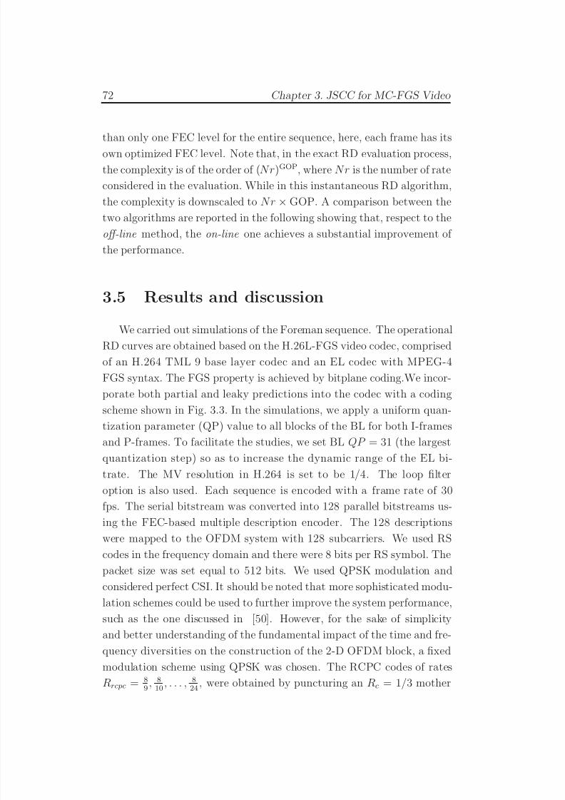
7/29/2019 Adaptive Wireless Multimedia
http://slidepdf.com/reader/full/adaptive-wireless-multimedia 90/187
72 Chapter 3. JSCC for MC-FGS Video
than only one FEC level for the entire sequence, here, each frame has itsown optimized FEC level. Note that, in the exact RD evaluation process,
the complexity is of the order of (Nr)GOP, where Nr is the number of rate
considered in the evaluation. While in this instantaneous RD algorithm,
the complexity is downscaled to Nr × GOP. A comparison between the
two algorithms are reported in the following showing that, respect to the
off-line method, the on-line one achieves a substantial improvement of
the performance.
3.5 Results and discussion
We carried out simulations of the Foreman sequence. The operational
RD curves are obtained based on the H.26L-FGS video codec, comprised
of an H.264 TML 9 base layer codec and an EL codec with MPEG-4
FGS syntax. The FGS property is achieved by bitplane coding.We incor-
porate both partial and leaky predictions into the codec with a coding
scheme shown in Fig. 3.3. In the simulations, we apply a uniform quan-
tization parameter (QP) value to all blocks of the BL for both I-frames
and P-frames. To facilitate the studies, we set BL QP = 31 (the largest
quantization step) so as to increase the dynamic range of the EL bi-
trate. The MV resolution in H.264 is set to be 1/4. The loop filter
option is also used. Each sequence is encoded with a frame rate of 30
fps. The serial bitstream was converted into 128 parallel bitstreams us-
ing the FEC-based multiple description encoder. The 128 descriptions
were mapped to the OFDM system with 128 subcarriers. We used RS
codes in the frequency domain and there were 8 bits per RS symbol. Thepacket size was set equal to 512 bits. We used QPSK modulation and
considered perfect CSI. It should be noted that more sophisticated modu-
lation schemes could be used to further improve the system performance,
such as the one discussed in [50]. However, for the sake of simplicity
and better understanding of the fundamental impact of the time and fre-
quency diversities on the construction of the 2-D OFDM block, a fixed
modulation scheme using QPSK was chosen. The RCPC codes of rates
Rrcpc = 89
, 810
, . . . , 824
, were obtained by puncturing an Rc = 1/3 mother

7/29/2019 Adaptive Wireless Multimedia
http://slidepdf.com/reader/full/adaptive-wireless-multimedia 91/187
3.5 Results and discussion 73
0 10 20 30 40 50 6025
30
35
40
45
50
EL Bitrate, kbps
P S N R − Y , d B
β=0.02, REL,MCP
=1.31 kbps
β=0.30, REL,MCP
=19.96 kbps
β=0.45, REL,MCP
=29.49 kbps
β=0.65, REL,MCP
=42.59 kbps
Figure 3.6: Rate-Distortion function for the MC-FGS with various MCPvalues (β ), without leaky prediction (α = 1), and with no time coding(Rrcpc = 1).
code with K = 7, p = 8 and generator polynomials (133, 165, 171)octal
with the puncturing table given in [51]. The decoded quality is reported
in terms of PSNR of the luminance, i.e., PSNR-Y 10log10(2552/MSE2).
We begin showing the mean rate-distortion curve, to make the reader
understand the importance of receiving the motion compensated loop.
Then, a comparison between the two proposed algorithms are reported,
showing that the on-line method achieves a substantial improvement in
the PSNR quality. Finally, we evaluate the luminance PSNR for several
levels of mobility (i.e., several orders of diversity in the time domain) and
numbers of correlated subcarriers (i.e., several order of diversity in the
frequency domain), to make understand the importance of an optimiza-
tion not only of the α and β parameters, but also of the code rate in the
time domain.
In Fig. 3.6, the average RD function vs. the EL-MCP rate is reported
for a sequence encoded with several EL-MCP values, and without leaky
prediction. No time coding is considered in this first plot. In the figure,
the x-axis corresponds to the received (decoding) bit rates of the EL. It
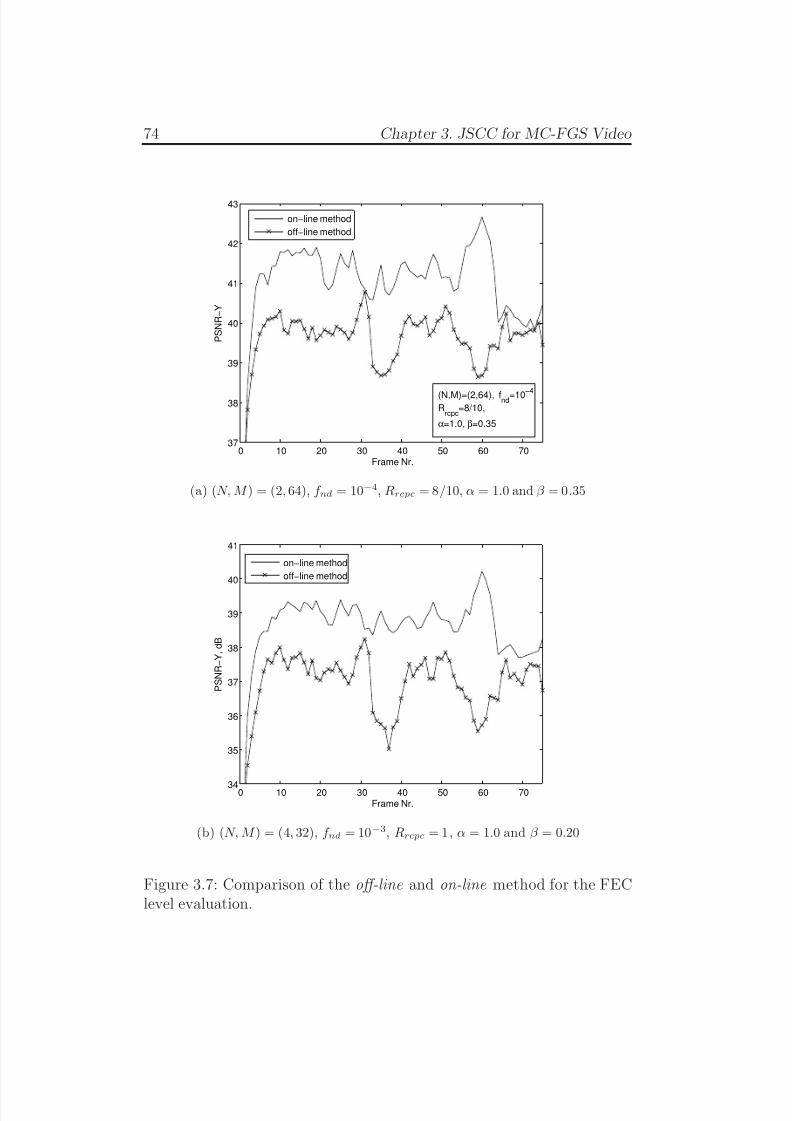
7/29/2019 Adaptive Wireless Multimedia
http://slidepdf.com/reader/full/adaptive-wireless-multimedia 92/187
74 Chapter 3. JSCC for MC-FGS Video
0 10 20 30 40 50 60 7037
38
39
40
41
42
43
Frame Nr.
P S N R − Y
on−line method
off−line method
(N,M)=(2,64), fnd=10−4
Rrcpc
=8/10,
α=1.0, β=0.35
(a) (N,M ) = (2, 64), f nd = 10−4, Rrcpc = 8/10, α = 1.0 and β = 0.35
0 10 20 30 40 50 60 7034
35
36
37
38
39
40
41
Frame Nr.
P S N R − Y , d B
on−line method
off−line method
(b) (N,M ) = (4, 32), f nd = 10−3, Rrcpc = 1, α = 1.0 and β = 0.20
Figure 3.7: Comparison of the off-line and on-line method for the FEClevel evaluation.
7/29/2019 Adaptive Wireless Multimedia
http://slidepdf.com/reader/full/adaptive-wireless-multimedia 93/187
3.5 Results and discussion 75
can be noted that sequences encoded with higher β values achieve a goodgain in the decoded quality (high PSNR) when the received EL rate is
greater than the EL-MCP rate. For example, compare the sequence with
β = 0.02 (Rel,mcp = 1.30 kps) with the curve β = 0.65 (Rel,mcp = 42.598
kps). If the bitbudget received in the EL is greater than the EL-MCP,
for example equal to 44 kbps, the gain achieved by using Rel,mcp = 42.598
kps rather than Rel,mcp = 1.30 kps is almost 4 dB. Unfortunately, when
the EL-MCP is not received, a mismatch in the predictors of the encoder
and decoder occurs, leading to a substantial drop in PSNR performance,
as shown in the plots. In the example, considering a received rate of 10 − 20 kbps, the Rel,mcp = 1.30 kps curve outperforms the one with
β = 0.65.
In Fig. 3.7, the off-line method for the RD curve evaluation is com-
pared to the on-line one. In Fig. 3.7(a), a channel with (N, M ) = (2, 64),
f nd = 10−4 is considered for the transmission of a sequence encoded with
β = 0.35 and α = 1, and mapped into a RB with a RCPC code rate equal
to 8/10. Conversely, in Fig. 3.7(b), a system with different order of diver-
sity and channel code rates is considered. In particular, (N, M ) = (4, 32),f nd = 10−3, β = 0.20, α = 1, and Rrcpc = 1. In both the figures, the
PSNR for each decoded frame of the sequence is provided. Even with
different system conditions, the on-line method achieves a satisfying gain
respect to the off-line RD curve evaluation. Since the latter method in-
troduces an approximation, an outperforming of the on-line method was
expected, but, the most interesting observation is that it is achieved a
gain of the order of 3 dB or even more. Thus, the drop in terms of PSNR
due to the assumption of an off-line method rather than the on-line one
is substantial and it can not be ignored. Therefore, in the following theon-line method is considered for the evaluation of the RD curve and
the FEC allocation optimization. In Fig. 3.8, the averaged RD curve
(Fig. 3.8(a)) and the optimal FEC allocation (Fig. 3.8(b)) are reported
for the two methods. Note how the rough approximation in considering
a mean RD curve rather than the instantaneous one leads to a different
protection level between the two methods.
In Fig. 3.9, we show the optimized construction of RS information
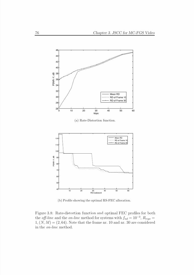
7/29/2019 Adaptive Wireless Multimedia
http://slidepdf.com/reader/full/adaptive-wireless-multimedia 94/187
76 Chapter 3. JSCC for MC-FGS Video
0 10 20 30 40 50 6026
28
30
32
34
36
38
40
42
44
46
kbps
P S N R − Y , d B
Mean RD
RD of Frame 10
RD of Frame 30
(a) Rate-Distortion function.
10 20 30 40 50 6040
50
60
70
80
90
100
110
120
RS Codeword
P S N R −
Y ,
d B
Mean RD
RD of Frame 10
RD of Frame 30
(b) Profile showing the optimal RS-FEC allocation.
Figure 3.8: Rate-distortion function and optimal FEC profiles for boththe off-line and the on-line method for systems with f nd = 10−3, Rrcpc =1, (N, M ) = (2, 64). Note that the frame nr. 10 and nr. 30 are consideredin the on-line method.
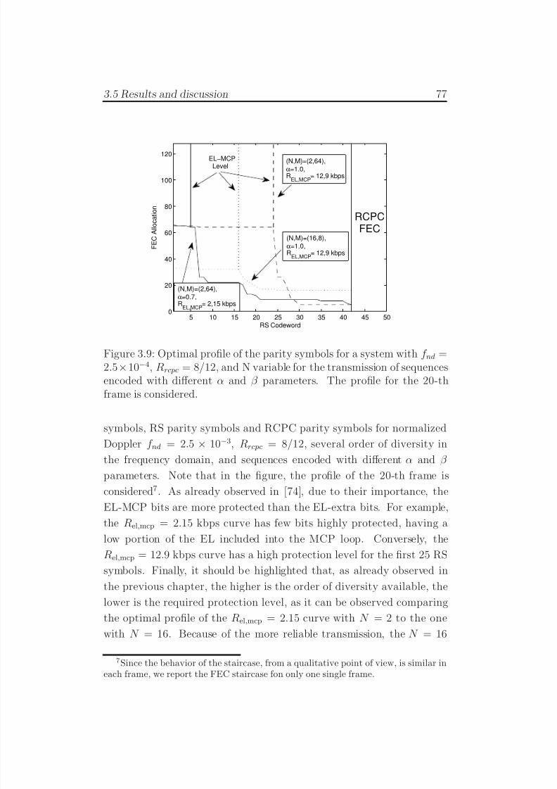
7/29/2019 Adaptive Wireless Multimedia
http://slidepdf.com/reader/full/adaptive-wireless-multimedia 95/187
3.5 Results and discussion 77
5 10 15 20 25 30 35 40 45 500
20
40
60
80
100
120
RS Codeword
F E C
A l l o c a t i o n
RCPCFEC
(N,M)=(2,64),
α=1.0,R
EL,MCP= 12,9 kbps
(N,M)=(16,8),
α=1.0,R
EL,MCP= 12,9 kbps
(N,M)=(2,64),
α=0.7,R
EL,MCP= 2,15 kbps
EL−MCPLevel
Figure 3.9: Optimal profile of the parity symbols for a system with f nd =2.5×10⁻⁴, Rrcpc = 8/12, and N variable for the transmission of sequencesencoded with different α and β parameters. The profile for the 20-thframe is considered.
symbols, RS parity symbols and RCPC parity symbols for normalized
Doppler f nd = 2.5 × 10⁻³, Rrcpc = 8/12, several order of diversity in
the frequency domain, and sequences encoded with different α and β
parameters. Note that in the figure, the profile of the 20-th frame is
considered7. As already observed in [74], due to their importance, the
EL-MCP bits are more protected than the EL-extra bits. For example,
the Rel,mcp = 2.15 kbps curve has few bits highly protected, having a
low portion of the EL included into the MCP loop. Conversely, the
Rel,mcp = 12.9 kbps curve has a high protection level for the first 25 RSsymbols. Finally, it should be highlighted that, as already observed in
the previous chapter, the higher is the order of diversity available, the
lower is the required protection level, as it can be observed comparing
the optimal profile of the Rel,mcp = 2.15 curve with N = 2 to the one
with N = 16. Because of the more reliable transmission, the N = 16
7Since the behavior of the staircase, from a qualitative point of view, is similar ineach frame, we report the FEC staircase fon only one single frame.
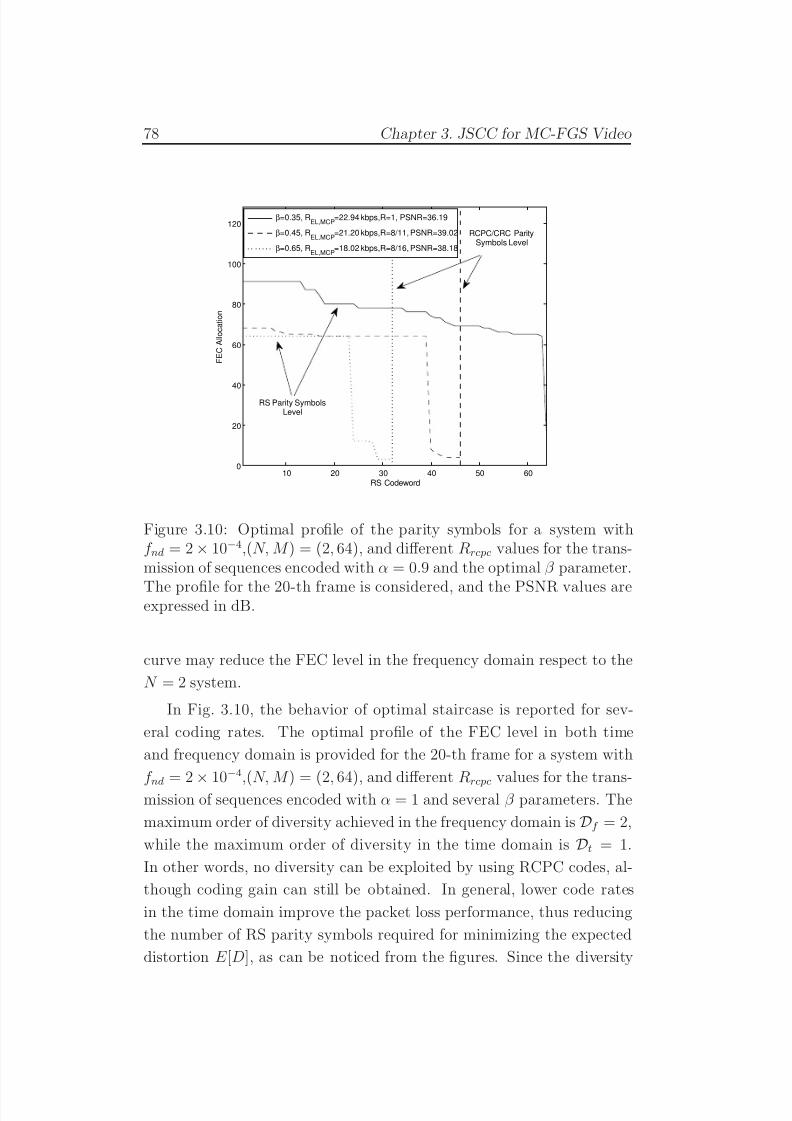
7/29/2019 Adaptive Wireless Multimedia
http://slidepdf.com/reader/full/adaptive-wireless-multimedia 96/187
78 Chapter 3. JSCC for MC-FGS Video
10 20 30 40 50 600
20
40
60
80
100
120
RS Codeword
F E C
A l l o c a t i o n
β=0.35, REL,MCP
=22.94 kbps,R=1, PSNR=36.19
β=0.45, REL,MCP
=21.20 kbps,R=8/11, PSNR=39.02
β=0.65, REL,MCP
=18.02 kbps,R=8/16, PSNR=38.18
RCPC/CRC ParitySymbols Level
RS Parity SymbolsLevel
Figure 3.10: Optimal profile of the parity symbols for a system withf nd = 2 × 10⁻⁴,(N, M ) = (2, 64), and different Rrcpc values for the trans-mission of sequences encoded with α = 0.9 and the optimal β parameter.
The profile for the 20-th frame is considered, and the PSNR values areexpressed in dB.
curve may reduce the FEC level in the frequency domain respect to the
N = 2 system.
In Fig. 3.10, the behavior of optimal staircase is reported for sev-
eral coding rates. The optimal profile of the FEC level in both time
and frequency domain is provided for the 20-th frame for a system with
f nd = 2 × 10⁻⁴
,(N, M ) = (2, 64), and different Rrcpc values for the trans-mission of sequences encoded with α = 1 and several β parameters. The
maximum order of diversity achieved in the frequency domain is Df = 2,
while the maximum order of diversity in the time domain is Dt = 1.
In other words, no diversity can be exploited by using RCPC codes, al-
though coding gain can still be obtained. In general, lower code rates
in the time domain improve the packet loss performance, thus reducing
the number of RS parity symbols required for minimizing the expected
distortion E [D], as can be noticed from the figures. Since the diversity
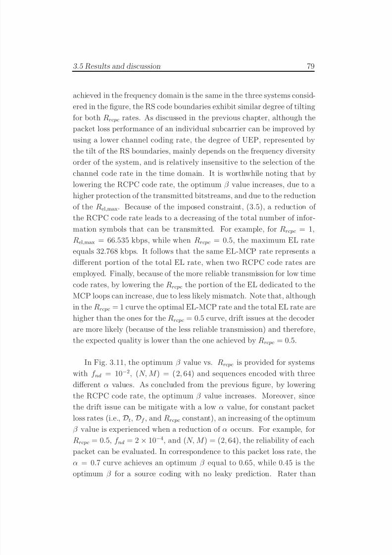
7/29/2019 Adaptive Wireless Multimedia
http://slidepdf.com/reader/full/adaptive-wireless-multimedia 97/187
3.5 Results and discussion 79
achieved in the frequency domain is the same in the three systems consid-ered in the figure, the RS code boundaries exhibit similar degree of tilting
for both Rrcpc rates. As discussed in the previous chapter, although the
packet loss performance of an individual subcarrier can be improved by
using a lower channel coding rate, the degree of UEP, represented by
the tilt of the RS boundaries, mainly depends on the frequency diversity
order of the system, and is relatively insensitive to the selection of the
channel code rate in the time domain. It is worthwhile noting that by
lowering the RCPC code rate, the optimum β value increases, due to a
higher protection of the transmitted bitstreams, and due to the reductionof the Rel,max. Because of the imposed constraint, (3.5), a reduction of
the RCPC code rate leads to a decreasing of the total number of infor-
mation symbols that can be transmitted. For example, for Rrcpc = 1,
Rel,max = 66.535 kbps, while when Rrcpc = 0.5, the maximum EL rate
equals 32.768 kbps. It follows that the same EL-MCP rate represents a
different portion of the total EL rate, when two RCPC code rates are
employed. Finally, because of the more reliable transmission for low time
code rates, by lowering the Rrcpc the portion of the EL dedicated to the
MCP loops can increase, due to less likely mismatch. Note that, although
in the Rrcpc = 1 curve the optimal EL-MCP rate and the total EL rate are
higher than the ones for the Rrcpc = 0.5 curve, drift issues at the decoder
are more likely (because of the less reliable transmission) and therefore,
the expected quality is lower than the one achieved by Rrcpc = 0.5.
In Fig. 3.11, the optimum β value vs. Rrcpc is provided for systems
with f nd = 10−2, (N, M ) = (2, 64) and sequences encoded with three
different α values. As concluded from the previous figure, by loweringthe RCPC code rate, the optimum β value increases. Moreover, since
the drift issue can be mitigate with a low α value, for constant packet
loss rates (i.e., Dt, Df , and Rrcpc constant), an increasing of the optimum
β value is experienced when a reduction of α occurs. For example, for
Rrcpc = 0.5, f nd = 2 × 10⁻⁴, and (N, M ) = (2, 64), the reliability of each
packet can be evaluated. In correspondence to this packet loss rate, the
α = 0.7 curve achieves an optimum β equal to 0.65, while 0.45 is the
optimum β for a source coding with no leaky prediction. Rater than
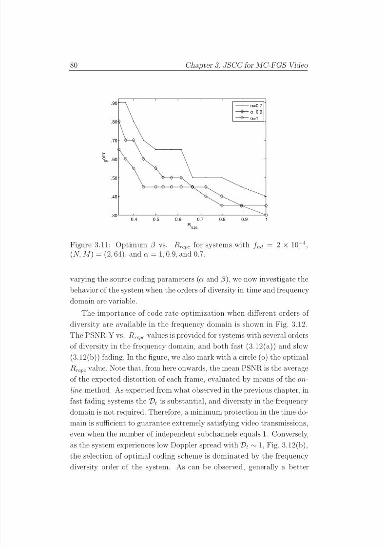
7/29/2019 Adaptive Wireless Multimedia
http://slidepdf.com/reader/full/adaptive-wireless-multimedia 98/187
80 Chapter 3. JSCC for MC-FGS Video
0.4 0.5 0.6 0.7 0.8 0.9 1.30
.40
.50
.60
.70
.80
.90
Rrcpc
β O P T
α=0.7
α=0.9
α=1
Figure 3.11: Optimum β vs. Rrcpc for systems with f nd = 2 × 10⁻⁴,(N, M ) = (2, 64), and α = 1, 0.9, and 0.7.
varying the source coding parameters (α and β ), we now investigate the
behavior of the system when the orders of diversity in time and frequency
domain are variable.
The importance of code rate optimization when different orders of
diversity are available in the frequency domain is shown in Fig. 3.12.
The PSNR-Y vs. Rrcpc values is provided for systems with several orders
of diversity in the frequency domain, and both fast (3.12(a)) and slow
(3.12(b)) fading. In the figure, we also mark with a circle (o) the optimal
Rrcpc value. Note that, from here onwards, the mean PSNR is the average
of the expected distortion of each frame, evaluated by means of the on-line method. As expected from what observed in the previous chapter, in
fast fading systems the Dt is substantial, and diversity in the frequency
domain is not required. Therefore, a minimum protection in the time do-
main is sufficient to guarantee extremely satisfying video transmissions,
even when the number of independent subchannels equals 1. Conversely,
as the system experiences low Doppler spread with Dt ∼ 1, Fig. 3.12(b),
the selection of optimal coding scheme is dominated by the frequency
diversity order of the system. As can be observed, generally a better
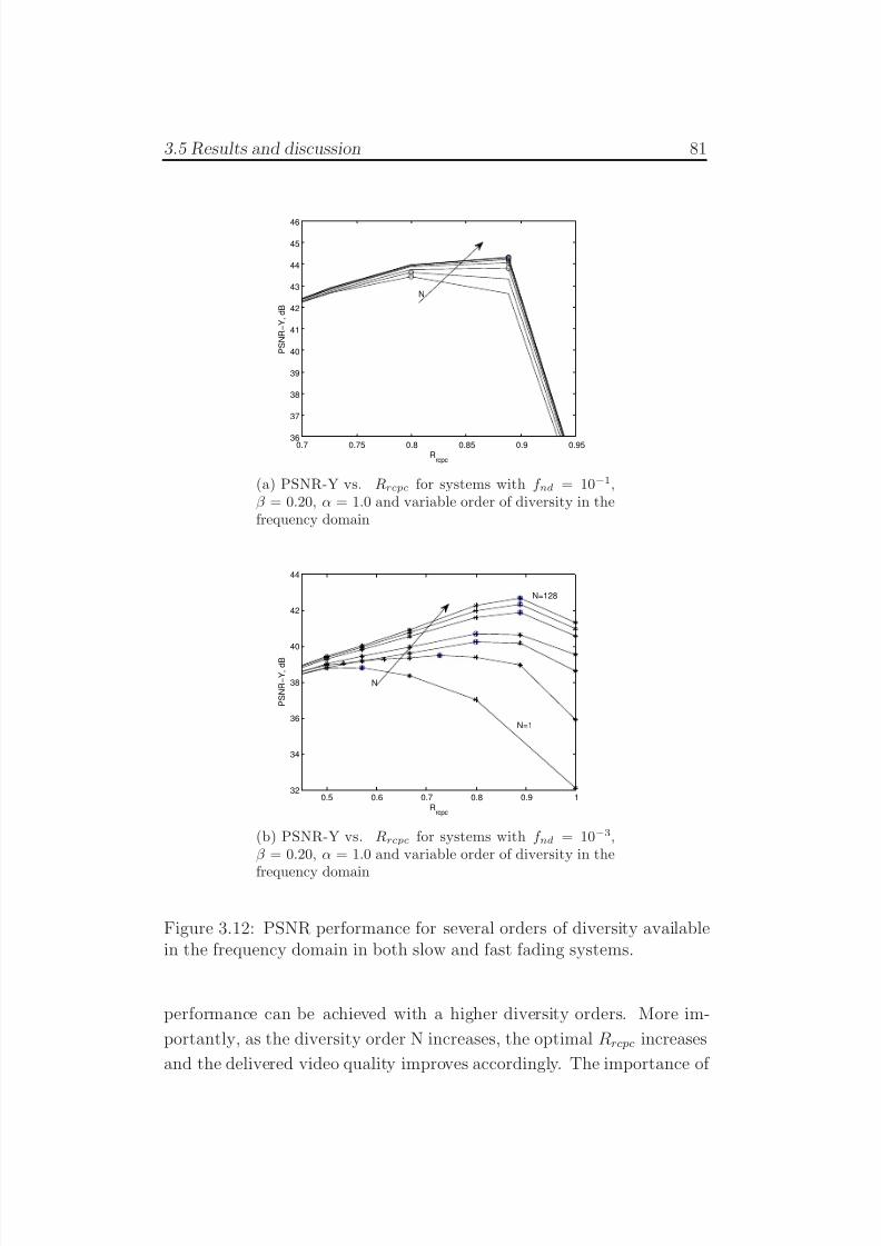
7/29/2019 Adaptive Wireless Multimedia
http://slidepdf.com/reader/full/adaptive-wireless-multimedia 99/187
3.5 Results and discussion 81
0.7 0.75 0.8 0.85 0.9 0.9536
37
38
39
40
41
42
43
44
45
46
Rrcpc
P S N R − Y , d B
N
(a) PSNR-Y vs. Rrcpc for systems with f nd = 10−1,β = 0.20, α = 1.0 and variable order of diversity in thefrequency domain
0.5 0.6 0.7 0.8 0.9 132
34
36
38
40
42
44
Rrcpc
P S N R − Y , d B
N
N=1
N=128
(b) PSNR-Y vs. Rrcpc for systems with f nd = 10−3,β = 0.20, α = 1.0 and variable order of diversity in the
frequency domain
Figure 3.12: PSNR performance for several orders of diversity availablein the frequency domain in both slow and fast fading systems.
performance can be achieved with a higher diversity orders. More im-
portantly, as the diversity order N increases, the optimal Rrcpc increases
and the delivered video quality improves accordingly. The importance of
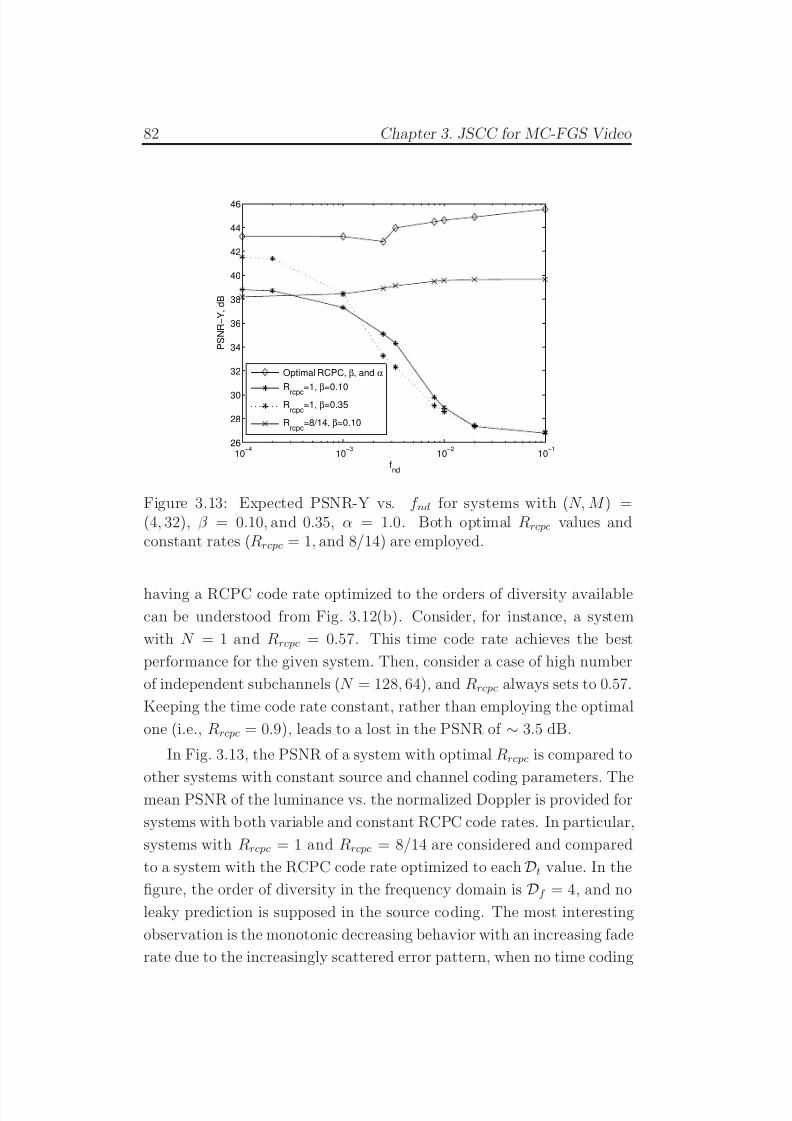
7/29/2019 Adaptive Wireless Multimedia
http://slidepdf.com/reader/full/adaptive-wireless-multimedia 100/187
82 Chapter 3. JSCC for MC-FGS Video
10−4
10−3
10−2
10−1
26
28
30
32
34
36
38
40
42
44
46
fnd
P S N R − Y , d B
Optimal RCPC, β, and α
Rrcpc
=1, β=0.10
Rrcpc
=1, β=0.35
Rrcpc
=8/14, β=0.10
Figure 3.13: Expected PSNR-Y vs. f nd for systems with (N, M ) =(4, 32), β = 0.10, and 0.35, α = 1.0. Both optimal Rrcpc values andconstant rates (Rrcpc = 1, and 8/14) are employed.
having a RCPC code rate optimized to the orders of diversity available
can be understood from Fig. 3.12(b). Consider, for instance, a system
with N = 1 and Rrcpc = 0.57. This time code rate achieves the best
performance for the given system. Then, consider a case of high number
of independent subchannels (N = 128, 64), and Rrcpc always sets to 0.57.
Keeping the time code rate constant, rather than employing the optimal
one (i.e., Rrcpc = 0.9), leads to a lost in the PSNR of ∼ 3.5 dB.
In Fig. 3.13, the PSNR of a system with optimal Rrcpc is compared to
other systems with constant source and channel coding parameters. Themean PSNR of the luminance vs. the normalized Doppler is provided for
systems with both variable and constant RCPC code rates. In particular,
systems with Rrcpc = 1 and Rrcpc = 8/14 are considered and compared
to a system with the RCPC code rate optimized to each Dt value. In the
figure, the order of diversity in the frequency domain is Df = 4, and no
leaky prediction is supposed in the source coding. The most interesting
observation is the monotonic decreasing behavior with an increasing fade
rate due to the increasingly scattered error pattern, when no time coding
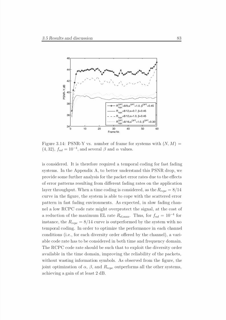
7/29/2019 Adaptive Wireless Multimedia
http://slidepdf.com/reader/full/adaptive-wireless-multimedia 101/187
3.5 Results and discussion 83
0 10 20 30 40 50 6034
36
38
40
42
44
46
Frame Nr.
P S N R − Y , d B
Rrcpc
OPT=8/9,α
OPT=1.0, β
OPT=0.45
Rrcpc=8/12,α=0.7, β=0.45R
rcpc=8/12,α=1.0, β=0.45
Rrcpc
OPT=8/16,α
OPT=1.0, β
OPT=0.30
Figure 3.14: PSNR-Y vs. number of frame for systems with (N, M ) =(4, 32), f nd = 10−4, and several β and α values.
is considered. It is therefore required a temporal coding for fast fading
systems. In the Appendix A, to better understand this PSNR drop, we
provide some further analysis for the packet error rates due to the effects
of error patterns resulting from different fading rates on the application
layer throughput. When a time coding is considered, as the Rrcpc = 8/14
curve in the figure, the system is able to cope with the scattered error
pattern in fast fading environments. As expected, in slow fading chan-
nel a low RCPC code rate might overprotect the signal, at the cost of
a reduction of the maximum EL rate Rel,max. Thus, for f nd = 10−4 for
instance, the Rrcpc = 8/14 curve is outperformed by the system with notemporal coding. In order to optimize the performance in each channel
conditions (i.e., for each diversity order offered by the channel), a vari-
able code rate has to be considered in both time and frequency domain.
The RCPC code rate should be such that to exploit the diversity order
available in the time domain, improving the reliability of the packets,
without wasting information symbols. As observed from the figure, the
joint optimization of α, β , and Rrcpc outperforms all the other systems,
achieving a gain of at least 2 dB.
7/29/2019 Adaptive Wireless Multimedia
http://slidepdf.com/reader/full/adaptive-wireless-multimedia 102/187
84 Chapter 3. JSCC for MC-FGS Video
The worthy performance of the optimized systems compared to otherpossible suboptimal configurations is reported in Fig. 3.14 in terms of
instantaneous PSNR (rather than average). Here the PSNR-Y for each
frame of the sequence is provided for systems with fixed coding parame-
ters. Again, a substantial improvement of the decoded quality is experi-
enced by the optimal system, as observed from the figure.
3.6 Conclusion
In this section, we studied the delivery of MC-FGS video employ-ing an OFDM signal format on the physical layer to transmit over a
frequency-selective Rayleigh fading, with both low and high level of mo-
bility. We proposed a n-channel symmetric motion-compensated multiple
description coding and transmission scheme, employing leaky prediction
for mismatch control. We showed that knowing the orders of diversity
offered by the channel in both time and frequency domain can improves
the overall performance in the construction of symmetric MDs. We pro-
posed an algorithm for the evaluation of the rate-distortion curve for the
considered sequence, and, based on this function, the optimal tradeoff
between coding efficiency and reliability can be investigated, by varying
the EL-MCP rate and the leak factor α, together with the code rates in
both time and frequency domain. Moreover, we demonstrated the impor-
tance of a time coding in the construction of 2D MDs, and we showed the
behavior of the optimal RCPC code rate for different order of diversity
in both time and frequency domain.
7/29/2019 Adaptive Wireless Multimedia
http://slidepdf.com/reader/full/adaptive-wireless-multimedia 103/187
Chapter 4
Adaptive modulationtechniques
In this chapter, adaptive modulation techniques are investigated for
systems experiencing channel estimation errors. We evaluate the perfor-
mance of both slow and fast adaptive modulation techniques when im-
perfect pilot-assisted channel estimation is considered at both the trans-
mitter and the receiver. Taking into account the number of pilot symbols
transmitted, the effective throughput is investigated and the tradeoff be-
tween channel estimation quality and throughput is addressed.
The reminder of the chapter is organized as follows. In Section 5.1
an introduction to the work together with a state-of-the-art overview in
adaptive modulation techniques is provided. In Section 5.2 we present
the system model, describing both adaptive modulation techniques andpilot-assisted channel estimation. Imperfect channel state information at
the transmitter is investigated in Section 4.3, and a comparison of the
performance between two adaptive modulation techniques is considered.
In Section 4.4, we evaluate the effects of estimation errors at the receiver.
In particular, slow adaptive modulation systems are investigated for both
Rayleigh and Nagakami-m fading channels, and the optimization of the
pilot scheme design is addressed in details. In Section 5.6 numerical
results are provided, and conclusions are given in Section 5.7.
85
7/29/2019 Adaptive Wireless Multimedia
http://slidepdf.com/reader/full/adaptive-wireless-multimedia 104/187
86 Chapter 4. Adaptive modulation techniques
4.1 Motivation and outline of the workThe diffusion of high-speed digital wireless communications has in-
creased the need of reliable high data rate transmission in variable chan-
nel conditions. Since adaptive modulation techniques allow to maximize
the transmitted throughput1 without compromising the performance (in
terms of bit error probability or outage probability), they has become
very popular in high data rate wireless applications [5–7, 94–96]. By
matching system parameters to channel conditions the optimal modula-
tion level can be selected maximizing the transmitted throughput stillsatisfying the QoS requirement, in terms of bit error probability (BEP)
and bit error outage probability (BEO).
Since M -QAM modulation achieves high spectral efficiency, it is widely
used in adaptive modulation systems. In [5], for example, power and rate
were both adopted to channel conditions for a M -QAM uncoded sys-
tem. The gain derived from an adaptive rather than a fixed transmitted
scheme is reported, together with the negligible channel capacity penalty
that the system displays varying only the data-rate rather than both rate
and power. In the literature, some authors proposed as adaptive mod-
ulation techniques systems that track instantaneous channel variations:
the receiver has to estimate the instantaneous signal-to-noise ratio (SNR)
and send a feedback to the transmitter with the optimal constellation size
and transmitting power to be used, [5–7,94,96,97]. Those parameters are
tuned to exploit good channel conditions by increasing the transmitted
throughput but, at the same time, to preserve the performance in case of
bad channel conditions. It is worth noting that, in perfect channel state
information (CSI) systems, tracking the small scale fading, fast adaptive
modulation (FAM), leads to best performance, at the cost of a frequent
channel estimation and feedback. With respect to FAM, a gain in terms
of feedback and complexity can be achieved by slow adaptive modula-
tion (SAM) techniques, that adapt modulation parameters to the average
channel variations. In [6], the authors investigated SAM techniques with
perfect channel estimation, adapting the system to the shadowing level
1Throughout this chapter, we use the terms “throughput” and “spectral efficiency(SE)” interchangeably.
7/29/2019 Adaptive Wireless Multimedia
http://slidepdf.com/reader/full/adaptive-wireless-multimedia 105/187
4.1 Motivation and outline of the work 87
of the channel. Although the throughput achieved with FAM systemis slightly better than the one obtained with SAM technique, SAM still
achieves improvements in terms of SE and BEO when compared to a fixed
modulation scheme, despite the lower complexity and the less frequent
feedback.
In fast as well as slow adaptive modulation, a critical role is played
by the channel estimation. Imperfect channel estimation poses a serious
issue that has been addressed in several ways. The effects of outdated
channel estimation are investigated for adaptive coding systems in [7]
and for adaptive modulation systems with Rayleigh and Nakagami fad-
ing channel in [5] and [97], respectively. In both [5] and [97], authors
evaluated the maximum acceptable delay that does not drastically affect
the performances. For a BEP target of 10−3, the maximum delay nor-
malized to the Doppler frequency corresponds to 10−2 for both Rayleigh
and Nakagami fading channels. Rather than delayed channel state infor-
mation, imperfect channel estimation are quickly investigated in [5]. A
general criterium is given to probe the effects of channel estimation er-
rors in the instantaneous SNR in the feedback. More detailed analysis onadaptive modulation system with imperfect CSI are addressed in [98–101]
for both single- and multi-carrier systems with or without diversity at the
receiver. To the best of our knowledge, the receiver was always assumed
to be channel estimation error free and the imperfect CSI was addressed
for FAM systems only.
In order to evaluate the effects of channel estimation errors in FAM
and SAM systems, in this chapter we investigate both fast and slow
adaptive modulation techniques for M -QAM systems with subset diver-sity (SSD) [102] and with imperfect channel state information. Imperfect
CSI will affect diversity, bit reconstruction, and the choice of the opti-
mal modulation size. We recall that, in SAM systems, the large scale
fading has to be estimated, while in FAM, the knowledge of the small
scale fading is required. Since the coherence time of the small-scale fad-
ing is lower than the coherence time of large scale fading, a slower and
more accurate estimation can be provided for SAM systems rather than
FAM. It follows that, although FAM achieves the best performance in
7/29/2019 Adaptive Wireless Multimedia
http://slidepdf.com/reader/full/adaptive-wireless-multimedia 106/187
88 Chapter 4. Adaptive modulation techniques
perfect CSI systems, when errors occur in channel estimation, SAM mayeven outperform FAM technique, as it will be demonstrated by numerical
results, reported in Section 5.6. This explain the importance of investi-
gating FAM and SAM in real systems. In this work, the simplification
of assuming the receiver channel estimation error free is not considered.
Thus, pilot-based channel estimation errors are assumed to happen at
both the transmitter and the receiver. In order to study separately those
effects, we address the imperfect CSI at the transmitter first, and then
we consider channel estimation errors at the receiver.
4.2 System model
In this section the system model is described and further details
on adaptive modulation techniques are provided, following the notation
adopted in [6]. We assume a M -QAM modulated symbol transmitted
over composite Rayleigh fading and log-normal shadowing channels, em-
ploying microdiversity at the receiver, i.e., the shadowing level is the same
on each branch. At the receiver, N antennas are considered and a hybrid-selection maximal ratio combiner (H-S/MRC) [19] is adopted for process-
ing the signal. Among N branches, the most powerful L are selected for
being processed by the maximal ratio combiner. We define by hi the fad-
ing gain Rayleigh distributed, by E s the mean (over the fading) symbol
energy transmitted and by N 0/2 the two-sided spectral density of the
AWGN. Since we consider microdiversity, for sake of simplicity, we omit
the branch subscript in the averaged SNR notation. The mean signal-to-
noise ratio on each branch can be expressed as γ = E |h|2E s/N 0. Since
a log-normal shadowing is considered, γ dB = 10 log10(γ ) is Gaussian dis-tributed with µdB mean and σ2
dB variance.
4.2.1 Adaptive modulation
As briefly stated before, adaptive modulation techniques achieve the
best throughput accordingly with channel conditions, minimizing in the
meanwhile the outage probability. When a discrete variable rate is con-
sidered, a set of J modulation levels can be adopted in adaptive modula-
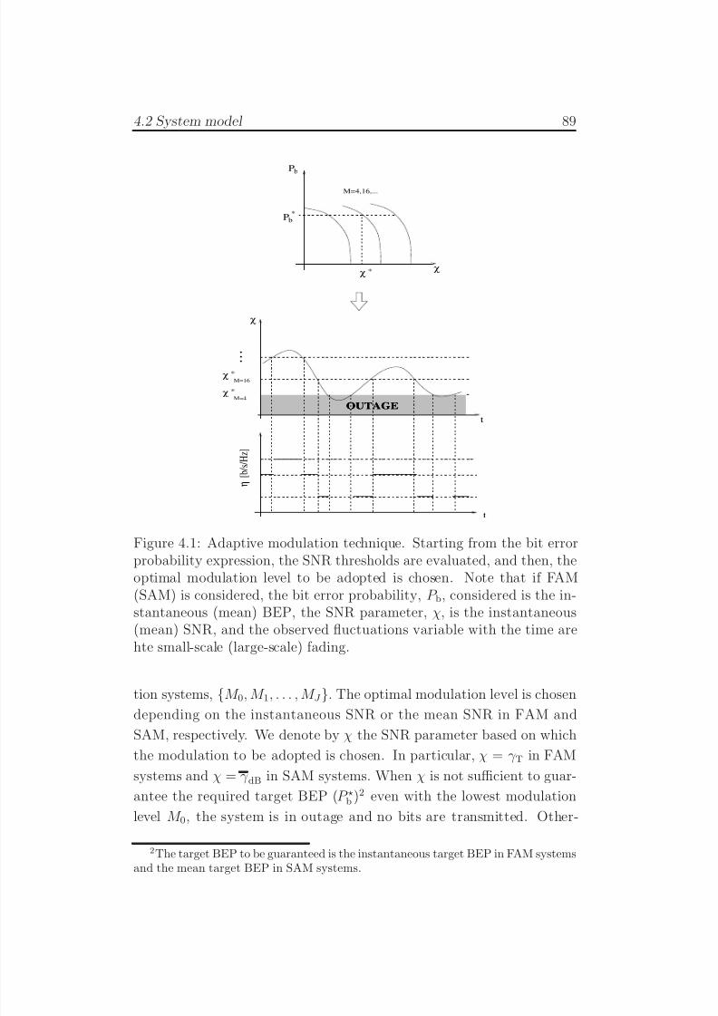
7/29/2019 Adaptive Wireless Multimedia
http://slidepdf.com/reader/full/adaptive-wireless-multimedia 107/187
4.2 System model 89
M=4,16,...
*M=16
χ *M=4
t
η
[ b / s / H z ]
Pb*
Pb
χ *
χ
t
.
.
.
OUTAGEOUTAGE
χ
χ
Figure 4.1: Adaptive modulation technique. Starting from the bit errorprobability expression, the SNR thresholds are evaluated, and then, theoptimal modulation level to be adopted is chosen. Note that if FAM(SAM) is considered, the bit error probability, P b, considered is the in-stantaneous (mean) BEP, the SNR parameter, χ, is the instantaneous(mean) SNR, and the observed fluctuations variable with the time arehte small-scale (large-scale) fading.
tion systems,
M 0, M 1, . . . , M J
. The optimal modulation level is chosen
depending on the instantaneous SNR or the mean SNR in FAM andSAM, respectively. We denote by χ the SNR parameter based on which
the modulation to be adopted is chosen. In particular, χ = γ T in FAM
systems and χ = γ dB in SAM systems. When χ is not sufficient to guar-
antee the required target BEP (P ⋆b )2 even with the lowest modulation
level M 0, the system is in outage and no bits are transmitted. Other-
2The target BEP to be guaranteed is the instantaneous target BEP in FAM systemsand the mean target BEP in SAM systems.
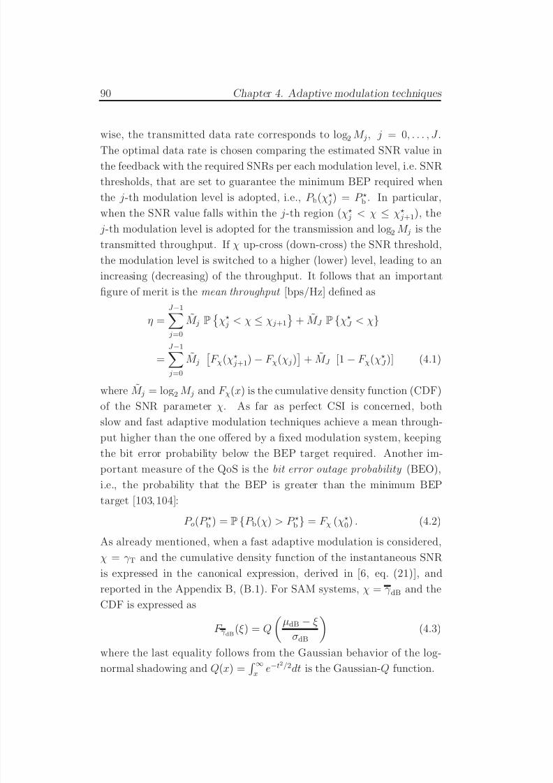
7/29/2019 Adaptive Wireless Multimedia
http://slidepdf.com/reader/full/adaptive-wireless-multimedia 108/187
90 Chapter 4. Adaptive modulation techniques
wise, the transmitted data rate corresponds to log2 M j, j = 0, . . . , J .The optimal data rate is chosen comparing the estimated SNR value in
the feedback with the required SNRs per each modulation level, i.e. SNR
thresholds, that are set to guarantee the minimum BEP required when
the j-th modulation level is adopted, i.e., P b(χ⋆ j) = P ⋆b . In particular,
when the SNR value falls within the j-th region (χ⋆ j < χ ≤ χ⋆ j+1), the
j-th modulation level is adopted for the transmission and log2 M j is the
transmitted throughput. If χ up-cross (down-cross) the SNR threshold,
the modulation level is switched to a higher (lower) level, leading to an
increasing (decreasing) of the throughput. It follows that an importantfigure of merit is the mean throughput [bps/Hz] defined as
η =J −1 j=0
M j P
χ⋆ j < χ ≤ χ j+1
+ M J P χ⋆J < χ
=J −1 j=0
M j
F χ(χ⋆ j+1) − F χ(χ j)
+ M J [1 − F χ(χ⋆J )] (4.1)
where M j = log2 M j and F χ(x) is the cumulative density function (CDF)
of the SNR parameter χ. As far as perfect CSI is concerned, bothslow and fast adaptive modulation techniques achieve a mean through-
put higher than the one offered by a fixed modulation system, keeping
the bit error probability below the BEP target required. Another im-
portant measure of the QoS is the bit error outage probability (BEO),
i.e., the probability that the BEP is greater than the minimum BEP
target [103, 104]:
P o(P ⋆b ) = P P b(χ) > P ⋆b = F χ (χ⋆0) . (4.2)
As already mentioned, when a fast adaptive modulation is considered,
χ = γ T and the cumulative density function of the instantaneous SNR
is expressed in the canonical expression, derived in [6, eq. (21)], and
reported in the Appendix B, (B.1). For SAM systems, χ = γ dB and the
CDF is expressed as
F γ dB(ξ ) = Q
µdB − ξ
σdB
(4.3)
where the last equality follows from the Gaussian behavior of the log-
normal shadowing and Q(x) =
∞x
e−t2/2dt is the Gaussian-Q function.
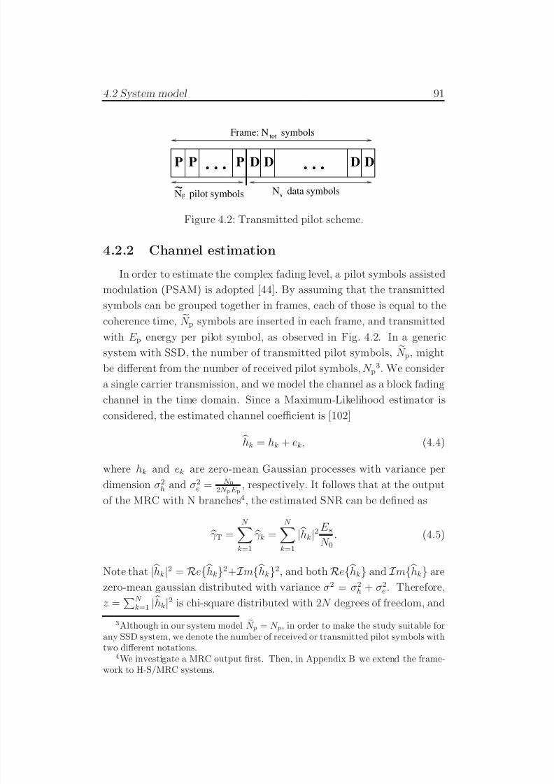
7/29/2019 Adaptive Wireless Multimedia
http://slidepdf.com/reader/full/adaptive-wireless-multimedia 109/187
4.2 System model 91
p
Frame: N symbols
P P DDDDP
N data symbolss
. . . . . .
~N pilot symbols
tot
Figure 4.2: Transmitted pilot scheme.
4.2.2 Channel estimation
In order to estimate the complex fading level, a pilot symbols assistedmodulation (PSAM) is adopted [44]. By assuming that the transmitted
symbols can be grouped together in frames, each of those is equal to the
coherence time, N p symbols are inserted in each frame, and transmitted
with E p energy per pilot symbol, as observed in Fig. 4.2. In a generic
system with SSD, the number of transmitted pilot symbols, N p, might
be different from the number of received pilot symbols, N p3. We consider
a single carrier transmission, and we model the channel as a block fading
channel in the time domain. Since a Maximum-Likelihood estimator is
considered, the estimated channel coefficient is [102]
hk = hk + ek, (4.4)
where hk and ek are zero-mean Gaussian processes with variance per
dimension σ2h and σ2
e = N 02N pE p
, respectively. It follows that at the output
of the MRC with N branches4, the estimated SNR can be defined as
γ T =N
k=1 γ k =N
k=1
| hk|2 E s
N 0. (4.5)
Note that | hk|2 = Re hk2+ I m hk2, and both Re hk and I m hk are
zero-mean gaussian distributed with variance σ2 = σ2h + σ2
e . Therefore,
z =N
k=1 | hk|2 is chi-square distributed with 2N degrees of freedom, and
3Although in our system model N p = N p, in order to make the study suitable forany SSD system, we denote the number of received or transmitted pilot symbols withtwo different notations.
4We investigate a MRC output first. Then, in Appendix B we extend the frame-work to H-S/MRC systems.
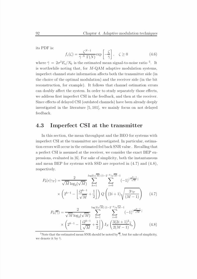
7/29/2019 Adaptive Wireless Multimedia
http://slidepdf.com/reader/full/adaptive-wireless-multimedia 110/187
92 Chapter 4. Adaptive modulation techniques
its PDF is:f z(ζ ) =
ζ N −1
γ N Γ(N )exp
−ζ
γ
, ζ ≥ 0 (4.6)
where γ = 2σ2E s/N 0 is the estimated mean signal-to-noise ratio 5. It
is worthwhile noting that, for M -QAM adaptive modulation systems,
imperfect channel state information affects both the transmitter side (in
the choice of the optimal modulation) and the receiver side (in the bit
reconstruction, for example). It follows that channel estimation errors
can doubly affect the system. In order to study separately those effects,
we address first imperfect CSI in the feedback, and then at the receiver.Since effects of delayed CSI (outdated channels) have been already deeply
investigated in the literature [5, 101], we mainly focus on not delayed
feedback.
4.3 Imperfect CSI at the transmitter
In this section, the mean throughput and the BEO for systems with
imperfect CSI at the transmitter are investigated. In particular, estima-
tion errors will occur in the estimated fed back SNR value . Recalling thata perfect CSI is assumed at the receiver, we consider the exact BEP ex-
pressions, evaluated in [6]. For sake of simplicity, both the instantaneous
and mean BEP for systems with SSD are reported in (4.7) and (4.8),
respectively.
P b(e|γ T ) =2√
M log2(√
M )
log2(√ M )
h=1
(1−2−h)√ M −1
i=0
(−1)⌊ i2h−1
√ M
⌋
× 2
h
−1
− i2h−1
√ M +
1
2Q(2i + 1) 3γ T
(M − 1) (4.7)
P b(γ ) =2√
M log2(√
M )
log 2(√ M )
h=1
(1−2−h)√ M −1
i=0
(−1)⌊ i2h−1√
M ⌋
×
2h−1 −
i2h−1
√ M
+1
2
I N
3(2i + 1)2
2(M − 1)bn (4.8)
5Note that the estimated mean SNR should be noted by
γ , but for sake of simplicity,
we denote it by γ .
7/29/2019 Adaptive Wireless Multimedia
http://slidepdf.com/reader/full/adaptive-wireless-multimedia 111/187
4.3 Imperfect CSI at the transmitter 93
where I k(x) = 1π π/20 sin2
θx+sin2θk dθ. From the bit error probability, ex-act SNR thresholds are evaluated and compared to the estimated SNR
value, i.e., χ⋆i < χ ≤ χ⋆i+1. In order to evaluate the mean throughput
and the outage probability in systems affected by estimation errors in the
feedback, the cumulative density function of χ, F χ(χ), has to be evalu-
ated. Considering a fast adaptive modulation system, the PDF of the
instantaneous estimated SNR γ T, conditioned on a given γ is
f
γ T|γ (ξ ) =
ξN −1
γ N σ2N t Γ(N )
exp
− ξγσ2t
, ξ ≥ 0
0, otherwise
(4.9)
where σ2t =
σ2e+σ2h
σ2h
and γ is the averaged signal-to-noise ratio per branch,
already defined as
γ = E|hk|2 E sN 0
= 2σ2h
E sN 0
.
It can be observed that σ2t = 1/ρ2, where ρ is the envelope of the complex
correlation between hk and hk defined as
ρ =Ehk
h∗k − EhkE
h∗k
E|hk − Ehk|2
E| hk − E hk|2
=
σ2h
σ2
h
(σ2
h
+ σ2
e
)=
σ2h
σ2h + σ2
e
.
(4.10)
It is worth noting that the correlation depends on the mean SNR per
branch and the parameter N pε, in particular
σ2t =
1
ρ2=
σ2h + N 0
2N pεE s
σ2h
=γ + 1
N pε
γ , (4.11)
where ε = E p/E s is the ratio between the energy dedicated to pilot sym-
bols and the data symbols energy. Substituting (4.11) in (4.9), the con-
ditioned PDF of the instantaneous estimated SNR f γ T|γ can be expressed
as
f γ T|γ (ξ ) =ξ N −1
γ + 1N pε
N Γ(N )
exp
− ξ
γ + 1N pε
, ξ ≥ 0 (4.12)
and 0 otherwise (ξ < 0). From (4.12), the marginal PDF and CDF of
the estimated instantaneous SNR can be derived as
f
γ T(ξ ) =
∞0
f γ T |γ (ξ )f γ (w)dw, ξ ≥ 0,
0, otherwise(4.13)
7/29/2019 Adaptive Wireless Multimedia
http://slidepdf.com/reader/full/adaptive-wireless-multimedia 112/187
94 Chapter 4. Adaptive modulation techniques
and
F γ T =
γ ⋆T0
f γ T(ξ )dξ =
γ ⋆T0
∞0
f γ T |γ (ξ )f γ (w)dw dξ (4.14)
where the pdf of the average SNR results to be
f γ (w) =ν √
2πσdBwexp
−(10log10w − µdB)2
2σ2dB
, w ≥ 0 (4.15)
where ν = 10/ln(10).
When a slow adaptive modulation is considered, the system is adapted
to the estimated mean SNR, γ . The estimated mean SNR per branch
can be expressed as
γ = Ehk γ k = 2σ2 E sN 0
= σ2t γ = γ +
1
N pε. (4.16)
Note that if the variance of the channel estimation error (σ2e) is zero, σ2
t
is equal to 1 and γ = γ . Knowing the marginal PDF of the log-normal
shadowing (4.15), the PDF of the estimated mean SNR is obtained by
making a change of variable and it is given by
f γ (υ) =ν √
2πσdB (υ − 1N pε
)exp
−
10log10(υ − 1N pε
) − µdB
2
2σ2dB
, υ ≥ 1
N pε
(4.17)
From (4.17), the CDF of the averaged estimated SNR can be derived as
follows
F γ (x) = x
1
N pε
f
γ (υ)dυ =
1
2 erfcµdB − 10log10(x − 1
N pε)
√ 2σ
dB (4.18)
The presented analysis is limited to systems employing MRC at the
receiver, but it can be easily extended to a SSD system, as explained in
the Appendix B.
4.3.1 Mean throughput
In adaptive modulation systems with imperfect CSI, the mean through-
put strictly depends on the adopted pilot scheme. Since in each frame,
N p
7/29/2019 Adaptive Wireless Multimedia
http://slidepdf.com/reader/full/adaptive-wireless-multimedia 113/187
4.3 Imperfect CSI at the transmitter 95
symbols are inserted (Fig.4.2), only a fraction ns of N tot symbols within aframe is dedicated to data transmission. Assuming the following notation
N p = np N tot
⇒ np + ns = 1N s = ns N tot
(4.19)
it can be observed the tradeoff between ns and np, that is the tradeoff
between performance and the determined throughput: the more pilot
symbols are adopted, the better is the channel estimation quality, but
the less is the transmitted throughput. In addition to np and ns, anotherimportant parameter in the pilot scheme design is the ratio between the
energy dedicated to pilot symbols and the one dedicated to data symbols,
that has been already defined as ε = E p/E s. In a system with no con-
straint on the maximum transmitted energy, a high E p would provide an
improvement in the channel quality, without affecting the BEP perfor-
mance. Unfortunately, in real systems, a maximum transmitted energy
is imposed and the following constraint has to be considered
N pE p + N sE s ≤ E tot. (4.20)
Imposing the constraint (4.20), an increasing of the energy dedicated
to the pilot symbols has to be balanced by a reduction of the number
of pilot symbols N p, or by a reduction of the energy E s. Note that,
when ε = 1, the constraint (4.20) merges to the constraint (4.19), i.e.,N p+N s = N tot. The optimization of the energy distribution between data
and pilot symbols has been already investigated in [105]. In this section
we assume ε = 1. Note that the aim of this section is the comparison
of FAM and SAM techniques in the presence of estimation errors in thefeedback. In the next section, we will investigate the effects of imperfect
CSI at the receiver for the SAM case only, and the N pε optimization issue
will be addressed in more details.
Considering the mean throughput evaluation, it is worth noting that,
knowing the CDF for both SAM and FAM systems, (4.18) and (4.14), the
mean throughput η can be evaluated from (4.1). For both the techniques,
η is the mean throughput for each symbol among the N s data symbols
transmitted. To obtain the effective mean throughput per frame, the
7/29/2019 Adaptive Wireless Multimedia
http://slidepdf.com/reader/full/adaptive-wireless-multimedia 114/187
96 Chapter 4. Adaptive modulation techniques
number of pilot symbols has to be considered. In particular, the effectivemean throughput per symbol per frame is:
η(eff) = η ns = η (1 − np) = η
1 −
N pN tot
. (4.21)
Since we are interested in a comparison between FAM and SAM, the
effective mean throughput per symbol per frame has to be considered.
We recall that in SAM systems, the coherence time as well as the frame
size are greater than the ones in FAM. Therefore, keeping constant thechannel estimation quality, (i.e., N p), the symbols dedicated to informa-
tion symbols in SAM systems are greater than the ones in FAM systems,
that is nFAMs ≤ nSAM
s . Conversely, when the np value is constant, in SAM
systems the number of symbols dedicated to pilot insertion is greater
than the one in FAM, it follows that ns is constant between SAM and
FAM, but the former has a better channel estimation. This is obvious if
we consider that
N FAM
p ≤
N SAM
p , and we assume E p constant.
4.3.2 Outage probability
In systems with imperfect CSI at the transmitter, the estimated SNR χ can be either underestimated or overestimated. The former case leads
to a reduction of the throughput, while the latter leads to an increase of
either the mean throughput and outage probability. In particular, when χ > χ, although the real SNR falls within the j-th modulation range,
the ( j + 1)-th modulation might be adopted. In this case, the effective
bit error probability is greater than the target BEP and the system is in
outage. It means that the system is in outage when χ < χ⋆0, and also
when the following condition is verified χ > χ⋆iχ ≤ χ⋆i
∀i. (4.22)
Assuming that χ = χ + ∆χ, the previous condition can be expressed as
χ⋆i − ∆χ < χ ≤ χ⋆i . (4.23)
7/29/2019 Adaptive Wireless Multimedia
http://slidepdf.com/reader/full/adaptive-wireless-multimedia 115/187
4.4 Imperfect CSI at the receiver 97
It follows that the outage probability of an adaptive modulation systemwith imperfect CSI at the transmitter can be expressed as
P o = F χ(χ⋆0) +J
j=1
F χ(χ⋆ j) − F χ(χ⋆ j − ∆χ)
. (4.24)
For a slow adaptive modulation, considering the CDF of the average
SNR in (4.16), ∆χ = 1/N pε and the outage probability conditioned on
the adopted pilot scheme is
P o = Q
µdB − γ ∗0,dB
σdB
+
+J
j=1
Q
µdB − γ ∗ j,dB
σdB aj
− Q
µdB − 10log10
γ ∗ j − 1
N pε
σdB bj
=
= Q
µdB − γ ∗0,dB
σdB +
J
j=1 bj
aj
e−y2
2 dy. (4.25)
As expected, increasing N pε, the estimation accuracy increases and the
outage probability converges to the BEO of systems with perfect CSI.
4.4 Imperfect CSI at the receiver
In this section, the bit error probability (BEP) and bit error outage
(BEO) expressions for SSD are evaluated in slow adaptive modulation
systems with imperfect CSI at the receiver and Rayleigh or Nakagami-m
fading channels. We recall that, to estimate the channel, a pilot sym-
bols assisted modulation (PSAM) is adopted and a Maximum-Likelihood
estimator is employed. We denote by N p the pilot symbols inserted in
each frame equal to the coherence time and transmitted with E p energy
per pilot symbol. The estimated channel coefficients are given by (4.4),
where ek is a zero-mean Gaussian process with variance per dimension
σ2e = N 0
2N pE p.
7/29/2019 Adaptive Wireless Multimedia
http://slidepdf.com/reader/full/adaptive-wireless-multimedia 116/187
98 Chapter 4. Adaptive modulation techniques
4.4.1 Bit error probabilityThe performance of N -branch diversity combining in the presence of
imperfect CSI was studied in [102] and [106] for MRC and SSD, respec-
tively. In [106], the symbols error probability (SEP) was obtained for
i.i.d. Nakagami-m fading channels for arbitrary two-dimensional signal-
ing constellations. When M -QAM modulation is considered, the SEP as
a function of the SNR averaged over the small scale fading and the sisymbols is expressed by
P e(γ, N pε) = 1M i
ω(a)i I N ζ (i), Φ2, π
4+
1
M
i
ω(b)i I N
ζ (i), Φ4, 0
, (4.26)
I N (ζ , φ , ψ) =1
2π
φ0
N n=1
sin2(θ + ψ)m
sin2(θ + ψ)m + bnζ
m, (4.27)
where ΦM = π(M −1)/M , and N p is the number of received pilot symbols.
The set of ζ (i) is a function of the averaged SNR:
ζ (i)(γ, N pε) E sρ2
σ2h
N 0
2+ |si|2σ2
eρ2
=γN pε cMQAM1γ
+ N pε + ξ i, (4.28)
where cMQAM = 3/(2(M − 1)), and ρ = σ2h/(σ2
h + σ2e). The parameters
ω(a)i , ω
(b)i and ξ i E i/E S depend on the modulation format, and are
given in [106]. Note that the summation in (4.26) is performed over
the non zero values ω(a)i , ω
(b)i and ξ . Moreover, the BEP for Rayleigh
fading channels can be obtained by setting m = 1, ∀n in (4.26). In thecase of ideal channel estimation (N pε −→ ∞), (4.28) results given by
ζ (i) = γ cMQAM. The set bn depends on the SSD technique. When a
hybrid-selection maximal ratio combiner (H-S/MRC) [19] is adopted at
the receiver, among N branches the strongest L are selected for being
processed by the maximal ratio combiner. For such systems, the bn’s are
expressed as
bn =
1 n ≤ LL/n otherwise.

7/29/2019 Adaptive Wireless Multimedia
http://slidepdf.com/reader/full/adaptive-wireless-multimedia 117/187
4.4 Imperfect CSI at the receiver 99
When a MRC is considered at the receiver, L = N and bn = 1, ∀n.In a perfect CSI system, as well as in an imperfect one, the modulation
regions are bounded by SNR thresholds evaluated from the BEP. Starting
from the SEP, and assuming Gray coding between bits and symbols, the
bit error probability, P b, can be expressed by a lower bound:
P b(γ, N pε) ≥ P e(γ, N pε)
log2(M ). (4.29)
By numerical root evaluations, the SNR estimated thresholds γ ⋆ are ob-
tained from (4.29) as the values that satisfy the target BEP, i.e. P b(γ ⋆, N pε) =P ⋆b . Note that, in an imperfect CSI system, the thresholds are a function
of the modulation level as well as the channel estimation quality.
Together with the bit error probability, the BEO depends on the
quality of the channel estimation. Since the estimated thresholds γ ⋆ are
greater than the ideal ones (∆γ dB is always greater or equal to zero), the
condition (4.22) is not verified and the BEO can be expressed as
P o = F χ( χ0). (4.30)
4.4.2 Mean throughput
As already observed, the throughput in adaptive modulation systems
with imperfect CSI strictly depends on the adopted pilot scheme. For
systems with SSD, the portion of the frame dedicated to pilot insertion
is defined as np = N p/N tot, and the following constraints are imposed
N p + N s = N tot
N pE p + N sE s = E tot.
(4.31)
As already observed, when ε = 1, the increasing of E p has to be balanced
by the reduction of N p or E s. It follows that the energy dedicated to the
information symbols strictly depends on the adopted pilot scheme. In
particular, from (4.31), it can be derived the following expression
E s =E
N pN tot
(ε − 1) + 1, (4.32)
7/29/2019 Adaptive Wireless Multimedia
http://slidepdf.com/reader/full/adaptive-wireless-multimedia 118/187
100 Chapter 4. Adaptive modulation techniques
where E
E tot/N tot. It can be better understood that the increasing of N pε leads to an improvement of the performance due to a better qual-
ity of the channel estimation on one hand, and to a reduction of the
performance due to a lowering of E s on the other hand. It follows that
even the exact mean SNR in (4.26) is a function of the pilot scheme, i.e.,
γ = γ ( N pε), as expressed in the following
γ = E|h|2 E sN 0
=E|h|2
N 0
E N pN tot
(ε − 1) + 1=
1N pN tot
(ε − 1) + 1Υ, (4.33)
where Υ = E|h|2
E/N 0. Substituting (4.33) in (4.26), the bit errorprobability can be expressed as a function of two parameters: N pε char-
acterizing the pilot scheme design, and Υ representing the mean SNR per
frame.
P b = P b
γ ( N pε), N pε
= P b
Υ1N p
N tot(ε − 1) + 1
, N pε
=⇒ P b = P b(Υ, N pε)
(4.34)
Note that, unlikely the mean SNR γ , Υ does not depend on the pilot
scheme, but only on the mean energy over the frame, N 0 andE
|h|2
.This independent variable might be employed to compare systems with
different pilot schemes. Thus, from here onwards, the SNR averaged
over the frame, Υ, will be the SNR variable in the BEP expression, and
thus the SNR thresholds will be denoted by Υ⋆. We assume that the
SNR averaged over the frame is a log-normal distributed6, i.e., ΥdB ∼N (µdB, σ2
dB). Thus, the cumulative density function of ΥdB is
F ΥdB(ξ ) = Q
µdB − ξ
σdB
(4.35)
and the mean throughput of each information symbols of the frame is
η =J −1 j=1
M j
F ΥdB(Υ⋆
dB,j+1) − F Υ(Υ⋆dB,j)
+ M J
1 − F Υ(Υ⋆
dB,J )
. (4.36)
6Note that, in the previous section, γ was log-normal distributed. Since here wedo not have any comparison with performance of the previous case, or with any FAMsystems (i.e., we do not have any comparison with systems employing γ as variablerather than Υ), we make the simplification that Υ is log normal with mean µdB andvariance σ2dB. Note that, eventually, knowing the PDF of γ , the PDF of Υ can beeasily derived.
7/29/2019 Adaptive Wireless Multimedia
http://slidepdf.com/reader/full/adaptive-wireless-multimedia 119/187
4.5 Numerical results 101
Recalling that in SSD systems, the number of transmitted pilot symbolsis not necessarily equal to the received pilot symbols, the effective mean
throughput per symbol per frame is
η(eff) = η ns = ηN tot − N p
N tot. (4.37)
From (4.21), the tradeoff between estimation quality and transmitted
data can be observed. The more pilot symbols are transmitted, the better
is the channel quality at the cost of a lower effective throughput.
4.5 Numerical results
In this section, numerical results are presented in terms of effective
throughput
η(eff)
and BEO for both slow and fast adaptive modulation
systems. Coherent detection of M -QAM with H-S/MRC and Gray code
mapping in composite Rayleigh or Nakagmai-m fading and log-normal
shadowing channels with both perfect and imperfect CSI was considered.
In the subsection 4.5.1, we provide numerical results when channel esti-mation errors occur at the transmitter side, while in the subsection 4.5.2,
results for systems with imperfect CSI at the receiver are considered.
In both the cases, pilot symbol assisted modulation with N p = N p is
considered.
4.5.1 Imperfect CSI at the transmitter
For systems with imperfect CSI at the transmitter, the effective through-
put is evaluated by (4.21) and (4.1), by imposing a target BEP of 10−2,
and a maximum outage probability of 5%. The exact BEP expressions
are reported (4.8) and (4.7), while the CDFs are given by (4.18) and
(4.14) for SAM and FAM systems, respectively. In the effective through-
put evaluation, the constraint (4.19) is assumed for the energy repartition
(ε = 1).
In Fig. 4.3, the outage probability as a function of µdB is reported
for SAM systems, with MRC with 4 branches and M max = 256. Sev-
eral channel estimation quality levels are considered and compared to
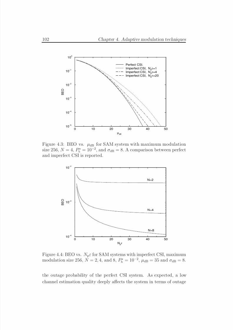
7/29/2019 Adaptive Wireless Multimedia
http://slidepdf.com/reader/full/adaptive-wireless-multimedia 120/187
102 Chapter 4. Adaptive modulation techniques
0 10 20 30 40 50
µdB
10−5
10−4
10−3
10−2
10−1
100
B E O
Perfect CSI.
Imperfect CSI, Npε=1
Imperfect CSI, Npε=4
Imperfect CSI, Npε=20
Figure 4.3: BEO vs. µdB for SAM system with maximum modulationsize 256, N = 4, P ⋆b = 10−2, and σdB = 8. A comparison between perfectand imperfect CSI is reported.
0 10 20 30 40 50
Npε
10−4
10−3
10−2
B E O
N=2
N=4
N=8
Figure 4.4: BEO vs. N pε for SAM systems with imperfect CSI, maximummodulation size 256, N = 2, 4, and 8, P ⋆b = 10−2, µdB = 35 and σdB = 8.
the outage probability of the perfect CSI system. As expected, a low
channel estimation quality deeply affects the system in terms of outage
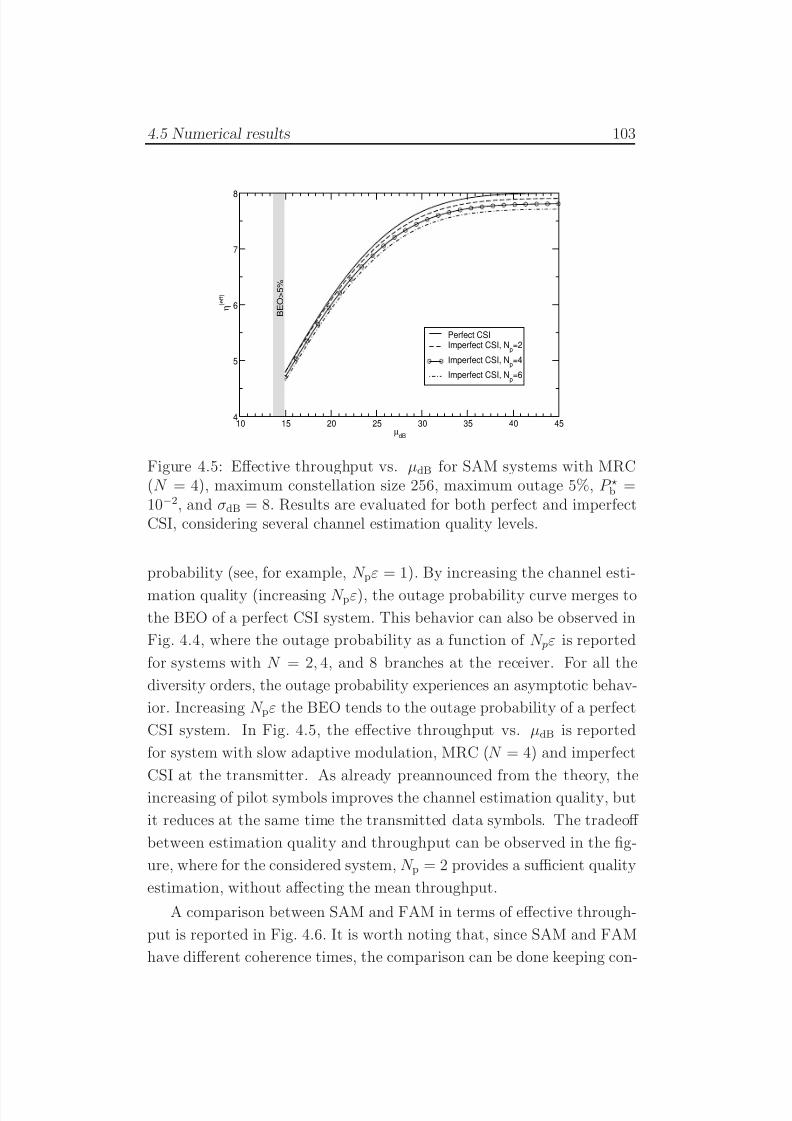
7/29/2019 Adaptive Wireless Multimedia
http://slidepdf.com/reader/full/adaptive-wireless-multimedia 121/187
4.5 Numerical results 103
10 15 20 25 30 35 40 45µ
dB
4
5
6
7
8
η ( e f f )
Perfect CSIImperfect CSI, N
p=2
Imperfect CSI, Np=4
Imperfect CSI, Np=6
B E O > 5 %
Figure 4.5: Effective throughput vs. µdB for SAM systems with MRC(N = 4), maximum constellation size 256, maximum outage 5%, P ⋆b =10−2, and σdB = 8. Results are evaluated for both perfect and imperfectCSI, considering several channel estimation quality levels.
probability (see, for example, N pε = 1). By increasing the channel esti-
mation quality (increasing N pε), the outage probability curve merges to
the BEO of a perfect CSI system. This behavior can also be observed in
Fig. 4.4, where the outage probability as a function of N pε is reported
for systems with N = 2, 4, and 8 branches at the receiver. For all the
diversity orders, the outage probability experiences an asymptotic behav-
ior. Increasing N pε the BEO tends to the outage probability of a perfect
CSI system. In Fig. 4.5, the effective throughput vs. µdB is reported
for system with slow adaptive modulation, MRC (N = 4) and imperfect
CSI at the transmitter. As already preannounced from the theory, the
increasing of pilot symbols improves the channel estimation quality, but
it reduces at the same time the transmitted data symbols. The tradeoff
between estimation quality and throughput can be observed in the fig-
ure, where for the considered system, N p = 2 provides a sufficient quality
estimation, without affecting the mean throughput.
A comparison between SAM and FAM in terms of effective through-
put is reported in Fig. 4.6. It is worth noting that, since SAM and FAM
have different coherence times, the comparison can be done keeping con-
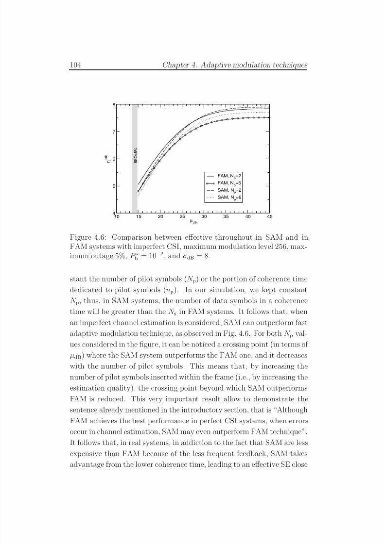
7/29/2019 Adaptive Wireless Multimedia
http://slidepdf.com/reader/full/adaptive-wireless-multimedia 122/187
104 Chapter 4. Adaptive modulation techniques
10 15 20 25 30 35 40 45µ
dB
4
5
6
7
8
η ( e f f )
FAM, Np=2
FAM, Np=6
SAM, Np=2SAM, N
p=6
B E O > 5 %
Figure 4.6: Comparison between effective throughout in SAM and inFAM systems with imperfect CSI, maximum modulation level 256, max-imum outage 5%, P ⋆b = 10−2, and σdB = 8.
stant the number of pilot symbols (N p) or the portion of coherence time
dedicated to pilot symbols (np). In our simulation, we kept constant
N p, thus, in SAM systems, the number of data symbols in a coherence
time will be greater than the N s in FAM systems. It follows that, when
an imperfect channel estimation is considered, SAM can outperform fast
adaptive modulation technique, as observed in Fig. 4.6. For both N p val-
ues considered in the figure, it can be noticed a crossing point (in terms of
µdB) where the SAM system outperforms the FAM one, and it decreases
with the number of pilot symbols. This means that, by increasing the
number of pilot symbols inserted within the frame (i.e., by increasing theestimation quality), the crossing point beyond which SAM outperforms
FAM is reduced. This very important result allow to demonstrate the
sentence already mentioned in the introductory section, that is “Although
FAM achieves the best performance in perfect CSI systems, when errors
occur in channel estimation, SAM may even outperform FAM technique”.
It follows that, in real systems, in addiction to the fact that SAM are less
expensive than FAM because of the less frequent feedback, SAM takes
advantage from the lower coherence time, leading to an effective SE close
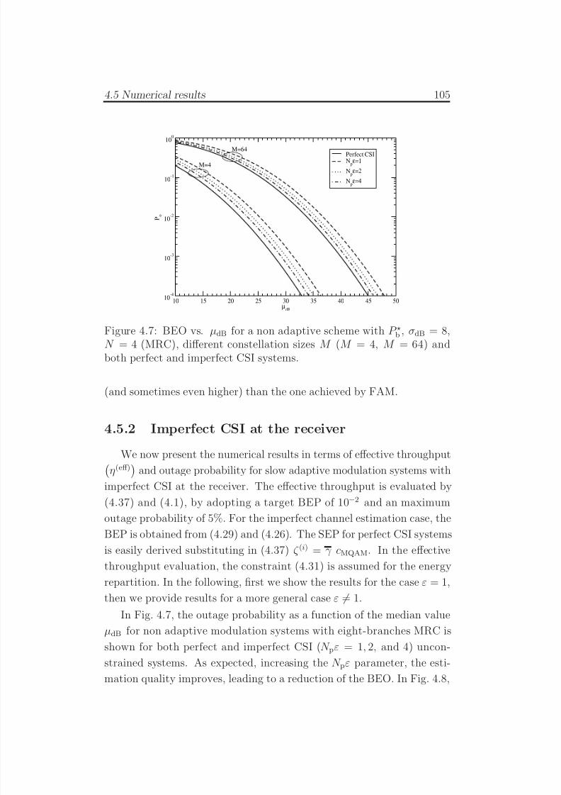
7/29/2019 Adaptive Wireless Multimedia
http://slidepdf.com/reader/full/adaptive-wireless-multimedia 123/187
4.5 Numerical results 105
10 15 20 25 30 35 40 45 50µ
dB
10-4
10-3
10-2
10-1
100
P o
Perfect CSIN
pε=1
Npε=2
Npε=4
M=64
M=4
Figure 4.7: BEO vs. µdB for a non adaptive scheme with P ⋆b , σdB = 8,N = 4 (MRC), different constellation sizes M (M = 4, M = 64) andboth perfect and imperfect CSI systems.
(and sometimes even higher) than the one achieved by FAM.
4.5.2 Imperfect CSI at the receiver
We now present the numerical results in terms of effective throughputη(eff)
and outage probability for slow adaptive modulation systems with
imperfect CSI at the receiver. The effective throughput is evaluated by
(4.37) and (4.1), by adopting a target BEP of 10−2 and an maximum
outage probability of 5%. For the imperfect channel estimation case, the
BEP is obtained from (4.29) and (4.26). The SEP for perfect CSI systems
is easily derived substituting in (4.37) ζ (i) = γ cMQAM
. In the effective
throughput evaluation, the constraint (4.31) is assumed for the energy
repartition. In the following, first we show the results for the case ε = 1,
then we provide results for a more general case ε = 1.
In Fig. 4.7, the outage probability as a function of the median value
µdB for non adaptive modulation systems with eight-branches MRC is
shown for both perfect and imperfect CSI (N pε = 1, 2, and 4) uncon-
strained systems. As expected, increasing the N pε parameter, the esti-
mation quality improves, leading to a reduction of the BEO. In Fig. 4.8,
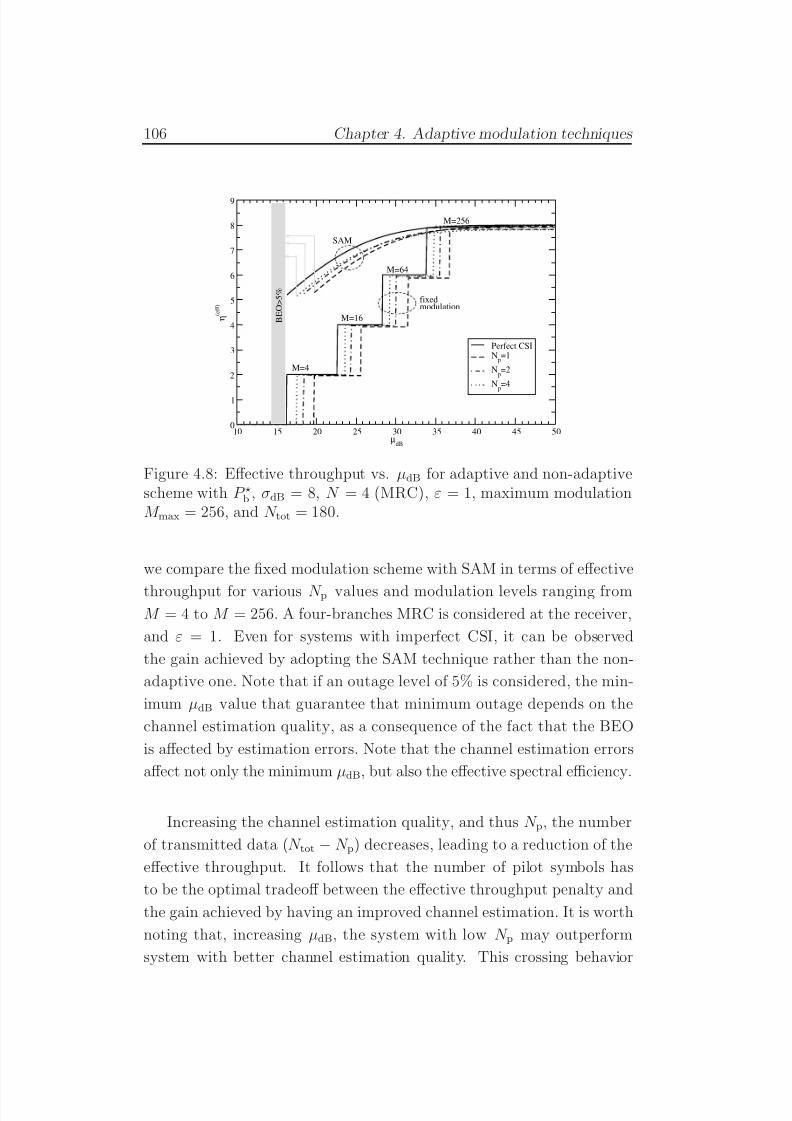
7/29/2019 Adaptive Wireless Multimedia
http://slidepdf.com/reader/full/adaptive-wireless-multimedia 124/187
106 Chapter 4. Adaptive modulation techniques
10 15 20 25 30 35 40 45 50µ
dB
0
1
2
3
4
5
6
7
8
9
η ( e f f )
Perfect CSIN
p=1
Np=2
Np=4
B E O > 5 %
SAM
fixedmodulation
M=4
M=16
M=64
M=256
Figure 4.8: Effective throughput vs. µdB for adaptive and non-adaptivescheme with P ⋆b , σdB = 8, N = 4 (MRC), ε = 1, maximum modulationM max = 256, and N tot = 180.
we compare the fixed modulation scheme with SAM in terms of effective
throughput for various N p values and modulation levels ranging fromM = 4 to M = 256. A four-branches MRC is considered at the receiver,
and ε = 1. Even for systems with imperfect CSI, it can be observed
the gain achieved by adopting the SAM technique rather than the non-
adaptive one. Note that if an outage level of 5% is considered, the min-
imum µdB value that guarantee that minimum outage depends on the
channel estimation quality, as a consequence of the fact that the BEO
is affected by estimation errors. Note that the channel estimation errors
affect not only the minimum µdB, but also the effective spectral efficiency.
Increasing the channel estimation quality, and thus N p, the number
of transmitted data (N tot − N p) decreases, leading to a reduction of the
effective throughput. It follows that the number of pilot symbols has
to be the optimal tradeoff between the effective throughput penalty and
the gain achieved by having an improved channel estimation. It is worth
noting that, increasing µdB, the system with low N p may outperform
system with better channel estimation quality. This crossing behavior
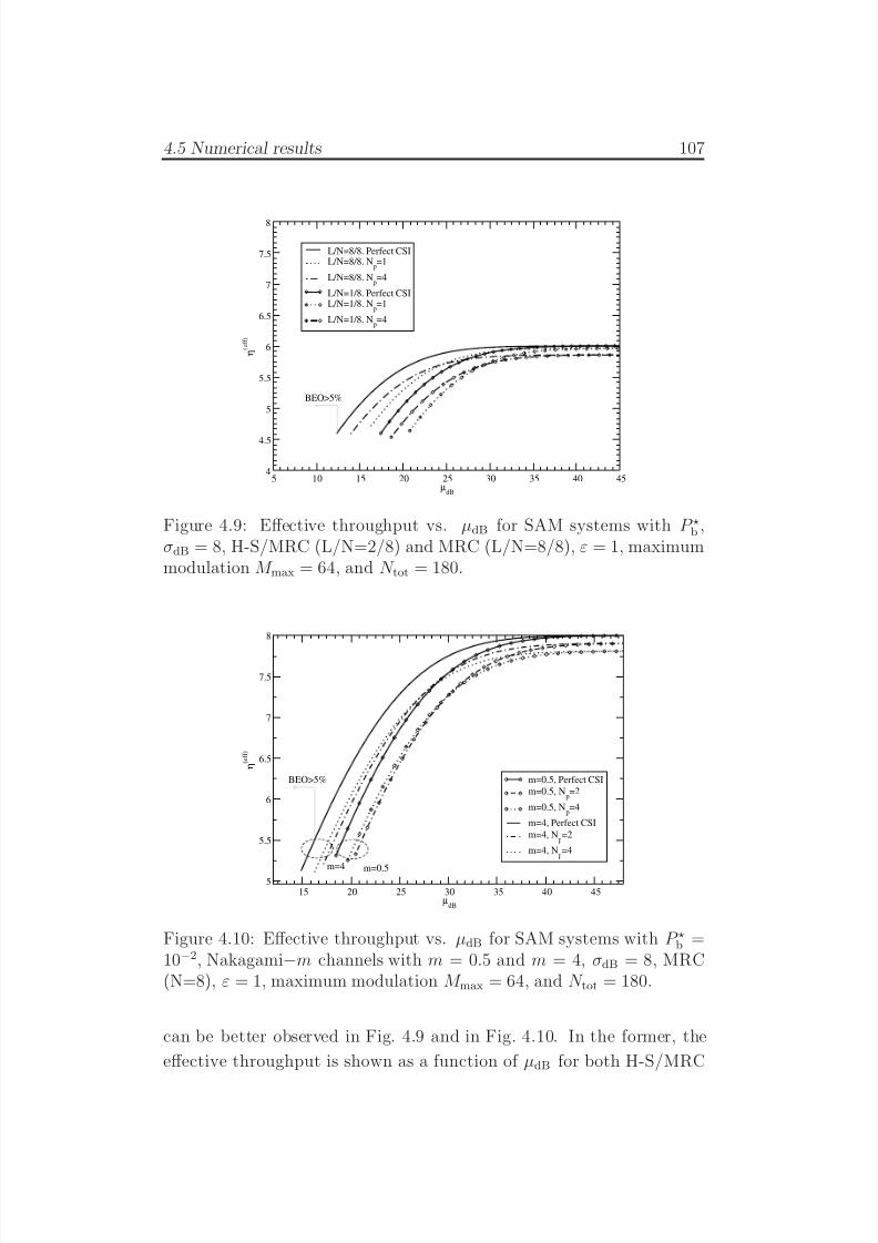
7/29/2019 Adaptive Wireless Multimedia
http://slidepdf.com/reader/full/adaptive-wireless-multimedia 125/187
4.5 Numerical results 107
5 10 15 20 25 30 35 40 45µ
dB
4
4.5
5
5.5
6
6.5
7
7.5
8
η ( e f f )
L/N=8/8. Perfect CSIL/N=8/8. N
p=1
L/N=8/8. Np=4
L/N=1/8. Perfect CSIL/N=1/8. N
p=1
L/N=1/8. Np=4
BEO>5%
Figure 4.9: Effective throughput vs. µdB for SAM systems with P ⋆b ,σdB = 8, H-S/MRC (L/N=2/8) and MRC (L/N=8/8), ε = 1, maximummodulation M max = 64, and N tot = 180.
15 20 25 30 35 40 45µ
dB
5
5.5
6
6.5
7
7.5
8
η ( e f f )
m=0.5, Perfect CSI
m=0.5, Np=2
m=0.5, Np=4
m=4, Perfect CSI
m=4, Np=2
m=4, Np=4
BEO>5%
m=0.5m=4
Figure 4.10: Effective throughput vs. µdB for SAM systems with P ⋆b =10−2, Nakagami−m channels with m = 0.5 and m = 4, σdB = 8, MRC(N=8), ε = 1, maximum modulation M max = 64, and N tot = 180.
can be better observed in Fig. 4.9 and in Fig. 4.10. In the former, the
effective throughput is shown as a function of µdB for both H-S/MRC
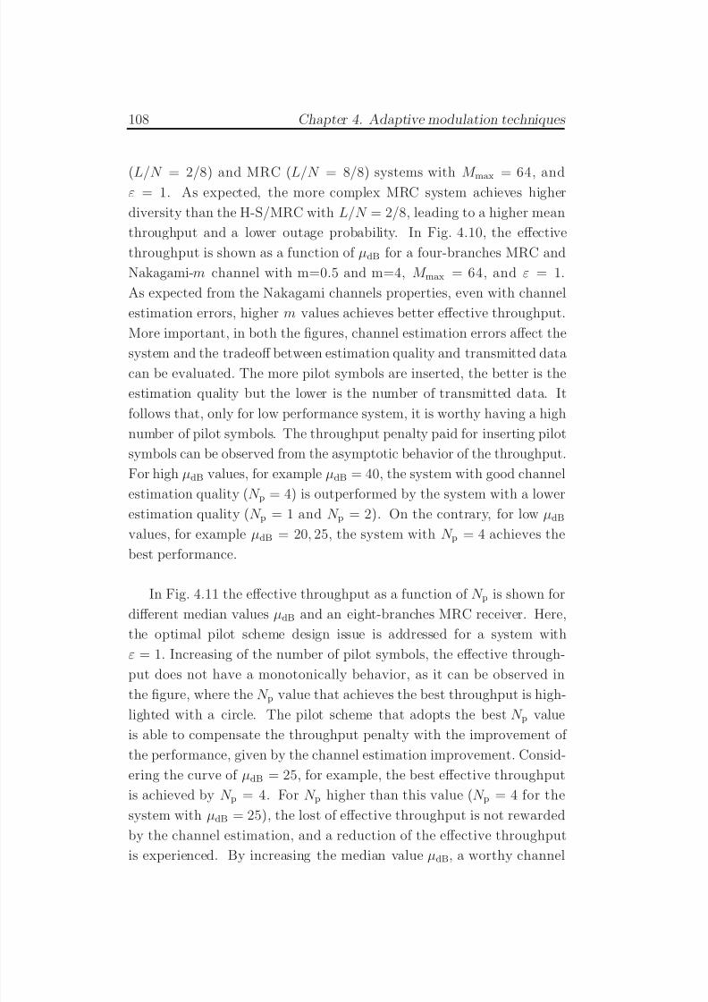
7/29/2019 Adaptive Wireless Multimedia
http://slidepdf.com/reader/full/adaptive-wireless-multimedia 126/187
108 Chapter 4. Adaptive modulation techniques
(L/N = 2/8) and MRC (L/N = 8/8) systems with M max = 64, andε = 1. As expected, the more complex MRC system achieves higher
diversity than the H-S/MRC with L/N = 2/8, leading to a higher mean
throughput and a lower outage probability. In Fig. 4.10, the effective
throughput is shown as a function of µdB for a four-branches MRC and
Nakagami-m channel with m=0.5 and m=4, M max = 64, and ε = 1.
As expected from the Nakagami channels properties, even with channel
estimation errors, higher m values achieves better effective throughput.
More important, in both the figures, channel estimation errors affect the
system and the tradeoff between estimation quality and transmitted datacan be evaluated. The more pilot symbols are inserted, the better is the
estimation quality but the lower is the number of transmitted data. It
follows that, only for low performance system, it is worthy having a high
number of pilot symbols. The throughput penalty paid for inserting pilot
symbols can be observed from the asymptotic behavior of the throughput.
For high µdB values, for example µdB = 40, the system with good channel
estimation quality (N p = 4) is outperformed by the system with a lower
estimation quality (N p = 1 and N p = 2). On the contrary, for low µdB
values, for example µdB = 20, 25, the system with N p = 4 achieves the
best performance.
In Fig. 4.11 the effective throughput as a function of N p is shown for
different median values µdB and an eight-branches MRC receiver. Here,
the optimal pilot scheme design issue is addressed for a system with
ε = 1. Increasing of the number of pilot symbols, the effective through-
put does not have a monotonically behavior, as it can be observed in
the figure, where the N p value that achieves the best throughput is high-lighted with a circle. The pilot scheme that adopts the best N p value
is able to compensate the throughput penalty with the improvement of
the performance, given by the channel estimation improvement. Consid-
ering the curve of µdB = 25, for example, the best effective throughput
is achieved by N p = 4. For N p higher than this value (N p = 4 for the
system with µdB = 25), the lost of effective throughput is not rewarded
by the channel estimation, and a reduction of the effective throughput
is experienced. By increasing the median value µdB, a worthy channel
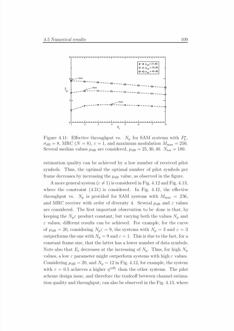
7/29/2019 Adaptive Wireless Multimedia
http://slidepdf.com/reader/full/adaptive-wireless-multimedia 127/187
4.5 Numerical results 109
1 2 3 4 5 6 7 8N
p
6
7
8
9
η ( e f f )
µdB
= 25 dB
µdB
= 30 dB
µdB
= 40 dB
max
max
max
Figure 4.11: Effective throughput vs. N p for SAM systems with P ⋆b ,σdB = 8, MRC (N = 8), ε = 1, and maximum modulation M max = 256.Several median values µdB are considered, µdB = 25, 30, 40. N tot = 180.
estimation quality can be achieved by a low number of received pilot
symbols. Thus, the optimal the optimal number of pilot symbols per
frame decreases by increasing the µdB value, as observed in the figure.
A more general system (ε = 1) is considered in Fig. 4.12 and Fig. 4.13,
where the constraint (4.31) is considered. In Fig. 4.12, the effective
throughput vs. N p is provided for SAM systems with M max = 256,
and MRC receiver with order of diversity 4. Several µdB and ε values
are considered. The first important observation to be done is that, by
keeping the N pε product constant, but varying both the values N p and
ε values, different results can be achieved. For example, for the curve
of µdB = 20, considering N pε = 9, the systems with N p = 3 and ε = 3outperforms the one with N p = 9 and ε = 1. This is due to the fact, for a
constant frame size, that the latter has a lower number of data symbols.
Note also that E s decreases at the increasing of N p. Thus, for high N p
values, a low ε parameter might outperform systems with high ε values.
Considering µdB = 20, and N p = 12 in Fig. 4.12, for example, the system
with ε = 0.5 achieves a higher η(eff) than the other systems. The pilot
scheme design issue, and therefore the tradeoff between channel estima-
tion quality and throughput, can also be observed in the Fig. 4.13, where
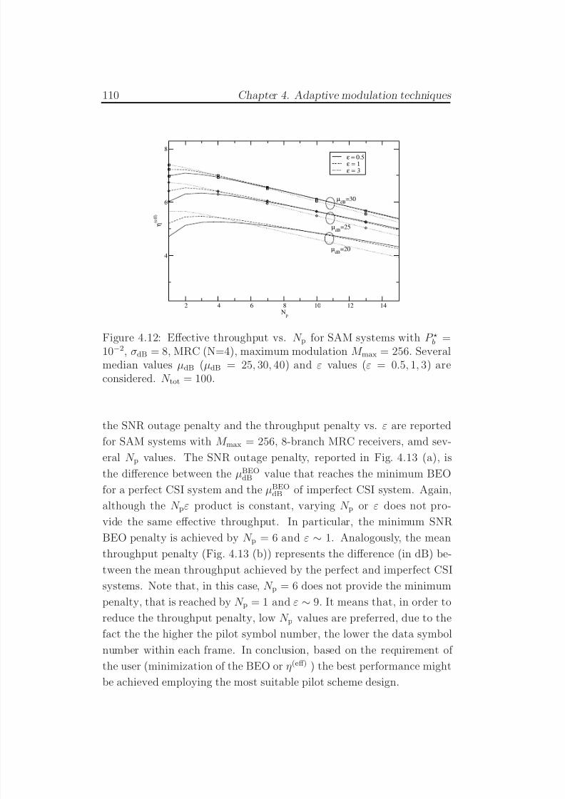
7/29/2019 Adaptive Wireless Multimedia
http://slidepdf.com/reader/full/adaptive-wireless-multimedia 128/187
110 Chapter 4. Adaptive modulation techniques
2 4 6 8 10 12 14N
p
4
6
8
η ( e f f )
ε = 0.5ε = 1ε = 3
µdB
=20
µdB
=25
µdB
=30
Figure 4.12: Effective throughput vs. N p for SAM systems with P ⋆b =10−2, σdB = 8, MRC (N=4), maximum modulation M max = 256. Severalmedian values µdB (µdB = 25, 30, 40) and ε values (ε = 0.5, 1, 3) areconsidered. N tot = 100.
the SNR outage penalty and the throughput penalty vs. ε are reported
for SAM systems with M max = 256, 8-branch MRC receivers, amd sev-
eral N p values. The SNR outage penalty, reported in Fig. 4.13 (a), is
the difference between the µBEOdB value that reaches the minimum BEO
for a perfect CSI system and the µBEOdB of imperfect CSI system. Again,
although the N pε product is constant, varying N p or ε does not pro-
vide the same effective throughput. In particular, the minimum SNR
BEO penalty is achieved by N p = 6 and ε ∼ 1. Analogously, the mean
throughput penalty (Fig. 4.13 (b)) represents the difference (in dB) be-tween the mean throughput achieved by the perfect and imperfect CSI
systems. Note that, in this case, N p = 6 does not provide the minimum
penalty, that is reached by N p = 1 and ε ∼ 9. It means that, in order to
reduce the throughput penalty, low N p values are preferred, due to the
fact the the higher the pilot symbol number, the lower the data symbol
number within each frame. In conclusion, based on the requirement of
the user (minimization of the BEO or η(eff) ) the best performance might
be achieved employing the most suitable pilot scheme design.
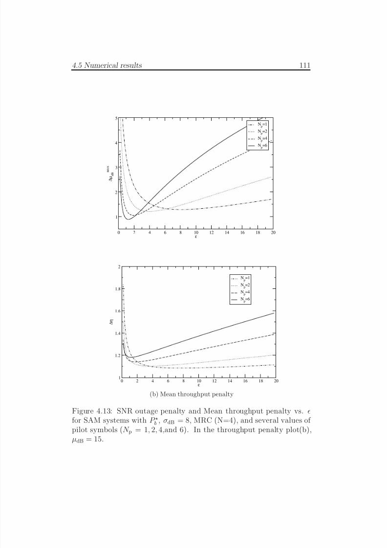
7/29/2019 Adaptive Wireless Multimedia
http://slidepdf.com/reader/full/adaptive-wireless-multimedia 129/187
4.5 Numerical results 111
0 2 4 6 8 10 12 14 16 18 20ε
1
2
3
4
5
∆ µ d B
B E O
Np=1
Np=2
Np=4
Np=6
(a) SNR outage penalty
0 2 4 6 8 10 12 14 16 18 20ε
1
1.2
1.4
1.6
1.8
2
∆ η
Np=1
Np
=2
Np=4
Np=6
(b) Mean throughput penalty
Figure 4.13: SNR outage penalty and Mean throughput penalty vs. ǫfor SAM systems with P ⋆b , σdB = 8, MRC (N=4), and several values of pilot symbols (N p = 1, 2, 4,and 6). In the throughput penalty plot(b),µdB = 15.
7/29/2019 Adaptive Wireless Multimedia
http://slidepdf.com/reader/full/adaptive-wireless-multimedia 130/187
112 Chapter 4. Adaptive modulation techniques
4.6 ConclusionIn this chapter, we investigated both fast and slow adaptive modu-
lation techniques when channel estimation errors are assumed. We ad-
dressed the effects imperfect CSI both at the transmitter and the receiver
on adaptive modulation. In the former case, a comparison between FAM
and SAM was provided for systems with MRC, showing that, for some
system configurations, the slow adaptive modulation technique can out-
perform the FAM. Then, channel estimation at the receiver was inves-
tigated for SAM systems with H-S/MRC for Rayleigh and Nakagami-mchannels. We compared SAM with fixed-modulation schemes in terms
of outage probability and effective spectral efficiency. Even for imper-
fect CSI systems, SAM technique achieves substantial improvement over
non adaptive schemes. Moreover, the optimal pilot scheme design was
investigated for systems employing subset diversity. A high number of
pilot symbols achieves a good estimation quality at the cost of a spectral
efficiency reduction. Thus, the tradeoff between estimation quality and
throughput was addressed. In particular, the higher is the median value
µdB, the lower is the number of pilot symbols required.
7/29/2019 Adaptive Wireless Multimedia
http://slidepdf.com/reader/full/adaptive-wireless-multimedia 131/187
Chapter 5
Adaptive modulation in thepresence of interference and
imperfect thresholds
In this chapter, we address the effects of signal-to-noise ratio thresh-
olds shifting in adaptive M -ary quadrature amplitude modulation sys-tems with diversity at the receiver. As already mentioned in the pre-
vious chapter, in adaptive modulation systems the optimal modulation
to be employed in the transmission is evaluated by comparing the esti-
mated signal-to-noise ratio (SNR) to some thresholds levels. Co-channel
interference signals or approximated bit error probability expressions em-
ployed in the system may lead to a variation of the thresholds. Here, we
investigate the effects of this thresholds variation on the system perfor-
mance, evaluated in terms of bit error outage and mean throughput.
The remainder of this chapter is organized as follows. In Section 5.1,
the motivations of the work together with a brief description of adaptive
modulation techniques are provided. In Section 5.2, the system model
description is provided for both slow and fast adaptive modulation tech-
niques. Then, the analysis of the effects of SNR thresholds shifting is
reported in Section 5.3 and two applicative examples are considered in
Section 5.4 and Section 5.5. In Section 5.6 numerical results are provided,
and conclusions are given in Section 5.7.
113
7/29/2019 Adaptive Wireless Multimedia
http://slidepdf.com/reader/full/adaptive-wireless-multimedia 132/187
114 Chapter 5. Adaptive modulation in the presence of...
5.1 Motivation and outline of the workThe diffusion of high speed digital wireless communications has in-
creased the need of reliable high data rate transmission in variable chan-
nel conditions. As already observed in the previous chapter, adaptive
modulation techniques allow to maximize the transmitted throughput 1
without compromising the performance in terms of bit error probability
(BEP) and bit error outage (BEO). Adaptive modulation techniques can
be classified into slow or fast adaptive modulation, SAM and FAM re-
spectively. The former adapts modulation parameters to the large-scalefading, while FAM tracks the small-scale fading. In both FAM and SAM,
the overall performance might be affected by imperfect channel estima-
tions (as investigated in Chapter 4) or by approximations in the SNR
thresholds that reach the target BEP for possible system configurations.
When the system experiences any non-idealities that affect the BEP per-
formance compared to in ideal system, a SNR thresholds shift occurs,
compromising therefore the overall performance. In particular, the mod-
ulation level switch can appear later (before) than the ideal case, leading
to a reduction (increasing) of the mean throughput (outage probabil-ity). A possible cause of this thresholds shifting can be represented by
any approximation introduced in the system, leading to a computational
simplification, as the employment of approximation BEP expressions.
Being the exponential BEP expression [5] invertible, for example, it is
extremely appealing and widely used in the literature, but, on the other
hand, the SNR thresholds achieved by the approximated BEP expression
may diverge from the original ones [107]. To the best of our knowledge,
there is no evaluation of the effects of SNR thresholds shifting in terms
of mean throughput and outage probability. Moreover, another possible
issue that affects the system performance is the presence of interfering
signals. Thus, in interfered systems, SNR thresholds shifting might oc-
curs, and the rising question is “How much an adaptive system is robust
to interferers?”. In the literature, some works addressed this question,
as in [108] and in [109]. In the former, the performance are quantified
1Throughout this chapter, we shall use the terms “throughput” and “spectralefficiency (SE)” interchangeably.
7/29/2019 Adaptive Wireless Multimedia
http://slidepdf.com/reader/full/adaptive-wireless-multimedia 133/187
5.2 System model 115
in terms of BER for OFDM systems, while in the latter, the authorsevaluated the mean throughput of an interfered system. Both the works
were limited to FAM systems and did not provide performance in terms
of BEO.
In this chapter, we probe the effects of SNR thresholds shifting, due
to co-channel interference or approximated BEP, investigating both slow
and fast adaptive modulation techniques for M -QAM systems with op-
timum combiner at the receiver. First, the thresholds shifting issue is in-
vestigated in the most general way, including all the possible causes, i.e.,
imperfect channel estimation, presence of interference, employment of ap-
proximated BEP expressions, or any other issue that affects the system
performance. Then, we address two applicative examples of thresholds
shifting: approximated bit error probability expressions and presence of
co-channel interference signals [110, 111]. The performance in terms of
mean throughput and bit error outage probability are then quantified in
the result section.
Notation : throughout the chapter, vectors and matrices are indicated
by bold m and M, respectively; det[M] denotes the determinant of the
matrix M; the superscript H indicates the conjugation and transposition,
and IN is the N × N identity matrix.
5.2 System model
We assume M -QAM modulated symbols transmitted over Rayleigh
fading and log-normal shadowing channels employing microdiversity at
the receiver, i.e., the shadowing level is the same on each branch. At thereceiver, N antennas are considered and the optimum combiner is em-
ployed for processing the signal. Maximum ratio combining (MRC) and
minimum mean square error (MMSE) are adopted for uninterfered and
interfered systems, respectively. We denote by E S the mean (over the fad-
ing) symbol energy transmitted, by h = hii=1,...,N the channel vector,
whose elements hi represent the Rayleigh distributed fading gain, and by
n(k) the additive Gaussian noise with zero mean and En(k)n(k)H =
N 0IN , where N 0/2 is the two-sided thermal noise power spectral den-
7/29/2019 Adaptive Wireless Multimedia
http://slidepdf.com/reader/full/adaptive-wireless-multimedia 134/187
116 Chapter 5. Adaptive modulation in the presence of...
sity. For sake of simplicity, we omit the branch subscript in the meanSNR notation. The average signal-to-noise ratio on each branch can be
expressed as γ = E |h|2E s/N 0 = E s/N 0, where E |h|2 = 2σ2h = 1.
Since we consider a log-normal shadowing, γ dB = 10 log10(γ ) is Gaussian
distributed with mean µdB mean and σ2dB variance.
As briefly stated before, adaptive modulation techniques allow to
achieve the best throughput accordingly with channel conditions, mini-
mizing in the meanwhile the outage probability, [6]. In particular, when
a discrete variable rate is considered, a set of J modulation levels can
be adopted, M 0, M 1, . . . , M J . As observed in the previous chapter, theoptimal modulation level is chosen depending on the instantaneous or
mean SNR in FAM or SAM, respectively. We denote by χ the SNR pa-
rameter, in particular, in SAM systems χ = γ , while in FAM systems
χ = γ T, where γ T is the instantaneous SNR at the combiner output2.
When, even with the lowest modulation level M 0, χ is not sufficient to
guarantee the target BEP P ⋆b , the system is in outage. Otherwise, the
transmitted data rate corresponds to log2 M j, j = 0, . . . , J . The op-
timal data rate is chosen comparing the χ value with modulation level
thresholds, that are set to guarantee the minimum BEP required when
the j-th modulation level is adopted, that is P b(χ⋆ j) = P ⋆b . In particular,
when the SNR value falls within the j-th region (χ⋆ j < χ ≤ χ⋆ j+1), the
j-th modulation level is adopted for the transmission. It follows that an
important figure of merit is the mean throughput [bps/Hz] defined as
η =J −1 j=0
M j P
χ⋆ j < χ ≤ χ⋆ j+1
+ M J P χ⋆J < χ
=
J −1 j=0
M j F χ(χ⋆ j+1) − F χ(χ⋆ j)+ M J [1 − F χ(χ⋆J )]
=J −1 j=0
M j
F χdB(χ⋆dB,j+1) − F χdB(χ⋆dB,j)
+ M J
1 − F χdB(χ⋆dB,J )
(5.1)
where M j = log2 M j and F χdB(x) is the CDF of the SNR value in dB,
2Note that, unlike the notation in the Chapter 4, here χ represents the SNRparameter in linear scale in both FAM and SAM.
7/29/2019 Adaptive Wireless Multimedia
http://slidepdf.com/reader/full/adaptive-wireless-multimedia 135/187
5.3 Imperfect thresholds 117
i.e., χdB = 10log10(χ). Another important measure of the QoS is thebit error outage probability (BEO), i.e., the probability that the bit error
probability is greater than the target BEP:
P o(P ⋆b ) = P P b(χ) > P ⋆b = F χ (χ⋆0) . (5.2)
For SAM systems, in log-normal shadowing, the CDF of the averaged
SNR is expressed as
F γ dB(ξ ) = QµdB − ξ
σdB
(5.3)
where Q(·) is the Gaussian-Q function.
5.3 Imperfect thresholds
In this section, the effects of imperfect thresholds in terms of through-put and outage probability are investigated for a general system, i.e.,
without explicating the causes of threshold shifting. When the system
experiences a decreasing of the performance, the BEP expression diverges
from the ideal one, and a shift of the SNR thresholds occurs. This ap-
proximation can be expressed as χ⋆ j,dB = χ⋆ j,dB + ∆ j,dB. Note that ∆ j,dB
might be either a deterministic or a random variable that might assume
positive and negative values.
To evaluate the mean throughput in realistic systems, (5.1) can still beconsidered by replacing the ideal thresholds χ⋆ j,dB with χ⋆ j,dB. Conversely,
the outage probability is not always given by (5.2). In particular, when
χ⋆ j,dB < χ⋆ j,dB, although the real SNR falls within the j-th modulation
range, the ( j + 1)-th modulation might be adopted. In this case, the
effective bit error probability is greater than the target BEP and the sys-
tem is in outage. It means that the system is in outage when χdB < χ⋆0,dB,
and also when the SNR value falls within the range (χ⋆ j,dB −|∆ j,dB|, χ⋆ j,dB]
for j = 1, . . . , J . Thus, when approximated thresholds are obtained, the
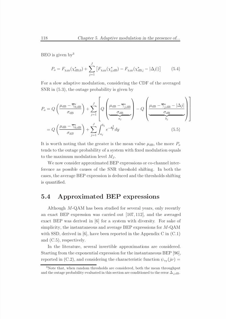
7/29/2019 Adaptive Wireless Multimedia
http://slidepdf.com/reader/full/adaptive-wireless-multimedia 136/187
118 Chapter 5. Adaptive modulation in the presence of...
BEO is given by3
P o = F χdB(χ⋆dB,0) +J
j=1
F χdB(χ⋆ j,dB) − F χdB(χ⋆dB,j − |∆ j|) (5.4)
For a slow adaptive modulation, considering the CDF of the averaged
SNR in (5.3), the outage probability is given by
P o = QµdB − γ ∗0,dB
σdB +J
j=1
Q
µdB − γ ∗ j,dB
σdB aj
−Q
µdB − γ ⋆ j,dB − |∆ j|σdB bj
= Q
µdB − γ ∗0,dB
σdB
+
J j=1
bjaj
e−y2
2 dy (5.5)
It is worth noting that the greater is the mean value µdB, the more P o
tends to the outage probability of a system with fixed modulation equals
to the maximum modulation level M J .
We now consider approximated BEP expressions or co-channel inter-
ference as possible causes of the SNR threshold shifting. In both the
cases, the average BEP expression is deduced and the thresholds shifting
is quantified.
5.4 Approximated BEP expressions
Although M -QAM has been studied for several years, only recently
an exact BEP expression was carried out [107, 112], and the averaged
exact BEP was derived in [6] for a system with diversity. For sake of
simplicity, the instantaneous and average BEP expressions for M -QAM
with SSD, derived in [6], have been reported in the Appendix C in (C.1)
and (C.5), respectively.
In the literature, several invertible approximations are considered.
Starting from the exponential expression for the instantaneous BEP [96],
reported in (C.2), and considering the characteristic function ψγ T( jν ) =
3Note that, when random thresholds are considered, both the mean throughputand the outage probability evaluated in this section are conditioned to the error ∆ j,dB.
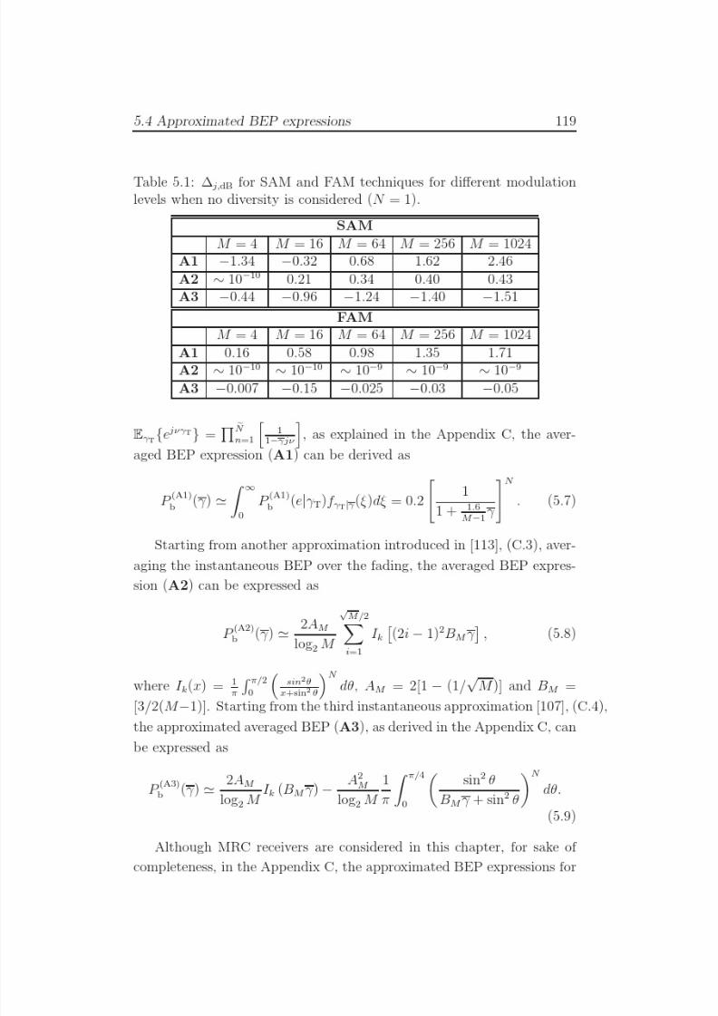
7/29/2019 Adaptive Wireless Multimedia
http://slidepdf.com/reader/full/adaptive-wireless-multimedia 137/187
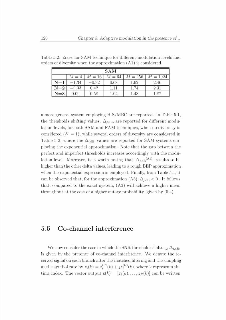
7/29/2019 Adaptive Wireless Multimedia
http://slidepdf.com/reader/full/adaptive-wireless-multimedia 138/187
120 Chapter 5. Adaptive modulation in the presence of...
Table 5.2: ∆ j,dB for SAM technique for different modulation levels andorders of diversity when the approximation (A1) is considered.
SAM
M = 4 M = 16 M = 64 M = 256 M = 1024
N=1 −1.34 −0.32 0.68 1.62 2.46
N=2 −0.33 0.42 1.11 1.74 2.31
N=8 0.09 0.58 1.04 1.48 1.87
a more general system employing H-S/MRC are reported. In Table 5.1,
the thresholds shifting values, ∆ j,dB, are reported for different modu-
lation levels, for both SAM and FAM techniques, when no diversity is
considered (N = 1), while several orders of diversity are considered in
Table 5.2, where the ∆ j,dB values are reported for SAM systems em-
ploying the exponential approximation. Note that the gap between the
perfect and imperfect thresholds increases accordingly with the modu-
lation level. Moreover, it is worth noting that |∆ j,dB(A1)| results to be
higher than the other delta values, leading to a rough BEP approximationwhen the exponential expression is employed. Finally, from Table 5.1, it
can be observed that, for the approximation (A3), ∆ j,dB < 0 . It follows
that, compared to the exact system, (A3) will achieve a higher mean
throughput at the cost of a higher outage probability, given by (5.4).
5.5 Co-channel interference
We now consider the case in which the SNR thresholds shifting, ∆ j,dB,
is given by the presence of co-channel interference. We denote the re-
ceived signal on each branch after the matched filtering and the sampling
at the symbol rate by z i(k) = z (P)i (k) + jz
(Q)i (k), where k represents the
time index. The vector output z(k) = [z 1(k), . . . , z N (k)] can be written
7/29/2019 Adaptive Wireless Multimedia
http://slidepdf.com/reader/full/adaptive-wireless-multimedia 139/187
5.5 Co-channel interference 121
as4
[114]z(k) = z(P)(k) + jz(Q)(k)
=
E Sh b0(k) +
E I
N In=1
hI,nbI,n(k) + n(k), (5.10)
where E I is the mean symbol energy transmitted of each interfering sig-
nals; b0(k) = b(P)0 (k) + jb(Q)
0 (k) is the desired signal sample and bI,n(k) =
b(P)I,n (k) + jb(Q)
I,n (k) is the interfering signal sample of the n-th interferer.
Since we assume a slow frequency flat Rayleigh distributed fading, the
vectors h and hI,n, n = 1, . . . , N I have distribution CN (0, IN ), and wedenote by HI = hI,j j=1,...,N I the interference channel matrix. Being
the desired signal affected by fading, the Gaussian approximation for
the interferers is justified [115]. Thus, b1(k), . . . , bN I(k) are independent
zero-mean complex Gaussian random variables, each with variance one
because of the normalization.
Following the steps in [114], we derive the bit error probability as
a function of the averaged signal-to-interference-plus-noise ratio (SINR)
for a M -QAM system with optimum combining at the receiver. The
optimum weight vector that maximizes the SINR is w = αR−1cD, whereα is an arbitrary constant and R the covariance matrix, expressed as
R = En(k),bj(k)
E I
N In=1
hI,nbI,n(k) + n(k)
E I
N In=1
hI,nbI,n(k) + n(k)
H = E I
N I j=1
hI,jhH I,j
RI
+N 0IN , (5.11)
where the last equality holds because the desired signal, the interferenceand the noise are assumed independent from each other. Considering
an overloaded system (i.e., N I ≥ N )5 the SINR of the output at the
combiner can be written as
γ =N i=1
E S hH S ui2
E I λi + N 0,
4Note that the superscripts (P) and (Q) stand for the in-phase and quadraturesymbols, respectively.
5The extension to the underloaded case is reported in the Appendix D.
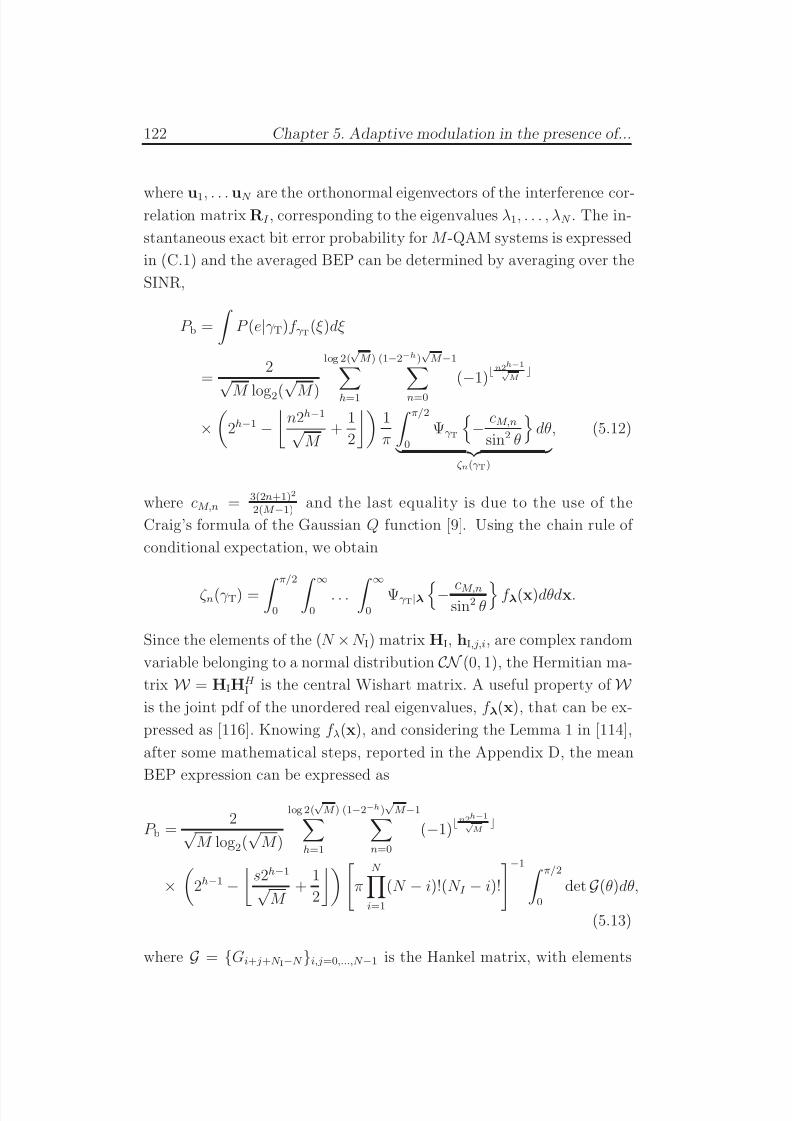
7/29/2019 Adaptive Wireless Multimedia
http://slidepdf.com/reader/full/adaptive-wireless-multimedia 140/187
122 Chapter 5. Adaptive modulation in the presence of...
where u1, . . . uN are the orthonormal eigenvectors of the interference cor-relation matrix RI , corresponding to the eigenvalues λ1, . . . , λN . The in-
stantaneous exact bit error probability for M -QAM systems is expressed
in (C.1) and the averaged BEP can be determined by averaging over the
SINR,
P b =
P (e|γ T)f γ T(ξ )dξ
=2
√ M log2(√ M )
log 2(√ M )
h=1
(1−2−h)√ M −1
n=0
(
−1)
⌊n2h−1√ M
⌋
×
2h−1 −
n2h−1
√ M
+1
2
1
π
π/2
0
Ψγ T
− cM,n
sin2 θ
dθ
ζ n(γ T)
, (5.12)
where cM,n = 3(2n+1)2
2(M −1)and the last equality is due to the use of the
Craig’s formula of the Gaussian Q function [9]. Using the chain rule of
conditional expectation, we obtain
ζ n(γ T) = π/2
0 ∞
0. . . ∞
0Ψγ T|λ− cM,n
sin2 θ f λ(x)dθdx.
Since the elements of the (N × N I) matrix HI, hI,j,i, are complex random
variable belonging to a normal distribution CN (0, 1), the Hermitian ma-
trix W = HIHH I is the central Wishart matrix. A useful property of W
is the joint pdf of the unordered real eigenvalues, f λ(x), that can be ex-
pressed as [116]. Knowing f λ(x), and considering the Lemma 1 in [114],
after some mathematical steps, reported in the Appendix D, the mean
BEP expression can be expressed as
P b =2√
M log2(√
M )
log 2(√ M )
h=1
(1−2−h)√ M −1
n=0
(−1)⌊n2h−1√
M ⌋
×
2h−1 −
s2h−1
√ M
+1
2
π
N i=1
(N − i)!(N I − i)!
−1 π/2
0
det G(θ)dθ,
(5.13)
where G = Gi+ j+N I−N i,j=0,...,N −1 is the Hankel matrix, with elements
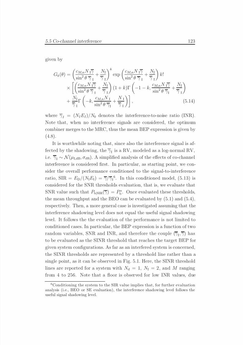
7/29/2019 Adaptive Wireless Multimedia
http://slidepdf.com/reader/full/adaptive-wireless-multimedia 141/187
5.5 Co-channel interference 123
given by
Gk(θ) =
cM,nN Iγ
sin2 θ γ I
+N Iγ I
kexp
cM,nN Iγ
sin2 θ γ I
+N Iγ I
k!
×
cM,nN Iγ
sin2 θ γ I
+N Iγ I
(1 + k)Γ
−1 − k,
cM,nN Iγ
sin2 θ γ I+
N Iγ I
+
N Iγ I
Γ
−k,
cM,nN I
sin2 θ γ I+
N I
γ I
, (5.14)
where γ I = (N I E I )/N 0 denotes the interference-to-noise ratio (INR).
Note that, when no interference signals are considered, the optimum
combiner merges to the MRC, thus the mean BEP expression is given by
(4.8).
It is worthwhile noting that, since also the interference signal is af-
fected by the shadowing, the γ I is a RV, modeled as a log-normal RV,
i.e. γ I ∼ N (µI,dB, σdB). A simplified analysis of the effects of co-channel
interference is considered first. In particular, as starting point, we con-
sider the overall performance conditioned to the signal-to-interference
ratio, SIR = E D/(N IE I) = γ/γ I
6. In this conditioned model, (5.13) is
considered for the SNR thresholds evaluation, that is, we evaluate that
SNR value such that P b|SIR(γ ) = P ⋆b . Once evaluated these thresholds,
the mean throughput and the BEO can be evaluated by (5.1) and (5.4),
respectively. Then, a more general case is investigated assuming that the
interference shadowing level does not equal the useful signal shadowing
level. It follows the the evaluation of the performance is not limited to
conditioned cases. In particular, the BEP expression is a function of two
random variables, SNR and INR, and therefore the couple (γ I, γ ) has
to be evaluated as the SINR threshold that reaches the target BEP forgiven system configurations. As far as an interfered system is concerned,
the SINR thresholds are represented by a threshold line rather than a
single point, as it can be observed in Fig. 5.1. Here, the SINR threshold
lines are reported for a system with N d = 1, N I = 2, and M ranging
from 4 to 256. Note that a floor is observed for low INR values, due
6Conditioning the system to the SIR value implies that, for further evaluationanalysis (i.e., BEO or SE evaluation), the interference shadowing level follows theuseful signal shadowing level.
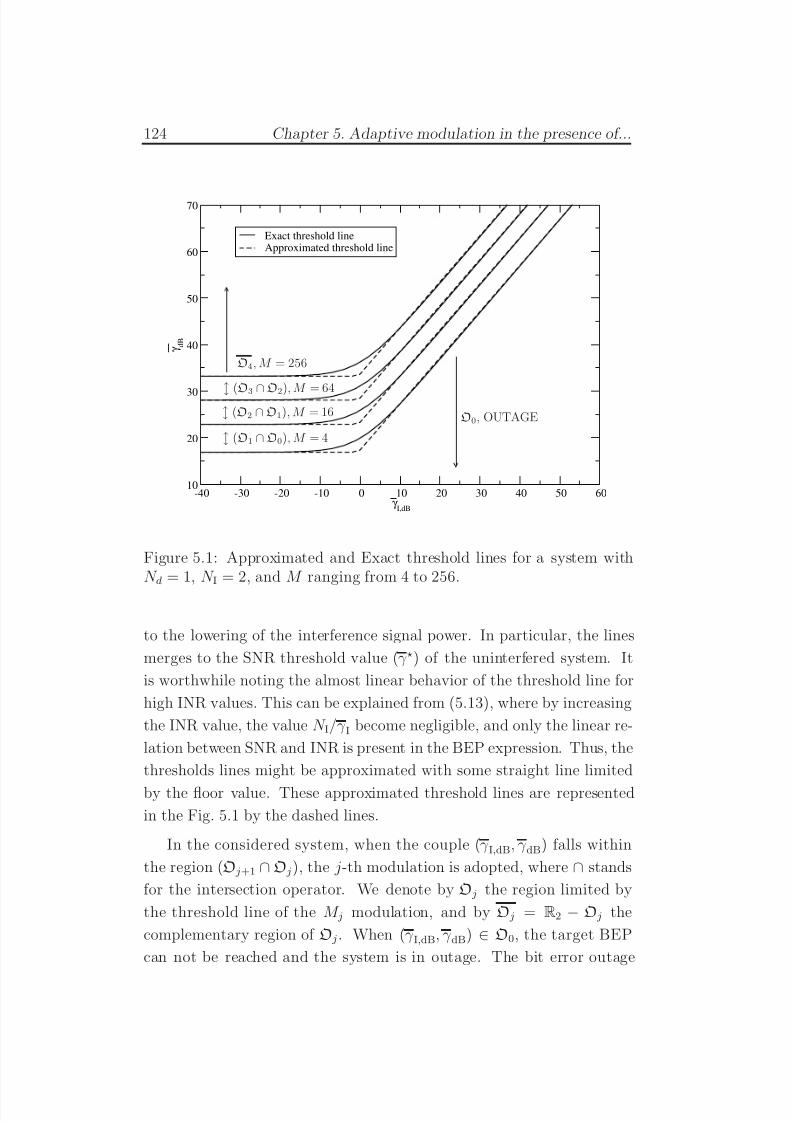
7/29/2019 Adaptive Wireless Multimedia
http://slidepdf.com/reader/full/adaptive-wireless-multimedia 142/187
124 Chapter 5. Adaptive modulation in the presence of...
-40 -30 -20 -10 0 10 20 30 40 50 60γ
I,dB
10
20
30
40
50
60
70
γ d B
Exact threshold lineApproximated threshold line
O4, M = 256
(O
3 ∩O2), M = 64 (O2 ∩O1), M = 16
(O1 ∩O0), M = 4
O0, OUTAGE
Figure 5.1: Approximated and Exact threshold lines for a system withN d = 1, N I = 2, and M ranging from 4 to 256.
to the lowering of the interference signal power. In particular, the lines
merges to the SNR threshold value (γ ⋆) of the uninterfered system. It
is worthwhile noting the almost linear behavior of the threshold line for
high INR values. This can be explained from (5.13), where by increasing
the INR value, the value N I/γ I become negligible, and only the linear re-
lation between SNR and INR is present in the BEP expression. Thus, the
thresholds lines might be approximated with some straight line limited
by the floor value. These approximated threshold lines are represented
in the Fig. 5.1 by the dashed lines.
In the considered system, when the couple (γ I,dB, γ dB) falls within
the region (O j+1 ∩O j), the j-th modulation is adopted, where ∩ stands
for the intersection operator. We denote by O j the region limited by
the threshold line of the M j modulation, and by O j = R2 − O j the
complementary region of O j . When (γ I,dB, γ dB) ∈ O0, the target BEP
can not be reached and the system is in outage. The bit error outage
7/29/2019 Adaptive Wireless Multimedia
http://slidepdf.com/reader/full/adaptive-wireless-multimedia 143/187
5.6 Numerical results 125
probability can be defined as
P o = F (γ I,dB,γ dB)(O0) = P
(γ I,dB, γ dB) ∈ O0
=
∞−∞
γ ⋆0,dB(γ I,dB)
−∞f γ dB(ξ )f γ I,dB(ξ I)dξdξ I
=
∞−∞
Q
µdB − γ ⋆0,dB
σdB
f γ I,dB(ξ I)dξ I, (5.15)
where f γ I,dB(·) and f γ dB(·) are the PDF of the SNR and INR, respectively,
and γ ⋆0,dB(γ I,dB) is the SNR value that reaches the target BEP when
INR= γ I,dB. Analogously, the mean throughput is given by
η =J −1 j=0
M j P
(γ I,dB, γ dB) ∈ (O j+1 ∩O j)
+ M J P
(γ I,dB, γ dB) ∈ OJ
=
J −1 j=0
M j
F (γ I,dB,γ dB)(O j+1) − F (γ I,dB,γ dB)(O j)
+ M J
1 − F (γ I,dB,γ dB)(OJ )
(5.16)
where, as already observed from (5.15), since the SNR and INR are log-
normal RVs, the joint CDF can be expressed as
F (γ I,dB,γ dB)(O j) = P
(γ I,dB, γ dB) ∈ O j
=
∞−∞
γ ⋆j,dB(γ I,dB)
−∞f γ dB(ξ )f γ I,dB(ξ I)dξdξ I
=
∞−∞
Q
µdB − γ ⋆ j,dB
σdB
f γ I,dB(ξ I)dξ I, (5.17)
5.6 Numerical results
In this section, numerical results are presented in terms of mean
throughput and BEO for both fast and slow adaptive modulation. Coher-
ent detection of M -QAM with optimum combiner and Gray code map-
ping in composite Rayleigh fading and log-normal shadowing channels
with perfect CSI was considered. The mean throughput is evaluated by
(5.1), where the thresholds are evaluated as the SNR values that achieve
a target BEP of 10−2 for different modulation sizes and a maximum out-
age probability of 5% is considered. For the approximated BEP case,
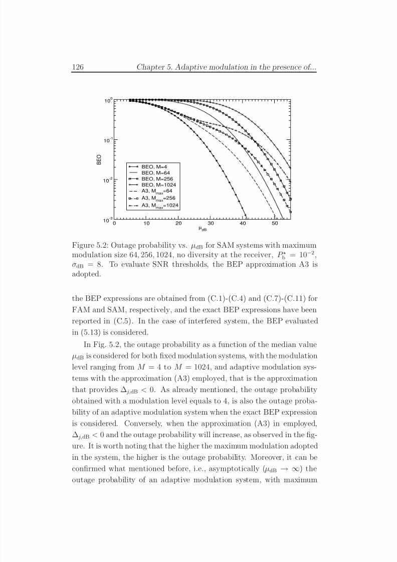
7/29/2019 Adaptive Wireless Multimedia
http://slidepdf.com/reader/full/adaptive-wireless-multimedia 144/187
126 Chapter 5. Adaptive modulation in the presence of...
0 10 20 30 40 50µ
dB
10-3
10-2
10-1
100
B E O
BEO, M=4
BEO, M=64
BEO, M=256
BEO, M=1024
A3, Mmax
=64
A3, Mmax=256
A3, Mmax
=1024
Figure 5.2: Outage probability vs. µdB for SAM systems with maximummodulation size 64, 256, 1024, no diversity at the receiver, P ⋆b = 10−2,σdB = 8. To evaluate SNR thresholds, the BEP approximation A3 isadopted.
the BEP expressions are obtained from (C.1)-(C.4) and (C.7)-(C.11) for
FAM and SAM, respectively, and the exact BEP expressions have been
reported in (C.5). In the case of interfered system, the BEP evaluated
in (5.13) is considered.
In Fig. 5.2, the outage probability as a function of the median value
µdB is considered for both fixed modulation systems, with the modulation
level ranging from M = 4 to M = 1024, and adaptive modulation sys-
tems with the approximation (A3) employed, that is the approximation
that provides ∆ j,dB < 0. As already mentioned, the outage probabilityobtained with a modulation level equals to 4, is also the outage proba-
bility of an adaptive modulation system when the exact BEP expression
is considered. Conversely, when the approximation (A3) in employed,
∆ j,dB < 0 and the outage probability will increase, as observed in the fig-
ure. It is worth noting that the higher the maximum modulation adopted
in the system, the higher is the outage probability. Moreover, it can be
confirmed what mentioned before, i.e., asymptotically (µdB → ∞) the
outage probability of an adaptive modulation system, with maximum
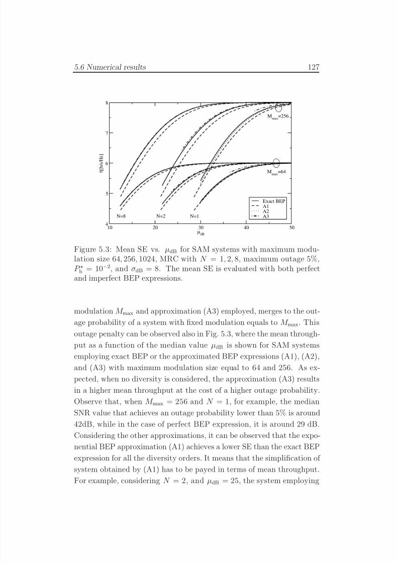
7/29/2019 Adaptive Wireless Multimedia
http://slidepdf.com/reader/full/adaptive-wireless-multimedia 145/187
5.6 Numerical results 127
10 20 30 40 50µ
dB
4
5
6
7
8
η [ b / s / H z ]
Exact BEPA1A2A3
Mmax
=256
Mmax
=64
N=1N=2N=8
Figure 5.3: Mean SE vs. µdB for SAM systems with maximum modu-lation size 64, 256, 1024, MRC with N = 1, 2, 8, maximum outage 5%,P ⋆b = 10−2, and σdB = 8. The mean SE is evaluated with both perfectand imperfect BEP expressions.
modulation M max and approximation (A3) employed, merges to the out-
age probability of a system with fixed modulation equals to M max. This
outage penalty can be observed also in Fig. 5.3, where the mean through-
put as a function of the median value µdB is shown for SAM systems
employing exact BEP or the approximated BEP expressions (A1), (A2),
and (A3) with maximum modulation size equal to 64 and 256. As ex-
pected, when no diversity is considered, the approximation (A3) results
in a higher mean throughput at the cost of a higher outage probability.Observe that, when M max = 256 and N = 1, for example, the median
SNR value that achieves an outage probability lower than 5% is around
42dB, while in the case of perfect BEP expression, it is around 29 dB.
Considering the other approximations, it can be observed that the expo-
nential BEP approximation (A1) achieves a lower SE than the exact BEP
expression for all the diversity orders. It means that the simplification of
system obtained by (A1) has to be payed in terms of mean throughput.
For example, considering N = 2, and µdB = 25, the system employing
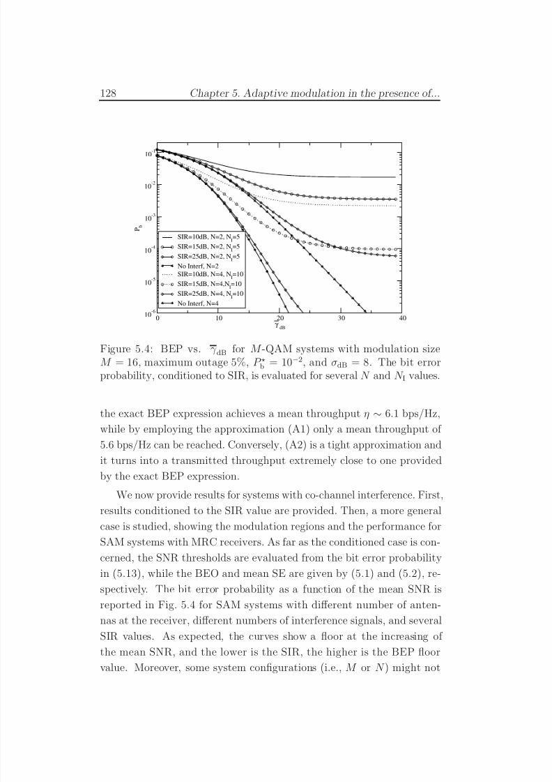
7/29/2019 Adaptive Wireless Multimedia
http://slidepdf.com/reader/full/adaptive-wireless-multimedia 146/187
128 Chapter 5. Adaptive modulation in the presence of...
0 10 20 30 40γ
dB
10-6
10-5
10-4
10-3
10-2
10-1
P b
SIR=10dB, N=2, NI=5
SIR=15dB, N=2, NI=5
SIR=25dB, N=2, NI=5
No Interf, N=2
SIR=10dB, N=4, NI=10SIR=15dB, N=4,N
I=10
SIR=25dB, N=4, NI=10
No Interf, N=4
Figure 5.4: BEP vs. γ dB for M -QAM systems with modulation sizeM = 16, maximum outage 5%, P ⋆b = 10−2, and σdB = 8. The bit errorprobability, conditioned to SIR, is evaluated for several N and N I values.
the exact BEP expression achieves a mean throughput η ∼ 6.1 bps/Hz,while by employing the approximation (A1) only a mean throughput of
5.6 bps/Hz can be reached. Conversely, (A2) is a tight approximation and
it turns into a transmitted throughput extremely close to one provided
by the exact BEP expression.
We now provide results for systems with co-channel interference. First,
results conditioned to the SIR value are provided. Then, a more general
case is studied, showing the modulation regions and the performance for
SAM systems with MRC receivers. As far as the conditioned case is con-cerned, the SNR thresholds are evaluated from the bit error probability
in (5.13), while the BEO and mean SE are given by (5.1) and (5.2), re-
spectively. The bit error probability as a function of the mean SNR is
reported in Fig. 5.4 for SAM systems with different number of anten-
nas at the receiver, different numbers of interference signals, and several
SIR values. As expected, the curves show a floor at the increasing of
the mean SNR, and the lower is the SIR, the higher is the BEP floor
value. Moreover, some system configurations (i.e., M or N ) might not
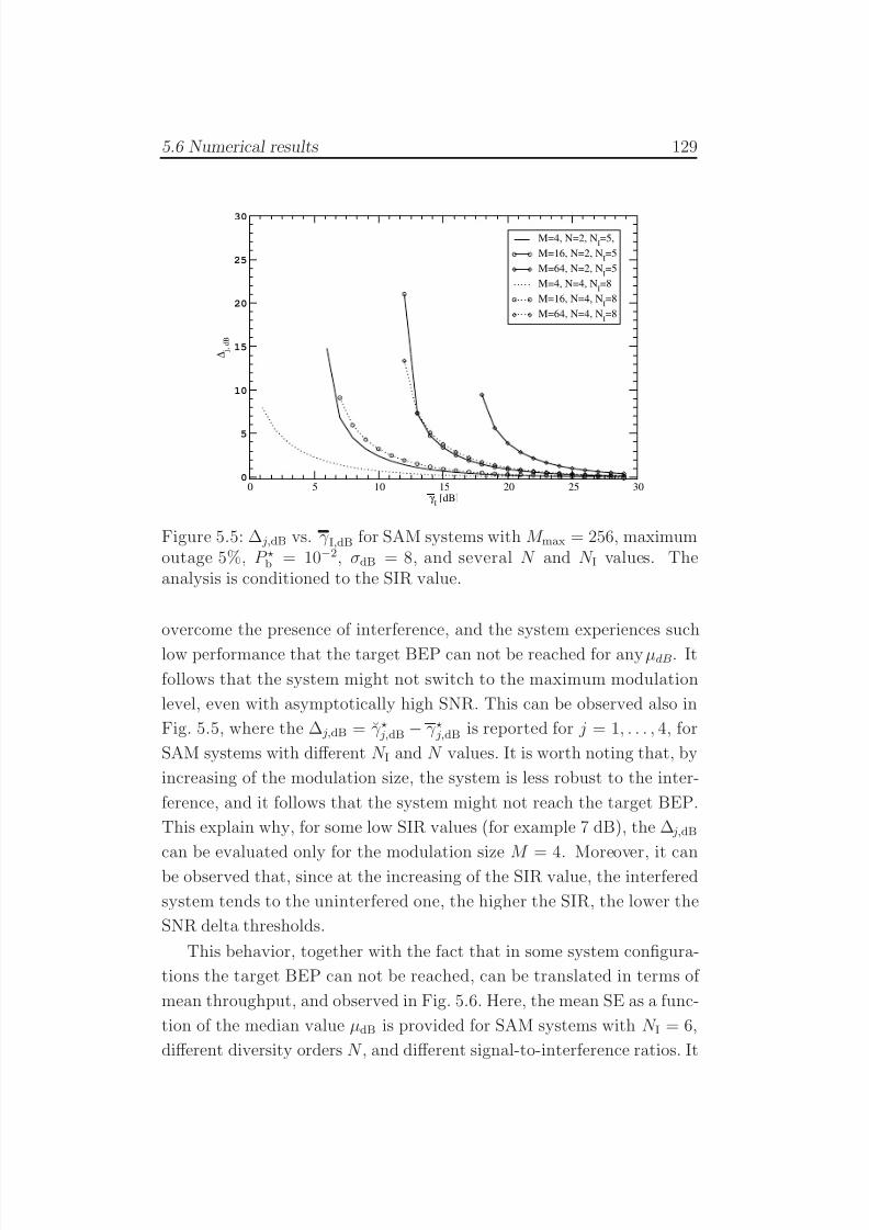
7/29/2019 Adaptive Wireless Multimedia
http://slidepdf.com/reader/full/adaptive-wireless-multimedia 147/187
5.6 Numerical results 129
0 5 10 15 20 25 30γ
I[dB]
0
5
10
15
20
25
30
∆ j , d B
M=4, N=2, NI=5,
M=16, N=2, NI=5
M=64, N=2, NI=5
M=4, N=4, NI=8
M=16, N=4, NI=8
M=64, N=4, NI=8
Figure 5.5: ∆ j,dB vs. γ I,dB for SAM systems with M max = 256, maximumoutage 5%, P ⋆b = 10−2, σdB = 8, and several N and N I values. Theanalysis is conditioned to the SIR value.
overcome the presence of interference, and the system experiences such
low performance that the target BEP can not be reached for any µdB. It
follows that the system might not switch to the maximum modulation
level, even with asymptotically high SNR. This can be observed also in
Fig. 5.5, where the ∆ j,dB = γ ⋆ j,dB − γ ⋆ j,dB is reported for j = 1, . . . , 4, for
SAM systems with different N I and N values. It is worth noting that, by
increasing of the modulation size, the system is less robust to the inter-
ference, and it follows that the system might not reach the target BEP.
This explain why, for some low SIR values (for example 7 dB), the ∆ j,dB
can be evaluated only for the modulation size M = 4. Moreover, it can
be observed that, since at the increasing of the SIR value, the interfered
system tends to the uninterfered one, the higher the SIR, the lower the
SNR delta thresholds.
This behavior, together with the fact that in some system configura-
tions the target BEP can not be reached, can be translated in terms of
mean throughput, and observed in Fig. 5.6. Here, the mean SE as a func-
tion of the median value µdB is provided for SAM systems with N I = 6,
different diversity orders N , and different signal-to-interference ratios. It
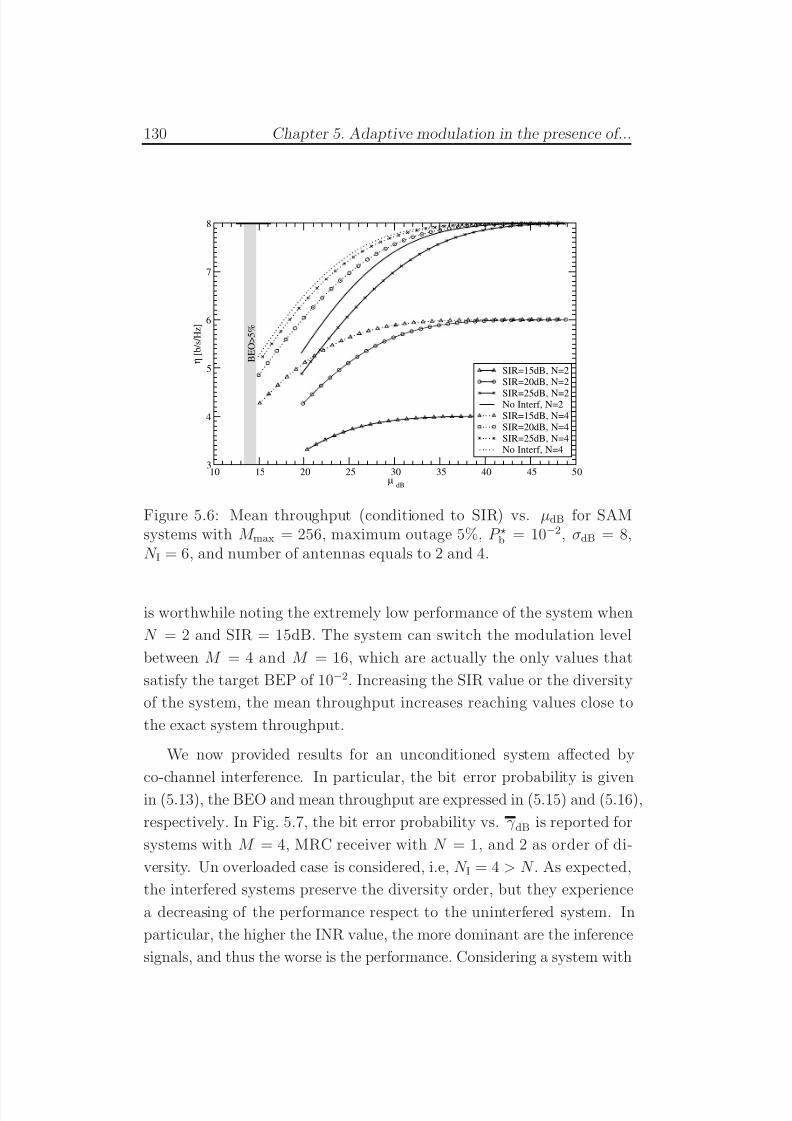
7/29/2019 Adaptive Wireless Multimedia
http://slidepdf.com/reader/full/adaptive-wireless-multimedia 148/187
130 Chapter 5. Adaptive modulation in the presence of...
10 15 20 25 30 35 40 45 50µ
dB
3
4
5
6
7
8
η [ b
/ s / H z ]
SIR=15dB, N=2
SIR=20dB, N=2
SIR=25dB, N=2No Interf, N=2
SIR=15dB, N=4
SIR=20dB, N=4
SIR=25dB, N=4No Interf, N=4
B E O > 5 %
Figure 5.6: Mean throughput (conditioned to SIR) vs. µdB for SAMsystems with M max = 256, maximum outage 5%, P ⋆b = 10−2, σdB = 8,N I = 6, and number of antennas equals to 2 and 4.
is worthwhile noting the extremely low performance of the system when
N = 2 and SIR = 15dB. The system can switch the modulation level
between M = 4 and M = 16, which are actually the only values that
satisfy the target BEP of 10−2. Increasing the SIR value or the diversity
of the system, the mean throughput increases reaching values close to
the exact system throughput.
We now provided results for an unconditioned system affected by
co-channel interference. In particular, the bit error probability is givenin (5.13), the BEO and mean throughput are expressed in (5.15) and (5.16),
respectively. In Fig. 5.7, the bit error probability vs. γ dB is reported for
systems with M = 4, MRC receiver with N = 1, and 2 as order of di-
versity. Un overloaded case is considered, i.e, N I = 4 > N . As expected,
the interfered systems preserve the diversity order, but they experience
a decreasing of the performance respect to the uninterfered system. In
particular, the higher the INR value, the more dominant are the inference
signals, and thus the worse is the performance. Considering a system with
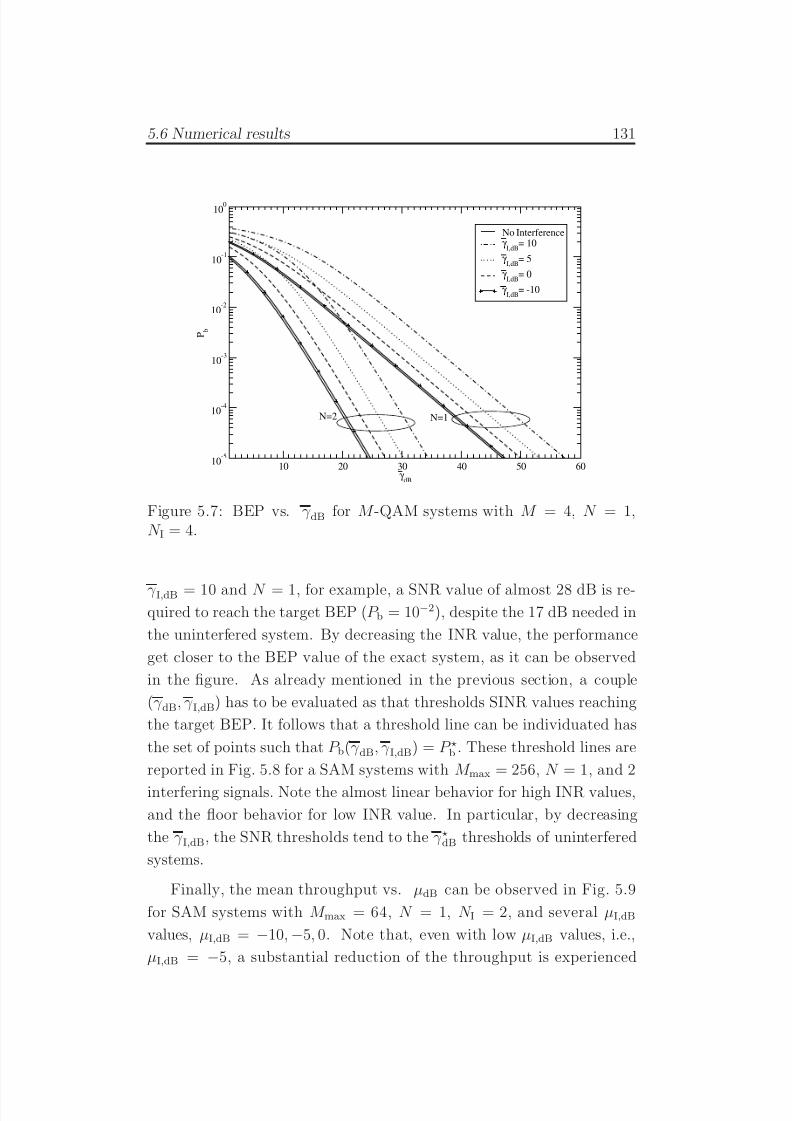
7/29/2019 Adaptive Wireless Multimedia
http://slidepdf.com/reader/full/adaptive-wireless-multimedia 149/187
5.6 Numerical results 131
10 20 30 40 50 60γ
dB
10-5
10-4
10-3
10-2
10-1
100
P b
No Interferenceγ
I,dB= 10
γ I,dB
= 5
γ I,dB
= 0
γ I,dB
= -10
N=2 N=1
Figure 5.7: BEP vs. γ dB for M -QAM systems with M = 4, N = 1,N I = 4.
γ I,dB = 10 and N = 1, for example, a SNR value of almost 28 dB is re-quired to reach the target BEP (P b = 10−2), despite the 17 dB needed in
the uninterfered system. By decreasing the INR value, the performance
get closer to the BEP value of the exact system, as it can be observed
in the figure. As already mentioned in the previous section, a couple
(γ dB, γ I,dB) has to be evaluated as that thresholds SINR values reaching
the target BEP. It follows that a threshold line can be individuated has
the set of points such that P b(γ dB, γ I,dB) = P ⋆b . These threshold lines are
reported in Fig. 5.8 for a SAM systems with M max = 256, N = 1, and 2
interfering signals. Note the almost linear behavior for high INR values,
and the floor behavior for low INR value. In particular, by decreasing
the γ I,dB, the SNR thresholds tend to the γ ⋆dB thresholds of uninterfered
systems.
Finally, the mean throughput vs. µdB can be observed in Fig. 5.9
for SAM systems with M max = 64, N = 1, N I = 2, and several µI,dB
values, µI,dB = −10, −5, 0. Note that, even with low µI,dB values, i.e.,
µI,dB = −5, a substantial reduction of the throughput is experienced
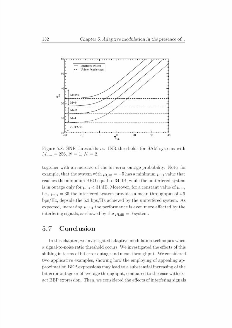
7/29/2019 Adaptive Wireless Multimedia
http://slidepdf.com/reader/full/adaptive-wireless-multimedia 150/187
132 Chapter 5. Adaptive modulation in the presence of...
-20 -10 0 10 20 30 40γ
I,dB
10
20
30
40
50
60
γ d B
Interfered system
Uninterfered system
M=16
M=64
M=256
M=4
OUTAGE
Figure 5.8: SNR thresholds vs. INR thresholds for SAM systems withM max = 256, N = 1, N I = 2.
together with an increase of the bit error outage probability. Note, for
example, that the system with µI,dB = −5 has a minimum µdB value that
reaches the minimum BEO equal to 34 dB, while the uniterfered system
is in outage only for µdB < 31 dB. Moreover, for a constant value of µdB,
i.e., µdB = 35 the interfered system provides a mean throughput of 4.9
bps/Hz, depside the 5.3 bps/Hz achieved by the uniterfered system. As
expected, increasing µI,dB the performance is even more affected by the
interfering signals, as showed by the µI,dB = 0 system.
5.7 ConclusionIn this chapter, we investigated adaptive modulation techniques when
a signal-to-noise ratio threshold occurs. We investigated the effects of this
shifting in terms of bit error outage and mean throughput. We considered
two applicative examples, showing how the employing of appealing ap-
proximation BEP expressions may lead to a substantial increasing of the
bit error outage or of average throughput, compared to the case with ex-
act BEP expression. Then, we considered the effects of interfering signals
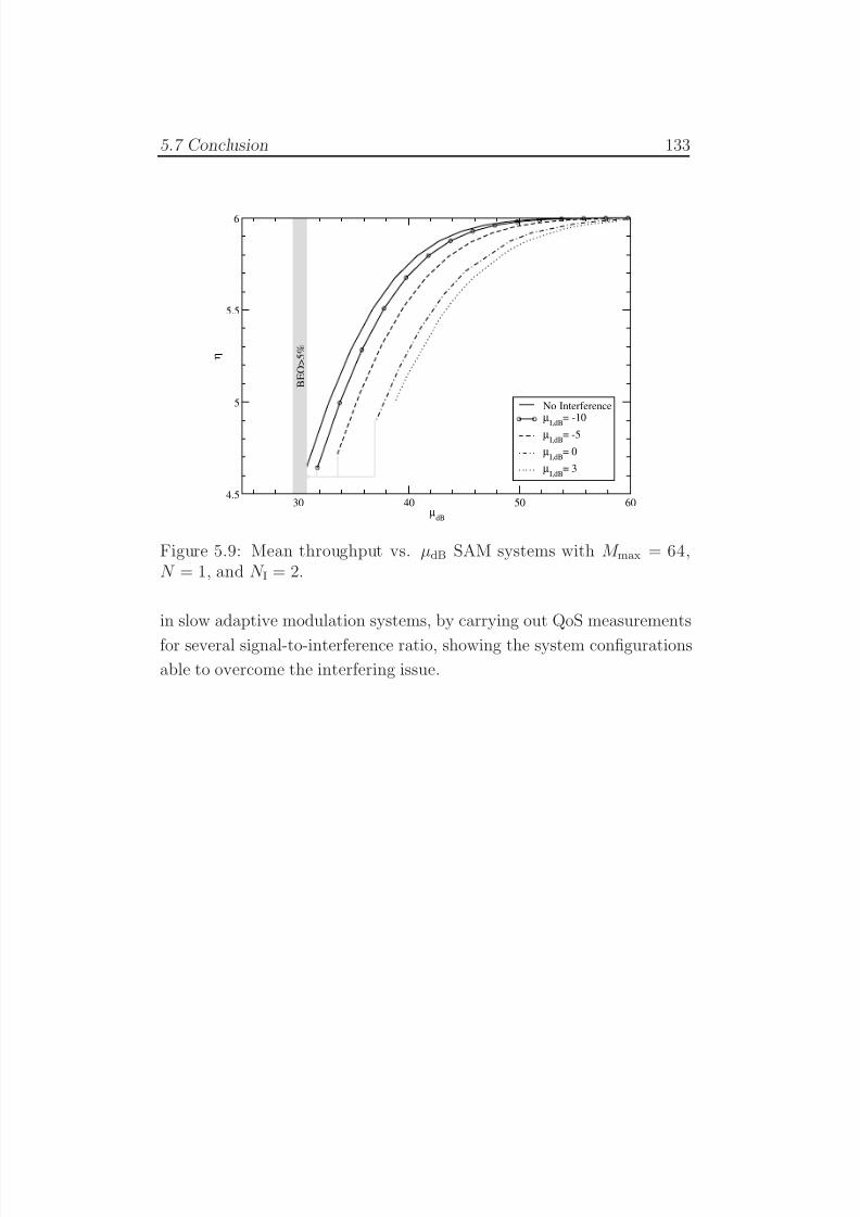
7/29/2019 Adaptive Wireless Multimedia
http://slidepdf.com/reader/full/adaptive-wireless-multimedia 151/187
5.7 Conclusion 133
30 40 50 60µ
dB
4.5
5
5.5
6
η
No Interferenceµ
I,dB
= -10
µI,dB
= -5
µI,dB
= 0
µI,dB
= 3
B E O > 5 %
Figure 5.9: Mean throughput vs. µdB SAM systems with M max = 64,N = 1, and N I = 2.
in slow adaptive modulation systems, by carrying out QoS measurements
for several signal-to-interference ratio, showing the system configurations
able to overcome the interfering issue.

7/29/2019 Adaptive Wireless Multimedia
http://slidepdf.com/reader/full/adaptive-wireless-multimedia 152/187
7/29/2019 Adaptive Wireless Multimedia
http://slidepdf.com/reader/full/adaptive-wireless-multimedia 153/187
Chapter 6
Conclusion
This final chapter summarizes the contributions of this dissertation
and highlights numerous areas for further research. We developed a
framework for optimizing multimedia applications over wireless channels.
We showed how to take advantage from channel conditions, by adopting
to them transmitting parameters at the physical layer, such as source
and channel coding rates, as well as modulation levels. Specifically, as
far as the joint source and channel coding was concerned, we investi-
gated the optimal design of joint source and channel coding (JSSC) in
a 2D time-frequency resource block for multimedia transmissions over
OFDM systems. We used symmetric n-channel FEC-based multiple de-
scriptions with time coding based on the diversity order in the frequency
and time domains. Results showed that, even with only one of the two
diversities available, extremely worthy performance can be achieved. As
far as video bitstreams are concerned, important considerations on the
methods to evaluate the rate distortion (RD) curve were provided. We
showed that great simplification can be considered in the algorithm forthe RD function and the optimal staircase design, without jeopardizing
the overall performance system. Beyond JSSC, as another method to
improve the reliable data rate to be decoded, adaptive modulation tech-
niques was investigated. We investigated adaptive modulation techniques
in real systems, affected by channel estimation errors, co-channel interfer-
ence or any possible issue compromising the bit error probability (BEP)
performance. First, we compared slow adaptive modulation techniques
to the fast ones in the presence of imperfect channel estimations. Results
135
7/29/2019 Adaptive Wireless Multimedia
http://slidepdf.com/reader/full/adaptive-wireless-multimedia 154/187
136 Chapter 6. Conclusion
showed that tracking the large-scale fading achieves an enormous im-provement in the performance compared to a fixed modulation systems,
and it can also outperform fast adaptive modulation techniques, that fol-
lows the small scale fading. Then, we provide a general analysis for the
evaluation of system performance when imperfect signal-to-noise thresh-
olds are experienced. We also studied two applicative examples, showing
the effects of co-channel interference, and demonstrating that employing
approximated BEP expression might reduce the system performance.
A large number of areas exists for future research on wireless multime-
dia transmissions and related topics. The proposed model can be appliedto some existing standards, as WiMax for example, investigating an opti-
mization suitable for the given system. The channel and model conditions
of the standard might drive us to different considerations in the trans-
mission scheme design. Due to the high decorrelation in the frequency
domain, and due to the high number of subcarriers in WiMax systems,
more than one frame might be transmitted in all the available subcarriers,
for example, introducing a new parameter in the optimization problem.
Moreover, a multicast scenario can be investigated, aimed at satisfying
all the user requirements, providing at least a target quality to each user,
or maximizing the sumrate capacity of the system. Adaptive modula-
tion techniques can be applied to OFDM systems, for transmission of
both images and video bitstreams. The optimal modulation level might
be chosen for each independent subchannel, or suboptimal bit-loading
algorithms can be employed. Finally, a cross-layer (physical-scheduling-
application level) optimization in the multimedia transmission can be
considered, introducing therefore the scheduling level in the optimization
problem.
7/29/2019 Adaptive Wireless Multimedia
http://slidepdf.com/reader/full/adaptive-wireless-multimedia 155/187
Appendix A
Packet loss rate
For a Rayleigh fading process r(t), consider a simple two-state thresh-
old model [52] with Rth being the threshold for the Rayleigh fading signal.
If the signal level is above Rth (strong fade), the channel is considered to
be in the good state, in which the probability of receiving the informa-
tion is equal to 1, while if the signal level is below Rth (deep fade), the
probably of receiving the particular information bit is equal to 0. Let us
further assume that τ f , τ nf and τ s are the deep fade duration, the strong
fade duration and the deep fade inter-arrival intervals, so that
τ s = τ f + τ nf . (A.1)
The average deep fade inter-arrival interval is the inverse of the level
crossing rate (the expected rate at which the signal crosses the Rth),
defined as [14]
τ s =1√
2πf Dρe−ρ2, (A.2)
where f D is the maximum Doppler frequency, ρ2 = (Rth/Rrms)2 is the
inverse of the fade margin and Rrms is the root mean square of the fading
signal. Denoting by N r the level crossing rate, the average deep fade
duration is defined as [14]
τ f =P (r(t) ≤ Rth)
N r=
eρ2 − 1√
2πf Dρ, (A.3)
so that the average strong fade duration can be expressed as
τ nf = τ s − τ f =1√
2πρf D. (A.4)
137
7/29/2019 Adaptive Wireless Multimedia
http://slidepdf.com/reader/full/adaptive-wireless-multimedia 156/187
138 Appendix A. Packet loss rate
Note that the ratio between the average strong fade duration and theaverage deep fade duration is not a function of the Doppler spread. Thus,
increasing f D causes a reduction of the average deep fade inter-arrival
interval (τ s), but also a shorter deep fade duration, as can be observed
from (A.2) and (A.3), respectively. Hence, faster fading produces deep
fade events that are shorter in duration but occur more frequently.
Since r(t) is a Rayleigh random process, r2(t) is a χ2 process and thus
its asymptotic1 level down-crossing rate forms a Poisson process [117].
From the properties of Poisson random variables [118], it follows that
P τ s(τ ) = Prob(τ s ≤ τ ) = 1 − exp
− τ
τ s
, (A.5)
and we can define the probability of having k deep fade arrivals within
an interval of T PL seconds as
Prob K(T PL) = k =(T PL/τ s)
ke−T PL/τ s
k!(A.6)
where T PL corresponds to the duration of a packet, and K(T PL) is a
random variable representing the number of deep fade arrivals in T PLseconds.
Thus, in an uncoded system, the probability of having a packet cor-
rectly received (P succ) is
P succ = P good · Prob(K(T PL) = 0) = exp
−ρ2 − T PL
τ s
(A.7)
where:
P good = Prob (packet starts in good fade) = P (r(t) > Rth) = exp(−ρ
2
)(A.8)
is the probability that a packet starts in the good state. From (A.7), it can
be seen that the packet success rate probability decreases with decreasing
inter-arrival time of the deep fades due to the fact that deep fading arrival
are shorter but occur more frequently. In Fig. A.1, we show both the
simulation results and analytical results with different fade rates. As
1We use “asymptotic level down-crossing” to mean the level crossing of a very lowthreshold (Rth → 0) [117].
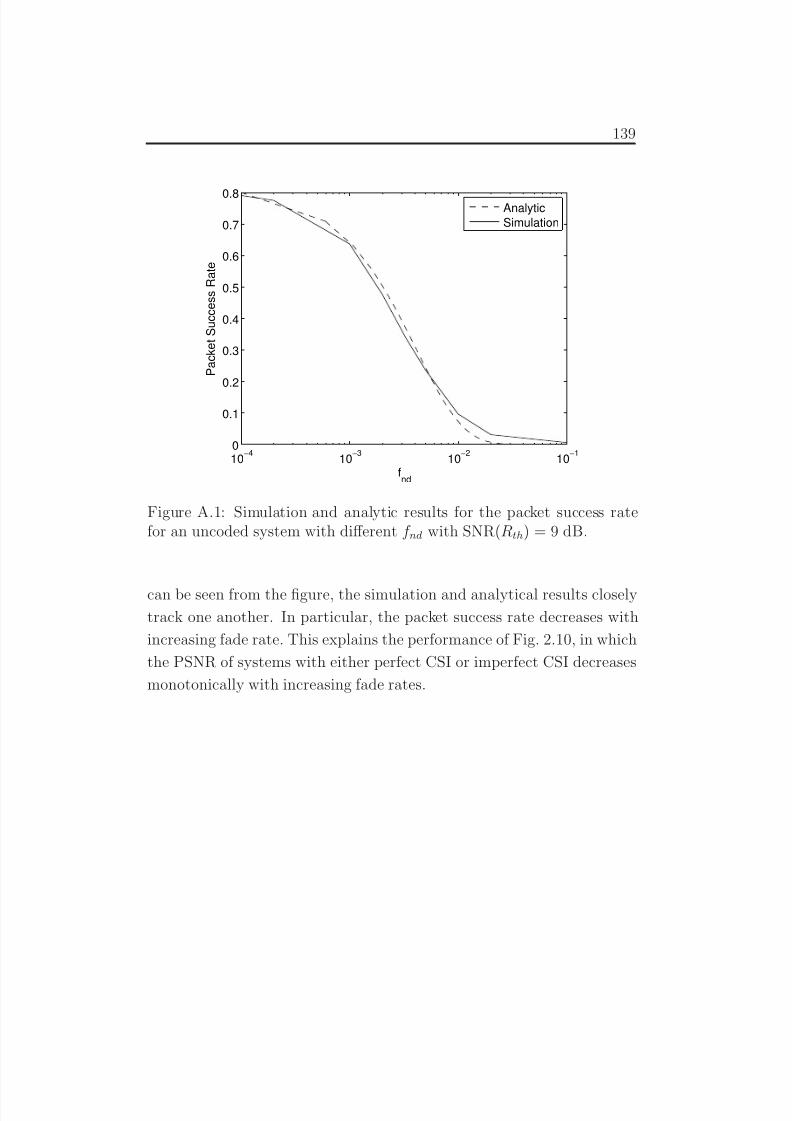
7/29/2019 Adaptive Wireless Multimedia
http://slidepdf.com/reader/full/adaptive-wireless-multimedia 157/187
139
10−4
10−3
10−2
10−1
0
0.1
0.2
0.3
0.4
0.5
0.6
0.7
0.8
fnd
P a c k e t S u c c e s s R a t e
Analytic
Simulation
Figure A.1: Simulation and analytic results for the packet success ratefor an uncoded system with different f nd with SNR(Rth) = 9 dB.
can be seen from the figure, the simulation and analytical results closely
track one another. In particular, the packet success rate decreases with
increasing fade rate. This explains the performance of Fig. 2.10, in which
the PSNR of systems with either perfect CSI or imperfect CSI decreases
monotonically with increasing fade rates.

7/29/2019 Adaptive Wireless Multimedia
http://slidepdf.com/reader/full/adaptive-wireless-multimedia 158/187
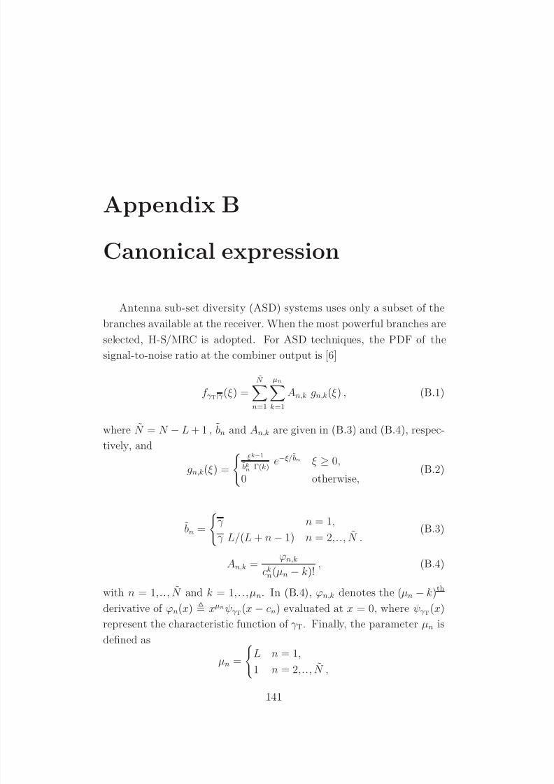
7/29/2019 Adaptive Wireless Multimedia
http://slidepdf.com/reader/full/adaptive-wireless-multimedia 159/187
Appendix B
Canonical expression
Antenna sub-set diversity (ASD) systems uses only a subset of the
branches available at the receiver. When the most powerful branches are
selected, H-S/MRC is adopted. For ASD techniques, the PDF of the
signal-to-noise ratio at the combiner output is [6]
f γ T|γ (ξ ) =N
n=1
µn
k=1
An,k gn,k(ξ ) , (B.1)
where N = N − L + 1 , bn and An,k are given in (B.3) and (B.4), respec-
tively, and
gn,k(ξ ) =
ξk−1
bkn Γ(k)e−ξ/bn ξ ≥ 0,
0 otherwise,(B.2)
bn =
γ n = 1,
γ L/(L + n
−1) n = 2,.., N .
(B.3)
An,k =ϕn,k
ckn(µn − k)!, (B.4)
with n = 1,.., N and k = 1,..,µn. In (B.4), ϕn,k denotes the (µn − k)th
derivative of ϕn(x) xµnψγ T(x − cn) evaluated at x = 0, where ψγ T(x)
represent the characteristic function of γ T. Finally, the parameter µn is
defined as
µn =
L n = 1,
1 n = 2,.., N ,
141
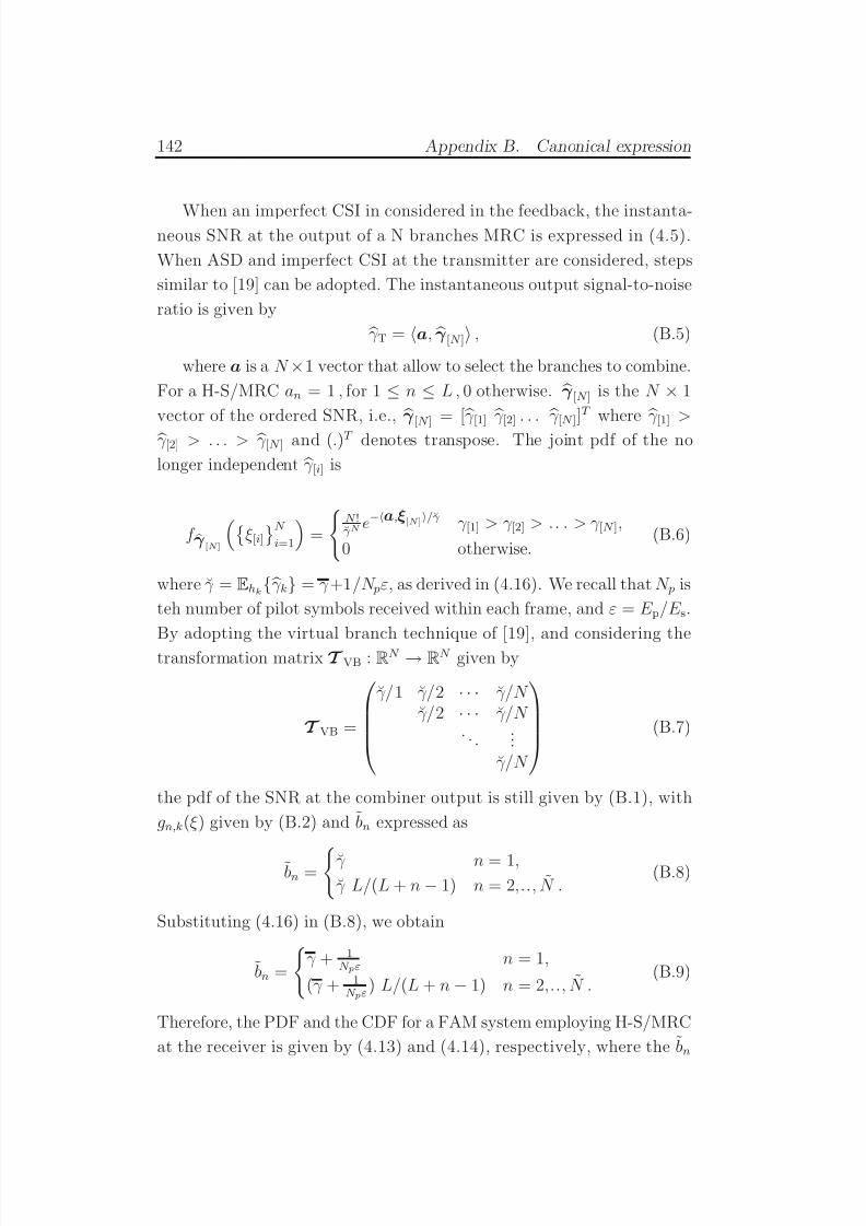
7/29/2019 Adaptive Wireless Multimedia
http://slidepdf.com/reader/full/adaptive-wireless-multimedia 160/187
142 Appendix B. Canonical expression
When an imperfect CSI in considered in the feedback, the instanta-neous SNR at the output of a N branches MRC is expressed in (4.5).
When ASD and imperfect CSI at the transmitter are considered, steps
similar to [19] can be adopted. The instantaneous output signal-to-noise
ratio is given by γ T = a, γ [N ] , (B.5)
where a is a N ×1 vector that allow to select the branches to combine.
For a H-S/MRC an = 1 , for 1 ≤ n ≤ L , 0 otherwise.
γ [N ] is the N × 1
vector of the ordered SNR, i.e., γ [N ] = [ γ [1] γ [2] . . . γ [N ]]T where γ [1] > γ [2] > . . . > γ [N ] and (.)T denotes transpose. The joint pdf of the no
longer independent γ [i] is
f γ [N ]
ξ [i]N i=1
=
N !γ N e
−a,ξ[N ]/γ γ [1] > γ [2] > .. . > γ [N ],
0 otherwise.(B.6)
where γ = Ehk γ k = γ +1/N pε, as derived in (4.16). We recall that N p is
teh number of pilot symbols received within each frame, and ε = E p/E s.
By adopting the virtual branch technique of [19], and considering the
transformation matrix T VB : RN → RN given by
T VB =
γ/1 γ/2 · · · γ/N
γ/2 · · · γ/N . . .
...γ/N
(B.7)
the pdf of the SNR at the combiner output is still given by (B.1), with
gn,k(ξ ) given by (B.2) and bn expressed as
bn = γ n = 1,γ L/(L + n − 1) n = 2,.., N .
(B.8)
Substituting (4.16) in (B.8), we obtain
bn =
γ + 1
N pεn = 1,
(γ + 1N pε
) L/(L + n − 1) n = 2,.., N .(B.9)
Therefore, the PDF and the CDF for a FAM system employing H-S/MRC
at the receiver is given by (4.13) and (4.14), respectively, where the bn

7/29/2019 Adaptive Wireless Multimedia
http://slidepdf.com/reader/full/adaptive-wireless-multimedia 161/187
143
values are given by (B.9). The SNR thresholds are evaluated from theBEP expression in (C.1). For SAM systems, the PDF and CDF are
represented by (4.17) and (4.18). The SNR thresholds are evaluated
from the BEP expression in (C.6).

7/29/2019 Adaptive Wireless Multimedia
http://slidepdf.com/reader/full/adaptive-wireless-multimedia 162/187

7/29/2019 Adaptive Wireless Multimedia
http://slidepdf.com/reader/full/adaptive-wireless-multimedia 163/187
Appendix C
Approximation on BEP
expressions
In the following, the derivation of the exact and the approximated
BEP expressions is reported for both the instantaneous and mean case,
for systems with H-S/MRC receiver.
C.1 Instantaneous BEP
The exact BEP expression for a M -QAM system was carried out
in [112]. In particular, for a given modulation level M , the instantaneous
exact bit error proability can be expressed as
P b(e|γ T ) =2√
M log2(√
M )
log2(√ M )
h=1
(1−2−h)√ M −1
i=0
(−1)⌊ i2h−1
√ M
⌋ ×
× 2h−
1
− i2h−1
√ M +
1
2Q(2i + 1) 3γ T (M − 1) (C.1)
Since (C.1) is not invertible, bounds and approximations has gained
great attention in the last year. One of the most employed BEP ex-
pression is the exponential approximation [96], that results to be easily
invertible but not that tight and it is defined as (A1):
P (A1)
b (e|γ T) ≈ 0.2 exp
−1.6γ TM − 1
. (C.2)
145
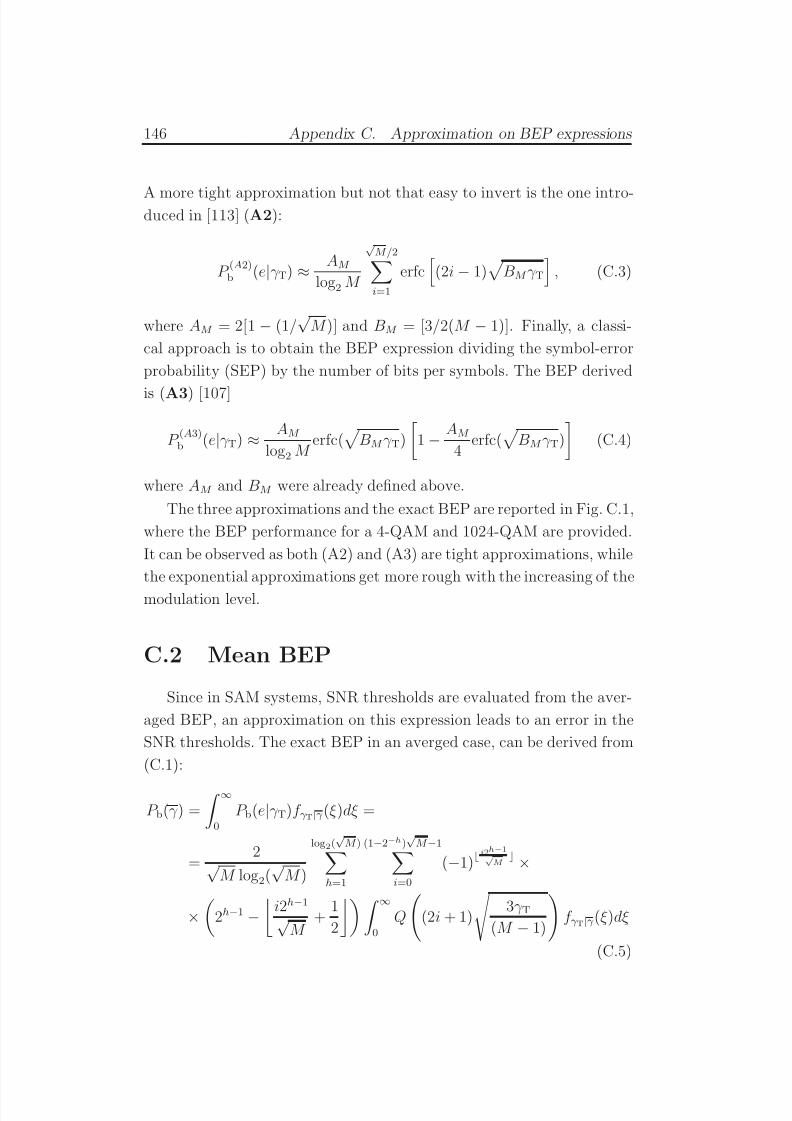
7/29/2019 Adaptive Wireless Multimedia
http://slidepdf.com/reader/full/adaptive-wireless-multimedia 164/187
146 Appendix C. Approximation on BEP expressions
A more tight approximation but not that easy to invert is the one intro-duced in [113] (A2):
P (A2)
b (e|γ T) ≈ AM
log2 M
√ M/2i=1
erfc
(2i − 1)
BM γ T
, (C.3)
where AM = 2[1 − (1/√
M )] and BM = [3/2(M − 1)]. Finally, a classi-
cal approach is to obtain the BEP expression dividing the symbol-error
probability (SEP) by the number of bits per symbols. The BEP derived
is (A3) [107]
P (A3)b (e|γ T) ≈ AM
log2 M erfc(
BM γ T)
1 − AM
4erfc(
BM γ T)
(C.4)
where AM and BM were already defined above.
The three approximations and the exact BEP are reported in Fig. C.1,
where the BEP performance for a 4-QAM and 1024-QAM are provided.
It can be observed as both (A2) and (A3) are tight approximations, while
the exponential approximations get more rough with the increasing of the
modulation level.
C.2 Mean BEP
Since in SAM systems, SNR thresholds are evaluated from the aver-
aged BEP, an approximation on this expression leads to an error in the
SNR thresholds. The exact BEP in an averged case, can be derived from
(C.1):
P b(γ ) = ∞
0
P b(e|γ T)f γ T|γ (ξ )dξ =
=2√
M log2(√
M )
log2(√ M )
h=1
(1−2−h)√ M −1
i=0
(−1)⌊ i2h−1√
M ⌋ ×
×
2h−1 −
i2h−1
√ M
+1
2
∞0
Q
(2i + 1)
3γ T
(M − 1)
f γ T|γ (ξ )dξ
(C.5)
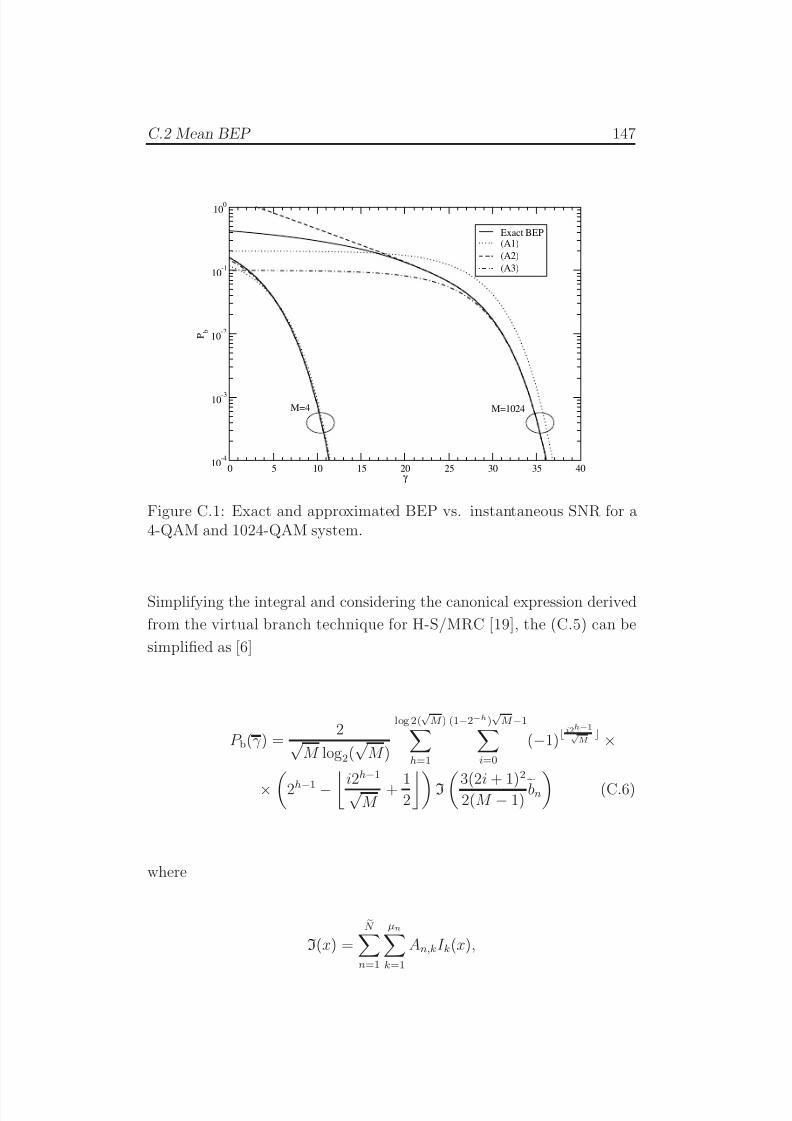
7/29/2019 Adaptive Wireless Multimedia
http://slidepdf.com/reader/full/adaptive-wireless-multimedia 165/187
C.2 Mean BEP 147
0 5 10 15 20 25 30 35 40γ
10-4
10-3
10-2
10-1
100
P b
Exact BEP(A1)
(A2)
(A3)
M=4 M=1024
Figure C.1: Exact and approximated BEP vs. instantaneous SNR for a4-QAM and 1024-QAM system.
Simplifying the integral and considering the canonical expression derived
from the virtual branch technique for H-S/MRC [19], the (C.5) can be
simplified as [6]
P b(γ ) =2√
M log2(√
M )
log 2(√ M )
h=1
(1−2−h)√ M −1
i=0
(−1)⌊ i2h−1
√ M
⌋ ×
× 2h−1 − i2h
−1
√ M
+ 12I3(2i + 1)2
2(M − 1)bn (C.6)
where
I(x) =
N n=1
µnk=1
An,kI k(x),
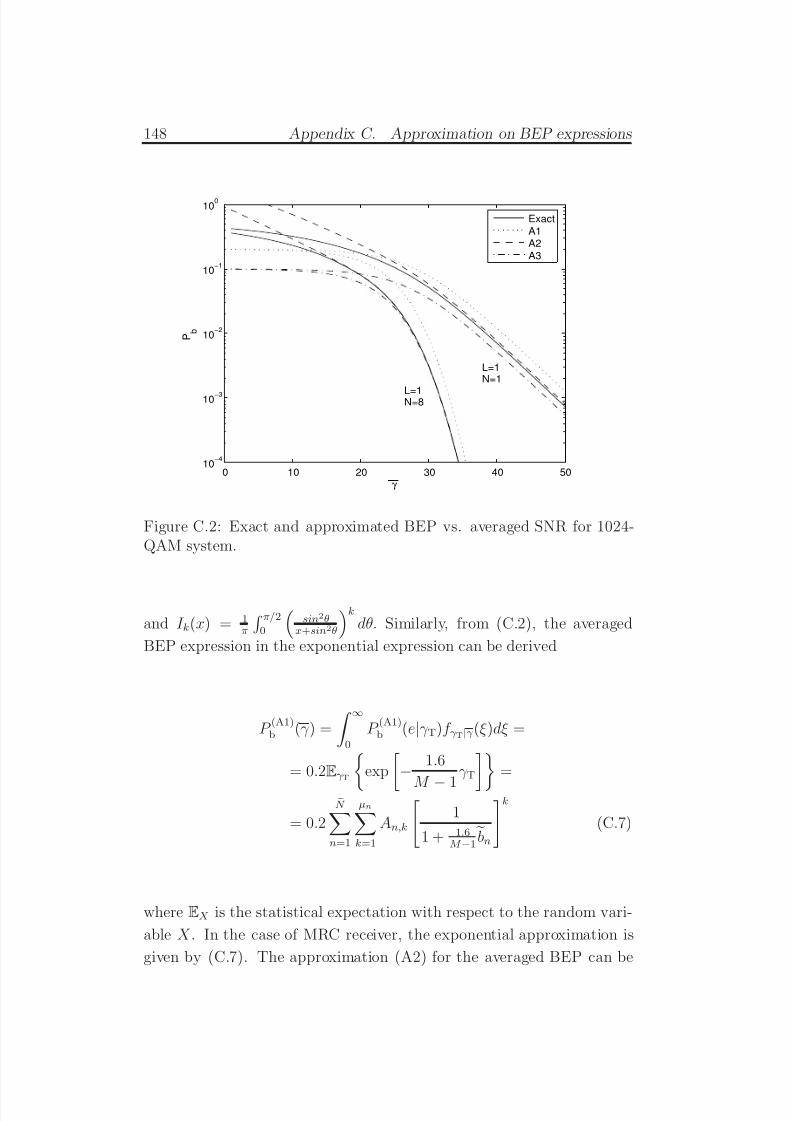
7/29/2019 Adaptive Wireless Multimedia
http://slidepdf.com/reader/full/adaptive-wireless-multimedia 166/187
148 Appendix C. Approximation on BEP expressions
0 10 20 30 40 5010
−4
10−3
10−2
10−1
100
γ
P b
Exact
A1
A2
A3
L=1N=8
L=1
N=1
Figure C.2: Exact and approximated BEP vs. averaged SNR for 1024-QAM system.
and I k(x) = 1π
π/2
0
sin2θx+sin2θ
kdθ. Similarly, from (C.2), the averaged
BEP expression in the exponential expression can be derived
P (A1)
b (γ ) =
∞0
P (A1)
b (e|γ T)f γ T|γ (ξ )dξ =
= 0.2Eγ T exp −1.6
M − 1
γ T =
= 0.2
N n=1
µnk=1
An,k
1
1 + 1.6M −1
bnk
(C.7)
where EX is the statistical expectation with respect to the random vari-
able X . In the case of MRC receiver, the exponential approximation is
given by (C.7). The approximation (A2) for the averaged BEP can be

7/29/2019 Adaptive Wireless Multimedia
http://slidepdf.com/reader/full/adaptive-wireless-multimedia 167/187
C.2 Mean BEP 149
expressed as:
P (A2)b (γ ) =
∞0
P (A2)b (e|γ T)f γ T|γ (ξ )dξ =
=2AM
log2 M
√ M/2i=1
1
π
π/2
0
Eγ T
exp
−(2i − 1)2BM γ T
sin2θ
dθ =
=2AM
log2 M
√ M/2i=1
N n=1
µnk=1
An,kI k
(2i − 1)2BM
bn . (C.8)
Thus, in the case of MRc receiver, the approximation (A2) becomes (C.8).
Finally, the third approximation can be derived as
P (A3)b (γ ) =
∞0
P (A3)b (e|γ T)f γ T|γ (ξ )dξ =
=
∞0
2AM
log2 M Q
2BM γ T
1 − AM
2Q
2BM γ T
f γ T|γ (ξ )dξ
(C.9)
In order to solve the integral, we need to recall that [9]
Q2(x) =1
π π/4
0
exp −x2
2 sin2
θ dθ. (C.10)
Substituting (C.10) in (C.9), the BEP becomes
P (A3)
b (γ ) =2AM
log2 M
1
π
π/2
0
Eγ T
exp
−BM γ T
sin2 θ
dθ −
− A2M
log2 M
1
π
π/4
0
Eγ T
exp
−BM γ T
sin2 θ
dθ
=
=2AM
log2 M
N n=1
µnk=1
An,kI k
BM
bn
−
− A2M
log2 M 1π
N n=1
µnk=1
An,k π/4
0
sin2 θ
BM bn + sin2 θ
kdθ. (C.11)
It is easy to demonstrate that, for a MRC systems, the approximation
(A3) is given by (C.11)
The approximated BEP expression and the exact one for different
diversity orders are reported in Fig. C.2. We recall that N is the number
of branches before the re-order of the HS/MRC and L are the most
powerful branches processed by the MRC.

7/29/2019 Adaptive Wireless Multimedia
http://slidepdf.com/reader/full/adaptive-wireless-multimedia 168/187
7/29/2019 Adaptive Wireless Multimedia
http://slidepdf.com/reader/full/adaptive-wireless-multimedia 169/187
Appendix D
Co Channel Interference
In this appendix, we derive the bit error probability of M -QAM
systems in the presence of co-channel interference. We consider N an-
tennas at the receiver, and we assume a fading rate much slower than
the signal rate [114]. The received signal on each branch after the
matched filtering and the sampling at the symbol rate is denoted by
z i(k) = z (P )i (k) + jz
(Q)i (k), where k represents the time index. The vector
output z(k) = [z 1(k), . . . , z N (k)] can be written as1(D.1)
z(k) = z(P )(k) + jz(Q)(k)
=
E Shb0(k) +
E I
N In=1
hI,nbI,n(k) + n(k), (D.1)
where E I is the mean symbol energy transmitted of each interfering sig-
nals; b0(k) = b(P )0 (k) + jb
(Q)0 (k) is the desired signal sample and bI,n(k) =
b(P )I,n (k) + jb
(Q)I,n (k) is the interfering signal sample of the n-th interferer.
Since we assume a slow frequency flat Rayleigh distributed fading, the
vectors h and hI,n, n = 1, . . . , N I have distribution CN (0, IN ), and we
denote by HI = hI,j j=1,...,N I the interference channel matrix. Being
the desired signal affected by fading, the Gaussian approximation for
the interferers is justified [115]. Thus, b1(k), . . . , bN I(k) are independent
zero-mean complex Gaussian random variables, each with variance one
because of the normalization. Following the steps in [114], we derive the
1Note that the subscript I represents the interference symbols, while the superscriptI is used to indicate the in-phase symbols.
151
7/29/2019 Adaptive Wireless Multimedia
http://slidepdf.com/reader/full/adaptive-wireless-multimedia 170/187
152 Appendix D. Co Channel Interference
bit error probability as a function of the averaged signal-to-interference-plus-noise ratio (SINR) for a M -QAM system with optimum combining
at the receiver. The optimum weight vector that maximizes the SINR
is w = αR−1cD, where α is an arbitrary constant and R the covariance
matrix, expressed as
R = En(k),bj(k)
E I
N In=1
hI,nbI,n(k) + n(k)
E I
N In=1
hI,nbI,n(k) + n(k)
H
= E I
N I j=1
hI,jhH I,j RI
+N 0IN , (D.2)
where the last equality holds because the desired signal, the interference
and the noise are assumed independent from each other. As observed
in [114], considering an overloaded system (i.e., N I ≥ N ) the SINR of
the output at the combiner can be written as γ = E S hH S R
−1hS . The
matrix R−1 can be written as UΛUH , where U is a unitary matrix with
elements c1, . . . , cN , and Λ is a diagonal matrix whose elements on the
principal diagonal are the eigenvalues of R, denoted by λ1, . . . ,λN . The
SINR can be rewritten as
γ = E S hH S UΛUH hS =
N i=1
E DcH Dui
2E I λi + N 0
, (D.3)
where cH Du1, . . . , cH DuN have the same distribution of cD, being U a uni-
tary transformation, and the eigenvalues of R have been written in terms
of the eigenvalues of RI,
λi = E IλI + N 0, i = 1, . . . , N .
Since H I is a matrix whose elements are complex values normal dis-
tributed CN (0, 1), then the matrix W = H IH H I = RI is called central
Wishart matrix [116], and the distribution of the eigenvalues of a central
Wishart matrix is given by
f λ(x1, . . . , xN ) =1
N !
N i=1
xN I−N i e−xi
(N − i)!(N I − i)!
N i<j
(xi − x j)2. (D.4)

7/29/2019 Adaptive Wireless Multimedia
http://slidepdf.com/reader/full/adaptive-wireless-multimedia 171/187
153
Starting from the instantaneous exact bit error probability (C.1), themean BEP for M -QAM systems can be derived averaging over the SNIR:
P b =
P (e|γ )f γ (ξ )dξ
=2√
M log2(√
M )
log 2(√ M )
h=1
(1−2−h)√ M −1
n=0
(−1)⌊n2h−1
√ M
⌋ ×
×
2h−1 −
n2h−1
√ M
+1
2
1
π
π/2
0
Ψγ
− 3(2n + 1)2
2(M − 1) sin2 θ
dθ
ζ n(γ T)
,
(D.5)
where the last equality is due to the use of the Craig’s formula of the
Gaussian Q function [9]. Using the chain rule of conditional expectation,
we obtain
ζ n(γ T) =
π/2
0
∞0
. . .
∞0
Ψγ T|λ− cM,n
sin2 θ
f λ(x)dθdx. (D.6)
where cM,n = 3(2n+1)2
2(M −1).
Since the vector [cH Du1, . . . , cH DuN ] is Gaussian with i.i.d. elements,
the conditional characteristic function of γ is given by
Ψγ |λ( jν ) =N i=1
1 − jν
E DE I λi + N 0
−1
(D.7)
Substituting (D.7) in (D.6), we obtain
ζ n(γ T) =1
πN !
1N i=1(N − i)!(N I − i)!
×
π/2
0 ∞
0
. . .
∞
0
|V1(x)|2N
i=1
sin2 θ
sin2 θ + cM,nE D
E I xi+N 0
e−xixN I−N i
(D.8)
where V1(x) is the Vandermonde matrix and |V1(x)|2 =N i<j(xi − x j)2.
Recalling the Lemma 1 in [114] ∞0
. . .
∞0
|Ψ(x)||Φ(x)|K k=1
ξ (xi)dx1 . . . d xK
= K !det
∞0
Φi(x)Ψ j(x)ξ (x)dx
k,j=1,...,K
(D.9)

7/29/2019 Adaptive Wireless Multimedia
http://slidepdf.com/reader/full/adaptive-wireless-multimedia 172/187
154 Appendix D. Co Channel Interference
considering |Ψ(x)| = |Φ(x)| = |V1(x)|, K = N and
ξ (x) =sin2 θ
sin2 θ + cM,nE D
E Ixi+N 0
e−xixN I−N i
we obtain
ζ n(γ T) =1
π
1N i=1(N − i)!(N I − i)!
× π/2
0
det ∞
0
e−xxN I−N + j+i−2
cM,nE D
E Ixi + N 0 dxi,j=1,...,N dθ.
(D.10)
Considering the following identity [110, eq. (16)] ∞0
e−xxnx + a
x + bdx = bnebn![b(1 + n)Γ(−1 − n, b) + aΓ(−n, b)], (D.11)
where
a =N 0E I
=N Iγ I
,
b =E DN 0
+E dE I
cM,nsin2 θ
=N Iγ I
+N Iγ
γ I
cM,nsin2 θ
n = N I − N + i + j − 2,
(D.10) can be expressed as
ζ n(γ T) =1
π
1N i=1(N − i)!(N I − i)!
π/2
0
det
b(i+ j+N I−N )eb(i + j + N I − N )!
× [b(1 + (i + j + N I − N ))Γ(−1 − i − j − N I + N, b)
+ aΓ(−(i + j + N I − N ), b)]i,j=0,...,N −1 dθ. (D.12)
Substituting (D.12) in (D.5), the mean BEP expression is given by the
equation (5.12).
When an underloaded system is considered, i.e., N I < N , the condi-
tional characteristic function of γ is given by
Ψγ |λ( jν ) =
1 − jν
E DN 0
−(N −N I) N Ii=1
1 − jν
E DE I λi + N 0
−1
(D.13)

7/29/2019 Adaptive Wireless Multimedia
http://slidepdf.com/reader/full/adaptive-wireless-multimedia 173/187
155
and the Wishart matrix is equal to W = HH I HI. Being the pdf of the
eigenvalues λ is expressed as [116]
f λ(x1, . . . , xN ) =1
N I!
N Ii=1
xN −N Ii e−xi
(N − i)!(N I − i)!
N Ii<j
(xi − x j)2
|V1((x))|2
, (D.14)
considering the Lemma 1 (D.9) and the identity (D.11), with similar step
to the overloaded case, it can be derived that (D.12) become
ζ n(γ T) =1
π
1N i=1(N − i)!(N I − i)!
π/2
0
sin2 θ
sin2 θ + cM,nγ
N −N Idet
N Iγ I
+N Iγ
γ I
cM,nsin2 θ
kexp
N Iγ I
+N Iγ
γ I
cM,nsin2 θ
k!
×
N Iγ I
+N Iγ
γ I
cM,nsin2 θ
(1 + k)Γ
−1 − k,
N Iγ I
+N Iγ
γ I
cM,nsin2 θ
+ aΓ
−k,
N Iγ I
+N Iγ
γ I
cM,nsin2 θ
i,j=0,...,N −1
dθ. (D.15)
where k = i + j + N − N I. Thus, the mean BEP expression for an
underloaded system can be derived, substituting (D.15) in (D.5).

7/29/2019 Adaptive Wireless Multimedia
http://slidepdf.com/reader/full/adaptive-wireless-multimedia 174/187
7/29/2019 Adaptive Wireless Multimedia
http://slidepdf.com/reader/full/adaptive-wireless-multimedia 175/187
Bibliography
[1] A. Said and W. A. Pearlman, “A new, fast, and efficient image codec
based on set partitioning in hierarchical trees,” IEEE Trans. Circuits Syst. Video Technol., vol. 6, pp. 243–249, Jun. 1996.
[2] V. K. Goyal, “Multiple description coding: Compression meets thenetwork,” IEEE Signal Processing Mag., vol. 18, no. 5, pp. 74–93, Sept.2001.
[3] V. M. Stankovic, R. Hamzaoui, Y. Charfi, and Z. Xiong, “Real-timeunequal error protection algorithms for progressive image transmission,”IEEE J. Select. Areas Commun., vol. 21, no. 10, pp. 1526–1535, Dec.2003.
[4] V. M. Stankovic, R. Hamzaoui, and Z. Xiong, “Efficient channel coderate selection algorithms for forward error correction of packetized mul-timedia bitstreams in varying channels,” IEEE Trans. Multimedia , vol.6, no. 2, pp. 240–248, Apr. 2004.
[5] A. J. Goldsmith and S.-G. Chua, “Variable-rate variable-power MQAMfor fading channel,” IEEE Trans. Commun., vol. 45, no. 10, pp. 1218–1230, Oct. 1997.
[6] A. Conti, M. Z. Win, and M. Chiani, “Slow adaptive M-QAM with
diversity in fast fading and shadowing,” IEEE Trans. Commun., vol.55, no. 5, pp. 895–905, May 2007.
[7] D. L. Goeckel, “Adaptive coding for time-varying channels using out-dated fading estimates,” IEEE Trans. Commun., vol. 47, no. 6, pp.844–855, June 1999.
[8] J. N. Laneman, E. Martinian, G. W. Wornell, J. G. Apostolopoulos,and S. J. Wee, “Comparing application- and physical-layer approachesto diversity on wireless channels,” in Proc. ICC , Anchorage, Alaska,May 2003, vol. 4, pp. 2678 – 2682.
157
7/29/2019 Adaptive Wireless Multimedia
http://slidepdf.com/reader/full/adaptive-wireless-multimedia 176/187
158 Bibliography
[9] M. K. Simon and M.-S. Alouini, Digital Communication over Fading Channels: A Unified Approach to Performance Analysis , John Wiley &Sons, Inc., New York, NY, 10158, first edition, 2000.
[10] J. G. Proakis, Digital Communications , McGraw-Hill, Inc., New York,NY, 10020, third edition, 1995.
[11] G. L. Stuber, Principles of Mobile Communication , Kluwer AcademicPublishers, Norwell, MA 02061, second edition, 2001.
[12] A. Goldsmith, Wireless Communications , John Wiley & Sons, Inc., NewYork, NY 10011-4211,USA, 2002.
[13] R. H. Clarke, “A statistical theory of mobile-radio reception,” Bell Syst.Tech. J., pp. 957–1000, Jul-Aug 1968.
[14] W. C. Jakes, Microwave Mobile Communications , Wiley, John and Sons,1994.
[15] Y. R. Zheng and C. Xiao, “Simulation models with correct statisticalproperties for rayleigh fading channels,” IEEE Trans. Commun., vol.51, no. 6, pp. 920–928, June 2003.
[16] D. Gesbert, M. Shafi D.-S. Shiu, P. J. Smith, and A. Naguib, “Fromtheory to practice: an overview of MIMO space-time coded wireless
systems,” IEEE J. Select. Areas Commun., vol. 21, no. 3, pp. 281–302,Apr 2003.
[17] T. Eng, N. Kong, and L. B. Milstein, “Comparison of diversity com-bining techniques for rayleigh-fading channels,” IEEE Trans. Commun.,vol. 44, no. 9, pp. 1117–1129, Sep 1996.
[18] J. Winters, “Optimum combining in digital mobile radio with cochannelinterference,” IEEE J. Select. Areas Commun., vol. 2, no. 4, pp. 528–539, Jul 1984.
[19] M. Z. Win and J. H. Winters, “Virtual branch analysis of symbol er-ror probability for hybrid selection/maximal-ratio combining in rayleighfading,” IEEE Trans. Commun., vol. 49, no. 11, pp. 1926–1934, Nov.2001.
[20] P. G. Sherwood and K. Zeger, “Progressive image coding for noisychannels,” IEEE Signal Processing Lett., vol. 4, no. 7, pp. 191–198, July1997.
[21] P. Cosman, J. Rogers, P. G. Sherwood, and K. Zeger, “Combined for-ward error control and packetized zerotree wavelet encoding for transmis-sion of images over varying channels,” IEEE Trans. Image Processing ,vol. 9, pp. 132–140, Jun. 2000.
7/29/2019 Adaptive Wireless Multimedia
http://slidepdf.com/reader/full/adaptive-wireless-multimedia 177/187
Bibliography 159
[22] P. G. Sherwood and K. Zeger, “Error protection for progressive im-age transmission over memoryless and fading channels,” IEEE Trans.Commun., vol. 46, no. 12, Dec. 1998.
[23] A. Albanese, J. Blomer, J. Edmonds, M. Luby, and M. Sudan, “Priorityencoded transmission,” IEEE Trans. Inform. Theory , vol. 46, no. 6, pp.1737–1744, Nov. 1996.
[24] A. E. Mohr, E. A. Riskin, and R. E. Ladner, “Graceful degradationover packet erasure channels through forward error correction,” in Proc.IEEE Data Compression Conference , Snowbird, UT, March 1999, pp.92–101.
[25] R. Puri, K.-W. Lee, K. Ramchandran, and V. Bharghavan, “An in-tegrated source transcoding and congestion control paradigm for videostreaming in the Internet,” IEEE Trans. Multimedia , vol. 3, no. 1, pp.18–32, Mar. 2001.
[26] D. G. Sachs, R. Anand, and K. Ramchandran, “Wireless image trans-mission using multiple-description based concatenated codes,” in Proc.SPIE , San Jose, CA, Jan. 2000, vol. 3974, pp. 300–311.
[27] Y. S. Chan, P. C. Cosman, and L. B. Milstein, “A cross-layer diversity
technique for multi-carrier OFDM multimedia networks,” IEEE Trans.Image Processing , vol. 15, no. 4, pp. 833–847, Apr. 2006.
[28] Y. Li, Jr. L.J. Cimini, and N.R. Sollenberger, “Robust channel esti-mation for ofdm systems with rapid dispersive fading channels,” IEEE Trans. Commun., vol. 46, no. 7, pp. 902–915, Jul. 1998.
[29] Ye Li, “Pilot-symbol-aided channel estimation for OFDM in wirelesssystems,” IEEE Trans. Veh. Technol., vol. 49, no. 4, pp. 1207–1215,Jun. 2000.
[30] X. Cai and G.B. Giannakis, “Adaptive PSAM accounting for channel
estimation and prediction errors,” IEEE Trans. Wireless Commun., vol.4, no. 1, pp. 246–256, Jan. 2005.
[31] A. Stefanov and T. M. Duman, “Turbo-coded modulation for systemswith transmit and receive antenna diversity over block fading channels:system model, decoding approaches and practical considerations,” IEEE J. Select. Areas Commun., vol. 19, no. 5, pp. 958–968, 2001.
[32] R. M. Buehrer and N. A. Kumar, “The impact of channel estimationerror on space-time block codes,” in Proc. VTC , Vancouver, BritishColumbia, Canada, Sep. 2002, vol. 3, pp. 1921–1925.
7/29/2019 Adaptive Wireless Multimedia
http://slidepdf.com/reader/full/adaptive-wireless-multimedia 178/187
160 Bibliography
[33] V. Tarokh, N. Seshadri A. Naguib, and A. R. Calderbank, “Space-timecodes for high data rate wireless communication: performance criteria inthe presence of channel estimation errors, mobility, and multiple paths,”IEEE Trans. Commun., vol. 47, no. 2, pp. 199–207, 1999.
[34] J. Song and K. J. R. Liu, “Robust progressive image transmission overOFDM systems using space-time block code,” IEEE Trans. Multimedia ,vol. 4, no. 3, pp. 394–406, Sept. 2002.
[35] Y. Sun, Z. Xiong, and X. Wang, “Scalable image transmission overdifferentially space-time coded OFDM systems,” in Proc. GlobeCom ,Taipei, Taiwan, Nov. 2002, vol. 1, pp. 379 – 383.
[36] F. Masoud, S. Cho, and W. A. Pearlman, “Robust image transmissionusing a new joint source channel coding algorithm and dual adaptiveOFDM,” in Proc. GlobeCom , San Jose, CA, U.S.A., Jan. 2004, vol.5308, pp. 636–646.
[37] J. M. Shapiro, “Embedded image coding using zerotrees of waveletcoefficients,” IEEE Trans. Signal Processing , vol. 41, no. 12, pp. 3445–3462, Dec 1993.
[38] R. J. McEliece and W. E. Stark, “Channels with block interference,”IEEE Trans. Inform. Theory , vol. IT-30, no. 1, pp. 44–53, Jan. 1984.
[39] Y. R. Zheng and C. Xiao, “Simulation models with correct statisticalproperties for Rayleigh fading channels,” IEEE Trans. Commun., vol.51, no. 6, pp. 920–928, Jun. 2003.
[40] T. S. Rappaport, Wireless Communications: Principles & Practice ,Prentice Hall, Upper Saddle River, NJ, 1996.
[41] M. Russell and G.L. Stuber, “Interchannel interference analysis of OFDM in a mobile environment,” in Proc. VTC , Chicago, IL, Jul.1995, vol. 2, pp. 820–824.
[42] P. Robertson and S. Kaiser, “The effects of doppler spreads in OFDM(A)mobile radio systems,” in Proc. VTC , Amsterdam, Netherlands, Fall1999, vol. 1, pp. 329–333.
[43] T. Wang, J.G. Proakis, E. Masry, and J.R. Zeidler, “Performance degra-dation of ofdm systems due to doppler spreading,” IEEE Trans. Wireless Commun., vol. 5, no. 6, pp. 1422–1432, Jun. 2006.
[44] J.K. Cavers, “An analysis of pilot symbol assisted modulation forrayleigh fading channels,” IEEE Trans. Veh. Technol., vol. 40, no. 4,pp. 686–693, Nov. 1991.
7/29/2019 Adaptive Wireless Multimedia
http://slidepdf.com/reader/full/adaptive-wireless-multimedia 179/187
Bibliography 161
[45] X. Tang, M.-S. Alouini, and A.J. Goldsmith, “Effect of channel esti-mation error on M-QAM BER performance in rayleigh fading,” IEEE Trans. Commun., vol. 47, no. 12, pp. 1856–1864, Dec. 1999.
[46] R. Negi and J. Cioffi, “Pilot tone selection for channel estimation in amobile OFDM system,” IEEE Trans. on Consumer Electronics , vol. 44,no. 3, pp. 1122–1128, Aug. 1998.
[47] M.-A.R. Baissas and A.M. Sayeed, “Pilot-based estimation of time-varying multipath channels for coherent cdma receivers,” IEEE Trans.Signal Processing , vol. 50, no. 8, pp. 2037–2049, Aug. 2002.
[48] M. Dong, L. Tong, and B.M. Sadler, “Optimal insertion of pilot symbolsfor transmissions over time-varying flat fading channels,” IEEE Trans.Signal Processing , vol. 52, no. 5, pp. 1403–1418, May. 2004.
[49] S. M. Kay, Fundamentals of Statistical Processing, Volume I: Estimation Theory , Upper Saddle River, NJ: Prentice-Hall,, 1993.
[50] S.-S. Tan, M. Rim, P.C. Cosman, and L.B. Milstein, “Adaptive modula-tion for OFDM-based multiple description progressive image transmis-sion,” in Proc. GlobeCom , New Orleans, LA, U.S.A., Nov./Dec. 2008.
[51] P. Frenger, P. Orten, T. Ottosson, and A. Svensson, “Multi-rate con-volutional codes, technical report no. 21,” Tech. Rep., Department of
Information Theory, Chalmers University of Technology, Apr. 1998.
[52] M. Zorzi, R. R. Rao, and L. B. Milstein, “Error statistics in data trans-mission over fading channels,” IEEE Trans. Commun., vol. 46, no. 11,pp. 1468–1477, Nov. 1998.
[53] J. Lai and N.B. Mandayam, “Performance of reed-solomon codes forhybrid-arq over rayleigh fading channels under imperfect interleaving,”IEEE Trans. Commun., vol. 48, no. 10, pp. 1650–1659, Oct. 2000.
[54] William C. Jakes, Ed., Microwave Mobile Communications , IEEE Press,Piscataway, New Jersey, 08855-1331, classic reissue edition, 1995.
[55] W. Xu and L. B. Milstein, “On the performance of multicarrier RAKEsystems,” IEEE Trans. Commun., vol. 49, no. 10, pp. 1812–1823, Oct.2001.
[56] A. J. Goldsmith and S. B. Wicker, “Design challenges for energy-constrained ad hoc wireless networks,” IEEE Trans. on Wireless Com-mun., vol. 9, no. 4, pp. 8–27, Aug. 2002.
[57] Y. Shen, P. C. Cosman, and L. B. Milstein, “Video coding with fixedlength pcketization for a tandem channel,” IEEE Trans. on Image Pro-cessing , vol. 15, no. 2, pp. 273–288, Feb. 2006.
7/29/2019 Adaptive Wireless Multimedia
http://slidepdf.com/reader/full/adaptive-wireless-multimedia 180/187
162 Bibliography
[58] Y. Wang and S. Lin, “Error-resilient video coding using multiple de-scription motion compensation,” IEEE Trans. on Circuits and Syst. for Video Tech., vol. 12, no. 6.
[59] Y. Liu, P. Salama, Z. Li, and E. J.Delp, “An enhancement of leakyprediction layered video coding,” Circuits and Systems for Video Tech-nology, IEEE Transactions on , vol. 15, no. 11, pp. 1317–1331, Nov. 2005.
[60] B. Girod, “Efficiency analysis of multihypothesis motion-compensatedprediction for video coding,” IEEE Trans. Image Processing , vol. 9, pp.173–183, Feb. 2000.
[61] M. van der Schaar and H. Radha, “Adaptive motion-compensation fine-granular-scalability (AMC-FGS) for wireless video,” IEEE Trans. on Circuits and Syst. for Video Tech., vol. 12, no. 6, pp. 360–371, Jun2002.
[62] S. Han and B. Girod, “Robust and efficient scalable video coding withleaky prediction,” in Int. Conf. Image Proccessing , 2002, pp. 2422–2427,Boston, MA.
[63] D. Fan, Y. S. Chan, X. Yu, and J. W. Modestino, “Network-adaptivetransport of motion-compensated fine franularity scalability video usingmultiple asymmetric paths,” in Intern. Conf. on Image Proc. (ICIP),
San Diego, CA, Oct. 2008.
[64] F. Wu, S. Li, and Y.-Q. Zhang, “A framework for efficient progressivefine granularity scalable video coding,” IEEE Trans. on Circuits and Syst. for Video Tech., vol. 11, no. 3, pp. 332–344, Mar 2001.
[65] W. Li, J. Ohm, M. V. Schaar, H. Jiang, and S. Li, Eds., MPEG-4 Video Verification Model Version 18.0, ISO/ IEC/ JTC1/ SC29/ WG11/ N3908 , Jan 2001.
[66] “Editor proposed draft text modifications for joint video specification(ITU-T Rec. H.264 — ISO/IEC 14496-10 AVC), Geneva Modification
draft 37, Joint Video Team (JVT) of ISO/ IEC MPEG and ITU-TVCEG, JVT-E146d37, geneva, oct. 2002.,” .
[67] B. G. Haskell, A. Puri, and A. N. Netravali, Eds., Digital Video: An Introduction to MPEG-2 , New York: Chapman and Hall, Sept. 1996.
[68] Generic Coding of Moving Pictures and Associated Audio, Part-2 Video,, ISO/IEC 13 818-2, 1994.
[69] R. Aravind, M. R. Civanlar, and A. R. Reibman, “Packet loss resilienceof MPEG-2 scalable video coding algorithm,” IEEE Trans. on Circuits and Syst. for Video Tech., vol. 6.
7/29/2019 Adaptive Wireless Multimedia
http://slidepdf.com/reader/full/adaptive-wireless-multimedia 181/187
Bibliography 163
[70] Y. S. Chan, L. Toni, P. C. Cosman, and L. B. Milstein, “Channel codingfor progressive multimedia in a 2-D time-frequency block of an OFDMsystem,” ACSSC 2007. Forty-First Asilomar Conference on Signals,Systems and Computers, 2007 , pp. 904–908, Nov. 2007.
[71] L. Toni, Y. S. Chan, P. C. Cosman, and L. B. Milstein, “Channel codingfor progressive images in a 2-D time-frequency OFDM block with channelestimation errors,” Submitted to IEEE Trans. on Image Proc.
[72] Y. S. Chan, P. C. Cosman, and L. B. Milstein, “A cross-layer diversitytechnique for multicarrier OFDM multimedia networks,” vol. 15, no. 4,pp. 833–847, Apr. 2006.
[73] M. van der Schaar and H. Radha, “Unequal packet loss resilience forfine-granular-scalability video,” vol. 3, no. 4, pp. 381–394, Dec 2001.
[74] Y. S. Chan, P. C. Cosman, and L. B. Milstein, “A multiple descrip-tion coding and delivery scheme for motion-compensated fine granulatiryscalable video,” vol. 17, no. 8, pp. 1353–1367, Aug. 2008.
[75] W. Li, “Overview of fine granularity scalability in MPEG-4 video stan-dard,” IEEE Trans. on Circuits and Syst. for Video Tech., vol. 11, no.3, pp. 301–317, Mar 2001.
[76] G. H. Park and K. Kim, “Adaptive scanning method fpr fine granularityscalable video coding,” ETRI Journal , vol. 26, no. 4, pp. 332–343, Aug.2004.
[77] T. Wiegand, G. J. Sullivan, G. Bjøntegaard, and A. Luthra, “Overviewof the H.264/AVC video coding standard,” IEEE Trans. on Circuits and Syst. for Video Tech., vol. 13, no. 7, pp. 560–576, Jul. 2003.
[78] H.-C. Huang, C.-N. Wang, and T. Chiang, “A robust fine granularityscalability using trellis-based predictive leak,” IEEE Trans. on Circuits and Syst. for Video Tech., vol. 12, no. 6, pp. 372–385, Jun 2002.
[79] B. Girod, “The efficiency of motion-compensating prediction for hybridcoding of video sequences,” IEEE J. Select. Areas Commun., vol. SAC-5,no. 7, pp. 1140–1154, Aug. 1987.
[80] K.-Y. Chang and R. Donaldson, “Analysis, optimization, and sensitivitystudy of differential PCM systems operating on noisy communicationchannels,” IEEE Trans. Commun., vol. 20, no. 3, pp. 338–350, Jun1972.
[81] Y. Liu, Z. Li, P. Salama, and E. J. Delp, “A discussion of leaky predictionbased scalable coding,” July 2003, vol. 2, pp. II–565–8 vol.2.
7/29/2019 Adaptive Wireless Multimedia
http://slidepdf.com/reader/full/adaptive-wireless-multimedia 182/187
164 Bibliography
[82] V. Vaishampayan and S. John, “Interframe balanced multiple descrip-tion video compression,” in Proc. Packet Video Workshop, New York,NY, Apr. 1999.
[83] V. K. Goyal, J. Kovaevic, R. Arean, and M. Vetterli, “Multiple de-scription transform and selective coding images,” Oct. 1998, vol. 1, pp.674–678.
[84] V. Vaishampayan and S. John, “Balanced interframe multiple descrip-tion video compression,” in Proc. ICIP , Kobe, Japan, Apr. 1999, pp.812–816.
[85] A. R. Reibman, L. Bottou, and A. Basso, “Scalable video coding withmanaged drift,” IEEE Trans. Circuits Syst. Video Technol., vol. 13, no.2, pp. 131–140, Feb. 2003.
[86] A. R. Reibman, H. Jafarkhani, Y. Wang, M. T. Orchard, and R. Puri,“Multiple-description video coding using motion-compensated temporalprediction,” IEEE Trans. Circuits Syst. Video Technol., vol. 12, no. 3,pp. 193–204, Mar. 2002.
[87] C.-S. Kim and S.-U. Lee, “Multiple description coding of motion fieldsfor robust video transmission,” IEEE Trans. Circuits Syst. Video Tech-nol., vol. 11, no. 9, pp. 999–1010, Sep. 2001.
[88] H. Yang, R. Zhang, and K. Rose, “Optimal end-to-end distortion esti-mation for drift management in scalable video coding,” in Proc. Packet Video Workshop, Pittsburgh, PA, Apr. 2002.
[89] C. Mayer, H. Crysandt, and J. R. Ohm, “Bit plane quantization forscalable video coding,” in Proc. SPIE Visual Commun. Image Processing Conf., San Jose, CA, U.S.A., Jan. 2002, vol. 4671, pp. 1142–1152.
[90] A. E. Mohr, R. E. Ladner, and E. A. Riskin, “Approximately optimalassignment for unequal loss protection,” in Proc. ICIP , Sept. 2000, vol. 1,pp. 367–370.
[91] R. Puri, K.-W. Lee, K. Ramchandran, and V. Bharghavan, “An in-tegrated source transcoding and congestion control paradigm for videostreaming in the internet,” vol. 3, no. 1, pp. 18–32, Mar 2001.
[92] T Stockhammer and C. Buchner, “Progressive texture video stream-ing for lossy packet network,” in Proc. 11th Packet Video Workshop,Kyongju, Korea, May 2001.
[93] S. Dumitrescu, X. Wu, and Z. Wang, “Globally optimal uneven error-protected packetization of scalable code streams,” IEEE Trans. Multi-media , vol. 6, no. 2, pp. 230–239, Apr. 2004.
7/29/2019 Adaptive Wireless Multimedia
http://slidepdf.com/reader/full/adaptive-wireless-multimedia 183/187
Bibliography 165
[94] J. K. Cavers, “Variable-rate transmission for Rayleigh fading channels,”IEEE Trans. Commun., vol. COM-20, no. 1, pp. 15–22, Feb. 1972.
[95] W. T. Webb and R. Steele, “Variable rate QAM for mobile radio,” IEEE Trans. Commun., vol. 43, no. 7, pp. 2223–2230, July 1995.
[96] S. T. Chung and A. J. Goldsmith, “Degree of Freedom in AdaptiveModulation: A Unified View,” IEEE Trans. Commun., vol. 49, no. 9,pp. 1561–1571, Sept. 2001.
[97] M.-S. Alouini and A. J. Goldsmith, “Adaptive modulation over nak-agami fading channels,” Wireless Personal Communications Journal ,
vol. 13, no. 1-2, pp. 119–143, May 2000.
[98] J. F. Paris, M. C. Aguayo-Torrse, and J. T. Entrambasaguas, “Impactof channel estimation error on adaptive modulation performance in flatfading,” IEEE Trans. Commun., vol. 52, no. 5, pp. 716–720, May 2004.
[99] T. Keller and L. Hanzo, “Adaptive modulation techniques for duplexOFDM transmission,” IEEE Trans. on Veh. Technol., vol. 49, no. 5, pp.1893–1906, Sept. 2000.
[100] S. Ye, Rick S. Blum, and Jr. Leonard J. Cimini, “Adaptive OFDM
systems with imperfect channel state information,” IEEE Trans. on Wireless Commun., vol. 5, no. 11, pp. 3255–3265, Nov. 2006.
[101] S. Zhou and G. B. Giannakis, “How accurate channel prediction needsto be for transmit-beamforming with adaptive modulation over rayleighMIMO channels?,” IEEE Trans. on Wireless Commun., vol. 3, no. 4,pp. 1285–1294, July 2004.
[102] W. M. Gifford, M. Z. Win, and M. Chiani, “Diversity with practicalchannel estimation,” IEEE Trans. on Wireless Commun., vol. 4, no. 4,pp. 1935–1947, July 2005.
[103] A. Conti, M. Z. Win, M. Chiani, and J. H. Winters, “Bit error outage fordiversity reception in shadowing environment,” IEEE Commun. Lett.,vol. 7, no. 1, pp. 15–17, Jan 2003.
[104] A. Conti, M. Z Win., and M. Chiani, “On the inverse symbol-errorprobability for diversity reception,” IEEE Trans. Commun.
[105] M. Chiani, A. Conti, and C. Fontana, “Improved performance in td-cdma mobile radio system by optimizing energy partition in channelestimation,” IEEE Trans. on Wireless Commun., vol. 51, no. 35, pp.352–355, Mar. 2003.
7/29/2019 Adaptive Wireless Multimedia
http://slidepdf.com/reader/full/adaptive-wireless-multimedia 184/187
166 Bibliography
[106] W. M. Gifford, M. Z. Win, and M. Chiani, “Antenna subset diversitywith non-ideal channel estimation,” IEEE Trans. on Wireless Commun.,vol. 7, no. 5, pp. 1527–1539, May 2008.
[107] A. Conti, M. Z. Win, and M. Chiani, “Invertible bounds for M-QAM inrayleigh fading,” IEEE Trans. on Wireless Commun., vol. 4, no. 5, pp.1994–2000, 2005.
[108] M. Munster, T. Keller, and L. Hanzo, “Co-channel interference suppres-sion assisted adaptive OFDM in interference limited environments,” inVTC-Fall , Sept. 1999, pp. 284–288, Amsterdam.
[109] S. Catreux, P. F. Driessen, and L. J. Greenstein, “Attainable through-put of an interference-limited MIMO cellular system,” IEEE Trans.Commun., vol. 49, no. 8, pp. 1307–1311, Aug 2001.
[110] L. Toni and A. Conti, “Slow adaptive modulation with diversity inthe presence of interference and imperfect thresholds,” Submitted toSPAWC’09 .
[111] L. Toni, A. Conti, and et al., “Slow adaptive modulation with diversityin the presence of interference,” Submitted to IEEE Transaction .
[112] K. Cho and D. Yoon, “On the general BER expression of one- and two-dimensional amplitude modulations,” IEEE Trans. Commun., vol. 50,no. 7, pp. 1074–1080, July 2002.
[113] J. Lu, K. B. Letaief, J. C-I Chuang, and M. L. Liou, “M-PSK andM-QAM BER computation using signal-space concepts,” IEEE Trans.Commun., vol. 47, no. 2, pp. 181–184, Feb. 1999.
[114] A. Zanella, M. Chiani, and M. Z. Win, “MMSE reception and suc-cessive interference cancellation for MIMO systems with high spectralefficiency,” IEEE Trans. on Wireless Commun., vol. 4, no. 3, pp. 1244–1253, May 2005.
[115] A. Giorgetti and M. Chiani, “Influence of fading on the gaussian approxi-mation for BPSK and QPSK with asynchronous cochannel interference,”IEEE Trans. on Wireless Commun., vol. 4, no. 2, pp. 384–389, March2005.
[116] A. T. James, “Distributions of matrix variates and latent roots derivedfrom normal samples,” Ann. Math. Statist., vol. 35, pp. 475–501, 1964.
[117] M. Aronowich and R. J. Adler, “Extrema and level crossings of χ2
processes,” Adv. Appl. Probab., vol. 18, no. 4, pp. 901–920, Dec 1986.

7/29/2019 Adaptive Wireless Multimedia
http://slidepdf.com/reader/full/adaptive-wireless-multimedia 185/187
Bibliography 167
[118] A. Papoulis, Probability, Random Variables and Stochastic Processes ,New York: McGraw Hill, 3rd edition, 1991.

7/29/2019 Adaptive Wireless Multimedia
http://slidepdf.com/reader/full/adaptive-wireless-multimedia 186/187

7/29/2019 Adaptive Wireless Multimedia
http://slidepdf.com/reader/full/adaptive-wireless-multimedia 187/187
Acknowledgments
The research presented in this thesis would not have been possible without
the support and the help of the following people that I would like to warmlythank:
my advisor Prof. Oreste Andrisano and my co-advisor Prof. Andrea Conti,WiLab, University of Bologna, that guided me during my PhD research;
![Mapa y mundi [Multimedia]](https://static.fdocumenti.com/doc/165x107/616a426f11a7b741a3508ec6/mapa-y-mundi-multimedia.jpg)