Universit a degli Studi di Padova Facolta di...
160
Universit a degli Studi di Padova Facolt a di Ingegneria
Transcript of Universit a degli Studi di Padova Facolta di...

Universita degli Studi di PadovaFacolta di Ingegneria

Finito di scrivere il giorno January 27, 2011 utilizzando LATEX 2"
UNIVERSITA DEGLI STUDI DI PADOVA
DIPARTIMENTO DI INGEGNERIADELL’INFORMAZIONE
Dottorato di Ricerca in Ingegneria dell’Informazione
Indirizzo in Scienza e Tecnologia dell’Informazione
XXIII Ciclo
—This thesis is presented for the degree of Doctor of Philosophy of the
University of Padova—
A NeuromuscularHuman-Machine Interface
for Applications inRehabilitation Robotics
PhD Advisor: Professor Enrico Pagello
PhD Reviewer: Professor Yoshihiko Nakamura
PhD Candidate: MASSIMO SARTORI
Padova, January, 2011


Abstract
This research work presents a novel neuromusculoskeletal (NMS) model of the
human lower limb that is physiologically accurate and computationally fast. The
NMS model uses electromyography (EMG) signals recorded from 16 muscles to
predict the force developed by 34 musculotendon actuators (MTAs). The operation
of each MTA is constrained to simultaneously satisfy the joint moments generated
with respect to 4 degrees of freedom (DOF) including: hip adduction-abduction, hip
flexion-extension, knee flexion-extesion and ankle dorsi-plantar flexion. Advanced
methods are developed to capture the human movement and produce realistic
motion simulations. These are used to provide dynamic consistency to the NMS
model operation. Pattern recognition and machine learning technology is used to
predict the human motor intention from the analysis of EMG signals and integrate
context knowledge into the EMG-driven NMS model.
This research develops the technology needed to establish an EMG-driven
human-machine interface (HMI) for the simultaneous actuation of multiple joints
in a lower limb powered orthosis. This work, indeed, shows for the first time it
is possible to use EMG signals to estimate the joint moments simultaneously
produced about multiple DOFs and this is crucial to provide better estimates of
muscle force with respect to the state of the art. This thesis also suggests the
NMS model can be exploited to address the challenge of autonomous locomotion
in musculoskeletal humanoids.
The objective of this work therefore, is to provide effective solutions and readily
available software tools to improve the human interaction with robotic assistive
devices. This is achieved by advancing research in neuromusculoskeletal modeling
to better understand the mechanisms of actuation provided by human muscles.
Understanding these mechanisms is the key to realize human interaction with
wearable assistive devices. This work designs and develops the technology for
achieving this.
V


Sommario
Questo lavoro di ricerca presenta un innovativo modello neuromuscoloscheletrico
(NMS) dell’arto inferiore umano. Il modello e fisiologicamente accurato e compu-
tazionalmente efficiente. Utilizza segnali elettromiografici (EMG) acquisiti da 16
muscoli per predire la forza sviluppata da 34 attuatori muscolo-tendinei (MTAs).
Ogni MTA e vincolato a soddisfare i momenti articolari generati rispetto a 4 gradi
di liberta: adduzione-abduzione e flessione-estensione dell’anca, flessione-estensione
del ginocchio e flessione plantare-dorsale della caviglia. Sono stati sviluppati me-
todi avanzati per digitalizzare il movimento umano e creare simulazioni motorie
realistiche. Queste vengono utilizzate per assicurare consistenza dinamica durante
l’esecuzione del modello NMS. Tecniche di pattern recognition e machine learning
vengono poi utilizzate per predire il tipo di movimento che il soggetto umano
vuole compiere attraverso l’analisi dei segnali EMG. Questa ricerca sviluppa gli
strumenti necessari per realizzare un interfaccia uomo macchina (HMI) comandata
da segnali EMG che consenta l’attuazione simultanea dei giunti articolari in un
esoscheletro dell’arto inferiore.
Viene mostrato, infatti, per la prima volta, che e possibile usare segnali EMG
per stimare i momenti articolari prodotti rispetto a piu gradi di liberta e che
questo e fondamentale per ottenere stime corrette della forza muscolare. Questa
tesi illustra anche la possibilita di implementare strategie di locomozione per robot
umanoidi dotati di una struttura muscoloscheletrica.
L’obiettivo di questo lavoro e quindi quello di fornire soluzioni efficaci e
strumenti software avanzati per migliorare l’interazione umana con dispositivi
robotici di assistenza. Questo e ottenuto attraverso una ricerca nel campo della
modellazzione neuromuscoloscheletrica per comprendere i meccanismi di attuazione
propri dei muscoli uniarticolari e biarticolari umani. La comprensione di tali
meccanismi rappresenta il punto chiave per lo sviluppo di soluzioni efficaci per
il controllo di sistemi assistivi indossabili. Questo lavoro mette a disposizione la
tecnologia necessaria per ottenere tali risultati.
VII


Contents
List of Figures XIII
List of Tables 1
1 Introduction 3
1.1 The Problem . . . . . . . . . . . . . . . . . . . . . . . . . . . . . 4
1.2 Statement of the Problem . . . . . . . . . . . . . . . . . . . . . . 7
1.2.1 Man in the Loop . . . . . . . . . . . . . . . . . . . . . . . 9
1.3 EMG-driven NMS Modeling: An Overview . . . . . . . . . . . . . 9
1.4 Novelty of this Research . . . . . . . . . . . . . . . . . . . . . . . 11
1.5 Delimitations . . . . . . . . . . . . . . . . . . . . . . . . . . . . . 12
1.6 Research Questions to be Addressed . . . . . . . . . . . . . . . . . 13
1.7 Significance of this Research . . . . . . . . . . . . . . . . . . . . . 14
1.8 Thesis Overview . . . . . . . . . . . . . . . . . . . . . . . . . . . . 15
2 Workflow 17
2.1 Human Movement . . . . . . . . . . . . . . . . . . . . . . . . . . 18
2.2 Movement Modeling . . . . . . . . . . . . . . . . . . . . . . . . . 19
2.2.1 Optimal Joint Centres and Functional Axes . . . . . . . . 21
2.2.2 Scaling . . . . . . . . . . . . . . . . . . . . . . . . . . . . . 27
2.2.3 Inverse Kinematics . . . . . . . . . . . . . . . . . . . . . . 28
2.2.4 Residual Reduction Analysis . . . . . . . . . . . . . . . . . 28
2.2.5 Contact Model . . . . . . . . . . . . . . . . . . . . . . . . 30
2.3 An Elastic-Tendon NMS Model of the Knee Joint . . . . . . . . . 32
2.3.1 Musculoskeletal Model . . . . . . . . . . . . . . . . . . . . 34
IX
2.3.2 Muscle Activation . . . . . . . . . . . . . . . . . . . . . . . 35
2.3.3 Muscle Dynamics . . . . . . . . . . . . . . . . . . . . . . . 36
2.3.4 Validation and Calibration . . . . . . . . . . . . . . . . . . 39
2.4 Differences to Lloyd’s NMS model . . . . . . . . . . . . . . . . . . 42
2.5 Conclusions and Future Work . . . . . . . . . . . . . . . . . . . . 43
3 A Stiff-Tendon Neuromusculoskeletal Model of the Knee Joint 45
3.1 Introduction . . . . . . . . . . . . . . . . . . . . . . . . . . . . . . 46
3.2 Workflow . . . . . . . . . . . . . . . . . . . . . . . . . . . . . . . 50
3.3 Human Movement . . . . . . . . . . . . . . . . . . . . . . . . . . 50
3.4 Movement Modeling . . . . . . . . . . . . . . . . . . . . . . . . . 51
3.5 NMS Model . . . . . . . . . . . . . . . . . . . . . . . . . . . . . . 52
3.5.1 Musculotendon Kinematics . . . . . . . . . . . . . . . . . . 53
3.5.2 Muscle Activation . . . . . . . . . . . . . . . . . . . . . . . 56
3.5.3 Muscle Dynamics . . . . . . . . . . . . . . . . . . . . . . . 56
3.5.4 Moment Computation . . . . . . . . . . . . . . . . . . . . 58
3.5.5 Validation and Calibration . . . . . . . . . . . . . . . . . . 59
3.6 Validation Procedure . . . . . . . . . . . . . . . . . . . . . . . . . 59
3.7 Results . . . . . . . . . . . . . . . . . . . . . . . . . . . . . . . . . 63
3.8 Musculoskeletal Humanoids Actuation . . . . . . . . . . . . . . . 68
3.9 Conclusions and Future Work . . . . . . . . . . . . . . . . . . . . 69
4 Estimation of Musculotendon Kinematics 73
4.1 Introduction . . . . . . . . . . . . . . . . . . . . . . . . . . . . . . 74
4.2 Methods . . . . . . . . . . . . . . . . . . . . . . . . . . . . . . . . 75
4.2.1 Musculoskeletal Models . . . . . . . . . . . . . . . . . . . . 75
4.2.2 Multidimensional Cubic B-Splines . . . . . . . . . . . . . . 76
4.2.3 Validation Procedure . . . . . . . . . . . . . . . . . . . . . 78
4.3 Results . . . . . . . . . . . . . . . . . . . . . . . . . . . . . . . . . 81
4.4 Conclusions and Future Work . . . . . . . . . . . . . . . . . . . . 85
5 Fast Calibration of the Elastic-Tendon NMS Model 89
5.1 Methods . . . . . . . . . . . . . . . . . . . . . . . . . . . . . . . . 90
X
5.2 Validation Procedure . . . . . . . . . . . . . . . . . . . . . . . . . 91
5.3 Results . . . . . . . . . . . . . . . . . . . . . . . . . . . . . . . . . 92
5.4 Discussion . . . . . . . . . . . . . . . . . . . . . . . . . . . . . . . 94
5.5 Conclusions and Future Work . . . . . . . . . . . . . . . . . . . . 95
6 A Neuromusculoskeletal Model of the Human Lower Extremity 97
6.1 Introduction . . . . . . . . . . . . . . . . . . . . . . . . . . . . . . 98
6.2 Methods . . . . . . . . . . . . . . . . . . . . . . . . . . . . . . . . 99
6.3 NMS Model . . . . . . . . . . . . . . . . . . . . . . . . . . . . . . 101
6.3.1 Musculotendon Kinematics . . . . . . . . . . . . . . . . . . 101
6.3.2 Muscle Activation . . . . . . . . . . . . . . . . . . . . . . . 103
6.3.3 Muscle Dynamics . . . . . . . . . . . . . . . . . . . . . . . 104
6.3.4 Moment Computation . . . . . . . . . . . . . . . . . . . . 104
6.3.5 Validation and Calibration . . . . . . . . . . . . . . . . . . 104
6.4 Validation Procedure . . . . . . . . . . . . . . . . . . . . . . . . . 106
6.5 Results . . . . . . . . . . . . . . . . . . . . . . . . . . . . . . . . . 107
6.6 Conclusions and Future Work . . . . . . . . . . . . . . . . . . . . 111
7 Scaling Tendons Preserving the Consistency of the EMG-to-Activation
Relationship 113
7.1 Data Collection . . . . . . . . . . . . . . . . . . . . . . . . . . . . 114
7.2 Rationale . . . . . . . . . . . . . . . . . . . . . . . . . . . . . . . 114
7.3 Methods . . . . . . . . . . . . . . . . . . . . . . . . . . . . . . . . 115
7.4 Results . . . . . . . . . . . . . . . . . . . . . . . . . . . . . . . . . 116
7.5 Conclusions and Future Work . . . . . . . . . . . . . . . . . . . . 117
8 Classification of Locomotion Modes 119
8.1 Introduction . . . . . . . . . . . . . . . . . . . . . . . . . . . . . . 120
8.2 Methods . . . . . . . . . . . . . . . . . . . . . . . . . . . . . . . . 120
8.2.1 Signal Analysis . . . . . . . . . . . . . . . . . . . . . . . . 121
8.2.2 Support Vector Machine . . . . . . . . . . . . . . . . . . . 122
8.3 Validation Procedure . . . . . . . . . . . . . . . . . . . . . . . . . 124
8.4 Results . . . . . . . . . . . . . . . . . . . . . . . . . . . . . . . . . 127
XI

8.5 Combining the EMG-driven NMS Model to the SVM Classifier . . 129
8.6 Conclusions and Future Work . . . . . . . . . . . . . . . . . . . . 130
9 Conclusions 131
9.1 Summary . . . . . . . . . . . . . . . . . . . . . . . . . . . . . . . 131
9.2 Future Work . . . . . . . . . . . . . . . . . . . . . . . . . . . . . . 134
Bibliography 137
XII

List of Figures
1.1 Man-in-the-Loop control strategy. . . . . . . . . . . . . . . . . . . 8
2.1 Workflow. . . . . . . . . . . . . . . . . . . . . . . . . . . . . . . . 18
2.2 Musculoskeletal model used in this research. . . . . . . . . . . . . 20
2.3 Musculotendon Actuators . . . . . . . . . . . . . . . . . . . . . . 21
2.4 Movement Modeling process . . . . . . . . . . . . . . . . . . . . . 21
2.5 Marker placement and anatomical coordinate systems . . . . . . . 23
2.6 Hip joint centre calculation . . . . . . . . . . . . . . . . . . . . . . 24
2.7 Knee joint axes calculation . . . . . . . . . . . . . . . . . . . . . . 25
2.8 Knee joint anatomical model . . . . . . . . . . . . . . . . . . . . . 26
2.9 Scaling procedure . . . . . . . . . . . . . . . . . . . . . . . . . . . 27
2.10 Inverse kinematics . . . . . . . . . . . . . . . . . . . . . . . . . . 28
2.11 Residual Reduction Analysis computation of joint moments . . . . 29
2.12 Residual Reduction Analysis computation of joint angles . . . . . 30
2.13 Dynamically consistent motion simulation . . . . . . . . . . . . . 30
2.14 Foot-ground contact model . . . . . . . . . . . . . . . . . . . . . . 31
2.15 Baseline neuromusculoskeletal model . . . . . . . . . . . . . . . . 33
2.16 EMG-to-activation process . . . . . . . . . . . . . . . . . . . . . . 34
2.17 Hill-type elastic-tendon muscle model . . . . . . . . . . . . . . . . 35
2.18 Force-length and force-velocity relationships . . . . . . . . . . . . 36
2.19 Schematic diagram of muscle dynamics . . . . . . . . . . . . . . . 37
3.1 Musculotendon kinematics computation . . . . . . . . . . . . . . . 52
3.2 Structure of the neuromusculoskeletal model proposed in this thesis 53
3.3 Powered orthosis control loop . . . . . . . . . . . . . . . . . . . . 62
XIII

3.4 Comparison of stiff-tendon and elastic-tendon models . . . . . . . 65
3.5 Musculotendon kinematics fitting accuracy . . . . . . . . . . . . . 67
4.1 Comparison of spline method versus polynomial regression . . . . 82
4.2 Fitting accuracy impact on muscle force estimation . . . . . . . . 84
5.1 Fast calibration of the elastic-tendon NMS model . . . . . . . . . 90
5.2 Fast calibration computational time performances . . . . . . . . . 92
5.3 Fast calibration fitting accuracy . . . . . . . . . . . . . . . . . . . 93
6.1 Multi-DOF EMG-driven NMS model. . . . . . . . . . . . . . . . . 102
6.2 Comparison of different single-DOF NMS models . . . . . . . . . 108
6.3 Joint moments predicted by both the multi-DOF and the single-
DOF NMS models. . . . . . . . . . . . . . . . . . . . . . . . . . . 109
6.4 Muscle forces predicted by both the multi-DOF and the single-DOF
NMS models. . . . . . . . . . . . . . . . . . . . . . . . . . . . . . 110
7.1 Results of tendon slack length calibration. . . . . . . . . . . . . . 117
7.2 Prediction accuracy before and after the tendon slack length scaling.118
8.1 Example of filtered EMG signals for different locomotion modes . 122
8.2 Support Vector Machine method. . . . . . . . . . . . . . . . . . . 123
8.3 Classification accuracy for different sets of feature combinations. . 126
8.4 Classification errors for different locomotion modes . . . . . . . . 127
8.5 Hinton diagrams of the average confusion matrix. . . . . . . . . . 127
8.6 SVM classification accuracy for reduced sets of muscles. . . . . . . 128
XIV

List of Tables
2.1 The selected musculotendon actuators and the joints they span . . 22
3.1 Comparison of NMS models computational time performances . . 64
4.1 Musculoskeletal models used in this Chapter . . . . . . . . . . . . 76
4.2 Comparing polynomial regression fitting accuracy to B-splines’ . . 83
4.3 Error measures on semimembranosus length interpolation . . . . . 83
4.4 Percentage of the MFE for the semimembrabosus muscle . . . . . 86
5.1 Calibration algorithms computational time performances . . . . . 94
1


Chapter 1
Introduction
The skeletal muscles are the natural actuators responsible for human movement [1–
4]. Understanding how muscles activate and generate force about multiple joints
and propel the human body towards a specific motion will significantly impact
several research areas ranging from physical therapy to neuro-rehabilitation, from
computer animation to robotics [5]. Research in rehabilitation robotics strongly
relies on understanding the mechanisms underlying human muscle activation for
the purpose of improving the interaction between the human and the machine [5–7].
The design of intelligent assistive devices such as powered orthoses or exoskeletons
requires indeed a deep understanding of the force the patient’s muscles are able
to produce. Such knowledge will better define the dynamics and the magnitude
of support the machine will have to provide the user with [7–11]. Research in
humanoid robots is also moving toward human-inspired methodologies. The new-
generation of humanoid robots will have highly complex skeletal structures and
artificial muscle actuators that increasingly resemble the human musculoskeletal
system [12, 13]. Understanding how muscles are activated to actuate the human
body will directly allow designing motion and balance controller to move humanoid
robots in a more sophisticated way.
3
4 1. INTRODUCTION
1.1 The Problem
Research on assistive devices to support disabled people’s mobility or to augment
healthy subjects’ capabilities has always been an important topic in the robotics
community. In 1970’s the pioneer group around Vukobratovic proposed one of
the first wearable exoskeletons to help patients with defects in their locomotion
system regain their motor capabilities [14]. However, lack of computer processor
power, heavy actuators (both pneumatic and electrical), and heavy power supplies
limited the realization of interesting theoretical results. Since then, the mechanics
and electronics design has significantly improved. This led to light-weight and
reduced-size devices that the operator can easily wear and carry [7–10, 15–17].
The fast advancement of mechatronics design (i.e. mechanics and electronics), was
not followed however by an equally fast advancement in the design of effective
interfaces between the operator and the device [18]. Whatever the application of
the assistive device is, there is the need for a human-machine interface (HMI) to
realize the online device control. The HMI needs to be intuitive, i.e. it has to allow
the operator to concentrate on fulfilling a task in cooperation with the assistive
device rather than on the control.
A HMI essentially has to estimate the subject’s motor intention and provide
an adequate device control command. The motor intention can be evaluated in
different ways. A common solution is that of evaluating the dynamics of the
operator together with that of the assistive device and use them to calculate the
support moment for the joints. In other words, the HMI evaluates the current
contribution of both subject and assistive device to the movement and defines
how much extra support has to be given. In case of the BLEEX exoskeleton for
example, the evaluation of the inverse dynamics model of the exoskeleton results
in the joint moments that are currently applied [19]. By contributing a certain
share of these moments through the actuation of the exoskeleton, the operator is
relieved of some of the load. In other projects the exoskeletons add fixed shares
of the moment that is required to maintain a static pose with the current joint
configuration [16, 20]. The drawback of these HMIs is that to perform a movement,
the operator has to be able to initiate the movement before they can receive

1.1. THE PROBLEM 5
support from the system. As a result, the assistive device operation is not directly
coupled to that of the operator. Furthermore, the utilized dynamic models are
very sensitive to kinematic measurements and to changes in the mass of operators,
exoskeletons, payloads, and to external contact forces that have not been modeled
or have not been accurately measured [9].
In recent years a body of research has been conducted on connecting the control
system to biological signals generated by the operator that are directly linked to
the desire of motion [7–9, 15, 17]. The process of generation of movement is dealt
by the central and peripheral nervous systems. That is, movements are generated in
the brain, some in the brain stem, and some in the spinal cord. As a result, muscles
are activated to actuate the human joints. HMIs have been proposed in which
EEG1 signals recorded from the brain motor cortex are evaluated [21–23]. EEG
signals are described using a series of parameters in both the frequency and time
domain. These are used to generate a set of features that can be used to identify
EEG patterns as members of specific classes associated to a type of movement.
This approach uses pattern recognition and machine learning technology and does
not need biologically relevant models of the human neuromusculoskeletal system.
Once the specific movement is recognized, predefined trajectories are used to
actuate the assistive device and passively move the patient limb. This technique
is mostly used for the control of prosthetic upper limbs. Indeed, rhythmic and
cyclic movements such as walking are generated in the spinal cord rather than in
the brain and EEG classification cannot be exploited effectively [24, 25].
An alternative solution is that of recording the final output of the process of
generation of movement, that is the muscle activity. This can be done by using
electromyography (EMG). According to [26], electromyography is the study of
muscle function through the inquiry of the electrical signals the muscles emanate.
EMG signals are emitted prior to muscle contraction and can be detected by
superficial non-invasive electrodes. EMG signals appear in lower limb muscles
approximately 10ms before the muscle actually contracts [27]. In the upper limb
muscles, delays are between 20 and 80ms. This is called electromechanical delay
(EMD). If the EMD can be exploited in the assistive device control system, the
1Abbreviation for Electroencephalography
6 1. INTRODUCTION
evaluation of the signal can be done by the time muscles contract and a robust
coupling between human and machine can be achieved [9, 10]. Furthermore, even
if the muscles are too weak to perform any movement, a support can still be
given as long as a proper evaluation can be done within the EMD. Furthermore,
EMG signals are generated unconsciously and no additional mental load is needed
by the operator. This makes EMG signals good candidates for establishing an
intuitive and effective HMI. A lot of interest was therefore paid in the development
of EMG-driven HMIs.
Pattern recognition and machine learning methods have also been used to
classify EMG activation patterns for the detection of different lomotion modes
[7, 28–30]. Likewise the EEG-based approach, this one does not need biologically
relevant models of the human musculoskeletal system and predefined trajectories
are used to actuate the assistive device and passively move the patient limb.
Neuromusculoskeletal (NMS) models of the human joints can alternatively be
used in which EMG signals are continuously evaluated and used as input to the
NMS model to estimate somatosensory information including: length, contraction
velocity and force of the muscles crossing a joint. These are then used to estimate
the moments produced at the subject’s joints during movement which are used
to subsequently control the actuation of the powered orthosis joints as in [9, 10].
EMG-driven NMS models allow designing HMIs that allow the user to actively
control the assistive device at all times as opposed to pattern-recognition-based
techniques that use predefined trajectories to actuate the device. The idea is that
of exploiting the natural actuation provided by muscles to create human-machine
interaction.
The most important problem in the study of human movement is the devel-
opment of accurate, non-invasive methods of calculating individual muscle and
ligament forces [31]. Furthermore, the use of EMG-driven NMS models to estimate
somatosensory informations has also been regarded as a key-point for the design
of assistive device control systems that can robustly embody humans ability of
moving. Citing Nakamura et al.: when the man-machine interface obtains access to
the somatosensory information, machines would make the first step to understand
humans [6].

1.2. STATEMENT OF THE PROBLEM 7
1.2 Statement of the Problem
The role of technology in the health sector has been growing increasingly in the
past years as well as the capability and the power of the systems involved. People
suffering from a debilitating disease can now benefit from the recent progresses in
healthcare technologies but many issues are still open. Current motor rehabilitation
therapies still cannot give back to patients their lost motor capabilities within a
short time frame or at affordable cost. The possibility of integrating robot-assisted
treatments in the physiotherapy could help decrease the length of the recovery
process as well as the costs involved. Researchers are currently developing models
of the human body that can simulate the motion of the human limbs and help
design better assistive robotic devices for people with disabilities. Indeed, the
availability of accurate and comprehensive human limbs models is required for the
development of effective human-machine interfaces (HMIs) and control systems
for rehabilitation robotic devices such as powered orthoses.
Mobility represents a basic need that has to be guaranteed to ensure inde-
pendence and to boost the integration of disabled people in the society. This is
one motivation that led this study to focus on lower limbs. A significant lack of
research on lower limbs compared to upper limbs was another reason.
This work presents the design and development of a novel NeuroMusculoSkeletal
(NMS) model of the human lower extremity. This model aims to be used as an
innovative HMI for the continuous active control of wearable assistive devices such
as powered orthoses to support disabled people’s lower limbs.
Because the intended HMI has to be able to recognize the motor intention of
disabled people, the use of methods that evaluate the subject’s dynamics (i.e. as
in the BLEEX example [19]) were regarded as unsuitable. The operator would
have to be able to move autonomously before receiving support from the system.
Because the intended HMI has to be able to recognize the motor intention
associated to lower limbs, EEG-based HMIs were regarded as unsuitable as
rhythmic movements such as walking are generated at the spinal cord level
[24, 25].
In this research work, EMG signals were therefore chosen to establish the HMI.

8 1. INTRODUCTION
Figure 1.1: Man-in-the-Loop approach using an EMG-driven NMS model to control a poweredorthosis.
Because the HMI has to provide active and continuous control, the use of pattern
recognition and machine learning techniques were regarded as unsuitable because
they use predefined joint trajectories to control the device. In this context the
operator plays a passive role. This fact leads to poor rehabilitation processes as
the user passively adapts to the imparted movements [7].
To ensure the user can continuously control the assistive device, EMG signals
were used in this work to drive a novel biologically relevant neuromusculoskeletal
model of the lower limb for the estimation of somatosensory information including:
length, contraction velocity, activation and force of the muscles crossing a joint.
The model is designed so that it can provide accurate estimates of forces produced
by the lower limb muscles during the human movement as well as the moments
simultaneously produced at the hip, knee and ankle joints. Pattern recognition
and machine learning methods were still investigated in this work with the plan
to combine this technology to that based on NMS models.

1.3. EMG-DRIVEN NMS MODELING: AN OVERVIEW 9
1.2.1 Man in the Loop
The general idea behind the use of the NMS model to control assistive devices
is depicted in Fig. 1.1. The human subject is placed in a loop within which
the NMS model evaluates motion data and biological signals generated by the
subject as they move. Evaluations are used by the NMS model to predict the
force the subject’s muscles are able to generate. These are then further evaluated
to calculate the amount of support the assistive device will have to provide the
user with, in order to allow for the proper execution of the desired movement.
The assistive device will then actively support the subject by providing a force
feedback. For this to work, by the time the human muscles contract, the entire
loop has to be completed. This will allow actuating the orthosis as soon as the
human muscles activate. The real-time constraint for our proposed NMS model is
therefore the EMD. That is, the NMS model has to be able to produce estimates
of muscle forces and joint moments in less than 10ms.
1.3 EMG-driven NMS Modeling: An Overview
A great body of research has been previously conducted in the field of neuromus-
culoskeletal modeling. In the literature there have been adopted either simplified
neuromusculoskeletal models that are suitable for applications with real-time
constraints or very detailed and physiologically accurate models that are not
efficients from a computational point of view.
Biomechanists have developed complex NMS models that combine together
kinematic and kinetic data with EMG signals to study human muscle behavior
in vivo. This technique has been separately applied to various joints in the
human body such as the elbow [32], lower back [33], shoulder [34] and the knee
[1–3, 35–37]. These models are extremely accurate in the way they represent
physiological properties of the musculoskeletal system but are not suitable for
robotics applications with stringent real-time constraints. Only recently, robotics
researchers have developed models that are suitable for real-time applications [8–
10, 15, 38]. In [10], the authors present a model of the elbow joint that is able
to predict flexion-extension moments as a function of the joint kinematics and
10 1. INTRODUCTION
muscle neural activation level. The controlled device is an arm exoskeleton in
which the user straps into and performs exercises imparted by the machine. In [9]
EMG signals are used as input for a simplified EMG-driven model to derive the
force generated by 6 thigh muscles and estimate the knee joint flexion-extension
moment used to control a lower limb powered orthosis. These works, however,
utilize very simplified models of the human joint and the predicted somatosensory
information is often not representative of the actual muscle behavior. This makes
them not ideal for being integrated into the control system of assistive devices
that are to support a wide range of movements. The availability of accurate and
comprehensive human limbs models, combining high reliability and real-time
operation, is therefore needed for the development of effective HRIs and control
systems for rehabilitation robotic devices.
An additional limitation of current EMG-driven NMS models is they only
predict forces of muscles crossing one joint and moments about one single degree
of freedom (DOF), i.e. knee flexion-extension, elbow flexion-extension, etc. We will
refer to these models to as single-DOF EMG-driven NMS models. This limitation
poses questions on whether the estimated muscle forces are truly representative
of the real muscle behavior. Indeed, muscles normally develop forces that satisfy
multiple DOFs in multiple joints. Furthermore, when single-DOF EMG-driven
NMS models are used to control assistive devices, only the control of one DOF in
one joint only is allowed.
In [6] a whole-body NMS model was presented. However, it was not driven by
EMG signals and the muscle redundancy problem, i.e. the way muscles share the
load about a joint, was solved using optimization models. Optimisation models
typically involve partitioning individual muscle forces based upon an objective
function using a set of adjustable parameters within the model. Parameters
such as activation are optimised to achieve a solution for the objective function,
for example, achieving a movement with minimal joint contact force, minimal
muscle stress, or minimal muscle force. Achieving a solution to satisfy equilibrium
equations based on a single objective criterion give rise to questions regarding
the physiological validity of optimisation models [39]. The question arises then,
how do we know what the body is trying to optimise? And can an assumption on
1.4. NOVELTY OF THIS RESEARCH 11
this optimisation process be generalised across all individuals? Challis et al [40]
showed that by using appropriate constraints, muscle forces can be kept within
physiological boundaries using optimisation techniques, however, the inferred
activation used to achieve a result is not necessarily related to the activation
patterns that are actually used by the central nervous system. Buchanan et al. [41]
also showed that any of a number of optimisation criteria could not adequately
represent actual muscle activity in their elbow joint experiments. These problems
remain if assumptions are made concerning the relative activations from individual
muscles surrounding a joint.
A hybrid approach that used optimisation criteria and muscle activation
patterns (measured using EMG) was presented in [42]. This is to overcome the
indeterminate biomechanical model. Selected gains were used to change individual
muscle forces and satisfy moment constraints about multiple joints using an
optimisation process whilst preserving the biological muscle recruitment patterns.
Although moment constraints were satisfied using this technique, the physiological
basis for using a set of gains to satisfy moment constraints must be questioned.
1.4 Novelty of this Research
This research work develops advanced methods for the realistic simulation of the
human movement from motion capture data. These data are used as input to the
NMS model to provide dynamic and anatomical consistency in the process. A new
knee joint model is developed in which functional axes can be defined and scaled
to the subject’s characteristics. Also, a new foot-ground contact model is created
and used to derive more accurate estimates of joint loading during movement
(Chapter 2).
This work proposes a novel EMG-driven NMS model that combines together
the physiological accuracy of the models proposed by the biomechanists, to the fast
operation of those proposed by robotics researchers. This work also demonstrates
the proposed NMS model can meet the real-time deadline associated to the control
of a lower limb powered orthosis (Chapters 3 and 4).
An effective way to speed up the calibration of complex NMS models is achieved

12 1. INTRODUCTION
by exploiting the fast operation of the NMS model proposed in this thesis (Chapter
5).
This work shows for the first time it is possible to use EMG signals to accu-
rately estimate muscle forces from all major muscles in the lower limb. A novel
methodology is proposed that allows constraining the operation of muscles so that
the forces they produce satisfy the joint moments simultaneously generated at
multiple DOFs including: hip adduction-abduction, hip flexion-extension, knee
flexion-extension and ankle dorsi-plantar flexion. This is achieved by the use of a
novel calibration algorithm. We will refer to this to to as the multi-DOF EMG-
driven NMS model (Chapter 6). Single-DOF models such as knee flexion-extension
(FE) models [2–4, 9, 35, 43] allow estimating the muscle forces involved in the
production of FE moments at the knee joint only. However, most of the muscles
spanning the knee also span the hip and the ankle joints too. Therefore, the forces
the muscles generate for the production of knee FE moment also have to satisfy
the generation of moments about hip and ankle joints. Results obtained in this
work show that the force that a muscle can generate during a specific movement
can be predicted in extremely different ways when different single-DOF models
are used, i.e. the force of a muscle crossing the hip joint can be estimated by a
hip flexion-extension NMS model as well as by a hip adduction-abduction model
as well as by a hip internal-external rotation model. If this muscle was biarticular,
its force could also be predicted by a knee flexion-extension model. The problem
is, it is not possible to know what single-DOF model is best using. The proposed
multi-DOF NMS model allows removing this indeterminacy by providing a single
solution for each muscle. Results show this model has the potential to better
estimate muscle force than single-DOF models.
A novel method is developed that uses physiologically-based rationales to
better scale important musculotendon parameters (Chapter 7).
1.5 Delimitations
This research develops the technology needed to achieve power orthosis continuous
control and the simultaneous EMG-driven actuation of multiple DOFs in multiple

1.6. RESEARCH QUESTIONS TO BE ADDRESSED 13
joints. The work is focused on the design and validation of the core component,
that is, the EMG-driven NMS model. This work does not realize real-time syn-
chronization with powered orthoses. Neither does it improve disabled people’s
mobility using robotics assistive devices. This work provides the theoretical results
and the methodology needed to achieve this.
Below are summarized the key-points that delimit the boundaries within which
this research work investigates:
∙ The EMG-driven NMS model is used to predict muscle force and joint
moments using data previously collected during the subject’s movement.
This work represents the first step in the development of a neuromuscular
HMI for assistive device control. The study is focused on the pure model
design and validation and not on its synchronization with real-time data
acquisition systems.
∙ The proposed multi-DOF EMG-driven NMS model is not used to control
real assistive devices.
∙ Experiments are conducted on a population of healthy subjects.
∙ A motion capture system is used to collect human movement data.
1.6 Research Questions to be Addressed
This work addresses a number of research questions including:
∙ Is it possible to ensure dynamic consistency in the operation of the EMG-
driven NMS model (Chapter 2)?
∙ To which extent physiological accuracy in the NMS model design has to be
sacrificed to achieve real-time operation (Chapters 3, 4 and 5)?
∙ Can tendons be assumed infinitely stiff during walking and running with no
loss in the NMS model predictive ability (Chapter 3)?
∙ Can estimations of musculotendon kinematics (i.e. musculotendon length and
moment arms) be done with the same accuracy of third-party musculoskeletal

14 1. INTRODUCTION
softwares such as SIMM [44, 45] and OpenSim [11, 46] and with the possibility
of integration into custom softwares? Can fast computation time be also
achieved (Chapter 4)?
∙ How can a NMS model be used to provide effective control strategies for
powered orthoses and musculoskeletal humanoid robots (Chapters 3)?
∙ Do single-DOF NMS models provide reliable muscle force estimates (Chap-
ter 6)?
∙ Is it possible to constrain the operation of lower limb muscles to satisfy
joint moments produced about multiple DOFs in EMG-driven modeling
(Chapter 6)?
∙ How do muscle force estimates change with respect to those obtained by
single-DOF NMS models (Chapter 6)?
∙ Is it possible to achieve accurate estimates of the joint moments simulta-
neously produced about multiple DOFs using an EMG-driven NMS model
(Chapter 6)?
∙ Is it possible to define physiologically-based rationales to better scale mus-
culotendon parameters (Chapter 7)?
∙ Can pattern recognition and machine learning techniques be combined to
NMS modeling and provide a superior way to extract motor information
from EMG signals (Chapter 8)?
1.7 Significance of this Research
The real time execution of the EMG driven NMS model will have a substantial
contribution to the design and implementation of robotic exoskeletons and powered
orthoses. Indeed, a better understanding of the real-time behavior of muscles can
improve the actuation of these devices and their control algorithms, resulting in
enhanced biomimetic control systems. Also, the ability to directly study muscles
behavior in healthy and impaired people will be readily possible.

1.8. THESIS OVERVIEW 15
The possibility to constrain the operation of each single muscle in the model
to satisfy joint moments about multiple DOFs will allow estimating more physio-
logically accurate muscle forces. This will permit expanding the number of studies
into how the nervous system controls muscles in both healthy and impaired
populations.
The possibility of estimating the moments simultaneously produced at multiple
joints can be applied to the design of more intuitive assistive devices control systems
for the simultaneous actuation of multiple joints and the support of an even wider
range of movements.
The NMS model can also provide effective solutions for the actuation of
humanoid robots that have a musculoskeletal architecture and artificial muscles.
The proposed NMS model allows taking inspiration from the way humans move and
addressing the challenge of autonomous locomotion in musculoskeletal humanoids.
Indeed, a better understanding of the dynamics of muscles during movement
will allow designing more sophisticated systems to actuate and control artificial
muscles.
This research development aims to integrate musculoskeletal dynamics into
robotics systems to achieve more advanced bio-inspired control strategies. Neu-
romusculoskeletal modeling technology not only can offer great solutions for
exoskeletons control and humanoids actuation, but can also boost research that
aims to realize comprehensive virtual humans by providing a more realistic esti-
mation of the human internal state [5].
1.8 Thesis Overview
This thesis consists of nine Chapters inclusive of this introduction. Chapter 2
illustrates the general workflow that goes from the collection of motion data to
the creation of a digital representation of the human musculoskeletal system to
achieve realistic simulations of the musculoskeletal dynamics. The novel method-
ologies proposed in this thesis will be illustrated. Furthermore, an overview of the
main components forming the physiologically accurate single-DOF NMS model
developed by the biomechanics group around David G. Lloyd is given [3, 4, 35, 43].

16 1. INTRODUCTION
This model will be used as a baseline for comparison to the NMS model pro-
posed in this thesis. Chapter 3 describes the development of a novel single-DOF
NMS model of the knee joint that combines together physiological accuracy to
real-time operation. A discussion on how the proposed NMS model can be used
to control powered orthoses and musculoskeletal humanoids is given. Chapter
4 presents a novel methodology to estimate musculotendon kinematics in large
musculoskeletal models. This is used within the NMS model to achieve real-time
operation. Chapter 5 shows the proposed single-DOF NMS model can be used to
achieve a faster calibration of the more complex NMS model developed by Lloyd
et al. presented in Chapter 2. Chapter 6 extends the single-DOF NMS model
(Chapter 3) to a multi-DOF NMS model of the whole human lower extremity
and shows it is more robust in the estimation of muscle forces than single-DOF
models. Chapter 7 presents a physiologically-based methodology to scale the
resting length of tendons in NMS models showing this helps achieving better
prediction performances. Chapter 8 presents the use of Support Vector Machine
to classify locomotion modes from EMG patterns and suggests how this technique
can be integrated with the EMG-driven NMS model. Chapter 9 summarizes the
results of this research and sketches future research paths.
Chapter 2
Workflow
This work uses motion capture technology together with sophisticated algorithms
for motion kinematics and dynamics computation to produce the most accurate
inputs for the neuromusculoskeletal (NMS) model of the lower limb presented
in this thesis. Fig. 2.1 illustrates the workflow that goes from the acquisition
of motion data from the human subject to the execution of the NMS model
to estimate somatosensory information. The next sections will first illustrate
the Human Movement and the Movement Modeling steps. Then, the general
structure of the single-DOF EMG-driven NMS model developed by Lloyd et al.
[3, 35, 37, 43] will be presented. This is a well established model of the knee joint
that is physiologically accurate and that has been extensively validated in the
past. Muscles are modeled using a modified Hill-type model with non-linear elastic
tendons. Within this thesis, this model is regarded as the gold standard with
respect to the physiological and predictive accuracy because no simplifications in
the modeling design have been done to achieve faster operation.
The NMS model that is proposed in this thesis has the same general structure
of the elastic-tendon model proposed by Lloyd et al. However, novel components
are introduced to achieve faster execution and to constrain the operation of muscles
to satisfy all moments in the lower extremity joints (Chapters 3, 4 and 6). The
operation of the NMS model proposed in this thesis is always compared to that
of the elastic-tendon model developed by Lloyd et al.[3] and presented in this
Chapter.
17

18 2. WORKFLOW
Figure 2.1: Motion data are collected from the human subject. These are used by sophisticatedalgorithms for the dynamic motion simulation to calculate 3D joint angles and joint moments.These are then used, together with EMG signals, as inputs for the NMS model. The NMS modelinput data are highlighted in red.
2.1 Human Movement
This is the first step of the workflow in which the data from the subject’s movement
is collected using motion capture technology and surface electromyography.
A data set for the calibration of the model is initially created. This includes:
1) static trials, in which the subject stands still, 2) swinger trials, in which the
subject performs specific exercises to repeatedly flex and extend their hip, knee
and ankle joints, 3) dynamic trials, in which the subject performs specific motor
tasks. Data collected from the static and swinger trials are used in the Movement
Modeling step to create a musculoskeletal model scaled to the subject’s anatomical
dimensions (Fig. 2.2) as described in Section 2.2. Data collected from the dynamic
trials are used to calibrate the biomechanical parameters of the NMS model as
described in Section 2.3.
A 12 camera motion capture system (Vicon, Oxford, UK) is used to record the
human body kinematics with sampling frequency at 250Hz. A set of reflecting
markers are placed on the human body and their instantaneous three-dimensional
position is then reconstructed and used to measure the movement of body segments

2.2. MOVEMENT MODELING 19
including: arms, trunk, pelvis, thigh, shank, and foot. Ground reaction forces
(GRFs) generated during the dynamic trials are collected using a multi-axis in-
ground force plate (AMTI, Watertown, USA) with a sampling frequency at 2kHz.
Double-differential surface electrodes are used to collect EMG signals from the
selected muscles. A telemetered system (Noraxon, Scottsdale, USA) transfers the
EMGs to a 16 channel amplifier (Delsys, Boston, USA) with sampling frequency
at 2kHz.
Both body kinematics and GRFs are low-pass filtered with cut-off frequencies
ranging from 2 to 8Hz depending on the motor task, i.e. walking, running, etc.
Raw EMG signals are first band-pass filtered (10− 150Hz), and then full-wave
rectified and low-pass filtered (6Hz) subsequently. The processed signal is the
linear envelope which is then normalized against the maximum values from EMG
linear envelopes obtained from a range of extra trials including: running and squat
jumps.
2.2 Movement Modeling
This is the second step in which three-dimensional joint angles and moments
are recorded during the human movement. 3D joint angles and joint moments
in general are not easily recordable using external sensors. To have accurate
measurements of those quantities, the external sensor would have to be centered
on the joint centre of rotation. For some joints, like the hip, it is practically
impossible because of the amount of tissues surrounding it. Furthermore, the
human joints are not ideal hinge joints. Therefore, the centre of rotation is not
a fixed point but it moves as a function of the joint angle itself. The knee joint
centre of rotation, for instance, moves on an elliptical surface. Therefore, the
use of an external sensor would not give satisfactory results. This work therefore
uses motion capture technology to drive a dynamic motion simulation of the
human movement. This has the advantage of giving the possibility of modeling
the morphology of the joint such as the shape of the surfaces of the bones that
make up the joint, and the location of the joint centre of rotation as a function of
the joint angle.

20 2. WORKFLOW
(a)
Hip flexion
Knee extension
Ankle dorsi-flexion
Ankle subtalar angle
Hip adduction
Hip internal rotation
(b)
Figure 2.2: (a) Model to define the subject’s musculoskeletal system. (b) Angles conventionsused in this thesis. Orientations with a positive sign are shown.
The freely available musculoskeletal modeling software OpenSim [11, 46] is
used to customize a generic musculoskeltal model of the human body1 (Fig. 2.2a).
The musculoskeletal model is customized to include all muscles of interest and to
define 6 degrees of freedom across the joints (Fig. 2.2b).
Most of the muscles in the model are described by a single musculotendon
actuator (MTA). That is, muscle fibers and tendons together are modeled as a
single wire which has only an origin and an end and can have internal via points
that appear when the muscle line of action touches a bone as a function of the
3D joint angle (Fig. 2.3). Some muscles are instead described by multiple MTAs.
That is, muscle fibers and tendons together are modeled as a multi wire complex
composed of multiple single MTAs. This is to describe large muscles composed of
a great complex of fibers. This model includes 34 MTAs per leg (Table 2.1). It
1The musculoskeletal model is freely available from the Neuromuscular Models Library:https://simtk.org/home/nmblmodels/
2.2. MOVEMENT MODELING 21
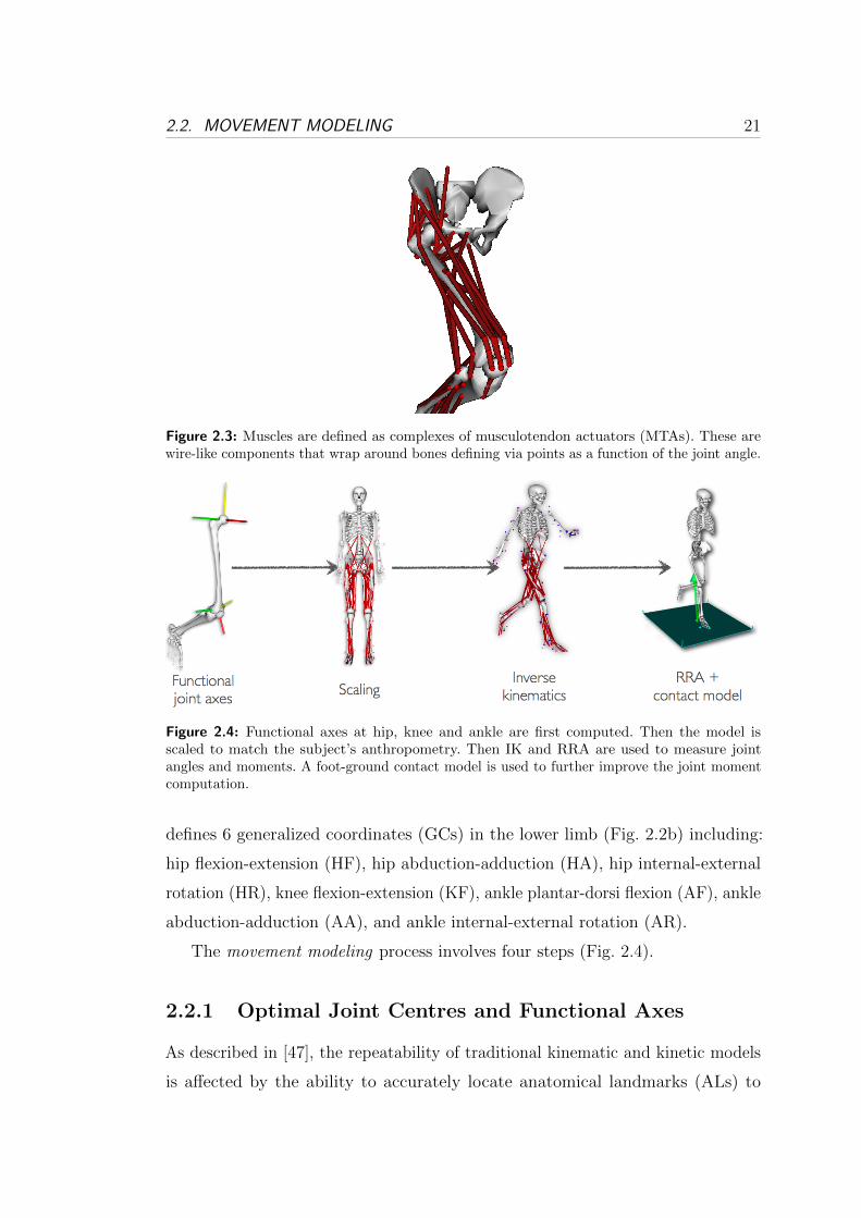
Figure 2.3: Muscles are defined as complexes of musculotendon actuators (MTAs). These arewire-like components that wrap around bones defining via points as a function of the joint angle.
Figure 2.4: Functional axes at hip, knee and ankle are first computed. Then the model isscaled to match the subject’s anthropometry. Then IK and RRA are used to measure jointangles and moments. A foot-ground contact model is used to further improve the joint momentcomputation.
defines 6 generalized coordinates (GCs) in the lower limb (Fig. 2.2b) including:
hip flexion-extension (HF), hip abduction-adduction (HA), hip internal-external
rotation (HR), knee flexion-extension (KF), ankle plantar-dorsi flexion (AF), ankle
abduction-adduction (AA), and ankle internal-external rotation (AR).
The movement modeling process involves four steps (Fig. 2.4).
2.2.1 Optimal Joint Centres and Functional Axes
As described in [47], the repeatability of traditional kinematic and kinetic models
is affected by the ability to accurately locate anatomical landmarks (ALs) to

22 2. WORKFLOW
Table 2.1: The 34 musculotendon actuators included in the model and the joints they span
Joints Musculotendon Actuators
Hip Adductor Brevis, Adductor Longus, Adductor Mag-nus1, Adductor Magnus2, Adductor Magnus3, Glu-teus Maximus1, Gluteus Maximus2, Gluteus Maximus3,Gluteus Medius1, Gluteus Medius2, Gluteus Medius3,Gluteus Minimus1, Gluteus Minimus2, Gluteus Min-imus3, Illiacus, Psoas
Knee Vastus Interioris, Vastus Lateralis, Vastus Medialis,Biceps Femoris Short Head
Ankle Peroneus Brevis, Peroneus Longus, Peroneus Tertis,Soleus, Tibialis Anterior
Hip, Knee Biceps Femoris Long Head, Semimembranosus, Semi-tendinosus, Gracilis, Rectus Femoris, Sartorius, TensorFascia Latae
Knee, Ankle Gastrocnemius Lateralis, Gastrocnemius Medialis
define joint centres and anatomical coordinate systems (ACS) (Fig. 2.5). The
development of numerical methods that define joint centres and axes of rotation
independent of ALs may therefore improve the repeatability of kinematic and
kinetic data. In this thesis, the numerical methodology presented in [47] is used to
derive the three-dimensional position of the centre of rotation for the hip, knee and
ankle joints. Furthermore the three dimensional orientation of the flexion-extension
axis of the knee joint is calculated.
To determine the three-dimensional position and orientation of each lower limb
segment, clusters of three retro-reflective markers (20 mm) were firmly adhered
to the subject’s pelvis, thighs, shank, and feet (Fig. 2.5). For the hip joint, a
functional method is employed, whereby subjects are required to consecutively
move the right and left thigh through a range of flexion, abduction, adduction,
and extension [47]. These data are used in a constrained optimization program
written in MATLAB (Optimization Toolbox, Mathworks Inc.; Natick, MA), where
spheres are fit to each thigh marker to find a left and right hip joint centre (HJC)
location relative to the pelvis coordinate system and sphere radii. Fig. 2.6 shows
the results of this computation.
For the knee joint, a mean helical axis is used to define the knee joint centre

2.2. MOVEMENT MODELING 23
Figure 2.5: Experimental and virtual markers used in this work. The anatomical coordinatesystem (ACS) for each joint is also visible.
and flexion-extension axis. To achieve this, subjects stand on one leg and flex the
contra-lateral thigh to enable the shank to freely flex and extend about the knee
from full extension to approximately 100 degrees of flexion. This is performed
for at least three cycles for each limb. Using the custom MATLAB program, the
tibia markers are expressed in the femoral coordinate system and instantaneous
helical axes are calculated throughout the range of motion using a singular value
decomposition method from [48, 49]. A mean helical axis is then calculated for
each knee, analogous to the method presented in [50] for the elbow joint. The
mean helical axis is used to define the flexion-extension axis of the knee relative
to the thigh coordinate system. The KJC is then defined relative to the mean
helical axis, at a point along the helical axis that intersects a plane that is normal

24 2. WORKFLOW
(a) (b)
Figure 2.6: Swinger trial for the calculation of the optimal hip joint centre. The blue trajectoriesrepresent the motion of the thigh markers. (a) The three-dimensional range of motion of thethigh markers is computed throughout the whole swinger trial. A sphere per marker is thencreated to fit the respective trajectory. (b) The optimal centre (green circle) is then calculatedwith respect to the pelvis anatomical coordinate system.
to the transepicondylar line, midway between the epicondyles. Fig. 2.7a shows the
results of this computation. Furthermore, Fig. 2.7b shows the knee helical axes
(KHA) that have been imported and visualized into the motion capture system
software. An analogous procedure is used to define the ankle joint centre in which
the relative movement of foot marker with respect to the shank ones is used.
The computed 3D positions of the hip, knee and ankle joint centres are then
integrated in the OpenSim musculoskeletal model (Fig. 2.2).
For the integration of the 3D orientation of the knee joint flexion-extension
axis, a novel procedure was developed in this thesis to define a 3-DOF knee joint
in the OpenSim musculoskeletal model. The estimated mean helical axis is used
to compute its 3D orientation with respect to the thigh reference frame. The
OpenSim musculoskeletal model is then integrated with this information in the
following way. The generic OpenSim musculoskeletal model that is used in this
thesis has a knee joint that is based on the work presented by Delp et al. [44]. In
this work the pelvis, thigh, shank and foot bones are digitized to create 3D meshes
of polygons to define each bone surface. Based on the anatomical digitized bone
surfaces the motion of the tibia with respect to the femur bone was determined as

2.2. MOVEMENT MODELING 25
(a) (b)
Figure 2.7: (a) The motion of the 3 shank markers (red trajectories) is calculated with respectto the left thigh (LTH1, LTH2, LTH3) and right thigh (RTH1, RTH2, RTH3) markers. Then themean helical axes are calculated (blue lines). (b) helical knee axes placed in the marker-basedmodel.
a function of knee joint angle. Fig. 2.8a shows the geometry used in this model
for determining knee moments and kinematics in the sagittal plane. The femoral
condyles were represented as an ellipse; the tibial plateau was represented as a
line segment. The transformation from the femoral reference frame to the tibial
reference frame was then determined so that the femoral condyles remain in
contact with the tibial plateau throughout the range of knee motion. The tibia
is therefore constrained to move on an elliptical surface defined by the femur
medial-lateral condyles. From a numerical point of view, this is defined by two
uni-dimensional spline functions that respectively associate a vertical (y-axis) and
an anterior-posterior (x-axis) translation of the tibia to the current knee angle
with respect to the femur reference frame. These two translations are combined
with the rotation of the tibia about the origin of its reference frame as a linear
function of the knee angle. As a result, the tibia moves and rotates simultaneously
on an elliptical trajectory. The OpenSim model used in this thesis defines the
spline functions with the assumption that the knee joint flexion-extension axis has
an orientation of zero degrees. That is, it is perpendicular to the vertical axis of the
femur reference frame. In this thesis a custom MATLAB routine was implemented
to apply the 3D orientation of the knee helical axis to the two uni-dimensional

26 2. WORKFLOW
(a) (b)
Figure 2.8: (a) Geometry for determining knee moments and kinematics in the sagittal plane.�k is the knee angle; � is the patellar ligament angle; � is the angle between the patella and thetibia; Fq, is the quadriceps force; lpl is the length of the patellar ligament. From these kinematics,the moment of the quadriceps force about the instant center of knee rotation can be computed.(b) The knee joint angle is defined by the orientation of the tibia reference frame (located on thetibia head) with respect to the femur reference frame (located on the femur head). The yellow,red and green axes represent the y, x and z coordinate axes respectively. This figure shows thecomputation of the flexion-extension angle (about the z-axis).
spline functions defined in the OpenSim model. This allows moving the tibia on
an inclined elliptical surface. In the OpenSim musculoskeletal model, the knee
angle is defined by the orientation of the tibia reference frame with respect to
the femur reference frame (Fig. 2.8b). The tibia reference frame was first rotated,
in the femur reference frame, with respect to the anterior posterior axis (x-axis)
according to the computed knee helical axis. This caused the tibia to move on a
circle whose radius was the distance from the femur reference frame to that of the
tibia. Then, the two translational spline functions were counter rotated, about
the same axis using a rotation matrix. This process produced a third spline that
translates the tibia on the medial-lateral axis (z-axis) as a function of the knee
angle.
2.2. MOVEMENT MODELING 27
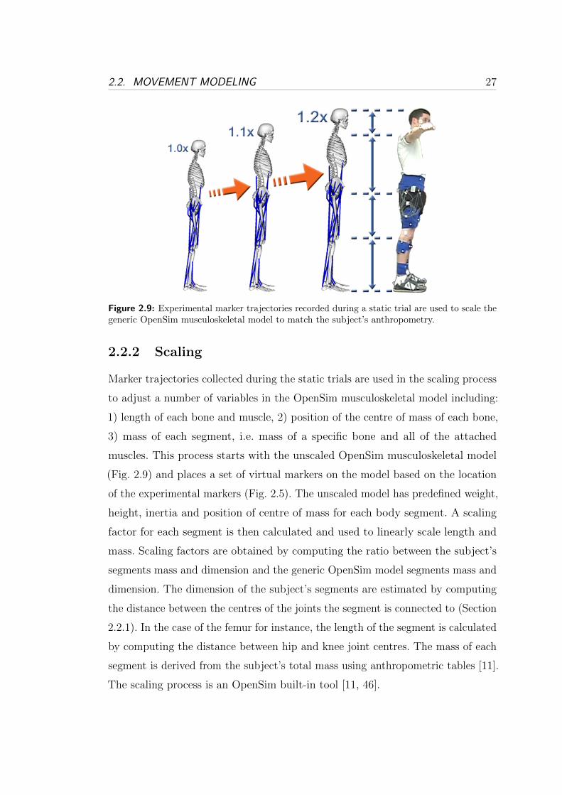
Figure 2.9: Experimental marker trajectories recorded during a static trial are used to scale thegeneric OpenSim musculoskeletal model to match the subject’s anthropometry.
2.2.2 Scaling
Marker trajectories collected during the static trials are used in the scaling process
to adjust a number of variables in the OpenSim musculoskeletal model including:
1) length of each bone and muscle, 2) position of the centre of mass of each bone,
3) mass of each segment, i.e. mass of a specific bone and all of the attached
muscles. This process starts with the unscaled OpenSim musculoskeletal model
(Fig. 2.9) and places a set of virtual markers on the model based on the location
of the experimental markers (Fig. 2.5). The unscaled model has predefined weight,
height, inertia and position of centre of mass for each body segment. A scaling
factor for each segment is then calculated and used to linearly scale length and
mass. Scaling factors are obtained by computing the ratio between the subject’s
segments mass and dimension and the generic OpenSim model segments mass and
dimension. The dimension of the subject’s segments are estimated by computing
the distance between the centres of the joints the segment is connected to (Section
2.2.1). In the case of the femur for instance, the length of the segment is calculated
by computing the distance between hip and knee joint centres. The mass of each
segment is derived from the subject’s total mass using anthropometric tables [11].
The scaling process is an OpenSim built-in tool [11, 46].

28 2. WORKFLOW
Figure 2.10: The unscaled model (grey) is first scaled to subject’s real dimension. During theinverse kinematics step the scaled model (blue model) is driven so that the displacement errorbetween virtual markers (pink markers) and the experimental ones (blue markers) is minimizedat each time step.
2.2.3 Inverse Kinematics
Marker trajectories recorded during dynamic movements are used by an Inverse
Kinematics (IK) model to calculate 3D joint angles (Fig. 2.10). This is done using
the OpenSim Inverse Kinematics tool in which an IK algorithm solves for the
joint angles that minimize the difference between the experimentally measured
marker positions and the virtual markers on the model (Section 2.2.2).
2.2.4 Residual Reduction Analysis
Ground reaction forces (GRF) recorded during motor tasks are used in conjunc-
tion with the thee-dimensional joint angles computed through IK to derive the
experimental joint moments. This is usually done by performing standard Inverse
Dynamics (ID). However, this method does not provide optimal solutions. Due to
limitations in marker trajectory acquisition and processing, there is an inherent
mismatch between the recorded trajectories and the recorded GRF. As a results,
in traditional ID algorithms, a non-physical external force and moment (i.e.,
residuals) are applied to a body in the model (e.g.,the pelvis) to resolve dynamic
inconsistency between the measured kinematics and GRF. This implies that, the

2.2. MOVEMENT MODELING 29
Figure 2.11: Comparison between the joint moments computed using standard inverse dynamics(ID) and residual reduction analysis (RRA).
moments computed via ID do not match the motion computed via IK. In this work
Residual Reduction Analysis (RRA) is used to minimize the mismatch between
trajectories and GRF and to compute the joint moments needed to track the
subject’s motion. RRA is an optimization procedure that slightly adjusts the
joint kinematics and model mass properties until an inverse dynamic solution is
found that minimizes the magnitude of the residuals [11]. Fig. 2.12 and 2.11 show
how estimates of joint moments and angles change when using standard ID as
opposed to RRA. Fig. 2.13 shows how the motion simulation differs when using
ID and RRA. Experiments are obtained from one male subject (age:28, weight:
67Kg, height: 183cm) who performed walking trials at self selected speed. The
residuals held in the pelvis body associated to the ID simulation were as follows:
FX = −19.31N , FY = 108.608N , FZ = −4.94242N , MX = −13.9448Nm,
MY = −4.00663Nm and MZ = 26.8262Nm. These were significantly reduced by
the RRA algorithm: FX = −0.692733N , FY = −0.709131N , FZ = −0.104057N ,
MX = −9.7929Nm, MY = 0.285471Nm and MZ = −18.4733Nm. The terms
F and M represent the magnitude of forces and moments respectively, that are
applied to the pelvis body to resolve the dynamic inconsistency.

30 2. WORKFLOW
Figure 2.12: Comparison between the joint angles computed using standard inverse dynamics(ID) and residual reduction analysis (RRA).
(a) (b) (c) (d)
Figure 2.13: (a) Motion simulation using standard inverse dynamics (red model) is compared tothe dynamically consistent one obtained using RRA (green model). The global reference frameis shown. (b) Lateral view. (c) Posterior view. (d) Anterior view.
2.2.5 Contact Model
The RRA approach has the disadvantage that while it allows perturbing the
whole-body kinematics it does not allow perturbing the feet kinematics when they
are in contact with the ground. This is because RRA can only use GRFs obtained
experimentally. Therefore, if the foot kinematics was changed, the experimental
2.2. MOVEMENT MODELING 31
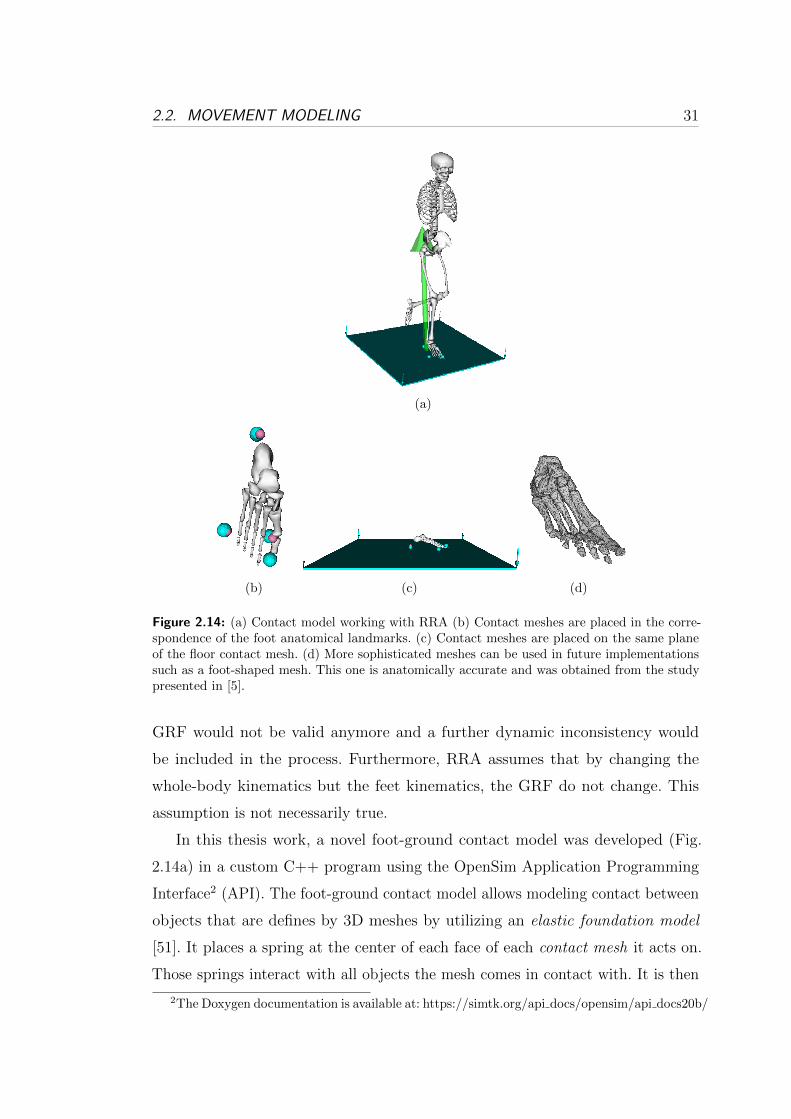
(a)
(b) (c) (d)
Figure 2.14: (a) Contact model working with RRA (b) Contact meshes are placed in the corre-spondence of the foot anatomical landmarks. (c) Contact meshes are placed on the same planeof the floor contact mesh. (d) More sophisticated meshes can be used in future implementationssuch as a foot-shaped mesh. This one is anatomically accurate and was obtained from the studypresented in [5].
GRF would not be valid anymore and a further dynamic inconsistency would
be included in the process. Furthermore, RRA assumes that by changing the
whole-body kinematics but the feet kinematics, the GRF do not change. This
assumption is not necessarily true.
In this thesis work, a novel foot-ground contact model was developed (Fig.
2.14a) in a custom C++ program using the OpenSim Application Programming
Interface2 (API). The foot-ground contact model allows modeling contact between
objects that are defines by 3D meshes by utilizing an elastic foundation model
[51]. It places a spring at the center of each face of each contact mesh it acts on.
Those springs interact with all objects the mesh comes in contact with. It is then
2The Doxygen documentation is available at: https://simtk.org/api docs/opensim/api docs20b/

32 2. WORKFLOW
possible to assign different physical properties to each contact mesh including:
stiffness, dissipation and static, dynamic and viscous frictions.
Four spheres were placed on the OpenSim musculoskeletal model’s in the
correspondence of heel, first and fifth metatarsal bones and toe (Fig. 2.14b). This
was done using the 3D position of the experimental markers obtained from motion
capture data. Because no experimental marker was placed on the toe, the position
of the associated contact sphere was placed at 2cm from the first metetarsal bone.
Then, the four spheres were placed on the same plane and the floor contact mesh
was consequently aligned as in Fig. 2.14c. Finally, the dynamic contact parameters
were assigned a meaningful physical value to define appropriate contact. In this
work both floor location and contact parameter values were defined manually. In
future implementations an optimization algorithm will be used to find optimal
position of the floor and optimal contact parameters. The optimization procedure
will minimize the difference from the experimental GRF recorded during a static
standing trial and those simulated by the proposed contact model. Furthermore,
more sophisticated meshes will be used (Fig. 2.14d).
Once the contact model is calibrated it is possible to use it in conjunction with
RRA to also adjust the foot kinematics (Fig. 2.14a) and subsequently recompute
the associated GRF. In general, at each time step, the contact model computes the
the GRF generated by the RRA kinematics change. A more accurate ID solution
can then be used in RRA. The contact model presented in this section was not
used in the studies reported within this thesis due to lack of time. Although it is
very promising, further validation is needed.
In future work, the presented contact model can be also utilized to create
dynamic motion simulations of humanoid robots.
2.3 An Elastic-Tendon NMS Model of the Knee
Joint
This section briefly reviews the NMS model developed by Lloyd et al. and previously
presented in [2, 3, 35, 37]. Lloyd’d NMS model is used to validate the novel NMS
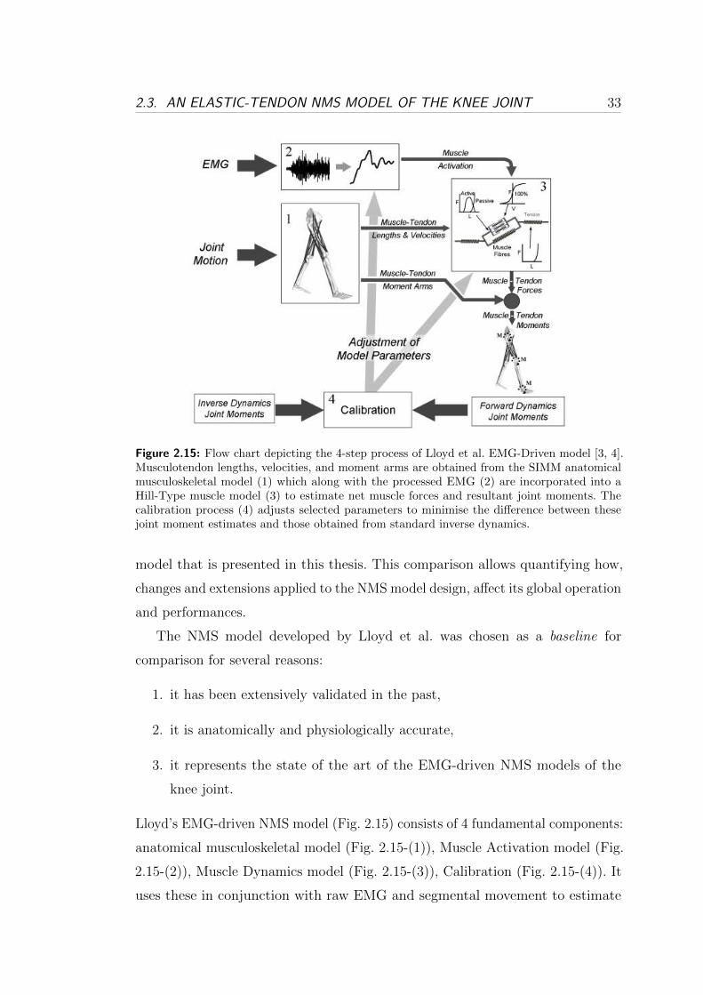
2.3. AN ELASTIC-TENDON NMS MODEL OF THE KNEE JOINT 33
Figure 2.15: Flow chart depicting the 4-step process of Lloyd et al. EMG-Driven model [3, 4].Musculotendon lengths, velocities, and moment arms are obtained from the SIMM anatomicalmusculoskeletal model (1) which along with the processed EMG (2) are incorporated into aHill-Type muscle model (3) to estimate net muscle forces and resultant joint moments. Thecalibration process (4) adjusts selected parameters to minimise the difference between thesejoint moment estimates and those obtained from standard inverse dynamics.
model that is presented in this thesis. This comparison allows quantifying how,
changes and extensions applied to the NMS model design, affect its global operation
and performances.
The NMS model developed by Lloyd et al. was chosen as a baseline for
comparison for several reasons:
1. it has been extensively validated in the past,
2. it is anatomically and physiologically accurate,
3. it represents the state of the art of the EMG-driven NMS models of the
knee joint.
Lloyd’s EMG-driven NMS model (Fig. 2.15) consists of 4 fundamental components:
anatomical musculoskeletal model (Fig. 2.15-(1)), Muscle Activation model (Fig.
2.15-(2)), Muscle Dynamics model (Fig. 2.15-(3)), Calibration (Fig. 2.15-(4)). It
uses these in conjunction with raw EMG and segmental movement to estimate

34 2. WORKFLOW
Figure 2.16: Raw EMGs are low-lass filtered (30Hz), full-wave rectified and low-pass filtered(6Hz). Signals are then normalized to maximal voluntary contraction (MVC) to obtain the nor-malized linear envelope. A second order recursive filter is applied to model the electromechanicaldelay and to include the muscle’s twitch response [3]. Signals are then non-linearly mapped toaccount for the non-linear relationship between EMG amplitude and muscle force [3].
individual muscle force and subsequently joint moments and soft tissue loading.
This is a forward dynamic model because it estimates muscle force directly from
muscle EMG signals in an open-loop fashion.
2.3.1 Musculoskeletal Model
The musculoskeletal model of the lower limb (Fig. 2.15-(1)) is created using the
SIMM Biomechanics Software Suite (Musculographics, Inc.) [45] based on the
results presented in [37, 44]. It consists of line segment representations of 13 muscu-
lotendon actuators (MTAs) spanning the knee joint including: semimembranosus,
semitendinosus, biceps femoris long head, biceps femoris short head, sartorius,
tensor fascia latae, gracilis, vastus lateralis, vastus medialis, vastus intermedius,
rectus femoris, gastrocnemius medialis, and gastrocnemius lateralis. Only two
muscles crossing the knee are not included: the plantaris and the popliteus. They
are assumed to have a negligible contribution to the total flexion-extension (FE)
moment due to their relatively small physiological cross sectional area (PCSA).
The lengths of the modeled bones and MTAs are linearly scaled to the actual

2.3. AN ELASTIC-TENDON NMS MODEL OF THE KNEE JOINT 35
Figure 2.17: Hill-type elastic-tendon muscle model. Each tendons is represented by a singleelastic passive element. The fibre is represented by an active contractile element in parallel witha passive element. The two-element fibre is placed between the two tendons. The fibre is orientedwith respect to the tendon according to the pennation angle '. lmt is the musculotendon length.lm is the fibre length. lts is the tendon slack length. FA is the force produced by the fibre activeelement. FP is the force produced by the fibre passive element. Fmt musculotendon force, i.e.the fibre force projected on to the tendon line of action.
subject’s size. This muscuoskeletal model is used in SIMM to perform a kinematic
driven simulation to determine muscletendon lengths, lmt, velocities, vmt, and
moment arms, r during movement. These values are then input in the Muscle
Dynamics model together with muscle activation to estimate muscle force (Section
2.3.3).
2.3.2 Muscle Activation
Raw EMG signals are processed as in Section 2.1 to obtain normalized linear
envelopes. Then, a second order recursive filter is applied to characterize the muscle
electromechanical delay and twitch response [3]. We will refer to the processed
signals to as, u(t). Then, a non-linear map is applied to account for the non-linear
relationship between EMG amplitude and muscle force [3] (Fig. 2.16). To achieve
this step, an exponential relationship is used which includes a single parameter A
36 2. WORKFLOW
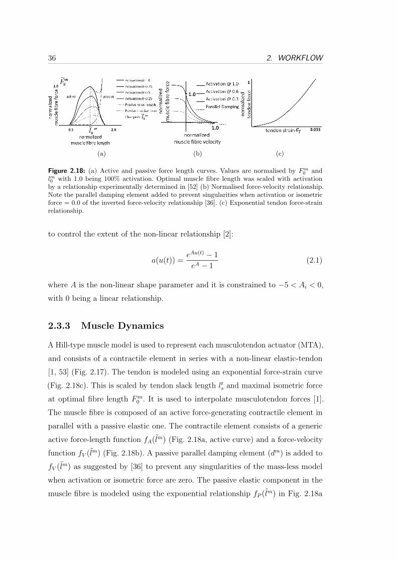
(a) (b) (c)
Figure 2.18: (a) Active and passive force length curves. Values are normalised by Fm0 and
lm0 with 1.0 being 100% activation. Optimal muscle fibre length was scaled with activationby a relationship experimentally determined in [52] (b) Normalised force-velocity relationship.Note the parallel damping element added to prevent singularities when activation or isometricforce = 0.0 of the inverted force-velocity relationship [36]. (c) Exponential tendon force-strainrelationship.
to control the extent of the non-linear relationship [2]:
a(u(t)) =eAu(t) − 1
eA − 1(2.1)
where A is the non-linear shape parameter and it is constrained to −5 < Ai < 0,
with 0 being a linear relationship.
2.3.3 Muscle Dynamics
A Hill-type muscle model is used to represent each musculotendon actuator (MTA),
and consists of a contractile element in series with a non-linear elastic-tendon
[1, 53] (Fig. 2.17). The tendon is modeled using an exponential force-strain curve
(Fig. 2.18c). This is scaled by tendon slack length lts and maximal isometric force
at optimal fibre length Fm0 . It is used to interpolate musculotendon forces [1].
The muscle fibre is composed of an active force-generating contractile element in
parallel with a passive elastic one. The contractile element consists of a generic
active force-length function fA(lm) (Fig. 2.18a, active curve) and a force-velocity
function fV (lm) (Fig. 2.18b). A passive parallel damping element (dm) is added to
fV (lm) as suggested by [36] to prevent any singularities of the mass-less model
when activation or isometric force are zero. The passive elastic component in the
muscle fibre is modeled using the exponential relationship fP (lm) in Fig. 2.18a

2.3. AN ELASTIC-TENDON NMS MODEL OF THE KNEE JOINT 37
~
~ F
m
F m
∫ Initial guess of fibre velocity
Lm(i+1), m(i+1)
Runge-Kutta Integration
Calculate Tendon Force
Calculate Tendon Length
New Pennation Angle
)1(
sinsin)1( 001
il
li
m
m
Calculate Active and Passive
Components of Force
so: F A = F t - F P
1
Interpolate Force-Velocity Curve
(calculate Factive/Fisometric to determine
Calculate Strain in Tendon
)1(il m
0.033
Interpolate Force-Length Curve to
calculate isometric force in the fibre
using and activation
cosmmtt lll
t
t
s
t
l
ll
tF)(iF t
)1(ilmt
)1(ivm )1(ilm
)1(ivm
ml~
)(~
iF m
mv
Muscle fibre velocity
Optimal fibre length
Time step
Pennation angle of muscle
fibre
Tendon length
Muscle tendon length
Tendon slack length
Force in tendon
Pennation angle at optimal
fibre length
)(ivm
mvml0
0
tlmtlt
sltF
i
Figure 2.19: Schematic diagram of muscle dynamics

38 2. WORKFLOW
(passive curve). The final MTA force depends on a number of parameters including:
maximum isometric muscle force at optimal fibre length Fm0 , optimal muscle fibre
length lm0 , instantaneous pennation angle ', instantaneous muscle fibre length lm,
instantaneous fibre contraction velocity vm, and instantaneous muscle activation
a(u). It is the contractile element of the model that represents the culmination of
the forward dynamics component of the EMG-driven NMS model, as the muscle
fibre velocities are numerically integrated to predict the time evolution of the
muscle fibre length. The dependence of lm0 on muscle activation [54] is modeled
using a linear relationship [3]:
new lm0 (t) = lm0 ⋅ ( ⋅ (1− a(t)) + 1) (2.2)
where:
∙ = percentage change in optimal fibre length
∙ new lm0 = new optimal fibre length
∙ lm0 = current optimal fibre length
∙ a(t) = activation at time t
The effect of this relationship is illustrated in Figure 2.18a. The percentage change
in optimal fibre length, , is altered in the calibration process between 0 and 20%
as a function of activation (Section 2.3.4). Muscle fibre lengths are calculated
by forward integration of the fibre velocities obtained from the force-velocity
and force-length relationships using a Runge-Kutta-Fehlberg algorithm. Using a
method developed by Loan [55], initial muscle fibre lengths and fibre velocities
are determined by calculating the stiffnesses of muscle fibre and tendon, and
apportioning the total muscle tendon velocity to the muscle fibre and tendon
based on their relative stiffnesses. A schematic diagram of the complete muscle
model is shown in Figure 2.19.
Muscle fibre force can then be expressed as:
Fm = (fA(lm) ⋅ fV (vm) ⋅ a(u) + fP (lm) + dm ⋅ vm) ⋅ Fm0 ⋅ � (2.3)

2.3. AN ELASTIC-TENDON NMS MODEL OF THE KNEE JOINT 39
where the term � is the muscle strength coefficient (Section 2.3.4) whereas all
other terms have been defined previously. The force produced by the MTA, Fmt,
can then be derived by projecting the fiber force Fm onto the tendon line of action
as follows:
Fmt = Fm ⋅ cos(') (2.4)
Indeed, the pennation angle, ' defines the angle at which fibers are oriented with
respect to the tendon (Fig. 2.17).
Net knee joint flexion-extension (FE) moments (M) are obtained by summing
the product of each MTA’s force by its flexion-extension moment arm r:
M =N∑i=1
riFmti (2.5)
where riFmti represents the individual FE moment generated by the itℎ muscle.
2.3.4 Validation and Calibration
To validate a model, it is usually desirable to compare the output of that model
with data measured empirically. Unfortunately, the methodological difficulties in
measuring individual muscle forces prevent any direct validation of the EMG-driven
model on humans. An indirect validation process is instead used to validate and
calibrate the model to an individual. The validation process involves comparing
the predicted net knee flexion-extension moments with the net moments measured
experimentally. If the muscle forces are accurate, then the model estimates of net
joint moments should be equal to the external moments measured experimentally.
Lloyd et al. used standard Inverse Dynamics to calculate experimental knee
FE moments. It is here clear the importance of utilizing dynamically consistent
joint moments in the calibration. If this is not done, the calibration will constrain
muscles to satisfy join moments that are not truly representative of the actual
joint dynamics.
The aim of the calibration process is to obtain a set of model parameters for an
individual to accurately estimate the net FE moments at the knee. The calibration
process uses a set of calibration trials to learn the muscle dynamics across a
40 2. WORKFLOW
wide range of muscle contractile conditions. Starting from a set of uncalibrated
parameters a simulated annealing algorithm [56] is used to alter the selected
parameters so that the moments estimated by the NMS model fit the net joint
moments experimentally measured and minimize the sum of squared difference
between the estimated and experimental moments. Once the calibration process
has completed it is possible to use the subject-specific calibrated parameters to
estimate muscle forces and joint moments during the subject’s movement. It is
worth noting that once calibrated, the NMS model only requires EMG signals and
joint angles and can execute in open-loop. That is, no tracking is required to match
the experimental joint moments. If properly calibrated, the model will naturally
track novel data with no need for optimization. Tracking the experimental moment
is required during the calibration step only. This feature allows deceasing the
amount of information required during the model run-time execution and maximize
its speed.
The adjustable parameters used in the calibration process are divided into
two groups. One group includes activation parameters, chosen from the Muscle
Activation model and the other group includes muscle parameters from the Muscle
Dynamics model. Activation filtering parameters are constrained in the calibration
process to realize a stable positive solution to the discrete linear dynamic model
and used to determine the gain and recursive coefficients of the recursive filter.
These coefficients are dimensionless and are varied between -1 and 1. They take
into account changes in muscle excitation levels due to different EMG electrode
placement, skin preparation, and impedance. It is assumed that these values
may differ between individuals, different muscles, and different testing sessions.
The non-linear muscle activation shape factor A in (2.1) is also altered in the
calibration process between -5 and 0 (2.1). The non-linearity of the EMG to
force relationship has been well documented and has shown that the inclusion
of this parameter within a transfer function improves model estimates of stress
from EMG data [57]. Parameters in the Hill-type Muscle model that are adjusted
include:
1. muscles strength coefficients

2.3. AN ELASTIC-TENDON NMS MODEL OF THE KNEE JOINT 41
2. resting tendon slack length
3. muscle optimal fiber length
The strength coefficients allow scaling the relative maximum isometric force a
muscle can produce to account for well documented individual differences in muscle
strength, i.e. Physiological cross-sectional area and difference in strength between
different muscles. To maintain relative strength across all muscles, global gains
were used as opposed to individual muscle gains. The inclusion of muscle dependent
force coefficients is physiologically valid to account for strength differences between
individuals and has been used previously in EMG-Driven models. However, care
must be taken when increasing the number of parameters within an optimisation
process as this may compromise the physiological construct of the model, as
each parameter becomes a fix for a general solution to be obtained. Constraints
on muscle gain coefficients were used to prevent unrealistic muscle forces being
estimated by the model. These were applied such that each strength coefficient
was allowed to vary from 0.5 to 1.5. In the NMS model presented in this Chapter,
strength coefficients grouped muscles into three categories: knee extensors, knee
flexors and gastrocnemious muscles.
Resting tendon slack length (lts) directly defines the length of the fibers and
the force they can produce. Furthermore, there is very little information in the
literature in regards to tendon slack lengths of lower limb musculature. The reason
for this lack of information is mostly due to the difficulty in measuring these values
and the ill-defined junction between muscle and tendon. This further motivated
the need for calibrating this parameter. Initial values were obtained from [37] and
constrained such that: lts = initial value± 5%.
Optimal fibre length (lm0 ) is also calibrated as it has been shown to vary
between individuals and to have a strong impact on the behavior of each muscle
[37]. Initial values were obtained from [37] and constrained such that: lm0 =
initial value± 2.5%.
The objective function used in the calibration algorithm is defined as follows:
min∑Nt
M2−M2
var(M)+ Penalty
Nt
(2.6)
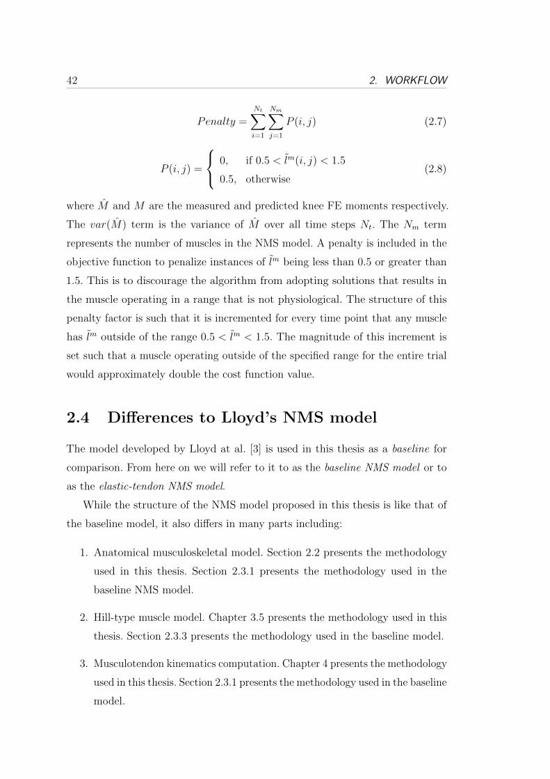
42 2. WORKFLOW
Penalty =Nt∑i=1
Nm∑j=1
P (i, j) (2.7)
P (i, j) =
⎧⎨⎩ 0, if 0.5 < lm(i, j) < 1.5
0.5, otherwise(2.8)
where M and M are the measured and predicted knee FE moments respectively.
The var(M) term is the variance of M over all time steps Nt. The Nm term
represents the number of muscles in the NMS model. A penalty is included in the
objective function to penalize instances of lm being less than 0.5 or greater than
1.5. This is to discourage the algorithm from adopting solutions that results in
the muscle operating in a range that is not physiological. The structure of this
penalty factor is such that it is incremented for every time point that any muscle
has lm outside of the range 0.5 < lm < 1.5. The magnitude of this increment is
set such that a muscle operating outside of the specified range for the entire trial
would approximately double the cost function value.
2.4 Differences to Lloyd’s NMS model
The model developed by Lloyd at al. [3] is used in this thesis as a baseline for
comparison. From here on we will refer to it to as the baseline NMS model or to
as the elastic-tendon NMS model.
While the structure of the NMS model proposed in this thesis is like that of
the baseline model, it also differs in many parts including:
1. Anatomical musculoskeletal model. Section 2.2 presents the methodology
used in this thesis. Section 2.3.1 presents the methodology used in the
baseline NMS model.
2. Hill-type muscle model. Chapter 3.5 presents the methodology used in this
thesis. Section 2.3.3 presents the methodology used in the baseline model.
3. Musculotendon kinematics computation. Chapter 4 presents the methodology
used in this thesis. Section 2.3.1 presents the methodology used in the baseline
model.

2.5. CONCLUSIONS AND FUTURE WORK 43
4. Number of DOFs. Chapter 6 presents the methodology used in this thesis.
Section 2.3.1 presents the methodology used in the baseline model.
5. Calibration. Chapters 5, 6 and 7 present the methodology used in this thesis.
Section 2.3.4 presents the methodology used in the baseline model.
2.5 Conclusions and Future Work
In this chapter the general workflow that was used in this research work was
presented. This included: 1) the acquisition and processing of data from the
subject’s movement, 2) the creation of a dynamic musculoskeletal simulation to
estimate joint kinematics and moments, 3) the execution of the NMS model.
Advanced methods were developed and used to scale a generic OpenSim
musculoskeletal model to match the subject’s anthropometry and anatomy and to
define optimal centres and axes in the hip, knee and ankle joints. Advanced motion
simulation methods were used to calculate three-dimensional joint kinematics and
moments and to ensure dynamic consistency between kinematics and kinetics. To
further improve this process a foot-ground contact model was also implemented.
These methods were used to generate the best input data for the NMS model
developed and presented in this thesis. The aim of this specific work was that
of introducing anatomical and dynamic consistency into EMG-driven modeling.
The quality of the data used to calibrate the EMG-driven NMS model strongly
affects its operation post-calibration. Because the EMG-driven NMS model is
physiologically accurate and it uses real muscles excitation signals (i.e. EMG
signals), the hypothesis is that by providing calibration data that better represent
the dynamics of the human movement, the model will learn more naturally the
prescribed muscle dynamics. Future work will therefore compare the NMS model
performances when both traditional and advanced techniques are used to obtain
calibration data.
The last two sections of the chapter illustrated the general structure of the
NMS model developed by Lloyd et al. and the main differences with respect to
the model presented in this thesis.

Chapter 3
A Stiff-Tendon
Neuromusculoskeletal Model of
the Knee Joint
In this Chapter motion capture technology is used together with a novel neu-
romusculoskeletal (NMS) model of the knee joint and sophisticated algorithms
for motion kinematics and dynamics computation, to estimate somatosensory
information during the human movement. Although the NMS model represents
the single knee joint, it has been designed so that it is straightforward to extend
to whole-body level with minor loss of computational time performances. This
Chapter shows the proposed NMS model is as accurate as the complex models
previously presented in the literature. It shows it achieves superior computational
time performances. It validates the model on a population of 6 male subjects and
directly compares its behavior to that of the model previously developed by a
leading research group in musculoskeletal modeling. The Chapter illustrates how
the proposed model can be used as a human-machine interface for the control
of a powered orthosis of the lower limb and discusses how it can be used for
the actuation of humanoid robots equipped with artificial muscles. This research
development aims to integrate musculoskeletal dynamics into robotics systems to
achieve more advanced bio-inspired control strategies.
45

46 3. A STIFF-TENDON NMS MODEL OF THE KNEE JOINT
3.1 Introduction
The development of computer simulation methods based on biologically relevant
neuromusculoskeletal (NMS) models has gained particular emphasis in recent
years in the field of robotics for effectively helping understand mechanisms of
motion in humans [25, 58]. The need for better understanding the role of muscle
function during movement is regarded as a key-point for the design of robotic
systems that can robustly embody humans ability of moving. This trend can be
identified as Musculoskeletal Robotics [59].
Indeed, the human musculoskeletal system provides form, support and stability
to the body. The extraordinary capacity to efficiently use muscles allows us to
realize challenging tasks including: 1) the ability to actively move in a huge variety
of unknown environments, 2) the ability to add compliance to our movements
and make interaction with humans and real-world objects, 3) the ability to realize
multi-modal locomotion, i.e. different locomotion modes such as walking, running
or hopping.
As a result, several bio-inspired humanoid robots have been proposed in which
artificial muscle and tendon structures are attached to different parts of the
humanoid body just like real muscles are attached in the human body [12, 13, 60–
62]. This gives the robot more degrees of freedom of actuation than could be
achieved with motorized rotary joints and the potential ability of moving around
and interacting with the physical world in the same way our flesh bodies do
[60, 62]. Despite this great advancement in the musculoskeletal design, no effective
solutions have been proposed yet to activate the artificial muscles and actuate the
humanoid robots. In this context, the development of accurate musculoskeletal
software models can help defining the humanoids artificial muscles contraction
dynamics. For this purpose, human muscle contraction dynamics can be used as a
means of bio-inspired control system for humanoids.
The need for understanding muscle contraction dynamics also plays a central
role in the design of assistive devices such as powered orthoses and exoskeletons.
In this case, a better understanding of the real-time behavior of human muscles
can improve the actuation of these devices and their control algorithms, resulting

3.1. INTRODUCTION 47
in enhanced biomimetic control systems [6, 8]. Citing Nakamura et al.: when the
man-machine interface obtains access to the somatosensory information, machines
would make the first step to understand humans. Such implicit communication
between humans and machines could be termed as a cognitive-level communication
[6]. Bringing human musculoskeletal models into robotics will open the door to a
new generation of human-machine interfaces (HMIs) for a more intuitive device
control.
Therefore, it is crucial to develop models that reflect the action of muscles
while minimizing processing time in musculoskeletal robotics research.
This Chapter presents a novel neuromusculoskeletal (NMS) model of the knee
joint that is used together with motion capture technology and sophisticated
algorithms for motion kinematics and dynamics computation, to estimate so-
matosensory information during the human movement (Fig. 2.1). Although the
model represents a single joint, it has been designed so that it is straightforward to
extend to whole-body level with minor loss of computational time performances.
Chapter 6 will present an extension to the lower extremity level. The somatosen-
sory information includes activation, force, length and contraction velocity of the
muscles spanning the knee joint. This information is also used to estimate the
knee flexion-extension moments as well as contact forces between bones generated
during movement. The Chapter also shows the proposed model can be used as a
human-machine interface (HMI) for the real-time control of a powered orthosis
of the lower limb. It is then discussed how the NMS model can be used for the
actuation of humanoid robots equipped with artificial muscles.
A great body of research has been previously conducted in the field of neu-
romusculoskeletal modeling. In the literature there have been adopted either
simplified neuromusculoskeletal models that are suitable for applications with
real-time constraints or very detailed and physiologically accurate models that
are not efficients from a computational point of view.
Biomechanists have developed complex models of the human joints that com-
bine together kinematic and kinetic data with neural signals to study human
muscle behavior in vivo [1–3, 35, 36]. These models are extremely accurate in
the way they represent physiological properties of the musculoskeletal system. To
48 3. A STIFF-TENDON NMS MODEL OF THE KNEE JOINT
enable the estimation of muscle force and joint moment, musculoskeletal models
usually require explicit expressions of muscle-tendon kinematics including: muscu-
lotendon length, three-dimensional muscle moment arms, muscle fiber length and
contraction velocity.
A main limitation of these models is they usually do not integrate these
operations into a common framework. Third party musculoskeletal geometry
software is used to estimate musculotendon length and three-dimensional muscle
moment arms and include: SIMM [44, 45], OpenSim [11, 46] and AnyBody [63].
These are driven by graphical user interfaces (GUIs) and are difficult to implement
in custom software or micro controllers due to their extreme detail of complexity
in modeling the pathways of the musculo-tendon complexes. This prevents the
NMS model, that uses them, to be entirely executed on line.
A second limitation is their complexity. These NMS models have complex
muscle models in which tendons and fibers are represented as elastic bodies capable
of stretching and contracting. An ordinary differential equation (ODE) has to
be integrated at each time step to estimate the instantaneous value of muscle
fiber length and contraction velocity (Section 2.3). This usually requires a great
amount of computational time which quickly grows with the number of muscles in
the model. Therefore, these models are unsuitable for robotics applications with
real-time constraints.
Only recently, robotics researchers have developed models that are suitable for
real-time applications [6, 8–10, 15, 38, 64]. These works, however, either utilize
very simplified models of the human joints or they do not integrate information of
the human musculoskeletal system at all. In general, real-time performances are
obtained by simplifying the model design. One main simplification is that of using
simple musculoskeletal geometry models that estimate musculotendon length and
muscle moment arms on a plane only, i.e. the joint flexion-extension plane. This
leads to inaccurate estimations of musculotendon kinematics and represents a
critical point because small errors in their values can result in large errors in
musculotendon force and joint moment prediction.
A second simplification is that of including a very limited number of muscles
spanning a specific joint. This implies the impossibility of correctly estimating
3.1. INTRODUCTION 49
the moments developed by the user at that joint. In fact joint moments can only
be correctly estimated if all muscles spanning that joints are considered and their
force is estimated.
Another limitation is that of not taking into consideration the change in muscle
force due to fibers contraction velocity. This plays an important role when the
subject transitions from one locomotion mode to another, i.e. from walking to
running.
Furthermore these models allow calibrating a small number of subject-specific
parameters thus making the scaling process less able to adapt to different subjects.
Finally, validation of the model is not paid much attention and the model is
usually evaluated on one subject only and on a small number of motor tasks. In
general, the degree of simplification often makes these models unsuitable for being
integrated into the control system of assistive devices that are to support a wide
range of movements.
This Chapter shows the proposed NMS model is accurate and achieves superior
computational time performances and proposes a solution that addresses the
limitations of the complex but slow models developed by biomechanists and the
fast but simplified ones developed by robotics engineers [65–67].
A novel methodology is proposed to produce accurate estimates of musculo-
tendon length and three-dimensional muscle moment arms eliminating the need
for using an off-line GUI-driven software. This allows executing the entire NMS
model on line and.
Fast operation of the NMS model is achieved by designing a novel muscle
model that allows estimating muscle fiber length and contraction velocity much
faster than the NMS models developed by biomechanics and with comparable
predictive accuracy.
The muscle redundancy problem is solved using electromyographic (EMG)
signals produced by the human muscles during movement. Previously presented
approaches [6, 9] assume the muscles share the load about a joint based on some
objective function that has to be carefully chosen before hand or based upon
statistical assumptions. This is a limitation because muscles in general use different
criteria depending on the subject and on the movement and it is often impossible

50 3. A STIFF-TENDON NMS MODEL OF THE KNEE JOINT
to assess the appropriateness of the chosen optimization criteria or statistical
approach.
A robust validation methodology of the model is adopted. The NMS model is
used on a population of 6 male subjects who performed 75 of motor tasks. The
prediction accuracy was assessed by comparing the proposed methodology to the
well established model developed by biomechanists Lloyd et al. [2, 3, 35, 37, 47].
Real-time operation was assessed by running the proposed NMS model on an
embedded system that could be used for the real-time control of a powered orthosis.
This research development aims to integrate musculoskeletal dynamics into
robotics systems to achieve more advanced bio-inspired control strategies. Neu-
romusculoskeletal modeling technology not only can offer great solutions for
exoskeletons control and humanoids actuation, but can also boost research that
aims to realize more realistic virtual humans by providing a more realistic estima-
tion of human internal state [5].
3.2 Workflow
Fig. 2.1 gives a schematic view of the three steps that involve the acquisition of data
from the human movement, the use of sophisticated algorithms for the dynamic
simulation of the human motion and the execution of the neuromusculoskeletal
(NMS) model for the estimation of somatosensory information.
3.3 Human Movement
This is the first step in which the data needed for the model calibration and
validation are collected and processed.
A data set for the calibration of the model is initially created which includes:
1 static trial, 3 swinger trials, 2 walking trials and 2 running trials per subject.
Data collected from the static trial are used to scale the anatomical dimensions of
the musculoskeletal model (Fig. 3.1). Data collected from the swinger trials are
used to compute the optimal centre of the hip, knee and ankle joints.
Data collected from the 4 dynamic trials are used to calibrate the biomechanical
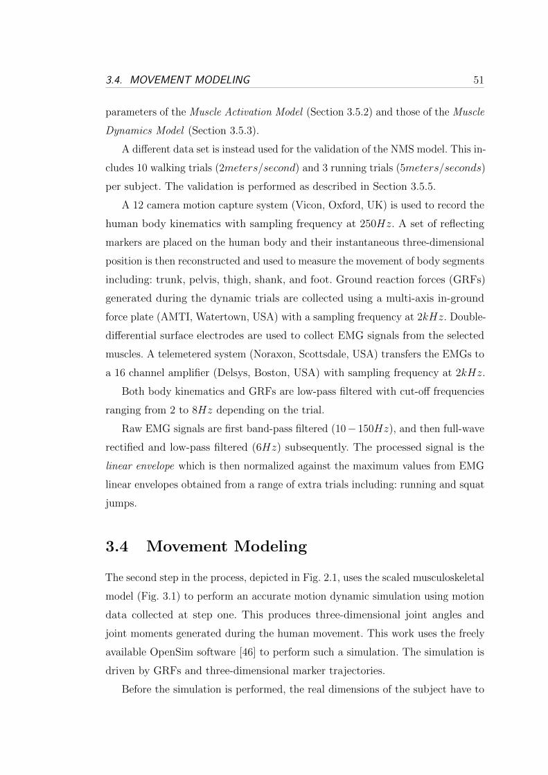
3.4. MOVEMENT MODELING 51
parameters of the Muscle Activation Model (Section 3.5.2) and those of the Muscle
Dynamics Model (Section 3.5.3).
A different data set is instead used for the validation of the NMS model. This in-
cludes 10 walking trials (2meters/second) and 3 running trials (5meters/seconds)
per subject. The validation is performed as described in Section 3.5.5.
A 12 camera motion capture system (Vicon, Oxford, UK) is used to record the
human body kinematics with sampling frequency at 250Hz. A set of reflecting
markers are placed on the human body and their instantaneous three-dimensional
position is then reconstructed and used to measure the movement of body segments
including: trunk, pelvis, thigh, shank, and foot. Ground reaction forces (GRFs)
generated during the dynamic trials are collected using a multi-axis in-ground
force plate (AMTI, Watertown, USA) with a sampling frequency at 2kHz. Double-
differential surface electrodes are used to collect EMG signals from the selected
muscles. A telemetered system (Noraxon, Scottsdale, USA) transfers the EMGs to
a 16 channel amplifier (Delsys, Boston, USA) with sampling frequency at 2kHz.
Both body kinematics and GRFs are low-pass filtered with cut-off frequencies
ranging from 2 to 8Hz depending on the trial.
Raw EMG signals are first band-pass filtered (10− 150Hz), and then full-wave
rectified and low-pass filtered (6Hz) subsequently. The processed signal is the
linear envelope which is then normalized against the maximum values from EMG
linear envelopes obtained from a range of extra trials including: running and squat
jumps.
3.4 Movement Modeling
The second step in the process, depicted in Fig. 2.1, uses the scaled musculoskeletal
model (Fig. 3.1) to perform an accurate motion dynamic simulation using motion
data collected at step one. This produces three-dimensional joint angles and
joint moments generated during the human movement. This work uses the freely
available OpenSim software [46] to perform such a simulation. The simulation is
driven by GRFs and three-dimensional marker trajectories.
Before the simulation is performed, the real dimensions of the subject have to
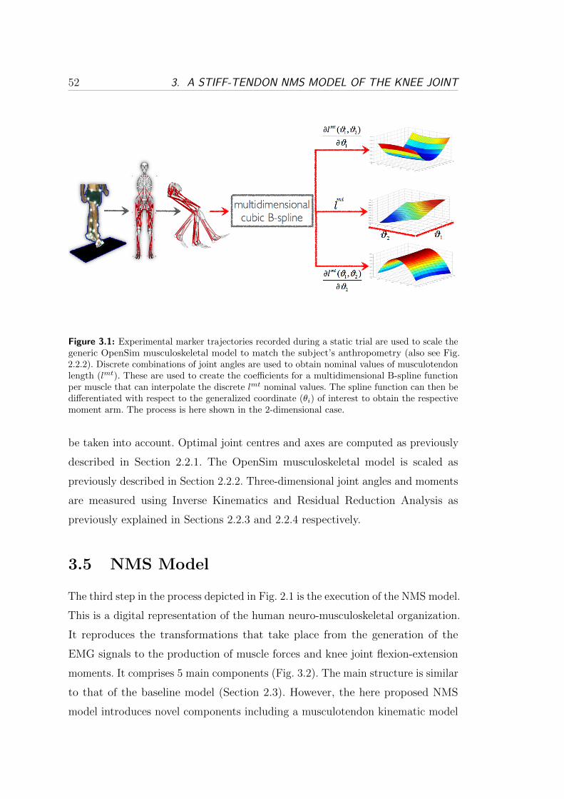
52 3. A STIFF-TENDON NMS MODEL OF THE KNEE JOINT
Figure 3.1: Experimental marker trajectories recorded during a static trial are used to scale thegeneric OpenSim musculoskeletal model to match the subject’s anthropometry (also see Fig.2.2.2). Discrete combinations of joint angles are used to obtain nominal values of musculotendonlength (lmt). These are used to create the coefficients for a multidimensional B-spline functionper muscle that can interpolate the discrete lmt nominal values. The spline function can then bedifferentiated with respect to the generalized coordinate (�i) of interest to obtain the respectivemoment arm. The process is here shown in the 2-dimensional case.
be taken into account. Optimal joint centres and axes are computed as previously
described in Section 2.2.1. The OpenSim musculoskeletal model is scaled as
previously described in Section 2.2.2. Three-dimensional joint angles and moments
are measured using Inverse Kinematics and Residual Reduction Analysis as
previously explained in Sections 2.2.3 and 2.2.4 respectively.
3.5 NMS Model
The third step in the process depicted in Fig. 2.1 is the execution of the NMS model.
This is a digital representation of the human neuro-musculoskeletal organization.
It reproduces the transformations that take place from the generation of the
EMG signals to the production of muscle forces and knee joint flexion-extension
moments. It comprises 5 main components (Fig. 3.2). The main structure is similar
to that of the baseline model (Section 2.3). However, the here proposed NMS
model introduces novel components including a musculotendon kinematic model

3.5. NMS MODEL 53
Figure 3.2: Schematic view of the NMS model structure. Model inputs are highlighted in red.Main outputs are muscle force and estimated joint moment.
(Section 3.5.1) and a stiff-tendon muscle model (Section 3.5.3). The EMG-driven
NMS model presented in this Chapter was entirely implemented in a C++ custom
program and no additional toolboxes were used.
3.5.1 Musculotendon Kinematics
The musculotendon kinematics (MTK) model uses the scaled musculoskeletal
model depicted in Fig. 3.1 to describe the organization of the muscular and
skeletal systems and to define the way muscles and bones interact with each other
towards the generation of joint motions. The MTK model is fed with 3D joint
angles and generates instantaneous estimates of musculotendon lengths lmt, and
moment arms r. It enables the subsequent estimation of musculotendon force Fmt
and joint moments. Models of the musculoskeletal geometry have been used in
the biomechanics community to estimate musculotendon kinematics including
software packages such as SIMM [45], OpenSim [46] and AnyBody [63]. These are
usually driven by graphical user interfaces (GUIs) and are difficult to implement in
custom software and/or micro controllers. To overcome these issues this Chapter
develops an alternative approach that can be easily integrated in custom programs.
54 3. A STIFF-TENDON NMS MODEL OF THE KNEE JOINT
The freely available musculoskeletal software OpenSim is used in this work to
precompute subject-specific values of lmt at discrete joint configurations. That is,
the musculoskeletal model in Fig. 3.1 is set at different discrete joint configurations
and the length of each musculotendon actuator (MTA) is evaluated. A single
multidimensional cubic spline per MTA is then used to interpolate the discrete
values and thus generate lmt estimates at any joint configuration. Estimates of r
are obtained by calculating the partial derivative of the lmt spline with respect to
the DOF of interest (Fig. 3.1). A detailed description of this method is provided
in Chapter 4.
OpenSim Musculoskeletal Model: A freely available musculoskeletal model (Fig.
3.1) is used1 in OpenSim and customized to include only the muscles crossing
the knee joint and to define 6 generalized coordinates (GCs) in the lower limb.
The selected muscles include: semimembranosus (sm), semitendinosus (st), bi-
ceps femoris long head (bflh), biceps femoris short head (bfsh), sartorius (sar),
tensor fascia latae (tfl), gracilis (gra), vastus lateralis (vl), vastus medialis (vm),
vastus intermedius (vi), rectus femoris (rf), medial gastrocnemius (mg), and lat-
eral gastrocnemius (lg). The modelled GCs include: hip flexion-extension (HF),
hip abduction-adduction (HA), hip internal-external rotation (HR), knee flexion-
extension (KF), ankle plantar-dorsi flexion (AF), ankle subtalar angle (SA). By
adding more muscles to the musculoskeletal model it is possible to easily extend
it until the whole-body level.
Multidimensional Cubic Spline: The problem of finding musculotendon length
as a function of d joint angles generalized coordinates (�1, ..., �d) may be formu-
lated as determining the coefficients for the generic d-dimensional spline function
sd,n(�1, ..., �d). The terms x0(�1, ..., �d), ..., xn(�1, ..., �d), with xi, 0 ≤ i ≤ n, corre-
spond to n discrete configurations of the d joint angles (�1, ..., �d). To each joint
angle configuration there is a correspondent value of musculotendon length. These
musculotendon length values are the spline interpolation data and are used to
calculate the spline coefficients. The moment arm spline function can be found by
1Available to download from the musculoskeletal library: http://www.simtk.com
3.5. NMS MODEL 55
differentiating sd,n(�1, ..., �d) with respect to the specific GC of interest.
To achieve better performances in terms of memory storage and computational
time B-Spline basis functions are used [68]. In general, a spline with n+ 1 nodes,
a = x0 < x1 < ... < xn = b ∈ ℝ (3.1)
where
Δn = [a = x0, x1, ..., xn = b]
can be written as a linear combination of n+ 3 cubic polynomials (B-Spline
functions) {u1, u2, ..., un+3} that define a basis. That is, any one-dimensional cubic
spline can be written as a linear combination of basis cubic polynomials ui:
s1,n(x) =m∑i=l
ciui(x) (3.2)
with some coefficients ci, where x ∈ ℝ is the point at which the spline is evaluated.
Furthermore l =⌊x−aℎ
⌋+ 1 and m = min(l + 3, n + 3). The ℎ term is the
fixed-distance between the discrete nodes in (3.1). With this arrangement, to
compute a single spline value, m − l + 1 coefficients ci and basis ui are needed
where m − l + 1 ≤ 3. If the bounded interval Δn and the interpolation data
yi ∈ ℝ, i = 0, ..., n are given, a spline interpolates the data if it satisfies the n+ 1
conditions on the nodes: s1(xi) = yi for i = 0, ..., n. In the general d-dimensional
case a total number of Nc =∏d
i=1(ni + 3) coefficients are needed to construct a
spline on the experimental data whereas the evaluation of a single spline value
requires∏d
i=1(mi − li + 1) ≤ 3d coefficients and bases.
B-Spline functions provide a straightforward way to compute partial derivatives.
The partial derivative of a bivariate cubic spline function takes the form:
∂s2,n(x, z)
∂x=
m1∑i1=l1
m2∑i2=l2
ci1i2ui1(x)vi2(z) (3.3)
where x and z are real-valued variables on the bounded intervals Δn1 = [a1, b1] and
Δn2 = [a2, b2]. The terms ui1(x) and vi2(z) are basis functions for the two variables

56 3. A STIFF-TENDON NMS MODEL OF THE KNEE JOINT
respectively and ui1(x) is the x-basis function first derivative. The (n1 + 3)(n2 + 3)
coefficients ci1i2 for the non-differentiated spline function can therefore be reused
to estimate its derivative.
3.5.2 Muscle Activation
EMG linear envelopes are further processed and converted into muscle activation.
This is a percentage value that expresses how much a specific muscle is activated
toward the generation of force. The transformation from EMG to activation
accounts for the non-linear relationship between EMG and muscle force (Section
2.3.2). Fig. 2.16 shows the transformations involved from the acquisition of the
raw EMG signal to the derivation of muscle activation. The final activation time
series are obtained for 10 of the 13 muscles previously listed in Section 3.5.1
following the procedure described in [3]. Muscle activation from vi is estimated
as an average of the vm and vl activation, whilst st is assumed to have the same
activation as sm and bfsh is assumed to have the same activation as the bflh.
3.5.3 Muscle Dynamics
It calculates the force developed by each musculotendon actuator (MTA) in the
model. Section 2.3.3 described the structure of the elastic-tendon Hill-type muscle
model also depicted in Fig. 2.17. A brief summary will be given here and the
modifications that lead to the infinitely stiff-tendon model will be presented.
Each MTA consists of an active force generating component in series with two
passive elastic ones. These three components can be viewed as non-linear springs
whose force production ability is defined by specific functions (Fig. 2.18a, 2.18b
and 2.18c).
The active force generating component represents the muscle fibers. It is widely
accepted that the muscle fiber force depends on three factors. The first one, fA(lm),
is the non-linear active force-length function that expresses the ability of muscle
fibers to produce force at different lengths. The second factor, fP (lm), is the
non-linear passive force-length function that represents the passive element of the
fibers producing resistive force when stretched and compressed. These first two
3.5. NMS MODEL 57
components relate the instantaneous length of the fibers (lm) to the force produced
in the muscle. The third factor, fV (vm), is the non-linear force-velocity function
that expresses the ability of muscle fibers to produce force as a function of the
fiber contraction velocity. Fiber length (lm) and velocity (vm), in this specific
work, are derived from the musculotendon length (lmt) and velocity (vmt) output
from the MTK model. The remaining two elastic passive components represent
the tendons. These are modeled to act like rubber bands. As the muscle fiber force
grows, the tendon gets stretched. When the tendon resting length is exceeded,
the tendon produces a resistive force that is non-linearly related to the amount
of tendon strain. Muscle fiber force and elastic-tendon force are then combined
together with muscle activation level computed by the Muscle Activation model
to estimate the total force produced by the MTA. To estimate the force produced
by the MTA at each time step, the equilibrium of the three-element system has
to be calculated using an ordinary differential equation (ODE). This involves the
execution of several computation steps including: the estimation of the current
musculotendon velocity, the apportion of it to the the muscle fibers and tendon
(based on their relative stiffness), and the integration of the derived fiber and
tendon contraction velocities. When several samples of lm need to be estimated,
the numerical integration of the ODE considerably increases the computational
time involved (Fig. 2.19).
To reduce the computational time, the elastic tendon was replaced with an
infinitely stiff one. The force produced by the MTA depends now on the action of
the muscle fibers only. This simplification was introduced under the hypothesis it
does not affect the model prediction ability. Indeed, according to [1] the tendon is
rather stiff. The strain, i.e. the percentage of length variation with respect to its
resting length, is only the 3.3% of the tendon length when the muscle generates the
maximum isometric force as shown in Fig. 2.18c. In the following of this Chapter
we will refer to this model to as the Stiff-tendon Hill-type Muscle (SHM) model
and to the previous one to as the Elastic-tendon Hill-type Muscle (EHM) model.
The force produced by the muscle fibers alone, is expressed in the SHM model
58 3. A STIFF-TENDON NMS MODEL OF THE KNEE JOINT
in the same way it is expressed in the EHM. This can be written as follows:
Fm = (fA(lm) ⋅ fV (vm) ⋅ a(u) + fP (lm) + dm ⋅ vm) ⋅ Fm0 ⋅ � (3.4)
where dm represents a passive parallel damping element that was added to the
force-velocity relationship to account for the muscles damping characteristics as
suggested in [36]. The term a(u) is the muscle activation as a function of the
post processed EMG signal u. The term Fm0 expresses the force generated by the
muscle when fibers are at their optimal length, while the term � is the muscle
strength coefficients. The force produced by the musculotendon unit, Fmt can
then be derived by projecting the fiber force Fm onto the tendon line of action as
follows: Fmt = Fm ⋅ cos('), where the term ' is the pennation angle. This is the
angle at which fibers are oriented with respect to the tendon. The computation of
Fm and Fmt can then be done when the instant values of lm and vm are known
at all times.
The SHM model is designed so that the tendon length (lt) is constant regardless
of the force projected onto the tendon and is always equal to the resting tendon
slack length lts, i.e. lt = lts. Because of this, the muscle model has now one non-linear
spring only and the computation of its instantaneous length does not require the
integration of an ODE anymore. In fact lm is calculated as in (3.5):
lm =
√(lm0 ⋅ sin('0))2 + (lmt − lt)2 (3.5)
where '0 is the pennation angle at optimal fiber length. The fiber contraction
velocity vm can then be found by differentiation. As shown in Sec. 3.7, SHM has
better time performances with respect to the EHM, with no loss of accuracy.
3.5.4 Moment Computation
The net knee FE moments, MKFE, are finally computed as the sum of the product
of each MTU force, Fmt, by its FE moment arm (rKFE) as in (3.6):
MKFE =∑i
Fmti ⋅ rKFE,i (3.6)
3.6. VALIDATION PROCEDURE 59
where i is the itℎ muscle in the model.
3.5.5 Validation and Calibration
The NMS model presented in this Chapter is calibrated and validated likewise
the procedure described in Section 2.3.4.
3.6 Validation Procedure
Experiments were performed at the Gait Laboratory of the School of Sport Science
Exercise and Health of the University of Western Australia. Data were collected
from 6 healthy male subjects (mass = 81.73± 16.4Kg, height = 175.75± 6.39cm,
age= 30.67± 7.84years) who gave informed consent. The validation comprised of
three tests.
The first test compared the behavior of the stiff-tendon muscle model (SHM)
to that of the elastic-tendon muscle model (EHM). This was done for the purpose
of validating our hypothesis that the human tendon, in the lower limb muscles, is
rather stiff and its contribution to the production of muscle force and knee FE
moments can be neglected in the experiments conducted in this study. To quantify
how stiff the tendon actually was during the dynamic trials, the tendon strain
(�T ) was calculated using the EHM model, where �T is defined by the following
equation:
�T =lt − ltslts× 100 (3.7)
and where all the terms in (3.7) are defined in Section 3.5. The term �T represents
the percentage of tendon length variation with respect to its resting length. The
instantaneous tendon strain associated to each muscle was computed at each
instant of time for all dynamic trials of all subjects. For each muscle, the average
tendon strain was then calculated. To quantify the impact of assuming the tendon
infinitely stiff (i.e. its length always equals the resting length), the percentage
of the variation of the muscle fibre length calculated using SHM with respect to

60 3. A STIFF-TENDON NMS MODEL OF THE KNEE JOINT
EHM was computed using the following equation:
ΔF =lms − lmelme
× 100 (3.8)
where lms is the fibre length calculated using SHM, i.e. assuming the tendon
infinitely stiff, and lme is the fibre length calculated using EHM, i.e. assuming the
tendon is elastic. This is an important quantity because the force produced in
the musculotendon unit directly depends on the force produced by the muscle
fibers. Therefore, assessing how the fibre length varies when assuming the tendon
infinitely stiff or elastic, helps quantifying how important the role of the tendon is
in the NMS model design. The fibre length variation associated to each muscle
was computed for all trials of all subjects at each instant of time. For each muscle,
the average length variation was then calculated. Finally, the impact of assuming
the tendon infinitely stiff on the model ability of predicting knee FE moments
was quantified. Knee FE moments were estimated during the stance phase. This
is defined as the period of time between the heel-strike and toe-off events and it
represents the interval during which the foot is in contact with the ground floor
and the lower limb is supporting the entire body. The stance phase represents
about 60% of the gait cycle. The remaining 40% is associated to the swing of the
leg, that is the swing phase. Moments estimated by the SHM and EHM models
and those obtained experimentally were time normalized using a cubic spline. This
allowed comparing results associated to different trials and subjects. The time
normalized moments estimated by SHM, EHM, and those experimentally recorded
were respectively averaged across all trials from all subjects. This produced three
ensemble average curves of the knee FE moments. The SHM ensemble average
curve was then compared to that associated to EHM and to that associated to the
experimental moments. This allowed assessing how the predicted knee FE moments
changed with an infinitely stiff tendon and with an elastic one. Furthermore, it
allowed quantifying whether or not the assumption of an infinitely stiff tendon
produced a loss of accuracy in the prediction of the joint moments. Statistical
coefficients including Pearson Correlation and Root Mean Squared Error were
also used to better assess the prediction accuracy.

3.6. VALIDATION PROCEDURE 61
The second test assessed the accuracy of the Musculotendon Kinematics
(MTK) Model. The model uses multidimensional cubic splines that are created
from nominal values of musculotendon length lmt obtained from OpenSim (Section
3.5.1). Therefore, the accuracy of the model is defined based on the capability of
reproducing the original OpenSim values of both lmt and r. The range of motion of
the lower limb joints about all associated GCs were sampled into equidistant nodes
that were input, together with the selected musculoskeletal model, into OpenSim
to compute the experimental lmt and r. Nominal values of lmt only, were used
to calculate the coefficients for both the lmt and the r spline functions (Section
3.5.1). The fitting accuracy was assessed both on the nodes used for coefficients
calculation as well as on a novel set of evaluation points located midway between
each pair of consecutive nodes. As a measure of error in estimated values we used
the Mean Fitting Error (MFE) and its standard deviation (�):
MFE =1
N
N∑i=1
∣∣∣Xi −Xi
∣∣∣ , (3.9)
where X is the OpenSim-generated value of lmt or r. The term X is the corre-
sponding estimated value from the MTK model. N is the number of points at
which the fitting function was evaluated. The created splines can now be used to
predict the musculotendon kinematics for any possible combination of 3D joint
angles (Fig. 3.1). A more detailed description of this process is provided in Chapter
4. The impact of the fitting error on the knee FE moment prediction was also
investigated. Moments calculated using OpenSim-generated values of lmt and r
were compared to the moments obtained using estimates of lmt and r from the
MTK model. Moments were time normalized and two ensemble average curves
were produced: one for the joint moments obtained from OpenSim estimates of
lmt and r (MOSIM ), and one obtained from estimates of the MTK model (MMTK).
The ensemble average curves were obtained from all dynamic trials of all subjects
during the stance phase. The percentage of the variation of MMTK with respect
to MOSIM was then computed:
ΔM =MMTK −MOSIM
MOSIM
× 100 (3.10)

62 3. A STIFF-TENDON NMS MODEL OF THE KNEE JOINT
Figure 3.3: The EMG-driven NMS model can be integrated in the control loop for the actuationof a lower limb powered orthosis as previously presented in [9]. The powered orthosis itself isvisible aside along with a schematic view of its mechanical structure.
The third test investigated whether the stiff-tendon muscle (SHM) model
executed faster than the elastic-tendon muscle (EHM) model. Finally, the time
performances of the entire NMS model were investigated for the purpose of
assessing whether the proposed SHM model can be used in robotics applications
with real-time constraints. In this work we assume the specific application is the
control of a powered orthosis for the lower limb, using EMG signals to establish an
interface between the human and the machine as in [9]. Fig. 3.3 gives a schematic
view of the control scheme. The powered orthosis control system can use the
EMG-driven NMS model to estimate the force the user’s muscles can produce and
the resulting user’s moments produced at the knee joint. When muscle forces are
not strong enough to allow for a proper joint movement, they can be amplified
to produce the target FE moment at the knee. This is the moment the subject
should produce to properly carry out the desired movement. The powered orthosis
controller can then be fed with the difference between the target moment and
the current moment produced by the user wearing the powered orthosis. This
difference defines the amount of extra moment the orthosis actuation system
should add to obtain the target motion. The muscle amplification factor that

3.7. RESULTS 63
leads to the target moment can be initially defined by a medical doctor who
had previously analyzed the patient. However, automated procedures for the
calibration of this parameter can be implemented. Alternatively, if the subject
is healthy, the amplification factor can be used to further facilitate the user’s
movement and to augment their motor ability. For this to work, by the time
the human muscles contract, the NMS model has to provide a prediction on the
amount of force produced by each muscle and the FE moments produced at the
knee joint to be supported. This will allow actuating the orthosis as soon as the
human muscles activate. Recent studies have established that there is a delay
between the time instant the neural system generates EMG signals in the muscles
and the time instant when muscles contract mechanically and generate moments
around the joints. This is called the electromechanical delay (EMD). In the lower
limb muscles, the EMD is in the order of 10ms [27]. If the EMD is exploited
in the control algorithm of the powered orthosis, a non invasive and seamless
integration between the human operator and the assistive device is achievable and
the device can become a natural extension of the operator’s body. The real-time
constraint for the proposed NMS model is therefore the EMD. That is, the NMS
model has to be able to produce estimates of muscle forces and joint moments
in less than 10ms. Tests were performed on an embedded system (Digital Logic,
Switzerland) equipped with a 1.6Gℎz Atom CPU with 512MB RAM. This choice
was motivated by the fact of verifying whether the proposed NMS model would
run on a hardware architecture with low computation resources that could be
actually used for the control of a powered orthosis. The computational time of
the NMS model needed to produce one estimate of muscle force and one estimate
of knee FE moment, was calculated as the average time needed for computing
one thousand estimates.
3.7 Results
Results from the first tests are shown in Fig. 3.4. Fig. 3.4a shows that the tendon
strain associated to all muscles in the model was always less than 2% during all the
dynamic trials. This validated our hypothesis and suggested the contribution of the

64 3. A STIFF-TENDON NMS MODEL OF THE KNEE JOINT
Table 3.1: Comparison of computational time performances (mean ± sdev) in ms
SHM EHM MTK NMS(SHM, MTK) NMS(EHM, MTK)
0.07± 0.00068 17.5± 0.072 1.1± 0.043 3.6± 0.064 21.1± 0.11
tendon to the production of muscle force and joint moment could be potentially
neglected in our experiments.
Fig. 3.4b shows that the fibre length variation associated to all muscles in the
model was always less than 9% during all dynamic trials. This suggested that the
impact of assuming the tendon infinitely stiff might not lead to drastic changes in
the predicion of muscle force with respect to the model with elastic tendons.
Fig. 3.4c shows that the SHM model predicted FE knee moments that were very
closely related to the reference knee FE moments. Both predicted and reference
moment curves had peaks that occurred at the same time instants. A small
discrepancy was noticeable at the edges of the graph and it was mostly due to
filtering issues. For each time step, filter algorithms needed to process data over a
predefined time window. At the edges of the data time series the window is not
full and therefore approximation errors were introduced. The Pearson correlation
coefficient R was 0.932. This means that the SHM model generated estimates that
were highly correlated to reference values over all subjects’ trials. The root mean
squared error RMSE was 7.898Nm. This means the SHM model introduced an
error that, on average, was less than the 10% of the range of variation observed
in the reference values (i.e. 86.673Nm). The maximum absolute error (emax) was
equal to 21.494Nm. It occurred at 73% of the stand phase and was located at the
edge region where the observed data was less significant due to the filtering issues.
The minimum absolute error (emin) was equal to 0.114Nm and occurred at 47%
that was the peak region. This proved that the model was capable of providing
high performances within the most significant part of the observed data.
Fig. 3.4c also shows the predictive ability of the EHM model. Surprisingly,
this was found to be slightly lower, on average, than that provided by the SHM.
Statistical coefficients assumed poorer values with respect to the SHM ones:
R = 0.893, RMSE = 9.714Nm. However, minimum and maximum absolute
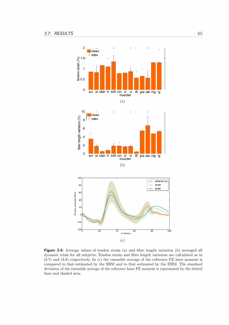
3.7. RESULTS 65
(a)
(b)
(c)
Figure 3.4: Average values of tendon strain (a) and fibre length variation (b) averaged alldynamic trials for all subjects. Tendon strain and fibre length variation are calculated as in(3.7) and (3.8) respectively. In (c) the ensemble average of the reference FE knee moment iscompared to that estimated by the SHM and to that estimated by the EHM. The standarddeviation of the ensemble average of the reference knee FE moment is represented by the dottedlines and shaded area.

66 3. A STIFF-TENDON NMS MODEL OF THE KNEE JOINT
errors provided better results: emax = 19.031Nm and emin = 0.012Nm. The
proposed results showed that by assuming the tendon infinitely stiff, the model
prediction accuracy did not decrease in our experiments but slightly increased
with respect to the case in which the tendon was modeled as an elastic body.
Results from the second tests are shown in Fig. 3.5. Fig. 3.5a and 3.5b show
that the MTK model was able to produce estimates of lmt and r with negligible
fitting errors which always were less then 0.004mm and 0.25mm respectively.
Fig. 3.5c shows that the lmt and r fitting errors introduced by the MTK model
produced a percent variation in the predicted knee FE moments that was always
less than the 2.5% of the moments obtained using OpenSim-generated estimates
of lmt and r.
The proposed results showed that the MTK model produces accurate estimates
of lmt and r and can be reliably used instead of GUI-driven third-party software
such as OpenSim to allow for an on-line execution of the entire NMS model.
Results from the third test are shown in Table 3.1. The SHM model executed
in 0.07ms, that is 250 times faster than the EHM model execution time, i.e.
17.5ms. This proved that modeling the tendon as an infinitely stiff body leads to
a substantial improvement in the computational time performances.
Table 3.1 also reports the time needed by the MTK model to execute. Because
the spline coefficients for each muscle are pre-calculated off-line, the total time
needed for the MTK model to execute is associated to the evaluation of both lmt and
r multidimensional spline functions for all muscles in the model. Spline functions
can be uni-dimensional in the case of uniarticular muscles crossing the knee joint
only, three-dimensional, in the case of biarticular muscles crossing the ankle and
knee joints and four-dimensional in the case of biarticular muscles crossing the hip
and knee joints. Spline function evaluation is done using generalizations to higher
dimensions of (3.2) and (3.3). The multidimensional spline evaluation time grows
as a function of the number of dimensions. In our tests, it ranged from 0.001ms
(uni-dimensional spline) to 0.08ms (four-dimensional spline).
Finally, Table 3.1 reports the time needed by the entire NMS model to execute.
Execution time significantly differed when using the NMS model with SHM
and MTK (NMS(SHM,MTK)) with respect to using the NMS model with
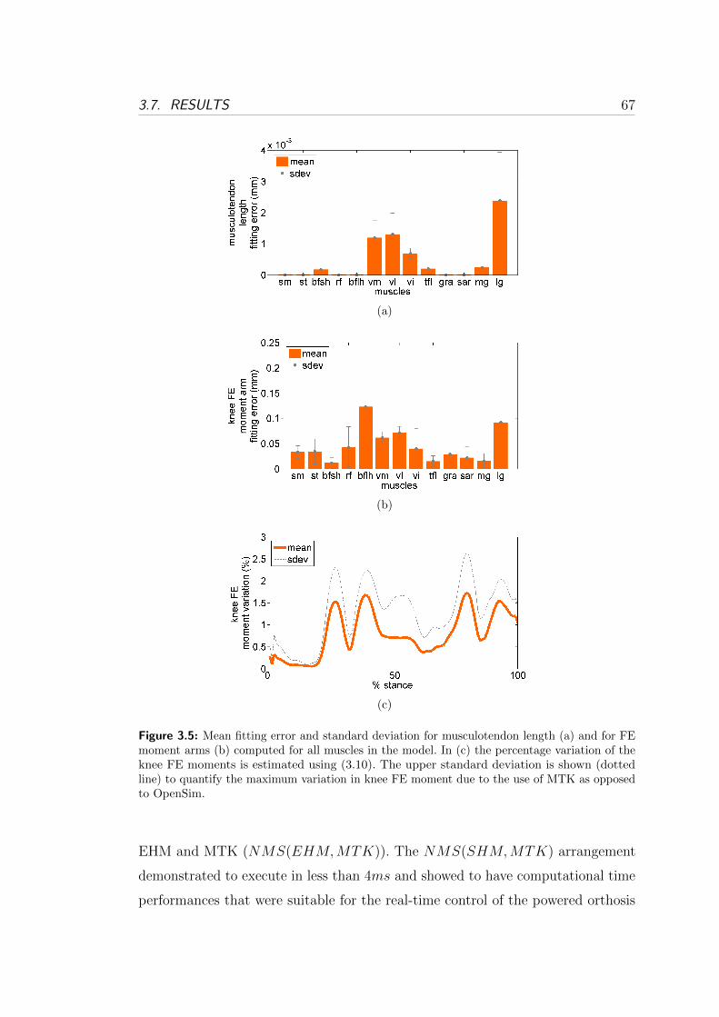
3.7. RESULTS 67
(a)
(b)
(c)
Figure 3.5: Mean fitting error and standard deviation for musculotendon length (a) and for FEmoment arms (b) computed for all muscles in the model. In (c) the percentage variation of theknee FE moments is estimated using (3.10). The upper standard deviation is shown (dottedline) to quantify the maximum variation in knee FE moment due to the use of MTK as opposedto OpenSim.
EHM and MTK (NMS(EHM,MTK)). The NMS(SHM,MTK) arrangement
demonstrated to execute in less than 4ms and showed to have computational time
performances that were suitable for the real-time control of the powered orthosis

68 3. A STIFF-TENDON NMS MODEL OF THE KNEE JOINT
where the real-time deadline was set to be 10ms (Section 3.6). On the contrary,
the NMS(EHM,MTK) arrangement needed more than 20ms to execute and
was therefore regarded as unsuitable for the real-time control of the orthosis.
Finally we assessed the time needed to calibrate the NMS(SHM,MTK)
model (Sec. 2.3.4) on each subject separately and we compared it to that needed
by the NMS(EHM,MTK). For each subject the NMS models were calibrated on
4 trials (Section 3.3). While NMS(SHM,MTK) was calibrated in just 6 minutes
and 37 seconds it took 15 hours and 48 minutes for the NMS(EHM,MTK).
3.8 Musculoskeletal Humanoids Actuation
In the previous sections we illustrated how the proposed NMS model can be used
for the real-time control of a powered orthosis. However, the NMS model can
also provide effective solutions for the actuation of humanoid robots that have a
musculoskeletal architecture and artificial muscles.
The proposed NMS model allows taking inspiration from the way humans
move and addressing the challenge of autonomous locomotion in musculoskeletal
humanoids. A direct biological observation of how humans activate their muscles
and actuate their joints can therefore be done using the proposed NMS model.
The model can be used to experimentally estimate the muscle forces generated
by the human subject during dynamic motor tasks. The estimated muscle force
patterns during a specific movement can then be mapped and used to actuate the
humanoids artificial muscles and produce the observed movement in the robot.
The human-humanoid mapping has to take into account the different number
of muscles in the humanoid robot, the different mass properties and size of the
humanoid limbs and the different number of DOF in the humanoid joints.
A similar approach can be based on the recent studies suggesting that muscle
activation patterns are generated by a functional module located in the spinal
cord primarily based on global kinematics parameters that define the orientation
of the human limbs [24]. The proposed NMS model can be used to establish a
function that relates joint angle and moments to the corresponding force produced
by the muscles crossing that joint. This can be done by observing a broad range of

3.9. CONCLUSIONS AND FUTURE WORK 69
dynamic motor tasks from a great number of human subjects. It is then possible
to derive average muscle force patterns of the whole subject population using
the proposed EMG-driven NMS model. Finally it is possible to create a function
that maps a specific combination of joint angle and moment to the corresponding
muscle force level. This can be done for each muscle spanning the specific joint. It
is then possible to prescribe a specific force to each artificial actuator depending
on the angle and moment that has to be produced by the humanoid joint.
Finally the proposed NMS model can play a very important role in determining
joint stiffness in humanoid robots. This is a very important parameter that has
been intensively used for the design of compliant humanoids and artificial limbs.
Indeed, joint stiffness can be easily expressed as a function of the activation of
the antagonistic muscles crossing a specific joint.
3.9 Conclusions and Future Work
This Chapter presented a novel neuromusculoskeletal model of the knee joint that
was used to estimate somatosensory information during the human movement.
The presented model proved to be as accurate as the detailed ones developed in the
biomechanics community but with superior computational time performances. Our
proposed NMS model was directly compared to the well known model developed by
Lloyd et al. [2, 3, 35, 37, 47]. A robust validation methodology was also provided
in which data obtained from 6 male subjects who performed a total of 78 motor
tasks were used to assess the time performances and prediction accuracy of the
NMS model. This work demonstrated the proposed NMS model has computational
time performances that make it suitable for the control of powered orthosis. That
is, the NMS model computation loop executes in less than 10ms which is the
electromechanical delay (EMD) in the lower limb muscles. The EMD was identified
as the real-time deadline that is necessary to achieve intuitive real-time orthosis
control. Computational time tests were performed on an embedded system that
can be used as the orthosis control unit. The Chapter then illustrated a control
strategy in which the model can be effectively used as an intuitive EMG-driven
human-machine interface following research previously done in [9]. The NMS

70 3. A STIFF-TENDON NMS MODEL OF THE KNEE JOINT
model can be easily extended to whole-body level and this can play a crucial role
for the the actuation of humanoid robots with artificial muscles.
Results demonstrated the NMS model can achieve faster execution and cali-
bration time by integrating the proposed stiff-tendon muscle model (SHM) and
musculotendon kinematics model (MTK) within a common framework. The lower
prediction performances of the elastic-tendon model (EHM) are related to the fact
that the model does not always correctly estimate the amount of stiffness in the
musculotendon actuator. This can be related to calibration issues or to limitations
in the elastic-tendon model design. On the contrary, the SHM does not rely on
tendon stiffness to compute the muscle force and joint moments. Results suggested
that assuming the tendon length always constant might better represents the real
tendon dynamics that actually occurred in the experiments and might be a better
approximation than that provided by the elastic-tendon model. Further studies
have to be carried out to assess whether this assumption is valid for a wider range
of movements including: squat, jump, fast running, side stepping and cross-over
cutting manoeuvres.
Fast operation in calibration can be further exploited in future research to
develop more advanced algorithms for the continuous calibration of the model
biomechanical parameters. As the NMS model executes, the continuous calibration
algorithm will keep refining those parameters that vary with muscle fatigue such
as: optimal fibre length, maximum isometric force, maximum EMG. This will
allow designing more advanced powered orthosis control systems that will be able
to adapt to the user’s conditions on the fly.
The time complexity of the NMS model is bound to increase as a function of
the number of muscles. The superior computational time performances provided
by the SHM model with respect to the EHM not only allow executing within the
real-time deadline but also will allow including a greater number of muscles in
the model. This in turn will allow estimating the moments generated at multiple
joints including: hip, knee and ankle and controlling powered orthosis for the
simultaneous support of those joints (Chapter 6).
Furthermore, integration of pattern recognition technology in the NMS model
will be used to extrapolate more information out of the EMG signals (Chapter 8).

3.9. CONCLUSIONS AND FUTURE WORK 71
This research development aims to integrate musculoskeletal dynamics into
robotics systems to achieve more advanced bio-inspired control strategies.

Chapter 4
Estimation of Musculotendon
Kinematics
This Chapter presents a robust and computationally inexpensive method to
estimate lengths and three-dimensional moment arms for a large number of
musculotendon actuators of the human lower limb using a single multidimensional
B-spline function per muscle. This is the method that is used in the Musculotendon
Kinematics (MTK) Model briefly illustrated in Section 3.5.1. Also see Fig. 3.1
and 3.2.
This Chapter presents a more detailed explanation of this methodology and
compares it to the approach currently used in the literature which is based on
polynomial regression. Compared to the polynomial regression method, the multi-
dimensional spline method produced lower errors for estimating musculotendon
lengths and moment arms at the generalized coordinate boundaries. The fitting
accuracy was also less affected by the dependant number of degrees of freedom
and by the amount of experimental data available. Furthermore, a single spline
function can be used to estimate both musculotendon length and moment arms
as opposed to polynomial regression where different equations had to be chosen
depending on the shape of the surface to be fitted. Finally, the spline method was
further tested in conjunction with an EMG-driven musculoskeletal model for the
estimation of muscle force under different contractile conditions. This confirms the
spline methodology is actually suitable for the integration in predictive models.
73

74 4. ESTIMATION OF MUSCULOTENDON KINEMATICS
4.1 Introduction
The development of mathematical models of human physiology and biology is
enabling a better understanding of whole body function from the genome to the
tissue and organ levels [5]. Musculoskeletal-level models and simulation tools are
providing effective ways to study muscle contribution to human movement and
this is offering possibilities to investigate how in vivo tissue loading is implicated
in the mechanisms of musculoskeletal injury and disease [4, 11]. The availability of
comprehensive and fast musculoskeletal models may also play an important role
in establishing intuitive Human-Machine Interfaces (HMIs) at the neuromuscular
level and providing new solution to implement effective control systems for assistive
devices [8]. Therefore it is crucial to develop models that reflect the action of
muscles while minimizing processing time in musculoskeletal modeling research.
Musculoskeletal models usually require computation of musculotendon kinematics
including musculotendon length (lmt) and three-dimensional muscle moment arms
(r) that enable the estimation of musculotendon forces (Fmt) and joint moments
(Section 3.5). The estimation of these musculotendon kinematics is critical because
small variations in their values can result in large variations in musculotendon force
[35]. It is therefore important to develop methods that are capable of producing
estimates that accurately reflect results obtained from experimental techniques
such as MRI or ultrasound. This introduces reliability and consistency in the
modeling process and assures results are directly related to the experimental
data set that was used. Models of the musculoskeletal geometry can be used to
estimate musculotendon kinematics including software packages such as SIMM
[44, 45], OpenSim [11, 46] and AnyBody [63]. These are usually driven by graphical
user interfaces and are difficult to implement in custom software and/or micro
controllers. To overcome these issues, an alternative approach has been proposed
in the literature to fit the musculotendon kinematics using polynomial regression
on both lmt and r [69]. That is, different polynomial regression equations (P eq)
were individually fitted to experimental values of both lmt and r thus requiring
the gathering of both sets of experimental data. In this Chapter we develop
a novel inexpensive model that can produce accurate estimates of lmt and r
4.2. METHODS 75
and that can be integrated into large scale musculoskeletal models and custom
programs. The aim was to determine if a single piecewise multidimensional cubic
spline could be used to generate estimates for both lmt and r from nominal
values of musculotendon length only, corresponding to discrete combinations of
generalized coordinates (GC) that specify joint kinematics. Nominal values for lmt
can be obtained from experimental data using MRI or ultra-sound technologies.
Alternatively, nominal values can be derived from models of the musculoskeletal
geometry [3, 4, 11, 44]. An additional aim of the paper was that of comparing our
methodology to polynomial regression equations and assessing whether spline can
provide more robust solutions. The EMG-driven NMS model previously presented
in Chapter 3 was used to quantify to which extent lmt misfits compromised the
capability of the EMG-driven model to predict Fmt [3].
4.2 Methods
This section presents the two musculoskeletal biomechanical models of the human
lower-limb that were used (Table 4.1) and the theory of the proposed spline-based
approach. This was entirely implemented by the author of this Thesis in a custom
program and no additional toolboxes where used1. More details about spline
interpolation and the generalization to the multidimensional case can be found in
[68]. Please refer to Menegaldo et al. [69] for details about polynomial regression.
4.2.1 Musculoskeletal Models
The first model (LowerLimb4307 ) had 43 musculotendon actuators (MTAs) and 7
generalized coordinates (GCs), i.e. 7 joint angles [44]. The lengths and moment
arms for each MTA depended on all GCs associated to the corresponding joints. The
LowerLimb4307 model had a maximum number of 4 GCs per MTA corresponding
to the biarticular muscles crossing hip and knee. This model was used by Menegaldo
et al. [69] to study fitting accuracy of polynomial regression equations and was
also used in this study as the comparison to our method. The second model
1The software C++ implementation, MATLAB interface, User’s Manual and all originaldata will be made freely available to download at http://www.massimosartori.net/
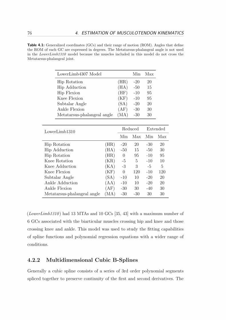
76 4. ESTIMATION OF MUSCULOTENDON KINEMATICS
Table 4.1: Generalized coordinates (GCs) and their range of motion (ROM). Angles that definethe ROM of each GC are expressed in degrees. The Metatarsus-phalangeal angle is not usedin the LowerLimb1310 model because the muscles included in this model do not cross theMetatarsus-phalangeal joint.
LowerLimb4307 Model Min Max
Hip Rotation (HR) -20 20Hip Adduction (HA) -50 15Hip Flexion (HF) -10 95Knee Flexion (KF) -10 95Subtalar Angle (SA) -20 20Ankle Flexion (AF) -30 30Metatarsus-phalangeal angle (MA) -30 30
LowerLimb1310Reduced Extended
Min Max Min Max
Hip Rotation (HR) -20 20 -30 20Hip Adduction (HA) -50 15 -50 30Hip Rotation (HR) 0 95 -10 95Knee Rotation (KR) -5 5 -10 10Knee Adduction (KA) -3 3 -5 5Knee Flexion (KF) 0 120 -10 120Subtalar Angle (SA) -10 10 -20 20Ankle Adduction (AA) -10 10 -20 20Ankle Flexion (AF) -30 30 -40 30Metatarsus-phalangeal angle (MA) -30 -30 30 30
(LowerLimb1310 ) had 13 MTAs and 10 GCs [35, 43] with a maximum number of
6 GCs associated with the biarticular muscles crossing hip and knee and those
crossing knee and ankle. This model was used to study the fitting capabilities
of spline functions and polynomial regression equations with a wider range of
conditions.
4.2.2 Multidimensional Cubic B-Splines
Generally a cubic spline consists of a series of 3rd order polynomial segments
spliced together to preserve continuity of the first and second derivatives. The
4.2. METHODS 77
points at which polynomials are spliced together,
a = x0 < x1 < ... < xn = b ∈ ℝ (4.1)
are called nodes, where
Δn = [a = x0, x1, ..., xn = b]. (4.2)
If Δn and the interpolation data yi ∈ ℝ, i = 0, ..., n are given, a spline interpolates
the data if it satisfies the n+ 1 conditions on the nodes: s1(xi) = yi for i = 0, ..., n,
where s1 represents a 3rd order one-dimensional spline function on the bounded
interval Δn. To achieve better performances in terms of memory storage and
computation time B-Spline basis functions were used. In general, a spline with
n+ 1 nodes can be written as a linear combination of n+ 3 cubic polynomials (B-
Spline functions) u1, u2, ..., un+3 that define a basis. That is, any one-dimensional
cubic spline can be written as:
s1(x) =m∑i=l
ciui(x) (4.3)
with some coefficients ci, where l =⌊x−aℎ
⌋+ 1 and m = min(l + 3, n+ 3). With
this arrangement, to compute a single spline value, only m− l + 1 coefficients ci
and basis functions ui are needed out of the n+ 3 ones, where m− l + 1 ≤ 3. In
the general d-dimensional case a total number of Nc =∏d
i=1(ni + 3) coefficients
are needed to construct a spline on the experimental data whereas the evaluation
of a single spline value requires∏d
i=1(mi − li + 1) ≤ 3d coefficients and basis
functions. B-Spline basis functions provide a straightforward way to compute
partial derivatives. The partial derivative of a bivariate cubic spline function takes
the form:∂s2(x, z)
∂x=
m1∑i1=l1
m2∑i2=l2
ci1i2ui1(x)vi2(z) (4.4)
where x and z are real-valued variables on the bounded intervals Δn1 = [a1, b1]
and Δn2 = [a2, b2]. The terms ui1(x) and vi2(z) represent basis functions for the
two variables respectively and ui1(x) is the x-basis function first derivative. The

78 4. ESTIMATION OF MUSCULOTENDON KINEMATICS
(n1 + 3) ⋅ (n2 + 3) coefficients ci1i2 for the non-differentiated spline function can
therefore be used to estimate its derivative.
The estimation of musculotendon lengths and moment arms can be done using
the B-spline function previously defined. The problem of finding musculotendon
length as a function of d joint GC-angles, (q1, ..., qd) may be formulated as deter-
mining the (n1 + 3) ⋅ ... ⋅ (nd + 3) coefficients ci1i2...id for the generic d-dimensional
spline function sd(q1, ..., qd) where the yi1,...id interpolation data are given by lmt.
The moment arm spline function can then be found by differentiating sd(q1, ..., qd)
with respect to the specific GC of interest.
4.2.3 Validation Procedure
The validation is comprised of three tests. In the first one, the same input data,
biomechanical model and procedure as published by Menegaldo et al. [69] were
used for a direct comparison to our methodology. The second test was performed
to study spline and polynomial regression equations under a wider range of
experimental conditions. In the third test the impact of lmt misfit on muscle force
estimation was assessed.
In all tests, the range of motion (ROM) of each GC was sampled into equidistant
nodes that were input, together with the selected biomechanical model, into
OpenSim to compute the experimental lmt and r. Coefficients were then computed
for the polynomial regression equations, P eq using nominal values of both lmt
and r. Data for lmt only were used to compute the coefficients for the spline
function. The fitting accuracy was assessed both on the nodes used for coefficients
calculation as well as on a novel set of evaluation points located midway between
each pair of consecutive nodes. In this work, the accuracy of a model is defined
based on the capability of reproducing the original values of lmt and r that were
generated using OpenSim. This is because the coefficients of both spline functions
and polynomial regression equations were obtained using nominal values produced
by OpenSim. Therefore, the accuracy of a spline function as well as that of a
polynomial regression equation depends on how well they are able to replicate
the same dataset that was used to calculate their coefficients. The third test also
involved the collection of experimental data from gait analysis trials, reported
4.2. METHODS 79
previously by Winby and collegaues [35, 43].
The evaluation of the LowerLimb4307 model was performed using the ROM
of each GC sampled at 20 points (Table 4.1). However, when four GCs were used,
only 15 nodes per GC were used for coefficients computation.
The evaluation using the LowerLimb1310 model concentrated on the biarticular
muscles and tested three different sets of GC across the lower limb joints. Tests
on 4 GCs included: hip internal-external rotation (HR), hip adduction-abduction
(HA), hip flexion-extension (HF) and knee flexion-extenion (KF) for the thigh
muscles and KF, ankle adduction-abduction (AA), subtalar flexion-extension
angle (SA), ankle dorsi-plantar flexion (AF) for the shank muscles. With 5 GCs,
internal-external rotation (KR) was added and the 6 GC tests also included knee
adduction-abduction (KA). In this model no muscles crossing the metatarso-
phalangeal joint were included therefore the metatarso-phangeal angle (MA) was
not used. All tests were executed with the two different ROM arrangements as
defined in Table 4.1, i.e. reduced and extended. The ROM of each GC was sampled
at 10 nodes both with the reduced and extended arrangements. As a result, the
distance from one node to another was greater in the extended ROM. These
tests assessed how the fitting accuracy was affected by a number of experimental
conditions including: the distance between interpolation nodes, the number of
dimensions (GCs) to interpolate and distance of the evaluation points from the
interpolation nodes.
The impact of using the spline model on muscle force estimations was eval-
uated using the LowerLimb1310 model in conjunction with the EMG-driven
NMS model presented in Chapter 3.5. In the current study, two different tests
were performed where muscle forces were computed using musculotendon length
estimates generated using OpenSim, polynomial regression and the spline-based
approach respectively. Muscle force derived using OpenSim estimates of lmt were
assumed to be the gold standard and were compared to the muscle force derived
by estimates produced by spline and P eq.
In the first muscle force test no EMG signals and kinematic data on real subjects
were recorded. The musculotendon lengths and KF moment arms as a function
of 4 GCs were estimated as described previously. The estimated musculotendon

80 4. ESTIMATION OF MUSCULOTENDON KINEMATICS
lengths were then used in the EMG-driven model to calculate the isometric muscle
force produced at each data point. Since this test assumed isometric conditions,
no velocity effects were modeled therefore Fmt was only a function of muscle fiber
length and muscle activation. Each muscle was assumed to be maximally activated
at each GC configuration. This represented the worst-case scenario because when
the muscle is maximally activated, the effects of the musculotendon length fitting
errors on muscle force are amplified.
The second test studied the impact of lmt fitting error in dynamic conditions.
Data were collected from one male subject who gave informed consent and who
performed 15 gait and 5 jogging trials. Kinematic and ground reaction force
data were input into a RRA model to calculate knee flexion-extension moments
(Section 3.4). The EMG-driven model was then scaled and calibrated to the subject
(Sections 3.4 and 3.5). OpenSim was used to generate values of lmt for each sampled
time instant. The same was done using spline functions and polynomial regression.
EMG signals were used to determine the activation in the muscles and the Hill-
type model was used to estimate Fmt. A measure of force prediction error due
to musculotendon misfit was calculated. This test also assessed whether during
jogging trials, the effect of lmt fitting error on muscle force prediction was magnified
by the increased muscle activation as opposed to walking.
As a measure of the differences in estimated values from the different methods
the Mean Fitting Error (MFE) and its standard deviation (�) were used:
MFE =1
N
N∑i=1
∣∣∣Xi −Xi
∣∣∣ , (4.5)
where, X is the OpenSim-generated value of lmt or r. The term X can also refer
to Fmt calculated using OpenSim-generated lmt. The term X is the corresponding
estimated value from the P eq or spline methods. N is the number of points at
which the fitting function has been evaluated. Additionally, the percentage of the
MFE relative to the OpenSim-generated value averaged on all angle configurations
(E[X]) was computed:
%� =MFE
E[X]× 100 (4.6)

4.3. RESULTS 81
Confidence Interval (CI) at at 90% and 95% of the MFE was estimated using
Chebyshev’s Theorem, which can be conservatively applied to any probability
distribution with known mean and standard deviation:
MEE = MFE + 3.16�, (90%) (4.7)
MEE = MFE + 4.47�, (95%) (4.8)
The number of errors that has fallen inside the previously defined CIs was counted
for all muscles and proposed in a histogram form.
As discussed, computation time is important for neuromuscular skeletal model-
ing so it can be potentially used in real-time applications. Therefore, computation
time was evaluated on repeated tests where the number of GC was increased from
1 to 6. In each test, the reported time needed to compute a single estimate of lmt
or r was the average time computed from the evaluation of 10000 estimates. A
desktop computer with a 2.26GHz Intel Xeon CPU and 3GB RAM memory was
used. Both spline and polynomial regression equations evaluation routines were
implemented in C++ to better compare their relative speeds.
4.3 Results
The tibialis anterior muscle was chosen to demonstrate the performance of the
spline method. In the LowerLimb4307 model the tibialis anterior kinematics
depended on two GCs (AF and SA) and the variation of lmt and r errors are easy
to visualize in 3D. Fig. 4.1a shows the space distribution of the spline fitting error
associated to the prediction of lmt is uniform throughout the workspace and is
substantially smaller than that associated to P eq which reaches larger values at
the boundaries2. In Fig. 4.1c the P eq fitting error associated to the prediction of
rAF is clearly visible and it gets larger at the boundaries reaching a maximum of
0.15cm. Fig. 4.1e shows a very good agreement between the OpenSim-generated
surface associated to rSA and that generated by the spline function. The error
2The polynomial regression equations that were chosen to generate the results presented inthis work are the ones that produced the smallest fitting error.
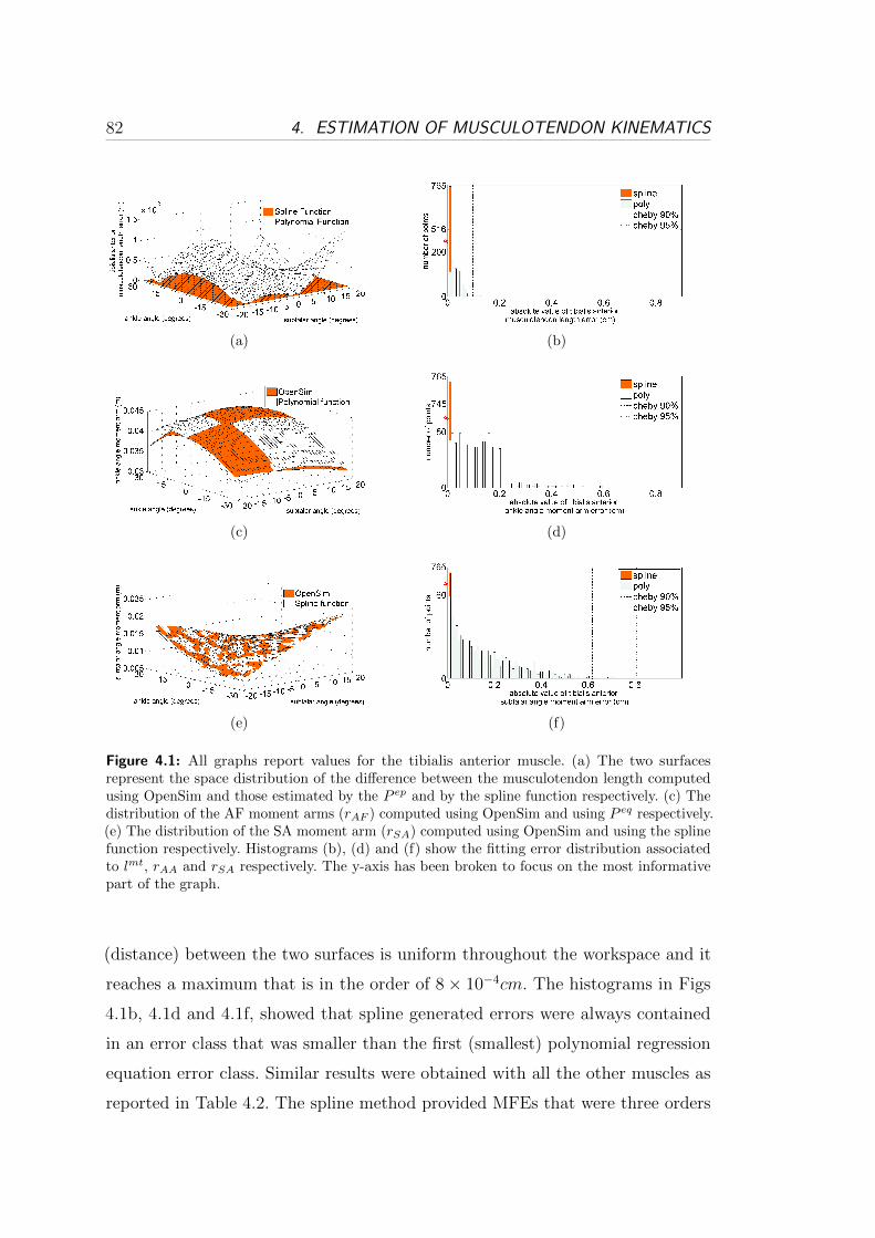
82 4. ESTIMATION OF MUSCULOTENDON KINEMATICS
(a) (b)
(c) (d)
(e) (f)
Figure 4.1: All graphs report values for the tibialis anterior muscle. (a) The two surfacesrepresent the space distribution of the difference between the musculotendon length computedusing OpenSim and those estimated by the P ep and by the spline function respectively. (c) Thedistribution of the AF moment arms (rAF ) computed using OpenSim and using P eq respectively.(e) The distribution of the SA moment arm (rSA) computed using OpenSim and using the splinefunction respectively. Histograms (b), (d) and (f) show the fitting error distribution associatedto lmt, rAA and rSA respectively. The y-axis has been broken to focus on the most informativepart of the graph.
(distance) between the two surfaces is uniform throughout the workspace and it
reaches a maximum that is in the order of 8× 10⁻⁴cm. The histograms in Figs
4.1b, 4.1d and 4.1f, showed that spline generated errors were always contained
in an error class that was smaller than the first (smallest) polynomial regression
equation error class. Similar results were obtained with all the other muscles as
reported in Table 4.2. The spline method provided MFEs that were three orders
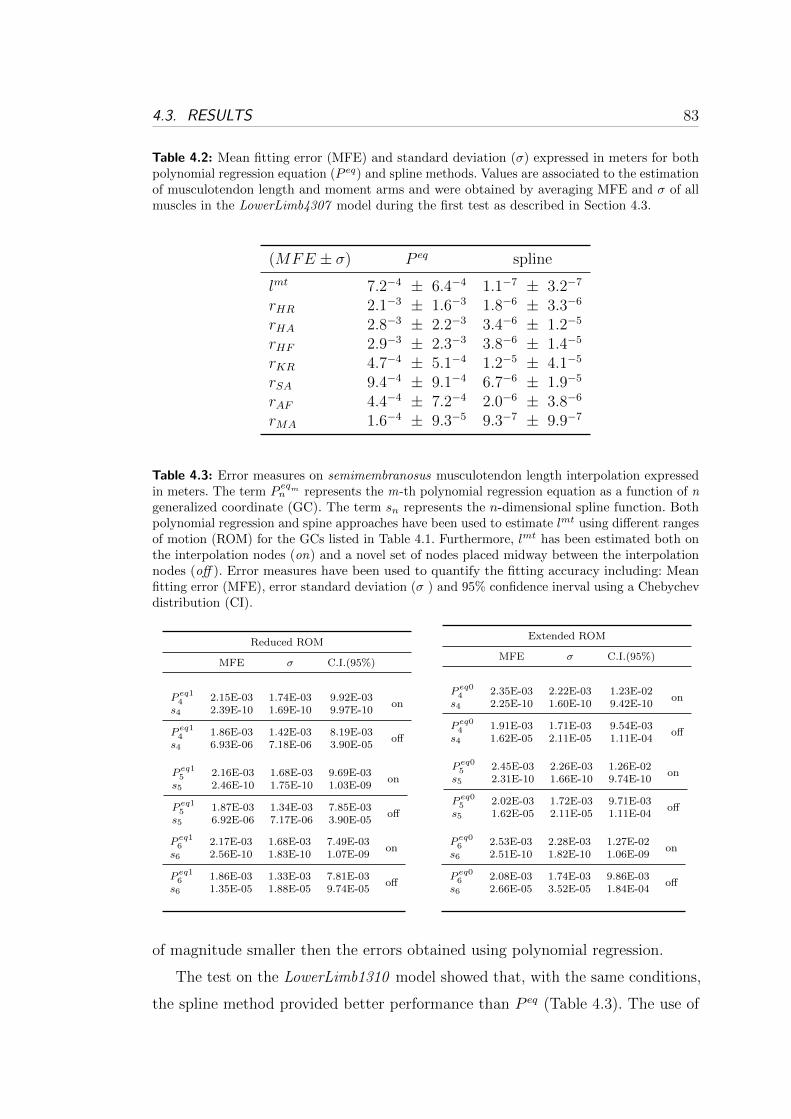
4.3. RESULTS 83
Table 4.2: Mean fitting error (MFE) and standard deviation (�) expressed in meters for bothpolynomial regression equation (P eq) and spline methods. Values are associated to the estimationof musculotendon length and moment arms and were obtained by averaging MFE and � of allmuscles in the LowerLimb4307 model during the first test as described in Section 4.3.
(MFE ± �) P eq spline
lmt 7.2−4 ± 6.4−4 1.1−7 ± 3.2−7
rHR 2.1−3 ± 1.6−3 1.8−6 ± 3.3−6
rHA 2.8−3 ± 2.2−3 3.4−6 ± 1.2−5
rHF 2.9−3 ± 2.3−3 3.8−6 ± 1.4−5
rKR 4.7−4 ± 5.1−4 1.2−5 ± 4.1−5
rSA 9.4−4 ± 9.1−4 6.7−6 ± 1.9−5
rAF 4.4−4 ± 7.2−4 2.0−6 ± 3.8−6
rMA 1.6−4 ± 9.3−5 9.3−7 ± 9.9−7
Table 4.3: Error measures on semimembranosus musculotendon length interpolation expressedin meters. The term P
eqmn represents the m-th polynomial regression equation as a function of n
generalized coordinate (GC). The term sn represents the n-dimensional spline function. Bothpolynomial regression and spine approaches have been used to estimate lmt using different rangesof motion (ROM) for the GCs listed in Table 4.1. Furthermore, lmt has been estimated both onthe interpolation nodes (on) and a novel set of nodes placed midway between the interpolationnodes (off ). Error measures have been used to quantify the fitting accuracy including: Meanfitting error (MFE), error standard deviation (� ) and 95% confidence inerval using a Chebychevdistribution (CI).
Reduced ROM
MFE � C.I.(95%)
P eq14 2.15E-03 1.74E-03 9.92E-03
ons4 2.39E-10 1.69E-10 9.97E-10
P eq14 1.86E-03 1.42E-03 8.19E-03
offs4 6.93E-06 7.18E-06 3.90E-05
Extended ROM
MFE � C.I.(95%)
P eq04 2.35E-03 2.22E-03 1.23E-02
ons4 2.25E-10 1.60E-10 9.42E-10
P eq04 1.91E-03 1.71E-03 9.54E-03
offs4 1.62E-05 2.11E-05 1.11E-04
P eq15 2.16E-03 1.68E-03 9.69E-03
ons5 2.46E-10 1.75E-10 1.03E-09
P eq15 1.87E-03 1.34E-03 7.85E-03
offs5 6.92E-06 7.17E-06 3.90E-05
P eq05 2.45E-03 2.26E-03 1.26E-02
ons5 2.31E-10 1.66E-10 9.74E-10
P eq05 2.02E-03 1.72E-03 9.71E-03
offs5 1.62E-05 2.11E-05 1.11E-04
P eq16 2.17E-03 1.68E-03 7.49E-03
ons6 2.56E-10 1.83E-10 1.07E-09
P eq16 1.86E-03 1.33E-03 7.81E-03
offs6 1.35E-05 1.88E-05 9.74E-05
P eq06 2.53E-03 2.28E-03 1.27E-02
ons6 2.51E-10 1.82E-10 1.06E-09
P eq06 2.08E-03 1.74E-03 9.86E-03
offs6 2.66E-05 3.52E-05 1.84E-04
of magnitude smaller then the errors obtained using polynomial regression.
The test on the LowerLimb1310 model showed that, with the same conditions,
the spline method provided better performance than P eq (Table 4.3). The use of

84 4. ESTIMATION OF MUSCULOTENDON KINEMATICS
(a) (b)
Figure 4.2: (a) The error associated to the prediction of the maximal isometric Fmt. Thehistogram combines values for all muscles in the LowerLimb1310 obtained during the third test.A set of error classes have been defined, each one representing a different error range and thenumber of points falling into each class have been counted and graphed. The x an y axes havebeen broken to focus on the most informative part of the graph. (b) The semimembranosusforce prediction errors during all gait and jogging trials are estimated and the average errors arehere reported.
an extended ROM, significantly affected P eq accuracy. Furthermore, a different
regression equation had to be used on the extended ROM even though, experiments
were done on the same muscle and and kinematic variable. The spline method was
less affected than the P eq by the distance between interpolation nodes, and their
associated difference measures were always at least three orders of magnitude
smaller. When the number of GCs was increased, splines were not significantly
affected whereas P eq fitting accuracy showed higher variability. In general, spline
functions evaluated on the interpolation nodes produced negligible errors (10−10m)
thanks to the (n + 1) interpolation conditions that assure perfect fit on-nodes
(Section 4.2.2). When evaluated off-nodes, errors were still very small, i.e. in the
order of 10−5m. Interestingly, P eq produced slightly bigger errors when evaluated
on the interpolation nodes although always in the order of 10−2m. As shown in
Table 4.4, the percentage mean fitting error %� associated to the HA moment arm
(rHA) showed that the non-differentiated spline, that was individually fitted to
rHA(sℎa4
)provided the best results. However, ∂slmt4 /∂qHA still produced very small
values of %� in the order of 0.1% of E[rHA] with better performances off-nodes.
Errors associated to P eq were higher and corresponded to a thick 10% of E[rHA].
The lmt fitting error impacted the estimates of muscle force. Estimations of
lmt using P eq reached a MEE of 1.23cm with four GCs and an extended ROM

4.4. CONCLUSIONS AND FUTURE WORK 85
(Table 4.3). On the other hand, splines produced a MEE of only 0.01cm. When
muscles were maximally activated, a 1cm difference in lmt with respect to the true
length can result in variations of hundreds of newtons (N ) in the estimation of
the isometric musculotendon force. The force errors stemming from P eq fell into
error classes of hundreds of newtons whereas spline related errors were always
less than 20N and always contained in the first (smallest) error class (Fig. 4.2a).
In the LowerLimb1310 test, errors of all muscles from the spline-based approach
provided superior results than P eq (Fig. 4.2a). During tests involving dynamic
motor tasks, errors in force prediction associated to P eq were highly dependent on
the muscle activation level as opposed to errors associated to the spline method
(Fig. 4.2b). The force prediction instantaneous error during walking reached a
maximum error of 6N using P eq which increased up to almost 20N during jogging,
while the spline errors were not affected by the increased muscle activation and
was always less than 1N .( Fig. 4.2b).
The computation time needed to evaluate one point on the spline function
depends on the number of GCs [68]. This dimension dependency was observed in
the computational time tests although computational costs were always reasonably
low. Computational time ranged from 10−5ms (one-dimensional case) to 10−2ms
(six-dimensional case) both for spline and for its derivative. The P eq computation
time was always in the order of 10−6ms as the number of coefficients is not a
function of the number of GCs.
4.4 Conclusions and Future Work
In this study, multidimensional cubic B-splines were used to estimate musculoten-
don kinematics for a set of lower-limb musculotendon actuators. The proposed
methodology was compared to previous research work that used polynomial re-
gression [69]. A single spline function could be used to estimate both lmt and
r with only very small errors compared to the original data. Contrary to this,
different P eq had to be chosen according to the surface to be fitted. If 6 GCs were
involved, 7 different regression equations had to be chosen (i.e. one for lmt and six
for r) and their coefficients had to be calculated. This requires in general more
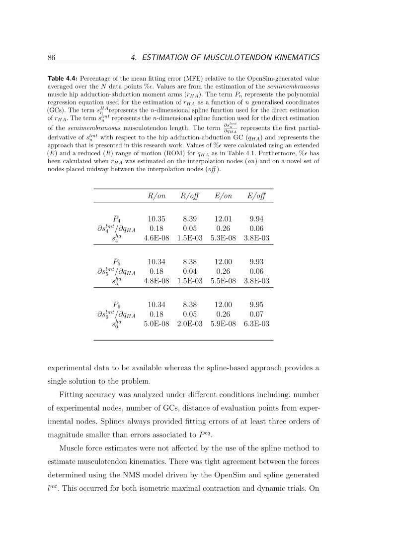
86 4. ESTIMATION OF MUSCULOTENDON KINEMATICS
Table 4.4: Percentage of the mean fitting error (MFE) relative to the OpenSim-generated valueaveraged over the N data points %�. Values are from the estimation of the semimembranosusmuscle hip adduction-abduction moment arms (rHA). The term Pn represents the polynomialregression equation used for the estimation of rHA as a function of n generalised coordinates(GCs). The term sHA
n represents the n-dimensional spline function used for the direct estimationof rHA. The term slmt
n represents the n-dimensional spline function used for the direct estimation
of the semimembranosus musculotendon length. The term∂slmt
n
∂qHArepresents the first partial-
derivative of slmtn with respect to the hip adduction-abduction GC (qHA) and represents the
approach that is presented in this research work. Values of %� were calculated using an extended(E ) and a reduced (R) range of motion (ROM) for qHA as in Table 4.1. Furthermore, %� hasbeen calculated when rHA was estimated on the interpolation nodes (on) and on a novel set ofnodes placed midway between the interpolation nodes (off ).
R/on R/off E/on E/off
P4 10.35 8.39 12.01 9.94∂slmt4 /∂qHA 0.18 0.05 0.26 0.06
sℎa4 4.6E-08 1.5E-03 5.3E-08 3.8E-03
P5 10.34 8.38 12.00 9.93∂slmt5 /∂qHA 0.18 0.04 0.26 0.06
sℎa5 4.8E-08 1.5E-03 5.5E-08 3.8E-03
P6 10.34 8.38 12.00 9.95∂slmt6 /∂qHA 0.18 0.05 0.26 0.07
sℎa6 5.0E-08 2.0E-03 5.9E-08 6.3E-03
experimental data to be available whereas the spline-based approach provides a
single solution to the problem.
Fitting accuracy was analyzed under different conditions including: number
of experimental nodes, number of GCs, distance of evaluation points from exper-
imental nodes. Splines always provided fitting errors of at least three orders of
magnitude smaller than errors associated to P eq.
Muscle force estimates were not affected by the use of the spline method to
estimate musculotendon kinematics. There was tight agreement between the forces
determined using the NMS model driven by the OpenSim and spline generated
lmt. This occurred for both isometric maximal contraction and dynamic trials. On

4.4. CONCLUSIONS AND FUTURE WORK 87
the other hand, forces produced using P eq showed large discrepancies during the
isometric tests. During dynamic tests the force discrepancy significantly increased
with muscle activation.
Computational requirements associated to both spline and polynomial regres-
sion were compared. The computational time of P eq is not a function of the
number of GCs and was always in the order of 10−6ms. Because the number of
spline coefficients is a function of the number of GCs (Section 4.2), the compu-
tational cost associated to the spline approach varies with the number of GCs
too. However, results showed that good performances were obtained even with
6 GCs where the time needed to estimate a single data point for lmt and for
the 6 moment arms was estimated to be in the order of 0.1ms per muscle. The
splines’ first derivatives could be estimated at the same computational cost needed
for the non-differentiated spline. Computational performances provided by the
proposed spine method make this approach suitable for applications with real-time
requirements.
The use of splines is not limited to fitting lmt data from muscluotendon models
such as SIMM or OpenSim. Alternatively, lmt could be determined from the
centroids of three dimensional muscles based on MRI data [70, 71] or from three
dimensional geometric modeling of musculoskeletal systems [72–74]. These methods
allow modeling muscles as complex of fibers with different contraction properties,
mass distributions and shapes. However, the amount of information needed to
represent these models and the associated computational requirements would
prevent any direct implementation into real-time systems or micro controllers.
The approach proposed in this Chapter allows creating a multivariate function
that can reliably replicate the behavior of complex systems at low computational
cost.
In summary, the results obtained using the spline-based approach are promising
and further demonstrate the methodology can be reliably integrated in complex
neuromusculoskeletal models for the prediction of muscle force for a large number
of musculotendon actuators as previously shown in Chapter 3.

Chapter 5
Fast Calibration of the
Elastic-Tendon NMS Model
Chapters 3 and 4 presented the design of the proposed EMG-driven NMS model
based on infinitely stiff tendons. In some applications however, it may be useful to
have accurate estimates of the instantaneous tendon and muscle fibre lengths. In
such a situation, an elastic-tendon NMS model may be the best choice. The main
problem though, is the time required to properly calibrate it. Indeed, as explained
in Chapter 3 the calibration of the single-DOF knee joint model may take several
hours. This time is bounded to significantly increase with the number of muscles
and DOFs in the model but also with the number of calibration trials that are
used. The required calibration time can therefore easily become unmanageable
even with powerful machines.
This Chapter illustrates an alternative solution to the use of standard global
optimization algorithms (Section 2.3.4) to optimize the model. We will refer to the
NMS model that uses an elastic-tendon Hill-type muscle model to as the EHM.
We will instead refer to the NMS model that uses a stiff-tendon Hill-type muscle
model to as the SHM.
89

90 5. FAST CALIBRATION OF THE ELASTIC-TENDON NMS MODEL
Figure 5.1: Proposed procedure for the fast calibration of the elastic-tendon NMS model.
5.1 Methods
Chapter 3 showed that the SHM proposed in this thesis achieves faster execution
and calibration time with no loss of accuracy in the prediction of knee flexion-
extension (FE) moments with respect to the EHM. Because of this, it is reasonable
to hypothesize that the set of parameters obtained for the SHM may represent
a good sub-optimal solution for the EHM. If this hypothesis holds, it could be
possible to create a faster calibration procedure for the EHM that comprises two
steps:
1. Pre-calibration: the global optimization criteria (i.e. simulated annealing)
presented in Section 2.3.4 is used to calibrate the stiff-tendon model. The
resulting parameter set represents the initial sub-optimal solution for the
elastic-tendon model. The simulated annealing procedure will be referred to
as the standard calibration procedure.
2. Refinement: the fast local optimization criteria (i.e. downhill simplex) pre-
sented in [75] is used to further refine the initial sub-optimal solution to
obtain an optimal parameter set for the EHM. The pre-calibration step
allows localizing and avoiding all the locally optimal solutions in the work
space. The local optimization algorithm is then used to explore the neighbor-
hood of the sub-optimal solution and quickly converge towards the closest
optimum.
Fig. 5.1 gives a schematic view of the proposed calibration procedure.

5.2. VALIDATION PROCEDURE 91
5.2 Validation Procedure
Experiments were performed at the Gait Laboratory of the School of Sport Science
Exercise and Health of the University of Western Australia. Data were collected
from one male subject (age: 28, weight: 67, height: 183 cm) who gave informed
consent and who performed 5 walking trials at self-selected speed. The same data
collection protocol and the same modeling process described in Chapter 2 were
used. The data collected during the 5 walking trials were used to calibrate the
elastic-tendon model presented in Section 2.3. A total number of 19 parameters
were adjusted during the calibration process. These included: muscle-specific
tendon slack length, global EMG-to-activation shape factor and recursive filter
coefficients and muscle strength coefficients (Section 2.3.4).
The validation procedure comprises three tests. In all tests knee FE moments
are estimated during the stance phase. Outputs are time-normalized using a cubic
spline and averaged over the 5 walking trials to produce a single ensemble average
knee FE moment curve. Furthermore, the mean fitting error (MFE), as described
in (3.9), is used as an additional measure of error in the estimated moments.
The first test assesses whether the set of parameters obtained from the standard
calibration of the SHM actually represents a good sub-optimal solution for the
EHM. This represents the pre-calibration step. The knee FE moments estimated
by the pre-calibrated EHM (P-EHM) are then compared to those obtained by the
standard-calibrated stiff (C-SHM) and elastic (C-EHM) tendon models.
The second test assesses whether the refinement step further improves the
solution found during the pre-calibration step. For this purpose, the refined pre-
calibrated solution (RP-EHM) is compared to that obtained from C-EHM and
C-SHM. Furthermore, to prove that the refinement step alone does not lead to
satisfactory solutions, the elastic-tendon NMS model (EHM) is calibrated using
the local downhill simplex algorithm starting with an uncalibrated parameter set.
We will refer to this model to as D-EHM (i.e. downhill simplex calibrated EHM
model).
The third test assesses whether the proposed calibration procedure is faster
than the standard one. For this purpose the calibration time is measured and
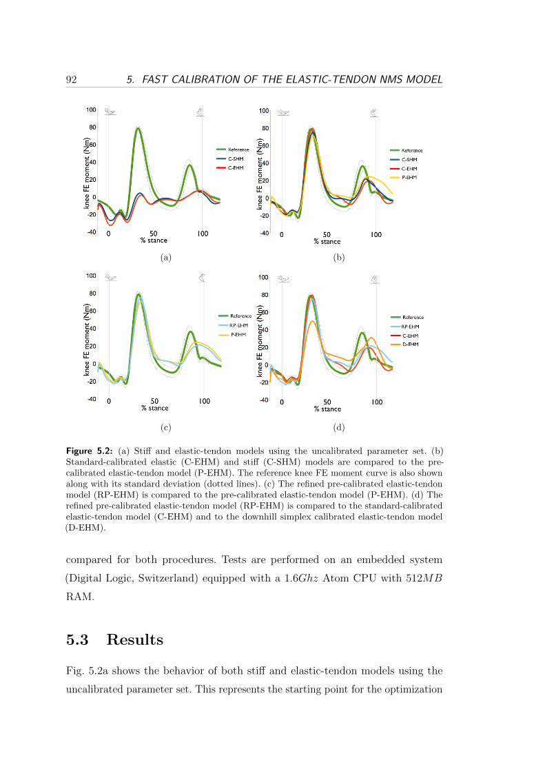
92 5. FAST CALIBRATION OF THE ELASTIC-TENDON NMS MODEL
(a) (b)
(c) (d)
Figure 5.2: (a) Stiff and elastic-tendon models using the uncalibrated parameter set. (b)Standard-calibrated elastic (C-EHM) and stiff (C-SHM) models are compared to the pre-calibrated elastic-tendon model (P-EHM). The reference knee FE moment curve is also shownalong with its standard deviation (dotted lines). (c) The refined pre-calibrated elastic-tendonmodel (RP-EHM) is compared to the pre-calibrated elastic-tendon model (P-EHM). (d) Therefined pre-calibrated elastic-tendon model (RP-EHM) is compared to the standard-calibratedelastic-tendon model (C-EHM) and to the downhill simplex calibrated elastic-tendon model(D-EHM).
compared for both procedures. Tests are performed on an embedded system
(Digital Logic, Switzerland) equipped with a 1.6Gℎz Atom CPU with 512MB
RAM.
5.3 Results
Fig. 5.2a shows the behavior of both stiff and elastic-tendon models using the
uncalibrated parameter set. This represents the starting point for the optimization
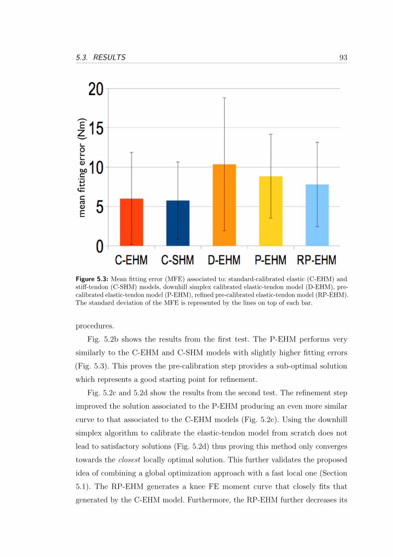
5.3. RESULTS 93
Figure 5.3: Mean fitting error (MFE) associated to: standard-calibrated elastic (C-EHM) andstiff-tendon (C-SHM) models, downhill simplex calibrated elastic-tendon model (D-EHM), pre-calibrated elastic-tendon model (P-EHM), refined pre-calibrated elastic-tendon model (RP-EHM).The standard deviation of the MFE is represented by the lines on top of each bar.
procedures.
Fig. 5.2b shows the results from the first test. The P-EHM performs very
similarly to the C-EHM and C-SHM models with slightly higher fitting errors
(Fig. 5.3). This proves the pre-calibration step provides a sub-optimal solution
which represents a good starting point for refinement.
Fig. 5.2c and 5.2d show the results from the second test. The refinement step
improved the solution associated to the P-EHM producing an even more similar
curve to that associated to the C-EHM models (Fig. 5.2c). Using the downhill
simplex algorithm to calibrate the elastic-tendon model from scratch does not
lead to satisfactory solutions (Fig. 5.2d) thus proving this method only converges
towards the closest locally optimal solution. This further validates the proposed
idea of combining a global optimization approach with a fast local one (Section
5.1). The RP-EHM generates a knee FE moment curve that closely fits that
generated by the C-EHM model. Furthermore, the RP-EHM further decreases its

94 5. FAST CALIBRATION OF THE ELASTIC-TENDON NMS MODEL
Table 5.1: Comparison of computational time performances (h=hour, m=minute, s=second)
C-EHM C-SHM D-EHM P-EHM RP-EHM
19h,13m 8m,7s 55m,13s 8m,7s 63m,20s
MFE with respect to the P-EHM and reaches a similar value to that associated
to the C-EHM (Fig. 5.3).
Table 5.1 shows the results associated to the third test. The time needed
to calibrate the elastic-tendon model using the standard calibration procedure
(C-EHM) is approximately 19 hours. The time needed using the methodology
proposed in this Chapter (RP-EHM) is significantly lower, i.e. approximately 63
minutes.
5.4 Discussion
It is worth noting that the pre-calibrated elastic-tendon model (P-EHM) performed
very well with a MFE of 8.8 ± 5.3Nm. The time for its calibration is the time
required to calibrate the stiff-tendon model using the standard calibration approach
that is approximately 8 minutes. The refined pre-calibrated elastic-tendon model
(RP-EHM) performed slightly better than the P-EHM, i.e the associated MFE
was 7.8± 5.3Nm. However, the time for calibration was much higher (63 minutes).
This work shows that the stiff-tendon model alone can be used to calibrate the
elastic-tendon model in just 8 minutes as opposed to the 19 hours required from
the standard calibration and the 55 minutes required by the refinement step.
Furthermore, the loss of prediction accuracy is significantly low. The standard-
calibrated elastic-tendon model achieved a MFE of 6.01± 5.9Nm which is only
2.79Nm lower to that associated to the P-EHM and 1.79Nm lower than that
associated to the RP-EHM.

5.5. CONCLUSIONS AND FUTURE WORK 95
5.5 Conclusions and Future Work
In this Chapter a novel methodology was presented to achieve faster calibration
of the elastic-tendon model. Results showed the proposed methodology allows
calibrating the elastic-tendon model achieving the same calibration accuracy of
the standard calibration procedure but in significantly less time.
This result is particularly significant when an elastic-tendon model is to be
used to simulate the behavior of a large number of musculotendon actuators or
when the NMS model has to be calibrated on a large number of trials. Indeed,
the calibration time is a function of the number of MTAs and DOF in the model
as well as number of calibration trials.
Future research will further assess the potential of the proposed calibration
methodology on the multi-DOF NMS model presented in Chapter 6. Furthermore,
the low calibration time associated to the stiff-tendon model will be exploited
to implement an on-line calibration algorithm that keeps refining the model
parameters as it executes. This will allow coping with time-varying parameters
associated to muscle fatigue including the muscle maximal isometric force. This
will allow creating NMS model that automatically adapt to the subject’s physical
conditions.


Chapter 6
A Neuromusculoskeletal Model of
the Human Lower Extremity
The previous Chapters presented the single-DOF EMG-driven NMS model de-
veloped in this thesis. The model can estimate the force from 13 musculotendon
actuators (MTAs) crossing the knee joint and the moments about the flexion-
extension (FE) DOF. It was compared to the previously developed single-DOF
NMS model based on elastic tendons (Section 2.3). It was demonstrated the single-
DOF NMS model proposed in this thesis achieves faster execution and calibration
time with no loss of accuracy in the prediction of knee flexion-extension (FE)
moments. It was also proved the model can be used to implement fast calibration
of the elastic-tendon model.
This Chapter further extends the work presented in the previous Chapters.
A novel neuromusculoskeletal (NMS) model of the human lower limb is here
presented. The model uses EMG signals from 16 muscles to estimate forces from
34 muscles and moments at the hip, knee and ankle joints. We will refer to the
model presented in this Chapter to as the multi-DOF EMG-driven NMS model.
Results show the multi-DOF model is capable of constraining the operation of
the muscles to satisfy the moments generated at all joints and about all degrees
of freedom during the human movement. This allows better estimating muscle
forces providing a single solution to the problem with respect to current NMS
models proposed in the literature that only constrain the operation of muscles
97

98 6. A NMS MODEL OF THE HUMAN LOWER EXTREMITY
to satisfy moments produced at one joint only. This technology can be applied
to the design of more intuitive human-machine interfaces for the simultaneous
EMG-driven actuation of multiple joints in powered orthoses.
6.1 Introduction
The study of how muscles activate, generate force and actuate multiple joints
simultaneously is crucial to understand the mechanisms behind human movement
[25]. This is becoming an important topic in the design of wearable assistive device
control systems such as powered orthoses. In recent years a body of research has
been conducted on connecting the control system to biological signals generated
by the operator that are directly linked to the desire of motion [8, 9, 15]. EMG
signals represent a good candidate for extracting motor information from the lower
limb and establishing an intuitive HMI for assistive device control (Chapter 1).
In this context, EMG-driven neuromusculoskeletal (NMS) models of the human
limbs provide a way to implement continuous active control of assistive devices as
opposed to pattern recognition and machine learning methods (Section 1.1).
To date though, only single-DOF EMG-driven NMS models have been proposed.
That is, muscle forces are used to predict moments about a single DOF of a single
joint. In [6] a whole-body NMS model was presented. However, it was not driven
by EMG signals and the muscle redundancy problem, i.e. the way muscles share
the load about a joint, was solved based on some objective function that had to
be carefully chosen before hand. This is a limitation because muscles in general
use different criteria depending on the subject and on the movement and it is
often impossible to assess the appropriateness of the chosen optimization criteria.
Furthermore, not using EMG signals has the drawback that to perform a movement,
the operator has to be able to initiate the movement before he or she can receive
support from the system.
This Chapter shows it is possible to use EMG signals to accurately estimate
muscle forces from all major muscles in the lower limb. A novel NMS model is
proposed which allows constraining the operation of muscles so that the forces
they produce can satisfy the moments simultaneously generated at multiple DOFs

6.2. METHODS 99
in multiple joints including the hip, knee and ankle joints. This is achieved by the
use of a novel calibration algorithm (Section 6.3.5). Single-DOF models such as
knee flexion-extension (FE) models allow estimating the muscle forces involved in
the production of FE moments only. However, most of the muscles spanning the
knee also span the hip and the ankle joints too. Therefore, the forces the muscles
generate for the production of knee FE moment also have to satisfy the generation
of moments about hip and ankle joints.
Single-DOF models, therefore, constrain the operation of muscles to satisfy
the moments generated at a single joint and about a single DOF only. Because
of this, Single-DOF models can usually fit the experimental single-DOF joint
moment with good accuracy. However, the underlying behavior of the simulated
muscles is questionable as it may not be truly representative of the real muscle
behavior. Results in this Chapter show that the force a muscle can generate during
a specific movement can be predicted in extremely different ways when different
single-DOF models are used and it is not possible to know what single-DOF
model gives the best estimates. The multi-DOF NMS model presented in this
Chapter allows removing this indeterminacy by providing a single solution for each
muscle. Results show the multi-DOF model has the potential to better estimate
somatosensory information than single-DOF models.
This research has the potential to help design effective HMIs that can provide a
better estimation of the human internal state. This research develops the technology
needed to achieve power orthosis continuous control and the simultaneous actuation
of multiple DOFs in multiple joints. This is a crucial requirement when the assistive
device is to be used for the support of the lower limb. Indeed, all functional motor
activities such as walking and climbing stairs involve the simultaneous actuation
of hip, knee and ankle joints. This will also allow supporting an even wider range
of movements.
6.2 Methods
Experiments were performed at the Gait Laboratory of the School of Sport Science
Exercise and Health of the University of Western Australia. One healthy, male
100 6. A NMS MODEL OF THE HUMAN LOWER EXTREMITY
subject volunteered for this investigation (age: 28years, height: 183cm, mass:
67kg). The subject was taken through the testing protocols and informed consent
was obtained prior to data collection.
A data set for the calibration of the model is initially created which includes
static and swinger trials. Furthermore, a number of dynamic trials are performed by
the subject including: walking, jogging, step jumps and lateral hops. Data collected
from the static and swinger trials are used to create a musculoskeletal model
that is scaled to the subject’s real dimensions (Section 2.2). The musculoskeletal
model that is used in this work is customized to include all the muscles of interest
and to define 6 degrees of freedom across the joints: hip adduction-abduction
(HAA), hip flexion-extension (HFE), hip internal-external rotation (HRO), knee
flexion-extension (KFE), ankle dorsi-plantar flexion (AFE), ankle subtalar angle
(ASA). Data collected from the dynamic trials are used to calibrate the NMS
model parameters (see Section 6.3.5).
A data set for the validation of the model (see Section 6.3.5) is then created
which includes 10 repeated trials per motor task: fast walking (FW), running (RN),
sidestepping (SS) and crossover (CO) cutting maneuvers. These tasks were chosen
as they involve the activation of all the lower limb muscles and the subsequent
production of moments across all joints.
A 12 camera motion capture system (Vicon, Oxford, UK) is used to record the
human body kinematics with sampling frequency at 250Hz. A set of reflecting
markers are placed on the human body and their instantaneous three-dimensional
position is reconstructed and used to measure the movement of body segments
including: trunk, pelvis, thigh, shank, and foot. Ground reaction forces (GRFs)
generated during the motor tasks are collected using a multi-axis in-ground force
plate (AMTI, Watertown, USA) with a sampling frequency at 2kHz. Both body
kinematics and GRFs are low-pass filtered with cut-off frequencies ranging from 2
to 8Hz depending on the trial. Marker trajectories recorded during dynamic trials
are used to drive the scaled musculoskeletal model. OpenSim Inverse Kinematics
(IK) tool is used to derive three-dimensional joint angles. GRFs are used in
conjunction with the thee-dimensional joint angles computed through IK to derive
the experimental joint moments. OpenSim Residual Reduction Analysis (RRA)
6.3. NMS MODEL 101
tool is used to compute the experimental joint moments.
Double-differential surface electrodes are used to collect EMG signals from 16
selected muscles including: Gluteus Maximus (gmax ), Gluteus Medius (gmed),
Tensor Fascia Latae (tfl), Medial Hamstrings (medham), Lateral Hamstrings
(latham), Rectus Femoris (recfem), Sartorius (sar), Gracilis (gra), Adductor Mag-
nus (addmag), Vastus Medialis (vasmed), Vastus Lateralis (vaslat), Gastrocnemius
Lateralis (gaslat), Gastrocnemius Medialis (gasmed), Tibialis Anterior (tibant),
Peroneus (per) and Soleus (sol). A telemetered system (Noraxon, Scottsdale, USA)
transfers the EMGs to a 16 channel amplifier (Delsys, Boston, USA) with sampling
frequency at 2kHz. Raw EMG signals are first band-pass filtered (10− 150Hz),
and then full-wave rectified and low-pass filtered (6Hz) subsequently. The pro-
cessed signal is the linear envelope which is then normalized against the maximum
values from EMG linear envelopes obtained from a range of extra trials including:
running and squat jumps.
6.3 NMS Model
The multi-DOF EMG-driven NMS model comprises 5 main components (Fig. 6.1).
The main structure is similar to that of the single-DOF model previously presented
(Chapter 3). The multi-DOF NMS model extends each single component to allow
the estimation of forces from 34 muscle tendon actuators (see Table 2.1) and the
joint moments about the following 4 DOF: hip adduction-abduction (HAA), hip
flexion-extension (HFE), knee flexion-extension (KFE), ankle dorsi-plantar flexion
(AFE). The NMS model proposed in this Chapter is entirely implemented in C++
likewise that presented in Chapter 3.
6.3.1 Musculotendon Kinematics
The musculotendon kinematics model estimates lengths and three-dimensional
moment arms of the musculotendon actuators (MTA) included in the model as
a function of the 3D angles of the joints each specific MTA crosses and was
presented in Chapter 4 (also see Fig. 3.1). Most of the muscles in the model
are described by a single MTA. That is, muscle fibers and tendons together are
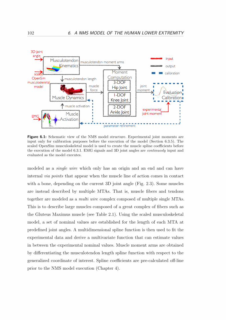
102 6. A NMS MODEL OF THE HUMAN LOWER EXTREMITY
Figure 6.1: Schematic view of the NMS model structure. Experimental joint moments areinput only for calibration purposes before the execution of the model (Section 6.3.5). Thescaled OpenSim musculoskeletal model is used to create the muscle spline coefficients beforethe execution of the model 6.3.1. EMG signals and 3D joint angles are continuosly input andevaluated as the model executes.
modeled as a single wire which only has an origin and an end and can have
internal via points that appear when the muscle line of action comes in contact
with a bone, depending on the current 3D joint angle (Fig. 2.3). Some muscles
are instead described by multiple MTAs. That is, muscle fibers and tendons
together are modeled as a multi wire complex composed of multiple single MTAs.
This is to describe large muscles composed of a great complex of fibers such as
the Gluteus Maximus muscle (see Table 2.1). Using the scaled musculoskeletal
model, a set of nominal values are established for the length of each MTA at
predefined joint angles. A multidimensional spline function is then used to fit the
experimental data and derive a multivariate function that can estimate values
in between the experimental nominal values. Muscle moment arms are obtained
by differentiating the musculotendon length spline function with respect to the
generalized coordinate of interest. Spline coefficients are pre-calculated off-line
prior to the NMS model execution (Chapter 4).

6.3. NMS MODEL 103
6.3.2 Muscle Activation
Muscles linear envelopes are processed and converted into muscle activation. This
is a percentage value that expresses how much a specific muscle is activated towards
the generation of force. The transformation from EMG to activation accounts for
the non-linear relationship between EMG and muscle force and a more detailed
description of the transformation involved as been presented previously (Section
2.3.2).
EMG signals recorded from 16 muscles (see Section 6.2) are used to estimate
the activation of 34 musculotendon actuators (MTAs). EMG signals that could
be experimentally recorded from those muscles that are modeled as a single wire
are assigned to their respective MTA. These include: vaslat, vasmed, sol, tibant,
tfl, recfem, sar, gra, gaslat, gasmed. EMG signals that could be experimentally
recorded from those muscles that are modeled as a multi wire complex are assigned
to all the MTAs that compose each muscle complex. That is, addmag EMG signals
are used to drive: addmag1, addmag2, addmag3. The gmax EMG signals are used to
drive: gmax1, gmax2 and gmax3. The gmed EMG signals are used to drive: gmed1,
gmed2 and gmed3. The per EMG signals are used to drive: Peroneus Longus
(perlong), Peroneus Brevis (perbrev), Peroneus Tertis (perter). The medham EMG
signals are used to drive: Semimembranosus (semimem) and Semitendinosus
(semiten). The latham EMG signals are used to drive: Biceps Femoris Short Head
(bicfemsh) and Biceps Femoris Long Head (bicfemlh). The EMG signals for the
remaining muscles can not be experimentally recorded because they are located
too deep under the skin surface. However, muscles that are innervated in the
same zone associated to those muscles whose EMG activity can be recorded, are
assumed to produce similar EMG activity and contraction patterns. Therefore,
the addmag EMG signal is used to also drive: Adductor Brevis (addbrev) and
Adductor Longus (addlong). In the case of muscles that are innervated in two
points, a linear combination of the EMG signals associated to the two innervations
locations is used. Therefore a linear combination of the vasmed and vaslat EMG
signals is used to drive the Vastus Interioris (vasint) MTA. Finally, a linear
combination of the gmax and gmed EMG signals is used to drive the Gluteus
Minimum (gmin) muscle that is composed of 3 MTAs. The Illiacus and Psoas

104 6. A NMS MODEL OF THE HUMAN LOWER EXTREMITY
muscles are not driven by EMG signals and their activation is not computed in
this current implementation of the model. However, these muscles still contribute
to the production of force at the hip joint because the passive force generated
during stretching and compression is calculated by NMS model anyway.
Some muscles of the lower extremity have not been included in the model
because either too small and therefore negligible or too deep under the skin surface.
However, the selected MTAs generate the majority of the moment in all selected
joints about all considered DOFs. That is, the muscles in the model that have a
HAA moment arm cover the 91% of the total physiological cross sectional area
(PCSA). Muscles that have a HFE moment arm cover the 87% of the total PCSA.
Muscles with a KFE moment arm in the model cover the 95% and muscles in the
model that have an AFE moment arm cover the 80% of the total PCSA.
6.3.3 Muscle Dynamics
It uses the values computed in the previous two blocks to calculate the force
developed by each MTA in the model as previously described in Section 3.5.
6.3.4 Moment Computation
This component evaluates the moments produced about all the DOFs of each
joint included in the model. The estimated muscle forces are combined with the
corresponding moment arms to calculate the torque about a specific DOF.
6.3.5 Validation and Calibration
To validate a model, it is usually desirable to compare the output of that model
with data measured empirically. Unfortunately, the methodological difficulties in
measuring individual muscle forces prevent any direct validation of the NMS model
on humans. An indirect process was therefore designed. This involves comparing
the net moments from muscles crossing the hip, knee and ankle joints with the
net moments measured experimentally. If the muscle forces are accurate, the net
joint moments estimated by the model should be equal to the external moments
measured experimentally.

6.3. NMS MODEL 105
The calibration process is critical for the proper operation of the model. It
defines how muscles activate in response to EMG signals and generate moments
about multiple DOFs. Biarticular muscles crossing the hip and knee joints for
instance, have to produce a force that satisfy moments about up to 4 DOFs
(HROT, HAA, HFE and KFE). The aim of the calibration process therefore
is to obtain a set of parameters for each muscle to accurately estimate the net
experimental moments at the hip, knee, and ankle across all corresponding DOFs
(Section 6.2). An optimization procedure has been designed to alter the initial
uncalibrated parameters until the error function (Section 2.3.4) associated to the
joint moment prediction is minimized. The calibration process repeatedly calls
an optimization routine. The steps involved in the calibration of a 4-DOF NMS
models are here summarized:
1. objective function: min(EKFE). Adjust parameters for all muscles crossing
the knee joint (13 MTAs).
2. objective function: min(EKFE + EHFE). Adjust parameters for all muscles
crossing the knee joint (13 MTAs) and the hip joint (23 MTAs).
3. objective function: min(EKFE + EHFE + EHAA). Adjust parameters for all
muscles crossing the knee joint (13 MTAs) and the hip joint (23 MTAs).
4. objective function: min(EKFE +EHFE +EHAA +EAFE). Adjust parameters
for all muscles crossing the knee joint (13 MTAs) and the hip joint (23
MTAs) and the ankle joint (8 MTAs).
where EX is the error function associated to the prediction of the moments about
the X tℎ DOF with X ∈ {HAA, HFE, KFE, AFE}. At each step, the error
function is extended by including a new DOF. The parameter set to be calibrated is
also extended by adding the parameters associated to a new set of muscles. The first
call uses an uncalibrated set of parameters. At each step the optimization process
utilizes the optimal solution produced by the previous step. The optimization
process is designed so that it can only produce a better solution than the initial
one. This assures that by adding a new DOF to the objective function, the fitting
accuracy provided from the previous calls is always guaranteed. At each call,

106 6. A NMS MODEL OF THE HUMAN LOWER EXTREMITY
the parameters associated to the currently added muscles are calibrated in order
to fit the joint moments associated to the currently added DOF. Furthermore,
the parameters associated to the muscles added by the previous steps are also
re-calibrated. This ensures that muscle behavior accounts for the new DOF added
to the process. If this was not done the biarticular muscles calibrated at Step 1
would satisfy the knee FE moments only and would not be able to satisfy the hip
adduction-abduction and hip flexion-extension moments added in Step 2 and Step
3 respectively. The same applies to each step. Once calibrated, the NMS model
only requires EMG signals and joint angles as inputs. GRF and experimental joint
moments are needed during the calibration step only.
6.4 Validation Procedure
The validation procedure is comprised of three tests. In all tests the NMS model
outputs, i.e. muscle force and joint moments, are estimated during the stance phase.
Outputs are then time-normalized using a cubic spline. Time-normalized muscle
force predicted from each motor task respectively, i.e. fast walking (FW), running
(RN), side-stepping (SS), cross-over (CO) are averaged over the 10 repeated trials
and an ensemble average force curve per muscle is produced for each of the 4
motor tasks. The same procedure is applied to the time-normalized experimental
and predicted joint moments.
The first test assesses whether the force generated by the same MTA is
predicted in a different way by using different single-DOF NMS models. This
is done for the purpose of validating the hypothesis that single-DOF models
introduce indeterminacy and the impossibility to know what model to use for
the estimation of a specific muscle force. For this purpose, the ensemble average
force curves of the biarticular MTAs Gastrocnemius Lateralis and Medialis are
predicted during FW both using a KFE NMS model and an AFE NMS model.
The ensemble average force curves of the biarticular MTAs Semimembranosus
and Semitendinosus are predicted during RN both using a HFE and a KFE NMS
model. Finally the ensemble average force curves of the uniarticular MTAs Gluteus
Medius 1, 2 and 3 are predicted during SS both using a HFE and a HAA NMS

6.5. RESULTS 107
model.
The second test assesses the ability of the proposed multi-DOF NMS model to
predict joint moments about 4 DOFs including: HAA, HFE, KFE and AFE. The
ensemble average curves associated to the predicted joint moments are directly
compared to those associated to the experimentally measured moments (Section
6.3.5) as well as to those associated to the moments predicted by the respective
single-DOF models i.e. HAA NMS model, HFE NMS model, KFE NMS model
and AFE NMS model. This is done for the purpose of assessing the impact, of
adding more DOFs to a NMS model, on its prediction capability. Furthermore,
it validates whether the proposed calibration scheme (Section 6.3.5) is capable
of producing a set of parameters that constraints the operation of the muscles
to satisfy the joint moments produced about all the DOFs of all the joints they
span. As an additional measure of error, the Mean Fitting Error (MFE) and its
standard deviation (�) are used : MFE = 1N
∑Ni=1
∣∣∣Mi −Mi
∣∣∣ , where M is the
ensemble average curve associated to the experimentally measured joint moments.
The term M is the corresponding estimated value either from the multi-DOF
NMS model or from the single-DOF NMS model. N is the number of points the
ensemble average curves are composed of.
In the third test the forces of the muscles crossing the knee joint are predicted
both using the proposed multi-DOF NMS model and the single-DOF KFE NMS
model model during running trials. Forces estimated by both models are then
compared.
6.5 Results
Results from the first tests are showed in Fig. 6.2. The Gastrocnemius Medialis
force estimated by the KFE NMS model reached drastically higher values than
those estimated by the AFE NMS model. Also the Gastrocnemius Lateralis force
estimated by the KFE NMS model assumed higher values than that estimated by
the AFE model. The Semimembranosus and Semitendinosus forces estimated by
the KFE NMS models reached significantly higher values than those estimated by
the HFE NMS model. The Gluteus Medius forces estimated by the HFE NMS

108 6. A NMS MODEL OF THE HUMAN LOWER EXTREMITY
Figure 6.2: Comparison of muscle forces estimated by different single-DOF models. Gastrocne-mius Medialis and Lateralis forces are estimated during fast walking trials. Semimembranosusand Semitendinosus forces are estimated during running trials. Gluteus Medius forces areestimated during side-stepping trials.
model were significantly higher than those estimated by the HAA NMS model.
In general different single-DOF models produced different force estimates for the
same muscle during the same specific movement. Similar results were obtained
for all other muscles. This validates the hypothesis defined in Section 6.4. This
test shows that although each single-DOF NMS model was driven by the same
EMG signals, a high discrepancy in the behavior of different models was still
produced. This is because the NMS model is not only EMG-driven but it is also
Optimization-driven. That is, the calibration process that is performed prior to
the model execution strongly influences the way muscles convert EMG into force
post-calibration. Therefore, the same EMG signal for the same muscle can be
converted in an extremely different muscle force if different single-DOF models
are used. Indeed, the parameter sets associated to different single-DOF models
are highly diverse.
Results from the second test are shown in Fig. 6.3. The multi-DOF NMS
model achieved better performances in the prediction of the AFE moments in
all 4 motor tasks. The multi-DOF NMS model behaved very similarly to the
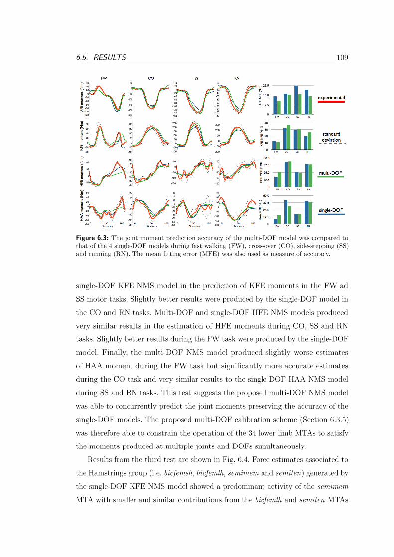
6.5. RESULTS 109
Figure 6.3: The joint moment prediction accuracy of the multi-DOF model was compared tothat of the 4 single-DOF models during fast walking (FW), cross-over (CO), side-stepping (SS)and running (RN). The mean fitting error (MFE) was also used as measure of accuracy.
single-DOF KFE NMS model in the prediction of KFE moments in the FW ad
SS motor tasks. Slightly better results were produced by the single-DOF model in
the CO and RN tasks. Multi-DOF and single-DOF HFE NMS models produced
very similar results in the estimation of HFE moments during CO, SS and RN
tasks. Slightly better results during the FW task were produced by the single-DOF
model. Finally, the multi-DOF NMS model produced slightly worse estimates
of HAA moment during the FW task but significantly more accurate estimates
during the CO task and very similar results to the single-DOF HAA NMS model
during SS and RN tasks. This test suggests the proposed multi-DOF NMS model
was able to concurrently predict the joint moments preserving the accuracy of the
single-DOF models. The proposed multi-DOF calibration scheme (Section 6.3.5)
was therefore able to constrain the operation of the 34 lower limb MTAs to satisfy
the moments produced at multiple joints and DOFs simultaneously.
Results from the third test are shown in Fig. 6.4. Force estimates associated to
the Hamstrings group (i.e. bicfemsh, bicfemlh, semimem and semiten) generated by
the single-DOF KFE NMS model showed a predominant activity of the semimem
MTA with smaller and similar contributions from the bicfemlh and semiten MTAs

110 6. A NMS MODEL OF THE HUMAN LOWER EXTREMITY
Figure 6.4: Muscle forces estimated during running tasks. The estimates of the multi-DOFmodel were compared to those of the single-DOF KFE model.
and very little force produced by the bicfemsh MTA. On the other hand, the
force dynamics estimated by the multi-DOF model suggested these MTAs shared
the load at the knee joint more equally. Indeed, the two MTAs comprising the
Lateral Hamstrings bicfemlh and bicfemsh were estimated to generate similar
curves. The same results were obtained for the semimem and semiten MTAs.
Results produced by the multi-DOF model are in line with findings from the
biomechanics community [24, 76].
Force estimates associated to the Quadriceps group (i.e. vaslat, vasint, vasmed
and recfem) generated by the single-DOF KFE NMS model showed a predominant
activity of the vasmed and vasint MTAs and a negligible production of force
from the Rectus Femoris (recfem) MTA. On the other hand, the forces estimated
by the multi-DOF model were more proportioned between the MTAs forming
the Quadriceps group. More importantly the estimated behavior of the Rectus
Femoris showed this MTA significantly produces force during running as also
demonstrated in [76, 77]. The single-DOF KFE model could not predict this
behavior because the recfem MTA is mostly active during running to support the
hip flexion-extension movement. The proposed multi-DOF NMS model did not
6.6. CONCLUSIONS AND FUTURE WORK 111
fail to catch such important feature because it properly constrained its operation
to satisfy not only KFE moments but also HFE and HAA moments.
Force estimates associated to the Gastrocnemius group (i.e. gasmed and gaslat)
generated by the single-DOF KFE NMS model showed a drastically predominant
activity of the gasmed MTA towards the end of the stance phase. On the other hand
the dynamics estimated by the multi-DOF NMS model more equally apportioned
the force to both MTAs.
6.6 Conclusions and Future Work
The research work presented in this Chapter, developed a novel EMG-driven
neuromusculoskeletal model of the lower limb that uses EMG signals recorded
from 16 muscles to derive the activity of 34 muscles and to estimate moments
about hip, knee and ankle joints. Results showed that the force a muscle can
generate during a specific movement can be predicted in extremely different ways
when different single-DOF models are used. This fact introduces indeterminacy as
it is not possible to know what single-DOF model is best to use. The proposed
multi-DOF NMS model allows removing this indeterminacy by providing a single
solution to the problem. The proposed model was able to predict joint moments
with the same accuracy of the 4 individual single-DOF EMG-driven models thus
proving each muscle was successfully constrained to satisfy moments about all
associated joints and DOFs. As a result, the multi-DOF model was able to produce
force dynamics estimates that were more in line with biomechanics findings. The
single-DOF KFE model failed to estimate the force produced by the Rectus
Femoris muscle during running because this is a muscle that is mostly active to
support the hip flexion. The multi-DOF model correctly predicted this. Future
version of the multi-DOF NMS model will feature a predictive algorithm for the
estimation of the activation of muscles without EMG. This will allow estimating
muscle forces generated by the Illiacus and Psoas muscles. Pattern recognition
technology will be integrated in the NMS model and used to extrapolate more
information out of the EMG signals as discussed in Chapter 8. A study on a larger
population will be conducted to further validate the methodology.

112 6. A NMS MODEL OF THE HUMAN LOWER EXTREMITY
This technology can offer great solutions for the implementation of more
realistic virtual humans by providing a more accurate estimation of the human
internal state [5]. This can also be applied to the design of more intuitive assistive
devices control systems for the simultaneous actuation of multiple joints and the
support of an even wider range of movements.

Chapter 7
Scaling Tendons Preserving the
Consistency of the
EMG-to-Activation Relationship
Neuromusculoskeletal modeling is a powerful tool for understanding how the
nervous system controls muscles to generate movements. Experiments conducted
in this thesis and the results that were obtained demonstrated that to properly
scale NMS models to different subjects, physiological parameters that characterize
individual muscle properties must be integrated in the NMS model design and
properly calibrated. However, most of them cannot be measured directly unless
invasive or expensive approaches are adopted. This is the case for the tendon slack
length (lts). This is a key-parameter because it directly defines how muscle develop
force as a function of their fibre length.
There is very little information in the literature in regards to tendon slack
lengths of lower limb musculature mostly because of the difficulty in measur-
ing these values and the ill-defined junction between muscle and tendon. It was
therefore decided to investigate a robust methodology for properly deriving physi-
ologically relevant values for this important parameter.
This Chapter presents a method for scaling lts for muscles crossing the knee
joint. This method can be used alone or in addition to the standard calibration
procedure (Section 2.3.4) to significantly refine the parameter initial guess.
113

114 7. SCALING TENDON SLACK LENGTH
7.1 Data Collection
Experiments were performed at the Gait Laboratory of the School of Sport Science
Exercise and Health of the University of Western Australia. Data were collected
from one male subject (age: 28, weight: 67, height: 183 cm) who gave informed
consent. The subject performed knee flexion-extension (FE) maximal isometric
trials using a Biodex dynamometer (Shirley, NY) at different knee joint angles:
−30∘, −60∘, −90∘, −120∘, where 0∘ represents the leg totally extended and aligned
with the thigh (Fig. 2.2). The hip joint was firmly held at 80∘ according to the
convention depicted in Fig. 2.2. During each FE trial, EMG signals were recorded
from the muscles crossing the knee as described in Section 3.5.2.
One walking trial was also performed and motion capture data were used to
measure the knee FE moment generated following the procedure presented in
Chapter 2.
7.2 Rationale
The aim of this study is to show that if lts is not properly calibrated, the EMG-
to-activation relationship (Fig. 2.16) is not consistent between different trials.
That is, a different curve is generated when the knee joint is placed at different
angles. The EMG-to-activation relationship becomes therefore a function of muscle
fiber length if lts is not properly calibrated. This should not happen because the
EMG-to-activation relationship is independent of muscle fibre length for definition
as described by equation (2.1).
In this study an initial guess of lts is obtained by using the standard calibration
procedure. This is used to also calibrate muscle strength coefficients, activation
shape factor and optimal fibre length. Then, the scaling procedure presented in
this Chapter is applied to further adjust the tendon slack length for every muscle
in such a way that the computation of the muscle activation based on the EMG
signal for a specific muscle is consistent for all joint angles.
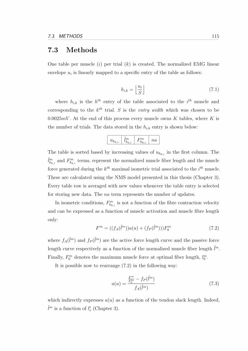
7.3. METHODS 115
7.3 Methods
One table per muscle (i) per trial (k) is created. The normalized EMG linear
envelope ui is linearly mapped to a specific entry of the table as follows:
ℎi,k =⌊uiS
⌋(7.1)
where ℎi,k is the ℎtℎ entry of the table associated to the itℎ muscle and
corresponding to the ktℎ trial. S is the entry width which was chosen to be
0.0025mV . At the end of this process every muscle owns K tables, where K is
the number of trials. The data stored in the ℎi,k entry is shown below:
uℎk,i lmℎk,i Fmℎk,i
na
The table is sorted based by increasing values of uℎk,i in the first column. The
lmℎk,i and Fmℎk,i
terms, represent the normalized muscle fiber length and the muscle
force generated during the ktℎ maximal isometric trial associated to the itℎ muscle.
These are calculated using the NMS model presented in this thesis (Chapter 3).
Every table row is averaged with new values whenever the table entry is selected
for storing new data. The na term represents the number of updates.
In isometric conditions, Fmℎk,i
is not a function of the fibre contraction velocity
and can be expressed as a function of muscle activation and muscle fibre length
only:
Fm = ((fA(lm))a(u) + (fP (lm)))Fm0 (7.2)
where fA(lm) and fP (lm) are the active force length curve and the passive force
length curve respectively as a function of the normalized muscle fiber length lm.
Finally, Fm0 denotes the maximum muscle force at optimal fiber length, lm0 .
It is possible now to rearrange (7.2) in the following way:
a(u) =
Fm
Fm0− fP (lm)
fA(lm)(7.3)
which indirectly expresses a(u) as a function of the tendon slack length. Indeed,
lm is a function of lts (Chapter 3).

116 7. SCALING TENDON SLACK LENGTH
We can now compute the standard deviation (�ℎ,i) of (7.3) for the table entry
ℎ from all K tables associated to the itℎ muscle:
�ℎ,i(lts) =
√√√⎷ 1
K
K∑k=1
(aℎk,i − aℎ,i)2 (7.4)
where aℎ,i is the average of aℎk,i over all K trials. The notation used in (7.4)
highlights the fact that the standard deviation is also a function of the tendon
slack length, i.e. �ℎ,i(lts).
It is now possible to optimize lts so that it minimizes the average of �ℎ,i over
all table rows:
minlts(�(lts)) = minlts
(1
Nℎ
Nℎ∑ℎ=1
(�ℎ(lts))
)(7.5)
where Nℎ is the number of entries in the tables. A simulated annealing algorithm
(Section 2.3.4) was used to vary lts within a 15% of its initial guess for each muscle.
7.4 Results
In Fig. 7.1 it is shown the effect of the geometry calibration on one extensor muscle
(vastus lateralis) and one flexor muscle (biceps femoris). Same results were obtained
for the other muscles. When lts is not calibrated the muscle activation function
assumes different values in the correspondence of the same level of normalized
postprocessed EMG for different trials (Figs 7.1a and 7.1c). After the scaling
procedure discussed in Section 7.3 is performed, the muscle activation has a more
similar behavior over different trials.
Fig. 7.2 shows that using the proposed scaling procedure, the EMG-driven
NMS model better is capable of better estimating knee joint FE moments as
opposed to when the standard calibration alone is used. The results in Fig. 7.2
are obtained during one walking trial.

7.5. CONCLUSIONS AND FUTURE WORK 117
0 0.2 0.4 0.6 0.8 1
1
0.9
0.8
0.7
0.6
0.5
0.4
0.3
0.2
0.1
0
Mu
scle
Act
ivat
ion
Normalized EMG linear envelope
Ext 1
Ext 2
Ext 3
Ext 4
Flex 1
Flex 2
Flex 3
(a)
0 0.2 0.4 0.6 0.8 1
1
0.9
0.8
0.7
0.6
0.5
0.4
0.3
0.2
0.1
0
Mu
scle
Act
ivat
ion
Normalized EMG linear envelope
Ext 1
Ext 2
Ext 3
Ext 4
Flex 1
Flex 2
Flex 3
(b)
0 0.2 0.4 0.6 0.8 1
1
0.9
0.8
0.7
0.6
0.5
0.4
0.3
0.2
0.1
0
Mu
scle
Act
ivat
ion
Normalized EMG linear envelope
Ext 1
Ext 2
Ext 3
Ext 4
Flex 1
Flex 2
Flex 3
(c)
0 0.2 0.4 0.6 0.8 1
1
0.9
0.8
0.7
0.6
0.5
0.4
0.3
0.2
0.1
0
Mu
scle
Act
ivat
ion
Normalized EMG linear envelope
Ext 1
Ext 2
Ext 3
Ext 4
Flex 1
Flex 2
Flex 3
(d)
Figure 7.1: Muscle activation functions behave differently for the same level of postprocessedEMG over different trials when lts is not calibrated. (a) Vastus lateralis (lts not calibrated). (b)Vastus lateralis (lts calibrated). (c) Biceps femoris (lts not calibrated). (d) Biceps femoris (ltscalibrated).
7.5 Conclusions and Future Work
In this Chapter a method for scaling the tendon slack length (lts) of muscles
crossing the knee joint was presented. Results showed that the standard calibration
procedure (Chapter 3) does not optimally scale the tendon slack length parameter.
As a result, the EMG-to-activation relationship changes as a function of muscle fibre
length. This is a dangerous inconsistency that the proposed scaling methodology
allows eliminating. A similar methodology was used in [9] to scale lts as well as Fm0
and the EMG-to-activation shape factor A. However, an objective function was
used to solve the muscle redundancy problem. The joint flexion-extension moment
was recorded using external force sensor during isometric trials. Then a specific
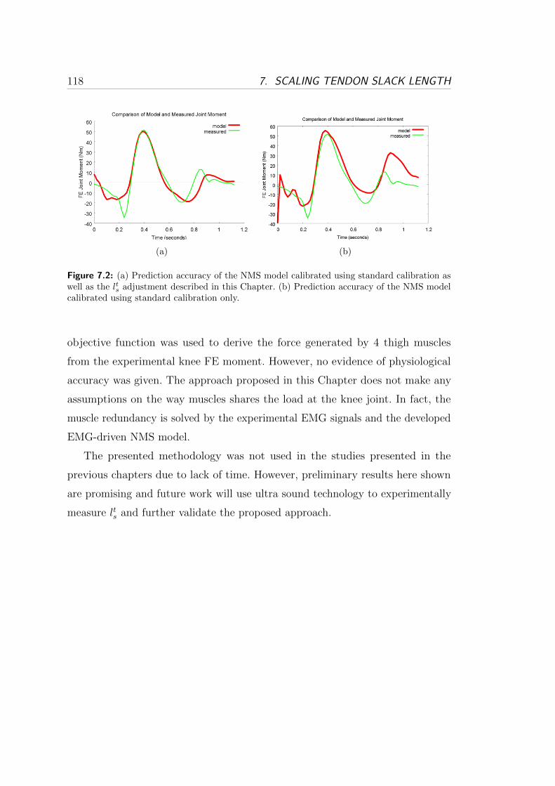
118 7. SCALING TENDON SLACK LENGTH
(a) (b)
Figure 7.2: (a) Prediction accuracy of the NMS model calibrated using standard calibration aswell as the lts adjustment described in this Chapter. (b) Prediction accuracy of the NMS modelcalibrated using standard calibration only.
objective function was used to derive the force generated by 4 thigh muscles
from the experimental knee FE moment. However, no evidence of physiological
accuracy was given. The approach proposed in this Chapter does not make any
assumptions on the way muscles shares the load at the knee joint. In fact, the
muscle redundancy is solved by the experimental EMG signals and the developed
EMG-driven NMS model.
The presented methodology was not used in the studies presented in the
previous chapters due to lack of time. However, preliminary results here shown
are promising and future work will use ultra sound technology to experimentally
measure lts and further validate the proposed approach.
Chapter 8
Classification of Locomotion
Modes
The previous Chapters of this thesis focused on the design and validation of the
multi-DOF EMG-driven NMS model of the lower limb. This was presented as a
means for establishing an EMG-based interface for the continuous extraction of
somatosensory information from the human movement and provide an effective
solution to actively control lower limb powered orthoses.
This Chapter, takes a different path. EMG signals are evaluated by a phase-
dependent Support Vector Machine (SVM) classifiers for the identification of
locomotion modes. This approach does not rely on biologically relevant models of
the human musculoskeletal system and does not aim to realize continuous device
control. The aim is to obtain context knowledge from the movement the user wants
to perform, i.e. understanding whether the subject wants to walk rather than
turning left or right and so forth. This study was conducted with the plan of
combining the EMG-driven NMS model presented in the previous Chapters with
the EMG-classifier to achieve a superior neuromuscular HMI that maximizes the
information exchange between the human and the machine. More details about
this integration will be provided in the following Sections.
119
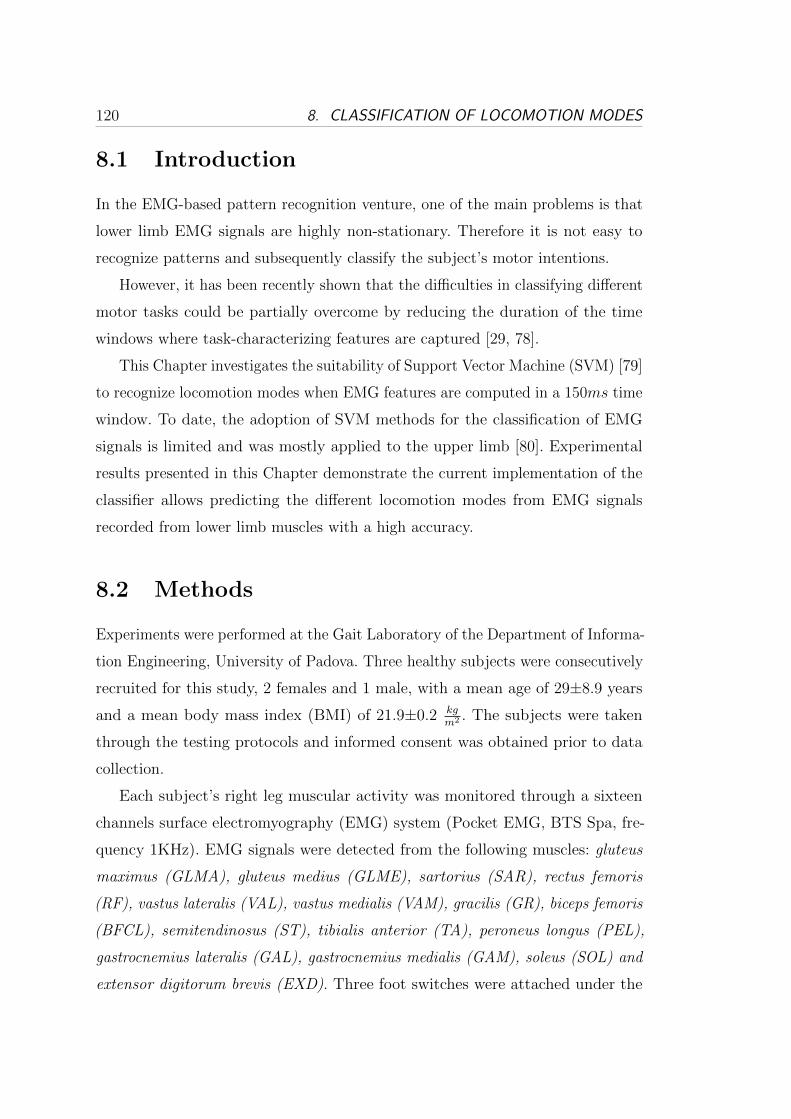
120 8. CLASSIFICATION OF LOCOMOTION MODES
8.1 Introduction
In the EMG-based pattern recognition venture, one of the main problems is that
lower limb EMG signals are highly non-stationary. Therefore it is not easy to
recognize patterns and subsequently classify the subject’s motor intentions.
However, it has been recently shown that the difficulties in classifying different
motor tasks could be partially overcome by reducing the duration of the time
windows where task-characterizing features are captured [29, 78].
This Chapter investigates the suitability of Support Vector Machine (SVM) [79]
to recognize locomotion modes when EMG features are computed in a 150ms time
window. To date, the adoption of SVM methods for the classification of EMG
signals is limited and was mostly applied to the upper limb [80]. Experimental
results presented in this Chapter demonstrate the current implementation of the
classifier allows predicting the different locomotion modes from EMG signals
recorded from lower limb muscles with a high accuracy.
8.2 Methods
Experiments were performed at the Gait Laboratory of the Department of Informa-
tion Engineering, University of Padova. Three healthy subjects were consecutively
recruited for this study, 2 females and 1 male, with a mean age of 29±8.9 years
and a mean body mass index (BMI) of 21.9±0.2 kgm2 . The subjects were taken
through the testing protocols and informed consent was obtained prior to data
collection.
Each subject’s right leg muscular activity was monitored through a sixteen
channels surface electromyography (EMG) system (Pocket EMG, BTS Spa, fre-
quency 1KHz). EMG signals were detected from the following muscles: gluteus
maximus (GLMA), gluteus medius (GLME), sartorius (SAR), rectus femoris
(RF), vastus lateralis (VAL), vastus medialis (VAM), gracilis (GR), biceps femoris
(BFCL), semitendinosus (ST), tibialis anterior (TA), peroneus longus (PEL),
gastrocnemius lateralis (GAL), gastrocnemius medialis (GAM), soleus (SOL) and
extensor digitorum brevis (EXD). Three foot switches were attached under the
8.2. METHODS 121
monitored foot in correspondence of the first and fifth metatarsal head, and the
calcaneus. A 6-camera (150Hz) motion capture system (BTS SpA, Padova) was
used to collect lower limb kinematics, synchronized with the EMG acquisition
system. Each subject performed the motion tasks bare foot including: level walk-
ing, stepping over an obstacle, turning right, ascending stairs, descending stairs,
standing still. Stepping over an obstacle was performed asking the subject to step
over a wooden block of 14.5 cm hight, 40 cm width and 28.5 cm depth, while
walking. In this context the non-tested side passed over the obstacle first, followed
by the instrumented leg. A two-step staircase 16 cm high, 80 cm wide, and 28
cm deep was used for the stair ascending and descending test. The turning right
was acquired asking the subject to perform a 90∘ turn while walking, pivoting on
their own controlateral leg. Each subject performed the 6 motion modes randomly
during each trial within the same experimental session. At least 12 complete stride
cycles of each task were acquired.
8.2.1 Signal Analysis
The first and the last strides were excluded from each trial due to noise introduced
by gait initiation and termination. Each subject’s gait speed was measured by
using the foot switch to verify whether it fell within the normal range. Indeed,
muscle activation patterns are related to gait velocity [81]. Timings of footContact
and footOff events were identified by means of basographic and motion analysis
data. The footContact event is characterized by the activation of any of the three
foot switch signals. The footOff event is recognized by the deactivation of all
signals. Analysis windows within which data were processed and classified, were
identified as occurring immediately before the foot-contact and after the foot-
off events. Four phases were taken into consideration: preContact, postContact,
preOff and postOff (Fig. 8.1). The window length was set to 150ms following
recommendations in literature: EMG signals can be considered quasi-stationary
within 200ms intervals, while they are not sufficiently informative when analysis
windows shorter than 50ms are used [29]. Features were extracted from EMG
linear envelopes (Section 2.1).
Features defined in the time-domain were used. These included: mean absolute

122 8. CLASSIFICATION OF LOCOMOTION MODES
Figure 8.1: Example of filtered EMG signals for two types of locomotion modes (left: levelground walking; right: ascending stairs). A contact-to-contact cycle is reported. footContact andfootOff events are shown (green and red vertical lines, respectively). Analysis windows that aretaken into consideration are also highlighted: from left to right, the first green area correspondsto postContact phase, then preOff and postOff (red areas) occur respectively before and afterfootOff, finally preContact is shown as occurring before the following footContact event (lastgreen area).
value (MAV), number of zero-crossings (ZC), waveform length (WFL), number
of slope sign changes (SSC), root mean square (RMS) [78]. Furthermore, 3rd-
order auto-regression coefficients (AR1, AR2, AR3) as defined in [29] were also
considered.
8.2.2 Support Vector Machine
Support vector machine (SVM) is a well-established technique used to classify
a novel set of data after a training process that is conducted on a collection of
pre-classified events. In this study, the pre-classified events are feature vectors
associated to the same phase but generated during different locomotion modes.
During the training process, the pre-classified event vectors are prescribed to SVM
together with the information associated to the respective locomotion mode.

8.2. METHODS 123
Figure 8.2: Two classes are not linearly separable in the input space X. A kernel function isused to map X in a feature space H where the two classes become linearly separable. Thehyperplane built by SVM algorithm in H corresponds to a non-linear solution in the input spaceX.
A detailed description of the theoretical foundations and applications associated
to SVM can be found in [79, 82]. This Section briefly describes the ideas and
motivations behind SVM, explaining its four basic concepts: 1) the separating
hyperplane, 2) the kernel function, 3) the optimal separating hyperplane, and 4)
the soft margin. An introduction on the extension to multi-class classification will
be also given.
The main objective of a SVM algorithm is to identify a line, or hyperplane in a
n-dimensional space H (Fig. 8.2), separating a set of input points, each one known
to belong to either one of two different classes. If the algorithm is successful in
finding an hyperplane that reduces the probability of misclassifying future data,
the new sample is easily classified based on what side of the hyperplane it lies on.
However, it is often not possible to linearly separate the data represented in
the original space X. The idea is that, by mapping the input data into a higher
dimensional space H, a linear separation my be achievable. The mapping is done
by using the kernel function. The objective is to find the kernel function that
allows the data to be linearly separated while keeping the final dimension of the
H space reasonable.
In the higher dimensional space H, it is usually possible to identify several
linear classifiers that separate the data. The optimal separating hyperplane (OSH)
allows maximizing the margin that separates the distance between the hyperplane
and the nearest data points of each class. The points closest to OSH are called
124 8. CLASSIFICATION OF LOCOMOTION MODES
support vectors.
Data can often contain errors. To deal with the noise in the training data, the
standard OSH algorithm would usually overfit the data. That is, the solution is
found, but the price you pay is a useless increment in the dimension of the feature
space H. To tolerate training errors, the SVM algorithm was modified introducing
the concept of soft margin. This allows accepting a few outliers on the wrong side
of the hyperplane. The definition of the proper number of outliers and the size of
the margin, requires a process of parameter tuning for the specific problem.
The generalization to multiclass SVM classification can be achieved with
different methods. Two common strategies include: 1) one-against-all and 2) one-
against-one. In the one-against-all approach, SVM compares one pre-classified
class to the samples of all the other classes. This is done for each class. The one-
against-one approach is often a more robust solution because it allows minimizing
the amount of misclassifications [83]. This approach is based on binary classifiers
which compare one given class to another one. Given m classes, m(m− 1) binary
classifiers are generated and trained to recognize the right class from a given pair.
A bottom-up binary tree is created to perform the pair-classification on the whole
data set. The given m classes are first arranged in m/2 pairs. At the binary tree
lowest level, m/2 classes are selected by m/2 classifiers from the initial m/2 pairs.
Each classifier is trained with data taken from a different pair. The m/2 selected
classes as regarded as winner-classes. These access the next upper-level. Here, m/4
classifiers, which are trained on the pairs associated to the winner classes, select
the next m/4 winner-classes that are allowed to access the next step. The class
that reaches the root of the binary tree, is the class predicted by the multiclass
SVM.
8.3 Validation Procedure
To quantify the classification accuracy of our methodology, the leave-one-out
cross-validation (LOOCV) approach was used. This is used in situations in which
a limited set of samples is available for validation. Every sample in the dataset is
used to test the multiclass SVM trained on the rest of the samples. Performances

8.3. VALIDATION PROCEDURE 125
can therefore be quantified in terms of overall classification error, i.e. the ratio
between the number of samples that are not classified correctly and the size of
the whole dataset. LOOCV ratios are summarized in a confusion matrix. This is
a square matrix of size m, where m is the number of the classes. The cij element
represents the percentage of samples belonging to class j that are misclassified as
belonging to class i. If no errors occur, the confusion matrix is an identity matrix
with non-zero elements only on the main diagonal. The confusion matrix allows
identifying the pairs of classes that are not properly separated by the OSH.
The proposed multiclass SVM classifier was implemented in a custom C++ us-
ing the Open-Source library libSVM [84]. This provides standard implementations
of different SVM algorithms as well as a set of tools to automatically optimize
SVM parameters. A RBF kernel function was used in this study as previous
research demonstrated it achieves good performances in the classification of upper
limb motions [80].
Validation comprised three tests. For each phase, results were averaged over all
subjects and locomotion modes. The first test assessed what combination of EMG
features gives the best classification performances on different phases. The second
test assessed whether the classification accuracy of the proposed multiclass SVM
method varies depending on the phase that is used to extract the features from.
The third test assessed how classification accuracy was influenced by reducing the
number of muscles to extract the EMG features from. This was done to obtain the
optimal minimum set of muscles that allows minimizing the the amount of input
data and sensors needed. In the context of the design of wearable devices this
plays an important role. The muscles selected for this study were chosen based on
the physiology governing their recruitment during the analyzed motion modes.
Furthermore, their activation timing was also considered. The GLMA, GLME,
and BFCL muscles regulate hip extension, which is particularly important during
preContact and postContact phases. The GLMA and BFCL muscles, together
with GR, are also hip adductors and are activated in preOff and postOff phases.
The GLME muscles acts as hip abductor during the footContact phase. Hip flexion
is mainly regulated by RF, GR and SAR during postContact, preOff and postOff
phases. As for knee motion, it is mainly regulated by quadriceps’ VAL, VAM,
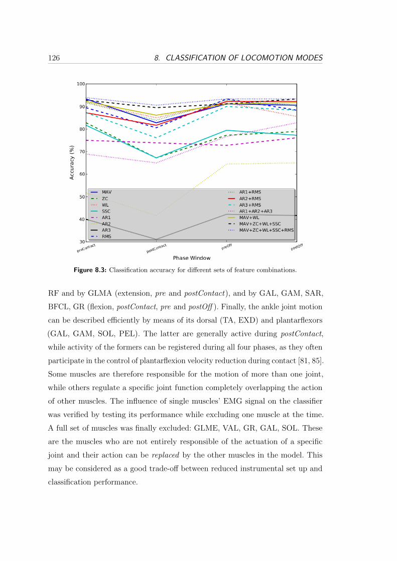
126 8. CLASSIFICATION OF LOCOMOTION MODES
Figure 8.3: Classification accuracy for different sets of feature combinations.
RF and by GLMA (extension, pre and postContact), and by GAL, GAM, SAR,
BFCL, GR (flexion, postContact, pre and postOff ). Finally, the ankle joint motion
can be described efficiently by means of its dorsal (TA, EXD) and plantarflexors
(GAL, GAM, SOL, PEL). The latter are generally active during postContact,
while activity of the formers can be registered during all four phases, as they often
participate in the control of plantarflexion velocity reduction during contact [81, 85].
Some muscles are therefore responsible for the motion of more than one joint,
while others regulate a specific joint function completely overlapping the action
of other muscles. The influence of single muscles’ EMG signal on the classifier
was verified by testing its performance while excluding one muscle at the time.
A full set of muscles was finally excluded: GLME, VAL, GR, GAL, SOL. These
are the muscles who are not entirely responsible of the actuation of a specific
joint and their action can be replaced by the other muscles in the model. This
may be considered as a good trade-off between reduced instrumental set up and
classification performance.
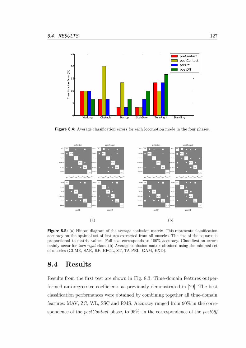
8.4. RESULTS 127
Figure 8.4: Average classification errors for each locomotion mode in the four phases.
(a) (b)
Figure 8.5: (a) Hinton diagram of the average confusion matrix. This represents classificationaccuracy on the optimal set of features extracted from all muscles. The size of the squares isproportional to matrix values. Full size corresponds to 100% accuracy. Classification errorsmainly occur for turn right class. (b) Average confusion matrix obtained using the minimal setof muscles (GLME, SAR, RF, BFCL, ST, TA PEL, GAM, EXD).
8.4 Results
Results from the first test are shown in Fig. 8.3. Time-domain features outper-
formed autoregressive coefficients as previously demonstrated in [29]. The best
classification performances were obtained by combining together all time-domain
features: MAV, ZC, WL, SSC and RMS. Accuracy ranged from 90% in the corre-
spondence of the postContact phase, to 95%, in the correspondence of the postOff
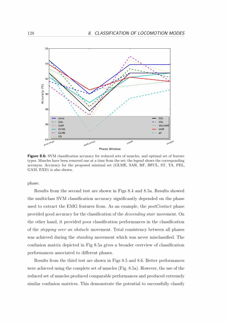
128 8. CLASSIFICATION OF LOCOMOTION MODES
Figure 8.6: SVM classification accuracy for reduced sets of muscles, and optimal set of featuretypes. Muscles have been removed one at a time from the set; the legend shows the correspondingacronym. Accuracy for the proposed minimal set (GLME, SAR, RF, BFCL, ST, TA, PEL,GAM, EXD) is also shown.
phase.
Results from the second test are shown in Figs 8.4 and 8.5a. Results showed
the multiclass SVM classification accuracy significantly depended on the phase
used to extract the EMG features from. As an example, the postContact phase
provided good accuracy for the classification of the descending stair movement. On
the other hand, it provided poor classification performances in the classification
of the stepping over an obstacle movement. Total consistency between all phases
was achieved during the standing movement which was never misclassified. The
confusion matrix depicted in Fig 8.5a gives a broader overview of classification
performances associated to different phases.
Results from the third test are shown in Figs 8.5 and 8.6. Better performances
were achieved using the complete set of muscles (Fig. 8.5a). However, the use of the
reduced set of muscles produced comparable performances and produced extremely
similar confusion matrices. This demonstrate the potential to successfully classify

8.5. COMBINING THE EMG-DRIVEN NMSMODEL TO THE SVM CLASSIFIER129
locomotion modes using a reduced set of lower limb muscles.
In general, the misclassification errors were associated to tasks that were quite
similar and the corresponding EMG features naturally assumed similar trends.
Misclassification is mainly associated to walking, stepping over an obstacle and
turning. In this study the obstacles that were used were particularly narrow and
low. Furthermore, turning were not abrupt. There were therefore classified as
ground-level walking.
8.5 Combining the EMG-driven NMS Model to
the SVM Classifier
The study presented in this Chapter aims to be directly integrated with the
EMG-driven NMS model presented in the previous Chapters. This integration
can be implemented in two ways.
The first way is to use the EMG-driven NMS model to provide more stationary
and more descriptive input data for the classifier. In this context the NMS model is
used to convert EMG signals into muscle force. This is a more stable signal which
better describes the action of single muscles and better differentiate locomotion
modes. The hypothesis is that classifying muscle forces instead of EMG signals
will provide a straightforward solution to improve classification performances. This
will also allow using wider time windows to extract the force features from. This
application can help improve the control of robotics prostheses.
The second way is to use the context knowledge on the locomotion mode
provided by the classifier to improve the operation of the EMG-driven NMS model.
This will help improving the force prediction for those muscles whose EMG activity
cannot be recorded experimentally such as the Psoas and Illiacus muscles. Indeed,
by knowing what kind of movement the subject wants to perform it is possible to
use task-specific objective functions in optimization problems to share the residual
joint moments to those two muscles. This approach is superior to the approach
currently used in literature in which one single objective function is used to solve
an optimization problem for all movements.
130 8. CLASSIFICATION OF LOCOMOTION MODES
8.6 Conclusions and Future Work
This paper presented a classifier based on support vector machine. Experimental
results showed that SVM provides good accuracy when a time dependent multi-
feature set is used. Misclassification errors were mostly on pair of tasks with high
similarity, such as walking and stepping over an obstacle. Results on the selection
of important muscles demonstrated that it is possible to reduce the number of
EMG signals without significantly affecting the classifier accuracy. This allows to
reduce the number of electrodes to place on the leg, thus improving the usability
of powered orthoses. Future studies will integrate the SVM classifier and the
EMG-driven NMS model presented in the previous Chapters within a common
framework. This will allow reducing the limitation that both methods inherently
have.

Chapter 9
Conclusions
This work presented the design and development of a novel EMG-driven Neuro-
MusculoSkeletal (NMS) model of the human lower limb. The theoretical results
that were obtained provided solutions to better understand the mechanisms of
human muscle actuation. Understanding these mechanisms is the key to realize
effective human interaction with wearable assistive devices. This work did not
realize real-time synchronization with powered orthoses. Neither did it improve
disabled people’s mobility using robotics assistive devices.
This work provided the technology needed to achieve this, i.e. to establish an
EMG-driven human-machine interface (HMI) for the simultaneous actuation of
multiple joints in a lower limb powered orthosis. The software developed in this
thesis will be made available to researchers who wish to use this technology.
Neuromusculoskeletal modeling technology not only can offer great solutions
for exoskeletons control and humanoids actuation, but can also boost research
that aims to realize more realistic virtual humans by providing a more accurate
estimation of the human internal state.
9.1 Summary
Chapter 1 defined the research problem investigated within this thesis. It gave an
overview of the research conducted in the field of EMG-driven musculoskeletal
modeling, it highlighted the novelty and the significance of the proposed research
131
132 9. CONCLUSIONS
as well as the research questions to be addressed and the boundaries within which
this research work investigates.
Chapter 2 presented the general workflow used in this study. It described how
the the human movement can be recorded utilizing motion capture technology
and digitized to create realistic motion simulations. The OpenSim Application
Programming Interface (API) was used in a custom C++ program to develop
advanced methods for the simulation of the human movement and provide the
most accurate input for the NMS model. A new knee joint model was developed in
which functional axes could be defined and scaled to the subject’s characteristics.
Also, a foot-ground contact model was created using an elastic foundation model
and used in conjunction with Residual Reduction Analysis (RRA) to derive even
more accurate estimates of joint loading during movement. The use of the OpenSim
API allowed for a direct integration of OpenSim’s optimization algorithms into
the NMS model framework. This provided full access to a number of powerful
software tools including: Functional Scaling, Inverse Kinematics, and Residual
Reduction Analysis.
Chapters 3 and 4 presented a novel muscle dynamics model and a novel mus-
culotendon kinematics model respectively. These are used by the EMG-driven
NMS model to achieve fast operation and high muscle force and joint moment
predictive accuracy. The muscle dynamics model was designed under the assump-
tion that tendons are infinitely-stiff. This allowed eliminating the need for solving
an ordinary differential equation at each time step for the computation of mus-
cle fibre length and the subsequent musculotendon force. The infinitely stiffness
assumption allowed obtaining a closed-form expression that could be computed
inexpensively. Results showed the stiff-tendon model could be executed 250 times
faster than the elastic-tendon model with no loss of accuracy in the prediction of
joint moments. The musculotendon kinematics model was design to allow fast and
accurate estimation of musculotendon length (lmt) and muscle moment arms (r).
These values are used by the muscle dynamics model to compute musculotendon
force. The musculotendon kinematics model uses a single multidimensional cubic
spline per muscle to generate estimates for both lmt and r from nominal values of
musculotendon length only, corresponding to discrete combinations of generalized
9.1. SUMMARY 133
coordinates. This method provided fast and accurate estimation of musculotendon
kinematics and superior results in terms of fitting accuracy with respect to the
approach currently used in literature that is based on polynomial regression.
Chapter 3 also illustrated how the proposed NMS model can be used to control
a powered orthosis for the knee joint support. Furthermore, it demonstrates the
proposed EMG-driven NMS model is fast enough to meet the real-time deadline
associated to this specific application. Chapter 3 suggested how the NMS model
can be used to actuate humanoid robots equipped with artificial muscles.
In Chapter 5 a novel method is developed to achieve faster calibration of
EMG-driven models based on elastic tendons. Indeed, some applications may
require accurate estimates of the instantaneous tendon and muscle fibre lengths.
The idea was that of using the stiff-tendon muscle model to quickly solve a
global optimization problem and obtain a sub-optimal parameter set for the
elastic-tendon model. A refinement step is then performed to further refine the
initial sub-optimal solution. Results showed the proposed methodology allowed
calibrating the elastic-tendon model achieving the same calibration accuracy of
the procedures currently used in literature but in significantly less time.
Chapter 6 extended the results obtained in the previous Chapter to realize a
novel multi-DOF EMG-driven NMS model. It was shown it is possible to use EMG
signals recorded from 16 muscles to estimate the activity of 34 musculotendon
actuators (MTAs) in the lower limb. A novel calibration algorithm was designed
to constrain the operation of each MTA in the model to satisfy the moments
simultaneously produced at the hip, knee and ankle joints about 4 degrees of
freedom including: hip adduction-abduction, hip flexion-extension, knee flexion-
extension and ankle dorsi-plantar flexion. To date, only single-DOF EMG-driven
NMS models were proposed. That is, EMG signals were used to estimate muscle
forces that satisfy moments about a single DOF of a single joint only. Results
showed that the force that a muscle can generate during a specific movement
can be predicted in extremely different ways when different single-DOF models
are used. This fact introduces indeterminacy as it is not possible to know what
single-DOF model is best to use. The proposed multi-DOF NMS model allows
removing this indeterminacy by providing a single solution to the problem. As

134 9. CONCLUSIONS
a result, the multi-DOF model was able to produce muscle force estimates that
were more in line with biomechanics findings. The multi-DOF EMG-driven model
significantly improved the estimation of the force produced by biarticular muscles.
Results obtained using the single-DOF knee flexion-extension model showed it
could not properly predict the activity of the Rectus Femoris muscle. This is a
muscle crossing both the hip and knee joint and it is mostly active during running
to support the hip flexion-extension movement. The proposed multi-DOF NMS
model did not fail to catch such important feature because it properly constrained
its operation to satisfy not only the knee flexion-extension moments but also the
hip flexion-extension moments.
Chapter 7 presented a new technique to scale the tendon slack length of each
individual musculotendon unit in the model. Experiments proved that a good
rationale to scale tendons is to preserve the consistency of the EMG-to-activation
relationship across the whole joint operating range of motion. Results proved this
new scaling technique allows deriving physiologically appropriate estimates of the
tendon length and significantly contributes to improve the prediction accuracy of
the NMS model.
In Chapter 8, EMG signals were evaluated by a phase-dependent Support
Vector Machine (SVM) classifier for the identification of locomotion modes. This
approach did not rely on biologically relevant models of the human musculoskeletal
system and did not aim to realize continuous device control. The aim was to obtain
context knowledge of the movement the user wants to perform, i.e. understanding
whether the subject wants to walk rather than turning left or right and so forth.
This study was conducted with the plan of combining the EMG-driven NMS
model presented in this thesis with the EMG-classifier to achieve a superior
neuromuscular HMI that maximizes the information exchange between the human
and the machine.
9.2 Future Work
This research work was conducted on healthy subjects only. Future work will
therefore test the behavior of the model on disabled people.

9.2. FUTURE WORK 135
In this work, the EMG-driven NMS model was used to predict muscle force
and joint moments using data previously collected during the subject’s movement.
This work represented the first step towards the creation of a neuromuscular
HMI for assistive device control. Therefore, the study was focused on the pure
validation of the model operation and not on its synchronization with real-time
data acquisition systems. Future studies will integrate the proposed EMG-driven
NMS model into real-time systems. This will allow executing the NMS model in
parallel to the subject’s movement and obtaining real-time estimates of muscle
force and joint moments. This work designed and developed the technology for
achieving this. The next step will then be that of utilizing the real-time NMS
model to control a real powered orthosis.
This research work combined for the first time advanced motion simulation
techniques (Chapter 2) to EMG-driven NMS modeling (Chapters 3 and 6). This
process integrated anatomical and dynamic consistency into NMS model. Future
work will validate whether providing input data that better represent the dynamics
of the human movement, improves the ability of the EMG-driven NMS model to
learn the prescribed muscle dynamics.
Fast operation in calibration will be further exploited in future research to
develop more advanced algorithms for the continuous calibration of the model
biomechanical parameters. As the NMS model executes, the on-line calibration
algorithm will keep refining those parameters that vary with muscle fatigue such
as: optimal fiber length, maximum isometric force, maximum EMG. This will
allow designing more advanced powered orthosis control systems that will be
able to adapt to the user’s conditions on the fly. Fast operation in execution will
be exploited in future research to further extend the multi-DOF EMG-driven
NMS model (Chapter 6) to whole-body level. This study will assess whether the
proposed approach can be scaled up to simulate all muscles in the human body
maintaining fast execution and calibration.
The use of the proposed spline method in Chapter 4 is not limited to fitting
lmt data from musculoskeletal geometry software packages such as OpenSim [46].
Alternatively, lmt could be determined from the centriods of three dimensional
muscles based on MRI data or from three dimensional geometric modeling of
136 9. CONCLUSIONS
musculoskeletal systems. In this context the spline approach can be used to create
a multivariate function that can reliably replicate the behavior of complex systems
at low computational cost.
The multi-DOF NMS model presented in Chapter 6 will be extended to include
predictive algorithms for the estimation of the activation of muscles without EMG.
This will be achieved by using the context knowledge from the locomotion mode
provided by the SVM classifier presented in Chapter 8. Indeed, by knowing what
kind of movement the subject wants to perform it is possible to use task-specific
objective functions in optimization problems to share the residual joint moments
to muscles for which EMG signals are not available. This approach is superior to
the approach currently used in literature in which one single objective function is
used to solve an optimization problem for all movements.
The multi-DOF NMS model (Chapter 6) will be also used to actuate humanoid
robots that have a musculoskeletal architecture and artificial muscles by following
the approach illustrated in Section 3.8. Experiments will be done in simulation.
The approach proposed in Chapter 7 to scale tendon slack length will be
further validated using ultra sound technology to experimentally measure the
tendon length and compare experimental values to the predicted estimates.
The EMG-driven NMS model will be used in future studies to provide more
stationary and more descriptive input data for the SVM classifier (Chapter 8).
Precisely, the NMS model will convert EMG signals into muscle force. Experiments
will then assess whether classification performance will benefit from this.

Bibliography
[1] F. E. Zajac, “Muscle and tendon: properties, models, scaling, and application
to biomechanics and motor control,” Crit. Rev. Biomed. Eng., vol. 17, no. 4,
pp. 359–411, 1989.
[2] T. Buchanan, D. G. Lloyd, K. Manal, and T. Besier, “Neuromusculoskeletal
modeling: Estimation of muscle forces and joint moments and movements
from measurements from neural command,” J. of Applied Biomechanics,
vol. 20, no. 4, pp. 367–395, 2004.
[3] D. G. Lloyd and T. F. Besier, “An EMG-driven musculoskeletal model to
estimate muscle forces and knee joint moments in vivo,” J. of Biomech.,
vol. 36, no. 6, pp. 765–776, 2003.
[4] D. Lloyd, T. Besier, C. Winby, and T. Buchanan, “Neuromusculoskeletal
modelling and simulation of tissue load in the lower extremities,” in Routledge
handbook of Biomechanics and Human Movement Science, Y. Hong and
R. Barlett, Eds., 2008, pp. 3–17.
[5] M. Viceconti, G. Clampworthy, and S. Jan, “The virtual human: A european
initiative for in silico human modeling,” J. Physiol Sci., vol. 58, no. 7, pp.
441–446, 2008.
[6] Y. Nakamura, K. Yamane, Y. Fujita, and S. I., “Somatosensory computation
for man-machine interface from motion-capture data and musculoskeletal
human model,” IEEE Trans. Robot., vol. 21, no. 1, pp. 58–66, 2005.
[7] J. Pons, Ed., Wearable Robots. Biomechatronic Exoskeletons. Wiley, 2008.
137
138 BIBLIOGRAPHY
[8] A. Dollar and H. Herr, “Lower extremity exoskeletons and active orthoses:
Challenges and state-of-the-art,” IEEE Trans. Biomed. Eng., vol. 24, no. 1,
pp. 144–158, 2008.
[9] C. Fleischer and G. Hommel, “A human-exoskeleton interface utilizing elec-
tromyography,” IEEE Trans. Robot., vol. 24, no. 4, pp. 872–882, 2008.
[10] E. Cavallaro, J. Rosen, J. Perry, and S. Burns, “Real-time myoprocessors for
a neural controlled powered exoskeleton arm,” IEEE Trans. Biomed. Eng.,
vol. 53, no. 11, pp. 2387–2396, 2006.
[11] S. Delp, F. Anderson, A. Arnold, P. Loan, A. Habib, C. John, E. Guendelman,
and D. Thelen, “Opensim: Open-source software to create and analyze dy-
namic simulations of movement,” IEEE Trans. Biomed. Eng., vol. 54, no. 11,
pp. 1940–1950, Nov. 2007.
[12] K. Narioka and K. Hosoda, “Designing synergistic walking of a whole-body hu-
manoid driven by pneumatic artificial muscles: An empirical study,” Advanced
Robotics, vol. 22, no. 10, pp. 1107–1123, 2008.
[13] T. Yoshikai, I. Mizuuchi, D. Sato, S. Yoshida, M. Inaba, and H. Inoue,
“Behavior system design and implementation in spined musle-tendon humanoid
kenta,” J. of Robotics and Mechatronics, vol. 15, no. 2, pp. 143–152, 2003.
[14] M. Vukobratovic, D. Hristic, and Z. Stojiljkovic, “Development of active
anthropomorphic exoskeletons,” Med. Biol. Eng., vol. 12, no. 1, pp. 66–80,
1974.
[15] D. P. Ferris, K. E. Gordon, G. S. Sawicki, and A. Peethambaran, “An
improved powered ankle-foot orthosis using proportional myoelectric control,”
Gait Posture, vol. 23, no. 4, pp. 425–428, 2006.
[16] K. Yamamoto, M. Ishii, K. Hyodo, T. Yoshimitsu, and T. Matsuo, “Devel-
opment of power assisting suit (miniaturization of supply system to realize
wearable suit),” JSME Intl. Journal Series C, vol. 46, no. 3, pp. 923–930,
2003.

BIBLIOGRAPHY 139
[17] H. Kawamoto and Y. Sankai, “Power assist system hal-3 for gait disorder
person,” in Intl. Conf. Computers Helping People with Special Needs (ICCHP),
Lecture Notes on Computer Science (LNCS). Berlin, Germany: Springer
Verlag, 2002.
[18] H. Herr, “Exoskeletons and orthoses: classification, design challenges and
future directions,” J. NeuroEngineering and Rehabilitation, vol. 6, no. 1, p. 21,
2009.
[19] A. Zoss, H. Kazerooni, and A. Chu, “Biomechanical design of the berkeley
lower extremity exoskeleton (bleex),” IEEE/ASME Trans. Mechatronics,
vol. 11, no. 2, pp. 128 –138, 2006.
[20] J. Pratt, S. H. Collins, B. Krupp, and K. Morse, “The roboknee: An exoskele-
ton for enhancing strength and endurance during walking,” in IEEE Intl.
Conf. Robotics and Automation, 2004.
[21] J. M. Carmena, M. A. Lebedev, R. E. Crist, J. E. O’Doherty, D. M. Santucci,
D. F. Dimitrov, P. G. Patil, C. S. Henriquez, and M. A. L. Nicolelis, “Learning
to control a brainmachine interface for reaching and grasping by primates,”
PLoS Biol, vol. 1, no. 2, pp. 192–208, 2003.
[22] G. Santhanam, S. Ryu, B. You, A. Afshar, and K. Shenoy, “A high-
performance braincomputer interface,” Nature, vol. 442, no. 2, pp. 195–198,
2006.
[23] L. Qin, L. Ding, and B. He, “Motor imagery classification by means of source
analysis for brain computer interface applications,” J. of Neural Engineering,
vol. 4, no. 2, pp. 65–72, 2005.
[24] A. d’Avella, P. Saltiel, and E. Bizzi, “Combinations of muscle synergies in
the construction of a natural motor behavior,” Nature Neuroscience, vol. 6,
no. 3, pp. 300–308, 2003.
[25] K. Pearson, O. Ekeberg, and A. Bushges, “Assessing sensory function in loco-
motor systems using neuro-mechanical simulations,” Trend in Neurosciences,
vol. 29, no. 11, pp. 625–631, 2006.

140 BIBLIOGRAPHY
[26] R. Merletti, Electromyography: Physiology, Engineering, and Non-Invasive
Applications, P. Parker, Ed. IEEE Pres., 2004.
[27] A. Nordez, T. Gallot, S. Catheline, A. Guvel, C. Cornu, and F. Hug, “Elec-
tromechanical delay revisited using very high frame rate ultrasound,” J. of
Applied Physiology, vol. 106, no. 6, pp. 1970–1975, 2009.
[28] G. Li, A. Schultz, and T. Kuiken, “Quantifying pattern recognition-based
myoelectric control of multifunctional transradial prostheses,” IEEE Trans.
Neural Syst. Rehabil. Eng., vol. 18, no. 2, pp. 185 –192, 2010.
[29] H. Huang, T. Kuiken, and R. Lipschutz, “A strategy for identifying locomotion
modes using surface electromyography,” IEEE Trans. Biomed. Eng., vol. 56,
no. 1, pp. 65 –73, 2009.
[30] C. Pattichis, C. Schizas, and L. Middelton, “Neural network models in emg
diagnosis,” IEEE Trans. Biomed. Eng., vol. 42, no. 5, pp. 486–496, 1995.
[31] R. Norman, “A barrier to understanding human motion mechanisms: a
commentary,” in Future directions in exercise and sport science research,
C. L. D. Skinner, J.S. Corbin, Ed., 1989, pp. 151–161.
[32] J. Soechting and F. M., “Evaluating an integrated musculoskeletal model
of the human arm.” J. of Biomechanical Engineering, vol. 119, no. 1, pp.
93–102, 1997.
[33] M. Nussbaum and D. Chaffin, “Lumbar muscle force estimation using a
subject-invariant 5-parameter emg-based model,” J. of Biomechanics, vol. 31,
no. 7, pp. 667 – 672, 1998.
[34] B. Laursen, B. Jensen, G. Nmeth, and G. Sjgaard, “A model predicting
individual shoulder muscle forces based on relationship between electromyo-
graphic and 3d external forces in static position,” J. of Biomechanics, vol. 31,
no. 8, pp. 731 – 739, 1998.
BIBLIOGRAPHY 141
[35] C. Winby, D. Lloyd, and T. Kirk, “Evaluation of different analytical methods
for subject-specific scaling of musculotendon parameters,” J. of Biomech.,
vol. 41, no. 8, pp. 1682–1688, 2008.
[36] L. Schutte, “Using musculoskeletal models to explore strategies for improving
performance in electrical stimulation-inducted leg cycle ergonometry.” Ph.D.
dissertation, Stanford University, 1992.
[37] D. G. Lloyd and T. S. Buchanan, “A model of load sharing between muscles
and soft tissues at the human knee during static tasks,” J. of Biomechanical
Engineering, vol. 118, no. 3, pp. 367–376, 1996.
[38] H. Kawamoto and Y. Sankai, “Comfortable power assist control method for
walking aid by hal-3,” in IEEE Intl. Conf. Systems, Man and Cybernetics,
2002.
[39] J. Challis and K. D.G., “An analytical examination of muscle force estimations
using optimization techniques.” Proc Inst Mech Eng H., vol. 207, no. 3, pp.
139–148, 1993.
[40] J. Challis, “Producing physiologically realistic individual muscle force estima-
tions by imposing constraints when using optimization techniques,” Medical
Engineering & Physics, vol. 19, no. 3, pp. 253 – 261, 1997.
[41] T. Buchanan and D. Shreeve, “An evaluation of optimization techniques for
the prediction of muscle activation patterns during isometric tasks.” J. of
Biomechanical Engineering, vol. 114, no. 4, pp. 565–74, 1996.
[42] J. Cholewicki, , and S. McGill, “Emg assisted optimization: A hybrid approach
for estimating muscle forces in an indeterminate biomechanical model,” J. of
Biomechanics, vol. 27, no. 10, pp. 1287 – 1289, 1994.
[43] C. Winby, D. Lloyd, T. Besier, and T. Kirk, “Muscle and external load con-
tribution to knee joint contact loads during normal gait.” J. of biomechanics,
vol. 42, no. 14, pp. 2294–2300, 2009.
142 BIBLIOGRAPHY
[44] S. Delp, J. Loan, M. Hoy, F. Zajac, E. Topp, and J. Rosen, “An interactive
graphics-based model of the lower extremity to study orthopaedic surgical
procedures,” IEEE Trans. Biomed. Eng., vol. 37, no. 8, pp. 757–767, 1990.
[45] “Simm software suite,” Available at: http://www.musculographics.com.
[46] “Opensim project overview,” Available at: https://simtk.org/home/opensim.
[47] T. Besier, D. Sturnieks, J. Anderson, and D. Lloyd, “Repeatability of gait
data using a functional hip joint centre and a mean helical knee axis,” J. of
Biomechanics, vol. 36, no. 8, pp. 1159–1168, 2003.
[48] C. Spoor and F. Veldpaus, “Rigid body motion calculated from spatial
co-ordinates of markers,” J. of Biomechanics, vol. 13, no. 4, pp. 391–393,
1980.
[49] C. Reinschmidt and T. van den Bogert, “Kinemat: a matlab toolbox for
three-dimensional kinematic analyses,” 1997.
[50] M. Stokdijk, C. G. M. Meskers, H. E. J. Veeger, Y. A. de Boer, and P. M.
Rozing, “Determination of the optimal elbow axis for evaluation of placement
of prostheses,” Clinical Biomechanics, vol. 14, no. 3, pp. 177 – 184, 1999.
[51] J. Kalker, “Three-dimensional elastic bodies in rolling contact,” in Solid
Mechanics and Its Application, K. A. Publishers, Ed., 1990.
[52] P. Huijing, “Important experimental factors for skeletal muscle modelling:
nonlinear changes of muscle length force characteristics as a function of degree
of activity,” European Journal of Morphology, vol. 34, no. 1, pp. 47–54, 1996.
[53] A. V. Hill, “The Heat of Shortening and the Dynamic Constants of Muscle,”
Proc. of the Royal Society of London. Series B, Biological Sciences, vol. 126,
no. 843, pp. 136–195, 1938.
[54] A. Guimaraes, W. Herzog, Y. Zhang, and S. Day, “Effects of muscle length on
the emg-force relationship of the cat soleus muscle studied using non periodic
stimulation of ventral root filaments.” J. of Experimental Biology, vol. 193,
no. 1, pp. 49–64, 1994.

BIBLIOGRAPHY 143
[55] J. Loan, Dymanics Pipeline. Evanston, IL: Musculographics Inc., 1992.
[56] K. Genovese, L. Lamberti, and C. Pappalettere, “Improved global-local simu-
lated annealing formulation for solving non-smooth engineering optimization
problems.” Intl. J. of Solids and Structures, vol. 42, no. 1, pp. 203 – 237,
2005.
[57] J. Potvin, R. Norman, and S. McGill, “Mechanically corrected emg for the
continuous estimation of erector spinae muscle loading during repetitive
lifting,” European Journal of Applied Physiology & Occupational Physiology,,
vol. 74, no. 1, pp. 119 – 132, 1996.
[58] A. Frigon and S. Rossignol, “Experiments and models of sensorimotor interac-
tions during locomotion,” Biological Cybernetics, vol. 95, no. 6, pp. 607–627,
2006.
[59] “Musculoskeletal robotics and mechanical testing core,” Available at: http:
//www.lerner.ccf.org/orc/cores/mrmtc/.
[60] I. Mizuuchi, Y. Nakanishi, Y. Sodeyama, Y. Namiki, T. Nishino, N. Mu-
ramatsu, J. Urata, K. Hongo, T. Yoshikai, and M. Inaba, “An advanced
musculoskeletal humanoid kojiro,” in IEEE-RAS Intl. Conf. Humanoids,
2007, pp. 294 – 299.
[61] I. Mizuuchi, T. Yoshikai, Y. Sodeyama, Y. Nakanishi, A. Miyadera, T. Ya-
mamoto, T. Niemela, M. Hayashi, J. Urata, Y. Namiki, T. Nishino, and
M. Inaba, “A musculoskeletal flexible-spine humanoid kotaro aiming at year
2020,” in 36th Intl. Symp. Robotics, 2005.
[62] K. Hosoda, T. Takuma, A. Nakamoto, and S. Hayashi, “Biped robot design
powered by antagonistic pneumatic actuators for multi-modal locomotion,”
Robotics and Autonomous Systems, vol. 56, no. 1, pp. 46–53, 2008.
[63] “The anybody modeling system,” Available at: http://www.anybodytech.
com/.

144 BIBLIOGRAPHY
[64] K. Artemiadis and K. Kyriakopoulos, “Emg-based position and force esti-
mates in coupled human-robot systems: Towards emg-controlled exoskeletons,”
Experimental Robotics, vol. 54, pp. 241–250, 2009.
[65] M. Sartori, M. Reggiani, C. Mezzato, and E. Pagello, “A lower limb emg-
driven biomechanical model for applications in rehabilitation robotics,” in
IEEE Intl. Conf. Advanced Robotics, 2009, pp. 144–158.
[66] M. Sartori, D. Lloyd, M. Reggiani, and E. Pagello, “A stiff tendon neuromus-
culoskeletal model of the knee,” in IEEE Workshop Advanced Robotics and
its Social Impacts, 2009, pp. 132–138.
[67] ——, “Fast operation of anatomical and stiff tendon neuromuscular models
in emg-driven modeling,” in IEEE Intl. Conf. Robotics and Automation, 2010,
pp. 2228–2234.
[68] C. Habermann and F. Kindermann, “Multidimensional spline interpolation:
Theory and applications,” Comput. Econ., vol. 30, no. 8, pp. 153–166, 2007.
[69] L. Menegaldo, D. Fleury, and H. Weber, “Moment arms and musculoten-
don lengths estimation for a three-dimensional lower-limb model,” J. of
Biomechanics, vol. 37, no. 9, pp. 1447–14 453, 2004.
[70] A. Arnold, S. Salinas, D. Asakawa, and S. Delp, “Accuracy of muscle moment
arms estimated from mri-based musculoskeletal models of the lower extremity.”
Computer Aided Surgery, vol. 5, no. 2, pp. 108 –119, 2000.
[71] S. Blemker, D. Asakawa, G. Gold, and S. Delp, “Image-based musculoskeletal
modeling: applications, advances, and future opportunities.” J. Magnetic
Resonance Imaging, vol. 25, no. 2, pp. 441 –451, 2007.
[72] J. Fernandez, P. Mithraratne, S. Thrupp, M. Tawhai, and P. Hunter, “Anatom-
ically based geometric modelling of the musculo-skeletal system and other
organs,” Biomechanics and Modeling in Mechanobiology, vol. 2, no. 3, pp.
139–155, 2004.
BIBLIOGRAPHY 145
[73] J. Fernandez and P. Hunter, “An anatomically based patient-specific finite el-
ement model of patella articulation: towards a diagnostic tool,” Biomechanics
and Modeling in Mechanobiology, vol. 4, no. 1, pp. 20–38, 2005.
[74] K. Oberhofer, N. Scott, K. Mithraratne, and I. Anderson, “Subject-specific
modelling of lower limb muscles in children with cerebral palsy.” Clinical
biomechanics, vol. 25, no. 1, pp. 88–94, 2010.
[75] K. McKinnon, “Convergence of the nelder–mead simplex method to a non-
stationary point,” SIAM J. on Optimization, vol. 9, no. 1, pp. 148–158,
1998.
[76] T. F. Besier, D. Lloyd, and T. Ackland, “Muscle activation strategies at the
knee during running and cutting maneuvers,” Medicine & Science in Sports
& Exercise, vol. 35, no. 1, pp. 119–127, 2003.
[77] S. Hamner, A. Seth, and S. Delp, “Muscle contributions to propulsion and
support during running,” J. of Biomechanics, vol. 43, no. 14, pp. 2709–2716,
2010.
[78] B. Hudgins, P. Parker, and R. Scott, “A new strategy for multifunction
myoelectric control,” IEEE Trans. Biomed. Eng., vol. 40, no. 1, pp. 82–94,
1993.
[79] T. Hormann, B. Scholkopf, and A. J. Smola, “Kernel methods in machine
learning,” The Annals of Statistics, vol. 36, no. 3, pp. 1171–1220, 2008.
[80] M. A. Oskoei and H. Hu, “Support vector machine-based classification scheme
for myoelectric control applied to upper limb,” IEEE Trans. Biomed. Eng.,
vol. 55, no. 8, pp. 1956–1965, 2008.
[81] J. Perry, Gait Analysis, Normal and Pathological Function. New York:
McGraw-Hill, 1992.
[82] O. Bousquet, S. Boucheron, and G. Lugosi, “Theory of classification: a survey
of recent advances,” ESAIM Probab. Statist., vol. 9, pp. 323–375, 2005.

146 BIBLIOGRAPHY
[83] C. W. Hsu and C. J. Lin, “A comparison of methods for multiclass support
vector machines,” IEEE Trans. Neural Netw., vol. 13, no. 2, pp. 415–425,
2002.
[84] C.-C. Chang and C.-J. Lin, LIBSVM: a library for support vector machines,
2001, software available at http://www.csie.ntu.edu.tw/∼cjlin/libsvm.
[85] D. Winder, “Biomechanics of normal and pathological gait: implications for
understanding human locomotor control,” J. Mot. Behav., vol. 21, no. 4, pp.
337–355, dec 1989.