Dipartimento di Scienze Economiche e Sociali

UNIVERSITÀ POLITECNICA DELLE MARCHE

DOES EXPORT COMPLEXITY MATTER FOR

FIRMS’ OUTPUT VOLATILITY?

Daniela Maggioni, Alessia Lo Turco, Mauro Gallegati∗

QUADERNI DI RICERCA n. 407ISSN: 2279-9575

December 2014

Comitato scientifico:

Renato BalducciMarco GallegatiAlberto NiccoliAlberto Zazzaro

Collana curata da:Massimo Tamberi

Contents1 Introduction 2

2 Literature Review 4

3 Data and Descriptive Statistics 63.1 Data sources and sample . . . . . . . . . . . . . . . . . . . . . . . . . . . . . . . . 63.2 Measuring export product complexity . . . . . . . . . . . . . . . . . . . . . . . . 7

4 The empirical analysis of the firm level complexity-volatility nexus 94.1 Empirical Model . . . . . . . . . . . . . . . . . . . . . . . . . . . . . . . . . . . . . 94.2 Baseline Results . . . . . . . . . . . . . . . . . . . . . . . . . . . . . . . . . . . . . 9

5 Robustness checks 125.1 Export or Product Complexity? . . . . . . . . . . . . . . . . . . . . . . . . . . . . 22

6 Looking for the channels: what drives the export complexity-volatility nexus? 25

7 Conclusions 30

Appendix 35A Additional Figures and Tables . . . . . . . . . . . . . . . . . . . . . . . . . . . . . 35

Does export complexity matter for�rms' output volatility?

Daniela Maggioni, Alessia Lo Turco, Mauro Gallegati∗

Abstract

With this paper we provide, for the first time to our knowledge, micro-level evidence on thenegative linkage between firm complexity and volatility. A higher sophistication level of afirm’s export basket reduces its output fluctuations. When focusing on a sample of exportingand non exporting firms, the average complexity of the production mix equally affects stabil-ity of sales of both groups. The stabilising role of firms’ production sophistication is drivenby complex products’ higher income elasticity, technological diversification and market en-try barriers.

JEL: F43, D22, E32, O12Keywords: Output fluctuations, Product Sophistication, Capabilities, Demand and supplychannels

∗ Common Affiliation of Authors: Università Politecnica delle Marche, Department of Economics and Social

Sciences; Piazzale Martelli 8, 60121 Ancona - Italy.

E-mail: d.maggioni@univpm.it, a.loturco@univpm.it, mauro.gallegati@univpm.it. Financial support from the EU

7th FP project RASTANEWS, grant no 320278 is gratefully acknowledged. We thank Jože Damijan, Francesco di

Comite, Philipp Marek, Christian Volpe Martincus and all participants to the 11th Annual FREIT-LETC Conference

for useful comments and suggestions.

Corresponding Author : Alessia Lo Turco. The data used in this work are from the Foreign Trada Data, the Annual

Business Statistics and the Production Surveys provided by Turkish Statistical Office (TurkStat). All elaborations have

been conducted at the Microdata Research Centre of TurkStat under the respect of the law on the statistic secret and

the personal data protection. The results and the opinions expressed in this article are exclusive responsibility of

the Authors and, by no means, represent official statistics. We are grateful to Bülent Tungul, Mahmut Öztürk, Kenan

Orhan and Erdal Yildirim from TurkStat for their help with foreign trade data. We also thank Vedat Metin, Ülkü Ünsal

and Oguzhan Türkoglu from dissemination department.

1 IntroductionDoes a country’s specialisation in more complex goods affect the stability of its growth path?With this paper we aim at answering this question by adopting a micro-level perspective.

The stability of countries’ development paths affects their long run economic growth.Cross-country studies, indeed, show that there is a robust association between volatility andgrowth which seems to reflect the negative effect of the former on the latter (Ramey andRamey, 1995; Hnatkovska and Loayza, 2004; Norrbin and Yigit, 2005; Lin and Kim, 2014). Re-cent literature, though, has stressed the importance of microeconomic dynamics as relevantdrivers of aggregate fluctuations (di Giovanni and Levchenko, 2012).1 Within an economy,idiosyncratic shocks to firms, especially to the largest or/and the most interconnected ones(Gabaix, 2011; Acemoglu et al., 2012; di Giovanni et al., 2014), significantly contribute to ag-gregate output volatility. Hence, a few firms’ growth paths can affect a country’s long rungrowth perspectives.

Among the determinants of growth, great attention has been devoted to the key roleplayed by international trade. More specifically, an important strand of literature has de-livered an unambiguous and robust finding: the sophistication level of exports, capturedby their income/productivity content, rather than their value, would explain countries’ eco-nomic growth (Hausmann et al., 2007). This evidence is corroborated when the notion ofproduct sophistication, instead of being linked to exporters’ income level, rests on the setof diverse capabilities needed in the production process of goods, which is considered tobe negatively related to their ubiquity in countries’ export baskets (Hausmann and Hidalgo,2009). However, in line with recent development in trade theory (Melitz, 2003; Melitz andOttaviano, 2008), aggregate exports are driven by a few top exporters and the relative exportperformance of countries at the macro level is positively correlated with the relative produc-tivity of their firms measured at the micro level (Ottaviano and Mayer, 2007). Hence, exportsophistication of countries ultimately rests on export sophistication of a bunch of their firms.The trade-growth nexus, thereby, hinges on the impact of firms’ export sophistication on theirgrowth trajectories.

The goal of this work is, therefore, studying the effect of firms’ export complexity on theiroutput volatility. In particular, we aim at making three main contributions.

First of all, to the best of our knowledge, this is the first piece of research dealing withthe role of export complexity for their output volatility at micro level. Previous works haveeither explored this relationship at aggregate level (Krishna and Levchenko, 2013) or inves-tigated the impact of an economy’s complexity on firm performance, in particular in termsof export growth (Poncet and de Waldemar, 2012). We, instead, show that a firm’s compar-ative advantage in more complex and sophisticated goods acts as a relevant stabiliser forits turnover. While across countries differences in comparative advantage in more sophis-ticated goods can hinge on international differences in institutional quality and human capi-

1Part of literature (Acemoglu and Zilibotti, 1997) has proposed models of financial di-versification which predict a negative relationship between aggregate and microeconomicvolatility. In financially developed countries, firms could engage in more risky businesses andinvestments which increase their volatility, but as long as performance of firms are weaklycorrelated, a reduction in the macro-volatility is consequential. However, Davis et al. (2007)find that the reduction in aggregate volatility in the US economy between the mid 1980s andthe mid 2000s was mainly caused by a reduction of firm level volatility. Empirically, microe-conomic and macroeconomic volatility seems to co-move.

2

tal endowments (Costinot, 2009; Nunn, 2007; Levchenko, 2007)2, our single country firm levelanalysis aims at highlighting whether, in the absence of any difference in institutions and/oraccess to human capital and further production factors, export complexity is still an impor-tant source of heterogeneity across very similar - in terms of productivity, size, etc. - firmswhich are active within very narrowly defined sectors and territories and if such a hetero-geneity significantly affects firms’ growth stability. If this were the case, our work would callfor the implementation of micro-policies directed at the development of within firm capa-bilities (OECD, 2005) to upgrade production and, thus, favour higher aggregate stability andgrowth.

Second, our focus is on the Turkish manufacturing sector which, we believe, represents aparticularly suitable context in which to develop the analysis. In general, firm level dynam-ics are more relevant for the macroeconomy of smaller and emerging countries, where fewfirms account for the lion’s share in the economy, and the economic structure is fragile andexposed to external shocks. In this framework, exporting firms play a prominent role. On theone hand, they are among the largest firms in an economy and are the ones that typically ben-efit more from deeper international integration and increased trade openness. On the otherhand, export markets are the main drivers of the ups and downs of the internal economy,as emerging countries’ manufacturing is rather export oriented and internal demand is onlyweakly able to cushion the swings of international markets. Investigating the determinantsof exporters’ volatility is then relevant for these economies, as it could ultimately have severerepercussions on the economic stability of the aggregate system. Turning more specifically tothe Turkish emerging economy, during the last decades it has experienced dramatic changesin its economic structure (Hidalgo, 2009), sustained growth and a rapid and increasing in-tegration in the world trade network. Hence, we expect such a dynamic context to deliverimportant insights on the firm level complexity-volatility nexus under analysis.

Third, by measuring product complexity á la Hausmann and Hidalgo (2009), we furthercontribute by shedding light on the black-box of product complexity. We, indeed, exploredifferent supply and demand side channels through which a higher complexity of firms’ pro-duction may translate into a more stable path of their output growth. We, therefore, extendand depart from existing industry level empirical evidence which shows that a lower com-plexity, meant as a smaller set of inputs used by an output sector, makes its growth morevolatile, due to a higher exposition to input-specific shocks (Krishna and Levchenko, 2013).In particular, we argue that the technological diversification of products is not the only mech-anism at work and other mechanisms contribute to explain the complexity-volatility nexus.As a further supply-side channel we explore the role of high fixed and sunk costs which couldcharacterise production processes of more complex goods and, therefore, constitute relevantentry barriers. Firms producing these goods could, then, face less competition and, hence,higher stability of their sales. We, furthermore, move the attention to the demand side andinspect the contribution of the good’s price and income elasticities. Complex and more so-phisticated goods, generally, are less substitutable, due to their higher technological diversi-fication, and are purchased by high-income countries (Hallak, 2006) and, within countries,by those segments of consumers which are less exposed to shocks and may guarantee a morestable demand. As their consumers are less sensitive to price and to income shocks, morecomplex goods could then present lower demand and, hence, production fluctuations.

The work is structured as follows: the next section briefly reviews the existing literature on

2Nonetheless, countries’ export complexity has a very low correlation with their rule oflaw index or with their population’s average years of schooling (Hausmann and Hidalgo,2011).

3

the effects of product complexity and the drivers of volatility. Section 3 presents the data andour empirical strategy, Section 4 reports our baseline results and robustness checks. Finallyin Section 6 we look for the channels behind the complexity-volatility nexus and Section 7concludes.

2 Literature ReviewThis article is related to a number of works in the literature dealing with the trade-volatilitynexus at the country, industry and firm level. At the macro level, some contributions havedealt with the consequences of countries’ international integration on volatility, by disclosingan important role for both international trade (Easterly et al., 2000) and financial integration(Kose and Terrones, 2003). Trade openness can increase a country’s volatility by favouringspecialisation in comparative advantage sectors at the cost of production diversification andby making the economy more exposed to external shocks (Blattman et al., 2007; Novy andTaylor, 2014). This is in line with the evidence shown by di Giovanni and Levchenko (2009).By exploiting industry-level panel data set of manufacturing production and trade, they findthat increased specialisation induced by trade turns into higher aggregate volatility. However,the degree of export specialisation is not the only mechanism behind the nexus betweentrade and macroeconomic volatility since the export patterns also matter. di Giovanni andLevchenko (2011), indeed, discover that countries are characterised by a heterogeneous levelof export risk content according to their export basket composition. Some countries maythen be specialised in low risky sectors, thus recording low variation in their growth even iftheir production is concentrated in a few sectors.3

A growing number of studies, though, have recently highlighted the importance of thedynamics at micro level in the explanation of shocks experienced by countries and sectors.Gabaix (2011) demonstrates that, if an economy is granular, shocks to single firms can ex-plain an important part of aggregate fluctuations. Building on this work, di Giovanni andLevchenko (2012) develop and calibrate a multi-country model where aggregate volatilityis driven by firms’ idiosyncratic shocks. Besides explaining the negative relationship be-tween country size and volatility, the model highlights a positive linkage between volatilityand country’s trade openness. Small economies’ larger firms account for a relevant shareof aggregate output and, as a consequence, their fluctuations have a large impact on aggre-gate volatility. Since trade integration promotes and expands the weight of large firms it alsomakes an economy more sensitive to shocks faced by single firms. Although trade affectsvolatility at the macro level, in the model a firm’s entry in foreign markets would not impactits own volatility. This finding is at odds with the existing scant empirical firm level evidenceon the relationship between exporting and volatility. On a sample of German manufacturingfirms over the period 1980-2001, Buch et al. (2009) find that exporters are in general charac-

3 Koren and Tenreyro (2007), more generally, try to explain the higher volatility of poorcountries by focusing on the importance of production specialisation in more risky sectors,their exposition to macroeconomic shocks and the existing correlation between the sectoraland macroeconomic fluctuations. Countries when developing tend to diversify their produc-tion, thus reducing their volatility. However, after a certain income level threshold, diver-sification decreases, thus confirming the U-shaped relationship between specialisation anddevelopment (Imbs and Wacziarg, 2003), and this turns into a further reduction of volatilitybecause more developed countries tend to increase their specialisation in less volatile sec-tors.

4

terised by a lower volatility. They may indeed present different input and output elasticitiesand react differently to demand, technology and supply shocks. However, by focusing on therelationship between export share, on one side, and export and domestic sales volatility, onthe other side, Vannoorenberghe (2012) finds that firms with a large export share have morevolatile domestic sales and less volatile exports. This finding hinges on the negative correla-tion between output variations in the domestic and export markets.

In this framework, we move a step further and try to dissect how the "nature" of a firm’sexports affects its growth path stability. In this respect, our work contributes to building abridge between the empirical literature showing a negative linkage between output volatil-ity and economic growth (Ramey and Ramey, 1995; Hnatkovska and Loayza, 2004; Norrbinand Yigit, 2005; Lin and Kim, 2014) and the one disclosing the positive impact of export com-plexity on countries’ development (Hausmann et al., 2007; Poncet and de Waldemar, 2012).4

If complexity is positively related to a country’s growth and negatively related to volatility, itmay emerge as one of the drivers behind the negative nexus between volatility and countrydevelopment generally found in the literature. This line of enquiry has been investigated atthe industry level by Krishna and Levchenko (2013), who have shown that more complex sec-tors - i.e. sectors exploiting a larger set of inputs - present lower volatility5 and that the higherstability of developed countries, indeed, rests on their comparative advantage in more com-plex goods. This specialisation pattern would stem from the availability of better institutionsand higher human capital endowment: while the former allow to easily deal with the problemof imperfect contract enforcement, which particularly affects those productions requiring alarger number of inputs and contracts (Nunn, 2007; Levchenko, 2007), the latter entails lowerlearning costs which are relatively more important in complex productions (Costinot, 2009).Nonetheless, our work departs from this research in two important aspects. First, our firmlevel analysis shows that complexity is heterogeneous not only across sectors, but also acrossvery similar firms sharing the same institutional framework and having access to the samepool of human capital. Indeed, we show that such a heterogeneity determines a differentperformance of rather similar firms in terms of output stability. Secondly, by measuring prod-uct complexity á la Hausmann and Hidalgo (2009), we extend the view on complexity fromthe sector to the product level and, more importantly, we enlarge the scope of the channelsthrough which product sophistication can affect firms’ volatility. On the one hand, besidestechnological diversification, we explore a further supply side mechanism by accounting fordifferences in entry barriers across products with heterogeneous complexity levels. On theother hand, we allow demand factors to contribute to drive the export complexity-volatilitynexus. In this respect, Kraay and Ventura (2007) have calibrated a model in which rich coun-tries specialise in more technology and skilled labour intensive sectors. As their industries

4In particular, Hausmann et al. (2007) measure the sophistication level of the country’s ex-ports by means of the income level associated with the goods and show that a higher sophis-tication of production is positively associated with faster growth. Also, Poncet and de Walde-mar (2012) use the Hausmann and Hidalgo’s indicator of economic complexity to measurethe extent of export sophistication in China. They find that cities’ economic complexity isa much more robust growth determinant than is export sophistication measured à la Haus-mann et al. (2007). Furthermore, it is mainly the complexity associated with ordinary exportactivities undertaken by domestic firms, which are well embedded in the local economy, tosignificantly affect the growth.

5This is consistent with the work by Koren and Tenreyro (2013), who formalise and cali-brate a model where more developed countries are less volatile thanks to a higher degree oftechnological diversification (which translate into a wider set of inputs).

5

face inelastic product demands and labour supplies, country-specific supply shocks havemoderate income effects. The opposite is true in poor countries. From their model, differ-ences in demand elasticity emerge as more important than differences in labour supply elas-ticity in the explanation of the heterogeneous volatility level across countries. We, therefore,explore whether firms exporting more complex goods actually benefit from these products’low demand elasticity which translates into more stable sales. Finally, we also account thehigher income elasticity of complex goods.

3 Data and Descriptive Statistics

3.1 Data sources and sampleThe data we use in this work originate from the matching of Turkish Structural BusinessStatistics (SBS) and Foreign Trade Statistics provided by the Turkish Statistical Office (Turk-Stat). The first data source contains data on output, input costs, employment, and locationover the period 2003-2009 for the whole population of firms with more than 20 employeesand for a representative sample of firms with less than 20 employees. The second one, in-stead, provides information on firms’ export and import activities for the period 2002/2009.Firm foreign trade flows are recorded by 12-digit GTIP product and export destination/importsource country, thus allowing us to compute for each firm its export/import sophisticationindicators and number of export/import countries and products.

Our estimation sample is made up of all Turkish manufacturing firms6 with more than20 employees exporting in 2002 and whose economic activity, in terms of total (export anddomestic) turnover, was continuously observed in the 2003-2008 year time span. We mea-sure firm output volatility, gvol, as the log standard deviation of firm yearly growth outputrates (Koren and Tenreyro, 2013; di Giovanni and Levchenko, 2012) over a 5-year time span.Output is calculated by deflating turnover by means of 4 digit sector level production priceindexes and correcting for changes in inventories. 7 The focus on a 5-year, or slightly longer,period for the computation of volatility is pretty standard in micro-level literature on out-put fluctuations, due to the limited short time spans typically available in firm level paneldata. Buch et al. (2009) analyse standard deviations of output growth over rolling five-yearwindows for German firms. Vannoorenberghe (2012), on an unbalanced panel for the period1998-2007, considers all firms with at least 5years of information of output growth. (Kalemli-Ozcan et al., 2014) investigate the standard deviation of growth over the years 2002/2008 forfirms in 16 European countries. Finally, (García-Vega et al., 2012) also focus on volatility com-puted on 5-year time spans.Our final8 sample of 4,168 firms represents 47% of manufacturing employment referrable to

6We only exclude firms in manufacturing NACE Rev 1 sectors 16 and 23. Firms in thesesectors are very few - about 60 - and we exclude them due to the peculiarity of their economicactivities. Nonetheless, their inclusion in the estimation sample does not affect our evidenceat all. Results are available upon request.

7We decided to stop our analysis at 2008, thus excluding the 2009 global crisis year whichcould distort the linkage between micro level complexity and volatility in a short-time span.

8We excluded outliers by trimming our data at 1% below and above the volatility distri-bution. As alternative data cleaning procedure, we winsorised the data at the same centileof distribution and the insights from the following analysis are unchanged. The same is truewhen no data cleaning is applied. Results are available upon request.

6

firms with more than 20 employees and about 55% of output produced by them. Also, firmsin our sample are responsible for about 73% of employment and 78% of output respectivelyemployed and produced by manufacturing exporters with more than 20 employees in 2002.It is worth mentioning that in Turkish manufacturing, the correlation between firm level andaggregate two digit sector level output volatility is around 0.60, thus pointing at the relevanceof micro-level output dynamics for aggregate phenomena. Furthermore, the focus on themanufacturing sector is of particular relevance for an emerging country such as Turkey. As amatter of fact, manufacturing has a growing role in emerging markets’ economies, and thuslargely contributes to aggregate volatility.9

3.2 Measuring export product complexityTo measure firm export complexity we use the indicators suggested by Hausmann and Hi-dalgo (2009). They adopt the so-called Method of Reflections which exploits informationgathered from the bipartite (country-product) network of world trade. The main assump-tion is that the higher the number of products a country exports with Revealed ComparativeAdvantage (RCA), the higher its economic complexity. At the same time, a product that isexported by fewer countries with RCA and is, thus, less ubiquitous can be considered morecomplex than a product that is exported by a higher number of countries with RCA. The un-derlying idea is that a country can export a particular product with RCA if it is endowed withthe necessary and suitable capabilities. Thus, a country with more diversified export basketshas more capabilities. Similarly, a product that is less ubiquitous requires more exclusive ca-pabilities. Complexity of products and countries, therefore, is associated with the set of capa-bilities required by a product and with the set of capabilities that are available to an economy.For each country c the diversification index, Kc,0, is calculated as the summation over prod-ucts of the RCA dummy, dRCA, that is equal to 1 for product p a country exports with RCA andzero otherwise:

Kc,0 =∑p

dRCA cp

Similarly, for each product p the extent of ubiquity is given by the number of countries thatexport p with RCA:

Kp,0 =∑c

dRCA cp

Starting with these measures of a country’s diversification,Kc,0, and a product’s ubiquity,Kp,0, the Method of Reflections consists in refining these complexities’ indicators by calcu-lating jointly and iteratively the average value of the measure computed in the precedingiteration (Felipe et al., 2012). By jointly using diversification and ubiquity information in suc-ceeding iterations, thus, one can add information on the extent of ubiquity of the productsa country produces to the original information on its diversification and can refine the in-formation on products’ ubiquity by adding information on the diversification of countriesexporting them. After n iterations, these measures are then given by:

9Koren and Tenreyro (2007) show that manufacturing sectors present intermediate levelsof volatility compared to the agriculture sector, which is characterised by the highest volatil-ity, and the services which are characterised by lower fluctuations.

7

Kc,n =1

Kc,0

∑p

dRCA cp ∗Kp,n−1

Kp,n =1

Kp,0

∑c

dRCA cp ∗Kc,n−1

Iterations stop when no more information can be drawn, that is the relative rankings ofcountries and products do not vary between iterations n and n+1. For product level index,even numbered iterations give measures of a product’s ubiquity, while odd numbered itera-tions give measures of the diversification of its exporters. The two indicators identify, then, acountry’s complexity by means of its specialisation in products that are not only less ubiqui-tous but also exported by complex countries - which export a larger number of less ubiqui-tous products - and a product’s complexity by means of its presence in the export basket offewer complex countries.As we are interested in investigating the role of firms’ product complexity, or, better still, of thecomplexity of firms’ comparative advantage products, we focus on the standardised productcomplexity indicator Kp,15, gathered after n = 15 iterations.The attractiveness of this indicator lies in its ability to capture different features of complexity.It could indeed reflect different elements contributing to the complexity of a good: techno-logical diversification, the need for specific investments, a higher human capital content, alower competition in its supply. All these elements indeed translate into the fact that just asmall number of countries (i.e. the most rich and advanced ones) are able to produce andexport (with comparative advantage) that good, and that these countries present a high levelof product diversification. Also, this indicator has the advantage to allow for the assessmentof the sophistication of products defined at a very detailed and disaggregated level. Nonethe-less, this indicator has the shortcoming of being an ex-post measure of complexity whose realsources, i.e. firms’ endowments of capabilities, remain unmeasured and, therefore, untestedin our work.

Among roughly 4,500 HS products our indicator ranks in the top 5% radiography or ra-diotherapy apparatus based on the use of X-rays, optical instruments for inspecting semicon-ductor wafers, and particle accelerators, while among the bottom 5% we can find pyjamas,matting, plywood and statuettes of wood.

Then, firm i’s export complexity is computed as a simple and weighted average complex-ity across all exported products:

Kit =

∑Nexpit

p=1 Kp,15

Nexpit

(1)

Kwit =

Nexpit∑

p=1

Kp,15 ∗xipt∑Nexpit

p=1 xipt(2)

where Nexpit is the number of products exported by firm i at time t, and xipt is the value of

product p exported by firm i at time t.

8

Ubiquity measures are computed at 6digit-HS product level by exploiting BACI exportdata collected by CEPII and available for a large number of countries and a large time span.We then match this information with our micro-level information on firms’ exports availableat a more disaggregated level.10

From Figure A.1 in the appendix it emerges that more and less complex firms differ allalong the whole volatility distribution. The kernel distributions of output volatility for firmswith high (above the median) and low (below the median) complexity levels, K, in 2002 revealthat more complex firms appear to be systematically less volatile and this evidence is con-firmed by a two-sample Kolmogorov-Smirnov test for equality of distribution functions.11

4 The empirical analysis of the firm level complexity-volatility nexus

4.1 Empirical ModelTo investigate the complexity-volatility nexus we estimate the following empirical model bymeans of OLS:

gvoli,2008/2004 = α+ βKi,2002 + ωXi2003 + γj + εi (3)

where gvol represents firm i’s output growth volatility, which, as previously mentioned, is cal-culated as the logarithm of the standard deviation of growth rates measured on output levelsobserved in the 2003-2008 period. X is a set of relevant firm characteristics which are allmeasured in the base year 2003 and are: size, l, measured as the log number of employees,labour productivity, lp, measured as log of value added over number of persons employed, logof average wage, w, import status, imp, measured as a dummy variable equal to one if firmreports positive imports and to zero otherwise, and investments in tangible, Itang, and in-tangible, Iintang, assets, measured by means of dummy variables equal to one when the firmreports a non zero value of investments and zero otherwise. Finally, in the model, γj rep-resents a 2-digit sector fixed effect. Table 1 presents descriptive statistics for our estimationsample and shows that output volatility varies substantially across firms. Also, a large hetero-geneity exists in product complexity across firms’ export baskets and cross firm averages ofstandardised complexity indicators show that Turkish firms actually export products that areless complex than the world average and that, within firms’ export baskets, lower complex-ity goods have higher shares. The Table reports descriptives for the further above mentionedfirm level right hand side variables that, besides export complexity, will be included in thebaseline specification of our empirical model. As our sample is made up of exporters, firmsare on average larger compared to the average size of Turkish manufacturing firms and im-porters constitute 84% of our observations. Investors in tangible assets are about 81%, whileinvestors in intangibles only represent one third of the total sample.

Our interest is on the coefficient associated to K, that is firm i’s export complexity. K ismeasured in the pre-sample year 2002 in order to attenuate reverse causality issues for which

10The first 6 digit of GTIP classification correspond to the HS classification. Since our anal-ysis covers the period 2002-2008, we harmonised product codes in order to take into accountthe update the HS classification underwent in 2006.

11We obtain the same evidence when using firms’ weighted average export product com-plexity, Kw.

9

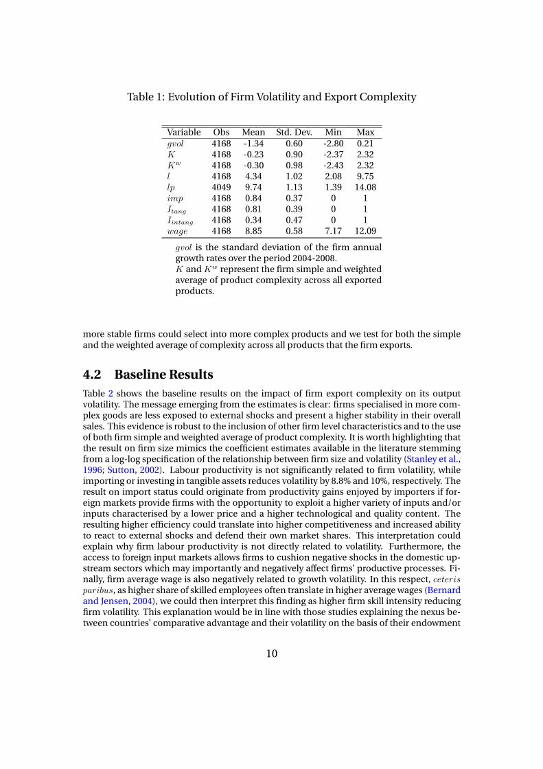
Table 1: Evolution of Firm Volatility and Export Complexity

Variable Obs Mean Std. Dev. Min Maxgvol 4168 -1.34 0.60 -2.80 0.21K 4168 -0.23 0.90 -2.37 2.32Kw 4168 -0.30 0.98 -2.43 2.32l 4168 4.34 1.02 2.08 9.75lp 4049 9.74 1.13 1.39 14.08imp 4168 0.84 0.37 0 1Itang 4168 0.81 0.39 0 1Iintang 4168 0.34 0.47 0 1wage 4168 8.85 0.58 7.17 12.09

gvol is the standard deviation of the firm annualgrowth rates over the period 2004-2008.K and Kw represent the firm simple and weightedaverage of product complexity across all exportedproducts.

more stable firms could select into more complex products and we test for both the simpleand the weighted average of complexity across all products that the firm exports.

4.2 Baseline ResultsTable 2 shows the baseline results on the impact of firm export complexity on its outputvolatility. The message emerging from the estimates is clear: firms specialised in more com-plex goods are less exposed to external shocks and present a higher stability in their overallsales. This evidence is robust to the inclusion of other firm level characteristics and to the useof both firm simple and weighted average of product complexity. It is worth highlighting thatthe result on firm size mimics the coefficient estimates available in the literature stemmingfrom a log-log specification of the relationship between firm size and volatility (Stanley et al.,1996; Sutton, 2002). Labour productivity is not significantly related to firm volatility, whileimporting or investing in tangible assets reduces volatility by 8.8% and 10%, respectively. Theresult on import status could originate from productivity gains enjoyed by importers if for-eign markets provide firms with the opportunity to exploit a higher variety of inputs and/orinputs characterised by a lower price and a higher technological and quality content. Theresulting higher efficiency could translate into higher competitiveness and increased abilityto react to external shocks and defend their own market shares. This interpretation couldexplain why firm labour productivity is not directly related to volatility. Furthermore, theaccess to foreign input markets allows firms to cushion negative shocks in the domestic up-stream sectors which may importantly and negatively affect firms’ productive processes. Fi-nally, firm average wage is also negatively related to growth volatility. In this respect, ceterisparibus, as higher share of skilled employees often translate in higher average wages (Bernardand Jensen, 2004), we could then interpret this finding as higher firm skill intensity reducingfirm volatility. This explanation would be in line with those studies explaining the nexus be-tween countries’ comparative advantage and their volatility on the basis of their endowment

10

of human capital (Costinot, 2009; Krishna and Levchenko, 2013).Turning to the economic meaning of our complexity indicators, in order to grasp an idea

of the magnitude of the effects, we take as reference the descriptive statistics shown in Table1. A one standard deviation increase in complexity would reduce a firm’s growth rate stan-dard deviation by roughly 10%, which corresponds to about one sixth of the volatility vari-ability, as measured by its standard deviation in Table 1. Also, if a firm with a complexity levelequal to the observed mean complexity jumped to the maximum complexity level observedin our sample, its volatility would decrease by about 25% which is slightly less than half of thevolatility standard deviation. More intuitively, if a firm moved from the production of tung-sten halogen lamps to the production of arc-lamps, its volatility would fall by 6.2%. Movingfrom the production of pocket-size radio cassette-players to radar apparatus or, alternatively,switching from electrically operated alarm clock to pacemakers would, instead, deliver largereffects, as firm volatility would drop by 13.1% and 22%, respectively.

Figure A.2 in Appendix A shows the distribution of predicted volatility from estimates ofmodel 3 under four alternative scenarios concerning firms’ complexity level. First of all, weplot the distribution of predicted volatility for the observed firm complexity levels, then weexplore how such a distribution would change if all firms increased their complexity by 10%and by one standard deviation. Finally, we plot the distribution under the hypothesis thatall firms were able to reach the maximum complexity recorded in sample within their 2digitsector. From the picture it emerges that only important changes in firms’ complexity levelsare able to considerably reduce their volatility. In this respect, this picture conveys an im-portant message: large resources need to be devoted to the sophistication of manufacturingproduction, as far as it becomes rewarding in terms of growth path stabilisation.

Table 2: Firm Volatility and Export Complexity: Baseline

(1) (2) (3) (4) (5) (6)K -0.134*** -0.114*** -0.098***

[0.017] [0.016] [0.017]Kw -0.102*** -0.102*** -0.090***

[0.015] [0.015] [0.015]l -0.134*** -0.099*** -0.140*** -0.103***

[0.009] [0.010] [0.009] [0.010]lp 0 0

[0.009] [0.009]imp -0.086*** -0.088***

[0.026] [0.026]ITang -0.109*** -0.107***

[0.025] [0.025]IIntang -0.001 -0.004

[0.020] [0.020]w -0.089*** -0.090***

[0.020] [0.020]Const. -1.381*** -0.742*** 0.056 -1.370*** -0.719*** 0.079

[0.037] [0.054] [0.162] [0.037] [0.053] [0.160]

Observations 4168 4168 4049 4168 4168 4049R-squared 0.071 0.12 0.136 0.066 0.12 0.136

Notes: * Significant at 10% level; ** significant at 5% level; *** significant at 1% level.Robust standard errors in brackets.All specifications include 2 digit NACE Rev 1.1 sector dummies and year fixed effects.

11

5 Robustness checksAlternative Volatility Indicators and Instrumental Variables- To further checkthe robustness of the relationship between firms’ export complexity and their volatility, in Ta-ble 3 we use alternative measures of volatility as left hand side variables which have usuallybeen used in the literature on firm volatility (Kalemli-Ozcan et al., 2014). In particular, we usethe log of the coefficient of variation (columns 1 to 4), the log of the standard deviation of dis-crete growth rates which could better approximate firm growth patterns (columns 5 to 8) andthe log of the absolute value of the residual of a firm growth regression on time and firm fixedeffects (columns 9 to 12) (Blanchard and Simon, 2001; Buch et al., 2009). It is worth stressingthat when the latter conditional volatility measure is used, it does not rely on a time windowof five years and all firms exporting in 2002 are included in the estimation sample, regardlessof their survival across the whole five year time span that we chose as our baseline estimationsample. Therefore, we consider results in columns [9]-[12] as a test of sample selection whichcould affect and, thus, cast doubts on our main result.Our baseline results hold even when we adopt alternative volatility indicators and, followingan increase of firm complexity by one standard deviation, they all imply a decrease of volatil-ity whose magnitude is consistent with estimate from the baseline specification.An important issue to investigate is whether the significant impact of past complexity onsubsequent firm output volatility is driven by the omission of the firm’s past growth pat-tern. In other words, a potential endogeneity concern stems from the fact that firms withheterogeneous volatility levels could sort themselves into products with different extent ofcomplexity. On the one hand, more stable firms could more easily start and continue morecomplex productions and this would imply a downward bias in our estimates, on the otherhand, if higher firm volatility reflects lower risk aversion, then, more volatile firms could bemore likely to start producing more sophisticated goods and in this case we would under-estimate the stabilising effect of product complexity. If this is the case, it is then importantto account for autocorrelation in the observed firm’s growth pattern to purge residuals fromany unaccounted persistence in firms’ growth rates. Although we are not able to account forfirms’ output growth patterns before 2003, we estimate a model of firm growth rates in thetime span at our disposal where, besides firm and year fixed effects, we alternatively includeone first and one first and one second order autoregressive term. Estimates are shown inTable 4 for log-squared residuals obtained from continuous and discrete firm level growthrates and our main findings are largely confirmed.12 This empirical approach, by cleansingthe turnover evolution from autocorrelation dynamics, together with the use of pre-samplemeasures of firm complexity, makes us more confident about the existence of a causal nexusrunning from complexity to volatility. Furthermore, when accounting for a second order au-toregressive growth process, coefficients on complexity indicators increase in absolute value,thus hinting at a systematic sorting of less stable firms into more complex products.To further inspect this issue, we perform an instrumental variable estimation where we usetwo alternative sets of instruments for firm complexity. First, we use the complexity of goods,different from the goods exported by the firm, that are exported by other firms within thesame 4digit sectors and located both in the same NUTS3 province and in other provinces. To

12We also used employment and labour productivity growth volatility. Furthermore, toaccount for heterogeneous sectoral growth patterns, we calculated a firm’s growth relative toits 2 digit and 4 digit sector output growth and measured a firm’s volatility on the basis of thisrelative output growth. As baseline results are largely confirmed, we do not show this set ofestimates for the sake of brevity, nonetheless, it is available from the authors upon request.

12

allow for higher variation of complexity, we consider only exports to high income countries.We assume that other firms’ export complexity exerts positive spillover effects on firms’ prod-uct sophistication, and we expect this effect to be magnified by geographical proximity. Com-plex goods require more capabilities and skills for their production and it is likely that knowl-edge flows among neighbouring firms performing similar activities. Nonetheless, a compe-tition effect - which would reduce the complexity of produced goods - could also be at workand prevail if firms could actually try to respond to low/high complexity neighbours’ compe-tition by upgrading/downgrading their product sophistication. In the estimation we controlfor 4digit sector effects and NUTS3 province fixed effects. Second, we instrument a firm’scomplexity by means of the share of women in its workforce and by the number of mosquesper 1000 inhabitants in its NUTS3 province of location. As far as the former instrument isconcerned, women in developing and emerging economies’ manufacturing are usually en-dowed with lower education and technical skills, hence, a higher feminisation of manufac-turing production is expected to be characterised by a lower degree of complexity (Barrientoset al., 2004). By the same token, turning to the latter instrument, we expect a higher numberof mosques per 1000 inhabitant to reflect a lower extent of product sophistication of firms inthe province. Empirical evidence has shown, in general, that countries’ economic growth re-sponds negatively to church attendance (Barro and McCleary, 2003). Turning to the specificrole of Islam for economic performance, some literature regards a reduction of religious di-versity as the major historical factor hampering innovation, science evolution and technolog-ical upgrading within the muslim world (Chaney, 2008). In particular, some specific values ofislamic religion would foster a diminished capacity for adaptation and innovation, would dis-courage an individualist economic morality, would favour an educational system that limitscuriosity and innovation and would reduce the role of public discourse, hence, discouragingindividuals from questioning (Kuran, 1997). These traits can importantly affect the accumu-lation of advanced and sophisticated capabilities, therefore we expect firms in provinces witha higher number of potential practising muslims to have a lower extent of product complex-ity. Results from the IV strategy are presented in Table 5. For the sake of brevity, they onlyconcern simple average of firms’ complexity.13 First stage evidence in the lower panel of theTable, actually, fulfils our expectations about the relationship between product complexity,on one side, and neighbouring firms’ complexity, female employment share and the muslimintensity of a firm’s location province, on the other. Also instrument validity is corroboratedby standard testing shown in the Table. Findings from second stage, in turn, corroborate andreinforce the existence of a negative causal nexus between a firm’s complexity and its volatil-ity. In particular, IV coefficient estimates reveal a higher stabilising impact of complexity onvolatility, thus, confirming an upward bias in OLS estimates stemming from selection of morevolatile firms into more complex products. OLS complexity coefficient, then, represents aconservative estimate of the real stabilising effect of firms’ complexity.

13Insights are the substantially unchanged when firms’ weighted average of export productcomplexity is used. Results are available upon request.

13

Table 3: Firm Volatility and Export Complexity: Further Volatility Measures

Log (Coeff. Var.) Discrete Growth Rates Log (Residual)(1) (2) (3) (4) (5) (6) (7) (8) (9) (10) (11) (12)

K -0.140*** -0.139*** -0.131*** -0.091*** -0.112*** -0.060***[0.029] [0.030] [0.018] [0.017] [0.015] [0.015]

Kw -0.116*** -0.117*** -0.098*** -0.086*** -0.081*** -0.057***[0.026] [0.027] [0.016] [0.016] [0.014] [0.014]

l -0.014 -0.019 -0.118*** -0.121*** -0.107*** -0.110***[0.020] [0.020] [0.011] [0.011] [0.009] [0.009]

lp 0.029* 0.028* -0.011 -0.011 -0.005 -0.006[0.017] [0.017] [0.009] [0.009] [0.010] [0.010]

imp -0.094* -0.097** -0.092*** -0.093*** -0.087*** -0.088***[0.049] [0.049] [0.029] [0.029] [0.023] [0.023]

ITang 0.022 0.024 -0.123*** -0.122*** -0.091*** -0.091***[0.045] [0.045] [0.027] [0.027] [0.022] [0.022]

IIntang 0.017 0.013 0.007 0.005 -0.019 -0.02[0.040] [0.040] [0.022] [0.022] [0.018] [0.018]

w 0.02 0.018 -0.098*** -0.098*** -0.090*** -0.091***[0.037] [0.037] [0.022] [0.021] [0.020] [0.020]

Const. 1.191*** 0.844*** 1.197*** 0.898*** -1.312*** 0.416** -1.300*** 0.438** -1.918*** -0.388** -1.909*** -0.370**[0.064] [0.300] [0.064] [0.298] [0.039] [0.176] [0.039] [0.174] [0.037] [0.161] [0.038] [0.160]

Observations 4,168 4,048 4,168 4,048 4,168 4,051 4,168 4,051 22,835 22,201 22,835 22,201R-squared 0.028 0.03 0.027 0.03 0.066 0.144 0.062 0.145 0.023 0.043 0.022 0.043

Notes: * Significant at 10% level; ** significant at 5% level; *** significant at 1% level. Robust standard errors in brackets.All specifications include 2 digit NACE Rev 1.1 sector dummies and year fixed effects.

14

Table 4: Firm Volatility and Export Complexity: Log-residuals from AR modelof firm growth

Continuous Growth Rates Discrete Growth RatesAR(1) AR(2) AR(1) AR(2)

(1) (2) (3) (4) (5) (6) (7) (8)K -0.082** -0.115*** -0.072** -0.089**

[0.035] [0.041] [0.036] [0.041]Kw -0.094*** -0.116*** -0.090*** -0.097***

[0.031] [0.036] [0.031] [0.037]l -0.215*** -0.219*** -0.232*** -0.236*** -0.222*** -0.225*** -0.233*** -0.237***

[0.021] [0.021] [0.024] [0.024] [0.021] [0.021] [0.024] [0.024]lp -0.037 -0.037 -0.083*** -0.083*** 0.051** 0.052** 0.008 0.008

[0.023] [0.023] [0.029] [0.028] [0.024] [0.024] [0.028] [0.028]imp -0.145*** -0.144*** -0.177*** -0.176*** -0.094* -0.092* -0.157*** -0.156***

[0.052] [0.052] [0.060] [0.060] [0.053] [0.053] [0.060] [0.060]wage -0.180*** -0.179*** -0.027 -0.028 -0.314*** -0.313*** -0.262*** -0.263***

[0.047] [0.047] [0.054] [0.054] [0.047] [0.047] [0.055] [0.055]Itang -0.159*** -0.159*** -0.194*** -0.194*** -0.107** -0.107** -0.049 -0.049

[0.051] [0.051] [0.058] [0.058] [0.050] [0.050] [0.057] [0.057]Iintang -0.052 -0.052 -0.028 -0.029 -0.075* -0.075* -0.088* -0.088*

[0.040] [0.040] [0.045] [0.045] [0.040] [0.040] [0.046] [0.046]cons -0.700* -0.706* -1.955*** -1.939*** -0.47 -0.486 -0.716 -0.719*

[0.372] [0.369] [0.421] [0.419] [0.376] [0.373] [0.438] [0.436]

Observations 17,973 17,973 13,562 13,562 17,700 17,700 13,335 13,335R2 0.047 0.047 0.047 0.047 0.041 0.041 0.045 0.046

Notes: * Significant at 10% level; ** significant at 5% level; *** significant at 1% level. Robust standard errors inbrackets.All specifications include 2 digit NACE Rev 1.1 sector dummies and year fixed effects.

Import complexity and Export Diversification - To further prove the robustnessof our findings in Table 6 we include additional firm level controls which could affect a firm’sstability and which capture different dimensions of the firm’s involvement in foreign markets.

First, we explore the role of import complexity. In the baseline specification we tested forthe access to foreign source markets, by means of a dummy for importer status and we foundthat the opportunity to purchase inputs abroad reduces the firm volatility. Nonetheless, thiscould not be a sufficient control for the effective firm import activity, as the type of inputsimported by firms matters for the extent of their export sophistication (Manova and Zhang,2012), and could be relevant for their output stability as well. On the one hand, more complexinputs could prove more efficient and lead to more sophisticated and stable productions. Onthe other hand, dependence on more complex goods could make production more volatilesince a supplier’s substitution would be difficult in case of negative shocks affecting her, thusdriving to a break or a drop in production. Then, to account for the possible omission ofimport sophistication from the model, we include import complexity together with exportcomplexity in the baseline specification. We, thus, restrict the analysis to the sample of firmsthat in addition to being exporters are also importers in 2002. We find that the impact ofexport complexity is still preserved even controlling for the import complexity, while importcomplexity, when significant, has a mild negative effect which is, however, not robust acrossspecifications.

15

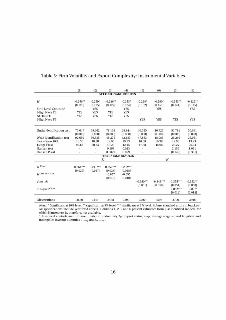
Table 5: Firm Volatility and Export Complexity: Instrumental Variables

(1) (2) (3) (4) (5) (6) (7) (8)SECOND STAGE RESULTS

K -0.256** -0.259* -0.246** -0.253* -0.268* -0.290* -0.353** -0.329**[0.128] [0.135] [0.127] [0.134] [0.152] [0.151] [0.141] [0.145]

Firm Level Controlsa YES YES YES YES4digit Nace FE YES YES YES YESNUTS3 FE YES YES YES YES2digit Nace FE YES YES YES YES

Underidentification test 77.647 69.362 78.103 69.944 46.535 46.727 53.791 50.081[0.000] [0.000] [0.000] [0.000] [0.000] [0.000] [0.000] [0.000]

Weak identification test 92.650 80.535 48.278 42.153 47.883 48.083 28.269 26.031Stock-Yogo 10% 16.38 16.38 19.93 19.93 16.38 16.38 19.93 19.931stage Ftest 92.65 80.53 48.28 42.15 47.88 48.08 28.27 26.03Hansen test - - 0.167 0.023 - - 2.156 1.071Hansen P-val - - 0.6829 0.879 - - [0.142] [0.301]

FIRST STAGE RESULTSK K

KProv 0.261*** 0.241*** 0.252*** 0.232***[0.027] [0.027] [0.028] [0.028]

KOtherPRov -0.057 -0.055[0.042] [0.040]

fem_sh -0.350*** -0.348*** -0.355*** -0.352***[0.051] [0.050] [0.051] [0.050]

mosquesProv -0.042*** -0.027*[0.014] [0.014]

Observations 3539 3445 3488 3399 3700 3598 3700 3598

Notes: * Significant at 10% level; ** significant at 5% level; *** significant at 1% level. Robust standard errors in brackets.All specifications include year fixed effects. Columns 1, 2, 5 and 6 present estimates from just identified models, forwhich Hansen test is, therefore, not available.a firm level controls are firm size, l, labour productivity, lp, import status, imp, average wage w, and tangibles andintangibles investor dummies, Itang andIintang .

16

Second, we control for firm export diversification in terms of foreign destinations. Ex-porting to several markets allows firms to diversify the risk of potential market-specific shocksand to move the activity towards other destinations when a country experiences a drop in thedemand. Also, it is likely that more complex firms have access to a large number of countries,thanks to their larger size, better human capital, better access to financial resources and so on(Manova and Zhang, 2012). We, then, control if our main findings are affected by the inclu-sion of a firm level indicator of diversification, as expressed by the number of export destina-tion,Ncexp, in order to exclude that the effect we are capturing is the volatility-reducing effectof diversification and from Table 6 the linkage between export complexity and firm volatilityproves to be robust to the control for export diversification. This evidence also confirms theinterpretation of findings in the work by Buch et al. (2009): the authors state that the lowervolatility of exporters compared to non exporters may be due to the low correlation betweendomestic and foreign shocks which would lead to gains from diversification. While they arenot able to empirically investigate this hypothesis, we show that exposition to a larger num-ber of destinations, indeed reduces a firm’s volatility, thus suggesting a negative correlationamong shocks experienced by different countries.

Third, we test and confirm that the finding of a negative nexus between complexity andvolatility holds even when we check for the number of exported products, NProducts. As forfirms serving multiple destinations, a multi-product exporter could better cushion the neg-ative shock on a product by intensifying the export of the remaining goods. We show thisis the case, as the number of exported products is negatively associated with firm volatility.However, by no means does this have an effect on size and significance of export complexity.Nonetheless, when the number of export products and destinations are included in the samespecification, only the latter stays significant.14

Further Robustness - In Table 7 we further show that the relationship between exportcomplexity and firm volatility is robust to the inclusion of both NUTS 2 level region dummies(columns 1-4), and 4-digit NACE Rev 1.1 sector fixed effects (columns 5-8), to the substitutionof regressor averages across the 2003-2008 period for their 2003 level (columns 9-12), and tothe inclusion of further firm level controls (columns 13-16). As far as firm level controls areconcerned, from the wider specifications of columns 13 and 16 we find that subcontractorsare more volatile, while firms outsourcing part of their production process have a more stableoutput growth path. The firm’s share of R&D employees, instead, does not directly affectoutput volatility.

Furthermore, in Table 8 we test two relative export complexity measures obtained by di-viding the firm product complexity by the 4digit average complexity.15 Relative measuresof export complexity with respect to the 4digit sectoral average, indeed, confirm that exportcomplexity is a further important source firm heterogeneity. As a matter of fact, from ourresults it emerges that across firms with comparable size and productivity which performsimilar activities, those producing and exporting relatively more complex goods are indeedless volatile. This result holds regardless of the inclusion of 4-digit sector fixed effects and ofcontrolling for export diversification. Thus, the type of specialisation does not only matterfor countries but for firms too. We, thus, conclude that within the same country and narrowly

14As further diversification indicators we use the Herfindahl index calculated across afirm’s destinations and across a firm’s products and results are not affected. Results are notshown here for the sake of brevity, but they are available from the authors upon request.

15These indicators (X) are then normalised by implementing the following transforma-tion: (X-1)/(X+1).

17

defined sector and within the same territories, firms which are more specialised than othersin complex goods perform better in terms of reduced volatility.

Finally, it is worth mentioning that our results are robust to the adoption of further com-plexity indicators that are similar, although not coincident, to the complexity measure adoptedin this study. First, we alternatively use the export share of products with a complexity indexabove the median or the 75th percentile of the product complexity distribution. Second, weadopt the PRODY indicator proposed by Hausmann et al. (2007) which assesses the incomecontent of products. Third, we use the measure of product ubiquity proposed by Tacchellaet al. (2013) which adjusts the Hausmann and Hidalgo’s definition of product complexity byaccounting for the fact that if a poorly diversified country is able to export a given product,very likely this product has a low level of sophistication. Fourth, we use the indicator wegather after an even-numbered iteration, Kp12, which conveys information about the prod-uct’s ubiquity and the ubiquity of related products which are exported - with RCA - by thesame countries. Results in all cases corroborate our evidence and are not shown for the sakeof brevity, nonetheless they are available upon request.16

16Besides this set of estimates and results presented in this section, we ran several fur-ther robustness checks, consisting in the inclusion among the right hand side variables ofregion-sector controls, of the firm’s average growth, total export value and a dummy for firmschanging (adding/dropping/switching) the product basket. These results are not show forbrevity, but they are available from the authors upon request.

18

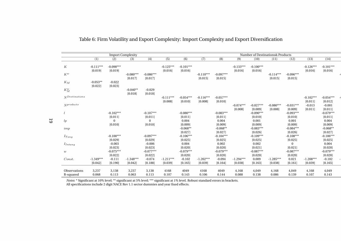
Table 6: Firm Volatility and Export Complexity: Import Complexity and Export Diversification

Import Complexity Number of Destinations& Products(1) (2) (3) (4) (5) (6) (7) (8) (9) (10) (11) (12) (13) (14) (15) (16)

K -0.111*** -0.098*** -0.125*** -0.101*** -0.133*** -0.100*** -0.126*** -0.101***[0.019] [0.019] [0.016] [0.016] [0.016] [0.016] [0.016] [0.016]

Kw -0.080*** -0.086*** -0.110*** -0.097*** -0.114*** -0.096*** -0.112*** -0.097***[0.017] [0.017] [0.015] [0.015] [0.015] [0.015] [0.015] [0.015]

KM -0.053** -0.022[0.022] [0.023]

KwM -0.040** -0.029

[0.018] [0.018]NDestinations -0.111*** -0.054*** -0.116*** -0.057*** -0.102*** -0.054*** -0.105*** -0.055***

[0.008] [0.010] [0.008] [0.010] [0.011] [0.012] [0.011] [0.012]Nproducts -0.074*** -0.027*** -0.080*** -0.031*** -0.013 -0.001 -0.017 -0.004

[0.008] [0.009] [0.008] [0.009] [0.011] [0.011] [0.011] [0.011]l -0.102*** -0.107*** -0.080*** -0.083*** -0.090*** -0.093*** -0.079*** -0.082***

[0.011] [0.011] [0.011] [0.011] [0.010] [0.010] [0.011] [0.011]lp 0 0 0.004 0.004 0.001 0.001 0.004 0.004

[0.010] [0.010] [0.009] [0.009] [0.009] [0.009] [0.009] [0.009]imp -0.068** -0.068** -0.083*** -0.084*** -0.068** -0.068**

[0.027] [0.027] [0.026] [0.026] [0.027] [0.027]ITang -0.100*** -0.097*** -0.106*** -0.104*** -0.109*** -0.108*** -0.106*** -0.104***

[0.029] [0.029] [0.025] [0.025] [0.025] [0.025] [0.025] [0.025]IIntang -0.003 -0.006 0.004 0.002 0.002 0 0.004 0.002

[0.023] [0.023] [0.020] [0.020] [0.021] [0.021] [0.020] [0.020]w -0.075*** -0.077*** -0.079*** -0.079*** -0.087*** -0.087*** -0.079*** -0.079***

[0.022] [0.022] [0.020] [0.020] [0.020] [0.020] [0.020] [0.020]Const. -1.349*** -0.111 -1.348*** -0.074 -1.211*** -0.102 -1.202*** -0.094 -1.294*** 0.009 -1.285*** 0.021 -1.208*** -0.102 -1.199*** -0.095

[0.042] [0.190] [0.042] [0.188] [0.039] [0.165] [0.039] [0.164] [0.038] [0.163] [0.038] [0.161] [0.039] [0.165] [0.039] [0.164]

Observations 3,237 3,138 3,237 3,138 4168 4049 4168 4049 4,168 4,049 4,168 4,049 4,168 4,049 4,168 4,049R-squared 0.068 0.113 0.063 0.113 0.107 0.143 0.106 0.144 0.088 0.138 0.086 0.139 0.107 0.143 0.107 0.144

Notes: * Significant at 10% level; ** significant at 5% level; *** significant at 1% level. Robust standard errors in brackets.All specifications include 2 digit NACE Rev 1.1 sector dummies and year fixed effects.

19

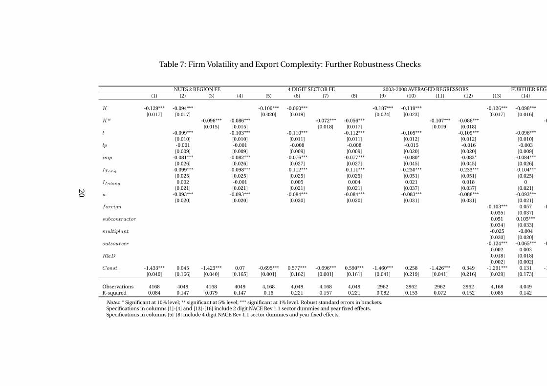
Table 7: Firm Volatility and Export Complexity: Further Robustness Checks

NUTS 2 REGION FE 4 DIGIT SECTOR FE 2003-2008 AVERAGED REGRESSORS FURTHER REGRESSORS(1) (2) (3) (4) (5) (6) (7) (8) (9) (10) (11) (12) (13) (14) (15) (16)

K -0.129*** -0.094*** -0.109*** -0.060*** -0.187*** -0.119*** -0.126*** -0.098***[0.017] [0.017] [0.020] [0.019] [0.024] [0.023] [0.017] [0.016]

Kw -0.096*** -0.086*** -0.072*** -0.056*** -0.107*** -0.086*** -0.098*** -0.090***[0.015] [0.015] [0.018] [0.017] [0.019] [0.018] [0.015] [0.015]

l -0.099*** -0.103*** -0.110*** -0.112*** -0.105*** -0.109*** -0.096*** -0.100***[0.010] [0.010] [0.011] [0.011] [0.012] [0.012] [0.010] [0.010]

lp -0.001 -0.001 -0.008 -0.008 -0.015 -0.016 -0.003 -0.004[0.009] [0.009] [0.009] [0.009] [0.020] [0.020] [0.009] [0.009]

imp -0.081*** -0.082*** -0.076*** -0.077*** -0.080* -0.083* -0.084*** -0.085***[0.026] [0.026] [0.027] [0.027] [0.045] [0.045] [0.026] [0.026]

ITang -0.099*** -0.098*** -0.112*** -0.111*** -0.230*** -0.233*** -0.104*** -0.102***[0.025] [0.025] [0.025] [0.025] [0.051] [0.051] [0.025] [0.025]

IIntang 0.002 -0.001 0.005 0.004 0.021 0.018 0 -0.002[0.021] [0.021] [0.021] [0.021] [0.037] [0.037] [0.021] [0.021]

w -0.093*** -0.093*** -0.084*** -0.084*** -0.083*** -0.088*** -0.093*** -0.094***[0.020] [0.020] [0.020] [0.020] [0.031] [0.031] [0.021] [0.021]

foreign -0.103*** 0.057 -0.111*** 0.056[0.035] [0.037] [0.035] [0.037]

subcontractor 0.051 0.105*** 0.049 0.104***[0.034] [0.033] [0.034] [0.033]

multiplant -0.025 -0.004 -0.026 -0.004[0.020] [0.020] [0.020] [0.020]

outsourcer -0.124*** -0.065*** -0.127*** -0.066***0.002 0.003 0.002 0.003

R&D [0.018] [0.018] [0.018] [0.018][0.002] [0.002] [0.002] [0.002]

Const. -1.433*** 0.045 -1.423*** 0.07 -0.695*** 0.577*** -0.696*** 0.590*** -1.460*** 0.258 -1.426*** 0.349 -1.291*** 0.131 -1.278*** 0.152[0.040] [0.166] [0.040] [0.165] [0.001] [0.162] [0.001] [0.161] [0.041] [0.219] [0.041] [0.216] [0.039] [0.173] [0.039] [0.172]

Observations 4168 4049 4168 4049 4,168 4,049 4,168 4,049 2962 2962 2962 2962 4,168 4,049 4,168 4,049R-squared 0.084 0.147 0.079 0.147 0.16 0.221 0.157 0.221 0.082 0.153 0.072 0.152 0.085 0.142 0.082 0.142

Notes: * Significant at 10% level; ** significant at 5% level; *** significant at 1% level. Robust standard errors in brackets.Specifications in columns [1]-[4] and [13]-[16] include 2 digit NACE Rev 1.1 sector dummies and year fixed effects.Specifications in columns [5]-[8] include 4 digit NACE Rev 1.1 sector dummies and year fixed effects.

20

Table 8: Firm Volatility and Export Complexity: Relative Complexity Measures

2 DIGIT FE 4 DIGIT FE 4 DIGIT FE + # DEST&PRODUCTS(1) (2) (3) (4) (5) (6) (7) (8) (9) (10) (11) (12)

KRel4d -0.861*** -0.482*** -0.871*** -0.494*** -0.740*** -0.506***[0.149] [0.147] [0.149] [0.144] [0.146] [0.143]

KwRel4d -0.580*** -0.444*** -0.570*** -0.447*** -0.648*** -0.512***

[0.136] [0.134] [0.137] [0.131] [0.134] [0.132]l -0.097*** -0.100*** -0.109*** -0.112*** -0.088*** -0.090***

[0.010] [0.010] [0.011] [0.011] [0.011] [0.011]lp -0.001 -0.001 -0.008 -0.008 -0.004 -0.004

[0.009] [0.009] [0.009] [0.009] [0.009] [0.009]imp -0.092*** -0.093*** -0.076*** -0.077*** -0.059** -0.058**

[0.026] [0.026] [0.027] [0.027] [0.027] [0.027]ITang -0.107*** -0.107*** -0.112*** -0.111*** -0.109*** -0.108***

[0.025] [0.025] [0.025] [0.025] [0.025] [0.025]IIntang -0.004 -0.006 0.005 0.003 0.011 0.009

[0.021] [0.021] [0.021] [0.021] [0.021] [0.021]w -0.096*** -0.096*** -0.084*** -0.084*** -0.072*** -0.071***

[0.020] [0.020] [0.020] [0.020] [0.020] [0.020]NDestinations -0.106*** -0.056*** -0.109*** -0.057***

[0.011] [0.012] [0.011] [0.012]Nproducts -0.009 0.001 -0.013 -0.002

[0.011] [0.011] [0.011] [0.011]Const. -1.305*** 0.178 -1.303*** 0.194 -0.688*** 0.578*** -0.692*** 0.593*** 0.334** -0.315*** 0.335** -0.311***

[0.036] [0.161] [0.036] [0.160] [0.002] [0.161] [0.002] [0.161] [0.168] [0.036] [0.168] [0.036]

Observations 4168 4049 4168 4049 4,168 4,049 4,168 4,049 4049 4168 4049 4168R-squared 0.064 0.131 0.06 0.131 0.161 0.222 0.157 0.221 0.228 0.217 0.228 0.215

Notes: * Significant at 10% level; ** significant at 5% level; *** significant at 1% level. Robust standard errors in brackets.Specifications in columns [1]-[4] include 2 digit NACE Rev 1.1 sector dummies and year fixed effects.Specifications in columns [5]-[12] include 4 digit NACE Rev 1.1 sector dummies and year fixed effects.

21

5.1 Export or Product Complexity?The above findings show a robust negative relationship between exporters’ specialisation incomplex goods and volatility. Nonetheless, such linkage is supposed to hold independentlyof a firm’s export status. To validate this hypothesis we repeat the baseline analysis by esti-mating a model of production volatility on the basis of production data available from Turk-Stat’s PRODCOM database for all Turkish manufacturing firms with more than 20 employ-ees for the period 2005-2009. In this database, firms’ products are recorded at the 10 digitPRODTR classification level which we converted into HS in order to classify them in terms oftheir complexity level. As from PRODCOM database firm production growth rates are onlyavailable for the four year period 2006-2009 and the global turmoil heavily hit Turkey in 2009(Lo Turco and Maggioni, 2014), we present two set of estimates concerning both output andproduction volatility by focusing on the 2006-2008 only. Results are shown in Table 9 andreveal that the negative coefficient on product complexity holds, regardless of a firm’s ex-porter status. Nonetheless, from the interaction term between a firm’s export status and thecomplexity indicator it emerges that, ceteris paribus, exporters seem to enjoy an additionalpremium from complex production in terms of reduced volatility. When we relax the ceterisparibus assumption and allow for structural differences between exporters and non exportersby running separate estimates for the two groups of firms in Table 10, indeed we find that,after we control for a number of firm level covariates, no statistically significant differenceemerges among them in the relationship between product complexity and volatility.17

17Results of production volatility are not shown for brevity, nonetheless they are availablefrom the authors upon request.

22

Table 9: Firm Volatility and Product Complexity: Production Data 2005-2008

Output Volatility: 2006/2008 Production Volatility: 2006/2008(1) (2) (3) (4) (5) (6) (7) (8) (9) (10) (11) (12)

K -0.045*** -0.050*** -0.055*** -0.052*** -0.048*** -0.048***[0.016] [0.016] [0.016] [0.017] [0.018] [0.018]

K ∗ exp -0.067*** -0.063*** -0.047*** -0.045*** -0.042** -0.027[0.016] [0.016] [0.016] [0.017] [0.017] [0.017]

Kw -0.039** -0.046*** -0.052*** -0.050*** -0.050*** -0.049***[0.016] [0.016] [0.016] [0.016] [0.017] [0.018]

Kw ∗ exp -0.067*** -0.063*** -0.046*** -0.197*** -0.073*** -0.052*** -0.199*** -0.074*** -0.054***[0.015] [0.015] [0.016] [0.016] [0.017] [0.019] [0.016] [0.017] [0.019]

exp -0.215*** -0.138*** -0.105*** -0.215*** -0.138*** -0.105*** -0.050*** -0.046*** -0.032*[0.015] [0.016] [0.017] [0.015] [0.016] [0.017] [0.016] [0.017] [0.017]

l -0.137*** -0.104*** -0.137*** -0.105*** -0.133*** -0.101*** -0.133*** -0.101***[0.008] [0.009] [0.008] [0.009] [0.008] [0.010] [0.008] [0.010]

lp -0.056*** -0.056*** -0.041*** -0.041***[0.009] [0.009] [0.010] [0.010]

imp -0.036** -0.037** 0.004 0.004[0.018] [0.018] [0.020] [0.020]

ITang -0.067*** -0.067*** -0.103*** -0.103***[0.018] [0.018] [0.020] [0.020]

IIntang -0.046*** -0.047*** -0.032* -0.032*[0.018] [0.018] [0.019] [0.019]

w -0.067*** -0.067*** -0.086*** -0.086***[0.019] [0.019] [0.019] [0.019]

Const. -1.490*** -0.983*** 0.061 -1.485*** -0.977*** 0.069 -0.869*** 0.883*** 2.055*** -0.867*** 0.883*** 2.051***[0.024] [0.038] [0.148] [0.024] [0.038] [0.148] [0.100] [0.036] [0.163] [0.100] [0.036] [0.162]

Observations 11511 11509 10987 11511 11509 10987 11,774 10,759 10,274 11,774 10,759 10,274R-squared 0.049 0.072 0.087 0.048 0.072 0.087 0.045 0.059 0.07 0.046 0.06 0.07

Notes: * Significant at 10% level; ** significant at 5% level; *** significant at 1% level. Robust standard errors in brackets.

23

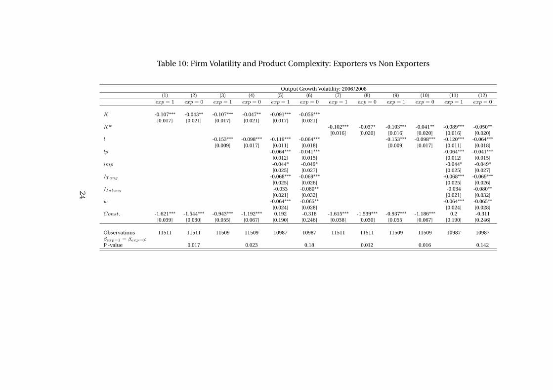
Table 10: Firm Volatility and Product Complexity: Exporters vs Non Exporters

Output Growth Volatility: 2006/2008(1) (2) (3) (4) (5) (6) (7) (8) (9) (10) (11) (12)

exp = 1 exp = 0 exp = 1 exp = 0 exp = 1 exp = 0 exp = 1 exp = 0 exp = 1 exp = 0 exp = 1 exp = 0

K -0.107*** -0.043** -0.107*** -0.047** -0.091*** -0.056***[0.017] [0.021] [0.017] [0.021] [0.017] [0.021]

Kw -0.102*** -0.037* -0.103*** -0.041** -0.089*** -0.050**[0.016] [0.020] [0.016] [0.020] [0.016] [0.020]

l -0.153*** -0.098*** -0.119*** -0.064*** -0.153*** -0.098*** -0.120*** -0.064***[0.009] [0.017] [0.011] [0.018] [0.009] [0.017] [0.011] [0.018]

lp -0.064*** -0.041*** -0.064*** -0.041***[0.012] [0.015] [0.012] [0.015]

imp -0.044* -0.049* -0.044* -0.049*[0.025] [0.027] [0.025] [0.027]

ITang -0.068*** -0.069*** -0.068*** -0.069***[0.025] [0.026] [0.025] [0.026]

IIntang -0.033 -0.080** -0.034 -0.080**[0.021] [0.032] [0.021] [0.032]

w -0.064*** -0.065** -0.064*** -0.065**[0.024] [0.028] [0.024] [0.028]

Const. -1.621*** -1.544*** -0.943*** -1.192*** 0.192 -0.318 -1.615*** -1.539*** -0.937*** -1.186*** 0.2 -0.311[0.039] [0.030] [0.055] [0.067] [0.190] [0.246] [0.038] [0.030] [0.055] [0.067] [0.190] [0.246]

Observations 11511 11511 11509 11509 10987 10987 11511 11511 11509 11509 10987 10987βexp=1 = βexp=0:P -value 0.017 0.023 0.18 0.012 0.016 0.142

24

6 Looking for the channels: what drives the exportcomplexity-volatility nexus?

In this section, we inspect the mechanisms lying behind the negative relationship betweenfirm export complexity and output volatility. In particular, we explore the drivers of exportcomplexity by building on different streams of existing literature and, thus, shed light onboth demand and supply side factors associated with complex productions which may favourhigher stability of output growth.

On the one hand, export complexity could reflect different conditions in demand. First,more sophisticated goods can enjoy lower demand and substitution elasticities because theyare less ubiquitous. As a consequence, we expect their demand to be less affected by externalshocks. Krishna and Levchenko (2013) corroborate this prediction by showing that the elas-ticity of substitution of sectors is significantly and positively related to their volatility. How-ever, they are interested in isolating the impact of the number of required inputs on firms’volatility, by cleansing the effect from the existing differences in demand conditions amongsectors. We test, instead, whether a good’s higher complexity is associated with a lower elas-ticity of substitution/demand and whether this represents a potential channel of the stabilis-ing effect of product complexity for a firm’s output growth. Second, more complex goods arecharacterised by a higher income elasticity. As a matter of fact, they are mainly consumed byricher countries (Hallak, 2006) - and, within each country, by richer consumers - whose in-come is less volatile. Hence, we expect that a the higher income elasticity of complex goods,reflected in higher consumption shares of richer countries in the products, could be a furtherrelevant demand side channel driving the above robust complexity-volatility nexus at firmlevel.

On the other hand, turning to the supply side, since our complexity indicator hinges oncountries’ diversification and products’ ubiquity, it could capture the notion of technologi-cal diversification, meant as the number of inputs required by a good’s production process.Firms’ complexity would, then, stabilise their turnover, due to a minor impact of an input-specific shock on the production outcome. Furthermore, entry into production of complexgoods could entail higher fixed and sunk costs. Entry barriers reduce the extent of compe-tition and, hence, increase market concentration. For this reason, firms involved in theseproductions could enjoy higher stability. In this respect, Irvine and Pontiff (2009) find thatincreased competition, driven by both the entry of foreign firms and deregulation processes,is one of the main sources at the basis of the rise in idiosyncratic volatility over the period1964-2003.

In order to shed light on the factors behind the product complexity-volatility nexus atfirm level, we proceed in two steps.

First, we estimate the following model for the determinants of firm i’s production com-plexity, Ki:

Ki = θ + δ0σi + δ0ImpshHIi + δ1N

inputi + δ2Herfi + εi (4)

Here, σi is the average elasticity of substitution of a firm’s product, as measured by Brodaand Weinstein (2006) for the U.S. economy at 5 digit SITC level and converted into HS 2002.ImpshHI

i represents the share of consumption by rich economies and is calculated as theaverage share, across 6 digit HS products exported by the firm in 2002, of imports by Highincome economies in total world imports. Import data are from COMTRADE- WITS-WorldBank online database. N input

i captures the extent of technological diversification and is mea-

25

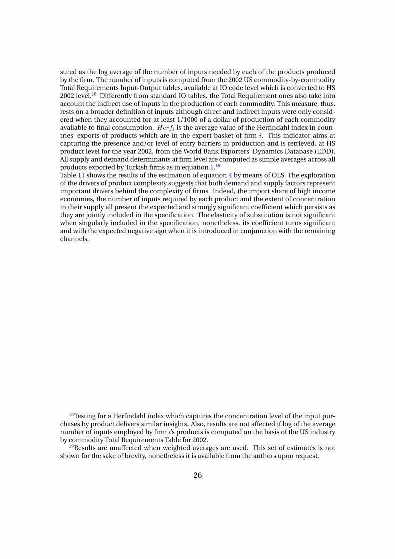
sured as the log average of the number of inputs needed by each of the products producedby the firm. The number of inputs is computed from the 2002 US commodity-by-commodityTotal Requirements Input-Output tables, available at IO code level which is converted to HS2002 level.18 Differently from standard IO tables, the Total Requirement ones also take intoaccount the indirect use of inputs in the production of each commodity. This measure, thus,rests on a broader definition of inputs although direct and indirect inputs were only consid-ered when they accounted for at least 1/1000 of a dollar of production of each commodityavailable to final consumption. Herfi is the average value of the Herfindahl index in coun-tries’ exports of products which are in the export basket of firm i. This indicator aims atcapturing the presence and/or level of entry barriers in production and is retrieved, at HSproduct level for the year 2002, from the World Bank Exporters’ Dynamics Database (EDD).All supply and demand determinants at firm level are computed as simple averages across allproducts exported by Turkish firms as in equation 1.19

Table 11 shows the results of the estimation of equation 4 by means of OLS. The explorationof the drivers of product complexity suggests that both demand and supply factors representimportant drivers behind the complexity of firms. Indeed, the import share of high incomeeconomies, the number of inputs required by each product and the extent of concentrationin their supply all present the expected and strongly significant coefficient which persists asthey are jointly included in the specification. The elasticity of substitution is not significantwhen singularly included in the specification, nonetheless, its coefficient turns significantand with the expected negative sign when it is introduced in conjunction with the remainingchannels.

18Testing for a Herfindahl index which captures the concentration level of the input pur-chases by product delivers similar insights. Also, results are not affected if log of the averagenumber of inputs employed by firm i’s products is computed on the basis of the US industryby commodity Total Requirements Table for 2002.

19Results are unaffected when weighted averages are used. This set of estimates is notshown for the sake of brevity, nonetheless it is available from the authors upon request.

26

Table 11: The drivers of Firm Product Complexity

(1) (2) (3) (4) (5) (6) (7) (8) (9) (10)

K Kw

σ 0.000 -0.012*** 0.004 -0.009**[0.005] [0.004] [0.004] [0.004]

ImpshHI 106.323*** 133.678*** 34.565*** 75.532***[14.479] [16.172] [12.317] [11.271]

N input 7.059*** 6.155*** 6.198*** 5.609***[0.201] [0.221] [0.177] [0.186]

Herf 2.778*** 1.861*** 2.307*** 1.534***[0.163] [0.158] [0.138] [0.129]

cons -0.031 -0.295*** -35.741*** -1.358*** -31.812*** -0.154*** -0.321*** -31.481*** -1.233*** -28.999***[0.033] [0.015] [1.014] [0.071] [1.084] [0.031] [0.016] [0.894] [0.062] [0.919]

Observations 4061 4168 4168 4139 4035 4061 4168 4168 4139 4035R-squared 0.01 0.012 0.34 0.089 0.383 0.006 0.002 0.308 0.077 0.343

Notes: * Significant at 10% level; ** significant at 5% level; *** significant at 1% level. Robust standard errors in brackets.Dependent variable Product Complexity, Kp, at HS level.σ: average, across products exported by the firm in 2002, elasticity of substitution. σs are sourced from Broda and Weinstein (2006).ImpshHI : average, across products exported by the firm in 2002, of the share of imports by High income economies in total worldimports for the product. Imports at 6 digit HS 2002 for year 2002 come from COMTRADE-WITS-World Bank online database.N input: log of average, across products exported by the firm in 2002, number of inputs employed by product p computed by exploitingthe US commodity-commodity Total Requirements Table for 2002.Herf : average, across products exported by the firm in 2002, product Herfindahl index retrieved from EDD of World Bank for 2002.

27

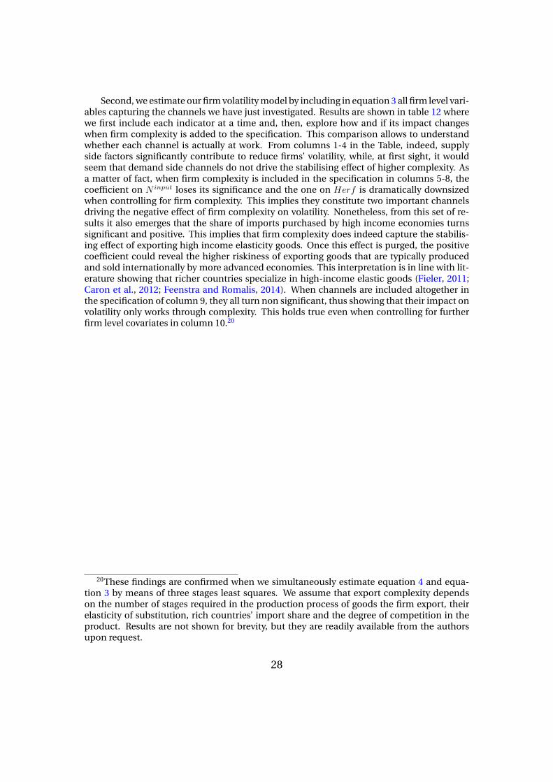
Second, we estimate our firm volatility model by including in equation 3 all firm level vari-ables capturing the channels we have just investigated. Results are shown in table 12 wherewe first include each indicator at a time and, then, explore how and if its impact changeswhen firm complexity is added to the specification. This comparison allows to understandwhether each channel is actually at work. From columns 1-4 in the Table, indeed, supplyside factors significantly contribute to reduce firms’ volatility, while, at first sight, it wouldseem that demand side channels do not drive the stabilising effect of higher complexity. Asa matter of fact, when firm complexity is included in the specification in columns 5-8, thecoefficient on N input loses its significance and the one on Herf is dramatically downsizedwhen controlling for firm complexity. This implies they constitute two important channelsdriving the negative effect of firm complexity on volatility. Nonetheless, from this set of re-sults it also emerges that the share of imports purchased by high income economies turnssignificant and positive. This implies that firm complexity does indeed capture the stabilis-ing effect of exporting high income elasticity goods. Once this effect is purged, the positivecoefficient could reveal the higher riskiness of exporting goods that are typically producedand sold internationally by more advanced economies. This interpretation is in line with lit-erature showing that richer countries specialize in high-income elastic goods (Fieler, 2011;Caron et al., 2012; Feenstra and Romalis, 2014). When channels are included altogether inthe specification of column 9, they all turn non significant, thus showing that their impact onvolatility only works through complexity. This holds true even when controlling for furtherfirm level covariates in column 10.20

20These findings are confirmed when we simultaneously estimate equation 4 and equa-tion 3 by means of three stages least squares. We assume that export complexity dependson the number of stages required in the production process of goods the firm export, theirelasticity of substitution, rich countries’ import share and the degree of competition in theproduct. Results are not shown for brevity, but they are readily available from the authorsupon request.

28

Table 12: Firm Volatility and Export Complexity: The Channels

[1] [2] [3] [4] [5] [6] [7] [8] [9] [10]

σ -0.002 -0.001 -0.001 0.000[0.004] [0.003] [0.003] [0.004]

ImpshHI 7.408 19.819** 5.884 16.793[9.544] [9.832] [10.688] [11.366]

N input -0.457*** 0.029 0.144 0.055[0.170] [0.180] [0.160] [0.161]

Herf -0.525*** -0.229** -0.16 0.082[0.096] [0.098] [0.117] [0.118]

K -0.135*** -0.117*** -0.135*** -0.107*** -0.119*** -0.104***[0.017] [0.010] [0.018] [0.010] [0.013] [0.013]

l -0.090***[0.010]

lp -0.006[0.009]

imp -0.083***[0.027]

Itang -0.110***[0.025]

Iintang 0.01[0.021]

wage -0.098***[0.020]

Constant -1.256*** -1.347*** 1.025 -1.132*** -1.356*** -1.382*** -1.531* -1.277*** -2.005** -0.225[0.044] [0.011] [0.865] [0.040] [0.045] [0.011] [0.921] [0.041] [0.796] [0.816]

hlineObservations 4061 4168 4168 4139 4061 4168 4168 4139 4035 3919R-squared 0.056 0 0.057 0.007 0.071 0.031 0.071 0.031 0.032 0.096

Notes: * Significant at 10% level; ** significant at 5% level; *** significant at 1% level. Robust standard errors in brackets.σ: average, across products exported by the firm in 2002, elasticity of substitution. σs are sourced from Broda and Weinstein (2006).ImpshHI : average, across products exported by the firm in 2002, of the share of imports by High income economies in total worldimports for the product. Imports at 6 digit HS 2002 for year 2002 come from COMTRADE-WITS-World Bank online database.N input: log of average, across products exported by the firm in 2002, number of inputs employed by product p computed by exploitingthe US commodity-commodity Total Requirements Table for 2002.Herf : average, across products exported by the firm in 2002, product Herfindahl index retrieved from EDD of World Bank for 2002.

29

7 ConclusionsWith this work we have contributed to empirical literature on the role of countries’ tradespecialisation for economic growth.

By using firm level data on Turkish manufacturing sectors we have shown, for the firsttime to our knowledge, that firms’ higher export complexity reduces their volatility and thisfinding is robust to several sensitivity checks. Furthermore, we have found that specialis-ing in complex productions positively affects firms’ output stability, regardless of their in-volvement in export markets. The potential consequences of product sophistication for aneconomy are, therefore, sizeable. Finally, by measuring product complexity according to theHausmann and Hidalgo’s (2009) indicator we have enlarged the scope of possible channelsthrough which specialisation in more sophisticated goods can promote more stable growth.As a matter of fact, we have found that the stabilising effect of firm complexity works boththrough demand and supply side channels. Besides wider technological diversification whichallows cushioning input specific shocks, higher income elasticity and entry barriers drive thenegative effect of firms’ product complexity on their volatility. The former allows for morestable sales, due to reduced exposition of richer consumers’ incomes to external shocks, thelatter, instead, reduce the extent of competition in the market for product and, then, curbincumbents’ turnover fluctuations.

Two main insights emerge from our work.First, as long as trade integration across countries involved in global production networks

confines emerging countries’ firms in less complex productions, the growth path of theseeconomies is doomed to be unstable and this could be detrimental for their long run growthperspectives.

Second, product complexity is a further important dimension of heterogeneity acrossfirms with very similar relevant observable characteristics. More specifically, our evidenceshows that such heterogeneity matters for the stability of firms sharing the same institutionalframework and all having access to the same production factors. Differences in complexitylevels across firms encompass product differences in technological diversification, in the ex-tent of entry barriers and in the price and income elasticities. Complexity appears then tobe importantly determined by firms’ time-varying unobservables, among which managerialand workforce competencies and skills undoubtedly play a key role.

As firm product sophistication could importantly affect a country’s overall economic growthperformance, our evidence suggests that micro policies for growth could be relevant. Promot-ing creation, upgrading and diffusing entrepreneurial human capital and managerial skillscould allow firms to upgrade production and hook onto a more stable growth path. Thiswould promote less volatile and, hence, higher aggregate growth.

Future research should be devoted to delving further into the notion of firm complexity.In particular, the most important goal would be to map firms’ capabilities into their productbaskets. The availability of linked employer-employee database would allow to measure andidentify firms’ capabilities on the bases of their workforce’s skills and competencies. Then,one could verify if more complex firms are less volatile due to their wider range of capabili-ties which allows them to be more flexible and to more easily adjust production to externalshocks.

30

ReferencesAcemoglu, D., Carvalho, V.M., Ozdaglar, A., Tahbaz-Salehi, A., 2012. The Network Origins of

Aggregate Fluctuations. Econometrica 80, 1977–2016.

Acemoglu, D., Zilibotti, F., 1997. Was prometheus unbound by chance? risk, diversification,and growth. Journal of Political Economy 105, 709–51.

Barrientos, S., Kabeer, N., Hossain, N., 2004. The gender dimensions of the globalizationof production. World Commission on the Social Dimension of Globalization - WorkingPapers 17. International Labour Office - Policy Integration Department.

Barro, R.J., McCleary, R., 2003. Religion and Economic Growth. NBER Working Papers 9682.National Bureau of Economic Research, Inc.

Bernard, A., Jensen, J., 2004. Why some firms export. The Review of Economics and Statistics, 561–569.

Blanchard, O., Simon, J., 2001. The Long and Large Decline in U.S. Output Volatility. Brook-ings Papers on Economic Activity 32, 135–174.

Blattman, C., Hwang, J., Williamson, J.G., 2007. Winners and losers in the commodity lottery:The impact of terms of trade growth and volatility in the Periphery 1870-1939. Journal ofDevelopment Economics 82, 156–179.

Broda, C., Weinstein, D.E., 2006. Globalization and the Gains from Variety. The QuarterlyJournal of Economics 121, 541–585.

Buch, C.M., Döpke, J., Strotmann, H., 2009. Does Export Openness Increase Firm-level Out-put Volatility? The World Economy 32, 531–551.

Caron, J., Fally, T., Markusen, J.R., 2012. Skill Premium and Trade Puzzles: a Solution LinkingProduction and Preferences. NBER Working Papers 18131. National Bureau of EconomicResearch, Inc.

Chaney, E., 2008. Tolerance, Religious Competition and the Rise and Fall of Muslim Science.mimeo. Harvard University.

Costinot, A., 2009. On the origins of comparative advantage. Journal of International Eco-nomics 77, 255–264.

Davis, S.J., Haltiwanger, J., Jarmin, R., Miranda, J., 2007. Volatility and Dispersion in BusinessGrowth Rates: Publicly Traded versus Privately Held Firms, in: NBER MacroeconomicsAnnual 2006, Volume 21. National Bureau of Economic Research, Inc. NBER Chapters, pp.107–180.

Easterly, W., Islam, R., J. E., S., 2000. Shaken and stirred: Explaining growth volatility. mimeo .

Feenstra, R.C., Romalis, J., 2014. International prices and endogenous quality. The QuarterlyJournal of Economics .

31

Felipe, J., Kumar, U., Abdon, A., Bacate, M., 2012. Product complexity and economic devel-opment. Structural Change and Economic Dynamics 23, 36 – 68.

Fieler, A.C., 2011. Nonhomotheticity and Bilateral Trade: Evidence and a Quantitative Expla-nation. Econometrica 79, 1069–1101.

Gabaix, X., 2011. The granular origins of aggregate fluctuations. Econometrica 79, 733–772.

García-Vega, M., Guariglia, A., Spaliara, M.E., 2012. Volatility, financial constraints, and trade.International Review of Economics & Finance 21, 57–76.

di Giovanni, J., Levchenko, A.A., 2009. Trade Openness and Volatility. The Review of Eco-nomics and Statistics 91, 558–585.

di Giovanni, J., Levchenko, A.A., 2011. The Risk Content of Exports: A Portfolio View of Inter-national Trade, in: NBER International Seminar on Macroeconomics 2011. National Bu-reau of Economic Research, Inc. NBER Chapters, pp. 97–151.

di Giovanni, J., Levchenko, A.A., 2012. Country Size, International Trade, and Aggregate Fluc-tuations in Granular Economies. Journal of Political Economy 120, 1083 – 1132.

di Giovanni, J., Levchenko, A.A., Mejean, I., 2014. Firms, destinations, and aggregate fluctua-tions. Econometrica .

Hallak, J.C., 2006. Product quality and the direction of trade. Journal of International Eco-nomics 68, 238–265.

Hausmann, R., Hidalgo, C., 2011. The network structure of economic output. Journal ofEconomic Growth 16, 309–342.

Hausmann, R., Hidalgo, C.A., 2009. The building blocks of economic complexity. Proc. Natl.Acad. Sci. 106, 10570–10575.

Hausmann, R., Hwang, J., Rodrik, D., 2007. What you export matters. Journal of EconomicGrowth 12, 1–25.

Hidalgo, C., 2009. The dynamics of economic complexity and the product space over a 42 yearperiod. Working Papers 189. Center for International Development, Harvard University.

Hnatkovska, V., Loayza, N., 2004. Volatility and growth. Policy Research Working Paper Series3184. The World Bank.

Imbs, J., Wacziarg, R., 2003. Stages of Diversification. American Economic Review 93, 63–86.

Irvine, P.J., Pontiff, J., 2009. Idiosyncratic Return Volatility, Cash Flows, and Product MarketCompetition. Review of Financial Studies, Society for Financial Studies 22, 1149–1177.

Kalemli-Ozcan, S., Sorensen, B., Volosovych, V., 2014. Deep financial integration and volatil-ity. Journal of the European Economic Association .

Koren, M., Tenreyro, S., 2007. Volatility and Development. The Quarterly Journal of Eco-nomics 122, 243–287.

32

Koren, M., Tenreyro, S., 2013. Technological Diversification. American Economic Review 103,378–414.

Kose, M. A., E.S.P., Terrones, M.E., 2003. inancial integration and macroeconomic volatility.mimeo .

Kraay, A., Ventura, J., 2007. Comparative Advantage and the Cross-section of Business Cycles.Journal of the European Economic Association 5, 1300–1333.

Krishna, P., Levchenko, A.A., 2013. Comparative advantage, complexity, and volatility. Journalof Economic Behavior & Organization 94, 314–329.

Kuran, T., 1997. Islam and Underdevelopment: An Old Puzzle Revisited. Journal of Institu-tional and Theoretical Economics 153, 41–71.

Levchenko, A.A., 2007. Institutional Quality and International Trade. Review of EconomicStudies 74, 791–819.

Lin, S.C., Kim, D.H., 2014. The link between economic growth and growth volatility. EmpiricalEconomics 46, 43–63.

Lo Turco, A., Maggioni, D., 2014. The micro evolution of trade and turnover in turkey underthe global crisis. Economic Systems .

Manova, K., Zhang, Z., 2012. Export prices across firms and destinations. The QuarterlyJournal of Economics 127, 379–436.

Melitz, M.J., 2003. The impact of trade on intra-industry reallocations and aggregate industryproductivity. Econometrica 71, 1695–1725.

Melitz, M.J., Ottaviano, G.I.P., 2008. Market size, trade, and productivity. Review of EconomicStudies 75, 295–316.

Norrbin, S.C., Yigit, F.P., 2005. The Robustness of the Link between Volatility and Growth ofOutput. Review of World Economics (Weltwirtschaftliches Archiv) 141, 343–356.

Novy, D., Taylor, A.M., 2014. Trade and Uncertainty. NBER Working Papers 19941. NationalBureau of Economic Research, Inc.

Nunn, N., 2007. Relationship-Specificity, Incomplete Contracts, and the Pattern of Trade. TheQuarterly Journal of Economics 122, 569–600.

OECD, 2005. Micro-policies for growth and productivity. Technical Report. OECD.

Ottaviano, G., Mayer, T., 2007. The happy few: the internationalisation of European firms.Number 12 in Blueprints, Bruegel.

Poncet, S., de Waldemar, F.S., 2012. Export upgrading and growth: the prerequisite of domes-tic embeddedness. Working Papers 2012-26. CEPII research center.

Ramey, G., Ramey, V.A., 1995. Cross-Country Evidence on the Link between Volatility andGrowth. American Economic Review 85, 1138–51.

33

Stanley, M.H., Amaral, L.A., Buldyrev, S.V., Havlin, S., Leschhorn, H., Maass, P., Salinger, M.A.,Stanley, H.E., 1996. Scaling behaviour in the growth of companies. Nature 379, 804–806.

Sutton, J., 2002. The variance of firm growth rates: the ‘scaling’ puzzle. Physica A 312, 577–590.

Tacchella, A., Cristelli, M., Caldarelli, G., Gabrielli, A., Pietronero, L., 2013. Economic com-plexity: Conceptual grounding of a new metrics for global competitiveness. Journal ofEconomic Dynamics and Control 37, 1683 – 1691.

Vannoorenberghe, G., 2012. Firm-level volatility and exports. Journal of International Eco-nomics 86, 57 – 67.

34

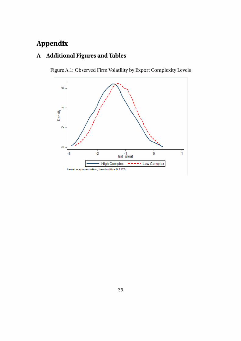
Appendix

A Additional Figures and Tables

Figure A.1: Observed Firm Volatility by Export Complexity Levels

35

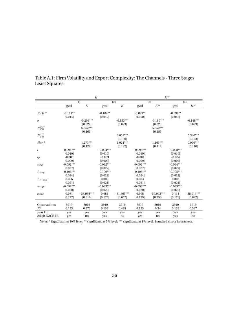
Table A.1: Firm Volatility and Export Complexity: The Channels - Three StagesLeast Squares

K Kw

(1) (2) (3) (4)gvol K gvol K gvol Kw gvol Kw

K/Kw -0.101** -0.104** -0.099** -0.098**[0.044] [0.042] [0.050] [0.048]

σ -0.204*** -0.153*** -0.190*** -0.148***[0.024] [0.023] [0.023] [0.023]

NCCTR 6.652*** 5.850***

[0.165] [0.153]NIC

TR 6.051*** 5.330***[0.130] [0.123]

Herf 1.271*** 1.024*** 1.163*** 0.976***[0.127] [0.122] [0.114] [0.110]

l -0.094*** -0.094*** -0.098*** -0.098***[0.010] [0.010] [0.010] [0.010]

lp -0.003 -0.003 -0.004 -0.004[0.009] [0.009] [0.009] [0.009]

imp -0.092*** -0.092*** -0.093*** -0.094***[0.027] [0.027] [0.027] [0.027]

Itang -0.106*** -0.106*** -0.105*** -0.105***[0.024] [0.024] [0.024] [0.024]

Iintang 0.006 0.006 0.003 0.003[0.021] [0.021] [0.021] [0.021]

wage -0.092*** -0.093*** -0.093*** -0.093***[0.020] [0.020] [0.020] [0.020]

cons 0.081 -33.988*** 0.084 -31.665*** 0.108 -30.002*** 0.111 -28.013***[0.177] [0.816] [0.175] [0.657] [0.179] [0.756] [0.178] [0.622]

Observations 3919 3919 3919 3919 3919 3919 3919 3919R2 0.133 0.373 0.133 0.429 0.133 0.34 0.133 0.387year FE yes yes yes yes yes yes yes yes2digit NACE FE yes no yes no yes no yes no

Notes: * Significant at 10% level; ** significant at 5% level; *** significant at 1% level. Standard errors in brackets.

36

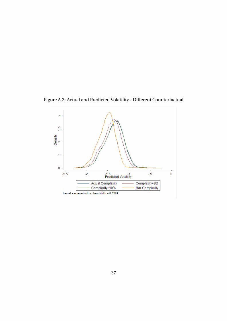
Figure A.2: Actual and Predicted Volatility - Different Counterfactual

37