TESI DI LAUREA MAGISTRALE IN INGEGNERIA CIVILE...

UNIVERSITÀ DEGLI STUDI DI PADOVA

TESI DI LAUREA MAGISTRALE IN INGEGNERIA CIVILE

CORRELAZIONE DI IMMAGINI DIGITALI PER LA

VALUTAZIONE DI DEFORMAZIONI DI PROFILI IN

ACCIAIO

USE OF DIGITAL IMAGE CORRELATION FOR STEEL

SECTION STRAIN EVALUATION

Relatore:

Prof. CLAUDIO MODENA

Prof. CHRISTOS GEORGAKIS

Studente:

MATTEO FURLAN

a.a. 2013-2014

1 INDEX

ACKNOWLEDGMENTS ............................................................................................ 1

ABSTRACT .................................................................................................................... 3

CHAPTER 1 STRUCTURAL HEALTH MONITORING...................................... 9

1.1 Background ...................................................................................................................................... 9

1.2 Historical review ........................................................................................................................... 11

1.2.1 Dams ...................................................................................................................................... 13

1.2.2 Bridges ................................................................................................................................... 14

1.2.3 Offshore installations ........................................................................................................... 15

1.2.4 Buildings and Towers .......................................................................................................... 17

1.2.5 Nuclear installations ............................................................................................................ 17

1.2.6 Tunnels and excavations ..................................................................................................... 18

1.3 Traditional and modern monitoring methods ......................................................................... 19

1.3.1 The process ............................................................................................................................ 19

1.3.2 Instrumentation and data acquisition ................................................................................ 20

1.3.2.1 Traditional sensors .......................................................................................................... 20

1.3.2.2 Innovative sensors ........................................................................................................... 23

1.3.3 Signal processing .................................................................................................................. 25

1.3.4 Damage identification .......................................................................................................... 25

1.4 Digital Image Correlation (DIC) ................................................................................................ 26

CHAPTER 2 CONCEPTUAL FRAMEWORK ....................................................... 29

2.1 Experiment background .............................................................................................................. 29

2.2 The project ...................................................................................................................................... 31

2.2.1 Description of the structure ................................................................................................ 31

2.2.2 Application of the load ........................................................................................................ 32

2.2.3 Undamaged and damaged conditions .............................................................................. 33

2.3 Design of the structure ................................................................................................................. 34

2.4 Materials and hypothesis ............................................................................................................ 35

2.4.1 Elasticity theory .................................................................................................................... 35

2.4.2 Materials ................................................................................................................................ 35

2.5 Aramis ............................................................................................................................................. 36

2.5.1 A new project ........................................................................................................................ 36

2.5.2 Set up ...................................................................................................................................... 36

2.6 Other technologies ........................................................................................................................ 40

2.6.1 Abaqus ................................................................................................................................... 40

2.6.2 Strain gauges ......................................................................................................................... 42

CHAPTER 3 UNDAMAGED CONDITION ......................................................... 43

3.1 Conduct of the test ........................................................................................................................ 43

3.2 Experiment results ........................................................................................................................ 44

3.2.1 Top beam ............................................................................................................................... 44

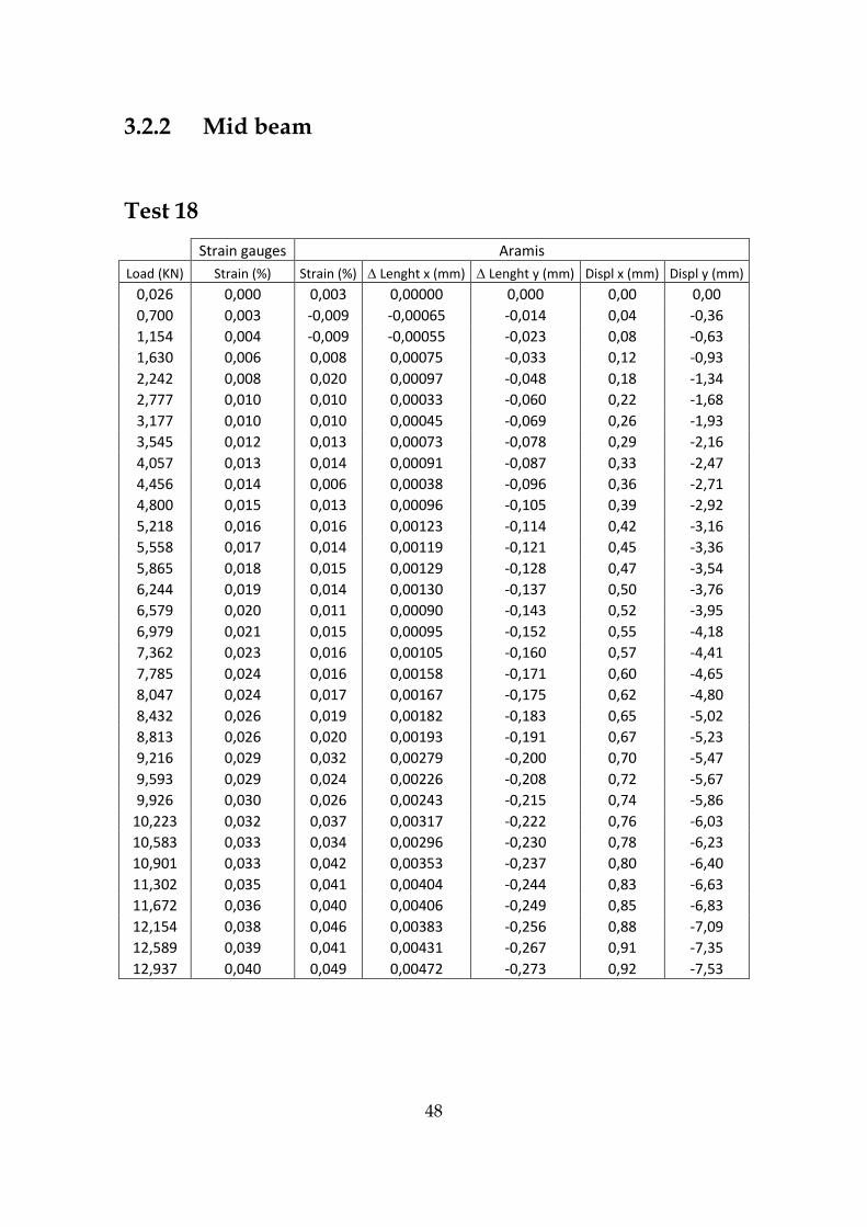
3.2.2 Mid beam ............................................................................................................................... 48

3.2.3 Bottom beam ......................................................................................................................... 54

3.2.4 Top joint ................................................................................................................................. 58

3.2.5 Mid joint................................................................................................................................. 62

3.2.6 Bottom joint ........................................................................................................................... 66

3.3 Considerations ............................................................................................................................... 70

CHAPTER 4 DAMAGED CONDITION ............................................................... 71

4.1 Conduct of the test ........................................................................................................................ 71

4.2 Experiment results ........................................................................................................................ 72

4.2.1 Top beam ............................................................................................................................... 72

4.2.2 Mid beam ............................................................................................................................... 76

4.2.3 Bottom beam ......................................................................................................................... 80

4.2.4 Top joint ................................................................................................................................. 84

4.2.5 Mid joint................................................................................................................................. 88

4.2.6 Bottom joint ........................................................................................................................... 90

4.3 Considerations ............................................................................................................................... 94

CHAPTER 5 RESULTS COMPARISON ................................................................ 95

5.1 Beam part ........................................................................................................................................ 96

5.2 Joint part ......................................................................................................................................... 98

CHAPTER 6 CONCLUSIONS ............................................................................... 101

APPENDICES ............................................................................................................ 103

REFERENCES ............................................................................................................ 107

1

Acknowledgments

A special acknowledgment goes to Associated Professor Christos Georgakis for

the help, support and assistance he gave me throughout my stay in Denmark.

I give thanks to my supervisor, Associate Professor Claudio Modena who

permit me to carry on the Master Thesis in DTU.

Special thanks are also for Ph.D Jan Winkler and Ieva Paegle for their helpful

advices and support about Aramis, for Silvia Finazzi for the support and for her

helpful tips about the spray pattern and for the lab technician for their

assistance during testing.

I would like to thank my friends, especially my flatmates, with whom I shared

a great period of time during our stay in Copenhagen and who made these

months really special.

Last but not least a great thanks to my family who made this possible for me

and supported me in these years of study and to my best friends, whose

friendship has never failed, even thought my last two years abroad.

3

Abstract

Bridge structures are exposed to several external loads as traffic, earthquake

and wind. Structures may get ruined during their lifetime in unpredicted ways

which could be reasons of structural damage and consequently costly repair

and of loss of human lives. To prevent this possibility health monitoring has

become an important way to evaluate the structural integrity.

In this thesis were carried out real time displacements measurement on bridges

evaluating steel section strain. The main objective of the work was to discover if

it is possible to realize the presence of a hidden crack just studying and

analyzing local strain of the structure.

The technique used in this work is Digital Image Correlation (DIC), because it is

innovative, highly cost-effective and easy to implement, but still maintain the

advantages of high resolution. Fields tests were carried out building a steel

plate structure, where the behavior of a bolted joint increasing loads in the

terminal side of the plate was checked.

Key words: Digital Image Correlation, Local strain, global displacements, ideal

conditions.

5

Introduction

Bridge health monitoring has become an important topic in the current

engineering research. This has been motivated by the possibility for a structure

to get deteriorated during its lifetime in unexpected ways and to get an

inadequate structural behavior can lead to a possible loss of safety. So become

really important to be able to obtain displacement of the structure, especially

when they start to overcome a certain loading condition.

Installation of these sensors in a flexible bridge is costly but possible because

during last decades new technologies helped to improve this monitoring

process also if bridges span over rivers, highways and mountainous terrain. So

nowadays the range of applications covered by sensors is really wide and is

possible to perform measurement of a specific point of the bridge, but still with

problems due to the need of a stationary platform to fasten wireless sensors

close to the structure. These difficulties can be deleted using the most recent

no-contact technologies, as photogrammetry and laser technologies, but the last

one is costly so in thesis we will use the first one, known as Digital Image

Correlation.

The aim of the project was to analyze and reproduce the behavior of a steel

bolted joint in damaged conditions in order to understand if the Digital Image

Correlation(DIC) can be used to catch the presence of a crack in a beam also if it

is hidden from a plate or another structural element, just using local strain of

the bolts of the joint and comparing the results with the ones in undamaged

conditions. The phenomenon was studied via tests in the laboratory (ideal

conditions) and pictures were taken from different distances trying to

understand the limits of the method.

6

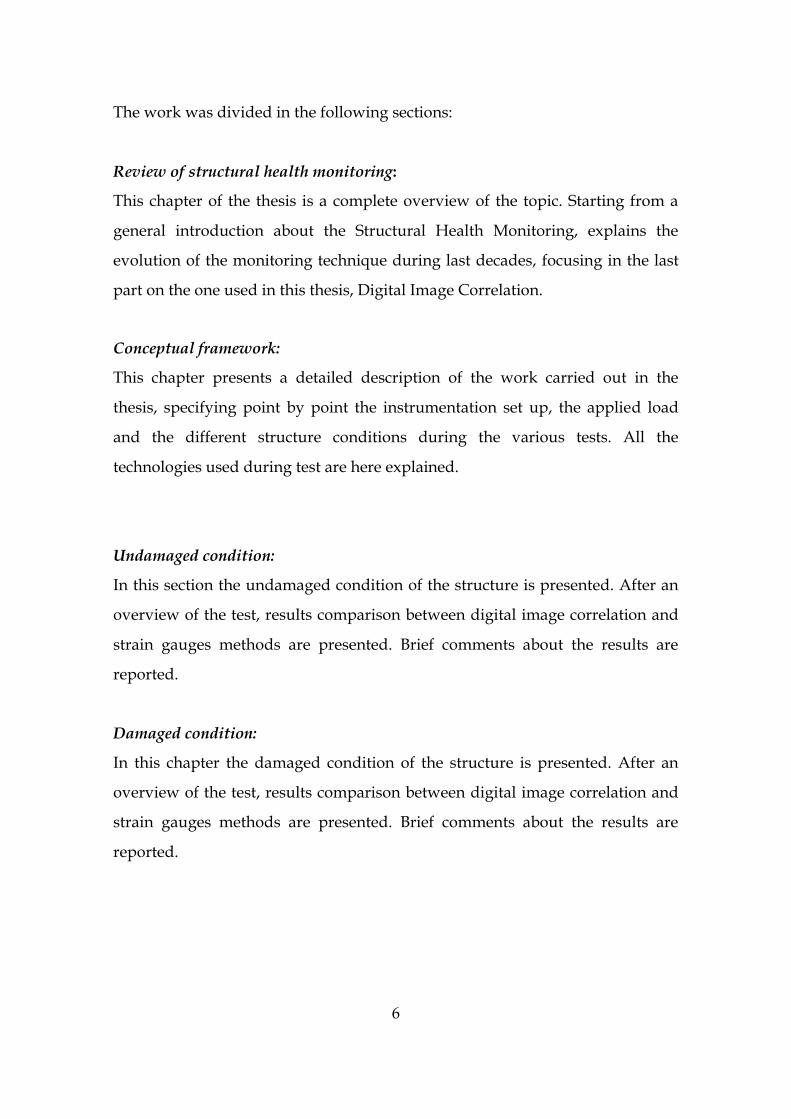
The work was divided in the following sections:

Review of structural health monitoring:

This chapter of the thesis is a complete overview of the topic. Starting from a

general introduction about the Structural Health Monitoring, explains the

evolution of the monitoring technique during last decades, focusing in the last

part on the one used in this thesis, Digital Image Correlation.

Conceptual framework:

This chapter presents a detailed description of the work carried out in the

thesis, specifying point by point the instrumentation set up, the applied load

and the different structure conditions during the various tests. All the

technologies used during test are here explained.

Undamaged condition:

In this section the undamaged condition of the structure is presented. After an

overview of the test, results comparison between digital image correlation and

strain gauges methods are presented. Brief comments about the results are

reported.

Damaged condition:

In this chapter the damaged condition of the structure is presented. After an

overview of the test, results comparison between digital image correlation and

strain gauges methods are presented. Brief comments about the results are

reported.

7

Results comparison:

This section contains a comparison between the undamaged and damaged

condition of the structure, in order to obtain results related to the main objective

of the thesis.

Conclusions:

Final comments about the comparison of the health monitoring structures

methods are presented. Final conclusion regarding Aramis reliability are

reported.

9

Chapter 1

Structural Health Monitoring

1.1 Background

Structural Health monitoring(SMH) represent the process of implementing a

damage identification strategy for civil engineering buildings, where damage

means changes to the material and/or geometric properties might lead to

compromise the integrity of the structure. The same holds true for bridges,

structures in which this thesis will focused on.

Bridges are subjected to several types of external loads during their lifetime.

These actions can be environmental like an earthquake or the wind, or can be

due to human interaction. All external load leads some changes into the bridge

and this induces new stresses on it. Since it is not possible to calculate the exact

effect on the structure, the new state has to be continuously compare with the

initial and undamaged one, so as to be able to estimate the residual life. This

process is called monitoring. The most important steps are to identify, locate

and classify type and severity of damages and estimated the effects on the

structural performance. Even if the found damage does not imply a total loss of

system functionality, the part of the structure close to it is not working in the

optimal way, so the damage could grow and it could reach a point no more

acceptable for a safety use of the bridge. To avoid this possibility, once the

damage is identified and valuated is necessary to intervene as quickly as

possible.

10

Fig. 1.1: Tacoma Narrows Bridge, some instants before the collapse in 1940.

Nowadays many SHM systems use a network of sensors connected to an

external data acquisition unit. Since the presence of cable presence between

them was cause of limitation, most modern systems use wireless transmitters

and receivers. But health monitoring technique born in a simple way, based on

visual monitoring and mere tests. some of were also done destroying part of the

structure to check its condition. First and traditional methods met several

problems, from the limitation of the access to some building areas to the

impossibility to have a continuously inspection of the structure, passing

through the subjectivity of the inspectors judgments.

These monitoring methods have been developed during last years and many if

most recent ones use automatic sensor stably associated to the bridge. They

have some high initial costs but make able to get cadenced data(with

established time interval), giving real time information about the structure and

above all in the moment of a particular event like an earthquake, to check

immediately the bridge state: have sensors already fixed to the bridge means a

save of time, no need for new investments and being able to decide if the

structure have to be closed to be repaired or not after the event. So in a long-

term view the benefits are higher than the cost, also because this technique

avoids the possibility to waste money making periodical maintenance also if

not necessary, but rather just when they are required.

11

Others still more recent techniques called no-contact technologies not even

provide any sensor into the structure. They use modern technologies like

photogrammetry and GPS System, where thanks to particular software it is

possible to process and analyze data and keep the bridge continuously under

control, checking local strain and global displacement and without problems

about any breakdown of sensors into the bridge, besides an important save of

money.

Whatever type of health monitoring need first of all to define the most

important areas and parameters to monitor, namely those where (based on

accurate analyses on the structural geometry of the structure) the structure

might be more sensitive to damages.

In this context SHM represent an important and increasingly widespread

checking method.

1.2 Historical review

Discounting as structural monitoring just a simple periodic visual observation,

the formal structural monitoring and interpretation using recording

instruments started in the second half of the last century and the great

development came hand in hand with the electronic growth. Structural Health

Monitoring growth involved mechanical and aerospace engineering, but after

that moved also to engineering structures and infrastructures during last

decades. Installation of large dams and long-span cable-bridges allows to

receive the greatest attention and research effort, meanwhile was not given the

same interest to residential and commercial structures, underestimating the

benefits of a structural monitoring. Every single structure requires a prior

12

particular study to apply the monitoring technique, because building is unique

and therefore every single case has to be studied like new.

Ross & Matthews (1995) and Mita(1999) identified the case where structural

monitoring may be required:

- Modification of an existing structure;

- Monitoring of structures affected by external works;

- Monitoring during demolition;

- Structures subjected to long term movement or degradation of materials;

- Feedback loop to improve future design based on experience;

- Fatigue assessment;

- Novel system of construction;

- Assessment of post-earthquake structural integrity;

- Decline in construction and growth in maintenance needs;

- Move towards performance-based design philosophy.

As presented by Brown John in 2007 on the article “Structural health

monitoring of civil infrastructure” are presented the main case of monitoring

applications on civil structures and infrastructures.

Fig. 1.2: Main fields of application of the Structural Health Monitoring

13

1.2.1 Dams

During the year 1864, close to Sheffield(UK), 254 people lost their lives due to

the failure of a 30 meters embankment dam. Due to that event a legislation was

induced in order to have a regular inspection on dams. At present, the law

governs dams in UK is the Reservoir Act of 1975: it requires the presence of a

supervising engineer who is responsible to oversee the dam, it means also

keeping and interpreting data. In this way dams are historically present as the

first structure for the mandated application of SHM.

The main points of the SHM were fixed in the International Commission on

Large Dams (ICOLD 2000).

- Range of tools and instrumentations to provide response data,

supplemented by visual inspections;

- Need for automatic data collection;

- Intelligent interpretation of data against established behavior patterns

and identification of anomalies.

The Italian company ENEL introduced for its dams a monitoring program

reported by Fanelli(1992). All the principles dams of the company provide

sensors to keep data about the structure with a regular time interval, such as:

- Relative or absolute displacements: horizontal crest displacement are the

most important for concrete dams;

- Strains(for concrete dams);

- Uplift pressure quantifying loads, which, for example, contributed to the

failure of Malpasset Dam in 1959;

- Seepage rates;

- Water level;

- Structural temperature;

- Meteorological conditions.

14

Dam case permitted to learn much about the monitoring technique and it was

helpful also to be applied to many others type structures.

1.2.2 Bridges

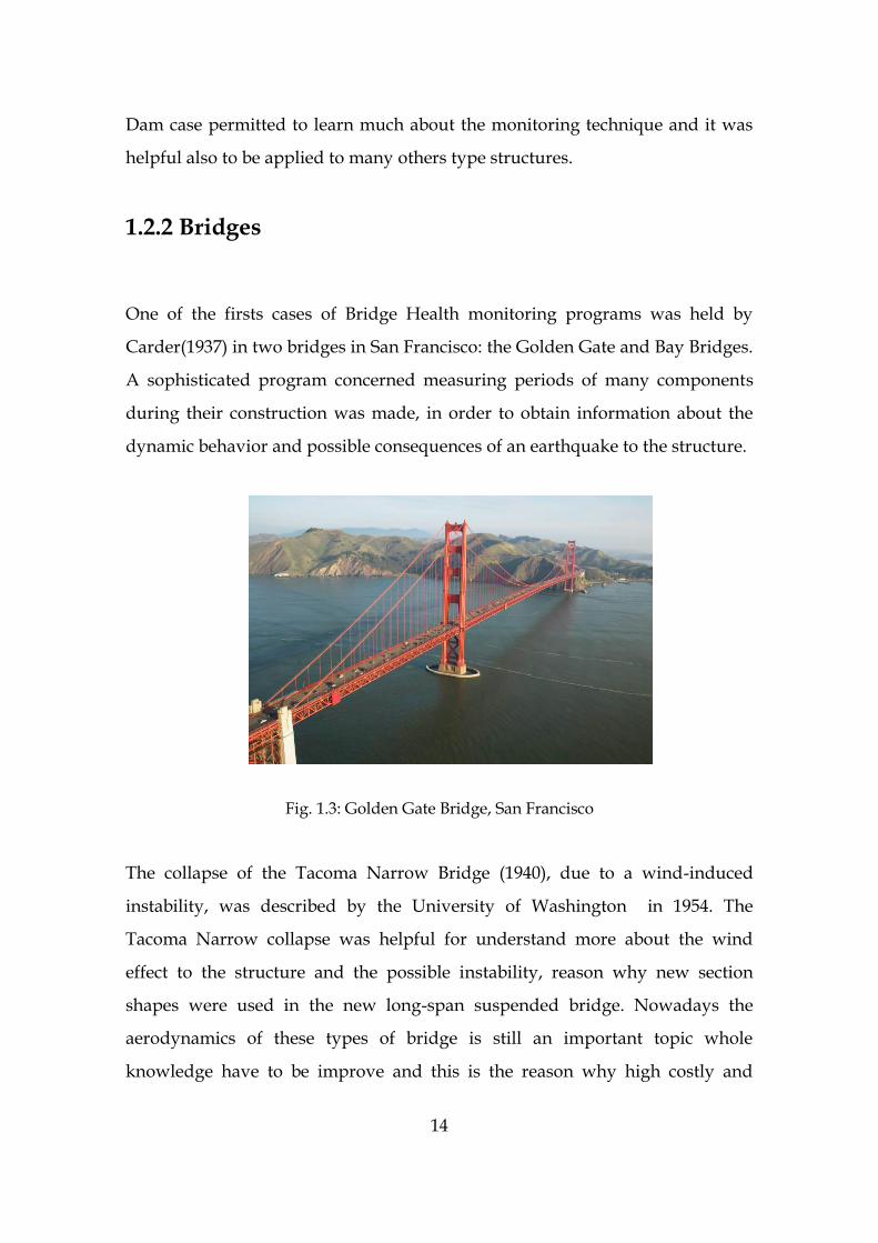
One of the firsts cases of Bridge Health monitoring programs was held by

Carder(1937) in two bridges in San Francisco: the Golden Gate and Bay Bridges.

A sophisticated program concerned measuring periods of many components

during their construction was made, in order to obtain information about the

dynamic behavior and possible consequences of an earthquake to the structure.

Fig. 1.3: Golden Gate Bridge, San Francisco

The collapse of the Tacoma Narrow Bridge (1940), due to a wind-induced

instability, was described by the University of Washington in 1954. The

Tacoma Narrow collapse was helpful for understand more about the wind

effect to the structure and the possible instability, reason why new section

shapes were used in the new long-span suspended bridge. Nowadays the

aerodynamics of these types of bridge is still an important topic whole

knowledge have to be improve and this is the reason why high costly and

15

elaborate structural health monitoring systems to civil infrastructure are

justified.

Several bridges were monitoring during last decades and this permitted to

develop new SHM systems, implemented in Japan, Hong Kong, and later in

North America.

Modern long-span suspension bridges programs provide inspection and

maintenance in order to pick up visually if some important damage and/or

deterioration come out. In this way is possible to reduce the density of

sensorscounting just in a minimum but well located number, so as sensors are

used to detect global changes such as foundation settlement, bearing failure,

loss of main cable tension, rupture of deck element.

Conventional short-span bridges are monitored as well and SHM systems were

developed during last decades. There is a history of research in full-scale testing

for short-span highway bridge assessment(Salane et al. 1981; Bakht & Jaeger

1990) and the possibility to envelop it for automated monitoring exercises. In

these type of bridges the visual inspection is less frequent as less important:

SHM systems can give almost all the information about the structure. European

research focused on short-span bridges and led to develop the BRIMOS system

(Geier & Wenzel 2002) that permit to track dynamic characteristics. Australian

studies permitted to analyze and get information about the strains in very

short-span highways and railway bridges due to the presence of the vehicle.

1.2.3 Offshore installations

In 1970s, the energy crisis and discovery of large oil reserve in the North Sea

permitted a quick growth in offshore infrastructure, especially for the part of

the installation of steel and concrete products operating to depth up to 150m

and subjected to important environmental loads. In 1977 inspections became

16

mandatory (Det Norske Veritas) and diver inspection were as expensive as

danger, so vibration-based diagnostic systems were developed (Coppolino&

Rubin 1980; Kenley &Dodds 1980; Shahrivar&Boukamp 1980; Brederode et al.

1986). As required from the Norwegian Petroleum Directorate, data about

structure performance were taken and managed from an operator of the

platform, in order to monitoring the shelf and its foundation, identifying

dynamics properties and load-response mechanisms.

Fig. 1.4: Example of an offshore platform

Around 1980s increased the number of system identification techniques whole

led to the modern discipline of ‘operational modal analysis’ (Peeters& De Roeck

2001). The increasing of reliability and accuracy of dynamic parameter

estimates for the vibration-based diagnostics permitted to say detection was

possible but just under controlled conditions or where were structural damage.

The most important problem of offshore installation and in which the research

is still working on is about the non-stationary nature of the structure, subjected

to many changes in mass properties due to fluid movements and drilling

operations.

17

1.2.4 Buildings and Towers

Health monitoring on buildings started due to the necessity to study the

structural behavior during earthquakes and storms. At the beginning, the low-

amplitude dynamics response was based on vibration testing (Hudson 1977;

Jeary & Ellis 1981) but knowing the building response during a typical but not

ultimate large amplitude loading eventwas more important, and this has

required long term monitoring. In California the mandatory structural

monitoring is manage by the California Strong Motion Instrumentation

Program (CSMIP), and it use levies on building owners in order to check the

condition of the structure. Such data can help to understand the structural

behavior of the building, but also information about the ground motions need

to be studied, to improve the knowledge about the performance during

earthquake.

Due to important recent earthquake SHM system has to been improved in order

to take timely information about the condition of the structure during the

earthquake event. This meant the necessity to develop new autonomous

sensors, embedded systems, communications, data management and

mining(Kiremidjian & Straser 1998; Lynch 2005).

1.2.5 Nuclear installations

Nowadays nuclear energy is really widespread around the world, but some

important disaster like Three Mile Island (1979), Chernobyl (1986) and

Fukushima (2011) recalled how this technology is potentially dangerous and

hence forced to stay focused on the safety of these structures.

18

In the UK licenses to operate nuclear reactors are granted by the Nuclear

Installation Inspectorate (NII) as required by the Nuclear Installation Act of

1965. To grant the permission the performance of the prestressed concrete

pressure vessel (PCPV) must be proven with structural tests and they have to

be repeated every three years turning the reactors, meanwhile the online

monitoring of structural response does not play an important contribution in

tracking the health of the structure. Strain data are used just to obtain

information about changes in other operational parameters.

1.2.6 Tunnels and excavations

Tunnel monitoring aim is to keep monitored deformations and deflections, in

order to be sure they don't overpass the established limit for the stability and

therefore the safety of the structure.

Monitoring of heritage and other structures during nearby tunneling or mining

is a major concern: some known example are the monitoring of Mansion House

in London during an extension of the underground railway, the monitoring of

listed nineteenth century mining facilities in Australia close to explosive

blasting in nearby open cast mining operation.

Important benefits may come out using SHM system in geotechnical

constructions. In April 2004 in Singapore occurred a collapse of tunneling

excavations. Post-accident examination of recordings from instrumentation

showed some movements in the excavation already two months before the

accident. Using online processes wired with automatic alarms might probably

permitted to avoid the collapse.

19

1.3 Traditional and modern monitoring methods

1.3.1 The process

The structural health monitoring is a no invasive survey process of particular

structural quantities subjected to known or unknown actions, in which data are

taken with a preset time period. In this way several parameters can be

monitored in real time or at least with short time interval, in order to be able to

collect any anomaly in the structure and identify the presence of structural

damages. When the sensor able to keep this type of data have to fixed in the

structure, this traditional technique is also known as contact method; notice

sensors able to send information in wireless mode are as well part of this

category, due to the need to fix them to the structure. On the other hand, most

modern methods do not need the presence of some fixed sensors into the

structure: these methods are called no-contact methods.

Every SHM process, as the traditional as the most innovative, is composed by

three main parts:

- Instrumentation and data acquisition;

- Signal processing and feature extraction;

- Damage detection, alarms and reports.

Fig. 1.5: Structural Health Monitoring process (Kullaa 2008)

20

1.3.2 Instrumentation and data acquisition

The first part of each SHM consists in setting the limitations about what will be

monitored and how it will be accomplished, including justification for

performing SHM (Farrar et al. 2001). The parts compose the monitoring system

are:

- sensors (except the most modern that do not need them, how will be

explain afterwards);

- acquisition unit;

- database to collect and store data.

To have a complete monitoring and to check every single point of the structure

the number of the sensors should be as high as costly so, the number of points

to monitor can be chosen in order to avoid useless expense that can led to

overpass the maximum financial resources, but at the same time permitting to

monitor efficiently the structure, controlling all the fundamental parameters.

Once points are chosen, data are recorded and, in different ways according to

the chosen strategy (static, dynamic) and method(traditional, modern),

information about the structure is given.

A transducer is a device able to convert a physical quantity (as displacement,

strains, stresses, etc) into a proportional electrical signal, processed by the data

acquisition unit. The recorded signal can be analogical or digital. Traditional

and innovative sensors are now presented.

1.3.2.1 Traditional sensors

- Pendulum: exist two types of pendulum, hanging or inverted, and both permit

to perform long term monitoring of horizontal structural movements in

structures with important dimension such as dams, bridges and tall buildings.

The pendulum is composed by a steel cable, which upper end of the steel wire

is fixed to the structure, meanwhile the bottom end is free to move in an oil tank

21

in order to damp the cable oscillations. Displacements are measured with a

portable optical readout unit or an automatic x/y coordinator.

- Inclinometers: permit to evaluate and measure the variation of inclination of a

structural element. To provide the output signal the instrument considers the

angle of inclination respect to the vertical direction.

- Strain gauges: measure as the strains as the elongations between couples of

structural points. as reported in Ko & Ni 2005, the mainly used types of these

sensors are three: electrical resistance strain gauges, vibrating wire strain

gauges and, relatively to the last years, fiber optic strain gauges.

Fig. 2.1: mono directional electrical strain gauges

- Displacement transducers: permit to keep monitored a crack present in the

structure, describing its development over the time. Usually is not placed just

one, but rather two, both in the plane of the structure, one in the vertical

direction and the other in the horizontal one, in order to split the study and

identify easier contraction and expansion along the crack directions.

- Thermocouples: measure the air temperature of a particular element of the

structure. Widely used in this area are thermally sensitive resistors as

Thermistors and Resistance Temperature Detectors (RTD).

22

- Accelerometers: three main types are present: Piezoelectric accelerometers,

Piezoresistive and capacitive accelerometers, Force-balance accelerometers. All

three permit to obtain acceleration induced by vibrations and it is provided by a

detection of inertia of a mass as a consequence of an acceleration.

Piezoelectric accelerometers produce, proportionally to the acceleration, an

electric signal in a frequency band below their resonant frequency. A part of the

piezoelectric material, which represent the active element of the accelerometer,

is connected to the base sensor. The other side, instead, is wired to a seismic

mass. In this way, when a vibration hit the accelerometer a force equal to the

product of the seismic mass and the acceleration is generated. This permit to

obtain a charge output, which value is proportional to the applied force. Due to

inability to measure the DC components, this type of sensor is not

recommended for suspension bridges or other really flexible structures.

Piezoresistive and capacitive accelerometers: contain a diaphragm which, if

subject to an acceleration, behaves as a mass that undergoes flexion.

Force-Balance accelerometers: these types of sensors present a freely suspense

mass constrained by an electrical equivalent mechanical spring. They cover a

wide range of frequencies (from DC to 1000Hz) and accelerations (from 0.0001g

up to 200g). Besides, with some alteration, it is possible to measure also angles

of inclination and with a good precision.

23

1.3.2.2 Innovative sensors

Fiber optic sensors: in spite of the high cost, this sensors widely increased their

importance during last year, because they can be used for a several different

number of applications. Their main characteristic is to be easy to handle,

dielectrics, immune to electromagnetic interference and capable of detecting

very small deformations with high accuracy also if the observation period is

long. The most important field of application of this technology is the long-term

monitoring of big civil structures as bridges, dams, tunnels, geotechnical

structures. Recent studies showed as fiber optic sensors are useful to study as

well dynamic phenomena (Inaudi et al. 1996).

Piezoresistive cement-based strain sensors: piezoresistive cement-based

material is a quite recent material in civil engineering. Differently from the

traditional cement-based, it involves the insertion of carbon fibers in the cement

paste. Many studies have been done to develop properties and focused

measurement methods, but the research is still going on.

Corrosion monitoring sensors: In civil engineering structures, the presence of a

corroded element have to be avoided because could lead to a deterioration of

the structural performance. Trying to avoid the arise of this phenomenon, a

sensor was developed by Qiao & Ou in the 2007. It is able to find the presence

of corrosion using a time-frequency analysis approach thanks to the wavelet

transform.

GPS systems: The use of the GPS technology gave a new approach of

displacement measuring and more generally to SHM in civil engineering. In

fact this technique permit to have a direct measurement of the request

parameters, resolving in this way many of the main problems which traditional

methods were affected by, because no sensor are required to be fixed to the

24

studied structure. Important results were showed in some recent project, such

as a ratio tower in Japan (Li et al. 2004) and a group of three high-rise buildings

in Chicago(Kijewski et al. 2003). Low frequencies and slow displacements own

of the long-span suspended bridges induct by environmental vibrations permit

the best apply of this method, as reported by Wong et al. in 2001 with same

applications example.

Wireless sensor Network(WSN): it consist in a wireless network able to connect

different types of sensors, which can communicate each other through elements

called nodes, detecting, sharing and processing data obtained from the single

points of the structure. Although nodes still need a battery to work, the absence

of connecting cables has been an important development because it prevents

wires tear or breakage typical of the traditional systems. Besides installation

time and costs are significantly reduced (Celebi, 2002). This technology has

been widely used in civil engineering field during last period, especially for

Structural Health Monitoring.

Digital Image Correlation (DIC): this recent and innovative technology, as

explain for the GPS system, permit a direct measurement of the request

parameters, without the need of install any weather-sensible sensor to the

structure, often difficulty to place and costly. Although with this monitoring

process there is no need to use an external technology such as GPS: the required

equipment is based to some cameras, which cost is widely lower than all the

other used technologies. Due to this reason, DIC technologies is the one chosen

for carry on this thesis: a wider description of this method is discussed in the

paragraph 1.4.

25

1.3.3 Signal processing

Although most modern technologies such as GPS and DIC systems work in a

different way, is presented in this section how signal is processing to obtain

information we need. Signal processing provides some useful information from

the time histories using stochastic properties (Kullaa 2008).

Most of the sensor acquired information in time domain, but due to

computation requirements frequency domain is preferred. The conversion

signal is made possible without information loss using The Fast Fourier

Transform FTT (Cooley & Tukey 1965). Some problems, known as leakage

error, derived because FTT is supposed to be used by time series of infinite

length, but techniques have been developed to reduce them to acceptable

values.

1.3.4 Damage identification

For a civil building, damage means a variation of the initial and undamaged

state that might lead to compromise the integrity of the structure. The rule of

the Structural Health Monitoring consists exactly in a continuously check of the

structure, in order to notice when parameter values start to differ from the

initials or expected ones. Different part of the structure are usually sensible to

different kind of damage, so the fundamental step in order to furnish a well

monitored system is the choice of the parameters to check. Development of

automatic and continuously monitoring methods of last period permitted to

find easily and quickly many types of damage.

26

1.4 Digital Image Correlation (DIC)

Digital Image Correlation is a modern no-contact technology of structural

health monitoring. As for the GPS-system this method allows to check the

structure without a direct contact to the building and at the same time no-one

sensor is required to be located into the bridge. Once the measurement point is

chosen, it has to be marked with a target panel of known geometry or painted

with same spray, in order to define points will permit to identify, though the

camera and the software, displacement of single points. A commercial digital

camera with telescopic lens is installed on a fixed point as the coast, or on a pier

(abutment) that can be considered as fixed point as well (in this case the camera

will be without telescopic lens). The technique of digital image correlation

allows to calculate the displacement of the chosen point comparing several

motion pictures of the target; displacement are furnished with a process

involves the use of texture recognition algorithms, projection of the captured

images, calculation of the actual displacement based on the number of the pixel

moved. Image processing software as MATLAB and ARAMIS permit nowadays

to have all this functions.

This bridges monitoring system is basically composed by hardware (digital

camera, laptop computer, target object, telescopic lens) and software

(continuous image capturing, target recognition algorithm, calculation of a

trigonometric transformation matrix from pre captured images, actual

displacement calculation from online image data. This equipment cost is really

economic amount comparing to other bridges health monitoring techniques.

Target panel/sprayed area dimension is determined in order to the distance of

the camera, the expected maximum displacement and the performance of the

camera considering the telescopic lens. A light source can be used to brighten

white spots on the target. In the case of target panel, to recognize the white

27

spots on a threshold for the white and black image is calculated basing on the

brightness of background and target region as:

= average of brightness in background region

= standard deviation of brightness in background region

= average of brightness in target region

= standard deviation of brightness in target region

Direction vectors permit to have actual horizontal and vertical direction, basing

calculation on pixel coordinates (x,y). Actual displacement ) are

calculated basing on the number of pixel of target movement and using the

trigonometric transformation matrix (T) and the scaling factors (SFx, SFy):

[

]

√

⁄ , √

⁄

The accuracy of the system is correlated to the hardware performance and the

distance to the target. Using a commercial digital camera with 30x optical zoom

and telescopic lens with 8x optical zoom it is possible to have a resolution of

0.021mm/pixel at the distance of 10m. It means that basing on the expected

displacement, the camera could be placed at the distance of several tens of

meters in the case of a normal bridge, till a couple of hundreds for the case of

long-spam ones, where expected displacement are about tens of centimeters.

Displacements of the considered point are calculated from correlation of image

frames using image processing techniques. It provides displacement after a

process of recognition and calculation, where the information quality of the

result is related to the number of pixel for frame and to the number of frame for

second.

29

Chapter 2

Conceptual framework

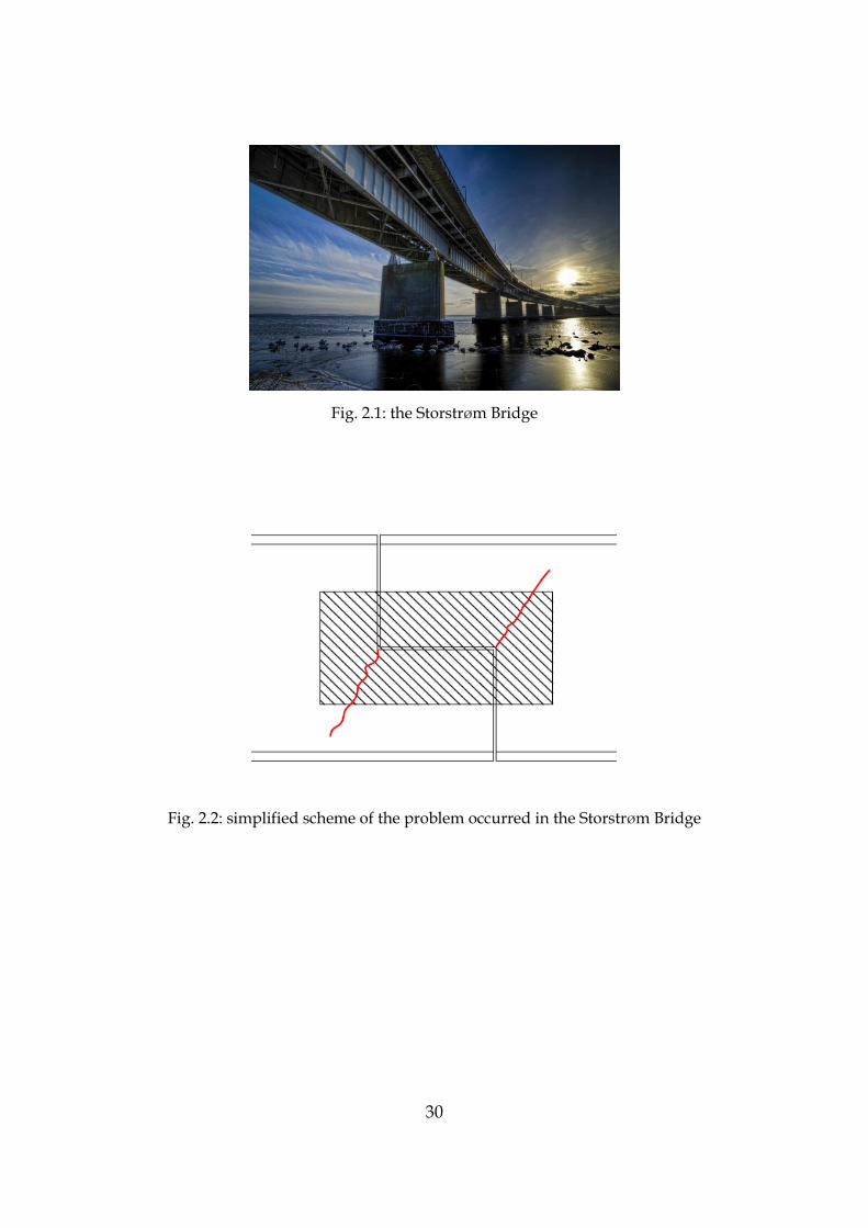
2.1 Experiment background

The present thesis takes its inspiration to a real bridge in the south part of

Denmark, the Storstrøm Bridge (figure 2.1). In the structure occurred a problem

of cracking in several of the steel beams, but this problem was discovered just

when the cracks came out from the plates used as junction between beams

through bolting (figure 2.2). The discovery of these cracks leads to check all the

bridge, in order to understand the entity of the problem. Quick interventions of

rehabilitation have been done in order to guarantee the restore of the safe

conditions, but vehicles speed limit had to be reduced from 120km/h to

80km/h. From this case born the idea of this thesis, mainly focus on discover if

it is possible to understand the presence of a crack also when it is not visible

because hidden from plates. The structural health monitoring in which the

thesis focused on is a no-contact technology based on the digital image

correlation (DIC), in order to have a not fixed set of sensors to the studied

structure, but based on a no contact technology that could permit to check the

bridge when is request.

30

Fig. 2.1: the Storstrøm Bridge

Fig. 2.2: simplified scheme of the problem occurred in the Storstrøm Bridge

31

2.2 The project

2.2.1 Description of the structure

The model used and tested in the laboratory does not reproduce exactly the

structure of the Storstrøm Bridge, but is a simplified structure that permit as

well to study the request problem. The structure built in the laboratory consists

in three plates of 10mm thickness. The main one is 850mm long and 150mm

high: one edge is free and the other one is bolted with the other two plates (both

are 300mm long and 150mm high) through 9 high resistance bolts. The structure

is finally welded to a fixed plate through the two smaller plates.

The load applied needed to induce in the joint actions of shear forces and in the

same time bending moment so, due to these requests, the load was applied in

the external free edge of the main plate (called in the rest of the work as beam).

After a first solution made with a hole in the upper part of the beam but this

one was a little too wide and the gap could not permit to have a precise load

application point. In this way a second solution with a 16mm hole, close to the

middle of the beam high, has been preferred because in this way there was no

variation of the load application point and the force was applied exactly in the

vertical direction.

32

Fig. 2.3: structure during test

2.2.2 Application of the load

To applied the load to the beam there were two different set up to choose

between: a mechanical one and an hydraulic jack. Instead the hydraulic jack

could have been easier to use, it was as well harder to control. In fact, due to the

reduced maximum value of the load (13,10KN for the undamaged condition

and 5,57 KN for the damaged one), the mechanical set up was easier to control

increasing manually in every step the actual force, and vibration due to the load

increase (vibration were responsible of noise in the strain diagram) was much

lower than using the hydraulic solution. The measurement of the load was

carried out using strain gauges, as showed in figure 2.17. In order to compare

strain gauges technology with digital image correlation method, photographs

were taken exactly in the same moment in which strain gauges were taking

data.

33

2.2.3 Undamaged and damaged conditions

In order to understand if it is possible to understand the presence of a crack also

when it is not visible because hidden from plates, the project presents two main

part: the undamaged and the damaged. These two states differ from a crack,

from the more external and upper bolt going almost in vertical direction, in

order to take data from each condition and be able to compare and analyze

results.

The place creation of the crack has been decided studying a 3D fem model

(Abaqus) and looking at the location of the main stresses in the beam, in order

to have a crack in the most stressed point of the structure(figure 2.4a).

Fig. 2.4: (a) Von Mises stresses in the undamaged state and (b) damaged beam in

Abaqus

Fig. 2.5: Damaged real beam

34

Due to the crack, in the damaged condition the structure is subjected to a

different distribution of the strain and this lead to overpass the plasticization of

the section. In order to avoid this situation, tests in damaged and undamaged

condition have been performed reaching different values of the maximum load.

The choice of the maximum load has been based in order to reach in both cases

the 70% of the load that lead the structure to yield.

2.3 Design of the structure

After the choice of the dimension of plates and the calculation of the maximum

load to apply, 9 high resistance M10 bolts of class 8.8 have been selected for the

joint, in order they worked below their yield stress to have the same initial

condition for every test.

Maximum shear force applied on bolts (due to shear and bending moment):

27,26KN

Shear resistance of a M10 8.8 class(EC3):

Preload of bolts(EC3) :

Tightening of bolts(EC3) :

Burr plates(EC3):

35

2.4 Materials and hypothesis

2.4.1 Elasticity theory

In order to valuate Aramis results is given a brief explication of elasticity and

deformations, parameters on which Aramis mainly works and gives results.

Generally a strain can be defined as a tensor quantity, decomposed in normal

and shear components. The state of strain in a material point of a continuum

body is defined as the totally of all changes in length of material lines or fibers:

The engineering meaning of strain is usually defined as the ratio between the

variation of length during the process and the total initial length:

Values of strain Aramis provides (called green strain) are obtained as:

⁄ (

)

2.4.2 Materials

The materials used in the tested model:

- Plates: Steel S355/Fe510;

- Bolts: M10 class 8.8

36

2.5 Aramis

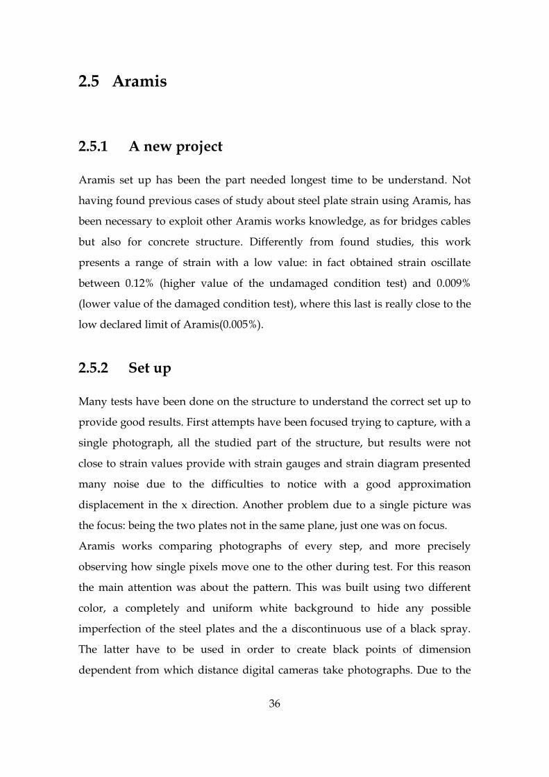
2.5.1 A new project

Aramis set up has been the part needed longest time to be understand. Not

having found previous cases of study about steel plate strain using Aramis, has

been necessary to exploit other Aramis works knowledge, as for bridges cables

but also for concrete structure. Differently from found studies, this work

presents a range of strain with a low value: in fact obtained strain oscillate

between 0.12% (higher value of the undamaged condition test) and 0.009%

(lower value of the damaged condition test), where this last is really close to the

low declared limit of Aramis(0.005%).

2.5.2 Set up

Many tests have been done on the structure to understand the correct set up to

provide good results. First attempts have been focused trying to capture, with a

single photograph, all the studied part of the structure, but results were not

close to strain values provide with strain gauges and strain diagram presented

many noise due to the difficulties to notice with a good approximation

displacement in the x direction. Another problem due to a single picture was

the focus: being the two plates not in the same plane, just one was on focus.

Aramis works comparing photographs of every step, and more precisely

observing how single pixels move one to the other during test. For this reason

the main attention was about the pattern. This was built using two different

color, a completely and uniform white background to hide any possible

imperfection of the steel plates and the a discontinuous use of a black spray.

The latter have to be used in order to create black points of dimension

dependent from which distance digital cameras take photographs. Due to the

37

low range of strain values, to obtain good results the only way found in this

work was to place the camera really close to the structure (from 10cm to 30cm)

and so the pattern needed to contain black points with a very limited coverage

area, otherwise the processing of Aramis was not able to give as good results.

The used digital camera was a Nikon D800 and three lens with different focal

distance has been used: 24mm, 60mm, 105mm. The best obtained results have

been provided with the 60mm lens. Tripod were used in order to have the

control directly from the laptop and avoiding in this way vibrations due to the

manual release photo.

Fig 2.6: (a) one of the used tripods and (b) a release during tests.

Many types of pattern has been tried, and better results have been provided

every time a finer pattern has been created.

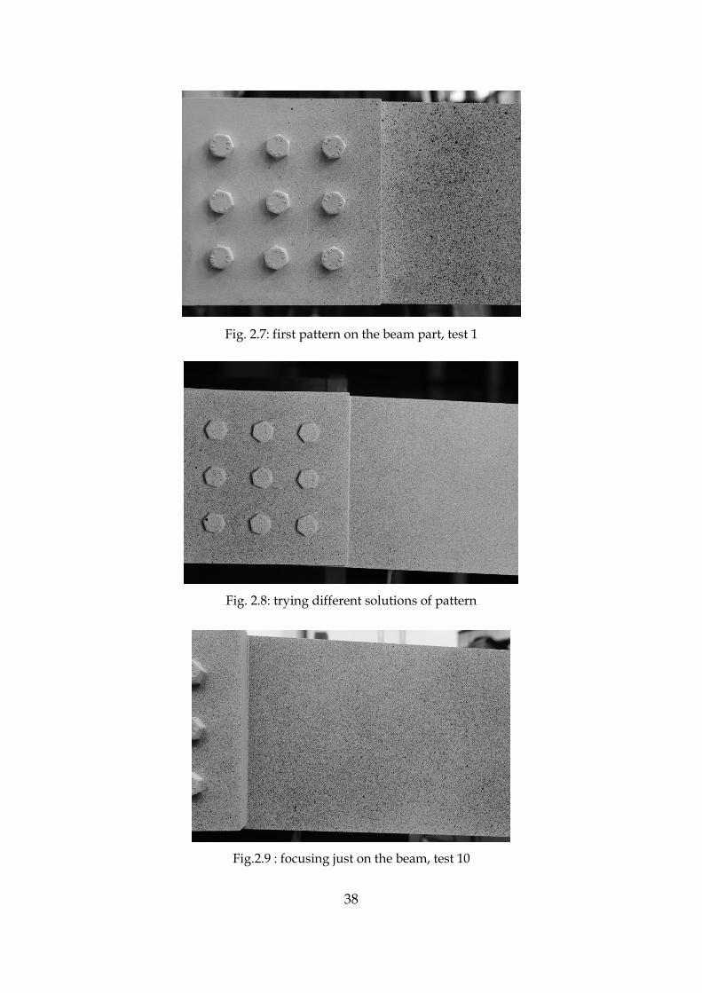
The final selected set up was taking pictures around 10cm from the structure.

This permitted to take photos just to one small area of the structure, so two

cameras were used at the same time: one in the beam part, the other on the

joint, but in this way not all the structure points has been possible to be checked

at the same time.

38

Fig. 2.7: first pattern on the beam part, test 1

Fig. 2.8: trying different solutions of pattern

Fig.2.9 : focusing just on the beam, test 10

39

Fig.2.10 : focusing on the joint, test11

Fig. 2.11: final solution for the middle joint, camera really close to the structure

Fig. 2.12: final solution for the bottom joint, camera really close to the structure

40

2.6 Other technologies

The finite element model of the structure and the strain gauges have been used

in this work in support of the digital image correlation method. The choice of

strain gauges is due to the reliability of the technology to evaluate strains,

meanwhile the 3D finite element method is basically due to place the strain

gauges in the most interesting point of the structure, that is where high

variation of stress are present.

2.6.1 Abaqus

Trying to have a more precise model as possible, the finite element model

created in Abaqus is not a simplified one, but present all the characteristics the

real structure has.

In this study a 0.2 coefficient friction has been used between plates, as suggest

in the Eurocode 3 part 6.5.8.3.

The model presents two different steps:

- Preload of bolts;

- Application of the load.

An important point of the experiment was to not overpass the yield stress of the

structure. Especially for the damaged condition, due to the presence of the

crack, could have been quite hard to obtain the exact value of the load lead the

structure to yield, but the model permitted to obtain this limit value. In order to

do this the load application step was defined with fixed increments of 0.01.

In this way the fem model permit to obtain the limit load value:

- Undamaged condition: 18,71KN;

- Damaged condition: 7,95KN.

41

Another important contribute of the model for the project was the possibility to

have a general all-round stresses and strains view, and this permit to have an

easier results valuation from strain gauges and DIC technology, especially for

the comparison between undamaged and damaged conditions.

Fig. 2.13: mesh of the model

Fig. 2.14: application of bolts pre-stress

Fig. 2.15: defining friction between plates

42

2.6.2 Strain gauges

Strain gauges represented in this work an important part. The reliability of this

technology permitted, especially at the beginning of the tests, to understand if

Aramis results were correct. At the same time, comparing diagrams of strain

gauges with Aramis ones was possible to understand the main problem in the

first part of the tests (despite the trend line was close to strain gauges one) that

was the wide oscillation of Aramis values.

Fig. 2.16: a mono directional strain gauges

Fig. 2.17: photo of the six applied strain gauges

43

Chapter 3

Undamaged condition

3.1 Conduct of the test

This chapter present all the final tests have been done on the structure in

undamaged condition, that means without the crack in the beam at the joint.

Measured loads were plotted in graphs with load as a function of strains

obtained from digital image correlation method and also with those obtained

from strain gauges. For every test, due to the close proximity required from

camera and structure to obtain good results, just two restricted areas were

analyzed: one in the main beam, the other in the joint part.

As explained in the chapter 2, six points of particular importance were

analyzed, three of them in the joint part of the structure and the other three in

the beam, as with Aramis as with strain gauges. These points, due to the

positioning respect to the height of the structure will be called as top beam, mid

beam, bottom beam, top joint, mid joint and bottom joint. Two tests for each

single relevant point are presented in this chapter. Every test presents a

comparison graph with both technologies used.

44

3.2 Experiment results

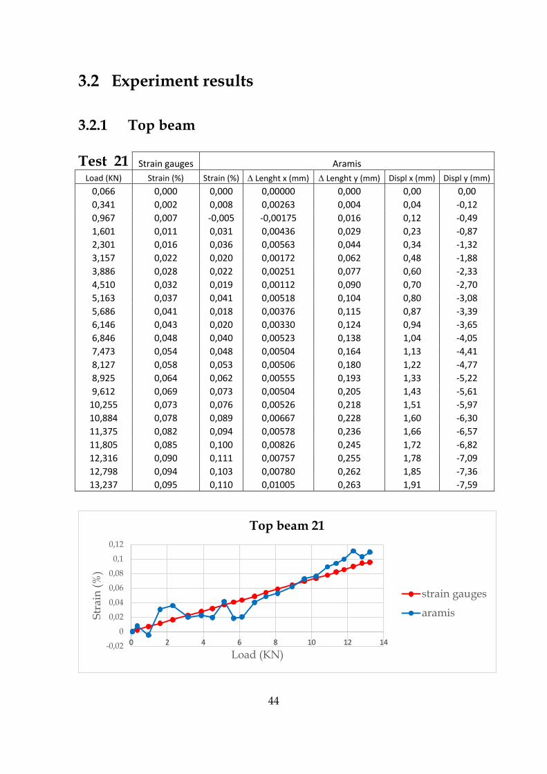
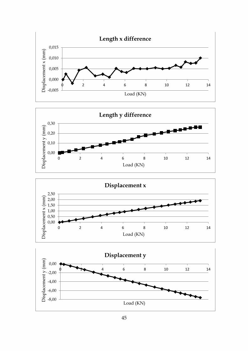
3.2.1 Top beam

Test 21 Strain gauges Aramis

Load (KN) Strain (%) Strain (%) Lenght x (mm) Lenght y (mm) Displ x (mm) Displ y (mm)

0,066 0,000 0,000 0,00000 0,000 0,00 0,00

0,341 0,002 0,008 0,00263 0,004 0,04 -0,12

0,967 0,007 -0,005 -0,00175 0,016 0,12 -0,49

1,601 0,011 0,031 0,00436 0,029 0,23 -0,87

2,301 0,016 0,036 0,00563 0,044 0,34 -1,32

3,157 0,022 0,020 0,00172 0,062 0,48 -1,88

3,886 0,028 0,022 0,00251 0,077 0,60 -2,33

4,510 0,032 0,019 0,00112 0,090 0,70 -2,70

5,163 0,037 0,041 0,00518 0,104 0,80 -3,08

5,686 0,041 0,018 0,00376 0,115 0,87 -3,39

6,146 0,043 0,020 0,00330 0,124 0,94 -3,65

6,846 0,048 0,040 0,00523 0,138 1,04 -4,05

7,473 0,054 0,048 0,00504 0,164 1,13 -4,41

8,127 0,058 0,053 0,00506 0,180 1,22 -4,77

8,925 0,064 0,062 0,00555 0,193 1,33 -5,22

9,612 0,069 0,073 0,00504 0,205 1,43 -5,61

10,255 0,073 0,076 0,00526 0,218 1,51 -5,97

10,884 0,078 0,089 0,00667 0,228 1,60 -6,30

11,375 0,082 0,094 0,00578 0,236 1,66 -6,57

11,805 0,085 0,100 0,00826 0,245 1,72 -6,82

12,316 0,090 0,111 0,00757 0,255 1,78 -7,09

12,798 0,094 0,103 0,00780 0,262 1,85 -7,36

13,237 0,095 0,110 0,01005 0,263 1,91 -7,59

-0,02

0

0,02

0,04

0,06

0,08

0,1

0,12

0 2 4 6 8 10 12 14

Str

ain

(%

)

Load (KN)

Top beam 21

strain gauges

aramis

45

-0,005

0,000

0,005

0,010

0,015

0 2 4 6 8 10 12 14

Dis

pla

cem

ent

x (

mm

)

Load (KN)

Length x difference

0,00

0,10

0,20

0,30

0 2 4 6 8 10 12 14

Dis

pla

cem

ent

y (

mm

)

Load (KN)

Length y difference

0,00

0,50

1,00

1,50

2,00

2,50

0 2 4 6 8 10 12 14

Dis

pla

cem

ent

x (

mm

)

Load (KN)

Displacement x

-8,00

-6,00

-4,00

-2,00

0,00

0 2 4 6 8 10 12 14

Dis

pla

cem

ent

y (

mm

)

Load (KN)

Displacement y

46

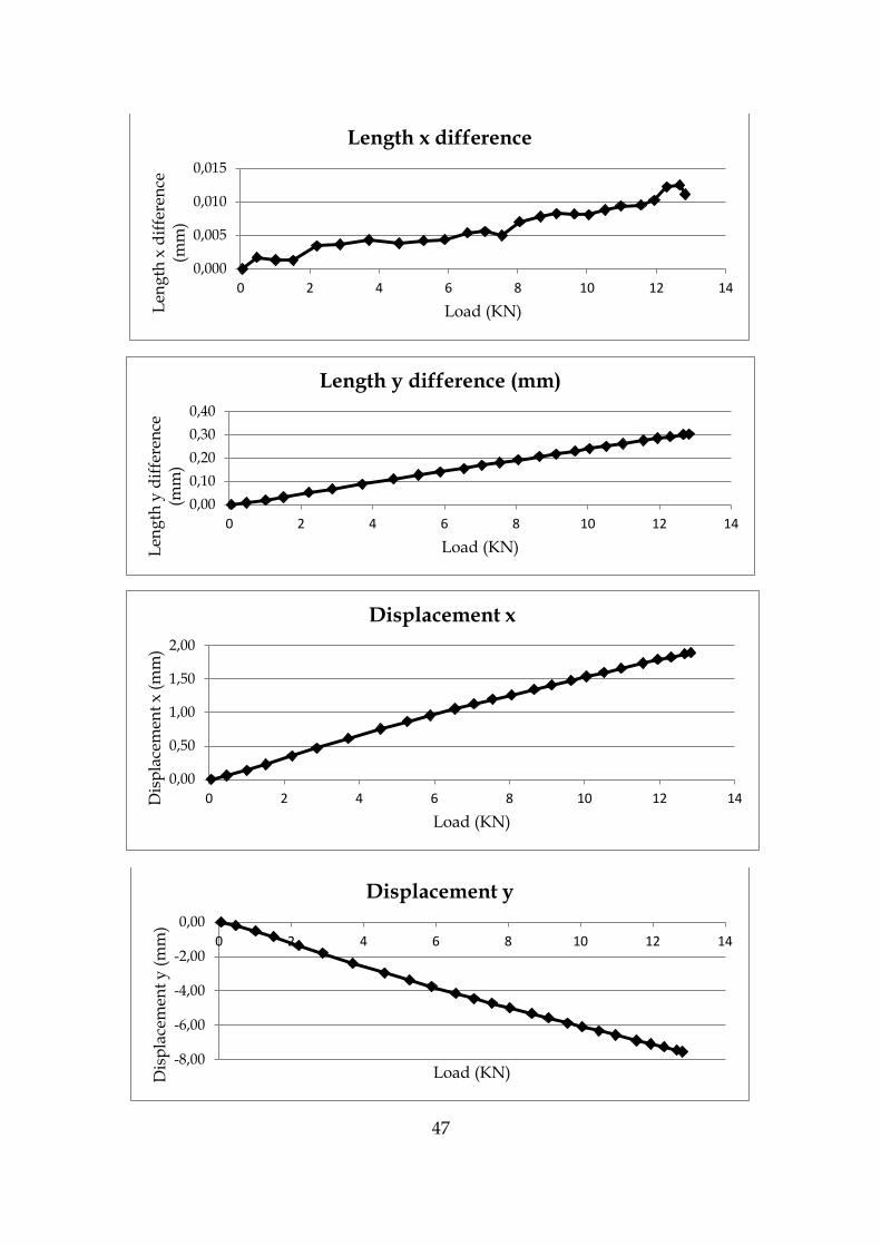
Test 25

Strain gauges Aramis


0,064 0,000 0,000 0,0000 0,000 0,00 0,00

0,476 0,003 -0,006 0,0017 0,008 0,06 -0,21

1,013 0,007 0,010 0,0013 0,020 0,14 -0,52

1,515 0,011 0,019 0,0013 0,032 0,22 -0,85

2,211 0,016 0,009 0,0035 0,052 0,35 -1,35

2,873 0,020 0,012 0,0037 0,067 0,47 -1,81

3,710 0,026 0,022 0,0043 0,088 0,61 -2,39

4,578 0,033 0,016 0,0038 0,110 0,75 -2,95

5,284 0,037 0,023 0,0042 0,127 0,87 -3,39

5,886 0,042 0,027 0,0044 0,141 0,95 -3,75

6,554 0,046 0,032 0,0054 0,155 1,05 -4,14

7,059 0,050 0,036 0,0056 0,169 1,13 -4,44

7,554 0,054 0,034 0,0050 0,181 1,20 -4,72

8,057 0,057 0,048 0,0070 0,193 1,26 -4,98

8,658 0,062 0,060 0,0078 0,206 1,34 -5,31

9,122 0,065 0,068 0,0083 0,217 1,41 -5,56

9,644 0,069 0,068 0,0082 0,230 1,48 -5,87

10,057 0,072 0,069 0,0081 0,241 1,54 -6,08

10,522 0,075 0,080 0,0088 0,251 1,60 -6,32

10,979 0,078 0,090 0,0094 0,262 1,66 -6,57

11,561 0,083 0,094 0,0095 0,276 1,74 -6,89

11,948 0,085 0,105 0,0102 0,285 1,79 -7,08

12,309 0,089 0,094 0,0123 0,292 1,83 -7,25

12,676 0,091 0,098 0,0125 0,300 1,88 -7,45

12,833 0,093 0,111 0,0111 0,304 1,90 -7,54

-0,02

0

0,02

0,04

0,06

0,08

0,1

0,12

0 2 4 6 8 10 12 14

Str

ain

(%

)

Load (KN)

Top beam 25

strain gauges

aramis

47

0,000

0,005

0,010

0,015

0 2 4 6 8 10 12 14

Len

gth

x d

iffe

ren

ce

(mm

)

Load (KN)

Length x difference

0,00

0,10

0,20

0,30

0,40

0 2 4 6 8 10 12 14

Len

gth

y d

iffe

ren

ce

(mm

)

Load (KN)

Length y difference (mm)

0,00

0,50

1,00

1,50

2,00

0 2 4 6 8 10 12 14Dis

pla

cem

ent

x (

mm

)

Load (KN)

Displacement x

-8,00

-6,00

-4,00

-2,00

0,00

0 2 4 6 8 10 12 14

Dis

pla

cem

ent

y (

mm

)

Load (KN)

Displacement y

48

3.2.2 Mid beam

Test 18



0,026 0,000 0,003 0,00000 0,000 0,00 0,00

0,700 0,003 -0,009 -0,00065 -0,014 0,04 -0,36

1,154 0,004 -0,009 -0,00055 -0,023 0,08 -0,63

1,630 0,006 0,008 0,00075 -0,033 0,12 -0,93

2,242 0,008 0,020 0,00097 -0,048 0,18 -1,34

2,777 0,010 0,010 0,00033 -0,060 0,22 -1,68

3,177 0,010 0,010 0,00045 -0,069 0,26 -1,93

3,545 0,012 0,013 0,00073 -0,078 0,29 -2,16

4,057 0,013 0,014 0,00091 -0,087 0,33 -2,47

4,456 0,014 0,006 0,00038 -0,096 0,36 -2,71

4,800 0,015 0,013 0,00096 -0,105 0,39 -2,92

5,218 0,016 0,016 0,00123 -0,114 0,42 -3,16

5,558 0,017 0,014 0,00119 -0,121 0,45 -3,36

5,865 0,018 0,015 0,00129 -0,128 0,47 -3,54

6,244 0,019 0,014 0,00130 -0,137 0,50 -3,76

6,579 0,020 0,011 0,00090 -0,143 0,52 -3,95

6,979 0,021 0,015 0,00095 -0,152 0,55 -4,18

7,362 0,023 0,016 0,00105 -0,160 0,57 -4,41

7,785 0,024 0,016 0,00158 -0,171 0,60 -4,65

8,047 0,024 0,017 0,00167 -0,175 0,62 -4,80

8,432 0,026 0,019 0,00182 -0,183 0,65 -5,02

8,813 0,026 0,020 0,00193 -0,191 0,67 -5,23

9,216 0,029 0,032 0,00279 -0,200 0,70 -5,47

9,593 0,029 0,024 0,00226 -0,208 0,72 -5,67

9,926 0,030 0,026 0,00243 -0,215 0,74 -5,86

10,223 0,032 0,037 0,00317 -0,222 0,76 -6,03

10,583 0,033 0,034 0,00296 -0,230 0,78 -6,23

10,901 0,033 0,042 0,00353 -0,237 0,80 -6,40

11,302 0,035 0,041 0,00404 -0,244 0,83 -6,63

11,672 0,036 0,040 0,00406 -0,249 0,85 -6,83

12,154 0,038 0,046 0,00383 -0,256 0,88 -7,09

12,589 0,039 0,041 0,00431 -0,267 0,91 -7,35

12,937 0,040 0,049 0,00472 -0,273 0,92 -7,53

49

-0,02

-0,01

0

0,01

0,02

0,03

0,04

0,05

0,06

0 2 4 6 8 10 12 14

Str

ain

(%

)

Load (KN)

Middle beam 18

strain gauges

aramis

-0,001

0,000

0,001

0,002

0,003

0,004

0,005

0 2 4 6 8 10 12 14

Len

gth

x d

iffe

ren

ce (

mm

)

Load (KN)

Length x difference

-0,30

-0,25

-0,20

-0,15

-0,10

-0,05

0,00

0 2 4 6 8 10 12 14

Len

gth

y d

iffe

ren

ce (

mm

)

Load (KN)

Length y difference

50

0,00

0,20

0,40

0,60

0,80

1,00

0 2 4 6 8 10 12 14

Dis

pla

cem

ent

x (

mm

)

Load (KN)

Displacement x

-8,00

-7,00

-6,00

-5,00

-4,00

-3,00

-2,00

-1,00

0,00

0 2 4 6 8 10 12 14

Dis

pla

cem

ent

y (

mm

)

Load (KN)

Displacement y

51

Test 25



0,0636 0,0000 0,0000 0,0000 0,000 0,00 0,00

0,4762 0,0018 -0,0184 -0,0020 0,007 0,03 -0,20

1,0128 0,0038 0,0032 0,0009 0,018 0,07 -0,51

1,5151 0,0053 0,0207 0,0029 0,029 0,11 -0,86

2,2109 0,0076 0,0116 0,0020 0,045 0,17 -1,35

2,8728 0,0098 0,0060 0,0009 0,059 0,23 -1,80

3,7105 0,0121 0,0045 0,0006 0,078 0,31 -2,38

4,5784 0,0149 0,0198 0,0012 0,096 0,38 -2,94

5,2843 0,0167 0,0107 0,0001 0,111 0,43 -3,40

5,8857 0,0184 0,0180 0,0008 0,124 0,48 -3,74

6,5536 0,0203 0,0094 0,0007 0,139 0,53 -4,13

7,0588 0,0215 0,0211 0,0019 0,149 0,56 -4,44

7,5539 0,0233 0,0093 0,0011 0,160 0,60 -4,71

8,0574 0,0245 0,0256 0,0040 0,170 0,63 -4,94

8,6582 0,0265 0,0377 0,0040 0,183 0,67 -5,30

9,1224 0,0282 0,0360 0,0037 0,192 0,70 -5,58

9,6437 0,0295 0,0239 0,0017 0,202 0,74 -5,86

10,0569 0,0310 0,0377 0,0035 0,213 0,77 -6,09

10,5223 0,0322 0,0398 0,0035 0,222 0,80 -6,31

10,9794 0,0336 0,0473 0,0042 0,231 0,83 -6,56

11,5606 0,0356 0,0429 0,0045 0,244 0,87 -6,88

11,9483 0,0365 0,0341 0,0023 0,251 0,90 -7,07

12,3092 0,0387 0,0488 0,0050 0,258 0,91 -7,25

12,6755 0,0393 0,0433 0,0053 0,265 0,94 -7,44

12,8329 0,0398 0,0418 0,0051 0,269 0,95 -7,51

52

-0,03

-0,02

-0,01

0

0,01

0,02

0,03

0,04

0,05

0,06

0 2 4 6 8 10 12 14

Str

ain

(%

)

Load (KN)

Middle beam 25

strain gauges

aramis

-0,004

-0,002

0,000

0,002

0,004

0,006

0 2 4 6 8 10 12 14

Len

gth

x d

iffe

ren

ce (

mm

)

Load (KN)

Length x difference

0,00

0,05

0,10

0,15

0,20

0,25

0,30

0 2 4 6 8 10 12 14

Len

gth

y d

iffe

ren

ce (

mm

)

Load (KN)

Length y difference

53

0,00

0,20

0,40

0,60

0,80

1,00

0 2 4 6 8 10 12 14

Dis

pla

cem

ent

x (

mm

)

Load (KN)

Displacement x

-8,00

-7,00

-6,00

-5,00

-4,00

-3,00

-2,00

-1,00

0,00

0 2 4 6 8 10 12 14

Dis

pla

cem

ent

y (

mm

)

Load (KN)

Displacement y

54

3.2.3 Bottom beam

Test 32



0,1295 0,0000 0,0000 0,0000 0,000 0,00 0,00

0,5148 -0,0018 -0,0127 -0,0002 0,006 -0,02 -0,20

1,2301 -0,0055 -0,0193 -0,0007 0,019 -0,06 -0,61

2,1283 -0,0106 -0,0187 -0,0013 0,037 -0,11 -1,19

2,9090 -0,0152 -0,0204 -0,0018 0,052 -0,16 -1,69

3,5460 -0,0186 -0,0237 -0,0021 0,066 -0,20 -2,09

4,2994 -0,0229 -0,0263 -0,0024 0,079 -0,24 -2,56

4,9584 -0,0270 -0,0275 -0,0026 0,092 -0,28 -2,95

5,2612 -0,0311 -0,0422 -0,0035 0,098 -0,30 -3,11

5,5182 -0,0297 -0,0311 -0,0029 0,102 -0,32 -3,28

6,1303 -0,0333 -0,0304 -0,0031 0,114 -0,35 -3,63

6,7483 -0,0368 -0,0406 -0,0035 0,126 -0,39 -3,98

7,4524 -0,0403 -0,0396 -0,0037 0,139 -0,44 -4,39

8,0871 -0,0438 -0,0425 -0,0040 0,151 -0,48 -4,74

8,7799 -0,0475 -0,0465 -0,0043 0,164 -0,53 -5,13

9,3272 -0,0506 -0,0498 -0,0045 0,174 -0,57 -5,44

9,9832 -0,0541 -0,0456 -0,0047 0,185 -0,61 -5,81

10,4706 -0,0569 -0,0598 -0,0057 0,195 -0,64 -6,07

10,8179 -0,0592 -0,0518 -0,0051 0,201 -0,67 -6,26

11,4793 -0,0623 -0,0553 -0,0054 0,213 -0,71 -6,62

11,9073 -0,0646 -0,0558 -0,0055 0,220 -0,74 -6,85

12,3769 -0,0670 -0,0595 -0,0058 0,229 -0,77 -7,11

12,9261 -0,0701 -0,0650 -0,0061 0,238 -0,81 -7,40

13,4123 -0,0728 -0,0655 -0,0063 0,247 -0,84 -7,66

-0,08

-0,07

-0,06

-0,05

-0,04

-0,03

-0,02

-0,01

0

0 2 4 6 8 10 12 14 16

Str

ain

(%

)

Load (KN)

Bottom beam 32

strain gauges

aramis

55

-0,008

-0,006

-0,004

-0,002

0,000

0 2 4 6 8 10 12 14 16

Len

gth

x d

iffe

ren

ce

Load (KN)

Length x difference

0,00

0,10

0,20

0,30

0 2 4 6 8 10 12 14 16

Len

gth

x d

iffe

ren

ce

Load (KN)

Length y difference

-1,00

-0,80

-0,60

-0,40

-0,20

0,00

0 2 4 6 8 10 12 14 16

Dis

pla

cem

ent

x (

mm

)

Load (KN)

Displacement x

-10,00

-5,00

0,00

0 2 4 6 8 10 12 14 16

Dis

pla

cem

ent

x (

mm

)

Load (KN)

Displacement y

56

Test 34



0,1283 0,0000 0,0000 0,0000 0,000 0,00 0,00

0,2755 -0,0007 -0,0120 0,0003 0,001 -0,01 -0,07

0,9042 -0,0038 -0,0081 -0,0004 0,014 -0,05 -0,42

1,5531 -0,0074 -0,0135 -0,0007 0,029 -0,10 -0,81

2,0524 -0,0101 -0,0164 -0,0009 0,042 -0,13 -1,14

2,4786 -0,0127 -0,0186 -0,0013 0,051 -0,16 -1,41

3,1275 -0,0163 -0,0066 -0,0017 0,068 -0,20 -1,82

3,8714 -0,0204 -0,0171 -0,0022 0,087 -0,25 -2,29

4,6687 -0,0251 -0,0191 -0,0024 0,105 -0,31 -2,77

5,4179 -0,0295 -0,0257 -0,0029 0,122 -0,36 -3,20

5,9783 -0,0323 -0,0278 -0,0042 0,134 -0,41 -3,53

6,7596 -0,0368 -0,0462 -0,0052 0,153 -0,47 -3,96

7,3847 -0,0406 -0,0419 -0,0039 0,166 -0,51 -4,33

8,0140 -0,0434 -0,0577 -0,0045 0,181 -0,56 -4,68

8,6035 -0,0466 -0,0441 -0,0043 0,193 -0,61 -5,02

9,3011 -0,0504 -0,0503 -0,0041 0,210 -0,67 -5,41

9,8693 -0,0534 -0,0541 -0,0046 0,223 -0,71 -5,72

10,4457 -0,0566 -0,0478 -0,0050 0,235 -0,75 -6,04

10,9076 -0,0586 -0,0556 -0,0054 0,246 -0,79 -6,29

11,5161 -0,0631 -0,0601 -0,0053 0,258 -0,83 -6,62

12,0771 -0,0650 -0,0555 -0,0058 0,272 -0,87 -6,92

12,6518 -0,0681 -0,0625 -0,0062 0,283 -0,92 -7,23

13,3013 -0,0719 -0,0825 -0,0070 0,299 -0,97 -7,57

-0,09

-0,08

-0,07

-0,06

-0,05

-0,04

-0,03

-0,02

-0,01

0

0 2 4 6 8 10 12 14

Str

ain

(%

)

Load (KN)

Bottom beam 34

strain gauges

aramis

57

-0,008

-0,006

-0,004

-0,002

0,000

0,002

0 2 4 6 8 10 12 14

Len

gth

x d

iffe

ren

ce

(mm

)

Load (KN)

Length x difference

0,00

0,10

0,20

0,30

0,40

0 2 4 6 8 10 12 14

Le

ng

th y

dif

fere

nce

(m

m)

Load (KN)

Length y difference

-1,50

-1,00

-0,50

0,00

0 2 4 6 8 10 12 14

Dis

pla

cem

ent

x (

mm

)

Load (KN)

Displacement x

-8,00

-6,00

-4,00

-2,00

0,00

0 2 4 6 8 10 12 14

Dis

pla

cem

ent

y (

mm

)

Load (KN)

Displacement y

58

3.2.4 Top joint

Test 31



0,1419 0,0000 0,0000 0,0000 0,000 0,00 0,00

0,4791 0,0008 0,0033 0,0003 0,006 0,04 -0,10

0,9659 0,0020 0,0026 0,0003 0,016 0,09 -0,27

1,8297 0,0040 -0,0059 -0,0005 0,034 0,22 -0,59

2,4287 0,0054 0,0076 0,0008 0,048 0,31 -0,82

3,2261 0,0074 0,0159 0,0015 0,066 0,44 -1,12

3,9521 0,0091 0,0143 0,0016 0,080 0,55 -1,39

4,5731 0,0106 0,0033 0,0009 0,095 0,64 -1,61

5,3811 0,0125 0,0186 0,0021 0,111 0,76 -1,89

6,1089 0,0140 0,0140 0,0016 0,126 0,86 -2,13

6,7649 0,0156 0,0156 0,0015 0,138 0,95 -2,35

7,4708 0,0171 0,0144 0,0016 0,152 1,04 -2,59

8,0544 0,0183 0,0174 0,0019 0,163 1,12 -2,78

8,6285 0,0196 0,0247 0,0027 0,174 1,20 -2,97

9,3100 0,0211 0,0198 0,0022 0,187 1,28 -3,19

9,9399 0,0226 0,0165 0,0019 0,198 1,37 -3,40

10,4095 0,0238 0,0280 0,0031 0,207 1,43 -3,55

10,8743 0,0249 0,0244 0,0027 0,215 1,49 -3,70

11,4021 0,0262 0,0244 0,0027 0,225 1,55 -3,87

11,8385 0,0272 0,0248 0,0028 0,234 1,61 -4,01

12,3003 0,0283 0,0289 0,0032 0,242 1,68 -4,16

12,6839 0,0292 0,0428 0,0038 0,249 1,73 -4,28

13,2235 0,0305 0,0418 0,0046 0,261 1,80 -4,45

-0,01

0

0,01

0,02

0,03

0,04

0,05

0 2 4 6 8 10 12 14

Str

ain

(%

)

Load (KN)

Top joint 31

strain gauges

aramis

59

-0,001

0,000

0,001

0,002

0,003

0,004

0,005

0 2 4 6 8 10 12 14

Len

gth

x d

iffe

ren

ce (

mm

)

Load (KN)

Length x difference

0,00

0,10

0,20

0,30

0 2 4 6 8 10 12 14

Len

gth

y d

iffe

ren

ce

(mm

)

Load (KN)

Length y difference

0,00

0,50

1,00

1,50

2,00

0 2 4 6 8 10 12 14

Dis

pla

cem

ent

x (

mm

)

Load (KN)

Displacement x

-5,00

-4,00

-3,00

-2,00

-1,00

0,00

0 2 4 6 8 10 12 14

Dis

pla

cem

ent

y (

mm

)

Load (KN)

Displacement y

60

Test 33



0,1295 0,0000 0,0000 0,0000 0,000 0,00 0,00

0,5148 0,0008 -0,0055 -0,0016 0,007 0,04 -0,12

1,2301 0,0025 0,0066 -0,0043 0,021 0,12 -0,37

2,1283 0,0046 0,0039 -0,0072 0,040 0,25 -0,73

2,9090 0,0064 0,0015 -0,0094 0,057 0,35 -1,04

3,5460 0,0079 0,0092 -0,0104 0,071 0,44 -1,28

4,2994 0,0097 0,0136 -0,0118 0,087 0,54 -1,57

4,9584 0,0113 0,0069 -0,0133 0,101 0,63 -1,81

5,2612 0,0117 0,0042 -0,0136 0,101 0,63 -1,81

5,5182 0,0127 0,0093 -0,0136 0,112 0,70 -2,01

6,1303 0,0141 0,0070 -0,0145 0,124 0,77 -2,22

6,7483 0,0155 0,0133 -0,0145 0,136 0,84 -2,44

7,4524 0,0171 0,0139 -0,0158 0,150 0,93 -2,68

8,0871 0,0185 0,0170 -0,0163 0,162 1,00 -2,89

8,7799 0,0198 0,0153 -0,0165 0,176 1,08 -3,13

9,3272 0,0211 0,0209 -0,0164 0,186 1,15 -3,32

9,9832 0,0226 0,0256 -0,0166 0,198 1,22 -3,54

10,4706 0,0238 0,0233 -0,0174 0,207 1,28 -3,70

10,8179 0,0246 0,0267 -0,0174 0,213 1,32 -3,82

11,4793 0,0262 0,0311 -0,0177 0,225 1,39 -4,04

11,9073 0,0272 0,0311 -0,0182 0,233 1,44 -4,18

12,3769 0,0284 0,0320 -0,0186 0,242 1,49 -4,34

12,9261 0,0297 0,0317 -0,0193 0,252 1,55 -4,52

13,4123 0,0308 0,0306 -0,0201 0,262 1,60 -4,67

-0,10

-0,08

-0,06

-0,04

-0,02

0,00

0,02

0,04

0 2 4 6 8 10 12 14 16

stra

in (

%)

load (KN)

top joint 33

strain gauges

aramis

61

-0,025

-0,020

-0,015

-0,010

-0,005

0,000

0 2 4 6 8 10 12 14 16

Len

gth

dif

fere

nce

(m

m)

Load (KN)

Length difference x

0,00

0,10

0,20

0,30

0 2 4 6 8 10 12 14 16

Len

gth

dif

fere

nce

(m

m)

Load (KN)

Length difference y

0,00

0,50

1,00

1,50

2,00

0 2 4 6 8 10 12 14 16

Dis

pla

cem

ent

x (

mm

)

Load (KN)

Displacement x

-5,00

-4,00

-3,00

-2,00

-1,00

0,00

0 2 4 6 8 10 12 14 16

Dis

pla

cem

ent

y (

mm

)

Load (KN)

Displacement y

62

3.2.5 Mid joint



0,01 0,0000 0,0000 0,0000 0,000 0,00 0,00

0,18 0,0002 -0,0009 0,0001 0,001 0,01 -0,06

0,49 0,0005 -0,0016 0,0000 0,006 0,03 -0,18

0,97 0,0010 0,0015 -0,0001 0,014 0,06 -0,38

1,45 0,0015 0,0003 0,0003 0,022 0,10 -0,59

2,11 0,0023 0,0005 0,0000 0,034 0,16 -0,90

2,37 0,0025 0,0005 0,0000 0,038 0,18 -1,02

2,97 0,0031 0,0003 0,0000 0,049 0,24 -1,30

3,61 0,0037 0,0003 0,0000 0,060 0,30 -1,59

4,15 0,0042 0,0015 0,0001 0,069 0,34 -1,83

4,63 0,0047 0,0021 0,0001 0,077 0,38 -2,03

5,25 0,0055 0,0025 0,0001 0,087 0,43 -2,30

5,67 0,0058 0,0038 0,0001 0,094 0,46 -2,48

6,33 0,0065 0,0048 0,0002 0,105 0,51 -2,75

6,91 0,0069 0,0042 0,0003 0,114 0,55 -2,99

7,33 0,0073 0,0064 0,0003 0,121 0,58 -3,16

7,79 0,0076 0,0058 0,0004 0,127 0,62 -3,35

8,34 0,0081 0,0065 0,0006 0,136 0,66 -3,58

8,85 0,0086 0,0081 0,0008 0,144 0,69 -3,78

9,48 0,0090 0,0096 0,0008 0,153 0,74 -4,03

10,33 0,0098 0,0130 0,0012 0,167 0,80 -4,38

10,90 0,0103 0,0139 0,0012 0,175 0,83 -4,61

11,56 0,0110 0,0153 0,0016 0,186 0,88 -4,88

12,06 0,0116 0,0171 0,0016 0,192 0,91 -5,08

12,46 0,0119 0,0165 0,0019 0,198 0,94 -5,24

12,86 0,0125 0,0183 0,0017 0,205 0,97 -5,40

13,16 0,0127 0,0181 0,0019 0,209 0,99 -5,53

-0,005

0

0,005

0,01

0,015

0,02

0 2 4 6 8 10 12 14

Str

ain

(%

)

Load (KN)

Middle joint 13

strain gauges

aramis

63

-0,001

0,000

0,001

0,001

0,002

0,002

0 2 4 6 8 10 12 14

Len

gth

x d

iffe

ren

ce (

mm

)

Load (KN)

Length x difference

0,00

0,05

0,10

0,15

0,20

0,25

0 2 4 6 8 10 12 14

Len

gth

x d

iffe

ren

ce

(mm

)

Load (KN)

Length y difference

0,00

0,50

1,00

1,50

0 2 4 6 8 10 12 14

Dis

pla

cem

ent

x (

mm

)

Load (KN)

Displacement x

-6,00

-4,00

-2,00

0,00

0 2 4 6 8 10 12 14

Dis

pla

cem

ent

y (

mm

)

Load (KN)

Displacement y

64

Test 40



0,12 0,0000 0,000 0,0000 0,000 0,00 0,00

0,46 0,0003 -0,019 -0,0018 0,006 0,01 -0,12

1,17 0,0012 -0,038 -0,0037 0,018 0,05 -0,42

2,27 0,0023 -0,065 -0,0064 0,038 0,12 -0,93

3,26 0,0033 -0,093 -0,0091 0,056 0,19 -1,38

4,17 0,0042 -0,101 -0,0101 0,074 0,25 -1,79

4,99 0,0051 -0,111 -0,0112 0,088 0,30 -2,14

5,87 0,0060 -0,117 -0,0119 0,102 0,34 -2,50

6,41 0,0065 -0,121 -0,0124 0,112 0,37 -2,72

7,06 0,0069 -0,134 -0,0138 0,123 0,41 -2,98

7,57 0,0073 -0,130 -0,0135 0,131 0,44 -3,19

8,02 0,0076 -0,136 -0,0141 0,138 0,46 -3,37

8,62 0,0080 -0,145 -0,0152 0,148 0,49 -3,61

9,15 0,0086 -0,146 -0,0155 0,157 0,52 -3,82

9,67 0,0089 -0,147 -0,0157 0,166 0,54 -4,03

10,15 0,0094 -0,145 -0,0155 0,172 0,57 -4,22

10,79 0,0100 -0,151 -0,0163 0,183 0,60 -4,47

11,47 0,0107 -0,148 -0,0163 0,194 0,63 -4,73

11,98 0,0112 -0,145 -0,0161 0,201 0,66 -4,93

12,55 0,0118 -0,157 -0,0175 0,212 0,68 -5,15

13,12 0,0121 -0,153 -0,0173 0,220 0,71 -5,36

-0,18

-0,16

-0,14

-0,12

-0,10

-0,08

-0,06

-0,04

-0,02

0,00

0,02

0,04

0 2 4 6 8 10 12 14

Str

ain

(%

)

Load (%)

Mid joint 40

strain gauges

aramis

65

-0,020

-0,015

-0,010

-0,005

0,000

0 2 4 6 8 10 12 14

Len

gth

dif

fere

nce

(m

m)

Load (KN)

Length x difference

0,00

0,05

0,10

0,15

0,20

0,25

0 2 4 6 8 10 12 14

Len

gth

dif

fere

nce

(m

m)

Load (KN)

Length x difference

0,00

0,20

0,40

0,60

0,80

0 2 4 6 8 10 12 14

Dis

pla

cem

ent

(mm

)

Load (KN)

Displacement x

-6,00

-4,00

-2,00

0,00

0 2 4 6 8 10 12 14

Dis

pla

cem

ent

(mm

)

Load (KN)

Displacement x

66

3.2.6 Bottom joint



0,00 0,0000 0,0000 0,00000 0,000 0,00 0,00

0,27 -0,0006 -0,0022 -0,00004 0,006 -0,02 -0,08

0,62 -0,0015 0,0042 0,00009 0,014 -0,04 -0,19

1,30 -0,0031 0,0011 -0,00003 0,030 -0,09 -0,43

2,14 -0,0051 -0,0065 -0,00031 0,053 -0,16 -0,74

2,70 -0,0065 -0,0017 -0,00042 0,068 -0,20 -0,95

3,25 -0,0079 -0,0047 -0,00049 0,083 -0,24 -1,15

3,86 -0,0095 -0,0061 -0,00055 0,098 -0,28 -1,37

4,51 -0,0111 -0,0084 -0,00061 0,115 -0,33 -1,60

5,00 -0,0123 -0,0125 -0,00070 0,127 -0,36 -1,77

5,63 -0,0138 -0,0144 -0,00076 0,142 -0,41 -1,98

6,29 -0,0153 -0,0150 -0,00081 0,158 -0,45 -2,20

6,80 -0,0167 -0,0157 -0,00085 0,169 -0,49 -2,37

6,79 -0,0167 -0,0152 -0,00084 0,170 -0,49 -2,37

7,31 -0,0179 -0,0188 -0,00093 0,182 -0,53 -2,54

7,94 -0,0194 -0,0190 -0,00097 0,196 -0,57 -2,74

8,45 -0,0203 -0,0225 -0,00105 0,208 -0,61 -2,90

8,90 -0,0213 -0,0221 -0,00108 0,218 -0,64 -3,04

9,46 -0,0226 -0,0256 -0,00116 0,231 -0,68 -3,22

9,93 -0,0236 -0,0262 -0,00121 0,242 -0,71 -3,37

10,55 -0,0251 -0,0253 -0,00124 0,256 -0,75 -3,57

11,12 -0,0262 -0,0301 -0,00135 0,268 -0,79 -3,75

11,63 -0,0274 -0,0323 -0,00142 0,280 -0,83 -3,91

12,12 -0,0286 -0,0338 -0,00148 0,291 -0,86 -4,06

12,66 -0,0300 -0,0360 -0,00155 0,303 -0,90 -4,23

13,17 -0,0311 -0,0405 -0,00166 0,315 -0,93 -4,39

-0,045

-0,04

-0,035

-0,03

-0,025

-0,02

-0,015

-0,01

-0,005

0

0,005

0,01

0 2 4 6 8 10 12 14

Str

ain

(%

)

Load (KN)

Bottom joint 16

strain gauges

aramis

67

-0,0020

-0,0015

-0,0010

-0,0005

0,0000

0,0005

0 2 4 6 8 10 12 14

Len

gth

x d

iffe

ren

ce (

mm

)

Load (KN)

Length x difference

0,000

0,100

0,200

0,300

0,400

0 2 4 6 8 10 12 14

Len

gth

y d

iffe

ren

ce (m

m)

Load (KN)

Length y difference

-1,00

-0,80

-0,60

-0,40

-0,20

0,00

0 2 4 6 8 10 12 14

Dis

pla

cem

ent

x (m

m)

Load (KN)

Displacement x

-5,00

-4,00

-3,00

-2,00

-1,00

0,00

0 2 4 6 8 10 12 14

Dis

pla

cem

ent

y (m

m)

Load (KN)

Displacement y

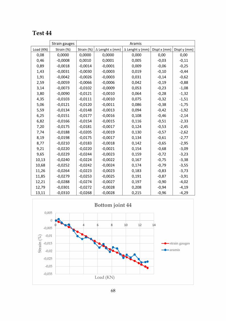
68

Test 44



0,08 0,0000 0,0000 0,0000 0,000 0,00 0,00

0,46 -0,0008 0,0010 0,0001 0,005 -0,03 -0,11

0,89 -0,0018 -0,0014 -0,0001 0,009 -0,06 -0,25

1,43 -0,0031 -0,0030 -0,0003 0,019 -0,10 -0,44

1,91 -0,0042 -0,0026 -0,0003 0,031 -0,14 -0,62

2,59 -0,0059 -0,0066 -0,0006 0,042 -0,19 -0,88

3,14 -0,0073 -0,0102 -0,0009 0,053 -0,23 -1,08

3,80 -0,0090 -0,0121 -0,0010 0,064 -0,28 -1,32

4,35 -0,0103 -0,0111 -0,0010 0,075 -0,32 -1,51

5,06 -0,0121 -0,0120 -0,0011 0,086 -0,38 -1,75

5,59 -0,0134 -0,0148 -0,0013 0,094 -0,42 -1,92

6,25 -0,0151 -0,0177 -0,0016 0,108 -0,46 -2,14

6,82 -0,0166 -0,0154 -0,0015 0,116 -0,51 -2,33

7,20 -0,0175 -0,0181 -0,0017 0,124 -0,53 -2,45

7,74 -0,0188 -0,0205 -0,0019 0,130 -0,57 -2,62

8,19 -0,0198 -0,0175 -0,0017 0,134 -0,61 -2,77

8,77 -0,0210 -0,0183 -0,0018 0,142 -0,65 -2,95

9,21 -0,0220 -0,0220 -0,0021 0,154 -0,68 -3,09

9,65 -0,0229 -0,0244 -0,0023 0,159 -0,72 -3,23

10,13 -0,0240 -0,0224 -0,0022 0,167 -0,75 -3,38

10,68 -0,0252 -0,0242 -0,0024 0,174 -0,79 -3,55

11,26 -0,0264 -0,0223 -0,0023 0,183 -0,83 -3,73

11,85 -0,0279 -0,0253 -0,0025 0,191 -0,87 -3,91

12,21 -0,0288 -0,0274 -0,0027 0,197 -0,90 -4,02

12,79 -0,0301 -0,0272 -0,0028 0,208 -0,94 -4,19

13,11 -0,0310 -0,0268 -0,0028 0,215 -0,96 -4,29

-0,035

-0,03

-0,025

-0,02

-0,015

-0,01

-0,005

0

0,005

0 2 4 6 8 10 12 14

Str

ain

(%

)

Load (KN)

Bottom joint 44

strain gauges

aramis

69

-0,003

-0,002

-0,001

0,000

0,001

0 2 4 6 8 10 12 14

Len

gth

x d

iffe

ren

ce (

mm

)

Load (KN)

Length x difference

0,00

0,05

0,10

0,15

0,20

0,25

0 2 4 6 8 10 12 14

Len

gth

y d

iffe

ren

ce (

mm

)

Load (KN)

Length y difference

-1,50

-1,00

-0,50

0,00

0 2 4 6 8 10 12 14

Dis

pla

cem

ent

x (

mm

)

Load (KN)

Displacement x

-6,00

-4,00

-2,00

0,00

0 2 4 6 8 10 12 14

Dis

pla

cem

ent

y (

mm

)

Load (KN)

Displacement y

70

3.3 Considerations

Graphs presented in the previous paragraph show a general good comparison

between strain data obtained from strain gauges and whom obtained from

digital image correlation.

All the test in the undamaged condition were carried out loading the beam up

to 13,10KN which coincides with the 70% of the yield strength.

Some considerations relatively to strain comparison in different parts of the

structure: good results were given in all the beam parts of the structure, as

taking photos really close to the beam as taking farther in order to take data of

top and mid beam with the same photos. Relatively to the joint part, a good

comparison of values was obtained, but have to be considered that some of the

test gave a not good result. This problem was present in some tests of the tense

part, but especially into the middle area of the joint, the one subjected to lower

strain (up to 0,015%). The compressed part gave better result if compared to the

same range of strain. In general, good comparison was found until 0.035%

strain values, while with lower values the reliability was not guaranteed.

71

Chapter 4

Damaged condition

4.1 Conduct of the test

This chapter present all the final tests have been done on the structure in

damaged condition, that means with the crack in the beam at the joint.

Measured loads were plotted in graphs with load as a function of strains

obtained from digital image correlation method and also with those obtained

from strain gauges. As explained in the previous chapter, just two restricted

areas were analyzed in the same time, due to the close proximity required from

camera and structure to obtain good results: one in the main beam, the other in

the joint part.

The six points of particular importance analyzed in this chapter are exactly the

same of the previous one in order to compare the two condition: three of them

are in the joint part of the structure and the other three in the beam, as with

Aramis as with strain gauges. The name of these points is the same, due to the

positioning respect to the height of the structure will be called as top beam, mid

beam, bottom beam, top joint, mid joint and bottom joint. Two tests for each

single relevant point are presented. Every test presents a comparison graph

with both technologies used.

72

4.2 Experiment results

4.2.1 Top beam



0,20 0,0000 0,0000 0,0000 0,000 0,000 0,000

0,30 0,0005 0,0021 0,0002 -0,002 0,007 -0,050

0,56 0,0020 0,0022 0,0006 -0,007 0,033 -0,190

0,76 0,0032 0,0051 0,0006 -0,011 0,053 -0,296

1,14 0,0053 0,0087 0,0013 -0,019 0,097 -0,517

1,57 0,0078 0,0102 0,0018 -0,029 0,149 -0,776

1,80 0,0095 0,0133 0,0020 -0,035 0,185 -0,932

2,03 0,0107 0,0151 0,0019 -0,040 0,213 -1,072

2,25 0,0121 0,0138 0,0023 -0,046 0,245 -1,214

2,41 0,0131 0,0173 0,0024 -0,050 0,268 -1,318

2,63 0,0148 0,0178 0,0025 -0,055 0,300 -1,463

2,91 0,0164 0,0186 0,0027 -0,063 0,340 -1,642

3,15 0,0180 0,0198 0,0027 -0,069 0,374 -1,797

3,39 0,0197 0,0196 0,0028 -0,074 0,406 -1,946

3,73 0,0217 0,0267 0,0024 -0,082 0,453 -2,159

3,96 0,0232 0,0288 0,0029 -0,088 0,483 -2,300

4,18 0,0246 0,0276 0,0030 -0,093 0,512 -2,432

4,40 0,0259 0,0279 0,0031 -0,098 0,539 -2,561

4,62 0,0276 0,0276 0,0029 -0,103 0,568 -2,694

4,87 0,0291 0,0272 0,0031 -0,109 0,599 -2,841

5,18 0,0314 0,0296 0,0030 -0,116 0,637 -3,023

5,37 0,0320 0,0300 0,0034 -0,120 0,660 -3,133

0

0,005

0,01

0,015

0,02

0,025

0,03

0,035

0 1 2 3 4 5 6

stra

in (

%)

Load (KN)

top beam 103

strain gauges

aramis

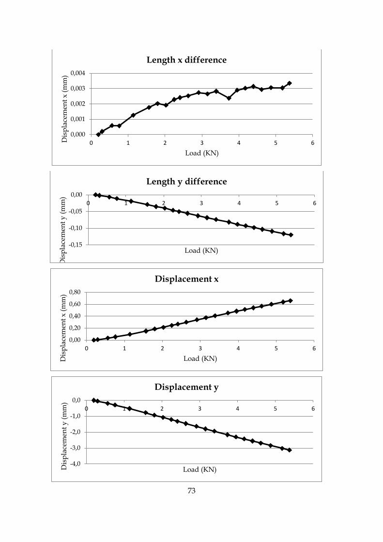
73

0,000

0,001

0,002

0,003

0,004

0 1 2 3 4 5 6Dis

pla

cem

ent

x (

mm

)

Load (KN)

Length x difference

-0,15

-0,10

-0,05

0,00

0 1 2 3 4 5 6

Dis

pla

cem

ent

y (

mm

)

Load (KN)

Length y difference

0,00

0,20

0,40

0,60

0,80

0 1 2 3 4 5 6

Dis

pla

cem

ent

x (

mm

)

Load (KN)

Displacement x

-4,0

-3,0

-2,0

-1,0

0,0

0 1 2 3 4 5 6

Dis

pla

cem

ent

y (

mm

)

Load (KN)

Displacement y

74

Test 113



0,15 0,0000 0,000 0,0000 0,000 0,000 0,000

0,32 0,0012 -0,017 -0,0021 0,004 0,011 -0,089

0,53 0,0027 -0,024 -0,0030 0,009 0,032 -0,201

0,77 0,0043 -0,034 -0,0042 0,014 0,063 -0,340

1,08 0,0060 -0,043 -0,0052 0,021 0,104 -0,524

1,70 0,0093 -0,045 -0,0056 0,038 0,193 -0,916

2,23 0,0121 -0,071 -0,0087 0,050 0,279 -1,277

2,75 0,0147 -0,065 -0,0082 0,065 0,361 -1,625

3,19 0,0172 -0,073 -0,0092 0,076 0,430 -1,920

3,56 0,0188 -0,079 -0,0100 0,085 0,488 -2,163

3,93 0,0206 -0,075 -0,0096 0,095 0,542 -2,396

4,32 0,0225 -0,083 -0,0106 0,106 0,599 -2,640

4,60 0,0240 -0,086 -0,0111 0,112 0,638 -2,814

4,90 0,0255 -0,084 -0,0109 0,120 0,679 -2,991

5,13 0,0266 -0,080 -0,0104 0,126 0,711 -3,136

5,33 0,0279 -0,093 -0,0121 0,130 0,738 -3,254

5,58 0,0288 -0,073 -0,0097 0,136 0,781 -3,401

-0,10

-0,08

-0,06

-0,04

-0,02

0,00

0,02

0,04

0 1 2 3 4 5 6

stra

in (

%)

load (KN)

top beam 113

strain gauges

aramis

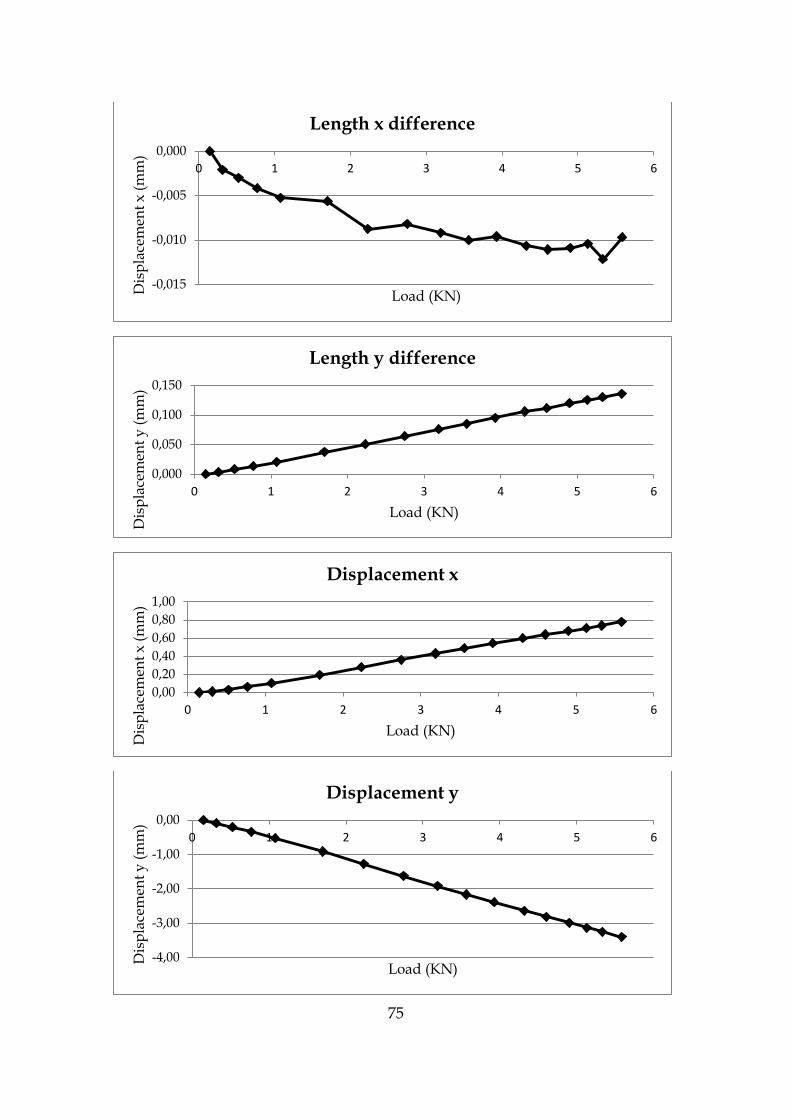
75

-0,015

-0,010

-0,005

0,000

0 1 2 3 4 5 6

Dis

pla

cem

ent

x (

mm

)

Load (KN)

Length x difference

0,000

0,050

0,100

0,150

0 1 2 3 4 5 6

Dis

pla

cem

ent

y (

mm

)

Load (KN)

Length y difference

0,00

0,20

0,40

0,60

0,80

1,00

0 1 2 3 4 5 6

Dis

pla

cem

ent

x (

mm

)

Load (KN)

Displacement x

-4,00

-3,00

-2,00

-1,00

0,00

0 1 2 3 4 5 6

Dis

pla

cem

ent

y (

mm

)

Load (KN)

Displacement y

76

4.2.2 Mid beam

Test 122



0,13 0,0000 0,0000 0,00000 0,000 0,000 0,000

0,34 0,0011 0,0052 0,00068 0,002 0,011 -0,103

0,50 0,0021 0,0046 0,00049 0,006 0,023 -0,191

0,71 0,0034 0,0055 0,00074 0,010 0,036 -0,298

1,01 0,0051 -0,0038 -0,00025 0,016 0,061 -0,471

1,26 0,0066 0,0098 0,00070 0,021 0,083 -0,620

1,61 0,0087 0,0048 0,00045 0,029 0,116 -0,833

1,91 0,0105 0,0086 0,00039 0,035 0,148 -1,031

2,23 0,0126 0,0096 0,00048 0,043 0,181 -1,238

2,55 0,0148 0,0069 -0,00005 0,050 0,216 -1,451

2,85 0,0166 0,0171 0,00149 0,057 0,247 -1,641

3,10 0,0184 0,0085 0,00001 0,063 0,272 -1,798

3,35 0,0201 0,0222 0,00209 0,069 0,298 -1,960

3,59 0,0216 0,0218 0,00192 0,074 0,322 -2,108

3,90 0,0237 0,0173 0,00105 0,081 0,354 -2,299

4,13 0,0251 0,0217 0,00165 0,086 0,377 -2,439

4,40 0,0269 0,0290 0,00267 0,092 0,402 -2,597

4,74 0,0290 0,0262 0,00204 0,099 0,433 -2,793

4,93 0,0303 0,0335 0,00309 0,103 0,450 -2,906

5,32 0,0324 0,0349 0,00307 0,111 0,487 -3,132

5,48 0,0340 0,0368 0,00327 0,115 0,500 -3,222

-0,01

-0,005

0

0,005

0,01

0,015

0,02

0,025

0,03

0,035

0,04

0 1 2 3 4 5 6

stra

in (

%)

load (KN)

middle beam 122

strain gauges

aramis

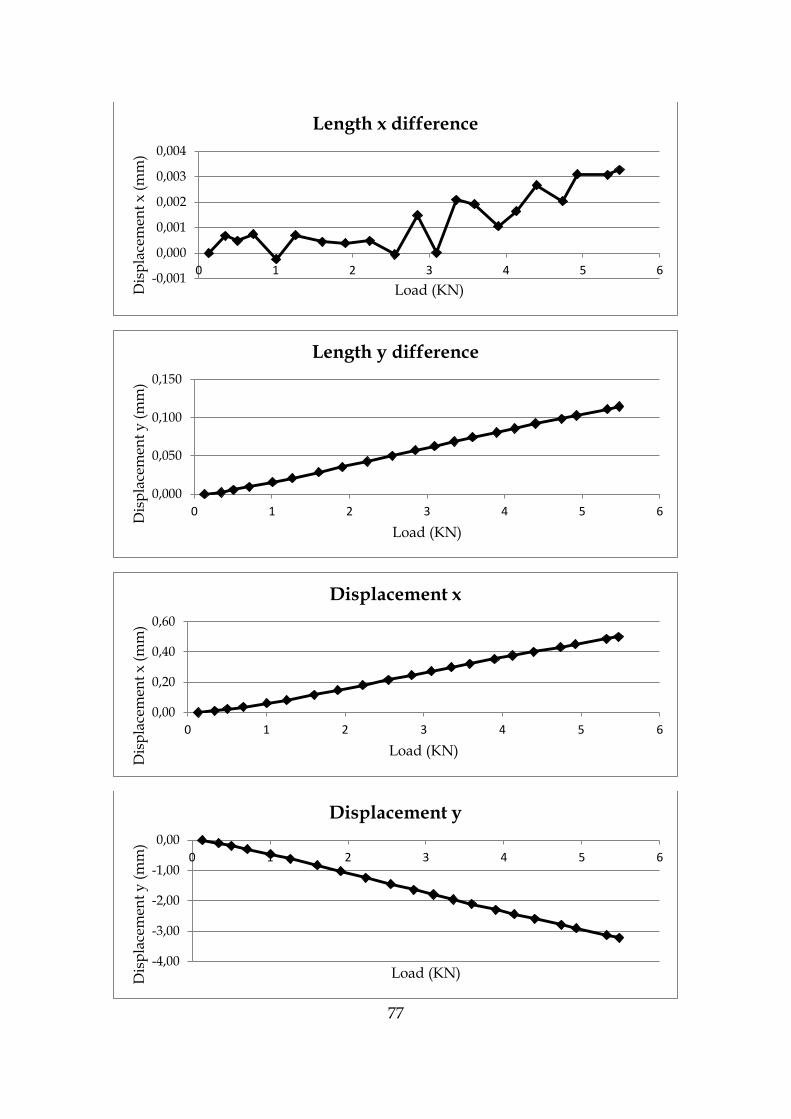
77

-0,001

0,000

0,001

0,002

0,003

0,004

0 1 2 3 4 5 6

Dis

pla

cem

ent

x (

mm

)

Load (KN)

Length x difference

0,000

0,050

0,100

0,150

0 1 2 3 4 5 6

Dis

pla

cem

ent

y (

mm

)

Load (KN)

Length y difference

0,00

0,20

0,40

0,60

0 1 2 3 4 5 6

Dis

pla

cem

ent

x (

mm

)

Load (KN)

Displacement x

-4,00

-3,00

-2,00

-1,00

0,00

0 1 2 3 4 5 6

Dis

pla

cem

ent

y (

mm

)

Load (KN)

Displacement y

78

Test 124



0,14 0,0000 0,0000 0,0000 0,000 0,000 0,000

0,31 0,0009 0,0046 0,0015 0,002 0,006 -0,087

0,52 0,0022 0,0067 0,0028 0,002 0,016 -0,198

0,80 0,0038 0,0011 0,0012 0,010 0,036 -0,350

1,16 0,0059 -0,0020 0,0008 0,018 0,062 -0,563

1,49 0,0080 -0,0003 0,0010 0,023 0,089 -0,767

1,82 0,0101 0,0052 0,0015 0,031 0,117 -0,972

2,12 0,0121 0,0154 0,0026 0,038 0,145 -1,173

2,40 0,0136 0,0144 0,0025 0,044 0,172 -1,353

2,66 0,0155 0,0122 0,0007 0,048 0,197 -1,523

2,89 0,0170 0,0203 0,0030 0,056 0,216 -1,668

3,15 0,0187 0,0242 0,0034 0,059 0,240 -1,841

3,51 0,0210 0,0278 0,0037 0,068 0,272 -2,062

3,79 0,0229 0,0163 0,0025 0,075 0,297 -2,233

4,06 0,0247 0,0291 0,0038 0,081 0,320 -2,401

4,34 0,0266 0,0224 0,0027 0,087 0,344 -2,563

4,62 0,0285 0,0258 0,0027 0,091 0,367 -2,730

4,88 0,0300 0,0348 0,0042 0,099 0,386 -2,879

5,29 0,0322 0,0284 0,0027 0,106 0,420 -3,115

5,54 0,0338 0,0299 0,0036 0,110 0,439 -3,267

0

0,005

0,01

0,015

0,02

0,025

0,03

0,035

0,04

0,045

0,05

0 1 2 3 4 5 6

stra

in (

%)

Load (KN)

middle beam 124

strain gauges

aramis

79

0,000

0,001

0,002

0,003

0,004

0,005

0 1 2 3 4 5 6

Dis

pla

cem

ent

x (

mm

)

Load (KN)

Length x difference

0,000

0,050

0,100

0,150

0 1 2 3 4 5 6

Dis

pla

cem

ent

y (

mm

)

Load (KN)

Length y difference

0,00

0,10

0,20

0,30

0,40

0,50

0 1 2 3 4 5 6

Dis

pla

cem

ent

x (

mm

)

Load (KN)

Displacement x

-4,00

-3,00

-2,00

-1,00

0,00

0 1 2 3 4 5 6

Dis

pla

cem

ent

y (

mm

)

Load (KN)

Displacement y

80

4.2.3 Bottom beam

Test 107



0,16 0,0000 0,0000 0,00000 0,0000 0,000 0,000

0,35 -0,0008 -0,0007 -0,00007 0,0030 -0,015 -0,090

0,56 -0,0017 0,0020 0,00010 0,0062 -0,032 -0,202

0,86 -0,0034 -0,0063 -0,00050 0,0112 -0,057 -0,370

1,30 -0,0059 -0,0059 -0,00053 0,0188 -0,096 -0,625

1,72 -0,0085 -0,0142 -0,00115 0,0262 -0,134 -0,888

2,08 -0,0109 -0,0113 -0,00101 0,0340 -0,167 -1,126

2,33 -0,0125 -0,0222 -0,00180 0,0384 -0,190 -1,293

2,60 -0,0143 -0,0169 -0,00148 0,0445 -0,214 -1,467

2,82 -0,0158 -0,0224 -0,00189 0,0487 -0,235 -1,611

3,01 -0,0170 -0,0187 -0,00167 0,0525 -0,251 -1,729

3,17 -0,0181 -0,0244 -0,00209 0,0557 -0,266 -1,836

3,34 -0,0194 -0,0238 -0,00208 0,0589 -0,281 -1,945

3,51 -0,0205 -0,0261 -0,00227 0,0622 -0,297 -2,054

3,69 -0,0218 -0,0244 -0,00219 0,0659 -0,313 -2,165

3,85 -0,0229 -0,0263 -0,00235 0,0696 -0,327 -2,263

3,99 -0,0240 -0,0335 -0,00287 0,0715 -0,340 -2,351

4,24 -0,0257 -0,0297 -0,00266 0,0766 -0,362 -2,500

4,47 -0,0274 -0,0319 -0,00284 0,0801 -0,383 -2,636

4,64 -0,0284 -0,0348 -0,00308 0,0832 -0,396 -2,734

4,92 -0,0307 -0,0372 -0,00330 0,0886 -0,423 -2,898

5,12 -0,0318 -0,0337 -0,00310 0,0926 -0,442 -3,014

5,34 -0,0334 -0,0343 -0,00318 0,0962 -0,462 -3,141

-0,0400

-0,0350

-0,0300

-0,0250

-0,0200

-0,0150

-0,0100

-0,0050

0,0000

0,0050

0,00 1,00 2,00 3,00 4,00 5,00 6,00

stra

in (

%)

load (KN)

bottom beam 107

strain gauges

aramis

81

-0,004

-0,003

-0,002

-0,001

0,000

0,001

0 1 2 3 4 5 6

Dis

pla

cem

ent

x (

mm

)

Load (KN)

Length x difference

0,00

0,05

0,10

0,15

0 1 2 3 4 5 6

Dis

pla

cem

ent

y (

mm

)

Load (KN)

Length y difference

-0,60

-0,40

-0,20

0,00

0 1 2 3 4 5 6

Dis

pla

cem

ent

x (

mm

)

Load (KN)

Displacement x

-4,00

-3,00

-2,00

-1,00

0,00

0 1 2 3 4 5 6

Dis

pla

cem

ent

y (

mm

)

Load (KN)

Displacement y

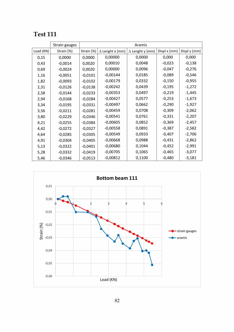
82

Test 111



0,15 0,0000 0,0000 0,00000 0,0000 0,000 0,000

0,43 -0,0014 0,0020 0,00010 0,0048 -0,023 -0,138

0,69 -0,0024 0,0020 0,00000 0,0096 -0,047 -0,276

1,16 -0,0051 -0,0101 -0,00144 0,0185 -0,089 -0,546

1,82 -0,0093 -0,0102 -0,00179 0,0332 -0,150 -0,955

2,31 -0,0126 -0,0138 -0,00242 0,0439 -0,195 -1,272

2,58 -0,0144 -0,0233 -0,00353 0,0497 -0,219 -1,445

2,94 -0,0168 -0,0284 -0,00427 0,0577 -0,253 -1,673

3,34 -0,0195 -0,0331 -0,00497 0,0662 -0,290 -1,927

3,56 -0,0211 -0,0281 -0,00459 0,0708 -0,309 -2,062

3,80 -0,0229 -0,0346 -0,00541 0,0761 -0,331 -2,207

4,21 -0,0255 -0,0384 -0,00605 0,0852 -0,369 -2,457

4,42 -0,0272 -0,0327 -0,00558 0,0891 -0,387 -2,582

4,64 -0,0285 -0,0305 -0,00549 0,0933 -0,407 -2,706

4,91 -0,0304 -0,0405 -0,00668 0,0988 -0,431 -2,862

5,13 -0,0322 -0,0401 -0,00680 0,1044 -0,452 -2,991

5,28 -0,0332 -0,0419 -0,00705 0,1065 -0,465 -3,077

5,46 -0,0346 -0,0513 -0,00812 0,1100 -0,480 -3,181

-0,06

-0,05

-0,04

-0,03

-0,02

-0,01

0,00

0,01

0 1 2 3 4 5 6

Stra

in (

%)

Load (KN)

Bottom beam 111

strain gauges

aramis

83

-0,010

-0,008

-0,006

-0,004

-0,002

0,000

0,002

0 1 2 3 4 5 6

Dis

pla

cem

ent

x (

mm

)

Load (KN)

Length x difference

0,000

0,020

0,040

0,060

0,080

0,100

0,120

0 1 2 3 4 5 6

Dis

pla

cem

ent

y (

mm

)

Load (KN)

Length y difference

-0,60

-0,40

-0,20

0,00

0 1 2 3 4 5 6

Dis

pla

cem

ent

x (

mm

)

Load (KN)

Displacement x

-4,00

-3,00

-2,00

-1,00

0,00

0 1 2 3 4 5 6

Dis

pla

cem

ent

y (

mm

)

Load (KN)

Displacement y

84

4.2.4 Top joint

Test 109



0,16 0,0000 0,000 0,0000 0,000 0,000 0,00

0,35 0,0003 -0,002 -0,0003 0,003 0,022 -0,06

0,56 0,0008 -0,014 -0,0018 0,007 0,049 -0,12

0,86 0,0013 -0,024 -0,0031 0,014 0,087 -0,23

1,30 0,0022 -0,051 -0,0064 0,023 0,153 -0,39

1,72 0,0031 -0,064 -0,0081 0,032 0,221 -0,55

2,08 0,0039 -0,072 -0,0093 0,041 0,287 -0,70

2,33 0,0043 -0,080 -0,0103 0,047 0,332 -0,80

2,60 0,0049 -0,084 -0,0109 0,053 0,380 -0,91

2,82 0,0054 -0,086 -0,0112 0,058 0,420 -1,00

3,01 0,0058 -0,094 -0,0122 0,062 0,452 -1,07

3,17 0,0061 -0,089 -0,0116 0,067 0,482 -1,14

3,34 0,0064 -0,090 -0,0119 0,070 0,511 -1,21

3,51 0,0068 -0,095 -0,0125 0,075 0,540 -1,27

3,69 0,0071 -0,093 -0,0123 0,078 0,571 -1,34

3,85 0,0074 -0,101 -0,0134 0,082 0,596 -1,40

3,99 0,0077 -0,101 -0,0134 0,085 0,620 -1,46

4,24 0,0081 -0,102 -0,0137 0,091 0,660 -1,55

4,47 0,0086 -0,106 -0,0141 0,095 0,697 -1,63

4,64 0,0090 -0,108 -0,0145 0,099 0,724 -1,69

4,92 0,0095 -0,106 -0,0144 0,105 0,767 -1,80

5,12 0,0099 -0,106 -0,0144 0,109 0,796 -1,87

5,34 0,0104 -0,107 -0,0147 0,114 0,830 -1,95

-0,12

-0,1

-0,08

-0,06

-0,04

-0,02

0

0,02

0,00 1,00 2,00 3,00 4,00 5,00 6,00

stra

in (

%)

Load (KN)

bottom joint

strain gauges

aramis

85

-0,020

-0,015

-0,010

-0,005

0,000

0 1 2 3 4 5 6

Dis

pla

cem

ent

x (

mm

)

Load (KN)

Length x difference

0,00

0,05

0,10

0,15

0 1 2 3 4 5 6

Dis

pla

cem

ent

y (

mm

)

Load (KN)

Length y difference

0,00

0,20

0,40

0,60

0,80

1,00

0 1 2 3 4 5 6

Dis

pla

cem

ent

x (

mm

)

Load (KN)

Displacement x

-3,00

-2,00

-1,00

0,00

0 1 2 3 4 5 6

Dis

pla

cem

ent

y (

mm

)

Load (KN)

Displacement y

86

Test 110



0,15 0,0000 0,0000 0,0000 0,000 0,000 0,000

0,37 0,0005 0,0010 -0,0006 0,001 0,001 0,000

0,54 0,0009 0,0025 -0,0016 0,003 0,029 -0,061

0,86 0,0014 0,0026 -0,0017 0,006 0,052 -0,113

1,24 0,0022 0,0033 -0,0023 0,012 0,096 -0,213

1,58 0,0028 0,0052 -0,0035 0,018 0,154 -0,342

1,90 0,0035 0,0056 -0,0039 0,025 0,207 -0,460

2,30 0,0043 0,0064 -0,0044 0,030 0,262 -0,577

2,75 0,0051 0,0063 -0,0046 0,039 0,335 -0,727

3,21 0,0061 0,0078 -0,0056 0,048 0,414 -0,893

3,60 0,0069 0,0085 -0,0062 0,056 0,493 -1,055

3,91 0,0074 0,0091 -0,0067 0,063 0,559 -1,197

4,15 0,0080 0,0094 -0,0070 0,069 0,611 -1,305

4,53 0,0088 0,0087 -0,0067 0,074 0,651 -1,391

4,83 0,0093 0,0084 -0,0066 0,080 0,709 -1,515

5,14 0,0100 0,0093 -0,0073 0,086 0,756 -1,617

5,33 0,0104 0,0099 -0,0078 0,091 0,802 -1,718

5,51 0,0107 0,0097 -0,0078 0,095 0,831 -1,782

-0,07

-0,06

-0,05

-0,04

-0,03

-0,02

-0,01

0

0,01

0,02

0 1 2 3 4 5 6

Stra

in (

%)

Load (KN)

Top joint 110

87

-0,010

-0,008

-0,006

-0,004

-0,002

0,000

0 1 2 3 4 5 6

Dis

pla

cem

ent

x (

mm

)

Load (KN)

Length x difference

0,000

0,020

0,040

0,060

0,080

0,100

0 1 2 3 4 5 6

Dis

pla

cem

ent

y (

mm

)

Load (KN)

Length y difference

0,00

0,20

0,40

0,60

0,80

1,00

0 1 2 3 4 5 6

Dis

pla

cem

ent

x (

mm

)

Load (KN)

Displacement x

-2,00

-1,50

-1,00

-0,50

0,00

0,50

0 1 2 3 4 5 6

Dis

pla

cem

ent

y (

mm

)

Load (KN)

Displacement y

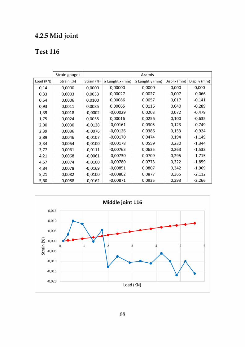
88

4.2.5 Mid joint

Test 116



0,14 0,0000 0,0000 0,00000 0,0000 0,000 0,000

0,33 0,0003 0,0033 0,00027 0,0027 0,007 -0,066

0,54 0,0006 0,0100 0,00086 0,0057 0,017 -0,141

0,93 0,0011 0,0085 0,00065 0,0116 0,040 -0,289

1,39 0,0018 -0,0002 -0,00029 0,0203 0,072 -0,479

1,75 0,0024 0,0055 0,00016 0,0256 0,100 -0,635

2,00 0,0030 -0,0128 -0,00161 0,0305 0,123 -0,749

2,39 0,0036 -0,0076 -0,00126 0,0386 0,153 -0,924

2,89 0,0046 -0,0107 -0,00170 0,0474 0,194 -1,149

3,34 0,0054 -0,0100 -0,00178 0,0559 0,230 -1,344

3,77 0,0061 -0,0111 -0,00763 0,0635 0,263 -1,533

4,21 0,0068 -0,0061 -0,00730 0,0709 0,295 -1,715

4,57 0,0074 -0,0100 -0,00780 0,0773 0,322 -1,859

4,84 0,0078 -0,0169 -0,00851 0,0807 0,342 -1,969

5,21 0,0082 -0,0100 -0,00802 0,0877 0,365 -2,112

5,60 0,0088 -0,0162 -0,00871 0,0935 0,393 -2,266

-0,020

-0,015

-0,010

-0,005

0,000

0,005

0,010

0,015

0 1 2 3 4 5 6

Stra

in (

%)

Load (KN)

Middle joint 116

89

-0,010

-0,005

0,000

0,005

0 1 2 3 4 5 6

Len

gth

dif

fere

nce

(m

m)

Load (KN)

Length x difference

0,000

0,050

0,100

0 1 2 3 4 5 6

Len

gth

dif

fere

nce

(m

m)

Load (KN)

Length y difference

0,00

0,20

0,40

0,60

0 1 2 3 4 5 6

Dis

pla

cem

ent

x (

mm

)

Load (KN)

Displacement x

-2,50

-2,00

-1,50

-1,00

-0,50

0,00

0 1 2 3 4 5 6

Dis

pla

cem

ent

y (

mm

)

Load (KN)

Displacement y

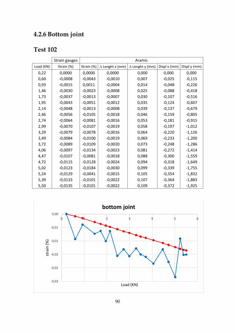
90

4.2.6 Bottom joint

Test 102



0,22 0,0000 0,0000 0,0000 0,000 0,000 0,000

0,60 -0,0008 -0,0043 -0,0010 0,007 -0,025 -0,115

0,93 -0,0015 0,0011 -0,0004 0,014 -0,048 -0,226

1,46 -0,0030 -0,0023 -0,0008 0,025 -0,088 -0,418

1,73 -0,0037 -0,0013 -0,0007 0,030 -0,107 -0,516

1,95 -0,0043 -0,0051 -0,0012 0,035 -0,124 -0,607

2,14 -0,0048 -0,0013 -0,0008 0,039 -0,137 -0,679

2,46 -0,0056 -0,0105 -0,0018 0,046 -0,159 -0,805

2,74 -0,0064 -0,0081 -0,0016 0,053 -0,181 -0,915

2,99 -0,0070 -0,0107 -0,0019 0,058 -0,197 -1,012

3,29 -0,0079 -0,0078 -0,0016 0,064 -0,220 -1,126

3,49 -0,0084 -0,0100 -0,0019 0,069 -0,233 -1,200

3,72 -0,0089 -0,0109 -0,0020 0,073 -0,248 -1,286

4,06 -0,0097 -0,0134 -0,0023 0,081 -0,272 -1,414

4,47 -0,0107 -0,0081 -0,0018 0,088 -0,300 -1,559

4,72 -0,0115 -0,0128 -0,0024 0,094 -0,318 -1,649

5,02 -0,0123 -0,0184 -0,0030 0,099 -0,339 -1,755

5,24 -0,0129 -0,0041 -0,0015 0,105 -0,354 -1,832

5,39 -0,0133 -0,0101 -0,0022 0,107 -0,364 -1,883

5,50 -0,0135 -0,0101 -0,0022 0,109 -0,372 -1,925

-0,03

-0,02

-0,02

-0,01

-0,01

0,00

0 1 2 3 4 5 6

stra

in (

%)

Load (KN)

bottom joint

91

-0,004

-0,003

-0,002

-0,001

0,000

0 1 2 3 4 5 6

Dis

pla

cem

ent

x (

mm

)

Load (KN)

Length x difference

0,000

0,050

0,100

0,150

0 1 2 3 4 5 6

Dis

pla

cem

ent

y (

mm

)

Load (KN)

Length y difference

-0,40

-0,30

-0,20

-0,10

0,00

0 1 2 3 4 5 6

Dis

pla

cem

ent

x (

mm

)

Load (KN)

Displacement x

-2,50

-2,00

-1,50

-1,00

-0,50

0,00

0 1 2 3 4 5 6

Dis

pla

cem

ent

y (

mm

)

Load (KN)

Displacement y

92

Test104



0,20 0,0000 0,0000 0,0000 0,000 0,000 0,000

0,30 -0,0003 -0,0055 -0,0005 0,001 -0,006 -0,028

0,56 -0,0008 -0,0052 -0,0005 0,005 -0,025 -0,109

0,76 -0,0011 -0,0041 -0,0004 0,007 -0,039 -0,171

1,14 -0,0021 -0,0125 -0,0011 0,014 -0,066 -0,299

1,57 -0,0031 -0,0172 -0,0016 0,021 -0,097 -0,448

1,80 -0,0038 -0,0121 -0,0011 0,024 -0,115 -0,538

2,03 -0,0044 -0,0162 -0,0015 0,029 -0,131 -0,618

2,25 -0,0050 -0,0136 -0,0013 0,032 -0,146 -0,701

2,41 -0,0054 -0,0155 -0,0015 0,036 -0,157 -0,760

2,63 -0,0059 -0,0214 -0,0020 0,040 -0,172 -0,844

2,91 -0,0067 -0,0193 -0,0018 0,044 -0,192 -0,947

3,15 -0,0073 -0,0263 -0,0025 0,049 -0,209 -1,035

3,39 -0,0079 -0,0243 -0,0023 0,052 -0,225 -1,121

3,73 -0,0089 -0,0228 -0,0022 0,059 -0,250 -1,243

3,96 -0,0095 -0,0220 -0,0022 0,062 -0,267 -1,323

4,18 -0,0101 -0,0358 -0,0034 0,065 -0,281 -1,399

4,40 -0,0108 -0,0300 -0,0029 0,069 -0,296 -1,474

4,62 -0,0113 -0,0340 -0,0033 0,072 -0,310 -1,549

4,87 -0,0121 -0,0362 -0,0035 0,077 -0,328 -1,634

5,18 -0,0129 -0,0413 -0,0043 0,081 -0,346 -1,729

5,37 -0,0136 -0,0418 -0,0041 0,085 -0,363 -1,801

-0,045

-0,04

-0,035

-0,03

-0,025

-0,02

-0,015

-0,01

-0,005

0

0,00 1,00 2,00 3,00 4,00 5,00 6,00

stra

in (

%)

load (KN)

bottom joint

strain gauges

aramis

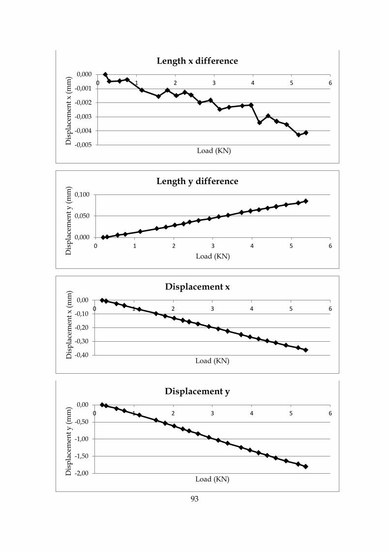
93

-0,005

-0,004

-0,003

-0,002

-0,001

0,000

0 1 2 3 4 5 6

Dis

pla

cem

ent

x (

mm

)

Load (KN)

Length x difference

0,000

0,050

0,100

0 1 2 3 4 5 6

Dis

pla

cem

ent

y (

mm

)

Load (KN)

Length y difference

-0,40

-0,30

-0,20

-0,10

0,00

0 1 2 3 4 5 6

Dis

pla

cem

ent

x (

mm

)

Load (KN)

Displacement x

-2,00

-1,50

-1,00

-0,50

0,00

0 1 2 3 4 5 6

Dis

pla

cem

ent

y (

mm

)

Load (KN)

Displacement y

94

4.3 Considerations

Graphs presented in this chapter show the comparison between Aramis and

strain gauges results in the damaged situation, which means with the presence

of the crack. All the test in the damaged condition were carried out loading the

beam up to 5,57 KN which coincides with the 70% of the yield strength. All the

photos were taken positioning the camera really close to the beam, in order to

evaluate only one of the analyzed areas.

Relatively to strain comparison in different parts of the model, in the beam part

of the structure strain analyzed were up to 0,035% and a quite good comparison

was obtained, in particular in the compressed part (bottom beam), meanwhile

some tests on the tense part were not comparable. In fact some tests presented

strain-load graphs with Aramis trend completely different from the ones

obtained from strain gauges. This consideration is even more present in the

joint part, where strain values were really low (not up to 0,013%): here a not

reliable comparison were found in many tests.

95

Chapter 5

Results comparison

This chapter presents a strain comparison between the two analyzed states,

damaged and undamaged, in order to understand if the presence of the crack

brings variation on the pattern and for this reason if it is possible to realize the

presence of an hidden crack.

The first part presents a comparison between strain of the undamaged and

damaged condition for the beam part of the structure obtained with Aramis,

with strain gauges and with Abaqus. In the second part the joint area is

considered and, due to not enough reliable result from digital image

correlation, are presented strain comparison provided with strain gauges and

with Abaqus. Strain comparison obtained from Aramis considered test 18, test

25 and test 32 for the undamaged values, while test 103, test 111 and test 122

have been used for the damaged condition.

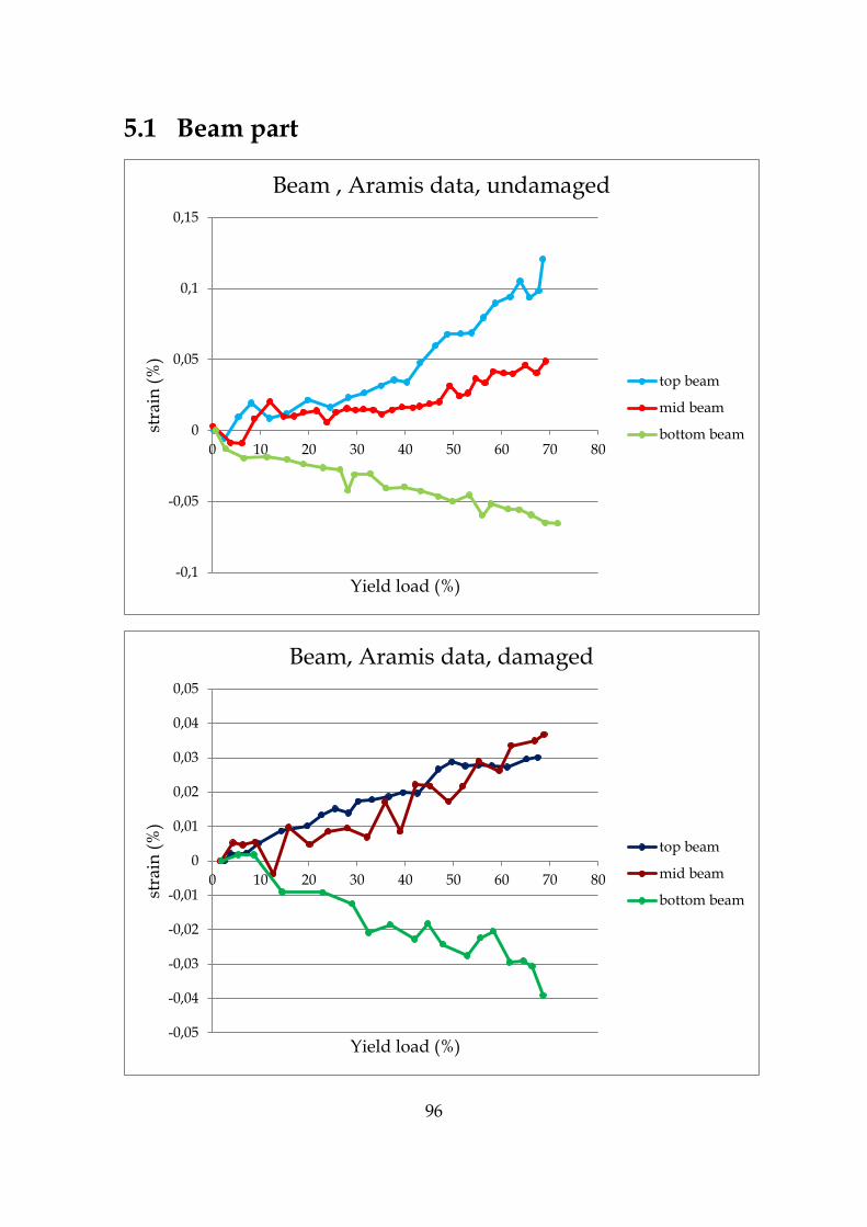
96

5.1 Beam part

-0,1

-0,05

0

0,05

0,1

0,15

0 10 20 30 40 50 60 70 80

stra

in (

%)

Yield load (%)

Beam , Aramis data, undamaged

top beam

mid beam

bottom beam

-0,05

-0,04

-0,03

-0,02

-0,01

0

0,01

0,02

0,03

0,04

0,05

0 10 20 30 40 50 60 70 80

stra

in (

%)

Yield load (%)

Beam, Aramis data, damaged

top beam

mid beam

bottom beam

97

-0,1

-0,05

0

0,05

0,1

0,15

0 2 4 6 8 10 12 14 16

stra

in (

%)

Load (KN)

Beam, Aramis data

top beam

mid beam

bottom beam

top beam und

mid beam und

bottom beamund

-0,10

-0,05

0,00

0,05

0,10

0,15

0 2 4 6 8 10 12 14

Str

ain

(%

)

Load (KN)

Beam, Abaqus data

top beam und

top beam d

mid beam und

mid beam d

bottom beam und

bottom beam d

98

5.2 Joint part

-0,1

-0,08

-0,06

-0,04

-0,02

0

0,02

0,04

0,06

0,08

0,1

0,12

0 2 4 6 8 10 12 14stra

in (

%)

Load (KN)

Beam, strain gauges data

top beam und

mid beam und

bottom beam und

top beam d

mid beam d

bottom beam d

-0,08

-0,06

-0,04

-0,02

0,00

0,02

0,04

0,06

0,08

0 2 4 6 8 10 12 14

Str

ain

(%

)

Load (KN)

Joint, Abaqus data

top joint und

top joint d

mid joint und

mid joint dam

bottom joint und

bottom joint dam

99

-0,04

-0,03

-0,02

-0,01

0

0,01

0,02

0,03

0,04

0 2 4 6 8 10 12 14

stra

in (

%)

Load (KN)

joint, strain gauges data

top joint

mid joint

bottom joint

top joint und

mid joint und

bottom joint und

101

Chapter 6

Conclusions

The previous chapters presented a comparison between results provided from

Aramis, from strain gauges and from a finite element model. Two main

conclusions are presented in this chapter: the first one is about the comparison

of the structure strains in undamaged and damaged condition, in order to

evaluate the possibility to understand the presence of a crack hidden by plates

in a steel structure, while the second one concerns the reliability of digital image

correlation as structural health monitoring method.

Regarding the identification of a hidden crack using digital image correlation as

structural health monitoring, graphs reported in the previous chapter show that

it is possible, but depends from the strain values considered. In fact can be

observed as the pattern changes from undamaged to damaged condition. Due

to the presence of the crack, the variation of strain in the beam part is not linear

from the bottom to the top of the structure, because the crack causes the higher

part is not working as in the previous condition. In this way, as it is also

confirmed by the finite element method model, from the bottom of the beam to

the top there is an increase in strain values that suddenly stops and starts to

decrease. This is the reason why in the damaged condition the strain presents

almost the same values in the mid and top analyzed areas, differently from the

situation without crack were values are distinct. The bottom part of the beam,

that is in the other side of the structure compared to the crack, does not present

a variation in the strain trend. The same speech could be done for the joint part

looking at the graphs obtained with strain gauges and Abaqus, but this result

102

could not be obtained with Aramis because the strain values were really low

and carried tests did not give correct results.

Regarding the Aramis reliability as structural health monitoring method, the

evaluation has to be provide in order of the strain values considered. In this

work good results were obtained until strain of 0,10%, with almost all the test

providing expected values once the set up (spray pattern, camera distance from

the beam, set up of the camera) was correctly fixed. Below strain values of

0,10% was still possible to obtain reliable results, but just until values of 0,035%

and with an high attention to set up details: have to be stated that also doing

this some of the tests failed providing results quite far from the expected.

Generally better results were found in the compressed part, but under the strain

level of 0,035% just few tests gave good results. Must be considered, as showed

in chapters three and four, that the trend of the strain were really dependent by

the length x difference trend. In fact, despite the software was able to get

perfectly linear trend of displacement in both direction, the length x difference

presented undulations in the graph. In this way, can be affirmed that digital

image correlation is a really good structural health monitoring if used for

checking displacements.

103

Appendices

ARAMIS GUIDE

An easy guide about how to upload pictures from image series into the

ARAMIS system and all the steps needed to create a project will be explained in

the following:

1. Run CodeMeter: we have to choose the right license to get into the system

because there is just 1 full license (to create projects) and 4 half-licenses (to do

calculations). To run the CodeMeter, we have to choose the program on the

taskbar.

2. Choose the full license to create a project.

· Click on WebAdmin.

104

· Select 172.16.0.78 IP, then click “up” and finally “apply”:

3. Run ARAMIS system.

4. Create a project:

5. Set the parameters: they can be changed later, so the best we can do is select

the folder where we want to save the project and click next in all the following

windows:

105

6. Attach the photos to the project: “From image series” has to be choosen, if the

photos were taken with a camera and we want to compute them with ARAMIS.

· If photos are taken with an external camera:

· Now is time to select the first photo of the series, all the photos have to be

correlative:

106

· We will be asked about if we want to convert the photos. “Yes” has to be

clicked.

· Then, “OK” has to be clicked.

· Finally, “USE ALL” has to be clicked.

7. Define the mask.

8. Add the start point.

9. Click compute.

10. Once the computation is finished, the program has to be closed.

11. The step 2 has to be repeated but now choosing the other IP.

12. Go to the folder where the project is and run it.

107

References

ARAMIS 6.1 [Computer software]. Braunschweig, Germany, Mittelweg.

Filippo Lorenzoni(2013) “Integrated methodologies based on Structural health

monitoring for the Protection of cutural heritage buildings.”

NKRemote 2.7 [computer software]

Chiang, C., Shih, M., Chen, W., and Yu, C. (2011) “Displacement measurements

of highway bridges using digital image correlation methods.” Proc. SPIE,

8321(1), 83211G.

Jauregui, D. V., White, K. R., Woodward, P. E., and Leitch, K. R. (2003).

“Noncontact photogrammetric measurement of vertical bridge deflection.”

Lee, J. J., and Shinozuka, M. (2006a). “A vision-based system for remote sensing

of bridge displacement.”

Jan Winkler, G.Fisher and C. Georgakis (2014). “Measurement of local

deformations in steel monostrands using digital image correlation”.

Luis Santiago Perez (2012) “Determination of localized strains and global

deformations using video system”.

Simon Stafford [Nikon Manual] Magic Lantern guides.

Jan Winkler, G.Fisher and C. Georgakis (2012), “Localized bending fatigue

behavior of high-strength steel monostrands.”

Jan Winkler, G.Fisher and C. Georgakis (2012), “Monitoring of localized

deformations in high-strength steel cables.”

Busca, G., Cigada, A., Mazzoleni, P., Zappa, E., and Franzi, M. (2012). “Cameras

as displacement sensors to get the dynamic motion of a bridge: Performance

evaluation against traditional approaches.” Proc., 6th Int. Conf. on Bridge

Maintenance, Safety and Management, Taylor & Francis, LondonJ.J.Lee, M.

108

Shinozuka (2006), “Real-time displacement measurement of a flexible bridge

using digital image correlation.”

Brad Pease, “Aramis users’ manual – Quick guide to setup, calibration, and

data collection and analysis.”

Bales, F. B. (1985). “Close-range photogrammetry for bridge measurement.”

TESI DI LAUREA MAGISTRALE IN INGEGNERIA CIVILE...

Documents

Transcript of TESI DI LAUREA MAGISTRALE IN INGEGNERIA CIVILE...