
STUDY OF DTL STABILIZATION WITH POST COUPLERS FOR … · FACOLTÀ DI SCIENZE MATEMATICHE, FISICHE E...
97
CERN-THESIS-2009-199 //2009 UNIVERSITÀ DEGLI STUDI DI MILANO FACOLTÀ DI SCIENZE MATEMATICHE, FISICHE E NATURALI DOTTORATO DI RICERCA IN FISICA, ASTROFISICA E FISICA APPLICATA STUDY OF DTL STABILIZATION WITH POST COUPLERS FOR THE SPES DRIVER LINAC Settore Scientifico disciplinare FIS/04 Coordinatore: Prof. Marco Bersanelli Tutore: Prof. Angela Bracco Tesi di Dottorato di: Francesco Grespan Ciclo XXII Anno Accademico 2008-2009
Transcript of STUDY OF DTL STABILIZATION WITH POST COUPLERS FOR … · FACOLTÀ DI SCIENZE MATEMATICHE, FISICHE E...

CER
N-T
HES
IS-2
009-
199
//20
09
UNIVERSITÀ DEGLI STUDI DI MILANO
FACOLTÀ DI SCIENZE MATEMATICHE, FISICHE E NATURALI
DOTTORATO DI RICERCA IN
FISICA, ASTROFISICA E FISICA APPLICATA
STUDY OF DTL STABILIZATION WITH POST
COUPLERS FOR THE SPES DRIVER LINAC
Settore Scientifico disciplinare FIS/04
Coordinatore: Prof. Marco Bersanelli
Tutore: Prof. Angela Bracco
Tesi di Dottorato di:
Francesco Grespan
Ciclo XXII
Anno Accademico 2008-2009

To Agnese.

Table of Contents
Table of Contents
Introduction ............................................................................................... 1
Chapter 1. The SPES Project .................................................................... 3
1.1 Physics with Radioactive Ion Beams (RIBs) .................................................................. 3
1.2 SPES project layout ......................................................................................................... 8
1.3 SPES driver linac RF structures .................................................................................... 11
References ................................................................................................................................ 18
Chapter 2. The Linac4 Project ................................................................ 19
2.1 New injectors at CERN ...................................................................................................... 19
2.2 Linac4 RF structures ........................................................................................................... 23
2.3 The Linac4 Drift Tube Linac (DTL) .................................................................................. 26
References ................................................................................................................................ 29
Chapter 3. Drift Tube Linac and Resonant Coupling............................. 30
3.1 Alvarez Drift Tube Linac (DTL) ........................................................................................ 30
3.2 Resonant Coupling ............................................................................................................. 34
3.3 Post Coupled DTL .............................................................................................................. 37
References ................................................................................................................................ 40
Chapter 4. Post couplers: simulation results .......................................... 41
4.1 Slater perturbation theorem calculation versus measurements .......................................... 41
4.2 3D simulations and bead-pull measurements on post coupler modes ................................ 43
4.3 3D simulation study of post coupler geometrical parameters ............................................ 45
References ................................................................................................................................ 50
Chapter 5. Post couplers: equivalent circuit ........................................... 51
5.1 Circuit equations and matrix form ...................................................................................... 51
5.2 Circuit derivation of the stabilizing post couplers condition .............................................. 54
5.3 1st and 2
nd magnetic coupling between post couplers ......................................................... 58
References ................................................................................................................................ 62
Chapter 6. Post couplers: tuning procedure and measurements ............. 63
6.1 Circuit extrapolation of stabilizing post coupler setting ..................................................... 63
6.2 Measurements on DTL cold model .................................................................................... 67
References ................................................................................................................................ 73

Table of Contents
Chapter 7. Conclusions ........................................................................... 74
Appendix A. Cavity figures of merit ...................................................... 75
References ................................................................................................................................. 77
Appendix B. High Power Test on DTL hot Prototype ........................... 78
B.1 Low power RF measurements for cavity characterization ................................................. 78
B.2 Bead pulling measurements and post couplers setting ....................................................... 81
B.3 Power measurement calibration ......................................................................................... 82
B.4 High power test .................................................................................................................. 84
References ................................................................................................................................. 88
Appendix C. Equivalent circuit for the Stems ........................................ 89
References ................................................................................................................................. 92
Acknowledgements................................................................................. 93
Introduction
Page 1
Introduction
Particle accelerators are powerful instruments for physics investigation. They allow
researching unknown matter components, as new nuclei or new fundamental particle, or
reproducing in a laboratory the very early instants of the universe. On the other hand,
accelerators are used for cancer therapy and for radio-pharmaceutical production.
Furthermore accelerators allow generating intense photon and neutron beams for a large
number of applications (electronics, spectroscopy, material science).
Main parameters for accelerator characterization are final energy and beam intensity.
Over last years, together with construction and start-up of the high energy collider LHC
for elementary particle study, demand and supply of more intense beams has increased, for
experiments on synthesis of exotic nuclei, for study of new radioactive waste disposal
systems and for medical applications. Construction of high intensity beam accelerator
entails to get through a large number of scientific and technological challenges, related to
the transport of high power beams, to the beam loss control and finally to the accelerator
structure activation. In a word, what must be guaranteed is the stability of the accelerator.
The concept of stability in accelerator physics includes a vast number of topics and
one of the most important is the stabilization of the accelerating field. Stabilizing the
accelerating field means reducing the field sensitivity to geometric factors of perturbation,
in order to keep the field within the limits which guarantee a good beam quality.
Perturbation factors can have different origins, from the mechanical machining to the
heating during high power operation, but they always cause a geometric error which
affects the nominal field configuration. Furthermore, a larger L/ ratio (structure length
over wave length) accentuates the effect of geometrical errors on the accelerating field.
In drift tube linear accelerators the accelerating field stabilization is obtained by
equipping the cavity with special devices called post couplers, which consist of resonant
bars installed in the horizontal cavity plane. The study of this stabilization device is the
core of my thesis.
This thesis work arose from the research and development program related to the
proposal of a normal conducting linac as a driver accelerator for the SPES RIB facility at
LNL. Based on some parameter similarities of the two projects, the collaboration between
SPES and Linac4 project on the design and construction of drift tube linacs (DTL) gave to
Introduction
Page 2
me the opportunity to deepen the knowledge on this accelerating structure by using DTL
prototypes already present at CERN.
Main objectives of my thesis are:
to analyze 2D and 3D simulations of DTL cavity, in order to deepen the understanding
of the post coupler working principle;
to develop the equivalent circuit for DTL cavity, describing the complete cavity
topology, including stems and post couplers;
to define a procedure for optimum post coupler length calculation, based on the
equivalent circuit analysis;
to validate equivalent circuit and tuning procedure with measurements.
In Chapter 1 the physics scenario concerning the SPES project is presented, together
with the facility layout. The proposed driver linac, consisting in the RFQ and the DTL, is
then introduced.
Chapter 2 is an introduction to the Linac4 project, presented in the frame of the
CERN new injectors. The DTL of Linac4, more involved in this work, is presented in
detail.
Chapter 3 consists of a brief overview of the concept of Alvarez Drift Tube Linac,
Resonant Coupling and Post Coupler Stabilization in a DTL.
The core of the research work starts at Chapter 4, where 2D and 3D simulations
performed on post couplers are shown, together with a geometrical estimation of
equivalent circuit parameters in the quasi-static approximation.
In Chapter 5 the equivalent circuit development is presented.
Chapter 6 illustrates the tuning procedure defined on the equivalent circuit
assumptions and measurements undertaken to validate it.
Chapter 7 summarizes the conclusions of this work.
In three Appendices we present arguments of interest or related to the thesis body.
Appendix A is an introduction to the figures of merit of a resonant cavity. Appendix B
describes the high power test of the DTL prototype. Appendix C presents the equivalent
circuit for the Stems.
The SPES Project
Page 3
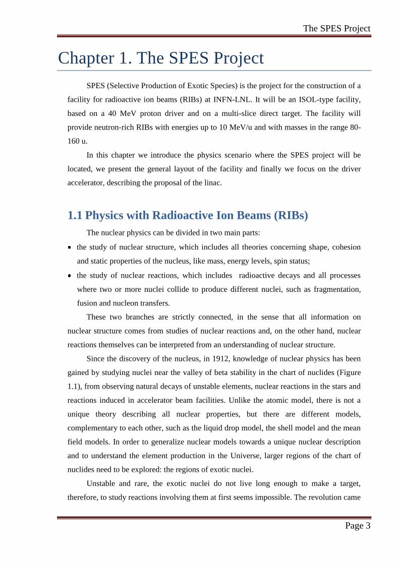
Chapter 1. The SPES Project
SPES (Selective Production of Exotic Species) is the project for the construction of a
facility for radioactive ion beams (RIBs) at INFN-LNL. It will be an ISOL-type facility,
based on a 40 MeV proton driver and on a multi-slice direct target. The facility will
provide neutron-rich RIBs with energies up to 10 MeV/u and with masses in the range 80-
160 u.
In this chapter we introduce the physics scenario where the SPES project will be
located, we present the general layout of the facility and finally we focus on the driver
accelerator, describing the proposal of the linac.
1.1 Physics with Radioactive Ion Beams (RIBs)
The nuclear physics can be divided in two main parts:
the study of nuclear structure, which includes all theories concerning shape, cohesion
and static properties of the nucleus, like mass, energy levels, spin status;
the study of nuclear reactions, which includes radioactive decays and all processes
where two or more nuclei collide to produce different nuclei, such as fragmentation,
fusion and nucleon transfers.
These two branches are strictly connected, in the sense that all information on
nuclear structure comes from studies of nuclear reactions and, on the other hand, nuclear
reactions themselves can be interpreted from an understanding of nuclear structure.
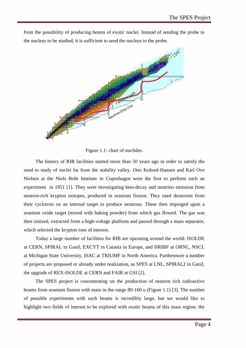
Since the discovery of the nucleus, in 1912, knowledge of nuclear physics has been
gained by studying nuclei near the valley of beta stability in the chart of nuclides (Figure
1.1), from observing natural decays of unstable elements, nuclear reactions in the stars and
reactions induced in accelerator beam facilities. Unlike the atomic model, there is not a
unique theory describing all nuclear properties, but there are different models,
complementary to each other, such as the liquid drop model, the shell model and the mean
field models. In order to generalize nuclear models towards a unique nuclear description
and to understand the element production in the Universe, larger regions of the chart of
nuclides need to be explored: the regions of exotic nuclei.
Unstable and rare, the exotic nuclei do not live long enough to make a target,
therefore, to study reactions involving them at first seems impossible. The revolution came
The SPES Project
Page 4
from the possibility of producing beams of exotic nuclei. Instead of sending the probe to
the nucleus to be studied, it is sufficient to send the nucleus to the probe.
Figure 1.1: chart of nuclides.
The history of RIB facilities started more than 50 years ago in order to satisfy the
need to study of nuclei far from the stability valley. Otto Kofoed-Hansen and Karl Ove
Nielsen at the Niels Bohr Institute in Copenhagen were the first to perform such an
experiment in 1951 [1]. They were investigating beta-decay and neutrino emission from
neutron-rich krypton isotopes, produced in uranium fission. They used deuterons from
their cyclotron on an internal target to produce neutrons. These then impinged upon a
uranium oxide target (mixed with baking powder) from which gas flowed. The gas was
then ionized, extracted from a high-voltage platform and passed through a mass separator,
which selected the krypton ions of interest.
Today a large number of facilities for RIB are operating around the world: ISOLDE
at CERN, SPIRAL in Ganil, EXCYT in Catania in Europe, and HRIBF at ORNL, NSCL
at Michigan State University, ISAC at TRIUMF in North America. Furthermore a number
of projects are proposed or already under realization, as SPES at LNL, SPIRAL2 in Ganil,
the upgrade of REX-ISOLDE at CERN and FAIR at GSI [2].
The SPES project is concentrating on the production of neutron rich radioactive
beams from uranium fission with mass in the range 80-160 u (Figure 1.1) [3]. The number
of possible experiments with such beams is incredibly large, but we would like to
highlight two fields of interest to be explored with exotic beams of this mass region: the

The SPES Project
Page 5
study of the shell structure for nuclei of intermediate mass and the r-process in
astrophysics.
The shell model of nuclear structure is based on a picture where nucleons experience
a mean field generated by all the others, and they are arranged in shells, each one able to
contain up to a certain number of nucleons determined by quantum numbers. If a shell is
fully occupied, a sizeable energy gap appears between the last occupied shell and the first
unoccupied shell, providing an extra stability of the nucleus. Shell completions defines
magic numbers for protons and neutrons: 2, 8, 20, 28, 50, 82, 126. Nuclei which have both
neutron number N and proton number Z equal to one of the magic numbers are called
double magic. Magic numbers are well established for nuclei along the stability line.
However, for neutron-rich nuclei far from stability the vanishing of the classical
shell gaps and the presence of new magic numbers might occur. In fact, magic numbers
are generated by the spin-orbit interaction, which pushes up the energy gap if the relative
orientation of the intrinsic spin is anti-parallel to the orbital angular momentum, or push it
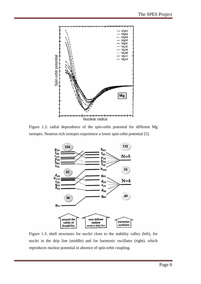
down if parallel. A large excess of neutrons with respect to protons (N>>Z) could affect
the shell structure because of a reduction of the spin-orbit interaction due to the neutron
spatial distribution, which forms a skin on the outside of the nucleus (Figure 1.2). New
magic numbers could be similar to those produced by a harmonic oscillator when
switching off the spin-orbit coupling (Figure 1.3). These predictions can be tested by
measuring binding energies of single particle states in neutron rich nuclei with N=40, 50,
70, which are in the range of masses foreseen for SPES [4].
Exotic nuclei produced by the SPES facility are in the ideal range of masses to
investigate a nucleo-synthesis process called r-process. This process involves n-capture
n + (Z, N) → (Z, N+1) + , the photodisintegration + (Z, N+1) → (Z, N) + n and the beta
decay (Z, N) → (Z+1, N-1) + e- + . In core-collapse supernovae, where neutron flux and
temperature are extremely high, a rapid succession of neutron captures (r-process) occurs.
Neutron captures are much faster than beta-minus decays, meaning that the r-process "runs
up" the N axis in the chart of nuclides. After an element has captured enough neutrons to
close a neutron shell, there is an equilibrium between n-captures and -decays and a slower
beta decay occurs, taking the r-process path closer to the stability valley (vertical parts of
the r-process path in Figure 1.1). SPES could allow experiments to follow the r-process
path up to N=82 by producing exotic species with mass range A ≈ 80-130 [6].
The SPES Project
Page 6
Nuclear radius
Spin
-orb
it p
ote
ntial
Figure 1.2: radial dependence of the spin-orbit potential for different Mg
isotopes. Neutron rich isotopes experience a lower spin-orbit potential [5].
Figure 1.3: shell structures for nuclei close to the stability valley (left), for
nuclei in the drip line (middle) and for harmonic oscillator (right), which
reproduces nuclear potential in absence of spin-orbit coupling.
The SPES Project
Page 7
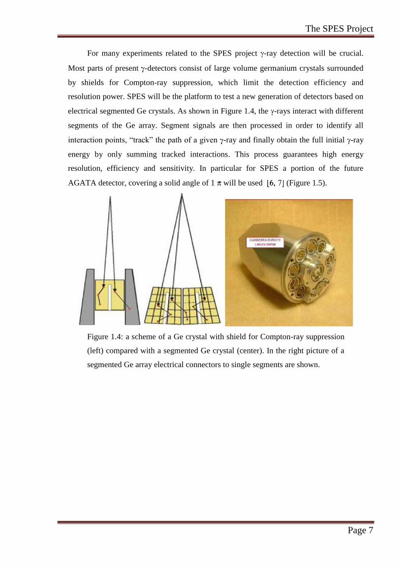
For many experiments related to the SPES project -ray detection will be crucial.
Most parts of present -detectors consist of large volume germanium crystals surrounded
by shields for Compton-ray suppression, which limit the detection efficiency and
resolution power. SPES will be the platform to test a new generation of detectors based on
electrical segmented Ge crystals. As shown in Figure 1.4, the -rays interact with different
segments of the Ge array. Segment signals are then processed in order to identify all
interaction points, “track” the path of a given -ray and finally obtain the full initial -ray
energy by only summing tracked interactions. This process guarantees high energy
resolution, efficiency and sensitivity. In particular for SPES a portion of the future
AGATA detector, covering a solid angle of 1 will be used (Figure 1.5).
Figure 1.4: a scheme of a Ge crystal with shield for Compton-ray suppression
(left) compared with a segmented Ge crystal (center). In the right picture of a
segmented Ge array electrical connectors to single segments are shown.
The SPES Project
Page 8
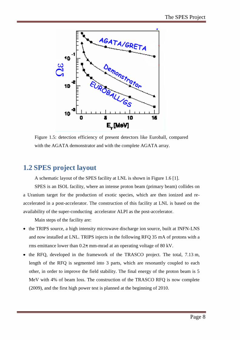
Figure 1.5: detection efficiency of present detectors like Euroball, compared
with the AGATA demonstrator and with the complete AGATA array.
1.2 SPES project layout
A schematic layout of the SPES facility at LNL is shown in Figure 1.6 [1].
SPES is an ISOL facility, where an intense proton beam (primary beam) collides on
a Uranium target for the production of exotic species, which are then ionized and re-
accelerated in a post-accelerator. The construction of this facility at LNL is based on the
availability of the super-conducting accelerator ALPI as the post-accelerator.
Main steps of the facility are:
the TRIPS source, a high intensity microwave discharge ion source, built at INFN-LNS
and now installed at LNL. TRIPS injects in the following RFQ 35 mA of protons with a
rms emittance lower than 0.2 mm-mrad at an operating voltage of 80 kV.
the RFQ, developed in the framework of the TRASCO project. The total, 7.13 m,
length of the RFQ is segmented into 3 parts, which are resonantly coupled to each
other, in order to improve the field stability. The final energy of the proton beam is 5
MeV with 4% of beam loss. The construction of the TRASCO RFQ is now complete
(2009), and the first high power test is planned at the beginning of 2010.

The SPES Project
Page 9
the Drift Tube Linac (DTL), which accelerates the 30 mA beam from 5 MeV to
43 MeV. For such an energy the DTL will be 15.2 m long, divided in 2 tanks, but the
possibility of upgrading it up to 95 MeV has been considered.
the multi-slice direct target, where 30 mA of protons at 43 MeV are directed for
production of exotic species. The target consists of 7 disks of Uranium Carbide (UCx).
The impact of the proton beam on the UCx disks induces the production of fission
fragments. Because of the high temperature of the target ( T > 2000° C), fragments
diffuse to the surface and can be directed to the ion source, where they are ionized at +1
charge state.
the high resolution spectrometer, able to distinguish nuclear species with a mass
resolution of 1/20000. This spectrometer selects the element candidate for the
radioactive ion beam. To optimize the reacceleration, a Charge Breeder will be
developed to increase the charge state to +N, because for efficient acceleration in the
ALPI linac a charge over mass of 1/10 is required.
the post-accelerator, consisting of the bunching RFQ, the PIAVE Superconducting RFQ
and the superconducting linac, ALPI. The selected RIB is accelerated up to 10 MeV/u
with an overall transmission of 70% and finally sent to the experimental areas.
TRASCO RFQ (5MeV, 30mA)
DTL (43MeV, 30mA)
Target/ Source
(80<A<160 q=+1)
High resol.
Spectro-meter
(1/20000)
Piave SRFQ
ALPI Linac (10 MeV/u)Exp.
areas
TRIPS source
(H+)
Charge breeder
(80<A<160 q=+N)
Figure 1.6: schematic layout of the SPES facility at LNL.
The SPES Project
Page 10
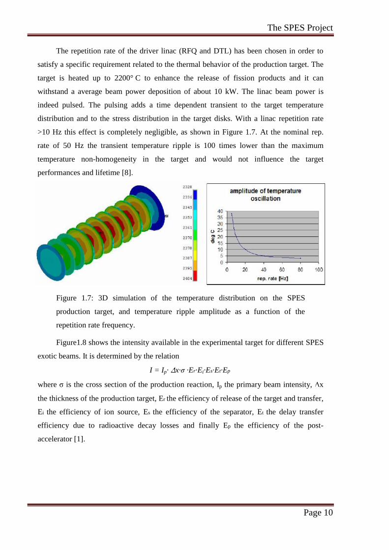
The repetition rate of the driver linac (RFQ and DTL) has been chosen in order to
satisfy a specific requirement related to the thermal behavior of the production target. The
target is heated up to 2200° C to enhance the release of fission products and it can
withstand a average beam power deposition of about 10 kW. The linac beam power is
indeed pulsed. The pulsing adds a time dependent transient to the target temperature
distribution and to the stress distribution in the target disks. With a linac repetition rate
>10 Hz this effect is completely negligible, as shown in Figure 1.7. At the nominal rep.
rate of 50 Hz the transient temperature ripple is 100 times lower than the maximum
temperature non-homogeneity in the target and would not influence the target
performances and lifetime [8].
Figure 1.7: 3D simulation of the temperature distribution on the SPES
production target, and temperature ripple amplitude as a function of the
repetition rate frequency.
Figure1.8 shows the intensity available in the experimental target for different SPES
exotic beams. It is determined by the relation
I = Ip· x·σ ·Er·Ei·Es·Et·Ep
where σ is the cross section of the production reaction, Ip the primary beam intensity, x
the thickness of the production target, Er the efficiency of release of the target and transfer,
Ei the efficiency of ion source, Es the efficiency of the separator, Et the delay transfer
efficiency due to radioactive decay losses and finally Ep the efficiency of the post-
accelerator [1].

The SPES Project
Page 11
Figure 1.8: SPES RIB intensities on experimental targets, calculated by
considering the primary beam intensity, the production target release and the
acceleration efficiencies.
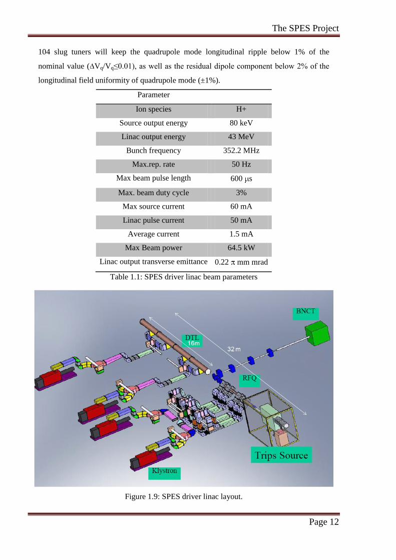
1.3 SPES driver linac RF structures
The layout of the LINAC is presented in Figure 1.9; the main elements are the off
resonance ECR source (TRIPS), the Low Energy Beam Transport (LEBT), the radio
frequency quadrupole (RFQ), the Medium Energy Beam Transport (MEBT) and the Drift
Tube Linac (DTL). The main beam parameters of the linac are listed in Table 1.1 [1, 8].
The RFQ, initially designed for the TRASCO project, is able to accelerate the beam
from 80 keV up to 5 MeV with a current of 30 mA, with 100% duty cycle. The CW
operation option is foreseen in order to satisfy requirements of the Boron Neutron Capture
Therapy application, which requires a powerful proton beam (150 kW) delivered to a
beryllium target for the production of neutrons for an innovative cancer therapy study. The
maximum duty cycle for SPES operation is 3%, the operating frequency is 352 MHz with
the design choice of the use of a single 1.3 MW klystron already used at LEP. The RF
power will be fed by means of eight high power loops. In order to keep beam losses below
4%, the longitudinal field stabilization for the operating mode will be achieved with two
coupling cells, which reduce the effect of perturbing quadrupole modes, and with 24
dipole stabilizing rods in order to reduce the effect of perturbing dipole modes. Indeed,
The SPES Project
Page 12
104 slug tuners will keep the quadrupole mode longitudinal ripple below 1% of the
nominal value ( Vq/Vq≤0.01), as well as the residual dipole component below 2% of the
longitudinal field uniformity of quadrupole mode (±1%).
Parameter
Ion species H+
Source output energy 80 keV
Linac output energy 43 MeV
Bunch frequency 352.2 MHz
Max.rep. rate 50 Hz
Max beam pulse length 600 s
Max. beam duty cycle 3%
Max source current 60 mA
Linac pulse current 50 mA
Average current 1.5 mA
Max Beam power 64.5 kW
Linac output transverse emittance 0.22 mm mrad
Table 1.1: SPES driver linac beam parameters
Figure 1.9: SPES driver linac layout.

The SPES Project
Page 13
The parameters of the SPES DTL are listed in Table 1.2.
Parameter Tank 1 Tank 2
Frequency [MHz] 352.2 352.2
Average pulse current [mA] 50 50
Design RF duty cycle 10% 10%
Tank inner diameter [mm] 520 520
Drift tube diameter [mm] 90 90
Aperture radius [mm] 10 10
Length [m] 7.53 7.68
PMQ length [mm] 45 45
Focusing scheme FFDD FFDD
Max. surface field [kilp] 1.6 1.23
Synchronous phase [deg] -35/-20 -20
Gradient E0 [MV/m] 3.1 3.1
Final Energy [MeV] 23.82 43
RF peak power (incl. beam)[MW] 2.0 2.0
N. of klystrons 1 (2.5 MW) 1 (2.5 MW)
N. of gaps 55 35
N. of Post Couplers 27 17
Stem diameter [mm] 29 29
Post coupler diameter [mm] 20 20
Number of Tuners 10 10
Tuner diameter [mm] 90 90
Table 1.2: SPES DTL parameters.
The DTL is designed to provide an high quality proton beam to the production target
of the SPES project. The structure, composed by 2 tanks of 7.53 m and 7.68 m for a total
length of 15.2 m, accelerates proton pulses of 50 mA from 5 MeV to 43 MeV. The input
energy of 5 MeV, higher with respect to other similar cases (Linac4: 3MeV, SNS:
2.5 MeV), allows avoiding troublesome constraints on focusing strength and peak electric
field due to short length of gaps at low energy.
The average electric field is constant at 3.1 MV/m for the whole structure, while the
synchronous phase is ramped from -35° up to -20° in the first tank to accommodate the
The SPES Project
Page 14
input beam. The maximum surface electric field is kept below 1.6 kilpatrick to avoid RF
breakdown risks.
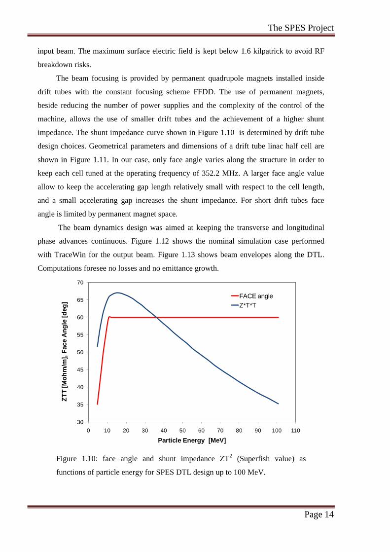
The beam focusing is provided by permanent quadrupole magnets installed inside
drift tubes with the constant focusing scheme FFDD. The use of permanent magnets,
beside reducing the number of power supplies and the complexity of the control of the
machine, allows the use of smaller drift tubes and the achievement of a higher shunt
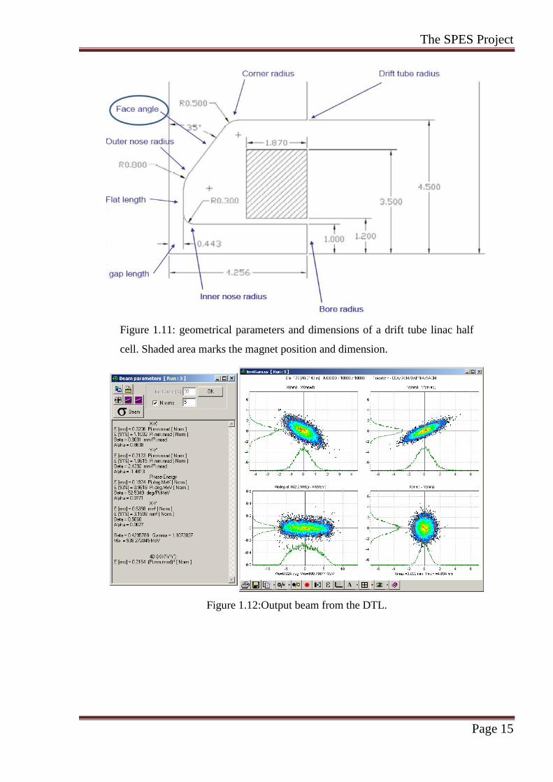
impedance. The shunt impedance curve shown in Figure 1.10 is determined by drift tube
design choices. Geometrical parameters and dimensions of a drift tube linac half cell are
shown in Figure 1.11. In our case, only face angle varies along the structure in order to
keep each cell tuned at the operating frequency of 352.2 MHz. A larger face angle value
allow to keep the accelerating gap length relatively small with respect to the cell length,
and a small accelerating gap increases the shunt impedance. For short drift tubes face
angle is limited by permanent magnet space.
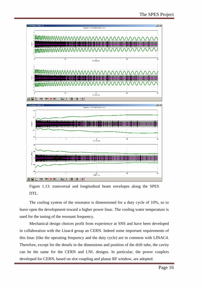
The beam dynamics design was aimed at keeping the transverse and longitudinal
phase advances continuous. Figure 1.12 shows the nominal simulation case performed
with TraceWin for the output beam. Figure 1.13 shows beam envelopes along the DTL.
Computations foresee no losses and no emittance growth.
30
35
40
45
50
55
60
65
70
0 10 20 30 40 50 60 70 80 90 100 110
ZT
T [M
oh
m/m
], F
ace A
ng
le [
deg
]
Particle Energy [MeV]
FACE angle
Z*T*T
Figure 1.10: face angle and shunt impedance ZT2 (Superfish value) as
functions of particle energy for SPES DTL design up to 100 MeV.
The SPES Project
Page 15
Figure 1.11: geometrical parameters and dimensions of a drift tube linac half
cell. Shaded area marks the magnet position and dimension.
Figure 1.12:Output beam from the DTL.
The SPES Project
Page 16
Figure 1.13: transversal and longitudinal beam envelopes along the SPES
DTL.
The cooling system of the resonator is dimensioned for a duty cycle of 10%, so to
leave open the development toward a higher power linac. The cooling water temperature is
used for the tuning of the resonant frequency.
Mechanical design choices profit from experience at SNS and have been developed
in collaboration with the Linac4 group an CERN. Indeed some important requirements of
this linac (like the operating frequency and the duty cycle) are in common with LINAC4.
Therefore, except for the details in the dimensions and position of the drift tube, the cavity
can be the same for the CERN and LNL designs. In particular, the power couplers
developed for CERN, based on slot coupling and planar RF window, are adopted.
The SPES Project
Page 17
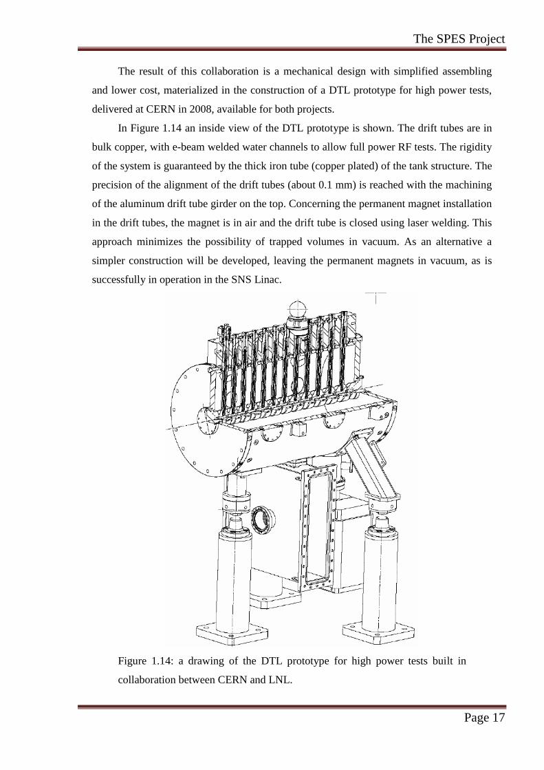
The result of this collaboration is a mechanical design with simplified assembling
and lower cost, materialized in the construction of a DTL prototype for high power tests,
delivered at CERN in 2008, available for both projects.
In Figure 1.14 an inside view of the DTL prototype is shown. The drift tubes are in
bulk copper, with e-beam welded water channels to allow full power RF tests. The rigidity
of the system is guaranteed by the thick iron tube (copper plated) of the tank structure. The
precision of the alignment of the drift tubes (about 0.1 mm) is reached with the machining
of the aluminum drift tube girder on the top. Concerning the permanent magnet installation
in the drift tubes, the magnet is in air and the drift tube is closed using laser welding. This
approach minimizes the possibility of trapped volumes in vacuum. As an alternative a
simpler construction will be developed, leaving the permanent magnets in vacuum, as is
successfully in operation in the SNS Linac.
Figure 1.14: a drawing of the DTL prototype for high power tests built in
collaboration between CERN and LNL.
The SPES Project
Page 18
References
[1] J. C. Cornell, “Radioactive ion beam facilities in Europe: current status and future
developments”, Proc. EPAC04.
[2] Y. Blumenfeld, “Radioactive ion beam facilities in Europe”, NIM B, 2008, Vol. 266,
4074.
[3] G. Prete, A. Pisent (ed.), “SPES technical design report”, INFN-LNL 220, 2007.
[4] A. Bracco, A. Pisent (ed.), “SPES technical design report”, INFN-LNL 181/02, 2007.
[5] G. A. Lalazissis et al., “Reduction of the spin-orbit potential in light drip-line nuclei”,
Phys. Lett. B, 1998, Vol. 418, 7.
[6] A. Bracco, Lectures at Varenna, 2006.
[7] S. Leoni, “Lectures on Detectors for Nuclear Physics”, 2007.
[8] A. Pisent et al., “Design of the high current linac of SPES project”, Proc. EPAC08.
The Linac4 Project
Page 19
Chapter 2. The Linac4 Project
The normal conducting accelerator Linac4 is the first step of the CERN accelerator
complex upgrade. The construction of Linac4 was approved in 2007 as a high priority
project and will replace the existing Linac2.
In this chapter the motivations and related solutions for new accelerators at CERN
are introduced and the Linac4 main parameters and accelerating structures are described.
Finally we focus on the DTL structure, which will be the focus of this thesis.
2.1 New injectors at CERN
There are two main reasons leading to the upgrade of the proton injector complex at
CERN: the reliability of the present injector chain and the LHC performance limitations
[1,2].
The present injector chain of LHC is comprised of 4 accelerators (Figure. 2.1):
Linac2, commissioned in 1978 and upgraded in 1993, with the replacement of the
Cockroft-Walton with the present RFQ as pre-injector for the DTL. It accelerates
protons up to 50 MeV at an operating frequency of 202 MHz.
Proton Synchrotron Booster (PSB), the first circular accelerator of the complex,
commissioned in 1972. It is a four ring synchrotron, accelerating protons from 50 MeV
to 1.4 GeV.
Proton Synchrotron (PS), switched on in 1959. It leads the proton beam up to 26 GeV
energy.
Super Proton Synchrotron (SPS), in operation since 1976. It can accelerate particles up
to 450 GeV, the injection energy in LHC.
The original design parameters of these accelerators have been amply exceeded
during the years of operation, in order to satisfy continuous new requirements of CERN
users. The number of experiments using beams from these accelerators requires a very
large machine time availability (e.g. Linac2 annual operation time is about 6000 hours!).
Age, performance stretch and using time have gradually caused recurrent hardware
problems during recent years (radiation damages in PS magnets, water leaks in SPS
magnets, vacuum leaks in Linac2, etc.), which compromise the LHC operation reliability
[2].
The Linac4 Project
Page 20
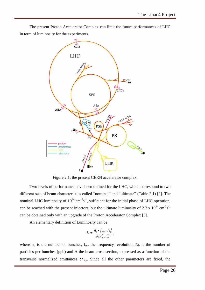
The present Proton Accelerator Complex can limit the future performances of LHC
in term of luminosity for the experiments.
Figure 2.1: the present CERN accelerator complex.
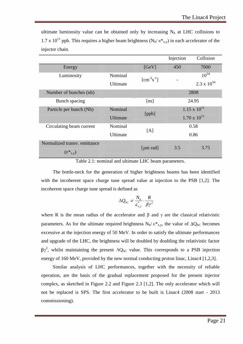
Two levels of performance have been defined for the LHC, which correspond to two
different sets of beam characteristics called “nominal” and “ultimate” (Table 2.1) [2]. The
nominal LHC luminosity of 1034
cm-2
s-1
, sufficient for the initial phase of LHC operation,
can be reached with the present injectors, but the ultimate luminosity of 2.3 x 1034
cm-2
s-1
can be obtained only with an upgrade of the Proton Accelerator Complex [3].
An elementary definition of Luminosity can be
2
* *( , )
b rev b
x y
n f NL
A,
where nb is the number of bunches, frev the frequency revolution, Nb is the number of
particles per bunches (ppb) and A the beam cross section, expressed as a function of the
transverse normalized emittances *x,y. Since all the other parameters are fixed, the
The Linac4 Project
Page 21
ultimate luminosity value can be obtained only by increasing Nb at LHC collisions to
1.7 x 10¹¹
ppb. This requires a higher beam brightness (Nb/ *x,y) in each accelerator of the
injector chain.
Injection Collision
Energy [GeV] 450 7000
Luminosity
Nominal
Ultimate [cm
-2s
-1] -
1034
2.3 x 1034
Number of bunches (nb) 2808
Bunch spacing [ns] 24.95
Particle per bunch (Nb)
Nominal
Ultimate [ppb]
1.15 x 10¹¹
1.70 x 10¹¹
Circulating beam current
Nominal
Ultimate [A]
0.58
0.86
Normalized transv. emittance
( *x,y) [ m rad] 3.5 3.75
Table 2.1: nominal and ultimate LHC beam parameters.
The bottle-neck for the generation of higher brightness beams has been identified
with the incoherent space charge tune spread value at injection to the PSB [1,2]. The
incoherent space charge tune spread is defined as
* 2
,
bSC
x y
N RQ
where R is the mean radius of the accelerator and and are the classical relativistic
parameters. As for the ultimate required brightness Nb/ *x,y, the value of QSC becomes
excessive at the injection energy of 50 MeV. In order to satisfy the ultimate performances
and upgrade of the LHC, the brightness will be doubled by doubling the relativistic factor
2, whilst maintaining the present QSC value. This corresponds to a PSB injection
energy of 160 MeV, provided by the new normal conducting proton linac, Linac4 [1,2,3].
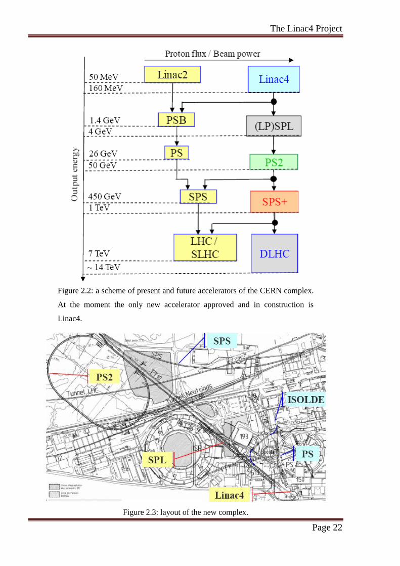
Similar analysis of LHC performances, together with the necessity of reliable
operation, are the basis of the gradual replacement proposed for the present injector
complex, as sketched in Figure 2.2 and Figure 2.3 [1,2]. The only accelerator which will
not be replaced is SPS. The first accelerator to be built is Linac4 (2008 start - 2013
commissioning).
The Linac4 Project
Page 22
Figure 2.2: a scheme of present and future accelerators of the CERN complex.
At the moment the only new accelerator approved and in construction is
Linac4.
Figure 2.3: layout of the new complex.
The Linac4 Project
Page 23
The last remark is on the choice to build the new linacs (Linac4 and SPL) as H-
machines. The notable advance during the last 20 years of the technology of H- sources
and linear accelerators has allowed the upgrade to take advantage of the charge-exchange
injection of H- into the synchrotrons (PSB or PS2) using a stripping foil [3].
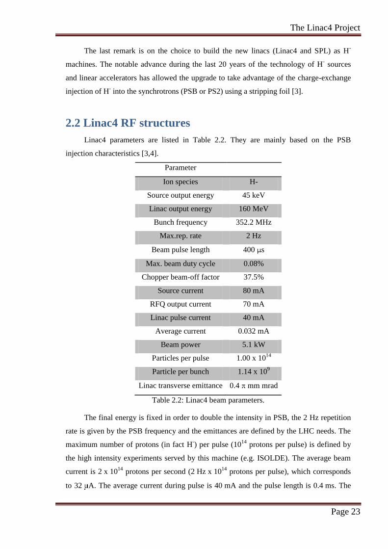
2.2 Linac4 RF structures
Linac4 parameters are listed in Table 2.2. They are mainly based on the PSB
injection characteristics [3,4].
Parameter
Ion species H-
Source output energy 45 keV
Linac output energy 160 MeV
Bunch frequency 352.2 MHz
Max.rep. rate 2 Hz
Beam pulse length 400 s
Max. beam duty cycle 0.08%
Chopper beam-off factor 37.5%
Source current 80 mA
RFQ output current 70 mA
Linac pulse current 40 mA
Average current 0.032 mA
Beam power 5.1 kW
Particles per pulse 1.00 x 10¹⁴
Particle per bunch 1.14 x 10⁹
Linac transverse emittance 0.4 mm mrad
Table 2.2: Linac4 beam parameters.
The final energy is fixed in order to double the intensity in PSB, the 2 Hz repetition
rate is given by the PSB frequency and the emittances are defined by the LHC needs. The
maximum number of protons (in fact H-) per pulse (10
14 protons per pulse) is defined by
the high intensity experiments served by this machine (e.g. ISOLDE). The average beam
current is 2 x 10¹⁴
protons per second (2 Hz x 1014
protons per pulse), which corresponds
to 32 A. The average current during pulse is 40 mA and the pulse length is 0.4 ms. The
The Linac4 Project
Page 24
beam duty cycle is 0.08% and considering an RF pulse of 0.5 ms, the RF duty cycle is
0.1%.
Nevertheless this machine is going to be the front end of the H- SPL, which will
provide a 4 GeV beam at repetition rate of 5 Hz (5% duty cycle). In order to keep a margin
for future operations, all Linac4 accelerating structures are designed for a maximum duty
cycle of 10%.
The RF frequency is determined by the availability of RF equipment at 352 MHz
(klystrons, wave-guides, circulators) from the decommissioning of the LEP RF system.
The operating frequency is the same for all the structures.
The chopping system located after the RFQ is devoted to stop a selected sequence
of beam bunches, in order to avoid beam losses at high energy during longitudinal capture
into the PSB buckets. Since the fraction of beam removed by the chopper is 37.5%, the
pulse current before chopping has to be 64 mA. Including margins for beam losses in the
transfer line, in the RFQ and in the chopper line, the RFQ output current is set at 70 mA
and the source current at 80 mA.
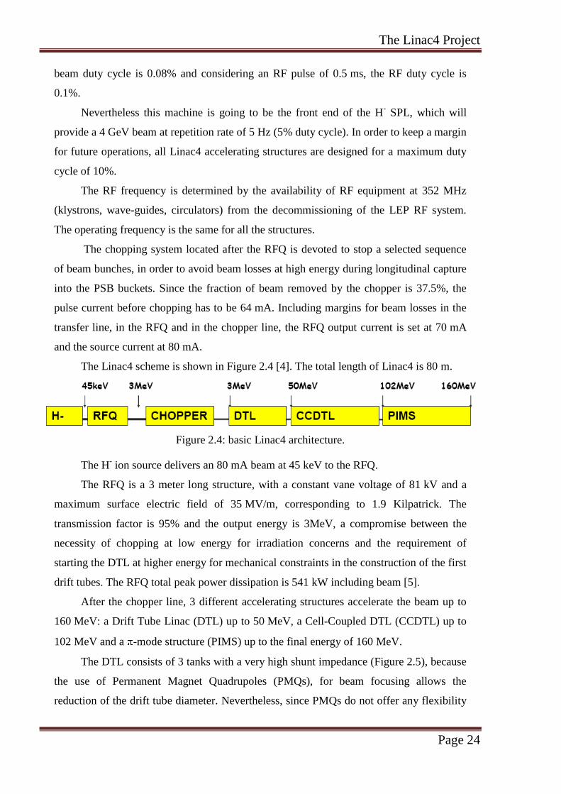
The Linac4 scheme is shown in Figure 2.4 [4]. The total length of Linac4 is 80 m.
Figure 2.4: basic Linac4 architecture.
The H- ion source delivers an 80 mA beam at 45 keV to the RFQ.
The RFQ is a 3 meter long structure, with a constant vane voltage of 81 kV and a
maximum surface electric field of 35 MV/m, corresponding to 1.9 Kilpatrick. The
transmission factor is 95% and the output energy is 3MeV, a compromise between the
necessity of chopping at low energy for irradiation concerns and the requirement of
starting the DTL at higher energy for mechanical constraints in the construction of the first
drift tubes. The RFQ total peak power dissipation is 541 kW including beam [5].
After the chopper line, 3 different accelerating structures accelerate the beam up to
160 MeV: a Drift Tube Linac (DTL) up to 50 MeV, a Cell-Coupled DTL (CCDTL) up to
102 MeV and a -mode structure (PIMS) up to the final energy of 160 MeV.
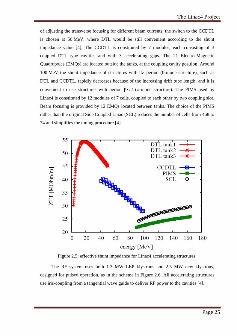
The DTL consists of 3 tanks with a very high shunt impedance (Figure 2.5), because
the use of Permanent Magnet Quadrupoles (PMQs), for beam focusing allows the
reduction of the drift tube diameter. Nevertheless, since PMQs do not offer any flexibility
The Linac4 Project
Page 25
of adjusting the transverse focusing for different beam currents, the switch to the CCDTL
is chosen at 50 MeV, where DTL would be still convenient according to the shunt
impedance value [4]. The CCDTL is constituted by 7 modules, each consisting of 3
coupled DTL–type cavities and with 3 accelerating gaps. The 21 Electro-Magnetic
Quadrupoles (EMQs) are located outside the tanks, at the coupling cavity position. Around
100 MeV the shunt impedance of structures with period (0-mode structure), such as
DTL and CCDTL, rapidly decreases because of the increasing drift tube length, and it is
convenient to use structures with period /2 ( -mode structure). The PIMS used by
Linac4 is constituted by 12 modules of 7 cells, coupled to each other by two coupling slot.
Beam focusing is provided by 12 EMQs located between tanks. The choice of the PIMS
rather than the original Side Coupled Linac (SCL) reduces the number of cells from 468 to
74 and simplifies the tuning procedure [4].
Figure 2.5: effective shunt impedance for Linac4 accelerating structures.
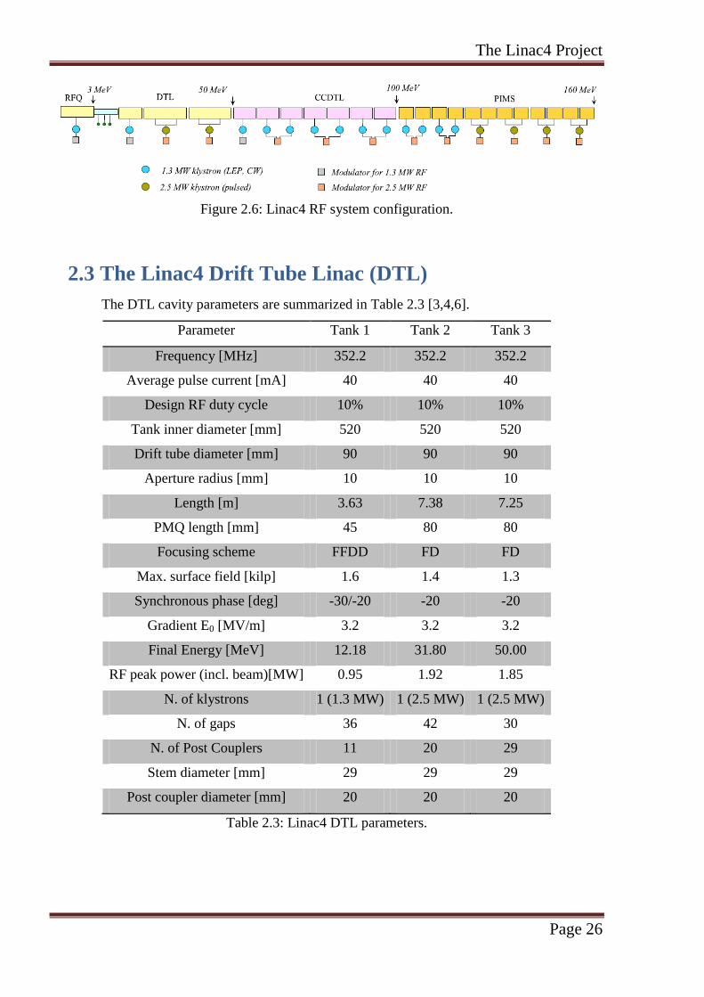
The RF system uses both 1.3 MW LEP klystrons and 2.5 MW new klystrons,
designed for pulsed operation, as in the scheme in Figure 2.6. All accelerating structures
use iris-coupling from a tangential wave guide to deliver RF power to the cavities [4].
The Linac4 Project
Page 26
Figure 2.6: Linac4 RF system configuration.
2.3 The Linac4 Drift Tube Linac (DTL)
The DTL cavity parameters are summarized in Table 2.3 [3,4,6].
Parameter Tank 1 Tank 2 Tank 3
Frequency [MHz] 352.2 352.2 352.2
Average pulse current [mA] 40 40 40
Design RF duty cycle 10% 10% 10%
Tank inner diameter [mm] 520 520 520
Drift tube diameter [mm] 90 90 90
Aperture radius [mm] 10 10 10
Length [m] 3.63 7.38 7.25
PMQ length [mm] 45 80 80
Focusing scheme FFDD FD FD
Max. surface field [kilp] 1.6 1.4 1.3
Synchronous phase [deg] -30/-20 -20 -20
Gradient E0 [MV/m] 3.2 3.2 3.2
Final Energy [MeV] 12.18 31.80 50.00
RF peak power (incl. beam)[MW] 0.95 1.92 1.85
N. of klystrons 1 (1.3 MW) 1 (2.5 MW) 1 (2.5 MW)
N. of gaps 36 42 30
N. of Post Couplers 11 20 29
Stem diameter [mm] 29 29 29
Post coupler diameter [mm] 20 20 20
Table 2.3: Linac4 DTL parameters.
The Linac4 Project
Page 27
The Linac4 DTL is designed to accelerate pulses of 40 mA of H- ions from 3 MeV
to 50 MeV. The structure is composed by 3 tanks with a total length of 18.7 m. The tank
diameter is 520 mm and the drift tube diameter is 90 mm, with a beam aperture of 20 mm.
The beam focusing is provided by PMQs installed inside the drift tubes. The choice
to use PMQs keeps the drift tube size small and avoids current wires and additional power
supplies. Increased flexibility of the focusing system is obtained by placing
electromagnetic quadrupoles in each of the intertank spaces.
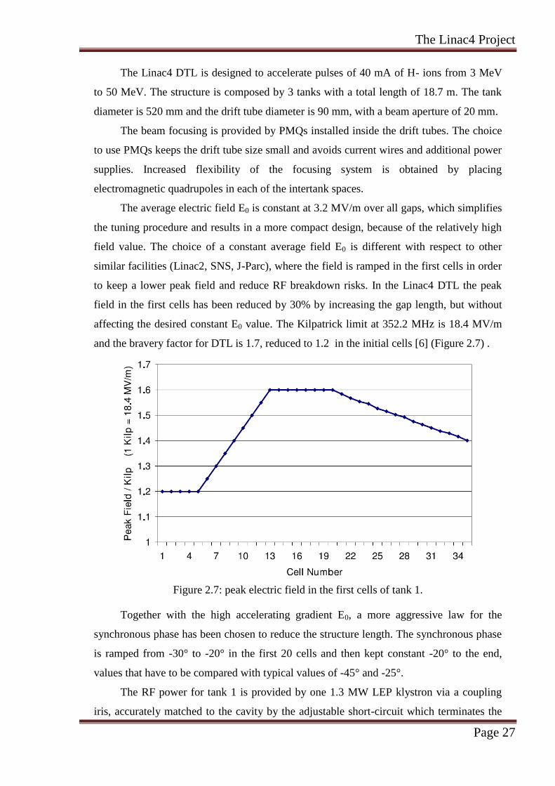
The average electric field E0 is constant at 3.2 MV/m over all gaps, which simplifies
the tuning procedure and results in a more compact design, because of the relatively high
field value. The choice of a constant average field E0 is different with respect to other
similar facilities (Linac2, SNS, J-Parc), where the field is ramped in the first cells in order
to keep a lower peak field and reduce RF breakdown risks. In the Linac4 DTL the peak
field in the first cells has been reduced by 30% by increasing the gap length, but without
affecting the desired constant E0 value. The Kilpatrick limit at 352.2 MHz is 18.4 MV/m
and the bravery factor for DTL is 1.7, reduced to 1.2 in the initial cells [6] (Figure 2.7) .
Figure 2.7: peak electric field in the first cells of tank 1.
Together with the high accelerating gradient E0, a more aggressive law for the
synchronous phase has been chosen to reduce the structure length. The synchronous phase
is ramped from -30° to -20° in the first 20 cells and then kept constant -20° to the end,
values that have to be compared with typical values of -45° and -25°.
The RF power for tank 1 is provided by one 1.3 MW LEP klystron via a coupling
iris, accurately matched to the cavity by the adjustable short-circuit which terminates the
The Linac4 Project
Page 28
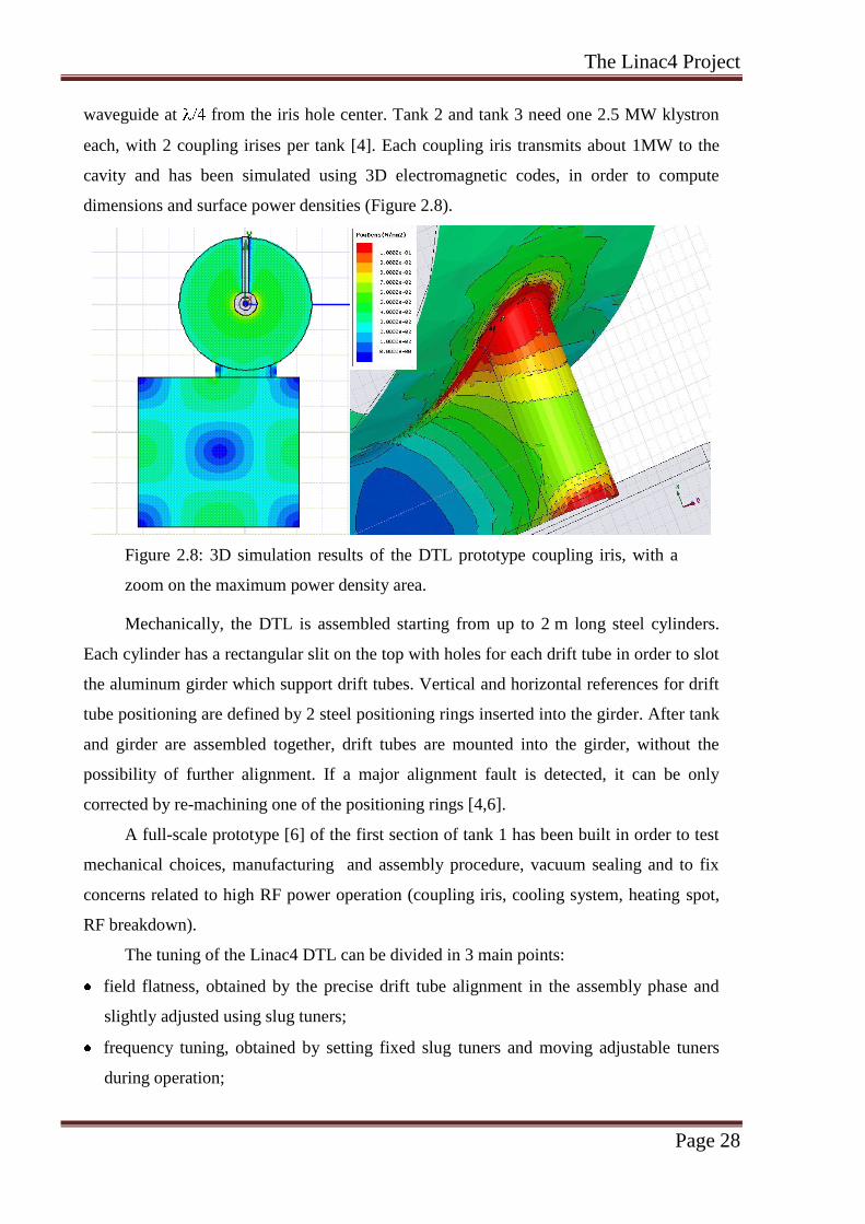
waveguide at from the iris hole center. Tank 2 and tank 3 need one 2.5 MW klystron
each, with 2 coupling irises per tank [4]. Each coupling iris transmits about 1MW to the
cavity and has been simulated using 3D electromagnetic codes, in order to compute
dimensions and surface power densities (Figure 2.8).
Figure 2.8: 3D simulation results of the DTL prototype coupling iris, with a
zoom on the maximum power density area.
Mechanically, the DTL is assembled starting from up to 2 m long steel cylinders.
Each cylinder has a rectangular slit on the top with holes for each drift tube in order to slot
the aluminum girder which support drift tubes. Vertical and horizontal references for drift
tube positioning are defined by 2 steel positioning rings inserted into the girder. After tank
and girder are assembled together, drift tubes are mounted into the girder, without the
possibility of further alignment. If a major alignment fault is detected, it can be only
corrected by re-machining one of the positioning rings [4,6].
A full-scale prototype [6] of the first section of tank 1 has been built in order to test
mechanical choices, manufacturing and assembly procedure, vacuum sealing and to fix
concerns related to high RF power operation (coupling iris, cooling system, heating spot,
RF breakdown).
The tuning of the Linac4 DTL can be divided in 3 main points:
field flatness, obtained by the precise drift tube alignment in the assembly phase and
slightly adjusted using slug tuners;
frequency tuning, obtained by setting fixed slug tuners and moving adjustable tuners
during operation;

The Linac4 Project
Page 29
field stabilization, provided by post couplers.
Slug tuners are placed at 45° with respect to stem position. The present configuration
foresees about 3 tuners per meter. Post coupler distribution foresees one post coupler every
3 drift tubes in tank 1, one post coupler every 2 drift tubes in tank 2 and one post coupler
every drift tube in tank 3. These configurations correspond respectively to 3.3, 2.8 and 4.1
post couplers per meter. The small drift tube diameter, allowed by the small PMQ size, has
the advantage of increasing the shunt impedance, but at the same time the distance
between drift tube and tank is larger than /4 (1.01 /4), considered to be critical for
achieving field stabilization. The stabilization effectiveness of this post coupler
configuration has been verified in detail with 3D simulations and with a dedicated
aluminum scaled prototype, showing that stabilization can be achieved [6,7].
References
[1] R. Garoby, “Upgrade issues for the CERN accelerator complex”, Proc. EPAC08.
[2] Interdepartmental working group on “Proton Accelerators for the Future” (PAF),
http://paf.web.cern.ch/paf/.
[3] F. Gerigk, M. Vretenar (ed.), “Linac4 Technical Design Report”, CERN-AB-2006-084
ABP/RF.
[4] F. Gerigk et al., “RF structures for Linac4”, Proc. PAC07.
[5] A. M. Lombardi, C. Rossi, M. Vretenar, “Design of an RFQ Accelerator optimised for
Linac4 and SPL”, CERN-AB-Note-2007-027.
[6] S. Ramberger et al., “Drift Tube Linac Design and Prototyping for the CERN Linac4”,
Proc. LINAC08.
[7] N. Alharbi, F. Gerigk and M. Vretenar, “Field Stabilization with Post Couplers for
DTL Tank1 of Linac4”, Tech. Rep. CARE-Note-2006-012-HIPPI, CARE, 2006.

Drift Tube Linac and Resonant Coupling
Page 30
Chapter 3. Drift Tube Linac and Resonant
Coupling
In this chapter we briefly introduce some concepts about resonant cavities and linear
accelerator structures
The Drift Tube Linac (DTL) cavity is a common accelerating structure at ion
facilities since the end of World War II. DTLs are efficient at providing the second
acceleration step for ions, in the velocity region of 0.1 < < 0.5, corresponding to proton
kinetic energy W of 3 MeV < W < 150 MeV. For reasons of RF power saving it is
convenient to build a long DTL tank, but this choice involves risks of accelerating field
instability. This problem has been fixed by using the resonant coupling stabilization
method and equipping DTL cavities with enigmatic coupled resonators, called post
couplers.
3.1 Alvarez Drift Tube Linac (DTL)
The Drift Tube Linac (DTL) is an accelerating structure proposed by L. Alvarez in
1946 [1], consisting of an array of drift tubes on the beam axis, suspended from the cavity
tank by supporting stems (Figure 3.1).
Figure 3.1: internal and external view of the SNS DTL.
Starting from a pillbox cavity [2,3] operating at the TM010 resonant mode, where the
electric field is uniform along the beam axis z of the cavity, a reentrant gap is introduced
to concentrate the electric field in the beam axis region and therefore to increase the
accelerating efficiency of the structure. Now a set of identical single-cell cavities are
concatenated to form a multigap accelerator (Figure 3.2). If the RF fields in all the cavities

Drift Tube Linac and Resonant Coupling
Page 31
are phased to be identical in time and the cavities are dimensioned such that the space
between gaps is , by the time the ion transits from one gap to the next the field has
progressed by one wave and the ion experiences an accelerating field in each gap. Since
the cavities are all in synchronism, the velocity at each point is fixed: the Alvarez structure
is inherently a fixed-velocity structure.
Figure 3.2: a single cell cavity array. Wall currents and lumped circuit
elements are shown.
The accelerator is now an array of single cavities all in phase, but this configuration
can be improved. In the TM010 mode currents flow along the walls, heating them and
requiring RF power. The fields on each side of the walls separating each cell are identical
in amplitude and direction, so the walls separating the cells can be removed and the drift
tubes suspended on stems (Figure 3.3).
H
E
Figure 3.3: in a DTL cavity separating walls are removed, and drift tube are
supported by stems.
This is one way to look the DTL: a series of single-cell cavities all in phase, where
the separating walls are removed without altering the field configuration.

Drift Tube Linac and Resonant Coupling
Page 32
We can also consider the DTL as a long pillbox cavity with the electric field along
the axis. If the cavity is made longer than the distance a particle travels in half an RF
period ( /2), the particle is both accelerated and decelerated as well. If hollow drift tubes
are installed along the axis the particle will be inside a Faraday Cage that shields the
particles when the polarity of the axial field is opposite to the beam direction. The drift
tubes divide the cavity into cells of length . As the particles gain energy at each gap, the
cell lengths increase with . Because the fields in all the cells are in phase, the Alvarez
DTL structures operates in a 0 mode, where zero refers to the cell-to-cell field phase
difference at a fixed time.
An interesting quantity for accelerator design is the average axial field E0 for a
single accelerating cell defined as
00
(0, )Lcell
cell cell
E z d zV
EL L
.
If we apply the Faraday’s law to the rectangular path in Figure 3.3, we have
E dl B d At
.
Since the line integral of the electric field is nonzero only on the beam axis path, the
left side of the equation is
0 0(0, )E dl E z d z V E .
The integral on the right side is B d A jt
where is the magnetic flux.
Therefore the magnitudes of the left and the right sides are related by 0E .
E0 is proportional to the magnetic flux per unit length of the cell. Frequently DTLs are
designed in order to have constant E0 for all the cells and, in a structure with constant tank
diameter and constant drift tube diameter, this can be obtained with the same radial
distribution of B along the cavity. Generally, DTLs with constant E0 have different peak
electric field in the gaps and different peak surface electric field, depending on the cell
length and geometry.
Coming back to the cavity cell description in Figure 3.2, each cavity can be seen as a
lumped circuit whit a capacitance on the drift tube gap, and an inductance associated to the
current loop from one drift tube to the outer walls and back to the other drift tube,
becoming displacement current in the gap. An approximate value of the capacitance can be
Drift Tube Linac and Resonant Coupling
Page 33
calculated with the parallel plate formula 2
0 0 / 4C d g and the inductance with the
coaxial inductance formula 0 0 ln / / 2L D d where is the cell length, d is the
drift tube diameter, D is the tank diameter and g is the gap. The cell resonant frequency is
000 /1 LC .
As the cell length increases with along the structure, the lumped circuit inductance
L0 increases as well. In order to keep the resonant frequency constant, the capacitance
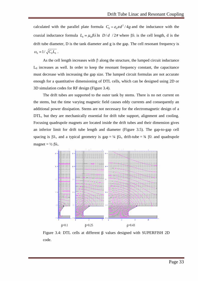
must decrease with increasing the gap size. The lumped circuit formulas are not accurate
enough for a quantitative dimensioning of DTL cells, which can be designed using 2D or
3D simulation codes for RF design (Figure 3.4).
The drift tubes are supported to the outer tank by stems. There is no net current on
the stems, but the time varying magnetic field causes eddy currents and consequently an
additional power dissipation. Stems are not necessary for the electromagnetic design of a
DTL, but they are mechanically essential for drift tube support, alignment and cooling.
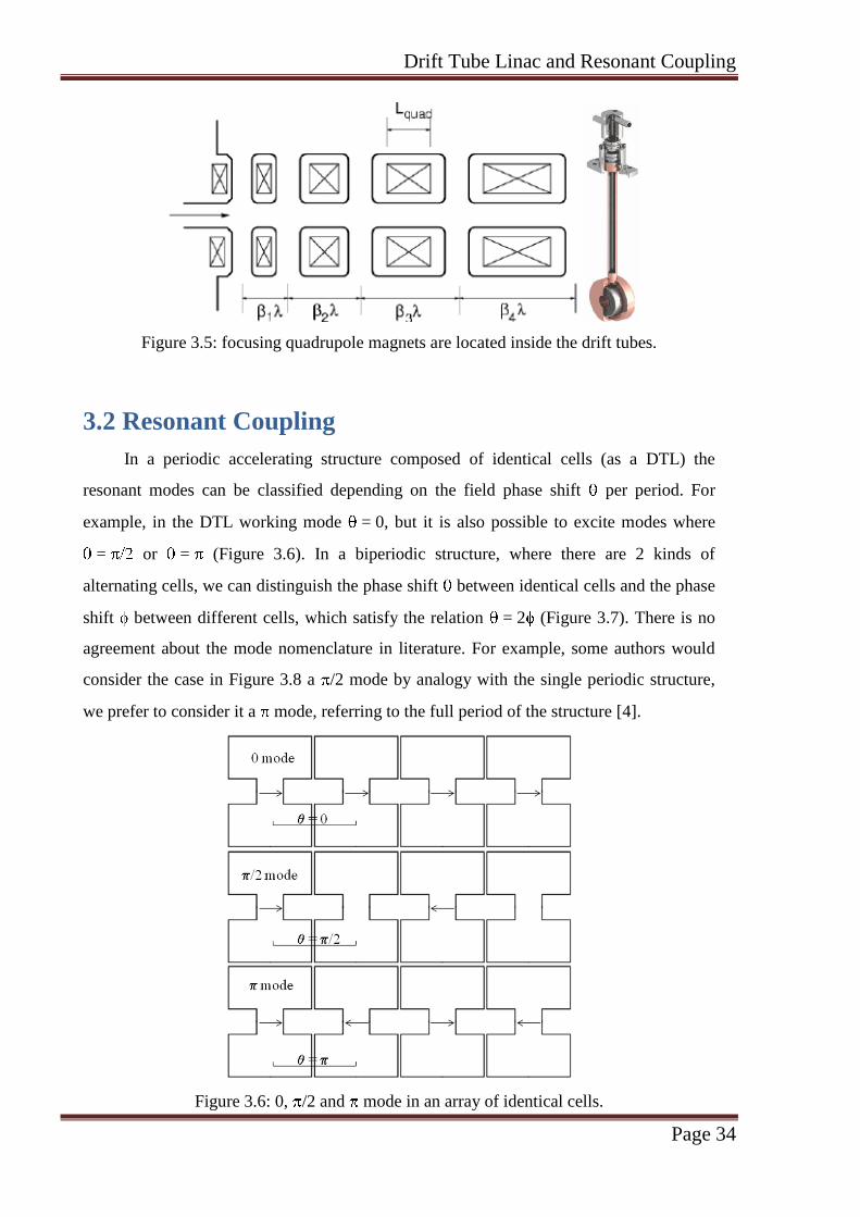
Focusing quadrupole magnets are located inside the drift tubes and their dimension gives
an inferior limit for drift tube length and diameter (Figure 3.5). The gap-to-gap cell
spacing is , and a typical geometry is gap = ¼ , drift-tube = ¾ and quadrupole
magnet = ½ .
=0.1 =0.25 =0.43
Figure 3.4: DTL cells at different values designed with SUPERFISH 2D
code.
Drift Tube Linac and Resonant Coupling
Page 34
Figure 3.5: focusing quadrupole magnets are located inside the drift tubes.
3.2 Resonant Coupling
In a periodic accelerating structure composed of identical cells (as a DTL) the
resonant modes can be classified depending on the field phase shift per period. For
example, in the DTL working mode = 0, but it is also possible to excite modes where
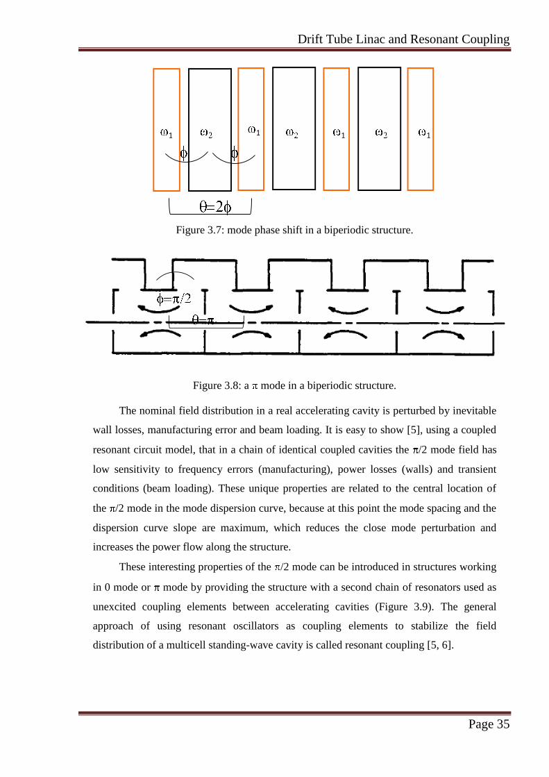
= or = (Figure 3.6). In a biperiodic structure, where there are 2 kinds of
alternating cells, we can distinguish the phase shift between identical cells and the phase
shift between different cells, which satisfy the relation = 2 (Figure 3.7). There is no
agreement about the mode nomenclature in literature. For example, some authors would
consider the case in Figure 3.8 a /2 mode by analogy with the single periodic structure,
we prefer to consider it a mode, referring to the full period of the structure [4].
Figure 3.6: 0, /2 and mode in an array of identical cells.
Drift Tube Linac and Resonant Coupling
Page 35
1 1 1 1
Figure 3.7: mode phase shift in a biperiodic structure.
Figure 3.8: a mode in a biperiodic structure.
The nominal field distribution in a real accelerating cavity is perturbed by inevitable
wall losses, manufacturing error and beam loading. It is easy to show [5], using a coupled
resonant circuit model, that in a chain of identical coupled cavities the /2 mode field has
low sensitivity to frequency errors (manufacturing), power losses (walls) and transient
conditions (beam loading). These unique properties are related to the central location of
the /2 mode in the mode dispersion curve, because at this point the mode spacing and the
dispersion curve slope are maximum, which reduces the close mode perturbation and
increases the power flow along the structure.
These interesting properties of the /2 mode can be introduced in structures working
in 0 mode or mode by providing the structure with a second chain of resonators used as
unexcited coupling elements between accelerating cavities (Figure 3.9). The general
approach of using resonant oscillators as coupling elements to stabilize the field
distribution of a multicell standing-wave cavity is called resonant coupling [5, 6].

Drift Tube Linac and Resonant Coupling
Page 36
Figure 3.9: in a side coupled linac accelerating cavities are coupled by external
coupling cavities.
Because of the existence of a second resonator chain, the dispersion curve has now 2
passbands, separated by a stopband. If the cavities are tuned in order to remove the
stopband, the structure gets the desired /2 mode properties. Such a joining up of two
passbands is called confluence point. A structure where the operating point (0 or mode)
is the confluence point is called a compensated or stabilized structure. The stopband can
be completely eliminated only in an infinite structure. In terminated structures only the
accelerating cavity mode can be excited at the confluence point, the coupling cavity mode
being forbidden because of boundary conditions [4] (Figure 3.10).
Figure 3.10: dispersion curve of an infinitely long coupled structure (left) and
for a terminated coupled structure.
Drift Tube Linac and Resonant Coupling
Page 37
The resonant coupling principle, originally developed for the Side Coupled Linac
(Figure 3.9), has been applied to other accelerating structures. The most common
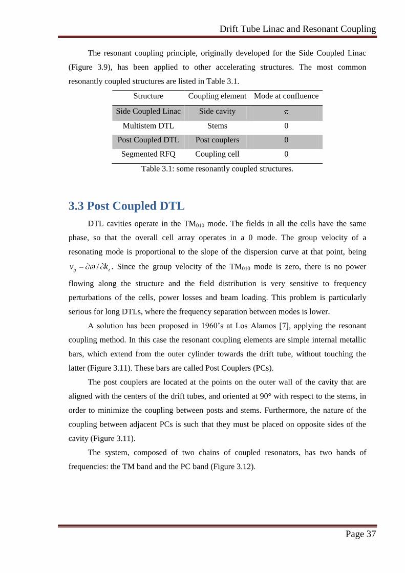
resonantly coupled structures are listed in Table 3.1.
Structure Coupling element Mode at confluence
Side Coupled Linac Side cavity
Multistem DTL Stems 0
Post Coupled DTL Post couplers 0
Segmented RFQ Coupling cell 0
Table 3.1: some resonantly coupled structures.
3.3 Post Coupled DTL
DTL cavities operate in the TM010 mode. The fields in all the cells have the same
phase, so that the overall cell array operates in a 0 mode. The group velocity of a
resonating mode is proportional to the slope of the dispersion curve at that point, being
zg kv / . Since the group velocity of the TM010 mode is zero, there is no power
flowing along the structure and the field distribution is very sensitive to frequency
perturbations of the cells, power losses and beam loading. This problem is particularly
serious for long DTLs, where the frequency separation between modes is lower.
A solution has been proposed in 1960’s at Los Alamos [7], applying the resonant
coupling method. In this case the resonant coupling elements are simple internal metallic
bars, which extend from the outer cylinder towards the drift tube, without touching the
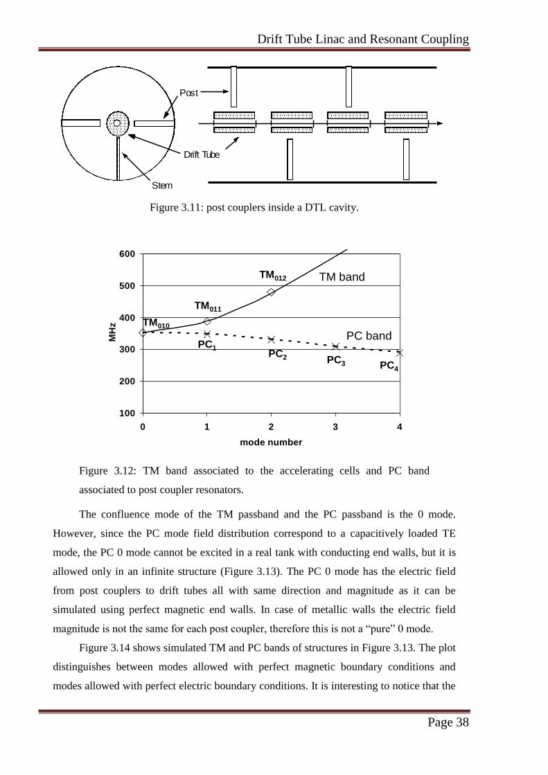
latter (Figure 3.11). These bars are called Post Couplers (PCs).
The post couplers are located at the points on the outer wall of the cavity that are
aligned with the centers of the drift tubes, and oriented at 90° with respect to the stems, in
order to minimize the coupling between posts and stems. Furthermore, the nature of the
coupling between adjacent PCs is such that they must be placed on opposite sides of the
cavity (Figure 3.11).
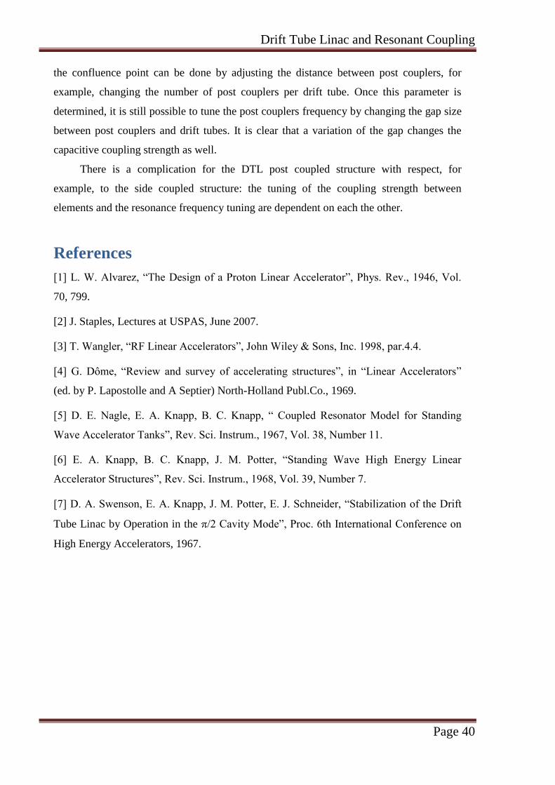
The system, composed of two chains of coupled resonators, has two bands of
frequencies: the TM band and the PC band (Figure 3.12).
Drift Tube Linac and Resonant Coupling
Page 38
Post
Stem
Drift Tube
Figure 3.11: post couplers inside a DTL cavity.
100
200
300
400
500
600
0 1 2 3 4
mode number
MH
z
TM band
PC bandPC1
PC2 PC3 PC4
TM010
TM012
TM011
100
200
300
400
500
600
0 1 2 3 4
mode number
MH
z
TM band
PC bandPC1
PC2 PC3 PC4
TM010
TM012
TM011
Figure 3.12: TM band associated to the accelerating cells and PC band
associated to post coupler resonators.
The confluence mode of the TM passband and the PC passband is the 0 mode.
However, since the PC mode field distribution correspond to a capacitively loaded TE
mode, the PC 0 mode cannot be excited in a real tank with conducting end walls, but it is
allowed only in an infinite structure (Figure 3.13). The PC 0 mode has the electric field
from post couplers to drift tubes all with same direction and magnitude as it can be
simulated using perfect magnetic end walls. In case of metallic walls the electric field
magnitude is not the same for each post coupler, therefore this is not a “pure” 0 mode.
Figure 3.14 shows simulated TM and PC bands of structures in Figure 3.13. The plot
distinguishes between modes allowed with perfect magnetic boundary conditions and
modes allowed with perfect electric boundary conditions. It is interesting to notice that the

Drift Tube Linac and Resonant Coupling
Page 39
three PC modes simulated with perfect electric boundary conditions have the same
frequencies as the three central modes of the PC band simulated with perfect magnetic
boundary conditions.
Figure 3.13: the PC 0 mode can be simulated only with perfect magnetic end
walls (left). With metallic end walls (right) it is not possible to excite a “pure”
PC 0 mode.
200
250
300
350
400
450
500
0 1 2 3 4 5
MH
z
mode number
Perfect magnetic bound.cond.
Perfect electric bound.cond.
TM band
PC band
Figure 3.14: dispersion curves simulated with perfect electric boundary
conditions and with perfect magnetic boundary conditions in a DTL with post
couplers (Figure 3.13).
The coupling between post couplers and DTL accelerating cells is provided by the
capacitance from the end of PCs to the drift tube walls. The coupling is stronger if the gap
between PCs and drift tubes is small. The tuning of the coupling element resonance to get
Drift Tube Linac and Resonant Coupling
Page 40
the confluence point can be done by adjusting the distance between post couplers, for
example, changing the number of post couplers per drift tube. Once this parameter is
determined, it is still possible to tune the post couplers frequency by changing the gap size
between post couplers and drift tubes. It is clear that a variation of the gap changes the
capacitive coupling strength as well.
There is a complication for the DTL post coupled structure with respect, for
example, to the side coupled structure: the tuning of the coupling strength between
elements and the resonance frequency tuning are dependent on each the other.
References
[1] L. W. Alvarez, “The Design of a Proton Linear Accelerator”, Phys. Rev., 1946, Vol.
70, 799.
[2] J. Staples, Lectures at USPAS, June 2007.
[3] T. Wangler, “RF Linear Accelerators”, John Wiley & Sons, Inc. 1998, par.4.4.
[4] G. Dôme, “Review and survey of accelerating structures”, in “Linear Accelerators”
(ed. by P. Lapostolle and A Septier) North-Holland Publ.Co., 1969.
[5] D. E. Nagle, E. A. Knapp, B. C. Knapp, “ Coupled Resonator Model for Standing
Wave Accelerator Tanks”, Rev. Sci. Instrum., 1967, Vol. 38, Number 11.
[6] E. A. Knapp, B. C. Knapp, J. M. Potter, “Standing Wave High Energy Linear
Accelerator Structures”, Rev. Sci. Instrum., 1968, Vol. 39, Number 7.
[7] D. A. Swenson, E. A. Knapp, J. M. Potter, E. J. Schneider, “Stabilization of the Drift
Tube Linac by Operation in the /2 Cavity Mode”, Proc. 6th International Conference on
High Energy Accelerators, 1967.
Post Coupler stabilization: simulation results
Page 41
Chapter 4. Post couplers: simulation results
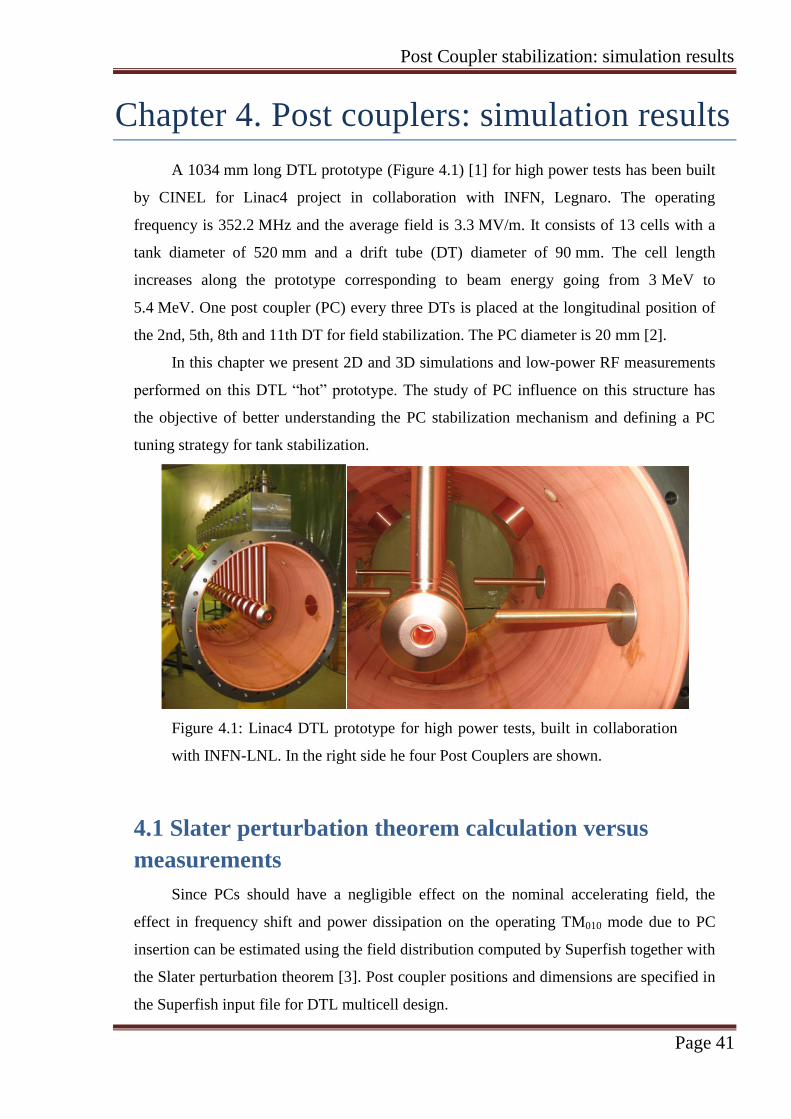
A 1034 mm long DTL prototype (Figure 4.1) [1] for high power tests has been built
by CINEL for Linac4 project in collaboration with INFN, Legnaro. The operating
frequency is 352.2 MHz and the average field is 3.3 MV/m. It consists of 13 cells with a
tank diameter of 520 mm and a drift tube (DT) diameter of 90 mm. The cell length
increases along the prototype corresponding to beam energy going from 3 MeV to
5.4 MeV. One post coupler (PC) every three DTs is placed at the longitudinal position of
the 2nd, 5th, 8th and 11th DT for field stabilization. The PC diameter is 20 mm [2].
In this chapter we present 2D and 3D simulations and low-power RF measurements
performed on this DTL “hot” prototype. The study of PC influence on this structure has
the objective of better understanding the PC stabilization mechanism and defining a PC
tuning strategy for tank stabilization.
Figure 4.1: Linac4 DTL prototype for high power tests, built in collaboration
with INFN-LNL. In the right side he four Post Couplers are shown.
4.1 Slater perturbation theorem calculation versus
measurements
Since PCs should have a negligible effect on the nominal accelerating field, the
effect in frequency shift and power dissipation on the operating TM010 mode due to PC
insertion can be estimated using the field distribution computed by Superfish together with
the Slater perturbation theorem [3]. Post coupler positions and dimensions are specified in
the Superfish input file for DTL multicell design.

Post Coupler stabilization: simulation results
Page 42
Formulas used for frequency and power calculation are [4]:
2 2
2 2
2
4 4
cyl cylV
H E dVk H k E
df R dr fU U
2 2 2 212 ( , ) ( , )
2 2 2
scyl PC PC
S
RP H dS R dr k H z r R H z h
where R is the object radius, dr the radial step between 2 SuperFish data, f the cavity
frequency, kcyl
= 2 is the shape factor due to the field distortion close to the PC surface, µ
and ε are the material permeability and permittivity, H and E the unperturbed magnetic
and electric fields, U the cavity stored energy, Rs the RF surface resistance, ρ the electrical
resistivity, h the post coupler length.
The frequency shift calculated as function of PC length for DTL prototype is shown
in Figure 4.2, together with measurements on the DTL hot prototype equipped with 4 PCs.
The strong variations in frequency shift measured at certain PC lengths [5] have been
investigated with more accurate measurements (Figure 4.3), indicating that the crossing
and local coupling of the 3 highest modes of the PC band with the TM010. The Slater
perturbation theorem describes the TM010 frequency shift due to the PC insertion, but
cannot give information on the coupling between the TM01 band and the PC band and
consequently on the optimum length of the PCs for the tank stabilization.
0.00
0.05
0.10
0.15
0.20
0.25
0 50 100 150 200 250
PCs length [mm]
TM
01
0 f
req
ue
nc
y s
hif
t [M
Hz]
.
Measured Freq. Shift
Simulated Freq. Shift
Figure 4.2: Simulated (Superfish) and measured TM010 detuning as a function
of PC length.

Post Coupler stabilization: simulation results
Page 43
351.0
351.4
351.8
352.2
352.6
353.0
158 162 166 170 174 178
PCs length [mm]
Fre
qu
en
cy
[M
Hz]
.
TM010_mode
PC3 mode
PC2 mode
PC1 mode
Figure 4.3: Measurements showing PC modes crossing TM010 mode.
4.2 3D simulations and bead-pull measurements on post
coupler modes
3D HFSS [6] simulations and bead-pull measurements have been undertaken on the
four PC modes of the DTL hot prototype. PC modes can be recognized in simulations due
to a characteristic field pattern with electric field between PCs and drift tubes and
magnetic field around PCs (Figure 4.4). The simulated axial field corresponds well with
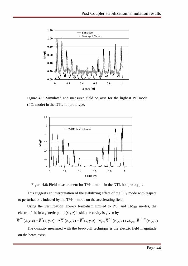
the bead-pull measurements performed on the PC modes close to confluence. Figure 4.5
shows the highest PC mode (PC1 mode), which presents the same axial field pattern as the
TM011 mode shown in Figure 4.6.
Figure 4.4: Electric and Magnetic Field of the higher PC mode (PC1 mode) in
the DTL hot prototype.
Post Coupler stabilization: simulation results
Page 44
0.00
0.20
0.40
0.60
0.80
1.00
1.20
0 0.2 0.4 0.6 0.8 1
z axis [m]
Ma
gE
Simulation
Bead-pull Meas.
Figure 4.5: Simulated and measured field on axis for the highest PC mode
(PC1 mode) in the DTL hot prototype.
0
0.2
0.4
0.6
0.8
1
1.2
0 0.2 0.4 0.6 0.8 1
z axis [m]
Ma
gE
.
TM011 bead pull meas
Figure 4.6: Field measurement for TM011 mode in the DTL hot prototype.
This suggests an interpretation of the stabilizing effect of the PC1 mode with respect
to perturbations induced by the TM011 mode on the accelerating field.
Using the Perturbation Theory formalism limited to PC1 and TM011 modes, the
electric field in a generic point (x,y,z) inside the cavity is given by
0 0 0 1 011
1 011( , , ) ( , , ) ( , , ) ( , , ) ( , , ) ( , , )pert PC TM
PC TME x y z E x y z E x y z E x y z E x y z E x y z
The quantity measured with the bead-pull technique is the electric field magnitude
on the beam axis:
Post Coupler stabilization: simulation results
Page 45
0 0 0 1 011
1 011(0,0, ) (0,0, ) (0,0, ) (0,0, ) (0,0, ) (0,0, )pert PC TM
PC TME z E z E z E z E z E z
with
0
,0
2 2 2 2
( , , ) ( , , ) ( , , )modemodei i j j
i jcavity
mode
o mode o mode
E x y z P x y z E x y z dxdydzE P E
.
The perturbation coefficients PC1 and TM011 depend on the local geometry
perturbation described by the matrix ( , , )P P x y z and on the field pattern of modes. If
mode resonant frequencies PC1 and TM011 are tuned in such a way that coefficients PC1
and TM011 are equal and opposite, the accelerating field perturbation can be canceled.
4.3 3D simulation study of post coupler geometrical
parameters
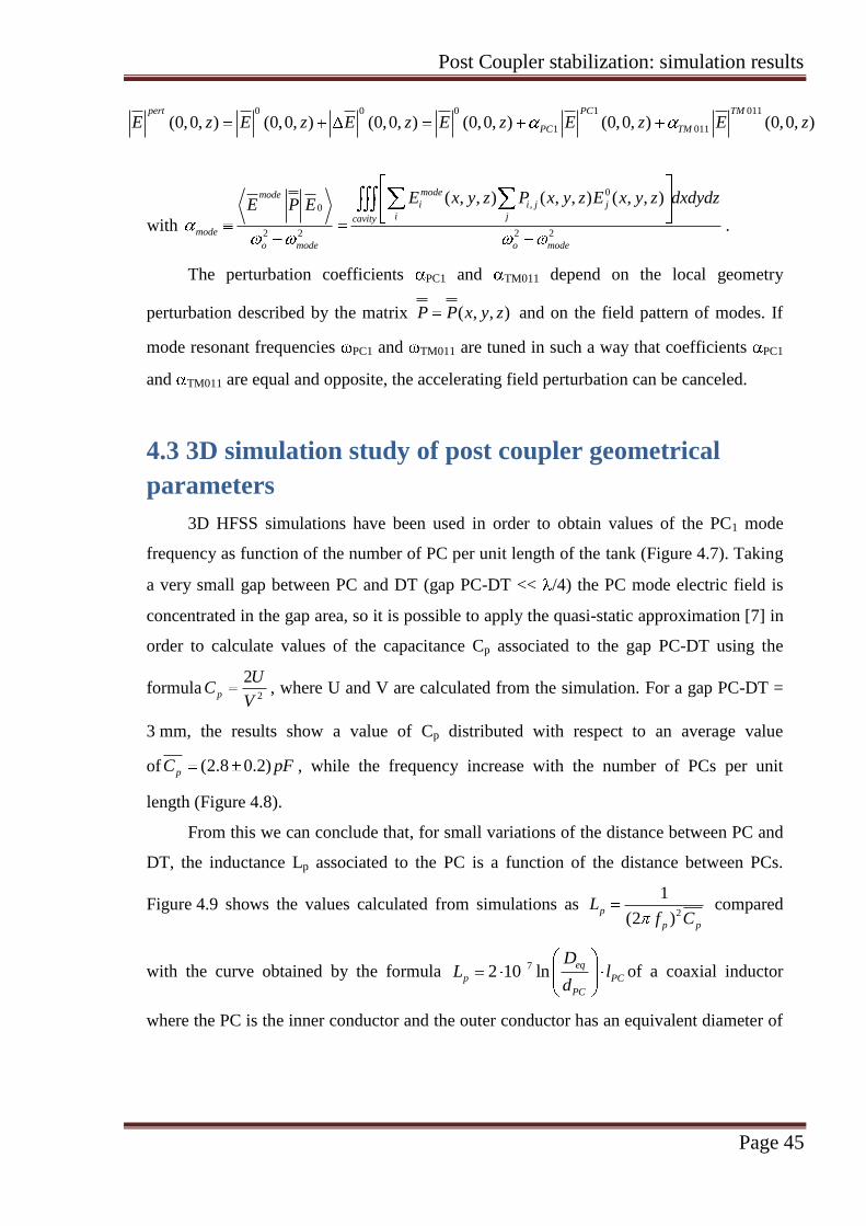
3D HFSS simulations have been used in order to obtain values of the PC1 mode
frequency as function of the number of PC per unit length of the tank (Figure 4.7). Taking
a very small gap between PC and DT (gap PC-DT << /4) the PC mode electric field is
concentrated in the gap area, so it is possible to apply the quasi-static approximation [7] in
order to calculate values of the capacitance Cp associated to the gap PC-DT using the
formula2
2p
UC
V, where U and V are calculated from the simulation. For a gap PC-DT =
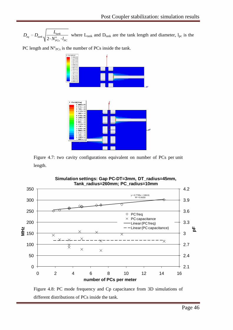
3 mm, the results show a value of Cp distributed with respect to an average value
of (2.8 0.2)pC pF , while the frequency increase with the number of PCs per unit
length (Figure 4.8).
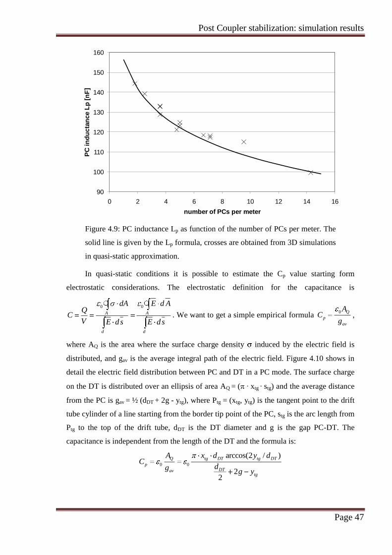
From this we can conclude that, for small variations of the distance between PC and
DT, the inductance Lp associated to the PC is a function of the distance between PCs.
Figure 4.9 shows the values calculated from simulations as 2
1
(2 )p
p p
Lf C
compared
with the curve obtained by the formula 72 10 lneq
p PC
PC
DL l
dof a coaxial inductor
where the PC is the inner conductor and the outer conductor has an equivalent diameter of
Post Coupler stabilization: simulation results
Page 46
2
tankeq tank o
PCs PC
LD D
N l where Ltank and Dtank are the tank length and diameter, lpc is the
PC length and N°PCs is the number of PCs inside the tank.
Figure 4.7: two cavity configurations equivalent on number of PCs per unit
length.
y = 3.7735x + 249.01R² = 0.9333
2.1
2.4
2.7
3
3.3
3.6
3.9
4.2
0
50
100
150
200
250
300
350
0 2 4 6 8 10 12 14 16
pF
MH
z
number of PCs per meter
Simulation settings: Gap PC-DT=3mm, DT_radius=45mm, Tank_radius=260mm; PC_radius=10mm
PC freq
PC capacitance
Linear (PC freq)
Linear (PC capacitance)
Figure 4.8: PC mode frequency and Cp capacitance from 3D simulations of
different distributions of PCs inside the tank.
Post Coupler stabilization: simulation results
Page 47
90
100
110
120
130
140
150
160
0 2 4 6 8 10 12 14 16
PC
in
du
cta
nce L
p [
nF
]
number of PCs per meter
Figure 4.9: PC inductance Lp as function of the number of PCs per meter. The
solid line is given by the Lp formula, crosses are obtained from 3D simulations
in quasi-static approximation.
In quasi-static conditions it is possible to estimate the Cp value starting form
electrostatic considerations. The electrostatic definition for the capacitance is
0 0
A A
d d
dA E d AQ
CV E d s E d s
. We want to get a simple empirical formula 0 Q
p
av
AC
g,
where AQ is the area where the surface charge density induced by the electric field is
distributed, and gav is the average integral path of the electric field. Figure 4.10 shows in
detail the electric field distribution between PC and DT in a PC mode. The surface charge
on the DT is distributed over an ellipsis of area AQ = ( ∙ xtg ∙ stg) and the average distance
from the PC is gav = ½ (dDT + 2g - ytg), where Ptg = (xtg, ytg) is the tangent point to the drift
tube cylinder of a line starting from the border tip point of the PC, stg is the arc length from
Ptg to the top of the drift tube, dDT is the DT diameter and g is the gap PC-DT. The
capacitance is independent from the length of the DT and the formula is:
0 0
arccos(2 / )
22
Q tg DT tg DT
pDTav
tg
A x d y dC
dgg y

Post Coupler stabilization: simulation results
Page 48
Figure 4.11 shows the curve given by the formula with the values calculated from
simulations as 2
2p
UC
V. The equation overestimates the capacitance by about 10% with
respect to the simulation results.
Figure 4.10: electric field pattern between PC and DT in a PC mode.
1.5
1.7
1.9
2.1
2.3
2.5
2.7
2.9
0 2 4 6 8 10 12 14 16
PC
cap
acit
an
ce C
p [
pF
]
gap PC-DT [mm]
Figure 4.11: PC capacitance Cp as function of the gap PC-DT. The solid line is
given by the Cp formula, crosses are obtained from 3D simulations in quasi-
static approximation.
The interaction of PCs and stems has also been studied with 3D simulations, in order
to properly insert stems in the DTL equivalent circuit.
Stem modes can be distinguished in RF measurements because of the much lower
frequencies with respect to the operating mode and because of the low sensitivity to gap
displacements. 3D simulations show that the presence of DT stems weakly affects the field
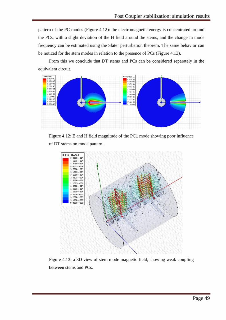
Post Coupler stabilization: simulation results
Page 49
pattern of the PC modes (Figure 4.12): the electromagnetic energy is concentrated around
the PCs, with a slight deviation of the H field around the stems, and the change in mode
frequency can be estimated using the Slater perturbation theorem. The same behavior can
be noticed for the stem modes in relation to the presence of PCs (Figure 4.13).
From this we conclude that DT stems and PCs can be considered separately in the
equivalent circuit.
Figure 4.12: E and H field magnitude of the PC1 mode showing poor influence
of DT stems on mode pattern.
Figure 4.13: a 3D view of stem mode magnetic field, showing weak coupling
between stems and PCs.
Post Coupler stabilization: simulation results
Page 50
References
[1] S. Ramberger et al., “Drift Tube Linac Design and Prototyping for the CERN Linac4”,
Proc. LINAC08.
[2] N. Alharbi, F. Gerigk and M. Vretenar, “Field Stabilization with Post Couplers for
DTL Tank1 of Linac4”, Tech. Rep. CARE-Note-2006-012-HIPPI, CARE, 2006.
[3] Los Alamos Accelerator Code Group, Poisson Superfish.
[4] Los Alamos Accelerator Code Group, Poisson Superfish User’s Manual.
[5] S. Machida, T. Kato, S. Fukumoto, “Stabilizing characteristics of post-couplers”,
Transaction on Nuclear Science, 1985, Vol. 32.
[6] Ansoft Corporation, HFSS 10.1.
[7] T. Wangler, “RF Linear Accelerators”, John Wiley & Sons, Inc. 1998, par.5.14.

Post Coupler stabilization: equivalent circuit
Page 51
Chapter 5. Post couplers: equivalent circuit
With the objective of better understanding the post coupler (PC) stabilization
mechanism and in order to define a tuning strategy for longer DTL cavities, an equivalent
circuit model was developed and it is presented in this chapter. Principal ingredients for a
representative circuit are its equivalent circuit elements including their interdependence
expressed by connections and mutual inductances.
5.1 Circuit equations and matrix form
A complete equivalent circuit for a DTL cell equipped with PCs is shown in Figure
5.1. In this circuit C0 represents the gap capacitance, L0/2 represents the inductance of half
dirft tube (DT), C is the capacitance of a DT to the tank wall, represented by the ground
conductor. Stems are represented by inductors Ls in parallel with the shunt capacitance Cs.
Cp is the capacitance between PC and DT and Lp the inductance of a PC.
C0 can be estimated with the parallel plate capacitance formula, L0 and Cs with
coaxial inductance and capacitance formulas and Ls with straight wire inductance formula
[1]. Cp and Lp estimation formulas are described in Chapter 4. Geometrical formulas, DTL
hot prototype dimensions and circuit element values calculated are listed in Table 5.1 and
obtained frequency values are compared measured frequencies. These approximations are
obtained by electrostatic arguments, but they can give an idea of the orders of magnitude
of the circuit elements.
There are 3 main resonator chains in a DTL: drift tube resonators, stem resonators
and PC resonators. The TM010 mode frequency is given by 000 /1 LC and we define a
PC frequency ppp LC/1 and a stem frequency 1/s s sC L . Frequency values
estimated from geometrical parameters give s (≈ 200 MHz) lower than 0 and p
(≈ 350 - 370 MHz). This is confirmed by measurements on the DTL prototype, where the
stem dispersion curve is lower than TM and PC dispersion curves (Figure 5.2). Since for
frequencies close to the operating mode the stem impedance 2
21 s
stem sY j C is
capacitive and there is not coupling between stem and PC, as discussed in Chapter 4, the
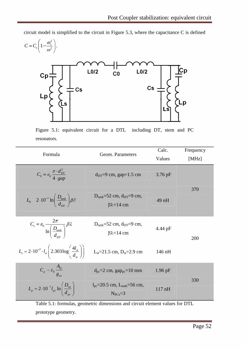
Post Coupler stabilization: equivalent circuit
Page 52
circuit model is simplified to the circuit in Figure 5.3, where the capacitance C is defined
2
21 s
sC C .
Figure 5.1: equivalent circuit for a DTL including DT, stem and PC
resonators.
Formula Geom. Parameters Calc.
Values
Frequency
[MHz]
2
0 04
DTdC
gap dDT=9 cm, gap=1.5 cm 3.76 pF
370
7
0 2 10 ln tank
DT
DL
d
Dtank=52 cm, dDT=9 cm,
=14 cm 49 nH
0
2
ln
s
tank
DT
CD
d
Dtank=52 cm, dDT=9 cm,
=14 cm 4.44 pF
200
7 42 10 2.303log st
s st
st
lL l
d Lst=21.5 cm, Dst=2.9 cm 146 nH
0
Q
p
av
AC
g dpc=2 cm, gappc=10 mm 1.96 pF
330
72 10 lneq
p pc
pc
DL l
d
lpc=20.5 cm, Ltank=56 cm,
NPCs=3 117 nH
Table 5.1: formulas, geometric dimensions and circuit element values for DTL
prototype geometry.
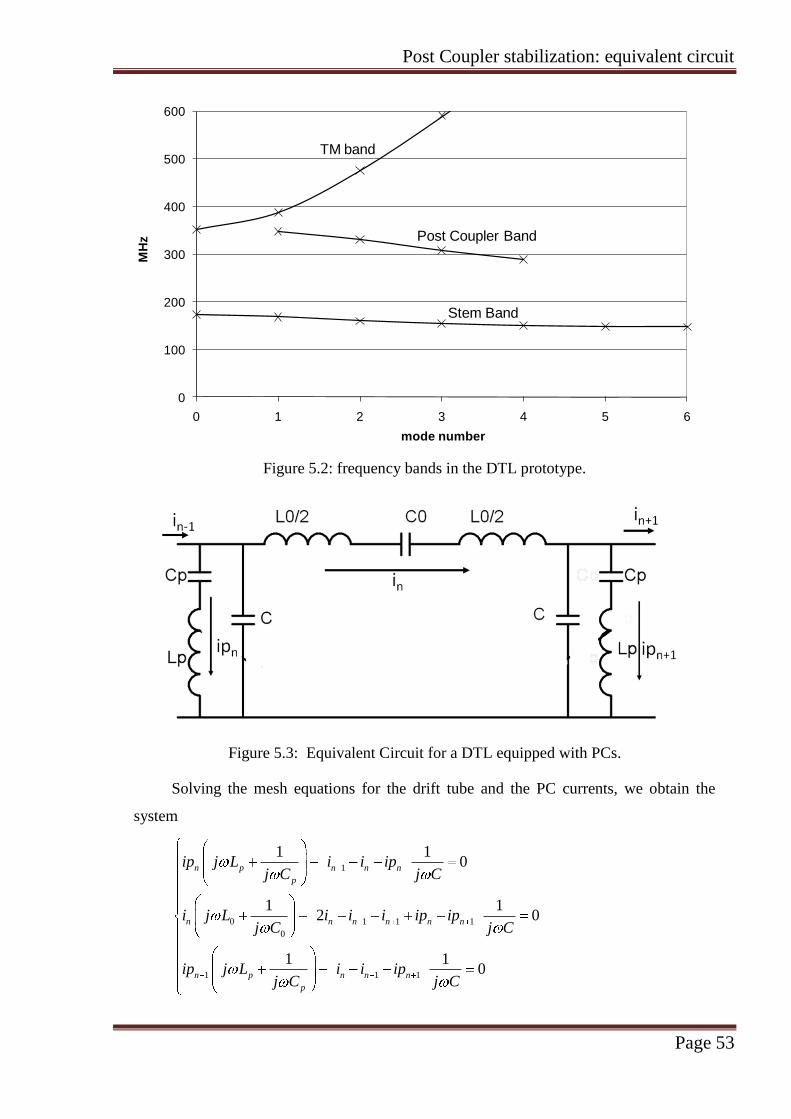
Post Coupler stabilization: equivalent circuit
Page 53
0
100
200
300
400
500
600
0 1 2 3 4 5 6
MH
z
mode number
Stem Band
Post Coupler Band
TM band
Figure 5.2: frequency bands in the DTL prototype.
Figure 5.3: Equivalent Circuit for a DTL equipped with PCs.
Solving the mesh equations for the drift tube and the PC currents, we obtain the
system
1
0 1 1 1
0
1 1 1
1 10
1 12 0
1 10
n p n n n
p
n n n n n n
n p n n n
p
ip j L i i ipj C j C
i j L i i i ip ipj C j C
ip j L i i ipj C j C
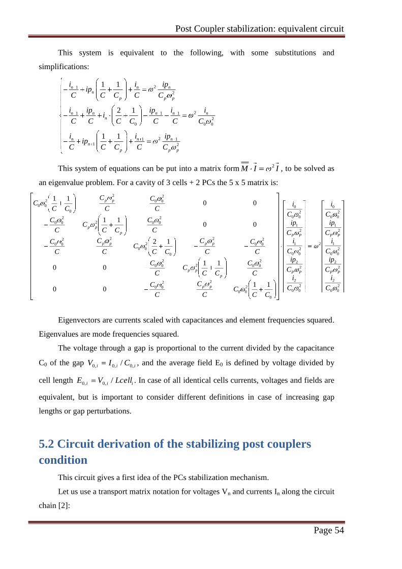
Post Coupler stabilization: equivalent circuit
Page 54
This system is equivalent to the following, with some substitutions and
simplifications:
21
2
21 1 1
2
0 0 0
21 11 2
1 1
2 1
1 1
n n nn
p p p
n n n n nn
n n nn
p p p
i i ipip
C C C C C
i ip ip i ii
C C C C C C C
i i ipip
C C C C C
This system of equations can be put into a matrix form IIM 2 , to be solved as
an eigenvalue problem. For a cavity of 3 cells + 2 PCs the 5 x 5 matrix is:
2
00
2
2
2
2
00
1
2
1
2
00
0
2
2
00
2
2
2
2
00
1
2
1
2
00
0
0
2
00
22
00
2
0022
00
2
00
2
0
2
00
22
00
2
0022
00
2
00
2
0
2
00
1100
1100
12
0011
0011
C
i
C
ip
C
i
C
ip
C
i
C
i
C
ip
C
i
C
ip
C
i
CCC
C
C
C
C
C
C
CCC
C
C
C
C
C
C
CCC
C
C
C
C
C
C
CCC
C
C
C
C
C
C
CCC
PP
PP
PP
PP
pp
p
pp
pppp
p
pp
pp
Eigenvectors are currents scaled with capacitances and element frequencies squared.
Eigenvalues are mode frequencies squared.
The voltage through a gap is proportional to the current divided by the capacitance
C0 of the gap iii CIV ,0,0,0 / , and the average field E0 is defined by voltage divided by
cell length iii LcellVE /,0,0 . In case of all identical cells currents, voltages and fields are
equivalent, but is important to consider different definitions in case of increasing gap
lengths or gap perturbations.
5.2 Circuit derivation of the stabilizing post couplers
condition
This circuit gives a first idea of the PCs stabilization mechanism.
Let us use a transport matrix notation for voltages Vn and currents In along the circuit
chain [2]:
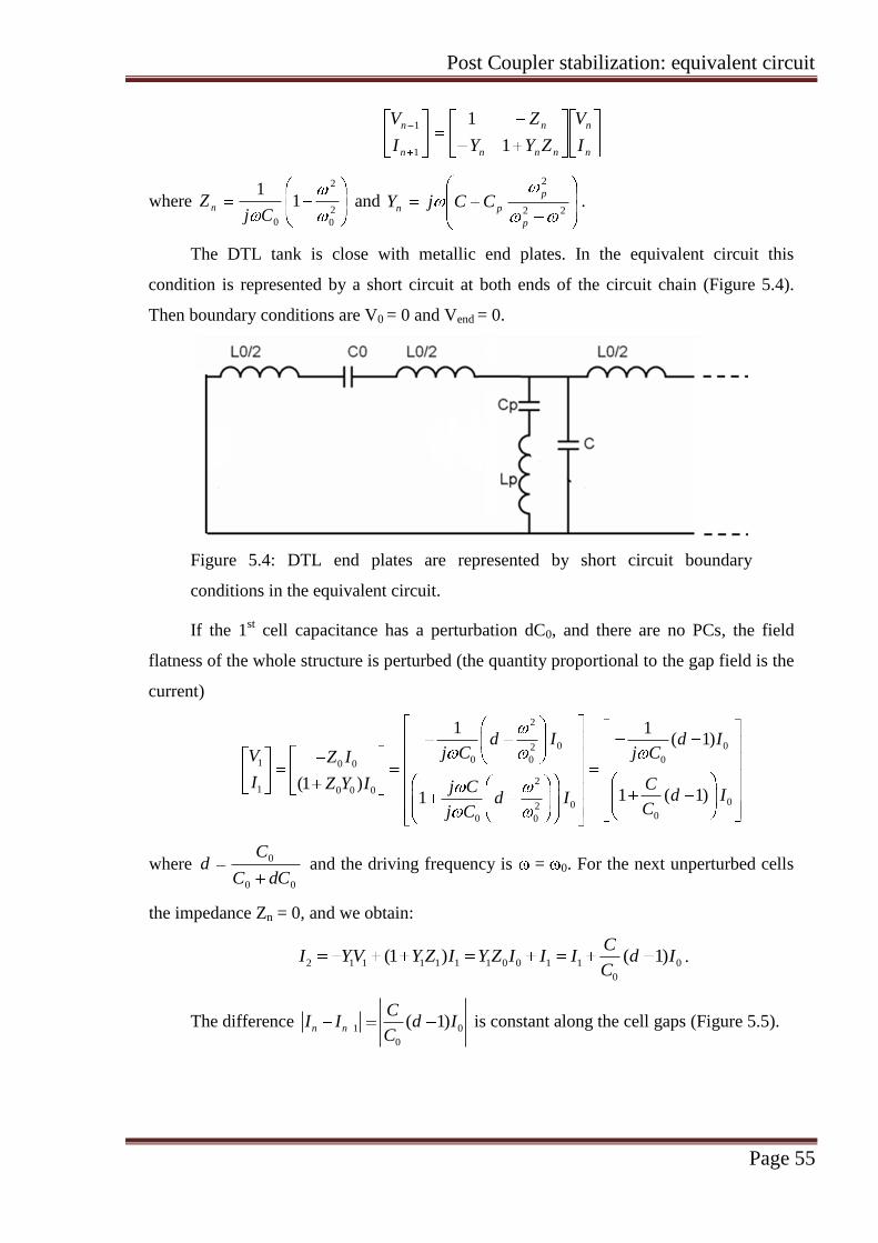
Post Coupler stabilization: equivalent circuit
Page 55
n
n
nnn
n
n
n
I
V
ZYY
Z
I
V
1
1
1
1
where 2
0
2
0
11
CjZ n and
22
2
p
p
pn CCjY .
The DTL tank is close with metallic end plates. In the equivalent circuit this
condition is represented by a short circuit at both ends of the circuit chain (Figure 5.4).
Then boundary conditions are V0 = 0 and Vend = 0.
Figure 5.4: DTL end plates are represented by short circuit boundary
conditions in the equivalent circuit.
If the 1st cell capacitance has a perturbation dC0, and there are no PCs, the field
flatness of the whole structure is perturbed (the quantity proportional to the gap field is the
current)
2
0 02
0 0 01 0 0
21 0 0 0
00200 0
1 1( 1)
(1 )1 ( 1)1
d I d Ij C j CV Z I
I Z Y I Cj Cd Id I
Cj C
where 00
0
dCC
Cd and the driving frequency is = 0. For the next unperturbed cells
the impedance Zn = 0, and we obtain:
2 1 1 1 1 1 1 0 0 1 1 0
0
(1 ) ( 1)C
I YV Y Z I Y Z I I I d IC
.
The difference 1 0
0
( 1)n n
CI I d I
C is constant along the cell gaps (Figure 5.5).

Post Coupler stabilization: equivalent circuit
Page 56
Moreover, if the cell length scales with , the perturbation effect at other cells
becomes stronger where the ratio C/C0 is larger. The effect is therefore stronger towards
higher beam energies in the DTL!
Let us now suppose to have one PC every other cell (Figure 5.5).
2
2 1 02 2
0 0 0
( 1) ( 1)p p
p
CCI I d d I
C C.
The formula shows that the presence of the PCs can modify the propagation of the
perturbation from one cell to the next one.
The PCs stabilize if I2 = I0:
2
2 0 0 02 2
0 0 0 0
1 ( 1) ( 1) ( 1)p p
p
CC CI d I d d I I
C C C
and from this equation a condition for the optimum value of the PC frequency is obtained:
p
pCC
C
2
2 2
02.
If we assume that, when changing the PC - DT gap, the variation of Lp is negligible
with respect to the variation of Cp, it is useful to solve the previous relation for Cp:
12
22
0p
stab
pCL
CC .
In general the conditions are 2
2 0
1p
pn C
C
and 2
0
stab
p
p
CC
CL n where
number post couplersn
number cells. Let us define the coupling coefficient
p
p
Ck
C and the
previous relation becomes 2
2 0
1p
pn k where both p and kp depend on Cp.

Post Coupler stabilization: equivalent circuit
Page 57
0.97
0.98
0.99
1
1.01
1.02
1.03
1.04
0 2 4 6 8 10 12 14 16 18
E0
cell number
stabilized E0
perturbed E0
Figure 5.5: perturbed E0 without PCs and with PCs at stabilizing value of Cp
from a circuit simulation.
The optimum value of Cp for stabilization decreases as function of the capacitance C
(Figure 5.6). Where DTs are longer, gap PC-DT must be larger; where DTs are shorter,
gap PC-DT must be smaller.
0.5
0.6
0.7
0.8
0.9
1
1.1
1.2
0 5 10 15 20
Cp
(p
F)
C (pF)
Cp (n=1)
Cp (n=1/2)
Figure 5.6: Cp as function of C (case of n=1 and n=1/2).
Some observations can be made about the distance between PC and DT in order to
understand the stabilizing setting of gap PC-DT (Figure 5.7):
if the gap is too short (stab
pp CC ), PCs can compensate the perturbation, but not
completely;

Post Coupler stabilization: equivalent circuit
Page 58
if the gap is slightly larger than the stabilizing condition
( stab
pp CC with stab
pp0 ) there is a kind of over-compensation that changes the
slope with respect to the perturbation;
if gap is much larger than the stabilizing condition ( stab
pp CC and 0p ), the
PC effect is de-stabilizing.
0.94
0.96
0.98
1
1.02
1.04
1.06
0 2 4 6 8 10 12 14 16 18
E0
cell number
under-compensation
over-compensated
de-stabilized
Figure 5.7: the PC effect in a perturbed field with gap PC-DT at 3 different
configurations described above.
5.3 1st and 2
nd magnetic coupling between post couplers
A comparison of measured PC dispersion curve with curve obtained by the
equivalent circuit (Figure 5.10a) shows that one needs to take into account a next nearest
coupling between PCs, which couples PCs placed in opposite sides of the DTL tank. This
nearest neighbor coupling is equivalent to a magnetic coupling between PC inductors Lp
(Figure 5.8) with the coupling factor 2
1 0/p p pk M L at the operating frequency
using self and mutual inductances Lp and Mp.
A next nearest neighbor coupling factor kp2 between PCs is included in the matrix as
well. It is equivalent to a mutual inductance Mp2 acting between PCs placed at the same
side of the DTL tank. Mp2 has an opposite sign with respect to Mp.
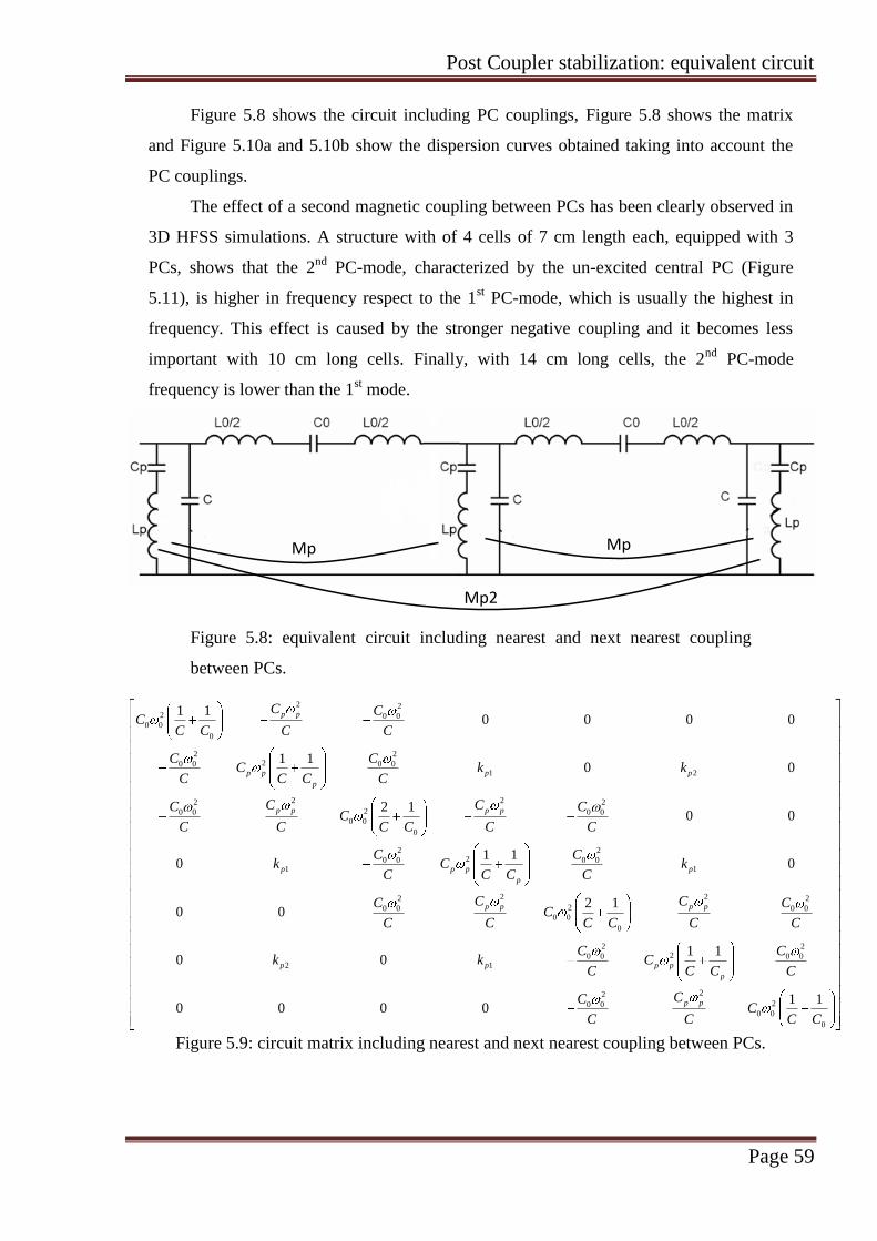
Post Coupler stabilization: equivalent circuit
Page 59
Figure 5.8 shows the circuit including PC couplings, Figure 5.8 shows the matrix
and Figure 5.10a and 5.10b show the dispersion curves obtained taking into account the
PC couplings.
The effect of a second magnetic coupling between PCs has been clearly observed in
3D HFSS simulations. A structure with of 4 cells of 7 cm length each, equipped with 3
PCs, shows that the 2nd
PC-mode, characterized by the un-excited central PC (Figure
5.11), is higher in frequency respect to the 1st PC-mode, which is usually the highest in
frequency. This effect is caused by the stronger negative coupling and it becomes less
important with 10 cm long cells. Finally, with 14 cm long cells, the 2nd
PC-mode
frequency is lower than the 1st mode.
Mp Mp
Mp2
Mp Mp
Mp2
Figure 5.8: equivalent circuit including nearest and next nearest coupling
between PCs.
2 22 0 0
0 0
0
2 220 0 0 0
1 2
2 22 220 0 0 0
0 0
0
2 220 0 0 0
1 1
2 2220 0
0 0
0
1 10 0 0 0
1 10 0
2 10 0
1 10 0
2 10 0
p p
p p p p
p
p p p p
p p p p
p
p p p p
C CC
C C C C
C CC k k
C C C C
C CC CC
C C C C C C
C Ck C k
C C C C
C CCC
C C C C
2
0 0
2 220 0 0 0
2 1
2220 0
0 0
0
1 10 0
1 10 0 0 0
p p p p
p
p p
C
C C
C Ck k C
C C C C
CCC
C C C C
Figure 5.9: circuit matrix including nearest and next nearest coupling between PCs.
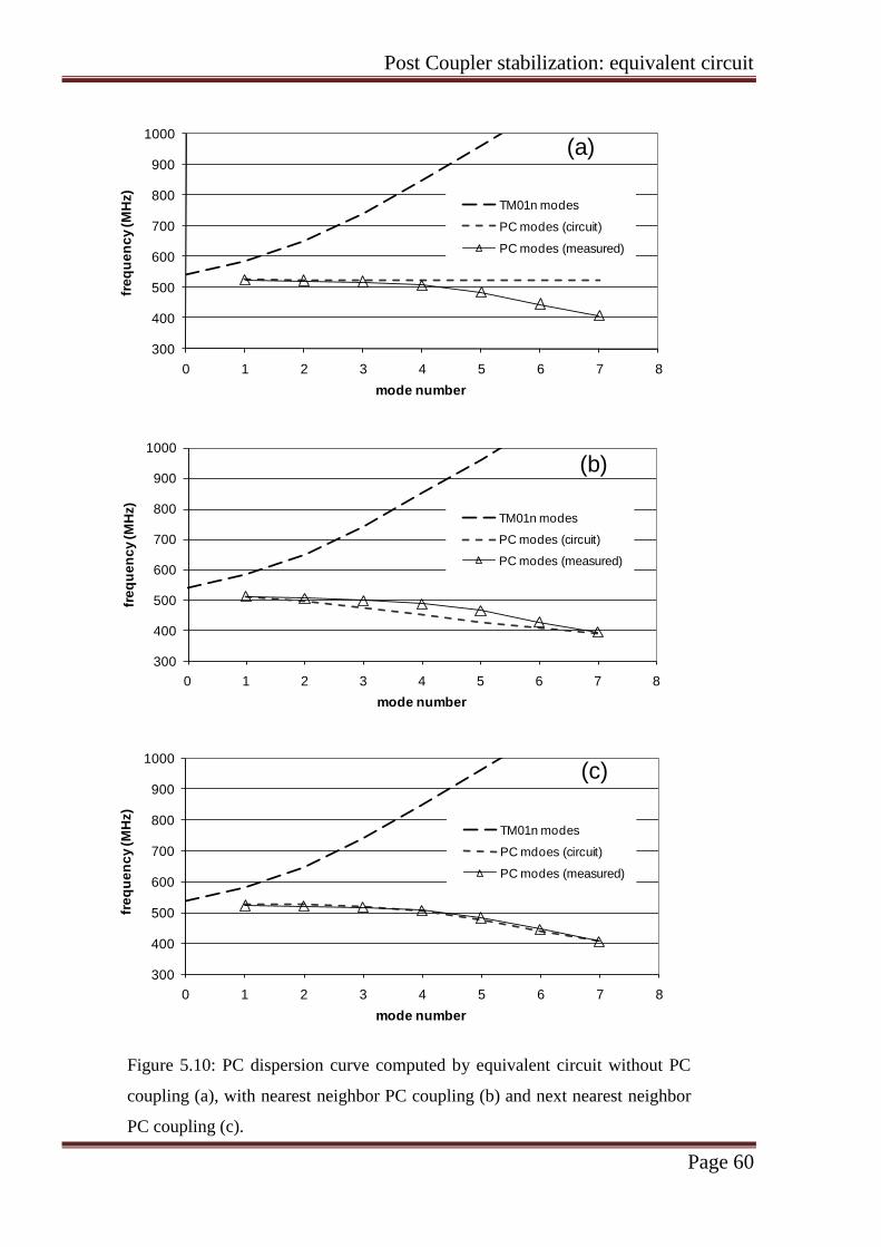
Post Coupler stabilization: equivalent circuit
Page 60
300
400
500
600
700
800
900
1000
0 1 2 3 4 5 6 7 8
mode number
fre
qu
en
cy
(M
Hz)
.
TM01n modes
PC modes (circuit)
PC modes (measured)
(a)
300
400
500
600
700
800
900
1000
0 1 2 3 4 5 6 7 8
mode number
fre
qu
en
cy
(M
Hz)
.
TM01n modes
PC mdoes (circuit)
PC modes (measured)
(b)
300
400
500
600
700
800
900
1000
0 1 2 3 4 5 6 7 8
mode number
fre
qu
en
cy
(M
Hz)
ù
.
TM01n modes
PC mdoes (circuit)
PC modes (measured)
(c)
300
400
500
600
700
800
900
1000
0 1 2 3 4 5 6 7 8
fre
qu
en
cy (
MH
z)
mode number
TM01n modes
PC modes (circuit)
PC modes (measured)
(a)
300
400
500
600
700
800
900
1000
0 1 2 3 4 5 6 7 8
fre
qu
en
cy (
MH
z)
mode number
TM01n modes
PC modes (circuit)
PC modes (measured)
(b)
300
400
500
600
700
800
900
1000
0 1 2 3 4 5 6 7 8
fre
qu
en
cy (
MH
z)
mode number
TM01n modes
PC mdoes (circuit)
PC modes (measured)
(c)
Figure 5.10: PC dispersion curve computed by equivalent circuit without PC
coupling (a), with nearest neighbor PC coupling (b) and next nearest neighbor
PC coupling (c).
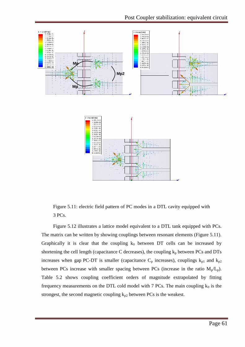
Post Coupler stabilization: equivalent circuit
Page 61
Mp2
Mp
Mp
Mp2
Mp
Mp
Figure 5.11: electric field pattern of PC modes in a DTL cavity equipped with
3 PCs.
Figure 5.12 illustrates a lattice model equivalent to a DTL tank equipped with PCs.
The matrix can be written by showing couplings between resonant elements (Figure 5.11).
Graphically it is clear that the coupling k0 between DT cells can be increased by
shortening the cell length (capacitance C decreases), the coupling kp between PCs and DTs
increases when gap PC-DT is smaller (capacitance Cp increases), couplings kp1 and kp2
between PCs increase with smaller spacing between PCs (increase in the ratio Mp/Lp).
Table 5.2 shows coupling coefficient orders of magnitude extrapolated by fitting
frequency measurements on the DTL cold model with 7 PCs. The main coupling k0 is the
strongest, the second magnetic coupling kp2 between PCs is the weakest.
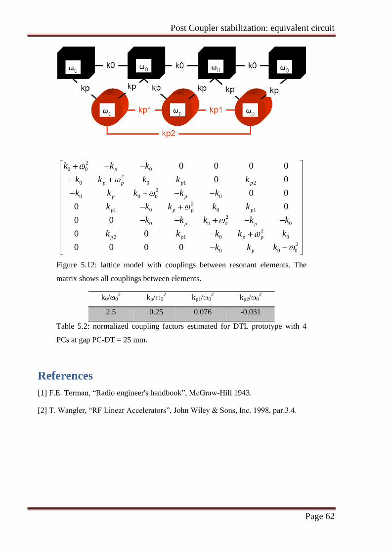
Post Coupler stabilization: equivalent circuit
Page 62
2
0 0 0
2
0 0 1 2
2
0 0 0 0
2
1 0 0 1
2
0 0 0 0
2
2 1 0 0
2
0 0 0
0 0 0 0
0 0
0 0
0 0
0 0
0 0
0 0 0 0
p
p p p p
p p
p p p p
p p
p p p p
p
k k k
k k k k k
k k k k k
k k k k k
k k k k k
k k k k k
k k k
Figure 5.12: lattice model with couplings between resonant elements. The
matrix shows all couplings between elements.
k0/ 02 kp/ 0
2 kp1/ 0
2 kp2/ 0
2
2.5 0.25 0.076 -0.031
Table 5.2: normalized coupling factors estimated for DTL prototype with 4
PCs at gap PC-DT = 25 mm.
References
[1] F.E. Terman, “Radio engineer's handbook”, McGraw-Hill 1943.
[2] T. Wangler, “RF Linear Accelerators”, John Wiley & Sons, Inc. 1998, par.3.4.

Post Coupler stabilization: tuning procedure and measurements
Page 63
Chapter 6. Post couplers: tuning procedure
and measurements
A DTL cold model with scaled dimensions has been built by KASCT in Saudi
Arabia for tuning study (Figure 6.1) [1]. The operating frequency is 538.7 MHz, the tank
diameter 340 mm and the DT diameter 58.8 mm, the length is 862 mm. It consists of a 16
cells cavity equipped with holes for PC positioning at each DT, in order to test the
effectiveness of stabilization for different PC configurations. The end cells can be easily
moved in order to induce a perturbation on the accelerating field.
In this chapter we present a tuning procedure based on the equivalent circuit analysis
of the measured frequencies, which allows to calculate the gap PC-DT for field
stabilization. The advantage of this method with respect to the usual one [2,3] is in
avoiding a large number of bead pulling measurements at different PC lengths. The
prediction of the circuit are verified with measurements on the DTL cold model, in cavity
configurations with 5 and 7 PCs.
Figure 6.1: DTL cold model at CERN and a view of the drift tubes in the
alignment phase.
6.1 Circuit extrapolation of stabilizing post coupler
setting
The following results are deduced from the 16 cell DTL cold model present at
CERN, equipped with 5 and 7 PCs. Because PCs are every 3 or every 2 drift tube, we
minimize the average value of the tilt sensitivity, resulting in a saw-tooth pattern. Tilt

Post Coupler stabilization: tuning procedure and measurements
Page 64
Sensitivity is defined as 0 0 / 0 (1/ )pert unpert unpert
i i i iTS E E E f and Tilt Sensitivity Slope
is the slope of the linear interpolation of the Tilt Sensitivity curve.
A procedure to find an optimum average PC length is the following:
The gap capacitance C0 is calculated from a SUPERFISH simulation, using the formula
UVC 2
02
1
Measurement of the TM010 and TM011 without PCs to calculate the coupling
capacitance C between tank and drift tubes (Figure 6.2) (Note: here we make the
assumption that all the cells have the same average length, we don’t take into account
the increasing cell length)
Measurement of the PC frequency band (at least 3 modes, for example PChighest,
PClowest, PCcentral modes) and of the TM010 and TM011 modes at different length of the
PCs (Figure 6.3)
Fitting of the measured frequencies with dispersion curves computed by the circuit, by
adjusting the circuit parameters 0 p, Cp, kp1, kp2
Insertion of a perturbation C0 in the end capacitances of the circuit, which simulates
the end cell displacement
Looking at the fields given by the previously fitted circuits: the goal is to minimize the
Tilt Sensitivity (Figure 6.4)
Extrapolation of the stabilizing PC length from the parameter curves (Table 6.1),
looking at the zero of TS_Slope curve (Figure 6.5).
The same analysis has been done for both 5 PCs configuration and 7 PCs
configuration.
500
550
600
650
700
750
800
0 1 2 3 4
fre
qu
en
cy (M
Hz)
mode number
Fitted_freq
Meas_Freq
Figure 6.2: TM010 and TM011 modes measured without PCs and fitted curve.
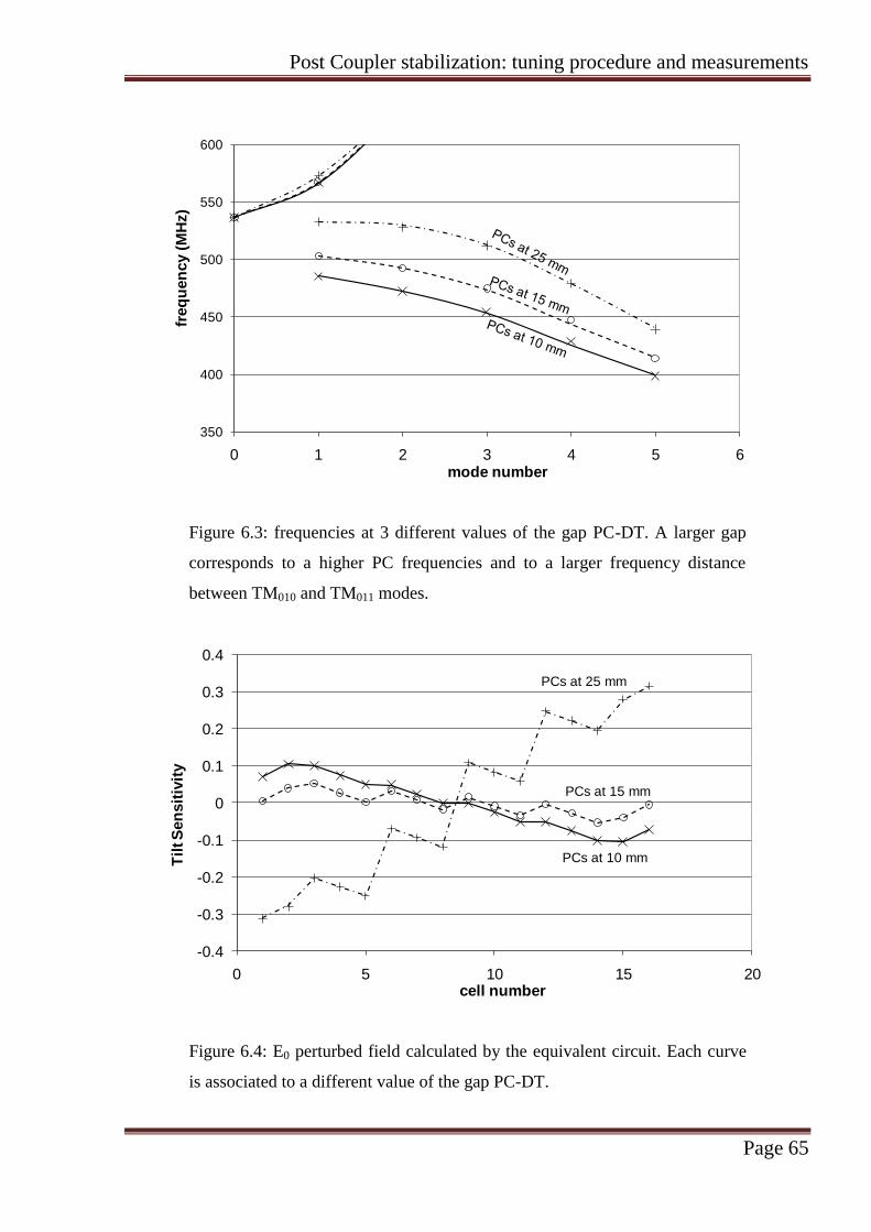
Post Coupler stabilization: tuning procedure and measurements
Page 65
350
400
450
500
550
600
0 1 2 3 4 5 6
freq
uen
cy (
MH
z)
mode number
Figure 6.3: frequencies at 3 different values of the gap PC-DT. A larger gap
corresponds to a higher PC frequencies and to a larger frequency distance
between TM010 and TM011 modes.
-0.4
-0.3
-0.2
-0.1
0
0.1
0.2
0.3
0.4
0 5 10 15 20
Til
t S
en
sit
ivit
y
cell number
PCs at 10 mm
PCs at 15 mm
PCs at 25 mm
Figure 6.4: E0 perturbed field calculated by the equivalent circuit. Each curve
is associated to a different value of the gap PC-DT.

Post Coupler stabilization: tuning procedure and measurements
Page 66
0
200
400
600
800
1000
1200
-0.06
-0.04
-0.02
0
0.02
0.04
0.06
0.08
0.1
0 5 10 15 20 25 30
freq
_P
C, C
p
kp
1, kp
2, T
S_S
lop
e
PC-DT space [mm]
5 PCs settings
kp1
kp2
TS_Slope
freq_PC [MHz]
Cp [pF*1000]
0
100
200
300
400
500
600
700
800
900
1000
-0.06
-0.04
-0.02
0
0.02
0.04
0.06
0.08
0.1
0.12
0 5 10 15 20 25
freq
_P
C, C
p
kp
1, kp
2, T
S_S
lop
e
PC-DT space [mm]
7 PCs settings
kp1
kp2
TS_Slope
freq_PC [MHz]
Cp [pF*1000]
Figure 6.5: circuit parameters and Tilt Sensitivity Slope as function of the gap
PC-DT for 5 PCs and 7 PCs configurations. The Tilt Sensitivity zero point is
marked.
Stabilizing Parameters
gappc [mm] p [MHz] Cp [pF] k0/ 02 kp/ 0
2 kp1/ 0
2 kp2/ 0
2
5 post–couplers 22.5 485 0.62 2.3 0.20 0.087 -0.033
7 post–couplers 19.0 477 0.61 2.3 0.19 0.096 -0.044
Table 6.1: stabilizing PC setting for DTL cold model equipped with 5 PCs and
7 PCs.

Post Coupler stabilization: tuning procedure and measurements
Page 67
Let us consider the ratio ( _ )
PC DT
TS Sloper
gap as the sensitivity criterion for the PC
length adjustment. This sensitivity is larger in the case of 5 PCs, where r = 9 around the
optimum gap = 22.5 mm, than in the case of 7 PCs, where r = 2 around the optimum
gap = 19 mm. An increased sensitivity to the PC length adjustment is related to a larger
gap PC-DT and it makes more difficult to fix the optimum PC length for stabilization.
6.2 Measurements on DTL cold model
In order to verify the equivalent circuit results, we use the Tilt Sensitivity method to
find the stabilization length on the DTL cold model equipped with 5 and 7 PCs.
First, we need a measurement of the reference field (Figure 6.6) to be stabilized,
which is called the “natural field distribution” of the tank [4]. In order to verify the
effectiveness of PCs for stabilization of the accelerating field, it is not necessary to refer to
a perfectly flat field.
We perturb the first and the last gap to create a tilt in the field (Figure 6.7).
Now we start with a small gap PC-DT (15 mm), and as expected from the equivalent
circuit, PCs are not able to stabilize the tilt of the field (Figure 6.8).
If gap is too large (25 mm for 5 PCs, 22 mm for 7 PCs), the field reverses its slope,
and we reach over-compensation (Figure 6.9).
Finally we set the PCs at gappc calculated with the equivalent circuit: 22.5 mm gap
for 5 PCs, 19 mm gap for 7 PCs. One can see the tilt sensitivity curve approaching to zero,
except that for the cells close to the tank ends (Figure 6.10).
This effect can be mitigated by adjusting the gappc in order to take into account the
increasing cell length in this model. What we expect is an optimum PC configuration
where the central PC is kept at the computed gappc, but with smaller gappc at the low
energy side, larger gappc at the high energy side (Figure 6.11). Table 6.2 shows the final
PC settings.

Post Coupler stabilization: tuning procedure and measurements
Page 68
0
0.05
0.1
0.15
0.2
0.25
0.3
0 2 4 6 8 10 12 14 16 18
cell number
E0
.
-0.25
-0.2
-0.15
-0.1
-0.05
0
0.05
0.1
0.15
0.2
0.25
TS
.
E0 field
Tilt Sensitivity
Figure 6.6: reference field and tilt sensitivity.
0
0.05
0.1
0.15
0.2
0.25
0.3
0 2 4 6 8 10 12 14 16 18
cell number
E0
.
-0.25
-0.2
-0.15
-0.1
-0.05
0
0.05
0.1
0.15
0.2
0.25
TS
.
E0 field
Tilt Sensitivity
Figure 6.7: perturbed field and tilt sensitivity.
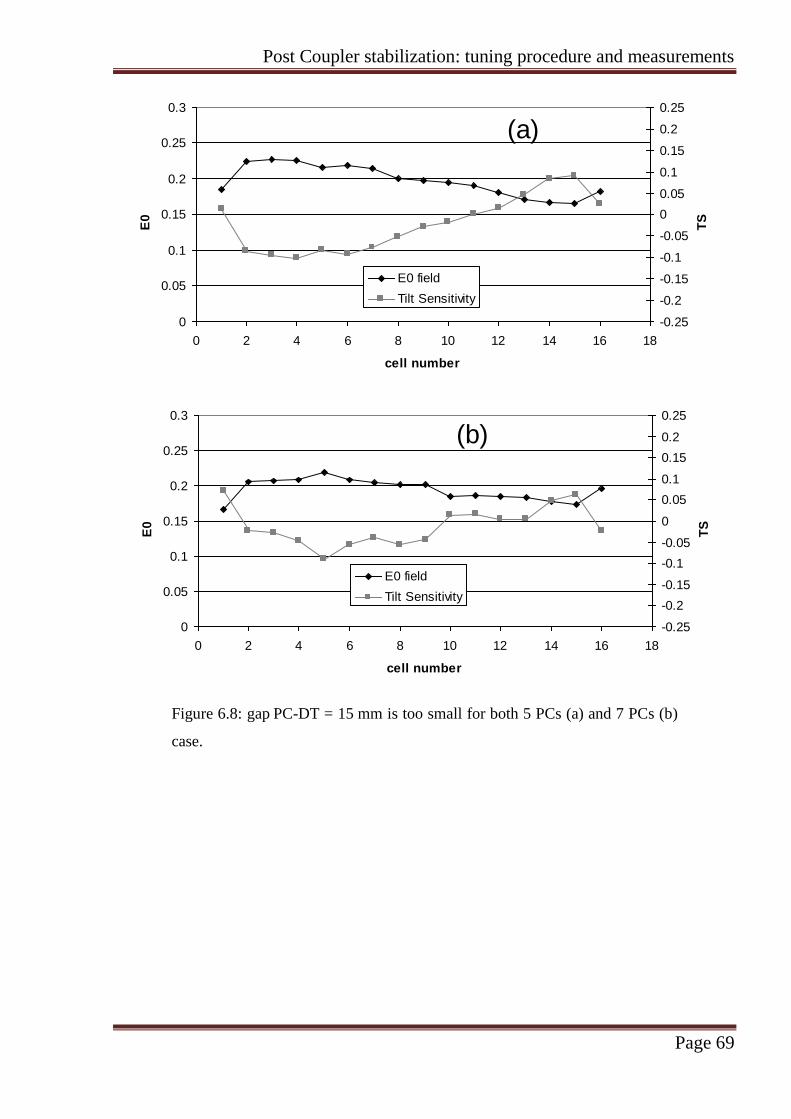
Post Coupler stabilization: tuning procedure and measurements
Page 69
0
0.05
0.1
0.15
0.2
0.25
0.3
0 2 4 6 8 10 12 14 16 18
cell number
E0
.
-0.25
-0.2
-0.15
-0.1
-0.05
0
0.05
0.1
0.15
0.2
0.25
TS
.
E0 field
Tilt Sensitivity
(a)
0
0.05
0.1
0.15
0.2
0.25
0.3
0 2 4 6 8 10 12 14 16 18
cell number
E0
.
-0.25
-0.2
-0.15
-0.1
-0.05
0
0.05
0.1
0.15
0.2
0.25
TS
.
E0 field
Tilt Sensitivity
(b)
Figure 6.8: gap PC-DT = 15 mm is too small for both 5 PCs (a) and 7 PCs (b)
case.

Post Coupler stabilization: tuning procedure and measurements
Page 70
0
0.05
0.1
0.15
0.2
0.25
0.3
0 2 4 6 8 10 12 14 16 18
cell number
E0
.
-0.5
-0.4
-0.3
-0.2
-0.1
0
0.1
0.2
0.3
0.4
0.5
TS
.
E0 field
Tilt Sensitivity
(a)
0
0.05
0.1
0.15
0.2
0.25
0.3
0 2 4 6 8 10 12 14 16 18
cell number
E0
.
-0.5
-0.4
-0.3
-0.2
-0.1
0
0.1
0.2
0.3
0.4
0.5
TS
.
E0 field
Tilt Sensitivity
(b)
Figure 6.9: (a) gap PC-DT = 25 mm is too large for 5 PCs configuration. (b)
gap PC-DT = 22 mm is too large for 7 PCs configuration.

Post Coupler stabilization: tuning procedure and measurements
Page 71
0
0.05
0.1
0.15
0.2
0.25
0.3
0 2 4 6 8 10 12 14 16 18
cell number
E0
.
-0.25
-0.2
-0.15
-0.1
-0.05
0
0.05
0.1
0.15
0.2
0.25
TS
.
E0 field
Tilt Sensitivity
(a)
0
0.05
0.1
0.15
0.2
0.25
0.3
0 2 4 6 8 10 12 14 16 18
cell number
E0
.
-0.25
-0.2
-0.15
-0.1
-0.05
0
0.05
0.1
0.15
0.2
0.25
TS
.
E0 field
Tilt Sensitivity
(b)
Figure 6.10: (a) 5 PCs are set all at the gappc = 22.5 mm, as calculated by the
equivalent circuit simulation (Figure 6.5). (b) 7 PCs are set all at the
gappc = 19 mm, as calculated by the equivalent circuit simulation (Figure 6.5).
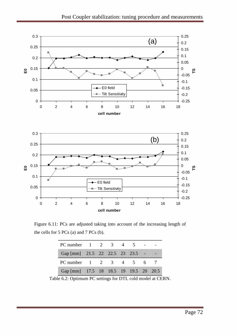
Post Coupler stabilization: tuning procedure and measurements
Page 72
0
0.05
0.1
0.15
0.2
0.25
0.3
0 2 4 6 8 10 12 14 16 18
cell number
E0
.
-0.25
-0.2
-0.15
-0.1
-0.05
0
0.05
0.1
0.15
0.2
0.25
TS
.
E0 field
Tilt Sensitivity
(a)
0
0.05
0.1
0.15
0.2
0.25
0.3
0 2 4 6 8 10 12 14 16 18
cell number
E0
.
-0.25
-0.2
-0.15
-0.1
-0.05
0
0.05
0.1
0.15
0.2
0.25
TS
.
E0 field
Tilt Sensitivity
(b)
Figure 6.11: PCs are adjusted taking into account of the increasing length of
the cells for 5 PCs (a) and 7 PCs (b).
PC number 1 2 3 4 5 - -
Gap [mm] 21.5 22 22.5 23 23.5 - -
PC number 1 2 3 4 5 6 7
Gap [mm] 17.5 18 18.5 19 19.5 20 20.5
Table 6.2: Optimum PC settings for DTL cold model at CERN.

Post Coupler stabilization: tuning procedure and measurements
Page 73
References
[1] N. Alharbi, F. Gerigk and M. Vretenar, “Field Stabilization with Post Couplers for
DTL Tank1 of Linac4”, Tech. Rep. CARE-Note-2006-012-HIPPI, CARE, 2006.
[2] G. Dôme, “Review and survey of accelerating structures”, in “Linear Accelerators”
(ed. by P. Lapostolle and A Septier) North-Holland Publ. Co., 1969.
[3] J. M. Potter, “Drift Tube Linacs”, in “Handbook of Accelerator Physics and
Engineering” (ed. By A. Wu Chao and M. Tigner) World Scientific Publ. Co., 2006.
[4] J. Billen, private communication.

Conclusions
Page 74
Chapter 7. Conclusions
We can now summarize results obtained and illustrated in previous chapters,
following the scheme presented in the Introduction.
2D simulations, performed with Superfish code, are reliable for the calculation of
frequency detuning effect and power dissipation due to the post coupler insertion, as
shown by the comparison with measurements taken on the DTL “hot” prototype. This
comparison shows also that 2D simulations cannot give any hint about the coupling
between post couplers (PCs) and accelerating cells.
3D simulations, performed with HFSS code, compute cavity fields and frequency
modes in agreement with measurements taken in DTL hot prototype. The stabilizing effect
of PCs for the accelerating mode is interpreted on the basis of a mutual cancelation of the
perturbations induced by the TM011 and PC1 mode. 3D simulations were undertaken to
study PCs mode frequencies as a function of number of PCs per meter and of the gap PC-
DT. In quasi-static approximation, formulas for estimation of PC circuit parameters as a
function of the PC geometry were defined and verified to be consistent with simulation
results. 3D simulations allow a graphical picture of mode patterns in order to understand
couplings between different elements inside the cavity.
The equivalent circuit for a DTL equipped with PCs is exhaustive. It gives an
explanation of stabilizing PC settings in terms of circuit parameters and shows clearly that
PC frequency tuning is indissolubly related to the PC-DT coupling. The matrix form of
circuit equations allows the introduction of nearest neighbor coupling and next nearest
neighbor coupling between PCs. With the insertion of couplings, experimental dispersion
curves are precisely reproduced.
A tuning procedure based on the equivalent circuit and on frequency measurements
was defined, tested and validated with measurements on the DTL aluminum model in 2
different PC configurations.

Appendix A. Cavity figures of merit
Page 75
Appendix A. Cavity figures of merit
There are several figure of merit used to characterize accelerating cavities. We will
introduce most important ones in this Appendix [1, 2].
First of all we define the average axial field E0 for a single accelerating cell of
length Lcell as
00
(0, )Lcell
cell cell
E z d zV
EL L .
Power P is dissipated from resistive losses in the walls of the cavity to maintain the
fields. The figure of merit for stored energy U per unit power loss Pcav is the quality factor
Q0 = U/Pcav.
The shunt impedance measures how effective the cavity is in producing an axial
electric field per unit power loss, and it is defined by
rs = (V0)2/Pcav.
The energy gain of an arbitrary particle with charge q traveling through the
accelerating cell on axis is
(0, )cos[ ( ) ]
cellL
W q E z t z dz
where is the phase of the electric field relative to the crest at t = 0. The equation can be
written in the form
0 cosW qV T
where the transit time factor is defined by
(0, )cos ( ) (0, )sin ( )
tan(0, ) (0, )
Lcell Lcell
Lcell Lcell
E z t z dz E z t z dz
TE z dz E z dz
.
The maximum energy gain of a particle in an accelerating gap is then
W = qV0T = qE0LcellT.
The effective shunt impedance measures the efficiency for delivering energy to a
particle per unit power loss. It is defined by
2 2
0 21s
cav cav
E TLWr r T
q P P.
The shunt impedance per unit length is simply
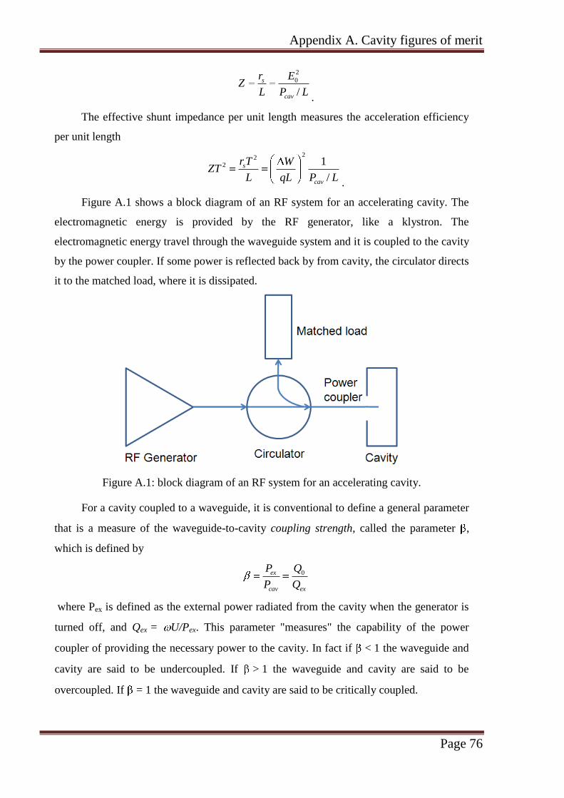
Appendix A. Cavity figures of merit
Page 76
2
0
/
s
cav
r EZ
L P L.
The effective shunt impedance per unit length measures the acceleration efficiency
per unit length
222 1
/
s
cav
r T WZT
L qL P L.
Figure A.1 shows a block diagram of an RF system for an accelerating cavity. The
electromagnetic energy is provided by the RF generator, like a klystron. The
electromagnetic energy travel through the waveguide system and it is coupled to the cavity
by the power coupler. If some power is reflected back by from cavity, the circulator directs
it to the matched load, where it is dissipated.
Figure A.1: block diagram of an RF system for an accelerating cavity.
For a cavity coupled to a waveguide, it is conventional to define a general parameter
that is a measure of the waveguide-to-cavity coupling strength, called the parameter ,
which is defined by
0ex
cav ex
P Q
P Q
where Pex is defined as the external power radiated from the cavity when the generator is
turned off, and Qex = U/Pex. This parameter "measures" the capability of the power
coupler of providing the necessary power to the cavity. In fact if < 1 the waveguide and
cavity are said to be undercoupled. If > 1 the waveguide and cavity are said to be
overcoupled. If = 1 the waveguide and cavity are said to be critically coupled.

Appendix A. Cavity figures of merit
Page 77
The coupling strength is related to the reflection coefficient according to the
formula
1
1
V P
V P.
References
[1] T. Wangler, “RF Linear Accelerators”, John Wiley & Sons, Inc. 1998, par. 2.5.
[2] T. Wangler, “RF Linear Accelerators”, John Wiley & Sons, Inc. 1998, par. 5.4.
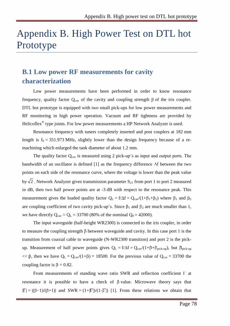
Appendix B. High power test on DTL hot prototype
Page 78
Appendix B. High Power Test on DTL hot
Prototype
B.1 Low power RF measurements for cavity
characterization
Low power measurements have been performed in order to know resonance
frequency, quality factor Qcav of the cavity and coupling strength of the iris coupler.
DTL hot prototype is equipped with two small pick-ups for low power measurements and
RF monitoring in high power operation. Vacuum and RF tightness are provided by
Helicoflex® type joints. For low power measurements a HP Network Analyzer is used.
Resonance frequency with tuners completely inserted and post couplers at 182 mm
length is f0 = 351.973 MHz, slightly lower than the design frequency because of a re-
machining which enlarged the tank diameter of about 1.2 mm.
The quality factor Qcav is measured using 2 pick-up’s as input and output ports. The
bandwidth of an oscillator is defined [1] as the frequency difference f between the two
points on each side of the resonance curve, where the voltage is lower than the peak value
by 2 . Network Analyzer gives transmission parameter S21 from port 1 to port 2 measured
in dB, then two half power points are at -3 dB with respect to the resonance peak. This
measurement gives the loaded quality factor QL = f/ f = Qcav/(1+ 1+ 2) where 1 and 2
are coupling coefficient of two cavity pick-up’s. Since 1 and 2 are much smaller than 1,
we have directly Qcav ≈ QL = 33700 (80% of the nominal Q0 = 42000).
The input waveguide (half-height WR2300) is connected to the iris coupler, in order
to measure the coupling strength between waveguide and cavity. In this case port 1 is the
transition from coaxial cable to waveguide (N-WR2300 transition) and port 2 is the pick-
up. Measurement of half power points gives QL = f/ f = Qcav/(1+ + pick-up), but pick-up
<< , then we have QL = Qcav/(1+ ) = 18500. For the previous value of Qcav = 33700 the
coupling factor is = 0.82.
From measurements of standing wave ratio SWR and reflection coefficient at
resonance it is possible to have a check of value. Microwave theory says that
| = |( −1)/( +1)| and SWR = (1+| |)/(1-| |) [1]. From these relations we obtain that

Appendix B. High power test on DTL hot prototype
Page 79
= 1/SWR if waveguide and cavity are undercoupled ( < 1), = SWR if they are
overcoupled ( > 1), = SWR = 1 if they are critically coupled ( = 1) and in this case
= 0 (no reflection). Since S11 circle in the Smith Chart representation has diameter < 1
(Figure B.1), our case is undercoupled. The measurement of SWR = 1.14 gives = 0.88.
A measurement performed after cavity installation in SM18 bunker confirms this result, in
fact S11 = -22.3 dB (Figure B.2) means | | = 0.0767, SWR = 1.17 and finally = 0.85.
With the previous value of QL we obtain Qcav = QL(1+ ) = 18500 ∙ 1.85 = 34200.
Figure B.1: S11 circle in Smith Chart shows that waveguide and cavity are
undercoupled.
Figure B.2: measurement of S11 of DTL prototype.
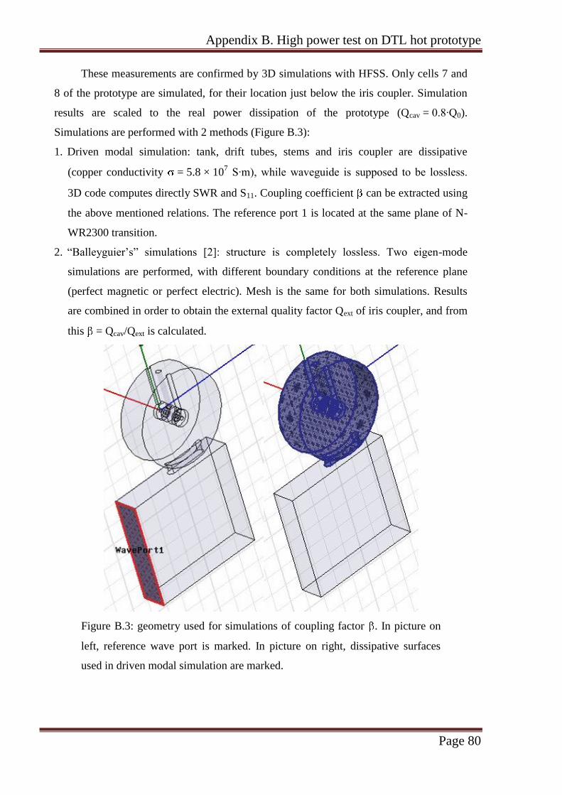
Appendix B. High power test on DTL hot prototype
Page 80
These measurements are confirmed by 3D simulations with HFSS. Only cells 7 and
8 of the prototype are simulated, for their location just below the iris coupler. Simulation
results are scaled to the real power dissipation of the prototype (Qcav = 0.8∙Q0).
Simulations are performed with 2 methods (Figure B.3):
1. Driven modal simulation: tank, drift tubes, stems and iris coupler are dissipative
(copper conductivity = 5.8 × 10⁷ S∙m), while waveguide is supposed to be lossless.
3D code computes directly SWR and S11. Coupling coefficient can be extracted using
the above mentioned relations. The reference port 1 is located at the same plane of N-
WR2300 transition.
2. “Balleyguier’s” simulations [2]: structure is completely lossless. Two eigen-mode
simulations are performed, with different boundary conditions at the reference plane
(perfect magnetic or perfect electric). Mesh is the same for both simulations. Results
are combined in order to obtain the external quality factor Qext of iris coupler, and from
this = Qcav/Qext is calculated.
Figure B.3: geometry used for simulations of coupling factor . In picture on
left, reference wave port is marked. In picture on right, dissipative surfaces
used in driven modal simulation are marked.

Appendix B. High power test on DTL hot prototype
Page 81
Simulation results are listed in Table B.1 in comparison with measurements.
Agreement between simulations is 1.5%, and between simulations and measurements is
10%.
Measurements Driven Modal Sim. Balleyguier's Sim.
0.85 0.95 0.93
Table B.1: comparison between measurements and simulations of waveguide-
cavity coupling factor .
Finally we can summarize cavity RF parameters:
cavity frequency is f0 = 351.973 MHz with tuners completely inserted and post couplers
182 mm long;
quality factor is Qcav = 34500, about 80% of nominal value, simulated with Superfish
code;
coupling strength is = .85, for a power reflection of 2
= P-/P+ = 0.6%.
B.2 Bead pulling measurements and post couplers
setting
Bead pulling measurements have been performed in order to check field flatness and
set post coupler length for stabilization.
Measured reference field E0 is shown in Figure B.4. The curve shows a 30% slope,
due to the data analysis based on the integration of the measured field E(z). Since for post
coupler setting it is sufficient to have a reference field not necessarily flat, we can use
curves from integration analysis.
Post coupler lengths are calculated with procedure described in Chapter 6. Stabilized
field shown in Figure B.6 is obtained with a post coupler length of 182 mm.

Appendix B. High power test on DTL hot prototype
Page 82
0
0.05
0.1
0.15
0.2
0.25
0.3
0.35
0.4
0 5 10 15
av
era
ge
fie
ld E
0
cell number
reference field perturbed field stabilized field
Figure B.4: field stabilization with post couplers.
B.3 Power measurement calibration
Three power signals are measured during cavity conditioning:
1. P+: the incident power from klystron to the DTL, measured by a directional coupler on
the waveguide, located about 1 meter before the iris coupler;
2. P-: the power reflected from DTL to the waveguide, measured by a second directional
coupler located at the same point;
3. Pcav: the power in cavity, measured by the two pick-ups on the tank wall.
Directional couplers on the waveguide are calibrated using a Network Analyzer, two
transitions N-WR2300 and 50 matched loads (Figure B.5). One coupler measures P+,
the other P-. For each one we need to know the attenuation, which is the ratio between
power in waveguide and power extracted by the coupler. A second parameter to be known
is the directivity of the directional coupler, which gives the capability of distinguishing
forward and reverse power direction and finally gives the measurement error.
Measurements at 352 MHz give:
P+: attenuation = -50 dB, directivity = 32 dB (error on P+ < 1/1000);
P-: attenuation = -50 dB, directivity = 22 dB (error on P- < 4/1000).

Appendix B. High power test on DTL hot prototype
Page 83
Figure B.5: directional coupler calibration.
In order to characterize the attenuation of cavity pick-ups, the input waveguide with
transition N-WR2300 is installed. The pick-up is rotated up to have attenuation
Ppickup/P+ = −50 dB. We assume to have the same attenuation for power in cavity:
Ppickup/Pcav = Ppickup/P+ = -50 dB. This assumption is true only if two conditions are
satisfied:
1. pick-up coupling factor pick-up << 1 (Ppick-up <<Pcav);
2. iris coupling factor ≈1.
In fact we have that cav pick upP P P P and, considering that P- = (2)∙P+, if
Ppickup<<Pcav we obtain the following relation: 2
4
1cavP P . We know that
P+/Ppickup = 50 dB, then substituting P+ we obtain 5
2
410
1cav pick upP P P . This
relation is fully correct for =1. In our case =0.85, the approximation is correct at 99.3%,
as Figure B.6 shows.
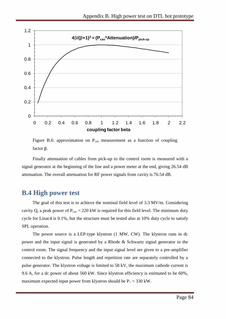
Appendix B. High power test on DTL hot prototype
Page 84
0
0.2
0.4
0.6
0.8
1
1.2
0 0.2 0.4 0.6 0.8 1 1.2 1.4 1.6 1.8 2 2.2
coupling factor beta
4 /( +1)2 = (Pcav*Attenuation)/Ppick-up
Figure B.6: approximation on Pcav measurement as a function of coupling
factor .
Finally attenuation of cables from pick-up to the control room is measured with a
signal generator at the beginning of the line and a power meter at the end, giving 26.54 dB
attenuation. The overall attenuation for RF power signals from cavity is 76.54 dB.
B.4 High power test
The goal of this test is to achieve the nominal field level of 3.3 MV/m. Considering
cavity Q, a peak power of Pcav = 220 kW is required for this field level. The minimum duty
cycle for Linac4 is 0.1%, but the structure must be tested also at 10% duty cycle to satisfy
SPL operation.
The power source is a LEP-type klystron (1 MW, CW). The klystron runs in dc
power and the input signal is generated by a Rhode & Schwartz signal generator in the
control room. The signal frequency and the input signal level are given to a pre-amplifier
connected to the klystron. Pulse length and repetition rate are separately controlled by a
pulse generator. The klystron voltage is limited to 58 kV, the maximum cathode current is
9.6 A, for a dc power of about 560 kW. Since klystron efficiency is estimated to be 60%,
maximum expected input power from klystron should be P+ ≈ 330 kW.

Appendix B. High power test on DTL hot prototype
Page 85
Temperatures are monitored by a set of thermocouples installed on drift tubes,
tuners, post couplers and on the iris coupler. The overall water flow is 30 l/m, the water
temperature is 26°C. Water flows are also locally monitored on the iris coupler, on the
cavity tank, on post couplers and drift tubes. The input water pressure is 6.5 bar, the output
pressure is 3.5 bar. The water flow is maximum in drift tubes (3 l/m), in fact water drift
tube temperatures are constant at 26°C during the test. Other points, like tuners and end
cones, have been monitored also at 40°C and 55°C respectively. Vacuum level in the
cavity is in the order of 10-7
mbar, with interlock at 9.0∙10-6
mbar.
During cavity conditioning the RF duty cycle is increased with different values of
pulse length and repetition rate. P+ is raised by setting the level of the signal generator.
The signal generator frequency is adjusted to follow the cavity resonance frequency and
maximize Pcav. Each level of P+ is kept up to the stabilization of vacuum and power level
in the cavity.
All RF signals are shown in an oscilloscope in the control room (Figure B.8).
Figure B.7: view of the high power installation of DTL prototype in SM18
bunker.

Appendix B. High power test on DTL hot prototype
Page 86
Figure B.8: view of the instrumentation in the control room.
If all power goes to enhance the cavity field level, energy balance should be
P+ = Pcav + P-. In our case there is some incongruence, because maximum of Pcav does not
coincide with minimum of P-, and when P- = 0, Pcav is different from P+. Part of P+ is lost
in dissipative phenomena (dark current, electron loading phenomena). We assume to be at
resonance frequency when P- = 0. Figure B.9 shows that P+ and Pcav curves match up to -
23 dBm of signal generator level (P- = 0). Above -23 dBm power increases not linearly
because of the klystron saturation. Furthermore the difference between P+ and Pcav
indicates power lost in electron loading phenomena.
After two weeks of conditioning nominal field level has been achieved with
Pcav = 240 kW, and Linac4 duty cycle has been exceeded with 20 Hz repetition rate and
1.3 ms pulse length (duty cycle = 2.6%). Figure B.10 shows peak values of Pcav as a
function of P+ at different steps.
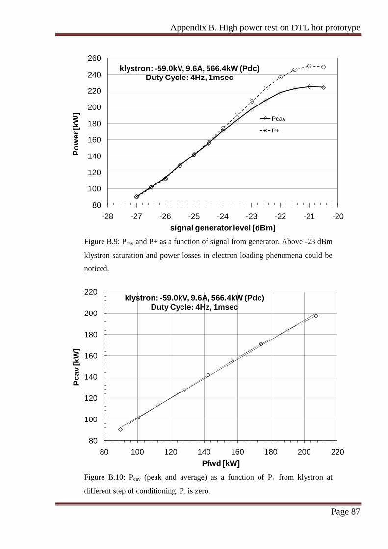
Appendix B. High power test on DTL hot prototype
Page 87
80
100
120
140
160
180
200
220
240
260
-28 -27 -26 -25 -24 -23 -22 -21 -20
Po
we
r [k
W]
signal generator level [dBm]
klystron: -59.0kV, 9.6A, 566.4kW (Pdc)Duty Cycle: 4Hz, 1msec
Pcav
P+
Figure B.9: Pcav and P+ as a function of signal from generator. Above -23 dBm
klystron saturation and power losses in electron loading phenomena could be
noticed.
80
100
120
140
160
180
200
220
80 100 120 140 160 180 200 220
Pcav [kW
]
Pfwd [kW]
klystron: -59.0kV, 9.6A, 566.4kW (Pdc)Duty Cycle: 4Hz, 1msec
Figure B.10: Pcav (peak and average) as a function of P+ from klystron at
different step of conditioning. P- is zero.

Appendix B. High power test on DTL hot prototype
Page 88
References
[1] T. Wangler, “RF Linear Accelerators”, John Wiley & Sons, Inc. 1998, chap.5.
[2] P. Balleyguier, " A Straightforward Method for Cavity External Q Computation”, Part.
Accelerators, 1997, Vol. 57, 113.

Appendix C. Equivalent circuit for the Stems
Page 89
Appendix C. Equivalent circuit for the
Stems
In this appendix the stem equivalent circuit is presented, together with and a sample
of parameter determination based on the frequencies measured for the DTL hot prototype.
The equivalent circuit for the analysis of stem resonances is shown in Figure C.1 [1].
In this circuit the series inductor L0/2 represents the inductance of a half DT, the series
capacitor C0 corresponds to the capacitance of a gap, the shunt capacitor Cs summarizes
the capacitance of a DT to the tank wall represented by the ground conductor. Stems are
represented by inductors Ls in parallel with the shunt capacitance Cs. Each inductor is
magnetically coupled with the next one by means of the mutual inductance Ms. The stem
inductance Ls is written as 2 inductors 2×Ls in parallel, in order to separate the mutual
coupling with the previous stem from the mutual coupling with the next stem.
V0 V0ejI0 I0e
j
i1 i2 i3 i1ej i2e
j i3ej
Figure C.1: equivalent circuit of a basic DTL cell with stems.
The equivalent circuit for the stems has been solved by applying Floquet’s theorem
for periodic structures. Currents and voltages are multiplied by a factor e j
when we move
by one period along the chain. The system is described by 5 equations:
0 0 0 0
0
1jV e V I j Lj C
(C.1)
0 1 32 j
s sV j L i j M i e (C.2)

Appendix C. Equivalent circuit for the Stems
Page 90
0 3 12 j
s sV j L i j M i e (C.3)
20
s
iV
j C(C.4)
0 0 1 2 3
jI I e i i i (C.5)
From equations (C.2), (C.3) and (C.4) we have
2 2 2 2
1 2 3 0 2 2
4 4 2 cos( )
(4 )
s s s s s s
s s
L C L C M Mi i i jV
L M.
Equations (C.1) and (C.5) give the ratio V0/I0 and the dispersion equation
2 2 2
2 2 2 2 2
00
(1 )(4 ) 1(1 ) 1
4 4 2 cos( ) 1
jjs s
js s s s s s
j e L Me
L C L C M M e j C
which can be written as
2 220
2
0
2 1 (1 cos( )(2 )(1 cos( ))
2 (2 )
s s s
s s s
bC L Ma
C L M
with 0
0
2 12
s s
s s
C L Ma
L C L and
2
s
s s
Mb
L M.
The equation has 2 solutions for =0:
the zero mode (TM010) of the main resonator chain 0 0 01/ C L and
the zero mode of the stem resonator chain 2 / (2 )s s s sC L M .
The previous equation can be simplified to
2 22 20
2
0
(2 )(1 cos( )) 1 (1 cos( )
2
s s ss
s
C L Ma b .
The DTL hot prototype consists of 13 accelerating cells and 12 stem cells. In order
to determine parameters a, b, and s we use measured frequencies of modes 0 and
3 /13 of the TM band and modes 0 and 4 /12 of the Stem band. Results are in Table C.1.
Capacitance C0 can be calculated from a Superfish simulation of the DTL hot
prototype, using the relation U = 1/2 × (C0V2). Then from formulas of 0, s, a and b
parameters we obtain circuit element values listed in Table C.2, in comparison with values
obtained from geometrical formulas in Chapter 5. They show a good agreement.
Finally, Figure C.2 shows the comparison between frequencies measured on the
DTL prototype and dispersion curves calculated with equivalent circuit, using parameter
values listed in Table C.1.

Appendix C. Equivalent circuit for the Stems
Page 91
mode Frequency parameter value
TM010 ( =0) 351.8 MHz 0 351.8 MHz
TM012 ( =2 /13) 462.5 MHz s 174.1 MHz
Stem 0 ( =0) 174.1 MHz a 10.9
Stem 4 ( =4 /12) 151.9 MHz b 4.6
Table C.1: measured frequencies and values of equation parameters.
parameter Value Geom. value
(Chap.5)
C0 [pF] 9.07 3.76
L0 [nH] 22.7 49
Cs [pF] 3.32 4.44
Ls [nH] 138 144
Ms [nH] 227 -
Table C.2: stem circuit parameters fitted from frequency measurements in
comparison with values calculated with geometrical formulas in Chapter 5.
TM band
0
200
400
600
800
1000
1200
1400
0 0.5 1 1.5 2 2.5 3 3.5
MH
z
phase shift per period [ unit]
Stem band
Figure C.2: comparison between measured (crosses) and calculated
(continuous lines) dispersion curves.

Appendix C. Equivalent circuit for the Stems
Page 92
References
[1] K. Batchelor et al., " Numerical Analysis of the RF Field in a Drift Tube Loaded
Cavity", Proc. PAC1967.

Acknowledgements
Page 93
Acknowledgements
I would like to thank peoples which have contributed to this thesis work.
First of all my supervisors, Andrea Pisent (LNL-INFN) and Suitbert Ramberger
(CERN), for their attention and steers.
My friends and colleagues, Antonio Palmieri and Giovanni De Michele, for their
continuous support, collaboration and patience.
Maurizio Vretenar and Jean Michel Giguet, for what I have learned from their
experience.
Finally, I thank my family.