
Ricostruzione 3D tramite fusione di dati stereo e ToFtesi.cab.unipd.it/25031/1/tesi.pdfRicostruzione...
82
UNIVERSITÀ DEGLI STUDI DI PADOVA Facoltà di Ingegneria Corso di Laurea in Ingegneria Informatica Tesi di Laurea Specialistica BATCH SIZE ESTIMATE Relatore Laureando Prof. Andrea Zanella Marco Bettiol Matricola 586580-IF Anno Accademico 2009-2010
Transcript of Ricostruzione 3D tramite fusione di dati stereo e ToFtesi.cab.unipd.it/25031/1/tesi.pdfRicostruzione...

Università degli Studi di PadovaFacoltà di Ingegneria
Corso di Laurea Specialistica in Ingegneria delle Telecomunicazioni
Tesi di Laurea
Ricostruzione 3D tramite fusionedi dati stereo e ToF
Relatore: Ch.mo Prof. G.M. CortelazzoCorrelatore: Ing. P. Zanuttigh
Laureando: Carlo Dal Mutto
29 giugno 2009
UNIVERSITÀ DEGLI STUDI DI PADOVA
Facoltà di IngegneriaCorso di Laurea in Ingegneria Informatica
Tesi di Laurea Specialistica
BATCH SIZE ESTIMATE
Relatore Laureando
Prof. Andrea Zanella Marco Bettiol
Matricola 586580-IF
Anno Accademico 2009-2010

Defended on 28th June, 2010Palazzo del Bo, Padova
Author email: bettiol.marco at gmail dot com

i
Ai miei genitori e allo zio Toni. . .


iii
“ [...] sempre nella mia camicia [...]
Ho ancora la forza di chiedere anche scusa
o di incazzarmi ancora con la coscienza offesa,
di dirvi che comunque la mia parte
ve la posso garantire . . . ”
Francesco Guccini
“ E quando pensi che sia finita,
è proprio allora che comincia la salita.
Che fantastica storia è la vita. ”
Antonello Venditti


v
Abstract
In this work we analyze the main batch resolution algorithms. We particularly focus on the
tree-based class to underline how their efficiency depends on the batch size. In fact, batch size is
a critical parameter when using smart resolution strategies that take advantage this information
to improve resolution efficiency. The dissertation will continue with the analysis of noteworthy
techniques available in literature for the batch size estimate: in fact, original papers pay attention
on the resolution process and leave the estimate problem in the background. Finally we propose
and analyze GEGA, an estimate algorithm particularly good in terms of estimate accuracy over
time taken by the estimate process.


vii
Sommario
In questo lavoro sono stati analizzati i principali algoritmi per la risoluzione di insiemi di conflitto.In particolare ci si è concentrati sugli algoritmi ad albero evidenziando come la loro efficaciadipenda dalla taglia del problema. La cardinalità dell’insieme di collisione è infatti un parametrocritico se si desidera utilizzare strategie ottimizzate per risolvere più efficientemente i nodi. Atal fine sono state analizzate, in primo luogo, le tecniche note in letteratura per la stima dellacardinalità di insiemi di conflitto: infatti i paper originali non presentavano un’analisi adeguatadel loro comportamento poiché l’attenzione era rivolta al processo di risoluzione dei nodi e nondirettamente alla fase di stima. Nella parte finale del lavoro, al fine di ottenere una stimasufficientemente accurata per finalità operative, viene proposto GEGA. L’algoritmo presentatoè particolarmente valido in termini di accuratezza della stima rispetto al tempo impiegato epermette di ottenere sempre una stima finita del numero di nodi sufficientemente vicina allareale cardinalità dell’insieme esaminato.

Contents
1 Introduction 1
1.1 System Model . . . . . . . . . . . . . . . . . . . . . . . . . . . . . . . . . . . . . . 3
1.2 Goals . . . . . . . . . . . . . . . . . . . . . . . . . . . . . . . . . . . . . . . . . . 4
1.3 Content organization . . . . . . . . . . . . . . . . . . . . . . . . . . . . . . . . . . 4
2 Batch Resolution 7
2.1 Binary Tree Algorithms . . . . . . . . . . . . . . . . . . . . . . . . . . . . . . . . 9
2.1.1 Basic Binary Tree . . . . . . . . . . . . . . . . . . . . . . . . . . . . . . . 10
Example . . . . . . . . . . . . . . . . . . . . . . . . . . . . . . . . . . . . . 12
Nodes id interpretation . . . . . . . . . . . . . . . . . . . . . . . . . . . . 13
Tree traversal rules . . . . . . . . . . . . . . . . . . . . . . . . . . . . . . . 14
2.1.2 Modified Binary Tree . . . . . . . . . . . . . . . . . . . . . . . . . . . . . . 15
2.1.3 Clipped Modified Binary Tree . . . . . . . . . . . . . . . . . . . . . . . . . 16
2.1.4 m Groups Tree Resolution . . . . . . . . . . . . . . . . . . . . . . . . . . . 18
2.1.5 Estimating Binary Tree . . . . . . . . . . . . . . . . . . . . . . . . . . . . 20
2.2 Others . . . . . . . . . . . . . . . . . . . . . . . . . . . . . . . . . . . . . . . . . . 21
2.2.1 IERC . . . . . . . . . . . . . . . . . . . . . . . . . . . . . . . . . . . . . . 21
2.2.2 Window Based Approaches . . . . . . . . . . . . . . . . . . . . . . . . . . 22
3 Batch Size Estimate Techniques 23
3.1 Clipped Binary Tree . . . . . . . . . . . . . . . . . . . . . . . . . . . . . . . . . . 23
3.2 Cidon . . . . . . . . . . . . . . . . . . . . . . . . . . . . . . . . . . . . . . . . . . 24
3.3 Greenberg . . . . . . . . . . . . . . . . . . . . . . . . . . . . . . . . . . . . . . . . 26
3.3.1 Base b variant . . . . . . . . . . . . . . . . . . . . . . . . . . . . . . . . . 29
3.4 Window Based . . . . . . . . . . . . . . . . . . . . . . . . . . . . . . . . . . . . . 31
4 Estimate Performance Analysis 35
4.1 Cidon BSE . . . . . . . . . . . . . . . . . . . . . . . . . . . . . . . . . . . . . . . 35
ix

x CONTENTS
4.1.1 Performance . . . . . . . . . . . . . . . . . . . . . . . . . . . . . . . . . . . 36
4.2 Greenberg BSE . . . . . . . . . . . . . . . . . . . . . . . . . . . . . . . . . . . . . 39
4.2.1 Considerations . . . . . . . . . . . . . . . . . . . . . . . . . . . . . . . . . 41
4.3 EGA BSE . . . . . . . . . . . . . . . . . . . . . . . . . . . . . . . . . . . . . . . . 43
4.3.1 Performance . . . . . . . . . . . . . . . . . . . . . . . . . . . . . . . . . . . 46
4.4 GEGA BSE . . . . . . . . . . . . . . . . . . . . . . . . . . . . . . . . . . . . . . . 47
4.4.1 Performance . . . . . . . . . . . . . . . . . . . . . . . . . . . . . . . . . . . 49
4.5 Comparison . . . . . . . . . . . . . . . . . . . . . . . . . . . . . . . . . . . . . . . 52
Conclusions 55
A Appendix 57
A.1 Probability . . . . . . . . . . . . . . . . . . . . . . . . . . . . . . . . . . . . . . . 57
A.2 Binary Trees Performance Summary . . . . . . . . . . . . . . . . . . . . . . . . . 59
A.3 Greenberg bounded m-moments . . . . . . . . . . . . . . . . . . . . . . . . . . . . 60
A.4 CBT Estimate Experimental Distribution . . . . . . . . . . . . . . . . . . . . . . 60
A.5 Greenberg Estimate Distribution . . . . . . . . . . . . . . . . . . . . . . . . . . . 62
A.6 GEGA . . . . . . . . . . . . . . . . . . . . . . . . . . . . . . . . . . . . . . . . . . 64
Bibliography 65

List of Figures
2.1 Expected cost for tree algorithms in slotted-ALOHA scenario . . . . . . . . . . . 12
2.2 BT : Basic binary tree example . . . . . . . . . . . . . . . . . . . . . . . . . . . . 13
2.3 MBT : Modified binary tree example . . . . . . . . . . . . . . . . . . . . . . . . . 16
2.4 CMBT vs MBT . . . . . . . . . . . . . . . . . . . . . . . . . . . . . . . . . . . . 18
2.5 m Groups Split: ALOHA scenario . . . . . . . . . . . . . . . . . . . . . . . . . . 19
2.6 m Groups Split: CSMA scenario . . . . . . . . . . . . . . . . . . . . . . . . . . . 20
3.1 CBT : Example . . . . . . . . . . . . . . . . . . . . . . . . . . . . . . . . . . . . . 24
3.2 Cidon: Initial split . . . . . . . . . . . . . . . . . . . . . . . . . . . . . . . . . . . 25
3.3 Basic Greenberg : batch split idea . . . . . . . . . . . . . . . . . . . . . . . . . . . 28
4.1 Cidon: Normalized variance . . . . . . . . . . . . . . . . . . . . . . . . . . . . . . 37
4.2 Cidon: Minimum pε required for error coefficient k . . . . . . . . . . . . . . . . . 38
4.3 Cidon: Expected time as function of the error coefficient . . . . . . . . . . . . . . 39
4.4 Basic Greenberg : Small 2k sizes distribution. . . . . . . . . . . . . . . . . . . . . . 40
4.5 Basic Greenberg : Large 2k sizes distribution. . . . . . . . . . . . . . . . . . . . . . 41
4.6 Basic Greenberg : General batch sizes distribution. . . . . . . . . . . . . . . . . . 42
4.7 Basic Greenberg : Event probability fixed p . . . . . . . . . . . . . . . . . . . . . . 43
4.8 EGA: Large 2k sizes distribution. . . . . . . . . . . . . . . . . . . . . . . . . . . . 46
4.9 EGA: Estimate distribution when varying T . . . . . . . . . . . . . . . . . . . . . 46
4.10 GEGA: Estimate Bias . . . . . . . . . . . . . . . . . . . . . . . . . . . . . . . . . 49
4.11 GEGA: Biased/unbiased absolute normalized estimate error . . . . . . . . . . . . 50
4.12 GEGA: Minimum T to achieve error coefficient lower than k with θ = 0.99 . . . . 51
4.13 GEGA: Minimum T to achieve error coefficient lower than k with θ = 0.99 ,
detailed view . . . . . . . . . . . . . . . . . . . . . . . . . . . . . . . . . . . . . . 51
4.14 GEGA vs Cidon: Error coefficient k as function of elapsed time . . . . . . . . . . 52
xi

List of Tables
3.1 Basic Greenberg : Expected estimate and bias . . . . . . . . . . . . . . . . . . . . 29
3.2 Base b Greenberg : Bias and expected cost summary . . . . . . . . . . . . . . . . . 30
3.3 Window Based Estimate: Possible estimates when L = 10 . . . . . . . . . . . . . 32
4.1 GEGA: Possible estimates when T = 10 and l = 10. . . . . . . . . . . . . . . . . . 48
4.2 GEGA: Average bias. . . . . . . . . . . . . . . . . . . . . . . . . . . . . . . . . . . 50
A.1 Basic Binary Tree: Performance report . . . . . . . . . . . . . . . . . . . . . . . . 59
A.2 Modified Binary Tree: Performance report with p = 0.5 . . . . . . . . . . . . . . . 59
A.3 Modified Binary Tree: Performance report with p = 0.4175 . . . . . . . . . . . . . 60
A.4 Clipped Modified Binary Tree: Performance report. . . . . . . . . . . . . . . . . . 60
A.5 Experimentally computed CBT Estimate Distributon . . . . . . . . . . . . . . . . 61
A.6 Basic Greenberg : Analytically computed estimate distribution . . . . . . . . . . . 63
A.7 GEGA: Possible estimates when T = 20 and l = 10 . . . . . . . . . . . . . . . . . 64
xiii

Chapter 1
Introduction
Generally speaking a set of actors contending for a common resource defines a conflicting set.
As always, limited resources require access policies to provide efficient and, hopefully, fair use.
When the system is distributed, resource access can be assimilated to a coordination problem.
In the scenario considered in this thesis the contended resource is the physical transmission
medium that is shared among several stations.
At the beginning of wired computer networks, multiple access control (MAC) was a big issue for
efficient communication. The introduction of buffered switches in LANs reduced the conflicting
set to only few stations simplifying the original problem. Switched networks, in fact, split large
collision domains into smaller pieces thus realizing ring, star or mesh structures.
In a wireless context the problem can not be easily overcome, due to the broadcast nature of
the wireless medium.
Nowadays wireless connectivity in pervasive computing has ephemeral character and can be
used for creating ad-hoc networks, sensor networks, connections with RFID (Radio Frequency
Identification) tags etc. The communication tasks in such wireless networks often involve an
inquiry over a shared channel, which can be invoked for discovery of neighboring devices in
ad-hoc networks, counting the number of RFID tags that have a certain property, estimating
the mean value contained in a group of sensors, etc. Such an inquiry solicits replies from a
possibly large number of terminals.
In particular we analyze the scenario where a reader broadcasts a query to the in-range nodes.
Once the request is received, devices with data of interest are all concerned in transmitting
the information back to the inquirer as soon as possible and, due to the shared nature of the
communication medium, collision problems come in: only one successful transmission at time
can be accomplished, concurrent transmissions result in destructive interference with waste of
1

2 CHAPTER 1. INTRODUCTION
energy/time. This data traffic shows a bursty nature which is the worst case for all shared
medium scenarios.
In the literature this problem is referred to with different names: Batch/Conflict Resolution
Problem, Reader Collision Problem, Object Identification Problem.
Algorithms trying to solve this problem are called Batch Resolution Algorithms (BRA) or
Collision Resolution Algorithms (CRA).
Batch Resolution Problem is implicitly present in many practical applications over wireless
networks such as:
• Neighbor Discovery. After being deployed, nodes generally need to discover their neighbors,
which is an information required by almost all routing protocols, medium-access control
protocols and several other topology-control algorithms, such as construction of minimum
spanning trees. Ideally, nodes should discover their neighbors as quickly as possible since
rapid discovery of neighbors often translates into energy efficiency and allows for other
tasks to quickly start their execution on the system.
• Batch Polling. It consists in collecting a possibly very large number of messages from
different devices in response to time-driven or event-driven events. Time-driven batch
polling takes place when an inquirer periodically broadcasts a request to the nodes.
Event-driven batch polling takes place when nodes send packets because triggered by the
occurrence of events of interest. The problem is not properly a Batch Resolution Problem
when the aim is to obtain only one message out of n as rapidly as possible. This case was
studied in [4].
• Object identification. Physical objects are bridged to virtual ones by attaching to each
object a sensor or an RFID tag. This allows asset tracking (e.g. libraries, animals),
automated inventory and stock-keeping, toll collecting and similar tasks. Wireless
connection allows unobtrusive management and monitoring of resources.
In these applications:
• Communications show spatially and timely correlated contention for channel access;
• In general, nodes multiplicity is time-varying. When a node wakes up it has no knowledge
of the environment around it. In particular this holds when nodes sleep for most of time
and seldom wake up to transmit.
To adapt to any scenario, BRAs can be oblivious of the batch multiplicity n: in this case,
however, the expected batch resolution time (often referred to as batch resolution interval,

1.1. SYSTEM MODEL 3
BRI ) is not optimal. In fact, the knowledge of the conflict multiplicity n is the most critical
factor to optimize the batch resolution and to allow the usage of advanced resolution schemes
characterized by higher resolution efficiency. For this reason the Batch Size Estimate is pivotal.
1.1 System Model
We consider the following standard model of a multiple access channel. A large number of
geographically distributed nodes communicate through a common radio channel. Any node
generates a single packet to be transmitted over the channel. The set of nodes with a packet to
transmit constitutes the batch whose size is unknown. When not otherwise stated, we consider
a pure-slotted system where time is partitioned in units of the same length, called slots.
In pure-slotted systems nodes are synchronized at slot boundaries. Nodes can start a
transmission only at the beginning of the slot, otherwise they will stay quiet until the next slot
to come. Each transmission lasts a single slot.
A different model refers to carrier-sense multiple-access (CSMA) networks, where each node
is able to determine the beginning of a new slot by sensing the energy on the channel: when
the channel is idle a device can start transmitting its message. In our scenario we assume that
all the transmitted messages have a fixed duration. Once a node has started transmitting it
can not sense the channel so that it can not be aware of the result of its transmission until
it receives feedback. For this reason we have that a transmission always takes the same time,
whether it results in a success or a collision. On the other hand, empty slots take less time than
transmissions. Usually the duration of transmissions and idle slots are identified respectively
by Tp and Ts. An important parameter in the CSMA channel is the Carrier Sense Factor
β =TsTp
< 1.
We assume that there is no external source of interference and that a transmission fails only
in case of collision. In short, saying k nodes transmit simultaneously in a slot, the following
events may occur:
• k = 0: there are no transmissions in the slot, which is said to be empty or idle;
• k = 1: a single node transmits in the slot, which is said to be successful ;
• k ≥ 2: more than one node transmits, so that a collision occurs and the slot is said to be

4 CHAPTER 1. INTRODUCTION
collided.
Furthermore, throughout this work we assume that no new message is generated by the
system while it is running an estimate or resolution algorithm. In other words, newly generated
packets are inhibited from being transmitted while an algorithm is in progress and they will
eventually be considered only in the subsequent estimate or resolution process. This way to
manage the channel access of the nodes in the system is known as obvious-access scheme.
1.2 Goals
In this work, we will study and characterize different estimate techniques considering the relation
between the estimate accuracy and the time required to provide it.
Most works concerning estimate techniques (e.g.: [7, 8]) define the estimate algorithm but do
not analyze the “quality” of the estimate nor the time taken by the process. In fact, after
proposing an estimate scheme, the authors focus on the definition of an optimized resolution
scheme, considering perfect knowledge of the batch size n and ignoring the fact that the estimate
of n is actually error prone, unless the batch is completely resolved.
In this work we will focus on the estimate phase preferring analytical error study when possible
and using computer based simulations otherwise.
Finally, we will propose improvements to a technique in order to achieve better estimate quality
and we will compare all the considered estimate algorithms to provide a comprehensive overview
of pros and cons of each solution.
1.3 Content organization
This thesis is organized as follows.
• In Chapter 2 we will introduce the Batch Resolution Problem that motivates the study
of Batch Size Estimate Problem. We will describe in details the fundamental schemes
proposed in the literature and provide an overview of the most recent and advanced
schemes. In particular we will concentrate on binary tree algorithms.
• Chapter 3 introduces the Batch Size Estimate Problem. We describe and analyze some
noteworthy batch size estimate algorithm, both for slotted and framed scenarios.
• Chapter 4 is the core of the work. We will analytically and numerically analyze the
algorithms described in Chapter 3 to provide a comprehensive evaluation of the tecniques.

1.3. CONTENT ORGANIZATION 5
Hence, we will propose and analyze a new algorithm, namely GEGA, with the goal to
provide a good estimate as quickly as possible. Finally, we will compare the described
algorithms.
• The last Chapter draws conclusions.


Chapter 2
Batch Resolution
One of the first MAC protocols for wireless systems is the Pure-ALOHA. It is very simple:
• Nodes transmit their packets as soon as they are available
• If the transmission collides with another transmission, resend the packet in a later time.
Slotted-ALOHA is an improvement over Pure-ALOHA in which time is slotted and transmissions
can start only at the beginning of slots boundaries. ALOHA schemes assume that nodes receive
feedback after each transmission, so that all nodes know whether or not a collision occurred.
ALOHA protocols were studied under the assumption that a large number of identical sources
transmit on the channel, so that the number of new packets generated during any slot can be
modeled as a Poisson random variable with mean λ (packet/slot).
Slotted ALOHA achieves maximum throughput of 1/e ≈ 0.368 packet/slot, but it suffers
stability problems.
The attempt to obtain stable throughput random-access protocols brought to the discovery of
Collision Resolution Algorithms.
A CRA can be defined as a random-access protocol such that, whenever a collision occurs,
then at some later time all senders will simultaneously learn from the feedback information
that all packets involved in that collision have now been successfully transmitted. The crux
of collision resolution is the exploitation of the feedback information to control the “random”
retransmission process in such a way that chaotic retransmission can never occur [9].
CRAs are interesting since their are able to solve conflicts of unknown multiplicities.
Furthermore they are not tailored to solve only conflicts among packets arrivals characterized by
Poisson’s distributions but they are robust since they work for any arrival process characterized
7

8 CHAPTER 2. BATCH RESOLUTION
by an average arrival rate λ.
CRAs can also be used to solve collisions among a batch of nodes, each having a single
message to deliver. In this case CRAs are commonly called Batch Resolution Algorithms (BRAs).
In particular, the scenario we consider is the following: the reader probes a set of nodes.
In-range devices try to reply as soon as possible transmitting over the wireless medium. If two
ore more devices reply at the same time we get a collision and the delivery of the messages
fails. Consequently we require each node to run a distributed algorithm which implements
anti-collision schemes in order to resolve all the nodes.
There are many algorithms that enable batch resolution, and these, according to [3], can be
classified into two categories: (a) probabilistic, and (b) deterministic 1.
In probabilistic algorithms, a framed ALOHA2 scheme is used where the reader communicates
the frame length, and the nodes pick a particular slot in the frame to transmit. The reader
repeats this process until all nodes have transmitted at least once successfully in a slot without
collisions.
Deterministic algorithms typically use a slotted ALOHA model and try to reduce the
contending batch in the next slot based on the transmission result in the previous one. These
algorithms fall into the class of tree-based algorithms with the nodes classified on a binary tree
based on their id and the reader moving down the tree at each step to identify all nodes.
Deterministic algorithms are typically faster than probabilistic schemes in terms of actual
node response slots used, however, they suffer from reader overhead since the reader has to
specify address ranges to isolate subsets of contending nodes using a probe at the beginning of
each slot.
Deterministic schemes assume that each node can understand and respond to complex
commands from the reader, such as responding only if the id is within an address range specified
by the reader. Consequently not every device is able to support this class of algorithms. For1Both classes of algorithms use a probabilistic approach to solve the problem. As aforementioned, CRA
were initially thought to solve Poisson-like packets arrivals. Hence, each packet is characterized by an arrivaltime. CRAs are able so solve collisions respecting the first-come first-served (FCFS) policy. In Batch ResolutionProblem packets can be associated to virtual arrival times. Once the arrival time (alias node ID) is fixed each runof the same deterministic algorithm behaves in the same way and nodes always get resolved in the same orderand time amount. On the other hand, probabilistic algorithms are not able to maintain the relative order amongresolved nodes in different runs of the algorithms even if they globally solve the same initial collision.
2framed ALOHA is a modification of slotted ALOHA where consecutive slots are grouped. Each node isallowed to choose only one slot per group. Its transmission is allowed to take place only in the choosed slot.

2.1. BINARY TREE ALGORITHMS 9
example passive tags, which are the most dummy devices, cannot understand this kind of requests
and they will continue to transmit in every resolution cycle. This lengthens the total time needed
for the resolution process to complete. Wireless sensors, semi-active and active tags should allow
to implement tree-based algorithms: the reader can acknowledge nodes that have succeeded at
the end of each slot (immediate feedback), and hence those nodes can stay silent in subsequent
slots, reducing the probability of collisions thereby shortening the overall identification time.
Usually a node that successfully transmits its message is said resolved and stays silent until the
end of the algorithm.
Furthermore, since tree algorithms require explicit feedback about channel status, they force
devices to be always active and listening to the channel in each step of the algorithm. Moreover,
reader feedback in each slot adds overhead to the resolution.
On the other hand windows based algorithms are more energy saving since a device can sleep for
most of time in the transmission window and only wake up in the slot it has decided to transmit
on. In a windows of w slots a node will be up only for 1/w of time and wait for feedback at the
end of the window.
Most of the batch resolution algorithms were originally developed for slotted scenarios but
can be flawlessly ported to the CSMA scheme.
2.1 Binary Tree Algorithms
In ‘70s, concern over the instability of most ALOHA-like protocols led some researchers to look
for random-access schemes that were provably stable. The breakthrough in these efforts was
reached in 1977 by J. Capetanakis [12], then a MIT doctoral student working with Prof. R.
Gallager3, and independently achieved shortly thereafter by two Soviet researchers, B. Tsybakov
and V. Mihhailov [11]. Basic Binary Tree is the result of their studies.
In the following sections we will describe and analyze the Basic Binary Tree Algorithm and
some of its variants applied to the Batch Resolution Problem.
We notice that tree-based algorithms require for the nodes in the batch to be unique: without
a distinctive property it is impossible to force two nodes to behave in a different way. In this
Chapter we refer to this node uniqueness property as id, address, token: in our terminology
they are equivalent.
We also assume to operate in a slotted -ALOHA scenario, unless otherwise specified.3FCFS splitting algorithm for Poisson’s arrivals is one of his famous contributions.

10 CHAPTER 2. BATCH RESOLUTION
2.1.1 Basic Binary Tree
Let’s consider a batch B of size n.
Initially all the nodes try to transmit and we can have, according to what expressed in Section
1.1, three different events: idle, success, collision.
The supervisor broadcasts the result of the transmission to all the nodes.
If we get idle or success events, the resolution process stops meaning respectively that there
were no nodes to resolve or there was only one node that was successfully resolved. That node
delivered its message and will no longer take part in the current batch resolution.
In case of collision we know that at least 2 nodes are present and we have to solve the collision
to obtain their messages. In this case all the n nodes run the same algorithm.
Each node chooses to transmit with probability p and not to transmit with probability 1 − p.Nodes that transmit are said to belong to set R while the others to set S. Of course R∩S = ∅and B = R∪ S. The two sets are then resolved recursively starting from R.Nodes in S wait until each terminal in R transmits successfully its packet, then they transmit.
Algorithm 1 binary tree (B)// current slot status can be idle, success, collision
Input: B batch with |B| = neach node transmits its messageif (idle or success) then
returnelse
each node flips a fair coinR ← { nodes that flipped head}S ← { nodes that flipped tail}Binary tree (R)Binary tree (S)
end if
Pseudo-code in Alg. 1 provides a very high level description of the splitting technique. The
role of the supervisor is implicit in the code.
Intuitively setting p = 1/2 can be a good choice since the algorithm is in some sense
“symmetric”: best performance are achieved when R and S are balanced.
Let LBTn be the expected running time in slots required to resolve a conflict among n nodes
using the Basic Binary Tree Algorithm (BT). Let Qi(n) =(ni
)pi(1 − p)n−i be the probability
that i among n nodes decide to transmit in a slot (probability that |R| = i). If i nodes transmit

2.1. BINARY TREE ALGORITHMS 11
we have first to solve a conflict of size |R| = i with expected time LBTi and later a conflict of
size |S| = n− i with expected time LBTn−i. LBTn is given by the cost of the current slot plus the
expected time to solve all the possible decompositions of the current set.
LBTn can be recursively computed (considering the factorial in Qi(n)) collecting LBTn in the
following equation:
LBTn = 1 +n∑i=0
Qi(n)(LBTi + LBTn−i), (2.1)
with
LBT0 = LBT1 = 1.
To obtain an upper bound on the expected time as n→∞ further analysis techniques have to
be used.
Here we want simply focus on how the algorithm behaves when n grows.
The behaviour of LBTn is presented in Figure 2.1 and was obtained evaluating equation
(2.1) for n = 0, 1, . . . , 19. LBTn grows almost linearly after the initial step from 1 to 2 which
dramatically impacts on the performance (LBT2 = 5).
Figure 2.1 also reports the results for MBT Alg. that will be introduced in following Section
2.1.2. We chose to anticipate the results for MBT to avoid inserting too many figures and, at
the same time, provide a useful performance comparison between BT and MBT.

12 CHAPTER 2. BATCH RESOLUTION
0 1 2 3 4 5 6 7 8 9 10 11 12 13 14 15 16 17 18 190
5
10
15
20
25
30
35
40
45
50
Batch Size
Exp
ecte
dT
ime
insl
ots
LBTn
LMBTn p = 0.5
LMBTn p = 0.4175
Figure 2.1: The plot illustrates the expected cost in slots to solve batches of size n = 0, 1, . . . , 19 ina slotted Aloha-like scenario using all the basic variants of the tree based algorithms: BT, MBT withsub-optimal p = 0.5, MBT with optimal p = 0.4175. All the algorithms show the same behavior: almostlinear grow for large n. Best performance are provided by MBT with optimal p.
Considering the efficiency ηn = n/LBTn (number of resolved nodes over slots) we have a
decreasing series η1 = 1, η2 = 0.40, η3 = 0.3913, . . . , η16 = 0.3542 , . . . , η31 = 0.3505. It can be
shown [10] that η∞ ≈ 0.347.
Since the algorithm is much more efficient in solving small rather than large batches we
would prefer to have (ideally) n batches of size 1 rather than 1 batch of size n.
Hence, knowing exactly the cardinality n of the initial batch B, we can split the nodes into small
groups, of approximately one node each, and resolve them faster.
This is the idea behind many improvements over the basic BT and it reveals the importance of
having an accurate estimate of n to efficiently solve a batch.
Example
In Figure 2.2 we provide an example to further investigate the behavior of the algorithm. We
notice that the instance starts with a collision in slot 1. Then nodes n1, n2, n3 decide to
proceed with a retransmission while n4, n5 remain idle. In slot 2 we see another collision, after
it n1 transmits again while n2 and n3 to stay quiet. In slot 3 we have the first resolution, n1
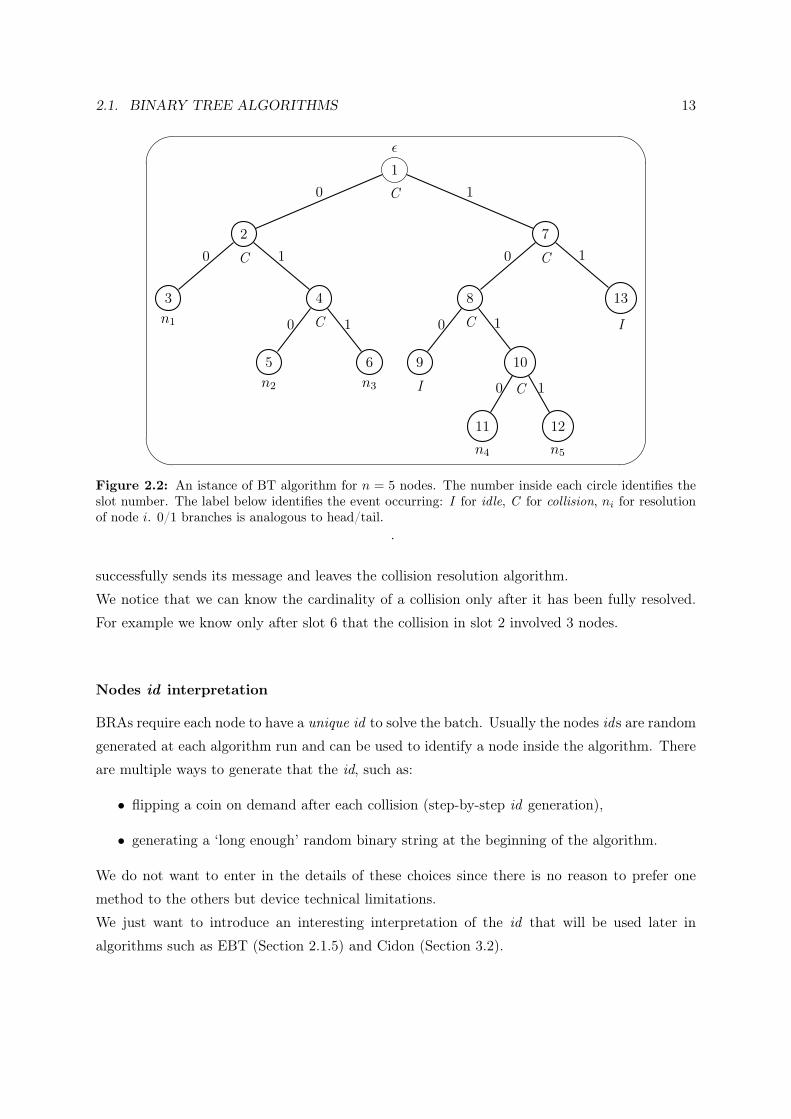
2.1. BINARY TREE ALGORITHMS 13
'
&
$
%
1
C
ε
2
C
3n1
0
4
C
5n2
0
6n3
1
1
0
7
C
8
C
9
I
0
10
C
11n4
0
12n5
1
1
0
13
I
1
1
Figure 2.2: An istance of BT algorithm for n = 5 nodes. The number inside each circle identifies theslot number. The label below identifies the event occurring: I for idle, C for collision, ni for resolutionof node i. 0/1 branches is analogous to head/tail.
.
successfully sends its message and leaves the collision resolution algorithm.
We notice that we can know the cardinality of a collision only after it has been fully resolved.
For example we know only after slot 6 that the collision in slot 2 involved 3 nodes.
Nodes id interpretation
BRAs require each node to have a unique id to solve the batch. Usually the nodes ids are random
generated at each algorithm run and can be used to identify a node inside the algorithm. There
are multiple ways to generate that the id, such as:
• flipping a coin on demand after each collision (step-by-step id generation),
• generating a ‘long enough’ random binary string at the beginning of the algorithm.
We do not want to enter in the details of these choices since there is no reason to prefer one
method to the others but device technical limitations.
We just want to introduce an interesting interpretation of the id that will be used later in
algorithms such as EBT (Section 2.1.5) and Cidon (Section 3.2).
14 CHAPTER 2. BATCH RESOLUTION
In general any infinite length binary string bi = (bi1bi2bi3 . . .), with bij ∈ {0, 1}, can be
associated to a real number ri ∈ [0, 1) by a bijective map r defined as follows:
ri = r(bi) =∞∑j=1
bij2j
(2.2)
Each node ni can be associated to a point ri within the real interval [0,1) as well as to the string
bi.
For a finite length bit-string a = (a1a2 . . . aL) with length L = l(a) we adapt the definition of r
as follows:
r(a) =L∑j=1
aj2j
(2.3)
In this case we have to carry L as auxiliary information to allow the map to remain bijective.
Following standard conventions, the empty string ε is prefix of any other string, it has length 0
and r(ε) = 0.
Tree traversal rules
The duality in the interpretation of nodes’ ids (bit-strings or real numbers) reflects on the duality
of the tree traversal rules.
According to the adopted approach, enabled nodes can be specified by:
• a finite length string a which matches the path from the root to the first node in the
sub-tree they belong to. In this case a is a prefix of the enabled nodes ids.
• the couple(r(a), l(a)
)which enables the sub-interval r(a) ≤ x < r(a) +
12l(a)
To complete the overview of the algorithm we now intuitively describe the tree visit. The
following description uses the bit-string approach since a binary string can be immediately
mapped to a path in the tree starting from the root. We assume, following the standard approach,
to visit the tree in pre-order, giving precedence to left sub-trees, conventionally associated to 0
branches.
The visit starts from the root which has address ε.
Let a be the current enabled string, then the following rules apply:
• If a = ε and last the event is success or idle then the whole conflict has been resolved;
• If the last event is collision then we visit the left child of the current node (a0);
• If the last event is success or idle and aL = 0 then we visit the right sibling (aL−11) of the
current enabled node;

2.1. BINARY TREE ALGORITHMS 15
• If the last event is success or idle and aL = 1 then we look in the path back to the root for
the first node whose sibling has not yet been visited. Since we visit the tree in pre-order
the next enabled string will be in the form ak1 with k < L.
A detailed pseudo-code of an algorithm that implements the rules above (and more) can be
found in [2]. The Modified Binary Tree algorithm presented in next section gets a remarkable
performance improvement over BT by adding just one new rule.
2.1.2 Modified Binary Tree
The Modified Binary Tree (MBT) is a simple way to improve the BT algorithm.
To keep the notation simple, we will explain the idea illustrating what happens the first time
it is applied. In this case node τ is visited in slot τ . This does not holds in general, but
explanation would have required to use two different indexes for slots and nodes, and Figure
2.3 would have been less immediate to understand.
The observation is that, during the tree traversal, sometimes we know in advance if the next
slot will be collided. This happens when, after a collided slot τ , we get an idle slot (τ + 1) in the
left branch of the binary tree. In this case, visiting the right branch (τ + 2), we will certainly
get a collision .
In fact, after sensing slot τ is collided, we know that there are at least 2 nodes in the last visited
sub-tree. None of them belongs to the left-branch of that sub-tree since slot (τ + 1) is idle.
Consequently they must be in the right branch of the sub-tree, whose enabling will hence result
into a collision. This collision can be avoided by skipping node (τ + 2) and visiting its left-child
node in slot (τ + 2).
Expected time analysis is analogous to Section 2.1.1. The only difference is that after a
collision, if we get an idle slot, we will skip the “next one” (saving a slot that would certainly
be wasted otherwise). Consequently the expected slot cost is[1 ·(1−Q0(n)
)+ 0 ·Q0(n)
]. Let
LMBTn be the expected cost in slots to solve a batch of size n using the MBT algorithm, then
LMBTn =
(1−Q0(n)
)+
n∑i=0
Qi(n)(LMBTi + LMBT
n−i ), (2.4)
with
LMBT0 = LMBT
1 = 1.
Intuitively in this case, since a higher probability to stay silent reduces the expected slot cost,

16 CHAPTER 2. BATCH RESOLUTION
'
&
$
%
1
C
ε
2
C
3n1
0
4
C
5n2
0
6n3
1
1
0
7
C
8
C
9
I
0
10
C
SKIP
11n4
0
12n5
1
1
0
13
I
1
1
Figure 2.3: Same example as in Figure 2.2 but using MBT: tree structure do not change but node 10is skipped in the traversal.
optimal transmit probability will be no longer equal to one half. At the same time, reducing
the transmit probability will increase the number of (wasted) idle slots. Thus the new optimal
probability p will be somewhere in the interval (0,0.5).
It can be shown [9] that the best result is achieved for p = 0.4175, for which the efficiency is
asymptotically equal to η ≈ 0.381. This is +10% higher than basic BT.
In general we have
LMBTn ≤ C · n+ 1, where C = 2.623. (2.5)
Using probability p =12results, for large n, in about 1.6% peak performance loss (C = 2.667),
which is a moderate decrease. It is important to notice that p = 0.4175 is very close to the
optimal bias for small n as well.
2.1.3 Clipped Modified Binary Tree
In this section we will show that, in some cases, partial resolution algorithms can achieve higher
efficiency than complete resolution algorithms.
The Clipped Modified Binary Tree (CMBT) is an adaptation of the CBT (see Section 3.1)
algorithm for complete batch resolution. CBT is like the MBT algorithm but it ends up after
two consecutive successful transmissions. Each CBT execution resolves at least two nodes but
2.1. BINARY TREE ALGORITHMS 17
eventually the last run. Hence, since the multiplicity of the batch to resolve decreases of at least
two units after each run, the algorithm terminates for sure.
Collisions tree visit is defined by the following rules:
• If the last run of the CBT does not resolves completely the left sub-tree of the current
root, then the next CBT starts from the same root;
• If the last run of the CBT resolves completely the left sub-tree of the current root, next
CBT run is applied to the right child of the current root, that will be considered the new
root;
• While current root left child is idle, set the root to the current root right child.
Applying the CBT starting each time from the current root makes the algorithm memoryless:
its behavior is not affected by previous algorithm runs but the trivial root update. In fact,
the root update allows to skip certain collisions and empty slots associated to already resolved
sub-sets.
Efficiency in solving very small batches is CMBT most interesting property. This is a
consequence of being memoryless. Figures 2.4 shows how in the average case, the CMBT
performs a few better than the MBT for batch sizes smaller than 5. Expected maximum
performance improvement is about 5% when batch size is 3. Nonetheless, for bigger batch sizes,
MBT performs better than CMBT and the gap between the two algorithms gets bigger and
bigger as the batch size increases.
Consequently, using CMBT is a good idea when the cardinality of the batch to solve is
less than or equal to 5 with very high probability. For this reason CMBT is used by the EBT
algorithm (following Section 2.1.5) to speed up the resolution.

18 CHAPTER 2. BATCH RESOLUTION
0 1 2 3 4 5 60
1
2
3
4
5
6
7
8
9
10
11
12
13
14
15
16
17
Batch Size
Exp
ecte
dT
ime
insl
ots
LCM BTn
LMBTn p opt
(a) CMBT vs MBT : very small batch sizes
0 1 2 3 4 5 6 7 8 9 10 11 12 13 14 15 16 17 18 190
5
10
15
20
25
30
35
40
45
50
Batch SizeE
xpec
ted
Tim
ein
slot
s
LCM BTn
LMBTn p opt
(b) CMBT vs MBT : larger batch sizes
Figure 2.4: Expected resolution time in slots for the CMBT and MBT algorithms for small batch sizes.
2.1.4 m Groups Tree Resolution
More advanced algorithms for batch resolution, such as those presented in [7] and [8], share a
common idea: divide the initial batch into m groups. We will not deal here about the details of
the algorithms and the different approaches they use to choose m. Instead we will concentrate
on the common part of these algorithms: divide a batch of size n into m groups and apply a
BRA to each group.
Given m groups, the probability to have exactly i among n nodes in a group is given by
Pm(i|n) =(n
i
)(1m
)i(1− 1
m
)n−i. (2.6)
Let Lk be the expected cost to solve a batch of size k with a chosen BRA. Then the expected
cost to solve a batch of size n dividing it into m groups is given by
L′n(ρ) = mn∑i=0
LiPm(i|n), (2.7)
where ρ =n
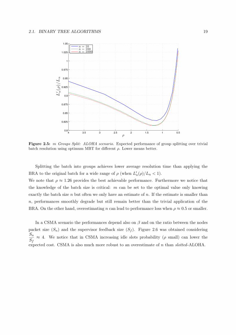
mis the mean number of nodes in a group.
Figure 2.5 plots L′n(ρ), the average time to solve a batch of size n using group splitting, over Ln,
the average time without splitting. Results were obtained computing equation (2.7) for three
different batch sizes varying ρ. We plotted the results for the MBT algorithm with optimal
probability p in a slotted ALOHA scenario but considerations hold for any tree-based BRA.
2.1. BINARY TREE ALGORITHMS 19
0.511.522.533.540.8
0.825
0.85
0.875
0.9
0.925
0.95
0.975
1
1.025
1.05
ρ
L′ n(ρ
)/L
n
n = 10n = 100n = 1000
Figure 2.5: m Groups Split: ALOHA scenario. Expected performance of group splitting over trivialbatch resolution using optimum MBT for different ρ. Lower means better.
Splitting the batch into groups achieves lower average resolution time than applying the
BRA to the original batch for a wide range of ρ (when L′n(ρ)/Ln < 1).
We note that ρ ≈ 1.26 provides the best achievable performance. Furthermore we notice that
the knowledge of the batch size is critical: m can be set to the optimal value only knowing
exactly the batch size n but often we only have an estimate of n. If the estimate is smaller than
n, performances smoothly degrade but still remain better than the trivial application of the
BRA. On the other hand, overestimating n can lead to performance loss when ρ ≈ 0.5 or smaller.
In a CSMA scenario the performances depend also on β and on the ratio between the nodes
packet size (Sn) and the supervisor feedback size (Sf ). Figure 2.6 was obtained consideringSnSf≈ 4. We notice that in CSMA increasing idle slots probability (ρ small) can lower the
expected cost. CSMA is also much more robust to an overestimate of n than slotted -ALOHA.

20 CHAPTER 2. BATCH RESOLUTION
00.250.511.522.533.540.65
0.7
0.75
0.8
0.85
0.9
0.95
1
1.05
1.1
ρ
L′ n(ρ
)/L
n
n = 10n = 100n = 1000
Figure 2.6: m Groups Split: CSMA scenario. Expected performance of group splitting over trivialbatch resolution using optimum MBT for different ρ. Lower means better.
2.1.5 Estimating Binary TreeNUOVA
Estimating Binary Tree (EBT) has been recently proposed in [2]. It does not work on parameters
optimization but tries to use simple heuristics to skip tree nodes that will result in collisions
with high probability.
Given a batch of size n, the keys to understand EBT are the following:
• in the luckiest scenario, running BT results in a balanced binary tree where all the leaves
are at the same level,
• consequently it seems to be a good idea to assume that nodes at levels in the tree less than
blog2 nc will likely result in collided slots.
EBT tries to skip inner nodes of the tree by visiting only nodes at levels equal or deeper
than blog2 nc. Since n is not a priori known, a dynamic estimating technique is adopted.
To effectively use this estimate tecnique each node must be able to generate values from the
standard uniform distribution on the interval [0,1) and to use that value as its unique id.
Assume that there are k nodes whose ids are in the sub-interval [0,pε) and that they have been
previously resolved: all and only the nodes with id less than pε successfully transmitted their
messages. Let n express the estimate of n. When pε is greater than 0, setting n tok
pεprovides
a good estimate of n that becomes more and more accurate as the algorithm goes on. EBT uses

2.2. OTHERS 21
n (as soon as it is available) to choose the right level in the tree to analyze.
The most straightforward interpretation of the EBT algorithm can be:
Algorithm 2 Estimating Binary TreeRun the CBT algorithmwhile batch is not resolved do
Update the estimate nStart a new CMBT at the next node from level blog2 nc
end while
Here we gave only a short insight of the algorithm and the estimate technique. In particular
this estimate technique is a dynamic adaptation of that described later in Section 3.2 and
originally proposed in [7].
2.2 Others
In this section we will shortly describe non tree-based algorithms for batch resolution.
2.2.1 IERC
The Interval Estimation Conflict Resolution (IERC) [2] is an adaptation of the FCFS [5]
algorithm for Poisson’s arrivals of packets to the batch resolution.
FCFS is the fastest known algorithm to solve Poisson’s arrivals and it achieves efficiency
η = 0.4871. It assumes a priori knowledge of the arrival rate λ of the packets and works by
splitting the time in epochs of length τ .
Now we briefly describe FCFS algorithm. and then we will show how it can be translated to
the batch resolution problem.
At any time k, let T (k) be the start time of the current enabled allocation interval. Packets
generated in the enabled window (T (k), T (k) + τ ] are allowed to be transmitted. When an
idle or successful event occurs enabled time window gets incremented (shifted towards current
time) by τ . On the other hand, if a collision takes place, a Clipped Binary Tree (see Section
3.1) algorithm is started. Given that CBT resolves the sub-interval (T (k), T (k) + α(k)],
then next FCFS enabled window at time k′ will be (T (k′), T (k′) + min(τ, k′ − T (k′))] where
T (k′) = T (k) + α(k).
22 CHAPTER 2. BATCH RESOLUTION
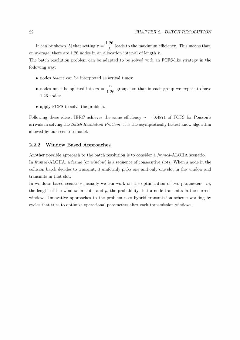
It can be shown [5] that setting τ =1.26λ
leads to the maximum efficiency. This means that,
on average, there are 1.26 nodes in an allocation interval of length τ .
The batch resolution problem can be adapted to be solved with an FCFS-like strategy in the
following way:
• nodes tokens can be interpreted as arrival times;
• nodes must be splitted into m =n
1.26groups, so that in each group we expect to have
1.26 nodes;
• apply FCFS to solve the problem.
Following these ideas, IERC achieves the same efficiency η = 0.4871 of FCFS for Poisson’s
arrivals in solving the Batch Resolution Problem: it is the asymptotically fastest know algorithm
allowed by our scenario model.
2.2.2 Window Based Approaches
Another possible approach to the batch resolution is to consider a framed -ALOHA scenario.
In framed -ALOHA, a frame (or window) is a sequence of consecutive slots. When a node in the
collision batch decides to transmit, it uniformly picks one and only one slot in the window and
transmits in that slot.
In windows based scenarios, usually we can work on the optimization of two parameters: m,
the length of the window in slots, and p, the probability that a node transmits in the current
window. Innovative approaches to the problem uses hybrid transmission scheme working by
cycles that tries to optimize operational parameters after each transmission windows.

Chapter 3
Batch Size Estimate Techniques
Here we present some noteworthy techniques for batch size estimate that can be found in the
literature. If a technique was not already identified by a name or associated to an acronym, we
used the name of one the authors as reference.
In general, we assume to have no a priori statistical knowledge about the conflict
multiplicity. Estimation techniques are thus required to provide accurate estimates for the
general zero-knowledge scenario.
3.1 Clipped Binary Tree
A simple way to obtain an estimate of the batch size is to solve a certain number of nodes and
then infer the batch size according to the time taken to solve these nodes. This can be done, for
example, by using deterministic algorithms such as the Clipped Binary Tree (CBT) Algorithm.
CBT is a partial resolution algorithm since only a fraction of the packets of the batch are
successfully transmitted. The algorithm is identical to the MBT, with p =12since we require
nodes to be uniformly distributed in the interval [0,1), except that it stops (the tree is clipped)
whenever two consecutive successful transmissions follow a conflict.
When the algorithm stops, after i collisions, we know than the last two resolved nodes belong
to the same level i of the tree (root is assumed to be at level 0). Therefore, an estimate of the
initial batch size is given by:
n← 2i (3.1)
23

24 CHAPTER 3. BATCH SIZE ESTIMATE TECHNIQUES
'
&
$
%
1
C
ε
2
C
3n1
0
4
C
5n2
0
6n3
1
1
0
Figure 3.1: Same example as in Figure 2.2 but resolution using CBT ends up after two consecutivesuccessful transmissions.
Experimental results show that the variance of this estimate is extremely high and the
resulting accuracy is rather poor. This is due to the fact that the batch we use for the estimate
becomes, at each level, smaller and smaller. Using this algorithm we do not have knowledge of
a sufficiently large number of intervals but we limit to analyze only a few leafs. The resulting
estimate, even for huge sizes, depends only on very few (3-5) outer nodes (those at the most left
in the tree). Consequently estimate is quite inacurate.
From the tables A.5 reported in Appendix you can notice that the distribution probability
decreases rather slowly.
3.2 Cidon
In [7] Cidon and Sidi proposed a complete resolution algorithm based on two phases:
1. Estimate the initial batch size using a partial deterministic resolution scheme.
2. Perform an optimized complete deterministic resolution based on the results of phase 1.
Phase 1 consists in resolving a small part of the initial batch, counting the number of
successful transmissions. A node takes part either to the estimate phase or to the following
resolution phase, not both. The probability pε, which is an algorithm input parameter,
determines this choice. We called it pε to underlined that this initial choice reflects the expected
accuracy of the resulting estimate, as it will be discussed in more detail later on.
3.2. CIDON 25
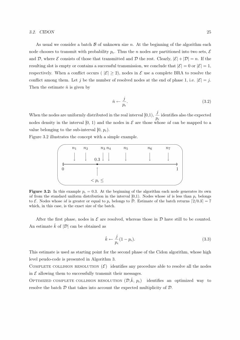
As usual we consider a batch B of unknown size n. At the beginning of the algorithm each
node chooses to transmit with probability pε. Thus the n nodes are partitioned into two sets, Eand D, where E consists of those that transmitted and D the rest. Clearly, |E|+ |D| = n. If the
resulting slot is empty or contains a successful transmission, we conclude that |E| = 0 or |E| = 1,
respectively. When a conflict occurs ( |E| ≥ 2), nodes in E use a complete BRA to resolve the
conflict among them. Let j be the number of resolved nodes at the end of phase 1, i.e. |E| = j.
Then the estimate n is given by
n← j
pε. (3.2)
When the nodes are uniformly distributed in the real interval [0,1),j
pεidentifies also the expected
nodes density in the interval [0, 1) and the nodes in E are those whose id can be mapped to a
value belonging to the sub-interval [0, pε).
Figure 3.2 illustrates the concept with a simple example.'
&
$
%0 1
n1 n2 n3 n4 n5 n6 n7
< pε ≤
0.3
Figure 3.2: In this example pε = 0.3. At the beginning of the algorithm each node generates its ownid from the standard uniform distribution in the interval [0,1). Nodes whose id is less than pε belongsto E . Nodes whose id is greater or equal to pε belongs to D. Estimate of the batch returns d2/0.3e = 7which, in this case, is the exact size of the batch.
After the first phase, nodes in E are resolved, whereas those in D have still to be counted.
An estimate k of |D| can be obtained as
k ← j
pε(1− pε). (3.3)
This estimate is used as starting point for the second phase of the Cidon algorithm, whose high
level peudo-code is presented in Algorithm 3.
Complete collision resolution (E) identifies any procedure able to resolve all the nodes
in E allowing them to successfully transmit their messages.
Optimized complete collision resolution (D,k, pε) identifies an optimized way to
resolve the batch D that takes into account the expected multiplicity of D.

26 CHAPTER 3. BATCH SIZE ESTIMATE TECHNIQUES
Algorithm 3 Cidon(B, pε)Input: B batch with |B| = nInput: pε, fraction of the whole batch to solve1: // Phase 12: each node flips a coin getting 0 with probability pε, 1 otherwise3: E ← { nodes that flipped 0}4: D ← { nodes that flipped 1}5: Complete collision resolution (E)6: k ← |E|/pε7: // Phase 28: Optimized complete collision resolution (D,k, pε)
The original paper proposes to use an m groups split (Section 2.1.4) approach to resolve D,where
m = max(1, dαk − βe), (3.4)
and each group is resolved by applying the MBT algorithm.
The parameter α determines the number of groups, and therefore the efficiency of the resolution
process, when n is large, while β reduces the number of groups when n is small in order to
reduce the risk of empty groups.
α = 0.786 determines ρ ≈ 1.27 which is the unique optimum nodes per group density. β and
pε depend on operational requirements: in [7] it is showed that setting β = 8 and pε = 0.1 is a
good compromise to get efficient resolution for a wide range of batch sizes.
The average cost of the estimate phase (phase 1) depends on the BRA used but in general,
for tree-based BRAs, can be considered O(pεn).
3.3 Greenberg
Basic Greenberg algorithm searches for a power of 2 that is close to n with high probability:
n ≥ 2i ≈ n (3.5)
Let each of the n conflicting stations either or not transmit in accordance with the outcome
of a biased binary coin. The coin is biased to turn up 0 (transmit) with probability 2−i and
1 (do not transmit) with complementary probability 1 − 2−i. Since the expected number of
transmitters in the slot is 2−in, a conflict supports the hypothesis that n ≥ 2i.
Using this test repeatedly with i = 1, 2, 3, . . ., leads to the Greenberg base 2 estimation algorithm.
Each of the conflicting stations executes Algorithm (4), resulting in a series of collisions whose

3.3. GREENBERG 27
length determines n. The probability that at most one node transmits in a slot, monotonically
grows with the slot number and approaches 1 very rapidly as i increases beyond log2 n.
Consequently, we expect that the collision series stops at slot i that is close to log2 n.
Algorithm 4 Basic Greenberg (B)// Each node performs these operationsi← 0repeat
i← i+ 1choose to transmit with probability p = 2−i
until no collision occursn← 2i
The idea behind Algorithm 4 appears to be quite simple: as the algorithm goes on, the initial
unknown batch (of size n) is progressively sliced into smaller pieces. Only the nodes virtually
inside the enabled slice are allowed to transmit. Slices get thinner and thinner until at most one
node is contained in a slice. Figure 3.3 illustrates the idea with an example: visually, nodes can
be thought to be uniformly distributed on a circumference. Using Greenberg algorithm we will
analyze at each slot a smaller sector (in this case the half of the previous one) of the circle and
discover when a sector contains at most 1 node. Note that no overlapping sectors are drawn
to maintain the image simple. However, in general, enabled nodes get redistributed at each
transmission test performed by the algorithm.
Expected running time is O(log2 n). In particular, since in the slotted -ALOHA model,
feedback is supposed to be transmitted at the end of each transmission slot, the expected
running time in slots can be expressed as ≈ 1 + log2 n.
An important note is that the algorithm always involves all the nodes in the batch: at each
slot, each node decides whatever or not transmit. Each choice is independent of the past. This
is of great importance and allows n to have bounded statistical moments: it can be shown that,
for large n, it holds:
E[n] ≈ nφ, (3.6)
E[n2] ≈ nΦ, (3.7)
where
φ =1
log 2
∫ ∞0e−x(1 + x)
∞∏k=1
(1− e−2kx(1 + 2kx)
)x−2 dx = 0.91422 (3.8)

28 CHAPTER 3. BATCH SIZE ESTIMATE TECHNIQUES
π
n/2
π/2
n/4
π/4
n/8
Figure 3.3: Basic Greenberg : batch split idea
Φ =1
log 2
∫ ∞0e−x(1 + x)
∞∏k=1
(1− e−2kx(1 + 2kx)
)x−3 dx = 1.23278 (3.9)
φ and Φ are obtained in [8] using advanced mathematical analysis supported by Mellin integral
transform1. In general φ and Φ depend on the size of the problem. Table 3.1 shows the behavior
of the expected estimate (and, therefore of φ) as a function of n. We note that the ratio
E[n|n]/n monotonically decreases and gets stable at 0.9142. This shows that this estimate
technique provides biased results.
The fact that, for large n, E[n] ≈ nφ suggests a way for correcting the estimate bias as
n+ =n
φ. Due to the contribution of periodic functions, n+ is not an asymptotically unbiased
estimate of n, in the sense that E[n+]/n does not tend to 1 as n gets large. Fortunately, the
amplitude of the periodic functions turns out to be less than 2 · 10−5, so this bias is negligible
for all practical purposes.
Interestingly, a simple variant of the estimation algorithm shows really poor performance.1In this work we only report the final results. Please, refer to the original paper for details.

3.3. GREENBERG 29
Table 3.1: Basic Greenberg : Expected estimate and bias
n E[n|n] E[n|n]/n
1 2.00 2.00002 2.56 1.28224 4.21 1.05338 7.89 0.986316 15.20 0.949832 29.82 0.932064 59.08 0.9231128 117.59 0.9186256 234.60 0.9164512 468.64 0.91531024 936.71 0.91482048 1872.86 0.91454096 3745.14 0.91438192 7489.72 0.914316384 14978.86 0.914232768 29957.16 0.914265536 59913.74 0.9142
Consider the algorithm in which each station involved in the initial collision transmits to the
channel with probability 1/2. If this causes another collision, then those that just transmitted,
transmit again with probability 1/2. The others drop out. This process continues until there
are no collisions. Let 2i be the estimate of the conflict multiplicity, where i is the slot at which
there is no collision. It can be shown [8] that the second and all higher moments of this estimate
are infinite.
3.3.1 Base b variant
Using basic Algorithm 4, the expected value of n+ is likely different from n by a factor 2. In
the original work, a small generalization of the base 2 algorithm is proposed to overcome this
limitation, by simply using a base b instead of 2, with 1 < b ≤ 2.

30 CHAPTER 3. BATCH SIZE ESTIMATE TECHNIQUES
Algorithm 5 base b Greenberg (B)i← 0repeat
i← i+ 1transmit with probability b−i
until no collision occursn(b)← 2i
n+(b)← n(b)/φ(b)
In Algorithm 5, the term φ(b) corrects the bias of the estimator. Table 3.2 shows how φ
and the expected cost in slots vary for different b. Expected cost (. logb n) is expressed as
a multiplicative factor for the basic Greenberg algorithm cost (. log2 n). We can notice that
smaller b results in smaller φ(b). This means that b deeply biases the estimate: if b′< b
′′ then
E[n(b′)] < E[n(b
′′)]. This follows from the fact that, decreasing b, the stop probability “shift”
towards “early slots” associated to lower estimates.
Table 3.2: Base b Greenberg : Bias and expected cost summary
b φ(b) Expected cost in slots-1
2 ≈ 0.9142 . 1 × log2 n1.1 ≈ 0.3484 . 7.271.01 ≈ 0.1960 . 69.661.001 ≈ 0.1348 . 693.491.0001 ≈ 0.1027 . 6931.81
In[8], it is shown that, for all n greater than some constant n0(b), it holds∣∣∣∣E[n+(b)]n
− 1∣∣∣∣ < ε(b), (3.10)
σ(n+(b)
)n
< ε(b), (3.11)
where ε(b)→ 0 as b→ 1.
In other words when b→ 1 and n is large the estimate becomes unbiased and its variance goes
to zero. However, our experimental results showed that the performance of base b estimator is
not ideal in practical scenarios.

3.4. WINDOW BASED 31
3.4 Window Based
Window based approaches use a framed -ALOHA transmission scheme, where the reader provides
feedback to the nodes after each frame. Framed -ALOHA is characterized by the frame length
L, whose choice is critical for the performance of the resolution process as well as the estimation
phase. Setting L large compared to the batch size increases the probability to solve all the nodes
in the current window but, on the other hand, it leads to a waste of slots and consequently
sub-optimal running time. At the same time, a large value of L allows for a very accurate
estimate of the batch size.
Setting L small increases the probability of collided slots. Since the number of nodes involved
in a collision is unknown, collisions provide poor information about the batch multiplicity. The
more collisions we have, the less accurate the estimate.
An interesting approach to the problem is presented in [3]. When the scenario allows to use
a probabilistic-framed-ALOHA2 scheme we can act on the parameter p, i.e. the probability for
a node to take part in the current transmission window. Small p value allows to keep L small
too and hence, when n is large, provides an accurate estimate of the whole batch considering
only a sub-set of it. This results in shorter estimate time.
Since when p = 1 probabilistic-framed-ALOHA reduces to simple framed-ALOHA and it is
reasonable to start any estimate algorithm with p = 1, we will show a possible approach to the
problem in a framed-ALOHA scenario.
Let n be the batch size and L the window length. The number of nodes k out of n that
choose the same slot is binomially distributed with parameters B(n, 1/L). Then, the probability
to get an idle, successful or collision slot is respectively given by:
p0(n) =(
1− 1L
)n, (3.12)
p1(n) =n
L
(1− 1
L
)n−1
, (3.13)
p2+(n) = 1− p0(n)− p1(n). (3.14)2Probabilistic-framed-ALOHA is an extension of the framed-ALOHA model where a node takes part to the
current contention window with probabily p or waits for the next one with probability 1− p. Nodes that decideto transmit behave like in the standard framed-ALOHA.

32 CHAPTER 3. BATCH SIZE ESTIMATE TECHNIQUES
Considering the whole window, the outcome consists in a tuple (i, s, c), denoting the number
of idle, success, and collision slots, which satisfies i+ s+ c = L. Hence, the probability of (i,s,c)
is given by:
P (i, s, c) =L!
i! s! c!p0(n)i p1(n)s p2+(n)c =
L!i! s! c!
fL(i, s, c, n). (3.15)
We note that (3.15), does not take into account the fact that a node is allowed to transmit only
once in a window: equation (3.15) is only an approximation of the distribution of the nodes
in the slots when both n and L are large. A Poisson distribution of parameter λ = n 1L would
model better the scenario but (3.15) allows simpler numerical computation.
Once we have tried to resolve the batch using a window approach we know how many idle,
successful or collided slots there were.
Then we find the estimate n as the batch size that maximizes the probability to see the tuple
(i, s, c) in a L length window:
n = arg maxn
fL(i, s, c, n), (3.16)
where we discarded the factorial terms because they not contribute to identify the maximum since
L, i, s, c are fixed. Furthermore, since L, i, s, c are fixed, fL(i, s, c, n) becomes a one-variable
function which results well behaved in n, being initially monotonically increasing and then
monotonically decreasing. Therefore fL(i, s, c, n) has only one maximum.
By setting
f ′L(i, s, c, n) = 0, (3.17)
and numerically solving (3.17) we can obtain the batch size that maximizes our function. In
general the solution will not be integer-valued and a rounding operation is necessary to achieve
a real world batch estimate.
Table 3.3: Estimate given (i, c, s) when L = i+ c+ s = 10.
HHHHHHc
s 0 1 2 3 4 5 6 7 8 9
1 3 3 4 5 6 7 8 9 10 112 5 6 7 8 8 10 11 12 13 -3 7 8 9 10 11 12 13 14 - -4 10 11 12 13 14 15 16 - - -5 12 14 15 16 17 19 - - - -6 16 17 19 20 22 - - - - -7 20 22 23 25 - - - - - -8 26 28 30 - - - - - - -9 35 38 - - - - - - - -10 ∞ - - - - - - - - -
Table 3.3 shows the estimate provided by the explained technique when L = 10. Cells,

3.4. WINDOW BASED 33
identified by (c, s), where c+ s > 10 cannot be associated to any estimate since their events are
impossible. The case c = 0 is trivial since the estimate is exact and is given by the number of
successful transmission.
We note also that when we see only collisions, the estimator is not able to provide a finite
estimate. The event c = 10 in the table is in fact associated to n =∞. In general, when c = L
we have that (3.15) reduces to:
P (0, 0, L) = p2+(n)L =
[1−
(1− 1
L
)n− n
L
(1− 1
L
)n−1]L
, (3.18)
which is maximized (P (0, 0, L) = 1) by n = ∞ for any L. Hence we would not to have only
collisions since they do not provide any information about the cardinality of the batch.
A larger window has to be used to get a finite estimate but its optimal length remains unknown.


Chapter 4
Estimate Performance Analysis
In this Chapter, we present a performance analysis of some of the already mentioned noteworthy
batch size estimation (BSE) algorithms. The overview will obviously consider different batch
sizes, algorithm parameters, time required and accuracy of the estimate. We want to support
reader in choosing the best estimate technique suitable for its needs.
First we will provide a detailed analytical analysis of Cidon algorithm and then, supported by
numerical computation, we will derive its features in term of time and accuracy.
We will then discuss the behavior of Greenberg with its pros and cons and try to overcome its
limitations by introducing a modification of the original algorithm to achieve better estimate.
Enhanced Greenberg Algorithm (EGA) is the middle-step in the development of our proposed
estimate algorithm: it improves the estimate in terms of “choosing the best power of 2”,
maintaining the same target estimates allowed by basic Greenberg. Then, we will describe and
analyze the Generalized Enhanced Greenberg Algorithm (GEGA), which combines Greenberg
with a further test and performs a maximum likelihood estimation to determine the “best”
estimate. Finally, the comparison between GEGA and Cidon will lead to the conclusions.
4.1 Cidon BSE
The original paper [7] describes the estimate technique but does not characterize it in details.
The interest is focused on other aspects and, therefore, no detailed analysis of the behavior of
the estimate algorithm is presented: it is only mentioned that as n grows the estimator becomes
more accurate. Hence, in this section we will provide a complete analysis of the estimate
algorithm.
Following from Section 3.2, let j denote the number of nodes in E and pε be the expected
fraction of nodes to be resolved in Cidon algorithm Phase 1. Parameter pε can be considered
35
36 CHAPTER 4. ESTIMATE PERFORMANCE ANALYSIS
fixed a priori since it is an input of the algorithm and, therefore, given a batch of size n, j is a
binomially distributed random variable with parameters n and pε. Hence, we have the following:
E[j|n, pε] = npε, (4.1)
var(j|n, pε) = npε(1− pε). (4.2)
By applying Chebychev’s Inequality (A.1), we have for any ε > 0
P(|j − npε| ≥ εn |n, pε
)≤ pε(1− pε)
ε2n. (4.3)
We remember that the Cidon estimate is given by n =j
pε. Then, from the aforementioned
equations (4.1)-(4.3), it follows that:
E[n|n, pε] =1pεE [j|n, pε] = n, ∀ pε (4.4)
and
P
(∣∣∣∣ nn − 1∣∣∣∣ ≥ ε ∣∣n, pε) ≤ 1− pε
ε2npε. (4.5)
which shows that using this estimation method we can trade off the accuracy with the
consumption of resources in terms of time or messages. Furthermore, Cidon estimate is unbiased
independently of pε, which influences the variance of the estimator. In fact, we have
var(n|n) =n
pε− n (4.6)
which reveals that as the number of resolved terminals (and therefore pε) increases the estimate
n becomes more accurate.
4.1.1 Performance
Figure 4.1 shows that the variance is strict monotonically decreasing in pε. Furthermore, you
can notice that, for pε smaller than 0.1, a small increment in pε produces a large decrease
in the normalized variance which reflects in a large estimate accuracy improvement. Hence,
considering the tread-off between estimate overhead and resolution efficiency, solving up to 110
of the initial batch in the estimate phase is a good practical choice.
However, it is difficult to establish in what measure an estimate can be considered accurate.
The idea we adopt is to require the estimate to be “near” the real batch size with very high
probability. Given the real batch size n, let the error coefficient k ≥ 1 identify an interval

4.1. CIDON BSE 37
0 0.1 0.2 0.3 0.4 0.5 0.6 0.7 0.8 0.9 1
0
10
20
30
40
50
60
70
80
90
100
var(n|n
)/n
pǫ
(1 − pǫ)/pǫ
Figure 4.1: Cidon: estimate normalized variance as function of pε.
surrounding n in the following way:n
k≤ n ≤ kn (4.7)
We can study the algorithm behavior by considering as index for the estimate accuracy
θk = P(nk≤ n ≤ kn
)(4.8)
Let θ be the minimum allowed value for θk: in other words θ is the probability we require for
constrains (4.7) to be satisfied.
If we set θ = 0.99, we can find the minimum pε, ensuring the estimate to be within interval
(4.7), by solving the following problem.
P(nk≤ n ≤ kn
∣∣k, n) =P(nk≤ j/pε ≤ kn
∣∣k, n, pε)=P
(npεk≤ j ≤ knpε
∣∣k, n, pε) (4.9)
Since j assumes positive integer values, we introduce rounding operations. In particular,
rounding effect is non neglectible when n ≤ 200.
f(k, n, pε) = P(⌈npε
k
⌉≤ j ≤ bknpεc
∣∣k, n, pε) ≥ θ (4.10)
38 CHAPTER 4. ESTIMATE PERFORMANCE ANALYSIS
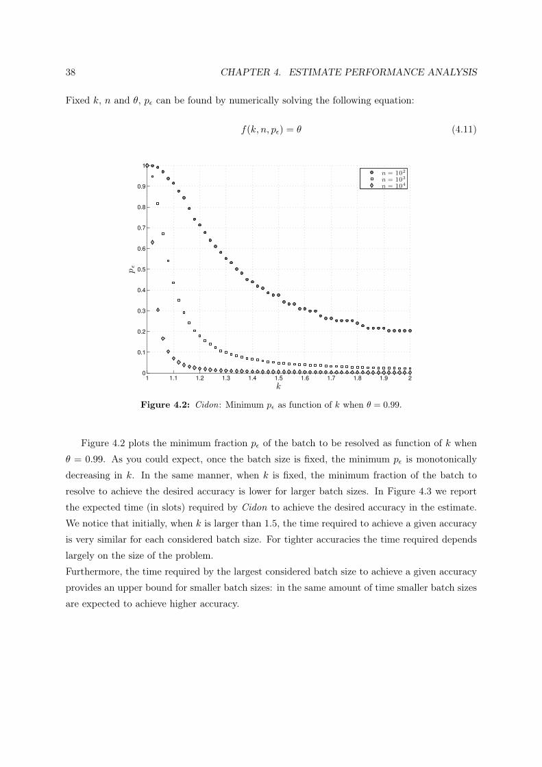
Fixed k, n and θ, pε can be found by numerically solving the following equation:
f(k, n, pε) = θ (4.11)
1 1.1 1.2 1.3 1.4 1.5 1.6 1.7 1.8 1.9 20
0.1
0.2
0.3
0.4
0.5
0.6
0.7
0.8
0.9
1
k
pǫ
n = 102
n = 103
n = 104
Figure 4.2: Cidon: Minimum pε as function of k when θ = 0.99.
Figure 4.2 plots the minimum fraction pε of the batch to be resolved as function of k when
θ = 0.99. As you could expect, once the batch size is fixed, the minimum pε is monotonically
decreasing in k. In the same manner, when k is fixed, the minimum fraction of the batch to
resolve to achieve the desired accuracy is lower for larger batch sizes. In Figure 4.3 we report
the expected time (in slots) required by Cidon to achieve the desired accuracy in the estimate.
We notice that initially, when k is larger than 1.5, the time required to achieve a given accuracy
is very similar for each considered batch size. For tighter accuracies the time required depends
largely on the size of the problem.
Furthermore, the time required by the largest considered batch size to achieve a given accuracy
provides an upper bound for smaller batch sizes: in the same amount of time smaller batch sizes
are expected to achieve higher accuracy.
4.2. GREENBERG BSE 39
1 1.1 1.2 1.3 1.4 1.5 1.6 1.7 1.8 1.9 210
1
102
103
104
105
k
Ln
pǫ
n = 102
n = 103
n = 104
Figure 4.3: Cidon: Expected time as function of k when θ = 0.99.
4.2 Greenberg BSE
Given a current slot transmission probability p and a batch of size n we define respectively:
1. the probability to get an empty slot (no transmissions)
q0(p, n) = (1− p)n (4.12)
2. the probability to get a successful slot (exactly one transmission)
q1(p, n) = np(1− p)n−1 (4.13)
3. the probability to get a collision (two or more transmissions)
q2+(p, n) = 1− q0(p, n)− q1(p, n) (4.14)
In basic Greenberg (algorithm 4) each slot is associated with a different probability p.
Numbering slots i from 1, 2, and so on we hence have
pi = p(i) = 2i. (4.15)
40 CHAPTER 4. ESTIMATE PERFORMANCE ANALYSIS
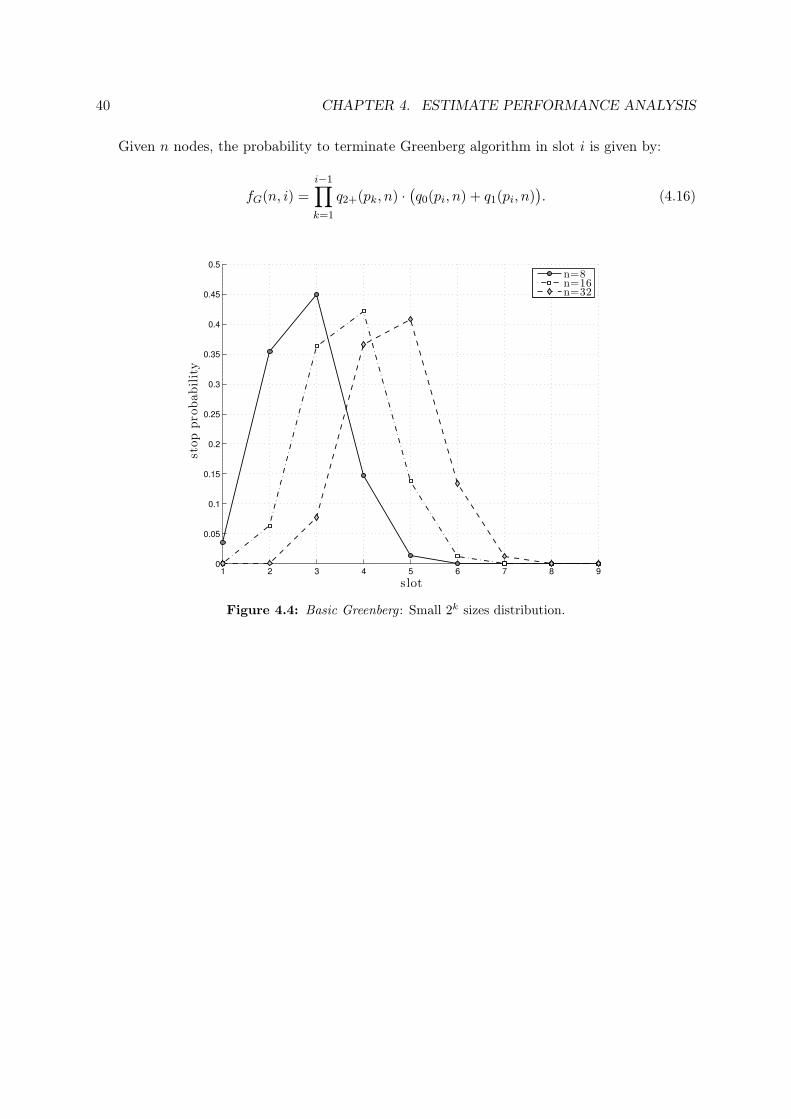
Given n nodes, the probability to terminate Greenberg algorithm in slot i is given by:
fG(n, i) =i−1∏k=1
q2+(pk, n) ·(q0(pi, n) + q1(pi, n)
). (4.16)
1 2 3 4 5 6 7 8 90
0.05
0.1
0.15
0.2
0.25
0.3
0.35
0.4
0.45
0.5
slot
stop
prob
abilit
y
n=8n=16n=32
Figure 4.4: Basic Greenberg : Small 2k sizes distribution.
4.2. GREENBERG BSE 41
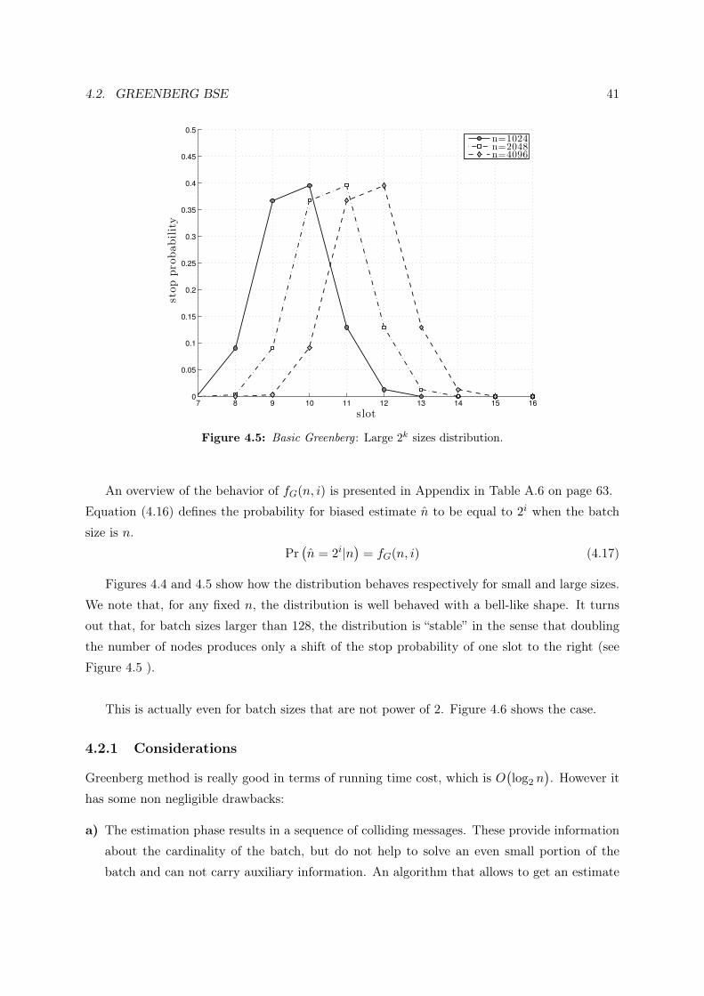
7 8 9 10 11 12 13 14 15 160
0.05
0.1
0.15
0.2
0.25
0.3
0.35
0.4
0.45
0.5
slot
stop
prob
abilit
y
n=1024n=2048n=4096
Figure 4.5: Basic Greenberg : Large 2k sizes distribution.
An overview of the behavior of fG(n, i) is presented in Appendix in Table A.6 on page 63.
Equation (4.16) defines the probability for biased estimate n to be equal to 2i when the batch
size is n.
Pr(n = 2i|n
)= fG(n, i) (4.17)
Figures 4.4 and 4.5 show how the distribution behaves respectively for small and large sizes.
We note that, for any fixed n, the distribution is well behaved with a bell-like shape. It turns
out that, for batch sizes larger than 128, the distribution is “stable” in the sense that doubling
the number of nodes produces only a shift of the stop probability of one slot to the right (see
Figure 4.5 ).
This is actually even for batch sizes that are not power of 2. Figure 4.6 shows the case.
4.2.1 Considerations
Greenberg method is really good in terms of running time cost, which is O(log2 n
). However it
has some non negligible drawbacks:
a) The estimation phase results in a sequence of colliding messages. These provide information
about the cardinality of the batch, but do not help to solve an even small portion of the
batch and can not carry auxiliary information. An algorithm that allows to get an estimate

42 CHAPTER 4. ESTIMATE PERFORMANCE ANALYSIS
7 8 9 10 11 12 130
0.05
0.1
0.15
0.2
0.25
0.3
0.35
0.4
0.45
slot
stop
prob
abilit
y
n=555n=597n=640n=683n=725n=768n=811n=853n=896n=939n=981n=1024n=1110n=1194n=1280n=1366n=1450n=1536n=1622n=1706n=1792n=1878n=1962
Figure 4.6: Basic Greenberg : General batch sizes distribution.
while resolving nodes would offer some advantages when the problem is not only the pure
batch size estimation, but the batch resolution.
b) Basic Greenberg does not allow to achieve arbitrary precision in the estimate. In fact, we
have that:
i. the estimate is, by construction, a power of 2. Only a small subset of batch sizes can be
mapped without error.
ii. the estimate distribution is not sharp enough around the correct value of the batch size
but it spans over a few slots: this is shown in Figure 4.5. We notice that using Greenberg
algorithm it is difficult to discriminate between n and n2 .
c) Base b Greenberg could be used to get a tighter estimate. Anyway, to improve the accuracy,
very small b has to be choosen which results in much worse running times (see Table 3.2):
even if theoretically it remains O(logbn) which is sublinear in n, in practice estimate time
can even overwhelm n when b is small.
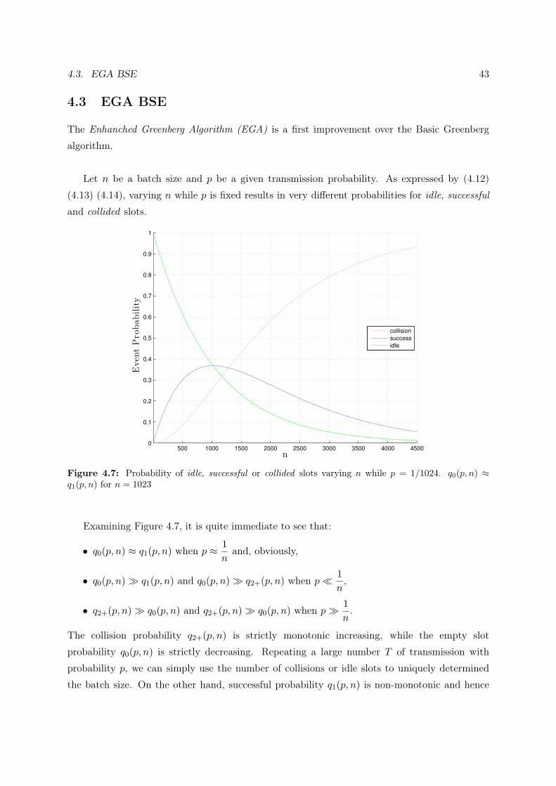
4.3. EGA BSE 43
4.3 EGA BSE
The Enhanched Greenberg Algorithm (EGA) is a first improvement over the Basic Greenberg
algorithm.
Let n be a batch size and p be a given transmission probability. As expressed by (4.12)
(4.13) (4.14), varying n while p is fixed results in very different probabilities for idle, successful
and collided slots.
500 1000 1500 2000 2500 3000 3500 4000 45000
0.1
0.2
0.3
0.4
0.5
0.6
0.7
0.8
0.9
1
n
Eve
ntP
roba
bility
collision
success
idle
Figure 4.7: Probability of idle, successful or collided slots varying n while p = 1/1024. q0(p, n) ≈q1(p, n) for n = 1023
Examining Figure 4.7, it is quite immediate to see that:
• q0(p, n) ≈ q1(p, n) when p ≈ 1n
and, obviously,
• q0(p, n)� q1(p, n) and q0(p, n)� q2+(p, n) when p� 1n,
• q2+(p, n)� q0(p, n) and q2+(p, n)� q0(p, n) when p� 1n.
The collision probability q2+(p, n) is strictly monotonic increasing, while the empty slot
probability q0(p, n) is strictly decreasing. Repeating a large number T of transmission with
probability p, we can simply use the number of collisions or idle slots to uniquely determined
the batch size. On the other hand, successful probability q1(p, n) is non-monotonic and hence
44 CHAPTER 4. ESTIMATE PERFORMANCE ANALYSIS
can not be used to uniquely determine the batch size.
The proposed technique to refine the estimate is the following.
Running Basic Greenberg Algorithm provides a raw estimate and the associated transmission
probability p. Then we perform T more transmissions and use aMaximum Likelihood Estimation
(MLE) to refine the estimate.
Let T be the number of slots we will use to refine the estimate and let N0, N1, N2+ be random
variables which represent the total number of idle, successful and collided slots, respectively,
observed after the T additional slots.
N0, N1, N2+ are binomial distributions with parameters B(n, q0(p, n)), B(n, q1(p, n)) and
B(n, q2+(p, n)), respectively. Of course N0 +N1 +N2+ = T and
E[N0] = Tq0(p, n),
E[N1] = Tq1(p, n),
E[N2+] = Tq2+(p, n).
Let fT (i, s, c, p′, n′) denote the probability to get i idle, s success and c collision slots:
fT (i, s, c, p′, n′) = Pr(N0 = i,N1 = s,N2+ = c|n = n′, p = p′) (4.18)
= Pr(N0 = i|n = n′, p = p′)Pr(N1 = s,N2+ = c|n = n′, p = p′, i),
when we transmit with probability p′ and the batch size is n′.
Let N be the set of the target batch sizes. Then, we can define
MLE(i, s, c, l)← arg maxn′ ∈ N
(fT(i, s, c, p(l), n′) · fG
(n′, l
)). (4.19)
MLE(i, s, c, l) is a T × T × L matrix where L is the index of the “farthest” slot that can be
visited during the Basic Greenberg Algorithm. L depends on the maximum cardinality nmax
considered for the problem. Consequently L must be chosen so not to worse the performance of
our estimator (if nmax is smaller than the real batch size n) and not to waste too much memory.
Hence, our estimate is simply the result of a look-up in the MLE table,
n←−MLE(i, s, c, l). (4.20)
Is it worth mentioning that:
• For performance tuning, the MLE table can be precomputed before running the estimate

4.3. EGA BSE 45
algorithm. The computational cost to fill the whole MLE table depends on T and L and,
if trivial exhaustive search on N is performed, also on |N |. A fast way to compute the
MLE table is described in Section 4.4.
• The size of the MLE table does not depend on |N | but only on T and L.
• The estimate deeply depends on the way the elements in N are chosen.
The high level pseudo-code of the algorithm is the following:
Algorithm 6 EGA (B, T,N )precompute or load the MLE table characterized by T , L, Nl← 0repeat
l← l + 1p← 1
2lchoose to transmit with probability p
until no collision occurs(i, s, c)← events resulting from T transmissions with probability pn←MLE(i, s, c, l)
Expected running time in slots follows from Greenberg expected running time and the further
used slots. Therefore expected slot cost is is ≈ log2 n+ T .
We note also that onlyMLE(i, s, c, l) is involved by the algorithm and not the wholeMLE table.
Hence, is it possible to choose wheter precomputing and storing the whole table or computing
only MLE(i, s, c, l) on-demand.
Once both the batch size n and the MLE table are fixed, the probability to estimate n can be
expressed as:
Pr(n = n′|n) =∑l
fG(n, l)∑i
∑s
XMLE(i,s,c,l)(n′) · fT
(i, s, c, p(l), n
), (4.21)
where XMLE(i,s,c,l)(n′) = 1 iff MLE(i, s, c, l) = n′, XMLE(i,s,c,l)(n′) = 0 otherwise.
Hence the expected value of the estimate given n can be trivially computed as follows:
E[n|n] =∑n′∈N
n′ · Pr(n = n′|n). (4.22)

46 CHAPTER 4. ESTIMATE PERFORMANCE ANALYSIS
4.3.1 Performance
7 8 9 10 11 12 13 14 150
0.1
0.2
0.3
0.4
0.5
0.6
0.7
0.8
0.9
l og 2 n, (slot)
Est
imat
eP
rob
abil
ity
1024=210
2048=211
4096=212
Figure 4.8: EGA: Large 2k sizes distribution.
7 8 9 10 11 12 130
0.1
0.2
0.3
0.4
0.5
0.6
0.7
0.8
0.9
1
l og 2 n, (slot)
Est
imat
eP
rob
abil
ity
Estimate distribution for n = 210
T=10
T=20
T=30
Figure 4.9: EGA: Estimate distribution when varying T . Plot refers to n = 1024.

4.4. GEGA BSE 47
Figures in this section were obtained by considering N = {powers of 2}. Therefore, the target
estimates are the same as for basic Greenberg algorithm.
Figure 4.8 shows that the proposed method peaks sharply near the right estimate. Comparing
to the basic Greenberg method (see Figure 4.5) you can notice that there is only one extremely
sharp peak located in a single slot, instead of a bell-like shape distributed among consecutive
slots. Furthermore, you can also notice how the probability to overestimate the batch size is a
bit higher than the probability to underestimate it.
Figure 4.9 shows how the peak behaves when varying T for a fixed batch size: increasing T the
peak becomes more and more sharp.
4.4 GEGA BSE
The Generalized Enhanced Greenberg Algorithm (GEGA) is a less restrictive form of the EGA
algorithm in the sense that we do not limit a priori the set of target estimates. This can be
simply achieved by letting N be the set of all the positive integer numbers.
N = {1, 2, 3, ...}.
In this case the algorithm can be interpreted as follows:
1. Find the transmission probability p for which the multiplicity of the activated set is 1 with
very high probability,
2. Use T consecutive slots (a “window”) to refine the estimate. The idea is similar to a window
based estimate except that a node is allowed to transmit in each slot.
Recalling (4.19), given i, s, c and l, the estimate can be found by solving:
d(fT(i, s, c, p(l), n) · fG
(n, l))
dn= 0, (4.23)
which is not trivial to solve and involves numerical problems since fG(n, l) can present very small
product terms. Then we solved the problem by using bisection method on (4.19) and taking the
largest integer n for which
fT(i, s, c, p(l), n+ 1) · fG
(n+ 1, l
)− fT
(i, s, c, p(l), n) · fG
(n, l)≥ 0. (4.24)
As an example, the results of this computation when T = 10 and l = 10 are presented in Table
4.1.
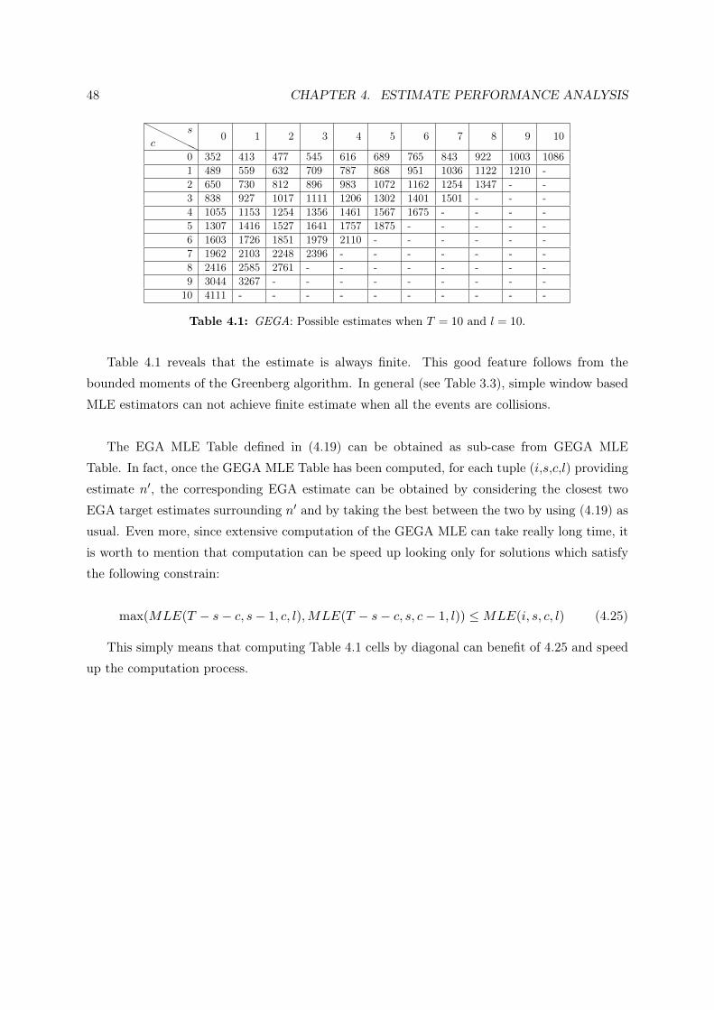
48 CHAPTER 4. ESTIMATE PERFORMANCE ANALYSIS
HHHHHHc
s 0 1 2 3 4 5 6 7 8 9 10
0 352 413 477 545 616 689 765 843 922 1003 10861 489 559 632 709 787 868 951 1036 1122 1210 -2 650 730 812 896 983 1072 1162 1254 1347 - -3 838 927 1017 1111 1206 1302 1401 1501 - - -4 1055 1153 1254 1356 1461 1567 1675 - - - -5 1307 1416 1527 1641 1757 1875 - - - - -6 1603 1726 1851 1979 2110 - - - - - -7 1962 2103 2248 2396 - - - - - - -8 2416 2585 2761 - - - - - - - -9 3044 3267 - - - - - - - - -10 4111 - - - - - - - - - -
Table 4.1: GEGA: Possible estimates when T = 10 and l = 10.
Table 4.1 reveals that the estimate is always finite. This good feature follows from the
bounded moments of the Greenberg algorithm. In general (see Table 3.3), simple window based
MLE estimators can not achieve finite estimate when all the events are collisions.
The EGA MLE Table defined in (4.19) can be obtained as sub-case from GEGA MLE
Table. In fact, once the GEGA MLE Table has been computed, for each tuple (i,s,c,l) providing
estimate n′, the corresponding EGA estimate can be obtained by considering the closest two
EGA target estimates surrounding n′ and by taking the best between the two by using (4.19) as
usual. Even more, since extensive computation of the GEGA MLE can take really long time, it
is worth to mention that computation can be speed up looking only for solutions which satisfy
the following constrain:
max(MLE(T − s− c, s− 1, c, l),MLE(T − s− c, s, c− 1, l)) ≤MLE(i, s, c, l) (4.25)
This simply means that computing Table 4.1 cells by diagonal can benefit of 4.25 and speed
up the computation process.

4.4. GEGA BSE 49
4.4.1 Performance
The estimate provided by GEGA is biased. Figure 4.10 shows that the algorithm tends to
overestimate the real batch size. Anyway, the bias can be easily corrected since it is always really
near to the average value: the oscillations have very small amplitude. Increasing T reduces the
bias as well as the oscillations amplitude. Very small batch sizes (less than 20) show higher
oscillations compared to larger ones: this fact is negligible in practice since the oscillations are
too small to affect the estimate and are hidden by the rounding operation. Table 4.2 reports
the average bias φ(T ) as a function of T .
100 500 1000 1500 20001.07
1.0705
1.071
1.0715
1.072
1.0725
n
E[n
|n]/
n
T = 10
100 500 1000 1500 20001.0405
1.041
1.0415
1.042
1.0425
1.043
1.0435
n
E[n
|n]/
n
T = 20
100 500 1000 1500 2000
1.0296
1.0298
1.03
1.0302
1.0304
1.0306
n
E[n
|n]/
n
T = 30
101
102
103
1.03
1.035
1.04
1.045
1.05
1.055
1.06
1.065
1.07
1.075
n
E[n
|n]/
n
T = 10
T = 20
T = 30
Figure 4.10: GEGA: Estimate Bias. The first tree plots show the estimate expected value over the realbatch size for different T . Right below corner plot provides a summary in a log x-scale. Data reportedwere computed using formula (4.22).

50 CHAPTER 4. ESTIMATE PERFORMANCE ANALYSIS
The results where computed by averaging the bias estimate for batch sizes from 2 to 2000.
T φ(T )
10 0.072320 0.042230 0.0299
Table 4.2: GEGA: Average bias.
0 200 400 600 800 1000 1200 1400 1600 1800 20000.07
0.08
0.09
0.1
0.11
0.12
0.13
0.14
0.15
0.16
0.17
0.18
0.19
0.2
0.21
0.22
0.23
0.24
0.25
Exp
ecte
dN
orm
aliz
edA
bso
lute
Err
or
n
T = 30, nT = 30, nT = 10, nT = 10, nT = 20, nT = 20, nT = 100, nT = 100, n
Figure 4.11: GEGA: biased/unbiased absolute normalized estimate error. The plot presents e(n) ande(n) for different T .
Estimate bias can be corrected by considering n =n
φ(T ) + 1. We will see that in this way
we get higher quality estimate.
To measure the performance of the proposed estimation method, we define the normalized
absolute estimate error as
e(n) =|n− n|n
. (4.26)
In the same manner we can define e(n). The parameter T is implicitly present in (4.26). Figure

4.4. GEGA BSE 51
4.11 shows that the bias-corrected estimate performs better than the biased estimate for any
batch size and T . Furthermore, you can notice that the error is independent of the batch size.
0 20 40 60 80 100 1201
2
3
4
5
6
7
T
kMinimum T to achieve accuracy k
n = 10
n = 102
n = 103
Figure 4.12: GEGA: Minimum T to achieve error coefficient lower than k with θ = 0.99
0 5 10 15 20 25 30 35 40 45 50 55 60 65 70 75 80 85 90 95 1001051101151201.2
1.3
1.4
1.5
1.6
1.7
1.8
1.9
2
2.1
2.2
T
k
Minimum T to achieve accuracy k : Detai l ed View
n=10
n=100
n=1000
Figure 4.13: GEGA: Minimum T to achieve error coefficient lower than k with θ = 0.99 , detailed view
Results presented in Figures 4.12 and 4.13 show that the accuracy in the estimate grows
as T increases and it is independent of the batch size when the batch size is not too small
(e.g.: n = 10). In fact, for very small batch sizes, the error coefficient k shows a descending
steps trend since the probability distribution is discrete and the adopted algorithm performs
rounding operations. Furthermore, it is important to mention that T allows the user to choose
estimate accuracy easily, without caring about the batch size. In other words, if we require a
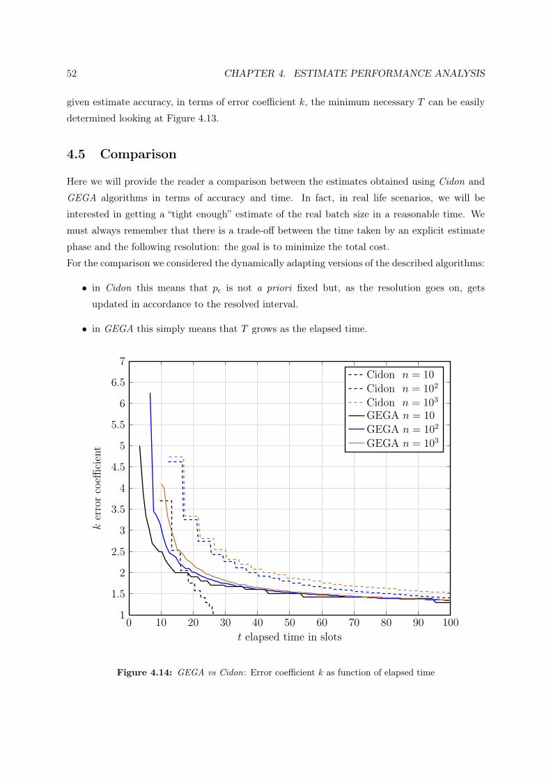
52 CHAPTER 4. ESTIMATE PERFORMANCE ANALYSIS
given estimate accuracy, in terms of error coefficient k, the minimum necessary T can be easily
determined looking at Figure 4.13.
4.5 Comparison
Here we will provide the reader a comparison between the estimates obtained using Cidon and
GEGA algorithms in terms of accuracy and time. In fact, in real life scenarios, we will be
interested in getting a “tight enough” estimate of the real batch size in a reasonable time. We
must always remember that there is a trade-off between the time taken by an explicit estimate
phase and the following resolution: the goal is to minimize the total cost.
For the comparison we considered the dynamically adapting versions of the described algorithms:
• in Cidon this means that pε is not a priori fixed but, as the resolution goes on, gets
updated in accordance to the resolved interval.
• in GEGA this simply means that T grows as the elapsed time.
0 10 20 30 40 50 60 70 80 90 1001
1.5
2
2.5
3
3.5
4
4.5
5
5.5
6
6.5
7
dydx
= −1.58
t elapsed time in slots
kerrorcoeffi
cient
Cidon n = 10
Cidon n = 102
Cidon n = 103
GEGA n = 10
GEGA n = 102
GEGA n = 103
Figure 4.14: GEGA vs Cidon: Error coefficient k as function of elapsed time

4.5. COMPARISON 53
In Figure 4.14 we try to answer the question: “When time t is elapsed, what is the accuracy
of the estimate?”. We considered the average running time for both the algorithms to provide
a meaningful and as fair as possible comparison: in GEGA t ≈ log(n) + T , in Cidon t ≈ npεC.
Figure 4.14 shows the minimum k for which θk in (4.8) is greater than or equal to 0.99. You
can notice that the GEGA algorithm, since it provides always a finite estimate, gives a bound
on the accuracy after just ≈ log2 n slots: as soon as phase 1 ends. Therefore, it results faster
than Cidon in providing the first bound for any batch size. Considering n = 10 in the Figure as
an index of the behavior for very small batch sizes, you can see that initially GEGA estimate is
more accurate than Cidon but later, for k smaller than two, Cidon takes less time. For larger
sizes (n = 100 and n = 1000) GEGA achieves accuracy k = 2 in about the half of the time
taken by Cidon , and k = 1.5 saving about 40% of time.
In general, we can say that GEGA performs great for middle-large batch sizes when we
require n to be, with high probability, in the intervaln
k≤ n ≤ kn with 1.5 ≤ k ≤ 2.

Conclusions
The final goal of this work was to investigate The Batch Size Estimate Problem in order
to develop, if possible, innovative techniques to solve the problem. Hence, we studied and
characterized both the Batch Size Estimate and some of the Batch Resolution Algorithms to
understand in what measure the estimate can influence, and hopefully speedup, the resolution
process. There are two possible ways to approach the matter: on one hand you can perform
an explicit estimate phase, followed by a resolution one, on the other hand, you can choose to
combine the two together. This second option is usually the case in window based scenarios where
the result of the resolution is used to preform an estimate and where estimate and resolution
processes coincide. Window based approach is really efficient when we have a good knowledge
of the batch multiplicity but has the disadvantage that performs really poor when the batch size
is different from the expected one. In fact, communication costs are reduced due to deferred
feedback but, at the same time, a wrong estimate of the multiplicity results in really poor
resolution performance. The big open problem of this approach is how to determine the size of
the initial window. A large window results in good estimate and resolution of a possibly large
amount of nodes but suffers poor performance if the batch to solve is much smaller than the
windows size (empty slots) or much larger (collisions). Using GEGA is a great choice in this
scenario to determine the batch size in terms of operational range.
The main advantages of GEGA are:
• Speed. In fact, for a wide range of minimum required accuracies and batch sizes, it is
faster than any other estimate algorithm known to us.
• Ability to adapt to any batch size. In fact, the time required by the algorithm depends
mostly on the user required accuracy and is quite independent of the real batch size
(logarithmic addictive term).
• Estimate accuracy can be considered independent of the batch size.
However, there are also some limitation to the proposed estimate scheme:
• It is not able to achieve arbitrary precision in the estimate;
55

56 CHAPTER 4. ESTIMATE PERFORMANCE ANALYSIS
• When looking for a really tight (almost exact) estimate, other estimate techniques are
faster.
Therefore we suggest to adopt it to:
• provide an initial estimate of the batch size which can be further refined using other
techniques or that can be used to speedup dynamically estimating resolution processes.
• provide an estimate for algorithms that are “robust” in terms of resolution efficiency: their
performance degrades smoothly when estimated batch size differs, but not too much, from
the real one (e.g. m Groups Splitting).
Understanding in details how to balance the estimate overhead with the improved resolution
efficiency depends on the applied BRA and goes beyond the goals of this work. Just to provide
you an idea on how things work, referring, as an example, to the m Groups Split in the CSMA
scenario described in Section 2.1.4 we have that, following the notations used throughout this
work, if estimate is within the interval nk ≤ n ≤ kn, maximum performance loss is below 3%
when k = 1.5 and 7% when k = 2. Therefore, considering the estimate overhead and choosing
the required accuracy in function of the batch size, using GEGA results convenient compared
to oblivious resolution (MBT, no estimate performed) when the batch size is larger than 30-70.

Appendix A
A.1 Probability
This section reviews basic probability theory notions used in this work.
Chebyshev’s inequality
Let X be a random variable with expected value µ and finite variance σ2. Then for any real
number k > 0,
Pr(|X − µ| ≥ k) ≤ σ2
k2(A.1)
Binomial Distribution
The binomial distribution is the discrete probability distribution of the number of successes in a
sequence of n independent yes/no experiments, each of which yields success with probability p.
In general, let a random variable K = B(n, p) be a binomial distribution with parameters n
and p. The probability of getting exactly k successes in n trials is given by the probability mass
function:
f(k;n, p) = Pr(K = k) =(n
k
)pk(1− p)n−k (A.2)
for k = 0, 1, . . . , n, where(n
k
)=
n!k!(n− k)!
.
The cumulative distribution function can be expressed as:
F (k;n, p) = Pr(K ≤ k) =bkc∑i=0
(n
i
)pi(1− p)n−i. (A.3)
The first and second moments are respectively given by:
E[K] = np (A.4)
and
57

58 APPENDIX A. APPENDIX
V ar[K] = np(1− p). (A.5)
Normal Approximation
If n is large enough, then the skew of the distribution is not too great. In this case, if a suitable
continuity correction1 is used, then an excellent approximation to B(n, p) is given by the normal
distribution N (np, np(1− p))The approximation generally improves as n increases and is better when p is not near to 0 or 1.
Various rules of thumb may be used to decide whether n is large enough, and p is far enough
from the extremes of zero or unity: One rule is that both np and n(1− p) must be greater than
5. However, the specific number varies from source to source, and depends on how good an
approximation one wants; some sources give 10. Another easy rule is that np(1− p) ≥ 10.
Poisson Approximation
The binomial distribution converges towards the Poisson distribution as the number of trials goes
to infinity while the product np remains fixed. Therefore the Poisson distribution with parameter
λ = np can be used as an approximation to B(n, p) of the binomial distribution if n is sufficiently
large and p is sufficiently small. According to two rules of thumb, this approximation is good if
n ≥ 20 and p ≤ 0.05, or if n ≥ 100 and np ≤ 10.
Numerical Computation
When n is large and p small, the numerical computation of the probability density function and
cumulative distribution function show to be problematic if trivially computed by definition (n!
is huge).
The following trick can be used for the computation when 0 < k < n:
f(k;n, p) = Pr(K = k) = elog(
n!k!(n− k)!
pk(1− p)n−k)= eφ, (A.6)
where
φ =n∑
i=k+1
log i−n−k∑i=1
log i+ k log p+ (n− k) log(1− p). (A.7)
1when approximating a discrete random variable K using a continuos one X, then Pr(K ≤ k) = Pr(K <k + 1) ≈ Pr(X ≤ k + 1/2)

A.2. BINARY TREES PERFORMANCE SUMMARY 59
Poisson Distribution
In probability theory and statistics, the Poisson distribution is a discrete probability distribution
that expresses the probability of a number of events occurring in a fixed period of time if these
events occur with a known average rate and independently of the time since the last event.
If the expected number of occurrences in this interval is λ, then the probability that there are
exactly k occurrences (k being a non-negative integer, k = 0, 1, 2, . . .) is equal to
f(k;λ) =λke−λ
k!(A.8)
Normal Distribution
Normal distribution is denoted as N (µ, σ2) where, as usual, µ identifies the mean and σ2 the
variance. The probability density function is defined as follows:
f(x;µ, σ2) =1√
2πσ2e−(x− µ)2
2σ2 (A.9)
A.2 Binary Trees Performance Summary
The following tables report the expected cost Ln in slots to solve a batch of given size n using
BT, MBT, and CMBT. Performance reports in Chapter 2 plot these data.
Table A.1: Basic Binary Tree: Performance report
LBT2 = 5.0000 LBT3 = 7.6667 LBT4 = 10.5238 LBT5 = 13.4190 LBT6 = 16.3131LBT7 = 19.2009 LBT8 = 22.0854 LBT9 = 24.9690 LBT10 = 27.8532 LBT11 = 30.7382LBT12 = 33.6238 LBT13 = 36.5096 LBT14 = 39.3955 LBT15 = 42.2812 LBT16 = 45.1668LBT17 = 48.0522 LBT18 = 50.9375 LBT19 = 53.8227 LBT20 = 56.7078 LBT21 = 59.5930LBT22 = 62.4783 LBT23 = 65.3636 LBT24 = 68.2489 LBT25 = 71.1344 LBT26 = 74.0198
Table A.2: Modified Binary Tree: Performance report with p = 0.5
LMBT2 = 4.5000 LMBT
3 = 7.0000 LMBT4 = 9.6429 LMBT
5 = 12.3143 LMBT6 = 14.9848
LMBT7 = 17.6507 LMBT
8 = 20.3140 LMBT9 = 22.9768 LMBT
10 = 25.6399 LMBT11 = 28.3036
LMBT12 = 30.9678 LMBT
13 = 33.6322 LMBT14 = 36.2966 LMBT
15 = 38.9609 LMBT16 = 41.6251
LMBT17 = 44.2892 LMBT
18 = 46.9531 LMBT19 = 49.6170 LMBT
20 = 52.2809 LMBT21 = 54.9448
LMBT22 = 57.6087 LMBT
23 = 60.2727 LMBT24 = 62.9367 LMBT
25 = 65.6008 LMBT26 = 68.2649
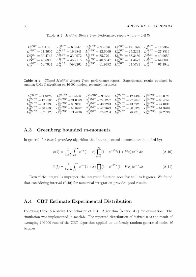
60 APPENDIX A. APPENDIX
Table A.3: Modified Binary Tree: Performance report with p = 0.4175
LMBT2 = 4.4143 LMBT
3 = 6.8847 LMBT4 = 9.4826 LMBT
5 = 12.1078 LMBT6 = 14.7352
LMBT7 = 17.3605 LMBT
8 = 19.9841 LMBT9 = 22.6069 LMBT
10 = 25.2293 LMBT11 = 27.8519
LMBT12 = 30.4745 LMBT
13 = 33.0972 LMBT14 = 35.7201 LMBT
15 = 38.3430 LMBT16 = 40.9659
LMBT17 = 43.5889 LMBT
18 = 46.2118 LMBT19 = 48.8347 LMBT
20 = 51.4577 LMBT21 = 54.0806
LMBT22 = 56.7034 LMBT
23 = 59.3263 LMBT24 = 61.9492 LMBT
25 = 64.5721 LMBT26 = 67.1949
Table A.4: Clipped Modified Binary Tree: performance report. Experimental results obtained byrunning CMBT algorithm on 10 000 random generated instances.
LCMBT2 = 4.3423 LCMBT
3 = 6.5558 LCMBT4 = 9.3585 LCMBT
5 = 12.1492 LCMBT6 = 15.0521
LCMBT7 = 17.9785 LCMBT
8 = 21.0389 LCMBT9 = 24.1297 LCMBT
10 = 27.2045 LCMBT11 = 30.4554
LCMBT12 = 33.6398 LCMBT
13 = 36.9191 LCMBT14 = 40.2243 LCMBT
15 = 43.5920 LCMBT16 = 47.0131
LCMBT17 = 50.4536 LCMBT
18 = 53.8787 LCMBT19 = 57.2679 LCMBT
20 = 60.8329 LCMBT21 = 64.3700
LCMBT22 = 67.8123 LCMBT
23 = 71.4436 LCMBT24 = 75.0234 LCMBT
25 = 78.7210 LCMBT26 = 82.2599
A.3 Greenberg bounded m-moments
In general, for base b greenberg algorithm the first and second moments are bounded by:
φ(b) =1
log b
∫ ∞0e−x(1 + x)
∞∏k=1
(1− e−bkx(1 + bkx))x−2 dx (A.10)
Φ(b) =1
log b
∫ ∞0e−x(1 + x)
∞∏k=1
(1− e−bkx(1 + bkx))x−3 dx (A.11)
Even if the integral is improper, the integrand function goes fast to 0 as k grows. We found
that considering interval (0,40) for numerical integration provides good results.
A.4 CBT Estimate Experimental Distribution
Following table A.5 shows the behavior of CBT Algorithm (section 3.1) for estimation. The
simulation was implemented in matlab. The reported distribution of n fixed n is the result of
averaging 100 000 runs of the CBT algorithm applied on uniformly random generated nodes id
batches.

A.4. CBT ESTIMATE EXPERIMENTAL DISTRIBUTION 61
Table A.5: Experimentally computed CBT Estimate Distributon. Table 1/3
n n : 2 4 8 16 32 64 128 256 512 1024 20482 0.499 0.253 0.125 0.061 0.031 0.015 0.007 0.004 0.002 9e-04 4e-044 0.189 0.303 0.225 0.133 0.072 0.038 0.020 0.010 0.005 0.0028 0.055 0.212 0.261 0.201 0.126 0.071 0.037 0.019 0.009 0.005
16 8e-04 0.070 0.209 0.252 0.197 0.125 0.070 0.038 0.019 0.01032 0.003 0.075 0.213 0.249 0.195 0.123 0.069 0.037 0.01864 0.004 0.077 0.208 0.250 0.193 0.124 0.069 0.037128 0.005 0.081 0.208 0.247 0.191 0.123 0.069256 2e-05 0.006 0.079 0.209 0.246 0.193 0.123512 0.005 0.081 0.207 0.245 0.1931024 0.005 0.080 0.208 0.2452048 2e-05 0.005 0.080 0.2094096 1e-05 0.006 0.0828192 1e-05 0.00616384 2e-0532768
Table A.5: Experimentally computed CBT Estimate Distributon. Table 2/3
n n : 4096 8192 16384 32768 216 217 218 219 220 221 222
2 2e-04 1e-04 1e-04 1e-054 0.001 5e-04 3e-04 1e-04 6e-05 4e-05 2e-05 1e-058 0.002 0.001 6e-04 3e-04 9e-05 8e-05 4e-05 1e-05
16 0.005 0.003 0.001 6e-04 3e-04 2e-04 6e-05 2e-05 2e-0532 0.009 0.005 0.003 0.001 6e-04 3e-04 1e-04 1e-04 6e-05 1e-05 1e-0564 0.019 0.009 0.005 0.002 0.001 7e-04 3e-04 7e-05 4e-05 2e-05128 0.037 0.019 0.010 0.005 0.003 0.001 5e-04 4e-04 2e-04 5e-05 4e-05256 0.068 0.038 0.019 0.009 0.005 0.002 0.001 6e-04 3e-04 6e-05 8e-05512 0.123 0.071 0.037 0.019 0.010 0.005 0.002 0.001 6e-04 3e-04 2e-04
1024 0.193 0.122 0.070 0.037 0.019 0.010 0.005 0.002 0.001 6e-04 2e-042048 0.246 0.194 0.123 0.068 0.037 0.019 0.010 0.005 0.002 0.001 6e-044096 0.210 0.246 0.193 0.121 0.068 0.037 0.019 0.009 0.004 0.003 0.0018192 0.080 0.208 0.247 0.192 0.123 0.070 0.037 0.019 0.009 0.005 0.00216384 0.006 0.080 0.208 0.247 0.192 0.123 0.069 0.037 0.019 0.010 0.00532768 0.006 0.079 0.209 0.248 0.194 0.122 0.069 0.036 0.019 0.010

62 APPENDIX A. APPENDIX
Table A.5: Experimentally computed CBT Estimate Distributon. Table 3/3
n n : 223 224 225 226 227 228 229 230 231 232
248
1632 1e-0564 2e-05 1e-05128 4e-05 1e-05256 4e-05 1e-05 2e-05 1e-05512 7e-05 2e-05 1e-05 3e-05 1e-051024 2e-04 1e-04 4e-05 2e-05 1e-052048 3e-04 1e-04 3e-05 3e-05 3e-05 3e-054096 6e-04 3e-04 9e-05 7e-05 1e-058192 0.001 8e-04 3e-04 2e-04 8e-05 7e-05 2e-05 3e-05 1e-0516384 0.002 0.001 6e-04 3e-04 1e-04 1e-04 4e-0532768 0.005 0.002 0.001 6e-04 3e-04 2e-04 1e-04 1e-05 2e-05 1e-05
A.5 Greenberg Estimate Distribution
In following table A.6 we report how the end up probability (equation 4.16) is distributed among
slots given a batch of size n. Column “n” lists the considered batch sizes. n is the resulting
estimation (without corrections) when ending up in the underneath slot.
For sake of simplicity considered values are all powers of 2.
Datas presented were post-processed to become more accessible:
• values above 10−3 are reported in format (’%1.3f ’);
• values below 10−12 are not presented since are tight close to 0.
• other values are presented in exponential notation and rounded to the first meaningful
digit (’%1.e’)
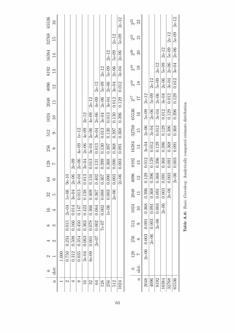
n2
48
1632
6412
825
651
210
2420
4840
9681
9216
384
3276
865
536
nslot:
12
34
56
78
910
1112
1314
1516
11.00
02
0.75
00.23
40.01
52e-04
1e-06
9e-10
40.31
20.50
80.16
60.01
43e-04
2e-06
2e-09
80.03
50.35
40.45
00.14
70.01
33e-04
2e-06
4e-09
1e-12
163e-04
0.06
30.36
30.42
20.13
80.01
33e-04
2e-06
4e-09
2e-12
328e-09
0.00
10.07
80.36
60.40
90.13
40.01
33e-04
2e-06
4e-09
2e-12
642e-07
0.00
20.08
40.36
70.40
20.13
10.01
33e-04
2e-06
4e-09
2e-12
128
7e-07
0.00
20.08
80.36
70.39
90.13
00.01
33e-04
2e-06
5e-09
2e-12
256
1e-06
0.00
30.09
00.36
80.39
70.13
00.01
33e-04
2e-06
5e-09
2e-12
512
2e-06
0.00
30.09
00.36
80.39
70.13
00.01
23e-04
2e-06
5e-09
2e-12
1024
2e-06
0.00
30.09
10.36
80.39
60.12
90.01
23e-04
2e-06
5e-09
2e-12
n128
256
512
1024
2048
4096
8192
16384
32768
65536
217
218
219
220
221
222
nslot:
78
910
1112
1314
1516
1718
1920
2122
2048
2e-06
0.003
0.091
0.368
0.396
0.129
0.012
3e-04
2e-06
5e-09
2e-12
4096
2e-06
0.003
0.091
0.368
0.396
0.129
0.012
3e-04
2e-06
5e-09
2e-12
8192
2e-06
0.003
0.091
0.368
0.396
0.129
0.012
3e-04
2e-06
5e-09
2e-12
16384
2e-06
0.003
0.091
0.368
0.396
0.129
0.012
3e-04
2e-06
5e-09
2e-12
32768
2e-06
0.003
0.091
0.368
0.396
0.129
0.012
3e-04
2e-06
5e-09
2e-12
65536
2e-06
0.003
0.091
0.368
0.396
0.129
0.012
3e-04
2e-06
5e-09
2e-12
Tab
leA
.6:Basic
Greenberg:Ana
lytically
compu
tedestimatedistribu
tion
63

64 APPENDIX A. APPENDIX
A.6 GEGA
From the table below you can see how Table 4.1 changes when T = 20. The density of target
estimates near the “right” one increases and also the difference between the maximum and
minimum allowed value gets larger.H
HH
HHH
cs
01
23
45
67
89
1011
1213
1415
1617
1819
20
0232
265300
336373
411451
491531
573615
658701
744788
832877
922967
10121058
1304
340378
417457
498539
582625
668712
756801
846892
938984
10301077
1124-
2383
423464
505548
591635
679724
769815
861908
9551002
10491097
11451193
--
3471
513556
600645
690736
782829
876924
9721020
10691118
11671217
1266-
--
4565
610656
702749
796844
892941
9901040
10901140
11901241
12921343
--
--
5667
714762
811860
909959
10091060
11111163
12151267
13191372
1425-
--
--
6776
826876
927978
10291082
11341187
12401294
13481402
14571511
--
--
--
7893
945997
10501104
11581212
12671322
13781434
14901547
1604-
--
--
--
81018
10731128
11831239
12961353
14101468
15261584
16431703
--
--
--
--
91153
12101268
13261385
14441504
15641624
16861747
1809-
--
--
--
--
101298
13581419
14801542
16051667
17311795
18591924
--
--
--
--
--
111455
15191583
16481714
17801846
19141981
2050-
--
--
--
--
--
121628
16951763
18321902
19722044
21152188
--
--
--
--
--
--
131817
18901963
20372112
21872264
2342-
--
--
--
--
--
--
142030
21082187
22672348
24312515
--
--
--
--
--
--
--
152271
23562443
25322621
2713-
--
--
--
--
--
--
--
162551
26472744
28442945
--
--
--
--
--
--
--
--
172888
29983111
3227-
--
--
--
--
--
--
--
--
183314
34483587
--
--
--
--
--
--
--
--
--
193907
4085-
--
--
--
--
--
--
--
--
--
204918
--
--
--
--
--
--
--
--
--
--
Table A.7: GEGA: Possible estimates when T = 20 and l = 10
Bibliography
[1] Wen-Tzu Chen, An Accurate Tag Estimate Method for Improving the Performance of
an RFID Anti-collision Algorithm Based on Dynamic Frame Length ALOHA, IEEE
Transactions on Automation Science and Engineering, Vol. 6, No. 1, January 2009, 9-15
[2] Peter Popovski, Frank H.P. Fitzek, Ramjee Prasad, A Class of Algorithms for Collision
Resolution with Multiplicity Estimation, Springer, Algorithmica, Vol. 49, No. 4, December
2007, 286-317
[3] Murali Kodialam, Thyaga Nandagopal, Fast and Reliable Estimation Schemes in RFID
Systems, MobiCom ’06: Proceedings of the 12th annual international conference on Mobile
computing and networking, ACM , September 2006, 322-333
[4] K. Jamieson, H. Balakrishnan, and Y. C. Tay, Sift: a MAC protocol for event-driven wireless
sensor networks, Proc. 3rd European Workshop on Wireless Sensor Networks, Zurich,
Switzerland, February 2006, 260–275
[5] Dimitri Bestekas, Robert Gallager, Data Networks, 2nd Ed., Prentice-Hall, New Jersey,
1992.
[6] Raphael Rom, Moshe Sidi, Multiple Access Protocols: Performance and analysis, Springer
Verlag, 1990. Freely available online for not commercial purposes.
[7] Israel Cidon, Moshe Sidi, Conflict Multiplicity Estimation and Batch Resolution Algorithms,
IEEE Transactions On Information Theory, Vol. 34, No. 1, January 1988, 101-110
[8] Albert G. Greenberg, Philippe Flajolet, Richard E. Ladner, Estimating the Multiplicities of
Conflicts to Speed Their Resolution in Multiple Access Channels, Journal of the Association
for Computing Machinery, Vol 34, No. 2, April 1987, 289-325
[9] J.L Massey, Collision-Resolution Algorithms and Random-Access Communications,
Springer, CISM Courses and Lectures, Vol. 265, Berlin 1981, 73–137
65

66 BIBLIOGRAPHY
[10] J.I. Capetanakis, Tree algorithms for packet broadcast channels, IEEE Transactions On
Information Theory, Vol. 25, No. 5, September 1979, 505-515
[11] B. S. Tsybakov, V. A. Mikhailov, Slotted multiaccess packet broadcasting feedback channel,
Probl. Peredachi Inform., Vol. 13, December 1978, 32-59
[12] J.I. Capetanakis, A protocol for resolving conflicts on ALOHA channels, Abstracts of
Papers, IEEE Int. Symp. Info. Th., Ithaca, New York, October 1977, 122-123