Questioni di Economia e Finanza(Occasional Papers)

Incentives to local public service provision: an evaluation of Italy’s Obiettivi di Servizio

by Guglielmo Barone, Guido de Blasio, Alessio D’Ignazio and Andrea Salvati

Num

ber 388S

epte

mb

er 2

017

Questioni di Economia e Finanza(Occasional papers)

Number 388 – September 2017

Incentives to local public service provision: an evaluation of Italy’s Obiettivi di Servizio

by Guglielmo Barone, Guido de Blasio, Alessio D’Ignazio and Andrea Salvati

The series Occasional Papers presents studies and documents on issues pertaining to

the institutional tasks of the Bank of Italy and the Eurosystem. The Occasional Papers appear

alongside the Working Papers series which are specifically aimed at providing original contributions

to economic research.

The Occasional Papers include studies conducted within the Bank of Italy, sometimes

in cooperation with the Eurosystem or other institutions. The views expressed in the studies are those of

the authors and do not involve the responsibility of the institutions to which they belong.

The series is available online at www.bancaditalia.it .

ISSN 1972-6627 (print)ISSN 1972-6643 (online)

Printed by the Printing and Publishing Division of the Bank of Italy

INCENTIVES TO LOCAL PUBLIC SERVICE PROVISION: AN EVALUATION OF ITALY’S OBIETTIVI DI SERVIZIO

by Guglielmo Barone, Guido de Blasio*, Alessio D’Ignazio§ and Andrea Salvati

Abstract

Set up by the Italian central government and implemented in the areas of the country that are lagging behind, Obiettivi di Servizio is an innovative scheme designed to encourage local authorities to reach given targets for public service provision in the areas of education, childcare and elderly care, waste management, and water supply. The paper makes an econometric evaluation of the scheme’s effectiveness. Our findings suggest that the program was only partially successful, with considerable differences across regions and targets. An important driver of effectiveness was local institutional quality, while some features of the scheme – such as the common targets and the distribution of the pledges – might have impacted negatively on local performance. We also find signs of displacement effects: local authorities involved in the program might have concentrated on the targets to the detriment of other local public services.

JEL Classification: C21, H75, H76. Keywords: public service provision, incentives.

Contents

1. Introduction .......................................................................................................................... 5

2. Program description ............................................................................................................. 7

2.1 The program ................................................................................................................. 7

2.2 Descriptive analysis ...................................................................................................... 9

3. Estimating the impact of the ODS ..................................................................................... 11

4. Drivers of effectiveness ..................................................................................................... 13

5. Unwanted consequences .................................................................................................... 15

6. Conclusions ........................................................................................................................ 16

References .............................................................................................................................. 19

Tables and figures................................................................................................................... 21

_______________________________________ Bank of Italy, Economic Research Unit, Florence Branch and RCEA (guglielmo.barone@bancaditalia.it); *

Bank of Italy, Directorate General for Economics, Statistics and Research (guido.deblasio@bancaditalia.it); § Bank of Italy, Directorate General for Economics, Statistics and Research (alessio.dignazio@bancaditalia.it); Rice University, Houston, Texas (andrea.salvati@rice.edu).

5

1. Introduction1

In this paper we carry out an econometric evaluation of an incentive scheme intended to enhance

the provision of local public services (LPS). The scheme, named Obiettivi di Servizio (ODS), was

rolled out in Italy in the 2007-13 EU programming cycle. It is a principal-agent scheme in which

central government (the principal) tries to encourage local authorities (the agents) to achieve certain

goals. The scheme applies to the administrative bodies of the eight regions of southern Italy, the

area of the country lagging behind. ODS involves three building blocks: targets, transparency, and

money. The targets are eleven quantitative indicators set by central government and relating to the

quality and quantity of some selected categories of LPS. Transparency is sought through a public

assessment exercise that monitors the progress of each region towards the attainment of the targets

and discloses the results to the general public. Money refers to the financial reward (€3 billion)

allocated to good performing regions.

To estimate the impact of the ODS on the provision of local public services we employ a

difference-in-differences (DID) approach, using as control group the twelve Italian regions of the

Centre and North that did not take part in the program. After estimating the treatment effects, we

look for region- or indicator-specific factors that may be systematically associated with

performance under the ODS, such as the quality of local institutions, the distance from the target,

and the financial rewards. We also consider whether the scheme had unintended consequences. For

instance, local authorities could have allocated efforts to strategically favour LPS’s involved in the

scheme over those not involved. Displacement might also have occurred within the LPS covered by

the ODS, favouring ODS targets over non-targeted indicators.

Our results show that the impact of the ODS was extremely heterogeneous across regions and

targets, and that a crucial driver of the effectiveness of the scheme was local institutional quality.

Moreover, some features of the incentive scheme, such as the equalization of targets across regions,

seem to have undermined the decentralized governance structure. We also find evidence of

displacement: in the transport sector, a key LPS not involved in the ODS, the treated authorities

performed relatively worse than those not part of the program. We also find similar displacement

1 We thank Paola Casavola, Paolo Sestito, Luigi Federico Signorini, Marco Tonello and seminar participants at the

Bank of Italy (Rome, 2016), ERSA (Wien, 2016), AIEL (Trento, 2016), LSE (London, 2016) and c.MET 05 (Ferrara,

2017) for comments and suggestions and Donato Milella for editorial assistance. The project was (partly) carried out

when Andrea Salvati was an intern at the Bank of Italy, Bologna Branch. The views and the opinions expressed in the

paper are those of the authors and do not necessarily correspond to those of the institutions they are affiliated with.

6

effects within the education sector when comparing performances covered by the ODS (concerning

early school-leavers and high-school competencies only) and those not covered.

Our study is linked to the literature on the assessment of incentive schemes for local government.

This literature mainly refers to the UK CPA, the Comprehensive Performance Assessment (Boyne

et al., 2009; Revelli, 2008 and 2010; and Lockwood and Porcelli, 2013). Other related papers are

Revelli (2006), who analyses the English SSPR (Social Service Performance Rating), Burgess et al.

(2010), who analyse the interplay between dissemination of information and performance in the

education sector (elaborating on the abolition of school league tables in Wales), and Besley et al.

(2009), who investigate the effect on patient waiting lists of the hospital star-rating regime in

England in 2001-05. More in general, our paper is connected with the literature on incentives in the

public sector. Propper and Wilson (2003) provide an overview of the issues involved in using

performance management schemes and explicitly refer to transparency-related incentives and

financial rewards. OECD (2009), Van Dooren et al. (2015), and Schumann (2016) discuss how to

use outcome indicators to improve policy, also with reference to regional policy.

Compared with existing studies, which refer mainly to the US and the UK, we consider the case of

Italy, a country with long-standing local differences in public service provision and an established

tradition of centralization in the public sector. Our findings might be useful for countries with

similar features (for instance, Southern European countries) that are also trying to enhance their

performance measures in the public sector. Our paper is also interesting from a slightly different

perspective: the incentive scheme experimented with the ODS will be replicated in many instances

with the EU programming cycle 2014-20 (under the heading of performance framework: see

McCann, 2015). Therefore, our study could be used to inform the incoming policy framework. Last

but not least, assessing the effectiveness of the ODS scheme might add evidence on the fiscal

federalism trade-off. Decentralization allows better matching of local idiosyncrasies, although local

ownership may magnify the power of local interest groups in setting the policy agenda, while the

provision of LPS could reflect the low quality of local institutions (see e.g. Faguet, 2004). In this

respect, providing local authorities with incentives to reach given targets for locally provided public

goods might be seen as a means of lessening the fiscal federalism trade-off (Joumard and Kongsrud,

2003).

The paper is structured as follows. The next section provides the institutional details of the ODS

and a descriptive analysis. Section 3 describes the identification framework and provides the DID

7

results. Section 4 documents the findings from our attempt to interpret the DID results in the light

of some underlying common explanations. Section 5 analyses the unwanted consequences of the

scheme. The last section concludes, proving some elements of policy relevance.

2. Program description

2.1 The program

The ODS incentive scheme was established in 2007 within the 2007-13 EU framework for cohesion

policy. Eight southern Italian regions – Abruzzo, Molise, Puglia, Campania, Basilicata, Calabria,

Sicily and Sardinia – were involved in the program (in our empirical exercise, they are the treated

units). Central government (the principal) fixed some quantitative targets for the treated regions (the

agents), relating to several LPS. Central government undertook to monitor and disclose progress

towards the targets and to give financial rewards to the agents that attained them. The remaining

Italian regions (twelve, from central and northern Italy) were not included in the scheme (they are

the control units). The incentive scheme was formally put in place in 2007, but the treated regions

had not finished preparing all the documentation needed to participate in the ODS until the end of

2008. This caused a delay of nearly one year in the actual implementation of the scheme.

Participation in the program was conditional on submitting a ‘strategic plan’ in which the local

authorities set out all the measures they would take in order to achieve the targets and set aside the

corresponding financing (from local, national, and EU sources). The final deadline for attainment of

the target was 2013.2

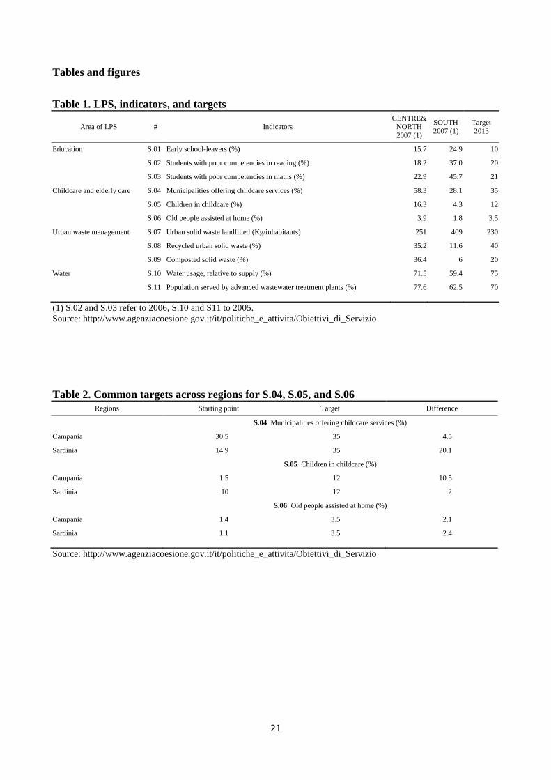
As reported in Table 1, ODS involved eleven outcome indicators (in what follows, we refer to each

indicator using the prefix ‘S’ followed by a number from 1 to 11) of the provision and quality of

LPS in the areas of a) education, b) childcare and elderly care, c) waste management, and d) water

supply. The Table also reports for each indicator the target fixed under the program and the (area

average) starting point in 2007, both in the South and (for comparison) in the Centre and North.

Gaps are huge and sometimes the actual 2007 figures for the central and northern regions compare

much better than the 2013 targets for the southern areas.

[Table 1]

2 The scheme also envisaged an intermediate deadline: a share of the financial reward was to be dispensed in 2009, in

proportion to the progresses made by the region in each indicator. The disbursement of the remaining part was entirely

contingent on attaining the final target in 2013.

8

Central government decided to restrict the aim of the policy to a relatively small number of targets

in order to focus the agents’ efforts on just few goals. Targets were common across regions (they

were based on the average value of the same indicators in either the central and northern regions of

Italy or in other EU or OECD countries, with the idea that these represented a minimum threshold).

As shown in Table 2 with reference to the indicators S.04-S.06 in the comparison between

Campania and Sardinia, the common target implies that the distance to fill can vary considerably.

Target S.04, referring to the percentage of regional municipalities offering childcare services, seems

to be quite within reach for Campania, as it has to fill a 4.5% gap over a seven-year period. On the

other hand, the distance Sardinia has to fill for the same indicator is 20.1%. However, the effort

required in the two cases is completely reversed for indicator S.05, referring to the percentage of

children in childcare in the region. The distance for S.06 – the share of old people assisted at home

– is instead similar for the two regions.

[Table 2]

The total amount of the financial reward was set at €3 billion (0.81% of the GDP of the treated

regions). Total funds were allocated uniformly across the four categories (€750 million each).

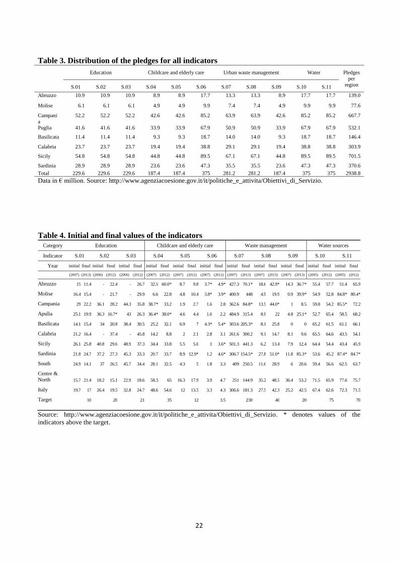
Within the same category, the targets might receive different financing shares (Table 3).

[Table 3]

For example, regarding the S.04-S.06 indicators it was decided to split the budget so that the two

targets for childcare got one quarter each and the target for elderly care had the remaining half. For

each target the distribution followed a criterion based on each region’s GDP and population level.

Sicily and Campania got the highest level of potential financial rewards, with respectively 21.9%

and 20.9% of the total amount, immediately followed by Puglia (16.6%), Sardinia (11.6%) and

Calabria (9.5%). The regions with the lowest amount of allocated rewards were Basilicata, Abruzzo

and Molise with 4.6%, 4.3% and 2.4% respectively. As explained, the amount of the financial

reward did not reflect the effort required of the local government to achieve the targets. It is also

important to note that the ODS rules require the funds attached to each indicator to be received

irrespective of the progress made in the other indicators.

The ODS framework underwent a number of changes over the years as far as the funds earmarked

by central government were concerned. First, the 2009 intermediate rewards, which were computed

9

according to the progress made up to then and set overall at €638 million, were never actually paid

to the regions because of political frictions caused by the change of central government in 2008 (the

new government was somehow reluctant to carry on the policy of its predecessor). Second, in 2011

the total amount of funds was reduced to €1,031.8 billion (without any change in the distribution

across regions and indicators) because of Italy’s increasing public finance difficulties at the time.

We discuss the issues raised by the reduction and postponement of part of the rewards in the final

section, arguing that, while a reward scheme is usually consistent, this is not the reason for the

unsatisfactory performance of the program.

The structure of the incentives was underpinned not only by the financial package. The idea was to

increase the local authorities’ accountability through public participation; by establishing easy-to-

measure targets and monitoring each region’s progress, it was hoped to involve the citizens and the

responsibility of the local élite. Central government set up a dedicated website to disclose

performances (http://www.agenziacoesione.gov.it/it/politiche_e_attivita/Obiettivi_di_Servizio). The

program received wide attention in the media, both national and local.

2.2 Descriptive analysis

To proceed with our analysis we needed to make all the eleven indicators comparable. Some of

them relate to a public good while others denote a public bad; moreover, they are often expressed in

different units as they refer to different public services. We use a transformed indicator �̃�𝑖𝑟𝑡that can

always be interpreted as a percentage with respect to the target. Specifically, for indicators S.04,

S.05, S.06, S.08, S.09, S.10 and S.11 (public goods) the transformation we use is given by the

following formula:

�̃�𝑖𝑟𝑡 =𝑦𝑖𝑟𝑡

𝑡𝑎𝑟𝑔𝑒𝑡𝑖× 100 (1)

where 𝑦𝑖𝑟𝑡 is the value of the indicator, �̃�𝑖𝑟𝑡 is its transformation, and subscripts 𝑖, 𝑟 and 𝑡 index the

indicator number, the region, and the year.

As for indicators S.01, S.02 and S.03 (public ‘bads’), the transformation is

�̃�𝑖𝑟𝑡 =100−𝑦𝑖𝑟𝑡

100−𝑡𝑎𝑟𝑔𝑒𝑡𝑖× 100 (2)

10

while for indicator S.07 (public bad), which, unlike S.01, S.02 and S.03, does not have an obvious

upper bound, we use

�̃�𝑖𝑟𝑡 =716−𝑦𝑖𝑟𝑡

716−𝑡𝑎𝑟𝑔𝑒𝑡𝑖× 100 (3)

where 716 is the highest observed value of per capita urban solid waste produced by the treated

regions from 1996 to 2013 (Tuscany in 2006, in kilograms).

Table 4 gives the initial and final values of the non-transformed indicators. As the table shows,

because of the features of the scheme (common targets fixed on the basis of central and northern or

international figures) some of the regions had already reached some of the targets before 2007 (the

target set for indicator S.06 had already been achieved by Abruzzo, Molise and Basilicata, the one

for indicator S.04 by Campania and Puglia, and the one for indicator S.11 by Molise, Campania and

Sardinia). At the end of period, the total number of targets attained increased sharply for some of

the regions. The most successful ones were Sardinia and Abruzzo, which attained seven and five

targets respectively, followed by Molise and Puglia with three, Basilicata and Campania with two,

and Sicily with only one, while none of the targets were achieved by Calabria.

[Table 4]

Although many targets had not yet been attained by the regions in 2013, the final scenario is one of

an overall reduction in the initial gaps. As shown in Figure 1, for almost all the indicators the mean

distance with the respective target had narrowed in 2013 with respect to 2007. The indicators that

recorded the best performance in terms of distance reduction were S.06 and S.09, which showed a

decrease in the initial distance of about 130 and 150 percentage points (pp) respectively and

therefore on average considerably exceeded the target. Indicators S.02, S.04 and S.07 saw large

average improvements as well, with a reduction of the mean initial gap of 67pp, 75pp and 84pp

respectively. A good reduction of the mean initial distance was also achieved for indicators S.03,

S.08 and S.11, which decreased by around 50-60pp. Finally, indicators S.01, S.05 and S.10

displayed the worst performance, with the first two showing a reduction in the initial distance of

about 20pp and the latter even an increase in the mean distance with respect to 2007 of about 12pp.

Another interesting analysis concerns the variability of the distance across regions and indicators.

An ANOVA exercise on the initial total variance indicates that 91% relates to between-indicator

11

variability while the remaining part stems from regions. The whisker plots on the bars of Figure 1

show the values of the standard deviations of the distances. The initial distances in 2007 were

heterogeneous across regions, especially for indicators S.04, S.06 and S.11, whose standard

deviations were even higher than their means. As regards the change in distance variability over

time, the scenario after the implementation of ODS was one of general divergence in the level of

public services provided across regions. The standard deviations of the transformed indicators S.02,

S.03, S.04, S.05, S.07, S.08, S.09 and S.10 all increased from 2007 to 2013, with changes ranging

from the 23pp of S.10 to a five-fold increase in the variability of the distance of S.09. The

remaining indicators S.01, S.06 and S.11, instead, showed a reduction in the variability of the

distances ranging from 8pp for S.01 to almost 33pp for S.11.

[Figure 1]

3. Estimating the impact of the ODS

The descriptive analysis suggests that during the period 2007-13 the southern regions of Italy

generally made improvements in the local public services covered by the scheme, even though the

progress was not uniform across regions and indicators. In the light of these results, the question is

whether such improvements were directly associated with the adoption of the ODS, or whether they

were instead due to a more general trend that was not related to the program.

In order to disentangle these two explanations, we compare changes in the indicators in the southern

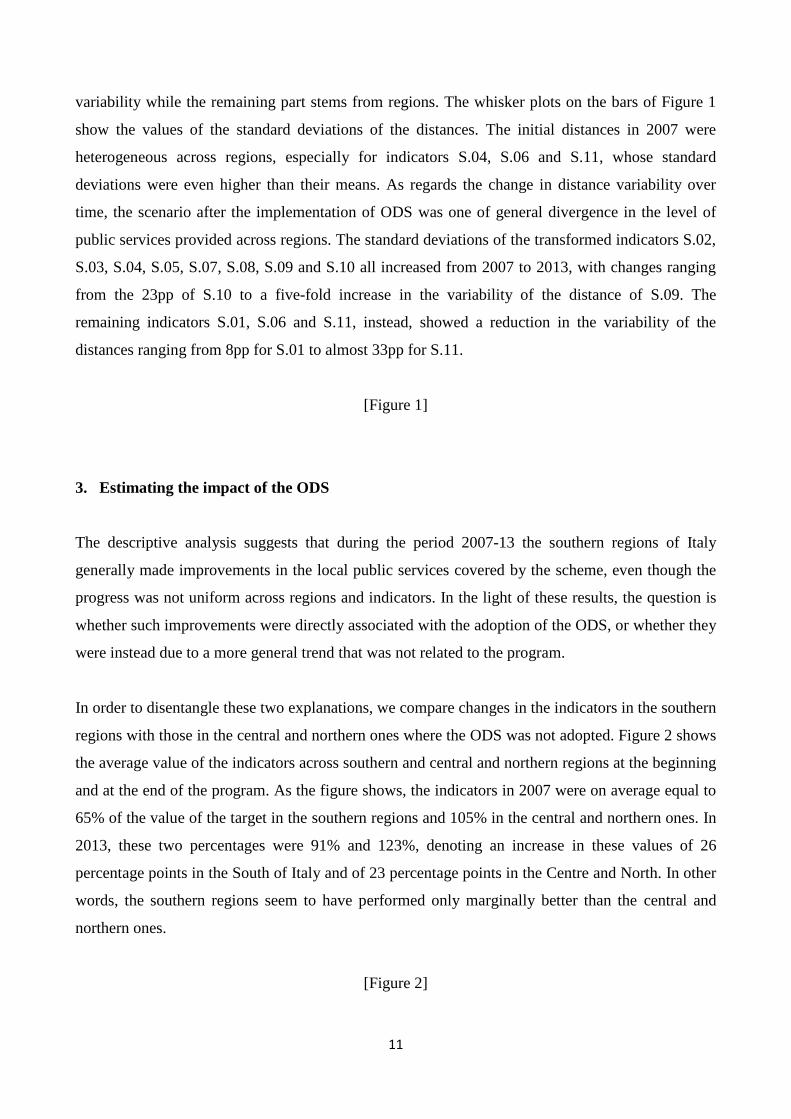
regions with those in the central and northern ones where the ODS was not adopted. Figure 2 shows

the average value of the indicators across southern and central and northern regions at the beginning

and at the end of the program. As the figure shows, the indicators in 2007 were on average equal to

65% of the value of the target in the southern regions and 105% in the central and northern ones. In

2013, these two percentages were 91% and 123%, denoting an increase in these values of 26

percentage points in the South of Italy and of 23 percentage points in the Centre and North. In other

words, the southern regions seem to have performed only marginally better than the central and

northern ones.

[Figure 2]

12

We propose an econometric exercise that is the formal counterpart of the evidence in Figure 2.

Namely, we use a DID approach in which the regions involved in the scheme are the treated units,

adopting as control group the twelve central and northern regions of Italy that were not treated. In

this way, we are able to control for possible trends common to all Italian regions and not related to

the policy. We consider the years from 2010 to 2013 as the treatment period because, as stated

above, the program effectively only started in 2009 and any action by the agents will reflect on the

outcome variables with some delay. The adoption of this econometric approach relies on the

assumption that indicator trends in the control regions represent a good counterfactual of the

treatment group in the hypothetical scenario in which the ODS scheme was not implemented.

Indeed, our analysis shows that this common trend assumption can be regarded as satisfied.3

Our starting point is the following estimating equation:

�̃�𝑟𝑖𝑡 = 𝑐𝑜𝑛𝑠𝑡𝑎𝑛𝑡 + 𝛿(𝑂𝐷𝑆𝑟 × 𝐷𝑡) + 𝜇𝑟 + 𝛾𝑖 + 𝜆𝑡 + 휀𝑟𝑡 (4)

Where the estimation is run on the pooled sample, r indicates the region, i the indicator, and t the

years;4 �̃�𝑟𝑖𝑡 is the transformed indicator;

5 𝑂𝐷𝑆𝑟 is a dummy variable that takes the value 1 for the

treated region and 0 otherwise; 𝐷𝑡 is a dummy variable that takes the value 1 if 𝑡 ≥ 2010 and 0

otherwise; 𝜇𝑟, 𝛾𝑖 and 𝜆𝑡 and are region, indicator and year fixed effects respectively; 휀𝑟𝑖𝑡is a random

disturbance. Our parameter of interest is the treatment effect 𝛿.

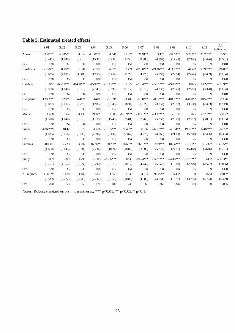
Our point estimate for 𝛿 is reported in the last row and last column of Table 5. The ODS program

had a weak negative effect on the outcome. However, the aggregate effect may mask heterogeneity

across regions and indicators. When we repeat our regression by region, it turns out that the

program encouraged a good performance in Sardinia, while it had a negative impact in Basilicata,

Calabria, Puglia and Sicily (Table 5, last column). In the other regions the effect is nil. Similarly,

breaking down the estimates by indicator suggests that the program was effective only for the

indicator S.01, while the impact on the indicators S.08 and S.09 was negative and significant (Table

5, last row). Again, aggregating along some dimension may obscure large heterogeneity, which we

3 In order to formally test for the common trend assumption, we focus on the seven-year pre-treatment period and re-run

regression (4) (data are available for indicators S.01, S.04, S,05, S.06, S.07, S.08 and S.09) using as a fake treatment

date the year 2006. The coefficient for the interaction (ODSr X Dt) is not statistically different from zero. 4 S1: 2004-2013; S2: 2000-2012; S3:2003-2012; S4:2004-2012; S5: 2004-2012; S6: 2001-2012; S7: 1996-2013; S8:

1996-2013; S9: 2001-2013; S10: 1987-2012; S11: 2005-2012. 5 Transformed indicators make interpretation easier. However, we also estimate regressions using non-transformed

indicators as a robustness exercise. The results (not reported but available upon request) mirror those of the model

estimated on transformed data in terms of both statistical significance and signs.

13

try to discover by re-estimating equation (4) for every single treated region and for each of the

eleven indicators. We perform in total 88 DID regressions. In the end we are left with 88 estimated

𝛿s. The remaining cells in Table 5 show that the ODS impact varies dramatically in both

significance and magnitude across both treated regions and indicators. In particular, the results

show that there are instances of positive (minimum at the 10% confidence level; 24 cases out of 88),

negative (32 cases at the same confidence level), and not statistically significant (22 cases) impacts

of ODS on the outcome variables. A common path does not emerge.

However, the econometric findings broadly confirm what emerged from the previous analysis.

Sardinia was the region where the ODS program was most effective. The performance of

Campania, instead, was slightly worse, with five positive treatment effects, four negative, and two

not statistically significant. Finally, all the remaining treated regions strongly underperformed,

especially Calabria and Sicily.

[Table 5]

4. Drivers of effectiveness

From our estimates of the previous section, effectiveness seems to be scattered across regions and

indicators. In this section we explore some of the reasons behind the marked heterogeneity of

estimated treatment effects. We look for region and region/indicator factors that might shape the

treatment effect by interacting them with the 𝑂𝐷𝑆𝑟 × 𝐷𝑡 term. These indicators are measured as

dummies taking the value of 1 for the treated regions above the median value of that specific

factor.6 In detail, we analyse the role of:

- The initial distance from the target (measured as 100 minus the value of the transformed

indicator in 2007; negative values are set equal to 0). The initial distance equals on average

36% of the value of the target and it ranges from 0 (target already achieved) to 100%. Under

the ODS setting, different targets may be rewarded by the same amount of money, even though

the efforts needed to attain them are actually different. Moreover, the funds attached to a single

target are received irrespective of the progress made with the other targets (see Section 2).

These features of the scheme may bring about substitution effects: the regional government

may concentrate its efforts on the closest, and thus easiest to reach, targets, while leaving aside

6 However, different specifications of the drivers will deliver very similar results.

14

the most difficult ones. This implies that a higher initial distance could be linked to a lower

impact of ODS on the indicator. Hence, the expected sign is negative.

- The financial reward set (initially) by the ODS scheme, which is the direct financial incentive

for the region to attain the target. As explained in Section 2, the financial reward for each target

reflects the distribution of the pledges across indicators within LPS categories and regional

GDP and population. In this analysis we use as regressor the ratio between reward and regional

GDP, rather than the raw monetary reward, in order to take into account regional size

heterogeneity (the value of the financial reward averages €33 million and ranges from €5

million to €89 million, while the reward-to-GDP ratio averages 0.092% with a standard

deviation of about 0.04%). For this variable, the expected sign of its interaction with the term is

positive.

- Areas displaying a lower quality of governance are generally associated with a misuse and

dissipation of public resources, which, in turn, may make public spending both less effective

and less efficient (Rajkumar and Swaroop, 2008; Gupta et al., 2002). Hence, such regions

might be less able to use resources to improve public services. For this reason, we expect local

institutional quality to be positively correlated to the estimated treatment effects. The proxy we

use is the European QoG Index (EQI) developed by the Quality of Governance Institute

(Charron et al., 2016), which is constructed through a large survey dataset on the level of

perceived corruption of institutions in 2010. The EQI for the southern regions is always lower

than that of their central and northern counterparts; however, within the South the variability is

also considerable, with a standard deviation equal to about one third of the absolute value of the

mean.

- Political alignment is relevant as long as the regional level depends financially on the central

level, as is the case in Italy. The main implication of this dependency is that central government

can channel more resources (over and above those relating to ODS) to politically aligned sub-

national governments in order to maintain political power, as documented also by Bracco et al.

(2015), Kang (2014), Rumi (2014), and Lema and Streb (2013). Since these financial resources

are fundamental for public expenditure on LPS, politically aligned regional governments could

have had some benefit from reaching the ODS targets. On the other hand, aligned regional

governments might receive extra money irrespective of their performance under the scheme.

Therefore, the expected sign is ambiguous. Political alignment is measured as the fraction of

15

the 2007-13 period in which the regional government was politically aligned with central

government. On average, regional governments were politically aligned for about 68% of the

total 2007-13 period, with minimum and maximum values of 44% and 89%.

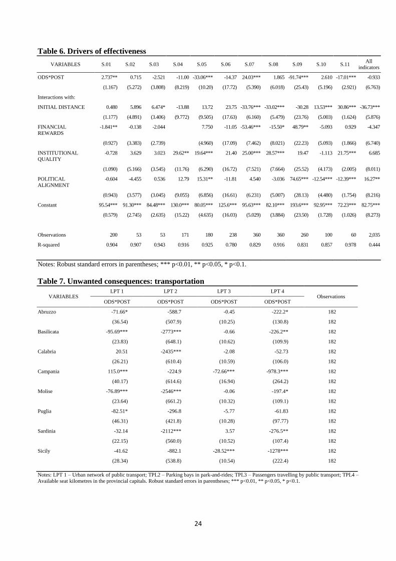
For the sake of brevity we show only the results with the pooled sample of treated regions (the

baseline is therefore the last row of Table 5). The results are reported in Table 6. We have also run

Eq. (5) for each specification (88 = 11 indicators X 8 regions), with findings pretty much in line

with those reported for the pooled sample. As a starting point, we also pooled data across indicators

and estimated the regression with region and indicator fixed effects (Table 6, last column). It turns

out that the impact of the program is larger the nearer is the target and the greater is the political

alignment. After allowing for indicator-level heterogeneity the results are slightly different. The

estimates in the first eleven columns of Table 6 suggest that the discouragement impact of the initial

distance is relevant only for urban waste management, underscoring that in this area of LPS large

initial gaps might require outsize investment in waste disposal plants (which the local population

often opposes).7 Very interestingly, we find that the quality of local governance always correlates

with ODS performance, except in education, where there is a strong tradition of centralized

management. Financial rewards do not show a clear correlation with performance under the

scheme; moreover, for S.04 and S.05 the double interaction coefficient cannot be estimated because

of collinearity. The time inconsistency of the payments might have played a role in determining

such an unclear picture. Political alignment with central government is also difficult to interpret: it

facilitates performance in the areas of childcare and composted solid waste, but discourages

performance for water supply.

[Table 6]

5. Unwanted consequences

The southern regions were treated under the scheme for the entire EU programming period 2007-

13. They may therefore have concentrated their efforts for a long period on the areas of LPS

covered by the ODS to the detriment of other LPS areas. To test whether displacement occurred, we

look at transport. This sector is a good example of a key public service that is financed and

managed locally. Moreover, for this LPS we have data to evaluate performance. In particular, we

7 One can reasonably argue that the role of distance may not be linear. For example, the discouragement effect may

take place after a given (large) distance. Additional evidence, obtained by interacting the 𝑂𝐷𝑆𝑟 × 𝐷𝑡 term with the quartiles of distance, shows that this is not the case for urban waste management.

16

consider the four main statistical indicators referring to transport: km of local transport network

(LTP1), parking spaces available in public facilities (LTP2), number of passengers (LTP3), and

number of seats for passengers (LTP4). For these indicators we replicate Eq. (4) by contrasting the

southern regions with their central and northern counterparts. Note that the outcome is now

expressed in terms of an untransformed indicator, as there is no target because this area of LPS is

not involved in the scheme. The results are provided in Table 7. Our DID estimates suggest that the

local authorities involved in the ODS scheme performed relatively worse than the regions not part

of the program. The estimated coefficients are negative most of the time and they often enter with

high statistical significance. These findings suggest that the (scattered) progress achieved for the

LPS involved in the program may have come at the expense of other areas of public services

managed by the local authorities.

[Table 7]

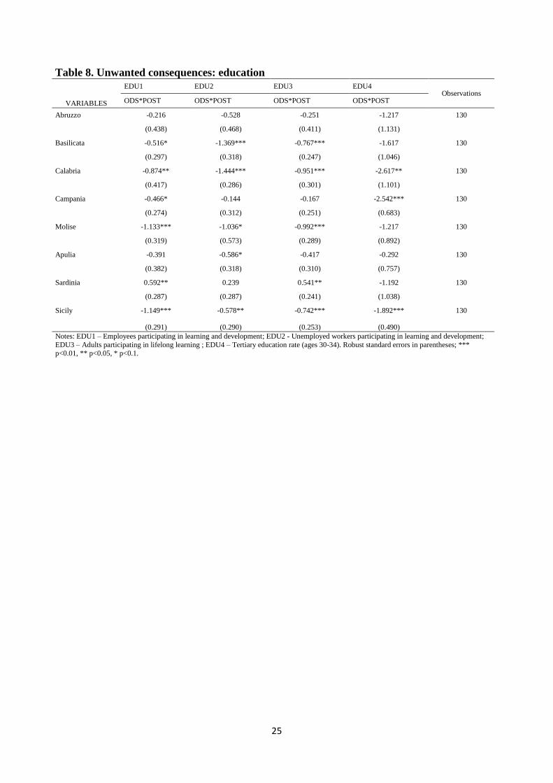
Displacement may also have occurred within areas of LPS covered by ODS, favouring ODS targets

over non-targeted indicators. This aspect is a standard risk when targets are employed to spur

effectiveness. For instance, Schuman (2016) warns that indicators are not ends in themselves but

rather instruments, and policies should not be tailored to do well on the targets but rather to achieve

their broader objectives. To verify whether this was the case, we look at indicators for education

that capture aspects not related to those involved in the scheme — concerning early school-leavers

and high-school competencies. We consider aspects relating to both human capital accumulation for

labour market participants and tertiary education. We use four indicators: employees participating

in learning and development (EDU1); unemployed workers participating in learning and

development (EDU2); adults participating in lifelong learning (EDU3); and the tertiary education

rate (EDU4). The DID estimated coefficients, displayed in Table 8, are negative in most regions (in

some cases with high statistical significance), suggesting that some displacement forces are at work

even within LPS covered by ODS, favouring ODS targets over non-targeted indicators.

[Table 8]

6. Conclusions

The aim of Obiettivi di servizio was to improve the provision of public services in southern Italy.

Our results suggest that the effect of the scheme on the indicators was generally low and highly

17

variable across regions and indicators. We find that better results are recorded when the quality of

local institutions is higher and, in some cases, when the distance from the target is lower. The latter

evidence suggests that the common target seems to have done poorly in enhancing effectiveness.

The positive relation between performance under the scheme and local institutional quality sheds

light on one of the biggest problems, relating to the involvement of local stakeholders within a

decentralization framework. Unfortunately, in the short run central governments cannot do much to

improve local governance and fight corruption, as these aspects are generally deeply rooted in the

territory and difficult to eradicate with immediate effect. However, a possible solution, when the

quality of local institutions is low, could be to force stronger and continuous control of the action of

local governments throughout the whole program, with the potential benefit of reducing the

dissipation of resources and the susceptibility to local interest groups.

A second consideration relates to the design of the incentive mechanism. Our analysis suggests that

when the magnitude of the incentive is not proportionate to the amount of effort the agent has to

make to achieve it, effectiveness is at risk. In some cases, the indicators that are initially more

distant from the targets are also those with the worst performance, which might imply that regions

put more effort into the targets that are easiest to achieve, while leaving aside the most difficult

ones. Also, the overall structure of the financial rewards, which was not designed to reflect effort

but rather the size of the participating regions, did not contribute to measured performance. In the

light of these results, future incentive schemes should try to attach higher financial rewards to more

distant targets, so that the incentives for the agents are aligned with the objective of the principal.

Finally, in line with the evidence on the unwanted effects documented in the paper, it is also

important to have targets for non-covered indicators, which are good candidates for displacement.

Finally, as explained in Section 2, central government did not respect the initial agreement (the

intermediate-target rewards envisaged for 2009 were never disbursed; in 2011 the total financial

resources for the program was cut to one third of the amount originally budgeted). It is important,

therefore, to discuss whether this failure to observe the initial promises had negative repercussions

on the credibility of the principal and so jeopardized the functioning of the incentive scheme. We

think this was not the case. To begin with, financial incentives were only part of the story. The

program received a lot of media attention and it probably increased both transparency and the

accountability of local authorities. Therefore, it seems safe to assume that there were also other

motivations (e.g. maximizing social welfare, or increasing the incumbent’s probability of re-

18

election) apart from financial rewards spurring performance under the scheme. Another aspect to

consider is that the measures taken by the local authorities required a lot of initial effort to prepare

the strategic plans and set up the public spending budget. Since the spending cuts mentioned earlier

occurred unexpectedly8 some years after the program was implemented, it is likely that before then

the regions had already started carrying out their ODS public spending plans. As long as

disinvesting is costly, it is hard to think of a complete dismantling of the entire plan thereafter. In

other words, the expectation of future financial rewards could have given an initial ‘big push’ to

improve local public services, and even though reality fell short of expectations, local authorities

may have found it convenient to carry on their initial plans nonetheless. Overall, it seems that the

problems with actual disbursement are not what drives our findings.

8 If the regional governments had anticipated these cuts, they would have promptly updated their attitudes and put less

initial effort into their ODS strategic plans. In practice, it seems that the problem with the receipt of the transfers was

not in fact expected. The lack of intermediate-target disbursement was due to a change in government (and was

particularly surprising as in previous changes cohesion programs had never been disputed). The reduction of the

rewards in 2011 was driven by the need to cut the public deficit in the aftermath of the 2011 debt crisis, which was

indeed hard to anticipate.

19

References

Besley, T. J., Bevan, G., and Burchardi, K.B., (2009), ‘Naming & Shaming: The Impacts of

Different Regimes on Hospital Waiting Times in England and Wales’, CEPR Discussion Papers,

7306.

Boyne, G.A., James, O., John, P., and Petrovsky, N. (2009), ‘Political and Managerial Succession

and the Performance of English Local Governments’, The Journal of Politics, 71: 1271–1284.

Bracco, E., Lockwood, B., Porcelli, F., and Redoano, M. (2015), ‘Intergovernmental Grants as

Signals and the Alignment Effect: Theory and Evidence’, Journal of Public Economics, 123: 78-91.

Burgess, S., Wilson, D., and Worth, J. (2010), ‘A Natural Experiment in School Accountability:

The Impact of School Performance Information on Pupil Progress and Sorting’, Centre for Market

and Public Organisation at the University of Bristol, 10/246.

Charron, N., Dahlberg, S., Holmberg, S., Rothstein, B., Khomenko, A., and R. Svensson (2016),

‘The Quality of Government EU Regional Dataset, version Sep16’, University of Gothenburg: The

Quality of Government Institute, http://www.qog.pol.gu.se.

Faguet, J-P. (2004), ‘Does Decentralization Increase Government Responsiveness to Local Needs?

Evidence from Bolivia’, Journal of Public Economics, 88: 867-893.

Gupta, S., Davoodi, H., and Tiongson, E. (2002), ‘Corruption and the Provision of Health Care and

Education Services’, IMF Working Paper, No. 00/116.

Joumard, I., and Kongsrud, P.M. (2003), ‘Fiscal Relations across Government Levels’, OECD

Economics Department Working Papers, No. 375.

Kang, W. (2015), ‘Electoral Cycles in Pork Barrel Politics: Evidence from South Korea 1989-

2008’, Electoral Studies, 38: 46-58.

Lema, D., and Streb, J. (2013), ‘Party Alignment and Political Budget Cycles: The Argentine

Provinces’, CEMA Working Papers: Serie Documentos de Trabajo, 520, Universidad del CEMA.

Lockwood, B., and Porcelli, F. (2013), ‘Incentive Schemes for Local Government: Theory and

Evidence from Comprehensive Performance Assessment in England’, American Economic Journal:

Economic Policy, 5(3): 254-286.

McCann, P. (2015), The Regional and Urban Policy of the European Union: Cohesion, Results-

Orientation and Smart Specialisation, Edward Elgar, Cheltenham.

OECD (2009), Governing Regional Development Policy: The Use of Performance Indicators,

OECD Publishing.

Propper C., and Wilson, D. (2003), ‘The Use and Usefulness of Performance Measures in the Public

Sector’, Oxford Review of Economic Policy, 19: 250-267.

Rajkumar, A., and Swaroop, V. (2008), ‘Public Spending and Outcomes: Does Governance

Matter?’, Journal of Development Economics, 86: 96–111.

20

Revelli, F. (2006), ‘Performance Rating and Yardstick Competition in Social Service Provision’,

Journal of Public Economics, 90: 459-475.

Revelli, F. (2008), ‘Performance Competition in Local Media Markets’, Journal of Public

Economics, 92(7): 1585-94.

Revelli, F. (2010),“’pend More, Get More? An Inquiry into English Local Government

Performance’, Oxford Economic Papers, 62: 185–207.

Rumi, C. (2014), ‘National Electoral Cycles in Transfers to Sub-national Jurisdictions. Evidence

from Argentina’, Journal of Applied Economics, 17(1): 161.

Schumann, A. (2016), ‘Using Outcome Indicators to Improve Policies’, OECD Regional

Development Working Papers, 2016/02.

Van Dooren, W., Bouckaert, G., and Halligan, J. (2015), Performance Management in the Public

Sector, Routledge.

21

Tables and figures

Table 1. LPS, indicators, and targets

Area of LPS # Indicators CENTRE&

NORTH

2007 (1)

SOUTH

2007 (1)

Target

2013

Education S.01 Early school-leavers (%) 15.7 24.9 10

S.02 Students with poor competencies in reading (%) 18.2 37.0 20

S.03 Students with poor competencies in maths (%) 22.9 45.7 21

Childcare and elderly care S.04 Municipalities offering childcare services (%) 58.3 28.1 35

S.05 Children in childcare (%) 16.3 4.3 12

S.06 Old people assisted at home (%) 3.9 1.8 3.5

Urban waste management S.07 Urban solid waste landfilled (Kg/inhabitants) 251 409 230

S.08 Recycled urban solid waste (%) 35.2 11.6 40

S.09 Composted solid waste (%) 36.4 6 20

Water S.10 Water usage, relative to supply (%) 71.5 59.4 75

S.11 Population served by advanced wastewater treatment plants (%) 77.6 62.5 70

(1) S.02 and S.03 refer to 2006, S.10 and S11 to 2005.

Source: http://www.agenziacoesione.gov.it/it/politiche_e_attivita/Obiettivi_di_Servizio

Table 2. Common targets across regions for S.04, S.05, and S.06

Regions Starting point Target Difference

S.04 Municipalities offering childcare services (%)

Campania 30.5 35 4.5

Sardinia 14.9 35 20.1

S.05 Children in childcare (%)

Campania 1.5 12 10.5

Sardinia 10 12 2

S.06 Old people assisted at home (%)

Campania 1.4 3.5 2.1

Sardinia 1.1 3.5 2.4

Source: http://www.agenziacoesione.gov.it/it/politiche_e_attivita/Obiettivi_di_Servizio

22

Table 3. Distribution of the pledges for all indicators

Education Childcare and elderly care Urban waste management Water Pledges per

region S.01 S.02 S.03 S.04 S.05 S.06 S.07 S.08 S.09 S.10 S.11

Abruzzo 10.9 10.9 10.9 8.9 8.9 17.7 13.3 13.3 8.9 17.7 17.7 139.0

Molise 6.1 6.1 6.1 4.9 4.9 9.9 7.4 7.4 4.9 9.9 9.9 77.6

Campania

52.2 52.2 52.2 42.6 42.6 85.2 63.9 63.9 42.6 85.2 85.2 667.7

Puglia 41.6 41.6 41.6 33.9 33.9 67.9 50.9 50.9 33.9 67.9 67.9 532.1

Basilicata 11.4 11.4 11.4 9.3 9.3 18.7 14.0 14.0 9.3 18.7 18.7 146.4

Calabria 23.7 23.7 23.7 19.4 19.4 38.8 29.1 29.1 19.4 38.8 38.8 303.9

Sicily 54.8 54.8 54.8 44.8 44.8 89.5 67.1 67.1 44.8 89.5 89.5 701.5

Sardinia 28.9 28.9 28.9 23.6 23.6 47.3 35.5 35.5 23.6 47.3 47.3 370.6

Total 229.6 229.6 229.6 187.4 187.4 375 281.2 281.2 187.4 375 375 2938.8

Data in € million. Source: http://www.agenziacoesione.gov.it/it/politiche_e_attivita/Obiettivi_di_Servizio.

Table 4. Initial and final values of the indicators

Category Education Childcare and elderly care Waste management Water sources

Indicator S.01 S.02 S.03 S.04 S.05 S.06 S.07 S.08 S.09 S.10 S.11

Year initial final initial final initial final initial final initial final initial final initial final initial final initial final initial final initial final

(2007) (2013) (2006) (2012) (2006) (2012) (2007) (2012) (2007) (2012) (2007) (2012) (2007) (2013) (2007) (2013) (2007) (2013) (2005) (2012) (2005) (2012)

Abruzzo 15 11.4 - 22.4 - 26.7 32.5 60.0* 8.7 9.8 3.7* 4.9* 427.3 70.1* 18.6 42.9* 14.3 36.7* 55.4 57.7 51.4 65.9

Molise 16.4 15.4 - 21.7 - 29.9 6.6 22.8 4.8 10.4 3.8* 3.9* 400.9 448 4.9 19.9 0.9 39.9* 54.9 52.8 84.8* 80.4*

Campania 29 22.2 36.1 28.2 44.3 35.8 38.7* 33.2 1.9 2.7 1.6 2.8 362.6 84.8* 13.5 44.0* 1 8.5 59.8 54.2 85.5* 72.2

Apulia 25.1 19.9 36.3 16.7* 43 26.3 36.4* 38.0* 4.6 4.4 1.6 2.2 484.9 315.4 8.9 22 4.8 25.1* 52.7 65.4 58.5 68.2

Basilicata 14.1 15.4 34 20.8 38.4 30.5 25.2 32.1 6.9 7 4.3* 5.4* 303.6 205.3* 8.1 25.8 0 0 65.2 61.5 61.1 66.1

Calabria 21.2 16.4 - 37.4 - 45.8 14.2 8.8 2 2.1 2.8 3.1 261.6 300.2 9.1 14.7 8.1 9.6 65.5 64.6 43.5 54.1

Sicily 26.1 25.8 40.8 29.6 48.9 37.3 34.4 33.8 5.5 5.6 1 3.6* 501.3 441.3 6.2 13.4 7.9 12.4 64.4 54.4 43.4 45.9

Sardinia 21.8 24.7 37.2 27.3 45.3 33.3 20.7 33.7 8.9 12.9* 1.2 4.6* 306.7 154.5* 27.8 51.0* 11.8 85.3* 53.6 45.2 87.4* 84.7*

South 24.9 14.1 37 26.5 45.7 34.4 28.1 32.5 4.3 5 1.8 3.3 409 250.5 11.6 28.9 6 20.6 59.4 56.6 62.5 63.7

Centre &

North 15.7 21.4 18.2 15.1 22.9 18.6 58.3 65 16.3 17.9 3.9 4.7 251 144.9 35.2 48.5 36.4 53.2 71.5 65.9 77.6 75.7

Italy 19.7 17 26.4 19.5 32.8 24.7 48.6 54.6 12 13.5 3.3 4.3 306.6 181.3 27.5 42.3 25.2 42.5 67.4 62.6 72.3 71.5

Target 10 20 21 35 12 3.5 230 40 20 75 70

Source: http://www.agenziacoesione.gov.it/it/politiche_e_attivita/Obiettivi_di_Servizio. * denotes values of the

indicators above the target.

23

Table 5. Estimated treated effects

S.01 S.02 S.03 S.04 S.05 S.06 S.07 S.08 S.09 S.10 S.11

All

indicators

Abruzzo 1.331*** -2.886** -1.312 40.38*** -4.641 23.92* 21.91** 5.429 -34.57** 5.792** 21.70*** 5.551

(0.441) (1.048) (0.913) (15.31) (5.737) (12.50) (8.900) (4.289) (17.41) (2.376) (2.496) (7.501)

Obs 130 34 34 108 117 154 234 234 169 65 39 1318

Basilicata -1.586* 8.182* 0.341 -6.952 -7.975 8.721 -18.98*** -19.26*** -111.1*** -0.542 7.696*** -26.09*

(0.885) (4.611) (4.801) (12.55) (5.457) (11.26) (4.776) (5.593) (22.94) (2.646) (2.489) (13.84)

Obs 130 35 35 108 117 154 234 234 169 65 39 1320

Calabria 0.822 -6.511*** -8.400*** -15.90** -18.11*** 3.322 -27.34*** -35.61*** -79.89*** 0.825 13.27*** -27.09**

(0.968) (1.048) (0.913) (7.841) (5.690) (9.912) (6.913) (4.938) (23.47) (2.505) (3.320) (11.54)

Obs 130 34 34 108 117 154 234 234 169 65 39 1318

Campania 3.396*** 5.028** 4.417* -14.81 -10.89* -1.405 26.98*** 20.62*** -101.1*** -6.808** -18.52*** -13.76

(0.887) (2.037) (2.275) (12.83) (5.946) (10.34) (5.622) (3.852) (23.52) (3.198) (2.493) (12.49)

Obs 130 35 35 108 117 154 234 234 169 65 39 1320

Molise 1.470 0.364 -1.438 21.00* 21.05 -86.09*** -30.71*** -23.17*** -16.06 1.025 -7.732** -18.72

(1.570) (1.048) (0.913) (11.18) (15.46) (25.81) (7.760) (5.833) (25.70) (2.557) (3.091) (11.85)

Obs 130 34 34 108 117 154 234 234 169 65 39 1318

Puglia 4.868*** 10.42 5.378 -4.476 -18.95*** -21.40** -0.237 -26.77*** -48.64** 19.19*** 14.84*** -14.72*

(1.095) (9.156) (9.635) (7.896) (6.132) (9.467) (4.278) (4.866) (21.81) (5.748) (2.496) (8.394)

Obs 130 35 35 108 117 154 234 234 169 65 39 1320

Sardinia -0.0301 2.223 4.602 16.76** 20.78** 36.68** 9.601*** 37.09*** 182.4*** -12.61** -6.232* 36.35**

(1.660) (6.045) (5.531) (7.734) (10.24) (18.02) (3.686) (5.279) (27.96) (5.468) (3.616) (15.61)

Obs 130 35 35 108 117 154 234 234 169 65 39 1320

Sicily 0.859 6.009 4.295 -9.905 -20.06*** 10.35 -19.74*** -35.37*** -74.48*** -6.875*** 3.482 -21.33**

(0.751) (4.357) (5.374) (9.790) (6.979) (18.17) (4.242) (5.648) (18.09) (2.229) (2.577) (9.066)

Obs 130 35 35 108 117 154 234 234 169 65 39 1320

All regions 1.391** 3.470 1.489 3.262 -4.850 -3.230 -4.814 -9.629** -35.43* 0 3.563 -10.05*

(0.539) (2.227) (2.033) (7.237) (5.956) (10.86) (4.006) (4.554) (18.97) (3.735) (4.724) (5.429)

Obs 200 53 53 171 180 238 360 360 260 100 60 2035

Notes: Robust standard errors in parentheses; *** p<0.01, ** p<0.05, * p<0.1.

24

Table 6. Drivers of effectiveness

VARIABLES S.01 S.02 S.03 S.04 S.05 S.06 S.07 S.08 S.09 S.10 S.11 All

indicators

ODS*POST 2.737** 0.715 -2.521 -11.00 -33.06*** -14.37 24.03*** 1.865 -91.74*** 2.610 -17.01*** -0.933

(1.167) (5.272) (3.808) (8.219) (10.20) (17.72) (5.390) (6.018) (25.43) (5.196) (2.921) (6.763)

Interactions with:

INITIAL DISTANCE 0.480 5.896 6.474* -13.88 13.72 23.75 -33.76*** -33.02*** -30.28 13.53*** 30.86*** -36.73***

(1.177) (4.891) (3.406) (9.772) (9.505) (17.63) (6.160) (5.479) (23.76) (5.003) (1.624) (5.876)

FINANCIAL

REWARDS

-1.841** -0.138 -2.044 7.750 -11.05 -53.46*** -15.50* 48.79** -5.093 0.929 -4.347

(0.927) (3.383) (2.739) (4.960) (17.09) (7.462) (8.021) (22.23) (5.093) (1.866) (6.740)

INSTITUTIONAL

QUALITY

-0.728 3.629 3.023 29.62** 19.64*** 21.40 25.00*** 28.57*** 19.47 -1.113 21.75*** 6.685

(1.090) (5.166) (3.545) (11.76) (6.290) (16.72) (7.521) (7.664) (25.52) (4.173) (2.005) (8.011)

POLITICAL

ALIGNMENT

-0.604 -4.455 0.536 12.79 15.31** -11.81 4.540 -3.036 74.65*** -12.54*** -12.39*** 16.27**

(0.943) (3.577) (3.045) (9.055) (6.856) (16.61) (6.231) (5.007) (28.13) (4.480) (1.754) (8.216)

Constant 95.54*** 91.30*** 84.48*** 130.0*** 80.05*** 125.6*** 95.63*** 82.10*** 193.6*** 92.95*** 72.23*** 82.75***

(0.579) (2.745) (2.635) (15.22) (4.635) (16.03) (5.029) (3.884) (23.50) (1.728) (1.026) (8.273)

Observations 200 53 53 171 180 238 360 360 260 100 60 2,035

R-squared 0.904 0.907 0.943 0.916 0.925 0.780 0.829 0.916 0.831 0.857 0.978 0.444

Notes: Robust standard errors in parentheses; *** p<0.01, ** p<0.05, * p<0.1.

Table 7. Unwanted consequences: transportation

VARIABLES LPT 1 LPT 2 LPT 3 LPT 4

Observations ODS*POST ODS*POST ODS*POST ODS*POST

Abruzzo -71.66* -588.7 -0.45 -222.2* 182

(36.54) (507.9) (10.25) (130.8) 182

Basilicata -95.69*** -2773*** -0.66 -226.2** 182

(23.83) (648.1) (10.62) (109.9) 182

Calabria 20.51 -2435*** -2.08 -52.73 182

(26.21) (610.4) (10.59) (106.0) 182

Campania 115.0*** -224.9 -72.66*** -978.3*** 182

(40.17) (614.6) (16.94) (264.2) 182

Molise -76.89*** -2546*** -0.06 -197.4* 182

(23.64) (661.2) (10.32) (109.1) 182

Puglia -82.51* -296.8 -5.77 -61.83 182

(46.31) (421.8) (10.28) (97.77) 182

Sardinia -32.14 -2112*** 3.57 -276.5** 182

(22.15) (560.0) (10.52) (107.4) 182

Sicily -41.62 -882.1 -28.52*** -1278*** 182

(28.34) (538.8) (10.54) (222.4) 182

Notes: LPT 1 – Urban network of public transport; TPL2 – Parking bays in park-and-rides; TPL3 – Passengers travelling by public transport; TPL4 –

Available seat kilometres in the provincial capitals. Robust standard errors in parentheses; *** p<0.01, ** p<0.05, * p<0.1.

25

Table 8. Unwanted consequences: education

VARIABLES

EDU1 EDU2 EDU3 EDU4 Observations

ODS*POST ODS*POST ODS*POST ODS*POST

Abruzzo -0.216 -0.528 -0.251 -1.217 130

(0.438) (0.468) (0.411) (1.131)

Basilicata -0.516* -1.369*** -0.767*** -1.617 130

(0.297) (0.318) (0.247) (1.046)

Calabria -0.874** -1.444*** -0.951*** -2.617** 130

(0.417) (0.286) (0.301) (1.101)

Campania -0.466* -0.144 -0.167 -2.542*** 130

(0.274) (0.312) (0.251) (0.683)

Molise -1.133*** -1.036* -0.992*** -1.217 130

(0.319) (0.573) (0.289) (0.892)

Apulia -0.391 -0.586* -0.417 -0.292 130

(0.382) (0.318) (0.310) (0.757)

Sardinia 0.592** 0.239 0.541** -1.192 130

(0.287) (0.287) (0.241) (1.038)

Sicily -1.149*** -0.578** -0.742*** -1.892*** 130

(0.291) (0.290) (0.253) (0.490)

Notes: EDU1 – Employees participating in learning and development; EDU2 - Unemployed workers participating in learning and development;

EDU3 – Adults participating in lifelong learning ; EDU4 – Tertiary education rate (ages 30-34). Robust standard errors in parentheses; *** p<0.01, ** p<0.05, * p<0.1.

26

Figure 1. Average progress across indicators

Source: http://www.agenziacoesione.gov.it/it/politiche_e_attivita/Obiettivi_di_Servizio

Figure 2. Average progress under the scheme: treated regions vs untreated counterparts

Source: http://www.agenziacoesione.gov.it/it/politiche_e_attivita/Obiettivi_di_Servizio

-200

-180

-160

-140

-120

-100

-80

-60

-40

-20

0

20

40

60

80

100

Per

cent

S.01 S.02 S.03 S.04 S.05 S.06 S.07 S.08 S.09 S.10 S.11

Indicator

2007 2013 + / -

Note: The distances are expressed in percentages with respect to the target

Source : Italian Ministry of Economic Development

(Distance = 100 - transformed indicator)

Mean distance from the target and variability across regions before and after ODS