ËÒ×ÊÛÎÍ×Ìß ÜÛÙÔ× ÍÌËÜ× Ü×...
146
ËÒ×ÊÛÎÍ×Ì ß ÜÛÙÔ× ÍÌËÜ× Ü× ÐßÜÑÊß Ü·°¿®¬·³»²¬± ¼· Ú·-·½¿ ÄÙ¿´·´»± Ù¿´·´»·þ ͽ«±´¿ ¼· ܱ¬¬±®¿¬± ¼· η½»®½¿ ·² Ú·-·½¿ Ý·½´± ÈÈ ÝÚÌ °¿®¬·¬·±² º«²½¬·±²- ¿²¼ ³±¼«´· -°¿½»- ±º ½¿²±²·½¿´ ½«®ª»- Ü·®»¬¬±®» ¼»´´¿ ͽ«±´¿æ ݸò³± Ю±ºò ߬¬·´·± ͬ»´´¿ Í«°»®ª·-±®»æ ݸò³± Ю±ºò Ó¿®½± Ó¿¬±²» ܱ¬¬±®¿²¼±æ α¾»®¬± ʱ´°¿¬± ÜßÌß ÝÑÒÍÛÙÒß ÌÛÍ× íï ¹»²²¿·± îððè
Transcript of ËÒ×ÊÛÎÍ×Ìß ÜÛÙÔ× ÍÌËÜ× Ü×...

ËÒ×ÊÛÎÍ×Ìß ÜÛÙÔ× ÍÌËÜ× Ü× ÐßÜÑÊß
Ü·°¿®¬·³»²¬± ¼· Ú··½¿ ÄÙ¿´·´»± Ù¿´·´»·þ
ͽ«±´¿ ¼· ܱ¬¬±®¿¬± ¼· η½»®½¿ ·² Ú··½¿
Ý·½´± ÈÈ
ÝÚÌ °¿®¬·¬·±² º«²½¬·±² ¿²¼³±¼«´· °¿½» ±º ½¿²±²·½¿´ ½«®ª»
Ü·®»¬¬±®» ¼»´´¿ ͽ«±´¿æ ݸò³± Ю±ºò ߬¬·´·± ͬ»´´¿
Í«°»®ª·±®»æ ݸò³± Ю±ºò Ó¿®½± Ó¿¬±²»
ܱ¬¬±®¿²¼±æ α¾»®¬± ʱ´°¿¬±
ÜßÌß ÝÑÒÍÛÙÒß ÌÛÍ×íï ¹»²²¿·± îððè


Le teorie di campo conformi (CFT) in due dimensioni rappresentano un am-bito di fecondo interscambio tra alcuni degli argomenti piu avanzati in fisica teo-rica e in geometria algebrica. In particolare, lo studio delle funzioni di partizionein teorie conformi appare strettamente legato all’analisi della corrispondenza traproprieta analitiche e proprieta algebriche delle superfici di Riemann chiuse. Inquesta tesi, vengono considerati alcuni nuovi aspetti di questa corrispondenza,in particolare quelli che emergono nelle teorie conformi associate a teorie distringa e superstringa. Piu precisamente, i parametri algebrici che determi-nano la curva canonica associata ad una superficie di Riemann non-iperellitticasono esplicitamente calcolati in termini di funzioni theta di Riemann valutatesu punti generici della curva. I metodi proposti vengono inoltre applicati allostudio del locus singolare della funzione theta, anche in relazione all’approcciodi Andreotti-Mayer al problema di Schottky, e alla restrizione della misura diSiegel allo spazio dei moduli delle curve canoniche.


Conformal field theories (CFT) represent a framework of fruitful interplaybetween some of the most advanced topics in theoretical physics and algebraicgeometry. In particular, the investigation of the CFT partition functions isclosely related to the analysis of the correspondence between analytic and al-gebraic properties of closed Riemann surfaces. In the present thesis, some newaspects of this correspondence, in particular the ones arising in the CFTs asso-ciated to string and superstring theories, are considered. More precisely, thealgebraic parameters, determining the canonical curve associated to a non-hyperelliptic Riemann surface, are explicitly computed in terms of Riemanntheta functions, evaluated at generic points of the curve. Moreover, the tech-niques here introduced are applied to the analysis of the singular locus of thetheta function, also considered with respect to the Andreotty-Mayer approachto the Schottky problem, and to the restriction of the Siegel’s measure to themoduli space of canonical curves.

CONTENTS
Introduction . . . . . . . . . . . . . . . . . . . . . . . . . . . . . . . . . . 3
1. Axiomatic definition of CFT . . . . . . . . . . . . . . . . . . . . . . . 91.1 Segal’s approach: motivations and axioms . . . . . . . . . . . . . 9
1.1.1 Field theories and cobordisms . . . . . . . . . . . . . . . . 91.1.2 Axiomatic definition and main properties . . . . . . . . . 13
1.2 Spaces of cobordisms . . . . . . . . . . . . . . . . . . . . . . . . . 141.2.1 The space of disks D . . . . . . . . . . . . . . . . . . . . . 141.2.2 The semigroup of annuli A . . . . . . . . . . . . . . . . . 151.2.3 Hilbert space structure on H and unitarity . . . . . . . . 161.2.4 Representations of A and representations of Vect(S1) . . . 171.2.5 Pants and algebra of operators . . . . . . . . . . . . . . . 18
1.3 Conformal anomaly and modular functors . . . . . . . . . . . . . 191.3.1 Extensions of the semi-group A . . . . . . . . . . . . . . . 191.3.2 Modular functors . . . . . . . . . . . . . . . . . . . . . . . 201.3.3 The determinant line bundle . . . . . . . . . . . . . . . . 221.3.4 CFT from weak conformal field theories . . . . . . . . . . 24
1.4 Axiomatic CFT and bosonic string theory . . . . . . . . . . . . . 26
2. Combinatorics of determinants . . . . . . . . . . . . . . . . . . . . . . 292.1 Identities in symmetric products of vector spaces . . . . . . . . . 292.2 Combinatorial lemmas . . . . . . . . . . . . . . . . . . . . . . . . 32
2.2.1 Computation of cg,2 . . . . . . . . . . . . . . . . . . . . . 352.2.2 Examples of the combinatorial lemmas . . . . . . . . . . . 38
3. Determinats of holomorhpic differentials and theta functions surfaces . 433.1 Determinants in terms of theta functions . . . . . . . . . . . . . . 433.2 Higher order theta derivatives . . . . . . . . . . . . . . . . . . . . 443.3 Combinatorial lemmas and holomorphic differentials . . . . . . . 473.4 The Mumford isomorphism . . . . . . . . . . . . . . . . . . . . . 48
4. Bases of holomorphic differentials . . . . . . . . . . . . . . . . . . . . . 534.1 Duality between Nn-tuples of points and bases of H0(Kn
C) . . . . 544.2 Special loci in Cg . . . . . . . . . . . . . . . . . . . . . . . . . . . 57
4.2.1 Determinants of distinguished bases and Fay’s identity . . 624.3 The function H and the characterization of the B locus . . . . . 65

2 Contents
5. The ideal of a canonical curve . . . . . . . . . . . . . . . . . . . . . . . 695.1 Relations among holomorphic quadratic differentials . . . . . . . 70
5.1.1 Consistency conditions on the quadrics coefficients . . . . 735.2 A correspondence between quadrics and θ-identities . . . . . . . 755.3 Relations among holomorphic cubic differentials . . . . . . . . . . 79
6. The section K . . . . . . . . . . . . . . . . . . . . . . . . . . . . . . . 836.1 Definition and fundamental properties . . . . . . . . . . . . . . . 836.2 Zeros of K and the singular locus Θs . . . . . . . . . . . . . . . . 856.3 Quadrics from double points on Θs . . . . . . . . . . . . . . . . . 896.4 The case of genus 4 . . . . . . . . . . . . . . . . . . . . . . . . . . 976.5 Modular properties of K(p3, . . . , pg) . . . . . . . . . . . . . . . . 99
7. Siegel’s induced measure on the moduli space . . . . . . . . . . . . . . 1057.1 Volume form and Laplacian on Hg . . . . . . . . . . . . . . . . . 1067.2 The Siegel metric on the moduli space . . . . . . . . . . . . . . . 1077.3 Powers of Bergman kernel . . . . . . . . . . . . . . . . . . . . . . 111
8. A genus 4 example . . . . . . . . . . . . . . . . . . . . . . . . . . . . . 1138.1 Definition and main properties . . . . . . . . . . . . . . . . . . . 1138.2 Computation of Kq∞ . . . . . . . . . . . . . . . . . . . . . . . . . 1178.3 The prime form . . . . . . . . . . . . . . . . . . . . . . . . . . . . 119
Appendix 123
A. Varieties . . . . . . . . . . . . . . . . . . . . . . . . . . . . . . . . . . . 125A.1 Analytic and algebraic varieties . . . . . . . . . . . . . . . . . . . 125A.2 Sheaves . . . . . . . . . . . . . . . . . . . . . . . . . . . . . . . . 126A.3 Curves and divisors . . . . . . . . . . . . . . . . . . . . . . . . . . 126
B. Theta functions on Riemann surfaces . . . . . . . . . . . . . . . . . . . 131B.1 Riemann theta functions and the prime form . . . . . . . . . . . 131B.2 Generalizations of Jacobi’s derivative identity . . . . . . . . . . . 135
Bibliography . . . . . . . . . . . . . . . . . . . . . . . . . . . . . . . . . . 137

INTRODUCTION
Conformal field theories [8, 19, 27] have played an important role in severalareas of theoretical physics and mathematics in the last 25 years.
The most famous application has been to string theory, since the classicaland quantum theory of excitations of a string is described by a two-dimensionalCFT on the world-sheet of the string. Conformal field theories have also beenapplied in statistical physics: in two dimensions for the Ising model and inthree dimensions to describe the critical points of second or higher order phasetransitions. Moreover, four dimensional CFT are supposed to play a role inelementary particle physics models. A result by Nahm [50] implies that sixis the maximal number of dimensions for a unitary non-trivial conformal fieldtheory; recently, some hints of the existence of such six-dimensional CFT’s havebeen given [63].
Conformal field theories are defined as field theories which are invariantunder the group of local conformal transformations, which, roughly speaking,are symmetries preserving the angles but not the lengths. In particular, intwo dimensions, the Lie algebra associated to the conformal group is infinitedimensional. The generators if such algebra correspond to an infinite number ofconserved charges and this implies that such theories are, in principle, exactlysolvable.
The choice of the conformal class for the metric on a two-dimensional mani-fold is equivalent to the definition of a complex structure on the surface. There-fore, amplitudes in CFT naturally depend on the analytic structure of the sur-face, i.e. on the sheaf of holomorphic functions defined on the Riemann surface.Such analyticity properties can be made explicit by splitting the CFT vertexoperator algebra in its chiral and anti-chiral part. On the other hand, one ofthe most fascinating aspects of conformal field theories is its relationship withsome of the deepest results in algebraic geometry. This is just a facet of amore general correspondence between classes of algebraic varieties, with regularmaps and sheaves, and classes of analytic spaces, with holomorphic mappingsand sheaves, known as the GAGA principle (from Serre’s Geometrie algebriqueet geometrie analytique, [58]).
Two manifestations of GAGA principle in conformal field theories will playa prominent role in this thesis. As shown in chapter 1, a CFT assigns to eachclosed surface of genus g a partition function, which is a section of a line bundleon the moduli space Mg of closed Riemann surfaces of genus g. In particular,for the CFTs related to gauge fixed bosonic strings and superstrings (afterintegration over odd supermoduli), each partition function defines a measureon the corresponding moduli space. For bosonic strings, this is known as thePolyakov measure, and it can be expressed, apart from a factor representingthe obstruction to the holomorphic factorization of the theory, as the square

4 Introduction
modulus of a holomorphic section of λ−131 ⊗ λ2. Here λn is, roughly speaking,
the line bundle whose fibre at the point C ∈ Mg is the maximal externalproduct of the space of holomorphic n-differentials on the Riemann surface C.Passing from the analytic to the algebraic data associated to Riemann surfaces,it is well-known that Mg admits a compactification (a la Deligne-Mumford)Mg that is the moduli space of stable curves of genus g. Mumford proved thatthe line bundle λ−13
1 ⊗ λ2 on Mg admits a unique (up to normalization) non-vanishing holomorphic section, extending to a meromorphic section on Mg withpoles at the boundary. Belavin and Knizhnik [7] proved that such a holomorphicsection is exactly the chiral factor in the Polyakov measure. The poles at theboundary admit a physical interpretation as the amplitudes corresponding tothe propagation of the bosonic string tachyon for Riemann surfaces degeneratingto stable curves with nodes.
Another example of this interplay between analytic and algebraic data isprovided by CFTs on Riemann surfaces with Zn-symmetry. Let us consider thesimplest case of hyperelliptic surfaces, corresponding to n = 2. Any hyperellipticsurface of genus g ≥ 2 can be described in terms of an affine curve C in C2,defined by the polynomial equation
w2 =2g+2∏
i=1
(z − ai) ,
where (z, w) ∈ C2. The restriction to C of the projection (z, w) 7→ z defines ameromorphic function z of degree 2 on the Riemann surface, which shows thatany hyperelliptic surface can be represented as a 2-fold branched covering ofthe Riemann sphere. The pairwise distinct complex numbers (a1, . . . , a2g+2),corresponding the position of the branching points on the sphere, representthe coordinates of the universal parameter space of hyperelliptic curves; thecorrespondent moduli space is the quotient of such a parameter space by the3-parameters group of automorphisms of the sphere. In [42], a procedure hasbeen described to obtain a CFT partition function on a hyperelliptic Riemannsurface, from an amplitude in a “double” CFT with Z2-symmetry on the sphere.Such an amplitude is characterized by the insertion of 2g+2 “twisted” operatorsat the branching points a1, . . . , a2g+2, so that the dependence of the resultingpartition function on such algebraic parameters of the hyperelliptic curve isexplicit. Recently, such a procedure has been applied to a conjectural CFT [64,28, 65], representing the holographic dual to a three-dimensional pure gravitytheory with negative cosmological constant, to prove that partition functionson hyperelliptic Riemann surfaces can be consistently defined for all genera.
By computing the same partition functions in terms of the analytic dataof the theory, one obtains remarkable algebro-geometric identities. More pre-cisely, to each surface one can attach the data of its Jacobian torus and thecorresponding theta functions (see appendix B). It is possible, in some cases, tocompute the same CFT amplitude in terms of theta functions. For a hyperellip-tic Riemann surface, by equating the results of the computations, one obtainsthe classical Thomae formula
θ[δ](0)8 =( detA
(2πi)g
)4 ∏
k<l
(aik− ail
)(ajk− ajl
) .

Introduction 5
In this formula, δ is an even theta-characteristic associated to a splitting of theset of complex parameters in a disjoint union ai1 , . . . , aig+1 t aj1 , . . . , ajg+1and A is a matrix of base change between bases of holomorphic abelian differ-entials.
The procedure described above extends to the computation of partition func-tions of n-fold coverings of the sphere. By applying the same reasoning to CFTamplitudes on Riemann surfaces with Zn-symmetry, with n > 2, Bershadskyand Radul [9] derived a generalization of Thomae formula, which has been suc-cessively proved using standard algebro-geometric methods by Nakayashiki [51](see also [20] for further generalizations).
In this thesis, some new methods are described toward an explicit descriptionof this GAGA correspondence in the case of generic non-hyperelliptic Riemannsurfaces of genus higher than two. The examples reported above nicely de-scribe the physical motivations for such an analysis. First of all, one of thefundamental problems both in bosonic and in superstring theories is the defi-nition of the measure on the moduli space Mg for g higher than two. By theBelavin-Knizhnik theorem in the bosonic string case and by analogous argu-ments for superstrings, this is strictly related to the problem of deriving anexplicit formula for the Mumford form. In second instance, generalizations ofthe techniques holding for theories with Zn-symmetry would be of great interestfor general CFTs.
There are two reasons for considering the space of non-hyperelliptic Riemannsurfaces for genus g ≥ 3. Fist of all, such a space is dense in Mg, so that onecan hope to extend most of the results to the whole moduli space by continuityarguments. This should be compared with the case of families of n-fold coveringsof the sphere, which are of positive codimension in the moduli space Mg for ggreater than three. In particular, hyperelliptic surfaces enjoy several peculiarproperties, which are not shared by general Riemann surfaces. For instance,in the case of the conjectural CFT dual to three-dimensional gravity proposedin [64], the existence of consistent partition functions for all non-hyperellipticRiemann surface would be a considerably stronger signal of the existence ofthe whole CFT, than just the hyperelliptic case. Another relevant example isprovided by the Polyakov measure on the locus of genus 3 non-hyperellipitcRiemann surfaces, whose expression in terms of Riemann period matrices andtheta constants has been derived in [6]. Such an expression does not hold inthe hyperelliptic case; in fact, it is a non-trivial problem to check that such aformula admits a regular limit as one approaches the hyperelliptic locus.
From a more technical point of view, another advantage in considering non-hyperelliptic Riemann surfaces is that they admit an algebraic description interms of canonical curves. As explained in chapter 5, a non-hyperelliptic Rie-mann surface of genus g ≥ 3 can be embedded as a projective curve (a 1-canonical or simply canonical curve) in PH0(KC)∗ ∼= Pg−1, where H0(KC)is the space of holomorphic abelian differentials on the surface. A similarconstruction enters in the definition of the Deligne-Mumford moduli space ofstable curves, which is based on an n-canonical embedding in PH0(Kn
C)∗ ∼=P(2n−1)(g−1)−1 for n ≥ 3; the moduli space Mg is defined by modding the pa-rameter space of the n-canonical curves of genus g by the group PGL((2n −1)(g− 1),C) acting on the projective space. In the case of (1-)canonical curves,Petri’s theorem [52] assures that the graded ideal I(C) of homogeneous poly-

6 Introduction
nomials in Pg−1 vanishing on the curve C is generated, with few exceptions, byits degree-2 component I2(C), i.e. by quadrics (for trigonal curves and smoothplane quintics, also the cubics are needed, see [3]). It follows that the parameterspace of the canonical curves can be given in terms of the coefficients of quadricsand cubics; such coefficients play the same role of the parameters a1, . . . , a2g+2for the hyperelliptic curves.
In analogy with the Thomae formula, it should be possible to express theparameters of the quadrics defining the canonical curve in terms of the analyticdata of the Jacobian torus associated to the Riemann surface and, more pre-cisely, in terms of its period matrices and of the Riemann theta functions. Sucha problem is one of the main subjects of the present thesis, thus it is worthexplaining it in some more detail. The pair (J,LΘ) composed by the Jacobiantorus J associated to a Riemann surface and the line bundle correspondingto the theta divisor Θ, defines a principally polarized abelian variety (ppav).Torelli’s theorem assures that the map
i : Mg → Ag ,
where Ag is the moduli space of g-dimensional ppav’s, is an injection. Suchan injection is induced by the period-mapping of the Torelli space Tg into theSiegel upper half-space Hg, with Mg
∼= Tg/Sp(2g,Z) and Ag∼= Hg/Sp(2g,Z).
The expression of a CFT amplitudes in terms of theta functions is of greatinterest: for example, the factorization formulae for theta functions, in the limitof degenerating surfaces, are well-known and this allow non-trivial consistencychecks among amplitudes for different genera. In particular, several resultshave been obtained for genus 2 and 3, a recent example being the expressionsfor the two-loop measure and 4-points amplitudes in type II superstring theory[12, 13, 14, 15, 17, 18]. Note that, whereas for genus 2 and 3, the image of Mg
is dense in Ag, for genus g ≥ 4 the locus of Jacobian tori is a sublocus (calledthe Jacobian locus and denoted by Jg
∼= i(Mg)) of positive codimension in Ag.The characterization of Jg in Ag is the Schottky problem.
Such a problem has been solved by Shiota [59], who proved a conjectureby Novikov, characterizing the elements in the Jacobian locus in terms of theKadomtsev-Petviashvili (KP) equation for the Riemann theta function. How-ever, this solution is quite implicit and not so useful for CFT and string-theoretical computations.
It is worth mentioning at least another different approach to such a problem,due to Andreotti and Mayer [2]. In their beautiful construction, Andreotti andMayer proposed to characterize the Jacobian locus in Ag through the dimensionof the singular locus Θs of the theta function, i.e. the locus of points in a ppavwhere the theta function and all its first derivatives vanish. More precisely,they showed that Jg is an irreducible component of the variety N4 ⊂ Ag,whose points satisfy dim Θs ≥ g − 4. A crucial point in the Andreotti-Mayerconstruction is the proof that, if C is a trigonal curve, I2(C) is generated byrelations in the form
g∑
i,j=1
θij(e)XiXj = 0 ,
as e varies in Θs. Here, (X1 : . . . : Xg) are the projective coordinates of Pg−1
corresponding to a canonically normalized basis ω1, . . . , ωg of H0(KC) (see

Introduction 7
appendix B) and θij denotes the second derivative of the theta function. Sucha result has received many remarkable generalizations, among which at leasttwo deserve citation: Arbarello and Harris [4] proved that the relations abovegenerate I2 for general curves of genus g ≤ 6 and that, for all g, they generateall the quadrics of rank not greater than 4; finally, Green [29] proved thatsuch relations generate I2 for all genera, so that, as a consequence, I2 can begenerated by quadrics of rank not greater than 4 only.
The relationship between the quadrics passing through a curve and the Jaco-bian locus Jg
∼= Tg/Sp(2g,Z) can be understood as follows. The cotangent T ∗CTg
to the Torelli space Tg at the point representing the curve C is naturally iden-tified, via the Kodaira-Spencer map, with the space of holomorphic quadraticdifferentials, which, after canonical embedding in Pg−1, correspond to the vectorspace of homogeneous polynomials of degree 2 on the projective curve. Sucha correspondence uniquely extends to an identification of the cotangent T ∗CHg
to Hg at (the Riemann period matrix of) C with the space of homogeneouspolynomials of degree 2 on Pg−1. Hence, the quadrics defining the canonicalcurve C correspond to the linear relations defining T ∗CTg as a subspace of T ∗CHg
(more details are given in chapter 7). Note that, once one fixes an Sp(2g,Z)-invariant measure on Hg, such linear relations for the cotangent spaces enter inthe restriction of such a measure to the moduli space Mg. An example, thatis relevant for string theory, is given by the Siegel measure, which, for genus2 and 3, is proportional to the Polyakov measure times the square modulus ofa meromorphic modular form. For genus g ≥ 4 the restriction of the Siegelmeasure to the moduli space, derived in [44], is described in chapter 7.
The content of this thesis is mainly based on the papers [44, 45, 46]. In thefirst chapter, we introduce an axiomatic definition of conformal field theories,following Segal’s approach [57]. The main point is the definition of the CFT par-tition function of genus g ≥ 1 as a section of a tensor power of the determinantline bundle on the moduli space Mg. As shown in section 1.4, for gauge-fixedbosonic strings, this result specializes to the Belavin-Knizhnik theorem, relatingthe Polyakov measure on the moduli space to the Mumford form.
In chapter 2, upon introducing a powerful notation for symmetric tensorproducts of vector spaces, two combinatorial lemmas [45] are proved, whichare of interest on their own and will be repeatedly applied in the subsequentderivations.
In chapter 3, some useful propositions due to Fay [23, 24] are presented,relating the determinants of holomorphic n-differentials to theta functions andprime forms. In literature, such formulae have been applied to the computationof string-theoretical multiloop amplitudes and, in particular, partition functions[1, 61, 62]. By combining such propositions and the lemmas of chapter 2, anexplicit expression for the Mumford form for genus 2 in terms of theta constantsis explicitly derived.
Chapters 4, 5 and 6 constitute the core of the thesis. In chapter 4, dis-tinguished bases of holomorphic n-differentials for non-hyperelliptic Riemannsurfaces are introduced. Such a definition resembles an analogous constructionintroduced by Petri [52] to derive his theorem on ideals of canonical curves. Thecrucial differences rely on the normalization of such bases and in their defini-tion in terms of determinants, which, when combined with the propositions ofchapter 3, immediately leads to a proof of Fay’s trisecant identity [44]. Such

8 Introduction
bases are used in chapter 5 to fix some preferred projective coordinates for thecanonical curve. This leads to an explicit expression in terms of Riemann thetafunctions, evaluated at general points of the surface, for the coefficients of aminimal set of quadrics and cubics generating the ideal of the canonical curveC. We notice that, even if the distinguished bases play a key role in the deriva-tion of such formulae, the coefficients can be readily expressed in terms of anarbitrary basis of holomorphic 1-differentials, or, equivalently, of an arbitraryset of projective coordinates on Pg−1. A crucial role in the derivation is playedby the combinatorial lemmas of chapter 2, which show that each quadric is es-sentially equivalent to a determinantal relation among Riemann theta functionson the curve [45]. The relationship between the quadrics derived in chapter 5and the the quadrics related to singular points of the theta function is analyzedin chapter 6. The main tool introduced in this chapter is the section K [46],which encodes the data of the set of generators of the ideal of quadrics intro-duced in the former chapter. The main results are Theorem 6.3, relating thezeroes of such a section to points on the singular locus of the theta function andTheorem 6.11, which describes the modular properties of K.
In chapter 7, the constructions of the former chapters are applied to derivethe volume form on the moduli space of canonical curves, induced by the Siegelmeasure. Several equivalent expressions are derived. The first one follows fromthe Wirtinger’s Theorem and its derivation heavily relies on the notation intro-duced in chapter 2. The second formula is given in terms of the distinguishedbases defined in chapter 4. Such a formula is the direct consequence of thedescription of the cotangent to Torelli space Tg as a subspace of the cotangentto the Siegel upper half-space Hg. The linear equations defining such a sub-space are in one to one correspondence with the quadrics described in chapter5. Moreover, a remarkable relationship between the Siegel metric at the pointrepresenting the curve C and the Bergman metric on C is shown.
Finally, in chapter 8, the distinguished bases, the set of quadrics and thesection K are explicitly constructed for a particular family of genus 4 non-hyperelliptic curves. Notice that a generalized Thomae formula has been re-cently derived in [20] for this family of curves. In this thesis, we give an inde-pendent derivation of the prime forms in term of the algebraic parameters ofthe curve.
1. AXIOMATIC DEFINITION OF CONFORMAL FIELDTHEORY
In this chapter, we describe the main steps towards an axiomatic definition ofconformal field theory, as proposed by Segal [57]. Segal’s approach is based onthe path integral formalism of quantum field theory; in facts, the aim of suchan approach is to rigorously axiomatize CFT by, simultaneously, keeping clearthe geometric intuition of a “sum over stories” which is typical of path inte-gral. (Several authors, however, point out that, in order to fix all the technicalsubtleties and give a rigorous and complete mathematical treatment of Segal’sdefinition, some concepts, such as the one of a 2-category, are required, whichare far from being “intuitive” from a physical point of view - see for example[34, 35, 36, 25]). This should be compared to other different approaches to CFT,whose starting point is the algebra of operators on the Hilbert spaces of states[8, 27].
One of the concepts we are most interested in is the definition of a genusg partition function. We will show that, in a general CFT, this is the sectionof a line bundle Det⊗p⊗Det
⊗q, p, q ∈ C, p − q ∈ Z, on the moduli Mg space
of closed Riemann surfaces of genus g. Some remarkable consequences of thisresult are the Mumford isomorphism and, when applied to the CFT’s arising inbosonic string theory, the Belavin-Knizhnik theorem [7], relating the Polyakovstring measure to the Mumford form.
1.1 Segal’s approach: motivations and axioms
In this section, we discuss the motivations and the problems related to an ax-iomatic definition of a two-dimensional Conformal Field Theory based on thepath integral quantization of the classical theory, and then we propose the ax-ioms along the lines described by G. Segal in [57].
1.1.1 Field theories and cobordisms
In order to justify the fundamental Segal’s axioms, let us first consider the gen-eral features expected from the path-integral formulation of a two-dimensionalfield theory and then specialize to the case of conformal theories.
We will only focus on theories whose main objects are closed oriented 1-manifolds X (generalizations, for example to open string theories, theories isconceptually analogous, but requires solving some technical issue). Note thatany such X is just the disjoint union of circles S1. Such a theory describes thedynamics of a space of fields F(X) defined on X. Hence, F(X) represents thespace of classical configurations; correspondingly, a state in the quantum theoryis given by a vector ray in the Hilbert space L2(F(X)) of wave-functions ψ(f)

10 1. Axiomatic definition of CFT
on the field space. Denote by X the 1-manifold X with reversed orientation. LetY be a 2-dimensional surface whose boundary is splitted in the disjoint union∂Y ∼= X1 t X2 of components diffeomorphic to an “outgoing” 1-manifold X2
and an “incoming” 1-manifold X1 with reversed orientation. Let us call such asurface Y a cobordism from X1 to X2. Depending on which kind of theory weare considering (topological, conformal, gravitational,...), one can require thatadditional structures are defined on such Y ; for example, one can require Y tobe a Riemannian manifold. The precise definition for a conformal field theorywill be given in Definition 1.1.
In the classical field theory, time evolution from a configuration of fields f1
on X1 to the fields f2 on X2 can be described by a configuration of fields g onthe surface Y such that g|Xi
= fi, i = 1, 2. Such a g must satisfy the classi-cal equations of motion, i.e. must be a stationary point for a bounded-belowreal functional S[g] (the action) defined of F(Y ). In the quantum theory, onepostulates the existence of an integral operator K : L2(F(X1)) → L2(F(X2)),which can be (formally) expressed as
(Kψ)(f2) =∫
f1∈F(X1)
K(f2, f1)ψ(f1)[df1] ,
where [df1] is some measure on the space F(X). In this expression, K(f2, f1) isthe sum over all the cobordisms Y from X1 to X2 of the operators
KY (f2, f1) :=∫
g∈F(Y )
e−S[g][dg] ,
where the integration is over all the fields g ∈ F(Y ) such that g|Xi= fi, i = 1, 2.
More precisely, one should sum over a space of “classes” of such cobordisms,where the equivalence relation defining such classes depends on the particularkind of theory we are considering. Here, S[g] is the action and e−S[g][dg] isassumed to be a well-defined measure on F(Y ).
For each pair of cobordisms Y1 from X1 to X2 and Y2 from X2 to X3, onecan define the composition Y2 Y1 as the cobordism from X1 to X3 given by“gluing” together Y1 and Y2 along X3. The precise definition of the process of“gluing” requires fixing some subtleties in the case some additional structures(for example, a metric) are defined on the surfaces. Locality of the theoryimposes that, for any such composition Y2 Y1,
KY2Y1(f3, f1) =∫
f2∈F(X2)
KY2(f3, f2)KY1(f2, f1) .
Such a construction applies in general to any theory whose basic objects are1-dimensional closed manifolds. The specialization to certain classes of theoriescan be given by specifying some additional data and requirements. Let usdescribe such data in the case of a conformal field theory:
1. Simmetries of the action. The characterizing feature of a CFT is thatthe action S[g] depends on the conformal class of a metric h (with someregularity conditions) defined on the surface Y . In other words, the actionis invariant under local conformal transformations, corresponding to localdiffeomorphisms and to local Weyl transformations
h(σ) 7→ eω(σ)h(σ) ,

1.1. Segal’s approach: motivations and axioms 11
where h is the metric, σ denotes some local coordinates on Y and ω is areal regular function with suitable boundary conditions.
2. Isomorphism classes of surfaces. In correspondence with such an invari-ance of the action, one must consider 2-dimensional manifolds Y with afixed conformal structure. Equivalently, Y is a Riemann surface, and the“classes” of cobordisms, one should sum over in the path integral, areidentified with isomorphism classes of Riemann surfaces.
3. Composition of cobordisms. The “gluing” process is naturally definedamong classes of diffeomorphic smooth 2-manifolds. However, given theconformal structures on Y1 and Y2, there are several inequivalent ways toobtain a conformal structure on Y1 Y2.
Let us consider a simple example of the problem considered in point 3. Let Ybe a Riemann surface with the topology of a cylinder S1× [0, 1] with one ingoingand one outgoing boundary circle. Any cylinder is conformally equivalent to anannulus Ar ⊂ C, given by
Ar := z ∈ C | r ≤ |z| ≤ 1 ,
for some suitable 0 < r < 1. Then, the moduli space of conformal structures ona cylinder is parametrized by a unique real parameter r, 0 < r < 1.
Let us consider the process of gluing the ingoing and the outgoing boundarytogether to obtain a 1-manifold with the topology of a torus. This amounts tochoose a diffeomorphism
f : Xout → Xin ,
from the outgoing circle Xout := |z| = 1 to the ingoing one Xin := |z| =r. Different choices of f lead to diffeomorphic 2-manifolds, so that the gluingprocess is well-defined from the purely topological point of view. Furthermore,by gluing the conformal structures, such a torus can be naturally seen as aRiemann surface. However, it is clear that such a conformal structure dependson the choice of f : for example, the Riemann surface given by eiαf , for any0 < α < 2π, is not isomorphic to the one given by f . It is also clear that thereis no canonical way, for general Riemann surfaces, to choose the gluing functionf .
This forces us to provide some additional information than just a conformalstructure on Y . It turns out that it is sufficient to fix a real-analytic parametriza-tion for the boundary ∂Y ∼= Xin tXout, compatible with the complex structureon Y and with the orientation of Xin and Xout. That is, for each circle S1 inthe boundary of Y , one should specify a map f from
S1 ≡ z ∈ C | |z| = 1 ,
to ∂Y , which extends to a holomorphic map f : A → Y , where
A :=
Ar ≡ z ∈ C | r < |z| < 1 , if X is outgoing ,
A∞1/r := z ∈ C | 1 < |z| < 1/r , if X is incoming ,
for some r ∈ (0, 1). Two Riemann surfaces Y1 and Y2 with parametrized bound-ary are isomorphic if there exists a biholomorphic function F : Y1 → Y2 compat-ible with parametrization, i.e. such that, for each circle S1 in ∂Y1 parametrizedby f , the parametrization of F (S1) is F f . This yields the following definition.

12 1. Axiomatic definition of CFT
Definition 1.1. In a 2-dimensional conformal field theory, a cobordism Y :Xin à Xout between the closed 1-manifolds Xin and Xout, is an isomorphismclass of Riemann surfaces, with a real-analytic parametrization XintXout → ∂Yof the boundary. On the space of cobordisms an involution and a compositionare defined:
Conjugation. For each cobordism Y : X1 Ã X2, the conjugate cobordismY : X2 Ã X1 corresponds to the complex conjugated Riemann surface,with the same boundary parametrization.
Composition. The composition Y ≡ Y1 Y2 (or gluing) of the cobordismsY1 : X1,in à X t X1,out and Y2 : X t X2,in à X2,out is the cobordismY : X1,in t X1,in à X2,out t X2,out such that there exist embeddingsφi : Yi → Y , i = 1, 2, satisfying
• φi is bi-holomorphic as a map from Yi to φi(Yi) and is compatible withparametrizations on each component of Xi,in and Xi,out, i = 1, 2.
• φ1(Y1) ∪ φ2(Y2) = Y .
• φ−1i (φ1(Y1) ∩ φ2(Y2)) = X.
• for each component of X, with parametrization fi with respect tothe morphism Yi, i = 1, 2, φ1 f1 = φ2 f2 as functions on S1.
Note that the composition of cobordisms depends on the 1-manifold alongwhich the Riemann surfaces are glued (in this sense, the notation Y1 Y2 isimprecise). The fourth condition in the definition of Y = Y1 Y2 implies thatthe function f : S1 → Y given by f := φ1 f1 = φ2 f2 extends to a holo-morphic function f : A → Y on an annulus A, with S1 ⊂ A ⊂ C. It followsthat the complex structure on Y is uniquely determined; furthermore, it is in-dependent of the choice of the embeddings φ1, φ2. (This is true if X has onlyone component; otherwise, there some subtleties related to permutations of thecomponents of X, which can be elegantly solved in the framework of 2-categories[34, 35, 36, 25].) Finally, we observe that Definition 1.1 also makes sense for thecomposition of two morphisms Y1 and Y2 along an empty 1-manifold X = ∅,with Y1Y2 being the disjoint union Y1tY2. The space of cobordisms is naturallyendowed with a topological structure; each connected component is the set ofcobordisms with a fixed topology and orientation of the boundary componentsfor the corresponding surface.
Proposition 1.1. Let Cα be the space of morphisms with a given topology α.If α has no closed components, then the tangent space at Y ∈ Cα is given by
TY Cα := Vect(∂Y )/ Vect(Y ) ,
i.e. the space of deformations of the boundary parametrization mod the subspaceof deformations that extend holomorphically to Y .
Proof. Proposition follows since, if Y has no closed components, any morphismY ′ sufficiently close to Y can be holomorphically embedded in Y (because Y isa Stein manifold). Therefore, each deformation of Y corresponds to an elementVect(∂Y ). On the other hand, Y and Y ′ are isomorphic if and only if thedeformation of the boundary extends holomorphically to the whole Y .

1.1. Segal’s approach: motivations and axioms 13
Definition 1.1 also describes the category C whose objects are the cobordismsand the morphisms are the identity, the conjugation Y → Y and the gluingY1 t Y2 → Y1 Y2.
1.1.2 Axiomatic definition and main properties
Let us consider the axiomatization of CFT on lines proposed by Segal. Formally,the basic object in such an axiomatization, is a functor from the category1 Swhose objects are 1-dimensional manifolds and the morphisms are the cobor-disms, to a category of vector spaces with linear operators as morphisms. Moreprecisely, we will consider topological vector spaces with a non-degenerate bi-linear form and trace-class operators on such spaces, defined as follows.
Definition 1.2. Let E and F be complete topological spaces with a non-degenerate bilinear form ( · , · ). An operator A : E → F is trace-class if itcan be written as
A =∑
i∈I
ρi(ei, · )fi ,
where I is a countable set of indices, eii∈I and fii∈I are orthonormal setsin E and F , respectively, and ρi, i ∈ I, are complex numbers such that
∑
i∈I
|ρi| < ∞ .
Definition 1.3. A conformal field theory is a projective functor from the cat-egory S of closed oriented 1-manifolds and cobordisms to the category of topo-logical vector spaces and trace-class operators, satisfying the following axioms:
1. To each closed smooth oriented 1-manifold X, a CFT associates a locallyconvex complete topological vector space HX with a non-degenerate bi-linear form, in such a way that finite disjoint unions correspond to tensorproducts. More precisely, there exists a canonical multilinear map
HX1t...tXn →⊗
HXi ,
which is required to be compatible with permutations of the components.
2. To each cobordism Y : X Ã X ′, we associate a ray in the space of trace-class linear operators from HX to HX′ , such that
(a) under composition Y1 Y2 of cobordisms along X, the trace withrespect toHX induces the projective isomorphism UY1Y2
∼= UY1UY2 ;
(b) UY varies continuously with respect to deformations of Y .
(c) If Y ′ : Xin à Xout t X is obtained from Y : Xin t X à Xout byreversing the orientation of the 1-manifold X, then UY is mapped toUY ′ through the canonical isomorphism Hom(HXin ⊗HX ,HXout) →Hom(HXin ,HXout ⊗ H∗X), where the map HX → H∗
X is induced bythe bilinear form ( · , · ).
1 Strictly speaking, this is not a category, because the identity morphism is missing. Thisissue can be fixed by letting S being a nuclear ideal in a larger category (see [10]), or admittingdegenerate cobordisms, such as annuli with zero width, among the morphisms.

14 1. Axiomatic definition of CFT
Here, for a complex topological vector space E, we denote by E its complexconjugate and by E∗ its dual, i.e. the vector space of complex continuous linearfunctionals on E.
Let us describe the basic properties and the direct consequences of thisaxioms.
• Any closed oriented 1-manifold X is just a union of circles, so that thevector space HX is completely determined by specifying
H := HS1 .
• The first axiom implies that the empty manifold X ≡ ∅ is associated toH∅ = C.
• By considering the disjoint union of cobordisms as a composition alongthe empty set X = ∅, the second axiom gives the following rule:
UY1tY2∼= UY1 ⊗ UY2 .
• Any closed Riemann surface Y is a cobordism Y : ∅ Ã ∅, so that thecorresponding UY : C→ C defines a continuous section Zg of a line bundleon the moduli space Mg of Riemann surfaces of genus g, for each g ≥ 0.
• Axiom 2) describes a functor from the category C of cobordisms to 1-dimensional vector spaces, together with a natural embedding EY → H∂Y ,where EY is the line associated to the cobordism Y .
A complex structure can naturally be defined on each component in thespace of morphisms.
Definition 1.4. A conformal field theory is holomorphic if for each holomorphicfamily of cobordisms Ybb∈B, parametrized by the complex manifold B, the raysUYb
b∈B form a holomorphic bundle on B.
1.2 Spaces of cobordisms
By a basic result in the theory of Riemann surfaces, each cobordism is thecomposition of cobordisms corresponding to disjoint unions of disks, cylinders(that can be also understood as disks with one hole, or annuli) and pants (ordisks with two holes). Therefore, to completely determine the theory, it issufficient to consider the linear operators associated to such topologies and theircomposition.
1.2.1 The space of disks DLet D (resp., D) denote the set of disks with one outgoing (resp., incoming)parametrized boundary. Any disk is conformally equivalent to the unit disc D.There is a preferred parametrization of the unit disk D, given by the identitymap S1 → ∂D. Any other element of D corresponds to a different parametriza-tion of the boundary, i.e. to an element of the group Diffan(S1) of real-analyticdiffeomorphisms of the circle. Thus is a Lie group, whose Lie algebra we denoteby Vect(S1). A set of generators of the complexification VectC(S1) is given by

1.2. Spaces of cobordisms 15
Ln := einθ ddθ , The map Diffan(S1) → D is not Note that the group PSU(1, 1,C)
of automorphisms of the unit disk, given by
z 7→ az + b
bz + a, |a|2 − |b|2 = 1 ,
is a subgroup of Diffan(S1). Two parametrizations that differ only by an elementof PSU(1, 1,C) should be identified, so that
D ≡ Diff+(S1)/PSU(1, 1,C) .
An analogous description holds for D, whose preferred element is given by
D∞ := z ∈ C | |z| > 1 ,
where C is the Riemann sphere.
1.2.2 The semigroup of annuli ALet A denote the set of annuli with one incoming and one outgoing parametrizedboundary circles. Note that A has a natural structure of a semigroup undercomposition. As stated before, any annulus is conformally equivalent to
Ar := z ∈ C | r < |z| < 1 (1.1)
for some r ∈ (0, 1). We identify Ar with the element of A given by theparametrizations z 7→ z and z 7→ rz of the outgoing and incoming circle, respec-tively. Any element of A is determined by r ∈ (0, 1) and by the parametrizationsof its boundary circles and the group of automorphisms of an annulus is givenby U(1), the group of rigid rotations, so that A is homeomorphic to
(0, 1)× (Diffan(S1)×Diffan(S1))/U(1) .
More explicitly, to each triple (r, φ, ψ), we denote by φArψ−1 ∈ A the annulus
given by Ar, with the parametrization φ and ψ−1 of the outgoing and of theincoming boundary circles, respectively.
The complex structure on A is provided by the following proposition.
Proposition 1.2. Each element of A corresponds to a pair of holomorphicfunctions f0 : D → C and f∞ : D∞ → C such that f0(∂D) ∩ f∞(∂D∞) = ∅and
f0(z) = a1z + a2z2 + . . . , z ∈ D , (1.2)
f∞(z) = (z−1 + b2z−2 + . . .)−1 , z ∈ D∞ . (1.3)
Proof. The functions f0 and f∞ naturally determine an element of A, corre-sponding to the annulus bounded by the curves f0(∂D) and f∞(∂D∞) andparametrizations given by f0 and f∞ themselves. Conversely, fix A ∈ A. Thecomposition D∞ A D with the disks D ∈ D and D∞ ∈ D can be identifiedwith the Riemann sphere C. By Definition 1.1, such a composition of cobor-disms corresponds to holomorphic embeddings of D, D∞ and A in C, we denoteby f0, f∞ and fA, respectively. Such functions are determined only up to au-tomorphisms of C, but the ambiguity can be fixed by requiring that f0(0) = 0and that f∞(∞) = 0 = f ′∞(∞). Then, f0 and f∞ satisfy the conditions of theproposition and the corresponding element of A is identified with A by fA.
16 1. Axiomatic definition of CFT
Note that the multiplicative semigroup
C×<1 := z ∈ C× | |z| < 1 ,
is a sub-semigroup of A. In fact, to each q ∈ C×<1, one can associate the annulusAq given by the functions f∞(z) = z and f0(z) = qz, and it is clear thatAq Aq′ = Aqq′ . Such a definition restricts to Eq.(1.1) for q = r ∈ R. On theother hand, a semigroup homomorphism
λ : A → C×<1 ,
is canonically defined. Let A be the torus obtained by gluing the incoming andthe outgoing boundary components and let τ(A) ∈ H be its modular parameter;then
λ(A) := e2πiτ(A) .
Note that λ(Aq) = q.
1.2.3 Hilbert space structure on H and unitarity
Axiom 2 associates a ray of trace-class linear maps on the locally convex H ≡HS1 to each A ∈ A. In particular, it is possible to choose the operators Uq :=UAq , 0 < |q| < 1, in such a way to obtain a genuine representation of thesemigroup C×<1. Let H be the union of the images of H under Ur, r ∈ R,0 < r < 1. In general, the completion of the image of H under the naturalmap H → H does not coincide with H. However, since any cobordism Y canbe written as a composition with some Ur as a component, it is clear that onlythe subspace of H corresponding to completion of such an image is relevantfor the description of the CFT. Hence, it is natural to add to the axioms anon-degeneracy assumption [56]:
Assumption 1.1. Ur → 1 as r → 1, uniformly on compact subsets of H.
Such an assumption implies that H, is dense in H. One can also define aninjective map with dense image H → H, where the elements of H are formallydefined as U−1
r ξ, 0 < r < 1, for some ξ ∈ H, with U−1r ξ ≡ U−1
rs η in H if η = Usξ.Such a map assigns to each element η ∈ H the formal element U−1
r (Urη), forsome 0 < r < 1.
The definition readily generalizes to the spaces HX and HX for each 1-manifold X = S1 t . . . t S1, by replacing each annulus Ar by a disjoint unionAr t . . .× tAr of annuli.
Proposition 1.3. The spaces HX and HX are in natural duality.
Proof. The natural pairing between an element Urξ of HX and U−1s η of HX ,
0 < r < s < 1, is defined by considering the cobordism Yr/s : X t X → ∅, sothat the corresponding operator is Ur/s : HX ⊗HX → C.
(U−1s η, Urξ) := Ur/s(ξ ⊗ η) .
By construction, this is well-defined and independent of the choice of r, s.

1.2. Spaces of cobordisms 17
With respect to such a duality, the operator UY : H∗X2→ H∗X1
correspondingto the cobordism Y : X2 Ã X1 is naturally identified with the transpose ofUY : HX1 → HX2 , corresponding to Y : X1 Ã X2.
Given an operator U on a complex vector space E, we denote by U complexconjugate operator on E and, if E is a Hilbert space, by U† the adjoint operator.
Definition 1.5. A conformal field theory is unitary is there is given a naturalisomorphism HX → HX , making HX a pre-Hilbert space with HX as its com-pletion, and such that UY
∼= UY . Equivalently, a CFT is unitary if HX is aHilbert space and UY = U†
Y (reflection-positivity).
1.2.4 Representations of A and representations of Vect(S1)
By axiom 2, the space H (and hence also HX for all the 1-manidfolds X)carries a projective representation of the semigroup A and, in particular, ofits sub-semigroup C×<1. In this section, we will show that such a represen-tation induces a representation of two copies (one holomorphic and one anti-holomorphic) of the algebra VectC(S1), the complexification of the algebra ofgenerators of Diffan(S1).
The relation between the semi-group A and the Lie group Diffan(S1) (andits Lie algebra Vect(S1)) can be understood by noticing that the tangent spaceat A of A is isomorphic to
TAA ∼= (VectC(S1)⊕VectC(S1))/ Vect(A) ,
where each VectC(S1) corresponds to the space of deformations of one of thecurves f0(∂D) and f∞(∂D∞), whereas Vect(A) is the space of deformationsof such curves that extend to the whole A. In the limit A → S1 of a thinannulus, Vect(A) → VectC(S1), so that (VectC(S1) ⊕ VectC(S1))/Vect(A) →VectC(S1). In this sense, one can think that the boundary of A contains some“complexification” of Diffan(S1) and, more generally of the group Diff(S1) ofsmooth diffoemorphisms of S1. However, we notice that such a group, rigorously,does not exists: the complexified algebra VectC(S1) is not the Lie algebra of anyLie group.
Let us consider the problem of analytically extending e representation ofDiffan(S1). It is useful to first consider to the sub-semigroup C×<1 ⊂ A, that isgenuinely a complexification of the subgroup T ⊂ Diffan(S1) of rigid rotations.Let the Hilbert space H carry a representation of T; then, H splits as a directsum
H =⊕
k∈ZHk ,
where the element eiθ ∈ T acts on Hk by multiplication by eikθ.
Definition 1.6. The Hilbert space H carries a positive energy representationof T if, for some fixed h ∈ Z, k < h implies Hk = 0.
It is clear that only the positive energy representations of T can be holomor-phically extended to a representation of C×<1. Analogous considerations hold forthe group Diffan(S1) and the semigroup A, as shown in the following proposi-tion. Note that each positive energy representation of Diffan(S1) is necessarilyprojective. We will restrict to representations of A such that the action of the
18 1. Axiomatic definition of CFT
subgroup C×<1 is diagonalizable and induces a (positive energy) representationof T.
Proposition 1.4. The projective positive energy representations of Diffan(S1)are in 1-1 correspondence with projective holomorphic representations of A.Moreover, the representation of Diffan(S1) is unitary if and only if the rep-resentation of A is reflection-positive, i.e. UA = U†
A.
Proof. We will only sketch the basic lines of the proof. Let φAψ−1 denotethe element of A corresponding to the annulus A with the parametrizationsof the incoming and outgoing circle modified by, respectively, the real-analyticdiffeomorphisms ψ and φ. If A 7→ UA is a projective holomorphic representationof A on the Hilbert space H, then we define φ 7→ Uφ, φ ∈ Diffan(S1), byUφ := UφAU−1
A , which is densely defined in H. More precisely, we define Uφ onthe dense subspace H by Uφ(UAs
ξ) := UφAsξ, for all UAs
ξ ∈ H.Conversely, let φ 7→ Uφ be a positive-energy representation of Diffan(S1) on
H. Then, the representation of the subgroup T extends in a unique way to aholomorphic representation of C×<1 (UAq acts by multiplication by qk on Hk).Since any element of A can be written as φAqψ
−1, for suitable 0 < |q| < 1 andφ, ψ ∈ Diffan(S1), we set UA := UφUAqU
−1ψ . It is easy to prove that the map
A 7→ UA is holomorphic and determines a representation of A (see [57]).Finally, if A = φAqψ
−1, then A = ψAqφ−1; moreover, by diagonalizing UAq ,
it is easy to verify that UAq = U†Aq
, and the proposition follows.
The proposition above implies that in a holomorphic CFT, the space H isa positive energy holomorphic representation of VectC(S1). In a general CFT,the projective representation of A is not holomorphic, and H can be split intoa direct sum ⊕
(a,b)∈Λ
Ha,b , (1.4)
where Λ is a discrete subset of R × R, with (a − b) ∈ Z, and Ha,b are finite-dimensional. The element Aq in the sub-semigroup C×<1 ⊂ A acts on Ha,b by
multiplication by qaqb. This implies H is a representation of two copies of thealgebra VectC(S1), a holomorphic and an anti-holomorphic one. A particularcase is given by the rational conformal field theories (see, for example, [47]),where the set of indices Λ is finite.
1.2.5 Pants and algebra of operators
A pant is a Riemann surface with the topology of a disk with two holes. Itis a basic result that any Riemann surface can be written as a finite union ofpants and disks. However, it is more useful in CFT to fix a pant P with twoincoming and one outgoing circles, and express any morphism as a compositionof morphisms given by disks, annuli and copies of P .
The axioms associate to such a P a ray UP which gives a map H⊗H → H.Such a map defines a non-associative algebra on H, which is knows as theoperator product expansion.

1.3. Conformal anomaly and modular functors 19
1.3 Conformal anomaly and modular functors
The axioms define a CFT as a projective functor from the category of oriented1-manifolds and (conformal classes with parametrized boundary) cobordisms tothe category of vector spaces and trace-class operators. This implies that eachvector space in the theory carries a projective representation of the semi-groupof annuli A.
In general, a projective representation of a group G can be conveniently seenas a genuine representation of a central extension G of G. In the same spirit,one can look for the definition of an extension of the category of 1-manifoldsand cobordisms. The morphisms of an extended category should be pairs (Y, λ)given by a cobordism and a complex number λ ∈ C, satisfying suitable propertiesunder composition.
It is useful to consider more general extension of such a category, in which themorphisms are given by pairs (Y, EY ), where EY is a finite dimensional vectorspace depending on Y . A correspondence which associates to each cobordismY a finite-dimensional vector space EY must satisfy some compatibility condi-tions with respect to composition of morphisms. Such conditions yield to thedefinition of modular functor, and will be discussed in section 1.3.2.
The main motivation for considering categories extended by modular func-tors is the description of the chiral part of the CFT, i.e. of the part depend-ing analytically (or anti-analytically) on the moduli space parameters. In thevertex-operators description of CFT, this corresponds to consider representa-tions of the vertex-operator algebra of meromorphic fields. In Segal’s approachthe chiral part of CFT can be obtained as a weakly conformal field theory, i.e.by applying the axioms of CFT to the extension of the category of 1-manifoldsand cobordisms by a modular functor. This will be clarified in section 1.3.4.
1.3.1 Extensions of the semi-group AA central extension G of a topological group G by C× can be given in terms ofa short exact sequence
1 C× G G 1- - -π - ,
of continuous homomorphisms, such that C× is mapped to the center Z(G)of G and G ∼= G/C×. In particular, in view of the surjection π : G → G,one can interpret G as a principal bundle on the base G with structure groupC× ⊆ Z(G). Equivalently, an extension can be given in terms of the associatedline bundle on G. Note that, if Lg and Lh are the fibres at g, h ∈ G, there is acanonical isomorphism Lgh
∼= Lg ⊗ Lh compatible with the action of C×.
Proposition 1.5. Holomorphic extensions of A by C× correspond to extensionsof Diffan(S1) by C×.
Proof. The argument is analogous to the one used to prove Proposition 1.4. Fixan extension A 7→ LA that associates a line LA to each annulus A ∈ A. Thisdetermines a line Lφ for each φ ∈ Diffan(S1), given by Lφ := LφA ⊗ L∗A, for anannulus A ∈ A. The line Lφ does not depend on A ∈ A and gives an extensionof Diffan(S1), since Lψφ = LψφA ⊗ L∗A ∼= LψφA ⊗ L∗φA ⊗ LφA ⊗ L∗A ∼= Lψ ⊗ Lφ.
Conversely, suppose that we have an extension φ 7→ Lφ of Diffan(S1). Then,we can define an extension of A by setting LAq := C and LφAqψ := Lφ⊗Lψ.

20 1. Axiomatic definition of CFT
Consider a projective representation of Diffan(S1), corresponding to a gen-uine representation of a central extension. This induces a representation of thecentral extension of the complexified Lie algebra VectC(S1) and one can choosethe representatives Ln, n ∈ Z, satisfying the commutation relation
[Ln, Lm] = i(m− n)Lm+n +c
12m(m2 − 1)δm,−n , (1.5)
where c ∈ R is the central charge of the representation.
Proposition 1.6. The extensions of Diffan(S1) by C× are classified by (c, h) ∈C× (C/Z), where c is the central charge and h is an eigenvalue of L0.
Proof. We only sketch the main lines of the proof; a complete treatment can befound in [55]. Consider an extension G of th topological group G as a principalC×-bundle on G. The choice of a splitting gC ∼= gC ⊕ C of the extended Liealgebra g into the direct sum of the Lie algebras of G and C×, corresponds to asplitting of the tangent space of G at its identity element into a vertical and ahorizontal space. Such a splitting extends uniquely as a G-left-invariant connec-tion on the C×-bundle G. The curvature α of such a connection determines aC-valued 2-form on G. Consider the case G ≡ Diffan(S1), so that g ≡ Vect(S1).Upon suitably choosing the map gC⊕C→ gC, the images of the generators of gform a commutator algebra given by (1.5), so that the curvature α correspondsto the central term proportional to the central charge c.
Now, consider two extensions π : G → G and π′ : G′ → G with the samecentral charge. Then, the “difference” extension is the quotient G ×G G′/C×,where G ×G G′ is the space of pairs (g, h) ∈ G × G′ such that π(g) = π′(h),and C× acts anti-diagonally u → (u, u−1) on G ×G G′. Such an extensionhas c = 0, so that the connection is flat and the bundle is determined by ahomomorphism π1(G) → C×. But π1(Diffan(S1)) ∼= π1(T) ∼= Z, so that all suchhomomorphisms are given by Z 3 n 7→ e2πihn for some h ∈ C/Z, which is aneigenvalue of L0, the generator of T. It follows that the central charge c and theeigenvalue h completely determine the C×-bundle and, therefore, the extensionof Diffan(S1).
Under the splitting (1.4), each Hh,h is a representation of two central ex-tensions of Diffan(S1), corresponding to the holomorphic and anti-holomorphicpart of A, associated to two pairs (c, h) and (c, h). In fact, consistency of thechiral and anti-chiral algebra of operators require that the pair of central chargesc, c is the same for all the representations Hh,h. The definition of the chiral (oranti-chiral) part of the vertex operator algebra in a CFT requires the conceptof modular functor.
1.3.2 Modular functors
Let Φ be a finite set of labels and consider the category CΦ whose objects are(not necessarily connected) Riemann surfaces with labeled and parametrizedboundary; the labeling is a continuous function lY : ∂Y → Φ assigning a labelin the set Φ to each boundary component of the Riemann surface Y . Two kindof morphisms are defined:
1. a gluing morphism Y → Y is defined if Y is obtained from Y by gluingtwo circles in ∂Y with the same label;

1.3. Conformal anomaly and modular functors 21
2. the involution Y → Y , is defined for each cobordism Y , where Y corre-sponds to the complex conjugate Riemann surface, with the same bound-ary parametrization and labeling.
Definition 1.7. A modular functor is a functor from the category CΦ to thecategory of finite dimensional vector spaces and injective linear maps, whichassociates to each cobordism Y with labeled parametrized boundary a finitedimensional vector space EY , satisfying the following axioms:
1. there is a natural isomorphism EY1tY2∼= EY1 ⊗ EY2 .
2. if Y can be obtained from Yϕ, ϕ ∈ Φ, by gluing two circles of ∂Yϕ labeledby ϕ, then there is a natural isomorphism
EY∼=
⊕
ϕ∈Φ
EYϕ.
3. dim ES2 = 1.
4. For each holomorphic family Yαα∈B of cobordisms, the vector bundleπ : EB → B with fiber π−1(α) ∼= EYα is a holomorphic vector bundle onthe base B.
Axiom 4) implies that, for each fixed topology α, the modular functor Edetermines a holomorphic vector bundle on space Cα of Riemann surfaces oftopology α, with labeled parametrized boundary. We made the non-degeneracyassumption that for each φ, there is a cobordism Y with a boundary componentlabeled by φ such that EY 6= 0.
Proposition 1.7. The following properties hold:
1. Let Dϕ, ϕ ∈ Φ be a disk with an outgoing circle labeled by ϕ. Thereexists a label, we denote by 1 ∈ Φ, such that dim EDϕ = 1 if ϕ = 1 anddim EDϕ = 0 otherwise.
2. Let Aϕψ be an annulus with one incoming and one outgoing circle, labeled,respectively, by φ and ψ. Then, dim EAϕϕ = 1 and EAϕψ
= 0 if ϕ 6= ψ.In particular, a modular functor determines an extension of A by C× foreach label ϕ.
3. Let Bϕψ be an annulus with two outgoing circles labeled by ϕ, ψ ∈ Φ.There is an involution ϕ 7→ ϕ in Φ such that such that dim EBϕϕ = 1 andEBϕψ
= 0 if ψ 6= ϕ.
Proof. Let us first prove 2). The matrix dϕψ := dim EAϕψhas non-negative
integer entries and, by applying axiom 2) in Definition 1.7 to a composition ofannuli, it follows that d2 = d. By the non-degeneracy assumption, the onlypossibility is dϕψ = δϕψ. To prove 3), notice that the matrices eϕψ := dimEBϕψ
and eϕψ := dim EBϕψ, where B denotes an annulus with two incoming circles,
are symmetric and invertible, since, by axiom 2) of Definition 1.7, ee = d ≡ 1.Note that the functoriality properties with respect to the involution Y → Ygive dim EY = dim EY , since the composition of linear maps EY → EY → EY
is the identity. In particular, dim EDϕ = dim EDϕand, since S2 is obtained by
gluing disks with opposite boundary orientation, statement 1) follows.

22 1. Axiomatic definition of CFT
Property 2) in the proposition above implies that modular functors deter-mine a central extension by C× of the semigroup A for each label φ ∈ Φ, so thatit is meaningful to classify E by the central charges associated to its labels. Infact, it can be proved that, in order for the modular functor to be consistentlydefined, all the labels must correspond to the same central charge.
Proposition 1.8. Let E be a modular functor with central charge c = 0 anddenote by Eα the corresponding holomorphic vector bundle on the space Cα ofcobordisms with a fixed topology α. Then, a holomorphic flat connection, com-patible with gluing, is canonically defined on Eα, for each topology α with noclosed components.
Proof. Let Y ∈ Cα be a Riemann surface with a boundary circle labeled byϕ ∈ Φ. The maps Y → Y Aϕϕ, with Aϕϕ ∈ A, correspond, through themodular functor, to an action EY → EY Aϕϕ
∼= EY of A on the fibre EY .In turn, this induces an action of the Lie algebra VectC(S1) on the fibre. Byconsidering all the boundary components of Y , a modular functor canonicallydefines an action of VectC(∂Y ) on the fibre at Y . Recall that, by proposition1.1 if the topology α has no closed components, the tangent space to Cα atY is VectC(∂Y )/ VectC(Y ). The action of VectC(∂Y ) on the fibre induces arepresentation of the subalgebra VectC(Y ); however, it can be proven that theonly finite dimensional representation of Vect(Y ) is the trivial one (see [57]).Hence, one can canonically define a connection TMα 3 ξ 7→ Dξ on Eα and thisis flat, because it comes from a Lie algebra action of Vect(∂Y ). Compatibilitywith gluing follows by construction.
Proposition 1.9. The extension of A associated to the label 1 ∈ Φ is classifiedby a pair (c, h), with h = 0.
Proof. Let Aq be an annulus with both boundary circles labeled by 1 ∈ Φ.Then, the relation Aq D = D implies that the action of Aq is trivial.
1.3.3 The determinant line bundle
Let E,F be Hilbert spaces. An operator B : E → F is determinant-class ifB = 1 + A, where A is trace-class (see Definition 1.2). Its determinant, definedas
det(1 + A) := exp[Tr log(1 + A)] =N∏
i=1
(1 + ρi) ,
is finite.
Definition 1.8. Let E,F be Hilbert spaces. A linear map T : E → F is aFredholm operator if there exists an operator P : F → E such that T P − 1and P T − 1 are finite rank operators.
It can be proven that a Fredholm operator T has finite-dimensional kerneland cokernel, so that it makes sense to define the index of T
indT := dim kerT − dim cokerT .
Definition 1.9. For any Fredholm operator T : E → F , the determinant lineDetT is defined as follows:
1.3. Conformal anomaly and modular functors 23
• If ind T = 0, then det T is the line whose points are the equivalence classesof pairs (S, λ), with S : E → F such that S − T is trace-class and λ ∈ C,where the equivalence relation is
(SB, λ) ∼ (S, detBλ) ,
where B : E → E is determinant-class.
• If ind T = n 6= 0, then DetT := DetT ′ , where T ′ ≡ T ⊕ 0 : E → F ⊕ Cn ifn > 0 and T ′ ≡ T ⊕ 0 : E ⊕ C−n → F if n < 0.
Definition 1.10. If T : E → F is Fredholm with ind T = 0, the determinantdet(T ) of T is the element [T, 1] of DetT . If ind T = 0, then det(T ) = 0 ∈ DetT .
Proposition 1.10. det(T ) 6= 0 if and only if T is invertible.
Proof. If ind T 6= 0, T is not invertible and det(T ) = 0 by definition. If ind T =0, then there exists an invertible S such that A := S − T is trace-class. Themap λ 7→ (S, λ) is an isomorphism C → DetT . If T is invertible, than we canchoose S ≡ T and det(T ) ∼= 1 ∈ C. If T is not invertible, then T = SB,where B := 1−S−1A is determinant-class and non-invertible, so that det(T ) =(T, 1) = (SB, 1) ∼ (S, detB) = 0.
The following proposition provides an equivalent definition of DetT
Proposition 1.11. If T : E → F is Fredholm, with dimker T = m anddim cokerT = n, then there is canonical isomorphism
DetT∼= (∧m kerT )∗ ⊗ (∧n cokerT ) .
Proof. One can reduce to the case ind T = n − m = 0. Let α1, . . . , αn andβ1, . . . , βn be bases for ker T ∗ and cokerT , respectively. Then, the isomor-phism is given by
(T +n∑
i=1
αi ⊗ βi, 1) 7→ (α1 ∧ . . . ∧ αn)⊗ (β1 ∧ . . . ∧ βn) .
Proposition 1.12. Let Txx∈B be a holomorphic family of Fredholm operatorsTx : Ex → Fx, parametrized by the complex manifold B. Then, the lines DetTx
form a holomorphic line bundle on B.
Proposition 1.13. Let
0 E′ E E′′ 0
0 F ′ F F ′′ 0
- -
?T ′
-
?T
-
?T ′′
- - - -
where E, E′, E′′, F, F ′, F ′′ are Hilbert spaces and T, T ′, T ′′ are Fredholm, be acommutative diagram with exact horizontal arrows. Then,
DetT∼= DetT ′ ⊗DetT ′′ .

24 1. Axiomatic definition of CFT
To each closed Riemann surface Y , one can associate an operator ∂ : Ω0(Y )→Ω0,1(Y ), which maps smooth functions to (0, 1)-forms. If Y has a boundary, onecan define ∂ as a map on the space Ω0(Y, ∂Y ) of smooth functions on Y that,when restricted to the boundary, can be expressed as
∑n>0 aneiθn on outgoing
circles and∑
n<0 bneiθn on incoming circles. With such a choice, the operator∂ : Ω0(Y, ∂Y ) → Ω0,1(Y, ∂Y ) is Fredholm and one can define the determinantline
DetY := Det∂∼= (∧ ker ∂)∗ ⊗ (∧ coker ∂) .
By Proposition 1.12, this determines a holomorphic line bundle, called the de-terminant line bundle, on the moduli space of Riemann surfaces for each fixedtopology. It is also obvious that
DetY1tY2∼= DetY1 ⊗DetY2 .
(Note, however, that such an isomorphism, in general, is invariant only upto a sign under permutation of terms in the disjoint union; for example, thegroup of permutations acting on the terms of S2 t . . . t S2, induces the signrepresentation on DetS2t...tS2 .) Hence, Y 7→ DetY satisfies the axioms 1), 3)and 4) in Definition 1.7 for a modular functor with one label. Axiom 2) issatisfied thanks to the following proposition, which is proved in [57].
Proposition 1.14. Let Y be the Riemann surface obtained from Y by gluingtogether an incoming and an outgoing circle in ∂Y . Then, there is a canonicalisomorphism DetY
∼= DetY .
By this proposition and by the above remarks, the following theorem follows.
Theorem 1.15. Any (even) tensor power Det⊗n, n ∈ Z, of the determinantline is a one-dimensional modular functor.
Rigorously, one should restrict to even tensor powers of Det, in order forDet⊗n to be invariant under permutations of components in disjoint unions. Inthe following section, we will see that the tensor powers of the determinant lineare essentially the unique one-dimensional modular functors.
1.3.4 CFT from weak conformal field theories
A modular functor E associated to a set Φ of labels determines an extensionSE of the category S of oriented 1-manifolds and cobordisms. The objects ofSE are oriented 1-manifolds labeled by an element of Φ and morphisms arethe pairs (Y, η) where Y is cobordism with labeled boundary and η ∈ EY .Composition is defined between compatibly labeled cobordisms (Y1, η)(Y2, ξ) =(Y1 Y2, ρ), where ρ is the image of η ⊗ ξ in EY1Y2 through the canonicalinjections EY1 ⊗ EY2 → EY1tY2 → EY1Y2 , defined, respectively, by axioms 2)and 3) in Definition 1.7.
Definition 1.11. A weak conformal field theory is a functor from the categorySE to the category of topological vector spaces with trace-class linear maps,satisfying the axioms of Definition 1.3, with the following modifications:
• Isomorphisms in axioms 2a) and 2c) hold genuinely and not just projec-tively.

1.3. Conformal anomaly and modular functors 25
• U(Y,ξ) depends holomorphically on the morphism (Y, ξ).
A weakly conformal field theory assigns a topological vector space Hϕ to thecircle S1, for each label ϕ ∈ Φ, and a finite-dimensional subspace EY , with anatural injection EY → Hϕ1⊗Hϕn , to each labeled cobordism Y with n outgoing(and no incoming) circles labeled by ϕ1, . . . , ϕn. This should be compared withthe definition of a CFT, where there is only one label and a cobordism with alloutgoing circles is associated to a 1-dimensional space, corresponding to the rayof trace-class operators UY : C → H∂Y . Furthermore, for a general CFT, noholomorphicity condition is required on the dependence of such a 1-dimensionalspace on Y .
The idea behind the definition of a weakly conformal field theory is that itshould correspond to the chiral or to the anti-chiral part of a CFT. Hence, oneexpects to be able to construct a CFT by gluing two weakly conformal fieldtheory. This procedure is not clear in general, but it is described in [57] in casethe modular functor satisfies a unitarity condition. We closely follow Segal’sdefinitions.
Definition 1.12. A modular functor E is unitary if there is a positive non-degenerate transformation
EY ⊗ EY → |DetY |c ,
for each surface Y with labeled boundary such that the diagram
⊕ϕ
EYϕ ⊗ EYϕ |DetY |c
EY ⊗ EY |DetY |c?
-
?-
commutes.
Proposition 1.16. A pair of weakly conformal field theories corresponding tothe same unitary modular functor E with index set Φ defines a conformal fieldtheory based on the space
⊕ϕ Hϕ ⊗Hϕ and the central extension |Det |c of C.
Proposition 1.17. Any one-dimensional modular functor is determined by itsrestriction to the semigroup A. More precisely, given two one-dimensional mod-ular functors E′ and E′′ with the same restriction to A and a normalizing iso-morphism E′
D∼= E′′
D, for an arbitrary disk D, there are canonical isomorphismsE′
Y∼= E′′
Y for all the cobordisms Y .
Proof. Axiom 2) of Definition 1.7 and property 2) of Proposition 1.7 imply thatdim ET, for a torus T, equals the number of labels |Φ|. Hence, one-dimensionalmodular functors have only one label. Let E′ and E′′ be one-dimensional modu-lar functors with the same restriction to A and normalized so that E′
D∼= E′′
D fora fixed disk D. Then, E := E′⊗ (E′′)∗ is a modular functor with trivial restric-tion to A and ED
∼= C; we have to prove that there are canonical isomorphismsEY
∼= C for all Y . Let Mα be the space of surfaces of a given topology α, not
26 1. Axiomatic definition of CFT
containing any closed component. Since E has vanishing central charge, Propo-sition 1.8 assures that there is a canonical flat connection on Eα. It follows thatEα corresponds to a one-dimensional representation of π1(Mα). Such a group isgenerated by Dehn twists, as follows. Choose a closed curve γ on Y ∈Mα andlet Ar, 0 < r < 1, be an annulus, embedded in Y , containing γ. Then, Y can beobtained by gluing both circles of Ar to a surface Y ′. Let Yt, t ∈ [0, 1], be thesurface obtained by gluing both circles of the annulus Aq(t), q(t) := e2πitr, to Y ′;then, t 7→ Yt represents a non-trivial element (with base-point Y ) in π1(Mα).It can be proved that π1(Mα) is generated by such elements; it follows thatthe bundle Eα is completely determined by the restriction of E on A. But Eis trivial on A, so that we can canonically identify the fibres of Eα for each α.This implies that EY depends only on the topology of Y .
On the other hand, if Y is obtained from Y ′ by removing k disks, the isomor-phism E(D) ∼= C induces an isomorphism EY
∼= EY ′ . Hence, E(Y ) dependsonly on the genus of Y , EY
∼= Eg. In particular, the line bundle Eα has acanonical flat connection also for surfaces with closed components. Finally, letYg be a surface of genus g with two holes; then, one can glue the boundarycircles of Yg to obtain a surface Yg+1 of genus g + 1, and axiom 2) of Definition1.7 implies that Eg
∼= Eg+1 and that such an isomorphism is compatible withcomposition of cobordisms.
The determinant line Y 7→ DetY is a one-dimensional modular functor andinduces an extension of A classified by (c, h) = (−2, 0).
Corollary 1.18. The only one-dimensional modular functors are integral tensorpowers of the determinant line.
Corollary 1.19. The only central extensions of the category S of 1-manifoldsand cobordisms by C× are given by Y 7→ (DetY )⊗p ⊗ (DetY )⊗q, with p, q ∈ C,p− q ∈ Z.
Proof. We will only sketch the main lines of the proof. By Proposition 1.17,such corollaries are equivalent to the claim that the only holomorphic centralextensions of A by C× that extend to a one dimensional modular functor areclassified by (c, 0), with c an even integer. The condition h = 0 follows byProposition 1.9. A holomorphic extension of A with central charge c mustcorrespond to the one given by Det
c2 . In order to be a modular functor, a line
bundle must be defined on each space of cobordisms Cα of fixed topology α.In particular, it must determine an element in H2(Cα,Z), since the topologicalclassification of line bundles is given by the first Chern class. But it can beproved that H2(Cα,Z) ∼= Z for genus high enough, and the Chern class of Detis a generator. Hence, only integer powers of Det are well-defined.
1.4 Axiomatic CFT and bosonic string theory
The axiomatic approach to CFT described in the previous sections can be ap-plied to bosonic string theory. In this respect, two problems arise. Fist of all,if the target space of string theory is not a compact manifold, the operatorsUY fail to be trace-class. This is a usual problem in quantum field theories ininfinite volume spaces. There are several standard ways to treat this issue, for

1.4. Axiomatic CFT and bosonic string theory 27
example by considering a manifold with finite volume V and then taking thelimit V →∞ at the end of the calculations.
A more serious issue concerns to the fact that Segal’s axiomatization con-siders Riemann surfaces with parameterized boundary, whereas no such a pa-rameterization is defined in bosonic string theory. This is strictly related tothe problem of restrict the Hilbert space of states to obtain conformal invari-ant amplitudes. As is well-known, the simple restriction to conformal invariantstates is a too strong condition. Instead, it is necessary to restrict to the BRSTcohomology. The definition of the BRST cohomology in axiomatic CFT hasbeen developed in [57]; we just notice that a consistency condition for such adefinition is that the total central charge of the theory is 0.
In this thesis, we will limit to show how Corollaries 1.18 and 1.19 can beused to derive the partition functions related to closed Riemann surfaces ofgenus g ≥ 2. Such partition functions define the bosonic string measure on themoduli space Mg of genus g.
We recall that bosonic string theory is formally defined by a path integralover the space of embeddings in a flat D-dimensional manifold M (the tar-get spaces) and over the space of world-sheet metrics. The measure is givenby a conformal and diffeomorphisms invariant action on the world-sheet. Af-ter gauge-fixing, we obtain a CFT with D real fields, corresponding to thetarget space coordinates, and two copies (holomorphic and anti-holomorphic)bc system of weight 2. The resulting CFT does not admit holomorphic fac-torization, the obstruction being related to the zero-modes of the operator ∂.Each amplitude can be written as an integration over the internal momentaof a holomorphic times an anti-holomorphic contribution. For a finite volumetarget space, such an integration is substituted by a discrete sum, which cor-responds to the summation in Eq.(1.4). It is straightforward to see that theone-dimensional modular functor giving the central extension of the category Scorresponds to (Det∂1
)⊗D2 ⊗Det∗∂2
, where ∂n is the derivative operator acting onn-differentials. By Proposition 1.18, such a modular functor must correspond toan integral power of Det. Obviously Det∂1
≡ Det; the relation between Det∂n
and Det is given by Mumford theorem, we state in terms of the dual bundlesλn := Det∗∂n
, for later reference.
Theorem 1.20 (Mumford). Let Mg be the moduli space of Riemann surfacesof genus g ≥ 2. For each n > 1,
λn∼= λ⊗cn
1 ,
where cn := 6n2 − 6n + 1.
Such a theorem can be seen as a direct consequence of Corollary 1.18, onceone proves that the central extension of A induced by Det∂n
has central charge−2cn. In particular, since c2 = 13, we get Det∂2
∼= Det13. Hence, the modularfunctor associated to such a theory is Det
D2 −26; however, we recall that consis-
tency conditions in string theory, in particular the requirement of nilpotency ofthe BRST charge, constrains the central charge of the modular functor to be 0.This fixes the critical dimension D = 26.
The genus g partition function (or, equivalently, the string measure on Mg),must be given by integration over the internal momenta of the modulus square

28 1. Axiomatic definition of CFT
of a non-vanishing holomorphic section of Det13∂1⊗Det∗∂2
≡ λ−131 ⊗λ2. The only
such section is the Mumford form
µg,2 ≡ Fg,2[φ]φ1 ∧ . . . ∧ φ3g−3
(ω1 ∧ . . . ∧ ωg)13,
where φ1, . . . , φ3g−3 is a basis of holomorphic quadratic differentials andω1, . . . , ωg is the canonical basis of holomorphic abelian differentials (seesection B). After integrating over internal momenta, we obtain the Belavin-Knizhnik theorem [7] relating the bosonic string measure dµg to the Mumfordform
dµg =|Fg,2|2
(det Im τ)13|φ1 ∧ . . . ∧ φ3g−3|2 ,
where Im τ is the Riemann period matrix.A more extensive treatment of the Mumford isomorphism and the derivation
of explicit expressions for the Mumford form for genera 2 and 3, are given inchapter 3.

2. COMBINATORICS OF DETERMINANTS
Determinants of holomorphic quadratic differentials play a crucial role in ourconstruction. In particular, in the following chapters, we will construct bases ofH0(K2
C) in terms of two-fold products of holomorphic abelian differentials. Inthis section, we will consider the purely combinatorial problem concerning thedeterminants of a basis of a two-fold symmetric product of a finite dimensionalspace of functions. We first introduce a very useful notation for symmetrictensor products of vector space, which we will adopt all along the paper; thenwe derive two lemmas on determinants which are of interest on their own.
2.1 Identities in symmetric products of vector spaces
Definition 2.1. For each n ∈ Z>0, set
In := 1, . . . , n ,
and let Pn denote the group of permutations of n elements.
Let V be a g-dimensional vector space and let
Mn :=(
g + n− 1n
),
be the dimension of the n-fold symmetrized tensor product Symn V . We denoteby
Symn V 3 η1 · η2 · · · ηn :=∑
s∈Pn
ηs1 ⊗ ηs2 ⊗ . . .⊗ ηsn ,
the symmetrized tensor product of an n-tuple (η1, . . . , ηn) of elements of V .
Fix a surjection m : Ig × Ig → IM , M := M2 = g(g + 1)/2, such that
m(i, j) = m(j, i) , (2.1)
i, j ∈ Ig. Such a surjection corresponds to an isomorphism CM → Sym2 Cg withem(i,j) 7→ ei · ej .
A useful choice for such an isomorphism is considered in the following defi-nition.
Definition 2.2. Let A : CM → Sym2Cg, M ≡ M2, be the isomorphismA(ei) := e1i · e2i , with eii∈IM
the canonical basis of CM and
(1i, 2i) :=
(i, i) , 1 ≤ i ≤ g ,(1, i− g + 1) , g + 1 ≤ i ≤ 2g − 1 ,(2, i− 2g + 3) , 2g ≤ i ≤ 3g − 3 ,
......
(g − 1, g) , i = g(g + 1)/2 ,

30 2. Combinatorics of determinants
so that 1i2i is the i-th element in the M -tuple (11, 22, . . . , gg, 12, . . . , 1g, 23, . . .).Similarly, let eii∈IM3
be the canonical basis of CM3 , and fix an isomorphismA : CM3 → Sym3Cg, M3 := g(g + 1)(g + 2)/6, with A(ei) := (e1i
, e2i, e3i
)S ,whose first 6g − 8 elements are
(1i, 2i, 3i) :=
(i, i, i) , 1 ≤ i ≤ g ,
(1, 1, i− g + 2) , g + 1 ≤ i ≤ 2g − 2 ,
(2, 2, i− 2g + 4) , 2g − 1 ≤ i ≤ 3g − 4 ,
(1, 2, i− 3g − 4) , 3g − 3 ≤ i ≤ 4g − 4 ,
(1, i− 4g + 6, i− 4g + 6) , 4g − 3 ≤ i ≤ 5g − 6 ,
(2, i− 5g + 8, i− 5g + 8) , 5g − 5 ≤ i ≤ 6g − 8 .
As we will see, we do not need the explicit expression of A(ei) for 6g − 8 <i ≤ M3. In general, one can define an isomorphism A : CMn → SymnCg, withA(ei) := (e1i
, . . . , eni), by fixing the n-tuples (1i, . . . , ni), i ∈ IMn
, in such a waythat 1i ≤ 2i ≤ . . . ≤ ni.
For each vector u := t(u1, . . . , ug) ∈ Cg and matrix B ∈ Mg(C), set
u · · ·ui︸ ︷︷ ︸n times
:=∏
m∈1,...,numi , (B · · ·B︸ ︷︷ ︸
n times
)ij :=∑
s∈Pn
∏
m∈1,...,nBmis(m)j
,
i, j ∈ IMn , where the product is the standard one in C. In particular, let usdefine
χi ≡ χ(n)i :=
g∏
k=1
( ∑
m∈1,...,nδkmi
)! = (δ · · · δ)ii ,
i ∈ IMn , (we will not write the superscript (n) when it is clear from the context)where δ denotes the identity matrix, so that, for example,
χ(2)i = 1 + δ1i2i , χ
(3)i = (1 + δ1i2i + δ2i3i)(1 + δ1i3i) .
Such a single indexing satisfies basic identities, repeatedly used in the following.
Lemma 2.1. Let V be a vector space and f an arbitrary function f : Ing → V ,
where Ing := Ig × . . .× Ig (n times). Then, the following identity holds
g∑
i1,...,in=1
f(i1, . . . , in) =Mn∑
i=1
χ−1i
∑
s∈Pn
f(s(1)i, . . . , s(n)i) , (2.2)
that, for f completely symmetric, reduces to
g∑
i1,...,in=1
f(i1, . . . , in) = n!Mn∑
i=1
χ−1i f(1i, . . . , ni) . (2.3)
Proof. Useg∑
i1,...,in=1
f(i1, . . . , in) =g∑
in≥...≥i1=1
∑
s∈Pn
f(is1 , . . . , isn)∏gk=1(
∑nm=1 δkim)!
.
2.1. Identities in symmetric products of vector spaces 31
Note that u⊗n ≡ u⊗ . . .⊗ u is an element of SymnCg ∼= CMn , for each u ∈ Cg.By (2.2), the following identities are easily verified
u⊗n ∼=Mn∑
i=1
χ−1i u · · ·uiei , (Bu)⊗n ∼=
Mn∑
i,j=1
χ−1i χ−1
j (B · · ·B)iju · · ·uj ei ,
where CMn 3 ei∼= e · · · ei ∈ SymnCg, i ∈ IMn
. Furthermore,
Mn∑
j=1
χ−1j (B · · ·B)ij(C · · ·C)jk = ((BC) · · · (BC))ik , (2.4)
where B, C are arbitrary g × g matrices. This identity yields, for any non-singular B
Mn∑
j=1
χ−1j χ−1
k (B · · ·B)ij(B−1 · · ·B−1)jk = (δ · · · δ)ikχ−1k = δik , (2.5)
and then
detij
((B · · ·B)ijχ
−1j
)detij
((B−1 · · ·B−1)ijχ
−1j
)= 1 . (2.6)
Also observe thatMn∏
i=1
u · · ·ui =g∏
k=1
ung Mn
k , (2.7)
where the product and the exponentiation are the standard ones among complexnumbers; in particular,
M∏
i=1
uui =g∏
k=1
ug+1k .
In the following we will denote the minors of (B · · ·B) by
|B · · ·B|i1...imj1...jm
:= deti∈i1,...,imj∈j1,...,jm
(B · · ·B)ij ,
i1, . . . , im, j1, . . . , jm ∈ IMn , with m ∈ IMn .
Definition 2.3. Fix g, n ∈ Z>0. Set
IMn ⊃ Idiagn := i ∈ IMn | 1i = 2i = . . . = ni .
Fix l < g and a, a1, . . . , al ∈ Ig and define the following subsets of IMn
Ian := i ∈ IMn | 1i = a ∨ 2i = a ∨ . . . ∨ ni = a ,
Ia1...aln :=
⋃
k∈Il
Iakn ,
Ia1a2N := Idiag
2 ∪ Ia1a22 ,
IMn,l := I1...ln .
32 2. Combinatorics of determinants
2.2 Combinatorial lemmas
Fix a surjection m : Ig × Ig → IM , M := g(g + 1)/2, such that
m(i, j) = m(j, i) ,
i, j ∈ Ig. Such a surjection corresponds to an isomorphism CM → Sym2Cg withem(i,j) 7→ (ei ⊗ ej)S .
For each morphism s : IM → IM consider the g-tuples dk(s), k ∈ Ig+1,where
dij(s) = dj+1
i (s) = sm(i,j) , (2.8)
i ≤ j ∈ Ig. Note that if s is a monomorphism, then each g-tuple consists ofdistinct integers, and each i ∈ IM belongs to two distinct g-tuples.
Consider Pg+1g ≡ Pg × · · · × Pg︸ ︷︷ ︸
g+1 times
and define κ : Pg+1g × IM → IM , depending
on m, byκm(i,j)(r1, . . . , rg+1) = m(ri
j , rj+1i ) , (2.9)
i ≤ j ∈ Ig, where (r1, . . . , rg+1) ∈ Pg+1g . Note that
dij(κ(r1, . . . , rg+1)) = dj+1
i (κ(r1, . . . , rg+1)) = m(rij , r
j+1i ) ,
i ≤ j ∈ Ig. Consider the subset of IM determined by
IM,n := m(i, j)|i ∈ In, j ∈ Ig ,
n ∈ Ig, with the ordering inherited from IM , and denote by
L := M − (g − n)(g − n + 1)/2 ,
its cardinality. The elements κl(r1, . . . , rg+1), l ∈ IM,n, are independent of rji ,
with n+1 ≤ i, j ≤ g, and κ can be generalized to a function κ : IM,n×Pg,n →IM , where Pg,n := Pn
g ×Pg−n+1n , by
κi(r1, . . . , rg+1) := κi(r1, . . . , rg+1) , (2.10)
i ∈ IM,n, (r1, . . . , rg+1) ∈ Pg,n, where rj ∈ Pg, j ∈ Ig+1, are permutationssatisfying rj = rj , j ∈ In, and rj
i = rji , i ∈ In, n + 1 ≤ j ≤ g. Furthermore, if
κi(r1, . . . , rg+1)i∈IM,nconsists of distinct elements, then it is a permutation
of IM,n. By a suitable choice of the surjection
m(j, i) = m(i, j) := M − (g − j)(g − j − 1)/2 + i , (2.11)
j ≤ i ∈ Ig, we obtain IM,n = IL as an equality between ordered sets.Consider the maps s : I → I, where I is any ordered subset of IM ; if s is
bijective, then it is a permutation of I. We define the function ε(s) to be thesign of the permutation if s is bijective, and zero otherwise.
Let F be a commutative field and S a non-empty set. Fix a set fi, i ∈ Ig,of F -valued functions on S, and xi ∈ S, i ∈ IM . Set
ffm(i,j) := fifj ,

2.2. Combinatorial lemmas 33
i, j ∈ Ig, anddet f(xdj(s)) := detik fk(xdj
i (s)) ,
j ∈ Ig+1, where xi ∈ S, i ∈ IM . Furthermore, for any ordered set I ⊆ IM , wedenote by
detI ff(x1, . . . , xCard(I)) ,
the determinant of the matrix (ffm(xi))i∈ICard(I)m∈I
.
Lemma 2.2. Choose n ∈ Ig and L points xi in S, i ∈ IL. Fix g − n pointspi ∈ S, n + 1 ≤ i ≤ g and g F -valued functions fi on S, i ∈ Ig. The followingg(g − n) conditions
fi(pj) = δij , (2.12)
1 ≤ i ≤ j, n + 1 ≤ j ≤ g, imply
detIM,n ff(x1, . . . , xL)
=1
cg,n
∑
s∈PL
ε(s)n∏
j=1
det f(xdj(s))g+1∏
k=n+1
det f(xdk1 (s), . . . , xdk
n(s), pn+1, . . . , pg)
(2.13)
where
cg,n :=∑
(r1,...,rg+1)∈Pg,n
g+1∏
k=1
ε(rk)ε(κ(r1, . . . , rg+1)) . (2.14)
In particular, for n = g
cg det ff(x1, . . . , xM ) =∑
s∈PM
ε(s)g+1∏
j=1
det f(xdj(s)) , (2.15)
where
cg := cg,g =∑
r1,...,rg+1∈Pg
g∏
k=1
ε(rk) ε(κ(r1, . . . , rg)) .
Proof. It is convenient to fix the surjection m as in (2.11), so that IM,n = IL.Next consider
cg,n detILff(x1, . . . , xL) = cg,n
∑
s∈PL
ε(s)ff1(xs1) · · · ffL(xsL) . (2.16)
Restrict the sums in (2.14) to the permutations (r1, . . . , rg+1) ∈ Pg,n, i ∈ In,such that ε(κ(r1, . . . , rg+1)) 6= 0, and set s′ := s κ(r1, . . . , rg+1), so that
ff1(xs1) · · · ffL(xsL) = ffκ1(xs′1) · · · ffκL
(xs′L) ,
where κi is to be understood as κi(r1, . . . , rg+1). Note that ∀ l ∈ IM , there isa unique pair i, j ∈ Ig, i ≤ j, such that l = m(i, j), and by (2.8) and (2.9) thefollowing identity
ffκl(r1,...,rg+1)(xs′l) = ffm(rij ,rj+1
i )(xs′m(i,j)
) = frij(xdi
j(s′))frj+1
i(xdj+1
i (s′)) ,
34 2. Combinatorics of determinants
holds ∀ (r1, . . . , rg+1) ∈ Pg+1g . On the other hand, if l ∈ IL, then i ≤ n and by
Eq.(2.10)
ff1(xs1) · · · ffL(xsL) =
n∏
i=1
fri1(xdi
1(s′)) · · · fri
g(xdi
g(s′))g+1∏
j=n+1
frj1(xdj
1(s′)) · · · frj
n(xdj
n(s′)) . (2.17)
The condition fi(pj) = δij , i ≤ j, implies∑
rj∈Pn
ε(rj)frj1(xdj
1(s′)) · · · frj
n(xdj
n(s′)) = det f(xdj1(s
′), . . . , xdjn(s′), pn+1, . . . , pg) ,
n + 1 ≤ j ≤ g + 1. Hence, Eq.(2.13) follows by replacing the sum over s withthe sum over s′ in (2.16), and using
ε(s) = ε(s′) ε(κ(r1, . . . , rg+1)) .
Eq.(2.15) is an immediate consequence of (2.13).
Remark 2.1. The summation over PM in Eq.(2.15) yields a sum over (g + 1)!identical terms, corresponding to permutations of the g +1 determinants in theproduct. Such an overcounting can be avoided by summing over the followingsubset of PM
P ′M := s ∈ PM , s.t. s1 = 1, s2 < s3 < . . . < sg, s2 < si, g + 1 ≤ i ≤ 2g− 1 ,
and by replacing cg by cg/(g + 1)!.
It can be verified that
cg,1 = g! , cg,2 = g!(g − 1)!(2g − 1) , c2 = 6 , c3 = 360 , c4 = 302400 .(2.18)
The only non-trivial computation is cg,2, which is more interesting case for thefollowing constructions. The computation of its value is reported in section2.2.1. For g = 2, cg/(g + 1)! = 1 and P ′M=3 = (1, 2, 3), so that
det ff(x1, x2, x3) = det f(x1, x2) det f(x1, x3) det f(x2, x3) . (2.19)
A crucial point in proving Lemma 2.2 is that if κi(r1, . . . , rg+1), i ∈ IM,n,are pairwise distinct elements in IM , then they belong to IM,n ⊆ IM , with κa permutation of such an ordered set. For a generic ordered set I ⊆ IM , oneshould consider κ as a function over g +1 permutations ri, i ∈ Ig+1, of suitableordered subsets of Ig. In particular, ri should be a permutation over all theelements j ∈ Ig such that m(i, j) ∈ I, for j ≥ i, or m(i − 1, j) ∈ I, for j < i.However, the condition that the elements κi(r1, . . . , rg+1), i ∈ I, are pairwisedistinct does not imply, in general, that they belong to I and Lemma 2.2 cannotbe generalized to a determinant of products ffi, i ∈ I. On the other hand, thesubsets
I := IM,n ∪ m(i, j) , (2.20)
satisfy such a condition for n < i, j ≤ g and yield the following generalizationof Lemma 2.2.

2.2. Combinatorial lemmas 35
Lemma 2.3. Choose n ∈ Ig and L + 1 points xi in S, i ∈ IL. Fix g− n pointspi ∈ S, n + 1 ≤ i ≤ g and g F -valued functions fi on S, i ∈ Ig, satisfying theg(g − n) conditions (2.12). For each fixed pair i, j, n < i, j ≤ g, the followingrelation
detIff(x1, . . . , xL+1) =1
c′g,n
(2.21)
·∑
s∈PL+1
ε(s) det f(xdn+11 (s), . . . , xdn+1
n+1(s), pn+1, . . . , pi, . . . , pg)
· det f(xdn+21 (s), . . . , xdn+2
n+1(s), pn+1, . . . , pj , . . . , pg)
·n∏
k=1
det f(xdk(s))g+1∏
l=n+3
det f(xdl1(s)
, . . . , xdln(s), pn+1, . . . , pg) ,
holds, where
c′g,n :=∑
(r1,...,rg+1)∈PI
g+1∏
i=1
ε(ri)ε(κ(r1, . . . , rg+1)) ,
PI := Png × P2
n+1 × Pg−n−1n , and I is defined in (2.19).
Proof. A straightforward generalization of the proof of Lemma 2.2.
2.2.1 Computation of cg,2
Let us choose the definition (2.11) for m(i, j), so that, in particular,
m(1, i) = i , i ∈ Ig , m(2, j) = j + g , j ∈ Ig \ 1 .
Definition (2.14), for n = 2, can be written as
cg,2 =∑
t2,...,tg∈P2
∑
r,s∈Pg
g∏
i=2
ε(ti)ε(r)ε(s)ε(κ(r, s, t2, . . . , tg)) ,
where κ(r, s, t2, . . . , tg) is a (2g − 1)-tuple of elements in I2g−1, whose i-th ele-ment is given by applying m to the i-th element of
(r(1)s(1), t2(1)r(2), . . . , tg(1)r(g), t2(2)s(2), . . . , tg(2)s(g)) . (2.22)
In other words, ε(κ(r, s, t2, . . . , tg)) vanishes if the elements in (2.22) are notpairwise distinct; otherwise, (2.22) is necessarily given by a permutation of
(11, 12, . . . , 1g, 22, 23, . . . , 2g) ,
and ε(κ(r, s, t2, . . . , tg)) is the sign of such a permutation.Denote by e and p the identity element and the non-trivial permutation of
P2. Fix t2, . . . , tg ∈ P2 and let k, 0 ≤ k ≤ g− 1, be the number of permutationsin this set which do not correspond to the identity element e ∈ P2. Then,∏g
2 ε(ti) = (−)k. We can reorder
t2, . . . , tg → t2, . . . , tg (2.23)

36 2. Combinatorics of determinants
in such a way that
t2, . . . , tg−k = e , tg−k+1, . . . , tg = p .
For each choice of r, s, one can apply the reordering (2.23) to r(2), . . . , r(g)and to s(2), . . . , s(g), while keeping r(1) and s(1) fixed, to obtain two newpermutations r, s. Then, it is readily verified that
ε(r)ε(s)ε(κ(r, s, t2, . . . , tg)) = ε(r)ε(s)ε(κ(r, s, t2, . . . , tg)) = ε(r)ε(s)ε(r, s, k) ,
whereε(r, s, k) := ε(κ(r, s, e, . . . , e︸ ︷︷ ︸
g−1−k times
, p, . . . , p︸ ︷︷ ︸k times
)) .
It follows that
cg,2 =g−1∑
k=0
(−)k
(g − 1
k
) ∑
r,s∈Pg
ε(r)ε(s)ε(r, s, k) ,
where(g−1
k
)are all the different ways to choose the k non-trivial permutations
among t2, . . . , tg. Let us consider the dependence of the product ε(r)ε(s)ε(r, s, k)on r ∈ Pg, for a fixed k. For each fixed r(1), such a product only depends onthe splitting of Ig \ r1 into the disjoint union of two subsets, given by
Ig \ r1 = r2, . . . , rg−k t rg−k+1, . . . , rg .
In particular, two different permutations r and r such that r1 = r1 and suchthat
r2, . . . , rg−k = r2, . . . , rg−k ,
rg−k+1, . . . , rg = rg−k+1, . . . , rg ,
give the same contribution to the summation. The conditions above determinean equivalence relation, depending on k, between elements in Pg, each equiva-lence class corresponding to k!(g − k − 1)! elements. The same considerationsapply to the permutation s, so that
cg,2 =g−1∑
k=0
(−)k
(g − 1
k
)[k!(g − k − 1)!]2
g∑r1,s1=1
∑
[r],[s]∈(g−1k )
r1,s1
ε(r)ε(s)ε(r, s, k) .
Here, the notation∑
[r]∈(g−1k )
r1
means that we are summing the equivalence
classes corresponding to a fixed k and r1. A representative for each class can bechosen by imposing, for example, r2 < . . . < rg−k and rg−k+1 < . . . < rg; thiswill be our ususal choice in the following.
Let us consider the sums over r1 and s1. If both r1 and s1 are greaterthan 2, then ε(r, s, k) = 0. If r1 = s1, then ε(r, s, k) 6= 0 if and only if r = sas permutations (so that ε(r)ε(s) = 1). In this case, it is easy to check thatε(r, s, k) = (−)k. Then,
2∑
i=1
∑
[r],[s]∈(g−1k )
i,i
ε(r)ε(s)ε(r, s, k) = 2(
g − 1k
)(−)k .
The other cases for which ε(r, s, k) is non-vanishing are:

2.2. Combinatorial lemmas 37
– r1 = 1, s1 = i > 1. Let n,m be the integers such that rn = i andsm = 1. Then, to obtain a non-vanishing ε(r, s, k), a necessary conditionis n, m > g − k; we can choose representatives r, s of the equivalenceclasses, in such a way that rg−k+1 = i, sg−k+1 = 1 and r2 < . . . < rg−k,rg−k+2 < . . . < rg and analogous ordering for s. Then, ε(r, s, k) 6= 0 ifand only if rl = sl for all l /∈ 1, g − k + 1 and, in this case, we haveε(r, s, k) = (−)k. It follows that
g∑
i=2
∑
[r],[s]∈(g−1k )1,i
ε(r)ε(s)ε(r, s, k) = (g − 1)(
g − 2k − 1
)(−)k .
Here, the factor(
g−2k−1
)is the number of different ways to choose rg−k+2 <
. . . < rg in the set Ig \ 1, i and the factor g − 1 is due to the sum overs1 = i.
– r1 = i > 1, s1 = 1. In this case the conditions for ε(r, s, k) 6= 0 are r2 = 1,s2 = i, and rl = sl for all l > 2, and again ε(r, s, k) = (−)k, so that
g∑
i=2
∑
[r],[s]∈(g−1k )
i,1
ε(r)ε(s)ε(r, s, k) = (g − 1)(
g − 2k
)(−)k .
The factor(g−2
k
)is to the number of different ways to choose rg−k+1 <
. . . < rg in Ig \ 1, i.– r1 = 2, s1 = i > 2. The contribution is
g∑
i=3
∑
[r],[s]∈(g−1k )2,i
ε(r)ε(s)ε(r, s, k) = (g − 2)(
g − 2k
)(−)k ,
where the factor g − 2 comes from the sum over s1 = i > 2.
– s1 = 2, r1 = i > 2. The contribution is
g∑
i=3
∑
[r],[s]∈(g−1k )
i,2
ε(r)ε(s)ε(r, s, k) = (g − 2)(
g − 2k − 1
)(−)k .
To summarize, we have
cg,2 =g−1∑
k=0
(g − 1
k
)[k!(g − k − 1)!]2
·[2(
g − 1k
)+ (2g − 3)
((g − 2
k
)+
(g − 2k − 1
))]
=g−1∑
k=0
(2g − 1)[(
g − 1k
)k!(g − k − 1)!
]2
=(2g − 1)g[(g − 1)!]2 = (2g − 1)g!(g − 1)! .

38 2. Combinatorics of determinants
2.2.2 Examples of the combinatorial lemmas
We now show some examples of the combinatorial construction described in thelast subsection. Set g = 4, so that M = g(g + 1)/2 = 10. Fix a surjectionm : I4 × I4 → I10 with m(i, j) = m(j, i), for example by setting m(i, j) = [m]ij ,with [m] the symmetric matrix
[m] =
1 2 3 42 5 6 73 6 8 94 7 9 10
.
For each function s : I10 → I10, the 4-tuples di(s), i = 1, . . . , g + 1 = 5, aredetermined by
dij(s) = dj+1
i (s) = sm(i,j) ,
i ≤ j ∈ Ig, so that, with the above choice of m,
d1(s) = (s1, s2, s3, s4) ,
d2(s) = (s1, s5, s6, s7) ,
d3(s) = (s2, s5, s8, s9) ,
d4(s) = (s3, s6, s8, s10) ,
d5(s) = (s4, s7, s9, s10) .
Let Pg be the group of permutations of g elements. The function κ : P54×I10 →
I10 is defined byκm(i,j)(r1, . . . , r5) = m(ri
j , rj+1i ) , (2.24)
i ≤ j ∈ Ig, where (r1, . . . , r5) ∈ P54 . For example, fix
r1 = (3, 4, 1, 2) ,
r2 = (1, 2, 4, 3) ,
r3 = (2, 4, 1, 3) ,
r4 = (1, 2, 3, 4) ,
r5 = (2, 4, 1, 3) .
To determine κ1(r1, . . . , r5), note that 1 = m(1, 1), so that, by definition,
κm(1,1)(r1, . . . , r5) = m(r11, r
21) = m(3, 1) = 3 .
As a further example note that 2 = m(1, 2) = m(2, 1), so that
κm(1,2)(r1, . . . , r5) = m(r12, r
31) = m(4, 2) = 7 ,
(observe that Eq.(2.24), which defines κ, holds only for i ≤ j). The 4-tuplesdi(κ(r1, . . . , r5)) are
d1(κ) = (3, 7, 1, 5) ,
d2(κ) = (3, 7, 7, 9) ,
d3(κ) = (7, 7, 3, 3) ,
d4(κ) = (1, 7, 3, 9) ,
d5(κ) = (5, 9, 3, 9) .

2.2. Combinatorial lemmas 39
It is readily verified the general relation
dij(κ(r1, . . . , r5)) = dj+1
i (κ(r1, . . . , r5)) = m(rij , r
j+1i ) ,
i ≤ j ∈ Ig. Note that if κ(r1, . . . , r5) : I10 → I10, for some fixed r1, . . . , r5, is amonomorphism, then it determines a permutation of I10. Hence, we can definethe function ε(κ(r1, . . . , r5)) to be the sign of the permutation κ(r1, . . . , r5) ifit is a monomorphism, and zero otherwise.Consider the subset
IM,n = m(i, j) | i ∈ In, j ∈ Ig ,
for some n ∈ Ig. κ can be generalized to a function from Pg,n × IM,n, wherePg,n := Pn
g ×Pg−n+1n , into IM . As an example, consider κ : P4,2× I10,2 → I10,
where I10,2 = 1, 2, 3, 4, 5, 6, 7 (the precise form of I10,2 depends on the choiceof m). Fix (r1, . . . , r5) ∈ P4,2 = P2
4 × P32 , e.g. by
r1 = (3, 4, 1, 2) ,
r2 = (1, 2, 4, 3) ,
r3 = (2, 1) ,
r4 = (1, 2) ,
r5 = (1, 2) .
As a specific case, say κ6, note that 6 = m(2, 3) = m(3, 2) and set
κm(2,3)(r1, . . . , r5) = m(r23, r
42) = m(4, 2) = 7 .
For general choices of r1, . . . , r5, κ(r1, . . . , r5) : I10,2 → I10 may not be amonomorphism. It can be verified that if the image κ(r1, . . . , r5)(I10,2) 6⊆ I10,2,then κ(r1, . . . , r5) is not a monomorphism. Therefore, if κ(r1, . . . , r5) is amonomorphism, then it determines a permutation of I10,2. Hence, we can definethe function ε(κ(r1, . . . , r5)) to be the sign of κ(r1, . . . , r5) if it is a monomor-phism, and zero otherwise.
Let us apply Lemma 2.2 to the previous examples. Consider four linearlyindependent functions f1, . . . , f4 : C→ C, and set
ffm(i,j)(z) := fi(z)fj(z) .
Next, fix x1, . . . , x10 ∈ C and consider
det
ff1(x1) . . . ff10(x1)...
. . ....
ff1(x10) . . . ff10(x10)
=det
f1(x1)f1(x1) . . . f4(x1)f4(x1)...
. . ....
f1(x10)f1(x10) . . . f4(x10)f4(x10)
so that m(i, j) determines the column where fifj appears. It is easily verifiedthat the above determinant is proportional to
∑
s∈P10
ε(s) det fi(xd1j (s)) det fi(xd2
j (s)) det fi(xd3j (s)) det fi(xd4
j (s)) det fi(xd5j (s)) .
(2.25)

40 2. Combinatorics of determinants
This expression, after expanding each determinant, consists of a summationover products of twenty factors fi(xj), where each xk appears twice. Afterskew-symmetrization of the xk’s, this expression is necessarily proportional tothe original determinant.
In Lemma 2.2 it is also considered the more general case of determinantsmade up of functions ffi, where i varies in a subset IM,n ⊂ IM of L < Melements. For example, let us consider the subset I10,2 = 1, . . . , 7 and fix thepoints x1, . . . , x7 ∈ C. We are interested in the determinant
det
ff1(x1) . . . ff7(x1)...
. . ....
ff1(x7) . . . ff7(x7)
= det
f1(x1)f1(x1) . . . f2(x1)f4(x1)...
. . ....
f1(x7)f1(x7) . . . f2(x7)f4(x7)
.
(2.26)By repeating the above construction, this determinant can be expressed as (asum over) products of two determinants of 4× 4 matrices times three determi-nants of lower-dimensional 2× 2 matrices
∑
s∈P10
ε(s) detI4 fi(xd1j (s)) detI4 fi(xd2
j (s)) detI2 fi(xd3j (s))
detI2 fi(xd4j (s)) detI2 fi(xd5
j (s)) ,
where detIn fi(xj) := detij∈In fi(xj). In order to obtain products of five deter-minants of 4 × 4 matrices in the form similar to Eq.(2.25), one has to imposesome conditions on the functions fi. In particular, it is sufficient to require thatthere exist two points, p3, p4 ∈ C, such that
f1(pi) = f2(pi) = 0 , i = 3, 4 ,
f3(p4) = f4(p3) = 0 ,
f3(p3) = f4(p4) = 1 .
In this case, the following identity
det(
f1(x1) f2(x1)f1(x2) f2(x2)
)= det
f1(x1) f2(x1) f3(x1) f4(x1)f1(x2) f2(x2) f3(x2) f4(x2)f1(p3) f2(p3) f3(p3) f4(p3)f1(p4) f2(p4) f3(p4) f4(p4)
,
holds and the determinants in (2.26) are proportional to
∑
s∈P7
ε(s) det fi(xd1j (s)) det fi(xd2
j (s)) det f(xd31(s)
, xd32(s)
, p3, p4) (2.27)
· det f(xd41(s)
, xd42(s)
, p3, p4) det f(xd51(s)
, xd52(s)
, p3, p4) ,
where det f(z1, . . . , z4) := detij∈I4 fi(zj). Lemma 2.2 generalizes such a resultto any g and n. Proportionality of Eqs.(2.26) and (2.27) can be understood asfollows. Upon expanding the determinants in (2.27) and using the conditionson fi, this expression corresponds to a summation of products of the form
f1f2f3f4 · f1f2f3f4 · f1f2 · f1f2 · f1f2 , (2.28)

2.2. Combinatorial lemmas 41
with the fi’s evaluated at x1, . . . , x7 (each xi appears twice). Such a productcan be re-arranged as
ffi1(x1)ffi2(x2) . . . ffi7(x7) ,
for some i1, . . . , i7 ∈ I10. After skew-symmetrization over the variables xi, onlythe products with distinct i1, . . . , i7 contribute. But this implies i1, . . . , i7 ∈I10,2, since the only possibility to construct seven different functions fifj out ofthe fourteen functions in Eq.(2.28) is
f21 (x1)f1f2(x2)f1f3(x3)f1f4(x4)f2
2 (x5)f2f3(x6)f2f4(x7) , (2.29)
up to permutations of the xi’s. This is strictly related to the observation thatif κ(r1, . . . , r5) is a monomorphism, then it corresponds to a permutation ofI10,2. The skew-symmetrization of (2.29) with respect to x1, . . . , x7 is exactlythe determinant we were looking for.
Note that Lemma 2.2 may not be generalized to the case of determinants ofmatrices with rows ffi1 , . . . , ffiL , when I := i1, . . . , iL is a generic subset ofI10. One can always define a generalization of the κ function as κ(r1, . . . , r5) :I → I10, with r1, . . . , r5 in some suitable subset of P5
4 . However, the necessarycondition for the generalization of Lemma 2.2 is that if κ is a monomorphism,then κ(I) = I. Such a condition is verified, for example, if I = I10,n, as showedbefore for I10,2. The condition still holds when I = I10,n ∪ j, for all theelements j ∈ I10\I10,n, which is the content of Lemma 2.3. An example for whichthe analog of Lemma 2.2 does not exist is for I = 1, 5, 8, 10, corresponding todeterminants of matrices with rows f2
1 , f22 , f2
3 , f24 . Actually, defining a formula
similar to (2.25) in order to obtain terms in the form f21 (x1)f2
2 (x2)f23 (x3)f2
4 (x4),some unwanted terms, such as f1f2(x1)f2f3(x2)f3f4(x3)f4f1(x4), do not cancelin the RHS.

42 2. Combinatorics of determinants

3. DETERMINATS OF HOLOMORHPIC DIFFERENTIALSAND THETA FUNCTIONS SURFACES
After reminding some basic facts about theta functions, we investigate the divi-sor structures of the theta function and its derivatives that will be used in thesubsequent chapters.
3.1 Determinants in terms of theta functions
Set
S(p1 + . . . + pg) :=θ(
∑g1 pi − y)
σ(y)∏g
1 E(y, pi), (3.1)
y, p1, . . . , pg ∈ C.
Lemma 3.1. For all p1, . . . , pg ∈ C, S(p1 + . . . + pg) is independent of y. Foreach fixed d ∈ Cg−1, consider the map πd : C → Cg, πd(p) := p + d. Thepull-back π∗dS vanishes identically if and only if d is a special divisor; if d is notspecial, then π∗dS is the unique (up to a constant) holomorphic 1/2-differentialsuch that [(π∗dS) + d] is the canonical divisor class.
Proof. If p1 + . . . + pg is a special divisor, the Riemann Vanishing Theoremimplies S = 0 identically in y; if p1 + . . . + pg is not special, S is a single-valued meromorphic section in y with no zero and no pole. It follows that, inany case, S is a constant in y. This also shows that S(p1 + . . . + pg) = 0 ifand only if p1 + . . . + pg is a special divisor. Hence, if d ∈ Cg−1 is a specialdivisor, S(p + d) = 0 for all p ∈ C. On the contrary, if d is not special, thenh0(KC ⊗O(−d)) = 1, and S(p+d) = 0 if and only if p is one of the zeros of the(unique, up to a constant) holomorphic section of H0(KC ⊗ O(−d)), and thisconcludes the proof.
Proposition 3.2 (Fay, [23, 24]). Fix n ∈ N+, set Nn := (2n− 1)(g − 1) + δn1
and let φni i∈INn
be arbitrary bases of H0(KnC). There are constants κ[φn]
depending only on the marking of C and on φni i∈INn
such that
κ[φ1] =det φ1
i (pj)S
(∑g1 pi
) ∏g1 σ(pi)
∏gi<j E(pi, pj)
, (3.2)
and
κ[φn] =det φn
i (pj)
θ(∑Nn
1 pi
) ∏Nn
1 σ(pi)2n−1∏Nn
i<j E(pi, pj), (3.3)
for n ≥ 2, for all y, p1, . . . , pNn ∈ C.
44 3. Determinats of holomorhpic differentials and theta functions surfaces
Proof. κ[φn] is a meromorphic function with empty divisor with respect toy, p1, . . . , pNn .
For each set φni i∈INn
⊂ H0(KnC), consider the Wronskian
W [φn](p) := det ∂j−1p φn
i (p) .
If W [φn](p) does not vanish identically, then, for each φn′i i∈INn
⊂ H0(KnC),
we have the constant ratio
κ[φn]κ[φn′ ]
=detφn′(p1, . . . , pNn
)detφn(p1, . . . , pNn
)=
W [φn′ ](p)W [φn](p)
, (3.4)
for arbitrary p, p1, . . . , pNn ∈ C.
3.2 Relations among higher order theta derivatives andholomorphic differentials
By Riemann Vanishing Theorem it follows that
θ(np + cg−n − y)
n ∈ Ig, as a function of y, has a zero of order n at p for all the effective divisorscg−n of degree g − n. In particular,
∑
i
θi(p + cg−2)ωi(p) = 0 . (3.5)
Proposition 3.3. Fix x1, . . . , xg−1 ∈ C. The following relations hold
∑
i
θi(x1 + . . . + xg−1)ωi(x1) = 0 ,
∑
i,j
θij(x1 + . . . + xg−1)ωi(x1)ωj(x2) = 0 ,
...∑
i1,...,ig−1
θi1...ig−1(x1 + . . . + xg−1)ωi1(x1) · · ·ωig−1(xig−1) = 0 .
Proof. Without loss of generality, we can assume distinct x1, . . . , xg−1; the gen-eral case follows by continuity arguments. The first relation is just Eq.(3.5).Let us assume that the equation
∑
i1,...,in
θi1...in(x1 + . . . + xg−1)ωi1(x1) . . . ωin(xn) = 0 ,
holds, for all n ∈ IN−1, with 1 < N ≤ g− 1. Then by taking its derivative withrespect to xn+1 one obtains the subsequent relation.
3.2. Higher order theta derivatives 45
Corollary 3.4. Fix p ∈ C and a set of effective divisors ck, k ∈ Ig−2 of degreek. The following relations hold
∑
i
θi(p + cg−2)ωi(p) = 0 ,
∑
i,j
θij(2p + cg−3)ωiωj(p) = 0 ,
...∑
i1,...,ig−1
θi1...ig−1((g − 1)p)ωi1 · · ·ωig−1(p) = 0 .
We denote by λ := λ1, . . . , λl a partition of length |λ| := l of some integerd > 0, that is
l∑
i=1
λi = d , λ1 ≥ . . . ≥ λl > 0 .
On the set of the partitions of an integer d, a total order relation can be definedby setting
λ′ > λ ⇐⇒ ∃i, 0 < i ≤ min|λ|, |λ′|, s.t.
λ′j = λj , 1 ≤ j < i ,
λ′i > λi .
With respect to such a relation, the minimal and the maximal partitions λmin
and λmax of d, are
λmin1 = . . . = λmin
d = 1 , λmax1 = d .
Also observe that λmin and λmax have, respectively, the maximal and minimallengths |λmin| = d, |λmax| = 1.For a general holomorphic d differential η, let η(z) be its trivialization arounda point p ∈ C, with respect to some local coordinate z and let us define
η(0)(p) := η(z) , η(n)(p) :=∂nη
∂zn(z) , n > 0 .
Theorem 3.5. Fix d ∈ Ig−1, a point p ∈ C and a effective divisor cg−d ofdegree g − d. Then, for each partition λ of d, there exists c(λ) ∈ Z independentof C, p, cg−d, such that
g∑
i1,...,il
θi1...il((d− 1)p + cg−d)ω
(λ1−1)i1
· · ·ω(λl−1)il
(p) (3.6)
= c(λ)g∑
j1,...,jd
θj1...jd((d− 1)p + cg−d)ωj1 · · ·ωjd
(p) , (3.7)
where l := |λ|.

46 3. Determinats of holomorhpic differentials and theta functions surfaces
Proof. The theorem is just an identity for λ = λmin, with c(λmin) = 1. Let usconsider a partition λ > λmin of d, and set l := |λ| < d (|λ| = d necessarilyimplies λ = λmin). Fix c = x1 + . . . + xg−1, with x1, . . . , xg−1 ∈ C, and applythe derivative operator
D(λ) :=( d
dx1
)λ1 · · ·( d
dxl
)λl
,
to the identityθ(c−∆) = 0 . (3.8)
Upon taking the limit x1, . . . , xl → p, we obtain a sum, such that each term canbe associated to a partition λ′ of d and written as
g∑
i1,...,il′
θi1...il′ (lp + cg−1−l −∆)ω(λ′1−1)i1
· · ·ω(λ′l′−1)
il′(p) ,
with l′ := |λ′| and cg−1−l = xl+1+ . . .+xg−1. The sum is over a set of partitionsλ′ satisfying λ′ ≤ λ and l′ ≥ l, so that λ is the maximal partition appearing.Thus, the sum can be rearranged as
∑
i1,...,il
θi1...il(lp + cg−1−l)ω
(λ1−1)i1
· · ·ω(λl−1)il
(p) (3.9)
=∑
λ′<λ
b(λ, λ′)∑
i1,...,il′
θi1...il′ (lp + cg−1−l)ω(λ′1−1)i1
· · ·ω(λ′l′−1)
il′(p) , (3.10)
for some coefficients b(λ, λ′) ∈ Z. If the only non-vanishing contribution tothe RHS corresponds to λ′ = λmin, the theorem follows after taking the limitxl+1, . . . , xd−1 → p. Otherwise, for each λ′ > λmin, one can obtain a furtheridentity by applying the operator D(λ′) to the identity (3.8) and taking the limitx1, . . . , xl′ → p. This procedure leads to an expression for
∑
i1,...,il′
θi1...il′ (l′p + cg−1−l′)ω
(λ′1−1)i1
· · ·ω(λ′l′−1)
il′(p) ,
analogous to Eq.(3.9), where the RHS is a sum of terms corresponding to par-titions λ′′ < λ′. This expression can be used to replace the term correspondingto λ′ in Eq.(3.9), considered in the limit xl+1, . . . , xl′ → p, with a sum over aset of partitions λ′′ < λ′. After a finite number of steps, the RHS of Eq.(3.9)reduces to a term corresponding to λmin times an integer coefficient
c(λ) :=∑
λ′<λ
∑
λ′′<λ′. . .
∑
λ...
b(λ, λ′)b(λ′, λ′′) · · · b(λ..., λmin) .
The arguments of the θ-functions on both sides are
l′p− cg−1−l′ −∆ ,
where l′ is the length of the minimal partition λ′ > λmin appearing in anyintermediate step of the procedure. Therefore, l′ ≤ d − 1 and the theoremfollows. (Actually, with some more effort, it can be proved that the bound d−1cannot be improved).

3.3. Combinatorial lemmas and holomorphic differentials 47
Corollary 3.6. Fix d ∈ Ig−1, a point p ∈ C and an effective divisor cg−d−1 ofdegree g − d− 1. Then, for each partition λ of d,
g∑
i1,...,il
θi1...il(dp + cg−d−1)ω
(λ1−1)i1
· · ·ω(λl−1)il
(p) = 0 ,
where l := |λ|.
Proof. A trivial application of Eq.(3.6), with cg−d := p+ cg−d−1, and Corollary3.4.
3.3 Combinatorial lemmas and determinants of holomorphicdifferentials
Applying Lemmas 2.2 and 2.3 to determinants of symmetric products of holo-morphic 1-differentials on an algebraic curve C of genus g leads to combinatorialrelations. By Eq.(3.2) and (3.3), such combinatorial relations yield non trivialidentities among products of theta functions.
Proposition 3.7. The following identities
det ηη(x1, x2, x3) = det η(x1, x2) det η(x1, x3) det η(x2, x3) , g = 2 ,
(3.11)
det ηη(x1, . . . , x6) =115
∑
s∈P′6ε(s)
4∏
i=1
det η(xdi1(s)
, xdi2(s)
, xdi3(s)
) , g = 3 ,
(3.12)
0 =∑
s∈PM
ε(s)g+1∏
i=1
det η(xdi(s)) , g ≥ 4 ,
(3.13)
where ηii∈Ig is an arbitrary basis of H0(KC) and xi, i ∈ IM , are arbitrarypoints of C, hold. Furthermore, they are equivalent to
det ηη(x1, x2, x3) = −κ[η]3∏3
i=1 θ(∑3
j=1 xj − 2xi)∏3
1 σ(xj)∏i<j E(xi, xj)
, (3.14)
for g = 2
det ηη(x1, . . . , x6) =κ[η]15
4 6∏
i=1
σ(xi)2 (3.15)
∑
s∈P′6ε(s)
4∏
k=1
θ(∑3
i=1 xdki (s) − yk,s
)∏3i<j E(xdk
i (s), xdkj (s))∏3
i=1 E(yk,s, xdki (s))σ(yk,s)
,
48 3. Determinats of holomorhpic differentials and theta functions surfaces
for g = 3
∑
s∈PM
ε(s)g+1∏
k=1
θ(∑g
i=1 xdki (s) − yk,s)
∏gi<j E(xdk
i (s), xdkj (s))∏g
i=1 E(yk,s, xdki (s))σ(yk,s)
= 0 , (3.16)
for g ≥ 4, where yk,s, k ∈ Ig+1, s ∈ PM , are arbitrary points of C.
Proof. Eqs.(3.11)-(3.13) follow by applying Lemma 2.2 to det ηη(x1, . . . , xM )and noting that it vanishes for g ≥ 4. Eqs.(3.14)-(3.16) then follow by Eq.(3.2).
In [15] D’Hoker and Phong made the interesting observation that for g = 2
detωω(x1, x2, x3) = det ω(x1, x2) det ω(x1, x3) det ω(x2, x3) , (3.17)
that proved by first expressing the holomorphic differentials in the explicit formand then using the product form of the Vandermonde determinant. Eq.(3.17)corresponds to (3.11) when the generic basis η1, η2 of H0(KC) is the canonicalone. On the other hand, the way (3.11) has been derived shows that (3.17) is analgebraic identity since it does not need the explicit hyperelliptic expression ofω1 and ω2. Eq.(3.17) is the first case of the general formulas, derived in Lemmas2.2 and 2.3, expressing the determinant of the matrix ffi(xj) in terms of a sumof permutations of products of determinants of the matrix fi(xj). In particular,by (3.12), for g = 3 we have
detωω(x1, . . . , x6) =115
∑
s∈P′6ε(s)
4∏
i=1
detω(xdi(s)) .
3.4 The Mumford isomorphism
Let Cgπ−→ Mg be the universal curve over Mg and Ln = Rπ∗(Kn
Cg/Mg) the
vector bundle on Mg of rank (2n − 1)(g − 1) + δn1 with fiber H0(KnC) at the
point of Mg representing C. Let λn := det Ln be the determinant line bundle.According to Mumford [49]
λn∼= λ⊗cn
1 ,
where cn = 6n2 − 6n + 1, which corresponds to (minus) the central charge ofthe chiral b− c system of conformal weight n [11]. The Mumford form
µg,n = Fg,n[φn]φn
1 ∧ · · · ∧ φnNn
(ω1 ∧ · · · ∧ ωg)cn,
where φni i∈INn
is a basis of H0(KnC), n ≥ 2. is the unique, up to a constant,
holomorphic section of λn ⊗ λ−⊗cn1 nowhere vanishing on Mg.
Explicit expressions of the Mumford form were derived in [7, 5, 1, 61] and[24]. In particular, in the following proposition, a modification of the expressionderived by Fay [24] is presented.

3.4. The Mumford isomorphism 49
Proposition 3.8 (Fay [24]). The Mumford form µg,n is given by
µg,n =κ[ω](2n−1)2
κ[φn]φn
1 ∧ · · · ∧ φnNn
(ω1 ∧ · · · ∧ ωg)cn. (3.18)
Proof. We will only sketch the main lines of the proof; the details can be foundin [24]. Let us consider the Teichmuller space Tg of genus g; each point of Tg
corresponds to a Riemann surface C with marking. For each positive integern, consider the bundle Ln of rank Nn, whose fiber at the point representingC is H0(Kn
C). Since Tg is topologically trivial, the sheaf of sections of such abundle is freely generated by Nn global holomorphic sections. In particular, anatural choice for L1, at the point representing the marked Riemann surfaceC, is given by the canonical basis ωii∈Ig
. The expression µg,n in Eq.(3.18)determines a non-vanishing holomorphic section of the line bundle λn ⊗ λ−⊗cn
1
on Tg, where λn := ∧NnLn, n > 0. Now, the moduli space Mg is the quotientof Tg by the mapping class group, and it is clear that a section of λn ⊗ λ−⊗cn
1
on Tg corresponds to a section of λn⊗λ−⊗cn1 on Mg if and only if it is invariant
under a change of marking. Any dependence of the basis φni i∈INn
on themarking cancels in the ratio κ[φn]/φn
1 ∧ · · · ∧ φnNn
. Consider the definition (3.2)and (3.3) of κ[ω] and κ[φn], respectively. Note that the number of functions σ in
the numerator and denominator of κ[ω](2n−1)2
κ[φn] is the same, so that, by Eq.(B.9),they can be replaced by theta functions and prime forms. The transformationsof theta functions, prime forms and determinants of the canonical basis ωii∈Ig
under the change of marking are well-known (see Eq.(B.10) and (B.11)), anddirect computation shows that, under a modular transformation,
κ[ω](2n−1)2
κ[φn]φn
1 ∧ · · · ∧ φnNn
→ (det(Cτ + D))cnκ[ω](2n−1)2
κ[φn]φn
1 ∧ · · · ∧ φnNn
,
and the proposition follows.
The normalization of (3.18) is chosen so that the Polyakov bosonic stringmeasure on Mg is given by (see [24] and [15])
dµPol =|Fg,2[φ]|2
(det Im τ)13|φ1 ∧ . . . ∧ φN |2 .
The Mumford form extends as a meromorphic section to the Deligne-Mumfordcompactification Mg of the moduli space, with prescribed polar singularities atthe boundary. In particular, such a form have poles of order n(n − 1) in thelimit in which the genus g Riemann surface C degenerates a Riemann surfacewith a node, separating it in lower genera components C1 and C2. From thepoint of view of bosonic string theory, such poles correspond to the divergencedue to tachyon states propagating between the Riemann surfaces C1 and C2.(For genus 2, the holomorphic section of λn ⊗ λ⊗cn
1 on M2 is unique only uponprescribing such a behavior on the boundary of M2.)
In [6, 48] it has been shown that
F2,2[ωω] =c2,2
Ψ10(τ), (3.19)
50 3. Determinats of holomorhpic differentials and theta functions surfaces
with c2,2 a complex constant and Ψ10 the modular form of weight 10
Ψ10(τ) :=∏
a,b even
θ [ab ] (0)2 ,
where the product is over the 10 even characteristics of g = 2. The derivationsimply follows by noting that F2,2 must be the inverse a modular form of weight10, with the correct polar singularities at the boundary of M2. Since the genus2 modular forms have been completely classified by Igusa [37], this is enoughto identify F2,2 up to the constant c2,2. This can be fixed by requiring that thebosonic string measure correctly factorizes in the degeneration limits. In [15] ithas been proved that the correct normalization for the bosonic string measureis given by c2,2 = 1/π12.
For what concerns the higher genus cases, it has been conjectured that [6, 48]
F3,2[ωω] =c3,2
Ψ9(τ), (3.20)
with Ψ9(τ)2 ≡ Ψ18(τ)Ψ18(τ) :=
∏
a,b even
θ [ab ] (0) ,
where the product is over the 36 even characteristics of g = 3 and c3,2 = 1/26π18
[16]. It is clear that such a derivation of the Mumford form can hardly begeneralized to higher genus cases, since, due to the Schottky problem, Fg,n, forg ≥ 4, is not well defined on the whole Siegel upper half-space Hg, but only ona 3g − 3-dimensional subspace.
Remarkably, Eq.(3.19) can be directly derived from Eq.(3.18), without ref-erences to Igusa classification of modular forms. It is natural to ask whetheran analogous computation can be performed for genus 3. This is still an openproblem; however, the constructions presented in the following chapters pro-vide a higher genus generalization to most of the steps involved in the genus 2computation.
The remainder of this section is devoted to the description of such a pro-cedure (a similar derivation is presented in [15]). Let us consider Eq.(3.18) forn = g = 2
µ2,2 =κ[ω]9
κ[ωω]dτ11 ∧ dτ12 ∧ dτ22
(ω1 ∧ ω2)13.
With respect to the canonical basis of H0(KC), Eq.(3.11), which follows byLemma 2.2, reads
deti,j=1,2,3
ωωi(zj) = det ω(z1, z2) det ω(z2, z3) det ω(z1, z3) ,
for all z1, z2, z3 ∈ C, where
(ωω1, ωω2, ωω3) ≡ (ω1ω1, ω1ω2, ω2ω2) .
Then, by Eq.(3.3)
κ[ωω] =detω(z1, z2) det ω(z2, z3) det ω(z1, z3)
θ(z1 + z2 + z3)∏3
i<j E(zi, zj)∏3
i=1 σ3(zi), (3.21)

3.4. The Mumford isomorphism 51
for arbitrary z1, z2, z3 ∈ C. Let us derive some useful identities which hold forgenus 2. By Eq.(3.2)
detω(p1, p2) = (−)iκ[ω]σ(pi)2∑
k=1
θk(pi)ωk(p3−i) ,
i = 1, 2, holds for all p1, p2 ∈ C. By integrating both hands along the cycle αj ,j = 1, 2, with respect to p3−i, we obtain
ωj(pi) = (−)jκ[ω]θ3−j(pi)σ(pi) ,
and, by taking the determinant of both sides with respect to the indices i andj, we get
detω(p1, p2) = κ[ω]2σ(p1)σ(p2) detij
θi(pj) . (3.22)
By comparing Eq.(3.22) and Eq.(3.2), it follows that
κ[ω] =θ(p1 + p2 − y)E(p1, p2)
E(y, p1)E(y, p2)σ(y)D(p1, p2), (3.23)
whereD(p1, p2) := det θi(pj) .
By Eqs.(3.21)(3.22)
κ[ωω] =κ[ω]6D(z1, z2)D(z2, z3)D(z1, z3)
θ(z1 + z2 + z3)∏3
i<j E(zi, zj)∏3
i=1 σ(zi),
and by (3.23) it follows that
κ[ω]9
κ[ωω]= −θ(z1 + z2 + z3)θ(z1 + z2 − z3)θ(z1 + z3 − z2)θ(z2 + z3 − z1)
D(z1, z2)2D(z1, z3)2D(z2, z3)2.
(3.24)This expression holds for z1, z2, z3 arbitrary points in C. Let us recall that
any Riemann surface C of genus 2 is necessarily hyperelliptic, i.e. it can bedefined by the equation
w2 =6∏
i=1
(z − ei) ,
(z, w) ∈ C2, with e1, . . . , e6 ∈ C distinct complex numbers. Three of suchparameters can be fixed (a conventional choice is e1 = 0, e2 = 1, e3 = ∞) bya fractional linear transformation on C and the other three correspond to thethree complex moduli of the curve. Denote by p1, . . . , p6 ∈ C the branch pointspi := (ei, 0), i = 1, . . . , 6. For each i ∈ I6,
(z − ei)dz
w,
is a holomorphic Abelian differential with a double zero at the branch point pi.Therefore, the divisor 2pi is canonical and νi ≡
[ν′iν′′i
]:= I(pi) is a (necessarily
52 3. Determinats of holomorhpic differentials and theta functions surfaces
odd) spin structure. The corresponding holomorphic 1/2-differential φνiis given
by
φ2νi
=2∑
j=1
θj [νi](0)ωj = eπiν′iτν′i+2πiν′iν′′i
2∑
j=1
θj(pi)ωj = Nνi(z − ei)
dz
w,
for all i ∈ I6, where Nνiis a normalization constant. By evaluating the formula
(3.24) at three branch points zi ≡ pi, we obtain (note the exponential factors infront of the thetas simplify)
κ[ω]9
κ[ωω]=
θ[ν1 + ν2 + ν3]4
[ν1, ν2]2[ν1, ν3]2[ν2, ν3]2, (3.25)
where[ν1, ν2] := det
i,j=1,2θi[νj ] .
The last tool needed to explicitly compute the Mumford form for genus 2, isa g = 2 generalization of the Jacobi’s derivative formula which holds for g = 1(see Appendix B.2). This is given by the Rosenhain’s formula [54, 32, 33]
[νi, νj ] = ±π26∏
k=1k 6=i,j
θ[νi + νj + νk] ,
where νi, νj are arbitrary odd spin structures, i 6= j. Similar extensions havebeen proved up to genus 5 [26, 23] and a modified version is conjectured to holdto all genera [40, 41].
By Rosenhain’s formula, Eq.(3.25) gives
µ2,2 =1
π12Ψ10
dτ11 ∧ dτ12 ∧ dτ22
(ω1 ∧ ω2)13, (3.26)
as expected.
For g = 3, no such a derivation is known. However, the formula (3.20) canbe used to derive a non-trivial expression for the constant κ[ω], considered inthe following Proposition. Higher genus generalizations of such an identity areconsidered in section 6.5.
Proposition 3.9. For g = 3
κ[ω]5 =2−6π−18
15Ψ9(τ)
∑s∈P′6 ε(s)
∏4k=1[θ
(∑3i=1 pdk
i (s) − y) ∏3
i<j E(pdki (s), pdk
j (s))]
θ(∑6
1 pi
)∏6i=1 σ(pi)σ(y)4
∏6i=1 E(y, pi)2
∏6i<j E(pi, pj)
.
(3.27)
Proof. By (3.15)
detωω(p1, . . . , p6)κ[ω]4
=∏6
1 σ(pi)2]
15σ(y)4∏6
i=1 E(y, pi)2
·∑
s∈P′6ε(s)
4∏
k=1
[θ( 3∑
i=1
pdki (s) − y
) 3∏
i<j
E(pdki (s), pdk
j (s)) ,
and (3.27) follows by the identity6∏
i=1
c(pi)−32 = κ[ω]9
6∏i=1
σ(pi)3.

4. DISTINGUISHED BASES OF HOLOMORPHICN -DIFFERENTIALS
One of the main tools in genus 2 calculations, both in bosonic string theories and,more generally, in 2-dimensional Conformal Field Theories, is the hyperellipticrepresentation, i.e. the representation of any Riemann surface C of genus 2 byan algebraic curve defined by the equation
w2 =∏
i
(z − ei) ,
z, w ∈ C, where ei are distinct points in C and the product is over 5 or 6factors. For example, in the explicit calculation of the Mumford form, describedin section 3.4, several steps rely on such a representation.
One of the advantages in using the hyperelliptic representation is the possi-bility explicitly define bases for abelian differentials in terms of of z, w. In turn,this allows to derive explicit expressions for bases of holomorphic n-differentials,for all the integer n > 1, in terms of n-fold products of such Abelian differentials.In [15], formula (3.14) was proved with respect to such bases of constructionturned out to be a crucial point in the derivation of the Mumford form. Such aproblem is greatly simplified by the combinatorial relation between determinantof Abelian differential and determinant of holomorphic n-differentials.
It is natural to ask whether a higher genus realization of such a constructionexists. The Max Noether’s theorem assures that, for g > 2, the natural map
ψ : Symn(H0(KC)) → H0(KnC) ,
is surjective if and only if C is not hyperelliptic. Hence, in the following, we willonly consider the case of non-hyperelliptic Riemann surfaces C.
A general procedure to define of a basis of holomorphic n-differentials interms of a distinguished basis of abelian differentials is provided by the Petri’sconstruction [52]. This has been used to study the ideal of the smooth irreduciblealgebraic curve, given by the canonical embedding of the Riemann surface C inPg−1. The main result of this approach is Petri’s theorem, we recall in section5.3. The starting point of such a construction is the choice of g distinct pointsp1, . . . , pg on C in general position (the precise condition is given below); then,one defines a a basis σ1, . . . , σg of abelian differentials, such that σi(pj) = 0 forall i 6= j, 1 ≤ i, j ≤ g. Such conditions determine the basis σ1, . . . , σg up to anon-singular diagonal transformation. Such an ambiguity in the normalizationwas not relevant for the aims of the original construction, but it is a crucial pointfor the following derivations. In facts, since we are going to look at σ1, . . . , σg
as sections on a line bundle on the moduli space Mg (more precisely, theyshould be considered as sections on the space Mg,g of Riemann surfaces with g

54 4. Bases of holomorphic differentials
distinguished points), one needs to specify the dependence of the normalizationof each σi on the moduli.
In this chapter, we provide a suitable refinement of Petri’s basis, whichaddresses such a issue.
4.1 Duality between Nn-tuples of points and bases of H0(KnC)
Let C be a canonical curve of genus g and let Cd, d > 0, be the set of effectivedivisors of degree d. Consider the pair (p, λ) given by a point p ∈ C and anelement λ ∈ π−1(p) in the fibre of the canonical bundle π : KC → C at p. Sucha pair corresponds to an element of H0(KC)∗, given by
pλ[η] :=ϕ(η(p))ϕ(λ)
,
for all η ∈ H0(KC), where ϕ : KU → U × C is an arbitrary trivialization ofthe canonical bundle on a neighborhood U of p. Note that the definition isindependent of ϕ. Similarly, (p, λ) determines an element of H0(Kn
C)∗. Letφii∈INn
be a basis of H0(KnC) and fix (p1, λ1), . . . , (pNn , λNn). A necessary
and sufficient condition for p1λ1 , . . . , pNnλNn to be a basis of H0(Kn
C)∗ is thatdeti,j∈INn
pi[φj ] 6= 0 (here and in the following, we drop the notation of λi whenthe meaning is clear). Note that such a condition only depends on the pointsp1, . . . , pNn and is independent of the choice of λ1, . . . , λNn and of the basisφii∈INn
.In the following, the notation
φ(p) ≡ p[φ] := pλ[φ] ,
for an arbitrary φ ∈ H0(KnC), and
detφ(p1, . . . , pNn) := deti,j∈INn
φi(pj) ,
is used, where the choice of λ is understood.
Proposition 4.1. Fix n ∈ N+ and let p1, . . . , pNn be a set of points of C suchthat
det φn(p1, . . . , pNn) 6= 0 ,
with φni i∈INn
an arbitrary basis of H0(KnC). Choose a class [αi] of local triv-
ializations around each pi, i ∈ Nn. Then, γni i∈INn
, with
γni (z) :=
det φn(p1, . . . , pi−1, z, pi+1, . . . , pNn)det φn(p1, . . . , pNn)
, (4.1)
is a basis of H0(KnC) which is independent of the choice of the basis φn
i i∈INn
and on the classes of local trivializations up to a non-singular diagonal trans-formation.
Proof. Since the matrix φni (pj) is non-singular, by
φni =
Nn∑
j=1
φni (pj)γn
j , (4.2)
i ∈ INn , it follows that γni , . . . , γn
Nnare linearly independent.

4.1. Duality between Nn-tuples of points and bases of H0(KnC) 55
Note that the basis γni i∈INn
of H0(KnC) and the basis p1,λ1 , . . . , pNn,λNn
of H0(Kn
C)∗ depend on the choice of λ1, . . . , λNn in such a way that the relation
γni (pj) ≡ pjλj (γ
ni ) = δij , (4.3)
i, j = 1, . . . , Nn, hold for all the choices of λi, i ∈ INn. In the following, we will
refer to γni i∈INn
and p1, . . . , pNn as dual bases, while keeping the choice ofλ1, . . . , λNn
understood.More generally, the choice of p1, . . . , pNn (and corresponding λ1, . . . , λNn)
also determines a basis of Symk H0(KnC) and of its dual space, for all k > 0. In
the case of Sym2(H0(KC)), we will denote by p · q ∈ P(Sym2(H0(KC))∗) theelement corresponding to the symmetrized pair ((p, λp), (q, λq)), defined by
(p · q)[∑k
ηk · ρk
]:=
∑
k
(ηk(p)ρk(q) + ηk(q)ρk(p)) , (4.4)
where∑
k ηk · ρk ∈ Sym2 H0(KC).For n = 1, for each choice of p1, . . . , pg ∈ C with det ηi(pj) 6= 0, we set
σi(z) := γ1i (z) , i ∈ Ig , (4.5)
so thatpi[σj ] = δij , (p · p)k[σ · σl] = χkδkl , (4.6)
i, j ∈ Ig, k, l ∈ IM , where (p · p)k := (∏
p1kp1k
) in the notation of section 2.1.
For any pair of bases φii∈INnand ψii∈INn
of H0(KnC), we denote by
[φψ
] ≡ [ψφ]−1
,
the matrix of basis change
φi =∑
j∈INn
[φψ
]ij
ψj ,
for all i ∈ INn . Then, the proof of proposition 4.1 shows that, for all the basesφii∈INn
,[φn
γn]ij
= φni (pj) .
The results of chapter 3 can be used to derive an explicit expression for the
matrix[σω]ij
, with ωii∈Ig the dual basis of the symplectic basis of H1(C,Z).
Definition 4.1. For each fixed g-tuple (p1, . . . , pg) ∈ Cg let us define the fol-lowing effective divisors
a :=∑
j∈Ig
pj , ai := a− pi , b := a− p1 − p2 ,
i ∈ Ig. Define the subset of Cg
A := (p1, . . . , pg) ∈ Cg | det ηi(pj) = 0 ,
with ηii∈Ig an arbitrary basis of H0(KC).

56 4. Bases of holomorphic differentials
Fix g + 1 arbitrary points p1, . . . , pg, z ∈ C. By taking the limit y → z inEq.(3.2), we obtain
det η(z, p1, . . . , pi, . . . , pg) = κ[η]g∑
l=1
θl(ai)ωl(z)∏
j,k 6=ij<k
E(pj , pk)∏
j 6=i
σ(pj) , (4.7)
for all i ∈ Ig. Note that, by (4.7), the condition (p1, . . . , pg) ∈ Cg \ A implies∑
j
θj(ai)ωj(pi) 6= 0 , (4.8)
for all i ∈ Ig.
Proposition 4.2. Fix (p1, . . . , pg) ∈ Cg \ A, with A defined in 4.1. Then
[ωσ]ij
= ωi(pj) ,[σω]ij
=∮
αj
σi =θj (ai)∑
k θk (ai) ωk(pi), (4.9)
i, j ∈ Ig, so that
σi(z) =σ(z)σ(pi)
θ(a + z − y − pi)θ(a− y)E(z, pi)
E(y, pi)E(y, z)
g∏
i=1
E(z, pi)∏j 6=i E(pi, pj)
,
(4.10)and
κ[σ] =σ(y)
∏g1 E(y, pi)
θ(a− y)∏g
i<j E(pi, pj)∏g
1 σ(pk), (4.11)
for all z, y, xi, yi ∈ C, i ∈ Ig, with a, ai as in Definition 4.1. Furthermore, fixp1, . . . , pNn ∈ C such that det φn(p1, . . . , pNn) 6= 0, with φn
i i∈INnan arbitrary
basis of H0(KnC). Then,
γni (z) = σ(z, pi)2n−1
θ(∑Nn
1 pj + z − pi
) ∏Nnj=1j 6=i
E(z, pj)
θ(∑Nn
1 pj
) ∏Nnj=1j 6=i
E(pi, pj), (4.12)
i ∈ INn , and
κ[γn] =1
θ(∑Nn
1 pi
) ∏Nn
1 σ(pi)2n−1∏Nn
i,j=1i<j
E(pi, pj). (4.13)
Proof. The first identity of (4.9) follows by (4.2) and (4.5) and the second oneby (3.2) and (4.7). Eqs.(4.10)(4.11) follow by (3.2) and by det σi(pj) = 1,respectively. Similarly, (4.12) follows by (4.1) and (3.3). Eq.(4.13) follows bydet γn
i (pj) = 1.
Corollary 4.3. Fix (p1, . . . , pg) ∈ Cg \ A. Then∑
i∈Ig
θj (ai)∑l θl (ai)ωl(pi)
ωk(pi) = δjk ,
j, k ∈ Ig.
Proof. Apply (4.9) to the identity∑
j∈Ig
[ωσ]ij
[σω]jk
= δjk.
4.2. Special loci in Cg 57
4.2 Special loci in Cg and linear independence for holomorphicdifferentials
There exist natural homomorphisms from Symn(H0(KC)) to H0(KnC), which,
for n = 2, we denote by
ψ : Sym2(H0(K2C)) → H0(K2
C)η · ρ 7→ ηρ .
By Max Noether’s Theorem, if C is a Riemann surface of genus two or non-hyperelliptic with g ≥ 3, then ψ is surjective. Set
vi := ψ(σ · σ)i = σ1iσ2i
, (4.14)
i ∈ IM , so that
vi(pj) =
δij , i ∈ Ig ,
0 , g + 1 ≤ i ≤ M ,(4.15)
j ∈ Ig. By dimensional reasons, it follows that for g = 2 and g = 3 in the non-hyperelliptic case, the set vii∈IN
is a basis of H0(K2C) if and only if σii∈Ig
is a basis of H0(KC). On the other hand, for g ≥ 3 in the hyperelliptic case,there exist holomorphic quadratic differentials which cannot be expressed aslinear combinations of products of elements of H0(KC), so that v1, . . . , vN arenot linearly independent. The other possibilities are considered in the followingproposition.
Proposition 4.4. Fix the points p1, . . . , pg ∈ C, with C non-hyperelliptic ofgenus g ≥ 4. If the following conditions are satisfied
i. det ηi(pj) 6= 0, with ηii∈Ig an arbitrary basis of H0(KC);
ii. b :=∑g
i=3 pi is the greatest common divisor of (σ1) and (σ2), with σii∈Ig
defined in (4.5),
then vii∈IN is a basis of H0(K2C). Conversely, if there exists a set σii∈Ig
of holomorphic 1-differentials, such that
a. i 6= j ⇒ σi(pj) = 0, for all i, j ∈ Ig;
b. vii∈IN is a basis of H0(K2C), with vi := σσi, i ∈ IN ;
then i) and ii) hold.
Proof. To prove that i) and ii) imply that vii∈IN is a basis of H0(K2C), we first
prove that σi is the unique 1-differential, up to normalization, vanishing at ci :=(σi) − b, i = 1, 2. Any 1-differential σ′i ∈ H0(KC) vanishing at ci correspondsto an element σ′i/σi of H0(O(b)), the space of meromorphic functions f on Csuch that (f)+b is an effective divisor. Suppose that there exists a σ′i such thatσ′i/σi is not a constant, so that h0(O(b)) ≥ 2. By the Riemann-Roch Theorem
h0(KC ⊗O(−b)) = h0(O(b))− deg b− 1 + g ≥ 3 ,
there exist at least 3 linearly independent 1-differentials vanishing at the sup-port of b and, in particular, there exists a linear combination of such differentials

58 4. Bases of holomorphic differentials
vanishing at p1, . . . , pg. This implies that det ηi(pj) = 0, with ηii∈Igan arbi-
trary basis of H0(KC), contradicting the hypotheses. Fix ζi, ζ1i, ζ2i ∈ C in sucha way that
g∑
i=3
ζiσ2i +
g∑
i=1
ζ2iσ1σi +g∑
i=2
ζ1iσ2σi = 0 .
Evaluating this relation at the point pj , 3 ≤ j ≤ g yields ζj = 0. Set
t1 := −g∑
j=2
ζ1jσj , t2 :=g∑
j=1
ζ2jσj , (4.16)
so that σ1t2 = σ2t1. Since the supports of c1 and c2 are disjoint, ti must bean element of H0(KC ⊗ O(−ci)), i = 1, 2 and then, by the previous remarks,t1/σ1 = t2/σ2 = ζ ∈ C. By (4.16)
ζσ1 +g∑
j=2
ζ1jσj = 0 , ζσ2 −g∑
k=1
ζ2kσk = 0 ,
and, by linear independence of σ1, . . . , σg, it follows that ζ = ζ1j = ζ2k = 0,2 ≤ j ≤ g, k ∈ Ig.Let us now assume that a) and b) hold for some set σii∈Ig . Then σii∈Ig
is a basis of H0(KC) if and only if det ηi(pj) 6= 0. If σii∈Ig is not a basisof H0(KC), the corresponding vi, i ∈ IN , cannot span a N -dimensional vectorspace. Then i) is satisfied and the basis σii∈Ig corresponds, up to a non-singular diagonal transformation, to the basis σii∈Ig , defined in (4.5).
Without loss of generality, to prove ii) we can assume that σi ≡ σi, i ∈ Ig
and then vi ≡ vi, i ∈ IN . Suppose there exists p ∈ C such that p + b ≤ (σi),for all i ∈ I2. If p ≡ p1 or p ≡ p2, then σi(p) = 0, for all i ∈ Ig, and thereforeσii∈Ig would not be a basis, which contradicts b).
Suppose there exists i, 3 ≤ i ≤ g, with p ≡ pi. In this case, each vj ,j ∈ IN \ i, has a double zero in pi, whereas vi(pi) 6= 0; therefore, an elementof H0(K2
C) with a single zero in pi (such as, for example, σiσj , with 3 ≤ j ≤ g,j 6= i) cannot be expressed as a linear combination of v1, . . . , vN , in contradictionwith the assumptions.
Finally, suppose that p 6= pi, for all i ∈ Ig. In this case, there exists at leastone σi, 3 ≤ i ≤ g, with σi(p) 6= 0, since, on the contrary, σii∈Ig would not bea basis of H0(KC). Suppose that σi(p) 6= 0 and σj(p) 6= 0 for some 3 ≤ i, j ≤ g,i 6= j. Then σiσj cannot be expressed as a linear combination of vk, k ∈ IN .In fact, σiσj(pk) = 0, for all k ∈ Ig, would imply that σiσj = σ1ρ1 + σ2ρ2,for some ρ1, ρ2 ∈ H0(KC); but this is impossible, since σ1(p) = 0 = σ2(p),whereas σiσj(p) 6= 0. Therefore, there should exist exactly one i ∈ Ig withσi(p) 6= 0. It follows that σj(p) = 0 = σj(pi), for all j ∈ Ig \ i; thenh0(KC ⊗ O(−p − pj)) ≥ g − 1 and, by Riemann-Roch Theorem, there existsa non-constant meromorphic function on C, with only single poles in p andpj . But this would imply that C is hyperelliptic, in contradiction with thehypotheses.
The proof that i) and ii) imply that vii∈INis a basis is due to Petri [52]
(see also [3]). It can be proved that on a non-hyperelliptic curve there always

4.2. Special loci in Cg 59
exists a set of points p1, . . . , pg satisfying the hypotheses of Proposition 4.4.This is related to the classical result dim Θs = g−4 for non-hyperelliptic surfacesof genus g ≥ 4, as will be shown in Corollary 4.11.
In view of Theorem 4.4, it is useful to introduce the following subset ofCg ≡ C × . . .× C︸ ︷︷ ︸
g times
.
Definition 4.2. Let B be the subset of Cg
B := (p1, . . . , pg) ∈ Cg | det ηi(pj) = 0 ∨ gcd((σ1), (σ2)) 6= b ,
for an arbitrary basis ηii∈Igof H0(KC).
Corollary 4.5. Fix (p1, . . . , pg) ∈ Cg \A such that the greatest common divisorof (σ1) and (σ2) be b + q1 + . . . + qn, for some q1, . . . , qn ∈ C, n ≥ 1. Then thedimension r of the vector space generated by vii∈IN
is r = N − n.
Proof. Let us prove that n is the number (N−r) of independent linear relationsamong v1, . . . , vN . Set d := q1 + . . .+qn. By det ηi(pj) 6= 0, the quadratic differ-entials σ2
i , i ∈ Ig, are linearly independent and independent of σ1σ2, σ1σi, σ2σi,i ∈ Ig \ 1, 2. Therefore, all the independent linear relations have the form
σ1t2 = σ2t1 , (4.17)
for some t1, t2 ∈ H0(KC), with the condition t1(p1) = 0 in order to excludethe trivial relation ti = σi, i = 1, 2. Consider the effective divisors c1, c2 ofdegree g− n with no common points, defined by ci := (σi)− d− b, i = 1, 2. Bydet ηi(pj) 6= 0, it follows that h0(KC ⊗ O(−b)) = 2, so that h0(KC ⊗ O(−b −d)) = 2 too. This implies that σ1/σ2 and σ2/σ1 are the unique elements ofH0(O(c1)) and H0(O(c2)), respectively. Then, by Riemann-Roch Theorem, wehave h0(KC ⊗ O(−ci)) = n + 1, i = 1, 2. By Eq.(4.17), the divisors of t1, t2satisfy
c1 + (t2) = c2 + (t1) ,
so that ti ∈ H0(KC⊗O(−ci)). In particular, a basis σ1, α1, . . . , αn of H0(KC⊗O(−c1)) can be chosen in such a way that αi(p1) = 0, for all i ∈ In. Hence, t1 isa linear combination of α1, . . . , αn and there are at most n linearly independentrelations of the form (4.17). This implies N − r ≤ n.
Let us now prove that such n linearly independent relations exist. By theRiemann-Roch Theorem, since h0(KC ⊗O(−b − d)) = 2, we obtain h0(O(b +d)) = n + 1; a basis for H0(O(b + d)) is given by α1/σ1, . . . , αn/σ1 and theconstant function. On the other hand, if σ2, β1, . . . , βn is a basis for H0(KC ⊗O(−c2)), then β1/σ2, . . . , βn/σ2 are n linearly independent elements of H0(O(b+d)). Hence, there exist n linearly independent relations
βi
σ2=
n∑
j=1
cijαj
σ1+ ci0 ,
i ∈ In, for some cij ∈ C, 0 ≤ j ≤ n. By multiplying both sides by σ1σ2, weobtain
σ1βi =n∑
j=1
cijσ2αj + ci0σ1σ2 .
Therefore, N − r ≥ n and the corollary follows.

60 4. Bases of holomorphic differentials
Consider the holomorphic 3-differentials (with the notation defined in section2.1)
ϕi = σσσi := σ1iσ2i
σ3i, (4.18)
i ∈ IM3 , with σii∈Ig a basis of H0(KC). By the Max Noether’s Theorem anddimensional reasons, it follows that the first N3 := 5g−5 of such differentials area basis of H0(K3
C) for g = 3 in the non-hyperelliptic case, whereas they are notlinearly independent for g ≥ 2 in the hyperelliptic case. The other possibilitiesare considered in the following proposition.
Proposition 4.6. Fix the points p1, . . . , pg ∈ C, with C non-hyperelliptic ofgenus g ≥ 4. If the following conditions are satisfied for a fixed i ∈ Ig \ 1, 2:
i. det ηj(pk) 6= 0, with ηjj∈Igan arbitrary basis of H0(KC);
ii. b :=∑g
j=3 pj is the greatest common divisor (gcd) of (σ1) and (σ2), withσjj∈Ig
defined in (4.5);
iii. pk is a single zero for σ1, for all k 6= i, 3 ≤ k ≤ g;
then the set ϕjj∈IN3−1 ∪ ϕi+5g−8 is a basis of H0(K3C). In particular, if i),
ii) and
iii’. p3, . . . , pg are single zeros for σ1,
are satisfied, then, for each i, 3 ≤ i ≤ g, the set ϕjj∈IN3−1 ∪ ϕi+5g−8 is abasis of H0(K3
C). Conversely, if for some fixed i ∈ Ig \ 1, 2 there exists a setσjj∈Ig of holomorphic 1-differentials, such that
a. j 6= k ⇒ σj(pk) = 0, for all j, k ∈ Ig;
b. ϕjj∈IN3−1 ∪ϕi+5g−8 is a basis of H0(K3C), with ϕj := σσσj, j ∈ IM3 ;
then i), ii) and iii) hold.
Proof. We first prove that if i), ii) and iii) hold for a fixed i, 3 ≤ i ≤ g, thenϕjj∈IN3−1 ∪ ϕi+5g−8 is a basis of H0(K3
C). To this end it is sufficient toprove that the equation
g∑
j=3
(ζjσ3j + ζ1jσ1σ
2j + ζ12jσ1σ2σj) + σ2
1µ + σ22ν + ζ2iσ2σ
2i = 0 ,
is satisfied if and only if ζj , ζ1j , ζ2i, ζ12j ∈ C, 3 ≤ j ≤ g, and µ, ν ∈ H0(KC)all vanish identically (no non-trivial solution). Evaluating such an equation atpj ∈ C, 3 ≤ j ≤ g, gives ζj = 0. Furthermore, note that, by condition iii), foreach j 6= i, 3 ≤ j ≤ g, σ1σ
2j is the unique 3-differential with a single zero in pj ,
so that ζ1j = 0. We are left with
ζ1iσ1σ2i + ζ2iσ2σ
2i + σ2
1µ + σ22ν +
g∑
j=3
ζ12jσ1σ2σj = 0 . (4.19)
By Riemann-Roch Theorem, for each k, 3 ≤ k ≤ g, h0(KC ⊗O(−b− pk)) ≥ 1;the condition ii) implies that h0(KC ⊗O(−b− pk)) ≤ 1, so that, in particular,

4.2. Special loci in Cg 61
there exists a unique (up to a constant) non-vanishing β in H0(KC⊗O(−b−pi)).Furthermore,
H0(KC ⊗O(−b)) 6=g⋃
k=3
H0(KC ⊗O(−b− pk)) ,
because the LHS is a 2-dimensional space and the RHS is a finite union of1-dimensional subspaces; then, there exists α ∈ H0(KC ⊗ O(−b)) such thatp3, . . . , pg are single zeros for α. Note that α and β span H0(KC ⊗ O(−b))and α2, β2 and αβ span H0(K2
C ⊗O(−2b)). Hence, the existence of non-trivialζ1i, ζ2i, ζ12j , ν, µ satisfying Eq.(4.19) is equivalent to the existence of non-trivialν′, µ′ ∈ H0(KC) and ζα, ζβ , ζαβj ∈ C satisfying
ζαασ2i + ζββσ2
i + α2µ′ + β2ν′ +g∑
j=3
ζαβjαβσj = 0 .
Note that ασ2i is the unique 3-differential with a single zero in pi, so that ζα = 0.
Condition ii) implies that b is the greatest common divisor of (α) and (β).Then α 6= 0 on the support of cβ , where cβ := (β) − b − pi. Hence, µ′ ∈H0(KC⊗O(−cβ)), which, by Riemann-Roch Theorem, is a 1-dimensional space,so that µ′ = ζ ′µβ, for some ζ ′µ ∈ C. Since, by construction, β 6= 0, we have
ζβσ2i + ζ ′µα2 + βν′ +
g∑
j=3
ζαβjασj = 0 .
By evaluating such an equation at pi gives ζβ = 0. Furthermore, since β 6= 0on the support of cα, where cα := (α) − b, it follows that ν′ = ζ ′να, for someζ ′ν ∈ C. Since α 6= 0
ζ ′µα + ζ ′νβ +g∑
j=3
ζαβjσj = 0 ,
which implies that ζ ′µ = ζ ′ν = ζαβj = 0, for all 3 ≤ j ≤ g.
Conversely, suppose that a) and b) hold for some fixed i, with 3 ≤ i ≤ g, andfor some set σjj∈Ig . If det ηj(pk) = 0, then σjj∈Ig is not a basis of H0(KC)and ϕjj∈IN3−1 cannot span a (N3 − 1)-dimensional vector space. Then i)is satisfied and the basis σjj∈Ig corresponds, up to a non-singular diagonaltransformation, to the basis σjj∈Ig , defined in (4.5).Without loss of generality, we can prove ii) and iii) for σj ≡ σj , j ∈ Ig and thenφj ≡ φj , j ∈ IM3 . Since the 3-differentials σ1vj , j ∈ IN , are distinct elementsof a basis of H0(K3
C), then vj , j ∈ IN , are linearly independent elements ofH0(K2
C) and, by Proposition 4.4, also condition ii) is satisfied.Finally, assume that there exists k 6= i, 3 ≤ k ≤ g, such that σ1 has a doublezero in pk. Then, apart from ϕk ≡ σ3
k, which satisfies ϕk(pk) 6= 0, all the other3-differentials of the basis have a double zero in pk. Therefore, an element ofH0(K3
C) with a single zero in pk cannot be a linear combination of the elementsof such a basis, which is absurd. (An example of a holomorphic 3-differentialwith a single zero in pk is σ2σ
2k, since, by condition ii), σ2 cannot have a double
zero in pk).

62 4. Bases of holomorphic differentials
4.2.1 Determinants of distinguished bases and Fay’s identity
In this sections, the combinatorial lemmas 2.2 and 2.3 are applied to the com-putation of determinants of the distinguished bases introduced in (4.14). Forn < g, a necessary condition for Eq.(2.13) to hold is the existence of the pointspi, 3 ≤ i ≤ g, satisfying Eq.(2.12); in particular, Lemmas 2.2 and 2.3 can beapplied to the basis σii∈Ig , of H0(KC), defined in Eq.(4.5).
Theorem 4.7. Fix the points p1, . . . , pg ∈ C, and σi ∈ H0(KC), i ∈ Ig, in sucha way that σi(pj) = 0, for all i 6= j ∈ Ig. Define vi ∈ H0(K2
C), i ∈ IN , by
vi := ψ(σ · σ)i = σ1iσ2i
,
and let ηii∈Ig be an arbitrary basis of H0(KC). Then, the following identity
det v(p3, . . . , pg, x1, . . . , x2g−1) =( A1A2
det ηi(pj)
)g+1g∏
i=3
A4i (4.20)
· (−)cg,2
g+1 ∑
s∈P2g−1
ε(s) det η(xd1(s)) det η(xd2(s))
·g+1∏
i=3
det η(xdi1(s)
, xdi2(s)
, p3, . . . , pg) ,
holds for all x1, . . . , x2g−1 ∈ C, where, according to (2.18), cg,2 = g!(g−1)!(2g−1), and for each i ∈ Ig
Ai := σi(pi) ,
is a 1-differential in pi.
Proof. Assume that p1, . . . , pg satisfy the hypotheses of Proposition 4.1, so thatσii∈Ig is a basis of H0(KC) and σi(pi) 6= 0, for all i ∈ Ig. Since the pointsp1, . . . , pg satisfying such a condition are a dense set in Cg, it suffices to proveEq.(4.20) in this case and then conclude by continuity arguments. A relationanalogous to (4.15) holds
vi(pj) =
A2
j δij , i ∈ Ig ,
0 , g + 1 ≤ i ≤ M ,
j ∈ Ig, so that
det v(p3, . . . , pg, x1, . . . , x2g−1) = (−)g+1
g∏
i=3
σi(pi)2 detIM,2
σσ(x1, . . . , x2g−1) .
By Lemma 2.2 for n = 2, detIM,2 σσ(x1, . . . , x2g−1) is equal to the RHS of (2.13)divided by
∏gi=3 Ag−1
i . Eq.(4.20) then follows by the identity
det σi(zj) =det ηi(zj)det ηi(pj)
det σi(pj) =det ηi(zj)det ηi(pj)
g∏
i=1
Ai .

4.2. Special loci in Cg 63
Remark 4.1. If det ηi(pj) 6= 0, then Theorem 4.7 holds for σi ≡ σi, so thatσi(pi) = 1, i ∈ Ig, and vi ≡ vi, i ∈ IN .
Corollary 4.8. Let b :=∑g
i=3 pi be a fixed divisor of C and define vi, i ∈ IN ,as in Theorem 4.7. Then for all x1, . . . , xN ∈ C
det v(x1, . . . ,xN ) = − F
cg,2
θ(∑N
1 xi
)∏Ni=2g(σ(xi)3
∏i−1j=1 E(xj , xi))
θ(∑2g−1
1 xi + b)∏g
i=3
∏2g−1j=1 E(pi, xj)
2g−1∏
i=1
σ(xi)2
(4.21)
·∑
s∈P2g−1
ε(s)S( g∑i=1
xsi
)S
(2g−1∑i=g
xsi
) g∏i,j=1i<j
E(xsi , xsj )2g−1∏i,j=gi<j
E(xsi , xsj )
·g−1∏
k=1
(S(xsk
+ xsk+g+ b)E(xsk
, xsk+g)
g∏
i=3
E(xsk, pi)E(xsk+g
, pi))
,
where F ≡ F (p1, . . . , pg) is
F :=( σ1(p1)σ2(p2)
S(a)σ(p1)σ(p2)E(p1, p2)
)g+1
g∏
i=3
σi(pi)4
σ(pi)5(E(p1, pi)E(p2, pi))g+1∏g
j>i E(pi, pj)3.
Proof. Apply Eq.(4.20) to
det v(x1, . . . , xN ) =det ρ(x1, . . . , xN ) det v(p3, . . . , pg, x1, . . . , x2g−1)
det ρ(p3, . . . , pg, x1, . . . , x2g−1),
with ρii∈IN an arbitrary basis of H0(K2C). Eq.(4.21) then follows by Eqs.(3.2)
and (3.3).
In this section, we will use the bases introduced in section 4 to derive acombinatorial proof of the Fay’s trisecant identity.
Theorem 4.9. The following are equivalent
a) Proposition (3.2) holds;
b) The Fay’s trisecant identity [22]
θ(w +∑m
1 (xi − yi))∏
i<j E(xi, xj)E(yi, yj)θ(w)
∏i,j E(xi, yj)
= ±detijθ(w + xi − yj)θ(w)E(xi, yj)
,
(4.22)m ≥ 2, holds for all x1, . . . , xm, y1, . . . , ym ∈ C, w ∈ J0(C).
Proof. (a ⇒ b) Fix x1, . . . , xm, y1, . . . , ym ∈ C and w ∈ J0(C), with θ(w) 6= 0.Choose y1, . . . , ym distinct, otherwise the identity is trivial. Set pi := yi, i ∈ Im,and fix n ∈ N+, with d := Nn −m ≥ g, and pm+1, . . . , pNn ∈ C, in such a waythat
I(Nn∑1
pi) = w .

64 4. Bases of holomorphic differentials
By Jacobi Inversion Theorem, such a choice is always possible. Note that theset of divisors pm+1 + . . . + pNn , such that pi = pj for some i 6= j ∈ INn , is theset of points of a subvariety in the space of positive divisors of degree d. Thenthe image of such a variety under the Jacobi map, which is analytic, correspondsto a proper subvariety W of J0(C). Hence, the conditions θ(w) 6= 0 and
w − I(m∑1
yi) ∈ J0(C) \W ,
are satisfied for w a dense subset in J0(C). It is therefore sufficient to proveEq.(4.22) on such a subset and the theorem follows by continuity arguments.
Let us then choose the points pm+1, . . . , pNnto be pairwise distinct and
distinct from y1, . . . , ym and fix a basis φni i∈INn
of H0(KnC). Since p1, . . . , pNn
are pairwise distinct and
θ(Nn∑1
pi) = θ(w) 6= 0 ,
it follows by Eq.(3.3) that det φni (pj) 6= 0. Therefore, by Proposition 4.1, one
can define the basis γni i∈INn
of H0(KnC) with the property γn
i (pj) = δij ,i, j ∈ INn . On the other hand, note that
det γn(x1, . . . , xm, pm+1, . . . , pNn) = detij∈Im
γni (xj) ,
can be expressed either by means of Eq.(4.12)
m∏
i=1
σ(xi, yi)2n−1Nn∏
j=m+1
E(xi, pj)E(yi, pj)
∏mi,j=1 E(xi, yj)∏mi,j=1i6=j
E(yi, yj)detij
θ(w + xi − yj)θ(w)E(xi, yj)
,
or by means of (3.3) and (4.13)
m∏
i=1
σ(xi, yi)2n−1Nn∏
j=m+1
E(xi, pj)E(yi, pj)
θ(w +
∑m1 (xi − yi)
)∏mi<j E(xi, xj)
θ(w)∏m
i,j=1i<j
E(yi, yj).
Eq.(4.22) then follows by observing that
m∏
i,j=1i 6=j
E(yi, yj) = (−)m(m−1)/2m∏
i,j=1i<j
E(yi, yj)2 . (4.23)
(b ⇒ a) Fix p1, . . . , pNn ∈ C, n ≥ 2, in such a way that the hypothesis of
Proposition 4.1 is satisfied. Let γni i∈INn
be the corresponding basis of H0(KnC)
satisfying (4.3). det γni (zj) can be evaluated, for arbitrary z1, . . . , zNn ∈ C,
by expressing γni (zj) by means of (4.12). In particular, by using (4.22) with
m = Nn, xi = zi, yi = pi, i ∈ INn , and w = I(∑Nn
1 pi), after a computationanalogous to the previous one, (3.3) follows, with κ[γn] given by Eq.(4.13).Therefore, (3.3) holds for an arbitrary basis φn
i i∈INnof H0(Kn
C), with κ[φn] =κ[γn] det φn
i (pj). The same result holds for (3.2) by using (4.22) with w =I(
∑g1 pi − y).

4.3. The function H and the characterization of the B locus 65
4.3 The function H and the characterization of the B locus
Proposition 4.1 shows that det ηi(pj) 6= 0, for an arbitrary basis ηii∈Igof
H0C(K), is a necessary and sufficient condition on the points p1, . . . , pg for the
existence of a basis of holomorphic 1-differentials σii∈Ig, such that i 6= j ⇒
σi(pj) = 0, i, j ∈ Ig. By Eq.(3.2) and (3.1) it follows that the subset A ⊂ Cg,for which such a condition is not satisfied, corresponds to the set of solutions ofthe equation
S(a)g∏
i<j
E(pi, pj) = 0 .
It is more difficult to characterize the locus B ⊂ Cg, whose elements are theg-tuples of points p1, . . . , pg which do not satisfy the conditions of Proposition4.4. The following theorems show that such a locus can be characterized as theset of solutions of the equation H = 0 for a suitable function H(p1, . . . , pg).
Theorem 4.10. Fix g − 2 distinct points p3, . . . , pg ∈ C such that
I(p + b)|p ∈ C ∩Θs = ∅ , (4.24)
b :=∑g
3 pi. Then, for each p2 ∈ C \ p3, . . . , pg, there exists a finite setof points S, depending on b and p2, with p2, . . . , pg ⊂ S ⊂ C, such that,for all p1 ∈ C \ S, the holomorphic 1-differentials σii∈Ig , associated to thepoints p1, . . . , pg by Proposition 4.1, is a basis of H0(KC) and the correspondingquadratic differentials vii∈IN is a basis of H0(K2
C). Conversely, if for somefixed g − 2 arbitrary points p3, . . . , pg ∈ C, there exist p1, p2 ∈ C such that theassociated σii∈Ig and vii∈IN
are bases of H0(KC) and H0(K2C), then (4.24)
holds.
Proof. Eq.(4.24) implies that h0(KC ⊗ O(−b − p)) = 1, for all p ∈ C. Hence,h0(KC ⊗O(−b)) = 2 and, for each pair of linearly independent elements σ1, σ2
of H0(KC⊗O(−b)), the supports of (σ1)−b and (σ2)−b are disjoint. Fix p2 ∈C \p3, . . . , pg and let σ1 be a non-vanishing element of H0(KC⊗O(−b−p2)).Define the finite set S as the support of (σ1) or, equivalently, as the union ofp2, . . . , pg and the set of zeros of S(x + p2 + b). Then, for all p1 ∈ C \ S, fixσ2 ∈ H0(KC ⊗O(−b − p1)) so that σ1 and σ2 are linearly independent. Thenp1, . . . , pg satisfy the conditions i) and ii) of Proposition 4.4, and vii∈IN
, asdefined in (4.14), is a basis of H0(K2
C). Conversely, if I(p + b) ∈ Θs for somep ∈ C, then, for each pair σ1, σ2 ∈ H0(KC ⊗ O(−b)), their greatest commondivisor satisfies gcd(σ1, σ2) ≥ p+b and the condition ii) of Proposition 4.4 doesnot hold.
The classical result that the dimension of Θs is g− 4 for a non-hyperellipticRiemann surface of genus g ≥ 4, immediately gives the following corollary bysimple dimensional considerations.
Corollary 4.11. In a non-hyperelliptic Riemann surface C of genus g ≥ 4,there always exist g points p1, . . . , pg ∈ C such that the corresponding vii∈IN
is a basis of H0(K2C).

66 4. Bases of holomorphic differentials
Proof. By Theorem 4.10, it is sufficient to prove that there exists b ∈ Cg−2
satisfying the condition (4.24). Suppose, by absurd, that this is not true. ThenWg−2 = I(Cg−2) is a subset of Θs ª W1 := e − I(p) | e ∈ Θs, p ∈ C. Thecorollary then follows by observing that Wg−2 has dimension g−2, whereas thedimension of each component of ΘsªW1 is less than dim Θs+dim W1 = g−3.
Theorem 4.12. Fix p1 . . . , pg ∈ C. The function H ≡ H(p1, . . . , pg)
H :=S(a)5g−7E(p1, p2)g+1
θ(b +
∑2g−11 xi
)∏2g−1i=1 σ(xi)
g∏
i=3
E(p1, pi)4E(p2, pi)4∏g
j>i E(pi, pj)5
σ(pi)
·∑
s∈P2g−1
S(∑g
i=1 xsi
)S
(∑2g−1i=g xsi
)∏g
i=3 E(xsg, pi)
g−1∏
i=1
S(xsi + xsi+g + b)∏g−1j=1j 6=i
E(xsi, xsj+g
), (4.25)
is independent of the points x1, . . . , x2g−1 ∈ C. Furthermore, the set vii∈IN,
defined as in (4.14), is a basis of H0(K2C) if and only if H 6= 0.
Proof. Consider the holomorphic 1-differentials
σi(z) := A−1i σ(z)S(ai + z)
g∏j=1j 6=i
E(z, pj) = A−1i
g∑
j=1
θj(ai)ωj(z) ,
i ∈ Ig, with ai as in Definition 4.1 and A1, . . . , Ag non-vanishing constants. Ifthe points p1, . . . , pg satisfy the hypotheses of Proposition 4.1, then σii∈Ig
corresponds, up to a non-singular diagonal transformation, to the basis definedin (4.5). Let ρii∈IN
be an arbitrary basis of H0(K2C). By (3.3) the following
identity
det ρ(p3, . . . , pg, x1, . . . , x2g−1) =κ[ρ]ε(s)2g−1∏i,j=1i<j
E(xsi , xsj )g∏
i=3
σ(pi)32g−1∏
i=1
σ(xi)3
θ(2g−1∑
1xi + b
) g∏i,j=3i<j
E(pi, pj)g∏
i=3
2g−1∏
j=1
E(pi, xj) ,
holds for all s ∈ P2g−1. Together with Eq.(4.21) and the above expression forσi, it implies that
H = κ[ρ]cg,2(A1A2)g+1
g∏
i=3
A4i
det v(p3, . . . , pg, x1, . . . , x2g−1)det ρ(p3, . . . , pg, x1, . . . , x2g−1)
. (4.26)
Hence, H is independent of x1, . . . , x2g−1, and H 6= 0 if and only if vii∈IN
is a basis of H0(K2C). On the other hand the vector (v1, . . . , vN ) corresponds,
up to a non-singular diagonal transformation, to (v1, . . . , vN ), with vi, i ∈ IN ,defined in (4.14).

4.3. The function H and the characterization of the B locus 67
Remark 4.2. By (4.26)
κ[v] =H(p1, . . . , pg)
cg,2(A1A2)g+1∏g
i=3 A4i
.
Furthermore, if (p1, . . . , pg) /∈ A, then one can choose
Ai = σ(pi)S(a)g∏
j=1j 6=i
E(pi, pj) =g∑
j=1
θj(ai)ωj(pi) ,
to obtain σi ≡ σi, i ∈ Ig, and
κ[v] =H(p1, . . . , pg)
cg,2
∏2i=1
(∑gj=1 θj(ai)ωj(pi)
)g+1 ∏gi=3
(∑gj=1 θj(ai)ωj(pi)
)4 (4.27)
=H(p1, . . . , pg)
cg,2S(a)6g−6∏2
i=1
(σ(pi)
∏gj=1j 6=i
E(pi, pj))g+1 ∏g
i=3
(σ(pi)
∏gj=1j 6=i
E(pi, pj))4 .
Observe that A ⊂ B. Theorem 4.10 shows that if (p1, . . . , pg) /∈ A, a necessaryand sufficient condition for (p1, . . . , pg) to be in B is that there exists p ∈ C suchthat I(b + p) ∈ Θs. Hence, B is the union of A together with the pull-back ofa divisor in Cg−2 by the projection Cg → Cg−2 which “forgets” the first pairof points: (p1, . . . , pg) → (p3, . . . , pg). Such a divisor is characterized by theequation K = 0, where K is defined in the following chapter.

68 4. Bases of holomorphic differentials

5. THE IDEAL OF A CANONICAL CURVE
Denote by φn : H0(KnC) → CNn the isomorphism φn(φn
i ) = ei, with eii∈INn
the canonical basis of CNn . The isomorphism η induces an isomorphism η · η :Sym2(H0(K2
C)) → Sym2Cg. The natural map ψ : Sym2(H0(K2C)) → H0(K2
C)is surjective if C is canonical.
The choice of a basis ηii∈Ig of H0(KC) determines an embedding of thecurve C in Pg−1 by p 7→ (η1(p), . . . , ηg(p)), so that the elements of ηii∈Ig
correspond to a set of homogeneous coordinates X1, . . . , Xg on Pg−1. Eachholomorphic n-differential corresponds to a homogeneous n-degree polynomialin Pg−1 by
φn :=∑
i1,...,in
Bi1,...,inηi1 · · · ηin 7→∑
i1,...,in
Bi1,...,inXi1 · · ·Xin ,
where X1, . . . , Xg are homogeneous coordinates on Pg−1. A basis of H0(KnC)
corresponds to a basis of the homogeneous polynomials of degree n in Pg−1 thatare not zero when restricted to C. The curve C is identified with the idealof all the polynomials in Pg−1 vanishing at C. Enriques-Babbage and Petri’sTheorems state that, with few exceptions, such an ideal is generated by quadrics
M∑
j=1
CηijXXj = 0 ,
N + 1 ≤ i ≤ M , where XXj := X1j X2j . Here, Cηi N<i≤M , with Cη
i :=(Cη
i1, . . . , CηiM ), is a set of linearly independent elements of P(Sym2 Cg) ∼= PM ,
each one defining a quadric. The isomorphism η · η induces the identificationP(Sym2(H0(KC))) ∼= PM , under which each quadric corresponds to an elementof kerψ ⊂ Sym2(H0(KC))
kerψ 3 ui :=M∑
j=1
Cηijη · ηj ,
N + 1 ≤ i ≤ M , or, equivalently, to a relation among holomorphic quadraticdifferentials
ψ(ui) ≡M∑
j=1
Cηijηηj = 0 .
Canonical curves that are not cut out by such quadrics are trigonal or iso-morphic to smooth plane quintic. In these cases, Petri’s Theorem assures thatthe ideal is generated by the quadrics above together with a suitable set ofcubics.
This section is devoted to the study of such relations among quadratic andcubic differentials.

70 5. The ideal of a canonical curve
5.1 Relations among holomorphic quadratic differentials
In the following we derive the matrix form of the map v ψ (σ · σ)−1, withrespect to the basis σii∈Ig constructed in the previous subsection. This willlead to the explicit expression of kerψ. Set
ψij :=κ[v1, . . . , vi−1, vj , vi+1, . . . , vN ]
κ[v]. (5.1)
i ∈ IN , j ∈ IM .
Lemma 5.1. v1, . . . , vM satisfy the following (g− 2)(g− 3)/2 linearly indepen-dent relations
vi =N∑
j=1
ψjivj =N∑
j=g+1
ψjivj , (5.2)
i = N + 1, . . . ,M .
Proof. The first equality trivially follows by the Cramer rule. The identities(4.15) imply ψji = 0 for j ∈ Ig and i = N+1, . . . ,M , and the lemma follows.
Eq.(5.2) implies that the diagram
S H0(K2C)
CM CN
-ψ
?
σ·σ
?
v
-ψ
where ψ : CM → CN is the homomorphism with matrix elements ψij andSym2Cg is isomorphic to CM through A, introduced in Definition 2.2, commutes.
Let ι : CN → CM be the injection ι(ei) = ei, i ∈ IN . The matrix elementsof the map ι ψ : CM → CM are
(ι ψ)ij =
ψij , 1 ≤ i ≤ N ,
0 , N + 1 ≤ i ≤ M ,
j ∈ IM . Noting that (ι ψ)ij = δij , for all i, j ∈ IN , we obtain
M∑
i=1
(ι ψ)ji(ι ψ)ik =N∑
i=1
(ι ψ)jiψik = (ι ψ)jk ,
j, k ∈ IM . Hence, ι ψ is a projection of rank N and, since ι is an injection,
ker ψ = ker ι ψ = (id− ι ψ)(CM ) . (5.3)
Lemma 5.2. The set uN+1, . . . , uM, ui := ei−∑N
j=1 ejψji, N + 1 ≤ i ≤ M ,is a basis of ker ψ.
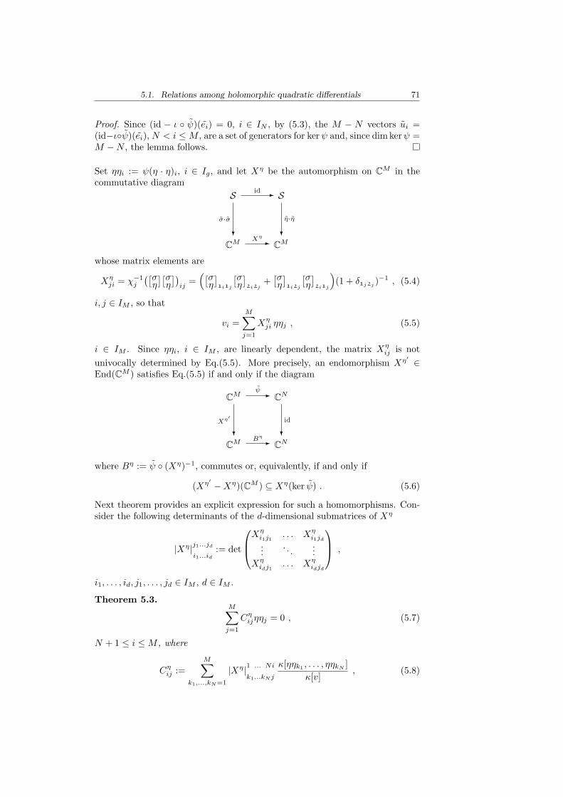
5.1. Relations among holomorphic quadratic differentials 71
Proof. Since (id − ι ψ)(ei) = 0, i ∈ IN , by (5.3), the M − N vectors ui =(id−ιψ)(ei), N < i ≤ M , are a set of generators for kerψ and, since dimkerψ =M −N , the lemma follows.
Set ηηi := ψ(η · η)i, i ∈ Ig, and let Xη be the automorphism on CM in thecommutative diagram
S S
CM CM
-id
?
σ·σ
?
η·η
-Xη
whose matrix elements are
Xηji = χ−1
j
([ση][σ
η])
ij=
([ση]1i1j
[ση]2i2j
+[ση]1i2j
[ση]2i1j
)(1 + δ1j2j
)−1 , (5.4)
i, j ∈ IM , so that
vi =M∑
j=1
Xηji ηηj , (5.5)
i ∈ IM . Since ηηi, i ∈ IM , are linearly dependent, the matrix Xηij is not
univocally determined by Eq.(5.5). More precisely, an endomorphism Xη′ ∈End(CM ) satisfies Eq.(5.5) if and only if the diagram
CM CN
CM CN
-ψ
?Xη′
?id
-Bη
where Bη := ψ (Xη)−1, commutes or, equivalently, if and only if
(Xη′ −Xη)(CM ) ⊆ Xη(ker ψ) . (5.6)
Next theorem provides an explicit expression for such a homomorphisms. Con-sider the following determinants of the d-dimensional submatrices of Xη
|Xη|j1...jd
i1...id
:= det
Xηi1j1
. . . Xηi1jd
.... . .
...Xη
idj1. . . Xη
idjd
,
i1, . . . , id, j1, . . . , jd ∈ IM , d ∈ IM .
Theorem 5.3.M∑
j=1
Cηijηηj = 0 , (5.7)
N + 1 ≤ i ≤ M , where
Cηij :=
M∑
k1,...,kN=1
|Xη|1 ... Ni
k1...kN j
κ[ηηk1 , . . . , ηηkN ]κ[v]
, (5.8)

72 5. The ideal of a canonical curve
are M −N independent linear relations among holomorphic quadratic differen-tials. Furthermore, for all p ∈ C
W [v](p) =M∑
i1,...,iN=1
|Xη|1 ... N
i1...iN
W [ηηk1 , . . . , ηηkN](p) . (5.9)
Proof. By (5.2) and (5.5)
M∑
j=1
(Xηji −
N∑
k=1
ψkiXηjk)ηηj = 0 ,
for all N + 1 ≤ i ≤ M , and by (5.1)
M∑
j=1
[ N∑
k=1
(−)k κ[vi, v1, . . . , vk, . . . , vN ]κ[v]
Xηjk + Xη
ji
]ηηj = 0 .
By (5.5)
κ[vi1 , . . . , viN ]κ[v]
=M∑
k1,...,kN=1
|Xη| i1...iN
k1...kN
κ[ηηk1 , . . . , ηηkN ]κ[v]
,
i1, . . . , iN ∈ IM , and we get (5.7) with
Cηij =
M∑
k1,...,kN=1
[ N∑
l=1
(−)lXηjl |Xη|i 1...l...N
k1......kN
+ Xηji |Xη|1 ... N
k1...kN
]κ[ηηk1 , . . . , ηηkN
]κ[v]
,
which is equivalent to (5.8) by the identity
N∑
l=1
(−)lXηjl |Xη|i 1...l...N
k1......kN
+ Xηji |Xη|1 ... N
k1...kN
= |Xη|i1 ... N
jk1...kN
.
Eq.(5.9) follows by (5.5).
The homomorphisms (Xη′ −Xη) ∈ End(CM ), satisfying (5.6), are the ele-ments of a M(M −N) dimensional vector space, spanned by
(Xη′ −Xη)ij =M∑
k=N+1
ΛjkCηki ,
i, j ∈ IM , with Λjk an arbitrary M×(M−N) matrix. An obvious generalizationof (5.2) yields
ηηi =N∑
j=1
vjBηji , (5.10)
i ∈ IM , implying that Bηij = κ[v1, . . . , vj−1, ηηi, vj+1, . . . , vN ]/κ[v], are the ma-
trix elements of the homomorphism Bη = ψ (Xη)−1. Such coefficients can beexpanded as
Bηij =
M∑
k1,...,kN−1=1
(−)j+1|Xη|1... ...N
k1... kN−1
κ[ηηi, ηηk1 , . . . , ηηkN−1 ]κ[v]
. (5.11)

5.1. Relations among holomorphic quadratic differentials 73
Define Cη,ijkl , 3 ≤ i < j ≤ g, k, l ∈ Ig, by
Cη,1m2m1n2n
:= Cηmn ,
m, n ∈ IM , m > N .The following result is a direct consequence of the Petri-like approach. The
bound r ≤ 6 for the rank of quadrics is not sharp, however: M. Green provedthat the ideal of quadrics of a canonical curve is generated by elements of rank4 [29].
Theorem 5.4. All the relations among holomorphic quadratic differentials haverank r ≤ 6.
Proof. The statement is trivial for g ≤ 6, so let us assume g ≥ 7. Each relationcan be written as
0 =σiσj + Cσ,ij12 σ1σ2 + Cσ,ij
1i σ1σi + Cσ,ij1j σ1σj + Cσ,ij
2i σ2σi + Cσ,ij2j σ2σj
+∑
k 6=1,2,i,j
Cσ,ij1k σ1σk +
∑
k 6=1,2,i,j
Cσ,ij2k σ2σk ,
where 3 ≤ i < j ≤ g and Cη,1i2i1j2j := Cη
ij . Set η1 ≡ σ1, η2 ≡ σ2, η3 ≡ σi,η4 ≡ σj , η5 ≡
∑k 6=1,2,i,j Cσ,ij
1k σk, η6 ≡∑
k 6=1,2,i,j Cσ,ij2k σk. Then the relations
can be written as6∑
k<l
Cη,ijkl ηkηl = 0 ,
for suitable Cη,ijkl , and the theorem follows.
5.1.1 Consistency conditions on the quadrics coefficients
In the construction in chapter 4, the points p1 and p2 play a special role withrespect to p3, . . . , pg. Relations among holomorphic quadratic differentials canbe obtained by replacing p1 and p2 with pa and pb, a, b ∈ Ig, a < b, (a, b) 6= (1, 2).In the following of this section, we will consider the relationships between thecoefficients Cσ obtained in section 4 and the analogous coefficients obtainedupon replacing (1, 2) by (a, b).
Proposition 5.5. There exist g distinct points p1, . . . , pg ∈ C such that
K(p1, . . . , pi, . . . , pj , . . . , pg) 6= 0 ,
for all i, j ∈ Ig, i 6= j.
Proof. Consider the function in Cg
F (p1, . . . , pg) :=∏
i<j
K(p1, . . . , pi, . . . , pj , . . . , pg) ,
and set Z := (p1, . . . , pg) ∈ Cg | F (p1, . . . , pg) = 0. Note that
Z =⋃
i<j
(p1, . . . , pg) ∈ Cg | K(p1, . . . , pi, . . . , pj , . . . , pg) = 0 ,

74 5. The ideal of a canonical curve
so that it is a finite union of varieties of codimension 1 in Cg and, in particular,Z 6= Cg. Suppose that Cg \ (
⋃i<j Πij) ⊆ Z, where Πij := (p1, . . . , pg) ∈ Cg |
pi = pj, 1 ≤ i < j ≤ g. Since Cg\(⋃i<j Πij) is dense in Cg, it would follow thatZ ≡ Cg, which is absurd. Hence, there exist pairwise distinct p1, . . . , pg ∈ Csuch that F (p1, . . . , pg) 6= 0.
By Proposition 5.5 and Proposition 4.4, one can choose the points p1, . . . , pg
in such a way that
v(ab)i i∈IN
:= σ2i i∈Ig
∪ σaσb ∪ σaσi, σbσii∈Ig\a,b ,
is a basis of H0(K2C). Furthermore, one can obtain M −N independent linear
relations ∑
1≤k≤l≤g
(ab)ijklσkσl = 0 , (5.12)
where i, j ∈ Ig \ a, b, i 6= j. The coefficients (ab)ijkl are defined by setting
(ab)ijij := 1,
(ab)ijkl :=
κ[v(ab)1 , . . . , σkσl, σiσj , . . . , v
(ab)N ]
κ[v(ab)1 , . . . , v
(ab)N ]
, (5.13)
if k 6= l and σkσl ∈ v(ab)i i∈IN
, and (ab)ijkl := 0 for all the other (k, l) ∈ Ig × Ig.
In this notation, the coefficients Cσij defined in (5.8), with N < i ≤ M , j ∈
IM , correspond to (12)1i2i1j2j
. Eqs.(5.12) and (5.13) can be derived by a trivialgeneralization of the same construction considered in section 2 in the particularcase a = 1, b = 2.
Proposition 5.6. The coefficients (ab)ijkl satisfy the following consistency con-
ditions
(ij)abkl =
∑
m≤n
(ij)abmn(ab)mn
kl =∑
m≤n
(ij)abmn(ai)mn
kl =∑
m≤n
(ij)abmn(aj)mn
kl (5.14)
=∑
m≤n
(ij)abmn(bi)mn
kl =∑
m≤n
(ij)abmn(bj)mn
kl , (5.15)
for all i, j, a, b ∈ Ig pairwise distinct, and for all k, l ∈ Ig.
Proof. Choose i, j, a, b ∈ Ig, with a < b < i < j, and consider the relations∑k≤l(ij)
abklσkσl = 0 and
∑k≤l(ab)ij
klσkσl = 0, that is
0 = (ij)abij σiσj + σaσb + (ij)ab
aiσaσi + (ij)abajσaσj + (ij)ab
bi σbσi (5.16)
+ (ij)abbj σbσj +
∑
k 6=a,b,i,j
(ij)abikσiσk +
∑
k 6=a,b,i,j
(ij)abjkσjσk ,
(5.17)
0 = σiσj + (ab)ijabσaσb + (ab)ij
aiσaσi + (ab)ijajσaσj + (ab)ij
biσbσi (5.18)
+ (ab)ijbjσbσj +
∑
k 6=a,b,i,j
(ab)ijakσaσk +
∑
k 6=a,b,i,j
(ab)ijbkσbσk .
(5.19)

5.2. A correspondence between quadrics and θ-identities 75
Replace the differentials σiσk and σjσk, k 6= i, j, a, b, in Eq.(5.16) by
σiσk = −∑
m≤n(m,n) 6=(i,k)
(ab)ijmnσmσn , k 6= i, j, a, b ,
and the analogous expression for σjσk. Then multiply Eq.(5.18) by (ij)abij and
consider the difference between (5.16) and (5.18). We obtain
0 =((ij)ab
ab −∑
m≤n
(ij)abmn(ab)mn
ab
)σaσb +
∑
k 6=a,b
((ij)ab
ak −∑
m≤n
(ij)abmn(ab)mn
ak
)σaσk
(5.20)
+∑
k 6=a,b
((ij)ab
bk −∑
m≤n
(ij)abmn(ab)mn
bk
)σbσk . (5.21)
Since the holomorphic quadratic differentials appearing in Eq.(5.20) are linearlyindependent, it follows that each coefficient vanishes, yielding the first identityin (5.14), in the cases in which at least one between k and l is equal to a or b.On the other hand, in the case k, l 6= a, b, the only non-vanishing term in thesum
∑m≤n(ij)ab
mn(ab)mnkl is (ij)ab
kl (ab)klkl = (ij)ab
kl , and the first identity in (5.14)follows. The other identities can be proved by applying the analogous procedureto the relation
∑k≤l(ij)
abklσkσl = 0 and one of the relations
∑k≤l(ai)bj
klσkσl = 0,∑k≤l(bi)
ajkl σkσl = 0, and so on.
5.2 A correspondence between quadrics and θ-identities
Theorem 5.7. Fix (p1, . . . , pg) ∈ Cg\B with B defined in Definition 4.2. Then,the associated holomorphic quadratic differentials vi, i ∈ IM , satisfy
vi =M∑
j=1
Xωji ωωj , (5.22)
i ∈ IN , where
Xωij =
θ1j (a1i)θ2j (a2i) + θ1j (a2i)θ2j (a1i)(1 + δ1j2j )
∑l,m θl(a1i)θm(a2i)ωl(p1i)ωm(p2i)
, (5.23)
i, j ∈ IM , with ai as in Definition 4.1, correspond to the coefficients defined in(5.4) for ηi ≡ ωi, i ∈ Ig. Furthermore, the M −N independent linear relations
M∑
j=1
Cωijωωj = 0 , (5.24)
N + 1 ≤ i ≤ M , hold, where
Cωij =
M∑
k1,...,kN=1
|Xω|1 ... Ni
k1...kN j
κ[ωωk1 , . . . , ωωkN]
κ[v]. (5.25)
correspond to the coefficients defined in (5.8).
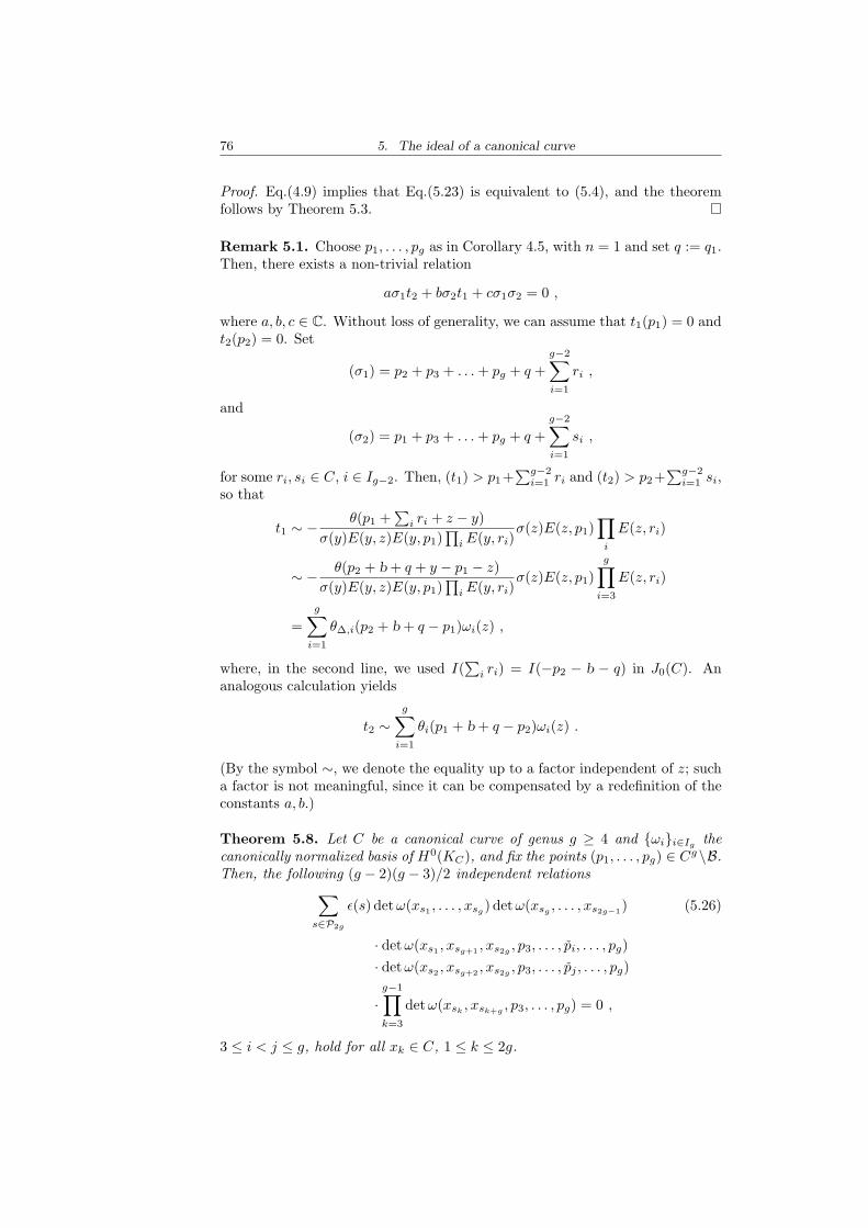
76 5. The ideal of a canonical curve
Proof. Eq.(4.9) implies that Eq.(5.23) is equivalent to (5.4), and the theoremfollows by Theorem 5.3.
Remark 5.1. Choose p1, . . . , pg as in Corollary 4.5, with n = 1 and set q := q1.Then, there exists a non-trivial relation
aσ1t2 + bσ2t1 + cσ1σ2 = 0 ,
where a, b, c ∈ C. Without loss of generality, we can assume that t1(p1) = 0 andt2(p2) = 0. Set
(σ1) = p2 + p3 + . . . + pg + q +g−2∑
i=1
ri ,
and
(σ2) = p1 + p3 + . . . + pg + q +g−2∑
i=1
si ,
for some ri, si ∈ C, i ∈ Ig−2. Then, (t1) > p1+∑g−2
i=1 ri and (t2) > p2+∑g−2
i=1 si,so that
t1 ∼ − θ(p1 +∑
i ri + z − y)σ(y)E(y, z)E(y, p1)
∏i E(y, ri)
σ(z)E(z, p1)∏
i
E(z, ri)
∼ − θ(p2 + b + q + y − p1 − z)σ(y)E(y, z)E(y, p1)
∏i E(y, ri)
σ(z)E(z, p1)g∏
i=3
E(z, ri)
=g∑
i=1
θ∆,i(p2 + b + q − p1)ωi(z) ,
where, in the second line, we used I(∑
i ri) = I(−p2 − b − q) in J0(C). Ananalogous calculation yields
t2 ∼g∑
i=1
θi(p1 + b + q − p2)ωi(z) .
(By the symbol ∼, we denote the equality up to a factor independent of z; sucha factor is not meaningful, since it can be compensated by a redefinition of theconstants a, b.)
Theorem 5.8. Let C be a canonical curve of genus g ≥ 4 and ωii∈Ig thecanonically normalized basis of H0(KC), and fix the points (p1, . . . , pg) ∈ Cg\B.Then, the following (g − 2)(g − 3)/2 independent relations
∑
s∈P2g
ε(s) det ω(xs1 , . . . , xsg ) det ω(xsg , . . . , xs2g−1) (5.26)
· detω(xs1 , xsg+1 , xs2g , p3, . . . , pi, . . . , pg)· detω(xs2 , xsg+2 , xs2g , p3, . . . , pj , . . . , pg)
·g−1∏
k=3
detω(xsk, xsk+g
, p3, . . . , pg) = 0 ,
3 ≤ i < j ≤ g, hold for all xk ∈ C, 1 ≤ k ≤ 2g.
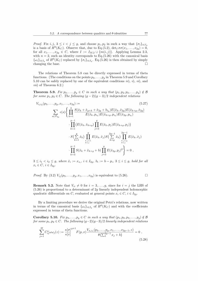
5.2. A correspondence between quadrics and θ-identities 77
Proof. Fix i, j, 3 ≤ i < j ≤ g, and choose p1, p2 in such a way that σii∈Ig
is a basis of H0(KC). Observe that, due to Eq.(5.2), detI σσ(x1, . . . , x2g) = 0,for all x1, . . . , x2g ∈ C, where I := IM,2 ∪ m(i, j). Applying Lemma 2.3,with n = 2, such an identity corresponds to Eq.(5.26) with the canonical basisωii∈Ig
of H0(KC) replaced by σii∈Ig. Eq.(5.26) is then obtained by simply
changing the base.
The relations of Theorem 5.8 can be directly expressed in terms of thetafunctions. (The conditions on the points p3, . . . , pg in Theorem 5.9 and Corollary5.10 can be safely replaced by one of the equivalent conditions iv), v), vi), andvii) of Theorem 6.2.)
Theorem 5.9. Fix p3, . . . , pg ∈ C in such a way that (p1, p2, p3, . . . , pg) /∈ Bfor some p1, p2 ∈ C. The following (g − 2)(g − 3)/2 independent relations
Vi1i2(p3, . . . , pg, x1, . . ., x2g) := (5.27)
∑
s∈P2g
ε(s)
2∏
k=1
S(xk + xg+k + x2g + bik)E(xk, x2g)E(xk+g, x2g)
E(xk, pik)E(xk+g, pik
)E(x2g, pik)
·g−1∏
k=1
(E(xk, xk+g)
g∏
j=3
E(xk, pj)E(xk+g, pj))
· S( g∑k=1
xk
) g∏k,j=1k<j
E(xk, xj)S(2g−1∑
k=g
xk
) 2g−1∏k,j=gk<j
E(xk, xj)
·g−1∏
k=3
S(xk + xk+g + b)g∏
j=3
E(x2g, pj)2
= 0 ,
3 ≤ i1 < i2 ≤ g, where xi := xsi , i ∈ I2g, bi := b − pi, 3 ≤ i ≤ g, hold for allxi ∈ C, i ∈ I2g.
Proof. By (3.2) Vij(p3, . . . , pg, x1, . . . , x2g) is equivalent to (5.26).
Remark 5.2. Note that Vii 6= 0 for i = 3, . . . , g, since for i = j the LHS of(5.26) is proportional to a determinant of 2g linearly independent holomorphicquadratic differentials on C, evaluated at general points xi ∈ C, i ∈ I2g.
By a limiting procedure we derive the original Petri’s relations, now writtenin terms of the canonical basis ωii∈Ig of H0(KC) and with the coefficientsexpressed in terms of theta functions.
Corollary 5.10. Fix p3, . . . , pg ∈ C in such a way that (p1, p2, p3, . . . , pg) /∈ Bfor some p1, p2 ∈ C. The following (g−2)(g−3)/2 linearly independent relations
M∑
j=1
Cωijωωj(z) :=
κ[σ]κ[v]
g+1
F (p, x)V1i2i(p3, . . . , pg, x1, . . . , x2g−1, z)
θ(∑2g−1
1 xj + b) = 0 ,
(5.28)

78 5. The ideal of a canonical curve
N + 1 ≤ i ≤ M , where
F (p, x) := c′g,2
∏gj,k=3j<k
E(pj , pk)g−4∏g
j=3j 6=1i
E(p1i, pj)
∏gj=3j 6=2i
E(p2i, pj)
∏2g−1j=1 (σ(xj)
∏gk=3 E(xj , pk)
∏2g−1k=j+1 E(xj , xk))
,
hold for all z ∈ C. Furthermore, Cωij are independent of p1, p2, x1, . . . , x2g−1 ∈ C
and correspond to the coefficients defined in (5.8) (with ηi ≡ ωi, i ∈ Ig) or,equivalently, in (5.25).
Proof. Consider the identity
detI σσ(x1, . . . , x2g−1, z)det v(p3, . . . , pg, x1, . . . , x2g−1)
= 0 , (5.29)
I := IM,2 ∪ i, N + 1 ≤ i ≤ M . Upon applying Lemma 2.3, with n =2, and Eq.(3.2) to the numerator and Eq.(3.3) to the denominator of (5.29),Eq.(5.28) follows by a trivial computation. On the other hand, for arbitrarypoints z, y1, . . . , yg−1 ∈ C,
S(y1 + . . . + yg−1 + z) =∑g
i=1 θi(y1 + . . . + yg−1)ωi(z)
σ(z)∏g−1
1 E(z, yi).
Consider V1i2i(p3, . . . , pg, x1, . . . , xg−1, z) and replace each term in of the formS(dg−1+z) by its expression above, for any effective divisor dg−1 of degree g−1.The dependence on z only enters through ωiωj(z) and the relations (5.28) canbe written in the form of Eq.(5.7).
To prove that Cωij are the coefficients in (5.8), with ηi ≡ ωi, i ∈ Ig, first
consider the identity
κ[ωωk1 , . . . , ωωkN ]κ[v]
=deti∈k1,...,kN ωωi(p3, . . . , pg, x1, . . . , x2g−1)
det v(p3, . . . , pg, x1, . . . , x2g−1),
then recall that
vi := σσi =M∑
j=1
Xωjiωωj ,
i ∈ IM , so that one obtains
M∑
k1,...,kN ,j=1
|Xω|1 ... Ni
k1...kN j
κ[ωωk1 , . . . , ωωkN ]κ[v]
ωωj(z)
=detI σσ(x1, . . . , x2g−1, z)
det v(p3, . . . , pg, x1, . . . , x2g−1),
as an algebraic identity (in the sense that it holds as an identity in Sym2(H0C(K))
after replacing σiσj → σi·σj and ωiωj → ωi·ωj , i, j ∈ Ig). Hence, the coefficientsof ωωj(z) on the LHS, given by (5.8) or, equivalently, by (5.25) and the ones onthe RHS, given by (5.28), are the same.
Eq.(5.8) explicitly shows that the coefficients Cωij are independent of xi for
all i = 1, . . . , 2g − 1. By (5.28) it follows that they may depend on p1 and p2

5.3. Relations among holomorphic cubic differentials 79
only through the term κ[σ]g+1/κ[v]. The dependence of κ[σ] and κ[v] on p1 andp2 is due to the dependence of the basis σii∈Ig and vii∈IN on the choiceof p1, . . . , pg ∈ C. On the other hand, Eq.(6.4) implies that κ[σ]g+1/κ[v] isindependent of p1, p2 and the proof of the corollary is complete.
5.3 Relations among holomorphic cubic differentials
According to Petri’s Theorem, in the most general case the ideal of a canonicalcurve C is generated by its ideals of quadrics together with the ideal of cubics.As discussed in the introduction of this section, such cubics correspond to linearrelations among holomorphic 3-differentials on C; a generalization of the previ-ous construction is necessary in order to explicitly determine such relations.
Fix p1, . . . , pg ∈ C satisfying the conditions i), ii) and iii) of Proposition 4.6with respect to some fixed i, 3 ≤ i ≤ g, and let ϕjj∈IN3−1 ∪ ϕi+5g−8 be thecorresponding basis of H0(K3
C). The kernel of the canonical epimorphism fromSym3H0(KC) onto H0(K3
C) has dimension (g − 3)(g2 + 6g − 10)/6, and eachelement corresponds to a linear combination of the following relations
σjσkσl =∑
m∈IN3−1
Bjkl,mϕm + Bjkl,i+5g−8σ2σ2i , (5.30)
3 ≤ j, k, l ≤ g, j 6= k, and
σ2σ2j =
∑
m∈IN3−1
B2jj,mϕm + B2jj,i+5g−8σ2σ2i , (5.31)
3 ≤ j ≤ g, j 6= i, where Bjkl,m, B2jj,m ∈ C, are suitable coefficients. On theother hand, a trivial computation shows that the relations (5.30) are generatedby (5.31) and by the relations among holomorphic quadratic differentials,
M∑
j=1
Cσkjσσj = 0 , (5.32)
k = N + 1, . . . , M . Therefore, relations among holomorphic 3-differentials,modulo relations among holomorphic quadratic differentials, provide at mostg − 3 independent conditions on products of elements of H0(KC).
The relations (5.31) can be restated in terms of an arbitrary basis ηjj∈Ig
of H0(KC). Let Y η be the automorphism of CM3 , determined by
Y ηkj := χ−1
k ([η]−1[η]−1[η]−1)jk , (5.33)
j, k ∈ IM3 , so that
ϕj =M3∑
k=1
Y ηkjηηηk ,
j ∈ IM3 . Consider the following determinants of d-dimensional submatrices ofY η
|Y η|j1...jd
i1...id
:= det
Y ηi1j1
. . . Y ηi1jd
.... . .
...Y η
idj1. . . Y η
idjd
,
i1, . . . , id, j1, . . . , jd ∈ IM3 , d ∈ IM3 .

80 5. The ideal of a canonical curve
Proposition 5.11.M3∑
j=1
Dηkjηηηj = 0 , (5.34)
N3 ≤ k ≤ N3 + g − 3, k 6= i where
Dηkj :=
M3∑
k1,...,kN3=1
|Y η|1...(N3−1) i k
k1 ... kN3 j
κ[ηηηk1 , . . . , ηηηkN3]
κ[ϕ], (5.35)
j ∈ IM3 , are g−3 independent linear relations among holomorphic 3-differentials.
Proof. Without loss of generality, we can assume i = N3; such an assumptioncan always be satisfied after a re-ordering of the points p3, . . . , pg. Fix N3 + 1arbitrary points x1, . . . , xN3 , xN3+1 ≡ z ∈ C and consider the singular matrix[ϕl(xm)]l∈I
m∈IN3+1with I := IN3∪k, with N3 < k ≤ N3+g−3. By expressing the
determinant with respect to the column (ϕl(z))l∈I , the identity det ϕl(xm) = 0,l ∈ I, m ∈ IN3+1, yields
M3∑m=1
[ N3∑
l=1
(−)l+1 κ[ϕ1, . . . , ϕl, . . . , ϕN3 , ϕk]κ[ϕ]
Y ηml − Y η
mk
]ηηηm = 0 .
The proposition follows by combinatorial identities analogous to the proof ofTheorem 5.3.
Whereas for g = 4 the relations (5.34) are independent of the relation amongholomorphic quadratic differentials, for g ≥ 5, (5.34) are generated by (5.32)in all but some particular curves. Set ψ1i2i,1j2j := ψij and Cσ
1i2i,1j2j:= Cσ
ij ,N + 1 ≤ i ≤ M , j ∈ IM . Consider the 3-differentials σiσjσk with 3 ≤ i < j <
k ≤ g (g ≥ 5). By Eq.(5.32) and by Cσij = ψij − δij , N + 1 ≤ i ≤ M , j ∈ IM ,
σiσjσk =2∑
m=1
g∑n=3
ψij,mnσmσnσk + ψij,12σ1σ2σj ,
so that2∑
m,p=1
g∑q=3
( g∑n=3n 6=j
ψik,mnψnj,pq
)σmσpσq + ψik,12σ1σ2σk +
2∑m=1
ψik,mjσmσ2j
=2∑
m,p=1
g∑q=3
( g∑n=3n 6=i
ψjk,mnψni,pq
)σmσpσq + ψjk,12σ1σ2σk +
2∑m=1
ψjk,miσmσ2i .
The above equation yields
Cσik,2jσ2σ
2j =
2∑m,p=1
g∑q=3
( g∑n=3n 6=i
Cσjk,mnCσ
ni,pq −g∑
n=3n 6=j
Cσik,mnCσ
nj,pq
)σmσpσq
+ Cσjk,12σ1σ2σk − Cσ
ik,12σ1σ2σk + Cσjk,1iσ1σ
2i
− Cσik,1jσ1σ
2j + Cσ
jk,2iσ2σ2i .

5.3. Relations among holomorphic cubic differentials 81
If Cσik,2j 6= 0 for some k, the above identity shows that the relation (5.31)
is generated by Eqs.(5.32). On the other hand, it can be proved [3] that ifCσ
ik,2j = 0 for all 3 ≤ k ≤ g, k 6= i, j, the relation (5.31) is independent of therelations among holomorphic quadratic differentials. This case occurs if andonly if the curve C is trigonal or a smooth quintic.
Proposition 5.12. Fix g points p1, . . . , pg ∈ C satisfying the conditions oftheorem 4.6. The coefficients Y ω
ij , defined in Eq.(5.33) with η ≡ ω, are given by
Y ωij =
(1 + δ1j2j + δ2j3j )(1 + δ1j3j )6
∏m∈1,2,3
∑l θl(ami)ωl(pmi)
∑
s∈P3
( ∏m∈1,2,3
θs(m)j(ami
))
, (5.36)
i, j ∈ IM .
Proof. The proposition follows immediately by the definition (5.33) and byEq.(4.9).

82 5. The ideal of a canonical curve

6. THE SECTION K
6.1 Definition and fundamental properties
Definition 6.1. For all p3, . . . , pg, x1, . . . , x2g−1 ∈ C, set
K(p3, . . . , pg) :=1
θ(b +
∑2g−11 xi
) ∏2g−11 σ(xi)
∏gi=3 σ(pi)
(6.1)
·∑
s∈P2g−1
S(∑g
i=1 xsi
)S
(∑2g−1i=g xsi
)∏g
i=3 E(xsg , pi)
g−1∏
i=1
S(xsi+ xsi+g
+ b)∏g−1j=1j 6=i
E(xsi , xsj+g ).
Theorem 6.1. For all p3, . . . , pg ∈ C, the following properties hold:
a. K ≡ K(p3, . . . , pg) is independent of x1, . . . , x2g−1 ∈ C.
b. For any p1, . . . , pg ∈ C such that det ηi(pj) 6= 0, the set vii∈IN , definedin (4.14), is a basis of H0(K2
C) if and only if K 6= 0.
c.S(p1 + p2 + b) = 0 , ∀p1, p2 ∈ C =⇒ K = 0 . (6.2)
d. If p3, . . . , pg are pairwise distinct and K 6= 0, then there exist p1, p2 ∈ Csuch that H 6= 0.
Proof. – a. The ratio
H
K= S(a)5g−7E(p1, p2)g+1
g∏
i=3
(E(p1, pi)E(p2, pi))4g∏
i,j=3i<j
E(pi, pj)5 , (6.3)
is independent of x1, . . . , x2g−1, so that a) follows by Theorem 4.12 or,equivalently, noticing that by Eqs.(4.11)(4.25)(4.27) and (6.3)
K(p3, . . . , pg) := (−)g+1cg,2κ[v]
κ[σ]g+1
g∏i,j=3i<j
E(pi, pj)2−g
g∏
i=3
σ(pi)3−g . (6.4)
– b. By (3.2) and (6.3) the condition det ηi(pj) 6= 0 implies H/K 6= 0. In thiscase K 6= 0 if and only if H 6= 0, and b) follows by Theorem 4.12.
– c. If S(p1+p2+b) = 0, for all p1, p2 ∈ C, then the numerators in each term ofthe sum in (6.1) vanish for all x1, . . . , x2g−1 ∈ C. Since K is independentof x1, . . . , x2g−1, it follows that the proof of point c) is equivalent to provethat there exist x1, . . . , x2g−1 ∈ C such that the denominators in (6.1) donot vanish. On the other hand, the possible zeros of such denominators

84 6. The section K
are the ones corresponding of the zeros of the primes forms, which areavoided by simply choosing p3, . . . , pg, x1, . . . , x2g−1 pairwise distinct, andthe ones of θ(b +
∑2g−11 xi). Fix an arbitrary y ∈ C and set w := I(b +∑2g−1
g+1 xi + y). Then
θ(b +
2g−1∑1
xi
)= θ
(w +
g∑1
xi − y)
,
and, by the Jacobi Inversion Theorem, by varying the points x1, . . . , xg ∈C one can span the whole Jacobian variety. Then, one can always choosex1, . . . , x2g−1 pairwise distinct and distinct from p3, . . . , pg in such a waythat θ
(w +
∑g1 xi − y
) 6= 0, so that the denominator does not vanish andc) follows.
–d. Since K 6= 0, by c) there exist p1, p2 ∈ C such that S(p1 + p2 + b) 6= 0.By continuity arguments, it follows that there exist some neighborhoodsUi ⊂ C of pi, i = 1, 2, such that S(x1+x2+b) 6= 0 for all (x1, x2) ∈ U1×U2.Hence, we can choose p1, p2 so that S(p1 + p2 + b) 6= 0 and p1, . . . , pg arepairwise distinct. Then, by Eq.(6.3), H/K 6= 0 and, since K 6= 0, weconclude that H 6= 0.
In view of Eq.(6.4), it is useful to define
k(p3, . . . , pg) :=K(p3, . . . , pg)g∏
i,j=3i<j
E(pi, pj)g−2
g∏
i=3
σ(pi)g−3 (6.5)
=(−)g+1cg,2κ[v]
κ[σ]g+1,
which is a holomorphic (g − 3)-differential in each of its g − 2 arguments.
Theorem 6.2. Fix p1, . . . , pg ∈ C, with C non-hyperelliptic of genus g ≥ 4and let σii∈Ig be a set of non-vanishing holomorphic 1-differentials such thati 6= j ⇒ σi(pj) = 0, for all i, j ∈ Ig. The following statements are equivalent
i) The conditions
i′) (p1, . . . , pg) /∈ A;
i′′) b :=∑g
i=3 pi is the greatest common divisor of (σ1) and (σ2);
are satisfied;
ii) H(p1, . . . , pg) 6= 0, where H is defined in Eq.(4.25);
iii) vii∈IN is a basis of H0(K2C), with vi := σσi, i ∈ IM .
More generally, fix p3, . . . , pg ∈ C. The following statements are equivalent:
iv) p3, . . . , pg are pairwise distinct and I(p + b)|p ∈ C ∩Θs = ∅;
v) p3, . . . , pg are pairwise distinct and K(p3, . . . , pg) 6= 0, where K is definedin Eq.(6.1);

6.2. Zeros of K and the singular locus Θs 85
vi) There exist p1, p2 ∈ C such that p1, . . . , pg satisfy i), ii) and iii);
vii) For all p ∈ C, S(x + p + b) does not vanish identically as a function of x;furthermore, for each p2 ∈ C \p3, . . . , pg, the points p1, . . . , pg satisfy i),ii) and iii) if and only if p1 is distinct from p2, . . . , pg and from the g − 1zeros of S(x + p2 + b).
Proof. i) ⇔ iii) is proved in Proposition 4.4 (in the direction i) ⇒ iii), only thecase of normalized 1-differentials σi(pi) = 1, for all i ∈ Ig is considered;however, by the hypothesis i′), the general case can be reduced to thischoice by a non-singular diagonal transformation on σii∈Ig
);
ii) ⇔ iii) is proved in Theorem 4.12;
vii) ⇒ vi) is obvious;
iv) ⇔ vii) follows by first noting that S(x + p + b) identically vanishes as afunction of x if and only if I(p + b) ∈ Θs, and then by Theorem 4.10;in particular, in such a theorem it is proved that for each fixed p2 ∈C \p3, . . . , pg, the points p1, . . . , pg satisfy i) if and only if the conditionsp1 /∈ p2, . . . , pg, S(p1 + p2 + b) 6= 0 and iv) hold;
vi) ⇒ iv) also follows by Theorem 4.10, where it is proved that if iv) does nothold, then i′′) cannot be satisfied;
v) ⇔ vi) follows by Corollary 6.1, where it is proved that i′) and v) are equiv-alent to ii) and that if v) holds, then there exist p1, p2 ∈ C such thatp1, . . . , pg satisfy ii).
6.2 Zeros of K and the singular locus Θs
The function K(p3, . . . , pg) defined in Eq.(6.1), whose zero divisor is character-ized in the theorem above, is the fundamental tool in the proof of the followingtheorem. Such a result heavily relies on the properties of Θs in the case thesublying ppav is the Jacobian torus of a canonical curve. By the RiemannSingularity Theorem,
Θs = W 1g−1 ≡ I(C1
g−1) ,
where C1g−1 ⊂ Cg−1 is the subvariety of codimension 2 in Cg−1, whose elements
are the effective divisors of degree g − 1 with index of specialty greater than 1.Note that each effective divisor d ∈ Cg−3 of degree g−3 canonically determinesan embedding
πd : C2 → Cg−1 ,
c 7→ c + d ,
of C2 as a subvariety of dimension 2 in Cg−1. Hence, by a simple dimensionalcounting, we expect the intersection C1
g−1∩πd(C2) to have (in general) dimension0. The following theorem shows that, in the general case in which such anintersection does not contain any component of dimension greater than 0, C1
g−1∩πd(C2) corresponds (set-theoretically) to a set of g(g−3)/2 points; furthermore,a remarkable relation of such a set of points with the canonical divisor is given.

86 6. The section K
Since the restriction of the Abel-Jacobi map to C2 is an injection (because C isnon-hyperelliptic), such points are in one to one correspondence with the pointsin the intersection Θs ∩ I(πd(C2)).
Theorem 6.3. Let C be non-hyperelliptic of genus g ≥ 4 and fix an effectivedivisor d ∈ Cg−3 of degree g − 3. Then, either:
a. For each point p ∈ C, there exists a point q ∈ C such that
I(p + q + d) ∈ Θs ;
or:
b. There exist k := g(g − 3)/2 effective divisors c1, . . . , ck ∈ C2 of degree 2,such that
ei := I(ci + d) ∈ Θs , ∀i ∈ Ik . (6.6)
Moreover, in this case
k∑
i=1
ci + (g − 2)d = (g − 3)KC .
Proof. Set d :=∑g
i=4 pi and consider K(z, p4, . . . , pg) as a function of z. Itvanishes at z ≡ p if and only if there exists a point q ∈ C such that I(p+q+d) ∈Θs. Then, K = 0 for all z ∈ C if and only if statement a) holds.Now, assume that K(z, p4, . . . , pg) does not vanish identically and consider
φ(z) := K(z, p4, . . . , pg)g∏
i=4
E(z, pi)g−2σ(z)g−3 . (6.7)
By (6.4), φ is a holomorphic (g−3)-differential on C. Therefore, the divisor e ofK(z, p4, . . . , pg) is effective (K has no poles) of degree g(g− 3) and e + (g− 2)dis the divisor of a (g− 3)-differential. It only remains to prove that e is the sumof all the effective divisors of degree 2 satisfying Eq.(6.6). By the equivalence ofiv) and v) in Theorem 6.2, if c := q1 + q2 satisfies Eq.(6.6), then q1 and q2 areboth zeros of K. By construction, K(z, p4, . . . , pg) can be written as
K(z, p4, . . . , pg) = F (z, p4, . . . , pg, x1, . . . , x2g−1) det ϕi(xj) ,
with ϕ1, . . . , ϕ2g−1 a set of generators (depending on z, p4, . . . , pg) of H0(K2C⊗
O(−z−d)) and x1, . . . , x2g−1 arbitrary points in C; F is such that, by Corollary6.1, K does not depend on x1, . . . , x2g−1. It is easy to verify that K vanishesonly if det ϕi(xj) = 0 for all x1, . . . , x2g−1 ∈ C; the multiplicity of such a zero is2g− 1− r, where r := h0(K2
C ⊗O(−z− d)). The space H0(K2C ⊗O(−z− d)) is
generated by elements σ1η, σ2ρ, as η, ρ vary in H0(KC); here, σ1, σ2 is a basisfor the 2-dimensional space H0(KC⊗O(−z−d)) (note that if there exists q ∈ Csuch that h0(KC ⊗O(−q − d)) > 2, then K(z, p4, . . . , pg) identically vanishes).Proposition 4.4 shows that K(z, p4, . . . , pg) 6= 0, that is r = 2g − 1, if and onlyif h0(KC ⊗O(−q − z − d)) = 1 for all q ∈ C. Let q1 be a zero of K and denoteby n the maximal integer for which there exist n− 1 points q2, . . . , qn ∈ C suchthat h0(KC ⊗O(−q1 − . . .− qn − d) = 2. By the considerations above, since q1

6.2. Zeros of K and the singular locus Θs 87
is a zero, n ≥ 2; furthermore, q2, . . . , qn are zeros of K too. Corollary 4.5 showsthat
r ≡ h0(K2C ⊗O(−q1 − d)) = h0(K2
C ⊗O(−q1 − . . .− qn − d)) = 2g − n ,
so that the multiplicity of each qi, i ∈ In, is 2g− 1− r = n− 1. Now, consider azero q′1 of K(z, p4, . . . , pg), distinct from q1, . . . , qn; by the same construction, ifq′1 has multiplicity n′−1, with n′ ≥ 2, then it is an element of a set of n′ (possiblycoincident) zeroes q′1, . . . , q′n with the same multiplicity. By repeating thisprocedure, we obtain a finite number l of disjoint sets of zeroes; for each i ∈ Il,the i-th set contains ni ≥ 2 zeroes, we denote by qi
1, . . . , qini
, each one withmultiplicity ni − 1. Therefore, we have
e =l∑
i=1
ni∑
j=1
(ni − 1)qij =
l∑
i=1
ni∑
j,k=1j<k
(qij + qi
k) ,
and, since h0(KC ⊗ O(−qij − qi
k − d)) = 2, each c := qij + qi
k satisfies Eq.(6.6);conversely, it follows immediately that if an element of C2 satisfies Eq.(6.6),then it is the sum of a pair of zeroes of K(z, p4, . . . , pg) in the same set.
Theorem 6.4. There exists a holomorphic section A on Θs × . . . × Θs ≡ΘM−N
s , completely anti-symmetric in its M −N arguments and such that, forall p3, . . . , pg ∈ C,
A(eN+1, . . . , eM ) =deti,j=N+1,...,M
(∑gk,l=1 θkl(ei)ωk(p1j )ωl(p2j )
)
k(p3, . . . , pg). (6.8)
Furthermore, the quadrics
g∑
ij=1
θij(ek)XiXj , (6.9)
k = N + 1, . . . ,M , generate the ideal I2 of quadrics of the canonical curve C ifand only if A(eN+1, . . . , eM ) 6= 0.
Proof. Let us first prove that the ratio on the right hand side of Eq.(6.8) doesnot depend on p3, . . . , pg ∈ C. The numerator of such a ratio is the determinantof a (M − N) × (M − N) matrix W , which can be expressed as the productW = UV of a (M − N) × M matrix U and a M × (M − N) matrix V , withentries
Uij := θ1j+N 2j+N(ei+N ) , Vjk := χ−1
j (p · p)k+N [ωωj ] ,
i, k = 1, . . . ,M −N , j ∈ IM , where, by definition (4.4),
(p · p)k[ωωj ] = ω1j (p1k)ω2j (p2k
) + ω1j (p2k)ω2j (p1k
) .
The determinant det W is a holomorphic (g − 3)-differential in each pi, i =3, . . . , g; furthermore, it is symmetric (for g even) or anti-symmetric (for g odd),with respect to permutations of such arguments. Fix p4, . . . , pg ∈ C and considerthe divisor of detW with respect to p3. Define a local trivialization of KC and

88 6. The section K
a local coordinate z on an open neighborhood of p4; with respect to such atrivialization, in the limit p3 → p4, det W can be seen as a holomorphic functionin (p3, p4) ∈ U × U . Such a determinant is invariant under the replacement, inthe matrix W , of the column
∑ij θij(eN+1)ωi(p3)ωj(pk)
...∑ij θij(eM )ωi(p3)ωj(pk)
)
,
by the column
∑ij θij(eN+1)(ωi(p3)− ωi(p4))ωj(pk)
...∑ij θij(eM )ωi(p3)(ωi(p3)− ωi(p4))ωj(pk)
,
for all k = 5, . . . , g. It follows that each of these columns is of order z(p3)−z(p4)in the limit p3 → p4. Then, consider the element
∑ij θij(ek)ωi(p3)ωj(p4), for
each k = N +1, . . . ,M . Such a function vanishes at p3 = p4 due to the relations(B.6); moreover, since it is symmetric with respect to the exchange p3 ↔ p4,the first non-vanishing contribution in the limit p3 → p4 must be of order(z(p3)− z(p4))2. It follows that det W has a zero of order g− 2 at p3 = p4 and,by symmetry arguments, at p3 = pi for all i = 4, . . . , g.
Fix p3, . . . , pg ∈ C and suppose that there exists a point p ∈ C such thate := I(p + p3 + . . . + pg) is in Θs. Each point of Θs is associated to a relationamong holomorphic quadratic differentials by Eq.(B.6). On the other hand,since at most M − N such relations can be linearly independent, there existsome coefficients c, cN+1, . . . , cM ∈ C such that
cθij(e) +M∑
k=N+1
ckθij(ek) = 0 , (6.10)
for all i, j = 1, . . . , g. By Proposition 3.3,
g∑
i,j=1
θij(e)ωi(pk)ωj(pl) = 0 ,
which, by (6.10), implies
M∑
n=N+1
cn
g∑
i,j=1
θij(en)ωi(pk)ωj(pl) = 0 ,
for all 3 ≤ k, l ≤ g, so that the rows of W are linearly dependent and detW = 0.Hence, det W , considered as a holomorphic (g − 3)-differential in p3, has a
zero of order g − 2 at each pi, i = 4, . . . , g, and vanishes if there exists p ∈ C,such that I(p + p3 + . . . + pg) ∈ Θs; it follows that the right hand side of (6.8)is a meromorphic function of p3 with no poles, and then is a constant. By thesame arguments, it does not depend on pi, for all i = 3, . . . , g.
The condition that the quadrics (6.9) generate the ideal I2 of degree 2 ofC is equivalent to the matrix U having its maximal rank. Therefore, if such

6.3. Quadrics from double points on Θs 89
quadrics does not generate I2, then A(eN+1, . . . , eM ) = 0. Conversely, sincethere always exist p3, . . . , pg ∈ C such that V has rank M −N , it follows thatif A(eN+1, . . . , eM ) 6= 0 then the matrix U has maximal rank.
Green [29] proved that the ideal I2 of degree 2 is generated by quadrics in theform (6.9). Together with Theorem 6.4, this implies that A(eN+1, . . . , eM ) doesnot vanish identically. Consider the coefficients Cω
ij , i = N + 1, . . . ,M , j ∈ IM ,given by Corollary 5.10 for some suitable p3, . . . , pg ∈ C. The correspondingquadrics (5.28) generate I2; it follows that each θij(ek), k = N + 1, . . . , M , canbe expressed as a linear combination
θ1j2j(ek) =
M∑
i=N+1
ckiCωij ,
for all j ∈ IM , i = N +1, . . . , M , for some complex coefficients cki. By Eq.(6.8),this implies that k(z3, . . . , zg), for arbitrary z3, . . . , zg ∈ C, is proportional to
k(z3, . . . , zg) ∼ deti,j=N+1,...,M
M∑
k=1
[Cωik(ω1k
(z1j )ω2k(z2j ) + ω1k
(z2j )ω2k(z1j ))] .
The multiplicative constant does not depend on z3, . . . , zg; hence, by settingzi ≡ pi, i = 3, . . . , g, and noting that
M∑
j=1
Cωijω · ωj =
M∑
j=1
Cσijσ · σj ,
and
(p · p)k[M∑
j=1
Cσijσ · σj ] = δik ,
i, k = N + 1, . . . ,M , we obtain
k(z3, . . . , zg) = k(p3, . . . , pg) deti,j=N+1,...,M
(z · z)j [M∑
k=1
Cωikω · ωk] .
In particular,
k(z, p4, . . . , pg) = k(p3, . . . , pg) deti,j=4,...,g
[g∑
k=1
Cσ3i,jkσk(z)] .
6.3 Quadrics from double points on Θs
Choose p3, . . . , pg ∈ C pairwise distinct and such that K(p3, . . . , pg) 6= 0. LetC2 3 c := u + v, u, v ∈ C, be an effective divisor of degree 2, such that u isdistinct from p3, . . . , pg and
∑gi=3 pi + c is special. Then there exists x ∈ C
such that (x, u, p3, . . . , pg) ∈ Cg \A (or, otherwise, K(p3, . . . , pg) would vanish);let σii∈Ig be the basis of H0(KC) associated to x, u, p3, . . . , pg by Proposition4.1.
Let A(c) ⊂ Ig \ 1, 2 be the set
A(c) := i ∈ Ig \ 1, 2 | σi(v) 6= 0 ,
and A(c) := 3, . . . , g \A(c) its complement.

90 6. The section K
Lemma 6.5. The set A(c) is independent of x, provided that (x, u, p3, . . . , pg) ∈Cg \A. Furthermore, for each subset A′ ⊆ Ig \1, 2, the divisor
∑i∈A′ pi +c is
exceptional if and only if A(c) ⊆ A′, and A(c) is the unique set satisfying sucha property.
Proof. An effective divisor d, with deg d ≤ g, is exceptional if and only ifh0(KC ⊗ O(−d)) > g − deg D. Consider the divisor d :=
∑i∈A(c) pi + c of
degree deg d = a+2, where a is the cardinality of A(c). Since H0(KC⊗O(−d))is generated by σ1 and by the elements of σii∈A(c),
h0(KC ⊗O(−d)) = g − 1− a > g − 2− a = g − deg d ,
and d is exceptional. It follows that if A(c) ⊆ A′ ⊆ 3, . . . , g, then∑
i∈A′ pi +c ≥ d is special.
Conversely, set d :=∑
i∈A′ pi and suppose that d + c is exceptional. Notethat, since d + u is not exceptional,
h0(KC ⊗O(−d− u)) = g − deg d− 1 ≤ h0(KC ⊗O(−d− c)) ,
and by H0(KC ⊗O(−d− c)) ⊆ H0(KC ⊗O(−d− u)), it follows that H0(KC ⊗O(−d− c)) = H0(KC ⊗O(−d− u)); in other words, each element of H0(KC ⊗O(−d− u)) also vanishes at v. Now, H0(KC ⊗O(−d− u)) is generated by σ1
and by the elements of σii∈A′ , where A′ := 3, . . . , g \ A′. Then, σi(v) = 0for all i ∈ A′, so that A′ ⊆ A(c) and then A(c) ⊆ A′.
Uniqueness follows by noting that if A satisfies the same property, thenA ⊆ A(c) (because
∑i∈A(c) pi + c is special) and A(c) ⊆ A (because A ⊆ A
implies that∑
i∈A pi + c is special).Finally, by defining A(c) as the unique set satisfying such a property, it
follows that A(c) is independent of x.
Lemma 6.6. Suppose that A(c) 6= ∅ and fix i ∈ A(c) and j 6= i, 3 ≤ j ≤ g. Letk + 1, with k ≥ 0, be the order of the zero of σ1 in pj. Then, the holomorphic1-differential
λ(c)i (z) :=
∑
a,b∈Ig
θab(c +∑
l 6=i
pl)ωa(pi)ωb(z) ,
has a zero of order n ≥ k in z = pj, and n > k if and only if j ∈ A(c).
Proof. Define the points x1, . . . , xg−2−k by
(σ1) =g∑
l=3
pl + u + v + kpj +g−2−k∑
l=1
xl ,
so that I(∑g
l=3 pl + u + v + kpj +∑g−2−k
l=1 xl) = b + τa, for some a, b ∈ Zg.Consider the identities
∑
l∈Ig
θl(u + v +g∑
m=3
pm − w)ωl(z)
∼ θ(∑
m xm + kpj + w + z − y)E(z, pj)kE(z, w)∏
l E(z, xl)σ(z)E(y, z)E(y, w)E(y, pj)k
∏l E(y, xl)σ(y)
∼ θ(y + u + v +∑
m pm − w − z)E(z, pj)kE(z, w)∏
l E(z, xl)σ(z)E(y, z)E(y, w)E(y, pj)k
∏l E(y, xl)σ(y)
,

6.3. Quadrics from double points on Θs 91
where ∼ denotes equality up to nowhere vanishing factors, which hold for arbi-trary w, y ∈ C. Dividing by E(pi, w) and taking the limit w → pi one obtains
λ(c)i (z) =
e−2πitaI(z−y)E(z, pj)kE(pi, z)∏
m E(z, xm)σ(z)E(y, z)E(y, pi)E(y, pj)k
∏m E(y, xm)σ(y)∑
l∈Ig
θl(y + u + v +∑
m 6=i
pm − z)ωl(pi) ,
where we recovered the right phase. Since the right hand side does not depend ony, the factor E(z, pj)k cannot be compensated by any factor in the denominatorand the 1-differential has a zero of order at least k in z = pj . Furthermore, sucha zero if of order strictly greater than k if and only if
∑
l∈Ig
θl(y + u + v +∑
m∈A′pm)ωl(pi) = 0 ,
for all y ∈ C, with A′ := 3, . . . , g \ i, j. In particular, for y ≡ x, this impliesthat the holomorphic 1-differential
∑
l∈Ig
θl(x + u + v +∑
m∈A′pm −∆)ωl(z) ,
vanishes at pi. Therefore, such a differential vanishes at x, u, v and pl, for alll 6= j, 3 ≤ l ≤ g; hence, it is proportional to σj , which is the generator ofH0(KC ⊗ O(−u − x −∑
l 6=j pl)), and it must be σj(v) = 0, so that j ∈ A(c).Conversely, if j ∈ A(c), then A(c) ⊆ A′ and, by Lemma 6.5, y+u+v+
∑l∈A′ pl is
a special divisor for all y ∈ C. Then, for each y ∈ C, there exist q1, . . . , qg−2 ∈ Csuch that I(y + u + v +
∑l∈A′ pl) = I(pi +
∑l ql), so that
∑
l∈Ig
θl(y + u + v +∑
m 6=i,j
pm)ωl(pi) =∑
l∈Ig
θl(pi +∑m
qm)ωl(pi) = 0 ,
for all y ∈ C, and the lemma follows.
SetΛ(i)
jk (c) :=∑
a,b∈Ig
θab(c +∑l 6=i
pl)ωa(pj)ωb(pk) , (6.11)
i, j, k ∈ Ig \ 1, 2. Note that, if i ∈ A(c), then Λ(i)jk (c) = 0 for j = k and for
j, k 6= i, andΛ(i)
ij (c) = λ(c)i (pj) ,
j 6= i.
Theorem 6.7. Choose p3, . . . , pg ∈ C, C2 3 c := u+v and x ∈ C as above. Sup-pose A(c) 6= ∅ and fix i ∈ A(c). If u is a single zero for K( · , p3, . . . , pi, . . . , pg),then the holomorphic quadratic differentials σσk, k ∈ I1i
N (see Definition 2.3 fornotation), satisfy a unique linear relation
∑
k∈I1iN
Cσ(i)k (c)σσk = 0 ,

92 6. The section K
whereC
σ(i)k (c) =
∑
j∈Ii2
j>N
Λ(i)j (c)Cσ
jk ,
k ∈ I1iN , with Λ(i)
j (c) := Λ(i)1j2j (c), j ∈ IM , defined in Eq.(6.11).
Proof. By Theorem 6.3 and Corollary 4.5, since u is a single zero for the functionK( · , p3, . . . , pi, . . . , pg), then σσk, k ∈ I1i
N , span a (N − 1)-dimensional vectorspace in H0(K2
C), and then satisfy a relation
∑
k∈I1iN
Cσ(i)k (c)σσk = 0 .
Such a relation determines, up to normalization, an element
kerψ 3 φ :=∑
k∈I1iN
Cσ(i)k σ · σk ,
where ψ : Sym2 H0(KC) → H0(K2C); by Theorem 5.3, kerψ is spanned by
∑Mk=1 Cσ
ikσ · σkN<i≤M , so that
∑
k∈I1iN
Cσ(i)k (c)σ · σk =
M∑
j=N+1
L(i)j (c)
∑
l∈IM
Cσjlσ · σl , (6.12)
for some complex coefficients L(i)j (c), N < j ≤ M . Note that, for all j, k,
with N < j, k ≤ M , Cσjk = δjk. Then, by applying (p · p)j (see Eq.(4.4)),
j = N + 1, . . . ,M , to both sides of (6.12), and by using Eq.(4.6), we obtain
L(i)j =
C
σ(i)j (c) , for j ∈ I1i
N ,
0 , for j 6∈ I1iN ,
N < j ≤ M .
Observe that if j ∈ I1iN and j > N , then j ∈ Ii
2 (see Def. 2.3), that is, at least onebetween 1j and 2j is equal to i; furthermore, the condition j > N implies 1j 6= 2j
and 1j , 2j 6= 1, 2. Therefore, it remains to prove that L(i)j (c) ≡ C
σ(i)j = Λ(i)
1j2j (c)for all j ∈ Ii
2, j > N , with respect to a suitable normalization of φ.The vector φ can be expressed as
φ ≡∑
k∈I1iN
Cσ(i)k (c)σ · σk = σ1 · η + σi · ρ + cσ1 · σi , (6.13)
for some η, ρ ∈ H0(KC), c ∈ C, so that the relation ψ(φ) = 0 corresponds to
σ1η + σiρ + cσ1σi = 0 . (6.14)
Note that, by the redefinition η → η + ασi, c → c− α, for a suitable α ∈ C, wecan assume η(pi) = 0. Applying pi · pj , 3 ≤ j ≤ g, j 6= i, to both sides of (6.13),it follows that
L(i)ij (c) = pi · pj [φ] = ρ(pj) ,

6.3. Quadrics from double points on Θs 93
where L(i)1k2k
(c) = L(i)2k1k
(c) := L(i)k (c), N < k ≤ M . Define d ∈ Cg−2 in such a
way that(σ1) = b + c + d ,
and observe that, by (6.14), ρ ∈ H0(KC ⊗ O(−d)) (since u is a single zero forK( · , p3, . . . , pi, . . . , pg), it follows that the gcd of (σ1) and (σi) is c +
∑k 6=i pk).
Furthermore, ρ cannot be a multiple of σ1, since, in this case, the only possibilityfor Eq.(6.14) to hold would be φ = 0. Finally, L
(i)ij (c) is invariant under the
redefinition ρ → ρ+aσ1, since σ1(pj) = 0 for all j = 3, . . . , g. Then, we can fix anarbitrary y ∈ C \supp(σ1) and assume that ρ is an element of the 1-dimensionalspace H0(KC ⊗ O(−d − y)). By using the relation I(b + c − y) = −I(d + y),such an element can be expressed as follows
ρ(z) =a(y)A
∑k∈Ig
θk(b + c− y)ωk(z)
E(y, pi), (6.15)
where the normalizing constant A can be arbitrarily fixed, and a is a functionsuch that
L(i)ij =
a(y)A
∑k∈Ig
θk(b + c− y)ωk(pj)
E(y, pi), (6.16)
3 ≤ j ≤ g, j 6= i, is independent of y. In other words, we assume that, underthe change
y → y , y, y ∈ C \ supp(σ1)ρ → ρ ,
ρ(pi) is equal to ρ(pi); this property, together with the fact that ρ ∈ H0(KC ⊗O(−d)), which is generated by σ1 and ρ, implies that
ρ = ρ + f(y, y)σ1 , (6.17)
for some function f . Though Eq.(6.15) only holds for y ∈ C \supp(σ1), the RHSof Eq.(6.16) is a constant and can be continued to all y ∈ C and, in particular,in the limit y → pi.
It is now sufficient to prove that a(pi) := limy→pi a(y) is finite and non-vanishing (by Eq.(6.16) such a limit necessarily exists); in fact, in this case,after fixing the normalization A ≡ a(pi), we obtain
L(i)ij = lim
y→pi
∑k∈Ig
θk(b + c− y)ωk(pj)
E(y, pi)= Λ(i)
ij (c) .
Then, to conclude, it remains to prove that limy→pi a(y) 6= 0,∞. Since L(i)ij and
Λ(i)ij are finite, limy→pi a(y) = 0 would imply that L
(i)ij = 0 for all j and then
that Eq.(6.13) is trivial, which is absurd.In order to prove that limy→pi a(y) 6= ∞, let us choose j 6= i, 3 ≤ j ≤ g, in
such a way that, at the point pj , σ1 has a zero of order k + 1 and λ(c)i (z) has
a zero of order k, for some k ≥ 0. Suppose, by absurd, that such a j does notexist. Then, by Lemma 6.6, σl(v) = 0, for all l ∈ Ig \ 2. On the other hand,such differentials also vanish at u, so that h0(KC ⊗O(−u− v)) = g− 1. By theRiemann-Roch Theorem, this would imply that h0(O(u + v)) = 1 and then Cwould be hyperelliptic, counter the hypotheses.
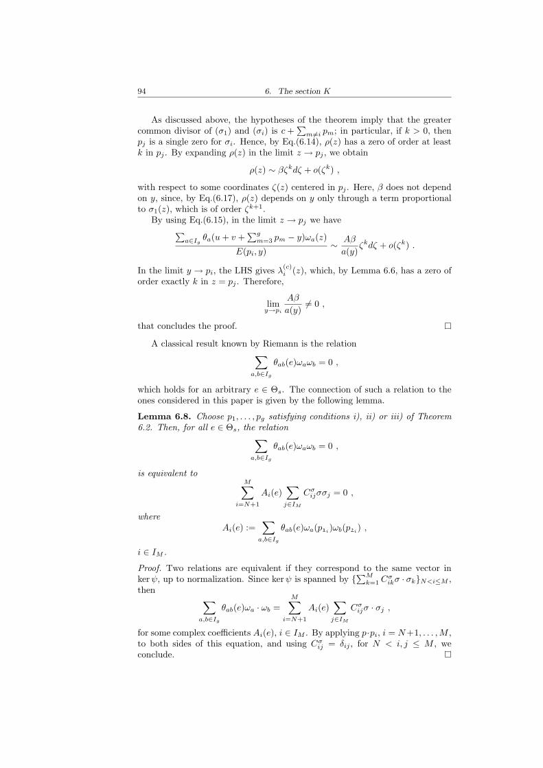
94 6. The section K
As discussed above, the hypotheses of the theorem imply that the greatercommon divisor of (σ1) and (σi) is c +
∑m 6=i pm; in particular, if k > 0, then
pj is a single zero for σi. Hence, by Eq.(6.14), ρ(z) has a zero of order at leastk in pj . By expanding ρ(z) in the limit z → pj , we obtain
ρ(z) ∼ βζkdζ + o(ζk) ,
with respect to some coordinates ζ(z) centered in pj . Here, β does not dependon y, since, by Eq.(6.17), ρ(z) depends on y only through a term proportionalto σ1(z), which is of order ζk+1.
By using Eq.(6.15), in the limit z → pj we have∑
a∈Igθa(u + v +
∑gm=3 pm − y)ωa(z)
E(pi, y)∼ Aβ
a(y)ζkdζ + o(ζk) .
In the limit y → pi, the LHS gives λ(c)i (z), which, by Lemma 6.6, has a zero of
order exactly k in z = pj . Therefore,
limy→pi
Aβ
a(y)6= 0 ,
that concludes the proof.
A classical result known by Riemann is the relation∑
a,b∈Ig
θab(e)ωaωb = 0 ,
which holds for an arbitrary e ∈ Θs. The connection of such a relation to theones considered in this paper is given by the following lemma.
Lemma 6.8. Choose p1, . . . , pg satisfying conditions i), ii) or iii) of Theorem6.2. Then, for all e ∈ Θs, the relation
∑
a,b∈Ig
θab(e)ωaωb = 0 ,
is equivalent toM∑
i=N+1
Ai(e)∑
j∈IM
Cσijσσj = 0 ,
whereAi(e) :=
∑
a,b∈Ig
θab(e)ωa(p1i)ωb(p2i) ,
i ∈ IM .
Proof. Two relations are equivalent if they correspond to the same vector inkerψ, up to normalization. Since kerψ is spanned by ∑M
k=1 Cσikσ · σkN<i≤M ,
then∑
a,b∈Ig
θab(e)ωa · ωb =M∑
i=N+1
Ai(e)∑
j∈IM
Cσijσ · σj ,
for some complex coefficients Ai(e), i ∈ IM . By applying p·pi, i = N +1, . . . , M ,to both sides of this equation, and using Cσ
ij = δij , for N < i, j ≤ M , weconclude.

6.3. Quadrics from double points on Θs 95
Theorem 6.9. Choose p3, . . . , pg ∈ C, C2 3 c := u+v and x ∈ C as above. Sup-pose A(c) 6= ∅ and fix i ∈ A(c). If u is a single zero for K( · , p3, . . . , pi, . . . , pg),then the linear relation ∑
k∈I1iN
Cσ(i)k (c)σσk = 0 ,
is equivalent to ∑
a,b∈Ig
θab(c +∑
j 6=i
pj)ωaωb = 0 .
Proof. By construction, I(c +∑
j 6=i pj) ∈ Θs. Then, use Theorem 6.7 andLemma 6.8, and note that
Ak(I(c +∑
j 6=i
pj)) = Λ(i)k (c) ,
k = N + 1, . . . , M .
Theorem 6.10. If C is a trigonal curve, then there exist 2g−4 pairwise distinctpoints p3, . . . , pg, u3, . . . , ug ∈ C such that the following conditions are satisfied
i. K(p3, . . . , pg) 6= 0
ii. K(uj , p3, . . . , pi, . . . , pg) = 0 if and only if j 6= i, for all i, j ∈ Ig \ 1, 2.Furthermore, if, for each i ∈ Ig \ 1, 2, the points uj, j ∈ Ig \ 1, 2, i, aresingle zeros for K( · , p3, . . . , pi, . . . , pg), then the following statements hold:
a. For each 3 ≤ j ≤ g, there exists a unique vj ∈ C such that
I(cj +∑
k 6=i
pk −∆) ∈ Θs ,
for all i 6= j, 3 ≤ i ≤ j, where cj := uj + vj, 3 ≤ j ≤ g;
b. The relations ∑
k∈I1iN
Cσ(i)k (cj)σσk = 0 ,
3 ≤ i < j ≤ g, considered in Lemma 6.7, are linearly independent andthen generate the ideal I2 of quadrics in Pg−1 containing the curve C.
Proof. Since C is trigonal, there exists a unique (up to a fractional linear trans-formation) meromorphic function f with three poles. Hence, for each p ∈ C,f−1(f(p)) consists of three (possibly coincident) points; note that, trivially, thesum of such three points (counting multiplicity) corresponds to the unique ef-fective divisor of degree three which is special and containing p in its support.
Fix x4, . . . , xg ∈ C, and consider the function
Fx4,...,xg (p) :=∏
x∈f−1(f(p)))
K(x, x4, . . . , xg) , p ∈ C .
Denote by [K]x4,...,xg ⊆ C and [F ]x4,...,xg the sets of zeros of K( · , x4, . . . , xg)and Fx4,...,xg , respectively. Then, one of the following alternatives holds: ifK( · , x4, . . . , xg) is not identically vanishing, then both [K]x4,...,xg and
[F ]x4,...,xg =⋃
x∈[K]x4,...,xg
f−1(f(x)) ,

96 6. The section K
are finite sets; otherwise, both [K]x4,...,xgand [F ]x4,...,xg
coincide with C.For each n, 1 ≤ n ≤ g − 2, let N
(n)xn+3,...,xg ⊆ Cn denote the set of n-tuples
(p3, . . . , pn+2) such that
F (n)xn+3,...,xg
(p3, . . . , pn+2) :=n∏
i=1
Fp3,...,pi,...,pn+2,xn+3,...,xg (pi) ,
is not zero. Note that F (1) ≡ F and N (1) = C \ [F ].Now, assume that, for some m, 1 ≤ m < g − 2, the set N (n) is dense in Cn
for all n ≤ m. The set [F (m+1)]xm+4,...,xgof zeros of
F (m+1)xm+4,...,xg
(p3, . . . , pm+2, p) = Fp3,...,pm+2,xm+4,...,xg(p)
m∏
i=1
Fp3,...,pi,...,pm+2,p,xm+4,...,xg (pi) ,
as a function of p, is given by
[F (m+1)]xm+4,...,xg =m⋃
i=1
( ⋃
x∈f−1(f(pi))
[K]p3,...,pi,...,pm+2,x,xm+4,...,xg
)
∪ [F ]p3,...,pm+2,xm+4,...,xg .
If (p3, . . . , pm+2) ∈ N (m), then the functions
K( · , p3, . . . , pm+2, xm+4, . . . , xg) ,
andK( · , p3, . . . , pi, . . . , pm+2, x, xm+4, . . . , xg) ,
for each i = 1, . . . , m, and x ∈ f−1(f(pi)), vanish identically on C (for example,xm+3 is not a zero). Hence, [F (m+1)]xm+4,...,xg ⊆ C is a finite set and, therefore,N
(m+1)xm+4,...,xg is dense in Cm+1. We proved that if K( · , x4, . . . , xg) does not
identically vanish for some x4, . . . , xg ∈ C, then Nnxn+3,...,xg
is dense in Cn forall n, 1 ≤ n ≤ g−2. It follows that Ng−2, which does not depend on x4, . . . , xg,is dense in Cg−2. Also note that the subset of Cg−2 for which
g⋃
i=3
f−1(f(pi)) ,
consists of pairwise distinct points is dense Cg−2. Hence, its intersection withN (g−2) is not empty.
Let us choose (p3, . . . , pg) in such an intersection and fix ui ∈ f−1(f(pi)),ui 6= pi, for all i ∈ Ig \1, 2. Then, the points p3, . . . , pg, u3, . . . , ug are pairwisedistinct and satisfy the condition
K(ui, p3, . . . , pj , . . . , pg) = 0 ⇔ i 6= j ,
for all i, j ∈ Ig \ 1, 2. Furthermore, if ui, i ∈ Ig \ 1, 2, is a single zero ofK( · , p3, . . . , pj , . . . , pg), for all j ∈ Ig \ 1, 2, i, then there exists a unique pointvij such that vij + ui +
∑k 6=j pk is special. Such a point satisfies necessarily

6.4. The case of genus 4 97
f−1(f(pi)) = pi, ui, vij, so that it is independent of j, and the statement a.follows.
Finally, note that A(cj) = pj and A(cj) = pi | 3 ≤ i ≤ g, i 6= j. Hence, byTheorem 6.7, for each k, N < k ≤ M the coefficients C
σ(1k)l (c2k
), l ∈ IM , aregiven by
Cσ(1k)l (c2k
) = Λ(1k)k (c2k
)Cσkl ,
where Λ(1k)k (c2k
) 6= 0. Linear independence of the Cσ(i)(cj)’s, 3 ≤ i < j ≤ g,follows by linear independence of the Cσ
k ’s.
6.4 The case of genus 4
Consider the case of a non-hyperelliptic curve C of genus 4. The identity (6.4)reduces to
K(p3, p4) := −c4,2κ[v]
κ[σ]5E(p3, p4)2σ(p3)σ(p4),
where c4,2 = 1008, and can be used to express Eq.(5.7) in terms of the functionK. For g = 4 Eq.(5.7) reduces to a unique relation
10∑
i=1
Cσi σσi = 0 .
It can be derived from the identity
deti,j∈I10 σσi(xj)deti,j∈I9 vi(xj)
= 0 ,
by expanding the determinant at the numerator with respect to the columncorresponding to x10 ≡ z. One obtains
∑
i∈I10
(−)idetj∈I10\i
k∈I9
σσj(xk)
detj,k∈I9 vj(xk)σσi(z) = 0 ,
where the ratios of determinants do not depend on x1, . . . , x9 and correspondto
detj∈I10\ik∈I9
σσj(xk)
detj,k∈I9 vj(xk)=
κ[σσ1, . . . , ˇσσi, . . . , σσ10]κ[v]
.
Now, note that for 1i = 2i, κ[σσ1, . . . , ˇσσi, . . . , σσ10] = 0. This can be checkedby observing that all the elements in σσjj∈I10\i vanish at pi, so that itcannot be a basis of H0(K2
C). Hence, we can restrict the summation over allthe i ∈ I10 with 1i 6= 2i. By a re-labeling of the points p1, . . . , p4, the relationbetween κ[v] and K at genus four is
K(p1i , p2i) = (−)i+1c4,2κ[σσ1, . . . , ˇσσi, . . . , σσ10]
κ[σ]5E(p1i , p2i)2σ(p1i)σ(p2i),
for all i, 5 ≤ i ≤ 10. Hence,
Cσi =
K(p1i , p2i)E(p1i , p2i)2σ(p1i)σ(p2i)
K(p3, p4)E(p3, p4)2σ(p3)σ(p4)=
k(p1i , p2i)k(p3, p4)
, (6.18)

98 6. The section K
5 ≤ i ≤ 10, with k defined in Eq.(6.5), whereas Cσi = 0 for i ≤ 4. Since
σσi =∑10
j=1 Xjiωωj , it follows that
Cωi =
10∑
j=5
XωijC
σj ,
i ∈ I10, and we obtain
Cωi = χ−1
i
4∑
k,l=1
k(pk, pl)k(p3, p4)
θ1i(ak)θ2i(al)∑m,n θm(ak)θn(al)ωm(pk)ωn(pl)
, (6.19)
i ∈ I10. Note that Cωi := k(p3, p4)Cω
i is symmetric under any permutation ofp1, . . . , p4. On the other hand, Corollary 5.10 shows that Cω
i , and therefore alsoCω
i , are independent of p1, p2. We conclude that Cωi , whose explicit form is
Cωi = − χ−1
i
S(a)2∏7
1 σ(xi)
·4∑
k,l=1k 6=l
[θ1i(ak)θ2i(al)
θ(pk + pl +
∑71 xi
)σ(pk)σ(pl)
∏i 6=k,l
(E(pk, pi)E(pl, pi)
)
·∑
s∈P7
S(∑4
i=1 xsi
)S
(∑7i=4 xsi
)
E(xsg , pk)E(xsg , pl)
3∏
i=1
S(xsi + xsi+4 + pk + pl)∏3j=1j 6=i
E(xsi , xsj+4)
],
does not depend on p1, . . . , p4, for all i ∈ I10.
Note that, at genus 4, the equivalent relations∑
i∈IM
Cωi ωωi = 0,
and ∑
i∈IM
Cωi ωωi = 0 ,
must be proportional to Eq.(B.6), with e one of the two points in Θs; in otherwords, Cω
i and Cωi must be proportional to χ−1
i θ1i2i(e). Such a proportionalityis immediately derived by noting that Eq. (6.8), for genus 4, gives
k(p, q) ≡ K(p, q)E(p, q)2σ(p)σ(q) = A(e)−1∑
a,b∈Ig
θab(e)ωa(p)ωb(q) , (6.20)
for all p, q ∈ C, where e one of the two points of Θs and A(e) is defined inEq.(6.8). By Eq.(6.18) and Eq.(6.20), it immediately follows that
Cσi =
∑a,b∈Ig
θab(e)ωa(p1i)ωb(p2i)∑a,b∈Ig
θab(e)ωa(p3)ωb(p4), (6.21)
for all i ∈ IM , and by Eq.(6.19)
Cωi = χ−1
i
θ1i2i(e)∑a,b∈Ig
θab(e)ωa(p3)ωb(p4), (6.22)

6.5. Modular properties of K(p3, . . . , pg) 99
for all i ∈ IM . Finally, we have
Cωi =
θ1i2i(e)
A(e)χi,
for all i ∈ IM .
6.5 Modular properties of K(p3, . . . , pg)
For each n ∈ Z>0, let us consider the rank Nn vector bundle Ln on Mg, definedin section 3.4, whose fiber at the point corresponding to a curve C is H0(Kn
C).A general section s ∈ Lm
n , i > 1, admits the local expression on an open setU ⊂Mg
s(p) =∑
i1,...,im∈INn
si1...im(p)φi1 ⊗ φi2 ⊗ · · · ⊗ φim , p ∈ U ⊂Mg , (6.23)
with respect to a set φii∈INnof linearly independent local sections of Ln on
U .For each non-hyperelliptic C of genus g ≥ 3, k(p3, . . . , pg) as defined in (6.5),
is a holomorphic (g − 3)-differential in each variable, and is symmetric (for geven) or anti-symmetric (for g odd) in its g − 2 arguments. Hence,
k :=∑
i1,...,ig−2∈INg−3
ki1...ig−2φi1 ⊗ · · · ⊗ φig−2 , (6.24)
can be naturally seen as an element of Eg, where
Eg :=
Symg−2 H0(Kg−3
C ) , g even ,∧g−2H0(Kg−3
C ) , g odd ,
for a fixed basis φii∈INg−3of H0(Kg−3
C ). The definition can be extended in acontinuous way to hyperelliptic curves, by setting ki1...ig−2 ≡ 0 in this case. Atgenus g = 3, k(p3) is a holomorphic function on C and therefore is a constant.Furthermore, Eq.(6.5) also makes sense at genus g = 2; in this case, k is againa constant. For g > 3, let us define Eg by
Eg :=
Symg−2 Lg−3 , g even ,∧g−2
Lg−3 , g odd .
In view of Eqs.(6.23) and (6.24), it is natural to seek for a section k ∈ Eg suchthat, at the point pC ∈Mg corresponding to the curve C, it satisfies
Eg 3 k(p3, . . . , pg) ∼= k(pC) ∈ (Eg)|pC,
under the identification (Eg)|pC∼= Eg. On the other hand, k(p3, . . . , pg) is not
modular invariant, and then it does not correspond to a well-defined element ofEg for each pC ∈Mg. The correct statement is given by the following theorem.
Theorem 6.11.
k := κ[ω]g−8k ⊗ (ω1 ∧ . . . ∧ ωg)12−g ,
is a holomorphic section of λ12−g1 for g = 2, 3 and of Eg ⊗ λ12−g
1 for g > 3,which vanishes only in the hyperelliptic locus for g ≥ 3.

100 6. The section K
Proof. Let us derive the modular properties of
κ[ω]g−8k(p3, . . . , pg) .
Eq.(6.5) and the identity κ[σ] = κ[ω]/ det ωi(pj) yield
κ[ω]g−8k(p3, . . . , pg) = (−)g+1cg,2κ[v]κ[ω]9
(det ωi(pj))g+1 .
By Eq.(3.18), it follows that κ[v]/κ[ω]9 has a simple modular transformation
κ[v]κ[ω]9
→ κ[v]κ[ω]9
(det(Cτ + D))−13 ,
(A BC D
)∈ Sp(2g,Z) ,
and, by using the modular transformation detωi(pj) → det ωi(pj) det(Cτ + D),we obtain
κ[ω]g−8k → κ[ω]g−8k(det(Cτ + D))g−12 .
Hence, κ[ω]g−8k ⊗ (ω1 ∧ . . . ∧ ωg)12−g is modular invariant and determines asection of Symg−2 Eg−3 ⊗ λ12−g
1 on Mg. Since κ[ω] 6= 0 for all C, k = 0at the point corresponding to the C if and only if k(p3, . . . , pg) = 0 for allp3, . . . , pg ∈ C, or, equivalently, if and only if C is hyperelliptic.
For g = 2 the section k corresponds to
k = κ[ω]6k(ω1 ∧ ω2)10 ,
and for g = 3k = κ[ω]5k(ω1 ∧ ω2 ∧ ω3)9 .
Note that, for g = 2, 3, Eqs.(3.11) and (3.12) lead to the following relations
κ[v]κ[σ]g+1
=κ[ωω]
κ[ω]g+1,
and, together with (3.19) and (3.20), we obtain the identification
k = 6π12κ[ω]6Ψ10 , g = 2 ,
k = 15 · 26κ[ω]5π18Ψ9 , g = 3 ,
recovering the results of Proposition 3.9.
Let C be a non-hyperelliptic curve of genus g = 4. In this case, k(p3, p4)is a holomorphic 1-differential in both p3 and p4, symmetric in its arguments.Then,
k(4) :=det k(pi, pj)(det ωi(pj))2
= det kij ,
is a meromorphic function on C in each pi, i ∈ I4.
Proposition 6.12. The function k(4) is a constant on C that depends only onthe choice of the marking. Furthermore, k(4) = 0 if and only if C is hyperel-liptic or if C is non-hyperelliptic and admits a (necessarily even) singular spinstructure.

6.5. Modular properties of K(p3, . . . , pg) 101
Proof. Let us suppose that, for a suitable choice of p1, . . . , p4 ∈ C, k(pi, z)i∈I4
is a basis of H0(KC). Then, the determinant
det k(pi, zj)detωi(zj)
,
does not depend on the points z1, . . . , z4 ∈ C. Hence, the ratio
det k(pi, zj)detωi(zj) det ωi(pj)
,
is a non-vanishing constant on C. In particular, by taking pi = zi, it followsthat such a constant is k(4). On the contrary, if for all p1, . . . , p4 ∈ C, theholomorphic 1-differentials k(pi, z), i ∈ I4, are linearly dependent, then k(4)
vanishes identically.Such a construction shows that k(4) vanishes if and only if k(pi, z), i ∈ I4, are
linearly dependent for all p1, . . . , p4 ∈ C. If C is hyperelliptic, then k(pi, pj) = 0for all pi, pj ∈ C and k(4) = 0. Assume that C admits a singular spin structureα and let Lα be the corresponding holomorphic line bundle with L2
α∼= KC . This
implies that Θs consists of a unique point of order 2 in the Jacobian torus. Foreach p ∈ C, the holomorphic 1-differential k(p, z) is the square of an elementof H0(Lα); by varying p ∈ C, such 1-differentials span the image of the mapϕ : Sym2H0(Lα) → H0(KC). If α is even, then h0(Lα) = 2 and Sym2 H0(Lα)has dimension three, so that ϕ cannot be surjective and k(4) = 0. If α is odd,then h0(Lα) = 3 so that, for each point p ∈ C, h0(Lα ⊗ O(−p)) ≥ 2; if h1, h2
span H0(Lα⊗O(−p)), then h1/h2 is a non-constant meromorphic function with2 poles and C is hyperelliptic.
Suppose that C is non-hyperelliptic and does not admit a singular spinstructure. Then, Θs consists of 2 distinct points, e and −e. Let us first observethat if there exist two points p, q ∈ C such that I(p − q) = 2e, then they areunique. For, if I(p − q) = 2e = I(p − q), then p + q − p − q is the divisor ofa meromorphic function on C. But, since C is non-hyperelliptic, the uniquemeromorphic function with less that 3 poles are the constants and, since p 6= q(because 2e 6= 0 in J0(C)), it follows that p = p and q = q.
Also, observe that K(z, z) is not identically vanishing as a function of z; sinceC is compact, K(z, z) has only a finite number of zeros. Fix a point p1 ∈ C anddefine x1, x2, y1, y2 ∈ C by
I(p1 + x1 + x2) = e , I(p1 + y1 + y2) = −e .
Then the divisor of k(p1, z) with respect to z is 2p1 +x1 +x2 +y1 +y2. Observethat at least one between x1 and x2 is distinct from y1 and y2, since otherwise wewould have e = −e. We choose p1 in such a way that p1, x1, x2, y1, y2 are distinctfrom the zeros of K(z, z) and from the points p, q such that I(p−q) = 2e (if theyexist). Note that such a condition can always be fulfilled, since it is equivalentto require that p1 is distinct from the zeros of k(p, ·), k(q, ·) and k(w, ·) for eachw such that K(w,w) = 0. Then, the points for which such a condition is notsatisfied is a finite set.
Set p2 := x1 and p3 := y1. The divisor of k(p3, z) is (k(p3, z)) = 2p3 + p1 +y2 + z1 + z2, where z1, z2 satisfy
I(p3 + z1 + z2) = e .

102 6. The section K
Since the condition on the choice of p1 implies K(p3, p3) 6= 0, it follows that z1
and z2 are distinct from p3. Set p4 := z1, so that
det k(pi, pj) = k(p1, p4)2k(p2, p3)2 .
The identities
I(p1 + p2 + x2 − p3 − p4 − z2) = 0 , I(p4 + z2 − p1 − y2) = 2e ,
imply that p4 and z2 are distinct from p1, p2, x2 (for example, if p4 = x2, thenp1 +p2−p3−z2 is the divisor of a meromorphic function and C is hyperelliptic)and from y2 (if p4 = y2, then I(z2−p1) = 2e, counter the requirement that p1 isdistinct from q and p). Therefore, k(p1, p4)k(p2, p3) 6= 0 and then k(4) 6= 0.
By Propositions 6.12 and 6.11, it follows that, for g = 4,
k(4) := κ[ω]−16 det kij(ω1 ∧ · · · ∧ ω4)34 ,
is a holomorphic section of λ341 vanishing only on the hyperelliptic locus, with
a zero of order 4[(3g− 3)− (2g− 1)] = 8, and on the locus of Riemann surfaceswith an even singular spin structure, with a zero of order 1. By Eq.(6.20), thefollowing relation holds
k(4) = A4 detij∈I4
θij(e) ,
where the constant A depends on the moduli. Recently, it has been shown thatthe Hessian detij∈I4 θij(e) plays a key role in the analysis of the Andreotti-Mayerloci at genus 4 and in the corresponding applications to the Schottky problem[21][31]. Whereas no natural generalization of such a Hessian exists at genusg > 4, the section k(4) is the g = 4 representative of a set of sections k(g) of atensor power of λ1 on Mg, defined for each even g ≥ 4.
Definition 6.2. Let C be a curve of even genus g ≥ 4. Fix Ng−3 = h0(Kg−3C )
points p1, . . . , pNg−3 ∈ C and let φii∈INg−3be a basis of H0(Kg−3
C ). Set
k(g) :=κ[φ]g−2
∑s1,...,sg−2
∏g−2i=1 ε(si)
∏Ng−3j=1 k(ps1
j, . . . , psg−2
j)
Ng−3!κ[ω](2g−7)2(g−2)+(8−g)Ng−3(detφ(p1, . . . , pNg−3)
)g−2 (ω1∧· · ·∧ωg)dg
where dg := (12 − g)Ng−3 + (g − 2)[6(g − 3)(g − 4) + 1] and the sum in thenumerator runs over g − 2 permutations s1, . . . , sg−2 ∈ PNg−3 .
Proposition 6.13. For all the even g ≥ 4, k(g) does not depend on the pointsp1, . . . , pNg−3 ∈ C and on the basis φii∈INg−3
of H0(Kg−3C ) and determines a
section of λdg
1 on Mg.
Proof. Choose (g − 2)Ng−3 points pi1, . . . , p
iNg−3
∈ C, i ∈ Ig−2 and note that
∑
s1,...,sg−2∈PNg−3
g−2∏
i=1
ε(si)Ng−3∏
j=1
k(pis1
j, . . . , pi
sg−2j
) , (6.25)

6.5. Modular properties of K(p3, . . . , pg) 103
is a product of g−3 differentials in each pij , i ∈ Ig−2, j ∈ INg−3 . Such a product
is completely anti-symmetric with respect to the permutations of each Ng−3-tuple (pi
1, . . . , piNg−3
), for all i ∈ Ig−2, so that it must be proportional to thedeterminant det φ(pi
1, . . . , piNg−3
). Therefore, the ratio of Eq.(6.25) and
∏
i∈Ig−2
detφ(pi1, . . . , p
iNg−3
) ,
does not depend on the points pi1, . . . , p
iNg−3
∈ C, i ∈ Ig−2; in particular, bychoosing, for each j ∈ INg−3 , p1
j ≡ p2j ≡ . . . ≡ pg−2
j ≡ pj , where p1, . . . , pNg−3
are the points in the definition 6.2, it follows that k(g) is a constant as a func-tion of CNg−3 . The proposition follows trivially by Theorem (6.11) and by theexpression (3.18) of the Mumford form, with n = g − 3.
Definition 6.2 and Proposition 6.13 make sense also at odd genera; however,simple algebraic considerations show that, in this case, k(g) is identically nullon Mg. In general, there exist some non-trivial generalizations of k(4) at oddgenus, but they are not as simple as the ones at even g. An example at genusg = 5 is
(ω1 ∧ · · · ∧ ω5)164κ[φ]4
κ[ω]84(detφ(p1, . . . , p12)
)4
∑i,j,k,l∈P12
ε(i)ε(j)ε(k)ε(l)k(pi1 , pi2 , pi3)
· k(pi4 , pi5 , pj1)k(pi6 , pi7 , pk1)k(pi8 , pi9 , pl1)· k(pi10 , pj2 , pj3)k(pi11 , pk2 , pk3)k(pi12 , pl2 , pl3)· k(pj4 , pj5 , pj6)k(pj7 , pj8 , pk4)k(pj9 , pj10 , pl4)· k(pj11 , pk5 , pk6)k(pj12 , pl5 , pl6)k(pk7 , pk8 , pk9)· k(pk10 , pk11 , pl7)k(pk12 , pl8 , pl9)k(pl10 , pl11 , pl12),
which does not depend on the points p1, . . . , p12 ∈ C and corresponds to asection of λ164
1 on M5.

104 6. The section K
7. SIEGEL’S INDUCED MEASURE ON THE MODULI SPACE
In this section we derive the explicit expression of the metric ds2|Mg
on the
moduli space Mg of genus g canonical curves induced by the Siegel metric. Thiswas previously known only for the trivial cases g = 2 and g = 3. By WirtingerTheorem, the explicit expression for the volume form on Mg is also obtained.A remarkable property of ds2
|Mgis that it is given by the Kodaira-Spencer map
of the square of the Bergman reproducing kernel (times 4π2). This is one of thebasic properties of the Bergman reproducing kernel derived in this section. Suchan approach will led to a notable relation satisfied by the determinant of powersof the Bergman reproducing kernel. The results are a natural consequence ofthe present approach, which also uses, as for the present derivation of ds2
|Mg,
the isomorphisms introduced in section 2.1.The Torelli space Tg of smooth algebraic curves of genus g can be embedded
in Hg by the period mapping, which assigns to a curve C, with a fixed basisof H1(C,Z), representing a point in Tg, the corresponding period matrix. Theperiod mapping has maximal rank 3g−3 on the subspace Tg of non-hyperellipticcurves and therefore a metric on Hg induces the pull-back metric on Tg. It istherefore natural to consider the Siegel metric on Hg [60]
ds2 := Tr (Y −1dZY −1dZ) , (7.1)
where Y := Im Z, Z ∈ Hg. Such a metric is Sp(2g,R) invariant, and sinceMg
∼= Tg/Γg, it also induces a metric on Mg. The Siegel volume form is [60]
dν =iM
2g
∧gi≤j(dZij ∧ dZij)
(detY )g+1. (7.2)
The explicit expression of the volume forms on Mg induced by the Siegelmetric, which coincides with (7.2) for g = 2 and g = 3 non-hyperelliptic curves,is given in Theorem 7.7. It is simply written in terms of the Riemann periodmatrix τij and of the basis dτij of T ∗Tg.
The Laplacian associated to the Siegel’s symplectic metric were derived, tenyears after Siegel’s paper [60], by H. Maass [43]
∆ = 4 Tr(Y
t(Y
∂
∂Z
) ∂
∂Z
). (7.3)
As we will see, as a byproduct of the present approach, and of the formalismdeveloped in section 2.1 in particular, both (7.2) and (7.3) are straightforwardlyderived.
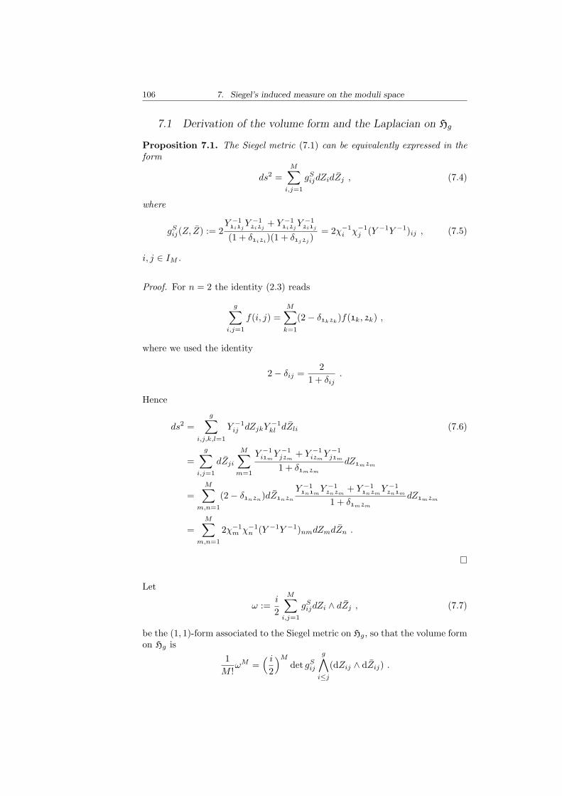
106 7. Siegel’s induced measure on the moduli space
7.1 Derivation of the volume form and the Laplacian on Hg
Proposition 7.1. The Siegel metric (7.1) can be equivalently expressed in theform
ds2 =M∑
i,j=1
gSijdZidZj , (7.4)
where
gSij(Z, Z) := 2
Y −11i1j
Y −12i2j
+ Y −11i2j
Y −12i1j
(1 + δ1i2i)(1 + δ1j2j
)= 2χ−1
i χ−1j (Y −1Y −1)ij , (7.5)
i, j ∈ IM .
Proof. For n = 2 the identity (2.3) reads
g∑
i,j=1
f(i, j) =M∑
k=1
(2− δ1k2k)f(1k, 2k) ,
where we used the identity
2− δij =2
1 + δij.
Hence
ds2 =g∑
i,j,k,l=1
Y −1ij dZjkY −1
kl dZli (7.6)
=g∑
i,j=1
dZji
M∑m=1
Y −1i1m
Y −1j2m
+ Y −1i2m
Y −1j1m
1 + δ1m2m
dZ1m2m
=M∑
m,n=1
(2− δ1n2n)dZ1n2n
Y −11n1m
Y −12n2m
+ Y −11n2m
Y −12n1m
1 + δ1m2m
dZ1m2m
=M∑
m,n=1
2χ−1m χ−1
n (Y −1Y −1)nmdZmdZn .
Let
ω :=i
2
M∑
i,j=1
gSijdZi ∧ dZj , (7.7)
be the (1, 1)-form associated to the Siegel metric on Hg, so that the volume formon Hg is
1M !
ωM =( i
2
)M
det gSij
g∧
i≤j
(dZij ∧ dZij) .

7.2. The Siegel metric on the moduli space 107
Proposition 7.2.
det gSij =
2M−g
(det Y )g+1.
Proof. Since Y is symmetric and positive-definite, we have
PY −1P−1 = diag(λ1, . . . , λg) ≡ D ,
for some non-singular g × g matrix P and some positive λ1, . . . , λg. By (7.5)and (2.6)
det gSij =2M detij
(Y −1Y −1)ij
χiχj
=2M detij(PP )ij
χjdetij
(P−1P−1)ij
χjdetij
(Y −1Y −1)ij
χiχj,
and by (2.4)
det gSij = 2M detij
(DD)ij
χiχj= 2M detij
λλi(δδ)ij
χiχj.
The proposition then follows observing that (δδ)ij = χjδij and that (2.7) yields
det gSij = 2M
M∏
i=1
λλiχ−1i = 2M−g
( g∏
k=1
λk
)g+1
.
Proposition 7.3. The Laplace-Beltrami operator acting on functions on Hg is
∆ =12
M∑
i,j=1
(Y Y )ij∂
∂Zi
∂
∂Zj.
Proof. Just use the definition of ∆ and note that gS ij = (Y Y )ij/2.
7.2 The Siegel metric on the moduli space
The following theorem provides a modular invariant basis of the fiber of T ∗Tg
at the point representing C.
Theorem 7.4. If p3, . . . , pg ∈ C are g − 2 pairwise distinct points such thatK(p3, . . . , pg) 6= 0, then
Ξi :=M∑
j=1
Xωjidτj , (7.8)
i ∈ IN , with Xωij, i, j ∈ IM , defined in Eq.(5.23), is a modular invariant basis
of the fiber of T ∗Tg at the point representing C.

108 7. Siegel’s induced measure on the moduli space
Proof. Consider the Kodaira-Spencer map k identifying the space of quadraticdifferentials on C with the fiber of the cotangent bundle of Mg at the pointrepresenting C. Next, consider a Beltrami differential µ ∈ Γ(KC ⊗ K−1
C ) (see[11] for explicit constructions) and recall that it defines a tangent vector at Cof Tg. The derivative of the period map τij : Tg → C at C in the direction of µis given by Rauch’s formula
dCτij(µ) =∫
C
µωiωj .
It follows thatk(ωjωk) =
12πi
dτjk ,
j, k ∈ Ig, so that, by (5.22),
k(vj) =1
2πi
M∑
k=1
Xωkjdτk , (7.9)
j ∈ IN , wheredτi := dτ1i2i ,
i ∈ IM . It follows that the differentials
Ξj := 2πi k(vj) , (7.10)
j ∈ IN , are linearly independent. Furthermore, since by construction the basisvii∈IN
is independent of the choice of a symplectic basis of H1(C,Z), suchdifferentials are modular invariant, i.e.
Ξi 7→ Ξi = Ξi , (7.11)
i ∈ IN , under (B.3).
Let ds2|Mg
be the metric on Mg induced by the Siegel metric. Set
gτij := gS
ij(τ, τ) = 2χ−1i χ−1
j (Im τ−1Im τ−1)ij . (7.12)
Corollary 7.5.
ds2|Mg
=N∑
i,j=1
gΞijΞiΞj , (7.13)
where
gΞij :=
M∑
k,l=1
gτklB
ωikBω
jl , (7.14)
and Bω is the matrix defined in (5.11) with ηi ≡ ωi, i ∈ Ig. Furthermore, thevolume form on Mg induced by the Siegel metric is
dν|Mg=
( i
2
)N
det gΞ dw ∧ dw , (7.15)
where
dw :=M∑
iN >...>i1=1
Xω1 ... N
i1...iN
dτi1 ∧ · · · ∧ dτiN . (7.16)
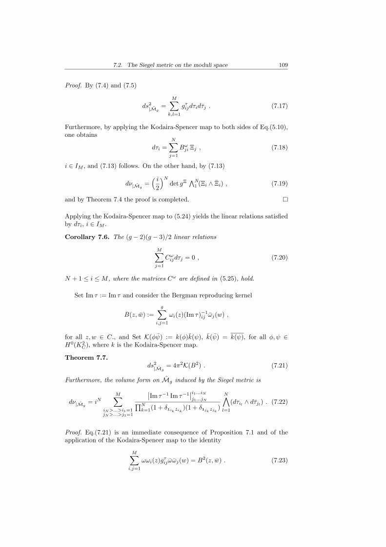
7.2. The Siegel metric on the moduli space 109
Proof. By (7.4) and (7.5)
ds2|Mg
=M∑
k,l=1
gτijdτidτj . (7.17)
Furthermore, by applying the Kodaira-Spencer map to both sides of Eq.(5.10),one obtains
dτi =N∑
j=1
Bωji Ξj , (7.18)
i ∈ IM , and (7.13) follows. On the other hand, by (7.13)
dν|Mg=
( i
2
)N
det gΞ ∧N1 (Ξi ∧ Ξi) , (7.19)
and by Theorem 7.4 the proof is completed.
Applying the Kodaira-Spencer map to (5.24) yields the linear relations satisfiedby dτi, i ∈ IM .
Corollary 7.6. The (g − 2)(g − 3)/2 linear relations
M∑
j=1
Cωijdτj = 0 , (7.20)
N + 1 ≤ i ≤ M , where the matrices Cω are defined in (5.25), hold.
Set Im τ := Im τ and consider the Bergman reproducing kernel
B(z, w) :=g∑
i,j=1
ωi(z)(Im τ)−1ij ωj(w) ,
for all z, w ∈ C., and Set K(φψ) := k(φ)k(ψ), k(ψ) = k(ψ), for all φ, ψ ∈H0(K2
C), where k is the Kodaira-Spencer map.
Theorem 7.7.ds2|Mg
= 4π2K(B2) . (7.21)
Furthermore, the volume form on Mg induced by the Siegel metric is
dν|Mg= iN
M∑
iN >...>i1=1jN >...>j1=1
∣∣Im τ−1 Im τ−1∣∣i1...iN
j1...jN∏Nk=1(1 + δ1ik
2ik)(1 + δ1jk
2jk)
N∧
l=1
(dτil∧ dτjl
) . (7.22)
Proof. Eq.(7.21) is an immediate consequence of Proposition 7.1 and of theapplication of the Kodaira-Spencer map to the identity
M∑
i,j=1
ωωi(z)gτijωωj(w) = B2(z, w) . (7.23)
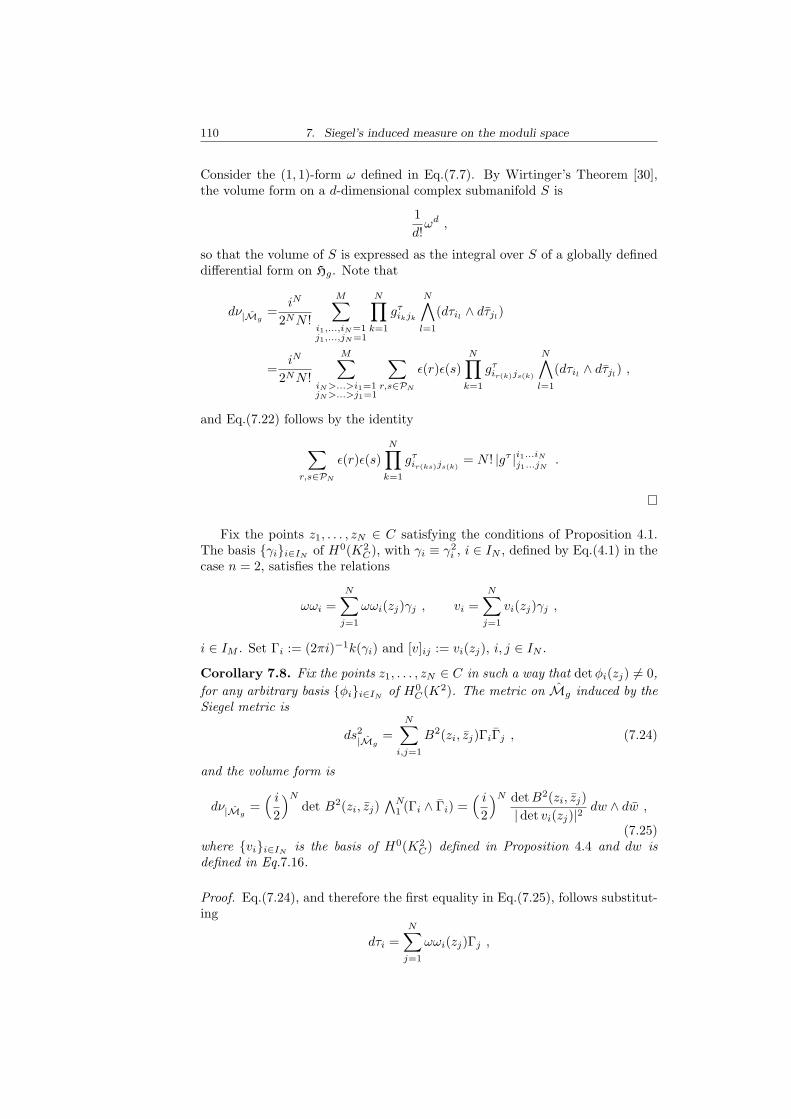
110 7. Siegel’s induced measure on the moduli space
Consider the (1, 1)-form ω defined in Eq.(7.7). By Wirtinger’s Theorem [30],the volume form on a d-dimensional complex submanifold S is
1d!
ωd ,
so that the volume of S is expressed as the integral over S of a globally defineddifferential form on Hg. Note that
dν|Mg=
iN
2NN !
M∑
i1,...,iN=1j1,...,jN=1
N∏
k=1
gτikjk
N∧
l=1
(dτil∧ dτjl
)
=iN
2NN !
M∑
iN >...>i1=1jN >...>j1=1
∑
r,s∈PN
ε(r)ε(s)N∏
k=1
gτir(k)js(k)
N∧
l=1
(dτil∧ dτjl
) ,
and Eq.(7.22) follows by the identity
∑
r,s∈PN
ε(r)ε(s)N∏
k=1
gτir(ks)js(k)
= N ! |gτ |i1...iN
j1...jN.
Fix the points z1, . . . , zN ∈ C satisfying the conditions of Proposition 4.1.The basis γii∈IN
of H0(K2C), with γi ≡ γ2
i , i ∈ IN , defined by Eq.(4.1) in thecase n = 2, satisfies the relations
ωωi =N∑
j=1
ωωi(zj)γj , vi =N∑
j=1
vi(zj)γj ,
i ∈ IM . Set Γi := (2πi)−1k(γi) and [v]ij := vi(zj), i, j ∈ IN .
Corollary 7.8. Fix the points z1, . . . , zN ∈ C in such a way that detφi(zj) 6= 0,for any arbitrary basis φii∈IN of H0
C(K2). The metric on Mg induced by theSiegel metric is
ds2|Mg
=N∑
i,j=1
B2(zi, zj)ΓiΓj , (7.24)
and the volume form is
dν|Mg=
( i
2
)N
det B2(zi, zj)∧N
1 (Γi ∧ Γi) =( i
2
)N det B2(zi, zj)| det vi(zj)|2 dw ∧ dw ,
(7.25)where vii∈IN is the basis of H0(K2
C) defined in Proposition 4.4 and dw isdefined in Eq.7.16.
Proof. Eq.(7.24), and therefore the first equality in Eq.(7.25), follows substitut-ing
dτi =N∑
j=1
ωωi(zj)Γj ,

7.3. Powers of Bergman kernel 111
i ∈ IM , in (7.17) and then using the identity (7.23). Next, note that comparing(7.24) and (7.13), and by Ξi =
∑Nj=1[v]ijΓj , i ∈ IN , yields
N∑
k,l=1
[v]kigΞkl[v]lj = B2(zi, zj) ,
which also follows by the definition (7.14) of gΞ and by Eq.(5.10), with ηi ≡ ωi,i ∈ Ig, and Eq.(7.23). Hence
det gΞ =detB2(zi, zj)| det vi(zj)|2 , (7.26)
which also follows by det γi(zj) = 1 and
Ξ1 ∧ · · · ∧ ΞN = det vi(zj)Γ1 ∧ · · · ∧ ΓN ,
and the second equality in Eq.(7.25) follows.
7.3 Determinants of powers of the Bergman reproducing kernel
Corollary 7.8, in particular Eq.(7.25), implies that the ratio
detB2(zi, zj)|det vi(zj)|2 ,
does not depend on zi, i ∈ IN , and therefore det B2(zi, zj) factorizes into aproduct of a holomorphic times an antiholomorphic function of z1, . . . , zN . Thisis a special case of a more general theorem.
Theorem 7.9. Fix n ∈ N+ and set
BA(z, w) :=g∑
i,j=1
ωi(z)Aijωj(w) ,
where A is a complex g × g matrix. Then, for all zi, wi ∈ C, i ∈ INn ,
detBnA(zi, wj) =
∣∣κ[φn]∣∣−2 det φn(z1, . . . , zNn) det φn(w1, . . . , wNn)Kn(A) ,
(7.27)where φn
i i∈INnis an arbitrary basis of H0(Kn
C) and
Kn(A) =Mn∑
iNn>...>i1=1jNn>...>j1=1
κ[ω · · ·ωi1 , . . . , ω · · ·ωiNn] (7.28)
·|A . . . A|i1...iNn
j1...jNn∏Nn
k=1 χikχjk
κ[ω · · ·ωj1 , . . . , ω · · ·ωjNn] .
Furthermore, for n ≥ 2
detBnA(zi, zj) =
∣∣∣θ∆
( Nn∑1
zi
) Nn∏
i<j
E(zi, zj)Nn∏1
σ(zi)2n−1∣∣∣2
Kn(A) . (7.29)

112 7. Siegel’s induced measure on the moduli space
Proof. Observe that
BnA(zi, wj) =
g∑
k1,...,kn=1l1,...,ln=1
ωk1(zi) · · ·ωkn(zi)Ak1l1 · · ·Aknln ωl1(wj) · · · ωln(wj)
=Mn∑
k,l=1
ω · · ·ωk(zi)(A · · ·A)kl
χkχlω · · · ωl(wj) ,
with the notation of section 2.1. Then
det BnA(zi, wj) =
Mn∑
k1,...,kNn=1l1,...,ln=1
∑
s∈PNn
ε(s)Nn∏
i=1
ω · · ·ωki(zi)ω · · · ωli(wsi
)(A · · ·A)kili
χkiχli
,
and by defining msi:= li, i ∈ IMn
, det BnA(zi, wj) becomes
Mn∑
k1,...,kNn=1m1,...,mNn=1
|A . . . A|k1...kNnm1...mNn∏Nn
i=1 χkiχmi
Nn∏
i=1
ω · · ·ωki(zi)ω · · · ωmi(wi)
=Mn∑
kNn >...>k1=1mNn >...>m1=1
|A . . . A|k1...kNnm1...mNn∏Nn
i=1 χkiχmi
∑
r,s∈PNn
ε(r)ε(s)Nn∏
i=1
ω · · ·ωkri(zi)ω · · · ωmsi
(wi)
=Mn∑
kNn >...>k1=1mNn >...>m1=1
|A . . . A|k1...kNnm1...mNn∏Nn
i=1 χkiχmi
deti=k1,...,kNnj=1,...,Nn
ω · · ·ωi(zj) deti=m1,...,mNn
j=1,...,Nn
ω · · · ωi(wj).
By Eq.(3.4), for an arbitrary basis φni i∈INn
of H0(KnC)
deti∈k1,...,kNn
j∈INn
ω · · ·ωi(zj) = det φn(z1, . . . , zNn)κ[ω · · ·ωk1 , . . . , ω · · ·ωkNn
]κ[φn]
,
leading to (7.27). Eq.(7.29) then follows by Eq.(3.3).

8. A GENUS 4 EXAMPLE: A 3-FOLD COVERING OF THESPHERE
In this chapter, the objects defined in the previous chapters, in particular thedistinguished basis σii∈Ig of H0(KC), are explicitly obtained for a family ofnon-hyperelliptic curves of genus 4, in terms of the algenraic parameters of thefamily.
8.1 Definition and main properties
Let C be the non-hyperelliptic curve of genus 4 defined by
w3 = z(z − 1)(z − λ1)2(z − λ2)2(z − λ3)2 ,
(z, w) ∈ P1 × P1 and let
q0 =z−1(0) , q1 =z−1(1) ,
q∞ =z−1(∞) , pi =z−1(λi) , i ∈ I3 ,
be the branching points on C, all with branching number 1. Since
(z) = 3q0 − 3q∞ , (w) = q0 + q1 + 2p1 + 2p2 + 2p3 − 8q∞ ,
(dz) =2q0 + 2q1 + 2p1 + 2p2 + 2p3 − 4q∞ ,
a basis of H0(KC) is given by
ϕ1 :=dz
w, ϕ3 :=
[∏3i=1(z − λi)
]dz
w2,
ϕ2 :=zdz
w, ϕ4 :=
z[∏3
i=1(z − λi)]dz
w2.
Note that ϕ1, ϕ2 generate U := H0(KC ⊗ O(−q0 − q1 − q∞)), whereas ϕ3, ϕ4
generate V := H0(KC ⊗ O(−p1 − p2 − p3)). Consider the automorphism φ ofC given by φ(z, w) := (z, ζw), where ζ := e2πi/3; then, the pull-back φ∗ is anautomorphism of H0(KC) and U and V are the eigenspaces corresponding tothe eigenvalues, respectively, ζ2 and ζ.
The Riemann surface C is a 3-fold covering of the sphere. Let us define thej-th sheet, j = 0, 1, 2, as the one containing the line Im z = 0, arg w = j(2πi/3).Let us fix a basis of H1(C,Z) as in the following figure.

114 8. A genus 4 example
0 λ1 1 λ2
0
0
λ1
λ1
1
1
λ2
λ2
∞
∞
∞
λ3
λ3
λ3
α1
α3
α2
α4
β1
β1
β2
β2
β3
β3
β4
β4
sheet 0
sheet 1
sheet 2
Fig. 1.
∫
α1
η =∫ λ1
0
η −∫ λ1
0
φ∗η ,
∫
α2
η =∫ λ2
1
η −∫ λ2
1
φ∗η ,
∫
α3
η =∫ λ1
0
φ∗η −∫ λ1
0
φ∗2η ,
∫
α4
η =∫ λ2
1
φ∗η −∫ λ2
1
φ∗2η ,
∫
β1
η =∫ ∞
λ1
η −∫ ∞
λ1
φ∗2η ,
∫
β2
η =∫ ∞
λ2
η −∫ ∞
λ2
φ∗2η ,
∫
β3
η =∫ ∞
λ1
φ∗η −∫ ∞
λ1
φ∗2η ,
∫
β4
η =∫ ∞
λ2
φ∗η −∫ ∞
λ2
φ∗2η .
Let u1, u2 ∈ U and v1, v2 ∈ V the holomorphic 1-differentials satisfying∫ λ1
0
u1 =13
=∫ λ1
0
v1 ,
∫ λ2
1
u1 = 0 =∫ λ2
1
v1 ,
∫ λ1
0
u2 = 0 =∫ λ1
0
v2 ,
∫ λ2
1
u2 =13
=∫ λ2
1
v2 ,
where the integration is above the cuts in the 0-sheet. Consistency requires∫ ∞
λ3
u1 =∫ ∞
λ3
u1 =∫ ∞
λ3
u1 =∫ ∞
λ3
u1 =13
,

8.1. Definition and main properties 115
where integration is along the cut in the 0-sheet. Then, it can be easily verifiedthat
ω1 := u1 + v1 , ω2 := u2 + v2 , ω3 := −ζ2u1 − ζv1 , ω4 := −ζ2u2 − ζv2 ,(8.1)
is the canonical basis of H0(KC) associated to our choice of basis of H1(C,Z).Furthermore, a lengthy but straightforward calculation yields
τ =
2a 2c a c2c 2b c ba c 2a 2cc b 2c 2b
,
where
∫ ∞
λ1
ω1 = a ,
∫ ∞
λ1
ω2 = c ,
∫ ∞
λ1
ω3 = 0 ,
∫ ∞
λ1
ω4 = 0 ,
∫ ∞
λ2
ω1 = c ,
∫ ∞
λ2
ω2 = b ,
∫ ∞
λ2
ω3 = 0 ,
∫ ∞
λ2
ω4 = 0 ,
∫ ∞
λ3
ω1 =23
,
∫ ∞
λ3
ω2 =23
,
∫ ∞
λ3
ω3 =13
,
∫ ∞
λ3
ω4 =13
,
∫ ∞
0
ω1 =23
+ a ,
∫ ∞
0
ω2 = c ,
∫ ∞
0
ω3 =13
,
∫ ∞
0
ω4 = 0 ,
∫ ∞
1
ω1 = c ,
∫ ∞
1
ω2 =23
+ b ,
∫ ∞
1
ω3 = 0 ,
∫ ∞
1
ω4 =13
,
where the path of integration is along the cuts and along the arcs representingpart of the β-cycles in the 0-sheet (see the figure above).
The vector of Riemann constants with base point q∞ can be computed tobe
Kq∞ =
1/2 + a− 1/6 + c1/2 + b− 1/6 + c1/2 + a + 1/6 + c1/2 + b + 1/6 + c
=
13
1122
+ τ
1111
.
Note that ϕ1, ϕ2 ∈ H0(KC ⊗ O(−q0 − q1 − q∞)) and ϕ1, ϕ3 ∈ H0(KC ⊗O(−3q∞)), so that I(q0 + q1 + q∞) and I(3q∞) are in W 1
3 . Furthermore, I(q0 +q1 − 2q∞) is not a period, so that Θs consists of two distinct points e1, e2
e1 = I(q0 + q1 + q∞ −∆) = −Kq∞ , e2 = I(3q∞ −∆) = Kq∞ .
By Proposition 6.12, k4 6= 0 for such a curve.
The points p1, p2, q0, q1 satisfy the condition of Proposition 4.1 with n = 1,

116 8. A genus 4 example
and the corresponding basis of H0(KC) is
σp1 :=3√
λ1(λ1 − 1)(λ1 − λ2)2(λ1 − λ3)2
3(λ1 − λ2)(z − λ2)dz
wdζλ1
,
σp2 :=3√
λ2(λ2 − 1)(λ2 − λ1)2(λ2 − λ1)2
3(λ2 − λ1)(z − λ1)dz
wdζλ2
,
σq0 :=
(3√
λ1λ2λ3
)2
3λ1λ2λ3
(z − 1)(z − λ1)(z − λ2)(z − λ3)dz
w2dζ0,
σq1 :=
(3√
(1− λ1)(1− λ2)(1− λ3))2
3(1− λ1)(1− λ2)(1− λ3)z(z − λ1)(z − λ2)(z − λ3)dz
w2dζ1,
where the argument a of each root is 0 ≤ a < 2πi/3 and ζλ1 , ζλ2 , ζ0, ζ1 are localcoordinates centered in p1, p2, q0, q1, respectively, such that
z(p) = λ1 + ζ3λ1
(p) ,
w(p) = 3√
λ1(λ1 − 1)(λ1 − λ2)2(λ1 − λ3)2ζ2λ1
+ O(ζ3λ1
) ,for p ∼ p1 ,
z(p) = λ2 + ζ3λ2
(p) ,
w(p) = 3√
λ2(λ2 − 1)(λ2 − λ1)2(λ2 − λ1)2ζ2λ2
+ O(ζ3λ2
) ,for p ∼ p2 ,
z(p) = ζ30 (p) ,
w(p) = 3√
λ1λ2λ3ζ0 + O(ζ20 ) ,
for p ∼ q0 ,
z(p) = 1 + ζ31 (p) ,
w(p) = 3√
(1− λ1)(1− λ2)(1− λ3)ζ1 + O(ζ21 ) ,
for p ∼ q1 ,
with the same convention as before for the third roots.By using Eq.(4.9),
σp1 =∑4
i θi(p2 + q0 + q1)ωi∑4i θi(p2 + q0 + q1)ωi(p1)
, σp2 =∑4
i θi(p1 + q0 + q1)ωi∑4i θi(p1 + q0 + q1)ωi(p2)
,
σq0 =∑4
i θi(p1 + p2 + q1)ωi∑4i θi(p1 + p2 + q1)ωi(q0)
, σp2 =∑4
i θi(p1 + p2 + q0)ωi∑4i θi(p1 + p2 + q0)ωi(q1)
.
Note that σp1 , σp2 ∈ U , whereas σq0 , σq1 ∈ V , so that, by using the decomposi-tion of the canonical basis under H0(KC) → U⊕V given by Eq.(8.1), we obtainthe following identities
0 =(θ1(p + q0 + q1)− ζθ3(p + q0 + q1))v1
+ (θ2(p + q0 + q1)− ζθ4(p + q0 + q1))v2 ,
0 =(θ1(q + p1 + p2)− ζ2θ3(q + p1 + p2))u1
+ (θ2(q + p1 + p2)− ζ2θ4(q + p1 + p2))u2 ,
for arbitrary p, q ∈ C. Since u1, u2, v1, v2 are linearly independent, we concludethat
θ3(p + q0 + q1)θ1(p + q0 + q1)
= ζ =θ4(p + q0 + q1)θ2(p + q0 + q1)
,
θ3(q + p1 + p2)θ1(q + p1 + p2)
= ζ2 =θ4(q + p1 + p2)θ2(q + p1 + p21)
,

8.2. Computation of Kq∞ . 117
for all p, q ∈ C. Hence,
σp1 =∑2
i θi(p2 + q0 + q1)ui∑2i θi(p2 + q0 + q1)ui(p1)
, σp2 =∑2
i θi(p1 + q0 + q1)ui∑2i θi(p1 + q0 + q1)ui(p2)
,
σq0 =∑2
i θi(p1 + p2 + q1)vi∑2i θi(p1 + p2 + q1)vi(q0)
, σp2 =∑2
i θi(p1 + p2 + q0)vi∑2i θi(p1 + p2 + q0)vi(q1)
.
Note that K(p1, p2) = 0 = K(q0, q1), so that
k4 =
(det
(k(p1, q0) k(p1, q1)k(p2, q0) k(p2, q1)
))2
(det ω(p1, p2, q0, q1)
)2 .
An alternative formula for k(p1, q0)
cg,2S(p1 + p2 + q0 + q1)4E(p1, q0)2E(p3, q∞)E(p3, p1)2E(q0, q∞)2E(q0, p1)4
E(p2, q1)3σ(p2)4σ(q1)4(E(p2, q∞)E(p2, p1)2E(q1, p3)E(q1, q0)2
)3
8.2 Computation of Kq∞ .
Set µ1 := 0 and µ2 := 1. Then, note that
∫
αi
η(x)∫ x
q∞ρ =
∫ λi
∞η(x)
∫ x
∞ρ +
∫ µi
λi
φ∗η(x)∫ x
λi
φ∗ρ +∫ ∞
µi
η(x)∫ x
µi
ρ
+(∫ µi
λi
φ∗η)(∫ λi
∞ρ)+
(∫ ∞
µi
η)(∫ λi
∞ρ +
∫ µi
λi
φ∗ρ)
,
∫
αi+2
η(x)∫ x
q∞ρ =
∫
αi
φ∗η(x)∫ x
q∞φ∗ρ ,
i = 1, 2, for arbitrary η, ρ ∈ H0(KC). Consider the 4g-edged polygon obtainedby the canonical dissection of C along the chosen basis of π1(C, q∞). Let Ui, Vi,i = 1, 2 be holomorphic functions on such a polygon such that ui = dUi andvi = dV − i. By
Ui(αi(q∞))− Ui(q∞) ≡∫
αi
ui =1
1− ζ,
Vi(αi(q∞))− Vi(q∞) ≡∫
αi
vi =1
1− ζ2,
we obtain∫
αi
ui(x)∫ x
q∞ui =
12
∫ αi(q∞)
q∞dU2
i − Ui(q∞)∫
αi
ui =1
2(1− ζ)2= −ζ2
6,
and analogously ∫
αi
vi(x)∫ x
q∞vi = −ζ
6.

118 8. A genus 4 example
Let us compute
∫
αi
uk(x)∫ x
q∞vj =
∫ λi
∞uk(x)
∫ x
∞vj +
∫ µi
λi
uk(x)∫ x
λi
vj +∫ ∞
µi
uk(x)∫ x
µi
vj
+ ζ2(∫ µi
λi
uk
)(∫ λi
∞vj
)+
(∫ ∞
µi
uk
)(∫ λi
∞vj + ζ
∫ µi
λi
vj
)
=− Vj(∞)∫ λi
∞uk − Vj(λi)
∫ µi
λi
uk
− Vj(µi)∫ ∞
µi
uk + ζ2(Vj(λi)− Vj(∞))∫ µi
λi
uk
+ (Vj(λi)− Vj(∞))∫ ∞
µi
uk + ζ(Vj(µi)− Vj(λi))∫ ∞
µi
uk
=(ζ2 − 1)(Vj(∞)− Vj(λi))∫ λi
µi
uk + (ζ − 1)(Vj(µi)− Vj(λi))∫ ∞
µi
uk
=(ζ2 − 1)∫ λi
µi
uk
∫ ∞
λi
vj + (1− ζ)∫ ∞
µi
uk
∫ λi
µi
vj ,
for all i, j, k = 1, 2. By an analogous calculation, or by noting that
∫
αi
uk(x)∫ x
q∞vj +
∫
αi
vj(x)∫ x
q∞uk
=∫ αi(q∞)
q∞d(UkVj)− Vj(q∞)
∫
αi
uk − Uk(q∞)∫
αi
vj
=(Uk(q∞) +∫
αi
uk)(Vj(q∞) +∫
αi
vj)− Uk(q∞)Vj(q∞)
− Vj(q∞)∫
αi
uk − Uk(q∞)∫
αi
vj
=∫
αi
uk
∫
αi
vj = (1− ζ)(1− ζ2)∫ λi
µi
uk
∫ λi
µi
vj
=[(1− ζ) + (1− ζ2)]∫ λi
µi
uk
∫ λi
µi
vj ,
one obtains
∫
αi
vj(x)∫ x
q∞uk = (ζ − 1)
∫ λi
µi
vj
∫ ∞
λi
uk + (1− ζ2)∫ ∞
µi
vj
∫ λi
µi
uk ,

8.3. The prime form 119
for all i, j, k = 1, 2, 3. Hence,∑
i6=1
∫αi
ωi(x)∫ x
q∞ω1 is given by
∫
α2
u2(x)(∫ x
q∞u1 +
∫ x
q∞v1
)+
∫
α2
v2(x)(∫ x
q∞u1 +
∫ x
q∞v1
)
− ζ2
∫
α1
φ∗u1(x)(∫ x
q∞φ∗u1 +
∫ x
q∞φ∗v1
)− ζ
∫
α1
φ∗v1(x)(∫ x
q∞φ∗u1 +
∫ x
q∞φ∗v1
)
− ζ2
∫
α2
φ∗u2(x)(∫ x
q∞φ∗u1 +
∫ x
q∞φ∗v1
)− ζ
∫
α2
φ∗v2(x)(∫ x
q∞φ∗u1 +
∫ x
q∞φ∗v1
)
=−∫
α1
u1(x)∫ x
q∞u1 −
∫
α1
v1(x)∫ x
q∞v1 − ζ2
∫
α1
u1(x)∫ x
q∞v1 − ζ
∫
α1
v1(x)∫ x
q∞u1
+ (1− ζ2)∫
α2
u2(x)∫ x
q∞v1 + (1− ζ)
∫
α2
v2(x)∫ x
q∞u1 ,
and we finally obtain
∑
i 6=1
∫
αi
ωi(x)∫ x
q∞ω1 =
ζ2
6+
ζ
6+
1− ζ
9+
ζ2 − 19
+1− ζ2
3c +
ζ − 13
c =16− c ,
where c = τ122 = τ34
2 = τ14 = τ23. Similar computations yield
∑
i 6=2
∫
αi
ωi(x)∫ x
q∞ω2 =
16− c ,
∑
i 6=3
∫
αi
ωi(x)∫ x
q∞ω3 = −1
6− c ,
∑
i 6=4
∫
αi
ωi(x)∫ x
q∞ω4 = −1
6− c ,
so that
Kq∞ =
1/2 + a− 1/6 + c1/2 + b− 1/6 + c1/2 + a + 1/6 + c1/2 + b + 1/6 + c
=
13
1122
+ τ
1111
.
8.3 The prime form
Set
fi :=[ (z − λ1)(z − λ2)(z − λ3)
w
]2−i
(dz)1/2 , i = 1, 2, 3 .
Note that f1, f2, f3 are meromorphic sections of the same line bundle L (sincefi/fj is a meromorphic function, for all i, j ∈ I3). Furthermore, since
(f1) = 2p1 + 2p2 + 2p3 − 3q∞ ,
(f2) = q0 + q1 + p1 + p2 + p3 − 2q∞ ,
(f3) = 2q0 + 2q1 − q∞ ,
andI(2q0 + 2q1 − q∞) ∈ Z4 + τZ4 ,

120 8. A genus 4 example
it follows that the sections of L are the single-valued 1/2-differentials corre-sponding to the spin structure [00].
Now, consider the meromorphic function z(p) − z(q), (p, q) ∈ C × C. Itsdivisor with respect to p is q + φ(q) + φ2(q)− 3q∞. Let us define
F (p, q) :=
∑i∈I3
fi(p)f4−i(q)3(z(p)− z(q))
,
It is a meromorphic section of π∗1L ⊗ π∗2L on C × C, where πi, i = 1, 2, is theprojection of C × C on the i-th component. Let us show that F (p, q) has onlya single pole at p = q. In facts, the only possible poles are q, φ(q), φ2(q). Onthe other hand, by using w(φr(q)) = ζrw(q), r = 0, 1, 2, one obtains
∑
i∈I3
fi(p)f4−i(q)p→φr(q)∼
√dz(p)
√dz(q)(ζ−r + 1 + ζr) ,
which vanishes if r = 1, 2.For each non-singular even spin structure δ, define the Szego kernel
Sδ(p, q) :=θ[δ](p− q)
θ[δ](0)E(q, p).
This is a meromorphic section of π∗1Lδ ⊗ π∗2Lδ on C × C with a unique pole inp = q, where the sections of Lδ are the 1/2-differentials with spin structure δ.Set S(p, q) := S[00]
(p, q).
Proposition 8.1.F (p, q) = S(p, q) .
Proof. Note that F (p, q) and S(p, q) are meromorphic sections of the same linebundle π∗1L⊗π∗2L on C×C. Fix a point q ∈ C and a local coordinate ζ centeredin q. In the limit p → q, θ(p− q) ∼ θ(0) +O(ζ(p)2) so that, by considering theexpansion of E(q, p), we have
S(p, q)p→q∼
√dζ(p)
√dζ(q)
ζ(p)(1 +O(ζ2(p))) .
Let us consider the expansion of F (p, q) in the same limit. If q is distinctfrom the branching points, then z is a good coordinate around q and we have
F (p, q)p→q∼
√dz(p)
√dz(q)
z(p)− z(q)(1 +O(z(p)− z(q))2
).
On the contrary, if q coincide with a branching point, for example p1, let usconsider a local coordinate ζ on a neighborhood U of p1 such that z(p) =λ1 + ζ3(p) for p ∈ U . Then dz(p) = 3ζ2(p)dζ(p) and
F (p, p1) =f1(p)f3(p1)3(z(p)− λ1)
p→p1∼√
dζ(p1)√
dζ(p)ζ(p)
(1 +O(ζ2(p))) .
By comparing the expansions of S(p, q) and F (p, q) around their unique pole,we conclude that
S(p, q)− F (p, q) ,

8.3. The prime form 121
is a holomorphic section of π∗1L ⊗ π∗2L. On the other hand, since [00] is evenand non-singular (the only singular points are K∞ and −K∞ and they are nothalf-periods) it follows that h0(L) = 0 and then also h0(π∗1L⊗π∗2L) = 0. Hence,S(p, q)− F (p, q) is the constant 0 and the proposition follows.

122 8. A genus 4 example

APPENDIX


A. VARIETIES
A.1 Analytic and algebraic varieties
Definition A.1. An analytic variety in an open set U ⊆ Cn is a subset V ⊆ Usuch that for each p ∈ U there exists an open neighborhood U ′ ⊆ U suchthat U ′ ∩ V is the set of zeros of a finite collection f1, . . . , fk of holomorphicfunctions on U ′.
A analytic variety V ⊂ U ⊆ Cn is
• irreducible if it cannot be written as the union V = V1 ∪ V2 of analyticvarieties V1, V2 ⊆ U , with V1, V2 6= V .
• smooth at p ∈ V if there exists a neighborhood U ′ ⊆ U such that U ′ ∩ Vis the set of zeroes of k holomorphic functions f1, . . . , fk on U ′, such thatthe matrix ∂fi/∂zj , where z1, . . . , zn are coordinates in Cn, has rank k.
It can be proved that any analytic variety is the finite union of irreduciblecomponents.
Definition A.2. A complex manifold is a differentiable manifold admitting anopen covering Uα and a collection of coordinate maps φα : Uα → Cn suchthat φα φ−1
β is holomorphic on φβ(Uα ∩ Uβ) for all α, β.
A complex manifold of dimension 1 is a Riemann surface.A holomorphic function on a complex manifold M is a function such that
f|Uα φ−1
α is a holomorphic function on φα(Uα) ⊂ Cn.As a generalization of definition A.1, an analytic subvariety of a complex
manifold M is locally defined as the set of zeroes of a collection of holomorphicfunctions.
An example of complex manifold is given by the complex projective spacePn ≡ PCn+1, defined as the space of 1-dimensional subspaces of Cn+1. Moregenerally, we denote by PV the space of 1-dimensional subspaces of a vectorspace V . Any complex homogeneous polynomial in n+1 variables is well definedas a polynomial in Pn. Such homogeneous form a graded ring C[X0, . . . , Xn],the grading being given by the degree of the polynomial.
Definition A.3. An algebraic variety is the locus of zeroes of a collection ofhomogeneous polynomials in Pn.
An algebraic variety is obviously an analytic subvariety of Pn. The converseis also true, by the following theorem.
Theorem A.1 (Chow’s Theorem). Any analytic subvariety of Pn is algebraic.
To each subvariety V of Pn, one cen attach the ideal I(V ) of homogeneouspolynomials in C[X0, . . . , Xn] whose zero locus contains V . Note that I(V )inherits the grading from C[X0, . . . , Xn].
126 A. Varieties
A.2 Sheaves
Definition A.4. Let X be a topological space and C be a category. Then,a C-valued pre-sheaf F on X is a controvariant functor from the category ofopen sets on X with inclusion morphisms to the category C. In other words, apresheaf is given by:
• to each open set U of X is associated an object F(U) of C.
• for each pair U, V of open sets of X, with V ⊆ U , a morphism (restrictionmorphisms) rV,U : F(U) → F(V ) is defined, such that
– rU,U = idU for all open sets U ;
– for all the open sets W ⊆ V ⊆ U , rW,U = rW,V rV,U .
In general, one considers categories C of rings, groups or fields. For eachopen subset U of X, the object F(U) is called the sections of F over U . IfC is a concrete category, i.e., roughly speaking, its objects are sets with someadditional structure and the morphisms are functions compatible with such astructure, then each element of the set F(U) is called a section of F . Sectionsof F on U are also denoted by Γ(U,F). In the following, we will only considerconcrete categories C.
Definition A.5. For each topological space X and a concrete category C, aC-valued pre-sheaf F over X is a sheaf if it satisfies the following conditions:
• Normalization: F(∅) is the terminal object of C.
• Gluing : Let Ui be an arbitrary family of open subsets of X and fix asection si of F on each Ui, in such a way that, for all the intersectionsUi ∩Uj , rUi∩Uj ,Ui(si) = rUi∩Uj ,Uj (sj). Then, there exists a unique sections ∈ F(U), with U :=
⋃i Ui, such that rUi,Us = si.
A.3 Curves and divisors
By a curve C, we mean a projective algebraic variety of dimension 1. We willonly consider smooth irreducible curves, which are in one-to-one correspondencewith Riemann surfaces. We denote by g its geometric genus, which correspondsto half its first Betti number
g =12
rankH1(C,Z) .
In the following we will identify invertible sheaves on C with line bundles andfreely-generated sheaves with vector bundles. For each sheaf of C-vector spaceon the topological space V , we set
hi(V,F) := dimCHi(V,F) .
For sheaves FC on a smooth curve C, we will often use the shorthand notation
Hi(FC) := Hi(C,FC) .

A.3. Curves and divisors 127
A divisor on C is a formal sum
d :=∑
p∈C
n(p)p ,
where n(p) ∈ Z are non-zero for a finite number of points in C. On the set ofdivisors on C is naturally the structure of abelian group Div C with respect tothe sum, with a grading given by the homomorphism
deg : Div C → Z∑
p∈C
n(p)p 7→∑
p∈C
n(p) .
A divisor d =∑
p∈C n(p)p is effective or positive if n(p) ≥ 0 for all p ∈ C; inthis case, we write d ≥ 0. The divisor d is greater than d′, and we write d ≥ d′
if and only if d − d′ ≥ 0. The set of effective divisors inherits the structureof abelian semigroup. The set of effective divisors of a given degree n ≥ 0 isnaturally identified with the space Cn := Symn C, which is the symmetrizationof the cartesian product Cn ≡ C × . . . × C; such a space is endowed with thetopology and complex structure induced by the Riemann surface C.
Any holomorphic function f defined on an open neighborhood U of p ∈ Ccan always be written as f(z) = (z − z(p))ng(z), where z is a local coordinatecentered in p and g is a holomorphic function with g(z(p)) 6= 0. The integer nis defined to be the multiplicity of f at p. Such a definition extends to the caseof holomorphic sections of line bundles, since the multiplicity does not dependon the local trivialization. Then, to each section s is associated a divisor
(s) :=∑
p
m(p)p ,
where m(p) is the multiplicity of s at p.A meromorphic function f on C is defined locally as the ratio of two holo-
morphic functions. More precisely, given an open covering Uα of C, f is givenby a collection of holomorphic functions hα, h′α such that hα, h′α are relativelyprime and hα/h′α = hβ/h′β on Uα ∩ Uβ , for all α, β. Roughly speaking, the re-striction of f to Uα should be identified with the ratio hα/h′α. The multiplicityof f at p ∈ Uα is well defined as the difference of the multiplicities of hα andh′α. The set M of meromorphic functions on C is a field and the map f 7→ (f)which maps f ∈ M to its divisor is a homomorphism between M, seen as amultiplicative group, and Div C. More generally, a meromorphic section of aline bundle L on C is given by a collection of holomorphic functions hα, h′αsuch that
hα/h′α = gαβhβ/h′β ,
on Uα ∩ Uβ , where gαβ are the transition functions of the line bundle Lwith respect to the covering Uα. For each arbitrary L, the space M(L) ofmeromorphic sections of L is non-empty (as a consequence of the Riemann-Roch Theorem below) and is a one-dimensional vector space over the field M.
An element d ∈ Div C is a principal divisor if it is the divisor of a meromor-phic function on C. For a compact Riemann surface C, the principal divisors

128 A. Varieties
have degree 0. Two elements d, d′ ∈ Div C are linearly equivalent if their differ-ence is a principal divisor; the class of divisors in Div C linearly equivalent to dis called the divisor class of d and is denoted by [d].
To each divisor d, one can attach the sheaf O(d) whose sections on the openset U ⊂ C are given by
Γ(U,O(d)) := f ∈ MU | (f) + d ≥ 0 ,
where MU denotes the field of meromorphic functions on U . One can alwayschoose a covering Uα and a collection of meromorphic functions hα suchthat
d|Uα= (hα) ,
where the restriction of a divisor d ≡ ∑p∈C n(p)p to an open subset U ⊆ C is
a divisor on U given by dU :=∑
p∈U n(p)p. Furthermore, we can require thatdUα∩Uβ
= 0 for all α, β. Therefore, the maps gαβ defined on Uα ∩ Uβ by
gαβ =hα
hβ,
are the transition functions of a line bundle L(d).Conversely, given a line bundle L the choice of a meromorphic section s of
L determines an isomorphism H0(C,L)∼=→ O((s)) by t 7→ t/s, t ∈ H0(C,L).
Therefore, any line bundle L can be written as L(d) for some d. Furthermore,L(d) and L(d′) are isomorphic if and only if d is linearly equivalent to d′.
The degree deg(d) corresponds to the first Chern class of L(d), which wealso denote by degL(d)
c1(L(d)) ≡ degL(d) = deg(d) .
Let KC denote the canonical line bundle on C, whose sections are the holo-morphic 1-differentials. Therefore, H0(KC) ≡ H0(C, KC) denotes the spaceof holomorphic abelian differentials on C. The following fundamental theoremholds.
Theorem A.2 (Riemann-Roch). For any line bundle L on a smooth curve Cof genus g
h0(L)− h0(KC ⊗ L−1) = degL − g + 1 .
Since the only holomorphic functions on a closed Riemann surface C are theconstants, it follows that h0(O) = 1, where O ≡ O(0). Then by the Riemann-Roch Theorem, we have
h0(KC) = g .
By considering L ≡ KC , this implies
deg KC = 2g − 2 .
Let us define
l(d) := h0(O(d)) , i(d) := h0(KC ⊗O(−d)) ,
where i(d) is called the index of specialty of d. Then, the Riemann-Roch theoremcan be restated as
l(d)− i(d) = deg(d)− g + 1 .

A.3. Curves and divisors 129
In the case of an effective divisor d =∑
n(p)p, H0(KC ⊗ O(−d)) is the spaceof holomorphic 1-differentials vanishing at each point p ∈ C with multiplicityat least n(p) and H0(O(d)) is the space of meromorphic functions with poles oforder at most n(p) at each p ∈ C.
An effective divisor d is called special if i(d) > 0. The following relationshold for any effective divisor d
i(d) = ≥ g − deg d for deg d < g
i(d) ≥0 for g ≤ deg d ≤ 2g − 2 ,
i(d) =0 for g > 2g − 2 .
Any effective divisor d, with deg d ≤ 2g−2, for which the disequalities above holdin strict sense is called an exceptional special divisor. The subset of exceptionalspecial divisors of degree d is a subvariety of non-zero codimension in the spaceCd of effective divisors. In particular, the subvariety of divisors of degree d andindex of specialty i(d) = d − g + r, r ≥ 1 is denoted by Cr
d . By the Riemann-Roch theorem, the condition i(d) = deg d − g + r corresponds to the existenceof r independent meromorphic functions with divisor greater than −d. It canbe proved that a meromorphic function with only one pole never exists on aRiemann surface C of genus g > 0. Therefore, an effective divisor of degree 1 isnever exceptional.
Definition A.6. A Riemann surface C of genus g is called
• hyperelliptic if it admits a meromorphic function with two poles
• trigonal if it admits a meromorphic function with three poles (but notless).
• more generally, n-gonal, n > 2, if it admits a meromorphic function withn poles (but not less).
Any Riemann surface C of genus g admits a meromorphic function with gpoles. It follows that any Riemann surface of genus 2 is hyperelliptic. Fur-thermore, any Riemann surface C of genus g > 3 always admit a meromorphicfunction with g−1 poles. More precisely, the space of exceptional special divisorsC1
g−1 has dimension g − 3 if C is hyperelliptic and g − 4 otherwise.

130 A. Varieties
B. THETA FUNCTIONS ON RIEMANN SURFACES
Set AZ := Cg/LZ , LZ := Zg + ZZg, where Z belongs to the Siegel upperhalf-space
Hg := Z ∈ Mg(C)| tZ = Z, Im Z > 0 ,
and consider the theta function with characteristics
θ [ab ] (z, Z) : =∑
k∈Zg
eπit(k+a)Z(k+a)+2πit(k+a)(z+b) (B.1)
= eπitaZa+2πita(z+b)θ[00
](z + b + Za, Z) , (B.2)
where z ∈ AZ , a, b ∈ Rg. It has the quasi-periodicity properties
θ [ab ] (z + n + Zm, Z) = e−πitmZm−2πitmz+2πi(tan−tbm)θ [ab ] (z, Z) ,
m, n ∈ Zg. Denote by Θ ⊂ AZ the divisor of θ(z, Z) := θ[00
](z, Z) and by
Θs ⊂ Θ the locus where θ and its gradient vanish. If δ′, δ′′ ∈ 0, 1/2g, thenθ [δ] (z, τ) := θ
[δ′δ′′
](z, τ) has definite parity in z
θ [δ] (−z, τ) = e(δ)θ [δ] (z, τ) ,
where e(δ) := e4πitδ′δ′′ . There are 22g different characteristics for which θ [δ] (z, τ)has definite parity. Note that, in particular, Θ = −Θ.
Geometrically θ [ab ] (z, Z) is the unique holomorphic section of the bundleLΘab
on AZ defined by the divisor Θab = Θ + b + Za of θ [ab ] (z, Z). A suitablenorm, continuous throughout AZ , is given by
||θ||2 (z, Z) = e−2πt Im z(Im Z)−1 Im z|θ|2 (z, Z) .
Computing c1(LΘ) and using the Hirzebruch-Riemann-Roch Theorem, it can beproved that θ is the unique holomorphic section of LΘ. It follows that (AZ ,LΘ)is a principally polarized abelian variety (ppav). We denote by Ag := Hg/Γg
the moduli space of ppav’s.
B.1 Riemann theta functions and the prime form
Let α, β ≡ α1, . . . , αg, β1, . . . , βg be a symplectic basis of H1(C,Z) andωii∈Ig the basis of H0(KC) satisfying the standard normalization condition∮
αiωj = δij , for all i, j ∈ Ig. Let τ ∈ Hg be the Riemann period matrix of C,
τij :=∮
βiωj . A different choice of the symplectic basis of H1(C,Z) corresponds
to a Γg := Sp(2g,Z) transformation(
αβ
)7→
(α
β
)=
(D CB A
) (αβ
),
(A BC D
)∈ Γg ,
132 B. Theta functions on Riemann surfaces
τ 7→ τ ′ = (Aτ + B)(Cτ + D)−1 . (B.3)
Let us define the Abel-Jacobi map I(d) := (I1(d), . . . , Ig(d)), acting on 0-degree divisors d on C, by
Ii(d) :=n∑
j=1
∫ pj
qj
ωi ∈ J0(C) ,
where d :=∑n
i=1 pi −∑n
i=1 qi and J0(C) := Cg/Lτ is the Jacobian varietyassociated to C. By Abel’s theorem, I(d) = 0 if and only if d is a principaldivisor (i.e. the divisor of a meromorphic function); hence, I is well defined asa map acting on divisor classes. For each fixed p0 ∈ C, the map p 7→ I(p− p0)is an embedding of C into the Jacobian; furthermore, by the Jacobi InversionTheorem, the map
Cg → J0(C)d 7→ I(d− gp0) ,
is surjective.
For each Riemann surface C, one can consider the Riemann theta functionwith characteristics θ [ab ] (z, τ) associated to the ppav J0(C). For each p ∈ C ande ∈ J0(C), the Riemann theta function f(x) := θ(I(x−p)−e) ≡ θ(I(x−p)−e, τ)is the section of a line bundle on C and has a well-defined divisor, which iscompletely characterized by a theorem by Riemann.
Definition B.1. The vector of Riemann constants is
Kpi :=
12
+12τii −
g∑
j 6=i
∮
αj
ωj
∫ x
p
ωi , (B.4)
i ∈ Ig, for all p ∈ C. For any p we define the Riemann divisor class ∆ by
I((g − 1)p−∆) := Kp , (B.5)
which has the property 2∆ = KC .
Theorem B.1 (Riemann Vanishing Theorem). For any p ∈ C and e ∈ J0(C)
i. if θ(e) 6= 0, then the divisor d of θ(I(x − p) − e), is effective of degree g,with index of specialty i(d) = 0 and e = I(d− p−∆);
ii. if θ(e) = 0, then for some ζ ∈ Cg−1, e = I(ζ −∆).
In view of the Riemann Vanishing Theorem, it is convenient to consider thefollowing generalization the Abel-Jacobi map to divisors of general degree.
Definition B.2. For each divisor d :=∑n
i=1 pi −∑m
i=1 qi on C, with n,mnon-negative integers, define the map I(d) ≡ (I1(d), . . . , Ig(d)) ∈ J0(C) givenby
I(d)i :=n∑
j=1
∫ pj
p0
ωi −m∑
j=1
∫ qj
p0
ωi +n−m
g − 1Kp0 .
Such a map does not depend on p0 ∈ C and reduces to the Abel-Jacobi map ifn = m.

B.1. Riemann theta functions and the prime form 133
By such a definition and by the Riemann Vanishing Theorem, Θ ≡ I(Cg−1).In the following, we will use the notation
θ(d + e) := θ(I(d) + e) ,
for all e ∈ J0(C) and divisors d of C.For each half-integer theta characteristic [δ] ≡
[δ′δ′′
]and point p ∈ C, let dp
be the divisor of the Riemann theta function θ[δ](x− p). It corresponds to thedivisor of θ(x − p + δ′ + τδ′′), where δ′ + τδ′′ is a half-period. Hence, by theRiemann vanishing theorem and by 2∆ = KC , it follows that dp−p correspondsto the divisor class of a spin bundle Lδ, with L2
δ ' KC , which only depends onδ (note that θ[δ](x−p)/θ[δ](x−q) is a single-valued meromorphic function in x,so that dp−p and dq− q are equivalent divisors). In particular, ∆ is the divisorclass associated to L[00]
. In other words, the theta characteristic on a JacobianJ0(C) are in one-to-one correspondence with the spin structures on C. Thereare 2g−1(2g + 1) even and 2g−1(2g − 1) odd spin structures.
By Riemann’s Singularity Theorem it follows that the dimension of Θs forg ≥ 4 is g − 3 in the hyperelliptic case and g − 4 if the curve is canonical.Furthermore, the following basic relation is easily proved.
Proposition B.2 (Riemann). For all e ∈ Θs,∑
i,j∈Ig
θij(e)ωiωj(z) = 0 , (B.6)
for all z ∈ C.
Let ν a non-singular odd characteristic. The holomorphic 1-differential
h2ν(p) :=
g∑1
ωi(p)∂ziθ [ν] (z)|z=0 , (B.7)
p ∈ C, has g − 1 double zeros. The prime form
E(z, w) :=θ [ν] (w − z, τ)hν(z)hν(w)
, (B.8)
is a holomorphic section of a line bundle on C×C, corresponding to a differentialform of weight (−1/2,−1/2) on C × C, where C is the universal cover of C. Ithas a first order zero along the diagonal of C × C. In particular, if t is a localcoordinate at z ∈ C such that hν = dt, then
E(z, w) =t(w)− t(z)√dt(w)
√dt(z)
(1 +O((t(w)− t(z))2)) .
Note that I(z + tαn + tβm) = I(z) + n + τm, m,n ∈ Zg, and
E(z + tαn + tβm, w) = χe−πitmτm−2πitmI(z−w)E(z, w) ,
where χ := e2πi(tν′n−tν′′m) ∈ −1,+1, m,n ∈ Zg.We will also consider the multi-valued g/2-differential σ(z) on C with empty
divisor, that is a holomorphic section of a trivial bundle on C, and satisfies theproperty
σ(z + tαn + tβm) = χ−geπi(g−1)tmτm+2πitmKz
σ(z) .

134 B. Theta functions on Riemann surfaces
Such conditions fix σ(z) only up to a factor independent of z; the precise def-inition, to which we will refer, can be given, following [24], on the universalcovering of C (see also [22]). Furthermore,
σ(z, w) :=σ(z)σ(w)
=θ(
∑g1 xi − z)
θ(∑g
1 xi − w)
g∏
i=1
E(xi, w)E(xi, z)
, (B.9)
for all z, w, x1, . . . , xg ∈ C, which follows by observing that the RHS is a nowherevanishing section both in z and w with the same multi-valuedness of σ(z)/σ(w).
Under the modular transformations z → z′ = z(CZ + D)−1, Z → Z ′ = (AZ +B)(CZ + D)−1 the theta characteristics transform as
(ab
)→
(a
b
)=
(D −C−B A
)(ab
),
G :=(
A BC D
)∈ Γg, for all a, b, z ∈ Cg, and the theta functions transform as
θ[ab ](z, Z) → θ[a′
b′ ](z′, Z ′), with [37]
θ[a′
b′ ](z′, Z ′) = εG(det(CZ +D))
12 e2πi[φ[ab ](G)+ 1
2tz(CZ+D)−1Cz]θ[ab ](z, Z) , (B.10)
where εG is an eighth root of 1 depending only on G,(
a′
b′
):=
(a
b
)+
12
(diag (CtD)diag (AtB)
),
and
2φ[ab ](G) := (ta tb)(−tBD tBC
tBC −tAC
)(ab
)+ diag(AtB) · (Da− Cb) .
Let ω(z, w) be the unique symmetric differential on C×C, with only a doublepole along z = w, satisfying
∮αj
ω(z, w) = 0 and∮
βjω(z, w) = 2πiωj , j ∈ Ig.
The latter conditions imply that under a modular transformation
ω(z, w) = ω(z, w)− 2πitω(z)(Cτ + D)−1ω(w) .
Since E(z, w) is the unique antisymmetric solution of ∂z∂w log E = ω(z, w)which is consistent with the expansion of ω(z, w) for z ∼ w, it follows that
E(z, w) = E(z, w)eπi(Cτ+D)−1C∫ w
zω·∫ w
zω , (B.11)
for all z, w ∈ C.
Lemma B.3 (Fay [24]). If α, β and α, β are two markings of C related by(B.3) and Kq and Kq ′ denote the respective vectors of Riemann constants forq ∈ C, then there are a0, b0 ∈ ( 1
2Z)g, depending on the markings, such that
a0 − 12diag (CtD) ∈ Zg , b0 − 1
2diag (AtB) ∈ Zg ,
Kq ′ = t(Cτ + D)−1Kq + τ ′a0 + b0 ∈ Cg ,
B.2. Generalizations of Jacobi’s derivative identity 135
and
θ(z′ +Kq ′ , τ ′) =ε′(det(Cτ + D))12
eπi[t(z+Kq)(Cτ+D)−1C(z+Kq)−ta0τ ′a0−2t(Cτ+D)−1(z+Kq)]θ(z, τ) ,
for all z = t(Cτ + D)z′ ∈ Cg, with ε′ an eighth root of 1 depending on themarkings.
Theta functions and, in particular, Thetanullwerte, i.e. theta constantsθ[δ](0), with δ even characteristics, can be used to construct modular forms,i.e. meromorphic functions on Hg which are invariant under modular trans-formations. Some regularity conditions at infinity are also required for g = 1,which are not necessary for g > 1 due to the Koecher principle. More generally,one considers modular forms of weight k < 0, i.e. holomorphic functions f onHg which transform as
f(Z ′) = det(CZ + D)−kf(Z) , (B.12)
under modular transformations or other discrete subgroups of Sp(2g,R)/Z2, thegroup of automorphisms of Hg.
The relationship between the Thetanullwerte and the Jacobi Nullwerte, i.e.the space of theta derivatives θi[ν](0), with [ν] odd spin structures, is analyzedin the following section.
B.2 Generalizations of Jacobi’s derivative identity
In this section, we consider the higher genus generalizations of the Jacobi’sderivative formula
θ′ [11] (0) = −πθ [00] (0)θ′ [01] (0)θ′ [10] (0) ,
which holds for g = 1. For any Z ∈ Hg, g ≥ 1, and any g-tuple ν1, . . . , νg of oddspin structures, let us define
[ν1, . . . , νg] := deti,j
θi[νj ] .
The generalization of Jacobi’s identity is the expression of [ν1, . . . , νg] as a poly-nomial in the theta constants θ[δ](Z), where δ are the even spin structures.More details can be found in [41, 33].
For g = 2, such a problem was considered by Thomae and Weber. Thesolution is given by the following theorem.
Theorem B.4 (Rosenhain’s formula, [54, 32]). For any Z ∈ H2 and any pairof odd characteristics ν1, ν2
[ν1, ν2](Z) = ±π2∏
ν oddν 6=ν1,ν2
θ[ν1 + ν2 + ν](Z) ,
where the sign does not depend on Z.

136 B. Theta functions on Riemann surfaces
Similar identities have been found by Frobenius for g = 3 and g = 4 [26]and by Fay for g = 5 [23]; some cases up to genus 7 have also been studied byRiemann [53].
The results valid for all g were firstly found by Igusa; in [39] it was shownthat the Jacobi Nullwerte is always a rational function of the Thetanullwerte. In[38], the following general theorem has been proved, which holds for all genera.
For each theta characteristic α ≡ [α′α′′
], set e(α) := exp(4πiα′ · α′′). Then, a
sequence α1, . . . , αn of theta characteristic is defined to be azygetic if
e(αi)e(αj)e(αk)e(αi + αj + αk) = −1 ,
for all 1 ≤ i < j < k ≤ n and essentially independent if, for any choice of1 ≤ i1 < . . . < i2k ≤ n, with k ≥ 1, we have
αi1 + . . . + αin 6= 0 mod 2 .
A fundamental system is an azygetic sequence of 2g+2 characteristics; a specialfundamental system is a fundamental system such that the first g characteristicsare odd and the other g + 2 are even.
Theorem B.5 (Igusa [38]). Let ν1, . . . , νg be g odd characteristics such that
[ν1, . . . , νg](Z) := det θi[νj ](0, Z) ,
Z ∈ H, does not identically vanish on H and is a polynomial in the theta con-stants. Then, ν1, . . . , νg are azygetic and essentially independent. Furthermore,
[ν1, . . . , νg](Z) = πg∑
±θ[δ1] · · · θ[δg+2] , (B.13)
where the sum is over all the sets δ1, . . . , δg+2 of g+2 even theta characteristicssuch that ν1, . . . , νg, δ1, . . . , δg+2 is a special fundamental system. In particular,if Z is the Riemann period matrix of a hyperelliptic Riemann surface, then thesum on the right hand side of Eq.(B.13) has exactly one non-vanishing term.
In fact, Fay in [23] proved that the formula (B.13) does not hold for g = 6;together with Theorem B.5, this is enough to conclude that the determinant[ν1, . . . , ν6] is never a polynomial in the theta constants. A generalized formula,however, was proved by Igusa in [41].

BIBLIOGRAPHY
[1] L. Alvarez-Gaume, J. B. Bost, G. W. Moore, P. C. Nelson, and C. Vafa.Bosonization on higher genus riemann surfaces. Commun. Math. Phys.,112:503–552, 1987.
[2] A. Andreotti and A. L. Mayer. On period relations for abelian integrals onalgebraic curves. Ann. Scuola Norm. Sup. Pisa, 21(3):189238, 1967.
[3] E. Arbarello, M. Cornalba, P. Griffiths, and J. Harris. Geometry of algebraiccurves, volume I of Grundlehren Math. Wiss. Springer-Verlag, 1985.
[4] E. Arbarello and J. Harris. Canonical curves and quadrics of rank 4. Com-positio Math., 43(2):145–179, 1981.
[5] A. A. Beilinson and Y. I. Manin. The mumford form and the polyakovmeasure in string theory. Commun. Math. Phys., 107:359–376, 1986.
[6] A. A. Belavin, V. Knizhnik, A. Morozov, and A. Perelomov. Two and threeloop amplitudes in the bosonic string theory. Phys. Lett., B177:324–328,1986.
[7] A. A. Belavin and V. G. Knizhnik. Algebraic geometry and the geometryof quantum strings. Phys. Lett., B168:201–2066, 1986.
[8] A. A. Belavin, A. M. Polyakov, and A. B. Zamolodchikov. Infinite con-formal symmetry in two-dimensional quantum field theory. Nucl. Phys.,B241:333–380, 1984.
[9] M. Bershadsky and A. Radul. Conformal field theories with additional z(n)symmetry. Int. J. Mod. Phys., A2:165–178, 1987.
[10] R. Blute, P. Panangaden, and D. Pronk. Conformal field theory as a nuclearfunctor. Electron. Notes Theor. Comput. Sci., 172:101–132, 2007.
[11] L. Bonora, A. Lugo, M. Matone, and J. Russo. A global operator formalismon higher genus riemann surfaces: b-c systems. Commun. Math. Phys., 123:329–359, 1989.
[12] E. D’Hoker and D. H. Phong. Two-loop superstrings. i: Main formulas.Phys. Lett., B529:241–255, 2002.
[13] E. D’Hoker and D. H. Phong. Two-loop superstrings. ii: The chiral measureon moduli space. Nucl. Phys., B636:3–60, 2002.
[14] E. D’Hoker and D. H. Phong. Two-loop superstrings. iii: Slice independenceand absence of ambiguities. Nucl. Phys., B636:61–79, 2002.

138 BIBLIOGRAPHY
[15] E. D’Hoker and D. H. Phong. Two-loop superstrings. IV: The cosmologicalconstant and modular forms. Nucl. Phys., B639:129–181, 2002.
[16] E. D’Hoker and D. H. Phong. Asyzygies, modular forms, and the super-string measure. II. Nucl. Phys., B710:83–116, 2005.
[17] E. D’Hoker and D. H. Phong. Two-loop superstrings. V: Gauge slice inde-pendence of the n-point function. Nucl. Phys., B715:91–119, 2005.
[18] E. D’Hoker and D. H. Phong. Two-loop superstrings. VI: Non-renormalization theorems and the 4-point function. Nucl. Phys., B715:3–90, 2005.
[19] P. Di Francesco, P. Mathieu, and D. Senechal. Conformal field theory.Springer, New York, 1997.
[20] V. Z. Enolski and T. Grava. Thomae type formulae for singular ZN curves.Lett. Math. Phys., 76(2-3):187–214, 2006.
[21] H. M. Farkas. Vanishing theta nulls and jacobians. Contemp. Math., (397):37–53, 2006.
[22] J. Fay. Theta Functions on Riemann surfaces. Number 352 in SpringerLecture Notes. Springer, 1973.
[23] J. Fay. On the Riemann-Jacobi formula. Nachr. Akad. Wiss. GottingenMath.-Phys. Kl. II, (5):61–73, 1979.
[24] J. Fay. Kernel functions, analytic torsion and moduli spaces. Mem. Am.Math. Soc., (96), 1992.
[25] T. M. Fiore. Pseudo limits, biadjoints, and pseudo algebras: categoricalfoundations of conformal field theory. Mem. Amer. Math. Soc., 182(860):x+171, 2006.
[26] F. G. Frobenius. Uber die constanten Factoren der Thetareihen. In Gesam-melte Abhandlungen. Bande II, Herausgegeben von J.-P. Serre, pages 241–260. Springer-Verlag, Berlin, 1968.
[27] M. R. Gaberdiel. An introduction to conformal field theory. Rept. Prog.Phys., 63:607–667, 2000.
[28] D. Gaiotto and X. Yin. Genus two partition functions of extremal conformalfield theories. JHEP, 08:029, 2007.
[29] M. Green. Quadrics of rank four in the ideal of a canonical curve. Invent.Math., 75(1):85–104, 1984.
[30] P. A. Griffiths and J. Harris. Principles of Algebraic Geometry. Wiley,1978.
[31] S. Grushevsky and R. Salvati Manni. Jacobians with a vanishing theta-nullin genus 4.
[32] J. Guardia. Jacobian nullwerte and algebraic equations. J. Algebra, 253(1):112–132, 2002.

BIBLIOGRAPHY 139
[33] J. Guardia. Jacobian Nullwerte, periods and symmetric equations for hy-perelliptic curves. Ann. Inst. Fourier (Grenoble), 57(4):1253–1283, 2007.
[34] P. Hu and I. Kriz. Conformal field theory and elliptic cohomology. Adv.Math., 189(2):325–412, 2004.
[35] P. Hu and I. Kriz. Closed and open conformal field theories and theiranomalies. Comm. Math. Phys., 254(1):221–253, 2005.
[36] P. Hu and I. Kriz. On modular functors and the ideal Teichmuller tower.Pure Appl. Math. Q., 1(3):665–682, 2005.
[37] J.-I. Igusa. Theta functions. Springer-Verlag, 1972.
[38] J.-I. Igusa. On Jacobi’s derivative formula and its generalizations. Amer.J. Math., 102:409–446, 1980.
[39] J.-I. Igusa. On the nullwerte of Jacobians of odd theta functions. In Sym-posia Mathematica, Vol. XXIV (Sympos., INDAM, Rome, 1979), pages83–95. Academic Press, London, 1981.
[40] J.-I. Igusa. Problems on abelian functions at the time of Poincare and someat present. Bull. Amer. Math. Soc. (N.S.), 6(2):161–174, 1982.
[41] J.-I. Igusa. Multiplicity one theorem and problems related to Jacobi’s for-mula. Amer. J. Math., 105(1):157–187, 1983.
[42] V. G. Knizhnik. Analytic fields on riemann surfaces. 2. Commun. Math.Phys., 112:567–590, 1987.
[43] H. Maass. Die differentialgleichungen in der theorie der siegelschen modul-fuktionen. Math. Ann., 126:44–68, 1953.
[44] M. Matone and R. Volpato. Linear relations among holomorphic quadraticdifferentials and induced Siegel’s metric on M g, 2005.
[45] M. Matone and R. Volpato. Determinantal characterization of canonicalcurves and combinatorial theta identities, 2006.
[46] M. Matone and R. Volpato. The singular locus of the theta divisor andquadrics through a canonical curve, 2007.
[47] G. W. Moore and N. Seiberg. Polynomial equations for rational conformalfield theories. Phys. Lett., B212:451, 1988.
[48] A. Morozov. Explicit formulae for one, two, three and four loop stringamplitudes. Phys. Lett., B184:171–176, 1987.
[49] D. Mumford. Stability of projective varieties. Enseign. Math., 23:39–110,1977.
[50] W. Nahm. Supersymmetries and their representations. Nucl. Phys., B135:149, 1978.
[51] A. Nakayashiki. On the Thomae formula for ZN curves. Publ. Res. Inst.Math. Sci., 33(6):987–1015, 1997.

140 BIBLIOGRAPHY
[52] K. Petri. Uber die invariante darstellung algebraischer funktionen einerveranderlichen. Math. Ann., 88:242–289, 1922.
[53] B. Riemann. Gesammelte mathematische Werke, wissenschaftlicher Nach-lass und Nachtrage. Springer-Verlag, Berlin, 1990. vi+911 pp.
[54] G. Rosenhain. Memoire sur les fonctions de deux variables eta quatreperiodes qui sont les inverses des integrales ultra-elliptiques de la premiereclasse. Memoires des savants etrangers, XI:362–468, 1851.
[55] G. Segal. Unitarity representations of some infinite dimensional groups.Commun. Math. Phys., 80:301–342, 1981.
[56] G. Segal. Notes of lectures at Stanford, 1996. Available athttp://www.cgtp.duke.edu/ITP99/segal/.
[57] G. Segal. The definition of conformal field theory. In Topology, geometryand quantum field theory, volume 308 of London Math. Soc. Lecture NoteSer., pages 421–577. Cambridge Univ. Press, Cambridge, 2004.
[58] J.-P. Serre. Geometrie algebrique et geometrie analytique. Ann. Inst.Fourier, Grenoble, 6:1–42, 1955–1956.
[59] T. Shiota. Characterization of Jacobian varieties in terms of soliton equa-tions. Invent. Math., 83(2):333–382, 1986.
[60] C. L. Siegel. Symplectic geometry. Amer. J. Math., 65:1–86, 1943.
[61] E. P. Verlinde and H. L. Verlinde. Chiral bosonization, determinants andthe string partition function. Nucl. Phys., B288:357, 1987.
[62] E. P. Verlinde and H. L. Verlinde. Multiloop calculations in covariantsuperstring theory. Phys. Lett., B192:95, 1987.
[63] E. Witten. Conformal field theory in four and six dimensions. In Topology,geometry and quantum field theory, volume 308 of London Math. Soc. Lec-ture Note Ser., pages 421–577. Cambridge Univ. Press, Cambridge, 2004.
[64] E. Witten. Three-dimensional gravity revisited. 2007.
[65] X. Yin. Partition functions of three-dimensional pure gravity. 2007.