
ISTITUTO DI ANALISI DEI SISTEMI ED INFORMATICAISTITUTO DI ANALISI DEI SISTEMI ED INFORMATICA...
27
ISTITUTO DI A NALISI DEI SISTEMI ED INFORMATICA CONSIGLIO NAZIONALE DELLE RICERCHE E. De Angelis, F. Fioravanti, A. Pettorossi, M. Proietti AUTOMATED VERIFICATION OF RELATIONAL PROGRAM PROPERTIES R. 7 2015 Emanuele De Angelis – DEC, University “G. d’Annunzio”, Pescara, Italy, and Istituto di Analisi dei Sistemi ed Informatica “Antonio Ruberti” del CNR, Via dei Taurini 15, I-00185 Roma, Italy. Email : [email protected]. URL: http://www.sci.unich.it/ ~ deangelis. Fabio Fioravanti – DEC, University “G. d’Annunzio”, Pescara, Italy, and Istituto di Analisi dei Sistemi ed Informatica “Antonio Ruberti” del CNR, Via dei Taurini 15, I-00185 Roma, Italy. Email : [email protected]. URL: http://www.sci.unich.it/ ~ fioravan. Alberto Pettorossi – DICII, University “Tor Vergata”, Roma, Italy, and Istituto di Analisi dei Sistemi ed Informatica “Antonio Ruberti” del CNR, Via dei Taurini 15, I-00185 Roma, Italy. Email : [email protected]. URL : http://www.iasi.cnr.it/ ~ adp. Maurizio Proietti – Istituto di Analisi dei Sistemi ed Informatica “Antonio Ruberti” del CNR, Via dei Taurini 19, I-00185 Roma, Italy. Email : [email protected]. URL : http://www.iasi.cnr.it/ ~ proietti. ISSN: 1128–3378
Transcript of ISTITUTO DI ANALISI DEI SISTEMI ED INFORMATICAISTITUTO DI ANALISI DEI SISTEMI ED INFORMATICA...

ISTITUTO DI ANALISI DEI SISTEMI ED INFORMATICA
CONSIGLIO NAZIONALE DELLE RICERCHE
E. De Angelis, F. Fioravanti,
A. Pettorossi, M. Proietti
AUTOMATED VERIFICATION OF
RELATIONAL PROGRAM PROPERTIES
R. 7 2015
Emanuele De Angelis – DEC, University “G. d’Annunzio”, Pescara, Italy, and Istituto di
Analisi dei Sistemi ed Informatica “Antonio Ruberti” del CNR, Via dei Taurini 15, I-00185
Roma, Italy. Email : [email protected].
URL: http://www.sci.unich.it/~deangelis.
Fabio Fioravanti – DEC, University “G. d’Annunzio”, Pescara, Italy, and Istituto di Analisi
dei Sistemi ed Informatica “Antonio Ruberti” del CNR, Via dei Taurini 15, I-00185 Roma,
Italy. Email : [email protected]. URL: http://www.sci.unich.it/~fioravan.
Alberto Pettorossi – DICII, University “Tor Vergata”, Roma, Italy, and Istituto di Analisi
dei Sistemi ed Informatica “Antonio Ruberti” del CNR, Via dei Taurini 15, I-00185 Roma,
Italy. Email : [email protected]. URL : http://www.iasi.cnr.it/~adp.
Maurizio Proietti – Istituto di Analisi dei Sistemi ed Informatica “Antonio Ruberti” del
CNR, Via dei Taurini 19, I-00185 Roma, Italy. Email : [email protected].
URL : http://www.iasi.cnr.it/~proietti.
ISSN: 1128–3378

Collana dei Rapporti dell’Istituto di Analisi dei Sistemi ed Informatica “Antonio Ruberti”,
CNR, via dei Taurini 19, 00185 ROMA, Italy
tel. ++39-0649931
fax ++39-0649937106
email: [email protected]
URL: http://www.iasi.cnr.it

Automated Verification
of Relational Program Properties
Emanuele De Angelis1, Fabio Fioravanti1,Alberto Pettorossi2, and Maurizio Proietti3
1 DEC, University ‘G. D’Annunzio’, Pescara, Italy{emanuele.deangelis,fabio.fioravanti}@unich.it
2 DICII, University of Rome Tor Vergata, Rome, [email protected]
3 IASI-CNR, Rome, [email protected]
Abstract. We present a method for verifying relational program prop-erties, that is, properties that relate the input and the output of twoprograms. Our verification method is parametric with respect to thedefinition of the semantics of the programming language in which theprograms are written. That definition consists of a set Int of constrainedHorn clauses (CHC) that encode the interpreter of the programminglanguage. Then, given the programs and the relational property we wantto verify, we generate, by using Int, a set of constrained Horn clauseswhose satisfiability is equivalent to the validity of the property. Unfortu-nately, state-of-the-art solvers for CHC have severe limitations in provingthe satisfiability, or the unsatisfiability, of such sets of clauses. We pro-pose some transformation techniques that increase the power of CHCsolvers when verifying relational properties. We show that these trans-formations, based on unfolding and folding rules, preserve satisfiability.Through an experimental evaluation we show that in many cases CHCsolvers are able to prove the (un)satisfiability of sets of clauses obtainedby applying the transformations we propose, whereas the same solversare unable to perform those proofs when given as input the original setsof constrained Horn clauses.
1 Introduction
During the process of software development it is often the case that severalversions of the same program are produced. This is due to the fact that theprogrammer, for instance, may want to replace an old program fragment by anew one with the objective of improving efficiency, or adding a new feature, orsimplifying the program structure. In these cases, in order to prove the correct-ness of the whole program, it may be desirable to consider relational propertiesof those program fragments, that is, properties that relate the semantics of theold fragments to the semantics of the new fragments. A particular example ofa relational property is program equivalence, but many other relations may beconsidered (see [5,29] for other significant examples).
It has been noted that proving relational properties between two structurallysimilar program versions is often easier than directly proving the desired cor-rectness properties for the new program version [5,21,29]. Moreover, in order toautomate the proof of such properties, it may be convenient to follow a trans-formational approach so as to use the already available methods and tools forproving correctness properties of individual programs. For instance, in [5,29] theauthors propose program composition techniques such that, in order to provethat a given relation between program P1 and P2 holds, it is sufficient to showthat suitable pre- and post-conditions for the composition of P1 and P2 hold. Thevalidity of these pre and postconditions is then checked by using state-of-the-artverification tools such as Why [22] and Boogie [4]. A different transformationalapproach is followed by [21]. The authors of [21] introduce a set of proof rules forprogram equivalence, and from these rules they generate verification conditionsin the form of constrained Horn clauses (CHC) which is a logical formalism re-cently suggested for program verification (see [7] for a survey of the techniqueswhich use CHC). The satisfiability of the verification conditions, which guaran-tees that the relational property holds, can be checked by using CHC solvers suchas Eldarica [25] and Z3 [18] (obviously, no complete solver may exist becausemost properties of interest, including equivalence, are in general undecidable).
Unfortunately, all the above mentioned approaches enable only a partial reuseof the available verification techniques, because one has to develop specific trans-formation rules for each programming language and each proof system in use.
In this paper we propose a method to achieve a higher parametericity withrespect to the programming language and the class of relational properties oneconsiders by pushing further the transformational approach.
As a first step of our method, we formalize a relational property betweentwo programs as a set of CHC. This is done by using the interpreter for thegiven programming language written in clausal form as indicated in [17,31]. Inparticular, the properties of the data domain in use, such as the integers and theinteger arrays, are formalized in the constraint theory of the CHC.
Now, it is very often the case that this first step is not sufficient to allow state-of-the-art CHC solvers to verify the properties of interest. Indeed, the strategiesfor checking satisfiability employed by those solvers deal with the sets of clausesencoding the semantics of each of the two programs in an independent way,thereby failing to exploit the structural similarities of the given programs. Inthis paper, instead of looking for a new, smarter strategy for satisfiability check-ing, we propose some transformation techniques for CHC that compose togetherin a suitable way the clauses relative to the two programs, so as to better exposetheir similarities of structure. This transformational approach has the advantagethat we can use existing techniques for CHC satisfiability as a final step of theverification process. This approach has been proved to be effective in practice asindicated in Section 5.
The main contributions of the paper are the following.
(1) We present a method for encoding as a set of CHC a large class of rela-tional properties of programs written in a simple imperative language. The only
4
language-specific element of our method is that we use a CHC interpreter as aformal definition of the semantics of the programming language.(2) We propose an automatic transformation technique for CHC, called predi-cate pairing, which combines together the clauses representing the semantics ofeach program with the objective of increasing the effectiveness of the subsequentapplication of a CHC solver. We prove that predicate pairing guarantees equisat-isfiability between the initial and the final sets of clauses. The proof is based onthe fact that this transformation can be expressed as a sequence of applicationsof the unfolding and folding rules [20,33].(3) We report on an experimental evaluation performed by a proof-of-conceptimplementation of our transformation technique by using the VeriMAP sys-tem [15]. The satisfiability of the transformed CHC is then verified by using thesolvers Eldarica [25], MathSAT [11], and Z3 [18]. Our experiments show thatthe transformation is effective on a number of small, but nontrivial examples.Moreover, our method is competitive with respect to some special purpose toolsfor checking equivalence [21].
The paper is organized as follows. We start off by presenting in Section 2a simple introductory example. Then, in Section 3 we present the translationof a relational property between two programs into constrained Horn clauses.In Section 4 we present the various transformation techniques and we provethat they preserve satisfiability (and unsatisfiability). The implementation ofthe verification method and its experimental evaluation is reported in Section 5.Finally, in Section 6, we discuss the related work.
2 An Introductory Example
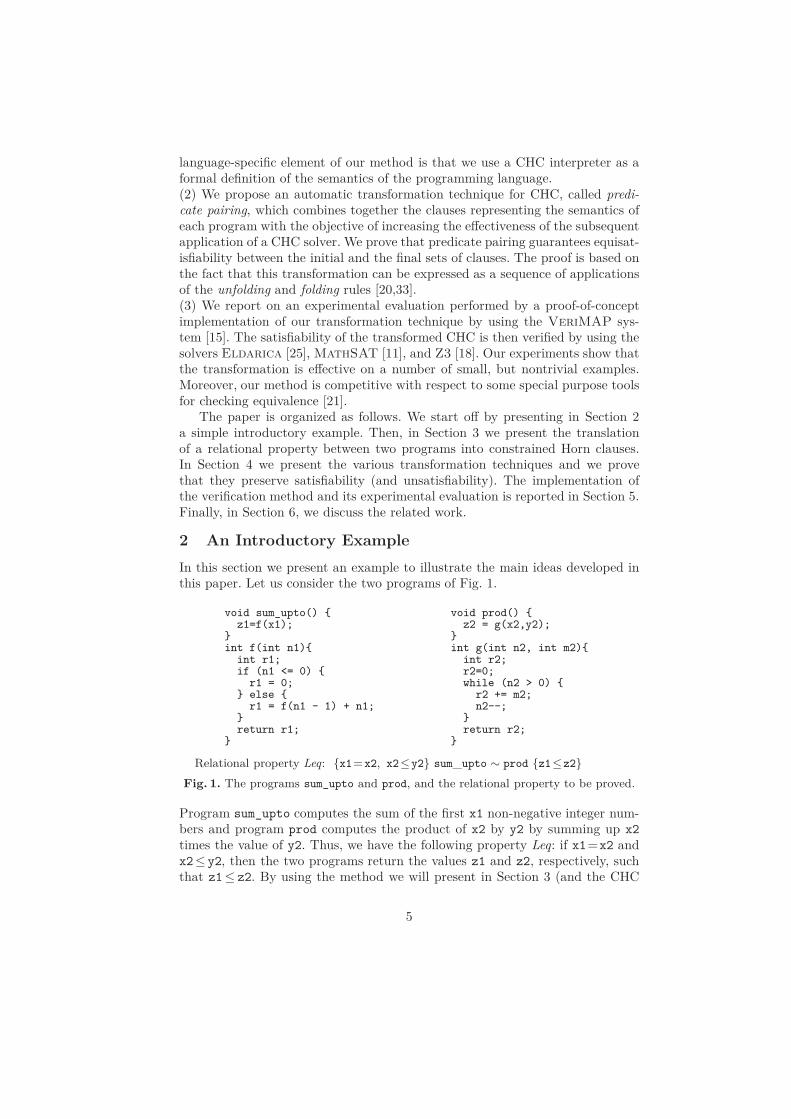
In this section we present an example to illustrate the main ideas developed inthis paper. Let us consider the two programs of Fig. 1.
void sum_upto() {z1=f(x1);
}int f(int n1){
int r1;if (n1 <= 0) {
r1 = 0;} else {
r1 = f(n1 - 1) + n1;}return r1;
}
void prod() {z2 = g(x2,y2);
}int g(int n2, int m2){
int r2;r2=0;while (n2 > 0) {
r2 += m2;n2--;
}return r2;
}
Relational property Leq: {x1=x2, x2≤y2} sum_upto ∼ prod {z1≤z2}
Fig. 1. The programs sum_upto and prod, and the relational property to be proved.
Program sum_upto computes the sum of the first x1 non-negative integer num-bers and program prod computes the product of x2 by y2 by summing up x2times the value of y2. Thus, we have the following property Leq: if x1=x2 andx2≤ y2, then the two programs return the values z1 and z2, respectively, suchthat z1≤ z2. By using the method we will present in Section 3 (and the CHC
5

specialization of Section 4.1), the property Leq relating the computations of thetwo programs is translated into the set of constrained Horn clauses listed inFig. 2, written in the syntax of Constraint Logic Programming (CLP) [26].
1. false ← X1=X2, X2≤Y 2, Z1′ >Z2′, su(X1, Z1′), p(X2, Y 2, Z2′)2. su(X1, Z1′)← f(X1, Z, X1, R, N1, Z1′)3. f(X, Z, N, R, N, 0)← N≤04. f(X, Z, N, R, N, Z1)← N≥1, N1=N−1, Z1=R2+N, f(X, Z, N1, R1, N2, R2)5. p(X2, Y 2, Z2′)← g(X2, Y 2, Z, X2, Y 2, 0, N, P, Z2′)6. g(X, Y, Z, N, P, R, N, P, R)← N≤07. g(X, Y, Z, N, P, R, N2, P 2, R2)← N≥1, N1=N−1, R1=P +R,
g(X, Y, Z, N1, P, R1, N2, P 2, R2)
Fig. 2. Translation into constrained Horn clauses of the relational property Leq.
Clause 1 specifies the relational property Leq, where primed logical variablesrefer to the final values of the corresponding imperative variables. In particular,note that the constraint Z1′ > Z2′ is the negation of the property we wantto prove. Clauses 2–4 and 5–7 encode the input-ouput relations computed byprograms sum_upto and prod, respectively. The relational property Leq holds iffclauses 1–7 are satisfiable.
Unfortunately, state-of-the-art solvers for constrained Horn clauses with lin-ear integer arithmetic (such as Eldarica [25], MathSAT [11], and Z3 [18])are unable to prove the satisfiability of clauses 1–7. This is due to the fact thatthose solvers reason on the predicate su and p separately, and hence, to provethat clause 1 is satisfiable (that is, its premise is unsatisfiable), they should dis-cover quadratic relations among variables (in our case, Z1′ = X1×(X1−1)/2and Z2′ =X2×Y 2), and these relations cannot be expressed by linear arithmeticconstraints.
In order to deal with this limitation one could extend constrained Hornclauses with solvers for the theory of non-linear integer arithmetic constraints [8].However, this extension has to cope with the additional problem that the satis-fiability problem for non-linear constraints is undecidable [30].
In this paper we propose an approach based on suitable transformations ofthe clauses that encode the property Leq into an equisatisfiable set of clauses,which, as shown in the sequel, are hopefully easier to solve. In our example, theclauses of Fig. 2 are transformed into the ones shown in Fig. 3.
false ← X1≤Y 2, Z1′ >Z2′, fg(X1,Z,X1,R, N1, Z1′, Y 2, Z, 0, N2, P 2, Z2′)fg(X, Z, N, R, N, 0, Y 2, V, Z2, N, P 2, Z2)← N≤0fg(X, Z, N, R, N, Z1, Y 2, V, W, N2, P 2, Z2)←
N≥1, N1=N−1, Z1=R2+N, M =Y 2+W,fg(X, Z, N1, R1, S, R2, Y 2, V, M, N2, P 2, Z2)
Fig. 3. Transformed clauses derived from the clauses 1–7 in Fig. 2.
6
The predicate fg(X, Z, N, R, N1, Z1, Y 2, V, W, N2, P 2, Z2) is equivalent tothe conjunction f(X, Z, N, R, N1, Z1), g(X, Y 2, V, N, Y 2, W, N2, P 2, Z2). The ef-fect of this transformation is that it is possible to infer linear relations amonga subset of the variables occurring in the conjunctions of predicates, withouthaving to use in an explicit way their non-linear relations with other variables.In particular, one can infer that fg(X1, Z, X1, R, N1, Z1′, Y 2, Z, 0, N2, P 2, Z2′)enforces the constraint (X1 > Y 2) ∨ (Z1′≤Z2′), and hence the satisfiability ofthe first clause of Fig. 3, without having to derive quadratic relations. Indeed,after this transformation MathSAT (and, after further transformation, also El-
darica and Z3) is able to prove the satisfiability of the clauses of Fig. 3, whichimplies the validity of the relational property Leq.
3 Specifying Relational Properties in CHC
In this section we introduce the notion of a relational property relative to twoprograms written in a simple imperative language and we show how a relationalproperty can be translated into constrained Horn clauses.
3.1 Relational properties
We consider a C-like programming language manipulating integers and inte-ger arrays via assignments, function calls, conditionals, while loops, and goto’s.A program is a sequence of labeled commands (or commands, for short), andin each program there is a unique halt command that, when executed, causesprogram termination.
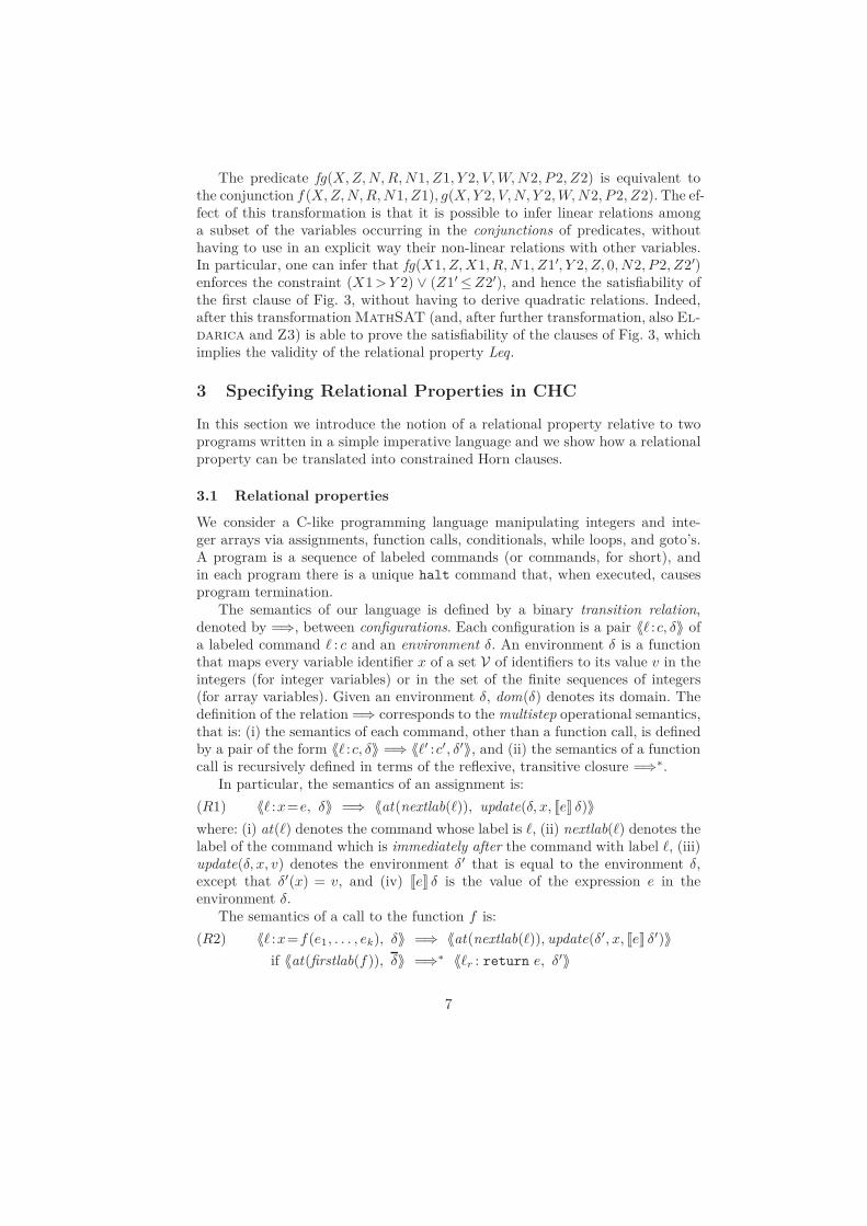
The semantics of our language is defined by a binary transition relation,denoted by =⇒, between configurations. Each configuration is a pair ⟨⟨ℓ :c, δ⟩⟩ ofa labeled command ℓ : c and an environment δ. An environment δ is a functionthat maps every variable identifier x of a set V of identifiers to its value v in theintegers (for integer variables) or in the set of the finite sequences of integers(for array variables). Given an environment δ, dom(δ) denotes its domain. Thedefinition of the relation =⇒ corresponds to the multistep operational semantics,that is: (i) the semantics of each command, other than a function call, is definedby a pair of the form ⟨⟨ℓ :c, δ⟩⟩ =⇒ ⟨⟨ℓ′ :c′, δ′⟩⟩, and (ii) the semantics of a functioncall is recursively defined in terms of the reflexive, transitive closure =⇒∗.
In particular, the semantics of an assignment is:
(R1) ⟨⟨ℓ :x=e, δ⟩⟩ =⇒ ⟨⟨at(nextlab(ℓ)), update(δ, x, !e" δ)⟩⟩
where: (i) at(ℓ) denotes the command whose label is ℓ, (ii) nextlab(ℓ) denotes thelabel of the command which is immediately after the command with label ℓ, (iii)update(δ, x, v) denotes the environment δ′ that is equal to the environment δ,except that δ′(x) = v, and (iv) !e" δ is the value of the expression e in theenvironment δ.
The semantics of a call to the function f is:
(R2) ⟨⟨ℓ :x=f(e1, . . . , ek), δ⟩⟩ =⇒ ⟨⟨at(nextlab(ℓ)), update(δ′, x, !e" δ′)⟩⟩
if ⟨⟨at(firstlab(f)), δ⟩⟩ =⇒∗ ⟨⟨ℓr : return e, δ′⟩⟩
7

where: (i) firstlab(f) denotes the label of the first command in the definitionof the function f , and (ii) δ is the environment δ extended by the bindings forthe formal parameters, say x1, . . . , xk, and the local variables, say y1, . . . , yh, off (we assume that the identifiers xi’s and yi’s do not occur in dom(δ)). Thus,we have that δ = δ ∪ {x1 )→ !e1" δ, . . . , xk )→ !ek" δ, y1 )→ v1, . . . , yh )→ vh}, forarbitrary values v1, . . . , vh. We refer to [17] for a more detailed presentation ofthe multistep semantics.
A program P terminates for an initial environment δ and computes the finalenvironment η, denoted ⟨P, δ⟩ ⇓ η, iff ⟨⟨ℓ0 :c, δ⟩⟩ =⇒∗ ⟨⟨ℓh :halt, η⟩⟩, where ℓ0 :c isthe first labeled command of P . ⟨⟨ℓ0 :c, δ⟩⟩ and ⟨⟨ℓh :halt, η⟩⟩ are called the initialconfiguration and the final configuration, respectively.
Now, we can formally define a relational property as follows. Let P1 and P2 betwo programs with global variables in V1 and V2, respectively, with V1∩V2 = ∅.Let ϕ and ψ be two first order formulas with variables in V1∪V2. Then, by usingthe notation of [5], a relational property is specified by the 4-tuple {ϕ} P1∼P2 {ψ}.For instance, the relational property Leq presented in Section 2 is specified by:{x1=x2, x2≤y2} sum_upto ∼ prod {z1≤z2}.
We say that {ϕ} P1 ∼ P2 {ψ} is valid iff the following holds: if the inputs of P1
and P2 satisfy the pre-relation ϕ and the programs P1 and P2 both terminate,then upon termination the outputs of P1 and P2 satisfy the post-relation ψ. Thevalidity of a relational property is formalized by Definition 1 below, where givena formula α and an environment δ, by α [δ] we denote the formula α where everyfree occurrence of a variable has been replaced by its values in δ.
Definition 1. A relational property {ϕ} P1 ∼ P2 {ψ} is said to be valid, denoted|= {ϕ} P1 ∼ P2 {ψ}, iff for all environments δ1 and δ2 with dom(δ1)⊆V1 anddom(δ2)⊆V2, the following holds:
if |= ϕ [δ1∪ δ2] and ⟨P1, δ1⟩ ⇓ η1 and ⟨P2, δ2⟩ ⇓ η2, then |= ψ [η1∪ η2].
3.2 Formal Semantics of the Imperative Language in CHC
In order to translate a relational program property into constrained Horn clauses,first we need to specify the operational semantics of our C-like language by aset of constrained Horn clauses. We follow the approach presented in [17] whichnow we briefly recall.
The transition relation =⇒ between configurations and its reflexive, transitiveclosure =⇒∗ are specified by the binary predicates tr and reach, respectively. Weonly show the formalization of the semantic rules R1 and R2 above, consistingof the following clauses D1 and D2, respectively. For the other rules of themultistep operational semantics we refer to [17].
(D1) tr(cf (cmd(L, asgn(X, expr(E))), Env), cf (cmd(L1, C), Env1))←eval(E, Env, V ), update(Env, X, V, Env1), nextlab(L, L1), at(L1, C)
(D2) tr(cf (cmd(L, asgn(X, call(F, Es))), Env), cf (cmd(L2, C2), Env2))←fun_env(Es, Env, F, FEnv), firstlab(F, FL), at(FL, C),reach(cf (cmd(FL, C), FEnv), cf (cmd(LR, return(E)), Env1)),eval(E, Env1, V ), update(Env1, X, V, Env2), nextlab(L, L2), at(L2, C2)
8
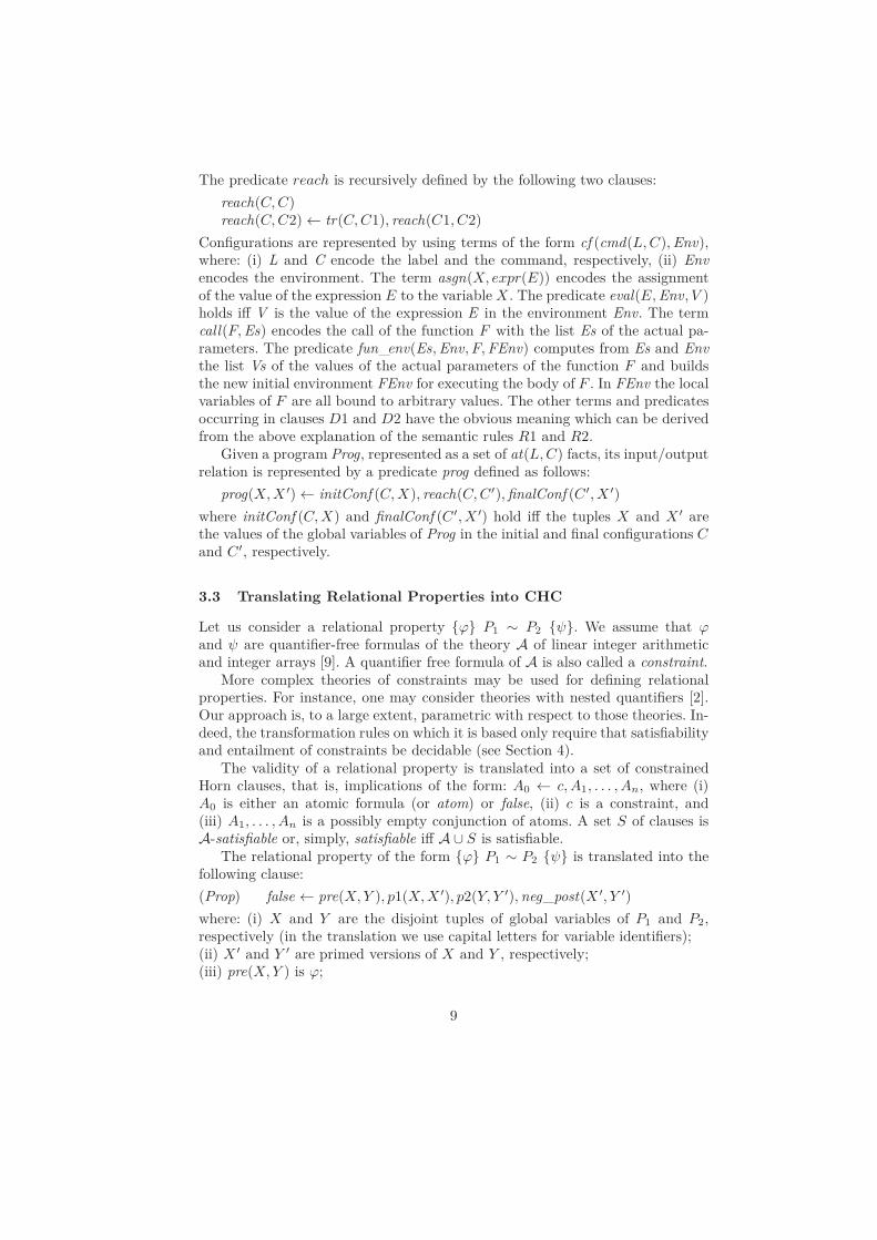
The predicate reach is recursively defined by the following two clauses:
reach(C, C)reach(C, C2)← tr(C, C1), reach(C1, C2)
Configurations are represented by using terms of the form cf (cmd(L, C), Env),where: (i) L and C encode the label and the command, respectively, (ii) Envencodes the environment. The term asgn(X, expr(E)) encodes the assignmentof the value of the expression E to the variable X . The predicate eval(E, Env, V )holds iff V is the value of the expression E in the environment Env. The termcall(F, Es) encodes the call of the function F with the list Es of the actual pa-rameters. The predicate fun_env(Es, Env, F, FEnv) computes from Es and Envthe list Vs of the values of the actual parameters of the function F and buildsthe new initial environment FEnv for executing the body of F . In FEnv the localvariables of F are all bound to arbitrary values. The other terms and predicatesoccurring in clauses D1 and D2 have the obvious meaning which can be derivedfrom the above explanation of the semantic rules R1 and R2.
Given a program Prog, represented as a set of at(L, C) facts, its input/outputrelation is represented by a predicate prog defined as follows:
prog(X, X ′)← initConf (C, X), reach(C, C′), finalConf (C′, X ′)
where initConf (C, X) and finalConf (C′, X ′) hold iff the tuples X and X ′ arethe values of the global variables of Prog in the initial and final configurations Cand C′, respectively.
3.3 Translating Relational Properties into CHC
Let us consider a relational property {ϕ} P1 ∼ P2 {ψ}. We assume that ϕand ψ are quantifier-free formulas of the theory A of linear integer arithmeticand integer arrays [9]. A quantifier free formula of A is also called a constraint.
More complex theories of constraints may be used for defining relationalproperties. For instance, one may consider theories with nested quantifiers [2].Our approach is, to a large extent, parametric with respect to those theories. In-deed, the transformation rules on which it is based only require that satisfiabilityand entailment of constraints be decidable (see Section 4).
The validity of a relational property is translated into a set of constrainedHorn clauses, that is, implications of the form: A0 ← c, A1, . . . , An, where (i)A0 is either an atomic formula (or atom) or false, (ii) c is a constraint, and(iii) A1, . . . , An is a possibly empty conjunction of atoms. A set S of clauses isA-satisfiable or, simply, satisfiable iff A ∪ S is satisfiable.
The relational property of the form {ϕ} P1 ∼ P2 {ψ} is translated into thefollowing clause:
(Prop) false ← pre(X, Y ), p1(X, X ′), p2(Y, Y ′), neg_post(X ′, Y ′)
where: (i) X and Y are the disjoint tuples of global variables of P1 and P2,respectively (in the translation we use capital letters for variable identifiers);(ii) X ′ and Y ′ are primed versions of X and Y , respectively;(iii) pre(X, Y ) is ϕ;
9

(iv) the predicates p1(X, X ′) and p2(Y, Y ′) are defined by a set of clauses derivedfrom P1 and P2, respectively, by using a formalization of the the operationalsemantics of the programming language, as explained in Section 3.2; and(v) neg_post(X ′, Y ′) is ¬ψ, with all variables replaced by their primed versions.
Note that we can always eliminate negation from the atoms pre(X, Y ) andneg_post(X ′, Y ′) by pushing negation inward and transforming negated equal-ities into disjunctions of inequalities. Moreover, we can eliminate disjunctionfrom constraints and replace clause Prop by a set of clauses with false in thehead. Although these transformations are not strictly needed by the techniquesdescribed in the rest of the paper, they may be helpful for the constraint solvingtools we use when automating our verification method.
Let RP be a relational property and TRP be the set of constrained Hornclauses generated by the translation process described above, then TRP is correctin the following sense.
Theorem 1 (Correctness of the CHC Translation). RP is valid iff TRP
is satisfiable.
The proof of this theorem directly follows from the fact that the predicatereach is a correct formalization of the semantics of the programming language.
4 Transforming Specifications of Relational Properties
The reduction of the validity problem, that is, the problem of testing whether ornot {ϕ} P1 ∼ P2 {ψ} is valid, to the problem of verifying the satisfiability of a setTRP of constrained Horn clauses allows us to apply reasoning techniques that areindependent of the specific programming language in which programs P1 and P2
are written. In particular, we can try to solve the satisfiability problem for TRP byapplying one of the available solvers for constrained Horn clauses. Unfortunately,as shown by the example in Section 2, it may be the case that these solvers failto prove satisfiability (or unsatisfiability). In Section 5 the reader will find anexperimental evidence of this limitation. However, a very significant advantageof having reduced the validity problem to a CHC satisfiability problem is thatwe can now transform the set TRP by applying any satisfiability preservingalgorithm, before submitting the new, transformed satisfiability problem to aCHC solver.
In this section we present some transformations of constrained Horn clausesthat have the objective of increasing the effectiveness of the subsequent usesof CHC solvers. These transformations, called transformation strategies, are:(1) CHC specialization, and (2) predicate pairing.
These strategies are variants of techniques developed in the area of logicprogramming for improving the efficiency of program execution [19,32]. We willshow that these techniques are very effective for the class of verification prob-lems we are considering here, and actually, they are more general and effectivethan other ad-hoc techniques developed for proving special cases of relationalproperties, such as program equivalence [21].
10

The above CHC Specialization and Predicate Pairing strategies are realizedas sequences of applications of some elementary transformation rules, collectivelycalled unfold/fold rules, proposed in the field of CLP [20].
Now we present the version of those rules we need in our context here. Thoserules allow us to derive from an old set Cls of constrained Horn clauses a newset TransfCls of constrained Horn clauses.
Definition Rule. We introduce a definition clause D of the form newp(X)← c, G,where newp is a new predicate symbol, X is a tuple of variables occurringin {c, G}, c is a constraint, and G is a non-empty conjunction of atoms. Wederive the set of clauses TransfCls = Cls ∪ {D}. We denote by Defs the set ofall definition clauses introduced in a sequence of application of the unfold/foldrules.
Unfolding Rule. Given a clause C in Cls of the form H ← c, L, A, R, where H iseither false or an atom, A is an atom, c is a constraint, and L and R are (possiblyempty) conjunctions of atoms, let us consider the set {Ki ← ci, Bi | i = 1, . . . , m}made out of the (renamed apart) clauses of Cls such that, for i=1, . . . , m, A isunifiable with Ki via the most general unifier ϑi and A |= ∃X.(c, ci)ϑi whereX is the tuple of variables in (c, ci)ϑi. By unfolding C w.r.t. A using Cls, wederive the set of clauses TransfCls = (Cls− {C})∪U(C), where the set U(C) is{(H ← c, ci, L, Bi, R)ϑi | i = 1, . . . , m}.
Folding Rule. Given a clause E of the form: H ← e, L, Q, R and a clause D inDefs of the form K ← d, G such that: (i) for some substitution ϑ, Q = Gϑ, and(ii) A |= ∀X. (e→ dϑ) holds, where X is the tuple of variables in e→ dϑ, thenby folding E using D we derive the set of clauses TransfCls = (Cls − {E}) ∪{H ← e, L, Kϑ, R}.
By using the results in [20], which ensure that the transformation rules pre-serve the least model of a set of constrained Horn clauses, if any, we get thefollowing result.
Theorem 2 (Soundness of the Unfold/Fold Rules). Suppose that from aset Cls of constrained Horn clauses we derive a new set TransfCls of clausesby a sequence of applications of the unfold/fold rules, where every definitionclause used for folding is unfolded during that sequence. Then Cls is satisfiableiff TransfCls is satisfiable.
4.1 CHC Specialization
Specialization is a transformation technique that has been proposed in variousprogramming contexts to take advantage of static information to simplify andcustomize programs [27]. In the field of program verification it has been shownthat the specialization of constrained Horn clauses can be very useful to simplifyclauses before checking their satisfiability [13,28].
We will use CHC specialization to simplify our initial set of clauses TRP.In particular, starting from clause Prop of Section 3.3, we introduce two newpredicates p1sp and p2sp, defined by the clauses:
(S1) p1sp(V, V ′)← p1(X, X ′) (S2) p2sp(W, W ′)← p2(Y, Y ′)
11

where V, V ′, W, W ′ are the sub-tuples of X, X ′, Y, Y ′, respectively, which occurin pre(X, Y ) or neg_post(X ′, Y ′). Then, by applying the folding rule, we canreplace p1 and p2 in clause Prop, by p1sp and p2sp, thereby obtaining:
(Propsp) false ← pre(V, W ), p1sp(V, V ′), p2sp(W, W ′), neg_post(W, W ′)
Now, by applying the specialization strategy of [13] starting from the set ofclauses (TRP − {Prop})∪ {Propsp, S1, S2}, we derive specialized versions of theclauses that define the semantics of programs P1 and P2. In particular, in thoseclauses there are reference to neither the predicate reach, nor the predicate tr,nor the terms encoding configurations.
For instance, let us consider again our example of Section 2. The translationof the relational property Leq: {x1 = x2, x2 ≤ y2} sum_upto ∼ prod {z1 ≤ z2}is as follows:
false ← X1=X2, X2≤Y 2, Z1′ >Z2′,sum_upto(X1, Z1, X1′, Z1′), prod(X2, Y 2, Z2, X2′, Y 2′, Z2′)
where predicates sum_upto and prod are defined in terms of the predicate reachas shown in Section 3.2. By specialization we get clauses 1–7 of Fig. 2, where suand p are the specialized versions of sum_upto and prod , respectively.
CHC specialization is performed by applying the unfold/fold rules, and henceby Theorem 2 the following property holds.
Theorem 3. Let Tsp be derived from TRP by specialization. Then TRP is satis-fiable iff Tsp is satisfiable.
4.2 Predicate Pairing
The core of our verification method is the predicate pairing transformation strat-egy (see Fig. 4), which composes pairs of predicates q and r into one new predi-cate t equivalent to their conjunction. As suggested by the example of Section 2,this transformation may ease the discovery of relations between variables oc-curring in the two original predicates, and thus it may ease the satisfiabilitytest.
Let us see the predicate pairing strategy in action by considering again theexample of Section 2.
First Iteration of the while loop.Unfolding: The strategy starts off by unfolding su(X1, Z1′) and p(X2, Y 2, Z2′)in clause 1 of Fig. 2, hence deriving the following new clause:
8. false ← X≤Y 2, Z1>Z2,f(X1, Z, X1, R, N1, Z1′), g(X1, Y 2, Z, X, Y 2, 0, N2, P 2, Z2′)
Definition & Folding: A new atom with predicate fg is introduced for replac-ing the conjunction of the atoms with predicates f and g in the premise ofclause 8:
9. fg(X1, Z, N, R, N1, Z1′, Y 2, V, W, N2, P 2, Z2′)←f(X1, Z, N, R, N1, Z1′), g(X1, Y 2, V, N, Y 2, W, N2, P 2, Z2′)
12

Input: A set Q ∪R ∪ {C} of clauses where: (i) C is of the form false ← c, q(X), r(Y ),(ii) q and r occur in Q and R, respectively, and (iii) no predicate occurs in both Qand R.Output: A set TransfCls of clauses.
Initialization: InCls := {C}; Defs := ∅; TransfCls := Q ∪R;
while there is a clause C in InCls doUnfolding: From clause C derive a set U(C) of clauses by unfolding C with respect
to every atom occurring in its body using Q ∪R;Rewrite each clause in U(C) to a clause of the form H ← d, A1, . . . , Ak, suchthat, for i = 1, . . . , k, Ai is of the form p(X1, . . . , Xm), where X1, . . . , Xm are, notnecessarily distinct, variables;
Definition & Folding:F (C) := U(C);for every clause E ∈ F (C) of the form H ← d, G1, qi(Vi), G2, ri(Wi), G3 where qi
and ri occur in Q and R, respectively, doif in Defs there is no clause of the form newp(Z)← qi(Vi), ri(Wi), where Z is
the tuple of distinct variables in (Vi, Wi)then add newp(Z)← qi(Vi), ri(Wi) to InCls and to Defs;F (C) := (F (C)− {E}) ∪ {H ← d, G1, newp(Z), G2, G3}
end-for
InCls := InCls− {C}; TransfCls := TransfCls ∪ F(C);end-while
Fig. 4. The predicate pairing transformation strategy.
and that conjunction is folded, hence deriving:
10. false ← X≤Y 2, Z1′ >Z2′, fg(X1, Z, X1, R, N1, Z1′, Y 2, Z, 0, N2, P 2, Z2′)
Second Iteration of the while loop.Unfolding: Now, the atoms with predicate f and g in the premise of the newlyintroduced clause 9 are unfolded, and the following new clauses are derived:
11. fg(X, Z, N, R, N, 0, Y, V, W, N2, Y, Z2)← N≤012. fg(X, Z, N, R, N, Z1, Y 2, V, W, N2, P 2, Z2)←
N≥1, N1=N−1, Z1=R2+N, M =Y 2+W,f(X, Z, N1, R1, S, R2), g(X, Y 2, V, N1, Y 2, M, N2, P 2, Z2)
Definition & Folding: No new predicate is needed, as the conjunction of theatoms with predicate f and g in clause 12 can be folded using clause 9. We get:
13. fg(X, Z, N, R, N, Z1, Y 2, V, W, N2, P 2, Z2)←N≥1, N1=N−1, Z1=R2+N, M =Y 2+W,fg(X, Z, N1, R1, S, R2, Y 2, V, M, N2, P 2, Z2)
Clauses 10, 11, and 13, which are the ones shown in Fig. 3, constitute the finalset of clauses we have derived.
The predicate pairing strategy always terminates because the number of thepossible new predicate definitions is bounded by the number γ of conjunctionsof the form qi(Vi), ri(Wi), where qi occurs in Q and ri occurs in R and, hence,the number of executions of the while loop of the strategy is bounded by γ.
13
Thus, from the fact that the unfold/fold transformation rules preserve satis-fiability (see Theorem 2), we get the following result.
Theorem 4 (Soundness of the predicate pairing strategy). Let the setQ ∪ R ∪ {C} of clauses be the input of the predicate pairing strategy. Then thestrategy terminates and returns a set TransfCls of clauses such that Q∪R∪{C}is satisfiable iff TransfCls is satisfiable.
5 Implementation and Experimental Evaluation
We have implemented the techniques presented in Sections 3 and 4 by using theVeriMAP transformation and verification system [15]. The satisfiability of theconstrained Horn clauses derived by transformation has been checked by usingthe SMT solvers Eldarica [25], MathSAT [11], and Z3 [18].
We have considered 90 problems referring to relational properties of small,yet non-trivial, C-like programs mostly taken from the literature [5,6,21]. Thesources of the problems are available at http://map.uniroma2.it/releq. Theproperties we have considered belong to the following categories. All programsact on integers, except for those in the arr category which act on integer arrays.
The ite (respectively, rec) category consists of equivalence properties be-tween pairs of iterative (respectively, recursive) programs, that is, we have veri-fied that for every pair of programs, the two programs in the pair compute thesame outputs when given the same inputs.
The i-r category consists of equivalence properties between an iterative and arecursive (non-tail recursive) program. For example, we have verified the equiv-alence of iterative and recursive versions of programs computing the greatestcommon divisor of two integers and the n-th triangular number Tn =
!n
i=1i.
The arr category consists of equivalence properties between programs actingon integer arrays.
The leq category consists of inequality properties stating that if the inputsof two programs satisfy some given precondition, then their outputs satisfy aninequality postcondition. For instance, we have verified that for all non-negativeintegers m and n: (i) if n≤m, then Tn≤n×m (see the example of Section 2),and (ii) n2≤n3.
The mon (respectively, inj) category consists of properties stating that pro-grams, under some given preconditions, compute monotonically non-decreasing(respectively, injective) functions. For example, we have verified monotonicityand injectivity of programs computing the Fibonacci numbers, the square of anumber, and the triangular numbers (for non-negative input values).
The fun category consists of properties stating that, under some given pre-conditions, some of the outputs of the given programs are functionally dependenton a proper subset of the inputs.
The results of our experimental evaluation are summarized in Table 1. Allexperiments have been performed on a single core of an Intel Core Duo E73002.66Ghz processor with 4GB of memory running Ubuntu. Timings are in seconds.A time limit of 60 seconds has been set for all problems.
14

Cat n Tr Eld Z3 PP Eld MS Z3 CP+Eld CP+MS CP+Z3ite 21 0.04 7 (5.61) 6 (1.06) 1.23 13 (5.10) 19 (7.39) 6 (1.08) 4 (0.07) 1 (0.10) 15 (2.55)rec 18 0.06 7 (4.16) 8 (3.10) 1.82 7 (5.19) 11 (1.09) 6 (0.94) 7 (0.06) 0 7 (0.08)i-r 4 0.05 0 0 0.58 0 3 (8.16) 0 4 (0.35) 1 (0.08) 4 (0.35)arr 5 0.05 0 1 (0.78) 1.02 1 (4.29) 1 (0.78) 4 (0.81) 1 (5.81) 1 (2.26) 1 (0.75)leq 6 0.03 1 (2.83) 1 (0.77) 0.29 1 (4.76) 6 (2.52) 1 (0.80) 2 (1.74) 0 3 (0.64)mon 18 0.02 4 (4.60) 4 (0.90) 2.78 11 (5.55) 16 (1.61) 8 (0.98) 0 1 (3.12) 6 (0.81)inj 11 0.02 0 0 1.87 0 11 (1.70) 4 (1.10) 7 (1.71) 0 6 (0.63)fun 7 0.02 5 (4.49) 5 (0.80) 3.90 6 (4.77) 7 (1.03) 5 (0.91) 0 0 2 (0.69)Tot 90 0.04 24(4.67) 25(1.61) 1.84 39(5.16) 74(3.30) 34(0.97) 25(0.93) 4(1.39) 44(1.20)
Table 1. Timings are in seconds. The timeout occurs after 60 seconds.
The first two columns (Cat) and (n) report the names of the categories andthe number of problems in each category, respectively. The third column (Tr)reports the average time taken for generating the set of CHC encoding the rela-tional property by applying the method presented in Section 3 (including CHCspecialization).
Columns 4 (Eld) and 5 (Z3 ) report the number of problems that were solvedby applying Eldarica and Z3, respectively, on the CHC encoding of the relationalproperty. Between parentheses we have indicated the average time taken for eachsolved problem. There is no column for MathSAT because it is unable to dealwith clauses containing multiple atoms in their premise.
Column 6 (PP) reports the average time taken for applying the predicatepairing transformation strategy presented in Section 4.2. Predicate pairing ter-minates before the timeout for all problems.
Columns 7 (Eld), 8 (MS), and 9 (Z3 ) report the results obtained by applyingEldarica, MathSAT, and Z3, respectively, on the CHC derived by applying thepredicate pairing strategy. We indicate the number of solved problems and theaverage solving time.
If a CHC solver is unable to solve a problem after predicate pairing, we applyCHC specialization again with the goal of propagating the constraints occurringin the clauses and discovering invariants by means of the widening and convex-hull operators [13]. In some cases this constraint propagation produces a setof CHC without constrained facts (that is, clauses of the form A ← c), andhence satisfiable. If the other cases, we apply again the solvers on the clausesobtained after constraint propagation. Columns 10 (CP+Eld), 11 (CP+MS),and 12 (CP+Z3 ) report the results obtained by applying constraint propagation,possibly followed by Eldarica, MathSAT, and Z3, respectively, in the cases wherethe predicate pairing and the CHC solvers were unable to deliver an answer. Asusual, we report the number of problems solved and the average solving time.The solving times include the time spent for constraint propagation.
More details about the results of our experimental evaluation are reportedin the Appendix.
The use of the predicate pairing and constraint propagation strategies signif-icantly increases the number of problems that have been solved. In particular,the number of problems that can be solved by Eldarica increases from 24 (see
15

Column 4) to 64 (sum of Columns 7 and 10). Similarly for MathSAT from zeroto 78 (sum of Columns 8 and 11), and for Z3 from 25 (see Column 5) to 78 (sumof Columns 9 and 12). The number of problems that can be solved by using anyof the considered CHC solvers is 86.
We observe that the application of the predicate pairing strategy is veryeffective in increasing the number of solved problems. For instance, it allowsEldarica to solve 15 more problems (see Columns 4 and 7). For problems that canalready be solved without using the pairing strategy the performance overheadis almost always tolerable. However, for three problems out of the 90 we haveconsidered, Z3 is unable to prove the property within the considered time limitafter the application of the pairing strategy (although one of these problems canbe solved after the constraint propagation phase).
Also the application of constraint propagation turns out to be very useful forsolving additional problems. For instance, for Z3 constraint propagation allowsthe solution of additional 44 problems (see Column 12).
It is worth noticing that for the problems in the ite and rec categories ourverification method is competitive with the approach to the proof of programequivalences presented in [21]. However, that approach cannot be directly appliedto problems belonging to the other categories.
6 Related Work
Various logics and methods for reasoning about program relations have been pre-sented in the literature. Their main purpose is the formal, possibly automated,validation of program transformation and program analysis techniques.
A Hoare-like axiomatization of relational reasoning for simple while programshas been proposed in [6], which however does not present any technique forautomating proofs.
A partial automation of relational reasoning has been proposed in [5], whichintroduces a notion of a program product that allows the reduction of a relationalverification problem to a standard program verification problem. The methodrequires human ingenuity to generate program products via ad-hoc refinementsand also to provide suitable invariants to the program verifier. Similarly to [5],the Differential Assertion Checking technique proposed in [29] makes use of thenotion of a program composition to reduce the relative correctness of two pro-grams to a suitable safety property of the composed program.
The idea of using program transformations to help the proof of relationalproperties between higher-order functional programs has been explored in [3].The main difference between the approach in [3] and ours is that, besides thedifference of programming languages, we transform the logical representationof the property to be proved, rather than the two programs under analysis.Our approach allows higher parametericity with respect to the programminglanguage, and also enables us to use very effective tools for CHC solving.
Our notion of the predicate pairing is related to that of the mutual summariespresented in [24]. Mutual summaries relate the summaries of two procedures,and can be used to prove relations between them, including relative termination
16

(which we do not consider in our technique). Similarly to the above mentionedpapers [5,29], this approach requires human ingenuity to generate suitable proofobligations, which can then be discharged by automated theorem provers.
Program equivalence is one of the relational properties that has been exten-sively studied (see [10,12,21,23,34] for some recent work). Indeed, during soft-ware development one may want to modify the program text and prove that itssemantics has not changed (this kind of proofs is sometimes called regression ver-ification). Among the various approaches to prove program equivalence, the onewhich is most related to ours is the one reported in [21], which proposes proofrules for the equivalence of simple imperative programs that are then trans-lated into constrained Horn clauses. The satisfiability of these clauses is thenchecked by state-of-the-art CHC solvers. As already mentioned, our method canbe applied to more general relational properties. Moreover, we need not spe-cial purpose proof rules for equivalence and, instead, we use transformations ofconstrained Horn clauses.
Finally, we want to mention that in the present paper we have used (vari-ants and extensions of) transformation techniques for constrained Horn clausesproposed in previous work in the area of program verification (see, for in-stance, [1,13,14,16,17,28,31]). However, the goal of that previous work was theverification of partial and total correctness of single programs, and not the ver-ification of relations between two programs which has been the objective of ourstudy in this paper.
7 Conclusions
We have presented a method for verifying relational properties of programs writ-ten in a simple imperative language with integer and array variables. The methodconsists in: (i) translating the property to be verified into a set of constrainedHorn clauses, then (ii) transforming these clauses to better exploit the interac-tions between the predicates which represent the computations evoked by theprograms, and finally, (iii) using state-of-the-art constrained Horn clause solversto prove satisfiability.
Although we have considered imperative programs, the only language-specificelement of our method is the constrained Horn clause interpreter that we haveused to represent in clausal form the program semantics and the property tobe verified. Indeed, our method can also be applied to prove relations betweenprograms written in different programming languages. Thus, our approach isbasically independent of the programming language used.
Finally, we think that our approach can be refined and improved by takingadvantage of the progress that in the future could be made in the developmentof techniques and tools for reasoning about constrained Horn clauses.
Acknowledgements
We wish to thank Arie Gurfinkel, Vladimir Klebanov, and the participants inthe VPT workshop at ETAPS 2015 for stimulating conversations.
17

References
1. E. Albert, M. Gómez-Zamalloa, L. Hubert, and G. Puebla. Verification of Javabytecode using analysis and transformation of logic programs. In M. Hanus,ed., Practical Aspects of Declarative Languages, LNCS 4354, pages 124–139.Springer, 2007.
2. F. Alberti, S. Ghilardi, and N. Sharygina. Decision procedures for flat array prop-erties. In TACAS ’14, Grenoble, France, LNCS 8413, pages 15–30. Springer, 2014.
3. K. Asada, R. Sato, and N. Kobayashi. Verifying relational properties of functionalprograms by first-order refinement. In Proc. PEPM ’15, Mumbai, India, pages61–72. ACM, 2015.
4. M. Barnett, B.-Y. E. Chang, R. De Line, B. Jacobs, and K. R. M. Leino. Boogie:A modular reusable verifier for object-oriented programs. In F. de Boer, M. Bon-sangue, S. Graf, and W.-P. de Roever, eds., Formal Methods for Components andObjects, LNCS 4111, pages 364–387. Springer, 2006.
5. G. Barthe, J. M. Crespo, and C. Kunz. Relational verification using productprograms. In FM ’11: Formal Methods, Limerick, Ireland, LNCS 6664, pages 200–214. Springer, 2011.
6. N. Benton. Simple relational correctness proofs for static analyses and programtransformations. In Proc. 31st ACM SIGPLAN-SIGACT, POPL ’04, Venice, Italy,pages 14–25. ACM, 2004.
7. N. Bjørner, A. Gurfinkel, K. L. McMillan, and A. Rybalchenko. Horn clausesolvers for program verification. In L. D. Beklemishev, A. Blass, N. Dershowitz,B. Finkbeiner, and W. Schulte, eds., Fields of Logic and Computation II - Essaysdedicated to Y. Gurevich, LNCS 9300, pages 24–51. Springer, 2015.
8. C. Borralleras, S. Lucas, A. Oliveras, E. Rodríguez-Carbonell, and A. Rubio. SATmodulo linear arithmetic for solving polynomial constraints. J. Autom. Reasoning,48(1):107–131, 2012.
9. A. R. Bradley, Z. Manna, and H. B. Sipma. What’s decidable about arrays? InProc. VMCAI ’06, LNCS 3855, pages 427–442. Springer, 2006.
10. S. Chaki, A. Gurfinkel, and O. Strichman. Regression verification for multi-threaded programs. In V. Kuncak and A. Rybalchenko, eds., VMCAI ’12, Philadel-phia, PA, USA, LNCS 7148, pages 119–135. Springer, 2012.
11. A. Cimatti, A. Griggio, B. Schaafsma, and R. Sebastiani. The MathSAT5 SMTSolver. In N. Piterman and S. Smolka, eds., Proc. TACAS ’13, LNCS 7795, pages93–107. Springer, 2013.
12. S. Ciobâcă, D. Lucanu, V. Rusu, and G. Rosu. A language-independent proof sys-tem for mutual program equivalence. In S. Merz and J. Pang, eds., Formal Meth-ods and Software Engineering ICFEM ’14, Luxembourg, Luxembourg, LNCS 8829,pages 75–90. Springer, 2014.
13. E. De Angelis, F. Fioravanti, A. Pettorossi, and M. Proietti. Program verificationvia iterated specialization. Sci. Comput. Program., 95, Part 2:149–175, 2014.
14. E. De Angelis, F. Fioravanti, A. Pettorossi, and M. Proietti. Verifying array pro-grams by transforming verification conditions. In Proc. VMCAI ’14, LNCS 8318,pages 182–202. Springer, 2014.
15. E. De Angelis, F. Fioravanti, A. Pettorossi, and M. Proietti. VeriMAP: A tool forverifying programs through transformations. In Proc. TACAS ’14, LNCS 8413,pages 568–574. Springer, 2014. http://www.map.uniroma2.it/VeriMAP.
16. E. De Angelis, F. Fioravanti, A. Pettorossi, and M. Proietti. Proving correctness ofimperative programs by linearizing constrained Horn clauses. Theory and Practiceof Logic Programming, 15(4-5):635–650, 2015.
18
17. E. De Angelis, F. Fioravanti, A. Pettorossi, and M. Proietti. Semantics-basedgeneration of verification conditions by program specialization. In Proc. Symp. onPrinciples and Practice of Declarative Programming, Siena, Italy, pages 91–102.ACM, 2015.
18. L. M. de Moura and N. Bjørner. Z3: An efficient SMT solver. In Proc. TACAS ’08,LNCS 4963, pages 337–340. Springer, 2008.
19. D. De Schreye, R. Glück, J. Jørgensen, M. Leuschel, B. Martens, and M. H.Sørensen. Conjunctive partial deduction: Foundations, control, algorithms, andexperiments. Journal of Logic Programming, 41(2–3):231–277, 1999.
20. S. Etalle and M. Gabbrielli. Transformations of CLP modules. Theoretical Com-puter Science, 166:101–146, 1996.
21. D. Felsing, S. Grebing, V. Klebanov, P. Rümmer, and M. Ulbrich. Automat-ing regression verification. In I. Crnkovic, M. Chechik, and P. Grünbacher, eds.,ACM/IEEE ASE ’14, Vasteras, Sweden, pages 349–360, 2014.
22. J.-C. Filliâtre and A. Paskevich. Why3 - Where programs meet provers. In Pro-gramming ESOP ’13, LNCS 7792, pages 125–128. Springer, 2013.
23. B. Godlin and O. Strichman. Regression verification: Proving the equivalence ofsimilar programs. Softw. Test., Verif. Reliab., 23(3):241–258, 2013.
24. C. Hawblitzel, M. Kawaguchi, S. K. Lahiri, and H. Rebêlo. Towards modularlycomparing programs using automated theorem provers. In M. P. Bonacina, ed.,Automated Deduction - CADE 24, LNCS 7898, pages 282–299. Springer, 2013.
25. H. Hojjat, F. Konecný, F. Garnier, R. Iosif, V. Kuncak, and P. Rümmer. A verifica-tion toolkit for numerical transition systems. In D. Giannakopoulou and D. Méry,eds., FM ’12: Formal Methods, LNCS 7436, pages 247–251. Springer, 2012.
26. J. Jaffar and M. Maher. Constraint logic programming: A survey. Journal of LogicProgramming, 19/20:503–581, 1994.
27. N. D. Jones, C. K. Gomard, and P. Sestoft. Partial Evaluation and AutomaticProgram Generation. Prentice Hall, 1993.
28. B. Kafle and J. P. Gallagher. Constraint specialisation in Horn clause verification.In Proc. PEPM ’15, Mumbai, India, pages 85–90. ACM, 2015.
29. S. K. Lahiri, K. L. McMillan, R. Sharma, and C. Hawblitzel. Differential assertionchecking. In B. Meyer, L. Baresi, and M. Mezini, eds., ESEC/FSE ’13, SaintPetersburg, Russian Federation, pages 345–355. ACM, 2013.
30. Y. V. Matijasevic. Enumerable sets are diophantine. Doklady Akademii NaukSSSR (in Russian), 191:279–282, 1970.
31. J. C. Peralta, J. P. Gallagher, and H. Saglam. Analysis of imperative programsthrough analysis of constraint logic programs. In G. Levi, ed., Proc. SAS ’98,LNCS 1503, pages 246–261. Springer, 1998.
32. A. Pettorossi and M. Proietti. Transformation of logic programs: Foundations andtechniques. Journal of Logic Programming, 19,20:261–320, 1994.
33. H. Tamaki and T. Sato. Unfold/fold transformation of logic programs. In S.-Å.Tärnlund, ed., Proc. ICLP ’84, pages 127–138, Uppsala, Sweden, 1984. UppsalaUniversity.
34. S. Verdoolaege, G. Janssens, and M. Bruynooghe. Equivalence checking of staticaffine programs using widening to handle recurrences. ACM Trans. Program. Lang.Syst., 34(3):11, 2012.
19

Deta
iled
resu
lts
of
the
ex
peri
men
tal
evalu
ati
on
Pro
ble
m
Translation
Eldarica
Z3
PredicatePairing(PP)
Eldarica
MathSAT
Z3
ConstraintPropagation(CP)
Answer
Eldarica
MathSAT
Z3
CP+Eldarica
CP+MathSAT
CP+Z3
bart
he0.
04T
OT
O1.
65T
O30
.79
TO
0.09
true
N/A
N/A
N/A
0.09
N/A
0.09
bart
he2
0.03
TO
TO
0.54
TO
2.78
TO
0.13
un
know
nT
ON
/A0.
94T
ON
/A1.
07ba
rthe
2-bi
g0.
04T
OT
O1.
43T
O5.
69T
O26
.62
un
know
nT
ON
/A1.
46T
ON
/A28
.08
bart
he2-
big2
0.06
TO
TO
3.92
TO
56.6
8T
O4.
36un
know
nT
ON
/A2.
89T
ON
/A7.
25bu
g15
0.03
3.78
0.81
0.20
2.89
0.75
0.76
0.05
true
N/A
N/A
N/A
N/A
N/A
N/A
digi
ts10
0.07
3.52
TO
2.41
7.17
3.29
0.94
0.77
un
know
nN
/AN
/AN
/AN
/AN
/AN
/Adi
gits
10_
inl
0.09
3.48
0.81
2.42
6.92
1.90
TO
0.14
true
N/A
N/A
N/A
N/A
N/A
0.14
fib0.
04T
OT
O0.
66T
O4.
74T
O0.
11un
know
nT
ON
/A0.
79T
ON
/A0.
90lo
op0.
03T
OT
O0.
463.
594.
43T
O0.
06tr
ue
N/A
N/A
N/A
N/A
N/A
0.06
loop
20.
03T
OT
O0.
483.
571.
57T
O0.
06tr
ue
N/A
N/A
N/A
N/A
N/A
0.06
loop
30.
03T
OT
O0.
333.
351.
00T
O0.
05tr
ue
N/A
N/A
N/A
N/A
N/A
0.05
loop
40.
04T
OT
O0.
55T
O19
.26
TO
0.07
true
N/A
N/A
N/A
0.07
N/A
0.07
loop
50.
02T
OT
O0.
47T
OT
OT
O0.
10tr
ue
N/A
N/A
N/A
0.10
0.10
0.10
nest
ed-w
hile
0.06
TO
TO
2.42
8.93
1.27
TO
0.19
true
N/A
N/A
N/A
N/A
N/A
0.19
sim
ple-
loop
0.02
7.58
0.93
0.13
5.69
1.50
0.99
0.03
true
N/A
N/A
N/A
N/A
N/A
N/A
upco
unt
0.03
TO
TO
0.19
3.24
0.88
TO
0.04
true
N/A
N/A
N/A
N/A
N/A
0.04
whi
le-i
f0.
04T
OT
O0.
874.
031.
20T
O0.
09tr
ue
N/A
N/A
N/A
N/A
N/A
0.09
bart
he-f
ault
y0.
0714
.86
2.29
3.55
9.77
TO
2.21
0.21
un
know
nN
/AT
ON
/AN
/AT
ON
/Alo
op5-
faul
ty0.
022.
760.
750.
453.
170.
870.
770.
08un
know
nN
/AN
/AN
/AN
/AN
/AN
/Ane
sted
-whi
le-f
ault
y0.
053.
300.
792.
364.
001.
040.
830.
19un
know
nN
/AN
/AN
/AN
/AN
/AN
/Ain
vari
anth
oist
ing
0.02
TO
TO
0.29
TO
0.80
TO
0.02
true
N/A
N/A
N/A
0.02
N/A
0.02
To
tal
tim
e0
.86
39
.28
6.3
82
5.7
86
6.3
21
40
.44
6.5
03
3.4
6–
–6
.08
0.2
80
.10
38
.21
#o
fP
ro
ble
ms
21
76
21
13
19
62
11
3–
–4
41
15
Av
era
ge
tim
e0
.04
5.6
11
.06
1.2
35
.10
7.3
91
.08
1.5
9–
–1
.52
0.0
70
.10
2.5
5
Ta
ble
2.
Cat
egor
yit
e.
Col
umn
‘Tra
nsla
tion
’re
por
tsth
eti
me
take
nby
Ver
iMA
Pto
tran
slat
eth
epr
oble
min
toC
HC
.C
olum
ns3
and
4re
por
tth
eti
me
take
nby
Eld
aric
aan
dZ
3fo
rso
lvin
gth
epr
oble
ms
afte
rth
etr
ansl
atio
n.C
olum
n‘P
redi
cate
Pai
ring
(PP
)’re
por
tsth
eti
me
take
nby
Ver
iMA
Pto
appl
yth
epr
edic
ate
pair
ing
stra
tegy
.C
olum
ns6,
7,an
d8
repo
rtth
eti
me
take
nby
Eld
aric
a,M
athS
AT
,an
dZ
3fo
rso
lvin
gth
epr
oble
ms
afte
rP
P.C
olum
n‘C
onst
rain
tP
ropa
gati
on(C
P)’
rep
orts
the
tim
eta
ken
byV
eriM
AP
toap
ply
the
cons
trai
ntpr
opag
atio
n.C
olum
n‘A
nsw
er’
rep
orts
the
answ
erpr
ovid
edby
Ver
iMA
Paf
ter
the
appl
icat
ion
ofC
P.
Col
umns
11,
12,
and
13re
port
the
tim
eta
ken
byE
ldar
ica,
Mat
hSA
T,
and
Z3
for
solv
ing
the
prob
lem
saf
ter
CP
.C
olum
ns14
,15
,an
d16
repo
rtth
eti
me
take
nby
appl
ying
CP
,pl
usth
eti
me
pos
sibl
yta
ken
byE
ldar
ica,
Mat
hSA
T,
and
Z3
resp
ecti
vely
,in
the
case
sw
here
the
pred
icat
epa
irin
gan
dth
eC
HC
solv
ers
wer
eun
able
tode
liver
anan
swer
.‘T
O’
mea
nsth
atth
eto
olw
asno
tab
leto
prov
eth
egi
ven
prop
erty
wit
hin
the
tim
eout
limit
of60
seco
nds.
‘N/A
’m
eans
not
appl
icab
leb
ecau
seal
read
ypr
oved
ina
prev
ious
phas
e.T
imes
are
inse
cond
s.
20
Pro
ble
m
Translation
Eldarica
Z3
PredicatePairing(PP)
Eldarica
MathSAT
Z3
ConstraintPropagation(CP)
Answer
Eldarica
MathSAT
Z3
CP+Eldarica
CP+MathSAT
CP+Z3
add-
horn
0.06
TO
TO
1.14
TO
0.94
TO
0.15
true
N/A
N/A
N/A
0.15
N/A
0.15
coco
me1
0.03
TO
TO
0.27
TO
0.99
TO
0.05
true
N/A
N/A
N/A
0.05
N/A
0.05
inlin
ing
0.04
2.84
TO
0.25
4.00
0.85
TO
0.15
true
N/A
N/A
N/A
N/A
N/A
0.15
limit
10.
02T
OT
O0.
21T
OT
OT
O0.
05un
know
nT
OT
OT
OT
OT
OT
Olim
it1u
nrol
led
0.05
TO
TO
0.19
TO
1.10
TO
0.04
true
N/A
N/A
N/A
0.04
N/A
0.04
limit
20.
03T
OT
O0.
37T
O0.
89T
O0.
02tr
ue
N/A
N/A
N/A
0.02
N/A
0.02
limit
30.
04T
OT
O0.
18T
O0.
82T
O0.
07tr
ue
N/A
N/A
N/A
0.07
N/A
0.07
loop
_re
c0.
06T
O0.
770.
28T
O1.
240.
790.
03tr
ue
N/A
N/A
N/A
0.03
N/A
N/A
tria
ngul
ar0.
03T
OT
O0.
27T
O0.
99T
O0.
07tr
ue
N/A
N/A
N/A
0.07
N/A
0.07
tria
ngul
ar-m
od0.
13T
OT
O4.
71T
OT
OT
O31
.08
un
know
nT
OT
OT
OT
OT
OT
Om
ccar
thy9
10.
043.
630.
760.
313.
52T
OT
ON
/Aun
know
nN
/AT
OT
ON
/AT
OT
Oac
kerm
ann
0.15
TO
TO
9.58
TO
TO
TO
N/A
un
know
nT
OT
OT
OT
OT
OT
Oac
kerm
ann-
faul
ty0.
213.
450.
8310
.66
6.68
TO
1.08
N/A
un
know
nN
/AT
ON
/AN
/AT
ON
/Aad
d-ho
rn-f
ault
y0.
063.
150.
771.
214.
221.
000.
840.
20un
know
nN
/AN
/AN
/AN
/AN
/AN
/Ain
linin
g-fa
ulty
0.03
2.79
0.75
0.26
3.49
0.82
0.78
0.12
un
know
nN
/AN
/AN
/AN
/AN
/AN
/Alim
it1-
faul
ty0.
022.
550.
750.
212.
90T
O0.
750.
10un
know
nN
/AT
ON
/AN
/AT
ON
/Alim
it2-
faul
ty0.
0410
.72
1.03
0.34
11.5
42.
391.
380.
11un
know
nN
/AN
/AN
/AN
/AN
/AN
/Atr
iang
ular
-mod
-fau
lty
0.09
TO
19.1
72.
26T
OT
OT
O19
.96
un
know
nT
OT
OT
OT
OT
OT
OT
ota
lti
me
1.1
32
9.1
32
4.8
33
2.7
03
6.3
51
2.0
35
.62
52
.20
––
–0
.43
–0
.55
#o
fP
ro
ble
ms
18
78
18
71
16
15
8–
––
7–
7
Av
era
ge
tim
e0
.06
4.1
63
.10
1.8
25
.19
1.0
90
.94
3.4
8–
––
0.0
6–
0.0
8
Ta
ble
3.
Cat
egor
yr
ec
.Col
umn
‘Tra
nsla
tion
’re
por
tsth
eti
me
take
nby
Ver
iMA
Pto
tran
slat
eth
epr
oble
min
toC
HC
.C
olum
ns3
and
4re
por
tth
eti
me
take
nby
Eld
aric
aan
dZ
3fo
rso
lvin
gth
epr
oble
ms
afte
rth
etr
ansl
atio
n.C
olum
n‘P
redi
cate
Pai
ring
(PP
)’re
por
tsth
eti
me
take
nby
Ver
iMA
Pto
appl
yth
epr
edic
ate
pair
ing
stra
tegy
.C
olum
ns6,
7,an
d8
repo
rtth
eti
me
take
nby
Eld
aric
a,M
athS
AT
,an
dZ
3fo
rso
lvin
gth
epr
oble
ms
afte
rP
P.C
olum
n‘C
onst
rain
tP
ropa
gati
on(C
P)’
rep
orts
the
tim
eta
ken
byV
eriM
AP
toap
ply
the
cons
trai
ntpr
opag
atio
n.C
olum
n‘A
nsw
er’
rep
orts
the
answ
erpr
ovid
edby
Ver
iMA
Paf
ter
the
appl
icat
ion
ofC
P.
Col
umns
11,
12,
and
13re
port
the
tim
eta
ken
byE
ldar
ica,
Mat
hSA
T,
and
Z3
for
solv
ing
the
prob
lem
saf
ter
CP
.C
olum
ns14
,15
,an
d16
repo
rtth
eti
me
take
nby
appl
ying
CP
,pl
usth
eti
me
pos
sibl
yta
ken
byE
ldar
ica,
Mat
hSA
T,
and
Z3
resp
ecti
vely
,in
the
case
sw
here
the
pred
icat
epa
irin
gan
dth
eC
HC
solv
ers
wer
eun
able
tode
liver
anan
swer
.‘T
O’
mea
nsth
atth
eto
olw
asno
tab
leto
prov
eth
egi
ven
prop
erty
wit
hin
the
tim
eout
limit
of60
seco
nds.
‘N/A
’m
eans
not
appl
icab
leb
ecau
seal
read
ypr
oved
ina
prev
ious
phas
e.T
imes
are
inse
cond
s.
21

Pro
ble
m
Translation
Eldarica
Z3
PredicatePairing(PP)
Eldarica
MathSAT
Z3
ConstraintPropagation(CP)
Answer
Eldarica
MathSAT
Z3
CP+Eldarica
CP+MathSAT
CP+Z3
cub
e_vs
_sq
uare
0.04
TO
TO
0.39
TO
2.60
TO
0.21
un
know
nT
ON
/A0.
77T
ON
/A0.
98sq
uare
n0.
03T
OT
O0.
24T
O1.
24T
O0.
09un
know
n3.
31N
/A0.
783.
40N
/A0.
87su
mod
d_vs
_sq
uare
0.03
2.83
0.77
0.41
4.76
0.89
0.80
0.08
un
know
nN
/AN
/AN
/AN
/AN
/AN
/Asu
m_
vs_
prod
uct
0.02
TO
TO
0.24
TO
3.81
TO
0.13
un
know
nT
ON
/AT
OT
ON
/AT
Osu
m_
vs_
prod
uct2
0.03
TO
TO
0.27
TO
5.50
TO
0.12
un
know
nT
ON
/AT
OT
ON
/AT
Osu
m_
vs_
squa
re0.
02T
OT
O0.
16T
O1.
05T
O0.
07tr
ue
N/A
N/A
N/A
0.07
N/A
0.07
To
tal
tim
e0
.17
2.8
30
.77
1.7
14
.76
15
.09
0.8
00
.70
3.3
1–
1.5
53
.47
–1
.92
#o
fP
ro
ble
ms
61
16
16
16
11
–2
2–
3
Av
era
ge
tim
e0
.03
2.8
30
.77
0.2
94
.76
2.5
20
.80
0.1
23
.31
–0
.78
1.7
4–
0.6
4
Ta
ble
4.
Cat
egor
yle
q.
Col
umn
‘Tra
nsla
tion
’re
por
tsth
eti
me
take
nby
Ver
iMA
Pto
tran
slat
eth
epr
oble
min
toC
HC
.C
olum
ns3
and
4re
por
tth
eti
me
take
nby
Eld
aric
aan
dZ
3fo
rso
lvin
gth
epr
oble
ms
afte
rth
etr
ansl
atio
n.C
olum
n‘P
redi
cate
Pai
ring
(PP
)’re
por
tsth
eti
me
take
nby
Ver
iMA
Pto
appl
yth
epr
edic
ate
pair
ing
stra
tegy
.C
olum
ns6,
7,an
d8
repo
rtth
eti
me
take
nby
Eld
aric
a,M
athS
AT
,an
dZ
3fo
rso
lvin
gth
epr
oble
ms
afte
rP
P.C
olum
n‘C
onst
rain
tP
ropa
gati
on(C
P)’
rep
orts
the
tim
eta
ken
byV
eriM
AP
toap
ply
the
cons
trai
ntpr
opag
atio
n.C
olum
n‘A
nsw
er’
rep
orts
the
answ
erpr
ovid
edby
Ver
iMA
Paf
ter
the
appl
icat
ion
ofC
P.
Col
umns
11,
12,
and
13re
port
the
tim
eta
ken
byE
ldar
ica,
Mat
hSA
T,
and
Z3
for
solv
ing
the
prob
lem
saf
ter
CP
.C
olum
ns14
,15
,an
d16
repo
rtth
eti
me
take
nby
appl
ying
CP
,pl
usth
eti
me
pos
sibl
yta
ken
byE
ldar
ica,
Mat
hSA
T,
and
Z3
resp
ecti
vely
,in
the
case
sw
here
the
pred
icat
epa
irin
gan
dth
eC
HC
solv
ers
wer
eun
able
tode
liver
anan
swer
.‘T
O’
mea
nsth
atth
eto
olw
asno
tab
leto
prov
eth
egi
ven
prop
erty
wit
hin
the
tim
eout
limit
of60
seco
nds.
‘N/A
’m
eans
not
appl
icab
leb
ecau
seal
read
ypr
oved
ina
prev
ious
phas
e.T
imes
are
inse
cond
s.
22

Pro
ble
m
Translation
Eldarica
Z3
PredicatePairing(PP)
Eldarica
MathSAT
Z3
ConstraintPropagation(CP)
Answer
Eldarica
MathSAT
Z3
CP+Eldarica
CP+MathSAT
CP+Z3
gcd
0.12
TO
TO
1.55
TO
15.2
4T
O1.
02tr
ue
N/A
N/A
N/A
1.02
N/A
1.02
sum
VSp
rod(
RE
)0.
03T
OT
O0.
33T
O7.
56T
O0.
15tr
ue
N/A
N/A
N/A
0.15
N/A
0.15
tria
ngul
ar_
nont
ail
0.03
TO
TO
0.23
TO
1.68
TO
0.13
true
N/A
N/A
N/A
0.13
N/A
0.13
tria
ngul
ar_
tail
0.03
TO
TO
0.21
TO
TO
TO
0.08
true
N/A
N/A
N/A
0.08
0.08
0.08
To
tal
tim
e0
.21
––
2.3
2–
24
.48
–1
.38
––
–1
.38
0.0
81
.38
#o
fP
ro
ble
ms
4–
–4
–3
–4
4–
––
41
4
Av
era
ge
tim
e0
.05
––
0.5
8–
8.1
6–
0.3
52
.00
–1
.00
0.3
50
.08
0.3
5
Ta
ble
5.
Cat
egor
yi-
r.
Col
umn
‘Tra
nsla
tion
’re
por
tsth
eti
me
take
nby
Ver
iMA
Pto
tran
slat
eth
epr
oble
min
toC
HC
.C
olum
ns3
and
4re
por
tth
eti
me
take
nby
Eld
aric
aan
dZ
3fo
rso
lvin
gth
epr
oble
ms
afte
rth
etr
ansl
atio
n.C
olum
n‘P
redi
cate
Pai
ring
(PP
)’re
por
tsth
eti
me
take
nby
Ver
iMA
Pto
appl
yth
epr
edic
ate
pair
ing
stra
tegy
.C
olum
ns6,
7,an
d8
repo
rtth
eti
me
take
nby
Eld
aric
a,M
athS
AT
,an
dZ
3fo
rso
lvin
gth
epr
oble
ms
afte
rP
P.C
olum
n‘C
onst
rain
tP
ropa
gati
on(C
P)’
rep
orts
the
tim
eta
ken
byV
eriM
AP
toap
ply
the
cons
trai
ntpr
opag
atio
n.C
olum
n‘A
nsw
er’
rep
orts
the
answ
erpr
ovid
edby
Ver
iMA
Paf
ter
the
appl
icat
ion
ofC
P.
Col
umns
11,
12,
and
13re
port
the
tim
eta
ken
byE
ldar
ica,
Mat
hSA
T,
and
Z3
for
solv
ing
the
prob
lem
saf
ter
CP
.C
olum
ns14
,15
,an
d16
repo
rtth
eti
me
take
nby
appl
ying
CP
,pl
usth
eti
me
pos
sibl
yta
ken
byE
ldar
ica,
Mat
hSA
T,
and
Z3
resp
ecti
vely
,in
the
case
sw
here
the
pred
icat
epa
irin
gan
dth
eC
HC
solv
ers
wer
eun
able
tode
liver
anan
swer
.‘T
O’
mea
nsth
atth
eto
olw
asno
tab
leto
prov
eth
egi
ven
prop
erty
wit
hin
the
tim
eout
limit
of60
seco
nds.
‘N/A
’m
eans
not
appl
icab
leb
ecau
seal
read
ypr
oved
ina
prev
ious
phas
e.T
imes
are
inse
cond
s.
23
Pro
ble
m
Translation
Eldarica
Z3
PredicatePairing(PP)
Eldarica
MathSAT
Z3
ConstraintPropagation(CP)
Answer
Eldarica
MathSAT
Z3
CP+Eldarica
CP+MathSAT
CP+Z3
fib0.
02T
OT
O1.
09T
OT
O0.
801.
40un
know
n4.
410.
86N
/A5.
812.
26N
/Afin
dmax
0.06
TO
0.78
1.22
TO
TO
0.80
1.41
un
know
nT
OT
ON
/AT
OT
ON
/Alo
opal
ign
0.05
TO
TO
1.12
TO
TO
0.80
25.5
9un
know
nT
OT
ON
/AT
OT
ON
/Alo
oppi
pe
0.14
TO
TO
1.52
TO
TO
0.84
0.06
un
know
nT
OT
ON
/AT
OT
ON
/Apr
opag
ate
0.01
TO
TO
0.14
4.29
0.78
TO
0.75
true
N/A
N/A
N/A
N/A
N/A
0.75
To
tal
tim
e0
.28
–0
.78
5.0
94
.29
0.7
83
.24
29
.21
4.4
10
.86
–5
.81
2.2
60
.75
#o
fP
ro
ble
ms
5–
15
11
45
11
1–
11
1
Av
era
ge
tim
e0
.06
–0
.78
1.0
24
.29
0.7
80
.81
5.8
44
.41
0.8
6–
5.8
12
.26
0.7
5
Ta
ble
6.
Cat
egor
ya
rr
.Col
umn
‘Tra
nsla
tion
’re
por
tsth
eti
me
take
nby
Ver
iMA
Pto
tran
slat
eth
epr
oble
min
toC
HC
.C
olum
ns3
and
4re
por
tth
eti
me
take
nby
Eld
aric
aan
dZ
3fo
rso
lvin
gth
epr
oble
ms
afte
rth
etr
ansl
atio
n.C
olum
n‘P
redi
cate
Pai
ring
(PP
)’re
por
tsth
eti
me
take
nby
Ver
iMA
Pto
appl
yth
epr
edic
ate
pair
ing
stra
tegy
.C
olum
ns6,
7,an
d8
repo
rtth
eti
me
take
nby
Eld
aric
a,M
athS
AT
,an
dZ
3fo
rso
lvin
gth
epr
oble
ms
afte
rP
P.C
olum
n‘C
onst
rain
tP
ropa
gati
on(C
P)’
rep
orts
the
tim
eta
ken
byV
eriM
AP
toap
ply
the
cons
trai
ntpr
opag
atio
n.C
olum
n‘A
nsw
er’
rep
orts
the
answ
erpr
ovid
edby
Ver
iMA
Paf
ter
the
appl
icat
ion
ofC
P.
Col
umns
11,
12,
and
13re
port
the
tim
eta
ken
byE
ldar
ica,
Mat
hSA
T,
and
Z3
for
solv
ing
the
prob
lem
saf
ter
CP
.C
olum
ns14
,15
,an
d16
repo
rtth
eti
me
take
nby
appl
ying
CP
,pl
usth
eti
me
pos
sibl
yta
ken
byE
ldar
ica,
Mat
hSA
T,
and
Z3
resp
ecti
vely
,in
the
case
sw
here
the
pred
icat
epa
irin
gan
dth
eC
HC
solv
ers
wer
eun
able
tode
liver
anan
swer
.‘T
O’
mea
nsth
atth
eto
olw
asno
tab
leto
prov
eth
egi
ven
prop
erty
wit
hin
the
tim
eout
limit
of60
seco
nds.
‘N/A
’m
eans
not
appl
icab
leb
ecau
seal
read
ypr
oved
ina
prev
ious
phas
e.T
imes
are
inse
cond
s.
24

Pro
ble
m
Translation
Eldarica
Z3
PredicatePairing(PP)
Eldarica
MathSAT
Z3
ConstraintPropagation(CP)
Answer
Eldarica
MathSAT
Z3
CP+Eldarica
CP+MathSAT
CP+Z3
add-
horn
0.02
TO
TO
5.48
5.58
1.31
TO
0.33
true
N/A
N/A
N/A
N/A
N/A
0.33
bart
he0.
02T
OT
O7.
25T
OT
OT
O0.
47un
know
nT
O2.
65T
OT
O3.
12T
Oba
rthe
20.
02T
OT
O1.
76T
O1.
93T
O0.
31un
know
nT
ON
/AT
OT
ON
/AT
Obu
g15
0.02
5.88
0.83
0.68
4.07
0.81
0.98
0.09
true
N/A
N/A
N/A
N/A
N/A
N/A
cub
e0.
02T
OT
O4.
11T
OT
OT
O0.
14un
know
nT
OT
OT
OT
OT
OT
Odi
gits
100.
020.
801.
040.
504.
821.
020.
860.
25tr
ue
N/A
N/A
N/A
N/A
N/A
N/A
fib0.
02T
OT
O2.
56T
O7.
36T
O0.
40un
know
nT
ON
/A1.
08T
ON
/A1.
48lo
op0.
02T
OT
O1.
205.
131.
040.
840.
15tr
ue
N/A
N/A
N/A
N/A
N/A
N/A
loop
20.
01T
OT
O1.
117.
581.
321.
380.
14tr
ue
N/A
N/A
N/A
N/A
N/A
N/A
loop
30.
02T
OT
O3.
638.
601.
480.
780.
30tr
ue
N/A
N/A
N/A
N/A
N/A
N/A
loop
40.
02T
OT
O1.
214.
771.
051.
000.
16tr
ue
N/A
N/A
N/A
N/A
N/A
N/A
nest
ed-w
hile
0.04
3.37
0.76
14.7
48.
791.
341.
160.
27tr
ue
N/A
N/A
N/A
N/A
N/A
N/A
prod
uct
0.02
TO
TO
1.21
TO
1.44
TO
0.31
un
know
nT
ON
/AT
OT
ON
/AT
Osi
mpl
e-lo
op0.
028.
370.
950.
353.
980.
820.
860.
07tr
ue
N/A
N/A
N/A
N/A
N/A
N/A
squa
re0.
02T
OT
O0.
93T
O1.
48T
O0.
33un
know
nT
ON
/A1.
14T
ON
/A1.
47su
m0.
01T
OT
O0.
46T
O1.
02T
O0.
27un
know
nT
ON
/A0.
87T
ON
/A1.
14up
coun
t0.
01T
OT
O0.
710.
741.
03T
O0.
15tr
ue
N/A
N/A
N/A
N/A
N/A
0.15
whi
le-i
f0.
02T
OT
O2.
186.
961.
29T
O0.
26tr
ue
N/A
N/A
N/A
N/A
N/A
0.26
To
tal
tim
e0
.35
18
.42
3.5
85
0.0
76
1.0
22
5.7
47
.86
4.4
0–
2.6
53
.09
–3
.12
4.8
3
#o
fP
ro
ble
ms
18
44
18
11
16
81
81
1–
13
–1
6
Av
era
ge
tim
e0
.02
4.6
10
.90
2.7
85
.55
1.6
10
.98
0.2
4–
2.6
51
.03
–3
.12
0.8
1
Ta
ble
7.
Cat
egor
ym
on
.Col
umn
‘Tra
nsla
tion
’re
por
tsth
eti
me
take
nby
Ver
iMA
Pto
tran
slat
eth
epr
oble
min
toC
HC
.C
olum
ns3
and
4re
por
tth
eti
me
take
nby
Eld
aric
aan
dZ
3fo
rso
lvin
gth
epr
oble
ms
afte
rth
etr
ansl
atio
n.C
olum
n‘P
redi
cate
Pai
ring
(PP
)’re
por
tsth
eti
me
take
nby
Ver
iMA
Pto
appl
yth
epr
edic
ate
pair
ing
stra
tegy
.C
olum
ns6,
7,an
d8
repo
rtth
eti
me
take
nby
Eld
aric
a,M
athS
AT
,an
dZ
3fo
rso
lvin
gth
epr
oble
ms
afte
rP
P.C
olum
n‘C
onst
rain
tP
ropa
gati
on(C
P)’
rep
orts
the
tim
eta
ken
byV
eriM
AP
toap
ply
the
cons
trai
ntpr
opag
atio
n.C
olum
n‘A
nsw
er’
rep
orts
the
answ
erpr
ovid
edby
Ver
iMA
Paf
ter
the
appl
icat
ion
ofC
P.
Col
umns
11,
12,
and
13re
port
the
tim
eta
ken
byE
ldar
ica,
Mat
hSA
T,
and
Z3
for
solv
ing
the
prob
lem
saf
ter
CP
.C
olum
ns14
,15
,an
d16
repo
rtth
eti
me
take
nby
appl
ying
CP
,pl
usth
eti
me
pos
sibl
yta
ken
byE
ldar
ica,
Mat
hSA
T,
and
Z3
resp
ecti
vely
,in
the
case
sw
here
the
pred
icat
epa
irin
gan
dth
eC
HC
solv
ers
wer
eun
able
tode
liver
anan
swer
.‘T
O’
mea
nsth
atth
eto
olw
asno
tab
leto
prov
eth
egi
ven
prop
erty
wit
hin
the
tim
eout
limit
of60
seco
nds.
‘N/A
’m
eans
not
appl
icab
leb
ecau
seal
read
ypr
oved
ina
prev
ious
phas
e.T
imes
are
inse
cond
s.
25

Pro
ble
m
Translation
Eldarica
Z3
PredicatePairing(PP)
Eldarica
MathSAT
Z3
ConstraintPropagation(CP)
Answer
Eldarica
MathSAT
Z3
CP+Eldarica
CP+MathSAT
CP+Z3
add-
horn
0.03
TO
TO
4.09
TO
1.20
TO
0.20
true
N/A
N/A
N/A
0.20
N/A
0.20
fib0.
02T
OT
O2.
77T
O5.
15T
O0.
29un
know
nT
ON
/A0.
77T
ON
/A1.
06lo
op0.
01T
OT
O1.
34T
O1.
071.
570.
20un
know
n6.
65N
/AN
/A6.
85N
/AN
/Alo
op2
0.02
TO
TO
1.22
TO
1.01
1.00
0.18
true
N/A
N/A
N/A
0.18
N/A
N/A
loop
30.
02T
OT
O3.
89T
O1.
230.
930.
22un
know
n3.
96N
/AN
/A4.
18N
/AN
/Alo
op4
0.02
TO
TO
1.34
TO
1.22
0.90
0.17
true
N/A
N/A
N/A
0.17
N/A
N/A
prod
uct
0.01
TO
TO
1.23
TO
1.18
TO
0.17
un
know
nT
ON
/AT
OT
ON
/AT
Osq
uare
0.01
TO
TO
1.01
TO
1.93
TO
0.25
un
know
nT
ON
/A0.
76T
ON
/A1.
01su
m0.
02T
OT
O0.
51T
O1.
95T
O0.
33un
know
nT
ON
/A0.
77T
ON
/A1.
10up
coun
t0.
01T
OT
O0.
79T
O1.
17T
O0.
19tr
ue
N/A
N/A
N/A
0.19
N/A
0.19
whi
le-i
f0.
02T
OT
O2.
38T
O1.
58T
O0.
22tr
ue
N/A
N/A
N/A
0.22
N/A
0.22
To
tal
tim
e0
.19
––
20
.57
–1
8.6
94
.42
.42
10
.61
–2
.31
1.9
9–
3.7
8
#o
fP
ro
ble
ms
11
––
11
–1
14
11
52
–3
7–
6
Av
era
ge
tim
e0
.02
––
1.8
7–
1.7
01
.10
0.2
25
.31
–0
.77
1.7
1–
0.6
3
Ta
ble
8.
Cat
egor
yin
j.C
olum
n‘T
rans
lati
on’
rep
orts
the
tim
eta
ken
byV
eriM
AP
totr
ansl
ate
the
prob
lem
into
CH
C.
Col
umns
3an
d4
rep
ort
the
tim
eta
ken
byE
ldar
ica
and
Z3
for
solv
ing
the
prob
lem
saf
ter
the
tran
slat
ion.
Col
umn
‘Pre
dica
teP
airi
ng(P
P)’
rep
orts
the
tim
eta
ken
byV
eriM
AP
toap
ply
the
pred
icat
epa
irin
gst
rate
gy.
Col
umns
6,7,
and
8re
port
the
tim
eta
ken
byE
ldar
ica,
Mat
hSA
T,
and
Z3
for
solv
ing
the
prob
lem
saf
ter
PP
.Col
umn
‘Con
stra
int
Pro
paga
tion
(CP
)’re
por
tsth
eti
me
take
nby
Ver
iMA
Pto
appl
yth
eco
nstr
aint
prop
agat
ion.
Col
umn
‘Ans
wer
’re
por
tsth
ean
swer
prov
ided
byV
eriM
AP
afte
rth
eap
plic
atio
nof
CP
.C
olum
ns11
,12
,an
d13
repo
rtth
eti
me
take
nby
Eld
aric
a,M
athS
AT
,an
dZ
3fo
rso
lvin
gth
epr
oble
ms
afte
rC
P.
Col
umns
14,
15,
and
16re
port
the
tim
eta
ken
byap
plyi
ngC
P,
plus
the
tim
ep
ossi
bly
take
nby
Eld
aric
a,M
athS
AT
,an
dZ
3re
spec
tive
ly,
inth
eca
ses
whe
reth
epr
edic
ate
pair
ing
and
the
CH
Cso
lver
sw
ere
unab
leto
deliv
eran
answ
er.
‘TO
’m
eans
that
the
tool
was
not
able
topr
ove
the
give
npr
oper
tyw
ithi
nth
eti
meo
utlim
itof
60se
cond
s.‘N
/A’
mea
nsno
tap
plic
able
bec
ause
alre
ady
prov
edin
apr
evio
usph
ase.
Tim
esar
ein
seco
nds.
26

Pro
ble
m
Translation
Eldarica
Z3
PredicatePairing(PP)
Eldarica
MathSAT
Z3
ConstraintPropagation(CP)
Answer
Eldarica
MathSAT
Z3
CP+Eldarica
CP+MathSAT
CP+Z3
add-
horn
0.02
3.86
0.74
5.92
6.90
1.15
0.97
0.37
true
N/A
N/A
N/A
N/A
N/A
N/A
bug1
50.
015.
850.
820.
690.
770.
800.
800.
09tr
ue
N/A
N/A
N/A
N/A
N/A
N/A
fib0.
02T
OT
O1.
71T
O1.
34T
O0.
29un
know
nT
ON
/A0.
93T
ON
/A1.
22ne
sted
-whi
le0.
033.
390.
7615
.87
9.37
1.33
1.16
0.29
true
N/A
N/A
N/A
N/A
N/A
N/A
sim
ple-
loop
0.01
6.27
0.93
0.34
3.08
0.76
0.81
0.06
true
N/A
N/A
N/A
N/A
N/A
N/A
upco
unt
0.02
3.07
0.75
0.68
3.93
0.82
0.80
0.05
true
N/A
N/A
N/A
N/A
N/A
N/A
whi
le-i
f0.
02T
OT
O2.
124.
541.
02T
O0.
15tr
ue
N/A
N/A
N/A
N/A
N/A
0.15
To
tal
tim
e0
.13
22
.44
4.0
02
7.3
32
8.5
97
.22
4.5
41
.30
––
0.9
3–
–1
.37
#o
fP
ro
ble
ms
75
57
67
57
6–
–1
––
2
Av
era
ge
tim
e0
.02
4.4
90
.80
3.9
04
.77
1.0
30
.91
0.1
9–
–0
.93
––
0.6
9
Ta
ble
9.
Cat
egor
yfu
n.
Col
umn
‘Tra
nsla
tion
’re
por
tsth
eti
me
take
nby
Ver
iMA
Pto
tran
slat
eth
epr
oble
min
toC
HC
.C
olum
ns3
and
4re
por
tth
eti
me
take
nby
Eld
aric
aan
dZ
3fo
rso
lvin
gth
epr
oble
ms
afte
rth
etr
ansl
atio
n.C
olum
n‘P
redi
cate
Pai
ring
(PP
)’re
por
tsth
eti
me
take
nby
Ver
iMA
Pto
appl
yth
epr
edic
ate
pair
ing
stra
tegy
.C
olum
ns6,
7,an
d8
repo
rtth
eti
me
take
nby
Eld
aric
a,M
athS
AT
,an
dZ
3fo
rso
lvin
gth
epr
oble
ms
afte
rP
P.C
olum
n‘C
onst
rain
tP
ropa
gati
on(C
P)’
rep
orts
the
tim
eta
ken
byV
eriM
AP
toap
ply
the
cons
trai
ntpr
opag
atio
n.C
olum
n‘A
nsw
er’
rep
orts
the
answ
erpr
ovid
edby
Ver
iMA
Paf
ter
the
appl
icat
ion
ofC
P.
Col
umns
11,
12,
and
13re
port
the
tim
eta
ken
byE
ldar
ica,
Mat
hSA
T,
and
Z3
for
solv
ing
the
prob
lem
saf
ter
CP
.C
olum
ns14
,15
,an
d16
repo
rtth
eti
me
take
nby
appl
ying
CP
,pl
usth
eti
me
pos
sibl
yta
ken
byE
ldar
ica,
Mat
hSA
T,
and
Z3
resp
ecti
vely
,in
the
case
sw
here
the
pred
icat
epa
irin
gan
dth
eC
HC
solv
ers
wer
eun
able
tode
liver
anan
swer
.‘T
O’
mea
nsth
atth
eto
olw
asno
tab
leto
prov
eth
egi
ven
prop
erty
wit
hin
the
tim
eout
limit
of60
seco
nds.
‘N/A
’m
eans
not
appl
icab
leb
ecau
seal
read
ypr
oved
ina
prev
ious
phas
e.T
imes
are
inse
cond
s.
27