Development of novel ultrasound techniques for imaging and elastography
124
Transcript of Development of novel ultrasound techniques for imaging and elastography


premio tesi di dottorato– 37 –
PREMIO TESI DI DOTTORATO
Commissione giudicatrice, anno 2012
Luigi Lotti, Facoltà di Scienze Politiche (Presidente della Commissione)
Fortunato Tito Arecchi, Facoltà di Scienze Matematiche, Fisiche e NaturaliFranco Cambi, Facoltà di Scienze della Formazione Paolo Felli, Facoltà di Architettura Michele Arcangelo Feo, Facoltà di Lettere e Filosofia Roberto Genesio, Facoltà di Ingegneria Mario Pio Marzocchi, Facoltà di Facoltà di Farmacia Adolfo Pazzagli, Facoltà di Medicina e ChirurgiaMario Giuseppe Rossi, Facoltà di Lettere e FilosofiaSalvatore Ruggieri, Facoltà di Medicina e ChirurgiaSaulo Sirigatti, Facoltà di Psicologia Piero Tani, Facoltà di Economia Fiorenzo Cesare Ugolini, Facoltà di Agraria Vincenzo Varano, Facoltà di GiurisprudenzaGraziella Vescovini, Facoltà di Scienze della Formazione
Alessandro Ramalli
Development of novel ultrasound techniques for imaging and elastography
From simulation to real-time implementation
Firenze University Press2013
Development of novel ultrasound techniques for imaging and elastography : from simulation to real-time implementation / Alessandro Ramalli. – Firenze : Firenze University Press, 2013.(Premio FUP. Tesi di dottorato ; 37)
http://digital.casalini.it/9788866554578
ISBN 978-88-6655-456-1 (print)ISBN 978-88-6655-457-8 (online)
Peer Review ProcessAll publications are submitted to an external refereeing process under the responsibility of the FUP Editorial Board and the Scientific Committees of the individual series. The works published in the FUP catalogue are evaluated and approved by the Editorial Board of the publishing house. For a more detailed description of the refereeing process we refer to the official documents published in the online catalogue of the FUP (http://www.fupress.com).Firenze University Press Editorial BoardG. Nigro (Co-ordinator), M.T. Bartoli, M. Boddi, R. Casalbuoni, C. Ciappei, R. Del Punta, A. Dolfi, V. Fargion, S. Ferrone, M. Garzaniti, P. Guarnieri, A. Mariani, M. Marini, A. Novelli, M. Verga, A. Zorzi.
© 2013 Firenze University PressUniversità degli Studi di FirenzeFirenze University PressBorgo Albizi, 28, 50122 Firenze, Italyhttp://www.fupress.com/Printed in Italy
Contents
Introduction 9Contributions 10
1. Ultrasound Basics 131.1. Ultrasound propagation 131.2. Transducers and probes 161.3. Echo-signal elaboration 251.4. Open issues in ultrasound investigation 28
2. ULA-OP 312.1. Introduction 312.2. System description 322.3. Examples of non-standard application 372.4. High Frame Rate Imaging 392.5. Expansion capabilities and future work 40
3. Novel Ultrasound Simulation Methods 433.1. Field simulation in homogeneous linear media: Simag 433.2. Field simulation in nonlinear media: GASM 55
4. A Novel Ultrasound Experimental Method: Frequency Domain Elastography 734.1. Introduction 734.2. Methods 744.3. Computational cost analysis and reduction 794.4. Computer-guided compression experiments 804.5. Freehand compression experiments 864.6. Real-time implementation 904.7. Discussion and conclusion 92
Alessandro Ramalli, Development of novel ultrasound techniques for imaging and elastography : from simulation to real-time implementation ISBN 978-88-6655-456-1 (print) ISBN 978-88-6655-457-8 (online) © 2013 Firenze University Press

5. Novel Ultrasound Experimental Methods: Work in Progress 955.1. 2D HFR color vector Doppler 955.2. Adaptive beamforming through layered structures 1015.3. Pulse compression 109
6. Conclusion 111
Bibliography 113
Development of novel ultrasound techniques for imaging and elastography
8
Introduction
Ultrasound imaging techniques are a widely used diagnostic tool in medicine. They owe their success to a series of features that make them ideal for medical applications. Indeed, they use a form of energy that does not entail harmful effects on biological tissues. Moreover, these techniques can be implemented in relatively low-cost and low-size systems working in real-time, which can be used to perform exams directly at the bedside or in the operating room. Moreover, ultrasound is complementary to other diagnostic techniques (e.g. magnetic resonance imaging), allowing a more complete diagnosis. For these reasons, research studies focusing on introducing new methods to improve quality, specificity and fields of application of ultrasound technology assume great importance.
Any new imaging method, which may be proposed, must always be validated by simulations and experimental tests. The latter is often difficult or prohibitive, since the available commercial equipment are not “open” nor sufficiently flexible to be arbitrarily programmed in both the transmission and the reception sections. For example, it could be necessary to process the transmission of custom excitation waveforms or pulse sequences, to acquire data from different points of the receiver section, and/or to elaborate the real-time echo-signal according to specific algorithms.
The ultrasound advanced open platform ULA-OP, developed by the microelectronics systems design laboratory (MSDLab) of the University of Florence, overcomes most of the typical problems of commercial equipment. In fact, it is a research sonographer characterized by high flexibility and wide access to raw data. However, notwithstanding such a flexibility, real-time implementation of a new algorithm always takes a long time and it is often hard. The behavior of the new algorithm on real signals must be envisaged before embarking on very difficult roads. It should be necessary to have software to post-process the data acquired by the sonographer in order to develop solutions to emerged issues and to optimize the code in a computationally efficient way. Furthermore, it is important to provide ULA-OP with suitable simulation tools capable of predicting the behavior of the real system even before testing it. The ultrasound simulators carry out this task which can take into account the characteristics of the system and its performance in an environment where all parameters are perfectly controlled, making it easier to develop and to debug new methodologies.
For this reason, we implemented a special simulator, called Simag, which allows predicting the actual behavior of ULA-OP, considering both its hardware and Alessandro Ramalli, Development of novel ultrasound techniques for imaging and elastography : from simulation to real-time implementation ISBN 978-88-6655-456-1 (print) ISBN 978-88-6655-457-8 (online) © 2013 Firenze University Press
Development of novel ultrasound techniques for imaging and elastography
10
software architecture and the entire signals generation chain in terms of quantization and sampling. Furthermore Simag, supported by the well-known ultrasound simulator Field II, allows testing the ULA-OP behavior when original transmission or reception strategies are performed.
The development of several techniques has already started, considering innovative beamforming schemes as well as innovative signal elaboration techniques for ultrasound imaging. Above all, a frequency domain-based strain estimator exploiting high frame-rate imaging was presented for quasi-static elastography. It was developed, validated and implemented in real-time on ULA-OP.
The manuscript is organized as follows:
• Chapter 1: The fundamental concepts of ultrasonic wave propagation, the characteristic parameters of propagation media and the effects they generate are briefly described. The main features of single elements and array transducers are reported. Classic signal elaboration and display modes are summarized.
• Chapter 2: The ULA-OP system is presented in detail. In particular, its architecture, the data access possibilities and the expansion capabilities are described.
• Chapter 3: Two simulation tools are detailed: the first one is Simag, and the second one, based on a nonlinear propagation theory, predicts the ultrasound propagation in nonlinear nonhomogeneous media.
• Chapter 4: A novel algorithm for quasi-static elastography is presented. It is shown that the quality of elastograms can be improved in two different ways: by estimating in the frequency domain the strain induced by a freehand compression of the tissue; and/or by taking advantage of a high frame-rate averaging method. The main results are compared with those obtained by a well-established elastography algorithm. Freehand and computer assisted compression elastograms are presented both for in-vitro and in-vivo experiments. The ULA-OP real-time implementation is also briefly described.
• Chapter 5: This chapter reports on the work-in-progress. Three innovative ultrasound techniques that have been studied during this thesis are described. In particular, a new adaptive beamforming scheme for ultrasonic phased array focusing through layered structures and a color/vector Doppler algorithm are detailed.
Development of novel ultrasound techniques for imaging and elastography
10
Alessandro Ramalli
11
A. Ramalli, O. Basset, C. Cachard, E. Boni, and P. Tortoli, «Fourier domain-based strain estimation and high frame-rate imaging for quasi-static elastography», IEEE Transactions on Ultrasonics, Ferroelectrics and Frequency Control, accepted for pubblication, 2012.
F. Varray, A. Ramalli, C. Cachard, P. Tortoli, and O. Basset, «Fundamental and second-harmonic ultrasound field computation of inhomogeneous nonlinear medium with a generalized angular spectrum method», IEEE Transactions on Ultrasonics, Ferroelectrics and Frequency Control, vol. 58, n°. 7, pagg. 1366-1376, July 2011.
F. Varray, C. Cachard, A. Ramalli, P. Tortoli, and O. Basset, «Simulation of ultrasound nonlinear propagation on GPU using a generalized angular spectrum method», EURASIP Journal on Image and Video Processing, vol. 2011, n°. 1, pag. 17, Nov 2011.
E. Boni, L. Bassi, A. Dallai, F. Guidi, A. Ramalli, S. Ricci, R. Housden, and P. Tortoli, «A reconfigurable and programmable FPGA based system for non-standard ultrasound methods», IEEE Transactions on Ultrasonics, Ferroelectrics, and Frequency Control, vol. Special Issue, accepted for publication, 2011. Conference proceedings
A. Ramalli, O. Basset, C. Cachard, and P. Tortoli, «Quasi-static elastography based on high frame-rate imaging and frequency domain displacement estimation», in 2010 IEEE Ultrasonics Symposium (IUS), 2010, pag. 9-12.
S. Ricci, L. Bassi, A. Cellai, A. Ramalli, F. Guidi, and P. Tortoli, «ULA-OP: A Fully Open Ultrasound Imaging/Doppler System», in Acoustical Imaging, vol. 30, Dordrecht: Springer Netherlands, 2011, pag. 79-85.
A. Ramalli, E. Boni, O. Basset, C. Cachard, e P. Tortoli, «High frame-rate imaging applied to quasi-static elastography», in Acoustical Imaging, vol. in press, 2011.
K. Shapoori, J. Sadler, E. Malyarenko, F. Seviaryn, E. Boni, A. Ramalli, P. Tortoli, and R. G. Maev, «Adaptive beamforming for ultrasonic phased array focusing through layered structures», in 2010 IEEE Ultrasonics Symposium (IUS), 2010, pag. 1821-1824.
A. Ramalli, S. Ricci, E. Giannotti, D. Abdulcadir, J. Nori, O. Basset, C. Cachard, e P. Tortoli, «Fourier domain and high frame-rate based elastography for breast nodules investigation», in 2011 IEEE Ultrasonics Symposium (IUS), 2011, vol. in press.
K. Shapoori, J. Sadler, E. Malyarenko, F. Seviaryn, E. Maeva, E. Boni, A. Ramalli, P. Tortoli, and R. G. Maev, «Transmission mode adaptvie beamforming through a human skull phantom with an ultrasonic phased array», in Acoustical Imaging, vol. in press, 2011.
E. Boni, L. Bassi, F. Guidi, A. Ramalli, S. Ricci, and P. Tortoli, «Implementation of non-standard methods with the ultrasound advanced open platform (ULA-OP)», in 2011 IEEE Ultrasonics Symposium (IUS), 2011, vol. in press.
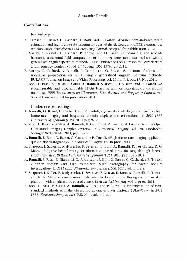
Contributions
Journal papers
Alessandro Ramalli
11

1.Ultrasound Basics
This chapter aims at illustrating the ultrasound physical principles, which are the basis of the ultrasound systems. It constitutes the fundamental for understanding the nature of the topics discussed in the thesis and it does not claim to be exhaustive, but rather helps to point out the way in the ultrasound environment.
1.1. Ultrasound propagation
The sound is a physical phenomenon in which an elastic wave propagates from a source (vibrating body) through an elastic medium (air, water, etc..). Such perturbations consist in the alteration of the medium particles which vibrate around the equilibrium position. Among acoustic waves, ultrasound are those not audible by the human hear, i.e. those which have a frequency higher than 20 kHz. In particular ultrasound are longitudinal waves that cause a particle oscillation parallel to the direction of propagation.
1.1.1. Linear propagation
The ultrasound wave propagation along the axial direction (z) is expressed as follows:
𝜕𝜕!𝑇𝑇𝜕𝜕𝑧𝑧!
=𝜌𝜌𝛽𝛽∙𝜕𝜕!𝑇𝑇𝜕𝜕𝑡𝑡!
(1.1)
where T [N/m2] is the stress, β [N/m2] is the elastic constant of the medium and ρ [kg/m3] is the volumetric medium density, which has solution:
𝑇𝑇 𝑧𝑧, 𝑡𝑡 = 𝑇𝑇! ∙ 𝑒𝑒! !!"#±!"
𝜆𝜆 = 𝑐𝑐 𝑓𝑓 (1.2)
where f is the frequency, c the speed of sound and λ [m] is the wavelength, i.e. the distance between two points along the z-axis presenting the same stress value.
The propagation speed of acoustic waves is strictly dependent by the elastic properties and the density of the medium, since its particles oscillate around the equilibrium position transmitting energy to the neighboring particles. Finally, the speed of sound propagation can be expressed as:
𝑐𝑐 = 𝛽𝛽 𝜌𝜌 (1.3)
Alessandro Ramalli, Development of novel ultrasound techniques for imaging and elastography : from simulation to real-time implementation ISBN 978-88-6655-456-1 (print) ISBN 978-88-6655-457-8 (online) © 2013 Firenze University Press
Development of novel ultrasound techniques for imaging and elastography
14
Another important properties of a not much absorbent medium is the acoustic impedance Z, which for a propagating plane wave, or for a spherical wave far away from the vibrating source, is expressed as:
𝑍𝑍 = 𝜌𝜌 ∙ 𝑐𝑐 (1.4)
which unit is Rayl (1 Rayl=1 kg/(m2 s)).
1.1.2. Nonlinear propagation
Actually, the propagation of ultrasound is nonlinear; it means that during propagation the shape of the propagating signal is no longer proportional to the shape of the excitation. Indeed, in a compressible medium, a pressure increase causes a temperature rise, which consequently involves a higher propagation speed. In practice, during propagation, the wave travels faster during the high pressure phase than during the lower pressure phase. Such speed variations modify the spectral content of the propagating signal, with an increase of the amplitude of the higher harmonics.
The linear propagation of ultrasound waves, in lossless and homogeneous media, is based on the conservation of motion equation, which states that:
𝜌𝜌𝜕𝜕𝑢𝑢𝜕𝜕𝜕𝜕
+ ∇𝑝𝑝 = 0 (1.5)
where u is the particle velocity and p the pressure. The nonlinear wave propagation is based on the modified motion equation:
𝜌𝜌𝜕𝜕𝑢𝑢𝜕𝜕𝜕𝜕
+ 𝑢𝑢 ∙ ∇ 𝑢𝑢 + ∇𝑝𝑝 = 0 (1.6)
where the convective acceleration 𝑢𝑢 ∙ ∇ 𝑢𝑢 is introduced. The solution of the pressure wave as a function of the density is expressed as the
Taylor series:
𝑝𝑝 − 𝑝𝑝! = 𝐴𝐴𝜌𝜌 − 𝜌𝜌!𝜌𝜌!
+𝐵𝐵2!
𝜌𝜌 − 𝜌𝜌!𝜌𝜌!
!+ …
𝐴𝐴 = 𝜌𝜌!𝜕𝜕𝜕𝜕𝜕𝜕𝜕𝜕 !
= 𝜌𝜌!𝑐𝑐!!
𝐵𝐵 = 𝜌𝜌!!𝜕𝜕!𝑝𝑝𝜕𝜕𝜌𝜌!
!
(1.7)
The speed of sound in the nonlinear propagation description is then
𝑐𝑐 = 𝑐𝑐! + 1 +𝐵𝐵2𝐴𝐴
𝑢𝑢 (1.8)
and the nonlinear coefficient of the medium is defined as follows:
Development of novel ultrasound techniques for imaging and elastography
14

Alessandro Ramalli
15
𝛽𝛽 = 1 +𝐵𝐵2𝐴𝐴
(1.9)
1.1.3. Scattering, reflection, refraction and attenuation
In a homogeneous medium an ultrasound wave propagates along a straight line but if the wave front meets an acoustic impedance discontinuity (interface), smaller or comparable to its wavelength, part of the energy is transmitted through the interface and another part is spread isotropically in all directions. This phenomenon is referred to as Rayleigh scattering and it is described by the scattering cross section (σ) defined as the ratio between the total spread power (S) and the intensity of the incident wave (I):
𝜎𝜎 = 𝑆𝑆 𝐼𝐼 (1.10)
In ultrasound echography the backscattering cross-section is particularly important; it is defined as the ratio between the scattered power per solid angle, in the opposite direction to the source, and the incident intensity. This parameter describes the effective power of echo signal available for an imaging system.
When the interface roughness is larger than the wavelength of the incident wave (smooth interface) reflection and refraction phenomena occur. In such case, a part of the energy is transmitted through the second medium and a part is reflected. Considering the interface between two media in which the ultrasound respectively propagate with c1 and c2 speed, the Snell’s law states:
sin 𝜃𝜃!sin 𝜃𝜃!
=𝑐𝑐!𝑐𝑐!
(1.11)
where θi and θt are the direction angle of the incident wave and the direction angle of the refracted wave respectively. The reflection, R, and the transmission, T, coefficients can be defined as follows:
𝑅𝑅 =𝑍𝑍! cos 𝜃𝜃! − 𝑍𝑍! cos 𝜃𝜃! !
𝑍𝑍! cos 𝜃𝜃! + 𝑍𝑍! cos 𝜃𝜃! !
𝑇𝑇 = 1 − 𝑅𝑅 =4𝑍𝑍!𝑍𝑍! cos 𝜃𝜃! cos 𝜃𝜃! !
𝑍𝑍! cos 𝜃𝜃! + 𝑍𝑍! cos 𝜃𝜃! !
(1.12)
The latters are coefficient of direct proportionality of the ratios between the incident wave and the reflected and the transmitted waves respectively.
Another important phenomenon the ultrasound wave is subjected to during the propagation is attenuation. This term refers to any phenomenon that brings to a reduction of the wave intensity. There are many attenuation causes: among them absorption and dispersion are the most significant. The first process converts part of the mechanical energy into heat energy, by compression, expansion (thermo-elastic effect) and sliding of the particles (viscous effect). The dispersion process is due to
Alessandro Ramalli
15
Development of novel ultrasound techniques for imaging and elastography
16
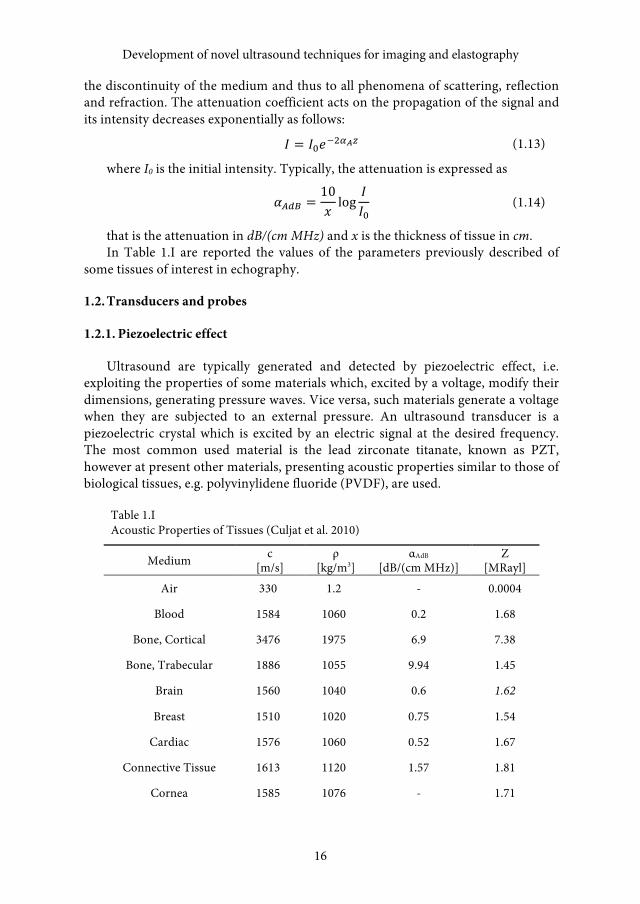
the discontinuity of the medium and thus to all phenomena of scattering, reflection and refraction. The attenuation coefficient acts on the propagation of the signal and its intensity decreases exponentially as follows:
𝐼𝐼 = 𝐼𝐼!𝑒𝑒!!!!! (1.13)
where I0 is the initial intensity. Typically, the attenuation is expressed as
𝛼𝛼!"# =10𝑥𝑥log
𝐼𝐼𝐼𝐼!
(1.14)
that is the attenuation in dB/(cm MHz) and x is the thickness of tissue in cm. In Table 1.I are reported the values of the parameters previously described of
some tissues of interest in echography.
1.2. Transducers and probes
1.2.1. Piezoelectric effect
Ultrasound are typically generated and detected by piezoelectric effect, i.e. exploiting the properties of some materials which, excited by a voltage, modify their dimensions, generating pressure waves. Vice versa, such materials generate a voltage when they are subjected to an external pressure. An ultrasound transducer is a piezoelectric crystal which is excited by an electric signal at the desired frequency. The most common used material is the lead zirconate titanate, known as PZT, however at present other materials, presenting acoustic properties similar to those of biological tissues, e.g. polyvinylidene fluoride (PVDF), are used.
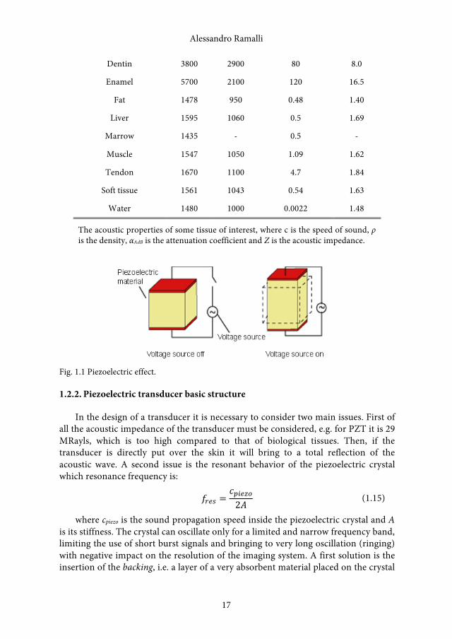
Table 1.I Acoustic Properties of Tissues (Culjat et al. 2010)
Medium c [m/s]
ρ [kg/m3]
αAdB [dB/(cm MHz)]
Z [MRayl]
Air 330 1.2 - 0.0004
Blood 1584 1060 0.2 1.68
Bone, Cortical 3476 1975 6.9 7.38
Bone, Trabecular 1886 1055 9.94 1.45
Brain 1560 1040 0.6 1.62
Breast 1510 1020 0.75 1.54
Cardiac 1576 1060 0.52 1.67
Connective Tissue 1613 1120 1.57 1.81
Cornea 1585 1076 - 1.71
Development of novel ultrasound techniques for imaging and elastography
16
Alessandro Ramalli
17
Dentin 3800 2900 80 8.0
Enamel 5700 2100 120 16.5
Fat 1478 950 0.48 1.40
Liver 1595 1060 0.5 1.69
Marrow 1435 - 0.5 -
Muscle 1547 1050 1.09 1.62
Tendon 1670 1100 4.7 1.84
Soft tissue 1561 1043 0.54 1.63
Water 1480 1000 0.0022 1.48
The acoustic properties of some tissue of interest, where c is the speed of sound, ρ is the density, αAdB is the attenuation coefficient and Z is the acoustic impedance.
Fig. 1.1 Piezoelectric effect.
1.2.2. Piezoelectric transducer basic structure
In the design of a transducer it is necessary to consider two main issues. First of all the acoustic impedance of the transducer must be considered, e.g. for PZT it is 29 MRayls, which is too high compared to that of biological tissues. Then, if the transducer is directly put over the skin it will bring to a total reflection of the acoustic wave. A second issue is the resonant behavior of the piezoelectric crystal which resonance frequency is:
𝑓𝑓!"# =𝑐𝑐!"#$%2𝐴𝐴
(1.15)
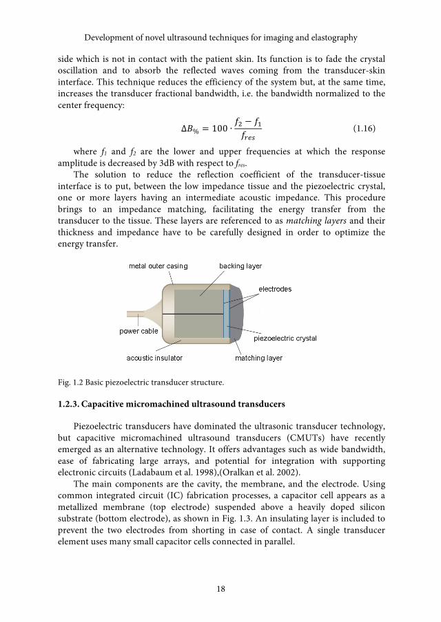
where cpiezo is the sound propagation speed inside the piezoelectric crystal and A is its stiffness. The crystal can oscillate only for a limited and narrow frequency band, limiting the use of short burst signals and bringing to very long oscillation (ringing) with negative impact on the resolution of the imaging system. A first solution is the insertion of the backing, i.e. a layer of a very absorbent material placed on the crystal
Alessandro Ramalli
17
Development of novel ultrasound techniques for imaging and elastography
18
side which is not in contact with the patient skin. Its function is to fade the crystal oscillation and to absorb the reflected waves coming from the transducer-skin interface. This technique reduces the efficiency of the system but, at the same time, increases the transducer fractional bandwidth, i.e. the bandwidth normalized to the center frequency:
∆𝐵𝐵% = 100 ∙𝑓𝑓! − 𝑓𝑓!𝑓𝑓!"#
(1.16)
where f1 and f2 are the lower and upper frequencies at which the response amplitude is decreased by 3dB with respect to fres.
The solution to reduce the reflection coefficient of the transducer-tissue interface is to put, between the low impedance tissue and the piezoelectric crystal, one or more layers having an intermediate acoustic impedance. This procedure brings to an impedance matching, facilitating the energy transfer from the transducer to the tissue. These layers are referenced to as matching layers and their thickness and impedance have to be carefully designed in order to optimize the energy transfer.
Fig. 1.2 Basic piezoelectric transducer structure.
1.2.3. Capacitive micromachined ultrasound transducers
Piezoelectric transducers have dominated the ultrasonic transducer technology, but capacitive micromachined ultrasound transducers (CMUTs) have recently emerged as an alternative technology. It offers advantages such as wide bandwidth, ease of fabricating large arrays, and potential for integration with supporting electronic circuits (Ladabaum et al. 1998),(Oralkan et al. 2002).
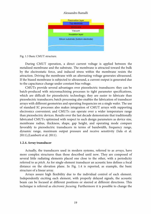
The main components are the cavity, the membrane, and the electrode. Using common integrated circuit (IC) fabrication processes, a capacitor cell appears as a metallized membrane (top electrode) suspended above a heavily doped silicon substrate (bottom electrode), as shown in Fig. 1.3. An insulating layer is included to prevent the two electrodes from shorting in case of contact. A single transducer element uses many small capacitor cells connected in parallel.
Development of novel ultrasound techniques for imaging and elastography
18
Alessandro Ramalli
19
Fig. 1.3 Basic CMUT structure.
During CMUT operation, a direct current voltage is applied between the metalized membrane and the substrate. The membrane is attracted toward the bulk by the electrostatic force, and induced stress within the membrane resists the attraction. Driving the membrane with an alternating voltage generates ultrasound. If the biased membrane is subjected to ultrasound, a current output is generated due to the capacitance change under constant bias voltage.
CMUTs provide several advantages over piezoelectric transducers: they can be batch-produced with micromachining processes to tight parameter specifications, which are difficult for piezoelectric technology; they are easier to fabricate than piezoelectric transducers; batch processing also enables the fabrication of transducer arrays with different geometries and operating frequencies on a single wafer. The use of standard IC processes also makes integration of CMUT arrays with supporting electronics convenient; and CMUTs can operate over a wider temperature range than piezoelectric devices. Results over the last decade demonstrate that traditionally fabricated CMUTs optimized with respect to such design parameters as device size, membrane radius, thickness, shape, gap height, and operating mode compare favorably to piezoelectric transducers in terms of bandwidth, frequency range, dynamic range, maximum output pressure and receive sensitivity (Iula et al. 2011),(Lamberti et al. 2011).
1.2.4. Array transducer
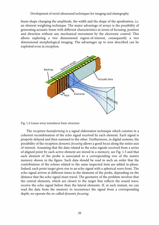
Actually, the transducers used in modern systems, referred to as arrays, have more complex structures than those described until now. They are composed of several little radiating elements placed one close to the other, with a periodicity referred to as pitch. As for single-element transducer an acoustic lens defines a focal distance on the elevation plane. In Fig. 1.4 is reported, as example, the basic structure of a linear array.
Arrays assure high flexibility due to the individual control of each element. Independently exciting each element, with properly delayed signals, the acoustic beam can be focused at different positions or steered at different directions. This technique is referred as electronic focusing. Furthermore it is possible to change the
Alessandro Ramalli
19
Development of novel ultrasound techniques for imaging and elastography
20
beam shape changing the amplitude, the width and the shape of the apodization, i.e. an element weighting technique. The major advantage of arrays is the possibility of generating acoustic beam with different characteristics in terms of focusing, position and direction without any mechanical movement by the electronic control. This allows exploring a two dimensional region-of-interest, consequently a two dimensional morphological imaging. The advantages up to now described can be exploited even in reception.
Fig. 1.4 Linear array transducer basic structure.
The reception beamforming is a signal elaboration technique which consists in a coherent recombination of the echo signal received by each element. Each signal is properly delayed and then summed to the other. Furthermore, in digital systems, the possibility of the reception dynamic focusing allows a good focus along the entire axis of interest. Assuming that the data related to the echo-signals received from a series of aligned point by each active element are stored in a memory, see Fig. 1.5 and that each element of the probe is associated to a corresponding row of the matrix memory shown in the figure. Such data should be read in such an order that the contributions of the echoes related to the same inspected item are added in-phase. Indeed, each point target gives rise to an echo signal with a spherical wave front. The echo signal arrives at different times to the elements of the probe, depending on the distance that the echo signal must travel. The geometry of the problem involves that the central elements, which are closest to the target that reflects the sound wave, receive the echo signal before than the lateral elements. If, at each instant, we can read the data from the memory to reconstruct the signal from a corresponding depth, we operate the so-called dynamic focusing.
Development of novel ultrasound techniques for imaging and elastography
20

Alessandro Ramalli
21
Fig. 1.5 Reception dynamic focusing diagram.
1.2.5. Acoustic beam
Single-element transducer beam
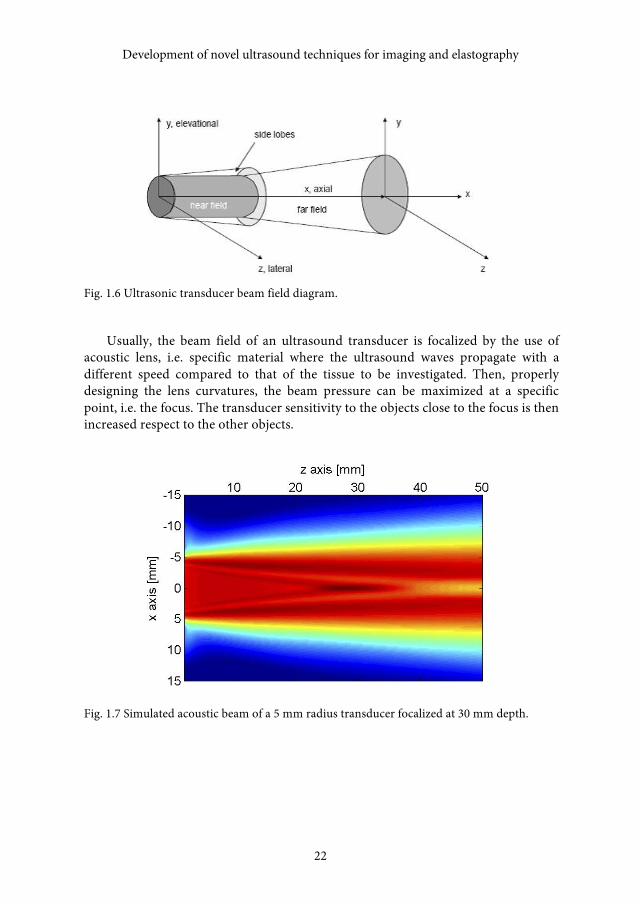
In the surrounding space, a transducer generates an acoustic field depending on the source geometry. As an example, in Fig. 1.6, the acoustic beam field diagram of a circular transducer is reported. It can be divided into two distinct zones: the first, referred to as near field, or Fresnel zone, having a constant width; the second, far field of Fraunhofer zone, in which the beam diverges. The border between the two zones is at a depth equal to:
𝑧𝑧 = 𝑟𝑟! 𝜆𝜆 (1.17)
where r is the transducer radius and λ is the wavelength of the transmitted signal. In addition to the main radiation lobe there are side lobes of lower intensity, due to constructive and destructive interferences of the waves generated from each point of the transducer. The origin of these lobes can be demonstrated with the diffraction theory. It demonstrates that, in the Fraunhofer zone, the diffracted beam has the same shape of the Fourier transform of the beam on the aperture, which is the transducer surface the beam is originated from. Then, the side lobes are due to the lobes of the sinc-shape functions related to the Fourier transform of finite apertures.
Alessandro Ramalli
21
Development of novel ultrasound techniques for imaging and elastography
22
Fig. 1.6 Ultrasonic transducer beam field diagram.
Usually, the beam field of an ultrasound transducer is focalized by the use of acoustic lens, i.e. specific material where the ultrasound waves propagate with a different speed compared to that of the tissue to be investigated. Then, properly designing the lens curvatures, the beam pressure can be maximized at a specific point, i.e. the focus. The transducer sensitivity to the objects close to the focus is then increased respect to the other objects.
Fig. 1.7 Simulated acoustic beam of a 5 mm radius transducer focalized at 30 mm depth.
Development of novel ultrasound techniques for imaging and elastography
22

Alessandro Ramalli
23
dependent by λ and p from the main lobe. The cosines direction to the field point, u, is defined as:
𝑢𝑢 = sin 𝜃𝜃 (1.18)
where θ is the direction angle on the xz plane.
Fig. 1.8 Array samples along the x axis where p is the pitch (A). Fourier transform of a finite length array (B).
Actually, the array aperture is not composed of point sources; indeed the elements have a width that is not infinitesimal. Thus, the aperture can be described by the convolution between the Dirac-comb and a Rect-function of length equal to the width of the element. Considering the Fourier transform properties follows that the radiation lobe of the diffracted beam are weighted by a Sinc-function obtained by the Fourier transform of the Rect related to the single element. Note that the wider is the element the lower the amplitude of the side lobes. In general the final field beam is obtained by the product of two factors, the array factor and the element factor, as described in Fig. 1.9.
A particular effect happens when the electronic steering is used. Indeed it mathematically corresponds to an angular translation of the array factor while the element factor remains the same, see Fig. 1.10. The effect is the reduction of the main lobe amplitude and a gain of the grating lobe amplitude. Evidently, in this case, the echo signals quality is deteriorated losing energy along the direction of interest while spreading energy in undesired direction. Thus, the steering angle is limited by the width of the array elements to avoid high energy grating lobe.
Array transducer beam
As previously stated, the shape of the diffracted field in the Fraunhofer zone corresponds to the Fourier transform of the source aperture. The arrays aperture can be firstly approximated by a sampled Rect-function of width equal to the width of the array and sampling step equal to the pitch of the elements. As reported in Fig. 1.8, the diffracted beam is a Sinc-function with repetitions due to the sampling of the aperture. The repetitions appear as a series of radiation lobes, separated by a distance
Alessandro Ramalli
23

Development of novel ultrasound techniques for imaging and elastography
24
Fig. 1.9 A finite length array of width w and periodicity p (A). Fourier transform of periodic spatial element (B). Factors contributing to the overall transform (C).
Fig. 1.10 Effect of beam steering on the overall pattern.
The approach until now described does not take into account the cross-talk effect, typically occurring in real array transducer. That phenomenon consists of the mutual influence between adjacent elements, by which an element oscillates under the vibrations of the adjacent elements. In practice, as an approximation, the cross-talk can be modeled as the “widening” of each element further reducing the probe maximum achievable steering angle.
Development of novel ultrasound techniques for imaging and elastography
24

Alessandro Ramalli
25
1.2.6. System spatial resolution
The system spatial resolutions are directly correlated to the transducer characteristics. In particular can be defined two parameters: the axial and the lateral resolution. The first indicates the smallest detectable distance between two targets placed on planes that are parallel to the transducer plane. This parameter is directly proportional to the transmission frequency and to the transducer bandwidth. The lateral resolution indicates the smallest detectable distance between two targets placed on planes that are orthogonal to the transducer plane. This parameter depends on the focalization, on the transducer geometry and on the transmission frequency.
1.2.7. Issues of non-ideality
Cross-talk effect
In array transducer based ultrasound systems, the electric and the acoustic coupling of near neighbor elements compose in a single effect, i.e. the cross-talk effect. The electric cross-talk is due to the active elements supply traces proximity, which, as known, coupled electro-magnetically. In the acoustic cross-talk, a vibrating element generates a mechanic wave in the surrounding space, which travels both through the backing and the inter-elements materials, inducing the hit elements in coupled resonance. The cross-talk effect causes an apparent widening of the transmitting elements, thus increases the directivity of the elements.
Modes coupling
The experiments conducted in (Smith et al. 1979) show that linear array transducers sensitivity differs from the theoretically predicted one. The angular response of a piezoelectric element, which is many wavelengths long and less than one wavelength wide, does not agree the diffraction theory for planar aperture. A spectral analysis of isolated elements showed a significant amount of energy coupled into the transverse mode due to the small width-to-thickness ratio of piezoelectric elements. Furthermore, experimental data indicate that the same behavior can be highlighted for elements in an array, which can be a further reason for element directivity increase.
1.3. Echo-signal elaboration
1.3.1. Classic scanning techniques
The advent of array transducers opened up new imaging opportunities, indeed as previously stated the arrays allow steering or moving the view line. Several scanning techniques exist and differ in the geometry of the examined region and in
Alessandro Ramalli
25
Development of novel ultrasound techniques for imaging and elastography
26
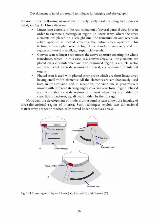
the used probe. Following an overview of the typically used scanning techniques is listed; see Fig. 1.11 for a diagram:
• Linear scan consists in the reconstruction of several parallel view lines inorder to examine a rectangular region. In linear array, where the array elements are placed on a straight line, the transmission and reception active aperture is moved covering the entire array aperture. This technique is adopted when a high lines density is necessary and the region of interest is small, e.g. superficial vessels.
• Convex scan as linear scan moves the active aperture covering the wholetransducer, which, in this case, is a convex array, i.e. the elements are placed on a circumference arc. The examined region is a circle sector and it is useful for wide regions of interest, e.g. abdomen or internal organs.
• Phased scan is used with phased array probe which are short linear arrayhaving small width elements. All the elements are simultaneously used both in transmission and in reception; the view line is progressively moved with different steering angles covering a sectorial region. Phased scan is suitable for wide regions of interest when they are hidden by superficial structures, e.g. di heart hidden by the rib cage.
Nowadays the development of modern ultrasound system allows the imaging of three-dimensional region of interest. Such techniques exploit two dimensional matrix array probes or mechanically moved linear or convex arrays.
Fig. 1.11 Scanning techniques: Linear (A), Phased (B) and Convex (C).
Development of novel ultrasound techniques for imaging and elastography
26
Alessandro Ramalli
27
1.3.2. Advanced methods: high frame-rate imaging
Recently, new scanning techniques were proposed for high frame rate (HFR) ultrasound imaging. Such methods allow reconstructing images of very fast moving objects where an accurate evaluation of their movement is of fundamental importance. An example could be the human heart movement during the cardiac cycles. It is very complex and each part of the heart structure contracts and relaxes at different times and in different directions.
The frame-rate can be increased reducing the maximum depth of interest and then increasing the PRF. In some cases, e.g. during heart investigation, where high depth of interest are necessary, the latter solution is not appropriate. Another solution, the most common one, consists in the reduction of the transmitted pulses number and in a proper processing method of the received echo-signals. These techniques are referred to as high-frame rate imaging methods. Even if a lot of advanced techniques were presented, in the following sub-paragraphs only two of them will be detailed, since they will be used in the next chapters.
High-frame rate imaging with limited diffraction beams
In this method, referred to as Fourier method, presented in (Lu 1997a), (Cheng & Lu 2006), (Jian-yu Lu & Sung-Jae Kwon 2007), steered plane waves are transmitted exciting all the elements of a 2D or a 1D array transducer to uniformly illuminate the objects to be imaged. Echo-signals returned from the objects are received with the same transducer and weighted to produce limited diffraction responses. The signals are further used to calculate the Fourier transform of the object to be imaged. Finally object functions are constructed with a 2D or 3D inverse spatial Fourier transform.
Ultrafast compound imaging
In this method, referred to as coherent steered plane waves compounding, presented in (Montaldo et al. 2009) (Tanter et al. 2002), as in the previous one, steered plane waves are transmitted exciting all the elements of a 1D array transducer. The echo-signals received by each element are processed in parallel during the reception mode by adding coherently the echoes coming from the same scatterer, considering the delay of the two way path. In such way an image is obtained for each transmission, and then the images obtained by each steered plane waves are coherently added to obtain the final image.
1.3.3. Elaboration modes and display
The echo signals received by the ultrasound probes are properly processed by the ultrasound system extracting the information content and displaying it in a user accessible way. The displaying techniques are various and most of them are actually
Alessandro Ramalli
27

Development of novel ultrasound techniques for imaging and elastography
28
used in medical diagnosis. The simplest, now obsolete, displaying mode is the so-called A-Mode. No scanning is employed and as an oscilloscope the system display shows only the temporal trace of the echo signal. The M-Mode, as the A-Mode, is based on a single view line and the intensity of the signal received on consecutive shots are displayed on different columns on a gray scale image, appreciating the temporal evolution of the examined structures. In recent sonographers B-mode is the most used, which allows showing the morphological structure of tissues. It is reached by scanning the region of interest with several view lines and by representing the signal intensity on a gray-scale coded two-dimensional image. Other modes are employed for Doppler applications; the most common is the so-called spectral Doppler or spectrogram which, by the use of a single view line, shows the evolution of the flow speed at a single depth. This limitation is overcome by the multigate-spectral-Doppler (MSD-Mode) which allows seeing the flow temporal evolution at each depth along a single view line. Finally, the color-flow-mapping-mode (CFM-Mode) shows on a color coded scale the flow speed information on a two-dimensional image. Another elaboration and visualization technique, widely discussed in this thesis work, is elastogrpahy which reconstructs the two dimensional map of the examined tissue elasticity, representing it in a color scale image.
Fig. 1.12 B-Mode (left), MSD-Mode (right) and Spectrogram (bottom) displays example.
1.4. Open issues in ultrasound investigation
Ultrasounds are used in a wide variety of applications including medical imaging, nondestructive evaluation, ranging, and flow metering. Current theoretical understanding indicates, however, that many fruitful applications of ultrasound
Development of novel ultrasound techniques for imaging and elastography
28
Alessandro Ramalli
29
remain unrealized. Often a lack of adequate hardware (ultrasound transducers and systems) precludes theoretically interesting developments in the ultrasound field. Lack of innovative transducers precludes ultrasonic systems from materializing, which in turn precludes innovative practical applications (Ladabaum et al. 1998).
Available commercial systems do not always fit the needs for testing the proposed novel approaches, and dedicated equipment has thus to be made. Research laboratories, especially in academia, which are typically expected to propose novel approaches, must dedicate many efforts even to hardware developments (Tortoli & Jensen 2006).
Alessandro Ramalli
29


2. ULA-OP
The experimental test of novel ultrasound investigation methods can be made difficult by the lack of flexibility of commercial ultrasound machines. In the best options, these only provide beamformed radiofrequency or demodulated echo-signals for acquisition. More flexibility is achieved in high-level research platforms, but these are typically characterized by high cost and dimensions. This chapter draws on (Boni et al. 2012) and (Ricci et al. 2011) presents a powerful but portable ultrasound system, specifically designed for research purposes.
2.1. Introduction
The progress of electronics technology has made available devices like Field Programmable Gate Arrays (FPGAs) and Digital Signal Processors (DSPs) containing millions of gates and/or multiple cores, which are capable of unprecedented performance in terms of processing and control capability of other hardware resources.
This progress has directly involved ultrasound (US) technology, as the major electronics companies have developed specific processors and front-end circuits for applications in this field. Such advancements have pushed the development of ultra-portable devices and high-level equipment, but have also increased the number and quality of possible working modalities of commercial equipment. Advanced processing algorithms introduced in other fields, e.g. pulse compression, initially proposed for use in radar, are now suitable for improved real-time US imaging (Misaridis & Jensen 2005a),(Misaridis & Jensen 2005b). Methods which were introduced several years ago, such as compound or 4-D imaging, are now implemented in high-level commercial equipment, while new techniques, e.g. harmonic imaging (Averkiou et al. 1997), have rapidly become a standard diagnostic tool.
Nowadays electronics advancements are sufficiently mature to contribute to remarkable improvements in the quality of images provided by US equipment. This goal may be facilitated by the availability of programmable research platforms, which can make feasible the experimental test of novel transmission strategies or challenging processing methods. For example, special research platforms were specifically developed in Paris (Bercoff et al. 2004) and Toledo (Lu et al. 2006) to obtain images at high (kHz) frame rate through the transmission of plane waves or limited diffraction beams, respectively, and the independent acquisition of echo signals from 128 elements. The RASMUS system developed at the Technical
Alessandro Ramalli, Development of novel ultrasound techniques for imaging and elastography : from simulation to real-time implementation ISBN 978-88-6655-456-1 (print) ISBN 978-88-6655-457-8 (online) © 2013 Firenze University Press
Development of novel ultrasound techniques for imaging and elastography
32
University of Denmark (Jensen et al. 2005) is addressed to a wider range of applications, allowing arbitrary transmission/reception (TX/RX) strategies to be tested for array transducers with a large number of elements. More recently, commercial systems like the SonixTOUCH Research (Ultrasonix Medical Corporation, Vancouver, BC, Canada) or the DiPhAS platform (Fraunhofer-IBMT, St.Ingbert, Germany) have also been introduced.
In this chapter, the programmability and reconfigurability of the ULtrasound Advanced Open Platform (ULA-OP) is highlighted through the description of a number of non-standard applications made possible by its flexible architecture. The system, which was recently developed in our University laboratory (Tortoli et al. 2009), contains in two boards all the electronics necessary to control up to 64 active elements of a 192 element array probe.
The chapter is organized as follows. Sec. 2.2 describes the system architecture, providing details of how the system can be configured and controlled in real-time through its advanced FPGAs and DSP. Sec. 2.3 reports five sample applications of ULA-OP. All such applications are non-standard, ranging from real-time vector Doppler measurements and elastography to Flow Mediated Dilation studies, pulse compression and high frame rate imaging experiments. The different exploitation of ULA-OP’s hardware resources aimed at realizing these applications is discussed in Sec. 2.5.
2.2. System description
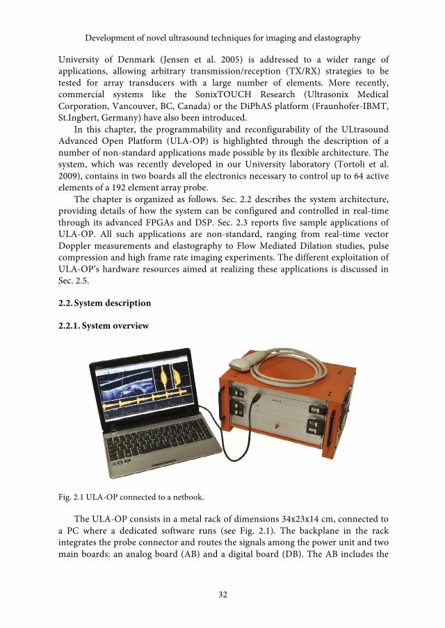
2.2.1. System overview
Fig. 2.1 ULA-OP connected to a netbook.
The ULA-OP consists in a metal rack of dimensions 34x23x14 cm, connected to a PC where a dedicated software runs (see Fig. 2.1). The backplane in the rack integrates the probe connector and routes the signals among the power unit and two main boards: an analog board (AB) and a digital board (DB). The AB includes the
Development of novel ultrasound techniques for imaging and elastography
32
Alessandro Ramalli
33
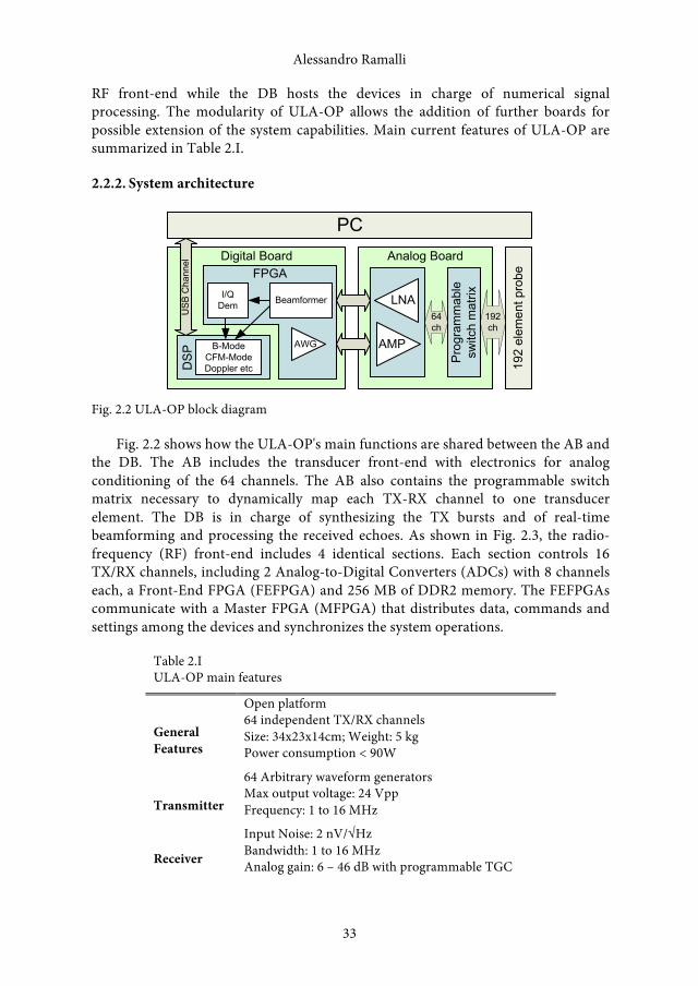
RF front-end while the DB hosts the devices in charge of numerical signal processing. The modularity of ULA-OP allows the addition of further boards for possible extension of the system capabilities. Main current features of ULA-OP are summarized in Table 2.I.
2.2.2. System architecture
Prog
ram
mab
le
switc
h m
atrixLNA
AMP
64ch
AWG
I/QDem Beamformer
FPGA
B-ModeCFM-Mode Doppler etcD
SP
Digital Board Analog Board
PC
USB
Cha
nnel
192
elem
ent p
robe
192ch
Fig. 2.2 ULA-OP block diagram
Fig. 2.2 shows how the ULA-OP's main functions are shared between the AB and the DB. The AB includes the transducer front-end with electronics for analog conditioning of the 64 channels. The AB also contains the programmable switch matrix necessary to dynamically map each TX-RX channel to one transducer element. The DB is in charge of synthesizing the TX bursts and of real-time beamforming and processing the received echoes. As shown in Fig. 2.3, the radio-frequency (RF) front-end includes 4 identical sections. Each section controls 16 TX/RX channels, including 2 Analog-to-Digital Converters (ADCs) with 8 channels each, a Front-End FPGA (FEFPGA) and 256 MB of DDR2 memory. The FEFPGAs communicate with a Master FPGA (MFPGA) that distributes data, commands and settings among the devices and synchronizes the system operations.
Table 2.I ULA-OP main features
General Features
Open platform 64 independent TX/RX channels Size: 34x23x14cm; Weight: 5 kg Power consumption < 90W
Transmitter
64 Arbitrary waveform generators Max output voltage: 24 Vpp Frequency: 1 to 16 MHz
Receiver
Input Noise: 2 nV/√Hz Bandwidth: 1 to 16 MHz Analog gain: 6 – 46 dB with programmable TGC
Alessandro Ramalli
33
Development of novel ultrasound techniques for imaging and elastography
34
12bit @ 50 MSPS ADCs
Beamformer Programmable apodization and delays (dynamic focusing)
Processing Modules
Coherent demodulation, band-pass filtering, decimation, B-mode, Multigate Spectral Doppler, Vector Doppler… (open to new, custom modules).
Storage capabilities
Up to 1 GB for RF data (pre- or post-beamformed) Up to 512 MB for baseband data Fast data streaming toward high capacity storage units (HD)
Software tools
Beam Planner, Config Editor, Real-time Module, Video Browser, RF viewer
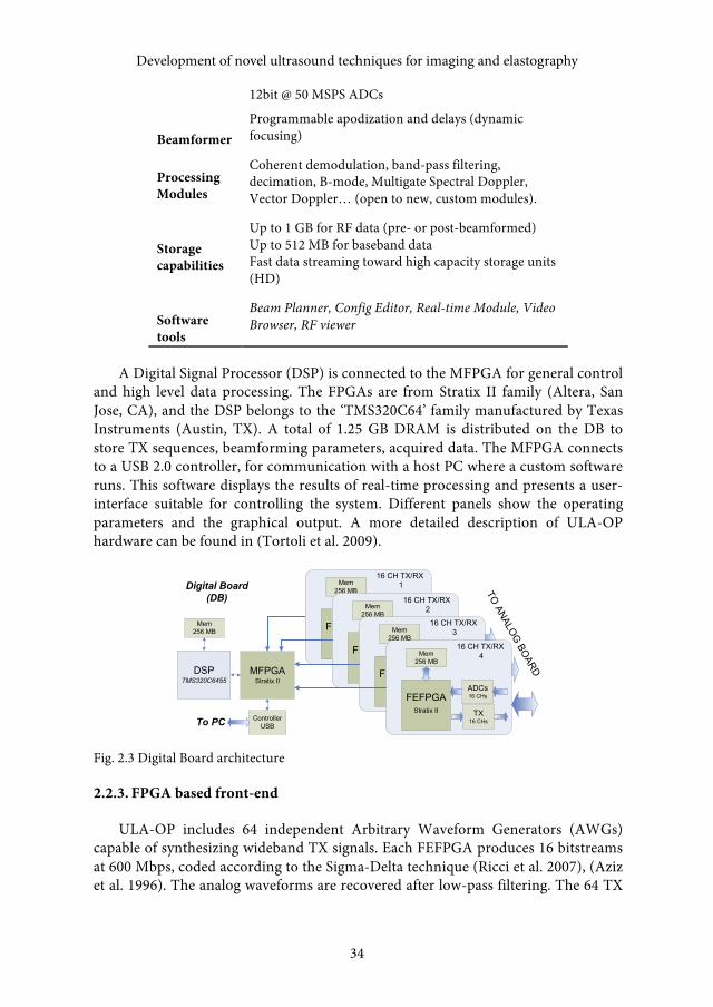
A Digital Signal Processor (DSP) is connected to the MFPGA for general control and high level data processing. The FPGAs are from Stratix II family (Altera, San Jose, CA), and the DSP belongs to the ‘TMS320C64’ family manufactured by Texas Instruments (Austin, TX). A total of 1.25 GB DRAM is distributed on the DB to store TX sequences, beamforming parameters, acquired data. The MFPGA connects to a USB 2.0 controller, for communication with a host PC where a custom software runs. This software displays the results of real-time processing and presents a user-interface suitable for controlling the system. Different panels show the operating parameters and the graphical output. A more detailed description of ULA-OP hardware can be found in (Tortoli et al. 2009).
Fig. 2.3 Digital Board architecture
2.2.3. FPGA based front-end
ULA-OP includes 64 independent Arbitrary Waveform Generators (AWGs) capable of synthesizing wideband TX signals. Each FEFPGA produces 16 bitstreams at 600 Mbps, coded according to the Sigma-Delta technique (Ricci et al. 2007), (Aziz et al. 1996). The analog waveforms are recovered after low-pass filtering. The 64 TX
MFPGA Stratix II
DSPTMS320C6455
ControllerUSB
Mem256 MB
Digital Board(DB)
To PC
FEFPGAStratix II
ADCs16 CHs
Mem256 MB
TX16 CHs
16 CH TX/RX 1
FEFPGAStratix II
ADCs16 CHs
Mem256 MB
TX16 CHs
16 CH TX/RX 2
FEFPGAStratix II
ADCs16 CHs
Mem256 MB
TX16 CHs
16 CH TX/RX 3
FEFPGAStratix II
ADCs16 CHs
Mem256 MB
TX16 CHs
16 CH TX/RX 4
TO ANALO
G BO
ARD
Development of novel ultrasound techniques for imaging and elastography
34
Alessandro Ramalli
35
signals are transferred to the AB where they are amplified and addressed, through the switch matrix controlled by the DSP, to the selected probe elements. Once the synthesized bursts have been fired, ULA-OP is ready to receive the consequent echoes.
The echo-signals are conditioned by the Low Noise Amplifiers (LNAs), whose gain is programmable in the range 6-46 dB. This feature is exploited by the Time Gain Control (TGC), controlled by the DSP, to produce a gain trend ramping up with programmable tilt and offset.
In the DB, each RX signal is sampled at 50 Msps with 12-bit resolution, producing a 38.4Gb/s data flow which feeds the FEFPGAs through Low Voltage Differential Signaling (LVDS) lines. Beamforming is completed in the MFPGA that processes the partial results calculated by the 4 FEFPGAs. When requested, the MFPGA demodulates the beamformed RF signal into quadrature (IQ) channels and processes the I/Q data in a programmable low-pass decimator filter.
2.2.4. DSP control & processing tasks
The DSP is in charge of many tasks, mainly correlated to real-time acquisition and elaboration. It primarily acts as a supervisor, taking care of the overall system management. This is accomplished upon user request, which reaches the DSP in the form of multiple commands. An interpreter, embedded in the DSP firmware, lets the processor execute all commands that the PC sends to the system through the USB channel.
While real-time operation is in progress, a thread running on the DSP, named “Sequence Manager” (SM) is enabled. According to the sequence of operations programmed by the software, every Pulse Repetition Interval (PRI) the DSP dispatches a new set of parameters toward other devices. The TX waveforms, the analog switch matrix, the TGC parameters, the beamformer weights and delays, the demodulation frequency and the base-band filters can thus be dynamically set.
The DSP gathers the RF and/or the IQ demodulated samples from the MFPGA through a 4.8 Gb/s multipurpose parallel bus. The external memory may be split into several buffers, called slices, that the DSP fills according to the SM commands. Each slice, having user programmable size, stores the samples arriving at selectable PRIs. Since the slices are managed like circular buffers, they permanently enclose the most recent samples of the current acquisition, conferring them a dual purpose: once the acquisition is stopped, the slices hold fresh data ready to be downloaded to the PC on user request, while, during the real-time processing, they behave as a buffer available for computationally intensive algorithms.
Specific signal processing methods can be implemented in real-time by means of the DSP. Its firmware is structured to facilitate the insertion of concurrent “processing modules”, treated like independent threads, each enclosing a specific elaboration algorithm. The DSP firmware core allocates an instance of the appropriate processing module and hooks it on a processing queue, controlled by a module manager. Several modules can co-exist and work on the same or on different
Alessandro Ramalli
35
Development of novel ultrasound techniques for imaging and elastography
36
data slices transferred from the DRAM memory into the DSP internal memory. Each module can produce output data that, once transferred to the PC and displayed, will result in the real-time presentation.
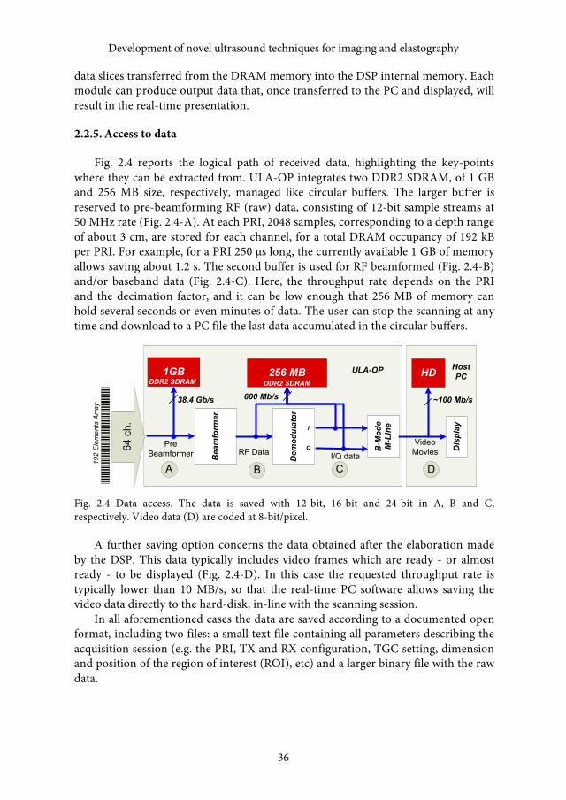
2.2.5. Access to data
Fig. 2.4 reports the logical path of received data, highlighting the key-points where they can be extracted from. ULA-OP integrates two DDR2 SDRAM, of 1 GB and 256 MB size, respectively, managed like circular buffers. The larger buffer is reserved to pre-beamforming RF (raw) data, consisting of 12-bit sample streams at 50 MHz rate (Fig. 2.4-A). At each PRI, 2048 samples, corresponding to a depth range of about 3 cm, are stored for each channel, for a total DRAM occupancy of 192 kB per PRI. For example, for a PRI 250 µs long, the currently available 1 GB of memory allows saving about 1.2 s. The second buffer is used for RF beamformed (Fig. 2.4-B) and/or baseband data (Fig. 2.4-C). Here, the throughput rate depends on the PRI and the decimation factor, and it can be low enough that 256 MB of memory can hold several seconds or even minutes of data. The user can stop the scanning at any time and download to a PC file the last data accumulated in the circular buffers.
Fig. 2.4 Data access. The data is saved with 12-bit, 16-bit and 24-bit in A, B and C, respectively. Video data (D) are coded at 8-bit/pixel.
A further saving option concerns the data obtained after the elaboration made by the DSP. This data typically includes video frames which are ready - or almost ready - to be displayed (Fig. 2.4-D). In this case the requested throughput rate is typically lower than 10 MB/s, so that the real-time PC software allows saving the video data directly to the hard-disk, in-line with the scanning session.
In all aforementioned cases the data are saved according to a documented open format, including two files: a small text file containing all parameters describing the acquisition session (e.g. the PRI, TX and RX configuration, TGC setting, dimension and position of the region of interest (ROI), etc) and a larger binary file with the raw data.
38.4 Gb/s
1GB
Bea
mfo
rmer
256 MB
Dem
odul
ator
I
Q B-M
ode
M-L
ine
HD
192
Ele
men
ts A
rray
Dis
play
A B C D
64 c
h.
600 Mb/s ~100 Mb/s
PreBeamformer RF Data I/Q data
VideoMovies
ULA-OP HostPC
DDR2 SDRAMDDR2 SDRAM
Development of novel ultrasound techniques for imaging and elastography
36
Alessandro Ramalli
37
2.2.6. Operating modes setting
All system settings are managed through a configuration file held in the host PC. This includes details about the display parameters, acquisition setting, SM configuration, elaboration module instances and TX/RX signal definitions. Whenever the user wants to implement arbitrary TX/RX schemes and/or use personalized waveforms, ULA-OP needs to be programmed by two additional configuration files. For example, this happens when 2D array probes are used, or non-standard excitation waveforms have to be transmitted.
The availability of different configuration files allows the user to quickly switch between predefined settings simply by choosing from a menu. Furthermore, some parameters such as the PRF, focal depth and steering angle are directly editable from the real-time software interface.
2.2.7. Probe connection
Any probe with a maximum number of 192 elements can be associated to ULA-OP through the ITT Cannon DLM5-260P connector. We chose a pin-out which is directly compatible with the commercially available linear, phased and convex array probes produced by Esaote Spa (Firenze, Italy). This pin-out can also be used as a guide in the development of custom arrays to be associated to ULA-OP. In the elastography experiments reported in the next section, the commercial linear array probe LA523, having a 4 MHz 6-dB bandwidth between 6 MHz and 10 MHz, was used. In all other experiments we employed a linear array prototype (LA533) with 6-dB bandwidth ranging from 3 MHz to 13 MHz. Tests with small 2-D arrays are also being performed at the University of Windsor (Kustron et al. 2011).
2.3. Examples of non-standard application
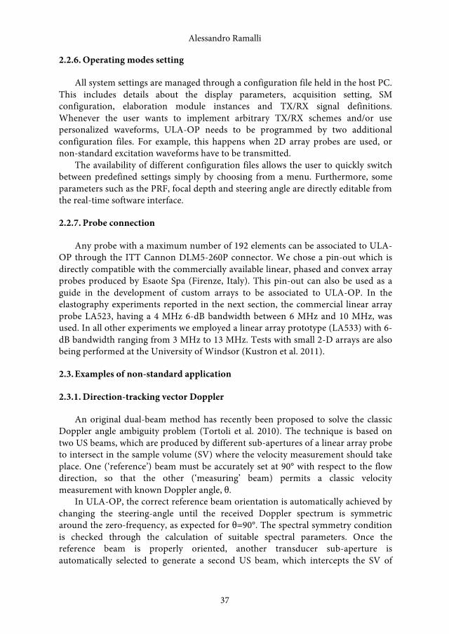
2.3.1. Direction-tracking vector Doppler
An original dual-beam method has recently been proposed to solve the classic Doppler angle ambiguity problem (Tortoli et al. 2010). The technique is based on two US beams, which are produced by different sub-apertures of a linear array probe to intersect in the sample volume (SV) where the velocity measurement should take place. One (‘reference’) beam must be accurately set at 90° with respect to the flow direction, so that the other (‘measuring’ beam) permits a classic velocity measurement with known Doppler angle, θ.
In ULA-OP, the correct reference beam orientation is automatically achieved by changing the steering-angle until the received Doppler spectrum is symmetric around the zero-frequency, as expected for θ=90°. The spectral symmetry condition is checked through the calculation of suitable spectral parameters. Once the reference beam is properly oriented, another transducer sub-aperture is automatically selected to generate a second US beam, which intercepts the SV of
Alessandro Ramalli
37
Development of novel ultrasound techniques for imaging and elastography
38
interest with a beam-flow angle as different as possible from 90°. The velocity magnitude is directly estimated from the echoes of this measuring beam.
Fig. 2.5 Real-time ULA-OP display in direction-tracking vector Doppler Mode (see text)
For example, Fig. 2.5 shows a screenshot frozen during the real-time investigation of the common carotid artery in a healthy volunteer. Yellow and blue lines superimposed on B-mode represent the reference and measuring beams, respectively. The velocity measurement trend, shown on the bottom of Fig. 2.5, refers to the SV at the crossing of the two lines. The two spectrograms in the middle panel are obtained from the reference (left) and measuring (right) beam, respectively. The symmetry of the former spectrogram confirms that the reference beam position, automatically tracked by the system, was correct.
The reproducibility of the new vector Doppler method in the ULA-OP implementation has been tested both in vitro and in vivo through experiments which have produced mean coefficients of variability below 8% in all cases (Tortoli et al. 2010).
2.3.2. Flow Mediated Dilation (FMD)
In Flow-mediated dilation (FMD) studies for non-invasive evaluation of the endothelial function (Harris et al. 2010), only the brachial artery diameter changes due to reactive hyperaemia are usually measured. The stimulus of such change, i.e. the flow change, is only qualitatively estimated by measuring the mean velocity in the vessel, and assuming a parabolic velocity profile.
ULA-OP allows, for the first time, the simultaneous estimation of both the stimulus (wall shear stress change) and the effect (diameter change) in FMD studies. To reach this goal, the DSP is programmed to produce real-time B-Mode images of the investigated artery together with Multigate Spectral Doppler (MSD) data. The latter comprises so-called spectral profiles (Tortoli et al. 1996), reporting the
Development of novel ultrasound techniques for imaging and elastography
38
Alessandro Ramalli
39
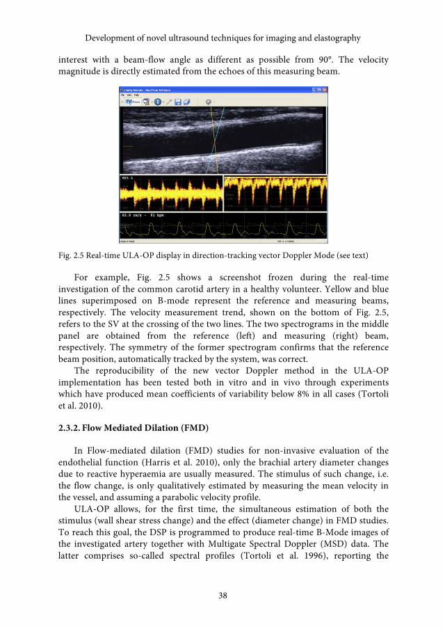
distribution of Doppler spectra at 128 different depths along a direction selected by the operator over the B-Mode image. In Fig. 2.6, an example of the ULA-OP real time application window during an FMD exam is reported. Through the combination of MSD- and B-Mode, both the morphology and the hemodynamics over the ROI are continuously under the operator’s control, which is particularly important in this test usually lasting more than 10 minutes.
Fig. 2.6 The B-Mode and MSD images are shown in the upper part of the window, while the sonogram related to the depth selected from the MSD profile (yellow line) is reported in the lower part.
Although the B-Mode image and the spectral profiles are produced in real-time by the DSP, the image and the Doppler raw IQ data are transmitted to the PC for accurate post-processing measurements. It is in fact convenient to measure the diameter through a contour tracking technique (Gemignani et al. 2007), while the instantaneous wall shear stress (WSS) is estimated by extracting the maximum gradient of peak frequencies from the spectral profiles. The preliminary results obtained on a first group of young volunteers (ages 25-29) indicate mean increments during reflow against baseline of 105% ± 22% for the peak WSS and 8% ± 3% for the diameter increase (Tortoli et al. 2011), (Francalanci et al. 2010). The mean time interval between the WSS peak and the beginning of plateau of diameter waveform was 38 ± 8 s. These results are encouraging toward a detailed investigation of mechanisms underlying FMD in different clinical models.
2.4. High Frame Rate Imaging
New methods have recently been proposed to produce B-Mode images at high frame-rates (HFR), i.e. up to thousands of images per second (Boni et al. 2012)(Cheng & Lu 2006), (Montaldo et al. 2009). Since the patterns transmitted in such methods are different from those used for standard focused beams, the implementation of those techniques in commercial scanners is prevented by their closed architecture.
Alessandro Ramalli
39
Development of novel ultrasound techniques for imaging and elastography
40
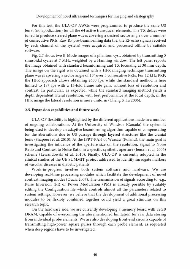
For this test, the ULA-OP AWGs were programmed to produce the same US burst (no apodization) for all the 64 active transducer elements. The TX delays were tuned to produce steered plane waves covering a desired sector angle over a number of consecutive PRIs. Raw RF pre-beamforming data (i.e. the RF echo signals received by each channel of the system) were acquired and processed offline by suitable software.
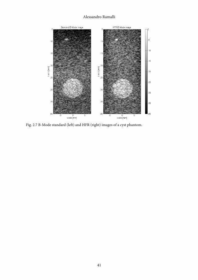
Fig. 2.7 shows two B-Mode images of a phantom cyst, obtained by transmitting 5 sinusoidal cycles at 7 MHz weighted by a Hanning window. The left panel reports the image obtained with standard beamforming and TX focussing at 30 mm depth. The image on the right was obtained with a HFR imaging technique transmitting plane waves covering a sector angle of 15° over 5 consecutive PRIs. For 12 kHz PRF, the HFR approach allows obtaining 2400 fps, while the standard method is here limited to 187 fps with a 13-fold frame rate gain, without loss of resolution and contrast. In particular, as expected, while the standard imaging method yields a depth dependent lateral resolution, with best performance at the focal depth, in the HFR image the lateral resolution is more uniform (Cheng & Lu 2006).
2.5. Expansion capabilities and future work
ULA-OP flexibility is highlighted by the different applications made in a number of ongoing collaborations. At the University of Windsor (Canada) the system is being used to develop an adaptive beamforming algorithm capable of compensating for the aberrations due to US passage through layered structures like the cranial bone (Shapoori et al. 2010). At the IPPT-PAN of Warsaw (Poland), the main goal is investigating the influence of the aperture size on the resolution, Signal to Noise Ratio and Contrast to Noise Ratio in a specific synthetic aperture (Jensen et al. 2006) scheme (Lewandowski et al. 2010). Finally, ULA-OP is currently adopted in the clinical studies of the UE SUMMIT project addressed to identify surrogate markers of vascular diseases in diabetic patients.
Work-in-progress involves both system software and hardware. We are developing real-time processing modules which facilitate the development of novel contrast imaging modes (Quaia 2007). The transmission of signals according to, e.g., Pulse Inversion (PI) or Power Modulation (PM) is already possible by suitably editing the Configuration file which controls almost all the parameters related to system settings. However, we believe that the development of additional processing modules to be flexibly combined together could yield a great stimulus on this research topic.
On the hardware side, we are currently developing a memory board with 32GB DRAM, capable of overcoming the aforementioned limitation for raw data storing from individual probe elements. We are also developing front-end circuits capable of transmitting high-power square pulses through each probe element, as requested when deep regions have to be investigated.
Development of novel ultrasound techniques for imaging and elastography
40
Alessandro Ramalli
41
Fig. 2.7 B-Mode standard (left) and HFR (right) images of a cyst phantom.
Alessandro Ramalli
41

3. Novel Ultrasound Simulation Methods
The performance improvement of ultrasound systems, providing high flexibility and high programmability, leads to the need of new development tools which can help in managing all the available features. A valid tool is an ultrasound simulator that helps the developer predicting the behavior of the real system before testing it. This chapter is divided into two parts: the first (3.1) is addressed to the description of a linear simulator, based on Field II, which even allows programming ULA-OP; the second part (3.2), draws on (F. Varray et al. 2011) and (Francois Varray et al. 2011) is devoted to presenting a nonlinear simulator, based on an angular spectrum method and was conducted with Franҫois Varray. He finally developed an image simulator for harmonic imaging, called Creanuis (Varray et al. 2010), (Varray 2011).
3.1. Field simulation in homogeneous linear media: Simag
Simag is a development tool which simulates the behavior of an ultrasound system. In particular the final goal of the simulator consists in the study of the behavior of single-element, linear-array and two-dimensional array transducers in order to optimize their use. With this aim, Simag guarantees the highest degree of freedom in terms of available configurations. It allows setting: the sound speed, the physical and electrical transducer properties, the transmission and reception sampling frequencies of the ultrasound system, the excitation signal, the transmission and reception beamforming schemes, and the position and the scattering amplitude of numeric phantoms scatterers. Finally, the simulator shows as the results of the simulation, the image of the transmitted beam (one-way field) and received beam (two-way field), the movie of the related beam propagation, the B-mode image of numerical phantoms and the echo signals received by the single transducers.
3.1.1. Application package: Field II
The software is based on a well-established and optimized ultrasound simulator, internationally recognized as a valid development tool for ultrasound system design: Field II (Jensen 1996). This software is an application package composed of several functions for ultrasound simulation, implemented in C and provided with Matlab® functions. The latter are used as interface between Matlab® and the C code. In such a way the advantages in terms of computation speed of C codes and the versatility of a development tool are both exploited. Alessandro Ramalli, Development of novel ultrasound techniques for imaging and elastography : from simulation to real-time implementation ISBN 978-88-6655-456-1 (print) ISBN 978-88-6655-457-8 (online) © 2013 Firenze University Press
Development of novel ultrasound techniques for imaging and elastography
44
The base of Field II is the spatial impulse response concept, i.e. the function which gives the emitted ultrasound field at a specific point in the space as a function of time, when the transducer is excited by a Dirac delta function. Then, exploiting the theory of linear systems, the emitted ultrasonic field even for pulsed and continuous wave systems is found. The ultrasonic field for any kind of excitation signal is computed by convolving it with the spatial impulse response, more details are given in (Jensen & Svendsen 1992), (Jensen 1999).
In Simag, the package Field II is only exploited to simulate the ultrasound propagation, each system parameter and setting, e.g. beamforming or signal generation, is directly and individually computed by the mathematical modules of Simag.
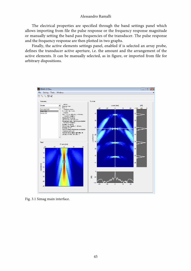
3.1.2. Simag interfaces
The main interface (Fig. 3.1) gives access to all the other interfaces through a menu bar and provides a general overview of the main settings and simulations. Each setting, e.g. transducer or mode settings, is summarized in a dedicated list. The results of the primary simulations, i.e. B-mode and fields, are displayed as two separate images.
Following the available menu functions: • File: to open and to save the settings or the simulation results, to export
the ULA-OP configuration files, to import the ULA-OP acquisition data files.
• Setting: to open the transducer, mode and scatterers settings interfaces.• Tools: to simulate one-way and two-way fields, received echo signals, B-
mode images, and Doppler data according to the previously set modes;to check the format of the ULA-OP configuration files.
• Windows: to open graphic interfaces which modify the aspect of thedisplayed images.
The transducers settings interface (Fig. 3.2), accessible from the tools menu of the main interface, defines all the transducer properties, i.e. physical properties, electrical properties and the displacement of the active elements. The names of the already set transducers are arranged in a list, which is useful to recall all the transducer properties by a mouse click. In this version the available transducer type are: single-element, linear array and 2D array.
The interface is divided in four main panels. The first, transducer elements settings panel, queries for the elements properties, according to the transducer type, which must be filled by the user. As an example, in Fig. 3.2, the panel is set for a linear array transducer.
The second panel is the acoustic lens settings where it is defined the shape and the sound speed of the acoustic lens placed in the very front of the transducer surface. The shape of the lens can be acquired from specific files and it is displayed at the right.
Development of novel ultrasound techniques for imaging and elastography
44
Alessandro Ramalli
45
The electrical properties are specified through the band settings panel which allows importing from file the pulse response or the frequency response magnitude or manually setting the band pass frequencies of the transducer. The pulse response and the frequency response are then plotted in two graphs.
Finally, the active elements settings panel, enabled if is selected an array probe, defines the transducer active aperture, i.e. the amount and the arrangement of the active elements. It can be manually selected, as in figure, or imported from file for arbitrary dispositions.
Fig. 3.1 Simag main interface.
Alessandro Ramalli
45

Development of novel ultrasound techniques for imaging and elastography
46
Fig. 3.2 Transducer settings interface.
The tx/rx settings interface is used to set the modes of transmission and reception, i.e. the signal to be transmitted, the transmission focusing, the reception beamforming and the demodulation parameters. It is organized in three panels: mode, signal and demodulation, and tx/rx beamforming.
The mode panel defines how the scan is performed i.e. how the active aperture is moved over the elements of an array probe. It could be a linear scan, a sector scan, a single-shot or a plane waves scan. Furthermore, the transmission and the reception transducers to be assigned to the mode can be selected. The names of the already set modes are arranged in a list, which is useful to recall all the mode properties by a mouse click.
In the signal and demodulation panel, a popup allows selecting among different kind of signals, e.g. sine wave, square wave, chirp etc.. Then the related panel is loaded with the proper forms that have to be filled by the user with the desired signal properties. Accordingly to the signal must be set the demodulation parameters which can be defined in the demodulation settings sub-panel. The signal and the demodulation filter response are then plotted in the related graphs.
The last panel, tx/rx beamforming, is employed to set the transmission and reception beamforming schemes. Standard focusing is available but it is even possible to use limited diffraction beams or file imported electronic delays. The transmission apodization curve can be selected by a popup menu and the aperture width can be modified by a slider control. The reception beamforming can be set, with the same setting in transmission, but dynamic focusing and apodization are available.
The scatterers position and then the region of interest can be defined by the scatterers setting interface (Fig. 3.4). It allows manually setting the position and amplitude of each single scatterer or loading from file a predefined set of scatterers. Defining the region of interest is useful to test new beamforming schemes, to evaluate the system resolution or to compare different imaging modalities.
Development of novel ultrasound techniques for imaging and elastography
46

Alessandro Ramalli
47
Fig. 3.3 Tx/Rx settings interface.
Fig. 3.4 Scatterers settings interface.
Alessandro Ramalli
47

Development of novel ultrasound techniques for imaging and elastography
48
special configuration files. Furthermore, the acquired echo-signals data require to be post-processed according to the specific case. In such cases, Simag serves to the purpose, since it generates the necessary configuration files and post-processes the related acquired data. These features were used for pulse compression imaging (see sec. 5.3), high-frame rate imaging (see sec. 2.4), one-way field measurement (see sec. 3.1.4) or high-frame rate elastography (see chapter 4).
3.1.4. Simulations, measurements and acquisitions
Cross-talk model
In Simag, the model of the electro-acoustical cross-talk among neighbor elements consists in adding on the signal transmitted by an element a percentage (C) of the nearest neighbor elements transmitted signals. Then, considering Sin the signals matrix to be transmitted, accordingly delayed to the focalization delays pattern and Sout the actually transmitted signals matrix after considering the cross-talk, the model could be expressed in matrix product as:
𝑺𝑺𝒐𝒐𝒐𝒐𝒐𝒐 !!"#,!! =
1 𝐶𝐶 0 ⋯ 0 0𝐶𝐶 1 𝐶𝐶 ⋯ 0 00 𝐶𝐶 1 ⋯ 0 0⋮ ⋮ ⋮ ⋱ ⋮ ⋮0 0 0 ⋯ 𝐶𝐶 00 0 0 ⋯ 1 𝐶𝐶0 0 0 ⋯ 𝐶𝐶 1 !!"#,!!"#
×𝑺𝑺𝒊𝒊𝒊𝒊 !!"#,!! (3.1)
where Nact is the amount of active elements and Nt is the transmitted signal length in samples including the transmission delays. In Fig. 3.5 examples of the effect due to a 35% cross-talk on the actually transmitted matrix are shown. It appears evident that the cross-talk among signals with different delays brings to constructive and destructive interferences. The final effect is a sort of an undesired apodization of the transmitted matrix.
3.1.3. ULA-OP compatibility
The experimental test of novel ultrasound investigation methods may require the transmission of custom excitation waveforms or pulse sequences, the acquisition of data from different points of the receiver section, and/or the real-time echo-signal elaboration according to specific algorithms (Tortoli & Jensen 2006). ULA-OP fulfils to each of the previous requirements, but, when non-standard transmission and reception beamforming schemes are necessary, it requires to be configured through
Development of novel ultrasound techniques for imaging and elastography
48
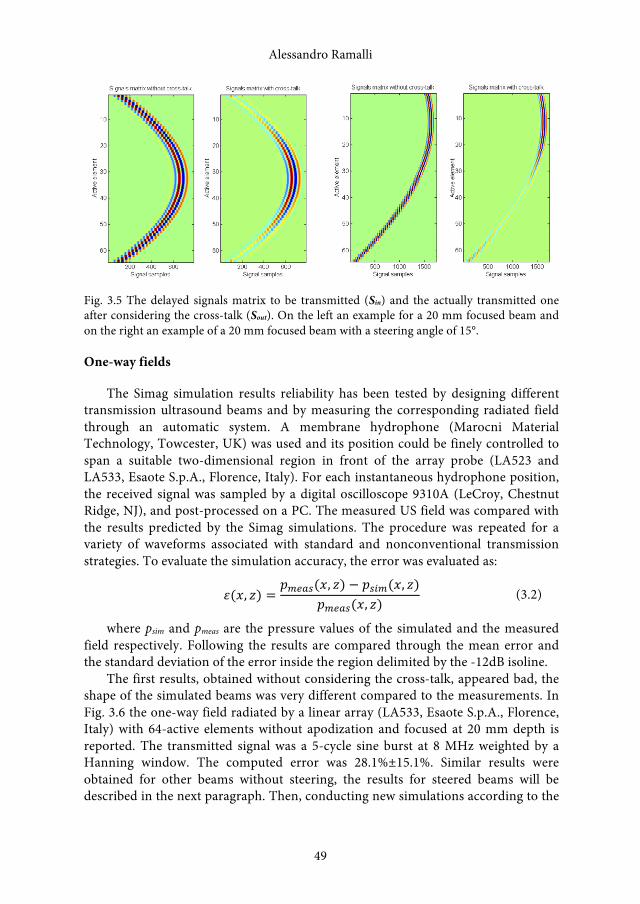
Alessandro Ramalli
49
Fig. 3.5 The delayed signals matrix to be transmitted (Sin) and the actually transmitted one after considering the cross-talk (Sout). On the left an example for a 20 mm focused beam and on the right an example of a 20 mm focused beam with a steering angle of 15°.
One-way fields
The Simag simulation results reliability has been tested by designing different transmission ultrasound beams and by measuring the corresponding radiated field through an automatic system. A membrane hydrophone (Marocni Material Technology, Towcester, UK) was used and its position could be finely controlled to span a suitable two-dimensional region in front of the array probe (LA523 and LA533, Esaote S.p.A., Florence, Italy). For each instantaneous hydrophone position, the received signal was sampled by a digital oscilloscope 9310A (LeCroy, Chestnut Ridge, NJ), and post-processed on a PC. The measured US field was compared with the results predicted by the Simag simulations. The procedure was repeated for a variety of waveforms associated with standard and nonconventional transmission strategies. To evaluate the simulation accuracy, the error was evaluated as:
𝜀𝜀(𝑥𝑥, 𝑧𝑧) =𝑝𝑝!"#$(𝑥𝑥, 𝑧𝑧) − 𝑝𝑝!"#(𝑥𝑥, 𝑧𝑧)
𝑝𝑝!"#$(𝑥𝑥, 𝑧𝑧) (3.2)
where psim and pmeas are the pressure values of the simulated and the measured field respectively. Following the results are compared through the mean error and the standard deviation of the error inside the region delimited by the -12dB isoline.
The first results, obtained without considering the cross-talk, appeared bad, the shape of the simulated beams was very different compared to the measurements. In Fig. 3.6 the one-way field radiated by a linear array (LA533, Esaote S.p.A., Florence, Italy) with 64-active elements without apodization and focused at 20 mm depth is reported. The transmitted signal was a 5-cycle sine burst at 8 MHz weighted by a Hanning window. The computed error was 28.1%±15.1%. Similar results were obtained for other beams without steering, the results for steered beams will be described in the next paragraph. Then, conducting new simulations according to the
Alessandro Ramalli
49

Development of novel ultrasound techniques for imaging and elastography
50
proposed cross-talk model, better results were obtained. In Fig. 3.7 the same measured beam of Fig. 3.6 and the simulated beam considering a 35% electro-acoustical cross-talk among neighbor elements are reported. The computed error was 5.9%±15.1% which was considerably reduced compared to the first simulation. In Fig. 3.8 the one-way field on the lens plane is reported and even in this case the error was low, 3.4%±14.5%.
Even if a 35% cross-talk could appear very high the manufacturer did not exclude that possibility. At present, we do not have a direct measurement of the cross-talk and it was experimentally estimated by choosing the cross-talk value which brings to the best-fit simulation results. The 35 percentage best-fits the behavior of the LA533 probe.
Fig. 3.6 A one-way field of a linear array focused at 20 mm depth. On the top-left the measured beam, on the top-right the simulated beam, on the bottom the axial and the lateral beams profiles, intersecting at the focus point. The simulation did not consider the cross-talk model.
Development of novel ultrasound techniques for imaging and elastography
50

Alessandro Ramalli
51
Fig. 3.7 A one-way field of a linear array focused at 20 mm depth. On the top-left the measured beam, on the top-right the simulated beam, on the bottom the axial and the lateral beams profiles, intersecting at the focus point. The simulation considered a 35% electro-acoustical cross-talk among neighbor elements.
Fig. 3.8 A one-way field on the lens plane radiated from a linear array focused at 20 mm depth. On the top-left the measured beam, on the top-right the simulated beam, on the bottom the axial and the lateral beams profiles, intersecting at the focus point. The simulation considered a 35% electro-acoustical cross-talk among neighbor elements.
Alessandro Ramalli
51
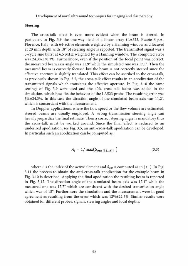
Development of novel ultrasound techniques for imaging and elastography
52
Florence, Italy) with 64-active elements weighted by a Hanning window and focused at 20 mm depth with 18° of steering angle is reported. The transmitted signal was a 5-cycle sine burst at 6.5 MHz weighted by a Hanning window. The computed error was 24.3%±30.3%. Furthermore, even if the position of the focal point was correct, the measured beam axis angle was 11.9° while the simulated one was 17.1°. Then the measured beam is correctly focused but the beam is not correctly steered since the effective aperture is slightly translated. This effect can be ascribed to the cross-talk, as previously shown in Fig. 3.5, the cross-talk effect results in an apodization of the transmitted signals which translates the effective aperture. In Fig. 3.10 the same settings of Fig. 3.9 were used and the 40% cross-talk factor was added in the simulation, which best-fits the behavior of the LA523 probe. The resulting error was 5%±24.3%. In this case the direction angle of the simulated beam axis was 11.2°, which is concordant with the measurement.
In Doppler applications, where the flow speed or the flow volume are estimated, steered beams are usually employed. A wrong transmission steering angle can heavily jeopardize the final estimate. Then a correct steering angle is mandatory thus the cross-talk must be worked around. Since the final effect is reduced to an undesired apodization, see Fig. 3.5, an anti-cross-talk apodization can be developed. In particular such an apodization can be computed as:
𝐴𝐴! = 1/max 𝑺𝑺𝒐𝒐𝒐𝒐𝒐𝒐 [𝒊𝒊,𝟏𝟏…𝑵𝑵𝒕𝒕] (3.3)
where i is the index of the active element and Sout is computed as in (3.1). In Fig. 3.11 the process to obtain the anti-cross-talk apodization for the example beam in Fig. 3.10 is described. Applying the final apodization the resulting beam is reported in Fig. 3.12. The direction angle of the simulated beam axis was 17.1° while the measured one was 17.7° which are consistent with the desired transmission angle which was of 18°. Furthermore the simulation and the measurement were in good agreement as resulting from the error which was 12%±22.5%. Similar results were obtained for different probes, signals, steering angles and focal depths.
Steering
The cross-talk effect is even more evident when the beam is steered. In particular, in Fig. 3.9 the one-way field of a linear array (LA523, Esaote S.p.A.,
Development of novel ultrasound techniques for imaging and elastography
52
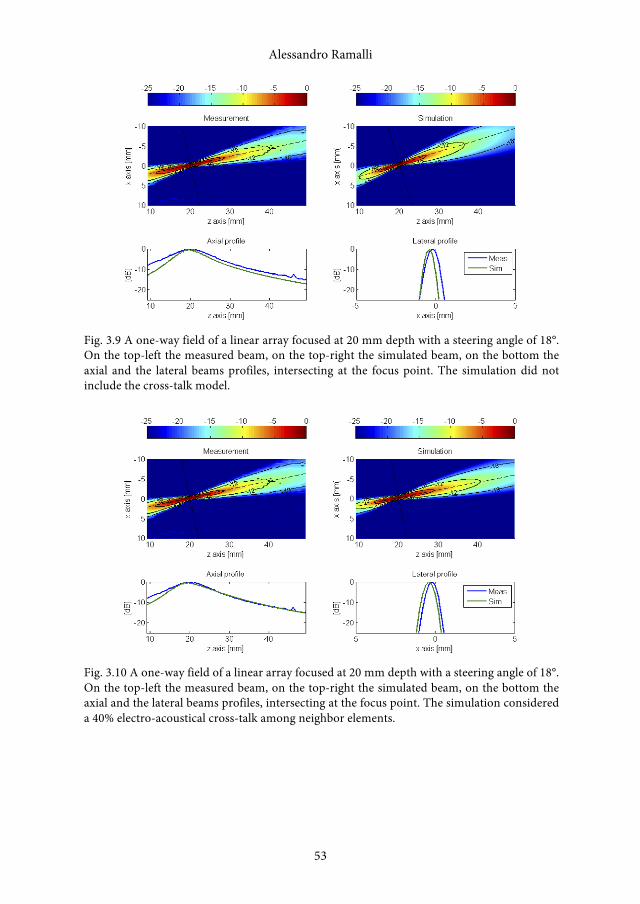
Alessandro Ramalli
53
Fig. 3.9 A one-way field of a linear array focused at 20 mm depth with a steering angle of 18°. On the top-left the measured beam, on the top-right the simulated beam, on the bottom the axial and the lateral beams profiles, intersecting at the focus point. The simulation did not include the cross-talk model.
Fig. 3.10 A one-way field of a linear array focused at 20 mm depth with a steering angle of 18°. On the top-left the measured beam, on the top-right the simulated beam, on the bottom the axial and the lateral beams profiles, intersecting at the focus point. The simulation considered a 40% electro-acoustical cross-talk among neighbor elements.
Alessandro Ramalli
53

Development of novel ultrasound techniques for imaging and elastography
54
Fig. 3.11 Computation of the anti-cross-talk apodization for the beam shown in Fig. 3.10. The signal matrix affected by the cross-talk (Sout) is computed from the delayed signals matrix to be transmitted (Sin). The reciprocal of the maximum of Sout for each element returns the anti-cross-talk apodization, which is further multiplied by the transmission desired apodization (Hanning) to obtain the final apodization.
Fig. 3.12 A one-way field of a linear array focused at 20 mm depth with a steering angle of 18°. The apodization is computed to compensate the cross-talk effect. On the top-left the measured beam, on the top-right the simulated beam, on the bottom the axial and the lateral beams profiles, intersecting at the focus point. The simulation considered a 40% electro-acoustical cross-talk among neighbor elements.
Limited diffraction beams
Diffraction is one of the physical phenomenon which involves any wave field without exception and it is described by the Helmholz equation. Usually it is supposed that any wave field suffers from the diffraction effect, which is not true for
Development of novel ultrasound techniques for imaging and elastography
54
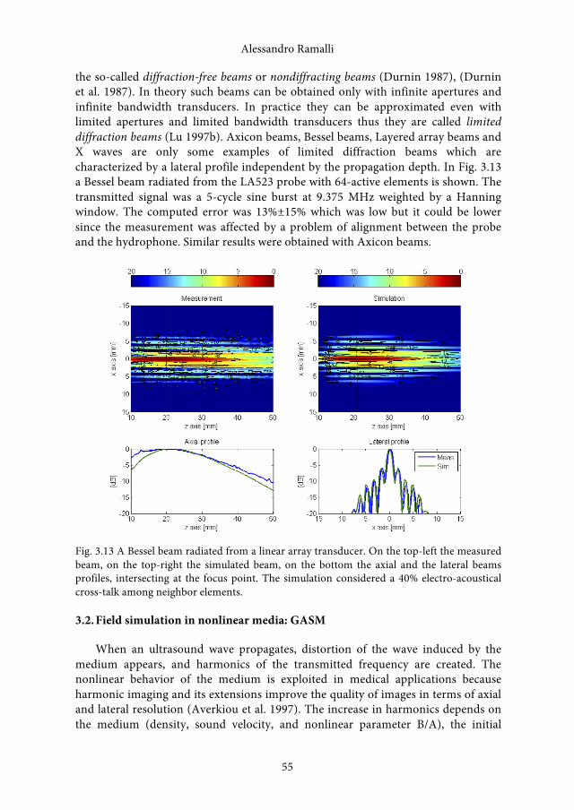
Alessandro Ramalli
55
the so-called diffraction-free beams or nondiffracting beams (Durnin 1987), (Durnin et al. 1987). In theory such beams can be obtained only with infinite apertures and infinite bandwidth transducers. In practice they can be approximated even with limited apertures and limited bandwidth transducers thus they are called limited diffraction beams (Lu 1997b). Axicon beams, Bessel beams, Layered array beams and X waves are only some examples of limited diffraction beams which are characterized by a lateral profile independent by the propagation depth. In Fig. 3.13 a Bessel beam radiated from the LA523 probe with 64-active elements is shown. The transmitted signal was a 5-cycle sine burst at 9.375 MHz weighted by a Hanning window. The computed error was 13%±15% which was low but it could be lower since the measurement was affected by a problem of alignment between the probe and the hydrophone. Similar results were obtained with Axicon beams.
Fig. 3.13 A Bessel beam radiated from a linear array transducer. On the top-left the measured beam, on the top-right the simulated beam, on the bottom the axial and the lateral beams profiles, intersecting at the focus point. The simulation considered a 40% electro-acoustical cross-talk among neighbor elements.
3.2. Field simulation in nonlinear media: GASM
When an ultrasound wave propagates, distortion of the wave induced by the medium appears, and harmonics of the transmitted frequency are created. The nonlinear behavior of the medium is exploited in medical applications because harmonic imaging and its extensions improve the quality of images in terms of axial and lateral resolution (Averkiou et al. 1997). The increase in harmonics depends on the medium (density, sound velocity, and nonlinear parameter B/A), the initial
Alessandro Ramalli
55
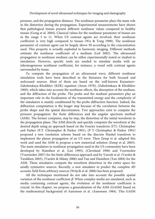
Development of novel ultrasound techniques for imaging and elastography
56
pressure, and the propagation distance. The nonlinear parameter plays the main role in the distortion during the propagation. Experimental measurements have shown that pathological tissues present different nonlinear values compared to healthy tissues (Gong et al. 2004). Classical values for the nonlinear parameter of tissues are in the range 5 to 11. When US contrast agents are involved, their nonlinear coefficient is very high compared to tissues (Wu & Tong 1998). The nonlinear parameter of contrast agent can be largely above 50 according to the concentration used. This property is actually exploited in harmonic imaging. Different methods estimate the nonlinear coefficient of a medium (Leif 2002). The ultrasound propagation in nonlinear medium can be either experimentally tested or studied in simulation. However, specific tools are needed to simulate media with an inhomogeneous nonlinear coefficient, for instance, a vessel with contrast agents surrounded by tissue.
To compute the propagation of an ultrasound wave, different nonlinear simulation tools have been described in the literature for both focused and unfocused sources. Most of them are based on the well-known Kuznetsov-Zabolotskaya-Khokhlov (KZK) equation (Anon 1970), (Zabolotskaya & Khokhlov 1969), which takes into account the nonlinear effects, the absorption of the medium, and the diffraction of the probe. The probe and the medium parameters play an important role in the focalization of the transmitted energy and the complexity of the simulators is mainly conditioned by the probe diffraction function. Indeed, the diffraction computation is the longer step because of the correlation between the probe shape and the spatial discretization. Two approaches exist to compute the pressure propagation: the finite differences and the angular spectrum method (ASM). The former computes, step by step, the distortion of the initial waveform in the propagation plane. The ASM directly and quickly computes the waveform at the desired depth using an approach based on the Fourier transform (FT). Christopher and Parker (P.T. Christopher & Parker 1991), (P T Christopher & Parker 1991) proposed a new resolution scheme based on the discrete Hankel transform to implement the planar propagation of an US wave. Then Zemp et al. adapted this work and used the ASM to propose a new numerical solution (Zemp et al. 2003). The main simulators in nonlinear propagation used in the US community have been developed by Hamilton et al. (Lee 1995), (Cleveland 1996) and Voormolen (Voormolen 2007) for the finite differences approach and by Varsolt et al. (Varslot & Taraldsen 2005), (Varslot & Måsøy 2006) and Yan and Hamilton (Yan 2004) for the ASM. These simulators compute the waveform distortion in the entire space for axially symmetric sources. Recently, a new simulator to predict the complete 4D acoustic field from arbitrary sources (Wójcik et al. 2006) has been proposed.
All the techniques mentioned do not take into account the possible spatial variation of the nonlinear coefficient β. When complex media are simulated, such as media containing contrast agents, the evolution of the nonlinear coefficient is crucial. In this chapter, we propose a generalization of the ASM (GASM) based on the mathematical background of Aanonsen et al. (Aanonsen 1984). This GASM
Development of novel ultrasound techniques for imaging and elastography
56
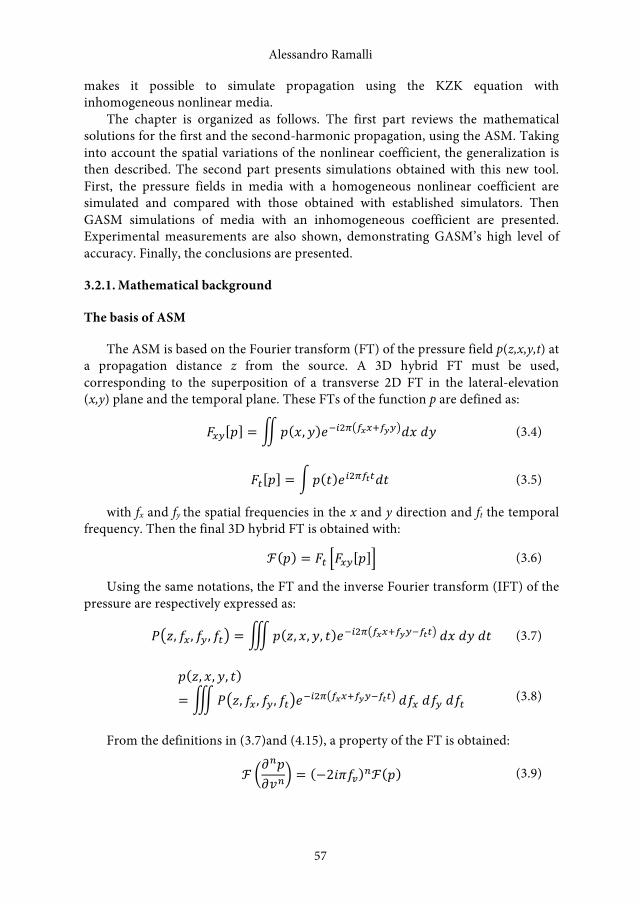
Alessandro Ramalli
57
makes it possible to simulate propagation using the KZK equation with inhomogeneous nonlinear media.
The chapter is organized as follows. The first part reviews the mathematical solutions for the first and the second-harmonic propagation, using the ASM. Taking into account the spatial variations of the nonlinear coefficient, the generalization is then described. The second part presents simulations obtained with this new tool. First, the pressure fields in media with a homogeneous nonlinear coefficient are simulated and compared with those obtained with established simulators. Then GASM simulations of media with an inhomogeneous coefficient are presented. Experimental measurements are also shown, demonstrating GASM’s high level of accuracy. Finally, the conclusions are presented.
3.2.1. Mathematical background
The basis of ASM
The ASM is based on the Fourier transform (FT) of the pressure field p(z,x,y,t) at a propagation distance z from the source. A 3D hybrid FT must be used, corresponding to the superposition of a transverse 2D FT in the lateral-elevation (x,y) plane and the temporal plane. These FTs of the function p are defined as:
𝐹𝐹!" 𝑝𝑝 = 𝑝𝑝 𝑥𝑥, 𝑦𝑦 𝑒𝑒!!!! !!!!!!! 𝑑𝑑𝑑𝑑 𝑑𝑑𝑑𝑑 (3.4)
𝐹𝐹! 𝑝𝑝 = 𝑝𝑝 𝑡𝑡 𝑒𝑒!!!!!!𝑑𝑑𝑑𝑑 (3.5)
with fx and fy the spatial frequencies in the x and y direction and ft the temporal frequency. Then the final 3D hybrid FT is obtained with:
ℱ 𝑝𝑝 = 𝐹𝐹! 𝐹𝐹!" 𝑝𝑝 (3.6)
Using the same notations, the FT and the inverse Fourier transform (IFT) of the pressure are respectively expressed as:
𝑃𝑃 𝑧𝑧, 𝑓𝑓! , 𝑓𝑓! , 𝑓𝑓! = 𝑝𝑝 𝑧𝑧, 𝑥𝑥, 𝑦𝑦, 𝑡𝑡 𝑒𝑒!!!! !!!!!!!!!!! 𝑑𝑑𝑑𝑑 𝑑𝑑𝑑𝑑 𝑑𝑑𝑑𝑑 (3.7)
𝑝𝑝 𝑧𝑧, 𝑥𝑥, 𝑦𝑦, 𝑡𝑡
= 𝑃𝑃 𝑧𝑧, 𝑓𝑓! , 𝑓𝑓! , 𝑓𝑓! 𝑒𝑒!!!! !!!!!!!!!!! 𝑑𝑑𝑓𝑓! 𝑑𝑑𝑓𝑓! 𝑑𝑑𝑓𝑓! (3.8)
From the definitions in (3.7)and (4.15), a property of the FT is obtained:
ℱ𝜕𝜕!𝑝𝑝𝜕𝜕𝑣𝑣!
= −2𝑖𝑖𝑖𝑖𝑓𝑓! !ℱ 𝑝𝑝 (3.9)
Alessandro Ramalli
57
Development of novel ultrasound techniques for imaging and elastography
58
ℱ𝜕𝜕!𝑝𝑝𝜕𝜕𝑡𝑡!
= 2𝑖𝑖𝑖𝑖𝑓𝑓! !ℱ 𝑝𝑝 (3.10)
with the variable v corresponding to x or y.
Propagation equation
The propagation equation of a pressure wave p(z,x,y,t) in a lossless medium is expressed as (Aanonsen 1984):
∇! −1𝑐𝑐!!
𝜕𝜕!
𝜕𝜕𝑡𝑡!𝑝𝑝 = −
𝛽𝛽𝜌𝜌!𝑐𝑐!!
𝜕𝜕!𝑝𝑝!
𝜕𝜕𝑡𝑡!(3.11)
with c0 the sound speed, ρ0 the density, ∇ is the Laplacian, and β the nonlinear coefficient related to the nonlinear parameter β=1+B/2A. The nonlinear coefficient is directly responsible of the increase of the harmonics in the propagation equation (Hamilton & Blackstock 1988). The Laplacian is expressed as:
∇!𝑝𝑝 =𝜕𝜕!
𝜕𝜕𝑥𝑥!+𝜕𝜕!
𝜕𝜕𝑦𝑦!+𝜕𝜕!
𝜕𝜕𝑧𝑧!𝑝𝑝 (3.12)
The pressure p(z,x,y,t) can be defined as the sum of the harmonics pi:
𝑝𝑝 = 𝑝𝑝! + 𝑝𝑝! + 𝑝𝑝! +⋯+ 𝑝𝑝! (3.13)
The ASM can compute the fundamental p1 and second harmonic p2 of the pressure wave at a given position. However, its use is based on the quasi-linear approximation, which state that p1≫p2 and that the higher harmonics are negligible. This approximation reduces the total pressure p to the sum of the fundamental and second-harmonic wave (Yan 2004), (Dursun et al. 2005). Equation (3.11) can be separated into two equations: the first one corresponds to the fundamental frequency f0 and the second one to the second harmonic at 2f0 so that two classic propagation equations are obtained. These two equations allow p1 and p2 to be expressed as a function of the medium parameters:
∇! −1𝑐𝑐!!
𝜕𝜕!
𝜕𝜕𝑡𝑡!𝑝𝑝! = 0 (3.14)
∇! −1𝑐𝑐!!
𝜕𝜕!
𝜕𝜕𝑡𝑡!𝑝𝑝! = −
𝛽𝛽𝜌𝜌!𝑐𝑐!!
𝜕𝜕!𝑝𝑝!!
𝜕𝜕𝑡𝑡!(3.15)
Solution for the fundamental frequency
The 3D FT of equations (3.14) and (4.15) is computed to obtain the pressure wave P1 and P2 in the Fourier domain. For the fundamental, using properties (3.9)and (3.10), equation (3.14) is changed to:
Development of novel ultrasound techniques for imaging and elastography
58

Alessandro Ramalli
59
4𝜋𝜋! −𝑓𝑓!! − 𝑓𝑓!! 𝑃𝑃! +4𝜋𝜋!𝑓𝑓!!
𝑐𝑐!!𝑃𝑃! +
𝑑𝑑!𝑃𝑃!𝑑𝑑𝑧𝑧!
= 0 (3.16)
It can be noted in equation (4.15) that the ratio 2πft /c0 is similar to the classic wave vector k=2πf0 /c0. Moreover, 2πfx and 2πfy are directly related to the x- and y-axis definition and can be assimilated to the wave vector on these axes. Using kt=2πft /c0, kx=2πfx /c0, and ky=2πfy /c0, equation (4.15) can be rewritten as a classic harmonic oscillator differential equation:
𝑑𝑑!𝑃𝑃!𝑑𝑑𝑧𝑧!
+ 𝐾𝐾!𝑃𝑃! = 0 (3.17)
with K the 3D k-vector that depends on the sampling frequencies in m-1:
𝐾𝐾 𝑘𝑘! , 𝑘𝑘! , 𝑘𝑘! = 𝑘𝑘!! − 𝑘𝑘!! − 𝑘𝑘!! (3.18)
Only the part where K is real has been kept (i.e., 𝑘𝑘!! > 𝑘𝑘!! + 𝑘𝑘!!) because an imaginary K corresponds to evanescent waves, which can be ignored without loss of accuracy if the wave propagates longer than a few wavelengths (Belgroune et al. 2002). In our case, this condition is considered to be respected.
The solution for the fundamental wave at each point (x,y,z) of the medium can be expressed from equation (3.17) as:
𝑝𝑝! 𝑧𝑧, 𝑥𝑥, 𝑦𝑦, 𝑡𝑡 = ℱ!! 𝑃𝑃! 𝑧𝑧!, 𝑘𝑘! , 𝑘𝑘! , 𝑘𝑘! 𝑒𝑒!!" !!!! (3.19)
with P0 the 3D FT of the source wave p0 at the original position z0. The final expression of the fundamental wave corresponds to a simple phase shift in the Fourier domain of the initial waveform. The matrix P0 depends on the probe definition and the transmission strategy. Specific windows and signals can be used on the transducer because of its discretization. With an array transducer, specific apodization can also be selected on each element.
Solution for the second-harmonic frequency
For the second-harmonic wave, the left part of equation (3.15) is solved in a procedure similar to that of the fundamental. When considering the FT of the right part, if the nonlinear parameter β is considered homogeneous in each direction, it can be removed from the integral in the FT and the resulting expression is similar to the one proposed by Du and Jensen (Yigang Du & Jensen 2008). Our contribution consists in considering the possible variations in the three spatial directions of the nonlinear parameter of the medium. The expression of the FT of the right part of (3.15) is developed as:
ℱ −𝛽𝛽
𝜌𝜌!𝑐𝑐!!𝜕𝜕!𝑝𝑝!!
𝜕𝜕𝑡𝑡!=
−1𝜌𝜌!𝑐𝑐!!
ℱ 𝛽𝛽 𝑥𝑥, 𝑦𝑦, 𝑧𝑧𝜕𝜕!𝑝𝑝!!
𝜕𝜕𝑡𝑡! (3.20)
Alessandro Ramalli
59
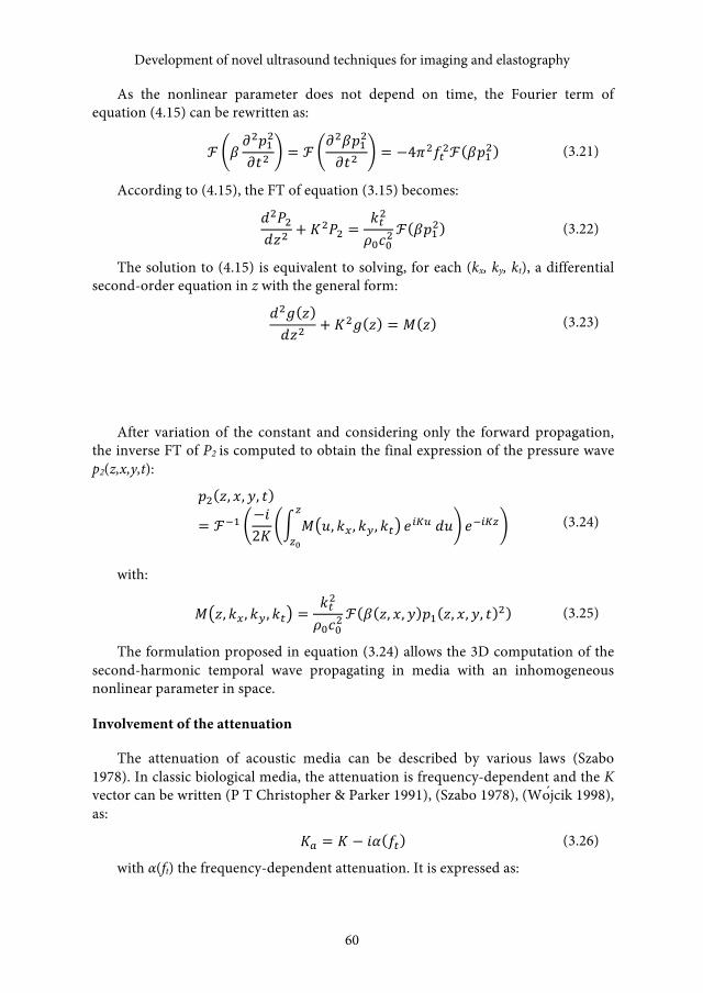
Development of novel ultrasound techniques for imaging and elastography
60
As the nonlinear parameter does not depend on time, the Fourier term of equation (4.15) can be rewritten as:
ℱ 𝛽𝛽𝜕𝜕!𝑝𝑝!!
𝜕𝜕𝑡𝑡!= ℱ
𝜕𝜕!𝛽𝛽𝑝𝑝!!
𝜕𝜕𝑡𝑡!= −4𝜋𝜋!𝑓𝑓!!ℱ 𝛽𝛽𝑝𝑝!! (3.21)
According to (4.15), the FT of equation (3.15) becomes:
𝑑𝑑!𝑃𝑃!𝑑𝑑𝑧𝑧!
+ 𝐾𝐾!𝑃𝑃! =𝑘𝑘!!
𝜌𝜌!𝑐𝑐!!ℱ 𝛽𝛽𝑝𝑝!! (3.22)
The solution to (4.15) is equivalent to solving, for each (kx, ky, kt), a differential second-order equation in z with the general form:
𝑑𝑑!𝑔𝑔 𝑧𝑧𝑑𝑑𝑧𝑧!
+ 𝐾𝐾!𝑔𝑔 𝑧𝑧 = 𝑀𝑀 𝑧𝑧 (3.23)
After variation of the constant and considering only the forward propagation, the inverse FT of P2 is computed to obtain the final expression of the pressure wave p2(z,x,y,t):
𝑝𝑝! 𝑧𝑧, 𝑥𝑥, 𝑦𝑦, 𝑡𝑡
= ℱ!! −𝑖𝑖2𝐾𝐾
𝑀𝑀 𝑢𝑢, 𝑘𝑘! , 𝑘𝑘! , 𝑘𝑘!!
!!𝑒𝑒!"# 𝑑𝑑𝑑𝑑 𝑒𝑒!!"# (3.24)
with:
𝑀𝑀 𝑧𝑧, 𝑘𝑘! , 𝑘𝑘! , 𝑘𝑘! =𝑘𝑘!!
𝜌𝜌!𝑐𝑐!!ℱ 𝛽𝛽 𝑧𝑧, 𝑥𝑥, 𝑦𝑦 𝑝𝑝! 𝑧𝑧, 𝑥𝑥, 𝑦𝑦, 𝑡𝑡 ! (3.25)
The formulation proposed in equation (3.24) allows the 3D computation of the second-harmonic temporal wave propagating in media with an inhomogeneous nonlinear parameter in space.
Involvement of the attenuation
The attenuation of acoustic media can be described by various laws (Szabo 1978). In classic biological media, the attenuation is frequency-dependent and the K vector can be written (P T Christopher & Parker 1991), (Szabo 1978), (Wo ́jcik 1998), as:
𝐾𝐾! = 𝐾𝐾 − 𝑖𝑖𝑖𝑖 𝑓𝑓! (3.26)
with α(ft) the frequency-dependent attenuation. It is expressed as:
Development of novel ultrasound techniques for imaging and elastography
60

Alessandro Ramalli
61
𝛼𝛼 𝑓𝑓! = 𝛼𝛼!𝑓𝑓!10!
!
(3.27)
with γ a number between 1 and 2 for biological media that translates the frequency-dependent law and α0 the attenuation constant of the medium in Np.m-1
MHz-γ. To take into account the attenuation of the medium using the GASM, the previous expressions of p1 and p2 using the K vector have to be updated by replacing K with Ka. If different absorption behaviors have to be used, only this part must be updated to take into account the new law.
Computer implementation
Equations (3.19) and (3.24) were implemented using C language and the FT was performed using the FFTW library (Frigo & Johnson 2005). The accuracy and the calculation time of the simulations depend on the resolution considered in the spatial and temporal dimensions. For each Δz step, the evolution of the fundamental wave p1 in 3D (x,y,t) is computed, first in the Fourier domain and then in the temporal domain. It must be noted that the fundamental does not depend on the z sampling. With the temporal evolution of the fundamental, the matrix M(z+Δz) could be computed. Then, to obtain the final evolution of the second-harmonic wave, an integral part, noted I, must be computed. A classic finite difference method has been chosen to compute this integral. Thanks to the previous computed value at M(z), the new value of the integral can be obtained by:
𝐼𝐼 𝑧𝑧 + ∆𝑧𝑧 = 𝑀𝑀 𝑢𝑢 𝑒𝑒!"# 𝑑𝑑𝑑𝑑!!∆!
!!
= 𝑀𝑀 𝑢𝑢 𝑒𝑒!"# 𝑑𝑑𝑑𝑑 + 𝑀𝑀 𝑢𝑢 𝑒𝑒!"# 𝑑𝑑𝑑𝑑!!∆!
!
!
!!
(3.28)
Then the iteration solution of (4.15) gives:
𝐼𝐼 𝑧𝑧 + ∆𝑧𝑧 = 𝐼𝐼 𝑧𝑧 +𝑀𝑀 𝑧𝑧 + ∆𝑧𝑧 𝑒𝑒!" !!∆! +𝑀𝑀 𝑧𝑧 𝑒𝑒!"#
2∆𝑧𝑧 (3.29)
From (3.29), the final Fourier and temporal evolution of the second harmonic is easily computed from the two 3D matrices M(z) and M(z+Δz). This integration step is the key point necessary to take into account the total 3D inhomogeneous nonlinear parameter.
Alessandro Ramalli
61
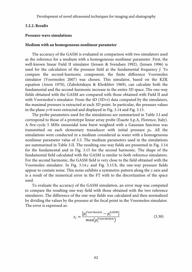
Development of novel ultrasound techniques for imaging and elastography
62
3.2.2. Results
Pressure-wave simulations
Medium with an homogeneous nonlinear parameter
The accuracy of the GASM is evaluated in comparison with two simulators used as the reference for a medium with a homogeneous nonlinear parameter. First, the well-known linear Field II simulator (Jensen & Svendsen 1992), (Jensen 1996) is used for the calculation of the pressure field at the fundamental frequency f. To compare the second-harmonic component, the finite difference Voormolen simulator (Voormolen 2007) was chosen. This simulator, based on the KZK equation (Anon 1970), (Zabolotskaya & Khokhlov 1969), can calculate both the fundamental and the second-harmonic increase in the entire 3D space. The one-way fields obtained with the GASM are compared with those obtained with Field II and with Voormolen’s simulator. From the 4D (3D+t) data computed by the simulators, the maximal pressure is extracted at each 3D point. In particular, the pressure values in the plane y=0 were extracted and displayed in Fig. 3.14 and Fig. 3.15.
The probe parameters used for the simulations are summarized in Table 3.I and correspond to those of a prototype linear array probe (Esaote S.p.A, Florence, Italy). A five-cycle 5 MHz sinusoidal tone burst weighted with a Gaussian function was transmitted on each elementary transducer with initial pressure p0. All the simulations were conducted in a medium considered as water with a homogeneous nonlinear parameter value of 3.5. The medium parameters used in the simulations are summarized in Table 3.II. The resulting one-way fields are presented in Fig. 3.14 for the fundamental and in Fig. 3.15 for the second harmonic. The shape of the fundamental field calculated with the GASM is similar to both reference simulators. For the second harmonic, the GASM field is very close to the field obtained with the Voormolen simulator. In Fig. 3.14.c and Fig. 3.15.b, the one-way pressure fields appear to contain noise. This noise exhibits a symmetric pattern along the z-axis and is a result of the numerical error in the FT with to the discretization of the space used.
To evaluate the accuracy of the GASM simulation, an error map was computed to compare the resulting one-way field with those obtained with the two reference simulators. The difference of the one-way fields was calculated and then normalized by dividing the values by the pressure at the focal point in the Voormolen simulator. The error is expressed as:
𝜀𝜀! =𝑝𝑝!!""#$"%&' − 𝑝𝑝!!"#$
max 𝑝𝑝!!""#$"%&'(3.30)
Development of novel ultrasound techniques for imaging and elastography
62
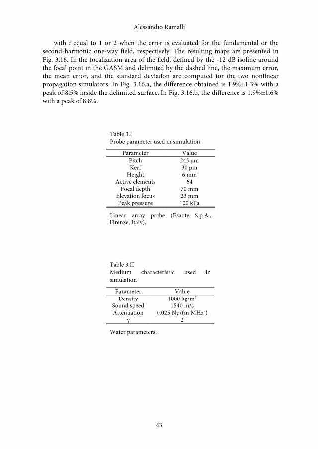
Alessandro Ramalli
63
Firenze, Italy).
Table 3.II Medium characteristic used in simulation
Parameter Value Density 1000 kg/m3
Sound speed 1540 m/s Attenuation 0.025 Np/(m MHz2)
γ 2
Water parameters.
Table 3.I Probe parameter used in simulation
Parameter Value Pitch 245 µm Kerf 30 µm
Height 6 mm Active elements 64
Focal depth 70 mm Elevation focus 23 mm Peak pressure 100 kPa
Linear array probe (Esaote S.p.A.,
with i equal to 1 or 2 when the error is evaluated for the fundamental or the second-harmonic one-way field, respectively. The resulting maps are presented in Fig. 3.16. In the focalization area of the field, defined by the -12 dB isoline around the focal point in the GASM and delimited by the dashed line, the maximum error, the mean error, and the standard deviation are computed for the two nonlinear propagation simulators. In Fig. 3.16.a, the difference obtained is 1.9%±1.3% with a peak of 8.5% inside the delimited surface. In Fig. 3.16.b, the difference is 1.9%±1.6% with a peak of 8.8%.
Alessandro Ramalli
63
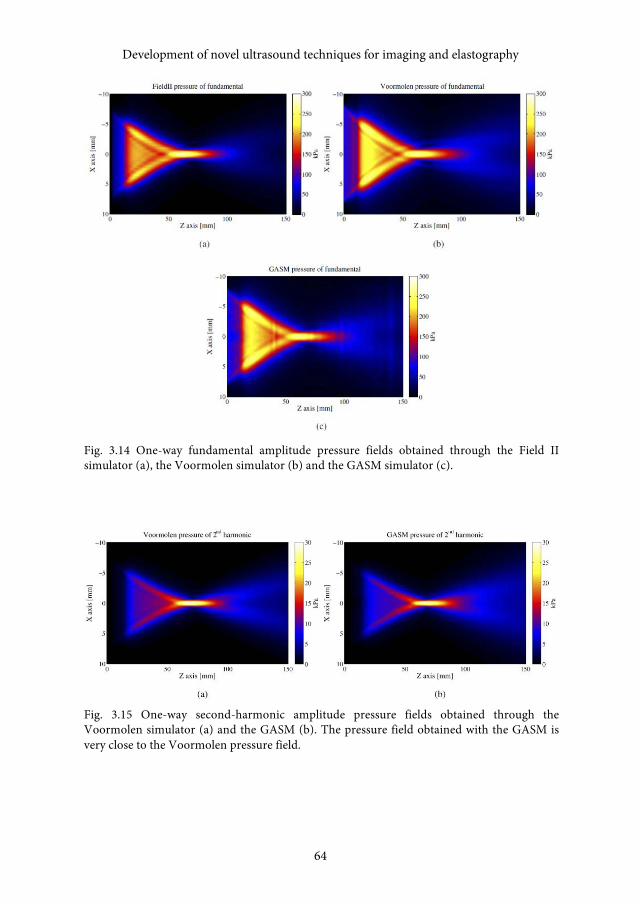
Development of novel ultrasound techniques for imaging and elastography
64
Fig. 3.14 One-way fundamental amplitude pressure fields obtained through the Field II simulator (a), the Voormolen simulator (b) and the GASM simulator (c).
Fig. 3.15 One-way second-harmonic amplitude pressure fields obtained through the Voormolen simulator (a) and the GASM (b). The pressure field obtained with the GASM is very close to the Voormolen pressure field.
Development of novel ultrasound techniques for imaging and elastography
64
Alessandro Ramalli
65
Fig. 3.16 Error map of the fundamental component of the GASM in comparison with (a) the Field II and (b) the Voormolen simulator. The dashed line is the -12 dB isoline and outlines the region where the error is considered. The pressure fields are normalized by the pressure obtained in the focal point.
Medium with an inhomogeneous nonlinear parameter
The GASM takes into account the variations of the nonlinear parameter by the integrative part of the variable M(z,kx,ky,kt) (3.25).With Voormolen’s KZK simulator (Voormolen 2007), it is possible to simulate a variation of the nonlinear parameter only along the z-axis. To compare the two simulators, we considered the case of a surrounding medium with a nonlinear parameter β1=3.5 with an inclusion of a nonlinear parameter β2=7. A linear slope of the nonlinear parameter’s evolution was used at the interface of the two media to avoid a discontinuity (Fig. 3.17.a). The probe parameters of the transmitted signal are the same as the previous ones and are summarized in Table 3.I. The resulting pressure profiles are presented in Fig. 3.17.b. The peak of the temporal response was computed along the z-axis of the probe with the GASM. Its evolution is very similar to that calculated with the Voormolen simulator. The error obtained for the second harmonic, when a medium with a homogeneous nonlinear parameter is considered, is 3.7%±1.9% with a peak error of 8.1%. When the inclusion is considered (inhomogeneous β), the error is 3.4%±2.2% with a peak error of 7.8%.
The GASM simulates more complex media, with 3D variations of the nonlinear parameter which cannot be simulated by the previously mentioned simulators. This property of the GASM is illustrated by two simulations. The first one is based on a phantom including two media disposed as follows: the upper region (corresponding to the negative x-axis) has a nonlinear parameter that is ten times higher than in the lower region. The resulting second-harmonic field obtained with the GASM is shown in Fig. 3.18.a. The pressure field is significantly different in the two regions. The amplitude of the second-harmonic component is larger in the area with higher nonlinear parameter and the peak is not centered on the probe axis. In the second simulation, the nonlinear parameter varies simultaneously along the x and z directions. The resulting second-harmonic image is shown in Fig. 3.18.b. This
Alessandro Ramalli
65

Development of novel ultrasound techniques for imaging and elastography
66
variation creates two focal points in the second-harmonic field: one at a position close to the focal point of the fundamental, and another one in the region where the nonlinearity increases sharply.
Fig. 3.17 (a) Profiles along the z-axis of the nonlinear parameter set in simulations; it is constant in medium 1 but not in medium 2. (b) Second-harmonic normalized pressure profile computed with the Voormolen and GASM simulators along the beam axis.
Fig. 3.18 One-way field of the second harmonic when the nonlinear parameter is not homogeneous in different directions of space. The dashed line separates the two different regions defined by the nonlinear parameter. Note that these simulations are not possible with the Voormolen and Field II simulators.
Experimental measurements
To test the accuracy of the simulator, experimental acquisition of the fundamental and of the second-harmonic pressure fields was measured and compared with the simulation results. We repeated this test for two different transmission modalities. First, a conventional beam was considered. A five-cycle sine at 6.5 MHz with a Hanning window focused at 20 mm was transmitted. A Hanning apodization was also used on the active elements. Then a nonstandard transmission was used, requiring the application of specific apodization weights wi to each
Development of novel ultrasound techniques for imaging and elastography
66

Alessandro Ramalli
67
element. A Bessel function apodization with respect to the x-axis was chosen (Lu 1997b):
𝑤𝑤! = 𝐽𝐽! 𝛼𝛼𝑟𝑟! (3.31)
with J0 the zero-order Bessel function, α the spatial compression factor and ri the distance between the active element and the center of the probe. To have the maximum intensity transmitted between 10 and 50 mm, an α value of 2100 m-1 was used. A five-cycle sine at 8 MHz with a Hanning window was transmitted. The scanner used was the ULA-OP system developed in the Microelectronics System Design Lab of the University of Florence (Tortoli et al. 2009) coupled with a prototype probe (Esaote S.p.A, Florence, Italy) whose parameters are summarized in Table 3.I. Measurements were made in water, which has a nonlinear parameter of 3.5. A hydrophone (Marconi, Bologna, Italy) recorded the pressure at different positions in the water tank with an accuracy of 0.8 mm in the z-direction and 0.2 mm in the x-direction. The resulting experimental one-way fields are compared with those simulated by GASM in Fig. 3.19 for the focused beam and in Fig. 3.20 for the unfocused beam. The simulated fields show good agreement with the measurement for both the fundamental and second-harmonic components. The error maps of the fundamental and second-harmonic one-way fields were calculated as previously described using the -12dB isoline around the focal point. The error value measurement is summarized in Table 3.III. The large error peak observed in the second-harmonic field is localized in a very small area that is assumed to be an experimental artifact recorded during the experiment as a slight misalignment between the probe and the hydrophone. Because the signal is filtered around the fundamental and second harmonic components, higher harmonics did not degrade the quality of the result. Moreover, the third harmonic is merged in the experimental noise recorded by the hydrophone.
Table 3.III GASM simulations errors
Mean Error Standard deviation Peak error Focused beam p1 5.4% 2.7% 14.5%
p2 6.7% 5.3% 24.8% Unfocused beam p1 6.1% 3.8% 18.2%
p2 5.8% 4.6% 30.7%
Simulations were compared with experimental measurements
Alessandro Ramalli
67
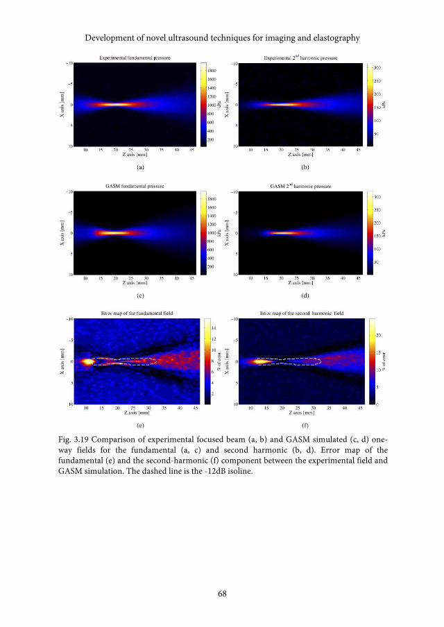
Development of novel ultrasound techniques for imaging and elastography
68
Fig. 3.19 Comparison of experimental focused beam (a, b) and GASM simulated (c, d) one-way fields for the fundamental (a, c) and second harmonic (b, d). Error map of the fundamental (e) and the second-harmonic (f) component between the experimental field and GASM simulation. The dashed line is the -12dB isoline.
Development of novel ultrasound techniques for imaging and elastography
68
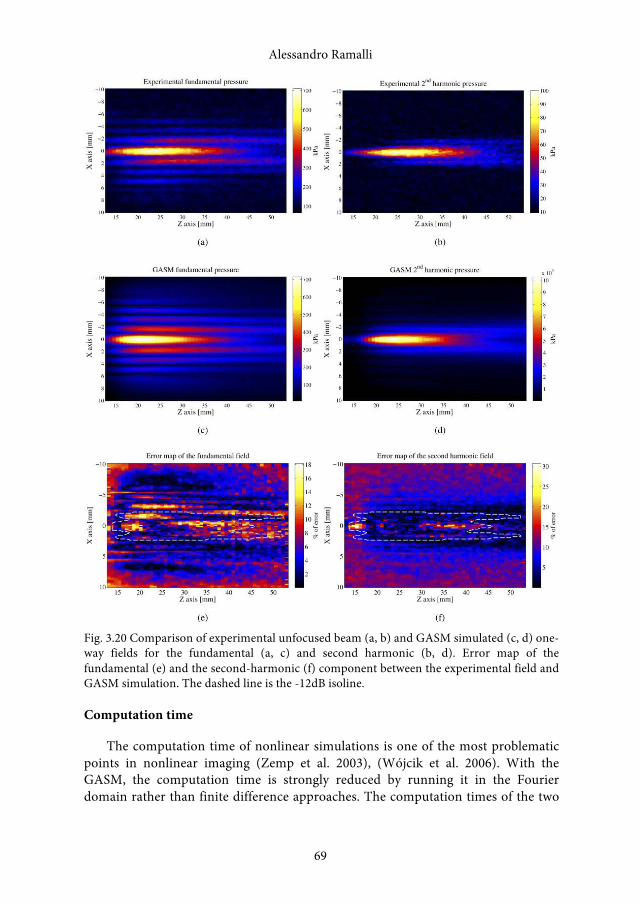
Alessandro Ramalli
69
Fig. 3.20 Comparison of experimental unfocused beam (a, b) and GASM simulated (c, d) one-way fields for the fundamental (a, c) and second harmonic (b, d). Error map of the fundamental (e) and the second-harmonic (f) component between the experimental field and GASM simulation. The dashed line is the -12dB isoline.
Computation time
The computation time of nonlinear simulations is one of the most problematic points in nonlinear imaging (Zemp et al. 2003), (Wójcik et al. 2006). With the GASM, the computation time is strongly reduced by running it in the Fourier domain rather than finite difference approaches. The computation times of the two
Alessandro Ramalli
69
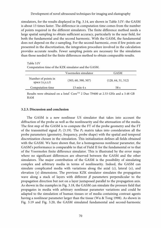
Development of novel ultrasound techniques for imaging and elastography
70
simulators, for the results displayed in Fig. 3.14, are shown in Table 3.IV: the GASM is about 13 times faster. The difference in computation time comes from the number of points required in the different simulators. The finite difference method needs a large spatial sampling to obtain sufficient accuracy, particularly in the near field, for both the fundamental and the second harmonic. With the GASM, the fundamental does not depend on the z-sampling. For the second-harmonic, even if few points are presented in the discretization, the integration procedure involved in the calculation provides accurate results. Fewer sampling points are necessary for the simulation than those needed for the finite differences method to obtain comparable results.
Table 3.IV Computation time of the KZK simulator and the GASM.
Voormolen simulator GASM
Number of points in space (x,y,z,t) (303, 60, 390, 507) (128, 64, 51, 512)
Computation time 13 min 4 s 58 s
Results were obtained on a Intel® CoreTM 2 Duo T9400 at 2.53 GHz and a 3.48 GB RAM
3.2.3. Discussion and conclusion
The GASM is a new nonlinear US simulator that takes into account the diffraction of the probe as well as the nonlinearity and the attenuation of the media. The first step of the GASM is to compute the FT of the probe geometry and the FT of the transmitted signal P0 (3.19). The P0 matrix takes into consideration all the probe parameters (geometry, frequency, probe shape) with the spatial and temporal discretization chosen in the simulation. This initialization defines all fields obtained with the GASM. We have shown that, for a homogeneous nonlinear parameter, the GASM’s performance is comparable to that of Field II for the fundamental or to that of the Voormolen finite difference simulator. This is illustrated by the error maps where no significant differences are observed between the GASM and the other simulators. The major contribution of the GASM is the possibility of simulating complex and arbitrary media in terms of nonlinearity. Indeed, the GASM can simulate complicated media with variations along the axial (z), lateral (x), and elevation (y) dimensions. The previous KZK simulator simulates the propagation wave along a stack of layers with different β parameters perpendicular to the propagation direction but not on a layer juxtaposed parallel to the propagation axis. As shown in the examples in Fig. 3.18, the GASM can simulate the pressure field that propagates in media with arbitrary nonlinear parameter variations and could be adapted to the simulation of human tissues or of media containing contrast agents having a nonlinear parameter larger than the tissue (Wu & Tong 1998). As shown in Fig. 3.19 and Fig. 3.20, the GASM simulated fundamental and second-harmonic
Development of novel ultrasound techniques for imaging and elastography
70
Alessandro Ramalli
71
fields are close to the experimental fields. The computation time of the GASM is about 13 times faster than standard nonlinear simulators. Faster nonlinear simulations of a complete 3D space can be made. Of course, it must be remembered that the Voormolen simulator works for higher-order nonlinear interactions, while the GASM is based on first-order perturbation.
The GASM presents certain unavoidable limitations. First, the use of the FT adds noise in the resulting pressure field. This noise slightly degrades the final aspect of the field, although, as shown by the error maps, the accuracy of the GASM in the active part of the field is satisfactory. In the proposed approach, a compromise has been made between the accuracy and the speed of computation. An increase of the considered number of points in the different matrices will decrease the aliasing effect but also increase the computation time. For high resolution simulations, tools based on finite difference scheme, computing high order nonlinear effect, have to be preferred. Secondly, no nonlinear interactions between different frequency components are taken into account in the proposed simulator. Indeed, if a wave composed of two frequencies is transmitted in the medium, the simulator processes the wave as two single-frequency waves with no interactions between them. In a real medium, a nonlinear interaction takes place and creates other pressure waves at the difference and sum frequencies. Another limitation of the GASM is the quasi-linear approximation, which limits the simulation in terms of initial amplitude. If the second harmonic is no more small compared to the fundamental, this assumption is no longer valid and the nonlinearity phenomena are too large to be simulated with the GASM. This limit depends on the different probe parameters, on the beamforming in transmission, on the transmitted signal and on the propagation depth to reach. The last approximation made in the proposed method consists in considering only transmitted waves and to not take into account possible reflected waves due to the inhomogeneous nonlinear map. This effect has to be quantified in future version of the GASM.
Future developments of this work would include the possibility of creating nonlinear radio-frequency (RF) images combining the GASM field simulation of a 3D nonlinear parameter map with a 3D scatterer map and a strategy in reception to reconstruct the RF image. Three-dimensional simulations of any application involving nonlinear imaging can be considered.
The GASM is currently usable for fundamental and second-harmonic computation. However, with the same quasi-linear approximation, a higher order of nonlinearity can be reached. The third or fourth harmonic can be simulated versus an increase in computation time. An optimal implementation has to be found to relate the nonlinear order, the desired accuracy, and the computation time.
Alessandro Ramalli
71

4. A Novel Ultrasound Experimental Method: FrequencyDomain Elastography
As the result of the system development process a novel algorithm for quasi-static elastography is presented. This chapter, draws on (Ramalli et al. 2010),(Ramalli, Boni, et al. 2011),(Ramalli, Ricci, et al. 2011),(Ramalli et al. 2012), shows that the quality of elastograms can be improved through the integration of two distinct techniques in the strain estimation procedure, taking further advantage from high frame-rate imaging. The results are compared with those of a well-established algorithm; in-vitro and in-vivo elastograms are shown. The ULA-OP real-time implementation and the related results are presented.
4.1. Introduction
Modifications of a tissue elasticity are often correlated with pathological processes: breast (Samani et al. 2007), (Thitaikumar et al. 2008), prostate (Krouskop et al. 1998) and thyroid (Dighe et al. 2008), (Lyshchik et al. 2005) carcinoma appear as hard nodules, cirrhosis of the liver brings on a diffuse reduction of its elasticity (Kapoor et al. 2011), and benign tumors such as cysts are softer than the surrounding tissue. The simplest and the most widely used technique to reveal such diseases is manual palpation, which allows the examiner to feel for abnormalities. In recent years, a new ultrasound imaging technique, elastography, has been developed (Ophir et al. 1991). It allows imaging the stiffness of tissue, in so-called elastograms, with improved sensitivity, objectivity, and accuracy compared to manual palpation.
The different elastography approaches can be divided into three main groups: quasi-static, transient and harmonic. In the first case, stress is applied by compressing the medium and in the other two it is dynamically applied by the generation and propagation of shear waves (Sandrin et al. 2002), (Tanter et al. 2002). In freehand quasi-static elastography, which is the topic of this chapter, the operator applies compression over the region of interest through an ultrasound probe, in order to induce strain inside the tissue. The response to such compression depends on the tissue stiffness. The consecutive radio-frequency (RF) ultrasonic echoes, recorded during compression, are exploited to calculate displacement, which, in gradient-based strain estimators, is differentiated to obtain the strain field.
The displacement can be estimated from the time-shift between consecutive echo-signals considering either the maximum of the cross-correlation function (Ophir et al. 1991), (Bilgen 1996), the correlation phase (Pesavento et al. 1999),
Alessandro Ramalli, Development of novel ultrasound techniques for imaging and elastography : from simulation to real-time implementation ISBN 978-88-6655-456-1 (print) ISBN 978-88-6655-457-8 (online) © 2013 Firenze University Press
Development of novel ultrasound techniques for imaging and elastography
74
(O’Donnell et al. 1994) or the weighted phase separation (Lindop et al. 2008). For example, the reference method proposed by Pesavento (Pesavento et al. 1999), consists in an iterative phase zero estimation algorithm that estimates the time shifts from the phase of the correlation function and converges to the position of the maximum of the cross-correlation function. Such phase-sensitive methods are called coherent and are distinguished from the incoherent methods, which directly estimate strain without computing displacement (Konofagou et al. 1999), (Varghese & Ophir 1998b). As reported in (Konofagou et al. 2000), (Varghese et al. 2000), the accuracy of incoherent methods suffers from the low signal-to-noise ratio of elastograms obtained at low strain values. On the other hand, the robustness of all coherent methods suffers from possible decorrelation of consecutive echoes due to undesired lateral and elevational motion of tissue, to the operator’s hand, which does not have a perfectly axial movement, or to any other phase noise source (Konofagou et al. 1999). Although 2D and 3D techniques take into account lateral and elevational displacements (Brusseau et al. 2008), (Deprez et al. 2009), (Ebbini 2006), they are time-consuming and require the development of a computationally efficient code.
The goal of this chapter is to contribute to the improvement of elastogram quality by integrating two distinct approaches. First, we propose a method for time-shift estimation, based on the calculation of the phase shift between the spectra of consecutive RF echo signals. This method can accurately evaluate the time shift considering only a small number of points in the Fourier domain. Second, it is proposed to exploit the huge amount of echo data available in the so-called high-frame-rate (HFR) imaging systems, to improve the signal-to-noise ratio of elastography images. This latter goal is met by performing multiple displacement estimations, which are averaged maintaining the usual elastogram frame rate (in the order of tens of Hertz). It is shown that the two approaches, which are independent of each other, can individually provide significant benefits in terms of image quality and that their integration leads to greater benefits.
Furthermore, the proposed method is applied in freehand investigation both for phantom and in-vivo investigation of breast nodules. Elastography movies were obtained for 11 patients with breast nodules, aged between 30 and 84 years and the lesions were clearly visible in all elastograms.
Finally, a real-time implementation of the frequency domain displacement estimation algorithm is implemented on ULA-OP and results are shown.
4.2. Methods
Displacement and strain estimation in the frequency domain
Let us consider two RF signals, 𝑠𝑠! and 𝑠𝑠!, referring to the same line on consecutive images during a quasi-static elastography exam. In the following, we will refer to them as pre- and post-compression signals, respectively, see diagram in Fig. 4.1. If such signals are sampled at a rate fs and gated over an interval of length Nw/fs, we obtain the sequences:
Development of novel ultrasound techniques for imaging and elastography
74
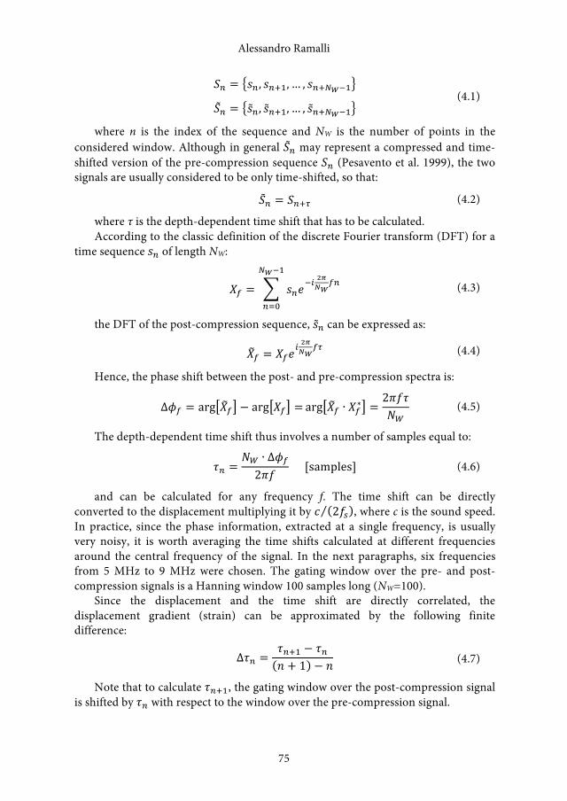
Alessandro Ramalli
75
𝑆𝑆! = 𝑠𝑠!, 𝑠𝑠!!!,… , 𝑠𝑠!!!!!!
𝑆𝑆! = 𝑠𝑠!, 𝑠𝑠!!!,… , 𝑠𝑠!!!!!! (4.1)
where n is the index of the sequence and NW is the number of points in the considered window. Although in general 𝑆𝑆! may represent a compressed and time-shifted version of the pre-compression sequence 𝑆𝑆! (Pesavento et al. 1999), the two signals are usually considered to be only time-shifted, so that:
𝑆𝑆! = 𝑆𝑆!!! (4.2)
where τ is the depth-dependent time shift that has to be calculated. According to the classic definition of the discrete Fourier transform (DFT) for a
time sequence 𝑠𝑠! of length NW:
𝑋𝑋! = 𝑠𝑠!𝑒𝑒!! !!!!
!"!!!!
!!!
(4.3)
the DFT of the post-compression sequence, 𝑠𝑠! can be expressed as:
𝑋𝑋! = 𝑋𝑋!𝑒𝑒! !!!!
!" (4.4)
Hence, the phase shift between the post- and pre-compression spectra is:
∆𝜙𝜙! = arg 𝑋𝑋! − arg 𝑋𝑋! = arg 𝑋𝑋! ∙ 𝑋𝑋!∗ =2𝜋𝜋𝜋𝜋𝜋𝜋𝑁𝑁!
(4.5)
The depth-dependent time shift thus involves a number of samples equal to:
𝜏𝜏! =𝑁𝑁! ∙ ∆𝜙𝜙!2𝜋𝜋𝜋𝜋
[samples] (4.6)
and can be calculated for any frequency f. The time shift can be directly converted to the displacement multiplying it by 𝑐𝑐 2𝑓𝑓! , where c is the sound speed. In practice, since the phase information, extracted at a single frequency, is usually very noisy, it is worth averaging the time shifts calculated at different frequencies around the central frequency of the signal. In the next paragraphs, six frequencies from 5 MHz to 9 MHz were chosen. The gating window over the pre- and post-compression signals is a Hanning window 100 samples long (NW=100).
Since the displacement and the time shift are directly correlated, the displacement gradient (strain) can be approximated by the following finite difference:
∆𝜏𝜏! =𝜏𝜏!!! − 𝜏𝜏!𝑛𝑛 + 1 − 𝑛𝑛
(4.7)
Note that to calculate 𝜏𝜏!!!, the gating window over the post-compression signal is shifted by 𝜏𝜏! with respect to the window over the pre-compression signal.
Alessandro Ramalli
75
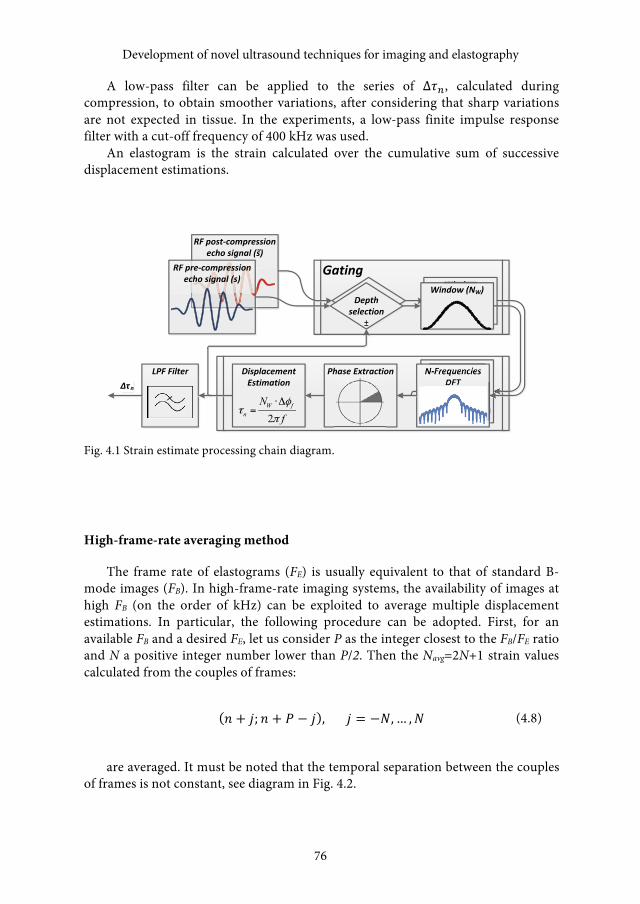
Development of novel ultrasound techniques for imaging and elastography
76
A low-pass filter can be applied to the series of ∆𝜏𝜏!, calculated during compression, to obtain smoother variations, after considering that sharp variations are not expected in tissue. In the experiments, a low-pass finite impulse response filter with a cut-off frequency of 400 kHz was used.
An elastogram is the strain calculated over the cumulative sum of successive displacement estimations.
Gating
Depth selectionDepth
selection
Window (NW)
RF post-‐compression echo signal (s)̃
RF pre-‐compression echo signal (s)
N-‐FrequenciesDFT
Phase ExtractionDisplacement Estimation
2W f
n
Nfφ
τπ
⋅Δ=
±
LPF FilterΔτn
Fig. 4.1 Strain estimate processing chain diagram.
High-frame-rate averaging method
The frame rate of elastograms (FE) is usually equivalent to that of standard B-mode images (FB). In high-frame-rate imaging systems, the availability of images at high FB (on the order of kHz) can be exploited to average multiple displacement estimations. In particular, the following procedure can be adopted. First, for an available FB and a desired FE, let us consider P as the integer closest to the FB/FE ratio and N a positive integer number lower than P/2. Then the Navg=2N+1 strain values calculated from the couples of frames:
𝑛𝑛 + 𝑗𝑗; 𝑛𝑛 + 𝑃𝑃 − 𝑗𝑗 , 𝑗𝑗 = −𝑁𝑁,… ,𝑁𝑁 (4.8)
are averaged. It must be noted that the temporal separation between the couples of frames is not constant, see diagram in Fig. 4.2.
Development of novel ultrasound techniques for imaging and elastography
76

Alessandro Ramalli
77
Fig. 4.2 Averaging of HFR elastograms.
This is equivalent to locally varying the elastogram frame rate. The number of frames that can contribute to averaging depends on the actual values of FB and FE. Examples are given in the following section.
The proposed method was tested with two different HFR imaging methods. In both methods, multiple steered plane waves, covering a sector angle, are subsequently transmitted by a linear array transducer to reconstruct a single compounded B-mode frame. In the Fourier method, proposed by Lu et al. (Lu 1997a), (Cheng & Lu 2006) the RF echo signals are received and weighted in order to produce limited diffraction beams. The elaborated signals are then used to calculate the spatial Fourier transform of the region of interest. The Fourier domain images are compounded and the final B-mode image is reconstructed by an inverse spatial Fourier transform. In the coherent plane-wave compounding method, proposed by Tanter et al. (Tanter et al. 2002), (Montaldo et al. 2009) the reception consists in the coherent sum of backscattered echoes from all illuminations and the images are compounded in the time domain. The use of different steering angles increases the quality of the B-mode images in terms of noise, artifacts, and resolution, while reducing the frame rate.
Elastogram non-uniformity level and contrast-to-noise ratio
The different elastograms were compared using the non-uniformity (NU) level as a quality index (Magnusson & Olsson 2000), (Giannelli et al. 2010) together with the elastographic contrast-to-noise ratio (CNRe) (Varghese & Ophir 1998a).
Alessandro Ramalli
77
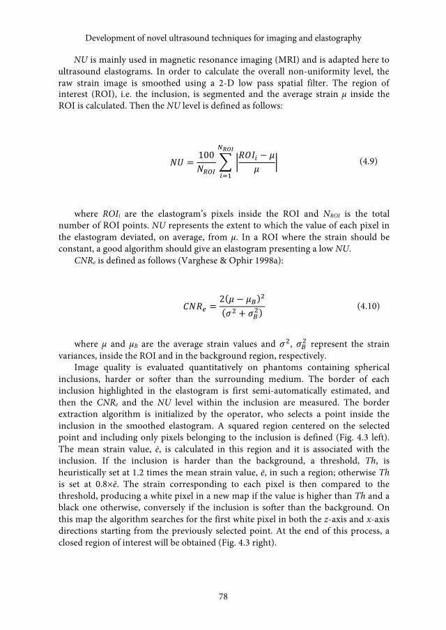
Development of novel ultrasound techniques for imaging and elastography
78
interest (ROI), i.e. the inclusion, is segmented and the average strain µ inside the ROI is calculated. Then the NU level is defined as follows:
𝑁𝑁𝑁𝑁 =100𝑁𝑁!"#
𝑅𝑅𝑅𝑅𝐼𝐼! − 𝜇𝜇𝜇𝜇
!!"#
!!!
(4.9)
where ROIi are the elastogram’s pixels inside the ROI and NROI is the total number of ROI points. NU represents the extent to which the value of each pixel in the elastogram deviated, on average, from µ. In a ROI where the strain should be constant, a good algorithm should give an elastogram presenting a low NU.
CNRe is defined as follows (Varghese & Ophir 1998a):
𝐶𝐶𝐶𝐶𝑅𝑅! =2 𝜇𝜇 − 𝜇𝜇! !
𝜎𝜎! + 𝜎𝜎!!(4.10)
where µ and µB are the average strain values and 𝜎𝜎!, 𝜎𝜎!! represent the strain variances, inside the ROI and in the background region, respectively.
Image quality is evaluated quantitatively on phantoms containing spherical inclusions, harder or softer than the surrounding medium. The border of each inclusion highlighted in the elastogram is first semi-automatically estimated, and then the CNRe and the NU level within the inclusion are measured. The border extraction algorithm is initialized by the operator, who selects a point inside the inclusion in the smoothed elastogram. A squared region centered on the selected point and including only pixels belonging to the inclusion is defined (Fig. 4.3 left). The mean strain value, ē, is calculated in this region and it is associated with the inclusion. If the inclusion is harder than the background, a threshold, Th, is heuristically set at 1.2 times the mean strain value, ē, in such a region; otherwise Th is set at 0.8×ē. The strain corresponding to each pixel is then compared to the threshold, producing a white pixel in a new map if the value is higher than Th and a black one otherwise, conversely if the inclusion is softer than the background. On this map the algorithm searches for the first white pixel in both the z-axis and x-axis directions starting from the previously selected point. At the end of this process, a closed region of interest will be obtained (Fig. 4.3 right).
NU is mainly used in magnetic resonance imaging (MRI) and is adapted here to ultrasound elastograms. In order to calculate the overall non-uniformity level, the raw strain image is smoothed using a 2-D low pass spatial filter. The region of
Development of novel ultrasound techniques for imaging and elastography
78

Fig. 4.3 Extraction of the inclusion border. The filtered elastogram is shown on the left. The white dot represents the initialization point and the white square is the region where the mean value of the elastogram, ē, is evaluated. On the right, the result of the semi-automatic segmentation procedure. The red contour outlines the ROI. The dotted lines define the background region used to compute the CNRe.
4.3. Computational cost analysis and reduction
A modified version of the frequency domain displacement estimation method, capable of reducing its computational cost, is presented here. This approach is based on the hypothesis that sharp strain variations in biological tissues are not present and the strain signal is inherently a smooth signal.
This hypothesis reduces the depths over which the displacement is evaluated by a decimation factor, K. This means that the position of the gating windows over the pre- and post-compression RF signals is changed in steps of K samples.
The computational cost is assessed by considering three different cost functions, i.e. the number of multiplications (Nmult), sums (Nsum) and phase extractions (Nph-ext).
𝑁𝑁!"#$ = 𝑁𝑁!"# ≅ 4𝑁𝑁!𝑁𝑁!𝑁𝑁!"#𝑁𝑁!𝑁𝑁!
𝐾𝐾
𝑁𝑁!!!!"# = 2𝑁𝑁!𝑁𝑁!𝑁𝑁!"#𝑁𝑁!
𝐾𝐾
(4.11)
where NL is the number of lines of the elastogram, NS the number of samples of the RF signal, Navg is the number of averaged frames, NW is the number of points of the local window over the RF signal and NP is the number of frequencies considered.
Alessandro Ramalli
79

4.4. Computer-guided compression experiments
4.4.1. Experimental setup
The ultrasound system used for acquisition was the ULA-OP (Tortoli et al. 2009), the research sonographer described in 2.
ULA-OP was programmed to provide HFR images, by driving the 64 central elements of a 192-element linear array (LA533, Esaote SpA, Florence, Italy). The excitation signal was a five-cycle sinusoidal burst at 6 MHz, weighted by a Hanning window. Steered plane waves were transmitted with steering angles of −6.5°, −3.25°, 0°, 3.25°, 6.5° over five consecutive PRIs, thus covering a total sector of 13°. The pulse repetition frequency (PRF) was 6.25 kHz so that FB could be set at 1.25 kHz. RF echo-signals (32 µs) received during each PRI by each active element of the probe were acquired. By repeating the acquisition on multiple consecutive PRIs, a total acquisition time of 0.64 s was obtained. The acquired data were then post-processed according to both the HFR imaging methods (Lu 1997a), (Cheng & Lu 2006), (Montaldo et al. 2009), as described in Section 4.2 B.
An elastography-dedicated phantom (CIRS, model 049, Norfolk, VA, USA), composed of a background tissue with 29-kPa elasticity containing eight inclusions of four different stiffnesses (elasticity: 6, 17, 54 and 62 kPa) and two different dimensions (diameter, 10 and 20 mm), was used. Data were acquired for the smallest inclusions that are within a 20-mm depth. The probe was fixed to a three-axis numerically controlled motion system, capable of compressing the tissue at a speed of 15, 25 and 35 mm/s. The elastograms were calculated at FE of 12.5, 25, 30, 35, 40, 50 and 75 Hz.
4.4.2. Validation of the displacement estimation method
The proposed displacement estimation method, based on the phase shift in the frequency domain, was estimated by comparing the related elastograms with those obtained according to the method proposed by Pesavento (Pesavento et al. 1999). Indeed, even if other approaches, such as those proposed in (Chaturvedi et al. 1998), (Shiina et al. 2002) could be used, we have assumed the Pesavento method as reference because it is considered particularly efficient and suitable for real-time implementation (Lindop et al. 2006), (Pallwein et al. 2008). In the comparison, the
The above equations clarify the trend of the cost functions that are directly proportional to the number of lines, the samples of the signal, the averaged frames, the window samples and the DFT points and in inverse proportion with the decimation factor. Considering that NL and NS are imposed by the spatial dimensions of a frame and that Navg, NP and NW affect the quality of the elastograms, the decimation factor is the only parameter that can be modified to reduce the computational cost without excessively degrading image quality.
Development of novel ultrasound techniques for imaging and elastography
80
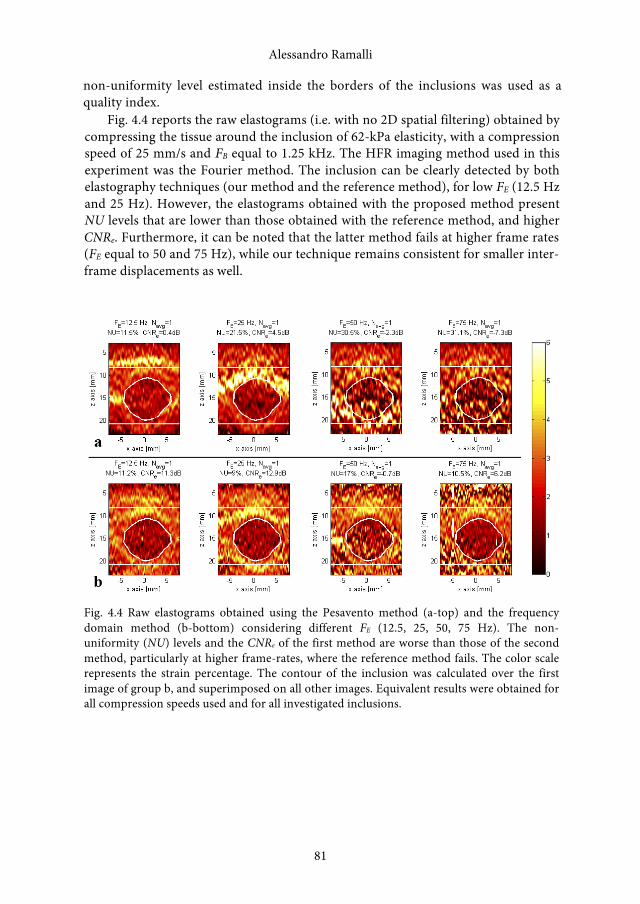
CNRe. Furthermore, it can be noted that the latter method fails at higher frame rates (FE equal to 50 and 75 Hz), while our technique remains consistent for smaller inter-frame displacements as well.
Fig. 4.4 Raw elastograms obtained using the Pesavento method (a-top) and the frequency domain method (b-bottom) considering different FE (12.5, 25, 50, 75 Hz). The non-uniformity (NU) levels and the CNRe of the first method are worse than those of the second method, particularly at higher frame-rates, where the reference method fails. The color scale represents the strain percentage. The contour of the inclusion was calculated over the first image of group b, and superimposed on all other images. Equivalent results were obtained for all compression speeds used and for all investigated inclusions.
Fig. 4.4 reports the raw elastograms (i.e. with no 2D spatial filtering) obtained by compressing the tissue around the inclusion of 62-kPa elasticity, with a compression speed of 25 mm/s and FB equal to 1.25 kHz. The HFR imaging method used in this experiment was the Fourier method. The inclusion can be clearly detected by both elastography techniques (our method and the reference method), for low FE (12.5 Hz and 25 Hz). However, the elastograms obtained with the proposed method present NU levels that are lower than those obtained with the reference method, and higher
non-uniformity level estimated inside the borders of the inclusions was used as a quality index.
Alessandro Ramalli
81
the visual detection of the inclusion. At 75 Hz, the averaging method has no effect and the algorithm fails.
Considering the standard frequency domain displacement estimation method (Fig. 4.5c), the algorithm fails at 75 Hz and is noisy at 40 and 50 Hz, as confirmed by the high NU level and the poor CNRe, but the inclusion is still detectable. The effect of averaging several strain images obtained with the proposed method (Fig. 4.5d) produces a significant reduction of the NU level and a gain in terms of CNRe. Indeed in all the elastograms, NU is reduced to a value around 9%.
To evaluate if the averaging effect is influenced by the HFR imaging method, the same acquired data were used to reconstruct the RF images with the two HFR methods described in (Cheng & Lu 2006) and (Montaldo et al. 2009), respectively, the Fourier method and the coherent compounding method. Fig. 4.6 shows the raw elastograms obtained investigating the inclusion of 6-kPa elasticity, i.e. softer than the background, and compressing the tissue with a speed of 35 mm/s. Only the elastograms for the frame rates of 50 and 75 Hz are reported, i.e., the more critical cases.
Both the Fourier method (Fig. 4.6a,b) and the coherent compounding method (Fig. 4.6c,d) are performed: the frequency domain displacement estimation produces very noisy elastograms, particularly at 75 Hz. Averaging (Navg=9) reduces the NU level and increases CNRe equivalently in both cases.
Using the same inclusion selected for Fig. 4.6, the trend of the NU level over time, i.e. during a compression sequence, was obtained and is reported in Fig. 4.7. These graphs are useful to better understand the effect of averaging during compression.
The selected FE was 75 Hz and the effects of three different Navg values (1,3,9) are compared. The dotted line at 15% represents a heuristic threshold under which the
Fig. 4.5 shows the raw elastograms obtained compressing the tissue around the inclusion of 54 kPa elasticity, with a compression speed of 35 mm/s and FB equal to 1.25 kHz. The values of FE are here equal to 25, 40, 50 and 75 Hz and the algorithms without averaging are compared to those computed by averaging nine frames.
The standard Pesavento method fails for high FE: indeed, in Fig. 4.5a, the NU level is high, the CNRe is low, and the inclusion is not detectable for 40, 50 and 75 Hz. In Fig. 4.5b, the effect of averaging is appreciable for the lowest elastogram frame rates (FE ≤ 40 Hz), where NU is reduced and the inclusion is detectable. A particular case is 50 Hz where NU is reduced and CNRe is increased but not enough to allow
algorithm and the proposed algorithm are compared considering different numbers of averaged frames.
4.4.3. Validation of the HFR averaging method
This section evaluates the performance enhancement provided by the HFR averaging method. The elastograms obtained performing both the Pesavento
Development of novel ultrasound techniques for imaging and elastography
82

83
K=1 K=3 K=5 K=9 Nmult,, Nsum 315 105 63 35
Nph-ext 1.60 0.52 0.30 0.17
Number of Mega operations involved in a single elastogram for different decimation factors (K).
Fig. 4.8 shows the elastograms obtained with and without decimation, by compressing the tissue around the inclusion of 54-kPa elasticity with a compression speed of 35 mm/s and FE equal to 12.5 Hz. The resulting images maintain good quality in each case; indeed the non-uniformity level is quite constant and the CNRe decreases slightly. This confirms that the decimation does not significantly affect the final image but considerably reduces the computational cost. In general, the maximum decimation factor is limited by the speed of compression, indeed when the latter is high, K must be decreased.
4.4.4. Test of the computational cost reduction method
Table 4.I reports the number of multiplications, sums and phase extractions for each frame considering different decimation factors. The setting used in these experiments, i.e. NS=2048, NW=100, NL=64, Navg=1 and NP=6, have been considered here. It is important to note that decimating by a factor of 9, the reduction of thecomputational cost is by approximately one order of magnitude, suggesting that a stronger decimation is feasible, although not necessary.
Table 4.I Computational Cost for an Elastogram Frame
inclusion is considered recognizable in the elastogram. The averaging assures a lower NU level, with both HFR imaging methods, during the entire compression period. In particular, the curves with Navg equal to 9 (red and yellow lines in Fig. 4.7) always remain under the threshold of 15%. The curves decrease slightly because the NU level is progressively reduced by the cumulative sum of the elastograms.
Alessandro Ramalli
83
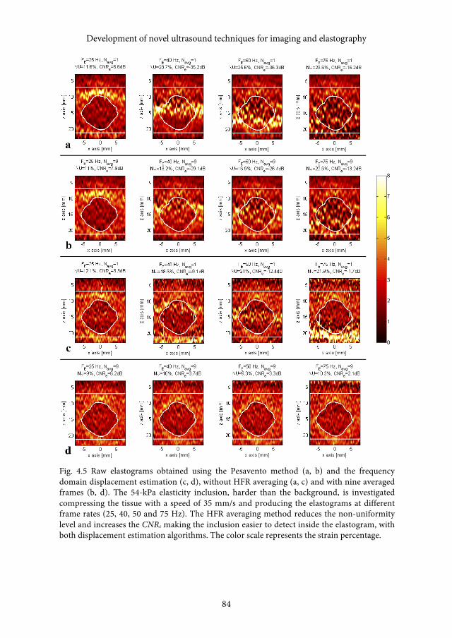
Development of novel ultrasound techniques for imaging and elastography
84
Fig. 4.5 Raw elastograms obtained using the Pesavento method (a, b) and the frequency domain displacement estimation (c, d), without HFR averaging (a, c) and with nine averaged frames (b, d). The 54-kPa elasticity inclusion, harder than the background, is investigated compressing the tissue with a speed of 35 mm/s and producing the elastograms at different frame rates (25, 40, 50 and 75 Hz). The HFR averaging method reduces the non-uniformity level and increases the CNRe making the inclusion easier to detect inside the elastogram, with both displacement estimation algorithms. The color scale represents the strain percentage.
Development of novel ultrasound techniques for imaging and elastography
84
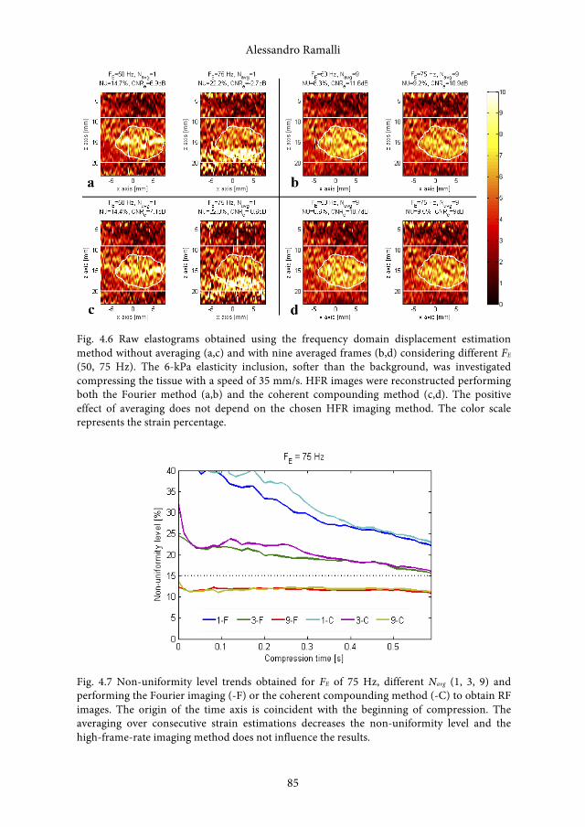
Alessandro Ramalli
85
Fig. 4.6 Raw elastograms obtained using the frequency domain displacement estimation method without averaging (a,c) and with nine averaged frames (b,d) considering different FE (50, 75 Hz). The 6-kPa elasticity inclusion, softer than the background, was investigated compressing the tissue with a speed of 35 mm/s. HFR images were reconstructed performing both the Fourier method (a,b) and the coherent compounding method (c,d). The positive effect of averaging does not depend on the chosen HFR imaging method. The color scale represents the strain percentage.
Fig. 4.7 Non-uniformity level trends obtained for FE of 75 Hz, different Navg (1, 3, 9) and performing the Fourier imaging (-F) or the coherent compounding method (-C) to obtain RF images. The origin of the time axis is coincident with the beginning of compression. The averaging over consecutive strain estimations decreases the non-uniformity level and the high-frame-rate imaging method does not influence the results.
Alessandro Ramalli
85
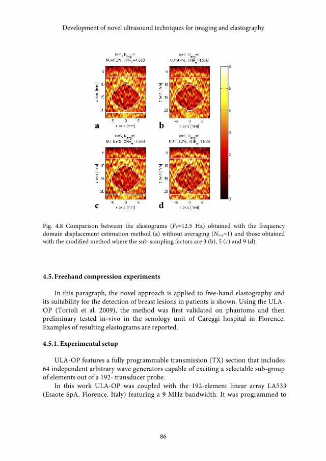
Fig. 4.8 Comparison between the elastograms (FE=12.5 Hz) obtained with the frequencydomain displacement estimation method (a) without averaging (Navg=1) and those obtainedwith the modified method where the sub-sampling factors are 3 (b), 5 (c) and 9 (d).
4.5. Freehand compression experiments
In this paragraph, the novel approach is applied to free-hand elastography and its suitability for the detection of breast lesions in patients is shown. Using the ULA-OP (Tortoli et al. 2009), the method was first validated on phantoms and then preliminary tested in-vivo in the senology unit of Careggi hospital in Florence. Examples of resulting elastograms are reported.
4.5.1. Experimental setup
ULA-OP features a fully programmable transmission (TX) section that includes 64 independent arbitrary wave generators capable of exciting a selectable sub-group of elements out of a 192- transducer probe.
In this work ULA-OP was coupled with the 192-element linear array LA533 (Esaote SpA, Florence, Italy) featuring a 9 MHz bandwidth. It was programmed to
Development of novel ultrasound techniques for imaging and elastography
86
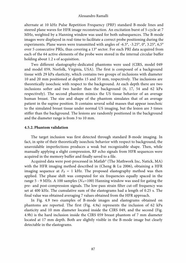
alternate at 10 kHz Pulse Repetition Frequency (PRF) standard B-mode lines and steered plane waves for HFR image reconstruction. An excitation burst of 5-cycle at 7 MHz, weighted by a Hanning window was used for both subsequences. The B-mode images were displayed in real-time to facilitate a correct probe positioning during the experiments. Plane waves were transmitted with angles of -6.5°, -3.25°, 0°, 3.25°, 6,5° over 5 consecutive PRIs, thus covering a 13° sector. For each PRI data acquired from each of the 64 active elements of the probe were stored in the internal circular buffer holding about 1.2 s of acquisition.
Two different elastography-dedicated phantoms were used (CIRS, model 049 and model 059, Norfolk, Virginia, USA). The first is composed of a background tissue with 29 kPa elasticity, which contains two groups of inclusions with diameter 10 and 20 mm positioned at depths 15 and 35 mm, respectively. The inclusions are theoretically isoechoic with respect to the background. At each depth there are two inclusions softer and two harder than the background (6, 17, 54 and 62 kPa respectively). The second phantom mimics the US tissue behavior of an average human breast. The size and shape of the phantom simulates that of an average patient in the supine position. It contains several solid masses that appear isoechoic to the simulated breast tissue under normal US imaging, but the lesion are 3 times stiffer than the background. The lesions are randomly positioned in the background and the diameter range is from 3 to 10 mm.
4.5.2. Phantom validation
The target inclusion was first detected through standard B-mode imaging. In fact, in spite of their theoretically isoechoic behavior with respect to background, the unavoidable imperfections produces a weak but recognizable shape. Then, while manually applying a slight compression, RF echo signals from HFR sequences were acquired in the memory buffer and finally saved to a file.
Acquired data were post-processed in Matlab® (The Mathwork Inc, Natick, MA) with the HFR imaging method described in (Cheng & Lu 2006), obtaining a HFR imaging sequence at FB = 1 kHz. The proposed elastography method was then applied. The phase shift was computed for six frequencies equally spaced in the range 5 - 9 MHz. A 100 samples (NW=100) Hanning window was used for gating the pre- and post-compression signals. The low-pass strain filter cut-off frequency was set at 400 kHz. The cumulative sum of the elastograms had a length of 0.25 s. The final value was obtained averaging 7 values obtained from the HFR approach.
In Fig. 4.9 two examples of B-mode images and elastograms obtained on phantoms are reported. The first (Fig. 4.9a) represents the inclusion of 62 kPa elasticity and 10 mm diameter located inside the CIRS 049, and the second (Fig. 4.9b) is the hard inclusion inside the CIRS 059 breast phantom of 7 mm diameter located at 17 mm depth. Both are slightly visible in the B-mode image but clearly detectable in the elastograms.
Alessandro Ramalli
87
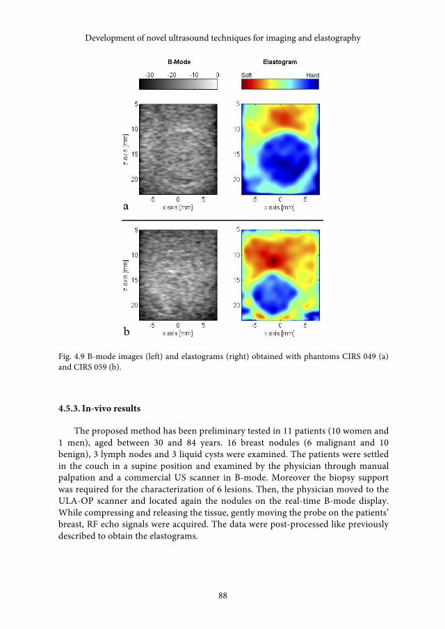
Development of novel ultrasound techniques for imaging and elastography
88
Fig. 4.9 B-mode images (left) and elastograms (right) obtained with phantoms CIRS 049 (a) and CIRS 059 (b).
4.5.3. In-vivo results
The proposed method has been preliminary tested in 11 patients (10 women and1 men), aged between 30 and 84 years. 16 breast nodules (6 malignant and 10 benign), 3 lymph nodes and 3 liquid cysts were examined. The patients were settled
in the couch in a supine position and examined by the physician through manual
palpation and a commercial US scanner in B-mode. Moreover the biopsy support was required for the characterization of 6 lesions. Then, the physician moved to the ULA-OP scanner and located again the nodules on the real-time B-mode display. While compressing and releasing the tissue, gently moving the probe on the patients’ breast, RF echo signals were acquired. The data were post-processed like previously described to obtain the elastograms.
Development of novel ultrasound techniques for imaging and elastography
88
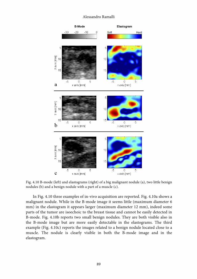
Alessandro Ramalli
89
Fig. 4.10 B-mode (left) and elastograms (right) of a big malignant nodule (a), two little benign nodules (b) and a benign nodule with a part of a muscle (c).
In Fig. 4.10 three examples of in-vivo acquisition are reported. Fig. 4.10a shows a malignant nodule. While in the B-mode image it seems little (maximum diameter 6 mm) in the elastogram it appears larger (maximum diameter 12 mm), indeed some parts of the tumor are isoechoic to the breast tissue and cannot be easily detected in B-mode. Fig. 4.10b reports two small benign nodules. They are both visible also in the B-mode image but are more easily detectable in the elastograms. The third example (Fig. 4.10c) reports the images related to a benign nodule located close to a muscle. The nodule is clearly visible in both the B-mode image and in the elastogram.
Alessandro Ramalli
89
Development of novel ultrasound techniques for imaging and elastography
90
4.6. Real-time implementation
All the results, described in the previous paragraphs, were obtained through Matlab® developed post-processing functions, which elaborated raw-radiofrequency data acquired by ULA-OP. However, a freehand elastography algorithm that could be considered usable requires being a real-time algorithm.
4.6.1. Real-time algorithm
The proposed quasi-static elastography method was adapted to the ULA-OP architecture for its real-time implementation. In particular, since the system is not capable of a real-time high frame rate imaging, only the frequency domain displacement estimation method could be implemented.
In principle the algorithm can be divided in six logical jobs:
• Gating
• Discrete Fourier transforming
• Phases extraction
• Displacement estimation
• Strain estimation
• Filtering
The first three jobs were assigned to the Master FPGA, while the last three ones to the DSP. This particular choice is driven by the already existent ULA-OP architecture. Indeed it could be easily adapted to compute the discrete Fourier transform over a limited number of frequencies, which is the most time consuming job of the entire algorithm.
Considering the rectangular form of the exponential function, the DFT definition in (4.3) can be modified as:
𝑋𝑋! = 𝑠𝑠! cos2𝜋𝜋𝑁𝑁!
𝑓𝑓𝑓𝑓 + 𝑖𝑖 ∙ sin2𝜋𝜋𝑁𝑁!
𝑓𝑓𝑓𝑓
!!!!
!!!
(4.12)
The last DFT formulation can be associated to the sum of the quadrature-demodulated samples of 𝑠𝑠!, which is weighted by a NW samples window. Since the DFT must be computed for each position of the weighting window, equation (4.12) can be further developed as follows:
𝑋𝑋!(𝑛𝑛) = FIR!! 𝑠𝑠! cos2𝜋𝜋𝑁𝑁!
𝑓𝑓𝑓𝑓 + 𝑖𝑖 ∙ sin2𝜋𝜋𝑁𝑁!
𝑓𝑓𝑛𝑛 ∙ 𝑒𝑒!!!,!"# ! (4.13)
Development of novel ultrasound techniques for imaging and elastography
90
Alessandro Ramalli
91
where FIR!! represents a function which computes a NW samples long finite-impulse-response filter and 𝜙𝜙!,!"#(n) is an additive phase term due to the quadrature demodulation, which is:
𝜙𝜙!,!"# 𝑛𝑛 =2𝜋𝜋𝑁𝑁!
𝑓𝑓𝑓𝑓 (4.14)
Since ULA-OP already performed both the quadrature demodulation and the FIR filtering it was sufficient to replicate NP times the dedicated FPGA logical blocks, i.e. one for each frequency of interest, to finally obtain the DFT. In ULA-OP NP was equal to 8. Furthermore, the spectral phases were extracted from the DFT through a lookup-table (LT), which returns the four-quadrant inverse tangent of a complex number. Then, the “arg” function used in (4.5) returns:
arg 𝑋𝑋!(𝑛𝑛) = LT 𝑋𝑋!(𝑛𝑛) − 𝜙𝜙!,!"# 𝑛𝑛 (4.15)
which computes the spectral phases and compensates them by the phase term due to the quadrature demodulation.
The displacement estimation and the strain computation were performed by the DSP as in the original form in (4.6) and (4.7) respectively, with the only difference that are computed in fixed point arithmetic. The strain is then filtered by four consecutive comb filters, which are 16-samples long each.
4.6.2. Real-time results
ULA-OP was coupled with the 192-element linear array LA533 (Esaote SpA, Florence, Italy). It was programmed to alternate two different modes at 6 kHz PRF. The first one, dedicated to reconstruct a standard B-mode image, consisted in the transmission of 3-cycle burst at 8 MHz, weighted by a Hanning window, focused at 20 mm depth and scanning 128 lines. 64 active elements were used both in transmission and in reception. The second mode, dedicated to elastography, differed from the first one in the transmitted signal which, in this case, was a 7-cycle burst at 7 MHz weighted with a Hanning window. A elastography-dedicated phantom were used (CIRS, model 049, Norfolk, Virginia, USA).
In Fig. 4.11, screenshot examples of the ULA-OP real-time software, while the elastography module was activated, are presented. In all the examples the inclusion are roughly visible in the B-mode and are clearly visible in the elastograms. In particular, Fig. 4.11a and Fig. 4.11b show the inclusions which were harder (62 and 54 kPa respectively) than the background (29 kPa). In the elastogram, they are highlighted in blue and their shapes are almost circular as expected. Fig. 4.11b, especially, demonstrates how elastography can highlights tissues with different elasticity which are isoechoic with the surrounding tissues. Indeed the inclusion is undetectable in the B-mode image. Fig. 4.11c shows the softest inclusion inside the phantom (6 kPa) and it appears as an orange circle in the elastogram. A green dot is detected at the center of the inclusion which is due to a fabrication defect, even visible in the B-mode image as a white dot.
Alessandro Ramalli
91
Development of novel ultrasound techniques for imaging and elastography
92
4.7. Discussion and conclusion
A displacement estimation method based on the calculation of the frequency domain phase shift of RF signals has been presented and its suitability for improving elastography has been highlighted.
In the proposed test conditions, considering the non-uniformity level and the elastographic contrast-to-noise ratio as quality indexes, the elastograms obtained with the new method present higher quality compared to the reference Pesavento method (Fig. 4.4). Even if both indexes can be used to compare different elastograms, the NU level seems more suitable to quantify the quality of an algorithm since its value does not depend on the applied stress or on tissue stiffness.
Furthermore, a HFR averaging method has been presented. It must be noted that the proposed approach is different from that proposed in (Tanter et al. 2002), indeed we obtain decorrelated strain images by locally varying FE, while in (Tanter et al. 2002) the decorrelation of the images is obtained by estimating the strain for each insonation angle. The results in Fig. 4.5 show that when the elastogram frame rate is appropriate with respect to the compression speed, the averaging method does not introduce significant improvements. However, in all other cases averaging is demonstrated to significantly increase the quality of elastograms, whatever the displacement estimation algorithm. Averaging has the effect of increasing the signal-to-noise ratio of elastography images, thus increasing the highest achievable frame rate.
Although the averaging and the Fourier domain displacement estimation are independent, optimal results are obtained by combining them, as highlighted in Fig. 4.6. In addition, it is shown that the HFR imaging algorithm does not influence image quality. Indeed, the behavior of the non-uniformity level during compression time depends only on the number Navg of images involved in the averaging step, as reported in Fig. 4.7.
In terms of computational cost, the proposed method is equivalent to the Pesavento method, here assumed as the reference. However, in our approach the computational cost can be reduced by decimating the number of depths at which the displacements are estimated. As shown in sec. 4.4.4, in most cases it is expected that this simplification does not influence the quality of images. This could further expand the implementation of the novel method in standard ultrasound machines, as no extra equipment is needed.
This work has shown the suitability of the proposed method for breast investigation in clinical condition through free-hand elastography. All breast nodules detected in patients undergoing the standard clinical procedure were visible in both elastograms and B-Mode images. In several cases the elastograms produced more detailed images.
Finally, the computational cost efficacy of the frequency domain methods allowed its real-time implementation on the research platform ULA-OP. A planned test on a larger number of patients will clarify if the novel method can actually improve the diagnostic accuracy and thus reduce the biopsy assistance.
Development of novel ultrasound techniques for imaging and elastography
92
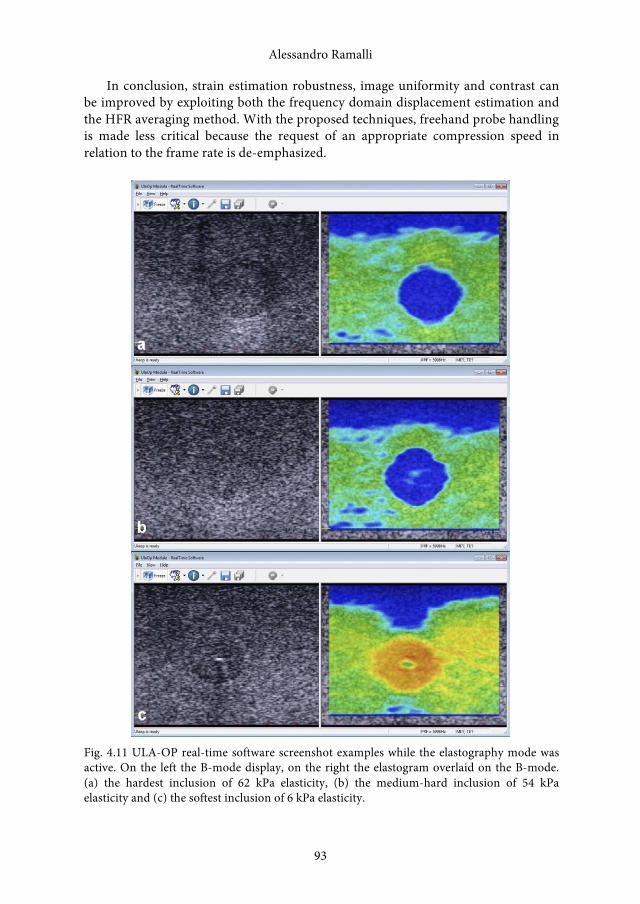
Alessandro Ramalli
93
In conclusion, strain estimation robustness, image uniformity and contrast can be improved by exploiting both the frequency domain displacement estimation and the HFR averaging method. With the proposed techniques, freehand probe handling is made less critical because the request of an appropriate compression speed in relation to the frame rate is de-emphasized.
Fig. 4.11 ULA-OP real-time software screenshot examples while the elastography mode was active. On the left the B-mode display, on the right the elastogram overlaid on the B-mode. (a) the hardest inclusion of 62 kPa elasticity, (b) the medium-hard inclusion of 54 kPa elasticity and (c) the softest inclusion of 6 kPa elasticity.
Alessandro Ramalli
93


5. Novel Ultrasound Experimental Methods:Work in Progress
This chapter is divided in four parts: the first describes a new color vector Doppler algorithm and shows some preliminary results; the second one draws on (Shapoori et al. 2011) presents a new adaptive beamforming scheme; the third and the forth ones shows preliminary results on pulse compression and high frame-rate imaging respectively.
5.1. 2D HFR color vector Doppler
5.1.1. Introduction
In medicine, the evaluation of blood flow within the body assumes particular importance. Color flow mapping (CFM) mode is an ultrasound imaging technique whereby color coded images of the blood flow are superimposed to the morphological B-mode images. In particular a retrograde flow is represented in blue color and a anterograde flow is characterized by a red color. In such way the identification of vessels and their possible diseases becomes easier.
Conventional Color Doppler techniques are limited by low frame-rates, which means that only low varying flow can be reconstructed. This is a consequence of the performed method, which exploits the phase changes of the echo-signals on consecutive pulses. To have a good estimate it is necessary averaging on different pulses leading to a reduction of the final frame-rate.
Another main limitation is that CFM only leads to the estimation of the axial velocity component. This is not considered as a big issue for simple flows, in which the flow direction can be assumed parallel to the vessel axis. Indeed the angle between the vessel and the ultrasonic beam can be estimated in a B-mode image. For turbulent and complex flow the latter assumption is no longer verified and the CFM is only used as qualitative method since no angle correction is performed.
Recently blood velocity vector imaging methods were presented. They are based on the transmission of plane waves and on high frame-rate reconstruction algorithms, which yields one image for each pulse emission. Through a cross-correlation among consecutive images the velocity vector is then estimated in a two-dimensional region of interest (Udesen et al. 2008), (Hansen et al. 2008).
In this chapter a new 2D velocity vector estimation algorithm is presented. It differs from the existing ones, since the motion estimator is based on a Fourier
Alessandro Ramalli, Development of novel ultrasound techniques for imaging and elastography : from simulation to real-time implementation ISBN 978-88-6655-456-1 (print) ISBN 978-88-6655-457-8 (online) © 2013 Firenze University Press
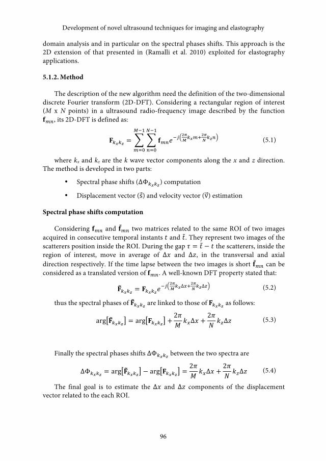
Development of novel ultrasound techniques for imaging and elastography
96
domain analysis and in particular on the spectral phases shifts. This approach is the 2D extension of that presented in (Ramalli et al. 2010) exploited for elastography applications.
5.1.2. Method
The description of the new algorithm need the definition of the two-dimensional discrete Fourier transform (2D-DFT). Considering a rectangular region of interest (M x N points) in a ultrasound radio-frequency image described by the function 𝐟𝐟!", its 2D-DFT is defined as:
𝐅𝐅!!!! = 𝐟𝐟!"𝑒𝑒!! !!
!!!!!!!! !!!
!!!
!!!
!!!
!!!
(5.1)
where kx and kz are the k wave vector components along the x and z direction. The method is developed in two parts:
• Spectral phase shifts (∆Φ!!!!) computation
• Displacement vector (s) and velocity vector (v) estimation
Spectral phase shifts computation
Considering 𝐟𝐟!" and 𝐟𝐟!" two matrices related to the same ROI of two images acquired in consecutive temporal instants 𝑡𝑡 and 𝑡𝑡. They represent two images of the scatterers position inside the ROI. During the gap 𝜏𝜏 = 𝑡𝑡 − 𝑡𝑡 the scatterers, inside the region of interest, move in average of ∆𝑥𝑥 and ∆𝑧𝑧, in the transversal and axial direction respectively. If the time lapse between the two images is short 𝐟𝐟!" can be considered as a translated version of 𝐟𝐟!". A well-known DFT property stated that:
𝐅𝐅!!!! = 𝐅𝐅!!!!𝑒𝑒!! !!
!!!∆!!!!! !!∆! (5.2)
thus the spectral phases of 𝐅𝐅!!!! are linked to those of 𝐅𝐅!!!! as follows:
arg 𝐅𝐅!!!! = arg 𝐅𝐅!!!! +2𝜋𝜋𝑀𝑀𝑘𝑘!∆𝑥𝑥 +
2𝜋𝜋𝑁𝑁𝑘𝑘!∆𝑧𝑧 (5.3)
Finally the spectral phases shifts ∆Φ!!!! between the two spectra are
∆Φ!!!! = arg 𝐅𝐅!!!! − arg 𝐅𝐅!!!! =2𝜋𝜋𝑀𝑀𝑘𝑘!∆𝑥𝑥 +
2𝜋𝜋𝑁𝑁𝑘𝑘!∆𝑧𝑧 (5.4)
The final goal is to estimate the ∆𝑥𝑥 and ∆𝑧𝑧 components of the displacement vector related to the each ROI.
Development of novel ultrasound techniques for imaging and elastography
96

Alessandro Ramalli
Displacement and velocity vectors estimation
The ROI displacement s is defined as:
s = ∆𝑥𝑥 ∙ 𝑥𝑥 + ∆𝑧𝑧 ∙ 𝑧𝑧 (5.5)
where 𝑥𝑥 and 𝑧𝑧 are the unit vectors in the x and z direction respectively. ∆Φ!!!! is the spectral phases shift defined for any wave-vector couple 𝑘𝑘! , 𝑘𝑘! . It can be assumed as the sum of two separate components:
∆Φ!! =2𝜋𝜋𝑀𝑀𝑘𝑘!∆𝑥𝑥 ∆Φ!! =
2𝜋𝜋𝑁𝑁𝑘𝑘!∆𝑧𝑧 (5.6)
thus (5.4) become
∆Φ!!!! = ∆Φ!! + ∆Φ!! (5.7)
The estimation of the displacement components needs the definition of the following equations system with ∆𝑥𝑥 and ∆𝑧𝑧 unknown:
2𝜋𝜋𝑀𝑀𝑘𝑘!(!)∆𝑥𝑥 +
2𝜋𝜋𝑁𝑁𝑘𝑘!(!)∆𝑧𝑧 = ∆Φ!!
(!)!!(!)
2𝜋𝜋𝑀𝑀𝑘𝑘!(!)∆𝑥𝑥 +
2𝜋𝜋𝑁𝑁𝑘𝑘!(!)∆𝑧𝑧 = ∆Φ!!
(!)!!(!)
(5.8)
where the superscripts (1) and (2) refer to two different couple of values 𝑘𝑘! , 𝑘𝑘! . The final system solution is:
∆𝑥𝑥 =∆Φ!!
! !!! − ∆Φ!!
! !!!
!!!
𝑘𝑘!! − 𝑘𝑘!
!
∆𝑧𝑧 =𝑘𝑘!! ∆Φ!!
! !!! − 𝑘𝑘!
! ∆Φ!!! !!
!
!!!𝑘𝑘!! 𝑘𝑘!
! − 𝑘𝑘!!
(5.9)
Since the phases information ∆Φ!!!! are usually very noisy, ∆𝑥𝑥 and ∆𝑧𝑧 are estimated as the average over different estimates obtained with multiple pairs of couples 𝑘𝑘!
(!), 𝑘𝑘!(!) and 𝑘𝑘!
(!), 𝑘𝑘!(!) . The displacement s related to a single ROI is
computed as in (5.5). Finally the velocity vector v is evaluated as:
v = s ∙ 𝐹𝐹! = ∆𝑥𝑥 ∙ 𝑥𝑥 + ∆𝑧𝑧 ∙ 𝑧𝑧 ∙ 𝐹𝐹! (5.10)
where FB is the frame-rate of images.
Color-Vector Doppler of an image The method just described estimates the velocity vector for a single and limited
ROI. In order to have a complete view of the flow behavior it is necessary to move the ROI both in the x and z direction, covering the entire image dimension. The
Alessandro Ramalli
97
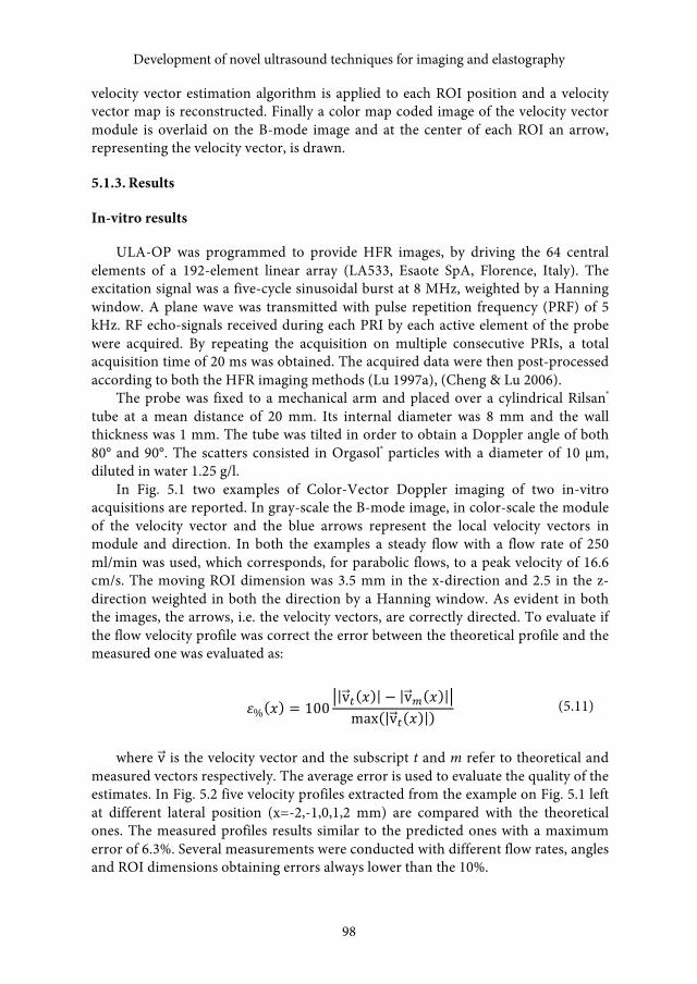
Development of novel ultrasound techniques for imaging and elastography
98
velocity vector estimation algorithm is applied to each ROI position and a velocity vector map is reconstructed. Finally a color map coded image of the velocity vector module is overlaid on the B-mode image and at the center of each ROI an arrow, representing the velocity vector, is drawn.
5.1.3. Results
In-vitro results
ULA-OP was programmed to provide HFR images, by driving the 64 central elements of a 192-element linear array (LA533, Esaote SpA, Florence, Italy). The excitation signal was a five-cycle sinusoidal burst at 8 MHz, weighted by a Hanning window. A plane wave was transmitted with pulse repetition frequency (PRF) of 5 kHz. RF echo-signals received during each PRI by each active element of the probe were acquired. By repeating the acquisition on multiple consecutive PRIs, a total acquisition time of 20 ms was obtained. The acquired data were then post-processed according to both the HFR imaging methods (Lu 1997a), (Cheng & Lu 2006).
The probe was fixed to a mechanical arm and placed over a cylindrical Rilsan® tube at a mean distance of 20 mm. Its internal diameter was 8 mm and the wall thickness was 1 mm. The tube was tilted in order to obtain a Doppler angle of both 80° and 90°. The scatters consisted in Orgasol® particles with a diameter of 10 µm, diluted in water 1.25 g/l.
In Fig. 5.1 two examples of Color-Vector Doppler imaging of two in-vitro acquisitions are reported. In gray-scale the B-mode image, in color-scale the module of the velocity vector and the blue arrows represent the local velocity vectors in module and direction. In both the examples a steady flow with a flow rate of 250 ml/min was used, which corresponds, for parabolic flows, to a peak velocity of 16.6 cm/s. The moving ROI dimension was 3.5 mm in the x-direction and 2.5 in the z-direction weighted in both the direction by a Hanning window. As evident in both the images, the arrows, i.e. the velocity vectors, are correctly directed. To evaluate if the flow velocity profile was correct the error between the theoretical profile and the measured one was evaluated as:
𝜀𝜀% 𝑥𝑥 = 100v! 𝑥𝑥 − v! 𝑥𝑥max v! 𝑥𝑥
(5.11)
where v is the velocity vector and the subscript t and m refer to theoretical and measured vectors respectively. The average error is used to evaluate the quality of the estimates. In Fig. 5.2 five velocity profiles extracted from the example on Fig. 5.1 left at different lateral position (x=-2,-1,0,1,2 mm) are compared with the theoretical ones. The measured profiles results similar to the predicted ones with a maximum error of 6.3%. Several measurements were conducted with different flow rates, angles and ROI dimensions obtaining errors always lower than the 10%.
Development of novel ultrasound techniques for imaging and elastography
98
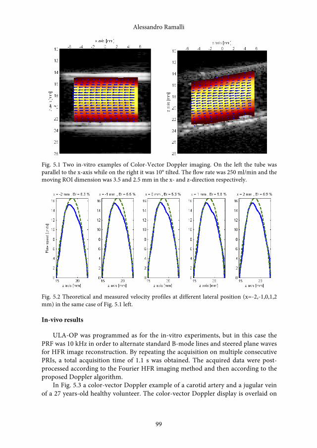
Alessandro Ramalli
99
Fig. 5.1 Two in-vitro examples of Color-Vector Doppler imaging. On the left the tube was parallel to the x-axis while on the right it was 10° tilted. The flow rate was 250 ml/min and the moving ROI dimension was 3.5 and 2.5 mm in the x- and z-direction respectively.
Fig. 5.2 Theoretical and measured velocity profiles at different lateral position (x=-2,-1,0,1,2 mm) in the same case of Fig. 5.1 left.
In-vivo results
ULA-OP was programmed as for the in-vitro experiments, but in this case the PRF was 10 kHz in order to alternate standard B-mode lines and steered plane waves for HFR image reconstruction. By repeating the acquisition on multiple consecutive PRIs, a total acquisition time of 1.1 s was obtained. The acquired data were post-processed according to the Fourier HFR imaging method and then according to the proposed Doppler algorithm.
In Fig. 5.3 a color-vector Doppler example of a carotid artery and a jugular vein of a 27 years-old healthy volunteer. The color-vector Doppler display is overlaid on
Alessandro Ramalli
99
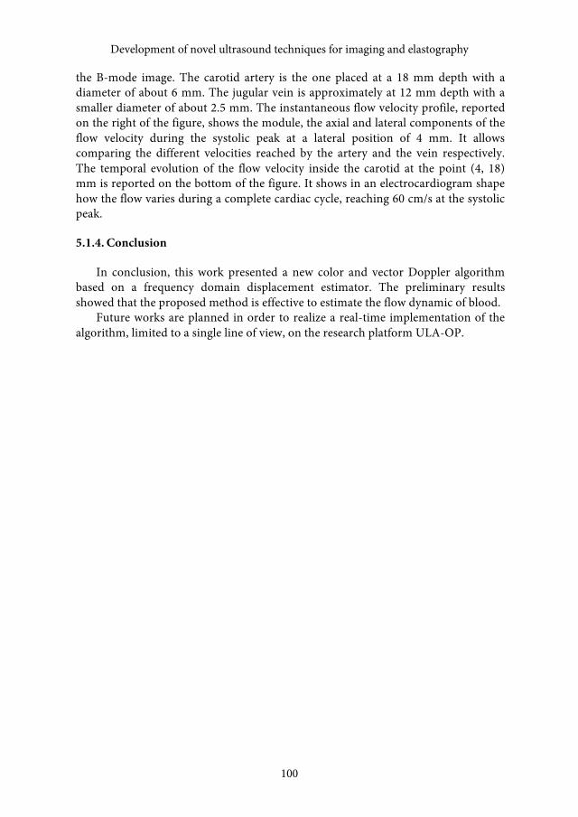
Development of novel ultrasound techniques for imaging and elastography
100
the B-mode image. The carotid artery is the one placed at a 18 mm depth with a diameter of about 6 mm. The jugular vein is approximately at 12 mm depth with a smaller diameter of about 2.5 mm. The instantaneous flow velocity profile, reported on the right of the figure, shows the module, the axial and lateral components of the flow velocity during the systolic peak at a lateral position of 4 mm. It allows comparing the different velocities reached by the artery and the vein respectively. The temporal evolution of the flow velocity inside the carotid at the point (4, 18) mm is reported on the bottom of the figure. It shows in an electrocardiogram shape how the flow varies during a complete cardiac cycle, reaching 60 cm/s at the systolic peak.
5.1.4. Conclusion
In conclusion, this work presented a new color and vector Doppler algorithm based on a frequency domain displacement estimator. The preliminary results showed that the proposed method is effective to estimate the flow dynamic of blood.
Future works are planned in order to realize a real-time implementation of the algorithm, limited to a single line of view, on the research platform ULA-OP.
Development of novel ultrasound techniques for imaging and elastography
100
Alessandro Ramalli
101
Fig. 5.3 In-vivo example of color-vector Doppler investigation on a carotid artery and a jugular vein of a healthy volunteer. On the left color-vector Doppler display overlaid on the B-mode image; on the right the module, the axial and lateral components of the instantaneous flow velocity profile and on bottom the flow speed temporal evolution.
5.2. Adaptive beamforming through layered structures
5.2.1. Introduction
Ultrasonic diagnosis of brain injuries through thick human skull bones may offer tremendous benefits to the community. The most attractive approach to its realization is based on the application of ultrasonic phased array systems (Sasso & Cohen-Bacrie 2005),(Clement & Hynynen 2002),(Hynynen et al. 2004),(Thomas & Fink 1996),(Tanter et al. 1998). Due to the flexibility in steering and focusing of the ultrasonic field provided by such systems, better signal-to-noise ratio (SNR) of the received signals and better image quality can be achieved compared to the single transducer approaches.
Alessandro Ramalli
101

Development of novel ultrasound techniques for imaging and elastography
102
However, the success of transcranial ultrasonic imaging depends on our ability to overcome the effects of strong absorption and distortion of the acoustic field by the thick, multilayered skull bone. The human skull bone is inhomogeneous and consists of three main layers (Fry & Barger 1978). The outer and inner layers are composed of compact bone, while the middle porous layer is only present in adults (it is absent in both children and animals) and (when present) is the main contributor to the distortion of ultrasonic waves (Leissner et al. 1970),(Pichardo et al. 2011). The total skull thickness in adults varies from 3 to 10 mm (Fry & Barger 1978). While the outer layer has a relatively smooth surface, the inner layer is of variable thickness and has an irregular surface profile. In the past few decades, several researchers tried to tabulate the acoustical and geometrical properties of the human skull and brain tissue (Fry & Barger 1978), (Leissner et al. 1970),(Pichardo et al. 2011). The results of some of these measurements are also used in this study.
In this work, the recently developed adaptive beamforming algorithm for small-aperture linear phased arrays (Shapoori et al. 2010) is applied to the specific case of transcranial imaging. The acoustic mismatch between the human skull and the brain tissue plays a major role in distorting the focused field generated with conventional beamforming techniques. This acoustic mismatch originates unwanted refraction (and reflection) of the acoustic waves and eventually causes misplacement and blurring of the focal spots and additional loss of energy. Displaced focal spots and altered wave trajectories will result in the wrong assumptions about the received field, and eventually lead to a distorted and non-informative reconstructed image. The focus of this study is to determine and apply proper timing corrections to the phased array elements in order to compensate for the effects of refraction and multiple reflections caused by the human skull.
In the proposed method, the local topography of the skull segment under the phased array probe is obtained from an ultrasonic B-Scan and then used in the adaptive beamforming process, which aims at refocusing the beam at a desired location. Based on the variable thickness of the skull and the impedance mismatch between the skull and the brain tissue, a corrected timing pattern is calculated and applied to the temporally apodized, frequency-modulated tone burst signals driving the array elements. At the final step, the image of the spatial power pattern is formed by superimposing the received attenuated fields from all transmitting elements (active in synthetic focusing) at each pixel. The results for the original, distorted and corrected field patterns are presented. The possibility of using large synthetic apertures is also investigated.
5.2.2. Theory and simulation
As mentioned above, the power of using phased arrays is in the capability of focusing their ultrasound field at a desired location in front of the array. The steering and focusing flexibility depends on the ultrasonic wavelength, as well as on the size of the array elements and distance between them. For the particular case of this study, based on the average longitudinal sound velocities in the human skull and
Development of novel ultrasound techniques for imaging and elastography
102
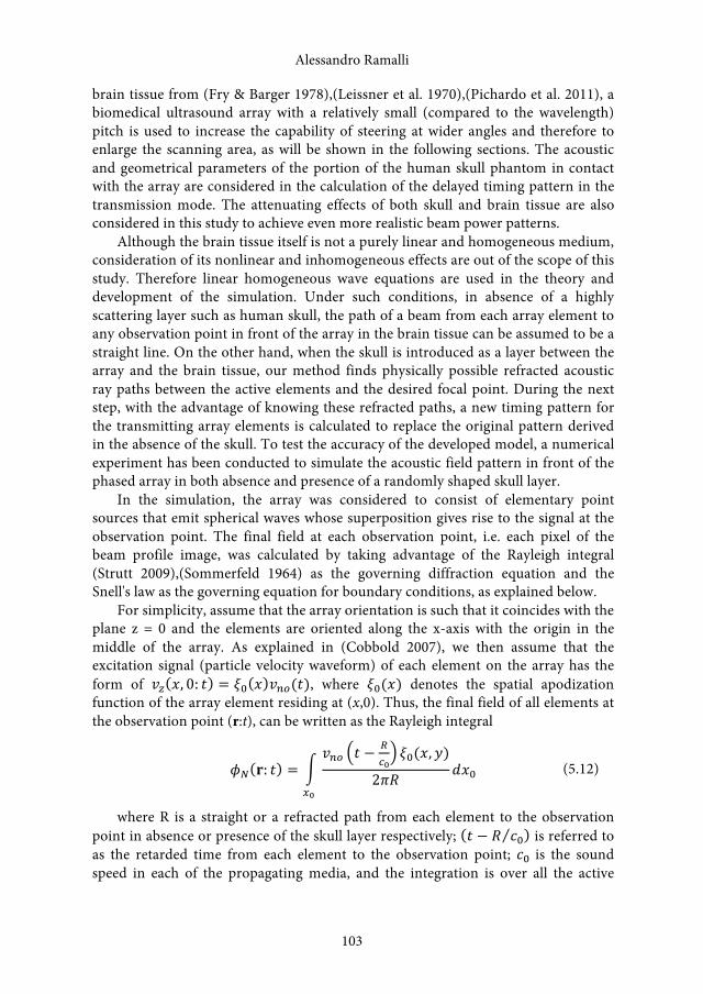
Alessandro Ramalli
103
brain tissue from (Fry & Barger 1978),(Leissner et al. 1970),(Pichardo et al. 2011), a biomedical ultrasound array with a relatively small (compared to the wavelength) pitch is used to increase the capability of steering at wider angles and therefore to enlarge the scanning area, as will be shown in the following sections. The acoustic and geometrical parameters of the portion of the human skull phantom in contact with the array are considered in the calculation of the delayed timing pattern in the transmission mode. The attenuating effects of both skull and brain tissue are also considered in this study to achieve even more realistic beam power patterns.
Although the brain tissue itself is not a purely linear and homogeneous medium, consideration of its nonlinear and inhomogeneous effects are out of the scope of this study. Therefore linear homogeneous wave equations are used in the theory and development of the simulation. Under such conditions, in absence of a highly scattering layer such as human skull, the path of a beam from each array element to any observation point in front of the array in the brain tissue can be assumed to be a straight line. On the other hand, when the skull is introduced as a layer between the array and the brain tissue, our method finds physically possible refracted acoustic ray paths between the active elements and the desired focal point. During the next step, with the advantage of knowing these refracted paths, a new timing pattern for the transmitting array elements is calculated to replace the original pattern derived in the absence of the skull. To test the accuracy of the developed model, a numerical experiment has been conducted to simulate the acoustic field pattern in front of the phased array in both absence and presence of a randomly shaped skull layer.
In the simulation, the array was considered to consist of elementary point sources that emit spherical waves whose superposition gives rise to the signal at the observation point. The final field at each observation point, i.e. each pixel of the beam profile image, was calculated by taking advantage of the Rayleigh integral (Strutt 2009),(Sommerfeld 1964) as the governing diffraction equation and the Snell's law as the governing equation for boundary conditions, as explained below.
For simplicity, assume that the array orientation is such that it coincides with the plane z = 0 and the elements are oriented along the x-axis with the origin in the middle of the array. As explained in (Cobbold 2007), we then assume that the excitation signal (particle velocity waveform) of each element on the array has the form of 𝑣𝑣! 𝑥𝑥, 0: 𝑡𝑡 = 𝜉𝜉! 𝑥𝑥 𝑣𝑣!"(𝑡𝑡), where 𝜉𝜉!(𝑥𝑥) denotes the spatial apodization function of the array element residing at (x,0). Thus, the final field of all elements at the observation point (r:t), can be written as the Rayleigh integral
𝜙𝜙! 𝐫𝐫: 𝑡𝑡 =𝑣𝑣!" 𝑡𝑡 − !
!!𝜉𝜉!(𝑥𝑥, 𝑦𝑦)
2𝜋𝜋𝜋𝜋𝑑𝑑𝑥𝑥!
!!
(5.12)
where R is a straight or a refracted path from each element to the observation point in absence or presence of the skull layer respectively; 𝑡𝑡 − 𝑅𝑅 𝑐𝑐! is referred to as the retarded time from each element to the observation point; 𝑐𝑐! is the sound speed in each of the propagating media, and the integration is over all the active
Alessandro Ramalli
103

Development of novel ultrasound techniques for imaging and elastography
104
elements of the array. In case of using synthetic apertures in the transmission mode, the integral is replaced with summation. Then, 𝑣𝑣!"can be written as a convolution integral
𝑣𝑣!" 𝑡𝑡 −𝑅𝑅𝑐𝑐!
= 𝑣𝑣!"(𝜏𝜏)𝛿𝛿 𝑡𝑡 −𝑅𝑅𝑐𝑐!− 𝜏𝜏 𝑑𝑑𝑑𝑑
!
!!
(5.13)
which, when substituted into (5.12) and after changing the order of integration, enables the velocity potential to be written as
𝜙𝜙! 𝐫𝐫: 𝑡𝑡 = 𝑣𝑣!" 𝜏𝜏𝜉𝜉! 𝑥𝑥, 𝑦𝑦 𝛿𝛿 𝑡𝑡 − !
!!− 𝜏𝜏
2𝜋𝜋𝜋𝜋!!
𝑑𝑑𝑥𝑥! 𝑑𝑑𝑑𝑑!
!!
(5.14)
where
ℎ 𝐫𝐫: 𝑡𝑡 =𝜉𝜉! 𝑥𝑥, 𝑦𝑦 𝛿𝛿 𝑡𝑡 − !
!!2𝜋𝜋𝜋𝜋
!!
𝑑𝑑𝑥𝑥! (5.15)
is the spatial impulse response at the observation point due to a δ-function excitation of each element of the array. It can be seen that (5.14) is basically the convolution of the velocity waveform and the impulse response.
With reference to phasing the array, the delay pattern in terms of active array aperture depends on the acoustic path between the desired focal area and each excited array element (Shapoori et al. 2010). In (Dhanantwari et al. 2004) Stergiopolous showed that a linear frequency-modulated function multiplied by a temporal window could be used as an appropriate choice of the excitation signal. The use of a temporal window in the excitation signal reduces the spectral leak in the transmitted pulse.
In the specific application of interest, due to the high attenuation of the skull bone material, secondary echoes in the bone provide negligible contribution to the final intensity at the focal zone due to their lower SNR compared to the refracted-only waves. This could be explained by their longer propagation path (higher attenuation), loss of energy at each reflection, and to the additional time delay causing improper timing. Thus, it can be stated that multiple reflected waves mostly make a noise contribution.
The acoustical properties of human skull and brain tissue (Fry & Barger 1978),(Leissner et al. 1970),(Pichardo et al. 2011) used in the simulation, i.e. sound speed (longitudinal), attenuation, density and impedance are listed in Table 5.I.
Table 5.I Properties of human skull and skull phantom
Skull phantom Human skull Density [g/cm3] 1.91 ~ 1.93
Development of novel ultrasound techniques for imaging and elastography
104
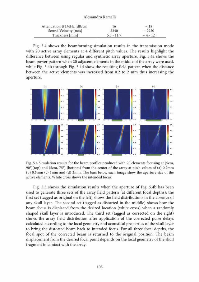
Alessandro Ramalli
105
Attenuation @2MHz [dB/cm] 16 ~ 18 Sound Velocity [m/s] 2340 ~ 2920
Thickness [mm] 5.3 - 11.7 ~ 4 - 12
Fig. 5.4 shows the beamforming simulation results in the transmission mode with 20 active array elements at 4 different pitch values. The results highlight the difference between using regular and synthetic array aperture. Fig. 5.4a shows the beam power pattern when 20 adjacent elements in the middle of the array were used, while Fig. 5.4b through Fig. 5.4d show the resulting field pattern when the distance between the active elements was increased from 0.2 to 2 mm thus increasing the aperture.
Fig. 5.4 Simulation results for the beam profiles produced with 20 elements focusing at (5cm, 90°)(top) and (5cm, 75°) (bottom) from the center of the array at pitch values of (a) 0.2mm (b) 0.5mm (c) 1mm and (d) 2mm. The bars below each image show the aperture size of the active elements. White cross shows the intended focus.
Fig. 5.5 shows the simulation results when the aperture of Fig. 5.4b has been used to generate three sets of the array field pattern (at different focal depths): the first set (tagged as original on the left) shows the field distributions in the absence of any skull layer. The second set (tagged as distorted in the middle) shows how the beam focus is displaced from the desired location (white cross) when a randomly shaped skull layer is introduced. The third set (tagged as corrected on the right) shows the array field distribution after application of the corrected pulse delays calculated according to the local geometry and acoustical properties of the skull layer to bring the distorted beam back to intended focus. For all three focal depths, the focal spot of the corrected beam is returned to the original position. The beam displacement from the desired focal point depends on the local geometry of the skull fragment in contact with the array.
Alessandro Ramalli
105

Development of novel ultrasound techniques for imaging and elastography
106
Fig. 5.5 Simualtion results of (a) original (b) distorted and (c) corrected beam profiles in absence and presence of a randomly defined skull layer (shown as a white curve at the bottom of the (b) and (c) images). Results for three focal depths of (2cm, 90°)(top), (5cm, 90°)(middle) and (8cm, 90°)(bottom) are shown. White cross shows the intended focus.
5.2.3. Experiment
To check the validity of the proposed theory and simulation, a series of laboratory experiments were conducted with a custom skull phantom fabricated in our lab. The skull phantom has been made of a combination of Epoxy Abocast and Titanium powder (grade 50µm). The major acoustical properties of the phantom, i.e. density, longitudinal sound speed and attenuation shown in Table 5.I, very closely match the respective properties of the human skull. To match the above described one-dimensional numerical model, this particular phantom was built with a flat outer and a randomly curved (in 1 dimension) inner surface approximating the topology of a real human skull segment. An intermediate porous layer was also introduced into the phantom to resemble the diploe layer found in the human skull (Fry & Barger 1978). Fig. 5.6 shows a picture of the implemented skull phantom.
Development of novel ultrasound techniques for imaging and elastography
106

Alessandro Ramalli
107
Fig. 5.6 Skull phantom with a porous intermediate layer
Fig. 5.7 shows a schematic configuration of our experimental setup. The new adaptive beamforming algorithm was implemented on the ultrasound advanced open-platform system (ULA-OP (Tortoli et al. 2009)), simultaneously controlling 64 active elements selected out of a 128-element (of 0.1mm width and 0.2mm pitch) phased array with 2 MHz central frequency (PA230-Esaote SpA). The probe was submerged in water and held in contact with the skull phantom. An ultrasonic hydrophone (Pinducer, Valpey-Fisher) was attached to a 4D scanner to measure the acoustic field intensity in the plane of the linear probe with 1mm step. At each scanning point, the hydrophone signal was amplified, digitized, averaged, and then processed to calculate the acoustic power.
Fig. 5.7 Schematic configuration of the experimental setup
To obtain information about the geometry of the skull phantom prior to the beamforming process, a B-scan of the phantom was recorded using all 128 elements of the array. The phantom profile extracted from the B-scan and properly smoothed afterwards was fed into the simulation program to calculate the new pulse delay
Alessandro Ramalli
107

Development of novel ultrasound techniques for imaging and elastography
108
pattern. After loading this pattern to the ULA-OP and applying desired delays to the excitation pulses for all active elements, the hydrophone starts scanning to measure the resulting beam profile.
5.2.4. Results
Fig. 5.8 shows the beam pattern measured using the above described apparatus. A synthetic aperture of 30 elements of the linear array, pitched at 0.6 mm (total width of 1.5 cm), was chosen to transmit according to the presented adaptive delay scheme. Fig. 5.8a shows the experimentally measured beam profile in water without the phantom. Fig. 5.8b shows the experimentally measured beam pattern through the skull phantom. Again it can be seen that the beam is deflected from its intended focal point (white cross). Fig. 5.8c shows the experimentally measured beam profile after applying the corrected delay pattern through ULA-OP. It is clearly seen that the adaptive beamforming algorithm brings the beam back to the desired focus.
Fig. 5.8 Experimental results of (a) original (b) distorted and (c) corrected beam profiles in absence and presence of a the skull phantom for two different intended focal coordinates (top and bottom). White cross shows the intended focus.
From the simulation and experimental results, it can be seen that the use of a larger synthetic aperture produces a more accurate focus with a smaller focal spot size at the intended location (white cross), which means a higher lateral resolution in the final image. But it also should be noted that using a larger aperture and a smaller focal spot will require more processing time, because a smaller focal spot should be moved in smaller increments to scan the desired area in front of the array. Therefore, based on the processing time limitations in each application, there always
Development of novel ultrasound techniques for imaging and elastography
108
Alessandro Ramalli
109
ought to be a compromise between the lateral resolution and the time required to generate the final image.
From Fig.5.4 it can also be noticed that using larger transmission apertures with the adaptive beamforming method can lead to the increasing side lobes effect, which eventually decreases the SNR (signal to noise ratio) of the received signals.
5.2.5. Conclusion
The application of the recently developed adaptive beamforming algorithm to the case of one-way transmission through the human skull has been investigated. The numerical modeling results fully support the initial hypothesis. The experimental results, which are in complete agreement with the numerical simulation, demonstrate the ability of the adaptive beamforming approach to correct the position of the beam’s focal spot misplaced after passing through the skull phantom. A tradeoff between using larger synthetic apertures and the increasing side lobe levels was discussed and practical guidelines provided.
In future, the presented adaptive method will be expanded to include the reception mode corrections, and the full algorithm will be applied to enhance the quality of the reconstructed ultrasonic images.
5.3. Pulse compression
Pulse compression methods, consisting of the transmission of coded waveforms followed by matched filtering in the receiver (Chiao & Xiaohui Hao 2005), can be used to increase the signal-to-noise ratio (SNR) while maintaining the TX signal power. This is particularly useful to image deep structures inside the human body (Misaridis & Jensen 2005a) (Misaridis & Jensen 2005b).
To test this application, the 64 independent AWGs of ULA-OP were programmed to transmit linear frequency-modulated chirps. Post-beamforming raw RF data were saved in a file to be elaborated by a post-processing software that performs RF pulse compression, demodulation and B-Mode image formation.
As an example, the left panel of Fig. 5.9 shows a standard B-mode image of the abdomen obtained by exciting the probe elements with 3 cycles at 8 MHz weighted by a Hanning window, with 25 Vpp amplitude, focussed at 60 mm. The detection of a 70 mm deep vessel, i.e. the region of interest (ROI), is difficult due to poor SNR. The image in the right panel was obtained through matched filtering of a 10 µs long linear FM chirp maintaining the same peak-to-peak amplitude of 25 Vpp, i.e. the same transmission power. Since no signal optimization was made, the SNR increase here yields a sacrifice of both the lateral and axial resolution. Inside the ROI, the SNR is increased by about 6.5 dB. This is lower than the theoretical value, 10.5dB. The degradation is due to the frequency dependent attenuation of tissue that reduces the bandwidth of received signals.
Alessandro Ramalli
109
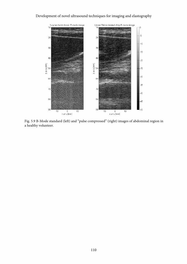
Development of novel ultrasound techniques for imaging and elastography
110
Fig. 5.9 B-Mode standard (left) and “pulse compressed” (right) images of abdominal region in a healthy volunteer.
Development of novel ultrasound techniques for imaging and elastography
110
6. Conclusion
This PhD project addressed many issues, ranging from simulations to experimental tests, related to the introduction of innovative ultrasound techniques.
Two innovative ultrasound field simulation tools were presented: the first one, based on the linear propagation theory, was designed to develop both novel beamforming schemes and signal elaboration techniques; the second one, based on an angular spectrum method, allows predicting the transmitted ultrasound field in media having a nonhomogeneous nonlinear parameter. In both cases, simulations were demonstrated in good agreement with measurements, presenting low relative errors.
A novel algorithm for freehand quasi-static elastography based on a frequency domain displacement estimation was presented. The elastograms were compared to those obtained with a well-established method and, by evaluating the nonuniformity level and the constrast-to-noise ratio, they resulted of higher quality. After evaluating the computational cost, the algorithm was implemented in real-time on ULA-OP. Both in-vitro and in-vivo elastograms were presented showing the effectiveness of the proposed approach.
Innovative techniques, which are still under development, were also presented, showing encouraging preliminary results. The first technique consisted on a novel adaptive beamforming scheme which compensates the diffraction effect of the human skull; the second one was a novel color Doppler imaging algorithm which evaluates vector flow dynamics.
Alessandro Ramalli, Development of novel ultrasound techniques for imaging and elastography : from simulation to real-time implementation ISBN 978-88-6655-456-1 (print) ISBN 978-88-6655-457-8 (online) © 2013 Firenze University Press

Bibliography
Aanonsen, S.I., 1984. Distortion and harmonic generation in the nearfield of a finite amplitude sound beam. The Journal of the Acoustical Society of America, 75, p.749.
Anon, 1970. Equation of nonlinear acoustics. Sov. Phys. Acoustics, 16, pp.749–768. Averkiou, M.A., Roundhill, D.N. & Powers, J.E., 1997. A new imaging technique based on the
nonlinear properties of tissues. In , 1997 IEEE Ultrasonics Symposium, 1997. Proceedings. , 1997 IEEE Ultrasonics Symposium, 1997. Proceedings. IEEE, pp. 1561–1566 vol.2.
Aziz, P.M., Sorensen, H.V. & vn der Spiegel, J., 1996. An overview of sigma-delta converters. IEEE Signal Processing Magazine, 13(1), pp.61–84.
Belgroune, D., de Belleval, J.F. & Djelouah, H., 2002. Modelling of the ultrasonic field by the angular spectrum method in presence of interface. Ultrasonics, 40(1-8), pp.297–302.
Bercoff, J., Tanter, M. & Fink, M., 2004. Supersonic shear imaging: a new technique for soft tissue elasticity mapping. IEEE Transactions on Ultrasonics, Ferroelectrics and Frequency Control, 51(4), pp.396–409.
Bilgen, M., 1996. Deformation models and correlation analysis in elastography. The Journal of the Acoustical Society of America, 99, p.3212.
Boni, E. et al., 2012. A reconfigurable and programmable FPGA-based system for nonstandard ultrasound methods. IEEE Transactions on Ultrasonics, Ferroelectrics and Frequency Control, 59(7), pp.1378 –1385.
Brusseau, E. et al., 2008. 2-D Locally Regularized Tissue Strain Estimation From Radio-Frequency Ultrasound Images: Theoretical Developments and Results on Experimental Data. IEEE Transactions on Medical Imaging, 27(2), pp.145–160.
Chaturvedi, P., Insana, M.F. & Hall, T.J., 1998. 2-D companding for noise reduction in strain imaging. IEEE Transactions on Ultrasonics, Ferroelectrics and Frequency Control, 45(1), pp.179–191.
Cheng, J. & Lu, J.-Y., 2006. Extended high-frame rate imaging method with limited-diffraction beams. IEEE Transactions on Ultrasonics, Ferroelectrics and Frequency Control, 53(5), pp.880–899.
Chiao, R.Y. & Xiaohui Hao, 2005. Coded excitation for diagnostic ultrasound: a system developer’s perspective. IEEE Transactions on Ultrasonics, Ferroelectrics and Frequency Control, 52(2), pp.160–170.
Christopher, P.T. & Parker, K.J., 1991. New approaches to nonlinear diffractive field propagation. The Journal of the Acoustical Society of America, 90(1), pp.488–499.
Christopher, P T & Parker, K.J., 1991. New approaches to the linear propagation of acoustic fields. The Journal of the Acoustical Society of America, 90(1), pp.507–521.
Clement, G.T. & Hynynen, K., 2002. A non-invasive method for focusing ultrasound through the human skull. Physics in Medicine and Biology, 47(8), pp.1219–1236.
Cleveland, R.O., 1996. Time-domain modeling of finite-amplitude sound in relaxing fluids. The Journal of the Acoustical Society of America, 99, p.3312.
Alessandro Ramalli, Development of novel ultrasound techniques for imaging and elastography : from simulation to real-time implementation ISBN 978-88-6655-456-1 (print) ISBN 978-88-6655-457-8 (online) © 2013 Firenze University Press

Development of novel ultrasound techniques for imaging and elastography
114
Cobbold, R.S.C., 2007. Foundations of biomedical ultrasound, Oxford University Press. Culjat, M.O. et al., 2010. A Review of Tissue Substitutes for Ultrasound Imaging. Ultrasound
in Medicine & Biology, 36(6), pp.861–873. Deprez, J.-F. et al., 2009. 3D estimation of soft biological tissue deformation from radio-
frequency ultrasound volume acquisitions. Medical Image Analysis, 13(1), pp.116–127. Dhanantwari, A.C. et al., 2004. An efficient 3D beamformer implementation for real-time 4D
ultrasound systems deploying planar array probes. In 2004 IEEE Ultrasonics Symposium. 2004 IEEE Ultrasonics Symposium. IEEE, pp. 1421– 1424 Vol.2.
Dighe, M. et al., 2008. Differential diagnosis of thyroid nodules with US elastography using carotid artery pulsation. Radiology, 248(2), pp.662–669.
Durnin, 1987. Exact solutions for nondiffracting beams. I. The scalar theory. Journal of the Optical Society of America A, 4(4), p.651.
Durnin, J., Miceli, J.J. & Eberly, J.H., 1987. Diffraction-free beams. Physical Review Letters, 58(15), pp.1499–1501.
Dursun, S. et al., 2005. Fast 3D simulation of 2nd harmonic ultrasound field from arbitrary transducer geometries. In 2005 IEEE Ultrasonics Symposium. 2005 IEEE Ultrasonics Symposium. IEEE, pp. 1964– 1967.
Ebbini, E.S., 2006. Phase-coupled two-dimensional speckle tracking algorithm. IEEE Transactions on Ultrasonics, Ferroelectrics and Frequency Control, 53(5), pp.972–990.
Francalanci, L. et al., 2010. Simultaneous measurement of wall shear stress and arterial distension in FMD studies. In 2010 IEEE Ultrasonics Symposium (IUS). 2010 IEEE Ultrasonics Symposium (IUS). IEEE, pp. 1210–1213.
Frigo, M. & Johnson, S.G., 2005. The Design and Implementation of FFTW3. Proceedings of the IEEE, 93(2), pp.216–231.
Fry, F.J. & Barger, J.E., 1978. Acoustical properties of the human skull. The Journal of the Acoustical Society of America, 63(5), pp.1576–1590.
Gemignani, V. et al., 2007. A System for Real-Time Measurement of the Brachial Artery Diameter in B-Mode Ultrasound Images. IEEE Transactions on Medical Imaging, 26(3), pp.393–404.
Giannelli, M. et al., 2010. Effect of echo spacing and readout bandwidth on basic performances of EPI-fMRI acquisition sequences implemented on two 1.5 T MR scanner systems. Medical Physics, 37(1), pp.303–310.
Gong, X. et al., 2004. Study of acoustic nonlinearity parameter imaging methods in reflection mode for biological tissues. The Journal of the Acoustical Society of America, 116, p.1819.
Hamilton, M.F. & Blackstock, D.T., 1988. On the coefficient of nonlinearity β in nonlinear acoustics. J. Acoust. Soc. Am., 83(1), pp.74–77.
Hansen, K.L. et al., 2008. Fast Blood Vector Velocity Imaging using ultrasound: In-vivo examples of complex blood flow in the vascular system. In IEEE Ultrasonics Symposium, 2008. IUS 2008. IEEE Ultrasonics Symposium, 2008. IUS 2008. IEEE, pp. 1068–1071.
Harris, R.A. et al., 2010. Ultrasound assesment of flow-mediated dilation: a tutorial. Hypertension, 55(5), pp.1075–1085.
Hynynen, K. et al., 2004. 500-element ultrasound phased array system for noninvasive focal surgery of the brain: a preliminary rabbit study with ex vivo human skulls. Magnetic Resonance in Medicine: Official Journal of the Society of Magnetic Resonance in Medicine / Society of Magnetic Resonance in Medicine, 52(1), pp.100–107.
Iula, A., Savoia, A. & Caliano, G., 2011. Capacitive micro-fabricated ultrasonic transducers for biometric applications. Microelectronic Engineering, 88(8), pp.2278–2280.
Development of novel ultrasound techniques for imaging and elastography
114
Alessandro Ramalli
115
Jensen, J.A., 1996. FIELD: A Program for Simulating Ultrasound Systems. Medical & Biological Engineering & Computing, 34(Supplement 1, Part 1), pp.351–353.
Jensen, J.A., 1999. Linear description of ultrasound systems. Jensen, J.A. et al., 2006. Synthetic aperture ultrasound imaging. Ultrasonics, 44, Supplement,
pp.e5–e15. Jensen, J.A. et al., 2005. Ultrasound research scanner for real-time synthetic aperture data
acquisition. IEEE Transactions on Ultrasonics, Ferroelectrics, and Frequency Control, 52(5), pp.881–891.
Jensen, J.A. & Svendsen, N.B., 1992. Calculation of pressure fields from arbitrarily shaped, apodized, and excited ultrasound transducers. IEEE Transactions on Ultrasonics, Ferroelectrics and Frequency Control, 39(2), pp.262–267.
Jian-yu Lu & Sung-Jae Kwon, 2007. Simplification of High Frame Rate Imaging System with Coordinate Rotation. In IEEE Ultrasonics Symposium, 2007. IEEE Ultrasonics Symposium, 2007. IEEE, pp. 33–36.
Kapoor, Atul et al., 2011. Real-time elastography in differentiating metastatic from nonmetastatic liver nodules. Ultrasound in Medicine & Biology, 37(2), pp.207–213.
Konofagou, E.E. et al., 1999. Power spectral strain estimators in elastography. Ultrasound in Medicine & Biology, 25(7), pp.1115–1129.
Konofagou, E.E., Varghese, T. & Ophir, J., 2000. Spectral estimators in elastography. Ultrasonics, 38(1-8), pp.412–416.
Krouskop, T.A. et al., 1998. Elastic moduli of breast and prostate tissues under compression. Ultrasonic Imaging, 20(4), pp.260–274.
Kustron, P. et al., 2011. Application of a programmable multi-channel ultrasonic system for in-line monitoring of spot welds quality. Acoustical Imaging, 31.
Ladabaum, I. et al., 1998. Surface micromachined capacitive ultrasonic transducers. IEEE Transactions on Ultrasonics, Ferroelectrics and Frequency Control, 45(3), pp.678–690.
Lamberti, N. et al., 2011. A high frequency cMUT probe for ultrasound imaging of fingerprints. Sensors and Actuators A: Physical, 172(2), pp.561–569.
Lee, Y.-S., 1995. Time-domain modeling of pulsed finite-amplitude sound beams. The Journal of the Acoustical Society of America, 97, p.906.
Leif, B., 2002. Forty years of nonlinear ultrasound. Ultrasonics, 40(1-8), pp.11–17. Leissner, P., Lindholm, L. & Petersen, I., 1970. Alpha amplitude dependence on skull
thickness as measured by ultrasound technique. Electroencephalography and Clinical Neurophysiology, 29(4), pp.392–399.
Lewandowski, M. et al., 2010. Comparison of different schemes of synthetic transmit aperture using an ultrasound advanced open platform (ULA-OP). In 2010 IEEE Ultrasonics Symposium (IUS). IEEE, pp. 1988–1991.
Lindop, J.E. et al., 2006. 3D elastography using freehand ultrasound. Ultrasound in Medicine & Biology, 32(4), pp.529–545.
Lindop, J.E. et al., 2008. Phase-based ultrasonic deformation estimation. IEEE Transactions on Ultrasonics, Ferroelectrics and Frequency Control, 55(1), pp.94–111.
Lu, J.-Y., 1997a. 2D and 3D high frame rate imaging with limited diffraction beams. IEEE Transactions on Ultrasonics, Ferroelectrics and Frequency Control, 44(4), pp.839–856.
Lu, J.-Y., 1997b. Designing limited diffraction beams. IEEE Transactions on Ultrasonics, Ferroelectrics, and Frequency Control, 44(1), pp.181–193.
Lu, J.-Y., Cheng, J. & Wang, J., 2006. High frame rate imaging system for limited diffraction array beam imaging with square-wave aperture weightings high frame rate imaging system for limited diffraction array beam imaging with square-wave aperture weightings.
Alessandro Ramalli
115

Development of novel ultrasound techniques for imaging and elastography
116
IEEE Transactions on Ultrasonics, Ferroelectrics and Frequency Control, 53(10), pp.1796–1812.
Lyshchik, A. et al., 2005. Thyroid Gland Tumor Diagnosis at US Elastography1. Radiology, 237(1), pp.202 –211.
Magnusson, P. & Olsson, L.E., 2000. Image analysis methods for assessing levels of image plane nonuniformity and stochastic noise in a magnetic resonance image of a homogeneous phantom. Medical Physics, 27(8), pp.1980–1994.
Misaridis, T. & Jensen, J.A., 2005a. Use of modulated excitation signals in medical ultrasound. Part I: basic concepts and expected benefits. IEEE Transactions on Ultrasonics, Ferroelectrics and Frequency Control, 52(2), pp.177–191.
Misaridis, T. & Jensen, J.A., 2005b. Use of modulated excitation signals in medical ultrasound. Part II: design and performance for medical imaging applications. IEEE Transactions on Ultrasonics, Ferroelectrics and Frequency Control, 52(2), pp.192–207.
Montaldo, G. et al., 2009. Coherent plane-wave compounding for very high frame rate ultrasonography and transient elastography. IEEE Transactions on Ultrasonics, Ferroelectrics and Frequency Control, 56(3), pp.489–506.
O’Donnell, M. et al., 1994. Internal displacement and strain imaging using ultrasonic speckle tracking. IEEE Transactions on Ultrasonics, Ferroelectrics and Frequency Control, 41(3), pp.314–325.
Ophir, J. et al., 1991. Elastography: a quantitative method for imaging the elasticity of biological tissues. Ultrasonic Imaging, 13(2), pp.111–134.
Oralkan, O. et al., 2002. Capacitive micromachined ultrasonic transducers: next-generation arrays for acoustic imaging? IEEE Transactions on Ultrasonics, Ferroelectrics, and Frequency Control, 49(11), pp.1596–1610.
Pallwein, L. et al., 2008. Sonoelastography of the prostate: comparison with systematic biopsy findings in 492 patients. European Journal of Radiology, 65(2), pp.304–310.
Pesavento, A. et al., 1999. A time-efficient and accurate strain estimation concept for ultrasonic elastography using iterative phase zero estimation. IEEE Transactions on Ultrasonics, Ferroelectrics and Frequency Control, 46(5), pp.1057–1067.
Pichardo, S., Sin, V.W. & Hynynen, K., 2011. Multi-frequency characterization of the speed of sound and attenuation coefficient for longitudinal transmission of freshly excised human skulls. Physics in Medicine and Biology, 56(1), pp.219–250.
Quaia, E., 2007. Contrast-specific ultrasound techniques. La Radiologia Medica, 112(4), pp.473–490.
Ramalli, A., Ricci, S., et al., 2011. Fourier domain and high frame rate based elastography for breast nodules investigation. In Ultrasonics Symposium (IUS), 2011 IEEE International. pp. 2241 –2244.
Ramalli, A. et al., 2012. Frequency-domain-based strain estimation and high-frame-rate imaging for quasi-static elastography. Ultrasonics, Ferroelectrics and Frequency Control, IEEE Transactions on, 59(4), pp.817 –824.
Ramalli, A., Boni, E., et al., 2011. High frame-rate imaging applied to quasi-static elastography. In Acoustical Imaging. pp. 11–18.
Ramalli, A. et al., 2010. Quasi-static elastography based on high frame-rate imaging and frequency domain displacement estimation. In 2010 IEEE Ultrasonics Symposium (IUS). 2010 IEEE Ultrasonics Symposium (IUS). IEEE, pp. 9–12.
Ricci, S. et al., 2007. Multichannel FPGA-based arbitrary waveform generator for medical ultrasound. Electronics Letters, 43(24).
Development of novel ultrasound techniques for imaging and elastography
116
Alessandro Ramalli
117
Ricci, S. et al., 2011. ULA-OP: A Fully Open Ultrasound Imaging/Doppler System. In Acoustical Imaging. Dordrecht: Springer Netherlands, pp. 79–85. Available at: http://www.springerlink.com/content/g7752g84m857221j/ [Accessed November 22, 2011].
Samani, A., Zubovits, J. & Plewes, D., 2007. Elastic moduli of normal and pathological human breast tissues: an inversion-technique-based investigation of 169 samples. Physics in Medicine and Biology, 52(6), pp.1565–1576.
Sandrin, L. et al., 2002. Shear modulus imaging with 2-D transient elastography. IEEE Transactions on Ultrasonics, Ferroelectrics, and Frequency Control, 49(4), pp.426–435.
Sasso, M. & Cohen-Bacrie, C., 2005. medical ultrasound imaging using the fully adaptive beamformer. In IEEE International Conference on Acoustics, Speech, and Signal Processing, 2005. Proceedings. (ICASSP ’05). IEEE International Conference on Acoustics, Speech, and Signal Processing, 2005. Proceedings. (ICASSP ’05). IEEE, pp. 489– 492.
Shapoori, K. et al., 2010. Adaptive beamforming for ultrasonic phased array focusing through layered structures. In 2010 IEEE Ultrasonics Symposium (IUS). 2010 IEEE Ultrasonics Symposium (IUS). IEEE, pp. 1821–1824.
Shapoori, K. et al., 2011. Transmission mode adaptvie beamforming through a human skull phantom with an ultrasonic phased array. In Acoustical Imaging.
Shiina, T. et al., 2002. Real time tissue elasticity imaging using the combined autocorrelation method. Journal of Medical Ultrasonics, 29, pp.119–128.
Smith, S.W. et al., 1979. Angular Response of Piezoelectric Elements in Phased Array Ultrasound Scanners. IEEE Transactions on Sonics and Ultrasonics, 26(3), pp.185– 190.
Sommerfeld, A., 1964. Optics, Academic Press. Strutt, J.W., 2009. On the Passage of Waves through Apertures in Plane Screens, and Allied
Problems. In Scientific Papers. Cambridge Library Collection - Mathematics. Cambridge University Press. Available at: http://dx.doi.org/10.1017/CBO9780511703997.
Szabo, T.L., 1978. Generalized Fourier transform diffraction theory for parabolically anisotropic media. The Journal of the Acoustical Society of America, 63, p.28.
Tanter, M. et al., 2002. Ultrafast compound imaging for 2-D motion vector estimation: application to transient elastography. IEEE Transactions on Ultrasonics, Ferroelectrics, and Frequency Control, 49(10), pp.1363–1374.
Tanter, M., Thomas, J.L. & Fink, M., 1998. Focusing and steering through absorbing and aberrating layers: application to ultrasonic propagation through the skull. The Journal of the Acoustical Society of America, 103(5 Pt 1), pp.2403–2410.
Thitaikumar, A. et al., 2008. Breast tumor classification using axial shear strain elastography: a feasibility study. Physics in Medicine and Biology, 53(17), pp.4809–4823.
Thomas, J.-L. & Fink, M.A., 1996. Ultrasonic beam focusing through tissue inhomogeneities with a time reversal mirror: application to transskull therapy. IEEE Transactions on Ultrasonics, Ferroelectrics and Frequency Control, 43(6), pp.1122–1129.
Tortoli, P. et al., 2010. An Automatic Angle Tracking Procedure for Feasible Vector Doppler Blood Velocity Measurements. Ultrasound in Medicine & Biology, 36(3), pp.488–496.
Tortoli, P. et al., 2011. Simultaneous ultrasound assessment of brachial artery shear stimulus and flow-mediated dilation during reactive hyperemia. Ultrasound in Medicine & Biology, 37(10), pp.1561–1570.
Tortoli, P. et al., 1996. Spectral velocity profiles for detailed ultrasound flow analysis. IEEE Transactions on Ultrasonics, Ferroelectrics and Frequency Control, 43(4), pp.654–659.
Alessandro Ramalli
117
Development of novel ultrasound techniques for imaging and elastography
118
Tortoli, P. et al., 2009. ULA-OP: an advanced open platform for ultrasound research. IEEE Transactions on Ultrasonics, Ferroelectrics and Frequency Control, 56(10), pp.2207–2216.
Tortoli, P. & Jensen, J.A., 2006. Introduction to the Special Issue on Novel Equipment for Ultrasound Research. IEEE Transactions on Ultrasonics, Ferroelectrics and Frequency Control, 53(10), pp.1705–1706.
Udesen, J. et al., 2008. High frame-rate blood vector velocity imaging using plane waves: simulations and preliminary experiments. IEEE Transactions on Ultrasonics, Ferroelectrics, and Frequency Control, 55(8), pp.1729–1743.
Varghese, T. et al., 2000. Direct strain estimation in elastography using spectral cross-correlation. Ultrasound in Medicine & Biology, 26(9), pp.1525–1537.
Varghese, T. & Ophir, J., 1998a. An analysis of elastographic contrast-to-noise ratio. Ultrasound in Medicine & Biology, 24(6), pp.915–924.
Varghese, T. & Ophir, J., 1998b. Characterization of elastographic noise using the envelope of echo signals. Ultrasound in Medicine & Biology, 24(4), pp.543–555.
Varray, F. et al., 2011. Fundamental and second-harmonic ultrasound field computation of inhomogeneous nonlinear medium with a generalized angular spectrum method. IEEE Transactions on Ultrasonics, Ferroelectrics and Frequency Control, 58(7), pp.1366–1376.
Varray, F. et al., 2010. Nonlinear radio frequency image simulation for harmonic imaging: Creanuis. In 2010 IEEE Ultrasonics Symposium (IUS). 2010 IEEE Ultrasonics Symposium (IUS). IEEE, pp. 2179–2182.
Varray, F., 2011. Simulation in nonlinear ultrasound. Application to nonlinear prameter imaging in echo mode configuration. Université de Lyon.
Varray, Francois et al., 2011. Simulation of ultrasound nonlinear propagation on GPU using a generalized angular spectrum method. EURASIP Journal on Image and Video Processing, 2011(1), p.17.
Varslot, T. & Måsøy, S.-E., 2006. Forward propagation of acoustic pressure pulses in 3D soft biological tissue. Modeling Identification and Control A Norwegian Research Bulletin, 27(3), pp.181–190.
Varslot, T. & Taraldsen, G., 2005. Computer simulation of forward wave propagation in soft tissue. IEEE Transactions on Ultrasonics, Ferroelectrics and Frequency Control, 52(9), pp.1473–1482.
Voormolen, M.M., 2007. Three dimensional harmonic echocardiography. Ph. D. dissertation. Erasmus University of Rotterdam.
Wo ́jcik, J., 1998. Conservation of energy and absorption in acoustic fields for linear and nonlinear propagation. The Journal of the Acoustical Society of America, 104, p.2654.
Wójcik, J. et al., 2006. Wave envelopes method for description of nonlinear acoustic wave propagation. Ultrasonics, 44(3), pp.310–329.
Wu, J. & Tong, J., 1998. Measurements of the nonlinearity parameter B/A of contrast agents. Ultrasound in Medicine & Biology, 24(1), pp.153–159.
Yan, X., 2004. Statistical model of beam distortion by tissue inhomogeneities in tissue harmonic imaging. Ph. D. dissertation. The university of Texas at Austin.
Yigang Du & Jensen, J.A., 2008. Feasibility of non-linear simulation for Field II using an angular spectrum approach. In IEEE Ultrasonics Symposium, 2008. IUS 2008. IEEE Ultrasonics Symposium, 2008. IUS 2008. IEEE, pp. 1314–1317.
Zabolotskaya, E. & Khokhlov, R., 1969. Quasi-plane waves in nonlinear acoustics of confind beams. Sov. Phys. Acoustics, 15, pp.35–40.
Development of novel ultrasound techniques for imaging and elastography
118

Alessandro Ramalli
119
Zemp, R.J., Tavakkoli, J. & Cobbold, R.S.C., 2003. Modeling of nonlinear ultrasound propagation in tissue from array transducers. The Journal of the Acoustical Society of America, 113(1), pp.139–152.
Alessandro Ramalli
119

premio tesi di dottorato
anno 2007Bracardi M., La Materia e lo Spirito. Mario Ridolfi nel paesaggio umbro Coppi E., Purines as Transmitter Molecules. Electrophysiological Studies on Purinergic Signalling in Different
Cell Systems Mannini M., Molecular Magnetic Materials on Solid Surfaces Natali I., The Ur-Portrait. Stephen Hero ed il processo di creazione artistica in A Portrait of the Artist as a
Young Man Petretto L., Imprenditore ed Università nello start-up di impresa. Ruoli e relazioni critiche
anno 2008Bemporad F., Folding and Aggregation Studies in the Acylphosphatase-Like Family Buono A., Esercito, istituzioni, territorio. Alloggiamenti militari e «case Herme» nello Stato di Milano (secoli
XVI e XVII) Castenasi S., La finanza di progetto tra interesse pubblico e interessi privati Colica G., Use of Microorganisms in the Removal of Pollutants from the Wastewater Gabbiani C., Proteins as Possible Targets for Antitumor Metal Complexes: Biophysical Studies of their
Interactions
anno 2009Decorosi F., Studio di ceppi batterici per il biorisanamento di suoli contaminati da Cr(VI) Di Carlo P., I Kalasha del Hindu Kush: ricerche linguistiche e antropologiche Di Patti F., Finite-Size Effects in Stochastic Models of Population Dynamics: Applications to Biomedicine and
BiologyInzitari M., Determinants of Mobility Disability in Older Adults: Evidence from Population-Based
Epidemiologic Studies Macrì F., Verso un nuovo diritto penale sessuale. Diritto vivente, diritto comparato e prospettive di riforma
della disciplina dei reati sessuali in Italia Pace R., Identità e diritti delle donne. Per una cittadinanza di genere nella formazione Vignolini S., Sub-Wavelength Probing and Modification of Complex Photonic Structures
anno 2010Fedi M., «Tuo lumine». L’accademia dei Risvegliati e lo spettacolo a Pistoia tra Sei e Settecento Fondi M., Bioinformatics of genome evolution: from ancestral to modern metabolism. Phylogenomics and
comparative genomics to understand microbial evolution Marino E., An Integrated Nonlinear Wind-Waves Model for Offshore Wind Turbines Orsi V., Crisi e Rigenerazione nella valle dell’Alto Khabur (Siria). La produzione ceramica nel passaggio dal
Bronzo Antico al Bronzo Medio Polito C., Molecular imaging in Parkinson’s disease Romano R., Smart Skin Envelope. Integrazione architettonica di tecnologie dinamiche e innovative per il
risparmio energetico
anno 2011Acciaioli S., Il trompe-l’œil letterario, ovvero il sorriso ironico nell’opera di Wilhelm HauffBernacchioni C., Sfingolipidi bioattivi e loro ruolo nell’azione biologica di fattori di crescita e citochineFabbri N., Bragg spectroscopy of quantum gases: Exploring physics in one dimensionGordillo Hervás R., La construcción religiosa de la Hélade imperial: El PanhelenionMugelli C., Indipendenza e professionalità del giudice in CinaPollastri S., Il ruolo di TAF12B e UVR3 nel ciclo circadiano dei vegetaliSalizzoni E., Paesaggi Protetti. Laboratori di sperimentazione per il paesaggio costiero euro-mediterraneo

anno 2012Evangelisti E., Structural and functional aspects of membranes: the involvement of lipid rafts in Alzheimer’s
disease pathogenesis. The interplay between protein oligomers and plasma membrane physicochemical features in determining cytotoxicity
Bondì D., Filosofia e storiografia nel dibattito anglo-americano sulla svolta linguistica Petrucci F., Petri Candidi Decembrii Epistolarum iuvenilium libri octo. A cura di Federico PetrucciAlberti M., La ‘scoperta’ dei disoccupati. Alle origini dell’indagine statistica sulla disoccupazione nell’Italia
liberale (1893-1915)Gualdani R., Using the Patch-Clamp technique to shed light on ion channels structure, function and
pharmacologyAdessi A., Hydrogen production using Purple Non-Sulfur Bacteria (PNSB) cultivated under natural or
artificial light conditions with synthetic or fermentation derived substratesRamalli A., Development of novel ultrasound techniques for imaging and elastography. From simulation to
real-time implementation