UNIVERSITÀ DEGLI STUDI DI PALERMO DIPARTIMENTO DI SCIENZE ECONOMICHE, AZIENDALI E FINANZIARIE

FACOLTÀ DI ECONOMIA

Dottorato di ricerca in Analisi economiche, innovazione tecnologica e gestione delle politiche per lo sviluppo territoriale

XXII Ciclo

THREE ESSAYS ON THE SIGNIFICANCE OF CREDIT AND RISK

ON THE REGIONAL LEVEL

SECS-P/06

TESI DI DOTTORATO DI: Cristina Demma Coordinatore: Chiar.mo Prof. Fabio Mazzola Tutor: Chiar.mo Prof. Vincenzo Provenzano

I

INDEX

INTRODUCTION --------------------------------------------------------------- 1

CHAPTER 1: THE INTERREGIONAL INTEREST RATE

DIFFERENTIALS IN ITALY: THE EMPIRICAL EVIDENCE ---- 5

1.1 INTRODUCTION --------------------------------------------------------------- 5

1.2 LITERATURE REVIEW --------------------------------------------------------- 6

1.3 THE EMPIRICAL EVIDENCE ------------------------------------------------- 12

1.4 DATA AND METHODOLOGY ------------------------------------------------ 19

1.5 THE ECONOMETRIC ANALYSIS --------------------------------------------- 23

1.6 CONCLUSIONS ---------------------------------------------------------------- 29

1.7 REFERENCES ------------------------------------------------------------------ 32

APPENDIX 1.1: TABLES ------------------------------------------------------------ 36

APPENDIX 1.2: THE ARELLANO AND BOND ESTIMATOR ------------------- 45

CHAPTER 2: CREDIT RISK DETERMINANTS AND SPREADS

RISK ADJUSTED FOR ITALIAN REGIONS --------------------------- 52

2.1 INTRODUCTION -------------------------------------------------------------- 52

2.2 LITERATURE REVIEW -------------------------------------------------------- 54

2.3 THE MODEL ------------------------------------------------------------------- 67

2.3.1 The methodology ------------------------------------------------------------------------ 67

2.3.2 The variables ---------------------------------------------------------------------------- 70

2.3.3 The empirical analysis ---------------------------------------------------------------- 73

II

2.4 THE IMPACT OF CREDIT RISK IN BANK INTEREST RATES AND THE

CALCULATION OF THE SPREAD RISK ADJUSTED ----------------------------- 78

2.5 SIMULATING SRAS FOR ITALIAN REGIONS ------------------------------ 90

2.6 CONCLUSIONS ---------------------------------------------------------------- 95

2.7 REFERENCES ------------------------------------------------------------------ 98

APPENDIX 2.1: TABLES ---------------------------------------------------------- 101

CHAPTER 3: INSTITUTIONAL ENVIRONMENT AND THE

COST OF MONEY IN ITALIAN PROVINCES ----------------------- 109

3.1 INTRODUCTION ------------------------------------------------------------ 109

3.2 LITERATURE REVIEW ------------------------------------------------------ 110

3.3 THE EMPIRICAL ANALYSIS: ESTIMATING AN INSTITUTIONAL INDEX

FOR ITALIAN PROVINCES ------------------------------------------------------- 119

3.3.1 Institutional environment and the cost of money ------------------------------- 119

3.3.2 The Italian judicial system --------------------------------------------------------- 120

3.3.3 Estimating an institutional indicator for Italian provinces ----------------- 123

3.3.4 Does institutional environment affect borrowing conditions in Italian

provinces? ----------------------------------------------------------------------------------------- 129

3.4 CONCLUSIONS -------------------------------------------------------------- 133

3.5 REFERENCES ---------------------------------------------------------------- 136

APPENDIX 3.1: TABLES ---------------------------------------------------------- 139

APPENDIX 3.2: PRINCIPAL COMPONENT ANALYSIS ----------------------- 141

CONCLUSIONS --------------------------------------------------------------- 145

III

ACKNOWLEDGMENTS

It is a pleasure to express my appreciation to those who have helped me during

these years.

I am grateful to Prof. Vincenzo Provenzano for his assistance and a fruitful

dialogue to prepare my thesis, madding many constructive comments. He has

been remarkably patient and I have very much enjoyed working with him.

Particularly thanks to my parents, grandparents and Giuseppe Vaccaro for their

encouragement and help during these years.

1

INTRODUCTION

Understanding the elements affecting bank lending rates is an important issue in

those contexts, such as the Italian one, characterized by the large presence of

small and medium enterprises for which bank credit is the main and almost

unique source of funding.

During the nineties of the last century, the Italian banking system was interested

of several legislative and regulatory changes that led to an increase in the degree

of concentration and an improvement in the operating efficiency of the system.

At the beginning of this period, almost the entire system was managed by the

public sector, characterized by small or medium-sized banks and a limited

degree of competition, efficiency and profitability.

After the privatization process concerning major Italian banks, the increasing

level of competition in both national and international financial markets, the

progressive deregulation of the banking activity, and following several merger

and acquisition operations that determined an increase in the average size of all

banks, the Italian banking system revealed an increase of efficiency and

profitability together with a more ample range of financial services offered.

Particularly, the concentration process led to a substantial increase in the weight

of the Central and Northern banks ownership in the Southern banks. Among the

89 acquisitions operations (period 1990-2000) completed in the Mezzogiorno,

only 9 were associated to Southern banks resident in the same area (Daniele,

2003).

Several authors believe that, since the second half of the nineties, these

processes have improved profitability and assets quality of all Southern banks1.

1 For example, Panetta (2003), analysing the accounting data of the Southern banks in 1990, 1995 and 2001, comes to at conclusion that, since the second half of the nineties, there has been, for these banks, a substantial improvement in the profitability indexes and, in opposite to the dynamics observed during the previous years, a significant reduction in the ratio of bad loans to total loans.

2

Nevertheless these improvements in the efficiency of the Southern banking

system, lending rates charged to the customers operating in the Mezzogiorno

area have remained considerable larger than those applied to Northern and

Central borrowers2.

Particularly, at the end of 2009, short-term lending rates from 1 to 5 years

observed in Southern Italy and in the Islands were equal, respectively, to 5.19%

and 4.30%, while the national average rate was equal to 3.40%.

Worse borrowing conditions penalize Southern firms’ activities and, in this way,

are able to hinder the local economic growth processes. It is hence necessary to

understand the causes of these differentials.

The relevant question is if these spreads reflect objective and structural

differences in the economic and banking system among regions or represent the

result of a territorial discrimination based on exogenous and institutional factors.

To this purpose, this thesis develops an empirical analysis based on

macroeconomic elements, at a regional and provincial level, and microeconomic

factors at firm level.

In more details, this thesis is organized in three essays examining three different

fields of research: the analysis of the determinants of interest rate spreads among

the Italian provinces; the identification of the systematic and idiosyncratic

elements influencing credit risk of the Italian firms; the relationship between

institutional environment and the cost of money in Italy.

Particularly, in order to identify the crucial factors influencing lending rates at a

macro level, taking into consideration the period 1998-2003, the first essay

examines the causal relationships between the cost of money and the main

characteristics of the banking system at a provincial level.

The second essay develops an analysis at microeconomic level. In order to

identify credit risk’s determinants, the second chapter estimates a set of probit

2 The Mezzogiorno area comprises the Islands area (Sardinia and Sicily) and the regions of Southern Italy (Abruzzo, Basilicata, Calabria, Campania, Molise and Puglia).

3

panel models on the basis of the balance sheets of 10,058 Italian firms. Also the

main macroeconomic features of the regions where firms operate are included in

the models. Because credit risk is one of the main factors that banks assess in

their credit policy, this element should contribute to explain the territorial

spreads in the cost of money observed in Italy.

The results indicate that firms’ credit risk is influenced by both idiosyncratic

elements (such as firms’ profitability, solidity and liquidity) and by the general

conditions of the economic system.

The third essay intends to verify the possibility Southern borrowers pay higher

lending rates because of specific features of the institutional environment in

which they operate rather than structural economic and financial characteristics.

The previous empirical research has been concentrated on the relationship

between social infrastructure and growth economic processes, while few

contributions are focused on the effects of the institutional environment on the

financial system (Guiso et al., 2004, Guiso, 2006 and Bonaccorsi di Patti, 2009).

This aspect is crucial allowing to investigate if the increasing attention imposed

by the Basel Accords on the objective relationship between capital requirements

(and lending rates) and credit risk is actually implemented by Italian banks or if,

instead, Southern firms must pay a larger cost of money nevertheless their actual

risk of default.

The third essay indicates the institutional environment matters.

The results achieved show that the more cumbersome conditions applied to

Southern borrowers are caused, together with elements concerning both credit

demand and supply, also by the worse quality of the institutional environment in

the Mezzogiorno area in terms of crime, corruption and inefficiency of the

justice system.

4

Main references

BONACCORSI DI PATTI E. (2009), Weak institutions and credit availability:

the impact of crime on bank loans, in “Questioni di Economia e Finanza della

Banca d’Italia”, No. 52.

DANIELE V. (2003), Il costo dello sviluppo. Note sul sistema creditizio e

sviluppo economico nel Mezzogiorno, in “Rivista economica del

Mezzogiorno”, No. 1-2.

GUISO L. (2006) in CANNARI L. Perché i tassi di interesse sono più elevati

nel Mezzogiorno e l’accesso al credito più difficile?, in CANNARI L. and

PANETTA F. (Eds.), Il sistema finanziario e il Mezzogiorno. Squilibri

strutturali e divari finanziari, pp. 239-265, Cacucci Editore, Bari.

GUISO L., SAPIENZA P. and ZINGALES L. (2004), The Role of Social

Capital in Financial Development, in “American Economic Review”, Vol.

94, No. 3, pp. 526-556.

PANETTA F. (2003), Evoluzione del sistema bancario e finanziamento

dell’economia nel Mezzogiorno, in “Temi di Discussione della Banca

d’Italia”, No. 467.

5

CHAPTER 1: THE INTERREGIONAL INTEREST RATE DIFFERENTIALS IN ITALY: THE EMPIRICAL EVIDENCE

1.1 Introduction

The aim of this chapter is to identify, on the basis of an analysis developed at a

provincial level, the determinants of the differences in bank lending rates among

the Italian areas.

The quantitative analysis is based on a balanced panel data sample concerning

the main features of the economic and banking system in the 103 Italian

provinces during the period 1998-2003.

The chapter is organized into five parts, beside this introduction. Paragraph 1.2

illustrates the main theoretical contributions examining the reasons of

interregional interest rate spreads especially with reference – as regards the

Italian context – to the different interpretations of Daniele (2003), Mattesini and

Messori (2004) and the opinion of Bank of Italy, Panetta (2003).

Paragraph 1.3 illustrates the dynamics of bank lending rates and of other

characteristics of the banking system in Italian provinces, pointing out that the

differential of about 2 percentage points among Southern and Northern areas

observed during the eighties of the last century has remained substantially

unchanged until 2003.

Paragraph 1.4 describes the sample data and the methodology employed, while

paragraph 1.5 develops an empirical analysis based on the estimation of a set of

dynamic panel models. This analysis examines the relationships among interest

rates and several financial variables (ratio of bad debts to total loans, number of

branches every 10,000 inhabitants, the utilization rate ratio per average loan

granted and average loans for branch) to identify the several and hypothetical

causes of these spreads such as the differences in the size and industry

6

composition of the bank customers, or a different explanation concerning

structural features of the economic and financial system.

Finally, the last paragraph summarizes the main results of the analysis.

1.2 Literature review

The literature on the regional differences in terms of cost of money, i.e. interest

rate differentials, represents an old debate.

At the beginning, this topic was stressed among US economists, while

Europeans’ attention flourished in the last decades.

Particularly, among the causes of these differentials, the main theoretical

contributions enumerated together with imperfections of financial markets also

elements such as structural differences in the perceived borrowers’ credit risk in

different areas.

According to Keleher (1979), interregional interest rates differentials were not

due to credit market segmentation in the United States (the author assumed that

financial markets were integrated) but were imputable to the heterogeneity, in

terms of costs and risk, of financial assets. Therefore, financial assets were not

perfectly comparable.

Cebula and Zaharoff (1974) analysed the hypothesis of integrated financial

markets in USA examining the responsiveness of financial flows (especially for

deposits) to the differences, among regions, in terms of interest rates. The

authors came to at conclusion that deposits were partially sensitive to

interregional interest rate spread because of the gap among different areas in

credit cost and risk.

Henderson (1944), Edwards (1965), James (1976) and Aspinwall (1979)

demonstrated interregional interest rates spreads were due to the following

causes:

7

• factors related to credit market structure, such as degree of concentration,

number of financial institutions operating in the market and existence of

interest rate ceilings;

• demand factors such as the diverse pressure on financial resources

exerted in the different areas;

• differences in terms of risk concerning both the demand side (borrowers’

credit risk) and the supply side (risk of banking default);

• regional differences in transaction costs due, primarily, to larger costs that

banks must sustain to obtain information about the degree of borrowers’

solvency in the peripheral areas.

Interregional differences in transaction costs depend also on a “size

effect” because of the existence of fixed costs in granting loans. In other

words, the dimension of economies of scale is reduced if banks are

constrained to finance small amount of loans to a pool of fragmented

clients;

• spatial factors such as the distance from central financial markets: large

distances, in fact, may reduce the quantity and the quality of information

available to local economic agents.

Landon-Lane and Rockoff (2004) presented a different approach regarding how

long regional financial markets in the USA became fully integrated. During the

twentieth century the financial integration in the USA, i.e. the homogeneity

across regions of interest rates, was paralleled by the economic integration of the

American regions.

Galli and Onado (1990), observing the Italian context and, particularly, the

regional interest rate spread between Northern regions and Mezzogiorno,

pointed out that during the eighties of the last century, on average, bank lending

rates in Southern Italy and in the Islands were above the national average

respectively of 2 and 2.4 percentage points.

8

According to these authors spreads could be caused by the larger credit risk of

Southern households and firms, together with some features of the Italian

Mezzogiorno credit supply related to a lower efficiency and ability of the

Southern banks to allocate financial resources in the area with respect to the

Northern banks.

Finaldi Russo and Rossi (2000), analysing the cost and the credit availability for

firms operating in the Italian industrial districts, emphasized how the

localization affects lending rates. Particularly, firms operating in the Italian

Mezzogiorno suffered higher costs and financial constraints with respect the

ones operating in North and Central Italy.

Daniele (2003) emphasized the decisive role of the banking system, especially

in those contexts characterized by a large presence of small and medium-sized

firms. By analysing the main features of the Southern banking system during the

period 1996-2001, the author noted that short-term lending rates observed in the

Mezzogiorno were significantly higher than those applied in the other Italian

regions. This situation hinders the regional economic development via higher

interest rates, slowing capital accumulation, and therefore reducing the

production capacity. Among the Italian regions, interregional interest rates

differentials could be caused by the differences in terms of degree of

concentration of the banking system, risk of loans granted and operating

efficiency of banks. Furthermore, according to Daniele, a lower level of

economic regional development (represented by a smaller value of the real GDP

per capita), determines a higher credit risk and, therefore, the application of

larger lending rates and a lower supply of loans. Moreover, the latter

circumstance hinders the economic development determining a vicious circle

between the level of economic development and the amount of credit available

at local level.

Panetta (2003), taking into account the period 1986-2001, stressed that a part of

the spread between the cost of bank credit to firms in the South and North Italy

9

was only nominal. This portion reflected differences, among regions, in firms’

size and industry structure. Particularly, by assuming the same firms’ size and

industry composition in all regions, according to Panetta, at the end of 2001, the

gap between interest rates in the Mezzogiorno and North and Central Italy was

about of 0.9 point percentages.

Panetta ascribed this further spread to the greater borrowers’ credit risk in the

Italian Mezzogiorno in comparison with the Central and Northern part of Italy.

This situation reflected the structural difficulties of the Southern productive

system and external diseconomies that burden on firms operating in the

Mezzogiorno such as the large distance from final markets, the insufficiency of

infrastructures and the inefficiencies of the bureaucratic apparatus. Moreover,

higher lending rates in the Mezzogiorno might be partially explained by the

limited degree of efficiency of judicial proceedings that could be activated in

order to recuperate the granted credit in case of borrower’s default. These

proceedings seemed to be characterised in this area by a longer length to

recuperate default loans, inducing banks to increase the required risk premium.

Also Beretta (2004) focuses on the importance to neutralize the effect of the

differences, among areas, in terms of industry and size composition of the bank

customers.

According to the author, during the period 1997-2003, lending rates are

positively affected by the overall loans’ riskiness, the degree of concentration in

the loan market and the share of collateralized loans. Particularly, the latter

element indicates that banks tend to apply more cumbersome lending conditions

in the regions where the share of loans backed by collateral is higher because

they consider this element such as a signal of greater ex-ante credit risk.

Furthermore, the diffusion of the branch network on the territory, the incidence

of loans supplied by local banks and the degree of branches’ efficiency

negatively influence the cost of money.

10

Mattesini and Messori (2004), analysing data concerning the Italian banking

system for the period 1990-2000, underlined that, although since the second half

of the nineties of the last century interregional differentials in the cost of money

have been reduced, at the end of 2000 these spreads remained considerable.

The authors examined the dynamics of these differentials together with the bank

consolidation process in the Southern banking system and came to at conclusion

that the higher lending rates in the Italian Mezzogiorno were caused by the

greater credit risk in the area that was been partially influenced by the

aggressive policies of entry in the banking system adopted by the Northern and

Central banks.

Furthermore, interregional interest rate differentials were due also to

endogenous elements of the economic and financial system. Among these

factors, authors emphasized the inadequacy of the Southern financial system that

was not able to provide sufficient resources in order to support the economic

development of the area. This inadequacy determined mechanisms of pressure

inside the system causing, therefore, the application of greater interest rates to

Southern households and firms.

In this framework, another important contribution is the analysis developed by

Guiso (2006). Particularly, the author aspired to verify if the differences in

credit availability and lending rates, among the Italian provinces, are affected,

together with the firms’ structural characteristics, also by institutional elements.

Particularly, Guiso takes into consideration the following institutional variables

(expressed at a provincial level): the inefficiency of the court system (measured

by the number of civil suits pending per inhabitant), the level of social capital

(expressed by the referenda turnout) and the ratio between illegal checks and

GDP.

In details, to assess the territorial differences in credit availability, Guiso

examines the results of the Mediocredito Centrale surveys that have been

conducted in 1998 and 2000 on about 4,500 Italian firms. The author develops a

11

set of probit models where the dependent variable is a limited variable that takes

value 1 in case of credit rationing (the firm asked for a loan but its require has

been totally or partially denied) and 0 otherwise.

The probability to observe credit rationing is positively affected by the firm

leverage and the share of material assets. The latter element is explained by

assuming that firms with greater material assets tend to chose riskier projects

because risk aversion reduces as total wealth increases. On the contrary, the

exclusivity degree of the relationship between bank and firm does not influence

credit availability. As regards the institutional aspects taken into consideration

by Guiso, the level of social capital and the degree of inefficiency of the court

system negatively affect the probability to be credit-rationed, while the ratio

between illegal checks and GDP does not significantly explain differences,

among the Italian provinces, in credit availability.

The data on lending rates applied to the firms interviewed by the Mediocredito

Centrale are obtained from Central Credit Register by calculating, for every

firm, the average short-term lending rate applied during the fourth quarter of

2000.

According to the author, lending rates are negatively affected by the firm’s age,

size and profitability. Furthermore, banks tend to apply better borrowing

conditions to subsidiary firms. On the contrary, sales growth, ownership

concentration and the incidence of intangible assets positively influence lending

rates. However, the firms’ structural characteristics cannot explain the overall

differences in the cost of credit between North and Central Italy and the

Mezzogiorno.

As regards the features of the relationship between bank and firm, the length of

the relationship and the territorial distance do not affect lending rates, while the

cost of money positively depends on the degree of loan concentration and the

share of collateralized loans (banks tend to require more collateral to riskier

firms).

12

Finally, with reference to the institutional variables analyzed by Guiso, social

capital and the number of civil suits pending per inhabitant negatively influence

lending rates. The negative relationship between the cost of money and the

degree of inefficiency of the justice system is explained, according to the author,

by hypothesizing that banks use more restrictive screening criteria in the

provinces where the average length of civil trials is higher. Consequently, in

these areas, banks tend to finance firms characterized by a lower default risk.

On the whole, the work of Guiso points out that in Italy, in order to explain

territorial differences in borrowing conditions, it is necessary to take into

consideration also the institutional environment where firms operate. Indeed, the

worse borrowing conditions observed in the Mezzogiorno depend on the lower

quality of formal and informal institutions.

1.3 The empirical evidence

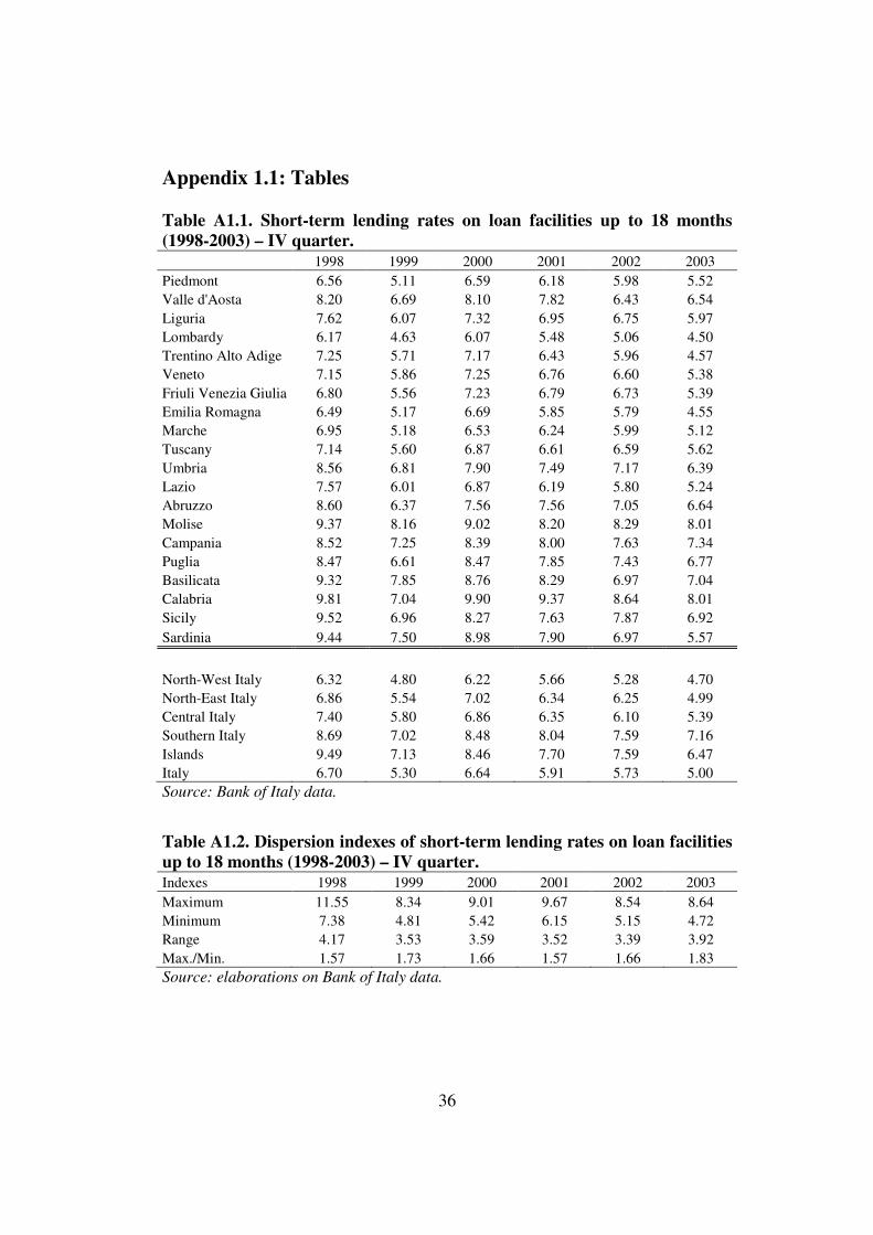
Between 1998 and 2003, short-term lending rates decreased considerably in all

Italian regions. During this period, the greatest reduction occurred in the Islands

where short-term lending rates declined by 3.02 percentage points from 9.49%

to 6.47%, while in the other geographical areas the reduction of the cost of

money was about 2 percentage points (see table A1.1).

The difference between the maximum and the minimum lending rate observed

in Italian regions decreased from 4.17% in 1998 to 3.92% in 2003 (see table

A1.2). Although this diminishing trend, the regional spread on borrowing

conditions charged to economic agents continued to be large. At the end of

2003, lending rates in Southern Italy and in the Islands were, respectively, 2.16

and 1.47 percentage points above the national average value. In the same year,

the difference between the largest and the smallest lending rate at provincial

level was equal to 4.36%: the province with the highest lending rate – equal to

8.36% - was Vibo Valentia (in Calabria, in Southern Italy), while the province

13

characterized by the best borrowing conditions was Bologna (in Emilia

Romagna, in North-East Italy), with a provincial lending rate equal to 4.00%.

Data show that the substantial reduction of lending rates in Italian regions

between 1998 and 2003 was not associated with a significant reduction of

interregional differentials in the cost of money also in relative terms; on the

contrary, the difference between lending rates charged in Southern regions and

the national average values remained around 2 percentage points. The same

values were observed by Galli and Onado during the eighties of the last century.

Although data on the cost of money are available up to the third semester of

2010, it is not possible to compare the values of lending rates before 2003 with

those observed in the subsequent period because of the relevant changes

introduced in the sample survey of deposit and lending rates by Bank of Italy at

the beginning of 2004.

Because of this reason, the empirical analysis of the determinants of the

interregional interest spreads in Italy will be based exclusively on the years

1998-2003.

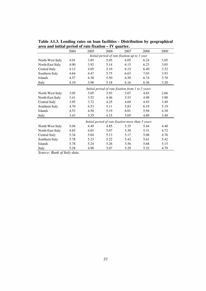
In fact, by looking at the lending rates during after 2003, it is possible to notice

that, in 2004, the cost of money is more homogenous among geographical areas.

In details, the interest rates applied in Southern Italy and in the Islands are

greater than the national value just of about 50 basis points taking into

consideration an initial period of rate fixation up to 1 year or more than 5 years.

Only for the intermediate time horizon (from 1 to 5 years) the gap between

lending rates charged in Southern regions and the national value was significant

(less than 130 basis point) but lower than the spread observed in 2003 (see table

A1.3).

Consequently, any comparison between these two different periods would be

misleading. The sudden reduction of the spreads between 2003 and 2004 seems

to be attributed to statistical causes and not to an actual improving of borrowing

conditions in the Mezzogiorno area.

14

However, it is interesting to observe that also during the period 2004-2009,

lending rates applied in Southern Italy and in the Islands were above the average

national values.

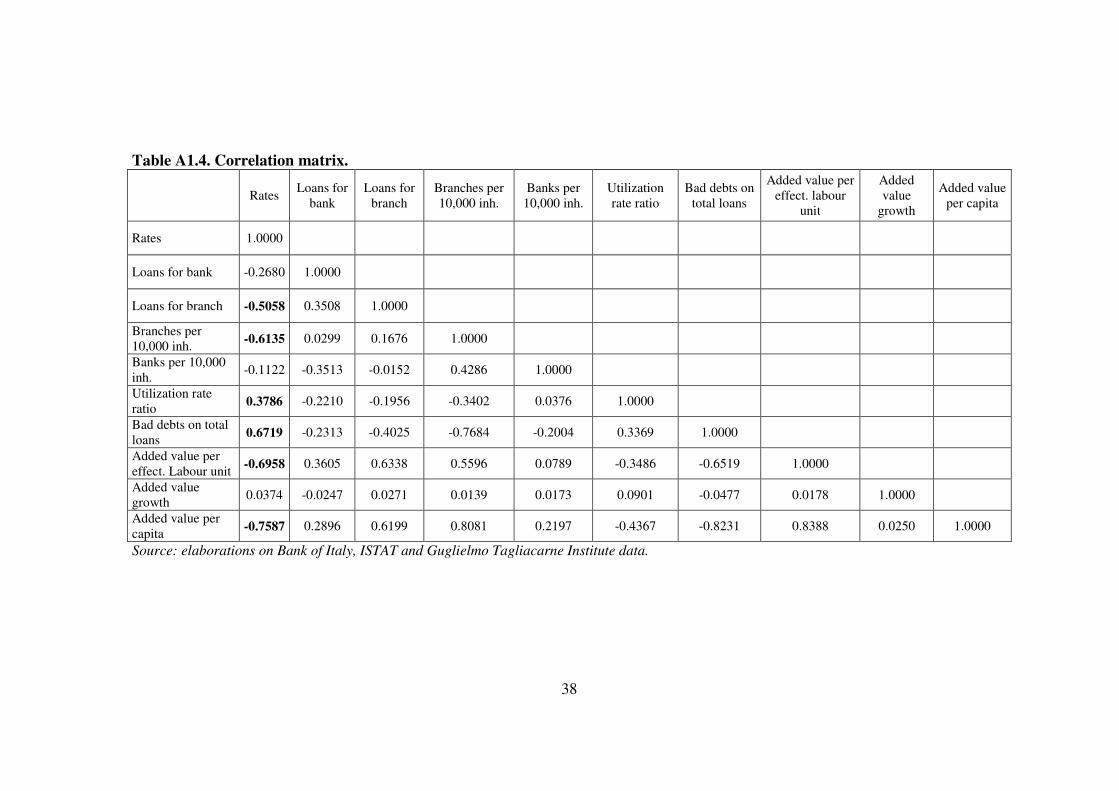
By taking into consideration the lending rates at a provincial level during the

period 1998-2003, an initial correlation analysis indicates that the cost of money

is larger in the provinces characterized by a larger riskiness of loans (expressed

in terms of ratio between bad debts and total loans), a greater value of the

amount of credit used by borrowers relative to credit granted by the banking

system, a lower diffusion of branches into the territory (measured by the number

of branches every 10,000 inhabitants) and a smaller value of average loans for

branch (see table A1.4).

The provinces whose banking system is characterized by these features are

localized in the Mezzogiorno area. This element indicates, consistently with the

main literature, that interregional spreads in the cost of money can be explained

by looking at the differences in the structure of the banking system among areas.

During the nineties of the last century, in Italy, the aggregation processes among

banks led to a substantial increase in the degree of concentration of the banking

system. Particularly, between 1990 and 2000, in the Italian banking system there

were 229 acquisitions operations; nevertheless, while in the Northern Italy these

acquisitions occurred, almost exclusively, in the same area, in the Italian

Mezzogiorno only 9 out of 89 were effectuated by banks with legal residence in

Southern regions.

These events caused, between 1990 and 2003, a drastic reduction in the number

of banks in the Mezzogiorno where, on the whole, banks decreased by 58 units.

This diminution occurred largely from 1997 to 2003, when the number of banks

operating in Southern Italy decreased by 42 units.

As regards the number of banks every 10,000 inhabitants, during the same

period, the value of this indicator in Southern Italy and in the Islands was lower

than the value observed in North-West and Central Italy denoting, thereby, a

15

lower degree of competition of the banking system in Southern regions. In order

to adequately assess the degree of competition of the banking system, it would

be necessary to compute an indicator, such as the Herfindahl-Hirschman index,

for each area. Nevertheless, because data on banks’ market share are not

publically available, the territorial diffusion of the bank network (expressed by

the number of banks or branches per 10,000 inhabitants) can be considered a

proxy of the banking system’s structure and, indirectly, of the degree of

competition. This approach is consistent with the analysis developed by Bank of

Italy (Bonaccorsi di Patti, 2009) that examines the relationship between credit

availability and institutional environment in Italy and includes the number of

branches per 1,000 inhabitants as a measure of spatial competition.

Under the same conditions, a lower degree of competition could have led to a

worsening of borrowing conditions applied to bank customers because of

possible gains in the market power for banks involved. Nevertheless, the

examined data do not support the hypothesis of a significant relationship

between the degree of competition of the banking system and the cost of money

(the correlation coefficients between the number of banks every 10,000

inhabitants and lending rates is equal to -0.11).

The lack of a significant correlation between the degree of competition and the

cost of money can be caused by several factors.

First, the increase in the degree of concentration of the Italian banking system

may not be associated with a contemporaneous boost in the market power of the

banks originated via the merger and acquisition procedures. This hypothesis

might be confirmed by the expansion of the branch network that occurred

contemporaneously with the reduction of the number of banks and that was

facilitated by the deregulation process that, during the nineties of the last

century, eliminated the territorial constraints to banking activity.

Nevertheless, although during the period examined the number of branches

increased in all areas, in 2003, in Southern regions the degree of territorial

16

diffusion of branches remained noticeably lower in comparison with the other

ones. In details, in Southern Italy and in the Islands there were, respectively,

3.10 and 3.53 branches per 10,000 inhabitants, a value less than the number

observed, in the same year, at national level (5.27).

Second, the lack of a significant relationship between the degree of

concentration and the cost of money can be due to the possible gains in the

operating efficiency that mergers and acquisition may have determined for the

Italian banking system. According to Angelini and Cetorelli (2000), banks

involved in concentration operations during the nineties, exhibited considerably

lower marginal costs than other banks and, therefore, they were able to apply

better borrowing conditions (in terms of lending rates) to all customers.

Data show the presence of a negative relationship between operation size and

the cost of money (the correlation coefficient between average loans for branch

and lending rates is equal to -0.51). In addition, the level of average loans for

bank in Southern Italy and in the Islands (equal, respectively, to 0.937 and 1.267

millions of euros) were lower than the value observed, on average, in Italy

(1.381 millions of euros).

These data seem to indicate that larger size of loans should allow the Northern

banks to apply better credit conditions given larger economies of scale. In order

to verify this hypothesis, it would be interesting also to analyse microeconomic

factors and examine, for example, micro and accounting data concerning the

degree of innovation for each bank. However, data about these elements are not

publically available.

Another factor to explain interregional interest rate spread is the degree of “gap”

of the banking system expressed in terms of utilization rate ratio per average

loan granted. This indicator can be considered as a proxy for a spatial credit

rationing because it relates actual satisfied credit demand with respect to credit

supply granted. Values of the index greater than 1 denote the presence of

potential credit crunch in the system because borrowers actually need an amount

17

of credit greater than the amount granted and, hence, the banking system is not

be able or not willing to satisfy the local economic agents’ credit demand.

Table A1.5, in appendix 1.1, shows that the utilization rate ratio was

substantially stable in each macroarea. In 2003, this index took the highest value

in Calabria, where it was equal to 85.0% (at national level, in the same year, the

utilization rate ratio amounted to 72.3%).

Finally, it is necessary to compare lending rates with the different perceived

borrowers’ credit risk in the areas. This element can be expressed, in a macro

perspective, through the ratio between bad debts and total loans, while at a

micro level, the probability of default is a better indicator.

Data show that during the period 1998-2003 the loans’ riskiness in the regions

of the Italian Mezzogiorno was significantly higher than that observed in

Northern and Central areas.

During this period, the weight of bad debts to total loans decreased in all

provinces. Southern Italy and the Islands were the geographical areas with the

most substantial improvement of credit quality and, inside these areas, Sicily

registered the highest reduction in the ratio of bad debts to total loans (from

34.8% in 1998 to 13.5% in 2003).

Although these positive results, at the end of the period taken into consideration,

in Southern regions this indicator remained considerably higher with respect the

national average value (in 2003, this ratio amounted, respectively, to 12.3%,

13.1% and 4.9% in Southern Italy, in Islands and, on average, in Italy). These

data denote, hence, the existence of a positive relationship between the cost of

money and riskiness of loans.

In order to evaluate the determinants of interregional interest-rate spreads, it is

important to consider also the different levels of economic development of the

areas.

18

The more intuitive proxy for this element is the level of GDP per capita, under

the hypothesis that the areas with a larger value of this indicator are

characterized also by a greater level of economic development.

However, data on GDP per capita are not available at a provincial level but only

at a regional level. Hence, it is necessary to consider another proxy for local

development.

Because the added value is strictly correlated to the GDP (the added value of an

economy is the difference between total production and the value of the

productive factors used into the productive phases), it appears appropriate to use

the added value as a proxy for provinces’ total wealth. Hence, the added value

per capita can be considered as a proxy of the degree of economic development,

while the added value for employed represents a measure of the productivity of

the economies.

Data show that worse borrowing conditions are associated to lower levels of

added value per capita and added value per effective labour unit (the correlation

coefficient between these indicators and lending rates amount, respectively, to -

0.76 and -0.70).

Furthermore, data show that the provinces more developed in terms of added

value per capita are characterized also by a greater degree of territorial diffusion

of branches, a larger banks’ operating size and a better credit quality (see table

A1.4).

The correlation matrix between the characteristics of the provincial economic

and banking systems illustrated in this paragraph is shown in table A1.4. This

matrix can be considered as a tool to choose relevant factors that can contribute

to explain differences in the cost of money across the provinces, as well as to

identify possible multicollinearity problems between the explanatory variables

in a regression framework.

19

1.4 Data and methodology

In order to identify the causes of the heterogeneity in bank interest rates among

the Italian provinces, this work develops a quantitative analysis based on a set of

balanced panel data concerning the main features of the economic and banking

system in Italian provinces during the period 1998-2003.

As I pointed out in paragraph 1.3, because of problems of data homogeneity, it

is not possible to consider data concerning the cost of money after 2003. In fact,

since 2004, data relating to interest rates are not comparable with those referred

to the previous period because of the changes introduced in the quarterly sample

survey of deposit and lending rates by Bank of Italy. Particularly, the new

survey, applied since the first quarter of 2004, is based on a larger number of

banks and on a modified report form. All comparisons are therefore not

homogeneous.

The following section examines the relationship among the cost of money

(expressed in terms of short-term lending rates on loan facilities up to 18

months) and several macroeconomic and financial variables that can influence

the level of provincial lending rates.

Short-term lending rates at provincial level have been estimated by the

Guglielmo Tagliacarne Institute on the basis of the regional lending rates

calculated by Bank of Italy according to the national sample survey developed at

regional level3.

3According to section 2.3 of the methodological appendix of the Statistical Bulletin published by Bank of Italy in the last quarter of the period object of analysis: “Pursuant to Article 51 of the Banking Law, two groups of banks participate in the quarterly

survey of interest rates: around 70 banks for lending rates and 60 for deposit rates. Both groups

include the principal banks at national level. The information on lending rates refers to the rates

charged to resident non–bank customers reported to the Central Credit Register in the last

month of the reference quarter, provided the related loans and guarantees exceed the reporting

threshold.

For each name and with reference to each reporting category, banks must report the interest

products and the amount received or debited for interest, commissions and fees. On the basis of

these data, interest rates are calculated as the weighted average of the effective rate charged to

customers, according to the formula:

20

These data represent the most reliable estimates of provincial lending rates that

are available and the estimation methodology has been positively verified by

Bank of Italy staff.

The necessity to use provincial data is due to the limited number of observations

(and, hence, of degrees of freedom) that would characterize an analysis based on

regional data. In fact, if this analysis would be based on regional data, the

number of observations for each variable would be equal to 120 (observations

about 20 regions for 6 years). The possibility to consider provincial data

noticeably increases the number of observations, improving the significance and

the robustness of the whole analysis (for every variable, it is in fact possible to

take into consideration 618 observations, i.e. data on 103 provinces for 6 years).

The variables employed in the analysis and potentially able to affect regional

lending rates are, on the basis of the correlation analysis previously developed,

the ratio of bad debts to total loans, the number of branches per 10,000

inhabitants, the utilization rate ratio (per average loan granted) and the level of

average loans for branch.

As regards the ratio of bad debts to total loans and the utilization rate ratio, it is

necessary to consider that the numerator and the denominator of these indicators

are characterized by different temporal dynamics; in fact, for each year, both

bad debts and the amount of credit actually used refer to loans granted in

previous years. Therefore, for each year, the ratio of bad debts to total loans was

calculated as the ratio between the amount of bad debts during the year in

question and the amount of total loans concerning the previous year.

Analogously, the utilization rate ratio is computed as the ratio between the

r(%) = amounts due*36.5/products

This weighted average is used for the data on interest rates published in the Bulletin unless

otherwise specified in the notes to the tables”.

21

amount of credit actually used by borrowers during the year taken into

consideration and the total amount of credit granted during the previous period.

Data concerning the financial system are elaborated by Bank of Italy, with the

exception of data on lending rates that, as pointed out before, are provided by

Guglielmo Tagliacarne Institute; data on population are elaborated by the Italian

National Statistical Office (ISTAT).

As regards the riskiness of loans, this analysis does not take into account also

the quarterly default rates for loan facilities defined by Bank of Italy as “the

ratio whose denominator is the amount of credit used by all the borrowers

covered by the Central Credit Register not classified as “adjusted bad debtors”

at the end of the previous quarter and whose numerator is the amount of credit

used by such borrowers who become “adjusted bad debtors” during the quarter

in question”4.

Because of the considerable volatility of default rates, I preferred to include in

the analysis the ratio of bad debts to total loans as proxy of granted loans’

riskiness. The high volatility of default rates would have biased the results of

this work.

An important element to verify is the stationarity of the variables included in the

model. Generally, in order to evaluate the hypothesis of stationarity of panel

series, the literature has proposed several tests based on different assumptions.

Particularly, the most important unit root tests for panel data are those

introduced by Im, Pesaran and Shin (1997), Maddala and Wu (1999) and Levin

et al. (2002).

4 Bank of Italy defines adjusted bad debts as “the total loans outstanding when a borrower is

reported to the Central Credit Register: a) as a bad debt by the only bank that disbursed credit;

b) as a bad debt by one bank and as having an overshoot by the only other bank exposed; c) as a

bad debt by one bank and the amount of the bad debt is at least 70% of its exposure towards the

banking system or as having overshoots equal to or more than 10% of its total loans

outstanding; d) as a bad debt by at least two banks for amounts equal to or more than 10% of its

total loans outstanding”.

22

Among these tests, I took into consideration the Im, Pesaran and Shin test

(henceforth IPS test) and the Maddala and Wu test (henceforth MW test)

because these two tests explicitly consider heterogeneity among groups5. This

element seems to be very important in this analysis where the individual units

are the Italian provinces, whose economic and banking structure is rather

different. The test introduced by Levin and Lin, on the contrary, by assuming

common unit root processes, does not allow this possibility.

Furthermore, the IPS test and the MW test are more appropriate to evaluate the

stationarity in micro-panel samples, with T fixed.

The results are shown in appendix 1.1. According to these tests, we cannot reject

the null hypothesis of not stationarity for the following series: loans for bank,

loans for branches, added value per effective labour unit and added value per

capita. On the contrary, lending rates, the number of banks and branches per

10,000 inhabitants, the utilization rate ratio, the ratio between bad debts and

total loans and the growth rate of the added value are stationary series. However,

all variables are I(1), i.e. if the series are expressed in terms of first differences,

these tests lead to the rejection of the null hypothesis of not stationarity6.

In light of the above considerations, the econometric analysis is based on a set of

dynamic panel models that analyze the statistical relationship between lending

rates and the financial and macroeconomic variables mentioned above.

The econometric models employed to identify the elements that, at a macro

level, affect the cost of money, have been estimated through the methodology

introduced by Arellano and Bond in 1991. In fact, it is clear that the causal

relationships hypothesized have a dynamic and not static nature. This

5 The criterion used to choose the number of lags included into the autoregressive equations that have been employed to verify the null hypothesis of unit root is the Schwarz Info Criterion. 6 As regards the ratio between bad debts and total loans expressed in first differences, according to the MW test it is not possible to reject the null hypothesis of not stationarity.

23

specification allows hence to take into consideration the degree of persistence

that characterizes borrowing conditions at provincial level.

Among the dynamic panel models, the choice of the Arellano and Bond

methodology is justified by three reasons. First, because the Arellano and Bond

method is a procedure based on the moment conditions, its use allows to

overcome possible endogeneity problems of the regressors; second, because the

instrumental variables used through this method are expressed in first

differences, the Arellano and Bond procedure allows to overcome the problem

of not stationary of several regressors that are, however, I(1); third, the Arellano

and Bond procedure leads to consistent estimates, for micro-panel samples,

where there are a large number of individuals (N) observed over a short period

of time (T).

1.5 The econometric analysis

The following analysis shows that the worse borrowing conditions in Southern

provinces can be caused by factors concerning the structure of the banking

system.

In order to understand the effect of the banking structure on lending rates at

regional level, the Arellano and Bond methodology is employed to estimate a set

of dynamic panel models that examine the relationship between interest rates

and the financial variables previously indicated.

The explanatory variables of these models have been chosen by taking into

consideration both the main results of the literature about the elements able to

influence the cost of money at macroeconomic level and the results of the

correlation analysis previously developed.

It would be appropriate to have an exact measure of the degree of concentration

of the banking system in every province, given the general positive relationship

between concentration and price pointed out by the structure-conduct-

performance paradigm. However, in order to build up an indicator of the degree

24

of concentration of the banking system it would be necessary to analyse data on

banks’ market shares. Because these data are not available, it is not possible to

compute an indicator of this type. The dataset used in this work, however, gives

us an implicit measure of the degree of competition of the banking system,

because the diffusion of the branch network on the territory is generally positive

correlated with the degree of competition of the system.

According to the previous analysis, the factors potentially able to explain the

different levels in the lending rates among the areas are:

• operating size of branches, expressed in terms of average loans for

branch;

• diffusion of the branch network on the territory, measured by the number

of branches per 10,000 inhabitants;

• degree of tension in the banking system, expressed in terms of utilization

rate ratio;

• riskiness of loans, calculated as ratio between bad debts and total loans;

• degree of economic development, approximated by the amount of added

value per capita;

• degree of productivity in the system, measured by the amount of added

value per effective labour unit.

Obviously, it is not possible to insert all these variable in a single model because

of the significant correlation relationships between them that would cause

multicollinearity problems. In fact, by looking at table A1.4, it is possible to

notice as the added value per capita and the added value per effective labour unit

are highly correlated with the other variables. Hence, these two variables are not

included into the regression models.

As regards the other variables, the most significant correlation is observed

between the ratio of bad debts on total loans and the number of branches per

10,000 inhabitants (the correlation index between these two indicators amounts

25

to -0.77). Therefore, in order to avoid multicollinearity, these two variables

cannot be included into the same models.

Nevertheless, as pointed out by Baltagi (2008) and Hsiao (2003), in panel data

models the multicollinearity problems are substantially reduced, given the more

degrees of freedom and information on individual attributes that panel data

offer. Hence, I decided to not include, in the same model, variables for which

the correlation coefficient is, in absolute value, bigger than 0.4.

I estimated 16 specifications that are characterized by different assumptions on

the nature – strictly exogenous or predetermined – of the explanatory variables.

In order to analyze the effects of the structure of the banking system on lending

rates, the estimated dynamic panel models include, among the regressors, the

average loans for branch, the utilization rate ratio and, separately, the ratio of

bad debts to total loans (from model 1 to model 8) and the number of branches

per 10,000 inhabitants (from model 9 to model 16). The results are shown in

appendix 1.1 (tables A1.7 and A1.8).

Because of the limited number of periods taken into consideration in the

analysis (6 years), the inclusion of a number of lags greater than 2 would

significantly reduce the degrees of freedom and the robustness of the estimates.

Furthermore, because of the high degree of persistence that characterizes

lending rates (that is caused also by the imperfections in the banking system that

cause sluggish adjustments in lending rates), every model includes 2 lags for the

dependent variable.

Three cross-sections are lost in constructing lags and taking first differences, so

that the estimation period is 2001-2003 and the number of useable observations

for each series is equal to 309.

Each model has been evaluated on the basis of the Wald test, the Sargan test and

the Arellano and Bond test in order to assess the consistency of the estimated

coefficients.

26

The Wald test verifies the joint significance of the coefficients associated to the

regressors7.

The Sargan test verifies the hypothesis that the overidentifying restrictions are

valid, i.e. the validity of the instruments employed in the regression.

Finally, the Arellano and Bond test verifies the lack of second-order serial

correlation among the residuals of the regression, i.e. �[�����(���)] = 08. This

condition represents a crucial assumption of the Arellano and Bond

methodology and if it is not respected the estimated coefficients are inconsistent

because, in this case, there exists a significant correlation between the regressors

included into the matrix of instruments and the idiosyncratic component of the

error.

All models have been estimated through the one-step and the two-steps Arellano

and Bond methodology (the results are shown in tables A1.7 and A1.8).

However, as suggested by Arellano and Bond, because for samples of small size

the two-steps standard errors are downward biased, it is preferable to make

inference based on the one-step estimator.

The results, confirm the consistency of the estimated coefficients. In fact, with

the exception of three specifications (model 2, 3 and 7), the results of the

Arellano and Bond test indicates that it is not possible to reject the null

hypothesis of the lack of second-order serial correlation among the residuals of

the regression. Furthermore, for all the models, the Wald test rejects the

hypothesis that the estimated coefficient are not jointly significantly different

from zero.

Among the models for which the Arellano and Bond test does not reject the null

hypothesis, the Sargan test leads to do not reject the hypothesis of validity of the

instruments only for two specifications (model 8 and 15). In these two models,

7 Under the null hypothesis of not joint significance of the estimated coefficients, the probability distribution of the Wald test is a chi-square with a number of degrees of freedom equal to the number of the regressors. 8 See appendix 1.2 for more details about the Sargan test and the Arellano and Bond test.

27

the ratio between bad debts and total loans, the average loans for branch and the

utilization rate ratio are considered as predetermined while the number of

branches every 10,000 inhabitants is considered as strictly exogenous. These

results imply that it could be not appropriate to treat the features of the banking

system included in the models as strictly exogenous because some shock could

influence the future changes in these elements.

The regression output indicates that, after controlling for the persistence in the

lending rates series, borrowing conditions remain significantly affected by the

regional banking structure.

The sum of the coefficients associated to the lagged values of the dependent

variable is always less than 1; the stationarity condition is therefore respected.

Lending rates are negatively affected by the average branches’ operating size

and of the territorial diffusion of the branch network.

Particularly, under the same conditions, if average loans for branch increase of 1

million of euros, lending rates reduces of 51 basis points, according to model 8,

or 42 basis points according to model 15; an increase of 1 branch per 10,000

inhabitants leads to a reduction of 162 basis points in lending rates (model 15).

The results seem to confirm that the general augment in banks’ operating

efficiency caused by the increase in their average operating size was be able to

offset the possible gains in banks’ market power due to the aggregation

processes.

Consequently, the lower branches’ operating size (and, hence, the smaller

degree of banks’ efficiency) and the smaller degree of spatial closeness between

banks and firms in Southern Italy and in the Islands, represent one of the causes

that determine worse borrowing conditions in these areas.

Also the degree of diffusion of the branch network in the territory affects the

cost of money. Under the hypothesis that a greater number of branches per

10,000 inhabitants implies a larger degree of competition in the banking system,

28

the negative and significant relationship between this variable and lending rates

is consistent with the structure-conduct-performance paradigm.

The smaller number of branches per 10,000 inhabitants in Southern provinces

(and, hence, the more implicit concentration of the banking system in these

zones) contributes hence to determine a larger cost of money in Southern Italy

and in the Islands.

Another factor causing higher interest rates in Southern areas is the worse credit

quality. Credit risk represents one of the main elements that banks take into

account in their credit and pricing policies. While at microeconomic level credit

risk is usually expressed in terms of probability of default, in a macro

perspective the regional ratio of bad debts to total loans can be used as a proxy

of borrowers’ credit risk.

The results are consistent with the theory: a greater degree of borrowers’

riskiness determines the application of higher bank interest rates. In detail,

according to model 8, an augment of 1% in the ratio of bad debts to total loans is

associated with an increase of 11 basis points in lending rates.

According to models 8 and 15, the utilization rate ratio does not significantly

influence lending rates.

The lack of a significant relationship between these two variables can be due to

the greater homogeneity of the utilization rate ratio across the areas in

comparison with the other explanatory variables.

Particularly, in 2003, this index was equal, in Southern Italy, in the Islands and

at national level, respectively, to 80.7%, 81.8% and 72.3% (table A1.5).

In conclusion, these models show that the differences among regions in lending

rates can be explained by taking into consideration the differences in terms of

banking structure and borrowers’ behaviour. Larger branches operating in

Northern regions, by exploiting bigger scale economies, are able to apply to

their customers better borrowing conditions.

29

Another reason why banks apply larger lending rates in Southern regions is the

larger loans’ riskiness that characterizes this area. On the other hand, this pricing

policy can cause adverse selection phenomena in credit market and,

consequently, increases the average regional credit risk determining a vicious

circle between higher lending rates and larger borrowers’ risk.

The higher cost of money in Southern provinces represents a crucial element

because worse borrowing conditions are able to hinder the regional economic

development, slowing investments and the capital accumulation process.

It is important to analyze the structure of the banking system in those contexts,

such as the Italian one, in which bank credit is the main (and in the most part of

the cases the only) source of funding for private firms. The structural

characteristics of the banking system, among which the worse borrowing

conditions observed in Southern areas, can have large effects on the real

economic system, by hindering the level of economic development.

Furthermore, the difficulties that Southern firms face to obtain bank credit, can

obstruct also their innovation ability and, hence, their productivity. This

situation prevents improvements in Southern economy’s competitive level, a

necessary condition to overcame the structural crisis that, for several decades,

have burden on the Southern areas.

1.6 Conclusions

The causes of interregional interest rate differentials observed in several

countries represents a topic, for a long period, object of debate in economic

literature. Among the different reasons, several authors enumerate together with

imperfections of financial markets also real and economic variables.

Particularly, literature tends to explain these spreads through factors concerning

credit market’s structure, regional differences in transaction costs, demand,

borrowers’ localization and according to the differences, across the areas, in the

perceived counterparts’ credit risk.

30

In Italy the difference of about 2 percentage points between lending rates

charged in Southern regions and the national average, observed on average

during the eighties of the last century, remained substantially unchanged until

2003.

A school of thought assumes that the higher lending rates in Southern regions

are due, mainly, to the differences among areas, in the size and industry

composition of bank customers, and the lack of infrastructures adequate to

support economic growth (Panetta, 2003).

A second view, instead, considers that the higher lending rates charged in the

Italian Mezzogiorno can be due, primarily, to the greater riskiness of loans

observed in the area and other factors such as a credit rationing strategy

occurred in the Italian Mezzogiorno because of the inadequacy of the Southern

financial system, not able to provide financial resources sufficient to sustain

local development processes (Mattesini and Messori, 2004).

The endogenous nature of the causes of interregional interest rate spreads was

confirmed, as regards the American context, by the analysis developed by

Landon-Lane and Rockoff in 2004. The American financial system achieved a

high degree of financial integration (and, therefore, interregional interest rate

differentials decreased) only after the second post-war, when the American

economic system became more homogeneous.

As regards the Italian case, the results of this work are partially in contrast with

Panetta’s opinion. In order to understand why, in Southern areas, banks apply

greater lending rates, before looking at the differences in the size and industry

composition of borrowers, it is necessary to take into consideration the

differences, among areas, in the banks’ structural characteristics.

The analysis developed indicates, in fact, that during the period 1998-2003 in

Southern Italy and in the Islands the larger cost of money was caused by several

structural factors such as the lower average branches’ size and the smaller

territorial diffusion of the branch network.

31

The operating size of branches (expressed in terms of average loans for branch)

negatively influences bank interest rates because of the ability of large-sized

branches to achieve greater levels of efficiency (by exploiting scale economies)

and, hence, under the same conditions, to charge lower lending rates to the

counterparts.

The smaller degree of diffusion of branches in the territory observed in the

Mezzogiorno (measured by the number of branches per 10,000 inhabitants)

denotes a lower degree of competition in the area and hence determines worse

borrowing conditions.

Consistently with Panetta’s results, however, this analysis shows the existence

of a significant and positive relationship between borrowers’ riskiness

(measured by the ratio of bad debts to total loans) and the cost of money. Hence,

a share of the interregional interest rate spreads in Italy is caused by the higher

borrowers’ riskiness perceived in Southern Italy and in the Islands.

However, the higher riskiness in these areas can be caused by adverse selection

phenomena in the credit market (in other words, by the same application of

worse borrowing conditions). Therefore, it is important to understand if the

higher riskiness in Southern regions measured by the larger ratio of bad debts to

total loans reflects the borrowers’ structural characteristics or if it is caused by

market imperfections.

This topic is very important in the light of the restraining effect of worse

borrowing conditions on the degree of economic development.

32

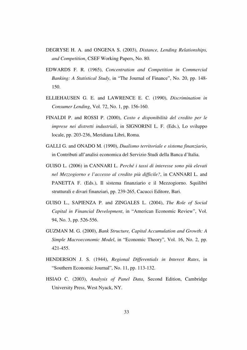
1.7 References

ANGELINI P. and CETORELLI N. (2000), Bank Competition and Regulatory

Reform: The Case of the Italian Banking Industry, in “Temi di Discussione

della Banca d'Italia”, No. 380.

ANGELONI I., KASHYAP A., MOJON B. and TERLIZZESE D. (2003),

Monetary transmission in the euro area: does the interest rate channel

explain all?, in Working Paper 9984 – National Bureau of Economic

Research, Cambridge.

ARELLANO M. and BOND S. (1991), Some Tests of Specifications for Panel

Data: Monte Carlo Evidence and an Application to Employment Equations,

in “The Review of Economic Studies Limited”, No. 58, pp. 277-297.

ASPINWALL R. C. (1979), Market Structure and Commercial Bank Mortgage

Interest Rates, in “Southern Economic Journal”, No. 36, pp. 378-384.

BALTAGI B. H. (2008), Econometric Analysis of Panel Data – 4th edition,

Chichester, John Wiley and Sons.

BANCA D’ITALIA, Statistical Bulletin, (from 1991 up 2010).

BERETTA E. (2004), I divari regionali tra i tassi bancari in Italia, in “Banca

Impresa e Società”, No. 3, pp. 565-584.

CANNARI L. and PANETTA F. (2006), Il sistema finanziario e il Mezzogiorno.

Squilibri strutturali e divari finanziari, Cacucci Editore, Bari.

CEBULA R. J. and ZAHAROFF M. (1974), Interregional Capital Transfers

and Interest Rate Differentials: An Empirical Note, in “Annals of Regionals

Science”, 8, No. 1, pp. 87-94.

DANIELE V. (2003), Il costo dello sviluppo. Note sul sistema creditizio e

sviluppo economico nel Mezzogiorno, in “Rivista economica del

Mezzogiorno”, No. 1-2.

33

DEGRYSE H. A. and ONGENA S. (2003), Distance, Lending Relationships,

and Competition, CSEF Working Papers, No. 80.

EDWARDS F. R. (1965), Concentration and Competition in Commercial

Banking: A Statistical Study, in “The Journal of Finance”, No. 20, pp. 148-

150.

ELLIEHAUSEN G. E. and LAWRENCE E. C. (1990), Discrimination in

Consumer Lending, Vol. 72, No. 1, pp. 156-160.

FINALDI P. and ROSSI P. (2000), Costo e disponibilità del credito per le

imprese nei distretti industriali, in SIGNORINI L. F. (Eds.), Lo sviluppo

locale, pp. 203-236, Meridiana Libri, Roma.

GALLI G. and ONADO M. (1990), Dualismo territoriale e sistema finanziario,

in Contributi all’analisi economica del Servizio Studi della Banca d’Italia.

GUISO L. (2006) in CANNARI L. Perché i tassi di interesse sono più elevati

nel Mezzogiorno e l’accesso al credito più difficile?, in CANNARI L. and

PANETTA F. (Eds.), Il sistema finanziario e il Mezzogiorno. Squilibri

strutturali e divari finanziari, pp. 239-265, Cacucci Editore, Bari.

GUISO L., SAPIENZA P. and ZINGALES L. (2004), The Role of Social

Capital in Financial Development, in “American Economic Review”, Vol.

94, No. 3, pp. 526-556.

GUZMAN M. G. (2000), Bank Structure, Capital Accumulation and Growth: A

Simple Macroeconomic Model, in “Economic Theory”, Vol. 16, No. 2, pp.

421-455.

HENDERSON J. S. (1944), Regional Differentials in Interest Rates, in

“Southern Economic Journal”, No. 11, pp. 113-132.

HSIAO C. (2003), Analysis of Panel Data, Second Edition, Cambridge

University Press, West Nyack, NY.

34

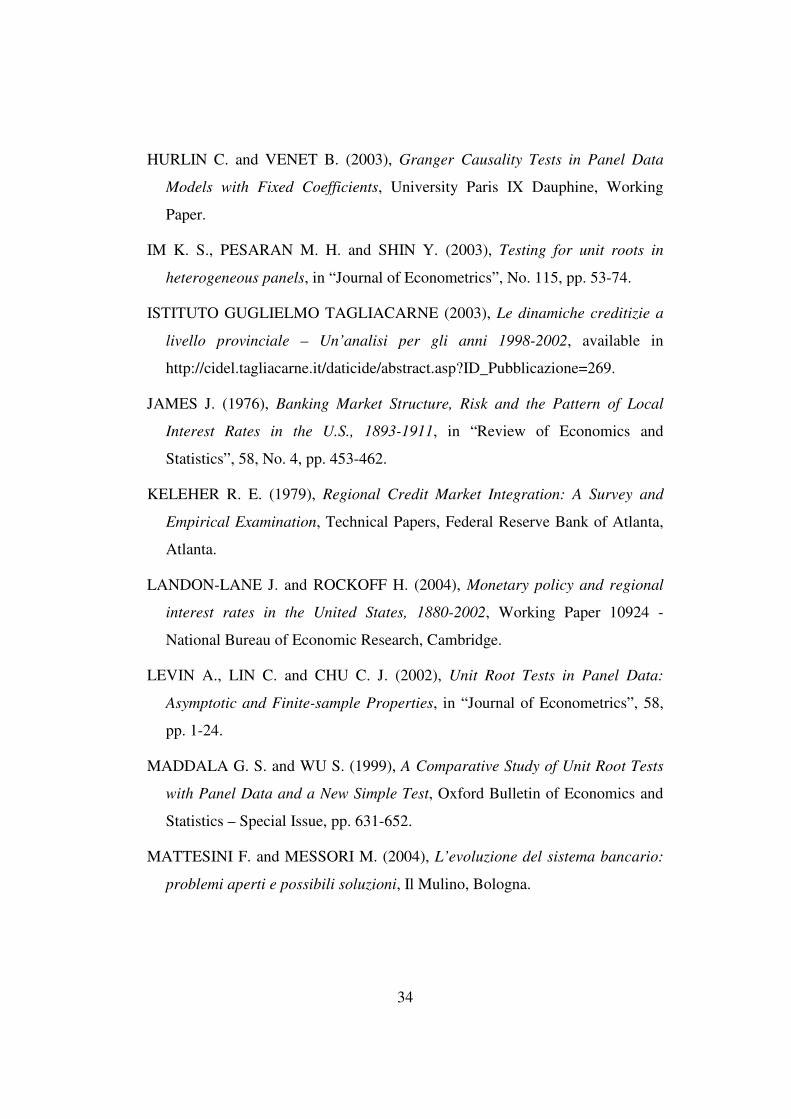
HURLIN C. and VENET B. (2003), Granger Causality Tests in Panel Data

Models with Fixed Coefficients, University Paris IX Dauphine, Working

Paper.

IM K. S., PESARAN M. H. and SHIN Y. (2003), Testing for unit roots in

heterogeneous panels, in “Journal of Econometrics”, No. 115, pp. 53-74.

ISTITUTO GUGLIELMO TAGLIACARNE (2003), Le dinamiche creditizie a

livello provinciale – Un’analisi per gli anni 1998-2002, available in

http://cidel.tagliacarne.it/daticide/abstract.asp?ID_Pubblicazione=269.

JAMES J. (1976), Banking Market Structure, Risk and the Pattern of Local

Interest Rates in the U.S., 1893-1911, in “Review of Economics and

Statistics”, 58, No. 4, pp. 453-462.

KELEHER R. E. (1979), Regional Credit Market Integration: A Survey and

Empirical Examination, Technical Papers, Federal Reserve Bank of Atlanta,

Atlanta.

LANDON-LANE J. and ROCKOFF H. (2004), Monetary policy and regional

interest rates in the United States, 1880-2002, Working Paper 10924 -

National Bureau of Economic Research, Cambridge.

LEVIN A., LIN C. and CHU C. J. (2002), Unit Root Tests in Panel Data:

Asymptotic and Finite-sample Properties, in “Journal of Econometrics”, 58,

pp. 1-24.

MADDALA G. S. and WU S. (1999), A Comparative Study of Unit Root Tests

with Panel Data and a New Simple Test, Oxford Bulletin of Economics and

Statistics – Special Issue, pp. 631-652.

MATTESINI F. and MESSORI M. (2004), L’evoluzione del sistema bancario:

problemi aperti e possibili soluzioni, Il Mulino, Bologna.

35

MISTRULLI P. E. and CASOLARO L. (2008), Distance, Lending Technologies

and Interest Rates, paper presented at the 21st Australasian Finance and

Banking Conference, 2008.

PANETTA F. (2003), Evoluzione del sistema bancario e finanziamento

dell’economia nel Mezzogiorno, in “Temi di Discussione della Banca

d’Italia”, No. 467.

PANETTA F. (2004), Il sistema bancario italiano negli anni novanta, Il

Mulino, Bologna.

PROVENZANO V. (2002), Sviluppo regionale e sistema finanziario, Edizioni

Anteprima, Palermo.

36

Appendix 1.1: Tables

Table A1.1. Short-term lending rates on loan facilities up to 18 months (1998-2003) – IV quarter.

1998 1999 2000 2001 2002 2003 Piedmont 6.56 5.11 6.59 6.18 5.98 5.52 Valle d'Aosta 8.20 6.69 8.10 7.82 6.43 6.54 Liguria 7.62 6.07 7.32 6.95 6.75 5.97 Lombardy 6.17 4.63 6.07 5.48 5.06 4.50 Trentino Alto Adige 7.25 5.71 7.17 6.43 5.96 4.57 Veneto 7.15 5.86 7.25 6.76 6.60 5.38 Friuli Venezia Giulia 6.80 5.56 7.23 6.79 6.73 5.39 Emilia Romagna 6.49 5.17 6.69 5.85 5.79 4.55 Marche 6.95 5.18 6.53 6.24 5.99 5.12 Tuscany 7.14 5.60 6.87 6.61 6.59 5.62 Umbria 8.56 6.81 7.90 7.49 7.17 6.39 Lazio 7.57 6.01 6.87 6.19 5.80 5.24 Abruzzo 8.60 6.37 7.56 7.56 7.05 6.64 Molise 9.37 8.16 9.02 8.20 8.29 8.01 Campania 8.52 7.25 8.39 8.00 7.63 7.34 Puglia 8.47 6.61 8.47 7.85 7.43 6.77 Basilicata 9.32 7.85 8.76 8.29 6.97 7.04 Calabria 9.81 7.04 9.90 9.37 8.64 8.01 Sicily 9.52 6.96 8.27 7.63 7.87 6.92 Sardinia 9.44 7.50 8.98 7.90 6.97 5.57

North-West Italy 6.32 4.80 6.22 5.66 5.28 4.70 North-East Italy 6.86 5.54 7.02 6.34 6.25 4.99 Central Italy 7.40 5.80 6.86 6.35 6.10 5.39 Southern Italy 8.69 7.02 8.48 8.04 7.59 7.16 Islands 9.49 7.13 8.46 7.70 7.59 6.47 Italy 6.70 5.30 6.64 5.91 5.73 5.00 Source: Bank of Italy data.

Table A1.2. Dispersion indexes of short-term lending rates on loan facilities up to 18 months (1998-2003) – IV quarter. Indexes 1998 1999 2000 2001 2002 2003 Maximum 11.55 8.34 9.01 9.67 8.54 8.64 Minimum 7.38 4.81 5.42 6.15 5.15 4.72 Range 4.17 3.53 3.59 3.52 3.39 3.92 Max./Min. 1.57 1.73 1.66 1.57 1.66 1.83 Source: elaborations on Bank of Italy data.

37

Table A1.3. Lending rates on loan facilities - Distribution by geographical area and initial period of rate fixation – IV quarter.

2004 2005 2006 2007 2008 2009 Initial period of rate fixation up to 1 year

North-West Italy 4.01 3.85 5.05 6.05 6.24 3.05 North-East Italy 4.00 3.92 5.14 6.15 6.23 3.03 Central Italy 4.12 4.05 5.19 6.15 6.40 3.32 Southern Italy 4.64 4.47 5.75 6.63 7.03 3.93 Islands 4.57 4.38 5.50 6.50 6.74 3.70 Italy 4.10 3.98 5.18 6.16 6.36 3.20

Initial period of rate fixation from 1 to 5 years

North-West Italy 3.05 3.05 3.93 5.07 4.65 2.66 North-East Italy 3.41 3.52 4.46 5.53 4.98 3.98 Central Italy 3.95 3.72 4.25 4.69 4.93 3.49 Southern Italy 4.70 4.53 5.11 5.83 6.19 5.19 Islands 4.53 4.58 5.19 6.01 5.94 4.30 Italy 3.43 3.35 4.15 5.05 4.89 3.40

Initial period of rate fixation more than 5 years

North-West Italy 5.04 4.49 4.85 5.35 5.44 4.40 North-East Italy 4.65 4.65 5.07 5.30 5.31 4.72 Central Italy 5.34 5.04 5.13 5.17 5.08 4.76 Southern Italy 5.78 5.23 5.22 5.42 5.61 5.42 Islands 5.78 5.24 5.26 5.56 5.68 5.15 Italy 5.28 4.90 5.07 5.29 5.32 4.79 Source: Bank of Italy data.

38

Table A1.4. Correlation matrix.

Rates

Loans for bank

Loans for branch

Branches per 10,000 inh.

Banks per 10,000 inh.

Utilization rate ratio

Bad debts on total loans

Added value per effect. labour

unit

Added value

growth

Added value per capita

Rates 1.0000

Loans for bank -0.2680 1.0000

Loans for branch -0.5058 0.3508 1.0000

Branches per 10,000 inh.

-0.6135 0.0299 0.1676 1.0000

Banks per 10,000 inh.

-0.1122 -0.3513 -0.0152 0.4286 1.0000

Utilization rate ratio

0.3786 -0.2210 -0.1956 -0.3402 0.0376 1.0000

Bad debts on total loans

0.6719 -0.2313 -0.4025 -0.7684 -0.2004 0.3369 1.0000

Added value per effect. Labour unit

-0.6958 0.3605 0.6338 0.5596 0.0789 -0.3486 -0.6519 1.0000

Added value growth

0.0374 -0.0247 0.0271 0.0139 0.0173 0.0901 -0.0477 0.0178 1.0000

Added value per capita

-0.7587 0.2896 0.6199 0.8081 0.2197 -0.4367 -0.8231 0.8388 0.0250 1.0000

Source: elaborations on Bank of Italy, ISTAT and Guglielmo Tagliacarne Institute data.

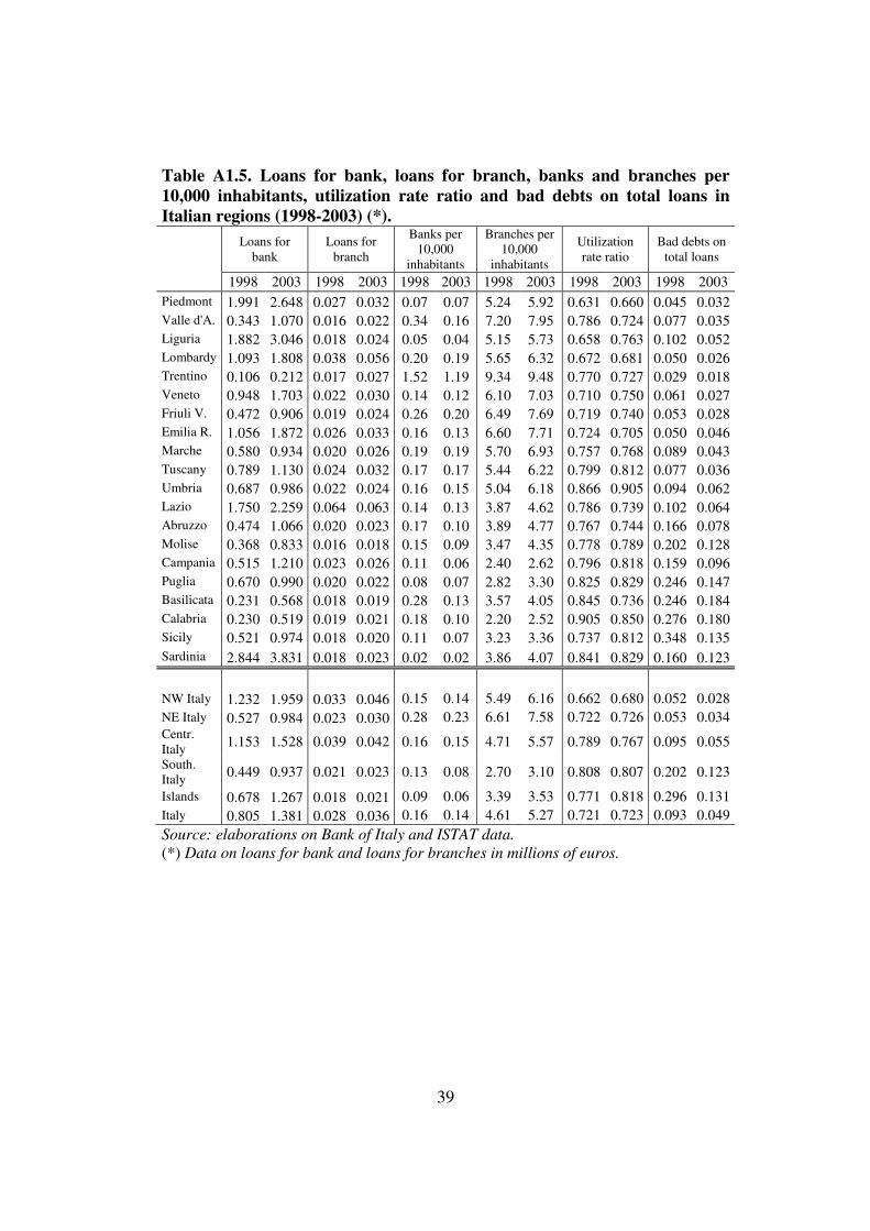
39

Table A1.5. Loans for bank, loans for branch, banks and branches per 10,000 inhabitants, utilization rate ratio and bad debts on total loans in Italian regions (1998-2003) (*).

Loans for

bank Loans for

branch

Banks per 10,000

inhabitants

Branches per 10,000

inhabitants

Utilization rate ratio

Bad debts on total loans

1998 2003 1998 2003 1998 2003 1998 2003 1998 2003 1998 2003 Piedmont 1.991 2.648 0.027 0.032 0.07 0.07 5.24 5.92 0.631 0.660 0.045 0.032 Valle d'A. 0.343 1.070 0.016 0.022 0.34 0.16 7.20 7.95 0.786 0.724 0.077 0.035 Liguria 1.882 3.046 0.018 0.024 0.05 0.04 5.15 5.73 0.658 0.763 0.102 0.052 Lombardy 1.093 1.808 0.038 0.056 0.20 0.19 5.65 6.32 0.672 0.681 0.050 0.026 Trentino 0.106 0.212 0.017 0.027 1.52 1.19 9.34 9.48 0.770 0.727 0.029 0.018 Veneto 0.948 1.703 0.022 0.030 0.14 0.12 6.10 7.03 0.710 0.750 0.061 0.027 Friuli V. 0.472 0.906 0.019 0.024 0.26 0.20 6.49 7.69 0.719 0.740 0.053 0.028 Emilia R. 1.056 1.872 0.026 0.033 0.16 0.13 6.60 7.71 0.724 0.705 0.050 0.046 Marche 0.580 0.934 0.020 0.026 0.19 0.19 5.70 6.93 0.757 0.768 0.089 0.043 Tuscany 0.789 1.130 0.024 0.032 0.17 0.17 5.44 6.22 0.799 0.812 0.077 0.036 Umbria 0.687 0.986 0.022 0.024 0.16 0.15 5.04 6.18 0.866 0.905 0.094 0.062 Lazio 1.750 2.259 0.064 0.063 0.14 0.13 3.87 4.62 0.786 0.739 0.102 0.064 Abruzzo 0.474 1.066 0.020 0.023 0.17 0.10 3.89 4.77 0.767 0.744 0.166 0.078 Molise 0.368 0.833 0.016 0.018 0.15 0.09 3.47 4.35 0.778 0.789 0.202 0.128 Campania 0.515 1.210 0.023 0.026 0.11 0.06 2.40 2.62 0.796 0.818 0.159 0.096 Puglia 0.670 0.990 0.020 0.022 0.08 0.07 2.82 3.30 0.825 0.829 0.246 0.147 Basilicata 0.231 0.568 0.018 0.019 0.28 0.13 3.57 4.05 0.845 0.736 0.246 0.184 Calabria 0.230 0.519 0.019 0.021 0.18 0.10 2.20 2.52 0.905 0.850 0.276 0.180 Sicily 0.521 0.974 0.018 0.020 0.11 0.07 3.23 3.36 0.737 0.812 0.348 0.135 Sardinia 2.844 3.831 0.018 0.023 0.02 0.02 3.86 4.07 0.841 0.829 0.160 0.123

NW Italy 1.232 1.959 0.033 0.046 0.15 0.14 5.49 6.16 0.662 0.680 0.052 0.028 NE Italy 0.527 0.984 0.023 0.030 0.28 0.23 6.61 7.58 0.722 0.726 0.053 0.034 Centr. Italy 1.153 1.528 0.039 0.042 0.16 0.15 4.71 5.57 0.789 0.767 0.095 0.055

South. Italy 0.449 0.937 0.021 0.023 0.13 0.08 2.70 3.10 0.808 0.807 0.202 0.123

Islands 0.678 1.267 0.018 0.021 0.09 0.06 3.39 3.53 0.771 0.818 0.296 0.131 Italy 0.805 1.381 0.028 0.036 0.16 0.14 4.61 5.27 0.721 0.723 0.093 0.049 Source: elaborations on Bank of Italy and ISTAT data.

(*) Data on loans for bank and loans for branches in millions of euros.

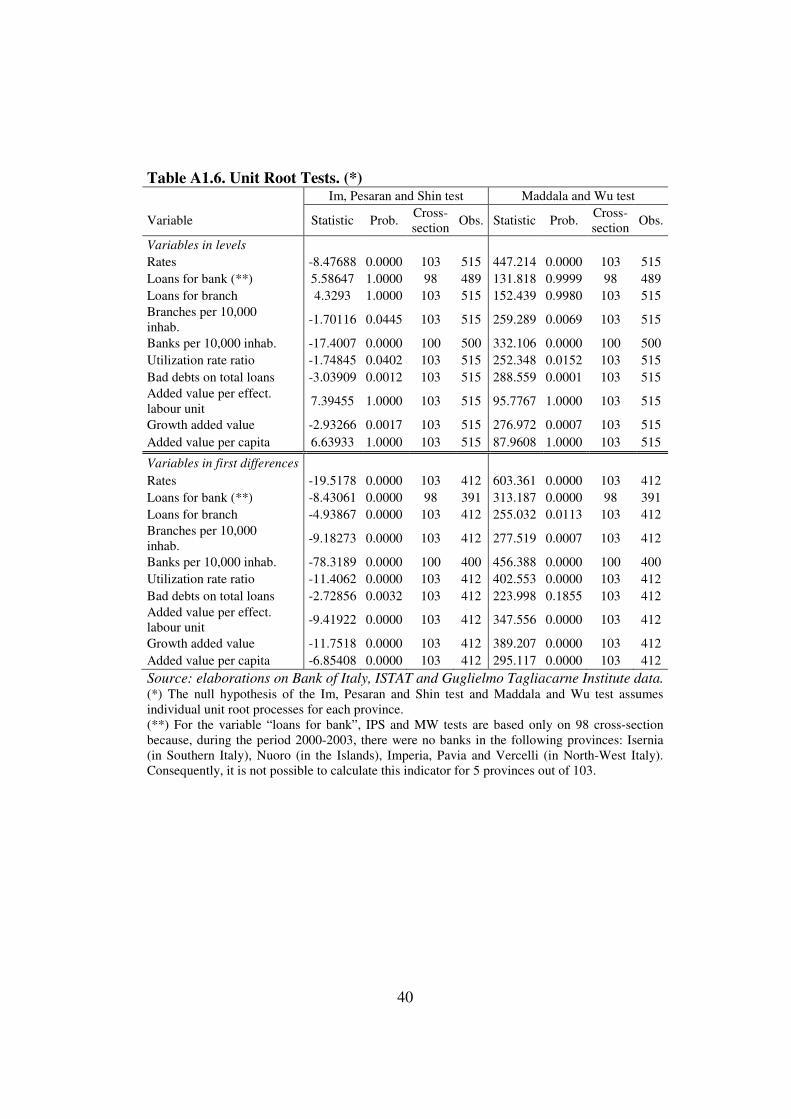
40

Table A1.6. Unit Root Tests. (*) Im, Pesaran and Shin test Maddala and Wu test

Variable Statistic Prob. Cross- section

Obs. Statistic Prob. Cross- section

Obs.

Variables in levels

Rates -8.47688 0.0000 103 515 447.214 0.0000 103 515 Loans for bank (**) 5.58647 1.0000 98 489 131.818 0.9999 98 489 Loans for branch 4.3293 1.0000 103 515 152.439 0.9980 103 515 Branches per 10,000 inhab.

-1.70116 0.0445 103 515 259.289 0.0069 103 515

Banks per 10,000 inhab. -17.4007 0.0000 100 500 332.106 0.0000 100 500 Utilization rate ratio -1.74845 0.0402 103 515 252.348 0.0152 103 515 Bad debts on total loans -3.03909 0.0012 103 515 288.559 0.0001 103 515 Added value per effect. labour unit

7.39455 1.0000 103 515 95.7767 1.0000 103 515

Growth added value -2.93266 0.0017 103 515 276.972 0.0007 103 515 Added value per capita 6.63933 1.0000 103 515 87.9608 1.0000 103 515

Variables in first differences

Rates -19.5178 0.0000 103 412 603.361 0.0000 103 412 Loans for bank (**) -8.43061 0.0000 98 391 313.187 0.0000 98 391 Loans for branch -4.93867 0.0000 103 412 255.032 0.0113 103 412 Branches per 10,000 inhab.

-9.18273 0.0000 103 412 277.519 0.0007 103 412

Banks per 10,000 inhab. -78.3189 0.0000 100 400 456.388 0.0000 100 400 Utilization rate ratio -11.4062 0.0000 103 412 402.553 0.0000 103 412 Bad debts on total loans -2.72856 0.0032 103 412 223.998 0.1855 103 412 Added value per effect. labour unit

-9.41922 0.0000 103 412 347.556 0.0000 103 412

Growth added value -11.7518 0.0000 103 412 389.207 0.0000 103 412 Added value per capita -6.85408 0.0000 103 412 295.117 0.0000 103 412 Source: elaborations on Bank of Italy, ISTAT and Guglielmo Tagliacarne Institute data. (*) The null hypothesis of the Im, Pesaran and Shin test and Maddala and Wu test assumes individual unit root processes for each province. (**) For the variable “loans for bank”, IPS and MW tests are based only on 98 cross-section because, during the period 2000-2003, there were no banks in the following provinces: Isernia (in Southern Italy), Nuoro (in the Islands), Imperia, Pavia and Vercelli (in North-West Italy). Consequently, it is not possible to calculate this indicator for 5 provinces out of 103.

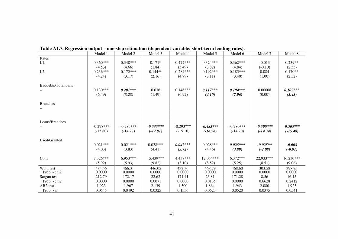
41

Table A1.7. Regression output – one-step estimation (dependent variable: short-term lending rates). Model 1 Model 2 Model 3 Model 4 Model 5 Model 6 Model 7 Model 8 Rates L1. 0.360*** 0.348*** 0.171* 0.472*** 0.324*** 0.362*** -0.013 0.239**

(4.53) (4.66) (1.84) (5.49) (3.82) (4.84) (-0.10) (2.55) L2. 0.236*** 0.172*** 0.144** 0.284*** 0.192*** 0.185*** 0.084 0.170**

(4.24) (3.17) (2.16) (4.79) (3.11) (3.40) (1.00) (2.52)

Baddebts/Totalloans -- 0.130*** 0.201*** 0.036 0.146*** 0.117*** 0.194*** 0.00008 0.107***

(6.49) (8.28) (1.49) (6.92) (4.10) (7.96) (0.00) (3.43)

Branches --

Loans/Branches -- -0.298*** -0.285*** -0.535*** -0.293*** -0.483*** -0.280*** -0.590*** -0.505***

(-15.80) (-14.77) (-17.81) (-15.16) (-16.76) (-14.70) (-14.34) (-15.48)

Used/Granted -- 0.021*** 0.021*** 0.028*** 0.042*** 0.028*** 0.025*** -0.025** -0.008

(4.03) (3.83) (4.41) (5.72) (4.46) (3.89) (-2.08) (-0.91)

Cons 7.326*** 6.953*** 15.439*** 4.438*** 12.054*** 6.372*** 22.933*** 16.230*** (5.92) (5.93) (9.82) (3.10) (8.52) (5.25) (8.51) (9.06) Wald test 484.56 466.31 446.05 432.30 468.79 468.60 303.58 398.75 Prob > chi2 0.0000 0.0000 0.0000 0.0000 0.0000 0.0000 0.0000 0.0000 Sargan test 212.79 172.17 22.62 171.41 23.81 171.28 8.56 16.15 Prob > chi2 0.0000 0.0000 0.0071 0.0000 0.0135 0.0000 0.6628 0.2412 AB2 test 1.923 1.967 2.139 1.500 1.864 1.943 2.080 1.923 Prob > z 0.0545 0.0492 0.0325 0.1336 0.0623 0.0520 0.0375 0.0541

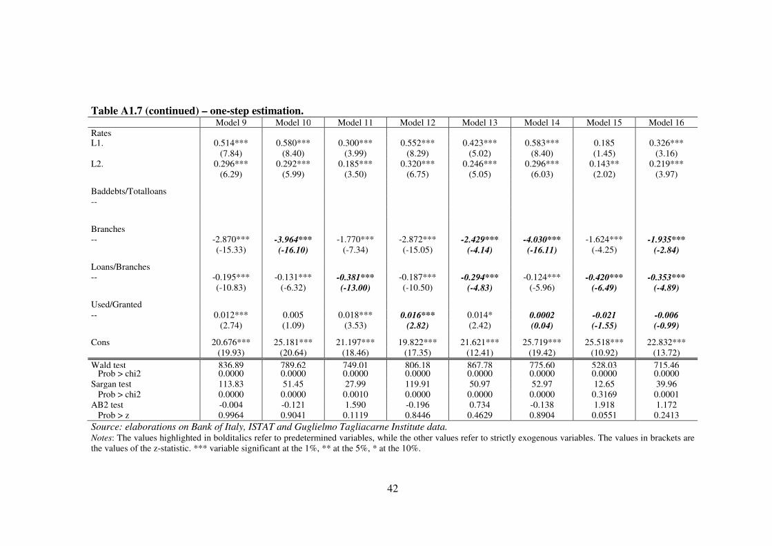
42

Table A1.7 (continued) – one-step estimation. Model 9 Model 10 Model 11 Model 12 Model 13 Model 14 Model 15 Model 16 Rates L1. 0.514*** 0.580*** 0.300*** 0.552*** 0.423*** 0.583*** 0.185 0.326***

(7.84) (8.40) (3.99) (8.29) (5.02) (8.40) (1.45) (3.16) L2. 0.296*** 0.292*** 0.185*** 0.320*** 0.246*** 0.296*** 0.143** 0.219***

(6.29) (5.99) (3.50) (6.75) (5.05) (6.03) (2.02) (3.97)

Baddebts/Totalloans --

Branches -- -2.870*** -3.964*** -1.770*** -2.872*** -2.429*** -4.030*** -1.624*** -1.935***

(-15.33) (-16.10) (-7.34) (-15.05) (-4.14) (-16.11) (-4.25) (-2.84)

Loans/Branches -- -0.195*** -0.131*** -0.381*** -0.187*** -0.294*** -0.124*** -0.420*** -0.353***

(-10.83) (-6.32) (-13.00) (-10.50) (-4.83) (-5.96) (-6.49) (-4.89)

Used/Granted -- 0.012*** 0.005 0.018*** 0.016*** 0.014* 0.0002 -0.021 -0.006

(2.74) (1.09) (3.53) (2.82) (2.42) (0.04) (-1.55) (-0.99)

Cons 20.676*** 25.181*** 21.197*** 19.822*** 21.621*** 25.719*** 25.518*** 22.832*** (19.93) (20.64) (18.46) (17.35) (12.41) (19.42) (10.92) (13.72) Wald test 836.89 789.62 749.01 806.18 867.78 775.60 528.03 715.46 Prob > chi2 0.0000 0.0000 0.0000 0.0000 0.0000 0.0000 0.0000 0.0000 Sargan test 113.83 51.45 27.99 119.91 50.97 52.97 12.65 39.96 Prob > chi2 0.0000 0.0000 0.0010 0.0000 0.0000 0.0000 0.3169 0.0001 AB2 test -0.004 -0.121 1.590 -0.196 0.734 -0.138 1.918 1.172 Prob > z 0.9964 0.9041 0.1119 0.8446 0.4629 0.8904 0.0551 0.2413 Source: elaborations on Bank of Italy, ISTAT and Guglielmo Tagliacarne Institute data. Notes: The values highlighted in bolditalics refer to predetermined variables, while the other values refer to strictly exogenous variables. The values in brackets are the values of the z-statistic. *** variable significant at the 1%, ** at the 5%, * at the 10%.

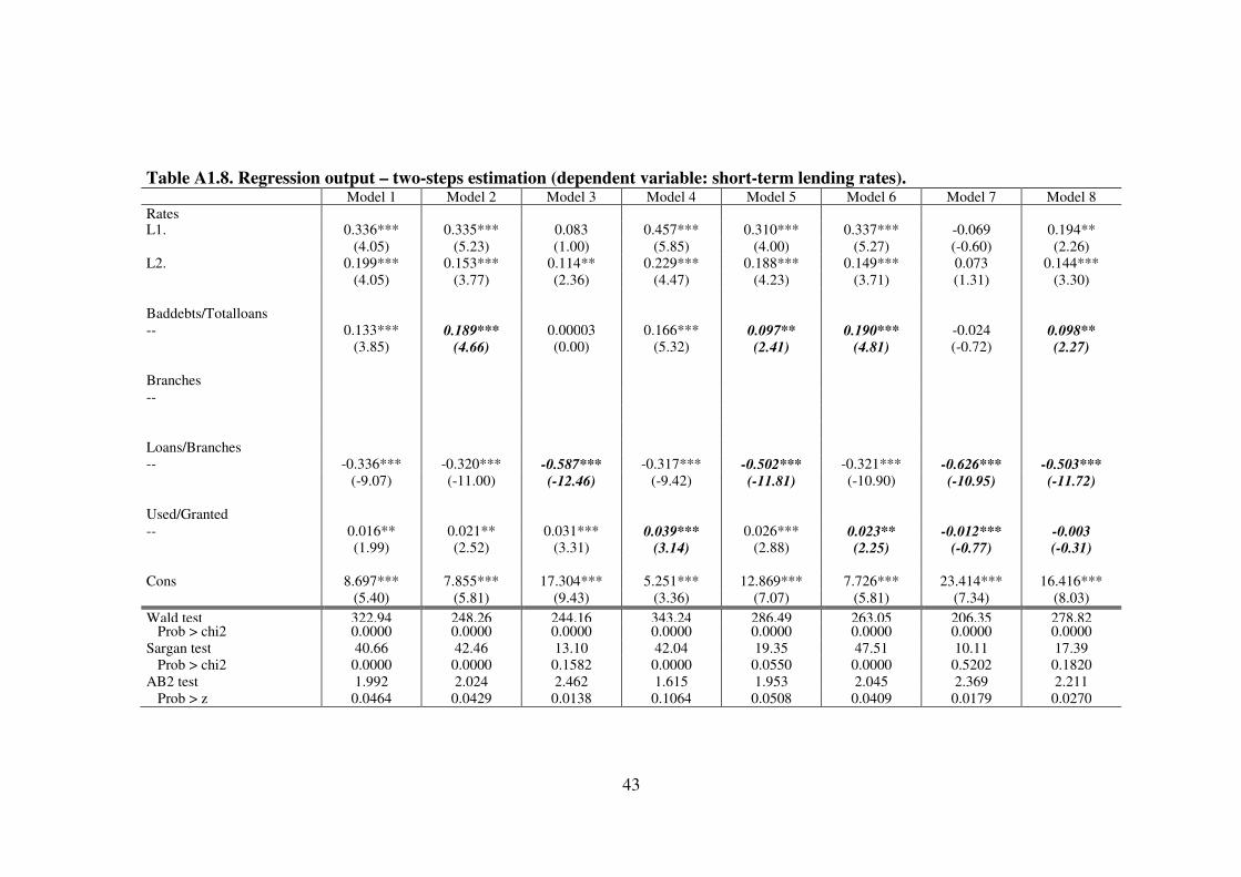
43

Table A1.8. Regression output – two-steps estimation (dependent variable: short-term lending rates). Model 1 Model 2 Model 3 Model 4 Model 5 Model 6 Model 7 Model 8 Rates L1. 0.336*** 0.335*** 0.083 0.457*** 0.310*** 0.337*** -0.069 0.194**

(4.05) (5.23) (1.00) (5.85) (4.00) (5.27) (-0.60) (2.26) L2. 0.199*** 0.153*** 0.114** 0.229*** 0.188*** 0.149*** 0.073 0.144***

(4.05) (3.77) (2.36) (4.47) (4.23) (3.71) (1.31) (3.30)

Baddebts/Totalloans -- 0.133*** 0.189*** 0.00003 0.166*** 0.097** 0.190*** -0.024 0.098**

(3.85) (4.66) (0.00) (5.32) (2.41) (4.81) (-0.72) (2.27)

Branches --

Loans/Branches -- -0.336*** -0.320*** -0.587*** -0.317*** -0.502*** -0.321*** -0.626*** -0.503***

(-9.07) (-11.00) (-12.46) (-9.42) (-11.81) (-10.90) (-10.95) (-11.72)

Used/Granted -- 0.016** 0.021** 0.031*** 0.039*** 0.026*** 0.023** -0.012*** -0.003

(1.99) (2.52) (3.31) (3.14) (2.88) (2.25) (-0.77) (-0.31)

Cons 8.697*** 7.855*** 17.304*** 5.251*** 12.869*** 7.726*** 23.414*** 16.416*** (5.40) (5.81) (9.43) (3.36) (7.07) (5.81) (7.34) (8.03) Wald test 322.94 248.26 244.16 343.24 286.49 263.05 206.35 278.82 Prob > chi2 0.0000 0.0000 0.0000 0.0000 0.0000 0.0000 0.0000 0.0000 Sargan test 40.66 42.46 13.10 42.04 19.35 47.51 10.11 17.39 Prob > chi2 0.0000 0.0000 0.1582 0.0000 0.0550 0.0000 0.5202 0.1820 AB2 test 1.992 2.024 2.462 1.615 1.953 2.045 2.369 2.211 Prob > z 0.0464 0.0429 0.0138 0.1064 0.0508 0.0409 0.0179 0.0270

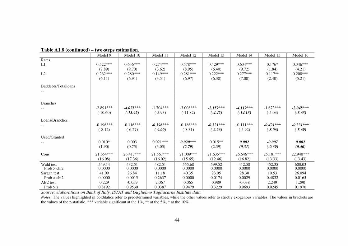
44

Table A1.8 (continued) – two-steps estimation. Model 9 Model 10 Model 11 Model 12 Model 13 Model 14 Model 15 Model 16 Rates L1. 0.522*** 0.636*** 0.274*** 0.578*** 0.429*** 0.634*** 0.176* 0.346***

(7.89) (9.70) (3.62) (8.95) (6.40) (9.72) (1.84) (4.21) L2. 0.262*** 0.280*** 0.149*** 0.281*** 0.222*** 0.277*** 0.117** 0.200***

(6.11) (6.91) (3.51) (6.97) (6.38) (7.00) (2.40) (5.21)

Baddebts/Totalloans --

Branches -- -2.891*** -4.075*** -1.704*** -3.008*** -2.159*** -4.119*** -1.673*** -2.048***

(-10.60) (-13.92) (-5.93) (-11.82) (-4.42) (-14.13) (-5.03) (-3.63)

Loans/Branches -- -0.196*** -0.116*** -0.398*** -0.186*** -0.321*** -0.111*** -0.421*** -0.331***

(-8.12) (-6.27) (-9.00) (-8.31) (-6.26) (-5.92) (-8.06) (-5.69)

Used/Granted -- 0.010* 0.003 0.021*** 0.020*** 0.015** 0.002 -0.007 0.002

(1.90) (0.75) (3.05) (2.79) (2.39) (0.31) (-0.69) (0.40)

Cons 21.654*** 26.417*** 21.567*** 21.009*** 21.635*** 26.646*** 25.181*** 22.940*** (16.08) (17.36) (16.02) (15.65) (12.46) (16.82) (13.33) (13.43) Wald test 549.14 432.51 482.51 555.68 599.52 412.58 452.35 600.03 Prob > chi2 0.0000 0.0000 0.0000 0.0000 0.0000 0.0000 0.0000 0.0000 Sargan test 41.09 26.84 11.18 40.35 23.05 28.30 10.53 26.094 Prob > chi2 0.0000 0.0015 0.2637 0.0000 0.0174 0.0029 0.4832 0.0165 AB2 test 0.229 -0.059 2.067 0.065 0.989 -0.038 2.249 1.290 Prob > z 0.8192 0.9530 0.0387 0.9479 0.3229 0.9693 0.0245 0.1970 Source: elaborations on Bank of Italy, ISTAT and Guglielmo Tagliacarne Institute data. Notes: The values highlighted in bolditalics refer to predetermined variables, while the other values refer to strictly exogenous variables. The values in brackets are the values of the z-statistic. *** variable significant at the 1%, ** at the 5%, * at the 10%.

45

Appendix 1.2: The Arellano and Bond estimator

In 1991, Arellano and Bond (AB henceforth) provided an efficient estimator for

dynamic panel models in which the number of time periods, T, is small and the

number of individual units, N, is large.

More in details, this estimator is an application of the Generalized Method of

Moments (GMM) on first-differenced equations.

Let us take into consideration the following autoregressive model without

regressors:

�� = ∑ �� �(���)���� + ���, |�� | < 1, t = (p+1), ..., T, i = 1, ..., N [1]

where ��� = η� + ���, |�� | < 1 is the stationarity condition, p is the number of

lags of the dependent variable, ηi ~ IID(0, σ2η) and vit ~ IID(0, σ2

v)

Note that �(���) and η� are necessarily correlated. The transformation in first

differences allows to eliminate the individual effects, but it reduces the number

of observations.

The AB estimator exploits all the possible moment conditions and let their

number change according to t.

Let us suppose, for example, that the number of lags, p, is equal to 1 and that the

only parameter to be estimated, α, is associated with the variable y lagged value

of one period.

Model [1] becomes:

�� = � �(���) + η� + ���, |�| < 1, t = 2, ..., T, i = 1, ..., N [2]

while the model in first differences becomes:

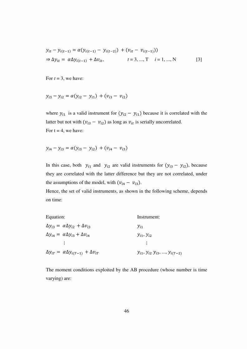
46

�� − �(���) = �( �(���) − �(���)) + (��� − ��(���))) � ∆ �� = �∆ �(���) + ∆���, t = 3, ..., T i = 1, ..., N [3]

For t = 3, we have:

�� − �� = �( �� − ��) + (��� − ���)

where �� is a valid instrument for ( �� − ��) because it is correlated with the

latter but not with (��� − ���) as long as ��� is serially uncorrelated.

For t = 4, we have:

�� − �� = �( �� − ��) + (��� − ���)

In this case, both �� and �� are valid instruments for ( �� − ��), because

they are correlated with the latter difference but they are not correlated, under

the assumptions of the model, with (��� − ���).

Hence, the set of valid instruments, as shown in the following scheme, depends

on time:

Equation: Instrument: ∆ �� = �∆ �� + ∆��� �� ∆ �� = �∆ �� + ∆��� ��, ��

⋮ ⋮ ∆ �� = �∆ �(���) + ∆��� ��, �� ��, ..., �(���)

The moment conditions exploited by the AB procedure (whose number is time

varying) are:

47

��(��� − ���) ��� = 0 t = 3

��(��� − ���) ��� = 0 t = 4 ��(��� − ���) ��� = 0

Generally, for T time periods, the model implies the following m = (���)(���)�

moment conditions:

�!(��� − �����) �(���)" = 0 j = 2, …, (t – 1), t = 3, …, T [4]

These moment conditions can be concisely written as:

��#′� �%�� = 0 [5]

that is equivalent to:

�!#&�(∆ �� − ∆ �(���))" = 0 [6]

where #� is the matrix of instruments9:

#� = ' �� 0 00 ��, �� 0∙ ∙ ∙0 0 ��, ⋯ , �,��� + [7]

and �%� = (∆���, ⋯ , ∆���)′ is a [(, − 2) × 1] vector [8]

Analogously, let us define the vectors:

9 #� is a [(, − 2) × 0] block diagonal matrix whose sth block is ( ��, ⋯ , �1).

48

2� = (∆ ��, ⋯ , ∆ ��)′ as a [(, − 2) × 1] vector [9]

and 2�(��) = (∆ ��, ⋯ , ∆ ����)′ as a [(, − 2) × 1] vector [10]

If the errors are independent distributed with constant variance σ2, we have �[�%��%′�] = σ�3, where H is a (, − 2) square matrix which has twos in the

main diagonal, minus ones in the first subdiagonal and zeros otherwise.

3 =45556 2 −1 0 ⋯ 0 0 0−1 2 −1 ⋯ 0 0 0⋮ ⋮ ⋮ ⋱ ⋮ ⋮ ⋮0 0 0 ⋯ −1 2 −10 0 0 ⋯ 0 −1 2 899

9: [11]

The AB estimator of � is based on the sample moments ∑ ;&<=2<><?@A = ;B=2A

Where # = (#�& , ⋯ , #A& ) is a C(, − 2) × 0 matrix and �% = (�%�& , ⋯ , �%A& ) is a C(, − 2) × 1 vector.

In details, we have:

�D = EFG0HIJ(�%�&#�)KA(#�&�%�) = ∑ L2<(M@)B< ;<N> ∑ ;<BL2<<∑ L2<(M@)B ;<< N> ∑ ;<BL2<(M@)< [12]

By setting KA = (∑ ;<BO;<< A )��, the one step AB estimator, �D�, is obtained. In

equation [12], the expression (∑ #&�3#�� )�� is a weighting matrix that leads to a

consistent estimator of α as long as ��� is serially uncorrelated.

If the errors ��� are heteroskedastic, it is possible to obtain a more efficient

estimator - the so-called two-steps AB estimator, �D� - by imposing KA = PQA��

in equation [12], where:

49

PQA = ∑ ;<B=2Q<=2Q<B;<< A [13]

and �%Q� are the differenced residuals obtained from the preliminary consistent

estimator �D�.

A consistent estimate of the variance matrix of �D, for an arbitrary KA, is given

by:

E�EFR (�D) = C ∑ L2<(M@)B< ;<N>ST>N> ∑ ;<B< L2<(M@)(∑ L2<(M@)B ;<< N> ∑ ;<BL2<(M@)< )U [14]

Note that �D� and �D� are asymptotically equivalent if the ��� are IID(0, σ=�).

However, AB suggest to employ the one-step estimator in finite-sample

inference because, in this framework, according to their simulations, the two-

step standard errors could be downward biased in samples of small size.

Let us extend model [2] by including k explanatory variables:

�� = � �(���) + V&W�� + η� + ���, |�| < 1, t = 2, ..., T, i = 1, ..., N [15]

The parameters in equation [15] can be estimated by using GMM, analogously

with the model without explanatory variables above illustrated. In other words,

the procedure remains the same as before, but the set of valid instruments will

change according to the hypothesis about W��.

More in details, if all the W�� are correlated with η�: • If W�� are strictly exogenous, that is if �[W����1] = 0, for all X, Y = 1, 2, ⋯ , ,,

then all the W�� are valid instruments for the first differenced equation of [15].

In this case, [W��& , W��& , ⋯ , W��& ] should be added to each diagonal element of #�. Therefore, the instruments matrix becomes:

50

#� = 4556[ ��, W��& , W��& , ⋯ , W��& ] 0 0 00 [ ��, ��, W��& , W��& , ⋯ , W��& ] 0 0⋮ ⋯ ⋱ ⋯0 0 0 [ ��, ⋯ , �(���), W��& , W��& , ⋯ , W��& ]899

: [16]

• If W�� are predetermined¸ that is if �[W����1] = 0 for Y ≥ X and �[W����1] ≠ 0

for Y < X, then, for every s, only [W��& , W��& , ⋯ , W�(1��)& ] are valid instruments for

the differenced equation at period s.

In this case, the instrument matrix becomes:

#� = 4556[ �� , W��& , W��& ] 0 0 00 [ �� , ��, W��& , W��& , W��& ] 0 0⋮ ⋯ ⋱ ⋯0 0 0 [ ��, ⋯ , �(���), W��& , W��& , ⋯ , W�(���)& ]899

: [17]

Let us suppose instead that there exists a subset W��� of W�� uncorrelated with η�. In this case:

• If W�� are strictly exogenous, observation on W�� for all t become valid

instruments in the levels equations. There are only T extra restrictions that

can be expressed as:

� ]∑ ��1W����1�� , ^ = 0, (X = 1, ⋯ , ,)

• If W�� are predetermined, according to AB there are other T extra restrictions: �[���W���] = 0 and �[���W���] = 0, for (X = 2, ⋯ , ,). The optimal matrix of

instruments becomes:

#�_ = 45556#� 0 0 0 00 [W��& , W��& ] 0 0 00 0 W��& 0 0⋮ ⋮ ⋯ ⋱ ⋮0 0 0 0 W��& ]89

99: [18]

51

where #� is given by [17].

The AB estimator is consistent if there is no second-order serial correlation

among the residuals of the regression, i.e. �[�����(���)] = 0.

In order to test this hypothesis, AB propose a test based on residuals from the

first-differenced equations and that is defined only for , ≥ 510. The null

hypothesis of lack of second-order serial correlation is not rejected if the errors

in the model in levels are not serially correlated or if they follow a random walk

process. In the latter case, AB pointed out that both OLS and GMM estimates in

first-differences are consistent and they suggest a Hausman type test based on

the differences between the two estimators.

Furthermore, AB suggest a Sargan test to verify the hypothesis of validity of

over-identifying restrictions given by:

Y = ∑ �D�&� #�(∑ #�&A��� �D��D�&#�)�� ∑ #�&� �D� ab χ��c��� [19]

where �D� = �� − �D� �(���) − Vd�& W��, �D� and Vd� are the two-step estimates of �

and V for a given instrument matrix of instrument #�, p is the number of

columns in #� and k is the number of coefficients to be estimated.

10 See equations (8) and (9), page 282, in Arellano and Bond (1991), Some Tests of

Specifications for Panel Data: Monte Carlo Evidence and an Application to Employment

Equations, in “The Review of Economic Studies Limited”, 58.

52

CHAPTER 2: CREDIT RISK DETERMINANTS AND SPREADS RISK ADJUSTED FOR ITALIAN REGIONS

2.1 Introduction

During the last decade, the debate about the possible consequences of the Basel

Accords generated a renewed interest in modeling credit risk’s determinants.

Economists generally believed that Basel II would have ensured an increase in

the stability of the financial system by identifying a quantitative relationship

between banks’ capital requirements and riskiness of their assets.

The recent global crisis has determined concerns about the Basel II Accord

efficacy. However, the main weaknesses of this accord were due to the limited

attention on liquidity risk, on the quality of the instruments that could be

included into the regulatory capital and on capital requirements’ procyclicality;

on the contrary, credit risk management continues to play a central role also in

the current revision framework.

Hence, the default risk assessment remains a crucial aspect in credit policies.

Particularly, because capital requirements positively depend on borrowers’

probability of default (PD), if banks overestimate the credit risk of their assets,

they must set aside larger capital provisions and sustain higher costs; on the

contrary, an underestimation of the riskiness of banks’ assets reduces the overall

degree of financial stability in the system.

The relationship between credit risk and capital requirements is on the basis of

pricing models currently employed by banks in order to determine the lending

rates applicable to their customers.

In light of the above considerations, understanding credit risk’s determinants is a

crucial issue. Credit risk, expressed in terms of probabilities of default (PD),

depends on borrowers’ specific characteristics (idiosyncratic components)

together with the general economic environment where borrowers operate

(systematic factors) that reflects exogenous territorial elements.

53

In this framework, this chapter aims to examine the idiosyncratic and systematic

elements influencing Italian firms’ PD. To reach this aim the relationship

between credit risk and borrowing conditions is examined at a regional level.

The empirical analysis takes into consideration the period 2002-2006 and

focuses on 36,303 observations for 10,058 Italian private firms and 639 default

cases.

The work is organized into five parts, besides this introduction. Paragraph 2.2

illustrates the main theoretical contributions on the determinants of firms’ credit

risk. Particularly, it is possible to distinguish four fields of research: models

mainly based on firm-specific characteristics; models analyzing the joint effect

of idiosyncratic and systematic elements; contributions that are mainly focused

on the relationship between default and macroeconomic variables and, finally,

contributions mainly based on market information.

Paragraph 2.3 describes the methodology employed, the sample analyzed, the

explanatory variables taken into consideration and the main results obtained by

estimating the models proposed. The independent variables included in the

models are accounting indicators (amount and growth rate of total annual sales,

ratio between bank debts and total sales, ratio between equity and total assets,

ratio between current assets and current liabilities and ROA index),

macroeconomics variables (GDP growth rate and GDP per capita) and

indicators of the financial system structure (loans growth rate, incidence of

cooperative banks and branches in the banking system and number of branches

and banks every 10,000 inhabitants).

Paragraph 2.4 analyzes the effect of credit risk in the determination of lending

rates. By following Zazzara and Cortese (2004), this paragraph presents a model

to estimate the Spread Risk Adjusted (SRA), that is the metric the represents the

share of the final lending rate exclusively based on loans’ credit risk.

In paragraph 2.5, the value of the SRA for each observation is estimated while

the main results of the analysis are summarized in paragraph 2.6.

54

2.2 Literature review

In recent years, the debate about the possible consequences of the Basel Accords

has renewed the attention on the measurement and pricing of credit risk, tools

able to favor the stability of the banking and financial system.

The earliest analysis concerning the identification of credit risk’s determinants

date back to the sixties of the last century. During this period, Beaver (1966) and

Altman (1969) developed the first models to assess private firms’ credit risk.

These studies applied discriminant analysis and used, primarily, firms’

accounting data.

The following developments focused on the identification of the idiosyncratic

and systematic components of credit risk and are subdivided into the following

categories (table 2.1):

• models mainly based on firm-specific characteristics;

• models analyzing the joint effect of the idiosyncratic and systematic

components of credit risk;

• models primarily focused on the relationship between default and

macroeconomic variables;

• models that point out the importance of market information to evaluate

firms’ credit risk.

The first group of studies includes Bernhardsen (2001), Eklund et al. (2001),

Bunn and Redwood (2003) and Jiménez and Saurina (2004).

Models based on accounting data take into account some measures of

profitability, liquidity and leverage. Nevertheless, there is no consensus about

which variables are the most important in the estimation of the PD.

Bernhardsen (2001), Eklund et al. (2001) develop a model in order to predict

bankruptcy probability on the basis of a sample of Norwegian firms during the

period 1990-1996 (about 400,000 observations). According to firm-specific data

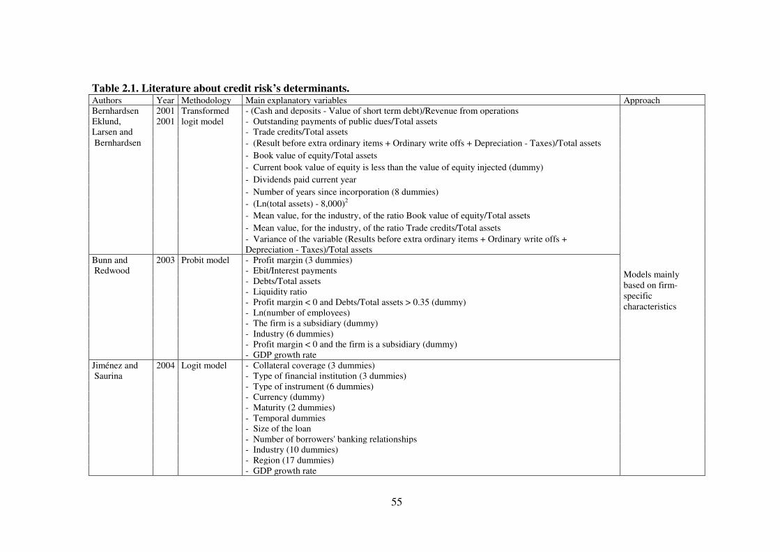
55

Table 2.1. Literature about credit risk’s determinants. Authors Year Methodology Main explanatory variables Approach Bernhardsen 2001 Transformed

logit model - (Cash and deposits - Value of short term debt)/Revenue from operations

Models mainly based on firm-specific characteristics

Eklund, 2001 - Outstanding payments of public dues/Total assets Larsen and - Trade credits/Total assets Bernhardsen - (Result before extra ordinary items + Ordinary write offs + Depreciation - Taxes)/Total assets - Book value of equity/Total assets - Current book value of equity is less than the value of equity injected (dummy) - Dividends paid current year - Number of years since incorporation (8 dummies) - (Ln(total assets) - 8,000)2 - Mean value, for the industry, of the ratio Book value of equity/Total assets - Mean value, for the industry, of the ratio Trade credits/Total assets

- Variance of the variable (Results before extra ordinary items + Ordinary write offs + Depreciation - Taxes)/Total assets

Bunn and 2003 Probit model - Profit margin (3 dummies) Redwood - Ebit/Interest payments - Debts/Total assets - Liquidity ratio - Profit margin < 0 and Debts/Total assets > 0.35 (dummy) - Ln(number of employees) - The firm is a subsidiary (dummy) - Industry (6 dummies) - Profit margin < 0 and the firm is a subsidiary (dummy) - GDP growth rate Jiménez and 2004 Logit model - Collateral coverage (3 dummies) Saurina - Type of financial institution (3 dummies) - Type of instrument (6 dummies) - Currency (dummy) - Maturity (2 dummies) - Temporal dummies - Size of the loan - Number of borrowers' banking relationships - Industry (10 dummies) - Region (17 dummies) - GDP growth rate

56

Table 2.1 (continued) - Literature about credit risk’s determinants. Authors Year Methodology Main explanatory variables Approach Benito, Javier Delgado and 2004 Probit model - Industry (15 dummies)

Models analyzing the joint effect of the idiosyncratic and systematic components of credit risk

Martinez Pagés - Borrowing ratio (Interest payments/Ordinary profit plus interest payments) - Return on assets - Liquid assets/Total assets - Debts/Total Assets - Trade credits/Total Assets - Omit dividend - Real sales growth - Ln(real sales) - Firm age (dummy) - GDP growth rate - Time dummies Carling, Jacobson, Lindé and 2007 Duration model - Duration dummies Roszbach - Credit type according to the maturity (3 dummies) - Total sales - EBITDA/Total assets - Debts/Total assets - Inventories/Total sales - Bank payment remarks - Legal payment remarks - Output gap - Household expectations - Yield curve Bonfim 2009 Probit model and

duration model - Sales growth

- ROA - Solvency ratio - Investment rate - Liquidity ratio - Industry (11 dummies) - Size (3 dummies) - Interest rate on loans to firms - Yield cuve slope - Loan growth rate - Stock market price variation - GDP growth rate - Temporal dummies

57

Table 2.1 (continued) - Literature about credit risk’s determinants. Authors Year Methodology Main explanatory variables Approach Borio, Furfine and Lowe 2001 Descriptive analysis - Output gap

Models that are mainly focused on the relationship between default and macroeconomic variables

- Indicators of banking system performance (provisions, profitability, equity prices, capital)

- Loan to value ratio

Pederzoli and Torricelli 2005 Conditional and unconditional PDs and probit models

- Term spread between the ten-year treasury bond and the three-month treasury bill rate

Jiménez and Saurina 2006 GMM estimations, logit and probit models

- Loan growth rate - Size of the loan - Maturity of the loan (2 dummies) - Collateral coverage (2 dummies) - Region (dummies) - Industry (dummies) - Size of bank - Type of bank (dummies) - Time dummies - GDP growth rate

- Borrowers' characteristics (if they were in default the year before or the year after the loan was granted, their indebtedness level)

- Characteristics of the borrower-lender relationship (duration and scope) - Level of competition in the loan market

58

Table 2.1 (continued) - Literature about credit risk’s determinants. Authors Year Methodology Main explanatory variables Approach Shumway 2001 Multiperiod logit model - Market size

Models mainly based on market information

- Past stock returns - Idiosyncratic standard deviation of stock returns - Net income/Total assets - Total liabilities/Total assets Tudela and 2003 Merton approach - Value and volatility of the company's equity Young - Book value of the company's equity Moody's 2004 Functional form related to generalized

additive models (with non-parametric transforms) and Merton approach

- Accounting data, varying according to the country taken into consideration and concerning, generally, profitability, leverage, debt coverage, assets and sales growth rates, liquidity, inventories, cash flow and size

- Industry (dummies) - Industry distance to default Couderc 2005 Parametric and semi-parametric factor

models - Return on S&P500

and - Volatility of S&P500 Renault - 10 year treasury yield - Slope of term structure - GDP growth rate - Industrial production growth - Personal Income growth - CPI growth - Spread of long term BBB bonds over treasuries - Spread of long term BBB bonds over AAA bonds - Net issues of Treasury securities - Loan growth rate - Investment grade and non investment grade classes upgrade rates - Investment grade and non investment grade classes downgrade rates

59

such as firms’ age, size, profitability, liquidity and industry’s characteristics, the

analysis is based on a logit model that estimates the bankruptcy probability.

The non linear nature of the model permits transformations of the explanatory

variables to obtain flexible rates of compensation (i.e. varying according to the

level of the variables).

According to the model, riskier firms, with a larger bankruptcy probability, are

characterized by a lower size (in terms of total assets), profitability, liquidity, an

higher gearing and greater value of the ratios between trade creditors and total

assets and between outstanding public dues and total assets. The dividend

distribution during the last year can be interpreted as a signal of solidity and

profitability; therefore the dummy associated with this event negatively

influences the bankruptcy probability. Furthermore, under the same conditions,

youngest firms are riskier than the oldest ones. Finally, firms’ bankruptcy

probability is higher in the industries with a greater average degree of leverage

and a larger volatility of firms’ profitability. Moreover, Bernhardsen

distinguishes between the probability of bankruptcy and the probability of

insolvency. While bankruptcy probability can be empirically estimated because

the bankruptcy event is observable, the prediction of the probability of

insolvency is problematic because of the impossibility to observe the state of

insolvency. Although these difficulties, according to the author it is possible to

compute the bankruptcy probability conditional on the insolvency (estimated to

equal 49%).

Runn and Redwood (2003) develop a probit model to identify the determinants

of PD on the basis of a sample of English firms (about 100,000 observations),

on the period 1991-2001. This sample, however, is not completely

representative because it does not include observations about firms with less

than 100 employees because, according to the authors, accounting data are

generally incomplete for smaller firms.

60

According to the model, PD is influenced by firm-specific elements (such as

profitability, size, industry, liquidity, interest cover and ratio debt/total assets)

together with the general conditions of the economy that are represented by the

GDP growth rate. Particularly, there is a negative relationship between credit

risk and firms’ profitability, liquidity, size (in terms of number of employees),

interest cover and capitalization. Thanks to the possibility that, in case of

difficulties, subsidiary firms can be assisted by the holding company, subsidiary

firms are less risky and the size of this effect is larger if the firm makes a loss.

Finally, there is a negative relationship between PD and GDP growth rate. This

event can be determined by the behavior of banks that, during recession periods,

are more risk adverse and tend to close down the largest risks more rapidly.

Jimenéz and Saurina (2004) present a different approach and examine the

determinants of the PD analyzing credit risk at a loan level and not at a borrower

level. The study is based on over 3 millions loans granted by the Spanish

financial system during the period 1988-2000.

The authors, by estimating logit models, come to the conclusion that more

collateral imply greater PD because banks tend to require more collaterals for

those loans characterized by a greater ex-post credit risk. PD decreases in case

of loans in foreign currency, of larger size or with longer maturity. For these

loans, in fact, banks pay more attention on their screening process, diminishing

ex-post credit risk.

Closer relationships between banks and borrowers (expressed by the number of

banks with which each borrowers relates) are characterized by larger PDs: in

these conditions, banks are willing to finance riskier loans because they can

recover the larger expected loss by applying higher lending rates to their other

exclusive or nearly exclusive borrowers. Hence, there are informational rents for

banks thanks to the higher quality of information about their borrowers due to

the close relationship with the customer.

61

Finally, the authors point out that, in order to obtain more appropriate estimates

of loans’ PD, it is necessary to take into consideration also the general

conditions of the macroeconomic environment. These conditions can be

expressed by the GDP growth rate, variable that negatively influences credit

risk.

The group of contributions that jointly analyze the effect of idiosyncratic and

systematic elements include Benito et al. (2004), Carling and al. (2007) and

Bonfim (2009).

Benito et al. (2004) develop a probit model to estimate the PD on the basis of a

sample of about 18,000 non-financial Spanish firms and take into consideration

the period 1985-2001. According to the authors, in order to explain exhaustively

the determinants of firms’ PD, it is necessary to combine accounting data and

macroeconomic factors. Furthermore, it is important also to evaluate the firms’

credit status since that financial indicators can summarize different information

if the default status is a persistent conditions (i.e. if the firm object of analysis

stays in this status for more than a year) or a non persistent condition.

Compared with non-defaulting firms, those defaulting are characterized by

larger debts, more dividend omissions and lower profitability, liquidity and sales

growth. There is a positive relationship between PD and size (in terms of annual

sales); younger companies have a higher PD with respect to the older ones. The

analysis points out the relevance of the non-linearities in the relationship

between PD and financial ratios.

As regards macroeconomic factors, there is a positive relationship between PD

and the aggregate cost of debt; on the contrary, GDP growth rate negatively

influences firms’ credit risk. This condition might be determined by externalities

among firms and by a growing risk aversion of banks during recession periods.

Carling et al. (2007) use a different methodology and develop a duration model

to explain the determinants of the survival time to default for a sample of about

55,000 Swedish firms (period 1994-2000).

62

The model includes accounting information, loan-specific characteristics and

macroeconomic variables. According to the authors, the general conditions of

the macroeconomic environment have a significant explanatory power in the

analysis of credit risk. Particularly, the output-gap (defined by the difference

between actual and potential GDP), households’ expectations and the slope of

the yield curve negatively influence credit risk. In terms of idiosyncratic

elements, credit risk is positively influenced by the debt ratio and the level of

inventories over total sales; on the contrary, there is a negative relationship

between credit risk and profitability and credit risk and firms’ size (measured by

total sales).

The authors point out the importance to take into consideration also the survival

time of loans because of the existence of duration dependence. In fact, firms’

credit risk increases over the survival of their loans. Particularly, “the time a

borrower has managed to avoid default directly affects the risk of default”

(Carling at al., page 15). This situation is explained by the fact that when firms

obtain the required loans, they are characterized by a good degree of solidity

because they had managed to pass the banks’ screening process. Successively,

borrowers’ default risk might increase and this tendency is captured by the

introduction of time dummies in the model.

In order to explain exhaustively the causes of default rates, also Bonfim (2009)

focuses on the necessity to jointly analyze accounting data at firm level and

macroeconomic elements. Using a sample of 33,000 Portuguese firms (period

1996-2002), Bonfim develops a probit model to estimate firms’ PD and duration

models examining the time dimension of default risk.

Firms with greater sales growth and investment rates and larger profitability,

liquidity and a higher value of the solvency ratio, are also characterized by a

lower credit risk in terms of both PD and time to default. Instead, size does not

significantly explain the difference in the PD across firms. Among

63

macroeconomic elements, GDP and loan growth rates are the variables with the

largest effect, negative, on credit risk.

According to the author, credit risk is created during expansive periods while the

high default rates observed during recession periods represent mainly the

materialization of credit risk accumulated during upturns. Macroeconomic

dynamics matters and influences firms’ credit risk.

The analysis developed by Borio et al. (2001), Pederzoli and Torricelli (2005)

and Jiménez and Saurina (2006) belong to the third category of contributions

that focus on the relationship between default rates and macroeconomic

elements.

Borio et al. (2001) focuses on the procyclical behavior of the financial system

that is caused by banks’ difficulties in the assessment of credit risk’s time

dimension. Because of these difficulties, risk tends to be underestimated during

expansion periods and, on the contrary, to be overestimated in recession phases.

These errors tend to amplify economic fluctuations, causing instability in the

system.

According to the authors, banks have to establish their credit policies taking into

consideration that risk tends to build up during expansion phases while, during

recession periods, most defaults represent the materialization of the risk

originated in the past expansion periods. These defaults do not imply,

necessarily, an increase in the overall risk in the system.

Hence, banks have to adopt longer time horizons in their risk assessment, while

capital requirements should increase during upturns in order to cover losses that

will materialize during successive downturns.

Also Pederzoli and Torricelli (2005) focus on the procyclicality caused by the

general methodology used by banks in order to compute patrimonial

requirements. Particularly, they estimate a forward-looking model for time-

varying capital requirements. This model could reduce procyclicality and, at the

same time, preserve risk-sensitivity of bank provisions proposed by the Basel

64

Accords. Thanks to the determination of capital requirements depending on the

expected macroeconomic conditions, this model allows to overtake the trade-off

between risk-sensitivity and procyclicality of provisions. According to this new

approach, in fact, banks’ provisions increase during upturns (in anticipation of a

recession phase) and reduce during downturns (in anticipation of an expansion

phase). On the whole, provisions should be more stable during the business

cycle.

This model presupposes the estimation of PDs conditional on the expected

macroeconomic conditions. For each rating class, particularly, the PD is

estimated as the expected value of a default rate whose distribution is a weighted

average of an expansion and a recession distribution and the weights are the

probability of a future expansion phase and the probability of a future recession

phase.

The theoretical model is applied to US data for the period 1971-2002. In this

application, the probability of a recession phase is a decreasing function of the

term spread between the ten-year Treasury bond and the three-month treasury

bill rate.

Jiménez and Saurina (2006) take into consideration the credit risk profile of

banks’ loan portfolios along the business cycle and, hence, the risk’s time

dimension.

For the period 1984-2002, the authors verify the hypothesis that during credit

expansion (characterized by a loan growth rate larger than the average value),

loans’ PDs tend to increase. Furthermore, they show that collaterals tend to

decrease during expansion periods, when the GDP growth rate is greater than

the average level. Therefore, during upturns, banks increase their loan

portfolios’ risk by reducing the amount and the quality of required collaterals

and by financing, with a greater willingness, riskier borrowers. The larger risks

built up during upturns will materialize during recession periods, inducing a

lower stability in the financial system.

65

Finally, Shumway (2001), Tudela and Young (2003), Moody’s (2004) and

Couderc and Renault (2005) belong to the group of works that estimate firms’

credit risk on the basis of market information.

According to Shumway (2001), traditional single-period models used to predict

firms’ credit risk obtain biased and inconsistent estimates with respect to hazard

models that are, instead, based on the whole time-series for each firm. In this

context, Shumway proposes a hazard model for the estimation of bankruptcy

probability that is able to capture the time changes in firms’ credit risk. This

methodology is empirically applied to a sample of about 3,000 US firms taking

into account the period 1962-2002.

Shumway shows that, including in his hazard model the accounting variables

used by Altman and Zmijewski, only the ratios EBIT/total assets, market

equity/total assets and net income/total assets can significantly explain credit

risk. On the contrary, the other variables taken into consideration are not

statistically significant bankruptcy predictors.

The author develops a new hazard model that examines the joint effect, on the

bankruptcy probability, of accounting data and market variables. Particularly,

credit risk is negatively influenced by firm’s market size and past stock returns.

On the contrary, there is a positive relationship between bankruptcy probability

and the idiosyncratic standard deviation of stock returns and between

bankruptcy probability and firm’s liability. The inclusion in the model of market

information considerably improves the accuracy of the estimated bankruptcy

probabilities.

Tudela and Young (2003) apply the Merton approach in order to quantify

credit risk for a sample of about 7,500 English firms (period 1990-2001).

Differently from the original Merton model, in the Tudela and Young model the

event of default can take place at any time and not only at the maturity of the

debt.

66

The predictive capacity, in terms of accuracy-ratio, seems to be larger with

respect to the models based exclusively on accounting variables. So, in order to

adequately assess credit risk, it is important to take into account also market

information at firm level.

The RiskCalc v3.1 model developed by Moody’s (2004) estimates a credit risk

measure, the Expected Default Frequency, on the basis of market information

(systematic elements), accounting data (idiosyncratic factors) and industry

variables.

This model is developed on the basis of a database concerning accounting data

for about 1,500,000 firms and is based on financial ratios varying according to

the country where firms operate. Furthermore, the model allows taking into

consideration the non-linearities in the relationship between credit risk and

financial ratios.

By applying the Merton methodology, the model permits to obtain an

assessment of credit risk based on market information also for not publicly

traded firms for which market data are not available. This result is achieved by

including in the model the distance to default for a sample of publicly trade

firms operating in the same industry of the firm object of assessment. According

to Moody’s, this indicator has a larger predictive capacity with respect to other

macroeconomic variables such as interest rates, GNP or unemployment rate.

Finally, Couderc and Renault (2005) point out that some of the shortcomings

of the most analysis in the literature are the scarce importance given to the

business cycle and the use of explanatory variables without lags.

The authors estimate times-to-default of individual firms that belong to different

rating classes on the basis of Standard & Poor’s ratings database including

information concerning ratings of about 10,000 firms during the period 1981-

2003. Particularly, the paper examines common drivers of PD by using

information about the business cycle and market data. The conclusion is that, in

order to identify credit risk’s determinants, it is necessary to take into

67

consideration jointly market data and information about business cycle and

credit market. Furthermore, in their analysis, not lagged explanatory variables

have a limited predictive capacity.

Couderc and Renault reach at the conclusion that economic trends and past

shocks appear as the main drivers of the PD.

2.3 The model

2.3.1 The methodology

After analyzing the main factors that, according to the literature, influence

private firms’ PD in several economic and territorial contexts, in this paragraph I

will examine the methodology employed to develop a probit panel model which

aim is to identify the main determinants of the default risk for a representative

sample of Italian private firms11.

11 The analysis developed in this essay is based on level firm data extracted from the database AIDA (Analisi Informatizzata delle Aziende - Firms analysis computerized), that is provided by Bureau van Dijk Electronic Publisher. I wish particularly to thank Umberto De Marco for the sample provided. The sample is composed by 10,058 Italian firms (registering 639 default events) for which I examined balance sheets during the period 2002-2006 (on the whole, the number of observations is 36,303). The stratification method employed to extract the sample permits to examine a representative subset, in terms of industry and territorial distribution, of Italian firms. In more details, for every region, the share of firms extracted from the database AIDA is equal to the percentage actually observed in 2006 according to Unioncamere data. Furthermore, for every region, the number of firms extracted in each economic sector (according to the Classification Ateco 2002), has been established by taking into consideration the actual incidence of each industry in the number of firms in 2006. For every region and industry, the share of default firms is equal to 6%, which is, on average, the percentage of default firms included in the empirical contributions that I examined in paragraph 2.2. After determining, the territorial and industry composition of the sample, I used a procedure that permits to consider the main representative firms in the different territorial contexts. First, for every region, inside each industry, I identified the median firm, in terms of total sales, whose balance sheet is included in the AIDA database. Second, the firms extracted have been selected in order to obtain an interval of observations that is centered on the median firm.

68

The model developed is a probit model applied to panel data with random

effects. This type of models is commonly employed in the empirical literature

under the hypothesis that errors are normally distributed.

The dependent variable is a binary variable that takes value 1 if the firm “i” is in

default at the time “t” and 0 otherwise.

Particularly, a firm is in default if, alternatively, has been declared in failure, has

been subject to bankruptcy agreement, is in receivership or if insolvency status

has been declared12.

The model is based on the latent variables methodology that assumes that the

variable e�� ∈ (0,1) is function of a not observable variable – the latent variable

– e��∗ that depends, in a linear way, from k independent variables h���, h���, ⋯ , hc�� and an error term ���:

e��∗ = Vi + V�h��� + V�h��� ⋯ + ⋯ Vchc�� + ��� = h��& V + ��� [1]

e�� = j 1 Hk e��∗ > 00 mXℎoFpHYoq

where: h��& = matrix of the k independent variables; β = vector of the k + 1 coefficients.

Given the random structure of the model13, the error term ��� can be subdivided

into two components according to the following formula:

12 This definition is employed by Bureau van Dijk Electronic Publisher. 13 It is not possible to consider fixed effects in probit panel models. As C → ∞, for ,fixed (that is the case analyzed in this chapter), the number of parameters µ� increases with C; therefore, µ� cannot be consistently estimated for T fixed (incidental parameters problem). The inconsistency of µD � is transmitted also to the maximum likelihood estimator of β. In the linear case this problem is overcame by eliminating µ� (by the Within transformation). Instead, in our case, the transformation of the latent model to eliminate the fixed effects does not

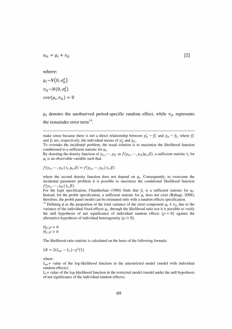
69

��� = µ� + ��� [2] where: µ�~C~0,σ��� ���~C(0,σ=�) �m�(µ�, ���) = 0 µ� denotes the unobserved period-specific random effect, while ��� represents

the remainder error term14.

make sense because there is not a direct relationship between ��∗ − 2�∗ and �� − 2�, where 2�∗ and 2� are, respectively, the individual means of ��∗ and ��. To overtake the incidental problem, the usual solution is to maximize the likelihood function conditioned to a sufficient statistic for µ�. By denoting the density function of ��, ⋯ , �� as k( ��, ⋯ , ��|µ� , V), a sufficient statistic X� for µ� is an observable variable such that: k( ��, ⋯ , ��| X� , µ� , V) = k( ��, ⋯ , ��| X�, V) where the second density function does not depend on µ�. Consequently, to overcome the incidental parameter problem it is possible to maximize the conditional likelihood function k( �� , ⋯ , ��| X� , V). For the logit specification, Chamberlain (1980) finds that 2� is a sufficient statistic for µ�. Instead, for the probit specification, a sufficient statistic for µ� does not exist (Baltagi, 2008); therefore, the probit panel model can be estimated only with a random effects specification. 14 Defining ρ as the proportion of the total variance of the error component µ� + ��� due to the variance of the individual fixed effects µ�, through the likelihood ratio test it is possible to verify the null hypothesis of not significance of individual random effects (ρ = 0) against the alternative hypothesis of individual heterogeneity (ρ > 0). 3i: ρ = 0 3�: ρ > 0 The likelihood ratio statistic is calculated on the basis of the following formula: �� = 2(��� − ��)~χ�(1) where: ���= value of the log-likelihood function in the unrestricted model (model with individual random effects); ��= value of the log-likelihood function in the restricted model (model under the null hypothesis of not significance of the individual random effects).

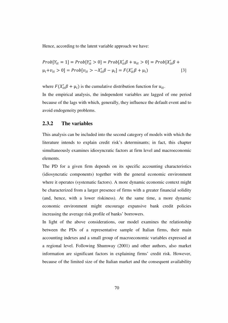
70

Hence, according to the latent variable approach we have:

�Fm�[e�� = 1] = �Fm�[e��∗ > 0] = �Fm�[h��& V + ��� > 0] = �Fm�[h��& V +µ�+��� > 0] = �Fm�[��� > −h��& V − µ�] = �(h��& V + µ�) [3]

where �(h��& V + µ�) is the cumulative distribution function for ���.

In the empirical analysis, the independent variables are lagged of one period

because of the lags with which, generally, they influence the default event and to

avoid endogeneity problems.

2.3.2 The variables

This analysis can be included into the second category of models with which the

literature intends to explain credit risk’s determinants; in fact, this chapter

simultaneously examines idiosyncratic factors at firm level and macroeconomic

elements.

The PD for a given firm depends on its specific accounting characteristics

(idiosyncratic components) together with the general economic environment

where it operates (systematic factors). A more dynamic economic context might

be characterized from a larger presence of firms with a greater financial solidity

(and, hence, with a lower riskiness). At the same time, a more dynamic

economic environment might encourage expansive bank credit policies

increasing the average risk profile of banks’ borrowers.

In light of the above considerations, our model examines the relationship

between the PDs of a representative sample of Italian firms, their main

accounting indexes and a small group of macroeconomic variables expressed at

a regional level. Following Shumway (2001) and other authors, also market

information are significant factors in explaining firms’ credit risk. However,

because of the limited size of the Italian market and the consequent availability

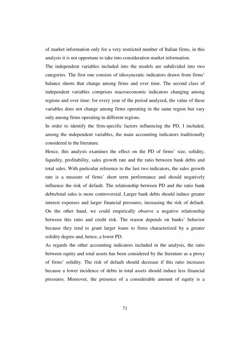
71

of market information only for a very restricted number of Italian firms, in this

analysis it is not opportune to take into consideration market information.

The independent variables included into the models are subdivided into two

categories. The first one consists of idiosyncratic indicators drawn from firms’

balance sheets that change among firms and over time. The second class of

independent variables comprises macroeconomic indicators changing among

regions and over time: for every year of the period analyzed, the value of these

variables does not change among firms operating in the same region but vary

only among firms operating in different regions.

In order to identify the firm-specific factors influencing the PD, I included,

among the independent variables, the main accounting indicators traditionally

considered in the literature.

Hence, this analysis examines the effect on the PD of firms’ size, solidity,

liquidity, profitability, sales growth rate and the ratio between bank debts and

total sales. With particular reference to the last two indicators, the sales growth

rate is a measure of firms’ short term performance and should negatively

influence the risk of default. The relationship between PD and the ratio bank

debts/total sales is more controversial. Larger bank debts should induce greater

interest expenses and larger financial pressures, increasing the risk of default.

On the other hand, we could empirically observe a negative relationship

between this ratio and credit risk. The reason depends on banks’ behavior

because they tend to grant larger loans to firms characterized by a greater

solidity degree and, hence, a lower PD.

As regards the other accounting indicators included in the analysis, the ratio

between equity and total assets has been considered by the literature as a proxy

of firms’ solidity. The risk of default should decrease if this ratio increases

because a lower incidence of debts in total assets should induce less financial

pressures. Moreover, the presence of a considerable amount of equity is a

72

crucial aspect because, in this case, firms are more likely able to get external

finances and reduce the probability of default.

Also liquidity should negatively influence, in the short run, firms’ credit risk.

Particularly, the liquidity index taken into consideration in the empirical analysis

is the ratio between current assets and current liabilities. An increase of this ratio

should allow to firms to punctually manage their short-term obligations,

reducing their PD.

Profitability should negatively affect the risk of default; in fact, a larger

profitability should be associated with greater cash flows allowing firms to

manage their obligations with more facility. Additionally, greater earnings

should increase the firms’ ability to obtain external finance. Finally, a greater

profitability should allow to firms to set aside larger financial reserves

increasing, by this way, their solidness.

More in details, the profitability measures taken into consideration are the

Return on Assets (ROA) and the Return on Equity (ROE). I consider ROA a

better indicator to analyze the firm’s ability to generate wealthy because it is a

metric of the normal profitability level. This index expresses the profitability of

the operating activity and does not include the results of financial and extra

ordinary activities. In order to avoid multicollinearity problems caused by the

significant correlation between ROE and ROA (0.43 in the sample), only the

ROA index is included in the econometric analysis.

I employed two indicators for firms’ size: total sales and total assets. The current

literature agrees with the presence of a significant and negative relationship

between size and PD. However, there are several contributions stressing that

larger firms have a greater risk of default (Benito et al., 2004) or retaining that

the relationship between firms’ size and PD is not statistically significant

(Bonfim, 2009).

For the second category of regressors, reflecting macroeconomic dynamics on

default risk, I included in the econometric analysis a set of variables (at a

73

regional level) able to summarize the general conditions of the economic and

financial system: the real GDP growth rate, the real GDP per capita, the

unemployment rate, the loan growth rate, the ratio between cooperative banks

(branches) and total banks (branches) and the number of banks and branches per

10,000 inhabitants.

While the real macroeconomic variables (GDP and loan growth rates) have been

traditionally taken into consideration to explain credit risk according to

macroeconomic dynamics, information about the structural conditions of the

banking system is generally ignored. By considering these variables, it is

possible to verify if there exists a statistical relationship between the banking

structure and the default event. Particularly, the analysis of the statistical

significance of the number of banks and branches per 10,000 inhabitants and the

incidence of cooperative banks and branches in the system allows to empirically

evaluate if the spatial and social proximity between banks and firms influences

firms’ risk of default.

2.3.3 The empirical analysis

The empirical analysis takes into consideration the period 2002-2006 focusing

on 36,303 observations for 10,058 Italian firms registering 639 default events.

Firm-specific accounting data are drawn from the database AIDA (Analisi

Informatizzata delle Aziende - Firms analysis computerized) produced by

Bureau van Dijk Electronic Publishing. Data on GDP growth rate, GDP per

capita, unemployment rate and population have been elaborated by the Italian

National Statistical Office (ISTAT), while data concerning the banking system

structure have been supplied by Bank of Italy.

Table A2.1 shows the mean and median values of the main accounting indexes

for the firms in default and for the remaining firms.

On average, default firms seem to differ from other firms. Particularly, in terms

of median values, default firms are slightly smaller with respect to non-default

74

firms both in terms of total sales and total assets. Moreover, coherently with the

literature, default firms present a lower degree of profitability (both in terms of

ROA and ROE) and liquidity, larger debts and a lower ratio between equity and

total assets.

Also the median sales growth rate is considerably different among these

subsamples. Particularly, this indicator takes a positive value (+10.0%) for non

default firms and is equal to zero for the other firms.

The differences between default firms and non-default firms in terms of ratio

between bank debts and total sales are less significant: for the first subsample

the mean of this indicator is equal to 8.57 while it is equal to 9.26 for non

default firms.

In order to avoid possible biases caused by outlier values, in the econometric

estimation, for every accounting index, I set those observations above the 99th

percentile and below the 1st percentile at the value, respectively, of the 99th and

1st percentile.

On the basis of the methodology illustrated in paragraph 2.3.1, I elaborated a set

of probit models with random effects in order to estimate the probability of firm

being in default during the following year, based on accounting and

macroeconomic data for the current year. Table A2.4 shows the results for the

estimated models.

Initially, the estimated models are based exclusively on firm-specific accounting

data (model 1 – model 4); then, in order to analyze the determinants of firms’

PD taking simultaneously into consideration data at firm level and

macroeconomic dynamics, also macroeconomic indicators have been included

among the explanatory variables (model 5 – model 13).

The models do not include regional and industrial dummies because, for every

region and industry, the share of default firms is the same, i.e. it is equal to 6%

(for further information see note 11).

75

To avoid multicollinearity problems caused by the correlation between the ratio

equity/total assets and the liquidity index (as shown in table A2.2, the

correlation coefficient between these two indicators amounts to 0.45), the effect

of these variables on default risk is evaluated through different regression

models.

The explanatory variables in model 1 and model 2 are the amount and the

growth rate of total sales, the ratio between bank debts and total sales and the

ROA index. The first model includes, among regressors, also the ratio

equity/total assets; the liquidity ratio is considered in model 2. Coherently with

the literature, the degree of profitability and liquidity and the amount of equity

affect negatively and significantly the risk of default; on the contrary, there is no

significant relationship between size (expressed in terms of total sales) and PD.

Moreover, according to these models, the sales growth rate does not influence

credit risk, while there is a negative relationship between the ratio bank

debts/total sales and PD at 10% level of significance.

As indicated above, the literature agrees on the presence of a significant and

negative statistical relationship between firms’ size and PD. However, other

works consider a positive relationship between these two variables (Benito et al.,

2004) or a not significant relationship (Bonfim, 2009). In order to assess more

accurately the dimensional effect, I take into consideration an alternative

indicator of the firms’ size: the amount of total assets.

Model 3 and model 4 examine the relationship between PD, total assets, sales

growth rate, ratio between bank debts and total sales, ROA, ratio equity/total

assets (model 3) and liquidity index (model 4). These models confirm the

existence of a negative and significant relationship between PD, profitability,

equity and liquidity. Furthermore, according to model 3, there is a positive

statistical relationship between firms’ PD and size (measured by total assets) at

10% level of significance.

76

Departing from model 3 (that is the best model, among these four specifications,

in terms of pseudo-R2), I tried several other specifications including also

macroeconomic variables. Because of the significant correlation between GDP

per capita and unemployment rate, GDP per capita and number of branches per

10.000 inhabitants and between the latter variable and the unemployment rate

(see table A2.3), the effect of these pairs of variables on firms’ PD is estimated

through separated regressions.

All these specifications confirm the results achieved by the first four models. In

other words, at idiosyncratic level, an increase in profitability or equity leads to

a decline in PD.

On the contrary, the relationship between size (expressed in terms of total

assets) and default risk is significantly positive, in agreement with Benito’s

conclusions. This finding denies the traditional opinion that smaller firms,

because of their “structural weakness”, are riskier than larger firms. This result

can be explained by two possible factors. A self selection approach could

indicate how the sample’s coverage of small firms might be biased towards

“good” companies (in order to explain the positive relationship between credit

risk and size, Benito follows this reason). The second cause, of economic nature,

might be the existence, for larger firms, of possible diseconomies of scale that

reduce their creditworthiness.

In order to identify the possible macroeconomic determinants of default risk,

together with the accounting indicators included in model 3, model 5 and 6

comprise also GDP and loan growth rates, GDP per capita (model 5) and

unemployment rate (model 6). According to these models, GDP and loan growth

rates influence significantly and negatively firms’ PD, while the structural

characteristics of regional economies (expressed in terms of GDP per capita or

unemployment rate) do not affect significantly the risk of default.

Models 7 and 8 add to the variables included in model 5, respectively, the share

of cooperative banks in the system and the number of banks per 10,000

77

inhabitants. These two models confirm the results achieved by model 5 and

show that there does not exist a significant relationship between the two

variables concerning the structure of the banking system and firms’ PD. In other

words, in the Italian context a higher spatial and social closeness between banks

and firms does not lead to better performances of the entrepreneurial system

measured via default events.

These conclusions remain valid even if the share of cooperative banks is

replaced using the share of cooperative branches (model 9).

Models 10, 11 and 12 include the same regressors of models 7, 8 and 9 with the

exception of GDP per capita that is replaced by the unemployment rate. These

models generally confirm the results illustrated above; however, according to

model 11 there exists a positive relationship (at 10% level of significance)

between number of banks per 10,000 inhabitants and risk of default.

Finally, model 13 includes among the macroeconomic regressors, GDP and

loans growth rates and the number of branches per 10,000 inhabitants. The

positive relationship between the latter variable and PD is coherent with model

11.

The lack of a negative impact, on firms’ PD, of the social closeness between

banks and firms, expressed in terms of incidence, in the banking system, of

cooperative banks and branches, might be due to the low amounts of loans

granted by these financial institutions.

In other words, although at a microeconomic level, cooperative banks can play

an important role in supporting firms that experience financial difficulties (in

fact, they traditionally tend to be more sensitive to local firms’ problems), at an

aggregate level the limited share of loans granted by these banks might lead to

the lack of a negative statistical relationship between their number and the risk

of default.

Totally, these estimates indicate that, in the Italian system, the crucial

determinants of credit risk are idiosyncratic factors at firm level: particularly,

78

firms’ financial structure, liquidity and profitability. Macroeconomics elements

at a regional level can be useful in explaining the differences in the riskiness of

firms operating in different regions but their inclusion does not improve

considerably the models’ goodness of fit in terms of pseudo-R2 (see table A2.4).

Banks should hence carefully determine lending rates via a correct and deep

analysis of borrowers’ structural characteristics.

2.4 The impact of credit risk in bank interest rates and the

calculation of the Spread Risk Adjusted

The Basel Accords determine quantitatively the relationship between PD and

regulatory capital provisions that banks have to set aside in order to face the

credit risk of their loan portfolios. This relationship is on the basis of the pricing

models currently employed by banks in order to determine the borrowing

conditions to apply to their customers.

Banks have to calculate lending rates that are able to remunerate, together with

the funding cost and operating costs, also a set of risks that are linked both to

borrowers’ riskiness and to the overall banking activity.

Particularly, the main risks of credit intermediation can be subdivided into the

following classes:

• operational risk;

• credit risk;

• liquidity risk;

• market risk.

Operational risk is the typical risk of whatever firm and it is related to the

variability of expected profit. It is defined by the Basel II Accord (§644) as “the

risk of loss resulting from inadequate or failed internal processes, people and

systems or from external events. This definition includes legal risk, but excludes

strategic and reputational risk”. For smaller banks, for example, a classical

79

operational risk is the possibility to suffer diseconomies of scale linked to the

small size.

As regards the second category, credit risk is the possibility that borrowers are

not able or willing to accomplish, at the maturity, to their obligations and, hence,

do not pay the granted debt (principal and/or interests).

This type of risk was crucial in Basel II and continues to play a central role also

in the new proposal to strengthen the resilience of the banking sector (Basel III).

In this context, this paragraph focuses on credit risk and aims to examine the

relationship between firms’ PD and lending rate. Particularly, the share of the

final bank interest rate that remunerates exclusively the loan’s credit risk is the

Spread Risk Adjusted (SRA). This indicator is function of the borrower’s PD,

the Loss Given Default (LGD), the Exposure at Default (EAD) at the loan’s

Maturity (M). These values are internally estimated by banks if they adopt the

Advanced Internal Rating Based Approach. For those banks adopting the

Foundation Internal Rating Based Approach, the only indicator estimated

through internal models is the PD; the other parameters assume, instead, values

defined by the Basel II Accord.

The current debate focuses with a particular emphasis on the third category of

risk. Generally, liquidity risk is linked to the probability that financial entries

and disbursements are not temporally correlated compromising, by this way, a

firm’s profitability or reputation. For banks a careful management of liquidity

risk represents a very crucial element because a substantial share of their assets

(represented by loans) is not negotiable into secondary markets and a

considerable share of their liabilities is represented by short-term debts.

This situation actually occurred, at a global level, during the last two years when

the economic crisis and the uncertainty about the correct functioning of the

financial system locked the interbank market.

80

After that the financial crisis had showed the considerable intensity of liquidity

risk and its effects on the overall financial system’s stability, supervisors have

significantly increased their commitment to face this kind of risk.

Particularly, the Basel Committee is introducing a global minimum liquidity

standard for internationally active banks that includes a 30-days liquidity

coverage ratio requirement underpinned by a longer-term structural liquidity

ratio.

Finally, market risk is defined by the Basel II Accord (§683) as “the risk of

losses in on and off-balance-sheet positions arising from movements in market

prices”.

In order to determine the final pricing applied to loans, banks have to add to the

funding cost a spread to cover operating costs, the SRA and, finally, have to

downgrade or upgrade the pricing on the basis of the specific borrower’s

assignment (also of business type). Although the SRA is a crucial metric to

calculate lending rates (it allows to adjust the pricing to the credit risk) it is not

binding because the determination of the final pricing remains a business choice.

In fact, in the determination of the final lending rate, it is possible to “depart

from” the SRA by recuperating profitability margins through an increase of “not

lending” earnings and, hence, through those earnings’ components that are not

linked to credit risk. A parallel way to recuperate profitability margins is the

request of further collaterals (banks can reduce the expected loss and capital

provisions via loss given default), but at the extreme this procedure denies the

logic of a correct pricing determination of risk.

This section, following Zazzara and Cortese (2004), presents a model to

calculate the SRA and demonstrates a negative relationship, under the same

SRA, between PD and LGD. Furthermore, I simulate the calculation of capital

requirements established by Basel II and show that, under the same conditions,

capital requirements are larger for loans granted to greater firms.

81

The underlying logic of the SRA determination process is of statistical-actuarial

nature, based on the link between borrower’s risk (measured by PD), loans’

collaterals (expressed in terms of LGD) and credit risk’s remuneration.

Particularly, the SRA can be considered as the theoretical price for an insurance

against the borrower’s default risk, that is the probability of default.

The SRA is computed by adding the expected loss remuneration and the

unexpected loss remuneration:

SRA = expected loss remuneration + unexpected loss remuneration [4]

The expected loss (EL) is calculated by multiplying borrower’s PD, LGD and

EAD and, because it is expected, it has to be covered by an account-specific

provision.

Expected loss (EL) = PD × LGD × EAD [5]

The unexpected loss (UL) represents an uncertain event, covered by the bank’s

equity and can be reduced through adequate diversification policies.

Particularly, the UL is the difference between the possible maximum loss for a

given time horizon and confidence level (Value at Risk) and the EL. The UL can

be considered as a systematic component of risk, estimable through a portfolio

model. Nevertheless, according to several authors15, the portfolio models

employed by the main investment banks and by the main international

consulting companies (the Creditmetrics model of JP Morgan, the CreditRisk+

model of Credit Suisse First Boston, the Credit Portfolio View model of

McKinsey and the Portfolio Manager model of KMV) are not sufficiently

adequate to estimate the UL linked to illiquid assets (such as credit loans)

15 See Zazzara and Cortese (2004).

82

because these models are mainly based on market data. Taking into

consideration these limits, the Basel Committee developed the functions to

calculate the level of capital requirements that banks have to set aside in face of

a given exposure and that can be considered as an estimate of the UL. In this

work, I employ the general functions indicated by the Basel Committee.

According to these formulas, the UL is function of PD, LGD, Maturity and total

annual sales.

� = �IoW o�Xo¡ �mYY =k[�¢(+), �£¢(+), ¤(+), ,mXE¥ EII�E¥ YE¥oY(−)] = �¦KY × 0.08 [6]

where RWAs indicates banks’ risk weighted assets.

The formulas to compute capital requirements are distinguished according to

borrower’s total sales level. Particularly, firms are subdivided into three

segments: Corporate (if the firm’s total sales are greater than 50 millions of

euros), Small Medium Enterprise (if the firm’s total sales are not greater than 50

millions of euros and the firm does not belong to the Retail class) and Retail

(firms whose loans are managed as detail credits and for which the total

exposure of the banking group is less than 1 million of euros). Under the same

conditions, on the basis of these functions, capital requirements are larger for

Corporate segment and decrease for SME and Retail exposures. This

relationship derives from the hypothesis that, among the different segments, the

average correlation between loans is lower for smaller firms because these firms

are less sensitive to the business cycle. Hence, the assumption is that the

systematic component of risk, not diversifiable, decreases if also borrowers’ size

reduces. Consequently, under the same conditions, banks must set aside larger

provisions for loans granted to Corporate firms because of the greater riskiness

linked to the larger correlation among loans into this segment.

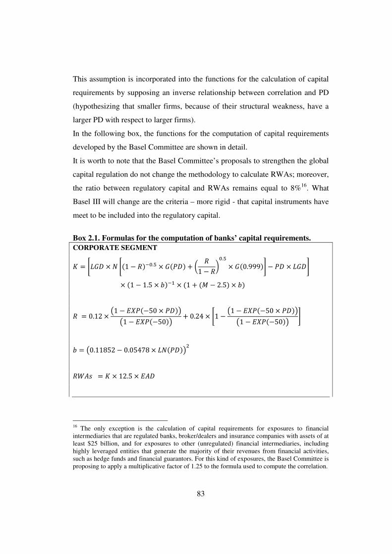
83

This assumption is incorporated into the functions for the calculation of capital

requirements by supposing an inverse relationship between correlation and PD

(hypothesizing that smaller firms, because of their structural weakness, have a

larger PD with respect to larger firms).

In the following box, the functions for the computation of capital requirements

developed by the Basel Committee are shown in detail.

It is worth to note that the Basel Committee’s proposals to strengthen the global

capital regulation do not change the methodology to calculate RWAs; moreover,

the ratio between regulatory capital and RWAs remains equal to 8%16. What

Basel III will change are the criteria – more rigid - that capital instruments have

meet to be included into the regulatory capital.

Box 2.1. Formulas for the computation of banks’ capital requirements. CORPORATE SEGMENT

� = ]�£¢ × C ](1 − �)�i.© × £(�¢) + ª �1 − �«i.© × £(0.999)^ − �¢ × �£¢^× (1 − 1.5 × �)�� × (1 + (¤ − 2.5) × �)

� = 0.12 × ~1 − �h�(−50 × �¢)�~1 − �h�(−50)� + 0.24 × ]1 − ~1 − �h�(−50 × �¢)�~1 − �h�(−50)� ^

� = ~0.11852 − 0.05478 × �C(�¢)��

�¦KY = � × 12.5 × �K¢

16 The only exception is the calculation of capital requirements for exposures to financial intermediaries that are regulated banks, broker/dealers and insurance companies with assets of at least $25 billion, and for exposures to other (unregulated) financial intermediaries, including highly leveraged entities that generate the majority of their revenues from financial activities, such as hedge funds and financial guarantors. For this kind of exposures, the Basel Committee is proposing to apply a multiplicative factor of 1.25 to the formula used to compute the correlation.

84

SME SEGMENT

� = ]�£¢ × C ](1 − �)�i.© × £(�¢) + ª �1 − �«i.© × £(0.999)^ − �¢ × �£¢^× (1 − 1.5 × �)�� × (1 + (¤ − 2.5) × �)

� = 0.12 × ~1 − �h�(−50 × �¢)�~1 − �h�(−50)� + 0.24 × ]1 − ~1 − �h�(−50 × �¢)�~1 − �h�(−50)� ^ − 0.04× ¯1 − (° − 5)45 ±

� = ~0.11852 − 0.05478 × �C(�¢)��

�¦KY = � × 12.5 × �K¢

RETAIL SEGMENT17

� = �£¢ × C ](1 − �)�i.© × £(�¢) + ª �1 − �«i.© × £(0.999)^ − �¢ × �£¢

� = 0.03 × ~1 − �h�(−35 × �¢)�~1 − �h�(−35)� + 0.16× ´1 − ~1 − �h�(−35 × �¢)�/~1 − �h�(−35)�¶

� = ~0.11852 − 0.05478 × �C(�¢)��

�¦KY = � × 12.5 × �K¢

where: K = capital requirement; R = average correlation among loans into the segment taken into consideration; b = maturity adjustment;

17 The formulas shown for the calculation of capital requirements and correlation concerning the exposures to the Retail segment refer to loans that are not secured by residential mortgages and that do not represent qualifying revolving retail exposures. For these classes of loans, the Basel II Accord (§§328-329) indicates specific formulas in order to determine capital requirements, whereas correlations take predefined values.

85

S = total annual sales (total annual sales smaller than 5 millions of euros are considered equivalent to 5 millions of euros in order to calculate capital requirements); N and G denote, respectively, the cumulative distribution function and the inverse cumulative distribution function for a standard normal random variable; RWAs = risk weighted assets. Source: Basel II Accord (§§271-274; 324-330).

Following Zazzara and Cortese (2004), taking into consideration an horizon

time of 1 year, in order to compute the cost of EL concerning a given loan, it is

possible to adopt the risk-neutrality approach by assuming that a bank is

indifferent between to invest in a risk-free security (with a yield equal to Fk�) or

to grant, at a rate equal to H�, a guaranteed loan (with a Loss Given Default equal

to �£¢�) to a borrower with a probability of default equal to �¢�. According to

this approach, we obtain the following formula:

(1 + Fk�) = (1 + H�) × (1 − �¢�) + (1 − �£¢�) × �¢� [7]

where H� indicates the remuneration of the EL linked to a given exposure.

Generalizing for n years, formula [7] becomes:

(1 + Fk·)· = (1 + H·)· × (1 − �¢·) + (1 − �£¢·) × �¢· [8]

and by solving for H· we obtain:

H· = ��� = ¸((�_�¹º)º�(��»¼½º)×¾½º)(��¾½º) ¿� ·À − 1 [9]

where: Fk· = n years-risk-free rate; H·(���) = n years rate adjusted for risk. This rate expresses the remuneration of

the expected loss;

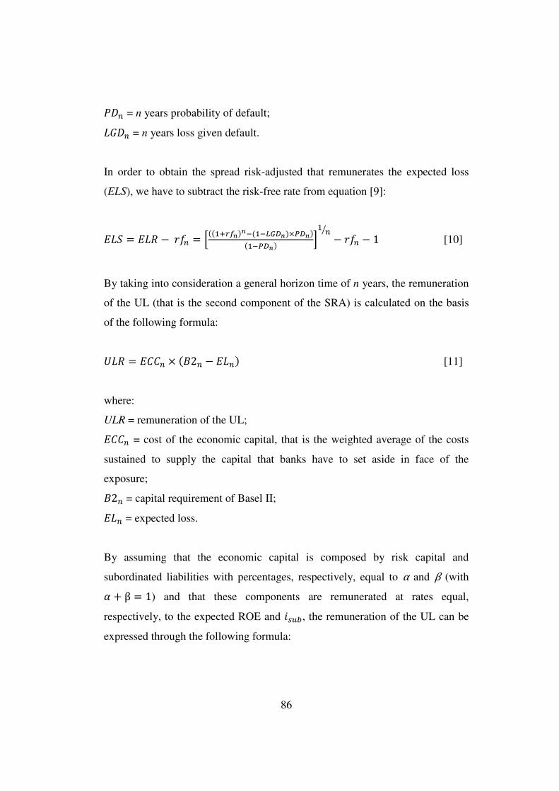
86

�¢· = n years probability of default; �£¢· = n years loss given default.

In order to obtain the spread risk-adjusted that remunerates the expected loss

(ELS), we have to subtract the risk-free rate from equation [9]:

��° = ��� − Fk· = ¸((�_�¹º)º�(��»¼½º)×¾½º)(��¾½º) ¿� ·À − Fk· − 1 [10]

By taking into consideration a general horizon time of n years, the remuneration

of the UL (that is the second component of the SRA) is calculated on the basis

of the following formula:

��� = �ÁÁ· × (Â2· − ��·) [11]

where:

ULR = remuneration of the UL; �ÁÁ· = cost of the economic capital, that is the weighted average of the costs

sustained to supply the capital that banks have to set aside in face of the

exposure; Â2· = capital requirement of Basel II; ��· = expected loss.

By assuming that the economic capital is composed by risk capital and

subordinated liabilities with percentages, respectively, equal to α and β (with � + β = 1) and that these components are remunerated at rates equal,

respectively, to the expected ROE and H1�Ä, the remuneration of the UL can be

expressed through the following formula:

87

��� = (Â2· − ��·) × ~� × �Å�ÆÇ�ÆÈ�ÆÉ + V × H1�Ä� [12]

The UL spread remuneration (ULS) is then computed by subtracting the risk-

free rate from formula [12]:

��° = ��� − Fk· = (Â2· − ��·) × ~� × (�Å�ÆÇ�ÆÈ�ÆÉ − Fk·) + V × (H1�Ä −Fk·)) [13]

Finally, adding the EL spread to the UL spread, we obtain the total value of the

SRA:

°�K =¸((�_�¹º)º�(��»¼½º)×¾½º)(��¾½º) ¿� ·À − Fk· − 1 + (Â2· − ��·) × ~� × (�Å�ÆÇ�ÆÈ�ÆÉ −Fk·) + V × (H1�Ä − Fk·)) [14]

According to these results, the lending rate applied to a given exposure is

positively influenced by borrower’s riskiness (expressed in terms of the

borrower’s PD) and loan’s riskiness (measured by LGD that is influenced by the

amount and solidity of collaterals).

Figure 2.1 shows capital requirements distinguished according to the borrower’s

class. This graph has been elaborated according to the functions defined by the

Basel Committee and taking into consideration benchmarking values for LGD,

Maturity and EAD equal, respectively, to 45%, 5 years and 100%. Furthermore,

for the SME segment, total annual sales are set to 10 millions of euros.

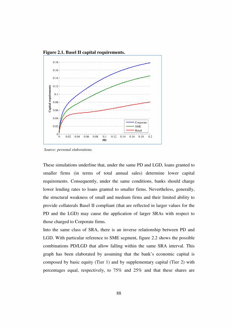
88

Figure 2.1. Basel II capital requirements.

Source: personal elaborations.

These simulations underline that, under the same PD and LGD, loans granted to

smaller firms (in terms of total annual sales) determine lower capital

requirements. Consequently, under the same conditions, banks should charge

lower lending rates to loans granted to smaller firms. Nevertheless, generally,

the structural weakness of small and medium firms and their limited ability to

provide collaterals Basel II compliant (that are reflected in larger values for the

PD and the LGD) may cause the application of larger SRAs with respect to

those charged to Corporate firms.

Into the same class of SRA, there is an inverse relationship between PD and

LGD. With particular reference to SME segment, figure 2.2 shows the possible

combinations PD/LGD that allow falling within the same SRA interval. This

graph has been elaborated by assuming that the bank’s economic capital is

composed by basic equity (Tier 1) and by supplementary capital (Tier 2) with

percentages equal, respectively, to 75% and 25% and that these shares are

0 0.02 0.04 0.06 0.08 0.1 0.12 0.14 0.16 0.18 0.20

0.02

0.04

0.06

0.08

0.1

0.12

0.14

0.16

0.18

PD

Cap

ital

req

uir

emen

ts

CorporateSMERetail

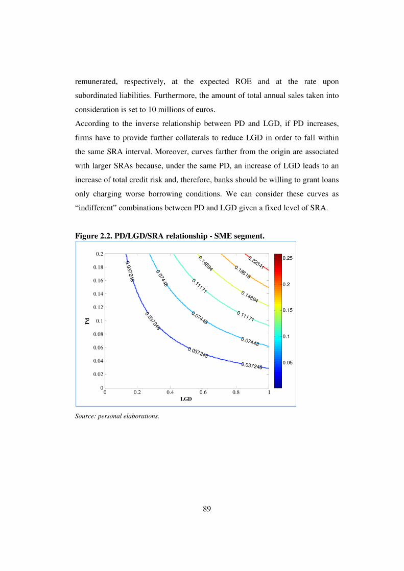
89

remunerated, respectively, at the expected ROE and at the rate upon

subordinated liabilities. Furthermore, the amount of total annual sales taken into

consideration is set to 10 millions of euros.

According to the inverse relationship between PD and LGD, if PD increases,

firms have to provide further collaterals to reduce LGD in order to fall within

the same SRA interval. Moreover, curves farther from the origin are associated

with larger SRAs because, under the same PD, an increase of LGD leads to an

increase of total credit risk and, therefore, banks should be willing to grant loans

only charging worse borrowing conditions. We can consider these curves as

“indifferent” combinations between PD and LGD given a fixed level of SRA.

Figure 2.2. PD/LGD/SRA relationship - SME segment.

Source: personal elaborations.

0 0.2 0.4 0.6 0.8 10

0.02

0.04

0.06

0.08

0.1

0.12

0.14

0.16

0.18

0.2

LGD

Pd

0.0

37

248

0.0

37248

0.037248

0.037248

0.0

7448

0.07448

0.07448

0.1

1171

0.11171

0.1

4894

0.14894

0.18618

0.22341

0.05

0.1

0.15

0.2

0.25

90

2.5 Simulating SRAs for Italian regions

In this section, the pricing model illustrated in paragraph 2.4 is employed to

simulate the SRAs applicable to a sample of Italian firms subdivided into 20

regional subsamples.

These simulations represent the borrowing conditions that banks should apply to

their customers, at a regional level, on the basis of objective elements such as

the borrowers’ PD and loans’ LGD.

First, for each firm into the sample, the PD has been estimated taking into

account, simultaneously, idiosyncratic factors at firm level and systematic

(macroeconomic) elements at regional level.

Among the models that include both idiosyncratic and systematic regressors, I

had chosen to employ model 11 given the higher pseudo-R2 and the greater

number of significant independent variables (see Table A2.4).

The mean and median values of the PDs of the non-defaulting firms in the

sample are reported in table A2.5.

Southern firms are characterized by a credit risk similar to firms operating in

Central Italy, while the territorial area with the greatest average aggregate PD is

North-West Italy. These results are contrasting with the common opinion that

Southern firms are riskier than Northern and Central firms because of their

structural weakness. Presumably, they could be caused by the slenderness of the

sample (comprising 10,058 firms) with respect to the entire population (in 2006

Italian firms amounted to 6,125,514) but they remain very significant.

The estimated PDs represent the first input in order to determine the pricing.

The procedure that I use to compute SRA for each observation allows getting

results perfectly comparable inside the sample; in other words, the calculated

SRAs reflect, exclusively, the differences among firms in terms of PD and, for

the SME segment, total annual sales. Therefore, for two firms characterized by

the same values of total annual sales and PD, the methodology employed leads

91

to the same value for the SRA, nevertheless the region where the two firms

operate.

In order to calculate banks’ capital requirements, I applied the functions defined

by Basel II (see Box 2.1). These formulas remain valid also according to the

current Basel Committee’s proposals to determine banks’ regulatory capital.

Particularly, for 35,658 observations (that do not include default events), I

employ the formula defined for the SME segment, while for the remaining 6

observations (regarding firms with total annual sales larger than 50 millions of

euros), I use the formula concerning the Corporate segment. Following a general

practice in the literature, I hypothesize that banks’ economic capital is composed

by risk capital (Tier 1) and subordinated liabilities (Tier 2) with percentages

respectively equal to 75% and 25%. According to the Basel Committee’s new

proposal, from 2015 these values will actually become compulsory.

For each firm, the SRA is computed by assuming:

• a PD estimated through model 11;

• with reference to the SME segment, as established by the Basel II Accord,

an amount of total annual sales equal to the actual value if sales are larger

than 5 millions of euros or, alternatively, equal to 5 millions of euros;

• an LGD equal to 45% for each exposure. This value represents the

percentage that, according to the Basel II Accord (paragraph 287), under

the IRB Foundation, has to be applied to senior claims on corporate,

sovereigns and banks not secured by recognized collaterals;

• a value of maturity equal to 1 year;

• a risk-free rate equal to EURIRS rate 1 year;

• a subordinated claims interest rate (that is the rate that remunerates Tier 2

capital) equal to EURIRS rate 10 years plus a spread of 0,20%;

• an expected ROE (that is the rate that remunerates Tier 1 capital) equal to

the subordinate claims interest rate multiplied by 1.5 (I had also

92

considered a multiplying factor equal to 2, but the results differ, on

average, only of about 0.06 percentage points).

After calculating the SRA value for each observation, I estimated 20 regional

SRAs by computing, for every region, the arithmetic mean of the SRAs

calculated for each firm operating in the region taken into consideration. The

results are shown in table A2.5 (not weighted SRA).

The differences, among regions, in terms of SRA, reflect the different aggregate

riskiness expressed by the regional average of the PDs.

For Southern regions, the average value of SRA is similar to the one observed in

Central Italy, while the geographical area characterized by the highest average

SRA is North-West Italy.

By calculating 20 regional SRAs through the arithmetic mean of the SRAs

applicable to the firms operating in each region, it is not possible to take into

consideration that firms are not equally important in terms of the implications of

their potential default. So, I calculated also two synthetic indicators of regional

SRA that reflect the amount of total debts and the amount of bank debts for each

firm.

The first indicator, SRA1r, is defined, for the region r, as the weighted average of

the SRAs applicable to the Fr firms operating in the region r, where the weights

are the amounts of total debts of each firm.

°�K�� = ∑ ~°�K¹� × ,mXE¥ ¡o�XY¹��/,mXE¥ ¡o�XY�Ê�¹��� [15] F = 1 ⋯ 20

where: �� = number of observations in region r; k� = observation f in region r, with k� = 1 ⋯ �F; °�K¹� = SRA applicable to observation f in region r;

93

,mXE¥ ¡o�XY¹� = total debts of observation f in region r; ,mXE¥ ¡o�XY� = total debts of firms operating in region r.

Analogously, for each region, the second indicator, SRA2r, is the weighted

average of the SRAs applicable to every firm in the region, where the weights

are the amount of bank debts of each firm.

°�K�� = ∑ ~°�K¹� × ÂEIË ¡o�XY¹��/ÂEIË ¡o�XY�Ê�¹��� [16] F = 1 ⋯ 20

where: �� = number of observations in region r; k� = observation f in region r, with k� = 1 ⋯ �F; °�K¹� = SRA applicable to observation f in region r; ÂEIË ¡o�XY¹� = bank debts of observation f in region r; ÂEIË ¡o�XY� = total bank debts of firms operating in region r.

The results, shown in table A2.5, confirm the conclusion above illustrated: in

Southern regions the indicators SRA1r and SRA2r take values similar to those

observed in Central regions and lower than those observed in North areas.

These simulations imply that, on the basis of the sample analyzed and under the

hypothesis illustrated, banks should not apply larger lending rates to the firms

operating in Southern regions.

Nevertheless, in order to calculate the actual SRA applicable to each firm, it is

necessary to know the actual value of the LGD that depends on the type of

collaterals provided. This information is not available into the dataset used in the

analysis.

94

A first potential proxy of the LGD at a regional level could be the ratio

losses/total debts in the bankruptcy procedures. Table A2.6 shows that in North-

West and North-East Italy the losses occurred in bankruptcies are generally

smaller than those observed in the other areas. On the other hand, by substituting

the regional values of the ratio losses/total debts to the regional LGDs, the

resulting SRAs in the Mezzogiorno are less than the ones simulated for Northern

regions. This result remains valid nevertheless the arithmetic or the weighted

averages of the SRAs applicable to the regional customers are taken into

account (table A2.7).

However, it is necessary to note that in the Mezzogiorno the bankruptcy

procedures’ average length is considerable larger with respect to Northern

regions. Particularly, during the period 2002-2006, in North-West Italy, North-

East Italy, Southern Italy and in the Islands, the bankruptcies lasted, on average,

2,572, 2,947, 3,072 and 3,486 days.

This element is important because the larger bankruptcies’ length reduces the

expected recovery rate and, on the contrary, increases the expected LGD.

Consequently, to estimate a proxy for LGD, it seems opportune to combine

information about bankruptcies’ losses and average length. To this end, for each

year of the period 2002-2006, I normalized the bankruptcies’ length in the

interval 0-1 by calculating an index number with base equal to the maximum

length observed in Italian regions. Afterwards, I calculated a second proxy of

the LGD at a regional level by computing the mean of this index number and the

ratio losses/total debts for each region (the underlying hypothesis is that for

creditors the amounts that they can recover in bankruptcies procedures and the

time length of these procedure have the same importance).

By considering this second regional LGD proxy, the resulting SRAs are more

homogenous among areas (table A2.8).

As previously discussed, although the SRA is a crucial indicator to compute

lending rates, it is not constraining for banks. In order to determine the final

95

pricing, banks have to take into consideration also other elements such as

operating and funding costs. Finally, the determination of the final lending rate

remains a “business choice” because banks can “depart from” the SRA by

recuperating profitability margins through the increase of “not lending”

earnings, not linked to the credit risk.

The results obtained in this analysis allow to conclude that the main cause of the

larger lending rates observed, empirically, in Italian Southern regions, cannot be

identified in the greater credit risk of the borrowers operating in these areas

implied by their structural characteristics. Interregional interest rate spreads in

Italy seem related to other factors such as business and institutional

considerations.

2.6 Conclusions

The identification of credit risk’s determinants continues to be an important

topic also in the current revision framework of the Basel II Accord. The Basel

Committee’s new proposals attribute greater relevance to the credit risk

management process, promoting the strengthening of banks’ ability to assess

borrowers’ creditworthiness.

In this framework, this work can be included into the second category of

contributions with which the literature intends to explain credit risk’s

determinants by analyzing simultaneously idiosyncratic factors at firm level and

macroeconomic elements. Particularly, the empirical analysis, based on the

Italian economic system, took into consideration the period 2002-2006 and the

sample examined is composed by 36,303 observations for 10,058 Italian firms.

The factors that are potentially able to explain differences in borrowers’

riskiness include both accounting and macroeconomic elements together with

variables related to the banking system’s structure. On the contrary, the analysis

did not take into consideration market information because of the limited size of

96

the Italian market and the consequent availability of this type of information

only for a very restricted number of firms.

The results suggest that firms’ credit risk is negatively influenced by firms’

profitability, degree of liquidity and level of equity on total liabilities.

The relationship between size and default risk is positive. This finding is

contrasting with the common opinion that smaller firms are characterized by a

larger credit risk because of their structural weakness, but at the same time

dimension is not a proxy variable for firm’s profitability and solvency.

Firms’ probability of default is negatively influenced by GDP and loan growth

rate, while the structural characteristics of regional economies (expressed in

terms of GDP per capita or unemployment rate) do not affect significantly the

risk of default. As regards the structure of the banking system, the degree of

territorial diffusion of branches and banks seems to positively influence firms’

PD, while the incidence of cooperative banks and branches does not affect

firms’ default risk. Hence, in the analyzed context, the spatial and social

closeness between banks and firms does not reduce the number of default

events.

The estimated models indicate that systematic variables can be useful in order to

explain the regional differences in the risk of default, but their inclusion does

not significantly improve models’ goodness of fit. Hence, banks should establish

their credit policies and lending rates on the basis of borrowers’ structural

characteristics such as firms’ financial structure, liquidity and profitability.

Moreover, this work points out that in order to establish a credit policy that

maximizes the value creation, an adequate bank pricing system represents a

crucial aspect together with the actual comprehension of credit risk’s

determinants.

The analyzed sample shows that another important element is represented by the

fact that the SRAs applicable to Southern firms should be not greater than those

chargeable to North-Western firms because, according to the sample analyzed,

97

the firms operating in Southern Italy and in the Islands are characterized by a

lower average probability of default. So, the higher lending rates actually

observed in Southern regions do not seem to reflect the different borrowers’

credit risk.

These results should be certainly corrected in order to take into consideration

possible differences, among regions, such as the ability to provide recognized

collaterals or the degree of efficiency of the bureaucratic apparatus.

However, these results indicate that, in Italy, the application of higher lending

rates in Southern regions is not caused by the actual structural borrowers’

characteristics but it could be due to the different economic and territorial

environment where firms operate and by other exogenous factors.

Therefore, in this framework, it is opportune to verify the hypothesis of a

territorial discrimination of lending rates potentially based on exogenous and

institutional factors.

98

2.7 References

ALTMAN E. (1968), Financial ratios, discriminant analysis and the prediction

of corporate bankruptcy, in “The Journal of Finance” 23 (4), 589–609.

BALTAGI B. H. (2008), Econometric Analysis of Panel Data – 4th edition,

Chichester, John Wiley and Sons.

BASEL COMMITTEE ON BANKING SUPERVISION (2006), International

convergence of capital measurement and capital standards: A revised

framework, BIS report, June.

BASEL COMMITTE ON BANKING SUPERVISION (2009), Strengthening

the resilience of the banking sector, December.

BASEL COMMITTE ON BANKING SUPERVISION (2010a), Countercyclical

capital buffer proposal – Consultive Document, July.

BASEL COMMITTE ON BANKING SUPERVISION (2010b), An assessment

of the long-term economic impact of stronger capital and liquidity

requirements, August.

BEAVER W. (1966), Financial Ratios as Predictors of Failure, in “Journal of

Accounting Research”, pp. 77-111.

BENITO A., JAVIER DELGADO F. and MARTÍNEZ PAGÉS J. (2004), A

synthetic indicator of financial pressure for Spanish firms, Banco de Espana

Working Paper 411.

BERNHARDSEN E. (2001), A model of bankruptcy prediction, Norges Bank

Working Paper 2001/10.

BONFIM D. (2009), Credit risk drivers: Evaluating the contribution of firm

level information and of macroeconomic dynamics, in “Journal of Banking &

Finance”, Vol. 2, 33, pp. 281-99.

99

BORIO C., FURFINE C. and LOWE P. (2001), Procyclicality of the financial

system and financial stability: Issues and policy options, BIS Papers 1, pp. 1–

57.

BUNN P. and REDWOOD V. (2003), Company accounts based modelling of

business failures and the implications for financial stability, Bank of

England, Working Paper 210.

CAPITALIA (2004), Risk-Adjusted Pricing Model, Wyman M. O, internal

report.

CARLING K., JACOBSON T., LINDÉ J. and ROSZBACH K. (2007),

Corporate credit risk modeling and the macroeconomy, in “Journal of

Banking and Finance”, No. 31, pp. 845–868.

CHAMBERLAIN, G., 1980, Analysis of covariance with qualitative data, in

“Review of Economic Studies”, Vol. 47, pp. 225–238.

COUDERC F. and RENAULT O. (2005), Times-to-default: Life cycle, global

and industry cycle impacts, FAME Research Paper 142.

DE LAURENTIS G. and CASELLI S. (2004), Miti e verità di Basilea 2, Egea,

Milano.

EKLUND T., LARSEN K. and BERNHARDSEN E. (2001), Model for

analyzing credit risk in the enterprise sector, in “Norges Bank Economic

Bulletin”, Q3 01.

JIMÉNEZ G. and SAURINA J. (2004), Collateral, type of lender and

relationship banking as determinants of credit risk, in “Journal of Banking

and Finance”, No. 28, pp. 2191–2212.

JIMÉNEZ G. and SAURINA J. (2006), Credit cycles, credit risk and prudential

regulation, in “International Journal of Central Banking”, pp. 65–98.

100

MATTESINI F. and MESSORI M. (2004), L’evoluzione del sistema bancario:

problemi aperti e possibili soluzioni, Il Mulino, Bologna.

MOODY’S (2004), The Moody’s KMV EDF Riskcalc v3.1 Model. Moody’s

KMV Company.

PANETTA F. (2003), Evoluzione del sistema bancario e finanziamento

dell’economia nel Mezzogiorno, in “Temi di Discussione della Banca

d’Italia”, N. 467.

PANETTA F. (2004), Il sistema bancario italiano negli anni novanta, Il

Mulino, Bologna.

PEDERZOLI C. and TORRICELLI C. (2005), Capital requirements and

business cycle regimes: Forward-looking modelling of default probabilities,

in “Journal of Banking and Finance” 29, pp. 3121–3140.

SHUMWAY T. (2001), Forecasting bankruptcy more accurately: A simple

hazard Model, in “The Journal of Business”, 74 (1), 101–124.

TUDELA M. and YOUNG G. (2003), Predicting default among UK companies:

A Merton Approach, in “Bank of England Financial Stability Review”, June.

ZAZZARA C. and CORTESE A. (2004), Il pricing risk-adjusted dei prestiti nel

nuovo contesto di Basilea 2, in “Finanza, Marketing e Produzione”, Egea, n.

2.

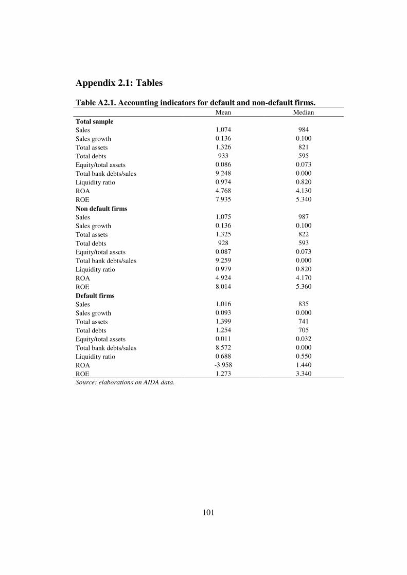
101

Appendix 2.1: Tables

Table A2.1. Accounting indicators for default and non-default firms. Mean Median Total sample Sales 1,074 984 Sales growth 0.136 0.100 Total assets 1,326 821 Total debts 933 595 Equity/total assets 0.086 0.073 Total bank debts/sales 9.248 0.000 Liquidity ratio 0.974 0.820 ROA 4.768 4.130 ROE 7.935 5.340 Non default firms Sales 1,075 987 Sales growth 0.136 0.100 Total assets 1,325 822 Total debts 928 593 Equity/total assets 0.087 0.073 Total bank debts/sales 9.259 0.000 Liquidity ratio 0.979 0.820 ROA 4.924 4.170 ROE 8.014 5.360 Default firms Sales 1,016 835 Sales growth 0.093 0.000 Total assets 1,399 741 Total debts 1,254 705 Equity/total assets 0.011 0.032 Total bank debts/sales 8.572 0.000 Liquidity ratio 0.688 0.550 ROA -3.958 1.440 ROE 1.273 3.340 Source: elaborations on AIDA data.

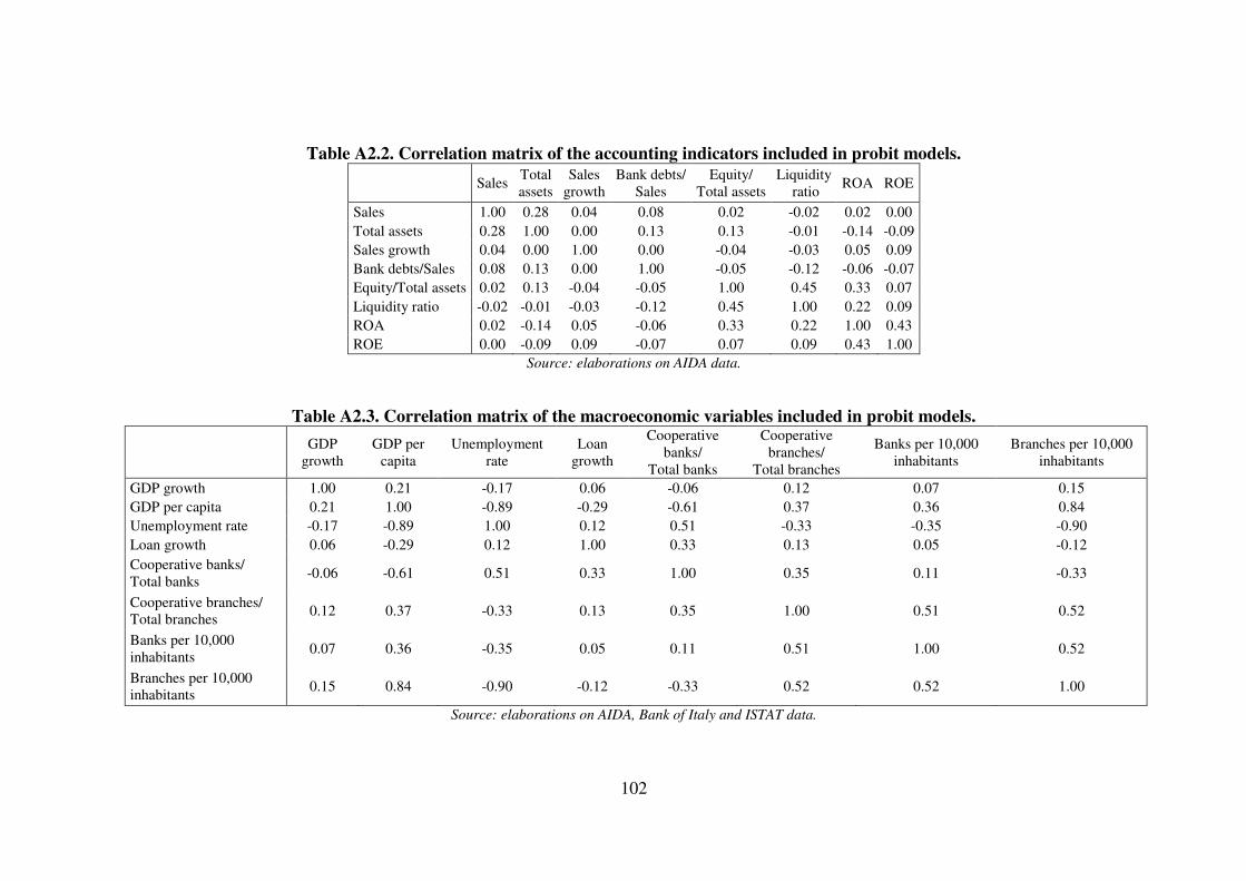
102

Table A2.2. Correlation matrix of the accounting indicators included in probit models.

Sales

Total assets

Sales growth

Bank debts/ Sales

Equity/ Total assets

Liquidity ratio

ROA ROE

Sales 1.00 0.28 0.04 0.08 0.02 -0.02 0.02 0.00 Total assets 0.28 1.00 0.00 0.13 0.13 -0.01 -0.14 -0.09 Sales growth 0.04 0.00 1.00 0.00 -0.04 -0.03 0.05 0.09 Bank debts/Sales 0.08 0.13 0.00 1.00 -0.05 -0.12 -0.06 -0.07 Equity/Total assets 0.02 0.13 -0.04 -0.05 1.00 0.45 0.33 0.07 Liquidity ratio -0.02 -0.01 -0.03 -0.12 0.45 1.00 0.22 0.09 ROA 0.02 -0.14 0.05 -0.06 0.33 0.22 1.00 0.43 ROE 0.00 -0.09 0.09 -0.07 0.07 0.09 0.43 1.00

Source: elaborations on AIDA data.

Table A2.3. Correlation matrix of the macroeconomic variables included in probit models.

GDP

growth GDP per

capita Unemployment

rate Loan

growth

Cooperative banks/

Total banks

Cooperative branches/

Total branches

Banks per 10,000 inhabitants

Branches per 10,000 inhabitants

GDP growth 1.00 0.21 -0.17 0.06 -0.06 0.12 0.07 0.15 GDP per capita 0.21 1.00 -0.89 -0.29 -0.61 0.37 0.36 0.84 Unemployment rate -0.17 -0.89 1.00 0.12 0.51 -0.33 -0.35 -0.90 Loan growth 0.06 -0.29 0.12 1.00 0.33 0.13 0.05 -0.12 Cooperative banks/ Total banks

-0.06 -0.61 0.51 0.33 1.00 0.35 0.11 -0.33

Cooperative branches/ Total branches

0.12 0.37 -0.33 0.13 0.35 1.00 0.51 0.52

Banks per 10,000 inhabitants

0.07 0.36 -0.35 0.05 0.11 0.51 1.00 0.52

Branches per 10,000 inhabitants

0.15 0.84 -0.90 -0.12 -0.33 0.52 0.52 1.00

Source: elaborations on AIDA, Bank of Italy and ISTAT data.

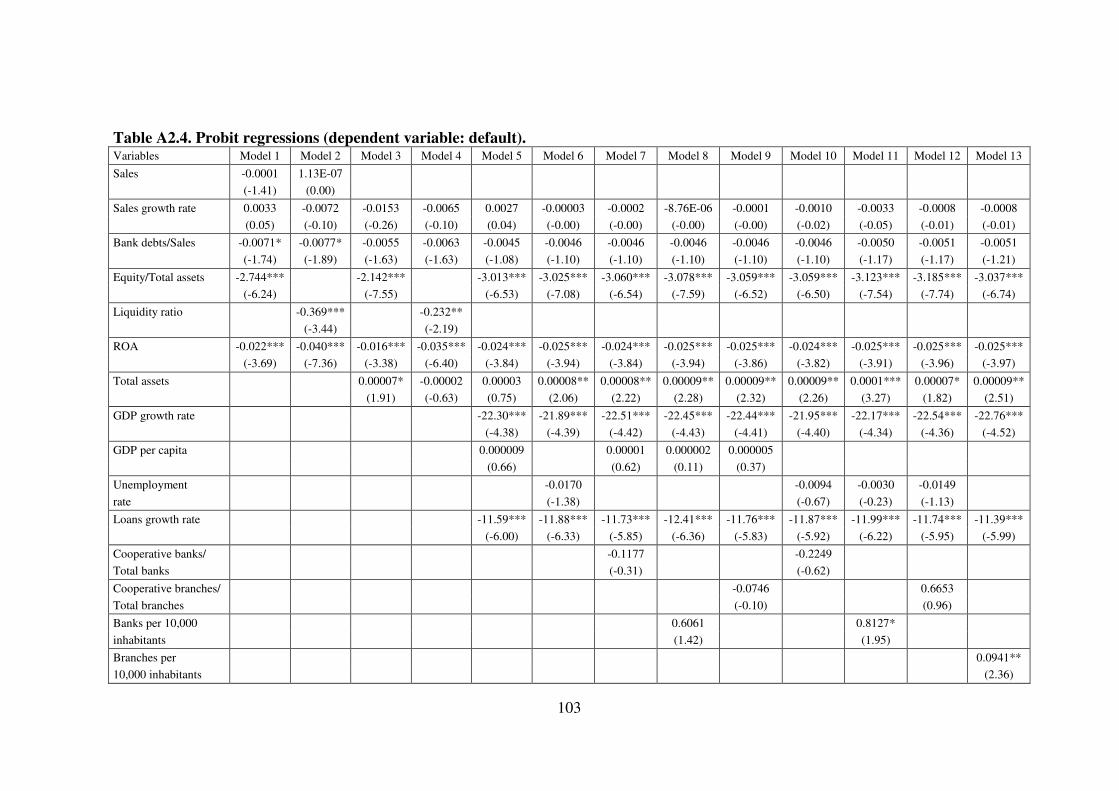
103

Table A2.4. Probit regressions (dependent variable: default). Variables Model 1 Model 2 Model 3 Model 4 Model 5 Model 6 Model 7 Model 8 Model 9 Model 10 Model 11 Model 12 Model 13

Sales -0.0001 1.13E-07

(-1.41) (0.00)

Sales growth rate 0.0033 -0.0072 -0.0153 -0.0065 0.0027 -0.00003 -0.0002 -8.76E-06 -0.0001 -0.0010 -0.0033 -0.0008 -0.0008

(0.05) (-0.10) (-0.26) (-0.10) (0.04) (-0.00) (-0.00) (-0.00) (-0.00) (-0.02) (-0.05) (-0.01) (-0.01)

Bank debts/Sales -0.0071* -0.0077* -0.0055 -0.0063 -0.0045 -0.0046 -0.0046 -0.0046 -0.0046 -0.0046 -0.0050 -0.0051 -0.0051

(-1.74) (-1.89) (-1.63) (-1.63) (-1.08) (-1.10) (-1.10) (-1.10) (-1.10) (-1.10) (-1.17) (-1.17) (-1.21)

Equity/Total assets -2.744*** -2.142*** -3.013*** -3.025*** -3.060*** -3.078*** -3.059*** -3.059*** -3.123*** -3.185*** -3.037***

(-6.24) (-7.55) (-6.53) (-7.08) (-6.54) (-7.59) (-6.52) (-6.50) (-7.54) (-7.74) (-6.74)

Liquidity ratio -0.369*** -0.232**

(-3.44) (-2.19)

ROA -0.022*** -0.040*** -0.016*** -0.035*** -0.024*** -0.025*** -0.024*** -0.025*** -0.025*** -0.024*** -0.025*** -0.025*** -0.025***

(-3.69) (-7.36) (-3.38) (-6.40) (-3.84) (-3.94) (-3.84) (-3.94) (-3.86) (-3.82) (-3.91) (-3.96) (-3.97)

Total assets 0.00007* -0.00002 0.00003 0.00008** 0.00008** 0.00009** 0.00009** 0.00009** 0.0001*** 0.00007* 0.00009**

(1.91) (-0.63) (0.75) (2.06) (2.22) (2.28) (2.32) (2.26) (3.27) (1.82) (2.51)

GDP growth rate -22.30*** -21.89*** -22.51*** -22.45*** -22.44*** -21.95*** -22.17*** -22.54*** -22.76***

(-4.38) (-4.39) (-4.42) (-4.43) (-4.41) (-4.40) (-4.34) (-4.36) (-4.52)

GDP per capita 0.000009 0.00001 0.000002 0.000005

(0.66) (0.62) (0.11) (0.37)

Unemployment -0.0170 -0.0094 -0.0030 -0.0149

rate (-1.38) (-0.67) (-0.23) (-1.13)

Loans growth rate -11.59*** -11.88*** -11.73*** -12.41*** -11.76*** -11.87*** -11.99*** -11.74*** -11.39***

(-6.00) (-6.33) (-5.85) (-6.36) (-5.83) (-5.92) (-6.22) (-5.95) (-5.99)

Cooperative banks/ -0.1177 -0.2249

Total banks (-0.31) (-0.62)

Cooperative branches/ -0.0746 0.6653

Total branches (-0.10) (0.96)

Banks per 10,000 0.6061 0.8127*

inhabitants (1.42) (1.95)

Branches per 0.0941**

10,000 inhabitants (2.36)

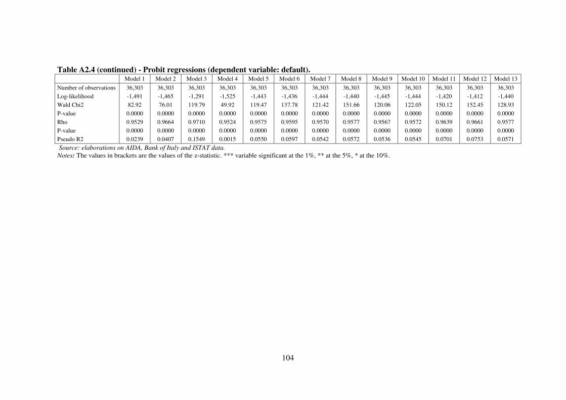
104

Table A2.4 (continued) - Probit regressions (dependent variable: default). Model 1 Model 2 Model 3 Model 4 Model 5 Model 6 Model 7 Model 8 Model 9 Model 10 Model 11 Model 12 Model 13

Number of observations 36,303 36,303 36,303 36,303 36,303 36,303 36,303 36,303 36,303 36,303 36,303 36,303 36,303

Log-likelihood -1,491 -1,465 -1,291 -1,525 -1,443 -1,436 -1,444 -1,440 -1,445 -1,444 -1,420 -1,412 -1,440

Wald Chi2 82.92 76.01 119.79 49.92 119.47 137.78 121.42 151.66 120.06 122.05 150.12 152.45 128.93

P-value 0.0000 0.0000 0.0000 0.0000 0.0000 0.0000 0.0000 0.0000 0.0000 0.0000 0.0000 0.0000 0.0000

Rho 0.9529 0.9664 0.9710 0.9524 0.9575 0.9595 0.9570 0.9577 0.9567 0.9572 0.9639 0.9661 0.9577

P-value 0.0000 0.0000 0.0000 0.0000 0.0000 0.0000 0.0000 0.0000 0.0000 0.0000 0.0000 0.0000 0.0000

Pseudo R2 0.0239 0.0407 0.1549 0.0015 0.0550 0.0597 0.0542 0.0572 0.0536 0.0545 0.0701 0.0753 0.0571

Source: elaborations on AIDA, Bank of Italy and ISTAT data.

Notes: The values in brackets are the values of the z-statistic. *** variable significant at the 1%, ** at the 5%, * at the 10%.

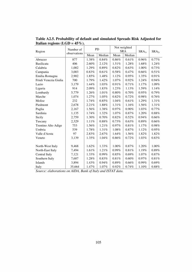
105

Table A2.5. Probability of default and simulated Spreads Risk Adjusted for Italian regions (LGD = 45%).

Region Number of

observations PD

Not weighted SRA SRA1r SRA2r

Mean Median Mean Median Abruzzo 877 1.38% 0.84% 0.86% 0.61% 0.96% 0.77% Basilicata 406 2.60% 2.12% 1.51% 1.28% 1.68% 1.24% Calabria 1,002 1.29% 0.89% 0.82% 0.63% 1.00% 0.73% Campania 3,003 0.83% 0.61% 0.58% 0.47% 0.66% 0.51% Emilia Romagna 2,902 1.85% 1.48% 1.12% 0.95% 1.35% 0.91% Friuli Venezia Giulia 700 1.79% 1.42% 1.07% 0.92% 1.24% 0.94% Lazio 3,179 1.44% 1.03% 0.91% 0.71% 1.17% 1.09% Liguria 914 2.09% 1.83% 1.23% 1.13% 1.59% 1.14% Lombardy 5,779 1.26% 1.01% 0.80% 0.70% 0.95% 0.79% Marche 1,074 1.27% 1.05% 0.82% 0.72% 0.98% 0.76% Molise 232 1.74% 0.85% 1.04% 0.61% 1.29% 1.31% Piedmont 2,678 2.21% 1.88% 1.31% 1.16% 1.56% 1.31% Puglia 2,167 1.56% 1.38% 0.97% 0.90% 1.03% 0.77% Sardinia 1,135 1.74% 1.32% 1.07% 0.87% 1.20% 0.88% Sicily 2,759 1.30% 0.70% 0.82% 0.52% 0.94% 0.66% Tuscany 2,329 1.11% 0.88% 0.73% 0.63% 0.89% 0.66% Trentino Alto Adige 753 1.56% 1.21% 0.97% 0.81% 1.17% 0.98% Umbria 539 1.78% 1.31% 1.08% 0.87% 1.12% 0.95% Valle d'Aosta 97 2.83% 2.67% 1.64% 1.56% 1.82% 1.82% Veneto 3,139 1.35% 1.04% 0.86% 0.72% 1.03% 0.83%

North-West Italy 9,468 1.62% 1.33% 1.00% 0.87% 1.20% 1.00% North-East Italy 7,494 1.61% 1.21% 0.99% 0.81% 1.19% 0.89% Central Italy 7,121 1.33% 0.99% 0.85% 0.69% 1.07% 0.87% Southern Italy 7,687 1.28% 0.83% 0.81% 0.60% 0.97% 0.81% Islands 3,894 1.43% 0.94% 0.89% 0.66% 0.99% 0.69% Italy 35,664 1.47% 1.07% 0.92% 0.74% 1.10% 0.88% Source: elaborations on AIDA, Bank of Italy and ISTAT data.

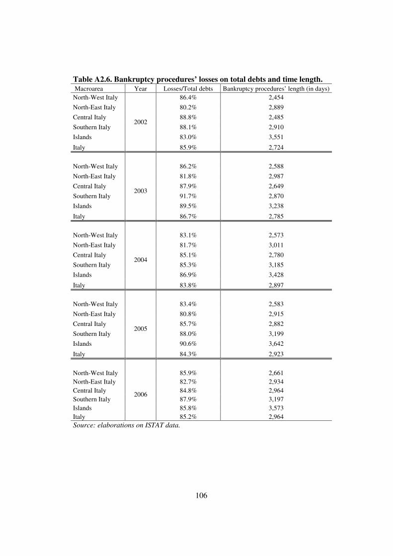
106

Table A2.6. Bankruptcy procedures’ losses on total debts and time length. Macroarea Year Losses/Total debts Bankruptcy procedures’ length (in days) North-West Italy

2002

86.4% 2,454

North-East Italy 80.2% 2,889

Central Italy 88.8% 2,485

Southern Italy 88.1% 2,910

Islands 83.0% 3,551

Italy 85.9% 2,724

North-West Italy

2003

86.2% 2,588

North-East Italy 81.8% 2,987

Central Italy 87.9% 2,649

Southern Italy 91.7% 2,870

Islands 89.5% 3,238

Italy 86.7% 2,785

North-West Italy

2004

83.1% 2,573

North-East Italy 81.7% 3,011

Central Italy 85.1% 2,780

Southern Italy 85.3% 3,185

Islands 86.9% 3,428

Italy 83.8% 2,897

North-West Italy

2005

83.4% 2,583

North-East Italy 80.8% 2,915

Central Italy 85.7% 2,882

Southern Italy 88.0% 3,199

Islands 90.6% 3,642

Italy 84.3% 2,923

North-West Italy

2006

85.9% 2,661 North-East Italy 82.7% 2,934 Central Italy 84.8% 2,964 Southern Italy 87.9% 3,197 Islands 85.8% 3,573 Italy 85.2% 2,964 Source: elaborations on ISTAT data.

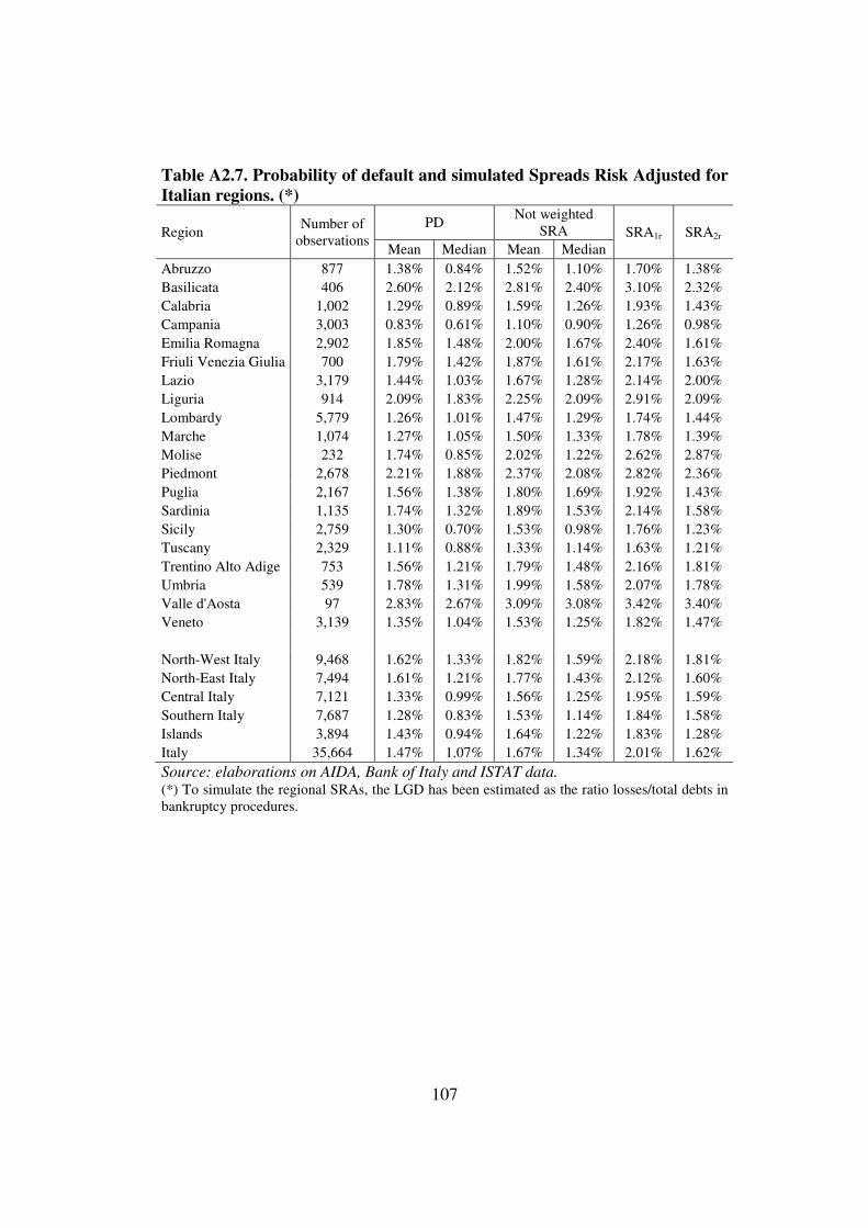
107

Table A2.7. Probability of default and simulated Spreads Risk Adjusted for Italian regions. (*)

Region Number of

observations PD

Not weighted SRA SRA1r SRA2r

Mean Median Mean Median Abruzzo 877 1.38% 0.84% 1.52% 1.10% 1.70% 1.38% Basilicata 406 2.60% 2.12% 2.81% 2.40% 3.10% 2.32% Calabria 1,002 1.29% 0.89% 1.59% 1.26% 1.93% 1.43% Campania 3,003 0.83% 0.61% 1.10% 0.90% 1.26% 0.98% Emilia Romagna 2,902 1.85% 1.48% 2.00% 1.67% 2.40% 1.61% Friuli Venezia Giulia 700 1.79% 1.42% 1.87% 1.61% 2.17% 1.63% Lazio 3,179 1.44% 1.03% 1.67% 1.28% 2.14% 2.00% Liguria 914 2.09% 1.83% 2.25% 2.09% 2.91% 2.09% Lombardy 5,779 1.26% 1.01% 1.47% 1.29% 1.74% 1.44% Marche 1,074 1.27% 1.05% 1.50% 1.33% 1.78% 1.39% Molise 232 1.74% 0.85% 2.02% 1.22% 2.62% 2.87% Piedmont 2,678 2.21% 1.88% 2.37% 2.08% 2.82% 2.36% Puglia 2,167 1.56% 1.38% 1.80% 1.69% 1.92% 1.43% Sardinia 1,135 1.74% 1.32% 1.89% 1.53% 2.14% 1.58% Sicily 2,759 1.30% 0.70% 1.53% 0.98% 1.76% 1.23% Tuscany 2,329 1.11% 0.88% 1.33% 1.14% 1.63% 1.21% Trentino Alto Adige 753 1.56% 1.21% 1.79% 1.48% 2.16% 1.81% Umbria 539 1.78% 1.31% 1.99% 1.58% 2.07% 1.78% Valle d'Aosta 97 2.83% 2.67% 3.09% 3.08% 3.42% 3.40% Veneto 3,139 1.35% 1.04% 1.53% 1.25% 1.82% 1.47%

North-West Italy 9,468 1.62% 1.33% 1.82% 1.59% 2.18% 1.81% North-East Italy 7,494 1.61% 1.21% 1.77% 1.43% 2.12% 1.60% Central Italy 7,121 1.33% 0.99% 1.56% 1.25% 1.95% 1.59% Southern Italy 7,687 1.28% 0.83% 1.53% 1.14% 1.84% 1.58% Islands 3,894 1.43% 0.94% 1.64% 1.22% 1.83% 1.28% Italy 35,664 1.47% 1.07% 1.67% 1.34% 2.01% 1.62% Source: elaborations on AIDA, Bank of Italy and ISTAT data. (*) To simulate the regional SRAs, the LGD has been estimated as the ratio losses/total debts in bankruptcy procedures.

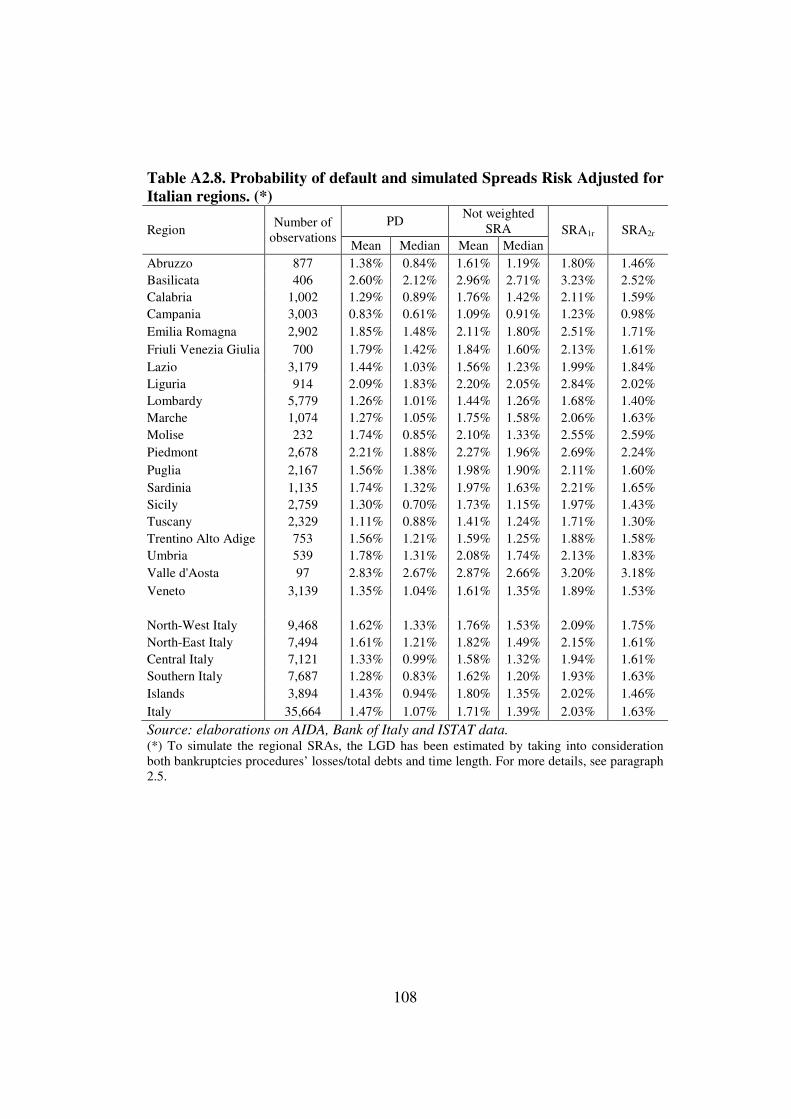
108

Table A2.8. Probability of default and simulated Spreads Risk Adjusted for Italian regions. (*)

Region Number of

observations PD

Not weighted SRA SRA1r SRA2r

Mean Median Mean Median Abruzzo 877 1.38% 0.84% 1.61% 1.19% 1.80% 1.46% Basilicata 406 2.60% 2.12% 2.96% 2.71% 3.23% 2.52% Calabria 1,002 1.29% 0.89% 1.76% 1.42% 2.11% 1.59% Campania 3,003 0.83% 0.61% 1.09% 0.91% 1.23% 0.98% Emilia Romagna 2,902 1.85% 1.48% 2.11% 1.80% 2.51% 1.71% Friuli Venezia Giulia 700 1.79% 1.42% 1.84% 1.60% 2.13% 1.61% Lazio 3,179 1.44% 1.03% 1.56% 1.23% 1.99% 1.84% Liguria 914 2.09% 1.83% 2.20% 2.05% 2.84% 2.02% Lombardy 5,779 1.26% 1.01% 1.44% 1.26% 1.68% 1.40% Marche 1,074 1.27% 1.05% 1.75% 1.58% 2.06% 1.63% Molise 232 1.74% 0.85% 2.10% 1.33% 2.55% 2.59% Piedmont 2,678 2.21% 1.88% 2.27% 1.96% 2.69% 2.24% Puglia 2,167 1.56% 1.38% 1.98% 1.90% 2.11% 1.60% Sardinia 1,135 1.74% 1.32% 1.97% 1.63% 2.21% 1.65% Sicily 2,759 1.30% 0.70% 1.73% 1.15% 1.97% 1.43% Tuscany 2,329 1.11% 0.88% 1.41% 1.24% 1.71% 1.30% Trentino Alto Adige 753 1.56% 1.21% 1.59% 1.25% 1.88% 1.58% Umbria 539 1.78% 1.31% 2.08% 1.74% 2.13% 1.83% Valle d'Aosta 97 2.83% 2.67% 2.87% 2.66% 3.20% 3.18% Veneto 3,139 1.35% 1.04% 1.61% 1.35% 1.89% 1.53%

North-West Italy 9,468 1.62% 1.33% 1.76% 1.53% 2.09% 1.75% North-East Italy 7,494 1.61% 1.21% 1.82% 1.49% 2.15% 1.61% Central Italy 7,121 1.33% 0.99% 1.58% 1.32% 1.94% 1.61% Southern Italy 7,687 1.28% 0.83% 1.62% 1.20% 1.93% 1.63% Islands 3,894 1.43% 0.94% 1.80% 1.35% 2.02% 1.46% Italy 35,664 1.47% 1.07% 1.71% 1.39% 2.03% 1.63%

Source: elaborations on AIDA, Bank of Italy and ISTAT data. (*) To simulate the regional SRAs, the LGD has been estimated by taking into consideration both bankruptcies procedures’ losses/total debts and time length. For more details, see paragraph 2.5.

109

CHAPTER 3: INSTITUTIONAL ENVIRONMENT AND THE COST OF MONEY IN ITALIAN PROVINCES

3.1 Introduction

The results obtained in the first essay indicate that, at a macroeconomic level,

interregional differentials in the cost of money in Italy are caused both by the

greater overall riskiness of loans and by factors concerning credit supply, such

as the average operating size and the degree of territorial diffusion of the branch

network. Nevertheless, according to the analysis developed in the second

chapter (based on a representative sample of Italian firms), specific elements at

firm level are not able to completely explain the interregional interest rate

spread actually observed in Italy. Therefore, it is interesting to verify the

hypothesis that the worse borrowing conditions in the Mezzogiorno area are due

also to institutional elements.

Generally, in order to adequately assess the performance of an economic system,

economists agree about the importance of the institutional environment. In other

words, according to this recent paradigm, it is not possible to completely

understand the economic dynamics of a system if the quality of social

institutions is not taken into consideration.

Because in an efficient credit market the economic agents’ results are the main

factors that banks should evaluate in order to determine borrowing conditions, it

is natural to hypothesize that a causal relationship between institutional

environment and local lending rates also exists.

In the last years, in order to verify this assumption, the literature has increased

its attention towards the relationship between social infrastructure, credit

availability and borrowing conditions. The elements taken into consideration are

the degree of crime, the efficiency of the court system and the effective

protection of property rights. Generally, these aspects have been examined

separately.

110

In this context, this chapter intends to verify if the quality of the institutional

environment is able to influence local borrowing conditions together with the

other elements taken into consideration in the previous chapters.

In order to reach this aim, it is necessary to summarize the several aspects

reflecting the institutional environment in a small number of variables.

The methodology that will be applied is the principal component analysis (PCA)

because it allows to sum up the information contained in a dataset composed by

many variables, keeping the largest part of data variability.

The aspects of the social infrastructure examined in this work are the degree of

crime, the degree of corruption and the degree of property rights protection

guaranteed by the court system.

The chapter is subdivided into three paragraphs, besides this introduction.

Paragraph 3.2 illustrates the main contributions that analyze the effects on

economic performances and on the financial system determined by the

institutional environment.

After describing the variables used in the empirical analysis, paragraph 3.3

develops an institutional index for Italian provinces during the period 2000-2003

and examines the relationship between the quality of social institutions and the

cost of money. Finally, the last paragraph summarizes the main results of the

chapter.

3.2 Literature review

The economic literature largely recognizes the relationship between institutional

environment and economic performance.

North (1990), particularly, focused on the necessity to integrate institutions’

role into economic theory. This need is caused by the presence of asymmetric

information and transaction costs that make the neoclassic paradigm of complete

markets only a theoretical assumption.

111

According to North, “institutions consist of a set of constraints on behavior in

the form of rules and regulations; and, finally, a set of moral, ethical behavioral

norms which define the contours that constrain the way in which the rules and

regulations are specified and enforcement is carried out […] institutions are

therefore the framework within which human interaction takes place”.

Consequently, because institutions (both formal and informal) influence

transaction and production costs, according to North, they can be included

among the determinants of the long run performances of economic systems.

On the basis of the North’s work, economists have traditionally focused on the

direct effect of the institutional environment on GDP growth rates and on the

level of economic development. These analysis are mainly based on cross-

country data.

The quality of the institutions is generally measured by taking into consideration

the following elements: social and human capital, corruption, crime rates and

degree of property rights protection.

The general conclusion is that the quality of the institutional environment affects

economic results because it is a crucial aspect to guarantee the correct

implementation of operators’ transaction.

This element is particularly pointed out by Zak and Knack (2001) that

elaborate a general equilibrium growth model with transaction costs in which

heterogeneous agents face a moral hazard problem. In this context, a low degree

of trust (that is caused by a insufficient level of social capital and weak formal

institutions) reduces the rates of investment and growth. This hypothesis is

confirmed by the empirical analysis that is based on a sample of 41 countries

during the period 1970-1992.

With particular reference to the Italian context, the main contributions about the

relationship between social infrastructure and economic performance are Aiello

and Scoppa (2000), Del Monte and Papagni (2001), Golden and Picci (2005),

Daniele and Marani (2008) and Albanese (2010).

112

Taking into consideration the period 1980-1982, Aiello and Scoppa (2000)

explain the regional differences in the levels of output per worker according to

the greater degree of total factor productivity (TFP) observed in Northern

regions. Particularly, the TFP is also influenced by the institutional environment

because it depends on the degree of development of the financial system, the

agglomeration economies, the efficiency of infrastructures, the degree of crime

and the government intervention in the economy (that is expressed in terms of

incidence of public employment in the labour market).

Del Monte and Papagni (2001) verify if corruption can be included among the

causes of the failure of the huge program of public expenditure that has been

carried out during the last fifty years in favor of the Mezzogiorno regions.

Particularly, this program has not been able to reduce the distance between

Northern and Southern regions in terms of GDP per capita.

On the basis of data concerning the Italian regions during the period 1963-1991,

the authors show a negative effect of corruption (measured in terms of the

number of crimes against the public administration per million employees) on

GDP per capita. This relationship is due to the reduction of the quantity and the

quality of infrastructures and public services provided to the private sector that

is caused by corruption and, hence, to a lower degree of efficiency of the public

expenditure in the regions characterized by a high level of corruption.

For the year 1997, Golden and Picci (2005) develop a specific indicator of

corruption for Italian provinces. This measure is obtained by calculating the

difference between the amounts of physically existing public infrastructure and

what government cumulatively pays for public infrastructure (that represents the

potentially feasible stock of public capital). The hypothesis underlying the

significance of this index is that, for the most part, this difference is caused by

the loss of public money for fraud and embezzlement activities. Golden and

Picci point out that, although the amount of public investments is greater in

113

Southern regions, Northern regions are more infrastructure-abundant. This result

indicates a greater degree of corruption in the Mezzogiorno area.

Taking into consideration the period 2004-2006, Daniele and Marani (2008)

show that organized crime negatively affects the Mezzogiorno attractiveness

and, generally, the overall potential investors’ opinion about Southern regions.

Organized crime (measured by the number of extortions, people denounced for

criminal conspiracies, attempts and arsons per inhabitant) negatively influences

foreign direct investments in the Mezzogiorno area because it represents an

additional cost for private firms.

Finally, Albanese (2010) develops a cross-section analysis for Italian regions

during the year 2004. The aim of this work is to estimate an indicator that takes

into consideration the main aspects of the social infrastructure (corruption,

crime, efficiency of the court system and degree of intervention in the economy)

and that is able to explain differences between North and South Italy in the level

of GDP per capita.

According to the author, the differences among Italian regions in the level of

economic development are caused by an institutional gap among Northern and

Southern areas, while the traditional impact of social and human capital on the

level of GDP per capita observed by the literature is not any more significant

when the role played by social infrastructure is taken into account.

During the last years, another research field has been represented by the study of

the relationship between institutional environment and economic system by

means of the credit market’s and financial system’s channels.

Particularly, because the cost and the availability of financial resources

influence the investors’ investment ability, these aspects are crucial factors for

the economic growth processes above all in those contexts characterized by the

dominant presence of small firms for which external financial resources are the

main source of funding.

114

The group of works that analyze the relationship between institutional

environment and financial system includes Mauro (1995), La Porta et al. (1998),

Claessens and Laeven (2003), Diamond (2004), Qian and Strahan (2007) and

Bae and Goyal (2009) and, for the Italian context, Guiso et al. (2004), Jappelli et

al. (2005) and Bonaccorsi di Patti (2009).

Taking into consideration a panel of 32,665 households during the period 1989-

1995, Guiso et al. (2004) focus on the relationship between institutional

environment and degree of development of the financial system.

The aspects of the social infrastructure analyzed by these authors are the degree

of crime (expressed by the number of violent crime divided by the population),

the degree of inefficiency of the law enforcement (measured by the average

length of the first-degree trials), the human capital (expressed in terms of

average number of schooling years) and the social capital (measured by the

participation in referenda and by the number of blood donations every 1,000

inhabitants, i.e. by behaviors that are not caused by economic reasons but are

driven only by social pressure and internal norms).

With particular reference to the latter aspect, social capital should influence the

level of development of the financial system because the probability that a

contract takes place depends not only on its legal enforceability but also on the

degree of trust among the agents, that is positively influenced by social capital.

A greater development of the financial system is expressed by a larger incidence

of the households that use checks, portfolio allocation, face less constraints to

obtain bank loans and do not depend on informal lending (i.e. on loans that are

made by relatives and friends and that are considered as an alternative to bank

credit if banks reject the household’s credit request).

The authors show that the level of development of the financial system is greater

in the areas characterized by larger levels of human and social capital, a better

efficiency of the court system and a smaller presence of organized crime.

115

Particularly, social capital significantly affects the use of checks, the probability

to face constraints in the credit market and the probability to ask for informal

lending only in the areas with a smaller efficiency of the judicial system.

Consequently, in areas characterized by a low contracts’ enforceability (that is

caused by a low degree of efficiency of the court system), the role played by

social capital is more relevant because social capital imposes internal norms and

social sanctions that are able to reduce opportunistic behavior on the part of

borrowers.

Furthermore, social capital significantly influences the borrowers’ probability to

be financed by banks in the areas with a low average level of education. The

reason is that, low-education people involved in the transaction cannot fully

understand most of the terms of the contracts; consequently low-education

people will delegate more educated agents to conclude the transaction and they

will require more trust.

Jappelli et al. (2005) have a different approach concerning how the degree of

efficiency of the court system influences credit availability.

In more details, this work develops a theoretical model where agents transact

and face a moral hazard problem and the court system is inefficient. According

to this model, an improvement in the degree of efficiency of the judicial system

leads to a reduction of credit rationing because of the greater protection of

banks’ rights in case of default. This hypothesis is confirmed by an empirical

analysis based on data about the 27 Italian judicial districts (that existed during

the nineties of the last century) during the period 1984-1998. Particularly, the

degree of efficiency of the court system (measured by the average length of the

civil judicial processes and the number of civil suits pending per 1,000

inhabitants) positively affects credit availability; on the contrary a greater degree

of efficiency of the judicial system determines lower lending rates and a smaller

number of default events.

116

This result is also obtained by Bonaccorsi di Patti (2009) that, developing a

cross-section analysis at a provincial level on 300,000 bank-firm relationships in

2000, shows that access to credit is positively affected by the degree of

efficiency of the court system.

The institutional aspects taken into consideration by Bonaccorsi di Patti reflect,

at a provincial level, the level of crime (number of offences for which the

authorities have opened a judicial procedure per 1,000 inhabitants and the share

of offences against individuals reported to law enforcement officers) and the

inefficiency of the judicial system (expressed in terms of length in years of a

first-degree civil court trial used in Guiso et al. (2004)).

According to the author, lending rates are higher in the areas where crime rates

are larger and courts are inefficient; on the contrary, where there is more trust in

institutions, borrowing conditions are better. Particularly, borrowers operating in

the provinces with a larger degree of crime must pay lending rates that are

around 30 basis points higher than those paid by similar borrowers operating in

low-crime provinces. The effect of crime on the cost of money decreases for

larger firms.

Furthermore, crime rates positively affect the collateral amount and the

probability that the utilization rate ratio (i.e. the ratio between used and granted

credit) is bigger than 1, denoting the existence of credit rationing.

As regards the international framework, taking into consideration data on 70

countries during the period 1980-1983, Mauro (1995) examines the relationship

between institutional environment and economic performance by means of the

investment channel. According to the author, corruption and inefficiency of

bureaucracy slowdown investments and, by this way, reduce GDP growth rates.

La Porta et al. (1998) analyze the relationship between legal protection of

investors (both companies’ creditors and shareholders) and corporate

governance models.

117

In this context, by examining data on a set of 49 countries during the nineties of

the last century, the authors show that in French-civil-law countries (where

investors’ legal protection is the lowest one) the ownership is extremely

concentrated. This result support the idea the more concentrated ownership is

considered as an instrument that allows to investors to actually exercise their

control rights in an adverse institutional environment. On the contrary, in

common-law countries (that are the countries with the highest investors’ legal

protection) the ownership is generally not concentrated.

By analyzing a sample of 45 countries during the period 1980-1989, Claessens

and Laeven (2003) focus on the relationship between property rights protection

and resources allocation by firms.

According to the authors, firm growth is influenced, besides the financial

resources availability, also by the allocation of investable resources.

Particularly, property rights protection is able to affect the allocation of

resources across alternative investment projects because firms operating in

markets with weaker property rights tend to invest a share of their financial

resources in material assets that is larger than the optimal one. The reason is

that, in these frameworks, firms find relatively less difficult to secure the returns

from fixed assets from illegal behaviors on the part of their competitors.

The empirical analysis confirms this hypothesis: the authors show that a greater

development of the financial system (measured by the ratio between private

loans and GDP) and a better legal protection system (expressed by taking into

consideration several indexes that were developed by international agencies

according firms’ surveys) facilitate firms’ growth by increasing financial

resources availability and the efficiency of resources allocation by firms.

Qian and Strahan (2007) examine a sample of 4,321 bank loans in 43 countries

during the period 1994-2003 and come at the conclusion that the institutional

environment (measured by the degree of creditor rights protection) significantly

affects contract terms and the degree of loan concentration.

118

In details, in those contexts with better legal protection, banks generally grant

credit at better conditions (lower lending rates and longer maturities). The

reason is that, in these realities, banks have greater ability to force repayment or

take control of the firm in case of default.

Furthermore, on average, the number of lenders is lower (i.e. the concentration

of loan ownership is bigger) in countries with a larger degree of property rights

protection and for smaller and opaque firms.

Finally, because of the significant presence of asymmetric information, foreign

banks are more sensitive to the legal environment: a reduction of the degree of

creditor rights protection leads to a decline in foreign banks’ market shares in

favor of domestic banks.

Bae and Goyal (2009) point out that borrowing conditions are not influenced by

the formal creditor rights protection system but by the actual enforceability of

bank contracts.

On the basis of a sample of 63,158 bank loans in 48 countries during the period

1994-2003, these authors show that banks apply more cumbersome conditions in

those countries where the degree of creditor rights protection is worse in

response to the greater uncertainty of the legal environment. Particularly, in

these contexts, banks tend to reduce loans maturity in order to review their

lending decisions more frequently and apply higher interest rates to compensate

the greater credit risk. Moreover, Bae and Goyal show that firms with similar

structural characteristics pay larger lending rates if they operate in countries

characterized by higher levels of corruption, greater risk of expropriation and

larger risk of contract repudiation.

Finally, Diamond (2009) develops a theoretical analysis. The author elaborates

a model where short loans’ maturities represent a solution in those contexts

where creditors must sustain higher costs in order to enforce debt contracts.

If loans’ maturities are short and firms borrow from multiple lenders, borrowers

will repay their debts also if enforcement is costly and single lenders could be

119

induced not go to bankruptcy court after a borrower default. The reason is that,

in this case, borrowing with large amounts of short-term debts from different

lenders can lead to the threat of “firm runs” that are very similar to the bank runs

during liquidity crisis. This threat is able to commit borrowers to repay debt

rather than renegotiate the claim at the maturity.

According to Diamond, the minimum number of lenders that is necessary to

commit borrowers to repay debt increases with enforcement costs that are

positively influenced by the degree of corruption in the legal system and

negatively affected by the degree of creditor rights protection.

3.3 The empirical analysis: estimating an institutional index for

Italian provinces

3.3.1 Institutional environment and the cost of money

According to the literature illustrated in the previous paragraph, institutional

environment is an aspect able to significantly affect potential growth both

directly and indirectly by means of the financial channel (i.e. institutional

elements affect the functioning of the financial system and, consequently, the

operators’ investment ability).

In this framework, this chapter intends to verify if, in Italian provinces, social

infrastructure is able to significantly influence borrowing conditions. In order to

reach this aim, the quality of the institutions must be expressed in quantitative

terms.

Social infrastructure can be expressed by means of various factors. Particularly,

literature traditionally has taken into consideration the following aspects: crime,

degree of legal protection assured by the court system and corruption.

With particular reference to the first element, in high-crime areas, banks can

apply to their customers more cumbersome borrowing conditions because of the

greater perceived risk. In this situation, firms must indeed face the risk of losses

120

caused by criminal activities (such as extortions) and must sustain additional

costs for security and protection.

The negative effect of crime in a territory can be alleviated by an efficient

judicial system. Coherently with Bae and Goyal’s results, borrowing conditions

are not influenced by formal creditor rights protection but by the actual

contracts’ enforceability. In this context, an efficient court system allows to

operators to enforce contracts without time and financial resources waste.

A greater efficiency of the judicial system should improve borrowing conditions

by means of two channels. The first one is the disincentive to illegal behaviors

that determines the reduction of the average crime rate. The second channel is

the increase in the bank contracts’ enforceability and in the probability that bank

credits are totally repaid by borrowers. In light of the latter element, it appears

very important to take into consideration, together with data concerning penal

and civil justice, also data about bankruptcy procedures.

Finally, as regards the last aspect of the social infrastructure traditionally

analyzed by the literature, corruption can affect the accurate functioning of the

financial system because it distorts the whole economic system and the price

mechanisms.

3.3.2 The Italian judicial system

The following analysis concerns the period 2000-2003 and is based on

provincial data about civil and penal justice and bankruptcy proceedings

provided by the Territorial Information System of Justice developed by ISTAT.

I chose to take into consideration this period because of the limited availability

of data about justice at a provincial level: in fact, ISTAT releases the main data

about the court system in Italian provinces from 2000 to 2005. However, in

order to estimate an institutional indicator, I chose to take into account only the

period 2000-2003 because this work intends to analyze the relationship between

institutional environment and the cost of money and homogenous data on

121

lending rates are available exclusively during the period 1998-2003 (during the

period 2000-2003 both data on judicial system and homogenous data on lending

rates are hence available).

As regards the civil and penal justice, the variables included into the analysis are

those traditionally taken into consideration by the literature in order to assess the

effect of the social institutions on economic performance: the average length in

days of a first-degree civil court trial, the number of civil suits pending per

100,000 inhabitants, the ratio between the number of civil suits pending and

settled during the year (this indicator is an inverse measure of the courts’ ability

to dispose of civil trials) and the number of total crimes, crimes against the

State, criminal associations and mafia criminal associations (per 100,000

inhabitants) for which the judicial authority began the penal action.

Furthermore, I included into the analysis also a variable concerning bankruptcy

proceedings (that is a field that traditionally has not been taken into

consideration by the literature). Particularly, the indicator analyzed is the ratio

between losses and liabilities because it reflects the average amount that

creditors can obtain in bankruptcies procedures. This ratio can be considered

such as a proxy of the degree of contracts’ enforceability and, hence, of the

degree of property rights protection in the system.

As data demonstrate, in Italy there are relevant differences, among the different

geographical areas, in the degree of efficiency of the court system, crime and

corruption.

Table 3.1 confirms that Mezzogiorno is the geographical area with the highest

level of organized crime (the legend of the indicators is shown in table A3.1 in

appendix 3.1). Particularly, the differences among areas in terms of number of

criminal associations and extortions per 100,000 inhabitants are very significant

given that these types of offences are linked to organized crime. In Southern

Italy and in the Islands, indeed, both indicators take values considerably larger

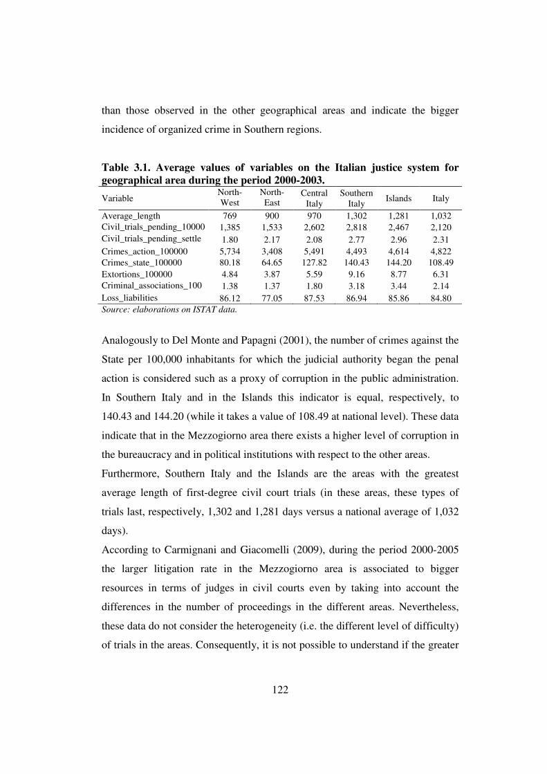
122

than those observed in the other geographical areas and indicate the bigger

incidence of organized crime in Southern regions.

Table 3.1. Average values of variables on the Italian justice system for geographical area during the period 2000-2003.

Variable North-West Italy

North-East Italy

Central Italy

Southern Italy

Islands Italy

Average_length 769 900 970 1,302 1,281 1,032 Civil_trials_pending_100000

1,385 1,533 2,602 2,818 2,467 2,120 Civil_trials_pending_settled

1.80 2.17 2.08 2.77 2.96 2.31 Crimes_action_100000 5,734 3,408 5,491 4,493 4,614 4,822 Crimes_state_100000 80.18 64.65 127.82 140.43 144.20 108.49 Extortions_100000 4.84 3.87 5.59 9.16 8.77 6.31 Criminal_associations_100000

1.38 1.37 1.80 3.18 3.44 2.14 Loss_liabilities 86.12 77.05 87.53 86.94 85.86 84.80 Source: elaborations on ISTAT data.

Analogously to Del Monte and Papagni (2001), the number of crimes against the

State per 100,000 inhabitants for which the judicial authority began the penal

action is considered such as a proxy of corruption in the public administration.

In Southern Italy and in the Islands this indicator is equal, respectively, to

140.43 and 144.20 (while it takes a value of 108.49 at national level). These data

indicate that in the Mezzogiorno area there exists a higher level of corruption in

the bureaucracy and in political institutions with respect to the other areas.

Furthermore, Southern Italy and the Islands are the areas with the greatest

average length of first-degree civil court trials (in these areas, these types of

trials last, respectively, 1,302 and 1,281 days versus a national average of 1,032

days).

According to Carmignani and Giacomelli (2009), during the period 2000-2005

the larger litigation rate in the Mezzogiorno area is associated to bigger

resources in terms of judges in civil courts even by taking into account the

differences in the number of proceedings in the different areas. Nevertheless,

these data do not consider the heterogeneity (i.e. the different level of difficulty)

of trials in the areas. Consequently, it is not possible to understand if the greater

123

quantity of pending trials in the Mezzogiorno area is caused by inadequate

resources or by courts’ lower degree of productivity.

However, the greater average length of civil trials and the bigger quantity of

pending trials determine a lower degree of rights protection in Southern regions.

Instead, the geographical distribution of the ratio between losses and liabilities

in bankruptcy proceeding (that can be considered such as a proxy of the loss

given default) is more homogenous among provinces.

The main conclusion to be drawn by analyzing data on the justice system is that

Mezzogiorno is the Italian area with the worst quality of the institutional

environment because of the highest degree of crime, corruption and the lowest

rights protection assured by the court system.

3.3.3 Estimating an institutional indicator for Italian provinces

Data discussed in the previous paragraph show that the degree of corruption,

crime and rights protection (indicators that reflect the quality of the institutions)

can be represented by several variables that tend to move in the same direction.

Although in order to represent the different characteristics of the institutional

environment it is important to take into consideration as many variables as

possible, the inclusion of too many correlated variables would not allow to

properly assess the importance of each element.

In order to overcome this trade-off, principal component analysis (PCA) is

employed. This methodology allows to express the information contained in a

dataset composed by a large number of highly correlated variables by using few

indicators. Appendix 3.2 explains this methodology in more details.

The PCA is hence applied to the eight variables analyzed in the previous

paragraph in order to calculate one or more indicators that are able to efficiently

summarize the information contained in the dataset.

The indicators obtained by means the PCA are linear combinations of the eight

variables, with weights equal to the elements of the corresponding eigenvectors

124

of the correlation matrix of the initial variables involved. These weights permit

to account for the largest part of data variability (see appendix 3.2).

PCA is based on the correlation matrix rather than the variance and covariance

matrix because the eight variables object of analysis have different order of

magnitude. Because the variance depends on the absolute value of the variables,

considering in the PCA the variance and covariance matrix rather than the

correlation one would lead to components that are considerably affected by the

variables with the largest absolute values; on the contrary the information

contained in the variables characterized by a large variability but low absolute

values would be lost. In other words, if the analysis developed in this paragraph

would have been based on the variance and covariance matrix of the original

variables, the calculated components would be a combination of the number of

offences per 100,000 inhabitants for which the authorities opened a judicial

procedure and the number of civil suits pending per 100,000 inhabitants (i.e. the

variables with the highest order of magnitude), while the weights associated to

the other six variables would be approximately equal to zero.

The eigenvalues of the correlation matrix are shown in table A3.2 in appendix

3.1. For every component, the corresponding eigenvalue represents its variance,

while the ratio between the eigenvalue and the total sum of all eigenvalues is the

percentage of the dataset variance that is explained by the component taken into

consideration (see appendix 3.2).

Table A3.2 shows that the first component explains 42.6% of the overall

variance with an eigenvalue equal to 3.41. Taken together, the first two

components explain almost 60% of the variance.

In order to summarize the information contained in the dataset, only the first two

components are considered. The choice of the number of components to take

into account is based on the Kaiser rule, according to which only the main

components corresponding to an eigenvalue which is higher or equal to 1 have

to be selected.

125

With reference to the first component, the eigenvector (reported in table A3.3)

shows how the number of civil suits pending, the ratio between the number of

civil suits pending and settled, the number of crimes against the State and the

average length of first-degree trials have similar weights. The number of crimes

for which the judicial authority began the penal action is instead the least

important variable to compute this component.

In more details, the first component is obtained by calculating the linear

combination of the initial eight variables on the Italian justice system, with

weights equal to the elements of the eigenvector corresponding to the highest

eigenvalue (that is equal to 3.41).

Because all weights associated to the initial eight variables have positive sign,

the first component can be considered such as an indicator of the quality of the

institutional environment at provincial level. Particularly, provinces with larger

and positive values of the first component are the areas where the eights

variables on the justice system are larger and, therefore, are characterized by a

worse quality of the institutions.

As regards the second component, variables concerning the civil justice and

variables concerning the penal justice and bankruptcy proceedings have opposite

sign. Therefore, provinces where the second component takes larger and

positive values are characterized by a greater degree of inefficiency in the civil

justice system.

Analogously to the first component, the second one is computed by weighting

the eight original variables concerning the court system in Italian provinces with

weights equal to the elements of the eigenvector associated to the second

eigenvalue (that is equal to 1.32).

The initial values of the two components are rescaled so that the range for each

indicator is between 0 and 1 with low values indicating higher average quality

levels of the institutional environment in Italian provinces during the period

2000-2003.

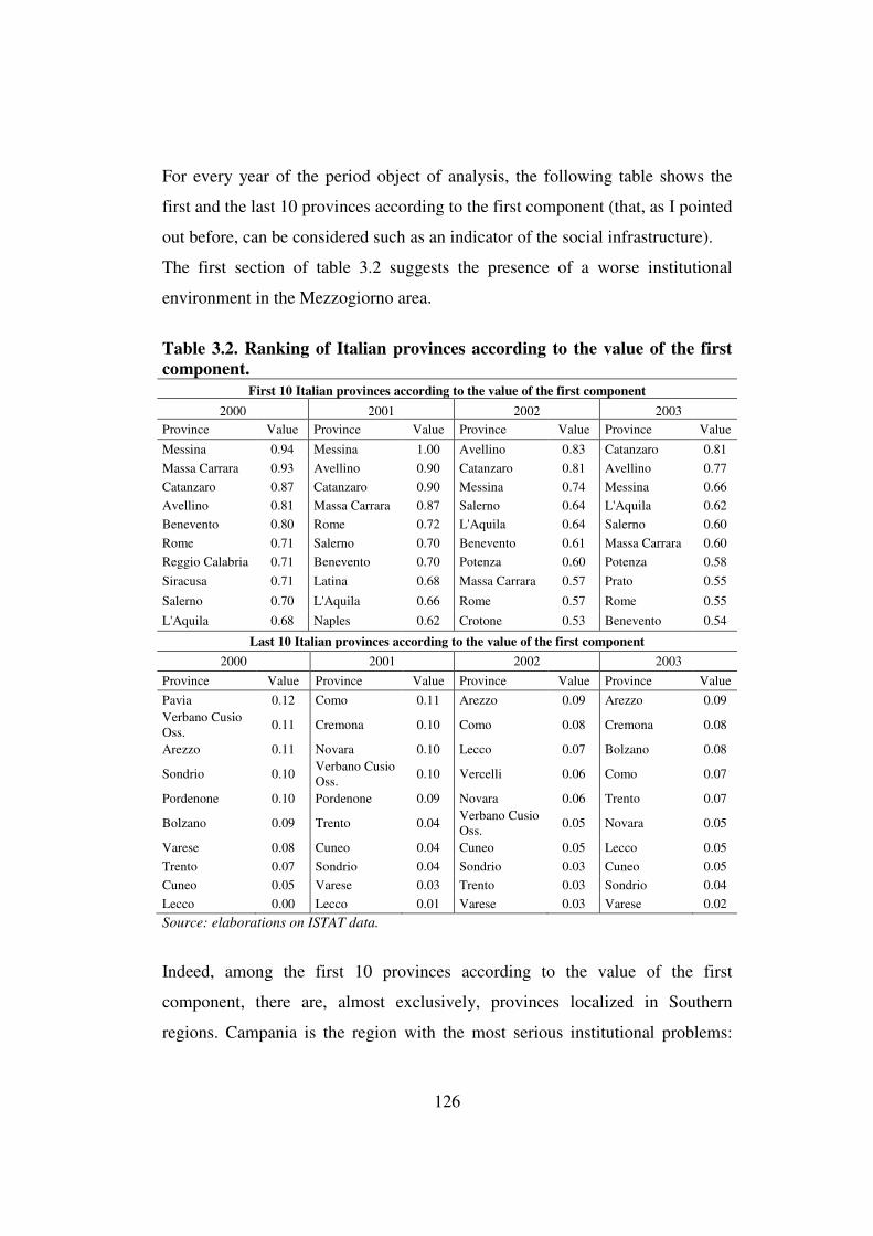
126

For every year of the period object of analysis, the following table shows the

first and the last 10 provinces according to the first component (that, as I pointed

out before, can be considered such as an indicator of the social infrastructure).

The first section of table 3.2 suggests the presence of a worse institutional

environment in the Mezzogiorno area.

Table 3.2. Ranking of Italian provinces according to the value of the first component.

First 10 Italian provinces according to the value of the first component

2000 2001 2002 2003

Province Value Province Value Province Value Province Value

Messina 0.94 Messina 1.00 Avellino 0.83 Catanzaro 0.81

Massa Carrara 0.93 Avellino 0.90 Catanzaro 0.81 Avellino 0.77

Catanzaro 0.87 Catanzaro 0.90 Messina 0.74 Messina 0.66

Avellino 0.81 Massa Carrara 0.87 Salerno 0.64 L'Aquila 0.62

Benevento 0.80 Rome 0.72 L'Aquila 0.64 Salerno 0.60

Rome 0.71 Salerno 0.70 Benevento 0.61 Massa Carrara 0.60

Reggio Calabria 0.71 Benevento 0.70 Potenza 0.60 Potenza 0.58

Siracusa 0.71 Latina 0.68 Massa Carrara 0.57 Prato 0.55

Salerno 0.70 L'Aquila 0.66 Rome 0.57 Rome 0.55

L'Aquila 0.68 Naples 0.62 Crotone 0.53 Benevento 0.54

Last 10 Italian provinces according to the value of the first component

2000 2001 2002 2003

Province Value Province Value Province Value Province Value

Pavia 0.12 Como 0.11 Arezzo 0.09 Arezzo 0.09 Verbano Cusio Oss.

0.11 Cremona 0.10 Como 0.08 Cremona 0.08

Arezzo 0.11 Novara 0.10 Lecco 0.07 Bolzano 0.08

Sondrio 0.10 Verbano Cusio Oss.

0.10 Vercelli 0.06 Como 0.07

Pordenone 0.10 Pordenone 0.09 Novara 0.06 Trento 0.07

Bolzano 0.09 Trento 0.04 Verbano Cusio Oss.

0.05 Novara 0.05

Varese 0.08 Cuneo 0.04 Cuneo 0.05 Lecco 0.05

Trento 0.07 Sondrio 0.04 Sondrio 0.03 Cuneo 0.05

Cuneo 0.05 Varese 0.03 Trento 0.03 Sondrio 0.04

Lecco 0.00 Lecco 0.01 Varese 0.03 Varese 0.02

Source: elaborations on ISTAT data.

Indeed, among the first 10 provinces according to the value of the first

component, there are, almost exclusively, provinces localized in Southern

regions. Campania is the region with the most serious institutional problems:

127

particularly, in every year of the period taken into consideration, in this region 3

provinces out of 5 (Avellino, Benevento and Salerno) are ranked among the 10

Italian provinces with the highest values of the first component.

On the contrary, the second part of table 3.2 shows that Northern provinces have

the best results. In fact, with the exception of Arezzo, the provinces

characterized by the lowest values of the first component are localized in North

Italy. Particularly, the Lombardy provinces have the best performance in terms

of social infrastructure.

The better institutional environment in Northern areas is confirmed in figure 3.1.

This figure allows to assess the overall distribution of Italian provinces

according to the average value of the first component during the period 2000-

2003.

Provinces with lighter colours are characterized by a better quality of the

institutions while the areas with darker colours are less virtuous.

Southern provinces generally belong to the highest quartiles of the distribution;

on the contrary, provinces located in the Northern and Central Italy are

characterized by smaller values of the indicator. Milano and Brescia are the only

Lombardy provinces that do not belong to the first quartile of the distribution.

In conclusion, the analyzed data point out relevant differences in the quality of

the institutions among Northern and Southern areas. The worse institutional

environment in the Mezzogiorno area is caused by the higher organized crime

and by the difficulties of the Southern courts to solve civil disputes and

bankruptcy proceedings. On the whole, these elements cause a lower rights

protection in the Mezzogiorno and are able to negatively influence borrowing

conditions applied to the firms operating in this area.

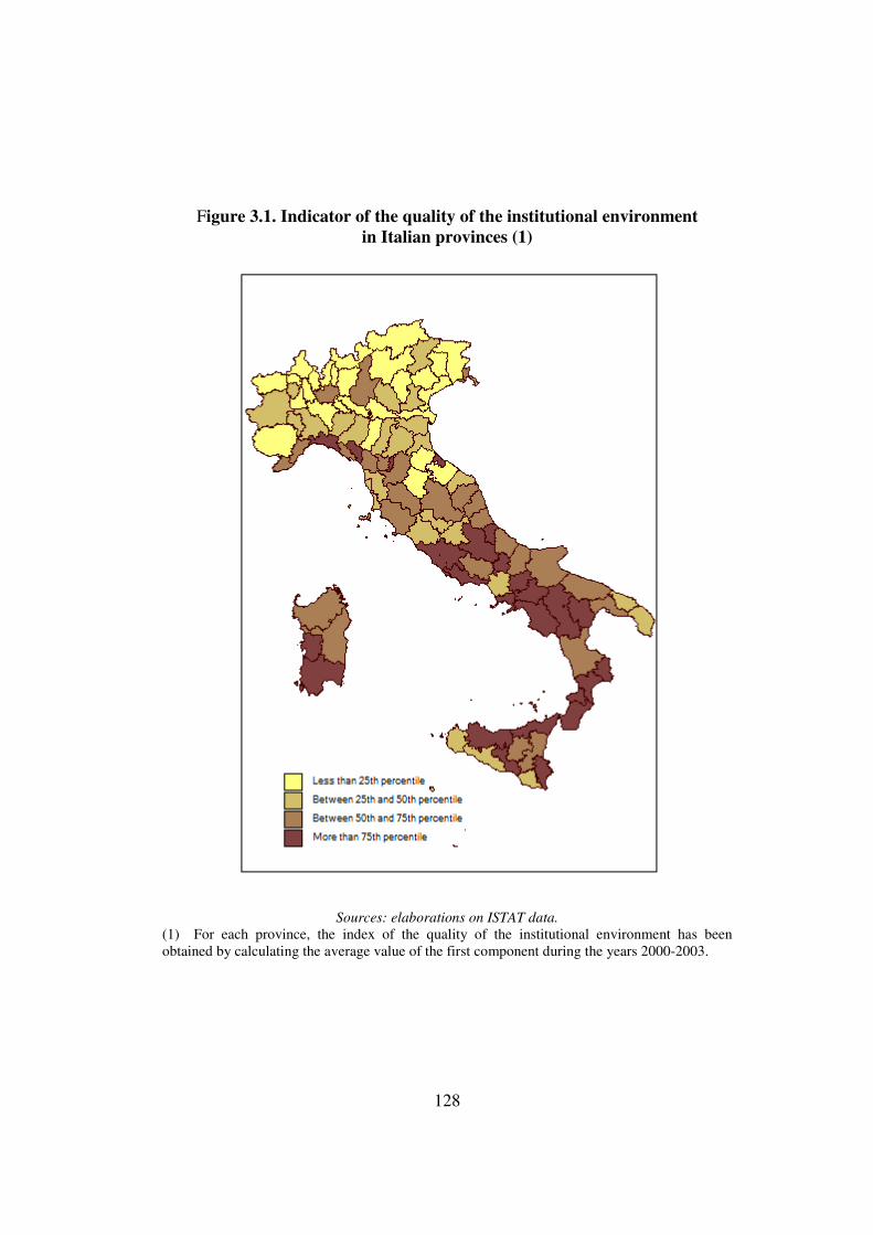
128

Figure 3.1. Indicator of the quality of the institutional environment in Italian provinces (1)

Sources: elaborations on ISTAT data.

(1) For each province, the index of the quality of the institutional environment has been obtained by calculating the average value of the first component during the years 2000-2003.

129

3.3.4 Does institutional environment affect borrowing conditions

in Italian provinces?

In light of the analysis developed in the previous paragraph, the aim of this

section is to verify if the higher lending rates applied to Southern borrowers are

caused, together with the structural elements concerning the financial system

examined in the first chapter, also by institutional factors.

In details, the following analysis intends to examine the impact on borrowing

conditions of social infrastructure at a provincial level.

In order to quantitatively express the level of the institutional environment, I

employ the first two components computed in the PCA developed in paragraph

3.3.3. I chose to take into consideration also the second component because,

together with the first one, it allows to express about 60% of the overall

variability of the information contained in the initial eight variables that reflect

the degree of crime, corruption, efficiency of the court system and rights

protection.

Analogously to the analysis developed in the first chapter, because of the

relevant persistence in lending rates, it would be appropriate to explain the

relationship between social infrastructure and the cost of money by using a

dynamic panel model. In this context, the Arellano and Bond estimator would

lead to consistent and efficient estimates.

However, while homogeneous data on lending rates are available for 6 years

(from 1998 to 2003), it is possible to employ data on the judicial system only for

4 years (from 2000 to 2003). If I would have included 2 lags for the dependent

variable and used first differences (according to the Arellano and Bond

methodology), the number of the remaining observations for each series would

not permit to obtain estimates for the Arellano and Bond estimator.

In light of the above considerations, the following analysis develops a set of

cross-section models where, for every province, the dependent variable is the

130

average of lending rates during the period 2000-2003 and the explanatory

variables are the average values of the first and the second component and the

average values of the variables concerning the banking system that, according to

the first chapter, significantly affect the cost of money at a macroeconomic

level: the degree of territorial diffusion and the average operating size of the

branch network and the riskiness of loans.

Because of the high negative correlation between the average value of the

number of branches per 10,000 inhabitants and the average value of the ratio

between non-performing loans and total loans (as shown in table A3.4, the

correlation coefficient between these variables is equal to -0.82), the effect of

these two variables on lending rates is evaluated separately in order to avoid

multicollinearity problems.

Table 3.3 shows the output of the estimated OLS regressions together with the

Breusch-Pagan heteroskedasticity test and the Ramsey Regression Equation

Specification Error Test (RESET test).

With reference to the first model, the Breusch-Pagan test leads to reject the null

hypothesis of homoskedastic errors. Consequently, the inferential analysis is

developed by using the White heteroskedasticity consistent standard errors.

Coherently with the results achieved in the first chapter, the first model indicates

a significant and negative relationship between the average operating size of

branches and lending rates; on the contrary the aggregate riskiness of loans

positively affects the cost of money.

As regards the institutional aspects, provinces with higher values of the first

component are characterized by more cumbersome borrowing conditions (large

values of the first component reflect worse institutional environments).

Particularly, the coefficient associated to the first component indicates that a

reduction of 0.53 in this variable (this value is the difference between the

median and the maximum values of the first component) leads to a decrease of

72 basis points in the provincial lending rate.

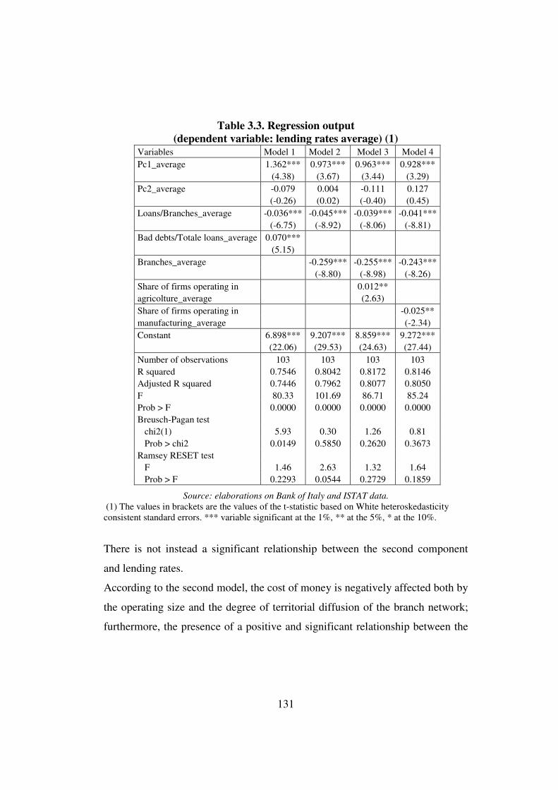
131

Table 3.3. Regression output

(dependent variable: lending rates average) (1)

Source: elaborations on Bank of Italy and ISTAT data.

(1) The values in brackets are the values of the t-statistic based on White heteroskedasticity consistent standard errors. *** variable significant at the 1%, ** at the 5%, * at the 10%.

There is not instead a significant relationship between the second component

and lending rates.

According to the second model, the cost of money is negatively affected both by

the operating size and the degree of territorial diffusion of the branch network;

furthermore, the presence of a positive and significant relationship between the

Variables Model 1 Model 2 Model 3 Model 4 Pc1_average 1.362*** 0.973*** 0.963*** 0.928*** (4.38) (3.67) (3.44) (3.29) Pc2_average -0.079 0.004 -0.111 0.127 (-0.26) (0.02) (-0.40) (0.45) Loans/Branches_average -0.036*** -0.045*** -0.039*** -0.041*** (-6.75) (-8.92) (-8.06) (-8.81) Bad debts/Totale loans_average 0.070*** (5.15) Branches_average -0.259*** -0.255*** -0.243*** (-8.80) (-8.98) (-8.26) Share of firms operating in 0.012** agricolture_average (2.63) Share of firms operating in -0.025** manufacturing_average (-2.34) Constant 6.898*** 9.207*** 8.859*** 9.272*** (22.06) (29.53) (24.63) (27.44) Number of observations 103 103 103 103 R squared 0.7546 0.8042 0.8172 0.8146 Adjusted R squared 0.7446 0.7962 0.8077 0.8050 F 80.33 101.69 86.71 85.24 Prob > F 0.0000 0.0000 0.0000 0.0000 Breusch-Pagan test chi2(1) 5.93 0.30 1.26 0.81 Prob > chi2 0.0149 0.5850 0.2620 0.3673 Ramsey RESET test F 1.46 2.63 1.32 1.64 Prob > F 0.2293 0.0544 0.2729 0.1859

132

indicator of the quality of the institutional environment and lending rates is

confirmed.

The RESET test leads do not reject the null hypothesis that the model has no

relevant omitted variables at 5% level of significance.

Furthermore, departing from model 2, I estimated other two specifications in

order to take into consideration also the differences, among provinces, in firms’

industry composition.

Particularly, models 3 and 4 include, respectively, the share of firms operating in

agriculture and manufacturing. By taking into consideration these two variables,

it should be possible to assess, in the same specifications, the impact on lending

rates of the territorial diffusion of branches and loans’ riskiness. In fact,

according to several authors, the overall riskiness of loans in an area is

significantly influenced by the size and industry composition of the bank

customers18.

A simple correlation analysis seems to confirm this assumption: higher ratios

between bad debts and total loans are associated with a large incidence of the

agriculture sector and a smaller share of firms operating in manufacturing (see

table A3.4). Because these two variables are not highly correlated with the

number of branches per 10,000 inhabitants, multicollinearity problems are

avoided.

Models 3 and 4 substantially confirm the results obtained in the first two

models: the cost of money is negatively affected by branches’ operating size and

territorial diffusion, while improvements in the quality of the institutional

framework lead to better borrowing conditions. Moreover, the industry

composition of the bank customers (that reflects also the overall loans’ riskiness

according to the Panetta’s opinion) significantly influences lending rates

(provinces with a higher incidence of the agriculture sector are characterized by

18 For example, Panetta (2003), Evoluzione del sistema bancario e finanziamento dell’economia

nel Mezzogiorno, in “Temi di Discussione della Banca d’Italia”, No. 467.

133

worse borrowing conditions, while the share of firms operating in manufacturing

negatively affects lending rates).

The Breusch-Pagan and the RESET tests allow do not rejecting the hypothesis

of homoskedastic errors and correct specification for both model 3 and 4.

On the whole, according to the estimated models, the effect of a decrease of the

first component from the maximum value observed in the province of Catanzaro

(0.85) to the minimum value noticed in the province of Lecco (0.03) amounts to

a reduction in the cost of money between 76 and 112 basis points. This result is

rather important because the actual difference among the lending rates observed

in these provinces is equal to 262 basis points.

The developed analysis indicates hence that, in order to adequately understand

the differences in the cost of money among the Italian provinces, it is necessary

to take into consideration, together with the features of the banking system, also

the quality of the institutional environment in different areas.

3.4 Conclusions

The economic literature widely recognizes that the quality of the institutions

positively affects economic performance.

Because the availability of financial resources determines the overall investment

ability in a system, it is important to understand if institutional environment also

influences local borrowing conditions.

Indeed, the quality of the institutions (measured by taking into consideration the

degree of corruption, crime, rights protection and efficiency of the court system)

is able to influence the conditions at which banks grant loans because it

represents a crucial aspect to assure the accurate functioning of every economic

transaction. In other words, banks tend to require an additional premium in those

areas characterized by a worse social infrastructure because this premium allows

facing the greater probability that borrowers will not repay their debts because

of exogenous factors that increase their fragility.

134

The analysis developed in this chapter aimed to verify the significance of the

relationship between the quality of the institutions and the cost of money in

Italy.

In order to reach this aim, by means of the principal component analysis I

elaborated an indicator at a provincial level that expresses the quality of the

institutions on the basis of data concerning the general crime (measured by the

number of crimes for which the judicial authority began the penal action per

100,000 inhabitants), the organized crime (expressed in terms of extortions and

criminal associations per 100,000 inhabitants), the level of corruption (measured

by the number of crimes against the State per 100,000 inhabitants) and the

degree of rights protection (expressed by the ratio between losses and liabilities

in bankruptcy proceedings, the average length of civil disputes, the number of

first-degree civil pending suits and the ratio between first-degree civil suits

pending and settled during the year).

Although politically unified since 150 years, Italy is a country where social and

economic gaps remain large among Northern and Southern areas. Organized

crime is particularly heavy in the Mezzogiorno area, where the incidence of

extortions and criminal associations continues to be significantly larger with

respect the other geographical areas.

According to the estimated models, the quality of the institutions negatively

influences lending rates even if the structural features of credit supply and

demand at provincial level are taken into account.

The effect on provincial lending rates of an improving in the indicator of the

quality of the institutions is significant. The effect of a reduction of this

indicator from the maximum value observed in the province of Catanzaro to the

minimum value in the province of Lecco is a significant improving of borrowing

conditions (the reduction of lending rates is comprised between 76 and 112 basis

points).

135

Consequently, the more cumbersome borrowing conditions applied to the

Southern bank customers are influenced, together with the greater aggregate

riskiness of loans and elements concerning credit supply (the lower operating

size and territorial diffusion of the branch network) also by the worse quality of

the institutional environment in the Mezzogiorno area.

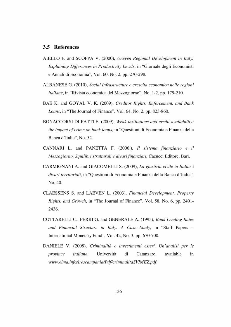
136

3.5 References

AIELLO F. and SCOPPA V. (2000), Uneven Regional Development in Italy:

Explaining Differences in Productivity Levels, in “Giornale degli Economisti

e Annali di Economia”, Vol. 60, No. 2, pp. 270-298.

ALBANESE G. (2010), Social Infrastructure e crescita economica nelle regioni

italiane, in “Rivista economica del Mezzogiorno”, No. 1-2, pp. 179-210.

BAE K. and GOYAL V. K. (2009), Creditor Rights, Enforcement, and Bank

Loans, in “The Journal of Finance”, Vol. 64, No. 2, pp. 823-860.

BONACCORSI DI PATTI E. (2009), Weak institutions and credit availability:

the impact of crime on bank loans, in “Questioni di Economia e Finanza della

Banca d’Italia”, No. 52.

CANNARI L. and PANETTA F. (2006.), Il sistema finanziario e il

Mezzogiorno. Squilibri strutturali e divari finanziari, Cacucci Editore, Bari.

CARMIGNANI A. and GIACOMELLI S. (2009), La giustizia civile in Italia: i

divari territoriali, in “Questioni di Economia e Finanza della Banca d’Italia”,

No. 40.

CLAESSENS S. and LAEVEN L. (2003), Financial Development, Property

Rights, and Growth, in “The Journal of Finance”, Vol. 58, No. 6, pp. 2401-

2436.

COTTARELLI C., FERRI G. and GENERALE A. (1995), Bank Lending Rates

and Financial Structure in Italy: A Case Study, in “Staff Papers –

International Monetary Fund”, Vol. 42, No. 3, pp. 670-700.

DANIELE V. (2008), Criminalità e investimenti esteri. Un’analisi per le

province italiane, Università di Catanzaro, available in

www.elma.info/irescampania/Pdf/criminalitaSVIMEZ.pdf.

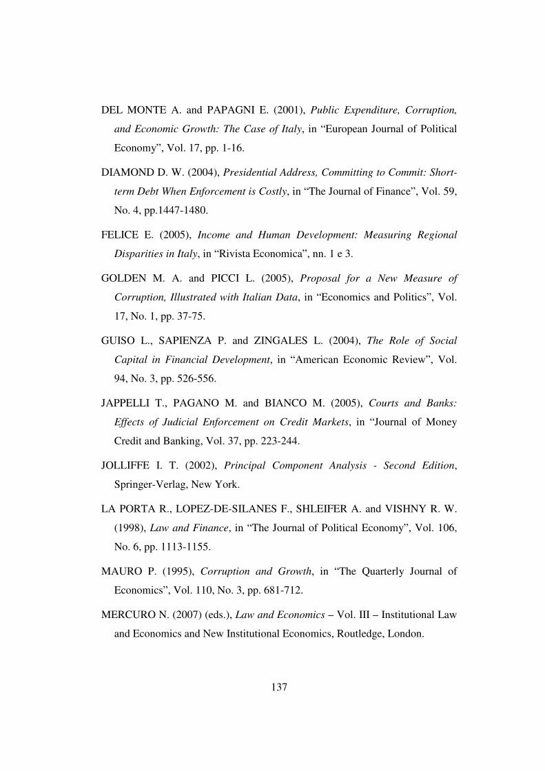
137

DEL MONTE A. and PAPAGNI E. (2001), Public Expenditure, Corruption,

and Economic Growth: The Case of Italy, in “European Journal of Political

Economy”, Vol. 17, pp. 1-16.

DIAMOND D. W. (2004), Presidential Address, Committing to Commit: Short-

term Debt When Enforcement is Costly, in “The Journal of Finance”, Vol. 59,

No. 4, pp.1447-1480.

FELICE E. (2005), Income and Human Development: Measuring Regional

Disparities in Italy, in “Rivista Economica”, nn. 1 e 3.

GOLDEN M. A. and PICCI L. (2005), Proposal for a New Measure of

Corruption, Illustrated with Italian Data, in “Economics and Politics”, Vol.

17, No. 1, pp. 37-75.

GUISO L., SAPIENZA P. and ZINGALES L. (2004), The Role of Social

Capital in Financial Development, in “American Economic Review”, Vol.

94, No. 3, pp. 526-556.

JAPPELLI T., PAGANO M. and BIANCO M. (2005), Courts and Banks:

Effects of Judicial Enforcement on Credit Markets, in “Journal of Money

Credit and Banking, Vol. 37, pp. 223-244.

JOLLIFFE I. T. (2002), Principal Component Analysis - Second Edition,

Springer-Verlag, New York.

LA PORTA R., LOPEZ-DE-SILANES F., SHLEIFER A. and VISHNY R. W.

(1998), Law and Finance, in “The Journal of Political Economy”, Vol. 106,

No. 6, pp. 1113-1155.

MAURO P. (1995), Corruption and Growth, in “The Quarterly Journal of

Economics”, Vol. 110, No. 3, pp. 681-712.

MERCURO N. (2007) (eds.), Law and Economics – Vol. III – Institutional Law

and Economics and New Institutional Economics, Routledge, London.

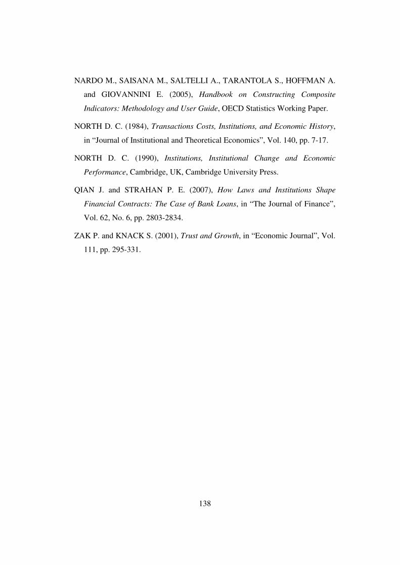
138

NARDO M., SAISANA M., SALTELLI A., TARANTOLA S., HOFFMAN A.

and GIOVANNINI E. (2005), Handbook on Constructing Composite

Indicators: Methodology and User Guide, OECD Statistics Working Paper.

NORTH D. C. (1984), Transactions Costs, Institutions, and Economic History,

in “Journal of Institutional and Theoretical Economics”, Vol. 140, pp. 7-17.

NORTH D. C. (1990), Institutions, Institutional Change and Economic

Performance, Cambridge, UK, Cambridge University Press.

QIAN J. and STRAHAN P. E. (2007), How Laws and Institutions Shape

Financial Contracts: The Case of Bank Loans, in “The Journal of Finance”,

Vol. 62, No. 6, pp. 2803-2834.

ZAK P. and KNACK S. (2001), Trust and Growth, in “Economic Journal”, Vol.

111, pp. 295-331.

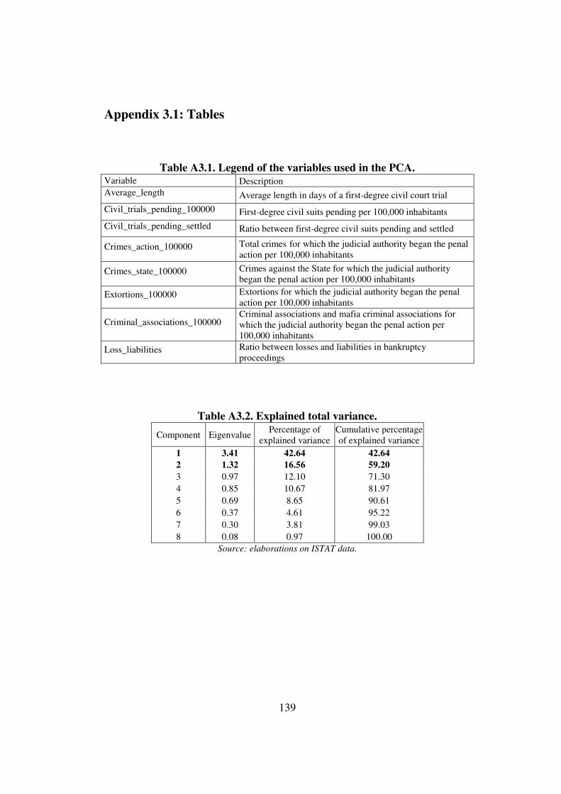
139

Appendix 3.1: Tables

Table A3.1. Legend of the variables used in the PCA. Variable Description Average_length Average length in days of a first-degree civil court trial

Civil_trials_pending_100000 First-degree civil suits pending per 100,000 inhabitants

Civil_trials_pending_settled Ratio between first-degree civil suits pending and settled

Crimes_action_100000 Total crimes for which the judicial authority began the penal action per 100,000 inhabitants

Crimes_state_100000 Crimes against the State for which the judicial authority began the penal action per 100,000 inhabitants

Extortions_100000 Extortions for which the judicial authority began the penal action per 100,000 inhabitants

Criminal_associations_100000 Criminal associations and mafia criminal associations for which the judicial authority began the penal action per 100,000 inhabitants

Loss_liabilities Ratio between losses and liabilities in bankruptcy proceedings

Table A3.2. Explained total variance.

Component Eigenvalue Percentage of

explained variance Cumulative percentage of explained variance

1 3.41 42.64 42.64 2 1.32 16.56 59.20 3 0.97 12.10 71.30 4 0.85 10.67 81.97 5 0.69 8.65 90.61 6 0.37 4.61 95.22 7 0.30 3.81 99.03 8 0.08 0.97 100.00

Source: elaborations on ISTAT data.

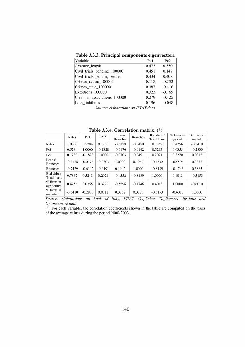
140

Table A3.3. Principal components eigenvectors. Variable Pc1 Pc2 Average_length 0.473 0.350 Civil_trials_pending_100000 0.451 0.147 Civil_trials_pending_settled 0.434 0.408 Crimes_action_100000 0.118 -0.553 Crimes_state_100000 0.387 -0.416 Extortions_100000 0.323 -0.169 Criminal_associations_100000 0.279 -0.425 Loss_liabilities 0.196 -0.048

Source: elaborations on ISTAT data.

Table A3.4. Correlation matrix. (*)

Rates Pc1 Pc2

Loans/ Branches

Branches Bad debts/ Total loans

% firms in agricult.

% firms in manuf.

Rates 1.0000 0.5284 0.1780 -0.6128 -0.7429 0.7862 0.4756 -0.5410

Pc1 0.5284 1.0000 -0.1828 -0.0176 -0.6142 0.5213 0.0355 -0.2833

Pc2 0.1780 -0.1828 1.0000 -0.3703 -0.0491 0.2021 0.3270 0.0312 Loans/ Branches -0.6128 -0.0176 -0.3703 1.0000 0.1942 -0.4532 -0.5596 0.3852

Branches -0.7429 -0.6142 -0.0491 0.1942 1.0000 -0.8189 -0.1746 0.3885 Bad debts/ Total loans

0.7862 0.5213 0.2021 -0.4532 -0.8189 1.0000 0.4013 -0.5153

% firms in agricolture 0.4756 0.0355 0.3270 -0.5596 -0.1746 0.4013 1.0000 -0.6010

% firms in manufact. -0.5410 -0.2833 0.0312 0.3852 0.3885 -0.5153 -0.6010 1.0000

Source: elaborations on Bank of Italy, ISTAT, Guglielmo Tagliacarne Institute and

Unioncamere data. (*) For each variable, the correlation coefficients shown in the table are computed on the basis of the average values during the period 2000-2003.

141

Appendix 3.2: Principal Component Analysis

The principal component analysis (PCA) is a method used in multivariate

statistics in order to reduce the dimensionality of a dataset containing a large

number (p) of interrelated variables. This simplification is realized by retaining

as much as possible the variation present in the dataset by transforming the

original variables x into a new set of variables z (the so-called principal

components), where x and z are, respectively, two vectors of p and m random

variables, with m much smaller than p.

The principal components (PCs) are uncorrelated and are ordered such that the

first few ones retain most of the variation present in the original dataset. This

transformation allows to analyze only the first few PCs without losing

information.

Hence, it is possible to compute up to p PCs but, because the aim of PCA is to

simplify the dataset by reducing its dimensionality, m PCs will be calculated,

with 0 ≪  .

If the correlation among the p original variables x is substantial, the first few

PCs (that are linear combinations of the x) will account for most of the variation

of them, allowing to not consider the remaining PCs.

The first PC is that linear function ��& W that has the maximum variance, where �� is a column vector of size p.

�� = ´��� ��� ⋯ ���¶′

Í� = ��& x = ���W� + ���W� + ⋯ + ���W� = Î ���W��

���

Hence, �� is that vector that maximizes PEF(Í�) = PEF(��& W) = ��&∑ ��, where

∑ is the variance-covariance matrix of the original variables x.

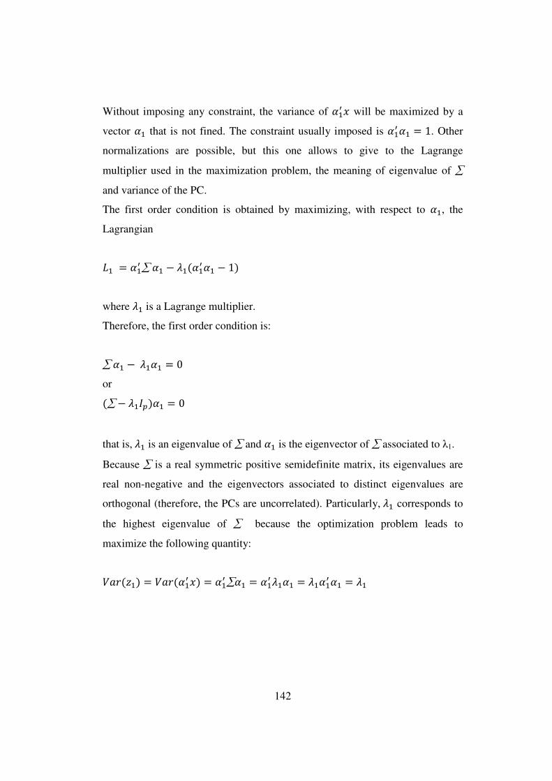
142

Without imposing any constraint, the variance of ��& W will be maximized by a

vector �� that is not fined. The constraint usually imposed is ��& �� = 1. Other

normalizations are possible, but this one allows to give to the Lagrange

multiplier used in the maximization problem, the meaning of eigenvalue of ∑

and variance of the PC.

The first order condition is obtained by maximizing, with respect to ��, the

Lagrangian

�� = ��&∑ �� − Ï�(��& �� − 1)

where � is a Lagrange multiplier.

Therefore, the first order condition is:

∑ �� − Ï��� = 0

or (∑ − Ï�Ð�)�� = 0

that is, Ï� is an eigenvalue of ∑ and �� is the eigenvector of ∑ associated to λ1.

Because ∑ is a real symmetric positive semidefinite matrix, its eigenvalues are

real non-negative and the eigenvectors associated to distinct eigenvalues are

orthogonal (therefore, the PCs are uncorrelated). Particularly, � corresponds to

the highest eigenvalue of ∑ because the optimization problem leads to

maximize the following quantity:

PEF(Í�) = PEF(��& W) = ��&∑�� = ��& Ï��� = Ï���& �� = Ï�

143

where the third and the last equality arise, respectively, from the first order

condition and the constraint. Therefore, � is the largest eigenvalue and �� is the

corresponding eigenvector.

The second PC, ��& W, is determined by computing the unit norm vector �� that

maximizes the variance of ��& W and that is uncorrelated with the first PC, ��& W.

The last condition requires that:

Ám�(��& W, ��& W) = ��&∑�� = ��&∑�� = Ï���& �� = Ï���& �� = 0

Therefore, the Lagrangian function associated to this maximization problem

becomes:

�� = ��&∑�� − Ï�(��& �� − 1) − γ��& ��

where Ï� and γ are the Lagrange multipliers associated to the two constraints of

the problem.

Differentiation of the Lagrangian function with respect to �� gives:

∑�� − Ï��� − γ�� = 0

or, equivalently ��&∑�� − Ï���& �� − γ��& �� = 0

Because ��&∑�� and Ï���& �� are equal to zero from the constraint about the

covariance between the first two PCs and ��& �� is equal to 1, the last equation is

verified only for γ equal to zero. Therefore, the first order condition can be

rewritten as:

∑�� − Ï��� = 0

or

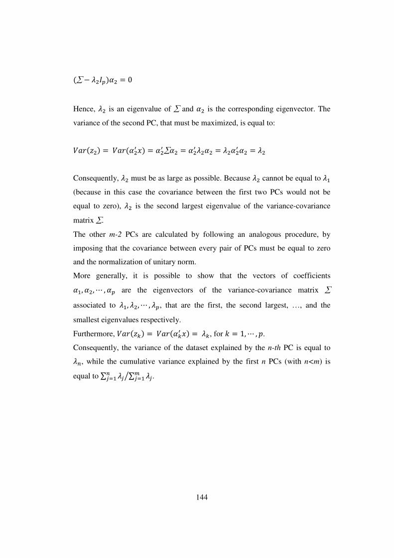
144

(∑ − Ï�Ð�)�� = 0

Hence, Ï� is an eigenvalue of ∑ and �� is the corresponding eigenvector. The

variance of the second PC, that must be maximized, is equal to:

PEF(Í�) = PEF(��& W) = ��&∑�� = ��& Ï��� = Ï���& �� = Ï�

Consequently, � must be as large as possible. Because � cannot be equal to �

(because in this case the covariance between the first two PCs would not be

equal to zero), � is the second largest eigenvalue of the variance-covariance

matrix ∑.

The other m-2 PCs are calculated by following an analogous procedure, by

imposing that the covariance between every pair of PCs must be equal to zero

and the normalization of unitary norm.

More generally, it is possible to show that the vectors of coefficients ��, ��, ⋯ , �� are the eigenvectors of the variance-covariance matrix ∑

associated to Ï�, Ï�, ⋯ , Ï�, that are the first, the second largest, …, and the

smallest eigenvalues respectively.

Furthermore, PEF(Íc) = PEF(�c& W) = Ïc, for Ë = 1, ⋯ ,  .

Consequently, the variance of the dataset explained by the n-th PC is equal to Ï·, while the cumulative variance explained by the first n PCs (with n<m) is

equal to ∑ Ï�·��� ∑ Ï�Ñ���À .

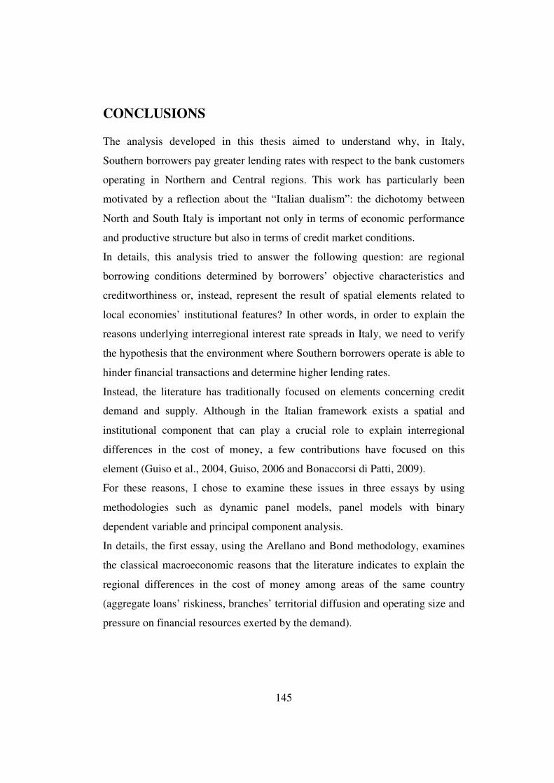
145

CONCLUSIONS

The analysis developed in this thesis aimed to understand why, in Italy,

Southern borrowers pay greater lending rates with respect to the bank customers

operating in Northern and Central regions. This work has particularly been

motivated by a reflection about the “Italian dualism”: the dichotomy between

North and South Italy is important not only in terms of economic performance

and productive structure but also in terms of credit market conditions.

In details, this analysis tried to answer the following question: are regional

borrowing conditions determined by borrowers’ objective characteristics and

creditworthiness or, instead, represent the result of spatial elements related to

local economies’ institutional features? In other words, in order to explain the

reasons underlying interregional interest rate spreads in Italy, we need to verify

the hypothesis that the environment where Southern borrowers operate is able to

hinder financial transactions and determine higher lending rates.

Instead, the literature has traditionally focused on elements concerning credit

demand and supply. Although in the Italian framework exists a spatial and

institutional component that can play a crucial role to explain interregional

differences in the cost of money, a few contributions have focused on this

element (Guiso et al., 2004, Guiso, 2006 and Bonaccorsi di Patti, 2009).

For these reasons, I chose to examine these issues in three essays by using

methodologies such as dynamic panel models, panel models with binary

dependent variable and principal component analysis.

In details, the first essay, using the Arellano and Bond methodology, examines

the classical macroeconomic reasons that the literature indicates to explain the

regional differences in the cost of money among areas of the same country

(aggregate loans’ riskiness, branches’ territorial diffusion and operating size and

pressure on financial resources exerted by the demand).

146

The Arellano and Bond estimator allowed to take into consideration the degree

of persistence that characterizes lending rates in Italian provinces.

At a macroeconomic level, lending rates depend both on elements concerning

credit demand and supply.

Although since the second half of the nineties of the last century the continuous

aggregation processes among banking groups have increased the average size of

the banking system, in the Mezzogiorno the branches’ operating size continues

to be lower with respect to other areas. Therefore, larger branches operating in

Northern regions, by exploiting bigger scale economies, often apply to their

customers better borrowing conditions with respect to branches localized in

Southern areas. At the same time, the expansion of the branch network has not

permitted to Southern regions to cover the gap, respect to Northern and Central

regions, in terms of number of branches per 10,000 inhabitants. Under the

hypothesis that a greater value of this indicator implies a larger degree of

competition in the banking system, the lower degree of territorial diffusion of

branches in the Mezzogiorno contributes to determine worse borrowing

conditions in the area.

Loans’ riskiness represents another important element that we need to analyze to

explain differences in provincial lending rates.

The quantification of firms’ credit risk and loans’ risk premium represents a

crucial aspect of banks’ credit policies. The subprime financial crisis in the USA

has made this topic more relevant. In fact, this crisis has been caused by

inadequate banks’ credit risk assessment procedures and has originated the

current global crisis, whose effects are still in progress.

The crucial role played by adequate banks’ credit risk management policies is

confirmed also in the current revision framework of the Basel Accords.

Particularly, the Basel Committee’s new proposals to strengthen the global

capital regulation do not change the methodology to calculate the Risk Weighted

Assets; consequently, the quantitative relationship between firms’ probability of

147

default and banks’ capital requirements remains valid also in the new

framework.

I largely analyzed these topics in the second essay elaborating a set of probit

panel models to estimate the probability of default for a stratified sample of

Italian firms. The stratification methodology employed permitted to obtain a

representative sample reflecting the actual territorial and industry distribution of

Italian firms.

Although the sample size is limited with respect to the population of Italian

firms, an interesting result can be drawn from this analysis: the Southern firms’

probability of default is not larger than the probability of default of the firms

operating in North and Central Italy.

Consequently, the spreads risk adjusted applicable to Southern borrowers should

not be greater than those chargeable to Northern and Central borrowers. Under

the same supply conditions (i.e. under the assumption that banks operating in

different areas sustain the same funding and operating costs), the interregional

interest rate differentials in Italy do not seem to be caused by the “pure” firms’

risk.

In order to explain differences in lending rates among North Italy and the

Mezzogiorno is necessary to look at other macro variables.

Because the literature has largely showed the existence of a causal relationship

between social infrastructure and economic performance, it appears to be natural

to ask whether potential differences in the quality of the institutions among the

Italian provinces can be considered among the elements underlying the

territorial gaps in credit market conditions.

Banks’ credit policies cannot disregard the institutional environment where

firms operate because of the significance of the strong interconnections between

economic operators and institutions, both formal and informal.

Indeed, in the areas characterized by a smaller quality of the institutions,

potential investors can perceive a greater risk because of negative externalities

148

that burden on local firms and caused by higher degrees of crime, corruption and

inefficiency of the court system.

These effects are further amplified if the territorial relationships system is not

enough transparent, causing significant asymmetric information problems about

borrowers’ credit risk.

In other words, these elements can induce banks to build a credit risk pricing

more related to a “spatial (territorial) framework” than a “specific risk logic”.

The changeover towards a spatial risk perspective could determine phenomena

of territorial discrimination of lending rates caused by institutional factors.

In the third essay the significance of institutional elements has been analyzed to

explain the differences in the cost of money at a provincial level; improvements

in the quality of the institutional framework lead to a significant reduction of

lending rates at local level.

Institutional environment matters because the structural problems of the

Mezzogiorno area represent actual negative externalities for local firms. In other

words, firms operating in a worse institutional environment must pay larger

lending rates not caused by their structural characteristics.

Hence, borrowing conditions do not reflect bank customers’ size but they

represent the result of the overall conditions of local systems.

Given the importance of credit availability to economic growth processes, it is

important to understand what governments can do.

The policy implications of these results seem clear: in order to facilitate

Southern firms’ access to credit market, it is necessary to carry out a program of

structural interventions able to improve the quality of the institutional

environment in the Mezzogiorno.

Interventions able to increase the degree of rights protection, contracts’

enforceability, efficiency of the justice system and to fight against organized

crime are necessary to increase the Mezzogiorno attractiveness improving

borrowing conditions applied to firms operating in this area: a necessary

149

condition to boost the Southern firms’ overall investment ability and able to

reduce the North-South disparities of Italian economy.

Main references

BONACCORSI DI PATTI E. (2009), Weak institutions and credit availability:

the impact of crime on bank loans, in “Questioni di Economia e Finanza della

Banca d’Italia”, No. 52.

GUISO L. (2006) in CANNARI L. Perché i tassi di interesse sono più elevati

nel Mezzogiorno e l’accesso al credito più difficile?, in CANNARI L. and

PANETTA F. (Eds.), Il sistema finanziario e il Mezzogiorno. Squilibri

strutturali e divari finanziari, pp. 239-265, Cacucci Editore, Bari.

GUISO L., SAPIENZA P. and ZINGALES L. (2004), The Role of Social

Capital in Financial Development, in “American Economic Review”, Vol.

94, No. 3, pp. 526-556.