UNIVERSITÀ DEGLI STUDI DI PADOVA

FACULTY OF ENGINEERING

DEPARTMENT OF INDUSTRIAL ENGINEERING

THESIS IN ENERGY ENGINEERING

SEMI-EMPIRICAL MODELLING OF A MULTI-DIAPHRAGM PUMP INTEGRATED INTO AN

ORC EXPERIMENTAL UNIT

Supervisors: Prof. Andrea Lazzaretto Prof. Sotirios Karellas

Majoring: Filippo D'Amico

ACCADEMIC YEAR 2015 – 2016

2

Abstract

The study of the pump in an Organic Rankine Cycle (ORC) permits to find

inefficiencies in a system that has in itself a low global efficiency. A key aspect of

this study is the prevention of the cavitation that produces strong inefficiency and

instability of the whole ORC system. The semi-empirical model proposed, after an

accurate calibration of the pump system in the ORC unit taken into account, is able to

predict the behaviour of the pump in different operating conditions, then it is possible

to obtain its characteristic curves. For the cavitation problem the model is able to

match its results with the experimental ones and find two-phase fluid at the same

operating conditions. Thanks to this characteristic feature of the model it is possible

to predict and avoid the cavitation during the operation of the experimental unit.

This thesis has been made in the Steam Boilers and Thermal Plants laboratory of the

National Technical University of Athens during the Erasmus program period.

3

4

Sommario

Lo studio della pompa presente nel ciclo Rankine organico (ORC) permette di trovare

inefficienze in un sistema che ha già di suo una bassa efficienza globale. Un aspetto

chiave di questo studio è la prevenzione alla cavitazione che produce forti

inefficienze ed instabilità dell'intero sistema ORC. Il modello semi empirico

proposto, dopo un'accurata calibrazione del sistema pompa dell'unità ORC presa in

considerazione, è in grado di prevedere il comportamento della pompa in differenti

condizioni operative, quindi è possibile ottenere le sue curve caratteristiche. Per il

problema della cavitazione il modello è in grado di ottenere risultati molto vicini a

quelli sperimentali e trovare condizioni di fluido bifase nelle stesse condizioni

operative. Grazie a questa caratteristica del modello è possibile prevedere ed

eliminare la cavitazione durante il funzionamento dell'unità sperimentale.

Il lavoro di tesi è stato fatto nel laboratorio dell'Università Tecnica Nazionale di

Atene durante il periodo del programma Erasmus.

5

6

Index

INTRODUCTION ………...…………………………………………………..9

CHAPTER 1 – The pump in an Organic Rankine Cycle ……...………….11

1.1 Why study the pump ………………………………………………..11

1.1.1 Impact of cavitation in ORC plant ………………………………….13

CHAPTER 2 – The pump system …………………………………………..17

2.1 The experimental unit ……………………………………………………17

2.1.1 The diaphragm pump ………………………………………………………….19

2.1.2 Datasheet of the pump ……………………………………………...20

2.1.3 The electric motor …………………………………………………..22

2.2 The pump system concept .…………………………………………23

CHAPTER 3 – The semi-empirical model and its calibration ……………25

3.1 The methodology …………………………………………………..26

3.2 General view of the semi-empirical model ……………………………...27

3.2.1 Geometrical parameters …………………………………………….28

3.2.2 Under and over compression ….…………………………………….33

3.5 Analysis of the model components ………………………………...35

3.6 Calibration of the model …………………………………………...36

CHAPTER 4 – Analysis of the main parameters ………………………….47

4.1 Characteristics maps ……………………………………………….47

CHAPTER 5 – Analysis of the cavitation …………………………………..55

5.1 The cavitation in the experimental unit ……………….……………55

5.2 Cavitation prediction with the semi-empirical model ……………..59

CONCLUSIONS ……………………………………………………………..65

NOMENCLATURE …………………………………………………………67

7

BIBLIOGRAPHY ……………………………………………………………71

8

Introduction

One of the goal in energy field is the reduction of the pollutant emissions. To achieve

this goal it is necessary the usage of the renewable sources, the recovery of waste

heat and the maximization of the efficiency of the energy conversion processes.

The ORC plants are useful to exploit the waste heat and the heat from renewable

sources, like geothermal and direct solar energy. There are different configurations of

ORC plants: subcritical and supercritical, with many types of working fluids, usually

hydrocarbons or CFCs, in function of the temperature of the source, cost,

maximization of the power or any other constrains.

Researches have been done about nominal steady-state optimization, screening

working fluid and operating conditions, and recently about off-design dynamic

behaviours. [9,10,11,12]

Also the components have been optimized, the most critical is the expander and the

are a lot of research about it [1,2,4,7,8], the heat exchangers and the evaporators are

also investigated, but few researches have been done studying the pump [3,6,7].

However, Quoilin et al. (2013) describes the pump as a key component that should be

carefully chosen according to its controllability, tightness, Net Positive Suction Head

(NPSH) and efficiency. Pump efficiency becomes a crucial parameter for low

temperature and supercritical cycles. Back Work Ratio defines as the ratio between

pump electrical consumption and expander outlet power is introduced to evaluate

pump impact, in the first chapter it is described how this parameter is worst for

organic fluids compared to the water. Under these motivations and the necessity of

the National Technical University of Athens it has been chosen to develop a thesis

work about a displacement pump integrated into an ORC experimental unit.

9

10

Chapter 1

The pump in an Organic Rankine cycle

This chapter describe the influence of the pump in an Organic Rankine Cycle in terms

of work and efficiency of the whole unit, the issues of the pump arise because of the

usage of organic fluids and the different operating conditions compared to the

conventional plants.

1.1 Why study the pump

To demonstrate the importance of the pump in an ORC plant, as it was done by

Declaye in [3], is useful consider the Back Work Ratio that can be defined as the ratio

of feed pump consumption over turbine production:

rw=Ẇ pp

Ẇ tur

(1)

and considering also the temperature ratio:

rT=(T ev−Tcond)

(T crit−T cond) (2)

in a simple subcritical Rankine Cycle with isobaric and isentropic transformations,

without superheating and constant condensing temperature, the influence of the

temperature ratio on the Back Work Ratio for some different fluids is showed in the

figure 1. The trend is the same for all the fluids: the higher is the temperature ratio

and the higher is the back work ratio. It is also clear how all the organic fluids have a

higher back work ratio than the water and it is also different from one fluid to

another, this is a first demonstration for how it is important to have an accurate model

for the pump in a cycle different than a conventional one that uses water.

11

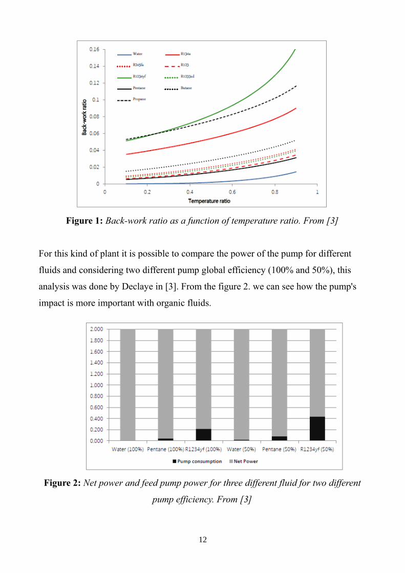
Figure 1: Back-work ratio as a function of temperature ratio. From [3]

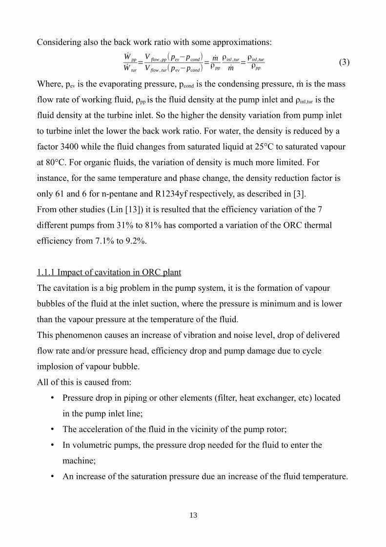
For this kind of plant it is possible to compare the power of the pump for different

fluids and considering two different pump global efficiency (100% and 50%), this

analysis was done by Declaye in [3]. From the figure 2. we can see how the pump's

impact is more important with organic fluids.

Figure 2: Net power and feed pump power for three different fluid for two different

pump efficiency. From [3]

12

Considering also the back work ratio with some approximations:

Ẇ pp

Ẇ tur

=V flow , pp( pev−pcond)

V flow , tur( pev−pcond)=

mρpp

ρinl ,tur

m=

ρinl ,turρpp

(3)

Where, pev is the evaporating pressure, pcond is the condensing pressure, ṁ is the mass

flow rate of working fluid, ρpp is the fluid density at the pump inlet and ρinl,tur is the

fluid density at the turbine inlet. So the higher the density variation from pump inlet

to turbine inlet the lower the back work ratio. For water, the density is reduced by a

factor 3400 while the fluid changes from saturated liquid at 25°C to saturated vapour

at 80°C. For organic fluids, the variation of density is much more limited. For

instance, for the same temperature and phase change, the density reduction factor is

only 61 and 6 for n-pentane and R1234yf respectively, as described in [3].

From other studies (Lin [13]) it is resulted that the efficiency variation of the 7

different pumps from 31% to 81% has comported a variation of the ORC thermal

efficiency from 7.1% to 9.2%.

1.1.1 Impact of cavitation in ORC plant

The cavitation is a big problem in the pump system, it is the formation of vapour

bubbles of the fluid at the inlet suction, where the pressure is minimum and is lower

than the vapour pressure at the temperature of the fluid.

This phenomenon causes an increase of vibration and noise level, drop of delivered

flow rate and/or pressure head, efficiency drop and pump damage due to cycle

implosion of vapour bubble.

All of this is caused from:

• Pressure drop in piping or other elements (filter, heat exchanger, etc) located

in the pump inlet line;

• The acceleration of the fluid in the vicinity of the pump rotor;

• In volumetric pumps, the pressure drop needed for the fluid to enter the

machine;

• An increase of the saturation pressure due an increase of the fluid temperature.

13

To avoid this phenomenon it is important keep the pressure of the fluid always higher

than the pressure of vapour.

The difference between the fluid and the saturation pressure is called NPSH

available:

NPSHa=pres

ρg+H−

Δ pres , pp

ρg−

psat

ρg (4)

Where:

pres = pressure in the reservoir located at the condenser outlet

H = altitude difference between the fluid reservoir and the pump

Δpres,pp = pressure drop between the fluid reservoir and the pump

psat = saturation pressure

ρ = fluid density

g = gravitational constant

The pump manufacturer provide the limit value for the NPSH to avoid the cavitation:

NPSHa>NPSHr (5)

Where NPSHr is the value provided by the pump manufacturer.

To increase the NPSHa the main measures are:

• Increase the pressure at the reservoir; it is possible introducing incondensable

gas, but this solution has a bad impact on the other cycle transformations and

then is not used.

• Increase the altitude difference between the reservoir and the pump suction; In

some MW scale units, a several meters deep hole is drilled behind the ground

and the pump is installed in that hole, but for KW units this solution is not

economically convenient, so usually the reservoir is at the top of the plant and

the pump at the bottom side with a distance like 1.5 meters.

• Reduce the pressure drop between the reservoir and the pump.

• Cooling down the liquid in order to reduce its saturation pressure; through a

heat exchanger between the reservoir and the pump.

This last solution is the only one that can be really managed because the others have

14

limits. It is possible see, from analysis studies by Declaye in [3], how the subcooling

impacts the cycle efficiency; considering a simple and ideal Rankine cycle with an

organic fluid the result is showed in the figure 3.

It is clear that the subcooling is good for the cavitation because of the increase of the

NPSHa, but from the point of view of the cycle is bad because of the decrease of the

cycle efficiency.

Concludying, the NPSH of the pump should be as low as possible in order to limit the

cycle efficiency reduction but enough to ensure stable operating condition without

cavitation.

Figure 3: Subcooling effect on the NPSH and cycle efficiency. From [3]

All these issues just described find a strong justification for this work that has been

developed following the same order of the follow chapters:

• characterization of the pump system in the ORC unit (chapter 2);

• modelling of the pump system (chapter 3);

• screening of the experimental data and calibration of the model (chapter 3);

• usage of the calibrated model to analyse the pump behaviour (chapter 4 & 5).

15

16

Chapter 2

The pump system

The chapter 2 describes the experimental equipment of the whole pump system

integrated into the ORC unit, it is defined as pump system the set of the pump, the

electric motor and the frequency driver.

The experimental unit is equipped of a multi-diaphragm pump because of its small

size (some KW), considering also the conditions of low flow rate and high pressure

head the volumetric pump is the best solution. Another reason of this choose are the

losses of organic fluid which the cost and environmental impact are important, then

the diaphragm pump is the best solution because has no leakages.

Diaphragm pumps are often used although the low efficiency because the organic

fluid looses are very important.

2.1 The experimental unit

The National Technical University of Athens provide a micro ORC unit and in this

paragraph is reported the description of the plant presented in the work Experimental

study on a low temperature ORC unit for onboard waste heat recovery from marine

diesel engines [7].

The marine ORC prototype unit is based on a conventional low-temperature

subcritical Organic Rankine Cycle using R134a as working medium. This

experimental unit has been designed as a waste heat recovery system for the jacket

water of marine diesel auxiliary internal combustion engines (ICEs). In order to

simulate the operating characteristics of such engines, the heat input is in the order of

90kWth at a low-temperature (90°C), and is supplied by a natural gas boiler via an

intermediate plate heat exchanger (evaporator). The boiler thermal output is

17

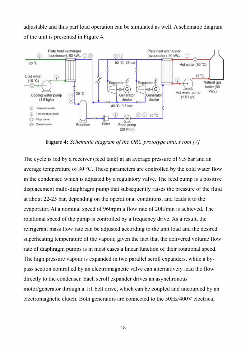
adjustable and thus part load operation can be simulated as well. A schematic diagram

of the unit is presented in Figure 4.

Figure 4: Schematic diagram of the ORC prototype unit. From [7]

The cycle is fed by a receiver (feed tank) at an average pressure of 9.5 bar and an

average temperature of 30 °C. These parameters are controlled by the cold water flow

in the condenser, which is adjusted by a regulatory valve. The feed pump is a positive

displacement multi-diaphragm pump that subsequently raises the pressure of the fluid

at about 22-25 bar, depending on the operational conditions, and leads it to the

evaporator. At a nominal speed of 960rpm a flow rate of 20lt/min is achieved. The

rotational speed of the pump is controlled by a frequency drive. As a result, the

refrigerant mass flow rate can be adjusted according to the unit load and the desired

superheating temperature of the vapour, given the fact that the delivered volume flow

rate of diaphragm pumps is in most cases a linear function of their rotational speed.

The high pressure vapour is expanded in two parallel scroll expanders, while a by-

pass section controlled by an electromagnetic valve can alternatively lead the flow

directly to the condenser. Each scroll expander drives an asynchronous

motor/generator through a 1:1 belt drive, which can be coupled and uncoupled by an

electromagnetic clutch. Both generators are connected to the 50Hz/400V electrical

18

grid via a regenerative inverter module, which provides both grid stability and

rotational speed control of the generators and hence of the expanders. For a given

pump rotational speed (and thus mass flow rate), the inlet pressure of the scroll

expanders is directly adjusted by their rotational speed, since the processed mass flow

rate for volumetric machines is given by the product of the inlet density (ρinl)

multiplied by the swept volume (VH) and the rotational speed (N) of the machine

(eq.6).

m=ρinl⋅V H⋅N (6)

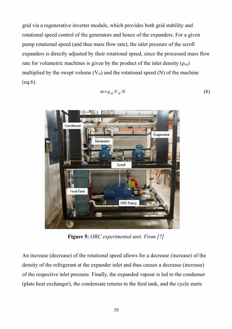
Figure 5: ORC experimental unit. From [7]

An increase (decrease) of the rotational speed allows for a decrease (increase) of the

density of the refrigerant at the expander inlet and thus causes a decrease (increase)

of the respective inlet pressure. Finally, the expanded vapour is led to the condenser

(plate heat exchanger), the condensate returns to the feed tank, and the cycle starts

19

over. The ORC unit (Figure 5.) produces 5 kWel of net electrical power, at a design

cycle pressure of 25bar and a temperature of 82°C.

Various instruments have been mounted at all key-points of the cycle, in order to

evaluate the performance of the different components of the ORC unit.

Thermocouples and pressure transducers record the thermodynamic procedure; an

electromagnetic flow-meter supervises the hot water volume flow rate and two

tachometers the scrolls actual rotational speed. All important parameters regarding

the electrical motors of both the pump and the generators, such as the

consumed/produced active power are retrieved by the respective frequency drives.

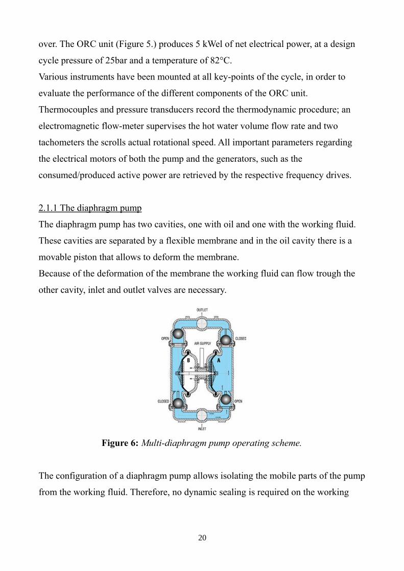
2.1.1 The diaphragm pump

The diaphragm pump has two cavities, one with oil and one with the working fluid.

These cavities are separated by a flexible membrane and in the oil cavity there is a

movable piston that allows to deform the membrane.

Because of the deformation of the membrane the working fluid can flow trough the

other cavity, inlet and outlet valves are necessary.

Figure 6: Multi-diaphragm pump operating scheme.

The configuration of a diaphragm pump allows isolating the mobile parts of the pump

from the working fluid. Therefore, no dynamic sealing is required on the working

20

fluid side.

There are also multi-diaphragm pump that are using the same principle of the single

diaphragm pump but there are several membranes in parallel. The flow rate from a

multi-diaphragm pump is more stable.

2.1.2 Datasheet of the pump

Are reported in this subparagraph the specifications data of the used pump.

Figure 7: Dimensions of the pump, from Hydra-Cell datasheet.

21

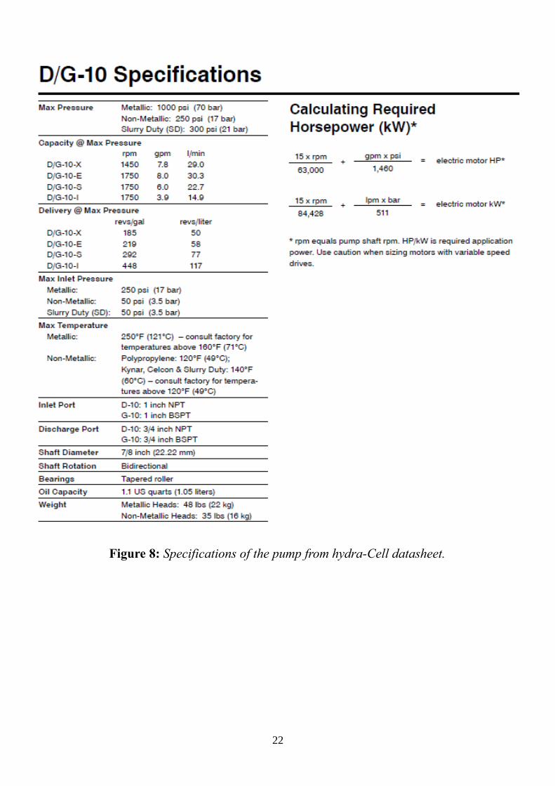
Figure 8: Specifications of the pump from hydra-Cell datasheet.

22

2.1.3 The electric motor

The data of the manufacturer of the electric motor are shown in this subparagraph.

Figure 9: Manufacturer specifications of the electric motor, from Valiadis S.A.

datasheet.

23

From the manufacturer test it is possible interpolate a performance curve that as

described in the next chapter is used in the pump model.

Figure 10: Interpolation of the experimental data of the electric motor.

2.2 The pump system concept

In this paragraph it is explained how is modelled the energy that flow trough the

pump system described before.

The energy from the grid comes to the frequency driver (VSD, variable speed driver)

Ẇel and go trough the motor, but a little part of this energy is wasted in heat Qlos,vsd.

Also in the motor the are losses, mechanic and electric, that are dissipated as heat in

the environment Qlos,mot. The electric work is transformed in mechanic work (Ẇmech)

and is delivered at the pump trough the hub, at the end in the pump there are other

losses that are dissipated as heat at the environment Qlos,pp or as a fictive heat of the

working fluid (Qlos,flu). Heat exchange between fluid, pump and environment is also

permitted (Qhex). Figure 11. show this chain.

24

Figure 11: Energetic conceptual scheme of the pump. From [6] without the adiabatic

assumption.

As said before, inside the pump, without consider the motor and the frequency driver,

there are different kind of losses that can be divided in:

Hydraulic losses

The flow in the pump is subjected to numerous disturbances which create

irreversibilities in the pumping process. They include internal leakages, friction

between the fluid and the pump parts, pressure drops through the admission and

exhaust ports, etc.

Mechanical losses

A fraction of the power delivered to the pump shaft by the motor is not converted into

hydraulic power. This fraction is dissipated, under the form of heat, into mechanical

parts subject to friction such as seals and bearings.

25

26

Chapter 3

The semi-empirical model and its calibration

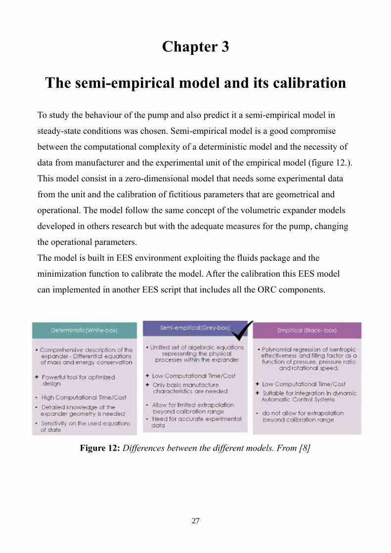
To study the behaviour of the pump and also predict it a semi-empirical model in

steady-state conditions was chosen. Semi-empirical model is a good compromise

between the computational complexity of a deterministic model and the necessity of

data from manufacturer and the experimental unit of the empirical model (figure 12.).

This model consist in a zero-dimensional model that needs some experimental data

from the unit and the calibration of fictitious parameters that are geometrical and

operational. The model follow the same concept of the volumetric expander models

developed in others research but with the adequate measures for the pump, changing

the operational parameters.

The model is built in EES environment exploiting the fluids package and the

minimization function to calibrate the model. After the calibration this EES model

can implemented in another EES script that includes all the ORC components.

Figure 12: Differences between the different models. From [8]

27

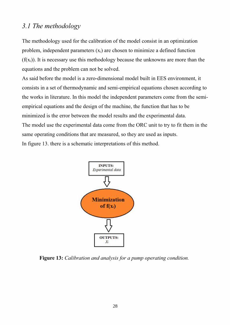
3.1 The methodology

The methodology used for the calibration of the model consist in an optimization

problem, independent parameters (xi) are chosen to minimize a defined function

(f(xi)). It is necessary use this methodology because the unknowns are more than the

equations and the problem can not be solved.

As said before the model is a zero-dimensional model built in EES environment, it

consists in a set of thermodynamic and semi-empirical equations chosen according to

the works in literature. In this model the independent parameters come from the semi-

empirical equations and the design of the machine, the function that has to be

minimized is the error between the model results and the experimental data.

The model use the experimental data come from the ORC unit to try to fit them in the

same operating conditions that are measured, so they are used as inputs.

In figure 13. there is a schematic interpretations of this method.

Figure 13: Calibration and analysis for a pump operating condition.

28

3.2 General view of the semi-empirical model

This model is inspired according to the model proposed by EXP-HEAT [8] for a

piston expander and also used in other research, like V.Lemort et al.[1] for the

modelling of Scroll expanders and Winandy [14] for the open drive reciprocating

compressor. It is reminded that a semi-empirical model consists of a set of parameters

which require to be calibrated with experimental results in order to simulate an actual

operating machine.

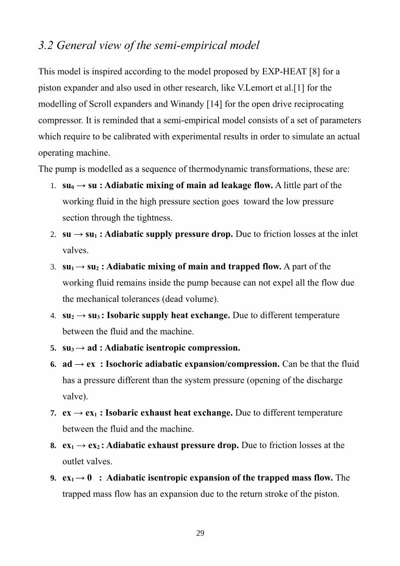
The pump is modelled as a sequence of thermodynamic transformations, these are:

1. su0 → su : Adiabatic mixing of main ad leakage flow. A little part of the

working fluid in the high pressure section goes toward the low pressure

section through the tightness.

2. su → su1 : Adiabatic supply pressure drop. Due to friction losses at the inlet

valves.

3. su1 → su2 : Adiabatic mixing of main and trapped flow. A part of the

working fluid remains inside the pump because can not expel all the flow due

the mechanical tolerances (dead volume).

4. su2 → su3 : Isobaric supply heat exchange. Due to different temperature

between the fluid and the machine.

5. su3 → ad : Adiabatic isentropic compression.

6. ad → ex : Isochoric adiabatic expansion/compression. Can be that the fluid

has a pressure different than the system pressure (opening of the discharge

valve).

7. ex → ex1 : Isobaric exhaust heat exchange. Due to different temperature

between the fluid and the machine.

8. ex1 → ex2 : Adiabatic exhaust pressure drop. Due to friction losses at the

outlet valves.

9. ex1 → 0 : Adiabatic isentropic expansion of the trapped mass flow. The

trapped mass flow has an expansion due to the return stroke of the piston.

29

10. 0 → 1 : Isochoric adiabatic expansion/compression. Can be that the

trapped mass flow has a different pressure than the pressure of the supply line

(opening of the suction valve).

11. ex → L : Adiabatic leakage pressure drop. To adapt the pressure of the

leakage to the suction pressure.

Figure 14. shows the whole process.

Figure 14: Thermodynamic scheme of the pump.

3.2.1 Geometrical parameters

This paragraph talk about the geometrical parameters of the pump, these are useful to

take into account the valves timing and others geometrical imperfections, like the

dead volume, that are indispensable for a good operation of the pump.

30

This method is used also for the reciprocating expander in [8,4] and to adapt the

parameters at the diaphragm pump some of these are modified because of the

different operation cycle.

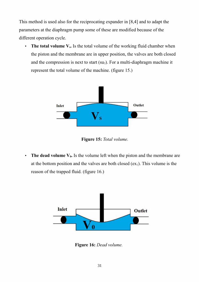
• The total volume Vs. Is the total volume of the working fluid chamber when

the piston and the membrane are in upper position, the valves are both closed

and the compression is next to start (su3). For a multi-diaphragm machine it

represent the total volume of the machine. (figure 15.)

Figure 15: Total volume.

• The dead volume V0. Is the volume left when the piston and the membrane are

at the bottom position and the valves are both closed (ex1). This volume is the

reason of the trapped fluid. (figure 16.)

Figure 16: Dead volume.

31

• The swept volume VH. Is the volume swept by the membrane during its

movement. For a multi-membrane machine it represents the total swept volume

of the machine. (figure 17.)

This geometrical parameter gives a quick measure of the delivered mass flow

and considering the total and dead volume it is equal to their difference:

V H=V s−V 0 (7)

Figure 17: Swept volume.

• The ratio C=V 0

V s

.

• The ratio f a=V 1

V s

. Where V1 is the chamber volume when the inlet valve

open and the suction phase begins (after the transformation number 10). The

ratio fa is directly linked with the mass flow that enters the pump. As it rises,

the inlet valve remain close for longer time and the processed mass flow is

reduced, it will be higher also the expansion of the trapped mass flow and so

can produce vapour. The longer is the expansion and the grater is the specific

volume of the trapped mass, as a consequence the available volume for the

inlet mass flow is lower. This ratio should be as low as possible to avoid the

formation of vapour and a huge expansion of the trapped fluid, but is not

possible avoid it because of the return stroke of the piston. (figure 18.)

The parameter fa is modified respect the one used in the expander model, in the

pump cycle is considered the time of opening of the valve instead of the

32

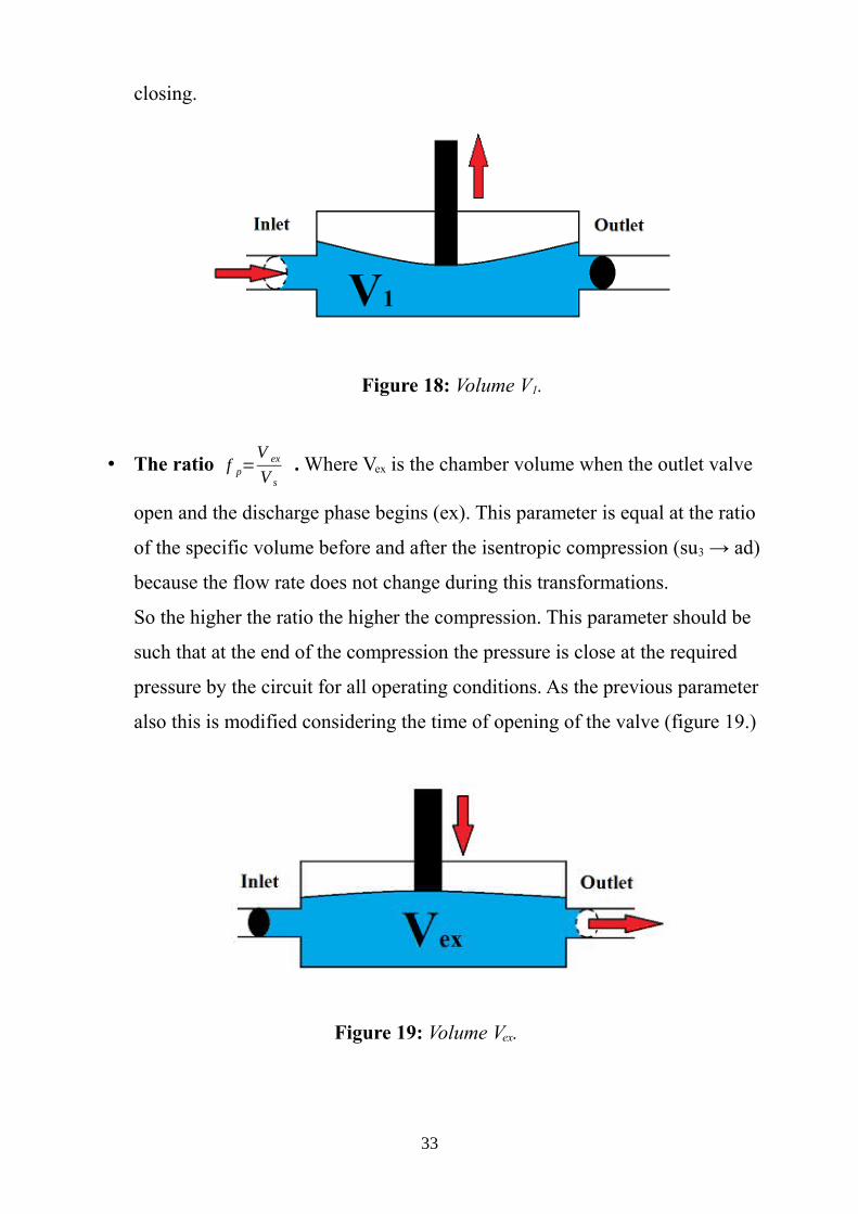
closing.

Figure 18: Volume V1.

• The ratio f p=V ex

V s

. Where Vex is the chamber volume when the outlet valve

open and the discharge phase begins (ex). This parameter is equal at the ratio

of the specific volume before and after the isentropic compression (su3 → ad)

because the flow rate does not change during this transformations.

So the higher the ratio the higher the compression. This parameter should be

such that at the end of the compression the pressure is close at the required

pressure by the circuit for all operating conditions. As the previous parameter

also this is modified considering the time of opening of the valve (figure 19.)

Figure 19: Volume Vex.

33

It is also introduced a new parameter that is the ratio between fa and C (equation 8.).

It is called fE and is also equal at the ratio between the specific volume after and

before the expansion.

f E=f aC

=V 1

V 0

=v1vex 1

(8)

In function of this parameter after the expansion of the trapped fluid there is a

isochoric expansion or compression, it is analogous to fp in the compression phase.

In figure 20. it is showed in a p-V diagram the sequence of the thermodynamic

transformations of the pump, this is a qualitative diagram.

Due to dead volume (V0) there is fluid trapped in the pump that after the expansion

go to occupy a volume (fa*Vs) bigger than Vo and because of that the pump can not

suck a mass flow proportional to the entire volume Vs.

Figure 20: p-V diagram of the pump.

34

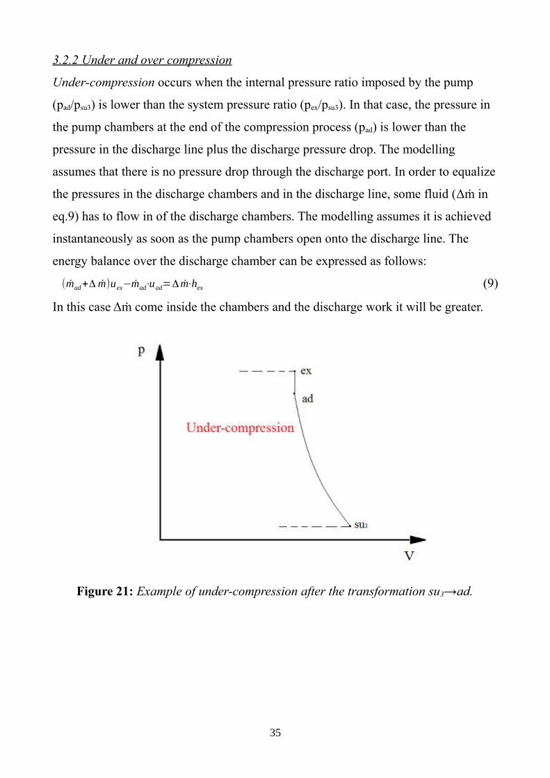
3.2.2 Under and over compression

Under-compression occurs when the internal pressure ratio imposed by the pump

(pad/psu3) is lower than the system pressure ratio (pex/psu3). In that case, the pressure in

the pump chambers at the end of the compression process (pad) is lower than the

pressure in the discharge line plus the discharge pressure drop. The modelling

assumes that there is no pressure drop through the discharge port. In order to equalize

the pressures in the discharge chambers and in the discharge line, some fluid (Δṁ in

eq.9) has to flow in of the discharge chambers. The modelling assumes it is achieved

instantaneously as soon as the pump chambers open onto the discharge line. The

energy balance over the discharge chamber can be expressed as follows:

(ṁad+Δṁ)uex−ṁad⋅uad=Δṁ⋅hex (9)

In this case Δṁ come inside the chambers and the discharge work it will be greater.

Figure 21: Example of under-compression after the transformation su3→ad.

35

Over-compression occurs when the internal pressure ratio imposed by the pump is

higher than the system pressure ratio. Here the fluid Δṁ (eq.10) flow out of the

discharge chambers spontaneously and the discharge work it will be lower.

The energy balance over the discharge chamber is:

(ṁad−Δ m)uex−ṁad⋅uad=−Δ m⋅hex (10)

Figure 22: Example of over-compression after the transformation su3→ad.

There is no work directly associated to the under- and over-compression throttling.

The discharge work has to be increased or decreased in function of the under or over-

compression, but this term of the work is neglected in the semi-empirical model

because the its low value.

The description of the over- and under-compression done is for the transformation

ad→ex but is also valid for the transformation 0→1.

This method is proposed by Quoilin et al. [1], used also in others articles [4,8] and is

adapted at the pump cycle in this work.

36

3.5 Analysis of the model components

I. Inlet mass flow rate

The inlet mass flow rate is calculated considering the trapped fluid at the end of the

isentropic expansion and the leakages, because they are already inside the chamber

volume during the suction phase:

ṁinl=N60

(V s

vsu 3

−f a⋅V s

v1)−ṁleak (11)

It is followed the same concept of [4,8] but using the pump geometrical parameters

and considering differently the behaviour of the leakages.

The total mass flow that is worked by the pump is:

ṁtot=ṁinl+ṁtrap+ṁleak (12)

Where ṁtrap and ṁleak are the mass flow rate trapped and from the leakages

respectively.

II. Adiabatic mixing between main and leakage flow (su0 → su)

This process is adiabatic and isobaric, the equations are:

ṁsu 0⋅hsu 0+ṁleak⋅hL=ṁ su⋅hsu (13)

ṁsu=ṁsu 0+ṁleak (14)

Figure 23: Adiabatic mixing between main and leakage flow.

37

III. Adiabatic supply pressure drop (su → su1)

The supply pressure drop is modelled as an isentropic flow in a simple nozzle. The

fluid can be also considered incompressible due to the liquid state and the low

pressure drop.

This method is used also in [3,8].

Figure 24: Adiabatic supply pressure drop.

The area Asu is a fictitious area that simulates the procedure of the pressure drops in

the current machine. This parameter is determined from experimental data, using the

model calibration process that will be presented in the next chapter.

From the momentum conservation equation for adiabatic flow and the previous

assumptions it is possible calculate the pressure drop:

Δ psu=12ṁsu 12

⋅v su

A su2 (15)

IV. Adiabatic mixing of main and trapped flow (su1 → su2)

As the adiabatic mixing showed before.

V. Isobaric supply heat exchange (su2 → su3)

Due to the fact that the pump shell is hotter than the working fluid there is heat

38

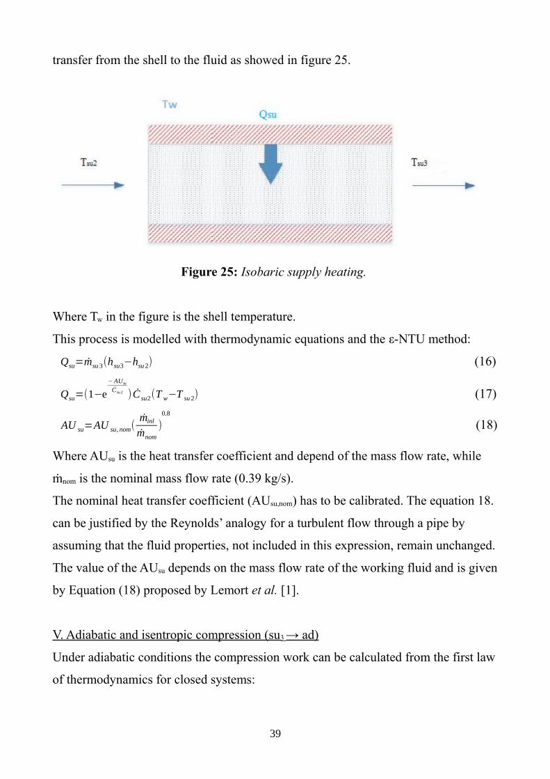
transfer from the shell to the fluid as showed in figure 25.

Figure 25: Isobaric supply heating.

Where Tw in the figure is the shell temperature.

This process is modelled with thermodynamic equations and the ε-NTU method:

Qsu=ṁsu 3(hsu3−hsu 2) (16)

Qsu=(1−e−AUsu

Ċ su 2 )Ċ su2(T w−T su 2) (17)

AU su=AU su, nom(ṁinl

ṁnom

)0.8

(18)

Where AUsu is the heat transfer coefficient and depend of the mass flow rate, while

ṁnom is the nominal mass flow rate (0.39 kg/s).

The nominal heat transfer coefficient (AUsu,nom) has to be calibrated. The equation 18.

can be justified by the Reynolds’ analogy for a turbulent flow through a pipe by

assuming that the fluid properties, not included in this expression, remain unchanged.

The value of the AUsu depends on the mass flow rate of the working fluid and is given

by Equation (18) proposed by Lemort et al. [1].

V. Adiabatic and isentropic compression (su3 → ad)

Under adiabatic conditions the compression work can be calculated from the first law

of thermodynamics for closed systems:

39

Ẇ comp=ṁad(uad−usu 3) (19)

The parameter fp is a key parameter in this process because how said before is equal

at the ratio of the specific volume before and after the compression.

f p=vad

vsu 3

(20)

This is one of the parameters that have to be calibrated.

VI. Isochoric adiabatic expansion/compression (ad → ex)

This transformation can be a compression or an expansion and this can be fixed by

the fp parameter. The higher is fp the higher is the specific volume vad and the lower

the pressure pad, if the pressure at the end of the isentropic compression is lower the

outlet pressure plus the discharge pressure drop this transformation it will be a

compression. Viceversa if pad is higher of the pressure pex.

VII. Internal leakages (ex → L)

The internal leakages are computed as an isentropic adiabatic flow through a nozzle,

just like the supply losses. The leakage mass flow rate is given as:

ṁleak=A leak√ 2 (pex−pL)

vex

(21)

A leak=Aleak ,nom(f

f nom) (22)

Where pL is equal at the inlet pressure (psu0).

The fictitious leakages area is proportional at the ratio between the actual and

nominal frequency of the motor [3] to take into account the performance drop of

check valves at high frequency, the Aleak, nom parameter has to be calibrated like the

suction cross area.

VIII. Isobaric exhaust heat exchange (ex → ex1)

This heat exchange is computed like the previous but in this case the flux of the heat

40

is from the fluid to the shell as in figure 26.

Figure 26: Isobaric exhaust heat exchange.

The equations used in this process are:

Qex=ṁex(hex 1−hex) (23)

Qex=(1−e−AUex

Ċex )Ċ ex(T w−T ex) (24)

AU ex=AU ex ,nom(ṁinl

ṁnom

)0.8

(25)

The nominal heat transfer coefficient (AUex,nom) has to be calibrated.

IX. Adiabatic exhaust pressure drop (ex1 → ex2)

The exhaust pressure drop is modelled like the supply pressure drop and the

characteristic equation is:

Δ pex=12ṁex 22

⋅v ex1

A ex2 (26)

The exhaust cross area (Aex) has to be calibrated.

X. Adiabatic isentropic expansion of the trapped mass flow (ex1 → 0)

Due to return stroke of the piston the trapped mass flow undergoes an expansion.

41

The work that comes from this transformation is neglected to be more conservative,

but also because its quantity is very low.

The trapped mass flow rate is calculate using the geometrical parameters:

ṁtrap=f a⋅V s⋅N

60⋅v0 (27)

During this transformation there is no entropy variations, from the first law of the

thermodynamic for closed systems:

Ẇ exp=ṁtrap (u0−uex 1) (28)

As explained in the paragraph 3.2 the parameter fE is a key parameter in this

transformation and is one of the parameters that have to be calibrated.

XI. isochoric adiabatic expansion/compression (0 → 1)

This transformation can be a compression or an expansion and this can be fixed with

the fE parameter. The higher is fE the higher is the specific volume vo and the lower

the pressure p0, if the pressure at the end of the isentropic expansion is lower the inlet

pressure minus the supply pressure drop this transformation it will be a compression.

Viceversa if p0 is higher of the pressure p1.

Required Work

The work required at the pump shaft is computed as a sum of more terms, the

hydraulic work transferred to the fluid is:

Ẇ hyd=Ẇ comp+Ẇ dis−Ẇ adm (29)

Where Ẇcomp is the comprehension work defined before in the transformation

su3→ad, Ẇdis and Ẇsuc are the discharge and admission work respectively. The

discharge work refers to the power consumed in order to drive the fluid out of the

chamber, it correspond to the process ex→ex1 in figure 20. and is work provided

under constant pressure. While the admission work refers to the power delivered

during the suction process of the fluid into the chamber and correspond to the process

su2→su3 in figure 20. The method to count the discharge and the admission work

42

follow the concept in [8] but the equations are adapted at the pump cycle and the

different geometrical parameters. These two terms are computed as:

Ẇ dis=pex 1⋅V s( f p−C)N

60 (30)

Ẇ adm=psu 3⋅V s(1−f a)N

60 (31)

Where Vs(fp-C) is the volume shift of the chamber during the whole discharge process

(from the moment the outlet valves open until they close) and Vs(1-fa) is the volume

shift of the chamber during the whole suction process (from the moment the inlet

valves open until they close).

To obtain the work at the pump shaft is necessary add the mechanical losses (Ẇloss)

caused by the internal frictions:

Ẇ sh=Ẇ hyd+Ẇ loss (32)

The mechanical losses are calculated using the method proposed by Declaye in [3]:

Ẇ loss=Tmech⋅f (33)

Where Tmech[Nm] is a constant parameter that has to be calibrated.

Mechanical losses are due to friction and losses in the bearings, these are dissipated

as heat into the environment . In the present modelling, all these losses are lumped

into one unique mechanical loss torque Tmech.

Finally using the motor electric efficiency extrapolate from the manufacturer data

(chapter 2) and the frequency driver efficiency, it is possible obtain the electric

power:

Ẇ el=Ẇ sh⋅ηmot⋅ηfd (34)

ηfd=0.92 (35)

The frequency driver efficiency is a constant precautionary value.

Overall heat balance

The thermal equilibrium of the pump is in steady-state conditions and is possible

calculate the wall temperature Tw from this, the heat balance is:

43

Qamb+Qex+Qsu−Ẇ loss=0 (36)

Where Qamb is heat transfer from the pump shell to the ambient and is calculated as:

Qamb=AU amb(Tw−Tamb) (37)

Where Tamb is the ambient temperature and AUamb (W/K) is the heat transfer

coefficient that must be identified through the model calibration procedure.

Pump efficiency

Four efficiencies are defined to measure the performance of the pump, these are the

isentropic efficiency:

ηis=h is−hsu 0

hex2−hsu 0

(38)

the filling factor (or volumetric efficiency):

ηvol=ṁinl

N⋅V s⋅(1−C)

60⋅v0

(39)

that represents the volume flow rate that passes through the pump related to the

theoretical volume flow rate that the pump can manage according to its swept

volume, the filling factor expresses a relative measure of the internal leakages and the

grade of expansion of the trapped mass.

The mechanical efficiency:

ηm=Ẇ hyd

Ẇ sh

(40)

and the global efficiency that measures the quality of the global process from the

electric grid to the working fluid:

ηgl=V flow ,inl (pout−pinl)

Ẇ el

(41)

44

3.6 Calibration of the model

The calibration of the model consists in fit the experimental data in several working

condition with the model results. The fitted experimental data are the mass flow rate

and the outlet temperature of the working fluid, the shaft power is given from the

manufacturer by the equation 43. A function to calculate the error between calculated

value and experimental data is implemented and has to be minimized.

The error equation is:

error=√∑1n

(ṁcal−ṁmeas

ṁmeas

)

2

+√∑1n

(Ẇ sh, cal−Ẇ sh ,man

Ẇ sh ,man

)

2

+√∑1n

(T out , cal−T out ,meas

T out ,meas

)

2

(42)

Ẇ sh .man=15⋅N84428

+V flow⋅Δ p

511 (43)

In the equation 43. N[RPM], Vflow[l/min] and Δp [bar] are experimental data in each

operating point.

To minimize this equation eleven parameters have to be calibrated, these parameters

are:

• AUamb (W/K)

• AUex.nom (W/K)

• AUsu,nom (W/K)

• Aex (m2)

• Asu (m2)

• Aleak,nom (m2)

• Vh (m3)

• C

• fp

• fE

• Tmech

The process flow diagram of the parameters identification (or equivalently of the

model calibration) procedure is depicted in figure 27.

45

Figure 27: Process flow chart of the Identification procedure of the model parameters

Also the inputs f, N, Tin, pin, pout are experimental data from the unit.

Results of the calibration:

The calibration is done minimizing the error for 20 different operational point using

the Variable metric method available on EES, the results are:

AUamb (W/K) 1

AUex,nom (W/K) 50

AUsu,nom (W/K) 60

Aex (m2) 0,00007

Asu (m2) 0,00005

Aleak,nom (m2) 0,0000003

C (-) 0,1

Vh (m3) 0,00002

fp (-) 0,9945

fE (-) 1,01

Tmech (Nm) 4,28

Table 1: Results of the calibration.

46

It is possible see the relative error in each point in the following graphics, the relative

error is always below the 10%.

Figure 28: Calculated mass flow respect the measured mass flow.

Figure 29: Calculated outlet temperature respect the measured outlet temperature.

47

Figure 30: Calculated shaft power respect the manufacturer shaft power.

48

Chapter 4

Analysis of the main parameters

After the calibration and the determination of the eleven independent parameters it is

made the analysis of the behaviour of the pump. The analysis uses the same model of

the calibration but with the values of the independent parameters (xi) fixed, then it is,

as a matter of fact, an off-design analysis. Then are chosen arbitrary parameters as

inputs in order to have as outputs the performance parameters of the pump.

4.1 Characteristics maps

Firstly are compare the model maps with the manufacturer maps, in figure 31. the

mass flow rate is compared:

Figure 31: Outlet mass flow Vs rotational speed maps by the model and

manufacturer.

49

It is possible see a good accordance between the manufacturer and model map.

Considering the curve of the pump D/G-10-X, that is the used model, the values of

the mass flow for different rotational speed are very close to the values obtained by

the EES model and it is to consider that are not included the different operational

conditions and working fluid.

The computed map is done for two different outlet pressure (Δp = 4- 60 bar) and in

accordance with the manufacturer curve the higher the Δp and the lower the slope of

the curve.

Figure 32: Variation of the NPSH with the speed rotation by the model and

manufacturer.

The ΔNPSH is calculate with the characteristics of the experimental unit that it will be

explained in the next chapter. Here (figure 32.) it is possible see the accordance

between the two graphics: the manufacturer propose an exponential grow of the

NPSH required and in the model the NPSH available go down with a similar way but

opposite. Considering that in the computed curve the NPSHr is kept constant, this

means that the NPSHa is decreasing with the speed rotation and because of this the

50

0 200 400 600 800 100012001400160018000

4

8

12

16

20

24

N [RPM]

NP

SH

a [m

H2

O]

manufacturer proposes a growing NPSHr curve.

The next comparison is done with the experimental result given by Declaye in [3].

The figure 33. shows how change the global efficiency with the pressure difference

and considering the multi-diaphragm pump the graphics are very similar, for the same

pressure ratio the value of the global efficiency is quite similar.

Figure 33: Global efficiency Vs pressure difference by the model and [3].

51

It is to consider that the two graphics are made in totally different conditions,

considering the instrumentation of the experimental units.

Like the previous figure also the figure 34. makes a comparison between the current

work and the research by Declaye in [3], in this case it is taken into account the

volumetric efficiency.

Figure 34: Volumetric efficiency Vs pressure difference by the model and [3].

52

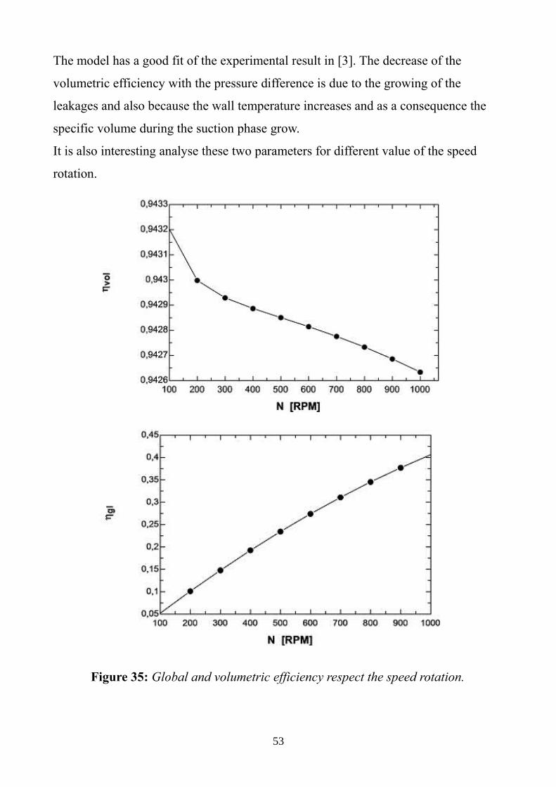
The model has a good fit of the experimental result in [3]. The decrease of the

volumetric efficiency with the pressure difference is due to the growing of the

leakages and also because the wall temperature increases and as a consequence the

specific volume during the suction phase grow.

It is also interesting analyse these two parameters for different value of the speed

rotation.

Figure 35: Global and volumetric efficiency respect the speed rotation.

53

The global efficiency increases with the speed rotation even though the mechanical

losses increase, this because the mass flow grows with N and as a consequence the

hydraulic work given to the fluid, that is the numerator of the global efficiency, grows

(eq.41). On the other side the volumetric efficiency decreases because the cross area

of the leakages and the mechanical losses increase with the frequency of rotation

(eq.22-33) and as a consequence of the mechanical losses the specific volume during

the suction phase increases because of an increase of the wall temperature.

Figure 36: Outlet mass flow in function of the pressure difference.

In the figure 36. it is possible see a concordance between the behaviour of outlet mass

flow and the volumetric efficiency (figure 34.), the decrease of the outlet mass flow

follows the same reasons of the decrease of the volumetric efficiency.

54

Figure 37: Variation of the Net Position Suction Head with the pressure difference.

Figure 37. shows how the Net Position Suction Head available is influenced by the

outlet pressure. The NPSH available increases with the pressure difference because as

figure 36. shows the mass flow decreases and this produce a decrease of the

acceleration head losses (the Ha term explained in the next chapter) at the suction

port.

The last sensitivity analysis regards the variation of the electric power with the

pressure difference and the speed rotation (figure 38.).

55

Figure 38: Electric power in function of the pressure difference and the speed

rotation.

It is interesting see that the electric power for low value of Δp and N is still around

1kW, that because even though the shaft power is very low the electric motor works

in a strong inefficiency zone and the global efficiency is very low (figure 32-34).

56

Chapter 5

Analysis of the cavitation

In this chapter it is presented the analysis of the model in cavitation condition in order

to find and predict this issue. As described in the introduction, cavitation condition

implies not only inefficiency for the pump but for the whole ORC unit. It is important

to be able to predict in different operational condition when the cavitation happens

and avoid it without losing in terms of efficiency of the plant (figure 3.).

In this chapter is not considered as inlet pressure the pressure at the suction port of

the pump, as the previous analysis, but the pressure at the feed tank outlet (positioned

just before the pump) to have a good match between the experimental work and the

semi-empirical model.

5.1 The cavitation in the experimental unit

From tests on the experimental unit it was found that the pump goes to cavitate in

different operational conditions. It is reported part of the work in [7] to present the

problem and how it has been solved.

To ensure stable operation of a pump, the available Net Positive Suction Head

(NPSHa) at the pump inlet should exceed the respective required Net Positive

Suction Head (NPSHr), given by the operation curves provided by the manufacturer,

by at least 100mbar or an equivalent of 1 mH2O. The NPSHa (mH20) is calculated

by the following equation:

NPSHa=patm+H z−H f−Ha−pvp (44)

Where:

patm = Atmospheric pressure

Hz = Vertical distance from surface liquid to pump center line (if liquid is below

57

pump center line, the Hz is negative)

Hf = Friction losses in suction piping

Ha = Acceleration head at pump suction

pvp = Absolute vapour pressure of liquid at pumping temperature

The acceleration head factor (Ha) is calculated by equation 45.

Ha=C⋅L⋅Vel⋅N

K⋅G (45)

Where:

C = Constant determined by type of pump (Wanner Engineering, Hydra Cell D/G10)

L = actual length of suction line

Vel = Velocity of liquid in suction line

N = RPM of crank shaft

G= Gravitational constant

K = Constant to compensate for compressibility of the fluid

In the experimental work in [7] it is used in the equation 44. the pressure at the outlet

of the tank and the term Hf is estimated in order to take into account also the kinetic

factor. For the operating conditions at the design point of the experimental unit the

NPSHr is 500mbar, Hz=0,3m, Ha≈200mbar, and Hf=200mbar.

The follow description of the unit behaviour in cavitation conditions and the next

solution at the problem is taken from [7].

The main parameters of the ORC feed pump under operation with cavitation effect

are depicted in Figure 39. In fact, the ORC pump was tested while just circulating the

refrigerant around the ORC circuit via the scroll by-pass section and thus practically

no pressure raise is implemented by the pump. Analyzing the pump operation at the

first oscillation cycle (cold start), it is observed that initially the pressure at the pump

inlet/outlet remains constant with time, indicating a constant mass flow rate, and that

the NPSHa - NPSHr difference is maintained well above the threshold of 100mbar (1

mH2O). As the whole system is ramping up, the temperature at the condenser outlet

58

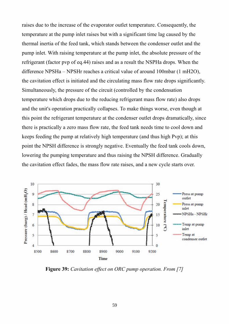
raises due to the increase of the evaporator outlet temperature. Consequently, the

temperature at the pump inlet raises but with a significant time lag caused by the

thermal inertia of the feed tank, which stands between the condenser outlet and the

pump inlet. With raising temperature at the pump inlet, the absolute pressure of the

refrigerant (factor pvp of eq.44) raises and as a result the NSPHa drops. When the

difference NPSHa – NPSHr reaches a critical value of around 100mbar (1 mH2O),

the cavitation effect is initiated and the circulating mass flow rate drops significantly.

Simultaneously, the pressure of the circuit (controlled by the condensation

temperature which drops due to the reducing refrigerant mass flow rate) also drops

and the unit's operation practically collapses. To make things worse, even though at

this point the refrigerant temperature at the condenser outlet drops dramatically, since

there is practically a zero mass flow rate, the feed tank needs time to cool down and

keeps feeding the pump at relatively high temperature (and thus high Pvp); at this

point the NPSH difference is strongly negative. Eventually the feed tank cools down,

lowering the pumping temperature and thus raising the NPSH difference. Gradually

the cavitation effect fades, the mass flow rate raises, and a new cycle starts over.

Figure 39: Cavitation effect on ORC pump operation. From [7]

59

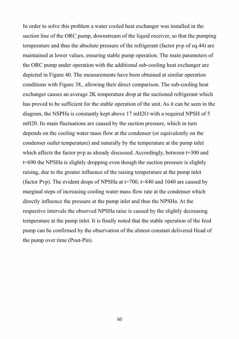
In order to solve this problem a water cooled heat exchanger was installed in the

suction line of the ORC pump, downstream of the liquid receiver, so that the pumping

temperature and thus the absolute pressure of the refrigerant (factor pvp of eq.44) are

maintained at lower values, ensuring stable pump operation. The main parameters of

the ORC pump under operation with the additional sub-cooling heat exchanger are

depicted in Figure 40. The measurements have been obtained at similar operation

conditions with Figure 38., allowing their direct comparison. The sub-cooling heat

exchanger causes an average 2K temperature drop at the suctioned refrigerant which

has proved to be sufficient for the stable operation of the unit. As it can be seen in the

diagram, the NSPHa is constantly kept above 17 mH2O with a required NPSH of 5

mH20. Its main fluctuations are caused by the suction pressure, which in turn

depends on the cooling water mass flow at the condenser (or equivalently on the

condenser outlet temperature) and naturally by the temperature at the pump inlet

which affects the factor pvp as already discussed. Accordingly, between t=300 and

t=690 the NPSHa is slightly dropping even though the suction pressure is slightly

raising, due to the greater influence of the raising temperature at the pump inlet

(factor Pvp). The evident drops of NPSHa at t=700, t=840 and 1040 are caused by

marginal steps of increasing cooling water mass flow rate at the condenser which

directly influence the pressure at the pump inlet and thus the NPSHa. At the

respective intervals the observed NPSHa raise is caused by the slightly decreasing

temperature at the pump inlet. It is finally noted that the stable operation of the feed

pump can be confirmed by the observation of the almost constant delivered Head of

the pump over time (Pout-Pin).

60

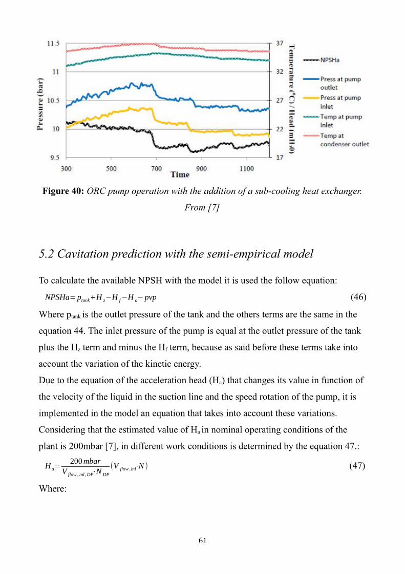
Figure 40: ORC pump operation with the addition of a sub-cooling heat exchanger.

From [7]

5.2 Cavitation prediction with the semi-empirical model

To calculate the available NPSH with the model it is used the follow equation:

NPSHa=ptank+H z−H f−H a−pvp (46)

Where ptank is the outlet pressure of the tank and the others terms are the same in the

equation 44. The inlet pressure of the pump is equal at the outlet pressure of the tank

plus the Hz term and minus the Hf term, because as said before these terms take into

account the variation of the kinetic energy.

Due to the equation of the acceleration head (Ha) that changes its value in function of

the velocity of the liquid in the suction line and the speed rotation of the pump, it is

implemented in the model an equation that takes into account these variations.

Considering that the estimated value of Ha in nominal operating conditions of the

plant is 200mbar [7], in different work conditions is determined by the equation 47.:

H a=200mbar

V flow , inl, DP⋅N DP

(V flow ,inl⋅N ) (47)

Where:

61

Vflow,inl,DP = Inlet volumetric flow rate at the design point of the unit (20 lt/min)

NDP = Pump speed rotation at the design point of the unit (960 RPM)

Vflow,inl = Inlet volumetric flow rate

N = Pump speed rotation

The velocity of the fluid in the suction line is replaced by the inlet volumetric flow

rate because of the continuity equation of the mass:

Vel=m⋅v⋅A (48)

Where Vel is the velocity (m/s), ṁ the mass flow rate (kg/s), v the specific volume

(m3/kg) and A the cross area (m2). The cross area is the same in the different operating

conditions, then velocity variations are due to mass flow rate and the specific volume

that together form the volumetric flow rate.

Also the friction losses have a dependence with the velocity of the fluid, in the model

this term changes with the square of the volumetric flow rate:

H f=200mbar(V flow ,inl

V flow ,inl , DP

)2

(49)

Variations of Hf with the Reynolds number are not considered because are also

function of the flow regime.

With this procedure are obtained the graphics in the previous chapter (figure 37-32)

and the next graphics used to compare the experimental result showed before (figure

39-40.) and the model results in the same operational conditions (figure 41-42.).

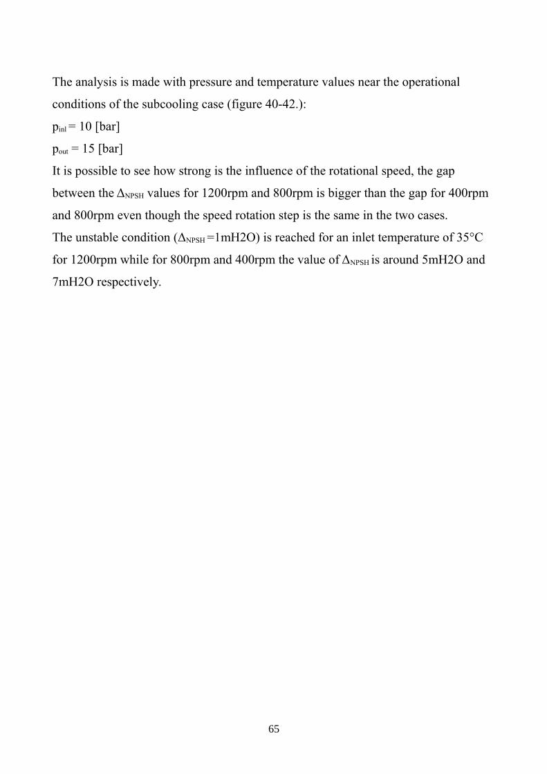
The two figures (41-42.) show the same behaviour of the ΔNPSH value of the

experimental results (figure 39-40.), this means that the method of calculation

implemented in the model is in concordance with the method proposed in [7].

62

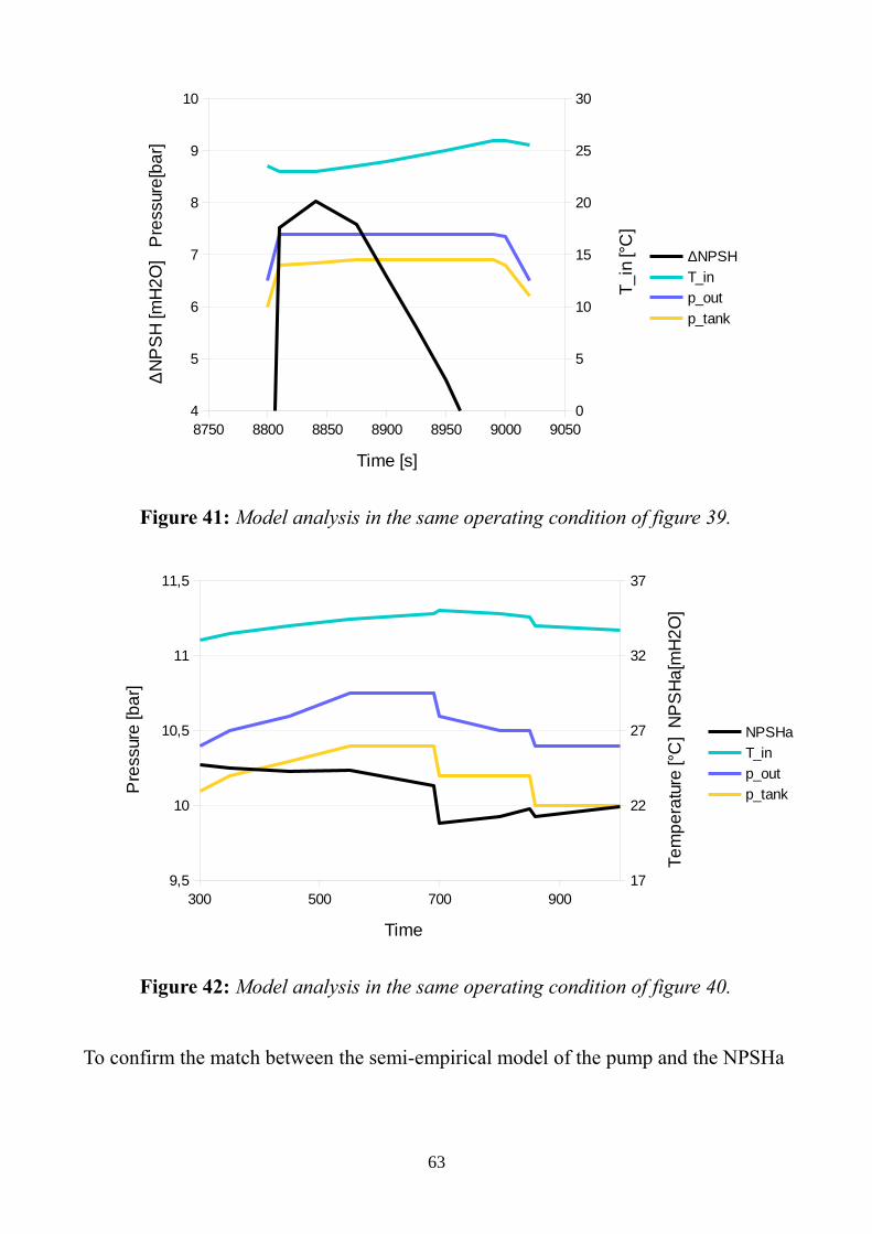
Figure 41: Model analysis in the same operating condition of figure 39.

Figure 42: Model analysis in the same operating condition of figure 40.

To confirm the match between the semi-empirical model of the pump and the NPSHa

63

8750 8800 8850 8900 8950 9000 90504

5

6

7

8

9

10

0

5

10

15

20

25

30

ΔNPSH

T_in

p_out

p_tank

Time [s]

ΔN

PS

H [m

H2

O]

Pre

ssur

e[b

ar]

T_

in [°

C]

300 500 700 9009,5

10

10,5

11

11,5

17

22

27

32

37

NPSHa

T_in

p_out

p_tank

Time

Pre

ssur

e [b

ar]

Te

mp

era

ture

[°C

] N

PS

Ha

[mH

2O

]

calculation method proposed before need that the model find two-phase fluid

condition in the suction phase when the value of the NPSHa calculated is near to

zero. With the follow operational conditions:

N = 960 [RPM]

ptank = 10 [bar]

pout = 15 [bar]

the inlet temperature was increased until a value of 37,4°C, where two-phase

condition has been found. In these conditions the value of the NPSHa is 2mH2O and

the ΔNPSH is -3,124mH2O, also considering what the manufacturer suggest to avoid

instabilities (paragraph 5.1) it is possible say that the calibration of the semi-empirical

model is in accordance with the terms Hf, Ha, Hz used to calculate the NPSHa.

The work presented by Leontaritis et al. [7] talks about a possible cavitation problem

for high speed rotation of the pump, this correlation between speed rotation and ΔNPSH

is showed in figure (32) and from this graphic is possible see the strong decrease of

the available net position suction head when the rotational speed is high.

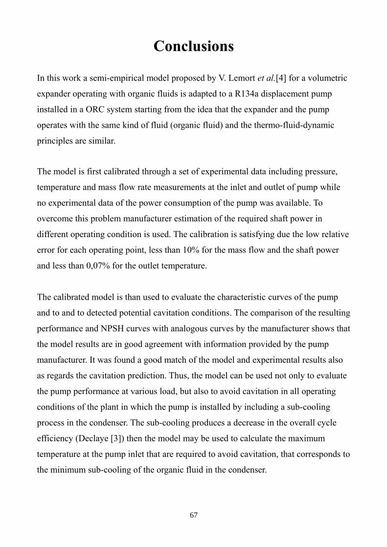
To have a better understanding of this phenomenon a last analysis is presented in

figure 43.

Figure 43: Cavitation analysis for different speed rotation.

64

32,5 33 33,5 34 34,5 35 35,5 36 36,5 37 37,5

-6

-4

-2

0

2

4

6

8

10

12

14

400rpm 800rpm 1200rpm

Inlet temperature [°C]

ΔN

PS

H [m

H2

O]

The analysis is made with pressure and temperature values near the operational

conditions of the subcooling case (figure 40-42.):

pinl = 10 [bar]

pout = 15 [bar]

It is possible to see how strong is the influence of the rotational speed, the gap

between the ΔNPSH values for 1200rpm and 800rpm is bigger than the gap for 400rpm

and 800rpm even though the speed rotation step is the same in the two cases.

The unstable condition (ΔNPSH =1mH2O) is reached for an inlet temperature of 35°C

for 1200rpm while for 800rpm and 400rpm the value of ΔNPSH is around 5mH2O and

7mH2O respectively.

65

66

Conclusions

In this work a semi-empirical model proposed by V. Lemort et al.[4] for a volumetric

expander operating with organic fluids is adapted to a R134a displacement pump

installed in a ORC system starting from the idea that the expander and the pump

operates with the same kind of fluid (organic fluid) and the thermo-fluid-dynamic

principles are similar.

The model is first calibrated through a set of experimental data including pressure,

temperature and mass flow rate measurements at the inlet and outlet of pump while

no experimental data of the power consumption of the pump was available. To

overcome this problem manufacturer estimation of the required shaft power in

different operating condition is used. The calibration is satisfying due the low relative

error for each operating point, less than 10% for the mass flow and the shaft power

and less than 0,07% for the outlet temperature.

The calibrated model is than used to evaluate the characteristic curves of the pump

and to and to detected potential cavitation conditions. The comparison of the resulting

performance and NPSH curves with analogous curves by the manufacturer shows that

the model results are in good agreement with information provided by the pump

manufacturer. It was found a good match of the model and experimental results also

as regards the cavitation prediction. Thus, the model can be used not only to evaluate

the pump performance at various load, but also to avoid cavitation in all operating

conditions of the plant in which the pump is installed by including a sub-cooling

process in the condenser. The sub-cooling produces a decrease in the overall cycle

efficiency (Declaye [3]) then the model may be used to calculate the maximum

temperature at the pump inlet that are required to avoid cavitation, that corresponds to

the minimum sub-cooling of the organic fluid in the condenser.

67

A critical part of the presented work consists in the shaft power calculation that

derives from manufacturer estimation, better results may be obtained in further

developments by measuring the shaft power or the electric consumption of the pump

in order to improve the model coefficients.

68

Nomenclature

A Area, m2

AU Heat transfer coefficient, W/K

C Ratio, -

Ċ Heat capacity, W/K

f Frequency, Hz

fp Ratio, -

fL Ratio, -

fa Ratio, -

g Gravity acceleration, m2/s

h Specific enthalpy, J/kg

H Altitude difference between the fluid reservoir and the pump, m

Hz Vertical distance from surface liquid to pump center line, m

Ha Acceleration head at pump suction, mbar

Hf Friction losses in suction piping, mbar

ṁ Mass flow rate, kg/s

N Speed rotation, RPM

NPSHa Available Net Position Suction Head, mH2O

NPSHr Required Net Position Suction Head, mH2O

p Pressure, Pa

pvp Absolute vapour pressure of liquid at pumping temperature, Pa

Q Heat transfer rate, W

rw Back-work ratio, -

rT Temperature ratio, -

s Specific entropy, J/(kg∙K)

T Temperature, K

Tmech Mechanical losses parameter, Nm

69

u Specific internal energy, J/kg

v Specific volume, m3/kg

Vflow Volumetric flow rate, lt/min

VH Swept volume, m3

VS Total volume, m3

V0 Dead Volume, m3

Vel Velocity, m/s

Ẇ Power, W

Greek symbols

Δ Difference, -

η Efficiency, -

ρ Density, kg/m3

Subscripts

ad Adapted L Leakages stream

adm Admission leak Leakage

amb Ambient loss Losses

atm Atmospheric m Mechanical

cal Calculated meas Measured

comp Compressor man Manufacturer

cond Condensing mot Motor

dis Discharge nom Nominal

DP Design point out Outlet

el Electric pp Pump

ev Evaporating res Reservoir

ex Exhaust exp Expansion

sat Saturation fd Frequency driver

70

sh Shaft gl Global

su Supply hyd Hydraulic

tank Tank inl Inlet

tot Total is Isentropic

tur Turbine

trap Trapped

vol Volumetric

w Wall

71

72

Bibliography

1. Vincent Lemort, Sylvain Quoilin, Cristian Cuevas, Jean Lebrun, Testing and

modelling a scroll expander integrated into an Organic Rankine Cycle,

Applied Thermal Engineering 29 (2009) 3094–3102.

2. Vincent Lemort, Sylvain Quoilin, Jean Lebrun, Experimental study and

modeling of an Organic Rankine Cycle using scroll expander, Applied Energy

87 (2010) 1260–1268.

3. Sèbatien Declaye, Vincent Lemort, Improving the performance of μ-ORC

systems, Phd thesis, Université de Liège, Liège, Belgium (2015).

4. Yulia Glavatskaya, Pierre Podevin, Vincent Lemort, Osoko Shonda, Georges

Descombes, Reciprocating Expander for an Exhaust Heat Recovery Rankine

Cycle for a Passenger Car Application, Energies 2012, 5, 1751-1765.

5. Byrne, P., Ghoubali, R., Miriel, J., Scroll compressor modelling for heatpumps

using hydrocarbons as refrigerants, International Journal of Refrigeration

(2013), doi: 10.1016/ j.ijrefrig.2013.06.003.

6. Arnaud Landelle, Nicolas Tauveron, Philippe Haberschill, Rémi Revellin,

Stephane Colasson, Study of reciprocating pump for supercritical ORC at full

and part load operation, 3rd International Seminar on ORC Power Systems,

October 12-14, 2015, Brussels, Belgium, Paper ID: 9, Page 1.

7. Aris-Dimitrios Leontaritis, Platon Pallis, Sotirios Karellas, Aikaterini

Papastergiou, Nikolaos Antoniou, Panagiotis Vourliotis, Nikolaos Matthaios

Kakalis, and George Dimopoulos, Experimental study on a low temperature

ORC unit for onboard waste heat recovery from marine diesel engines, 3rd

International Seminar on ORC Power Systems, October 12-14, 2015, Brussels,

Belgium, Paper ID: 55, Page 1.

8. EXP-HEAT, National Technical University of Athens, Energy recovery in new

and retrofitted heat pumps using a dedicated expander concept, Work Package

73

4. Report on the simulation of the expander prototype, Athens (2015).

9. Frangopoulos Christos, Kalikatzarakis Miltiadis, Thermo-economic

optimization of synthesis, design and operation of a marine organic Rankine

cycle system, journal of engineering for the maritime environment, Athens

(2015).

10.Marco Soffiato, Christos A. Frangopoulos, Giovanni Manente, Sergio Rech,

Andrea Lazzaretto, Design optimization of ORC systems for waste heat

recovery on board a LNG carrier, Energy Conversion and Management 92

(2015) 523–534.

11. Andrea Toffolo, Andrea Lazzaretto, Giovanni Manente, Marco Paci, A multi-

criteria approach for the optimal selection of working fluid and design

parameters in Organic Rankine Cycle systems, Applied Energy 121 (2014)

219–232.

12.N. Mazzi, S. Rech, A. Lazzaretto, Off-design dynamic model of a real Organic

Rankine Cycle system fuelled by exhaust gases from industrial processes,

Energy xxx (2015) 1e15.

13. Lin C, Feasibility of using power steering pumps in small-scale solar thermal

electric power systems, Bachelor Thesis, Massachusetts Institute of

Technology. Dept. of Mechanical Engineering, 2008

14. E. Winandy, C. S. O. and J. Lebrunb, Simplified modelling of an open-type

reciprocating compressor, Int. J. Therm. Sci. 41, Department of Mechanical

Engineering, University of Concepción, Casilla 160, Concepción, Chile, 2002.

74

75