UNIVERSITÀ DEGLI STUDI DI PADOVA

DIPARTIMENTO DI INGEGNERIA INDUSTRIALE

CORSO DI LAUREA IN INGEGNERIA ELETTRICA

Inverter control scheme for HVDC link

Controllo di un inverter con connessione ad una linea HVDC

per impianto eolico

Relatore: Prof. ROBERTO TURRI Correlatore: Michael Farrell

Laureando: FABIO SCARLATTI

Matricola: 1033739

Anno Accademico 2013/2014

2

3

Acknowledgement

I would like to thank the following persons who contributed to the realization of this project:

• M. Roberto TURRI to have given me the permission to make this project in Ireland at the DIT and for his help during its realization.

• M. Michael FARRELL for the proposition of this subject and his help during its realization in Dublin Institute of Technology.

• Miss Basu MALABIKA for her help on this project about power electronics and MATLAB.

4

5

Content

Abstract……………………………………………………………………………………

Chapter 1 Basic concepts……………………………………………………………...

1.1 Introduction……………………………………………………………

1.2 Characteristics of wind power…………………………………………

1.2.1 Winds origin……………………………………………………..

1.2.2 Location of wind turbines………………………………………..

1.3 Betz theory……………………………………………………………..

1.4 Wind sources in Italy and Ireland……………………………………...

1.4.1 Italy………………………………………………………………

1.4.2 Ireland……………………………………………………………

1.5 Mechanical aspects…………………………………………………….

1.5.1 Design aspects…………………………………………………...

1.5.2 Turbines typologies……………………………………………...

1.6 Various schemes adopted………………………………………………

Chapter 2 High voltage DC transmission……………………………………………..

2.1 Off-shore wind generation……………………………………………..

2.2 Advantages of HVDC compared with AC…………………………….

2.3 HVDC system………………………………………………………….

2.3.1 Main types of HVDC schemes…………………………………..

2.3.2 Components of a HVDC system………………………………...

2.3.3 Multiterminal system…………………………………………….

2.4 Core HVDC technologies……………………………………………...

2.4.1 Line commutated Current Source Converter…………………….

2.4.2 Self commutated Voltage Source Converter……………………

2.5 HVDC control…………………………………………………………

2.5.1 Control with CSC………………………………………………..

2.5.2 Control with VSC………………………………………………..

7

9

9

10

10

10

11

13

13

16

17

17

20

21

23

23

25

27

27

28

29

30

30

31

32

32

32

6

Chapter 3 Converters………………………………………………………………….

3.1 Introduction……………………………………………………………

3.1.1 Choice of thyristor……………………………………………….

3.2 PWM: Pulse Width Modulation……………………………………...

3.3 Rectifiers and inverters………………………………………………...

Chapter 4 Voltage control on the wind farm side……………………………………..

4.1 Model used in the simulation………………………………………….

4.2 d-q theory………………………………………………………………

4.3 PI Controller……………………………………………………...……

4.3.1 Controller tuning………………………………………………...

4.4 Simulink models and simulations……………………………………...

4.4.1 Diagrams and results………………..…………………………...

4.5 AC harmonic filter……………………………………………………..

4.5.1 Types of filter……………………………………………………

4.5.2 Scheme…………………………………………………………..

4.5.3 Harmonic analysis……………………………………………….

4.5.4 Filter design……………………………………………………...

4.6 Opal-rt………………………………………………………………….

4.6.1 Opal-rt software………………………………………………….

4.6.2 Diagrams………………………………………………………...

Chapter 5 P-Q control on the AC side………………………………………………...

5.1 Introduction……………………………………………………………

5.2 Scheme of the controller……………………………………………….

5.3 Simulink models and simulations……………………………………...

5.3.1 Scheme…………………….…………………………………….

5.3.2 Filter……………………………………………………………..

5.3.3 Diagrams…………………………………………………………

Conclusions……………………………………………………………………………….

Glossary…………………………………………………………………………………...

References…………………………………………………………………………………

35

35

36

36

40

45

45

46

47

49

49

53

60

60

61

61

67

68

68

68

75

75

76

79

79

80

82

87

89

91

7

Abstract

The increasing energy demand altogether with an attention to ecology has asked alternative

ways to produce energy respecting the latest green codes.

The wind energy resource answers smartly to this necessity. Hence it’s important to study

deeply the problems tied up with the production and transmission of wind produced

electricity. This work aims to study, through Matlab software, the control of inverters in a

HVDC link which connects the off-shore wind farms to the AC grid.

The purpose of the control is to maintain a constant voltage at the wind farm bus bar, after

wind speed variations, and to regulate active and active powers in the AC side.

Since this work was done by four hands, in this thesis more space will be dedicated to wind

farm side, control of sending inverter and filtering in the AC side, whilst the control of

receiving inverter was performed by Yves Pailhas. Anyway, I adapted the voltages of his

model to mine and I studied an appropriate filter. In this work I didn’t print the complete

model with control because it was performed only by my colleague.

Abstract

La crescente domanda di energia, unita ad una sempre maggiore attenzione all'ecologia, ha

portato ad investigare nuovi modi di produzione dell'energia, rispettando i più recenti

protocolli (green code).

L'energia eolica risponde perfettamente a questa necessità. Perciò è importante studiare con

accuratezza i problemi connessi alla trasmissione e produzione di elettricità prodotta da fonti

eoliche. Questo lavoro si propone di studiare , attraverso il software Matlab, il controllo di

inverter in una linea HVDC che connette le centrali eoliche off-shore alla rete nazionale AC.

Lo scopo del controllo è di mantenere costante la tensione alla barra di collegamento (busbar)

in seguito a variazioni di velocità del vento e regolare le potenze attiva e reattiva sul lato AC.

Poiché questo lavoro è stato condotto a quattro mani, in questa tesi sarà dedicato più spazio al

controllo sul lato del generatore, controllo e filtraggio della tensione lato AC; mentre il

controllo dell'inverter lato AC è stato investigato dal mio collega Yves Pailhas. Ad ogni modo

ho adattato le tensione del suo modello al mio per studiare un filtro appropriato. In questo

lavoro non ho studiato il modello completo col controllo perché parte del lavoro è stata

eseguita dal collega.

8

9

1. BASIC CONCEPTS

1.1 Introduction

The wind energy is the most common renewable energy thanks to the amount of power

produced over the plant cost, compared with other renewable resources.

It’ s competitive even compared with common energy resources. In fact the cost of wind

generated electricity has declined about 90% over the last 20 years, reaching the cost of 0.04

to 0.06 US dollars/kWh.[1]

In the late years the off-shore wind farms has been taken in consideration over the on-shore

ones because of their access to rather continuous flow of wind. Further more, such projects

are less likely to suffer with delays that would be normally experienced on land e.g. planning

objections for both the wind-farm and the grid connection, site access, annoying of

inhabitants, etc. That implies, though, a complication about the power transmission because

there’s more distance to face. This aspect is well solved with the adoption of HVDC system.

They have higher capital costs but it should be remembered that the higher generation do go a

considerably way to reduce them.[2]

As electric machine the choose falls amongst synchronous and induction generators. In this

work an induction one was adopted because of its most effectiveness and robustness,

although it requires reactive power for magnetizing, particularly during start-up, which may

cause voltage collapse in problematic situations. To work it out, power electronics helps a lot.

A serious issue is the integration of wind energy into the grid, contributing to its stability

10

1.2 Characteristics of wind power

1.2.1 Winds origin

The winds are a form of solar energy because they are originated by the temperature gradient

between the earth’s crust and the troposphere, which grow warm in a not homogeneous way.

At the equator line the cold air at high altitude moves northwards and drops at 30°latitude,

creating a wind circulation cell. This situation is repeated three times for each hemisphere, so

creating 6 cells for the whole world.

The wind direction, according to this theory, would be northwards, if weren’t for Coriolis

forces, which force the wind to be westerly at our latitude.

1.2.2 Location of wind turbines

What I said in the former paragraph concerns the worldwide winds movement, but the wind

turbines take the wind under 500m height. So it’s important to valuate the ground roughness

to maximize the wind speed and the power produced by the turbine. Aiming to design a wind

power plant it’s important then to classify the grounds according to their roughness:

-0 class: plain soil, such as the see.;

-1 not cultivated fields with few vegetation; airports;

-2 cultivated fields with few estates. and thin vegetation;

.-3 ground with slopes, vegetations and estates.

Fig.1.1: wind speed according to height for a 2 class terrain.

11

1.3 Betz theory [3][4]

The Betz theory is worldwide acknowledged to compute the power theoretically extracted by

a wind turbine from the wind flow.

It’s based upon the following assumptions:

-Homogeneous, incompressible, steady state flow;

-No friction drag;

-An infinite number of blades;

-Uniform thrust over the disk or rotor area;

-Non rotating wake; Fig.1.2: Behaviour of pressure and

-Static pressure far upstream and far downstream speed near the actuator disk.

of the rotor is equal to the undisturbed static pressure.

After fluid-dynamic considerations and mathematical operations, the power that a wind

turbine can capture from the wind flow results:

(1.1)

where ρ is the air density, λ the tip speed ratio, θ the blade angle, A the swept area of the

rotor, u the wind speed, Cp the power coefficient.

The product between ρ, A, u and 0.5 means the available wind power,

whilst Cp represents the capability of the wind turbine to capture the

wind energy. The theoretical maximum power which can be extracted

is 59% of available wind power.

(1.2)

(1.3)

12

Fig.1.3: behaviour of Cp, CT and U4/U.

Fig.1.4: elements of a wind turbine system

13

1.4 Wind sources in Italy and Ireland

1.4.1 Italy

Italy[5] is the sixth largest producer of wind power with an installed nameplate capacity of

8.144 MW at the end of 2012,of which 1273 MW were installed during 2012., that is 4% of

national demand.

Italy has good wind sources, specially in Campania, Apulia, Basilicata, Molise, Sicily and

Sardinia.

According to an official document by Italian government (2007), the wind capability until

2020 is 12 GW, that corresponds to 22.6TWh of electric power produced., that is the 17% of

electric energy national demand.

The best sites to produce power from wind is apennine ridge over 600m hight and, secondly,

the coast sites.

Fig.1.5: MWh/MW ratio at 50m upon the sea level.

14

Fig.1.6: MWh/MW ratio at 100m upon the sea level.

By 2012[6] the scheme for supporting the Renewable Energy Resources has changed, leaving

the market of tradable green certificates: it will expire on 2015. The new scheme considers

three different incentive access mechanism, according to technology and size of the plant.

That’s the main idea: it consists to fix the price over a certain time period of 20-25 years.

The different accesses are:

-direct access for P<60kW;

-for new plants with size 60kW-5MW, access by registration;

-auction for P>5MW;

-registration for refurbished plants P>60kW, irrespective of the plant size.

The prices are different for on-shore and off-shore plants.

15

Size (kW) Basic incentive tariff(€/MWh)

1<P<20 291

20<P<200 268

200<P<1000 149

1000<P<5000 135

P>5000 127 Tab1.1.: incentive schemes for on shore.

The granted period is 20 years for on-shore and 25 for off-shore.

Size (kW) Basic incentive tariff(€/MWh)

1<P<5000 176

P>5000 165 Tab.1.2: incentive scheme for on.shore.

It results from tables that the new scheme subsidizes at best the small plants and off-shore

ones.

Fig. 1.7wind capacities in Italian regions at the end of 2012 and installed during 2012.

16

Thanks to the incentives the wind energy production has grown very quickly, particularly

since 2011 to 2012.

Fig.1.8 Italian wind energy production and percent of national demand over the years.

In 2012 the average cost of wind energy was 1.75€/MWh with a large fluctuation due to long

permitting procedures and site characteristics.

1.4.2 Ireland

Ireland is the fifteenth largest producer in Europe, with 125MW installed in 2012 and 1738

MW totally installed at the end of 2012.

The best sites are located in the west and south

The renewable energy[7] plays a fundamental role not only for environmental quality, but to

deliver benefits in terms of growth, innovation, competitiveness and energy security as well.

For fulfilling this goals it’s important to develop an energy policy which promotes indigenous

renewable energy, with the purpose of decreasing the costs of energy imports. That’s proved

by the €305 saving achieved by the displacement of fossil fuel for electricity generation in

2012.

These considerations have brought to a commissioned total capacity of approximately

2400MW, that is 154 wind farms across Ireland, over the 1879MW wind power already

17

existing. There are other renewable sources as well as wind one, but the last one is the most

important for the island. The historic Irish average of wind power production figures 170MW

per year; the target is reaching 250MW in 2020, that is the 40% of system demand.

This is a complex task which requires social acceptance and good planning of electricity

production.

Fig.1.9: map of wind speed at 50m in Ireland

1.5 Mechanical aspects

1.5.1 Design aspects

The coefficient Cp seen formerly, that is the performance of the turbine, is affected by the

wake rotation, neglected in the Betz theory. Then, it varies with λ, the tip speed ratio:

(1.4)

18

Fig.1.10: Cp expressed as tip speed ratio

Further, Cp depends on the blades number, having an optimum ratio between costs and

performance at three blades.

Though, this isn’t the real diagram because Cp is affected also by the drag force, neglected in

Betz theory, which acts upon the blade.

Fig.1.11:Cp expressed as tip speed ratio.

If it’s desired working at maximum power after variations of wind speed, it’s possible to

change the angle of the blade, so obtaining different Cp curves.

19

Fig.1.12: power produced by the generator vs its rotational speed.

Any turbine is characterised by a cut-in speed (3-5m/s), whereby it starts to operate; a rated

speed(12-14 m/s) which allows to produce the rated power; a cut-off speed(25m/s) beyond

which the mechanical forces upon the blades are excessive, and the generator has to be

slowed down. It can be sorted out by a pitch regulation, obtained varying the blades angle, or

a stall regulation, obtained by an accurate design of the blade, so that it works badly beyond a

certain wind speed. The difference between two methods lies on the power produced after the

cut-off speed, as shown in the figure.

Fig.1.13: power expressed as wind speed for two control methods: pitch and stall regulation

20

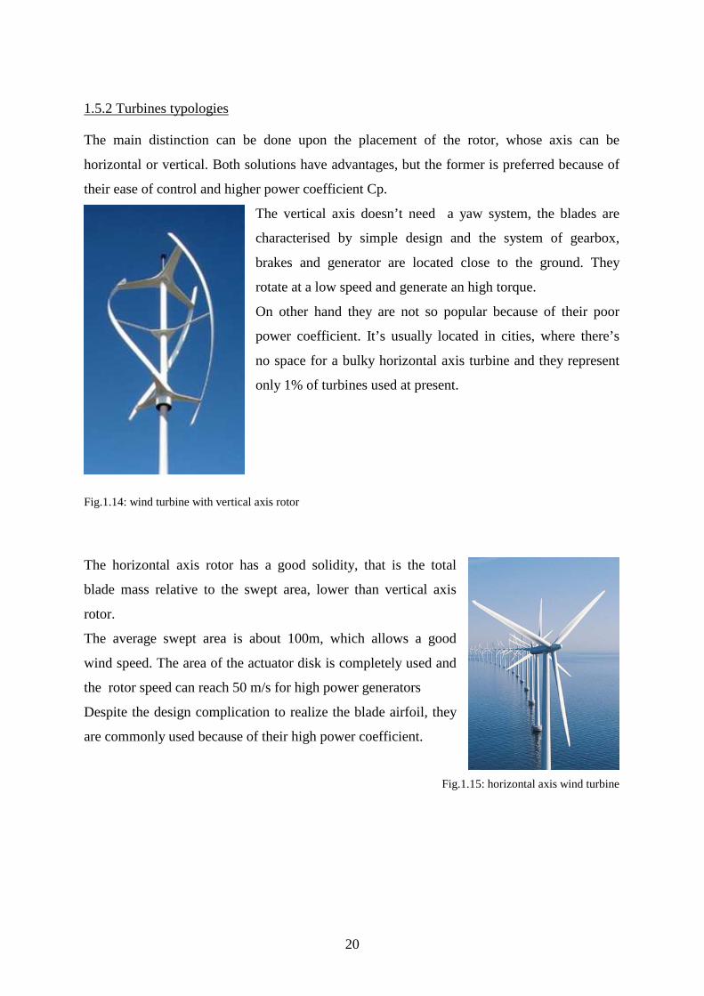
1.5.2 Turbines typologies

The main distinction can be done upon the placement of the rotor, whose axis can be

horizontal or vertical. Both solutions have advantages, but the former is preferred because of

their ease of control and higher power coefficient Cp. The vertical axis doesn’t need a yaw system, the blades are

characterised by simple design and the system of gearbox,

brakes and generator are located close to the ground. They

rotate at a low speed and generate an high torque.

On other hand they are not so popular because of their poor

power coefficient. It’s usually located in cities, where there’s

no space for a bulky horizontal axis turbine and they represent

only 1% of turbines used at present.

Fig.1.14: wind turbine with vertical axis rotor

The horizontal axis rotor has a good solidity, that is the total

blade mass relative to the swept area, lower than vertical axis

rotor.

The average swept area is about 100m, which allows a good

wind speed. The area of the actuator disk is completely used and

the rotor speed can reach 50 m/s for high power generators

Despite the design complication to realize the blade airfoil, they

are commonly used because of their high power coefficient.

Fig.1.15: horizontal axis wind turbine

21

The blades of horizontal axis rotor work according to

the lift principle[8]: the wind flows on both blade

surfaces, which have different profiles, thus creating

at the upper surface a depression area with respect to

the pressure in the lower surface.

This pressure difference creates a lift force which

makes the blades to rotate. A drag force is present as

well, opposed to the motion and perpendicular to the

lift force, but it’s of small value in well-designed

airfoils.

Fig.1.16: representation of forces acting

on a wind turbine.

1.6 Various schemes adopted

The most common type of generator corresponds to classic Danish concept [9]: the turbine is

connected through a gearbox, which increases the rotational speed, to a small diameter, light

weight induction generator. This robust machine has recently been substituted with DFIG,

thanks to variable speed technology: the converter feeds the rotor, whilst the stator is directly

connected to the grid. Since the converter is smaller than the power of the rating machine, the

latter can’t work in the full speed range, but that’s enough. This operation grants the

decoupling of mechanical end electrical frequencies.

This can be obtained as well with synchronous generator, for smaller plants, with the

advantage of avoiding the gear box and working in full range speed. The complete decoupling

is performed through two inverters and a DC link between the generator and the grid.

The sending converter controls the torque generator while the receiving converter controls the

amount of active and reactive power and the THD , improving so the quality power injected

into the grid.

22

23

2. HIGH VOLTAG E DC

TRANSMISSION

2.1 Off-shore wind generation

In the early six months of 2013, Europe fully connected 277 off-shore wind turbines, with a

combined capacity over 1GW. Overall, 18 wind farms were under construction, with whom

the total capacity will be 5,111MW. [10]

Fig.2.1: Annual installed offshore wind capacity (MW) in Europe.

The National Renewable Energy Action Plan fixed targets for 2012 and European Wind

Energy Association did forecasts in 2009. The targets, forecasts and real figures, are shown in

the following diagram:

24

Fig.2.2: wind power capacity targets (NREAPs) and EWEA 2009 and real (2012) (MW)

The offshore plants [11] have the great advantage of yielding some 50% more energy than

onshore ones because of the flatness of the sea. On the other hand the offshore plants

construction is more difficult and energy costly, but they have a longer life expectancy about

25-30 year, due to lower fatigue loads on the wind turbine..

The former figures show clearly the increasing importance of off-shore plants in the

realization of the targets, so that it’s fundamental working to improve the efficiency of these

plants. For this purpose all the advantages brought from the adoption of HVDC systems to

transmit the energy have been discovered. The HVDC has been studied since 1882 and

nowadays there are about 160 links all over around the world.

For long distances it’s known that the cables behave as capacitors in AC, so that's convenient

to use a DC link to connect the wind farm to the grid, otherwise the cables would release

reactive power. That implies the use of two electronic static converters, whose control allows

to control the voltage at the wind farm bus bar, the power flow. and the power quality.

25

Fig.2.3: basic scheme HVDC system

2.2 Advantages of HVDC compared with AC

The AC transmission encountered both efficiency and economic problems with long

distances, represented chiefly by the use of cables but also by overhead lines. Due to

inductive and capacitive elements, the AC cables exchange too much reactive power,

phenomena known as Ferranti effect., putting the limit of roughly 40-100 km for AC

overhead lines.[12]

Further more, the connection between two AC systems may be impossible, due to different

frequency, instability or undesired flow scenarios. DC transmission doesn’t suffer with

charging current neither skin effect; thus it’s not limited by distances and it’s preferred for

distances higher than 40 km. The DC has the further advantage to comply with fast power

control improving the system stability.

Also economic aspect has to be taken in consideration. Summing the cost of terminals and

line, a break-even distance has been recognized, beyond which the DC system is cheaper than

the AC one.

26

Fig.2.4: comparison of total costs over distance

for AC and DC systems.

The break-even distance lies usually between 500 and 800km. However the DC is preferred

as well for lower distances, considering the lower environmental impact, as audible noise,

visual impact, electromagnetic compatibility, use of ground or sea as return path in unipolar

operation. The HVDC transmission is most competitive [13] for distances over 100 km or

power levels between 200 and 900MW. That’s due [15] to the in line costs: a bipolar HVDC

line uses two insulated sets of conductors rather than three; AC needs more lines for system

stability, intermediate switching stations and reactive power compensation. The benefits are a

narrower rights of way, smaller transmission towers and lower line losses, compared with AC

lines with same capacity, with a rough global saving of 30%.

The great advantages that a HVDC link brings to the system are:

-it allows to decouple the frequencies at sending and receiving ends;

-in the DC system the transmission distance isn’t affected by cable charge current;

-the decoupling of offshore wind-turbines and AC onshore grid grants that the disturbances

don’t propagate through the two systems.

Currently there are two typologies of HVDC, according to the converters adopted: line

commutated current source converters (CSC) and self commutated voltage source converters

(VSC). Combining the effects of HVDC, VSC, PWM and DFIG, there are a lot of

advantages.[13][14]

27

Since the PWM operates at an high frequency value, it allows a fast response to disturbances

and the design of small high frequency filters. More over, along with IGBT, it makes VSC

operation independent of the grid strength, being even able to feed a passive load or energize

a dead network during a black start.

The VSC doesn't require any external AC source, absorbing then less reactive power Q.

The converter operation in 4 quadrants allows the fast control of active and reactive power

independently and helps the creation of multi-terminal systems, thanks to the power flow

reversal without changing the Vdc polarity.

The DC link allows a decoupled connection of wind farm to the AC grid, achieving a power

oscillation damping, thanks to the DC capacitor. In fact the capacitor acts as a energy storage,

releasing it at the right moment [12] to the AC grid.

Coming to the conclusion, this system allows good power quality, grid stability

and fault-ride through performances.

2.3 HVDC system

2.3.1 Main types of HVDC schemes

DC circuit

There’s no power flow inversion and the power flow

is controlled by means of voltage polarity.

Fig.2.5

Back to back converters

Located in the same station, it allows the power flow

control between two AC grids.

Fig.2.6

28

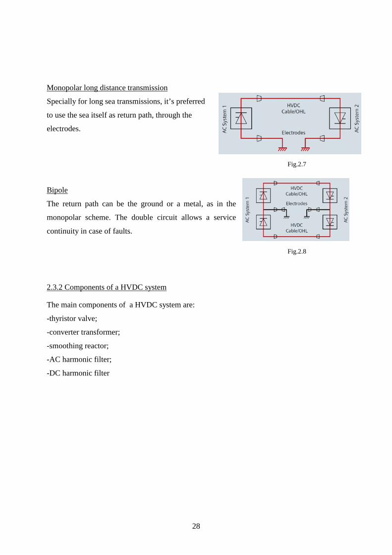
Monopolar long distance transmission

Specially for long sea transmissions, it’s preferred

to use the sea itself as return path, through the

electrodes.

Fig.2.7

Bipole

The return path can be the ground or a metal, as in the

monopolar scheme. The double circuit allows a service

continuity in case of faults.

Fig.2.8

2.3.2 Components of a HVDC system

The main components of a HVDC system are:

-thyristor valve;

-converter transformer;

-smoothing reactor;

-AC harmonic filter;

-DC harmonic filter

29

Fig.2.9: example of a bipolar scheme, in which the components are shown.

The transformer has multiple aims. First of all, it raises the AC voltage to high voltage for DC

converters; using 12 pulse transformers they attenuate the low harmonic at output; eventually

they ensure voltage insulation between AC and DC side.

The smoothing reactor has four functions: prevention of current interruption at minimum load

in case of intermittent current; reduces the DC fault current amount; avoids resonance at low

frequencies, which may saturate the transformer.; reduces the harmonic content.

The AC harmonic filter absorbs the harmonic current generated by the converter, reducing the

impact on the AC system and supplies reactive power for compensation.

The DC harmonic filter attenuates the harmonics in DC side through passive or active

filtering.

2.3.3 Multiterminal systems [15]

Along with the proliferation of off.-shore plants the problem of power transmission through

long distances appear. So, it’s economically convenient to use only a HVDC link for several

wind farms, in order to save with line costs.

This system implies some complications to reverse the power direction with conventional

CSC, because switching arrangements to reverse the polarity are needed; instead, with VSC

this isn’t necessary, because it’s enough to reverse the Id direction: in such a manner it’s

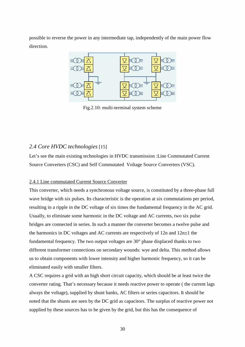
30

possible to reverse the power in any intermediate tap, independently of the main power flow

direction.

Fig.2.10: multi-terminal system scheme

2.4 Core HVDC technologies [15]

Let’s see the main existing technologies in HVDC transmission :Line Commutated Current

Source Converters (CSC) and Self Commutated Voltage Source Converters (VSC).

2.4.1 Line commutated Current Source Converter

This converter, which needs a synchronous voltage source, is constituted by a three-phase full

wave bridge with six pulses. Its characteristic is the operation at six commutations per period,

resulting in a ripple in the DC voltage of six times the fundamental frequency in the AC grid.

Usually, to eliminate some harmonic in the DC voltage and AC currents, two six pulse

bridges are connected in series. In such a manner the converter becomes a twelve pulse and

the harmonics in DC voltages and AC currents are respectively of 12n and 12n±1 the

fundamental frequency. The two output voltages are 30° phase displaced thanks to two

different transformer connections on secondary wounds: wye and delta. This method allows

us to obtain components with lower intensity and higher harmonic frequency, so it can be

eliminated easily with smaller filters.

A CSC requires a grid with an high short circuit capacity, which should be at least twice the

converter rating. That’s necessary because it needs reactive power to operate ( the current lags

always the voltage), supplied by shunt banks, AC filters or series capacitors. It should be

noted that the shunts are seen by the DC grid as capacitors. The surplus of reactive power not

supplied by these sources has to be given by the grid, but this has the consequence of

31

changing the voltage at the bus bar: that’s the reason why the network can’t be too weak nor

the converter too much far from it. In case these two situation occurred, a bank of capacitor

has to be present, as for the back to back applications; so the converter becomes a CCC, that

is a capacitor commutated converter. This configuration provides a better voltage stability and

allows to enhance the power rating level of the transmission.

Fig.2.11: an example of conventional HVDC with CSC.

2.4.2 Self Commutated Voltage Source Converter

That’s the converter adopted in my simulation, which uses the PWM concept. The great

difference with the former converter is that this one is self commutated: that means that the

commutation is independent with the short circuit capacity of the network. That’s due to the

VCS which doesn’t need any reactive power to operate.

Fig.2.12 an example of HVDC with VSC.

32

The strong point of this configuration is that the control of active and reactive powers are

independent one each other and the latter is even independent of the voltage level. These

aspects make it a very flexible and stout system.

2.5 HVDC control

The aims of the regulation are the following:

- control of DC current and voltage and transmitted power with a fast speed response;

- sufficient time margin in commutation between two polarities;

- control some quantities aiming to stabilize the network or damp the oscillations.

- to grant proper operations even during faults.

2.5.1 Control with CSC

To control the DC current it’s enough to vary the firing angle, while for the DC voltage two

methods exist: it’s possible to act upon the DC/AC voltage ratio through the delay angle or to

change the AC voltage acting mechanically , with load tap changers in the transformer. They

are characterized by different speed responses, reactive power demands and commutation

margin accuracy.

2.5.2 Control with VSC

The VSC can operate in all four quadrants: the power is controlled by varying the phase angle

of the AC voltage referred to filter bus voltage, whereas the reactive power is controlled by

varying the fundamental component of the AC voltage. All that means that the converter can

operate as a static var compensator and the real power transfer doesn’t affect the reactive

power exchange: that’s why it’s possible to say that active and reactive powers are

independent one each other, as it will be shown in chapter 5.

Referring to the below picture, the equations which act the regulation are the following:

(2.1)

(2.2)

33

where VL-L is the line to line voltage; ɣ is the firing angle of the receiving end converter; L is

the system inductance.

Fig.2.13: simple scheme of HVDC aiming to show the control concept.

Fig.2.14:diagram V=f(I)

In the control diagram α is the firing control of the receiving end converter.

The characteristic V=f(I) depicted operates at the least Q value; varying α, consequently the

Id value, the operation point can be chosen, so Vd and Id are defined.

34

35

3. CONVERTERS

3.1 Introduction

The wind farm works at AC, the power is transmitted via DC link and eventually in the AC

grid. Hence it’s necessary to provide the system with static electronic converters, that are

rectifiers and inverters.[16]

The HVDC systems[12] use traditionally CSC but this choice brings some limit: they need

two strong AC grids, don’t provide an independent control of active and reactive power and

produce a large amount of harmonics. So, for a HVDC transmission which links a offshore

plant the utilisation of VSC is more useful because they solve all bad points of CSC said

formerly. This progress has been possible thanks to IGBTs which switch off the currents,

avoiding the need for a commutating voltage. This component makes possible the

independent control of active and reactive power, reducing consequently the need for reactive

compensation and contributing to the stabilization of AC network at connection points.

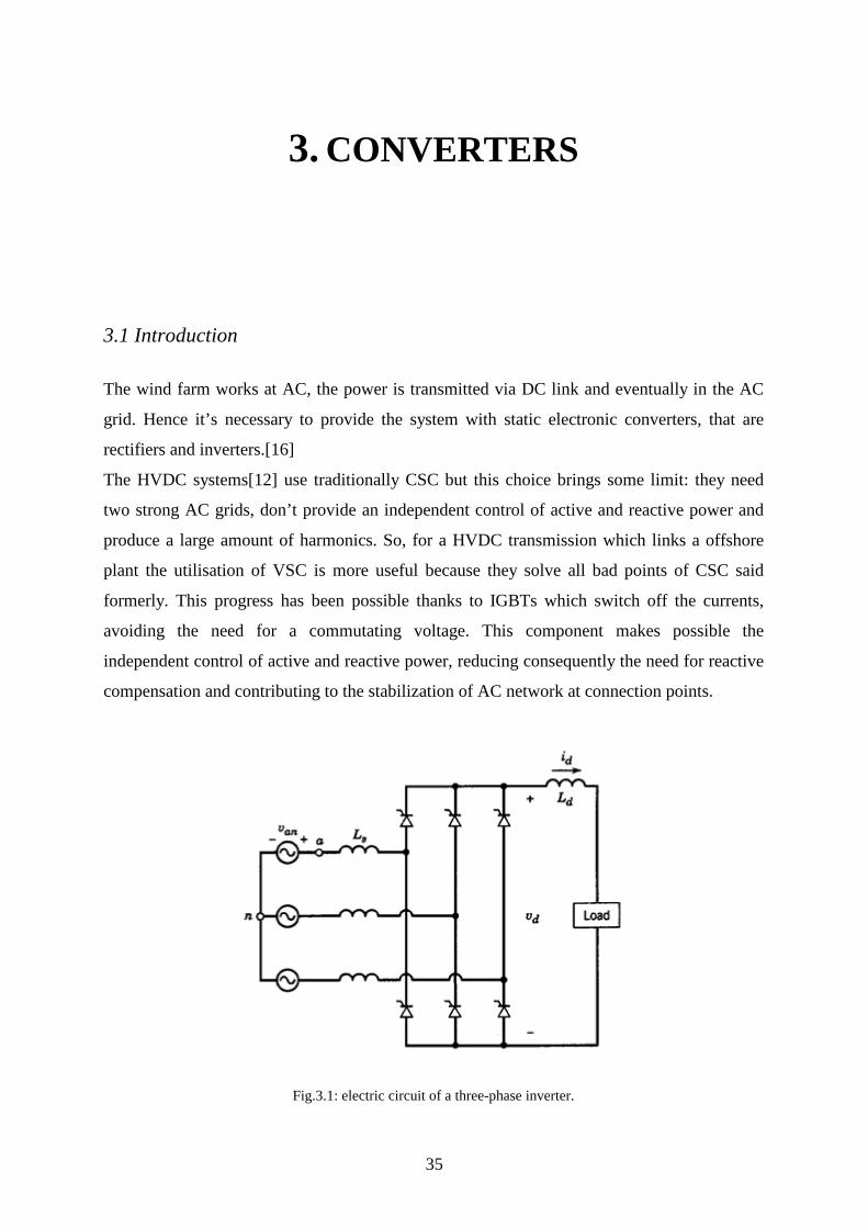
Fig.3.1: electric circuit of a three-phase inverter.

36

The bridge is constituted by electronic switches, such as transistors (BJT, MOSFET, IGBT)

and thyristors (GTO, IGCT, MCT). I used IGBTs, which are commanded through with

voltages. In order to reduce energy costs and improve energy efficiency, the trend followed is

to increase the power of plants. This request has lead to consider the multilevel converters

which make better the ratio between conducting losses and switching losses, index of the

overall converter efficiency. In fact, although they’re characterized by higher conducting

losses, they are affected by lower harmonic content with consequent less switching losses.

The most commonly disadvantage reported is the voltage unbalance between the capacitors,

but this problem can be solved modifying the reference voltage with just a little

computational effort.

3.1.1 Choise of thyristor

The best components for variable speed operations in wind power generation are IGCT and

IGBT: let’s compare the two types, discovering why the latter is preferred to the former one

[12].

The IGCTs are made like disk devices, which require a cooling supplied by an high voltage

DC source that, combined with thermal stress ( cooling-heating), constitutes a problem.

On the other hand the IGBTs are made like modular devices: the electromagnetic emission

problem is solved connecting the silicon to the ground and the thermal stress don’t occur

because it allows to create less harmonic content. The only bad point is the more consistent

power losses, respect to IGCTs. For these reasons, the IGBTs are preferred, especially for

wind power applications.

3.2 PWM : Pulse Width Modulation

Pulse width modulation is a technique which, through electronic switches, allows to obtain a

sine wave from a continue source, comparing a triangular carrier signal with a sine one.

It’s explained the behaviour of the mono-phase inverter for simplicity.

37

The carrier signal, a triangular one, is compared with a modulating signal, which is of the

same type and frequency of the requested output. In our case the modulating signal is a sine

wave of 50 Hz.

Fig.3.2: comparison of carrier signal with modulating one.

The technique is described through two ratios:

Pulse frequency modulation: . (3.1)

Pulse amplitude modulation: .. (3.2)

That’s the equation which describes the control voltage

dsdsdsd j (3.3)

An electronic comparator produces a square wave according this principle :

(3.4)

38

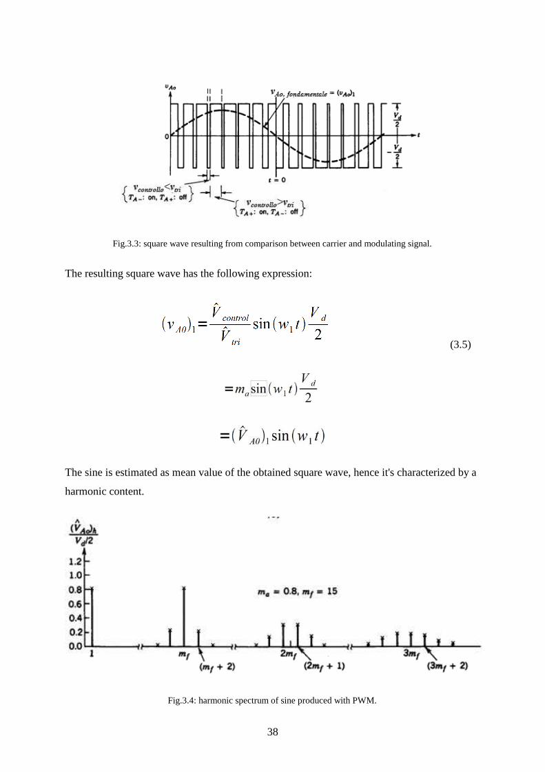
Fig.3.3: square wave resulting from comparison between carrier and modulating signal.

The resulting square wave has the following expression:

(3.5)

The sine is estimated as mean value of the obtained square wave, hence it's characterized by a

harmonic content.

Fig.3.4: harmonic spectrum of sine produced with PWM.

39

harmonic order: h=jmf+k

Tab.1.1

Managing the PWM at an high frequency, the harmonic content will be at an high frequency,

allowing then to use small filters to filter the high frequency out.

Fig.3.5: table of harmonic amplitude according to its order, ma and mf.

40

3.3 Rectifiers and inverters

The PWM technique seen formerly is applied for both operations.

Fig.3.6: an arm of a three phase inverter with a phase of the generator.

Fig.3.7: vector diagram of voltages and currents in the

bridge, working as inverter.

Fig.3.8: vector diagram of voltages and currents in the bridge, working as rectifier.

The difference between two operations lies in the load angle δ: for δ>0 the converter works as

invert, otherwise as rectifier. As inverter Van forwards EA with δ, whilst as rectifiers it lags

EA.

Fig.3.9: it’s shown that the steady current state is obtained varying VA

41

The active and reactive powers in a converter are so calculated:

(3.6)

Vll is the line to line voltage, Id the DC current and α the firing angle of the converter, which

is greater than 90° for rectifier operation and less than 90° working as inverter. The active

power changes sign for two different operation, while Q remains positive in both cases: the

converter absorbs always reactive power.

Fig.:3.10 Voltages and currents in a rectifier

It’s shown now the characteristics of a three-phase inverter, used in my simulation.

Fig.3.11: electric circuit of a three phase inverter

42

Fig.3.12: waveforms of a three-

phase inverter: carrier and

modulating wave.

Fig.3.13: phase to ground voltages

Van, Vbn and line to line voltage

Vab.

Fig.3.14: harmonic content of a three phase inverter

43

Fig. 3.15: ratio of a harmonic of VLL over Vd. for different harmonic orders.

In this table mf is supposed to be high value and multiple of three.

The inverter can be seen as a harmonic generator. Thus it’s important to filter the harmonic

out with filtering technique, which can be active or passive. In my simulation I chose the

latest one.

The major problem introduced by utilization of converters is the production of harmonics.

Let’s see the waveforms of DC voltage and AC currents for a 12 pulse converter.

44

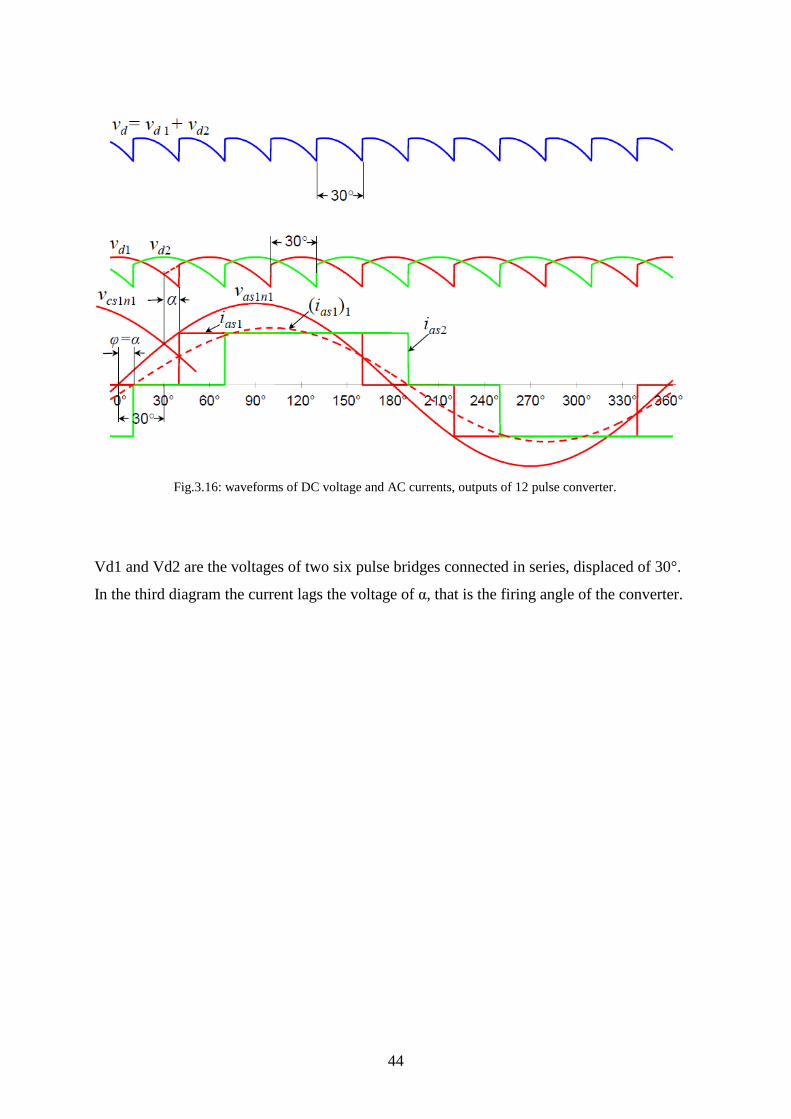
Fig.3.16: waveforms of DC voltage and AC currents, outputs of 12 pulse converter.

Vd1 and Vd2 are the voltages of two six pulse bridges connected in series, displaced of 30°.

In the third diagram the current lags the voltage of α, that is the firing angle of the converter.

45

4. VOLTAGE CONTROL ON THE

WINDFARM SIDE

4.1 Model used in the simulation

The purpose of the controller is obtaining a constant rms voltage on the bus bar on the

generator side, after variations of the torque applied at the asynchronous generator. The 3-

phase voltage is measured and shared in its three components 0,d ,q, according to 0 d q

theory. Then, it's compared with d and q components of the referring values and put into a PI

controller, which produces controlling voltage in its components d,q that, after been

transformed in abc reference, is sent as input of PWM block. The block “Discrete virtual

PLL” is a phase lock loop which is necessary for the block which converts dqo in abc

components. The block “hypot” is useful just to extract the value of modulation index from

the dq voltage.

Fig. 4.1: blocks models used in Simulink

The 0 component is neglected and q is set to zero so that vd is aligned to va.

46

4.2 d-q theory

The PI controller works upon d-q components of the current, obtained according the d-q

theory.

Fig. 4.2: Park transformation.

In this theory the currents α-β frame are rotated through the operator and split into two

rectangular components in the d-q frame. The θ is meant to be ωt, with ω angular frequency

and it’s the displacement angle between the reference systems α-β and d-q.

Fig.4.3 :the relationship between α-β Fig. 4.4 Relationship between α-β and a-b-c frame and d-q frame.

As stated formerly, it appears clearly from the graph that vd is aligned to va.

47

4.3 PI Controller

The PID controller is world wide used to control the output of a system. It’s constituted by

three terms: proportional, integral and derivative. In some applications, as mine, the

derivative term isn’t required.

Fig. 4.5: blocks model of the PI controller

The function in time domain is:

(4.1)

which is commonly written in Laplace domain:

(4.2)

The first term Kp means just a gain so that the desired final value can be achieved. Highest

values of that may originate overshoot in the output, as depicted in the following picture

5.3.2. The proportional gain reduces the steady error but can’t delete it.

48

Fig. 4.6: answers of a second order system with a step as input, varying Kp value.

To act upon the response speed it’s necessary to introduce the integral term Ki which,

moreover, deletes the steady error. Higher the integral gain, faster the response, but it may

produce accordingly an overshoot.

Fig. 4.7: answers of a second order system with a step as input, varying Ki value

49

4.3.1 Controller tuning

There aren’t mathematical methods to tune a second order PI controller but it’s possible doing

that manually. At first the integral gain is set to zero and the proportional gain to one.

Lets’ increase it until output oscillates. Then the Kp will be chosen half of that value.

Hence let’s increase Ki until the response speed and the final value are satisfactory.

A more scientific method id the Ziegler Nichols one, but it can be applied only to

third order systems.

4.4 Simulink models and simulations

The wind farm, composed by clusters of wind turbine and generators, was simplified by only

one induction machine. To work much close as possible to the machines available in the

laboratory, the rms phase to phase voltage was chosen equal to 220V, the rated power of 2kW

and frequency 50Hz. A low pass filter lies between the generator and the rectifier.

I began with the simplest model, that is:

Fig. 4.8: blocks model of the grid

50

I applied the maximum torque to achieve the desired power of 2KW, knowing that:

(4.3)

with f=50Hz, p=2 (number of magnetic poles), the speed results to be 1500 rpm, that is 157

rad/sec. Then:

(4.4)

T results roughly -12.5 Nm. The sign minus is necessary to make the machine to work as

generator. The AC grid and the DC link was represented with a simple DC source, which was

chosen a little greater than the rms voltage at the machine, that is 300 V. At first I studied a

simple open loop, that is without controller. To produce the input of the PWM I used the

“discrete PWM generator” block. To choose the frequency of the triangular wave it's

necessary to remember that higher its frequency, higher the frequency of harmonic produced.

Hence, a smaller filter will be required to delete them. Since the upper limit which ensures a

good work of the rectifier is 10KHz, I could choose whatever value beneath this vault, greater

enough than 50Hz, choosing 4KHz.

Applying a constant torque to the induction machine my first purpose was to design the filter

so that to obtain the desired voltage at the bus bar. I don't mind about reactive power because

it'll be compensated afterwards, in the AC grid side.

The filter is useful not only to smooth the current and stabilize the voltage, but also to step up

the voltage, because of the losses after the rectifier.

On the DC side I tried to smooth the voltage and the current at the rectifier terminals with a

capacitance and an inductance, whose values were chosen experimentally.

Once satisfied with the grid model, I went on controlling the voltage through the controller

depicted formerly. To do that a step was applied to the torque between –12.5 and –2Nm

0.4sec after simulation had been started.

51

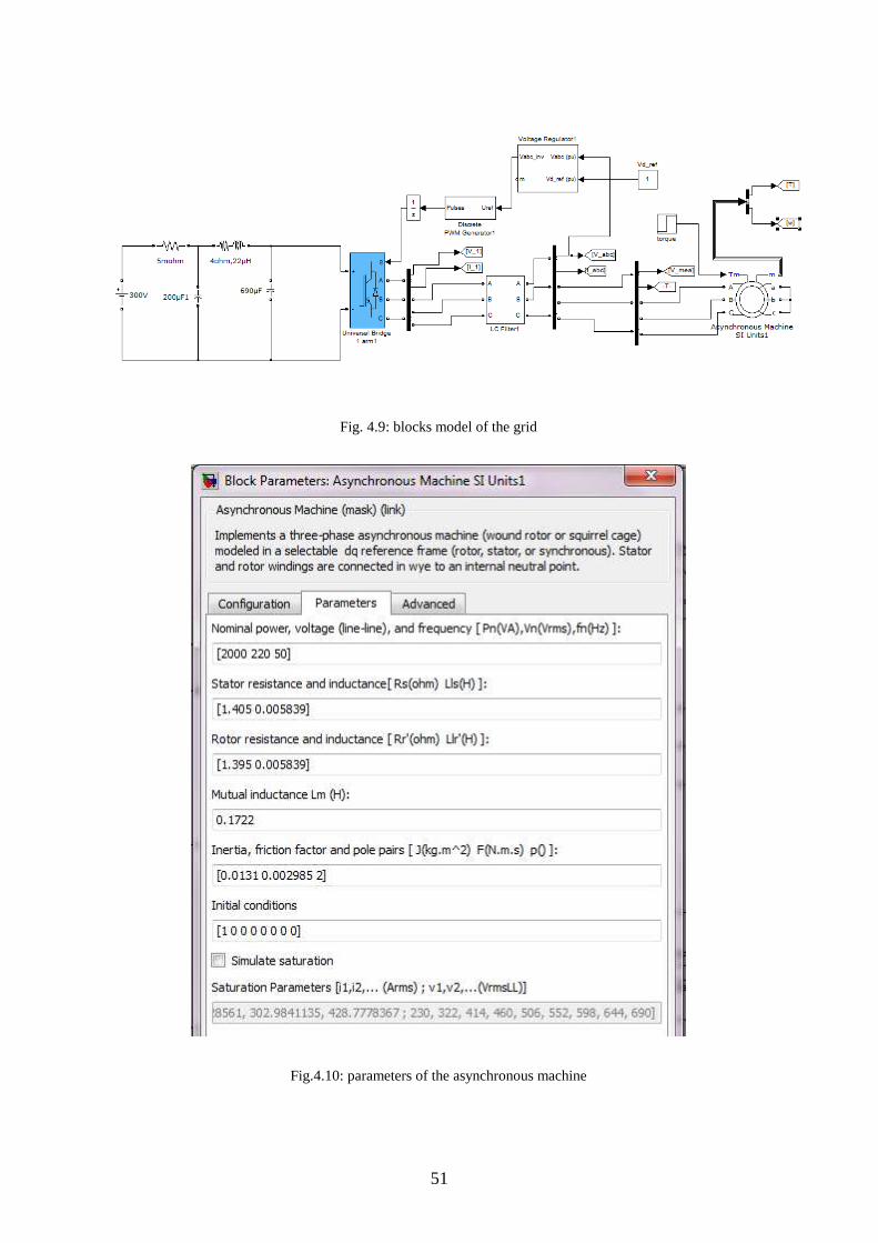
Fig. 4.9: blocks model of the grid

Fig.4.10: parameters of the asynchronous machine

52

Fig.4.11: parameters of the asynchronous machine

53

4.4.1 Diagrams and results

Fig.4.12: rms of the phase to phase voltage at the generator bus bar

The voltage rises to the desired value of 220 V in 0.2 sec. At 0.4 sec a torque step between -

12.5 and -2 is applied: after that the voltage flickers of 7V, coming back to the steady value in

80 msec.

54

Fig. 4.13.: rotor speed

Fig.4.14: mechanical torque.

The mechanical torque fluctuates to settle down to desired figures of –12.5 and –2 Nm.

55

Fig. 4.15: voltage used as input of PWM generator

That's the voltage produced by the controller expressed per units. Since the triangular signal

varies between -1 and 1 (per units), pulsing with 50Hz, it's expected that the modulation index

be the same value in the graph, that is 0.84.

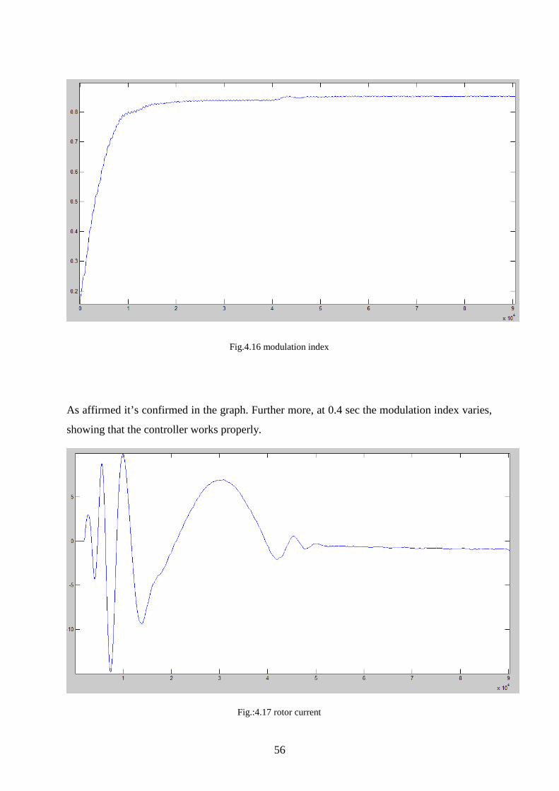
56

Fig.4.16 modulation index

As affirmed it’s confirmed in the graph. Further more, at 0.4 sec the modulation index varies,

showing that the controller works properly.

Fig.:4.17 rotor current

57

Fig.4.18: stator current.

The stator current settles on a negative value very close to zero, while the rotor current pulses

around zero with 50Hz.

Fig.4.19: vd before the PI controller

58

Fig.4.20: vq before the PI controller

Fig.4.21: vd after the PI controller

59

Fig.4.22: vq after the PI controller

Vd before PI presents a little of flicker close to 1, whilst after that it’s smoothed down and it

settles on 0.84. as the modulation index.

The vq component is modified by PI action, however its value remains close to zero.

Fig4.23: DC voltage before the inverter

60

The voltage at the inverter on the DC flickers badly around 300. I couldn’t do better because

of restrictions upon values of inductance and capacitance. Anyway everything would change

once connected the two models.

4.5 AC harmonic filter

4.5.1 Types of filter [6]

The following examples concern a case whereby the 12th harmonic is the first to be deleted,

but the behaviour has obviously general validity.

Fig.4.24: three types of filter commonly used in HVDC systems.

61

Each filter is tuned one, two or three harmonic orders, according to the filter type. The filter,

connected via a parallel to the grid, absorbs the harmonic order whereby the impedance is

lower.

These schemes haven’t been adopted because in my case of study a simple low-pass filter was

enough.

4.5.2 Scheme

As seen above the PWM produces currents at high frequency which provoke a distortion in

the current, of which we are interested only on fundamental component, 50 Hz.

The components different from the fundamental cause losses instead of contribute the active

power flow because the active power, mathematically, is given by the product of voltage and

current harmonics of the same order. Since the only voltage component is the 50 Hz one, we

desire to maintain only the correspondent current. To achieve this purpose we need a low-

pass filter, composed simply by an inductance in series with the current to filter and a

capacitance in parallel.

Fig.4.25: low-pass filter

62

Fig.4.26:filter impedante expressed as frequency

Fig.4.27: filter phase expressed as frequency

From the figure it’s clear that the filter is a low-pass one, whereby the impedance is very

close to zero around 100Hz.

Higher is the frequency, the phase is closest to –90°, because the capacitance prevails upon

the inductance.

63

4.5.3 Harmonic analysis

Fig.4.28: filtered current

Fig.:4.29 Unfiltered current

The current presents a THD (total harmonic distortion) of 1.26% with filter and 2.77%

without filter.

64

Fig.4.30: Harmonic content of filtered current

The filter adopted enables to delete high order harmonic.

65

Fig.4.31 Harmonic content of unfiltered current.

Fig.4.32: three-phase voltage at the inverter

66

Fig.4.33: three-phase voltage at the filter

Fig.4.34: one phase of the three-phase voltage at the filter

Fig.4.35: harmonic content of one phase of the three-phase voltage at the filter.

67

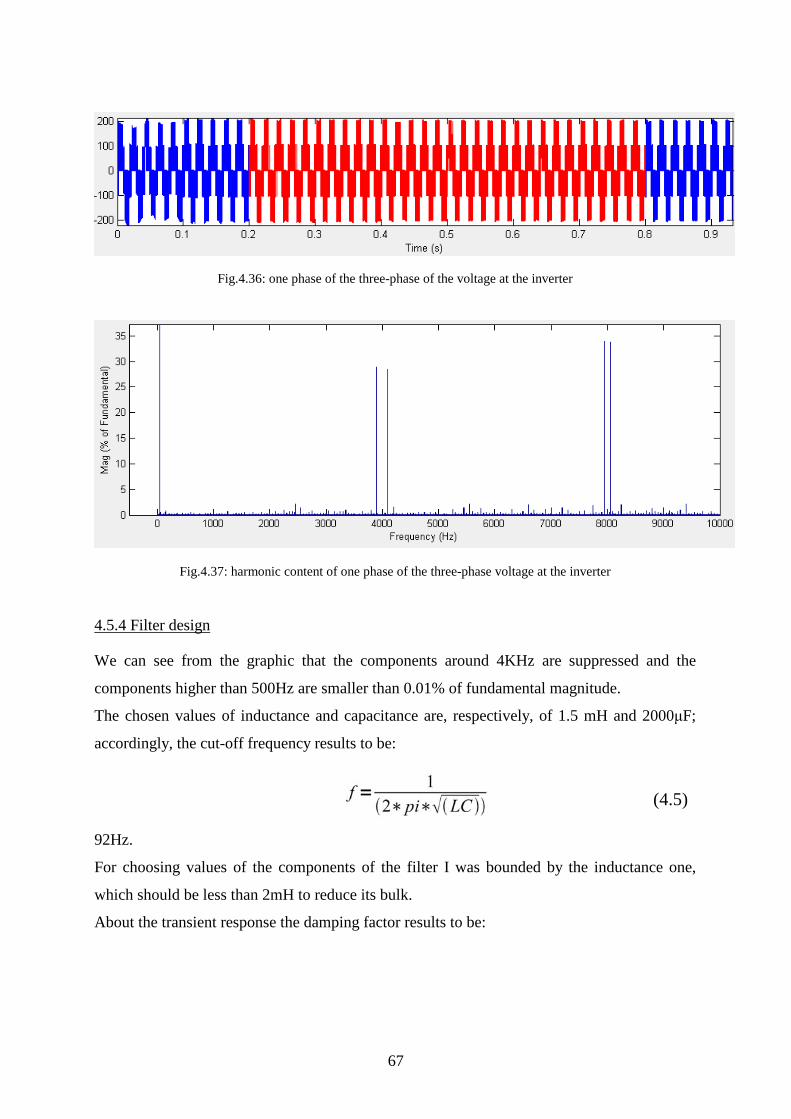
Fig.4.36: one phase of the three-phase of the voltage at the inverter

Fig.4.37: harmonic content of one phase of the three-phase voltage at the inverter

4.5.4 Filter design

We can see from the graphic that the components around 4KHz are suppressed and the

components higher than 500Hz are smaller than 0.01% of fundamental magnitude.

The chosen values of inductance and capacitance are, respectively, of 1.5 mH and 2000µF;

accordingly, the cut-off frequency results to be:

(4.5)

92Hz.

For choosing values of the components of the filter I was bounded by the inductance one,

which should be less than 2mH to reduce its bulk.

About the transient response the damping factor results to be:

68

(4.6) 0.0047, a very low value, due to the low value of inductance. The load resistance value was

obtained simply from V and I at the bus bar of the generator, and it’s RL=91.7Ω.

4.6 Opal-rt

4.6.1 Opal-rt software[18]

RT-LAB™ is a distributed real time platform fully integrated with MATLAB/Simulink® that

enables engineers to conduct real-rime simulation of Simulink models with hardware-in-the-

loop, in a very short time, at a low cost. Its scalability allows the developer to add computing

power where and when it is needed. It is flexible enough to be applied to the most complex

simulation and control problem, whether it is a real-time hardware-in-the-loop application or

for speeding up model execution, control and test. RT-LAB allows the user to readily convert

Simulink models, via real-time workshop (RTW), and then to conduct real-time simulation of

those models executed on multiple target computers equipped with multi-core PC processors.

This is used particularly for hardware-in-the-loop (HIL) and rapid control prototyping

applications. RT-LAB transparently handles synchronization, user interaction, real-world

interfacing using I/O boards and data exchanges for seamless distributed execution.

4.6.2 Diagrams

By now I’ve used Simulink, which is a simulator that works by time steps. After simulating

with this instrument we’re interested now upon simulations in real time because the

unknowns computed are more accurate.

69

Fig.4.38: three-phase voltage at the generator bus bar

The RMS value is slightly different for the three waveforms, but all of them are higher than

the corresponding matlab values.

70

Fig.4.39.

71

Fig.4.40: rotor speed.

The rotor speed is equal to 164 rad/sec, that is 1566 rpm, higher than 1509 rpm, the matlab value.

72

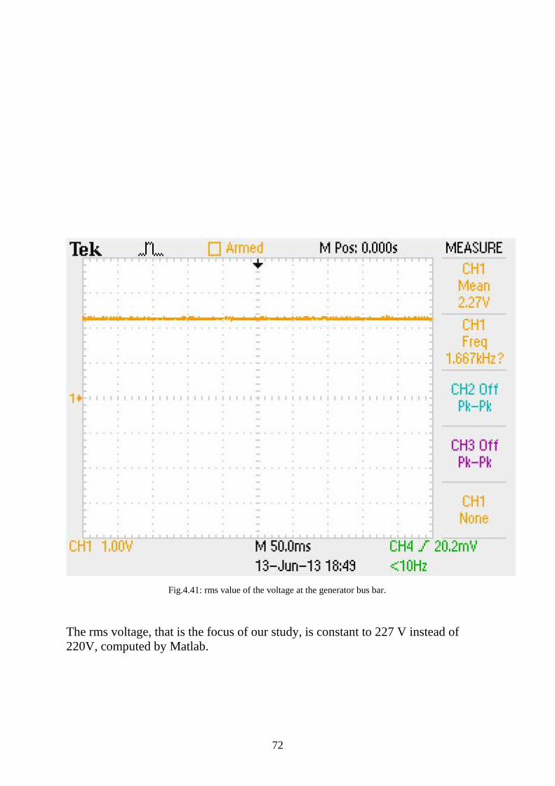
Fig.4.41: rms value of the voltage at the generator bus bar.

The rms voltage, that is the focus of our study, is constant to 227 V instead of 220V, computed by Matlab.

73

Fig.4.42: three-phase voltage before the filter

The voltage before the filter has a peak to peak value of 416 V instead 404 of matlab.

74

75

5. P-Q CONTROL ON THE AC SIDE

5.1 Introduction

This part of the project was developed by a colleague of mine. In this chapter I’ll show the

theory about the control and the schemes adopted, because I used it to continue with my

work.

The proliferation [11] of power converters using semiconductor devices such as thyristors,

diodes, transistors and so on, have brought the problems of working with non linear loads,

which draw a significant amount of harmonic current from the power network. Harmonic

current is an undesired phenomena for several negative effects:

-overheating of capacitors for power factor correction;

-voltage waveform distortion;

-voltage flicker;

-interference with communication systems.

These negative effects can be sorted out through two methods. Acting directly upon harmonic

current, filters can be adopted. Moreover, given that the harmonic components generates only

reactive power, working on reactive power compensation is possible.

Thus, the aim of this control is delivering a constant power to the grid and forcing the reactive

component to zero, trying to comply with power quality standards.

As well for this control the dq theory was adopted, being called vector oriented control

(VOC): the major advantage is that the vectors of AC currents and voltages act as constant

vectors in steady state, so it’s easy to remove the errors through PI controllers.

Here as well the dq transformation is adopted to obtain a synchronous control.

76

5.2 Scheme of the controller

Fig.5.1: P-Q control scheme.

Vgq and Vgd are the dq components of the three-phase voltage measured at the inverter.

The voltage equations in the synchronous frame are:

(5.1)

(5.2)

Laying the d-axis on the voltage vector the uLq results equal to zero. Moreover, for power

factor control the iq is set to zero, whilst id is controlled by DC link voltage controller. Thus,

neglecting R, we obtain:

(5.3)

(5.4)

77

The equations written above describe the third node of the scheme, whereby the decoupling

between the two components is obtained.

Note that direct id and iq are decoupled, in order to obtain a better control.

The complete scheme is the following:

Fig.5.2: scheme of VOC.

78

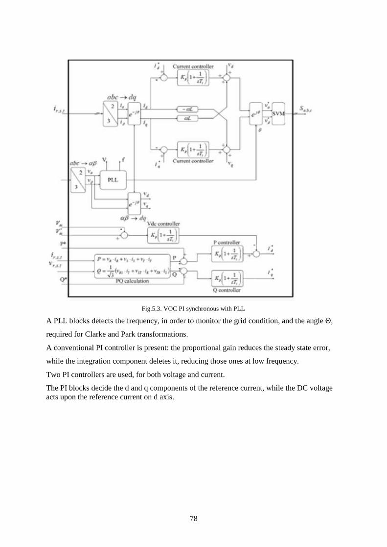
Fig.5.3. VOC PI synchronous with PLL

A PLL blocks detects the frequency, in order to monitor the grid condition, and the angle Θ,

required for Clarke and Park transformations.

A conventional PI controller is present: the proportional gain reduces the steady state error,

while the integration component deletes it, reducing those ones at low frequency.

Two PI controllers are used, for both voltage and current.

The PI blocks decide the d and q components of the reference current, while the DC voltage acts upon the reference current on d axis.

79

5.3 Simulink models and simulations

5.3.1 Scheme

Fig.5.4: model of the AC grid side

In this scheme the wind farm was represented by a DC source, as was done in the former

model for AC grid. A REC (receiving end converter) connects DC link to AC grid. The three

RLC series in parallel with the grid are notch filters for 150 and 250 Hz, while the capacitor

together with the series reactance is a low pass filter. The resistive and inductance element

placed between the filter aim to make the filter behaviour better.

Before controlling the power through the controller, the first step is to set the grid parameters.

I imposed 350 V on the DC source, about 2kW of power to the grid and 80V as phase to

phase root mean square value for the AC because in the laboratory I couldn’t exceed with the

voltage.

No power variations were imposed.

80

5.3.2 Filter

Two notch filters were tuned respectively on 150 and 250 Hz.

Fig.5.5. Figures of the filter 150Hz

Fig.5.6.: figures of the filter 250 Hz.

81

Fig.5.7: impedance of the total filter between inverter and AC grid expressed as frequency.

Fig.5.8: one phase of the current at the inverter as it appears in the FFT

(fourier fast transform) tool. The total harmonic distortion calculated between 0.025 and 0.105 sec (roughly 2 cycles)

results to be 4.27%.

Fig.5.9: one phase of the current at the filter as it appears in the FFT tool.

The total harmonic distortion calculated between 0.025 and 0.105 sec (roughly 2 cycles)

results to be 0.52%.

82

5.3.3 Diagrams

Fig.5.10: three-phase current at the inverter (A)

Fig.5.11: one phase of the iabc at the inverter as it appears in the FFT tool.

The total harmonic distortion calculated between 0.025 and 0.105 sec (roughly 2 cycles)

results to be 4.27%.

83

Fig.5.12: active power (W) transmitted to the AC grid.

Fig.5.13: reactive power (kvar) transmitted to the AC grid.

84

Fig.5.14: active power (W) at the inverter.

Fig.5.15: reactive power (kvar) at the inverter.

The filter absorbs nearly 2kW, thus it isn’t designed properly, because I focused only upon

the harmonic compensation.

85

Fig.5.16:three phase voltage(V) at the filter.

Fig.5.17: three-phase voltage at the inverter (V).

The reactive power will be compensated through a control upon the receiving inverter.

86

87

Conclusions

This project concerns the development of controls systems for connection of off-shore wind

farms to the AC grid through a HVDC link.

HVDC technology has been proven by years, but it’s been applied to wind farms only

recently, thus its study is needed to promote the wind energy generation in world wide

scenario.

The controllers, carried out with Simulink, aim to control the voltage at the generator bus bar

and the power flow transmitted to the grid, to match power quality requirements.

The realized controllers regulate the inputs of pulse width modulation in the electronic

converter.

Since the power electronic devices have reached extremely high performances, the only way

to improve the control is to focus upon the control methods.

Passive filters have been studied to improve the harmonic content of currents and voltages in

the ac side, but there’s still to work to decrease the losses.

The Clark and the αβ to dq transformation it’s a very powerful mathematical instrument to

ease the voltage and power control.

As next step, investigating more deeply with real motor and inverter would be interesting.

88

89

Glossary

- CCC: Capacitor Commutated Converter;

-CSC: Current Source Converter;

-DFIG: Double Fed Induction Generator.

- GTO: Gate Turn Off

- HVDC: High Voltage Direct Current Current;

- IGBT: Insulated Gate Bipolar Transistor;

- IGCT: Integrated Gate Commutated Transistor

-MOSFET: Metal Oxide Semiconductor Field Effect Transistor

-PWM : Pulse Width Modulation ;

-RMS: Root Mean Square;

- VSC: Voltage Source Converter;

90

91

References

[1] Lucian Mhiet-Popa, Voicu Groza: “Modeling and simulation of a 12 MW wind farm”,

Advances in electrical and computer engineering, vol.10, no.2, 2010.

[2] IWEA, www.iwea.com

[3] Lectures by Dr Zollino Giuseppe, Università degli Studi di Padova

[4] Lectures by Dr Michael Colon, Dublin Institute of Technology Baila Atha Cliath

[5] “Wind in power: 2012 european statistics”, The European wind energy association,

February 2013.

[6] “Italy”, Alberto Arena, GiacomoArsuffi, ENEA;Laura Serri, RSE. (3b vecchio)

[7] “Annual renewable report 2013”, Eirgrid. (3avecchio)

[8] “Wind power plants”, Technical application papers No.13,ABB,2011.(4vecchio)

[9] David Mac Millan, Graham W. Ault “Techno-economic comparison of operational

aspects for direct drive and gear box driven wind turbines”,IEEE transaction on energy

conversion, vol.25, no1, march 2010.

[10] “The European offshore wind industry-key trends and statistics1st half 2013”, The

European wind energy association, February 2013. (5vek)

[11] Juan Manuel Carrasco, Leopoldo Garcia Franquelo, Jan T. Bialasiewicz, Eduardo

Galvàn, Ramon C. Portillo Guisado, Ma. Angeles Martin Prats, Jose Ignacio Leon,

Narciso Moreno-Alfonso, “Power electronic systems for the grid integration of

renewable energy sources: a survey”, IEEE transaction on industrial electronics, vol.53,

no.4, august 2006.(12vek)

[12] “High voltage direct current transmission-proven technology for power exchange”

Siemens, 2011

92

[13] Huang Dong, Mao Yuan, “The study of control strategy for VSC.HVDC applied in off-

shorewind farm and grid connection. IEEE.

[14] Chih-Ju Chou, Yuan-Kang Wu, Gia-Yo Han, Ching-Yin Lee: “Comparative evaluation

of the HVDC and HVAC links integrated in a large offshore wind farm- an actual case study

in Taiwan”, IEEE, 2011.

[16] Mohan, Undeland, Robbins, “Power electronics”

[18] www.opal-rt.com

[17] Hirofumi Akagi, Edson Hirokazu Watanabe, Mauricio Aredes, “Instantaneous

power theory and applications to power conditioning” Wisley, 2007.

[15] Michael P. Bahrman, Brian K. Johnson “The ABCs of HVDC transmission

technologies”, IEEE, march/april 2007.

Other references

-Wei Xiaoguang, Tang Guangfu “Research of AC/DC parallel wind farm integration based on

VSC-HVDC.

-Tao Ding Chengxue Zhang Zhijian Hu, Zhiyuan Duan “Coordinated control strategy for

multi terminal VSC-HVDC based wind farm interconnection”.

-Haiping Yin,Lingling Fan “Modeling and control of DFIG based large off-shore wind farm

with HVDC link integration”.

-R:Meere, M.O’Malley, Keane “VSC-HVDC link to support voltage and frequency

fluctuations for variable speed wind turbines for grid connection”, 2012 3rd IEEE PES

innovative smart grid technologies Europe (ISGT Europe), Berlin.

93

-Shu Zhou, Jun Liang,Janaka B Ekanayake, Nick Jenkins, “Control of multi-terminal VSC-

HVDC transmission system for offshore wind power generation”.

-Percis, Ramesh, Rakesh, Gobinath “The impact of BoBC in offshore wind energy conversion

system”, International conference on computer, communication & electrical technology –

ICCCET2011, 18-19 march 2011.

-Jae-Hong Kim, Eel-Hwan Kim, Se-Ho Kim, Seong Bo Oh, Jaeho Choi “Modeling of Jeju

island power grid system using PSCAD/EMTDC”.

-Soon.Ryul Nam, Sang-Hee Kang, Hae-Kon Nam, Joon-Ho Choi “Dynamic modelyng of

DFIG wind farms and HVDC for the power system in Jeju island”.