Materiali di discussione

Viale Jacopo Berengario 51 – 41100 MODENA (Italy) tel. 39-059.2056711 (Centralino) 39-059.2056942 fax. 39-059.2056947

Università degli Studi di Modena e Reggio Emilia Dipartimento di Economia Politica

\\ 590 \\

Children capabilities and family characteristics in Italy

by

Tindara Addabbo1

Maria Laura Di Tommaso2

June 2008

1 Università degli Studi di Modena e Reggio Emilia, Dipartimento di Economia Politica, Via Berengario 51, 41100 Modena, Italy e-mail: tindara.addabbo@unimore.it 2 Università degli Studi di Torino Dipartimento di Economia Via Po,53 10124 Torino e-mail: marialaura.ditommaso@unito.it

1

Children capabilities and family characteristics in Italy

Tindara Addabbo1 and Maria Laura Di Tommaso2

Abstract3

This paper explores the possibilities of using structural equation modelling to measure capabilities of Italian children. In particular the paper focuses on two capabilities: “Senses, Imagination and Thought” and “Leisure and Play Activities ”. The indicators used to measure the capability of ‘Senses, imagination and thought’ for 6-13 years old children are attitude towards education, attendance to arts classes and other type of extra curriculum classes like computing and languages. The variables used as indicators of the capability of “Leisure and play activities” include how often children play in playground, various types of games, attendance to sports classes. We use both descriptive statistics, an ordered probit model, and a structural equation model in order to investigate the relation among the above mentioned indicators, the latent construct for capabilities and a set of covariates. Moreover we use a new data set in order to include family income among the covariates. The data result from the matching (through a propensity score method) of two data sets: Bank of Italy Survey on Income and Wealth for year 2000 and Istat Families, social subjects and childhood condition for year 1998.

JEL: I2, C1, J1

Keywords: Education, Capabilities, Child well-being, Structural Equation Modelling

1 Faculty of Economics Marco Biagi, CAPP, CHILD and RECent, University of Modena and Reggio Emilia, Viale Berengario 51, Modena Tel: 059 205 6879 Fax: 059 205 6947. e-mail: tindara.addabbo@unimore.it 2 Dept. of Economics and CHILD, University of Turin. Dept of Economics, via Po 53, Torino, 10124, Italy. Tel: +39 0116704411 Fax: +39 011 6703895. Frisch Centre, Gaustadalléenen 21, N-0349, Oslo, Norway, Oslo. e-mail: marialaura.ditommaso@unito.it 3 This paper is a revised version of a paper presented at the 2007 Human Capability and Development Association International Annual Conference in New York and has been accepted at the 2008 International Association for Research in Income and Wealth Annual Conference. We thank participants to the HDCA conference and to the 2007 Children’s capabilities workshop of the HDCA Thematic group on children’s capabilities that took place in Florence for stimulating comments and discussion. We gratefully acknowledge the highly qualified contribution of Marcello Morciano and Anna Maccagnan in building the matched data set.

2

1. Introducing children capabilities.

This paper explores the possibilities of using structural equation modelling to

measure capabilities of Italian children. We focus on two capabilities relevant for

evaluating children’s well being in Italy:

a. Senses Imagination and Thought.

b. Leisure activities, play.

These capabilities were chosen both because they are particularly relevant in

children development, they are very low in Italy compared to OECD countries

(UNICEF 2007), and they show high variance across regions.

In the capability literature, there has been an increasing concern about how to

choose and define capabilities (Robeyns 2003, Nussbaum 1999) and specifically

children capabilities (see the other contributions to this book, Saito 2003 and Phipps

2002). The paper of Phipps (2002) compares well being of children in USA, Canada

and Norway, measuring 10 specific functionings (low birth-weighting, asthma,

accidents, activity limitation, trouble concentrating, disobedience at school, bullying,

anxiety, lying, hyperactivity). She adopts a descriptive approach and finds out that

Norwegian children have better outcomes than US and Canada children. The paper of

Saito (2003) explores the possible relation between capabilities and education; she

reports Sen’s interview on the application of the capability approach to children.

“ If a child does not want to be inoculated, and you nevertheless think it is a good

idea for him/her to be inoculated, then the argument may be connected with the

freedom that this person will have in the future by having the measles shot now. The

child when it grows up must have more freedom. So when you are considering a

3

child, you have to consider not only the child’s freedom now, but also the child’s

freedom in the future”4

Nussbaum (2003) argues that the capability approach should endorse a theory of

social justice where the subjects are not anymore only “fully cooperating members of

society over a complete life”5 .

“ So I believe we need to delve deeper, redesigning the political conception of the

person, bringing the rational and the animal into a more intimate relation with one

another, and acknowledging that there are many types of dignity in the world,

including the dignity of mentally disabled children and adults, the dignity of the senile

demented elderly, and the dignity of babies at the breast.

………………………………………………………… We thus need to adopt a political

conception of the person that is more an Aristotelian than Kantian, one that sees the

person from the start as both capable and needy – “ in need of a rich plurality of life-

activities “ to use a Marx’s phrase, whose availability will be the measure of well-

being.” (Nussbaum 2003 pp. 29-30.)

Following Nussbaum, in order to conceptualise children capabilities, we consider

children as subjects and we use her definition for the capability of Senses

Imagination and Thought:

“Being able to use the senses, to imagine, think, and reason and do these things in

a “truly human” way informed and cultivated by an adequate education, including by

no means limited to, literacy and basic material skills.” (Nussbaum, 1999 p.81).

This is a basic capability for the development of children. Quality of education both

in primary schools and kindergartens plays a crucial role in children cognitive

4 Sen’s response in the interview with Saito in March 2001 reported in Saito (2003) pag 25. 5 Rawls 1980, pag 546, citation taken from Nussbaum 2003.

4

development (Clarke et al 2005). Attending a kindergarten has a positive effect on

children cognitive ability, and this effect is higher in poorer households (Waldfogel

2002), Magnuson et al. 2004). Positive effects of pre-compulsory education on

children’s cognitive development have been found to be significant and diminishing

up to the age of 16 (Goodman and Sianesi 2005).6

The other capability we analyse in this paper includes leisure and playing

activities. The role of this capability in children’s well being is essential.

Nevertheless, its functionings are not easily observable. Psychologists stress that it is

not only important to assess the quantity but also the quality of playing activities.

This capability is strongly correlated to other children’s capabilities like social

interaction and education. Not playing alone requires interaction with other children,

parents or with other individuals. This capability differs across regions which are

characterised by different types of schools and leisure activities. One element to be

considered is the decrease of time devoted to un-structured (not organised) leisure

time.

In this paper we try to measure the above mentioned capabilities utilising Italian

data on 6-13 years old children. In Section 2 we analyse the Italian children education

and labour conditions. In Section 3 the relation between income and children outcome

is explored. In Section 4, we outline the econometric model. We apply a Multiple

Indicator Multiple Causes model (MIMIC) because MIMIC models allow the use of

multiple indicators of the analysed capabilities and at the same time it allows to

analyse the effects of some covariates on children capabilities. The indicators used

to measure the capability of ‘Senses, imagination and thought’ for 6-13 years old

children are attitude towards education, attendance to cultural and artistic activities.

6 They used National Child Development Studies on children born in 1958 controlling for individual, household and neighbourhood variables.

5

The variables used as indicators of the capability of “Leisure activities and play”

include how often children play in playground and various types of children games,

attendance to sports classes.

Section 5 explains the data set which are the result of the matching of two data

set: the 2000 Bank of Italy Survey on Income and Wealth and the 1998 ISTAT FSS (

Famiglie, Soggetti Sociali e Condizione dell’Infanzia7). Finally results are presented

in Section 6.

2. Italian children education and labour.

According to a compounded index of some measures of school achievement at

age 15, the percentage of aged 15-19 children in education, the percentage of aged

15-19 not in education, training or employment, Italy ranks at the 23th position out of

24 OECD countries (Unicef 2007). The other dimensions analysed by Unicef (2007)

concern material well being (14th position), health and safety (5th position), family

and peer relationships (first position), behaviour and risks (10th position) and

subjective well being (10th). The Unicef educational well-being index utilises PISA

(Programme of International Student Assessment) 2000 survey. Italy (together with

Spain, Portugal and Greece) is at the bottom of the list of OECD countries in terms of

reading, mathematics and scientific literacy. The percentage of Italian aged 15-19

years old children in education (another measure included in Unicef educational

index) is also very low (18th position).

Drop out rates in primary school, in school year 2002/2003 are on average 0.08%

with a little variation across areas, drop outs in secondary school in year 2002/2003

are more heterogeneous across regions: 0.10% in the North to 0.59% in the South and

0.55% in the Islands. High school drop out rate in school year 2001/2002 is equal to

7 Households, Social Subjects, and Children conditions.

6

3.77% in the Islands, 2% in the South of Italy and around 1% in the Centre-North

(Ciccotti et al 2007).

Attending a kindergarten has a strong influence on school performances. On the

whole, kindergartens’ attendance increased from 5.8% in 1992 to 9.9% in 2005

(Ciccotti and Sabbadini, 2007). However, though increasing, the attendace rate of

children aged less than 3 in Italy is still far away from the 33% target fixed by the

European Union (Ciccotti, Moretti and Ricciotti, 2007). This figure shows a high

variance across regions: 2% in Calabria (a Southern region) and 24% in Emilia

Romagna (a Central region with a good regional social welfare), (Ciccotti et al 2007).

These figures are correlated with a high variance of the availability of nursery schools

across regions (Istituto degli Innocenti 2002), the lowest figures are to be found in the

South.

On the other hand, 104.4 per cent of the 3-5 years old children attended

kindergartens in school year 2003/2004, with a low variance across regions8 (Ciccotti

et al. 2007). However, the number of 3-5 years old children who don’t have a school

lunch in kindergartens is higher in the Southern regions and in the Islands (Ciccotti

and Sabbadini, 2007, p.15).

As far as primary school is concerned, we note that there is a high variance

across regions in the availability of ‘full-time’ schools whose time-table covers also

the afternoon (2% in Palermo and 90% in Milan) and can be more compatible with

parents’ working time, given the relatively low availability of part-time work in Italy

with respect to other countries.9 Moreover not all the schools provide lunch: Ciccotti

and Sabbadini (2007) using data of ISTAT multipurpose survey for the year 2005,

show that 71.7% in North West have school lunch, 62.1% in Norh East, 57.3% in the

Centre, 19.8% in the South and 11.8% in the Islands.

8 The above 100 percentage figure is due to the enrolment in schools of foreigners who have not yet been recorded by the Civil Register (Ciccotti et al., 2007 p.33). 9 First Report on School Quality by Tuttoscuola (www.tuttoscuola.com).

7

An important issue in assessing the capability to have leisure time and to play is to

what extent the child is free from paid or unpaid work. There has been an increased

concern for the amount of work performed by Italian children. According to ISTAT

2000 survey, 14.7% of young people from 15 to 18 in Italy had a work experience

before they were 15 years old; the percentage is higher for male (18.8%) than for

females (10.4%) and in the North-East (20.1%) than in the Centre of Italy (9.9%) and

relevant also in the South (14.7%) and in the Islands (13.2%). The higher the

secondary school grade is, the lower the percentage of those who had work

experience before the age of 15 (Moretti 2004). By using data on past work

experience one can estimate that 3% of children aged from 7 to 14 did work in Italy

in 2000 . The incidence of working children is 0.5% when they were aged from 7 to

10 and 11.6% for those aged 14.10

3. Some evidence on the relation between income and children outcomes.

According to the literature, family income has a positive effect on children’s

cognitive and social development in many ways. Income determines investments in

children’s human capital (Blau, 1999; Taylor et al. 2004); income is correlated with

parental education and better neighbourhood; higher income families have a lower

probability to fall in economic hardship and to experience its stressful consequences

(Elder et al. 1985, Taylor et al. 2004).

Nevertheless using sibling data from the Panel Study of Income Dynamics on

1,364 households following children between birth and at least age 20 and fixed-

effects estimator to control for omitted variables that might be correlated with family

income and child outcomes, Levy and Duncan (2000) show that the effect of family

income on children's completed years of schooling is very low; moreover only family

10 Moretti (2004, 71-72)

8

income at early childhood (0 to 4 years) positively and significantly affects children’s

schooling.

By using NLSY data (the matched mother-child sample) Blau (1999) finds that the

impact of family income on 0-3 years old children’s motor and social outcomes and

cognitive and language outcomes for 3-7 years old children is higher for permanent

rather than current income. In addition, the effect of income is not non linear (this is

not consistent with the hypothesis that income effects are higher at lower income

levels).

Taylor et al. (2004) focus on outcomes on 15-36 years old children when,

according to existing literature (Duncan and Brooks-Gunn 1997) income effects

should be larger. They use longitudinal data from the National Institute of Child

Health and Human Development (NICHD) Study of Early Child Care (SECC). They

find that the income effect is similar to the effect of other variables that the

literature finds related to children outcomes (like maternal verbal intelligence) by

using repeated measures of child’s outcomes and assessing their relative weight at

different points of income distribution. They also show that the effect of income

on children outcomes is not arising only because of the effect that income has on

the home environment or on maternal depressive symptoms. The inclusion of

other control variables decreases the size of income effect and using random effects

estimates, the size of income effect is smaller than by using OLS and permanent

income effects are higher than current income’s effects. Nonlinearities in the

income effects are found to occur at different points in the income distribution

according to different outcomes. Also the relative size of the family income

coefficient (compared to the coefficients of other relevant factors) are greater for

poorer households than for non poor (for instance family income coefficient in

poor households is found to be higher than the effect of maternal verbal

9

intelligence in poor households while the opposite is true in non poor

households)11 .

Chevalier, Harmon, O’Sullivan and Walker (2005) by using Labour Force Survey

data and Instrumental Variable estimate a significant effect of permanent income in

reducing drop out rates at age 16.

Policy implications call for alleviating financial constraints that prevent children in

disadvantaged environments to improve their education (Plug and Vijverberg 2001),

and for the importance of investing on children in disadvantaged environments

especially in their early age (Heckman and Masterov 2007).

Section 4 MIMIC and evaluation of Children Well being

Any attempt to operationalise the capability approach needs an adequate

framework for the measurement of the abstract unobservable multidimensional

concept. One such attempt is the latent variable approach including principal

components, factor analysis and Structural Equation Models (SEM). Multiple

Indicators Multiple Causes (MIMIC) models are the simplest form of SEM. The first

two models provide estimates of the latent variables but are silent on the factors

influencing these variables (capabilities in our context). MIMIC models represent a

step further in this direction as they include exogenous “causal” variables for the

latent factors. More complex SEM models allow for feed-back mechanisms where

that some of these causal factors not only influence human development but they are

also influenced by it. Previous papers which utilize Structural Equation Models to

estimate well-being within a capability framework include the following: Kuklys

(2004), Di Tommaso (2007b), Krishnakumar (2007). The seminal contribution by

Kuklys (2004) contains the first theoretical model of capabilities applied to SEM.

11 In contrast with this result, Jenkins and Schluter (2002) find that in Germany late childhood income effect on child’s outcomes is higher than early-childhood income.

10

Ballon and Krishnakumar (2006) utilise SEM to estimate the capability of being able

to be educated and to be adequately sheltered on Bolivian data. Di Tommaso (2007b)

The second paper estimate the well-being of Indian children (defined over

malnutrition, schooling and work indicators).

The principal advantage of this approach is that it does not rely on exact

measurement of the capability. Each indicator represents a noisy signal of it. This

modelling strategy has been extensively used in psychometrics and more recently in

econometrics (see for example Di Tommaso et al. 2007), and is founded upon the

specification of a system of equations which establishes the relationship between an

unobservable latent variable, a set of observable endogenous indicators and a set of

observable exogenous variables (which are believed to be the causes of a specific

capability).

This approach builds upon the early work of Joreskog and Goldeberger (1975) and

Zellner (1970) and has been formalized in the LISREL (Linear Structural

Relationships) model of a set of linear structural equations.12

The MIMIC approach allows us to think of this model as comprising two parts: 2

structural equations, one for the capability of Senses Imagination and Thought (SIT)

and one for the capability of Leisure and Play Activities (LPA) (which relates the 2

latent capability variables to the causes) and two measurement equations that each

capability is measured by many indicators.

For each of the indicators chosen to represent a latent construct, a weight (a factor

loading) will be estimated. This weight represents how much that specific functioning

counts in explaining the latent variable (either SIT or LPA) relative to other

functionings.

12 An excellent review of the literature is to be found in Bentler and Weeks (1980) and Aigner,

Hsiao, Kapteyn, and Wansbeek (1984), and Wansbeek and Meijer (2000).

11

4.1 Model Specification

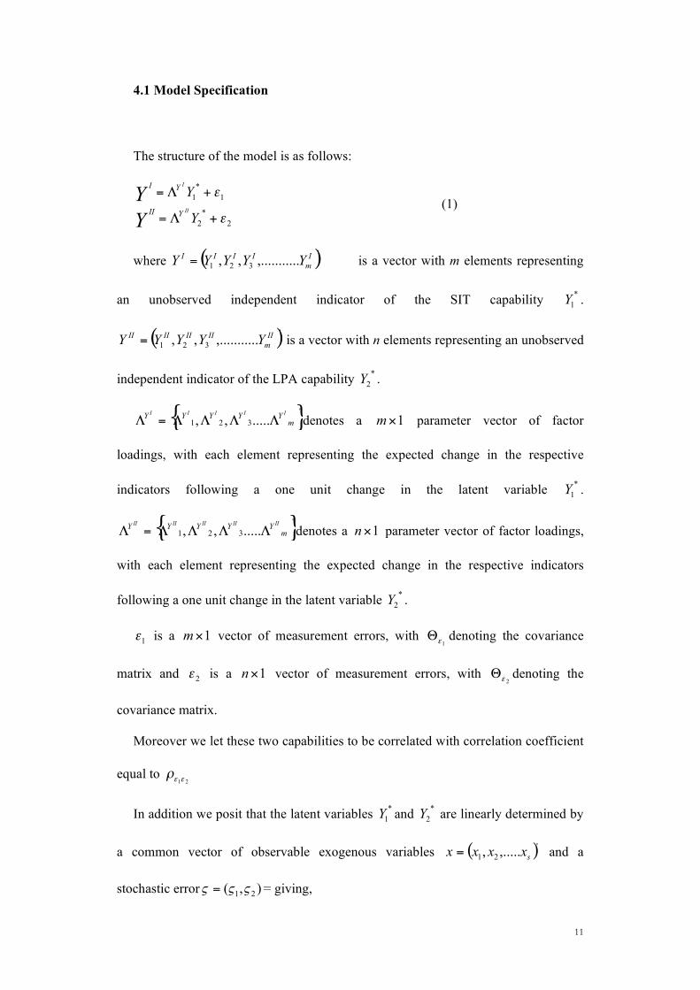
The structure of the model is as follows:

2

*

2

1

*

1

!

!

+"=

+"=

Y

Y

II

I

YII

YI

Y

Y (1)

where ( )'321

..,.........,, I

m

IIIIYYYYY = is a vector with m elements representing

an unobserved independent indicator of the SIT capability *

1Y .

( )'321

..,.........,, II

m

IIIIIIIIYYYYY = is a vector with n elements representing an unobserved

independent indicator of the LPA capability *

2Y .

{ }'321 .....,, m

YYYYYIIIII

!!!!=! denotes a 1!m parameter vector of factor

loadings, with each element representing the expected change in the respective

indicators following a one unit change in the latent variable *

1Y .

{ }'321 .....,, m

YYYYYIIIIIIIIII

!!!!=! denotes a 1!n parameter vector of factor loadings,

with each element representing the expected change in the respective indicators

following a one unit change in the latent variable *

2Y .

1! is a 1!m vector of measurement errors, with

1!" denoting the covariance

matrix and 2! is a 1!n vector of measurement errors, with

2!" denoting the

covariance matrix.

Moreover we let these two capabilities to be correlated with correlation coefficient

equal to 21!!"

In addition we posit that the latent variables *

1Y and *

2Y are linearly determined by

a common vector of observable exogenous variables ( )'21,.....,

sxxxx = and a

stochastic error ),( 21 !!! = = giving,

12

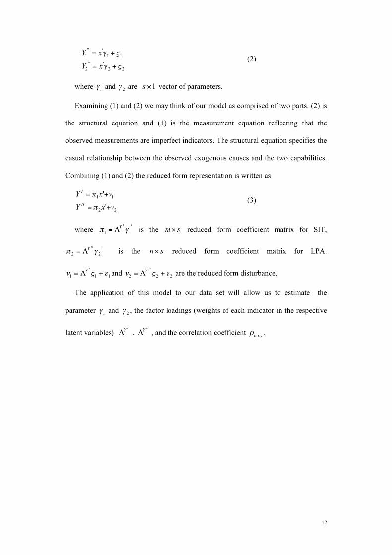
22

'*

2

11

'*

1

!"

!"

+=

+=

xY

xY (2)

where 1! and

2! are 1!s vector of parameters.

Examining (1) and (2) we may think of our model as comprised of two parts: (2) is

the structural equation and (1) is the measurement equation reflecting that the

observed measurements are imperfect indicators. The structural equation specifies the

casual relationship between the observed exogenous causes and the two capabilities.

Combining (1) and (2) the reduced form representation is written as

22

11

'

'

vxY

vxY

II

I

+=

+=

!

! (3)

where '

11!"I

Y#= is the sm! reduced form coefficient matrix for SIT,

'

22!"

IIY#= is the sn! reduced form coefficient matrix for LPA.

111!" +#=

IY

v and 222!" +#=

IIY

v are the reduced form disturbance.

The application of this model to our data set will allow us to estimate the

parameter 1! and

2! , the factor loadings (weights of each indicator in the respective

latent variables) IY! ,

IIY! , and the correlation coefficient

21!!" .

13

5. The Data

The capabilities “Senses, Imagination and Thought” and “Leisure and Play

Activities ” that are the object of our analysis on child well being in Italy cannot be

measured directly since primary data sources are not currently available and we are

therefore forced to use secondary data source. However our analysis on available

surveys on children’s well being in Italy shows that not all the variables that the

literature shows to be relevant in affecting the chosen dimensions of child well

being are available in one data set. Therefore, in order to measure child well being

with secondary data, we have used two sources of data to recover as much

information on the observables functionings of the two capabilities and on the

conversion factors. The first data set used is the ISTAT (Italian National Statistical

Office) multipurpose survey on family and on children condition (FSS98), this data

set provides us information on children’s education, play and leisure activities, the

socio-demographic structure of their families, child care provided by relatives and

parents according to the type of activities in which the children are involved.

However FSS98 lacks information on family income that can be considered as an

important factor affecting child well being and that we have recovered by using

propensity score matching techniques, matching ISTAT 1998 FSS (Famiglie,

Soggetti Sociali e Condizione dell’Infanzia) with Bank of Italy 2000 SHIW

(Surveys on Household Income and Wealth). For this purpose we have used in

Addabbo, Di Tommaso, Maccagnan and Morciano (2007) a micro procedure

inspired by propensity score matching (Rubin, 1977; Rosembaum, Rabin, 1983;

Dehejia, Wahba, 1999) and in this paper we use the matched data set constructed.

14

The resulting data set (BFSS98 in the following) contains information about

children aged from 3 to 13 who live in families where both parents are present. The

number of children is equal to 2,031 children (1,011 girls and 1,020 boys).

Amongst them 20% live in one-child families. The probability of living in a one-

child household is higher in the North-East of the country, while families with a high

number of children are more likely to be found in the Islands.

Turning to the type of family where the children live (according to their parents’

employment condition) 46% of children live in double-earner households and 47% in

one earner households where the father is employed, 2.15% where only the mother is

employed and 4.78% of the children live in households where both parents are

unemployed. The double-earner model is more spread in Centre-North whereas one-

earner traditional type of households are more spread in the South where double-

unemployed families are more likely to be found too. By analysing fathers’

employment condition we can see that 94% is employed (36% blue collar and 25%

self-employed). Amongst father 9% are in managerial positions and 4.3% is

unemployed. On the other hand more than 50% of mothers are housewives, 22% are

white-collar and 13% blue collar. Only 2.4% are manager and 8.9% self-employed.

(Tab.5.1).

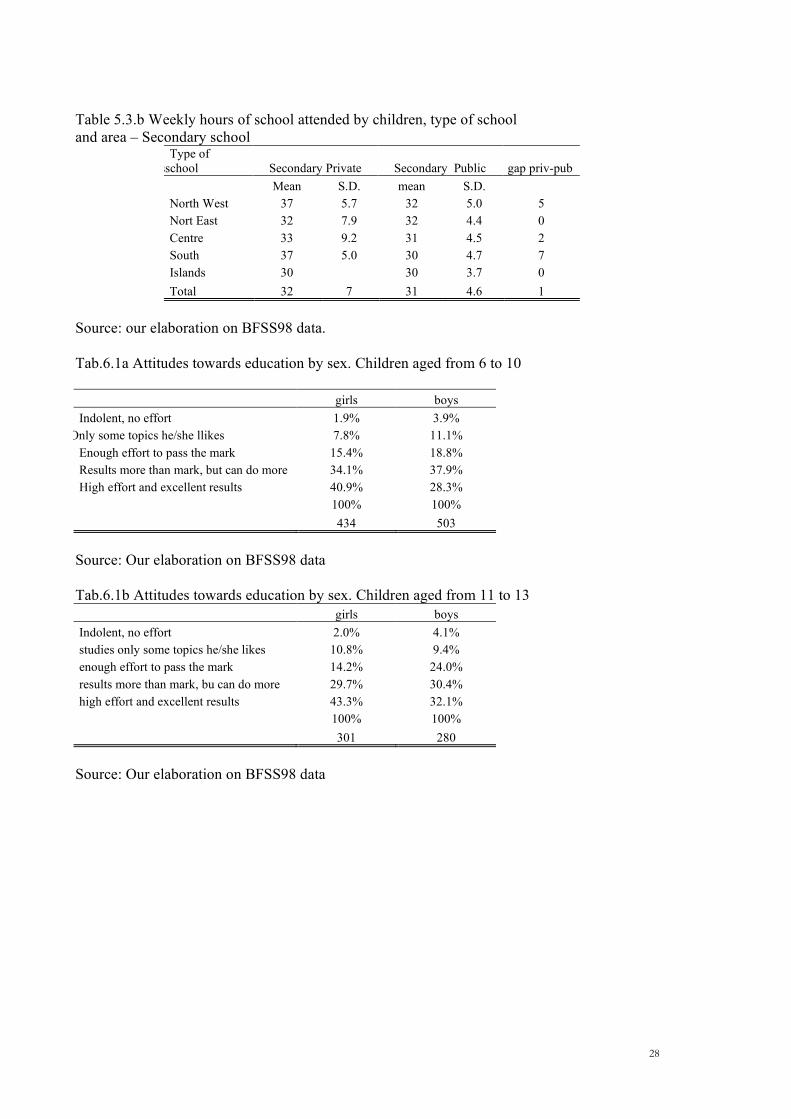
The data set provides us information on the type of school attended by children,

children living in the South of Italy have a lower probability of attending a private

school (Table 5.2), whereas the percentage of children attending private school is

higher than average in the North and in the Centre of Italy for primary school and in

the North west and Centre for secondary school. Another relevant dimension is how

long children stay at school (Tab.5.3): average number of hours in school is higher in

primary than in secondary school and the gap is in favour of private school in both

primary and secondary school. Average number of hours in school decreases from the

North to the South of the country in public school.

15

Section 6 . Measuring functionings of “Senses, Imagination and Thought”

and “Leisure and Play Activities ” dimensions of children well being in Italy

The capabilities that have been chosen as a focus of children’s well being in

this paper are crucial not only in determining actual children’s well being but also

in affecting well being later in their life. In this section we will use the available

secondary source data set in order to measure their observable functionings and

their interaction with family characteristics.

We have restricted our attention to the sample of 1,626 children (52% female) aged

from 6 to 13. BFSS98 provide us information on children’s attitude towards

education. Descriptive statistics by sex show higher values in terms of attitudes

towards education for girls than for boys in terms of efforts and results obtained.

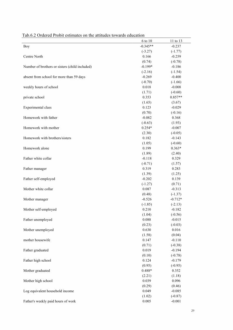
We have controlled for a set of observables environmental and individual variables

by estimating ordered probit models on the attitudes towards education separately for

children aged 6 to 10 (in elementary school age) and aged 11 to 13 (secondary school

age). The model estimated for children aged 6 to 10 (Tab.6.2) shows that being a girl

positively affects (controlling for other individual, family and area variables) the

attitudes towards education. The higher is the number of children in the family the

lower is the attitude of the child towards education. Looking at the type of school and

the number of hours in school the model shows a positive impact on attitudes

towards education of a higher number of hours in school and of being enrolled in a

private school. The attitude towards education improves if the child does her

homework alone or with her mother. Looking at parents’ employment condition only

mother’s number of hours of work (paid and unpaid) affects her child’s education

attitude (it decreases if mothers are in a managing position and increases with the

increase in paid and unpaid working hours – however the latter may include hours

16

spent by women in controlling children’s homework). Child’s attitude towards

education improves if her mother has a degree. A positive impact on 6 to 10 years old

attitude towards education is achieved when there is a high level of interaction

between parents. The latter is defined by observing parents going to restaurant,

cinema, for a walk, visiting relatives, friends or spending week-ends out together.

Turning to the educational attitude shown by children aged 11-13 (Tab.6.2) one

can notice that for children in this age group the educational attitude is still affected

by child’s gender (girls still show a more positive attitude towards education) but

becomes also negatively related to the absence from school (when children made

more than 59 days of absence from school) still positively related to being enrolled in

a private school and not related to the hours spent in school (notice however that in

this type of school one can observe a smaller variability in the time spent at school

than in elementary schools). Differently from the effects of the same factors on

children aged 6-10, mothers having a degree affect positively but not significantly

their children’s attitudes towards education and the other variables that are found to

significantly affect this attitude are doing homework alone or with father.

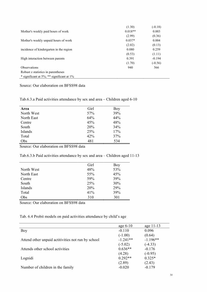
Together with child’s educational attitude another functioning of the “Senses,

Imagination and Thought” that we can observe in BFSS98 is the paid and unpaid

attendance of other activities not at school. Descriptive statistics show a high degree

of variation in this variable (Tab.6.3) across region.

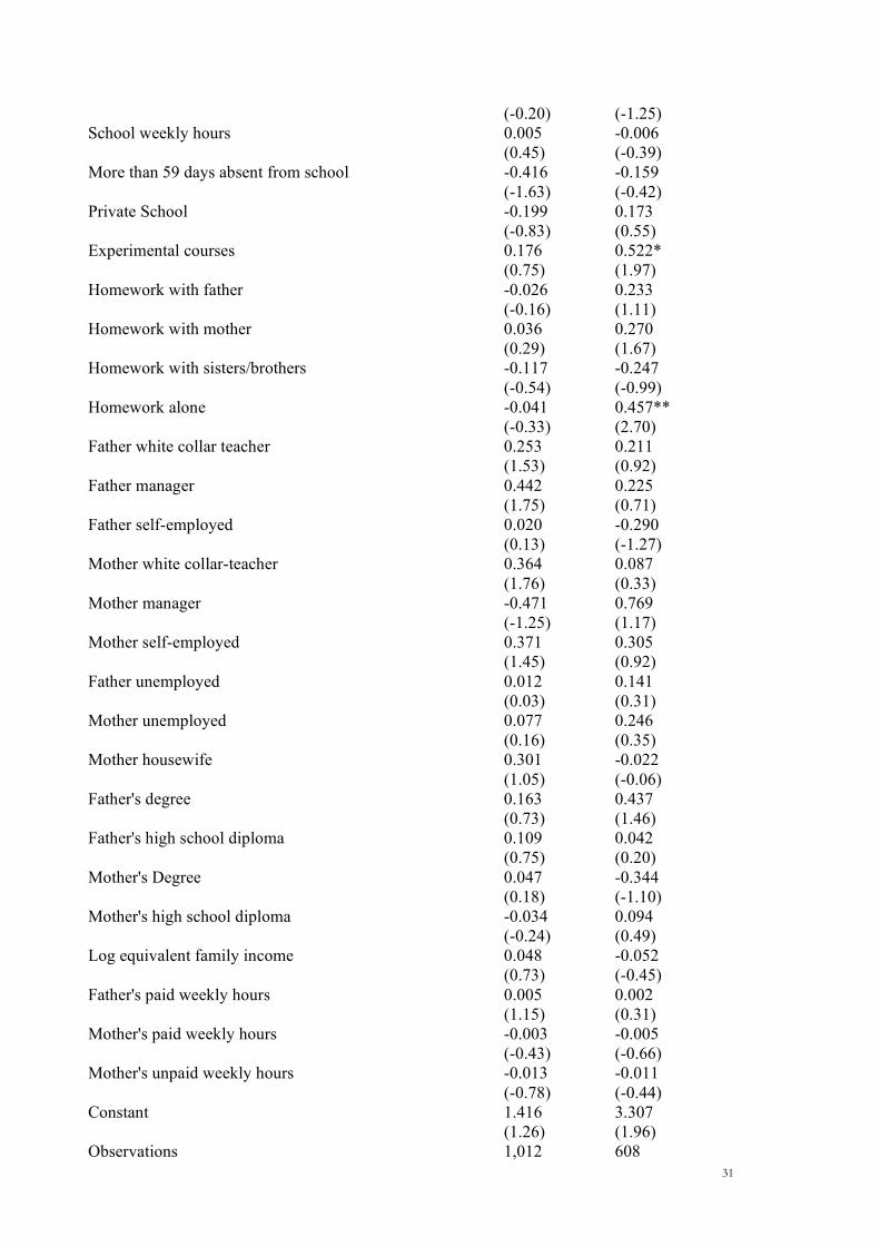
The probability of attending paid activities (music, painting, sport, languages,

computer) not run by the school (Tab.6.4) significantly decreases for children in

both age groups with their attendance to other unpaid activities not run by the school

and, only for children aged from 11 to 13, significantly increases if the child attends

experimental classes and does homework alone. A higher presence of kindergartens is

found to positively affect the attendance of paid activities for both age groups, this

17

probably may be related to the development in early age of a higher experience in

doing other activities (like painting, music…) by the higher probability of attending

kindergarten that children living in regions where kindergarten are more spread have.

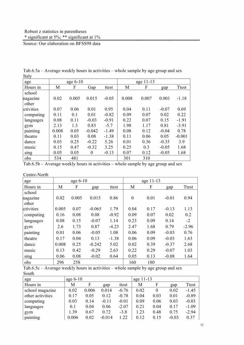
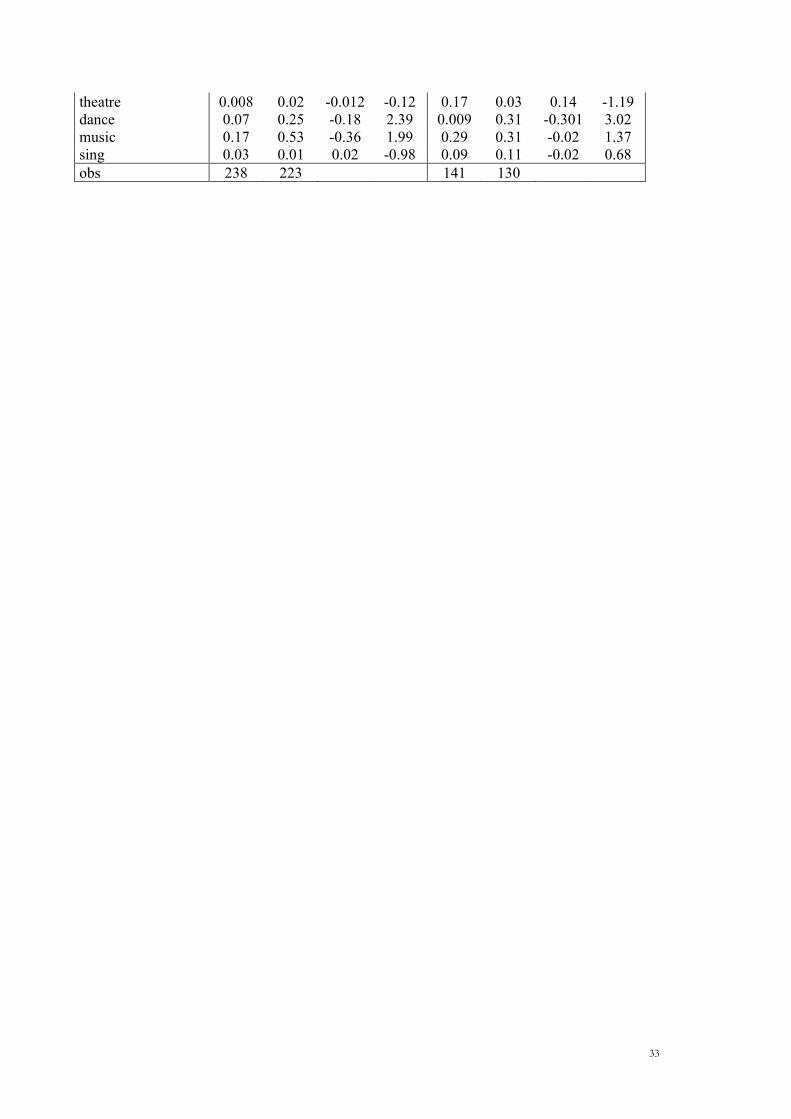
We assume that the sum of weekly hours in activities (painting, music, singing,

theatre, dance, sport, school magazine, and other) is a measure of a functioning of the

cognitive capabilities. On average taking the whole sample, Italian boys aged from 6-

13 spend 2 hours a week in sports and girls 1 hour (the average number of hours being

higher in the Centre North than in the South of Italy), girls outweigh boys in the

average number of hours in music and dance courses (Tab.6.5).

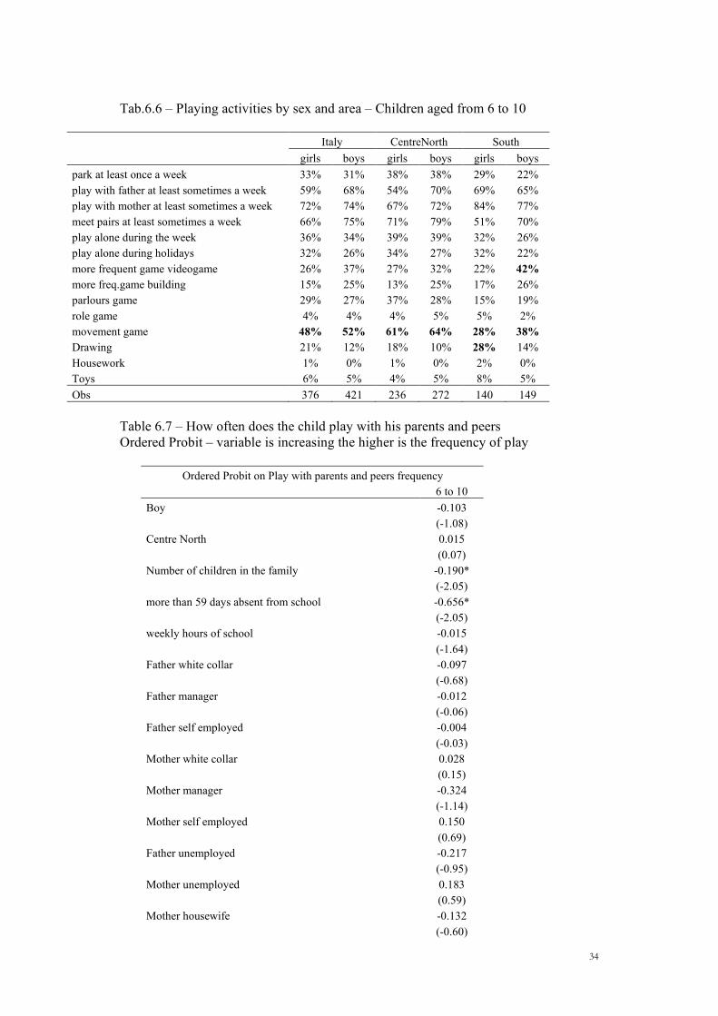
In order to proxy functionings of the capability “Leisure activities and Play” we

have used the variables in BFSS98 data set on the frequency children play with their

parents, meet children of their age, go to the park and their most frequent type of

game. We can also observe with whom they play during week days and during week

ends. Descriptive analysis on this set of variables (Tab.6.6) shows variability by sex

and by area where the children live. A similar relatively low percentage of children

by sex go to play in the park at least once a week, more in the Centre North than in

the South of Italy. More boys than girls play at least sometimes a week with the father

in the Centre North of Italy while more girls than boys play at least sometimes with

the father in the South of Italy. More boys than girls play at least sometimes a week

with their mother in the Centre North than in the South of Italy where 84% of girls

and 77% of boys play at least sometimes in a week with their mother. The frequency

children meet other children of the same age is higher in the Centre North of Italy and

higher for boys than for girls. The most frequent game, a part for boys living in the

South of Italy, are movement games (more than 60% of children living in the Centre

North against 28% of girls living in the South and 38% of boys living in the South,

the latter show a higher percentage of videogame as most frequent type of game).

Almost 40% of boys and girls play alone during week days against 32% of girls and

18

26% of boys in the South of Italy (this has to do probably with the higher number of

only one child families in the Centre and North of Italy than in the South).

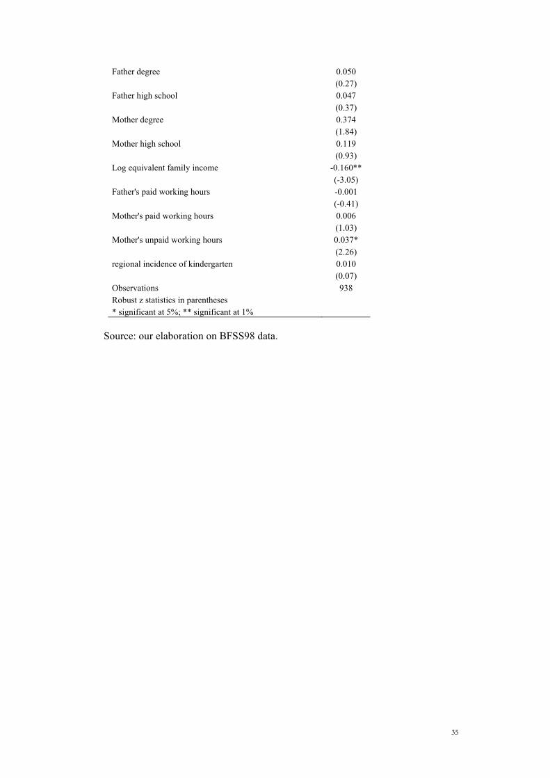
We have defined a new indicator whose values increase with the frequency

children play either with the parents or with peers. A multivariate analysis on this

indicator that relates it to family and child’s characteristics for children aged from 6

to 10 (Tab.6.7) shows how the frequency of play with parents or peers is lower the

higher is the number of hours at school and when the child has been absent from

school for more than 59 days, whereas it increases in connection with a higher

number of hours spent by mothers in unpaid care and housework activities and the

higher is her level of education (the latter being probably connected with a higher

attention to playing time with her child). How often does the child play with her

parents or peers is negatively affected by household equivalent income and by the

number of children in it.

7. MIMIC model

We have estimated the model described in Section 4 above on the data set

described in Section 5.

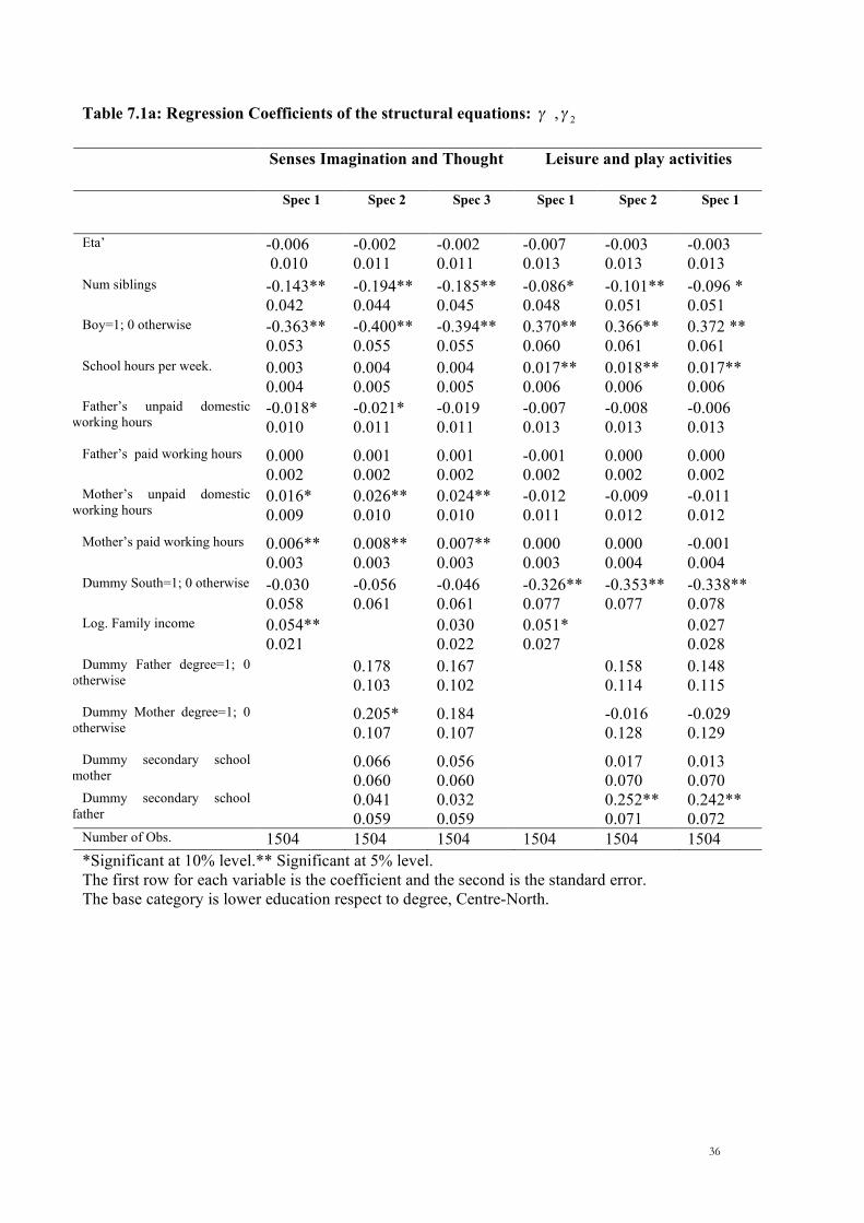
The main regression results are presented in Table 7.1. We report 3 specifications:

Specification 1 includes the log of family income but excludes parents education

dummies; Specification 2 includes parents education dummies and excludes income;

Specification 3 include both family income and parents education dummies. First of

all we note that the 3 specifications show similar results, implying that the estimates

of the coefficients of the covariates and the factor loading of the latent variable are

robust to different specifications. Our preferred specification is the 3rd one because it

includes both income and parents education variables and it shows that controlling for

parents education, income becomes not significantly different from 0.

19

Part a) of Table 7.1 reports regression coefficients of the structural equations for

the two capabilities studied.

First we analysed the results for the Senses Imagination and Thought capability.

The coefficients show a negative and significant effect of being male and of the

number of siblings, whereas there is a positive and significant effect of mother’s paid

and unpaid hours of work and if the father is graduated. In Spec.1 the log of family

income is significant but when we include parents education dummies than it looses

importance.

As far as the parameters of the covariates on the capabilities of Leisure and Play

activities are concerned we note that being a boy and hours of school have a strong

positive effect while coming from the South and the number of sibling have a

negative effect.

Note that parents education dummies are not significant in all the specification

with the exception of father secondary school dummy in the capability of Leisure and

Play activities.

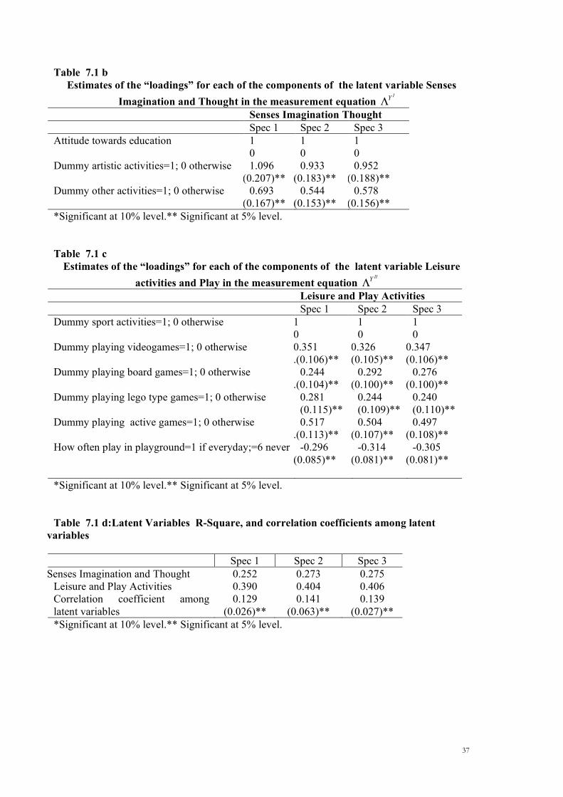
Part b of Table 7.1 presents estimates of the factor loadings for each of the

components of the capability of Senses Imagination and Thought in the measurement

equation. It shows that attitude towards education performing artistic activities has

the highest impact over the capability of Senses Imagination and Thought followed

by attitude towards education and other activities.

The third part of Table 7.1 (Table 7.1.c) shows the estimates of the factor loadings

for the components of the capability of Leisure and Play. Here the most important

indicators are the dummy for sport, for games which imply physical activities but also

playing with videogames, lego and playground activities play an important role.

As far as the squared multiple correlation for the latent variables is concerned (R

squared), it indicates to what extent the common factors account for the variance of

the indicators or how closely the model fits the data see Table 7.1 d. Specification 3 is

20

the one that has the highest R squared. This is quite obvious because it includes more

variables than Specification 1 and 2.

The correlation coefficient among the latent variables is positive and significantly

different from 0.

21

8. Conclusions

In this paper we deal with the problem of measuring children well being by using

the capability approach and in particular with regards to two capabilities: “Senses,

Imagination and Thought” and “Leisure activities and Play”.

We have faced different challenges: first, the type of data necessary to measure

these capabilities, second, which type of modelling structure to adopt. To tackle the

first challenge, we have used a data set (BFSS98) that has been created by matching

two different data sets: Bank of Italy Survey on Income and Wealth (SHIW2000) and

Istat Families, social subjects and childhood condition (FSS98). As far as the second

issue is concerned, we have adopted a Structural Equation modelling (SEM) approach

because capabilities are intrinsically unobserved construct of which we can only

measure some indicators and SEM allow to deal with this latent variables in a

sufficiently flexible way.

Our results are very robust to different specifications. A strong implication of our

results is the strong gender effect in Italy: being a boy implies both a negative effect

on the capability of Senses Imagination and Thought and a positive effect on Leisure

and playing activities. These two capabilities are also negatively affected by the

number of siblings in the household, after having controlled for family income and

parents hours of paid and unpaid work. After controlling for parents education, family

income looses importance in determining children capabilities.

References

Addabbo, T., Di Tommaso, M.L. and Facchinetti, G. (2004) To what extent fuzzy

set theory and structural equation modelling can measure functionings? An

22

application to child well being. Materiali di Discussione del Dipartimento di

Economia Politica n.468, Modena.

Addabbo, T., Di Tommaso, M.L., Maccagnan, A. and Marciano, M. (2007) ‘Child

well being and family characteristics. Towards a measure of cognitive capability’,

mimeo, paper presented at the HDCA-Thematic group on children’s capabilities

workshop on children’s capabilities, University of Florence, 18-19 April 2007.

Banca d’Italia, (2002), I Bilanci delle famiglie italiane nell’anno 2000, in

Supplementi al Bollettino Statistico – note metodologiche e informazioni statistiche,

Roma.

Blau, David M. (1999) "The Effect of Income on Child Development", Review of

Economics and Statistics 81(2): 261-16.

Clarke-Stewart, A., & Allhusen, V. (2005) What we know about childcare

Cambridge, MA: Harvard University Press.

Chevalier, A., Harmon, C., O’Sullivan, V. and Walker. I. (2005) ‘The impact of

parental income and education on the schooling of their children’ IZA discussion

paper, No. 1496, February 2005.

Ciccotti, E., Moretti, E. and Ricciotti, R. (eds) (2007) ‘I numeri italiani. Infanzia e

adolescenza in cifre – Edizione 2007’, Quaderni del Centro nazionale di

documentazione e analisi per l’infanzia e l’adolescenza, Firenze, Istituto degli

Innocenti, n.43.

Ciccotti, E. and Sabbadini, M.L. (eds) (2007) ‘Come cambia la vita dei bambini.

Indagine statistica multiscopo sulle famiglie’, Quaderni del Centro nazionale di

documentazione e analisi per l’infanzia e l’adolescenza, Firenze, Istituto degli

Innocenti, n.42.

Dehejia, R., Wahba, S., (1999), Causal Effects in Nonexperimental Studies:

Reevaluating the Evaluation of Training Programs, Journal of the American

Statistical Association, Dec99, Vol. 94 Issue 448, p1053-1062

23

Del Boca, D., Locatelli, M., Vuri, D., (2005), “Child Care Choices by Italian

Households”, Review of the Economics of the Household 3.

Di Tommaso, M.L. (2007), Measuring the Well Being of Children using a

Capability Approach. An application to Indian data.” Journal of Socio Economics, 36:

436-450.

Di Tommaso, M.L., Raiser, M. Weeks, M. (2007) “Home Grown or Imported?

Initial Conditions, External Anchors, and the Determinants of Institutional Reform in

the Transition Economies”, Economic Journal, 2007, vol 117, p 858-881.

Duncan, Greg J., and Jeanne Brooks-Gunn (1997) "Income Effects across the Life

Span: Integration and Interpretation." in Greg J. Duncan and Jeanne Brooks-Gunn

(eds.) (1997) Consequences of Growing Up Poor, 596-610. New York: Russell Sage

Foundation.

Elder, Glen H., Tri V. Nguyen, and Avshalom Caspi (1985) "Linking Economic

Hardship to Children's Lives." Child Development 56(2): 361-75.

Goodman, A. and Sianesi, B. (2005) ‘Early education and children’s outcomes:

how long do the impacts last?”, Fiscal Studies, 26 (4), 513-548.

Heckman J.J. (1979), Sample selection bias as a specification error, Econometrica,

47: 153-161.

Heckman, J.J. and Masterov, D.V. (2007) ‘The productivity argument for

investing in young children’, IZA Discussion Paper No.2725.

Jenkins, S.P. and Schluter, C. (2002) ‘The effect of family income during

childhood on later-life attainment: evidence from Germany’, IZA, Discussion Paper

No.604.

24

Joreskog, K. G., and A. S. Goldberger (1975), “Estimation of a Model with

Multiple Indicators and Multiple Causes of a Single Latent Variable,” Journal of the

American Statistical Association, 70, 631-639.

Krishnakumar J. (2007), Going beyond Functionings to Capabilities: An

Econometric Model to Explain and Estimate Capabilities. Journal of Human

Development, 8 (1):39-63

Kuklys, W. (2005) Amartya Sen’s Capability Approach: Theoretical Insights and

Empirical Applications, Berlin, Springer.

Istat, (2001), Parentela e reti di solidarietà, Collana Informazioni, Istat, Roma.

Istat, (2006), Rapporto annuale. La situazione del paese nel 2005, Istat, Roma.

Istituto degli Innocenti (2002) ‘I servizi educativi per la prima infanzia. Indagine

sui nidi d’infanzia e sui servizi educativi 0-3 anni integrativi al nido al 30 settembre

2002’ Quaderni del Centro Nazionale di documentazione e analisi per l’infanzia e

l’adolescenza. www.minori.it

Istituto degli Innocenti (2004) ‘Bambini e adolescenti che lavorano. Un panorama

dall’Italia all’Europa’ Quaderni del Centro Nazionale di documentazione e analisi

per l’infanzia e l’adolescenza, n.30, www.minori.it

Istituto degli Innocenti (2006) ‘I nidi e gli altri servizi educativi integrativi per la

prima infanzia. Rassegna coordinata dei dati e delle normative nazionali e regionali al

31/12/2005’, Questioni e Documenti 36, Quaderni del Centro Nazionale di

documentazione e analisi per l’infanzia e l’adolescenza, Firenze, Istituto degli

Innocenti, marzo 2006. www.minori.it

Levy, Dan, and Greg J. Duncan (2000) "Using Sibling Samples to Assess the

Effect of Childhood Family Income on Completed Schooling" JCPR Working Paper.

http://www.jcpr.org.

25

Maddala, G.S. (1983), Limited-dependent and qualitative variables in

econometrics,New York: Cambridge University Press.

Magnuson, K.A., Ruhm, C.J. and Waldfogel, J. (2004) ‘Does prekidergarten

improve school preparation and performance?’ NBER working paper, 10452.

Moretti, E. (2004) ‘Il lavoro minorile in Italia: un approfondimento a partire

dall’Indagine ISTAT’, in Istituto degli Innocenti (2004) ‘Bambini e adolescenti

che lavorano. Un panorama dall’Italia all’Europa’ Quaderni del Centro Nazionale

di documentazione e analisi per l’infanzia e l’adolescenza, n.30, www.minori.it

Nussbaum, M.C., 1999. Sex and Social Justice, Oxford University Press, New

York.

Phipps, S., 2002. The Well Being of Young Canadian Children in International

Perspective: A Functionings Approach, Review of Income and Wealth 48, 4,

493--513.

Rawls, J, 1980. Kantian Constructivism in Moral Theory: The Dewey Lectures” ,

The Journal of Philosophy 77, 515--571.

Robeyns, I., 2003. Sen’s Capabilities Approach and Gender Inequalities:

Selecting Relevant Capabilities. Feminist Economics 9, 2-3, 61--92.

Rosembaum, P.R. and Rubin, D.B., (1983), The Central role of the propensity

score in observational studies for causal effetcts, Biometrika 70:41-55.

Rubin, D., (1977), Assignement to a Treatment Group on the Basis of a Covariate,

Journal of Educational Statistics, vol. 2: 1-26.

Saito, M., 2003. Amartya Sen’s capability approach to education: A critical

exploration. Journal of Philosophy of Education 37, 1, 17-34.

UNICEF (2007) Child poverty in perspective: an overview of child well-being in

rich countries, Innocenti Report Card 7, Unicef Innocenti Research Centre, Florence.

26

Taylor, Beck A., Eric Dearing, and Kathleen McCartney (2004) "Incomes and

Outcomes in Early Childhood" Journal of Human Resources 39(4): 980-1007.

Waldfogel, J. (2002) ‘Child care, women’s employment, and child outcomes’

Journal of Population Economics 15:527-548.

Zellner, A (1970), “Estimation of Regression Relationships Containing

UnobservableVariables,” International Economic Review, 11, 441-454.

27

Table 5.1 – Parents level of education and employment status children aged from 3 to 13

Education Mother Father Primary school 12.62% 9.88% Secondary 46.97% 50.61% High School 30.56% 29.37% Degree 9.85% 10.14% Employment condition Mother Father Not employed 53.04% 6.05%

Retired 0.76% 1.39% Unemployed 1.78% 4.31%

Student 0.04% 0.22% Housewife 50.42% 0.11%

Employee 38.08% 68.08% Blue collar 12.85% 36.50%

White collar 22.82% 22.38% Manager 2.40% 9.13%

Self-employed 8.88% 25.96% Entrepreneur/professional 2.77% 11.77%

Self employed 5.38% 13.59% Co.co.co. 0.63% 0.60%

Source: our elaboration on BFSS98 data. Table 5.2 Type of private school attended by area. Children aged 6 to 13

Private school Primary Secondary North West 10% 8% Nort East 10% 4% Centre 8% 13% South 3% 1% Islands 1% 6% Total 7% 6%

Source: our elaboration on BFSS98 data. Table 5.3.a Weekly hours of school attended by children, type of school and area – Primary school

Type of school Primari Private Primary Public gap priv-pub Mean S.D. mean S.D. North West 34 9.5 32 5.6 2 Nort East 32 8.0 32 5.5 0 Centre 34 4.0 31 5.4 3 South 37 5.0 30 5.3 7 Islands 34 4.5 29 5.2 5 Total 34 8 31 6 3

Source: our elaboration on BFSS98 data.

28

Table 5.3.b Weekly hours of school attended by children, type of school and area – Secondary school

Type of sschool Secondary Private Secondary Public gap priv-pub

Mean S.D. mean S.D. North West 37 5.7 32 5.0 5 Nort East 32 7.9 32 4.4 0 Centre 33 9.2 31 4.5 2 South 37 5.0 30 4.7 7 Islands 30 30 3.7 0 Total 32 7 31 4.6 1

Source: our elaboration on BFSS98 data. Tab.6.1a Attitudes towards education by sex. Children aged from 6 to 10 girls boys Indolent, no effort 1.9% 3.9%

Only some topics he/she llikes 7.8% 11.1% Enough effort to pass the mark 15.4% 18.8% Results more than mark, but can do more 34.1% 37.9% High effort and excellent results 40.9% 28.3% 100% 100% 434 503

Source: Our elaboration on BFSS98 data Tab.6.1b Attitudes towards education by sex. Children aged from 11 to 13 girls boys Indolent, no effort 2.0% 4.1% studies only some topics he/she likes 10.8% 9.4% enough effort to pass the mark 14.2% 24.0% results more than mark, bu can do more 29.7% 30.4% high effort and excellent results 43.3% 32.1% 100% 100% 301 280

Source: Our elaboration on BFSS98 data

29

Tab.6.2 Ordered Probit estimates on the attitudes towards education 6 to 10 11 to 13 Boy -0.345** -0.237 (-3.27) (-1.77) Centre North 0.166 -0.259 (0.74) (-0.78) Number of brothers or sisters (child included) -0.199* -0.186 (-2.16) (-1.54) absent from school for more than 59 days -0.269 -0.400 (-0.70) (-1.66) weekly hours of school 0.018 -0.008 (1.71) (-0.60) private school 0.353 0.857** (1.65) (3.67) Experimental class 0.123 -0.029 (0.70) (-0.16) Homework with father -0.082 0.368 (-0.63) (1.93) Homework with mother 0.254* -0.007 (2.30) (-0.05) Homework with brothers/sisters 0.182 -0.143 (1.05) (-0.60) Homework alone 0.199 0.363* (1.89) (2.40) Father white collar -0.118 0.329 (-0.71) (1.57) Father manager 0.319 0.283 (1.39) (1.25) Father self-employed -0.202 0.139 (-1.27) (0.71) Mother white collar 0.087 -0.313 (0.48) (-1.37) Mother manager -0.526 -0.712* (-1.85) (-2.13) Mother self-employed 0.210 -0.182 (1.04) (-0.56) Father unemployed 0.088 -0.015 (0.23) (-0.03) Mother unemployed 0.630 0.016 (1.58) (0.04) mother housewife 0.147 -0.110 (0.71) (-0.38) Father graduated 0.019 -0.194 (0.10) (-0.78) Father high school 0.124 -0.179 (0.95) (-0.95) Mother graduated 0.488* 0.352 (2.21) (1.18) Mother high school 0.039 0.096 (0.29) (0.46) Log equivalent household income 0.049 -0.085 (1.02) (-0.87) Father's weekly paid hours of work 0.005 -0.001

30

(1.30) (-0.18) Mother's weekly paid hours of work 0.018** 0.003 (2.99) (0.36) Mother's weekly unpaid hours of work 0.037* 0.004 (2.02) (0.13) incidence of kindergarten in the region 0.080 0.259 (0.53) (1.11) High interaction between parents 0.391 -0.194 (1.70) (-0.56) Observations 940 566 Robust z statistics in parentheses * significant at 5%; ** significant at 1%

Source: Our elaboration on BFSS98 data Tab.6.3.a Paid activities attendance by sex and area – Children aged 6-10 Area Girl Boy North West 57% 39% North East 64% 44% Centre 45% 48% South 20% 34% Islands 25% 17% Total 42% 37% Obs 481 534

Source: Our elaboration on BFSS98 data Tab.6.3.b Paid activities attendance by sex and area – Children aged 11-13 Girl Boy North West 48% 53% North East 55% 45% Centre 59% 39% South 25% 30% Islands 20% 29% Total 41% 39% Obs 310 301

Source: Our elaboration on BFSS98 data Tab. 6.4 Probit models on paid activities attendance by child’s age age 6-10 age 11-13 Boy -0.110 0.096 (-1.00) (0.64) Attend other unpaid actitivities not run by school -1.241** -1.196** (-5.02) (-4.33) Attends other school activities 0.636** -0.176 (4.28) (-0.95) Lognidi 0.292** 0.325* (2.89) (2.43) Number of children in the family -0.020 -0.179

31

(-0.20) (-1.25) School weekly hours 0.005 -0.006 (0.45) (-0.39) More than 59 days absent from school -0.416 -0.159 (-1.63) (-0.42) Private School -0.199 0.173 (-0.83) (0.55) Experimental courses 0.176 0.522* (0.75) (1.97) Homework with father -0.026 0.233 (-0.16) (1.11) Homework with mother 0.036 0.270 (0.29) (1.67) Homework with sisters/brothers -0.117 -0.247 (-0.54) (-0.99) Homework alone -0.041 0.457** (-0.33) (2.70) Father white collar teacher 0.253 0.211 (1.53) (0.92) Father manager 0.442 0.225 (1.75) (0.71) Father self-employed 0.020 -0.290 (0.13) (-1.27) Mother white collar-teacher 0.364 0.087 (1.76) (0.33) Mother manager -0.471 0.769 (-1.25) (1.17) Mother self-employed 0.371 0.305 (1.45) (0.92) Father unemployed 0.012 0.141 (0.03) (0.31) Mother unemployed 0.077 0.246 (0.16) (0.35) Mother housewife 0.301 -0.022 (1.05) (-0.06) Father's degree 0.163 0.437 (0.73) (1.46) Father's high school diploma 0.109 0.042 (0.75) (0.20) Mother's Degree 0.047 -0.344 (0.18) (-1.10) Mother's high school diploma -0.034 0.094 (-0.24) (0.49) Log equivalent family income 0.048 -0.052 (0.73) (-0.45) Father's paid weekly hours 0.005 0.002 (1.15) (0.31) Mother's paid weekly hours -0.003 -0.005 (-0.43) (-0.66) Mother's unpaid weekly hours -0.013 -0.011 (-0.78) (-0.44) Constant 1.416 3.307 (1.26) (1.96) Observations 1,012 608

32

Robust z statistics in parentheses * significant at 5%; ** significant at 1%

Source: Our elaboration on BFSS98 data Tab.6.5a – Average weekly hours in activities – whole sample by age group and sex Italy age age 6-10 age 11-13 Hours in M F Gap ttest M F gap Ttest school

magazine 0.02 0.005 0.015 -0.05 0.008 0.007 0.001 -1.18 other

activities 0.07 0.06 0.01 0.95 0.04 0.11 -0.07 0.69 computing 0.11 0.1 0.01 -0.82 0.09 0.07 0.02 0.22 languages 0.08 0.11 -0.03 -0.91 0.22 0.07 0.15 -1.91 gym 2.13 1.3 0.83 -5.7 1.98 1.17 0.81 -3.91 painting 0.008 0.05 -0.042 -1.49 0.08 0.12 -0.04 0.78 theatre 0.11 0.03 0.08 -1.38 0.11 0.06 0.05 -0.001 dance 0.03 0.25 -0.22 5.26 0.01 0.36 -0.35 3.9 music 0.15 0.47 -0.32 3.25 0.25 0.3 -0.05 1.68 sing 0.05 0.05 0 -0.13 0.07 0.12 -0.05 1.68 obs 534 481 301 310

Tab.6.5b – Average weekly hours in activities – whole sample by age group and sex Centre-North age age 6-10 age 11-13 Hours in M F gap ttest M F gap Ttest school

magazine 0.02 0.005 0.015 0.86 0 0.01 -0.01 0.94 other

activities 0.005 0.07 -0.065 1.79 0.04 0.17 -0.13 1.13 computing 0.16 0.08 0.08 -0.92 0.09 0.07 0.02 0.2 languages 0.08 0.15 -0.07 1.14 0.23 0.09 0.14 -2 gym 2.6 1.73 0.87 -4.23 2.47 1.68 0.79 -2.96 painting 0.01 0.06 -0.05 1.08 0.06 0.09 -0.03 0.76 theatre 0.17 0.04 0.13 -1.38 0.06 0.09 -0.03 1.63 dance 0.008 0.25 -0.242 5.02 0.02 0.39 -0.37 2.68 music 0.13 0.42 -0.29 2.63 0.22 0.29 -0.07 1.03 sing 0.06 0.08 -0.02 0.64 0.05 0.13 -0.08 1.64 obs 296 258 160 180 Tab.6.5c – Average weekly hours in activities – whole sample by age group and sex South age age 6-10 age 11-13 Hours in M F gap ttest M F gap Ttest school magazine 0.02 0.006 0.014 -0.76 0.02 0 0.02 -1.45 other activities 0.17 0.05 0.12 -0.78 0.04 0.03 0.01 -0.89 computing 0.03 0.14 -0.11 -0.01 0.09 0.06 0.03 -0.03 languages 0.1 0.04 0.06 -2.07 0.21 0.04 0.17 -1.09 gym 1.39 0.67 0.72 -3.8 1.23 0.48 0.75 -2.94 painting 0.006 0.02 -0.014 1.22 0.12 0.15 -0.03 0.37

33

theatre 0.008 0.02 -0.012 -0.12 0.17 0.03 0.14 -1.19 dance 0.07 0.25 -0.18 2.39 0.009 0.31 -0.301 3.02 music 0.17 0.53 -0.36 1.99 0.29 0.31 -0.02 1.37 sing 0.03 0.01 0.02 -0.98 0.09 0.11 -0.02 0.68 obs 238 223 141 130

34

Tab.6.6 – Playing activities by sex and area – Children aged from 6 to 10

Italy CentreNorth South girls boys girls boys girls boys park at least once a week 33% 31% 38% 38% 29% 22% play with father at least sometimes a week 59% 68% 54% 70% 69% 65% play with mother at least sometimes a week 72% 74% 67% 72% 84% 77% meet pairs at least sometimes a week 66% 75% 71% 79% 51% 70% play alone during the week 36% 34% 39% 39% 32% 26% play alone during holidays 32% 26% 34% 27% 32% 22% more frequent game videogame 26% 37% 27% 32% 22% 42% more freq.game building 15% 25% 13% 25% 17% 26% parlours game 29% 27% 37% 28% 15% 19% role game 4% 4% 4% 5% 5% 2% movement game 48% 52% 61% 64% 28% 38% Drawing 21% 12% 18% 10% 28% 14% Housework 1% 0% 1% 0% 2% 0% Toys 6% 5% 4% 5% 8% 5% Obs 376 421 236 272 140 149

Table 6.7 – How often does the child play with his parents and peers Ordered Probit – variable is increasing the higher is the frequency of play

Ordered Probit on Play with parents and peers frequency 6 to 10 Boy -0.103 (-1.08) Centre North 0.015 (0.07) Number of children in the family -0.190* (-2.05) more than 59 days absent from school -0.656* (-2.05) weekly hours of school -0.015 (-1.64) Father white collar -0.097 (-0.68) Father manager -0.012 (-0.06) Father self employed -0.004 (-0.03) Mother white collar 0.028 (0.15) Mother manager -0.324 (-1.14) Mother self employed 0.150 (0.69) Father unemployed -0.217 (-0.95) Mother unemployed 0.183 (0.59) Mother housewife -0.132 (-0.60)

35

Father degree 0.050 (0.27) Father high school 0.047 (0.37) Mother degree 0.374 (1.84) Mother high school 0.119 (0.93) Log equivalent family income -0.160** (-3.05) Father's paid working hours -0.001 (-0.41) Mother's paid working hours 0.006 (1.03) Mother's unpaid working hours 0.037* (2.26) regional incidence of kindergarten 0.010 (0.07) Observations 938 Robust z statistics in parentheses * significant at 5%; ** significant at 1%

Source: our elaboration on BFSS98 data.

36

Table 7.1a: Regression Coefficients of the structural equations: 2

,!!

Senses Imagination and Thought Leisure and play activities

Spec 1 Spec 2 Spec 3 Spec 1 Spec 2 Spec 1

Eta’ -0.006 0.010

-0.002 0.011

-0.002 0.011

-0.007 0.013

-0.003 0.013

-0.003 0.013

Num siblings

-0.143** 0.042

-0.194** 0.044

-0.185** 0.045

-0.086* 0.048

-0.101** 0.051

-0.096 * 0.051

Boy=1; 0 otherwise

-0.363** 0.053

-0.400** 0.055

-0.394** 0.055

0.370** 0.060

0.366** 0.061

0.372 ** 0.061

School hours per week.

0.003 0.004

0.004 0.005

0.004 0.005

0.017** 0.006

0.018** 0.006

0.017** 0.006

Father’s unpaid domestic working hours

-0.018* 0.010

-0.021* 0.011

-0.019 0.011

-0.007 0.013

-0.008 0.013

-0.006 0.013

Father’s paid working hours

0.000 0.002

0.001 0.002

0.001 0.002

-0.001 0.002

0.000 0.002

0.000 0.002

Mother’s unpaid domestic working hours

0.016* 0.009

0.026** 0.010

0.024** 0.010

-0.012 0.011

-0.009 0.012

-0.011 0.012

Mother’s paid working hours

0.006** 0.003

0.008** 0.003

0.007** 0.003

0.000 0.003

0.000 0.004

-0.001 0.004

Dummy South=1; 0 otherwise

-0.030 0.058

-0.056 0.061

-0.046 0.061

-0.326** 0.077

-0.353** 0.077

-0.338** 0.078

Log. Family income 0.054** 0.021

0.030 0.022

0.051* 0.027

0.027 0.028

Dummy Father degree=1; 0 otherwise

0.178 0.103

0.167 0.102

0.158 0.114

0.148 0.115

Dummy Mother degree=1; 0 otherwise

0.205* 0.107

0.184 0.107

-0.016 0.128

-0.029 0.129

Dummy secondary school mother

0.066 0.060

0.056 0.060

0.017 0.070

0.013 0.070

Dummy secondary school father

0.041 0.059

0.032 0.059

0.252** 0.071

0.242** 0.072

Number of Obs. 1504 1504 1504 1504 1504 1504 *Significant at 10% level.** Significant at 5% level. The first row for each variable is the coefficient and the second is the standard error. The base category is lower education respect to degree, Centre-North.

37

Table 7.1 b Estimates of the “loadings” for each of the components of the latent variable Senses

Imagination and Thought in the measurement equation IY

! Senses Imagination Thought Spec 1 Spec 2 Spec 3 Attitude towards education 1

0 1 0

1 0

Dummy artistic activities=1; 0 otherwise 1.096 (0.207)**

0.933 (0.183)**

0.952 (0.188)**

Dummy other activities=1; 0 otherwise 0.693 (0.167)**

0.544 (0.153)**

0.578 (0.156)**

*Significant at 10% level.** Significant at 5% level. Table 7.1 c

Estimates of the “loadings” for each of the components of the latent variable Leisure activities and Play in the measurement equation

IIY

! Leisure and Play Activities Spec 1 Spec 2 Spec 3 Dummy sport activities=1; 0 otherwise 1

0 1 0

1 0

Dummy playing videogames=1; 0 otherwise 0.351 .(0.106)**

0.326 (0.105)**

0.347 (0.106)**

Dummy playing board games=1; 0 otherwise 0.244 .(0.104)**

0.292 (0.100)**

0.276 (0.100)**

Dummy playing lego type games=1; 0 otherwise 0.281 (0.115)**

0.244 (0.109)**

0.240 (0.110)**

Dummy playing active games=1; 0 otherwise 0.517 .(0.113)**

0.504 (0.107)**

0.497 (0.108)**

How often play in playground=1 if everyday;=6 never -0.296 (0.085)**

-0.314 (0.081)**

-0.305 (0.081)**

*Significant at 10% level.** Significant at 5% level. Table 7.1 d:Latent Variables R-Square, and correlation coefficients among latent

variables Spec 1 Spec 2 Spec 3

Senses Imagination and Thought 0.252 0.273 0.275 Leisure and Play Activities 0.390 0.404 0.406 Correlation coefficient among latent variables

0.129 (0.026)**

0.141 (0.063)**

0.139 (0.027)**

*Significant at 10% level.** Significant at 5% level.