Universita degli Studi di Milano

Facolta di Scienze Matematiche, Fisiche e Naturali

Laurea Triennale in Fisica

Quantized Lubricant Velocity ina Bi-Dimensional Sliding Model

Relatore: Dott. Nicola Manini

Correlatore: Dott. Rosario Capozza

Ivano Eligio Castelli

Matricola n◦ 671951

A.A. 2006/2007

Codice PACS: 46.55.d

Quantized Lubricant Velocity in

a Bi-Dimensional Sliding Model

Ivano Eligio Castelli

Dipartimento di Fisica, Universita degli Studi di Milano,

Via Celoria 16, 20133 Milano, Italia

October 25, 2007

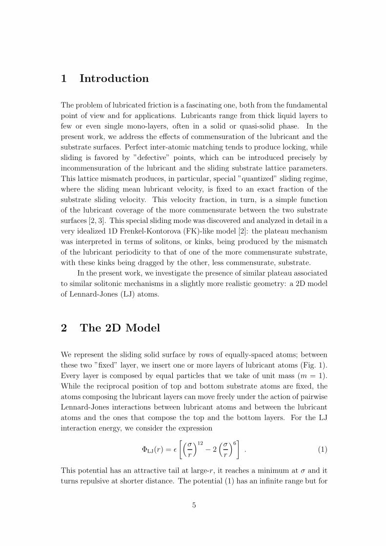
Abstract

Within the idealized scheme of a 1-dimensional Frenkel-Kontorova-like

model, a special ”quantized” sliding state was found for a solid lubricant

confined between two periodic layers [1]. This state, characterized by a non-

trivial geometrically fixed ratio of the mean lubricant drift velocity 〈vcm〉

and the externally imposed translational velocity vext, was understood as

due to the kinks (or solitons), formed by the lubricant due to incommen-

suracy with one of the substrates, pinning to the other sliding substrate.

A quantized sliding state of the same nature is demonstrated here for a

substantially less idealized 2-dimensional model, where atoms are allowed

to move perpendicularly to the sliding direction and interact via Lennard-

Jones potentials. Evidence for quantized sliding at finite temperature is

provided, even with a solid confined lubricant composed of multiple (up to

7) lubricant layers. Characteristic backward lubricant motion produced by

the presence of ”anti-kinks” is also shown in this more realistic context.

Advisor: Dr. Nicola Manini

Co-Advisor: Dr. Rosario Capozza

3

Contents

1 Introduction 5

2 The 2D Model 5

3 Technical Implementation 8

3.1 Boundary Conditions . . . . . . . . . . . . . . . . . . . . . . . . . 9

3.2 Simulation Time . . . . . . . . . . . . . . . . . . . . . . . . . . . 10

4 The Plateau Dynamics 11

4.1 Single Lubricant Layer . . . . . . . . . . . . . . . . . . . . . . . . 11

4.2 Two Lubricant Layers and Varied Kink Coverage . . . . . . . . . 17

4.3 Lubricant Multi-Layers . . . . . . . . . . . . . . . . . . . . . . . 22

4.4 Anti-Kinks . . . . . . . . . . . . . . . . . . . . . . . . . . . . . . . 26

5 Hysteresis 26

6 Analysis of the Fluctuations 31

7 Discussion and Conclusion 36

Bibliography 38

4

1 Introduction

The problem of lubricated friction is a fascinating one, both from the fundamental

point of view and for applications. Lubricants range from thick liquid layers to

few or even single mono-layers, often in a solid or quasi-solid phase. In the

present work, we address the effects of commensuration of the lubricant and the

substrate surfaces. Perfect inter-atomic matching tends to produce locking, while

sliding is favored by ”defective” points, which can be introduced precisely by

incommensuration of the lubricant and the sliding substrate lattice parameters.

This lattice mismatch produces, in particular, special ”quantized” sliding regime,

where the sliding mean lubricant velocity, is fixed to an exact fraction of the

substrate sliding velocity. This velocity fraction, in turn, is a simple function

of the lubricant coverage of the more commensurate between the two substrate

surfaces [2, 3]. This special sliding mode was discovered and analyzed in detail in a

very idealized 1D Frenkel-Kontorova (FK)-like model [2]: the plateau mechanism

was interpreted in terms of solitons, or kinks, being produced by the mismatch

of the lubricant periodicity to that of one of the more commensurate substrate,

with these kinks being dragged by the other, less commensurate, substrate.

In the present work, we investigate the presence of similar plateau associated

to similar solitonic mechanisms in a slightly more realistic geometry: a 2D model

of Lennard-Jones (LJ) atoms.

2 The 2D Model

We represent the sliding solid surface by rows of equally-spaced atoms; between

these two ”fixed” layer, we insert one or more layers of lubricant atoms (Fig. 1).

Every layer is composed by equal particles that we take of unit mass (m = 1).

While the reciprocal position of top and bottom substrate atoms are fixed, the

atoms composing the lubricant layers can move freely under the action of pairwise

Lennard-Jones interactions between lubricant atoms and between the lubricant

atoms and the ones that compose the top and the bottom layers. For the LJ

interaction energy, we consider the expression

ΦLJ(r) = ǫ

[

(σ

r

)12

− 2(σ

r

)6]

. (1)

This potential has an attractive tail at large-r, it reaches a minimum at σ and it

turns repulsive at shorter distance. The potential (1) has an infinite range but for

5

0 5 10 15 20 25 30

0

5

10a

t

ab

|F| vext

a0

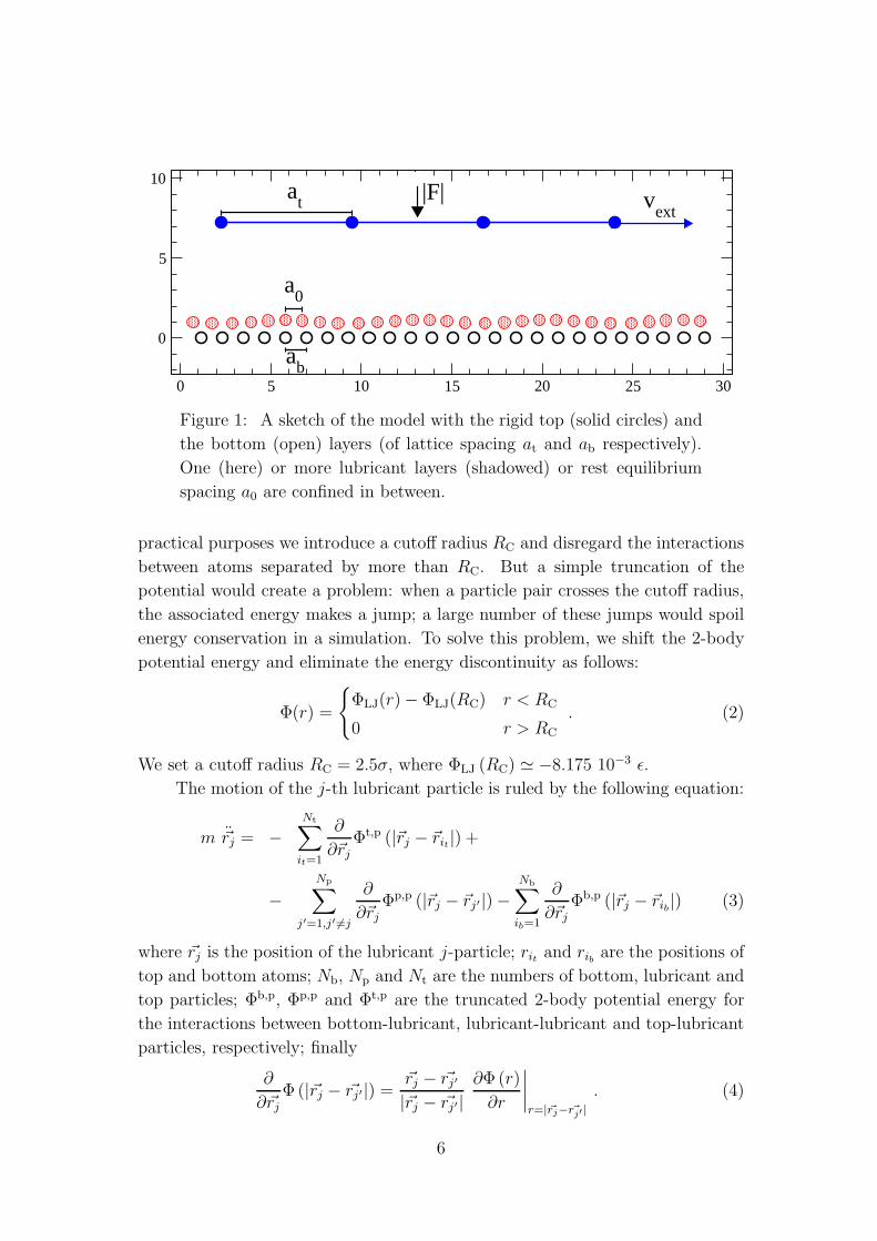
Figure 1: A sketch of the model with the rigid top (solid circles) and

the bottom (open) layers (of lattice spacing at and ab respectively).

One (here) or more lubricant layers (shadowed) or rest equilibrium

spacing a0 are confined in between.

practical purposes we introduce a cutoff radius RC and disregard the interactions

between atoms separated by more than RC. But a simple truncation of the

potential would create a problem: when a particle pair crosses the cutoff radius,

the associated energy makes a jump; a large number of these jumps would spoil

energy conservation in a simulation. To solve this problem, we shift the 2-body

potential energy and eliminate the energy discontinuity as follows:

Φ(r) =

{

ΦLJ(r) − ΦLJ(RC) r < RC

0 r > RC

. (2)

We set a cutoff radius RC = 2.5σ, where ΦLJ (RC) ≃ −8.175 10−3 ǫ.

The motion of the j-th lubricant particle is ruled by the following equation:

m ~rj = −Nt∑

it=1

∂

∂~rjΦt,p (|~rj − ~rit|) +

−

Np∑

j′=1,j′ 6=j

∂

∂~rjΦp,p (|~rj − ~rj′|) −

Nb∑

ib=1

∂

∂~rjΦb,p (|~rj − ~rib|) (3)

where ~rj is the position of the lubricant j-particle; rit and rib are the positions of

top and bottom atoms; Nb, Np and Nt are the numbers of bottom, lubricant and

top particles; Φb,p, Φp,p and Φt,p are the truncated 2-body potential energy for

the interactions between bottom-lubricant, lubricant-lubricant and top-lubricant

particles, respectively; finally

∂

∂~rjΦ (|~rj − ~rj′|) =

~rj − ~rj′

|~rj − ~rj′|

∂Φ (r)

∂r

∣

∣

∣

∣

r=|~rj− ~rj′ |

. (4)

6

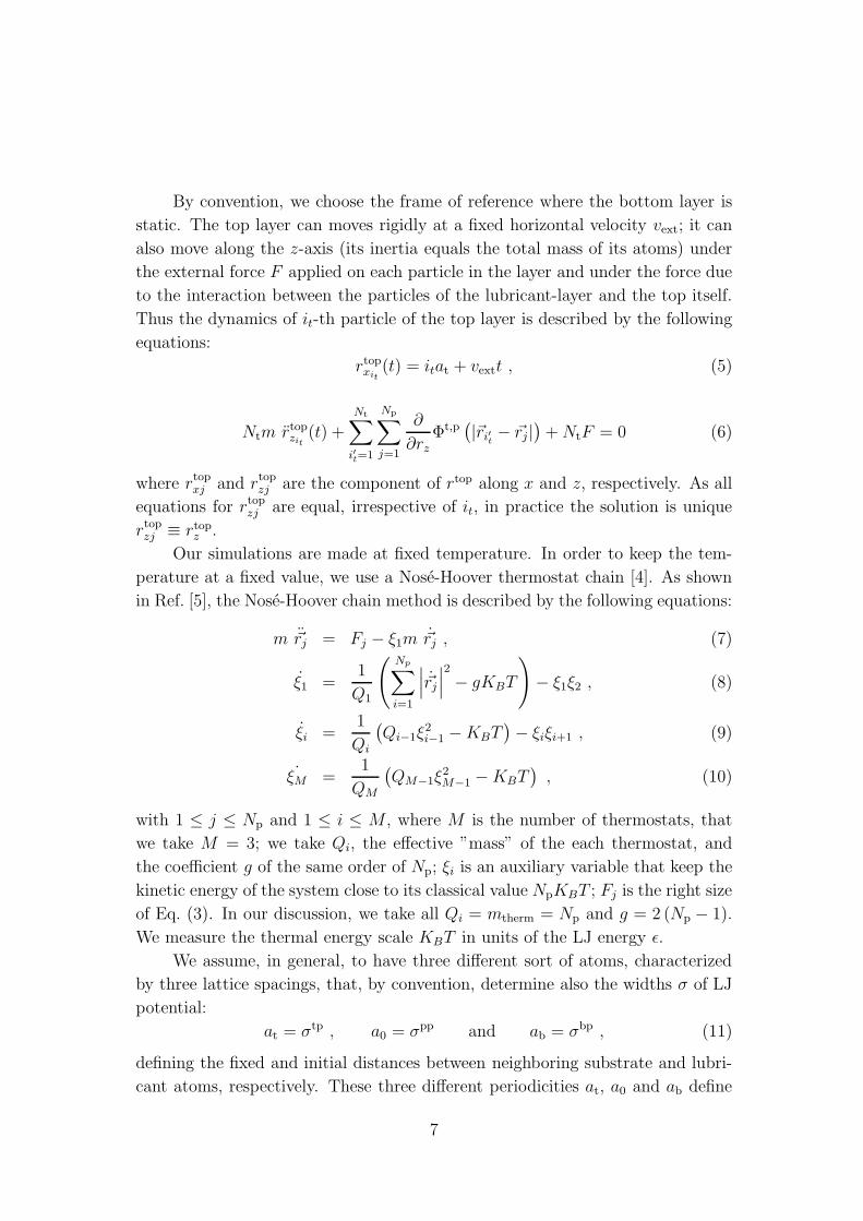
By convention, we choose the frame of reference where the bottom layer is

static. The top layer can moves rigidly at a fixed horizontal velocity vext; it can

also move along the z-axis (its inertia equals the total mass of its atoms) under

the external force F applied on each particle in the layer and under the force due

to the interaction between the particles of the lubricant-layer and the top itself.

Thus the dynamics of it-th particle of the top layer is described by the following

equations:

rtopxit

(t) = itat + vextt , (5)

Ntm rtopzit

(t) +

Nt∑

i′t=1

Np∑

j=1

∂

∂rzΦt,p

(

|~ri′t− ~rj |

)

+ NtF = 0 (6)

where rtopxj and rtop

zj are the component of rtop along x and z, respectively. As all

equations for rtopzj are equal, irrespective of it, in practice the solution is unique

rtopzj ≡ rtop

z .

Our simulations are made at fixed temperature. In order to keep the tem-

perature at a fixed value, we use a Nose-Hoover thermostat chain [4]. As shown

in Ref. [5], the Nose-Hoover chain method is described by the following equations:

m ~rj = Fj − ξ1m ~rj , (7)

ξ1 =1

Q1

(

Np∑

i=1

∣

∣

∣~rj

∣

∣

∣

2

− gKBT

)

− ξ1ξ2 , (8)

ξi =1

Qi

(

Qi−1ξ2i−1 − KBT

)

− ξiξi+1 , (9)

˙ξM =1

QM

(

QM−1ξ2M−1 − KBT

)

, (10)

with 1 ≤ j ≤ Np and 1 ≤ i ≤ M , where M is the number of thermostats, that

we take M = 3; we take Qi, the effective ”mass” of the each thermostat, and

the coefficient g of the same order of Np; ξi is an auxiliary variable that keep the

kinetic energy of the system close to its classical value NpKBT ; Fj is the right size

of Eq. (3). In our discussion, we take all Qi = mtherm = Np and g = 2 (Np − 1).

We measure the thermal energy scale KBT in units of the LJ energy ǫ.

We assume, in general, to have three different sort of atoms, characterized

by three lattice spacings, that, by convention, determine also the widths σ of LJ

potential:

at = σtp , a0 = σpp and ab = σbp , (11)

defining the fixed and initial distances between neighboring substrate and lubri-

cant atoms, respectively. These three different periodicities at, a0 and ab define

7

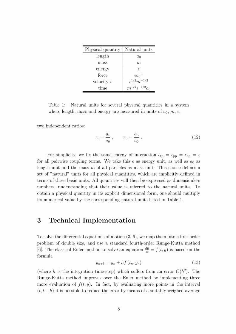
Physical quantity Natural units

length a0

mass m

energy ǫ

force ǫa−10

velocity v ǫ1/2m−1/2

time m1/2ǫ−1/2a0

Table 1: Natural units for several physical quantities in a system

where length, mass and energy are measured in units of a0, m, ǫ.

two independent ratios:

rt =at

a0

, rb =ab

a0

. (12)

For simplicity, we fix the same energy of interaction ǫtp = ǫpp = ǫbp = ǫ

for all pairwise coupling terms. We take this ǫ as energy unit, as well as a0 as

length unit and the mass m of all particles as mass unit. This choice defines a

set of ”natural” units for all physical quantities, which are implicitly defined in

terms of these basic units. All quantities will then be expressed as dimensionless

numbers, understanding that their value is referred to the natural units. To

obtain a physical quantity in its explicit dimensional form, one should multiply

its numerical value by the corresponding natural units listed in Table 1.

3 Technical Implementation

To solve the differential equations of motion (3, 6), we map them into a first-order

problem of double size, and use a standard fourth-order Runge-Kutta method

[6]. The classical Euler method to solve an equation dydt

= f(t, y) is based on the

formula

yn+1 = yn + hf (tn, yn) (13)

(where h is the integration time-step) which suffers from an error O(h2). The

Runge-Kutta method improves over the Euler method by implementing three

more evaluation of f(t, y). In fact, by evaluating more points in the interval

(t, t+h) it is possible to reduce the error by means of a suitably weighed average

8

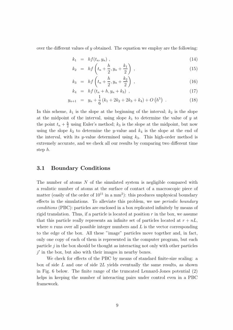
over the different values of y obtained. The equation we employ are the following:

k1 = hf(tn, yn) , (14)

k2 = hf

(

tn +h

2, yn +

k1

2

)

, (15)

k3 = hf

(

tn +h

2, yn +

k2

2

)

, (16)

k4 = hf (tn + h, yn + k3) , (17)

yn+1 = yn +1

6(k1 + 2k2 + 2k3 + k4) + O

(

h5)

. (18)

In this scheme, k1 is the slope at the beginning of the interval; k2 is the slope

at the midpoint of the interval, using slope k1 to determine the value of y at

the point tn + h2

using Euler’s method; k3 is the slope at the midpoint, but now

using the slope k2 to determine the y-value and k4 is the slope at the end of

the interval, with its y-value determined using k3. This high-order method is

extremely accurate, and we check all our results by comparing two different time

step h.

3.1 Boundary Conditions

The number of atoms N of the simulated system is negligible compared with

a realistic number of atoms at the surface of contact of a macroscopic piece of

matter (easily of the order of 1011 in a mm2): this produces unphysical boundary

effects in the simulations. To alleviate this problem, we use periodic boundary

conditions (PBC): particles are enclosed in a box replicated infinitely by means of

rigid translation. Thus, if a particle is located at position r in the box, we assume

that this particle really represents an infinite set of particles located at r + nL,

where n runs over all possible integer numbers and L is the vector corresponding

to the edge of the box. All these ”image” particles move together and, in fact,

only one copy of each of them is represented in the computer program, but each

particle j in the box should be thought as interacting not only with other particles

j′ in the box, but also with their images in nearby boxes.

We check for effects of the PBC by means of standard finite-size scaling: a

box of side L and one of side 2L yields eventually the same results, as shown

in Fig. 6 below. The finite range of the truncated Lennard-Jones potential (2)

helps in keeping the number of interacting pairs under control even in a PBC

framework.

9

7.1

7.2

7.3

-0.2

0

0.2

0.4

7.1

7.2

7.3

Zto

p

-0.2

0

0.2

0.4

<V

cm>

/vex

t

0 200 400 600 800time

7.1

7.2

7.3

0 200 400 600 800time

-0.2

0

0.2

0.4

T=0.001v

ext=0.1

T=0.01v

ext=0.1

T=0.001v

ext=5

(a) (b)

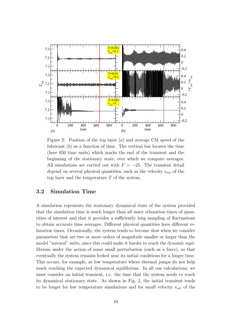
Figure 2: Position of the top layer (a) and average CM speed of the

lubricant (b) as a function of time. The vertical bar locates the time

(here 650 time units) which marks the end of the transient and the

beginning of the stationary state, over which we compute averages.

All simulations are carried out with F = −25. The transient detail

depend on several physical quantities, such as the velocity vext of the

top layer and the temperature T of the system.

3.2 Simulation Time

A simulation represents the stationary dynamical state of the system provided

that the simulation time is much longer than all inner relaxation times of quan-

tities of interest and that it provides a sufficiently long sampling of fluctuations

to obtain accurate time averages. Different physical quantities have different re-

laxation times. Occasionally, the system tends to become slow when we consider

parameters that are two or more orders of magnitude smaller or larger than the

model ”natural” units, since this could make it harder to reach the dynamic equi-

librium under the action of some small perturbation (such as a force), so that

eventually the system remains locked near its initial conditions for a longer time.

This occurs, for example, at low temperature where thermal jumps do not help

much reaching the expected dynamical equilibrium. In all our calculations, we

must consider an initial transient, i.e. the time that the system needs to reach

its dynamical stationary state. As shown in Fig. 2, the initial transient tends

to be longer for low temperature simulations and for small velocity vext of the

10

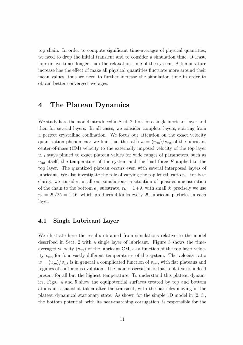
top chain. In order to compute significant time-averages of physical quantities,

we need to drop the initial transient and to consider a simulation time, at least,

four or five times longer than the relaxation time of the system. A temperature

increase has the effect of make all physical quantities fluctuate more around their

mean values, thus we need to further increase the simulation time in order to

obtain better converged averages.

4 The Plateau Dynamics

We study here the model introduced in Sect. 2, first for a single lubricant layer and

then for several layers. In all cases, we consider complete layers, starting from

a perfect crystalline confination. We focus our attention on the exact velocity

quantization phenomena: we find that the ratio w = 〈vcm〉/vext of the lubricant

center-of-mass (CM) velocity to the externally imposed velocity of the top layer

vext stays pinned to exact plateau values for wide ranges of parameters, such as

vext itself, the temperature of the system and the load force F applied to the

top layer. The quantized plateau occurs even with several interposed layers of

lubricant. We also investigate the role of varying the top length ratio rt. For best

clarity, we consider, in all our simulations, a situation of quasi-commensuration

of the chain to the bottom ab substrate, rb = 1+δ, with small δ: precisely we use

rb = 29/25 = 1.16, which produces 4 kinks every 29 lubricant particles in each

layer.

4.1 Single Lubricant Layer

We illustrate here the results obtained from simulations relative to the model

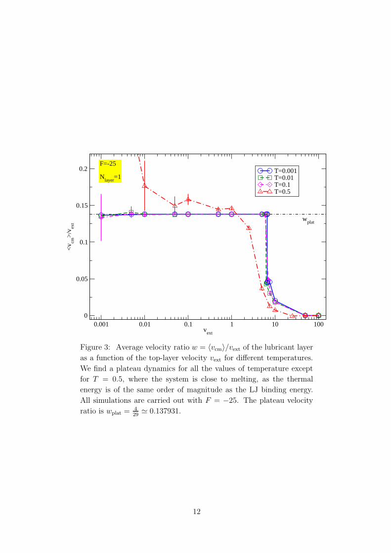
described in Sect. 2 with a single layer of lubricant. Figure 3 shows the time-

averaged velocity 〈vcm〉 of the lubricant CM, as a function of the top layer veloc-

ity vext for four vastly different temperatures of the system. The velocity ratio

w = 〈vcm〉/vext is in general a complicated function of vext, with flat plateaus and

regimes of continuous evolution. The main observation is that a plateau is indeed

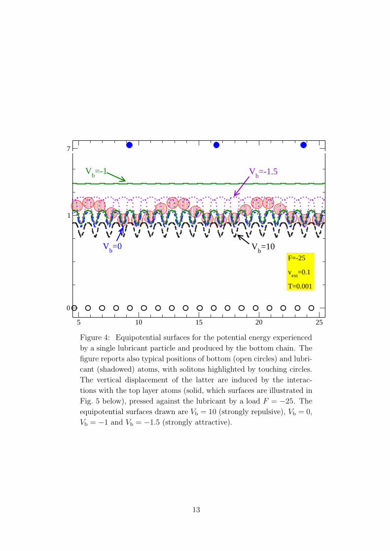
present for all but the highest temperature. To understand this plateau dynam-

ics, Figs. 4 and 5 show the equipotential surfaces created by top and bottom

atoms in a snapshot taken after the transient, with the particles moving in the

plateau dynamical stationary state. As shown for the simple 1D model in [2, 3],

the bottom potential, with its near-matching corrugation, is responsible for the

11

0.001 0.01 0.1 1 10 100v

ext

0

0.05

0.1

0.15

0.2

<v cm

>/v

ext

T=0.001T=0.01T=0.1T=0.5

F=-25

Nlayer

=1

wplat

Figure 3: Average velocity ratio w = 〈vcm〉/vext of the lubricant layer

as a function of the top-layer velocity vext for different temperatures.

We find a plateau dynamics for all the values of temperature except

for T = 0.5, where the system is close to melting, as the thermal

energy is of the same order of magnitude as the LJ binding energy.

All simulations are carried out with F = −25. The plateau velocity

ratio is wplat = 429

≃ 0.137931.

12

5 10 15 20 25

0

1

7

Vb=10V

b=0

Vb=-1 V

b=-1.5

F=-25

vext

=0.1

T=0.001

Figure 4: Equipotential surfaces for the potential energy experienced

by a single lubricant particle and produced by the bottom chain. The

figure reports also typical positions of bottom (open circles) and lubri-

cant (shadowed) atoms, with solitons highlighted by touching circles.

The vertical displacement of the latter are induced by the interac-

tions with the top layer atoms (solid, which surfaces are illustrated in

Fig. 5 below), pressed against the lubricant by a load F = −25. The

equipotential surfaces drawn are Vb = 10 (strongly repulsive), Vb = 0,

Vb = −1 and Vb = −1.5 (strongly attractive).

13

5 10 15 20 25

0

1

2

7

Vt=10

Vt=0

Vt=-1

Vt=-1.5

F=-25

vext

=0.1

T=0.001

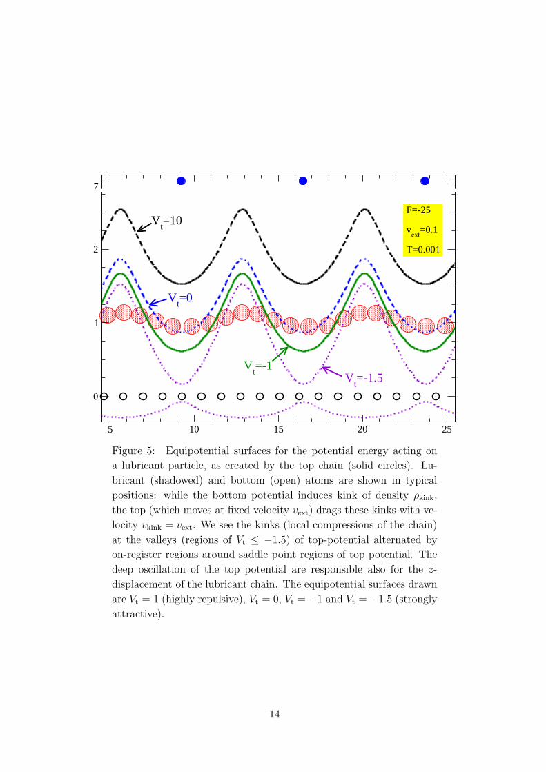
Figure 5: Equipotential surfaces for the potential energy acting on

a lubricant particle, as created by the top chain (solid circles). Lu-

bricant (shadowed) and bottom (open) atoms are shown in typical

positions: while the bottom potential induces kink of density ρkink,

the top (which moves at fixed velocity vext) drags these kinks with ve-

locity vkink = vext. We see the kinks (local compressions of the chain)

at the valleys (regions of Vt ≤ −1.5) of top-potential alternated by

on-register regions around saddle point regions of top potential. The

deep oscillation of the top potential are responsible also for the z-

displacement of the lubricant chain. The equipotential surfaces drawn

are Vt = 1 (highly repulsive), Vt = 0, Vt = −1 and Vt = −1.5 (strongly

attractive).

14

0.001 0.01 0.1 1 10 100v

ext

0

0.05

0.1

0.15

0.2

<v cm

>/v

ext

6.25 6.5 6.75 7v

ext

0

0.05

0.1

0.15

0.2

<v cm

>/v

ext

4-29-258-58-50

F=-25

T=0.001

wplat

wplat

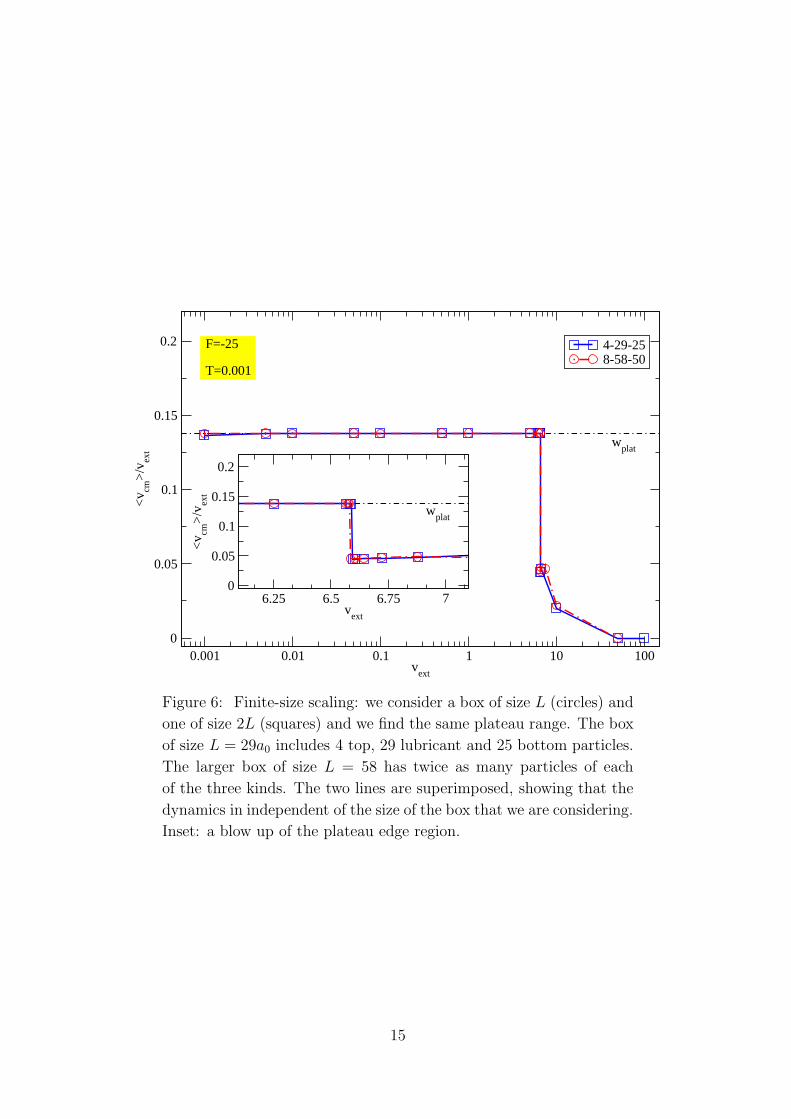
Figure 6: Finite-size scaling: we consider a box of size L (circles) and

one of size 2L (squares) and we find the same plateau range. The box

of size L = 29a0 includes 4 top, 29 lubricant and 25 bottom particles.

The larger box of size L = 58 has twice as many particles of each

of the three kinds. The two lines are superimposed, showing that the

dynamics in independent of the size of the box that we are considering.

Inset: a blow up of the plateau edge region.

15

0.0001 0.001 0.01 0.1 1 10 100 1000- F

0.125

0.15

<v cm

>/v

ext

T=0.001T=0.01T=0.1T=0.125

vext

=0.1

Nlayer

=1

wplat

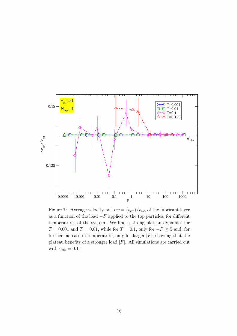
Figure 7: Average velocity ratio w = 〈vcm〉/vext of the lubricant layer

as a function of the load −F applied to the top particles, for different

temperatures of the system. We find a strong plateau dynamics for

T = 0.001 and T = 0.01, while for T = 0.1, only for −F ≥ 5 and, for

further increase in temperature, only for larger |F |, showing that the

plateau benefits of a stronger load |F |. All simulations are carried out

with vext = 0.1.

16

creation of kinks (or solitons), essentially local compressions of the lubricant chain

with the bottom substrate potential minima holding more than one particle, see

Fig. 4. As Fig. 5 shows, kinks pin to the minima of the top potential [7]. The

kink density is

ρkink =1

a0

δ

rb

=1

a0

(rb − 1)

rb

=1

a0

(

1 −1

rb

)

. (19)

The top-layer, with its slowly oscillating potential, tends to drag the kinks along

at the full speed vkink = vext. If ρ0 = 1/a0 is the linear density of the lubricant

particles, mass transport will obey vcm ρ0 = vkink ρkink; this yields

wplat =vcm

vext

=ρkink

ρ0

= 1 −1

rb

. (20)

The exact plateaus arise precisely when the top substrate drags the kinks at its

own full speed vext. For the length ratios of the present simulations, wplat =

4/29 ≃ 0.137931.

As shown in Fig. 3, we find robust plateaus for a wide range of vext and for

a wide range of temperature. There is evidence [3] that the plateau dynamics

should extend to the limit vext → 0, but it would take huge simulation time to

prove within the present model. Indeed, error bars indicate increasing relative

uncertainty in the determination of w for lower values of vext. For the large

T = 0.5 we do not find any plateau dynamics: this temperature is close to

melting temperature of the LJ solid [8] and the liquid lubricant does not show

the plateau phenomenon. Finite-size scaling, Fig. 6, shows no size effect on the

plateau boundary.

We find strong plateaus also for a wide range of load F , as shown in Fig. 7:

at low temperature we find a plateau for all the values that we consider (it would

become difficult investigate lower or greater load values because the simulation

time would increase greatly). At large temperature, higher load is beneficial to

the plateau state.

4.2 Two Lubricant Layers and Varied Kink Coverage

In the present Section, we check whether the plateau dynamics survives the pres-

ence of two layers. Figure 8 shows the typical arrangement of lubricant particles

relative to the substrates in a lubricant double-layer configuration: we can still

identify solitons, created by the bottom layer potential, in the lower chain, and,

like for the one layer, the solitons pinned at the minima of the top potential,

as in Fig. 5 for the one-layer model; the atoms of the upper lubricant layer are

17

0 5 10 15 20 25 30

0

1

2

8

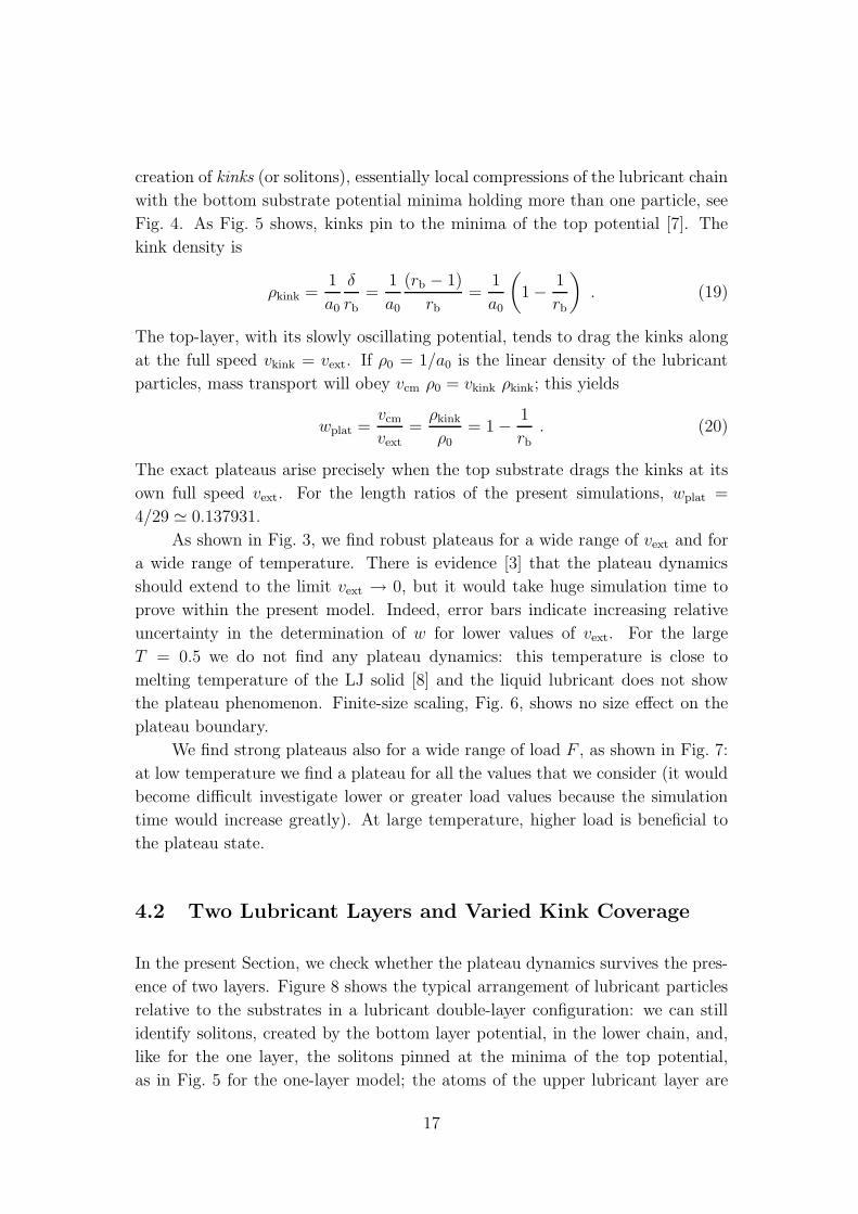
Figure 8: A sketch of the double-layer model with the top (solid

circles), the lubricant (shadowed) and the bottom atoms (open). With

the chosen radius of open circles, solitons are apparent as touching

circles. Note that for both layers solitons arise at the same positions

as in the single lubricant layer, namely near the minima of the top

potential, midway between top-layer atoms.

almost equispaced. The vertical displacement for both layers is induced by the

interactions with the top layer atoms.

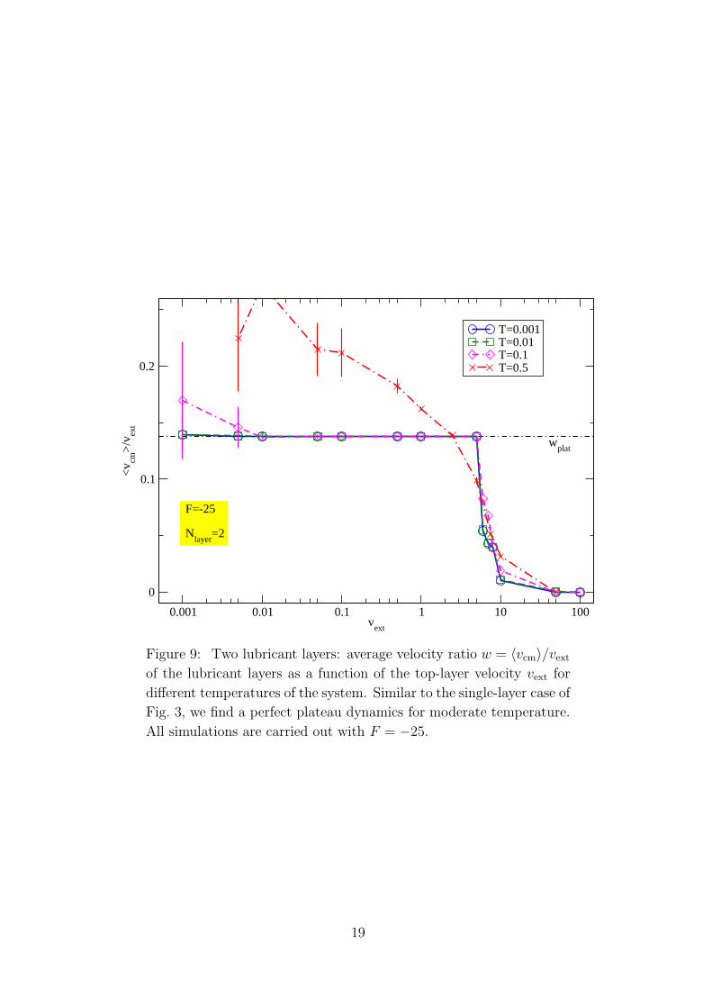
As hinted at by Fig. 8 and shown in detail by Fig. 9, we do indeed find

perfect plateau dynamics like for one lubricant chain. Thermal effects again act

to destroy the plateau.

Until this point, we have chosen a situation of full commensuration of the

number of kinks Nkink = ρkinkL to the number of top-atoms Nt. This is an

especially favorable configuration for kink dragging, thus for the plateau phe-

nomenon. It is then necessary to investigate situations where this full com-

mensuration is broken. As an example of non-full commensuration, we consider

5, rather than 4, particles in the top chain, thus producing a coverage ratio

Θ = Nkink

Nt=(

1 − 1rb

)

rt = 45

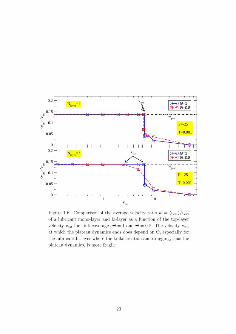
= 0.8. As shown in Fig. 10, strong plateaus occur

also for Θ = 0.8, both in a lubricant mono-layer and in a bi-layers. In both calcu-

lations we find a difference between the critical velocity vcrit at which the plateau

ends. This difference is small for a single lubricant layer, while for two layers the

plateau dynamics turns more fragile for a situation of imperfect commensuration

Θ = 0.8 than in the fully-commensurate case.

It is extremely instructive to study how vcrit varies when the ratio of com-

mensuration Θ varies. We leave rb, thus the density of solitons ρkink unchanged,

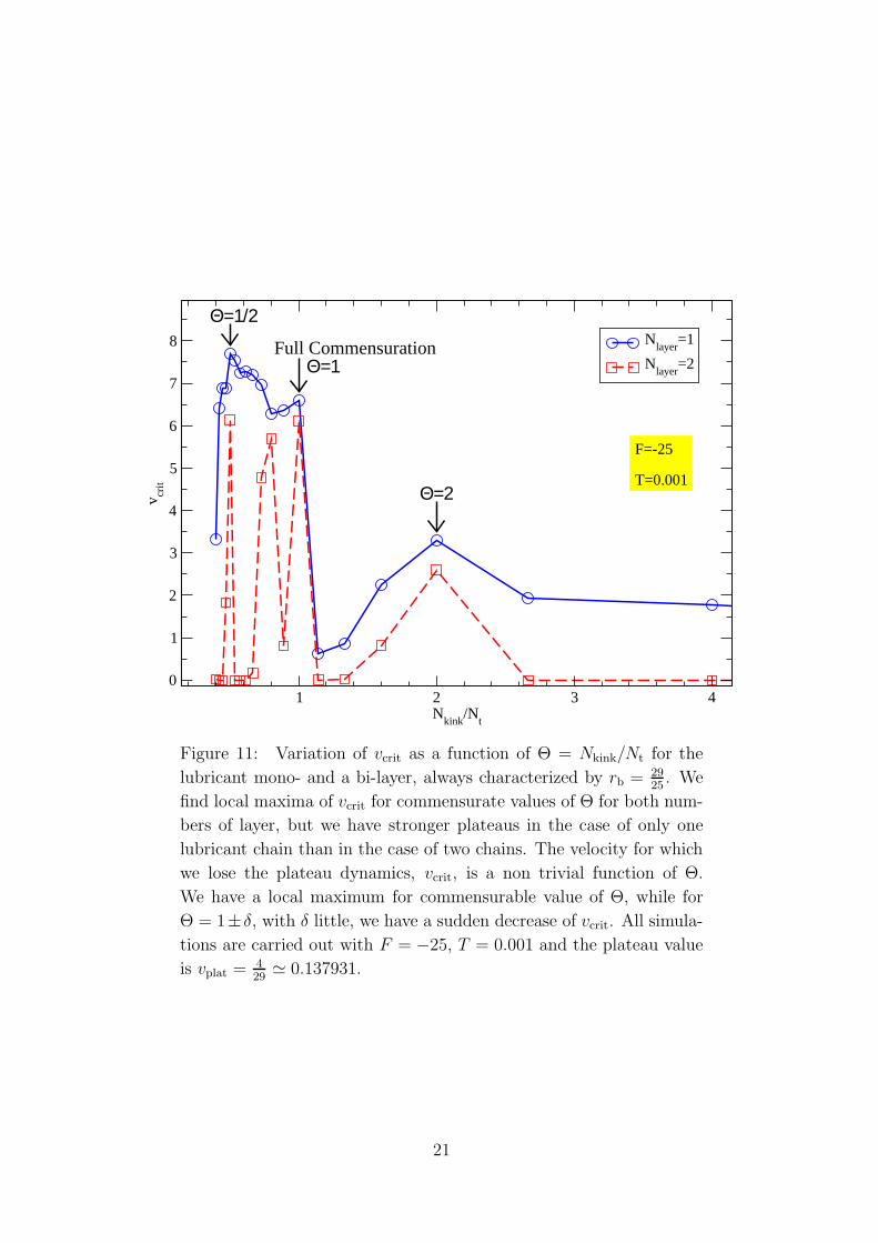
while we change the number of particles in the top substrate. In Fig. 11, we plot

the unpinning velocity vcrit as a function of the commensuration ratio Θ. We find

18

0.001 0.01 0.1 1 10 100v

ext

0

0.1

0.2

<v cm

>/v

ext

T=0.001T=0.01T=0.1T=0.5

F=-25

Nlayer

=2

wplat

Figure 9: Two lubricant layers: average velocity ratio w = 〈vcm〉/vext

of the lubricant layers as a function of the top-layer velocity vext for

different temperatures of the system. Similar to the single-layer case of

Fig. 3, we find a perfect plateau dynamics for moderate temperature.

All simulations are carried out with F = −25.

19

1 10v

ext

0

0.05

0.1

0.15

0.2

<v cm

>/v

ext

Θ=1Θ=0.8

0

0.05

0.1

0.15

0.2

<v cm

>/v

ext

Θ=1Θ=0.8

F=-25

T=0.001

wplat

wplat

F=-25

T=0.001

vcritN

layer=2

Nlayer

=1v

crit

Figure 10: Comparison of the average velocity ratio w = 〈vcm〉/vext

of a lubricant mono-layer and bi-layer as a function of the top-layer

velocity vext for kink coverages Θ = 1 and Θ = 0.8. The velocity vcrit

at which the plateau dynamics ends does depend on Θ, especially for

the lubricant bi-layer where the kinks creation and dragging, thus the

plateau dynamics, is more fragile.

20

1 2 3 4N

kink/N

t

0

1

2

3

4

5

6

7

8

v crit

Nlayer

=1

Nlayer

=2

F=-25

T=0.001

Full CommensurationΘ=1

Θ=1/2

Θ=2

Figure 11: Variation of vcrit as a function of Θ = Nkink/Nt for the

lubricant mono- and a bi-layer, always characterized by rb = 2925

. We

find local maxima of vcrit for commensurate values of Θ for both num-

bers of layer, but we have stronger plateaus in the case of only one

lubricant chain than in the case of two chains. The velocity for which

we lose the plateau dynamics, vcrit, is a non trivial function of Θ.

We have a local maximum for commensurable value of Θ, while for

Θ = 1±δ, with δ little, we have a sudden decrease of vcrit. All simula-

tions are carried out with F = −25, T = 0.001 and the plateau value

is vplat = 429

≃ 0.137931.

21

0.001 0.01 0.1 1 10v

ext

0

0.05

0.1

0.15

0.2

<v cm

>/v

ext

Fpart

=-25

T=0.001

Θ=1

wplat

1 Layer2 Layers

4 Layers

3 Layers

6 Layers5 Layers

8 Layers7 Layers

9 Layers10 Layers

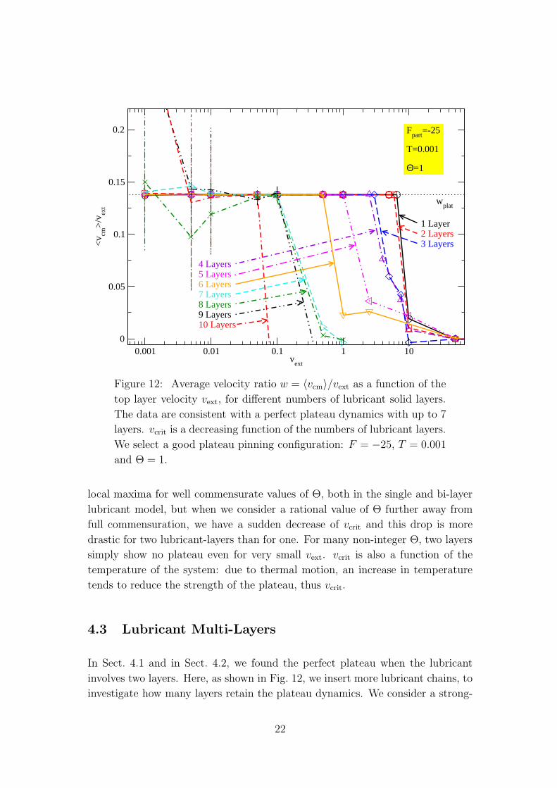
Figure 12: Average velocity ratio w = 〈vcm〉/vext as a function of the

top layer velocity vext, for different numbers of lubricant solid layers.

The data are consistent with a perfect plateau dynamics with up to 7

layers. vcrit is a decreasing function of the numbers of lubricant layers.

We select a good plateau pinning configuration: F = −25, T = 0.001

and Θ = 1.

local maxima for well commensurate values of Θ, both in the single and bi-layer

lubricant model, but when we consider a rational value of Θ further away from

full commensuration, we have a sudden decrease of vcrit and this drop is more

drastic for two lubricant-layers than for one. For many non-integer Θ, two layers

simply show no plateau even for very small vext. vcrit is also a function of the

temperature of the system: due to thermal motion, an increase in temperature

tends to reduce the strength of the plateau, thus vcrit.

4.3 Lubricant Multi-Layers

In Sect. 4.1 and in Sect. 4.2, we found the perfect plateau when the lubricant

involves two layers. Here, as shown in Fig. 12, we insert more lubricant chains, to

investigate how many layers retain the plateau dynamics. We consider a strong-

22

5 10 15 20 25

0

1

2

3

4

5

6

10.5

Vt=10

Vt=0

Vt=-1

Vt=-1.5

vext

=0.1

T=0.001

Vt=-1

Vb=-1 V

b=-1.5

Vb=10 V

b=0

1st

2nd

3rd

4th

5th

F=-25

Nlayer

=5

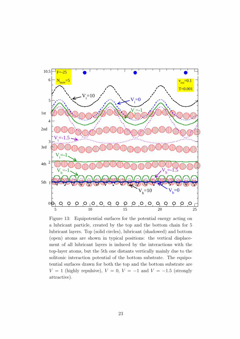
Figure 13: Equipotential surfaces for the potential energy acting on

a lubricant particle, created by the top and the bottom chain for 5

lubricant layers. Top (solid circles), lubricant (shadowed) and bottom

(open) atoms are shown in typical positions: the vertical displace-

ment of all lubricant layers is induced by the interactions with the

top-layer atoms, but the 5th one distants vertically mainly due to the

solitonic interaction potential of the bottom substrate. The equipo-

tential surfaces drawn for both the top and the bottom substrate are

V = 1 (highly repulsive), V = 0, V = −1 and V = −1.5 (strongly

attractive).

23

5 10 15 20 250

1

2

3

4

5

6

7

8

9

13.5

Vt=10

Vt=0

Vt=-1

Vt=-1.5

F=-25

Nlayer

=9

vext

=0.1

T=0.001

Vt=-1

Vb=-1 V

b=-1.5

Vb=10 V

b=0

1st

2nd

3rd

4th

5th

6th

7th

8th

9th

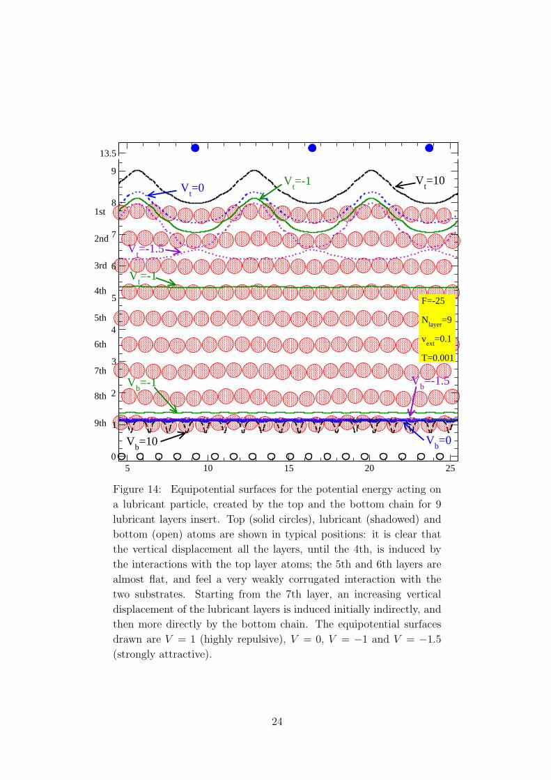
Figure 14: Equipotential surfaces for the potential energy acting on

a lubricant particle, created by the top and the bottom chain for 9

lubricant layers insert. Top (solid circles), lubricant (shadowed) and

bottom (open) atoms are shown in typical positions: it is clear that

the vertical displacement all the layers, until the 4th, is induced by

the interactions with the top layer atoms; the 5th and 6th layers are

almost flat, and feel a very weakly corrugated interaction with the

two substrates. Starting from the 7th layer, an increasing vertical

displacement of the lubricant layers is induced initially indirectly, and

then more directly by the bottom chain. The equipotential surfaces

drawn are V = 1 (highly repulsive), V = 0, V = −1 and V = −1.5

(strongly attractive).

24

pinning condition: full kink commensuration Θ = 1 with F = −25 and T = 0.001

in order to find the maximum possible number of layers capable to produce

a quantized plateau velocity of the solid lubricant chain; we expect that for a

weaker-pinning configuration, we should find weaker velocity plateaus compared

to those that we find here. As shown in Fig. 13, the vertical displacement of the

upper lubricant-layer atoms are induced by the interactions with the top layer

particles, while the displacement of the lower one is induced by the potential of

the bottom substrate. Although only the lowest layers interact with the bottom

layer, responsible for the creation of kinks, we find a perfect plateau, at least in

the limit of low vext. The cause of the z-displacement of the lubricant atoms is

more evident in Fig. 14: until 4th layer, the vertical corrugation is induced by the

potential of the top chain; the 5th layer is almost flat, as both the substrates are

too far, their interaction with their corrugation is negligible; from the 6th layer,

the chain starts to be corrugated by elastic interaction with the lubricant chain

immediately below. Only the z-displacement of the 9th layer is induced directly

by the bottom substrate. In a multi-layers model the solitons are created only

in few layers closer to the bottom, while the atoms of the other lubricant layer

are essentially equispaced. In a plateau-dynamics case, as shown in Fig. 13 the

top potential and the above layers reach in and drag these solitons, while for a

non-plateau case, as shown in Fig. 14, the top potential cannot move the solitons

at the right velocity vext.

Figure 12 shows the progressive shift of vcrit to smaller values, as the num-

ber of layers increases. For several lubricant chains (up to Nlayer = 7), we find

perfect velocity plateaus with a decreasing vcrit as a function of the number of

layers Nlayer. For a further increase in Nlayer, the top-chain slides over the higher

lubricant-layer and the deeper layers experience only a small perturbation, cre-

ated by the top-potential, that cannot drag the kinks created by the bottom

potential. For Nlayer > 7, the relaxation times become larger and larger, thus, to

make simulations converge, we need longer time of simulations; this is the cause

of the rather large error bars shown in Fig. 12. Even for large vext, the positions of

lubricant atoms are essentially ordered and we do not find a liquid configuration,

due to both the low temperature of the simulation and the full commensuration.

Note that confined-induced layering and solidification is demonstrate experimen-

tally in Ref. [9] for a few molecularly layers (tipically 7, after that the lubricant

becomes liquid) and analyzed theoretically in Ref. [10]. It is indeed reasonable

that for a larger number of Nlayer and even for a low vext, the top layer should not

able to drag the a kinks produced by the bottom and thus the plateau dynam-

ics disappears. Besides, as always (Fig. 3), for high temperatures, the thermal

excitations make the plateau weaker.

25

4.4 Anti-Kinks

In the rest of Sect. 4, we set a condition of quasi-commensuration of the chain

to the ab substrate, rb = 1 + δ = 1.16, with a kink density ρkink ≃ 4/29a−10 =

0.137930 a−10 . Here we consider a reversed quasi-commensurate condition that

induces a kinks density ρkink = −4/21a−10 ≃ −0.190476 a−1

0 . A positive ρkink > 0,

induces the formation of kinks, while a negative ρkink < 0 produces local dilata-

tions of the chain, called anti-kinks, alternated to in-register regions. The anti-

kinks are dragged forward at the full speed vext, since they pin to the minima

of the top potential. As anti-kinks are missing particles, like holes in semicon-

ductors, their rightward motion produces a net leftward motion of the lubricant:

the lubricant chain moves in the opposite direction with respect to the top layer.

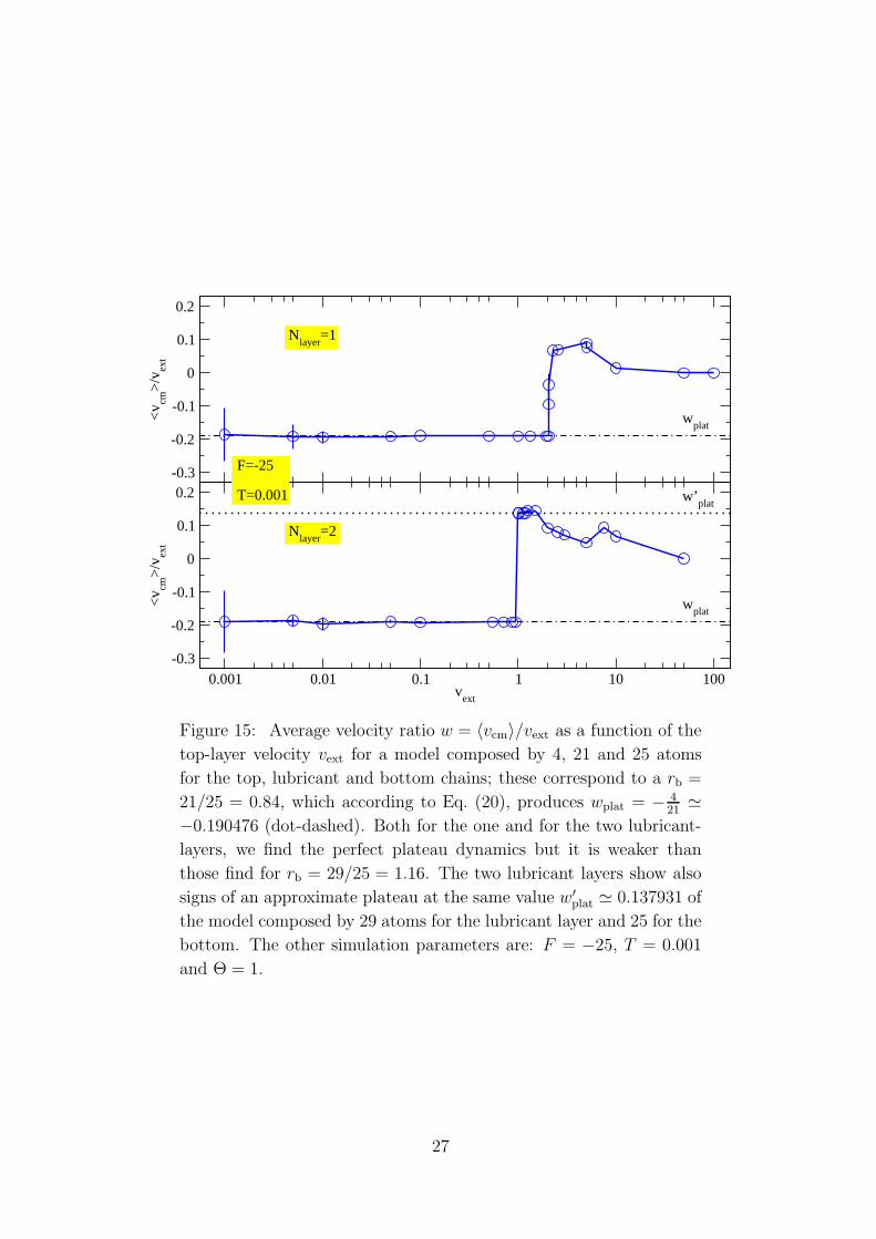
As shown in Fig. 15, we find a clear reversed-velocity (wplat = − 421

= −0.190476

plateau for the one-layer model). This plateau is comparably weaker, and ends at

a small vext than the plateau, produces by rb > 1, and shown in Fig. 3. Also two

lubricant layers produce the reversed plateau at the same value of wplat, but we

find some evidence of another plateau for w′plat = 4/29, that corresponds to a dis-

tance between two adjacent bottom atoms rb = 1.16, i.e. the kink configuration

of all previous calculations.

5 Hysteresis

We come to study the exciting bistable, hysteretic behavior found at the edge of

the plateau, already found in the 1D Frenkel-Kontorova model [3, 11, 12]. We

focus on the fully-commensurate Θ = 1, and on the strongly-pinning configuration

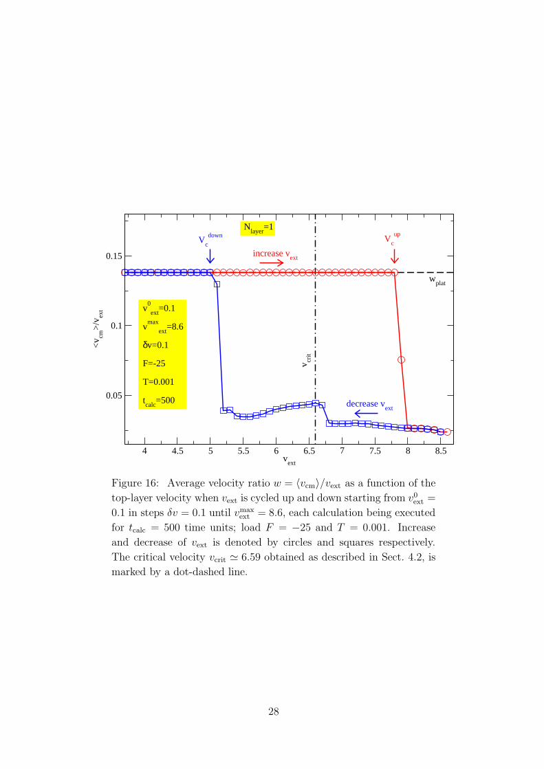
of parameters: F = −25, T = 0.001. Figure 16 depicts one typical such loop,

obtained by cycling up and down vext in small steps, in each of which the system is

let evolve for tcalc time units; at the next step the integration starts from the end

points and velocities of the previous step, rather than from scratch as in previous

Sections. The hysteretic loop is due to the meta-stable nature of the plateau

state, and the finite simulation time tcalc being insufficient to reach its dynamic

equilibrium state, such as the system is unlikely to fluctuate enough to overcome

thermally a potential barrier; if tcalc was infinite, the system would overcome this

barrier, and jump into the dynamically favored state (the plateau state below vcrit

and the unpinned state above vcrit): no hysteretic loop would then appear. Of

course, by increasing thermal energy even in the modest simulation times some

fluctuation is likely to occur and flip the state: the hysteretic loop shrinks and

26

-0.3

-0.2

-0.1

0

0.1

0.2

<v cm

>/v

ext

wplat

0.001 0.01 0.1 1 10 100v

ext

-0.3

-0.2

-0.1

0

0.1

0.2

<v cm

>/v

ext

wplat

w’plat

F=-25

T=0.001

Nlayer

=1

Nlayer

=2

Figure 15: Average velocity ratio w = 〈vcm〉/vext as a function of the

top-layer velocity vext for a model composed by 4, 21 and 25 atoms

for the top, lubricant and bottom chains; these correspond to a rb =

21/25 = 0.84, which according to Eq. (20), produces wplat = − 421

≃

−0.190476 (dot-dashed). Both for the one and for the two lubricant-

layers, we find the perfect plateau dynamics but it is weaker than

those find for rb = 29/25 = 1.16. The two lubricant layers show also

signs of an approximate plateau at the same value w′plat ≃ 0.137931 of

the model composed by 29 atoms for the lubricant layer and 25 for the

bottom. The other simulation parameters are: F = −25, T = 0.001

and Θ = 1.

27

4 4.5 5 5.5 6 6.5 7 7.5 8 8.5v

ext

0.05

0.1

0.15

<v cm

>/v

ext

increase vext

decrease vext

wplat

v crit

Vc

upV

c

down

v0

ext=0.1

vmax

ext=8.6

δv=0.1

F=-25

T=0.001

tcalc

=500

Nlayer

=1

Figure 16: Average velocity ratio w = 〈vcm〉/vext as a function of the

top-layer velocity when vext is cycled up and down starting from v0ext =

0.1 in steps δv = 0.1 until vmaxext = 8.6, each calculation being executed

for tcalc = 500 time units; load F = −25 and T = 0.001. Increase

and decrease of vext is denoted by circles and squares respectively.

The critical velocity vcrit ≃ 6.59 obtained as described in Sect. 4.2, is

marked by a dot-dashed line.

28

5.5 6 6.5 7 7.5 8 8.5v

ext

0.05

0.1

0.15

<v cm

>/v

ext

0.05

0.1

0.15

<v cm

>/v

ext

wplat

Vc

up

decrease vext

F=-25

T=0.1increase v

ext

Vc

down

wplat

Vc

up

increase vext

decrease vext

v crit

Vc

down

tcalc

=1000

tcalc

=100

b)

a)

One Lubricant-Layer

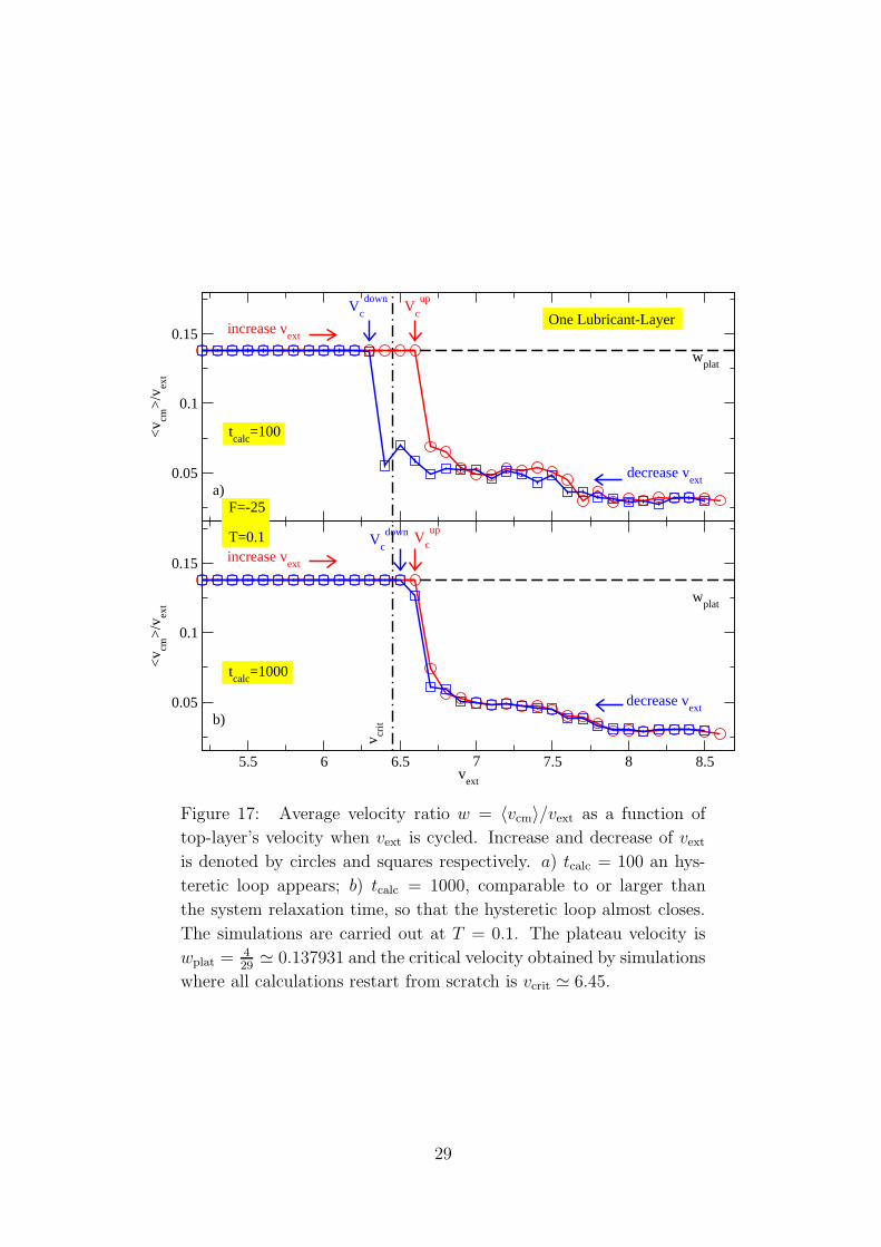
Figure 17: Average velocity ratio w = 〈vcm〉/vext as a function of

top-layer’s velocity when vext is cycled. Increase and decrease of vext

is denoted by circles and squares respectively. a) tcalc = 100 an hys-

teretic loop appears; b) tcalc = 1000, comparable to or larger than

the system relaxation time, so that the hysteretic loop almost closes.

The simulations are carried out at T = 0.1. The plateau velocity is

wplat = 429

≃ 0.137931 and the critical velocity obtained by simulations

where all calculations restart from scratch is vcrit ≃ 6.45.

29

4 4.5 5 5.5 6 6.5 7 7.5 8 8.5v

ext

0.05

0.1

0.15

<v cm

>/v

ext

wplat

v crit

Vc

upV

c

down

v0

ext=0.1

vmax

ext=8.6

F=-25

T=0.001

tcalc

=500

increase vext

decrease vext

Nlayer

=2

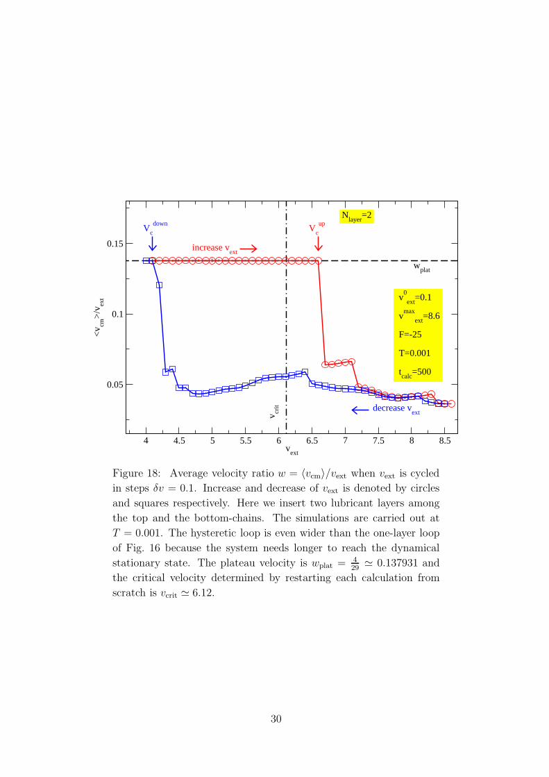
Figure 18: Average velocity ratio w = 〈vcm〉/vext when vext is cycled

in steps δv = 0.1. Increase and decrease of vext is denoted by circles

and squares respectively. Here we insert two lubricant layers among

the top and the bottom-chains. The simulations are carried out at

T = 0.001. The hysteretic loop is even wider than the one-layer loop

of Fig. 16 because the system needs longer to reach the dynamical

stationary state. The plateau velocity is wplat = 429

≃ 0.137931 and

the critical velocity determined by restarting each calculation from

scratch is vcrit ≃ 6.12.

30

eventually closes.

Within these theoretical limitations, in practice at not too large temperature

(e.g. T = 0.001 as in Fig. 16), for any practically conceivable simulation time the

hysteretic plateau boundary is a very clear reality: the plateau dynamics is only

abandoned above a critical velocity vupc > vcrit; when vext is reduced back, the

depinned state survives below vcrit to a smaller vdownc < vcrit where the plateau

dynamics is retrieved. Due to the reasons mentioned above, the detailed values

of vupc and vdown

c are functions of tcalc (beside the physical model parameters), but

in practice a very slowly varying function.

Figure 17 shows the hysteretic loop for two simulations carried out at the

same conditions as for Fig. 16, except for a comparably large temperature T = 0.1,

and with different duration of each velocity increase step, in panel (a) with tcalc =

100 and in (b) with tcalc = 1000: in Fig. 17b, the time of each simulation is ten

times larger than that of Fig. 17a, so that each simulation has a larger probability

to decay from the meta-stable state and reach the dynamical stationary state most

suitable for that value of vext. The hysteresis loop that appearing in a T = 0.1-

simulations is narrower than that of T = 0.001 because wider and more frequent

thermal fluctuations. Figure 18 shows an hysteretic loop also for two lubricant

layers: the hysteresis is even wider than for one layer, indicating higher energy

barriers and layer relaxation times than for one layer.

6 Analysis of the Fluctuations

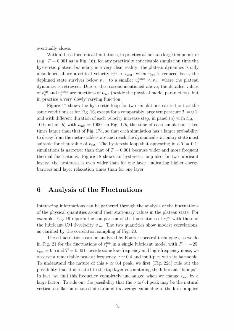
Interesting informations can be gathered through the analysis of the fluctuations

of the physical quantities around their stationary values in the plateau state. For

example, Fig. 19 reports the comparison of the fluctuations of rtopz with those of

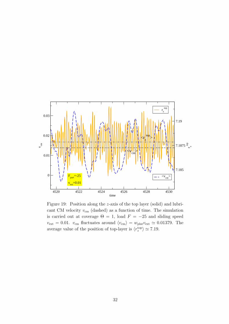
the lubricant CM x-velocity vcm. The two quantities show modest correlations,

as clarified by the correlation sampling of Fig. 20.

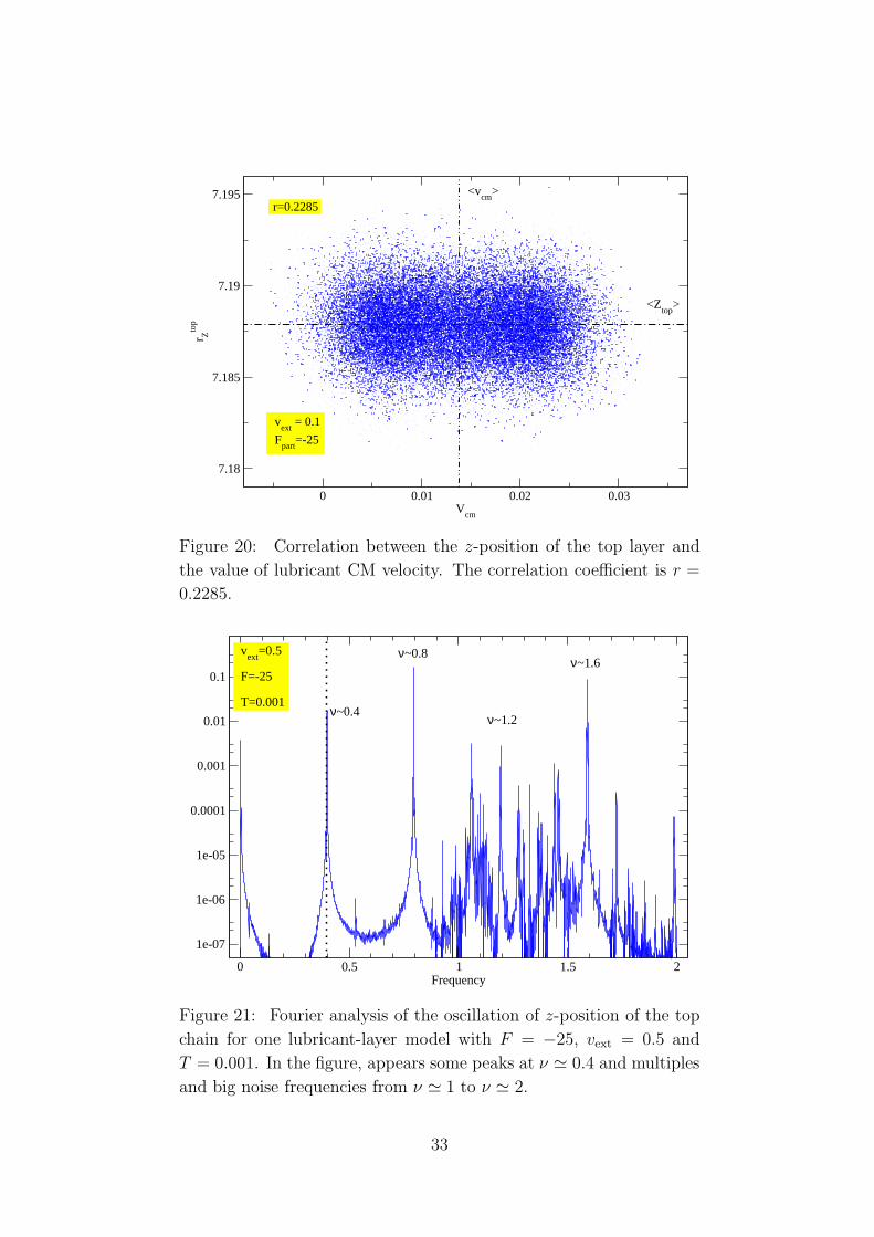
These fluctuations can be analyzed by Fourier spectral techniques, as we do

in Fig. 21 for the fluctuations of rtopz in a single lubricant model with F = −25,

vext = 0.5 and T = 0.001: beside some low-frequency and high-frequency noise, we

observe a remarkable peak at frequency ν ≃ 0.4 and multiples with its harmonic.

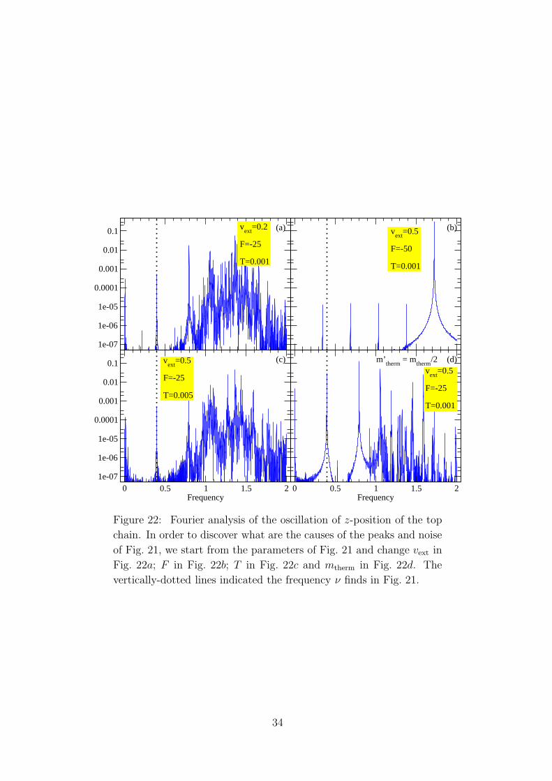
To understand the nature of this ν ≃ 0.4 peak, we first (Fig. 22a) rule out the

possibility that it is related to the top layer encountering the lubricant ”bumps”.

In fact, we find this frequency completely unchanged when we change vext by a

large factor. To rule out the possibility that the ν ≃ 0.4 peak may be the natural

vertical oscillation of top chain around its average value due to the force applied

31

7.185

7.1875

7.19

r ztop

rz

top

4520 4522 4524 4526 4528 4530time

0

0.01

0.02

0.03

v cm

<vcm

>

<vcm

>

<rz

top>

Fpart

=-25

vext

=0.01

Figure 19: Position along the z-axis of the top layer (solid) and lubri-

cant CM velocity vcm (dashed) as a function of time. The simulation

is carried out at coverage Θ = 1, load F = −25 and sliding speed

vext = 0.01. vcm fluctuates around 〈vcm〉 = wplatvext ≃ 0.01379. The

average value of the position of top-layer is 〈rtopz 〉 ≃ 7.19.

32

0 0.01 0.02 0.03V

cm

7.18

7.185

7.19

7.195r Z

top

<Ztop

>

<vcm

>

vext

= 0.1

Fpart

=-25

r=0.2285

Figure 20: Correlation between the z-position of the top layer and

the value of lubricant CM velocity. The correlation coefficient is r =

0.2285.

0 0.5 1 1.5 2Frequency

1e-07

1e-06

1e-05

0.0001

0.001

0.01

0.1

ν~0.4

ν~0.8ν~1.6

ν~1.2

vext

=0.5

F=-25

T=0.001

Figure 21: Fourier analysis of the oscillation of z-position of the top

chain for one lubricant-layer model with F = −25, vext = 0.5 and

T = 0.001. In the figure, appears some peaks at ν ≃ 0.4 and multiples

and big noise frequencies from ν ≃ 1 to ν ≃ 2.

33

1e-07

1e-06

1e-05

0.0001

0.001

0.01

0.1

0 0.5 1 1.5 2Frequency

1e-07

1e-06

1e-05

0.0001

0.001

0.01

0.1

0 0.5 1 1.5 2Frequency

(a) vext

=0.5

F=-50

T=0.001

vext

=0.5

F=-25

T=0.001

vext

=0.5

F=-25

T=0.005

vext

=0.2

F=-25

T=0.001

(b)

(d)(c) m’therm

= mtherm

/2

Figure 22: Fourier analysis of the oscillation of z-position of the top

chain. In order to discover what are the causes of the peaks and noise

of Fig. 21, we start from the parameters of Fig. 21 and change vext in

Fig. 22a; F in Fig. 22b; T in Fig. 22c and mtherm in Fig. 22d. The

vertically-dotted lines indicated the frequency ν finds in Fig. 21.

34

1e-07

1e-06

1e-05

0.0001

0.001

0.01

0.1rxj

rzj

7

8

9

10

11

12

13

14

r xj

800 810 820 830 840 850 860 870time

2.5

3

3.5

4

4.5

5

5.5

r xj

0 0.25 0.5 0.75 1Frequency

1e-07

1e-06

1e-05

0.0001

0.001

0.01

0.1

rxj

rzj

(a)

vext

=0.2

F=-25

T=0.005

vext

=0.5

F=-25

T=0.001

(b)

(d)(c)

j-part(j+1)-part

j-part (j+1)-part

ν’~0.059 ν~0.4

ν’’~0.023 ν~0.4

t~1/0.4~2.5

t’’~1/0.023~43.5

t~1/0.4~2.5

t’~1/0.059~16.9

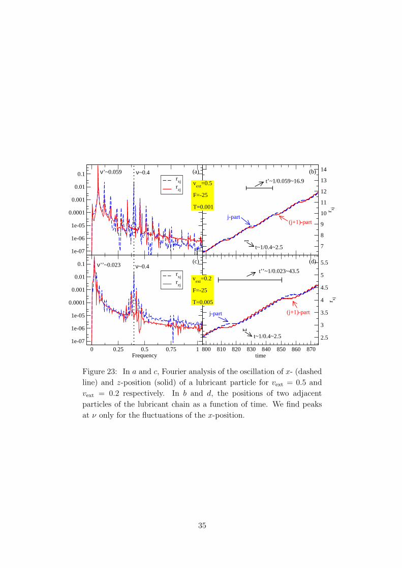
Figure 23: In a and c, Fourier analysis of the oscillation of x- (dashed

line) and z-position (solid) of a lubricant particle for vext = 0.5 and

vext = 0.2 respectively. In b and d, the positions of two adjacent

particles of the lubricant chain as a function of time. We find peaks

at ν only for the fluctuations of the x-position.

35

over the top and to the repulsive forces of potentials (1), in Fig. 22b we increase F

by a factor 2 and find the same peaks of Fig. 21 shifted to a slightly lower (rather

than higher!) frequency ν ≃ 0.345 and its multiples. We also rule out that there

is an unphysical oscillation related to energy exchange with the Nose-Hoover

thermostat, by changing the temperature T of the simulation (Fig. 22c), or the

mass of the thermostat mtherm, tuning the thermostat responsiveness (Fig. 22d):

no significant changes relative to Fig. 21. We obtain some insight about the

physical nature of the ν ≃ 0.4 by analyzing the fluctuations of the x- and z-

positions of a generic particle j of the lubricant chain. As shown in Fig. 23a

(solid line), the x motion contains the same frequency ν ≃ 0.4 as rtopz (Fig. 21)

plus a peak at ν ′ ≃ 0.059. ν ′ is related to the period T ′ ≃ 16.96 between two

stops of Fig. 23b, while the frequency ν ≃ 0.4 is linked with the rapid oscillations

that elapse between successive stops. The stop marks the moment when the

particle fits in between two atoms of the bottom substrate, while the stairway

part indicates the interval when a particle belongs to a kink. Comparing two

adjacent particles (Fig. 23b and d), we see that their x-movement is in phase,

thus indicating acoustic modes. Compare Fig. 23a and b (vext = 0.5), with

Fig. 23c and d (vext = 0.2): we see the same phonon ν ≃ 0.4, while the ν ′ shifts

to ν ′′ ≃ 0.023 (period t′′ ≃ 44.11) corresponding to the increased time interval

between successive stops. Remarkably, no sign of ν ′ is seen in the rtopz spectrum,

while the frequency ν ≃ 0.4 of a ”horizontal” lubricant vibration adds coherently

and is seen in the ”vertical” fluctuation of the top layer. The solid curves of

Fig. 23a and c shown the Fourier analysis of the z-position of the particle: we

find the same frequency ν ′ and thus the same period that elapses between two

stops, but no sign of the frequency ν, which is therefore a purely longitudinal

mode.

7 Discussion and Conclusion

Within the idealized scheme of a simple 1D Frenkel-Kontorova-like model, a spe-

cial ”quantized” sliding state was found for a solid lubricant confined between two

periodic layers [1]. This state, characterized by a nontrivial geometrically fixed

ratio of the mean lubricant drift velocity 〈vcm〉 and the externally imposed trans-

lational velocity vext, was understood as due to the kinks (or solitons), formed by

the lubricant due to incommensuration with one of the substrates, pinning to the

other sliding substrate.

In the present work, a quantized sliding state of the same nature is demon-

36

strated for a substantially less idealized 2D model, where atoms are allowed to

move perpendicularly to the sliding direction and interact via Lennard-Jones po-

tentials. At first, we analyze the single lubricant layer model for varied driving

speed vext and we find perfect plateaus, at the same geometrically determined

velocity ratio wplat as observed in the simple 1D model, not only at low tem-

peratures, but also for temperatures not too far from a melting point of the LJ

lubricant. An increased load-F is beneficial to the plateau state at high tem-

perature. The velocity plateau, as a function of vext, ends at a critical velocity

vcrit, and for vext > vcrit the lubricant moves at a speed which is generally lower

than that of the plateau state. In fact, by cycling vext, the layer sliding velocity

exhibits an hysteretic loop around vcrit. For a bi-layer model, we find very similar

results as for one layer. The unpinning velocity vcrit is linked to the rate of com-

mensuration Θ: local maxima are located at well-commensurate Θ values. The

plateau dynamics is found even with a confined solid lubricant composed of mul-

tiple (up to 7) lubricant layers: the strength of the plateau (measured by vcrit) is

a decreasing function of the number of layers. Characteristic backward lubricant

motion produced by the presence of ”anti-kinks” is also shown in this context.

The present work focuses on ordered configurations: both substrate are perfect

crystals and the lubricant retains the configuration of a strained crystalline solid.

It will be the object of future investigation the role of disorder both in the sub-

strate [13] and in the lubricant. The analysis of friction itself and the significance

of fluctuations in the dynamical properties will also require further study.

37

References

[1] N. Manini, M. Cesaratto, G. E. Santoro, E. Tosatti, and A. Vanossi, J. Phys.:

Condens. Matter 19, 305016 (2007).

[2] A. Vanossi, N. Manini, G. Divitini, G. E. Santoro and E. Tosatti, Phys. Rev.

Lett. 97, 056101 (2006).

[3] N. Manini, G. E. Santoro, E. Tosatti, and A. Vanossi, Phys. Rev. E 76,

046603 (2007).

[4] D. Frenkel and B. Smit, Understanding Molecular Simulation. From Algo-

rithms to Applications (Academic Press, 1996).

[5] G. J. Martyna, M. L. Klein and M. Tuckerman, J. Chem. Phys. 97, 2635

(1992).

[6] W. H. Press, S. A. Teukolsky, W. T. Vetterling and B. P. Flannery, Numerical

Recipes in Fortran. The Art of Parallel Scientific Computing (Cambridge

University Press, 1996).

[7] O. M. Braun and Y. S. Kivshar, The Frenkel-Kontorova Model: Concepts,

Methods, and Applications (Springer-Verlag, Berlin, 2004).

[8] S. Ranganathan and K. N. Pathak, Phys. Rev. A 45, 5789 (1992).

[9] J. Klein and E. Kumacheva, J. Chem. Phys. 108, 6996 (1998).

[10] B. N. J. Persson, Surf. Sci. Rep. 33, 83 (1999).

[11] A. Vanossi, G. E. Santoro, N. Manini, M. Cesaratto, and E. Tosatti, Surf.

Sci. 601, 3670 (2007).

[12] A. Vanossi, N. Manini, F. Caruso, G. E. Santoro, and E. Tosatti,

arXiv:0709.3706 [cond-mat.mtrl-sci], in print in Phys. Rev. Lett. (2007).

[13] R. Guerra, A. Vanossi, M. Ferrario, Surf. Sci. 601, 3676 (2007).

38