Thermal management model for a Plug-In Hybrid Electric Vehicle · Prof. Enrico Corti Ing. Michele...
119
ALMA MATER STUDIORUM - UNIVERSITÀ DI BOLOGNA SCUOLA DI INGEGNERIA E ARCHITETTURA DIPARTIMENTO DI INGEGNERIA INDUSTRIALE CORSO DI LAUREA MAGISTRALE IN INGEGNERIA MECCANICA TESI DI LAUREA in MOTORI A COMBUSTIONE INTERNA E PROPULSORI IBRIDI M Thermal management model for a Plug-In Hybrid Electric Vehicle CANDIDATO RELATORE: Lorenzo Morini Prof. Nicolò Cavina CORRELATORI Prof. Davide Moro Prof. Enrico Corti Ing. Michele Caggiano Ing. David Hemkemeyer Ing. Enrico Suzzani Anno Accademico 2015/2016 Sessione III
Transcript of Thermal management model for a Plug-In Hybrid Electric Vehicle · Prof. Enrico Corti Ing. Michele...

ALMA MATER STUDIORUM - UNIVERSITÀ DI BOLOGNA
SCUOLA DI INGEGNERIA E ARCHITETTURA
DIPARTIMENTO DI INGEGNERIA INDUSTRIALE
CORSO DI LAUREA MAGISTRALE IN INGEGNERIA MECCANICA
TESI DI LAUREA
in
MOTORI A COMBUSTIONE INTERNA E PROPULSORI IBRIDI M
Thermal management model for a Plug-In Hybrid
Electric Vehicle
CANDIDATO RELATORE:
Lorenzo Morini Prof. Nicolò Cavina
CORRELATORI
Prof. Davide Moro
Prof. Enrico Corti
Ing. Michele Caggiano
Ing. David Hemkemeyer
Ing. Enrico Suzzani
Anno Accademico 2015/2016
Sessione III


Ai miei genitori

i
Contents
Abstract………………………………………………………………….……...ii
List of figures………………………………...........................................……...vii
List of tables…………………………………..............................………………x
Notations……………………………………………………………………….xi
1.State of the art of thermal management for PHEV and BEV………...1
1.1 Cooling system general requirements........................................................2
1.2 Thermal management Layout for Hybrid Vehicle.....................................8
1.3 Control strategies……………………………………………………….14
1.4 Predictive thermal management……………………………………..…18
2. Introduction to the thermal model………………………………...25
2.1 Hydraulic modelling background……………………………………....25
2.2 Heat transfer theory…………………………………………………….30
3. PHEV thermal management modelling………………...................35
3.1 Scope of the model……………………………………………………...35
3.2 Description of the circuits and data available…………………………...36
3.3 PHEV Thermal management model…………………………………....38
3.3.1 Hydraulic model………………………………………………….38
3.3.2 Thermal model map-based……………………………………….45
3.3.3 Thermal model with thermal masses……………………………..64

ii
4. Results and validation…………………………………………….71
4.1 Hydraulic validation……………………………………………………71
4.2 Thermal model map-based validation…………………………………..75
4.3 Thermal model with thermal masses validation………………………...82
4.4 Validation summary …………………………………………………....91
5. Conclusions and future developments……………………….……93
Appendix……………………………………………………………………....97
Bibliography………………………………………….....................................101
Acknowledgements…………………………………………………………..103
iii
Abstract
Vehicle electrification becomes more and more important in order to reduce fuel consumption
and satisfy more restrictive emission legislations. Plug-in hybrid electric vehicles can use
energy from the grid to recharge their high voltage battery. This is converted with much higher
efficiency, and less CO2 emissions, compared to the combustion engine and so they will have
a significant role in the present transition from conventional to electric vehicles. The addition
of new components, such as power electronics, electric machine and high voltage battery,
increases the maximum torque available and the energy stored on-board, but increases the
weight as well. In addition, although they have really high efficiency, they produce a
significant amount of heat that has to be removed. To guarantee system efficiency and
reliability, a completely new thermal management layout has to be designed. Thermal
requirements of power electronics components are completely different from the ICE
requirements, much lower temperature can be accepted and higher values can request power
de-rating in order to preserve their integrity. High voltage battery is even more critic, since it
can work correctly only in a specific temperature window and outside this, it has a rapid
thermal degradation as well. The other thermal management main issue for PHEV and,
especially, for BEV is cabin heating since the engine waste heat is not more available. The
development of a vehicle thermal management model can surely help to better understand how
design the entire system. The vehicle considered is a PHEV with a P1-P4 architecture and it
has three separated cooling circuits for engine, electric machines and high voltage battery. The
model developed in the present work allows to predict coolant flow rate, pressure and
temperature for the three circuits. Firstly, the hydraulic part has been modelled, including
pumps and pressure losses characteristic curves. Secondly, the model has been completed with
the thermal description. The approach to the thermal model is simplified: for both heat sources
and heat sinks the heat exchange with the coolant is calculated from a thermal/efficiency map.
This limits its accuracy but guarantees low computational time. Globally, the model input are
powertrain parameters (engine and e-motor rotational speed and torque) plus the control
signals (for pumps, fans and HV compressor) and the output are coolant hydraulic and thermal
behavior, coolant thermal heat flows, e-motor and battery temperature.

iv
In chapter 1, a review on state of the art of PHEV and BEV thermal management has been
studied. Many different layout can be developed and different circuit integrations are studied
to reduce number of components and costs. In addition, control strategies can have a very
significant role in reduce the cooling system impact on fuel consumption. Some innovative
and predictive approaches are studied from literature. In chapter 2, basic equations that governs
a thermal-hydraulic model are reported, such as pump characteristic, pressure drops calculation
and heat transfer correlations. Chapter 3 describes how the model has been built in the software
in a detailed way. A step-by-step procedure has been followed, starting from a hydraulic model
and adding the thermal contribution only after the first part was validated. This kind of
procedure is time-consuming but allows to simplify the calibration and validation of model
parameters. In chapter 4, the main results obtained are compared to experimental data, made
available for the present work, and the model validation is evaluated. Final chapter 5 reports
the conclusions and possible future developments to complete and improve the present work.
v
Abstract in lingua italiana
L’elettrificazione dei veicoli diventerà sempre più preminente sia per ridurre i consumi sia per
soddisfare le sempre più stringenti normative sulle emissioni. I veicoli elettrici plug-in possono
utilizzare l’energia della rete per ricaricare la batteria (ad alto voltaggio). I rendimenti elettrici
caratteristici dei grossi impianti di produzione di energia elettrica sono molto più elevati di
quelli di un motore a combustione interna; ciò consente di ricaricare il veicolo riducendo le
emissioni di CO2 e dà a questo tipo di veicoli un ruolo importante nella attuale transizioni da
veicoli convenzionali a veicoli elettrici. L’aggiunta di nuovi componenti, cioè motori elettrici,
inverter e batteria ad alto voltaggio, permette di aumentare la massima coppia disponibile alle
ruote e l’energia immagazzinata a bordo, ma aumenta anche il peso della vettura. Inoltre, questi
componenti, pur avendo una efficienza molto elevata, producono una rilevante quantità di
calore che deve essere opportunamente rimossa. Al fine di garantire efficienza e affidabilità
dell’intero sistema veicolo, l’impianto di raffreddamento deve essere riprogettato. I limiti
termici dei componenti di elettronica di potenza sono completamente differenti da quelli del
motore a combustione, le temperature limite sono molto più basse e valori più elevati possono
costringere a diminuirne la potenza, al fine di preservarne l’integrità. La batteria è ancora più
critica, dato che funziona in modo ottimale solo all’interno di una specifica finestra di
temperature e all’infuori di essa ha un rapido degrado termico. Un altro importante aspetto del
thermal management per veicoli ibridi e, ancor di più, elettrici è il riscaldamento della cabina
poiché il calore di scarto del motore termico non può più essere utilizzato. Lo sviluppo di un
modello termico può certamente aiutare a progettare al meglio il completo sistema di gestione
e controllo della temperatura, visti i molteplici aspetti da considerare. Il veicolo considerato
nel presente lavoro di tesi ha un’architettura ibrida P1-P4 e comprende tre circuiti di
raffreddamento tra loro separati. Il modello permette di conoscere portata, pressioni e
temperature del refrigerante. In primo luogo, la parte idraulica è stata modellata, comprensiva
di curva caratteristica della pompa e perdite di carico. In secondo luogo, è stata inclusa la
descrizione termica. L’approccio al modello termico è semplificato, infatti sia le sorgenti
termiche che i dissipatori basano il calcolo del calore scambiato su delle mappe. Questo tipo
di approccio limita l’accuratezza del modello ma anche il tempo computazionale. L’obiettivo
principale del presente lavoro era quello di costruire un ambiente in cui successivamente

vi
sviluppare strategie di controllo di gestione termica e ciò giustifica un approccio alla
modellazione di questo tipo. Gli input del modello sono principalmente parametri legati al
powertrain (coppia e velocità di rotazione del motore termico ed elettrico) più i segnali di
controllo (per pompe elettriche, ventilatori e compressore) mentre gli output sono la
descrizione idraulica e termica del refrigerante nei tre diversi circuiti, più le temperature di
batteria e motori elettrici.
Nel capitolo 1 è riportata una descrizione dello stato dell’arte attuale riguardo al thermal
management in veicoli ibridi plug-in ed elettrici. I layout dei circuiti di raffreddamento sono
diversi e varie integrazioni sono studiate per ridurre ingombri e costi. È evidenziata anche
l’importanza delle strategie di controllo, riportando alcuni studi di strategie predittive e ottime.
Il capitolo 2 comprende una introduzione al modello e sono richiamate le equazioni di base
lato idraulico e lato termico. Nel capitolo 3 è descritto nel dettaglio lo sviluppo del modello: è
stata seguita una procedura step-by-step che da un lato richiede tempo ma dall’altro semplifica
la fase di validazione, rendendo non interdipendenti tra di loro i parametri idraulici e termici.
Nel capitolo 4 sono riportati i principali risultati ottenuti, confrontandoli con dati sperimentali
a disposizione. Viene valutata la validità e la robustezza del modello sviluppato nei diversi test
precedentemente realizzati. Infine, nel capitolo 5 sono descritte le principali conclusioni e
sottolineati possibili migliorie e sviluppi futuri.
vii
List of figures
Chapter 1
Figure 1a: Sankey diagram for gasoline internal combustion engines…………………………3
Figure 1b: Engine cooling system………………………..…………………………………….3
Figure 2: battery electric power available as function of the average temperature……………..5
Figure 3: Chevrolet Volt HV Battery Heating and Cooling System……………………………6
Figure 4: parallel hybrid possible architectures………………………………………………..8
Figure 5: general schematic of a plug-in hybrid cooling system………………………….......10
Figure 6: Range reduction of a BEV as function of cabin heating power……………………..11
Figure 7: indirect heat pump system with HV battery as heat source…………………………12
Figure 8: integrated cooling circuit for BEV with PCM storage……………………………...14
Figure 9: ADAS-ECU communication system…………………………………………….…20
Figure 10: Comparison of battery temperature for a predictive and non-predictive strategies in
a RDE cycle…………………………………………………………………………………..22
Chapter 2
Figure 11: Moody’s diagram for friction factor calculation…………………………………..26
Figure 12: pump and plant characteristic curves……………………………………………...28
Figure 13: pump losses distribution as function of the specific speed…………………….......29
Chapter 3
Figure 14: centrifugal pump component……………………………………………………...38
Figure 14a: electric pump characteristic curve……………………………………………….40
Figure 15: ideal fixed displacement hydraulic pump…………………………………………40
Figure 16: hydraulic orifice component………………………………………………………41

viii
Figure 17: inverter pressure drops, datasheet and experimental values……………………….44
Figure 18: hydraulic model for front axle circuit……………………………………………..45
Figure 19: thermal hydraulic capacity………………………………………………………..48
Figure 20: AMESim radiator block (cooling library)………………………………………...50
Figure 21: radiator heat exchanged map, function of coolant flow rate and air velocity……...51
Figure 22: power losses electric motor estimation……………………………………………52
Figure 23: engine left radiator, model and experimental data………………………………...53
Figure 24: condenser block (cooling library)…………………………………………………54
Figure 25: simplified map-based chiller model………………………………………………55
Figure 26: map-based power losses calculation for inverter and electric motor………....…...57
Figure 27a: thermal heat flows for electric motor…………………………………………….58
Figure 27b: thermal heat flows for inverter front axle………………………………………...58
Figure 28: engine power losses……………………………………………………………….60
Figure 29: comparison of engine heat rejected to coolant and engine rotational speed…….....61
Figure 30: two ways thermostat for the engine coolant circuit………………………………..62
Figure 31: battery power losses estimation and comparison with experimental results………63
Figure 32: thermal-hydraulic pipe with heat-exchange………………………………………65
Figure 33: electric motor thermal masses for temperature prediction………………………...67
Figure 34: battery cooling circuit with thermal mass…………………………………………68
Chapter 4
Figure 35a: volumetric flow rate validation for medium temperature circuit…………………72
Figure 35b: pressure validation for medium temperature circuit……………………………..73
Figure 36a: engine flow rate validation for high temperature circuit…………………………74
Figure 36b: engine pressure validation for high temperature circuit………………………….74

ix
Figure 37: engine coolant temperature, model values and measurements…………………….76
Figure 38: electric motor power losses and heat experimental coolant heat exchange………..77
Figure 39a: velocity and IPU1 current for handling electric cycle……………………………78
Figure 39b: e-motor and radiator coolant temperature………………………………………..78
Figure 40: ISG losses and experimental coolant heat exchange………………………………79
Figure 41a: velocity and ISG current for handling_corsa…………………………………….80
Figure 41b: ISG and radiator outlet coolant temperature……………………………………..80
Figure 42a: battery and chiller heat flows…………………………………………………….81
Figure 42b: battery coolant temperature for validation……………………………………….82
Figure 43a: EM power losses and coolant heat exchange calibration in hand_electric test…...83
Figure 43b: electric motor and inverter temperature calibration, handling electric…………...84
Figure 44a: electric motor power losses and coolant heat flow validation……………………85
Figure 44b: e-motor and DCDC outlet coolant temperature validation………………………86
Figure 44c: e-motor and inverter temperature validation……………………………………..86
Figure 45a: ISG power losses and coolant heat flow validation………………………………88
Figure 45b: ISG and IPU outlet coolant temperature validation……………………………...88
Figure 45c: ISG and inverter temperature validation…………………………………………89
Figure 46: battery and coolant temperature calibration……………………………………….90
Figure 47: battery and coolant temperature for validation……………………………………91

x
List of tables
Table 1 estimation of the distributive pressure drops…………………………………………43
Table 2 estimation of the concentrated pressure drops………………………………………..43
Table 3: summary of external model input…………………………………………………...64
Table 4: complete input list for simulations…………………………………………………..71
Table 5: summary hydraulic circuit errors……………………………………………………75
Table 6: electric motor parameters for two thermal masses model…………………………...83
Table 7: battery parameters setting for thermal mass model………………………………….87
Table 8: validation final summary……………………………………………………………91
Table 9: thermal management model circuits list …………………………………………….92

xi
Notations
PHEV - Plug-In Hybrid Electric Vehicle
BEV – Battery Electric Vehicle
ICE – Internal Combustion Engine
HV – High Voltage
PEEM – Power Electronics and Electric Machine
ESS – Energy Storage System
BMS – Battery Management System
AER – All Electric Range
HVAC – Heating Ventilating and Air Conditioning
PTC – Positive Temperature Coefficient
PCM – Phase Changing Material
HCU – Hybrid Control Unit
ISG – Integrated Starter Generator

xii

1
1.State of the art of thermal management for PHEV and BEV
Vehicle electrification brings new challenges to guarantee powertrain reliability, one of them
is to design a completely new thermal management architecture. Thermal management for an
electric-hybrid vehicle is more complex compared to a conventional one, since more heat
sources have to be taken into account. The additional e-components, such as electric motors,
high voltage battery and power electronics, generate heat and need a proper thermal
management system to maintain the temperature in the optimal range both for efficiency as
well as for safety. Electric machines and power electronics have very high efficiencies
compared to internal combustion engines, however they produce a considerable amount of heat
that it has to be removed by a coolant. Like for the ICE, the external air could cool down the
components, but in general its thermal power is not sufficient and so a liquid cooling circuit
better fits the hybrid powertrain requirements. A more complex cooling system requires a
higher energy consumption and has a stronger impact on the total energy (fuel + electrical)
consumption. Like for energy management, thermal management becomes more critical in
PHEV and especially in BEV, where the energy stored on-board is limited. To reduce its
impact on the energy balance, both hardware and software solutions can be applied and
combined, some of them are described in this chapter.
As an introduction, a brief description of the typical cooling/heating circuits of internal
combustion engines, electric motors, batteries, and vehicle cabins are reported. After that, the
complete layout is considered, underling the possible integrations of the different circuits.
One of the biggest constraints for hybrid and electric vehicles is cabin climatization, especially
because the engine waste heat is not more available. In the present review of vehicle thermal
management, new solutions are considered. The use of heat pumps and/or of phase changing
material allows a significant reduction of the thermal management impact on fuel consumption.
A description of control strategies is reported as well. First, standard strategies are considered
and the importance of more on-demand sensors is underlined. Then, some examples of optimal
and predictive approaches allow to demonstrate that a significant amount of energy can be
saved.

2
1.1 Cooling system general requirements
Coolant properties
The coolant is a mix of deionized water and ethylene glycol, usually a 50/50 mix is used. The
ethylene glycol is necessary to decrease the freezing point: with the mentioned mix the freezing
point of the coolant is -36 °C. It also has an important role in avoiding the corrosion of pipes.
Thanks to these properties, this mixture is used in most cooling circuits in the automotive field.
The use of deionized water in hybrid cars is a necessity not only to prevent corrosion issues
but also to ensure high voltage isolation.
It is interesting to notice that the addition of ethylene glycol to pure water modifies in a
significant way other important properties of the coolant. Comparing it to pure water, the
coolant has higher dynamic viscosity and therefore the pressure losses in the pipes are higher
as well. In addition, the density is higher but the specific heat capacity is lower. At room
temperature, the density is 1.077 times the density of pure water and the specific heat capacity
is 0.815. This means that in order to have the same heat transfer with the same inlet and outlet
temperatures, the volumetric flow rate has to be increased (approximately by 15%) [1].
Considering a hybrid electric vehicle, for each component, different thermal limits are
imposed. The three main heat sources require different temperature to ensure reliability and
avoid aging effects.
Internal Combustion Engine
The traditional internal combustion engine, that remains the main torque source in PHEV, need
a proper cooling system to remove the amount of heat produced. Usually, it is considered that
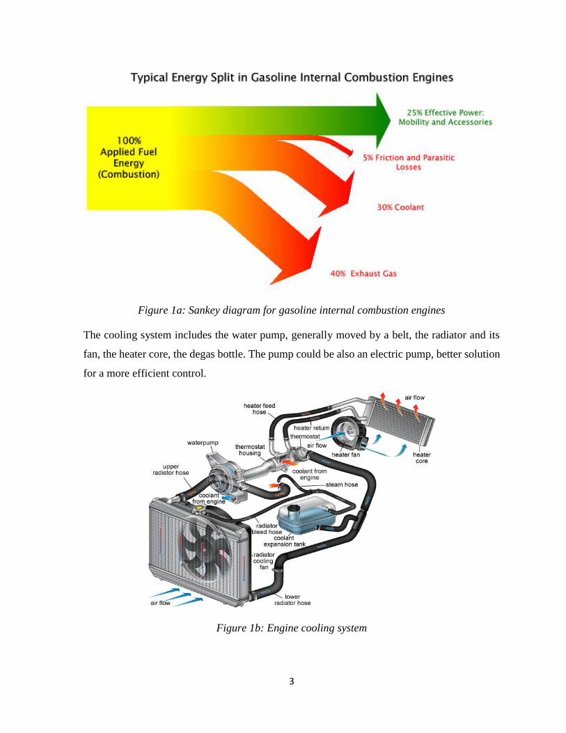
for a gasoline engine, the primary chemical energy of the fuel is divided in three equal part:
mechanical work, enthalpy remained in exhaust gases and energy absorbed by the cooling
system. An example is shown in the Sankey diagram in figure 1a.
It is known that for the internal combustion engine, the coolant should stay around 90°C and
not overreach approximately 110°C (it depends on the pressure of the circuit). This limit is due
to the boiling point of the coolant, that for the mixture considered is 107.2°C at atmospheric
pressure and it increases following the pressure [1].
3
Figure 1a: Sankey diagram for gasoline internal combustion engines
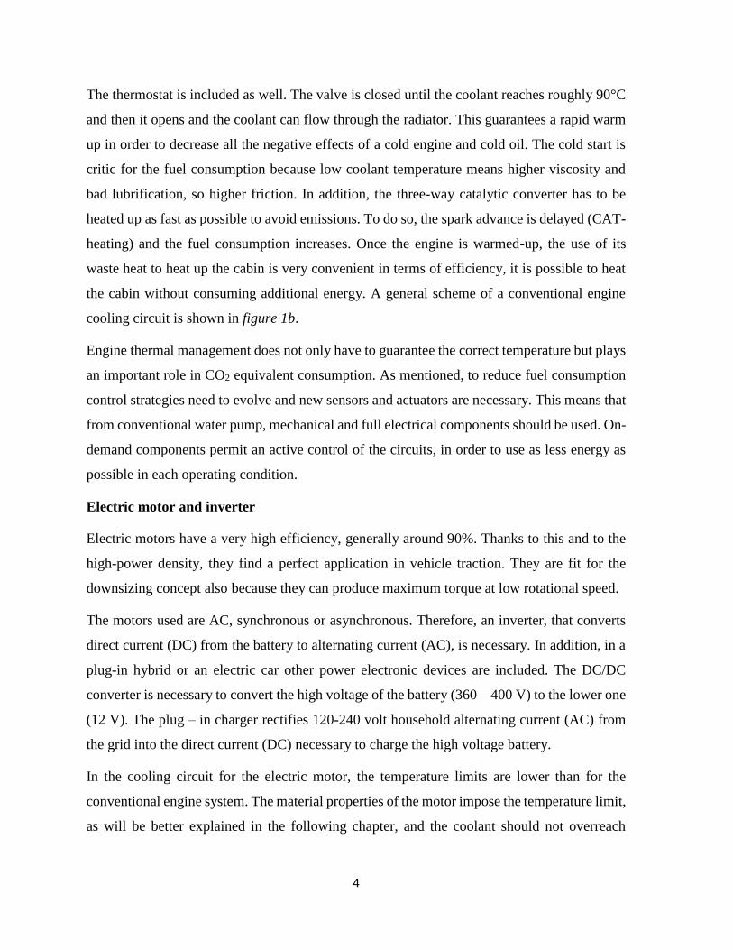
The cooling system includes the water pump, generally moved by a belt, the radiator and its
fan, the heater core, the degas bottle. The pump could be also an electric pump, better solution
for a more efficient control.
Figure 1b: Engine cooling system
4
The thermostat is included as well. The valve is closed until the coolant reaches roughly 90°C
and then it opens and the coolant can flow through the radiator. This guarantees a rapid warm
up in order to decrease all the negative effects of a cold engine and cold oil. The cold start is
critic for the fuel consumption because low coolant temperature means higher viscosity and
bad lubrification, so higher friction. In addition, the three-way catalytic converter has to be
heated up as fast as possible to avoid emissions. To do so, the spark advance is delayed (CAT-
heating) and the fuel consumption increases. Once the engine is warmed-up, the use of its
waste heat to heat up the cabin is very convenient in terms of efficiency, it is possible to heat
the cabin without consuming additional energy. A general scheme of a conventional engine
cooling circuit is shown in figure 1b.
Engine thermal management does not only have to guarantee the correct temperature but plays
an important role in CO2 equivalent consumption. As mentioned, to reduce fuel consumption
control strategies need to evolve and new sensors and actuators are necessary. This means that
from conventional water pump, mechanical and full electrical components should be used. On-
demand components permit an active control of the circuits, in order to use as less energy as
possible in each operating condition.
Electric motor and inverter
Electric motors have a very high efficiency, generally around 90%. Thanks to this and to the
high-power density, they find a perfect application in vehicle traction. They are fit for the
downsizing concept also because they can produce maximum torque at low rotational speed.
The motors used are AC, synchronous or asynchronous. Therefore, an inverter, that converts
direct current (DC) from the battery to alternating current (AC), is necessary. In addition, in a
plug-in hybrid or an electric car other power electronic devices are included. The DC/DC
converter is necessary to convert the high voltage of the battery (360 – 400 V) to the lower one
(12 V). The plug – in charger rectifies 120-240 volt household alternating current (AC) from
the grid into the direct current (DC) necessary to charge the high voltage battery.
In the cooling circuit for the electric motor, the temperature limits are lower than for the
conventional engine system. The material properties of the motor impose the temperature limit,
as will be better explained in the following chapter, and the coolant should not overreach
5
50/60°C. The same is valid for the inverter and for the DC/DC converter. Higher temperatures
can request power de-rating in order to preserve the integrity of the machines.
The power losses are divided in cooper and iron losses. The first are due to Joule losses, the
second are due to eddy current and hysteresis effect. Compared to the conventional engine
losses, they are quite low because the power is generally lower and the efficiency is much
higher. The pumps are electric and are connected to the low voltage circuit. They allow a more
efficient control of temperature and energy usage, compared to the driven belt pump of a
conventional engine. As mentioned, the coolant temperature is lower and the electric machine
does not need a fast warm up. The lower the temperature, the better it is for the machine. So, a
thermostat is not used in this cooling circuit. In addition, the power losses are not enough to
heat up the cabin and a heater core is not included as well.
Battery
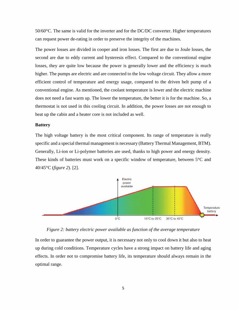
The high voltage battery is the most critical component. Its range of temperature is really
specific and a special thermal management is necessary (Battery Thermal Management, BTM).
Generally, Li-ion or Li-polymer batteries are used, thanks to high power and energy density.
These kinds of batteries must work on a specific window of temperature, between 5°C and
40/45°C (figure 2). [2].
Figure 2: battery electric power available as function of the average temperature
In order to guarantee the power output, it is necessary not only to cool down it but also to heat
up during cold conditions. Temperature cycles have a strong impact on battery life and aging
effects. In order not to compromise battery life, its temperature should always remain in the
optimal range.

6
For both PHEV and BEV, the battery cooling circuit is integrated with the air conditioning.
The refrigerant (R134a or R1234yf) cools down the battery coolant in a heat exchanger, the
chiller. In fact, the coolant must remain at no more than 30°C to be able to cool down the
battery from its maximum temperature of 40°C. Therefore, the radiator could not be sufficient
in a summer scenario with air temperature around these values and the integration with air
conditioning become necessary.
In figure 3, the Chevrolet Bolt HV Battery cooling system is reported. The battery cooling
system has its 12-volt coolant pump, heat exchanger (chiller) and a 3-way coolant flow control
valve to route coolant through the radiator, the chiller, or the bypass. [3]
Figure 3: Chevrolet Volt HV Battery Heating and Cooling System [2]

7
The thermal management control unit monitors ambient conditions, coolant inlet and outlet
temperatures, cells temperature, as well as refrigerant temperatures and pressures to establish
battery heating or cooling requirements. Then, it turns the coolant pump on or off, positions
the coolant flow control valve, and depending on whether cooling or heating is required, it
requests either the electric A/C compressor to operate or to turn on the battery electric heater.
It is interesting to notice that for PHEV and BEV the thermal management is not reduce to the
driving cycle but it is active also during recharging cycles. The plug-in charger and the other
electronic components should be cooled down in case of high power charging rates. More
related to electric vehicle, it is also possible begin to heat the cabin when the car is still
connected to the plug with a predictive strategy, this allows to save the energy of the battery
and increase the all-electric range (AER).
When battery heating is required the 3-way coolant flow control valve will be in position “A”
(figure 3) and allows fast heating of the Li-ion cells in cold weather.
Whenever the Li-ion battery cells are too hot, the flow control valve will typically be
commanded to position “B” and by operating the electric air-conditioning compressor, the
battery coolant goes to the chiller and is strongly cooled down by the refrigerant. During stable
operating conditions, the flow control valve will typically be commanded to position “C”
circulating the flow of the battery coolant out to the battery cooling radiator and back to the
pump. This allows to reach a thermal balance and maintain battery temperature at this optimum
value (from 25°C to 30°C).
Cabin climatization
The cabin climatization of a PHEV or a BEV is completely different compared to a
conventional vehicle. In the latter, as mentioned above, the engine gives its waste heat during
a winter scenario, and on the other hand, an air conditioning system (at 12 V) uses a refrigerant
to cool down the cabin in summer. The engine moves the compressor, a clutch allows to switch
on or off the machine.
In electric vehicles, the waste heat (power losses) by the e-motors is not enough to heat the
cabin because the efficiency is really high. Therefore, positive temperature coefficient (PTC)
cabin heaters are used. PTC elements are ceramic stones that increase their electrical resistance

8
with the temperature. They have an extremely low electrical resistance at low temperature, this
means a high current flow is converted into heat. When the temperature rises, less heat is
released.
They are used also to warm up the battery ‘coolant’ when the battery is below the threshold
(liquid PTC heaters). In some cases, they are also used in conventional vehicle to allow a faster
heating of the cabin. The heaters affect the energy available and the AER in a significant way.
The winter scenario is critic for electric vehicle both for battery heating and for cabin heating.
To improve performance, other solutions are applied, such as heat pump systems (explained in
the following paragraph). For what concerns the air conditioning, the system is the same as
conventional cars but the compressor has its own electric motor that receives current and
voltage from the HV battery. As shown in figure 3, the air conditioning does not only have to
cool down the cabin but also the high voltage battery. Therefore, the power of the compressor
must be higher than in a conventional system.
1.2 Thermal management Layout for Hybrid Vehicle
As it has been explained, each heat source needs a different coolant temperature. The
possibilities to design a complete thermal management layout of the vehicle are various, and
some of them are described in this paragraph. The layout is strictly connected to the hybrid
architecture, that is the position of the electric motors in the powertrain. The hybrid powertrain
considered has a parallel architecture, both the ICE and the electric motors can directly power
the wheels.
Parallel Hybrid topology
The driveline topology is the starting point for thermal management layout. Depending upon
the electric motor position, the hybrid topology takes different names, as shown in figure 4:
▪ P0, the electric motor is the integrated starter generator mechanically connected to the
engine.
▪ P1, in which the motor/generator is located on the engine shaft, before the clutch, so
their rotational speed are the same.

9
▪ P2, in which the electric motor is downstream the clutch and so pure electric driving is
possible.
▪ P3, where the motor is after the secondary shaft of the gearbox.
▪ P4, where the motor is on the axle directly.
Figure 4: parallel hybrid possible architectures
The battery position plays a key role in the entire thermal management layout as well.
Packaging problems must be considered in details in order to design cooling circuits avoiding
too complex layout and limiting their lengths.
For high voltage battery, an additional problem is due to electric high voltage connections.
They need special isolations for obvious safety reasons.
In the P0 and P1 configuration, the cooling of the electric motor and of the inverter become
more critic because they are heated not only by its power losses but also by the ICE.
Example of cooling systems layout
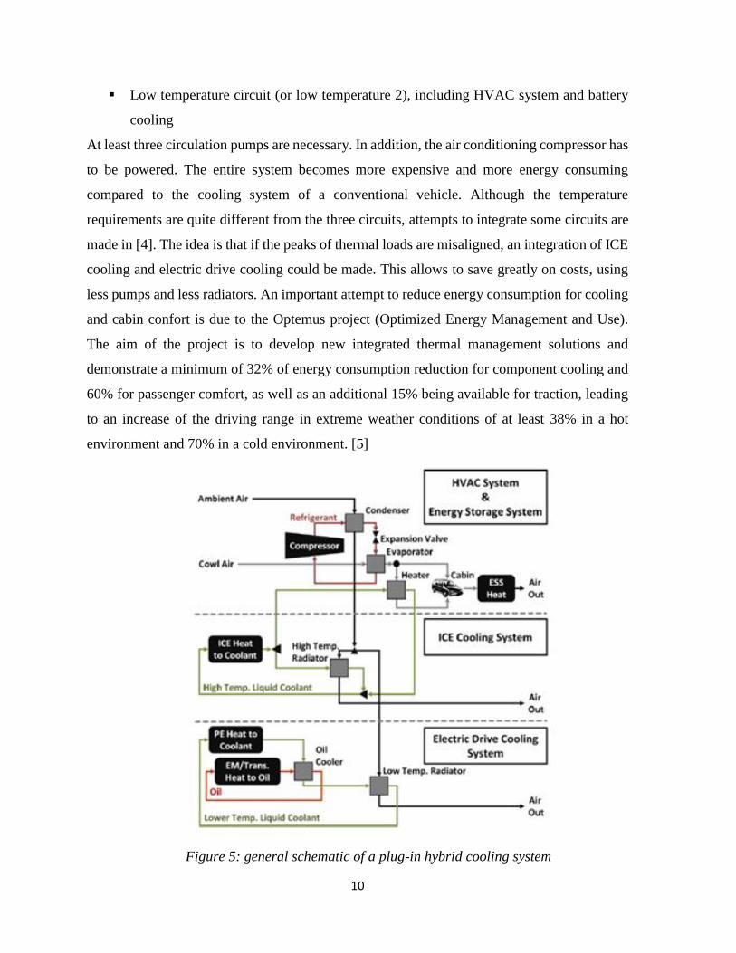
An example of a complete system is shown in figure 5. The circuits are divided in:
▪ High temperature circuit, including ICE and high temperature radiator (and engine oil)
▪ Medium temperature circuit (or Low temperature 1), including electric drives and
power electronics and also lubricant for transmission
10
▪ Low temperature circuit (or low temperature 2), including HVAC system and battery
cooling
At least three circulation pumps are necessary. In addition, the air conditioning compressor has
to be powered. The entire system becomes more expensive and more energy consuming
compared to the cooling system of a conventional vehicle. Although the temperature
requirements are quite different from the three circuits, attempts to integrate some circuits are
made in [4]. The idea is that if the peaks of thermal loads are misaligned, an integration of ICE
cooling and electric drive cooling could be made. This allows to save greatly on costs, using
less pumps and less radiators. An important attempt to reduce energy consumption for cooling
and cabin confort is due to the Optemus project (Optimized Energy Management and Use).
The aim of the project is to develop new integrated thermal management solutions and
demonstrate a minimum of 32% of energy consumption reduction for component cooling and
60% for passenger comfort, as well as an additional 15% being available for traction, leading
to an increase of the driving range in extreme weather conditions of at least 38% in a hot
environment and 70% in a cold environment. [5]
Figure 5: general schematic of a plug-in hybrid cooling system

11
However, nowadays the circuits are generally separated and the only integration is between air
conditioning and battery. The architecture with three separated circuits, air conditioning and
PTC heaters is the most common in new plug-in hybrid cars. The main problem is the high-
energy consumption for cabin climatization, this is particularly important in the battery electric
vehicle. In order to increase the efficiency of the system, new solutions, like the two examples
presented in the following paragraphs, are studied. They are already applied in electric
vehicles, and probably, they will be used in the next generation of hybrid cars.
Heat pumps
Cabin heating for electric vehicle (and partially for plug-in hybrid electric vehicle, during pure
electric mode) is critic. Waste heat from ICE is not more available and the power losses for
electric motor are not enough to satisfy the thermal power request. Usually, PTC heaters are
used but they cause a significant decrease of the all-electric range. In figure 6, an example of
the range reduction for an electric vehicle due to cabin heating is reported.
While the efficiency of the PTC heaters is limited to one, heat pump systems can have better
performance, thanks to Coefficient Of Performance (COP) greater than one. The efficiency of
the heat pump is so high because they use heat from ambient air (or waste heat from other heat
sources). The technology is already used in the Nissan Leaf, first mass-produced electric
vehicle to employ a heat pump as cabin heater, and also on the Audi Q7 e-tron, first on the
plug-in hybrid vehicle class.
Figure 6: Range reduction of a BEV as function of cabin heating power [6]
Thanks to the heat pump, that can work both as a heater and as a cooler, existing power unit
(electric motor, generator) can be included in the vehicle’s heat balance.

12
Improving AER with no comfort reduction is not the only advantage of this system: controlling
the temperature promotes better durability and less de-rating effects, reduction in refrigerant
losses into the environment (greenhouse gases). The main disadvantage is the higher cost.
Layout of the heat pump includes compressor, evaporator, expansion valve and condenser. It
also features accumulator, directional control valve and tubes. The directional 4/2 valve (four
ports and two positions) is the key component that allows the redirection of the coolant, making
both heating and cooling possible. [6]
After the compressor and the condenser, the refrigerant passes through the expansion valve
(ideally isenthalpic transformation) in which high temperature and high pressure drop to lower
values. The fluid moves on to the evaporator and cool down the refrigerant. The evaporator is
a plate exchanger identical to the condenser, so the heat transfer is the same. Thanks to this
and to the directional valve, reverse circulation is possible.
In some cases, the PTC heater is present in this architecture as well. If the heat provided by the
heat pump is not sufficient, it supplies the supplementary heat required. In addition, more
complex solutions are studied. The system here explained is a direct system, but also indirect
systems are developed,
Indirect systems do not exchange heat directly with the external air but with the battery (or
electric components) cooling circuit. Among the advantages of this solution, there are the
possibilities to use battery and electric components as heat sources. In addition, less refrigerant
is used compared to the direct system. The main disadvantage is the higher difference of
temperature between condenser and evaporator, due to the additional heat exchange. This
means higher pressure ratio and more power consumed by the compressor.
Indirect systems are very promising, since the reuse of dissipated heat for the cabin heating
could improve the efficiency significantly and decrease the impact of cabin climatization on
the AER reduction.
The figure 7 shows an example of indirect heat pump system with two 4/3 bidirectional valves
built by VOSS. [7]

13
Figure 7: indirect heat pump system with HV battery as heat source [7]
Thanks to the valves, the battery can be used as heat source for cabin heating in a winter
scenario. In the same way, the electric components can be used as well. The temperature and
the pressure in the evaporator should be higher than the case in which ambient air is used, and
so the efficiency. In addition, the system can prevent problems of ice formation on the
evaporator (possible in other heat pump systems). The battery can be used as heat source only
when its temperature overreaches the low limit, since in this condition it has to absorb heat and
cannot be a heat source.
In a summer scenario, the advantages of the system are less evident. The two valve force the
flow out of the evaporator to the cabin and to the battery (when necessary). They can regulate
the flow in order to maintain the desired temperature, like the thermal expansion valve does in
a conventional air conditioning system. On the other hand, the refrigerant must release the heat
to the coolant in the condenser. Then, the coolant is cooled down by the external air in the
radiator.
Phase Changing Material thermal energy storage (PCM)
Another solution to improve the heating of electric vehicles is Phase Changing Material (PCM)
thermal energy storage. They are materials with a specific melting temperature and a really
high heat of fusion. Like heat pumps, they find application in buildings to increase the thermal

14
mass and allow lower overheating in summer and higher thermal isolation in winter. Thanks
to the melting process, these storages reach very high energy densities. The difference of
density among liquid and solid should not be too high, otherwise the circuit would be
pressurized after a phase change. In addition, the thermal conductibility should be as lower as
possible to increase the efficiency of the system.
Some studies have been done, in which PCM storage are used in electric vehicle. The system
can absorb waste heat from battery cooling circuit and storage the thermal energy. This energy
can be gradually released in order to maintain battery and cabin warm, reducing the warm up
phase and its impact on AER reduction. The solution looks promising, it manages to reuse
waste heat during the most critical phase of the warm up. The limits are the costs of the
materials, still too expensive to find applications in common vehicles.
Figure 8: integrated cooling circuit for BEV with PCM storage

15
In figure 8, a BEV cooling system layout with PCM storage is reported. In [8], a long review
of PCM classification and main applications is described. Different PCM storage materials can
find applications in both electric and conventional vehicle. For the electric vehicle, battery and
cabin can maintain higher temperature during long stops. PCM storages suitable for this
application has a melting temperature of 30°C: during the last run they melt absorbing battery
power losses and can maintain a temperature that is 17°C higher than ambient temperature for
12 hours. PCM thermal storage can find application also in conventional vehicles to decrease
warm up times. Friction and emissions can be reduced, since oil and catalytic converter are
heated up faster.
1.3 Control strategies
The previous paragraph described some examples of the hardware cooling systems and some
solutions to decrease the energy consumption of cooling and climatization. Software strategies
can significantly contribute, as well.
Before describing the control approach, it is important to highlight that more electrical
actuators and smart valves are necessary. Substitution of the water pump and the thermostat
with on-demand components is essential to obtain a more efficient control depending on the
operating conditions. The rotational speed of a mechanical water pump moved directly by the
driven belt cannot be controlled but it only depends on the engine rotational speed. It is evident
that this kind of control cannot be optimal. But, on the other hand, mechanical water pumps
are the cheapest solution (variable mechanical water pump or electrical pump). The electric
pump has another advantage: since is completely independent on engine rotational speed, the
pump can cool down the engine also when this is not running, avoiding overheating at the end
of the run. The thermostat could be replaced with more efficient and on-demand components
too. An example is presented in [9].
The Thermal Management Module (TMM) is a multi-circuit valve which enables variable
coolant flow rate. It offers the option to control the circuits with electronical control and allows
the setting of the temperature according to the component requirements to maximize the fuel
efficiency.

16
The same is valid for the compressor, that in a conventional car is moved by a belt but in PHEV
is moved by an electric motor and it can be regulated independently by the HCU.
The targets of the control strategies must be defined.
Thermal management targets are:
▪ Maintain the optimal temperature range for each component in every operating
condition, in order to provide reliability and durability;
▪ Utilize as little energy as possible.
It is evident that the two targets are opposite, therefore a tradeoff must be achieved.
The energy consumption is due to pumps, fans, the air conditioning compressor and electric
heaters. They should only use the optimal amount of energy to guarantee the desired
temperature in each condition. The thermal management basic strategy is monitoring all the
critical temperatures with temperature sensors, and only when one overtakes a limit, the control
unit makes the electrical pumps move and the fans cool down that component. In the same
way, cabin temperature has to be guaranteed as required by the driver and the compressor is to
switch on or off depending upon the difference between real and target cabin temperature.
Pump regulation
The centrifugal coolant pump has a characteristic curve, increase of pressure as function of the
volumetric flow rate, and an efficiency curve. The fundamental equations to describe a
centrifugal pump are reported in the next chapter. The pumps are designed to work in a fixed
point, defined by the characteristic curve and by the circuit. But to save energy, the pump has
to run as less as possible. The flow rate of the pump can be regulated in different ways, with
different impact on the efficiency. One option is use a valve which cause a restriction and an
increase of pressure drop. The operating point shifts to the left, with a higher increase of
pressure and a smaller flow rate. This method has a strong impact on the efficiency, as it can
see from the efficiency curves, and it is used only when it is not possible to change the
rotational speed of the pump, since the electric motor is connected to the grid.
As mentioned, regulation is more efficient in changing the rotational speed of the pump,
allowing to work near the maximum efficiency area. If the motor is connected to the grid and

17
so its rotational speed is fixed, an inverter can modulate the frequency changing the speed of
the pump.
Actually, in the cooling system, the pumps are moved by separated motors. They absorb
current directly from the low-voltage battery and the rotational speed can be always modulated
to regulate the flow rate. The pump has maximum efficiency at a specific rotational speed and
so, generally, it always works at this point.
They always have the same flow rate and the maximum efficiency and they are switched on or
off depending upon the temperature and the control strategy. Apart from the basic strategies, a
more complex approach has been studied, like optimal approach based on predictive
information. Some examples are described in the next paragraph.
Thermostat and fan
The conventional engine cooling system uses a wax thermostat. The function of the
thermostatic valve is to maintain the desired temperature in the cooling system, that for the
engine is between 80°C and 90°C. Below this temperature, the wax is solid and the valve is
closed due to a spring force. Once this temperature is reached, the wax starts to melt and
expand, overtaking the spring force and opening the valve. It works well, but the sensible
element has a thermal inertia and so the response can be quite slow. Electric thermostat can be
also applied and guarantees faster response time.
While for the engine cooling system the thermostat allows good control, for the battery cooling
circuit more complex valves are necessary. As described in the example of the previous
chapter, the battery cooling system has a higher degree of freedom since it can heat up the
battery, cool down it with the radiator or cool down it with the chiller. A mechanical valve
cannot manage this system, therefore an electric, and more expensive, valve has to be
employed. For this situation, a 4/3 (4 ports and 3 positions) valve has to be foreseen.
Another electric controlled device in the cooling system is the fan. Its control is, generally,
simple: a temperature sensor measures the coolant temperature and sends the information to
the ECU. Depending upon this value, the control unit electrifies the fan with a linear, or a more
complex, response. The position of the temperature sensor can be downstream the radiator or
near the thermostat, but other solutions are possible as well.

18
Cabin climatization and battery thermal management
As described in the previous chapter, cabin climatization is critical for its strong impact on the
state of charge of the battery and many solutions have been adopted.
Not considering heat pump solutions for the moment, the typical HVAC system for PHEV
includes a high voltage compressor and an air conditioning system integrated with the battery
cooling system (through the chiller heat exchanger), plus the PTC heaters (air and liquid) and
eventually a heater core of the engine cooling system.
It is evident that a lot of control strategies can be applied and they play an important role in the
energy impact of cabin climatization.
Considering a summer scenario, the thermal management control unit has to guarantee the
driver-imposed cabin temperature and the battery temperature employing the HV compressor.
The refrigerant flow rate through the evaporator and through the chiller is regulated by the
thermal expansion valve (TXV) that divide the high and low pressure sides. The lamination
valve allows that the refrigerant flow rate is the exact amount to satisfy the evaporator thermal
request. It guarantees an increase of efficiency, since the compressor only works when it is
strictly necessary. The thermal sensitive element (bulb) is connected to the diagraph by a
capillary and it is located after the evaporator, monitoring the temperature change. This change
of temperature is also a change of pressure and it is received by the diagraph. When the pressure
of the bulb overtakes the preload of the spring, the valve opens and the refrigerant flows
through the heat exchanger. When the temperature of the evaporator, and so its pressure,
becomes lower the valve starts to close.
The thermal expansion valve does not need any electric connections, since, like the thermostat,
it is the sensitive element that allows the flow regulation.
The HCU controls the rotational speed of the HV compressor, in order to satisfy the
aforementioned thermal demands. The basic idea is that the cabin and battery temperatures are
monitored, and when they overtake the target, the compressor begin to run and the refrigerant
absorb heat from the evaporator or from the chiller. The relationship between the difference of
temperature and the increase of rotational speed can be linear or more complex.
In a winter scenario, the PTC heater and the heater core has to provide the heat requested by
the cabin and, eventually, by the battery. Not considering heat pump solutions, the battery
could be heated up only by the PTC heater. The electric heater can heat the air near the battery

19
or, more frequently, the battery coolant. In this configuration, there is not a degree of freedom,
the heater absorbs the necessary current until the battery overtakes the lower operating
temperature limit.
For the cabin, the control is more complex, since both the devices could satisfy the thermal
request. It is clear that it is more efficient to use the waste heat of the engine as much as possible
and save battery energy, but if the vehicle is driving in pure electric mode, this is not possible.
The choice is complex since different constraints have to be considered. Like for the pump
regulation, optimal approaches are studied and some examples are reported in the following
paragraph.
1.4 Predictive thermal management
After the description of some basic thermal management strategies, a predictive approach is
considered. A predictive strategy means a control system which can know different kinds of
information from external sources, and use these to improve the vehicle management.
Predictive strategies could be applied in both energy management and thermal management,
and can contribute to reduce the fuel consumption but also to the improve components’
lifecycle expectancy.
ADAS
New vehicles are able to communicate with the external environment thanks to the ADAS
(Advanced Driver Assistant Systems).
The systems are equipped with new sensors, like cameras and GPS. The technologies are
divided in V2V (Vehicle to Vehicle) and in V2I (Vehicle to Infrastructure). The second ones
are long- or medium-distance communication systems. The connected vehicle become can
know navigation data and route conditions, and allow the implementation of predictive
strategy.
For what concerns hybrid vehicle control strategies, route conditions info can be applied in
energy and thermal management. A typical situation is the traffic light: the car is at a constant
speed, the control unit receives information of red light phase in a known time, and calculates,
depending upon the known distance, if the vehicle, without accelerating, can pass the traffic
light in time. Therefore, it can decide not to interfere (if the vehicle manages to pass) or decide

20
to switch off the engine and start to recover energy with breaking (coasting). The earlier
information is known, the less is the energy consumption. [10]
Navigation data and preconditioning
Predictive control of the temperature is highly attractive because, due to the high thermal
inertia of both ICE and battery, the thermal response is always quite slow. The possibility to
know the temperature behaviour in advance gives a great gain comparing to the common
situational approach. The main idea is, once the driving cycle is known in terms of split factor,
the control unit can begin to precondition either the ICE or the battery. In this way, it is
possible, for example, to increase the all-electric range since the battery will reach its maximum
temperature later than in a common strategy.
The navigation data used in thermal management are map data, including speed limits, built-
up areas and slope, and traffic situation. They are obtained rearranging GPS and traffic info.
Like for energy management, many studies are made on thermal management optimal
strategies and the fuel saving advantages have been demonstrated. The problem is clearly the
too high computational data and so an optimal approach is not possible on-board. ADAS allows
a partial knowledge of the driving cycle (generally, only a few kilometres) and these strategies
are called sub-optimal.
To optimize the thermal management, data must be collected and organized very well. The
scheme here considered is reported in [11].
Data is transmitted via the controller area network (CAN) to the engine control unit (ECU). A
horizon reconstructor (HRC) should create the electronical horizon. Only the relevant
navigation events are saved and organized in array, fundamental to save computational
memory.
After data preparation, several detection algorithms analyse the data in order to find relevant
events for the thermal system. Example of events are the beginning of a city area or a high load
cycle with a relevant slope. Algorithms do not only consider data from ADAS sensors, but also
from conventional cooling system ones (actual temperature of the coolant). They calculate the
distance and the length of the event and send information to the application function, that
finally decide which strategy is the best.

21
Figure 9 shows the function and sensors involved in the predictive thermal management.
Figure 9: ADAS-ECU communication system [11]
As mentioned above, several events are provided by the horizon reconstructor: speed limits,
slopes, built up areas. All the data is stored by a value and a position. That means each speed
limit has a value in km/h and a position in m. The ADAS specification imposes a limit in the
counter of the position, that means every time the limit is reached the counter is reset. A trade
off must be done to save memory and not lose relevant information.
After the distance and the length of the event are known, the application function has to choose
a strategy. In a predictive strategy, it is not sufficient to know the coolant temperature from the
sensors but it should be important know the temperature behaviour in the next future. In this
way, the system can react in advance if it is suitable.
A cooling circuit model, real time and implemented in the HCU, can be developed. The
control-oriented model is presented again in [11], considering the cooling circuit model for
battery temperature prediction and preconditioning.
In the same article, a detection algorithm is used to detect city areas. Speed limits and built-up
areas data is provided by the horizon reconstructor. When the speed limit is 50 km/h and the
built-up area signal is true, the HCU detects a city area event. Then, the application function
has to decide from environmental conditions, battery temperature and length of the event, if a
predictive cooling is suitable. Another degree of freedom is present, since the battery can be
cooled either with the radiator or with the chiller and the air conditioning circuit. Therefore,

22
not only the application function has to decide to cool down or not, but also how heat sink
should be used.
The predictive strategy cool down the battery before the city area starts, maintaining the battery
temperature at lower values and, potentially, increasing the all-electric range. The system can
also predict the battery temperature at the end of the event and can decide that cooling via the
chiller is not necessary, use only the radiator, and save significant value of energy.
Optimal approaches
Another study is done in [12], where a non-linear model for predictive thermal management,
in particular for the HV battery and for Power Electronics, is developed. The method presented,
Model Predictive Control (MPC), is based on an optimal/suboptimal control and is
recommended for finding optimal solutions in complex multi inputs and multi outputs
problems. The main idea is to use the control-oriented model to predict the future behaviour of
the system within a time horizon and the optimization algorithm to find the best control
strategies in order to satisfy the constraints.
The model must be accurate while also being fast enough considering the computational
capacity of the HCU.
Once the model is developed, the optimization begins. The target function, the model equations
and the physical constraints must be provided. In the present case, the target function is the
optimal temperature for the battery, that is 28°C. The constraints impose values that the
mathematical optimizer cannot exceed. They are, for example, a maximum and a minimum
coolant temperature, maximum energy of the battery, torque of the electric motor, and so on.
The model is then validated and the optimal strategy is compared to the standard one.
The results are very promising, a significant energy reduction is feasible with an optimal
strategy. In figure 10, the battery temperature for the predictive and standard strategies is
reported. The energy consumption reduction due to the coolant pump is reported as well. The
optimal strategy manages to have a higher final temperature but inside the desired window,
allowing to consume less energy.

23
Figure 10: Comparison of battery temperature for a predictive and non-predictive strategies
in a RDE cycle [12]
Another example of optimal approach towards thermal management problem can be found in
the cabin heating, like in [13]. As mentioned, the cabin can be heated up either by the heater
core, using engine waste heat, or by the PTC electric heater, using battery energy. A predictive
model control is developed considering the start and stop of the ICE. The goal functions are:
providing the thermal power requested, maintaining the battery’s state of charge within the
desired limits and minimize the fuel consumption. The output of the algorithm is the optimal
split of the thermal power between the two heaters. The results show an improvement of 3%
of fuel savings, compared to the standard control strategy. To sum up, different studies
demonstrate the advantages of predictive strategies. The next step of development will be a
better integration of this approach in a real vehicle, optimizing data from ADAS and models
to temperature prediction in HCU. Predictive thermal management will be also integrated with
predictive energy management, realizing a global optimal control and important fuel
consumption/CO2 emissions reduction. Thermal requests have to be taken into account in order
to have a globally optimal control strategy and find the optimal split power factor. For example,
turning on the ICE should not be decided only by the energy management strategy (EMS) but
also by the TMS. If the cabin has to be heated up, it could be globally better to turn on the
engine and use its waste heat and not the electric heater, also if the EMS had decided on pure
electric driving.

24

25
2.Introduction to the thermal model and system description
Before starting the presentation of the cooling circuits and how these were designed in
AMESim® environment, a description of the fundamental equations for hydraulic and thermal
simulation is reported.
As mentioned above, the system is considered divided in three circuits with three levels of
temperature: high temperature for the engine, medium temperature for the electric motor, ISG
and the power electronics components and low temperature for battery cooling and air
conditioning.
For each circuit, a hydraulic description has been done. The pressure losses for each component
are calculated and the total pressure increase of the circulating pump has been imposed. From
its characteristic curve, the volumetric flow rate has been determined. Prior to considering the
model, a general mathematical description of pressure drops and pumps is reported in this
chapter.
For what concerns thermal generation modelling, the problem has been simplified considering
four types of heat sources: ICE, electric motors, power electronics and battery. In order to
model the thermal behaviour of each component, we need to understand the amount of heat
produced as function of the different operating conditions. As it will be better described, the
thermal generation is based on a map of efficiency. So, a detailed physical description is not
included. The heat produced will propagate inside the material and it will be transferred to the
coolant and to external air. Both conduction and convection are modelled in order to predict
material temperature. It is really important to know how these heat sources interact with the
coolant and understand how the heat exchange is calculated using heat transfer theories. In this
chapter the fundamental equations for heat transfer are discussed, since they are the base for
the simulations that include thermal masses.
2.1 Hydraulic modelling background
Pressure drops
In order to simulate the hydraulic circuit, we have to know the pressure drops in the ducts and
in the components. They are important to size the pumps and to understand the efficiency of
the entire system.
26
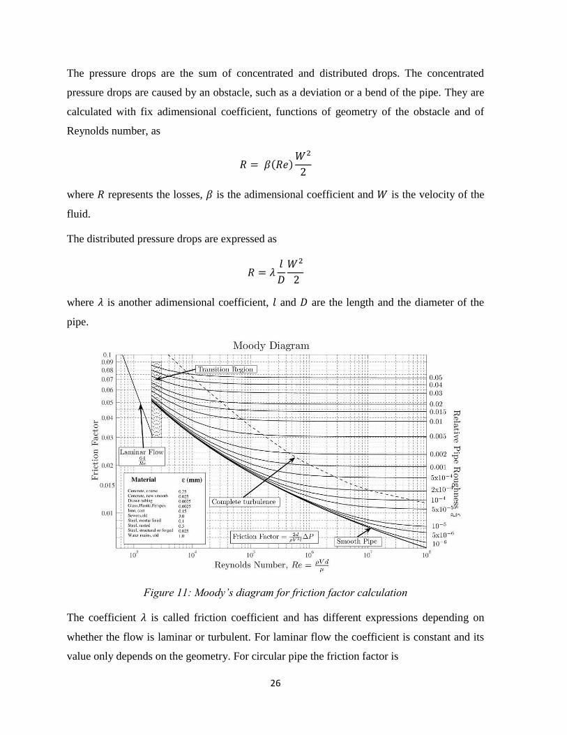
The pressure drops are the sum of concentrated and distributed drops. The concentrated
pressure drops are caused by an obstacle, such as a deviation or a bend of the pipe. They are
calculated with fix adimensional coefficient, functions of geometry of the obstacle and of
Reynolds number, as
𝑅 = 𝛽(𝑅𝑒)𝑊2
2
where 𝑅 represents the losses, 𝛽 is the adimensional coefficient and 𝑊 is the velocity of the
fluid.
The distributed pressure drops are expressed as
𝑅 = 𝜆𝑙
𝐷
𝑊2
2
where 𝜆 is another adimensional coefficient, 𝑙 and 𝐷 are the length and the diameter of the
pipe.
Figure 11: Moody’s diagram for friction factor calculation
The coefficient 𝜆 is called friction coefficient and has different expressions depending on
whether the flow is laminar or turbulent. For laminar flow the coefficient is constant and its
value only depends on the geometry. For circular pipe the friction factor is

27
𝜆 =64
𝑅𝑒
For turbulent flow 𝜆 is function of the Reynolds number and of the relative roughness. For
circular pipes, we can use the Moody diagram to calculate the friction coefficient (figure 11).
Once its value is known, the distributive pressure drops are determined by the geometrical
characteristic of the pipe.
Centrifugal pumps
To circulate the fluid in the cooling system, centrifugal pumps are employed. The characteristic
curves of these machines show the pressure increase and the efficiency as function of the
volumetric flow rate.
The hydraulic head indicates the work done by the pump on the fluid. It measured in meters
and it is derived from the general fluid equation, as reported in [14]. It is:
𝐻 = ∆𝑝
𝜌 𝑔
where the difference of velocity (kinetic contribution) and of height (gravitational contribution)
between inlet and outlet are neglected.
The net power transferred to the fluid is
𝑃 = 𝜌 �� 𝑔𝐻
The efficiency of the pump is the product of three contribution:
▪ hydraulic efficiency, which consider the fluid dynamics losses in the impeller
▪ volumetric efficiency, which consider the losses due to leakage along the seals
▪ mechanical efficiency, losses for friction in the bearings.
The total power absorbed by the pump is
𝑃𝑎 = 𝜌 �� 𝑔𝐻
𝜂ℎ𝜂𝑣𝜂𝑚
with the obvious meanings of the symbols.

28
The characteristic curve (QH graph) can be obtained as difference of the work made on the
fluid less the total pressure losses in the pump. For each rotational speed, a different
characteristic curve is defined.
Figure 12: pump and plant characteristic curves
The curve has to be put on the same chart with the total pressure drops of the circuit and the
intersection becomes the operating point, as shown in figure 12. The choice of the pump should
guarantee efficiency when the operating point is near the maximum. In addition, cavitation
must be avoided in every possible operating condition.
The hydraulic efficiency is function of the flow rate as well, as reported in figure 13, and has
a maximum at the operating point. In this chart, due to [15], the losses contributions as function
of the specific speed are reported.

29
Figure 13: pump losses distribution as function of the specific speed [15]
The regulation of the flow rate can be done in different ways, as described in the chapter 1.
The use of a restriction to decrease the flow rate increase the pressure drops of the circuit,
therefore the operating point moves to left in the chart. But the efficiency reductions are
significant if the variation is higher than a few percent. A regulation on the rotational speed is
more efficient, since the characteristic curve and the operating point change allowing to remain
in the maximum efficiency zone. It is possible to predict how the flow rate, the hydraulic head
and the power change as function of the rotational speed, using the affinity rules. These rules
are all derived under the condition that the velocity triangles are geometrically similar.
𝑄2 = 𝑄1
𝑛2
𝑛1
𝐻2 = 𝐻1 (𝑛2
𝑛1)
2
𝑃2 = 𝑃1 (𝑛2
𝑛1)
3
More specific control strategies are used, like proportional-pressure control or constant-
pressure control. They allow a more efficient use of the energy available.
The proportional-pressure control try to maintain the hydraulic head linear with the flow rate.
This is done changing the rotational speed and moving to other characteristic curves. The
regulation is done until the maximum speed is reached, then the pump remains in the same
curve. The strategy allows to keep the same differential pressure with different thermal request.
If a thermostatic valve is present, this control allows to avoid to leave the valve partially closed,

30
and to produce noise, reducing the flow rate with the pump. The constant-pressure control is
done to maintain the hydraulic head constant for every flow rate, until the maximum speed is
reached. This finds application in open circuits, like in a water supply system where a different
consumption does not affect the pressure of the fluid.
2.2 Heat transfer theory
Conduction
The conduction governs the heat exchange between solid materials. The general approach for
a thermal model is to consider the thermal losses concentrated in a single thermal mass and
link them together using thermal resistance. The heat source, as the electric motor, can be
divided in more thermal masses and the heat spreads from one to another following conduction
law. For example, the losses of the rotor propagate to the stator and then to the cooling plate.
In literature, very complex models of electric motor are studied, like in [16]. In the present
work, a simple approach has been used to determine the temperature of the motor (or other
heat sources) and the conduction effect are not modelled in a rigorous way. However, it is
interesting to report and keep in mind the heat transfer general laws, also for future
developments of the thermal model.
Inside a solid material, the heat power is equal to minus the temperature gradient multiplied by
a constant value, function of the physical properties of the solid considered. This law is called
Fourier’s law.
𝑞 = −𝑘 ∇𝑇
the constant value k is the thermal conductibility and is measured as [𝑊
𝑚 𝐾].
To describe a general problem of conduction we have to consider a closed system in which
heat could be generated. Fourier’s law and the conservation energy equation allow to write the
Heat equation (or Fourier’s equation) that describe different kinds of heat transfer problems.
𝜕𝑇
𝜕𝜏= 𝛼 ∇2𝑇 +
𝑞𝑔
𝜌 𝑐𝑝
where 𝛼 is the thermal diffusivity and is equal to

31
𝛼 =𝑘
𝜌 𝑐𝑝 [
𝑚2
𝑠]
𝑞𝑔 is the heat generated inside the closed system, 𝜌 is the density, 𝑐𝑝 is the specific heat
capacity.
With this equation, it is possible to determine the curves of temperature and heat flux along
the solid. For problems in which the temperature is function of only 1-D and no heat generation
is present, an analytical solution is possible. But in general, numerical solutions are required.
As an example, we consider a stationary problem with heat generation and cylindrical
geometry. The problem describes the electric resistor heated for Joule effect when the current
flows. The temperature is function only of the radius of the cylinder, and the heat flux is only
radial too. Using the heat equation, we can find the behavior of the temperature along the
radius 𝑟.
Heat power generated per volume unit is
𝑞𝑔 = 𝑉 𝐼
𝜋 𝑟2𝑙
Where 𝑉 and 𝐼 are the voltage and the current of the resistor, 𝑟 the radius and 𝑙 the length.
Since the problem is stationary, the first term of heat equation is equal to zero. So we can write
∇2𝑇 = − 𝑞𝑔
𝑘
Expressing the Laplace operator in cylindrical coordinates and integrating we find
𝑇(𝑟) = − 𝑞𝑔
4𝑘𝑟2 + 𝐵
We can find the constant B imposing the boundary conditions, i.e that the external surface is
at a fixed temperature 𝑇0.
𝐵 = 𝑇0 + 𝑞𝑔
4𝑘𝑟𝑒𝑥
2
𝑇(𝑟) = 𝑇0 + 𝑞𝑔
4𝑘(𝑟𝑒𝑥
2 − 𝑟2)

32
Finally, we find the temperature has a parabolic behavior with a maximum for 𝑟 = 0. It is
necessary to control that this temperature does not exceed a pre-fixed value. To maintain the
temperature of the external surface constant, the heat is exchanged with external air.
This problem could be generalized for more complex geometry and could be applied to
describe the heating of an electric motor as well as the heating of the battery.
Convection
The analytical description of convection problem is very complex. Fluidynamics and heat
transfer equations have to be resolved at the same time in order to completely describe the
physical system, such as finding the function of velocity and temperature.
A physical approach is out of the scope of this thesis and only the most important relationships
are reported.
The heat exchanged between the wall and the external fluid can be expressed as:
𝑄 = ℎ 𝑆 (𝑇𝑤 − 𝑇𝑓)
where ℎ is the heat exchange coefficient, 𝑇𝑤 is the temperature of the fluid and 𝑇𝑓 is a reference
temperature of the fluid and it has to be defined according to the kind of convection.
A series of adimensional parameters are introduced. The Nusselt number is
𝑁𝑢 =ℎ 𝐿
𝑘
where 𝐿 is a reference length and 𝑘 is the thermal conductivity of the fluid.
Different problems of convection exist. We speak of external convection when the fluid has
no space limits, of internal convection when the fluid is inside a pipe or a duct. In the first case
it is easy to define a reference temperature as the temperature of the fluid far enough to not be
influenced by the heat exchange. In the second case, the reference temperature is considered
the bulk temperature. This is defined as the temperature that the fluid would have if the
temperature was uniform in the duct and the enthalpy was the same.
The convection is also classified as forced or natural. In a forced convection problem, there is
an external machine to generate the motion of the fluid and to create a difference of pressure
(pump or fan). Instead if it is only the difference of density due to temperature the cause of the

33
motion, the convection is natural. If both the conditions are true, the convection is mixed. For
our purpose only forced convection is considered and all the following correlations are valid
in forced conditions.
In literature, we can find special correlations to express the Nusselt number (and so the heat
exchange coefficient) for different boundary conditions and both for laminar and turbulent
flows.
The correlations for the most common situations are reported. They are also used by AMESim®
to describe the external convection heat exchange as predefined correlations.
In the fully developed region, such as when a stationary thermal situation is reached, the
Nusselt number is constant and depends only on the geometry.
For a circular pipe, with laminar flow and uniform surface heat,
𝑁𝑢 =ℎ 𝐷
𝑘= 4.36
In the entry region, before a thermal balance is reached, the flow is turbulent and quite complex
correlations are used. For flows characterized by large property variations, the following
equation, due to Sieder and Tate, is recommended [17]:
𝑁𝑢 = 0.027𝑅𝑒0.8𝑃𝑟1/3(𝜇
𝜇𝑠)0.14
where 𝑅𝑒 is the Reynolds number, 𝑃𝑟 is the Prandtl number and 𝜇 is the kinematic viscosity.
The description of the convection is really complex and difficult to simulate. The Sieder and
Tate correlation are easily implemented in the commercial software, but errors as large as 25%
may result from its use [17].

34

35
3. PHEV thermal management modelling
3.1 Scope of the model
The developed model represents the three cooling circuits of a plug-in hybrid vehicle. The
problem is quite complex and multi-physics software have to be used.
It is important to point out the scope of the model from the beginning, in order to understand
what is necessary to model as best as possible and, on the other hand, what is possible to neglect
in order to save computational time.
The main purpose of this work is build up a model to implement and validate new control
strategies. As mentioned in the first chapter, energy consumption becomes more and more
important in hybrid and electric vehicles. In such a perspective, the cooling of thermal sources
plays a key role in saving energy and increasing battery autonomy.
The cooling system of the investigated car includes four electric pumps, one HV compressor
and the engine centrifugal pump. In addition, the fans of the different radiators increase the
current absorbed, as well as the PTC heaters. Clearly, the system has to guarantee an optimal
cooling of all the critic components (also in term of aging); but on the other hand, it should
minimize the energy consumption. This could be done both with an optimal design as well as
with an optimal control strategy.
Thermal management becomes so crucial for hybrid/electric cars both for the general limited
energy on the ‘tank’ and since the energy used for cooling and climatization is higher than in
a conventional car.
The vehicle’s cooling system has already been tested and validated and so it is not the primary
objective of the model to verify or design a new layout. Instead, the scope is having a platform
in which it is possible to implement new strategies. The basic strategy used for thermal
management is to switch on or off the electric pump when the temperature, for example of the
electric motor, overtakes a threshold (start and stop). The same is done for the activation of the
fans. Instead, the battery control is generally more complex and has a great influence on its life
expectancy and aging effects, and so specific controllers are used (so called BMS, battery
management system).

36
The development of a new model is strictly linked to the data available. For most of the
components, the prediction of temperature, pressure and volumetric flow rate is based on
external maps. The pump characteristics, the pressure drops, the heat exchanged with the
components and along the pipes are some of the information that have to be provided.
This data could be provided either from suppliers or from experimental activities. One of the
first activities was the analysis of the data available to understand what was ready to be
implemented, what could be calculated and, on the other hand what was missing. If a
components info is not available, the maps are estimated or extrapolated as it will be better
explained in the following pages.
3.2 Description of the circuits and data available
As mentioned before, the thermal management model of a plug-in hybrid car includes, at least,
three different circuits. They are classified as high temperature (internal combustion engine
and oil cooler), medium temperature (electric motors and power electronics) and low
temperature (battery and air conditioning). The cooling systems are now briefly described one
more time in order to point out the information available.
For the high temperature circuit, the coolant is moved by a centrifugal pump driven directly by
the belt. A map of fuel consumption of the engine was available. From this, It is possible to
calculate the efficiency, but it was not known how the thermal losses are divided in heat
exchanged with the coolant, enthalpy of exhaust gases, convection and irradiation. It is
necessary to estimate the real heat exchanged with the coolant, as it will be explained. The
pressure drops of the water along the engine are calculated from experimental data. Instead,
the radiators are completely characterized for what concern the heat exchanged, the pressure
drops and the fan influence.
The medium temperature circuit includes two separate parts, one for the front axle and one for
the ISG in the rear axle. The vehicle considered is a parallel plug in hybrid with a P1-P4
architecture, so it has two electric motors directly connected with the wheels and an integrated
starter generator directly connected to the internal combustion engine. The cooling circuit uses
two identical electric pumps and a radiator in the front of the car, the same is for the ISG circuit
(with only one pump). The data available include the efficiency map of the e-motors, the e-

37
pump characteristics and the heat exchanged by the radiators. As for the high temperature
circuit, the pressure drops are calculated from pressure measurements.
Finally, the low temperature circuit includes battery cooling system (battery, pump and chiller)
and air conditioning circuit (refrigerant compressor, condenser, evaporator and TXV valves).
In addition, PTC heaters are used to heat the cabin. Air conditioning is partially modelled and
not validated; cabin and PTC heaters are not modelled at all.
The three circuits are independent and they are modelled as three different models. The frontal
axle circuit is completely independent and it is not affected by the other systems at all. There
are a few interdependencies mentioned in the previous chapter:
▪ The A/C condenser affects the engine radiator since it heats up the air,
▪ The battery circuit is integrated with the A/C system through the chiller heat exchanger.
The experimental data available comes from real tests when the car was equipped with many
sensors. Coolant temperature, pressure and flow rate were measured in different points of the
cooling systems (like inlet and outlet of the electric motor) and in various driving situation.
The tests were done to validate the global cooling system, and the results were made available
to the present work. In addition to the experimental measurement, data from the different
control units were available as well.
The calculation of the various pressure drops for different temperature, as well as the heat
exchanged by water with each single component were used for the model calibration.
The procedure followed for the development of the model can be divided in three steps:
▪ First hydraulic validation, so only pump and pressure drops are included and
temperature changes are not taken into account.
▪ Second, the thermal models are implemented and the temperature are calculated but
only map based model are used in these parts. The power losses of the electric
components are estimated from efficiency maps or directly from the heat exchanged
with the water (calculated as mentioned above) has been used.
▪ Third and last, a more physical model is developed. In this last part, thermal masses are
used and the heat exchange coefficient is also imposed through convection correlations.

38
The reason for this step-by-step procedure is that allows the calibration of the different parts
separately and independently. Otherwise all the parameters are dependent from the each other’s
and the validation would become too complex.
The procedure followed to develop the model is now described in detail, dividing it in the three
parts just mentioned.
3.3 PHEV thermal management model
3.3.1 Hydraulic model
After the data analysis, the hydraulic model has been developed. A short description of the
AMESim® components used is reported.
Pump
Different blocks represent a hydraulic pump in AMESim®, The most suitable of this case, also
considering the data available, is the centrifugal pump that belongs to the hydraulic resistance
library.
Figure 14: centrifugal pump component
The pump receives a value of pressure from the inlet port (1) and from the outlet pressure (2)
a value of flow rate. The other port (3) is connected to the mechanical library and receives the
value of the rotational speed. The characteristic curve and the reference parameters are used to

39
calculate the pressure increaseThe flow rate is transferred to the inlet port and the calculated
torque to the port 3 (linked to an electric motor or combustion engine).
The calculation of the pressure increase is calculated using similarity laws [18]. The user has
to provide the characteristic curve, such as the pressure increase as function of the volumetric
flow rate, and the reference condition in which this curve is obtained. The curve could be
referred to a single rotational speed or also at different speeds. Also, the efficiency could be
specified as a constant or with a table as function of the volumetric flow rate. As mentioned in
the previous chapter, the similarity (or affinity) laws allow to calculate pressure and flow rate
for different rotation speeds, for different diameters of the pump and different densities of the
fluid (the user has also to provide the reference diameter of the pump and the reference
density). In order to use these laws, adimensional coefficients have to be used. The values of
volumetric flow rate, power and rotational speed are respectively multiplied by the following
coefficients:
𝐶𝑞 = 1
𝑁 𝐷3
𝐶𝑃 = 1
𝜌 (𝑁 𝐷)2
𝐶𝑊 = 1
𝜌 𝑁3 𝐷5
where N, D and 𝜌 are respectively the reference speed, diameter and density.
The curves are rescaled with these parameters. The recommendation is that similarity laws are
valid within a 10% of the original curves. The pumps of the system are five: four are identical
and they are electric centrifugal pump with characteristic curve (at the speed reference) and
efficiency available, the other one is the water pump of the engine. The characteristic curve of
the electric pump is reported in figure 14a.

40
Figure 14a: electric pump characteristic curve
For the engine pump, the characteristic curve was not available and another AMESim®
component had to be used. This is the ideal fixed displacement hydraulic pump: as it can be
seen from figure 15, the outlet port 2 receives a pressure information and gives a flow rate
value.
Figure 15: ideal fixed displacement hydraulic pump
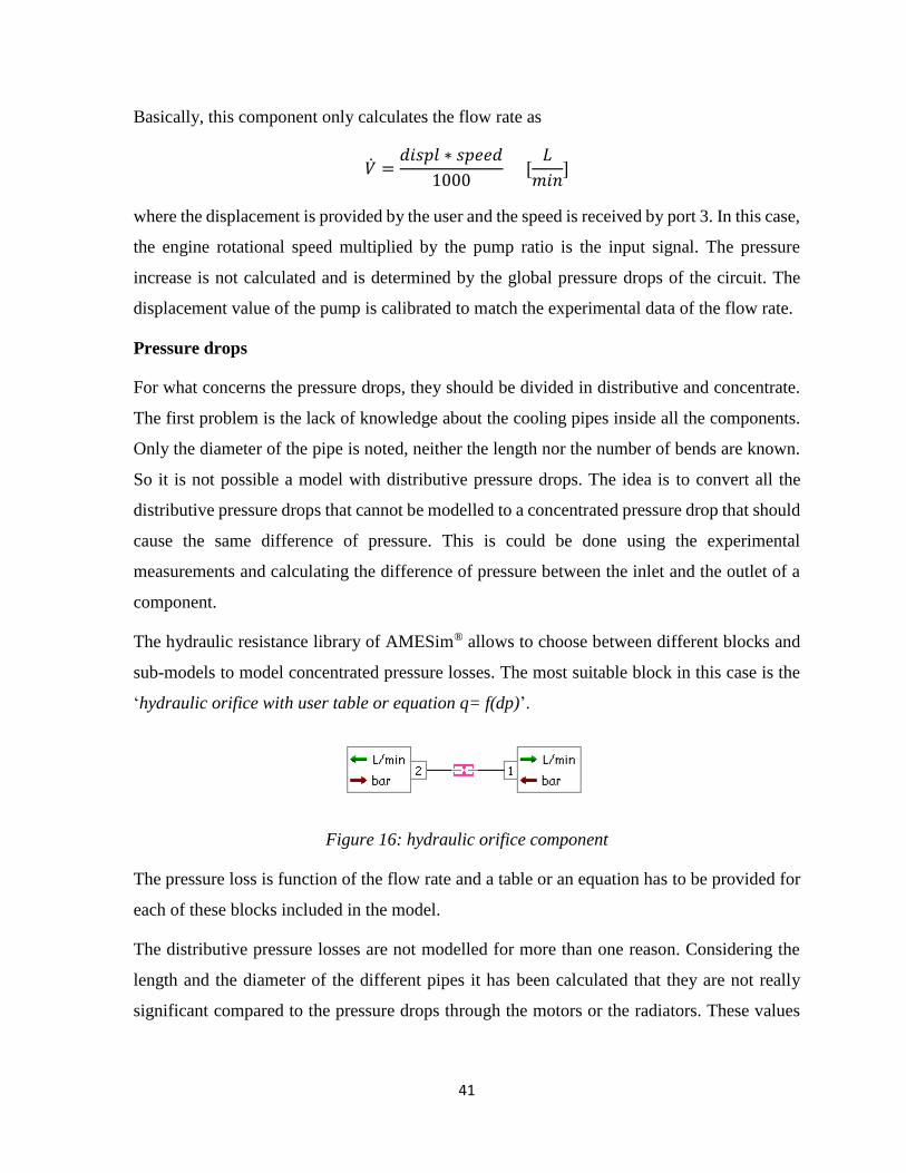
41
Basically, this component only calculates the flow rate as
�� =𝑑𝑖𝑠𝑝𝑙 ∗ 𝑠𝑝𝑒𝑒𝑑
1000 [
𝐿
𝑚𝑖𝑛]
where the displacement is provided by the user and the speed is received by port 3. In this case,
the engine rotational speed multiplied by the pump ratio is the input signal. The pressure
increase is not calculated and is determined by the global pressure drops of the circuit. The
displacement value of the pump is calibrated to match the experimental data of the flow rate.
Pressure drops
For what concerns the pressure drops, they should be divided in distributive and concentrate.
The first problem is the lack of knowledge about the cooling pipes inside all the components.
Only the diameter of the pipe is noted, neither the length nor the number of bends are known.
So it is not possible a model with distributive pressure drops. The idea is to convert all the
distributive pressure drops that cannot be modelled to a concentrated pressure drop that should
cause the same difference of pressure. This is could be done using the experimental
measurements and calculating the difference of pressure between the inlet and the outlet of a
component.
The hydraulic resistance library of AMESim® allows to choose between different blocks and
sub-models to model concentrated pressure losses. The most suitable block in this case is the
‘hydraulic orifice with user table or equation q= f(dp)’.
Figure 16: hydraulic orifice component
The pressure loss is function of the flow rate and a table or an equation has to be provided for
each of these blocks included in the model.
The distributive pressure losses are not modelled for more than one reason. Considering the
length and the diameter of the different pipes it has been calculated that they are not really
significant compared to the pressure drops through the motors or the radiators. These values

42
are calculated using Moody’s diagram evaluating the different tubes in their maximum flow
rate condition. The distributed pressure drops are expressed as
𝑅 = 𝜆𝑙
𝐷
𝑊2
2
where 𝜆 is the adimensional coefficient calculated from Moody’s diagram, 𝑙 is the length of
the pipe, 𝐷 is its diameter and 𝑊 is the velocity of the fluid. The concentrated pressure drops
are calculated as:
𝑅 = 𝛽(𝑅𝑒)𝑊2
2
where 𝛽 is the adimensional coefficient, function of the geometry of the obstacle and of
Reynolds number.
The values are reported in table 1. A length of one meter is considered as example. The fluid
used is 50% water and 50% glycol, density and dynamic viscosity are function of the
temperature. As it can be noticed, the flow is turbulent and so the pressure drops are function
of the relative roughness. The value of roughness used is the typical value for the material of
the pipe. The numerical values considered are from [1].
The total length of the circuit (precise data not available) should not be more than some meters,
and so the total drops should stay in tens of mbar, order of magnitude.
The pressure drops due to motors or radiators, are hundreds (until thousand) mbar. This
approximate estimation highlights that the neglection of the distributive pressure drops is not
so significant considering the pressure drops due to heat sources and heat sinks.
In addition, the distributive pressure drops, are partially taken into account in the restriction
block tables, In fact, as it will be described below, these tables are obtained from
measurements, so the pressure difference between two sensors is considered. Obviously, the
position of the sensor was not exactly out of the different components and so some pressure
drops are included in these differences.

43
Table 1
The same approach is valid for the concentrated pressure drops due to bends and three way
valves. Their estimated values are low, compared to the one of the heaters or coolers, as
reported in table 2. They are also partially taken into account in the tables used for the
restriction block. For the estimation of the concentrated pressure drops, the beta coefficient has
to be chosen. Different types of losses are present in the circuit (bends, valves, change of
section) and so the maximum value of beta, that is 1, is considered as example. The results
show that a single obstacle does not have a great impact in the total balance, but if they become
a remarkable number, the value of pressure losses it is significance. It has to be underlined that
the losses due the bends are probably overestimated because the beta coefficient is lower than
one, function of the ratio between the bend radius and the diameter.
Table 2
However, the modelling of every single pipes is too complex and it is also out of the scope of
the model because, in general, the effect are not so relevant, as demonstrated.

44
Definition of the pressure losses maps
All the pressure drops are included in the restriction blocks, and a map of volumetric flow rate
and difference of pressure has to be provided. The building of the maps could be done in two
ways: using the information available from the suppliers or the results of measurements done
on the same circuits. The data from the suppliers were available for only a few components. In
addition, the comparison of the curves with some experimental points shows that the pressure
losses are too underestimated. In figure 17, it is reported the comparison of inverter pressure
drops from datasheet and calculated from measurement value. The difference is roughly 100
mbar. This is probably due to the different position of the sensors in the two measurements.
Figure 17: inverter pressure drops, datasheet and experimental value
The attempt is to build maps as 1-D table for each component (pressure drops as function of
the volumetric flow rate). The pressure drops are function not only of the flow rate but also of
the temperature, and this dependency will be taken into account in the next parts, when
temperature is considered. In addition, the pressure losses are function of the square of the
velocity and so of the square of the flow rate (Bernoulli’s equation)
�� = 𝐶𝑞 𝐴𝑒𝑞√2 ∆𝑝
𝜌
0
100
200
300
400
500
600
700
0 2 4 6 8 10 12 14 16
Pre
ssu
re d
rop
s [m
bar
]
Volumetric flow rate [l/min]
Inverter pressure drops
---- Values from Inverter datasheet
---- Measurement value

45
where 𝐶𝑞 is called flow parameter, 𝐴𝑒𝑞 is the equivalent area of the pipe and 𝜌 the density of
the fluid. This formula cannot be directly implemented because flow parameter is not known,
In addition also the diameter and so the equivalent area of the pipes are not always known.
The limit of the table approach is that the electric pump always work at the same point. This
means that when the pump is switched on, the flow rate and the difference of pressure between
inlet and outlet are constant. Only one point can be calculated, one other is [0;0] and, knowing
that a parabola should be built, one other point misses. Attempts to extend the maps with
extrapolation or from curves found in literature are a possible further development of the
model. The idea is to consider 𝐴𝑒𝑞, 𝜌 and especially 𝐶𝑞 as constant and calculate the ratio 𝐾
from the experimental point as
𝐾 =𝑉
√∆𝑝
= 𝐶𝑞 𝐴𝑒𝑞√
2
𝜌
and substitute the table with this relationship.
Summary of the hydraulic validation
The three circuits built up are quite similar in this first step and so only the hydraulic model of
the front axle circuit (electric motors, inverter and DCDC converter) is reported in figure 18,
as an example.
Figure 18: hydraulic model for front axle circuit

46
First, the pumps are calibrated with their characteristic curves and with the control signal of
the rotational speed. In this case, the pumps always work at the same point (maximum
efficiency), therefore, the velocity is the typical rotational speed or zero. Then, the pressure
drops of all components are provided as function of the flow rate. Due to the control strategy
of the pump, only two experimental points were available (zero and the typical flow rate). Once
all the pressure drops are provided, the total losses of the circuit are known, and the pressure
increases of the pumps are calculated to obtain a balance. The pressure and the flow rate are
known for each branch. The next step is to convert the hydraulic library into the thermal
hydraulic library, including the temperature effect.
3.3.2 Thermal model map-based
After the hydraulic validation, the development of the model can proceed with the thermal part.
The conversion of the hydraulic model to a thermal-hydraulic model, using the appropriate
library, is the first step. The blocks (pump and ‘restriction’) of the hydraulic resistance library
are also included in the ‘thermal hydraulic resistance’ library, with the addition of the
temperature description.
The settings of this blocks is easy, once the model is calibrated in the hydraulic part. This is
one of the main reasons that justify the procedure step by step.
The pump block can be directly copied from the previous step without any modification. It is
possible to implement a map of pressure increase that is not only function of the flow rate but
also of the temperature, but this information was not available and so the same map was used.
The map of efficiency is reused without modification as well.
For the restriction block, the map of pressure drops has to be converted from volumetric to
mass flow rate, and influence of temperature should be taken into account as well. The
Bernoulli’s equation become
��(𝑝, 𝑇) = 𝐶𝑞 𝐴𝑒𝑞√2 ∆𝑝 ∗ √𝜌 (𝑇)
The temperature changes the density of the fluid, and so the mass flow rate. For the coolant
considered, water/ethylene glycol 50%, the density can be expressed with a second grade
polynom, as reported in [18].

47
𝜌(𝑇) = 0.024 𝑇2 − 0.3381 𝑇 + 1081.1
Like for the hydraulic model, only a couple of points were known from the experimental data.
So the map was built only using the information available. This is quite a strong estimation, in
particular in order to predict the temperature effect on the pressure drops more points are
necessary. The model has only been calibrated in a few test cases and due to this, its general
validity is not guaranteed. However, the block used is the equivalent of the hydraulic resistance
in the thermal hydraulic resistance library. The pressure drops are not not function of the
volumetric flow rate but of the mass flow rate, so the previous tables were multiplied by the
density of the fluid.
The 1-D table could be substituted with equations that express the relationship of the mass
flow rate versus pressure and temperature. Like for the hydraulic part, if we consider 𝐶𝑞 and
𝐴𝑒𝑞 constant, Bernoulli’s equation can be used and implemented in the AMESim® block as
��(𝑝, 𝑇) = 𝐾1√ ∆𝑝 ∗ √(0.024 𝑇2 − 0.3381 𝑇 + 1081.1)
after that the ratio 𝐾1 has been calculated from the experimental measurement.
Once the hydraulic parameters are set, the calibration of the heat flows can begin.
The procedure followed is organized in three steps.
▪ Firstly, only calculated experimental heat flows are provided (both for the heat sources
and for the heat sinks). This allows the calibration of the thermal losses along the pipes.
▪ Then the radiators are inserted and the real heat exchanged calculated by AMESim® is
compared with the experimental results.
▪ Finally, also the experimental results of the heat sources are substituted with the
AMESim® results.
In this first step of thermal model, thermal masses are not used. Only coolant temperatures are
calculated, but not component temperature. They will be considered in the next and last step.
Thermal losses along the pipes
As mentioned, whether the distributive pressure drops along the pipes could be neglected for
hydraulic validation, in the thermal model the pipes play a determinant role in the model
description. The heat exchange between the pipe and the external air has to be considered. This

48
is evident studying the experimental data: in test cases in which the temperature of the water
is roughly constant, the total heat exchanged should be zero. But this is not true and it is always
greater than zero. This means that an additional contribution (losses along the pipes) is present
and cannot be neglected in order to obtain a correct prediction of the coolant temperature.
This heat loss is function of the car velocity and can be described as external convection. The
convection is mixed, both natural and forced, and the heat exchange coefficient increases with
the speed of the car.
Instead to model each single pipe with its own heat exchange coefficient, the idea is to include
all the heat exchanged along the pipes in a single block. In this block an amount of thermal
power is removed from the water and this amount is function of the car velocity.
There are different ways in AMESim® to model like that. The thermal hydraulic library
includes a piloted external convection block in which the air speed is input and a heat exchange
coefficient is calculated using predefined correlations. Some attempt has been made using this
block, but the results are always really different from the experimental values.
After these attempts, it has been decided to use the other way and relate the losses along the
pipes only to car velocity. There is not information available about the air velocity and so a
parameter has to be calibrated. The block used is shown in figure 19, it is a thermal chamber
and allows to calculate directly the thermal power absorbed. As mentioned above, the signal
used is the car velocity and must be converted with a gain, or a more complex function, to the
heat exchanged. The component receives a thermal power amount (from port 3), that in this
case is negative since the heat is removed from the system.
Figure 19: thermal hydraulic capacity

49
The calibration of the gain is done using constant speed and constant water temperature test
cases. After the net heat exchanged is calculated, it is divided by the speed of the car and so
we obtain a linear relationship. Like for the pressure drops, due to lack of information, the
validity of the model is guaranteed only in the ‘points’ available and not in every condition. In
fact, we know that the heat exchange coefficient is not linear with the air velocity but has more
complex relationship that depends on convective heat exchange coefficient and that has not
been considered.
Heat sinks
Radiators
After the calibration of the gain for model the heat exchanged along the pipes, the thermal
model proceeds with the calibration of the radiators.
There are two ways to represent a radiator in AMESim®: one is with the cooling library and
one is with the heat exchangers assembly tools. The first one is simpler and the heat exchanged
is calculated from a map, function of air velocity and coolant flow rate. The second one is more
complex and the heat is calculated using convection equations and Nusselt number
relationships. Considering the scope of the model, it is preferable to use the simpler block in
order to not complicate the model calibration and save computational time. The heat
exchangers assembly tool is very detailed and it should be used, for example, to test and
validate a new cooling layout. The tool is really interesting, thanks to the regression tool: it
allows to obtain Nusselt number relationship starting from experimental data (difference of
temperature of water and air). In addition, the influence of the different components on the air
and its pressure drops could be taken into account in a very detailed way. In a future
development, it would be interesting the use of this block in the model and the comparison
with the cooling library block. The decision was to use the map based block, belonging to the
cooling library. The input and output of the different ports (external variables) are reported in
figure 20.

50
Figure 20: AMESim® radiator block (cooling library)
Port 1 brings information of temperature and velocity of the external air, port 3 and 5 are the
inlet and outlet of the coolant, port 4 is the signal of the fan. Different sub-models can be used,
according to the data available. For a good description of the air pressure drops, an under-hood
model could be used, but it was not available in this case. The sub-model chosen has been the
radiator with prescribed air velocity and table or expression for the pressure drops.
The external air velocity input at port 1 is 10-20 % of the vehicle speed. This reduction is
attributed to the cooling duct opening (if the duct opening is made larger it increases the drag
and hence a trade-off is made between aerodynamic coefficient and cooling performance). [18]
This gain between the car velocity and the air velocity has been calibrated for each radiator.
The table for the pressure drops is the same used in the hydraulic validation. The map of the
heat exchange between air and coolant for different conditions was available for experimental
data. The 3-D map is reported in figure 21.
The heat exchanged increases both with the air velocity and with the coolant flow rate. The
geometrical parameters are specified as well. The map is obtained with a difference of 70
degrees between coolant and air. The heat calculated with the map is scaled on the real
difference of temperature.
The influence of the fan is considered as well. The control signal of the fan is converted (with
a table or an equation) to an increase of air velocity. In order to calibrate the radiators, the heat
calculated by AMESim® and the results of experimental data are compared. Inlet and outlet

51
temperatures of the radiators, as well as the flow rate, were available for different driving
cycles. The heat exchanged is calculated using density and specific heat function of the
temperature. The expression for the density has already been reported, for the specific heat,
always in [18], it is:
𝑐𝑝(𝑇) = 2.64 ∗ 10−9 𝑇2 + 3.86 ∗ 10−3 𝑇 + 3.203
The calibration is done changing the gains of the air velocity and of the influence of the fan.
The other parameters are known and constant. An example of comparison for the radiator of
the frontal axle is reported in figure 22. The car velocity is also reported to better understand
the results.
Figure 21: radiator heat exchanged map, function of coolant flow rate and air velocity

52
As it is possible to notice in figure 22, when the velocity is stable at the maximum value, the
calibration is correct (the red and the green lines are similar). The air velocity is only the 8%
of the car velocity.
The problem is when the velocity is in the other stable region, from 200 to 400 seconds. In this
situation, the heat calculated by AMESim® is too high. We know that the coolant flow rate is
constant because the electric pump works always at the same point (max efficiency), so is the
air velocity that is too high. This suggests that the relationship between the car velocity and
the air velocity through the radiator is not linear but it is at least a second-grade polynomial.
Figure 22: power losses electric motor estimation
Another reason is probably that the map is obtained in different conditions and so the
experimental data can be not completely in accordance with it. The influence of the fan is
calibrated thank to the last seconds, when the car is at standstill: the air velocity at that moment
is only due to the fan. When we obtain that the two heat exchanges are equal, we have found

53
the right gain for the increase of air speed. The relationship is linear and the control signal (that
is a 0 – 1 signal) is multiplied by 4 (AMESim® default file use the same value).
This procedure is repeated for the two radiators of the ISG circuit (which have only one fan)
and for the two radiators of the ICE circuit. The vehicle has one other radiator for oil cooling,
but no information was known about this circuit and so it was decided not to model it in this
work. Comparison between model and experimental data for one of the engine radiator is
shown in figure 23. The test is the same and, like in the front axle radiator from 200 to 400 s,
the heat exchanged calculated by the model is higher. The gain to convert car velocity to air
velocity has been calibrated to 10%.
The values of thermal power are completely different between the two circuits: the engine
radiator absorb almost ten times the amount of power absorbed by the electric motor radiator.
Of course, it depends on the driving condition and of the split factor: in this situation, the power
to the wheel is provided mostly by the engine but, anyway, it is significant to highlight the
ratio between the two contributions.
Figure 23: engine left radiator, model and experimental data
The tests at constant speed are used to calibrate the numerical values (air velocity and fan
influence) in order to match the experimental heat exchanged. Some other tests are used to
validate the model in different driving condition. This will be reported in the following chapter.
The two radiators of the high temperature circuit have the same size but the heats exchanged
are different. This is since the condenser of the air conditioning system is in front of only the
right radiator. The air is first heated by the condenser and the higher inlet air temperature the

54
lower the heat exchanged. In order to impose a higher inlet temperature of the air, the condenser
block, belonging to the cooling library, should be used. Port 3 and 4 have the information on
the air (temperature and velocity), the control signal at port 2 says if the air conditioning is on
or off, and port 1 calculates the power absorbed by the compressor. When the air conditioning
is on and the condenser has to remove heat from the refrigerant, the air is heated, typically
around 10-15 degrees and this limits the performance of the radiator.
Figure 24: condenser block (cooling library)
Chiller
The radiators are not the only heat sinks, since the battery circuit uses a chiller. The temperature
of the battery must stay below 40°C and, consequently, the external air cannot always be used.
As described in the first chapter, the battery circuit is linked with the air conditioning system
through a heat exchanger, which is like an additional evaporator, and a thermal expansion
valve.
A map of heat exchange for the chiller was available. This is function of the coolant flow rate,
coolant inlet temperature and refrigerant outlet pressure. A specific component is not present
in the cooling library. Another possibility was to use the air conditioning library which include
particular heat exchangers, but it is too detailed for the scope of the model. Therefore, the
solution used was to calculate the heat exchanged using the map, and use a thermal capacity
of the thermal hydraulic library to cool down the coolant. The built model is reported in figure
25.

55
Figure 25: simplified map-based chiller model
The coolant inlet temperature and the coolant flow rate which enter in the map, are calculated
by the model, so no additional data is necessary. Instead for the refrigerant pressure, the ECU
signal is used. The air conditioning circuit has not been modelled yet and for a first validation
it was preferable have a correct value. This signal cannot always be available and it will be
switched with an internal AMESim® parameter in the following step. The map is defined only
for coolant temperature over 20°C, but typically the coolant could reach lower temperatures.
In this situation, it is necessary to extrapolate data from the table. The problem is that when
the coolant temperature is really low, the extrapolation gives negative values of heat exchanged
which are not physical (the coolant cannot cool down the refrigerant). To avoid negative
extrapolation of heat exchanged, a switch is added: when from the table a negative value is
calculated, this is converted to zero. The experimental heat exchanged for the chiller was not
available because during the test the sensors of temperature were only in the battery side. To
be able to validate the model, the idea was to use the experimental value for the battery and
the calculated one for the chiller, and to compare the two coolant temperature values
(experimental and of the model).
Heat sources
After the validation of the radiators it is time to substitute the heat exchanged by coolant with
the real heat produced by the different components (and estimate an appropriate heat exchange
coefficient).

56
Power electronic and electric motors
For the medium temperature circuit, the thermal sources are power electronic components,
they are DC/DC converter, inverter and electric motor. The model has to predict the heat
generated by each component in the different operating conditions.
Usually they have very high efficiency, however their power losses produce a significant
amount of heat. All the power losses become heat and increase the temperature of the
component. The maximum limit of temperature is linked to silicon properties. A temperature
limit for the coolant is specified as well. This is around 80°C for the inverter and around 60°C
for the electric motor. They are quite preventive because, like in the batteries, the thermal
cycles and the maximum temperature have an important effect on the derating of the power
electronic components. In order to avoid premature derating, it is important to leave the
temperature as low as possible.
The losses of the electric motor are divided in iron and copper losses. The copper losses are
due to Joule effect, the iron losses are more complicated to estimate and are due to hysteresis
and eddy currents. The thermal models of electric motors are quite complex and the topic is
out of the scope of the present work. It would be necessary to model all the electric connections
using specific libraries. The software used allows this approach since an electric library is
included and most of the other component can be connected to this. However, this is not
considered in the present work. Luckily, it is possible to have a simple thermal model using
the map of efficiency (map-based thermal model).
For the two electric motors (three including also the Integrated Starter Generator) the efficiency
map was available. The efficiency is function of rotational speed of the motor and torque,
obtaining a 2-D table. For the inverters, a map of efficiency was not available, but it has been
obtained starting from a map of global efficiency of the system (including both the inverter
and the motor). For the DC/DC converter a constant efficiency, around 90%, is implemented.
In order to enter in the efficiency map of the electric motor, torque and rotational speed have
to be calculated. For what concerns the rotational speed, the hybrid car has a P1-P4
configuration. This means that the speed of the two frontal electric motors have a constant ratio
with the wheel rotational speed, and so with the car velocity. Instead the generator has the same
rotational speed of the ICE. So the rotational speeds of the motors could both be calculated

57
from two known signals. On the other hand, the torque could be calculated starting from the
voltage and the current of the inverters, both included in HCU signals, available after the test
cases done. The calculation of the power is immediate, then the inverter efficiency has to be
considered. At the end the electric power is multiplied by one less the efficiency to obtain the
power losses.
The control scheme for the front electric motor is reported in figure 26. It has been done using
the control library of AMESim® that is actually like Simulink.
The same procedure has been used for the calculation of the power losses of the ISG, the only
difference is for the rotational speed, that is directly the engine rotational speed.
Figure 26: map-based power losses calculation for inverter and electric motor
The thermal heat flows obtained are compared with the experimental coolant heat exchanged.
The results for a test case are presented in figure 27a and 27b both for electric motor and
inverter. The difference between the two curves is related to the heat exchange coefficient that,
obviously, is limited. The heat produced and not exchanged with coolant determine the
increase of temperature of the component.
As mentioned before, in this first thermal step model the components and the convection heat
exchange are not included. In order to convert the power losses to coolant heat exchanged a
constant ratio is estimate. This is necessary to obtain correct values of coolant temperature and

58
be able to validate the model. This ratio, which is around 0.7-0.8, cannot be always constant,
as it can be seen from the figures. Therefore, the estimation is not rigorous but it is necessary
in this first step. Two test cases were considered: one to calibrate a good value of this gain and
the other to validate the model. This ratio has no physical value and it will be substituted with
a physical description of convection and heat transfer in the next step.
Figure 27a: thermal heat flows for electric motor
Figure 27b: thermal heat flows for inverter front axle

59
Internal Combustion Engine
The ICE remains the main heat source also in a hybrid car. Its power is generally much higher
than the electric motors and its efficiency is much lower.
As a first estimation, it is possible to consider that the chemical power of the gasoline is
divided in three equal contributions: mechanical, remained in exhaust gases and exchanged
with the coolant. Actually, the problem is more difficult for two reasons:
▪ the various ratios are not constant but are function of the engine rotational speed
▪ additional contribution must be considered, such as irradiation, convection with air and
losses due to combustion inefficiency
and so, the division by three cannot bring good results.
The best thing would be having a thermal map of the engine with the coolant heat exchanged
as function of rpm and shaft torque. Unfortunately, only a map of fuel consumption was
available.
The idea was to calculate the mechanical efficiency from the fuel consumption and then
estimate the heat percentage exchanged with the coolant.
In order to go into the fuel consumption map, we need the engine rotational speed signal
(known) and the engine torque. For the engine torque a throttle signal is used and it is
multiplied for the maximum engine torque. Dividing the fuel consumption for the mechanical
power, the brake specific fuel consumption is obtained, and considering the lower heating
value, the mechanical efficiency is found. Now it is possible to calculate the total power given
to the engine and from that, estimate the power to the coolant with a suitable percentage. Values
suggested in literature from spark ignition engine go from 26% (at low rotational speed) to
17% (higher rotational speed). [19]
𝑏𝑠𝑓𝑐 = 𝑓𝑢𝑒𝑙 𝑐𝑜𝑛𝑠𝑢𝑚𝑝𝑡𝑖𝑜𝑛
𝑏𝑟𝑎𝑘𝑒 𝑝𝑜𝑤𝑒𝑟 [
𝑔
𝑘𝑊ℎ]
𝜂𝑒𝑛𝑔 = 1
𝑏𝑠𝑓𝑐 𝐿𝐻𝑉
𝑃𝑜𝑤𝑒𝑟𝑐𝑜𝑜𝑙𝑎𝑛𝑡 =𝑃𝑏𝑟𝑎𝑘𝑒
𝜂𝑒𝑛𝑔∗ 𝑘(𝑟𝑝𝑚) [𝑘𝑊]

60
The scheme implemented is reported in figure.
Figure 28: engine power losses
Experimental results available are used to find the correct percentage of the total heat given to
the coolant and to build up the table for different rpm.
A test case is reported in figure. The engine speed is very high and the value that fits the curve
at that velocity is around 0.14. It is a bit different from the ones suggested in literature, but the
engine considered is different as well. The experimental data is, of course, limited; for the other
rotational speed a linear interpolation is considered. In addition, with this approach thermal
inertia is not taken into account. For example, if the brake power is zero and so is the fuel
consumption, the calculated heat rejected is zero as well. But due to thermal inertia of the
coolant and of the engine components, the experimental data could show the heat exchange is
still positive. This is also the reason for the spikes and for the too high slope, compared to the
experimental results, of the curve. To sum up, the approach is not the best because estimations
are necessary and results are not so coherent. But, on the other hand, it is the only possible with
the data available and it is allowed to have a main thermal description of the engine cooling
circuit.

61
Figure 29: comparison of engine heat rejected to coolant and engine rotational speed
Thermostat
The model of the thermostat has to be included as well. The warm up of the engine has to be
as fast as possible to reduce emissions and frictions (warming up post-treatment devices and
oil). The thermostat allows this with a bypass of the radiator when the coolant temperature is
below a threshold. Once the warm up has concluded, the thermostat opens and the coolant can
go through the radiators. It allows to maintain the desired temperature during all operating
conditions.

62
The thermostat behaves like two orifices of variable cross-sectional area and the variation of
the cross-sectional areas is a function of the convective exchange between the coolant and the
wax, [18], which is the thermo-sensible element. The opening and the closure laws are defined
in the ‘hysteresis’ block and stabilize the fractional area opened as function of the wax
temperature. A value 0-1 is calculated and passed to the two additional blocks. This is
necessary to model the fact that when one part (line to the radiators) is partially open, the other
(bypass). receives the remaining flow rate. The aperture and closure laws, generally, are
different in order to take into account the thermal hysteresis effect of the wax. The sketch is
represented in figure
Figure 30: two ways thermostat for the engine coolant circuit
Battery
The battery is the most critical component from a thermal point of view. Its temperature has to
stay between 5°C and 40°C [2]. Battery circuit is integrated with the air conditioning and, as
already mentioned, a chiller cools down it. An electric heater is necessary to warm up the
battery when the external temperature is below the low threshold. This can be warm the liquid
or directly the battery surface. The PTC heater is not modelled in the present work.
The battery power losses are due to its internal resistance and to Joule effect. A map of internal
resistance of a battery cell, function of the battery temperature, was available. Thanks to this,
the heat calculation is quite simple. The internal resistance has to be multiplied by the cell
number and by the square of battery current. If available, the resistance of the conductors can
be added to obtain the global battery resistance.
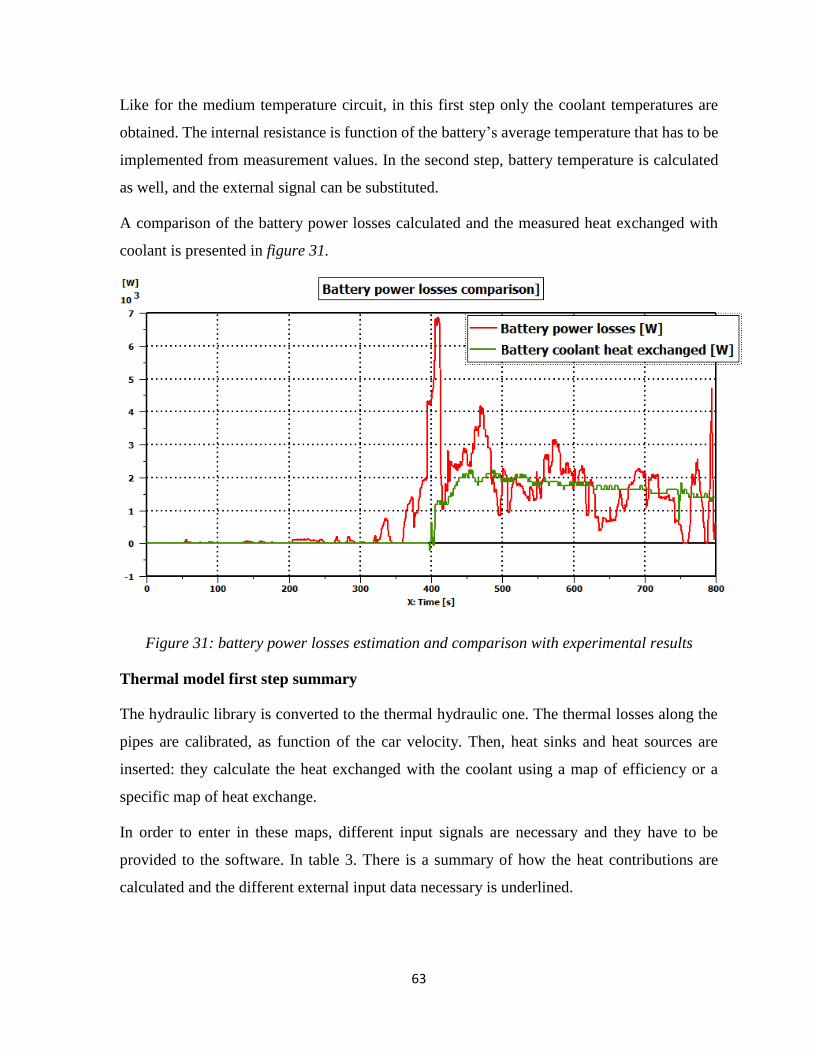
63
Like for the medium temperature circuit, in this first step only the coolant temperatures are
obtained. The internal resistance is function of the battery’s average temperature that has to be
implemented from measurement values. In the second step, battery temperature is calculated
as well, and the external signal can be substituted.
A comparison of the battery power losses calculated and the measured heat exchanged with
coolant is presented in figure 31.
Figure 31: battery power losses estimation and comparison with experimental results
Thermal model first step summary
The hydraulic library is converted to the thermal hydraulic one. The thermal losses along the
pipes are calibrated, as function of the car velocity. Then, heat sinks and heat sources are
inserted: they calculate the heat exchanged with the coolant using a map of efficiency or a
specific map of heat exchange.
In order to enter in these maps, different input signals are necessary and they have to be
provided to the software. In table 3. There is a summary of how the heat contributions are
calculated and the different external input data necessary is underlined.

64
Circuit Heat source Map External Input for heat source External input for heat sink
HT Fuel Consumption engine rpm and engine torque car velocity
MT Efficiency motor rpm and motor torque car velocity
LT Internal Resistance HV battery current chiller outlet pressure
Table 3: summary of external model input
The validation of the model was done using HCU signals from the test as external input files
and comparing the coolant temperature and heat flows obtained with the ones calculated
starting from experimental data.
3.3.3 Thermal model with thermal masses
In the first thermal model, only the coolant temperature is calculated. In addition, the
conversion from power losses to thermal power to the coolant has been done without
physical meaning but in order to fit measurement results. In the last step of the model, these
two limits are overtaken.
The addition of thermal masses and thermal resistance allows to predict the temperatures of
the components, like the electric motor, the battery, and the inverter. The amount of thermal
power exchanged with the coolant and the remaining part, exchanged with air or that heats up
the mass, are calculated using convection relationships.
The description of thermal behaviour of a component is quite complex and to obtain highly
accurate results, a detailed model is necessary. The electric motor, in particular, is very
complex since it has different materials, internal gap air, complicated shapes. In literature,
complex thermal model are built, like the one in [16].
The thermal mass belongs to the thermal library and has four thermal ports. They are
connected to other libraries, where the thermal power is calculated. The thermal properties of
the material has to be specified.
The temperature is calculated as:

65
𝑚 𝑐𝑝(𝑇)𝑑𝑇
𝑑𝑡= ∑ 𝑑ℎ𝑖
4
𝑖=1
𝑇(𝑡) = 𝑇(0) + ∑ 𝑑ℎ
𝑚 𝑐𝑝(𝑇)
where 𝑚 is the mass, 𝑐𝑝is the specific thermal capacity and ∑ 𝑑ℎ is the sum of the four thermal flows
of the block. If the component is composed of different materials, more than one thermal mass has to
be considered. The different thermal blocks are linked together with a block that models the
conduction. The general conduction equations are reported in chapter 2. Not only the specific thermal
capacity, but the thermal conductibility determines how fast the material increases or decreases its
temperature as well.
The heat exchanged between solid material and external air is considered using an external
mixed convective exchange. The external surface of the material, such as the surface cooled
down by the air, has to be specified. The air velocity characterizes the thermal exchange and
in a car, it is function of the car velocity, as mentioned in the previous pages.
The majority of the power losses are removed by the coolant through convection. This is
modelled using the block in figure 32. Port 1 and 3 are inlet and outlet of the coolant, the port
2 calculates the thermal exchange and it is connected to a thermal mass. The heat exchange is
internal convection between the fluid in the pipe and the wall of the pipe. [18]
Figure 32: thermal-hydraulic pipe with heat-exchange
The internal convection can be modelled imposing a convective heat exchange coefficient or
providing correlations for the Nusselt number. Neither of these options is in general available
without specific investigation. A third option is to use predefined correlations that are
generally accepted to describe the heat exchange with laminar or turbulent flows. They are
described in chapter 2 and this option is the one used in the present model. Beyond

66
convective correlations, the heat exchange is also function of the geometry of the pipe, in
particular of the diameter and the length of heat exchange.
The predefined correlations calculate the Nusselt number, and from this, it is possible to
know the heat exchange coefficient as
ℎ𝑐𝑜𝑛𝑣 = 𝑁𝑢 𝑘
𝐿
where 𝐿 is a reference length and 𝑘 is the thermal conductivity of the fluid. The convective
heat exchange is computed as
𝑄𝑐𝑜𝑛𝑣 = ℎ𝑐𝑜𝑛𝑣𝜋𝐷𝑙 (𝑇𝑖𝑛 − 𝑇𝑤𝑎𝑙𝑙)
Some of these parameters were not known. The approach was to give them a physical value in
the first attempt and try to calibrate this value in order to match some of the experimental
results. Once a good value is found, other tests are used for the validation of the model.
The thermal masses for the electric motor and the battery are included in the respective circuit.
On the other hand, the ICE circuit is not modelled anymore in this step and its final model is
the one described in the previous chapter. In fact, the thermal power to the coolant has already
been calculated from the fuel consumption map. It is different from the other two circuits where
the total power losses have been obtained. In addition, while in the PEEM all the power losses
are converted to heat, this is not true in the combustion engine, where part of the energy
remains in the gas enthalpy or it is not converted at all due to combustion inefficiencies. The
problem is much more complicated and more estimation are necessary. Engine thermal model
need a big effort and has been deeply investigated, so is not included in the present model.
Electric motor and inverter
As mentioned, electric motor thermal model need to be complicated in order to reach a high
level of accuracy. This is not the specific focus of this work, therefore the thermal model had
to be as simple as possible. After some attempts using only one thermal mass, the decision was
to use one more mass. In fact, it was not possible to match both the material temperature and
the coolant heat flow with this approach. On the other hand, using two thermal masses is more
realistic and allow to match the experimental data better. The model scheme is shown in figure
33, it is an extract and all the cooling circuit is cut away.

67
Figure 33: electric motor thermal masses for temperature prediction
The first thermal mass includes all the thermal generation. This is an important approximation
but it has been considered acceptable in this easy thermal model. Actually, the electric motor
thermal losses are divided between rotor, stator and bearings. Different kinds of motor have
different iron and joule losses and different distribution inside the component. Another mass
is used to implement the cooling plate, that absorbs part of the losses for conduction and it is
cooled down by the fluid for convection. A port of the cooling plate is also connected to
external convection with environmental air, to simulate its cooling effect. This contribution is
function of the air velocity and so of the car velocity. The parameters specified are the mass of
the motor and the thermal properties of its materials. In addition, the surfaces for the
conduction and convection exchanges have to be specified. For the conduction, geometrical
data was not available and the value is calibrated to match a test case and obtain a good
matching with the motor temperature. For the convection exchange, the diameter of the pipe
was known but not the heat exchange length and so also this value is calibrated in one test case
to obtain the experimental coolant heat exchange. The thermal properties used are the one of
the copper for the motor and of aluminum for the cooling plate. The total weight of the motor
was known, the division between the two thermal masses was estimated. The parameters are
the same both for the two motors at the front axle and for the ISG in the rear axle, since the
motors are identical.
For the inverter, only one thermal mass was used, choosing aluminum as material and using
the known value of weight. The inverter power losses are quite low compared to the electric
motor ones, since its efficiency is higher. In addition, it is very well cooled down by this
system. Due to this, its temperature maintains lower values than the motor.

68
Battery
For the battery, the approach used is identical to the one used for the electric motor, but only
one thermal mass is used. The weight of the component was known, while its thermal
properties were looked up in literature, where they are widely investigated. Experimental value
of Li-ion battery thermal properties can be found in [20] and [21]. Using only one thermal
mass, only the specific thermal capacity influences the results, while the thermal conductibility
is important if more thermal masses are considered and determines the thermal resistance. It is
difficult to calculate the specific thermal capacity and quite different values have been
calculated. Starting from values reported in the papers, the parameter has been calibrated in a
test case and the value used is 1100 𝑘𝐽
𝑘𝑔 𝐾.
The internal resistance of the battery, used to calculate the power losses, is function of the
battery temperature. In the previous step, the external signal (from the BMS) was implemented,
but now it can be deleted. In order to calculate the battery power losses, only the battery current
has to be provided to the model. The battery circuit model is reported in figure 34.
Figure 34: battery cooling circuit with thermal mass
69
Air Conditioning modelling
In PHEV and BEV, the A/C compressor not only has to cool down the cabin but also the
battery. It is interesting to be able to model the integrated system to design it and also to study
control strategies since the HV compressor has a considerable power and it has an important
impact on the battery SoC.
Air Conditioning modelling is much more complicated than a cooling system, since the fluid
changes phase in the condenser and the evaporator. More variables, like the gas mass fraction,
have to be taken into account. The heat exchange in condenser and evaporator have to be
modelled in details to ensure that the all the fluid changes its phase. Specific libraries are
implemented in AMESim®: the two-phase flow library substitute the thermal-hydraulic and
the Air Conditioning library allows the modelling of the four main components, compressor,
condenser, lamination valve and evaporator. Since the physics of the problem is much more
complex, the model becomes extremely detailed and many parameters have to be provided.
Most of these parameters were not available, in addition the effort to obtain a good model was
too high. For these two reasons the system has not been validated.
However, thanks to the aforementioned library, building a generic air conditioning model is
not so difficult and a first attempt is included in the present work. The compressor block
receives a rotational speed signal from the mechanical library and its displacement and
efficiencies are required. The condenser model is really detailed and both the refrigerant and
the environmental air side are modelled. For the refrigerant side, each heat exchanger tube is
considered and its geometrical parameters are specified. In addition, heat exchange coefficients
for Nusselt number correlations have to be provided. For the external air side, the temperature,
humidity, pressure and mass flow rate are the external input. After the condenser, the fluid
goes to the lamination valve, that in this system is a thermal expansion valve. As described in
the first chapter, it allows a better regulation of the refrigerant mass flow rate, only an amount
which satisfies the evaporator request goes to the heat exchanger and the superheat of the fluid
controlled, reducing the energy consumption of the compressor. Thanks to the valve, the liquid
mass fraction at the outlet of the evaporator is zero and the liquid accumulator can be omitted.
After the lamination valve, the refrigerant goes to the evaporator. The air conditioning system
integrated with the battery cooling circuit has two evaporators, one is for the cabin and one is
70
for the chiller. While the first is the classical air conditioning evaporator (liquid-gas
exchanger), the chiller is a liquid-liquid heat exchanger (or liquid- two phase flow). In the
present work, the chiller is not physical modelled but the calculation of its heat exchange is
map-based. As mentioned, the outlet pressure of the chiller is a necessary data to enter in the
map and from the A/C model can be transmitted to the battery coolant circuit.
A first attempt of model the liquid-liquid heat exchanger has been done: the idea is to use
internal convective exchange, one for the coolant side and one for the refrigerant side,
connected to a thermal mass that represent the chiller plates. The approach has been found in
literature in [22]. The cabin evaporator is not modelled at all, since neither the cabin is included
in the model. The A/C model has not been validated, only a generic model of the system has
been built but most of the necessary input has not been specified. In addition, more complex
models are necessary to consider heat exchange effects in more detail. However, it is
interesting for this work to include this first attempt and underline that this is not difficult
thanks to the specific library of the software used.

71
4. Results and validation
The results obtained in the three steps of the model are compared to experimental data in terms
of volumetric flow rate, coolant pressure, coolant temperature, thermal heat flows of heat
sinks/sources and temperature of components (e-motor, inverter and battery). As already
mentioned, the experimental data includes signals from the control unit and acquisitions from
additional sensors. From this data, all the information necessary to compare and validate the
model was available.
To perform the simulation, the external input data listed in table 3 (car velocity, battery current,
invert current and voltage, etc..) is taken from the available data. Neither a vehicle model or a
powertrain model is built, so this is the only way to be able to compare the results. In addition,
the control signals for the pumps and fans must be the same. They are copied from the control
unit data as well. For the three circuits, the complete list of external input to perform a test case
is reported in table 4.
Circuit External Input for thermal model Control signals
HT engine rpm / engine torque / car velocity Fan signals (2)
MT motor rpm / motor torque / car velocity E-pump rpm (3), Fan signals (3)
LT HV battery current / chiller pressure E-pump rpm (1), HV Compressor rpm
Table 4: complete input list for simulations
During the validation, all these signals are provided from experimental data. Once the model
is validated, the thermal model could be connected to a drivetrain model and different control
strategies could be studied and developed. This is better point out in the next conclusive
chapter. In addition, initial conditions are specified as well. Air, coolant and material
temperature values are set equal to the real conditions during the test.
Like for the modelling part, the validation is divided in three steps. For each one, the main
relevant results are here discussed.
4.1 Hydraulic validation
The first model developed considers only the hydraulic library and temperature is not taken
into account. As described in the previous chapter, the pressure losses are calculated from
experimental data. In addition, for the medium and low temperature, electric pumps are used

72
and they are controlled with a start and stop strategy. When they work, they have always the
same flow rate, that allows to have the maximum efficiency. Due to this, only one operating
point was available from data and the validation is not guaranteed for different flow rates.
From the characteristic curve of the pump and the total pressure losses, the operating point is
found; flow rates and pressures in each point of the circuit are determined and compared with
measurements. Flow rate and pressure results for the front axle circuit are reported,
respectively, in figure 35a and figure 35b.
In figure 35a, also the ISG flow rate is reported. Its value is roughly the half of the front axle
value, since it has one e-pump and one e-motor, while the second one has two of both.
The same results are obtained for the low temperature circuit, in which the hydraulic model is
very simple. In fact, no three-way valves are present and only two thermal sources are
modelled. The electric pump is the same used in the medium temperature circuit, the total
pressure losses are a bit higher than the medium temperature circuits and so the operating point
is found for a lower flow rate value (20 l/min against 27 l/min for the previous circuit).
Figure 35a: volumetric flow rate validation for medium temperature circuit
-5
0
5
10
15
20
25
30
Vo
lum
etri
c fl
ow
rat
e [L
/min
]
Time [s]
Flow rate Electric Motor and ISG_test 4
AM. VFEM
MEAS. VFEM
AM.VFISG
MEAS.VFISG

73
Figure 35b: pressure validation for medium temperature circuit
For the high temperature circuit, the model is different since the pump is not electric but is
driven by engine belt. As a consequence, the flow rate and the pressure drops are not constant
but always change following the engine rotational speed. The rotational speed of the pump has
a fixed ratio with the engine and the flow rate is calculated as rotational speed times
displacement. In some of the test cases the thermostat was not used and these are chosen for
the hydraulic validation, since it is not possible to include this thermal component. As
described in the previous chapter, a different pump block is used for the engine circuit because
the pump characteristic was not available. In figure 36a and 36b, flow rate and pressures
obtained with the model are compared to experimental data. The test considered is the same of
the previous charts. While the flow rate and pressure were constant using the e-pump, the
engine pump follows engine rotational speed and its flow rate is more variable. The error
between the two curves was calculated after that a stationary operating point was reached.
-0,5
0
0,5
1
1,5
2
2,5P
ress
ure
[b
ar]
Time [s]
Pressure Front Axle Circuit_test 4
PCDCI bar
AME.P_DCDC_I
PRADI
AME.P_RAD_I
PCR1RO
AME.P_RAD_O

74
Figure 36a: engine flow rate validation for high temperature circuit
Figure 36b: engine pressure validation for high temperature circuit
-20
0
20
40
60
80
100
120
140
160
180
200
0 200 400 600 800 1000 1200 1400 1600
Vo
lum
etr
ic f
low
rat
e [
l/m
in]
Time [s]
Engine flow rate_test 4
VFCE_AME
VFCE_MEASUR
0
0,5
1
1,5
2
2,5
0 200 400 600 800 1000 1200 1400 1600
Pre
ssu
re [
bar
]
Time [s]
Pressure engine_test 4
AME.Eng_out
PCEO
AME.Rad_out
PC_RAD_O

75
The different curves are compared and the percentage error has been calculated. The results
obtained are reported in table 5. The medium error does not overtake the 5%, which is
considered acceptable for the aim of the project. Therefore, the hydraulic model is considered
validated.
Variable Position Medium error Maximum error
% %
HT Flow rate (steady) 3,69 8,88 Pressure Engine out 4,45 5,73
Radiator out 1,75 4,15
MT Flow rate EM 5,11 5,95 ISG 3,51 10,1
Pressure EM input 0,62 3,74 FA Rad outlet 2,97 5,41 IPU (ISG) in 3,33 5,29
LT Flow rate
1,55 2,57 Pressure Battery inlet 4,63 8,7
Table 5: summary hydraulic circuit errors
4.2 Thermal model map-based validation
Once the hydraulic part is validated, it has been converted into the thermal-hydraulic library
and no other modifications are necessary. The volumetric flow rate and the coolant pressure of
the model are still valid and no other results are presented. This is the main advantage of the
step-by-step procedure.
The first step of the thermal model calculates the heat exchange between the coolant and the
heat source/sink using maps. For the engine and for the radiators, the heat exchanged with the
coolant is directly calculated from these thermal maps and no other operations are necessary.
For the electric motor, inverter and battery, the total power losses are obtained from the maps
and they have to be converted to heat exchange with the coolant. To do so, in this first step, a
fixed ratio is calibrated, as described in the previous chapter. The results compare heat flows
and coolant temperature in some of the test cases available. They are presented divided in the
three circuits.
High temperature circuit
The developed model for the engine coolant circuit is reported in Appendix. The engine heat
exchange with the coolant is calculated using a map of fuel consumption. The total energy

76
available is obtained and then the heat-transfer rate to the cooling medium is calculated
considering a calibrated percentage. The values found are, generally, lower than the values in
literature, around 25% for low rotational speed to 15% for high rotational speed. For the two
radiators, heat exchange map as function of coolant flow rate and air velocity are used and the
results have already been reported in the previous chapter. In addition, the thermostat is
included. Putting together the heat source and the two heat sinks, providing the different
external input necessary (engine rpm, engine load, etc..) and the initial conditions, the coolant
temperature is calculated. In figure 37, the engine and one of the radiator outlet temperatures
are compared to the measured values. The test is always the test 4, that is the same used for the
previous comparison of the engine and radiator heat flows.
Figure 37: engine coolant temperature, model values and measurements
The heat flows were reported in figure 23 and 29 and they were quite similar to the
experimental values. Once the temperature is stable, the two temperature curves are quite
similar as well and this proof the model is correctly built and calibrated. Once the stationary
state is reached, in this case after 200s, the medium temperature error is ± 3°C and the
maximum error is ± 5°C, values considered acceptable in the present work. Higher errors are
40
50
60
70
80
90
100
0 200 400 600 800 1000 1200
Tem
pe
ratu
re [
°C]
Time [s]
Temperature ICE and RAD_test 4
T_ICE_OUT_model [°C]
TCEO [°C]
T_RAD_R_model [°C]
TCRERO [°C]

77
obtained in the first part, during the warm up of the engine. This is due to the thermostat model,
which has to be better calibrated to obtain better results also in transient cycles. While for the
other two circuits thermal masses will be included in the second step, for the engine circuit
these are the final results.
Medium temperature circuit (first step)
The conversion of the power losses to a heat exchange with the coolant is based on a calibrated
gain without any physical meaning. This is done considering a test case at constant
speed/constant inverter current and finding the value between 0 and 1 that matches the
experimental curve. For the electric motor is 0.7 and the curves obtained are reported in figure
38. The grey and the orange curves match each other only once heat flows are stable and it is
evident that the approach is too simplified to obtain good results also in transient conditions.
For this scope, a model which includes thermal masses and convective exchange is necessary.
Thermal inertia is not modelled with this approach: when the current request increases, in the
same time step also the heat absorbed by the coolant increases and this is not realistic.
Figure 38: electric motor power losses and heat experimental coolant heat exchange
-0,5
0
0,5
1
1,5
2
2,5
3
3,5
0 50 100 150 200 250 300 350 400 450
Hea
t tr
ansf
er [
kW]
Time [s]
Thermal heat flows EM1_test 2
Power losses EM1 [kW]
Coolant heat exchange [kW]
Power losses *0.7 [kW]
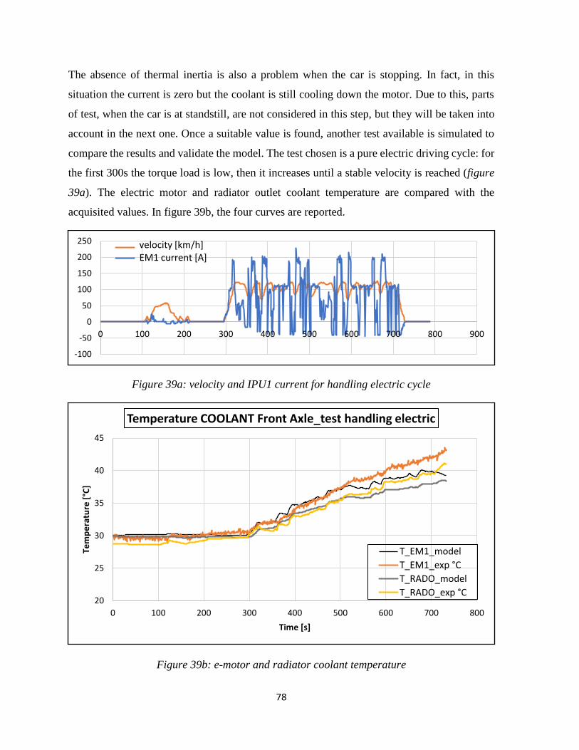
78
The absence of thermal inertia is also a problem when the car is stopping. In fact, in this
situation the current is zero but the coolant is still cooling down the motor. Due to this, parts
of test, when the car is at standstill, are not considered in this step, but they will be taken into
account in the next one. Once a suitable value is found, another test available is simulated to
compare the results and validate the model. The test chosen is a pure electric driving cycle: for
the first 300s the torque load is low, then it increases until a stable velocity is reached (figure
39a). The electric motor and radiator outlet coolant temperature are compared with the
acquisited values. In figure 39b, the four curves are reported.
Figure 39a: velocity and IPU1 current for handling electric cycle
Figure 39b: e-motor and radiator coolant temperature
-100
-50
0
50
100
150
200
250
0 100 200 300 400 500 600 700 800 900
velocity [km/h]EM1 current [A]
20
25
30
35
40
45
0 100 200 300 400 500 600 700 800
Tem
pe
ratu
re [
°C]
Time [s]
Temperature COOLANT Front Axle_test handling electric
T_EM1_model
T_EM1_exp °C
T_RADO_model
T_RADO_exp °C
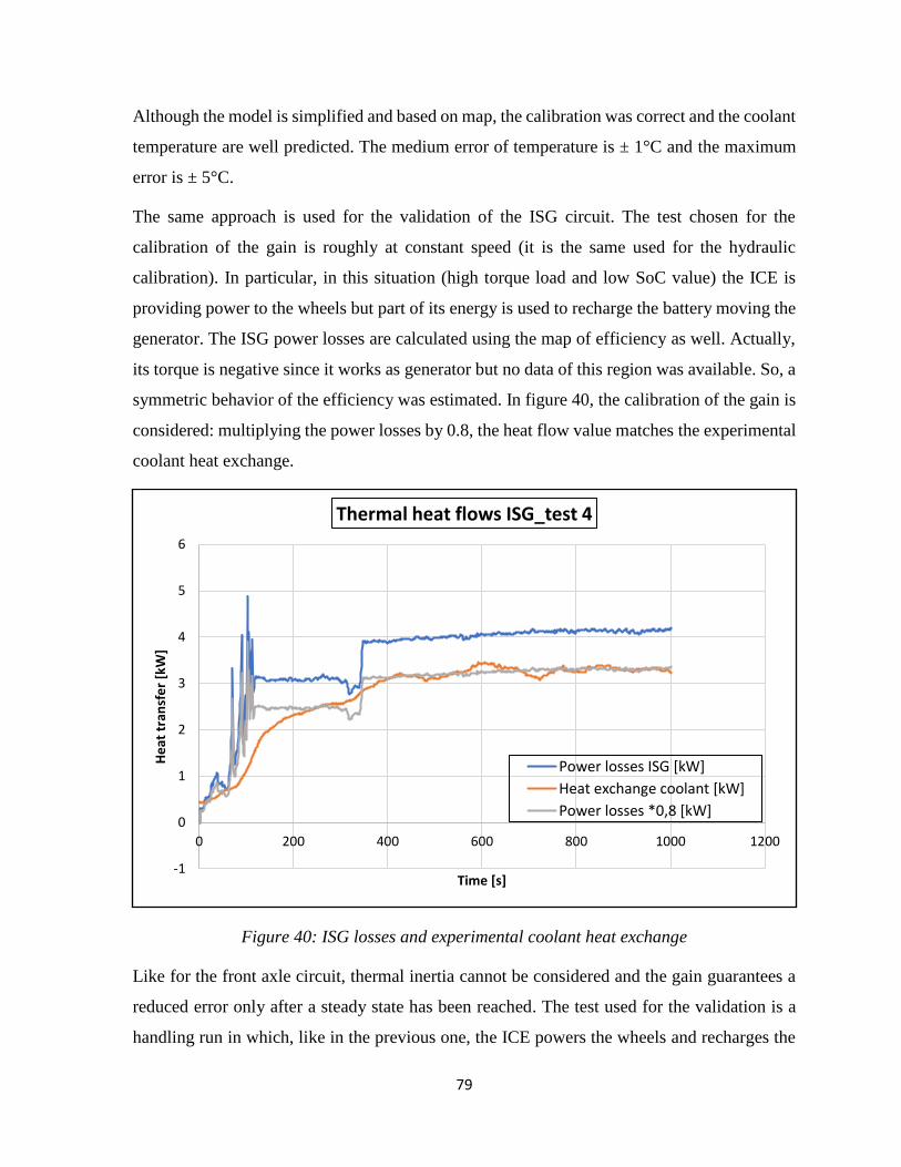
79
Although the model is simplified and based on map, the calibration was correct and the coolant
temperature are well predicted. The medium error of temperature is ± 1°C and the maximum
error is ± 5°C.
The same approach is used for the validation of the ISG circuit. The test chosen for the
calibration of the gain is roughly at constant speed (it is the same used for the hydraulic
calibration). In particular, in this situation (high torque load and low SoC value) the ICE is
providing power to the wheels but part of its energy is used to recharge the battery moving the
generator. The ISG power losses are calculated using the map of efficiency as well. Actually,
its torque is negative since it works as generator but no data of this region was available. So, a
symmetric behavior of the efficiency was estimated. In figure 40, the calibration of the gain is
considered: multiplying the power losses by 0.8, the heat flow value matches the experimental
coolant heat exchange.
Figure 40: ISG losses and experimental coolant heat exchange
Like for the front axle circuit, thermal inertia cannot be considered and the gain guarantees a
reduced error only after a steady state has been reached. The test used for the validation is a
handling run in which, like in the previous one, the ICE powers the wheels and recharges the
-1
0
1
2
3
4
5
6
0 200 400 600 800 1000 1200
He
at t
ran
sfe
r [k
W]
Time [s]
Thermal heat flows ISG_test 4
Power losses ISG [kW]
Heat exchange coolant [kW]
Power losses *0,8 [kW]

80
battery. Velocity and current absorbed by the ISG are reported in figure 41a. The coolant
temperature comparison is shown in figure 41b: like for the e-motor, the ISG and radiator outlet
temperature are chosen for the validation.
Figure 41a: velocity and ISG current for handling_corsa
Figure 41b: ISG and radiator outlet coolant temperature
Also, these results are acceptable: the medium temperature error between the two curves is ±
2.5 °C and the maximum error is ± 5.5°C.
-300
-200
-100
0
100
200
300 velocity [km/h]ISG current [A]
30
35
40
45
50
55
60
0 200 400 600 800 1000 1200 1400
Tem
pe
ratu
re [
°C]
Time [s]
Temperature COOLANT ISG and RADO_test_handling_corsa
T_ISG_model
T_ISG_exp
T_RADO_model
T_RADO_exp
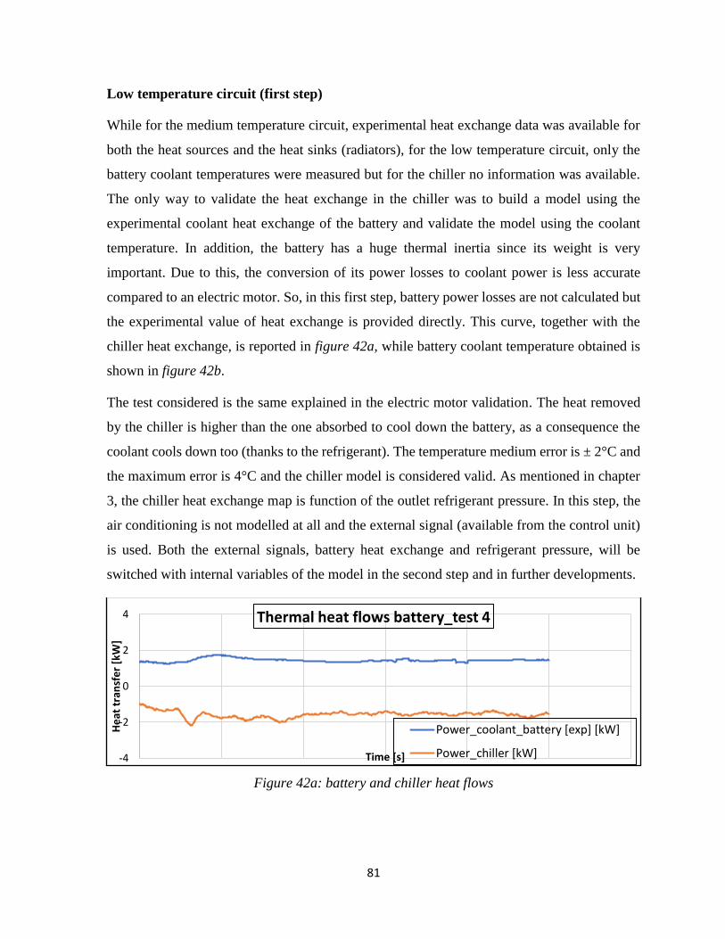
81
Low temperature circuit (first step)
While for the medium temperature circuit, experimental heat exchange data was available for
both the heat sources and the heat sinks (radiators), for the low temperature circuit, only the
battery coolant temperatures were measured but for the chiller no information was available.
The only way to validate the heat exchange in the chiller was to build a model using the
experimental coolant heat exchange of the battery and validate the model using the coolant
temperature. In addition, the battery has a huge thermal inertia since its weight is very
important. Due to this, the conversion of its power losses to coolant power is less accurate
compared to an electric motor. So, in this first step, battery power losses are not calculated but
the experimental value of heat exchange is provided directly. This curve, together with the
chiller heat exchange, is reported in figure 42a, while battery coolant temperature obtained is
shown in figure 42b.
The test considered is the same explained in the electric motor validation. The heat removed
by the chiller is higher than the one absorbed to cool down the battery, as a consequence the
coolant cools down too (thanks to the refrigerant). The temperature medium error is ± 2°C and
the maximum error is 4°C and the chiller model is considered valid. As mentioned in chapter
3, the chiller heat exchange map is function of the outlet refrigerant pressure. In this step, the
air conditioning is not modelled at all and the external signal (available from the control unit)
is used. Both the external signals, battery heat exchange and refrigerant pressure, will be
switched with internal variables of the model in the second step and in further developments.
Figure 42a: battery and chiller heat flows
-4
-2
0
2
4
He
at t
ran
sfe
r [k
W]
Time [s]
Thermal heat flows battery_test 4
Power_coolant_battery [exp] [kW]
Power_chiller [kW]

82
Figure 42b: battery coolant temperature for validation
4.3 Thermal model with thermal masses validation
In this last step, electric motors, inverter and battery power losses are modelled with one/two
thermal masses in order to predict their temperature. This allows to calculate their temperature
and evaluate if the coolant power is enough or not. The thermal mass is then linked to the
coolant circuit with a block that describe the convective heat exchange. Additional parameters
have to be set, some of them are known but others have to be calibrated.
Electric motor and ISG
Two thermal masses are used to model the electric motor. A summary of all the parameters
necessary is reported in table 6.
The values of first attempts used for the calibration are the default values proposed by the
software. More variables are present, compared to the previous step, and the real heat
exchanged by the model depends on all of them. The calibration is more difficult and not
perfect results are obtained.
5
7
9
11
13
15
17
19
0 200 400 600 800 1000 1200
Tem
pe
ratu
re [
°C]
Time [s]
Battery temperature_test 4
Temperature_coolant_battery_model [°C]
Temperature_coolant_battery_exp [°C]

83
Model Parameter Known Calibrated Value
Motor (thermal mass 1) Weight x
15 kg Material (for cp) x
copper
Conduction Contact surface
x 50000 mm2 Thermal conductance
x 550 W/m2/K
Cooling plate (thermal mass 2) Weight x
5 kg Material (for cp) X
aluminum
Convection exchange Pipe diameter x
20 mm Length heat exchange
x 2 m
Table 6: electric motor parameters for two thermal masses model
The test case used for the calibration is the handling pure electric drive, in which reasonable
results are obtained with the parameter values shown in the table. In figure 43a, the calculated
heat flows are shown: the motor power losses are the blue curve, the heat exchanged between
motor and coolant calculated by the model is the orange, and the experimental heat exchanged
is the grey. The medium difference between the last two curves is 0.1 kW and the maximum
difference is 0.4 kW.
Figure 43a: EM power losses and coolant heat exchange calibration in hand_electric test
-2
-1
0
1
2
3
4
5
0 200 400 600 800 1000 1200 1400 1600 1800
He
at e
xch
ange
d [
kW]
Time [s]
EM1_heat flows_test_handling_electric
EM_power_losses [kW]
Heat_coolant_model [kW]
Heat_coolant_exp [kW]

84
While in the previous model, when the power losses were zero, also the thermal power
exchanged with the coolant was zero, in this one a thermal inertia is present. This can be seen
in the previous chart: after 700s the car stops and the motor current is zero but the coolant
carries on to cool down the motor. This is also a clear advantage of the electric pump,
completely independent of the powertrain load.
The calibration is not completely since also the motor temperature has to be considered. The
results are reported in figure 43b, the temperature of the thermal mass obtained by the model
is compared with the motor temperature signal from the control unit. The medium error is
± 5°C and the maximum is ± 11.4 °C: they are quite high especially during the cooling phase,
showing that some thermal contributions are not well considered.
In the same figure, the inverter temperature is reported as well. Only one thermal mass is used
to model it, so only its weight and its thermal properties have to be set. A 5kg aluminum plate
is modelled to obtain this result. As it can be seen, its temperature remains at low value: its
power losses are small and the cooling system seems really efficient.
Figure 43b: electric motor and inverter temperature calibration, handling electric
20
30
40
50
60
70
80
90
100
110
0 200 400 600 800 1000 1200 1400 1600 1800
Tem
pe
ratu
re [
°C]
Time [s]
EM_IPU1_temperature_test_handling_electric
T_EM [°C]
T_EM_ECU [°C]
T_IPU1_model [°C]
T_IPU1_exp [°C]

85
It has been demonstrated that the heat flows of the heat sources and heat sinks match
experimental data, so also the coolant temperature should be well predicted. In fact, the values
obtained are really similar to the ones proposed in figure 39b (first step validation without
thermal masses). In addition, also the standstill phase can be validated thanks to the thermal
masses.
Once that all the parameter values are set, performing another simulation is necessary to
validate the model. The other test available for the front axle is the test 2, already proposed in
the previous pages. The results are reported in figure 44a, 44b, 44c.
The heat flow result is acceptable, the medium error is 0.13kW and the maximum error is
0.67kW. A first conclusion is that the convective heat exchange is correctly described and the
use of predefined correlations could be acceptable for the scope of the work. Since the heat
flows have acceptable error, so the coolant temperature. The medium coolant temperature error
in this test case is ± 3.9°C and the maximum error is ± 5.9°C (figure 44b).
Figure 44a: electric motor power losses and coolant heat flow validation
-1,5
-1
-0,5
0
0,5
1
1,5
2
2,5
3
3,5
0 200 400 600 800 1000 1200 1400 1600 1800
He
at e
xch
ange
d [
kW]
Time [s]
EM heat flows_test 2
EM_power_losses [kW]
Heat_coolant_model [kW]
Heat_coolant_exp [kW]

86
Figure 44b: e-motor and DCDC outlet coolant temperature validation
Figure 44c: e-motor and inverter temperature validation
20
25
30
35
40
45
50
0 200 400 600 800 1000 1200 1400 1600 1800
Tem
pe
ratu
re [
°C]
Time [s]
EM_coolant temperature_test 2
T_C_EM_model [°C]
T_C_EM_exp [°C]
T_C_DCDC_model [°C]
T_C_DCDC_exp [°C]
20
30
40
50
60
70
80
90
0 200 400 600 800 1000 1200 1400 1600 1800
Tem
pe
ratu
re [
°C]
Time [s]
EM_IPU1_temperature_test 2
T_EM [°C]
T_EM_ECU [°C]
T_IPU1_model [°C]
T_IPU1_exp [°C]

87
For what concerns the motor temperature, the results are less accurate. The medium and
maximum error are respectively ± 8°C and ± 16°C. The reasons of these incomplete results are
due to:
▪ too simplified electric motor thermal model, more thermal masses and materials must
be taken into consideration;
▪ incomplete calibration, some of the ‘not known’ parameters could be modified in order
to obtain better results;
▪ the model considers a uniform temperature inside the thermal mass, while the motor
has a complex temperature distribution that cannot be represented with this modelling
approach.
The same parameters are used also for the ISG circuit model. The only difference is the pipe
diameter for which the ISG circuit value is changed to the front axle value. The two motors are
identical and also the cooling properties should be equivalents. The test used for the ISG circuit
validation is the ‘handling_corsa’, already described in figure 41. The heat flows and
component temperatures are compared and reported in figure 45a, 45b and 45c. The errors are
calculated: for the coolant heat flow the medium error is 0.65kW and the maximum error is
1.4 kW. The percentage error is quite important, over 10%, Although this, the coolant
temperature prediction is accurate anyway (error less than ± 5°C). For the motor temperature,
as it is possible to see from the graph, the error is higher and model improvements are necessary
in order to consider validate it. Generally, the coolant circuit models and the heat exchange
description (with convection predefined correlations) can be considered acceptable while the
motor thermal mass model need further developments.

88
Figure 45a: ISG power losses and coolant heat flow validation
Figure 45b: ISG and IPU outlet coolant temperature validation
-6
-4
-2
0
2
4
6
8
0 200 400 600 800 1000 1200 1400 1600 1800
He
at e
xch
ange
d [
kW]
Time [s]
ISG_heat flows_test_handling_corsa
ISG_power_losses [kW]
Heat_coolant_model [kW]
Heat_coolant_exp [kW]
20
25
30
35
40
45
50
55
60
65
0 200 400 600 800 1000 1200 1400 1600 1800
Tem
pe
ratu
re [
°C]
Time [s]
ISG coolant temperature_test handling_corsa
T_C_ISG_model °C
T_C_ISG_exp °C
T_C_IPU_model °C
T_C_IPU_exp °C

89
Figure 45c: ISG and inverter temperature validation
Battery
As described in chapter 3, the battery thermal model has only one thermal mass and the
calculated temperature is used to obtain internal resistance. The setting of the parameters is
reported in table 7. Its weight is the product of the single cell weight times the cell number
multiplied by an additional contribution that consider all the other parts of the entire battery
pack. An amount which goes from 60% to 80% is added. The specific thermal capacity is
chosen from literature values, where many works have investigated Li-ion battery thermal
properties. The only value to calibrate is the length of heat exchange for the convection
description.
Model Parameter Value notes
Battery (thermal mass 1) Weight cell_w * number *gain from company benchmark
Material (for cp) 1100 kJ/kg/K from literature [20,21]
Convection exchange Pipe diameter 25 mm
Length heat exchange 2,5 m calibrated
Table 7: battery parameters setting for thermal mass model
20
30
40
50
60
70
80
90
100
110
120
0 200 400 600 800 1000 1200 1400 1600 1800
Tem
pe
ratu
re [
°C]
Time [s]
ISG temperature_test handling_corsa
T_ISG [°C]
T_ISG_ECU [°C]
T_IPU3_model [°C]
T_IPU3_exp [°C]
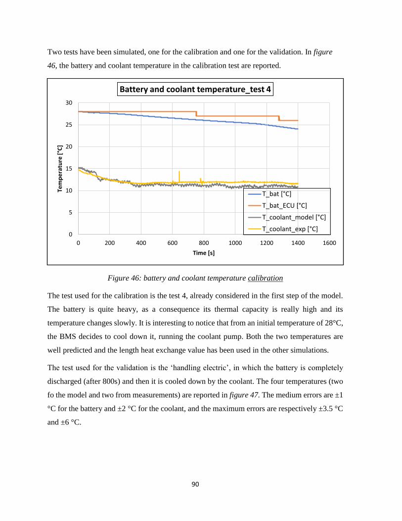
90
Two tests have been simulated, one for the calibration and one for the validation. In figure
46, the battery and coolant temperature in the calibration test are reported.
Figure 46: battery and coolant temperature calibration
The test used for the calibration is the test 4, already considered in the first step of the model.
The battery is quite heavy, as a consequence its thermal capacity is really high and its
temperature changes slowly. It is interesting to notice that from an initial temperature of 28°C,
the BMS decides to cool down it, running the coolant pump. Both the two temperatures are
well predicted and the length heat exchange value has been used in the other simulations.
The test used for the validation is the ‘handling electric’, in which the battery is completely
discharged (after 800s) and then it is cooled down by the coolant. The four temperatures (two
fo the model and two from measurements) are reported in figure 47. The medium errors are ±1
°C for the battery and ±2 °C for the coolant, and the maximum errors are respectively ±3.5 °C
and ±6 °C.
0
5
10
15
20
25
30
0 200 400 600 800 1000 1200 1400 1600
Tem
pe
ratu
re [
°C]
Time [s]
Battery and coolant temperature_test 4
T_bat [°C]
T_bat_ECU [°C]
T_coolant_model [°C]
T_coolant_exp [°C]

91
Figure 47: battery and coolant temperature for validation
Compared to the electric motor thermal mass, better results have been obtained for the battery
circuit. As it has already been described, the chiller heat exchange map is function of the
refrigerant pressure. Since the air conditioning model has not been included in the validation
stage, this signal has provided from external data.
4.4 Validation summary
A summary of the results obtained is reported in table 8. The medium errors for the coolant
temperature, thermal heat flows and thermal mass temperature are summed up.
Validation
test Coolant temp
Heat flow
Thermal mass temperature
Notes
HT test 4 ± 5 °C
not modelled Only in steady state condition
MT_F test 2 ± 6 °C 0.2 kW ± 10 °C Improve thermal mass
MT_IS hand_cors ± 5 °C 0.5 kW ± 10 °C Improve thermal mass
LT hand_el ± 2 °C
± 4 °C
Table 8: validation final summary
0
5
10
15
20
25
30
35
40
45
0 200 400 600 800 1000 1200 1400 1600 1800
Tem
pe
ratu
re [
°C]
Time [s]
Battery and coolant temperature_test handling_electric
T_bat [°C]T_bat_ECU [°C]T_coolant_model [°C]T_coolant_exp [°C]

92

93
5. Conclusions and future developments
In the last chapter, some conclusions and possible future works are described.
For what concerns the model, three different circuits of a PHEV have been modelled.
Following a step-by-step procedure, the hydraulic and thermal model have been developed. In
addition to the cooling circuits, the air conditioning has been considered as well. A first attempt
of modelling has been done using the specific library. However, the A/C model is not calibrated
and it has not been taken into account during the validation. To complete thermal management
model, cabin climatization should be included as well. In fact, it is known that it has a strong
impact on fuel consumption and, in order to develop innovative control strategies, its
contribution cannot be neglected. The development of a cabin model is quite complex and it
has not been considered at all in the present work, but it can represent a possible future
development. The same is valid for the PTC heaters: it would be really interesting predict their
impact on battery SoC and AER. In table 9, a complete list of the circuits just mentioned is
reported. It is specified what it has been developed and validated in the present work and what
else it could be interesting to include in future.
Table 9: thermal management model circuits list
Circuit Modelled Validated Rating Reliability
HT YES YES Sufficient Limited
MT YES YES
Good (except for
e-motor temp)
Good (except for
e-motor temp)
LT YES YES Good Good
A/C YES NO
Cabin NO NO
PTC heaters NO NO

94
In addition, for the circuits for which a validation has been done, a rating and the reliability of
the model are evaluated. A justification of these judgements is now described.
For the engine cooling circuit, two limits must be highlighted: the calibration of the thermostat
and how the heat exchange between engine and coolant was calculated. For what concerns the
thermostat, the results (figure 37) show the coolant temperature are correctly predicted only
after a steady state is reached, and so the thermostat has reached a thermal balance. Instead,
during the opening and the closure of the thermostatic valve, the temperatures and the flow
rate are not correct. The calibration of the thermostat model, as wax characteristic and
hysteresis effect, is incomplete. The other limit is due to the absence of the engine thermal map
and the use, instead, of a fuel consumption map. This forces to estimate the amount of total
heat exchanged with the coolant: a table of this value as function of the rotational speed has
been built. A couple of points are calibrated considering experimental data, but from different
rpm the value has been estimated from literature values. Due to this factor, its reliability is
must be considered limited.
For the electric motor circuit and ISG circuit, the reported results show that the model has been
correctly developed and calibrated. Coolant temperatures and heat flows of heat sources and
heat sinks are well predicted. On the other hand, the e-motor temperature is not correct: as
mentioned, the thermal model is too simplified and the calibration of some parameters is
incomplete. A good level of accuracy can be reached only with higher effort in both the
modelling phase and the parameters calibration. At the present status, the model cannot
correctly predict the temperature of the electric motor, but only the coolant temperature.
Improvements in this topic could be a further development as well.
For the battery coolant circuit both the coolant and the battery temperature are predicted in a
quite accurate way. The results are satisfying and the model general validity can be tested in
new cases. Once that the A/C model has been validated, the two circuits can be integrated and
the chiller can be modelled as liquid-liquid heat exchanger, as already described at the end of
chapter 3. In addition, the heat exchange map can be replaced by physical correlations,
improving model accuracy.

95
The general approach to the model is quite simple, the heat produced/absorbed by heat
source/sink is always map-based. The accuracy cannot be so high but, on the other hand, the
simulations are fast (the MT circuit with thermal masses simulates 1000s in 25 real seconds).
In order to enter in these maps, external signals must be provided, as reported in table 3
(chapter 3). This is an important limit that has to be considered. It would be really interesting
integrate the thermal management model with a hybrid powertrain and vehicle model. This can
allow to start only from the car velocity, calculate engine and e-motors rotational speed and
torque and be able to enter in the desired maps. In the present work, the e-motor torque was
not available and this has been calculated starting from inverter current and voltage. With an
integration with a powertrain model, this can be directly calculated. The software used allows
to integrate different libraries and different model. As an alternative, the model could be
converted to Simulink and then integrated with an existing powertrain model. The conversion
from AMESim® to Simulink should be very easy, the software is able to compile a S-function
that can be directly used into a Simulink environment.
The main target of the model is to develop control strategies. As described in chapter 1, they
can increase the cooling performance reducing the fuel consumption; their impact is very
remarkable. All the control signals are summed up in table 4. Strategies can be developed in
two ways:
▪ using the AMESim® control library
▪ convert the model into Simulink and use this environment

96

97
Appendix
Figures of the completed models are here reported.
High temperature circuit

98
Medium Temperature Circuit

99
Low temperature circuit
Battery Circuit integrated with Air Conditioning

100

101
Bibliography
[1] www.EngineeringToolBox.com
[2] L. Lefebvre, Smart Battery Thermal Management for PHEV Efficiency,
Oil & Gas Science and Technology – Rev. IFP Energies nouvelles, Vol. 68 (2013)
[3] G.M. Corporation Data, Dec 2010. Available, http://gm-volt.com/
[4] K. Bennion and M. Thornton , Integrated Vehicle Thermal Management for Advanced
Vehicle Propulsion Technologies, National Renewable Energy Laboratory, SAE 2010 World
Congress
[5] www.optemus.eu
[6] M. Hopp, C. Ebert, K.-H. Hassel, H. Dismon, Thermal Conditioning and Efficiency
Increase of Electric Vehicles Using a Heat Pump, KSPG AG, 25th Aachen Cooloquium 2016
[7] S.Gmeiner, P. Rajan, J. Gissing, D. Backes , VOSS Innovative Valve Technology for
Thermal Management, 25th Aachen Colloquium 2016
[8] Nicholas R. Jankowski, F. Patrick McCluskey, A review of phase change materials for
vehicle component thermal buffering, Applied Energy, 2012
[9] Rainer W. Jorach, Fritz Atschreiter, Axel Gößling,
Integrated Thermal Management: System Approach towards CO2 Reduction
Magna Powertrain GmbH - Fluid, Pressure & Controls Group, 25th Aachen Cooloquium 2016
[10] G.Caramia, Development of an innovative non rule-based energy management strategy
for a hybrid electric vehicle, structured for predictive driving controls based on external
information knowledge, Master thesis, University of Bologna, 2016
[11] Marcel Stöcker, Norbert Rohleder, Heiko Möckel, Ulf Säger, Matthias Hailer,
Thermal Management for Energy – Efficient Improvement of Automobile Cooling Systems
Based on Navigation Data, Daimler AG, 25th Aachen Cooloquium 2016
[12] J.Lopez-Sanz, Carlos Ocampos-Martinez et al. Nonlinear Model Predictive Control for
Thermal Management in Plug-in Hybrid Electric Vehicles, IEEE 2015

102
[13] H.Esen, T.Tashiro, D. Bernardini, A. Bemporad, Cabin Heat Thermal Management in
Hybrid Vehicles using Model Predictive Control, 2014 22nd Mediterranean Conference on
Control and Automation (MED), University of Palermo, June 16-19 2014
[14] G.Negri di Montenegro, M. Bianchi, A. Peretto, Sistemi energetici e macchine a fluido
Volume 1, Ed. Pitagora, 2009
[15] The Centrifugal Pump, GRUNDFOS®, www.grundfos.com
[16] C.Cesario, M.Vrardi, S.Borges, J.Carlos da Silva, A.A Martins Oliveira, Transient thermal
amalysis of an induction electric motor, 18th International Congress of Mechanical
Engineering, 2005
[17] F.P.Incropera, D.P. DeWitt, Fundamentals of Heat and Mass Transfer, 1998
[18] AMESim® guide Help
[19] John B. Heywood, Internal Combustion Engine Fundamentals, Ed. McGraw-Hill, 1988,
p. 674
[20] Hossein Maleki, Said Al Hallaj, J. Robert Selman, Ralph B. Dinwiddie,b and H. Wangb.
Thermal Properties of Lithium-Ion Battery and Components, Journal of The Electrochemical
Society, 146 (3) 947-954 (1999)
[21] O.S. Burheima,b, M.A. Onsrudc , J.G. Pharoahd,e, F. Vullum-Bruerc , P.J.S. Vie, Thermal
Conductivity, Heat Sources and Temperature Profiles of Li-ion Secondary Batteries, The
Electrochemical Society, 2013
[22] Thomas GILLET, Emmanuelle ANDRES, Amin EL-BAKKALI, Gérard OLIVIER,
Vincent LEMORT , Romuald RULLIERE, Philippe HABERSCHILL, Modelling of an
automotive multi-evaporator air-conditioning system, Purdue University, Purdue e-pubs, 2016

103
Acknowledgements
I would like to thank Ing. Michele Caggiano and Professor Nicolò Cavina for giving me the
opportunity to develop this project in such a high-level company and for their support and their
advice.
I would like to express my gratitude also to Dipl. Ing. David Hemkemeyer, Ing. Enrico Suzzani
and Ing. Alberto Garaffoni for their precious help during the whole thesis period.
Finally, I would like to thank Laura, Simone and my parents for supporting and inspiring me
during the course of my studies.