Strain gradient elasticity within the symmetric …. Terravecchia et al., Frattura ed Integrità...

S. Terravecchia et al., Frattura ed Integrità Strutturale, 29(2014) 164-176; DOI: 10.3221/IGF-ESIS.29.15

164

Strain gradient elasticity within the symmetric BEM formulation S. Terravecchia, T. Panzeca, C. Polizzotto University of Palermo [email protected], [email protected], [email protected]

ABSTRACT. The symmetric Galerkin Boundary Element Method is used to address a class of strain gradient elastic materials featured by a free energy function of the (classical) strain and of its (first) gradient. With respect to the classical elasticity, additional response variables intervene, such as the normal derivative of the displacements on the boundary, and the work-coniugate double tractions. The fundamental solutions - featuring a fourth order partial differential equations (PDEs) system - exhibit singularities which in 2D may be of the order 41/ r . New techniques are developed, which allow the elimination of most of the latter singularities. The present paper has to be intended as a research communication wherein some results, being elaborated within a more general paper [1], are reported. KEYWORDS. Strain gradient elasticity; Symmetric Galerkin BEM. INTRODUCTION

fter the pioneering work of Mindlin [2], theories of strain gradient elasticity have become very popular, particularly within the domain of nano-technologies, that is, for problems where the ratio surface/volume tends to become very large and there is a need to introduce at least one internal length.

However the model introduced by Mindlin and then improved by Mindlin et al. [3] and Wu [4] leads to an excessive number of material coefficients, which at the best for isotropic materials reduce to the number of seven. In the early 1990’s, Aifantis [5] introduced a signified material model of strain gradient elasticity which requires only three material coefficients, that is, the Lame' constants and one length scale parameter. The latter model was then developed further following the so-called Form II format given by Mindlin et al. [3], that is a theory centered on the existence of a free energy function of the (classical) strain and of its first gradient, which leads to the generation of symmetric stress fields (see Askes et al. [6] for historical details about the latter formulations and its applications). Formulations in the boundary element method based on the strain gradient elasticity were pioneered by Polyzos et al. [7], Karlis et al. [8], who provide a collocation BEM formulation where the simplified constitutive equation by Aifantis [5], has been adopted. In latter papers only the fundamental solutions used in the collocation approach to BEM are provided. In the case of the symmetric formulation of the BEM, Somigliana Identities (SIs) for the tractions and for the double tractions are also needed. These new SIs are necessary in order to get, through the process of modeling and weighing, a solving equation system having symmetric operators. In Polizzotto et al. [1] all the set of fundamental solutions is derived starting from the displacement fundamental solution given in [7,8].

A

S. Terravecchia et al., Frattura ed Integrità Strutturale, 29 (2014) 164-176; DOI: 10.3221/IGF-ESIS.29.15

165

The symmetric formulation is motivated by the high efficiency achieved within classical elasticity by the method in [9] with regard to the techniques used to eliminate the singularities of the fundamental solutions, the evaluation of the coefficients of the solving system and the computational procedures characterized by great implementation simplicity. This has already led to the birth of the computer code Karnak sGbem [10] operating in the classical elasticity. The objective of this paper is to experiment new techniques and procedures that, applied in the context of strain gradient elastic materials, may permit one to obtain the related solving system. NOTATION

s a rule, a compact notation is used, with vectors and tensors denoted by bold-face symbols. The dot , the colon products : and :: indicate the simple and higher index contraction. The following notations are also utilized: the gradient operator: grad ( ) ( ) ;

the divergence operator : div ( ) ( ) ;

the Laplacian operator : 22 2

( ) ( ) ( ) ( )x y

;

the component of the normal derivation of u is denoted as n k kn g u u ; the quantities with bar superscripts indicate know quantities. Other symbols will be specified in the text at their first appearance. BASIC RELATIONS IN 2D

he class of strain gradient elastic materials herein considered is featured by the following strain elastic energy

21: : :: ( )

2 2TW ε E ε E ε ε

(1)

that is a function of the symmetric 2nd order strains (0 ) ( )S ε ε u and of the strain gradient (1) ε ε , where is the internal length which relates the microstructure with macrostructure. Eq.(1) provides the stress tensors work-coniugate of (0 )ε and (1)ε respectively

( 0 ) (1) 2 2 (0 ): ; σ E ε σ σ (2a,b)

where E is the classic isotropic elasticity tensor. By the principle of the virtual work, the indefinite equilibrium equation and the following boundary conditions prove to be

in Ω σ b 0 , on Γt t , on Γr r , on the corner CCt t (3a,b,c,d)

where the total stresses σ , the tractions t , the double tractions r and the force at the corner P are so defined

( 0 ) 2 2 (0 ) σ σ σ , ( ) (1)( ) ( )s K t n σ n n σ , (1):r nn σ , (1):C t sn σ (4a,b,c,d)

In eq.(4b), the symbol ( ) ( )s I nn denotes the tangent gradient on the boundary and ( )sK n is the curvature on the boundary having normal n ; in eq.(4d) s denotes a unit vector tangent to the two boundary portions convergent in the corner C and the brackets indicate that the enclosed quantity is the difference between the related values taken on

two sides of the corner C. For a more exhaustive understanding of the jump to see [2].

The constitutive equation relating the total stress σ to the strain is

2 2 ) σ E ε ε: ( . (5)

A

T


166

THE FUNDAMENTAL SOLUTIONS

he introduction of eq.(5) in (3a) valid in infinity domain allows to express the latter in terms of displacements only [7,8] and to determine the fundamental solution of the displacements that for 2D solids proves to be

2

22

2

0 22

22 4

1=

16 (1 ) 22(3 4 ) [ ] 2

uu

rK

r

r rLog r K K

r

I

G

r r

(6)

where 0K and 2K are Bessel functions of the second kind and of order 0 and 2, respectively, and r ξ x is the

distance between effect ξ and cause x points. One can note that the singularity of the fundamental solution uuG does not depend on r . Indeed, by performing the limit r 0 one obtains

1( ) 2(3 4 ) ln(2 ) 1

16 (1 )uu

G ξ x I (7)

where is the Eulero constant and the fundamental solution for isotropic gradient elasticity shows singularity of type ln( ) .

In eq.(6) the limit of uuG for 0 gives the classic isotropic elasticity solution (Kelvin) with singularity of type ln( )r .

Table 1: Fundamental solutions for strain gradient elasticity and relative singularities.

By the fundamental solution uuG in (6), taking in account eqs.(4b,c,d) and using the well-known procedure given in [11], it is possible, by exploiting the known properties of symmetry of the fundamental solutions, to derive the entire tableau provided in Table 1. The fundamental solutions hkG of Tab. 1 are characterized by two subscripts: the first indicates the effect at ξ , i.e. displacement for h u , traction for h t , displacement normal derivative for h g , double traction for h r , corner

T


167

displacement for Ch u , corner force for Ch t , stress for h ; whereas the second subscript indicates – through a work-conjugate rule – the cause applied at x , i.e. a unit concentrated force for k u , a unit surface relative displacement for k t , a unit concentrated double force for k g , a unit higher order surface distortion for k r , a unit corner force

for Ck u , a unit corner displacement for Ck t , a unit imposed strain for k . To consider the way in which the

fundamental solutions included in the single and double brackets to see [2].

While the fundamental solutions represent the response in a point ξ of the unlimited domain caused by unit kinematical or mechanical action imposed at x , the response to the distributed actions is provided by the SIs that in [1] are obtained by a generalization of the Betti theorem for the gradient elastic materials. A CASE STUDY

s a premise, it should be noted that the theory of strain gradient should be applied to those bodies where the ratio between surface and volume in 3D and between boundary and area in 2D is high. In these cases, the body should be considered as composed of a nucleus, a crust and its boundary.

The example we want to meet will show that on the basis of this theory the behavior of the cortex has different characteristics from the classical behavior of the nucleus, and this depends on the presence of new variables such as double traction r and normal derivative g of the displacements. Obviously, the body will suffer the effects due to the presence of these new variables. From computational point of view, the fundamental solutions present in the Tab. 1 show various orders of singularity, up to 41/ r in the column related to u , up to 31/ r in that related to Cu ; furthermore the singularities present in the

column Cu present an order lower than that of u , relatively to the same effect. In order to investigate the techniques useful to remove the singularities from the blocks of coefficients, a simple application in two-dimensional space is shown, but at this stage involving the study of fundamental solutions having the maximum order of singularity equal to 21/ r . It has to be remembered that in the symmetric BEM the coefficients are obtained by a double integration, the first (inner) regarding the modeling of the cause through appropriate shape functions and the second (external) regarding the effect weighing through shape functions, but dual in the energetic sense.

x

y

1

1

1 1

a b

c

d

ef

g

1 2 3

4

567

8

x

y

h

a) b)

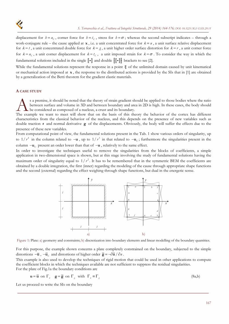
Figure 1: Plate: a) geometry and constraints; b) discretization into boundary elements and linear modelling of the boundary quantities.

For this purpose, the example shown concerns a plate completely constrained on the boundary, subjected to the simple distortions u , Cu and distortions of higher order / n g u . This example is also used to develop the techniques of rigid motion that could be used in other applications to compute the coefficient blocks in which the techniques available are not sufficient to suppress the residual singularities. For the plate of Fig.1a the boundary conditions are

u u on u g g on g with u g (8a,b)

Let us proceed to write the SIs on the boundary

A


168

,

1d + d ( )d ( ) ( )d + ( )

2u g u g

uu ug ut ur u tc C

u G t G r G u u G g G u on u (9a)

,

1d + d ( )d ( )d ( )+ ( )

2u g u g

gu gg gt gr g tc C

g G t G r G u G g g G u on g (9b)

and, following the compact notation proposed by Panzeca et al. [9], the latter equations become

1[ ] [ ] [ ] ( ) [ ] [ ]

2CPV

C u u t u r u u u u g u u on u (10a)

1[ ] [ ] [ ] [ ] ( ) [ ]

2CPV

C g g t g r g u u g g g u on g (10b)

In the SIs: the bar superscripts characterize known quantities; the apex CPV indicates that the corresponding integral is evaluated as Cauchy Principal Value to which the related

free term 1

( )2 is added;

Cu is a vector containing only the known displacement of the corner;

[ ]Cu u and [ ]C g g u are, respectively, the displacement and normal derivative of displacement distribution on the boundary, computed as the difference between the response to the values of displacement imposed on the two portions of boundary afferent to the corner.

Introducing the latter SIs given in eqs.(10a,b) into the boundary conditions eqs.(9a,b) one has:

1[ ] [ ] [ ] ( ) [ ] [ ]

2CPV

C u t u r u u u u g u u 0 on u (11a)

1

[ ] [ ] [ ] [ ] ( ) [ ]2

CPVC g t g r g u u g g g u 0 on g (11b)

Let us now discretize the plate boundary into boundary elements (Fig.1b) and introduce the modeling of the quantities on the boundary as functions of the nodal variables through suitable matrices of shape functions hN , with , , ,h t r u g

; ; ; f r u g t N T r N R u N U g N G (12a,b,c,d)

Since the vector Cu collects nodal quantities to not be modeled, the following identity has to be imposed

C Cu U (13)

In eqs.(12a-d) the quantities T , R , U , G have the meaning of nodal quantities and precisely: force and double traction as unknowns, displacements and normal derivatives of displacements as known quantities. To evaluate the vector G , because the discontinuity of the normal derivative at the corner C, a double node belonging respectively to the two portions of boundary afferent to C has to be considered. Introducing the modeling (12a-d) and the relation (13) into eqs.(11a,b) and performing the weighing second Galerkin, by using the shape functions in dual form, one writes

,

1+ ( ) ( )

2

( )+ ( )

u u u g u u u

uu ut utug

u g u

ur u tc

t uu t f ug r t ut u t u

t ur g t up C

A A CA

A a

N G N T N G N R N G N U N N U

N G N G N G U 0

(14a)


169

,

+ ( ) ( )

1( ) ( )

2

g u g g g u g g

gu gg gt gr

g g

gr g tc

r gu f r gg r r gt u r gr g

r g r gp C

A A A A

C a

N G N T N G N R N G N U N G N G

N N G N G U 0

(14b)

and, following the compact notation proposed by Panzeca et al. [9], the latter equations become

,

,

( )u tcuu ug ut ut ur

Cgu gu gt gr gr g tc

aA A A C AT 0UU

A A A A CR 0G a

(14c)

Since some components of the vector U and of the vector CU coincide, it is opportune to introduce the following relation

C CU H U (15)

where the low rectangular matrix CH is a topological matrix made by 2 2I and 2 20 blocks. The previous relation can be rewritten

*

,

*

,

( )( ) ( )

gu

ut ut u tcuu ug ur

gu gu gr grgt g tc

K L

L

A C aA A AT 0U G

A A A CR 0A a

(16)

where

**

, , , ,; u tc u tc C g tc g tc C a a H a a H . (17a,b)

Finally, the solving system is rewritten in compact way with obvious meaning of symbols

u g L

K X L L 0

(18)

with K symmetric flexibility matrix of the system, X vector of nodal unknowns, uL and gL load vectors due to U e

G respectively, being u g L L L the total load vector.

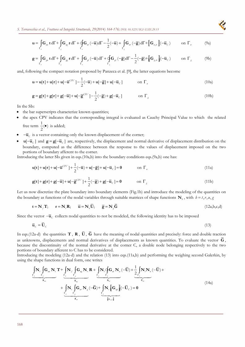
In order to evaluate the coefficients of the equation system, the numerical techniques to remove the singularities and the rigid motion strategy have to be employed. Observation about rigid motions Let the plate of Fig.2 be subjected to a) a rigid motion of translation obtained as the sum of constant displacement fields xu and yu (Fig.2a),

b) a rigid motion of rotation having wideness around any point (Fig.2b), c) a rigid motion of roto-translation obtained as a combination of a) and b). In all these cases the displacement and normal derivative of the displacement fields are entirely known both in the domain and on the boundary of the plate. Particularly - for the case of rigid motion of translation (Fig.2a)


170

, 0

, 0

xx x

yy y

uu c1 g

nu

u c2 gn

(19a,b,c,d)

with c1 and 2c being the wideness of the displacements; - for the case of rigid motion of rotation having width f (Fig.2b)

f (20a)

xx x y

yy y x

uu f y g f n

nu

u f x g f nn

(21b,c,d,e)

x

y

x

yxu c1=

yu c2= f=f

a) b)

Figure 2: Rigid motions: a) translation, b) rotation. Observations about the load vector as a consequence of the rigid motion 1) If the solid is subject to a rigid motion of translation (Fig.2a) having assigned values of the displacements c1 and 2c , one has U 0 and G 0 but the total load vector has to be u g L L L 0 with

*

,

*

,

( )( )

ut ut u tc

u

gt g tc

A C a 0L U

0A a

(22)

( )ur

ggr gr

A 0L G

A C 0 (23)

and as a consequence the solution vector X has to be null. 2) If the solid is subject to a rigid motion of rotation (Fig.2a) having assigned rotation vector fφ , in the generic node

i one has

i i U r φ 0 i i i G φ n φ s 0 (24a,b)

with ir vector distance between the instantaneous center of rotation and the node i , in e is being respectively the unit normal and tangent vectors to the boundary elements on which the node i lies, but the total load vector has to be

u g L L L 0 with


171

*

,

*

,

( )( )

ut ut u tc

u

gt g tc

A C a 0L U

0A a

(25)

( )ur

ggr gr

A 0L G

A C 0 (26)

because the solution vector X has to be null. 3) If the solid is subjected to a combination of the rigid motions 1) and 2), the condition u g L L L 0 has to be

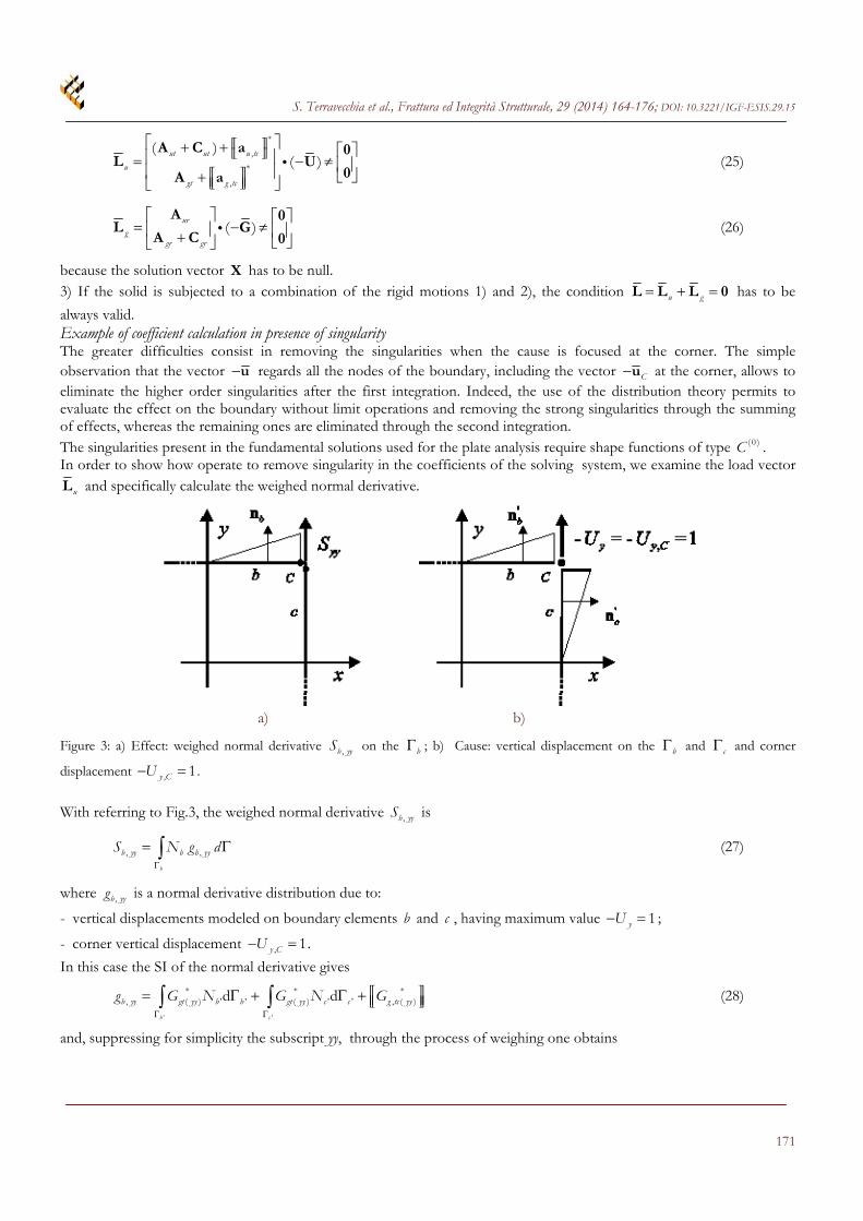
always valid. Example of coefficient calculation in presence of singularity The greater difficulties consist in removing the singularities when the cause is focused at the corner. The simple observation that the vector u regards all the nodes of the boundary, including the vector Cu at the corner, allows to eliminate the higher order singularities after the first integration. Indeed, the use of the distribution theory permits to evaluate the effect on the boundary without limit operations and removing the strong singularities through the summing of effects, whereas the remaining ones are eliminated through the second integration. The singularities present in the fundamental solutions used for the plate analysis require shape functions of type (0 )C . In order to show how operate to remove singularity in the coefficients of the solving system, we examine the load vector

uL and specifically calculate the weighed normal derivative.

a) b)

Figure 3: a) Effect: weighed normal derivative ,b yyS on the b ; b) Cause: vertical displacement on the b and c and corner

displacement , 1y CU .

With referring to Fig.3, the weighed normal derivative ,b yyS is

, ,

b

b yy b b yyS N g d

(27)

where ,b yyg is a normal derivative distribution due to:

- vertical displacements modeled on boundary elements b and c , having maximum value 1yU ;

- corner vertical displacement , 1y CU .

In this case the SI of the normal derivative gives

' '

* * *, ( ) ' ' ( ) ' ' , ( )d d

b c

b yy gt yy b b gt yy c c g tc yyg G N G N G

(28)

and, suppressing for simplicity the subscript yy, through the process of weighing one obtains


172

' '

* * *' ' ' ' ,d d d

b b cbC

bb bc

b b gt b b gt c c g tc b

gg g

S N G N G N G

(29)

The following contributions bbg , bcg bCg are provided distinguishing between the singular and the regular part

(sing ) ( reg ) ( reg )

3 4 1[ ] [1 ]

16(1 ) 1bb bb bb bbg g g Log x Log x gx

(30a)


3 4 3

16(1 ) 1bc bc bc bcg g g gx

(30b)


3 4 2

16(1 ) 1bC bC bC bCg g g gx

(30c)

(sing ) (sing ) (sing ) ( reg ) ( reg ) ( reg )

( reg ) ( reg ) ( reg )

d d d d

3 4 1( ) d d d

16(1 ) 2

b b b b

b b b

b b bb bc bC b b bb b b bc b b bC b

b bb b b bc b b bC b

S N g g g N g N g N g

N g N g N g

(31)

The sum of the effects in terms of distributions bbg , bcg bCg eliminates the strong singularity 1/ r , while the weak

singularity ( )Log r present in the bbg distribution is eliminated in the weighing operation by integration by parts. Eqn. (31) gives the coefficient in closed form.

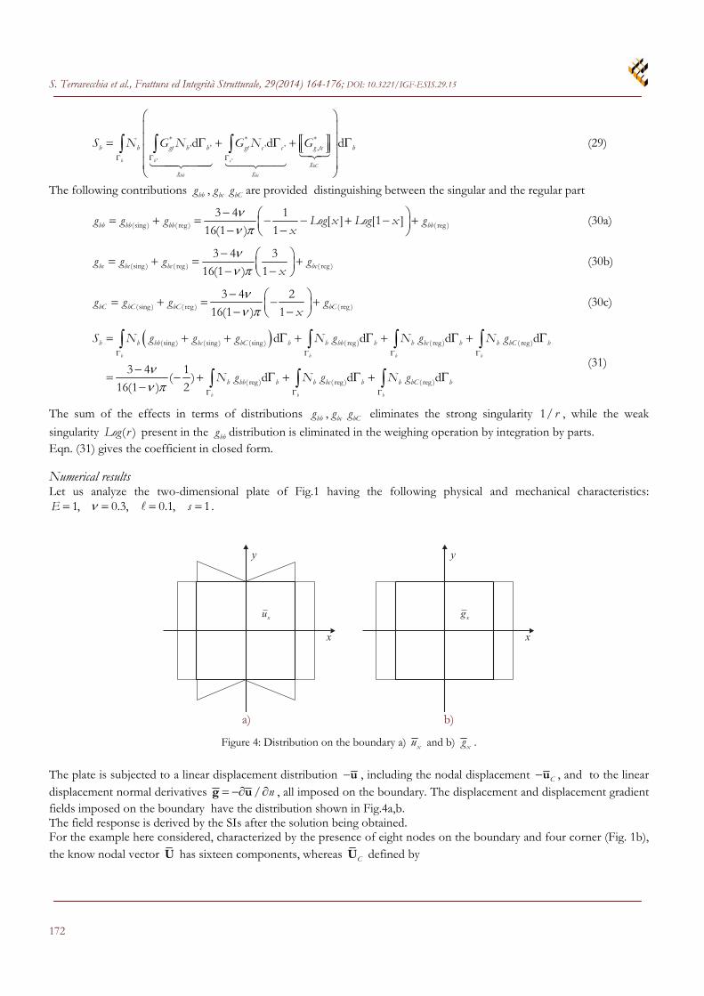
Numerical results Let us analyze the two-dimensional plate of Fig.1 having the following physical and mechanical characteristics:

1, 0.3, 0.1, 1E s .

y

xu

x

y

xg

x

a) b)

Figure 4: Distribution on the boundary a) xu and b) xg .

The plate is subjected to a linear displacement distribution u , including the nodal displacement Cu , and to the linear displacement normal derivatives / n g u , all imposed on the boundary. The displacement and displacement gradient fields imposed on the boundary have the distribution shown in Fig.4a,b. The field response is derived by the SIs after the solution being obtained. For the example here considered, characterized by the presence of eight nodes on the boundary and four corner (Fig. 1b), the know nodal vector U has sixteen components, whereas CU defined by


173

C C

I 0 0 0 0 0 0 0

0 0 I 0 0 0 0 0U H U U

0 0 0 0 I 0 0 0

0 0 0 0 0 0 I 0

shows eight components; the vector G collects twenty-four components, due to the presence of the double node belonging respectively to the two portions of boundary afferent to the corners,. Two load conditions are considered:

First load condition

1 1

0x

x

uat x

g

(32)

For this condition the vectors of know nodal quantities U , CU and G are

1 0 0 0 1 0 1 0 1 0 0 0 1 0 1 0T U (33)

1 0 1 0 1 0 1 0TC U (34)

0 0 0 0 0 0 0 0 0 0 0 0 0 0 0 0 0 0 0 0 0 0 0 0T G (35)

Second load condition

1

11

x

x

uat x

g

(36)

For this condition the vectors of known nodal quantities U , CU and G are

1 0 0 0 1 0 1 0 1 0 0 0 1 0 1 0T U (37)

1 0 1 0 1 0 1 0TC U (38)

0 0 0 0 0 0 1 0 1 0 1 0 0 0 0 0 0 0 1 0 1 0 1 0T G (39)

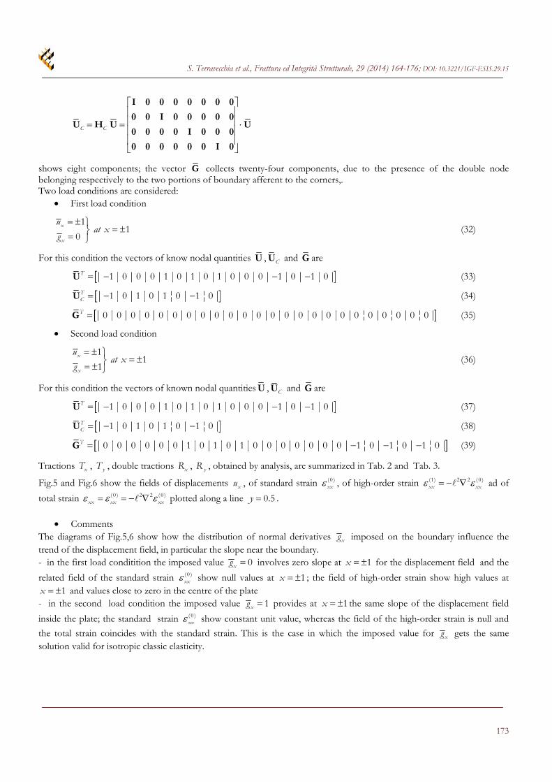
Tractions xT , yT , double tractions xR , yR , obtained by analysis, are summarized in Tab. 2 and Tab. 3.

Fig.5 and Fig.6 show the fields of displacements xu , of standard strain (0 )xx , of high-order strain (1) 2 2 (0 )

xx xx ad of

total strain (0 ) 2 2 (0 )xx xx xx plotted along a line 0.5y .

Comments

The diagrams of Fig.5,6 show how the distribution of normal derivatives xg imposed on the boundary influence the trend of the displacement field, in particular the slope near the boundary. - in the first load conditition the imposed value 0xg involves zero slope at 1x for the displacement field and the

related field of the standard strain (0 )xx show null values at 1x ; the field of high-order strain show high values at

1x and values close to zero in the centre of the plate - in the second load condition the imposed value 1xg provides at 1x the same slope of the displacement field

inside the plate; the standard strain (0 )xx show constant unit value, whereas the field of the high-order strain is null and

the total strain coincides with the standard strain. This is the case in which the imposed value for xg gets the same solution valid for isotropic classic elasticity.


174

xT yT xR yR

1a 0.591253 0.673221 1a -0.0391933 -0.00500786

2a -0.188974 0.066697 2a 0.00922674 -0.0104388

2b 0.188974 0.066697 2b -0.00922674 -0.0104388

3b -0.591253 0.673221 3b 0.0391933 -0.00500786

3c 2.05806 -0.371508 3c -0.201115 0.0048963

4c 1.28042 0.246566 4c -0.129643 0.00265313

4d 1.28042 -0.246566 4d -0.129643 -0.00265313

5d 2.05806 0.371508 5d -0.201115 -0.0048963

5e -0.591253 -0.673221 5e 0.0391933 0.00500786

6e 0.188974 -0.066697 6e -0.00922674 0.0104388

6f -0.188974 -0.066697 6f 0.00922674 0.0104388

7f 0.591253 -0.673221 7f -0.0391933 0.00500786

7g -2.05806 0.371508 7g 0.201115 -0.0048963

8g -1.28042 -0.246566 8g 0.129643 -0.00265313

8h -1.28042 0.246566 8h 0.129643 0.00265313

1h -2.05806 -0.371508 1h 0.201115 0.0048963

Table 2: Results for the first load condition.

xT yT xR yR

1a 0.00 0.576923 1a 0.00 0.00

2a 0.00 0.576923 2a 0.00 0.00

2b 0.00 0.576923 2b 0.00 0.00

3b 0.00 0.576923 3b 0.00 0.00

3c 1.34615 0.00 3c 0.00 0.00

4c 1.34615 0.00 4c 0.00 0.00

4d 1.34615 0.00 4d 0.00 0.00

5d 1.34615 0.00 5d 0.00 0.00

5e 0.00 -0.576923 5e 0.00 0.00

6e 0.00 -0.576923 6e 0.00 0.00

6f 0.00 -0.576923 6f 0.00 0.00

7f 0.00 -0.576923 7f 0.00 0.00

7g -1.34615 0.00 7g 0.00 0.00

8g -1.34615 0.00 8g 0.00 0.00

8h -1.34615 0.00 8h 0.00 0.00

1h -1.34615 0.00 1h 0.00 0.00

Table 3: Results for the second load condition.


175

Figure 5: Field mechanical characteristics regarding the first load condition.

Figure 6: Field mechanical characteristics regarding the second load condition.


176

CONCLUSIONS

he table of fundamental solutions for isotropic strain gradient elasticity is similar to an analogous table used within classical boundary element method. Computational techniques have been pursued in order to eliminate the singularities of order 1/ r , 21/ r , in the

blocks of the coefficients related to the corners of the solid and new techniques based on the rigid motion strategy have been introduced in order to test the coefficients of the blocks of the solving system. The displacement and internal deformation fields were obtained. Numerical techniques in order to remove the singularity of higher order like 31/ r and 41/ r are in advanced study. REFERENCES [1] Polizzotto, C., Panzeca, T., Terravecchia, S., A symmetric Galerkin BEM formulation for a class of gradient elastic

materials of Mindlin type. Part I: Theory, (2014). In preparation. [2] Mindlin, R.D., Second gradient of strain and surface tension in linear elasticity, Int. J. Solids Struct., 1.(1965) 417-

438. [3] Mindlin, R.D., Eshel, N.N., On first strain-gradient theories in linear elasticity, Int. J. Solids Struct., 28 (1968) 845-

858. [4] Wu, C.H., Cohesive elasticity and surface phenomena, Quart. Appl. Math., L(1) (1968) 73-103. [5] Aifantis, E.C., On the role of gradients in the localization of deformation and fracture, Int. J. Eng. Sci., 30 (1992)

1279-1299. [6] Askes, H., Aifantis, E.C., Gradient elasticity in statics and dynamics: An overview of formulations, length scale

identification procedures, finite element implementations and new results, Int. J. Solids Struct., 48 (2011) 1962-1990.

[7] Polyzos, D., Tsepoura, K.G., Tsinopoulos, S.V., Beskos, D.E., A boundary element method for solving 2-D and 3-D static gradient elastic problems. Part.I: integral formulation, Comput. Meth. Appl. Mech. Engng., 192 . (2003) 2845-2873.

[8] Karlis, G. F. , Charalambopoulos, A., Polyzos, D., An advanced boundary element method for solving 2D and 3D static problems in Mindlin's strain gradient theory of elasticity, Int. J. Numer. Meth. Engng., 83 (2010) 1407-1427.

[9] Panzeca, T., Cucco, F., Terravecchia S., Symmetric Boundary Element Method versus Finite Element Method, Comp. Meth. Appl. Mech. Engrg., 191 (2002) 3347-3367.

[10] Cucco F., Panzeca T., Terravecchia S., The program Karnak.sGbem Release 2.1, (2002) Palermo University. [11] Polizzotto C., An energy approach to the boundary element method. Part.I: elastic solids, Comput. Meth. Appl.

Mech. Engng., 69 (1988) 167-184.

T

Strain gradient elasticity within the symmetric …. Terravecchia et al., Frattura ed Integrità...

Documents

Transcript of Strain gradient elasticity within the symmetric …. Terravecchia et al., Frattura ed Integrità...