SEMINARIO DI GEOMETRIA ALGEBRICA 2009-10

MARCO MANETTI

Contents

1. La corrispondenza di Serre 12. Risoluzioni minimali 23. Il teorema di Horrocks 44. La corrispondenza di Horroks 6References 7

Sia N > 1 un intero fissato e K un campo algebricamente chiuso. Denotiamo con S =K[x0, . . . , xN ] l’anello delle coordinate omogenee su PN e con m = (x0, . . . , xN ) il suo idealeirrilevante.

Sia ModZS la categoria degli S-moduli Z-graduati. Sono oggetti di tale categoria i moduli S(h),

dove S(h)i = Sh+i ed i moduli liberi⊕

i S(hi).

1. La corrispondenza di Serre

Se F e un fascio quasi coerente su PN denotiamo con:(1) Γ∗(F) =

⊕t Γ(F(t)) ∈ModZ

S ,(2) Hi

∗(F) =⊕

tHi(F(t)) ∈ModZ

S .

Notiamo che Γ∗(O(h)) = H0∗ (O(h)) = S(h) e Hi

∗(O(h)) = 0 per ogni i tale che 0 < i < N .Denotiamo con Qcoh la categoria dei fasci quasi-coerenti su Pn; il funtore di fascificazione

· : ModS → Qcoh

e definito nel modo seguente: Se M e un S-modulo graduato e p ∈ Pn, la spiga e ugualle allalocalizzazione omogenea

Mp = {mf| deg(m) = deg(f), f ∈ S, f(p) 6= 0}.

Theorem 1.1. Il funtore · e esatto e per ogni fascio quasicoerente F vale F = Γ∗(F).

Proof. Vedi Hartshorne [1]. �

Per ogni M ∈ ModS esiste un morfismo naturale Mα−→Γ∗(M) che in generale non e ne

iniettivo ne surgettivo.

Definition 1.2. Per ogni M ∈ModS denotiamo

Γm(M) = {a ∈M | mka = 0 per k >> 0}.Lemma 1.3. Per ogni M ∈ModS esiste una successione esatta

0→ Γm(M)→Mα−→Γ∗(M).

Inoltre, se M e iniettivo allora α e surgettiva.1

2 MARCO MANETTI

Proof. Vale α(m) = 0 se e solo se per ogni p ∈ Pn esiste fp ∈ S omogeneo tale che fp(p) 6= 0 efm = 0. Per il teorema degli zeri l’ideale generato dagli fp contiene una potenza di m.

Supponiamo adesso M iniettivo e indichiamo con M il fascificato affine di M . Per quantodimostrato in [1] M e un fascio fiacco su An+1. D’altra parte ogni sezione di M(h) puo essereinterpretato come una sezione diM su An+1−{0} omogenea di grado h e tale sezione puo essereestesa a tutto An+1. �

I funtori Γm e Γ∗ sono esatti a sinistra. La categoria ModS possiede abbastanza iniettivi eproiettivi; esistono quindi i funtori derivati destri

RΓm : D+(Mod)→ D+(Mod), RΓ∗ : D+(Qcoh)→ D+(Mod).

Poniamo per definizione Him(C∗) = RiΓm(C∗).

Il Lemma implica che esiste un triangolo di funtori dalla categoria D+(Mod) in se:

RΓm → Id→ RΓ∗ ◦ · → RΓm[1]

Corollary 1.4. Sia P ∈ModS libero. Allora:(1) Hi

m(P ) = 0 per ogni i 6= N + 1.(2) {a ∈ HN+1

m (P ) | ma = 0} 6= 0.

Proof. Basta considerare il caso P = S(h). Siccome S(h) → Γ∗(O(h)) e un isomorfismo, daltriangolo in D+(Mod)

RΓm(S(h))→ S(h)→ RΓ∗(O(h))→ RΓm[1](S(h))si deduce che Hi

∗(O(h)) ∼= Hi+1m (S(h)). In particolare HN+1

m (S(h)) = ⊕tHN (O(h+ t)) e quindiK = HN (O(−N − 1)) ⊂ HN+1

m (S(h)) e annullato da m. �

2. Risoluzioni minimali

Chiameremo complesso minimale un complesso finito P ∗ ∈ Cb(ModS) tale che ogni P i elibero di rango finito e tale che per ogni i vale δ(P i) ⊂ mP i+1.

Theorem 2.1 (Auslander-Buchsbaum). Ogni M ∈ ModZS finitamente generato possiede una

risuluzione0→ P−N−1 → · · · → P 0 →M → 0

dove P ∗ e un complesso minimale.

Proof. Vedi Matsumura. �Lemma 2.2. Sia

P ∗ : 0→ Pm → Pm+1 → · · · → Pn−1 → Pn → 0

un complesso minimale. Allora:(1) n = max{i | Hi(P ∗) 6= 0},(2) m+N + 1 = min{i | Hi

m(P ∗) 6= 0}.Proof. Il punto (1) segue immediatamente da Nakayama. Per il punto 2 osserviamo cheHi

m(P j) =0 per i 6= N + 1, mentre, se P j 6= 0 allora esiste un sottomodulo V ⊂ HN+1

m (P j) 6= 0 tale cheV 6= 0 e mV = 0. Segue dunque dalla successione spettrale del complesso doppio che Hi

m(P∗) = 0per ogni i < m+N + 1 e che Hm+N+1

m (P∗) e uguale al nucleo del morfismo

HN+1m (Pm)→ HN+1

m (Pm+1)

che, se Pm 6= 0, abbiamo visto essere non banale. �Lemma 2.3. Sia f : P → Q un morfismo di S-moduli graduati finitamente generati con Qlibero. Se

f :P

mP→ Q

mQe un isomorfismo, allora anche f e un isomorfismo.

SEMINARIO DI GEOMETRIA ALGEBRICA 2009-10 3

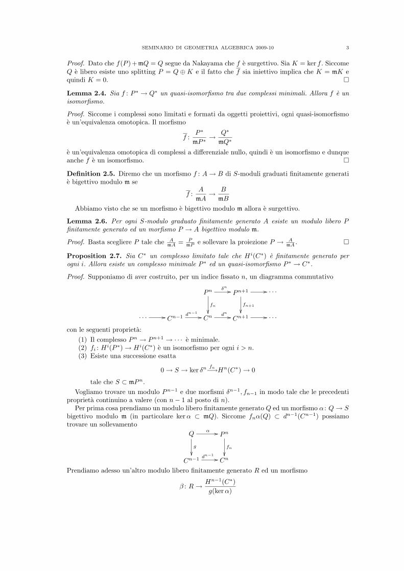
Proof. Dato che f(P ) + mQ = Q segue da Nakayama che f e surgettivo. Sia K = ker f . SiccomeQ e libero esiste uno splitting P = Q ⊕K e il fatto che f sia iniettivo implica che K = mK equindi K = 0. �

Lemma 2.4. Sia f : P ∗ → Q∗ un quasi-isomorfismo tra due complessi minimali. Allora f e unisomorfismo.

Proof. Siccome i complessi sono limitati e formati da oggetti proiettivi, ogni quasi-isomorfismoe un’equivalenza omotopica. Il morfismo

f :P ∗

mP ∗ →Q∗

mQ∗

e un’equivalenza omotopica di complessi a differenziale nullo, quindi e un isomorfismo e dunqueanche f e un isomorfismo. �

Definition 2.5. Diremo che un morfismo f : A→ B di S-moduli graduati finitamente generatie bigettivo modulo m se

f :A

mA→ B

mB

Abbiamo visto che se un morfismo e bigettivo modulo m allora e surgettivo.

Lemma 2.6. Per ogni S-modulo graduato finitamente generato A esiste un modulo libero Pfinitamente generato ed un morfismo P → A bigettivo modulo m.

Proof. Basta scegliere P tale che AmA = P

mP e sollevare la proiezione P → AmA . �

Proposition 2.7. Sia C∗ un complesso limitato tale che Hi(C∗) e finitamente generato perogni i. Allora esiste un complesso minimale P ∗ ed un quasi-isomorfismo P ∗ → C∗.

Proof. Supponiamo di aver costruito, per un indice fissato n, un diagramma commutativo

Pnδn

//

fn

��

Pn+1 //

fn+1

��

· · ·

· · · // Cn−1 dn−1// Cn

dn// Cn+1 // · · ·

con le seguenti proprieta:(1) Il complesso Pn → Pn+1 → · · · e minimale.(2) fi : Hi(P ∗)→ Hi(C∗) e un isomorfismo per ogni i > n.(3) Esiste una successione esatta

0→ S → ker δnfn−→Hn(C∗)→ 0

tale che S ⊂ mPn.Vogliamo trovare un modulo Pn−1 e due morfismi δn−1, fn−1 in modo tale che le precedenti

proprieta continuino a valere (con n− 1 al posto di n).Per prima cosa prendiamo un modulo libero finitamente generato Q ed un morfismo α : Q→ S

bigettivo modulo m (in particolare kerα ⊂ mQ). Siccome fnα(Q) ⊂ dn−1(Cn−1) possiamotrovare un sollevamento

Qα //

g

��

Pn

fn

��Cn−1 dn−1

// Cn

Prendiamo adesso un’altro modulo libero finitamente generato R ed un morfismo

β : R→ Hn−1(C∗)g(kerα)

4 MARCO MANETTI

bigettivo modulo m (in particolare kerβ ⊂ mR). Scegliamo infine un morfismo γ : R→ Zn−1(C∗)che solleva β e definiamo

Pn−1 = R⊕Q, δn−1(r, q) = α(q), fn−1(r, q) = γ(r) + g(q).

Si ha ker δn−1 = R⊕ kerα, per costruzione l’applicazione fn−1 : ker δn−1 → Hn−1(C∗) e suriet-tiva e e se fn−1(r, q) = 0 allora β(r) = 0 e quindi

ker fn−1 ⊂ kerβ ⊕ kerα ⊂ mR⊕mQ = mPn−1.

Chiaramente, se Ci = 0 per ogni i > n, si ha P i = 0 per ogni i > n, mentre se Ci = 0 perogni i < m, allora per Ausl.-Buch. si ha P i = 0 per ogni i < m−N − 1.

�

3. Il teorema di Horrocks

Theorem 3.1. Sia E un fibrato di rango finito su PN e k un intero. Se Hi∗(E) = 0 per ogni i

tale che k ≤ i < N (per k = N tale condizione e automaticamente soddisfatta), allora esiste unasuccessione esatta di fasci

0→ E → P0 → · · · → Pk−1 → 0

dove ogni Pi e somma diretta di line bundles. (Il viceversa e quasi ovvio).

Per uso futuro e utile premettere alla dimostrazione alcuni lemmi.

Lemma 3.2. Sia E un fibrato di rango finito su PN . Allora il modulo Hi∗(E) ha lunghezza finita

per ogni i tale che 0 < i < N .

Proof. Vanishing e dualita di Serre. �

Example 3.3. Supponiamo N > 2 e sia K il fascio grattacielo sul punto x1 = x2 = · · · = xN = 0e si consideri la successione esatta

0→ F → O(−1)N(x1,...,xN )−−−−−−−→ O → K→ 0.

Allora, H2(F(t)) = K per ogni t < 0 e quindi F non e localmente libero.

Lemma 3.4. Sia E un fibrato di rango finito su PN e C∗ ∈ Cb(Mod) un rappresentante diτ<NRΓ∗(E). Allora E e quasi-isomorfo a C∗, ossia E e isomorfo a C∗ nella categoria derivataDb(Qcoh).

Proof. Prendendo una risoluzione iniettiva di E e poi troncando, possiamo scegliere come rapp-resentante di τ<NRΓ∗(E) un complesso del tipo

C∗ : 0→ C0 δ0−→C1 → · · · → CN−1 → 0.

Siccome Hi(C∗) = Hi∗(E) ha lunghezza finita per ogni i con 0 < i < N , la successione di fasci

C0 δ0−→C1 → · · · → ˜CN−1 → 0.

Inoltre Γ∗ e esatto a sinistra e quindi Γ∗(E) = ker δ0 e quindi E = Γ∗(E) → C∗ e un quasi-isomorfismo. �

Lemma 3.5. Sia E un fibrato di rango finito su PN . Allora la risoluzione minimale di τ<NRΓ∗(E)ha la forma

P ∗ : 0→ P 0 → P 1 → · · · → PN−1 → 0

e vale E ' H0(P ∗).

SEMINARIO DI GEOMETRIA ALGEBRICA 2009-10 5

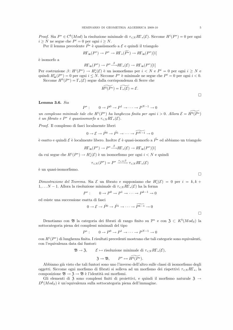
Proof. Sia P ∗ ∈ Cb(Mod) la risoluzione minimale di τ<NRΓ∗(E). Siccome Hi(P ∗) = 0 per ognii ≥ N ne segue che P i = 0 per ogni i ≥ N .

Per il lemma precedente P ∗ e quasiismorfo a E e quindi il triangolo

RΓm(P ∗)→ P ∗ → RΓ∗(P ∗)→ RΓm(P ∗)[1]

e isomorfo aRΓm(P ∗)→ P ∗ β−→RΓ∗(E)→ RΓm(P ∗)[1]

Per costruzione β : Hi(P ∗) → Hi∗(E) e un isomorfismo per i < N e P i = 0 per ogni i ≥ N e

quindi Him(P ∗) = 0 per ogni i ≤ N . Siccome P ∗ e minimale ne segue che P i = 0 per ogni i < 0.

Siccome H0(P ∗) = Γ∗(E) segue dalla corrispondenza di Serre che

H0(P ∗) = Γ∗(E) = E .�

Lemma 3.6. SiaP ∗ : 0→ P 0 → P 1 → · · · → PN−1 → 0

un complesso minimale tale che Hi(P ∗) ha lunghezza finita per ogni i > 0. Allora E = H0(P ∗)e un fibrato e P ∗ e quasiisomorfo a τ<NRΓ∗(E).

Proof. Il complesso di fasci localmemte liberi

0→ E → P 0 → P 1 → · · · → PN−1 → 0

e esatto e quindi E e localmente libero. Inoltre E e quasi-isomorfo a P ∗ ed abbiamo un triangolo

RΓm(P ∗)→ P ∗ β−→RΓ∗(E)→ RΓm(P ∗)[1]

da cui segue che Hi(P ∗)→ Hi∗(E) e un isomorfismo per ogni i < N e quindi

τ<N (P ∗) = P ∗ τ<Nβ−−−−→ τ<NRΓ∗(E)

e un quasi-isomorfismo.�

Dimostrazione del Teorema. Sia E un fibrato e supponiamo che Hi∗(E) = 0 per i = k, k +

1, . . . N − 1. Allora la risoluzione minimale di τ<NRΓ∗(E) ha la forma

P ∗ : 0→ P 0 → P 1 → · · · → P k−1 → 0

ed esiste una successione esatta di fasci

0→ E → P 0 → P 1 → · · · → P k−1 → 0

�

Denotiamo con B la categoria dei fibrati di rango finito su Pn e con Z ⊂ Kb(ModS) lasottocategoria piena dei complessi minimali del tipo

P ∗ : 0→ P 0 → P 1 → · · · → PN−1 → 0

con Hi(P ∗) di lunghezza finita. I risultati precedenti mostrano che tali categorie sono equivalenti,con l’equivalenza data dai funtori:

B→ Z, E 7→ risoluzione minimale di τ<NRΓ∗(E),

Z→ B, P ∗ 7→ H0(P ∗).Abbiamo gia visto che tali funtori sono uno l’inverso dell’altro sulle classi di isomorfismo degli

oggetti. Siccome ogni morfismo di fibrati si solleva ad un morfismo dei rispettivi τ<NRΓ∗, lacomposizione B→ Z→ B e l’identita sui morfismi.

Gli elementi di Z sono complessi finiti di proiettivi, e quindi il morfismo naturale Z →Db(ModS) e un’equivalenza sulla sottocategoria piena dell’immagine.

6 MARCO MANETTI

Ogni morfismo P ∗ → Q∗ in Z induce in Db(ModS) un diagramma commutativo

P ∗ → τ<NRΓ∗(P ∗)yy

Q∗ → τ<NRΓ∗(Q∗)

con le frecce orizzontali quasiisomorfismi. Ne segue che la composizione Z → B → Z e iniettivasui morfismi. Questo prova che tali categorie sono equivalenti.

4. La corrispondenza di Horroks

Lemma 4.1. Sia P ∈ ModS libero di rango finito e sia M ⊂ P un sottomodulo. Se M non econtenuto in mP , allora esiste un isomorfismo

φ : P → Q⊕ S(h)

con Q libero e N ⊂ Q tale che φ(M) = N ⊕ S(h).

Proof. Sia P =⊕n

i=1 S(hi), per ipotesi esiste un indice i tale che la restrizione ad M dellaproiezione P → S(hi) e surgettiva ed esiste usa sezione s : S(hi)→M . A meno di scambiare gliindici supponiamo i = 1; basta definire Q =

⊕ni=2 S(hi) e φ come l’inverso dell’isomorfismo

Q⊕ S(h1)→ P, (a, b) 7→ a+ s(b).

�

Definition 4.2. Diremo che un fibrato e minimale se non ha line bundles come addendi diretti.

Corollary 4.3. Sia E un fibrato minimale e sia

P ∗ : 0→ P 0 δ0−→P 1 → · · · → PN−1 → 0

la risoluzione minimale di τ<NRΓ∗(E). Allora ker δ0 ⊂ mP 0.

Proof. Se ker δ0 non e contenuto in mP 0, possiamo scrivere P 0 = Q0 ⊕ S(h) con S(h) ⊂ ker δ0

e quindi

E = H0(P ∗) = O(h)⊕ H0(Q∗)

doveQ∗ : 0→ Q0 → P 1 → · · · → PN−1 → 0

�

Theorem 4.4. Sia E fibrato e sia Q∗ la risoluzione minimale di τ>0τ<NRΓ∗(E). Allora vale

E ∼= Z0(Q∗) se e solo se E e minimale.

Proof. Supponiamo E minimale e sia

P ∗ : 0→ P 0 δ0−→P 1 → · · · → PN−1 → 0

la risoluzione minimale di τ<NRΓ∗(E). Allora

0→ P 0

ker δ0δ0−→P 1 → · · · → PN−1 → 0

e quasi-isomorfo a τ>0τ<NRΓ∗(E). Sia

· · · → Q−2 → Q−1 → ker δ0 → 0

una risoluzione minimale di ker δ0; siccome ker δ0 ⊂ mP 0 il complesso

Q∗ : · · ·Q−2 → Q−1 → P 0 δ0−→P 1 → · · · → PN−1 → 0

e la risoluzione minimale di τ>0τ<NRΓ∗(E) e Z0(Q∗) = ker δ0.

SEMINARIO DI GEOMETRIA ALGEBRICA 2009-10 7

Supponiamo adesso che E non sia minimale, possiamo scrivere E = H ⊕ G con H mini-male e G somma diretta di line bundles. Siccome τ>0τ<NRΓ∗(G) = 0 si ha τ>0τ<NRΓ∗(E) =

τ>0τ<NRΓ∗(H) e quindi H ∼= Z0(Q∗).�

References

[1] Hartshorne: Algebraic geometry.

[2] Hartshorne: Residues and duality.

[3] Walter: Pfaffian subschemes.

PFAFFIAN SUBSCHEMES, SECTION 2

CHARLES H. WALTER

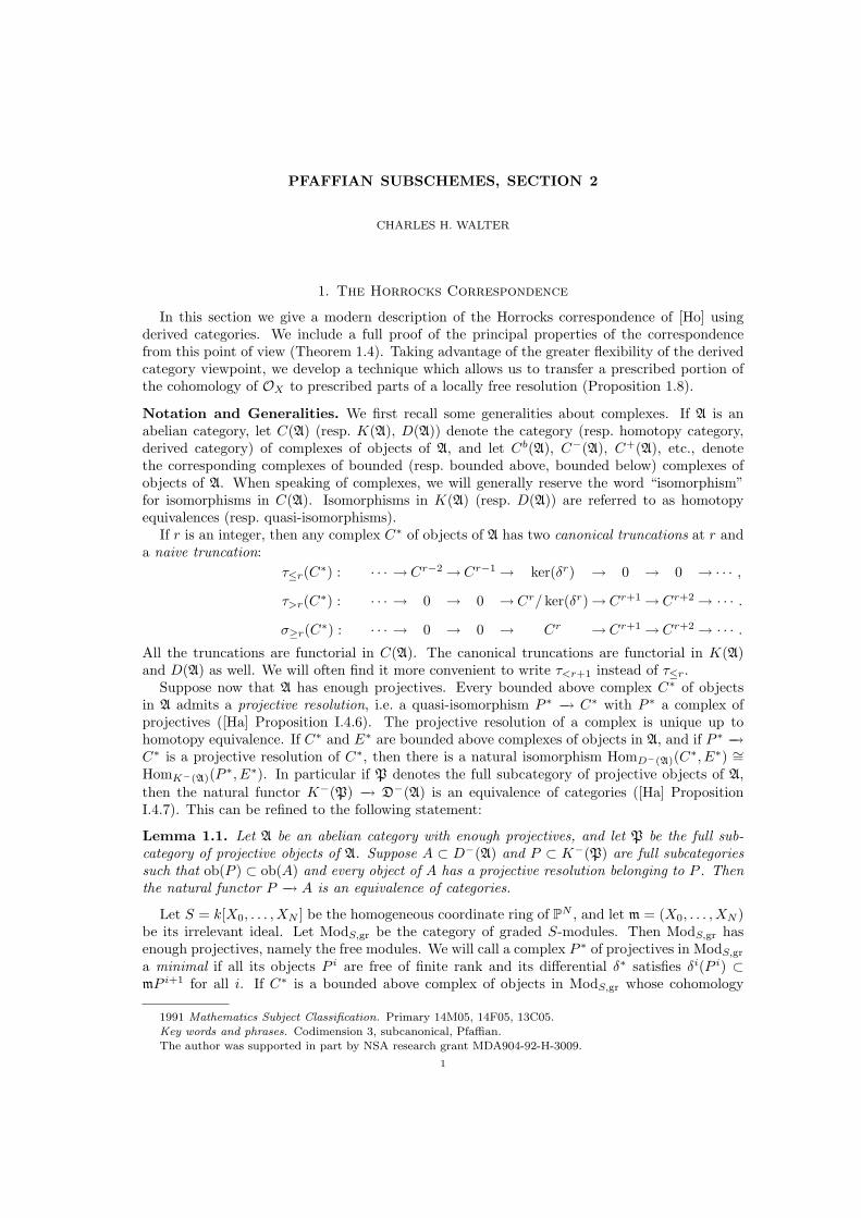
1. The Horrocks Correspondence

In this section we give a modern description of the Horrocks correspondence of [Ho] usingderived categories. We include a full proof of the principal properties of the correspondencefrom this point of view (Theorem 1.4). Taking advantage of the greater flexibility of the derivedcategory viewpoint, we develop a technique which allows us to transfer a prescribed portion ofthe cohomology of OX to prescribed parts of a locally free resolution (Proposition 1.8).

Notation and Generalities. We first recall some generalities about complexes. If A is anabelian category, let C(A) (resp. K(A), D(A)) denote the category (resp. homotopy category,derived category) of complexes of objects of A, and let Cb(A), C−(A), C+(A), etc., denotethe corresponding complexes of bounded (resp. bounded above, bounded below) complexes ofobjects of A. When speaking of complexes, we will generally reserve the word “isomorphism”for isomorphisms in C(A). Isomorphisms in K(A) (resp. D(A)) are referred to as homotopyequivalences (resp. quasi-isomorphisms).

If r is an integer, then any complex C∗ of objects of A has two canonical truncations at r anda naive truncation:

τ≤r(C∗) : · · · → Cr−2→ Cr−1→ ker(δr) → 0 → 0 → · · · ,

τ>r(C∗) : · · · → 0 → 0 → Cr/ ker(δr)→ Cr+1→ Cr+2→ · · · .

σ≥r(C∗) : · · · → 0 → 0 → Cr → Cr+1→ Cr+2→ · · · .All the truncations are functorial in C(A). The canonical truncations are functorial in K(A)and D(A) as well. We will often find it more convenient to write τ<r+1 instead of τ≤r.

Suppose now that A has enough projectives. Every bounded above complex C∗ of objectsin A admits a projective resolution, i.e. a quasi-isomorphism P ∗ −→ C∗ with P ∗ a complex ofprojectives ([Ha] Proposition I.4.6). The projective resolution of a complex is unique up tohomotopy equivalence. If C∗ and E∗ are bounded above complexes of objects in A, and if P ∗ −→C∗ is a projective resolution of C∗, then there is a natural isomorphism HomD−(A)(C∗, E∗) ∼=HomK−(A)(P ∗, E∗). In particular if P denotes the full subcategory of projective objects of A,then the natural functor K−(P) −→ D−(A) is an equivalence of categories ([Ha] PropositionI.4.7). This can be refined to the following statement:

Lemma 1.1. Let A be an abelian category with enough projectives, and let P be the full sub-category of projective objects of A. Suppose A ⊂ D−(A) and P ⊂ K−(P) are full subcategoriessuch that ob(P ) ⊂ ob(A) and every object of A has a projective resolution belonging to P . Thenthe natural functor P −→ A is an equivalence of categories.

Let S = k[X0, . . . , XN ] be the homogeneous coordinate ring of PN , and let m = (X0, . . . , XN )be its irrelevant ideal. Let ModS,gr be the category of graded S-modules. Then ModS,gr hasenough projectives, namely the free modules. We will call a complex P ∗ of projectives in ModS,gr

a minimal if all its objects P i are free of finite rank and its differential δ∗ satisfies δi(P i) ⊂mP i+1 for all i. If C∗ is a bounded above complex of objects in ModS,gr whose cohomology

1991 Mathematics Subject Classification. Primary 14M05, 14F05, 13C05.

Key words and phrases. Codimension 3, subcanonical, Pfaffian.

The author was supported in part by NSA research grant MDA904-92-H-3009.

1

2 CHARLES H. WALTER

modules Hi(C∗) are all finitely generated, then C∗ has a minimal projective resolution, i.e. aprojective resolution by a minimal complex of projectives. The next lemma, which is a wellknown consequence of Nakayama’s lemma, says that minimal projective resolutions are uniqueup to isomorphism and not merely up to homotopy equivalence:

Lemma 1.2. Let φ : P ∗ −→ Q∗ be a homotopy equivalence between minimal complexes of freegraded S-modules of finite rank. Then φ is an isomorphism.

Let ModO be the category of sheaves of OPN -modules. For E a sheaf of OPN -modules, letΓ∗(E) =

⊕t∈Z Γ(E(t)). Then Γ∗ defines a left exact functor from ModO to ModS,gr. It has a

right derived functor RΓ∗ : Db(ModO) −→ Db(ModS,gr) whose cohomology functors we denoteHi∗(E) =

⊕t∈Z H

i(E(t)). The functor Γ∗ has an exact left adjoint ˜, the functor of associatedsheaves.

Let Γm : ModS,gr −→ ModS,gr be the functor associating to a graded S-module M the maximalsubmodule Γm(M) ⊂ M supported at the origin 0 of AN+1. This functor is also left exact andhas a right derived functor RΓm : Db(ModS,gr) −→ Db(ModS,gr). Its cohomology functors aredenoted Hi

m.

Lemma 1.3. Let P ∗ be a bounded complex of free graded S-modules of finite rank where S =k[X0, . . . , XN ]. If P ∗ is minimal, then

max{i | P i 6= 0} = max{i | Hi(P ∗) 6= 0},min{i | P i 6= 0} = min{i | Hi

m(P ∗) 6= 0} −N − 1.

Proof. The assertion about maxima is a simple and well-known application of the minimal-ity condition and Nakayama’s Lemma. The assertion about minima, which is essentially theAuslander-Buchsbaum theorem, reduces to the assertion about maxima by Serre duality. �

The Horrocks Correspondence. We now begin to describe the components of the Horrockscorrespondence. Let B be the full subcategory of ModO of locally free sheaves of finite rank,and let Z denote the full category of Db(ModS,gr) of complexes C∗ such that Hi(C∗) is of finitelength for 0 < i < N and Hi(C∗) vanishes for all other i.

The Horrocks correspondence consists of a functor ζ : B −→ Z and a map H : ob(Z) −→ ob(B)in the opposite direction. The functor ζ is simply τ>0τ<NRΓ∗. For E a vector bundle on PN ,the cohomology of ζ(E) is of course:

Hi(ζ(E)) =

{Hi∗(E) if 0 < i < N,

0 otherwise.

Since E is locally free of finite rank, Hi∗(E) is of finite length for 0 < i < N . So ζ(E) ∈ ob(Z).

We now define H. Any C∗ ∈ ob(Z) has a minimal projective resolution P ∗ −→ C∗. We defineH(C∗) to be the kernel of the differential δ0 : P 0 −→ P 1. Then H(C∗) is a vector bundle becauseit fits into an exact complex of vector bundles

· · · −→ 0 −→ H(C∗) −→ P 0 −→ P 1 −→ · · · −→ PN−1 −→ 0 −→ · · · . (1)

Note that H(C∗) is well-defined up to isomorphism because the minimal projective resolutionP ∗ of C∗ is unique up to isomorphism because of Lemma 1.2. However, H is not a functor.

The principal results of Horrocks’ paper [Ho] can be described in the following way:

Theorem 1.4 (Horrocks). Let B be the category of locally free sheaves of finite rank on PN ,and let Z be the full subcategory of Db(ModS,gr) of complexes C∗ such that Hi(C∗) is of finitelength if 0 < i < N , and Hi(C∗) = 0 for all other i. Let ζ = τ>0τ<NRΓ∗ : B −→ Z, and letH : ob(Z) −→ ob(B) be the map defined as in (1) above.

(a) If E ∈ ob(B), then E ∼= Hζ(E)⊕⊕iOPN (ni) for some integers ni.(b) If C∗ ∈ ob(Z), then ζH(C∗) ' C∗.(c) If E ,F ∈ ob(B), then HomZ(ζ(E), ζ(F)) ∼= Hom(E ,F)/HomΦ(E ,F) where HomΦ(E ,F)

is the set of all morphisms which factor through a direct sum of line bundles.

PFAFFIAN SUBSCHEMES, SECTION 2 3

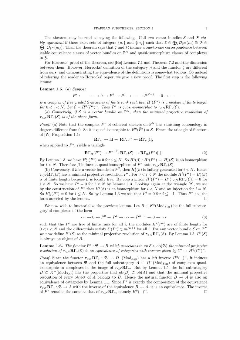
The theorem may be read as saying the following. Call two vector bundles E and F sta-bly equivalent if there exist sets of integers {ni} and {mj} such that E ⊕⊕iOPN (ni) ∼= F ⊕⊕

j OPN (mj). Then the theorem says that ζ and H induce a one-to-one correspondence betweenstable equivalence classes of vector bundles on PN and quasi-isomorphism classes of complexesin Z.

For Horrocks’ proof of the theorem, see [Ho] Lemma 7.1 and Theorem 7.2 and the discussionbetween them. However, Horrocks’ definition of the category Z and the functor ζ are differentfrom ours, and demonstrating the equivalence of the definitions is somewhat tedious. So insteadof referring the reader to Horrocks’ paper, we give a new proof. The first step is the followinglemma:

Lemma 1.5. (a) Suppose

P ∗ : · · · −→ 0 −→ P 0 −→ P 1 −→ · · · −→ PN−1 −→ 0 −→ · · ·is a complex of free graded S-modules of finite rank such that Hi(P ∗) is a module of finite lengthfor 0 < i < N . Let E = H0(P ∗)∼. Then P ∗ is quasi-isomorphic to τ<NRΓ∗(E).

(b) Conversely, if E is a vector bundle on PN , then the minimal projective resolution ofτ<NRΓ∗(E) is of the above form.

Proof. (a) Note that the complex P ∗ of coherent sheaves on PN has vanishing cohomology indegrees different from 0. So it is quasi-isomorphic to H0(P ∗) = E . Hence the triangle of functorsof [W] Proposition 1.1:

RΓm −→ Id −→ RΓ∗◦∼ −→ RΓm[1],when applied to P ∗, yields a triangle

RΓm(P ∗) −→ P ∗β−→ RΓ∗(E) −→ RΓm(P ∗)[1]. (2)

By Lemma 1.3, we have Him(P ∗) = 0 for i ≤ N . So Hi(β) : Hi(P ∗) −→ Hi

∗(E) is an isomorphismfor i < N . Therefore β induces a quasi-isomorphism of P ∗ onto τ<NRΓ∗(E).

(b) Conversely, if E is a vector bundle on PN , then Hi∗(E) is finitely generated for i < N . Hence

τ<NRΓ∗(E) has a minimal projective resolution P ∗. For 0 < i < N the module Hi(P ∗) = Hi∗(E)

is of finite length because E is locally free. By construction Hi(P ∗) = Hi(τ<NRΓ∗(E)) = 0 fori ≥ N . So we have P i = 0 for i ≥ N by Lemma 1.3. Looking again at the triangle (2), we seeby the construction of P ∗ that Hi(β) is an isomorphism for i < N and an injection for i = N .So Hi

m(P ∗) = 0 for i ≤ N . So by Lemma 1.3 we see that P i = 0 for i ≤ −1. Thus P ∗ has theform asserted by the lemma. �

We now wish to functorialize the previous lemma. Let B ⊂ Kb(ModS,gr) be the full subcate-gory of complexes of the form

· · · −→ 0 −→ P 0 −→ P 1 −→ · · · −→ PN−1 −→ 0 −→ · · · (3)

such that the P i are free of finite rank for all i, the modules Hi(P ∗) are of finite length for0 < i < N and the differentials satisfy δi(P i) ⊂ mP i+1 for all i. For any vector bundle E on PNwe now define P ∗(E) as the minimal projective resolution of τ<NRΓ∗(E). By Lemma 1.5, P ∗(E)is always an object of B.

Lemma 1.6. The functor P ∗ : B −→ B which associates to an E ∈ ob(B) the minimal projectiveresolution of τ<NRΓ∗(E) is an equivalence of categories with inverse given by C∗ 7→ H0(C∗)∼.

Proof. Since the functor τ<NRΓ∗ : B −→ D−(ModS,gr) has a left inverse H0(−)∼, it inducesan equivalence between B and the full subcategory A ⊂ D−(ModS,gr) of complexes quasi-isomorphic to complexes in the image of τ<NRΓ∗. But by Lemma 1.5, the full subcategoryB ⊂ K−(ModS,gr) has the properties that ob(B) ⊂ ob(A) and that the minimal projectiveresolution of every object of A belongs to B. Hence the natural functor B −→ A is also anequivalence of categories by Lemma 1.1. Since P ∗ is exactly the composition of the equivalenceτ<NRΓ∗ : B −→ A with the inverse of the equivalence B −→ A, it is an equivalence. The inverseof P ∗ remains the same as that of τ<NRΓ∗, namely H0(−)∼. �

4 CHARLES H. WALTER

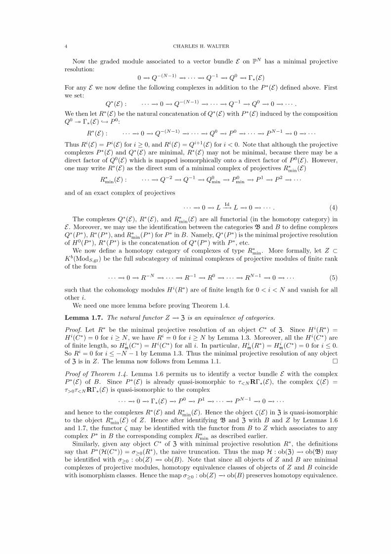
Now the graded module associated to a vector bundle E on PN has a minimal projectiveresolution:

0 −→ Q−(N−1) −→ · · · −→ Q−1 −→ Q0 −→ Γ∗(E)For any E we now define the following complexes in addition to the P ∗(E) defined above. Firstwe set:

Q∗(E) : · · · −→ 0 −→ Q−(N−1) −→ · · · −→ Q−1 −→ Q0 −→ 0 −→ · · · .We then let R∗(E) be the natural concatenation of Q∗(E) with P ∗(E) induced by the compositionQ0 � Γ∗(E) ↪→ P 0:

R∗(E) : · · · −→ 0 −→ Q−(N−1) −→ · · · −→ Q0 −→ P 0 −→ · · · −→ PN−1 −→ 0 −→ · · ·Thus Ri(E) = P i(E) for i ≥ 0, and Ri(E) = Qi+1(E) for i < 0. Note that although the projectivecomplexes P ∗(E) and Q∗(E) are minimal, R∗(E) may not be minimal, because there may be adirect factor of Q0(E) which is mapped isomorphically onto a direct factor of P 0(E). However,one may write R∗(E) as the direct sum of a minimal complex of projectives R∗min(E)

R∗min(E) : · · · −→ Q−2 −→ Q−1 −→ Q0min −→ P 0

min −→ P 1 −→ P 2 −→ · · ·

and of an exact complex of projectives

· · · −→ 0 −→ LId−→ L −→ 0 −→ · · · . (4)

The complexes Q∗(E), R∗(E), and R∗min(E) are all functorial (in the homotopy category) inE . Moreover, we may use the identification between the categories B and B to define complexesQ∗(P ∗), R∗(P ∗), and R∗min(P ∗) for P ∗ in B. Namely, Q∗(P ∗) is the minimal projective resolutionof H0(P ∗), R∗(P ∗) is the concatenation of Q∗(P ∗) with P ∗, etc.

We now define a homotopy category of complexes of type R∗min. More formally, let Z ⊂Kb(ModS,gr) be the full subcategory of minimal complexes of projective modules of finite rankof the form

· · · −→ 0 −→ R−N −→ · · · −→ R−1 −→ R0 −→ · · · −→ RN−1 −→ 0 −→ · · · (5)

such that the cohomology modules Hi(R∗) are of finite length for 0 < i < N and vanish for allother i.

We need one more lemma before proving Theorem 1.4.

Lemma 1.7. The natural functor Z −→ Z is an equivalence of categories.

Proof. Let R∗ be the minimal projective resolution of an object C∗ of Z. Since Hi(R∗) =Hi(C∗) = 0 for i ≥ N , we have Ri = 0 for i ≥ N by Lemma 1.3. Moreover, all the Hi(C∗) areof finite length, so Hi

m(C∗) = Hi(C∗) for all i. In particular, Him(R∗) = Hi

m(C∗) = 0 for i ≤ 0.So Ri = 0 for i ≤ −N − 1 by Lemma 1.3. Thus the minimal projective resolution of any objectof Z is in Z. The lemma now follows from Lemma 1.1. �

Proof of Theorem 1.4. Lemma 1.6 permits us to identify a vector bundle E with the complexP ∗(E) of B. Since P ∗(E) is already quasi-isomorphic to τ<NRΓ∗(E), the complex ζ(E) =τ>0τ<NRΓ∗(E) is quasi-isomorphic to the complex

· · · −→ 0 −→ Γ∗(E) −→ P 0 −→ P 1 −→ · · · −→ PN−1 −→ 0 −→ · · ·and hence to the complexes R∗(E) and R∗min(E). Hence the object ζ(E) in Z is quasi-isomorphicto the object R∗min(E) of Z. Hence after identifying B and Z with B and Z by Lemmas 1.6and 1.7, the functor ζ may be identified with the functor from B to Z which associates to anycomplex P ∗ in B the corresponding complex R∗min as described earlier.

Similarly, given any object C∗ of Z with minimal projective resolution R∗, the definitionssay that P ∗(H(C∗)) = σ≥0(R∗), the naive truncation. Thus the map H : ob(Z) −→ ob(B) maybe identified with σ≥0 : ob(Z) −→ ob(B). Note that since all objects of Z and B are minimalcomplexes of projective modules, homotopy equivalence classes of objects of Z and B coincidewith isomorphism classes. Hence the map σ≥0 : ob(Z) −→ ob(B) preserves homotopy equivalence.

PFAFFIAN SUBSCHEMES, SECTION 2 5

Since Z and B are subcategories of the homotopy category, this means that σ≥0 is well-definedon objects of Z. However, σ≥0 and hence H are not well-defined on morphisms of Z.

(a) The above identifications now say if E ∈ ob(B), then Hζ(E) is the object of B corre-sponding to the complex σ≥0(R∗min(E)):

σ≥0(R∗min(E)) : · · · −→ 0 −→ P 0min

µ−→ P 1 −→ · · · −→ PN−1 −→ 0 −→ · · · .

By Lemma 1.6, the sheaf Hζ(E) is ker(µ)∼. So E = Hζ(E)⊕L where L is the projective moduleof (4). Since L is now a direct sum of line bundles, (a) follows.

(b) If C∗ is an object of Z with minimal projective resolution R∗ in Z of the form (5), thenthe above computations identify H(C∗) in B with P ∗(H(C∗)) = σ≥0(R∗) in B. Thus ζH(C∗)becomes identified with R∗min(H(C∗)) which is just R∗ again. Since R∗ is quasi-isomorphic toC∗, we have ζH(C∗) ' C∗ as desired.

(c) After identifying B with B and Z with Z, assertion (c) becomes the statement: For anypair of objects E∗ and F ∗ in B, the natural map

HomB(E∗, F ∗) −→ HomZ(R∗min(E∗), R∗min(F ∗)) (6)

is surjective and its kernel is the subspace of morphisms which factor through an object of B ofthe form

· · · −→ 0 −→ L −→ 0 −→ · · · (7)

with L a free graded S-module of finite rank appearing in degree 0.We first prove surjectivity. Suppose φ ∈ HomZ(R∗min(E∗), R∗min(F ∗)). Since Z is a homotopy

category, φ is actually a homotopy equivalence class of maps in C(ModS,gr). So we may choosea chain map f in the class φ. Then f may be extended to a chain map f : R∗(E∗) −→ R∗(F ∗)by defining it to be 0 on the exact factor of the type (4). Then σ≥0f maps E∗ to F ∗, and itshomotopy class in B has image φ in Z. This proves surjectivity.

We now compute the kernel of (6). First if α ∈ HomB(E∗, F ∗) factors through a complex L∗

of the form (7), then R∗min(α) factors through R∗min(L∗) = 0 and so vanishes. So the kernel of(6) contains all morphisms which factor through complexes of the form (7).

Conversely, suppose α is in the kernel of (6). Since α is a morphism in B, it is a homotopyclass of chain maps from which we may choose a member β. We may complete β to a chain mapρ : R∗(E∗) −→ R∗(F ∗).

R∗(E∗) · · · → 0 → E−N → · · · → E

−1→ E0→ · · · → EN−1→ 0 → · · ·yρ

yy

yyβ

yβy

R∗(F ∗) · · · → 0 → F−N → · · · → F

−1→ F 0→ · · · → FN−1→ 0 → · · ·The homotopy class of ρ is the image of α under R∗ and so must vanish by hypothesis. (Notethat R∗ and R∗min are homotopy equivalent.) Thus ρ is homotopic to 0. Thus if we write δi forthe differentials of R∗(E∗), and εi for the differentials of R∗(F ∗), then there is a chain homotopyh = (hi) such that ρi = hi+1δi + εi−1hi for all i. Now restrict h to a chain homotopy h = (hi)with hi : Ei −→ F i−1 defined by defined by hi = hi for all i ≥ 1, and hi = 0 for all i ≤ 0. Thenβ is homotopic to a morphism whose components are

βi − (hi+1δi + εi−1hi) =

ρi − (hi+1δi + εi−1hi) = 0 if i ≥ 1,ρ0 − h1δ0 = ε−1h0 if i = 0,0 if i ≤ −1.

Hence the homotopy class α of β factors through the complex

· · · −→ 0 −→ F−1 −→ 0 −→ · · ·

of type (7). So the kernel of (6) is as asserted. This completes the proof of the theorem. �

6 CHARLES H. WALTER

We will use three further results concerning the Horrocks correspondence. The first will permitus to use the Horrocks correspondence to constuct locally free resolutions of coherent sheaves.

Proposition 1.8. Let Q be a quasi-coherent sheaf on PN , let C∗ ∈ ob(Z), and let β : C∗ −→τ>0τ<NRΓ∗(Q) be a morphism in Db(ModS,gr). Then there exists a morphism of quasi-coherentsheaves β : H(C∗) −→ Q such that β = τ>0τ<NRΓ∗(β). In particular, the induced morphismsHi∗(H(C∗)) −→ Hi

∗(Q) are the same as Hi(β) for 1 ≤ i ≤ N − 1.

Proof. Let R∗ be a minimal projective resolution of C∗, and let I∗ be an injective resolution ofQ. Then β may be identified with an actual chain map

· · · →R−2→ R−1 → R0 λ−→ R1 → · · · → RN−2 → RN−1 → 0y

yy

yy

y

· · · → 0 → Γ∗(Q)→ Γ∗(I0)µ−→ Γ∗(I1)→ · · · → Γ∗(IN−2)→ ker(δN−1)→ 0

Thus β induces a morphism β from H(C∗) = ker(λ)∼ to Q = ker(µ)∼.We now need to calculate RΓ∗(β). Consider the complex

P ∗ : · · · −→ 0 −→ R0 −→ R1 −→ · · · −→ RN−1 −→ 0 −→ · · · .The previous diagram induces a new commutative diagram

P ∗: · · · → 0 → R0→ R1→ · · · → RN−2→ RN−1→ 0 → 0 → · · ·yβ

yy

yy

yy

y

I∗ : · · · → 0 → I0 → I1 → · · · → IN−2 → IN−1 →IN → 0 → · · ·between resolutions of H(C∗) and Q extending β. Let γ : P ∗ −→ J∗ be an injective resolution ofP ∗. Then β factors through γ as P ∗ −→ J∗ −→ I∗. Applying Γ∗ now gives a factorization

P ∗ −→ Γ∗(J∗) −→ Γ∗(I∗). (8)

Now β is a map between resolutions of H(C∗) and Q, respectively, which extends β : H(C∗) −→ Q,while γ is a quasi-isomorphism. So the map J∗ −→ I∗ is a map between injective resolutions ofH(C∗) and Q extending β. So by definition, the second arrow of (8) is RΓ∗(β) : RΓ∗(H(C∗)) −→RΓ∗(Q). On the other hand, the proof of Lemma 1.5(a) shows that the first arrow of (8)can be identified with the truncation τ<N (RΓ∗(H(C∗))) −→ RΓ∗(H(C∗)) because it inducesisomorphisms Hi(P ∗) ∼= Hi(Γ∗(J∗)) = Hi

∗(H(C∗)) for i < N . Hence Γ∗(β) : P ∗ −→ Γ∗(I∗) canbe identified with the composition of the truncation τ<N (RΓ∗(H(C∗))) −→ RΓ∗(H(C∗)) withRΓ∗(β). Thus τ<NRΓ∗(β) may be identified with the diagram

· · · → 0 → R0 → R1 → · · · → RN−2 → RN−1 → 0 → · · ·y

yy

yy

y

· · · → 0 → Γ∗(I0)→ Γ∗(I1)→ · · · → Γ∗(IN−2)→ ker(δN−1)→ 0 → · · ·induced by β. Truncating on the left, we reach a diagram equivalent to the first diagram of theproof of the proposition. So β = τ>0τ<NRΓ∗(β). �

We now need two homological criteria for maps of vector bundles to be isomorphisms.

Lemma 1.9. Let E and F be vector bundles on PN with neither containing a line bundle as adirect factor. If α : E −→ F is a map such that Hi

∗(α) : Hi∗(E) −→ Hi

∗(F) is an isomorphism for0 < i < N , then α is an isomorphism.

Proof. We use the notation of the proof of Theorem 1.4. Let E∗ = P ∗(E) and F ∗ = P ∗(F),and let α : E∗ −→ F ∗ be the map induced by α. The hypothesis E = Hζ(E) implies thatE∗ is homotopy equivalent to σ≥0R

∗min(E∗), or equivalently that R∗(E∗) is a minimal complex

of projectives. Similarly, R∗(F ∗) is a minimal complex of projectives. The hypothesis on α

PFAFFIAN SUBSCHEMES, SECTION 2 7

implies that ζ(α) : ζ(E) −→ ζ(F) is a quasi-isomorphism. This in turn translates into R∗min(α)being a homotopy equivalence. But because of the earlier hypotheses, this means that R∗(α) :R∗(E∗) −→ R∗(F ∗) is a homotopy equivalence between the minimal complexes of projectives.Hence by Lemma 1.2 R∗(α) is actually an isomorphism of complexes. So its naive truncationσ≥0R

∗(α) = α is also an isomorphism. Therefore α is an isomorphism. �We will also need a slight generalization of the previous lemma.

Lemma 1.10. Let E = Hζ(E) ⊕⊕OPN (ni) and F be vector bundles on PN , and let Q be acoherent sheaf on PN . Suppose that there exist morphisms α : E −→ F and β : F −→ Q such that

(i) Hi∗(α) : Hi

∗(E) −→ Hi∗(F) is an isomorphism for 0 < i < N ,

(ii) βα takes the generators of the factors S(ni) of Γ∗(E) onto a minimal set of generators ofthe module Q := Γ∗(Q)/βα(Γ∗(Hζ(E))),

(iii) E and F have the same rank.Then α is an isomorphism.

Proof. Write F = Hζ(F) ⊕⊕OPN (mj). The splittings of E and of F into direct factors arenot canonical. But choosing such splittings gives an injection Hζ(E) ↪→ E and a projectionF � Hζ(F). Then the composition

α : Hζ(E) −→ E α−→ F −→ Hζ(F)

is, like α, an isomorphism on Hi∗ for 0 < i < N . So α is an isomorphism by Lemma 1.9. Hence

by identifying Hζ(F) with α(Hζ(E)) ⊂ F , we see that α induces a morphism of diagrams0 −−−−→ Hζ(E) −−−−→ E −−−−→ ⊕OPN (ni) −−−−→ 0

∥∥∥yα

yα1

0 −−−−→ Hζ(F) −−−−→ F −−−−→ ⊕OPN (mj) −−−−→ 0

(9)

The morphisms α and β therefore induce maps⊕

S(ni)Γ∗(α1)−−−−→

⊕S(mj)

β−→ Q = Γ∗(Q)/βα(Γ∗(Hζ(E))).

The composition is a surjection corresponding to a minimal set of generators of Q by hypothesis(ii). Hence the righthand map β must be a surjection corresponding to a set of generators of Q.However, the two free modules have the same rank by hypothesis (iii). Hence β also correspondsto a minimal set of generators, and Γ∗(α1) must be an isomorphism. So returning to diagram(9), α1 and hence α are isomorphisms. �

References

[BE1] D. Buchsbaum and D. Eisenbud, What Makes a Complex Exact?, J. Algebra 25 (1973), 259–268.

[BE2] , Algebra Structures for Finite Free Resolutions, and Some Structure Theorems for Ideals ofCodimension 3, Amer. J. Math. 99 (1977), 447–485.

[Ha] R. Hartshorne, Residues and Duality, Lecture Notes in Math., vol. 20, Springer-Verlag, Berlin, 1966.

[Ho] G. Horrocks, Vector Bundles on the Punctured Spectrum of a Local Ring, Proc. London Math. Soc. (3)14 (1964), 689–713.

[O] C. Okonek, Notes on Varieties of Codimension 3 in PN , preprint, Bonn, 1993.

[W] C. Walter, Algebraic Methods for the Cohomology of Normal Bundles of Algebraic Space Curves, preprint.

URA 168, Mathematiques, Universite de Nice–Sophia-Antipolis, Parc Valrose, F-06108 NICE Cedex

02, France

E-mail address: walter@math.unice.fr