Rapporto n. 238 - Home page | BOA Bicocca Open …...Kiweu (1991) and Dickinson and Muragu (1994)...

Dipartimento di Statistica e Metodi Quantitativi

Università degli Studi di Milano Bicocca Via Bicocca degli Arcimboldi , 8 - 20126 Milano - Italia

Tel +39/02/64483103 - Fax +39/2/64483105

Segreteria di redazione: Andrea Bertolini

Rapporto n. 238

Equity Stock Markets in Africa: Empirical Evidence

from the Random Walk Hypothesis

Eric Dongmo Guefack and Romuald N. Kenmoe S

Aprile 2013

1

Equity Stock Markets in Africa: Empirical Evidence

from the Random Walk Hypothesis

Romuald.N Kenmoe.S, PhD

(Dipartimento di metodi quantitativi, University of Milano-Bicocca,

[email protected])

and

Eric Dongmo Guefack

(Ergo S.P.A, Milan, [email protected])

Abstract

In this paper, weak-form market hypothesis is tested for some relevant African stock markets: Egypt,

Kenya, Mauritius, Morocco, Nigeria, South Africa, Tunisia. Using daily and weekly data which span

the period 2000 to 2012. We have used autocorrelation test, runs test, Augmented Dickey-Fuller

(ADF), Phillips-Perron (PP) and Kwiatkowski, Phillips, Schmidt and Shin (KPSS) uniroot test and

parametric and nonparametric multiple variance tests. The empirical results show that African stock

markets are not weak-form efficient using daily data; the South African one is characterized by a

martingale difference sequence. We find that most of the stock tend to comply with weak-form

efficiency when weekly data are used.

INTRODUCTION

The last decades have witnessed an increase in the amount of literature in the field of

the Efficient Market Hypothesis (EMH) and Random Walk Hypothesis (RWH). The

main motivation behind this branch of research is that the behavior of asset prices

(returns) is the cornerstone in every financial application. The examination of market

efficiency of financial asset is of interest for academicians, practitioners and

regulators. While academicians seek to understand the behavior of asset returns over

2

time, practitioners and investors are often interested in identifying market

inefficiencies in asset returns; regulators in contrast are interested in improving the

informational efficiencies of securities markets in which financial assets are traded.

Knowledge of the behavior of the stock market, particularly in the efficiency and (or)

randomness standpoint, is therefore of major concern to a large number of interested

groups. According to Fama and French (1965) stock price movements are not to such

a degree that one can predict them. Within the random walk hypothesis, prices adjust

rapidly as new and consistent information become available. Today’s price change

results from today’s news and it is independent of yesterday’s old news. News is

unpredictable and so are price changes. Many statistical tests were designed to test the

RWH but the class based on variance ratio (VR) methodology, has known a great

popularly in the recent years. Lo and Mackinlay (1988) pioneered this strand of

literature proposing seminal work for testing Efficient Market and Random Walk.

This type of statistic is based on the fact that aggregation of data sampled at different

frequencies verifies the following properties under i.i.d (independently and identically

distributed) hypothesis: the variance of the k period return should be k times the

variance of one period return. If in one way or another it can be proved that the ratio

is significantly different from one, the hypothesis of random walk in the stock price

will be rejected. The globalization and the growth of financial markets spawned

interest on the study of this issue, with many studies both on individual markets and

regional markets. While the theory of efficient markets is well consolidated in

developed markets (United States and Europe), we cannot say the same in the

emerging markets; things are worse concerning African stock markets. The majority

of studies relating to African stock markets have been focused on the Johannesburg

Stock Exchange (JSE). Smith et al. (2002), Smith and Jefferis (2002) and Magnusson

and Wydick (2002) among others. Appiah-Kusi and Menyah (2003) found the stock

markets of Botswana, Ghana and Ivory Coast not weak-form efficient in the analyzed

period. These results were stressed first in Magnusson and Widyck (2002) who found

that the Botswana and Ghana markets do not comply with random walk hypothesis. In

the same work, Appiah-Kusi and Menyah (2003) concluded that Egypt, Kenya,

Mauritius, Morocco and Zimbabwe are weak-form efficient. The investigation of

Kiweu (1991) and Dickinson and Muragu (1994) reached the same conclusion for

Kenya over the period spanning from 1986 to 1996 and 1979 to 1988 respectively,

while Chiwira (2001) found the Zimbabwe stock exchange to be weak-form efficient.

3

Smith et al (2002) concluded unlikely that there is no weak-form efficiency for the

periods January 1990 to August 1998 for Morocco and Mauritius, and January 1993

to August 1998 for Egypt. Bundo (2000) concluded in the same manner for the stock

Exchange for Mauritius (SEM) from the period 1992 to 1998. Asal (2000) found

Egypt Stock Exchange to be weak-form inefficient for the period 1992 to 1996

although he found some evidence of moving towards efficiency in 1996. Smith (2008)

in a recent work showed that Egypt, Nigeria, Tunisia and South Africa stock markets

comply with the martingale difference hypothesis and concluded that the random

walk hypothesis is out of reach for the 11 African stock markets examined using joint

variance ratio test. Studies which have investigated the EMH and the RWH in the

African market used either monthly or weekly data rather than daily data and the

analyzed period was very short. The principal limiting factor as pointed out by

Dickinson and Muragu (1994), has been the non-availability of computerized data

bases. The other argument of using those very low frequency data is the problem of

thin trading. Increasing the time intervals can be pursued to reduce the potential biases

associated to thin trading by increasing the probability of having at least one trade in

the interval, see Dickinson and Muragu (1994) for the topic. Nowadays, technological

innovation and trade globalization have brought us into a new era of financial

markets, therefore many well-known financial databases can provide daily and high-

frequency data for almost all markets, including African stock markets.

The main contribution of this work is to enrich the existing literature of random walk

and EMH theory in African markets using both daily and weekly data; perhaps of

more importance, this study examines the crisis effect on the market efficiency. To

our knowledge, this is the first contribution in this sense, even though, since the

contribution of Lo and Mackinlay (1988), variance ratio tests have been common

tools for testing market efficiency. Both parametric and nonparametric variance ratio

tests are used to examine the aforementioned issues. We use a period of 12 years, the

longest period ever used in African markets. We divide the sample in three periods

January 2000 to October 2012, January 2000 to July 2007 (pre-crisis period) and

August 2007 to October 2012 (crisis period) to highlight the crisis effects in our

study. The remainder of the paper is divided as follow: a brief literature reviews is

presented in Section 1. Section 2 discusses the various empirical methodologies used,

while the description of the data employed is provided by Section 3. Section 4

4

analyzes empirical results. We end the paper by summarizing the relevant findings in

Section 5.

I. LITERATURE REVIEW

The literature on random walk hypothesis in financial time series has been a subject of

much attention in the empirical finance literature. If the time series of an asset price

follows a random walk, then its return is non-predictable and investors are unable to

make abnormal returns consistently over time. According to the efficient markets

hypothesis, a market is efficient if stock prices reflect all currently available

information such that future prices cannot be predicted on the basis of this

information (Fama, 1965). The validity of random walk has strong implications for

market efficiency, and so this issue is relevant for academicians, investors and

regulatory authorities. Although there have been numerous empirical studies which

test for random walk in stock prices, most of these studies are focused around major

developed markets and emerging markets of Asia, Latin America, Eastern Europe, but

very little is known about the behaviour of emerging markets in Africa as the weak-

form hypothesis has received little attention from researchers. While the general

conclusion of the existing studies supports the weak-form efficiency for developed

markets, the research findings for emerging markets are mixed and mostly reject the

weak-form efficiency in these markets.

Some notable studies of market efficiency include Smith et al. (2002), Magnusson

and Wydick (2002), Jefferis and Smith (2005), Simons and Laryea (2005), Appiah-

Kusi and Menyah (2003), Smith (2008) and Mollah and Vitali (2011) for African

countries; Abraham et al. (2002) for Middle East countries; Huang (1995), Chang and

Ting (2000), Ryoo and Smith (2002), Groenewold and Ariff (1998) for Asian

countries; Lo and Mackinlay (1988), Kim et al. (1991) for Western countries;

Worthington and Higgs (2004), Smith and Ryoo (2003) for European countries.

Smith et al. (2002) tested the i.i.d random walk hypothesis using joint variance ratio

tests with weekly data on eight composite stock indices during the period from

January 1990 to August 1998. They found that except for the South African stock

market, none of the other stock markets examined (Botswana, Egypt, Kenya,

5

Mauritius, Morocco, Nigeria, Zimbabwe) followed an i.i.d random walk. Jefferis and

Smith (2005) used a GARCH approach with time-varying parameters to test the

changing efficiency of seven stock markets in Africa with weekly data over the period

from early 1990 to June 2001. They found that the Johannesburg stock market was

weak-form efficient, and three stock markets became weak-form efficient towards the

end of their study period, these were Egypt and Morocco from 1999 and Nigeria from

early 2001. These contrast with Kenya and Zimbabwe stock markets which show no

tendency towards weak-form efficiency and the Mauritius market which displays a

slow tendency to eliminate inefficiency. Magnusson and Wydick (2002) use the

partial autocorrelation test to examine the efficiency of eight largest African stock

markets from 1989 to 1998 in comparison with nine Asian and Latin American

markets. They find that six out of the eight examined African stock markets are weak-

form efficient. In another multi-country analysis Appiah-Kusi and Menyah (2003)

apply a GARCH-M model with weekly data of eleven African stock market indices.

Their findings suggest that Egypt, Morocco, Kenya, Zimbabwe and Mauritius are

weak-form efficient, whereas those of Ghana, Nigeria, Swaziland, Botswana, South

Africa and the Ivory Coast are not efficient. In a recent work, Smith (2008) tested the

hypothesis that a stock market price index follows a random walk for eleven African

stock markets, Botswana, Côte d’Ivoire, Egypt, Ghana, Kenya, Mauritius, Morocco,

Nigeria, South Africa, Tunisia and Zimbabwe using joint variance ratio tests with

finite-sample critical values, over the period beginning January 2000 and ending

September 2006. The i.i.d random walk hypothesis is rejected in all eleven markets.

In four stock markets, Egypt, Nigeria, Tunisia and South Africa, weekly returns are a

martingale difference sequence.

Abraham et al. (2002) studied Middle East markets, Saudi Arabia, Kuwait and

Bahrain, using variance ratio and run tests. The initial results indicated a rejection to

the random walk hypothesis in all three markets. However, after taking into

consideration possible infrequent trading, they applied a correction to the index using

Beveridge and Nelson’s (1981) decomposition index returns. As a results, they failed

to reject the random walk hypothesis in Saudi Arabia and Bahrain stock markets,

whereas it was rejected in the Kuwait stock market.

Worthington and Higgs (2004) perform an analysis of twenty European countries,

from August 1995 to May 2003, using various methodologies such as serial

correlation test, runs test, augmented Dickey Fuller test and a variance ratio test. They

6

find that only five countries out of twenty follow the most binding criteria for a

random walk, namely, Germany, Ireland, Portugal, Sweden and the United Kingdom,

while France, Finland, the Netherlands, Norway and Spain meet only some of the

requirements for a random walk. Smith and Ryoo (2003) perform an analysis of

weekly data for five European indexes, covering the period from April 1991 to

August 1998 using a variance ratio test. They reject the random walk hypothesis for

Greece, Hungary, Poland and Portugal but not for Turkey.

Lo and Mackinlay (1988) studied Western markets. They apply multiple variance

ratio to test the random walk in six equity markets using both monthly and daily data.

The results provide no evidence of random walk in all six markets using monthly

data. Working with daily data supports that the RWH for France, Germany, UK and

Spain follow the random walk but not for Greece and Portugal.

Huang (1995) examined the stock prices of Korea and Hong Kong. They concluded

that the stock prices of the two markets do not follow random walk. Ryoo and Smith

(2002), however, concluded on the contrary that the Korean stock market is efficient.

Chang and Ting (2000) found that the stock market of Taiwan is not efficient.

II. RESEARCH METHODOLOGY

Within the random walk hypothesis framework, Campbell et al (1997) define three

subsequent sub-hypothesis with further stronger tests for random walk.

The process of random walk can be expressed in the following form:

, ~ 0, )

c is the expected price change (drift) and ~ 0, ) denotes that the increments

are independently and identically distributed with mean 0 and variance

The most restrictive version known as Random Walk 1 (RW1) implies independent

and identically distributed (IID) prices increments or successive one-period returns.

As those authors recognized, this assumption is not reasonable for financial returns

over a long term period and, hence, they relax this assumption and define the Random

Walk 2 model (RW2). The RW2 implies independent but not identically distributed

increments and it allows for unconditional heteroskedasticity in the successive price

7

changes series. It is clear that RW2 encompasses RW1, the only difference being that

the process RW2 allows for unconditional heteroscedasticity in increments. A least

restrictive version of random walk can be obtained by replacing the independence

assumption in process RW2 by the assumption that the increments are uncorrelated.

This form of random walk is the weakest, it can be called Random Walk 3 or RW3.

RW1 and RW2 are special cases of RW3. An interesting example of process RW3 is

process for which , 0 for all 0 but , 0. This

form of process allows for conditional heteroscedasticity (for example the models

ARCH, GARCH).

Campbell et al. (1997) also illustrate the martingale model which implies that a

security price change, conditional on the price history of that security, is expected to

be equal to zero, namely the price at time t+1 is expected to equal the price at time t ,

so that the price is equally like to increase and to decrease. If the price index series is

said to follow a martingale, then the return series is said to follow a Martingale

Difference Sequence (MDS), while the martingale model does not require IID

increments and allows for time varying volatility, the RW is highly restrictive in the

sense that if an asset’s price follows a martingale, the subsequent changes are

unpredictable but the variance of price changes conditional on past variance is not, as

in the random walk hypothesis, because time-varying conditional variance is not

permitted. The martingale model is, therefore, a generalized version of the random

walk model.

These considerations make that a number of complementary testing procedures for

random walk or weak-form market efficiency will be examined. We start with the

parametric serial correlation test of independence in the series. As a matter of choice,

unit root test can be used to determine if the difference between series is stationary or

the series exhibit non-stationary as assume in random walk hypothesis. Hence, the

independence assumption of successive price changes, implied by the RWH, is

investigated through autocorrelation analysis and runs test. Finally, both parametric

and nonparametric multiple variance ratio procedures can focus attention on the

uncorrelated residuals in the series, under assumptions of both homoskedastic and

heteroskedastic random walks.

A. Serial independence tests

8

The spontaneous test of the random walk for an individual time series is checking for

serial correlation. If the stock market index returns exhibit a random walk, the returns

are uncorrelated at all leads and lags. We perform least square regressions of daily

and weekly returns on lags one to seven of the return series. To test the joint

hypothesis that all serial coefficients are simultaneously equal to zero, we apply

the Ljung-Box test, which fits the chi-square distribution, for small samples:

2 ∑

where is the serial correlation coefficient at lag t , with 0 , Under the

null hypothesis, is asymptotically distributed with t degrees of freedom.

The null hypothesis is rejected if the computed value is greater than the critical

value of with t d. f. at the specified significance level.

B. Runs test

To test for serial independence in the returns we also employ a runs test, which

determines whether successive price changes are independent of each other, as should

happen under the null hypothesis of a random walk. By observing the number of runs,

that is, the successive price changes (or returns) with the same sign, in a sequence of

successive price changes (or returns), we can test that null hypothesis. We consider

two approaches: in the first, we define as a positive return (+) any return greater than

zero, and a negative return (-) if it is below zero; in the second approach, we classify

each return according to its position with respect to the mean return of the period

under analysis. In this last approach, we have a positive (+) each time the return is

above the mean return and a negative (-) if it is below the mean return. This second

approach has the advantage of allowing for and correcting the effect of a possible time

drift in the series of returns. Note that this is a non-parametric test, which does not

require the returns to be normally distributed. The runs test is based on the assumption

that if price changes (returns) are random, the actual number of runs (R) should be

close to the expected number of runs .

Let and be the number of positive returns (+) and negative returns (-) in a

sample with observations, where . For large sample sizes, the test

statistic is approximately normally distributed

9

0.1

where and

C. Unit root tests

We used three different unit root tests to assess the null hypothesis of unit root. This

means that the covariance of the innovation is equal to zero at all leads and lags and

the covariance of their square is not constant, namely , 0 for all

0 but , 0

They are the augmented Dickey-Fuller (ADF) test, the Phillips-Perron (PP) test, and

the Kwiatkowski, Phillips, Schmidt and Shin (KPSS) test. We first apply the well-

known ADF unit root test of the hypothesis of non stationarity which is in the form of

the following regression

∆ ∆

where is the price at time t, and ∆ , are coefficients to be

estimated, q is the number of lagged terms, t is the trend term, is the estimated

coefficient for the trend, is the constant, and is white noise. The null hypothesis

of a random walk is : 0 and its alternative hypothesis is : 0 . Failing

to reject implies that we do not reject that the time series has the properties of a

random walk. We use the critical values of MacKinnon (1994) in order to determine

the significance of the t-statistic associated with .

The PP test incorporates an alternative (nonparametric) for the null hypothesis of a

unit root which accounts for the problem of auto-correlation in the residuals without

adding lagged differences to the test regression, more precisely it allows for weak

dependence and heterogeneity of the error term. For both ADF test and the PP test,

the null hypothesis is the existence of a unit root whereas for the KPSS test it is the

existence of no unit root in the time series.

10

D. Variance Ratio Tests

An important property of the random walk is explored by our final test, the variance

ratio test. If is a random walk, the ratio of the variance of the difference

scaled by q to the variance of the first difference tends to equal one, that is, the

variance of the q-differences increases linearly in the observation interval,

where is 1/q the variance of the q-differences and 1 is the variance of the

first differences. Under the null hypothesis VR(q) must approach unity. The following

formulas are taken from Lo and MacKinlay [1988], who propose this specification

test, for a sample size of nq+1 observations , , … , :

∑

Where m=q(nq-q+1)(1- ) and is the sample mean of :

and ∑

Lo and MacKinlay (1988) generate the asymptotic distribution of the estimated

variance ratios and propose two test statistics, Z(q) and Z*(q), under the null

hypothesis of homoskedastic increments random walk and heteroskedastic increments

random walk respectively. If the null hypothesis is true, the associated test statistic

has an asymptotic standard normal distribution. Assuming homoskedastic increments,

we have ∅

0,1

where ∅ / .

Assuming heteroskedastic increments, the test statistic is ∗∅

0,1

where ∅ 4∑ 1 / and ∑

∑

which is robust under heteroskedasticity, hence can be used for the analysis of a

longer time series. The procedure proposed by Lo and MacKinlay (1988) is devised to

test individual variance ratio tests for a specific q-difference, but under the random

walk hypothesis, we must have VR(q)=1 for all q.

E. Multiple Variance Ratio Test By Chow And Denning (1993)

11

Chow and Denning (1993) point out that failing to control the test size for variance

ratio estimates results in large Type I errors. To control the test size and reduce the

Type I errors, Chow and Denning (1993) extend Lo-MacKinlay’s (1988) conventional

variance ratio test methodology and form a simple multiple variance ratio test, which

uses Lo-MacKinlay test statistics as the Studentized Maximum Modulus (SMM)

statistics.

Consider a set of m variance ratio tests | 1,2, … , where

1, associated with the set of aggregation intervals \ 1,2, … , . Under

the random walk hypothesis, there are multiple sub-hypotheses:

: 0for 1,2, … ,

: 0for 1,2, … ,

The rejection of any or more rejects the random walk null hypothesis. In order to

facilitate comparison of this study with previous research (Lo and MacKinlay, 1988

and Campbell et al. 1997) on other markets, the q is selected as 2, 4, 8, and 16. For a

set of test statistics \ 1,2, … , the random walk hypothesis is rejected if

any one of the is significantly different from one, so only the maximum

absolute value in the set of test statistics is considered. The Chow and Denning (1993)

multiple variance ratio test is based on the result:

max | | , … , | | ; ; 1

in which ; ; is the point of the Studentized Maximum Modulus

(SMM) distribution with parameters and (sample size) degrees of freedom.

Asymptotically,

lim → ; ; ∗

where ∗ is standard normal with ∗ 1 1 ⁄ . Chow and Denning (1993)

control the size of the multiple variance ratio test by comparing the calculated values

of the standardized test statistics, either Z(q) or Z*(q) with the SMM critical values.

If the maximum absolute value of, say, Z(q) is greater than the critical value at a

predetermined significance level then the random walk hypothesis is rejected.

12

F. Non-Parametric VR Tests Using Ranks And Signs By Wright (2000)

Suppose that is a time series of asset returns with a sample size of .

. Let be the rank of among , , … , .

Ф

where Ф is the standard normal cumulative distribution function (Ф is the inverse

of the standard normal cumulative distribution function).

1 ∑ ⋯

1 ∑1

2 2 1 13

⁄

1 ∑ ⋯

1 ∑1

2 2 1 13

⁄

Note that

11

so that this term may be omitted from the definition of equation , whereas

∑ ≅ 1

For any series , let , 1 0.5. . So, , 0 is if is positive

and otherwise. Let 2 , 0 . Clearly, is an independent and identically

distributed (iid) series with mean 0 and variance 1. Each is equal to 1 with

probability and is equal to -1 otherwise. The sign-based variance ratio test statistic

is defined as

1 ∑ …

1 ∑1

2 2 1 13

/

13

Belaire-Franch and Contreras (2004) emphasize that it is possible to extend the idea

of Chow and Denning (1993) to the tests proposed by Wright (2000). Thus, the joint

tests of rank and sign is defined as follow:

max | |

max | |

max | |

This test follows a Studentized Maximus Modulus (SMM) distribution, with m and

T degrees of freedom.

III. DATA AND DESCRIPTIVE STATISTICS

We carry out the test of random walk and weak form market efficiency using market

value-weighted time series of stock price index for seven major African stock

markets: Egypt (EG), Kenya (KE), Mauritius (MU), Morocco (MA), Nigeria (NG),

South Africa (ZA), and Tunisia (TU). The data analysed consist of both daily and

weekly data observations which span the period beginning 03 January 2000 to 22

October 2012. All data are retrieved from the financial databases of the Bloomberg

archive and expressed in domestic currency. The series include dissimilar sampling

periods, given the varying availability of each market index, giving different lengths

for daily observations although the weekly observations have all the same length. The

end date for all series is 22 October 2012 with KE, MU and ZA starting on 03 January

2000, EG and MA on 04 January 2000, while NG and TU commencing on 05 January

2000. Bloomberg indices are a widely employed source for real-time financial

literature on the basis of the degree of comparability and flexibility.

Following Borges, M.R. (2010), we apply the empirical tests to the whole twelve year

period. We also split the whole period into two sub-periods, the pre-crisis period

from January 2000 to July 2007 and the crisis period from August 2007 to October

2012. The separation of the time series into two sub-groups has the advantage of

evidencing structural change and highlight the crisis effect of the analysed stock

14

markets, therefore the markets may follow random walk in some periods while in

others that hypothesis may be excluded. We are particularly interested in examining

the last four years, from August 2007 to October 2012, because it has not been

covered by previous studies and it is the period that financial market had been

affected by global financial crisis. The weekly price series is constructed with the

closing price on Wednesday, to minimize day-of-the-week effects. If the Wednesday

observation is not available, due to market closing, we use the Tuesday observation,

and if that is also not available, we use Thursday, and so on.

For both daily and weekly data, we computed the natural log of the relative price for

the corresponding interval to produce a time series of continuously compounded

returns, such that ln ; where tp and 1tp represent the stock index prices

at time t and 1t , respectively.

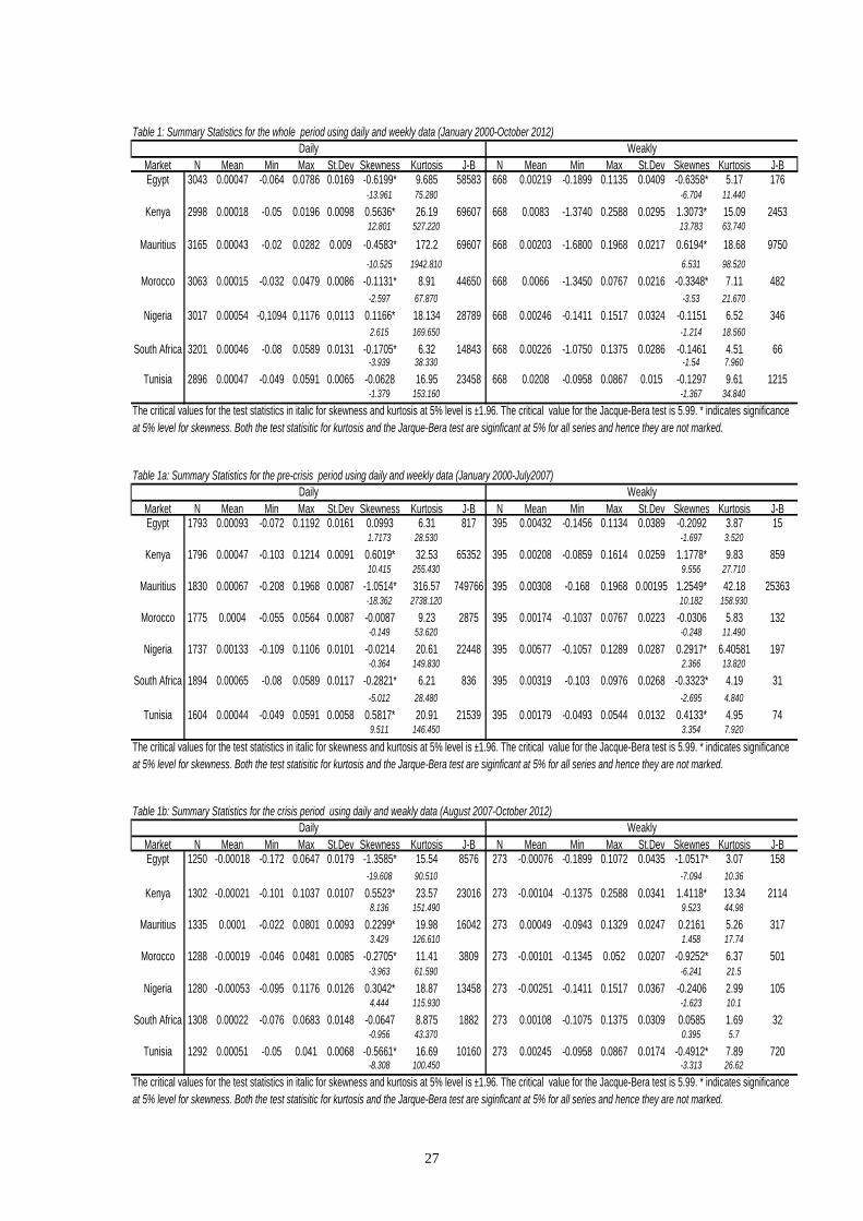
[INSERT TABLES 1, 1a AND 1b HERE]

The summary statistics of daily and weekly returns for the seven markets indices are

presented in Table 1, 1a and 1b. Specifically, information on the mean return, median,

standard deviation, maximum, minimum, skewness coefficient, kurtosis coefficient

and the Jacque-Bera test are presented. Table 1 for daily result shows that the lowest

mean returns are in Morocco (0.00015), and Kenya (0.00018) while the highest mean

returns are for Nigeria (0.00054). The lowest minimum and highest maximum returns

are in Nigeria: -0.1094 and 0,1176, respectively. The standard deviations of returns

range from 0.0065 (Tunisia) to 0.0169 (Egypt). On the contrary, for weekly data, the

lowest mean returns are in Mauritius (0.00203), and Egypt (0.00219) while the

highest mean returns are for Tunisia (0.0208). All return series are significantly

skewed, except those of Tunisia when considering daily data and Nigeria, South

Africa and Tunisia for weekly data. The results for skewness and kurtosis imply that

the distributional properties of all seven return series appear non-normal for daily and

weekly data. All markets except Kenya and Nigeria for daily data and Kenya and

Mauritius for weekly data are negatively skewed, indicating the greater probability of

large decreases in returns than rises, while for Kenya, Mauritius and Nigeria, this

means the greater likelihood of large increases in returns than falls. The kurtosis in all

market returns is also large, indicating leptokurtic distributions. Finally, the calculated

Jarque-Bera statistics and corresponding p-values in Table 1 are used to test the null

hypothesis that the daily and weekly distributions of African market returns are

15

normally distributed. All p-values are smaller than the 0.01 level of significance,

suggesting that the null hypothesis can be rejected in all periods and for all types of

data. None of these returns is then well approximated by the normal distribution.

In Table 1a and 1b, the summary statistics for daily and weekly market returns over

the two sub-periods are presented. During the pre-crisis period, all returns are positive

for all stock markets. On the contrary, during the crisis period, the mean return

becomes negative for Egypt, Kenya, Morocco and Nigeria for daily data; the same

results are obtained for weekly data. The crisis period is characterized by lower

average market return and higher volatility except for Tunisia, for which the mean

return has increased during the crisis period. Departure from normal distribution is

more consolidated, however. The level of kurtosis is high in the whole sample, but

with a tendency to decrease in the latter period. The Jarque-Bera statistic rejects the

hypothesis of a normal distribution of daily and weekly returns in all countries and

periods.

IV. EMPIRICAL RESULTS AND ANALYSIS

In this section, we present the empirical results of the tests presented above

and analysed in terms of theoretical and critical framework. A brief summary

of the results is included in order to have a comprehensive overview of our

results.

Serial correlation

The results for the test on serial correlation and Ljung Box Q-statistics are presented

in Tables 2 and 3 for daily and weekly returns.

[INSERT TABLE 2 HERE]

From results of Table 2, we can see that all stock markets exhibit strong positive

autocorrelation. The positive serial correlation coefficients are indicative of return

persistence (or predictability), with persistence being higher in Nigeria (0.1480) and

Kenya (0.1430) and lower in Mauritius (0.001) and South Africa (0.05). It is worth

noting that the positive sign of the autocorrelation coefficients indicates that

consecutive daily returns tend to have the same sign, so that positive (negative) return

in the current day tends to be followed by an increase (decrease) of return in the next

16

few days. The first order autocorrelations range from 0.266 for Kenya to 0.001 for

Mauritius. To emphasize our results, we extend the investigation to more than one lag

and consider k=30 (see Dickinson and Muruga 1994). The regressions strongly prove

that the daily return of day t is correlated with the return of day t-1. All Ljung Box Q-

statistic at lag k=30 are higher than the critical value at both 5% and 1% significance

levels. This indicates that the null hypothesis of no autocorrelation is rejected for all

indices. The significant non zero autocorrelation along with the significant Ljung Box

Q-statistic suggest rejection of the third hypothesis of random walk, viz. of the RW3.

[INSERT TABLES 3 HERE]

Results from the auto-correlation test on weekly returns over the whole sample period

are reported in Table 3.

The evidence of positive serial correlation at lag 1 of weekly returns is present for all

countries except South Africa, as most lag coefficients are not significantly different

from zero. The Ljung Box Q-statistics reject the null hypothesis of all coefficients

being jointly equal to zero up to lag 30 for all indices, except for Nigeria and Tunisia.

Auto-correlation of the daily and weekly changes in the seven stock indices is also

tested for the two sub-periods. Results are available upon request. During the pre-

crisis period, results of the Ljung Box Q-statistics indicate that Nigeria, South Africa

and Tunisia are not statistically different from zero. Therefore, time series for these

countries are consistent with the random walk theory. Regarding the Crisis period, the

same conclusion is found for Egypt, Kenya, Morocco, Nigeria and Tunisia.

Considering weekly returns, the time series of Nigeria, South Africa and Tunisia are

consistent with the random walk during the first sub-period; the same conclusion is

found for Egypt, Kenya, Morocco, Nigeria and Tunisia during the second sub-period.

However, since the autocorrelation test relies on the assumption of normally

distributed returns, these results must be interpreted with caution.

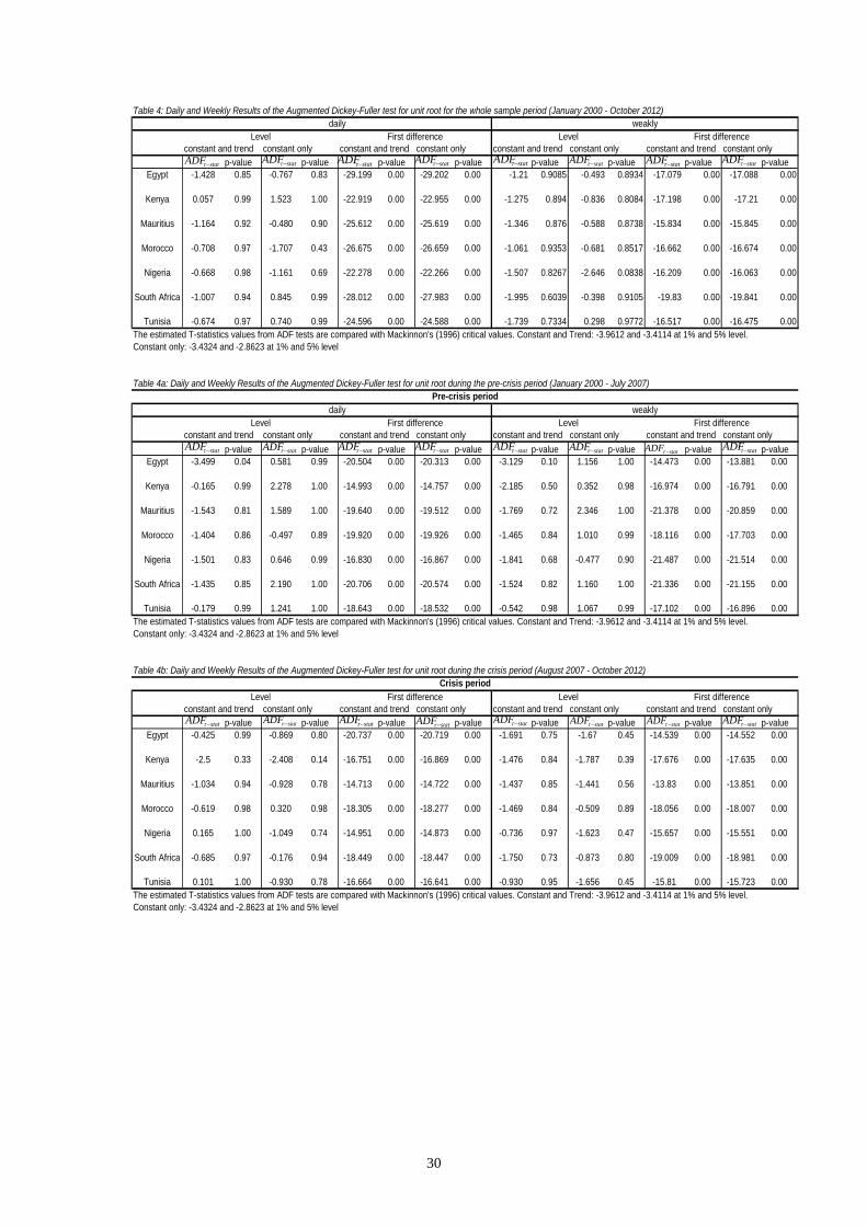
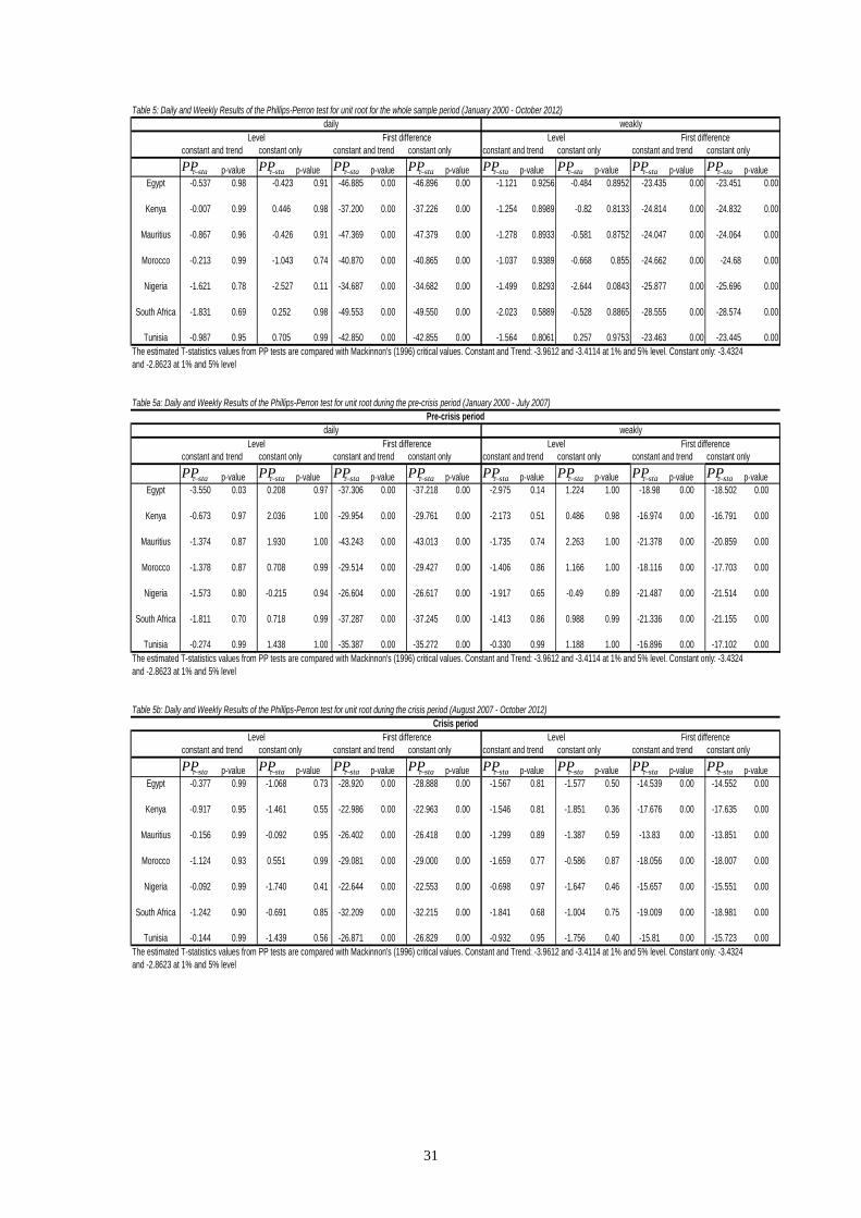
Unit Root tests

A unit root test tests time series for stationarity and finds out whether a time series is

non-stationary. The most common tests are the Augmented Dickey-Fuller (ADF) test,

the Phillips-Perron (PP) test and Kwiatkowski, Phillips, Schmidt and Shin (KPSS)

test. The null hypothesis is that the series have a unit root (the index series is non-

stationary), while the latter tests if it represents a stationary process (no unit root).

Another way to deal with stochastic trends (unit root) is by taking the first difference

17

of the variable. If the series is non-stationary and the first difference of the series is

stationary, the series contains a unit root or follows the random walk.

[INSERT TABLES 4 AND 5 HERE]

As can been seen from table 4 and 5, at level (log-price) the results of the ADF test

and PP test of null hypothesis are true for any type of returns (daily and weekly) and

for any stock markets under investigation but at the first difference, the null

hypothesis of unit root is strongly rejected as the t-statistic value of the ADF and PP

are greater than their critical values both at 5% and 1% level of significance which

means that all index series become stationary. So it can be said that all indices contain

a unit root, that is, non-stationary in their level forms, but stationary in their first

differenced forms.

[INSERT TABLES 4a, 4b, 5a and 5b HERE]

When considering the two sub-periods as they appear from tables 4a, 4b, 5a and 5b,

the ADF and PP t-statistics do not reject the null hypothesis of unit root for any type

of returns (daily and weekly) and any stock markets under investigation in the level

form. But inversely, for the first differences of all indices and for both test statistics,

the null hypothesis of a unit root is strongly rejected.

[INSERT TABLES 6, 6a and 6b HERE]

Concerning the KPSS test, the results reported in table 6, 6a and 6b are consistent

with those of the competing test. When analysing the full sample and the two sub-

periods, we notice that the LM statistics are significant both at the 5% and 1%

confidence level, thus rejecting the null hypothesis of stationarity for all indices at

levels, meaning that all price index series are nonstationary. Different results are

obtained for the first-difference of the price index series for South Africa, the first-

differenced series are proved to be stationary; for Morocco, the null hypothesis of

trend-stationarity is strongly rejected even though stationarity is accepted when the

trend is removed. The stationarity when the trend is removed from the equation is

also accepted for the remaining African stock markets with milder rejection. Nigeria

stock market proves to be trend-stationary: actually, the hypothesis of stationarity is

rejected when the trend is removed from the regression. Except for the Nigeria

market, the RWH necessary condition of unit root seems to hold for all price indices.

Furthermore, the first-differenced series are shown to be stationary for all indices

during the pre-crisis period, except for indices from Morocco, Mauritius and index

from Tunisia which proves to be stationary when trend are removed in its first-

18

differenced form. During the crisis period, the null hypothesis of stationarity is

accepted for the first-difference of all index price series. Results computed for weekly

data are in line with our findings; in addition, the statistic tests for first-difference

during the crisis period fall in the critical value band, this prerequisite condition is

consolidated further when the variance ratio test is computed.

Based on unit root tests, it may be concluded that all indices under investigation show

signs of random walk.

Runs Test

We show the empirical results from the run test over the entire period in the Tables 7,

7a and 7b.

[INSERT TABLES 7, 7a, 7b HERE]

It is important to stress that these results are back out from nonparametric test since it

does not assume any form for the returns. The tables display the number of

observations, the mean return, the number of actual and expected runs as well as the

Z-statistic. We notice that the number of runs is always less than the expected number

of runs, for daily and weekly data, and for all periods. This was stressed earlier by

several international studies (Borges 2011, Worthington and Higgs 2004, Abraham et

al. 2002). This produces a negative value for the Z-statistic. The negative value

indicates the presence of positive serial autocorrelation between returns, by far, as

shown by the results from auto-correlation test, the first-order autocorrelations are

positive and significantly different from zero for the whole sample period, in most

cases for the pre-crisis and crisis period as far as daily data are concerned. The null

hypothesis of the return series satisfying a random walk is rejected at 1% level for all

indices except for ZA where rejection occurred at 5%, in the full sample using daily

data. The results are in line with those found in the first sub-period. In the second sub-

period, the Z-statistic for South Africa stock exchange shows that the null hypothesis

of random walk cannot be rejected neither at 1% or 5% level of significance. The

number of runs is not statistically different from the expected number of runs, which

is consistent with a random walk hypothesis. When analysing weekly data the same

behaviour is remarked for the all sample except for ZA. In the first sub-period, the

hypothesis of randomness fails to be rejected for EG, NG and ZA. During the

turbulence period, at 1% significance level, the Z-statistic is not significant only for

19

MU whereas it is significant both at 1% and 5 % for MA, ZA and TU. By and large,

the significant Z-statistics of KE and MU using both daily and weekly data, indicates

some dependence in their returns series which jeopardizes market efficiency . The low

number of runs in the weekly returns also rejects the random walk hypothesis for KE,

MU, TU. But the latter is accepted only during the crisis period.

Parametric variance ratio test

Tables 8, 8a and 8b present the result of variance ratio test for the seven stock markets

analyzed. Following some preceding studies, we choose q=2,4,8,16 as in Ayadi and

Pyun (1994).


In the first step we test the random walk hypothesis for daily data in the full sample

which spans from January 2000 through October 2012. We expect to have the ratio of

(1/q) times the variance of the q-differences over the variance of the first-differences

being equal to unity. For each interval in the table we can read VR(q), and the test

statistics for the null hypotheses of homoskedastic, Z(q) and heteroskedastic, Z*(q)

increments random walk. Under the multiple variance ratio procedure, only the

maximum absolute values of the test statistics are examined: this is marked with

brackets in the tables. The maximum absolute value of the test statistic that exceeds

the critical value thereby indicates whether the null hypothesis of a random walk is

rejected. If we consider the result of Egypt, the Z statistic associated with the

maximum absolute value is higher than the critical values for daily equity returns

under homoskedasticity assumption, the variance ratios VR(q) are statistically

different from 1. Therefore, the results under homoskedasticity suggest that the

behaviour of Egypt stock market cannot be described as meeting the random walk

theory. The rejection of random walk from Z(q) under homoskedasticity could be due

to the presence of heteroskedasticity and/or serial correlation. Consistent

heteroskedasticity variance-ratio test Z*(q) is calculated to examine the problem.

The result for the maximum absolute value is superior to the 1% and 5% level of

significance viz. 2.49 and 3.02. The heteroskedastic random walk hypothesis is thus

rejected because of autocorrelation in the daily increments of returns on Egyptian

equity. We may conclude without ambiguity that Egypt stock market is weak-form

inefficient; these same results are found for Kenya, Morocco, Nigeria and Tunisia. In

addition, Lo and MacKinlay (1988) show that for q=2, estimates of the variance ratio

20

minus one and the first-order autocorrelation coefficient estimator of daily price

changes are asymptotically equal. For instance, considering the Egyptian stock

market, the variance ratio at q=2 minus one is roughly equal to the serial coefficient at

lag 1 in Table 2, implying that 18% of tomorrow’s return can be predicted by today’s

return. Further, where VR(2) <1 as in ZA a mean reverting process is indicated,

whereas when VR(2) >1 as in the remaining countries, persistence is suggested. This

indicates that there is positive autocorrelation (or persistence) in Egypt equity returns

over the long horizon. When analysing the South Africa market, at none of the

sampling intervals the test statistics for the null hypotheses of homoskedastic, Z(q)

and heteroskedastic, Z*(q) random walks are greater than the critical values of 2.49

and 3.02. This suggests that the South Africa equity market is weak form efficient.

More readily, in the case of Mauritius the null hypothesis of a homoskedastic random

walk is rejected [max abs(Z(q))=4.456], but the null hypothesis of heteroskedastic

random walk is not [max abs(Z*(q))=1.036]. Therefore, the Mauritius stock market

follows martingale difference sequence (MDS). This indicates that rejection of the

null hypothesis of a homoskedastic random walk could be the result, at least in part,

of heteroskedasticity in the returns, and cannot be assigned exclusively to the

autocorrelation in returns. To test the consistency of the results presented in Table 8,

we splitted the sample period into two subperiods and performed the variance ratio

test for each sub-sample. The first sub-period is from January 2000 through July 2007

whereas the second period runs from August 2007 through October 2012. The results

are presented in tables 8a and 8b. Under the homoskedastic assumption, the random

walk hypothesis is rejected for both periods except for ZA. One interesting thing

about the first sub-period is that all variance ratios are less than one for Mauritius

equity market unlike in the second period when they are all greater than unity. In

general, variance ratios are greater than one irrespectively from the sub-period under

consideration for all stock markets. Apart from this observation the results of the first

sub-period are consistent with those in the full sample. In the last sub-period, although

the ZA stock market is still weak form efficient, the remaining stock markets do not

satisfy either the random walk or the martingale difference sequence. In fact, we

evidence high autocorrelation for all market indexes: this suggests than during the

turbulence period the African stock markets became highly predictable.

In order to deal with the possible serial problem in daily data, the variance ratio was

computed using weekly data for the whole sample and the different sub-periods.

21

Results are displayed in the same tables with the daily results in order to be able to

make an immediate comparison between the VR tests on observations with different

frequencies. Unlike daily data, the variance ratios are in general not statistically

different from unity at the conventional 1% and 5% levels for weekly data. When

analysing the full sample, both Egypt and Nigeria stock markets are definitely weak

form inefficient, while Kenya, Mauritius, and Tunisia comply with MDS hypothesis.

Morocco and South Africa are weak form efficient. In the second sub-period, Kenya

and Tunisia lost their efficiency and became inefficient while the other stock markets

are shown to remain efficient. Finally in the last sub-period, apart from Mauritius, the

remaining stock markets are weak form efficient, and the Egypt stock market satisfies

only the MDS.

These results contrast with the findings inherent to daily data, using very low

frequency data some observations are neglected and this can convey distortions in

empirical results. Additionally, daily data reflect more precisely the true behaviour of

actual data with respect to the weekly counterpart.

Nonparametric variance ratio test

In order to shed some light on the ambiguity inherent in the results of the Lo and

MacKinlay (1988) variance-ratios test regarding the daily stock markets returns

behaviour in particular, we applied Wright’s (2000) version based on ranks and signs

to further examine the RW and the MDS hypothesis. Tables 9, 9a and 9b present the

results of Wright’s test for the entire sample. R1 and R2 report results of the rank

based test whereas S1 presents the results of the sign based alternative.


The R1 and R2 test statistics reject the RW for the all stock markets analysed except

for the ZA which evidences mixed results. The magnitude of rejections appears to be

comparatively stronger than those of the Lo and MacKinlay (1988) test at any value

of q for the whole financial price series investigated. When regarding S1 consistent

statistics test, the MDS hypothesis is excluded for the full sample for all reasonable

significance levels. Furthermore, the power of a test statistic of both ranks and signs

increases with the lag, evidence which is also in line with that of Wright (2000). In

addition, almost all rejections are in the upper tail of the null distribution, indicating

that the resulting variance ratios are statistically greater than one at all lags for all the

analysed series. The critical values for the Wright test are displayed in Table 10, they

22

differ by the sample size n and have been generated through simulation; for this study

we have used 1000 replications. Overall, the magnitude of rejections by the sign

based test seems weaker than the rank based alternative, which is in line with the

evidence of Wright (2000). To ascertain the impact of crisis over the period of

examination, the test statistics are computed for two sub-samples as in the Lo and

MacKinlay viz. from January 2000 to July 2007 and from August 2007 to October

2012. Tables 9a and 9b present the sub-sample results of Wright (2000). The evidence

from rank and sign shows that the conclusions based on the full sample are not

statistically significantly different from those of the first sub-sample periods for every

stock markets under consideration. None of the analysed stock markets comply with

RW and MDS hypothesis since their JR1, JR2, JS1 are greater than the critical values.

Turning to the last sub-period, the results are very tricky as we find out that, during

turbulence, all African stock markets were inefficient except ZA since for any lag of

q, both by the ranks and signs based test statistics, neither the RW nor the MDS

cannot be rejected at any reasonable significance level.

Examining now the results of weekly returns for the Egypt stock market in the entire

sample, at the conventional 0.01 and 0.05 significance levels, the random walk and

martingale hypothesis are rejected by both joint rank-based tests because

3.275 2.826 2.284 , 3.394 2.876 2.268

3.674>2.916(2.244). Similar results are obtained for weekly returns in Kenya,

Mauritius, Nigeria and Tunisia. Morocco stock market satisfies only the JR2

hypothesis of joint test, thus this rejection could be the result of various dependence

of higher degree of the moments or autocorrelation in weekly returns. The results for

South Africa are different. The ZA does follow an i.i.d random walk and martingale at

1% critical value but fails in doing so at 5%. For the first sub-period, only EG and ZA

are RDW and MDS, while NG, MA and TU present mixed results. However, MO,

KE, MU, are definitely inefficient stock markets. During the last period, the RDW is

unambiguously rejected for Kenya and Mauritius. It is nevertheless evident that over

time, some of the inefficiencies seem to have disappeared gradually. Using the

statistic JS1, the MDS hypothesis similarly cannot be excluded at any reasonable

significance level for Kenya, Nigeria and Morocco. Although Egypt and South Africa

stock markets remain efficient, some tendency of efficiency is noticeable in Morocco,

Nigeria and Tunisia.

23

V. CONCLUDING REMARKS

In this work, the re-examination of random walk and weak form efficiency of some

relevant African stock markets has been undertaken using both daily and weekly data.

The parametric serial correlation coefficient and the nonparametric runs test are used

to test for serial correlation; Augmented Dickey-Fuller, Phillips-Perron and

Kwiatkowski, Phillips, Schmidt and Shin unit root tests are used to test for non-

stationarity as a necessary condition for a random walk; and both parametric and non-

parametric multiple variance test statistics are used to test for random walk under the

varying distributional assumptions of homoskedasticity and heteroskedasticity.

Empirical robust non-parametric variance-ratios test suggested by Wright (2000) in

addition to the Lo and MacKinlay (1988) parametric alternative is applied to re-

investigate if the major African stock returns follow random walk (RW) or martingale

difference sequence (MDS). Empirical results found that computed returns are

characterized by non-normalities in the market’s returns series. On average, returns

are found to be characterised by large standard deviations, excess kurtosis, and are

either extremely skewed to the right or left, justifying the use of robust methodology.

The results for the tests of serial correlation are in broad agreement and conclusively

reject the presence of random walks in daily returns for all markets except South

Africa. The unit root tests fail to reject the RWH, indeed the unit root tests carried on

in this study accept RWH for all African stock market indices examined. However,

this is a necessary but not sufficient condition for a random walk. The lack of power

of the test urge to use the more sophisticated metrics for testing the RWH. Lo and

MacKinlay (1988) variance-ratios test are generally ambiguous. While it provides

conclusive evidence that the all African stock markets except South Africa and

Mauritius return series violates both the RW and the MDS hypotheses over the full

sample period as well as sub-sample periods when daily data are used, results

regarding weekly data are rather mixed. By contrast, the results of Wright’s (2000)

test are conclusive. Both the ranks and signs based test statistics consistently reject the

RW and the MDS hypotheses for daily data over the full sample and the first sub-

sample periods for the return series of the African stock markets analysed, at the 1%

and 5% significance level. However, the RW and the MDS hypotheses cannot be

rejected for ZA during the period of turbulence. When weekly data are used, the

24

results are in line with those of full sample, tendency to efficiency is noticed in the

last sub-period, showing that the crisis has little effect in the African markets. The

rejection of the weak form efficiency is not only consistent with previous evidence,

but also theoretically not surprising. The size of the some African stock market as

Kenya is comparatively small, and dominated by small capitalization stocks.

Associated high average transaction costs, for instance, result in limited market

activity and liquidity. Nevertheless, these are only persuasive rather than empirical

arguments. It is admitted that evidence from elsewhere (e.g., Appiah-Kusi and

Menyah, 2003), has demonstrated, for example, that size alone is neither necessary

nor sufficient for a market to be weak form efficient.

Since African stock markets are on ongoing improvement, the analysis of market

efficiency should be examined in the next coming years, because where the random

walk hypothesis is actually rejected, those markets evidence tendency to efficiency as

they could become more liquid and more institutionally sophisticated. To gain more

insight, a study focused on the individual prices may shed a light on the size and

liquidity: the reason being that, for individual stock markets, the liquidity, breadth,

depth, transactional and informational efficiency are known. It is therefore possible to

address the question of large capitalization and random walk.

25

REFERENCES

Abraham A., Seyyed F. and Alsakran S. (2002). Testing the Random Behavior and Efficiency of the Gulf Stock Markets, The Financial Review, 37, 3, 2002, pp. 469-480. Asal M. 2000. Are there trends towards efficiency? A case study of emerging markets: the Egyptian experience. Paper presented at the Financial Stabilization and Economic Growth conference, 26-27 October 2000, Svishtov, Bulgaria. Ayadi, O. F. and C. S. Pyum (1994). The application of the variance ratio test to the Korean securities market, Journal of Banking and Finance, 18, 643-658. Appiah-Kusi J. and Menyah K. (2003). Return predictability in African stock markets. Review of Financial Economics, 12, 247-270 Belaire-Franch, G. and Contreras, D., 2004. “Ranks and signs-based multiple variance ratio tests”, Working paper, University of Valencia. Beveridge, S. and C. R. Nelson, (1981). A New Approach to Decomposition of Economic Time Series into Permanent and Transitory Components with Particular Attention to Measurement of the Business Cycle. Journal of Monetary Economics, 7, 151-174. Borges, M.R. (2010). "Efficient market hypothesis in European stock markets," European Journal of Finance, Taylor and Francis Journals, vol. 16(7), 711-726 Campbell, J. Y., Lo, A. W., and MacKinlay, A. C. (1997). The Econometrics of Financial Markets. Second Edition. Princeton: Princeton University Press. Chang K.P. and Ting K. S. (2000). A Variance Ratio Test of the Random Walk Hypotheses for Taiwan's Stock Market, Applied Financial Economics, 10, 525-532. Chow, K. V., and Denning, K. C. (1993). A simple multiple variance ratio test. Journal of Econometrics, 58, 385-401 Fama E. (1965). The behaviour of stock market prices. Journal of Business, 38: 34-105. Fama, E. F. (1970). Efficient Capital Markets: A Review Of Theory And Empirical Work. Journal of Finance, 25(2), 383-417. Groenewold N. and Ariff M. (1998). The Effects of De-Regulation on Share-Market Efficiency in the Asia-Pacific, International Economic Journal, Vol.12, No.4,23-47. Huang B.N. (1995). Do Asian stock market prices follow random walks? Evidence from the variance ratio test, Applied Financial Economics, 5, 251-56. Jefferis K. and Smith G. (2005). The Changing Efficiency of African Stock Markets, South African Journal of Economics, 73, 54-67.

26

Kim M. J., Nelson, C. R. and Startz, R. (1991). Mean reversion in stock prices? A reappraisal of the empirical evidence, The Review of Economic Studies 58(3), 515–528. Kwiatkowski, D., Phillips, P. C. B., Schmidt, P., & Shin, Y. (1992). Testing the null hypothesis of stationarity against the alternative of a unit root. Journal of Econometrics, 54, 159-178. Lagoarde-Segot, T., and Lucey, B. M. (2008). Efficiency in emerging markets-Evidence from the MENA region. Journal of International Financial Markets, Institutions and Money, 18, 94-105. Lo, A. and MacKinlay A. C. (1988). Stock market prices do not follow random walks: evidence from a simple specification test, Review of Financial Studies, 1, 41-66. Magnusson M.A. and Wydick B. (2002). How efficient are Africa’s emerging stock markets? Journal of Development Studies, 38, 141-156. Mollah S. and Vitali F. (2011). Stock market efficiency in Africa: Evidence from Random Walk Hypothesis, paper submitted to the South Western Finance Conference, 2011, online at http://southwesternfinance.org/conf-2011/swfa2011_submission_82. Phillips, P. and Perron, P. (1988). “Testing for Unit Root in Time Series Regression”. Biometrika 75, 335-346. Ryoo H.J. and Smith G. (2002) Korean stock prices under price limits: variance ratio tests of random walks, Applied Financial Economics, 12(8), 543-51. Simons D. and Laryea S.A. (2005). Testing the Efficiency of Selected African Markets, Available online at SSRN: http://ssrn.com/abstract=874808 Smith G., Jefferis K. and Ryoo H.J. (2002). African stock markets: Multiple variance ratio tests of random walks. Applied Financial Economics Journal, 12, 475-484. Smith G. and Ryoo H.J. (2003). Variance ratio tests of the random walk hypothesis for European emerging stock markets. The European Journal of Finance, 9, 290-300. Smith G. (2008). Liquidity and the Informational Efficiency of African Stock Markets, South African Journal of Economics, 76(2), 161-175. Worthington A.C. and Higgs H. (2004). Random Walks and Market Efficiency in European Equity Markets, Global Journal of Finance and Economics, 1(1), 59-78. Wright, J. H. (2000). Alternative Variance-Ratio Tests Using Ranks and Signs. Journal of Business & Economic Statistics, 18 (1), 1-9.

27

Table 1: Summary Statistics for the whole period using daily and weekly data (January 2000-October 2012)

Market N Mean Min Max St.Dev Skewness Kurtosis J-B N Mean Min Max St.Dev Skewnes Kurtosis J-BEgypt 3043 0.00047 -0.064 0.0786 0.0169 -0.6199* 9.685 58583 668 0.00219 -0.1899 0.1135 0.0409 -0.6358* 5.17 176

-13.961 75.280 -6.704 11.440

Kenya 2998 0.00018 -0.05 0.0196 0.0098 0.5636* 26.19 69607 668 0.0083 -1.3740 0.2588 0.0295 1.3073* 15.09 245312.801 527.220 13.783 63.740

Mauritius 3165 0.00043 -0.02 0.0282 0.009 -0.4583* 172.2 69607 668 0.00203 -1.6800 0.1968 0.0217 0.6194* 18.68 9750

-10.525 1942.810 6.531 98.520

Morocco 3063 0.00015 -0.032 0.0479 0.0086 -0.1131* 8.91 44650 668 0.0066 -1.3450 0.0767 0.0216 -0.3348* 7.11 482-2.597 67.870 -3.53 21.670

Nigeria 3017 0.00054 -0,1094 0,1176 0,0113 0.1166* 18.134 28789 668 0.00246 -0.1411 0.1517 0.0324 -0.1151 6.52 3462.615 169.650 -1.214 18.560

South Africa 3201 0.00046 -0.08 0.0589 0.0131 -0.1705* 6.32 14843 668 0.00226 -1.0750 0.1375 0.0286 -0.1461 4.51 66-3.939 38.330 -1.54 7.960

Tunisia 2896 0.00047 -0.049 0.0591 0.0065 -0.0628 16.95 23458 668 0.0208 -0.0958 0.0867 0.015 -0.1297 9.61 1215-1.379 153.160 -1.367 34.840

The critical values for the test statistics in italic for skewness and kurtosis at 5% level is ±1.96. The critical value for the Jacque-Bera test is 5.99. * indicates significance at 5% level for skewness. Both the test statisitic for kurtosis and the Jarque-Bera test are siginficant at 5% for all series and hence they are not marked.

Table 1a: Summary Statistics for the pre-crisis period using daily and weekly data (January 2000-July2007)

Market N Mean Min Max St.Dev Skewness Kurtosis J-B N Mean Min Max St.Dev Skewnes Kurtosis J-BEgypt 1793 0.00093 -0.072 0.1192 0.0161 0.0993 6.31 817 395 0.00432 -0.1456 0.1134 0.0389 -0.2092 3.87 15

1.7173 28.530 -1.697 3.520

Kenya 1796 0.00047 -0.103 0.1214 0.0091 0.6019* 32.53 65352 395 0.00208 -0.0859 0.1614 0.0259 1.1778* 9.83 85910.415 255.430 9.556 27.710

Mauritius 1830 0.00067 -0.208 0.1968 0.0087 -1.0514* 316.57 749766 395 0.00308 -0.168 0.1968 0.00195 1.2549* 42.18 25363-18.362 2738.120 10.182 158.930

Morocco 1775 0.0004 -0.055 0.0564 0.0087 -0.0087 9.23 2875 395 0.00174 -0.1037 0.0767 0.0223 -0.0306 5.83 132-0.149 53.620 -0.248 11.490

Nigeria 1737 0.00133 -0.109 0.1106 0.0101 -0.0214 20.61 22448 395 0.00577 -0.1057 0.1289 0.0287 0.2917* 6.40581 197-0.364 149.830 2.366 13.820

South Africa 1894 0.00065 -0.08 0.0589 0.0117 -0.2821* 6.21 836 395 0.00319 -0.103 0.0976 0.0268 -0.3323* 4.19 31-5.012 28.480 -2.695 4.840

Tunisia 1604 0.00044 -0.049 0.0591 0.0058 0.5817* 20.91 21539 395 0.00179 -0.0493 0.0544 0.0132 0.4133* 4.95 749.511 146.450 3.354 7.920


Table 1b: Summary Statistics for the crisis period using daily and weakly data (August 2007-October 2012)

Market N Mean Min Max St.Dev Skewness Kurtosis J-B N Mean Min Max St.Dev Skewnes Kurtosis J-BEgypt 1250 -0.00018 -0.172 0.0647 0.0179 -1.3585* 15.54 8576 273 -0.00076 -0.1899 0.1072 0.0435 -1.0517* 3.07 158

-19.608 90.510 -7.094 10.36

Kenya 1302 -0.00021 -0.101 0.1037 0.0107 0.5523* 23.57 23016 273 -0.00104 -0.1375 0.2588 0.0341 1.4118* 13.34 21148.136 151.490 9.523 44.98

Mauritius 1335 0.0001 -0.022 0.0801 0.0093 0.2299* 19.98 16042 273 0.00049 -0.0943 0.1329 0.0247 0.2161 5.26 3173.429 126.610 1.458 17.74

Morocco 1288 -0.00019 -0.046 0.0481 0.0085 -0.2705* 11.41 3809 273 -0.00101 -0.1345 0.052 0.0207 -0.9252* 6.37 501-3.963 61.590 -6.241 21.5

Nigeria 1280 -0.00053 -0.095 0.1176 0.0126 0.3042* 18.87 13458 273 -0.00251 -0.1411 0.1517 0.0367 -0.2406 2.99 1054.444 115.930 -1.623 10.1

South Africa 1308 0.00022 -0.076 0.0683 0.0148 -0.0647 8.875 1882 273 0.00108 -0.1075 0.1375 0.0309 0.0585 1.69 32-0.956 43.370 0.395 5.7

Tunisia 1292 0.00051 -0.05 0.041 0.0068 -0.5661* 16.69 10160 273 0.00245 -0.0958 0.0867 0.0174 -0.4912* 7.89 720-8.308 100.450 -3.313 26.62


Daily Weakly

Daily Weakly

Daily Weakly

28

Table 2: Results of the auto-correlation test for the whole period using daily data (2000-2012)

Egypt Kenya Mauritus Morocco Nigeria South Africa

Tunisia

No 3043 2998 3165 3063 3017 3201 2896 1 2 3 4 5 6 7 8 9 10 11 12 13 14 15 16 17 18 19 20 21 22 23 24 25 26 27 28 29 30

0.180* 0.027 0.030 0.030 0.004 ‐0.019 ‐0.026 0.005 ‐0.009 0.048* 0.051* 0.031 0.030 ‐0.026 ‐0.016 0.014 0.039* ‐0.015 0.016 0.010 0.010 0.010 0.007 0.009 0.008 0.017 0.005 ‐0.004 0.022 0.032

0.266* 0.209* 0.103* 0.017 0.012 ‐0.028 ‐0.009 0.006 0.031 0.016 0.013 0.020 0.038* 0.029 0.030 0.032 0.002 0.001 ‐0.050* ‐0.030 ‐0.025 ‐0.011 0.000 ‐0.006 0.020 0.022 0.053* 0.061* 0.054* 0.058*

0.001 0.038* 0.001 0.056* 0.015 0.003 0.072* 0.060* ‐0.021 0.007 0.009 0.028 0.001 0.013 0.012 0.019 ‐0.021 ‐0.003 0.045* 0.006 ‐0.005 ‐0.007 0.018 0.024 0.002 0.024 0.016 0.030 0.049* 0.048*

0.252* 0.039* ‐0.004 0.000 ‐0.005 ‐0.022 0.020 0.012 ‐0.013 ‐0.007 0.033 0.014 0.005 0.034 0.001 ‐0.003 0.001 0.035 ‐0.025 ‐0.015 ‐0.024 ‐0.013 ‐0.003 0.017 0.025 0.015 ‐0.012 0.002 0.005 ‐0.000

0.348* 0.174* 0.020 ‐0.005 ‐0.040* ‐0.043* 0.005 0.039* 0.033 0.043* 0.043* 0.045* 0.032 0.016 0.001 0.010 0.031 ‐0.006 0.014 0.011 0.040* 0.031 0.028 0.027 0.040* 0.045* 0.056* 0.060* 0.022 ‐0.030

0.050* 0.000 ‐0.061* ‐0.026 ‐0.041* ‐0.022 0.024 0.007 0.002 ‐0.007 ‐0.040* ‐0.004 0.026 0.018 0.027 0.007 ‐0.031 ‐0.026 ‐0.023 0.025 ‐0.006 0.010 ‐0.027 ‐0.017 0.020 0.044* 0.012 0.008 0.005 ‐0.016

0.221* 0.064* 0.000 0.010 0.005 ‐0.003 ‐0.035 0.022 ‐0.001 0.030 0.056* 0.031 0.021 0.041* 0.011 0.020 0.025 0.020 ‐0.001 0.014 ‐0.005 ‐0.005 ‐0.012 ‐0.005 0.015 0.030 ‐0.012 0.008 0.022 ‐0.002

LB Q‐stat K=30

148.48‡ 471.03‡ 83.73‡ 224.82‡ 551.72‡ 66.17‡ 192.18‡

The confidence intervals at 5% level for the autocorrelation coefficients are: ±0.035 for n=3201, 3165, 3063 and ±0.036 for n=3043, 3017, 2998 and

2896. * indicates significance at 5% level. The Critical values for the Ljung‐Box Q‐statistic at lag k=30 are 43.77 and 50.89 at 5% and 1%, respectively.

‡ indicates rejec on at 1% ; ‡‡ indicates rejec on at 5% but acceptance at 1% level.

29

Table 3: Results of the auto-correlation test for the whole period using weekly data (2000-2012)

Egypt Kenya Mauritus Morocco Nigeria South Africa

Tunisia

No 668 668 668 668 668 668 668 1 2 3 4 5 6 7 8 9 10 11 12 13 14 15 16 17 18 19 20 21 22 23 24 25 26 27 28 29 30

0.094* 0.023 0.077* 0.015 0.044 ‐0.034 0.045 0.106* 0.083* 0.029 ‐0.072 0.070 0.080* 0.061 0.047 0.089* 0.027 0.016 0.004 0.017 0.019 0.046 0.027 ‐0.020 ‐0.011 0.055 ‐0.017 0.024 ‐0.004 0.037

0.037 0.037 0.078* ‐0.047 ‐0.005 0.157* 0.008 0.019 0.055 ‐0.041 0.032 0.084* 0.021 0.033 0.044 0.091* ‐0.030 0.059 0.027 0.025 0.058 0.025 ‐0.043 0.020 0.057 0.001 0.048 0.024 0.037 0.005

0.068 0.106* 0.005 ‐0.027 0.012 0.139* 0.039 0.015 0.034 0.004 0.076* 0.179* 0.043 0.014 0.015 0.083* 0.059 0.029 ‐0.028 0.022 0.017 ‐0.069 0.063 0.006 0.008 ‐0.060 ‐0.008 0.034 0.006 ‐0.027

0.041 0.064 0.007 ‐0.017 0.043 ‐0.018 ‐0.005 0.010 ‐0.000 0.111* 0.003 0.015 0.017 0.062 ‐0.007 ‐0.034 0.050 0.018 0.005 0.051 0.019 ‐0.019 0.012 ‐0.006 0.129* 0.021 0.062 0.002 ‐0.084* 0.057

0.003 0.123* 0.024 0.078* 0.046 0.040 0.032 0.052 0.050 ‐0.003 0.061 0.000 0.046 ‐0.009 0.015 0.043 0.022 ‐0.027 0.031 ‐0.005 ‐0.005 0.090* 0.033 0.014 0.030 0.047 ‐0.021 ‐0.019 ‐0.031 ‐0.015

‐0.101* ‐0.024 0.069 ‐0.078* 0.057 0.054 ‐0.099* 0.098* 0.032 ‐0.059 0.046 ‐0.083* 0.029 0.088* 0.000 ‐0.058 0.075 ‐0.043 ‐0.047 0.073 ‐0.040 0.020 ‐0.003 ‐0.037 0.059 ‐0.015 ‐0.050 0.016 ‐0.041 0.031

0.097* 0.078* 0.024 0.041 0.074 0.043 0.006 ‐0.016 ‐0.004 ‐0.012 0.035 0.083* 0.028 0.033 0.049 0.054 0.026 ‐0.033 0.015 0.044 0.019 0.016 0.010 ‐0.068 ‐0.049 ‐0.053 ‐0.006 0.045 ‐0.017 0.045

LB Q‐stat K=30

55.34‡ 55.46‡ 73.20‡ 44.72‡‡ 39.02 69.04‡ 41.33

The confidence intervals at 5% level for the autocorrelation coefficients are: ±0.076 for n=668. * indicates significance at 5% level. The Critical

values for the Ljung‐Box Q‐sta s c at lag k=30 are 43.77 and 50.89 at 5% and 1%, respec vely. ‡ indicates rejec on at 1% ; ‡‡ indicates rejec on at

5% but acceptance at 1% level.

30

Table 4: Daily and Weekly Results of the Augmented Dickey-Fuller test for unit root for the whole sample period (January 2000 - October 2012)

p-value p-value p-value p-value p-value p-value p-value p-valueEgypt -1.428 0.85 -0.767 0.83 -29.199 0.00 -29.202 0.00 -1.21 0.9085 -0.493 0.8934 -17.079 0.00 -17.088 0.00

Kenya 0.057 0.99 1.523 1.00 -22.919 0.00 -22.955 0.00 -1.275 0.894 -0.836 0.8084 -17.198 0.00 -17.21 0.00

Mauritius -1.164 0.92 -0.480 0.90 -25.612 0.00 -25.619 0.00 -1.346 0.876 -0.588 0.8738 -15.834 0.00 -15.845 0.00

Morocco -0.708 0.97 -1.707 0.43 -26.675 0.00 -26.659 0.00 -1.061 0.9353 -0.681 0.8517 -16.662 0.00 -16.674 0.00

Nigeria -0.668 0.98 -1.161 0.69 -22.278 0.00 -22.266 0.00 -1.507 0.8267 -2.646 0.0838 -16.209 0.00 -16.063 0.00

South Africa -1.007 0.94 0.845 0.99 -28.012 0.00 -27.983 0.00 -1.995 0.6039 -0.398 0.9105 -19.83 0.00 -19.841 0.00

Tunisia -0.674 0.97 0.740 0.99 -24.596 0.00 -24.588 0.00 -1.739 0.7334 0.298 0.9772 -16.517 0.00 -16.475 0.00The estimated T-statistics values from ADF tests are compared with Mackinnon's (1996) critical values. Constant and Trend: -3.9612 and -3.4114 at 1% and 5% level. Constant only: -3.4324 and -2.8623 at 1% and 5% level

Table 4a: Daily and Weekly Results of the Augmented Dickey-Fuller test for unit root during the pre-crisis period (January 2000 - July 2007)

p-value p-value p-value p-value p-value p-value p-value p-valueEgypt -3.499 0.04 0.581 0.99 -20.504 0.00 -20.313 0.00 -3.129 0.10 1.156 1.00 -14.473 0.00 -13.881 0.00

Kenya -0.165 0.99 2.278 1.00 -14.993 0.00 -14.757 0.00 -2.185 0.50 0.352 0.98 -16.974 0.00 -16.791 0.00

Mauritius -1.543 0.81 1.589 1.00 -19.640 0.00 -19.512 0.00 -1.769 0.72 2.346 1.00 -21.378 0.00 -20.859 0.00

Morocco -1.404 0.86 -0.497 0.89 -19.920 0.00 -19.926 0.00 -1.465 0.84 1.010 0.99 -18.116 0.00 -17.703 0.00

Nigeria -1.501 0.83 0.646 0.99 -16.830 0.00 -16.867 0.00 -1.841 0.68 -0.477 0.90 -21.487 0.00 -21.514 0.00

South Africa -1.435 0.85 2.190 1.00 -20.706 0.00 -20.574 0.00 -1.524 0.82 1.160 1.00 -21.336 0.00 -21.155 0.00

Tunisia -0.179 0.99 1.241 1.00 -18.643 0.00 -18.532 0.00 -0.542 0.98 1.067 0.99 -17.102 0.00 -16.896 0.00The estimated T-statistics values from ADF tests are compared with Mackinnon's (1996) critical values. Constant and Trend: -3.9612 and -3.4114 at 1% and 5% level. Constant only: -3.4324 and -2.8623 at 1% and 5% level

Table 4b: Daily and Weekly Results of the Augmented Dickey-Fuller test for unit root during the crisis period (August 2007 - October 2012)


Kenya -2.5 0.33 -2.408 0.14 -16.751 0.00 -16.869 0.00 -1.476 0.84 -1.787 0.39 -17.676 0.00 -17.635 0.00

Mauritius -1.034 0.94 -0.928 0.78 -14.713 0.00 -14.722 0.00 -1.437 0.85 -1.441 0.56 -13.83 0.00 -13.851 0.00

Morocco -0.619 0.98 0.320 0.98 -18.305 0.00 -18.277 0.00 -1.469 0.84 -0.509 0.89 -18.056 0.00 -18.007 0.00

Nigeria 0.165 1.00 -1.049 0.74 -14.951 0.00 -14.873 0.00 -0.736 0.97 -1.623 0.47 -15.657 0.00 -15.551 0.00

South Africa -0.685 0.97 -0.176 0.94 -18.449 0.00 -18.447 0.00 -1.750 0.73 -0.873 0.80 -19.009 0.00 -18.981 0.00

Tunisia 0.101 1.00 -0.930 0.78 -16.664 0.00 -16.641 0.00 -0.930 0.95 -1.656 0.45 -15.81 0.00 -15.723 0.00The estimated T-statistics values from ADF tests are compared with Mackinnon's (1996) critical values. Constant and Trend: -3.9612 and -3.4114 at 1% and 5% level. Constant only: -3.4324 and -2.8623 at 1% and 5% level

constant and trend constant only constant and trend constant onlyconstant and trend constant only constant and trend constant only

Crisis period

Level First difference Level First difference


Pre-crisis perioddaily weakly


Level First differencedaily weakly

Level First differenceconstant and trend constant onlyconstant and trend constant only constant and trend constant only constant and trend constant only

statADFstatADF statADF statADF statADFstatADF statADF statADF

statADFstatADF statADF statADF statADFstatADF statADF statADF

statADF statADF statADF statADF statADF statADF statADF statADF

31

Table 5: Daily and Weekly Results of the Phillips-Perron test for unit root for the whole sample period (January 2000 - October 2012)


Kenya -0.007 0.99 0.446 0.98 -37.200 0.00 -37.226 0.00 -1.254 0.8989 -0.82 0.8133 -24.814 0.00 -24.832 0.00

Mauritius -0.867 0.96 -0.426 0.91 -47.369 0.00 -47.379 0.00 -1.278 0.8933 -0.581 0.8752 -24.047 0.00 -24.064 0.00

Morocco -0.213 0.99 -1.043 0.74 -40.870 0.00 -40.865 0.00 -1.037 0.9389 -0.668 0.855 -24.662 0.00 -24.68 0.00

Nigeria -1.621 0.78 -2.527 0.11 -34.687 0.00 -34.682 0.00 -1.499 0.8293 -2.644 0.0843 -25.877 0.00 -25.696 0.00

South Africa -1.831 0.69 0.252 0.98 -49.553 0.00 -49.550 0.00 -2.023 0.5889 -0.528 0.8865 -28.555 0.00 -28.574 0.00

Tunisia -0.987 0.95 0.705 0.99 -42.850 0.00 -42.855 0.00 -1.564 0.8061 0.257 0.9753 -23.463 0.00 -23.445 0.00The estimated T-statistics values from PP tests are compared with Mackinnon's (1996) critical values. Constant and Trend: -3.9612 and -3.4114 at 1% and 5% level. Constant only: -3.4324and -2.8623 at 1% and 5% level

Table 5a: Daily and Weekly Results of the Phillips-Perron test for unit root during the pre-crisis period (January 2000 - July 2007)

p-value p-value p-value p-value p-value p-value p-value p-valueEgypt -3.550 0.03 0.208 0.97 -37.306 0.00 -37.218 0.00 -2.975 0.14 1.224 1.00 -18.98 0.00 -18.502 0.00

Kenya -0.673 0.97 2.036 1.00 -29.954 0.00 -29.761 0.00 -2.173 0.51 0.486 0.98 -16.974 0.00 -16.791 0.00

Mauritius -1.374 0.87 1.930 1.00 -43.243 0.00 -43.013 0.00 -1.735 0.74 2.263 1.00 -21.378 0.00 -20.859 0.00

Morocco -1.378 0.87 0.708 0.99 -29.514 0.00 -29.427 0.00 -1.406 0.86 1.166 1.00 -18.116 0.00 -17.703 0.00

Nigeria -1.573 0.80 -0.215 0.94 -26.604 0.00 -26.617 0.00 -1.917 0.65 -0.49 0.89 -21.487 0.00 -21.514 0.00

South Africa -1.811 0.70 0.718 0.99 -37.287 0.00 -37.245 0.00 -1.413 0.86 0.988 0.99 -21.336 0.00 -21.155 0.00

Tunisia -0.274 0.99 1.438 1.00 -35.387 0.00 -35.272 0.00 -0.330 0.99 1.188 1.00 -16.896 0.00 -17.102 0.00The estimated T-statistics values from PP tests are compared with Mackinnon's (1996) critical values. Constant and Trend: -3.9612 and -3.4114 at 1% and 5% level. Constant only: -3.4324and -2.8623 at 1% and 5% level

Table 5b: Daily and Weekly Results of the Phillips-Perron test for unit root during the crisis period (August 2007 - October 2012)


Kenya -0.917 0.95 -1.461 0.55 -22.986 0.00 -22.963 0.00 -1.546 0.81 -1.851 0.36 -17.676 0.00 -17.635 0.00

Mauritius -0.156 0.99 -0.092 0.95 -26.402 0.00 -26.418 0.00 -1.299 0.89 -1.387 0.59 -13.83 0.00 -13.851 0.00

Morocco -1.124 0.93 0.551 0.99 -29.081 0.00 -29.000 0.00 -1.659 0.77 -0.586 0.87 -18.056 0.00 -18.007 0.00

Nigeria -0.092 0.99 -1.740 0.41 -22.644 0.00 -22.553 0.00 -0.698 0.97 -1.647 0.46 -15.657 0.00 -15.551 0.00

South Africa -1.242 0.90 -0.691 0.85 -32.209 0.00 -32.215 0.00 -1.841 0.68 -1.004 0.75 -19.009 0.00 -18.981 0.00

Tunisia -0.144 0.99 -1.439 0.56 -26.871 0.00 -26.829 0.00 -0.932 0.95 -1.756 0.40 -15.81 0.00 -15.723 0.00The estimated T-statistics values from PP tests are compared with Mackinnon's (1996) critical values. Constant and Trend: -3.9612 and -3.4114 at 1% and 5% level. Constant only: -3.4324and -2.8623 at 1% and 5% level


Crisis periodLevel First difference Level First difference


Pre-crisis perioddaily weakly


daily weaklyLevel First difference

constant and trend constant onlyLevel First difference

constant and trend constant only constant and trend constant only constant and trend constant only

statPP statPP statPP statPP statPP statPP statPP statPP

staPP staPP staPP staPP staPP staPP staPP staPP

staPP staPP staPP staPP staPP staPP staPP staPP

32

Table 6: Daily and Weekly Results of the KPSS test for unit root during the whole sample period (January 2000 - October 2012)

C/T C C/T C C/T C C/T C

LM-stat LM-stat LM-stat LM-stat LM-stat LM-stat LM-stat LM-statEgypt 1.740 8.280 0,321** 0.323 1.313 6.325 0,229* 0.223

Kenya 1.438 6.325 0,197* 0.193 0.462 2.059 0,137** 0.134

Mauritius 1.009 10.393 0,209* 0.220 0.306 3.249 0,131** 0.135

Morocco 1.190 8.809 0,330** 0.333 0.379 2.841 0,283* 0,286**

Nigeria 2.091 5.864 0.091 0,542* 0.306 3.241 0.064 0,388**

South Africa 0.972 10.324 0.083 0.082 0.311 3.186 0.076 0.075

Tunisia 1.287 10.037 0,192* 0.219 0.559 3.220 0,149** 0.216The critical value for KPSS test: C/T (Constant and Trend) are 0.216 and 0.146 at 1% and 5% level, C (Constant only) are 0.739 and 0.463 at 1% and 5% level. * indicate rejection at 1% level and ** indicate rejection at 5% level.

Table 6a: Daily and Weekly Results of the KPSS test for unit root during the pre-crisis period (January 2000 - July 2007)

C/T C C/T C C/T C C/T CLM-stat LM-stat LM-stat LM-stat LM-stat LM-stat LM-stat LM-stat

Egypt 1.313 6.325 0,287* 0,873* 0,475* 2,029* 0,287* 0,873*

Kenya 1.234 5.486 0,150* 0,432** 0,395* 1,841* 0,150** 0.432

Mauritius 1.316 6.644 0.080 0,846* 0,439* 2,188* 0.080 0,846*

Morocco 1.581 4.404 0.046 0,804* 0,530* 1,501* 0.046 0,804*

Nigeria 0.330 6.606 0.094 0.094 0,162** 2,288* 0.094 0.094

South Africa 1.493 6.139 0,371** 0.046 0,509* 2,034* 0.046 0.371

Tunisia 1.544 4.214 0.115 0,469** 0,393* 1,450* 0.115 0.469The critical value for KPSS test: C/T (Constant and Trend) are 0.216 and 0.146 at 1% and 5% level, C (Constant only) are 0.739 and 0.463 at 1% and 5% level. * indicate rejection at 1% level and ** indicate rejection at 5% level.

Table 6b: Daily and Weekly Results of the KPSS test for unit root during the the crisis period (August 2007 - October 2012)

C/T C C/T C C/T C C/T CLM-stat LM-stat LM-stat LM-stat LM-stat LM-stat LM-stat LM-stat

Egypt 0.321 1.853 0.074 0.093 0.113 0,652** 0.057 0.074

Kenya 1.234 5.486 0.099 0.221 0.194 0.371 0.083 0.176

Mauritius 0.487 1.598 0.113 0.118 0.159 0,496* 0.079 0.082

Morocco 0.414 2.057 0.094 0.181 0.144 0,684** 0.089 0.177

Nigeria 0.865 3.648 0.090 0.310 0,291* 1,175* 0.066 0.218

South Africa 0.723 2.640 0.057 0.148 0,242* 0,849* 0.060 0.156

Tunisia 0.940 4.776 0.080 0.286 0,307* 1,.518* 0.069 0.159The critical value for KPSS test: C/T (Constant and Trend) are 0.216 and 0.146 at 1% and 5% level, C (Constant only) are 0.739 and 0.463 at 1% and 5% level. * indicate rejection at 1% level and ** indicate rejection at 5% level.

daily weakly



First difference

daily weakly

weaklyLevel First difference

dailyLevel

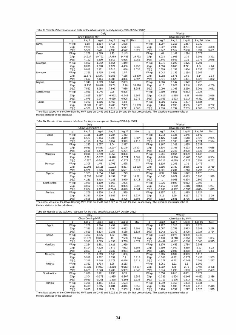
34

Table 8: Results of the variance ratio tests for the whole sample period (January 2000-October 2012)

q Lag 2 Lag 4 Lag 8 Lag 16 Max q Lag 2 Lag 4 Lag 8 Lag 16 MaxEgypt VR(q) 1.18 1.314 1.416 1.528 VR(q) 1.097 1.213 1.367 1.739

Z(q) 9.935 9.253 7.75 6.617 9.935 Z(q) 2.507 2.938 3.201 4.338 4.338Z*(q) 5.529 5.49 4.995 4.572 5.529 Z*(q) 2.247 2.512 2.668 3.631 3.631

Kenya VR(q) 1.268 1.665 1.93 2.143 VR(q) 1.04 1.142 1.274 1.578Z(q) 14.927 19.792 17.489 14.453 19.792 Z(q) 1.033 1.966 2.39 3.391 3.391Z*(q) 4.122 6.409 6.917 6.956 6.956 Z*(q) 0.446 0.945 1.31 2.078 2.078

Mauritius VR(q) 1.002 1.042 1.154 1.349 VR(q) 1.071 1.222 1.375 1.791Z(q) 0.098 1.278 2.924 4.456 4.456 Z(q) 1.836 3.065 3.271 4.64 4.64Z*(q) 0.011 0.171 0.516 1.036 1.036 Z*(q) 0.609 1.159 1.434 2.337 2.337

Morocco VR(q) 1.251 1.415 1.489 1.57 VR(q) 1.042 1.136 1.194 1.365Z(q) 13.879 12.277 9.153 7.155 13.879 Z(q) 1.092 1.871 1.69 2.14 2.14Z*(q) 7.597 7.164 5.783 4.825 7.597 Z*(q) 0.871 1.528 1.421 1.822 1.822

Nigeria VR(q) 1.348 1.709 1.848 2.063 VR(q) 1.006 1.147 1.372 1.725Z(q) 19.136 20.818 15.74 13.26 20.818 Z(q) 0.15 2.023 3.248 4.256 4.256Z*(q) 7.562 8.988 7.892 7.635 8.988 Z*(q) 0.096 1.365 2.266 3.061 3.061

South Africa VR(q) 1.051 1.046 0.95 0.895 VR(q) 0.899 0.861 0.853 0.924

Z(q) 2.865 1.397 -0.952 -1.345 2.865 Z(q) -2.616 -1.915 -1.28 -0.449 2.616Z*(q) 1.976 0.943 -0.639 0.905 1.976 Z*(q) -2.035 -1.503 -1.017 -0.362 2.035

Tunisia VR(q) 1.222 1.396 1.462 1.58 VR(q) 1.096 1.217 1.407 1.634Z(q) 11.939 11.381 8.403 7.089 11.939 Z(q) 2.484 2.998 3.555 3.722 3.722Z*(q) 4.528 4.666 3.918 3.721 4.666 Z*(q) 1.376 1.792 2.205 2.503 2.503

The critical values for the Chow-Denning MVR tests are 2.491 and 3.022 at 5% and 1% level, respectively. The absolute maximum value of the test statistics in the cells Max

Table 8a: Results of the variance ratio tests for the pre-crisis period (January2000-July 2007)

q Lag 2 Lag 4 Lag 8 Lag 16 Max q Lag 2 Lag 4 Lag 8 Lag 16 MaxEgypt VR(q) 1.156 1.269 1.384 1.463 VR(q) 1.072 1.126 1.245 1.649

Z(q) 6.587 6.104 5.496 4.449 6.587 Z(q) 1.425 1.344 1.648 2.925 2.925Z*(q) 4.118 4.014 3.857 3.349 4.118 Z*(q) 1.272 1.188 1.417 2.524 2.524

Kenya VR(q) 1.235 1.657 2.04 2.377 VR(q) 1.167 1.349 1.625 2.039Z(q) 9.951 14.867 14.907 13.254 14.907 Z(q) 3.304 3.706 4.193 4.685 4.685Z*(q) 2.518 4.479 5.64 6.294 6.294 Z*(q) 1.913 2.343 2.998 3.635 3.635

Mauritius VR(q) 0.816 0.749 0.759 0.838 VR(q) 0.951 0.964 0.939 1.147Z(q) -7.861 -5.725 -3.478 -1.574 7.861 Z(q) -0.964 -0.386 -0.406 0.665 0.964Z*(q) -0.627 -0.568 -0.461 -0.279 0.627 Z*(q) -0.213 -0.099 -0.126 0.251 0.251

Morocco VR(q) 1.306 1.54 1.703 1.875 VR(q) 1.116 1.263 1.31 1.475Z(q) 12.908 12.155 10.012 8.377 12.908 Z(q) 2.295 2.789 2.085 2.142 2.789Z*(q) 6.971 6.926 6.202 5.551 6.971 Z*(q) 1.801 2.234 1.713 1.797 2.234

Nigeria VR(q) 1.325 1.654 1.649 1.773 VR(q) 0.92 1.007 1.072 1.176Z(q) 13.555 14.581 9.151 7.321 14.581 Z(q) -1.585 0.079 0.483 0.795 1.585Z*(q) 4.231 5.418 4.183 3.979 5.418 Z*(q) -1 0.055 0.374 0.669 1

South Africa VR(q) 1.069 1.119 1.069 1.006 VR(q) 0.936 0.898 0.912 0.992Z(q) 3.002 2.784 1.019 0.065 3.002 Z(q) -1.257 -1.082 -0.589 -0.036 1.257Z*(q) 2.064 1.937 0.7348 0.049 2.064 Z*(q) -1.093 -0.962 -0.536 -0.034 1.093



Table 8b: Results of the variance ratio tests for the crisis period (August 2007-October 2012)

q Lag 2 Lag 4 Lag 8 Lag 16 Max q Lag 2 Lag 4 Lag 8 Lag 16 Max

Egypt VR(q) 1.209 1.364 1.451 1.599 VR(q) 1.127 1.313 1.523 1.878Z(q) 7.391 6.892 5.386 4.812 7.391 Z(q) 2.097 2.759 2.913 3.288 3.288Z*(q) 3.819 3.824 3.281 3.138 3.824 Z*(q) 1.942 2.342 2.405 2.724 2.724

Kenya VR(q) 1.302 1.676 1.82 1.916 VR(q) 0.934 0.975 0.989 1.243Z(q) 10.878 13.024 10 7.508 13.024 Z(q) -1.084 -0.218 -0.059 0.909 1.084Z*(q) 3.313 4.579 4.193 3.739 4.579 Z*(q) -0.449 -0.102 -0.031 0.545 0.545

Mauritius VR(q) 1.224 1.391 1.621 1.959 VR(q) 1.176 1.456 1.784 2.393Z(q) 8.194 7.628 7.672 7.962 8.194 Z(q) 2.899 4.042 4.369 5.22 5.22Z*(q) 2.857 2.9 3.347 3.984 3.984 Z*(q) 2.105 2.985 3.258 3.84 3.84

Morocco VR(q) 1.165 1.219 1.148 1.086 VR(q) 0.905 0.902 0.949 1.117Z(q) 5.918 4.202 1.791 0.7 5.918 Z(q) -1.563 -0.861 -0.279 0.438 1.563Z*(q) 3.311 2.548 1.171 0.486 3.311 Z*(q) -1.277 -0.731 -0.248 0.391 1.277

Nigeria VR(q) 1.362 1.733 1.96 2.183 VR(q) 1.061 1.21 1.5 1.909Z(q) 12.939 14.007 11.608 9.613 14.007 Z(q) 1.002 1.86 2.79 3.408 3.408Z*(q) 6.629 7.043 6.439 5.959 7.043 Z*(q) 0.674 1.296 1.963 2.429 2.429

South Africa VR(q) 1.036 0.981 0.838 0.78 VR(q) 0.858 0.818 0.801 0.879Z(q) 1.304 -0.378 -1.985 -1.807 1.985 Z(q) -2.336 -1.604 -1.109 -0.452 2.336Z*(q) 0.939 -0.261 -1.338 -1.194 1.338 Z*(q) -1.713 -1.176 -0.817 -0.337 1.713



Daily WeeklyChow-Denning MVR Chow-Denning MVR

WeeklyChow-Denning MVR

Daily

Chow-Denning MVR Chow-Denning MVR

Chow-Denning MVR

Daily Weekly

Rapporto n. 238 - Home page | BOA Bicocca Open …...Kiweu (1991) and Dickinson and Muragu (1994)...

Documents

Transcript of Rapporto n. 238 - Home page | BOA Bicocca Open …...Kiweu (1991) and Dickinson and Muragu (1994)...