Quantum Fluid Models for Electron Transport in Graphenenzamponi/Tesi_Dottorato_Zamponi.pdf ·...
112
UNIVERSIT ` A DEGLI STUDI DI FIRENZE Facolt`a di Scienze Matematiche, Fisiche e Naturali Dipartimento di Matematica e Informatica “Ulisse Dini” Dottorato di Ricerca in Matematica Tesi di Dottorato Quantum Fluid Models for Electron Transport in Graphene Candidato: Nicola Zamponi Tutor: Dott. Luigi Barletti Coordinatore del Dottorato: Prof. Alberto Gandolfi CICLO XXV, S.S.D. MAT/07 FISICA MATEMATICA
Transcript of Quantum Fluid Models for Electron Transport in Graphenenzamponi/Tesi_Dottorato_Zamponi.pdf ·...

UNIVERSITA DEGLI STUDI DI FIRENZE
Facolta di Scienze Matematiche, Fisiche e Naturali
Dipartimento di Matematica e Informatica “Ulisse Dini”
Dottorato di Ricerca in Matematica
Tesi di Dottorato
Quantum Fluid Models
for Electron Transport
in Graphene
Candidato:
Nicola Zamponi
Tutor:
Dott. Luigi BarlettiCoordinatore del Dottorato:
Prof. Alberto Gandolfi
CICLO XXV, S.S.D. MAT/07 FISICA MATEMATICA

Contents
I Derivation of the models 9
1 Kinetic models 10
1.1 The Von Neumann and Wigner equations . . . . . . . . . . . . . 10
1.1.1 Statistical quantum mechanics and density operators . . . 10
1.1.2 Wigner formalism for quantum mechanics . . . . . . . . . 11
1.1.3 The spinorial case . . . . . . . . . . . . . . . . . . . . . . 13
1.2 Quantum transport in graphene . . . . . . . . . . . . . . . . . . . 14
1.2.1 Non statistical closure: the pure state case . . . . . . . . 15
1.2.2 Collisional Wigner equations . . . . . . . . . . . . . . . . 18
2 Equilibrium distribution 20
2.1 The minimum entropy principle . . . . . . . . . . . . . . . . . . . 20
2.2 Semiclassical expansion of quantum exponential . . . . . . . . . . 22
2.3 The weakly spinorial case . . . . . . . . . . . . . . . . . . . . . . 26
3 Two-Band Models 27
3.1 A first-order two-band hydrodynamic model . . . . . . . . . . . . 28
3.1.1 Formal closure of the fluid equations . . . . . . . . . . . . 29
3.1.2 Semiclassical computation of the moments . . . . . . . . . 30
3.2 A first order two-band diffusive model . . . . . . . . . . . . . . . 36
3.2.1 Formal closure of the diffusive equations . . . . . . . . . . 36
3.2.2 Semiclassical expansion of the equilibrium distribution . . 40
3.2.3 Computation of the moments . . . . . . . . . . . . . . . . 42
3.3 A second order two-band diffusive model . . . . . . . . . . . . . . 47
3.3.1 Semiclassical expansion of the equilibrium distribution . . 47
3.3.2 Computation of the moments . . . . . . . . . . . . . . . . 49
4 Spinorial models 55
4.1 A first order spinorial hydrodynamic model . . . . . . . . . . . . 55
4.1.1 Formal closure of fluid equations . . . . . . . . . . . . . . 55
4.1.2 Semiclassical expansion of the equilibrium distribution . . 56
4.1.3 Computation of the moments . . . . . . . . . . . . . . . . 60
4.2 A second order spinorial hydrodynamic model . . . . . . . . . . . 61
4.2.1 Semiclassical expansion of the equilibrium distribution . . 61
4.2.2 Computation of the moments . . . . . . . . . . . . . . . . 64
2

CONTENTS 3
4.3 A first order spinorial diffusive model . . . . . . . . . . . . . . . . 66
4.3.1 Derivation of the model . . . . . . . . . . . . . . . . . . . 66
4.3.2 Semiclassical expansion of the equilibrium distribution . . 67
4.3.3 Computation of the moments . . . . . . . . . . . . . . . . 69
4.4 A first order spinorial diffusive model with pseudomagnetic field 72
4.4.1 Derivation of the model . . . . . . . . . . . . . . . . . . . 72
II Analytical results and numerical simulations 75
5 Analytical results 76
5.1 Introduction . . . . . . . . . . . . . . . . . . . . . . . . . . . . . . 76
5.2 Existence of solutions for first problem . . . . . . . . . . . . . . . 79
5.3 Existence of solution for second problem . . . . . . . . . . . . . . 82
5.4 Entropicity of the system . . . . . . . . . . . . . . . . . . . . . . 94
5.5 Long-time decay of the solutions . . . . . . . . . . . . . . . . . . 97
6 Numerical simulations 103
6.1 Introduction . . . . . . . . . . . . . . . . . . . . . . . . . . . . . . 103
6.2 Numerical results for the models QSDE1, QSDE2. . . . . . . . . 104

Introduction
Graphene is a single layer of carbon atoms disposed as an honeycomb lattice,
that is, a single sheet of graphite [23] (see fig. 1). This new semiconductor
material has attracted the attention of many physicists and engineers thanks
to its remarkable electronic properties, which make it an ideal candidate for
the construction of new electronic devices (see fig. 2) with strongly increased
performances with respect to the usual silicon semiconductors [3, 9, 21, 32].
Potential applications include, for instance, spin field-effect transistors [27, 51],
extremely sensitive gas sensors [46], one-electron graphene transistors [41], and
graphene spin transistors [14]. The great interest around graphene is attested
by the Nobel prize attributed in 2010 to Geim and Novoselov for its discovery.
Figure 1: Graphene honeycomb cristal lattice.
Physically speaking, graphene is a zero-gap semiconductor: in the energy
spectrum (shown in fig. 3) the valence band intersects the conduction band in
some isolated points, named Dirac points; moreover, around such points the
electron energy is approximately proportional to the modulus of pseudomomen-
tum (or “cristal momentum”):
E = ±vF |p| = ±vF~ |k| , (1)
where p = (p1, p2) is the cristal momentum, k = (k1, k2) is the Fermi wavevector,
4

CONTENTS 5
vF ≈ 106 m/s is the zero-temperature Fermi velocity [38] and, as usual, ~ denotes
the reduced Planck constant.
The dispersion relation (1) means that the electrons in graphene behave
as massless relativistic particles [49], which means, like photons, with an “ef-
fective light speed” equal to vF . This remarkable feature allows to test on
graphene some of the predictions of relativistic quantum mechanics with ex-
periments involving non-relativistic velocities; in particular, much attention has
been devoted to the so-called Klein paradox, that is, unimpeded penetration of
relativistic particles through high potential barriers (see e.g. [32] for details).
Another interesting consequence of the Dirac-like dispersion relation (1) is that
for positive energies the charge carriers are negatively charged and behave like
electrons, while at negative energies, if the valence band is not full, its unoccu-
pied electronic states behave as “holes”, that is, as positively charged quasipar-
ticles [32], which, in condensed matter physics, plays often the role of positrons
[2]. However in condensed matter physics the electron and hole states are re-
ciprocally independent, while in graphene they are interconnected, thanks to
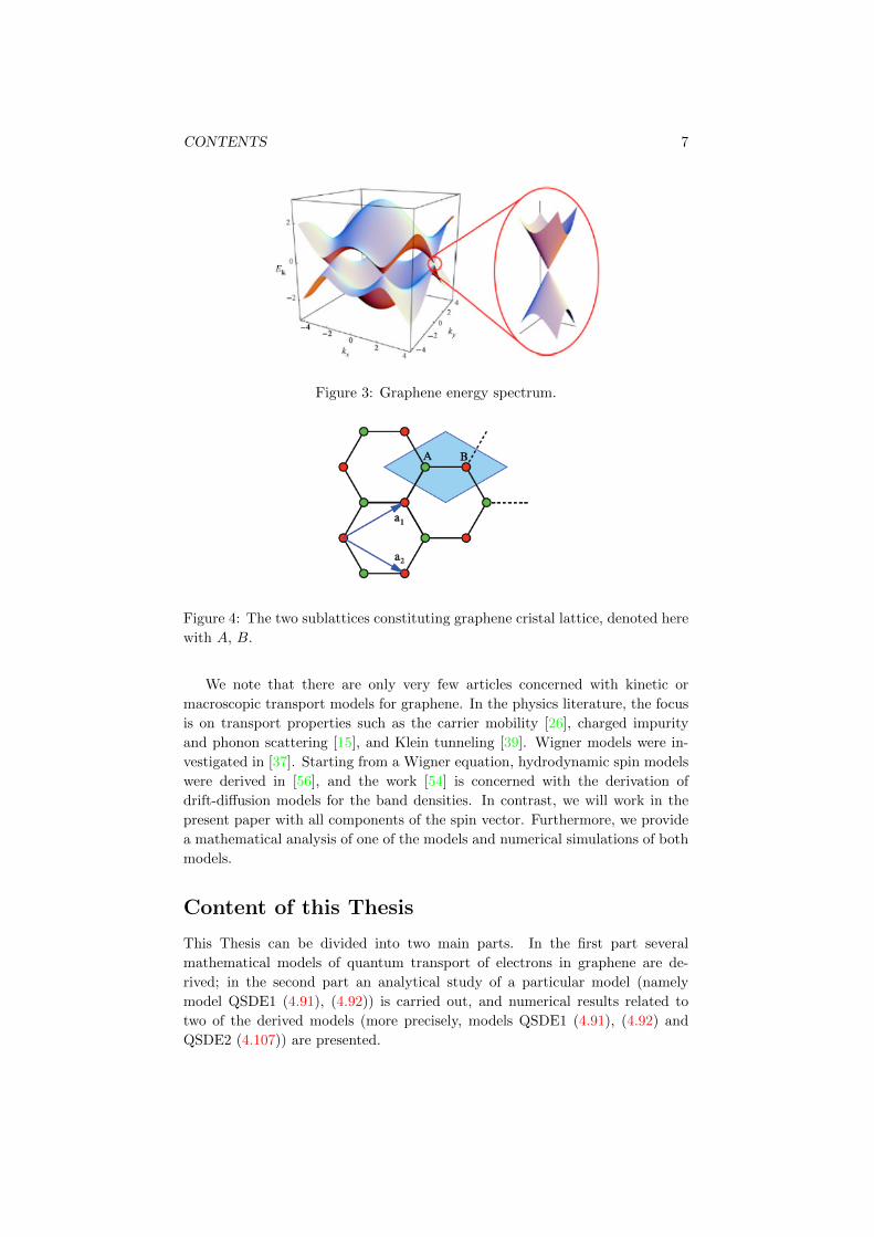
the particular structure of graphene cristal lattice, made up by two equivalent
triangular sublattices (see fig. 4). This fact is actually at the origin of the linear
(with respect to |p|) dispersion relation (1): the quantum-mechanical interac-
tions between the two sublattices lead to the formation of two energy bands with
sinusoidal shape, intersecting each other at the Dirac points and so yielding the
locally conical energy spectrum. As a consequence, the charge carriers have an
additional discrete degree of freedom, called “pseudospin”, different from the
real electron spin, indicating the contribution of each sublattice to the quasi-
particles composition: for this reason graphene quasiparticles must be described
by spinors, that is, two-component wavefunctions [32].
Recently, mathematical models of fluid-dynamic type has been developed
in order to describe quantum transport in semiconductors [7, 8, 16, 17, 18, 28,
29, 31, 56]. Such models rely on a kinetic formulation of quantum mechanics
(QM) by means of Wigner-type equations, and are derived by taking suitable
moments of these latter; the resulting equations involve the chosen fluid-dynamic
moments and usually additional expressions (referred to as not closed terms)
which cannot be written as functions of the previous moments without further
hypothesis. In order to solve the so-called closure problem, that is, to compute
the not closed terms from the known moments, many techniques are employed,
e.g. the pure-state hypothesis (which allows to obtain, for a scalar Hamiltonian
of type H = − ~2
2m∆ + V (x), the so-called Madelung equations [34]; see also [11]
for fluid-dynamic equations derived from a spinorial Hamiltonian of the form
H = −i~c ~σ · ~∇), the ad-hoc ansatz (like the Gardner’s equilibrium distribution,
see [29]), and a strategy of entropy minimization1 (which will be followed in
this paper, in analogy to the method employed in the closure of classical fluid-
dynamic systems derived from the Boltzmann transport equation in the classical
statistical mechanics, see [16, 17, 18, 33]).
In order to understand and describe the charge carrier transport in graphene,
1We adopt the reverse sign convention for entropy.

CONTENTS 6
Figure 2: Schematics of a graphene-based device.
transport models, which incorporate the pseudospin degree of freedom, have to
be devised. Theoretical models for spin-polarized transport involve fluid-type
drift-diffusion equations, kinetic transport equations, and Monte-Carlo simula-
tion schemes; see the references in [40]. A hierarchy of fluiddynamic spin models
was derived from a spinor Boltzmann transport equation in [10]. Suitable matrix
collision operators were suggested and analyzed in [42]. Drift-diffusion models
for spin transport were considered in several works; see, e.g., [8, 19, 45]. A
mathematical analysis of spin drift-diffusion systems for the band densities is
given in [25].
The main advantages of fluid-dynamic models with respect to ”basic” tools
like Schrodinger, Von Neumann, Wigner equations, are basically two. The first
advantage is about physical interpretation: fluid-dynamic models contain al-
ready the most physically interesting quantities (like particle, momentum and
spin densities), while other models usually involve more ”abstract” objects (such
as wavefunctions, density operators, Wigner functions), which do not have an
immediate physical interpretation; in this latter case, further computations have
to be made in order to obtain the quantities of real physical interest from the
solution of the model. The second and most important advantage is about
numerical computation: fluid-dynamic models for quantum systems with d de-
grees of freedom are sets of PDEs in d space variables and 1 time variable, while
other models usually have more complicated structures (for example, Wigner
equations are sets of PDEs in 2d space variables and 1 time variable); so fluid-
dynamic models are usually more easily and quickly solvable via numerical com-
putation than other models.
CONTENTS 7
Figure 3: Graphene energy spectrum.
Figure 4: The two sublattices constituting graphene cristal lattice, denoted here
with A, B.
We note that there are only very few articles concerned with kinetic or
macroscopic transport models for graphene. In the physics literature, the focus
is on transport properties such as the carrier mobility [26], charged impurity
and phonon scattering [15], and Klein tunneling [39]. Wigner models were in-
vestigated in [37]. Starting from a Wigner equation, hydrodynamic spin models
were derived in [56], and the work [54] is concerned with the derivation of
drift-diffusion models for the band densities. In contrast, we will work in the
present paper with all components of the spin vector. Furthermore, we provide
a mathematical analysis of one of the models and numerical simulations of both
models.
Content of this Thesis
This Thesis can be divided into two main parts. In the first part several
mathematical models of quantum transport of electrons in graphene are de-
rived; in the second part an analytical study of a particular model (namely
model QSDE1 (4.91), (4.92)) is carried out, and numerical results related to
two of the derived models (more precisely, models QSDE1 (4.91), (4.92) and
QSDE2 (4.107)) are presented.

CONTENTS 8
The first part is organized as follows.
In Chapter 1 some mathematical tools for the study of statistical quantum sys-
tems, that is, systems composed by many quantum particles, will be exposed:
the density matrices and Wigner formalism will be explained, and the Wigner
equations for the system of interest, that is, electrons in graphene, will be pre-
sented. Finally a fluid model describing a pure state and based upon the fluid
moments n0 (charge density), ~n (spin vector), ~J (current density) will be de-
rived, exploiting the closure relations that hold in this particular case.
In Chapter 2 the minimum entropy principle for quantum systems will be ex-
plained and a semiclassical expansion of the so-called “quantum exponential”
Exp(·) ≡ Op−1 exp(Op(·))2 in the general spin case will be performed; such ex-
pansion will be exploited in the subsequent part of the Thesis in order to obtain
explicit semiclassical approximations of the equilibrium distribution for many
fluid models.
In Chapter 3 one hydrodynamic model and two drift-diffusion two-band models
will be derived: the main feature of these models will reside in the choice of
fluid-dynamic moments, namely the two band densities n+, n− and the two
band currents J+, J−, that mirror the two-band structure of graphene energy
spectrum.
In Chapter 4 two hydrodynamic models and two drift-diffusion spinorial models
will be derived: differently from the two-band models exposed in the previous
chapter, in these models all the Pauli components of the Wigner function will
be taken into account separately in the definition of the fluid moments, which
will be the charge density n0, the spin vector ~n, and the current density ~J .
The second part is organized as follows.
In chapter 5 model QSDE1 (4.91), (4.92) will be studied from an analytical point
of view. An initial value problem in a bounded domain for the system will be
considered. The existence of a weak solution under suitable assumptions on the
data, as long as the uniqueness of such solutions under further hypothesis, and
strong regularity for the charge density n0 and potential V , will be proved. An
entropy inequality will be derived, and several results concerning the long-time
behavior of the solutions, namely the convergence to zero of the spin vector ~n
under suitable assumptions on the potential V , will be presented.
In chapter 6 several numerical results, related to models QSDE1 (4.91), (4.92)
and QSDE2 (4.107) obtained with a Crank-Nicholson finite difference scheme
in the 1-dimensional case, will be illustrated.
Almost all the results that will be presented in this Thesis have already been
published by the author in [54, 56, 57].
2In this Thesis Op denotes the Weyl quantization rule, given by Eq. (1.7).

Part I
Derivation of the models
9

Chapter 1
Kinetic models for quantum
transport
1.1 The Von Neumann and Wigner equations
In this section we will briefly introduce some mathematical tools employed in
the description of statistical quantum systems, i.e. systems composed of many
quantum particles.
1.1.1 Statistical quantum mechanics and density opera-
tors
It is known that the state of a statistical quantum system, whose wavefunctions
belong to a Hilbert space H , can be described by a density operator S, which
means, a linear self-adjoint operator on H such that:
• S is positive: (ψ, Sψ) ≥ 0 ∀ψ ∈H ;
• S has unitary trace: Tr(S) = 1 .
It can be proven that, as a consequence, S is a Hilbert-Schmidt operator:
Tr(S2) <∞.
The evolution of the system is described by the Von Neumann equation:
i~∂tS(t) = [H,S(t)] ≡ HS(t)− S(t)H , (1.1)
with H the system hamiltonian.
The following results hold:
Proposition 1 A linear operator S on L2(Rd) is a density operator if and only
10

CHAPTER 1. KINETIC MODELS 11
if a function ρ ∈ L2(Rd × Rd,C) exists such that:
(Sψ)(x) =
∫Rdρ(x, y)ψ(y) dy ∀ψ ∈ L2(Rd) ,
ρ(x, y) = ρ(y, x) ∀(x, y) ∈ Rd × Rd ,∫∫Rd×Rd
ρ(x, y)ψ(x)ψ(y) dxdy ≥ 0 ∀ψ ∈ L2(Rd) ,∑n∈N
∫∫Rd×Rd
ρ(x, y)ψn(x)ψn(y) dxdy = 1 ∀(ψn)n∈N Hilbert basis of L2(Rd,C) .
The function ρ is called the density matrix associated to S, or simply the kernel
of S.
Proposition 2 A linear operator S on a Hilbert space H is a density operator
if and only if a complete orthonormal system (ψn)n∈N of H and a sequence of
real nonnegative numbers (αn)n∈N exist such that:∑n∈N
αn = 1 , Sϕ =∑n∈N
αn(ψn, ϕ)ψn ∀ϕ ∈H ;
moreover:
Sψk = αkψk ∀k ∈ N , Tr(S2) =∑n∈N
α2n <∞ .
The system is said to be in a pure state if:
S = Pψ ≡ (ψ, ·)ψ (1.2)
for some (normalized) ψ ∈H , or equivalently, if:
ρ(x, y) = ψ(x)ψ(y) ∀x, y ∈ Rd ; (1.3)
in this case the Von Neumann equation (1.1) is equivalent to the Schrodinger
equation:
i~∂tψ = Hψ ; (1.4)
if the system is not in a pure state it is said to be in a mixed state.
1.1.2 Wigner formalism for quantum mechanics
1 The Wigner transform W~ is a map which takes a mixed state in something
like a phase-space distribution:
W~ : L2(Rd × Rd,C)→ L2(Rd × Rd,C) ,
(W~ρ)(r, p) := (2π)−d∫Rdρ(r +
~2ξ, r − ~
2ξ)e−ip·ξdξ (1.5)
for all ρ ∈ L2(Rd × Rd,C).
The most important properties of this map are:
1See [4, 5, 48] for details.
CHAPTER 1. KINETIC MODELS 12
• given ρ1, ρ2 ∈ L2(Rd × Rd,C),
(W~ρ1,W~ρ2) = (2π~)−d(ρ1, ρ2) ;
in particular,
W~ : L2(Rd × Rd,C)→ L2(Rd × Rd,C)
is continuous;
• The Wigner transform is invertible with bounded inverse given by:
(W−1~ w)(x, y) =
∫Rdw(x+ y
2, p)ei(x−y)·p/~dp (1.6)
for all w ∈ L2(Rd × Rd,C).
We remind that the Weyl quantization of a symbol γ is the functional Op~(γ)
such that, for all ψ ∈ L2(Rd,C):
(Op~(γ)ψ)(x) = (2π~)−2
∫R2×R2
γ
(x+ y
2, p
)ψ(y)ei(x−y)·p/~ dydp (1.7)
(for more details see Ref. [20]). So from property (1.6) we find immediately:
(Op~(γ)ψ)(x) = (2π~)−2
∫R(W−1
~ w)(x, y)ψ(y) dy ,
which means that Op~ and W−1~ can be identified, up to the identification of a
density operator with its kernel.
The Wigner transform of a density matrix is called a Wigner function. The
following results hold:
Proposition 3 A function w ∈ L2(Rd × Rd,C) is a Wigner function if and
only if:
(P1) w is real-valued;
(P2)∫Rd×Rd w(x, p) dx dp = 1 ;
(P3)∫Rd×Rd w(x, p)(W~Pψ)(x, p) dx dp ≥ 0 , ∀ψ ∈H .
Proposition 4 Let S a density operator and w := Op−1(S). Let γ a classical
symbol and Aγ = Op(γ). If Tr(SAγ) <∞ then:
Tr(SAγ) =
∫Rd×Rd
γ(x, p)w(x, p) dx dp . (1.8)
Recalling that Tr(SA) is the expected value of the measurement of the observ-
able A in the state S, from prop. 4 we deduce that w plays in the statistical
quantum mechanics the role of weight in the computation of expected values of
physical observables, like the Boltzmann distribution in the statistical classical
mechanics; however, w is not almost everywhere nonnegative, so it is not really
a phase-space distribution, unlike the Boltzmann distribution. Neverthless, it
is possible to prove that the “marginal distributions” are nonnegative:∫Rdw(x, p)dp = ρ(x, x) ≥ 0 ,
∫Rdw(x, p)dr = (Fρ)(p, p) ≥ 0 .2
2Here F is the Fourier transform with respect to p ∈ R2.

CHAPTER 1. KINETIC MODELS 13
From the Von Neumann equation (1.1) it is possible to derive an evolution
equation for the Wigner function w associated to the kernel ρ of the density
operator S. The general procedure consists in writing (1.1) with respecto to ρ
and then applying the Wigner transform to the resulting equation. For example,
for a standard scalar Hamiltonian H = − ~2
2m∆ + V this procedure leads to the
Wigner equation in standard form:
∂w
∂t+
~p
m· ~∇xw + Θ~(V )w = 0 , (1.9)
with the pseudo-differential operator Θ~(V ) defined by Eq. (1.17).
1.1.3 The spinorial case
It is of particular interest, in this Thesis, the extension of the Wigner formalism
to quantum systems with spin. This latter is a discrete degree of freedom of some
quantum particles (namely a form of intrinsic magnetic moment) which has no
classical counterpart, and leads to a more involved mathematical description of
the system (see e.g. [52]). Indeed, the pure states of a system with spin are not
represented by scalar wavefunctions, but rather by spinors, i.e. wavefunctions
taking values in Cn for some n > 1. In this Thesis we will discuss the simplest
case: n = 2.
The state of a spinorial quantum system is stil described by a density oper-
ator S, defined as in the scalar case; the evolution of the system is given again
by the Von Neumann equation (1.1). Proposition 1 can be riformulated for a
spinorial quantum system as:
Proposition 5 A linear operator S on L2(Rd)2 is a density operator if and
only if a function ρ ∈ L2(Rd × Rd,C2×2) exists such that:
(Sψ)(x) =
∫Rdρ(x, y)ψ(y) dy ∀ψ ∈ L2(Rd,C2) ,
ρij(x, y) = ρji(y, x) ∀(x, y) ∈ Rd × Rd , i, j = 1, 2 ,∫∫Rd×Rd
2∑i,j=1
ρij(x, y)ψi(x)ψj(y) dxdy ≥ 0 ∀ψ ∈ L2(Rd,C2) ,
∑n∈N
∫∫Rd×Rd
2∑i,j=1
ρij(x, y)ψn,i(x)ψn,j(y) dxdy = 1 ∀(ψn)n∈N Hilbert basis of L2(Rd,C2) .
The function ρ is called the density matrix associated to S, or simply the kernel
of S.
The analogue relations of eq. (1.3) for spinorial quantum systems is:
ρij(x, y) = ψi(x)ψj(y) ∀x, y ∈ Rd , i, j = 1, 2 . (1.10)
The Wigner transform w of a density matrix ρ = (ρij)i,j=1,2 and the Weyl
quantization A of a classical symbol γ = (γij)i,j=1,2 are defined componentwise:
wij =W~ρij , Aij = Op~(γij) , i, j = 1, 2 .

CHAPTER 1. KINETIC MODELS 14
The following result extends Proposition (3) to the spinorial case:
Proposition 6 A function w ∈ L2(Rd×Rd,C2×2) is a Wigner function if and
only if:
(P1) w(x, p) is a complex 2× 2 hermitian matrix, for all x, p ∈ Rd;
(P2) tr∫Rd×Rd w(x, p) dx dp = 1 ; 3
(P3) tr∫Rd×Rd w(x, p)(W~Pψ)(x, p) dx dp ≥ 0 , ∀ψ ∈H .
Let us introduce the Pauli matrices:
σ0 =
(1 0
0 1
), σ1 =
(0 1
1 0
), σ2 =
(0 −ii 0
), σ3 =
(1 0
0 −1
). (1.11)
The matrices in Eq. (1.11) form a basis of the space of the complex 2×2 hermi-
tian matrices. Since the Wigner function w(x, p) is a complex 2 × 2 hermitian
matrix for all x, p ∈ Rd, then it can be written in the Pauli basis:
w = w0σ0 +
3∑s=1
wsσs ≡ w0σ0 + ~w · ~σ , (1.12)
where the Pauli components w0 . . . w3 of w are real-valued scalar functions.
Proposition 7 Let S a density operator and w := Op−1~ (S). Let γ a classical
symbol and Aγ = Op~(γ). If Tr(SAγ) <∞ then:
Tr(SAγ) =
∫Rd×Rd
tr(γw)(x, p) dx dp = 2
∫Rd×Rd
(γ0w0 + ~γ · ~w)(x, p) dx dp .
(1.13)
1.2 Quantum transport in graphene
It is known (see e.g. [21], [32]) that the electron Hamiltonian in graphene can
be approximated, for low energies and in absence of external potential, by the
following Dirac-like operator:
H0 = −i~vF(σ1
∂
∂x1+ σ2
∂
∂x2
), (1.14)
where σ1, σ2 are given by Eq. (1.11).
The corresponding energy spectrum is:
E±(p) = ±vF |p| .
However, in this Thesis we are not going to use (1.14) as the system Hamiltonian,
because a rigorous discussion of a fluid-dynamic model involving (1.14) would
require considering the Fermi-Dirac entropy instead of the Maxwell-Boltzmann,
3Here tr is the classical matrix trace.

CHAPTER 1. KINETIC MODELS 15
due to the lower unboundedness of the energy spectrum of (1.14). Indeed, in
the rest of the Thesis we will make the hypothesis that the system Hamiltonian
is well approximated by the following operator:
H = Op~
(|p|2
2mσ0 + vF~σ · ~p
)= H0 − σ0
~2
2m∆ , (1.15)
with m > 0 parameter (with the dimensions of a mass), whose energy spectrum
is bounded from below:
E±(p) =|p|2
2m± vF |p| .
Let w = w(x, p, t) the system Wigner function, defined for (x, p, t) ∈ R2 ×R2 ×(0,∞). Notice that, due to the presence of the pseudospin, w is a complex
hermitian matrix-valued function instead of a real scalar function; so we can
write w =∑3s=0 wsσs with ws Pauli components of w. 4 Moreover let:
~w = (w1, w2, w3) , ∂t =∂
∂t, ~∇ =
(∂
∂x1,∂
∂x2, 0
), ~p = (p1, p2, 0) , p = (p1, p2) .
The collisionless Wigner equations for quantum transport in graphene, associ-
ated with the one-particle Hamiltonian H + V , with H defined by (1.15), are:
∂tw0 +
[~p
m· ~∇]w0 + vF ~∇ · ~w + Θ~(V )w0 =0
∂t ~w +
[~p
m· ~∇]~w + vF
[~∇w0 +
2
~~w ∧ ~p
]+ Θ~(V )~w =0
(1.16)
with the pseudo-differential operator Θ~(V ) defined by:
(Θ~(V )w)(x, p) =i
~(2π)−2
∫R2×R2
δV (x, ξ)w(x, p′)e−i(p−p′)·ξdξdp′ ,
δV (x, ξ) =V
(x+
~2ξ
)− V
(x− ~
2ξ
).
(1.17)
We refer to [55, 56] for details about the derivation of (1.32) from the Von
Neumann equation.
1.2.1 Non statistical closure: the pure state case
A first fluid-dynamic model for quantum electron transport in graphene can be
derived from the Wigner equations under the hypothesis of pure state. We refer
to [6] for further details.
Since we are considering the system in a pure state, we do not need to employ
a statistical closure, based upon the minimum entropy principle, of the fluid
4 Given a complex hermitian 2× 2 matrix a, its Pauli components are real numbers given
by:
as =1
2tr(aσs) s = 0, 1, 2, 3 .

CHAPTER 1. KINETIC MODELS 16
equations derived from the Wigner equation: thus we can, for the sake of sim-
plicity, use the operator H0 defined in (1.14) instead of H (given by (1.15)) as
the system Hamiltonian. As a consequence, the Wigner equation (1.16) take
the simpler form:
∂tw0 + vF ~∇ · ~w + Θ~(V )w0 =0 ,
∂t ~w + vF
[~∇w0 +
2
~~w ∧ ~p
]+ Θ~(V )~w =0 .
(1.18)
Eqs. (1.18) will be exploited in order to obtain the pure state fluid model we
are looking for.
Let us consider the following moments, for k = 1, 2, s = 1, 2, 3:
n0 =
∫w0 dp charge density,
ns =
∫ws dp pseudospin density,
Jk =
∫pkw0 dp pseudomomentum current,
tsk =
∫pkws dp pseudospin currents.
(1.19)
By taking moments of eqs. (1.18) it is easy to find the following system of
not-closed fluid equations:
∂tn0+c∂jnj = 0 ,
∂tns+c∂sn0 +2c
~ηsijtij = 0 ,
∂tJk+c∂stsk + n0∂kV = 0 .
(1.20)
In order to find closure relations we exploit some identities that hold for pure
states. The density matrix associated to such a state takes the form:
ρij(x, y) = ψi(x)ψj(y) (i, j = 1, 2); (1.21)
so it is easy to prove that:
ρ ∂xkρ = tr(∂xkρ)ρ , ∂ykρ ρ = tr(∂xkρ)ρ (k = 1, 2) ; (1.22)
writing eqs. (1.22) in Pauli components5 we obtain, for k = 1, 2:
ρ0∂xkρ0 =~ρ · ∂xk~ρ ,ρ0∂ykρ0 =~ρ · ∂yk~ρ ,i~ρ ∧ ∂xk~ρ =~ρ∂xkρ0 − ρ0∂xk~ρ ,
−i~ρ ∧ ∂yk~ρ =~ρ∂ykρ0 − ρ0∂yk~ρ ;
(1.23)
5 The matrices involved in the subsequent computations are not Hermitian; however, also
generic complex 2×2 matrices can be written in the Pauli basis, provided that the components
are complex numbers.
CHAPTER 1. KINETIC MODELS 17
from eqs. (1.23) we immediately deduce:
~ρ · (∂xk − ∂yk)~ρ = ρ0(∂xk − ∂yk)ρ0 ; (1.24)
moreover, it is easy to prove, exploiting eqs. (1.5), (1.19), that (we omit the
time dependence):
n0(x) =ρ0(x, x) , ~n(x) = ~ρ(x, x) ,
Jk(x) =~2i
(∂xkρ0 − ∂ykρ0)(x, x) (k = 1, 2) ;(1.25)
so from eqs. (1.24), (1.25) it follows:
nstsk = n0Jk (k = 1, 2, s = 1, 2, 3) ; (1.26)
finally from eqs. (1.23) we find:
i~ρ ∧ (∂xk − ∂yk)~ρ = ~ρ(∂xk + ∂yk)ρ0 − ρ0(∂xk + ∂yk)~ρ , (1.27)
and so, exploiting again eqs. (1.24), (1.25) we deduce:
2
~ηsijnitjk = n0∂kns − ns∂kn0 (k = 1, 2, s = 1, 2, 3) . (1.28)
Notice now that from eqs. (1.21), (1.25) it is possible to find the known relation
(see e.g. [6], [11]) between n0 and ~n that holds for pure states:
n0 = |~n| =√n2
1 + n22 + n2
3 ; (1.29)
so defining ~tk = (t1k, t2k, t3k) and exploiting eqs. (1.26), (1.28), (1.29) along
with the easy relation:
(~a ∧ ~v) ∧ ~a = (|~a|2 − ~a⊗ ~a)~v ∀~a, ~v ∈ R3 ,
we conclude:
~tk =
(~n
|~n|· ~tk)~n
|~n|+
(I − ~n⊗ ~n
|~n|2
)~tk
=
(~n
|~n|· ~tk)~n
|~n|+
(2
~~n
|~n|∧ ~tk
)∧ ~
2
~n
|~n|
=Jk~n
n0+
(∂k~n−
~n
n0∂kn0
)∧ ~
2
~n
n0(k = 1, 2) ,
which means:
n0tsk = nsJk −~2ηsαβnα∂knβ (k = 1, 2, s = 1, 2, 3) . (1.30)
So eq. (1.20) along with the closure relation (1.30) allows us to obtain the
following pure-state fluid model:
∂tn0+c~∇ · ~n = 0 ,
∂t~n+c~∇n0 +2c
~~n ∧ ~Jn0
+c
n0(~∇ · ~n− ~n · ~∇)~n = 0 ,
∂t ~J+c~∇ ·
(~J ⊗ ~nn0
)− c~
2∂s
(1
n0ηsijni~∇nj
)+ n0
~∇V = 0 .
(1.31)

CHAPTER 1. KINETIC MODELS 18
Eqs. (1.31) can be regarded as the Madelung equations for a quantum particle
described by the Hamiltonian (1.14). We remark that the first equation in (1.31)
is redundant, since Eq. (1.29) holds.
1.2.2 Collisional Wigner equations
We will now derive two different kinetic models by adding a collisional term to
the right side of eqs. (1.16) and performing two different scalings: a diffusive
one and an hydrodynamic one. These models will be the starting point for the
derivation of several fluid models in the subsequent part of this thesis.
The new set of Wigner equations we consider here is:
∂tw0 +
[~p
m· ~∇]w0 + vF ~∇ · ~w + Θ~(V )w0 =
g0 − w0
τc,
∂t ~w +
[~p
m· ~∇]~w + vF
[~∇w0 +
2
~~w ∧ ~p
]+ Θ~(V )~w =
~g − ~w
τc.
(1.32)
The terms on the left side of (1.32) come from the Von Neumann equation (1.1)
associated with the Hamiltonian (1.15). The terms on the right side of (1.32)
are relaxation terms of BGK type, with g the local thermal equilibrium Wigner
distribution, which will be defined later, and τc is the mean free time (the mean
time interval between two subsequent collisions experienced by a particle).
We make the following diffusive scaling of the collisional Wigner equations (1.32):
x 7→ xx , t 7→ tt , p 7→ pp , V 7→ V V , (1.33)
with x, t, p, V satisfying:
2vF p
~=
V
xp,
2pvF τc~
=~
2pvF t, p =
√mkBT ; (1.34)
T is the temperature of the phonon thermal bath [2]. Moreover let us define the
semiclassical parameter ε, the diffusive parameter τ and the scaled Fermi speed
c as:
ε =~xp
, τ =2pvF τc
~, c =
√mv2
F
kBT. (1.35)
Notice that, if we choose as m the electron mass me, then c2 = EF /Ecl is the
ratio between the Fermi energy EF = mev2F and the classical thermal energy
Ecl = kBT of the electrons.
We make two main approximations here: the well-known semiclassical hy-
pothesis ε 1, and the following assumption, which we call Low Scaled Fermi
Speed (LSFS):
c ∼ ε (ε→ 0) . (1.36)
By performing the scaling (1.33)–(1.35) on the equations (1.32) under the
previous hypothesis, we obtain the following scaled Wigner system:
τ∂tw0 + T0(w) =g0 − w0
τ,
τ∂tws + Ts(w) =gs − ws
τ, s = 1, 2, 3
(1.37)

CHAPTER 1. KINETIC MODELS 19
where:
T0(w) =~p · ~∇2γ
w0 +ε
2~∇ · ~w + Θε[V ]w0 ,
Ts(w) =~p · ~∇2γ
ws +ε
2∂sw0 + Θε[V ]ws + ηsjkwjpk , s = 1, 2, 3 ,
(1.38)
(Θε(V )w)(x, p) =i
ε(2π)−2
∫R2×R2
δV (x, ξ)w(x, p′)e−i(p−p′)·ξdξdp′ ,
δV (x, ξ) =V
(x+
ε
2ξ
)− V
(x− ε
2ξ
),
(1.39)
and:
γ ≡ c
ε= O(1) (ε→ 0) (1.40)
for the hypothesis (1.36), ∂s = ∂∂xs
for s = 1, 2, 3, and ηsjk denotes the Levicivita
tensor:
ηsjkajbk = (~a ∧~b)s (s = 1, 2, 3) , ∀~a, ~b ∈ R3 .
Now we make a hydrodynamic scaling of the Wigner equations (1.32):
x 7→ xx , t 7→ tt , p 7→ pp , V 7→ V V , (1.41)
with x, t, p, V satisfying:
1
t=
2vF p
~=
V
xp, p =
√mkBT ; (1.42)
moreover, let us define the hydrodynamic parameter τ as:
τ =τc
t. (1.43)
Let c (scaled Fermi speed) be given again by (1.35). We make the same assump-
tions as in the first diffusive model, that is, the semiclassical hypothesis ε 1
and the LSFS hypothesis (1.36). Let γ be defined as in (1.40). If we perform
the scaling (1.41) – (1.43) on (1.32) under the assumptions we have made, we
obtain the following scaled Wigner system:
∂tw0 +~p · ~∇2γ
w0 +ε
2~∇ · ~w + Θε[V ]w0 =
g0 − w0
τ,
∂t ~w +~p · ~∇2γ
~w +ε
2~∇w0 + ~w ∧ ~p+ Θε[V ]~w =
~g − ~w
τ.
(1.44)
Again, g is the quantum thermal equilibrium Wigner distribution.
Let us finish this chapter recalling some helpful formal properties of the
operator Θε defined in (1.39), already known in literature (see for example [55,
pp. 29–30]):∫Θε[V ] f dp = 0 ,
∫piΘε[V ] f dp = ∂iV
∫f dp (i = 1, 2) ,
Θε[V ]f = −~∇V · ~∇pf +O(ε2) as ε→ 0 ,
f even (resp. odd) w.r.t. p ⇒ Θε[V ]f odd (resp. even) w.r.t. p .
(1.45)

Chapter 2
Equilibrium distribution:
definition and explicit
construction
2.1 The minimum entropy principle
Given a quantum system, we define the local equilibrium distribution associated
to the system as the minimizer of a suitable quantum entropy functional under
the constraints of given macroscopic moments: this is, in short, the so-called
Minimum Entropy Principle (MEP). Let us now describe the MEP in more
details. Let w = w0σ0 + wsσs the (spinorial) system Wigner function, and
let S = Op~(w) the Weyl quantization of w; moreover, let H the one-particle
Hamiltonian of the system. We assume that the system temperature, T , is a
positive constant, and we denote with kB the Boltzmann constant.
We define following functional, which we call Quantum Entropy [17, 18]:
A (S) = Tr[S logS − S +H/kBT ] , (2.1)
defined for S ∈ D(A ) suitable subset of the set of the density operators associ-
ated to the system. We notice that A is actually not the entropy, but rather a
quantity proportional to the system free energy :
A (S) =1
kBT(Tr(HS)− TE (S)) ,
E (S) =− kBTr[S logS − S] system entropy;
(2.2)
neverthless, we will refer from now on to the functional A as quantum entropy
functional for conventional reasons.
We point out that the functional A in eq. (2.1) can be rewritten in terms of the
Wigner distribution w associated to the density operator S:
A(w) = tr
∫∫[wLog~ w − w + h/kBT ] dx dp , (2.3)
20

CHAPTER 2. EQUILIBRIUM DISTRIBUTION 21
where tr is the algebraic matrix trace, Log~ w =W~ log(W−1~ w) is the so-called
Quantum Logarithm of w, and h = W~H is the classical symbol of the Hamil-
tonian H.
Let now µ(k)0 (p), µ
(k)s (p) given real-valued functions of p ∈ R2, for s = 1, 2, 3,
k = 1 . . . N , and let µ(k)(p) ≡ µ(k)0 (p)σ0 + µ
(k)s σs for k = 1 . . . N ; moreover let
M (k)(x) real-valued functions of x ∈ R2, for k = 1 . . . N .
We define the distribution at thermal equilibrium g ≡ W~G associated to the mo-
ments(M (k)
)k=1...N
as the Wigner transform of the solution of the constrained
minimization problem:
A (G) = min
A (S) : S = Op~w ∈ D(A ) ,
tr
∫µ(k)(p)w(x, p) dp = M (k)(x) , k = 1 . . . N , x ∈ R2
.
(2.4)
This problem can be solved formally by means of Lagrange multipliers; see
[54, Section 3.2] (for scalar-valued Wigner functions, such problems are studied
analytically in [36]). First, we notice that the constraints in (2.4) can be written
as:
Tr[SOp~(µ(k)(p)ϕ(k)(x))] =
∫M (k)ϕ(k) dx ∀ϕ(1) . . . ϕ(N) test functions;
(2.5)
now let us define, for S ∈ D(A ) and(ξ(k)(x)
)k=1...N
real functions (with suit-
able summation properties), the following Lagrangian functional:
L (S, ξ(1) . . . ξ(N)) ≡ A (S)−Tr[SOp~(µ(k)(p)ξ(k)(x))] +
∫M (k)ξ(k) dx ; (2.6)
according to the Lagrange multipliers theory, if G solves (2.4) then the Frechet
derivative δL /δS of L with respect to S must vanish for S = G and ξ(k) = ξ(k)
(k = 1 . . . N), for suitable functions (ξ(k))k=1...N called Lagrange multipliers:
δL
δS(G, ξ(1) . . . ξ(N)) = 0 ; (2.7)
from (2.1), (2.6), (2.7) we deduce:
Tr[(logG+H −Op~(µ(k)(p)ξ(k)(x)))δS] = 0 ∀δS , (2.8)
and so, since the variation δS is arbitrary:
logG+H −Op~(µ(k)(p)ξ(k)(x)) = 0 , (2.9)
which means:
G = exp(−H + Op~(µ(k)(p)ξ(k)(x))) ,
g =Exp~(−h[ξ]) , h[ξ] =W~H − µ(k)(p)ξ(k)(x) ,(2.10)
where Exp is the so-called quantum exponential, defined by:
Exp~(w) ≡ W~ exp(W−1~ w) , ∀w Wigner function. (2.11)

CHAPTER 2. EQUILIBRIUM DISTRIBUTION 22
We call h[ξ] the modified hamiltonian of the system. For more details concerning
the quantum exponential see [20].
It is interesting to see that imposing that the variation of L with respect to
(ξ(k))k=1...N vanishes, we obtain the equations of the moments (2.5):
δξL =δL
δξ(k)δξ(k) = −Tr[SOp~(µ(k)(p)δξ(k)(x))] +
∫M (k)δξ(k) dx = 0 ,
for all δξ(k) . . . δξ(k).
Let us now perform a generic scaling x 7→ xx, p 7→ pp. It is easy to see that the
equilibrium distribution changes in this way:
g = Expε(−h[ξ]) =Wε exp(−W−1ε (h[ξ])) , (2.12)
with h[ξ] the scaled modified hamiltonian, and ε = ~/xp.The quantum exponential is a highly nonlinear and nonlocal operator: for this
reason, we will derive in the next section an explicit approximation of it valid
for small values of ε.
2.2 Semiclassical expansion of quantum expo-
nential
In this section we find an explicit approximation of the quantum exponential of
an arbitrary classical symbol with linear ε-dependence, which will be exploited
in the rest of the thesis to find an explicit approximation of the equilibrium
distribution for several fluid-dynamic models. Let:
f, g = ~∇xf · ~∇pg − ~∇pf · ~∇xg , (2.13)
denote the Poisson brackets between f(x, p), g(x, p) scalar smooth functions. We
apply here the general strategy for computing the semiclassical expansion of the
quantum exponential adapted for the spinorial case (see [28, 29] for details). Let
a = a0σ0 +~a · ~σ, b = b0σ0 +~b · ~σ be arbitrary matrix hermitian-valued classical
symbols, and let us consider the function:
gε(β) = Expε(β(a+ εb)) , β ∈ R . (2.14)
Let us recall the definition of the so-called Moyal product :
f1#εf2 = Op−1ε (Opε(f1)Opε(f2)) (2.15)
between arbitrary classical symbols f1, f2. It is known [16] that the Moyal
product has a semiclassical expansion:
#ε =
∞∑n=0
εn#(n) ,

CHAPTER 2. EQUILIBRIUM DISTRIBUTION 23
and the first three terms of this expansion (the only terms needed in this work)
are:
f1#(0)f2 = f1f2 ,
f1#(1)f2 =i
2(∂xsf1∂psf2 − ∂psf1∂xsf2) ,
f1#(2)f2 = −1
8
(∂2xjxsf1∂
2pjpsf2 − 2∂2
xjpsf1∂2pjxsf2 + ∂2
pjpsf1∂2xjxsf2
).
(2.16)
Now let us differentiate with respect to β the function gε(β) given by (2.14).
By using the definition (2.15) of the Moyal product we obtain:
∂βgε(β) =1
2((a+ εb)#εgε(β) + gε(β)#ε(a+ εb)) , (2.17)
and gε(0) = σ0. So by writing gε(β) = g(0)(β) + εg(1)(β) + ε2g(2)(β) + . . . and
expanding the expressions in (2.17) in powers of ε we find:
∂βg(0)(β) =
1
2(g(0)(β)a+ ag(0)(β)) , (2.18)
∂βg(1)(β) =
1
2(g(1)(β)a+ ag(1)(β)) +
1
2(g(0)(β)b+ bg(0)(β))
+1
2(g(0)(β)#(1)a+ a#(1)g(0)(β)) ,
(2.19)
with the initial conditions:
g(0)(0) = σ0 , g(1)(0) = 0 . (2.20)
The equations (2.18), (2.19) with the initial conditions (2.20) can be explicitly
solved in this order to obtain the O(ε2)−approximation of Expε(a) = gε(1): in
fact, each equation is, with respect to the variable β, a linear ODE with constant
coefficients. It is easy to find the leading term in the expansion of gε(β):
g(0)(β) = exp(βa) = eβa0
(cosh(β|~a|)σ0 + sinh(β|~a|) ~a
|~a|· ~σ). (2.21)
We now have to explicitly compute the first order correction of gε(β) from (2.19);
to this aim, it is useful to employ some properties of the Pauli matrices. It is
easy to verify that, for a, b arbitrary hermitian matrix-valued classical symbols,
the following holds:
1
2(a#(k)b+ b#(k)a) =(a0#(k)b0 + ~a ·#
(k) ~b)σ0
+ (a0#(k)~b+ b0#(k)~a) · ~σ for even k,
1
2(a#(k)b+ b#(k)a) =i(~a ∧#(k) ~b) · ~σ for odd k,
(2.22)
where we defined:
~a ·#(k) ~b = as#
(k)bs , (~a ∧#(k) ~b)j = ηjstas#(k)bt .
CHAPTER 2. EQUILIBRIUM DISTRIBUTION 24
The relations (2.22) allow us to reduce the calculus of the matrix g(1)(β) to that
of its Pauli components; if fact, due to (2.22), (2.19) becomes:
∂βg(1)0 (β) =a0g
(1)0 (β) + ~a · ~g(1)(β) + b0g
(0)0 (β) +~b · ~g(0)(β)
∂β~g(1)(β) =a0~g
(1)(β) + ~ag(1)0 (β) + b0~g
(0)(β) +~bg(0)0 (β) + i~a ∧#(1)
~g(0)(β)(2.23)
In order to solve (2.23), let us consider the homogeneous problem:
∂βx0(β) =a0x0(β) + ~a · ~x(β) β > 0 ,
∂β~x(β) =a0~x(β) + ~ax0(β) β > 0 .(2.24)
The problem (2.24) can be solved by elementary techniques, finding that the
vector X(β) = [x0(β), ~x(β)] is given by:
X(β) = Sa(β)X(0) β > 0 ,
with the semigroup operator Sa(β) given by:
Sa(β) = eβa0
(cosh(β|~a|) sinh(β|~a|)~αTsinh(β|~a|)~α (cosh(β|~a|)− 1)~α⊗ ~α+ I3×3
)(2.25)
with ~α ≡ ~a/|~a|, and ~αT denotes the transpose of the vector ~α. Now the semi-
group theory allows us to write the solution of (2.23):
g(1)0 (β) =
∫ β
0
e(β−λ)a0 cosh((β − λ)|~a|)Y0(λ) dλ
+
∫ β
0
e(β−λ)a0 sinh((β − λ)|~a|) ~a|~a|· ~Y (λ) dλ ,
(2.26)
~g(1)(β) =
∫ β
0
e(β−λ)a0 sinh((β − λ)|~a|) ~a|~a|Y0(λ) dλ
+
∫ β
0
e(β−λ)a0
([cosh((β − λ)|~a|)− 1]
~a⊗ ~a|~a|2
+ I3×3
)~Y (λ) dλ ,
(2.27)
Y0(λ) =b0g(0)0 (λ) +~b · ~g(1)(λ) ,
~Y (λ) =b0~g(0)(λ) +~bg
(1)0 (λ) + i~a ∧#(1)
~g(0)(λ) ;(2.28)
finally, from (2.21), (2.26), (2.27), (2.28) we obtain:
g(1)0 (β)
=βeβa0
(cosh(β|~a|)b0 + sinh (β|~a|)~a ·
~b
|~a|
)
+ βeβa0sinh(β|~a|)− β|~a| cosh(β|~a|)
4β|~a|3ηjksaj , akas ,
(2.29)

CHAPTER 2. EQUILIBRIUM DISTRIBUTION 25
~g(1)(β)
=βeβa0
(sinh(β|~a|)b0 + cosh (β|~a|)~a ·
~b
|~a|− sinh(β|~a|)
4|~a|2ηjksaj , akas
)~a
|~a|
+ βeβa0sinh(β|~a|)β|~a|
(~a ∧~b|~a|
)∧ ~a
|~a|+
+ βeβa0β|~a| sinh(β|~a|)− cosh(β|~a|) + 1
2β|~a|3ajaj ,~a ∧
~a
|~a|
+ βeβa0β|~a| cosh(β|~a|)− sinh(β|~a|)
2β|~a|2a0,~a ∧
~a
|~a|.
(2.30)
So we have explicitly computed the first-order semiclassical expansion of
gε(β) = Expε(β(a + εb)). We point out that in the scalar case the odd order
terms in the semiclassical expansion of the quantum exponential are zero, while
this does not happen in the spinorial case, due to the noncommutativity of
the matrix product, which increases much the complexity in computation with
respect to the scalar case.
We finish this section by considering a particular case, in which eqs. (2.29),
(2.30) are simpler, that is:
b0 ≡ 0 , ~a(x, p) = q(x, p)~p , ~b(x, p) = r(x, p)~p , (2.31)
for some suitable scalar functions q(x, p), r(x, p). In fact, in the case (2.31), the
following relations hold:
ηjksaj , akas =0 ,
~a ∧~b =0 ,
ajaj ,~a ∧~a
|~a|=|~a|2
|~p|2~∇x|~a| ∧ ~p ,
a0,~a ∧~a
|~a|=|~a||p|2
~∇xa0 ∧ ~p ,
(~a ·~b )~a
|~a|2=
(~p ·~b )~p
|~p|2,
(2.32)
so from eqs. (2.29), (2.30), (2.32) it follows:
g(1)0 (β) =βeβa0 sinh (β|~a|)~a ·
~b
|~a|,
~g(1)(β) =βeβa0 cosh (β|~a|) (~p ·~b )~p
|~p|2
+ βeβa0β|~a| sinh(β|~a|)− cosh(β|~a|) + 1
2β|~a|~∇x|~a| ∧ ~p|~p|2
+ βeβa0β|~a| cosh(β|~a|)− sinh(β|~a|)
2β|~a|~∇xa0 ∧ ~p|p|2
.
(2.33)

CHAPTER 2. EQUILIBRIUM DISTRIBUTION 26
2.3 The weakly spinorial case
In this section we are going to derive the second order semiclassical expansion
of the quantum exponential (2.14) in the case:
|~a| ≡ 0 , b0 ≡ 0 , (2.34)
which we call weakly spinorial.
Clearly from eqs (2.21), (2.34) it follows:
g(0)(β) = eβa0σ0 , (2.35)
and, since g(0)(β) is scalar, (2.23) takes the form:
∂βg(1)(β) = a0g
(1)(β) + g(0)(β)b = a0g(1)(β) + eβa0b β > 0 ;
with the condition g(1)(0) = 0; then the solution is:
g(1)(β) = βeβa0b β > 0 . (2.36)
Now we can compute also the second-order correction to gε(β), thanks to the
approximations we have done. From (2.17), (2.34) we obtain:
∂βg(2)(β) =a0g
(2)(β) + a0#(2)g(0)(β) +1
2(bg(1)(β) + g(1)(β)b)
=a0g(2)(β) + a0#(2)g(0)(β) + βeβa0b2
=a0g(2)(β) + a0#(2)g(0)(β) + βeβa0 |~b|2σ0 ,
g(2)(0) =0 ,
(2.37)
so we deduce that g(2)(β) is scalar: |~g(2)(β)| ≡ 0.
Now let us consider the scalar quantity:
gε(β) = g(0)(β) + ε2g(2)(β)− ε2 β2|~b|2
2eβa ; (2.38)
from (2.35), (2.37), (2.38) it follows:
∂β g(0)(β) =a0g
(0)(β) ,
∂β g(2)(β) =a0g
(2)(β) + a0#(2)g(0)(β) ,
g(0)(β) =σ0 , g(2)(β) = 0 ;
(2.39)
so one finds that:
Expε(βa0) = gε(β) +O(ε4) , (2.40)
which, along with (2.38), implies:
gε(β) = eβa0σ0 +εβeβa0~b ·~σ+ε2[Exp(2)(βa0) +
β2
2|~b|2eβa0
]σ0 +O(ε3) , (2.41)
where Exp(2)(βa0) is the second order correction in the semiclassical expansion
of the symbol Expε(βa0); since βa0 is scalar, then Exp(2)(βa0) is already known
in literature [16].

Chapter 3
Two-band models
We are going to derive two diffusive models and two hydrodynamic models for
quantum transport of electrons in graphene by taking moments of Eqs. (1.37)–
(1.38), (1.44) and closing the resulting fluid-dynamic equations by writing the
Wigner distribution w in terms of the equilibrium distribution g, constructed
as in chapter 2. We will consider moments of this type:
mk =
∫µk(p)
(w0(r, p)± ~p
|~p|· ~w(r, p)
)dp k = 0 . . . n , (3.1)
with µk : R2 → R | k = 0 . . . n suitable monomials depending on p, and n ∈ Ngiven.
The reason of such a choice is that the functions:
w±(r, p) ≡ w0(r, p)± ~p
|~p|· ~w(r, p) (3.2)
are the phase-space distribution functions of the two-bands (w+ is relative to the
conduction band, w− is relative to the valence band). For this reasons we will
refer to the models that are going to be presented in this chapter as “two-band
models”.
The monomials µ0(p) . . . µn(p) appearing in Eq. (3.1) will be chosen among
the set 1, p1, p2, corresponding to the moments:
n±(x) =
∫w± dp , J
(k)± (x) =
∫pkw±(x, p) dp (k = 1, 2) . (3.3)
The functions n+, n− in (3.3) are the so-called band densities, that is, the partial
trace (w.r.t. p) of the quantum operators band projections Π±:
Π± =Op(P±) , P±(p) =1
2
(σ0 ±
~p
|~p|· ~σ),
n±(x) = Tr(Π±S|x) =
∫tr(P±(p)w(x, p)) dp ;
here S = Op~(w) is the density operator which represents the state of the
system, and the matrices P±(p) are the projection operators into the eigenspaces
27

CHAPTER 3. TWO-BAND MODELS 28
of the classical symbol h of the quantum Hamiltonian H, that is:
H = Op~(h) , h(p) = E+(p)P+(p) + E−(p)P−(p) ,
and E±(p) are the eigenvalues of h, that is, the energy bands related to the
Hamiltonian H:
E±(p) =|p|2
2m± vF |p| .
The moments ~J+ = (J(1)+ , J
(2)+ , 0), ~J− = (J
(1)− , J
(2)− , 0) in (3.3) are the band
currents: they measure the contribution of each band to the total current,
namely ~J = (J(1)+ + J
(1)− , J
(2)+ + J
(2)− , 0) = ~J+ + ~J− .
In the following part of this thesis, in order to compute moments of fluid
equations, we will have to consider integrals in the sense of the principal value.
For this reason we define the operator 〈·〉 that generalizes the Lebesgue integral:
〈f〉 ≡ limr→0+
∫|p|>r
f(p) dp , (3.4)
for all scalar or vector functions f defined in R2 such that the limit in eq. (3.4) ex-
ists and is finite. If f ∈ L1(R2) clearly 〈f〉 exists, is finite and equals∫R2 f(p) dp.
In the remaining part of this thesis the following notations will be adopted:
aσ ≡ ~a ·~p
|~p|, a± = a0 ± aσ , ~a⊥ ≡ ~a− aσ
~p
|~p|, (3.5)
for all a hermitian 2× 2 matrices; moreover we define:
n0 =1
2(n+ + n−) charge density,
nσ =1
2(n+ − n−) pseudo-spin polarization.
(3.6)
3.1 A first-order two-band hydrodynamic model
In this section we present a hydrodynamic model with a two-band structure,
involving all the moments in Eq. (3.3).
The (scaled) equilibrium distribution has the following form:
g ≡g[n+, n−, J+, J−] = Expε(−hξ) ,
hξ =
(|p|2
2+A0 + ~A · ~p
)σ0 + (c|p|+B0 + ~B · ~p) ~p
|p|· ~σ ,
(3.7)
where the functionsA0(x), ~A(x) ≡ (A1(x), A2(x), 0), B0(x), ~B(x) ≡ (B1(x), B2(x), 0)
are such that the equilibrium distribution g[n+, n−, J+, J−] satisfies the con-
straints (recall (3.2)):
〈g±[n+, n−, J+, J−]〉(x) =n±(x) x ∈ R2 ,
〈pkg±[n+, n−, J+, J−]〉(x) =Jk±(x) x ∈ R2 , k = 1, 2 .(3.8)

CHAPTER 3. TWO-BAND MODELS 29
We notice the following property. Since clearly g(0)[n+, n−, J+, J−] = exp(−hξ),then:
g(0)[n+, n−, J+, J−] =e−(|p|2
2 +A0+A1p1+A2p2)[
cosh(c|p|+B0 +B1p1 +B2p2)σ0
+sinh(c|p|+B0 +B1p1 +B2p2)
c|p|+B0 +B1p1 +B2p2
~p
|p|· ~σ]
;
(3.9)
in particular: (~g(0)
)⊥= 0 . (3.10)
3.1.1 Formal closure of the fluid equations
The following formal proposition provides a closed two-band fluid system.
Proposition 8 Let nτ±, ~Jτ± the moments of a solution wτ of Eqs. (1.44) ac-
cording to eq. (3.3). If nτ± → n±, ~Jτ± → ~J as τ → 0 for suitable functions n±,~J±, then the limit moments n±, ~J± satisfy:
∂tn±+∂k
1
2γJk± +
ε
2
⟨gk ±
pk|~p|g0
⟩±⟨pk|~p|
Θεgk
⟩= 0 ,
∂tJi±+∂k
1
2γ〈pipkg±〉+
ε
2
⟨pi
(gk ±
pk|~p|g0
)⟩+n0∂iV ±
⟨pipk|~p|
Θεgk
⟩= 0 , (i = 1, 2) .
(3.11)
Proof. Since wτ satisfies eqs. (1.44) then the functions wτ± ≡ w0 ± ~w · ~p/|p|satisfy:
∂twτ±+
pk2γ∂kw
τ±+
ε
2
(∂kw
τk ±
pk|p|∂kw
τ0
)+Θεw
τ0±
pk|p|
Θεwτk =
g± − wτ±τ
; (3.12)
then, since eqs. (3.3) hold, by integrating eqs. (3.12) against the weight functions
1, p1, p2 we find:
∂tnτ± +
∂k2γ
(Jτ )k± +ε
2
⟨∂kw
τk ±
pk|~p|∂kw
τ0
⟩+
⟨Θεw
τ0 ±
pk|~p|
Θεwτk
⟩= 0 ,
∂t(Jτ )i± +
∂k2γ
⟨pipkw
τ±⟩
+ε
2
⟨pi
(∂kw
τk ±
pk|~p|∂kw
τ0
)⟩+
⟨pi
(Θεw
τ0 ±
pk|~p|
Θεwτk
)⟩= 0 ;
(3.13)
passing formally to the limit τ → 0 in eqs. (1.44) we deduce that wτ → g as
τ → 0; so taking the same limit in eqs. (3.13) we obtain:
∂tn±+1
2γ∂kJ
k± +
ε
2
⟨∂kgk ±
pk|~p|∂kg0
⟩+
⟨Θεg0 ±
pk|~p|
Θεgk
⟩= 0 ,
∂tJi±+
1
2γ∂k 〈pipkg±〉+
ε
2
⟨pi
(∂kgk ±
pk|~p|∂kg0
)⟩+
⟨pi
(Θεg0 ±
pk|~p|
Θεgk
)⟩= 0 ;
(3.14)

CHAPTER 3. TWO-BAND MODELS 30
finally, recalling the properties (1.45) of the operator Θε, we find eqs. (3.11).
2
Let us stress the fact that (3.11) is a formally closed system because g
depends on n± and ~J± through the constraints (3.8). Such dependance can
be written explicitly in the semiclassical approximation that will be discussed
in the next subsection.
3.1.2 Semiclassical computation of the moments
Now we solve the constraints (3.8) and find an explicit semiclassical expansion
of the Lagrange multipliers A±, B1±, B2
± in terms of the moments n±, J1±, J2
±.
From (3.9) we easily find:
g(0)± = e−(|~p|2/2+A±+Bk±p
k) = e−A±+| ~B±|2/2e−A±+| ~B±|2/2 , (3.15)
with ~B± = (B1±, B
2±, 0). Let us impose the constraints (3.8). It follows:
n± =⟨g(0)
⟩+O(ε) = e−A±+| ~B±|2/2
∫e−A±+| ~B±|2/2 dp+O(ε)
=2πe−A±+| ~B±|2/2 +O(ε) ,
Jk± =⟨pkg(0)
⟩+O(ε) = e−A±+| ~B±|2/2
∫pke−A±+| ~B±|2/2 dp+O(ε)
=− 2πBk±e−A±+| ~B±|2/2 +O(ε) ,
(3.16)
and so:
Bk± =− uk± +O(ε) , uk± ≡ Jk±/n± , (k = 1, 2) ,
A± =| ~B±|2
2− log
(n±2π
)+O(ε) =
1
2
2∑k=1
|uk±|2 − log(n±
2π
)+O(ε) ,
g(0)± =
n±2π
e−|~p−~u±|2/2 ;
(3.17)
since (3.10) holds, eq. (3.17) gives us the leading order term in the semiclassical
expansion of g. In order to compute the first order correction to g we exploit
eqs. (2.29), (2.30). In our case β = 1 and:
−a0 =|p|2
2+ α0 + ~β0 · ~p , −~a = (ασ + ~βσ · ~p)
~p
|~p|, −b0 = 0 , −~b = ~p ,
α0 =A+ +A−
2, ασ =
A+ −A−2
, ~β0 =~B+ + ~B−
2, ~βσ =
~B+ − ~B−2
.
(3.18)

CHAPTER 3. TWO-BAND MODELS 31
So from (3.18) follows:
ηjksaj , akas =− ηjks
(ασ + ~βσ · ~p)pj|~p|
, (ασ + ~βσ · ~p)pk|~p|
(ασ + ~βσ · ~p)
ps|~p|
= 0 ,
aj aj , ~a ∧~a
|~a|=(ασ + ~βσ · ~p)|ασ + ~βσ · ~p|~∇x(ασ + ~βσ · ~p) ∧
~p
|~p|2,
a0 , ~a ∧~a
|~a|=− |ασ + ~βσ · ~p|~∇x(α0 + ~β0 · ~p) ∧
~p
|~p|2;
(3.19)
so from (3.19) we conclude:
g(1)± =ea0
[sinh |~a||~a|
~a ·~b± cosh |~a||~a|
(~a ·~b) ~a · ~p|~a||~p|
]=ea0
~a ·~b|~a|
[sinh |ασ + ~βσ · ~p| ∓
ασ + ~βσ · ~p|ασ + ~βσ · ~p|
cosh |ασ + ~βσ · ~p|
]
=∓ ea0~a ·~b|~a|
ασ + ~βσ · ~p|ασ + ~βσ · ~p|
e∓(ασ+~βσ·~p)
=∓ |~p | e−(|~p |2/2+A±+ ~B±·~p) ;
(3.20)
so by making a comparison between (3.15) and (3.20) we conclude:
g± = e−(|~p|2/2+A±+Bk±pk)[ 1∓ ε|~p | ] +O(ε2) . (3.21)
Now we have to find the first-order correction to A±, ~B± by imposing that g±given by (3.21) satisfies (3.8). Let C± = e−A±+| ~B±|2/2. Then:
n± =⟨g(0) + εg(1)
⟩+O(ε2) , Jk± =
⟨pk(g(0) + εg(1))
⟩+O(ε2) ,
and so:
n± =2πC±
(1∓ ε
∫|p|e
−|B±+p|2/2
2πdp
)+O(ε2) ,
Jk± =2πC±
(−Bk ∓ ε
∫pk|p|e
−|B±+p|2/2
2πdp
)+O(ε2) ;
if we define the function:
F : R2 → R , F (u) =
∫|p|e−|p−u|
2/2 dp
2π∀u ∈ R2 , (3.22)
after straightforward computations it follows:
−Bk± =uk± ± ε∂F
∂uk(u±) +O(ε2) ,
C± =n±2π
(1± εF (u±)) +O(ε2) ,
(3.23)
and so we obtain the semiclassical expansion of the “equilibrium energy band
distributions” g±:
g± =n±2π
[1± ε
(F (u±)− |p|+ (pk − uk±)
∂F
∂uk(u±)
)]e−|p−u±|
2/2 +O(ε2) .
(3.24)

CHAPTER 3. TWO-BAND MODELS 32
Now we have to compute (~g(1))⊥. From eq. (2.30) it follows:
(~g(1))⊥ =ea0
[|~a| sinh |~a| − cosh |~a|+ 1
2|~a|3ajaj ,~a ∧
~a
|~a|
+|~a| cosh |~a| − sinh |~a|
2|~a|2a0,~a ∧
~a
|~a|
];
(3.25)
recalling eq. (3.19) we get:
(~g(1))⊥ =ea0
2
[|~a| sinh |~a| − cosh |~a|+ 1
|~a|2(ασ + ~βσ · ~p)~∇x(ασ + ~βσ · ~p)
+sinh |~a| − |~a| cosh |~a|
|~a|~∇x(α0 + ~β0 · ~p)
]∧ ~p
|p|2
=ea0
2
[(sinh(ασ + ~βσ · ~p) +
1− cosh(ασ + ~βσ · ~p)ασ + ~βσ · ~p
)~∇x(ασ + ~βσ · ~p)
+
(sinh(ασ + ~βσ · ~p)ασ + ~βσ · ~p
− cosh(ασ + ~βσ · ~p)
)~∇x(α0 + ~β0 · ~p)
]∧ ~p
|p|2;
(3.26)
but from (3.18), (3.17) we immediately find:
ασ + ~βσ · ~p =|~u+|2 − |~u−|2
4− 1
2log
(n+
n−
)− ~u+ − ~u−
2· ~p+O(ε) ,
α0 + ~β0 · ~p =|~u+|2 + |~u−|2
4− 1
2log(n+n−
4π2
)− ~u+ + ~u−
2· ~p+O(ε) ;
(3.27)
moreover from (3.18), (3.17) we find that:
ea0 =
√n+n−
2πe−|~u+−~u−|2/8e−|p−(u++u−)/2|2/2 +O(ε) ; (3.28)
so from (3.28), (3.27), (3.26) we conclude:
~g⊥ =ε|~p |−2 ~Λ ∧ ~p+O(ε2) ,
~Λ(x, p) ≡√n+n−
2πexp
[−1
2
(∣∣∣∣~u+ − ~u−2
∣∣∣∣2 +
∣∣∣∣p− u+ + u−2
∣∣∣∣2)]
~Ψ(x, p) ,
~Ψ(x, p) ≡[sinh Φσ +
1− cosh ΦσΦσ
]~∇xΦσ +
[sinh Φσ
Φσ− cosh Φσ
]~∇xΦ0 ,
Φ0(x, p) ≡|~u+|2 + |~u−|2
4− 1
2log(n+n−
4π2
)− ~u+ + ~u−
2· ~p ,
Φσ(x, p) ≡|~u+|2 − |~u−|2
4− 1
2log
(n+
n−
)− ~u+ − ~u−
2· ~p .
(3.29)
Eqs. (3.22), (3.24), (3.29) constitute the semiclassical expansion of the equilib-
rium distribution that we were looking for.
Now we will compute a first-order approximation of (3.11) with respect
to the semiclassical parameter ε exploiting the semiclassical expansion of the

CHAPTER 3. TWO-BAND MODELS 33
equilibrium distribution g given by eqs. (3.22), (3.24), (3.29). Recalling notation
(3.5) and adopting Einstein summation convention we find:
∂kgk ±pk|~p|∂kg0 =± pk
|~p|∂kg± + ∂k
(~g⊥)k,⟨
Θεg0 ±pk|~p|
Θεgk
⟩=∓
⟨gkΘε
(pk|~p|
)⟩,⟨
pi
(Θεg0 ±
pk|~p|
Θεgk
)⟩=n+ + n−
2∂iV ∓
⟨gkΘε
(pipk|~p|
)⟩;
so (3.11) becomes:
∂tn±+1
2γ∂kJ
k± +
ε
2∂k
[±⟨pk|~p|g±
⟩+⟨(~g⊥)k
⟩]∓⟨gkΘε
(pk|~p|
)⟩= 0 ,
∂tJi±+
1
2γ∂k 〈pipkg±〉+
ε
2∂k
[±⟨pipk|~p|
g±
⟩+⟨pi(~g⊥)k
⟩]+n+ + n−
2∂iV ∓
⟨gkΘε
(pipk|~p|
)⟩= 0 .
(3.30)
From eqs. (3.22), (3.24), (3.29) it follows:⟨gkΘε
(pk|~p|
)⟩= −ε∂jV
⟨g
(1)k
1
|~p|
(δjk −
pjpk|~p|2
)⟩+O(ε2) ;
⟨gkΘε
(pipk|~p|
)⟩=− ∂iV
⟨(g
(0)k + εg
(1)k )
pk|~p|
⟩− ε∂jV
⟨pi|~p|g
(1)k
(δjk −
pjpk|~p|2
)⟩+O(ε2)
− ∂iVn+ − n−
2− ε∂jV
⟨pi|~p|g
(1)k
(δjk −
pjpk|~p|2
)⟩+O(ε2) ;
so we conclude:
∂tn±+1
2γ∂kJ
k± ±
ε
2∂k
⟨pk|~p|g
(0)±
⟩± ε~∇xV ·
⟨(~g(1))⊥
|~p|
⟩= 0 ,
∂tJi±+
1
2γ∂k
⟨pipk(g
(0)± + εg
(1)± )⟩± ε
2∂k
⟨pipk|~p|
g(0)±
⟩+n±∂iV ± ε~∇xV ·
⟨pi
(~g(1))⊥
|~p|
⟩= 0 (i = 1, 2) .
(3.31)
Now let us compute the integrals involving g(0), g(1) in (3.31) exploiting eqs. (3.22),
(3.24), (3.29). Let us begin with:⟨pk|~p|g
(0)±
⟩=n±
∫pk|~p|e−|p−u±|
2/2 dp
2π= n±
∫∂pk |p| · e−|p−u±|
2/2 dp
2π
=n±∂uk
[∫|p|e−|p−u|
2/2 dp
2π
]∣∣u = u±
= n±∂F
∂uk(u±) .
(3.32)

CHAPTER 3. TWO-BAND MODELS 34
Then let us consider:⟨pipk(g
(0)± + εg
(1)± )⟩
=n±(1± εF (u±))
∫pipke
−|p−u±|2/2 dp
2π
± εn±[−∫|p|pipke−|p−u±|
2/2 dp
2π
+
∫pipk(ps − us±)e−|p−u±|
2/2 dp
2π
∂F
∂us(u±)
];
(3.33)
but it holds:∫pipke
−|p−u|2/2 dp
2π=
∫(pi + ui)(pk + uk)e−|p|
2/2 dp
2π= δik + uiuk ; (3.34)
moreover from the relations:
∂F
∂ui(u) =
∫(ui − pi)|p|e−|p−u|
2/2 dp
2π= uiF (u)−
∫pi|p|e−|p−u|
2/2 dp
2π,
∂2F
∂ui∂uk(u) =
∫[δik + (ui − pi)(uk − pk)]|p|e−|p−u|
2/2 dp
2π
=δikF (u) +
∫(pi − ui)(pk − uk)|p|e−|p−u|
2/2 dp
2π,
(3.35)
we deduce:
−∫|p|pipke−|p−u|
2/2 dp
2π=(δik − uiuk)F (u) + ui
∂F
∂uk(u)
+ uk∂F
∂ui(u)− ∂2F
∂ui∂uk(u) ;
(3.36)
finally from (3.34) it follows:∫pipk(ps − us)e−|p−u|
2/2 dp
2π=− ∂us
∫pipke
−|p−u|2/2 dp
2π
=− ∂us(δik + uiuk) = −δisuk − δikus ;
(3.37)
so from eqs. (3.33), (3.34), (3.36), (3.37) we conclude:⟨pipk(g
(0)± + εg
(1)± )⟩
=n±(1± εF (u±))(δik + ui±uk±)
± εn±[(δik − ui±uk±)F (u±) + ui±
∂F
∂uk±(u±)
− ∂2F
∂ui±∂uk±
(u±)− δikus±∂F
∂us±(u±)
].
(3.38)
CHAPTER 3. TWO-BAND MODELS 35
Now let us consider the term:⟨pipk|~p|
g(0)±
⟩=
∫pipk|~p|
n±2π
e−|p−u±|2/2 dp = n±
∫∂pi |p| · pke−|p−u±|
2/2 dp
2π
=n±
(−δik
∫|p|e−|p−u±|
2/2 dp
2π+
∫|p|pk(pi − ui±)e−|p−u±|
2/2 dp
2π
)=n±
[−δikF (u±)− (δik − ui±uk±)F (u)− ui±
∂F
∂uk(u±)
−uk±∂F
∂ui(u±) +
∂2F
∂ui∂uk(u±) + ui±
(∂F
∂uk(u±)− uk±F (u±)
)],
(3.39)
where in the last equality we applied eqs. (3.35), (3.36); so we find:⟨pipk|~p|
g(0)±
⟩= n±
[∂2F
∂ui∂uk(u±)− uk±
∂F
∂ui(u±)
]. (3.40)
Now we consider the terms in (3.31) depending on ~g⊥. We start with the term:⟨(~g(1))⊥
|~p|
⟩= ε
⟨~Λ ∧ ~p|~p |3
⟩+O(ε2) . (3.41)
We point out that the function p ∈ R2 7→ ~Λ ∧ ~p/|p|3 is not L1 due to a not
integrable singularity at p = 0, so we must use the definition (3.4) of the operator
〈·〉 as a principal value to deal with the term (3.41).
For the symmetry properties of the operator 〈·〉 and the fact that the map
p ∈ R2 7→ ~Λ(x, p) ∈ R3 is C∞ for all x ∈ R2, we obtain:⟨(~g(1))⊥
|~p|
⟩=ε
⟨[~Λ(· , p)− ~Λ(· ,−p)] ∧ ~p
2|~p |3
⟩+O(ε2)
=
∫[~Λ(· , p)− ~Λ(· ,−p)] ∧ ~p
2|p|3+O(ε2) ;
(3.42)
the other term in (3.31) depending on ~g⊥ is:⟨pi
(~g(1))⊥
|~p|
⟩=
∫pi
(~g(1))⊥
|~p|dp =
∫pi~Λ(x, p) ∧ ~p|~p|3
dp . (3.43)
Since the structure of (3.29) is very involved, we will not attempt to write the
integrals (3.42), (3.43) in a more explicit way.
Collecting eqs. (3.31), (3.22), (3.29), (3.32), (3.38), (3.40), (3.42), (3.43) we
finally complete the proof of the following proposition, which yields the explicit
first order model that we were looking for:
Proposition 9 Eq. (3.44) is equivalent, up to O(ε2) corrections, to the follow-
ing two-band hydrodynamic system:
∂tn±+1
2γ∂k
(Jk± ± εγn±
∂F
∂uk(u±)
)± εZk∂kV = 0 ,
∂tJi±+
1
2γ∂k(n±U
ik±)
+ (n±δik ± εRik)∂kV = 0 (i = 1, 2) ,
(3.44)
CHAPTER 3. TWO-BAND MODELS 36
where F is given by (3.22),
Zk =ηks`
∫[Λs(· , p)− Λs(· ,−p)]p`
2|p|3dp ,
U ik± =(1± εF (u±))(δik + ui±uk±)± εγ
(∂2F
∂ui∂uk(u±)− uk±
∂F
∂ui(u±)
)±ε[(δik − ui±uk±)F (u±) + ui±
∂F
∂uk±(u±)− ∂2F
∂ui±∂uk±
(u±)− δikus±∂F
∂us±(u±)
]Rik =ηks`
∫pi
Λs(· , p)p`|~p|3
dp ,
~Λ(x, p) is defined in (3.29), and ηks` is again the Levicivita tensor.
3.2 A first order two-band diffusive model
In this section we present a first order diffusive model with two-band structure
and Hamiltonian given by (1.15). This model will be based on a Chapman-
Enskog expansion of the Wigner distribution w and a semiclassical expansion
of the equilibrium distribution g that appear in Eqs. (1.37)–(1.38).
The moments we choose are the band densities n± defined by (3.3).
The (scaled) equilibrium distribution has the following form:
g[n+, n−] =Expε(−hξ) ,
hξ =
(|p|2
2+A
)σ0 + (c|p|+B)
~p
|p|· ~σ ,
(3.45)
where A = A(x) = (ξ∗+(x) + ξ∗−(x))/2, B = B(x) = (ξ∗+(x) − ξ∗−(x))/2 are
Lagrange multipliers such that:
〈g±[n+, n−]〉(x) = n±(x) , x ∈ R2 . (3.46)
3.2.1 Formal closure of the diffusive equations
Let nτ+, nτ− the moments of a solution w = wτ of (1.37) with g given by (3.45),
(3.46), and let:
Tw = σ0T0(w) + ~σ · ~T (w) . (3.47)
We claim that:
〈(Tg[nτ+, nτ−])±〉 = 0 ∀τ > 0 . (3.48)
Indeed, it is immediate to verify that Eq. (3.48) is satisfied if g0[nτ+, nτ−] is
an even function of p and ~g[nτ+, nτ−] is an odd function of p; as a matter of
fact, g[nτ+, nτ−] has this property, because of (3.45). The proof of this claim is
quite similar to the proof of proposition 5.1 in [7]: one only has to consider
the operator T given by (1.38), (3.47) instead of that one used in the paper
and consider C as the set of all the p−dependent 2× 2 matrices with the parity
structure:
(even, odd, odd, odd)

CHAPTER 3. TWO-BAND MODELS 37
instead of:
(even, even, odd, even) .
The following (formal) result holds:
Theorem 1 Let us suppose that:
nτ± → n± as τ → 0 , (3.49)
for suitable functions n+, n−; then n+, n− satisfy:
∂tn± = 〈(TTg[n+, n−])±〉 . (3.50)
Proof. The Wigner equation (1.37) can be rewritten, exploiting eq. (3.47):
τ∂twτ + Twτ =
g[nτ+, nτ−]− wτ
τ. (3.51)
By performing the formal limit τ → 0 in eq. (3.51) we find wτ → g; from this
fact and eq. (3.51) We easily obtain the following Chapman-Enskog expansion
of the Wigner distribution wτ :
wτ = g[nτ+, nτ−]− τTg[nτ+, n
τ−] +O(τ2) ; (3.52)
from eq. (3.51) we obtain immediately:
τ∂twτ± + (Twτ )± =
g±[nτ+, nτ−]− wτ±τ
; (3.53)
integrating eq. (3.53), exploiting the constraints (3.46) and the Chapman-Enskog
expansion (3.52) we get:
τ∂n± +⟨(Tg[nτ+, n
τ−])±
⟩− τ
⟨(TTg[nτ+, n
τ−])±
⟩= O(τ2) ; (3.54)
since property (3.48) holds, then dividing (3.54) by τ , passing to the limit τ → 0
and exploiting hypothesis (3.49) we finally obtain eq. (3.50).
2
Let us write eqs. (3.50) in a more explicit way. Let w = Tg[n+, n−]. In the
subsequent part we will often consider the moments n0, nσ defined in eq. (3.6).
We have:
〈(Tw)0〉 =1
2γ~∇ · 〈~pw0〉+
ε
2~∇ · 〈~w〉 , (3.55)
〈~pw0〉 = 〈~p (Tg[n+, n−])0〉
=
⟨~p
[~p · ~∇2γ
g0[n+, n−] +ε
2~∇ · ~g[n+, n−] + Θεg0[n+, n−]
]⟩
=~∇ ·⟨~p⊗ ~p
2γg0[n+, n−] +
ε
2~p⊗ ~g[n+, n−]
⟩+ n0
~∇V ,
(3.56)
CHAPTER 3. TWO-BAND MODELS 38
〈~w〉 =⟨~Tg[n+, n−]
⟩=
⟨~p · ~∇2γ
~g[n+, n−] +ε
2~∇g0[n+, n−] + Θε~g[n+, n−] + ~g[n+, n−] ∧ ~p
⟩
=1
2γ~∇ · 〈~g[n+, n−]⊗ ~p〉+
ε
2~∇n0 + 〈~g[n+, n−] ∧ ~p〉 ;
(3.57)
so from eqs. (3.55)–(3.57) it follows:
〈(Tw)0〉 =1
2γ~∇⊗ ~∇ :
⟨~p⊗ ~p
2γg0[n+, n−] +
ε
2~p⊗ ~g[n+, n−]
⟩+
1
2γ~∇ ·(n0~∇V)
+ε
4γ~∇⊗ ~∇ : 〈~g[n+, n−]⊗ ~p〉
+ε
2~∇ · 〈~g[n+, n−] ∧ ~p〉+
ε2
4∆n0
=1
2γ~∇⊗ ~∇ :
⟨~p⊗ ~p
2γg0[n+, n−] + ε~p⊗ ~g[n+, n−]
⟩+
1
2γ~∇ ·(n0~∇V)
+ε
2~∇ · 〈~g[n+, n−] ∧ ~p〉+
ε2
4∆n0 .
(3.58)
Now let us consider the term:⟨(~Tw) · ~p
|p|
⟩=
1
2γ~∇ ·⟨~p⊗ ~p|p|
~w
⟩+ε
2~∇ ·⟨~p
|p|w0
⟩+
⟨~p
|p|·Θε ~w
⟩; (3.59)
⟨~p⊗ ~p|p|
~w
⟩=
⟨~p⊗ ~p|p|
[~p · ~∇2γ
~g[n+, n−] +ε
2~∇g0[n+, n−]
]⟩
+
⟨~p⊗ ~p|p|
[Θε~g[n+, n−] + ~g[n+, n−] ∧ ~p ]
⟩=~∇ ·
⟨~p⊗ ~p|p|
[1
2γ~g[n+, n−] · ~p+
ε
2g0[n+, n−]
]⟩+
⟨~p⊗ ~p|p|
Θε~g[n+, n−]
⟩;
(3.60)
⟨~p
|p|w0
⟩=
⟨~p
|p|
[~p · ~∇2γ
g0[n+, n−] +ε
2~∇ · ~g[n+, n−] + Θεg0[n+, n−]
]⟩
=~∇ ·⟨
1
2γ
~p⊗ ~p|p|
g0[n+, n−] +ε
2
~p
|p|⊗ ~g[n+, n−]
⟩+
⟨~p
|p|Θεg0[n+, n−]
⟩;
(3.61)
⟨~p
|p|·Θε ~w
⟩=
⟨~p
|p|·Θε
[~p · ~∇2γ
~g[n+, n−] + ~g[n+, n−] ∧ ~p
]⟩
+
⟨~p
|p|·ΘεΘε~g[n+, n−]
⟩+ε
2
⟨~p
|p|·Θε
~∇g0[n+, n−]
⟩;
(3.62)

CHAPTER 3. TWO-BAND MODELS 39
so from eqs. (3.59)–(3.62) we find:⟨(~Tw) · ~p
|p|
⟩=~∇⊗ ~∇
2γ:
⟨~p⊗ ~p|p|
[1
2γ~g[n+, n−] · ~p+
ε
2g0[n+, n−]
]⟩+
1
2γ~∇ ·⟨~p⊗ ~p|p|
Θε~g[n+, n−]
⟩+ε
2~∇⊗ ~∇ :
⟨1
2γ
~p⊗ ~p|p|
g0[n+, n−] +ε
2
~p
|p|⊗ ~g[n+, n−]
⟩+ε
2~∇ ·⟨~p
|p|Θεg0[n+, n−]
⟩+
⟨~p
|p|·Θε
[~p · ~∇2γ
~g[n+, n−] + ~g[n+, n−] ∧ ~p
]⟩
+
⟨~p
|p|·ΘεΘε~g[n+, n−]
⟩+ε
2
⟨~p
|p|·Θε
~∇g0[n+, n−]
⟩=~∇⊗ ~∇ :
1
2γ
⟨~p⊗ ~p|p|
[1
2γ~g[n+, n−] · ~p+ εg0[n+, n−]
]⟩+ε2
4
⟨~p
|p|⊗ ~g[n+, n−]
⟩+ ~∇ ·
1
2γ
⟨~p⊗ ~p|p|
Θε~g[n+, n−]
⟩+ε
2
⟨~p
|p|Θεg0[n+, n−]
⟩+
⟨~p
|p|·Θε
[~p · ~∇2γ
~g[n+, n−] + ~g[n+, n−] ∧ ~p
]⟩
+
⟨~p
|p|·ΘεΘε~g[n+, n−]
⟩+ε
2
⟨~p
|p|·Θε
~∇g0[n+, n−]
⟩.
(3.63)
Recall eq. (3.6), we can write system (3.50) in a more explicit form:
∂tn0 =1
2γ~∇⊗ ~∇ :
⟨~p⊗ ~p
2γg0[n+, n−] + ε~p⊗ ~g[n+, n−]
⟩+
1
2γ~∇ ·(n0~∇V)
+ε
2~∇ · 〈~g[n+, n−] ∧ ~p〉+
ε2
4∆n0 ,
∂tnσ =~∇⊗ ~∇ :
1
2γ
⟨~p⊗ ~p|p|
[1
2γ~g[n+, n−] · ~p+ εg0[n+, n−]
]⟩+ε2
4
⟨~p
|p|⊗ ~g[n+, n−]
⟩+ ~∇ ·
1
2γ
⟨~p⊗ ~p|p|
Θε~g[n+, n−]
⟩+ε
2
⟨~p
|p|Θεg0[n+, n−]
⟩+
⟨~p
|p|·Θε
[~p · ~∇2γ
~g[n+, n−] + ~g[n+, n−] ∧ ~p
]⟩
+ε
2
⟨~p
|p|·Θε
~∇g0[n+, n−]
⟩+
⟨~p
|p|·ΘεΘε~g[n+, n−]
⟩.
(3.64)
System (3.64) is closed because we already defined (at least formally) the equi-
librium distribution g[nτ+, nτ−]. Nevertheless it is very implicit, as the quantum

CHAPTER 3. TWO-BAND MODELS 40
exponential which appears in Eqs. (3.64) through Eq. (3.45) is very difficult to
handle both analytically and numerically. As anticipated, in the following we
will search for an approximated but more explicit version of Eqs. (3.64).
3.2.2 Semiclassical expansion of the equilibrium distribu-
tion
In order to obtain an explicit model from Eq. (3.50), we will exploit the approx-
imations we have done, that is, the semiclassical one and the LSFS assumption
(given by (1.36)). We will expand the equilibrium distribution g[n+, n−] at the
first order in ε, neglecting O(ε2) terms; to do so, we exploit the approximation
of the quantum exponential obtained in Chapter 2.
The equilibrium distribution g[n+, n−] given by (3.45), (3.46), is written in the
form (2.14) with β = 1 and
−a =
(|p|2
2+A
)σ0 +B
~p
|p|· ~σ , −b = γ~p · ~σ ;
since (2.31) is satisfied, we can apply eqs. (2.21), (2.33) obtaining:
g(0)0 [n+, n−] =e−(|p|2/2+A) coshB ,
~g(0)[n+, n−] =− e−(|p|2/2+A) sinhB~p
|p|,
g(1)0 [n+, n−] =γ|p|e−(|p|2/2+A) sinhB ,
~g(1)[n+, n−] =− γ~pe−(|p|2/2+A) coshB
+ e−(|p|2/2+A)B sinhB − coshB + 1
2B
~∇xB ∧ ~p|~p|2
− e−(|p|2/2+A)B coshB − sinhB
2B
~∇xA ∧ ~p|p|2
.
(3.65)
Now we have to solve the constraints (3.46) with g[n+, n−] given by (3.65) in
order to write the Lagrange multipliers A, B as functions of n±. We have:⟨g
(0)0 [n+, n−]± ~g(0)[n+, n−] · ~p
|p|
⟩=e−A(coshB ∓ sinhB)
⟨e−|p|
2/2⟩
=2πe−(A±B) ,⟨g
(1)0 [n+, n−]± ~g(1)[n+, n−] · ~p
|p|
⟩=e−A(sinhB ∓ coshB)
⟨γ|p|e−|p|
2/2⟩
=∓ 2πe−(A±B)γ
√π
2;
(3.66)
so from eqs. (3.46), (3.66) we deduce:
2πe−(A±B)
[1∓ εγ
√π
2
]= n± +O(ε2) ,

CHAPTER 3. TWO-BAND MODELS 41
and so:
A±B = − logn±2π
+ log
[1∓ εγ
√π
2
]+O(ε2) = − log
n±2π∓ εγ
√π
2+O(ε2) ,
which implies:
A = − log
√n+n−
2π+O(ε2) , B = − log
√n+
n−− εγ
√π
2+O(ε2) . (3.67)
From (3.67) it follows that:
e−A coshB =1
2
[e−(A−B) + e−(A+B)
]=
1
2
[n−2π
(1 + εγ
√π
2
)−1
+n+
2π
(1− εγ
√π
2
)−1]
+O(ε2)
=1
2π
[n0 + nσεγ
√π
2
]+O(ε2) ,
(3.68)
e−A sinhB =1
2
[e−(A−B) − e−(A+B)
]=
1
2
[n−2π
(1 + εγ
√π
2
)−1
− n+
2π
(1− εγ
√π
2
)−1]
+O(ε2)
=− 1
2π
[nσ + n0εγ
√π
2
]+O(ε2) ;
(3.69)
moreover:
e−A[B sinhB − coshB + 1
2B~∇xB −
B coshB − sinhB
2B~∇xA
]=
1
4πB
[(Bnσ + n0 −
√n2
0 − n2σ)
1
2
(~∇x(n0 + nσ)
n0 + nσ−~∇x(n0 − nσ)
n0 − nσ
)
+ (Bn0 + nσ)1
2
(~∇x(n0 + nσ)
n0 + nσ+~∇x(n0 − nσ)
n0 − nσ
)]+O(ε)
=1
8π
[~∇x(n0 + nσ) + ~∇x(n0 − nσ)
]+
1
8πB
[(n0 −
√n2
0 − n2σ)
(~∇x(n0 + nσ)
n0 + nσ−~∇x(n0 − nσ)
n0 − nσ
)
+ nσ
(~∇x(n0 + nσ)
n0 + nσ+~∇x(n0 − nσ)
n0 − nσ
)]+O(ε)
=1
4π~∇xn0 +
1
8πB
[~∇x(n0 + nσ)− ~∇x(n0 − nσ)
−√n2
0 − n2σ
(n0 − nσ)~∇x(n0 + nσ)− (n0 + nσ)~∇x(n0 − nσ)
n20 − n2
σ
]+O(ε)
CHAPTER 3. TWO-BAND MODELS 42
=1
4π~∇xn0 −
1
4πlog−1
√n0 + nσn0 − nσ
[~∇xnσ −
1
2
√n0 − nσn0 + nσ
~∇x(n0 + nσ)
+1
2
√n0 + nσn0 − nσ
~∇x(n0 − nσ) ,
]+O(ε)
and so:
e−A[B sinhB − coshB + 1
2B~∇xB −
B coshB − sinhB
2B~∇xA
]=
1
4π~∇xn0 −
1
4πlog−1
√n0 + nσn0 − nσ
[nσ√n2
0 − n2σ
~∇xn0
+
(1− n0√
n20 − n2
σ
)~∇xnσ
]+O(ε) .
(3.70)
So from (3.65), (3.67), (3.68), (3.69), (3.70) we conclude:
g0[n+, n−] =e−|~p|
2/2
2π
n0 + εγ
(√π
2− |~p|
)nσ
+O(ε2) ,
~g[n+, n−] =e−|~p|
2/2
2π
[nσ + εγ
(√π
2− |~p|
)n0
]~p
|~p|+ ε ~F ∧ ~p
|~p|2
+O(ε2) ,
(3.71)
with:
~F ≡1
2~∇xn0 −
nσ ~∇xn0 +[√
n20 − n2
σ − n0
]~∇xnσ
[log(n0 + nσ)− log(n0 − nσ)]√n2
0 − n2σ
(3.72)
3.2.3 Computation of the moments
Now we will use eqs. (3.71), (3.72) to compute a O(ε2)−approximation of the
implicit terms contained in eqs. (3.64). First we start computing several useful
gaussian integrals: for i, j = 1, 2,∫pipj|p|3
e−|p|2/2 dp
2π=
∫1
2|p|e−|p|
2/2 dp
2πδij =
1
2
√π
2δij ,∫
pipj|p|2
e−|p|2/2 dp
2π=
∫1
2e−|p|
2/2 dp
2πδij =
1
2δij ,∫
pipj|p|
e−|p|2/2 dp
2π=
∫|p|2e−|p|
2/2 dp
2πδij =
1
2
√π
2δij ,∫
pipj e−|p|2/2 dp
2π=
∫|p|2
2e−|p|
2/2 dp
2πδij = δij ,∫
pipj |p| e−|p|2/2 dp
2π=
∫|p|3
2e−|p|
2/2 dp
2πδij =
3
2
√π
2δij .
(3.73)
CHAPTER 3. TWO-BAND MODELS 43
Now we can easily compute the moments in eqs. (3.64). We begin by considering
the terms that do not contain the potential V : for i, j = 1, 2,
〈pipj g0[n+, n−]〉 =
(n0 −
εγ
2
√π
2nσ
)δij +O(ε2) ,
〈εpigj [n+, n−]〉 =ε
2
√π
2nσδij +O(ε2) ,
〈εpig3[n+, n−]〉 =0 +O(ε2) ,ε
2〈~g[n+, n−] ∧ ~p〉 =0 +O(ε2) ,⟨
pipj ~g[n+, n−] · ~p|p|
⟩=
(nσ −
εγ
2
√π
2n0
)δij +O(ε2) ,⟨
pipj|p|
εg0[n+, n−]
⟩=ε
2
√π
2n0δij +O(ε2) ;
(3.74)
then we have to compute the terms containing the potential:⟨pipk|p|
Θεgk[n+, n−]
⟩=∂jV
∫∂pj
(pipk|p|
)gk[n+, n−] dp+O(ε2)
=∂jV
∫ [δijpk + δkjpi
|p|− pipjpk|p|3
]gk[n+, n−] dp+O(ε2)
=∂jV
∫ (δij −
pipj|p|2
)~p · ~g[n+, n−]
|p|dp
+ ∂jV
∫pi|p|gj [n+, n−] dp+O(ε2) ;
(3.75)
since the mapping ~p 7→ ~g[n+, n−] · ~p/|p| depends only on |p| up to O(ε2), then:∫ (δij −
pipj|p|2
)~p · ~g[n+, n−]
|p|dp =
∫δij2
~p · ~g[n+, n−]
|p|dp+O(ε2)
=nσ2δij +O(ε2) ;
(3.76)
moreover since (remember (3.72)):
~g[n+, n−] =
(~p
|p|· ~g[n+, n−]
)~p
|p|+ ε
e−|p|2/2
2π~F ∧ ~p
|p|2+O(ε2) ,
then: ∫pi|p|gj [n+, n−] dp =
∫pipj|p|2
~p
|p|· ~g[n+, n−] dp
+ εηjksFk
∫pips|p|3
e−|p|2/2 dp
2π+O(ε2)
=nσ2δij +
ε
2
√π
2ηijkFk +O(ε2) ;
(3.77)
so from eqs. (3.75)–(3.77) we deduce:⟨~p⊗ ~p|p|
Θε~g[n+, n−]
⟩=nσ ~∇V +
ε
2
√π
2~∇V ∧ ~F +O(ε2) ,

CHAPTER 3. TWO-BAND MODELS 44
ε
2
⟨pi|p|
Θεg0[n+, n−]
⟩=ε
2∂jV
⟨∂pj
(pi|p|
)g0[n+, n−]
⟩+O(ε2)
=ε
2n0∂jV
∫1
|p|
(δij −
pipj|p|2
)e−|p|
2/2 dp
2π+O(ε2)
=ε
2
(√π
2δij −
1
2
√π
2δij
)n0∂jV +O(ε2)
=ε
4
√π
2n0∂iV +O(ε2) ;⟨
~p
|p|·Θε
[~p · ~∇2γ
~g[n+, n−] + ~g[n+, n−] ∧ ~p
]⟩
= ∂iV
∫ (δij −
pipj|p|2
)(pk∂k2γ
gj [n+, n−] + ηjksgk[n+, n−]ps
)dp
|p|+O(ε2)
= ∂iV
∂k2γ
∫pk|p|
(δij −
pipj|p|2
)gj [n+, n−] dp+ ηiks
∫gk[n+, n−]
ps|p|
dp
+O(ε2)
= ε∂iV
∂k2γ
∫pk|p|ηijsFj
ps|p|2
e−|p|2/2 dp
2π+ ηksi
∫ηkjlFj
pl|p|2
ps|p|e−|p|
2/2 dp
2π
+O(ε2)
= ε∂iV
∂kFj2γ
ηijs
∫pkps|p|3
e−|p|2/2 dp
2π+ Fj(δjsδil − δlsδij)
∫plps|p|3
e−|p|2/2 dp
2π
+O(ε2)
=ε
2
√π
2∂iV
1
2γηijs∂sFj + Fj(δjsδil − δlsδij)δls
+O(ε2)
= − ε2
√π
2~∇V ·
[1
2γ~∇∧ ~F + ~F
]+O(ε2) ;
(3.78)ε
2
⟨~p
|p|·Θε
~∇g0[n+, n−]
⟩=ε
2∂jV
∫∂pj
(pi|p|
)∂i
[n0
2πe−|p|
2/2]dp+O(ε2)
=ε
2∂jV ∂in0
∫1
|p|
(δij −
pipj|p|2
)e−|p|
2/2 dp
2π+O(ε2)
=ε
2∂jV ∂in0δij
∫e−|p|
2/2
2|p|dp
2π+O(ε2)
=ε
4
√π
2~∇n0 · ~∇V +O(ε2) ;
(3.79)⟨~p
|p|·ΘεΘε~g[n+, n−]
⟩=
⟨~p
|p|·ΘεΘε
(gσ[n+, n−]
~p
|p|+ ~g⊥[n+, n−]
)⟩=∂jV ∂kV
⟨pi|p|∂pj∂pk
(~g⊥[n+, n−]
)i
⟩+
⟨pi|p|∂pj∂pk
(gσ[n+, n−]
pi|p|
)⟩+O(ε2) ,
(3.80)
where we have used notation (3.5).
Let us consider the first term in (3.80), exploiting the symmetry properties

CHAPTER 3. TWO-BAND MODELS 45
of the operator 〈·〉:⟨pi|p|∂jV ∂kV ∂pj∂pk
(~g⊥[n+, n−]
)i
⟩=
⟨pi|p|∂jV ∂kV ∂pj∂pk
(e−|p|
2/2
2π|p|2εηilsFlps
)⟩+O(ε2)
=
⟨εηilsFl∂jV ∂kV
pi|p|
[∂2pjpk
(e−|p|
2/2
2π|p|2
)ps + 2∂pj
(e−|p|
2/2
2π|p|2
)δks
]⟩+O(ε2)
= −
⟨εηilsFl∂jV ∂sV
pi|p|
pj|p|e−|p|
2/2
π|p|3(|p|2 + 2)
⟩+O(ε2)
= −
⟨εηilsFl∂jV ∂sV
δij2
e−|p|2/2
π|p|3(|p|2 + 2)
⟩+O(ε2)
= −
⟨εηilsFl∂iV ∂sV
e−|p|2/2
2π|p|3(|p|2 + 2)
⟩+O(ε2) = 0 +O(ε2) .
(3.81)
now we consider the other term in (3.80):⟨pi|p|∂pj∂pk
(gσ[n+, n−]
pi|p|
)⟩=
⟨pi|p|
[pi|p|∂pjpkgσ[n+, n−] + gσ[n+, n−]∂pjpk
(pi|p|
)]⟩+
⟨pi|p|
[∂pjgσ[n+, n−]∂pk
(pi|p|
)+ ∂pkgσ[n+, n−]∂pj
(pi|p|
)]⟩=
⟨gσ[n+, n−]
pi|p|∂pj∂pk
(pi|p|
)⟩= −
⟨1
|p|2
(δjk −
pjpk|p|2
)gσ[n+, n−]
⟩= −
⟨1
|p|2
(δjk −
pjpk|p|2
)[nσ + εγ
√π
2n0
]e−|p|
2/2
2π
⟩
+
⟨1
|p|
(δjk −
pjpk|p|2
)εγn0
e−|p|2/2
2π
⟩
=δjk2
[nσ + εγ
√π
2n0
]Γ + δjk
εγn0
2
√π
2,
(3.82)
with:
Γ ≡ −
⟨e−|p|
2/2
2π|p|2
⟩. (3.83)
Notice that, according to the definition of the operator 〈·〉 given in eq. (3.4), Γ
should be −∞: this cannot be allowed for obvious both physical and analitical
reasons, for the model we are deriving would be completely meaningless. So we
are going to give to the expression (3.83) a different (heuristic) interpretation,

CHAPTER 3. TWO-BAND MODELS 46
that will bring us to consider Γ as a real number.
We start considering the following Poisson equation in R2:
−∆u = δ R2 , (3.84)
with δ the Dirac delta distribution. It is well known that a noteworthy distri-
butional solution of (3.84) is the so-called fundamental harmonic:
u(x) = − 1
2πlog |x| x ∈ R2 ; (3.85)
let us now take the Fourier transform of eq. (3.84):
|k|2u(k) =1
2π; (3.86)
so from a heuristic point of view:
“1
2π|k|2= u(k) ” ; (3.87)
this suggests us to consider the expression in (3.83) as the duality product
between the Fourier transform of the tempered regular distribution u(x) and
the Schwartz function ϕ(p) ≡ e−|p|2/2 :
Γ =−
⟨e−|p|
2/2
2π|p|2
⟩= −〈u , ϕ〉(S′(R2) ,S(R2)) = −〈u , ϕ〉(S′(R2) ,S(R2))
=
∫log |p|e−|p|
2/2 dp
2π=
∫ ∞0
e−ρ2/2ρ log ρ dρ ,
(3.88)
where S(R2)) denotes the space of Schwartz functions. The latter integral can
be numerically evaluated and yields:∫ ∞0
e−ρ2/2ρ log ρ dρ ≈ 5.79657× 10⁻² .
Notice that Γ is a real positive number: this testifies the nature of the expression
in (3.83) as something different from the principal value of −e−|p|2/2/(2π|p|2).
The argument contained in eq. (3.88) that has lead us to define Γ as a
real number is heuristic; however, making this argument rigorous seems quite a
challenging task and goes beyond the purpose of this Thesis.
Collecting eqs. (3.64), (3.74)–(3.81) we finally obtain the following Quantum
Two-Bands Drift-Diffusion model, which we call QDE model:
∂tn0 =1
4γ2∆
(n0 +
εγ
2
√π
2nσ
)+
1
2γ~∇ ·(n0~∇V)
+O(ε2) ,
∂tnσ =1
4γ2∆
(nσ +
εγ
2
√π
2n0
)+
1
2γ~∇ ·[(nσ +
εγ
2
√π
2n0
)~∇V]
− ε
2γ
√π
2~∇V ·
[~∇∧ ~F + γ ~F
]+ε
4
√π
2~∇n0 · ~∇V
+|~∇V |2
2
[(nσ + εγ
√π
2n0
)Γ + εγ
√π
2n0
]+O(ε2) ,
(3.89)
with F and Γ respectively given by (3.72), (3.88).

CHAPTER 3. TWO-BAND MODELS 47
3.3 A second order two-band diffusive model
We are going to derive another diffusive model for quantum transport in graphene,
starting again from the Wigner equations in diffusive scaling (1.37), considering
the same fluid-dynamic moments n± of the Wigner distribution w(r, p, t) and
taking again as the equilibrium distribution the one given in (3.45), (3.46); how-
ever, we will now make stronger assumptions, which will allow us to consider
also O(ε2)−terms in the fluid equations.
We make the semiclassical hypothesis ε 1 like in the previous model, and
another hypothesis, stronger than (1.36), which we call Strongly Mixed State
(SMS):
c = O(ε) , B = O(ε) . (3.90)
(Recall the definitions (1.35), (3.45) of c and B, respectively). These further
assumptions are necessary to overcome the computational difficulties arising
from the spinorial nature of the problem: without these hypothesis, it would be
hard to compute the second order expansion of the equilibrium distribution.
We will see that the two approximations will result in the fact:∣∣∣∣n+ − n−n+ + n−
∣∣∣∣ =
∣∣∣∣nσn0
∣∣∣∣ = O(ε) . (3.91)
This means, from a physical point of view, that the charge carriers have approx-
imately the same probability of being found in the conduction band or in the
valence band of the energy spectrum, or equivalently, there is little difference
(with respect to the total charge density) between the electron density and the
hole density. From the analytical point of view, the main consequence of the
SMS hypothesis (3.90) will be the decoupling of the modified Hamiltonian in a
scalar part of order 1 and a spinorial perturbation of order ε; this fact will be
very useful in computations.
3.3.1 Semiclassical expansion of the equilibrium distribu-
tion
For the sake of simplicity let us redefine B 7→ εB and consider B = O(1).
Under our hypothesis, the classical symbol of the modified Hamiltonian be-
comes:
hξ =
(|p|2
2+A
)σ0 + ε(γ|p|+B)
~p
|p|· ~σ ;
that is, as anticipated, the modified Hamiltonian hξ decouples in a scalar part
of order O(1) and a spinorial part of order O(ε), so that hξ can be seen as a
small perturbation of a scalar Hamiltonian. We are going to see that this fact
leads to remarkable simplifications in computations.
In order to explicitly compute the second order semiclassical expansion of the
equilibrium distribution gε[n+, n−], let us write it in the form gε = Expε(a+εb),
with:
− a =
(|p|2
2+A
)σ0 , −b = (γ|p|+B)
~p
|p|· ~σ ; (3.92)

CHAPTER 3. TWO-BAND MODELS 48
we notice that condition (2.34) is satisfied. We can then exploit eq. (2.41) with
β = 1:
gε[n+, n−] =e−(|p|2/2+A)σ0 − εe−(|p|2/2+A)(γ|p|+B)~p
|p|· ~σ
+ ε2Exp(2)
(−(|p|2
2+A
))σ0
+ε2
2(γ|p|+B)2e−(|p|2/2+A)σ0 +O(ε3) ,
(3.93)
where the Lagrange multipliers A, B are such that (3.46) are satisfied at second
order in ε by gε[n+, n−] given by (3.93).
Now let us define, for an arbitrary positive scalar function n(x), the function
Mε[n] as the O(ε4)−approximation of the scalar quantum Maxwellian with
〈Mε[n]〉 = n, that is:
Mε[n] =n
2πe−|p|
2/2
[1 +
ε2
24(δij − pipj)∂2
ij log n
]; (3.94)
this means that, if M∗[n] = Expε(−A∗ − |p|2/2) with A∗ = A∗(x) such that:∫M∗[n] dp = n, then M∗[n] =Mε[n] +O(ε4). See e.g. [16], [29] for details.
For convenience of calculus, we substitute the Lagrange multiplier A in (3.93)
with a positive scalar function ρ(x) in such a way that:
e−(|p|2/2+A) + ε2Exp(2)
(−(|p|2
2+A
))=Mε[ρ] ; (3.95)
the relation between A and ρ can be written at first semiclassical order as:
ρ = 2πe−A +O(ε2) ; (3.96)
so eq. (3.93) can be rewritten in terms of ρ, B:
gε[n+, n−] =Mε[ρ]− ε ρ2πe−|p|
2/2(γ|p|+B)~p
|p|· ~σ
+ε2
2(γ|p|+B)2 ρ
2πe−|p|
2/2σ0 +O(ε3) ;
(3.97)
but from (3.46), (3.97) it follows:
n+ + n−2
= 〈gε[n+, n−]0〉
=ρ− ε2
2ρ
∫(γ2|p|2 +B2 + 2γB|p|)e−|p|
2/2 dp
2π+O(ε3)
=ρ+ ε2ρ
(γ2 +
B2
2+ γB
√π
2
)+O(ε3) ,
n+ − n−2
=
⟨~gε[n+, n−] · ~p
|~p|
⟩=− ε ρ
2π
∫e−|p|
2/2(γ|p|+B) dp+O(ε3)
=− ερ(γ
√π
2+B
)+O(ε3) ;
(3.98)

CHAPTER 3. TWO-BAND MODELS 49
if we recall definition (3.6) we obtain:
ρ =n0
[1− ε2
(γ2 +
B2
2+ γB
√π
2
)]+O(ε3) ,
−B =nσεn
+ γ
√π
2+O(ε2) ,
(3.99)
and so:
ρ =n0 − n0ε2
[(1− π
4
)γ2 +
1
2
(nσεn0
)2]
+O(ε3) ,
−B =nσεn0
+ γ
√π
2+O(ε2) .
(3.100)
Finally collecting eqs. (3.97), (3.100) we obtain the second order semiclassical
expansion of the equilibrium distribution (3.45), (3.46):
gε[n+, n−] =Mε
[n0 − n0ε
2
((1− π
4
)γ2 +
1
2
(nσεn0
)2)]
σ0
+ εn0
2πe−|p|
2/2
[γ
(√π
2− |p|
)+nσεn0
]~p
|p|· ~σ
+ε2
2
[γ
(√π
2− |p|
)+nσεn0
]2n0
2πe−|p|
2/2σ0 +O(ε3) ;
(3.101)
We point out that from eq. (3.100) it follows that the constraint (3.91) is satis-
fied.
3.3.2 Computation of the moments
Now we will exploit eqs. (3.94), (3.101) in order to compute a second order
semiclassical approximation of the terms in eqs. (3.64).
Let us begin computing:
〈pipj g0[n+, n−]〉 =
⟨pipjMε
[n0 − n0ε
2
((1− π
4
)γ2 +
1
2
(nσεn0
)2)]⟩
+ε2
2
⟨pipj
[γ
(|p| −
√π
2
)− nσεn0
]2n0
2πe−|p|
2/2
⟩+O(ε3) ;
(3.102)
from eq. (3.94) we deduce (here n is an arbitrary positive scalar function):
〈pipjMε[n]〉 =
⟨pipj
n
2πe−|p|
2/2
[1 +
ε2
24~∇ ·(
(σ0 − ~p⊗ ~p)~∇ log n)]⟩
=nδij +ε2
24n∂ks log n ·
∫pipj(δks − pkps)e−|p|
2/2 dp
2π;
(3.103)
CHAPTER 3. TWO-BAND MODELS 50
since:∫pipjpkpse
−|p|2/2 dp
2π=−
∫pipjpk∂ps
(e−|p|
2/2) dp
2π
=
∫(δispjpk + δjspipk + δkspipj)e
−|p|2/2 dp
2π
=δisδjk + δjsδik + δksδij ,
(3.104)
then eq. (3.103) becomes:
〈pipjMε[n]〉 = n δij −ε2
12n∂ij log n ; (3.105)
so from eqs. (3.102), (3.105) we find:
〈pipj g0[n+, n−]〉 =
[n0 − n0ε
2
((1− π
4
)γ2 +
1
2
(nσεn0
)2)]
δij −ε2
12n0 ∂ij log n0
+ε2
2
∫pipj
[γ
(|p| −
√π
2
)− nσεn0
]2n0
2πe−|p|
2/2 dp+O(ε3) ;
(3.106)
let us now focus on the last term of (3.106):∫pipj
[γ
(|p| −
√π
2
)− nσεn0
]2n0
2πe−|p|
2/2 dp
= δij
∫|p|2
2
[γ|p| −
(γ
√π
2+nσεn0
)]2n0
2πe−|p|
2/2 dp
= δij
∫|p|2
2
[γ2|p|2 − 2γ|p|
(γ
√π
2+nσεn0
)+
(γ
√π
2+nσεn0
)2]n0
2πe−|p|
2/2 dp
= δijn0
γ2
2
∫|p|4e−|p|
2/2 dp
2π− γ
(γ
√π
2+nσεn0
)∫|p|3e−|p|
2/2 dp
2π
+
(γ
√π
2+nσεn0
)2
;
(3.107)
let us now compute:∫|p|3e−|p|
2/2 dp
2π=
∫ ∞0
ρ4e−ρ2/2dρ = 2
∫R
ρ4
4e−ρ
2/2dρ
=2∂2
∂β2
[∫Re−βρ
2/2dρ
]∣∣β=1
= 2∂2
∂β2
[√2π√β
]∣∣β=1
= 3
√π
2;
∫|p|4e−|p|
2/2 dp
2π=4
∂2
∂β2
[∫e−β|p|
2/2 dp
2π
]∣∣β=1
= 4∂2
∂β2
[1
β
]∣∣β=1
= 8 ;
(3.108)

CHAPTER 3. TWO-BAND MODELS 51
so from eqs. (3.107), (3.108) it follows:∫pipj
[γ
(|p| −
√π
2
)− nσεn0
]2n0
2πe−|p|
2/2 dp
= δijn0
4γ2 − 3
2πγ2 − 3
√π
2γnσεn0
+π
2γ2 + 2
√π
2γnσεn0
+
(nσεn0
)2
= δijn0
(4− π)γ2 − γ
√π
2
nσεn0
+
(nσεn0
)2
;
(3.109)
so from eqs. (3.106), (3.109) we deduce:
〈pipj g0[n+, n−]〉 = n0δij − n0δijε2
((1− π
4
)γ2 +
1
2
(nσεn0
)2)
− ε2
12n0 ∂ij log n0 +
ε2
2δijn0
[(4− π)γ2 − γ
√π
2
nσεn0
+
(nσεn0
)2]
+O(ε3)
= n0δij −ε2
12n0 ∂ij log n0 + εδij
[(1− π
4
)γ2εn0 −
γ
2
√π
2nσ
]+O(ε3)
= δij
[(1 + ε2γ2
(1− π
4
))n0 −
εγ
2
√π
2nσ
]− ε2
12n0 ∂ij log n0 +O(ε2) .
(3.110)
Let us now consider the term:
〈2εγpigj [n+, n−]〉
= 2γε2∫
n0
2πe−|p|
2/2
[γ
(√π
2− |p|
)+nσεn0
]pipj|p|
dp+O(ε3)
= γε2δij
∫n0
2πe−|p|
2/2
[γ
(√π
2− |p|
)+nσεn0
]|p| dp+O(ε3)
= γε2δijn0
[(γ
√π
2+nσεn0
)√π
2− 2γ
]+O(ε3)
= δij
[−2ε2γ2
(1− π
4
)n0 + εγ
√π
2nσ
]+O(ε3) .
(3.111)
Putting eqs. (3.110), (3.111) together we find:
〈pipjg0[n+, n−] + 2γεpigj [n+, n−]〉
= δij
[(1− ε2γ2
(1− π
4
))n0 +
εγ
2
√π
2nσ
]− ε2
12n0 ∂ij log n0 +O(ε2) .
(3.112)
The last term to be computed in the equation for n0 is:
〈~g[n+, n−] ∧ ~p〉 = 0 +O(ε3) , (3.113)

CHAPTER 3. TWO-BAND MODELS 52
since ~g[n+, n−] is parallel to ~p at this order.
Now we consider the terms in the equation for nσ. Let us begin with:⟨pipj|p|
(~g[n+, n−] · ~p+ 2γεg0[n+, n−])
⟩=
∫pipj|p|
(εn0
2πe−|p|
2/2
[γ
(√π
2− |p|
)+nσεn0
]|p|+ 2γε
n0
2πe−|p|
2/2
)dp+O(ε3)
= εn0δij2
∫|p|[2γ +
(γ
√π
2+nσεn0
)|p| − γ|p|2
]e−|p|
2/2 dp
2π+O(ε3)
= εn0δij2
[2γ
√π
2+ 2
(γ
√π
2+nσεn0
)− 3γ
√π
2
]+O(ε3)
= δij
[εγ
2
√π
2n0 + nσ
]+O(ε3) .
(3.114)
Let us now compute the terms depending on the potential.⟨pipj|p|
Θεgj [n+, n−]
⟩= −
∫pipj|p|
∂kV ∂pkgj [n+, n−] dp
= ∂kV
∫∂pk
(pipj|p|
)εn0
2πe−|p|
2/2
[γ
(√π
2− |p|
)+nσεn0
]pj|p|
dp+O(ε3)
= εn0∂kV
∫ [δik
pj|p|
+ pi∂pk
(pj|p|
)]pj|p|
[γ
(√π
2− |p|
)+nσεn0
]e−|p|
2/2 dp
2π+O(ε3)
= εn0∂iV
∫ [γ
(√π
2− |p|
)+nσεn0
]e−|p|
2/2 dp
2π+O(ε3) = nσ∂iV +O(ε3) ;
(3.115)
εγ
⟨pi|p|
Θεg0[n+, n−]
⟩= εγ∂kV
∫∂pk
(pi|p|
)n0
2πe−|p|
2/2 dp+O(ε3)
= εγn0∂kV
∫1
|p|
(δik −
pipk|p|2
)e−|p|
2/2 dp
2π+O(ε3)
= εγn0∂iV
∫e−|p|
2/2
2|p|dp
2π+O(ε3) =
εγ
2
√π
2n0∂iV +O(ε3) ;
(3.116)
⟨~p
|p|·Θε
[~p · ~∇2γ
~g[n+, n−] + ~g[n+, n−] ∧ ~p
]⟩
= ∂jV
∂k2γ
∫∂pj
(pi|p|
)pkgi[n+, n−] dp+
∫∂pj
(pi|p|
)ηiksgk[n+, n−]ps dp
= 0 +O(ε3) ,
(3.117)
CHAPTER 3. TWO-BAND MODELS 53
because ~g[n+, n−] is parallel to ~p at this order;
ε
2
⟨~p
|p|·Θε
~∇g0[n+, n−]
⟩=ε
2∂jV ∂i
∫∂pj
(pi|p|
)n0
2πe−|p|
2/2 dp+O(ε3)
=ε
2∂in0 ∂jV
∫1
|p|
(δij −
pipj|p|2
)e−|p|
2/2 dp
2π+O(ε3)
=ε
2~∇n0 · ~∇V
∫e−|p|
2/2
2|p|dp
2π+O(ε3) =
ε
4
√π
2~∇n0 · ~∇V +O(ε3) ;
(3.118)⟨~p
|p|·ΘεΘε~g[n+, n−]
⟩= −∂iV ∂jV
⟨∂pi
(pk|p|
)∂pj
εn0
2πe−|p|
2/2
[γ
(√π
2− |p|
)+nσεn0
]pk|p|
⟩+O(ε3)
= −∂iV ∂jV⟨∂pi
(pk|p|
)∂pj
(pk|p|
)εn0
2πe−|p|
2/2
[γ
(√π
2− |p|
)+nσεn0
]⟩+O(ε3)
= −∂iV ∂jV⟨
1
|p|2
(δij −
pipj|p|2
)εn0
2πe−|p|
2/2
[γ
√π
2+nσεn0− γ|p|
]⟩+O(ε3)
= −εn0|∇V |2⟨e−|p|
2/2
4π|p|2
[γ
√π
2+nσεn0− γ|p|
]⟩+O(ε3)
= |∇V |2εγn0
∫e−|p|
2/2
4π|p|dp−
[εγ
√π
2n0 + nσ
]⟨e−|p|
2/2
4π|p|2
⟩+O(ε3)
=|∇V |2
2
εγ
√π
2n0 +
[εγ
√π
2n0 + nσ
]Γ
+O(ε3) ,
(3.119)
according to (3.88).
Let us collect eqs. (3.64), (3.112) – (3.119):
∂tn0 =∆
4γ2
[(1− ε2γ2
(1− π
4
))n0 +
εγ
2
√π
2nσ
]−∂2ij
4γ2
(ε2
12n0 ∂
2ij log n0
)+
1
2γ~∇ ·(n0~∇V)
+ε2
4∆n0 ,
∂tnσ =∆
4γ2
[εγ
2
√π
2n0 + nσ
]+
~∇2γ·nσ ~∇V +
εγ
2
√π
2n0~∇V
+ε
4
√π
2~∇n0 · ~∇V +
|∇V |2
2
εγ
√π
2n0 + Γ
[εγ
√π
2n0 + nσ
];
(3.120)
we notice that:
−∂2ij
4γ2
(ε2
12n0 ∂
2ij log n0
)=
1
2γ~∇ ·(n0~∇VB
), (3.121)
where VB is (up to a constant) the so-called Bohm potential (see e.g. [29]):
VB = − 1
2γ
ε2
6
∆√n0√n0
; (3.122)
so we have finally proven the following:

CHAPTER 3. TWO-BAND MODELS 54
Proposition 10 Under the assumption (3.90), eqs. (3.50) are equivalent, up to
O(ε3), to the second order two-band drift-diffusion model:
∂tn0 =∆
4γ2
[(1 + ε2γ2π
4
)n0 +
εγ
2
√π
2nσ
]+
~∇2γ·(n0~∇(V + VB)
),
∂tnσ =∆
4γ2
[εγ
2
√π
2n0 + nσ
]+
~∇2γ·[(nσ +
εγ
2
√π
2n0
)~∇V]
+ε
4
√π
2~∇n0 · ~∇V +
|∇V |2
2
εγ
√π
2(1 + Γ)n0 + Γnσ
,
(3.123)
with VB given by (3.122) and Γ defined in (3.88).
We notice that it would be possible to derive a second-order two-band hydro-
dynamic model based upon the Low Scaled Fermi Speed and Strongly Mixed
State hypothesis:
c = O(ε) ,|n+ − n−|n+ + n−
= O(ε) ,| ~J+ − ~J−|n+ + n−
= O(ε) as ε→ 0 , (3.124)
with the moments n±, ~J± defined by eq. (3.3), in analogy with the second-order
two-band diffusive model (3.123), (3.122); however, such an attempt would be
computationally very difficult and cumbersome, therefore the afore mentioned
hydrodynamic model will not be derived in this Thesis.

Chapter 4
Spinorial models
4.1 A first order spinorial hydrodynamic model
In this section we will derive a hydrodynamic model for quantum electron trans-
port in graphene following a strategy similar to that one employed in the con-
struction of the diffusive model (3.89).
The moments we choose are the following six:
ns =
∫ws dp s = 0, 1, 2, 3 ,
Jk =
∫pkw0 dp k = 1, 2 .
n0 is the charge density, ~n = (n1, n2, n3) is the spin vector, ~J = (J1, J2, 0) is
the flow vector. Note that the flow vector has only two components because
graphene is a two-dimensional object.
According to the theory exposed in Chapter 2, the equilibrium distribution has
the following form:
g[n0, ~n, ~J ] = Exp(−hξ) , hξ =
(|p|2
2+ pkΞk + ξ0
)σ0 + (ξs + cps)σs , (4.1)
with ξ0(x), (ξs(x))s=1,2,3, (Ξk(x))k=1,2 Lagrange multipliers to be determined
in such a way that:
〈g0[n0, ~n, ~J ]〉(x) = n0(x) , 〈~g[n0, ~n, ~J ]〉(x) = ~n(x) , 〈~pg0[n0, ~n, ~J ]〉(x) = ~J(x) ,
(4.2)
for x ∈ R2.
4.1.1 Formal closure of fluid equations
The following formal theorem holds:
55

CHAPTER 4. SPINORIAL MODELS 56
Theorem 2 Let nτ0 , ~nτ , ~Jτ the moments of a solution wτ of Eqs. (1.44). If
nτ0 → n0, ~nτ → ~n, ~Jτ → ~J as τ → 0, then the limit moments n0, ~n, ~J satisfy:
∂tn0 +~∇2γ· ~J +
ε
2~∇ · ~n =0
∂t~n+~∇2γ· 〈~g ⊗ ~p〉+
ε
2~∇n0 + 〈~g ∧ ~p〉 =0
∂t ~J +~∇2γ·
(~J ⊗ ~J
n0+ P
)+ε
2~∇ · 〈~p⊗ ~g〉+ n0
~∇V =0
(4.3)
where:
P =⟨
(~p− ~J/n0)⊗ (~p− ~J/n0)g0
⟩(4.4)
is the so-called quantum stress tensor.
The proof of Theorem 2 is analogue to the proof of Theorem 4.2 in [29]: one must
consider (1.44) as Wigner equations and use the weight functions k(p) = 1, ~pfor the first equation in (1.44) and k(p) = 1 for the second equation.
Eqs. (4.3) are a closed system of hydrodynamic equations, indeed g[n0, ~n, ~J ]
is a function of the moments n0, ~n, ~J only; however, the system (4.3) is a
very implicit model; in the next subsection we will derive an approximated but
more explicit version of (4.3) by exploiting the hypothesis we have done (the
semiclassical and Low Scaled Fermi Speed (1.36)).
4.1.2 Semiclassical expansion of the equilibrium distribu-
tion
It is possible to write the first-order approximation of g[n0, ~n, ~J ] given by (4.1) by
following a strategy similar to that one employed to compute the approximation
of the equilibrium distribution for the first diffusive model. More precisely, we
consider (2.21), (2.29), (2.30) with:
−a =
(|p|2
2+ pkΞk + ξ0
)σ0 + ξsσs , −b = γ~p · ~σ ;
then we impose the constraints (4.2). We recall the definition (2.13) of the
Poisson brackets. Since ~a does not depend from p then aj , ak = 0 for j, k =
1, 2, 3; so eqs. (2.21), (2.29), (2.30) becomes:
g(0)0 [n0, ~n, ~J ] =e−(|p|2/2+~p·~Ξ+ξ0) cosh |~ξ| ,
~g(0)[n0, ~n, ~J ] =− e−(|p|2/2+~p·~Ξ+ξ0) sinh |~ξ||~ξ|
~ξ ,(4.5)

CHAPTER 4. SPINORIAL MODELS 57
g(1)0 [n0, ~n, ~J ] =γe−(|p|2/2+~p·~Ξ+ξ0) sinh |~ξ|
|~ξ|~ξ · ~p ,
~g(1)[n0, ~n, ~J ] =− γe−(|p|2/2+~p·~Ξ+ξ0) cosh |~ξ|~ξ ⊗ ~ξ|~ξ|2
~p
− γe−(|p|2/2+~p·~Ξ+ξ0) sinh |~ξ||~ξ|
(~ξ ∧ ~p|~ξ|
)∧
~ξ
|~ξ|
− e−(|p|2/2+~p·~Ξ+ξ0) |~ξ| cosh |~ξ| − sinh |~ξ|2|~ξ|3
(|p|2
2+ pkΞk + ξ0
), ~ξ
∧ ~ξ ;
(4.6)
moreover, clearly:[(|p|2
2+ pkΞk + ξ0
), ~ξ
∧ ~ξ]i
=ηijk ∂ps
(|p|2
2+ plΞl + ξ0
)· ∂xsξj · ξk
=ηijk (ps + Ξs) · ∂xsξj · ξk
=[((~p+ ~Ξ) · ~∇)~ξ ∧ ~ξ
]i
(i = 1, 2, 3) ,
(4.7)(~ξ ∧ ~p|~ξ|
)∧
~ξ
|~ξ|=
(I −
~ξ ⊗ ~ξ|~ξ|2
)~p , (4.8)
so we obtain:
g(0)0 [n0, ~n, ~J ] =Ke−|p+Ξ|2/2 cosh |~ξ| ,
~g(0)[n0, ~n, ~J ] =−Ke−|p+Ξ|2/2 sinh |~ξ||~ξ|
~ξ ,
g(1)0 [n0, ~n, ~J ] =γKe−|p+Ξ|2/2 sinh |~ξ|
|~ξ|~ξ · ~p ,
~g(1)[n0, ~n, ~J ] =− γKe−|p+Ξ|2/2(A [~ξ](~p+ ~Ξ)−B[~ξ]~Ξ
),
(4.9)
where:K ≡ exp([(Ξ1)2 + (Ξ2)2]/2− ξ0) ,
Aij [~ξ] ≡ cosh |~ξ|ξiξj|ξ|2
+sinh |~ξ||~ξ|
(δij −
ξiξj|ξ|2
)+|~ξ| cosh |~ξ| − sinh |~ξ|
2γ|~ξ|3ηiks∂jξk · ξs ,
Bij [~ξ] ≡ cosh |~ξ|ξiξj|ξ|2
+sinh |~ξ||~ξ|
(δij −
ξiξj|ξ|2
).
(4.10)
Now we exploit eqs. (4.2), (4.9) to find an explicit semiclassical expansion of the
Lagrange multipliers ξ0, ~ξ, ~Ξ depending on the moments n0, ~n, ~J :
n0 =
∫ [Ke−|p+Ξ|2/2 cosh |~ξ|+ εγKe−|p+Ξ|2/2 sinh |~ξ|
|~ξ|~ξ · ~p
]dp+O(ε2)
=2πK cosh |~ξ| − 2πεγKsinh |~ξ||~ξ|
~ξ · ~Ξ +O(ε2) ;
(4.11)

CHAPTER 4. SPINORIAL MODELS 58
~n =
∫ [−Ke−|p+Ξ|2/2 sinh |~ξ|
|~ξ|~ξ − εγKe−|p+Ξ|2/2
(A (~p+ ~Ξ)−B~Ξ
)]dp+O(ε2)
=− 2πKsinh |~ξ||~ξ|
~ξ + 2πεγKB[~ξ]~Ξ +O(ε2) ;
(4.12)
~J =
∫~p
[Ke−|p+Ξ|2/2 cosh |~ξ|+ εγKe−|p+Ξ|2/2 sinh |~ξ|
|~ξ|~ξ · ~p
]dp+O(ε2)
=− 2πK cosh |~ξ| ~Ξ + 2πεγKsinh |~ξ||~ξ|
(I + ~Ξ⊗ ~Ξ
)~ξ +O(ε2) ;
(4.13)
to solve eqs. (4.11)–(4.13) we first consider them at leading order:
n0 =2πK cosh |~ξ|+O(ε) ,
~n =− 2πKsinh |~ξ||~ξ|
~ξ +O(ε) ,
~J =− 2πK cosh |~ξ| ~Ξ +O(ε) ;
(4.14)
if we define:
~u ≡~J
n0=
(J1
n0,J2
n0, 0
), ~s ≡ ~n
n0, (4.15)
it follows:
−~Ξ = ~u+O(ε) , |~s| = tanh |~ξ|+O(ε) ,~s
|~s|= −
~ξ
|~ξ|+O(ε) , (4.16)
and so:
~Ξ = −~u+O(ε) , ~ξ = − ~s
|~s|log
√1 + |~s|1− |~s|
+O(ε) ; (4.17)
again from eq. (4.14) we find:
K =1
2π
√n2
0 − |~n|2 +O(ε) =n0
2π
√1− |~s|2 +O(ε) . (4.18)
Let us observe the following fact. From eqs. (4.9), (4.17), (4.18) we easily
conclude that:
g0[n0, ~n, ~J ] =n0
2πe−|~p−~u|
2/2 (αε0(x) + p1αε1(x) + p2α
ε2(x)) +O(ε2) , (4.19)
for some scalar (ε−dependent) fuctions αεj(x), j = 0, 1, 2; but eq. (4.2) provides,
for a generic fixed x ∈ R2, three scalar constrants for g0[n0, ~n, ~J ], which translate
into a linear 3× 3 system for the vector (αε0(x), αε1(x), αε2(x)) with matrix:
M =
1 u1 u2
u1 1 + u21 u1u2
u2 u1u2 1 + u22
;

CHAPTER 4. SPINORIAL MODELS 59
since det M = 1, then for the uniqueness of the solution of a linear system with
nonsingular matrix we deduce that:
g0[n0, ~n, ~J ] =n0
2πe−|~p−~u|
2/2 +O(ε2) . (4.20)
In a similar way, from eqs. (4.9), (4.17), (4.18) we deduce:
~g[n0, ~n, ~J ] =n0
2πe−|~p−~u|
2/2 [~µ(x) +Mε(x)(~p− ~u)] +O(ε2) , (4.21)
for a suitable vector-valued function ~µ(x) and a suitable 3 × 3 matrix-valued
function M(x); but since eqs. (4.2) must hold then ~µ ≡ ~s:
~g[n0, ~n, ~J ] =n0
2πe−|~p−~u|
2/2 [~s+Mε(x)(~p− ~u)] +O(ε2) ; (4.22)
moreover from eqs. (4.9), (4.14) it follows immediately that Mε = O(ε); so we
can define Mε = −εγZ with Z independent from ε:
~g[n0, ~n, ~J ] =n0
2πe−|~p−~u|
2/2 [~s− εγZ(~p− ~u)] +O(ε2) . (4.23)
From a comparison between eqs. (4.9) and (4.23) we easily deduce:
Z(~p− ~u) =2π
n0K(0)A [~ξ(0)](~p− ~u) , (4.24)
with K(0) and ~ξ(0) the leading order terms in the expansion of K and ~ξ, respec-
tively; so from eqs. (4.14), (4.17) and (4.24) we conclude:
Zij =2π
n0K(0)Aij [~ξ
(0)]
=2π
n0K(0)
cosh |~ξ(0)|ninj
|~n|2+
sinh |~ξ(0)||~ξ(0)|
(δij −
ninj|~n|2
)
+|~ξ(0)| cosh |~ξ(0)| − sinh |~ξ(0)|
2γ|~ξ(0)|3ηiks∂jξ
(0)k · ξ
(0)s
+O(ε2)
=1
n0
n0ninj|~n|2
+|~n|
log√
n0+|~n|n0−|~n|
(δij −
ninj|~n|2
)
+1
2γ
n0 −|~n|
log√
n0+|~n|n0−|~n|
ηiks∂jsk · ss+O(ε2) ;
(4.25)
finally, by collecting eqs. (4.20), (4.23), (4.24) we find the first-order semiclassical
expansion of the equilibrium distribution that we were seeking:
g0[n0, ~n, ~J ] =n0
2πe−|~p−~u|
2/2 +O(ε2) ,
~g[n0, ~n, ~J ] =n0
2πe−|~p−~u|
2/2
(~n
n0− εγZ(~p− ~u)
)+O(ε2) ,
(4.26)
Zij ≡ninj|~n|2
+ ω
(δij −
ninj|~n|2
)+
1− ω2γ
ηiksnk|~n|∂j
(ns|~n|
),
ω ≡ |~n|/n0
log√
n0+|~n|n0−|~n|
.(4.27)

CHAPTER 4. SPINORIAL MODELS 60
4.1.3 Computation of the moments
Now we will exploit eq. (4.26) in order to compute a first-order expansion of the
implicit terms in eq. (4.3).
Let us begin with the quantum stress tensor, which coincides, at this semiclas-
sical order, with the classical stress tensor:
P =⟨
(~p− ~u)⊗ (~p− ~u)g0[n0, ~n, ~J ]⟩
=
∫(~p− ~u)⊗ (~p− ~u)
n0
2πe−|~p−~u|
2/2 dp+O(ε2) = n0 I +O(ε2) ;(4.28)
now let us consider the terms depending on ~g[n0, ~n, ~J ]:⟨~p⊗ ~g[n0, ~n, ~J ]
⟩=
∫~p⊗ n0
2πe−|~p−~u|
2/2
(~n
n0− εγZ(~p− ~u)
)dp+O(ε2)
= ~u⊗ ~n− εγn0
∫~p⊗ [Z(~p− ~u)] e−|~p−~u|
2/2 dp
2π+O(ε2)
= ~u⊗ ~n− εγn0
∫~p⊗ [Z~p ] e−|~p|
2/2 dp
2π+O(ε2) ;
(4.29)
but it holds: ∫piZjkpke−|~p|
2/2 dp
2π= Zjkδik = Zji ; (4.30)
so from eqs. (4.29), (4.30) it follows:⟨~p⊗ ~g[n0, ~n, ~J ]
⟩= ~u⊗ ~n− εγn0ZT +O(ε2) , (4.31)
where the superscript T denotes transpose.
From eq. (4.31) it is immediate to find:⟨~g[n0, ~n, ~J ] ∧ ~p
⟩i
=ηijk
⟨pkgj [n0, ~n, ~J ]
⟩=ηijk [uknj − εγn0Zjk] +O(ε2) ;
(4.32)
let us put our attention on the term:
ηijkZjk =ηijk1− ω
2γηjsl
ns|~n|∂k
(nl|~n|
)=(δksδil − δklδis)
1− ω2γ
ns|~n|∂k
(nl|~n|
)=
1− ω2γ
[~s · ~∇− ~∇ · ~s ]si ;
(4.33)
so from eqs. (4.32), (4.33) we deduce:⟨~g[n0, ~n, ~J ] ∧ ~p
⟩= ~n ∧ ~u+
ε
2n0(1− ω)[~∇ · ~s− ~s · ~∇ ]~s ; (4.34)
finally by collecting eqs. (4.3), (4.28), (4.31), (4.34) we have proven the following:

CHAPTER 4. SPINORIAL MODELS 61
Proposition 11 Under the LSFS hypothesis (1.36), Eqs. (4.3) are equivalent,
up to O(ε2), to the first-order spinorial hydrodynamic model:
∂tn0 +~∇2γ·(~J + εγ~n
)= 0 ,
∂t~n+~∇2γ· (~n⊗ ~u− εγn0Z + εγn0 I) + ~n ∧ ~u+
ε
2n0(1− ω)[~∇ · ~s− ~s · ~∇ ]~s = 0 ,
∂t ~J +~∇2γ·[n0(I + ~u⊗ ~u) + εγ
(~u⊗ ~n− εγn0ZT
)]+ n0
~∇V = 0 ,
(4.35)
where the functions ~u, ~s, Z are defined by eqs. (4.15), (4.27).
4.2 A second order spinorial hydrodynamic model
We are going to deduce another spinorial hydrodynamic model, which is ana-
logue to model (3.123). We will start again from the Wigner equations in
hydrodynamic scaling (1.44), we will consider the same fluid-dynamic moments
n0, ~n, ~J of the Wigner distribution w(r, p, t) and we will take again as the equi-
librium distribution the one given in (4.1), (4.2); however, we will make stronger
assumptions than (1.36), which will allow us to consider also O(ε2)−terms in
the fluid equations.
We make the semiclassical assumption ε 1 and the SMS hypothesis, that
is we suppose:
c = O(ε) , |~ξ 0| = O(ε) , (4.36)
where ~ξ 0 = (ξ01 , ξ
02 , ξ
03) are the Lagrange multipliers appearing in (4.1). We will
see that from the hypothesis (4.36) will follow that:
|~n|n0
= O(ε) (4.37)
which is the hydrodynamic analogue of the relation (3.91) valid for the diffusive
model (3.123).
Moreover, for the sake of simplicity we make the irrotational hypothesis
|curl ~u| = O(ε2), which means:
∂iuj − ∂jui = O(ε2) i, j = 1, 2 . (4.38)
4.2.1 Semiclassical expansion of the equilibrium distribu-
tion
For the sake of simplicity, let us redefine: ~ξ 0 7→ ε~ξ 0 and consider |~ξ 0| = O(1).
Under our hypothesis, the classical symbol of the modified Hamiltonian be-
comes:
− hξ = a+ εb , −a =
(|p|2
2+ Ξkpk + ξ0
)σ0 , −b = (γps + ξs)σs , (4.39)

CHAPTER 4. SPINORIAL MODELS 62
where γ = c/ε as in (1.40); that is, the modified Hamiltonian decouples in a
scalar part of order O(1) and a spinorial part of order O(ε): again, this fact
leads to remarkable simplifications in computations.
We can compute the second order expansion of the equilibrium distribution
(4.1), (4.2) under the hypothesis (4.36) through a strategy similar to that one
employed to compute the second order expansion of the equilibrium distribution
for the second diffusive model: first we substitute (4.39) in (2.41), then we
impose the constraints (4.2).
g0[n0, ~n, ~J ] =e−(|p|2/2+~Ξ·~p+ξ0)
(1 +
ε2
2|γ~p+ ~ξ|2
)+ ε2Exp(2)(−(|p|2/2 + ~Ξ · ~p+ ξ0)) +O(ε3) ,
~g[n0, ~n, ~J ] =− εe−(|p|2/2+~Ξ·~p+ξ0)(γ~p+ ~ξ) +O(ε3) .
(4.40)
Let us now consider the constraints (4.2) for charge density n0 and current ~J
up to O(ε2):
n0 =
∫e−(|p|2/2+~Ξ·~p+ξ0) dp+O(ε2) ,
Ji =
∫pie−(|p|2/2+~Ξ·~p+ξ0) dp+O(ε2) i = 1, 2 ;
(4.41)
it follows easily that:
e−(|p|2/2+~Ξ·~p+ξ0) =n0
2πe−|~p−~u|
2/2 +O(ε2) , (4.42)
with ~u given again by (4.15); so from eqs. (4.2), (4.42) it follows:
~n =− ε∫e−(|p|2/2+~Ξ·~p+ξ0)(γ~p+ ~ξ) dp+O(ε3)
=− ε∫
n0
2πe−|~p−~u|
2/2(γ~p+ ~ξ) dp+O(ε3)
=− εn0(γ~u+ ~ξ) +O(ε3) ,
and so:
− ε~ξ =~n
n0+ εγ~u+O(ε3) ; (4.43)
then from eqs. (4.40), (4.43) we deduce:
~g[n0, ~n, ~J ] =n0
2πe−|~p−~u|
2/2
[~n
n0− εγ(~p− ~u)
]+O(ε3) . (4.44)
Now let us put our attention on g0[n0, ~n, ~J ], which can be rewritten, exploit-
ing Eqs. (4.40), (4.42), (4.43), in the form:
g0[n0, ~n, ~J ] =e−(|p|2/2+~Ξ·~p+ξ0) + ε2Exp(2)(−(|p|2/2 + ~Ξ · ~p+ ξ0))
+n0
4πe−|~p−~u|
2/2
∣∣∣∣ ~nn0− εγ(~p− ~u)
∣∣∣∣2 +O(ε3) .(4.45)

CHAPTER 4. SPINORIAL MODELS 63
Let us define, for an arbitrary positive function N (x) and an arbitrary vector
function ~J (x) = (J1(x),J2(x), 0):
Mε[N , ~J ] =N2πe−|~p−
~U|2/2[1− ε2
24
(2∆ logN +
|∇N |2
N 2−Q(N , ~J )
)],
(4.46)
where:
Q(N , ~J ) =3(∆A+ pk∆Uk + ∂iUj ∂jUi)− 2∂iUj(pi − Ui)(∂jA+ pk∂jUk)
− (∂2ijA+ pk∂
2ijUk)(pi − Ui)(pj − Uj) + |∇(A+ pkUk)|2 ,
~U = ~J /N , A = log
(N2π
)− |
~U|2
2.
(4.47)
The functionMε[n, ~J ](x, p) is actually the O(ε4)−semiclassical expansion of the
scalar quantum Maxwellian with moments⟨Mε[N , ~J ]
⟩= N ,
⟨~pMε[N , ~J ]
⟩=
~J in the “irrotational case”, which means, under the hypothesis:
∂iUj − ∂jUi = O(ε2) i, j = 1, 2 ; (4.48)
see e.g. [30] for details.
Since the first two terms of (4.45) constitute the O(ε4)−semiclassical expan-
sion of a scalar quantum Maxwellian, and since we assumed (4.38), we have:
Mε[N , ~J ] = e−(|p|2/2+~Ξ·~p+ξ0) + ε2Exp(2)(−(|p|2/2 + ~Ξ · ~p+ ξ0)) , (4.49)
for a suitable choice of the moments N , ~J ; so we can rewrite g0[n0, ~n, ~J ] as:
g0[n0, ~n, ~J ] =Mε[N , ~J ] +n0
4πe−|~p−~u|
2/2
∣∣∣∣ ~nn0− εγ(~p− ~u)
∣∣∣∣2 +O(ε3) , (4.50)
with N (x), ~J (x) such that the right-hand side of eq. (4.50) satisfies the con-
straints for n0, ~J contained in eq. (4.2):
n0 =N +
∫n0
4πe−|~p−~u|
2/2
∣∣∣∣ ~nn0− εγ(~p− ~u)
∣∣∣∣2 dp+O(ε3) ,
~J = ~J +
∫~pn0
4πe−|~p−~u|
2/2
∣∣∣∣ ~nn0− εγ(~p− ~u)
∣∣∣∣2 dp+O(ε3) ;
(4.51)
so from (4.51) it follows:
N =n0 − n0
(1
2
∣∣∣∣ ~nn0
∣∣∣∣2 + ε2γ2
)+O(ε3) , (4.52)
~J = ~J − n0~u
(1
2
∣∣∣∣ ~nn0
∣∣∣∣2 + ε2γ2
)
−∫
(~p− ~u)n0
4πe−|~p−~u|
2/2
∣∣∣∣ ~nn0− εγ(~p− ~u)
∣∣∣∣2 dp+O(ε3)
= ~J − n0~u
(1
2
∣∣∣∣ ~nn0
∣∣∣∣2 + ε2γ2
)+ εγ~n+O(ε3) .
(4.53)

CHAPTER 4. SPINORIAL MODELS 64
We remark that, since n0 = N and ~J = ~J up to O(ε2), then Eq. (4.38) is
equivalent to Eq. (4.48).
By collecting Eqs. (4.50), (4.52), (4.53) we obtain the explicit second-order
semiclassical expansion of the equilibrium distribution g[n0, ~n, ~J ]:
g0[n0, ~n, ~J ] =M[n0 − n0
(|~n|2
2n20
+ ε2γ2
), ~J + εγ~n−
(|~n|2
2n20
+ ε2γ2
)~J
]
+n0
4πe−|~p−
~J/n0|2/2
∣∣∣∣∣ ~nn0− εγ
(~p−
~J
n0
)∣∣∣∣∣2
+O(ε3) ,
~g[n0, ~n, ~J ] =n0
2πe−|~p−
~J/n0|2/2
(~n
n0− εγ
(~p−
~J
n0
))+O(ε3) .
(4.54)
Let us just stress that eq. (4.43) shows that the SMS approximation leads to
(4.37), as anticipated.
4.2.2 Computation of the moments
Now let us exploit eq. (4.54) in order to compute a second-order semiclassical
expansion of the implicit terms in eq. (4.3).
Let us begin by recalling a known property of Mε[n0, ~J ] defined by (4.46) (see
[30] for details):⟨(~p−
~JN
)⊗
(~p−
~JN
)Mε[N , ~J ]
⟩= N − ε2
12N ~∇⊗ ~∇ logN , (4.55)
valid for arbitrary functions N (x) > 0, ~J (x).
Let us consider now N (x), ~J (x) given by eq. (4.53). We have:
~JN
=
~J − n0~u
(12
∣∣∣ ~nn0
∣∣∣2 + ε2γ2
)+ εγ~n
n0 − n0
(12
∣∣∣ ~nn0
∣∣∣2 + ε2γ2
) +O(ε3)
=
[~u− ~u
(1
2
∣∣∣∣ ~nn0
∣∣∣∣2 + ε2γ2
)+ εγ
~n
n0
][1 +
1
2
∣∣∣∣ ~nn0
∣∣∣∣2 + ε2γ2
]+O(ε3)
=~u− ~u
(1
2
∣∣∣∣ ~nn0
∣∣∣∣2 + ε2γ2
)+ εγ
~n
n0+ ~u
(1
2
∣∣∣∣ ~nn0
∣∣∣∣2 + ε2γ2
)+O(ε3)
=~u+ εγ~n
n0+O(ε3) ;
(4.56)

CHAPTER 4. SPINORIAL MODELS 65
so from eqs. (4.4), (4.54), (4.55), (4.56) we deduce:
P =⟨
(~p− ~J/n0)⊗ (~p− ~J/n0) g0[n0, ~n, ~J ]⟩
=
⟨(~p−
~JN
+ εγ~n
n0
)⊗
(~p−
~JN
+ εγ~n
n0
)Mε[N , ~J ]
⟩
+
⟨(~p− ~J/n0)⊗ (~p− ~J/n0)
n0
4πe−|~p−
~J/n0|2/2
∣∣∣∣∣ ~nn0− εγ
(~p−
~J
n0
)∣∣∣∣∣2⟩
+O(ε3)
=N − ε2
12N ~∇⊗ ~∇ logN +
∫|~p|2
2
n0
4πe−|~p|
2/2
∣∣∣∣ ~nn0− εγ~p
∣∣∣∣2 dp+O(ε3)
=n0 − n0
(1
2
∣∣∣∣ ~nn0
∣∣∣∣2 + ε2γ2
)− ε2
12n0
~∇⊗ ~∇ log n0
+n0
2
[∣∣∣∣ ~nn0
∣∣∣∣2 + 4ε2γ2
]+O(ε3)
=(1 + ε2γ2)n0 −ε2
12n0
~∇⊗ ~∇ log n0 +O(ε3) .
(4.57)
Now let us consider the term:⟨~p⊗ ~g[n0, ~n, ~J ]
⟩=
∫~p⊗
[n0
2πe−|~p−
~J/n0|2/2
(~n
n0− εγ
(~p−
~J
n0
))]dp+O(ε3)
=~J ⊗ ~nn0
− εγn0
∫~p⊗ ~p e−|p|
2/2 dp
2π+O(ε3)
=~J ⊗ ~nn0
− εγn0 I +O(ε3) .
(4.58)
Finally, by collecting Eqs. (4.3), (4.57), (4.58) and by recalling Eq. (3.121), we
obtain the proof of the following:
Proposition 12 Under the SMS assumption (4.36) and the irrotational hypoth-
esis (4.38), Eq. (4.3) is equivalent, up to O(ε3), to the second-order spinorial
hydrodynamic model:
∂tn0 +~∇2γ· ( ~J + εγ~n) =0 ,
∂t~n+~∇2γ·
(~n⊗ ~J
n0
)+~n ∧ ~Jn0
=0 ,
∂t ~J +~∇2γ·
(~J ⊗ ( ~J + εγ~n)
n0
)+~∇n0
2γ+ n0
~∇(V + VB) =0 ,
(4.59)
where VB is again the Bohm potential, defined by (3.122).

CHAPTER 4. SPINORIAL MODELS 66
4.3 A first order spinorial diffusive model
In this section we will derive a first order spinorial drift-diffusion model for
quantum transport of electrons in graphene, with a proceduce very similar to
the one adopted in the derivation of the first order diffusive model (3.89). In
fact, we will start from the Wigner equation in diffusive scaling (1.37), (1.38),
we will compute a Chapman-Enskog expansion of the Wigner distribution w
and a first order semiclassical expansion of the equilibrium distribution g, and
we will exploit these expansions to obtain a closed explicit fluid model.
The fluid-dynamic moments we will use to deduce the drift-diffusion model
of interest are the following, already considered in the derivation of the spinorial
hydrodynamic models:
n0(x, t) =〈w0(x, p, t)〉 charge density,
~n(x, t) =〈~w(x, p, t)〉 spin vector.(4.60)
The equilibrium distribution can be written as (we have already applied the
scaling (1.33)–(1.35)):
g[n0, ~n] = Expε(−hA, ~B) , hA, ~B =
(|p|2
2+A
)σ0 + (c~p+ ~B) · ~σ , (4.61)
where A(x, t), ~B(x, t) = (B1(x, t), B2(x, t), B3(x, t)) are Lagrange multipliers to
de determined in such a way that:
〈g0[n0, ~n]〉(x, t) = n0(x, t) , 〈~g[n0, ~n]〉(x, t) = ~n(x, t) ∀(x, t) ∈ R2 × (0,∞) .
(4.62)
4.3.1 Derivation of the model
Let us consider again the scaled Wigner equations for the system (1.37), (1.38).
We assume that the semiclassical parameter ε and the diffusive parameter τ are
of the same order and small, so we will take the limit τ → 0 in the Wigner
equations:
λ ≡ c
τ=εγ
τ= O(1) (τ → 0) . (4.63)
Under the assumption (4.63), we perform a Chapman-Enskog expansion (see
section 3.2) of the Wigner function w = w0 + ~w · ~σ:
w0 =g0 − τ
(~p · ~∇2γ
+ Θ0
)g0 +O(τ2) ,
~w =~g − τ
[(~p · ~∇2γ
+ Θ0
)~g + ~g ∧ ~p
]+O(τ2) ,
(4.64)
where Θ0 = −~∇V · ~∇p is the leading order term in the semiclassical expansion
of the operator Θε[V ] given by (1.39). Now we take moments of eqs. (1.37)

CHAPTER 4. SPINORIAL MODELS 67
obtaining:
τ∂tn0 +~∇2γ· 〈~pw0〉+
ε
2~∇ · ~n =0 ,
τ∂t~n+~∇2γ· 〈~w ⊗ ~p〉+
ε
2~∇n0 + 〈~w ∧ ~p〉 =0 .
(4.65)
4.3.2 Semiclassical expansion of the equilibrium distribu-
tion
Now we will derive a first-order semiclassical expansion of the equilibrium dis-
tribution (4.61), (4.62), which will be exploited in the subsequent sections to
compute up to O(ε2) the implicit terms in the fluid equations.
We start by considering eqs. (2.21), (2.29), (2.30) with:
β = 1 , −a =
(|p|2
2+A
)σ0 + ~B · ~σ , −b = γ~p · ~σ . (4.66)
Since ~a = −B depends only on x, then clearly:
aj , ak = 0 j, k = 1, 2, 3 ; (4.67)
moreover:
ηijka0, ajak = ηijk
[∂ps
(|p|2
2
)∂xsBj
]Bk = ηijk
[(~p · ~∇)Bj
]Bk (i = 1, 2, 3) ,
which means:
a0,~a ∧ ~a =[(~p · ~∇x) ~B
]∧ ~B ; (4.68)
so from eqs. (2.21), (2.29), (2.30), (4.66)–(4.68) we deduce:
g[n0, ~n] =g(0)[n0, ~n] + εg(1)[n0, ~n] +O(ε2) ,
g(0)[n0, ~n] =e−(A+|p|2/2)
[cosh | ~B|σ0 −
sinh | ~B|| ~B|
~B · ~σ
],
g(1)[n0, ~n] =γe−(A+|p|2/2)
sinh | ~B|| ~B|
~B · ~p σ0
+
[−
((cosh | ~B| − sinh | ~B|
| ~B|
)~B ⊗ ~B
| ~B|2+
sinh | ~B|| ~B|
I
)~p
+
(cosh | ~B| − sinh | ~B|
| ~B|
)[(~p · ~∇x) ~B] ∧ ~B
2γ| ~B|2
]· ~σ
.
(4.69)
Now we impose that the right-hand side of (4.69) satisfies the constraints (4.62)
up to O(ε2). We notice that g1[n0, ~n] is odd with respect to p, and so gives no

CHAPTER 4. SPINORIAL MODELS 68
contribution to the computation of 〈g0[n0, ~n]〉, 〈~g[n0, ~n]〉:
n0σ0 + ~n · ~σ =⟨g
(0)0 [n0, ~n]
⟩+ 0 +O(ε2)
=
∫e−(A+|p|2/2)
[cosh | ~B|σ0 −
sinh | ~B|| ~B|
~B · ~σ
]dp+O(ε2)
=2πe−A
[cosh | ~B|σ0 −
sinh | ~B|| ~B|
~B · ~σ
]+O(ε2) ;
(4.70)
it follows:
2πe−A =√n2
0 − |~n|2 +O(ε2) ,
tanh | ~B| = |~n|n0
+O(ε2) ,~B
| ~B|= − ~n
|~n|+O(ε2) ;
(4.71)
in particular:
cosh | ~B| = n0√n2
0 − |~n|2+O(ε2) , sinh | ~B| = |~n|√
n20 − |~n|2
+O(ε2) ; (4.72)
so from eqs. (4.69), (4.71), (4.72) we find:
g(0)0 [n0, ~n] =
e−|p|2/2
2πn0 ,
~g(0)[n0, ~n] =e−|p|
2/2
2π~n ,
g(1)0 [n0, ~n] =− γ e
−|p|2/2
2π~n · ~p ,
~g(1)[n0, ~n] =− γ e−|p|2/2
2πn0
[((1− ω)
~n⊗ ~n|~n|2
+ ω I
)~p− (1− ω)
[(~p · ~∇x)~n] ∧ ~n2γ|~n|2
],
(4.73)
where the function ω, already introduced in eq. (4.27), is given by:
ω =|~n|/n0
log√
n0+|~n|n0−|~n|
. (4.74)
Eqs. (4.73) provide an explicit approximation of the equilibrium distribution
g[n0, ~n]: in the next sections they will be exploited in order to derive a first-
order spinorial drift-diffusion model for the system.

CHAPTER 4. SPINORIAL MODELS 69
4.3.3 Computation of the moments
Now we will exploit eqs. (4.73) in order to compute the implicit terms of
eq. (4.65). From eqs. (4.63)–(4.65), it follows:
τ∂tn0+~∇2γ·
⟨~p
[g0 − τ
(~p · ~∇2γ
+ Θ0
)g0
]⟩+ε
2~∇ · ~n = O(ε2) = O(τ2) ,
τ∂t~n+~∇2γ·
⟨~g − τ
[(~p · ~∇2γ
+ Θ0
)~g + ~g ∧ ~p
]⊗ ~p
⟩+ε
2~∇n0
+
⟨~g − τ
[(~p · ~∇2γ
+ Θ0
)~g + ~g ∧ ~p
]∧ ~p
⟩= O(ε2) = O(τ2) ;
(4.75)
from eq. (4.73) we deduce that g(0)[n0, ~n] (respectively g(1)[n0, ~n]) is even (re-
spectively odd) with respect to p; so we can rewrite (4.75):
τ∂tn0+~∇2γ·
⟨~p
[εg
(1)0 − τ
(~p · ~∇2γ
+ Θ0
)g
(0)0
]⟩+ε
2~∇ · ~n = O(ε2) = O(τ2) ,
τ∂t~n+~∇2γ·
⟨ε~g(1) − τ
[(~p · ~∇2γ
+ Θ0
)~g(0) + ~g(0) ∧ ~p
]⊗ ~p
⟩+ε
2~∇n0
+
⟨ε~g(1) − τ
[(~p · ~∇2γ
+ Θ0
)~g(0) + ~g(0) ∧ ~p
]∧ ~p
⟩= O(ε2) = O(τ2) ;
(4.76)
dividing eq. (4.76) by τ and passing (formally) to the limit ε→ 0 (τ → 0) it is
immediate to obtain:
∂tn0 + ∂s
(1
2γF0s +
λ
2ns
)= 0 ,
∂tnj + ∂s
(1
2γFjs +
λ
2δjsn0
)+ ηjksFks = 0 (j = 1, 2, 3) ,
(4.77)
with (F0s)s=1,2,3, (Fjs)j,s=1,2,3 given by:
F0s =λ⟨psg
(1)0 [n0, ~n]
⟩−
1
2γ∂k
⟨pkpsg
(0)0 [n0, ~n]
⟩+ n0∂sV
(s = 1, 2, 3) ,
Fjs =λ⟨psg
(1)j [n0, ~n]
⟩−
1
2γ∂k
⟨pkpsg
(0)j [n0, ~n]
⟩+ nj∂sV
+ ηjkl
⟨psplg
(0)k [n0, ~n]
⟩(j, s = 1, 2, 3) .
(4.78)
Before computing the terms in Eq. (4.78), we notice the following fact. The
first order two-band diffusive model (3.89) is derived (see section 3.2) from a
closed set of fluid equations, namely Eq. (3.50), having a different structure from
Eqs. (4.77), (4.78): in fact, the ratio λ = c/τ , present in Eqs. (4.77), (4.78), does
not appear in Eq. (3.50). Actually, due to the particular choice of the moments
(4.60) used to derive Eqs. (4.77), (4.78), the equivalent of property (3.48) for

CHAPTER 4. SPINORIAL MODELS 70
the spinorial case, namely:
〈Tg[nτ0 , ~nτ ]〉 = 0 ∀τ > 0 , (4.79)
does not hold; instead we have:
〈Tg[n0, ~n]〉 = O(ε) as ε→ 0 . (4.80)
Because of property (4.80) we were forced to assume (4.63): otherwise the terms
containing the first order term in the semiclassical expansion of the equilibrium
distribution g[n0, ~n] would have been divergent for τ → 0.
Let us now compute the terms in eq. (4.78) by exploiting eqs. (4.73).
⟨psg
(1)0 [n0, ~n]
⟩=− γ
∫pse−|p|
2/2
2π~n · ~p dp = −γns ; (4.81)
⟨pkpsg
(0)0 [n0, ~n]
⟩=
∫pkps
e−|p|2/2
2πn0 dp = n0δks ; (4.82)
let us define, for the sake of brevity:
Njk = (1− ω)njnk|~n|2
+ ωδjk − (1− ω)ηjsl∂kns · nl2γ|~n|2
(j, k = 1, 2, 3) , (4.83)
so that from eqs. (4.73), (4.83) it follows:
~g(1)[n0, ~n] = −γn0e−|p|
2/2
2πN ~p ; (4.84)
but from eq. (4.84) we deduce:
⟨psg
(1)j [n0, ~n]
⟩= −γn0Njk
∫pspk
e−|p|2/2
2πdp = −γn0Njs ; (4.85)
⟨pkpsg
(0)j [n0, ~n]
⟩= nj
∫pkps
e−|p|2/2
2πdp = njδks ; (4.86)
then collecting eqs. (4.78)–(4.86) we find:
F0s =− λγns −
1
2γ∂sn0 + n0∂sV
,
Fjs =− λγn0Njs −
1
2γ∂snj + nj∂sV + ηjksnk
,
(4.87)
implying that:
ηjksFks =− ηjks[λγn0Nks +
1
2γ∂snk + nk∂sV + ηklsnl
]=− λγn0ηjksNks +
1
2γ(~∇∧ ~n)j − (~n ∧ ~∇V )j + ηjksηlksnl ;
(4.88)

CHAPTER 4. SPINORIAL MODELS 71
but clearly:
ηjksηlks =2δjl ,
−ηjksNks =− ηjks[(1− ω)
nkns|~n|2
+ ωδks − (1− ω)ηkαl∂snα · nl2γ|~n|2
]=(1− ω)ηksjηkαl
∂snα · nl2γ|~n|2
=(1− ω)(δsαδjl − δslδjα)∂snα · nl2γ|~n|2
=1− ω2γ|~n|2
[~∇ · ~n− ~n · ~∇
]nj ;
(4.89)
so from eqs. (4.88), (4.89) we deduce:
ηjksFks =
[λn0
1− ω2|~n|2
(~∇ · ~n− ~n · ~∇
)~n+
1
2γ~∇∧ ~n− ~n ∧ ~∇V + 2~n
]j
;
(4.90)
by collecting eqs. (4.74), (4.77), (4.83), (4.87), (4.90) we obtain the proof of the
following formal:
Proposition 13 Under the assumption (4.63), Eqs. (4.77), (4.78) are equiva-
lent to the first order spinorial drift-diffusion model:
∂tn0 =∂sJs ,
Js =∂sn0 + n0∂sV ,(4.91)
∂tnj =∂sAjs + Fj , (j = 1, 2, 3)
Ajs =
(δjl + bk
[~n
n0
]ηjkl
)∂snl + nj∂sV
− 2ηjslnl + bk
[~n
n0
](δjkns − δjsnk) , (j, s = 1, 2, 3)
Fj =ηjklnk∂lV − 2nj + bs
[~n
n0
]∂snj − bj
[~n
n0
]∂sns , (j = 1, 2, 3) ,
(4.92)
where we defined, for all ~u, ~v ∈ R3, 0 < |v| < 1:
bk[~v] =λvk|~v|−2
(1− 2|~v|
log(1 + |~v|)− log(1− |~v|)
), (k = 1, 2, 3) . (4.93)
We refer to model (4.91)–(4.93) as Quantum Spin Diffusion Equations (QSDE1).
We notice that:
|bk[~v]| < λ for 0 < |v| < 1, k = 1, 2, 3 ,
bk[~v] =λ
3vk +O(|~v|3) as |~v| → 0 ,
bk[~v]→ λvk as |~v| → 1 .
(4.94)
The model (4.91)–(4.93) will be studied from an analytical point of view in
chapter 6.

CHAPTER 4. SPINORIAL MODELS 72
4.4 A first order spinorial diffusive model with
pseudomagnetic field
In the model QSDE1 (4.91), (4.92) the charge density n0 evolves independently
of the spin vector ~n: we are going to modify the QSDE1 model in order to ob-
tain a fully coupled system by adding a ”pseudomagnetic” field able to interact
with the charge carriers pseudospin. The idea of such a field has already been
proposed in [24]: the Authors suggest that by breaking graphene sublattices
symmetry (see the Introduction to this thesis) through strain, it is possible to
generate a pseudomagnetic field and therefore obtain Landau levels and quan-
tum Hall phases without breaking time reversal symmetry (see e.g. [47] about
this topics).
Negulescu and Possanner, in their paper [42], consider a semiconductor sub-
ject to a magnetic field interacting with the electron spin, and derive a purely
semiclassical (without quantum corrections) diffusive model for the charge den-
sity n0 and the spin vector ~n throught a Chapman-Enskog espansion of the
Boltzmann distribution. We will follow a similar procedure to obtain our new
model.
4.4.1 Derivation of the model
We define two quantities:
ζ =ζ(x, t) pseudo-spin polarization of scattering rate;
~ω =~ω(x, t) direction of local pseudo-magnetization.(4.95)
The quantity ζ(x, t) satisfies:
s↑ =1 + |ζ(x, t)|1− |ζ(x, t)|
s↓ ,
where s↑↓ are the scattering rates of electrons in the upper band and in the
lower band; it is bounded between 0 and 1. The vector ~ω, being a direction, has
modulus equal to 1.
We modify the scaled Wigner equations (1.37) in this way:
τ∂tw0 +~p · ~∇2γ
w0 +ε
2~∇ · ~w + Θε[V ]w0 =
Q0(w)
τ,
τ∂t ~w +~p · ~∇2γ
~w +ε
2~∇w0 + ~w ∧ ~p+ Θε[V ]~w + τ~ω ∧ ~w =
~Q(w)
τ,
(4.96)
with the collision operator Q(w) defined by:
Q(w) = P1/2(g − w)P1/2 , P = σ0 + ζ~ω · ~σ . (4.97)
The hermitian matrix P is the so-called polarization matrix. Note that its
eigenvalues:
λ±(P) = 1± |ζ~ω|2 = 1± ζ2

CHAPTER 4. SPINORIAL MODELS 73
are positive since 0 ≤ ζ < 1, so P is positive definite and P1/2 makes sense.
We assume again (4.63) and we perform a Chapman-Enskog expansion of
the Wigner distribution w = w0σ0 + ~w · ~σ:
w = g − τP−1/2(T0[g]σ0 + ~T [g] · ~σ
)P−1/2 +O(τ2) , (4.98)
where the action of the operators T0, ~T on an arbitrary (smooth enough) func-
tion f = f0σ0 + ~f · ~σ is defined by:
T0[f ] =~p · ~∇2γ
f0 + Θ0f0 , ~T [f ] =~p · ~∇2γ
~f + Θ0~f + ~f ∧ ~p ; (4.99)
it is straightforward to prove that for all hermitian matrices a = a0σ0 + ~a · ~σthe following relation holds:
P−1/2aP−1/2 =(1− ζ2)−1(a0 − ζ~ω · ~a)σ0
+ [ζ~ωa0 + (~ω ⊗ ~ω +√
1− ζ2(I − ~ω ⊗ ~ω))~a] · ~σ ;(4.100)
so from eqs. (4.98), (4.100) we find:
w0 =g0 − τ(1− ζ2)−1(T0[g]− ζ~ω · ~T [g]) +O(τ2) ,
~w =~g − τ[ζ~ωT0[g] + (~ω ⊗ ~ω +
√1− ζ2(I − ~ω ⊗ ~ω))~T [g]
]+O(τ2) ;
(4.101)
now let us we take the moments of eqs. (4.96) obtaining:
τ∂tn0 +~∇2γ· 〈~pw0〉+
ε
2~∇ · ~n =0 ,
τ∂t~n+~∇2γ· 〈~w ⊗ ~p〉+
ε
2~∇n0 + 〈~w ∧ ~p〉+ τ~ω ∧ ~n =0 ;
(4.102)
So from eqs. (4.101), (4.102) we deduce:
τ∂tn0 +~∇2γ·⟨~pg0 − τ(1− ζ2)−1(T0[g]− ζ~ω · ~T [g])
⟩+ε
2~∇ · ~n = O(τ2) ,
τ∂t~n+~∇2γ·⟨~g − τ
[ζ~ωT0[g] + (~ω ⊗ ~ω +
√1− ζ2(I − ~ω ⊗ ~ω))~T [g]
]⊗ ~p⟩
+⟨~g − τ
[ζ~ωT0[g] + (~ω ⊗ ~ω +
√1− ζ2(I − ~ω ⊗ ~ω))~T [g]
]∧ ~p⟩
+ε
2~∇n0 + τ~ω ∧ ~n = O(τ2) ;
(4.103)
again, from eq. (4.73) we deduce that g(0)[n0, ~n] (respectively g(1)[n0, ~n]) is even
(respectively odd) with respect to p; moreover, T0, ~T are odd operators, in the
sense that, for an arbitrary function f = f0σ0 + ~f · ~σ:
f even with respect to p ⇒ T0[f ], ~T [f ] odd with respect to p ;
f odd with respect to p ⇒ T0[f ], ~T [f ] even with respect to p ;(4.104)

CHAPTER 4. SPINORIAL MODELS 74
so we can rewrite (4.103)in this form:
τ∂tn0 +~∇2γ·⟨~pεg
(1)0 − τ(1− ζ2)−1(T0[g(0)]− ζ~ω · ~T [g(0)])
⟩+ε
2~∇ · ~n = O(τ2) ,
τ∂t~n+~∇2γ·⟨ε~g(1) − τ
[ζ~ωT0[g(0)] + (~ω ⊗ ~ω +
√1− ζ2(I − ~ω ⊗ ~ω))~T [g(0)]
]⊗ ~p⟩
+⟨ε~g(1) − τ
[ζ~ωT0[g(0)] + (~ω ⊗ ~ω +
√1− ζ2(I − ~ω ⊗ ~ω))~T [g(0)]
]∧ ~p⟩
+ε
2~∇n0 + τ~ω ∧ ~n = O(τ2) ;
(4.105)
now we divide eqs. (4.105) for τ and, recalling eq. (4.63), we pass to the limit
τ → 0, obtaining:
∂tn0 +~∇2γ·⟨~pλg
(1)0 − (1− ζ2)−1(T0[g(0)]− ζ~ω · ~T [g(0)])
⟩+λ
2~∇ · ~n = 0 ,
∂t~n+~∇2γ·⟨λ~g(1) −
[ζ~ωT0[g(0)] + (~ω ⊗ ~ω +
√1− ζ2(I − ~ω ⊗ ~ω))~T [g(0)]
]⊗ ~p⟩
+⟨λ~g(1) −
[ζ~ωT0[g(0)] + (~ω ⊗ ~ω +
√1− ζ2(I − ~ω ⊗ ~ω))~T [g(0)]
]∧ ~p⟩
+λ
2~∇n0 + ~ω ∧ ~n = 0 ;
(4.106)
finally, exploiting eqs. (4.81), (4.82), (4.83), (4.85), (4.86), (4.99) to compute
the integrals in (4.106) we can prove the following formal:
Proposition 14 Under the assumption (4.63), Eqs. (4.106) are equivalent to
the first-order spinorial drift-diffusion model with pseudomagnetic field:
∂tn0 =∂sM0s ,
∂tnj =∂sMjs + ηjks(Mks + nkωs)
+ ∂s
bk
[~n
n0
](ηjkl∂snl + δjkns − δjsnk)
+ bs
[~n
n0
]∂snj − bj
[~n
n0
]∂sns (j = 1, 2, 3) ,
M0s =φ−2(∂sn0 + n0∂sV )− ζωk(∂snk + nk∂sV + ηklsnl) ,Mjs =φ−2−ζωj(∂sn0 + n0∂sV )
+ [ωjωk + φ(δjk − ωjωk)](∂snk + nk∂sV + ηklsnl) ,
φ =√
1− ζ2 ,
(4.107)
with bk[~n/n0] still given by (4.93).
We call model (4.107) Quantum Spin Diffusion Equation 2 (QSDE2).
We remark that in the model QSDE2 (4.107) the charge density n0 depends on
the spin vector ~n through the pseudomagnetic field; such dependence takes the
form of cross-diffusion terms proportional to ζ~ω.
Model QSDE2 (4.107) will be studied in Chapter 6 from the numerical point of
view.
Part II
Analytical results and
numerical simulations
75
Chapter 5
Analytical results
5.1 Introduction
In this section we will present some analytical results concerning the model
(4.91), (4.92). We will prove existence of (weak) solutions satisfying suitable
L∞ bounds, prove uniqueness of solutions under stronger assumptions, find an
entropy inequality, and study the long-time behaviour of the solutions.
The model (4.107) will not be studied from an analytical point of view in this
Thesis. Differently from model (4.91), (4.92), it is a completely coupled system
of PDE: the equation for n0 depends on ~n, and conversely. Moreover, it is possi-
ble to prove that the system (4.107) is uniformly parabolic if supΩT ζ(x, t) < 1.
However, the presence of cross-diffusion terms makes hard proving L∞ bounds
for the moments; for this reason, an analytical study of model (4.107) goes be-
yond the purpose of this Thesis.
From now on we will consider the potential V which appear in eqs. (4.91), (4.92)
as self-consistently given by the Poisson equation:
− λ2D∆V = n0 − C . (5.1)
The constant λD > 0 is the so-called scaled Debye length and C : Ω→ R is the
so-called doping profile, which is an assigned function.
We consider in this chapter the following two boundary value problems for the
model QSDE1 (4.91), (4.92):
∂tn0 =div (∇n0 + n0∇V ) x ∈ Ω , t ∈ [0, T ] ,
−λ2D∆V =n0 − C(x) x ∈ Ω , t ∈ [0, T ] ,
n0(x, t) =nΓ(x, t) x ∈ ∂Ω , t ∈ [0, T ] ,
V (x, t) =U(x, t) x ∈ ∂Ω , t ∈ [0, T ] ,
n0(x, 0) =n0I(x) x ∈ Ω ,
(5.2)
76

CHAPTER 5. ANALYTICAL RESULTS 77
∂t~n =div J + ~F x ∈ Ω , t ∈ [0, T ] ,
~n(x, t) =0 x ∈ ∂Ω , t ∈ [0, T ] ,
~n(x, 0) =~nI(x) x ∈ Ω ,
Fj =ηjk`nk∂`V − 2nj + bk[~n/n0]∂knj − bj [~n/n0]~∇ · ~n,Jjs =
(δj` + bk[~n/n0]ηjk`
)∂sn` + nj∂sV
− 2ηjs`n` + bk[~n/n0](δjkns − δjsnk) (j, s = 1, 2, 3) ,
~b[~v] =λ~v
|~v|2
1− 2|~v|
log(
1+|~v|1−|~v|
) ~v ∈ R3, 0 < |~v| < 1 .
(5.3)
Here Ω ⊂ R2 is a bounded domain, nΓ : ∂Ω × [0, T ] → R, nI : Ω → R,
U : ∂Ω× [0, T ]→ R (scaled applied voltage), ~nI = (n1I , n2I , n3I) : Ω→ R3 are
given functions, whose properties will be specified later.
Since problem (5.2) is decoupled from problem (5.3), we will first solve (5.2)
and then we will solve (5.3) considering n0 and V as given function with suit-
able properties. Moreover, we notice that problem (5.2) is already known in
literature, since it is the classical drift-diffusion model coupled with the Poisson
equation [22, 35].
We define ΩT ≡ Ω× [0, T ]; moreover, for an arbitrary A ⊂ R2, we denote with
1A the characteristic function of A:
1A(x) = 1 if x ∈ A , 1A(x) = 0 if x /∈ A ;
finally for an arbitrary function u : R2 → R we indicate with u+ the positive
part of u:
u+(x) = u(x) if u(x) > 0 , u+(x) = 0 if u(x) ≤ 0 .
To prove the subsequent theorems, we will need the following:
Lemma 1 Let u ∈ H1(Ω), u ≤ 0 a.e. on ∂Ω,1 Ω+ ≡ x ∈ Ω : u(x) > 0.Then u+ ∈ H1
0 (Ω) and ∂iu+ = 1Ω+∂iu for i = 1, 2.
Proof. Let us preliminarily consider the case u ∈ C1(R2). Let φ ∈ H1(Ω)
arbitrary, and D ∈ ∂1, ∂2. It follows:∫Ω
u+Dφ =
∫Ω+
uDφ =
∫∂Ω+
uφ−∫
Ω+
φDu =
∫∂Ω+
uφ−∫
Ω
φ1Ω+Du . (5.4)
Clearly ∂Ω+ = (∂Ω ∩ A+) ∪ (Ω ∩ ∂A+) with A+ = x ∈ R2 : u(x) > 0. Since
u is continuous on R2 it vanishes on ∂A+ and a fortiori on Ω ∩ ∂A+; but u ≡ 0
also on ∂Ω ∩A+ because u ≤ 0 on ∂Ω; so the boundary integral in Eq. (5.4) is
equal to zero. It follows: ∫Ω
u+Dφ = −∫
Ω
φ1Ω+Du ,
1It means that the set of points where the trace of u on ∂Ω is positive has zero measure
with respect to the one-dimensional Lebesgue measure on ∂Ω; see [12] for details.

CHAPTER 5. ANALYTICAL RESULTS 78
which proves the thesis for the case u ∈ C1(R2).
Let us now consider the general case u ∈ H1(Ω). From standard results on
Sobolev spaces (see [12] for details), a sequence (un)n ∈ C∞c (R2) exists such
that (un)|Ω → u in H1(Ω). Again let φ ∈ H1(Ω) arbitrary. From the previous
discussion we already know:∫Ω
(un)+Dφ = −∫
Ω
φ1Ω+,nDun , (5.5)
where Ω+,n = x ∈ Ω : un(x) > 0. Let us consider the first member of
Eq. (5.5):∫Ω
(un)+Dφ =
∫Ω
1Ω+,nunDφ =
∫Ω
(1Ω+,n − 1Ω+)unDφ+
∫Ω
1Ω+unDφ . (5.6)
We have:∣∣∣∣∫ (1Ω+,n− 1Ω+
)unDφ
∣∣∣∣ ≤ ‖1Ω+,n− 1Ω+
‖L4(Ω)‖un‖L4(Ω)‖φ‖L2(Ω) . (5.7)
From Sobolev embedding theorem it follows thatH1(Ω) ⊂ L4(Ω); since (un)|Ω →u on H1(Ω), this means that ‖un‖L4(Ω) is uniformely bounded with respect to
n. Moreover un → u a.e. on Ω, which implies 1Ω+,n→ 1Ω+
a.e. on Ω; so from
dominated convergence theorem we obtain ‖1Ω+,n− 1Ω+
‖L4(Ω) → 0. Thus the
left-hand side of Eq. (5.7) vanishes as n→∞:∫(1Ω+,n
− 1Ω+)unDφ→ 0 . (5.8)
Taking the limit n→∞ in Eq. (5.6), exploiting Eq. (5.8) and recalling the fact
that (un)|Ω → u in H1(Ω) we find:∫Ω
(un)+Dφ→∫
Ω
1Ω+uDφ =
∫Ω
u+Dφ . (5.9)
In a similar way it can be proven that:∫Ω
φ1Ω+,nDun →∫
Ω
φ1Ω+Du . (5.10)
Taking the limit n→∞ in Eq. (5.5) and exploiting Eqs. (5.9), (5.10) we obtain:∫Ω
u+Dφ = −∫
Ω
φ1Ω+Du ,
which yields the thesis.
2
In the next section we will also make use of the following Gagliardo-Niremberg
inequality (see e.g. [12]). Given 1 ≤ q ≤ p < ∞, a constant k > 0 exists such
that:
‖v‖Lp(Ω) ≤ k‖v‖q/pLq(Ω)‖v‖
1−q/pH1(Ω) ∀v ∈ H1(Ω) . (5.11)
CHAPTER 5. ANALYTICAL RESULTS 79
5.2 Existence of solutions for first problem
Now we will study the existence and regularity of solutions (n0, V ) of Problem
(5.2).
We impose the following conditions on the data:
nΓ ∈ H1(0, T ;H2(Ω)) ∩H2(0, T ;L2(Ω)) ∩ L∞(0, T ;L∞(Ω)), (5.12)
n0I ∈ H1(Ω), infΩn0I > 0, n0I = nΓ(0) on ∂Ω, inf
∂Ω×(0,T )nΓ > 0, (5.13)
U ∈ L∞(0, T ;W 2,p(Ω)) ∩H1(0, T ;H1(Ω)), C ∈ L∞(Ω), C ≥ 0 in Ω, (5.14)
for some p > 2. Under these assumptions, we are able to prove the existence
of strong solutions (n0, V ) to the drift-diffusion model (5.2). We remark that
results of existence and uniqueness of weak solutions to (5.2), as long as nonneg-
ativity of the charge density, under weaker assumptions on the data, are already
known in literature (see e.g. [22]); however, here we are going to prove a result
of improved regularity for the solution and uniform positivity for the charge
density, which will be exploited further on during the proof of the existence
theorem for Problem (5.3).
Theorem 3 Let T > 0 arbitrary and assume (5.12)-(5.14). Then there exists
a unique solution (n0, V ) to Problem (5.2) satisfying:
n0 ∈ L∞([0, T ], H2(Ω)) ∩H1([0, T ], H1(Ω)) ∩H2([0, T ], (H1(Ω))′), (5.15a)
V ∈ L∞([0, T ],W 1,∞(Ω)) ∩H1([0, T ], H2(Ω)), (5.15b)
0 < me−µt ≤ n0 ≤M in Ω, t > 0, (5.15c)
where:µ =λ−2
D m,
M = max
sup
∂Ω×(0,T )
nΓ, supΩn0I , sup
ΩC
,
m = min
inf
∂Ω×(0,T )nΓ, inf
Ωn0I
> 0 .
(5.16)
Proof. The existence and uniqueness of a weak solution (n0, V ) to problem
(5.2) satisfying:
n0 ≥ 0, n0 ∈ L2(0, T ;H1(Ω)) ∩H1(0, T ; (H1(Ω))′), V ∈ L2(0, T ;H1(Ω)),
is shown in [22] (also see Section 3.9 in [35]), for less regular boundary data. To
prove the L∞ bounds and the strong regularity properties for n0 we will first
prove that n0 ∈ L∞(ΩT ).
Let v ≡ (n0−M)+. From the definition (5.16) of M and Lemma 1 it follows
that v ∈ H10 (Ω) and ∇v = 1n0>M∇n0. By multiplying the first equation in
(5.2) by v and integrating in Ω we find, with simple manipulations:
d
dt
∫v2
2= −
∫|∇v|2 +
∫∆V
[v2
2+Mv
]; (5.17)

CHAPTER 5. ANALYTICAL RESULTS 80
the last integral in (5.17) can be rewritten using (5.1) as:∫∆V
[v2
2+Mv
]=λ−2
D
∫(C −M − v)
[v2
2+Mv
]≤ 0 ; (5.18)
so from eqs. (5.17), (5.18) we find:
d
dt
∫v(t)2
2≤ 0 ,
∫v(0)2
2= 0 ,
which implies v = (n0 −M)+ ≡ 0 in ΩT , meaning that n0 ≤M on ΩT . So the
upper bound for n0 in Eq. (5.15c) has been proved. Along with the nonnegativity
of n0, this implies that:
n0 ∈ L∞(ΩT ) . (5.19)
Eq. (5.19) shows that the right-hand side of the Poisson equation is an element
of L∞([0, T ], L∞(Ω)). Then, by elliptic regularity (see e.g. [12] for details ),
V ∈ L∞([0, T ],W 2,p(Ω)), where p > 2 is the same as in (5.14); in particular
V ∈ L2([0, T ], H2(Ω)) because Ω is bounded. Since W 2,p(Ω) → W 1,∞(Ω) (we
recall that Ω ⊂ R2), it follows that:
∇V ∈ L∞(ΩT ) . (5.20)
Now we prove the lower bound for n0 in Eq. (5.15c). Let:
n0 = eµtn0 , µ ≡ λ−2D , v = (n0 −m)− . (5.21)
From eqs. (4.91), (5.21) it follows:
∂tn0 = div(∇n0 + n0∇V ) + µn0 . (5.22)
Notice that v = (n0 −m)− = −(−n0 +m)+ ∈ H10 (Ω) from the definition (5.16)
of m and from Lemma 1; so we can multiply eq. (5.22) by v and integrate on Ω:
∂t
∫v2
2=−
∫|∇v|2 −
∫n0∇v · ∇V + µ
∫n0v
= −∫|∇v|2 −
∫v∇v · ∇V
−m∫∇v · ∇V + µ
∫v2 + µm
∫v
= −∫|∇v|2 −
∫v∇v · ∇V
+ µ
∫v2 +m
∫v [∆V + µ] .
(5.23)
Let us consider the last integral in Eq. (5.23):∫v [∆V + µ] =
∫v[λ−2D (C − e−µtn0) + µ
]=
∫v[λ−2D C − e−µtλ−2
D v − e−µtλ−2D m+ µ
]≤∫v[µ− e−µtλ−2
D m]
;
(5.24)

CHAPTER 5. ANALYTICAL RESULTS 81
from the definition (5.16) of µ and Eq. (5.24) we conclude:∫v [∆V + µ] ≤ 0 ,
whcih implies, along with Eq. (5.23):
∂t
∫v2
2≤ −
∫|∇v|2 −
∫v∇v · ∇V + µ
∫v2 . (5.25)
Exploiting the boundedness of ∇V and applying Young inequality we can esti-
mate the second integral on the right-hand side of Eq. (5.25) finding:∣∣∣∣∫ v∇v · ∇V∣∣∣∣ ≤ ‖∇V ‖L∞(ΩT )
[ε
2
∫|∇v|2 +
1
2ε
∫v2
], (5.26)
with ε = 2/‖∇V ‖L∞(ΩT ). By collecting Eqs. (5.16), (5.21), (5.25) and (5.26)
we obtain:
∂t
∫v(t)2 ≤
[1
2‖∇V ‖2L∞(ΩT ) + 2µ
] ∫v(t)2 t ∈ [0, T ] ,∫
v(0)2 =0 ,
so from Gronwall’s lemma we conclude that v = (n0 −m)− ≡ 0 and then the
lower bound for n0 in (5.15c) has been proved.
Now we exploit the full regularity of nΓ in (5.12) in order to show that n0
has the regularity stated in (5.15a).
Since Eq. (5.12) holds, from standard results about the theory of traces in
Sobolev spaces (see e.g. [12]), a functionNΓ : ΩT → R exists with the properties:
NΓ, ∂tNΓ ∈L2([0, T ], H2(Ω)) , ∂2ttNΓ ∈ L2(ΩT ) ,
NΓ =nΓ on ∂Ω× [0, T ] ;(5.27)
note in particular that, since NΓ, ∂tNΓ ∈ L2([0, T ], H2(Ω)), then:
NΓ ∈ C([0, T ], H2(Ω)) . (5.28)
We define n = n0 −NΓ which is the solution of:
∂tn =div(∇n+ n∇V ) + f on ΩT ,
f =− ∂tNΓ + div(∇NΓ +NΓ∇V ) ,
n =0 on ∂Ω× [0, T ] ,
n(x, 0) =n0I(x)−NΓ(x, 0) x ∈ Ω .
(5.29)
Let us rewrite f exploiting eq. (5.1):
f =− ∂tNΓ + ∆NΓ +∇NΓ · ∇V +NΓ∆V
=− ∂tNΓ + ∆NΓ +∇NΓ · ∇V − λ−2D (n0 − C)NΓ ;
(5.30)

CHAPTER 5. ANALYTICAL RESULTS 82
from eqs. (5.19), (5.20), (5.27), (5.28), (5.30) we can easily deduce that f ∈L2(ΩT ); so from standard results on parabolic PDE theory we obtain that:
∂tn0, ∂tn ∈ L2(ΩT ) . (5.31)
Now let us consider the time derivative of f , which can be immediately computed
from eqs. (5.2), (5.30):
∂tf =− ∂2ttNΓ + ∆∂tNΓ +∇∂tNΓ · ∇V +∇NΓ · ∇∂tV
− λ−2D NΓ∂tn0 − λ−2
D (n0 − C)∂tNΓ .(5.32)
From (5.1) we find:
− λ2D∆∂tV = ∂tn0 in ΩT , ∂tV = ∂tU in ∂Ω× [0, T ] , (5.33)
and so:
∂tV ∈ L2([0, T ], H2(Ω)) . (5.34)
Let us then estimate the term, appearing in (5.32):∫ T
0
||∇NΓ · ∇∂tV ||2L2(Ω) dt ≤∫ T
0
||∇NΓ||2L4(Ω)||∇∂tV ||2L4(Ω) dt
≤ sup[0,T ]
||∇NΓ||2L4(Ω)
∫ T
0
||∇∂tV ||2L4(Ω) dt ;
from (5.28) it follows that sup[0,T ] ||∇NΓ||2L4(Ω) <∞; moreover, applying (5.11)
with p = 4, q = 2 and recalling (5.34) we find:∫ T
0
||∇∂tV ||2L4(Ω) dt ≤c∫ T
0
||∇∂tV ||L2(Ω)||∇∂tV ||H1(Ω) dt
≤ c2
∫ T
0
(||∇∂tV ||2L2(Ω) + ||∇∂tV ||2H1(Ω)
)dt <∞ ;
so we conclude that: ∫ T
0
||∇NΓ · ∇∂tV ||2L2(Ω) dt <∞ . (5.35)
By collecting (5.19), (5.20), (5.27), (5.31), (5.32), (5.34) and (5.35) we can eas-
ily deduce that ∂tf ∈ L2(ΩT ); moreover from (5.27) we have n0I − NΓ(·, 0) ∈H2(Ω) ∩ H1
0 (Ω); so from [58, Theorem 1.3.1] the regularity statements on
n0 = n+NΓ finally follows.
2
5.3 Existence of solution for second problem
Now we are going to study Problem (5.3) considering n0 and V as given by
Theorem 3. We will prove the following:

CHAPTER 5. ANALYTICAL RESULTS 83
Theorem 4 Let (n0, V ) be the solution to Problem (5.2) according to Theo-
rem 3 and let ~n0 ∈ H10 (Ω)3 such that:
supx∈Ω
|~n0(x)|n0I(x)
< 1 ; (5.36)
then Problem (5.3) has a solution ~n such that:
~n ∈ L2([0, T ], H10 (Ω))3 ∩H1([0, T ], H−1(Ω))3 , sup
ΩT
|~n|n0
< 1 ; (5.37)
furthermore, there exists at most one weak solution satisfying (5.37) and
~n ∈ L∞([0, T ],W 1,4(Ω))3.
In order to prove Theorem 4, we will first truncate the differential equations
in (5.3) and prove existence of solutions for the truncated problem by applying
Leray-Schauder fixed-point theorem; then we will find an L∞ bound for the
solution of the truncated problem which will imply that this latter is also a
solution of (5.3).
For the sake of brevity we define:
X ≡ L2([0, T ], H10 (Ω)) ∩H1([0, T ], H−1(Ω)) ⊂ L2(ΩT ) . (5.38)
The compact embedding X ⊂⊂ C([0, T ], L2(Ω)) follows from Aubin’s lemma.
Let 0 < χ < 1 a fixed parameter, φχ : R → R a continuous nonincreasing
function such that: φχ(y) = 1 for y ≤ 1− χ, φχ(y) = 0 for y ≥ 1, and let:
~bχ[~v] = φχ(|~v|)~b[~v] ∀~v ∈ R3 . (5.39)
Notice in particular that, from eqs. (5.3), (5.39) it follows:
|~bχ[~v]| ≤ λ ∀~v ∈ R3 . (5.40)
We split the proof of Theorem 4 in several lemmas.
Lemma 2 (Application of the fixed-point theorem) The truncated prob-
lem:
∂t~n =div Jχ + ~Fχ in ΩT ,
Fχj =ηjk`nk∂`V − 2nj + bχk [~n/n0]∂knj − bχj [~n/n0]~∇ · ~n,
Jχjs =(δj` + bχk [~n/n0]ηjk`
)∂sn` + nj∂sV
− 2ηjs`n` + bχk [~n/n0](δjkns − δjsnk) (j, s = 1, 2, 3) ,
(5.41)
with ~bχ given by (5.39), has at least one weak solution ~n ∈ X3.
Proof. In order to define a fixed point operator, let ~n′ ∈ L2(ΩT ) and σ ∈ [0, 1].
We wish to solve the linear problem, which is the weak form of linearized (5.3):
〈∂tnj , zj〉(H−1(Ω),H10 (Ω)) + aσ(~n, ~z; t) =0 ~z ∈ H1
0 (Ω)3 , a.e. t ∈ [0, T ] ,
~n(t = 0) =~n0 ,(5.42)

CHAPTER 5. ANALYTICAL RESULTS 84
where, for a.e. t ∈ [0, T ], aσ(·, · ; t) is the bilinear form on H10 (Ω)3 defined by:
aσ(~n, ~z; t) =
∫∂szj
(δjl + σbχk
[~n′(t)
n0(t)
]ηjkl
)∂snl
+nj∂sV (t)− 2ηjslnl + σbχk
[~n′(t)
n0(t)
](δjkns − δjsnk)
−∫zj
ηjklnk∂lV (t)− 2nj + σbχs
[~n′(t)
n0(t)
]∂snj
− σbχj[~n′(t)
n0(t)
]∂sns
∀~n, ~z ∈ H1
0 (Ω)3 ,
(5.43)
and 〈 · , · 〉(H−1(Ω),H10 (Ω)) is the duality product between H−1(Ω) and H1
0 (Ω).
Due to the bounds (5.20), (5.40) on ~∇V and ~bχ [~n′/n0], we deduce that a con-
stant C > 0 independent of t and σ exists such that:
|aσ(~n, ~z; t)| ≤ C‖~n‖H10 (Ω)‖~z‖H1
0 (Ω) ∀~n, ~z ∈ H10 (Ω) , a.e. t ∈ [0, T ] ; (5.44)
moreover, since ηjkl is antisymmetric, for arbitrary ~n ∈ H10 (Ω) we have 2:
aσ(~n, ~n; t) =
∫ |~∇~n|2 + 2|~n|2 + nj∂kV (t)∂knj
+ σbχk
[~n′(t)
n0(t)
](δjkns − δjsnk) ∂snj
− nj(σbχs
[~n′(t)
n0(t)
]∂snj − σbχj
[~n′(t)
n0(t)
]∂sns
).
(5.45)
All the terms on the right-hand side can be written as a product of nj , ∂knl,
and possibly an L∞ function. Note that the only term in aσ(~n, ~n; t), which does
not have this structure, bχkηjkl∂snl∂snj , vanishes because of the antisymmetry
of ηjk`. Therefore, the Holder and Cauchy-Schwarz inequalities yield
aσ(~n, ~n; t) ≥ c1‖~n‖2H10 (Ω) − c2‖~n‖
2L2(Ω) , (5.46)
for some positive constants c1, c2, independent of t, σ. Finally, t 7→ aσ(~n, ~z; t)
is measurable in [0, T ], for all ~n, ~z ∈ H10 . So from standard results of lin-
ear parabolic equations theory (see e.g. [53, Corollary 23.26]) it follows that
Eq. (5.42) has exacly one solution ~n ∈ X3; moreover (5.42) is equivalent to the
following operator equation:
∂t~n(t) +A(t)~n(t) =0 a.e. t ∈ [0, T ] ,
~n(0) =~n0 ,(5.47)
where A(t) : H10 (Ω) → H−1(Ω) is defined by:
〈A(t)u , v〉(H−1(Ω),H10 (Ω)) = a(u, v; t) ∀u, v ∈ H1
0 (Ω) , a.e. t ∈ [0, T ] .
Notice that the test functions ~z in (5.42) are independent from t. However,
2here |~∇~n|2 =∑
s,k(∂snk)2.

CHAPTER 5. ANALYTICAL RESULTS 85
in the subsequent part of this thesis we will often choose time-dependent test
functions in (5.42); this is possible because (5.42) is equivalent to (5.47), and
the operator A(t) in (5.47) extends in a natural way to an operator
A : L2([0, T ], H10 (Ω)) → L2([0, T ], H−1(Ω)) defined by:
〈Au , v〉(L2([0,T ],H−1(Ω)),L2([0,T ],H10 (Ω))) =
∫ T
0
a(u(t), v(t); t) ,
for all u, v ∈ L2([0, T ], H10 (Ω)). This fact allows us to choose ~z ∈ L2([0, T ], H1
0 (Ω))
in (5.42).
We seek now an estimate of ‖~n‖X in terms of ‖~n0‖L2(Ω), which will be used
later. Using ~n ∈ L2([0, T ], H10 (Ω)) as a test function in (5.42) and exploiting
(5.46) we get:
1
2∂t‖~n‖L2(Ω) = −a(~n, ~n; t) ≤ −c1‖~n‖2H1
0 (Ω) + c2‖~n‖L2(Ω) , (5.48)
so from Gronwall’s Lemma we find:
‖~n‖L∞([0,T ],L2(Ω)) ≤ e2c2T ‖~n0‖L2(Ω) ; (5.49)
integrating in time (5.48) and exploiting (5.49) we obtain:
c1
∫ T
0
‖~n‖2H10 (Ω) ≤c2
∫ T
0
‖~n‖2L2(Ω) +1
2
(‖~n0‖2L2(Ω) − ‖~n(T )‖2L2(Ω)
)≤(c2Te
2c2T +1
2
)‖~n0‖2L2(Ω) .
(5.50)
Let us consider again (5.42). Making use of (5.44) we get:
〈∂t~n , ~z〉(H−1(Ω),H10 (Ω)) ≤ C‖~n‖H1
0 (Ω)‖~z‖H10 (Ω) ∀z ∈ H1
0 (Ω) ,
so:
‖∂t~n‖H−1(Ω) ≤ C‖~n‖H10 (Ω) a.e. t ∈ [0, T ] ,
which, together with (5.50), implies:
c1
∫ T
0
‖∂t~n‖2H−1(Ω) ≤ C2
(c2Te
2c2T +1
2
)‖~n0‖2L2(Ω) . (5.51)
From eqs. (5.50), (5.51) it follows that a constant D > 0 independent of σ exists
such that:
‖~n‖X ≤ D‖~n0‖L2(Ω) . (5.52)
We define now the operator F : [0, 1] × L2(ΩT ) → L2(ΩT ) such that: for all
(σ, ~n′) ∈ [0, 1] × L2(ΩT ), ~n = F (σ, ~n′) ∈ X3 is the solution of eq. (5.42). We
note that F (0, ~n′) = 0.
From the compact embedding X ⊂⊂ C([0, T ], L2(Ω)) and (5.52) it follows that
F is compact. Let us show that F is also continuous.
Let(~n′(k)
)k∈N ⊂ L2(ΩT ) a sequence converging in L2(ΩT ) to a function ~n′ ∈
L2(ΩT ), and (σ(k))k∈N ⊂ [0, 1] a sequence converging to σ. Let ~n(k) = F (~n′(k), σ(k)) ∈

CHAPTER 5. ANALYTICAL RESULTS 86
X3 and ~bχ,k = ~bχ[~n′(k)/n0
]for all k ∈ N . The following relations hold for all
k ∈ N:
〈∂tn(k)j , zj〉(H−1(Ω),H1
0 (Ω)) = −∫∂szj
(δjl + σbχ,kr ηjrl
)∂sn
(k)l
+ n(k)j ∂sV − 2ηjsln
(k)l + σbχ,kr
(δjrn
(k)s − δjsn(k)
r
)+
∫zj
ηjrln
(k)r ∂lV − 2n
(k)j + σbχ,ks ∂sn
(k)j
− σbχ,kj ∂sn(k)s
∀~z ∈ C∞c (Ω)3 ,
~n(k)(t = 0) = ~n0 .
(5.53)
Since X is relatively compact in L2(ΩT ) and F is compact, it follows that, up
to a subsequence:~n(k) →~n in L2(ΩT ) ,
~n(k) ~n in X3 ,
∂t~n(k) → ∂t~n in H−1(Ω) ,
~n′(k) →~n′ a.e. in Ω ;
(5.54)
from Lebesgue’s dominated convergence theorem and bound (5.40) follows that:
bχs
[~n′(k)
n0
]→ bχs
[~n′
n0
]in L2(ΩT ) (s = 1, 2, 3) ;
so in the limit k →∞ from (5.53) follows:
〈∂tnj , zj〉(H−1(Ω),H10 (Ω)) = −
∫∂szj
(δjl + σbχk
[~n′
n0
]ηjkl
)∂snl
+ nj∂sV − 2ηjslnl + σbχk
[~n′
n0
](δjkns − δjsnk)
+
∫zj
ηjklnk∂lV − 2nj + σbχs
[~n′
n0
]∂snj
− σbχj[~n′
n0
]∂sns
∀~z ∈ C∞c (Ω)3 ,
~n(t = 0) = ~n0 ;
(5.55)
by a density argument we conclude that ~n = F (~n′, σ), which proves the conti-
nuity.
Let now assume that ~n is a fixed point of F (· , σ) for all σ ∈ [0, 1]:
F (~n, σ) = ~n σ ∈ [0, 1] ; (5.56)
from eq. (5.52) follows that a constant K > 0 independent from σ exists such
that:
‖~n‖L2(ΩT ) ≤ K ∀σ ∈ [0, 1] . (5.57)
Finally, F (~n′, 0) is easily shown to be independent from ~n′ ∈ L2(ΩT ) since all
the terms in (5.42) containing ~n′ disappear when σ = 0.

CHAPTER 5. ANALYTICAL RESULTS 87
So we can apply Leray-Schauder fixed point theorem [53] and find that the
operator F (· , 1) : L2(ΩT ) → L2(ΩT ) has a fixed point ~n ∈ L2(ΩT ), that is,
~n ∈ X3 and satisfies:
〈∂tnj , zj〉(H−1(Ω),H10 (Ω)) = −
∫∂szj
(δjl + σbχk
[~n′
n0
]ηjkl
)∂snl
+ nj∂sV − 2ηjslnl + σbχk
[~n′
n0
](δjkns − δjsnk)
+
∫zj
ηjklnk∂lV − 2nj + σbχs
[~n′
n0
]∂snj
− σbχj[~n′
n0
]∂sns
∀~z ∈ H1
0 (Ω)3 ,
~n(t = 0) = ~n0 ;
(5.58)
which means that ~n ∈ X3 is a weak solution of Problem (5.41).
2
Lemma 3 (L∞ bound for ~n) The solution ~n of the truncated problem (5.41)
belongs to L∞(ΩT )3.
Proof. Now we will prove that the solution ~n of (5.58) is bounded in ΩT . To
this purpose, we define the function:
ψ ≡√
1 + |~n|2 ; (5.59)
clearly we have: ψ ∈ H10 (Ω), ∂tψ ∈ H−1(Ω). Let us scalarly multiply (5.41)
by ~n/√
1 + |~n|2 ∈ H10 (Ω); exploiting the antisymmetry of the tensor ηjks, we
obtain (in the sense of distributions):
ψ∂tψ =~n · ∂t~n = nj∂s
[(δjl + bχk
[~n
n0
]ηjkl
)∂snl + nj∂sV
− 2ηjslnl + bχk
[~n
n0
](δjkns − δjsnk)
]
+ nj
[ηjklnk∂lV − 2nj + bχs
[~n
n0
]∂snj − bχj
[~n
n0
]∂sns
]
=∂s
[∂s|~n|2
2+ |~n|2∂sV
]−
[∑j,k
(∂jnk)2 +1
2∇|~n|2 · ∇V
+ 2~n · ~∇∧ ~n+ bχk
[~n
n0
](δjkns − δjsnk) ∂snj
]
− 2|~n|2 + njbχs
[~n
n0
]∂snj − njbχj
[~n
n0
]∂sns ;
(5.60)
since from the definition of bk (see Eq. (5.3)) it follows that ~b[~v] is parallel to
~v for all ~v ∈ R3, then the terms containing ~bχ in eq. (5.60) cancel out and we

CHAPTER 5. ANALYTICAL RESULTS 88
obtain:
∂tψ =1
2ψ
(∆(|~n|2) + 2div(|~n|2∇V )−∇V · ∇|~n|2 − 2G [~n]
), (5.61)
where G is defined by:
G [~v] ≡∑j,k
(∂jvk)2
+ 2~v · curl ~v + 2|~v|2 ∀~v ∈ H1(Ω)3 . (5.62)
Let us find some relations that will be helpful for our argument. We have:
∆ψ =∂j
(nsψ∂jns
)= ψ−1
[∂j(ns∂jns)− ns∂jns
∂jψ
ψ
]=ψ−1
[∆
(|~n|2
2
)− |∇ψ|2
],
(5.63)
and so:1
2ψ∆(|~n|2) = ∆ψ +
1
ψ|∇ψ|2 ; (5.64)
moreover it is immediate to see that:
1
2ψ∇V · ∇|~n|2 = ∇V · ∇ψ ; (5.65)
finally exploiting eq. (5.65) we obtain:
div (ψ∇V ) =∇ψ · ∇V + ψ∆V =∇|~n|2
2ψ· ∇V + ψ∆V
=1
2ψdiv (|~n|2∇V )− |~n|
2
2ψ∆V + ψ∆V
=1
2ψdiv (|~n|2∇V ) +
2 + |~n|2
2ψ∆V
=1
ψdiv (|~n|2∇V ) +
1
ψ∆V +
|~n|2
2ψ∆V − 1
2ψdiv (|~n|2∇V )
=1
ψdiv (|~n|2∇V ) +
1
ψ∆V − ∇|~n|
2
2ψ· ∇V
=1
ψdiv (|~n|2∇V ) +
1
ψ∆V −∇ψ · ∇V ,
(5.66)
and so:1
ψdiv(|~n|2∇V ) = div(ψ∇V ) +∇V · ∇ψ − 1
ψ∆V ; (5.67)
so from eqs. (5.61), (5.64), (5.65), (5.67) we deduce:
∂tψ = ∆ψ + div(ψ∇V )− ψ−1∆V − ψ−1(G [~n]− |∇ψ|2) ; (5.68)
in order to estimate the term 2~v · curl ~v contained into G [~n] let us consider the
expression (~v : Ω→ R3 smooth arbitrary):
|curl ~v|2 =ηijk∂jvk ηisl∂svl = (δjsδkl − δjlδks) ∂jvk ∂svl=∂jvk (∂jvk − ∂kvj) = −∂kvj (∂jvk − ∂kvj)
=1
2
∑j,k
(∂jvk − ∂kvj)2 ≤∑j,k
[(∂jvk)2 + (∂kvj)
2],
(5.69)
CHAPTER 5. ANALYTICAL RESULTS 89
so we have proven the following inequality:
|curl ~v|2 ≤ 2∑j,k
(∂jvk)2
; (5.70)
then, exploiting (5.70) and applying Young inequality, from eq. (5.62) we obtain:
G [~v] ≥∑j,k
(∂jvk)2 − 2|~v||curl ~v|+ 2|~v|2
≥∑j,k
(∂jvk)2 − α|~v|2 − 1
α|curl ~v|2 + 2|~v|2
≥(
1− 2
α
)∑j,k
(∂jvk)2 + (2− α)|~v|2 ,
(5.71)
with α > 0 arbitrary; so, for all ~v : Ω → R3 smooth enough, the following
estimate holds:
G [~v] ≥ supα>0
(1− 2
α
)∑j,k
(∂jvk)2 + (2− α)|~v|2 ≥ 0 ; (5.72)
moreover from eq. (5.59) it follows:
ψ2∑j,k
[∂j
(nkψ
)]2
=∑j,k
ψ−2 [ψ∂jnk − nk∂jψ]2
=∑j,k
(∂jnk)2 − 2∑j,k
nkψ∂jnk∂jψ +
|~n|2
ψ2|∇ψ|2
=∑j,k
(∂jnk)2 +
(|~n|2
ψ2− 2
)|∇ψ|2
=∑j,k
(∂jnk)2 − (1 + ψ−2)|∇ψ|2 ;
(5.73)
so from eqs. (5.62), (5.72), (5.73) we deduce:
G [~n]− |∇ψ|2 = ψ2G
[~n
ψ
]+|∇ψ|2
ψ2≥ 0 . (5.74)
Now we are going to exploit eqs. (5.68), (5.74) and the boundedness of ∆V , ∇Vto prove, with the Stampacchia truncations method (see e.g. [12] for details),
that:
ψ =√
1 + |~n|2 ∈ L∞(ΩT ) , (5.75)
and so ~n ∈ L∞(ΩT )3.
Let:M ≡ sup
Ω
√1 + |~n 0|2 , µ ≡ −(1 + M−1) sup
ΩT
|∆V | ,
ψ ≡eµtψ , Ψ ≡ (ψ − M)+ .(5.76)

CHAPTER 5. ANALYTICAL RESULTS 90
Notice that Ψ ∈ H10 (Ω) from Lemma 1.
From eq. (5.68) we immediately find the following equation for ψ:
∂tψ = ∆ψ + div(ψ∇V )− eµtψ−1∆V − eµtψ−1(G [~n]− |∇ψ|2) + µψ . (5.77)
By multiplying eq. (5.77) by Ψ and integrating over Ω we find:
∂t
∫Ψ2
2=−
∫|∇Ψ|2 −
∫Ψ∇Ψ · ∇V + M
∫Ψ∆V
−∫
Ψeµtψ−1∆V −∫
Ψeµtψ−1(G [~n]− |∇ψ|2)
− µ∫
Ψ2 + µM
∫Ψ ;
(5.78)
but recalling the inequality (5.74) eq. (5.78) implies:
∂t
∫Ψ2
2≤−
∫|∇Ψ|2 −
∫Ψ∇Ψ · ∇V −
∫Ψ2
+
∫Ψ[M∆V − eµtψ−1∆V + µM
];
(5.79)
the last integral in eq. (5.79) is nonpositive because of eq. (5.76); so applying
Young inequality we find:
∂t
∫Ψ2 ≤−
∫|∇Ψ|2 +
(supΩT
|∇V | − 2
)∫Ψ2 ; (5.80)
finally, recalling that Ψ(t = 0) = 0, from eq. (5.80) and Gronwall’s lemma we
conclude: ∫Ψ2 =
∫(ψ −M)2
+ =
∫(eµtψ −M)2
+ ≡ 0
and so ψ =√
1 + |~n|2 ≤Me−µt, which implies that ~n ∈ L∞(ΩT )3.
2
Lemma 4 (L∞ bound for |~n|/n0) A number ε = ε(T ) independent from χ
exists such that:
|~n| ≤ (1− ε)n0 (x, t) ∈ ΩT ; (5.81)
in particular, we can choose χ < ε so that ~bχ[~n/n0] = ~b[~n/n0], implying that the
solution ~n of the truncated problem (5.41) satisfies (5.3).
Proof. Let us define
u ≡ 1− |~n|2
n20
; (5.82)
from the fact that ~n ∈(X3 ∩ L∞(ΩT )
)3follows that u ∈ H1(Ω), ∂tu ∈ H−1(Ω);
we will show that infΩT u > 0.
From eqs. (5.59), (5.61) we deduce:
~n · ∂t~n = ψ∂tψ = ∆(|~n|2) + 2div(|~n|2∇V )−∇V · ∇|~n|2 − 2G [~n] ; (5.83)

CHAPTER 5. ANALYTICAL RESULTS 91
so from eqs. (5.3), (5.82), (5.83) it follows:
∂tu =− 2
n20
~n · ∂t~n+2|~n|2
n30
∂tn0
=− 1
n20
∆(|~n|2) + 2div(|~n|2∇V )−∇V · ∇|~n|2 − 2G [~n]
+
2|~n|2
n30
∆n0 + div (n0∇V ) .
(5.84)
Let us consider the terms containing the potential:
− 2
n20
div (|~n|2∇V ) +1
n20
∇V · ∇|~n|2 +2|~n|2
n30
div (n0∇V )
=
[− 2
n20
∇(|~n|2) +∇(|~n|2)
n20
+2|~n|2
n30
∇n0
]· ∇V
=
[−∇(|~n|2)
n20
− |~n|2∇(
1
n20
)]· ∇V = ∇u · ∇V ;
(5.85)
moreover from eq. (5.62) it follows:
G
[~n
n0
]=∑j,k
[∂j
(nkn0
)]2
+ 2~n
n0· curl
~n
n0+ 2
∣∣∣∣ ~nn0
∣∣∣∣2
=∑j,k
[∂jnkn0− nkn2
0
∂jn0
]2
+ n−20
(2~n · curl ~n+ 2 |~n|2
)=n−2
0 G [~n]− 2n−30 nk∂jnk ∂jn0 + n−4
0 |~n|2|∇n0|2 ;
(5.86)
so from eqs. (5.84)–(5.86) we deduce:
∂tu =∇u · ∇V + 2G
[~n
n0
]+ 4n−3
0 nk∂jnk ∂jn0
− 2n−40 |~n|2|∇n0|2 −
∆(|~n|2)
n20
+2|~n|2
n30
∆n0 ;
(5.87)
but it holds:
∇ log n0 · ∇u =∇n0
n0· ∇(
1− |~n|2
n20
)=− ∂jn0
n0
(2nk∂jnkn2
0
− 2|~n|2
n30
∂jn0
)=
2|~n|2
n40
|∇n0|2 −2nk∂jnk ∂jn0
n30
;
(5.88)
so we can rewrite eq. (5.87) exploiting eq. (5.88):
∂tu =∇(2 log n0 + V ) · ∇u+ 2G
[~n
n0
]+ C ,
C =8n−30 nk∂jnk ∂jn0 − 6n−4
0 |~n|2|∇n0|2 −∆(|~n|2)
n20
+2|~n|2
n30
∆n0 .
(5.89)

CHAPTER 5. ANALYTICAL RESULTS 92
Now we find show that C = ∆u, in fact:
∆u =−∆
(|~n|2
n20
)= −∆(|~n|2)
n20
− 2∇(|~n|2) · ∇(n−20 )− |~n|2∆(n−2
0 )
=− ∆(|~n|2)
n20
+ 8n−30 nk∂jnk ∂jn0 − |~n|2div
(−2n−3
0 ∇n0
)=− ∆(|~n|2)
n20
+ 8n−30 nk∂jnk ∂jn0 + 2|~n|2
(−3n−4
0 |∇n0|2 + n−30 ∆n0
)=C ;
(5.90)
so from eqs. (5.89), (5.90) we conclude:
∂tu = ∆u+∇(2 log n0 + V ) · ∇u+ 2G [~n/n0] . (5.91)
We are going to prove the lower bound for u by means of the Stampacchia
truncations method (see e.g. [12] for details). Let:
m ≡ min
inf
∂Ω×[0,T ]u, inf
Ω×0u
, U ≡ (u−m)− . (5.92)
Notice that U ∈ L2([0, T ], H10 (Ω)) from Lemma 1. if we use U as a test function
in the weak formulation of (5.91), after an integration by parts we find:
∂t
∫U2
2= −
∫|∇U |2 +
∫U∇(2 log n0 + V ) · ∇U + 2
∫UG [~n/n0] ; (5.93)
let us estimate the term:∣∣∣∣∫ U∇ log n0 · ∇U∣∣∣∣ ≤ (inf
ΩTn0
)−1 ∫|U ||∇n0||∇U | ; (5.94)
applying the Young and Cauchy-Schwartz inequalities with an arbitrary ε > 0:∫|U ||∇n0||∇U | ≤
1
2ε
∫|U |2|∇n0|2 +
ε
2
∫|∇U |2
≤ 1
2ε||∇n0||2L4(Ω)||U ||
2L4(Ω) +
ε
2
∫|∇U |2 ;
(5.95)
applying Gagliardo-Nirenberg (5.11) and Young inequalities we deduce:
||U ||2L4(Ω) ≤ c||U ||L2(Ω)||U ||H1(Ω) ≤c
2
(ε−2||U ||2L2(Ω) + ε2||U ||2H1(Ω)
); (5.96)
from the regularity properties of n0 we find:
||∇n0||L4(Ω) ≤ c sup[0,T ]
||n0||H2(Ω) <∞ ; (5.97)
so from (5.94)–(5.97) and Poincare inequality we conclude:∣∣∣∣∫ U∇ log n0 · ∇U∣∣∣∣ ≤ k(ε)
∫|U |2 + εk
∫|∇U |2 , (5.98)

CHAPTER 5. ANALYTICAL RESULTS 93
for some positive constants k(ε), k, with k independent from ε.
So we rewrite eq. (5.98) exploiting eqs. (5.72), (5.93):
∂t
∫U2
2≤−
∫|∇U |2 +
1
2εsup
Ω×[0,T ]
|∇V |2∫U2 +
ε
2
∫|∇U |2
+ k(ε)
∫U2 + εk
∫|∇U |2 ;
(5.99)
if ε < (k + 1/2)−1 then:
∂t
∫U2
2≤
[k(ε) +
1
2εsup
Ω×[0,T ]
|∇V |2]∫
U2
2; (5.100)
so, since U(t = 0) ≡ 0 in Ω from eq. (5.36), we conclude from Gronwall’s lemma
that U = (u−m)− ≡ 0 in Ω× [0, T ] and so u ≥ m, which means |~n| < Cn0 in
ΩT for some constant 0 < C < 1 which is clearly independent from χ.
2
Lemma 5 (Uniqueness of solutions) If ~u, ~v are solutions of (5.3) satisfy-
ing (5.37) and ~u, ~v ∈ L∞([0, T ],W 1,4(Ω))3, then ~u = ~v a.e. on ΩT .
Proof. Let ~w = ~u − ~v. Taking the difference of the equations satisfied by ~u
and ~v, respectively, and employing ~w ∈ L2([0, T ], H10 (Ω)) as a test function, we
find that:
1
2
d
dt
∫|~w|2 +
∫‖∇~w‖2 ≤
∫ − wj∂kwj∂kV + 2ηjk`w`∂kwj
− (bk[~u]− bk[~v])(ηjk`∂su` + δjkus − δjsuk)∂swj − bk[~v](δjkws − δjswk)∂swj
+
∫ (ηjk`wk∂`V − 2wj)wj + [(bs[~u]− bs[~v])∂suj + bs[~v]∂swj ]wj
− [(bj [~u]− bj [~v])∂sus + bj [~v]∂sws]wj.
Thanks to the L∞ bounds on ∇V , ~u, and ~v, we can estimate as follows:
1
2
d
dt
∫|~w|2 ≤ −
∫‖∇~w‖2 + c
∫ (|~w| ‖∇~w‖+ ‖∇~u‖ |~w|2 + ‖∇~u‖ |~w| |∇~w‖
)≤ −1
2
∫‖∇~w‖2 + c‖∇~u‖L4(ΩT )(1 + ‖∇~u‖L4(ΩT ))
∫|~w|2 ,
where c > 0 is some generic constant.
Let us estimate now the following integral by exploiting the W 1,4 regularity for
~u: ∫|∇u||w||∇w| ≤ 1
2ε
∫|∇u|2|w|2 +
ε
2
∫|∇w|2
≤ 1
2ε
[sup[0,T ]
||∇u||2L4(Ω)
]||w||2L4(Ω) +
ε
2
∫|∇w|2
≤K2ε||w||L2(Ω)||w||H1(Ω) +
ε
2
∫|∇w|2
≤ K
4ε2
∫|w|2 + εK ′
∫|∇w|2 ,

CHAPTER 5. ANALYTICAL RESULTS 94
with ε > 0 arbitrary constant and K, K ′ > 0 suitable constants independent
from ε. So, choosing ε > 0 small enough, we obtain:
d
dt
∫|w|2 ≤ K ′′
∫|~w|2 , ~w(t = 0) = ~u(t = 0)− ~v(t = 0) = 0 ,
for K ′′ > 0 suitable constant. By applying Gronwall’s inequality we conclude
that ~w ≡ 0 a.e. on ΩT .
2
The proof of Theorem 4 is now concluded.
In the next section we shall prove an entropy dissipation relation for model
QSDE1 (5.2), (5.3).
5.4 Entropicity of the system
Let (n0, ~n, V ) be a solution to eqs. (5.2), (5.3) according to Theorems 3 and 4.
We assume boundary data of global thermal equilibrium for the charge density
n0 and vanishing spin vector ~n, i.e.
nΓ = e−U , V = U , ~n = 0 on ∂Ω, (5.101)
where U = U(x) is time-independent. We remark that the first equation in
(5.101) makes sense because we are working with dimensionless variables. In
this subsection, we will show that the macroscopic entropy
S(t) =
∫Ω
(1
2(n0 + |~n|)
(log(n0 + |~n|)− 1
)+
1
2(n0 − |~n|)
(log(n0 − |~n|)− 1
)+ (n0 − C(x))V − λ2
D
2|∇V |2
)dx
(5.102)
is nonincreasing in time. Note that n0 < |~n| by Theorem 3 and then log(n0−|~n|)is well defined.
The functional S(t) can be derived as follows. Inserting the thermal equilib-
rium distribution g[n0, ~n] in the quantum entropy A[w] defined by eq. (2.3) and
taking into account the electric energy contribution, it follows that the total
macroscopic free energy reads as
S(t) = A[g[n0, ~n]]−∫
Ω
(C(x)V +
λ2D
2|∇V |2
)dx.
Then the semiclassical expansion of g[n0, ~n] yields the above formula for S(t) =
S(t) +O(ε).
In fact, from eqs. (2.3), (4.61) we find immediately:
A[g[n0, ~n]] = tr
∫∫g[n0, ~n]
(−Aσ0 − ~B · ~σ − I
)dxdp
= −∫ (
(A+ 1)n0 + ~B · ~n)dx .
(5.103)

CHAPTER 5. ANALYTICAL RESULTS 95
Notice that from eqs. (5.2), (5.101) it follows that∫∂tn0 dx = 0, so the total
charge∫n0 dx is constant in time; since we are interested in an estimate for
∂tS, we can neglect terms proportional to∫n0 dx in the expression for S.
From eqs. (4.71) we obtain:
−A =− log(2π) + log√n2
0 − |~n|2 +O(ε2) ,
− ~B =~n
|~n|log
√n0 + |~n|n0 − |~n|
+O(ε2) ,(5.104)
so eq. (5.103) becomes:
A[g[n0, ~n]] =
∫ (n0 log
√n2
0 − |~n|2 + |~n| log
√n0 + |~n|n0 − |~n|
)+O(ε2) ; (5.105)
then we conclude that the total macroscopic free energy S can be approximated
up to O(ε2) terms by the entropy S.
Proposition 15 The entropy dissipation dS/dt can be written as:
dS
dt=− 1
2
∫(n0 + |~n|) |∇(log(n0 + |~n|) + V )|2
− 1
2
∫(n0 − |~n|) |∇(log(n0 − |~n|) + V )|2
− 1
2
∫|~n| log
(n0 + |~n|n0 − |~n|
)G
[~n
|~n|
]≤ 0 ,
(5.106)
with G given by (5.62).
Proof. In order to compute the time derivative of S, let us first consider the
function inside the first integral in (5.102). Putting:
ρ =1
2
∑ζ=±
(n0 + ζ|~n|) [log(n0 + ζ|~n|)− 1 + V ] ; (5.107)
from elementary computations follows:
∂tρ =ρ1∂tn0 + ~ρ2 · ∂t~n ,
ρ1 = log√n2
0 − |~n|2 + V , ~ρ2 =~n
|~n|log
√n0 + |~n|n0 − |~n|
;(5.108)
from the regularity results contained in Theorems 3, 4 we can easily prove that
ρ1 ∈ L2(ΩT ), ρ2 ∈ L2([0, T ], H10 (Ω)), so we can exchange integration and time
derivation and write:
dS
dt=
∫ [(log√n2
0 − |~n|2 + V
)∂tn0 +
1
|~n|log
√n0 + |~n|n0 − |~n|
~n · ∂t~n
]
+
∫n0∂tV − ∂t
∫ (CV +
λ2D
2|∇V |2
),
(5.109)
CHAPTER 5. ANALYTICAL RESULTS 96
where the second term in the first integral of eq. (5.109) makes sense since
∂~n ∈ L2([0, T ], H−1(Ω))3 and ~n|~n| log
√n0+|~n|n0−|~n| ∈ L
2([0, T ], H10 (Ω))3. from (5.1),
(5.101) (in particular from the fact that ∂tV vanishes in ∂Ω) we find:∫n0∂tV =
∫(C − λ2
D∆V )∂tV = ∂t
∫ (CV +
λ2D
2|∇V |2
); (5.110)
moreover from (5.3) we deduce:
~n · ∂t~n = ∆
(|~n|2
2
)+ div
(|~n|2∇V
)−∇
(|~n|2
2
)· ∇V − G [~n] ; (5.111)
so from (5.2), (5.109), (5.110), (5.111) we find:
dS
dt=
∫ (log√n2
0 − |~n|2 + V
)div(∇n0 + n0∇V )
+1
|~n|log
√n0 + |~n|n0 − |~n|
[∆
(|~n|2
2
)+ div
(|~n|2∇V
)−∇
(|~n|2
2
)· ∇V − G [~n]
];
(5.112)
from (5.112) follows integrating by parts:
dS
dt=−
∫ ∇(
log√n2
0 − |~n|2 + V
)· (∇n0 + n0∇V )
+∇
(1
|~n|log
√n0 + |~n|n0 − |~n|
)·[∇(|~n|2
2
)+ |~n|2∇V
]
+1
|~n|log
√n0 + |~n|n0 − |~n|
[∇(|~n|2
2
)· ∇V + G [~n]
],
(5.113)
and so:
dS
dt=−
∫ ∇(
log√n2
0 − |~n|2 + V
)· (∇n0 + n0∇V )
+1
|~n|∇
(log
√n0 + |~n|n0 − |~n|
)·[∇(|~n|2
2
)+ |~n|2∇V
]
−∫
log
√n0 + |~n|n0 − |~n|
∇(
1
|~n|
)·[∇(|~n|2
2
)+ |~n|2∇V
]+
1
|~n|
[∇(|~n|2
2
)· ∇V + G [~n]
];
(5.114)
from a computation very similar to the one shown in eq. (5.86) we obtain:
G
[~n
|~n|
]=|~n|−2G [~n]− 2|~n|−3nk∂jnk ∂j |~n|+ |~n|−2|∇|~n| |2
=|~n|−2G [~n]− |~n|−2|∇|~n| |2
=|~n|−2G [~n] + |~n|−1∇(
1
|~n|
)· ∇(|~n|2
2
),
(5.115)

CHAPTER 5. ANALYTICAL RESULTS 97
which leads to:
|~n|G[~n
|~n|
]=∇
(1
|~n|
)·[∇(|~n|2
2
)+ |~n|2∇V
]+
1
|~n|
[∇(|~n|2
2
)· ∇V + G [~n]
];
(5.116)
so rearranging the terms in the first integral in (5.114) and applying (5.116) in
the second one, we find:
dS
dt=− 1
2
∫ ∇(log(n0 + |~n|) + V ) · (∇(n0 + |~n|) + (n0 + |~n|)∇V )
+∇(log(n0 − |~n|) + V ) · (∇(n0 − |~n|) + (n0 − |~n|)∇V )
−∫|~n| log
√n0 + |~n|n0 − |~n|
G
[~n
|~n|
].
(5.117)
We observe that the expression
|~n| log
(n0 + |~n|n0 − |~n|
)G
[~n
|~n|
]=
1
n0
1
|~n|/n0log
(1 + |~n|/n0
1− |~n|/n0
)|~n|2G
[~n
|~n|
]is integrable because infΩT n0 > 0, supΩT |~n|/n0 < 1, the map
(0, 1− ε)→ R, x 7→ 1
xlog
(1 + x
1− x
)is bounded for all ε > 0 and |~n|2G [~n/|~n|] ∈ L1(ΩT ) (see eqs. (5.62), (5.115)).
Since
∇(n0 ± |~n|) + (n0 ± |~n|)∇V = (n0 ± |~n|)∇(
log(n0 ± |~n|) + V),
from eq. (5.117) we immediately obtain eq. (5.106).
2
5.5 Long-time decay of the solutions
Let (n0, ~n, V ) be a solution to (5.2), (5.3), according to Theorems 3 and 4. We
will show that, under suitable assumptions on the electric potential, the spin
vector converges to zero as t→∞.
We start by proving the following:
Lemma 6 Let G given by eq. (5.62). A constant KΩ > 0 exists, depending only
on Ω, such that: ∫G [~u] ≥ KΩ
∫|~u|2 , ∀~u ∈ H1(Ω)3 . (5.118)

CHAPTER 5. ANALYTICAL RESULTS 98
Proof. Let µ > 0, and let Bµ(~u,~v) the following bilinear form on H10 (Ω)3:
Bµ(~u,~v) =
∫ ∑j,k
∂juk ∂jvk + ~u · curl ~v + ~v · curl ~u+ (2 + µ)~u · ~v
. (5.119)
We point out that from eqs. (5.62), (5.119) follows:
Bµ(~u, ~u) =
∫Ω
G [~u] + µ
∫Ω
|~u|2dx ∀~u ∈ H10 (Ω)3 . (5.120)
The bilinear form B is symmetric, continuous, and coercive on H10 (Ω)3; in fact,
exploiting eq. (5.71) with α = 2 + µ, eq. (5.120) and the Poincare inequality:
Bµ(~u, ~u) ≥∫
Ω
(1− 2
α
)∑j,k
(∂juk)2 +
∫Ω
(2− α)|~u|2 + µ
∫Ω
|~u|2dx
=
∫Ω
(1− 2
2 + µ
)∑j,k
(∂juk)2 ≥ c(
1− 2
2 + µ
)‖~u‖2H1
0 (Ω) .
(5.121)
Hence by the Lax-Milgram lemma for all ~f ∈ L2(Ω)3 there exist a unique
solution ~u ∈ H10 (Ω) to:
B(~u,~v) =
∫~f · ~v ∀~v ∈ H1
0 (Ω)3 . (5.122)
This defines a linear operator Tµ : L2(Ω)3 → L2(Ω)3, Tµ(~f) = ~u. Moreover,
Tµ(L2(Ω)3) ⊂ H10 (Ω)3, Tµ is compact (since B is coercive and the embed-
ding H10 (Ω) ⊂ L2(Ω) is compact), symmetric (since B is symmetric), and pos-
itive, that is:∫~f · Tµ(~f) > 0 for all ~f ∈ L2(Ω) (since B is coercive). By the
Hilbert-Schmidt theorem for symmetric compact operators (see, e.g., [44, The-
orem VI.16]), there exists a complete orthonormal system (~u(k)) of L2(Ω) of
eigenfunctions of the operator Tµ:
Tµ(~u(k)) = λk~u(k) , 0 < λk 0 ,
∫~u(j) · ~u(k) = δjk ∀j, k ∈ N . (5.123)
Note that, since Tµ(L2(Ω)3) ⊂ H10 (Ω)3, (~u(k))k∈N ⊂ H1
0 (Ω)3.
From (5.122), (5.123) it follows:
Bµ(~u(k), ~v) = λ−1k
∫~u(k) · ~v ∀k ∈ N , ∀~v ∈ H1
0 (Ω) . (5.124)
We want to prove that λ−11 > µ. Let us suppose λ−1
1 ≤ µ; then from eqs. (5.119),
(5.120), (5.124) we deduce:∫Ω
G [~u(1)] = Bµ(~u(1), ~u(1))− µ∫
Ω
|~u(1)|2 = (λ−11 − µ)
∫Ω
|~u(1)|2 ≤ 0 ,
and so, since G [~u] ≥ 0 (see eq. (5.72)), from the definition (5.62) of G we obtain:
G [~u(1)] =∑j,k
(∂ju
(1)k
)2
+ 2~u(1) · curl ~u(1) + 2|~u(1)|2 ≡ 0 . (5.125)

CHAPTER 5. ANALYTICAL RESULTS 99
From eq. (5.70), (5.125) it follows:
|curl ~u(1)|2 + 4~u(1) · curl ~u(1) + 4|~u(1)|2 ≤ 0 , (5.126)
and so:
|curl ~u(1) + 2~u(1)|2 ≤ 0 ; (5.127)
moreover, since in eq. (5.127) the equal sign must hold almost everywhere (a.e.),
then it has to hold a.e. also in eq. (5.70); this means that the Young inequality
in eq. (5.69) must hold a.e. with the equal sign and so:
∂ju(1)k = −∂ku(1)
j (j, k = 1, 2, 3) ; (5.128)
so collecting eqs. (5.127), (5.128) we obtain:
curl ~u(1) = −2~u(1) , ∂ju(1)k = −∂ku(1)
j (j, k = 1, 2, 3) ; (5.129)
but since Ω ⊂ R2 then from eq. (5.129) it follows:
−2u(1)1 =∂2u
(1)3 − ∂3u
(1)2 = −2∂3u
(1)2 ≡ 0 ,
−2u(1)2 =∂3u
(1)1 − ∂1u
(1)3 = 2∂3u
(1)1 ≡ 0 ,
−2u(1)3 =∂1u
(1)2 − ∂2u
(1)1 ≡ 0 .
(5.130)
We have concluded that ~u(1) ≡ 0 in Ω, and this is absurd. Then λ−11 > µ.
Now let ~u ∈ H10 (Ω)3 ∩H2(Ω)3. We can write: ~u =
∑k∈N αk~u
(k), with the series
converging in L2(Ω). By an easy integration by parts we find that:∫Ω
~v · curl ~w =
∫Ω
~w · curl ~v ∀~v, ~w ∈ H10 (Ω) ; (5.131)
so from eqs. (5.119), (5.131) we obtain, again integrating by parts:
Bµ(~u, ~u) =
∫Ω
~u · −∆~u+ 2curl ~u+ (2 + µ)~u
=
∫Ω
∑j∈N
αj~u(j) · −∆~u+ 2curl ~u+ (2 + µ)~u
=∑j∈N
αj
∫Ω
~u(j) · −∆~u+ 2curl ~u+ (2 + µ)~u
=∑j∈N
αj
∫Ω
~u · −∆~u(j) + 2curl ~u(j) + (2 + µ)~u(j)
=∑j,k∈N
αjαk
∫Ω
~u(k) · −∆~u(j) + 2curl ~u(j) + (2 + µ)~u(j)
=∑j,k∈N
αjαkBµ(~u(j), ~u(k)) .
(5.132)
We point out that (5.132) is not trivial, since Bµ is countinuous on H10 (Ω)3,
while the series ~u =∑k∈N αk~u
(k) is only convergent in L2(Ω)3. Collecting

CHAPTER 5. ANALYTICAL RESULTS 100
eqs. (5.132), (5.123), (5.124) we find:
Bµ(~u, ~u) =∑j,k∈N
αjαkλ−1j
∫Ω
~u(j) · ~u(k) =∑j∈N
α2jλ−1j
∫Ω
|~u(j)|2
≥λ−11 ||~u||2L2(Ω) ;
(5.133)
by a density argument we deduce that eq. (5.133) holds for all ~u ∈ H10 (Ω).
From the fact that λ−11 > µ and eq. (5.120) we conclude that (5.118) holds with
KΩ = λ−11 − µ > 0.
2
We are now able to prove the following:
Theorem 5 Let KΩ as in (5.118), and let 2 < p <∞ arbitrary.
1 A positive constant c = c(p,Ω) exists such that: if supΩT |∇V | < c then:
‖~n‖Lp(Ω)(t) ≤ ‖~nI‖Lp(Ω)e−kt ∀t > 0 , (5.134)
for a suitable number k = k(p,Ω, supΩT |∇V |) > 0.
2 If supΩT ∆V < KΩ then:
‖~n‖L2(Ω)(t) ≤ ‖~nI‖L2(Ω)e−k′t ∀t > 0 , (5.135)
with k′ = 2KΩ − supΩT ∆V > 0.
3 If supΩT ∆V < 0 then:
‖~n‖L∞(Ω)(t) ≤ ‖~nI‖L∞(Ω)e−k′′t ∀t > 0 , (5.136)
with k′′ = − supΩT ∆V > 0.
Proof. Let us prove the first point. Since p > 2, from the smoothness
properties of ~n, n0 and the bound (5.37) on ~n it follows that |~n|p−2~n ∈ H10 (Ω).
So integrating the differential equation in (5.3) against the test function p|~n|p−2~n
and recalling eq. (5.111) we find:
∂t
∫|~n|p =〈∂t~n, p|~n|p−2~n〉(H−1, H1
0 ) =
∫p|~n|p−2
∆
(|~n|2
2
)+ div
(|~n|2∇V
)−∇
(|~n|2
2
)· ∇V − G [~n]
;
(5.137)
let us consider first:∫p|~n|p−2∆
(|~n|2
2
)=−
∫p
2∇(|~n|p−2) · ∇(|~n|2)
=−∫p(p− 2)
4(|~n|2)p/2−2|∇(|~n|2)|2
=−∫p(p− 2)
4
∣∣∣(|~n|2)p/4−1∇(|~n|2)∣∣∣2
=−∫p(p− 2)
4
∣∣∣∣4p∇(|~n|2)p/4∣∣∣∣2
=− 4(p− 2)
p
∫|∇|~n|p/2|2 ;
(5.138)

CHAPTER 5. ANALYTICAL RESULTS 101
now let us compute:∫p|~n|p−2
div(|~n|2∇V
)−∇
(|~n|2
2
)· ∇V
= −
∫ p∇(|~n|p−2) · |~n|2∇V + p|~n|p−2∇
(|~n|2
2
)· ∇V
= −
∫p∇(|~n|p) · ∇V +
∫p
2|~n|p−2∇(|~n|2) · ∇V
= −∫p∇(|~n|p) · ∇V +
∫∇(|~n|p) · ∇V
= −∫
(p− 1)∇(|~n|p) · ∇V ;
(5.139)
so from eqs. (5.137)–(5.139) we deduce:
∂t
∫|~n|p =− 4(p− 2)
p
∫|∇|~n|p/2|2 − (p− 1)
∫∇V · ∇|~n|p
− p∫|~n|p−2G [~n] .
(5.140)
Let us exploit the fact that G [~n] ≥ 0 (see eq. (5.72)):
∂t
∫|~n|p ≤ −4(p− 2)
p
∫|∇|~n|p/2|2 − (p− 1)
∫∇V · ∇|~n|p ; (5.141)
now, since ~n ∈ H10 (Ω)3, from Poincare inequality we deduce that a constant
C > 0 exists such that: ∫|∇|~n|p/2|2 ≥ C
∫|~n|p ; (5.142)
moreover from Cauchy-Schwartz and Young inequalities we get:∣∣∣∣∫ ∇V · ∇|~n|p∣∣∣∣ ≤ 1
αsupΩT
|∇V |2∫|~n|p + α
∫|∇|~n|p/2|2 , ∀α > 0 ; (5.143)
so from (5.142), (5.143) we conclude, choosing α > 0 small enough:
∂t
∫|~n|p ≤
(k1 sup
ΩT
|∇V |2 − k2
)∫|~n|p , (5.144)
with k1, k2 > 0 suitable constants, depending only on Ω, p. So by applying
Gronwall’s Lemma the estimate (5.134) is proved.
Now let us prove the second point. Writing (5.140) for p = 2, integrating by
parts and using (5.118) we find:
∂t
∫|~n|2 ≤ sup
ΩT
∆V
∫|~n|2 − 2
∫G [~n] ≤
(supΩT
∆V − 2KΩ
)∫|~n|2 , (5.145)
which immediately implies (5.135).

CHAPTER 5. ANALYTICAL RESULTS 102
Finally let us prove the third point. From (5.141) we easily deduce, by an
integration by parts:
∂t
∫|~n|p ≤ (p− 1) sup
ΩT
∆V
∫|~n|p ,
and so
||~n||Lp(Ω)(t) ≤ e(1−1/p)(supΩT∆V )t||~n||Lp(Ω)(0) ∀t > 0 ; (5.146)
passing to the limit p→∞ in (5.146) yields (5.136).
2
We observe that it is not possible to prove eq. (5.134) for p = 2 with the
strategy followed in Theorem 5. In fact, the first integral on the right-hand side
of (5.141) vanishes in this case, so we cannot control the term∫∇V · ∇|~n|p in
(5.141), unless we integrate it by parts and we bound it with the supΩT ∆V .
We also point out that (5.136) holds even if supΩT ∆V is nonnegative (it can be
easily seen from the proof of the third point of Theorem 5); it is clear, however,
that (5.136) is not trivial only if supΩT ∆V < 0, since ~n is bounded.

Chapter 6
Numerical simulations
6.1 Introduction
In this chapter we present some numerical results related to some of the models
derived in chapter 1. More precisely, we solved the spinorial diffusive model
without pseudomagnetic field QSDE1, and the spinorial diffusive model with
pseudo magnetic field QSDE2, both coupled with the Poisson equation, in one
space dimension.
Recall model QSDE1:
∂tn0 =div (∇n0 + n0∇V ) (x, t) ∈ ΩT ,
∂tnj =∂sJjs + Fj (j = 1, 2, 3) (x, t) ∈ ΩT ,
∆V =λ−2D (C − n0) (x, t) ∈ ΩT ,
(6.1)
Fj =ηjk`nk∂`V − 2nj + bk[~n/n0]∂knj − bj [~n/n0]~∇ · ~n,Jjs =
(δj` + bk[~n/n0]ηjk`
)∂sn` + nj∂sV
− 2ηjs`n` + bk[~n/n0](δjkns − δjsnk) (j, s = 1, 2, 3) ,
~b[~v] =λ~v
|~v|2
(1− 2|~v|
log(1 + |~v|)− log(1− |~v|)
)∀~v ∈ R3 ,
(6.2)
and model QSDE2:
∂tn0 =∂xM01 (x, t) ∈ ΩT ,
∂tnj =∂xMj1 + ηjks(Mks + nkωs)
+ ∂x
bk
[~n
n0
](ηjkl∂xnl + δjkn1 − δj1nk)
+ b1
[~n
n0
]∂xnj − bj
[~n
n0
]∂xn1 (j = 1, 2, 3) (x, t) ∈ ΩT ,
∆V =λ−2D (C − n0) (x, t) ∈ ΩT ,
(6.3)
103

CHAPTER 6. NUMERICAL SIMULATIONS 104
M0s =φ−2(∂sn0 + n0∂sV )− ζωk(∂snk + nk∂sV + ηklsnl) ,Mjs =φ−2−ζωj(∂sn0 + n0∂sV )
+ [ωjωk + φ(δjk − ωjωk)](∂snk + nk∂sV + ηklsnl) ,
φ =√
1− ζ2 ,
(6.4)
with~b[~v] given again by (6.2). In eqs. (6.1)–(6.4) ∂x = ∂1 is the partial derivative
with respect to the position x, ∂2 ≡ 0, ΩT ≡ Ω× [0, T ], and Ω ≡ (0, 1) (remem-
ber that we are working with scaled dimensionless variables). Remember that
the spinorial diffusive model without pseudomagnetic field QSDE1 (6.1), (6.2)
can be regarded as a particular case of the spinorial diffusive model with pseu-
domagnetic field QSDE2 (6.3), (6.4), and can obviously be obtained by putting
ζ = 0, ~ω = 0 in (6.3), (6.4).
We have discretized eqs. (6.1), (6.3) in space with the Crank-Nicolson finite-
difference scheme (see e.g. [43] for details), obtaining a set of ODE which have
been solved by means of the Matlab routine ode23s. More precisely, we have
discretized the first and second derivative operators by means of centered finite
differences: for arbitrary smooth functions u = u(x), v = v(x),
(∂xu)|x=xi≈ui+1 − ui−1
24x1 ≤ i ≤ N − 1 ,
(∂x(u ∂xv))|x=xi≈ 1
24x2[ui+1(vi+1 − vi) + ui(vi+1 − 2vi + vi−1)
− ui−1(vi − vi−1)] 1 ≤ i ≤ N − 1 ,
(6.5)
where the points xi , i = 0 . . . N are the nodes of the uniformely spaced dis-
cretization grid, 4x = xi+1 − xi and ui = u(xi) for 1 ≤ i ≤ N − 1. We point
out that, if u, v are smooth enough, the approximations in (6.5) are accurate
up to O(4x2), as 4x→ 0.
We simulated a ballistic diode to which a certain bias is applied: we chose
initial and boundary conditions corresponding to a state of global equilibrium
with zero applied voltage and zero spin, and we observed the evolution of the
system towards a new equilibrium due to the applied potential.
6.2 Numerical results for the models QSDE1,
QSDE2.
In this section we present some numerical results related to the models QSDE1
(6.3), (6.4) and QSDE2 (6.3), (6.4). We choose the boundary conditions:
n0 = C, ~n = 0, V = U on ∂Ω = 0, 1, t > 0, (6.6)
where U(x) = VAx and VA = 80 is the scaled applied potential, and the initial
conditions
n0(x, 0) = exp(−Veq(x)), ~n(x, 0) = 0, (6.7)
where Veq is the equilibrium potential, defined by
−λ2D∂
2xxVeq = exp(−Veq)− C(x) in Ω, Veq(0) = Veq(1) = 0.

CHAPTER 6. NUMERICAL SIMULATIONS 105
We choose λ2D = 10−3. The doping profile corresponds to that of a ballistic
diode:
C(x) = Cmin for x < x < 1− x, C(x) = 1 otherwise,
where Cmin = 0.025 and x = 0.2. The pseudo-spin polarization and the direction
of the local magnetization in the model QSDE2 (6.3), (6.4) are chosen as follows:
ζ = 0.5, ~ω = (0, 0, 1)>.
Table 6.1 shows the values of the units which allows for the computation of
the physical values from the scaled ones.
space unit 10−7 m
time unit 0.5× 10⁻¹³ s
voltage unit 1.25× 10⁻² V
charge density unit 1017 m−2
current density unit 2× 10²³ m−1 s−1
Table 6.1: Units used for the numerical simulations.
Models QSDE1 (6.1), (6.2) and QSDE2 (6.3), (6.4), with the correspond-
ing initial and boundary conditions (6.6)-(6.7) are discretized with the Crank-
Nicolson finite-difference scheme and the space step 4x = 10−2 (see eq. (6.5)).
The resulting nonlinear discrete ODE system is solved by using the Matlab
routine ode23s.1
Since the initial spin vector is assumed to vanish, the charge density n0,
computed from the model QSDE1, corresponds exactly to the charge density
of the standard drift-diffusion model, and the spin vector vanishes at all times.
The situation is different in the model QSDE2 since the equations are fully
coupled. For the model QSDE2, Figure 6.1 shows the charge density n0 and the
components nj of the spin vector versus position at various times. The solution
at t = 1 corresponds to the steady state. We observe a charge built-up of n0
in the low-doped region of the diode (i.e. where C = Cmin). The spin vector
components vary only slightly in this region but their gradients are significant
in the high-doped regions close to the contacts. Clearly, the components nj do
not need to be positive and, in fact, they even do not have a definite sign.
The presence of the pseudomagnetic field affects slightly the charge density
evolution. Figure 6.2 shows a comparison between the charge density profiles
for the models QSDE1, QSDE2 at (scaled) time t = 0.05, when the relative
difference between the two profiles is maximized.
The models QSDE1 and QSDE2 are well defined only if |~n|/n0 < 1. We
plot this ratio in Figure 6.3 at various times for the model QSDE2. In all the
presented cases, the quotient stays below one. This indicates that bk[~n/n0] is
well defined also in this model.
We have shown in Theorem 5 that the spin vector of the model QSDE1
converges to zero if the electric potential satisfies certain conditions. In Figure
1 The routine ode23s solves a system of stiff ODE with a low order method.

CHAPTER 6. NUMERICAL SIMULATIONS 106
0 0.2 0.4 0.6 0.8 10
0.2
0.4
0.6
0.8
1
x
n 0
Charge density
t = 0t = 7e 4t = 1
0 0.2 0.4 0.6 0.8 110
5
0
5 x 10 4
x
n 1
Spin vector, component 1
t = 0t = 7e 4t = 1
0 0.2 0.4 0.6 0.8 10.2
0.15
0.1
0.05
0
x
n 2
Spin vector, component 2
t = 0t = 7e 4t = 1
0 0.2 0.4 0.6 0.8 10.2
0.1
0
0.1
0.2
0.3
x
n 3
Spin vector, component 3
t = 0t = 7e 4t = 1
Figure 6.1: Model QSDE2: Charge density and components of the spin vector
versus position at times t = 0, t = 7 · 10−4, and t = 1.
6.4, the relative difference ‖n0(t)− n0(∞)‖2/‖n0(∞)‖2 versus time is depicted
(semilogarithmic plot), where n0(∞) denotes the steady-state particle density
of model QSDE1 or QSDE2, respectively. The norm ‖ · ‖2 is the discretized
L2 norm, which means, the Euclidean norm on RN where N is the number of
points in the space grid. The stationary solution is approximated by n0(t∗) with
t∗ = 1, because we have observed numerically that at t = t∗ = 1 the solution
almost perfectly steady. Whereas the decay of the solution to the model QSDE1
is numerically of exponential type (in agreement with the theoretical results),
the decay for the model QSDE2 seems to be exponential only for small times.
In the final Figure 6.5, we present the current-voltage characteristics for the
models QSDE1 and QSDE2, i.e. the relation between J0 at x = 1 and the applied
bias VA. The characteristics of model QSDE1 correspond to the current-voltage
curve of the standard drift-diffusion model coupled with the Poisson equation.
We observe that the additional terms in the definition of J0 lead to an increase
of the particle current density.

CHAPTER 6. NUMERICAL SIMULATIONS 107
0 0.1 0.2 0.3 0.4 0.5 0.6 0.7 0.8 0.9 10
0.1
0.2
0.3
0.4
0.5
0.6
0.7
0.8
0.9
1
x
n 0
Charge density for models QSDE1, QSDE2 at time t=0.05 versus position.
QSDE1QSDE2
Figure 6.2: Charge density for models QSDE1 and QSDE2 versus position at
time t = 0.05.
0 0.1 0.2 0.3 0.4 0.5 0.6 0.7 0.8 0.9 10
0.1
0.2
0.3
0.4
0.5
0.6
0.7
0.8
x
|n| /
n0
Ratio |n|/n0
t = 7.3e 4t = 2.0e 3t = 6.5e 3t = 1
Figure 6.3: Model QSDE2: Ratio |~n|/n0 versus position at various times.
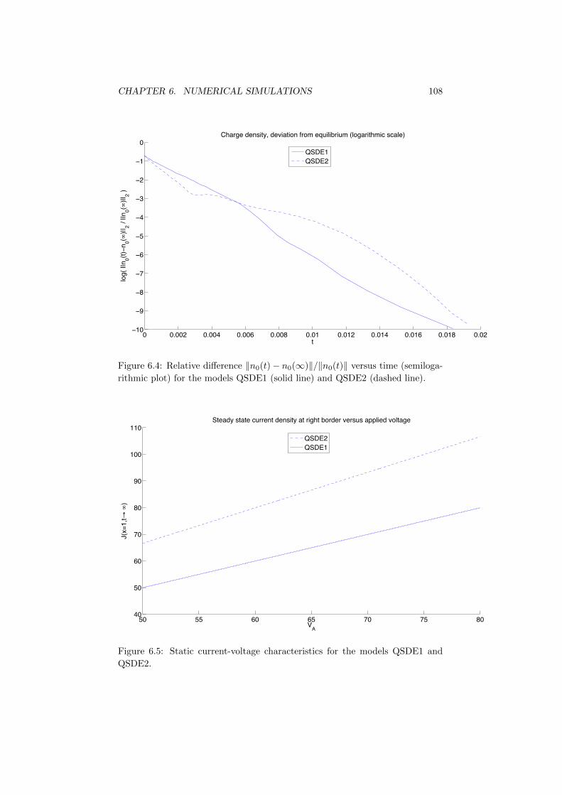
CHAPTER 6. NUMERICAL SIMULATIONS 108
0 0.002 0.004 0.006 0.008 0.01 0.012 0.014 0.016 0.018 0.0210
9
8
7
6
5
4
3
2
1
0
t
log(
||n 0(t)
n 0()||
2 / ||n
0()||
2 )
Charge density, deviation from equilibrium (logarithmic scale)
QSDE1QSDE2
Figure 6.4: Relative difference ‖n0(t)− n0(∞)‖/‖n0(t)‖ versus time (semiloga-
rithmic plot) for the models QSDE1 (solid line) and QSDE2 (dashed line).
50 55 60 65 70 75 8040
50
60
70
80
90
100
110
VA
J(x=
1,t
)
Steady state current density at right border versus applied voltage
QSDE2QSDE1
Figure 6.5: Static current-voltage characteristics for the models QSDE1 and
QSDE2.

Bibliography
[1] A. Arnold. Self-consistent relaxation-time models in quantum mechanics.
Communications in Partial Differential Equations 21(3–4) (1996), 473–506.
[2] N. W. Ashcroft, N. D. Mermin. Solid state physics. Harcourt College Pub-
lishers, 1976.
[3] C. Auer, F. Schurrer and C. Ertler. Hot phonon effects on the high-field
transport in metallic carbon nanotubes. Physical Review B 74 (2006),
165409.
[4] L. Barletti. A mathematical introduction to the Wigner formulation of
quantum mechanics. B. Unione Mat. Ital. B 6-B (2003), 693-716.
[5] L. Barletti. A “spinorial” Wigner function describing the two-band k.p dy-
namics of electrons in crystals. Industrial Mathematics in Italy, World Sci-
entific, Singapore, 2005.
[6] L. Barletti. Quantum fluid models for nanoelectronics. Communications in
Applied and Industrial Mathematics 3(1) (2012).
[7] L. Barletti and G. Frosali. Diffusive limit of the two-band k · p model for
semiconductors. Journal of Statistical Physics 139 (2010), 280–306.
[8] L. Barletti and F. Mehats. Quantum drift-diffusion modeling of spin trans-
port in nanostructures. J. Math. Phys. 51 (2010), 053304, 20 pp.
[9] C. Beenakker. Colloquium: Andreev reflection and Klein tunneling in
graphene. Reviews of Modern Physics 80 (2008), 1337–1354.
[10] N. Ben Abdallah and R. El Hajj. On hierarchy of macro-
scopic models for semiconductor spintronics. Preprint, 2009.
http://www.math.univ-toulouse.fr/∼elhajj/article/publie4.pdf.
[11] I. Bialynicki-Birula. Hydrodynamic form of the Weyl equation. Acta Phys-
ica Polonica 26 (1995), 1201–1208.
[12] H. Brezis. Functional Analysis, Sobolev Spaces and Partial Differential
Equations. Springer, New York, 2010.
109
BIBLIOGRAPHY 110
[13] C. Cercignani. The Boltzmann Equation and Its Applications. Springer,
New York, 1988.
[14] S. Cho, Y.-F. Chen, and M. Fuhrer. Gate-tunable graphene spin valve.
Appl. Phys. Lett. 91 (2007), 123105, 3 pp.
[15] S. Das Sarma, S. Adam, E. Hwang, and E. Rossi. Electronic transport in
two-dimensional graphene. Rev. Modern Phys. 83 (2011), 407-470.
[16] P. Degond, F. Mehats and C. Ringhofer. Quantum energy-transport and
drift-diffusion models. Journal of Statistical Physics 118 (2005), 625–667.
[17] P. Degond and C. Ringhofer. A note on quantum moment hydrodynamics
and the entropy principle. C. R. Math. Acad. Sci. Paris 335 (2002), 967–
972.
[18] P. Degond and C. Ringhofer. Quantum moment hydrodynamics and the
entropy principle. J. Stat. Phys. 112 (2003), 587-628.
[19] R. El Hajj. Etude mathematique et numerique de modeles de transport: ap-
plication a la spintronique. PhD thesis, Universite Paul Sabatier, Toulouse,
France, 2008.
[20] G. Folland. Harmonic Analysis in Phase Space. Princeton University Press,
Princeton, 1989.
[21] M. Freitag. Graphene: nanoelectronics goes flat out. Nature Nanotech. 3
(2008), 455-457.
[22] H. Gajewski. On existence, uniqueness and asymptotic behavior of solutions
of the basic equations for carrier transport in semiconductors. Z. Angew.
Math. Mech. 65 (1985), 101-108.
[23] A. K. Geim and K. S. Novoselov. The rise of graphene. Nature Materials 6
(2007), 183–191.
[24] K. K. Gomes, W. Mar, W. Ko, F. Guinea and H. C. Manoharan. Designer
Dirac fermions and topological phases in molecular graphene. Nature 483
(2012), 306–310.
[25] A. Glitzky. Analysis of a spin-polarized drift-diffusion model. Adv. Math.
Sci. Appl. 18 (2008), 401-427.
[26] F. Guinea. Models of electron transport in single layer graphene. J. Low
Temp. Phys. 153 (2008), 359-373.
[27] C. Jozsa, M. Popinciuc, N. Tombros, H. Jonkman, and B. van Wees. Elec-
tronic spin drift in graphene field effect transistors. Phys. Rev. Lett. 100
(2008), 236603, 4 pp.
[28] A. Jungel. Transport Equations for Semiconductors. Annals of Mathematics
Studies, 122, Springer-Verlag, Berlin, 2009.

BIBLIOGRAPHY 111
[29] A. Jungel. Dissipative quantum fluid models. Riv. Mat. Univ. Parma 3
(2012), 217-290.
[30] A. Jungel and D. Matthes. Isothermal quantum hydrodynamic equations.
Z. Angew. Math. Mech. 85 (2005), 806 814.
[31] A. Jungel, D. Matthes and J. Milsic. Derivation of new quantum hydro-
dynamic equations using entropy minimization. SIAM Journal of Applied
Mathematics 67 (2006), 46–68.
[32] M. Katsnelson, K. Novoselov and A. Geim. Chiral tunneling and the Klein
paradox in graphene. Nature Physics 2 9 (2006), 620–625.
[33] C. D. Levermore. Moment closure hierarchies for kinetic theories. Journal
of Statistical Physics 83 (1996), 1021–1065.
[34] E. Madelung. Quantentheorie in hydrodynamischer form. Zeitschrift fur
Physik A Hadrons and Nuclei 40 (1927), 322–326.
[35] P. Markowich, C. Ringhofer, and C. Schmeiser. Semiconductor Equations.
Springer, Vienna, 1990.
[36] F. Mehats and O. Pinaud. A problem of moment realizability in quantum
statistical physics. Kinetic Related Models 4 (2011), 1143-1158.
[37] O. Morandi and F. Schurrer. Wigner model for quantum transport in
graphene. J. Phys. A:Math. Theor. 44 (2011), 265301, 32 pp.
[38] S. Morozov, K. Novoselov, and A. Gleim. Electron transport in graphene.
Physics Uspekhi 51 (2008), 744-748.
[39] N. Peres. The transport properties of graphene. J. Phys.: Condens. Matter
21 (2009), 323201, 10 pp.
[40] Y. Pershin, S. Saikin, and V. Privman. Semiclassical transport models for
semiconductor spintronics. Electrochem. Soc. Proc. 2004-13 (2005), 183-
205.
[41] L. Ponomarenko, F. Schedin, M. Katsnelson, R. Yang, E. Hill,
K. Novoselov, and A. Geim. Chaotic Dirac billiard in graphene quantum
dots. Science 320 (2008), 356-358.
[42] S. Possanner and C. Negulescu. Diffusion limit of a generalized matrix
Boltzmann equation for spin-polarized transport. Kinetic Related Models 4
(2011), 1159-1191.
[43] A. Quarteroni, R. Sacco and F. Sareri. Numerical Mathematics. Springer-
Verlag, New York, 2000.
[44] M. Reed and B. Simon. Methods of Modern Mathematical Physics, Vol. 1.
Academic Press, London, 1980.
BIBLIOGRAPHY 112
[45] S. Saikin. Drift-diffusion model for spin-polarized transport in a non-
degenerate 2DEG controlled by spin-orbit interaction. J. Phys.: Condens.
Matter 16 (2004), 5071-5081.
[46] F. Schedin, A. Geim, S. Morozov, E. Hill, P. Blake, M. Katsnelson, and
K. Novoselov. Detection of individual gas molecules adsorbed on graphene.
Nature Materials 6 (2007), 652-655.
[47] R. Shankar. Principles of Quantum Mechanics. Plenum Press, New York,
1994.
[48] V. I. Tatarski. The Wigner formulation of quantum mechanics. Sov. Phys.
Usp. 26 (1983), 311.
[49] B. Thaller. The Dirac Equation. Springer Verlag, Berlin, 1992.
[50] J. Von Neumann. Mathematical Foundation of Quantum Mechanics.
Princeton University Press, Priceton, 1955.
[51] F. Xia, D. Farmer, Y.-M. Lin, and P. Avouris. Graphene field-effect tran-
sistors with high on/off current ratio and large transport band gap at room
temperature. Nano Lett. 10 (2010), 715-718.
[52] C. Zachos, D. Fairlie and T. Curtright, eds., Quantum Mechanics in Phase
Space. An Overview with Selected Papers. Worl Scientific Series in 20th
Century Physics 34, World Scientific Publishing Co. Pte. Ltd., Hackensack,
NJ, 2005.
[53] E. Zeidler. Nonlinear Functional Analysis and its Applications, Vol. II/A.
Springer, New York, 1990.
[54] N. Zamponi. Some fluid-dynamic models for quantum electron transport
in graphene via entropy minimization. Kinetic Related Models 5 (2012),
203-221.
[55] N. Zamponi. Trasporto Quantistico Degli Elettroni nel Grafene: Un Ap-
proccio Cinetico e Fluidodinamico. Tesi di Laurea Specialistica, Universita
di Firenze, Facolta di Scienze Mat. Fis. Nat., 2009.
[56] N. Zamponi and L. Barletti. Quantum electronic transport in graphene:
a kinetic and fluid-dynamic approach. Math. Meth. Appl. Sci. 34 (2011),
807-818.
[57] N. Zamponi and A. Jungel. Two spinorial drift-diffusion models for quan-
tum electron transport in graphene. Communications in Mathematical Sci-
ences (To appear).
[58] S. Zheng. Nonlinear Parabolic Equations and Hyperbolic-Parabolic Coupled
Systems. Longman Group, Essex, 1995.