
Laboratorio di Fisica (2 unità) - dmf.unicatt.itfisteam/labfisica1/Dispensa2.pdf · 5) Selezionare...
75
Università Cattolica del Sacro Cuore Facoltà di Scienze matematiche, fisiche e naturali a.a. 2012/2013 Laboratorio di Fisica (2 a unità) - Schede di presentazione delle esperienze - Docenti: Galimberti Gianluca Maianti Marco Indice: Esperienza 1: Momento di inerzia. Esperienza 2: Conservazione del momento angolare. Esperienza 3: Moti oscillatori accoppiati. Esperienza 4: Pendolo di torsione. Esperienza 5: Trasformazioni termodinamiche. Esperienza 6: Motore termico. Esperienza 7: Sonometro Calendario e suddivisione dei gruppi
Transcript of Laboratorio di Fisica (2 unità) - dmf.unicatt.itfisteam/labfisica1/Dispensa2.pdf · 5) Selezionare...
Università Cattolica del Sacro Cuore Facoltà di Scienze matematiche, fisiche e naturali
a.a. 2012/2013
Laboratorio di Fisica (2a unità)
- Schede di presentazione delle esperienze -
Docenti:
Galimberti Gianluca
Maianti Marco
Indice:
Esperienza 1: Momento di inerzia.
Esperienza 2: Conservazione del momento angolare.
Esperienza 3: Moti oscillatori accoppiati.
Esperienza 4: Pendolo di torsione.
Esperienza 5: Trasformazioni termodinamiche.
Esperienza 6: Motore termico.
Esperienza 7: Sonometro
Calendario e suddivisione dei gruppi
Esperienza 2 –Conservazione del momento angolare
1
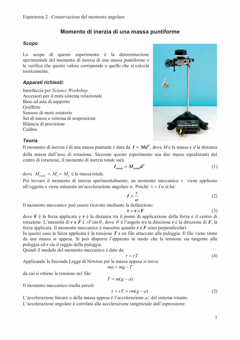
Momento di inerzia di una massa puntiforme Scopo Lo scopo di questo esperimento è la determinazione sperimentale del momento di inerzia di una massa puntiforme e la verifica che questo valore corrisponde a quello che si calcola teoricamente. Apparati richiesti:
Interfaccia per Science Workshop Accessori per il mini-sistema rotazionale Base ed asta di supporto Graffette Sensore di moto rotatorio Set di masse e sistema di sospensione Bilancia di precisione Calibro
Teoria
Il momento di inerzia I di una massa puntuale è data da 2MdI = , dove M è la massa e d la distanza
della massa dall’asse di rotazione. Siccome questo esperimento usa due masse equidistanti dal centro di rotazione, il momento di inerzia totale sarà
2dMI totaletotale = (1)
dove M M Mtotale = +1 2 è la massa totale.
Per trovare il momento di inerzia sperimentalmente, un momento meccanico t viene applicato
all’oggetto e viene misurata un’accelerazione angolare a. Poiché t = I a si ha:
at
=I (2)
Il momento meccanico può essere ricavato mediante la definizione: Frτ ´= (3)
dove F è la forza applicata e r è la distanza tra il punto di applicazione della forza e il centro di rotazione. L’intensità di r x F è qsinrF , dove q è l’angolo tra la direzione r e la direzione di F, la forza applicata. Il momento meccanico è massimo quando r e F sono perpendicolari. In questo caso la forza applicata è la tensione T a un filo attaccato alla puleggia. Il filo viene tirato da una massa m appesa. Si può disporre l’apparato in modo che la tensione sia tangente alla
puleggia ed r sia il raggio della puleggia. Quindi il modulo del momento meccanico è dato da:
rT=t (4) Applicando la Seconda Legge di Newton per la massa appesa si trova:
Tmgma -=
da cui si ottiene la tensione nel filo: )( agmT -=
Il momento meccanico risulta perciò:
)( agrmrT -==t (5)
L’accelerazione lineare a della massa appesa è l’accelerazione aT del sistema rotante.
L’accelerazione angolare è correlata alla accelerazione tangenziale dall’espressione:
Esperienza 2 –Conservazione del momento angolare
2
r
aT=a (6)
Sostituendo le Eqq. (5) e (6) in Eq. (2) si trova:
÷÷ø
öççè
æ-=-=-=
-== 1)(
)( 222
TTTT a
gmrmr
a
mgr
a
ragrm
ra
agrmI
at
(7)
Quindi il momento di inerzia I può essere calcolato dall’accelerazione tangenziale aT.
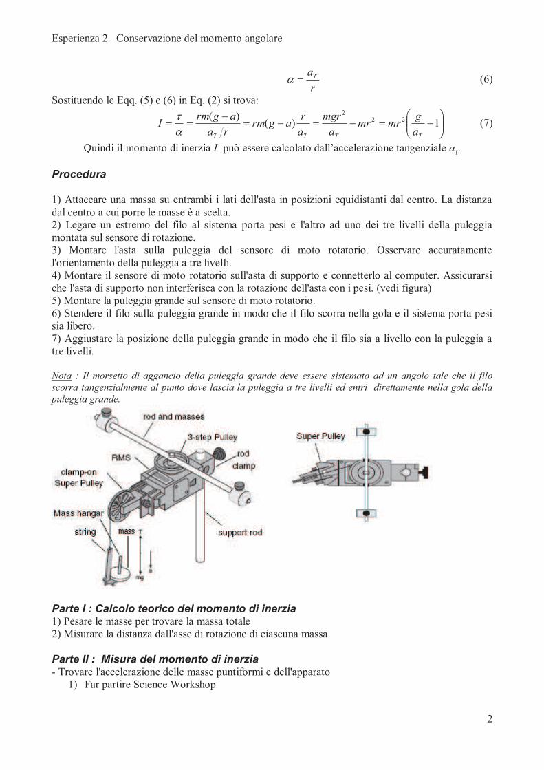
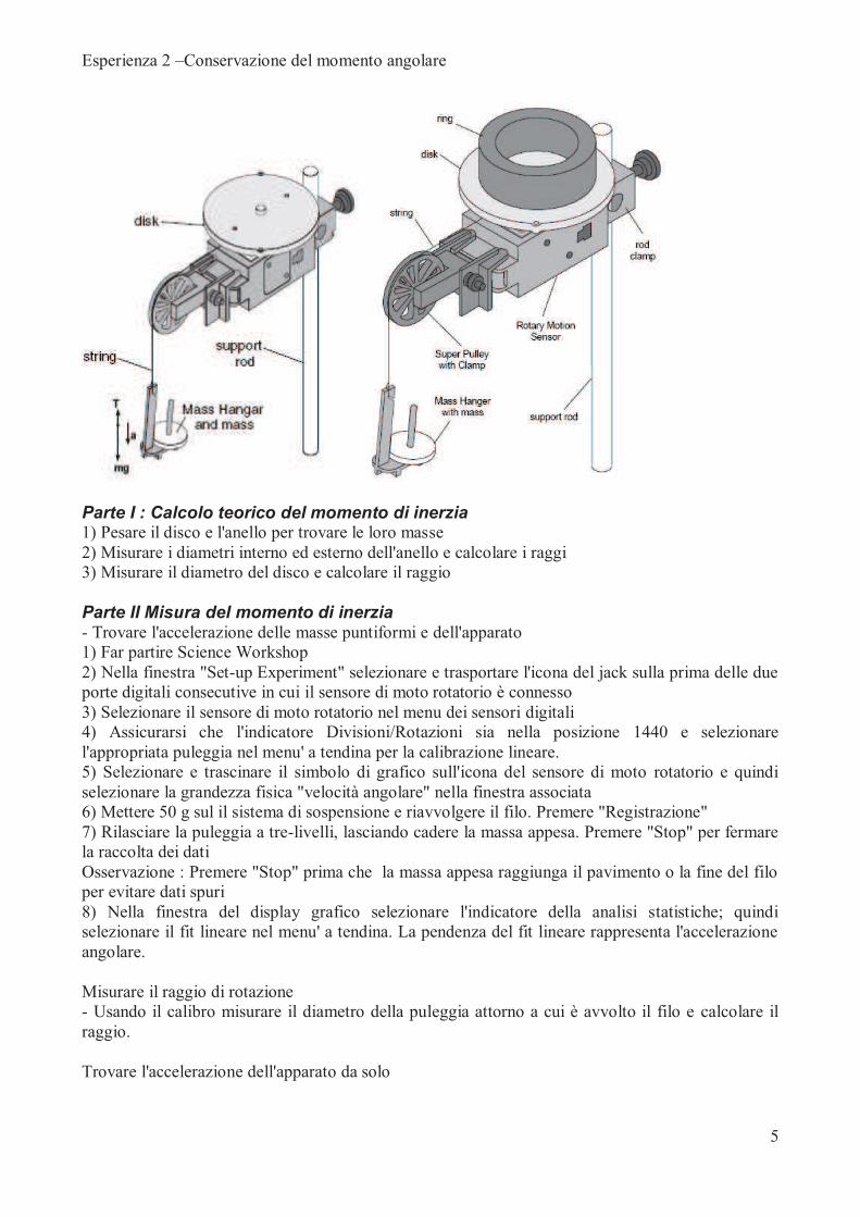
Procedura 1) Attaccare una massa su entrambi i lati dell'asta in posizioni equidistanti dal centro. La distanza dal centro a cui porre le masse è a scelta. 2) Legare un estremo del filo al sistema porta pesi e l'altro ad uno dei tre livelli della puleggia montata sul sensore di rotazione. 3) Montare l'asta sulla puleggia del sensore di moto rotatorio. Osservare accuratamente l'orientamento della puleggia a tre livelli. 4) Montare il sensore di moto rotatorio sull'asta di supporto e connetterlo al computer. Assicurarsi che l'asta di supporto non interferisca con la rotazione dell'asta con i pesi. (vedi figura) 5) Montare la puleggia grande sul sensore di moto rotatorio. 6) Stendere il filo sulla puleggia grande in modo che il filo scorra nella gola e il sistema porta pesi sia libero. 7) Aggiustare la posizione della puleggia grande in modo che il filo sia a livello con la puleggia a tre livelli. Nota : Il morsetto di aggancio della puleggia grande deve essere sistemato ad un angolo tale che il filo scorra tangenzialmente al punto dove lascia la puleggia a tre livelli ed entri direttamente nella gola della puleggia grande.
Parte I : Calcolo teorico del momento di inerzia 1) Pesare le masse per trovare la massa totale 2) Misurare la distanza dall'asse di rotazione di ciascuna massa
Parte II : Misura del momento di inerzia - Trovare l'accelerazione delle masse puntiformi e dell'apparato
1) Far partire Science Workshop
Esperienza 2 –Conservazione del momento angolare
3
Raccolta dei dati Ricordate: per dare inizio alla raccolta, potete, a vostra scelta: · fare click sul tasto “REC”, · selezionare “Record” dal menù Experiment, · premere “ALT R”. Per terminare la raccolta: · fare click sul tasto “STOP”, · selezionare “Stop” dal menù Experiment, · premere “ALT .” .
2) Nella finestra "Set-up Experiment" selezionare e trasportare l'icona del jack sulla prima delle
due porte digitali consecutive a cui il sensore di moto rotatorio è connesso. 3) Selezionare il sensore di moto rotatorio nel menu dei sensori digitali 4) Assicurarsi che l'indicatore Divisioni/Rotazioni sia nella posizione 1440 e selezionare
l'appropriata puleggia nel menu' a tendina per la calibrazione lineare. 5) Selezionare e trascinare il simbolo di grafico sull'icona del sensore di moto rotatorio e
quindi selezionare la grandezza fisica "velocità angolare" nella finestra associata 6) Mettere 50 g sul il sistema porta pesi e riavvolgere il filo. Premere "Registrazione". 7) Rilasciare la puleggia a tre-livelli, lasciando cadere la massa appesa. Premere "Stop" per
fermare la raccolta dei dati.
Osservazione : Premere "Stop" prima che la massa appesa raggiunga il pavimento o la fine del filo per evitare dati spuri.
8) Nella finestra del display grafico selezionare l'indicatore delle analisi statistiche; quindi selezionare il fit lineare nel menù a tendina. La pendenza del fit lineare rappresenta l'accelerazione angolare.
Misurare il raggio di rotazione - Usando il calibro misurare il diametro della puleggia attorno a cui è avvolto il filo e calcolare il raggio. Trovare l'accelerazione dell'apparato da solo Nella rotazione l'apparato ruota e contribuisce al momento di inerzia. Per trovare il vero momento di inerzia delle masse puntiformi, bisogna determinare l'accelerazione ed il momento di inerzia dell'apparato da solo. - Rimuovere le masse puntiformi dall'asta rotante e ripetere la procedura da 1) ad 8). Potrebbe essere necessario diminuire la massa appesa per evitare che l'apparato ruoti così velocemente da non permettere al computer di raccogliere i dati.
Calcoli Calcolare il valore sperimentale del momento di inerzia totale delle masse e dell'apparato Calcolare il valore sperimentale del momento di inerzia dell'apparato da solo Sottrarre il momento di inerzia dell'apparato da quello totale. Calcolare il valore aspettato del momento di inerzia. Confrontare i due valori
Esperienza 2 –Conservazione del momento angolare
4
Momento di inerzia di un disco e di un anello
Scopo Lo scopo di questo esperimento è la determinazione sperimentale del momento di inerzia di un anello ed un disco e la verifica che questo valore corrisponda a quello che si calcola.
Teoria
Il momento di inerzia di un anello è dato da
)(2
2
2
12
1RRMI +=
dove M è la massa dell’anello, R1 è il raggio interno e R2 è il raggio esterno dell’anello.
Il momento di inerzia di un disco è dato da 2
2
1 MRI =
dove M è la massa del disco e R è il raggio esterno del disco. Per trovare il momento di inerzia sperimentalmente si usano gli stessi ragionamenti fatti prima dall’equazione (2) fino alla equazione (7). Apparati richiesti : Interfaccia per Science Workshop Accessori per il mini-sistema rotazionale Base ed asta di supporto Graffette Sensore di moto rotatorio Set di masse e sistema di sospensione Bilancia di precisione Calibro
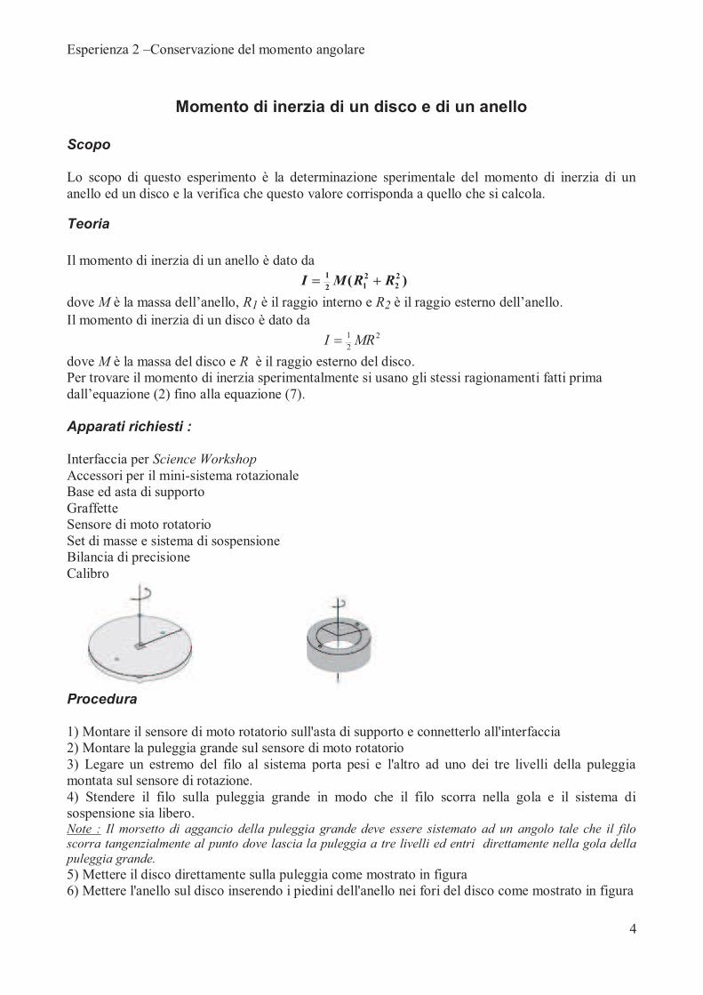
Procedura 1) Montare il sensore di moto rotatorio sull'asta di supporto e connetterlo all'interfaccia 2) Montare la puleggia grande sul sensore di moto rotatorio 3) Legare un estremo del filo al sistema porta pesi e l'altro ad uno dei tre livelli della puleggia montata sul sensore di rotazione. 4) Stendere il filo sulla puleggia grande in modo che il filo scorra nella gola e il sistema di sospensione sia libero. Note : Il morsetto di aggancio della puleggia grande deve essere sistemato ad un angolo tale che il filo scorra tangenzialmente al punto dove lascia la puleggia a tre livelli ed entri direttamente nella gola della puleggia grande. 5) Mettere il disco direttamente sulla puleggia come mostrato in figura 6) Mettere l'anello sul disco inserendo i piedini dell'anello nei fori del disco come mostrato in figura
Esperienza 2 –Conservazione del momento angolare
5
Parte I : Calcolo teorico del momento di inerzia 1) Pesare il disco e l'anello per trovare le loro masse 2) Misurare i diametri interno ed esterno dell'anello e calcolare i raggi 3) Misurare il diametro del disco e calcolare il raggio
Parte II Misura del momento di inerzia - Trovare l'accelerazione delle masse puntiformi e dell'apparato 1) Far partire Science Workshop 2) Nella finestra "Set-up Experiment" selezionare e trasportare l'icona del jack sulla prima delle due porte digitali consecutive in cui il sensore di moto rotatorio è connesso 3) Selezionare il sensore di moto rotatorio nel menu dei sensori digitali 4) Assicurarsi che l'indicatore Divisioni/Rotazioni sia nella posizione 1440 e selezionare l'appropriata puleggia nel menu' a tendina per la calibrazione lineare. 5) Selezionare e trascinare il simbolo di grafico sull'icona del sensore di moto rotatorio e quindi selezionare la grandezza fisica "velocità angolare" nella finestra associata 6) Mettere 50 g sul il sistema di sospensione e riavvolgere il filo. Premere "Registrazione" 7) Rilasciare la puleggia a tre-livelli, lasciando cadere la massa appesa. Premere "Stop" per fermare la raccolta dei dati Osservazione : Premere "Stop" prima che la massa appesa raggiunga il pavimento o la fine del filo per evitare dati spuri 8) Nella finestra del display grafico selezionare l'indicatore della analisi statistiche; quindi selezionare il fit lineare nel menu' a tendina. La pendenza del fit lineare rappresenta l'accelerazione angolare. Misurare il raggio di rotazione - Usando il calibro misurare il diametro della puleggia attorno a cui è avvolto il filo e calcolare il raggio. Trovare l'accelerazione dell'apparato da solo

Esperienza 2 –Conservazione del momento angolare
6
Poiché nella rotazione sia il disco che l'anello ruotano insieme è necessario determinare l'accelerazione ed il momento di inerzia del disco da solo cosicché il suo momento di inerzia possa essere sottratto dal totale per trovare il momento di inerzia dell'anello. - Rimuovere il disco dall'apparato e ripetere la procedura da 1) ad 8). Calcoli Calcolare il valore sperimentale del momento di inerzia totale del disco e dell'anello. Calcolare il valore sperimentale del momento di inerzia del disco da solo. Sottrarre il momento di inerzia del disco da quello totale. Questo è il momento d'inerza dell'anello. Calcolare il valore aspettato dei momenti di inerzia in base ai raggi ed alla massa. Confrontare i valori
Esperienza 2 –Conservazione del momento angolare
1
Conservazione Momento Angolare Scopo Un anello è fatto cadere su un disco rotante e la velocita' angolare finale del sistema è confrontata con il valore predetto usando la conservazione del momento angolare. Apparati richiesti : Interfaccia per Science Workshop Accessori per il mini-sistema rotazionale Base ed asta di supporto Graffette Sensore di moto rotatorio Set di masse e sistema di sospensione Bilancia di precisione Calibro
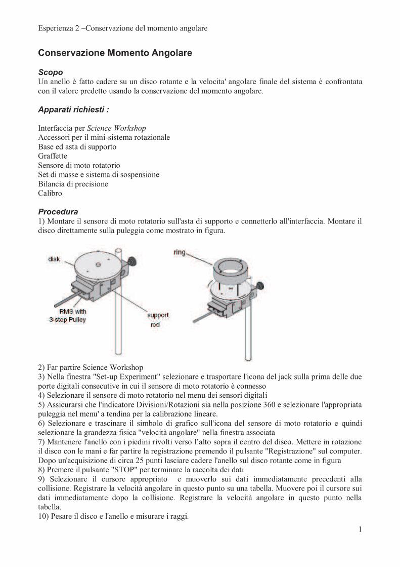
Procedura 1) Montare il sensore di moto rotatorio sull'asta di supporto e connetterlo all'interfaccia. Montare il disco direttamente sulla puleggia come mostrato in figura.
2) Far partire Science Workshop 3) Nella finestra "Set-up Experiment" selezionare e trasportare l'icona del jack sulla prima delle due porte digitali consecutive in cui il sensore di moto rotatorio è connesso 4) Selezionare il sensore di moto rotatorio nel menu dei sensori digitali 5) Assicurarsi che l'indicatore Divisioni/Rotazioni sia nella posizione 360 e selezionare l'appropriata puleggia nel menu' a tendina per la calibrazione lineare. 6) Selezionare e trascinare il simbolo di grafico sull'icona del sensore di moto rotatorio e quindi selezionare la grandezza fisica "velocità angolare" nella finestra associata 7) Mantenere l'anello con i piedini rivolti verso l’alto sopra il centro del disco. Mettere in rotazione
il disco con le mani e far partire la registrazione premendo il pulsante "Registrazione" sul computer. Dopo un'acquisizione di circa 25 punti lasciare cadere l'anello sul disco rotante come in figura 8) Premere il pulsante "STOP" per terminare la raccolta dei dati 9) Selezionare il cursore appropriato e muoverlo sui dati immediatamente precedenti alla collisione. Registrare la velocità angolare in questo punto su una tabella. Muovere poi il cursore sui dati immediatamente dopo la collisione. Registrare la velocità angolare in questo punto nella tabella. 10) Pesare il disco e l'anello e misurare i raggi.

Esperienza 2 –Conservazione del momento angolare
2
Calcoli Calcolare il valore aspettato per la velocità angolare finale. Calcolare la differenza percentuale tra il valore sperimentale e quello teorico della velocità angolare.
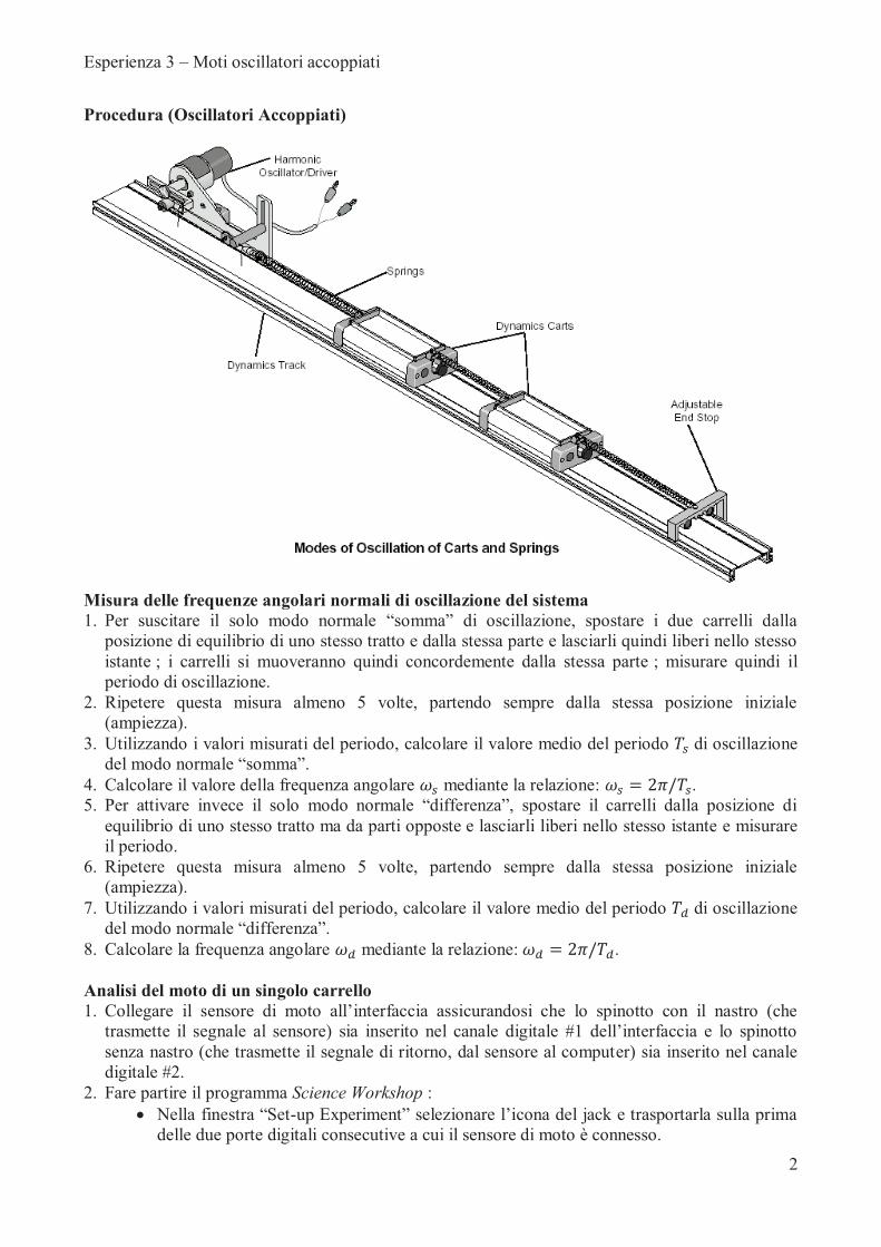
Esperienza 3 – Moti oscillatori accoppiati
1
Oscillatori Accoppiati - Modi Normali di Oscillazione
Materiale richiesto
Rotaia con 2 carrelli, massa addizionale e stop 3 molle (Set di masse e sistema di sospensione Filo Carrucola Cronometro) Bilancia Sensore di moto Interfaccia per Science Workshop/DataStudio Scopo
Lo scopo dell'esperienza è quello di considerare un sistema di due oscillatori accoppiati mediante una molla e di rilevare i modi normali di vibrazione e le relative frequenze. Teoria
Il sistema costituito da due carrelli di uguale massa m ciascuno collegato ad una molla di costante elastica ko , interagenti con una molla di costante elastica k e in moto su una rotaia rettilinea
orizzontale è un sistema a due gradi di libertà (che possono essere identificati dalle coordinate x1 e
x2 delle posizioni dei due carrelli rispetto alle relative posizioni di equilibrio).
Il moto generale di tali oscillatori accoppiati può essere descritto come sovrapposizione di due modi normali di vibrazione definiti dalla somma e dalla differenza delle coordinate dei due carrelli, secondo le equazioni :
x x S ts s1 2+ = × +cos( )w a , essendo : wsok
m=
x x D td d1 2- = × +cos( )w a , essendo : wdok k
m=
+2
dalle quali è possibile esprimere le leggi orarie dei due carrelli in movimento :
[ ]x S t D ts s d d1
1
2= × + + × +cos( ) cos( )w a w a
[ ]x S t D ts s d d2
1
2= × + - × +cos( ) cos( )w a w a
I valori delle costanti S, D, e dipendono dalle condizioni iniziali ; in particolare, nel caso in cui si abbia D = 0, si ha x1 - x2 = 0 cioè x1 = x2 e quindi i due carrelli si muovono in concordanza di
fase secondo il modo normale “somma” ; nel caso in cui sia invece S = 0, si ha x1 + x2 = 0 cioè si
ha x1 = - x2 e i carrelli si muovono in verso opposto secondo il modo normale “differenza”.
Esperienza 3 – Moti oscillatori accoppiati
2
Procedura (Oscillatori Accoppiati)
Misura delle frequenze angolari normali di oscillazione del sistema
1. Per suscitare il solo modo normale “somma” di oscillazione, spostare i due carrelli dalla
posizione di equilibrio di uno stesso tratto e dalla stessa parte e lasciarli quindi liberi nello stesso istante ; i carrelli si muoveranno quindi concordemente dalla stessa parte ; misurare quindi il periodo di oscillazione.
2. Ripetere questa misura almeno 5 volte, partendo sempre dalla stessa posizione iniziale (ampiezza).
3. Utilizzando i valori misurati del periodo, calcolare il valore medio del periodo di oscillazione del modo normale “somma”.
4. Calcolare il valore della frequenza angolare mediante la relazione: . 5. Per attivare invece il solo modo normale “differenza”, spostare il carrelli dalla posizione di
equilibrio di uno stesso tratto ma da parti opposte e lasciarli liberi nello stesso istante e misurare il periodo.
6. Ripetere questa misura almeno 5 volte, partendo sempre dalla stessa posizione iniziale (ampiezza).
7. Utilizzando i valori misurati del periodo, calcolare il valore medio del periodo di oscillazione del modo normale “differenza”.
8. Calcolare la frequenza angolare mediante la relazione: .
Analisi del moto di un singolo carrello
1. Collegare il sensore di moto all’interfaccia assicurandosi che lo spinotto con il nastro (che
trasmette il segnale al sensore) sia inserito nel canale digitale #1 dell’interfaccia e lo spinotto
senza nastro (che trasmette il segnale di ritorno, dal sensore al computer) sia inserito nel canale digitale #2.
2. Fare partire il programma Science Workshop : · Nella finestra “Set-up Experiment” selezionare l’icona del jack e trasportarla sulla prima
delle due porte digitali consecutive a cui il sensore di moto è connesso.
Esperienza 3 – Moti oscillatori accoppiati
3
· Selezionare “Motion Sensor” nel menù dei sensori digitali. 3. Nella finestra delle caratteristiche del sensore è possibile calibrare il sensore e stabilire il numero
di dati da registrare al secondo :
· per calibrare : puntare il sensore su un oggetto fermo alla distanza di 1 metro (la distanza di calibrazione predisposta) e selezionare “calibrate”, il programma calcolerà la velocità
del suono e il tempo di viaggio dell’impulso emesso e riflesso.
· per cambiare il numero di dati al secondo selezionare “Trigger Rate” e scegliere il
numero stabilito ; notare che il numero di dati determina anche i valori delle disytanze massima e minima che il sensore è in grado di rilevare.
4. Mettere in movimento in modo del tutto arbitrario i carrelli e iniziare la registrazione dei dati (comando ALT-R).
5. Continuare la registrazione per qualche oscillazione completa e quindi terminarla (comando ALT- .).
6. Dalla finestra dell’analisi statistica dei dati (icona ) scegliere lo sviluppo in somma di seni per identificare le due componenti dell’oscillazione e rilevarne i valori delle frequenze angolari.
Analisi dei dati Confrontare i valori misurati delle frequenze angolari dei due modi normali di oscillazione con quelli determinati dall’analisi del moto del singolo carrello e calcolarne la differenza percentuale.
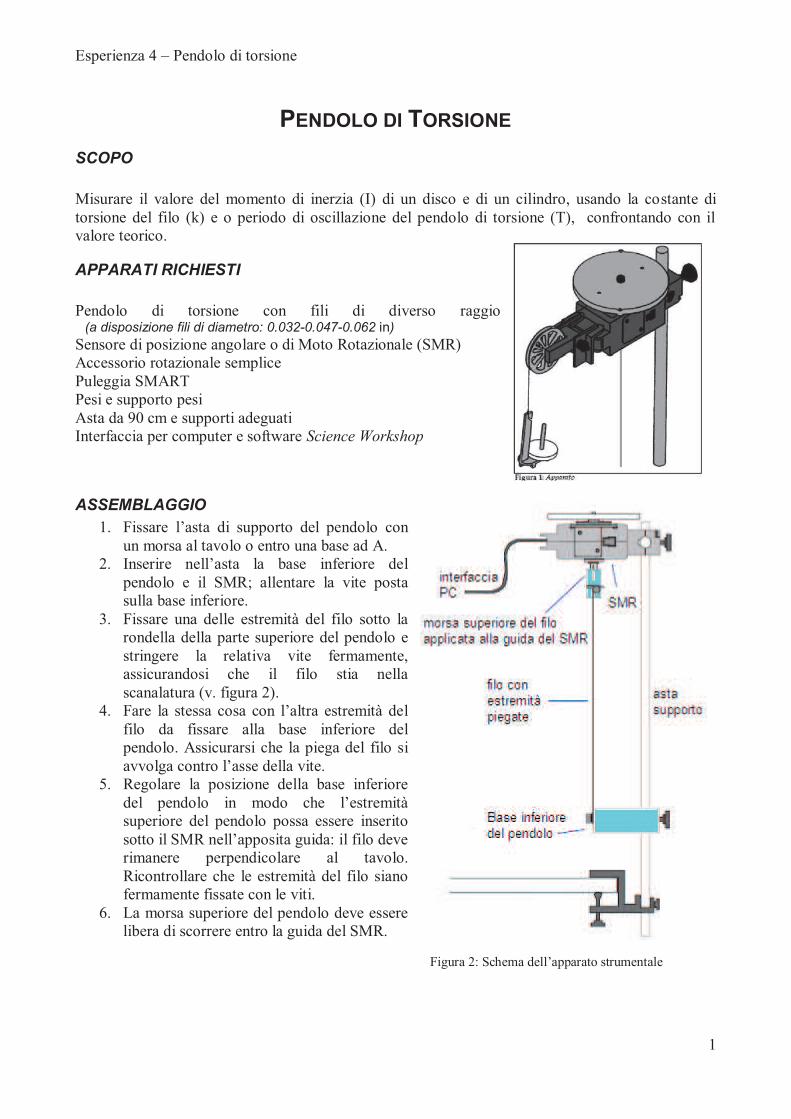
Esperienza 4 – Pendolo di torsione
1
PENDOLO DI TORSIONE
SCOPO
Misurare il valore del momento di inerzia (I) di un disco e di un cilindro, usando la costante di torsione del filo (k) e o periodo di oscillazione del pendolo di torsione (T), confrontando con il valore teorico.
APPARATI RICHIESTI
Pendolo di torsione con fili di diverso raggio
(a disposizione fili di diametro: 0.032-0.047-0.062 in)
Sensore di posizione angolare o di Moto Rotazionale (SMR) Accessorio rotazionale semplice Puleggia SMART Pesi e supporto pesi Asta da 90 cm e supporti adeguati Interfaccia per computer e software Science Workshop
ASSEMBLAGGIO
1. Fissare l’asta di supporto del pendolo con
un morsa al tavolo o entro una base ad A. 2. Inserire nell’asta la base inferiore del
pendolo e il SMR; allentare la vite posta sulla base inferiore.
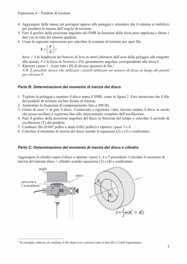
3. Fissare una delle estremità del filo sotto la rondella della parte superiore del pendolo e stringere la relativa vite fermamente, assicurandosi che il filo stia nella scanalatura (v. figura 2).
4. Fare la stessa cosa con l’altra estremità del
filo da fissare alla base inferiore del pendolo. Assicurarsi che la piega del filo si avvolga contro l’asse della vite.
5. Regolare la posizione della base inferiore del pendolo in modo che l’estremità
superiore del pendolo possa essere inserito sotto il SMR nell’apposita guida: il filo deve
rimanere perpendicolare al tavolo. Ricontrollare che le estremità del filo siano fermamente fissate con le viti.
6. La morsa superiore del pendolo deve essere libera di scorrere entro la guida del SMR.
Figura 2: Schema dell’apparato strumentale
Esperienza 4 – Pendolo di torsione
2
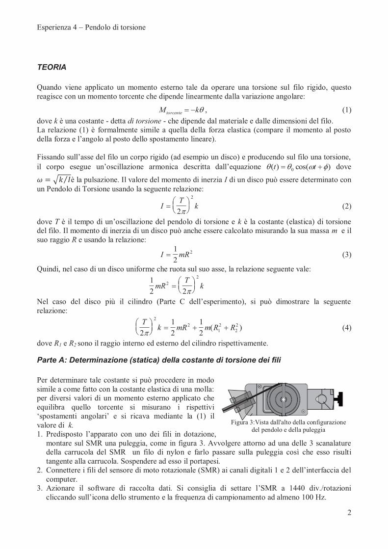
Figura 3:Vista dall'alto della configurazione del pendolo e della puleggia
TEORIA
Quando viene applicato un momento esterno tale da operare una torsione sul filo rigido, questo reagisce con un momento torcente che dipende linearmente dalla variazione angolare:
qkM torcente -= , (1)
dove k è una costante - detta di torsione - che dipende dal materiale e dalle dimensioni del filo. La relazione (1) è formalmente simile a quella della forza elastica (compare il momento al posto della forza e l’angolo al posto dello spostamento lineare). Fissando sull’asse del filo un corpo rigido (ad esempio un disco) e producendo sul filo una torsione,
il corpo esegue un’oscillazione armonica descritta dall’equazione )cos()( 0 fwqq += tt dove
è la pulsazione. Il valore del momento di inerzia I di un disco può essere determinato con
un Pendolo di Torsione usando la seguente relazione:
IT
k=æèç
öø÷
2
2
p (2)
dove T è il tempo di un’oscillazione del pendolo di torsione e k è la costante (elastica) di torsione del filo. Il momento di inerzia di un disco può anche essere calcolato misurando la sua massa m e il suo raggio R e usando la relazione:
I mR=1
22 (3)
Quindi, nel caso di un disco uniforme che ruota sul suo asse, la relazione seguente vale:
1
2 22
2
mRT
k=æèç
öø÷
p
Nel caso del disco più il cilindro (Parte C dell’esperimento), si può dimostrare la seguente
relazione:
Tk mR m R R
2
1
2
1
2
2
2
1
2
2
2
pæèç
öø÷ = + +( ) (4)
dove R1 e R2 sono il raggio interno ed esterno del cilindro rispettivamente.
Parte A: Determinazione (statica) della costante di torsione dei fili
Per determinare tale costante si può procedere in modo simile a come fatto con la costante elastica di una molla: per diversi valori di un momento esterno applicato che equilibra quello torcente si misurano i rispettivi ‘spostamenti angolari’ e si ricava mediante la (1) il valore di k. 1. Predisposto l’apparato con uno dei fili in dotazione,
montare sul SMR una puleggia, come in figura 3. Avvolgere attorno ad una delle 3 scanalature della carrucola del SMR un filo di nylon e farlo passare sulla puleggia così che esso risulti tangente alla carrucola. Sospendere ad esso il portapesi.
2. Connettere i fili del sensore di moto rotazionale (SMR) ai canali digitali 1 e 2 dell’interfaccia del
computer. 3. Azionare il software di raccolta dati. Si consiglia di settare l’SMR a 1440 div./rotazioni
cliccando sull’icona dello strumento e la frequenza di campionamento ad almeno 100 Hz.
Esperienza 4 – Pendolo di torsione
3
4. Aggiungere delle masse sul portapesi appeso alla puleggia e attendere che il sistema si stabilizzi per prendere la misura dell’angolo di torsione.
5. Fare il grafico della posizione angolare del SMR in funzione della forza peso applicata e fittare i dati con la retta dei minimi quadrati.
6. Usare la seguente espressione per calcolare la costante di torsione per ogni filo
l÷ø
öçè
æ=
qF
k
dove l è la lunghezza del braccio di leva in metri (distanza dall’asse della puleggia alla tangente
alla stessa), F è la forza in Newton e q lo spostamento angolare corrispondente alla forza F. 7. Ripetere i passi 1 - 6 per tutti i fili di diversi spessore di filo.1
N.B. È possibile invece che utilizzare i pesetti utilizzare un sensore di forza in luogo dei pesetti per rilevare F.
Parte B: Determinazione del momento di inerzia del disco
1. Togliere la puleggia e montare il disco sopra il SMR, come in figura 2. Fare attenzione che il filo
del pendolo di torsione sia ben fissato al sistema. 2. Aumentare la frequenza di campionamento fino a 200 Hz. 3. Girate di circa ¼ di giro il disco. Cominciate a registrare i dati, lasciare andare il disco in modo
che possa oscillare e registrare fino allo smorzamento completo dell’oscillazione. 4. Fate il grafico della posizione angolare del disco in funzione del tempo e calcolate il periodo di
oscillazione (T) del pendolo. 5. Cambiare filo (0.047 pollici e dopo 0.062 pollici) e ripetere i passi 3 e 4. 6. Calcolate il momento di inerzia del disco usando le equazioni (2) e (3) e confrontare.
Parte C: Determinazione del momento di inerzia del disco e cilindro
Aggiungere il cilindro sopra il disco e ripetere i passi 3, 4 e 5 precedenti. Calcolate il momento di inerzia del sistema disco + cilindro usando equazione (2) e (4) e confrontare.
1 Si consiglia, tuttavia, di cambiare il filo dopo aver concluso tutte le fasi (B e C) dell’esperimento.
012-05110C
5/94
© 1993 PASCO scientific $7.50
Adiabatic Gas
Law Apparatus
Instruction Manual and
Experiment Guide for
the PASCO scientific
Model TD-8565
IncludesTeacher's Notes
andTypical
Experiment Results

012-05110C Adiabatic Gas Law Apparatus
i
Table of Contents
Section Page
Copyright, Warranty and Equipment Return ....................................................... ii
Introduction:
Equipment Included ....................................................................................... 1
Features .......................................................................................................... 1
How to Use this Manual ................................................................................ 1
Theory .................................................................................................................. 2
Description of Apparatus ..................................................................................... 3
Setup:
Using the TD-8565 with the PASCO Series 6500 Computer Interface ........ 5
IBM compatible computers ........................................................................... 5
Apple II compatible computers ..................................................................... 7
Expansion of a Gas ........................................................................................ 7
Experiment:
Measurement of Work to Compress Gases Adiabatically ............................. 9
Equipment Needed: ................................................................................. 9
Purpose .................................................................................................... 9
Theory ...................................................................................................... 9
Procedure ................................................................................................. 9
Graphs and Data Tables ......................................................................... 10
Calculations ........................................................................................... 10
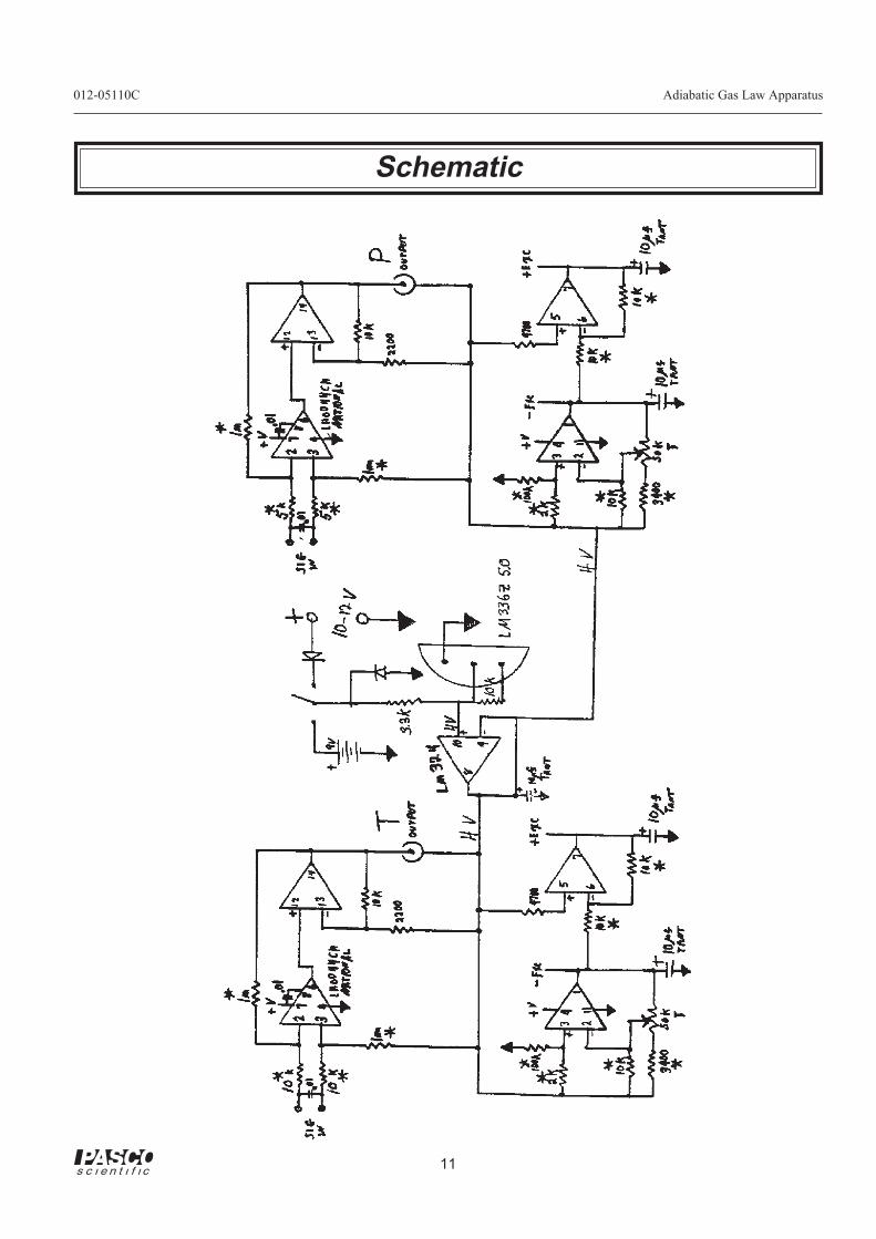
Schematic........................................................................................................... 11
Specifications / Sample Data ............................................................................. 12
Technical Support .................................................................... Inside Back Cover
Adiabatic Gas Law Apparatus 012-05110C
ii
Please—Feel free to duplicate this manual
subject to the copyright restrictions below.
Copyright, Warranty and Equipment Return
Copyright Notice
The PASCO scientific Model TD-8565 Adiabatic Gas
Law Apparatus manual is copyrighted and all rights
reserved. However, permission is granted to non-
profit educational institutions for reproduction of any
part of this manual providing the reproductions are
used only for their laboratories and are not sold for
profit. Reproduction under any other circumstances,
without the written consent of PASCO scientific, is
prohibited.
Limited Warranty
PASCO scientific warrants this product to be free
from defects in materials and workmanship for a
period of one year from the date of shipment to the
customer. PASCO will repair or replace, at its option,
any part of the product which is deemed to be defec-
tive in material or workmanship. This warranty does
not cover damage to the product caused by abuse or
improper use. Determination of whether a product
failure is the result of a manufacturing defect or
improper use by the customer shall be made solely by
PASCO scientific. Responsibility for the return of
equipment for warranty repair belongs to the cus-
tomer. Equipment must be properly packed to prevent
damage and shipped postage or freight prepaid.
(Damage caused by improper packing of the equip-
ment for return shipment will not be covered by the
warranty.) Shipping costs for returning the equipment,
after repair, will be paid by PASCO scientific.
Equipment Return
Should the product have to be returned to PASCO
scientific for any reason, notify PASCO scientific by
letter, phone, or fax BEFORE returning the product.
Upon notification, the return authorization and
shipping instructions will be promptly issued.
When returning equipment for repair, the units
must be packed properly. Carriers will not accept
responsibility for damage caused by improper
packing. To be certain the unit will not be
damaged in shipment, observe the following rules:
À The packing carton must be strong enough for the
item shipped.
Á Make certain there are at least two inches of
packing material between any point on the
apparatus and the inside walls of the carton.
 Make certain that the packing material cannot shift
in the box or become compressed, allowing the
instrument come in contact with the packing
carton.
Address: PASCO scientific
10101 Foothills Blvd.
Roseville, CA 95747-7100
Phone: (916) 786-3800
FAX: (916) 786-3292
email: [email protected]
web: www.pasco.com
NOTE: NO EQUIPMENT WILL BE
ACCEPTED FOR RETURN WITHOUT AN
AUTHORIZATION FROM PASCO.
012-05110C Adiabatic Gas Law Apparatus
1
Introduction
The PASCO Model TD-8565 Adiabatic Gas Law
Apparatus enables the user to investigate the compres-
sion and expansion of gases.
Sensitive transducers in the apparatus measure the
pressure, temperature, and volume of the gas almost
simultaneously as the gas is compressed or expanded
rapidly under near adiabatic conditions, or slowly
under isothermal conditions. Analog signals from the
sensors are monitored by the Series 6500 Computer
Interface, a three channel analog-to-digital data
acquisition system. The computer functions as a three
channel storage oscilloscope. In addition, the data
acquisiton program, Data Monitor, can plot graphs of
pressure, temperautre, and volume. It can plot a graph
of pressure versus volume and integrate under the
curve to determine the work done on the gas.
Equipment Included:
The TD-8565 consists of the Adiabatic Gas Law
Apparatus and this instruction manual (part number
012-05110). The apparatus comes with a permanently
attached cable with a five pin DIN plug that carries the
signal from the volume transducer, and two DIN-plug-
to-mini-phone-plug cables (part number 520-063) that
carry the signals from the pressure and temperature
sensors.
Features:
• Measure γ, the ratio of specific heats for the gas
(CP/C
V).
• Measure the work done on the gas and compare
it with the change in internal energy (CV∆T),
and also with the theoretical work performed.
• Compare the final pressure and temperature
with values predicted by the Adiabatic Gas
Law.
• Use monatomic, diatomic, and polyatomic gases
to determine the effects of molecular structure
on γ.
• Investigate isothermal compression and expan-
sion by performing the experiment slowly, in
incremental steps.
Other:
• The Adiabatic Gas Law Apparatus can also be
used with the MultiPurpose Lab Interface
(MPLI) from Vernier Software.
• The Apparatus can use a nine volt battery to
supply the excitation voltage for the bridge cir-
cuits of the temperature and pressure sensors.
You can also use an external 12 V, 10 mA
power supply, but it must be a "floating ground"
supply.
How to Use this Manual
The first section of this manual describes the theory
of the adiabatic process and the operation of the
apparatus. The next section describes the setup,
calibration, and data collection procedure. The final
section contains the experimental write-up, apparatus
schematic and specifications.
2
Adiabatic Gas Law Apparatus 012-05110C
T1V1γ – 1 = T2V2
γ – 1
Another relationship to be examined in this experi-
ment is the energy expended or work done on the
gas while compressing it adiabatically. Equation 3,
the Adiabatic Gas Law, states that:
PV γ = k = P1V1γ or P = k
V γ
work done to compress the gas is:
Ä
W = PdVV1
V2
= k dVV γ
V1
V2
= k V 1 – γ
1 – γ V1
V2
= P1V1γ V 1 – γ
1 – γ V1
V2
W =P1V1
γ
1 –γV2
1 –γ – V11 –γ
When a process takes place without thermal energy
entering or leaving the system it is an adiabaticprocess. This would occur if the system were per-
fectly thermally insulated or if the process occurred so
rapidly that there could be no heat transfer. The
following is a derivation of the relationship of the
pressure P, temperature T, and volume V when n
moles of a confined ideal gas are compressed or
expanded adiabatically.
The first law of thermodynamics can be stated as:
À dQ = nCvdT + pdV = 0
for an adiabatic process where CV is the molar
specific heat at constant volume, T is the absolute
temperature, n is the number of mole, and V is the
volume. For any ideal gas PV = nRT. Thus
PdV + Vdp = nRdT. Solving for dT gives:
Á dT = PdVnR + VdP
nR
Substituting equation 2 into equation 1 gives:
dQ = nCvPdVnR + VdP
nR + PdV = 0
=CvR + 1 PdV +
CvR VdP
= Cv + R PdV + CvVdP= CPPdV + CvVdP
where CP is the molar specific heat at constant pres-
sure. CP is related to C
V by C
P-C
V = R. The ratio
of CP to C
V is denoted as γ, (gamma). Using these
results we obtain:
CPPdVCvPV + dP
P = 0
γ dVV + dP
P = 0
γ ln V + ln P = constant
 PV γ = constant
P1V1γ = P2V2
γ
This result is the standard adiabatic gas law.
From equation 3 and the ideal gas law PV = nRT a
second form of the adiabatic gas law is:
Theory
R = universal gas constant (approximately 8.314 J/
mole˚K.
Ã
012-05110C Adiabatic Gas Law Apparatus
3
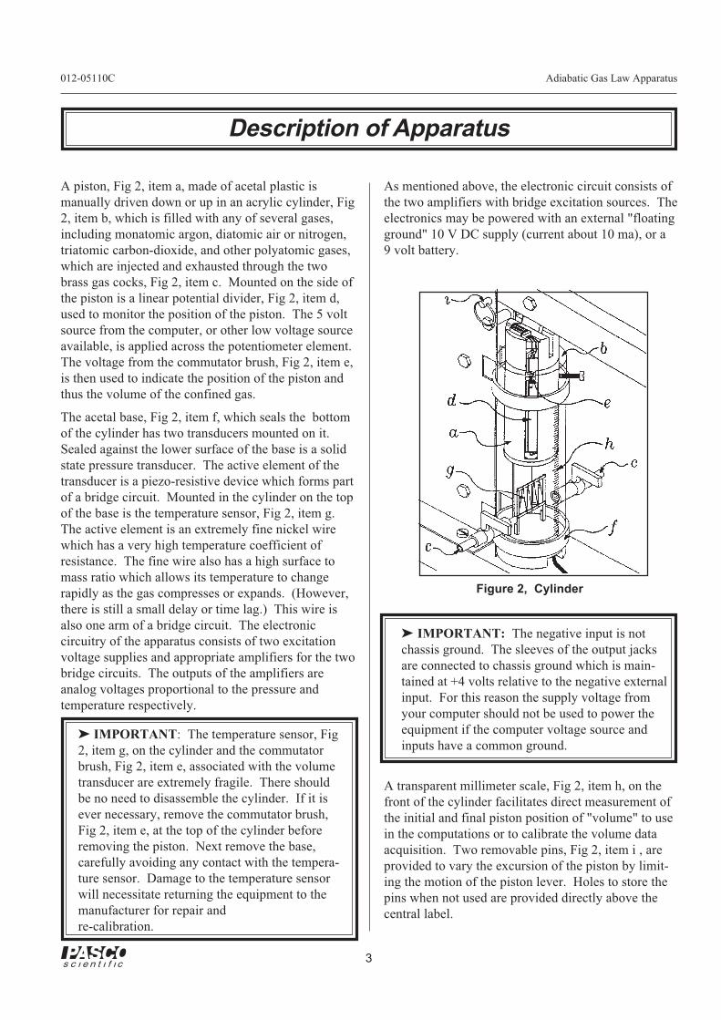
Description of Apparatus
A piston, Fig 2, item a, made of acetal plastic is
manually driven down or up in an acrylic cylinder, Fig
2, item b, which is filled with any of several gases,
including monatomic argon, diatomic air or nitrogen,
triatomic carbon-dioxide, and other polyatomic gases,
which are injected and exhausted through the two
brass gas cocks, Fig 2, item c. Mounted on the side of
the piston is a linear potential divider, Fig 2, item d,
used to monitor the position of the piston. The 5 volt
source from the computer, or other low voltage source
available, is applied across the potentiometer element.
The voltage from the commutator brush, Fig 2, item e,
is then used to indicate the position of the piston and
thus the volume of the confined gas.
The acetal base, Fig 2, item f, which seals the bottom
of the cylinder has two transducers mounted on it.
Sealed against the lower surface of the base is a solid
state pressure transducer. The active element of the
transducer is a piezo-resistive device which forms part
of a bridge circuit. Mounted in the cylinder on the top
of the base is the temperature sensor, Fig 2, item g.
The active element is an extremely fine nickel wire
which has a very high temperature coefficient of
resistance. The fine wire also has a high surface to
mass ratio which allows its temperature to change
rapidly as the gas compresses or expands. (However,
there is still a small delay or time lag.) This wire is
also one arm of a bridge circuit. The electronic
circuitry of the apparatus consists of two excitation
voltage supplies and appropriate amplifiers for the two
bridge circuits. The outputs of the amplifiers are
analog voltages proportional to the pressure and
temperature respectively.
ä IMPORTANT: The temperature sensor, Fig
2, item g, on the cylinder and the commutator
brush, Fig 2, item e, associated with the volume
transducer are extremely fragile. There should
be no need to disassemble the cylinder. If it is
ever necessary, remove the commutator brush,
Fig 2, item e, at the top of the cylinder before
removing the piston. Next remove the base,
carefully avoiding any contact with the tempera-
ture sensor. Damage to the temperature sensor
will necessitate returning the equipment to the
manufacturer for repair and
re-calibration.
Figure 2, Cylinder
As mentioned above, the electronic circuit consists of
the two amplifiers with bridge excitation sources. The
electronics may be powered with an external "floating
ground" 10 V DC supply (current about 10 ma), or a
9 volt battery.
ä IMPORTANT: The negative input is not
chassis ground. The sleeves of the output jacks
are connected to chassis ground which is main-
tained at +4 volts relative to the negative external
input. For this reason the supply voltage from
your computer should not be used to power the
equipment if the computer voltage source and
inputs have a common ground.
A transparent millimeter scale, Fig 2, item h, on the
front of the cylinder facilitates direct measurement of
the initial and final piston position of "volume" to use
in the computations or to calibrate the volume data
acquisition. Two removable pins, Fig 2, item i , are
provided to vary the excursion of the piston by limit-
ing the motion of the piston lever. Holes to store the
pins when not used are provided directly above the
central label.
4
Adiabatic Gas Law Apparatus 012-05110C
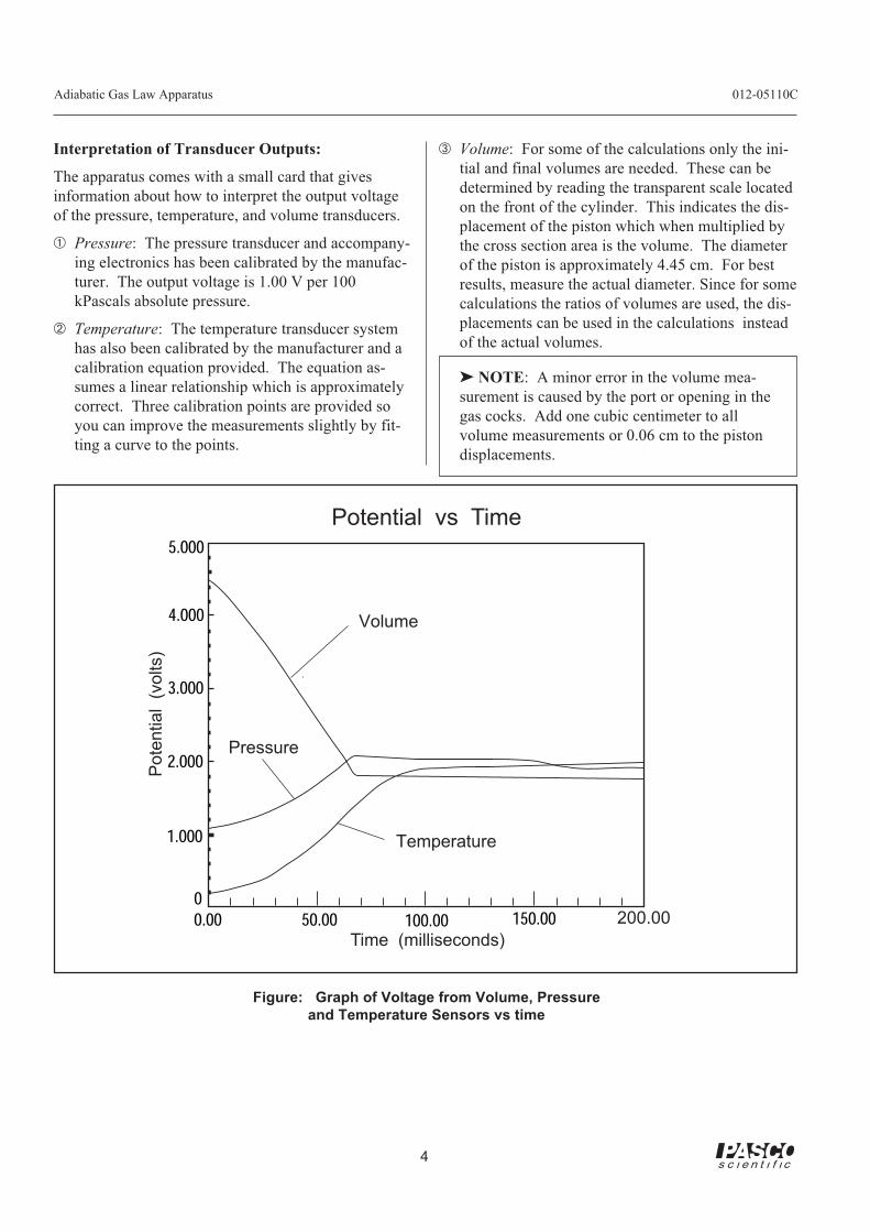
Interpretation of Transducer Outputs:
The apparatus comes with a small card that gives
information about how to interpret the output voltage
of the pressure, temperature, and volume transducers.
À Pressure: The pressure transducer and accompany-
ing electronics has been calibrated by the manufac-
turer. The output voltage is 1.00 V per 100
kPascals absolute pressure.
Á Temperature: The temperature transducer system
has also been calibrated by the manufacturer and a
calibration equation provided. The equation as-
sumes a linear relationship which is approximately
correct. Three calibration points are provided so
you can improve the measurements slightly by fit-
ting a curve to the points.
 Volume: For some of the calculations only the ini-
tial and final volumes are needed. These can be
determined by reading the transparent scale located
on the front of the cylinder. This indicates the dis-
placement of the piston which when multiplied by
the cross section area is the volume. The diameter
of the piston is approximately 4.45 cm. For best
results, measure the actual diameter. Since for some
calculations the ratios of volumes are used, the dis-
placements can be used in the calculations instead
of the actual volumes.
ä NOTE: A minor error in the volume mea-
surement is caused by the port or opening in the
gas cocks. Add one cubic centimeter to all
volume measurements or 0.06 cm to the piston
displacements.
5.000
4.000
3.000
2.000
1.000
00.00 50.00 100.00 150.00 200.00
Time (milliseconds)
Potential vs Time
Pote
ntial (
volts)
Temperature
Pressure
Volume
Figure: Graph of Voltage from Volume, Pressure
and Temperature Sensors vs time
012-05110C Adiabatic Gas Law Apparatus
5
Setup
Connecting the Voltage Supply
Install a nine volt battery (not included) in the battery
compartment located on the front of the electronics
box, OR, connect a "floating ground" external voltage
source to the jacks on the front of the electronics box.
The external power supply must provide a stable DC
voltage source of no more than 15 volts. Set the
indicator switch on the front of the electronics box to
"ON" for battery, or "ON" for an external power
supply, depending on which voltage supply you are
using. If you are using a battery, be sure to switch it
off when you are not using the apparatus.
Connecting the Signal Cables
Connect one of the DIN-plug-to-mini-phone-plug
cables to the output jack for the temperature sensor
(located on the back of the electronics box). Connect
the other cable to the pressure sensor output jack. The
signal cable for the volume sensor (the linear potential
divider) is permanently attached to the base of the
cylinder.
ä CAUTION: DIN connectors on the cables
provided are wired for use with the PASCO
Series 6500 Computer Interface, the Mac65
interface or the MPLI from Vernier Software.
(The pin configuration is shown elsewhere in this
manual. ) If you are using a different interface,
check the pin configuration on the inputs and
make any needed changes before connecting.
CONNECTING A VOLTAGE SOURCE TO
THE OUTPUT JACKS MAY DAMAGE THE
AMPLIFIERS.
Other Setup
Place the piston excursion limit pins in the position
selected to provide the compression ratio desired.
Maximum compression ratio may not give best results.
Using the TD-8565 with the PASCO Series
6500 Computer Interface
IBM compatible computers
À Connect the plug of the volume cable into Analog
Channel A of the Series 6500. Use the adapter
cables supplied with the apparatus to connect the
temperature and pressure sensors to Channels B and
C respectively.
Á Start the Data Monitor program. An ideal operating
mode for learning about the apparatus is the three
channel "L–Oscilloscope" mode. Set the sweep
speed to 20 milliseconds per division and the sensi-
tivity of each channel to 1.00 volts per division.
Move the piston up and down to determine that the
system is operating properly. Make any necessary
adjustments to the sweep speed and sensitivity.
 To facilitate setting the triggering level, return to
the Main Menu and select "M–Monitor Input".
This will allow you to observe the three input volt-
ages. For compressions, the temperature signal
should range from 0.1 volts to +3 volts and for ex-
pansion from 0 volts to about -2 volts. The pres-
sure signal should range from 0 volts to +3 volts for
compression and expansion. The volume signal
should range from +5 volts at highest value to 0
volts.
Return to the Main Menu and choose option “Z–
Calibration". In the calibration menu, choose “Z”
again to calibrate each input, then select the input
you wish to calibrate. Follow the directions given
on the screen.
A: Volume: Hold the piston at the highest position
(≈15.5 cm) and press enter when the reading has
stabilized. Enter the actual volume correspond-
ing to that reading. (Calculate it based on the
position and the radius of the cylinder.) Now put
the piston on the lowest position and enter an-
other calibration point.
B: Temperature: Use the calibration equation pro-
vided with your unit to calculate the temperature
corresponding to the voltage for the first calibra-
tion point. Pressurize the system and quickly
press <Enter> to get a higher reading, then use
the calibration equation again to get the second
point.
Ã
6
Adiabatic Gas Law Apparatus 012-05110C
C: Pressure: Hold the piston at a high position, and
press <Enter> when the reading has stabilized.
The pressure in Pascals is 100,000 times the
voltage from the apparatus; enter this value.
Make sure the gas cocks are closed and move
the piston to a low position. When the reading
has stabilized, press <Enter> and enter the new
pressure.
Now the three inputs are calibrated in SI units.
* The calibration information is on a card on the
side of the unit and also on the underside of the
lid of the battery compartment.
Ä Return to the Main Menu and choose "L–Oscillo-
scope" mode. Set the sweep speed to 20 ms/div
with the right and left arrow keys. Use the up and
down arrow keys and the space bar to set the sensi-
tivity 1 V/div
Go to the triggering menu and set triggering to
"Automatic on channel A". Voltage should be set to
about 4.75 V, and the direction should be "Down".
(Set the voltage threshold level to a voltage just be-
low the maximum you will be using.)
Return to the 'scope and press "S"for single-sweep
mode. Move the piston down sharply to see if all
three traces are showing correctly. You may wish
to change the sweep speed or the volts/div on the
three inputs to get better traces.
Ç Once you have a good trace, exit the oscilloscope
mode making sure that you save the data. Now you
may choose several options, including plotting the
graphs again (together or separately) or plotting
pressure vs. volume as suggested in the lab.
ä NOTE: If you wish to numerically integrate
the pressure vs. volume graph, you must first sort
the data. Choose “O–Other Options"—from the
main menu, then “S” to sort the data. Sort on the
Y axis, with respect to input A. This may take a
few seconds.
Figure: Oscilloscope Mode (MS-DOS version)
Å
Æ
012-05110C Adiabatic Gas Law Apparatus
7
Apple II compatible computers
ä NOTE: Operation with the Apple II series of
computers is severely limited by the speed of the
computer. If there is any other computer you can
use rather than an Apple II, please do so.
À Connection and calibration procedures are as
described for the IBM. We do not recommend cali-
brating the apparatus in SI units, since the round-
off error introduced by the Apple will be greater
than the volume of the cylinder in m3.
Á Because of the input limitations of the Apple II, it
is not possible to graph all three traces in oscillo-
scope mode. Instead, choose "C" for fast data col-
lection.
Enter the delay between data points as 1.0 ms, and
collect about 100 data points. (Actual delay be-
tween readings on individual channels will be 3.0
ms, since the computer alternates channels for each
reading.) Press the space bar when you are ready,
and simultaneously change the volume. The input
is not automatically triggered.
® Once the data is obtained, return to the main menu
and choose “P” to plot the data. The best graphs are
obtained when the inputs are uncalibrated; other-
wise the difference in scales between data sets may
result in only one of the lines being visible.
Expansion of a Gas
To perform a qualitative demonstration of the adiabatic
expansion of a gas, do the following:
Clamp the front foot of the apparatus base to the table.
Fill the cylinder to maximum displacement at atmo-
spheric pressure. Close the gas cock and compress the
gas. Set the trigger level to a value slightly higher than
the steady value and set the slope to positive or "going
up". When ready to take data, compress the gas to this
initial volume, hold it there until equilibrium is
achieved (about 30 seconds), press "S" for Single
Sweep, and then very rapidly expand the gas fully.
When compressing the gas, some work is done against
friction in the cylinder, but the part of the cylinder that
becomes warm is not in contact with the gas. How-
ever, when expanding the gas, the part of the cylinder
that is warmed is in contact with the gas. For this
reason, the expansion data does not give good quanti-
tative results.
Figure: Graph of Voltage vs. time (Apple II version)

8
Adiabatic Gas Law Apparatus 012-05110C
Notes:
012-05110C Adiabatic Gas Law Apparatus
9
EQUIPMENT NEEDED: Optional:
– Adiabatic Gas Law Apparatus, -Monatomic, Diatomic,
– Series 6500 Computer Interface. and Polyatomic Gases.
Purpose
The purpose of this experiment is to show P1V1γ = P2V2
γ and T1V1
(γ–1) = T2V2(γ–1), To
determine the value of Gamma, and to measure the amount of work done to compress a
gas adiabatically.
Theory
In this experiment a gas confined in the cylinder is compressed so rapidly that there is only
sufficient time for a small quantity of thermal energy to escape the gas. For this reason the
process is almost adiabatic. The more rapidly the volume is changed the closer the process
approaches being adiabatic.
ä NOTE: The response times of the pressure and volume transducers are negligibly short.
However the unavoidable thermal inertia of the temperature sensor causes the
temperature measurement to lag by 30-50 ms.
A complete experiment would include the study of gases having different structures
including monatomic argon, diatomic air or nitrogen, and triatomic carbon dioxide.
Procedure
À Select a gas to compress, (Air is a good gas to start with).
Á If you are using a gas other than air, purge the cylinder in the following manner:
a. Connect the gas supply to one of the gas cocks.
ä NOTE: The pressure should be less than 35 kPa or 5 PSI.This prevents damage
from the external gas cylinder or supply to the temperature sensor. The flow of gas
must be kept at a low level to avoid breaking the wire or the sensor.
b. Remove the piston excursion limit pins so the range of volumes is maximum
(approximately 16 to 6).
c. With the piston down and the second gas cock closed, fill the cylinder to maximum
volume with the gas.
d. Now shut the incoming gas cock off and exhaust through the second gas cock.
e. Close the exhaust cock and re-fill with gas.
Repeat this process at least nine more times, ending with a full cylinder. Shut both gas
cocks before performing the experiments. If during the experiment some gas escapes
simply add more.
Experiment: Measurement of Work to Compress
Gases Adiabatically
10
Adiabatic Gas Law Apparatus 012-05110C
Graphs and Data Tables
Now compress the gas while taking data as described in the Setup portion of your manual.
Obtain graphs and a data table for analysis.
Calculations
À From your graphs or data table determine the final pressure and temperature at the time the
compression was completed. By extrapolating the temperature graph, the best value of
temperature can be determined. Using equations 3 and 4 from the Theory section, calcu-
late the theoretical temperature and pressure predicted by the adiabatic gas law. Note that
pressure and temperature must be expressed in absolute units.
Á Plot Pressure vs Volume using a consistent set of units such as Pascals and m3. Perform a
numerical integration to determine the work done on the gas during the adiabatic process.
Next, by integration of the adiabatic gas law, equation 5, determine the theoretical value of
work done and compare with your measured value.
Optional
Plot Log Pressure vs Log Volume and determine Gamma which equals the negative of the
slope.
012-05110C Adiabatic Gas Law Apparatus
11
Schematic
12
Adiabatic Gas Law Apparatus 012-05110C
Specifications / Sample Data
Specifications
Operating Voltage:
9-15 volts DC or 9 volt battery. Higher voltage will
provide capability of increased range in temperature
and pressure measurements. A floating power supply
is required.
Operating Current:
10-12 mA.
Temperature Measurement:
±2 K
Pressure Measurement:
±2 kPa
DIN connector pin configuration: (Pins pointed at
you)
Volume Cable (flat)
Pressure and Temperature Cables (grey)
äNOTE: The Adiabatic Gas Law apparatus
operates ideally with a 12 V DC floating external
supply. However, for most measurements it will
operate satisfactorily with a 9 volt battery. If the
supply voltage is low or the signals very large,
either the pressure or temperature signal ampli-
fier may saturate and truncate the output signal.
If this occurs either increase the operating
voltage or decrease the compression ratio in the
experiment which will reduce the output signal
voltage.
GND
Signal V in
GND
Signal V in
+5 volts
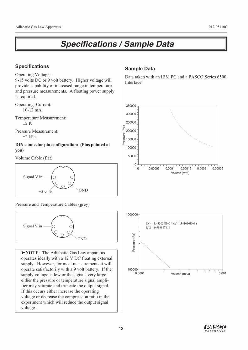
Sample Data
Data taken with an IBM PC and a PASCO Series 6500
Interface.
[[
[[
[[
[[
[
[[
[[
[[
[[[
[[
[[
[
[[
[
[[
[[
[
[[
[
[
[[
[
[
[[
[[
[
[
[[
[
[
[
[[
[
[
[
[
[
[
[
[[
[
[
[
[[
[
[
[
[
[
[
[
[
[
[
[
[
[
[
[
[
[
[
[
[
[
[
[
[
[
[
[
[
[
[
[
[
[
[
[
[
[
[
[
[
[
[
[
[
[
[
[
[
[
[
[
[
[
[
[
[
[
[
0
50000
100000
150000
200000
250000
300000
350000
0 0.00005 0.0001 0.00015 0.0002 0.00025
Pre
ssu
re (
Pa
)
Volume (m^3)
[
[
[[
[[
[
[
[
[
[[
[[
[
[[[
[
[[
[
[
[[
[
[
[[
[
[
[[
[
[
[[
[
[
[
[[
[[
[
[
[[
[
[
[
[[
[
[
[
[
[
[[
[
[
[
[
[[
[[
[
[
[
[
[
[
[
[[
[
[[
[
[
[
[
[
[
[
[
[
[
[
[
[
[
[
[
[
[
[
[
[
[
[
[
[
[
[
[
[
[
[
[
[
[
[
[
[
[
[
[
[
[
[
[
100000
1000000
0.0001 0.001
Pre
ssure
(P
a)
Volume (m^3)
f(x) = 1.433039E+0 * (x^-1.341016E+0 )
R^2 = 9.998867E-1

012-05110C Adiabatic Gas Law Apparatus
13
Technical Support
Contacting Technical Support
Before you call the PASCO Technical Support staff it
would be helpful to prepare the following information:
• If your problem is with the PASCO apparatus, note:
Title and Model number (usually listed on the label).
Approximate age of apparatus.
A detailed description of the problem/sequence of
events. (In case you can't call PASCO right away,
you won't lose valuable data.)
If possible, have the apparatus within reach when
calling. This makes descriptions of individual parts
much easier.
• If your problem relates to the instruction manual,
note:
Part number and Revision (listed by month and year
on the front cover).
Have the manual at hand to discuss your questions.
Feed-Back
If you have any comments about this product or this
manual please let us know. If you have any sugges-
tions on alternate experiments or find a problem in the
manual please tell us. PASCO appreciates any cus-
tomer feed-back. Your input helps us evaluate and
improve our product.
To Reach PASCO
For Technical Support call us at 1-800-772-8700 (toll-
free within the U.S.) or (916) 786-3800.

1
TD-8572
Apparato per le leggi sui gasMotore termico
Manuale di istruzioniCon esperimenti
Ultima revisione: 10/08/2003
ELItalia Srl – Via A. Gross ich 32
20131 Milano – tel 02.236.3972
elitalia@micronet. i t – www.elitalia. i t
2
Diritti d'autore e condizioni di garanzia
Siete autorizzati a duplicare questo manuale, tenendo però conto
delle seguenti norme sui diritti d’autore.
Avvertenze sui diritti d'autore
Tutti i diritti sul presente manuale sono riservati. Si garantisce, comunque, il permesso ad istituzioni
scolastiche di riprodurre qualsiasi parte di questo manuale, a patto che le riproduzioni stesse siano
utilizzate per i laboratori interni e non a scopo di lucro. In qualsiasi altra circostanza e senza
l'autorizzazione scritta della PASCO*, la riproduzione del manuale è vietata.
Limitazioni alla garanzia
La PASCO* garantisce il prodotto contro ogni difetto di fabbricazione o vizio di funzionamento per un
anno dalla data di spedizione al cliente. La PASCO* provvederà a riparare o sostituire, a sua
discrezione, qualsiasi parte del prodotto che presenti difetti di materiale o di fabbricazione. Questa
garanzia non copre i danni causati al prodotto da un uso improprio o errato. Spetta esclusivamente alla
PASCO* determinare se il mancato funzionamento sia dovuto ad un difetto di costruzione oppure ad un
uso improprio da parte dell’utente. La responsabilità della restituzione dell'apparecchiatura per la
riparazione in garanzia è interamente del cliente. L'apparecchiatura stessa deve essere imballata in modo
opportuno per non essere danneggiata durante il trasporto ed i costi di spedizione sono a carico del
cliente. Eventuali, ulteriori danneggiamenti dovuti ad un imballaggio insufficiente durante la
restituzione, non saranno coperti dalla garanzia. Le spese di spedizione, per la restituzione dopo la
riparazione, sono a carico della PASCO*.
Note per la restituzione
Prima di restituire, per qualsiasi motivo, il prodotto alla PASCO*, è necessario avvertire la PASCO* per
lettera o per telefono. Solo dopo questa comunicazione verranno fornite l'autorizzazione alla restituzione
e le istruzioni per la spedizione.
ATTENZIONE: non si accetterà la restituzione di alcun prodotto, senza la previa autorizzazione.
Quando si spedisce l'attrezzatura per la riparazione, ogni pezzo deve essere imballato adeguatamente. I
vettori non accettano responsabilità per i danni causati da un imballaggio inadeguato. Per essere sicuri
che i pezzi non vengano danneggiati durante il trasporto, osservate i seguenti consigli:
1. Scegliete un contenitore sufficientemente resistente.
2. Assicuratevi che su tutti i lati ci siano almeno 5 cm di materiale da imballaggio tra l'apparecchiatura
ed il contenitore.
3. Assicuratevi che il materiale da imballaggio non possa spostarsi o essere compresso, lasciando così
l'apparecchiatura a contatto con le pareti del contenitore.
(*) In Italia: ELItalia Srl, via A. Grossich 32, 20131 MILANO. Tel 02.236.3972, fax 02.236.2467.
WEB: www.elitalia.it e-mail [email protected]
3
Indice
Supporto tecnico 4
Introduzione 5
Esperimento 1: l' ascensore termico 7
Esperimento 2: legge di Charles 9
Esperimento 3: legge di Boyle 11
Esperimento 4: legge dei gas combinata (Gay Lussac) 13
Esperimento 5: la macchina termica per sollevare masse 15
4
Supporto Tecnico
Feed-back
Se avete un qualsiasi commento su questo
prodotto, o sul manuale, fatecelo sapere.
Comunicateci imprecisioni, suggerimenti, nuovi
esperimenti che ritenete significativi. La
PASCO apprezza il feed-back dagli utenti. I
vostri commenti ci aiutano a valutare e
migliorare i nostri prodotti.
Il nostro indirizzo è
c/o ELItalia srl
via A. Grossich 32
20131 MILANO
tel. 02-236.3742 / 236.3972
fax 02-236.2467
e-mail: [email protected]
Assistenza tecnica.
Prima di contattarci per richieste di assistenza
tecnica, è meglio che abbiate a disposizione
queste informazioni:
• Tipo e modello dell' apparato PASCO che
state utilizzando (normalmente tutte le
informazioni sono su un' etichetta sul
prodotto stesso, o sulla confezione).
• L' età approssimativa dell' apparato.
• Una dettagliata descrizione del problema e
delle condizioni in cui si verifica.
• Se possibile, tenete l' apparato a portata di
mano, quando siete al telefono. Ciò rende
l' identificazione delle varie parti alquanto
più semplice.
Se il vostro problema si riferisce al manuale,
abbiate sottomano:
• L' edizione del manuale (sulla copertina)
• Il manuale stesso, per discutere bene del
problema.
Se il vostro problema si riferisce al computer o
ad un software, abbiate sottomano:
• Nome e versione del software.
• Tipo di computer (Marca, modello,
velocità).
• Tipo delle periferiche connesse.
5
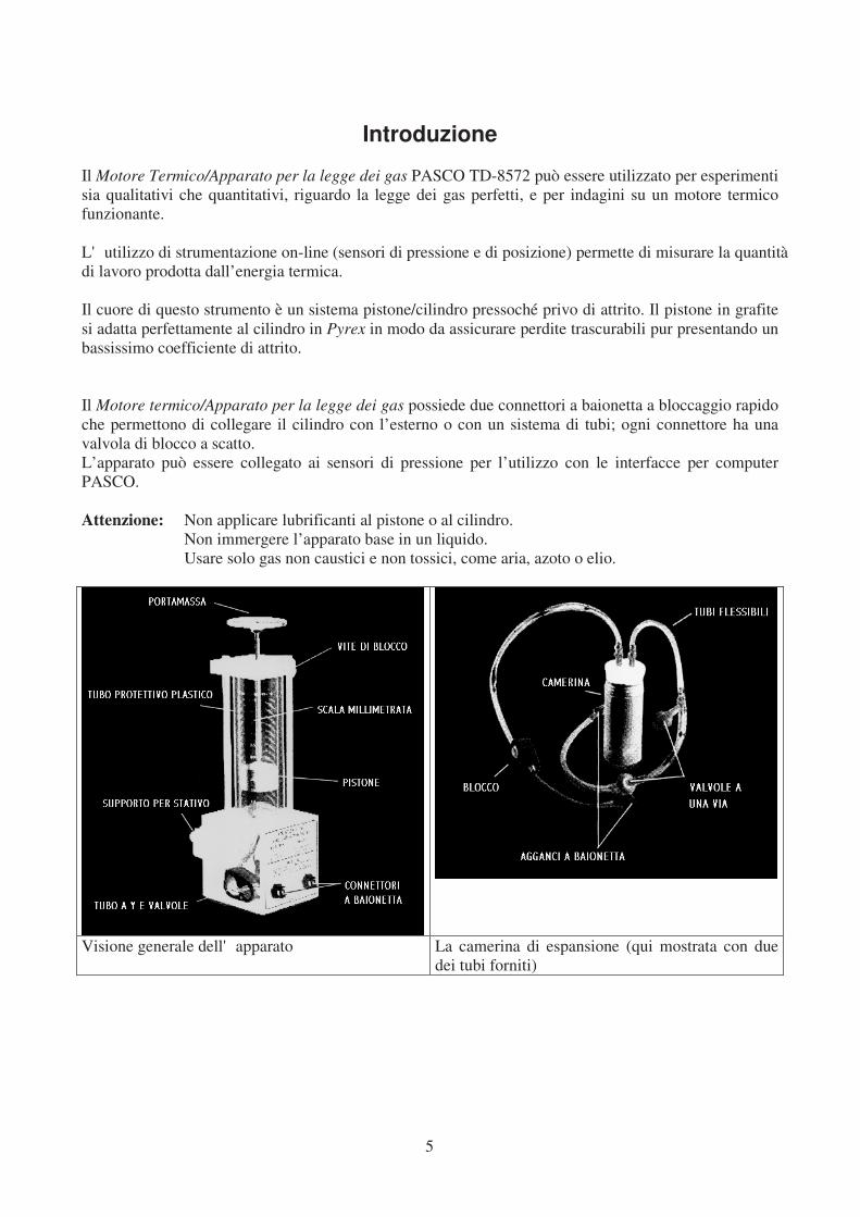
Introduzione
Il Motore Termico/Apparato per la legge dei gas PASCO TD-8572 può essere utilizzato per esperimenti
sia qualitativi che quantitativi, riguardo la legge dei gas perfetti, e per indagini su un motore termico
funzionante.
L' utilizzo di strumentazione on-line (sensori di pressione e di posizione) permette di misurare la quantità
di lavoro prodotta dall’energia termica.
Il cuore di questo strumento è un sistema pistone/cilindro pressoché privo di attrito. Il pistone in grafite
si adatta perfettamente al cilindro in Pyrex in modo da assicurare perdite trascurabili pur presentando un
bassissimo coefficiente di attrito.
Il Motore termico/Apparato per la legge dei gas possiede due connettori a baionetta a bloccaggio rapido
che permettono di collegare il cilindro con l’esterno o con un sistema di tubi; ogni connettore ha una
valvola di blocco a scatto.
L’apparato può essere collegato ai sensori di pressione per l’utilizzo con le interfacce per computer
PASCO.
Attenzione: Non applicare lubrificanti al pistone o al cilindro.
Non immergere l’apparato base in un liquido.
Usare solo gas non caustici e non tossici, come aria, azoto o elio.
Visione generale dell' apparato La camerina di espansione (qui mostrata con due
dei tubi forniti)
6
L’apparato comprende:
• Motore termico vero e proprio (vedi figura)
• Diametro del pistone 32.5 mm ± 0.1
• Massa di pistone e piattaforma portamassa (tutta la parte mobile) 35.0 g ± 0.6
• Camerina d' espansione (vedi figura)
• 3 configurazioni di tubi
• con valvole a senso unico
• con valvola a pinza
• solo tubo
• 2 tappi in gomma
• con foro singolo
• con due fori per l’inserimento del sensore di temperatura
Attenzione: Prima di riporre l’apparato aprire le valvole di blocco poste sul tubo a Y nella base del
motore termico per evitare deformazioni permanenti dei tubi e serrare la vite di blocco del pistone. La
pressione massima sopportabile dal sistema è di 345 kPa (circa 3.4 atm).
Nota sulla tenuta del pistone: Come risulta evidente dal tipo di utilizzo dell' apparato TD-8572, è
necessario che il pistone abbia una buona tenuta e, nel contempo, che abbia bassissimi attriti con la
parete della camera cilindrica. Nonostante l' utilizzo di un pistone di grafite lavorato ad alta precisione
permetta di ottenere degli ottimi risultati è evidente che è stato necessario raggiungere un compromesso,
dato che una tenuta assoluta farebbe si che vi siano forti attriti. Quindi una piccola perdita è accettabile e
permette comunque misure ragionevolmente accurate per esperienze di tipo didattico. Per verificare la
tenuta dell' apparato si esegua la seguente prova:
♣ Portate il pistone in posizione alta
♣ Chiudete accuratamente entrambe le valvole poste sulla base
♣ Ponete 420 gr sulla piattaforma portamassa
♣ Osservate quanti millimetri il pistone scende in 10 secondi, da quando avete appoggiato il peso sul
portamassa
♣ Se il pistone si abbassa meno di 7,8 mm l' apparato ha la tenuta necessaria e garantita
♣ Se li pistone si abbassa più di 7,8 mm:
♣ Controllate bene che le valvole sulla base siano effettivamente serrate
♣ Controllate che i tubicini siano ben fissati alle loro spine sul corpo daell' apparato
♣ Rieseguite la prova di tenuta
♣ Nel caso la prova dia nuovamente risultato negativo contattate il nostro servizio tecnico
7
Esperimento 1: l’ascensore termico
Apparati richiestiMotore termico/Apparato per la legge dei gas Contenitore con acqua ghiacciata
Masse 100 – 200 g Contenitore con acqua calda
Teoria:
Questo esperimento è puramente qualitativo. Si dimostra che una differenza di temperatura è sufficiente
per compiere un lavoro.
Preparazione:
1. Chiudere la camera d’aria con il tappo a foro singolo e collegarla, usando il tubo a Y con le valvole
a senso unico, ad uno dei connettori del' apparato, in modo che l’aria possa fluire nel senso indicato
dalle frecce in figura: l’aria deve essere in grado di passare dall’ambiente esterno alla camera d’aria
e dalla camera d’aria al cilindro del motore termico.
2. Chiudere la valvola di blocco del connettore non
utilizzato, col pistone a circa 1/5 delle corsa.
3. Appoggiare una massa di 100 ÷ 150 g. sulla piatta–
forma del pistone.
Attenzione: ricordarsi di allentare la vite di blocco del
pistone prima di procedere.
Nota: Utilizzare, al massimo, una massa di 200 g; per
masse superiori, infatti, le perdite, attraverso le valvole
e il pistone, non sono più trascurabili.
Procedimento:
1. Immergere la camera d’aria nel bagno di acqua
calda: si noti che l’aria all’interno della camera si
espande facendo innalzare il pistone. La particolare
disposizione delle valvole a senso unico permette
all’aria di passare dalla camera al motore termico senza fuoriuscire dal ramo di tubo libero.
2. Ora spostare la camera nel bagno ghiacciato: l’aria nella camera, contraendosi, richiama altra aria
attraverso la valvola a senso unico posta all’estremità libera del tubo di collegamento, mentre la
seconda valvola impedisce che il motore termico si svuoti mantenendone inalterata l’altezza.
3. Ripetendo più volte i passaggi 1 e 2 è possibile sollevare la massa fino al punto più alto
raggiungibile.

8
Note:
• Maggiore è la differenza di temperatura tra i bagni e maggiore sarà l’innalzamento del pistone e
quindi il lavoro prodotto ad ogni ciclo. Verificatelo.
• Di quanto si alza ogni volta la massa? Potete misurarlo con la scala millimetrata del motore termico.
L' entità di questo innalzamento dipende dalla temperatura dei bagni? E dalla quantità d' aria chiusa
nel sistema motore + camera?
• Per un’indagine quantitativa vedere l’esperimento 5.
9
Esperimento 2: legge di Charles
Apparati richiestiMotore termico/Apparato per la legge dei gas Becker con acqua bollente
Termometro Ghiaccio
Equipaggiamento opzionaleSensore di temperatura Sensore di distanza ad ultrasuoni (o posizione angolare)
Interfaccia per computer Science workshop
Teoria:
La legge di Charles afferma che, a pressione costante, il volume di una certa quantità di gas varia in
modo direttamente proporzionale alla sua temperatura assoluta:
V = cT (dove c è una costante, la pressione è costante e T è espressa in gradi kelvin)
Preparazione:
1. Collegare l’apparato base con la camera d’aria utilizzando il pezzo di tubo semplice.
2. Chiudere la valvola di blocco del connettore libero.
3. Posizionare il cilindro orizzontalmente, in modo che l’unica pressione ad agire sul sistema sia quella
atmosferica che si considera costante per la durata dell’esperimento.
4. Se si dispone dell’interfaccia Science Workshop, inserire il sensore di temperatura nella camera
d’aria (o nel bagno) e misurare lo spostamento del pistone con il sensore di posizione, "puntandolo"
contro la piattaforma; se utilizzate il sensore di posizione angolare, invece, fate passare un filo dalla
piattaforma (c' è un forellino apposta) sulla puleggia del sensore, posto fissato presso il bordo del
tavolo. Il filo sarà teso da una massa modesta (due fermagli, per esempio, quello che basta per far
ruotare la puleggia del sensore). Questo metodo non influenza sensibilmente il motore termico,
anche se ovviamente è meglio usare il sonar.
10
Procedimento:
1. Immergere la camera d’aria nel contenitore di acqua bollente: l’aria, espandendosi, spinge il pistone;
quando il sistema si stabilizza registrare la temperatura e la posizione del pistone; se invece si
dispone di Science Workshop, iniziare l’acquisizione dei dati.
2. Aggiungere ghiaccio in modo da abbassare progressivamente la temperatura e registrare ad intervalli
regolari posizione del pistone e temperatura del bagno (se si utilizza Science Workshop questa
operazione verrà effettuata automaticamente).
3. Calcolare il volume del gas sfruttando la scala millimetrata interna (si ricordi che il diametro del
cilindro è di 32.5 mm ) e disegnare un grafico di temperatura in funzione del volume.
4. Verificare che la relazione è lineare.
Nota per l' uso con Science Workshop: se utilizzate l' interfaccia, predisponete un campionamento al
secondo con partenza e arresto manuale. Ponete il sonar ad una distanza nota dalla piattaforma; potete
misurarla col sonar stesso in modalità Mon del software (ALT+M); annotate questa distanza perché vi
servirà per calcolare il volume del gas in esame.
In questo esempio supponiamo che la distanza iniziale sia 70 cm.
Il gas, contraendosi farà sì che la piattaforma si allontani dal sonar, che rileverà quindi una distanza che
aumenta col passare del tempo (e al diminuire della temperatura del bagno). Il volume della camera va
quindi calcolato col tool calcolatore di Science Workshop con una definizione del tipo
)7.0(0 −⋅−= dAVV
dove:
• V è il volume.
• V0 è un numero che rappresenta il volume iniziale della camera (desumibile dalla scala millimetrata
interna del motore termico) e dall' area del pistone.
• A è l' area del pistone (valore nominale 8.295 cm2).
• d è la distanza misurata dal sonar alla piattaforma. Aggiungendo ghiaccio il gas si contrae e quindi d
aumenta, diventando progressivamente 0.71, 0.72…(se all' inizio è 0.7)
• 0.7 è la distanza iniziale, in metri, tra il sonar e la piattaforma. Si usano i metri perché il sonar
risponde in metri. Questo valore dipende ovviamente dal vostro setup sperimentale.
Vi ricordiamo che per "battere" la definizione della formula nel calcolatore dovete richiamare il tool e
scrivere nella casella una formula simile a:
40-8.295*(@1.x-0.7) [@1.x appare scegliendo "Posizione" dalla lista del tastino INPUT]
(qui supponiamo che V0 sia 40 cc e che d dia 0.7 metri). Come nome della grandezza scegliete
"Volume", come nome breve "V" e come unità di misura "cc".
Nota: a rigore bisognerebbe usare i metri cubi, per il volume, per avere dati numericamente congrui al
sistema SI, ma risulta scomodo trattare i numeri molto piccoli che ne risultano. Ciò non è tuttavia
necessario per verificare la legge di Charles.
11
Esperimento 3: legge di Boyle
Apparati richiestiMotore termico/Apparato per la legge dei gas
Sensore di pressione (CI-6532)
Interfaccia per computer Science workshop, modello "300" o
superiore.
Per dettagli sull’impostazione del sensore di pressione con Science workshop, consultare il foglio di
istruzioni del sensore e il manuale utente di Science workshop.
Teoria:
la legge di Boyle afferma che il prodotto tra la pressione e il volume di un gas, a temperatura costante, è
costante:
PV=a
Quindi, a temperatura fissata, la pressione varia in modo inversamente proporzionale al volume:
V
aP =
Preparazione:
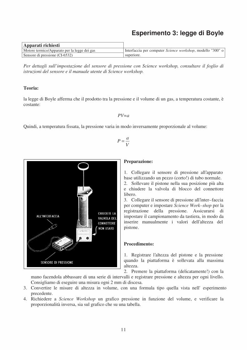
1. Collegare il sensore di pressione all’apparato
base utilizzando un pezzo (corto!) di tubo normale.
2. Sollevare il pistone nella sua posizione più alta
e chiudere la valvola di blocco del connettore
libero.
3. Collegare il sensore di pressione all’inter–faccia
per computer e impostare Science Work–shop per la
registrazione della pressione. Assicurarsi di
impostare il campionamento da tastiera, in modo da
inserire manualmente i valori dell’altezza del
pistone.
Procedimento:
1. Registrare l’altezza del pistone e la pressione
quando la piattaforma è sollevata alla massima
altezza.
2. Premere la piattaforma (delicatamente!) con la
mano facendola abbassare di una serie di intervalli e registrare pressione e altezza per ogni livello.
Consigliamo di eseguire una misura ogni 2 mm di discesa.
3. Convertire le misure di altezza in volume, con una formula tipo quella vista nell' esperimento
precedente.
4. Richiedere a Science Workshop un grafico pressione in funzione del volume, e verificare la
proporzionalità inversa, sia sul grafico che su una tabella.

12
Note:
• Per minimizzare l' errore sul volume dovuto all' aria presente nel tubo, utilizzate un collegamento il
più corto possibile tra il sensore e l' attacco sul motore termico. Tagliate, a questo scopo, un pezzo di
tubo di un centimetro e mezzo circa.
• Per pressioni vicine al limite di tenuta del motore termico la relazione tra P e V può diventare molto
imprecisa a causa delle perdite.
• Potete utilizzare un sensore di forza per "schiacciare" il motore termico. Potrete così verificare la
relazione tra forza e pressione (ricordiamo che la pressione è una forza su una superficie, e l' area dal
pistone è circa 8.3 cm2.
13
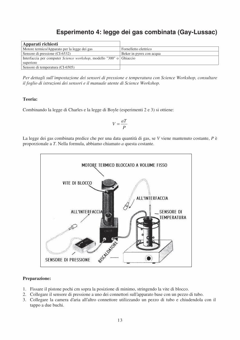
Esperimento 4: legge dei gas combinata (Gay-Lussac)
Apparati richiestiMotore termico/Apparato per la legge dei gas Fornelletto elettrico
Sensore di pressione (CI-6532) Beker in pyrex con acqua
Interfaccia per computer Science workshop, modello "300" o
superiore
Ghiaccio
Sensore di temperatura (CI-6505)
Per dettagli sull’impostazione dei sensori di pressione e temperatura con Science Workshop, consultare
il foglio di istruzioni dei sensori e il manuale utente di Science Workshop.
Teoria:
Combinando la legge di Charles e la legge di Boyle (esperimenti 2 e 3) si ottiene:
P
aTV =
La legge dei gas combinata predice che per una data quantità di gas, se V viene mantenuto costante, P è
proporzionale a T. Nella formula, abbiamo chiamato a questa costante.
Preparazione:
1. Fissare il pistone pochi cm sopra la posizione di minimo, stringendo la vite di blocco.
2. Collegare il sensore di pressione a uno dei connettori sull’apparato base con un pezzo di tubo.
3. Collegare la camera d’aria all’altro connettore utilizzando un pezzo di tubo e chiudendola con il
tappo a due buchi.

14
4. Inserire il sensore di temperatura nell’altro foro del tappo (Per facilitare l’ingresso ed evitare danni
alla sonda è possibile utilizzare un lubrificante al silicone). Nota: è possibile sostituire il sensore di
temperatura con un comune termometro facendo attenzione che il bulbo del termometro stesso non
tocchi il fondo del recipiente. In questo caso campionerete "secondo tastiera", fornendo al computer
la temperatura che leggete sul termometro come "Parametro".
5. Collegare i sensori all’interfaccia per computer e impostare il programma Science Workshop in
modo da mostrare un grafico di temperatura in funzione della pressione.
6. Immergere la camera d’aria nel beker e accendere il fornelletto.
Procedimento:
1. Registrare Pressione e temperatura mentre l’acqua si scalda. Effettuate un campionamento ogni 5
secondi, fino ad ebollizione dell' acqua. Se raccogliete i dati "secondo tastiera" effettuate una lettura
ogni trenta secondi circa fornendo la temperatura, oppure ogni aumento della temperatura di 2°.
2. Visualizzare un grafico di pressione in funzione della temperatura utilizzando Science Workshop, e
verificare la relazione tra P e T.
3. Facoltativa: la costante a nella formula scritta all' inizio di questo esperimento vale ovviamente nR.
Con il valore accettato di R, vi torna n col volume d' aria utilizzato? Quali sono le fonti di errore?
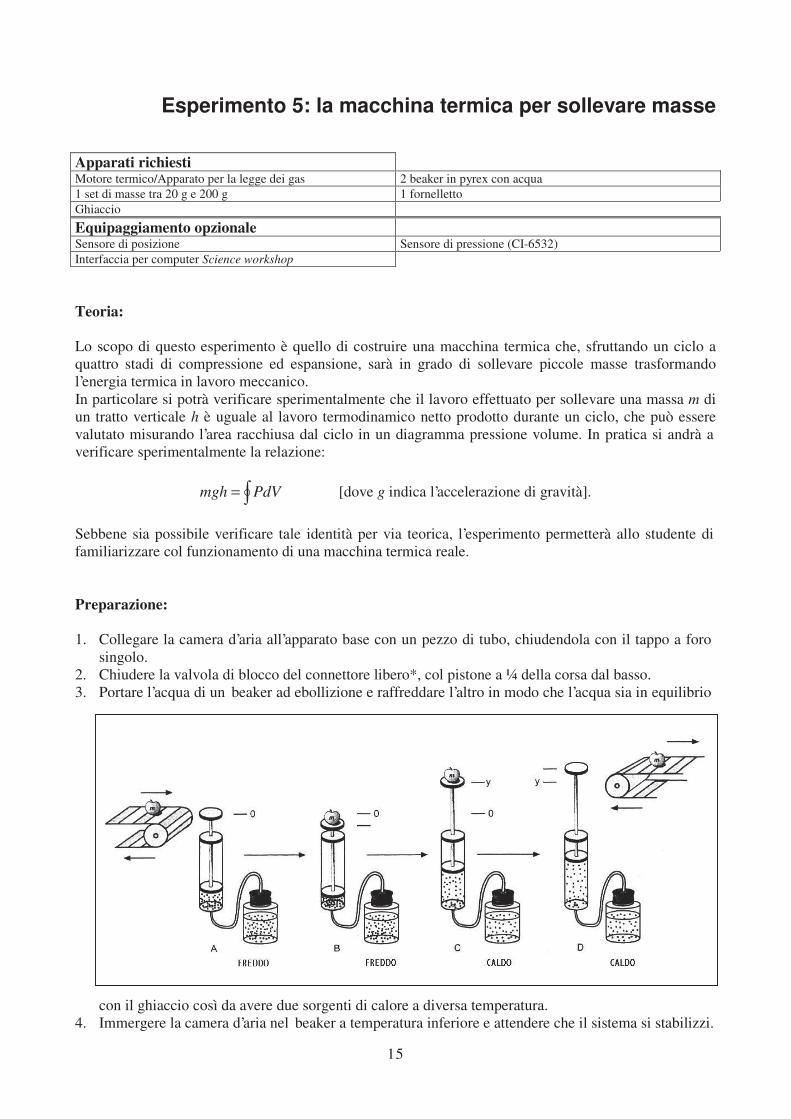
15
Esperimento 5: la macchina termica per sollevare masse
Apparati richiestiMotore termico/Apparato per la legge dei gas 2 beaker in pyrex con acqua
1 set di masse tra 20 g e 200 g 1 fornelletto
Ghiaccio
Equipaggiamento opzionaleSensore di posizione Sensore di pressione (CI-6532)
Interfaccia per computer Science workshop
Teoria:
Lo scopo di questo esperimento è quello di costruire una macchina termica che, sfruttando un ciclo a
quattro stadi di compressione ed espansione, sarà in grado di sollevare piccole masse trasformando
l’energia termica in lavoro meccanico.
In particolare si potrà verificare sperimentalmente che il lavoro effettuato per sollevare una massa m di
un tratto verticale h è uguale al lavoro termodinamico netto prodotto durante un ciclo, che può essere
valutato misurando l’area racchiusa dal ciclo in un diagramma pressione volume. In pratica si andrà a
verificare sperimentalmente la relazione:
∫= PdVmgh [dove g indica l’accelerazione di gravità].
Sebbene sia possibile verificare tale identità per via teorica, l’esperimento permetterà allo studente di
familiarizzare col funzionamento di una macchina termica reale.
Preparazione:
1. Collegare la camera d’aria all’apparato base con un pezzo di tubo, chiudendola con il tappo a foro
singolo.
2. Chiudere la valvola di blocco del connettore libero*, col pistone a ¼ della corsa dal basso.
3. Portare l’acqua di un beaker ad ebollizione e raffreddare l’altro in modo che l’acqua sia in equilibrio
con il ghiaccio così da avere due sorgenti di calore a diversa temperatura.
4. Immergere la camera d’aria nel beaker a temperatura inferiore e attendere che il sistema si stabilizzi.
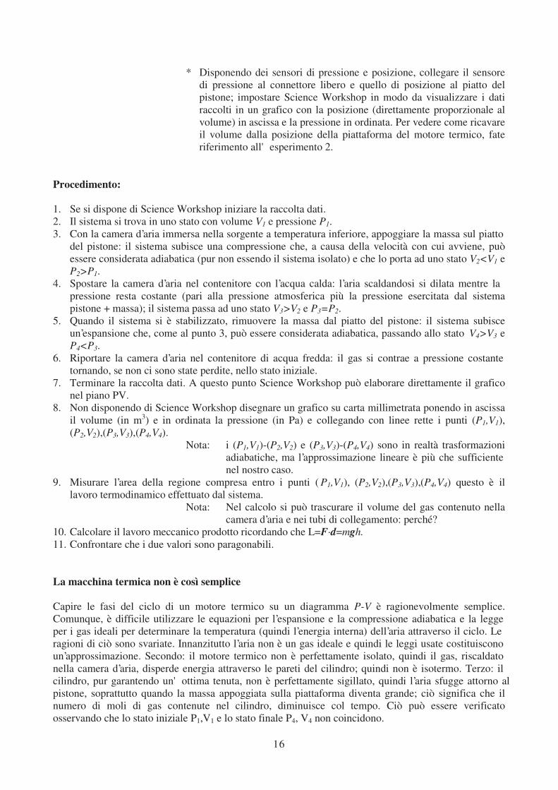
16
* Disponendo dei sensori di pressione e posizione, collegare il sensore
di pressione al connettore libero e quello di posizione al piatto del
pistone; impostare Science Workshop in modo da visualizzare i dati
raccolti in un grafico con la posizione (direttamente proporzionale al
volume) in ascissa e la pressione in ordinata. Per vedere come ricavare
il volume dalla posizione della piattaforma del motore termico, fate
riferimento all' esperimento 2.
Procedimento:
1. Se si dispone di Science Workshop iniziare la raccolta dati.
2. Il sistema si trova in uno stato con volume V1 e pressione P1.
3. Con la camera d’aria immersa nella sorgente a temperatura inferiore, appoggiare la massa sul piatto
del pistone: il sistema subisce una compressione che, a causa della velocità con cui avviene, può
essere considerata adiabatica (pur non essendo il sistema isolato) e che lo porta ad uno stato V2<V1 e
P2>P1.
4. Spostare la camera d’aria nel contenitore con l’acqua calda: l’aria scaldandosi si dilata mentre la
pressione resta costante (pari alla pressione atmosferica più la pressione esercitata dal sistema
pistone + massa); il sistema passa ad uno stato V3>V2 e P3=P2.
5. Quando il sistema si è stabilizzato, rimuovere la massa dal piatto del pistone: il sistema subisce
un’espansione che, come al punto 3, può essere considerata adiabatica, passando allo stato V4>V3 e
P4<P3.
6. Riportare la camera d’aria nel contenitore di acqua fredda: il gas si contrae a pressione costante
tornando, se non ci sono state perdite, nello stato iniziale.
7. Terminare la raccolta dati. A questo punto Science Workshop può elaborare direttamente il grafico
nel piano PV.
8. Non disponendo di Science Workshop disegnare un grafico su carta millimetrata ponendo in ascissa
il volume (in m3) e in ordinata la pressione (in Pa) e collegando con linee rette i punti (P1,V1),
(P2,V2),(P3,V3),(P4,V4).
Nota: i (P1,V1)-(P2,V2) e (P3,V3)-(P4,V4) sono in realtà trasformazioni
adiabatiche, ma l’approssimazione lineare è più che sufficiente
nel nostro caso.
9. Misurare l’area della regione compresa entro i punti ( P1,V1), (P2,V2),(P3,V3),(P4,V4) questo è il
lavoro termodinamico effettuato dal sistema.
Nota: Nel calcolo si può trascurare il volume del gas contenuto nella
camera d’aria e nei tubi di collegamento: perché?
10. Calcolare il lavoro meccanico prodotto ricordando che L=F·d=mgh.
11. Confrontare che i due valori sono paragonabili.
La macchina termica non è così semplice
Capire le fasi del ciclo di un motore termico su un diagramma P-V è ragionevolmente semplice.
Comunque, è difficile utilizzare le equazioni per l’espansione e la compressione adiabatica e la legge
per i gas ideali per determinare la temperatura (quindi l’energia interna) dell’aria attraverso il ciclo. Le
ragioni di ciò sono svariate. Innanzitutto l’aria non è un gas ideale e quindi le leggi usate costituiscono
un’approssimazione. Secondo: il motore termico non è perfettamente isolato, quindi il gas, riscaldato
nella camera d’aria, disperde energia attraverso le pareti del cilindro; quindi non è isotermo. Terzo: il
cilindro, pur garantendo un' ottima tenuta, non è perfettamente sigillato, quindi l’aria sfugge attorno al
pistone, soprattutto quando la massa appoggiata sulla piattaforma diventa grande; ciò significa che il
numero di moli di gas contenute nel cilindro, diminuisce col tempo. Ciò può essere verificato
osservando che lo stato iniziale P1,V1 e lo stato finale P4, V4 non coincidono.
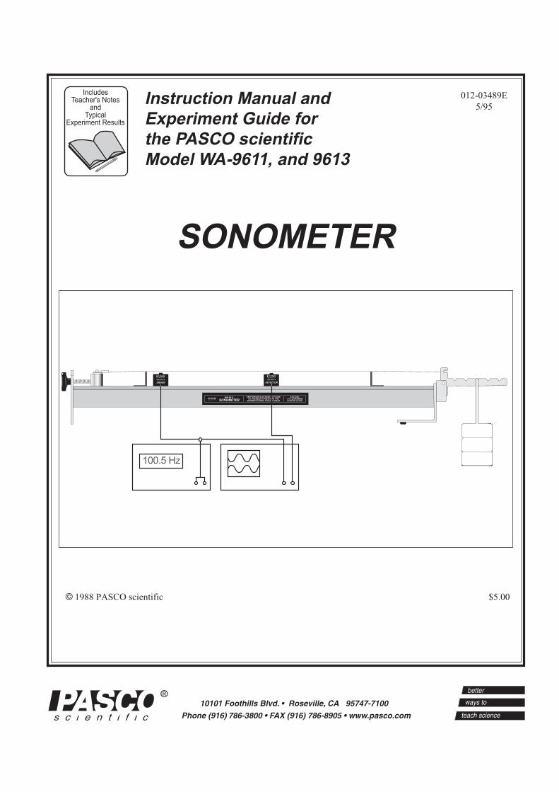
012-03489E
5/95
© 1988 PASCO scientific $5.00
Instruction Manual and
Experiment Guide for
the PASCO scientific
Model WA-9611, and 9613
SONOMETER
DETECTOR
WA-9613
DRIVER
WA-9613
WA-9611
SONOMETERKEEP WEIGHTS AS NEAR TO FLOOR
AS POSSIBLE IN THE EVENT THE SONOMETER WIRE SHOULD BREAK
CAUTION!1.75 kg MAXIMUM LOAD ON LEVER
100.5 Hz
IncludesTeacher's Notes
andTypical
Experiment Results

i
012-03489E Sonometer
Table of Contents
Section Page
Copyright, Warranty and Equipment Return ...................................................... ii
Introduction ...................................................................................................... 1
Equipment ........................................................................................................ 1
Setup and Operation .......................................................................................... 2
Using the Sonometer and the WA-9613 Driver/Detector Coils:
Sonometer w/WA-9613, Driver/Detector Coils ........................................... 3
Sonometer and Driver/Detector w/PASCO Computer Interface ................... 4
Power Amplifier w/Series 6500 Computer Interface .................................... 4
Power Amplifier w/CI-6550 or CI-6565 Computer Interface ....................... 4
Function Generator w/Series 6500 Computer Interface ................................ 5
Function Generator w/CI-6550 or CI-6565 Computer Interface ................... 6
Replacing Sonometer Strings ............................................................................ 7
Theory of Waves on a Stretched String .............................................................. 8
Experiments:
Experiment 1: Resonance Modes of a Stretched String ........................ 11
Experiment 2: Velocity of Wave Propagation ...................................... 13
Suggested Research Topics .............................................................................. 16
Teacher’s Guide ............................................................................................... 17
Technical Support .................................................................... Inside Back Cover
ii
Sonometer 012-03489E
Copyright Notice
The PASCO scientific Model WA-9611 Sonometer
manual is copyrighted and all rights reserved. However,
permission is granted to non-profit educational institu-
tions for reproduction of any part of this manual provid-
ing the reproductions are used only for their laboratories
and are not sold for profit. Reproduction under any other
circumstances, without the written consent of PASCO
scientific, is prohibited.
Limited Warranty
PASCO scientific warrants this product to be free from
defects in materials and workmanship for a period of one
year from the date of shipment to the customer. PASCO
will repair or replace, at its option, any part of the product
which is deemed to be defective in material or workman-
ship. This warranty does not cover damage to the product
caused by abuse or improper use. Determination of
whether a product failure is the result of a manufacturing
defect or improper use by the customer shall be made
solely by PASCO scientific. Responsibility for the return
of equipment for warranty repair belongs to the customer.
Equipment must be properly packed to prevent damage
and shipped postage or freight prepaid. (Damage caused
by improper packing of the equipment for return ship-
ment will not be covered by the warranty.) Shipping
costs for returning the equipment, after repair, will be
paid by PASCO scientific.
Copyright, Warranty and Equipment Return
Please—Feel free to duplicate this manual
subject to the copyright restrictions below.
Credits
This manual authored by: Clarence Bakken
This manual edited by: Dave Griffith
Teacher’s guide written by: Eric Ayars
Equipment Return
Should the product have to be returned to PASCO
scientific for any reason, notify PASCO scientific by
letter, phone, or fax BEFORE returning the product.
Upon notification, the return authorization and
shipping instructions will be promptly issued.
When returning equipment for repair, the units
must be packed properly. Carriers will not accept
responsibility for damage caused by improper
packing. To be certain the unit will not be
damaged in shipment, observe the following rules:
➀ The packing carton must be strong enough for the
item shipped.
➁ Make certain there are at least two inches of
packing material between any point on the
apparatus and the inside walls of the carton.
➂ Make certain that the packing material cannot shift
in the box or become compressed, allowing the
instrument come in contact with the packing
carton.
Address: PASCO scientific
10101 Foothills Blvd.
Roseville, CA 95747-7100
Phone: (916) 786-3800
FAX: (916) 786-3292
email: [email protected]
web: www.pasco.com
NOTE: NO EQUIPMENT WILL BE
ACCEPTED FOR RETURN WITHOUT AN
AUTHORIZATION FROM PASCO.
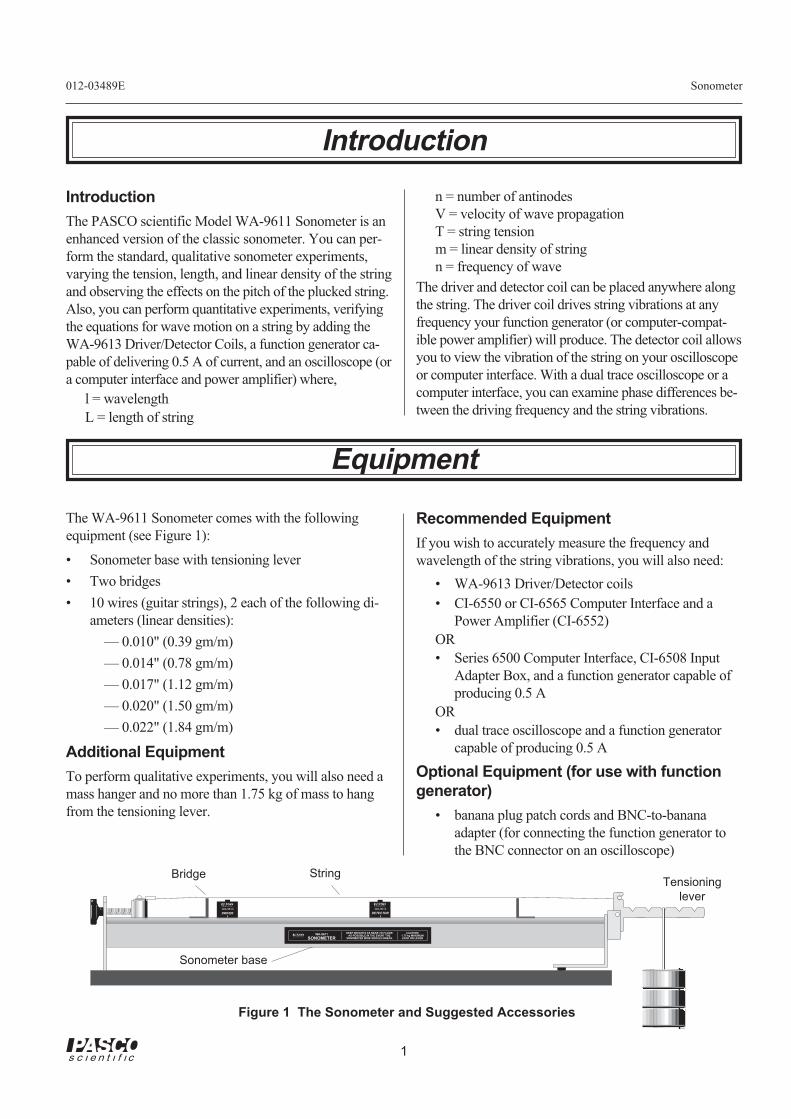
1
012-03489E Sonometer
Introduction
Figure 1 The Sonometer and Suggested Accessories
DETECTOR
WA-9613
DRIVER
WA-9613
WA-9611
SONOMETER
KEEP WEIGHTS AS NEAR TO FLOORAS POSSIBLE IN THE EVENT THE
SONOMETER WIRE SHOULD BREAK
CAUTION!1.75 kg MAXIMUMLOAD ON LEVER
Bridge StringTensioning
lever
Sonometer base
Introduction
The PASCO scientific Model WA-9611 Sonometer is an
enhanced version of the classic sonometer. You can per-
form the standard, qualitative sonometer experiments,
varying the tension, length, and linear density of the string
and observing the effects on the pitch of the plucked string.
Also, you can perform quantitative experiments, verifying
the equations for wave motion on a string by adding the
WA-9613 Driver/Detector Coils, a function generator ca-
pable of delivering 0.5 A of current, and an oscilloscope (or
a computer interface and power amplifier) where,
l = wavelength
L = length of string
n = number of antinodes
V = velocity of wave propagation
T = string tension
m = linear density of string
n = frequency of wave
The driver and detector coil can be placed anywhere along
the string. The driver coil drives string vibrations at any
frequency your function generator (or computer-compat-
ible power amplifier) will produce. The detector coil allows
you to view the vibration of the string on your oscilloscope
or computer interface. With a dual trace oscilloscope or a
computer interface, you can examine phase differences be-
tween the driving frequency and the string vibrations.
Equipment
The WA-9611 Sonometer comes with the following
equipment (see Figure 1):
• Sonometer base with tensioning lever
• Two bridges
• 10 wires (guitar strings), 2 each of the following di-
ameters (linear densities):
— 0.010" (0.39 gm/m)
— 0.014" (0.78 gm/m)
— 0.017" (1.12 gm/m)
— 0.020" (1.50 gm/m)
— 0.022" (1.84 gm/m)
Additional Equipment
To perform qualitative experiments, you will also need a
mass hanger and no more than 1.75 kg of mass to hang
from the tensioning lever.
Recommended Equipment
If you wish to accurately measure the frequency and
wavelength of the string vibrations, you will also need:
• WA-9613 Driver/Detector coils
• CI-6550 or CI-6565 Computer Interface and a
Power Amplifier (CI-6552)
OR
• Series 6500 Computer Interface, CI-6508 Input
Adapter Box, and a function generator capable of
producing 0.5 A
OR
• dual trace oscilloscope and a function generator
capable of producing 0.5 A
Optional Equipment (for use with function
generator)
• banana plug patch cords and BNC-to-banana
adapter (for connecting the function generator to
the BNC connector on an oscilloscope)
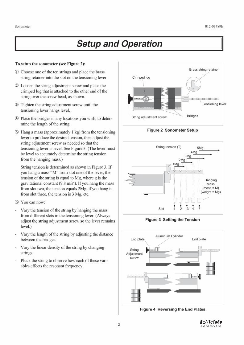
2
Sonometer 012-03489E
To setup the sonometer (see Figure 2):
➀ Choose one of the ten strings and place the brass
string retainer into the slot on the tensioning lever.
➁ Loosen the string adjustment screw and place the
crimped lug that is attached to the other end of the
string over the screw head, as shown.
➂ Tighten the string adjustment screw until the
tensioning lever hangs level.
➃ Place the bridges in any locations you wish, to deter-
mine the length of the string.
➄ Hang a mass (approximately 1 kg) from the tensioning
lever to produce the desired tension, then adjust the
string adjustment screw as needed so that the
tensioning lever is level. See Figure 3. (The lever must
be level to accurately determine the string tension
from the hanging mass.)
String tension is determined as shown in Figure 3. If
you hang a mass “M” from slot one of the lever, the
tension of the string is equal to Mg, where g is the
gravitational constant (9.8 m/s2). If you hang the mass
from slot two, the tension equals 2Mg; if you hang it
from slot three, the tension is 3 Mg, etc.
➅ You can now:
- Vary the tension of the string by hanging the mass
from different slots in the tensioning lever. (Always
adjust the string adjustment screw so the lever remains
level.)
- Vary the length of the string by adjusting the distance
between the bridges.
- Vary the linear density of the string by changing
strings.
- Pluck the string to observe how each of these vari-
ables effects the resonant frequency.
Setup and Operation
Tensioning lever
String adjustment screw
Brass string retainer
Crimped lug
Bridges
Figure 2 Sonometer Setup
Figure 3 Setting the Tension
Hanging
Mass
(mass = M)
(weight = Mg)
1Mg
2Mg
3Mg
4Mg
5MgString tension (T)
Figure 4 Reversing the End Plates
Aluminum CylinderEnd plate
String
Adjustment
screw
End plate
Slot 1 2 3 4 5
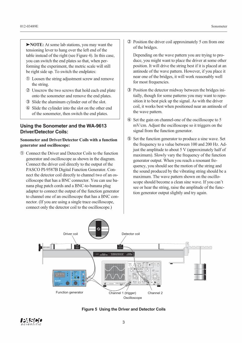
3
012-03489E Sonometer
NOTE: At some lab stations, you may want the
tensioning lever to hang over the left end of the
table instead of the right (see Figure 4). In this case,
you can switch the end plates so that, when per-
forming the experiment, the metric scale will still
be right side up. To switch the endplates:
➀ Loosen the string adjustment screw and remove
the string.
➁ Unscrew the two screws that hold each end plate
onto the sonometer and remove the end plates.
➂ Slide the aluminum cylinder out of the slot.
➃ Slide the cylinder into the slot on the other end
of the sonometer, then switch the end plates.
Using the Sonometer and the WA-9613
Driver/Detector Coils:
Sonometer and Driver/Detector Coils with a function
generator and oscilloscope:
➀ Connect the Driver and Detector Coils to the function
generator and oscilloscope as shown in the diagram.
Connect the driver coil directly to the output of the
PASCO PI-9587B Digital Function Generator. Con-
nect the detector coil directly to channel two of an os-
cilloscope that has a BNC connector. You can use ba-
nana plug patch cords and a BNC-to-banana plug
adapter to connect the output of the function generator
to channel one of an oscilloscope that has a BNC con-
nector. (If you are using a single trace oscilloscope,
connect only the detector coil to the oscilloscope.)
➁ Position the driver coil approximately 5 cm from one
of the bridges.
Depending on the wave pattern you are trying to pro-
duce, you might want to place the driver at some other
position. It will drive the string best if it is placed at an
antinode of the wave pattern. However, if you place it
near one of the bridges, it will work reasonably well
for most frequencies.
➂ Position the detector midway between the bridges ini-
tially, though for some patterns you may want to repo-
sition it to best pick up the signal. As with the driver
coil, it works best when positioned near an antinode of
the wave pattern.
➃ Set the gain on channel-one of the oscilloscope to 5
mV/cm. Adjust the oscilloscope so it triggers on the
signal from the function generator.
➄ Set the function generator to produce a sine wave. Set
the frequency to a value between 100 and 200 Hz. Ad-
just the amplitude to about 5 V (approximately half of
maximum). Slowly vary the frequency of the function
generator output. When you reach a resonant fre-
quency, you should see the motion of the string and
the sound produced by the vibrating string should be a
maximum. The wave pattern shown on the oscillo-
scope should become a clean sine wave. If you can’t
see or hear the string, raise the amplitude of the func-
tion generator output slightly and try again.
Figure 5 Using the Driver and Detector Coils
Driver coil Detector coil
WA-9611
SONOMETER
KEEP WEIGHTS AS NEAR TO FLOORAS POSSIBLE IN THE EVENT THE
SONOMETER WIRE SHOULD BREAK
CAUTION!1.75 kg MAXIMUMLOAD ON LEVER
BK PRECISION 200 Mhz OSCILLISCOPEMODEL2120
INTENSITY FOCUS
TRACE NOTATION
TRIG LEVEL
COUPLE SOURCE
SLOPE λ - Y
TIME/DIV
X-POS
VAR VAR
VAR SWEEP
CAL CALmVV
CH 1VOLTZ/DIV
CH 2VOLTZ/DIV
CALmVV
VERTICAL MODE
PULL XS PULL XS
CH 2 ∞CH 1 ∞
AC
DC
AC
DC
AC CH1
CH2
ALT
EXT
POS POSNORMEXT
CH1CH2
NORMEXT
CH1CH2
MANUAL AUTO
T X-Y
T X-Y
LINE
CAL EXT CH4
POWER200VMAX
400VMAX
400VMAX
- +
+
-
T TL
H IΩ
GN D
L OΩ
M IN
R AN G E
A D J US T
MA X
OUTPUT
FREQUENCY
AMPLITUDE
PI -9587BDIGITAL FUNCTIONGENERATOR -AMPLIF IER
H ER T Z
WAVEFORM
I N PU T
GN D
E X T ERNA L
DETECTOR
WA-9613
DRIVER
WA-9613
Oscilloscope
Channel 1 (trigger) Channel 2Function generator
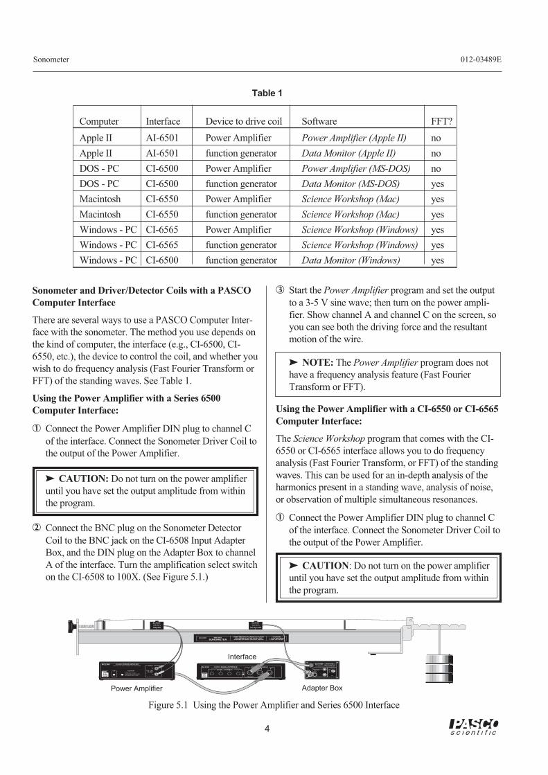
4
Sonometer 012-03489E
➂ Start the Power Amplifier program and set the output
to a 3-5 V sine wave; then turn on the power ampli-
fier. Show channel A and channel C on the screen, so
you can see both the driving force and the resultant
motion of the wire.
NOTE: The Power Amplifier program does not
have a frequency analysis feature (Fast Fourier
Transform or FFT).
Using the Power Amplifier with a CI-6550 or CI-6565
Computer Interface:
The Science Workshop program that comes with the CI-
6550 or CI-6565 interface allows you to do frequency
analysis (Fast Fourier Transform, or FFT) of the standing
waves. This can be used for an in-depth analysis of the
harmonics present in a standing wave, analysis of noise,
or observation of multiple simultaneous resonances.
➀ Connect the Power Amplifier DIN plug to channel C
of the interface. Connect the Sonometer Driver Coil to
the output of the Power Amplifier.
CAUTION: Do not turn on the power amplifier
until you have set the output amplitude from within
the program.
Table 1
Sonometer and Driver/Detector Coils with a PASCO
Computer Interface
There are several ways to use a PASCO Computer Inter-
face with the sonometer. The method you use depends on
the kind of computer, the interface (e.g., CI-6500, CI-
6550, etc.), the device to control the coil, and whether you
wish to do frequency analysis (Fast Fourier Transform or
FFT) of the standing waves. See Table 1.
Using the Power Amplifier with a Series 6500
Computer Interface:
➀ Connect the Power Amplifier DIN plug to channel C
of the interface. Connect the Sonometer Driver Coil to
the output of the Power Amplifier.
CAUTION: Do not turn on the power amplifier
until you have set the output amplitude from within
the program.
➁ Connect the BNC plug on the Sonometer Detector
Coil to the BNC jack on the CI-6508 Input Adapter
Box, and the DIN plug on the Adapter Box to channel
A of the interface. Turn the amplification select switch
on the CI-6508 to 100X. (See Figure 5.1.)
Computer Interface Device to drive coil Software FFT?
Apple II AI-6501 Power Amplifier Power Amplifier (Apple II) no
Apple II AI-6501 function generator Data Monitor (Apple II) no
DOS - PC CI-6500 Power Amplifier Power Amplifier (MS-DOS) no
DOS - PC CI-6500 function generator Data Monitor (MS-DOS) yes
Macintosh CI-6550 Power Amplifier Science Workshop (Mac) yes
Macintosh CI-6550 function generator Science Workshop (Mac) yes
Windows - PC CI-6565 Power Amplifier Science Workshop (Windows) yes
Windows - PC CI-6565 function generator Science Workshop (Windows) yes
Windows - PC CI-6500 function generator Data Monitor (Windows) yes
WA-9611
SONOMETER
KEEP WEIGHTS AS NEAR TO FLOORAS POSSIBLE IN THE EVENT THE
SONOMETER WIRE SHOULD BREAK
CAUTION!1.75 kg MAXIMUMLOAD ON LEVER
1 2 3 4
DIGITAL CHANNELS
ANALOG CHANNELS
A B C
ON
GAIN = 1,10,100ISOLATED
GAIN = 1ISOLATED
GAIN = 1REF TO GND
INTERFACESYSTEM
PASCO
6500SERIES
CI-6510 SIGNAL INTERFACEFOR USE WITH PASCO SERIES 6500 SENSORS
CI-6502 POWER AMPLIFIERFOR USE WITH PASCO SERIES 6500 INTERFACES
ON
+
INTERFACESYSTEM
PASCO
6500SERIES
SIGNAL OUTPUT
0 to ±10 V1 A MAX
CAUTION!
WHEN LIGHT IS ON
WAVEFORM IS DISTORTED.
DECREASE AMPLITUDE!
GAIN SELECT
NOTE: SWITCHFUNTIONS ONLY WHEN
ADAPTOR ISCONNECTED TO INPUT
MARKED ON THESIGNAL INTERFACE
X 100
X 10
X 1
INTERFACESYSTEM
PASCO
6500SERIES
ANALOG INPUT(±10V MAX)
INPUT ADAPTORFOR USE WITH PASCO SERIES 6500 INTERFACES
Model CI-6508
DRIVER
WA-9613
DETECTOR
WA-9613
Figure 5.1 Using the Power Amplifier and Series 6500 Interface
Power Amplifier Adapter Box
Interface
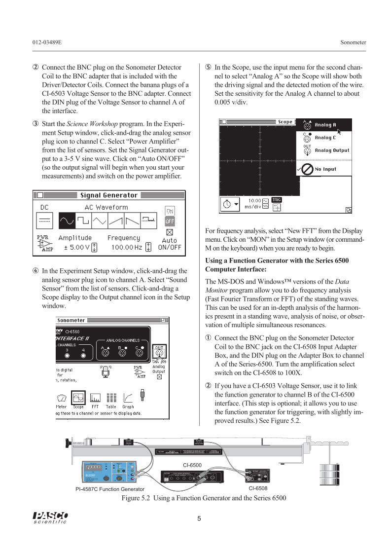
5
012-03489E Sonometer
➁ Connect the BNC plug on the Sonometer Detector
Coil to the BNC adapter that is included with the
Driver/Detector Coils. Connect the banana plugs of a
CI-6503 Voltage Sensor to the BNC adapter. Connect
the DIN plug of the Voltage Sensor to channel A of
the interface.
➂ Start the Science Workshop program. In the Experi-
ment Setup window, click-and-drag the analog sensor
plug icon to channel C. Select “Power Amplifier”
from the list of sensors. Set the Signal Generator out-
put to a 3-5 V sine wave. Click on “Auto ON/OFF”
(so the output signal will begin when you start your
measurements) and switch on the power amplifier.
➃ In the Experiment Setup window, click-and-drag the
analog sensor plug icon to channel A. Select “Sound
Sensor” from the list of sensors. Click-and-drag a
Scope display to the Output channel icon in the Setup
window.
➄ In the Scope, use the input menu for the second chan-
nel to select “Analog A” so the Scope will show both
the driving signal and the detected motion of the wire.
Set the sensitivity for the Analog A channel to about
0.005 v/div.
For frequency analysis, select “New FFT” from the Display
menu. Click on “MON” in the Setup window (or command-
M on the keyboard) when you are ready to begin.
Using a Function Generator with the Series 6500
Computer Interface:
The MS-DOS and Windows™ versions of the DataMonitor program allow you to do frequency analysis
(Fast Fourier Transform or FFT) of the standing waves.
This can be used for an in-depth analysis of the harmon-
ics present in a standing wave, analysis of noise, or obser-
vation of multiple simultaneous resonances.
➀ Connect the BNC plug on the Sonometer Detector
Coil to the BNC jack on the CI-6508 Input Adapter
Box, and the DIN plug on the Adapter Box to channel
A of the Series-6500. Turn the amplification select
switch on the CI-6508 to 100X.
➁ If you have a CI-6503 Voltage Sensor, use it to link
the function generator to channel B of the CI-6500
interface. (This step is optional; it allows you to use
the function generator for triggering, with slightly im-
proved results.) See Figure 5.2.
WA-9611
SONOMETER
KEEP WEIGHTS AS NEAR TO FLOORAS POSSIBLE IN THE EVENT THE
SONOMETER WIRE SHOULD BREAK
CAUTION!1.75 kg MAXIMUMLOAD ON LEVER
T TL
H IΩ
GN D
L OΩ
M IN
R AN G E
A D J US T
MA X
OUTPUT
FREQUENCY
AMPLITUDE
PI -9587BDIGITAL FUNCTIONGENERATOR -AMPLIF IER
H ER T Z
WAVEFORM
I N PU T
GN D
E X T ERNA L
1 2 3 4
DIGITAL CHANNELS
ANALOG CHANNELS
A B C
ON
GAIN = 1,10,100ISOLATED
GAIN = 1ISOLATED
GAIN = 1REF TO GND
INTERFACESYSTEM
PASCO
6500SERIES
CI-6510 SIGNAL INTERFACEFOR USE WITH PASCO SERIES 6500 SENSORS GAIN SELECT
NOTE: SWITCHFUNTIONS ONLY WHEN
ADAPTOR ISCONNECTED TO INPUT
MARKED ON THESIGNAL INTERFACE
X 100
X 10
X 1
INTERFACESYSTEM
PASCO
6500SERIES
ANALOG INPUT(±10V MAX)
INPUT ADAPTORFOR USE WITH PASCO SERIES 6500 INTERFACES
Model CI-6508
DRIVER
WA-9613
DETECTOR
WA-9613
Figure 5.2 Using a Function Generator and the Series 6500
CI-6508
CI-6500
PI-4587C Function Generator

6
Sonometer 012-03489E
➂ Set the function generator to produce a sine wave. Set
the frequency to a value between 100 and 200 Hz. Ad-
just the amplitude to about 5 V (approximately half of
maximum). Slowly vary the frequency of the function
generator output. When you reach a resonant frequency,
you should see the motion of the string and the sound
produced by the vibrating string should be a maximum.
For the Data Monitor (MS-DOS) Program:
Start the program. Select “Oscilloscope” from the Main
Menu. Set triggering to automatic on channel B. Show
channels A and B on the screen, and find the resonances
you are interested in. If you wish, turn on the frequency
analysis option (FFT) and observe the frequencies that are
contributing to the standing wave.
For the Data Monitor (Windows™) Program:
Start the program. Choose “Select Channels” from the
Experiment menu and turn off channel C. Select “Replace
Window” from the Window menu, and change the Plot-
ter/Graph window to an Oscilloscope window. Repeat the
process to change the Data Table window to the FFT win-
dow. Click on “Trigger” to set the triggering for channel B.
Using a Function Generator with a CI-6550 or CI-
6565 Computer Interface:
The Science Workshop program that comes with the CI-
6550 or CI-6565 interface allows you to do frequency
analysis (Fast Fourier Transform, or FFT) of the standing
waves. This can be used for an in-depth analysis of the
harmonics present in a standing wave, analysis of noise,
or observation of multiple simultaneous resonances.
➀ Connect the BNC plug on the Sonometer Detector
Coil to the BNC adapter that is included with the
Driver/Detector Coils. Connect the banana plugs of a
CI-6503 Voltage Sensor to the BNC adapter. Connect
the DIN plug of the Voltage Sensor to channel A of
the interface.
If you have another CI-6503 Voltage Sensor, use it to
link the function generator to channel B of the com-
puter interface. (This step is optional; it allows you to
use the function generator for triggering, with slightly
improved results.)
➁ Start the Science Workshop program. In the Experi-
ment Setup window, click-and-drag the analog sensor
plug icon to channel A. Select “Sound Sensor” from
the list of sensors. If you have connected a Voltage
Sensor from the function generator to channel B,
click-and-drag the analog sensor plug icon to channel
B and select “Voltage Sensor” from the list of sensors.
➂ To view the data, click-and-drag a Scope display to
the Sound Sensor icon. (If you have connected a Volt-
age Sensor from the function generator to channel B,
use the input menu of the first channel on the Scope to
switch the input to “Analog B”. Use the input menu of
the second channel on the Scope to select “Analog A”.
This will allow you to use the function generator for
triggering.) Set the sensitivity for the Analog A chan-
nel to about 0.005 v/div. Click on “MON” to begin
measuring data.
➃ Set the function generator to produce a sine wave. Set
the frequency to a value between 100 and 200 Hz. Ad-
just the amplitude to about 5 V (approximately half of
maximum). Slowly vary the frequency of the function
generator output. When you reach a resonant fre-
quency, you should see the motion of the string and
the sound produced by the vibrating string should be a
maximum.
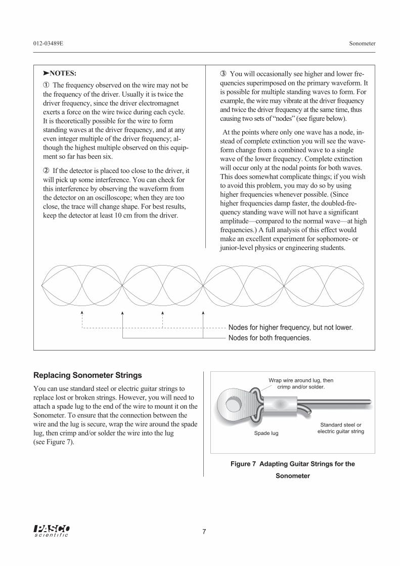
7
012-03489E Sonometer
➂ You will occasionally see higher and lower fre-
quencies superimposed on the primary waveform. It
is possible for multiple standing waves to form. For
example, the wire may vibrate at the driver frequency
and twice the driver frequency at the same time, thus
causing two sets of “nodes” (see figure below).
At the points where only one wave has a node, in-
stead of complete extinction you will see the wave-
form change from a combined wave to a single
wave of the lower frequency. Complete extinction
will occur only at the nodal points for both waves.
This does somewhat complicate things; if you wish
to avoid this problem, you may do so by using
higher frequencies whenever possible. (Since
higher frequencies damp faster, the doubled-fre-
quency standing wave will not have a significant
amplitude—compared to the normal wave—at high
frequencies.) A full analysis of this effect would
make an excellent experiment for sophomore- or
junior-level physics or engineering students.
NOTES:
➀ The frequency observed on the wire may not be
the frequency of the driver. Usually it is twice the
driver frequency, since the driver electromagnet
exerts a force on the wire twice during each cycle.
It is theoretically possible for the wire to form
standing waves at the driver frequency, and at any
even integer multiple of the driver frequency; al-
though the highest multiple observed on this equip-
ment so far has been six.
➁ If the detector is placed too close to the driver, it
will pick up some interference. You can check for
this interference by observing the waveform from
the detector on an oscilloscope; when they are too
close, the trace will change shape. For best results,
keep the detector at least 10 cm from the driver.
Replacing Sonometer Strings
You can use standard steel or electric guitar strings to
replace lost or broken strings. However, you will need to
attach a spade lug to the end of the wire to mount it on the
Sonometer. To ensure that the connection between the
wire and the lug is secure, wrap the wire around the spade
lug, then crimp and/or solder the wire into the lug
(see Figure 7).
Wrap wire around lug, then
crimp and/or solder.
Figure 7 Adapting Guitar Strings for the
Sonometer
Standard steel or
electric guitar stringSpade lug
Nodes for higher frequency, but not lower.
Nodes for both frequencies.
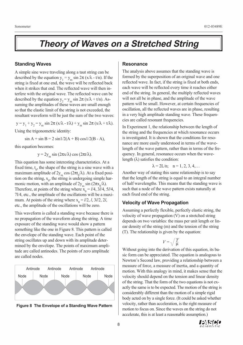
8
Sonometer 012-03489E
Theory of Waves on a Stretched String
Resonance
The analysis above assumes that the standing wave is
formed by the superposition of an original wave and one
reflected wave. In fact, if the string is fixed at both ends,
each wave will be reflected every time it reaches either
end of the string. In general, the multiply reflected waves
will not all be in phase, and the amplitude of the wave
pattern will be small. However, at certain frequencies of
oscillation, all the reflected waves are in phase, resulting
in a very high amplitude standing wave. These frequen-
cies are called resonant frequencies.
In Experiment 1, the relationship between the length of
the string and the frequencies at which resonance occurs
is investigated. It is shown that the conditions for reso-
nance are more easily understood in terms of the wave-
length of the wave pattern, rather than in terms of the fre-
quency. In general, resonance occurs when the wave-
length (λ) satisfies the condition:
λ = 2L/n; n = 1, 2, 3, 4,…
Another way of stating this same relationship is to say
that the length of the string is equal to an integral number
of half wavelengths. This means that the standing wave is
such that a node of the wave pattern exists naturally at
each fixed end of the string.
Velocity of Wave Propagation
Assuming a perfectly flexible, perfectly elastic string, the
velocity of wave propagation (V) on a stretched string
depends on two variables: the mass per unit length or lin-
ear density of the string (m) and the tension of the string
(T). The relationship is given by the equation:
V = T
µ
Without going into the derivation of this equation, its ba-
sic form can be appreciated. The equation is analogous to
Newton’s Second law, providing a relationship between a
measure of force, a measure of inertia, and a quantity of
motion. With this analogy in mind, it makes sense that the
velocity should depend on the tension and linear density
of the string. That the form of the two equations is not ex-
actly the same is to be expected. The motion of the string is
considerably different than the motion of a simple rigid
body acted on by a single force. (It could be asked whether
velocity, rather than acceleration, is the right measure of
motion to focus on. Since the waves on the string do not
accelerate, this is at least a reasonable assumption.)
Standing Waves
A simple sine wave traveling along a taut string can be
described by the equation y1 = y
m sin 2π (x/λ - t/n). If the
string is fixed at one end, the wave will be reflected back
when it strikes that end. The reflected wave will then in-
terfere with the original wave. The reflected wave can be
described by the equation y2= y
m sin 2π (x/λ + t/n). As-
suming the amplitudes of these waves are small enough
so that the elastic limit of the string is not exceeded, the
resultant waveform will be just the sum of the two waves:
y = y1 + y
2 = y
m sin 2π (x/λ - t/λ) + y
m sin 2π (x/λ + t/λ).
Using the trigonometric identity:
sin A + sin B = 2 sin1/2(A + B) cos1/2(B - A),
this equation becomes:
y = 2ym
sin (2πx/λ) cos (2πt/λ).
This equation has some interesting characteristics. At a
fixed time, t0, the shape of the string is a sine wave with a
maximum amplitude of 2ym
cos (2πt0/λ). At a fixed posi-
tion on the string, x0, the string is undergoing simple har-
monic motion, with an amplitude of 2ym sin (2πx
0/λ).
Therefore, at points of the string where x0 = l/4, 3l/4, 5l/4,
7l/4, etc., the amplitude of the oscillations will be a maxi-
mum. At points of the string where x0 = l/2, l, 3l/2, 2l,
etc., the amplitude of the oscillations will be zero.
This waveform is called a standing wave because there is
no propagation of the waveform along the string. A time
exposure of the standing wave would show a pattern
something like the one in Figure 8. This pattern is called
the envelope of the standing wave. Each point of the
string oscillates up and down with its amplitude deter-
mined by the envelope. The points of maximum ampli-
tude are called antinodes. The points of zero amplitude
are called nodes.
Node
Antinode
Node
Antinode
Node
Antinode
Node
Antinode
Node
Figure 8 The Envelope of a Standing Wave Pattern
9
012-03489E Sonometer
If the analogy with Newton’s Law is accepted, and it is
assumed that the wave velocity depends only on tension
and linear density, dimensional analysis shows that the
form of the equation must be as it is. There is no other
way to combine tension (with units of MLT -2) with linear
density (ML-1) to get velocity (LT -1).
Of course, the equation must be verified experimentally.
This is done in Experiment 2, in which the linear density
of the string is varied by using different strings. The ten-
sion is varied using hanging weights on a lever arm. The
wavelength is then measured by adjusting the frequency
until a resonance pattern develops. The velocity can then
be calculated using the relationship
V = λν, and the effects of tension and linear density on
velocity can be determined.
Experiments
The two experiments are:
• Resonance Modes of a Stretched String
• Velocity of Wave Propagation
Both can be done with a function generator and dual-trace
oscilloscope OR with a computer interface (such as the
CI-6550) and power amplifier.

10
Sonometer 012-03489E
Notes:
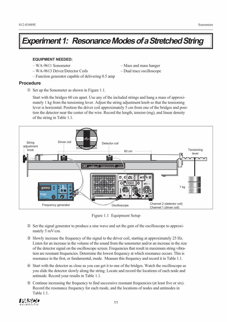
11
012-03489E Sonometer
Experiment 1: Resonance Modes of a Stretched String
EQUIPMENT NEEDED:
– WA-9611 Sonometer – Mass and mass hanger
– WA-9613 Driver/Detector Coils – Dual trace oscilloscope
– Function generator capable of delivering 0.5 amp
Procedure
➀ Set up the Sonometer as shown in Figure 1.1.
Start with the bridges 60 cm apart. Use any of the included strings and hang a mass of approxi-
mately 1 kg from the tensioning lever. Adjust the string adjustment knob so that the tensioning
lever is horizontal. Position the driver coil approximately 5 cm from one of the bridges and posi-
tion the detector near the center of the wire. Record the length, tension (mg), and linear density
of the string in Table 1.1.
➁ Set the signal generator to produce a sine wave and set the gain of the oscilloscope to approxi-
mately 5 mV/cm.
➂ Slowly increase the frequency of the signal to the driver coil, starting at approximately 25 Hz.
Listen for an increase in the volume of the sound from the sonometer and/or an increase in the size
of the detector signal on the oscilloscope screen. Frequencies that result in maximum string vibra-
tion are resonant frequencies. Determine the lowest frequency at which resonance occurs. This is
resonance in the first, or fundamental, mode. Measure this frequency and record it in Table 1.1.
➃ Start with the detector as close as you can get it to one of the bridges. Watch the oscilloscope as
you slide the detector slowly along the string. Locate and record the locations of each node and
antinode. Record your results in Table 1.1.
➄ Continue increasing the frequency to find successive resonant frequencies (at least five or six).
Record the resonance frequency for each mode, and the locations of nodes and antinodes in
Table 1.1.
Figure 1.1 Equipment Setup
Channel 2 (detector coil)
Channel 1 (driver coil)
Detector coil
1 kg
Driver coilString
adjustment
knob Tensioning
lever
WA-9611
SONOMETER
KEEP WEIGHTS AS NEAR TO FLOOR
AS POSSIBLE IN THE EVENT THESONOMETER WIRE SHOULD BREAK
CAUTION!
1.75 kg MAXIMUMLOAD ON LEVER
BK PRECISION
200 Mhz OSCILLISCOPEMODEL2 1 2 0
INTENSITY FOCUS
TRACE NOT ATION
TRIG LEVEL
COUPLE SOURCE
SLOPE - Y
TIME/DIV
X-POS
VAR VAR
VAR SWEEP
CALCAL
mVV
CH 1VOLTZ/DIV
CH 2VOLTZ/DIV
CALmVV
VERTICAL MODE
PULL XS PULL XS
CH 2∞CH 1∞
AC
DC
AC
DC
AC CH1
CH2
ALT
EXT
POS POSNORM
EXT
CH1
CH2
NORMEXT
CH1CH2
MANUAL AUTO T X-
YT X-
Y
LINE
CAL EXT CH4
POWER
200VMAX
400VMAX
400VMAX
- +
+
-
T TLH I
Ω
GN D
L OΩM I
N
R AN G E
A D J US T
MA X
OUTPU T
FREQUENC Y
AMPL ITUD E
P I -9587BD IG ITAL FUNCTIONGENERA TOR -AMPL IF IER
H ER T Z
WA VEFORM
I N PU T
GN DE X T E R N
A L
DETECTOR
W A-9613
DRIVER
WA-9613
60 cm
OscilloscopeFrequency generator
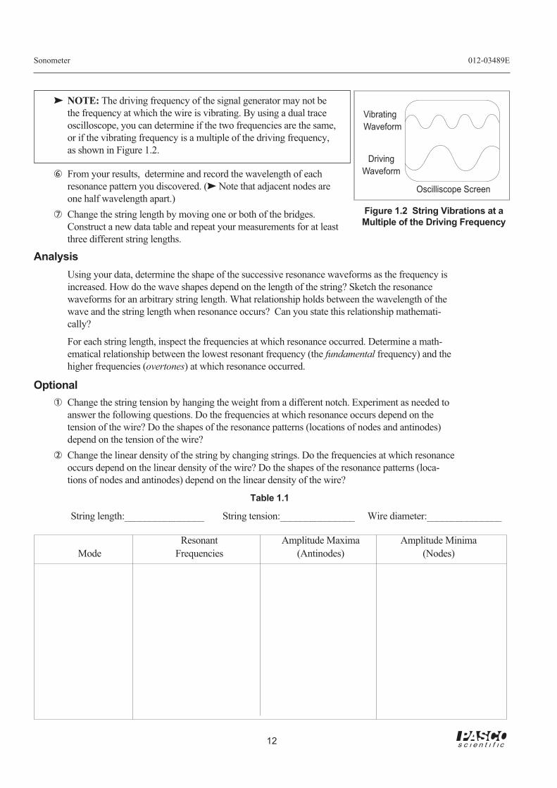
12
Sonometer 012-03489E
Vibrating
Waveform
Driving
Waveform
Oscilliscope Screen
Figure 1.2 String Vibrations at a
Multiple of the Driving Frequency
Resonant Amplitude Maxima Amplitude Minima
Mode Frequencies (Antinodes) (Nodes)
String length:________________ String tension:_______________ Wire diameter:_______________
Table 1.1
NOTE: The driving frequency of the signal generator may not be
the frequency at which the wire is vibrating. By using a dual trace
oscilloscope, you can determine if the two frequencies are the same,
or if the vibrating frequency is a multiple of the driving frequency,
as shown in Figure 1.2.
➅ From your results, determine and record the wavelength of each
resonance pattern you discovered. ( Note that adjacent nodes are
one half wavelength apart.)
➆ Change the string length by moving one or both of the bridges.
Construct a new data table and repeat your measurements for at least
three different string lengths.
Analysis
Using your data, determine the shape of the successive resonance waveforms as the frequency is
increased. How do the wave shapes depend on the length of the string? Sketch the resonance
waveforms for an arbitrary string length. What relationship holds between the wavelength of the
wave and the string length when resonance occurs? Can you state this relationship mathemati-
cally?
For each string length, inspect the frequencies at which resonance occurred. Determine a math-
ematical relationship between the lowest resonant frequency (the fundamental frequency) and the
higher frequencies (overtones) at which resonance occurred.
Optional
➀ Change the string tension by hanging the weight from a different notch. Experiment as needed to
answer the following questions. Do the frequencies at which resonance occurs depend on the
tension of the wire? Do the shapes of the resonance patterns (locations of nodes and antinodes)
depend on the tension of the wire?
➁ Change the linear density of the string by changing strings. Do the frequencies at which resonance
occurs depend on the linear density of the wire? Do the shapes of the resonance patterns (loca-
tions of nodes and antinodes) depend on the linear density of the wire?
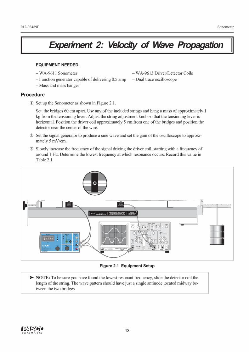
13
012-03489E Sonometer
EQUIPMENT NEEDED:
– WA-9611 Sonometer – WA-9613 Driver/Detector Coils
– Function generator capable of delivering 0.5 amp – Dual trace oscilloscope
– Mass and mass hanger
Procedure
➀ Set up the Sonometer as shown in Figure 2.1.
Set the bridges 60 cm apart. Use any of the included strings and hang a mass of approximately 1
kg from the tensioning lever. Adjust the string adjustment knob so that the tensioning lever is
horizontal. Position the driver coil approximately 5 cm from one of the bridges and position the
detector near the center of the wire.
➁ Set the signal generator to produce a sine wave and set the gain of the oscilloscope to approxi-
mately 5 mV/cm.
➂ Slowly increase the frequency of the signal driving the driver coil, starting with a frequency of
around 1 Hz. Determine the lowest frequency at which resonance occurs. Record this value in
Table 2.1.
NOTE: To be sure you have found the lowest resonant frequency, slide the detector coil the
length of the string. The wave pattern should have just a single antinode located midway be-
tween the two bridges.
Experiment 2: Velocity of Wave Propagation
Figure 2.1 Equipment Setup
WA-9611
SONOMETER
KEEP WEIGHTS AS NEAR TO FLOORAS POSSIBLE IN THE EVENT THE
SONOMETER WIRE SHOULD BREAK
CAUTION!1.75 kg MAXIMUMLOAD ON LEVER
BK PRECISION 200 Mhz OSCILLISCOPEMODEL2120
INTENSITY FOCUS
TRACE NOTATION
TRIG LEVEL
COUPLE SOURCE
SLOPE λ - Y
TIME/DIV
X-POS
VAR VAR
VAR SWEEP
CAL CALmVV
CH 1VOLTZ/DIV
CH 2VOLTZ/DIV
CALmVV
VERTICAL MODE
PULL XS PULL XS
CH 2 ∞CH 1 ∞
AC
DC
AC
DC
AC CH1
CH2
ALT
EXT
POS POSNORMEXT
CH1CH2
NORMEXT
CH1CH2
MANUAL AUTO
T X-Y
T X-Y
LINE
CAL EXT CH4
POWER200VMAX
400VMAX
400VMAX
- +
+
-
T TL
H IΩ
GN D
L OΩ
M IN
R AN G E
A D J US T
MA X
OUTPUT
FREQUENCY
AMPLITUDE
PI -9587BDIGITAL FUNCTIONGENERATOR -AMPLIF IER
H ER T Z
WAVEFORM
I N PU T
GN D
E X T ERNA L
DETECTOR
WA-9613
DRIVER
WA-9613
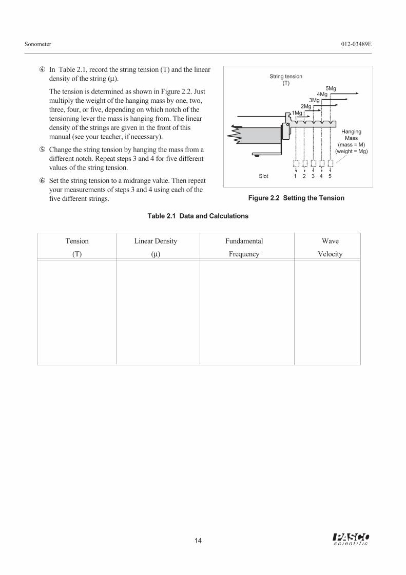
14
Sonometer 012-03489E
String tension
(T)
Hanging
Mass
(mass = M)
(weight = Mg)
Tension Linear Density Fundamental Wave
(T) (µ) Frequency Velocity
1 52 3 4Slot
Figure 2.2 Setting the Tension
1Mg
2Mg3Mg
4Mg5Mg
➃ In Table 2.1, record the string tension (T) and the linear
density of the string (µ).
The tension is determined as shown in Figure 2.2. Just
multiply the weight of the hanging mass by one, two,
three, four, or five, depending on which notch of the
tensioning lever the mass is hanging from. The linear
density of the strings are given in the front of this
manual (see your teacher, if necessary).
➄ Change the string tension by hanging the mass from a
different notch. Repeat steps 3 and 4 for five different
values of the string tension.
➅ Set the string tension to a midrange value. Then repeat
your measurements of steps 3 and 4 using each of the
five different strings.
Table 2.1 Data and Calculations
012-03489E Sonometer
Analysis
➀ Use your measured string length, the fundamental frequency, and the equation V = λν to determine the velocity
of the wave on the string for each value of tension and linear density that you used.
➁ Determine the functional relationship between the speed of the wave (V) and the wire tension (T). This can be
accomplished using either of the following three methods. If you are not familiar with these procedures, you
might want to try all three.
NOTE: Options A and B are easily performed using a computer with graphical analysis
software.
A. Plot a graph of V versus T, with V on the y-axis. If the graph is not a straight line, try plotting V versus some
power of T (such as T2, T1/2, etc.), until you get a straight line.
B. Assume that the functional relationship is of the form V = kTp. Then ln V = p ln T + ln k, where p and k are
unknown constants. Then, if lnV is plotted against the independent variable lnT, a straight line will be ob-
tained having a slope p, where p is lnV/ lnT and ln k is the y-intercept.
C. Many calculators have the ability to do power regressions or linear regressions on the logarithms of V and T.
This will accomplish essentially what the graph of method B did.
➂ Using one of the methods above, determine the functional relationship of the speed of the wave (V) to the linear
density of the string (µ).
Conclusions
Characterize the resonant modes of a vibrating wire. That is:
➀ Determine a mathematical relationship that describes the wavelengths of the waves that form standing wave
patterns in a wire of length L (see Experiment 1).
➁ Use your answer to question 1, and the expression V = λν, to determine the resonant frequencies of a wire of
length L.
➂ Use your experimental results to write an expression for the resonant frequencies of a vibrating wire in terms of
T, µ, and L.
16
Sonometer 012-03489E
Suggested Research Topics
The following are a few suggestions for further experimentation with the Sonometer.
➀ Obtain two wires of the same linear density (mass per unit length), one that is wound and one that
is not wound (a plain wire). Investigate the effects of the winding on the mathematical relation-
ships of wave propagation.
➁ Use a harmonic analyzer to analyze the effects of placing the Driver Coil at different places along
the wire. Also investigate the effects of placing the Detector Coil at different places along the
wire. You can also investigate the effects of plucking, strumming, and bowing the string.
➂ By devising a method to measure string stretch, you can use this apparatus to investigate the
Hooke's Law relationship for a wire placed under tension. Possible investigations include:
a. Strain versus Stress (Stretch versus Applied Load)
b. Strain versus Diameter of Wire (Constant Stress)
c. Strain versus Type of Wire (Constant Diameter)
➃ Obtain wires made of different materials, but with the same linear density. Investigate the speed
of wave propagation in these wires when the same tension is applied to each.
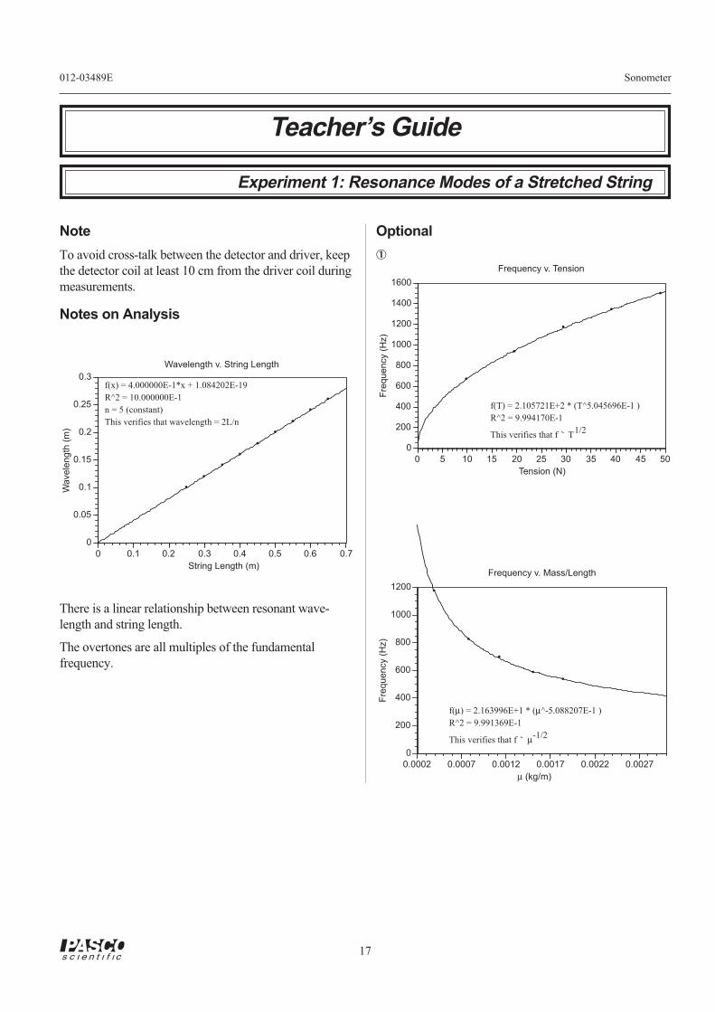
17
012-03489E Sonometer
Teacher’s Guide
Experiment 1: Resonance Modes of a Stretched String
Note
To avoid cross-talk between the detector and driver, keep
the detector coil at least 10 cm from the driver coil during
measurements.
Notes on Analysis
X
X
X
X
X
X
X
X
X
0
0.05
0.1
0.15
0.2
0.25
0.3
0 0.1 0.2 0.3 0.4 0.5 0.6 0.7
Wa
ve
len
gth
(m
)
String Length (m)
f(x) = 4.000000E-1*x + 1.084202E-19
R^2 = 10.000000E-1
n = 5 (constant)
This verifies that wavelength = 2L/n
Wavelength v. String Length
There is a linear relationship between resonant wave-
length and string length.
The overtones are all multiples of the fundamental
frequency.
Optional
➀
X
X
X
X
X
0
200
400
600
800
1000
1200
1400
1600
0 5 10 15 20 25 30 35 40 45 50
Fre
quency (
Hz)
Tension (N)
Frequency v. Tension
f(T) = 2.105721E+2 * (T^5.045696E-1 )
R^2 = 9.994170E-1
This verifies that f ` T1/2
X
X
X
X
X
0
200
400
600
800
1000
1200
0.0002 0.0007 0.0012 0.0017 0.0022 0.0027
Fre
quency (
Hz)
µ (kg/m)
Frequency v. Mass/Length
f(µ) = 2.163996E+1 * (µ^-5.088207E-1 )
R^2 = 9.991369E-1
This verifies that f ` µ-1/2
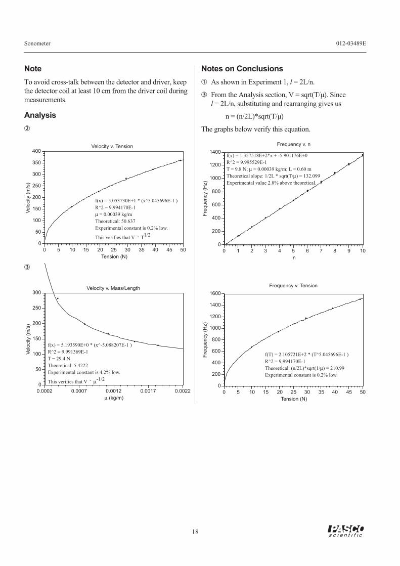
18
Sonometer 012-03489E
Note
To avoid cross-talk between the detector and driver, keep
the detector coil at least 10 cm from the driver coil during
measurements.
Analysis
➁
X
X
X
X
X
0
50
100
150
200
250
300
350
400
0 5 10 15 20 25 30 35 40 45 50
Ve
locity (
m/s
)
Tension (N)
Velocity v. Tension
f(x) = 5.053730E+1 * (x^5.045696E-1 )
R^2 = 9.994170E-1
µ = 0.00039 kg/m
Theoretical: 50.637
Experimental constant is 0.2% low.
This verifies that V ` T1/2
➂
X
X
X
X
X
0
50
100
150
200
250
300
0.0002 0.0007 0.0012 0.0017 0.0022
Ve
locity (
m/s
)
µ (kg/m)
f(x) = 5.193590E+0 * (x^-5.088207E-1 )
R^2 = 9.991369E-1
T = 29.4 N
Theoretical: 5.4222
Experimental constant is 4.2% low.
This verifies that V ` µ-1/2
Velocity v. Mass/Length
Notes on Conclusions
➀ As shown in Experiment 1, l = 2L/n.
➂ From the Analysis section, V = sqrt(T/µ). Since
l = 2L/n, substituting and rearranging gives us
n = (n/2L)*sqrt(T/µ)
The graphs below verify this equation.
X
X
X
X
X
X
X
X
X
X
X
X
X
X
X
0
200
400
600
800
1000
1200
1400
0 1 2 3 4 5 6 7 8 9 10
Fre
quency (
Hz)
n
Frequency v. n
f(x) = 1.357518E+2*x + -5.901176E+0
R^2 = 9.995529E-1
T = 9.8 N; µ = 0.00039 kg/m; L = 0.60 m
Theoretical slope: 1/2L * sqrt(T/µ) = 132.099
Experimental value 2.8% above theoretical.
X
X
X
X
X
0
200
400
600
800
1000
1200
1400
1600
0 5 10 15 20 25 30 35 40 45 50
Fre
qu
en
cy (
Hz)
Tension (N)
f(T) = 2.105721E+2 * (T^5.045696E-1 )
R^2 = 9.994170E-1
Theoretical: (n/2L)*sqrt(1/µ) = 210.99
Experimental constant is 0.2% low.
Frequency v. Tension

19
012-03489E Sonometer
Contacting Technical Support
Before you call the PASCO Technical Support staff it
would be helpful to prepare the following information:
• If your problem is with the PASCO apparatus, note:
Title and Model number (usually listed on the label).
Approximate age of apparatus.
A detailed description of the problem/sequence of
events. (In case you can't call PASCO right away,
you won't lose valuable data.)
If possible, have the apparatus within reach when
calling. This makes descriptions of individual parts
much easier.
• If your problem relates to the instruction manual,
note:
Part number and Revision (listed by month and year
on the front cover).
Have the manual at hand to discuss your questions.
Feed-Back
If you have any comments about this product or this
manual please let us know. If you have any sugges-
tions on alternate experiments or find a problem in the
manual please tell us. PASCO appreciates any cus-
tomer feed-back. Your input helps us evaluate and
improve our product.
To Reach PASCO
For Technical Support call us at 1-800-772-8700 (toll-
free within the U.S.) or (916) 786-3800.
Internet: [email protected]
Tech Support Fax: (916)786-3292
Technical Support

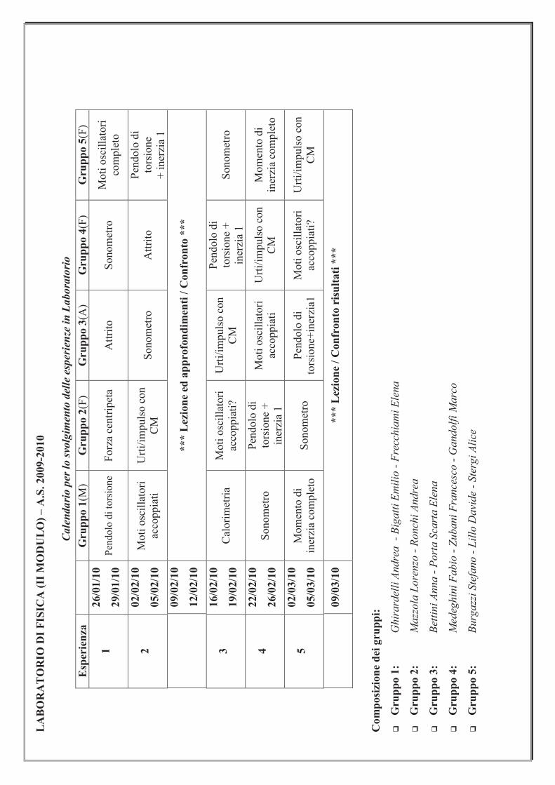
LA
BO
RA
TO
RIO
DI
FIS
ICA
(II
MO
DU
LO
) – A
.S. 2009-2
010
Cale
ndari
o p
er l
o s
volg
imen
to d
elle
esp
erie
nze
in
Labora
tori
o
Esp
erie
nza
G
rup
po 1
(M)
Gru
pp
o 2
(F)
Gru
pp
o 3
(A)
Gru
pp
o 4
(F)
Gru
pp
o 5
(F)
1
26/0
1/1
0
29/0
1/1
0
Pen
dolo
di
tors
ione
Forz
a ce
ntr
ipet
a A
ttri
to
Sonom
etro
M
oti
osc
illa
tori
co
mple
to
2
02/0
2/1
0
05/0
2/1
0
Moti
osc
illa
tori
ac
coppia
ti
Urt
i/im
puls
o c
on
CM
S
onom
etro
A
ttri
toP
endolo
di
tors
ione
+
iner
zia
1
09/0
2/1
0
12/0
2/1
0
*** L
ezio
ne
ed a
pp
rofo
nd
imen
ti /
Con
fron
to *
**
3
16/0
2/1
0
19/0
2/1
0
Cal
ori
met
ria
Moti
osc
illa
tori
ac
coppia
ti?
Urt
i/im
puls
o c
on
CM
Pen
dolo
di
tors
ione
+
iner
zia
1
Sonom
etro
4
22/0
2/1
0
26/0
2/1
0
Sonom
etro
P
endolo
di
tors
ione
+
iner
zia
1
Moti
osc
illa
tori
ac
coppia
ti
Urt
i/im
puls
o c
on
CM
M
om
ento
di
iner
zia
com
ple
to
5
02/0
3/1
0
05/0
3/1
0
Mom
ento
di
iner
zia
com
ple
to
Sonom
etro
P
endolo
di
tors
ione+
iner
zia1
M
oti
osc
illa
tori
ac
coppia
ti?
Urt
i/im
puls
o c
on
CM
09/0
3/1
0
*** L
ezio
ne
/ C
on
fron
to r
isu
ltati
***
Co
mp
osi
zion
e d
ei g
rup
pi:
G
rup
po 1
:
Ghi
rard
elli
And
rea
- B
igat
ti E
mil
io -
Fre
cchi
ami E
lena
G
rup
po 2
:
Maz
zola
Lor
enzo
- R
onch
i And
rea
G
rup
po 3
:
Bet
tini
Ann
a -
Por
ta S
cart
a E
lena
G
rup
po 4
:
Med
eghi
ni F
abio
- Z
uban
i Fra
nces
co -
Gan
dolf
i Mar
co
G
rup
po 5
: B
urga
zzi S
tefa
no -
Lil
lo D
avid
e -
Ster
gi A
lice
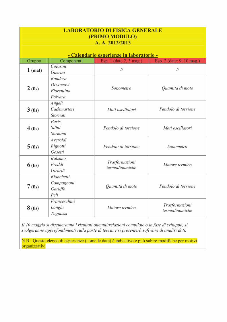
LABORATORIO DI FISICA GENERALE
(PRIMO MODULO)
A. A. 2012/2013
- Calendario esperienze in laboratorio - Gruppo Componenti Esp. 1 (date:2, 3 mag.) Esp. 2 (date: 9, 10 mag.)
1 (mat) Colosini Guerini
// //
2 (fis)
Bandera Devescovi Fiorentino Polvara
Sonometro Quantità di moto
3 (fis)
Angeli Cademartori Stornati
Moti oscillatori Pendolo di torsione
4 (fis)
Paris Silini Sormani
Pendolo di torsione Moti oscillatori
5 (fis)
Averoldi Bignotti Gosetti
Pendolo di torsione Sonometro
6 (fis)
Balzano Freddi Girardi
Trasformazioni termodinamiche
Motore termico
7 (fis)
Bianchetti Campagnoni Garuffo Peli
Quantità di moto Pendolo di torsione
8 (fis)
Franceschini Longhi Tognazzi
Motore termico Trasformazioni termodinamiche
Il 10 maggio si discuteranno i risultati ottenuti/relazioni compilate o in fase di sviluppo, si svolgeranno approfondimenti sulla parte di teoria e si presenterà software di analisi dati. N.B.: Questo elenco di esperienze (come le date) è indicativo e può subire modifiche per motivi organizzativi