
Is siHHoouusinngg taann IImmppeeddiimmeennt ttoo Co ... · Mariacristina Rossi, Dario Sansone,...
137
- Is Housing an Impediment to Consumption Smoothing? December, 2012 A report prepared by (in alphabetical order): Flavia Coda Moscarola, Elsa Fornero, Agnese Romiti, Mariacristina Rossi, Dario Sansone, Maria Cesira Urzì Brancati Principal Investigators: Elsa Fornero and Mariacristina Rossi University of Turin and CeRP-Collegio Carlo Alberto ([email protected]) Tel: +39 011 6705040 48 rue de Provence • 75009 Paris • France • Tel.: +33 (0) 1 43 12 58 00 • Fax: + 33 (0) 1 43 12 58 01 E-mail: [email protected] • www.oee.fr Siret: 424 667 947 00024
Transcript of Is siHHoouusinngg taann IImmppeeddiimmeennt ttoo Co ... · Mariacristina Rossi, Dario Sansone,...

-
IIss HHoouussiinngg aann IImmppeeddiimmeenntt ttoo
CCoonnssuummppttiioonn SSmmooootthhiinngg??
December, 2012
A report prepared by (in alphabetical order):
Flavia Coda Moscarola, Elsa Fornero, Agnese Romiti,
Mariacristina Rossi, Dario Sansone, Maria Cesira Urzì Brancati
Principal Investigators: Elsa Fornero and Mariacristina Rossi
University of Turin and CeRP-Collegio Carlo Alberto
Tel: +39 011 6705040
48 rue de Provence • 75009 Paris • France • Tel.: +33 (0) 1 43 12 58 00 • Fax: + 33 (0) 1 43 12 58 01
E-mail: [email protected] • www.oee.fr Siret: 424 667 947 00024

-

-
Table of Contents
EXECUTIVE SUMMARY ................................................................................. 1
Chapter I: Asset decumulation ............................................................................ 4
1.1. Patterns of housing wealth decumulation among European elderly. ................ 4
1.2. Introduction ............................................................................................................... 4
2. Literature review ........................................................................................................ 6
2.1. How dare the elderly not release equity as the life-cycle model predicts? ........ 6
2.2. Housing wealth as a bequest? .................................................................................. 7
2.3. Health status and wealth........................................................................................... 8
2.4. Equity release and financial markets development ............................................... 9
2.5. Releasing housing wealth as a relief to financial distress in old age ................... 9
2.6. Equity release and pension system........................................................................ 10
2.7. May the elderly not decumulate for a lack of financial literacy? ....................... 10
2.8. Financial literacy’s key role ..................................................................................... 11
3. SHARE data. ............................................................................................................ 15
3.1. Descriptive evidence. .............................................................................................. 15
3.2. An overview of health, financial literacy and wealth in Europe. ...................... 15
3.3. Patterns of asset decumulation across European households. ......................... 21
3.4. Health status, financial literacy and assets decumulation .................................. 24
3.4.1. Housing wealth decumulation, portfolio composition and financial literacy among the European elderly ............................................................................................... 35
3.4.2. Empirical strategy .................................................................................................... 37
4. ELSA data on the UK. ........................................................................................... 54
4.1. Descriptive evidence ............................................................................................... 54
4.2. Health ........................................................................................................................ 56
4.3. Numeracy – or financial literacy ............................................................................ 59
Chapter II: How to make real asset liquid. ...................................................... 62
1. The use of reverse mortgages around the word ................................................. 62
1.1. Reverse mortgage in the US ................................................................................... 62
1.2. Reverse mortgage in the UK ................................................................................. 69
1.3. Reverse mortgage in Australia ............................................................................... 74
1.4. Reverse mortgage in New Zealand ....................................................................... 75
2. Empirical Investigation: The Reverse Mortgage in Italy ................................... 79
2.1. RM literature overview ........................................................................................... 80
2.2. Descriptive statistics on microeconomic data ..................................................... 84
2.2.1. The UniCredit sample ............................................................................................. 84
2.2.2. Demographics and socio-economic indicators ................................................... 85
-
2.2.3. Preferences and attitudes ........................................................................................ 89
2.3. Estimating the money’s worth of a Reverse Mortgage ...................................... 94
2.4. Econometric specification ...................................................................................... 96
2.4.1. Ordered probit’s results .......................................................................................... 97
2.4.2. Robustness checks ................................................................................................. 104
2.5. What can we learn from Italy? ............................................................................. 105
Chapter III: Making assets a tool against poverty ........................................ 110
1. Introduction ........................................................................................................... 110
2. Poverty rates among the elderly in selected European countries ................... 111
2.1. One Euro today is worth more than one Euro tomorrow. ............................ 113
House Value converted as a Lump sum .......................................................................... 113
2.2. House Value converted into annuities ............................................................... 117
2.3. Different Scenarios: partially converting housing equity into annuities ........ 120
2.4. Converting financial wealth into annuities ........................................................ 126
CONCLUSIONS ............................................................................................. 132

Is housing an Impediment to Consumption Smoothing?
CeRP Collegio Carlo Alberto - 1 – OEE Report
EXECUTIVE SUMMARY
Asset accumulation by the elderly has been a major research focus so as to estimate
whether old households were well equipped to face their retirement, usually correlated
with a reduction in available resources. A buffer stock of wealth might immunize
households against bad shock realizations, thus constituting a crucial factor of financial
protection. From a policy standpoint, a high level of household wealth generates less
pressure for welfare policy interventions in time periods of financial crisis.
The reverse question, on whether the elderly are actually living below their possible
standards has been, on the other side, under-studied. What if households do not resort
to their wealth in times of instability and income drops? There might be an individual
reason for households’ decision not to use their assets. However, it is hard to agree that
public resources should be the sole response to economic downturns in the presence of
unused consistent assets. If over- savings should not worry Governments at first sight, it
may become a matter of concern whenever the elderly demand that Governments pay
for their reluctance to decumulate assets. Means tested interventions are generally based
on income available to the elderlies. Current income, however, is not a comprehensive
measure of welfare of individuals since for a given level of income, people who have
accumulated more assets are in fact less vulnerable to shocks. Assets, in addition to
current income, should be considered as the best proxy for attainable welfare.
The wealth of European households, particularly within the Southern Mediterranean
countries, is locked into illiquid assets, which are difficult to deplete when hard
economic times hit. Do the elderly bear strong consequences for the inability to use
their assets efficiently?
In this study we investigate these innovative research questions. The role of financial
literacy in the ability to save has been explored intensively. Retirement should be the
starting point of the decumulation phase. However, very little decumulation is observed
along the after-retirement path. Is financial illiteracy responsible for the small amount of
decumulation in old age? Moreover, is the portfolio allocation affected by the degree of
financial knowledge? Our ex ante expectation is that more financially sophisticated
households should be more active in their decumulation phase, as well as showing a

Is housing an Impediment to Consumption Smoothing?
CeRP Collegio Carlo Alberto - 2 – OEE Report
more balanced portfolio. We also explore the consequences of keeping the illiquid assets
as shadow assets. We thus test whether having problems in making ends meet can be
dependent on the degree of portfolio illiquidity. Our results, illustrated in Chapter I,
show that financial literacy might be imputed as responsible for portfolio imbalance,
however, the same does not hold for asset decumulation. More financially literate
people are as distant from the optimal life-cycle path as their less financially literate
peers.
The evidence on decumulation with particular emphasis on housing is scant. Is
housing wealth, in particular, considered as a shadow wealth by households? In order to
understand whether this is the case, we first perform, in the same chapter, a descriptive
and comprehensive picture of European households and their decumulation patterns of
wealth, both with respect to housing and non-housing wealth. The analysis is also
corroborated with robust econometric estimations. Our results indicate that little
decumulation is present among the elderly in all types of assets. Financial literacy slightly
mitigates the accumulation process during old ages, but it is never responsible for any
decumulation of assets after retirement. Conversely, we show that financial literacy
might reduce the exposure to excessively illiquid portfolios.
In Chapter II we investigate the attitudes of a sample of Italian households with
respect to products such as reverse mortgages helping making, at least partially, housing
assets liquid. Italy is an interesting case to study the potential of such financial
instruments because of its ageing population and because of the widespread
homeownership – more than 70 per cent of Italian households own their home. Our
empirical analysis draws from a unique survey, the UniCredit 2007, a rather large cross-
sectional dataset – 1,686 households – containing detailed information at both
household and individual level. A simple descriptive statistic shows that nearly 60 per
cent of respondents are not at all interested in the product, which is consistent with
previous literature on reverse mortgages in the US and other countries; the remaining 40
per cent expresses various degrees of interest, from quite low (roughly 20 per cent) to
very high (roughly 1 per cent), and therefore we can investigate which respondents’
features predict a higher level of interest and whether financial literacy plays a role.

Is housing an Impediment to Consumption Smoothing?
CeRP Collegio Carlo Alberto - 3 – OEE Report
We first quantify the benefits a reverse mortgage would yield in terms of income
increase for given demographics and socio-economic groups by applying the actuarial
formula for an annuity to our sample respondents, and find that very old (over 80s),
single females and households with a very large housing equity would be the recipients
with the highest gains. This group should therefore show a much higher level of
interest. An econometric analysis is then performed to find out whether this is the case.
We create a series of indicators related to both socio-economic variables and
respondents’ psychological attitudes, and assess their partial effects on our dependent
variable (i.e. the level of interest in reverse mortgages). Since only household heads, i.e.
the member of the household who is responsible for financial decisions, are asked to
express how interested they would be in taking out a reverse mortgage, the econometric
analysis is conducted at household level. What we find is that none of the demographics
explain interest in the product as we expected, while holding a larger housing equity is
negatively, rather than positively correlated with interest in the product. Conversely,
higher levels of risk aversion, negative expectations on future pension income and the
perception of housing investment as risky are the indicators predicting a higher level of
interest, while debt aversion is a strong impediment to the uptake of reverse mortgages,
even though the burden of repaying the debt lies with the heirs. Finally, higher levels of
financial literacy are not predictors of higher interest, but rather show a negative, albeit
not strongly significant, correlation with interest in the product.
In Chapter III we run a simulation exercise under different scenarios to understand
if and to what extent poverty alleviation could be realized through resorting to
annuitization of financial wealth and reverse mortgages. Particularly for countries such
as Italy and Spain, the impact of annuities on poverty rates is impressive. Converting all
housing value into an annuity, even at a high interest rate (10%) would generate ten
percentage point reduction in the poverty rate. Resorting to reverse mortgage would
reduce the degree of vulnerability of the elderly particularly in those countries which are
«poor» in current income but «rich» in wealth and could consistently reduce the
vulnerability among the elderly.

Is housing an Impediment to Consumption Smoothing?
CeRP Collegio Carlo Alberto - 4 – OEE Report
Chapter I: Asset decumulation
1.1. Patterns of housing wealth decumulation among European elderly.
1.2. Introduction
The welfare of the elderly is one of the main causes of concern for European policy
makers, particularly within a society with an increasing share of rapidly aging people.
One of the reasons for this being a concern is that elderly individuals are less able to
resort to the labour channel to cope with shocks, thus being more vulnerable to a shock
materialisation. Having adequate wealth available to face drops in income is therefore of
crucial importance.
Asset accumulation by the elderly has been a major focus of research so as to
estimate whether old households were well equipped to face their retirement and its
correlated reduction in available resources. The reverse question, on whether the elderly
are actually living below their possible standards has been, on the other side, under-
studied. If over- savings should not worry Governments at first sight, it may become a
matter of concern whenever the elderly demand that Governements pay for their
reluctance to decumulate assets. Means tested interventions are generally based on
income available to the elderlies. Current income, however, is not a comprehensive
measure of welfare of individuals since for a given level of income, people who have
accumulated more assets are in fact less vulnerable to shocks. Assets, in addition to
current income, should be considered as the best proxy for attainable wealth.
The evidence on decumulation with particular emphasis on housing is scant. In a
cross-section framework involving 15 OECD countries, Chiuri and Jappelli (2010)
recently document how the ownership rates decline after age 60 but this decline turns
out to be almost entirely explained by cohort effects. Once cohort effects are controlled
for, the ownership rate follows a slow decline as individuals age, reaching a rate of about
1 percentage point per year after age 75. Similar findings have been shown by other
studies: housing equity and home ownership do not decrease as individuals get older.
Elderly people could exploit their housing wealth in two ways in order to face the drop
in income occurring at retirement and finance their general consumption: they could

Is housing an Impediment to Consumption Smoothing?
CeRP Collegio Carlo Alberto - 5 – OEE Report
move to another smaller unit by downsizing or they could exploit financial services such
as reverse mortgage. However the evidence does not support a wide-spread use of the
latter, whereas the large reductions in home equity are typically associated with
exogenous factors such as the death of a spouse, the movement to a nursing home or a
worsening in the health status rather than to individual choices. (Venti and Wise; 2002,
2004). Since real (housing) wealth represents the overwhelming share of total wealth, in
particular for the elderly, all those aforementioned factors would appear to contradict
the standard life-cycle theory which states that individuals should use their accumulated
wealth in order to finance their consumption after retirement.
Our study looks at the relationship between financial literacy and wealth from a
different perspective, moving from the existing and answering the question of how
more financially literate individuals tend to accumulate higher wealth and to save more.
Our analysis aims at detecting how higher levels of financial literacy allow elderly
people to make better decisions regarding their wealth accumulation, especially in a life-
cycle perspective. Since it has been found that a higher endowment of financial literacy
allows elderly people to set better plans for their retirement, in a similar perspective we
would expect that the former should prevent elderly from getting to the end of their life
with too much (illiquid) wealth, out of the wealth that has been set apart for bequest
motives. Therefore, our main question looks at whether any wealth decumulation occurs
among elderly people and tries to understand how this behaviour varies across different
groups. We also highlight whether more vulnerable groups, such as women, or
immigrants display a different behaviour.
Hung et al. (2009) represents the only previous example trying to answer the
question of whether financial literacy has any impact on “decumulation planning”. They
analyze how financial literacy affects three different measures related to planning and
decumulation after retirement. Individuals are asked if they have tried to figure out how
much to withdraw from their savings after retirement, by spending down Defined
Contribution plan assets, if they have made a plan in order to do so and if they are
confident that their retirement spending plans will meet their needs1. By adopting a
1 The exact questions are: “Have you ever tried to figure out how much your household would be able to withdraw from your savings every year in retirement?”, “Have you made a plan for systematically spending down your

Is housing an Impediment to Consumption Smoothing?
CeRP Collegio Carlo Alberto - 6 – OEE Report
linear probability model their findings are in favour of a positive impact of financial
literacy on all these indicators of decumulation planning, however their estimation
strategy is flawed buy they fact that they don’t account for the endogeneity of the
financial literacy which is strongly correlated to other third factors affecting
decumulation planning.
2. Literature review
2.1. How dare the elderly not release equity as the life-cycle model predicts?
A robust demonstration of this flaw in the life-cycle model came a little more than
twenty years ago, when Venti and Wise showed that elderly were as likely to move into a
larger house as to move into a smaller one (Venti and Wise 1989). Analyzing a United
States panel interviewed every two years between 1969 and 1979, the evidence suggested
that typical elderly families do not use saving in the form of housing equity to finance
current consumption as they age, contrary to the usual life cycle theory. This puzzling
result had been suggested in earlier work (Merrill 1984), and Feinstein and McFadden
(1989) similarly demonstrated the remarkable resilience of elderly households to
financial downsizing.
Sheiner and Weil (1992) seemed to provide some reassurance to the conventional
life-cycle theorists because they noted that for people in their eighties and beyond there
was noticeable downsizing of housing, often as a result of widowhood or serious illness.
Their results are not inconsistent with Venti and Wise (1989) since these transitional
events are much more frequent for the oldest old, so the overall degree of downsizing
tends to be larger for this older group.
Venti and Wise returned in 2002 on this topic armed with much better data from the
Survey of Income and Program Participation (SIPP) and Asset and Health Dynamics
Among the Oldest Old (AHEAD) on housing choices among the oldest old as well as
the younger old. Surprisingly, they continued to find that elderly are not anxious to
downsize even at much older ages, aside from serious transitional changes such as
illness or death of a spouse.
savings during retirement?” and “Are you confident that your retirement spending plan will be sufficient to ensure that your needs are me in the future?”.

Is housing an Impediment to Consumption Smoothing?
CeRP Collegio Carlo Alberto - 7 – OEE Report
Venti and Wise (2004) extend previous studies considering the possibility of
releasing housing equity. As housing equity should not, in general, be counted on to
support non-housing consumption, the typical aging household is unlikely to seek a
reverse annuity mortgage to withdraw assets from home equity. Housing should rather
be considered as a reserve or buffer that can be used in catastrophic circumstances that
result in a change in household structure. “In this case”, the authors concluded, “having
used the home equity along the way—through a reverse mortgage for example— would
defeat the purpose of saving home equity for a rainy day.”
Jonathan Skinner commented on Venti and Wise (2004) observing that their study
does not dismantle the conventional lifecycle model but it demonstrates that the
conventional interpretation of the model entirely misses the motives for why
households are decumulating. This study demonstrate that assets, including housing
assets, are held for so long against future contingencies in later life, so in that sense it
can be viewed as a life-cycle model. “On the other hand, in the good and bad state of
the world, when the assets are not needed directly for very bad adverse outcomes, the
household members are happy to pass along a bequest. Only in the “very bad” state of
the world are assets largely depleted with regard to bequests.”
2.2. Housing wealth as a bequest?
Though bequest could be one motive of the absence of decumulation, empirically
there’s no sound evidence of that.
In Venti, Wise (1989), the absence of a significant relationship between changes in
housing equity and whether the family has children brings into question that attachment
to past living arrangements and the maintenance of housing equity may be motivated by
a bequest motive.
Most housing will apparently be left as a bequest, judging by the behaviour of the
Retirement History Survey (RHS) respondents through age 73.This does not necessarily
suggest that to leave a bequest is the reason that housing equity is not consumed. Indeed
the change in housing equity at the time of a sale by elderly persons without children is
about the same as the change for those with children. There is some evidence that
non—housing bequeathable wealth falls less for movers with than without children. The
differences are not substantial, however. This suggests that the elderly may well be

Is housing an Impediment to Consumption Smoothing?
CeRP Collegio Carlo Alberto - 8 – OEE Report
attached to their homes for reasons other than or in addition to the bequest motive.
This is consistent with the findings of Hurd (1986) for non—housing bequeathable
wealth.
2.3. Health status and wealth
As often sickness arises with aging, the possibility of getting ill could lead the elderly
non to decumulate and keep housing wealth as a buffer stock that can be used to
finance unexpected healthcare expenses.
The impact of health on consumption and savings behavior in old age has been
already documented by a few studies (Palumbo, 1999; Lillard and Weiss; 1996; Rosen
and Wu; 2004).
The first studies covering this topic focused on the relationship between health
status and household wealth: for example, Smith (1998) found that a serious decline in
health leads to a large decline in household wealth. Rosen and Wu (2004) go a step
further and test the impact of health status on household financial portfolio choices.
Using the US Health and Retirement Survey (HRS) data, Rosen and Wu (2004) find that
when the head of a household or the spouse is sick, the household is less likely to own
stocks, and invests a smaller proportion of its financial assets in stocks relative to
healthy ones. A similar correlation is found on Australia in Cardak, Wilkins (2009):
people with poor health are less likely to hold risky asset. According to the authors’
explanation poor health can be viewed as a source of labour income risk as well as a
source of “expense” risk: these may lead people in poor health to be less willing to take
financial risks and to have shorter savings horizons.
The relationship between health status and financial portfolio choices is explained in
deep by Berkowitz, Qiu (2006). Still considering the HRS data, they show that the
impact of health events on household financial and non-financial wealth is asymmetric:
a diagnosis of a new illness of a household member leads to a much larger decline in
financial wealth than in non-financial wealth. Health status affects household portfolio
choices primarily through a wealth effect engendered by a reduction in household
financial wealth,therefore, depending on the risk preferences of households, the effect
of health status on portfolio choices can be quite different among sick households.

Is housing an Impediment to Consumption Smoothing?
CeRP Collegio Carlo Alberto - 9 – OEE Report
In conclusion, a health event could lead to a significant reduction in household
financial wealth and, consequently, to a restructuring of the composition of its financial
portfolio. Families do reduce their housing wealth after an health shock but after having
reduced their financial wealth, that is easier to liquidate.
2.4. Equity release and financial markets development
Chiuri, Jappelli (2010) try to explain international differences in ownership
trajectories. Among the many possible factors affecting the rate at which ownership
changes across countries, they focus on transaction and moving costs, the availability of
mortgage equity withdrawal, property taxes, generosity of the social security systems,
unanticipated health expenditure, availability of nursing homes for the elderly, and
differences in mortality rates.
Their empirical findings do not contradict the view that market regulation and
financial market development—as proxied by the availability of mortgage equity
withdrawal and mortgage market regulation—affect the distribution of owner-
occupancy rates across age groups among the eldest old. Even though the decline is
slow and their sample limited, the international comparison suggests that indicators of
market regulation are correlated with ownership trajectories and therefore with the
wealth allocation of the elderly.
2.5. Releasing housing wealth as a relief to financial distress in old age
The impossibility of liquidating housing wealth could make old households more
exposed to financial distress. Angelini, Brugiavini, and Weber (2009) show that the low
development of mortgage markets not only limits the ability to withdraw equity by using
mortgage debt (that could be an obvious result), but has also a negative correlation with
the number of own-own transactions later in life, which means that lower fractions of
home-owners trade down by selling and buying. The low development of mortgage
markets is in turn responsible for higher financial distress among elderly people: the
study shows that there is a clear negative relation between the mortgage market
development - either measured as the typical loan-to-value ratio for mortgages or as a
mortgage market index constructed by Calza, Monacelli and Stracca (2007) – and the
proportion of homeowners who report difficulties making end meets.
Is housing an Impediment to Consumption Smoothing?
CeRP Collegio Carlo Alberto - 10 – OEE Report
2.6. Equity release and pension system
Countries where individuals are given more responsibility in their retirement choices
may represent a more fertile ground for equity release through reverse mortgages – due
to a better experience and confidence in financial instruments. In Australia for example
some workers have self-funded retirement system: Cardak, Wilkins(2009) find that those
persons are more likely to hold risky assets. Since July 1992, Australia has had in place a
mandatory employer-based retirement saving scheme operating in parallel with a
longstanding public pay-as-you-go pension scheme, requiring employers by federal law
to contribute (initially at least 3% of gross salary, progressively rising to 9% by July
2002) to individual retirement accounts for most employees. While employer-based
retirement accounts such as 401(k) plans in the US are important parts of the retirement
saving and investment landscape, they are not mandatory.
Australia’s experience may have some policy relevance for other countries as
compulsory retirement accounts - ensuring all working households indirectly own some
risky financial assets - adds an interesting dimension to the stockholding puzzle for
working households. This could suggest that in the equity release choices an important
role may be played by institutional structures and by the pension system that are
different in every country.
2.7. May the elderly not decumulate for a lack of financial literacy?
There has been recently an increasing interest in the role of financial literacy in
explaining wealth and savings decisions. Being financially “literate” could help
explaining the reluctance to use debt instruments or the failure to use them properly;
being able to understand instruments allowing equity release (e.g. reverse mortgages)
would allow people to avoid becoming “house-rich, cash-poor”, thus helping in solving
the puzzle of why many elderly people end up dying with a portfolio almost entirely
made up of illiquid assets, such as real (housing) wealth, which are more difficult to be
used in order to face hardship such as difficult health conditions.
The suspect that many people may not decumulate for financial literacy deficit grows
as many people do really lack in basic financial knowledge: elderly in particular could be
thought as a group less financially literate and disadvantaged. Van Rooij, Lusardi and
Alessie (2011) show that the majority of Dutch households possesses limited financial

Is housing an Impediment to Consumption Smoothing?
CeRP Collegio Carlo Alberto - 11 – OEE Report
literacy; financial illiteracy is widespread and particularly acute among specific groups of
the population, such as women, those with low educational attainment and – in
particular – the elderly.
On the contrary in the United States Hung et al(2009) discover that financial literacy
is monotonically related to age, with older individuals having higher levels of financial
literacy. Data used in this study from Rand’s American Life Panel (a national household
panel survey) show that lower levels of financial literacy are shared by economically
disadvantaged individuals: minorities (Hispanic, African American), women, not married
individuals, lower educated (high school or less), not employed (but also not retired),
and lower income (household income less than $50,000 per year). Cardak, Wilkins
(2009) find that Australian people over 55 are more likely to hold risky assets than
people between 25-54: the authors notice that those results are consistent with increased
knowledge of the investment landscape and opportunities that come with age and
experience.
Still, for making an optimal choice concerning a reverse mortgage, basic financial
literacy could just not be enough: individuals should be aware of sophisticated financial
concepts.
Lusardi, Mitchell, Curto (2012) consider an HRS sample of respondents age 55 and
their knowledge not just on financial concepts, but on sophisticated financial concepts:
those are, for example, knowledge of capital markets , the importance of risk
diversification, of the impact of fees of mutual funds and on the individual savvy and
numeracy with compound interests. They find a rather striking lack of financial
sophistication among the older population. In particularly persons over the age of 75 are
find to be significantly less sophisticated about financial matters.
2.8. Financial literacy’s key role
Understanding the role played by the lack of financial literacy could ultimately help
in fostering strategies aimed at making elderly people more confident with the use of
equity release instruments.
The relationship between financial literacy and savings decisions has been explored
so far mainly pointing out to the positive impact of the former on wealth, arguing that a

Is housing an Impediment to Consumption Smoothing?
CeRP Collegio Carlo Alberto - 12 – OEE Report
higher level of financial literacy fosters the accumulation of wealth (Behrman et al, 2010;
Jappelli and Pistaferri, 2011). In a recent study Jappelli and Pistaferri (2011) analyzed the
impact of financial literacy on savings decisions of elderly people. Accounting for the
endogeneity of the variable of interest, they found that rising financial literacy fosters
savings and wealth in a cross-country setting. Financial literacy has been also found to
be responsible for higher participation in the stock market (van Rooij, Lusardi and
Alessie 2011). This relationship holds true even after accounting for many of the
determinants of stock market participation, such as age, education, gender, income, and
wealth. Financial literacy has an effect on stock ownership above and beyond the effects
of word-of-mouth information of peers. Even considering a measure of risk aversion,
both the OLS and GMM estimates of financial literacy remain positive, statistically
significant, and do not change appreciably in magnitude.
This suggests that without financial literacy individuals wouldn’t be able to make
optimal financial decisions.
In addition, poor financial literacy has been found to bring about a failure of
planning for retirement (Hung et al., 2009; Lusardi and Mitchell, 2006, 2007a, 2007b,
2008).
Behram, Mitchell, Soo, Bravo (2010) observe that in Chile households that build up
more net wealth, particularly via the pension system, may be better able to smooth
consumption in retirement and thus enhance risk sharing and wellbeing in old age. Their
finding that financial literacy enhances peoples’ likelihood of contributing to their
pension saving suggests that this is a valuable pathway by which improved financial
literacy can build household net wealth.

Is housing an Impediment to Consumption Smoothing?
CeRP Collegio Carlo Alberto - 13 – OEE Report
References
Angelini V., Brugiavini A., Weber G., (2010). “Does Downsizing of Housing Equity Alleviate Financial Distress in Old Age?”, Mannheim research Institute for the Economics of Aging (MEA), WP 217. Behram, Mitchell, Soo, Bravo (2010) “Financial literacy, schooling and wealth accumulation” Working Paper 16452 NBER October 2010 Berkowitz M.K., Qiu J., (2006) “A further look at household portfolio choice and health status”, Journal of Banking & Finance 30 1201–1217 Chiuri M.C., Jappelli T., 2010. “Do the elderly reduce housing equity? An international comparison”, Journal of Population Economics 23, 643-663. Feinstein, Jonathan S., and Daniel McFadden. (1989). “The dynamics of housing demand by the elderly: Wealth, cash flow, and demographic effects. In The economics of aging, ed. David A. Wise, 55–86. Chicago: University of Chicago Press. Hung A., Meijer E., Mihali K., Yoong J. (September 2009) “Financial literacy, retirement saving management, and decumulation”, RAND WP 712 Hurd, Michael. (1986). "Savings and Bequests." NBER Working Paper No. 1826, January. Jappelli T., Padula M., (2011). “Investment in Financial Literacy and Saving Decisions”, CSEF WP 272 Lusardi A., Mitchell O., Curto V. (2012), “Financial Sophistication In The Older Population”. NBER WP 17863 Merrill, Sally R. (1984). “Home equity and the elderly”. In Retirement and economic behavior, ed. Henry J. Aaron and Gary Burtless, 197–227. Washington, D.C.: Brookings Institution. Rosen, H.S., Wu, S., (2004). “Portfolio choice and health status”. Journal of Financial Economics 72, 457– 484, forthcoming. Sheiner, Louise M., and David Weil. (1992). „The housing wealth of the aged”. NBER Working Paper no. 4115. Cambridge, Mass.: National Bureau of Economic Research, July. Smith, P.J., (1998). “Socioeconomic status and health”. American Economic Review 88, 145–166. van Rooij M., Lusardi A., Alessie R., (2011). “Financial literacy and stock market participation”. Journal of Financial Economics 101, 449–472. Venti S. F., Wise D.A., (1989). “Aging, Moving, and Housing Wealth”. In Wise D.A. (Ed.), The Economics of Aging. University of Chicago Press, 9-48.

Is housing an Impediment to Consumption Smoothing?
CeRP Collegio Carlo Alberto - 14 – OEE Report
Venti S.F., Wise D.A.(2002, “Aging and housing equity” in Olivia S. Mitchell et al. “Innovations in retirement financing”, University of Pennsylvania Press, Philadelphia, 2002. Venti S.F., Wise D.A., (2004) “Aging and housing equity: another look”, in David A. Wise “Perspectives on the Economics of Aging”, University of Chicago Presse

Is housing an Impediment to Consumption Smoothing?
CeRP Collegio Carlo Alberto - 15 – OEE Report
3. SHARE data.
3.1. Descriptive evidence.
3.2. An overview of health, financial literacy and wealth in Europe.
For our empirical analysis we use the SHARE dataset, a survey which in 2004 started
collecting data on the individual life circumstances of persons aged 50 and over in 12
European countries: Austria, Belgium, Denmark, France, Germany, Greece, Israel, Italy,
the Netherlands, Spain, Sweden, and Switzerland. In addition, three new countries
joined the survey in wave 2 which was released between 2006 and 2007: the Czech
Republic, Poland, and Ireland. The survey covers 19,286 households and 32,022
individuals and the main purpose of the survey was to collect comparable information
about health status, income, wealth and household characteristics of elderly people for
different European countries, following the example initiated by the US Health and
Retirement Study (HRS) and the English Longitudinal Survey on Ageing (ELSA).
Since we want to exploit the longitudinal dimension of the survey, we restrict the
analysis to the 11 countries which are present in both waves of the surveys excluding
Israel, the Czech Republic, Poland, and Ireland. We are left with the following 11
countries: Austria, Belgium, Denmark, France, Germany, Greece, Italy, Netherlands,
Spain, Sweden, and Switzerland.
We want to analyze household wealth and how the latter is related and shaped by
health status and financial literacy other than other demographic characteristics,
therefore we ideally need to identify the individual who is responsible for the family
finances. Since at the beginning of the survey individuals are asked who is the financial
respondent, the person responsible for the family finances, we select the latter for the
case in which it is uniquely identified, whereas when there is more than one financial
respondent (because both members of the couple manage the finances separately), we
consider the one with the highest income, or, in case of persons with no income, the
oldest one2.
We consider individuals aged 50 or older over the time-period between 2004 and
20073.
2 Individual income are computed as the sum of earnings, public and private pensions, life insurance payment received, private annuity, alimony, regular payment from charities, and income from rent. Interest from bank accounts, stocks, bonds, and mutual funds are not included because the asset questions in wave 2 refer to the household and not to individuals therefore the relevant variables are only available for wave 1. 3 The first wave of the SHARE survey is related to 2004 for most countries, for France, Greece and Belgium the data have been collected between 2004 and 2005, whereas the second wave is relevant to the period 2006-2007 with the exception of the Netherlands and Greece whose data have been collected in 2007.

Is housing an Impediment to Consumption Smoothing?
CeRP Collegio Carlo Alberto - 16 – OEE Report
From Figures 1-3 it is evident how the European countries are ranked in terms of the
different components of wealth. Figure 1 draws the net worth, obtained as the
difference between net real wealth and financial wealth minus liabilities.
Figure 1. Net worth wealth across European countries. Source: SHARE 2004-2007.
If we compare net worth wealth with the two components of real (Figure 2) and
financial wealth (Figure 3) it is evident how there is a group of countries such as Italy,
France, and Spain ranked the highest in terms of real wealth and with the lowest levels
of financial wealth. This polarization can be reasonably linked to the poor level of
financial literacy they are endowed with, which is the lowest (Figure 4), therefore they
prefer to invest in less risky assets such as housing wealth.
0
100000
200000
300000S
wed
en
Au
str
ia
Den
mark
Gre
ece
Germ
any
Ita
ly
Sp
ain
Neth
erla
nd
s
Fra
nce
Be
lgiu
m
Sw
itzerl
an
d
Net worth wealth

Is housing an Impediment to Consumption Smoothing?
CeRP Collegio Carlo Alberto - 17 – OEE Report
Figure 2. Real wealth across European countries. Source: SHARE 2004-2007.
Figure 3. Financial wealth across European countries. Source: SHARE 2004-2007.
0
50,000
100000
150000
200000
250000
Sw
ed
en
Den
mark
Au
str
ia
Germ
any
Gre
ece
Neth
erla
nd
s
Sw
itzerl
an
d
Be
lgiu
m
Ita
ly
Sp
ain
Fra
nce
Real wealth
0
20,000
40,000
60,000
80,000
100000
Gre
ece
Ita
ly
Sp
ain
Au
str
ia
Fra
nce
Germ
any
Sw
ed
en
Neth
erla
nd
s
Den
mark
Be
lgiu
m
Sw
itzerl
an
d
Financial wealth

Is housing an Impediment to Consumption Smoothing?
CeRP Collegio Carlo Alberto - 18 – OEE Report
Country Home owner
No Yes Total
Austria 991 1,358 2,349
42.19 57.81 100
Germany 1,563 2,002 3,565
43.84 56.16 100
Sweden 1,687 2,278 3,965
42.55 57.45 100
Netherlands 1,422 2,195 3,617
39.31 60.69 100
Spain 369 2,593 2,962
12.46 87.54 100
Italy 734 2,833 3,567
20.58 79.42 100
France 1,101 2,847 3,948
27.89 72.11 100
Denmark 1,013 1,827 2,840
35.67 64.33 100
Greece 612 3,407 4,019
15.23 84.77 100
Switzerland 784 935 1,719
45.61 54.39 100
Belgium 946 3,566 4,512
20.97 79.03 100
Total 11,222 25,841 37,063
30.28 69.72 100
Table 1. Home ownership by country.
Countries with the highest level of real wealth turn out to coincide with those with
the highest home ownership rate, in fact countries such as Italy, Spain, France, Belgium,
and Greece have both the highest real wealth and home ownership. Those countries,
with the only exception of Belgium are also those with relatively low levels of financial
wealth as it is clear from Figure 3.
The different pattern of real and financial wealth can be linked to different patterns
of financial literacy each country is endowed with (Figure 4). Following Jappelli and
Padula (2011) we adopt an indicator for financial literacy as taken from the SHARE
survey. This indicator is derived in SHARE from four questions, three questions test the
ability of playing with numbers, such as the ability of computing a percentage,

Is housing an Impediment to Consumption Smoothing?
CeRP Collegio Carlo Alberto - 19 – OEE Report
computing the final price of a discounted good from the original price, and the price of
a second hand car sold at two-third of its original price. The fourth question is instead
related to interest rate compounding in a savings account. The final indicator takes value
from 1 to 5 with 5 corresponding to the highest level of financial literacy4. In the
SHARE dataset the original variable is called “numeracy”, as indeed the first questions
refer to numerical ability. Jappelli and Padula (2010) illustrate how the stock of financial
literacy later in life is determined by early numerical skills, and therefore we can assume
that high numeracy can be a proxy for high financial literacy. , For simplicity in the
following descriptive statistics we define a binary indicator of financial literacy which we
set as equal to one for a value of numeracy equal to 55.
From Figure 4 it is evident a clear cross-country correlation between the level of
financial wealth and that of financial literacy, the group of countries with the lowest
level of financial wealth is characterized by the lowest level of financial literacy (Spain,
Italy, France, Greece).
Figure 4. Financial literacy / numeracy across European countries. Source: SHARE 2004-2007.
4 The answers to these 4 questions are combined into a single indicator, as for details on how the index is implemented see the Appendix. 5 If not otherwise specified, whenever we mention financial literacy we will be referring to the corresponding numeracy variable in SHARE.
0
1
2
3
4
Sp
ain
Ita
ly
Fra
nce
Gre
ece
Be
lgiu
m
Den
mark
Au
str
ia
Sw
ed
en
Neth
erla
nd
s
Germ
any
Sw
itzerl
an
d
Financial literacy

Is housing an Impediment to Consumption Smoothing?
CeRP Collegio Carlo Alberto - 20 – OEE Report
The SHARE dataset is extremely rich in information relevant to health status, both
in terms of objective and subjective measures. We compute an indicator for the
objective health status which is set equal to one if the individual has not been diagnosed
with any chronic conditions or illness by the doctor. We also consider an indicator for
subjective health status since individuals are asked to evaluate it6.
Looking at the pattern of health status (Figure 6) across countries, the correlation
between wealth and health status does not appear so clear-cut. A very similar pattern is
also reported by self-perceived health status (Figure 7). The real correlation will be
clarified in the subsequent empirical analysis when we will disaggregate further the two
variables according to other dimensions, such as demographic factors, which can be
responsible for composition effects.
Figure 6. Health (objective) across European countries. Source: SHARE 2004 2007.
6 Individuals are asked the following question: “Would you say that your health is: excellent, very good, good, fair, or poor.”
0.1
.2.3
.4
Sp
ain
Ita
ly
Be
lgiu
m
Fra
nce
Den
mark
Sw
ed
en
Germ
any
Gre
ece
Au
str
ia
Neth
erla
nd
s
Sw
itzerl
an
d
Health (objective)

Is housing an Impediment to Consumption Smoothing?
CeRP Collegio Carlo Alberto - 21 – OEE Report
Figure 7. Health (subjective) across European countries. Source: SHARE 2004-2007
3.3. Patterns of asset decumulation across European households.
As already mentioned in our introduction, there is poor evidence of wealth
decumulation at older ages. Indeed, our descriptive statistics confirm that individuals
hardly decumulate their assets as they get older. This seems to hold true by looking at
the two different dimensions of wealth: real, and financial (Figures 8, and 9) and only
slightly to be driven by potential cohort effects. In order to disentangle age from cohort
effects we define 4 cohorts, given by the following intervals in terms of year of birth:
1904-1925, 1926-1935, 1936-1945, and 1946-1957. The figures clearly report that, with
the only exception for the very old individuals (older than 80) there is neither asign of
decumulation, nor much evidence of cohort effects.
0.2
.4.6
.8
Sp
ain
Ita
ly
Germ
any
Fra
nce
Au
str
ia
Gre
ece
Neth
erla
nd
s
Be
lgiu
m
Den
mark
Sw
ed
en
Sw
itzerl
an
d
Health (subjective)

Is housing an Impediment to Consumption Smoothing?
CeRP Collegio Carlo Alberto - 22 – OEE Report
Figure 8. Real wealth by age and cohort.
Figure 9. Financial wealth by age and cohort.
0
50000
100000
150000
200000
250000
300000
50 60 70 80 90 100Age
1904-1925 1926-1935
1936-1945 1946-1957
Real wealth by cohort
0
10000
20000
30000
40000
50000
60000
70000
50 60 70 80 90 100Age
1904-1925 1926-1935
1936-1945 1946-1957
Financial wealth by cohort

Is housing an Impediment to Consumption Smoothing?
CeRP Collegio Carlo Alberto - 23 – OEE Report
Figure 10. Housing wealth over total net worth by cohort.
On top of that, Figure 10 shows how housing wealth represents a substantial share
of households’ assets (almost 70 percent on the all sample), but this picture does not
unveil the heterogeneity of the countries analyzed. Once we decompose Figure 10
according to two groups of countries, (Figure 11) Northern and Southern7, we find a lot
of heterogeneity in the data. The more inefficient portfolio seems to be accounted for
entirely by the group of Southern countries. People living in Northern countries have a
less “unbalanced” portfolio towards illiquid assets with respect to the second group,
because housing wealth represents always less the half of net worth and it is decreasing
for people older than 80. A completely different pattern comes out from the right panel
depicting the group of Southern countries. The level of the share is much higher for this
group, accounting for almost 90 percent of total net worth; in addition to that, older
people don’t decumulate their illiquid assets once they get older, in fact the pattern is
completely flat.
7 Northern countries include: Austria, Belgium, Denmark, Germany, Netherlands, Sweden, and Switzerland, whereas the group of Southern countries represent France, Greece, Italy, and Spain.
0
.3
.6
.9
1.2
1.5
1.8
2.1
50 60 70 80 90 100Age
1904-1925 1926-1935
1936-1945 1946-1957
Housing wealth over total net worth by cohort

Is housing an Impediment to Consumption Smoothing?
CeRP Collegio Carlo Alberto - 24 – OEE Report
This evidence seems to contradict the standard life-cycle theory whereby individuals
should move towards the end of their life reducing their assets, in particular those assets
which are more illiquid, in order to face exogenous and unexpected shocks in terms of
health or a partner’s death.
Figure 11. Housing wealth over total net worth by countries and cohort.
3.4. Health status, financial literacy and assets decumulation
The positive relationship between socio economic and health status at individual
level has been broadly documented in the economics literature (Deaton and Paxson,
2004; Lleras-Muney, 2005). This correlation is also evident when we consider wealth as
a measure of the economic status (Figures 12 and 13). People with better health status
are also those with higher level of accumulated wealth, both in terms of real and
financial wealth. However, when we look at the path of wealth decumulation, those with
a better health status are those decumulating relatively more as they age, this holds true
in particular for people older than 80 year.
This empirical evidence can be due to the fact that people use their accumulated
wealth as a “buffer” against unexpected shocks, so if they have a better health
0
.3
.6
.9
1.2
1.5
1.8
2.1
50 60 70 80 90 100 50 60 70 80 90 100
Northern Southern
1904-1925 1926-1935
1936-1945 1946-1957
Age
Graphs by group
Housing wealth over net worth by cohort

Is housing an Impediment to Consumption Smoothing?
CeRP Collegio Carlo Alberto - 25 – OEE Report
presumably they can be positively affected in terms of their expected future health status
and accordingly reducing their accumulated stock of wealth. On the contrary, those
suffering from worse health conditions can have a higher precautionary motives towards
the future and save more8. However, reverse causality could be at work here. People
with lower level of wealth could be not able to dissave and consume as much as they
would like to do because of worsening health conditions, thus lower decumulation being
a consequence of their health status
Figure 12. Real wealth by health status and cohort.
8 The noisy pattern relevant to individuals older than 90 belonging to the older cohort is due to the few observations relative to these age brackets. For the descriptive evidence we consider the sample up to age 100 (included), whereas for the estimation stage we restrict the sample to people younger than 90 year old.
0
100000
200000
300000
50 60 70 80 90 100 50 60 70 80 90 100
Unhealthy Healthy
1904-1925 1926-1935
1936-1945 1946-1957
Age
Graphs by subjhealth
Real wealth by cohort

Is housing an Impediment to Consumption Smoothing?
CeRP Collegio Carlo Alberto - 26 – OEE Report
Figure 13. Financial wealth by subjective health status and cohort.
Financial literacy has been documented to play a substantial role in shaping decisions
about saving, portfolio allocation, and retirement planning (Berhanm, Mitchell and Soo,
2010; Jappelli and Padula, 2011; Hung et al., 2009; Van Rooij, Lusardi, and Alessie ,
2011). Better informed individuals seem to be better prepared in planning for their
future retirement period (Hung et al., 2009; Lusardi and Mitchell, 2011), to invest more
in risky assets (van Rooij, Lusardi, and Alessie, 2011), such as stocks and to accumulate
more wealth (Jappelli and Padula, 2011).
We look at the correlation between financial literacy and different forms of wealth
by cohort.
As already mentioned in the previous section our measure of financial literacy is a
variable taken from the SHARE dataset and asked in both waves.
0
20000
40000
60000
80000
50 60 70 80 90 100 50 60 70 80 90 100
Unhealthy Healthy
1904-1925 1926-1935
1936-1945 1946-1957
Age
Graphs by subjhealth
Financial wealth by cohort

Is housing an Impediment to Consumption Smoothing?
CeRP Collegio Carlo Alberto - 27 – OEE Report
Financial Literacy Men Women Total
1=Bad 841 1,889 2,730 5 10 7.17
2 1,656 3,809 5,465 9.04 19.26 14.35
3 5,142 6,287 11,429 28.08 31.79 30.01
4 6,129 5,360 11,489 33.47 27.1 30.17
5=Good 4,542 2,431 6,973 24.81 12.29 18.31
Total 18,310 19,776 38,086 100 100 100
Table 2. Financial literacy by gender. SHARE: 2004-2007.
The distribution of financial literacy by gender (Table 2) shows how women
represent a disadvantaged group with respect to men in terms of planning for savings
and the ability to make informed choices about their wealth. Men score better than the
average respondent, since almost 25 percent of them get the maximum score in financial
literacy, whereas only 12 percent of women is able to get the same score. This gap is not
explained or accounted for by composition effects, since it doesn’t disappear once we
control for countries’ heterogeneity (Table 3), women systematically underperform
compared to men throughout the sample regardless of the country. There is a large
variability in the proportion of women getting the maximum score, ranging between the
lowest performing women in Spain where only 1 percent of women is “financially
literate” to the best performing ones in the Netherlands (20 percent of women).
Male Female Total
Austria 0.230553 0.135567 0.178151 Germany 0.331315 0.188853 0.259482 Sweden 0.334354 0.182944 0.256037 Netherlands 0.383277 0.204488 0.289607 Spain 0.058209 0.012644 0.032468 Italy 0.112692 0.059797 0.085399 France 0.177182 0.074503 0.12257 Denmark 0.36633 0.169705 0.27001 Greece 0.240835 0.104828 0.169365 Switzerland 0.326733 0.173963 0.25211 Belgium 0.184278 0.087803 0.136207
Total 0.248061 0.122927 0.183086
Table 3. Financial literacy by gender and country. Probability of a maximum score (equal to 5) in the financial literacy variable. SHARE: 2004-2007.

Is housing an Impediment to Consumption Smoothing?
CeRP Collegio Carlo Alberto - 28 – OEE Report
In order to analyze whether individuals decumulate their assets as they get older and
to relate this pattern to financial literacy, and health status, ideally we should follow the
same cohort over time as it ages in order to control for both age and cohort effects.
Since we have a very limited time interval (2003-2007) we can’t follow the same cohort
from the age of 50 up to very old ages. As a consequence, our strategy will be confined
to define cohorts made by individuals born in a ten year time-span so as to follow them
for a longer time span, taking the average value of the relevant variable for the cohort.
From Tables 4 and 5 it is clear how financial literacy has a substantial impact on the
level of wealth, as being more financially literate is correlated with higher levels of
wealth for each cohort. This is potentially signaling a pure correlation between financial
literacy and a third factor, in turn positively correlated with wealth. In addition, from
these descriptive statistics it is hard to see whether more financial literacy brings about a
more optimizing behavior in terms of reducing illiquid assets (i.e. real wealth) or even
reducing financial wealth since, as individuals get older, we face a “negatively” selected
sample, since we lose the less healthy and potentially also less wealthy individuals who
drop out from the sample because of death, therefore the observed increase in the
stock of wealth over time within each cohort can easily be due to this selection
mechanism. In fact what we observe is rather an increase in both components of wealth
as individuals get older by each cohort in particular for financial wealth.
The pattern of housing wealth over total net worth displays quite a mixed picture,
there is no evidence that better informed respondents tend to reduce the unbalance in
their portfolio decreasing the weight of the housing wealth over the total as they age,
and moving toward assets which are easier to be liquidated, and this trend seems to hold
true for all the cohorts9 .On the contrary we observe rather a decrease in the portfolio
imbalance more for the cohorts of less informed individuals. (Table 6)10.
Confirming the well-known empirical evidence of the positive correlation between
socio-economic status and health status, healthier people, both in terms of subjective
(Tables 7 and 8), and objective measures (Tables 10 and 11) have systematically higher
real and financial wealth. All cohorts, regardless of their health status, seem to
9 There are very few observations relative to the oldest cohort, therefore also the average value of wealth value should be taken with caution. 10 However in order to detect the true correlation we plan to rely on a multivariate analysis in the subsequent stage of the project.

Is housing an Impediment to Consumption Smoothing?
CeRP Collegio Carlo Alberto - 29 – OEE Report
accumulate more wealth as they age with the only exception of the two oldest cohort
(1904-1925 and 1926-1935); for the latter there is a slight decumulation, in particular for
the healthy and for real wealth, while this pattern is less pronounced for less healthy
individuals. This pattern is mostly present for the subjective measure of wealth, whereas
for the objective indicator the patter is less clear-.cut. We could interpret it as due to
buffer stock motivations as they might use the accumulated wealth in order to face
negative health shocks which are more likely to occur during the very old stage of the
life-cycle. As for the share of housing wealth over total net worth, there is not a clear-
cut difference by health status, the weight of housing wealth increases for the younger
cohorts up to around their 70’s, whereas for the older cohorts the former decreases over
the age-interval we examine (Tables 9 and 12). For the subjective indicator of health
status it seems that individuals in the very old cohort reduces more the portfolio
imbalance as they get older, this trend is instead less pronounced for those less healthy
individuals.
The distribution of wealth by gender reveals that women are systematically on
average less wealthy than men in terms of both real and financial wealth (the average
stock of real and financial wealth for women is 166,037€, and 33451€, respectively,
whereas the corresponding values for men are: 208,275€, and 50238€11), on the contrary
the share of housing wealth held by women is higher than that held by men (66 vs 63
percent). The gap by gender in terms of the stock of wealth doesn’t disappear once we
control for both cohort and age effects (Tables 13 and 14) and women remain the most
disadvantaged group with respect to the two components of wealth, whereas once we
account for age and cohort effects men have higher portfolio imbalance than women
with a bigger share of their wealth invested in housing (Table 15). Both gender tend to
accumulate real and financial wealth as they get older within cohort, with the exception
of the oldest cohort (1904-1925) reporting a slight decumulation pattern.
Low Literacy High Literacy
Cohort 1904-1925 1926-1935 1936-1945 1946-1957 1904-1925 1926-1935 1936-1945 1946-1957
Age Real Wealth
50-54 203334.2 226090
11 Throughout the analysis all monetary values are at ppp-adjusted constant prices taking as a reference Germany for the year 2005.

Is housing an Impediment to Consumption Smoothing?
CeRP Collegio Carlo Alberto - 30 – OEE Report
55-59 152408.4 207126.8 293464.4 247583.7
60-64 189069 227163 255157.8 220773
65-69 176820.6 180140.9 226993.2 238857.3
70-74 157690.8 194862.2 205587.9 240024.6
75-79 120997.1 148856.9 134845.1 198542.9
80-84 121286.4 160068.5 141210.8 205110.1
85-89 102074 103353.8
90-100 92367.1 319442.3
Table 4. Real wealth by age, cohort and financial literacy.
Low Literacy High Literacy
Cohort 1904-1925 1926-1935 1936-1945 1946-1957 1904-1925 1926-1935 1936-1945 1946-1957
Age Financial Wealth
50-54 40621.28 65247.84
55-59 36535.51 41804.01 60828.13 74728.41
60-64 40445.21 50568.86 74614.82 89681.69
65-69 28028.6 35279.72 53511.56 66006.05
70-74 28109.84 36852.74 57614.86 64641.2
75-79 20848.81 29746.19 59380.57 58494.01
80-84 26746.08 29520.5 59006.18 89865.44
85-89 27580.29 59845.72
90 100 21593.33 62559.58
Table 5. Financial wealth by age, cohort and financial literacy.
Low Literacy High Literacy
Cohort 1904-1925 1926-1935 1936-1945 1946-1957 1904-1925 1926-1935 1936-1945 1946-1957
Age Housing wealth over total net worth
50-54 0.594122 0.743637
55-59 0.709736 0.639081 0.312763 0.747468

Is housing an Impediment to Consumption Smoothing?
CeRP Collegio Carlo Alberto - 31 – OEE Report
60-64 0.732165 0.754582 0.521272 0.754458
65-69 0.719386 0.726151 0.746049 0.710994
70-74 0.679602 0.688352 0.511804 0.701021
75-79 0.724635 0.567267 0.521205 0.604695
80-84 0.508545 0.653083 0.418816 0.922141
85-89 0.576796 0.450573
90-100 0.460659 0.792629
Table 6. Housing wealth over total net worth by age, cohort and financial literacy.
Unhealthy (subjective) Healthy (subjective)
Cohort 1904-1925 1926-1935 1936-1945 1946-1957 1904-1925 1926-1935 1936-1945 1946-1957
Age Real wealth
50-54 157015 221327
55-59 161060.4 165957.4 193261.2 232133.3
60-64 166459.2 175410.8 216004.7 244093.9
65-69 149771.5 168982.5 202423.7 199553.6
70-74 153403.2 180681 170540.7 211729.9
75-79 118316.2 136338.3 125765.9 167923.9
80-84 118390.7 154809.8 127594.3 171963.8
85-89 94293.68 111848.4
90-100 84632.73 115401.1
Table 7. Real wealth by age, cohort and subjective health status.
Unhealthy (subjective) Healthy (subjective)
Cohort 1904-1925 1926-1935 1936-1945 1946-1957 1904-1925 1926-1935 1936-1945 1946-1957
Age Financial wealth
50-54 30183.47 50676.98

Is housing an Impediment to Consumption Smoothing?
CeRP Collegio Carlo Alberto - 32 – OEE Report
55-59 27415.64 31648.29 47258.6 54850.81
60-64 30333.96 38765.21 53613.21 68128.69
65-69 16567.92 25056.8 39312.19 47255.14
70-74 22093.44 28793.4 38077.88 47063.88
75-79 20552.62 23685.21 29196.83 39189.69
80-84 21012.8 24876.29 37647.52 43910.27
85-89 22259.09 37203.28
90-100 18812.6 26803.8
Table 8. Financial wealth by age, cohort and subjective health status.
Unhealthy (subjective) Healthy (subjective)
Cohort 1904-1925 1926-1935 1936-1945 1946-1957 1904-1925 1926-1935 1936-1945 1946-1957
Age Housing wealth over total net worth
50-54 0.6334 0.631644
55-59 0.696314 0.599236 0.588526 0.683938
60-64 0.643383 0.751046 0.701478 0.755168
65-69 0.675815 0.681259 0.745949 0.738791
70-74 0.690797 0.703101 0.638097 0.681391
75-79 0.522837 0.601887 0.863265 0.548979
80-84 0.499417 0.61191 0.506238 0.73685
85-89 0.568166 0.572303
90-100 0.527461 0.3856
Table 9. Housing wealth over total net worth by age, cohort and subjective health status
Unhealthy (objective) Healthy (objective)
Cohort 1904-1925 1926-1935 1936-1945 1946-1957 1904-1925 1926-1935 1936-1945 1946-1957
Age Real wealth
50-54 195624 226906.2

Is housing an Impediment to Consumption Smoothing?
CeRP Collegio Carlo Alberto - 33 – OEE Report
55-59 177864.5 206663.2 203007.3 236812.9
60-64 199431.9 212163.2 213120 250569.7
65-69 176076.5 186504 210244.1 204795.3
70-74 160277.7 193960.2 183990.8 232200.4
75-79 127200.3 152118.4 82208.28 167246.4
80-84 125520.6 157727.7 100020.7 210922.1
85-89 101408.2 111594.6
90-100 99098.1 89846.63
Table 10. Real wealth by age, cohort and objective health status.
Unhealthy (objective) Healthy (objective)
Cohort 1904-1925 1926-1935 1936-1945 1946-1957 1904-1925 1926-1935 1936-1945 1946-1957
Age Financial wealth
50-54 43252.7 51453.82
55-59 39187.41 46389.64 49801.46 55823.72
60-64 43453.62 54173.88 59144.46 73107.44
65-69 28498.38 38473.31 41330.87 48756.09
70-74 30779.38 37697.85 37736.61 54287.61
75-79 25432.43 31790.11 21639.13 37201.41
80-84 28293.84 32905.61 37488.21 45785.1
85-89 27781.89 42415.44
90-100 21330.12 31142.38
Table 11. Financial wealth by age, cohort and objective health status.
Unhealthy (objective) Healthy (objective)
Cohort 1904-1925 1926-1935 1936-1945 1946-1957 1904-1925 1926-1935 1936-1945 1946-1957
Age Housing wealth over total net worth
50-54 0.628028 0.637735

Is housing an Impediment to Consumption Smoothing?
CeRP Collegio Carlo Alberto - 34 – OEE Report
55-59 0.656592 0.6718 0.514384 0.65427
60-64 0.642585 0.729075 0.81263 0.80722
65-69 0.755069 0.733328 0.575391 0.682538
70-74 0.652089 0.687258 0.694254 0.693821
75-79 0.724992 0.599249 0.518444 0.39253
80-84 0.515349 0.670266 0.387719 0.705376
85-89 0.575788 0.513339
90-100 0.517683 0.022092
Table 12. Housing wealth over total net worth by age, cohort and objective health status
Men Women
Cohort 1904-1925
1926-1935
1936-1945
1946-1957
1904-1925
1926-1935
1936-1945
1946-1957
Age Real Wealth
50-54 214471.8 205727.7
55-59 216869.5 228627.8 160671.5 206902.9
60-64 228773.6 237289.6 177449.3 215702.6
65-69 190109.7 216622.5 174976.5 165424.7
70-74 189842.3 229510.5 139268.9 167286.3
75-79 154628.5 190230.8 92598.74 124128.8
80-84 140880 200244.7 112580 134497.1
85-89 125638.1 91842.86
90-100 120878.7 86497.29
Table 13. Real wealth by age, cohort and gender.
Men Women
Cohort 1904-1925 1926-1935 1936-1945 1946-1957 1904-1925 1926-1935 1936-1945 1946-1957
Age Financial Wealth
50-54 52423.47 41557.57
55-59 51564.24 56037.4 32648.86 43616.18
Is housing an Impediment to Consumption Smoothing?
CeRP Collegio Carlo Alberto - 35 – OEE Report
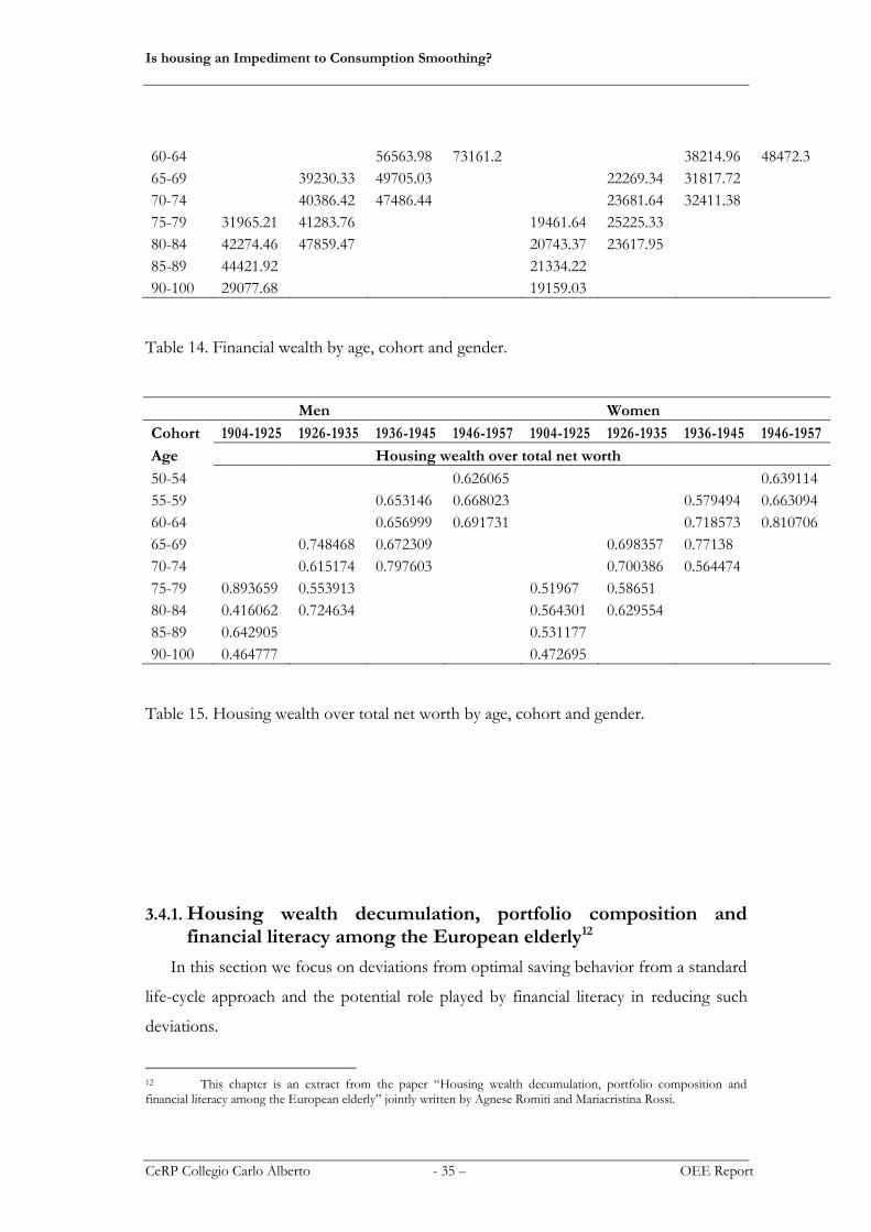
60-64 56563.98 73161.2 38214.96 48472.3
65-69 39230.33 49705.03 22269.34 31817.72
70-74 40386.42 47486.44 23681.64 32411.38
75-79 31965.21 41283.76 19461.64 25225.33
80-84 42274.46 47859.47 20743.37 23617.95
85-89 44421.92 21334.22
90-100 29077.68 19159.03
Table 14. Financial wealth by age, cohort and gender.
Men Women
Cohort 1904-1925 1926-1935 1936-1945 1946-1957 1904-1925 1926-1935 1936-1945 1946-1957
Age Housing wealth over total net worth
50-54 0.626065 0.639114
55-59 0.653146 0.668023 0.579494 0.663094
60-64 0.656999 0.691731 0.718573 0.810706
65-69 0.748468 0.672309 0.698357 0.77138
70-74 0.615174 0.797603 0.700386 0.564474
75-79 0.893659 0.553913 0.51967 0.58651
80-84 0.416062 0.724634 0.564301 0.629554
85-89 0.642905 0.531177
90-100 0.464777 0.472695
Table 15. Housing wealth over total net worth by age, cohort and gender.
3.4.1. Housing wealth decumulation, portfolio composition and financial literacy among the European elderly12
In this section we focus on deviations from optimal saving behavior from a standard
life-cycle approach and the potential role played by financial literacy in reducing such
deviations.
12 This chapter is an extract from the paper “Housing wealth decumulation, portfolio composition and financial literacy among the European elderly” jointly written by Agnese Romiti and Mariacristina Rossi.

Is housing an Impediment to Consumption Smoothing?
CeRP Collegio Carlo Alberto - 36 – OEE Report
The question we try to analyse by looking at different perspectives of saving
behaviour is whether financial literacy plays a role in the ability to use household wealth
efficiently.
The role of financial literacy on the ability to save has been intensively explored
(Behrman et al., 2010; Jappelli and Padula, 2011; Lusardi and Mitchell, 2011; van Roji et
al., 2012). After retirement, according to the standard life cycle model the decumulation
phase should start but very little decumulation is observed along the after-retirement
path. Is financial literacy responsible for the little decumulation in the old age?
Moreover, is the portfolio allocation affected by the degree of financial knowledge? Our
ex-ante expectation is that more financially sophisticated households should be more
active in their decumulation phase as well as show a more balanced portfolio. In
addition, we consider whether a bigger stock of financial literacy can also help
individuals to adopt optimal consumption behaviour. Finally, we want to investigate on
the consequences of the shadow illiquid asset. We test whether having problems in
making ends-meet can be dependent on the degree of portfolio illiquidity. We thus rely
on a multivariate analysis, which allows us to control for all potential factors affecting
wealth, with a particular focus on financial literacy.
Our aim is to analyze different measures of household wealth and how the decisions
about the latter are related and shaped by the stock of financial literacy other than by
other observed and unobserved individual characteristics of those in charge of dealing
with household finances, therefore we ideally need to identify the individual who is
responsible for them. Wealth-related survey questions refer to the household whereas
other questions such as all questions related to cognitive abilities (thus to financial
literacy) are asked to each respondent. We need to match the household related
variables to the individual characteristics of one person per household, ideally to the
person who is most in charge of household finances. The survey is well suited to this
purpose because at the beginning of the questionnaire individuals are asked about who
is the household financial respondent, the person responsible for the family finances,
therefore we select the latter when he/she is uniquely identified, whereas when there are
more than one financial respondent because both members of the couple manage the
finances separately, we consider the one with the highest income, or, in case of couples
with no income, the oldest one. Individual income is computed as the sum of earnings,
Is housing an Impediment to Consumption Smoothing?
CeRP Collegio Carlo Alberto - 37 – OEE Report
public and private pensions, life insurance payment received, private annuity, alimony,
regular payment from charities, and income from rent. Interest from bank accounts,
stocks, bonds, and mutual funds are not included because those questions in wave 2
refer to the household and not to individuals therefore the relevant variables at the
individual level are only available for wave 1.
We analyse household financial behaviour and its relationship with financial literacy
under three different perspectives: housing wealth decumulation, portfolio’s imbalance,
and consumption path. Accordingly we thus consider the following three main
dependent variables: the growth rate of household housing wealth (equivalent to the
first difference of the log value), the ratio between housing wealth and total net worth
(log), and a proxy for the optimal consumption path. The dataset does not provide a
proper measure of consumption since the information on total household consumption
is only available for one wave, whereas the only measure of consumption available for
the two waves consists in the amount spent on food at home or outside home plus the
amount spent on telephone. Thus we consider as a proxy for the optimal consumption
path an indicator for the self-reported household ability of making ends meet. The
relevant question is asked to respondents in charge of answering household-related
questions: “Is household able to make meets end? Thinking of your household's total
monthly income, would you say that your household is able to make ends meet”. From
this question we built an indicator set equal to one if the answer falls into one of the
following categories: “fairly easily” or “easily” and equal to zero if the answer is “with
some difficulties” or “with great difficulties”.
After excluding all observations with missing information on the variables of interest
we are left with a sample of 18,430 observations.
3.4.2. Empirical strategy
In order to estimate the impact of financial literacy on different dimensions of
wealth and saving decisions, we use the three dependent variables as described above:
the ratio of housing wealth over net worth (in logs) which we consider as a measure of
portfolio imbalance, an indicator equal to one for households being able to make ends
meet which is our proxy for optimal consumption, whereas the third dependent variable
representing housing wealth decumulation is the growth rate of housing wealth.

Is housing an Impediment to Consumption Smoothing?
CeRP Collegio Carlo Alberto - 38 – OEE Report
Financial literacy is likely to be endogenous for all these dependent variables since
individual unobserved characteristics such as individual preferences, innate ability, or the
household socio-economic environment are all correlated to both investments in
financial literacy and to decisions about savings and portfolio. As a consequence the
relevant coefficient is biased if this source of endogeneity is not taken into account.
Therefore we need to adopt an IV approach for all the specifications. Our instrument
for financial literature is an indicator for the last job or occupation held by the father; we
set this indicator equal to one if the father was employed in high skilled occupations,
which we define as manager, professional, or technician and associate. The intuition
driving this choice is due to the fact that first of all, within the family, it is often the
father in charge of dealing with finance and then aware of the role played by financial
literacy as opposed to the mother. In addition, being employed in a high skilled
occupation is certainly positively correlated to investing in children financial literacy
because of the awareness that higher financial literacy can have a positive and important
impact on children subsequent planning for retirement other than on dealing with
household finances. As a consequence, father employed in high skilled jobs can affect
and influence the past stock of children’s financial literacy at the same time without
having any impact on the children’s future decisions about wealth and consumption,
assuming that a sufficient time lag can dissipate the potential common socio-economic
context shared by both the young children and the father. That is to say that the past
father’s occupation should not be related to current (un)observed characteristics
affecting current decisions about household finances (in particular if we also control for
household income, another potential channel through which the children can be
affected by the past parental occupation if we assume low socio-economic
intergenerational mobility). The drawback with this instrument’s choice is that it is time-
invariant by its nature, since it is derived by a question (“What is or was the last job your
father had?”) only asked in the first wave. Therefore we are forced to consider only
respondents who were present in the first wave and we attribute the same value of this
variable also to the second wave assuming that given the old age of the sample (50+)
last parental job would not probably change in the second wave, the large majority of
parents would be already retired and also the very few not yet retired would probably do
not shift from a skilled to an unskilled category of occupation at the end of their

Is housing an Impediment to Consumption Smoothing?
CeRP Collegio Carlo Alberto - 39 – OEE Report
working career. As a consequence the instrument cannot be used in a longitudinal
setting such as a FE estimator. Our strategy is therefore to run first two separated
regressions one per each wave, then to compare the endogenous estimates obtained per
each wave with FE estimates in order to evaluate the potential incidence of the
unaccounted individual unobserved heterogeneity. If the difference between the two
estimators is not significant we can consider the cross-sectional IV estimates per wave
as the benchmark.
Since we use three dependent variables of different type, accordingly we need to use
different models’ specifications. The measure of portfolio imbalance is a continuous
variable which we model by using two OLS regressions and the relevant IV regressions,
one per each wave. Thus we compare the OLS results with a FE linear model. In
addition to that this dependent variable is censored because of the log transformation
which drops the zero values therefore we also control for potential selection bias by
adopting a standard Heckman selection model with its control function version, in order
to account for the endogeneity of financial literacy (Tables 16 and 17 – various
columns).
The second dependent variable of interest is a dichotomous variable representing an
indicator for being in a (self-reported) good financial situation, thus we need to adopt a
non linear model, such as a logit regression with a control function approach, and then
we contrast the results from the logit specifications with a FE non linear estimation
model, such as a conditional logit model (Table 18).
The third dependent variable is the growth rate of housing wealth, a continuous
variable, which we treat with OLS and IV specifications, and it is available for one wave
only since we only have two waves from which we can compute the growth rate (Table
19). We also replicate the same estimate on the growth rate of financial wealth (third
and fourth columns in Table 19).
For all the dependent variables we use the same vector of individual variables given
that the determinants underlying each of them are similar and all related to saving
decisions. The individual regressors consist in the following: the proxy for financial
literacy, three categorical indicators corresponding to being in the following age
brackets: 50-64, 65-85, and 85-100 which should account for the fact that three distinct
Is housing an Impediment to Consumption Smoothing?
CeRP Collegio Carlo Alberto - 40 – OEE Report
age-specific phases exist according to the standard life-cycle model, each of them
describing different saving behaviour: the younger age when individuals decumulate
because they are in the initial stage of their working life, afterwards the accumulation
period starts and workers face a steeper earning profile and eventually they enter the
retirement period where they should start to decumulate due to the less than unitary
pension benefit replacement rate. Since the dataset only involves individuals 50 aged and
older, we divide the two left conventional phases in three in order to account for the
additional variability due to the oldest-old phase (85-100). In addition we include the
self-reported probability of being alive which we assume as a proxy for expected life
expectancy assuming that the perceived longevity should have an impact on saving
behaviour. Individuals are asked the following question: “What are the chances that you
will live to be age (75, 80, 85, 90, 95, 100, 105, 110, 120) or more?” Each respondent can
answer by choosing a certain age among the list and then provide the probability of
being alive up to the chosen age. We then control for gender, immigration status (based
on country of birth), and education level including an indicator for being highly
educated where higher education corresponds to a post-secondary, non tertiary
education level. We also control for household income per capita (in logs) and its
squared value. Additional information is included in order to account for potential
determinants or shocks to saving decisions: an indicator for being retired, for being
widow/er, and for good subjective health status. From the question “Would you say
your health is" with the following possible answers: excellent, very good, good, fair, and
poor, an indicator is set equal to one if the respondent’s answer is excellent, very good,
or good. We also control for potential bequest motives by including the number of
children.13 Additional information included is: country fixed effects and time fixed
effects in case of the FE specifications. And we include our measure of portfolio
imbalance as an additional regressor in estimating the probability of making ends meet
since we want to evaluate whether being tied to excessively illiquid asset can be
responsible for deviations from the optimal consumption path.
13 The dataset also provides with the information about the intention to leave inheritance by asking the following question: “Within the next ten years, what are the chances that you will leave an inheritance worth more than 50,000 euro (in local currency)?”Instead of using this information we opt for using a more exogenous proxy given by the number of living children.

Is housing an Impediment to Consumption Smoothing?
CeRP Collegio Carlo Alberto - 41 – OEE Report
We start commenting the results on financial literacy and portfolio imbalance (Table
16 and 17). The first and second columns report the results obtained for both OLS and
IV estimations. Concentrating on the impact of financial literacy, both OLS and IV
results show that having a higher endowment of financial literacy brings about a
reduction in household portfolio imbalance: a lower proportion of household wealth
will consist of housing wealth and this result is consistent in both waves. We also
replicate the analysis by controlling for potential selection bias, since 30 percent of the
uncensored sample has zero housing wealth therefore it is dropped out because of the
log transformation. We adopt the standard likelihood Heckman selection model, and we
also account for the potential endogeneity of the financial literacy variable by using a
control function approach (columns 3-6 in Tables 16 and 17). Despite the LR test for
independent equations signals that the selection mechanism is not ignorable (p-
value=0.001), the coefficients relevant to financial literacy are substantially unchanged
with respect to the ones obtained on the censored sample. The selection mechanism is
instead ignorable in case of wave 2 where we cannot reject the null hypothesis of
independent equations (p-value=0.6). As it is reported in column 5, the significance of
the residuals’ coefficient reports the endogeneity of the financial literacy variable in both
waves. We consider the results reported in column 5 as our benchmark estimates
because they account for both endogeneity and potential selection bias. According to
these results increasing the stock of financial literacy by one point brings about a
significant reduction in household portfolio imbalance equal to about 20 percentage
points, which is a substantial effect given that the average value of the dependent
variable is about .71. We then compare the results obtained from the Heckman
specification to those of the FE linear model, since this allows us to control for time-
invariant unobserved factors affecting saving decisions and also correlated to the stock
of financial literacy. The results, shown in column 6, are consistent with those found for
both the OLS and Heckman specifications, suggesting that the unobserved
heterogeneity is only in part responsible for our main coefficient of interest; we can
argue that the endogeneity might be due to other time-varying factors which we control
for in the cross-sectional IV specification. Unfortunately we cannot compare the IV-FE
estimator with the cross-section one because our instrument is time-invariant therefore
it would be dropped from the estimation. As for the other coefficients, surprisingly

Is housing an Impediment to Consumption Smoothing?
CeRP Collegio Carlo Alberto - 42 – OEE Report
individual factors such as immigration status, gender, being widow/er or retired, and
also the number of children do not seem to have an impact on saving decisions, as it is
clear from column 5 in Tables 16 and 17, with the only exception for being retired
which increases portfolio imbalance (only for the second wave). From the selection
equation, which we identify by functional form instead of using any exclusion
restriction, we can argue which individual factors mostly increase the probability of
having no zero housing wealth. Immigrants are much less likely to own housing wealth,
whereas the opposite is true for being a widow/er which can be interpreted as due to
the fact that the widows/ers inherit the spouse’s housing wealth, moreover a self-
perceived longer life is positively correlated to having housing wealth, even though the
latter does not exert any impact on portfolio imbalance. The chosen instrument seems
not to suffer from any weakness throughout all the specifications, either when we
consider the IV estimates or the control function approach (see the bottom panel of
Tables 16, 17, 19, and 20), both the first stage F statistics and the t-test in the first stage
of the control function specifications are highly above any standard critical values.
The results for the impact of financial literacy on consumption patterns, proxied by
the likelihood of making meets end are shown in Table 18, which reports the cross-
section logit and its control function version by wave (wave 1 in columns 1 and 2, and
wave 2 in columns 3 and 4), whereas the FE results are reported in column 5 where we
use a conditional logit model. Both the OLS and the control function specifications
report a positive coefficient for financial literacy, thus suggesting the positive impact of
the latter on the probability of making meets end, thus having a higher endowment of
financial literacy increases the likelihood of optimal consumption behaviour. And this
pattern remains stable and significant (even if with a lower magnitude) also controlling
for unobserved individual heterogeneity in the FE estimation. Several individual factors
affect the probability of an optimal consumption pattern, but once we control for
individual fixed effects, we observe a significant positive impact of only higher life
expectancy and a negative impact of being a widow/widower. Commenting on the IV
specifications, our estimates show that increasing the numeracy score by one point
increases the probability of following an optimal consumption pattern of around 30
percent. As a robustness check we also control for unobserved individual heterogeneity
which might explain part of the financial literacy endowment and be responsible for the

Is housing an Impediment to Consumption Smoothing?
CeRP Collegio Carlo Alberto - 43 – OEE Report
endogeneity, and in case of the FE specification the impact is lower in magnitude
corresponding to a 2 percentage points increase, and loses a bit of significance (10
percent level) but still maintains the same positive sign. As for the role played by
financial literacy, since the FE estimates are very similar to the cross-section logit ones,
we argue that individual time-invariant unobserved heterogeneity plays a minor role,
whereas the endogeneity seems to be an issue as it is clear from the strong significance
of the residuals in the cross-section estimates, hence our preferred estimate are the latter
which control also for the endogeneity of financial literacy. Interesting to note is the role
played by our indicator for portfolio imbalance which exerts a negative effect on the
probability of making ends meet and it is strongly significant throughout all different
specifications.
The direction of the bias in the OLS estimates is not so clear-cut and it cannot be
known a priori since it depends on many different factors. Innate abilities can be
responsible for an upward bias in OLS estimates, assuming that they are positively
correlated to both the stock of financial literacy and the optimal consumption
behaviour. However OLS estimates can also be downward biased in case of
measurement errors in the financial literacy indicator. Therefore the direction of the bias
is an empirical question. Underestimation of the OLS coefficient has also been found by
Jappelli and Padula (2011) use the same SHARE dataset to estimate the impact of
financial literacy on saving rate. Taking the math test score at the age of 10 as the
instrument for the financial literacy indicator, they also found that the OLS coefficient
of financial literacy was an underestimation of the IV one.
The last model is related to the impact of financial literacy on housing wealth
decumulation, and the relevant results are shown in Table 19. Housing wealth
decumulation is measured by its growth rate, our dependent variable.
In order to interpret our results we first derive a model for asset depletion rate in
order to have the optimal behaviour according to which people would like to
decumulate. Our prediction is that more knowledgeable people dislike the idea of dying
with “too much” asset and therefore would be closer to the optimal depletion rate.
Conversely, people less financially literate are less conscious of the welfare loss of not
disposing of their asset optimally.

Is housing an Impediment to Consumption Smoothing?
CeRP Collegio Carlo Alberto - 44 – OEE Report
We derive the optimal decumulation path as follows. Consider the sum of lifetime
resources at time t
(1)
where T is the expected end of life, r is the real interest rate, At is total wealth, P are
pensions benefits, and c* is the optimal consumption; pension benefit are assumed
constant due to the institutional design of many pension systems and consumption is
constant over time because it represents the optimal consumption14 as it is the real
interest rate, r. Computing equation (1) at time t+1, dividing At+1 by At and taking logs,
we obtain the simplified version of the optimal decumulation path as follows
(2)
From this theoretical framework thus follows that asset depletion rate should just
depend upon the life expectancy and the interest rate and not be reactive to other
factors. However, given the small values taken by r, equation (2) simplifies as follows
thus asset depletion turns out to be only a function of individual life expectancy.15
We claim that the degree of financial literacy might play a role in this decumulation
planning. In particular, those households less financial literate might be less aware of
financial instruments to efficiently decumulate wealth and also less able to plan
14 The optimal consumption is constant under the simplifying assumption of equality between interest
rate and the discount rate. 15 In the empirical implementation we adopt a further simplification, driven by our measure of life
expectancy. Since our measure for life expectancy is the self-reported probability of being alive at a given future
age, and 5 percent of the sample reports a probability equal to zero, we approximate the factor k=-1/(T-t) with k=-
1/(1+(T-t)) in order not to lose the observations with probability equal to zero.

Is housing an Impediment to Consumption Smoothing?
CeRP Collegio Carlo Alberto - 45 – OEE Report
efficiently their welfare during retirement. In the empirical analysis we test this
hypothesis introducing as regressors in the regression modelling (housing) wealth
decumulation the constant term (k=-1/(1+lifeexp)) and its interaction with the financial
literacy indicator. According to our prior, we would expect that the sum of the k
coefficient and the coefficient of its interaction with financial literacy should correspond
to the optimal behaviour, thus it should be equal to one, the coefficient relevant to the
constant as in (1).
From both the OLS and the IV results we argue that financial literacy does not play
any role on wealth decumulation, and also its interaction with the constant k factor – as
derived from the theoretical framework in the above section and it is computed as an
inverse function of life expectancy16 - is only significant in the OLS estimates (column
1). Even trying to isolate subgroups of individuals which should potentially be more
subject to wealth decumulation, such as elderly or retired people, the role of financial
literacy is consistent with these results and remains insignificant. This lack of evidence
about the role of financial literacy on housing wealth decumulation can be explained by
the extremely poor evidence of overall (housing) wealth decumulation in the sample as
provided by the above descriptive statistics. Lastly we also replicate the analysis on the
growth rate of financial wealth (columns 3 and 4- Table 19) but the same results as for
housing wealth are confirmed suggesting no role for financial literacy on financial wealth
decumulation.
16 Life expectancy is represented by the same variable also included in all the regressions.

Is housing an Impediment to Consumption Smoothing?
CeRP Collegio Carlo Alberto - 46 – OEE Report
Portfolio imbalance. Housing wealth over total wealth: wave 1
OLS IV Heck Selec eqn Heck-IV Selec eqn FE
Fin Lit -0.0329*** -0.2280** -0.0203*** 0.1154*** -0.1633* 0.5272*** -0.0189***
-0.0062 -0.1020 -0.0075 -0.0143 -0.0952 -0.2009 -0.0068
Residuals 0.1439 -0.4139**
-0.0953 -0.2015
Age 65-84 0.0069 -0.0446 0.0156 0.0418 -0.0196 0.1440** 0.0178
-0.0144 -0.0316 -0.0146 -0.0376 -0.0280 -0.0623 -0.0247
Age 85-100 -0.0316 -0.1505** -0.0575** -0.2110*** -0.1365** 0.0150 -0.0192
-0.0258 -0.0679 -0.0277 -0.0561 -0.0579 -0.1232 -0.0385
Life exp -0.0002 -0.0001 0.0001 0.0026*** 0.0003 0.0022*** -0.0003
-0.0003 -0.0003 -0.0003 -0.0005 -0.0003 -0.0006 -0.0002
Fem 0.0344** -0.0424 0.0321** -0.0264 -0.0223 0.1314
-0.0140 -0.0431 -0.0144 -0.0302 -0.0394 -0.0819
Immig 0.0529* 0.0341 -0.0109 -0.4695*** -0.0404 -0.3814***
-0.0310 -0.0344 -0.0344 -0.0520 -0.0392 -0.0675
High Skilled -0.0255 0.0721 0.0133 0.3737*** 0.0923* 0.1474
-0.0168 -0.0533 -0.0205 -0.0371 -0.0544 -0.1158
Income(log) -0.0201 -0.0295** -0.0081 0.0720** -0.0108 0.0793** -0.0283***
-0.0128 -0.0143 -0.0134 -0.0325 -0.0134 -0.0327 -0.0106
Income (log)2 0.0011 0.0018* -0.0005 -0.0111*** -0.0003 -0.0116*** 0.0016*
-0.0010 -0.0011 -0.0011 -0.0023 -0.0011 -0.0023 -0.0009
Health (subj) -0.0322** 0.0170 -0.0126 0.1748*** 0.0265 0.0620 -0.0119
-0.0127 -0.0295 -0.0150 -0.0318 -0.0295 -0.0635 -0.0134
Retired 0.0220 0.0260* 0.0182 -0.0317 0.0208 -0.0400 -0.0038
-0.0141 -0.0154 -0.0147 -0.0353 -0.0149 -0.0355 -0.0188
Widow/er 0.0295 -0.0124 0.0494** 0.1795*** 0.0294 0.2378*** 0.0780
-0.0196 -0.0302 -0.0214 -0.0430 -0.0255 -0.0518 -0.0607
First stage
IV 0.1651***
0.028
F 35.621
Lambda 0.232 0.233
se (lambda) 0.07 0.069
p (indep eqn) 0.001 0.001
N 6472 6472 10102 10102 12754
Note: Robust standard errors in parenthesis. Additional regressors are country fixed effects in columns 1-6) and time fixed effects (column 7).
Table 16. Portfolio imbalance. Wave 1.

Is housing an Impediment to Consumption Smoothing?
CeRP Collegio Carlo Alberto - 47 – OEE Report
Portfolio imbalance. Housing wealth over total wealth: wave 2
OLS IV Heck Selec eqn Heck-IV Selec eqn FE
Fin Lit -0.0216*** -0.1962** -0.0211*** 0.1115*** -0.1863** 0.6252*** -0.0189***
-0.0055 -0.0918 -0.0055 -0.0166 -0.0831 -0.2369 -0.0068
Residuals 0.1662** -0.5164**
-0.0831 -0.2377
Age 65-84 0.0553*** 0.0078 0.0554*** -0.0110 0.0124 0.1226 0.0178
-0.013 -0.0281 -0.0131 -0.0453 -0.0246 -0.0768 -0.0247
Age 85-100 0.0121 -0.0886 0.0115 -0.1466** -0.0821 0.1437 -0.0192
-0.019 -0.0567 -0.019 -0.0624 -0.0507 -0.1474 -0.0385
Life exp -0.0003 -0.0001 -0.0002 0.0022*** -0.0001 0.0018*** -0.0003
-0.0002 -0.0002 -0.0002 -0.0006 -0.0002 -0.0006 -0.0002
Fem 0.0330*** -0.0353 0.0326*** -0.0842** -0.0308 0.1134
-0.0119 -0.0385 -0.0119 -0.0356 -0.0346 -0.0968
Immig 0.0121 0.0077 0.0098 -0.4229*** -0.0076 -0.3657***
-0.0242 -0.0264 -0.0242 -0.0610 -0.0258 -0.0663
High Skilled -0.0594*** 0.0223 -0.0577*** 0.3793*** 0.0262 0.1199
-0.0148 -0.0465 -0.0147 -0.0429 -0.0455 -0.1264
Income_pc (log) -0.0152* -0.0202* -0.0148 0.0448 -0.0162* 0.0500 -0.0283***
-0.0091 -0.0105 -0.0092 -0.0387 -0.0092 -0.0388 -0.0106
Income_pc (log)2 0.0007 0.0012 0.0006 -0.0100*** 0.0007 -0.0104*** 0.0016*
-0.0007 -0.0009 -0.0007 -0.0028 -0.0007 -0.0028 -0.0009
Health (subj) -0.0275** 0.0177 -0.0268** 0.1475*** 0.0174 0.0114 -0.0119
-0.0119 -0.0276 -0.0119 -0.0359 -0.0256 -0.0726 -34
Retired 0.0291** 0.0324** 0.0294** 0.0604 0.0368*** 0.0373 -0.0038
-0.0126 -0.0137 -0.0125 -0.0421 -0.013 -0.0436 -0.0188
Widow/er 0.0209 -0.0134 0.0216 0.1586*** -0.0073 0.2508*** 0.078
-0.0156 -0.0245 -0.0156 -0.0498 -0.0211 -0.0651 -0.0607
First stage
IV 0.170***
0.029
34.26
Lambda 0.017 0.02
se (lambda) 0.014 0.015
p (indep eqn) 0.227 0.191
N 6272 6272 8328 8328 8350 12754
Note: Robust standard errors in parenthesis. Additional regressors are country fixed effects in columns 1-6) and time fixed effects (column 7).
Table 17. Portfolio imbalance. Wave 2.

Is housing an Impediment to Consumption Smoothing?
CeRP Collegio Carlo Alberto - 48 – OEE Report
Optimal consumption. No difficult to make ends meet
logit logit-cf logit logit-cf FE
Fin Lit 0.0467*** 0.3003*** 0.0453*** 0.4042*** 0.0281*
-0.0070 -0.1073 -0.0069 -0.1068 -0.0159
Residuals -0.2549** -0.3606***
-0.1076 -0.1070
Life exp 0.0004 0.0004 0.0008*** 0.0005** 0.0014***
-0.0003 -0.0003 -0.0003 -0.0003 -0.0005
Hous w/ne worth(log) -0.1277*** -0.0984*** -0.1545*** -0.1150*** -0.0693*
-0.0172 -0.0213 -0.0223 -0.0253 -0.0387
Age 65-84 0.0175 0.0825*** 0.0231 0.1164*** 0.0157
-0.0172 -0.0316 -0.0172 -0.0319 -0.0551
Age 85-100 0.1061*** 0.2095*** 0.0695*** 0.2130*** 0.0653
-0.0237 -0.0387 -0.0231 -0.0353 -0.0974
Fem -0.0423*** 0.0561 -0.0547*** 0.0840*
-0.0145 -0.0441 -0.0142 -0.0434
Immig 0.0049 0.0275 -0.0150 -0.0053
-0.0305 -0.0308 -0.0323 -0.0318
High Skilled 0.1016*** -0.0193 0.1094*** -0.0500
-0.0157 -0.0565 -0.0154 -0.0544
Income_pc (log) 0.0580*** 0.0707*** 0.0597*** 0.0705*** -0.0468
-0.0136 -0.0147 -0.0132 -0.0134 -0.0382
Income_pc (log)2 -0.0039*** -0.0049*** -0.0043*** -0.0054*** 0.0045
-0.0010 -0.0011 -0.0010 -0.0011 -0.0030
Retired -0.0031 -0.0090 0.0051 -0.0033 -0.0680
-0.0164 -0.0166 -0.0164 -0.0165 -0.0450
Widow/er -0.0294 0.0236 -0.0185 0.0490* -0.2894**
-0.0223 -0.0301 -0.0219 -0.0275 -0.1464
Health (subj) 0.1117*** 0.0455 0.1176*** 0.0218 0.0244
-0.0166 -0.0317 -0.0157 -0.0314 -0.0322
Number children -0.0117* -0.0021 -0.0206*** -0.0166*** 0.0014
-0.0061 -0.0074 -0.0061 -0.0062 -0.037
First stage
IV 0.1609*** 0.1639***
0.027 0.028
N 6482 6482 6272 6272 2032
Note: Marginal effects. Robust standard errors in parenthesis. Additional regressors are country fixed effects in columns 1-4) and time fixed effects (column 5).
Table 18. Probability of making ends meet.
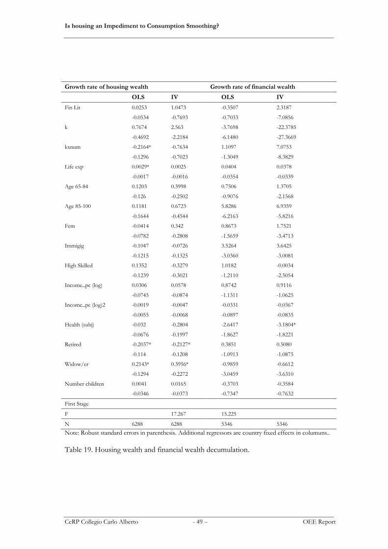
Is housing an Impediment to Consumption Smoothing?
CeRP Collegio Carlo Alberto - 49 – OEE Report
Growth rate of housing wealth Growth rate of financial wealth
OLS IV OLS IV
Fin Lit 0.0253 1.0473 -0.3507 2.3187
-0.0534 -0.7693 -0.7033 -7.0856
k 0.7674 2.563 -3.7698 -22.3785
-0.4692 -2.2184 -6.1480 -27.3669
kxnum -0.2164* -0.7634 1.1097 7.0753
-0.1296 -0.7023 -1.3049 -8.3829
Life exp 0.0029* 0.0025 0.0404 0.0378
-0.0017 -0.0016 -0.0354 -0.0339
Age 65-84 0.1203 0.3998 0.7506 1.3705
-0.126 -0.2502 -0.9076 -2.1568
Age 85-100 0.1181 0.6723 5.8286 6.9359
-0.1644 -0.4544 -6.2163 -5.8216
Fem -0.0414 0.342 0.8673 1.7521
-0.0782 -0.2808 -1.5659 -3.4713
Immigig -0.1047 -0.0726 3.5264 3.6425
-0.1215 -0.1325 -3.0360 -3.0081
High Skilled 0.1352 -0.3279 1.0182 -0.0034
-0.1239 -0.3021 -1.2110 -2.5054
Income_pc (log) 0.0306 0.0578 0.8742 0.9116
-0.0745 -0.0874 -1.1311 -1.0625
Income_pc (log)2 -0.0019 -0.0047 -0.0331 -0.0367
-0.0055 -0.0068 -0.0897 -0.0835
Health (subj) -0.032 -0.2804 -2.6417 -3.1804*
-0.0676 -0.1997 -1.8627 -1.8221
Retired -0.2037* -0.2127* 0.3851 0.5080
-0.114 -0.1208 -1.0913 -1.0875
Widow/er 0.2143* 0.3956* -0.9859 -0.6612
-0.1294 -0.2272 -3.0459 -3.6310
Number children 0.0041 0.0165 -0.3703 -0.3584
-0.0346 -0.0373 -0.7347 -0.7632
First Stage
F 17.267 15.225
N 6288 6288 5346 5346
Note: Robust standard errors in parenthesis. Additional regressors are country fixed effects in columuns..
Table 19. Housing wealth and financial wealth decumulation.

Is housing an Impediment to Consumption Smoothing?
CeRP Collegio Carlo Alberto - 50 – OEE Report

Is housing an Impediment to Consumption Smoothing?
CeRP Collegio Carlo Alberto - 51 – OEE Report
References:
Behrman, J. R., Mitchell, O. S., Soo, C., and Bravo, D. (2010). Financial literacy,
schooling, and wealth accumulation. Working Paper 16452, National Bureau of
Economic Research.
Chiuri, E, and T. Jappelli (2010). Do the elderly reduce housing equity? An
international comparison. Journal of Population Economics, 23:643–663.
Christelis, D, T. Jappelli, and M. Padula (2010). Cognitive abilities and portfolio
choices. European Economic Review, 54(1):18-38.
Deaton, A. S. and Paxson, C. (2004). Mortality, income, and income inequality over
time in britain and the united states. In Perspectives on the Economics of Aging, NBER
Chapters. National Bureau of Economic Research, Inc.
Lleras-Muney, A. (2005). The relationship between education and adult mortality in
the united states. Review of Economic Studies, 72(1):189-221.
Lusardi, A. and Mitchell, O. S. (2011). Financial literacy and planning: Implications
for retirement wellbeing. Working Paper 17078, National Bureau of Economic
Research.
Jappelli, T. and M. Padula (2011). Investment in financial literacy and savings
decisions. CSEF Working paper n. 272.
Van Rooj, M., A. Lusardi, and R. Alessie (2001). Financial literacy and stock market
participation. Journal of Financial Economics. 101: 449-472.
van Rooij, M. C., Lusardi, A., and Alessie, R. (2012). Financial literacy, retirement
planning and household wealth. The Economic Journal, 122(560):449–478.
Venti S.F., and D.A. Wise (1989). Aging, moving and housing wealth. NBER WP n.
2324.
Venti S.F., and D.A. Wise (2002). Aging and housing equity in Innovations and
Retirement financing. University of Pennsylvania Press.
Venti S.F., and D.A. Wise (2004). Aging and housing equity: another look. Chapter 3
in Perspective on the Economics of Aging. NBER.

Is housing an Impediment to Consumption Smoothing?
CeRP Collegio Carlo Alberto - 52 – OEE Report
Appendix.
A.1. Numeracy
The 4 questions relevant to the variable numeracy are the following. Possible answers
are shown in a card while the interviewer is instructed not to read them out to the
respondent:
1.If the chance of getting a disease is 10 per cent, how many people out of one thousand would be
expected to get the disease?
The possible answers are 100, 10, 90, 900 and another answer.
2. In a sale, a shop is selling all items at half price. Before the sale a sofa costs 300 euro. How much
will it cost in the sale?
The possible answers are 150, 600 and another answer.
3. A second hand car dealer is selling a car for 6,000 euro. This is two-thirds of what it costs new.
How much did the car cost new?
The possible answers are 9,000, 4,000, 8,000, 12,000, 18,000 and another answer.
4. Let’s say you have 2,000 euro in a saving account. The account earns ten per cent interest
each year. How much would you have in the account at the end two years?
The possible answers are 2,420, 2,020, 2,040, 2,100, 2,200, 2,400 and another answer.
The variable numeracy has been built as follow. If a person answers (1) correctly she is
then asked (3) and if she answers correctly again she is asked (4). Answering (1)
correctly results in a score of 3, answering (3) correctly but not (4) results in a score of 4
while answering (4) correctly results in a score of 5. On the other hand if she answers
(1) incorrectly she is directed to (2). If she answers (2) correctly she gets a score of 2
while if she answers (2) On the basis of these four questions Dewey and Prince (2005)
construct a numeracy indicator, which ranges from 1 to 5

Is housing an Impediment to Consumption Smoothing?
CeRP Collegio Carlo Alberto - 53 – OEE Report
Financial Literacy and portfolio imbalance in Italy: SHIW data(a)
The Bank of Italy’s Survey on Household Income and Wealth (SHIW) allows us to investigate the relationship between FL and housing investment as a share f total portfolio.
To gauge respondents’ level of FL, we follow Fornero and Monticone (2010) and exploit three survey questions regarding inflation, interest rates and a basic understanding of stocks and bonds.
Question 1: Imagine leaving 1,000 euros in a current account that pays 1% interest and has no charges. Imagine that inflation is running at 2%. Do you think that if you withdraw the money in a year’s time you will be able to buy the same amount of goods as if you spent the 1,000 euros today? (Yes/Less/More/Don’t know/No answer)
Question 2: Which of the following investment strategies do you think entails the greatest risk of losing your capital? (Investing in the shares of a single company/[…] more than one company/ Don’t know/No answer)
Question 3: Which of the following types of mortgage do you think would allow you from the very start to fix the maximum amount and number of instalments to be paid before the debt is extinguished? (Floating-rate mortgage/ Fixed-rate mortgage/ Floating-rate mortgage with fixed instalments/ Don’t know/No answer)
We first create three dummy variables taking the value of 1 for every correct answer for each individual, and then sum them up to build an indicator ranging from 1 to 3.
The descriptive statistics confirm what was found in the SHARE data, i.e. the level of FL is quite low
among Italians: less than one third of respondents (28.5%) is able to answer correctly all 3 FL questions, and the percentage of financially literate household heads is considerably lower among the over 65.
We define our dependent variable, HOMESHARE, as the ratio of housing wealth (net of mortgages) over total wealth (net of any financial liability) and estimate the partial effect of FL on portfolio imbalance with a fixed effects econometric specification.
The (preliminary) results show that a higher level of FL is indeed correlated with a lower share of housing investment, controlling for several demographics. If we isolate a sample of over 50 we find an even stronger and more significant effect.
All sample Over 50
b/se b/se
Financial Literacy index -0.009** -0.010*** (0.00) (0.00) Marital Status
Single -0.021 -0.073* (-0.03) (-0.04) Separated/divorced -0.096*** -0.130*** (-0.03) (-0.04) Widow(er) -0.030 -0.047**
(-0.02) (-0.02) House inherited 0.179*** 0.127*** (-0.01) (-0.01) Log of household income -0.033*** -0.051*** (-0.01) (-0.01) Log of average house price -0.006 0.048 (-0.04) (-0.04) Healthy 0.007 0.009* (0.00) (0.00) Year 2006-2010 YES YES Constant 1.162*** 0.348 (-0.37) (-0.50) Number of observations 1,2145 7,960 Loglikelihood 4310.999 4753.258 Pseudo R2
(a) Mean housing wealth is estimated taking the natural logarithm of housing value per square metre, by region and city size. The superscripts ***, **, and * indicate the 1%, 5%, and 10% levels of statistical significance, respectively. Control variables with insignificant effects are not reported: second order polynomial for age, female, household head graduate, number of average children, healthy household head, risk averse and area of residence.
(a) The information is taken form a MIMEO paper by Riccardo Calcagno and Csira Urzí Brancati on FL and portfolio imbalance.

Is housing an Impediment to Consumption Smoothing?
CeRP Collegio Carlo Alberto - 54 – OEE Report
4. ELSA data on the UK.
4.1. Descriptive evidence
The English Longitudinal Study of Ageing (ELSA) has been designed to represent people aged 50 and over, living in private households in England. The sample was drawn from households that had previously responded to the Health Survey for England (HSE) in 1998, 1999 or 2001; the data collected is known as “ELSA Wave 0”, and forms the basis for all subsequent waves of the study. As the name suggests, ELSA is a longitudinal study, hence participants have been followed and re-interviewed every two years. Eligible households have at least one member born on or after 1952, but as the study progresses the respondents get older, and therefore a refreshment sample of younger HSE members has been added at Wave 3 (2006). For the sake of consistency, we will only use ELSA wave 2 and wave 3 which refer to the same time frame as the first two waves of SHARE; this leaves us with a rather large pooled sample of 17,590 individuals or 12,716 households.
The ELSA dataset did not provide the definition of “head of household”, i.e. the breadwinner, so we chose the household component with the highest earnings; if the earnings were defined for the couple, we chose the eldest and if two householders were the same age, we chose the man. The majority of Female headed households is to be found in the first cohort – 1904-1925, where approximately 45% is divorced and 36% is widowed (not reported).
Table 1: Heads of household by gender and cohort
Cohort
1904-1925 1926-1935 1936-1945 1946-1957 All
Male 861 1,702 2,181 2,236 6,980
Female 1,195 1,470 1,457 1,614 5,736
Total 2,056 3,172 3,638 3,850 12,716
Source: ELSA wave 2 and 3.
Graph 1 shows the composition of the sample by wave, gender and cohort: as a refreshment sample was added in wave 3, the percentage of younger householders increases in approximately equal number for men and women.

Is housing an Impediment to Consumption Smoothing?
CeRP Collegio Carlo Alberto - 55 – OEE Report
Graph 1: ELSA composition by gender, cohort and year
Source: ELSA wave 2 and 3.
One of the strengths of ELSA is that it combines expertise from a number of disciplines, supplying very detailed information on both health and economic conditions of participants. Assessment of wealth is important not only because it provides a summary measure of economic fortunes through the life cycle, but because it also offer a measure of security for the future.
Indicators for real and financial wealth were built by combining a few different measures. The indicator of real (net) wealth includes the value of owned property and other estates, net of mortgage; the indicator of financial (net) wealth includes deposits and savings accounts, bonds, stocks, mutual funds, individual retirement account, whole life insurance net of liabilities. We then converted the values in Euros (PPP) and in current prices to make them compatible with the SHARE data.
Table 2: Average real wealth and financial wealth by gender and cohort (per household)
Real Wealth (in €) Financial Wealth (in €)
Cohort Male Female Male Female
1904-1925 219,122 151,241 57,094 29,366
1926-1935 267,733 190,532 59,473 34,910
1936-1945 331,556 280,491 94,826 70,480
1946-1957 334,199 266,644 135,678 94,620
Source: ELSA wave 2 and wave 3. Pooled sample. Euro at constant prices (PPP).
As Table 2 clearly shows, younger male household heads have substantially higher real and financial wealth.
1,141
1,6941,911
1,503
915
1,478
1,727
2,347
1904-1925 1926-1935 1936-1945 1946-1957 1904-1925 1926-1935 1936-1945 1946-1957
Male Female
year 2004 - total obs: 6,249 year 2006 - total obs: 6,467
13.9%
23.7%
26.6%
27.8%
33.4%
27.0%
26.1%
21.5%
10.7%
18.2%22.2%
25.5%
29.2%
25.7%
38.0%
37.0%

Is housing an Impediment to Consumption Smoothing?
CeRP Collegio Carlo Alberto - 56 – OEE Report
Table 3: Average real wealth and financial wealth by gender and cohort (per individual)
Real Wealth (in €) Financial Wealth (in €)
Cohort Male Female Male Female
1904-1925 117,524 90,663 49,557 28,074
1926-1935 145,396 115,473 47,791 36,138
1936-1945 186,228 169,432 78,608 63,687
1946-1957 199,993 193,800 107,239 82,394
Source: ELSA wave 2 and wave 3. Pooled sample. Euro at constant prices (PPP).
Since approximately 78% sample households own their own home – 56% own it outright and 22% with the help of a mortgage – it is not surprising to find that housing represents the greatest share of wealth.
Table 4: Share of net real wealth over total portfolio by gender and cohort
Cohort
Gender 1904-1925 1926-1935 1936-1945 1946-1957
Male 63.8% 70.1% 71.2% 67.6%
Female 55.9% 62.7% 70.5% 67.8%
Source: ELSA wave 2 and wave 3. Pooled sample.
Overall, only a small proportion of people in the sample have one or more children living in the household; however, approximately 86% have children either living in or outside the household. (Table 5)
Table 5: Average real wealth and financial wealth by parental status and cohort
Real Wealth (in €) Financial Wealth (in €)
Cohort Without Children With Children
Without Children With Children
1904-1925 151,500 175,000 45,219 38,242
1926-1935 191,823 224,983 45,089 46,139
1936-1945 267,961 281,419 90,253 80,967
1946-1957 282,387 254,532 141,660 107,563
Source: ELSA wave 2.
4.2. Health
The ELSA dataset provides a vast array of health indicators, therefore we have been able to adopt a few different ones for our analysis: firstly, an indicator of subjective health, ranging from “excellent” to “very bad”: more than 80 percent of the sample declares to be in good health of better, and there is no difference between men and women. (See Graph 2).

Is housing an Impediment to Consumption Smoothing?
CeRP Collegio Carlo Alberto - 57 – OEE Report
Graph 2: Subjective health by gender
Source: ELSA wave 2 and 3.
We are interested in finding out whether households may be reluctant to decumulate their wealth for fear of unexpected health shocks
Table 6: Average net real wealth by cohort and subjective health
Subjective Health
Real wealth by cohort (in €, constant prices)
1904-1925 1926-1935 1936-1945 1946-1957
Excellent 70,766 121,394 184,003 229,243
Very good 97,861 111,666 183,543 192,415
Good 107,305 144,009 174,830 204,688
Fair 130,236 151,975 178,034 136,838
Poor or very bad 96,654 107,616 127,931 158,110
Source: ELSA wave 2 and 3.
Table 7: Average net financial wealth by cohort and subjective health
Subjective Health
Financial wealth by cohort (in €, constant prices)
1904-1925 1926-1935 1936-1945 1946-1957
Excellent 45,894 51,123 103,838 126,101
Very good 46,622 52,200 84,642 100,697
Good 35,442 38,661 54,711 85,020
Fair 27,861 25,178 36,426 42,719
Poor or very bad 20,109 16,161 22,481 30,920
Source: ELSA wave 2 and 3.
The relationship between wealth decumulation and subjective health is not clear-cut and cannot be easily inferred by simple descriptive statistics. However, a quick glance at Table 10 and Table 11 seems to validate the predicted negative correlation between real wealth and subjective health for the older generations, while maintaining a positive correlation between subjective health and financial wealth.
34.1%29.4%
13.7%
5.1%
17.7%
4.7%
13.9%
29.2%
35.0%
17.3%
Excellent Very good Good Fair Poor or Very bad
Male Female
1,275
1,537
3,111
2,593
1,238
415
2,458
2,118
985
366

Is housing an Impediment to Consumption Smoothing?
CeRP Collegio Carlo Alberto - 58 – OEE Report
To build indicators of objective health, we used information regarding the presence of any chronic illnesses, such as cancer or a heart condition17. Interestingly, the correlation between subjective and objective health (defined as no chronic conditions) is quite low (not reported). Overall, women appear healthier than men when younger, but the situation reverts for the older generations, most likely because more women survive (see Graph 3.)
Graph 3: Health status by cohort and gender – do you any chronic disease?
Men Women
Source: ELSA wave 2 and wave 3. Pooled sample.
The correlation between objective health and real or financial wealth appears to be negative.
Table 8: Average real wealth and financial wealth by parental status and cohort
Real Wealth (in €) Financial Wealth (in €)
Cohort Without chronic diseases
With chronic diseases
Without chronic diseases
With chronic diseases
1904-1925 201,911 173,040 46,473 39,157
1926-1935 276,488 207,184 58,870 41,564
1936-1945 341,813 271,387 98,958 68,615
1946-1957 338,339 252,739 134,877 80,385
Source: ELSA wave 2 and wave 3. Pooled sample.
Another indicator of objective health is given by the presence of conditions limiting the respondent’s daily activities, and specifically whether she had problems: walking 100 yards, sitting for about two hours, getting up from a chair after sitting for long periods, climbing one or several flights of stairs without resting, stooping, kneeling, or crouching,
17 The chronic conditions mentioned are arthritis, osteoporosis, cancer or a malignant tumour (excluding minor skin cancers), Parkinson's disease, any emotional, nervous or psychiatric problems, Alzheimer’s disease, dementia, organic brain syndrome, senility or any other serious memory impairment, however we do not differentiate between types of conditions.
861
1,702
2,174 2,236
1904-1925 1926-1935 1936-1945 1946-1957
No Yes
54.9%
61.4%
66.2%79.8%
20.2%
45.1%
38.6%
33.8%
1,195
1,470 1,4531,614
1904-1925 1926-1935 1936-1945 1946-1957
41.0%41.6%
52.0%
73.5%59.0%
58.4%48.0%
26.5%

Is housing an Impediment to Consumption Smoothing?
CeRP Collegio Carlo Alberto - 59 – OEE Report
reaching or extending their arms above shoulder level, pulling or pushing large objects, lifting or carrying weights over 10 pounds, like a heavy bag of groceries and picking up a 5p coin from a table.
Graph 4: Average Real and Financial wealth by cohort and number of limitations (in € at constant prices)
Real Wealth Financial Wealth
Cohort:
Source: ELSA wave 2 and wave 3. Pooled sample.
Once again, there seems to be a negative correlation between average real or financial wealth and number of limitations.
4.3. Numeracy – or financial literacy
ELSA wave 1 features numeracy/financial literacy questions which we used to construct a financial literacy indicator: the first question investigated respondents’ ability to calculate a simple percentage (ten percent of a thousand), the second and third questions asked respondents to work out the initial price of an item on sale, with the new price set at 50 percent or two thirds of the original, and the last one assessing respondents’ ability to calculate compound interest in a savings account, commonly regarded as a good proxy for financial literacy. We followed the same methodology adopted by Jappelli and Padula (2011) and built an indicator ranging from 1 to 5 (low to high numeracy). In particular, if respondents answered the second, third and fourth questions correctly, we awarded 5 points; if they only answered correctly the second and third, but not fourth, 4 points, and if they only answered correctly the second question, 3 points. If they didn’t answer the second question correctly, but got the first one right, we awarded them 2 points, and if they didn’t give any correct answer, they were awarded only 1 point.
0
50,000
100,000
150,000
200,000
250,000
300,000
350,000
400,000
0 1 2 3 4 5 6 7 8 9 10
0
50,000
100,000
150,000
200,000
250,000
300,000
350,000
400,000
0 1 2 3 4 5 6 7 8 9 10
1904-1925 1926-1935 1936-1945 1946-1957

Is housing an Impediment to Consumption Smoothing?
CeRP Collegio Carlo Alberto - 60 – OEE Report
Graph 5: distribution of Numeracy/Financial Literacy by gender
Source: ELSA wave 1.
As reported in Table 9, roughly half of the sample (48%) scores 3 or less, with a marked difference between men (38%) and women (57%), while approximately 20% of men and 8% of women scores 5, the highest score. It is worth noting that the score of 5 is assigned only to people who could calculate compound interest correctly.
Table 9: Financial literacy (numeracy) by gender – ELSA wave 1
Score Men Women All
1 274 405 679
5.6% 6.9% 6.3%
2 383 1,022 1,405
7.8% 17.4% 13.0%
3 1,229 1,920 3,149
24.9% 32.6% 29.1%
4 2,062 2,085 4,147
41.9% 35.4% 38.3%
5 979 459 1,438
19.9% 7.8% 13.3%
Total 4,927 5,891 10,818
100% 100% 100%
Source: ELSA wave 1.
As shown in Table 10 and Table 11, average real and financial wealth are positively correlated with financial literacy.
01
02
03
04
0
1 2 3 4 5 1 2 3 4 5
Male Female
Pe
rcen
t
Numeracy / Financial Literacy
Distribution of numeracy/financial literacy by gender

Is housing an Impediment to Consumption Smoothing?
CeRP Collegio Carlo Alberto - 61 – OEE Report
Table 10: Average real wealth by cohort and numeracy/financial literacy score
Financial Literacy Score
Real wealth by cohort (in €)
1904-1925 1926-1935 1936-1945 1946-1957
1 103,634 119,489 122,209 150,315
2 100,691 127,889 135,807 121,726
3 156,141 196,553 204,541 201,296
4 206,167 267,812 306,421 264,994
5 250,270 301,505 420,629 352,170
Source: ELSA wave 2.
Table 11: Average financial wealth by cohort and numeracy/financial literacy score
Financial Literacy Score
Financial wealth by cohort (in €)
1904-1925 1926-1935 1936-1945 1946-1957
1 17,010 18,613 19,529 79,346
2 14,793 18,191 23,939 37,575
3 30,510 33,745 53,243 72,655
4 54,986 59,454 88,466 103,142
5 103,311 80,663 153,804 195,771
Source: ELSA wave 2.

Is housing an Impediment to Consumption Smoothing?
CeRP Collegio Carlo Alberto - 62 – OEE Report
Chapter II: How to make real asset liquid.
1. The use of reverse mortgages around the word
1.1. Reverse mortgage in the US
The most common - and usually the least expensive - type of reverse mortgage in the
US18 is the FHA19's Home Equity Conversion Mortgage (HECM) program, which is
designed for homeowners aged 62 or older. It has been authorized since 1987. People
who are interested in obtaining a reverse mortgage are obliged to participate in a
consumer information session given by a HUD20 approved HECM counsellor. This
ensures that borrowers are fully informed about the financial implications of this kind of
mortgage and about its alternatives.
There are five different payment plans:
Tenure: equal monthly payments as long as at least one borrower lives and
continues to occupy the property as a principal residence.
Term: equal monthly payments for a fixed period of months selected by the
borrower. At the end of the term, the borrower does not have to repay immediately
the loan, but he does not receive any other payment.
Line of Credit: unscheduled payments or in installments, at times and in an amount
selected by the borrower until the line of credit is exhausted. An attractive feature of
this method is that the amount of cash available and not withdrawn grows over time
at the same interest rate applied to the reverse mortgage plus 0.5%. For instance,
suppose the borrower has a credit-line of $120,000, the interest rate is 5.5%, and he
immediately withdraws $20,000, leaving $100,000. After one year, the available
credit-line would be $106,000, i.e. $100,000 plus (5.5%+0.5%) times $100,000.
Modified Tenure: combination of line of credit and scheduled monthly payments
for as long as the borrower remain in the home.
18 Other reverse mortgages are: Deferred Payment Loans (DPLs) offered by several local and state government agencies, Property Tax Deferral (PTD) offered by the public sector only to pay borrowers' property taxes, and Proprietary Reverse Mortgages developed by private companies mainly for homeowners whose house worth more than the HECM limit 19 Federal Housing Administration. 20 U.S. Department of Housing and Urban Development.

Is housing an Impediment to Consumption Smoothing?
CeRP Collegio Carlo Alberto - 63 – OEE Report
Modified Term: combination of line of credit plus monthly payments for a fixed
period of months selected by the borrower.
The FHA is responsible for paying the lender for any difference between the total
loan amount and the amount for which the mortgaged property is actually sold. FHA
insurance also ensures payments to the borrower in the event the lender is unable or
unwilling to make payments, and regardless of what happens to the property's value. For
this reason, there is an initial Mortgage Insurance Premium (MIP). In case of HECM
Standard it is 2% of the lesser of the appraised value of the home, the FHA HECM
mortgage limit of $625,500 or the sales price. On the other end, the HECM Saver -
introduced on October 4, 2010 - only charges 0.01%. However, in the latter case it is
possible to borrow a lower amount of money. Moreover, in both cases it is applied an
annual MIP of 1.25% of the mortgage balance21.
Other costs includes interests, third party charges, servicing fees, and origination
fees. The latter is equal to $2500 if the value of the house is less than $125,000,
otherwise it is equal to 2% of the first $200,000 of the home's value plus 1% of the
amount over $200,000. The cap for this fee is $6,000.
Table shows how much it is possible to get from a HECM at different ages and using
different interest rates22.
21 A mortgage balance is the full amount owed at any period of time during the duration of the mortgage. 22 The servicing fee is $35, closing costs are $2,500, and the origination fee is the maximum allowed by HUD. This table has been taken by AARP(2010)

Is housing an Impediment to Consumption Smoothing?
CeRP Collegio Carlo Alberto - 64 – OEE Report
Table 12: HECM Lump Sum or Credit Line
As shown in Table 13 the number of reverse mortgages has increased exponentially
in the last decade, although it has dropped sharply after 2009. However, this could be
interpreted as a short-lived reaction to the sub-prime crisis, rather than a change in the
long-term trend.
Table 13: Number of HECM in the US, 1990-2012
1990
1991
1992
1993
1994
1995
1996
1997
1998
1999
2000
2001
2002
2003
2004
2005
2006
2007
2008
2009
2010
2011
2012
-
20,000
40,000
60,000
80,000
100,000
120,000
140,000
Table 2. Number of HECM in the US, 1990-2012
Source: HUD, June 2012

Is housing an Impediment to Consumption Smoothing?
CeRP Collegio Carlo Alberto - 65 – OEE Report
Furthermore, Table 14 shows the gradual decrease in HECM average interest rates.
More precisely, it represents the expected interest rate for HECM, i.e. the 10-Yr
constant maturity treasury rate at closing plus lender margin.
Table 14: Average expected interest rate for HECM in the US, 1990-2012
It is interesting to compare it with the historical pattern of the average interest rates
for FHA-Insured 30-yr fixed rate one living unit home mortgages23 displayed in Table
15.
Table 15: Average expected interest rate home mortgage in the US, 1990-2012
In addition to this, according to FED, in June 2012 the average 30-year fixed-rate
conventional mortgage rate was 3.68%.
23 The interest rates are computed without considering the HECM loans
1990
1991
1992
1993
1994
1995
1996
1997
1998
1999
2000
2001
2002
2003
2004
2005
2006
2007
2008
2009
2010
2011
2012
-
2.0
4.0
6.0
8.0
10.0
12.0
Table 3. Average expected interest rate for HECM in the US, 1990-2012
Source: HUD, June 2012
1992
1993
1994
1995
1996
1997
1998
1999
2000
2001
2002
2003
2004
2005
2006
2007
2008
2009
2010
2011
2012
0.00
1.00
2.00
3.00
4.00
5.00
6.00
7.00
8.00
9.00
Table 4. Average interest rate home mortgage in the US, 1992-2012
Source: HUD, May 2012

Is housing an Impediment to Consumption Smoothing?
CeRP Collegio Carlo Alberto - 66 – OEE Report
Table 16 shows the average age of those who have applied for the HECM
programme. Starting from 2000, there has been a constant decrease in the average age.
This could be interpreted as a signal in favour of the life-cycle model, showing that
people are starting to decumulate at early stage, as it would be expected.
Table 16: Average borrower age in the US, 1990-2012
On the other hand, since reverse mortgages are often used as an extreme solution to
liquidity constraints, this decrease could indicate an increase in poverty among the
elderly (see Table 17, Table 18 and Table 19 below24)
24 These tables have been taken by Banerjee[2012].
1990
1991
1992
1993
1994
1995
1996
1997
1998
1999
2000
2001
2002
2003
2004
2005
2006
2007
2008
2009
2010
2011
2012
69.0
70.0
71.0
72.0
73.0
74.0
75.0
76.0
77.0
78.0
Table 5. Average borrower age in the US, 1990-2012
Source: HUD, June 2012

Is housing an Impediment to Consumption Smoothing?
CeRP Collegio Carlo Alberto - 67 – OEE Report
Table 17: Poverty rates for different age groups over age 50, 2001-2009
Table 18: Poverty rates for men and women ages 65 or above, 2001-2009

Is housing an Impediment to Consumption Smoothing?
CeRP Collegio Carlo Alberto - 68 – OEE Report
Table 19: Poverty rates across different races for ages 65 or above, 2001-2009
It is possible to verify from Table 20 how the type of HECM borrower has evolved
over time in the US. The proportion of single female has decreased over time, although
remaining the highest one.
Table 20: Type of borrower in the US, 1990-2012
1990
1992
1994
1996
1998
2000
2002
2004
2006
2008
2010
2012
0.0%
10.0%
20.0%
30.0%
40.0%
50.0%
60.0%
70.0%
Table 9. Type of borrower in the US, 1990-2012
Source: HUD, June 2012
Single Female
Single Male
More than one borrower

Is housing an Impediment to Consumption Smoothing?
CeRP Collegio Carlo Alberto - 69 – OEE Report
Figure 1: Reverse mortgage originations as a percentage of owner-occupied units with householders aged 60 or above, 1989-2007
1.2. Reverse mortgage in the UK
There are two types of equity release available to individuals aged 55 and over in UK:
Lifetime Mortgages and Home Reversion plans.
In the past decades reverse mortgages have been criticized in the United Kingdom
because of their unexpected impact on some consumers. Indeed, in the late 1980s
thousands of retired people took out variable rate reverse mortgages and put the money
thereby obtained into stock market-related investment bonds. The income from these
bonds was expected to be sufficient to pay the interest on the mortgage and provide
additional regular income. However, the market produced poor returns on the bonds,
and at the same time interest rates rose and property values fell. Many consumers’ debts
exceeded the value of their properties, so that providers evicted them and a significant
number are still involved in court actions with providers.
For this reason, in 1991 Safe Home Income Plans (SHIP) was established as a self-
regulatory body for equity release products. From October 2004, the United Kingdom’s
Financial Services Authority (FSA) has regulated mortgages, including reverse mortgages
and home reversion schemes. In particular, in the new regime reverse mortgages are

Is housing an Impediment to Consumption Smoothing?
CeRP Collegio Carlo Alberto - 70 – OEE Report
considered to be higher risk and, accordingly, the FSA provides extensive guidance
relating to the sale of these products to protect vulnerable older consumers25.
Types of equity release:
Roll-up lifetime mortgage: elderly people receive an agreed sum against the value
of their property and interest payments are added each year to the loan. The total
amount repaid to the provider when the property is eventually sold is the initial loan
amount plus any accumulated interest. For most plans the interest rate is fixed and
does not change during their lifetime.
Drawdown lifetime mortgage: Works the same as a roll-up lifetime mortgage
except people can choose to release the money flexibly, as and when they need it.
They can choose to have money in a reserve account, ready to withdraw. Interests
will not accrue on the money held in reserve until borrowers released it. It allows to
reduce the interest charge and have the safety of a cash reserve.
Interest only lifetime mortgage: As with the Roll-up and Drawdown lifetime
mortgages, borrowers receive a cash lump-sum and maintain 100% home
ownership. Unlike the others, though, borrowers can choose to pay the interest on a
monthly basis. In fact, they can choose to pay anything from £25 per month up to
the full amount of interest due. Any interest not paid will accrue as with the Roll-up
lifetime mortgage. It is possible to decide how long they want to pay interest for (for
example, 1 year, 5 years or even up to the lifetime of the loan). If they decide they
don't want to make monthly payments any more, they can stop and the plan will
change to a regular Roll-up lifetime mortgage.
Home reversion plan: A home reversion scheme involves the elderly selling part or
all of the value of their property to the equity release provider in exchange for a
lump sum. The cash lump sum that they would receive is the actual value of the full
market value of the property.
In the next tables26 it is possible to see the growth of equity release products over
the last years in the UK. Lifetime mortgages are by far the most important product. As
25 Despite all these regulations, international researches show that advice given to borrowers is often inadequate. Cfr. ASIC (2005).

Is housing an Impediment to Consumption Smoothing?
CeRP Collegio Carlo Alberto - 71 – OEE Report
in the case of the US, it is possible to see an absolute reduction in the number of reverse
mortgage after the sub-prime crisis. Nevertheless, from a relative point of view things
change. Indeed, according to FSA, there was a slight increase in the sales of lifetime
mortgages between the second quarter of 2010 and the first quarter of 2011. The
proportion of lifetime mortgages over total mortgages increased slightly - by 0.1
percentage points - up to 2.2% during this period; however, the biggest rise took place
between the first quarter of 2008 and the second quarter of 2009 (from 1.1% to 2.4%),
at the height of the crisis. In fact, in that period total sales of mortgages contracted by
52%, whilst lifetime mortgages expanded by 0.3%. The main reason behind this trend is
that for elderly people reverse mortgage might have been the only source of income,
particularly if their pensions were below or around subsistence level.
Table 21: Equity release product growth
26 All tables have been taken by SHIP (2009) and SHIP (2012

Is housing an Impediment to Consumption Smoothing?
CeRP Collegio Carlo Alberto - 72 – OEE Report
Table 22: Value of plans advised on (1992-2010)
Table 23: Volume of plans advised on (1992-2010)
There is a common perception that the interest rates applied to lifetime mortgages
are significantly higher than the interest rates associated with standard mortgages. In
fact, as the graph below demonstrates, the differential should not be overstated.
Between April 1999 and April 2009, the lifetime mortgage interest rate was on average
1.3% higher than the average five year fixed mortgage interest rate; 1.1% above the
average 10 year fixed mortgage interest rate; and just 0.5% above the standard variable
rate27. These spreads narrowed sharply after 2006.
27 The Standard Variable Interest Rate (SPV) is based on Bank of England's base lending rate.

Is housing an Impediment to Consumption Smoothing?
CeRP Collegio Carlo Alberto - 73 – OEE Report
Figure 2: Comparative interest rates
It is worth noting that the higher lifetime mortgage interest rate is due to a number
of factors. Firstly, the NNEG28 and other guarantees need to be financially sustained.
Secondly, the fact that the average duration of a lifetime mortgage is longer than that of
a standard mortgage introduces additional interest rate risk for the provider. Last but
not least, the investor perspective is important here. Indeed, reverse mortgages have
been introduced relatively recently, and its market is still thin and not liquid. Moreover,
lifetime mortgage assets tend to be viewed as longer-term and somewhat less certain.
Therefore, markets impose a premium price for risk when they do not feel familiar with
a product. These factors combine to increase the required interest rates on these
products. However, if the equity release market becomes more mainstream, it may be
likely to see a decline in the interest rates on lifetime mortgages.
Overall, borrowers surveys - as the one below - suggest there are two distinct (and
somewhat opposing) trends: an increase in people using released equity for lifestyle
purposes (holidays, leisure time, etc.), while several people use reverse mortgages to pay
back their debts. This latter trend might be a result of increased indebtedness of the UK
population over the last ten years, combined with the recent economic crisis which has
left many pensioners without an adequate income from their savings. On the other
hand, the former trend is likely to be the result of overall higher house prices - at least
before the recent economic crisis, a shift in attitudes towards using housing equity in
28 Borrowers have a no negative equity guarantee (NNEG), which means that they will never owe more than the value of their home.

Is housing an Impediment to Consumption Smoothing?
CeRP Collegio Carlo Alberto - 74 – OEE Report
retirement, and the higher expectations of retiring baby boomers looking to maintain
their standards of living in later life.
Figure 3: Popular uses for equity release
1.3. Reverse mortgage in Australia
Starting from 2004, Australia has seen a rapid development in the range of equity release
products29. The three types of products available - or soon to be available - in Australia
are:
Reverse mortgages: the consumer’s house is used as collateral for a loan, which is
provided to the consumer in the form of a lump sum, a regular stream of payments
or both.
Home reversion schemes: borrowers sell part or all of their homes to a reversion
company. The homes are sold for less than their market prices - namely, the actual
prices of their market value - but borrowers can remain in the property until they die
or voluntarily leave the homes.
Shared appreciation mortgages (SAMs): borrowers give up the rights to some of
the capital gains on the properties in return for paying reduced or no interest on
those parts of their borrowings.
29 Between the first quarter of 2004 and the first quarter of 2005, the number of new loans provided was 8,899, going in actual terms from $468 million to $770 million. This growth was mainly due to ageing population and rising housing prices.

Is housing an Impediment to Consumption Smoothing?
CeRP Collegio Carlo Alberto - 75 – OEE Report
These products are usually available for homeowners aged 60 or over, also without
an income. The sector is monitored by the Australian Securities&Investments
Commission (ASIC).
To better understand the product, it can be useful to have a look at the simulation
provided by ASF30. Suppose that Mr and Mrs Smith are both aged 73 and own their
home. Their property is valued at $350,000. They apply for $30,000. Then, after five
years, they apply for a further advance of $20,000. Five years later, they decide to and
apply for a further advance of $20,000.
The graph below shows the amount of capital remaining for Mr and Mrs Smith, or
their beneficiaries, after the loan is repaid. This is illustrated for three different property
growth rates - 2%, 5% and 8% growth per annum. Moreover, it is assumed that
Establishment fee is $995, variable interest rate is 8.30% per annum, Mortgage
Discharge fee is $395, and Variation fee is $295
1.4. Reverse mortgage in New Zealand
Equity release schemes have been introduced only recently in New Zealand. The
Housing Corporation of New Zealand began a pilot scheme Helping Hand Loans in
November 1990. So far, reverse mortgages have been almost synonymous with home
30 Australian Seniors Finance (ASF) is an Australian company specialized in home equity release

Is housing an Impediment to Consumption Smoothing?
CeRP Collegio Carlo Alberto - 76 – OEE Report
equity release in New Zealand and are the most common form of scheme currently
available, provided by the main players in the market as well as by smaller providers.
In general, firms have offered this kind of products to people aged at least 60.
Usually, if a couple apply for a reverse mortgage, the youngest partner is the one who
has to be 60-year-old or more, although Sentinel may consider applications where the
younger spouse is aged 55-59. In practice, people tend to enter the schemes at an older
age.
Reverse mortgages can take the form of lump sums - by far the most common -
annuities, and line-of-credit schemes. In this latter case, there is usually an inflation
clause, which means that the amounts not drawn will increase at 5% annually.
Moreover, most schemes guarantee that the borrower’s liability will never exceed the
market value of the home (“no negative equity guarantee”).
Looking at the market before the 2007-2009 crisis, Trowbridge Deloitte actuaries
published a study of the New Zealand reverse mortgage sector in late 200631. This
research found that in 2006 the market doubled over the year. Indeed, more than 4,500
loans were issued with a overall value of $227 million.
Albeit reverse mortgages do not have a good reputation, as in the US and UK,
surveys of equity release clients have found high levels of satisfaction.
In order to offer a case study, it is possibly to see below the terms and conditions
offered by one of the most important operators in this market, namely Sentinel.
According to the table below32, borrower aged 60 can borrow up to 15% of their
home's value. This percentage increase of 1 percentage point for each year of age.
31 Hickey and Sorbello (2007). 32 Taken by Sentinel (2011).

Is housing an Impediment to Consumption Smoothing?
CeRP Collegio Carlo Alberto - 77 – OEE Report
Table 24: Reverse mortgage, sentinel calculation
Moreover, the minimum value of the house has to be $150,000, whereas the
maximum loan amount is $250,000. As far as the interest rate is concern, in 2011
Sentinel did not offer reverse mortgages with fixed interest rate, while the variable rate
was 6.7% per annum compound and added to the loans monthly. However, Sentinel
aims to maintain the variable rate at approximately 1.5% above the major banks’
variable mortgage lending rates.
In the following simulation, it is assumed that a couple aged 73 and 74 year takes out
a lifetime loan for $40,000 in the form of lump sum, while their home's value is
$230,000. Moreover, it is supposed that the average interest rate during a 15 year loan
period is 9.95%. After 15 years, the chart below shows how the value of the home has
increased, whilst the red area shows how much of that value will be used to repay the
Sentinel Lifetime Loan. Please note that 15 years is just an example.

Is housing an Impediment to Consumption Smoothing?
CeRP Collegio Carlo Alberto - 78 – OEE Report
In addition to private cost and benefits, reverse mortgages may be a useful tool in
order to increase individual responsibility by making use of capital tied up in homes.
Policies may aim at exploiting housing wealth to provide funds for the care of older
people, in the community as well as institutional care, to meet health costs and to
maintain the housing stock. These could help to ease the strain on the public sector
budget in the face of population ageing.
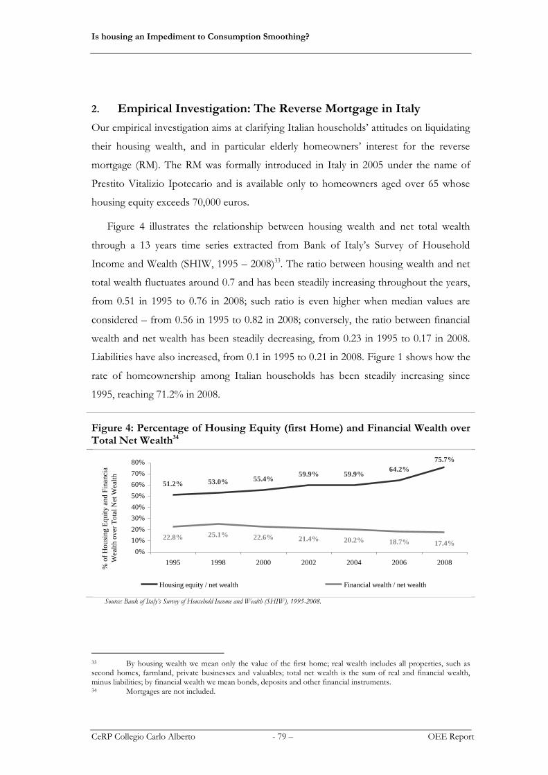
Is housing an Impediment to Consumption Smoothing?
CeRP Collegio Carlo Alberto - 79 – OEE Report
2. Empirical Investigation: The Reverse Mortgage in Italy
Our empirical investigation aims at clarifying Italian households’ attitudes on liquidating
their housing wealth, and in particular elderly homeowners’ interest for the reverse
mortgage (RM). The RM was formally introduced in Italy in 2005 under the name of
Prestito Vitalizio Ipotecario and is available only to homeowners aged over 65 whose
housing equity exceeds 70,000 euros.
Figure 4 illustrates the relationship between housing wealth and net total wealth
through a 13 years time series extracted from Bank of Italy’s Survey of Household
Income and Wealth (SHIW, 1995 – 2008)33. The ratio between housing wealth and net
total wealth fluctuates around 0.7 and has been steadily increasing throughout the years,
from 0.51 in 1995 to 0.76 in 2008; such ratio is even higher when median values are
considered – from 0.56 in 1995 to 0.82 in 2008; conversely, the ratio between financial
wealth and net wealth has been steadily decreasing, from 0.23 in 1995 to 0.17 in 2008.
Liabilities have also increased, from 0.1 in 1995 to 0.21 in 2008. Figure 1 shows how the
rate of homeownership among Italian households has been steadily increasing since
1995, reaching 71.2% in 2008.
Figure 4: Percentage of Housing Equity (first Home) and Financial Wealth over Total Net Wealth34
Source: Bank of Italy’s Survey of Household Income and Wealth (SHIW), 1995-2008.
33 By housing wealth we mean only the value of the first home; real wealth includes all properties, such as second homes, farmland, private businesses and valuables; total net wealth is the sum of real and financial wealth, minus liabilities; by financial wealth we mean bonds, deposits and other financial instruments. 34 Mortgages are not included.
22.8% 25.1% 22.6% 21.4% 20.2% 18.7% 17.4%
59.9%
51.2%
59.9%
75.7%
55.4%
64.2%
53.0%
0%
10%
20%
30%
40%
50%
60%
70%
80%
1995 1998 2000 2002 2004 2006 2008
% o
f H
ou
sin
g E
qu
ity
an
d F
inan
cial
Wea
lth
ov
er T
ota
l N
et W
ealt
h
Housing equity / net wealth Financial wealth / net wealth

Is housing an Impediment to Consumption Smoothing?
CeRP Collegio Carlo Alberto - 80 – OEE Report
Figure 5: Evolution of homeownership rate
Source: Bank of Italy’s Survey of Household Income and Wealth (SHIW), 1995-2008.
Given the high rates of homeownership and the substantial housing wealth, financial
instruments capable of unlocking such wealth could be welfare-improving for a large
number of elderly households. Our analysis will focus on the prospective market for a
RM in Italy and we will draw on a unique dataset (UniCredit 2007) to investigate the
potential determinants of its demand.
2.1. RM literature overview
Several studies on the potential use of RM have been carried out in the US and other
Anglo-Saxon countries, while a few newspaper articles (Sole24 ore) deal specifically with
the Italian market. They all draw on the idea that households accumulate housing wealth
as a buffer stock, often at the expenses of a more diversified, and therefore more
efficient allocation of savings.
Excessive illiquid wealth and poor portfolio diversification leave elderly households
particularly exposed to financial risks and house prices fluctuations, and a sound
financial literacy35 might reduce such risks. Furthermore, as reverse mortgages entail the
payment of compound interests, and are regulated under different tax regimes
depending on whether they are granted by a Bank or other institutions, a good level of
financial literacy, becomes a prerequisite for an effective choice. The lack of it may
35 Lusardi and Mitchell (2006) defines financial literacy as a set of tools enabling one to better allocate financial resources; it is often associated with numerical skills, such as the ability to calculate rates of return on investments, the interest rate on debt, or the understanding of economic concepts such as the trade-off between risk and return, the benefits of diversification, and the benefits and risks associated with specific financial decisions.
68.0%
70.5%69.8%
71.2%
69.8%
64.9%
70.1%
60%
62%
64%
66%
68%
70%
72%
1995 1998 2000 2002 2004 2006 2008
% H
om
eow
ner
s

Is housing an Impediment to Consumption Smoothing?
CeRP Collegio Carlo Alberto - 81 – OEE Report
induce miscalculation about the future gains granted by the loan and lead to
disappointment, as reported by Leviton (2002) in her study on elderly Australian
homeowners and Reverse Mortgage decision-making.
Economics literature itself is not univocal about the share of potential beneficiaries
from a RM, however, the general consensus is that the market is under-developed: Venti
and Wise (1991) maintain that, as RM determine only a small percentage increase in
income even at low income levels, the potential market is limited to very old, single
persons. Mayer & Simons (1993) claim instead that the potential market for RM is quite
large, as many elderly could use it to pay off pre-existing debts. Mitchell & Piggot (2003)
highlights the potential for RM not only to boost consumption among the elderly, but
also to reduce public pension liability, and mitigate the demand for long term care
facilities. In her study of the Australian market, Ong (2003) states that who would
benefit the most from a RM are single women aged 80 or over, and that RM had the
potential to lift out of poverty 95% income-poor elderly Australians. More recently,
Shan (2009)’s report to the US Federal Reserve Board of Governors, states that the
trend in the RM market has reversed: despite a slow uptake during the first ten years,
the number of loans more than decupled during the following seven, from less than
10,000 in 2001 to over 100,000 in 2007. His explanation for such exponential growth in
RM uptake lies primarily in a decrease of the interest rates, house price appreciation and
an increased willingness to take on debt – he shows that the fraction of indebted
homeowners has increased from 44% in 1989 to 57% in 2007.
Like all (intertemporal) choices, taking out a reverse mortgage involves a trade-off: a
euro borrowed on a reverse mortgage and consumed today is a euro (plus interest and
fees) which will not be available for other purposes tomorrow, (Webb 2009), therefore it
is worth analysing a series of possible reasons which could motivate a weak response on
behalf of the homeowners. First of all, the homeowners’ bequest motive, as reverse
mortgages severely reduce the inheritance they intend to leave; however, Mayer &
Simons (1993) mention a vast literature according to which the bequest motive may not
be as important in explaining savings behaviour, and that often bequests are involuntary.
Rodda et all (2000) confirms that, based on lenders’ perceptions, many actual borrowers
do in fact have children and that often it was the children who suggested they take out
the loan. A negative attitude towards borrowing (debt-aversion), may hamper the

Is housing an Impediment to Consumption Smoothing?
CeRP Collegio Carlo Alberto - 82 – OEE Report
willingness to take out any type of non strictly necessary loan, that is to cover basic
expenses or repay outstanding debt. Gibler and Rabianski (1993) consider debt-aversion
among the elderly as a deterrent; they find that older consumers do not generally like to
buy on credit and would rather live on less income than taking out a loan. Caplin (2000)
relates the presence of debt with an increase in uncertainty, suggesting that households
may prefer a lower level of consumption in a debt-free house to a somewhat higher
level in a debt-ridden one.
Lending is a trust intensive activity (Guiso, Sapienza, Zingales 2001), therefore a lack
of trust in financial advisers or financial institutions, could exacerbate homeowners’
scepticism towards new products such as RM. Finally, the products’ high costs, might
turn a potentially profitable financial instrument into a last resort remedy for liquidity
constrained households.
In order to better understand what could spark interest in RM, we exploit some
insights provided by qualitative research conducted in the US and Australia. The first
paper, Leviton (2002), is based on open-ended interviews of American elderly
homeowners who had received reverse mortgage counselling, and explores the decision
making process leading to the uptake of the loan. Leviton portrays the process as slow
and painful, both because of the uncertainty regarding the level of future payments, and
because of the irreversibility of the choice; she reveals that elderly homeowners prided
themselves with frugality, that RM directly conflicted with the desire to leave a legacy,
and highlights how for most households, RM had been a last resort choice, an
instrument to pay off debts rather than increase consumption. Support for Levitons’
analysis can be found in Shan (2009), where it is underlined that the fraction of indebted
homeowners has sharply increased and that only 10% of HECM borrowers had chosen
the tenure payment plan or the modified tenure payment plan, suggesting that the
annuity aspect of reverse mortgages is irrelevant to most borrowers and that
consolidating pre-existing debts is one of the driving motives to apply for the loan.
The second paper, Reed (2009), investigates Australian homeowners’ experience
with RM, focusing on their understanding of the product. Reed draws on two different
surveys: the first conducted by SEQUAL (Senior Australians Equity Release Association
of Lenders) in 2008, interviewing 1,000 homeowners, and the second conducted by

Is housing an Impediment to Consumption Smoothing?
CeRP Collegio Carlo Alberto - 83 – OEE Report
ASIC (Australian Securities & Investments Commission) in 2007 interviewing only 29
homeowners who had already taken out a reverse mortgage. Both surveys meant to
ascertain whether RM could benefit elderly Australians or alternatively be
misunderstood; the SEQUAL survey showed that, even though more than 70% of the
respondents were aware of reverse mortgages, only 40% understood their basic features,
and specifically that no repayments were due and the house would not be sold. As for
the ASIC survey, it focused on lenders behaviour and exposed that many did not
explain the workings of compound interest rates, or show a projection of how much the
loan would cost over time.
Tversky and Kahneman’s Prospect Theory (Kahneman & Tversky, 1979) provides
an important framework to analyse asymmetric or inertial behaviour36; loss aversion
induces a bias that favours the preservation of the status quo over other options, and
this would encourage inaction over action and usual behaviour over innovative
behaviour. Debt-aversion combined with loss-aversion and preference for the status
quo can account for the initial lack of interest in RM.
The demand side is not entirely responsible for the perceived underdevelopment of
the RM market: inadequate supply and the lack of appropriate regulation also play a big
role. Limitations on the supply side can be explained by the risk factors faced by the
credit institutions, primarily related to the dynamics of interest rates and house prices,
but also by the potential adverse selection in case of extremely long lived mortgagors,
and moral hazard in case of meagre house maintenance by homeowners intending to
default on their contract obligations. In order to compensate for all such risks, lenders
charge hefty insurance fees, which together with high commissions and compound
interests make RM rather costly. Davidoff & Welke (2005) ignore moral hazard in house
maintenance as they see it as irrelevant, and investigate adverse selection by comparing
the mobility rates between RM borrowers and not borrowers. Interestingly, they unearth
advantageous selection, as the homeowners who take out RM are also more likely to sell
their home and therefore repay the loan earlier. Caplin (2000) places more emphasis on
moral hazard in home maintenance; he argues that, as the typical RM borrower is very
36 Tversky and Kahneman (1991) state that (financial) decisions depend on the status quo, individual choices are not independent from initial entitlements and the outcome of risky prospects are evaluated by a value function that has the following three characteristics: reference dependence – the values of gains and losses are defined relatively to a reference point; loss aversion – the value function is steeper in the negative than in the positive domain; and diminishing sensitivity – the marginal value of both gains and losses decrease with their size.

Is housing an Impediment to Consumption Smoothing?
CeRP Collegio Carlo Alberto - 84 – OEE Report
old, very poor and likely to suffer from health problems, she is also more likely to let her
property deteriorate, and given such characteristics, the legal provisions put in place to
protect the lender may not be enforced. Caplin advocates a rationalisation of regulatory
system as a means to foster financial innovation in general, and promote RM in
particular.
As for what concerns RM regulation, Ong (2003) highlights the unfavourable tax
regimes as one of the reasons behind the scarce development of RM market in the UK,
where RM income was taxed and could reduce social security entitlements. While Reed
(2009) expresses concern among Australian RM users regarding the possibility for
negative equity to occur, where the amount of the loan exceeds the value of the house
and the homeowner is potentially evicted (and the house sold). Mitchell and Piggott
(2003)’s study on housing equity in Japan maintains that improving the efficiency of
capital markets and providing safeguards for both borrowers and lenders is a necessary
prerequisite for the development of a market for RM.
Albeit acknowledging the role played by credit institutions and regulators, we will
focus our empirical analysis on the demand side and will try to shed some light on
Italian households’ preferences and decisional dynamics.
2.2. Descriptive statistics on microeconomic data
2.2.1. The UniCredit sample
Our analysis draws from the 2007 UniCredit Survey (UCS). As well as collecting detailed
demographic and financial data on a sample of 1,686 individuals, the survey elicits
respondents’ opinions towards risk, investments and savings, and tests their level of
financial education. A specific question is asked to ascertain respondents’ interest in
RM. Additional data have been extracted by Bank of Italy’s Survey of Household
Income and Wealth (SHIW) 2006 to compare the characteristics of our respondents
with a representative sample of all Italian population.
We will consider households and not individual homeowners, and the interest in RM
expressed by householders: a brief description of the product – only the tenure option –
was given by the interviewer, who then asked respondents to assign a value between 1
and 5 according to their level of interest; 1.1% claimed to be “Very interested”, 6.2%

Is housing an Impediment to Consumption Smoothing?
CeRP Collegio Carlo Alberto - 85 – OEE Report
“Quite interested”, 12.9% “Somewhat interested”, 20.4% “Barely interested” and 59.4%
“Not interested”. Again, if we consider only the over 65, they are nearly twice as likely
to be “Very interested” (1.6% vs. 0.9%), but then the percentage of “Quite interested”
decreases from 6.7% to 5.1%, so from a first glance, the thesis that elderly homeowners
are more interested in the product does not find much support. (see Table 25)
Table 25: Interest in Reverse Mortgage
Interest in Reverse Mortgage
(% of total)
Under 65 Over 65
Male Female Male Female All
Very interested 0.7 1.7 1.6 1.4 1.1%
Quite Interested 6.6 7.2 5.3 4.2 6.2%
Somewhat interested 14.1 14.4 9.2 12.7 12.9%
Barely interested 20.3 19.4 20.7 22.5 20.4%
Not interested 58.3 57.2 63.2 59.2 59.7%
Source: UniCredit survey 2007
2.2.2. Demographics and socio-economic indicators
The survey has been conducted by phone interviews targeting the bank’s clients aged
21-75 with at least €10.000 in deposits.
Age and gender – The average (male or female) householder in UCS is about 55 years
old, only a couple of years younger than the average householder in Bank of Italy’s
SHIW; the percentage of female householders is 22% in UCS, and 37.0% in SHIW, and
the percentage of elderly (over 65) is 29.6% in UCS and 36.3% in SHIW. The average
household is composed of 2.6 members in UCS and 2.5 in SHIW. (see Table 26)
Geography – UCS partitions Italy into four macro areas, North East, North West,
Centre and South, resulting in an over-representation of residents in the North 51.3%
(accounting for 43% of the Italian population according to the Italian national office of
statistics) and the Centre 24% (19% of the population), and under-represents the South
and Islands, 24% (35% of the population).
Education – Table 26 also shows the different levels of education attained by sample
householders. It is worth mentioning that a small percentage of respondents did not
complete the level started (be it a higher education degree or a lower education
diploma), in which case the extra years have not been included and respondents have
been assigned to the immediately preceding level. The UCS sample is by far more
educated than average Italians: 5.3% of SHIW’s householders have no education vs.

Is housing an Impediment to Consumption Smoothing?
CeRP Collegio Carlo Alberto - 86 – OEE Report
0.5% in UCS; 26.5% have primary education in SHIW, vs. 8.9% in UCS; 28.2% have
lower secondary education in SHIW, vs. 20.4% in UCS; 24.2% have secondary
education in SHIW vs. 40.8% in UCS; and 8.9% have higher education in SHIW vs.
24.4% in UCS.
Occupation – As for the occupational status, the most striking difference between the
two samples is the high percentage of self-employed in UCS, 29.4% against the relatively
low one in SHIW, 10.2%. Pensioners, employees and unemployed, represent a larger
share of the population in SHIW.
Table 26: Summary statistics for demographics
UniCredit SHIW
Total number of observations / households 1,686 7,768
Average age of householder 56.0 57.6
% of female householders 22.0% 37.0%
% of elderly householders 29.6% 36.3%
Area of residence
North 51.3% 44.6%
Centre 24.3% 20.16%
South 24.4% 35.3%
Education37
No education 0.5% 5.3%
Primary education (5 years) 8.9% 26.5%
Lower secondary education (8 years) 20.4% 28.2%
Middle education / professional schools (11 years) 3.9% 6.7%
Upper secondary education (13 years) 40.8% 24.2%
Higher education (degree or more) 24.4% 8.9%
Occupation
Pensioner – retired from work 32.3% 36.1%
Pensioner – not retired from work (disability benefits, etc)
2.6% 9.3%
Employee 30.8% 34.9%
Self-employed 29.4% 10.2%
Unemployed 4.0% 9.1%38
Household size 2.6 2.5
Source: UniCredit survey 2007 and Banca d’Italia “Survey of household Income and Wealth” (SHIW) 2006
Income and wealth – UCS average household is also considerably wealthier than the
average Italian in SHIW39. Table 27 describes the summary statistics for income levels
37 The years of unfinished levels of education are added to the immediately preceding level attained. 38 Includes housewives and voluntarily unemployed.

Is housing an Impediment to Consumption Smoothing?
CeRP Collegio Carlo Alberto - 87 – OEE Report
and distribution in both UCS and SHIW: the average individual income in UCS is
50,717 euros (median 31,000), 2.75 times higher than the average SHIW income of
18,450 euros (median 15,349); the average UCS household income is 71,325 euros
(median 48,393), roughly 2.2 times the average SHIW household income of 31,893
euros (median 26,217). UCS does not provide reliable point values regarding
households’ financial wealth, as more than 75% or the respondents refuses to indicate
an amount, however, households are categorised according to their wealth bracket value,
defined by the amount of money deposited in UniCredit current accounts, ranked from
1 to 6, ranging from 10,000 to 5 million euros. While the average financial wealth in
SHIW amounts to 25,246 euros (median 6,674), with 18% households having no
financial wealth at all, the average wealth bracket in UCS is 100,000 to 150,000 euros
(with minimum wealth being 10,000 euros).
Table 27: Summary statistics for income levels and distribution
Percentile UniCredit SHIW
Household net disposable income
Individual net disposable income
Household net disposable income
Individual net disposable income
Total Observations 1,686 1,686 7,768 13,428
5th 17,934 9,500 9,078 3,767
10th 22,000 13,883 11,968 5,562
25th 31,733 20,000 17,169 10,000
50th 48,393 31,000 26,217 15,349
75th 76,655 55,000 39,766 22,487
90th 129,600 100,000 55,823 32,000
95th 195,827 150,239 69,275 41,294
Mean 71,325 50,717 31,893 18,450
Standard Deviation 86,024 67,847 27,276 18,578
Source: UniCredit survey 2007 and Banca d’Italia “Survey of household Income and Wealth” (SHIW) 2006
Housing equity – The percentage of home-owners is around 71% in SHIW, while in
UCS it approximates 90%. As for the housing equity, Table 28 shows how the average
house value in UCS is 1.8 times the average house value in SHIW. The data regarding
housing equity were somewhat misleading, as a few hundred respondents provided
inaccurate numbers (1s, 999s or 100 millions); after a sensible correction40 the average
39 However Banca d'Italia's official report on Household Wealth (2008) specifies that the sample is affected by selection bias, as in lower participation of wealthier households, and under-reporting regarding income and wealth. 40 excluding all properties with less than 4 digits, losing 184 observations, and above 5 millions, losing 13 observations.

Is housing an Impediment to Consumption Smoothing?
CeRP Collegio Carlo Alberto - 88 – OEE Report
house value in the UCS amounts to 387,367 euros (with a standard deviation of
337,694), while the average value for the Italian population is 215,418 euros (median
180,000).
Table 28: Summary statistics for housing wealth levels and distribution
Percentile UniCredit SHIW
Household Housing Wealth
Housing Wealth per squared metre
Household Housing Wealth
Housing Wealth per squared metre
Total Observations 1,686 1,686 7,768 13,428
5th 120,000 1,166.7 50,000 666.7
10th 150,000 1,400.0 70,000 892.9
25th 200,000 1,875.0 110,000 1,307.7
50th 300,000 2,500.0 180,000 1,875.0
75th 465,000 3,582.0 250,000 2,560.0
90th 700,000 5,000.0 400,000 3,529.4
95th 975,000 6,383.0 500,000 4,285.7
Mean 387,367 2,988.5 215,418 2,095.9
Standard Deviation 337,694 1,721.9 176,288 1,196.1
Source: UniCredit survey 2007 and Banca d’Italia “Survey of household Income and Wealth” (SHIW) 2006
Saving rates and Precautionary Savings – Saving rates are divided into 7 categories,
ranging from “over 50% of Yearly income” to “Could not save anything”, and
predictably they are slightly higher among the elderly. The average saving rate lies in the
“5% to 10%” interval, while more than 21% of householders declares not to have saved
anything. Predictably, saving rates are lower among the elderly, as approximately 25% of
the over 65 has no savings. Albeit dealing with a wealthier sample, we have lower saving
rates compared to what is reported in SHIW, where the average saving rate is 8.8%, and
only 18.5% has zero or negative savings. (See Table 29). Householders’ desired amount
of precautionary savings, that is the amount of money put aside to protect oneself from
increased uncertainty about their future earnings or unexpected expenses, is on average
4.5 times household income, and approximates 167,000 euros on average. Respondents
were also presented with several reasons for saving and were requested to rank them
according to their importance: as Table 30 shows, avoiding future debts, coping with
medical expenses or dealing with unforeseen circumstances are generally considered
more important than integrating one’s future pension, leaving an inheritance and
undertaking entrepreneurial activities.

Is housing an Impediment to Consumption Smoothing?
CeRP Collegio Carlo Alberto - 89 – OEE Report
Table 29: Summary statistics for household savings Age groups and sex householder
% of Savings over disposable income
Under 65 Over 65 Male Female Male Female
No savings 191 (20.7%) 64 (20.1%) 95 (24.1%) 28 (26.7%)
1% to 5% 121 (13.4) 40 (15.1) 48 (12.2) 18 (17.1)
5% to 10% 155 (16.8) 47 (17.7) 67 (17.0) 18 (17.1)
10% to 20% 169 (18.4) 59 (22.2) 81 (20.6) 20 (19.1)
20% to 30% 171 (18.6) 28 (10.5) 54 (13.7) 15 (14.3)
30% to 50% 82 (8.9) 23 (8.7) 34 (8.6) 5 (4.8)
More than 50% 32 (3.5%) 5 (1.9%) 15 (3.8%) 1 (0.9%)
Source: UniCredit survey 2007
Table 30: Summary statistics: reasons for savings Reasons for saving (% of all) Very
Important Quite Important
Somewhat Important
Not very Important
Not important
Dealing with unforeseen circumstances
46.5% 44.4% 7.7% 3.1% 1.3%
Providing for family’s future needs 36.7 37.7 9.9 9.1 6.6
Integrate pension (after retirement) 24.0 36.6 14.1 13.5 11.9
Deal with medical expenses 40.4 41.1 8.8 6.3 3.4
Undertake entrepreneurial activities 7.3 15.5 11.2 17.3 48.7
Leaving a legacy / inheritance 11.0 33.9 18.7 19.6 16.8
Not having future debts 49.2 36.5 6.6 4.3 3.5
Buy a house 19.8 25.4 12.9 17.0 24.9
Buy durable goods 7.0 28.9 23.7 25.2 15.3
Have profitable assets 18.2% 43.4% 20.8% 11.0% 6.6%
Source: UniCredit survey 2007
2.2.3. Preferences and attitudes
The UniCredit survey provides a wealth of qualitative responses regarding preferences
and attitudes, allowing us to outline a more detailed picture and better investigate
respondents characteristics. Whenever similar questions are to be found in SHIW, a
comparison between the two samples will be drawn.
Risk and Uncertainty – Many questions investigate respondents’ risk attitude. A
preliminary one prompts them to choose between a lottery with a 50/50 chance of
winning, and one whose odds were unknown; 53.6% prefers the more certain lottery,
24.7% are indifferent and less than 24% prefers (or slightly prefers) the uncertain
option. A second one looks into the perceived trade-off between risk and return,
revealing that the majority of respondents are moderately risk averse or rather risk
neutral, according to how the question is interpreted: less than 2% is willing to take on
high risks in order to have high returns, 27.6% prefers good returns, but a discrete level

Is housing an Impediment to Consumption Smoothing?
CeRP Collegio Carlo Alberto - 90 – OEE Report
of safety, about 52% requires a discrete return together with a good level of safety, and
less than 19% opts for low returns, as long as the risk is none. The same question is
present in SHIW, and the results show a much more prudent attitude as nearly 50% or
householders chooses the last option, low returns with no risks (See Table 31).
Table 31: Trade-off between risks and returns
Perception of risk/return (All) UniCredit SHIW
Total number of observations / households 1,686 7,768
High returns, high risks 1.8% 1.0%
Good returns, decent safety 27.6% 14.9%
Decent returns, good safety 52.0% 35.0%
Low returns, no risks 18.6% 49.2%
Source: UniCredit survey 2007 and Banca d’Italia “Survey of household Income and Wealth” (SHIW) 2006
The third set of risk-related questions is associated with the concept of framing – how
a choice or an option can be affected by the way it is presented to a decision maker –
and exposes respondents’ risk attitude in two opposite scenarios: gain and loss. In the
first scenario respondents were asked whether they would prefer a 50/50 chance to win
10,000 euros, or another amount – progressively increasing from 100 to 9,000 for every
negative answer – for certain. In the second scenario the situation is reversed, and
respondents have to decide whether they would prefer a sure loss of a smaller amount –
progressively increasing from 100 to 9,000 euros – or a 50/50 chance to lose 10,000
euros. If we define all respondents who prefer less than the expected value (5,000 euros)
as risk-averse, those who choose the expected value as risk-neutral, and the rest risk-loving,
we see that their percentages among the sample population are 54%, 16.1% and 29.9%,
respectively in a gain scenario, and 15.3%, 9.7% and 75% respectively, in a loss scenario,
confirming the asymmetric behaviour predicted by Kanheman and Tversky’s value
function. The combination of risk-aversion in gains and risk-loving in losses is denoted
as loss-aversion and characterises about 48% of the respondents. However, as much as
73.8% appears to increase their risk attitude of at least one degree in a loss scenario,
measured as the percentage of respondents who gamble a higher amount in the second
set of questions. Both elderly male and female householders are more risk averse and
more loss averse than their younger counterpart in a gain scenario, women under 65
years of age are the most risk loving, particularly in a loss scenario. (see Table 32).

Is housing an Impediment to Consumption Smoothing?
CeRP Collegio Carlo Alberto - 91 – OEE Report
Table 32: Risk attitude Risk attitude (% of total)
Under 65 Over 65 Male Female Male Female All
Gain Scenario
Risk averse 52.2 50.8 58.6 61.9 54.0
Risk neutral 16.4 15.4 15.2 18.1 16.1
Risk loving 31.4 34.2 26.1 20.0 29.9
Loss Scenario
Risk averse 16.1 12.0 15.0 18.1 16.3
Risk neutral 10.1 7.2 11.4 6.7 9.7
Risk loving 73.8 80.8 73.6 75.2 75.0
Loss averse 46.5 49.6 50.5 59.5 48.7
Source: UniCredit survey 2007
Finally, respondents are asked to assess their perception of risk connected to several
types of financial investments (see Table 33), from which it results that single company
stocks/equity, as well as equity mutual funds are considered very or quite risky by the
majority of people, while bank deposits and real estate are considered the safest. Repo
(pronti contro termine) and unit linked life insurances are the least known products. Among
the 10% who perceive housing as a very or “quite risky investment, interest in RM is
higher.
Table 33: Investments’ perceived risk Financial Investments Very Risky Quite
Risky Somewhat Risky
Not very Risky
Not Risky
Do not know them
Bank deposits 2.2 6.0 12.9 28.4 48.8 1.8
Repo (Pronti Contro Termine) 3.6 10.4 17.3 21.2 16.1 31.7
Government bonds 3.1 9.6 16.7 36.2 30.8 3.5
Bonds 4.5 17.5 27.1 32.4 11.9 7.4
Bond mutual funds 4.9 18.7 31.6 28.5 7.4 8.9
Stock mutual funds 16.3 42.1 23.1 8.3 2.0 8.3
Single company stocks/equity 39.2 38.0 12.3 4.0 1.1 5.5
Unit linked life insurance 5.7 16.9 21.5 27.2 13.5 18.3
Real estate 3.2 6.5 10.6 31.2 46.4 2.2
Source: UniCredit survey 2007
Trust in financial institutions – Informational asymmetries, particularly strong in case of
new products, are often associated with a lack of trust towards the more informed party;
as RM is a relatively new product and is better known by financial advisers or lenders, a
lack of trust in financial institutions may have a negative effect on respondents’ interest.
Trust in financial institutions/advisers is ascertained mainly by two questions, the first

Is housing an Impediment to Consumption Smoothing?
CeRP Collegio Carlo Alberto - 92 – OEE Report
one directly soliciting how much the respondents trusted their adviser (if they had one),
and the second one asking whether respondents’ trust in financial institutions had
decreased over the past few years (we are in pre subprime crisis time). About 45% of
respondents admit that their trust in financial institutions has decreased in the past few
years, while more than 72% of respondents places a lot, or enough trust in their
financial adviser. The percentage of respondents who have both trust in their adviser
and in financial institutions is around 38%.
Debt aversion – Few questions in the UniCredit survey cover respondents’ opinions
on borrowing and indebtedness; the desire of not having future debts is one of the main
reasons for saving (already mentioned above), considered “very” or “quite important”
by over 85% of respondents; when asked directly what they thought about borrowing,
only 10.5% replied not to have any qualms in taking out a loan, while over 70.5% would
rather not have any debt. When asked how they would finance a hypothetical
expenditure of 20,000 euros, more than 60% replied they would draw from their
savings, 20% would sell their financial assets, and about 16% would recur to a bank
loan. Respondents’ subjective debt aversion is reflected in their borrowing practices:
only 19.3% of surveyed households have outstanding loans other than mortgages, have
accessed their overdraft or purchased something in instalments. (See Table 34).
Table 34: Reasons for buying on credit
UCS
Renovation of real estates 1.9%
Purchase of vehicles (car, motorbike) 6.4%
Purchase of electrical appliances - furniture 1.8%
Purchase of computers, electronic goods 0.9%
Holiday 0.3%
Expensed for household health 0.5%
Other 2.1%
Total borrowers (for any of the above or more than one) 12.5%
Source: UniCredit survey 2007
Financial Literacy – The respondents’ financial literacy has been gauged by four
questions about inflation, interest rates and portfolio diversification, plus a self-
assessment of how well respondents thought they knew specific financial instruments.
19% did not give any correct answer, 37% only managed one, 32% managed two, 11%
three and only 0.8% gave a correct answer to all four questions. Elderly female
householders have an overall worse performance. A comparison with SHIW is possible,

Is housing an Impediment to Consumption Smoothing?
CeRP Collegio Carlo Alberto - 93 – OEE Report
as the 2006 wave includes a few financial literacy questions, however, while the ones
about interest rates and inflation were very similar, the ones on diversification were
considerably more difficult in UCS and may account for the lower score reported by
UCS respondents despite their higher general education.41 (See Table 35).
Table 35: Financial literacy Financial Literacy (% of correct answers)
Under 65 Over 65 Male Female Male Female All
Inflation 35.8 36.8 28.4 35.2 34.2
Interest 52.1 48.1 57.4 40.0 52.0
Diversification - theoretical 44.0 33.1 38.6 25.7 39.9
Diversification - practical 12.4 12.8 15.2 10.5 13.0
0 – 2 correct answers 86.1 91.0 86.6 96.2 87.6
3 – 4 correct answers 13.9 9.0 13.4 3.8 12.4
Source: UniCredit survey 2007
As for the self reported knowledge of financial products, self-assessed portfolio literacy
(PL), the respondents were asked to assign a value from 1 to 5 (from “I don’t know it at
all” to “I know it very well”) and assess their knowledge of ten financial products (the
list of products is reported in the appendix). The results are that 41% claim to know less
than three products, 41% between four and seven and 18% more than seven products.
The more knowledgeable – or more confident, are male householders under 65 years of
age, while the least knowledgeable are elderly female householders. (See Table 36) The
index of PL is important even if it overestimates actual knowledge, as it reveals the
respondent’s exposure to financial products. Arguably, the more familiar the elderly are
with all types of financial products, the less sceptical they will be about RM.
Table 36: Self-assessed PL
Portfolio Literacy
Under 65 Over 65
Male Female Male Female All
0 – 3 products (Low PL) 37.8% 47.4% 38.6% 61.9% 41.0%
4 – 7 products (Medium PL) 41.3% 39.9% 44.9% 32.4% 41.3%
8 – 10 products (High PL) 21.0% 12.8% 16.5% 5.7% 17.7%
PL index – 0 to 1 (mean values) 0.59 0.56 0.58 0.48 0.58
Source: UniCredit survey 2007
41 As shown by Fornero & Monticone (2010), most Italian householders lack knowledge of basic financial concepts: their analysis draws on SHIW 2006 and SHIW 2008, and they use three, rather than four questions. In 2006, less than 25% of respondents answers all three questions correctly, and more than 26% gets them all wrong. SHIW allowed for a “Don’t know” option, which is not present in UCS.

Is housing an Impediment to Consumption Smoothing?
CeRP Collegio Carlo Alberto - 94 – OEE Report
Retirement Expectations – Respondents were asked whether they were worried about
their economic well-being after retirement, and about 40% replied to be “quite” or
“very worried”. The least worried are elderly or pensioners, who face less uncertainty
(see Table 37). As RM are meant to increase welfare after retirement, it is plausible to
assume that negative expectations about post-retirement economic well-being raise the
probability of being interested in the product, and the data confirm the hypothesis.
Table 37: Retirement expectations
Worry about retirement wealth Under 65 Over 65
Male Female Male Female All
Not worried 17.5 15.4 31.7 22.9 20.8%
Barely worried 40.3 41.0 40.1 50.5 41.0%
Quite worried 30.3 32.3 22.6 19.1 29.2%
Very worried 10.0 11.3 5.6 7.6 9.0%
Source: UniCredit survey 2007
Preference for Downsizing – A specific question was asked to assess respondents’
willingness to sell their home as a means to increase future income and they were given
the following options: certainly not (53.1%), probably not (27.0%), probably yes (16.7%)
and definitely yes (3.2%). While elderly are much more likely to be willing to downsize
(4.2% vs. 2.8%), the percentage is still low, confirming Venti & Wise’s claim that elderly
homeowners do not wish to reduce their housing assets. (See Table 38)
Table 38: Preference for downsizing
Interested in downsizing
(% of total)
Under 65 Over 65
Male Female Male Female All
Definitely yes 2.9 2.2 3.0 9.1 3.2%
Probably yes 18.1 15.2 14.3 18.2 16.7%
Probably not 25.6 32.0 25.7 31.8 27.0%
Certainly not 53.4 50.7 57.0 40.9 53.1%
Source: UniCredit survey 2007
2.3. Estimating the money’s worth of a Reverse Mortgage
The money’s worth of reverse mortgages is limited by the amount of available equity
and by restrictions on loan size, and the main limit on loan size is the age of the

Is housing an Impediment to Consumption Smoothing?
CeRP Collegio Carlo Alberto - 95 – OEE Report
youngest borrower. In Italy, the maximum loan advance ranges from roughly 20% of
the housing equity for the 65 years olds, to roughly 50% for the over 9042: for example,
the maximum loan advance available to a 79 year old, for a house with an appraised
value of €387,798, at an expected interest rate of 7.3%, will be €150,000; should the
borrower die at age 89, that is 10 years after signing the reverse mortgage contract, the
amount to be reimbursed by his inheritors will be equal to €337,093. (Deutsche Bank
informative leaflet).
Ong (2003) provides a sink fund formula, based on the HUD HECM handbook
(1994) and Rodda et. al (2000), to calculate the monthly payments generated by a reverse
mortgage, for a given housing equity level, interest rate and life expectancy.
where
iA = monthly payment to (household) borrower i
HD is the housing value at predicted death
r = monthly interest rate (approximated)
ei = life expectancy at age i(in months), calculated as 100 minus current age
By applying the same formula, we can assess the money’s worth of a RM for our
average sample household. We will set the interest rate at 7.3%, in line with the
Deutsche Bank reverse mortgage rates43, and consider borrower’s life expectancy as 100
minus current age. The money’s worth is estimated in terms of percentage increase in
average household income for housing equity quintile, gender, status and age groups.
The results are in essence similar to what has been reported by Ong (2003), as over
80s and single females with lower income and above average housing equity are the
recipients with higher gains. However, the impact of RM on household income is much
weaker, as it would yield on average 16% increase (for median income level), as opposite
to a 71% increase in Ong’s study. This difference is due partly to the fact that we are
considering household and not individual income, that our sample population is
42 The values reported are for single male householders; the corresponding percentages for single females are: 15.3% for the 65 years olds, to 46% for the over 90. The maximum loan amount for couples is lower (14% to 45%). 43 Deutsche Bank informative leaflet for Italian reverse mortgage borrowers.

Is housing an Impediment to Consumption Smoothing?
CeRP Collegio Carlo Alberto - 96 – OEE Report
wealthier, and that the maximum loan advance in Italy is lower than in Australia. (Table
39).
Table 39: Reverse Mortgage monetary value
Average Housing Equity
Maximum Loan Advance
RM Annuity
Low Income I quartile
RM as % of Low Income
Median Income II quartile
RM as % of Median Income
High Income III quartile
RM as % of High Income
Average Housing Equity 376,989 94,247 7,661 31,733 24% 48,392 16% 76,654 10%
I quintile - up to €180,000 141,792 35,448 2,881 25,800 11% 40,000 7% 54,800 5%
II quintile - up to €250,000 222,309 55,577 4,517 29,183 15% 44,400 10% 65,700 7%
III quintile - up to €350,000 310,992 77,748 6,320 35,300 18% 49,600 13% 69,700 9%
IV quintile - up to €500,000 445,139 111,285 9,046 38,682 23% 59,898 15% 93,000 10%
V quintile - over €500,000 905,217 226,304 18,395 32,324 57% 53,150 35% 87,912 21%
Age Category
65-69 years 416,875 93,797 7,624 32,000 24% 50,315 15% 83,600 9%
70-74 years 429,384 139,550 11,343 25,763 44% 46,013 25% 74,313 15%
75-80 years 339,500 127,313 10,348 23,600 44% 35,800 29% 61,522 17%
80 years or over 433,333 173,333 14,089 18,356 77% 26,727 53% 70,003 20%
Household Income Unit
Couple 387,358 96,840 8,306 34,200 24% 52,460 16% 84,400 10%
Single / widower male 342,116 85,529 7,336 29,233 25% 42,000 17% 64,000 11%
Single / widow female 358,432 89,608 7,686 27,500 28% 39,600 19% 62,000 12%
Geographical Area
North 356,826 89,206 7,652 30,300 25% 47,400 16% 72,000 11%
Centre 421,820 105,455 9,045 32,407 28% 52,000 17% 83,100 11%
South 381,476 95,369 8,180 33,260 25% 46,900 17% 75,155 11% Source: UniCredit survey 2007
This exercise confirms the original formulation of RM as a product for the house-
rich, cash-poor. But in order to find out whether demographics and socio-economic
aspects are relevant in determining interest, we will have to further our analysis and
carry out an ordered probit regression to investigate the determinant of interest in RM.
2.4. Econometric specification
The respondent’s interest in RM in the survey is measured on an ordinal scale, and the
levels of interest are represented by a discrete variable which can take one of the
following five values:
yi = 1, if the respondent is “Not Interested”
yi= 2, if the respondent is “Barely Interested”
yi = 3, if the respondent is “Slightly Interested”
yi= 4, if the respondent is “Quite Interested”
yi = 5, if the respondent is “Very Interested”

Is housing an Impediment to Consumption Smoothing?
CeRP Collegio Carlo Alberto - 97 – OEE Report
We can assume that the discrete values are based on an underlying continuous and
latent variable y*, and that this latent variable is a linear function of all the explanatory
variables:
yi* = β’x +ε for I = 1, 2, …N
where x is a vector of covariates, N is the number of respondents and ε the error
term, which we assume to be normally distributed.
Let μ1< μ2 < μ3 < μ4 < μ5 be the unknown thresholds parameters or cut-off points,
then what we observe is:
yi = 1 if yi*≤ μ1,
yi = 2 if μ1 <yi*≤ μ2
yi = 3 if μ2 <yi*≤ μ3
yi = 4 if μ3 <yi*≤ μ4
yi = 5 if yi*> μ4
The threshold parameters will be estimated together with the β’s to help match the
probabilities associated with each discrete outcome.
The probability of yi being classified as “Not Interested”, “Barely Interested”,
“Slightly Interested”, “Quite Interested” and “Very Interested” are given by:
Prob(yi = 1) = Prob(β’x + ε ≤ μ1),
Prob(yi = 2) = Prob(μ1 < β’x + ε ≤ μ2),
Prob(yi = 3) = Prob(μ2 < β’x + ε ≤ μ3),
Prob(yi = 4) = Prob(μ3 < β’x + ε ≤ μ4),
Prob(yi = 5) = Prob(β’x + ε > μ4),
Both cut-off points and coefficients β can be estimated as an ordered probit model
(ORM) by maximum likelihood method (Greene, 2003). Estimating the β’s is not
enough as they do not reflect the marginal change in probability, therefore we have to
calculate the marginal effects in order to achieve a clearer interpretation of the results.
2.4.1. Ordered probit’s results
A rich set of socio-demographic factors, personal characteristics and preferences has
been used to capture respondents’ attitude in the ordered probit regression. (See Table
40). Demographic variables do not seem to have the impact we expected, as age, gender

Is housing an Impediment to Consumption Smoothing?
CeRP Collegio Carlo Alberto - 98 – OEE Report
and marital status are not significant; the same can be said for higher or middle
education, while having no education at all is negatively correlated with interest in RM.
However, given the small amount of respondents with no education (only 9), we cannot
consider the result of particular relevance. Both pensioners and self-employed
householders are more likely to be interested, as well as those who are resident in the
North of Italy, and in cities with fewer than 100,000 inhabitants.
The bequest motive does not emerge as one would expect, as there are not
significant differences in the level of interest between households with children and
household without, or between householders who consider leaving a bequest as an
important reason for saving and householders who do not.
Surprisingly, household income or owning more than one house/property, are not
significant, nor is the lack of savings. We must, however, bear in mind that all surveyed
households have at least €10,000 in deposits, so declaring that they are not able to save,
is not necessarily relevant.
Another interesting result is that, even though the maximum loan advance depends
positively on housing equity, housing equity is negatively correlated with interest in RM
and raises the probability of a “not interested” by 4.9%; the explanation can be found in
the Prospect Theory: as our sample population is wealthy not only in terms of housing
assets, but also in terms of income and financial assets, its reference point is higher, and
the relative gain from taking out a RM smaller, therefore a median income increase of
16%, which is what has been calculated applying the sink fund formula, may not be
profitable enough to compensate for the loss of the status quo.
The expression of interest in RM appears more significantly correlated with
preferences and personal attitudes than with demographics or socio-economic status.
The most significant, most robust result is that the preference for downsizing raises the
probability of being interested in the product by 2.1%, and decreases the probability of
not being interested at all by 27.6%. The link between a preference for downsizing and
an interest in RM is far from obvious. At a first glance, it seems plausible that those who
are not particularly attached to their homes should be more interested in RM – which is
what the data confirm. On the other hand, RM is conceived specifically as an alternative
to selling one’s home, and carries the risks related to homeowner’s extended longevity,

Is housing an Impediment to Consumption Smoothing?
CeRP Collegio Carlo Alberto - 99 – OEE Report
house price depreciation and poor maintenance, which account for its high cost. In this
framework, willingness to downsize and interest in RM should have opposite sign.
As financial literacy increases (from 0 to 4 correct answers), so does the probability
of not being interested in the product (2.8%); however, the results are not very robust,
and the correlation becomes not meaningful if controls are added or taken out of the
regression. (See robustness checks) As for portfolio literacy, the sign is positive, but its
effect is not meaningful.
Risk and uncertainty seem to have a major impact on homeowners’ response. Risk
aversion, measured by an index taking values from 0.1 to 1, is significantly and positively
correlated with interest in RM. However, when using separate dummies for risk averse,
risk neutral or risk lover, we see that the only significant correlation is the negative one
between risk-loving and interest in RM, while the dummy for risk-averse is not
significant. The more simplistic indicator of risk attitude, identified by the preference
between high risks or high returns, yields a similar result, but not as significant, and
therefore it is used as robustness check, but not included in the main regression.
Negative expectations about post-retirement economic well-being are significantly
positively correlated with interest in the product, decreasing the probability of a “not
interested” by 9.1%. The implications for Italy are quite clear, as the foreseeable
reduction in state funded pensions, due to an rising dependency-ratio and ageing
population, could generate a substantial demand for the product.
The rather small percentage (9.9%) of our sample homeowners who perceives
housing investment as “quite” or “very” risky is more likely to be interested in RM, as
the probability of a “Not Interested” decreases by 15.1%.
The research conducted in US and Australia brought to our attention how elderly
homeowners can be particularly averse to debt, and how this attitude may have an effect
on their interest in RM. Two questions in the survey could be used to build an indicator
of debt-aversion: the first one, closer to the concept of thrift, identifies respondents
who indicated not having future debts as an important reason for saving; the second
one collects those who simply state their dislike for taking on any debt. Only a general
unwillingness to take on debt is significantly negatively correlated with interest in RM: as
the binary variable for debt aversion takes the value of one, the probability of not being

Is housing an Impediment to Consumption Smoothing?
CeRP Collegio Carlo Alberto - 100 – OEE Report
interested in the product rises by 14.9%. Since avoiding future debt as a reason for
saving is not significant, it has been taken out from the main regression and used as a
robustness check.

Is housing an Impediment to Consumption Smoothing?
CeRP Collegio Carlo Alberto - 101 – OEE Report
Table 40: Ordered Probit’s (preliminary) Results Interested in Reverse Mortgage No
Y=1 Barely Y=2
Somewhat Y=3
Quite Y=4
Very Y=5
b/se b/se b/se b/se b/se
Age householder 0.012 -0.004 -0.005 -0.003 -0.000 (0.01) (0.00) (0.00) (0.00) (0.00) Single (d) -0.040 0.012 0.016 0.010 0.002 (0.05) (0.01) (0.02) (0.01) (0.00) Widower (d) -0.005 0.002 0.002 0.001 0.000 (0.06) (0.02) (0.02) (0.01) (0.00) Female (d) -0.036 0.011 0.014 0.009 0.002 (0.04) (0.01) (0.02) (0.01) (0.00) Higher Education (d) -0.038 0.012 0.015 0.009 0.002 (0.04) (0.01) (0.01) (0.01) (0.00) Primary Education (d) 0.025 -0.008 -0.010 -0.006 -0.001 (0.04) (0.01) (0.01) (0.01) (0.00) No education (d) 0.205 -0.090 -0.075 -0.035* -0.005** (0.17) (0.10) (0.06) (0.02) (0.00) Households with children (d) -0.038 0.012 0.015 0.009 0.002 (0.03) (0.01) (0.01) (0.01) (0.00) Householder pensioner (d) -0.234 0.066** 0.092* 0.063 0.013 (0.14) (0.03) (0.06) (0.04) (0.01) Householder self-employed (d) -0.211 0.057* 0.083 0.058 0.012 (0.14) (0.03) (0.06) (0.05) (0.01) Householder employed (d) -0.195 0.055* 0.077 0.052 0.011 (0.14) (0.03) (0.06) (0.04) (0.01) Householder unemployed (d) -0.223 0.044*** 0.088 0.072 0.018 (0.16) (0.01) (0.06) (0.07) (0.02) Log Household Income 0.004 -0.001 -0.002 -0.001 -0.000 (0.02) (0.01) (0.01) (0.01) (0.00) Log Property value 0.049* -0.016* -0.019* -0.012* -0.002* (0.03) (0.01) (0.01) (0.01) (0.00) Preference for Downsizing (d) -0.274*** 0.060*** 0.108*** 0.085*** 0.021*** (0.03) (0.01) (0.02) (0.02) (0.01) Fewer than 100,000 inhabitants (d) -0.052* 0.017* 0.020* 0.012* 0.002 (0.03) (0.01) (0.01) (0.01) (0.00) More properties (d) -0.027 0.009 0.011 0.006 0.001 (0.03) (0.01) (0.01) (0.01) (0.00) Trust in Financial Institutions -0.005 0.002 0.002 0.001 0.000 (0.03) (0.01) (0.01) (0.01) (0.00) Financial Literacy 0.026* -0.009* -0.010* -0.006* -0.001 (0.02) (0.01) (0.01) (0.00) (0.00) Portfolio Literacy -0.043 0.014 0.017 0.010 0.002 (0.10) (0.03) (0.04) (0.02) (0.00) Bequest (d) -0.030 0.010 0.012 0.007 0.001 (0.03) (0.01) (0.01) (0.01) (0.00) Risk Aversion (index 0.1 to 1) -0.108** 0.036** 0.042** 0.026** 0.005* (0.05) (0.02) (0.02) (0.01) (0.00) Real estate’s perceived risk (d) -0.153*** 0.039*** 0.061*** 0.044** 0.010* (0.05) (0.01) (0.02) (0.02) (0.00) Negative retirement expectations (d) -0.091*** 0.029*** 0.036*** 0.022*** 0.004** (0.03) (0.01) (0.01) (0.01) (0.00) Debt Averse (d) 0.149*** -0.043*** -0.059*** -0.039*** -0.008*** (0.03) (0.01) (0.01) (0.01) (0.00) No savings (d) -0.006 0.002 0.002 0.001 0.000 (0.04) (0.01) (0.01) (0.01) (0.00) Resident in the North (d) -0.065* 0.021* 0.025* 0.015* 0.003 (0.03) (0.01) (0.01) (0.01) (0.00) Resident in the South (d) 0.001 -0.000 -0.000 -0.000 -0.000 (0.04) (0.01) (0.02) (0.01) (0.00) Number of observations 1,071 1,071 1,071 1,071 1,071 Log likelihood -1,109.8 -1,109.8 -1,109.8 -1,109.8 -1,109.8 Pseudo R2 0.065 0.065 0.065 0.065 0.065
***=1% statistical significance level, **=5 % and *= 10%.

Is housing an Impediment to Consumption Smoothing?
CeRP Collegio Carlo Alberto - 102 – OEE Report
It is worth highlighting that those who would benefit the most from taking out a
RM, lower income elderly, singles and women, are also much more likely to be debt
averse (see Table 41) and therefore less likely to be interested in the product. Debt
aversion could also explain the recent growth in the US reverse mortgage market. Shan
(2009) reveals that only 10% of American HECM borrowers choose the tenure payment
plan or the modified tenure payment plan, suggesting that the annuity aspect of reverse
mortgages is irrelevant to most borrowers; given that consolidating off pre-existing debt
has been described as one of the reasons elderly might want to take out a RM (Leviton
2001), and given Shan’s reported increase in the level of indebtedness, one may be
tempted to conclude that the loan was used to pay off debts rather than increase
consumption.

Is housing an Impediment to Consumption Smoothing?
CeRP Collegio Carlo Alberto - 103 – OEE Report
Table 41: Probits on main regressors
Preference for downsizing
Negative Retirement Expectations
Debt Averse
Risk Lover (in gains)
b/se b/se b/se b/se
Age householder 0.003 -0.050* 0.058** -0.017 (0.03) (0.03) (0.03) (0.03) Age spouse -0.022** -0.003 0.021** -0.004 (0.01) (0.01) (0.01) (0.01) Single -0.280 0.238 0.527*** 0.215 (0.17) (0.17) (0.17) (0.17) Widower -0.276 -0.103 -0.002 -0.119 (0.21) (0.20) (0.19) (0.20) Female -0.057 0.005 0.341*** 0.209* (0.12) (0.11) (0.11) (0.11) Higher Education -0.080 -0.073 -0.079 -0.037 (0.11) (0.10) (0.09) (0.10) Primary Education 0.070 0.212** 0.033 -0.068 (0.10) (0.10) (0.09) (0.10) No education - -0.273 0.457 0.340 - (0.57) (0.65) (0.56) Households with children (d) -0.253*** 0.245*** -0.027 0.069 (0.10) (0.09) (0.09) (0.09) Householder pensioner (d) 0.708 -0.458 0.449 -0.251 (0.51) (0.31) (0.31) (0.32) Spouse pensioner 0.119 -0.261 0.105 0.309 (0.22) (0.21) (0.20) (0.21) Householder self-employed (d) 0.755 -0.331 0.332 -0.010 (0.51) (0.31) (0.30) (0.32) Spouse self-employed (d) 0.269 -0.265 -0.127 0.368* (0.21) (0.20) (0.19) (0.20) Householder employee (d) 0.716 -0.357 0.259 -0.148 (0.51) (0.31) (0.30) (0.32) Spouse employee (d) 0.260 -0.161 0.019 0.266 (0.18) (0.18) (0.17) (0.17) Householder unemployed (d) 0.610 -0.292 0.362 -0.203 (0.54) (0.35) (0.35) (0.36) Spouse unemployed (d) 0.168 -0.016 0.185 0.240 (0.19) (0.18) (0.17) (0.18) (log) Individual income 0.071 -0.110** -0.127*** 0.003 (0.05) (0.04) (0.04) (0.04) (log) Property value -0.093 -0.066 0.040 0.000 (0.07) (0.07) (0.06) (0.07) Fewer than 100,000 inhabitants 0.087 0.064 -0.060 -0.012 (0.08) (0.08) (0.08) (0.08) More properties 0.029 -0.249*** -0.028 -0.010 (0.09) (0.08) (0.08) (0.08) Financial Literacy 0.052 0.034 0.034 -0.062 (0.05) (0.04) (0.04) (0.04) Portfolio Literacy 0.218 -0.073 -0.244 0.555** (0.27) (0.25) (0.24) (0.25) No savings -0.032 0.377*** -0.024 -0.046 (0.11) (0.09) (0.09) (0.10) Resident in the North (d) 0.058 -0.170* -0.072 -0.270*** (0.10) (0.09) (0.09) (0.09) Resident in the South (d) -0.056 0.005 -0.019 0.121 (0.12) (0.11) (0.10) (0.10) Constant -0.939 3.915*** -1.380 -0.190 (1.37) (1.20) (1.16) (1.21) Number of observations 1,294 1,300 1,300 1,300 Log likelihood -624.753 -776.800 -816.008 -748.433 Pseudo R2 0.027 0.093 0.044 0.039
***=1% statistical significance level, **=5 % and *= 10%.

Is housing an Impediment to Consumption Smoothing?
CeRP Collegio Carlo Alberto - 104 – OEE Report
2.4.2. Robustness checks
A preference for downsizing, debt aversion, real estates’ perceived risk and retirement
expectations retain their significance at the 1% level even after several manipulations.
Given that the decision to take out a RM affects both the householder and her
spouse, additional controls indicating spouses’ characteristics (age and occupation) have
been used as control checks: the sign and magnitude of the abovementioned core
regressors do not vary.
If we replace the index for risk aversion with separate dummies for risk averse, risk
lover and risk neutral in both a gain and a loss scenario, we can see that only risk loving
in a gain scenario is significant (however, only at the 10% level) and increases the
probability of not being interested in the product. The sign and significance level of all
other core variables remains the same, while the coefficient for retirement expectation
decreases in magnitude.
We also built a separate indicator for impatience44 to see whether it had an effect.
The results show that it is negatively correlated with interest in RM, but its effects are
not meaningful; I tried replacing debt aversion with an indicator of impatience first, and
then I kept both in the regression to see whether any results changed and in both cases
the indicator for impatience is not meaningful and it does not substantially alter the
significance level, sign and magnitude of the core variables coefficients.
If the variable indicating trust in the financial sector is disaggregated into its two
components, trust in financial advisers and trust in the banking system, log housing
value and financial literacy lose significance, while having more properties becomes
significant and positively correlated with interest in reverse mortgage; once again the
core variables maintain the same sign, similar magnitude and significance level.
However, the sample size is reduced by 27%, so it is not included in the main regression
and only used as robustness check.
44 Respondents are asked whether they would prefer to get a hypothetical winning of 100,000 euros in a year or a smaller amount – progressively decreasing from 98,000 to 80,000 – today. Manipulating their answers I created an index of intertemporal discount rate (impatience) ranging from 0 to 0.2 (average 0.05). As the variable is not significant, I decided not to include it in the main regression and use it only as robustness check.

Is housing an Impediment to Consumption Smoothing?
CeRP Collegio Carlo Alberto - 105 – OEE Report
2.5. What can we learn from Italy?
The main purpose of this empirical investigation was to examine the potential use for
reverse mortgage in Italy. Our analysis shows how, more than income and wealth,
uncertainty and risk attitudes affect respondents’ interest in the financial instrument.
Demographics do not have a significant effect, the unwillingness to borrow (debt
aversion) increases the probability of not being interested in the product, while being
more risk averse, perceiving housing investment as risky or having negative expectations
about post-retirement welfare increase the probability of being interested.
Two opposite forces seem affect the reverse mortgage decision making process: on
one side a rough mental accounting exemplified by the unwillingness to take on debt45
(Loewenstein et all. 2003) presents an initial barrier to homeowners’ interest in the
product; on the other side, risk-aversion and uncertainty about the future push in the
direction of a higher interest. Given the positive correlation between risk aversion,
negative retirement expectation and interest for reverse mortgage, it is plausible to
conclude that as future public pensions will shrink, the market for reverse mortgage will
broaden, especially if accompanied by a simultaneous rise in households’ debt. Indeed,
the evolution of US reverse mortgage market suggests that an increased willingness to
take on debt has positive effects on the demand for the product.
Lastly, as reverse mortgages seem to have a greater appeal among the low earners,
alternative financial instruments, more suitable to the wealthy, could arise: one example
is the equity key product, in which homeowners agree to give up a percentage of future
housing equity (appreciation) for an immediate cash settlement. However the product is
still new and only offered by a few US lenders, therefore its drawbacks are not yet
known. Other instruments or practices, like circle-lending can replace a government
sponsored home equity program, as financial intermediaries could just facilitate the
reverse mortgage transaction between two private parties – possibly within the same
family – addressing to the potential bequest motive.
45 A vast literature on self imposed constraints describes rough rules of thumb, or mental accounting as a way to exercise self-control.
Is housing an Impediment to Consumption Smoothing?
CeRP Collegio Carlo Alberto - 106 – OEE Report
Appendix
Survey questions used to build control variables.
Risk aversion / loss aversion –
Gain Scenario
Imagine you are in a room from which you can exit through two doors: if you choose the correct one, you win €10,000, if you choose the wrong one, you win nothing. Of course, you don’t know where the prize is. You may also choose a backdoor and withdraw a fixed amount. Answer Yes/No.
1. If I offered €100, would you give up choosing between the two doors and settle for the backdoor? (Continue to the next if she says No)
2. And if I offered €500?
3. And if I offered €1,500?
.
10. And if I offered €9,000?
Loss scenario
Imagine now a more difficult situation. You can still exit the room through two doors, however if you choose the correct one, you win nothing, but if you choose the wrong one, you lose €10,000. You may also choose a third door and lose a fixed amount.
1. Would you pay €9,000 to exit through the backdoor? (Continue to the next if she says No)
2. What about €7,000?
.
.10. What about €100?
Debt Aversion – The following two questions have been used:
1. What is your opinion about borrowing?
a) I have no qualms / impediments in using loans should I need to (10.5%)
b) I am willing to resort only to limited borrowing, as I would rather not encumber my future with excessive burdens (18.9%)
c) I would rather not have debts (70.6%)
2. Right now, how important is it for you to save to avoid future debts?
a) Not important (3.5%)
b) Barely important (4.3%)
c) Somewhat important (6.6%)
d) Quite important (36.5%)
e) Very important (49.2%)
Trust in financial institutions – The following two questions have been used:
1. Overall, how much do you trust your banking adviser, consultant or financial adviser in relation to your financial investment? (Read)
a) A lot (17.8%)
b) Enough (54.6%)
c) Somewhat (18.6%)
d) Not much (5.9%)
e) Not at all (3.1%)
2. My trust in financial institution has decreased in the last years.
f) Not at all (10.7%)
g) Not much (17.8%)

Is housing an Impediment to Consumption Smoothing?
CeRP Collegio Carlo Alberto - 107 – OEE Report
h) Somewhat (25.1%)
i) Enough (30.3%)
j) A lot (16.2%)
Financial Literacy (FL)– the respondent has been awarded 1 point for choosing: the third answer for question 1; the second for question 2; the fourth for question 3 and the first one to question 4.
“Suppose a bank account yields a 2% interest per annum (after expenses and taxes). If actual inflation is 2% per year, (assuming you did not access your account) after two years, the amount deposited can buy you (read - 1 answer)”
More than it could buy today
Less than it could buy today
The same than it could buy today
Cannot answer (cannot read)
“Imagine having a "tip" and know for certain that in 6 months interest rates will rise. Do you think it is appropriate to purchase TODAY fixed rate bonds?”
Yes
No
I do not know
“In relation to investment people often talk about diversification. In your opinion, to have proper diversification of one’s investments means ... (read 1 response)”
Have in their investment portfolio in bonds and shares
Do not invest for too long in the same financial product
Investing in the greatest possible number of financial products
Investing simultaneously in multiple financial products in order to limit exposure to risks associated with individual products
Do not invest in high-risk instruments
I do not know (cannot read)
“Look at this card. In your opinion, which one of this portfolios is better diversified (1 answer)”
70% Special Treasury Bonds (BPT), 15% euro area equity fund, 15% in 2-3 activities of Italian companies
70% Special Treasury Bonds (BPT), 30% euro area equity fund
70% Special Treasury Bonds (BPT), 30% in 2-3 activities of Italian companies
70% Special Treasury Bonds (BPT), 30% in shares of a company that I know well
I do not know (cannot read)
Portfolio Literacy (PL)– the respondent has been awarded 1 point for choosing “very well” or “quite well” and 0 points for the other options.
“I am now going to read the names of some investment products. For each one please tell me if you think you know it very well, quite well, somewhat, little or not at all. Show card products and leave them at the respondent’s disposal.”
Government Bonds
Repo (repurchase agreement operations)
Bonds
Mutual Funds (cash, stock, bond, balanced, flexible, etc..)
Options and Futures (derivatives)
Unit-linked life insurance policies / index-linked
ETF (synthetic funds that track stocks indices)
Asset Management (in funds or securities)
Capital guaranteed products
Stocks

Is housing an Impediment to Consumption Smoothing?
CeRP Collegio Carlo Alberto - 108 – OEE Report
References
Banca d'Italia (2010). Indagini campionarie. I bilanci delle famiglie italiane nell'anno 2008. Supplementi al
Bollettino Statistico Nuova serie N 8. Anno XX - 10 febbraio 2010
Becker, W., Kennedy, P. (1992). “A graphical exposition of the ordered probit”, Econometric Theory, Vol. 8, No. 1, pp. 127-131.
Bowman, D., Minehart, D., Rabin, M. (1999). ”Loss aversion in a consumption – savings model” Journal of Economic Behavior & Organization, Vol. 38, 155 – 178.
Case, B. and Schnare, A. (1994). “Preliminary Evaluation of the HECM Reverse Mortgage Program”. Journal of American Real Estate and Urban Economics Association, Vol. 22, No. 2.
Carroll, C., Hall, R., Zeldes, S. (1992): “The buffer Stock Theory of Saving: Some Macroeconomic Evidence” Brookings Papers on Economic Activity, Vol. 1992, Issue 2, 61-156.
Carroll, C., Dynan, K., Krane, S., (1999): “Unemployment Risk and Precautionary Wealth: Evidence from Households Balance Sheet”. Economics Working Paper Archive 416, The Johns Hopkins University, Department of Economics.
Caplin, A., (2001). “The Reverse Mortgage Market: Problems and Prospects”, in Innovations in Housing Finance for the Elderly, Pension Research Council.
Caplin, A., Inertia in the U.S Housing Finance Market: Cases and Causes
Chiuri, M., Jappelli, T. (2007). “Do the elderly reduce housing equity? An international comparison”, CSEF.
Davidoff, T., Welke, G. (2005). “Selection and Moral Hazard in the RM Market.” Mimeo, UC Berkeley.
Deutsche Bank, (2010) FOGLIO INFORMATIVO relativo al contratto di Prestito Vitalizio Ipotecario.
Dimmock, S.,. and Kouwenberg, R. (2009). “Loss-Aversion and Household Portfolio Choice” Working Paper Series
Eckel, C., Johnson, C., Montmarquette, C. and Rojas, C. (2007). “Debt Aversion and the Demand for Loans for Postsecondary Education” Public Finance Review. Vol. 35, pp. 233 – 262.
Eschtruth, A., Tran, L. (2001). “A Primer on RM” Center for retirement research at Boston College.
Fornero, E., Monticone C. (2010). “Financial Literacy and pension plan participation in Italy”. Preliminary draft, presented at the international workshop: "Financial Literacy around the World" at Collegio Carlo Alberto, Torino.
Friedman, B. and Warshawsky, M. (1990): “The cost of Annuities: Implications for Saving Behaviour and Bequests”. The Quarterly Journal of Economics, pp. 135-154.
Greene, William H. (1993). “Econometric Analysis”, Prentice Hall (fourth edition)
Gibler, K. Rabianski, J. (1993). “Elderly interest in home equity conversion” Housing Policy Debate , vol. 4 issue 4. Fannie Mae
Guiso, L., Jappelli, T. (2009). “Financial literacy and portfolio diversification” CSEF working paper.
Guiso, L., Sapienza, P. and Zingales, L. (2001): “The Role of Social Capital in Financial Development” NBER Working Paper 7563. Cambridge, United States: National Bureau of Economic Research.
Hilgert, M., Hogarth, J. Beverly, S. (2003). “The Connection between Knowledge and Behavior”, Household Financial Management – Federal reserve bulletin.
Kahneman, D., Tversky, A. (1992). “Advances in Prospect Theory: Cumulative Representation of Uncertainty”, Journal of Risk and Uncertainty, 5. pp. 297 – 323.
Kahneman, D., Tversky, A., (1991). “Loss Aversion in Riskless choice: a Reference-Dependent Model”, Quarterly Journal of Economics. Vol. 106, pp 1039 – 1061.

Is housing an Impediment to Consumption Smoothing?
CeRP Collegio Carlo Alberto - 109 – OEE Report
Kahneman, D., Tversky, A., (1979). “Prospect theory: An analysis of decision under risk.” Econometrica, 47, 263 – 291.
Leviton, R. (2002). “Reverse Mortgage Decision-Making”, Journal of Aging & Social Policy, 13:4, 1 – 16
Loewenstein, G., Read, D. and Baumeister, R. (2003). „Time and decision: Economic and psychological perspectives on intertemporal choice”, Russell Sage Foundation, Pages: 569.
Loewenstein G., Prelec, D. (1992):“Anomalies in Intertemporal Choice: Evidence and an Interpretation”, The Quarterly Journal of Economics, Vol. 107, No. 2, pp. 573-597
Loewenstein G., Prelec, D. (1998). “The Red and Black: mental accounting of savings and debt” Marketing Science, vol. 17 no. 1.
Lusardi, A., Mitchell, O. (2006). “Baby Boomer Retirement Security: the Roles of Planning, Financial Literacy, and Housing Wealth”, Michigan Retirement Research Center.
Lusardi, A., Mitchell, O. (2006). “Financial Literacy and Retirement Preparedness: Evidence and Implications for Financial Education”, Michigan Retirement Research Center.
Lusardi, A., (2008). “Household saving behaviour: The role of financial literacy, information, and financial education programs” National Bureau Of Economic Research, working papers.
Mayer J., Simons K. (1993). “Reverse mortgages and the liquidity of housing wealth”. Working paper n. 93-5. Federal Reserve Bank of Boston.
Mitchell, O., Piggott, J. (2003). “Final Report: Unlocking Housing Equity in Japan”, Economic and Social Research Institute, Cabinet Office, Government of Japan.
Modigliani, F. (1976). “Life-cycle, individual thrift, and the wealth of nations,” American Economic Review, 76(3), 297–313
Ong, R. (2008).“Unlocking Housing Equity Through Reverse Mortgages: The Case of Elderly Homeowners in Australia”, International Journal of Housing Policy, 8: 1, 61 — 79
Pelizzon, L., Weber, G. (2007). “Are household portfolios efficient? An analysis conditional on housing”, Marco Fanno Working Paper N.21.
Piazzesia, M., Schneidera, T., Selale M. (2007). “Housing, consumption and asset pricing”, Journal of financial economics 83. pp. 531 – 569.
Reed, R., (2009). “The Increasing use of Reverse Mortgages by older Households”, Faculty of Science and Technology Deakin University Melbourne Australia.
Shan, H., (2009). "Reversing the Trend: the Recent Expansion of the Reverse Mortgage Market", Finance and Economics Discussion Series 2009-42, Board of Governors of the Federal Reserve System (U.S.).
Shelton, J., (1968). “The cost of Renting vs. Owning a Home”, Land Economics, Vol. 44, No. pp. 59 – 72.
Venti, S., Wise, D., (1987). “Aging Moving and Housing Wealth”. National Bureau of Economics Research, working paper n. 2324
Webb, A. (2009). “Providing Income for a Lifetime: Bridging the Gap between Academic Research and Practical Advice”. Center for Retirement Research, Boston College.

Is housing an Impediment to Consumption Smoothing?
CeRP Collegio Carlo Alberto - 110 – OEE Report
Chapter III: Making assets a tool against poverty
1. Introduction
From a rational and economic standpoint, private wealth does not represent a goal per
se, as indeed, people derive their utility from what they can consume, rather than what
they have accumulated. It seems, thus, a contradiction finding so many households with
a substantial amount of wealth even at old age.
Some could argue this is due to bequest motives. However, to this objection
economists would still reply that bequest is very difficult to be proven by the data.
People are in fact reluctant to declare a strong motive for bequest.
Whatever the reason people still hold a substantial part of wealth around predicted
death, the interest for a policy maker becomes crucial when private wealth could
represent a powerful tool to be immunized against poverty.
In Western countries, the unsustainability of PAYG system has shifted towards a
defined contribution system, much less generous than in the past, by imposing a
replacement rate far lower than 80%. Households face, therefore, a more acute drop in
their pension benefit than before. Pension benefit increases are often invoked as
necessary for reaching acceptable standards of living of low-pension-benefits retirees.
However, little is known on how pension benefit is actually reflecting the true potential
standard of living of a household. Ideally, the amount of resources available, weighted
by the remaining expected life, is the best measure of potential welfare households can
achieve.
In other words, assets as well as future pension benefits should be considered in
order to understand the degree of vulnerability of each household.
The rest of this chapter is laid out as follows. Section 2 illustrates the Poverty Rates
among European older households and quantifies the magnitude of the effect of
(partial) annuitization of wealth under different scenarios.

Is housing an Impediment to Consumption Smoothing?
CeRP Collegio Carlo Alberto - 111 – OEE Report
2. Poverty rates among the elderly in selected European countries
The aim of this report is to verify whether financial instruments such as reverse
mortgage could be effectively used to reduce poverty among the elderly. With this
purpose, t has been necessary, as a first step, to compute a poverty rate within the
sample used, namely SHARE.
Table 1 shows three different measures for eleven countries at the time of wave 1 of
SHARE, i.e. year 2004. The first one is based on the at-risk-of-poverty thresholds
provided by Eurostat in Purchasing Parity Standard (PPS)46. The thresholds are set at 60
% of the national median equivalised47 disposable income (after social transfers)48. It is
expressed in PPS in order to take into account differences in cost of living across EU
Member States. On the other hand, Poverty II has been computed taking as threshold
the 60% of the national median income per capita within the sample. Finally, the last
index is the one provided by Eurostat using the same thresholds of the first one, but
applying them to EU-SILC's sample.
46 Since data were not available for Germany and the Netherlands in 2004, it has been decided to take for these two countries the data of 2005 and adjust them using the national inflation rates. 47 According to Eurostat, the aim of equivalisation of household income is to adjust for the varying size and composition of households. Eurostat uses the “modified OECD scale” for equivalisation as a standard in income and living condition statistics. This scale assigns a weight of 1.0 to the first person, 0.5 to each subsequent person aged 14 or more, and 0.3 to each child aged under 14. The “equivalised size” of a household is the sum of the weights assigned to each person. The household's total income is divided by its “equivalised size” and the resulting “equivalised income” is assigned to the household and to each of its members. 48 According to Eurostat, Total income is defined as the total net monetary annual income in the year prior to the survey. It covers the following components: income from work, private income, and social transfers. More precisely, private income consists of: property income, capital income, and private transfers.

Is housing an Impediment to Consumption Smoothing?
CeRP Collegio Carlo Alberto - 112 – OEE Report
Conclusions about the incidence of poverty in European countries strictly depend
on the poverty measure adopted. Poverty rate for Italy, for example, ranges between 30
per cent and 21 per cent and the ranking of countries in an hypothetical scale of poverty
is not stable across measures. However, ranking countries on the basis of the poverty
rates is out of the scope of our exercise as we simply aim at measuring the relative
Poverty rates are usually higher in Southern Europe, i.e. Italy, Spain and Greece, where
they are usually above 16%, even more than 30% in certain cases. However, poverty is
also widespread in some countries in Northern Europe, such as Belgium or Denmark,
albeit with lower incidence rates.
Table 2 shows the same indexes with reference to wave 2, i.e. year 2006-2007. It is
worth noting that Eurostat has data available for Switzerland only starting from 2008,
when the poverty rate among over 65-year-old was 28.3%.
Table 1. Poverty rates (in percentage)
Wave 1 - 2004
Country Poverty I Poverty II Poverty Eurostat
Austria 11.30 19.02 17.00
Germany 21.35 27.81
Sweden 11.38 20.77 14.00
Netherlands 14.87 24.35
Spain 16.88 21.46 29.50
Italy 30.83 23.17 21.00
France 12.09 20.31 15.30
Denmark 24.59 32.86 17.00
Greece 22.00 28.17 28.20
Switzerland 34.59
Belgium 17.31 19.44 20.90 Sources: SHARE and Eurostat - SILC

Is housing an Impediment to Consumption Smoothing?
CeRP Collegio Carlo Alberto - 113 – OEE Report
2.1. One Euro today is worth more than one Euro tomorrow.
House Value converted as a Lump sum
Reverse mortgage does not necessarily have to be converted into an annuity. The
subscriber can decide whether to convert the house value in a lump sum as well. The
amount of money that can be converted into a lump sum depends on the age of the
subscriber as the current value of the house is discounted by the remaining life
expectancy. If common wisdom would be suspicious of such a strong discount on the
housing value, we are aware that the effect is pretty much due to the compound (high)
interest rate and the remaining life expectancy.
The financial instrument of reverse mortgage has been often accused of being
unfair, almost a daylight robbery, since the lump sum that the borrowers receive is much
lower that the house value, although the whole house is required as collateral and the
amount that has to be returned - usually by the heirs when the borrower dies - is much
higher.
Table 3 may be useful to give a clearer vision. Among the eleven countries
considered, the housing equity for a 65-year-old between 2004 and 2006 was roughly
146,000€ on average. Taking into account the life expectancy of the average respondent
- about 18.8 years - and an annual interest rate of 6%, the actual value of the house
would be around 49,250€ on average. Moreover, the latter value would be lower the
Table 2. Poverty rates (in percentage)
Wave 2 - 2006
Country Poverty I Poverty II Poverty Eurostat
Austria 14.63 11.22 16.2
Germany 25.42 16.20 12.5
Sweden 17.11 13.18 11.3
Netherlands 17.25 13.33 5.8
Spain 26.50 25.35 30.7
Italy 32.93 16.87 21.7
France 17.54 18.55 16.1
Denmark 46.72 25.26 17.4
Greece 26.28 25.08 25.6
Switzerland 18.82
Belgium 15.88 14.25 23.2 Sources: SHARE and Eurostat - SILC
Is housing an Impediment to Consumption Smoothing?
CeRP Collegio Carlo Alberto - 114 – OEE Report
higher the interest rate, whereas it rises when the borrower is older, corresponding to a
shorter life expectancy. For instance, using an interest rate of 8% would bring the house
value of average 65-year-old respondent down to 34,843€, while an interest rate of 10%
would yield 24,835€ on average. Furthermore, assuming that a 99-year-old customer is
expected to live for about 1 year on average, a banker would be happy to grant a reverse
mortgage whose value is much closer to the house value. Therefore, the loan amount
does not depend - at least in perfect competition - on the fairness of the financial
institution, but it is simply the result of a mathematical exercises.
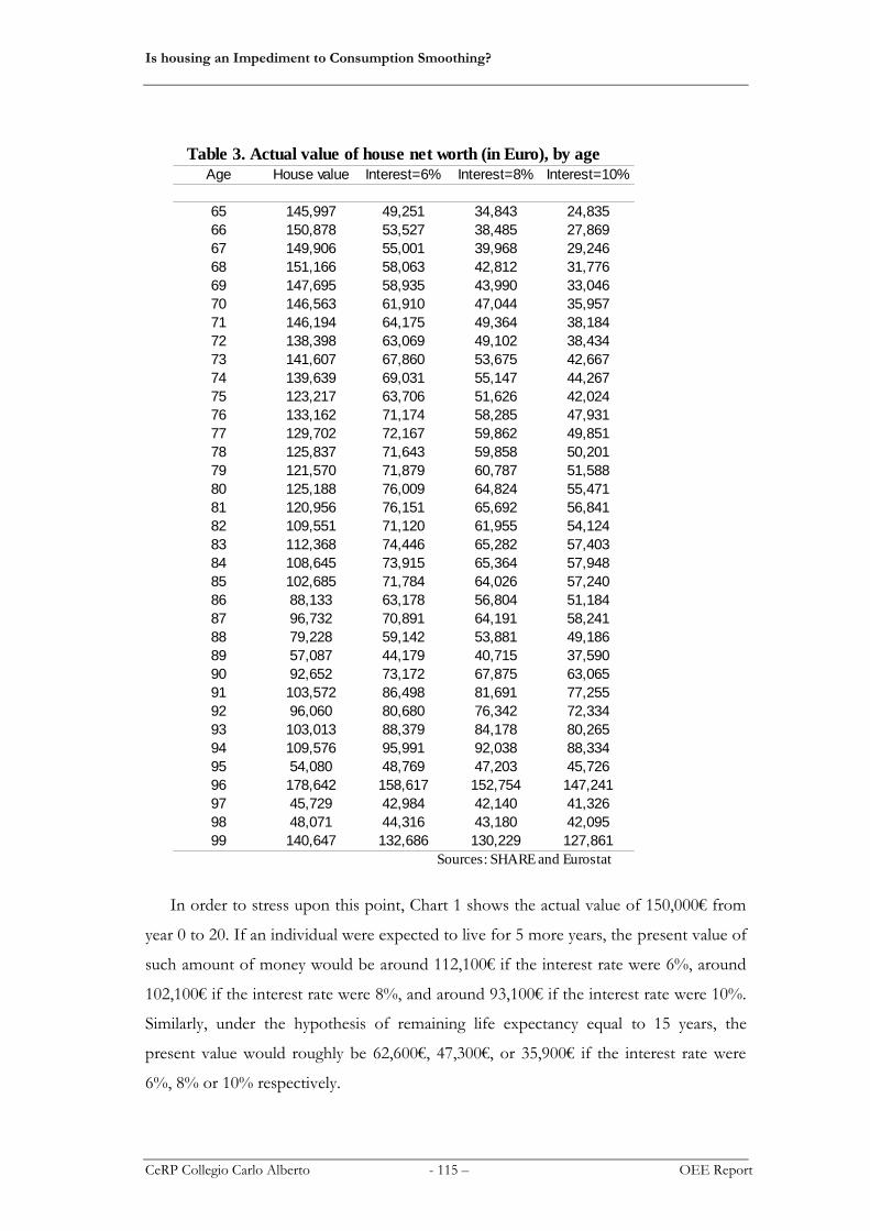
Is housing an Impediment to Consumption Smoothing?
CeRP Collegio Carlo Alberto - 115 – OEE Report
In order to stress upon this point, Chart 1 shows the actual value of 150,000€ from
year 0 to 20. If an individual were expected to live for 5 more years, the present value of
such amount of money would be around 112,100€ if the interest rate were 6%, around
102,100€ if the interest rate were 8%, and around 93,100€ if the interest rate were 10%.
Similarly, under the hypothesis of remaining life expectancy equal to 15 years, the
present value would roughly be 62,600€, 47,300€, or 35,900€ if the interest rate were
6%, 8% or 10% respectively.
Table 3. Actual value of house net worth (in Euro), by age
Age House value Interest=6% Interest=8% Interest=10%
65 145,997 49,251 34,843 24,835
66 150,878 53,527 38,485 27,869
67 149,906 55,001 39,968 29,246
68 151,166 58,063 42,812 31,776
69 147,695 58,935 43,990 33,046
70 146,563 61,910 47,044 35,957
71 146,194 64,175 49,364 38,184
72 138,398 63,069 49,102 38,434
73 141,607 67,860 53,675 42,667
74 139,639 69,031 55,147 44,267
75 123,217 63,706 51,626 42,024
76 133,162 71,174 58,285 47,931
77 129,702 72,167 59,862 49,851
78 125,837 71,643 59,858 50,201
79 121,570 71,879 60,787 51,588
80 125,188 76,009 64,824 55,471
81 120,956 76,151 65,692 56,841
82 109,551 71,120 61,955 54,124
83 112,368 74,446 65,282 57,403
84 108,645 73,915 65,364 57,948
85 102,685 71,784 64,026 57,240
86 88,133 63,178 56,804 51,184
87 96,732 70,891 64,191 58,241
88 79,228 59,142 53,881 49,186
89 57,087 44,179 40,715 37,590
90 92,652 73,172 67,875 63,065
91 103,572 86,498 81,691 77,255
92 96,060 80,680 76,342 72,334
93 103,013 88,379 84,178 80,265
94 109,576 95,991 92,038 88,334
95 54,080 48,769 47,203 45,726
96 178,642 158,617 152,754 147,241
97 45,729 42,984 42,140 41,326
98 48,071 44,316 43,180 42,095
99 140,647 132,686 130,229 127,861
Sources: SHARE and Eurostat

Is housing an Impediment to Consumption Smoothing?
CeRP Collegio Carlo Alberto - 116 – OEE Report
Put differently, if the borrower chooses to receive an annuity instead of a lump sum,
interests are compounded and, since the loan does not have to be paid back until the
borrower is passed away, the amount due by the heirs increases exponentially. Indeed, as
suggested in Chart 2, an agent borrowing 1,000€ at time 0 without repaying anything
back will generate a value of the loan at death which is obviously amplified by the
compounded interest rate effect. As an example, after 15 years if the interest rate were
6%, the heirs should reimburse 2,397€, 3,172€ if the interest rate were fixed at 8%,
4,177€ with 10% as interest rate.
0 1 2 3 4 5 6 7 8 9 10 11 12 13 14 15 16 17 18 19 20
0
20,000
40,000
60,000
80,000
100,000
120,000
140,000
160,000
Chart 1. Actual value of 150,000 euros
6%
8%
10%
Life expectancy
Actual value (in euro)
0 1 2 3 4 5 6 7 8 9 10 11 12 13 14 15
0
500
1,000
1,500
2,000
2,500
3,000
3,500
4,000
4,500
Chart 2. Compound interest rate effect
6%
8%
10%
Years
Amount due (in Euro)

Is housing an Impediment to Consumption Smoothing?
CeRP Collegio Carlo Alberto - 117 – OEE Report
2.2. House Value converted into annuities
In this first simulation we supposed that all over 65 respondents decide to convert their
housing equity into an annuity. Table 4 shows the average house value for each country
along with the average annuities computed using, respectively, an interest rate of 6%,
8%, or 10%.
If there were perfect competition in financial markets, lenders should compute the
annuities taking into account only the house value and the life expectancy of the
borrower. However, since real world is far from perfect, and life expectancy does
increase over time much more than mortality tables predict, it has been assumed that
operators add 5 years when deciding the amount of such annuities in order to increase
their profits and reduce their exposure. In fact, another reason which leads operators to
increase the life expectancy is that mortality tables computed by Eurostat or other
statistical centres usually do not take into account cohort effect. Therefore, a borrower
whose house is worth 100,000€ and with a life expectancy of 12 years would obtain an
annuity of 3,544€ instead of 5,928€ if the interest rate were 6%.
It is worth noting that a slightly increase in the interest rate produces a sharp
reduction in the annuities. For instance, in France home-owners would receive on
average an annuity of 6,422€, 5,401€, 4,541€ if the interest rate applied by the lender
were 6%, 8%, or 10% respectively.
Table 4. Reverse Mortgage - 100% House Value
Annuities (in Euro)
Country House value Interest=6% Interest=8% Interest=10%
Austria 119,778 4,158 3,492 2,930
Germany 121,436 4,086 3,408 2,837
Sweden 84,317 3,019 2,547 2,148
Netherlands 119,954 4,647 3,957 3,367
Spain 186,104 7,207 6,133 5,214
Italy 176,410 5,906 4,934 4,118
France 184,180 6,422 5,401 4,541
Denmark 97,696 3,955 3,382 2,889
Greece 103,701 4,351 3,745 3,224
Switzerland 126,877 4,646 3,927 3,317
Belgium 147,354 5,680 4,833 4,109Source: SHARE

Is housing an Impediment to Consumption Smoothing?
CeRP Collegio Carlo Alberto - 118 – OEE Report
Tables 5 to 8 display the effect of such annuities on poverty rates. For some
countries the outcome is impressive. For instance, using Poverty I as poverty index and
looking at wave 1 with interest rate equal to 6%, in Spain the poverty rate would
decrease by almost 12 percentage points (Table 5), from 16.88% to 5.2% (-69.20%); and
by almost 18 percentage points using Poverty SHARE (Table 6), from 21.46% to 3.54%
(-83.50%). Tables 7 (computed using Poverty I as poverty index) and Table 8 (using
Poverty SHARE) shows the same figures for wave 2. Also in this case, in Spain the
results would be highly effective, reducing poverty rates by 20 percentage points from
26.50% to 5.30% (-80%), and from 25.35% to 4.15% (-83.63%) using Poverty I and
Poverty SHARE respectively.
Furthermore, an increase in the interest rate from 6% to 8% or 10% would reduce
the magnitude of poverty reduction, but only slightly. In fact, for most of the country
the reduction would be only 1 or 2 percentage points lower, showing that the majority
of the poor in these countries is just above the poverty line, then these annuities,
although not so high, would boost most of them out of poverty.
Table 5. Poverty reduction (percentage points)
100% House Value
Wave 1 - 2004
Poverty I
Country Interest=6% Interest=8% Interest=10%
Austria 4.71 4.52 3.77
Germany 5.95 4.66 3.75
Sweden 3.65 3.20 2.76
Netherlands 7.62 7.43 7.06
Spain 11.67 11.46 10.83
Italy 20.27 17.21 13.80
France 5.93 5.80 4.96
Denmark 11.58 10.40 10.40
Greece 12.83 11.33 10.67
Belgium 8.01 7.26 6.84Source: SHARE
Is housing an Impediment to Consumption Smoothing?
CeRP Collegio Carlo Alberto - 119 – OEE Report
One of the main reasons explaining why the elderly are so wary of reverse mortgages
is that they are worried not to leave enough inheritance to their heirs, or even to leave
them with excessive debt.
Table 6. Poverty reduction (percentage points)
100% House Value
Wave 1 - 2004
Poverty II
Country Interest=6% Interest=8% Interest=10%
Austria 7.16 6.40 5.84
Germany 9.31 8.54 8.02
Sweden 6.74 6.08 5.52
Netherlands 9.11 8.18 7.62
Spain 17.92 17.50 16.67
Italy 13.12 11.93 10.90
France 11.00 10.40 9.19
Denmark 13.95 13.00 10.87
Greece 19.83 18.00 16.83
Switzerland 13.16 12.78 11.65
Belgium 12.29 11.97 11.32Source: SHARE
Table 8. Poverty reduction (percentage points)
100% House Value
Wave 2 - 2006
Poverty II
Country Interest=6% Interest=8% Interest=10%
Austria 6.81 6.41 6.01
Germany 6.01 5.87 5.17
Sweden 5.55 4.97 4.86
Netherlands 7.84 7.25 7.06
Spain 21.20 20.51 19.82
Italy 12.24 11.70 10.88
France 11.78 11.28 9.65
Denmark 15.62 14.74 14.16
Greece 19.49 18.73 18.13
Switzerland 7.87 7.02 6.18
Belgium 9.88 9.25 9.00Source: SHARE
Is housing an Impediment to Consumption Smoothing?
CeRP Collegio Carlo Alberto - 120 – OEE Report
First of all, it should be reminded that this types of loans usually have a non negative
equity clause which ensures that the amount of the loan will never exceed the house
value. Then, it is impossible that heirs receive a negative inheritance because of a house
with a mortgage loan bigger than the house value. Second, as Table 9 demonstrates,
borrowers would manage on average to leave a more than decent inheritance to their
offspring. It is interesting to note that even if the interest rate increase from 6% to 8%
or 10%, the inheritance becomes higher since the lower annuities more than offset the
heavier interest rates49.
2.3. Different Scenarios: partially converting housing equity into annuities
It seems clear from the simulation above that converting all house values into annuities
would be the best solution in order to cut sharply the poverty rates among the elderly.
However, such outcome is unlikely since not everybody would be happy to provide a
mortgage on his or her whole house. Moreover, financial institution would rather
oppose to accepting all these houses as collateral, without any kind of diversification.
49 It is important to stress that it has been assumed that house values do not increase neither decrease during the simulation, since the estimation of such growth rates in different cities and countries lies outside the aims of this report.
Table 9. Reverse Mortgage - Inheritance (in Euro)
100% House Value
Country House value Interest=6% Interest=8% Interest=10%
Austria 193,981 77,393 84,540 91,524
Germany 216,808 85,524 93,544 101,386
Sweden 117,698 47,500 51,791 55,984
Netherlands 254,994 106,059 115,032 123,794
Spain 204,692 85,127 92,315 99,333
Italy 201,394 79,302 86,818 94,165
France 247,759 99,007 108,145 117,076
Denmark 150,134 63,547 68,708 73,745
Greece 111,475 47,875 51,680 55,394
Switzerland 250,532 101,968 110,988 119,798
Belgium 190,759 79,189 85,911 92,475Source: SHARE
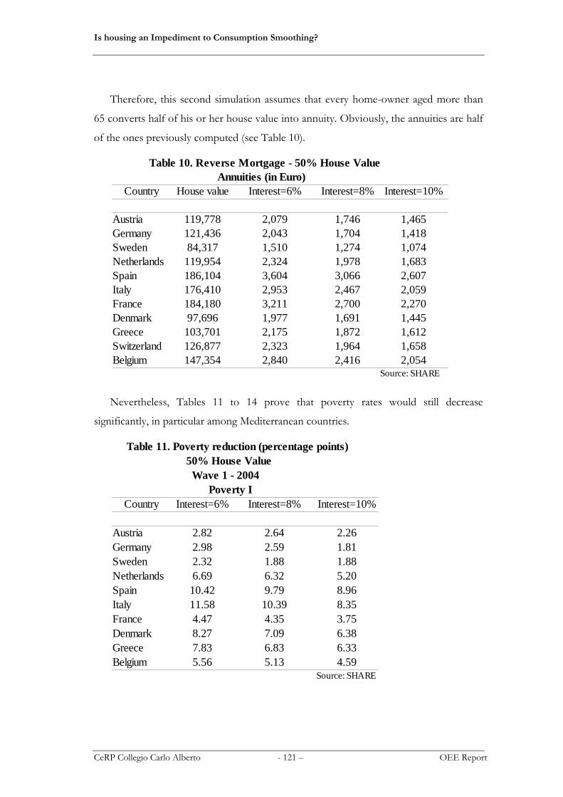
Is housing an Impediment to Consumption Smoothing?
CeRP Collegio Carlo Alberto - 121 – OEE Report
Therefore, this second simulation assumes that every home-owner aged more than
65 converts half of his or her house value into annuity. Obviously, the annuities are half
of the ones previously computed (see Table 10).
Nevertheless, Tables 11 to 14 prove that poverty rates would still decrease
significantly, in particular among Mediterranean countries.
Table 10. Reverse Mortgage - 50% House Value
Annuities (in Euro)
Country House value Interest=6% Interest=8% Interest=10%
Austria 119,778 2,079 1,746 1,465
Germany 121,436 2,043 1,704 1,418
Sweden 84,317 1,510 1,274 1,074
Netherlands 119,954 2,324 1,978 1,683
Spain 186,104 3,604 3,066 2,607
Italy 176,410 2,953 2,467 2,059
France 184,180 3,211 2,700 2,270
Denmark 97,696 1,977 1,691 1,445
Greece 103,701 2,175 1,872 1,612
Switzerland 126,877 2,323 1,964 1,658
Belgium 147,354 2,840 2,416 2,054Source: SHARE
Table 11. Poverty reduction (percentage points)
50% House Value
Wave 1 - 2004
Poverty I
Country Interest=6% Interest=8% Interest=10%
Austria 2.82 2.64 2.26
Germany 2.98 2.59 1.81
Sweden 2.32 1.88 1.88
Netherlands 6.69 6.32 5.20
Spain 10.42 9.79 8.96
Italy 11.58 10.39 8.35
France 4.47 4.35 3.75
Denmark 8.27 7.09 6.38
Greece 7.83 6.83 6.33
Belgium 5.56 5.13 4.59Source: SHARE
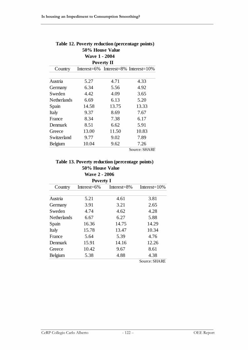
Is housing an Impediment to Consumption Smoothing?
CeRP Collegio Carlo Alberto - 122 – OEE Report
Table 12. Poverty reduction (percentage points)
50% House Value
Wave 1 - 2004
Poverty II
Country Interest=6% Interest=8% Interest=10%
Austria 5.27 4.71 4.33
Germany 6.34 5.56 4.92
Sweden 4.42 4.09 3.65
Netherlands 6.69 6.13 5.20
Spain 14.58 13.75 13.33
Italy 9.37 8.69 7.67
France 8.34 7.38 6.17
Denmark 8.51 6.62 5.91
Greece 13.00 11.50 10.83
Switzerland 9.77 9.02 7.89
Belgium 10.04 9.62 7.26Source: SHARE
Table 13. Poverty reduction (percentage points)
50% House Value
Wave 2 - 2006
Poverty I
Country Interest=6% Interest=8% Interest=10%
Austria 5.21 4.61 3.81
Germany 3.91 3.21 2.65
Sweden 4.74 4.62 4.28
Netherlands 6.67 6.27 5.88
Spain 16.36 14.75 14.29
Italy 15.78 13.47 10.34
France 5.64 5.39 4.76
Denmark 15.91 14.16 12.26
Greece 10.42 9.67 8.61
Belgium 5.38 4.88 4.38Source: SHARE

Is housing an Impediment to Consumption Smoothing?
CeRP Collegio Carlo Alberto - 123 – OEE Report
An advantage of this kind of deal would be an increase in the inheritance compared
to a reverse mortgage on the entire house (see Table 15).
Finally, even if the home-owners aged over 65 would convert 30% of their house
value into annuities with an interest rate of 8%, the effect on poverty rates would still be
sizeable, as shown in Table 16. Indeed, in Spain the poverty rate would still be reduced
Table 14. Poverty reduction (percentage points)
50% House Value
Wave 2 - 2006
Poverty II
Country Interest=6% Interest=8% Interest=10%
Austria 5.21 4.61 4.21
Germany 4.05 3.77 3.49
Sweden 4.28 4.05 3.82
Netherlands 6.47 5.88 5.69
Spain 18.43 17.28 15.67
Italy 9.80 8.57 7.48
France 8.52 7.39 6.14
Denmark 12.41 11.53 10.36
Greece 14.35 13.14 12.24
Switzerland 5.90 5.90 5.34
Belgium 8.75 8.13 7.25Source: SHARE
Table 15. Reverse Mortgage - Inheritance (in Euro)
50% House Value
Country House value Interest=6% Interest=8% Interest=10%
Austria 193,981 135,687 139,260 142,753
Germany 216,808 151,166 155,176 159,097
Sweden 117,698 82,599 84,744 86,841
Netherlands 254,994 180,527 185,013 189,394
Spain 204,692 144,910 148,504 152,013
Italy 201,394 140,348 144,106 147,780
France 247,759 173,383 177,952 182,417
Denmark 150,134 106,841 109,421 111,940
Greece 111,475 79,675 81,577 83,434
Switzerland 250,532 176,250 180,760 185,165
Belgium 190,759 134,974 138,335 141,617Source: SHARE
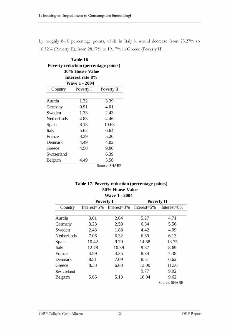
Is housing an Impediment to Consumption Smoothing?
CeRP Collegio Carlo Alberto - 124 – OEE Report
by roughly 8-10 percentage points, while in Italy it would decrease from 23.27% to
16.52% (Poverty II), from 28.17% to 19.17% in Greece (Poverty II).
Table 16
Poverty reduction (percentage points)
30% House Value
Interest rate 8%
Wave 1 - 2004
Country Poverty I Poverty II
Austria 1.32 3.39
Germany 0.91 4.01
Sweden 1.33 2.43
Netherlands 4.83 4.46
Spain 8.13 10.63
Italy 5.62 6.64
France 3.39 5.20
Denmark 4.49 4.02
Greece 4.50 9.00
Switzerland 6.39
Belgium 4.49 5.56
Source: SHARE
Table 17. Poverty reduction (percentage points)
50% House Value
Wave 1 - 2004
Poverty I Poverty II
Country Interest=5% Interest=8% Interest=5% Interest=8%
Austria 3.01 2.64 5.27 4.71
Germany 3.23 2.59 6.34 5.56
Sweden 2.43 1.88 4.42 4.09
Netherlands 7.06 6.32 6.69 6.13
Spain 10.42 9.79 14.58 13.75
Italy 12.78 10.39 9.37 8.69
France 4.59 4.35 8.34 7.38
Denmark 8.51 7.09 8.51 6.62
Greece 8.33 6.83 13.00 11.50
Switzerland 9.77 9.02
Belgium 5.66 5.13 10.04 9.62Source: SHARE

Is housing an Impediment to Consumption Smoothing?
CeRP Collegio Carlo Alberto - 125 – OEE Report
Table 18. Poverty reduction (percentage points)
50% House Value
Wave 2 - 2006
Poverty I Poverty II
Country Interest=5% Interest=8% Interest=5% Interest=8%
Austria 5.41 4.61 5.21 4.61
Germany 4.47 3.21 4.05 3.77
Sweden 4.86 4.62 4.28 4.05
Netherlands 7.06 6.27 6.47 5.88
Spain 16.82 14.75 18.43 17.28
Italy 16.87 13.47 9.80 8.57
France 5.89 5.39 8.52 7.39
Denmark 16.50 14.16 12.41 11.53
Greece 11.18 9.67 14.35 13.14
Switzerland 5.90 5.90
Belgium 6.00 4.88 8.75 8.13Source: SHARE
Table 19. Poverty reduction (percentage points)
30% House Value
Wave 1 - 2004
Poverty I Poverty II
Country Interest=5% Interest=8% Interest=5% Interest=8%
Austria 2.26 1.32 4.14 3.39
Germany 1.68 0.91 4.53 4.01
Sweden 1.88 1.33 3.09 2.43
Netherlands 5.58 4.83 5.39 4.46
Spain 8.75 8.13 12.50 10.63
Italy 8.01 5.62 7.84 6.64
France 3.75 3.39 6.41 5.20
Denmark 5.67 4.49 5.44 4.02
Greece 5.67 4.50 10.00 9.00
Switzerland 7.52 6.39
Belgium 4.91 4.49 7.05 5.56Source: SHARE

Is housing an Impediment to Consumption Smoothing?
CeRP Collegio Carlo Alberto - 126 – OEE Report
2.4. Converting financial wealth into annuities
In this last simulation, it has been decided to convert into annuities the 30%, 50%, and
70% respectively of the household's financial wealth. Also in this case, it has been
assumed that financial operators increase life expectancy of each borrower by 5 years.
Moreover, it has been taken an interest rate of 2,5% and 5%.
Tables 17 and 18 list the average financial wealth of households aged more than 65
sorted by country along with the average annuities which each individual would have
received if they would have decided to convert 30%, 50%, or 70% of their financial
wealth using an interest rate of 2.5%.
Table 20. Poverty reduction (percentage points)
30% House Value
Wave 2 - 2006
Poverty I Poverty II
Country Interest=5% Interest=8% Interest=5% Interest=8%
Austria 4.01 2.61 3.81 3.21
Germany 2.65 2.37 3.35 2.51
Sweden 3.70 3.24 3.70 3.24
Netherlands 6.08 5.10 5.69 5.29
Spain 13.82 12.67 14.98 13.13
Italy 11.16 8.71 7.48 6.53
France 4.26 3.76 6.14 4.89
Denmark 11.68 9.05 9.49 8.03
Greece 7.70 5.74 11.48 10.57
Switzerland 5.06 5.06
Belgium 4.38 3.75 7.25 5.88Source: SHARE

Is housing an Impediment to Consumption Smoothing?
CeRP Collegio Carlo Alberto - 127 – OEE Report
Tables 19-20 provide the same information obtained with an interest rate of 5%. It
is interesting to note that the average financial wealth varied greatly among the selected
European countries. Indeed, in 2004 it was only 10,613€ in Greece (8,107€ in 2006,
even lower), whereas it reached a mean of 82,902€ (98,463€ in 2006) in Switzerland.
Table 17
Financial wealth - Annuities (in Euro)
Interest rate: 2.5%
Wave 1 - 2004
Country Tot. fin. wealth Fin. wealth: 30% Fin. wealth: 50% Fin. wealth: 70%
Austria 20,956 441 735 1,029
Germany 36,113 769 1,282 1,794
Sweden 40,867 898 1,496 2,095
Netherlands 45,011 1,029 1,715 2,401
Spain 13,461 302 504 706
Italy 15,594 322 537 752
France 34,964 788 1,313 1,838
Denmark 35,911 845 1,409 1,973
Greece 10,613 241 402 563
Switzerland 82,902 1,840 3,067 4,293
Belgium 55,421 1,267 2,111 2,956Source: SHARE
Table 18
Financial wealth - Annuities (in Euro)
Interest rate: 2.5%
Wave 2 - 2006
Country Tot. fin. wealth Fin. wealth: 30% Fin. wealth: 50% Fin. wealth: 70%
Austria 21,938 455 759 1,062
Germany 36,003 751 1,251 1,751
Sweden 53,909 1,174 1,957 2,739
Netherlands 49,858 1,143 1,905 2,666
Spain 19,106 410 683 956
Italy 18,760 386 643 900
France 35,605 762 1,270 1,778
Denmark 50,964 1,125 1,874 2,624
Greece 8,107 178 297 415
Switzerland 98,463 2,123 3,539 4,955
Belgium 55,971 1,238 2,063 2,888Source: SHARE

Is housing an Impediment to Consumption Smoothing?
CeRP Collegio Carlo Alberto - 128 – OEE Report
Furthermore, in Spain and Italy citizens strongly preferred - and still prefer - to invest
their savings into real estate rather than financial markets: average house value was
extremely high in 2004 and 2006, whilst financial assets were relatively thin. Conversely,
in Sweden real assets held by households were lower than 100,000€ both in 2004 and
2006, while financial assets were above the sample mean. Finally, the financial wealth
held by the elderly is usually lower than their house value, then the corresponding
annuities are smaller.
Poverty reductions shows in Tables 22-23 are based on Poverty I and they have
been computed adding to the income of each individual in the sample the annuities
obtained converting the whole house value using an interest rate of 6%, and converting
the financial wealth using an interest rate of 2.5%. As expected, poverty rates were
already been sharply reduced in the previous simulation by converting into annuities
only real assets, then the marginal effect of converting into annuities financial wealth
would not be relevant. On the other hand, although not reaching a double-digit, poverty
reduction in Sweden and the Netherlands would be highly influenced by this last
operation: in Sweden Poverty I would have decrease from 11.38% in 2004 to 7.73%
converting only 100% of real asset, or to 4.97% converting both 100% of house value
and 70% of financial wealth into annuities. In the Netherlands poverty rates would have
shift from 14.87% to 7.25% or to 5.39% in the same two cases.
Table 19
Financial wealth - Annuities (in Euro)
Interest rate: 5%
Wave 1 - 2004
Country Tot. fin. wealth Fin. wealth: 30% Fin. wealth: 50% Fin. wealth: 70%
Austria 20,956 526 876 1,227
Germany 36,113 915 1,525 2,134
Sweden 40,867 1,062 1,770 2,478
Netherlands 45,011 1,207 2,012 2,817
Spain 13,461 356 593 831
Italy 15,594 386 643 900
France 34,964 927 1,546 2,164
Denmark 35,911 987 1,644 2,302
Greece 10,613 283 472 661
Switzerland 82,902 2,172 3,621 5,069
Belgium 55,421 1,487 2,478 3,469Source: SHARE

Is housing an Impediment to Consumption Smoothing?
CeRP Collegio Carlo Alberto - 129 – OEE Report
Tables 21-25 show poverty reductions if the interest rates were 8% for reverse
mortgage and 5% for financial wealth.
Table 20
Financial wealth - Annuities (in Euro)
Interest rate: 5%
Wave 2 - 2006
Country Tot. fin. wealth Fin. wealth: 30% Fin. wealth: 50% Fin. wealth: 70%
Austria 21,938 545 908 1,271
Germany 36,003 897 1,495 2,092
Sweden 53,909 1,391 2,319 3,246
Netherlands 49,858 1,341 2,235 3,129
Spain 19,106 487 811 1,136
Italy 18,760 462 770 1,078
France 35,605 907 1,511 2,115
Denmark 50,964 1,329 2,215 3,100
Greece 8,107 211 351 491
Switzerland 98,463 2,520 4,200 5,881
Belgium 55,971 1,462 2,436 3,411Source: SHARE
Table 21
Poverty reduction (percentage points)
100% House Value
Interest rate reverse mortgage: 6%
Interest rate financial wealth: 2.5%
Wave 1 - 2004
Poverty I
Country Fin. wealth: 30% Fin. wealth: 50% Fin. wealth: 70%
Austria 4.71 5.08 5.08
Germany 6.99 7.37 7.89
Sweden 5.30 6.08 6.41
Netherlands 9.11 9.11 9.48
Spain 12.08 12.29 12.29
Italy 20.78 20.95 21.12
France 6.17 6.65 7.01
Denmark 14.42 15.84 15.84
Greece 13.00 13.17 13.67
Belgium 9.29 9.94 10.58Source: SHARE

Is housing an Impediment to Consumption Smoothing?
CeRP Collegio Carlo Alberto - 130 – OEE Report
Table 22
Poverty reduction (percentage points)
100% House Value
Interest rate reverse mortgage: 6%
Interest rate financial wealth: 2.5%
Wave 2 - 2006
Poverty I
Country Fin. wealth: 30% Fin. wealth: 50% Fin. wealth: 70%
Austria 7.62 7.82 7.62
Germany 9.64 10.89 11.59
Sweden 9.71 10.52 11.33
Netherlands 9.02 9.61 10.00
Spain 21.89 22.35 22.35
Italy 23.27 23.40 23.95
France 9.52 9.90 10.28
Denmark 28.76 30.95 31.24
Greece 17.22 17.22 17.22
Belgium 9.25 9.50 9.88Source: SHARE
Table 23
Poverty reduction (percentage points)
100% House Value
Interest rate reverse mortgage: 8%
Interest rate financial wealth: 5%
Wave 1 - 2004
Poverty I
Country Fin. wealth: 30% Fin. wealth: 50% Fin. wealth: 70%
Austria 4.52 4.90 5.08
Germany 5.95 6.86 7.12
Sweden 5.30 5.97 6.30
Netherlands 8.92 9.11 9.85
Spain 11.88 12.08 12.08
Italy 18.74 19.08 19.42
France 6.17 6.41 6.89
Denmark 13.71 15.37 15.84
Greece 11.67 11.67 11.83
Belgium 8.87 9.62 10.26Source: SHARE
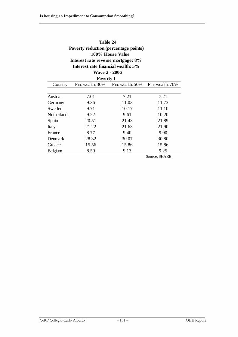
Is housing an Impediment to Consumption Smoothing?
CeRP Collegio Carlo Alberto - 131 – OEE Report
Table 24
Poverty reduction (percentage points)
100% House Value
Interest rate reverse mortgage: 8%
Interest rate financial wealth: 5%
Wave 2 - 2006
Poverty I
Country Fin. wealth: 30% Fin. wealth: 50% Fin. wealth: 70%
Austria 7.01 7.21 7.21
Germany 9.36 11.03 11.73
Sweden 9.71 10.17 11.10
Netherlands 9.22 9.61 10.20
Spain 20.51 21.43 21.89
Italy 21.22 21.63 21.90
France 8.77 9.40 9.90
Denmark 28.32 30.07 30.80
Greece 15.56 15.86 15.86
Belgium 8.50 9.13 9.25Source: SHARE

Is housing an Impediment to Consumption Smoothing?
CeRP Collegio Carlo Alberto - 132 – OEE Report
CONCLUSIONS
Our research has investigated the potential impact of wealth annuitization among older
European households. The magnitude of the welfare gains, particularly by subscribing
to reverse mortgage is of crucial importance. More specifically Italy and Spain would see
a reduction in their poverty rates by at least 10 percentage points if (part of) household
real wealth were converted in an annuity with a reverse mortgage. However, Italian
households do not seem to be interested in products as such, possibly because they do
not understand the complexity of the financial products. Moreover, the elderly do not
show any interest in decumulation, this evidence holding for most of European
countries.

Is housing an Impediment to Consumption Smoothing?
CeRP Collegio Carlo Alberto - 133 – OEE Report
References:
AARP, Reverse mortgage loans: borrowing against your house, October 2010 Update Australian Security&Investment Commission (ASIC), Equity release products,
Report 59, November 2005 Australian Seniors Finance (ASF), Frequently asked question about the Lifetime
Loan Banerjee, S. (2012), Time trends in poverty for older Americans between 2001-2009,
Employee Benefit Research Institute, 33(4) Davey, A. J. (2007), Home Equity Release Products in New Zealand: Risks and
Opportunities - Report to Retirement Commission, 2007 Review of Retirement Income Policies
Equity Release Council, SHIP Equity Release, Facing the Future - Redefining equity release to meet today’s social and economic challenges, Discussion paper, July 2009
Equity Release Council, SHIP Equity Release, SHIP 20th anniversary report - December 1991 to December 2011, Discussion paper, May 2012
Financial Services Authority (FSA), Mortgages Product Sales Data (PSD) - Trend Report : 2005-2011, August 2011
Hickey, J. and Sorbello, R. (2007), Trowbridge Deloitte New Zealand Reverse Mortgage Market Study December 2006, Press release 26 April
Jappelli T. (2005), Un reverse mortgage per il consumo degli anziani, LaVoce.info, 2005 (11)
Responsible Equity Release, Types of lifetime mortgages Shan H. (2009), Reversing the Trend: the Recent Expansion of the Reverse Mortgage
Market, Finance and Economics Discussion Series 2009-42, Board of Governors of the Federal Reserve System (U.S.)
Sentinel, Lifetime Loan Fact Sheet, 12 December 20111 Sentinel, Discover a new lease on life - The Sentinel lifetime loan in detail U.S. Department of Housing and Urban Development (HUD), HUD FHA
Reverse Mortgage for Seniors (HECM), Consumer fact sheet about HECM loans, November 2010
FED, Board of Governors of the Federal Reserve System, H.15 Selected Interest Rates, Conventional mortgages
U.S. Department of Housing and Urban Development (HUD), HECM Reports, Home Equity Conversion Mortgage Characteristics, June 2012
U.S. Department of Housing and Urban Development (HUD), Interest Rates Report, HUD FHA insured Single Family Interest Rates Historical