
IMPLEMENTING “QUALITY BY DESIGN IN THE...
213
Sede Amministrativa: Università degli Studi di Padova Dipartimento di Ingegneria Industriale SCUOLA DI DOTTORATO DI RICERCA IN: INGEGNERIA INDUSTRIALE INDIRIZZO: INGEGNERIA CHIMICA, DEI MATERIALI E MECCANICA CICLO XXVIII IMPLEMENTING “QUALITY BY DESIGN” IN THE PHARMACEUTICAL INDUSTRY: A DATA-DRIVEN APPROACH Direttore della Scuola: Ch.mo Prof. Paolo Colombo Coordinatore d’indirizzo: Ch.mo Prof. Enrico Savio Supervisore: Ch.mo Prof. Massimiliano Barolo Dottoranda: Natascia Meneghetti
Transcript of IMPLEMENTING “QUALITY BY DESIGN IN THE...

Sede Amministrativa: Università degli Studi di Padova
Dipartimento di Ingegneria Industriale
SCUOLA DI DOTTORATO DI RICERCA IN: INGEGNERIA INDUSTRIALE
INDIRIZZO: INGEGNERIA CHIMICA, DEI MATERIALI E MECCANICA
CICLO XXVIII
IMPLEMENTING “QUALITY BY DESIGN” IN THE
PHARMACEUTICAL INDUSTRY: A DATA-DRIVEN
APPROACH
Direttore della Scuola: Ch.mo Prof. Paolo Colombo
Coordinatore d’indirizzo: Ch.mo Prof. Enrico Savio
Supervisore: Ch.mo Prof. Massimiliano Barolo
Dottoranda: Natascia Meneghetti

______________________________________________________________________________________________ © 2016 Natascia Meneghetti, University of Padova (Italy)
Foreword
The realization of the work included in this Dissertation involved the intellectual and
financial support of many people and institutions, to whom the author is very grateful.
Most of the research activity that led to the results reported in this Dissertation has been
carried out at CAPE-Lab, Computer-Aided Process Engineering Laboratory, at the
Department of Industrial Engineering of the University of Padova (Italy), under the
supervision of Prof. Massimiliano Barolo and Prof. Fabrizio Bezzo. Part of the work was
carried out at Process Systems Enterprise, London (U.K.) during a 6-month stay under the
supervision of Dr. Sean Bermingham, and part represents a collaboration with Dr. Simeone
Zomer from GlaxoSmithKline, Ware (U.K.).
Financial support to this study has been provided by the University of Padova. The author is
grateful also to “Fondazione Ing. Aldo Gini” (Padova, Italy) and to LLP/Erasmus
Placement_SMP program (University of Padova, Italy) for their financial support for the project
carried out at PSE.
All the material reported in this Dissertation is original, unless explicit references to studies carried out by other people are indicated. In the following, a list of the publications stemmed from this project is reported.
CONTRIBUTIONS IN PEER-REVIEWED JOURNALS
Facco, P., F. Dal Pastro, N. Meneghetti, F. Bezzo, M. Barolo (2015). Bracketing the design space within
the knowledge space in pharmaceutical product development. Ind. Eng. Chem. Res., 54, 5128–5138. Meneghetti, N., P. Facco, F. Bezzo, M. Barolo (2014). A methodology to diagnose process/model mismatch
in first-principles models. Ind. Eng. Chem. Res., 53, 14002-14013
CONTRIBUTIONS IN PEER-REVIEWED JOURNALS (submitted)
Meneghetti N., P. Facco, F. Bezzo, C. Himawan, S. Zomer, M. Barolo (2016). Knowledge management
in secondary pharmaceutical manufacturing by mining of data historians – A proof-of-concept study, submitted to: Int. J. Pharm.
CONTRIBUTIONS IN PEER-REVIEWED CONFERENCE PROCEEDINGS
Meneghetti N., P. Facco, F. Bezzo, C. Himawan, S. Zomer, M. Barolo (2016). Automated Data Review in
Secondary Pharmaceutical Manufacturing by Pattern Recognition Techniques, to be presented at: ESCAPE 26, 26th European Symposium on Computer-Aided Process Engineering (Portorož, Slovenia, 12-15 June 2016).
Meneghetti, N., P. Facco, S. Bermingham, D. Slade, F. Bezzo, M. Barolo (2015). First-principles model diagnosis in batch systems by multivariate statistical modeling. In: Computer-Aided Chemical Engineering 37, 12th International Symposium on Process Systems Engineering and 25th European Symposium on Computer Aided Process Engineering (K.V. Gernaey, J.K. Huusom, R. Gani, Eds.), Elsevier, Amsterdam (The Netherlands), 437-442.
Meneghetti, N., P. Facco, F. Bezzo, M. Barolo (2014). Diagnosing process/model mismatch in first-principles models by latent variable modeling. In: Computer-Aided Chemical Engineering 33, 24th

ii
_____________________________________________________________________________________________ © 2016 Natascia Meneghetti, University of Padova (Italy)
European Symposium on Computer Aided Process Engineering (J.J. Klemeš, P.S. Varbanov, P.Y. Liew, Eds.), Elsevier, Amsterdam (The Netherlands) 1897-1902.
CONFERENCE PRESENTATIONS
Meneghetti, N., P. Facco, F. Bezzo, M. Barolo (2015) First-principles models enhancement by latent variable models. Oral presentation at: Workshop Italiano di Chemiometria 2015, February 25-27, Roma (Italy).
Meneghetti, N., P. Facco, F. Bezzo, M. Barolo (2014). Process/model mismatch diagnosis by latent variable modeling. Poster presentation at: APM – Advanced Process Modelling Forum, April 2-3, London (U.K.).

______________________________________________________________________________________________ © 2016 Natascia Meneghetti, University of Padova (Italy)
Abstract
Traditionally, the pharmaceutical industry is characterized by of peculiar characteristics (e.g., low
production volumes, multi-products manufacturing based mainly on batch processes, strict
regulatory framework) that make the implementation of modern quality principles more complex
for this sector. However, the innovation gap with respect to other manufacturing industries is
gradually reducing thanks to the introduction of the Quality-by-Design initiative by the
Regulatory Agencies (such as the Food and Drug Administration, FDA and the European
Medicines Agency, EMA). QbD is based on the concept that quality should be designed into a
product, by a thorough understanding of product and processes features and risks. This initiative
aims to support the transition of the pharmaceutical industry to a systematic approach based on
scientific (rather than empiric) knowledge of products and processes, in order to facilitate the
implementation of modern management tools, advanced technologies and innovative solutions.
Under this perspective, the application of Process Systems Engineering (PSE) solutions has
rapidly grown. Despite the challenges encountered to adapt classical PSE approaches (mainly
based on the use of mathematical modeling) to a pharmaceutical context, the benefits achieved
by the use of PSE tools to support the implementation of QbD, opened the route to several studies
in this field. Significant improvements have been observed in product quality and process
capability and robustness thanks to the increase of process and product knowledge and
understanding provided by modeling. This has allowed the pharmaceutical industries to accelerate
the launch of new products into the market, to improve productivity and to reduce costs.
Although, in many PSE applications, first-principles models are preferred, the use of data-driven
tools, such as latent variable modeling or pattern recognition techniques, is rapidly expanding.
Thanks to the increasing availability of measurement data, these techniques have been
demonstrated to be an optimal opportunity to address several problems that characterize
pharmaceutical development and manufacturing activities.
The main objective of the research presented in this Dissertation is to demonstrate how these data-
driven modeling techniques can be used to address some common issues that often affect the
practical implementation of QbD paradigms in pharmaceutical development and manufacturing
activities. Novel and general methodologies based on these techniques are presented with the aim
of: i) supporting the diagnosis of first-principles models of pharmaceutical operations; ii)
supporting the implementation of some fundamental QbD elements, such as the identification of
the design space (DS) of a new pharmaceutical product, as well as continual improvement
paradigms by periodic review of large manufacturing databases.

iv Abstract
_____________________________________________________________________________________________ © 2016 Natascia Meneghetti, University of Padova (Italy)
With respect to first-principle models diagnosis, a methodology is proposed to diagnose the root
cause of the process/model mismatch (PMM) that may arise when a first-principles (FP) model
is challenged against a set of historical experimental data. The objective is to identify which model
equations or model parameters most contribute to the observed mismatch, without carrying out
any additional experiment. The methodology exploits the available historical and simulated data,
generated respectively by the process and by the FP model using the same set of inputs. A data-
driven model (namely, a latent variable one) is used to analyze the correlation structure of the
historical and simulated datasets, and information on where the PMM originates from is obtained
using diagnostic indices and engineering judgment. The methodology is first tested on two
simulated steady-state systems (a jacket-cooled continuous stirred reactor and a solids milling
unit), and then it is extended to dynamic systems (a drying unit and a penicillin fermentation
process). It is shown that the proposed methodology is able to pinpoint the model section(s) that
actually originate the mismatch.
With respect to the design space identification issue, a methodology is proposed to limit the
extension of the domain over which experiments are carried out to determine the DS of a new
pharmaceutical product. In fact, for a new pharmaceutical product to be developed a reliable first-
principles model is often not available. In this case, the DS is found using experiments carried out
within a domain of input combinations (the so-called knowledge space; e.g. raw materials
properties and process operating conditions) that result from products that have already been
developed and are similar to the new one. The proposed methodology aims at segmenting the
knowledge space in such a way as to identify a subspace of it (called the experiment space) that
most likely brackets the DS, in order to limit the extension of the domain over which the new
experiments should be carried out. The methodology is based on the inversion of the latent-
variable model used to describe the system (accounting also for model prediction uncertainty) in
order to identify a reduced area of the knowledge space wherein the design space is supposed to
lie. Three different case studies are presented to demonstrate the effectiveness of the proposed
methodology.
Finally, with respect to the periodic review of large manufacturing databases, a methodology
is proposed to systematically extract operation-relevant information from data historians of
secondary pharmaceutical manufacturing systems. This operation may result particularly
burdensome, not only because of the very large dimension of the datasets (which may reach
millions of data entries) but also because not even the number of the operations completed in a
given time window may be known a priori. The proposed methodology permits not only to
automatically identify the number of batches carried out in a given time window, but also to assess
how many different products have been manufactured, and whether or not the features
characterizing a batch have changed throughout a production campaign. The results achieved by

Abstract v
______________________________________________________________________________________________ © 2016 Natascia Meneghetti, University of Padova (Italy)
testing the proposed methodology on two six-month datasets of a commercial-scale drying unit
demonstrate the potential of this approach, which can be easily extended to other manufacturing
operations.


______________________________________________________________________________________________ © 2016 Natascia Meneghetti, University of Padova (Italy)
Riassunto
Negli anni, l’industria farmaceutica ha sviluppato un forte carattere bipolare: se da un lato è stata
in grado di lanciare sul mercato prodotti sempre più avanzati, in grado di rispondere alle esigenze
di una società in continua evoluzione, dall’altro ha conservato una filosofia di produzione basata
soprattutto sull’esperienza più che sul rinnovamento e l’utilizzo di tecnologie avanzate. La
motivazione risiede in parte nel fatto che l’industria farmaceutica è caratterizzata da una serie di
fattori (ad esempio bassi volumi di produzione, processi prevalentemente di tipo batch e un quadro
normativo rigido) che rendono effettivamente più difficile l'attuazione delle moderne filosofie di
produzione basate su principi di rinnovamento continuo. Tuttavia, negli ultimi decenni, il divario
con le industrie di produzione più mature si sta gradualmente riducendo grazie al lancio di una
nuova iniziativa da parte delle agenzie regolatore internazionali, basata del concetto di Quality by
Design (QbD). Questa iniziativa si fonda nella convinzione che la qualità di un prodotto dovrebbe
essere concepita come parte integrante della progettazione del prodotto stesso e del suo processo
produttivo, ottenuti grazie ad una conoscenza approfondita delle caratteristiche e dei rischi legati
allo sviluppo del prodotto e del processo di produzione. L’iniziativa quindi, mira a sostenere la
transizione dell’industria farmaceutica verso un approccio sistematico per favorire soluzioni
innovative, l'applicazione di conoscenze scientifiche e tecniche avanzate, nonché di moderni
sistemi di gestione della qualità nello sviluppo dei prodotti e dei processi produttivi. Questo
rinnovamento dovrebbe garantire negli anni una serie di benefici sia economici (come la riduzione
del tempo necessario per il lancio di nuovi prodotti sul mercato, il miglioramento della
produttività e la riduzione dei costi di produzione) sia sociali (come la garanzia di fornire prodotti
di qualità e assicurare tale qualità nel tempo).
In questo contesto, è di fondamentale importanza l’utilizzo di strumenti di modellazione
matematica avanzata, già largamente utilizzati in altri e più maturi settori di produzione.
Nonostante le difficoltà incontrate per adattare questi strumenti alle esigenze delle applicazioni
farmaceutiche, i vantaggi dell’utilizzo della modellazione nell’attuazione dei principi di QbD
hanno aperto la strada a diversi studi in questo campo. Negli anni, l’utilizzo di questi strumenti
ha permesso di ottenere miglioramenti significativi sia nella qualità dei prodotti processati, sia
nella capacità e affidabilità dei processi di produzione. La modellazione di processo si basa
principalmente su due tipi di approcci: il primo (modelli a principi primi) riguarda la
rappresentazione matematica delle leggi fisiche alla base di un sistema, ad esempio bilanci di
materia ed energia, il secondo (modelli basati su dati o data-driven) si fonda sull’utilizzo
dell’informazione contenuta nei dati ottenuti dal sistema stesso. Anche se in molte applicazioni
si predilige l’utilizzo di modelli principi primi, non sempre questo tipo di modelli sono disponibili.
Per questo, l'uso di modelli data-driven, come per esempio di tecniche di modellazione a variabili

viii Riassunto
_____________________________________________________________________________________________ © 2016 Natascia Meneghetti, University of Padova (Italy)
latenti (LVM, latent variable models) o tecniche di riconoscimento di pattern, è in rapida
espansione. Grazie alla crescente disponibilità di dati, queste tecniche sono state in grado di
dimostrare la loro efficacia nel risolvere diversi problemi che caratterizzano le diverse attività
farmaceutiche. L'obiettivo di questa Dissertazione è quello di dimostrare come queste tecniche
possano essere utilizzate per risolvere alcuni problemi spesso riscontrati nell'implementazione
pratica dei paradigmi di QbD nell’industria farmaceutica. A tal proposito, vengono presentate
delle metodologie innovative e generali basate sull'impiego di modelli data-driven con l'obiettivo
di: i) consentire il miglioramento dei modelli di principi primi per facilitare il loro impiego nella
modellazione di sistemi farmaceutici; ii) condurre alcune delle attività nelle quali un approccio
QbD può tradursi, come l'identificazione dello spazio di progetto (design space) di un prodotto
farmaceutico e l’analisi critica di voluminose raccolte di dati storici di processo.
Per quanto riguarda il miglioramento di modelli a principi primi, è stata sviluppata una
metodologia per identificare la causa principale delle differenze (o process/model mismatches)
che possono presentarsi tra i dati storici sperimentali e le stime fornite da un modello a principi
primi. L'obiettivo è di identificare quali equazioni o parametri del modello contribuiscano
maggiormente alla differenza osservata, senza effettuare alcuna ulteriore esperimento. La
metodologia sfrutta i dati storici disponibili e un set di dati simulati, generati dal modello a
principi primi utilizzando le stesse condizioni alle quali sono stati ottenuti i dati storici. Grazie
all’utilizzo di un modello a variabili latenti, viene analizzata e confrontata la struttura di
correlazione dei due set di dati disponibili, quello storico e quello e simulato, in modo da ricavare
informazioni utili ad identificare la causa della scarsa accuratezza del modello. Per valutare
l’efficacia della metodologia, nel Capitolo 3 vengono considerati due sistemi simulati in stato
stazionario: un reattore continuo agitato e incamiciato e un molino. Nel Capitolo 4 la metodologia
viene estesa e adattata a sistemi dinamici, considerando altri due processi simulati: un'unità di
essiccazione e un fermentatore per la produzione di penicillina. I risultati ottenuti dimostrano che
la metodologia proposta è in grado di indicare un gruppo di termini molto correlati tra loro, o
addirittura un solo termine, che effettivamente contengono la reale causa d’errore nel modello.
Sebbene la metodologia proposta sia stata sviluppata per analizzare modelli a principi primi di
processi farmaceutici, essa può essere facilmente estesa a qualsiasi altro modello in regime
stazionario o dinamico.
Nel Capitolo 5, vengono discussi i problemi relativi all'identificazione dello spazio di progetto
(design space, DS) per un nuovo prodotto farmaceutico caratterizzato da singola specifica di
qualità, nel caso in cui non sia disponibile un modello a principi primi da utilizzare per
determinare tale spazio. In questi casi, lo spazio di progetto viene spesso identificato utilizzando
gli esperimenti effettuati in un dominio (knowledge space) costituito dalle combinazioni delle
condizioni operative di processo e delle proprietà delle materie prime utilizzate per la produzione

Riassunto ix
______________________________________________________________________________________________ © 2016 Natascia Meneghetti, University of Padova (Italy)
di prodotti già sviluppati, e simili al nuovo prodotto. Spesso, il numero di esperimenti da effettuare
per identificare lo spazio del progetto all’interno di tale dominio è elevato. Per questo motivo,
viene proposta una metodologia per identificare uno spazio limitato all’interno di questo dominio,
detto spazio degli esperimenti (experiment space), che contiene lo spazio di progetto, in modo da
ridurre notevolmente il numero di nuovi esperimenti necessari. La metodologia si basa
sull'inversione del modello a variabili latenti utilizzato per descrivere il sistema, tenendo conto
anche dell'incertezza del modello stesso. Lo spazio degli esperimenti viene stimato per tre diversi
sistemi (due simulati e uno reale), dimostrando in tutti i casi l’efficacia della metodologia
proposta.
Infine, per quanto riguarda l’analisi critica di set di dati di produzione, nel Capitolo 6 viene
proposta una metodologia per estrarre in modo sistematico informazioni dai dati di grandi
database storici di impianti produttivi industriali. Queste informazioni, possono essere utilizzate
per individuare rapidamente potenziali aree di miglioramento, in modo da favorirne
l’implementazione di paradigmi di miglioramento continuo. Trasformare in conoscenza questi
dati, è particolarmente difficile perché spesso non si conosce nemmeno il numero dei batch
effettuati in un certo periodo di produzione. La metodologia presentata consente di determinare
automaticamente il numero di batch effettuati in un determinato intervallo di tempo e il numero
di prodotti processati, e se le caratteristiche che contraddistinguono una certa produzione siano
cambiate nel corso di campagne diverse. La metodologia proposta, basata sull’utilizzo di tecniche
di riconoscimento di pattern, è stata utilizzata per analizzare due set di dati industriali relativi a
sei mesi di produzione ciascuno. I risultati ottenuti dimostrano chiaramente il potenziale
dell’approccio proposto.


______________________________________________________________________________________________ © 2016 Natascia Meneghetti, University of Padova (Italy)
Table of contents
FOREWORD ................................................................................................................................................. I
ABSTRACT ................................................................................................................................................ III
RIASSUNTO ............................................................................................................................................. VII
LIST OF ACRONYMS ................................................................................................................................. 1
CHAPTER 1 -MOTIVATION AND STATE OF THE ART.......................................................................... 3
1.1 THE IMPLEMENTATION OF A QBD APPROACH IN PHARMACEUTICAL INDUSTRY: A BIG CHALLENGE 3
1.1.1 A SNAPSHOT OF THE PHARMACEUTICAL INDUSTRY CURRENT SITUATION .............................. 3
1.1.2 QUALITY BY DESIGN PARADIGMS .......................................................................................... 6
1.1.2.1 A quality target product profile (QTPP) ..................................................................... 7 1.1.2.2 Product design and understanding ............................................................................... 7 1.1.2.3 Process design and understanding ............................................................................... 8 1.1.2.4 Design space ............................................................................................................... 9 1.1.2.5 A control strategy ...................................................................................................... 10 1.1.2.6 Process capability and continual improvement ......................................................... 10
1.1.3 PAT TOOLS ......................................................................................................................... 11
1.1.4 THE PHARMACEUTICAL QUALITY SYSTEM ........................................................................... 12
1.1.5 IMPACT OF QBD .................................................................................................................. 15
1.2 THE MODELING CONTRIBUTION IN THE IMPLEMENTATION OF A QBD APPROACH .......................... 17
1.2.1 KNOWLEDGE-DRIVEN MODELS ............................................................................................ 20
1.2.2 DATA-DRIVEN MODELS ....................................................................................................... 21
1.2.2.1 Latent variable modeling in QbD .............................................................................. 23 1.2.3 CONTINUOUS IMPROVEMENT AND KNOWLEDGE MANAGEMENT TOOLS ............................... 25
1.3 OBJECTIVES OF THE RESEARCH ..................................................................................................... 26
1.4 DISSERTATION ROADMAP ............................................................................................................. 28
CHAPTER 2 -MULTIVARIATE MODELING BACKGROUND ............................................................... 31
2.1 LATENT VARIABLE MODELING APPROACHES ................................................................................. 31
2.1.1 PRINCIPAL COMPONENT ANALYSIS ...................................................................................... 32
2.1.1.1 Data pretreatment ...................................................................................................... 35 2.1.1.2 Selection of the number of PCs ................................................................................. 36
2.1.2 PROJECTION TO LATENT STRUCTURES (PLS) ....................................................................... 37

______________________________________________________________________________________________ © 2016 Natascia Meneghetti, University of Padova (Italy)
2.1.2.1 Statistics associated with the use of LVMs ............................................................... 39 2.1.3 MODEL INVERSION .............................................................................................................. 42
2.1.3.1 Null space computation ............................................................................................. 44
2.2 PATTERN RECOGNITION TECHNIQUES ............................................................................................ 45
2.2.1 K-NEAREST NEIGHBORS....................................................................................................... 47
2.2.2 PCA FOR CLUSTER ANALYSIS .............................................................................................. 48
CHAPTER 3 -A METHODOLOGY TO DIAGNOSE PROCESS/MODEL MISMATCH IN FIRST-
PRINCIPLES MODELS FOR STEADY-STATE SYSTEMS ....................................................................... 51
3.1 INTRODUCTION ............................................................................................................................. 51
3.2 PROPOSED METHODOLOGY ........................................................................................................... 53
3.2.1 DIAGNOSING THE PROCESS/MODEL MISMATCH .................................................................... 53
3.3 EXAMPLE 1: JACKET-COOLED REACTOR ........................................................................................ 55
3.3.1 PROCESS AND HISTORICAL DATASET ................................................................................... 55
3.3.2 APPLICATION OF THE METHODOLOGY AND RESULTS ........................................................... 57
3.3.1.1 Case study 1.A .......................................................................................................... 58 3.3.1.2 Case study 1.B .......................................................................................................... 61 3.3.1.3 Case study 1.C .......................................................................................................... 64
3.4 EXAMPLE 2: SOLIDS MILLING UNIT ................................................................................................ 66
3.4.1 PROCESS AND HISTORICAL DATASET ................................................................................... 66
3.4.2 APPLICATION OF THE METHODOLOGY AND RESULTS ........................................................... 67
3.4.1.1 Case study 2.A .......................................................................................................... 69 3.4.1.2 Case study 2.B .......................................................................................................... 71 3.4.1.3 Case study 2.C .......................................................................................................... 72
3.5 CONCLUSIONS ............................................................................................................................... 73
CHAPTER 4 -FIRST-PRINCIPLES MODEL DIAGNOSIS IN BATCH SYSTEMS BY MULTIVARIATE
STATISTICAL MODELING ..................................................................................................................... 75
4.1 INTRODUCTION ............................................................................................................................. 75
4.2 CASE STUDY 1 ............................................................................................................................... 76
4.2.1 PROCESS DESCRIPTION AND AVAILABLE DATA .................................................................... 76
4.2.2 PROPOSED METHODOLOGY .................................................................................................. 77
4.2.2.1 Results for Example 1.A ........................................................................................... 79 4.2.2.2 Results for Example 1.B ........................................................................................... 80
4.3 CASE STUDY 2 ............................................................................................................................... 81
4.3.1 PROCESS DESCRIPTION AND AVAILABLE DATA .................................................................... 81
4.3.1.1 Results for Example 2.A ........................................................................................... 84
______________________________________________________________________________________________ © 2016 Natascia Meneghetti, University of Padova (Italy)
4.3.1.2 Results for Example 2.B ........................................................................................... 87
4.4 CONCLUSIONS ............................................................................................................................... 88
CHAPTER 5-BRACKETING THE DESIGN SPACE WITHIN THE KNOWLEDGE SPACE IN
PHARMACEUTICAL PRODUCT DEVELOPMENT ................................................................................. 91
5.1 INTRODUCTION ............................................................................................................................. 91
5.2 MATHEMATICAL BACKGROUND .................................................................................................... 95
5.2.1 PLS MODEL INVERSION ....................................................................................................... 95
5.2.2 PREDICTION UNCERTAINTY IN PLS MODELS ........................................................................ 97
5.3 BRACKETING THE DESIGN SPACE .................................................................................................. 98
5.3.1 PROPOSED KNOWLEDGE SPACE SEGMENTATION METHODOLOGY ........................................ 99
5.4 CASE STUDIES ............................................................................................................................. 100
5.4.1 CASE STUDY 1: MATHEMATICAL EXAMPLE ........................................................................ 100
5.4.2 CASE STUDY 2: DRY GRANULATION BY ROLLER COMPACTION........................................... 101
5.4.3 CASE STUDY 3: WET GRANULATION .................................................................................. 103
5.5 RESULTS AND DISCUSSION FOR CASE STUDY 1 ........................................................................... 104
5.5.1 DEVELOPMENT OF A NEW PRODUCT .................................................................................. 104
5.5.2 EFFECT OF THE DIMENSION OF THE CALIBRATION DATASET ON THE EXPERIMENT SPACE .. 105
5.6 RESULTS AND DISCUSSION FOR CASE STUDY 2 ........................................................................... 109
5.7 RESULTS AND DISCUSSION FOR CASE STUDY 3 ........................................................................... 110
5.8 CONCLUSIONS ............................................................................................................................. 111
CHAPTER 6 -KNOWLEDGE MANAGEMENT IN SECONDARY MANUFACTURING BY PATTERN
RECOGNITION TECHNIQUES ............................................................................................................... 113
6.1 INTRODUCTION ........................................................................................................................... 113
6.2 PROPOSED FRAMEWORK ............................................................................................................. 116
6.2.1 TAG SOURCES AND POSSIBLE DATA ANALYSIS SCENARIOS ................................................ 117
6.3 MANUFACTURING SYSTEM AND DATASETS ................................................................................. 118
6.3.1 HIGH-SHEAR WET GRANULATOR: PROCESS DESCRIPTION AND OPERATING PHASES ........... 118
6.3.2 FLUID-BED DRYER: PROCESS DESCRIPTION AND OPERATING PHASES ................................. 119
6.4 AVAILABLE DATA FOR DATASET 1 .............................................................................................. 120
6.4.1 GRANULATION UNIT DATA ................................................................................................ 120
6.4.2 DRYING UNIT DATA ........................................................................................................... 121
______________________________________________________________________________________________ © 2016 Natascia Meneghetti, University of Padova (Italy)
6.5 EXPLORATORY DATA ANALYSIS .................................................................................................. 122
6.5.1 RESULTS FOR THE GRANULATION UNIT ............................................................................. 123
6.5.2 RESULTS FOR THE DRYING UNIT ........................................................................................ 124
6.6 BATCH IDENTIFICATION AND PHASE IDENTIFICATION IN SCENARIO 1 ......................................... 124
6.6.1 TAG-BASED BATCH IDENTIFICATION ................................................................................. 125
6.6.1.1 Results for the granulation unit ............................................................................... 126 6.6.1.2 Results for the drying unit ....................................................................................... 126
6.6.2 PHASE IDENTIFICATION BY TAG ANALYSIS ........................................................................ 127
6.6.3 PHASE IDENTIFICATION BY PATTERN RECOGNITION .......................................................... 128
6.6.3.1 Phase classification for the granulation batches ...................................................... 129 6.6.3.2 Phase classification for the drying batches.............................................................. 132
6.7 BATCH IDENTIFICATION AND PHASE IDENTIFICATION IN SCENARIO 2 ......................................... 135
6.7.1 PHASE IDENTIFICATION IN THE ENTIRE DATA HISTORIAN ................................................... 136
6.7.2 PHASE-BASED BATCH IDENTIFICATION .............................................................................. 136
6.7.2.1 Results for the granulation unit ............................................................................... 136
6.8 BATCH CHARACTERIZATION ....................................................................................................... 137
6.8.1 BATCH CHARACTERIZATION BY PCA AND K-NN MODELING............................................. 137
6.8.1.1 Results for the granulation unit ............................................................................... 138
6.9 OBJECTIVES OF SECTION B ......................................................................................................... 140
6.10 BATCH IDENTIFICATION ......................................................................................................... 142
6.10.1 ADJUSTMENTS INTRODUCED IN THE TAG-BASED BATCH IDENTIFICATION ..................... 142
6.10.2.1 Results for the granulation unit ............................................................................... 143 6.10.2.2 Results for the drying unit ....................................................................................... 143
6.11 PHASE IDENTIFICATION .......................................................................................................... 143
6.11.1 PHASE IDENTIFICATION IN THE GRANULATION UNIT ..................................................... 144
6.11.1.1 Design of the classification model .......................................................................... 144 6.11.1.2 Phase identification for the validation batches ........................................................ 145
6.11.2 PHASE IDENTIFICATION IN THE DRYING UNIT ................................................................ 146
6.11.2.1 Design of the classification model .......................................................................... 146 6.11.2.2 Phase classification for the validation batches of Dataset 1 .................................... 148 6.11.2.3 Phase classification for the validation batches of Dataset 2 .................................... 149
6.12 BATCH CHARACTERIZATION ................................................................................................... 152
6.12.1 REMOVAL OF NON-DRYING/GRANULATION BATCHES ................................................... 153
6.12.2 CLUSTER IDENTIFICATION ............................................................................................ 153
6.12.3 BATCH CHARACTERIZATION WITHIN EACH CLUSTER .................................................... 154
6.12.4 RESULTS FOR THE GRANULATION UNIT ......................................................................... 155
6.12.4.1 Cluster identification ............................................................................................... 155 6.12.4.2 Batch characterization within each cluster .............................................................. 156
6.12.5 RESULTS FOR THE DRYING UNIT ................................................................................... 157
6.12.5.1 Cluster identification ............................................................................................... 157

______________________________________________________________________________________________ © 2016 Natascia Meneghetti, University of Padova (Italy)
6.12.5.2 Batch characterization within each cluster .............................................................. 158
6.13 IMPLEMENTATION ISSUES ....................................................................................................... 159
6.14 CONCLUSIONS ........................................................................................................................ 161
CONCLUSIONS AND FUTURE PERSPECTIVES ................................................................................... 163
APPENDIX A- ON THE INTERPRETATION OF THE LATENT VARIABLE MODEL
PARAMETERS ......................................................................................................................................... 169
A.1 INTERPRETATION OF THE SCORES AND LOADING PLOTS ......................................................... 169
APPENDIX B- DETAILS ON THE SIMULATED PROCESSES ANALYZED IN CHAPTER 3 .............. 173
B.1 GENERATION OF THE HISTORICAL DATASET FOR EXAMPLE 1 ................................................. 173
B.2 GENERATION OF THE HISTORICAL DATASET AND DIAGNOSTICS OF THE MPCA MODEL FOR
EXAMPLE 2 ........................................................................................................................................... 174
APPENDIX C- AN IMPROVED METHOD TO DIAGNOSE THE CAUSE OF A PROCESS/MODEL
MISMATCH: PRELIMINARY RESULTS ................................................................................................ 177
C.1 AN ALTERNATIVE APPROACH TO DIAGNOSE THE CAUSE OF A PMM ....................................... 177
C.1.1 EXAMPLE 1 ........................................................................................................................ 180
C.1.2 EXAMPLE 2 ........................................................................................................................ 181
REFERENCES ......................................................................................................................................... 183
ACKNOWLEDGEMENTS ....................................................................................................................... 195


______________________________________________________________________________________________ © 2016 Natascia Meneghetti, University of Padova (Italy)
List of acronyms
CDER = Center for Drug Evaluation and Research
CFD = computational fluid dynamics
CPP = critical process parameter
CSTR = continuous stirred tank reactor
CQA = critical-to-quality attribute
DAE = differential algebraic equation
DEM = discrete element method
DD = data-driven
DB = data-based
DoE = design of experiments
DS = design space
EMA = European Medicines Agency
FDA = Food and Drug Administration
FP = first-principles
ICH = International Conference on Harmonization of Technical Requirements for
Registration of Pharmaceuticals for Human Use
KD = knowledge-driven
k-NN = k-nearest neighbor
LV = latent variable
LVM = latent variable model
LVRM = latent variable regression model
MPCA = multiway principal component analysis
MBDoE = model-based design of experiments
MSPC = multivariate statistical process control
NIPALS = nonlinear iterative partial least squares
NME = new molecular entity
ODE = ordinary differential equation
OPQ = office of pharmaceutical quality
PAT = process analytical technology
PBM = population balance model
PC = principal component
2 List of acronyms
______________________________________________________________________________________________ © 2016 Natascia Meneghetti, University of Padova (Italy)
PCA = principal component analysis
PDE = partial differential equation
PLS = projection to latent structures
PMM = process-model mismatch
PQS = pharmaceutical quality system
PSD = particle size distribution
PSE = process systems engineering
QbD = quality-by-design
QTPP = quality target product profile
RSM = response surface model
SPE = squared prediction error
SVD = singular value decomposition
TDS = true design space

______________________________________________________________________________________________ © 2016 Natascia Meneghetti, University of Padova (Italy)
Chapter 1.
Motivation and state of the art
This Chapter provides an overview of the background and the motivations of this Dissertation.
First, the current situation of the pharmaceutical industry and the main aspects of Quality-by-
Design (QbD) initiative, as well as its main contributions to pharmaceutical development and
manufacturing, are presented. Then, the significance of this concept and the opportunities it gives
for the process systems engineering community are discussed. Finally, the role of knowledge-
driven and data-driven models, with particular attention to the latent variable models in the
implementation of QbD paradigms are highlighted, providing the objectives of the Dissertation
and a roadmap to its reading.
1.1 The implementation of a QbD approach in pharmaceutical industry: a big challenge
1.1.1 A snapshot of the pharmaceutical industry current situation
In the last decade, the pharmaceutical industry has been faced with unprecedented business
scenario changes, caused by continued patent expiration, market changes, drug reimbursement,
increasing costs and decreasing productivity in R&D, and regulatory pressure. This scenario
caused a substantial transformation of pharma traditional approach forcing the big pharma
companies to revamping their strategies to remain competitive (Gautam and Pan, 2015).
Economic evolution. It has been estimated that between 2009 and 2014, $120bn of sales were lost
from patent expiries, and between 2015 and 2020 a total of $215bn sales are at risk
(EvaluatePharma, 2015). Significant market changes have also been experienced. Many
countries’ public and private health care systems are moving from volume-based to value-based
payment models, and the slowing revenue growth in developed countries is prompting entry and
expansion in new, emerging markets (Deloitte, 2015). Consequently, the development of new
products is shifted towards more complex therapeutic targets, for which the patient base is
narrower than that of preceding blockbusters (Kukura and Paul Thien, 2011). Additionally, the
sales of pharmaceuticals is now much more strongly affected than in the past by the means by
which patients pay for medicine. In fact, one of the biggest hurdles for a new drug’s success is

4 Chapter 1
______________________________________________________________________________________________ © 2016 Natascia Meneghetti, University of Padova (Italy)
whether it would qualify for reimbursement from the payers (Sadat et al., 2014). Pharmaceutical
companies are increasingly losing their control over drug pricing as governments around the
world are taking radical measures to gain control over drug prices and determine reimbursement.
Governments and other payers are instituting price controls and increasing their use of generics
and biosimilars to contain drug and device costs. In fact, even if market for prescription drugs
will grow by 4.8% per year to reach $987bn by 2020, this value is lower than the one trillion
dollars predicted in the past (EvaluatePharma, 2015).
R&D evolution. From 2006 and 2013 a stagnant or declining number of new molecular entities
(NME) and biologicals have been approved by regulators each year in spite of the increases in
R&D expenditure (from $3.1-5bn per NME). However, despite the widespread perception that
pharmaceutical R&D is facing a decline period (Rafols et al., 2014) the recent trends indicate a
turnaround may be under way. In 2014, R&D expenditure was $2.8bn per NME, the lowest for at
least the past seven years (EvaluatePharma, 2015). This demonstrates that the efforts of the
companies to contain R&D costs, do not compromise the increasing of the productivity and the
ability of meeting regulatory requirements (EvaluatePharma, 2015). In fact, pharma companies
are asked to find innovative solutions to adapt the traditional R&D and manufacturing approach
to the new market requirements: the current big pharma model is transitioning to that of a lean,
focused company with a growing revenue stream from specialty products and biologics and
emerging markets (Gautam and Pan, 2015). Rafols et al., (2014) highlights the shift of pharma
R&D from the open science activities associated with drug discovery and towards a systems
integrator role, which is focusing on a diversification of the knowledge base, focused more on
computation, health services and clinical-related disciplines than on traditional expertise in
biomedical sciences. Furthermore, many big pharma companies are joining forces with academic
researchers as well as biotechnology and pharmaceutical companies to boost early stage drug
discovery research and improve R&D productivity (Sadat et al., 2014). Moreover, shifting the
locus of innovation from in-house R&D to collaborative networks with external (often academic)
collaborations (Rafols et al., 2014). This latter trend is demonstrated by the fact that
pharmaceutical firms have engaged in a series of major mergers with each other and of
acquisitions involving smaller drug discovery firms, and European and American R&D are
moved to emerging countries with large markets such as India and China (Rafols et al., 2014).
Finally, more efforts should to be addressed in moving compounds onto commercialization, but
focusing on improvements on R&D returns by maximizing the innovation and cost containment.
(Deloitte, 2015).
Manufacturing issues. Although a cutting-edge R&D represents the basis for a pharmaceutical
industry modernization, this cannot be achieved completely without a substantial renewal of the
manufacturing activities. Product manufacturing costs largely exceed the R&D expenses, and

Motivation and state of the art 5
______________________________________________________________________________________________ © 2016 Natascia Meneghetti, University of Padova (Italy)
amount to about 27% of revenues (am Ende et al., 2011). Therefore, even a fractional
improvement in the quality of the manufacturing processes can bring tremendous competitive
advantages.
In general, the manufacturing activities are categorized as primary or secondary manufacturing.
The first category consist of all the chemical stages up to and including the manufacture and
purification of the active pharmaceutical ingredient. All the steps after purification (except in
some cases milling) are usually included in secondary processing (Bennet and Cole, 2003).
Pharmaceutical product manufacturing is often done batchwise, and it follows strictly freezed
recipes. Due to improper process development, the factors affecting the final product are not
entirely known and therefore often cannot be controlled appropriately, thus determining potential
product quality risks; cycle times are very variable, because “out-of-specification” (“exceptions”)
need frequently to be dealt with. All of these factors contribute to significantly decrease
productivity and increase product costs, leading an increase of drug shortages and recalls.
The role of regulatory Agencies. There are a number of factors that traditionally differentiate the
pharmaceutical industry from other chemical sectors and impose significant challenges to
implement innovative principles. Among them, the high cost and low success rate in the discovery
of a new therapeutic drug, the major cost and time associated with the phase of clinical trials that
is required in order to demonstrate the safety and efficacy of a new molecular entity and the heavy
regulation to which any drug product is subjected over its entire life cycle (Laínez et al., 2012).
Regarding the last point, while there are continuing efforts to harmonize the regulatory
requirements and procedures, and to meet the pharmaceutical industry needs, the rigid regulatory
framework is still perceived as one of the main hurdles for a product development. In 2002, the
American FDA (Food and Drug Administration) announced a significant new initiative,
pharmaceutical current Good Manufacturing Practice (cGMP) for the 21st Century, to enhance
and modernize the regulation of pharmaceutical manufacturing and product quality. This
initiative, which was finalized by issuing in 2004 the Pharmaceutical CGMPs for the 21st century
– A risk based approach (FDA, 2004a) had a number of objectives, including encouraging early
adoption of new technological advances in the pharmaceutical industry, facilitating industry
application of modern quality management techniques, implementing risk-based approaches, and
ensuring that regulatory policies and decisions are based on state-of-the-art pharmaceutical
science (Woodcock, 2013). The transition to this new approach has been supported through a
number of subsequent initiatives launched by FDA (FDA, 2004b; FDA 2006). The heart of these
initiatives is the introduction of the concept of Quality by Design (QbD), which means designing
and developing a product and associated manufacturing processes that will be used during product
development to ensure that the product consistently attains a predefined quality at the end of the
manufacturing process (FDA, 2006). This concept have been further developed with the
collaboration of FDA with the International Conference on Harmonization of Technical

6 Chapter 1
______________________________________________________________________________________________ © 2016 Natascia Meneghetti, University of Padova (Italy)
Requirements for Registration of Pharmaceuticals of Human Use (ICH*), by providing a number
of guidances (ICH 2005, 2008, 2009, 2010, 2011) that have become the international foundation
for Quality by Design (Woodcock, 2013). Finally, very recently FDA CDER (Center for Drug
Evaluation and Research) has created the Office of Pharmaceutical Quality (OPQ), which
centralizes functions for regulatory review, policy, research and science activities, project
management, quality management systems, and administrative activities (Yu and Woodcock,
2015). OPQ represent the last effort of FDA to reduce the gap with the manufacturing industry,
by enhancing transparency and communication related to manufacturing technologies, issues, and
capabilities, thereby preventing drug shortages and ensuring the availability of high-quality drugs.
(Yu and Woodcock, 2015).
1.1.2 Quality by design paradigms
The concept of Quality by design (QbD) was introduced by Juran (Juran, 1992), who believed
that product features and failure rates are largely determined during planning of quality, where
the planning of quality is the activity of establishing quality goals and developing the product and
processes required to meet those goals. Taking inspiration from this concept, regulatory Agencies
recognized that quality should be built into the product, and testing alone cannot be relied on to
ensure product quality (FDA, 2006). The FDA fosters the implementation of QbD principles into
pharmaceutical development and manufacturing, recognizing the potential of this new approach
and that an increased testing does not necessarily improve product quality. The aim of QbD is to
support the transition from an experience-based to a systematic and science-based approach
guaranteeing at the same time high product quality from the patient’s perspective. “Instead of
being in a reactive mode and taking corrective actions once failures occur, QbD causes
manufacturers to focus on developing process understanding and supporting proactive actions to
avoid failures through vigilant lifecycle quality risk management” (Woodcock, 2013). A
systematic product and process design and development permits not only to facilitate the
achievement of the desired product quality, but also to reduce R&D and manufacturing costs.
A recent review provided by a collaboration between the FDA CDER and academic members,
clarifies the main goals of pharmaceutical QbD (Yu et al., 2014): i) achieving meaningful product
quality specifications that are based on clinical performance; ii) increasing process capability and
reduce product variability and defects by enhancing product and process design, understanding,
and control; iii) increasing product development and manufacturing efficiencies; iv) enhancing
root cause analysis and post approval change management.
According to the QbD approach, a systematic strategy that starts with the identification of the
characteristics of the product assuring the desired clinical performance, that translates them into
* ICH brings together the regulatory authorities of Europe, Japan and United States with experts from the pharmaceutical industry.
Motivation and state of the art 7
______________________________________________________________________________________________ © 2016 Natascia Meneghetti, University of Padova (Italy)
a product formulation, and then assures through the designing and developing a robust
manufacturing the achievement of the desired product quality, may guarantee the achievement of
these goals. The QbD guidelines identify and define different elements in order to support a
practical implementation of these goals (Yu et al., 2014):
1. a quality target product profile (QTPP) that identifies the critical quality attributes (CQAs) of
the drug product;
2. product design and understanding including the identification of critical material attributes
(CMAs);
3. Process design and understanding including the identification of critical process parameters
(CPPs) and a thorough understanding of scale-up principles, linking CMAs and CPPs to
CQAs;
4. A control strategy that includes specifications for the drug substance(s), excipient(s), and drug
products as well as controls for each step of the manufacturing process;
5. Process capability and continual improvement.
1.1.2.1 A quality target product profile (QTPP)
The heart of the QbD paradigms is the definition of quality: according to the ICH guidelines,
quality is defined as the suitability of either a drug substance or drug product for its intended use
(ICH, 1999). Under an industrial perspective, the definition of quality passes through the
identification of the quality target product profile (QTPP), which forms the basis of design for the
development of the product. The QTTP provides a prospective summary of the quality
characteristics of a drug product that ideally will be achieved to ensure the desired quality, taking
into account safety and efficacy of the drug product (ICH, 2009). To define the QTPP the route
of administration, dosage form, bioavailability, strength, and stability of a product should to be
considered. In turn QTPP is a starting point for identifying the potential critical quality attributes
CQAs, which represent all the physical, chemical, biological, or microbiological property or
characteristic that should be within an appropriate limit, range, or distribution to ensure the
desired product quality (ICH, 2009). The evaluation of the impact of these properties or
characteristics on the QTTP, can be performed on the base of prior knowledge or using an iterative
process of quality risk management. The list of CQAs should be continually updated, not only
when the formulation and manufacturing process are selected, but also during the product
lifecycle, as product knowledge and process understanding increase (ICH, 2009).
1.1.2.2 Product design and understanding
The identification of the potential CQAs should guide the product and process development in a
QbD framework (ICH, 2009). In order to assure the final desired quality, all possible sources of
variability that can have an impact on the CQAs should be identified. These sources of variability
can be related respectively to the raw/input materials used in product formulation (i.e., excipient,

8 Chapter 1
______________________________________________________________________________________________ © 2016 Natascia Meneghetti, University of Padova (Italy)
intermediate, APIs) and to the manufacturing process (ICH, 2009). In particular, under a QbD
perspective, the objective of product design and understanding is to develop a robust product that
can deliver the desired QTPP over the product shelf life (Yu et al., 2014). To this purpose, FDA
suggests to identify the properties and the characteristics of the components of the drug product
that can have an influence on its performance or on its manufacturability, such as physiochemical
and biological properties of the drug substances and of the excipient selected, as well as their
concentrations and interactions (ICH, 2009). All the property or characteristic of an input material
that should be within an appropriate limit, range, or distribution to ensure the desired quality of
that drug substance, excipient, or in-process material can be called critical material attributes
(CMAs, Yu et al., 2014). The identification of CMAs may be supported by risk assessment and
scientific knowledge for the identification of potentially high risk attributes, then appropriate
Design of Experiment (DoE) or, when possible, first-principles models may be used to determine
if an attribute is critical and consequently to support the establishment of levels or ranges that
assure the desired product quality (ICH, 2009, Yu et al., 2014).
1.1.2.3 Process design and understanding
A process is generally considered well-understood when i) all critical sources of variability are
identified and explained, ii) variability is managed by the process, and iii) product quality
attributes can be accurately and reliably predicted (FDA, 2004b). Therefore, in process design
and understanding, it is necessary to identify not only CMAs, but also the critical process
parameters (CPPs), namely those parameters whose variability has an impact on a critical quality
attribute and therefore should be monitored or controlled to ensure the process produces the
desired quality (ICH, 2009). When a process parameter is considered critical, it should be
monitored or controlled and limits for these CPPs should be established within which the quality
of drug product is assured (ICH, 2009). The analysis of the potential CPPs and CMAs, and of
their impact on the CQAs permit the evaluation of the process robustness, namely the ability of a
process to deliver acceptable drug product quality and performance while tolerating variability in
the process and material inputs (ICH, 2009). As product understanding, also process
understanding can be supported by risk assessment and scientific knowledge (by empirical or
mechanistic models) to establish the linkage between potential critical process parameters and
CQAs and establish appropriate levels or ranges for these (ICH, 2011).
FDA’s regulations stress the importance on the use of risk assessment tools in evaluating the risk
that a variation in a material or intermediate attribute or a process parameter has on product CQAs
(ICH 2009). Risk assessment is typically performed early in the pharmaceutical development
process and it is repeated as more information becomes available and greater knowledge is
obtained. In particular, principles and examples of tools for quality risk management that can be
applied to different aspects of pharmaceutical quality are provided in ICH Q9 guide (ICH, 2005).

Motivation and state of the art 9
______________________________________________________________________________________________ © 2016 Natascia Meneghetti, University of Padova (Italy)
1.1.2.4 Design space
Under a practical point of view, one of the main result of product and process understanding
which has a direct influence on the manufacturing activities, is the design space. The design space
is the multidimensional combination and interaction of input variables (e.g., material attributes)
and process parameters that have been demonstrated to provide assurance of quality (ICH, 2009).
According to the FDA’s regulations, the design space is subject to regulatory assessment and
approval, but once it has been defined, changes that occur within the design space are not
subjected to further regulatory approvals (ICH, 2009). The introduction of the design space
concept, is one of the example of the new approach of regulatory agencies with respect to pharma
industry activities, requiring more efforts in the achievement of a deep product and process
understanding, in return of a more flexibility in the manufacturing process improvement. ICH
guidelines provide only general indications on how to define and identify a design space, for
example, by using scientific first principles and/or empirical models, such as appropriate
statistical DoE techniques (ICH, 2011). Although on the one hand this position provides greater
flexibility to the companies, on the other hand it increases the uncertainties related to the
establishment of the design space. This is due mainly to the multivariate nature of the design
space, which required a comprehensive knowledge of both the effects on the product quality of
the single material attributes or process parameters, and of their interactions and combined effects.
This multivariate nature prevents the determination of the design space using a combination of
proven acceptable ranges, namely ranges of the process parameters obtained for each single
parameter while keeping the other constant, for which the operation resulted in producing a
product meeting the relevant quality criteria (ICH, 2009). This is due to the fact proven acceptable
ranges from only univariate experimentation may lack an understanding of interactions between
the process parameters and/or material attributes. According to ICH (2009) the design space can
be described in terms of ranges of material attributes and process parameters, or in terms of more
complex mathematical relationships, time dependent functions, or as a combination of variables
such as components of a multivariate model (ICH, 2009). When the design space is established
for a manufacturing process, it may be developed for single unit operations or across a series of
unit operations. Since separate design spaces for each unit operations is often simpler to develop,
a design space that spans the entire process can provide more operational flexibility. For this
reason a company can chose to establish independent design spaces for one or more unit
operations, or to establish a single design space that spans multiple unit operations in a line (ICH,
2009). Furthermore, a design space can be developed at any scale, but the applicant should justify
the relevance of a design space developed at small or pilot scale to the proposed production scale
manufacturing process, and discuss the potential risks in the scale up operation (ICH, 2009).

10 Chapter 1
______________________________________________________________________________________________ © 2016 Natascia Meneghetti, University of Padova (Italy)
1.1.2.5 A control strategy
Product and process understanding and design studies provide the basis for the establishment of
a control strategy. The identification of the sources of variability, represented both by process
parameters and input materials (drug substances and excipients), that can have an impact on
product quality, permits the definition of appropriate ranges and of a set of control activities to
ensure that a product of required quality will be produced consistently (ICH, 2009). According to
the ICH guidelines a proper control strategy should include the controls both on parameters and
attributes related to drug substance and drug product materials and components, and control on
facility and equipment operating conditions, in-process controls, finished product specifications
(ICH, 2009). Therefore a control strategy is not intended only for the control of unit operations
(as usually under an engineering perspective), but should include i) the control of input material
attributes (e.g., drug substance, excipients, primary packaging materials) based on an
understanding of their impact on processability or product quality, ii) product specifications, iii)
in-process or real-time release testing in lieu of end-product testing, iv) a monitoring program
(e.g., full product testing at regular intervals) for verifying multivariate prediction models (ICH,
2009). One of the aim of control strategy is to minimize end-product testing shifting the controls
upstream, and an appropriate control strategy should facilitate feedback/feedforward controls and
appropriate corrective/preventive action (ICH, 2008). Moreover, one of the effect of an
appropriate control strategy, is that a comprehensive understanding and control of the effect of
the critical material attributes on the process performance permit the acceptance of less tight limits
for the input materials, since corrective actions could be implemented to ensure consistent product
quality (ICH, 2009).
1.1.2.6 Process capability and continual improvement
An appropriate control strategy should provide assurance of continued suitability and capability
of the processes (ICH, 2008). Process capability measures the inherent variability of a stable
process that is in a state of statistical control in relation to the established acceptance criteria (Yu
et al., 2014). A set of process capability indices are usually used for monitoring the performance
of pharmaceutical manufacturing processes, in order to estimate the inherent variability due to
common cause of a stable process and process performance when the process has not been
demonstrated to be in a state of statistical control (Yu et al., 2014). A process is in a state of
statistical control when it is subject only to random or inherent variability, namely when no source
of variation cause detectable patterns or trends. Process and product understating, should help the
identification and quantification of the sources inherent variation of a process, thus providing the
basis for establishing appropriate control strategy (ICH, 2008).
Process capability monitoring is an example of how throughout the product lifecycle, companies
have opportunities to improve product quality and to identify areas for continual improvement
(ICH, 2008). Continual improvement represents the ongoing activities to evaluate and positively
Motivation and state of the art 11
______________________________________________________________________________________________ © 2016 Natascia Meneghetti, University of Padova (Italy)
change products, processes, and the quality system to increase effectiveness (FDA, 2006). This is
an essential element in a modern quality system in order to maintain high process performance,
namely to assure that the process is working within the design space, or even improve it, through
periodic maintenance of the design space model. Process performance monitoring could include
trend analysis of the manufacturing process as additional experience and process knowledge is
gained during routine manufacture. This can support the expansion, reduction or redefinition of
the design space and can contribute to justifying proposals for post approval changes (ICH, 2008).
Continual improvements typically have five phases as follows (Yu et al., 2014):
definition of the problem and of the project goals;
measurement of key aspects of the current process and collection of the relevant data;
analysis of the data to investigate and verify cause and effect relationships, and identification
of the root cause of the defect if any;
improvement or optimization of the current process based upon data analysis;
control of the future state process to ensure that any deviations from target are corrected before
they result in defects and implementation of control systems.
For continual improvements purposes, continuous learning through data collection and analysis
over the life cycle of a product is important, and opportunities need to be identified to improve
the usefulness of available relevant product and process knowledge during regulatory decision
making. Approaches and information technology systems that support knowledge acquisition
from historical databases are valuable for the manufacturers and can also facilitate scientific
communication with the Agencies (FDA, 2004b).
1.1.3 PAT tools
In 2004 FDA launched the process analytical technology tool (PAT) framework (FDA, 2004b).
The framework is founded on process understanding to facilitate innovation and risk-based
regulatory decisions by industry and the regulatory Agencies. The framework has two
components: i) a set of scientific principles and tools supporting innovation and ii) a strategy for
regulatory implementation that will accommodate innovation (FDA, 2004b). According to the
FDA’s definition, PAT is “a system for designing, analyzing and controlling manufacturing
through timely measurements (i.e., during processing) of critical quality and performance
attributes of raw and in - process materials and processes, with the goal of ensuring product
quality”. It is important to note that the term analytical in PAT is viewed broadly to include
chemical, physical, microbiological, mathematical and risk analysis conducted in an integrated
manner (FDA, 2004b).
Following the QbD concepts, the PAT guidance highlights the importance of the availability of
advanced tools that permit to analyze the relevant multi-factorial relationships among material,
manufacturing process, environmental variables, and their effects on quality, in order to provide
12 Chapter 1
______________________________________________________________________________________________ © 2016 Natascia Meneghetti, University of Padova (Italy)
a basis for identifying and understanding relationships among various critical formulation and
process factors and for developing effective risk mitigation strategies. In the PAT framework,
these tools can be categorized according to the following (FDA, 2004b):
multivariate tools for design, data acquisition and analysis;
process analyzers;
process control tools;
continuous improvement and knowledge management tools.
All the multivariate mathematical approaches, such as statistical design of experiments, response
surface methodologies, process simulation and pattern recognition tools, in conjunction with
knowledge management systems, are considered as multivariate tools which allow a scientific
understanding of the relevant multi-factorial relationships between formulation, process, and
quality attributes as well as a means to evaluate the applicability of this knowledge in different
scenarios (FDA, 2004b).
Process analyzers include all the tools used to collect process data. Thanks to process analyzers,
data can be analyzed at-line, i.e. by removing, isolating and analyzing the sample in proximity to
the process stream; on -line, i.e. by diverting the sample from the manufacturing process and
returning it to the process stream after the measurement; in-line, i.e. by keeping the sample inside
the process stream, while the measurement can be made invasively or not (FDA, 2004b).
Process control tools are intended to provide process monitoring and control strategies to monitor
the state of a process and actively manipulate it to maintain a desired state. Strategies should
accommodate the attributes of input materials, the ability and reliability of process analyzers to
measure CQAs, and the achievement to process end points to ensure consistent quality of the
output materials and the final product (FDA, 2004b). To this purpose, Multivariate Statistical
Process Control (MSPC) is presented as a feasible and valuable tool to realize the full benefit of
the measurements acquired by process control tools. Finally, the role of continuous improvement
and knowledge management tools, in increasing process and product understanding through the
data collected and analyzed over the lifecycle of the product and facilitating the communication
with the Agency on a scientific basis, has been already highlighted in § 1.1.2.6. A recent multi-
author review article (Simon et. al., 2015) reported some of the current trends in the field of
process analytical technology (PAT) by summarizing each aspect of the subject (sensor
development, PAT based process monitoring and control methods) and presenting applications
both in industrial laboratories and in manufacture.
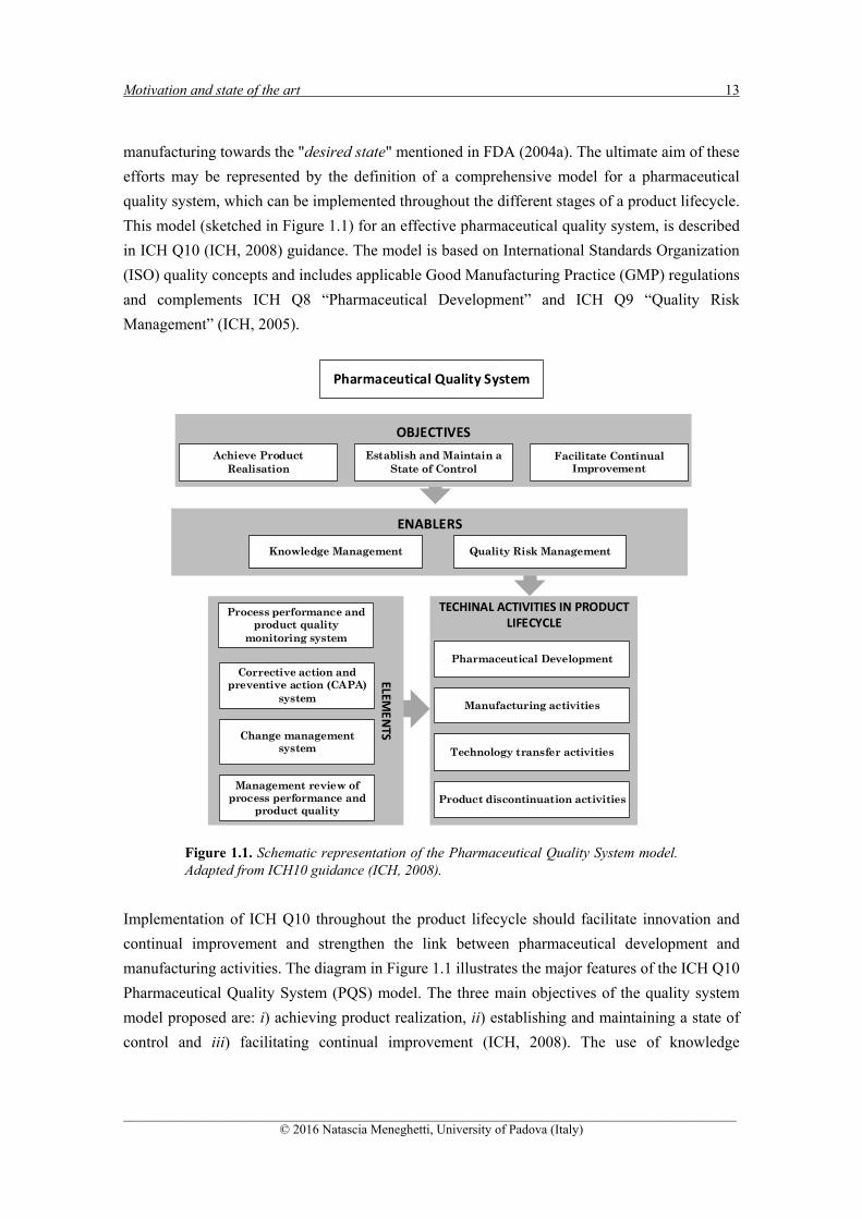
1.1.4 The pharmaceutical quality system
The efforts of the European and American regulatory Agencies in promoting the adoption of QbD
paradigms through a more efficient interaction with pharmaceutical industry, demonstrate the
clear purpose of supporting a radical renovation of the pharmaceutical development and
Motivation and state of the art 13
______________________________________________________________________________________________ © 2016 Natascia Meneghetti, University of Padova (Italy)
manufacturing towards the "desired state" mentioned in FDA (2004a). The ultimate aim of these
efforts may be represented by the definition of a comprehensive model for a pharmaceutical
quality system, which can be implemented throughout the different stages of a product lifecycle.
This model (sketched in Figure 1.1) for an effective pharmaceutical quality system, is described
in ICH Q10 (ICH, 2008) guidance. The model is based on International Standards Organization
(ISO) quality concepts and includes applicable Good Manufacturing Practice (GMP) regulations
and complements ICH Q8 “Pharmaceutical Development” and ICH Q9 “Quality Risk
Management” (ICH, 2005).
Figure 1.1. Schematic representation of the Pharmaceutical Quality System model. Adapted from ICH10 guidance (ICH, 2008).
Implementation of ICH Q10 throughout the product lifecycle should facilitate innovation and
continual improvement and strengthen the link between pharmaceutical development and
manufacturing activities. The diagram in Figure 1.1 illustrates the major features of the ICH Q10
Pharmaceutical Quality System (PQS) model. The three main objectives of the quality system
model proposed are: i) achieving product realization, ii) establishing and maintaining a state of
control and iii) facilitating continual improvement (ICH, 2008). The use of knowledge
Pharmaceutical Quality System
OBJECTIVES
Achieve Product Realisation
Facilitate Continual Improvement
Establish and Maintain a State of Control
ELEMENTS
Process performance and product quality
monitoring system
Change management system
Corrective action and preventive action (CAPA)
system
Management review of process performance and
product quality
ENABLERS
Knowledge Management
TECHINAL ACTIVITIES IN PRODUCT LIFECYCLE
Quality Risk Management
Pharmaceutical Development
Technology transfer activities
Manufacturing activities
Product discontinuation activities

14 Chapter 1
______________________________________________________________________________________________ © 2016 Natascia Meneghetti, University of Padova (Italy)
management and quality risk management facilitate the achievement of these objectives by
providing the means for science and risk based decisions related to product quality. Knowledge
management is a systematic approach to acquiring, analyzing, storing and disseminating
information related to products, manufacturing processes and components. Prior knowledge,
pharmaceutical development studies, process validation studies over the product lifecycle,
manufacturing experience and continual improvement represent some of the possible sources of
knowledge. Quality risk management is integral to an effective pharmaceutical quality system. It
can provide a proactive approach to identifying, scientifically evaluating and controlling potential
risks to quality (ICH, 2008).
The pharmaceutical quality system covers the entire lifecycle of a product, which includes the
following technical activities for new and existing products (ICH, 2008):
Pharmaceutical Development, whose goal is to design a product and its manufacturing process
to consistently deliver the intended performance, according to patients, regulatory authorities
and internal customers’ requirements;
Technology Transfer, whose goal is to transfer product and process knowledge between
development and manufacturing, and within or between manufacturing sites to achieve
product realization. This knowledge forms the basis for the manufacturing process, control
strategy, process validation approach and ongoing continual improvement;
Commercial Manufacturing, whose goals are to achieve product realization, establish and
maintain a state of control and facilitate continual improvement;
Product Discontinuation, whose goal is to manage the terminal stage of the product lifecycle
effectively.
In order to achieve the objectives of the pharmaceutical quality system, a set of elements should
be applied appropriately to each lifecycle stage. The intent is to enhance these elements in order
to promote the lifecycle approach to product quality (ICH, 2008):
Process performance and product quality monitoring system: an effective monitoring system
provides assurance of the continued capability of processes and controls to produce a product
of desired quality and to identify areas for continual improvement.
Corrective action and preventive action (CAPA) system: a system for implementing corrective
actions and preventive actions resulting from the investigation of complaints, product
rejections, non-conformances, recalls, deviations, audits, regulatory inspections and findings,
and trends from process performance and product quality monitoring. A structured approach
to the investigation process should be used with the objective of determining the root cause.
Change management system: an effective change management system should evaluate,
approve and implement changes of innovation, continual improvement, the outputs of process
performance and product quality monitoring and CAPA drive. The change management

Motivation and state of the art 15
______________________________________________________________________________________________ © 2016 Natascia Meneghetti, University of Padova (Italy)
system ensures continual improvement is undertaken in a timely and effective manner. It
should provide a high degree of assurance there are no unintended consequences of the change.
Management review of process performance and product quality: management review should
provide assurance that process performance and product quality are managed over the
lifecycle. Depending on the size and complexity of the company, management review can be
a series of reviews at various levels of management and should include a timely and effective
communication and escalation process to raise appropriate quality issues to senior levels of
management for review.
The implementation of a quality system throughout the product lifecycle, enables companies to
evaluate opportunities for innovative approaches to improve the process and product quality and
reduce the sources of variability that often cause wastes and reduce revenues.
1.1.5 Impact of QbD
“Potentially, the application of QbD paradigms should enhance development capability, speed,
manufacturing robustness, as well as the manufacturer’s ability to identify the root cause of
manufacturing failures, as well as post-approval changes and scale-up operations” (Woodcock,
2013). In 2005 IBM estimated that improving new product and process development to design
robust manufacturing processes through a QbD-based approach, could increase significantly the
total revenues a drug product brings, from the discovery to the patent expiration. Traditionally, as
reported in Figure 1.2 (solid line), after the pre-launch phase, in which investments in research
and development are needed and which usually lasts around ten years, the product is launched
and drug sales increase the revenues. Due to manufacturing process optimization usually required
after the launch of the product, there is still not revenues for a certain period (one or two years).
Afterwards, product sales start to increase, until reaching a peak usually ten years after the product
launch, and then remains stable or even decreases due to the increase of market competition. In
Figure 1.2 the dashed line shows the improvements that the adoption of the QbD-based approach
prior to the launch of new products could provide, reducing the period from launch to peak sales
by as much as five years.

16 Chapter 1
______________________________________________________________________________________________ © 2016 Natascia Meneghetti, University of Padova (Italy)
Figure 1.2. Revenue trend for a drug product during its lifetime, if a traditional (solid line) or a QbD-based approach (dashed line) were used for pharmaceutical development and manufacturing (adapted from IBM, 2005; Tomba, 2013).
A number of surveys have been performed to assess if after ten years from the introduction of the
"Pharmaceutical cGMPs for the 21st Century", the transition from an experience-based to an
innovative and modern industry has been completed, and if this transition has actually brought an
increase of revenues. After a preliminary period of assessment, QbD and quality systems are
beginning to gain ground in the pharmaceutical sector as reported by the International Society of
Pharmaceutical Engineers Process Analytical Technology Community of Practice of United
Kingdom/ Ireland (PAT COP UK/IR). The survey (Kourti and Davis, 2012), that contains the
views of 12 pharmaceutical companies including biotech companies, indicated that significant
benefits resulted from QbD-developed products, such as improved process and product
knowledge and understanding, improved product quality and robustness, improved control
strategy and increased process capability and robustness, which lead to a consistent decrease of
batch failures. Moreover, significant improvements in development efficiency and in the
formulation design, as well as significant reductions in the time required to develop a formulation
have been also reported. Finally, most of the companies highlight also how these improvements
lead to an effective cost reduction and leaner manufacturing.
Similar results were provided by the survey conducted by the Quality-by-Design and Product
Performance Focus Group of AAPS (American Association of Pharmaceutical Scientists) to
assess the state of adoption and perception of QbD. The survey (Cook et al., 2013) collected the
responses of 149 individuals from industry and academia about three main topics, regarding the
frequency of application of QbD tools, the motivators of the application of QbD, and the benefits
of the application of QbD. The results of the survey confirm that most of the companies are
actually using several tools and most QbD elements, and over two thirds of respondents from
industry have experienced the benefits of QbD regarding both the positive impact it can have on
the patient, as well as on internal processes. However, the surveyed companies, affirmed that QbD

Motivation and state of the art 17
______________________________________________________________________________________________ © 2016 Natascia Meneghetti, University of Padova (Italy)
does not lead to a better return on investment. Finally, the survey highlights that there are
contrasting views on the role of QbD in increased efficiency of the communication between
industry and regulatory authorities (that is actually the aim of the introduction of the new OPQ).
Therefore, according to the authors, the results of the survey indicate a broad adoption of QbD in
pharmaceutical environment, but that the process of gathering all experience and metrics required
for connecting and demonstrating QbD benefits to all stakeholders is still in progress (Cook et al.,
2013).
1.2 The modeling contribution in the implementation of a QbD approach
The ICH guidances highlight the importance of using mathematical models to support every stage
of pharmaceutical development and manufacturing (ICH, 2011). The same concept has been
stressed by Gernaey and Gani (2010), which presented a model-based framework to support a
systematic model-based design and analysis in pharmaceutical product and process development,
discussing also the modeling issues related to model identification, adaptation and extension.
Mathematical modeling represent a key element of Process Systems Engineering (PSE), a mature
and well-established discipline of chemical engineering (Klatt and Marquardt, 2009), whose
applications rapidly expanded also in the pharmaceutical industry. In a QbD context, PSE
provides the pharma sector with the opportunity to benefits of advanced modeling tools that have
already proved their effectiveness in other typical chemical sectors (García-Muñoz and Oksanen,
2010). Although some basic concepts described in the ICH guidances have been applied for quite
a long time by several other industries (e.g. petrochemical, polymer and energy sectors), the
challenge for PSE experts is to adapt these advanced modeling tools to the need of an industry
characterized by a great variety of products, low volumes, mainly batch manufacturing plants
with a strict regulatory environment (García-Muñoz and Oksanen, 2010).
An appropriate product and process understanding represents the minimum requirements of the
QbD approach. Hence, the mathematical formulation of the relationships between CQAs, CPPs
to product CQAs in a mathematical model can be used to support process/product development
and design, to assure quality of the products, to support analytical procedure and process
monitoring and control (ICH, 2011). Some direct outcomes of such an approach are for examples
the reduction of the time usually required for the launch of a new product in the market, the
improvement of the productivity and the reduction of the manufacturing costs. It is important to
note that process modeling is not meant to be performed as a stand-alone activity; rather, it needs
to be fully integrated with experimental strategy (García-Muñoz and Oksanen, 2010). This is
should be intended as a mutual integration, where the results of modeling guide experimentation
in order to reduce expensive experimental work, and the results of the experimentation are used
to support model validation and continual improvement.

18 Chapter 1
______________________________________________________________________________________________ © 2016 Natascia Meneghetti, University of Padova (Italy)
A model can derive from a mathematical representation of the physical laws underlying a system
(such as mass and energy balances in knowledge driven models), or from data (in data-driven
models), or from a combination of the two (in hybrid models). The selection of the type of model
to be used depend on the existing knowledge about the system, the data available and the objective
of the study (ICH, 2011). In particular, ICH guidelines emphasize the importance of the last
aspect, offering a classification of the models based on the aim of the use of the model itself.
Accordingly, models can be categorized for the purposes of regulatory submissions depending on
the model’s contribution in assuring the quality of the product, and for the purpose of
implementation, depending on the intended outcome of the model. For the purpose of regulatory
submission, models are categorized as low, medium and high impact models. Low impact models
includes those models that are typically used to support product and/or process development (e.g.,
formulation optimization), medium impact models such models can be useful in assuring quality
of the product but are not the sole indicators of product quality (e.g., most design space models,
many in-process controls) and finally high impact model as those models whose prediction model
is a significant indicator of quality of the product (e.g., a chemometric model for product assay, a
surrogate model for dissolution). For the purpose of implementation, models can also be
categorized on the basis of the intended outcome of the model (i.e., models to support process
design, analytical procedures, process monitoring and control), but within each of these
categories, models can be further classified, as low, medium or high, on the basis of their impact
in assuring product quality (ICH, 2011).
Another important aspect that cannot be separated from model development, is model validation
and verification. Model validation is an essential part of model development and implementation,
and once a model is developed and implemented, verification should be performed throughout
the lifecycle of the product (ICH, 2011). For model validation and verification, the ICH guidelines
suggest to set acceptance criteria for the model relevant to the purpose of the model and to its
expected performance, then to compare the accuracy of calibration and the accuracy of prediction,
and to validate the model using external datasets. In the case of well-established first principles-
driven models, prior knowledge can be leveraged to support model validation and verification, if
applicable. The prediction accuracy of the model should be verified by parallel testing with the
reference method during the initial stage of model implementation and can be repeated throughout
the lifecycle (ICH, 2011).
Aside from the kind of model used, the increasing of interest of the PSE community to the
pharmaceutical industry applications, demonstrates that this sector is actually undertaking a path
of modernization. The use of PSE tools is increasing in process monitoring, quality control and
process modeling as confirmed by the results reported by Troup and Georgakis (2012) regarding
an industrial survey performed on this topic. For example, with respect to process monitoring,
the survey results demonstrated an increasing trend in the use of multivariate statistical process
control charting and of process monitoring software packages, most of which are based on the

Motivation and state of the art 19
______________________________________________________________________________________________ © 2016 Natascia Meneghetti, University of Padova (Italy)
use of chemometric models. In fact, these statistical multivariate tools are used by the 67% of the
responding companies to analyze historical process and plant data. Regarding the use of process
modeling, all of the companies surveyed indicated that response surface models ware routinely
develop for unit operations, but when possible, fundamental models are preferred, especially in
primary manufacturing. In secondary manufacturing, the use of first-principles models is more
limited by the complexity of the mechanisms involved, forcing the employment of empirical
models. As a consequence, a part from specific exceptions, the use of empirical models is broadly
expanding (one third of the companies developed empirical models for 80-100% of the unit
operations). Finally, process modeling is widely employed in the determination of a multivariate
design space. More than two third of the companies surveyed report the use of design space
strategies to identify a robust area of operation with respect to all major disturbances to the process
(Troup and Georgakis, 2012). In summary, PSE tools are demonstrating their potential in
supporting a radical change in pharmaceutical development and manufacturing approach. A new
way of thinking is now developing, according to which “pharmaceutical ingredients,
pharmaceutical products, the related manufacturing processes, and the biopharmaceutical
properties are considered simultaneously and quantitatively” (Rantanen and Khinast, 2015).
An overview of the challenges associated with modeling common pharmaceutical processes,
providing also a discussion of the recent developments in pharmaceutical process modeling, has
been recently provided by Rogers and Ierapetritou (2015).
In Figure 1.3 a summary of the main contributions of knowledge-driven and data-driven models
in the implementation of the elements that characterize the QbD approach (Section 1.1.1) is
reported. A brief overview of these contributions is provided in the following, highlighting the
advantages and drawbacks of the two modeling approaches and the efforts required in the future.
Figure 1.3. Summary of the contribution of knowledge-driven and data-driven model to the elements that characterize a QBD approach.
Definition of QTPP to identify CQAs
Product design and understanding and identification of CMAs
Process design and understanding (identification of CPPs and linking CMAs
and CPPs to CQAs)
Definition of a control strategy
Monitoring of process capability and continual improvement
DoE, RSM, pattern recogniction, LVM, LVM inversion
First‐principles models, hybrid models
improving process understanding
supporting QRM (identification of CMAs, CPPs and their relations with CQAs)
supporting product and process design
supporting scale‐up or transfer a process from one equipment to another
supporting the design of new products and processes
improving process understanding
optimizing, scaling‐up or transferring a process from one equipment to another
providing quantitative measures in the context of QRM by performing sensitivity studies (identification of CPPS, CMAs)
replacing experiments for process characterization
studying the effect of process disturbances or of start‐up and shut‐down phases
supporting control systems (e.g., for model‐predictive control)
process monitoring and control (MSPC, LVM feedback/feedforward controllers, LVM predictive control)
20 Chapter 1
______________________________________________________________________________________________ © 2016 Natascia Meneghetti, University of Padova (Italy)
1.2.1 Knowledge-driven models
Knowledge-driven (KD) models, also called mechanistic (or first-principles, or fundamental
models) describe the underlying functional mechanisms of the system under investigation,
relaying on the use of fundamental knowledge typically in terms of mass, energy and momentum
balances and of constitutive equations. Stated differently, KD models are a convenient
representation of the available knowledge of a system. Under an industrial perspective, since first-
principle models offer increased process understanding, enable a more flexibility in the
incorporation of product physical properties, are often applicable for multiple products and allow
extrapolation (under certain assumptions), these models are usually preferred to empirical models
(Troup and Georgakis, 2010). Therefore, in the last years, the mechanistic modeling of
pharmaceutical unit operations has made significant progress, thanks to the ability of these model
to: i) improve the fundamental scientific understanding of a process, ii) optimize process scale-
up and monitoring, iii) provide quantitative measures in the context of quality risk management,
iv) replace experiments during a process characterization phase, v) study the effect of process
disturbance or start-up and shut-down phases on the process performance (Rantanen and Khinast,
2015). However, it cannot be ignored that the time and efforts required to develop these type of
models is often excessive for market requirements, especially in pharmaceutical environment,
characterized by a production rates not comparable to that one of bulk chemical; moreover, the
model assumptions are often not consistent with full scale process operating conditions (Troup
and Georgakis, 2010).
Depending on the characteristics of physical phenomena underling a process, mechanistic models
may lay on a systems of ordinary differential equations (ODEs), differential algebraic equations
(DAEs) and partial differential equations (PDEs). In particular, the applications of PDEs models
have rapidly expanded, due to the necessity of describing complex multi-phase dynamic systems,
such as crystallization, drying and granulation processes. In this context, PDEs models are used
in in the form of population balance models (PBM), to describe particle-size or crystal-size
distributions, or computational fluid dynamics (CFD) to simulate fluidic systems, including
multiphase flows (detailed reviews on the use the use of CFD for pharmaceutical unit operations,
are provided by Kremer and Hancock, 2006 and by Wassgren and Curtis, 2006). CFD models
may also be combined with different specific models to describe for example chemical reactions
(e.g. Kashid et al., 2007), or with PBM models to model the change of distributed properties as a
function of spatial coordinates within a unit operation (Woo et al., 2009). Finally, the complex
description of granular flows for example in powder blending, granulation, roller compaction, or
tableting, may be assisted by the mechanistic simulation of particulate flows, using for example
the discrete element method (DEM, Ketterhagen et al. (2009) reviewed a series of applications
of these techniques in common pharmaceutical processes).

Motivation and state of the art 21
______________________________________________________________________________________________ © 2016 Natascia Meneghetti, University of Padova (Italy)
The availability of detailed model is essential to provide a deep understanding of the process and
the assurance of the results obtained using the model for decision-making purposes. Anyway,
when the implementation of a detailed mechanistic model is much computationally expensive (to
be used for example to real-time applications), reduced order model represent an appropriate
solution in order to reduce simulation times for CFD and PBM models (Gernaey et al., 2012).
A second alternative that provides a compromise when full mechanistic models are not available,
is the use of hybrid models, that rely on the combination of a mechanistic model with a data-
driven model component. Often, in the interest of time, a hybrid approach will be preferred, where
the mechanistic part of the model is gradually extended when more process knowledge becomes
available, e.g. during process development (Gernaey et al., 2012).
For an extensive overview of the applications in the pharmaceutical industry of the above-
mentioned categories of mechanistic, reduced-order and hybrid models, the reader is encouraged
to refer to Gernaey et al. (2012) and Rantanen and Khinast (2015).
1.2.2 Data-driven models
Data-driven (DD) also called data-based (DB) or empirical models, do not require any prior
knowledge of the physical mechanisms underlying a process, since the information useful to
define mathematical relationships between its inputs and outputs is directly extracted by the
analysis of the process data recorded. In a way, DD models are nothing more than a convenient
representation of the available data. The empirical model category is very broad, including for
example latent variable models (LVMs), statistical design of experiments (DoE) and response
surface models (RSM), and pattern recognition techniques. The application of empirical models
as PAT tools on pharmaceutical industry is rapidly growing, as reported by a recent survey
according to which for most of the companies surveyed, more than one half of their unit operations
are modelled empirically (Troup and Georgakis, 2013). Many aspects contribute to the success of
DD models, such as the availability of an ever-increasing set of off-line and on-line process
measurements and the possibility of providing a multivariate description of the systems with a
significant time and effort saving with respect to mechanistic models. In this context,
chemometric models have generated particular interest, demonstrating their ability in improving
product and process knowledge especially in PAT applications (e.g. spectroscopy and image
analysis). The use of multivariate data analysis methods like principal component analysis (PCA;
Jackson, 1991), partial least-squares regression (PLS; Wold, 1983; Höskuldsson, 1988), statistical
design of experiments (DoE; Montgomery, 2005) and pattern recognition techniques (Bishop,
2006; Duda et al., 2001) has rapidly extended after the PAT initiative. Many reviews are available
on the use chemometric methods coupled with advanced characterization techniques, as for
example the work of Roggo et al. (2007), which focuses on chemometric techniques and
pharmaceutical NIRS applications, or the more extensive reviews provided by Rajalahti and
22 Chapter 1
______________________________________________________________________________________________ © 2016 Natascia Meneghetti, University of Padova (Italy)
Kvalheim (2011) and Pomerantsev and Rodionova (2012) that consider not only NIR
applications, but also applications of as infrared (IR), Raman spectroscopy, hyperspectral and
digital imaging, and other tools as X-ray diffraction, chromatography or mass spectroscopy (MS).
In particular, pattern recognition techniques are largely used coupled with analytical tools for
qualitative analysis (e.g. Realpe and Velasquez, 2006), in order to control for example the product
quality (color, surface characteristics, shape, particle size, etc.). However, in this Dissertation, an
alternative use of these techniques will be provided in Chapter 6.
Similarly to mechanistic models, empirical model are also asked to describe not only the
multivariate aspects of the relationships between CMAs, CPPs and CQAs, but also the non-linear
and dynamic behavior that usually characterize the system. This is often achieved by the
development of nonlinear DD such as quadratic response surface models (RSMs) usually related
to design of experiments (DoE) methodologies (Montgomery, 2005; Box and Draper, 2007).
Statistical design of experiments has been largely employed in pharmaceutical process and
product development, especially for formulation design and product optimization, as highlighted
by Gabrielsson et al. (2002) who reviewed several applications of DoE and multivariate analysis
in pharmaceutical applications. There are also several applications about the use of DoE to explore
the knowledge space and identify the regions within which parameter values are demonstrated to
ensure the desired product CQAs, in order to support the definition of the design space (e.g., am
Ende et al., 2007; Burt et al. 2011; Kapsi et al. 2012; Zacour et al., 2012a). Moreover, appropriate
DoE permit the definition of reliable RSM models, that can be consider even higher than quadratic
nonlinearities (including cubic, quartic, or higher terms). However, since the number of
experiments increases very rapidly as the number of input variables or factors increases, the
number of experiments that need to be performed to accurate estimate high nonlinearities is
usually prohibitive. An alternative method to account for nonlinearities, is represented by the
neural network models. However, although these models can describe even higher nonlinearities
compared to RSM models, they require a similar large number of experiments and their
predictions usually lack of transparency. Examples of the use of such data-driven models for the
mapping of the design space of pharmaceutical processes, are provided by Boukouvala et al.,
(2010), which proposed three approaches based on different data-driven modeling techniques,
using the ideas of process operability and flexibility under uncertainty.
While DoE and relating methods usually required large amount of new experiments, LVMs
techniques are conceived to exploit and analyze the large amount of research and product data
that usually derived from on-going manufacturing processes, experimental campaigns, data
historians from different process units. The information extracted from these data can be useful
not only to increase product and process understanding, but also to guide the development of new
product and process or to support control strategies in manufacturing activities.

Motivation and state of the art 23
______________________________________________________________________________________________ © 2016 Natascia Meneghetti, University of Padova (Italy)
1.2.2.1 Latent variable modeling in QbD
LVMs are multivariate statistical models that, by analyzing large amounts of data, permits one to
describe a system by using a reduced number of variables (called latent variables, LVs), obtained
by a linear combination of the original (usually correlated) measurements.
The physical meaning of these new set of variables, is actually related to the forces driving the
system and should be sought in the correlation existing between the original variables. Figure 1.3
reports a geometrical interpretation of the operation performed when a LVM is built on a dataset
X [20×3], where 20 is the number of available samples and 3 is the number of measured variables
(x1, x2, x3) for the collected samples.
Figure 1.3. Geometrical interpretation of an LVM (adapted from Tomba, 2013).
As can be seen, the LVM transforms the three-dimensional space of the original variables into a
two-dimensional space (called the latent space) defined by the two latent variables (LV1, LV2)
whose directions correspond to the directions along which the variability of the data is higher.
The projections of the original variables onto the latent space that describe the original space, are
called scores and become the new variables defining the state of the system.
LVMs can be used also to relate data from different datasets (Burnham et al., 1996) using latent
variable regression models (LVRMs). These models have been largely exploited coupled with
analytical instruments to relate highly correlated input variables to response variables as product
quality (examples of applications of LVMs on this topic, both in pharmaceutical and food industry
can be found in Ottavian, 2013).
Besides LVMs application as predictive tools, their potential has been exploited also for different
purposes. For example, given the statistical nature of LVMs, they can be employed for
multivariate statistical process control (MSPC) in online process monitoring. This is a well-
known and long-applied use of LVMs in several industrial sectors (Kourti, 2005). However,
control systems based on the use of LVMs are usually not limited to process control (Flores-
Cerrillo and MacGregor, 2004), process monitoring (MacGregor and Kourti, 1995) and
eventually to the implementation of corrective actions, but are also used for the purpose of fault
diagnosis (Wise and Gallagher, 1996; Birol et al., 2002; García-Muñoz et al., 2009). Moreover,

24 Chapter 1
______________________________________________________________________________________________ © 2016 Natascia Meneghetti, University of Padova (Italy)
LVMs are used for process understanding and troubleshooting (García-Muñoz et al., 2003), for
process operating conditions design (Jaeckle and MacGregor, 1998), process scale-up (García-
Muñoz et al., 2005) and also for product design (Muteki et al., 2006) and optimization (Yacoub
and MacGregor, 2004). A detailed review of pharmaceutical applications in these areas have been
provided by Tomba et al. (2013a). For the purposes of this Disseration, only a summary of the
main applications of LVM techniques will be provided in the following, in particular in relation
the use of LVMs to support the definition of the design space. To this end, LVMs can be used to
support pharmaceutical development activities in the selection of the materials to be included in
a formulation or of the optimal operating conditions at which a process should operate. According
to Tomba et al., (2013a), LVMs have found different applications to support the establishment of
a design space:
LVMs are coupled with DoE techniques to facilitate the choice of the parameters to include in
a DoE analysis or to disclose the relationships between the input and output variables of a
process. Moreover, these techniques are also ised to study the relationships between variables
manipulated in a DoE plan and those which are only measured. Thanks to the use of LVMs,
the information extracted by the analysis of the different kind of data (for example data
measured on-line or spectra), usually highly correlated, was introduced in the analysis of the
design space. Examples of these applications can be found in Huang et al. (2009), Streefland
et al. (2009), Zacour et al. (2012b), Thirunahari et al. (2011) and Lourenço¸ et al. (2012).
Moreover, starting from the concept that the design space in raw materials and in process
parameters must be developed jointly, as changes in either one would affect the other,
MacGregor and Bruwer (2008) proposed a framework for the development of design and
control spaces or pharmaceutical operations. On the same topic, Souihi et al. (2013) proposed
an application in which of DoE techniques combined with LVMs to identify the design space
for a roller compaction process.
LVMs are directly used to assist the identification of the design space through model inversion
(Jaeckle and MacGregor, 1998 and 2000), by analyzing the data available from historical
experiments and especially from already developed products. Used in this direct form, latent
variable regression models (LVRM) are used to relate raw material CQAs, CPPs, which
represent the inputs variables, to the product CQAs, which represent the response variables,
using the historical available data of the process. In this case a product property can be
estimated starting from a set of inputs (material properties and process parameters). Otherwise,
in the inverse use of a LVRM, the raw materials properties/fractions and process parameters
suitable to obtain the desired product properties are predicted starting from the desired product
properties themselves, to support product or process design. However, as proposed by Kourti
(2006) and demonstrated by García- Muñoz et al. (2010), an LVRM can be used to guide the
experimentation in developmental studies or for the definition of the process design space in
the LVM space. A general framework to perform LVRM inversion has been proposed by

Motivation and state of the art 25
______________________________________________________________________________________________ © 2016 Natascia Meneghetti, University of Padova (Italy)
Tomba et al. (2012), which consider different possible solutions to the inversion problem,
depending on the design problem objectives and constraints. In the same work, it has been
highlighted the analogy between the concepts of design space and of null space (Jaeckle and
MacGregor, 1998). The null space, which arises from the LVM inversion under certain
conditions, represents the space of the input variables that, according to the LVRM, correspond
to the same sets of output variables. For this reason, according to the authors, the null space
calculated from an LVRM inversion can be used as a starting point for the establishment of
the design space of a process. Anyway, further research is needed to show how to use LVMs
in the systematic identification of the design space of a process, especially focusing on a
practical definition of design space limits (e.g., in the latent space of the model) usable not
only to regulatory purposes but also to support ordinary manufacturing activities (Tomba,
2013a).
Many applications on the use of DoE and LVMs for process and product design purposes are
reported in Tomba et al., (2013a), whereas an overview of the application of process modeling to
determination of design space for pharmaceutical manufacturing processes has been recently
provided by Rogers and Ierapetritou (2016).
1.2.3 Continuous improvement and knowledge management tools
The knowledge available for a process continually grows throughout the product lifecycle.
Experiments conducted during product and process development and manufacturing, represent
the basement of this knowledge (FDA, 2004b), but can also provide information to support the
development of a knowledge system involving the overall production system. According to the
pharmaceutical quality system model, monitoring data and information are essential to achieving
problem resolution or problem prevention. In this context, multivariate tools can be used to review
periodically historical data as more knowledge is acquired during process/product development
and manufacturing, in order to assess possible changes in the relations between CMQ, CPPs and
CQAs. An example on how LVMs can be used as part of a continuous quality verification
approach for a new drug product is provided by Zomer et al., 2010.
In general, due to the complexity of the problems to be addressed in pharmaceutical product-
process design, an efficient and systematic knowledge base coupled with an inference system is
essential (Gernaey et al., 2012). An example of the efforts performed to address this issue is
represented by OntoCAPE, an overview of a general ontology for structuring knowledge in the
chemical process engineering field (Morbach et al., 2007 and 2010). Moreover, Singh et al.,
(2010) described an ontology for knowledge representation and management, with the purpose of
facilitating the selection of proper monitoring and analysis tools for a given application or process
and permitting the identification of potential applications for a given monitoring technique or
tool. An ontological information-centric infrastructure to support product and process

26 Chapter 1
______________________________________________________________________________________________ © 2016 Natascia Meneghetti, University of Padova (Italy)
development in the pharmaceutical manufacturing domain was developed by
Venkatasubramanian et al. (2006). Turning data into knowledge and managing that knowledge
will remain one of the major challenges for the future (Gernaey et al., 2012). In fact, storage of
historical data is usually managed by well established software product from an external supplier.
However, the lack of appropriate tools to extract from these data the necessary process
knowledge, for example in order to improve the performance of a process, is the actual bottleneck,
and should be one of the focus points of future research.
1.3 Objectives of the research
In the last decade the number of studies on the application of modeling in pharmaceutical
development and manufacturing has increased considerably, however, as acknowledged by
several authors, there are still many open issues. The main objective of the research presented in
this Dissertation is to demonstrate how LVMs and pattern recognition tools can be used to address
some common issues that often affect the practical implementation of QbD paradigms in
pharmaceutical development and manufacturing. The Dissertation presents novel and general
methodologies based on the use of latent variable models and pattern recognition tools that can
be employed to support the improvement of first-principles models, the identification of the
design space, and the review of large manufacturing databases. The applications of the procedures
proposed in this Dissertation and the innovative contributions they provide are summarized in the
following.
Supporting first-principles model diagnosis. The availability of a reliable first-principles
model is often desirable to support process and product development and in the
implementation of robust control strategy. However, the effort required to develop reliable
models or to adapt the existing ones, represents the main hurdle to an extensive employment
of these models. An FP model is constituted by equations and parameters. The appropriate set
of equations represents the available knowledge on the underlying mechanisms driving the
system. The values assigned to the parameters allow one to tune the general mechanism,
described by the set of equations, to the actual physical/chemical system under investigation.
When the FP model results do not match the available experimental data to a desired accuracy,
a process/model mismatch (PMM) exists, that can be structural or parametric (or both).
Tailored experiments can be designed to improve the model performance. Typically, model-
based design of experiment (MBDoE) techniques or sensitivity studies can be used to this
purpose, allowing either model discrimination among alternative set of equations, or parameter
identification from a given set of equations. However, these solutions may be very demanding
especially if the physical/chemical mechanisms driving the system are not known completely,
since uncertainty may exist both on the model equations and on the model parameters. In this
Motivation and state of the art 27
______________________________________________________________________________________________ © 2016 Natascia Meneghetti, University of Padova (Italy)
Dissertation, a methodology based on the use of LVMs is proposed to pinpoint which term of
the model is the most responsible for an observed PMM, both for steady-state and dynamic
systems. The purpose is to analyze the reason of the poor performance of a FP model using
only the available historical data, thus minimizing the overall experimental efforts usually
needed to improve the FP model.
Supporting design space identification. A key element of the Quality-by-Design initiative
set forth by the pharmaceutical regulatory Agencies is the determination of the design space
(DS) for a new pharmaceutical product. When the determination of the DS cannot be assisted
by the use of a first-principles model, one must heavily rely on experiments. In many cases,
the DS is found using experiments carried out within a domain of input combinations (e.g. raw
materials properties and process operating conditions) that result from similar products already
developed. This input domain is the knowledge space and the related experimentation can be
very demanding, especially if the number of inputs is large. The objective is therefore to limit
the extension of the domain over which the experiments are carried out hence, to reduce the
experimental effort. To this purpose a methodology is presented to segment the knowledge
space in such a way as to identify a subspace of it (called the experiment space) that most
likely brackets the DS.
Supporting periodic review of historical datasets. Thanks to the availability of fast, cheap
and reliable on-line measurement devices, the use of advanced technologies to monitor and
control pharmaceutical manufacturing processes has rapidly expanded. Large historical
datasets spanning several years of manufacturing are usually available in the pharmaceutical
industry. These datasets easily reach several millions of data entries. However, this data
overload often hinders the possibility to effectively use of the information embedded in the
data. Transforming data into knowledge may result particularly burdensome, considering that
not even the number of the batches completed in a given time window is known a priori. In
fact, data historians are usually recorded in a “passive” way, i.e. including in the same dataset
data segments that possibly refer to temporary stalls of the equipment or to cleaning and
maintenance operations. In this Dissertation, a methodology is proposed to systematically
review large data historians of secondary pharmaceutical manufacturing systems in order to
extract operation-relevant information, such as the number of batches carried out in a given
time window, how many different products have been manufactured, and whether or not the
features characterizing a batch have changed throughout a production campaign. The
methodology proposed represent a valid PAT tool that can be coupled to existing data
acquisition system to extract the information necessary to support the implementation of
continual improvement paradigms.

28 Chapter 1
______________________________________________________________________________________________ © 2016 Natascia Meneghetti, University of Padova (Italy)
The effectiveness of the general procedures proposed in this Dissertation is demonstrated by
applying each of them to experimental (industrial scale) or simulated case studies. The next
section presents a roadmap to the Dissertation.
1.4 Dissertation roadmap
In this Dissertation, data-driven modeling techniques are used to provide general solutions to
support first-principles models enhancement, design space identification, and periodic review of
historical datasets. A discussion of the recent evolution the pharmaceutical industry and of the
use of process modeling in this sector has been provided in this Chapter, along with the main
objectives of this Dissertation. The description of the data-driven modeling used in this
Dissertation (namely LVMs and pattern recognitions techniques) is reported in Chapter 2.
Figure 1.4. Sketch of the research topics considered in this Dissertation.
General methodologies based on the use of DD models are developed for each of the three areas
analyzed. The pplications of these methodologies are presented in the following according to the
sketch of Figure 1.4.
With respect to first-principles models diagnosis, in Chapter 3 and 4 a methodology is presented
to diagnose the possible cause of a process/model mismatch, with the objective of reducing the
experimental efforts usually needed to improve a first-principles model. The methodology relies
on the use of the information extracted by means of latent variable models from the available data
(namely, the historical process measurements and the first-principles model outputs). This
information, coupled with engineering judgment, permits one to identify which sections of the
IMPLEMENTING QbD IN PHARMACEUTICAL INDUSTRY: A DATA-DRIVEN APPROACH
First-principles model diagnosis
Design space identification
Periodic review of data
historians
Steady-state systems(Chapter 3)
Dynamic systems(Chapter 4)
Experiment space identification
(Chapter 5)
Database analysis of batch
processes(Chapter 6)

Motivation and state of the art 29
______________________________________________________________________________________________ © 2016 Natascia Meneghetti, University of Padova (Italy)
first-principles model mostly contribute to an observed process-model mismatch. In Chapter 3
two simulated steady-state systems are considered as test beds: a continuous jacketed stirred-tank
reactor and a milling unit. In Chapter 4, the methodology is adapted to cope with dynamic
systems. Two simulated case studies are considered: a dryer process and a penicillin fermentation
process. Although the proposed methodology is developed to deal with pharmaceutical process
models, it can be easily extended to any steady-state or dynamic model.
Chapter 5 focuses on the problems related to the identification of the design space (DS) for a new
pharmaceutical product characterized by a single quality specification. A methodology is
proposed to reduce the experiments needed to define the DS by exploiting the historical data of
products similar to the new one (‘‘knowledge space’’). Through the inversion of the PLS model
used to describe the system, a reduced area of the knowledge space wherein the design space is
supposed to lie is identified (also accounting for model prediction uncertainty). Three case studies
are presented to demonstrate the effectiveness of the proposed methodology.
Finally, Chapter 6 addresses the problem of the periodic review of large data historians to extract
useful information for the implementation of continual improvement paradigms. A methodology
based on the use of pattern recognition techniques (namely k-nearest neighbor and PCA models)
is presented that allows analyzing large historical datasets of secondary manufacturing batch
units. The effectiveness of the methodology in automatically isolating and analyzing meaningful
data segments is shown for two large industrial datasets. The proposed approach permits one to
monitor the evolution of the manufacturing campaigns over time and to detect possible exceptions
in the manufacturing procedures.
In a concluding section, the summary of the main achievements is provided for each of the three
areas analyzed along with the discussion of future investigations that may be carried out to
improve the methodologies proposed in this Dissertation.


______________________________________________________________________________________________ © 2016 Natascia Meneghetti, University of Padova (Italy)
Chapter 2
Multivariate modeling background
This Chapter provides a general overview of the statistical and mathematical techniques applied
in this Dissertation. First, a background on latent variable models (in particular principal
component analysis and partial least-squares regression) is presented, focusing both on the
algorithmic point of view and the practical one. Furthermore, the concepts of latent variable model
inversion are introduced, and the fundamentals for their determination are provided, along with a
brief introduction of the use of pattern recognition techniques for classification and clustering
purposes.
The applications of the techniques described in this Chapter, have been performed in Matlab®
(the MathWorks Inc., Natick, MA) using an in-house developed multivariate analysis toolbox (in
Chapter 5, Facco et al., 2015) and the PLS_Toolbox (Eigenvector Research, Inc., Wenatchee,
WA, USA, 2015).
2.1 Latent variable modeling approaches
Latent variable models (LVMs) are statistical models that have been conceived to analyze large
amounts of (usually correlated) data. The underlying concept of LVMs is that real data can be
expressed as a liner combination of factors (called latent variables, LVs) that describe the major
trend of the data and that can be interpreted based on the knowledge of the physical and chemical
phenomena involved in the system. Hence, the theoretical foundation for the modeling of
measured variables by means of latent variables (LV) is based on two principles (Eriksson et al.,
2006): i) the measurements, by definition, are sums of the underlying latent variables; ii) a set of
measurements X [N×I] generated by a function F (U,V), where each row u of X describes the
change between observations and each column v describes the change between variables, can be
transformed by the Taylor expansions of F in u direction, (after discretizing for n = observation
and i = variable) in an LV model. The smaller the interval of u that is modelled, the fewer terms
are needed in the Taylor expansion, and the fewer components are needed in the LV model. Under
a practical point of view, the latent directions found by a LVM, represent the driving forces acting
on the system and responsible for the variability of the data. Hence, LVMs are not only used for
data compression, but also for data interpretation, assuming that essential information can be
32 Chapter 2
______________________________________________________________________________________________ © 2016 Natascia Meneghetti, University of Padova (Italy)
extracted by analyzing how the variables co-vary, namely how they change with respect to one
another.
In general, data can be categorized, depending on the nature of the variables, as factors and
responses (Eriksson et al., 2006). The factors (also called predictors, parameters, regressors) are
variables whose different levels might exert an influence on the system or on the process. These
variables can be organized into a matrix X [I×N] in which the N variables have been observed
per I samples (or observations). The responses are variables which are measured to capture the
performance of the system and can be organized in a matrix Y [I × M] of M variables observed
per I samples. In the analysis of the factors matrix, the objective of a LVM analysis is to explain
the correlation structure of the N variables, in order to understand the relationships among them.
Principal component analysis (PCA; Jackson, 1991) is one of the most useful techniques to this
purpose. Alternatively, projection to latent structures (PLS, also called partial least-squares
regression; Höskuldsson, 1988) is used in the combined analysis of the regressors and responses
matrix to explain the cross-correlation structure of the variables in X and in Y, in order to study
and quantify the relationships between regressors and response variables. Basic theory about PCA
and PLS is reported in the following, largely based on the Dissertations of Tomba (2013) and
Ottavian (2014).
2.1.1 Principal component analysis
Principal component analysis (PCA; Jackson, 1991) is a multivariate statistical method that
summarizes the information embedded in a dataset X [I×N] of I samples and N correlated
variables (for example data on critical process parameters, initial conditions, process settings,
critical quality attributes), by projecting the data through a linear transformation onto a new
coordinate system of orthogonal (i.e., independent) principal components (PCs), which optimally
capture the correlation between the variables, identifying the direction of maximum variability of
the original data.
Principal component analysis permits to represent a dataset X as the sum of the R scores-loadings
vectors outer products:
R
aaa
1
TptX , (2.1)
where: R = rank(X), pa is the loading vector for PC a and contains information on how variables
are related, ta is called score vector for PC a and contains information on how samples are related
to each other and (T) indicates the transpose operator. The computation of the model scores and
loadings can be performed by solving the optimization problem (Burnham et al., 1996) in
Eq. (2.2). For one PC ( pp 1 ):

Multivariate modeling background 33
______________________________________________________________________________________________ © 2016 Natascia Meneghetti, University of Padova (Italy)
1 subject to
max
T
TT
pp
XpXpp
. (2.2)
Vector p represents the latent direction of maximum variance in the data, where the original data
can be projected, by obtaining the vector t of the coordinates into the PC space:
Xpt . (2.3)
As a consequence, the problem in (2.2) can be reformulated as in (2.4), representing the
maximization of the score vector length (Burnham et al., 1996):
1
..
max
T
T
pp
Xpt
ttp
ts . (2.4)
The analytical solution of this problem is readily obtained from its optimality conditions (López-
Negrete de la Fuente et al., 2010) and is represented by the following eigenvalue problem:
pXpXpX T)cov( , (2.5)
where p is the eigenvector corresponding to the eigenvalue λ of the covariance matrix of X. Eq.
(2.5) facilitates the geometrical interpretation of the optimization problem (2.2) whose aim is to
maximize the variance captured by λ, which represents the variance explained by the product tpT.
The eigenvector problem (2.5) can be used to determine the N loadings pn of the PCA model,
which correspond to the N orthonormal eigenvectors of the covariance matrix of X. As a
consequence the resulting score vectors are orthogonal and they have a length equal to the
eigenvalue λ associated to the n-th PC:
Nn
Nrnrn
nnnnn
rnrn
1,...with
1,..., with for 0TTT
TTT
ttXpXp
tXXtpp
. (2.6)
As a result of the eigenvector problem† (2.4), the PCs are ordered in Eq. (2.1) according to the
variance of the original dataset X that they capture. Usually, few principal components A are
sufficient (i.e., A << R) to adequately describe X because correlated variables identify a common
† Note that the solution of the eigenvector problem Eq. (2.5) results in the first PCA loading p. In order to evaluate the remaining components, matrix X has to be deflated.

34 Chapter 2
______________________________________________________________________________________________ © 2016 Natascia Meneghetti, University of Padova (Italy)
direction of variability that can be described by a single PC. Hence, assuming that only the first
A PCs are retained to represent X, Eq. (2.1) can be rewritten as:
EXETPptptX
ˆT
1
T
1
TR
Aaaa
A
aaa
, (2.7)
where T = [t1, t2, …, tA] is the score matrix, P = [p1, p2, …, pA] is the loading matrix, E is the
[IR] matrix of the residuals generated by the (R – A) discarded PCs of the PCA model when X
is reconstructed (i.e., approximated) by using only the first A PCs (i.e., Tˆ TPX ).
In general, using models the data are separated into two parts; the systematic part explained by
the model, and the noise (or inherent variability) that usually characterizes the measurements
(Eriksson et al., 2006). If the correct number of PCs are selected, X should comprehend all the
systematic part of the data, whereas the noise (and eventually the remaining un-modeled part of
the data) is discarded in E. Anyway, if data present strong non-linear characteristics the un-
modeled variability of the data may include a part of systematic information that the PCA, which
is basically a linear model, is not able to describe. Possible solution to this problem rely on
appropriate data pretreatment (Section 2.1.1.1) and on the use of modified PCA algorithms
(among others, NN-PCA, Dong and McAvoy, 1996; KPCA, Schölkopf et al., 1998; Mika et al.,
1999).
A simplified graphical representation of the geometrical interpretation of the PCA model is
provided in Figure 2.1. A dataset X of 7 samples and 2 variables (x1, x2) is considered. When a
PCA model is applied, the direction of maximum variability of the data is identified by PC1,
which represents the trend of the data in the (bidimensional) space of the original variables. This
is an example of the ability of each single PC to capture the variability of all the variables which
are correlated along that direction. This permit to describe the original dataset X by a lower
number of variables, by projecting the data in X from the original variable space to the low -
dimensional latent space of the PCs.
Under a geometrical point of view, the model loadings p1,1 and p1,2 represent the director cosines
of x1 and x2 respectively, on PC1, namely the cosines of the angles between the latent direction of
the model and the axes of the original variable space (gray area in Figure 2.1). Each score t1,n
represents the coordinate of the n-th sample of matrix X in the new model space, represented by
PC1. The distance of sample no. 1 to PC1, denoted by a dashed line perpendicular to the line
indicating the first PC direction, represents the residual e1,1, namely the information not captured
by the model for this sample. However, if a second principal component (PC2) was considered
(dashed gray line in Figure 2.1, orthogonal to PC1), it would account for the orthogonal distance
of each projection from the PC1 direction, capturing a very limited variability of the data
compared to PC1. Actually, in this case, a single PC is sufficient to adequately describe X.

Multivariate modeling background 35
______________________________________________________________________________________________ © 2016 Natascia Meneghetti, University of Padova (Italy)
Figure 2.1. Geometrical interpretation of the PCA scores and loadings for a dataset X [7×2]) (adapted from Tomba, 2013).
The ability of representing a system with a reduced number of latent variables compared to the
number of the original variables, is only a part of the advantages of the use of a PCA model. In
fact, the graphical representation of the PCA model parameters (scores and loadings) is often used
to gain understanding on the correlations among samples (through the scores) and variables
(through the loadings). Additional details on the interpretation of scores and loadings plots are
provided in Appendix A. For the computation of the model scores and loadings, the singular value
decomposition‡ (SVD; Meyer, 2000) of the covariance matrix of X (XTX) or the nonlinear
iterative partial least-squares algorithm (NIPALS; Wold, 1966) can be used.
2.1.1.1 Data pretreatment
Before building a PCA model, the data analyzed are usually pretreated. The appropriate
pretreatment of X depends on the characteristics of the data and on the objectives of the analysis,
and it may include filtering, denoising, transformations (e.g., logarithmic ones), advanced scaling
and data compression (Eriksson et al., 2006).
Usually, the datasets analyzed with LVMs (as process datasets), collects many variables of
different type and physical meaning. To correctly analyzed their structure by a PCA model, it is
important that variables are weighted in a similar way. The most common data pretreatment is
autoscaling, i.e. mean-centering the data and scaling them to unit variance (Wise et al., 2006).
Mean-centering (i.e., subtracting to each column xn of X its mean values) avoids to detect the
differences among the mean values of different variables as significant directions of variability.
Scaling to unit variance (i.e., diving each column xn of X by its standard deviation, so that the
total variance of the column is equal to one) makes the analysis independent of the measurement
‡ In this Dissertation the SVD has been used.
36 Chapter 2
______________________________________________________________________________________________ © 2016 Natascia Meneghetti, University of Padova (Italy)
units, thus enabling the simultaneous analysis of variables with values of very different
magnitudes, and has also the advantage of partially linearizing data. It is important to underline
that when data in X are only mean-centered, matrix Σ represents the covariance matrix of X, while
if data are auto-scaled, it becomes the correlation matrix of X. For this reason, correlations
between variables can be identified from the loadings of a PCA model performed on auto-scaled
data.
2.1.1.2 Selection of the number of PCs
As above-mentioned, usually the number (A) of PCs selected to adequately represent the original
variable space, is smaller than the rank of X. The determination of the dimensionality of the latent
space of the model, namely the selection of the number of PCs to be retained, is a critical aspect
in the development of a PCA model, since it may affect its effectiveness and reliability. Several
methods have been proposed in the literature (Valle et al., 1999) to deal with this issue. In general,
PCA can be used simply to model a given dataset X, or to predict or compare external datasets
using the information achieved by modeling the X dataset, called calibration set. Therefore, the
selection of an appropriate number of PCs, is linked to the difference between the degree of fit
and the predictive ability of the model, and depends on the purpose of the analysis performed.
The fit tells how well the model is able to mathematically reproduce the data of the training set,
whereas the predictive ability of the model is estimated by how accurately external X-data can be
predicted (Eriksson et al., 2006). Therefore, to select the appropriate number of PCs different
issues should be considered, as the number of samples, the total variance explained, the relative
size of the eigenvalues (i.e. the variance explained per component), and the subject-matter
interpretations of the PCs (Johnson and Wichern, 2007). In this Dissertation two of the several
available methods have been applied:
the scree test (Jackson et al., 1991);
the eigenvalue-greater-than-one rule (Mardia et al., 1979);
The scree test is an empirical and graphical procedure, which is based on the analysis of the profile
of an index indicating the variability of the original data captured by the PCA model per PC, in
terms of explained variance R2 per PC, eigenvalues (Eq. 2.5) or residual percent variance. The
explained variance R2 quantifies the amount of variability of the original data captured by the
model:
I
i
N
nni
I
i
N
nnini
x
xxR
1 1
2,
1 1
2,,
2
)(
)ˆ(1 , (2.8)

Multivariate modeling background 37
______________________________________________________________________________________________ © 2016 Natascia Meneghetti, University of Padova (Italy)
where nix , and nix ,ˆ represent respectively the element in the i-th row and n-th column of the
original matrix X and of the reconstructed matrix X. R2 is calculated for each PCs included in the
model. Its cumulative value is expressed as 2CUMR .
The method is based on the idea that the variance described by the model should reaches a
“steady-state”, when additional PCs begin to describe the variability due to random errors. When
a break point is found in the curve or when the profile stabilizes, that point corresponds to the
number of PCs to be included in the model. The implementation of the method is relatively easy,
but if the curve decreases smoothly it can be difficult to identify an “elbow” on it. The eigenvalue-
greater-than-one rule is a simple rule for which all the PCs whose corresponding eigenvalues are
lower than one are not considered in the model. The basic idea behind this method is that, if data
are auto-scaled, the eigenvalue corresponding to a PC represents roughly the number of original
variables whose variability is captured by the PC itself. If so, a PC capturing less than one original
variable should not be included in the model. Although this method is very easy to implement and
automate, in some cases PCs are discarded even if their eigenvalue is very close to one and their
contribution to explain the systematic variability is significant. In these cases, it may be
reasonable to lower the threshold in order to include PCs whose eigenvalue may be (slightly)
lower than one.
In relation to the selection of the number of PCs to be retained, several diagnostics can be used to
assess the performance of a PCA model. Further details and examples about this topic are
provided for example in Eriksson et al. (2006).
2.1.2 Projection to latent structures (PLS)
Projection to latent structures (PLS; Wold et al., 1983; Höskuldsson, 1988) is a regression
technique that relates a dataset of regressors X (e.g., initial conditions, process parameters,
process measurements, critical process parameters), to a dataset of response variables Y (e.g.,
qualitative features, critical quality attributes) through the projection onto their latent structure.
PLS allows modeling both the outer relations, that is the relations between the variables in X and
Y individually, and the inner relations, that is the relations within the two matrixes (Geladi and
Kowalski, 1986). PLS aims at finding a linear transformation of the X data in order to maximize
the covariance of its latent space and that of Y. The optimization problem formalizing the search
for the LVs can be converted into an eigenvector problem, namely the eigenvector decomposition
of the joint covariance matrix XTYYTX:
wXwYYX λTT , (2.9)
being w the vector of weights representing the coefficient of the linear combination of X-variables
determining the PLS scores t:

38 Chapter 2
______________________________________________________________________________________________ © 2016 Natascia Meneghetti, University of Padova (Italy)
Xwt . (2.10)
In order to obtain the weight vectors for the further LVs, the problem in Eq. (2.9) may be solved
iteratively using the deflated Xa and Ya matrices. In the deflation process at the a-th step, the
reconstructions of each dataset (Xa and Ya) from the a-th estimated LV are subtracted to the
datasets themselves assuming that A LVs have been retained. Eventually, the X and Y datasets
are decomposed and related through their latent structures:
ETPX T , (2.11)
FTQY T , (2.12) *XWT , (2.13)
where T is the [IA] score matrix, P and Q are the [NA] and [MA] loading matrices, E and F
are the [IN] and [IM] residual matrices, which are minimized in the least-square sense, and W*
is the [NA] weight matrix, which is calculated from the weights W to allow interpretation with
respect to the original X matrix:
1T* ) WW(PW . (2.14)
The advantage in using PLS is that it provides a model for the correlation structure of X, a model
for the correlation structure of Y, and a model of their mutual relation. The basic assumption is
that the spaces identified by X and Y have a common latent structure, which can be employed to
relate them. Note that oftentimes in (2.12) the score matrix T is substituted by the Y space score
matrix U[IA], with U=TB (called inner relation; Geladi and Kowalski, 1986).
This is explain in Figure 2.2 provides a geometrical interpretation of the PLS model: a dataset X
[20×3] of regressors and a dataset Y [20×2] of response variables are considered. As can be seen,
data in X arrange mainly on a plane, defined by two latent directions. Latent directions are
identified in the X and in the Y space in order to best approximate the directions of maximum
variability of the points in the original spaces and to provide a good correlation between the
projections of the points themselves along these directions. As in the PCA case (Figure 2.1), the
projections of the original points on these directions represent the PLS scores, while the loadings
are the director cosines of the latent directions. Note that, while weights W are orthogonal in the
X space, the loadings Q in the Y space may not necessarily be (Eriksson et al., 2006).
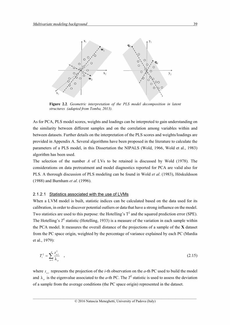
Multivariate modeling background 39
______________________________________________________________________________________________ © 2016 Natascia Meneghetti, University of Padova (Italy)
Figure 2.2. Geometric interpretation of the PLS model decomposition in latent structures (adapted from Tomba, 2013).
As for PCA, PLS model scores, weights and loadings can be interpreted to gain understanding on
the similarity between different samples and on the correlation among variables within and
between datasets. Further details on the interpretation of the PLS scores and weights/loadings are
provided in Appendix A. Several algorithms have been proposed in the literature to calculate the
parameters of a PLS model, in this Dissertation the NIPALS (Wold, 1966, Wold et al., 1983)
algorithm has been used.
The selection of the number A of LVs to be retained is discussed by Wold (1978). The
considerations on data pretreatment and model diagnostics reported for PCA are valid also for
PLS. A thorough discussion of PLS modeling can be found in Wold et al. (1983), Höskuldsson
(1988) and Burnham et al. (1996).
2.1.2.1 Statistics associated with the use of LVMs
When a LVM model is built, statistic indices can be calculated based on the data used for its
calibration, in order to discover potential outliers or data that have a strong influence on the model.
Two statistics are used to this purpose: the Hotelling’s T2 and the squared prediction error (SPE).
The Hotelling’s T2 statistic (Hotelling, 1933) is a measure of the variation in each sample within
the PCA model. It measures the overall distance of the projections of a sample of the X dataset
from the PC space origin, weighted by the percentage of variance explained by each PC (Mardia
et al., 1979):
A
a a
iai
tT
1
2,2
λ , (2.15)
where iat , represents the projection of the i-th observation on the a-th PC used to build the model
and aλ is the eigenvalue associated to the a-th PC. The T2 statistic is used to assess the deviation
of a sample from the average conditions (the PC space origin) represented in the dataset.

40 Chapter 2
______________________________________________________________________________________________ © 2016 Natascia Meneghetti, University of Padova (Italy)
On the other hand, the representativeness of the observation by the model is quantified through
the SPE statistic that is defined for the i-th sample as:
TTT )(SPE iiiii xPPIxee , (2.16)
where ei is the [N1] residual vector for the reconstruction of the i-th observation xi (i.e. the i-th
row of the residual matrix E), and I the identity matrix of size [NN]. SPEi measures the
orthogonal distance of the i-th observation from the latent space identified by the model, thus
accounting for the model mismatch. This means that samples with high values of SPE are
characterized by a different correlation structure with respect to the one described by the PCA
model and, as a consequence, are not well-represented by the model.
Confidence limits can be set both for Hotelling’s T2 and for SPE, based on the values they assume
for the data in model calibration, to evaluate possible outliers or analyze a new set of data (XPRED).
In particular, the scores have zero mean, variance equal to their associated eigenvalues and are
orthogonal. Assuming that the data used to build the model are independent and identically
distributed, scores are normally distributed. Therefore, for the scores on the a-th LV, a univariate
confidence limit can be calculated from the critical value of the Student’s t-distribution, with I-1
degrees of freedom at significance level α:
aItat 2,1lim)1( . (2.17)
Under this assumption, the Hotelling’s T2 can be well-approximated as a Fisher’s F- distribution,
being it computed from the ratio of approximately normal variables. Its relevant confidence limit
can therefore be estimated as (Mardia et al., 1979):
,,
22
lim)1( 1
1, AIAF
AI
IAIAT
, (2.18)
where ,, AIAF is the critical value of the F distribution with A and I - A degrees of freedom at
significance level α. This determines in the A-dimensional score space an ellipsoidal confidence
region, whose semi-axes are:
AaIATsa aa 1,...., with ,2lim)1( . (2.19)
In particular, to allow a visual representation, confidence ellipses can be determined through
Eq. (2.19) for the projections of the scores of data in bi-dimensional planes.

Multivariate modeling background 41
______________________________________________________________________________________________ © 2016 Natascia Meneghetti, University of Padova (Italy)
The SPE statistic is a sum of squared errors, which can be assumed to follow a normal distribution.
As a consequence, SPE can be approximated as a 2 - distribution, and its relevant limit
calculated as follows:
Aa
a1,...., with 2SPE 2
,2)lim-(1 2 , (2.20)
where 2
,2 2 a
is the critical value of the 2 - distribution with 22 degrees of freedom at
the significance level α; μ and ν are respectively the mean and the variance of the SPE values of
the data used to build the model (Nomikos and MacGregor, 1995).
Once a LVM has been calibrated on the available datasets, the model can be used to assess the
overall conformance of a new sample xPRED to the data used to build the model (i.e. the historical
data). This can be done by projecting xPRED onto the PCA model space, in order to calculate the
corresponding scores PREDt [A×1]:
PxtT PREDT PREDˆ . (2.21)
or, if a PLS model is used:
*T PREDT PREDˆ Wxt . (2.22)
The scores PREDt can be used to calculate the Hotelling’s T 2 (Eq. 2.18) of the new sample
( 2PREDx
T ) which provides a measure of the deviation of the new sample from the average conditions
of the data used to build the model. Once the scores have been calculated, sample PREDx can be
reconstructed from the model for X:
PRED PRED ˆˆ tPx . (2.23)
which is valid both for a PCA or a PLS model. Furthermore, in the case of the PLS model, a
prediction of the response variables can be obtained by reconstructing PREDy [M×1]:
PRED PRED ˆˆ tQy . (2.24)
From PREDx the value of the squared prediction error for PREDx ( PREDSPE
x) can be obtained from
Eq. (2.16). This statistic represents the model mismatch for the new incoming sample PREDx . The
statistics PREDt , 2 PREDx
T and PREDSPEx
provide therefore measures of the conformance of PREDx to
the historical data. In particular the T2 and SPE statistics calculated for the new sample are
compared with the relevant confidence limits defined in Eq. (2.18) and Eq. (2.20) to judge the

42 Chapter 2
______________________________________________________________________________________________ © 2016 Natascia Meneghetti, University of Padova (Italy)
similarity and the adherence of PREDx to the data used to build the model (the same rationale is
commonly used also to build monitoring charts for process monitoring purposes):
)lim-(1
2)lim-(1
2
SPESPE PRED
PRED
x
xTT
. (2.25)
If the conditions in (2.25) are satisfied, PREDx the hypothesis that PREDx complies with the
calibration (i.e. historical) data with a 100(1-α)% probability is satisfied (Johnson and Wichern, 2007); otherwise a change in the mean conditions ( 2
)lim-(12
PRED TT x
) or in the representativeness of
the model ()lim-(1SPESPE PRED
x) compared to the common cause data used to build the model
may have occurred. If a problem is detected, the root cause can be identified by analyzing the
relevant contributions of each variable in the X dataset to the T2 and SPE statistics of the sample.
These permit to identify the variables that are most responsible for the distance of a sample from
the origin of the PC space or from the PC space itself. This can be done both for calibration data
and for predicted data. In particular, the contributions to T2 can be calculated as follows:
T21TT
,CONT PΛtt ii , (2.26)
tCONT,i is a [N×1] vector of the contributions of each variable to the Hotelling’s T2 statistic and
can be considered a scaled version of the data within the PCA model. The formulation in (2.26) has the property that the sum of the squared elements of tCONT,i gives 2
iT for the i-th observation.
The contribution of each variable to the SPEi statistic for the i-th sample coincides instead with
the residuals in the reconstruction of the sample through the model (i.e. each single element ei,n
of the i-th row of the residual matrix E):
nii ,,CONTSPE e . (2.27)
The analysis of the variable contributions can reveal which variables mainly determine the
position of a sample in the score space or out of it. This, together with physical knowledge on the
system, may be useful especially when outliers are pinpointed, to understand the root cause of the
problem. Procedures to calculate limits for the variable contributions have been proposed (Conlin
et al., 2000).
2.1.3 Model inversion
Latent variable model inversion was first introduced by Jaeckle and MacGregor (1998; 2000a and
2000b) and recently generalized by Tomba et al. (2012). The basic idea under LVM inversion is
to exploit the relations between response variables and regressor variables, modelled by a LVRM,

Multivariate modeling background 43
______________________________________________________________________________________________ © 2016 Natascia Meneghetti, University of Padova (Italy)
in order to estimate a set of input variables xNEW (e.g., initial conditions, process parameters,
process settings, CPPs) starting from a desired set of response variables yDES (target product
profile). To estimate xNEW, the LVRM model is inverted as sketched in Figure 2.1.
Figure 2.3. Schematic of the direct use of LVM and of the LVM inversion (adapted from Ottavian et al., 2016)
Assuming that the desired response yDES has been defined, its projections NEWt onto the score
latent space can be estimated by the LVRM inversion of the PLS model used to describe their
relationship as (Jaeckle and MacGregor, 1998):
DEST1TT
NEW )(ˆ yQQQt . (2.28)
The set of input variables NEWx corresponding to the desired product quality yDES can be
reconstructed from NEWt (2.28) using Eq. (2.23). This is called direct LVRM inversion, and NEWx
follows the same covariance structure of the historical data (Jaeckle and MacGregor, 1998).
However, depending on the effective dimension of the latent spaces of X and Y (i.e., on their
statistical rank) and on the number A of LVs retained to build the model, the solution to the
inversion problem may not be unique. Assuming, RX as the statistical rank of X and RY as the
statistical rank of Y, the number of latent directions selected are usually A=max(RX, RY).
Depending on the ranks of the datasets, three cases may arise (Jaeckle and MacGregor, 1998):
1. A = RX (RX > RY): this is the most common situation, where there are some LVs (or their
combination) in the latent space of X statistically significant to describe the systematic
variability in X, but which do not contribute in explaining the variability of the data in Y. In
this case, part of the variability in the X space is not related to the Y space (Burnham et al.,
1999) hence, the inversion exercise requires a projection from a lower dimensional Y space
(RY) to the higher dimensional X space (RX).
2. A = RY (RY ≥ RX): in this case, there is a substantial overlapping between the latent space of
X and Y (Burnham et al., 1999), all the LVs of the X space potentially explain systematic

44 Chapter 2
______________________________________________________________________________________________ © 2016 Natascia Meneghetti, University of Padova (Italy)
variability in Y. In this case, the model inversion corresponds to a projection from a higher
dimensional Y space (RY) to a lower dimensional X space (RX).
3. A = RX = RY but rank([XY]) > A: in this case, although the statistical rank of X and Y is equal,
the rank RXY is greater, therefore (RXY – A) latent dimensions do not overlap between the X
and Y spaces. This situation is similar to the one where A = RX (RX > RY).
Only in the second case a unique solution exists by applying the direct model inversion. In the
first and last cases, the number of solutions is infinite. Although the direct model inversion
(Eq.2.28) provides the least-squares solution to the problem, this solution can be moved by
changing NEWt along the directions of latent space that do not contribute to explain the variability
of Y, namely which do not affect the response variables. These directions identify a null space,
which represents the locus of the X projections not affecting the quality space of Y (Jaeckle and
MacGregor, 1998). Therefore, the set xNEW suggested by the direct inversion can be moved along
the null space without affecting the product quality. In order to find the most suitable process
conditions xNEW along the null space that are necessary to achieve the desired quality yDES, an
optimization problem have to be solved (Yacoub and MacGregor, 2011; García-Muñoz et al.,
2006 and 2008). To this purpose, Tomba et al., (2012, 2013b) and Tomba (2013) proposed a
general framework that allows one to find a solution NEWx that is coherent with the historical data
used to build the underlying model, and also accounts for any experimental limitations or other
constraints that may be present.
A thorough discussion on the inversion/optimization problem, is provided by Yacoub and
MacGregor (2011), García-Muñoz et al. (2006, 2008) and Tomba et al. (2012, 2014).
2.1.3.1 Null space computation
As previously stated, when RY < RX a null space exists. Hence, the estimation NEWx and the
reconstruction of DESy are formed by two latent contributions, tNEW and tNULL, which accounts
respectively for the effective scores of DESy in the latent space and for the translation of the scores
along the null space in order to provide the reconstruction of NEWx at a minimum distance from
the latent space (minimum SPE). Therefore, any solution of the inversion problem x can be
defined as:
NULLNEWˆˆˆ xxx , (2.29)
where NEWNEWˆ Ptx NULLx and NULLNULL
ˆ Ptx (which falls on the remaining RX – RY directions).
The null space is needed for the model to represent adequately the regressor variables, but it does
not contribute in explaining the variability in the response variables, hence:
0NULL Qt . (2.30)

Multivariate modeling background 45
______________________________________________________________________________________________ © 2016 Natascia Meneghetti, University of Padova (Italy)
The null space represents the kernel of the loadings Q matrix and can be computed from the
singular value decomposition of matrix Q (Jaeckle and MacGregor, 2000a):
T
21T ][ GGSUVSUQ QQQQQ , (2.31)
where UQ is the matrix of the left singular vectors of Q, SQ is the diagonal matrix of the singular
values of Q, and VQ is the matrix of the right singular vectors of Q. In particular, the right singular
vectors corresponding to the vanishing (zeros) singular values of Q span its null space. These are
included in the columns of matrix G2 [A(A – RY)], which therefore defines the null space of the
model. Vector tNULL can therefore be moved arbitrarily along it, without affecting DESy , i.e.:
T2
TTNULL Gγt . (2.32)
In Eq. (2.32), which defines the model null space, is an [(A – RY) 1] vector arbitrary in
magnitude and direction.
It should be observed that the concept of the null space can be related to the definition of the
design space (ICH, 2009), namely to “the space of the input variable combinations that robustly
ensure to obtain a defined product in output”. As observed by Tomba et al. (2012) and Ottavian
et al. (2016), the null space represents a useful basis for further experimentation to properly
develop a DS, as will be shown in Chapter 5.
2.2 Pattern recognition techniques
Pattern recognition techniques are intended to devise ways and means of automating certain
decision-making processes that lead to classification and recognition of common patterns and
regularities in large sets of data (Pal and Mitra, 2004). Pattern recognition techniques present
several advantages in the analysis of large datasets, namely: i) they are able to recognize those
relationships that differentiate similar or not similar objects, thereby identifying the common
properties that characterize different groups of objects; ii) they are able to handle multivariate
data; iii) they facilitate the analysis of systems where the exact relationships are not fully
understood, by extracting the important feature from the available datasets (Lavine and Davidson,
2006). The number and type of techniques that can be categorized in the big family of pattern
recognition techniques are very broad, as well as are the application fields. In fact, thanks to their
potential, pattern recognition techniques have been found many applications in engineering, as
well as in medical, chemical pharmaceutical, social and economic sciences, both as classification
(or clustering) tools and as regression/prediction tools.
In this Dissertation we are mainly interested in the use of pattern recognition techniques in their
original acceptation, namely as classification tools. While regression methods model quantitative

46 Chapter 2
______________________________________________________________________________________________ © 2016 Natascia Meneghetti, University of Padova (Italy)
responses on the basis of a set of regressor variables, classification techniques are quantitative
methods for the modeling of qualitative responses, that attempt to find mathematical relationships
between a set of descriptive variables and a qualitative variable (Ballabio and Todeschini, 2009).
As mentioned above, pattern-recognition methods were originally designed to find classification
rules (or empirical relationships) to classify new samples in relation to a specific property,
according to the information extracted by a set of samples (called training or calibration set) for
which the property of interest and the measurements indirectly related to that property are known.
In this context, the term pattern indicates the set of measurements that describe each sample in
the training set, for which the property of interest and measurements are known, whereas the
assignment of a new sample to its respective class is called recognition, since it is performed by
recognizing the property of interest (Lavine and Davidson, 2006).
Three main steps characterize a typical pattern recognition system: data acquisition, feature
selection/extraction and classification/clustering. Once the data have been collected using a set of
sensors, they are then passed on to the feature selection/extraction phase, where the
dimensionality of the data is reduced by retaining only some characteristic features or properties.
Finally, in the classification/clustering phase, the selected features are passed on to the
classifying/clustering system that evaluates the incoming information and makes a final decision
(Pal and Mitra, 2004).
In classification analysis, if I objects are considered, each described by M variables and divided
into C categories (classes), they can be organized in a matrix X, composed of I rows (the samples),
and N columns (the explanatory variables). Each entry, xi,n represents the value of the n-th variable
for the i-th object. The additional information concerning the class is collected into a vector c
[C×1], constituted by C different labels or integers, each representing a class. Each sample xi,n can
be considered as a point in a high-dimensional measurement space. Points representing objects
from one class tend to cluster in a limited region of the measurement space separated from the
others. Therefore, to solve a classification problem, the feature space should be partitioned into
regions, namely one region for each category of input. This permits one to assign every data point
in the entire feature space to one of the possible classes (region). However, usually the complete
description of the classes is not known, since the available training set includes only a finite and
usually small number of samples, which often provides only partial information for design a
classifying/clustering system. On the basis of the information provided by the samples in the
training set, the pattern recognition systems are designed, namely the values of the parameters of
various pattern recognition methods are tuned to minimize the misclassification errors (Pal and
Mitra, 2004).
Depending on the features of the available data, different type of classifiers can be designed. For
example, the training set may include labeled or unlabeled data. In the first case, each new object
is classified based on the information acquired on a set of objects with known classifications (i.e.,
labels); this classification method is called supervised. Otherwise, if no a priori information on

Multivariate modeling background 47
______________________________________________________________________________________________ © 2016 Natascia Meneghetti, University of Padova (Italy)
the set of samples that is used for classification purposes is available (unlabelled data), the method
is called unsupervised. Supervised methods are used for classifying different objects, while
clustering is performed through unsupervised methods. Principal components analysis represents
an example of unsupervised methods. PCA does not focus on how many groups will be found,
since it does not use information related to predefined classes of objects (Ballabio and Todeschini,
2009).
Then, distinctions can be made among the different classification techniques on the basis of the
mathematical form of the decision boundary, i.e. on the basis of the ability of the method to detect
linear or non-linear boundaries between the region in which the analyzed space is partitioned.
Moreover, classification techniques can be probabilistic, if they are based on estimates of
probability distributions, i.e. a specific underlying probability distribution in the data is assumed.
Among probabilistic techniques, parametric and non-parametric methods can be distinguished,
when probability distributions are characterized by location and dispersion parameters (e.g. mean,
variance, covariance). Classification methods can also be defined as distance-based, if they
require the calculation of distances between objects or between objects and models.
Examples of pattern-recognition methods that have been used to classification or clustering
purposes include nearest neighbors, neural networks, discriminant analysis, clustering analysis,
and principal component analysis. In this Dissertation, only the first and the last one are employed
and described; further information and examples of application of other techniques can be found
(among others) in Lavine and Davidson (2006) and Varmuza and Filmozer (2009), Pal and Mitra
(2004).
2.2.1 K-nearest neighbors
k-nearest neighbor (k-NN) is a powerful classification technique. k-NN is a supervised method,
namely a training set is required for the classification of new observations. The nearest neighbor
classification rule (Cover and Hart, 1967) classifies an unclassified observation depending on
the class attribution for an assigned number k of neighbors idecavolntified according to a given
distance criterion. Therefore, k-NN is a distance-based method, since the classification is
performed by calculating the distances between the new observation and all the observations of
the training set.
In Figure 2.4a a graphical representation of the rationale underlying the k-NN method in the
classification of a new sample (black star) is shown. Two different clusters are considered (Cluster
1 and Cluster 2), whose samples are denoted respectively as open triangles and squares. Assuming
k=5, the k nearest neighbors to xi,n, are identified as the closest 5 objects to the new sample that
lie in the gray area around the sample. The predicted class membership nic ,ˆ of the new object xi,n
is obtained from the known class memberships c(x(1)), . . . , c(x(k)) of the k nearest neighbors,
and can be taken as the class that occurs most frequently among the k neighbors (Varmuza and

48 Chapter 2
______________________________________________________________________________________________ © 2016 Natascia Meneghetti, University of Padova (Italy)
Filzmoser, 2009). Thus, the prediction corresponds to a majority vote among the neighbors, that
with k=5, corresponds to Cluster 1, since 3 out of 5 closest samples belong to this cluster.
The decision boundary between different groups can be very rough, and it strongly depends on
the parameter k. Thus, for small values of k, it is easily possible that classes do no longer form
connected regions in the data space, but they can consist of isolated clouds. The classification of
new objects can thus be poor if k is chosen too small or too large. In the former case, we are
concerned with overfitting, and in the latter case with underfitting (Varmuza and Filzmoser,
2009). The importance of the selection of the parameter k is demonstrated in Figure 2.4b, where
if k=11 is selected, the new sample is assigned to Cluster 2 instead of Cluster 1, since 6 out of 5
neighbors belong to this cluster.
Different methods to calculate the distance between the observation to be classified and the
observations of the training set have been suggested, as well as different decision rules in case of
ties. Since the decision boundary between different groups strongly depends on the parameter k
(Varmuza and Filzmoser, 2009), cross-validation procedures should be implemented by testing a
set of k values (e.g. from 1 to 10). Note that if the samples analysed are characterized by different
variables measured in different units, similarly to the application of latent variables modeling, it
is suggested that the data are first mean-centered and scaled to unit variance.
k-NN is a non-parametric classification method (i.e., it does not assume a form of the underlying
probability density functions) and can handle multiclass problems. Another important advantage
is that k-NN is a nonlinear method, since the Euclidean distance between two observations in the
data space is a nonlinear function of the variables (Ballabio and Todeschini, 2009).
a b Figure 2.4. Graphical interpretation of the k-NN classification of a new sample ( ) considering (a) k=5 and (b) k=11.
2.2.2 PCA for cluster analysis
Employed as a cluster analysis tool, principal component analysis has also been demonstrated to
be a valid exploratory data analysis technique that is often very helpful in elucidating the complex
-2 0 2 4 6 8-10
-5
0
5
10
Cluster 1 Cluster 2 New sample
k=5
-2 0 2 4 6 8-10
-5
0
5
10
Cluster 1 Cluster 2 New sample
k=11

Multivariate modeling background 49
______________________________________________________________________________________________ © 2016 Natascia Meneghetti, University of Padova (Italy)
nature of multivariate relationships. Used for clustering purposes, this technique is employed to
uncover relationships in large multivariate datasets without directly using the information about
the class assignment of the samples. In fact, the latent variable space resulting from the application
of the PCA, permits one to visualize the relative position of the data points of the original dataset,
which usually group in different clusters. Hence, once the structure of a given dataset (called
calibration or training set) is modelled, new samples can be projected onto the PCA model space
built for that dataset, in order to recognize which cluster the new samples are most similar to.
Usually, only two or three principal components are necessary to explain a significant fraction of
the information present in multivariate data (Lavine and Davidson, 2006).
Clusters are usually defined intuitively, depending on the context, as shown in Figure 2.5. In this
example three main clusters can be distinguished (marked by different open symbols), and the
new projections (closed triangles) are clearly recognized as belonging to Cluster 3. However,
notice that no measure of cluster validity can serve as a reliable indicator of the quality of a
proposed partitioning of the data (Lavine and Davidson, 2006), even if some possible solutions
are provided in the literature (Rousseeuw, 1987).
Used as a clustering technique, principal component analysis can be applied to multivariate data
to identify outliers, to display data structure, and to classify samples.
Figure 2.5. Example of the discriminatory potential of the PCA model.
-2 0 2 4 6 8 10
-10
-5
0
5
10
Cluster 1 Cluster 2 Cluster 3 New samples
PC
2
PC1


______________________________________________________________________________________________ © 2016 Natascia Meneghetti, University of Padova (Italy)
Chapter 3
A methodology to diagnose process/model mismatch in first-principles models for steady-state
systems*
In this Chapter a methodology is proposed to diagnose the root cause of the process/model
mismatch (PMM) that may arise when a first-principles (FP) process model is challenged against
a set of historical experimental data. The objective is to identify which model equations or model
parameters most contribute to the observed mismatch, without carrying out any additional
experiment. The methodology exploits the available data (namely, the historical dataset and a
simulated one built by using the FP model) in order to analyze the correlation structure of the two
datasets by means of a PCA model. Information on where the PMM originates from is obtained
using diagnostic indices coupled to engineering judgment.
3.1 Introduction
Process modeling is an essential tool to support several process engineering activities
(Stephanopoulos and Reklaitis, 2011; Gani, 2009; Pantelides and Urban, 2004). Mathematical
modeling by first principles can be viewed as the best way to organize the available information
about a process or a system in a meaningful way (Kiparissides et al., 2014). First-principles (FP)
models are often preferred to data-driven (DD) ones, because they rely on a physical
understanding on the system under investigation and allow some extrapolation beyond the range
of data used to calibrate them (Pantelides and Renfro, 2013). On the other hand, DD (or data-
based, DB) models are often easier to develop than FP ones, and may be computationally less
intensive and more convenient for online use.
A model is made by equations and parameters. In an FP model, the equations represent the
available knowledge on the underlying mechanisms driving the process, whereas the parameter
values inform on how the general mechanisms are tuned to the actual system under investigation.
* Meneghetti, N., P. Facco, F. Bezzo, M. Barolo (2014). A methodology to diagnose process/model mismatch in first-
principles models. Ind. Eng. Chem. Res., 53, 14002-14013.

52 Chapter 3
______________________________________________________________________________________________ © 2016 Natascia Meneghetti, University of Padova (Italy)
When the FP model of a process is challenged against a historical dataset, the model outputs may
not match the historical evidence to a desired accuracy, and therefore process/model mismatch
(PMM) occurs. This may be due to different reasons: i) the knowledge about the underlying
process is limited, and therefore the model equations are (perhaps only partially) inappropriate;
ii) the complexity of the physical phenomena involved in the process has been mathematically
oversimplified, e.g. because the model has to be used online; iii) some of the model parameters
have been assigned inappropriate values (for example, some of them may have been taken from
the open literature, some other from proprietary information, some other from semi-theoretical
studies). The occurrence of PMM can be critical when the model is used for design, optimization
or control purposes.
The model adherence to reality can be enhanced by acting on the model equations (i.e., by
formulating alternative mechanisms that describe the process under investigation) or on the model
parameters. In both cases new experiments, i.e. experiments ranging over operating conditions
not included in the historical database, are usually needed to speculate on the alternative
mathematical formulations or to fine-tune the model parameters. To this purpose, model-based
design of experiments (MBDoE) techniques can be used (Franceschini and Machietto, 2008;
Marquardt 2005). MBDoE allows one to design experiments that can provide useful information
for model discrimination among alternative set of equations, or for parameter identification in an
assigned set of equations. Although effective, the MBDoE exercise may be quite demanding if
one does not know in advance which equations or parameters are most responsible for the
observed PMM. Additionally, carrying out new experiments is expensive by itself. Indeed, to
enhance the model performance when PMM is detected, it would be very useful if the PMM could
be diagnosed. This would amount to being able i) to assess whether the observed mismatch is due
to the use of an inappropriate set of equations (structural mismatch) or to the inaccurate estimation
of some parameters (parametric mismatch), and ii) to identify which equations or parameters are
mostly responsible of the observed PMM. With this piece of information available, the MBDoE
exercise could be sped up significantly, or perhaps even avoided.
The importance of diagnosing PMM has been recognized in process control applications (Wang
et al., 2012; Badwe et al., 2009) but has been somewhat overlooked with respect to general FP
models. In this study, a methodology is proposed to diagnose the PMM originating when an FP
model is challenged against a set of historical experimental data. “Synthetic” data are generated
by running the FP model under the same input conditions characterizing the historical dataset.
Then, using a DD model (namely, a multivariate statistical model), the correlation structure of
this synthetic dataset is compared to that of the historical dataset, and information on where the
PMM originates from is obtained using DD model diagnostic indices and engineering judgment.
The proposed methodology uses only information included in the historical database and does not
require any new experiment. Note that we are not interested in improving the FP model
performance by complementing the FP model with a DD model section, as is done for example

A methodology to diagnose process/model mismatch in FP models for steady-state systems 53
______________________________________________________________________________________________ © 2016 Natascia Meneghetti, University of Padova (Italy)
in hybrid modeling. Rather, we would like to provide the modeler with a tool that can help him/her
to detect which sections of the FP model are not performing well, thus targeting subsequent
theoretical and experimental efforts (e.g., through an MBDoE exercise) or complementing other
model analysis techniques (e.g., sensitivity analysis, Saltelli et al., 2000; Saltelli et al., 2008).
The proposed methodology is tested on two simulated systems of increasing complexity: a jacket-
cooled chemical reactor and a solids milling unit.
3.2 Proposed methodology
It is assumed that a FP model describing the process is available and that PMM has been observed
by comparing the model results to a set of historical steady-state process measurements. The
rationale of the proposed methodology for PMM diagnosis is the following. First, a DD model, is
developed to explain the correlation structure of appropriate nonlinear combinations of the
simulated process variables, these combinations (called auxiliary variables) being suggested by
the FP model structure. Then, it is assessed whether the same variable combinations, as calculated
from the historical measurements, conform to this correlation structure. Finally, from the analysis
of some model diagnostics, engineering knowledge is used to pinpoint the FP model equations or
parameters that are mostly responsible for the observed PMM. To analyze the correlation structure
of the datasets considered in this study, principal component analysis (PCA) is used (see Chapter
2, Section 2.1.1).
3.2.1 Diagnosing the process/model mismatch
The proposed methodology for PMM diagnosis consists of the following four steps, where
subscripts and M refer to the process and to the model, respectively. It is assumed that a PMM
has been observed by comparison of simulated and historical data.
1. Generation of the model matrix and of the process matrix. FP model simulations are run using
the set of inputs of the historical dataset (one simulation for each of the available I steady
state samples), and predictions of the measured outputs are obtained. We refer to this set of
measured inputs/simulated outputs as to the set of “simulated measurements”. On the other
hand, the set of “historical measurements” (or simply measurements, averaged over possibly
noisy steady state time series) corresponds to the historical dataset (i.e., measured
inputs/measured outputs). For each sample, the simulated measurements, historical
measurements and FP model parameters are appropriately combined to obtain two sets of V
auxiliary variables each: one set refers to combinations of the simulated measurements and
model parameters, and the other one to the same combinations, but using the historical
measurements instead of the simulated ones. As will be clarified later, how the variables
should be combined is suggested by the FP model structure. Note that each auxiliary variable

54 Chapter 3
______________________________________________________________________________________________ © 2016 Natascia Meneghetti, University of Padova (Italy)
must include at least one input or one output variable, i.e. no auxiliary variable is obtained by
combination of model parameters only, unless the model parameters change across the
samples (e.g., when the parameters depend on material properties, and the processed material
changes across the samples). The two sets of auxiliary variables are organized as columns of
two matrices, XM [I × V] and XΠ [I × V], which are called the model matrix and the process
matrix, respectively. Due to the existence of PMM, the correlation structure of XΠ is expected
to be different from that of XM.
2. Development of a PCA model for the model matrix. Both XM and XΠ are centered on the
mean of XM and scaled on the standard deviation of XM. Given that each auxiliary variable
contains at least one input or one output measurement, after the scaling operations no columns
in XM or XΠ result in null vectors. A PCA model is then built from XM and the residuals matrix
EM is calculated:
XXE
PTX
ˆ
ˆ
. (3.1)
In 3.6 the meaning of the symbols is the same as Eq. 2.6 in Section 2.1.1 (Chapter 2).The
PCA model describes the correlation structure of the data included in XM. The number of
PCs to be retained in the PCA model is determined by the eigenvalue-greater-than-one rule
(Mardia et al., 1979).
3. Projection of the process matrix onto the PCA model. XΠ is projected onto the PCA model
space and the residuals matrix EΠ is calculated:
XXE
PTX
PXT
ˆ
ˆ TM
. (3.2)
4. Analysis of the residuals matrices and diagnosis of the PMM. The two residuals matrices, EΠ
and EM, are analyzed to identify the auxiliary variables that most contribute to the
inconsistency in the correlation structures of XΠ and XM. These auxiliary variables, together
with engineering judgment, are then used to pinpoint the FP model equations or parameters
that most contribute to the observed PMM.
The residuals matrix reflects the data variability that is not captured by the model. If the elements
ei,v of the v-th column ev of EM follow a normal distribution, the variability not described by the
model is deemed to be non-deterministic, and confidence limits can be set for ev in the form:
)(2/, nzCL
mee , (3.3)

A methodology to diagnose process/model mismatch in FP models for steady-state systems 55
______________________________________________________________________________________________ © 2016 Natascia Meneghetti, University of Padova (Italy)
where is the significance level and typically takes a value of 0.01 or 0.05, zα/2 is the
corresponding standard normal deviate and (ev) is the standard deviation of ev. In this work,
= 0.05 (i.e. 95% confidence) is used, and zα/2 takes the approximate value of 1.96.
Note that EΠ accounts both for the mismatch between XΠ and XM, and for the fraction of the XΠ
variability that is not described by the PCA model built on the XM data. In order to account for
the contribution due to the PMM only, the contribution related to the un-modeled variability of
XΠ is removed from EΠ. Hence, for each column v of EΠ the residuals analysis is done in terms
of mean residuals-to-limit ratio (MRLRv):
I
CL
e
MRLR
I
i
vi
v
v
1 %,95
2
,
e
, (3.4)
that is the mean of the ratios between the residuals of each column of EΠ and the corresponding
95% confidence limit, calculated considering a normal distribution of residuals (see Eq. 3.3). In
this study, the Anderson-Darling test (Anderson and Darling, 1952) was employed in order to
check the null hypothesis that vector v,e belongs to a population with a normal distribution of
mean 0. Note that, if the residuals are not normally distributed, the confidence interval cannot be
calculated from Eq. (3.3). Alternative expressions for the estimation of the confidence limits
should be used if a different distribution of the residuals can be recognized (Martin and Morris,
1996; Doymaz et al., 2001).
3.3 Example 1: jacket-cooled reactor
3.3.1 Process and historical dataset
To illustrate the application of the proposed methodology, a jacket-cooled continuous stirred tank
reactor (CSTR) is first considered. Two consecutive exothermic reactions take place in the
reactor:
outB
outA
outoutB
outA CCkTCCkfR 1111 ),,,( C2BA :1reaction (3.5)
),,( DC :2 reaction 2222
outC
outoutC CkTCkfR (3.6)
where A and B are the reactants, C is the desired product, D is the byproduct, Rr is the reaction
rate expression for reaction r, Cs is the molar concentration of species s, T stands for temperature,

56 Chapter 3
______________________________________________________________________________________________ © 2016 Natascia Meneghetti, University of Padova (Italy)
and superscript out refers to a variable at the reactor outlet. The kinetic constant kr takes the
Arrhenius form:
out
rarr RT
EAk ,exp , (3.7)
where R is the universal gas constant. The meaning of the other symbols is reported in Table 1.
The process is described by the following set of equations (Luyben, 2007):
01 F
VCCkCC Rout
BoutA
inA
outA (3.8)
01 F
VCCkCC Rout
BoutA
inB
outB (3.9)
02 21 F
VCk
F
VCCkCC Rout
CRout
BoutA
inC
outC (3.10)
02 F
VCkCC Rout
CinD
outD (3.11)
0
F
V
V
QQTTc R
R
Rinout
P
(3.12)
0,
j
in
j
out
jwPw F
QTTc
(3.13)
out
jout TTUSQ (3.14)
outC
outB
outAR CkHCCkHQ 2211 (3.15)
where subscripts subscript j refers to the jacket and subscript w refers to the cooling utility.
As indicated in Table 3.1, it is assumed that measurements are available for 14 variables (8 inputs
and 6 outputs). The nominal values of the parameters are reported in Table B.1 of Appendix B.
The historical dataset consists of 25 sets of average measurements (samples) obtained for different
combinations of the following input variables: inAC , in
BC , inT , injT , FVR / and
jF. The ranges of the
input and output variables in the historical dataset are reported in Table B.2 of Appendix B.

A methodology to diagnose process/model mismatch in FP models for steady-state systems 57
______________________________________________________________________________________________ © 2016 Natascia Meneghetti, University of Padova (Italy)
Table 3.1. Example 1: variables and parameters.
Parameters and derived variables Measured variables in the historical dataset
Inputs Outputs Ar Pre-exponential constant in
AC
Inlet molar concentration of A
outAC Outlet molar
concentration of A
cp Specific heat inBC
Inlet molar concentration of B
outBC Outlet molar
concentration of B
Ea,r Activation energy inCC
Inlet molar concentration of C
outCC Outlet molar
concentration of C
S Total area available for the heat exchange
inDC
Inlet molar concentration of D
outDC Outlet molar
concentration of D
U Overall heat transfer coefficient
F Feed flowrate outjT Outlet jacket
temperature VR Reactor volume jF Cooling utility
flowrate outT Outlet reactor
temperature Q Heat exchange rate
between the reactor and the jacket
inT
Inlet reactor temperature
QR Heat rate generated by the reactions
injT
Inlet jacket temperature
H Enthalpy of reaction
Density
3.3.2 Application of the methodology and results
In order to test the effectiveness of the proposed methodology, three case studies are considered
(Case study 1.A, 1.B and 1.C) that correspond to three different models M being built to represent
process . Basically, the same set of equations as in Eqs. (3.8) - (3.15) is used in all case studies,
but different parametric and structural PMM are included in each model (such as imprecise
estimation of the heat exchange or kinetics parameters, or mis-modeling of the kinetic expression
itself; Table 3. 2). However, it is assumed that one has no a-priori knowledge of the origin of
mismatch. The objective is therefore to assess whether the observed PMM is structural or
parametric, and to highlight which equation or parameter most contributes to the mismatch.
In order to build the process matrix and the model matrix (step 1 of the proposed methodology),
the auxiliary variables are defined as appropriate (nonlinear) combinations of the process/model
variables and of the model parameters, where the combinations are suggested by the model
equations themselves. By looking at the structure of equation set (3.8) - (3.15), the model
equations are partitioned in such a way as to define the following 11 auxiliary variables xi:

58 Chapter 3
______________________________________________________________________________________________ © 2016 Natascia Meneghetti, University of Padova (Italy)
;;
;;
;;
;;
84
1173
,10262
9151
F
VQxCCx
FTTUSxTTcxCCx
TTcxF
VRxCCx
V
TTUS
F
Vx
F
VRxCCx
RR
inD
outD
j
out
joutinout
PinC
outC
inj
outjwPw
RinB
outB
R
out
jout
RRinA
outA
. (3.16)
Note that each auxiliary variable includes at least one measurable variable. In the next
subsections, the proposed methodology is applied to each case study and the results are discussed.
Table 3. 2. Summary of the case studies considered in this study.
Example Case study
Type of mismatch
Model term involved Applied variation
Example 1: CSTR
Case study 1.A Parametric U +50%
Case study 1.B Structural
kinetics of the first reaction
3/4M,
3/2M,1 BA CCk
Case study 1.C Parametric A1 +50%
Example 2: mill Case study
2.A Parametric Wm,kin –30% Case study
2.B Parametric fMat –40% Case study
2.C Parametric q +50%
3.3.1.1 Case study 1.A
Parametric mismatch is enforced by using a value UM of the overall heat exchange coefficient in
the model that is ~50% larger than the actual value (UΠ). Figure 3.1 provides a comparison
between the historical and simulated outputs. Although the concentrations deviations (Figure
3.1a) and the temperature deviations (Figure 3.1b) are not large, they are systematic. Hence, PMM
is observed, although its cause is not apparent from the inspection of Figure 3.1.
Following the definition of the auxiliary variables, the model matrix XM and the process matrix
X can be calculated (step 1). Note that the values taken by the auxiliary variables change
according to whether simulated measurements or historical measurements are used in equation
set (3.16). For example, in the calculation of x5 for use in the model matrix,
),,( MM,M,1,11outout
BoutA TCCfRR
is set. Instead, ),,( ,,1,11outout
BoutA TCCfRR is set in the
calculation of the same variables for use in the process matrix. Also note that, since the actual
values of the parameters are unknown, the model values are used both in XM and in X

A methodology to diagnose process/model mismatch in FP models for steady-state systems 59
______________________________________________________________________________________________ © 2016 Natascia Meneghetti, University of Padova (Italy)
(a) (b) Figure 3.1. Case study 1.A. Deviations between historical and simulated outputs for (a) concentrations and (b) temperatures.
A PCA model is then built on XM (step 2). Table 3.3 reports the eigenvalues λ, the explained
variance R2 and its cumulated value 2cumR for each PC of the model. Two PCs are selected, and
they explain more than 99% of the variability of the XM data. The model loadings in Figure 3.2
show that PC1, which captures most of the original variability (~72%), mainly describes the
behavior of variables that are strongly correlated with the reactions (auxiliary variables x1-6 and
x8), as well as that of x7, whereas PC2 captures the variability of variables that are related to heat
exchange (x7 and x9-11).
Table 3.3. Case study 1.A. Diagnostics of the PCA model on XM.
PC number Eigenvalue of
cov(XM) R2 R2
cum
1 7.88 71.60 71.60 2 3.02 27.46 99.06 3 0.08 0.71 99.77 4 0.02 0.23 100.00
Figure 3.2. Case study 1.A. Loadings on PC1 and PC2 for the PCA model on XM..
Devia
tion
for T
[K]
x1
x2
x3
x4
x5
x6
x7
x8
x9
x10
x11
-0.8
-0.6
-0.4
-0.2
0.0
0.2
0.4
0.6
0.8
Loa
ding
s
PC1 PC2

60 Chapter 3
______________________________________________________________________________________________ © 2016 Natascia Meneghetti, University of Padova (Italy)
After building the PCA model, X is projected onto it (step 3). The projection results are shown
in Figure 3.3: while the XM samples lie very close to the plane formed by PC1 and PC2, the X
samples are far away from this plane. Hence, the two PCs optimally describing the variability of
XM are not able to reliably represent also the correlation structure of the data in X, an issue that
is related to the observed PMM. The distance of each sample from the plane represents the sum
of the residuals of each auxiliary variable for that sample. The large residuals for X confirm that
the correlation structure of Xis not represented well by the PCA model built on XM.
Figure 3.3. Case study 1.A. Residuals in the scores space for each sample of the model matrix XM and of the process matrix XΠ .
After confirming that the residuals obtained by the projection of X are normally distributed,
further insight on the origin of the PMM is gained by analyzing the Xsample projections in
terms of MRLRv (step 4). The results are illustrated in Figure 3.4, from which one can see that the
largest values of MRLRv are associated to auxiliary variables x10, x11, x7 and x9. Hence, it can be
stated that these auxiliary variables mostly contribute to the observed PMM.
Figure 3.4. Case study 1.A. MRLRv for each column of XΠ.
x1
x2
x3
x4
x5
x6
x7
x8
x9
x10
x11
0
2
4
6
8
10
MR
LRv
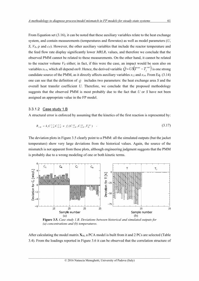
A methodology to diagnose process/model mismatch in FP models for steady-state systems 61
______________________________________________________________________________________________ © 2016 Natascia Meneghetti, University of Padova (Italy)
From Equation set (3.16), it can be noted that these auxiliary variables relate to the heat exchange
system, and contain measurements (temperatures and flowrates) as well as model parameters (U,
S, VR, and cP). However, the other auxiliary variables that include the reactor temperature and
the feed flow rate display significantly lower MRLRv values, and therefore we conclude that the
observed PMM cannot be related to these measurements. On the other hand, it cannot be related
to the reactor volume VR either; in fact, if this were the case, an impact would be seen also on
variables x5-9, which all depend on . Hence, the derived variable out
jout TTUSQ is one strong
candidate source of the PMM, as it directly affects auxiliary variables x12 and x14. From Eq. (3.14)
one can see that the definition of Q includes two parameters: the heat exchange area S and the
overall heat transfer coefficient U. Therefore, we conclude that the proposed methodology
suggests that the observed PMM is most probably due to the fact that U or S have not been
assigned an appropriate value in the FP model.
3.3.1.2 Case study 1.B
A structural error is enforced by assuming that the kinetics of the first reaction is represented by:
),,( MM,M,1
3/4,
3/2,1,1
outoutB
outAMBMA TCCfCCkR
. (3.17)
The deviation plots in Figure 3.5 clearly point to a PMM: all the simulated outputs (but the jacket
temperature) show very large deviations from the historical values. Again, the source of the
mismatch is not apparent from these plots, although engineering judgment suggests that the PMM
is probably due to a wrong modeling of one or both kinetic terms.
(a) (b) Figure 3.5. Case study 1.B. Deviations between historical and simulated outputs for (a) concentrations and (b) temperatures.
After calculating the model matrix XM, a PCA model is built from it and 2 PCs are selected (Table
3.4). From the loadings reported in Figure 3.6 it can be observed that the correlation structure of
−75
−50
−25
0
Sample number25 25
T TJ
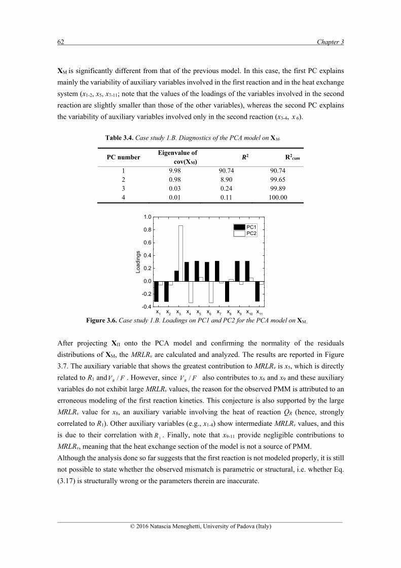
62 Chapter 3
______________________________________________________________________________________________ © 2016 Natascia Meneghetti, University of Padova (Italy)
XM is significantly different from that of the previous model. In this case, the first PC explains
mainly the variability of auxiliary variables involved in the first reaction and in the heat exchange
system (x1-2, x5, x7-11; note that the values of the loadings of the variables involved in the second
reaction are slightly smaller than those of the other variables), whereas the second PC explains
the variability of auxiliary variables involved only in the second reaction (x3-4, x 6).
Table 3.4. Case study 1.B. Diagnostics of the PCA model on XM.
PC number Eigenvalue of
cov(XM) R2 R2
cum
1 9.98 90.74 90.74 2 0.98 8.90 99.65 3 0.03 0.24 99.89 4 0.01 0.11 100.00
Figure 3.6. Case study 1.B. Loadings on PC1 and PC2 for the PCA model on XM..
After projecting XΠ onto the PCA model and confirming the normality of the residuals
distributions of XM, the MRLRv are calculated and analyzed. The results are reported in Figure
3.7. The auxiliary variable that shows the greatest contribution to MRLRv is x5, which is directly
related to R1 and FVR / . However, since FVR / also contributes to x6 and x9 and these auxiliary
variables do not exhibit large MRLRv values, the reason for the observed PMM is attributed to an
erroneous modeling of the first reaction kinetics. This conjecture is also supported by the large
MRLRv value for x8, an auxiliary variable involving the heat of reaction QR (hence, strongly
correlated to R1). Other auxiliary variables (e.g., x1-4) show intermediate MRLRv values, and this
is due to their correlation with 1R . Finally, note that x9-11 provide negligible contributions to
MRLRv, meaning that the heat exchange section of the model is not a source of PMM.
Although the analysis done so far suggests that the first reaction is not modeled properly, it is still
not possible to state whether the observed mismatch is parametric or structural, i.e. whether Eq.
(3.17) is structurally wrong or the parameters therein are inaccurate.
x1
x2
x3
x4
x5
x6
x7
x8
x9
x10
x11
-0.4
-0.2
0.0
0.2
0.4
0.6
0.8
1.0
Load
ings
PC1 PC2
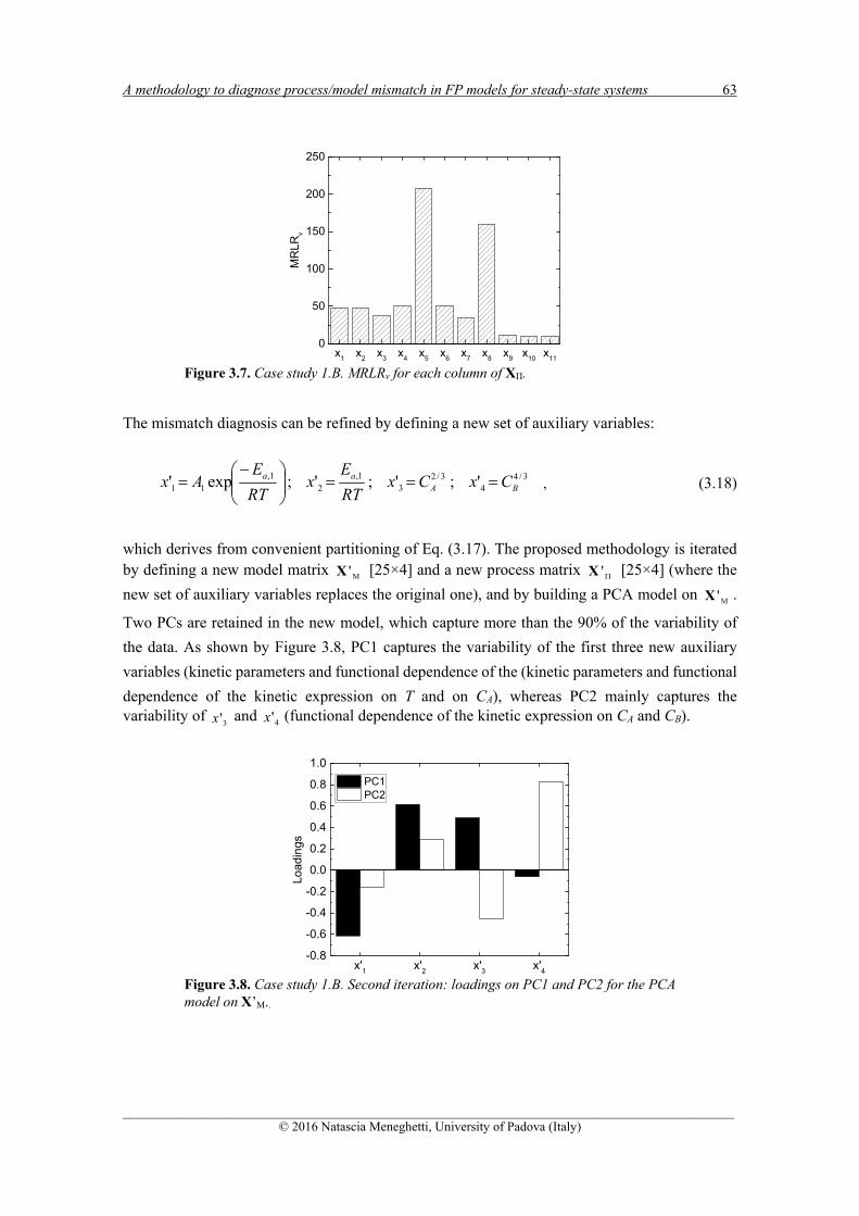
A methodology to diagnose process/model mismatch in FP models for steady-state systems 63
______________________________________________________________________________________________ © 2016 Natascia Meneghetti, University of Padova (Italy)
Figure 3.7. Case study 1.B. MRLRv for each column of XΠ.
The mismatch diagnosis can be refined by defining a new set of auxiliary variables:
3/44
3/23
1,2
1,11 ';';';exp' BA
aa CxCxRT
Ex
RT
EAx
, (3.18)
which derives from convenient partitioning of Eq. (3.17). The proposed methodology is iterated by defining a new model matrix M'X [25×4] and a new process matrix 'X [25×4] (where the
new set of auxiliary variables replaces the original one), and by building a PCA model on M'X .
Two PCs are retained in the new model, which capture more than the 90% of the variability of
the data. As shown by Figure 3.8, PC1 captures the variability of the first three new auxiliary
variables (kinetic parameters and functional dependence of the (kinetic parameters and functional
dependence of the kinetic expression on T and on CA), whereas PC2 mainly captures the variability of
3'x and 4'x (functional dependence of the kinetic expression on CA and CB).
Figure 3.8. Case study 1.B. Second iteration: loadings on PC1 and PC2 for the PCA model on X’M..
x1
x2
x3
x4
x5
x6
x7
x8
x9
x10
x11
0
50
100
150
200
250
MR
LRv
x'1
x'2
x'3
x'4
-0.8
-0.6
-0.4
-0.2
0.0
0.2
0.4
0.6
0.8
1.0
Load
ings
PC1 PC2
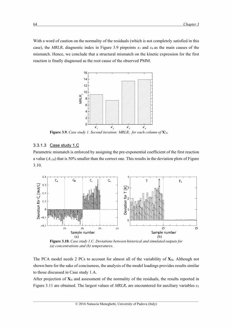
64 Chapter 3
______________________________________________________________________________________________ © 2016 Natascia Meneghetti, University of Padova (Italy)
With a word of caution on the normality of the residuals (which is not completely satisfied in this
case), the MRLRv diagnostic index in Figure 3.9 pinpoints x3 and x4 as the main causes of the
mismatch. Hence, we conclude that a structural mismatch on the kinetic expression for the first
reaction is finally diagnosed as the root cause of the observed PMM.
Figure 3.9. Case study 1. Second iteration: MRLRv for each column of X'Π.
3.3.1.3 Case study 1.C
Parametric mismatch is enforced by assigning the pre-exponential coefficient of the first reaction
a value (A1,M) that is 50% smaller than the correct one. This results in the deviation plots of Figure
3.10.
(a) (b) Figure 3.10. Case study 1.C. Deviations between historical and simulated outputs for (a) concentrations and (b) temperatures.
The PCA model needs 2 PCs to account for almost all of the variability of XM. Although not
shown here for the sake of conciseness, the analysis of the model loadings provides results similar
to those discussed in Case study 1.A.
After projection of XΠ and assessment of the normality of the residuals, the results reported in
Figure 3.11 are obtained. The largest values of MRLRv are encountered for auxiliary variables x5
x'1
x'2
x'3
x'4
0
2
4
6
8
10
12
14
16
MR
LRv
Devi
atio
n fo
r T [K
]

A methodology to diagnose process/model mismatch in FP models for steady-state systems 65
______________________________________________________________________________________________ © 2016 Natascia Meneghetti, University of Padova (Italy)
and x8, which both depend on R1 as well as on FV R / ; however, the mismatch cannot be attributed
to FVR / because MRLRv is not large for either x6 or x9. Therefore, it can be concluded that the
observed PMM is most probably caused by mismodeling of the first reaction kinetics. Whether
this is a parametric or a structural mismatch is impossible to state at this point.
Figure 3.11. Case study 1.C. MRLRv for each column of XΠ.
To provide further insight, the following new set of auxiliary variables is defined on the basis of
the first reaction kinetic expression:
BAaa CxCx
RT
Ex
RT
EAx
43
1,2
1,11 ';';';exp' (3.19)
and new model matrix M'X [25×4] and process matrix 'X [25×4] are built. The loadings of the
PCA model on M'X and the MRLRv values are shown in Figure 3.12.
(a) (b) Figure 3.12. Case study 1.C. Second iteration: (a) loadings on PC1 and PC2 and (b) MRLRv for each column of X'Π.
x1
x2
x3
x4
x5
x6
x7
x8
x9
x10
x11
0
10
20
30
40
MR
LRv
x'1
x'2
x'3
x'4
-0.8
-0.6
-0.4
-0.2
0.0
0.2
0.4
0.6
0.8
Loa
ding
s
PC1 PC2
x'1
x'2
x'3
x'4
0
2
4
MR
LR
v

66 Chapter 3
______________________________________________________________________________________________ © 2016 Natascia Meneghetti, University of Padova (Italy)
The results in Figure 12b clearly show that 3'x and 4'x negligibly contribute to the mismatch.
Hence, the mismatch is not due to a structural inadequacy of the kinetic expression; conversely,
it is due to a parametric error, as shown by the large contributions provided by 1'x and 2'x .
However, since the latter two auxiliary variables are strongly correlated, it is not possible to
decouple the effect of A1 from that of Ea,1. In conclusion, the proposed diagnosing methodology
correctly points to a parametric mismatch in the first kinetic expression, although the correlation
between parameters hinders unambiguous detection of the PPM origin.
3.4 Example 2: solids milling unit
3.4.1 Process and historical dataset
A solids milling unit is considered as the second test bed for the proposed methodology, where
the mill is used to reduce the mean particles size of a granulated polymer.
The process is described by the mass and population balances on the solid distributed phase.
Assuming to process a given amount of material, with an inlet particle size distribution PSDin, the
population balance equation on mass basis is (Vogel and Peukert, 2005):
max
0
),()(d),(),()(),(
y
BB tyMyPztzMzybzPy
tyM , (3.20)
where the change of the particle mass M of a certain size y is given by the mass leaving the size
band as fragments (second addendum on the right term in (3.20) and the mass entering the size
band as fragments from larger size z (integral term in Eq. 3.20). Two key quantities are
considered: the grinding rate selection function PB and the breakage function b. Different
empirical formulations for the breakage and selection functions are available in the literature. The
one suggested by Vogel and Peukert (2005) is used in this study:
),(),(
, '
'tanh1
2
1yzb
y
yzB
y
yy
y
zB
q
(3.21)
min,kin,Matexp1 mmB WWkzfP (3.22)
dcvq . (3.23)
Note that PB and b depend on several parameters (fMat, Wm,kin, Wm,min, q, k; Table 3.5), which are
specific of the type of the polymer involved. The parameter values used to obtain the process

A methodology to diagnose process/model mismatch in FP models for steady-state systems 67
______________________________________________________________________________________________ © 2016 Natascia Meneghetti, University of Padova (Italy)
results are those reported by Vogel and Peukert (2005) and their values are listed in Table B.4 of
Appendix B. The gSOLIDS® 3.0 (Process Systems Enterprise Ltd, London, UK, 2013) package
is used to simulate the system.
Table 3.5. Example 2: variables and parameters.
Parameters and derived variables
Measured variables in the historical dataset
Inputs Outputs c Parameter PSDin Inlet particle size
distribution PSDout Outlet particle size
distribution d Parameter v Mill rotational
velocity
fMat Mass based material strength parameter
bulk Bulk density
k Number of impacts q Power law exponent y’ Fragment size for
additional fading
Wm,kin Mass specific impact energy
Wm,mi
n Mass specific threshold energy
The historical dataset consists of N = 15 samples obtained for different combinations of the
following variables: inlet material particle size distribution PSDin (in terms of mean particle
diameter Din and standard deviation σin), bulk density ρbulk, mill rotational velocity v. Different
the values of the parameters fMat, Wm,kin, Wm,min are also considered, assuming to process 4 different
solid-phase polymers. The only measured output is the outlet PSD (PSDout). The range of the input
and output variables in the historical dataset are reported in Table B.3 of Appendix B.
3.4.2 Application of the methodology and results
As discussed previously, the only measured output is the outlet PSD, and diagnosing the PMM
by looking at a single output represents an additional challenge for the proposed methodology.
Note that the solution of Eq. (3.20) for this distributed-parameter system requires discretizing the
integration range. To this purpose, the analyzed size range (from 10·m to 8000·m) is
partitioned into B = 40 bins, each one corresponding to a different particle size. Therefore, the
change of particle mass in the discrete size band b ( bm ) during a grinding step is (Vogel and
Peukert, 2005):
jbjbjbiBb
i
jjBjbjb BBbPmPbmm ,,1,,
1
1,, with
, (3.24)

68 Chapter 3
______________________________________________________________________________________________ © 2016 Natascia Meneghetti, University of Padova (Italy)
where k = 1 is assumed. The particle size distribution vector m is obtained by considering all size
bands. The final particle size distribution mout resulting after a grinding step is calculated from:
mmm inout , (3.25)
where min is estimated from the known PSDin.
By inspection of Eq. (3.24), V = 5 auxiliary variables are defined for each bin b as:
1
1,,3
5
1
1,2
,4,1
)(
)()(
)()(
b
jjBjbj
out
b
jjb
bBbbB
Pbmb
PSDbbb
PmbPb
x
xx
xx
. (3.26)
Note that the auxiliary variables are vectors of dimension B, because each of them takes a different
value within each bin. Also note that, generally speaking, the definition of the auxiliary variables
may change according to how the model equations are solved numerically.
Since, for each auxiliary variable, all B bins and all I samples are spanned, the process and the
model matrices take the form of three-way arrays of dimension [I × V × B], as illustrated in Figure
3.13. These arrays are denoted with X and XM, respectively.
Figure 3.13. Example 2: unfolding of the three-way array X resulting from the auxiliary variables in Equation set (30).
In order to account for the contribution of each bin simultaneously, multi-way PCA (MPCA,
Nomikos and MacGregor, 1994) is employed instead of PCA. MPCA is equivalent to performing
a PCA on the two-dimensional (2D) matrix X formed by unfolding X sample-wise, i.e. by putting
side by side each vertical slice of X, where each slice corresponds to a different auxiliary variable
I samples
V auxiliaryvariables
B bins
V ·B variables
X
auxiliaryvariable 1
auxiliaryvariable 2
auxiliaryvariable V
I samplesUNFOLDING
X

A methodology to diagnose process/model mismatch in FP models for steady-state systems 69
______________________________________________________________________________________________ © 2016 Natascia Meneghetti, University of Padova (Italy)
(Figure 3.13). The resulting 2D matrix X has dimension [I × (V∙B)], and each column of X
represents the value of a given auxiliary variable within a given bin across all samples. This
unfolding procedure is applied to both X and XM, so that XΠ and XM are obtained; both matrices
have dimension [15×200]. Note that, since PSDout is the only measured output, the process and
model matrices turn out to be equal except for the columns that correspond to auxiliary variable.
Three case studies are considered in the following, including three different sources of parametric
mismatch (Table 3. 2).
3.4.1.1 Case study 2.A
Parametric mismatch is enforced by assigning parameter Wm,kin values that are 30% smaller than
the actual values (Table B.3 of Appendix B). Note that Wm,kin, which is related to the mass specific
impact energy, affects the grinding rate selection function and depends on the type of material
processed.
An MPCA model is built on XM (step 2), using 9 PCs (however, 8 PCs might also be appropriate;
Table B.5 of Appendix B). After projecting XΠ onto this model and assessing the normality of
distribution of the residuals of XM, MRLRv is calculated for each column of XΠ. The results
obtained are illustrated in Figure 3.14, where, in order to simplify the graphical interpretation of
the results, the MRLRv values are grouped according to the auxiliary variables they originate from.
Figure 3.14. Case study 2.A. MRLRc for each column of XΠ. The columns are grouped according to the auxiliary variables they originate from; each bar within an auxiliary variable refers to a different bin.
Figure 3.14 shows that auxiliary variables x1 and x5 have the largest MRLRv values. Since x5
directly relates to values of PSDout in each bin (Eq. set 3.26), its high residuals simply indicate the
existence of PMM. Auxiliary variable x1 directly relates to the grinding rate selection function.
Hence, it is diagnosed that the observed PMM is due to an inconsistent grinding rate selection
function, but it is not possible to identify whether the mismatch is due to a wrong estimation of
some of the parameters included in this function or to an inappropriate function itself. In the
MRL
R v
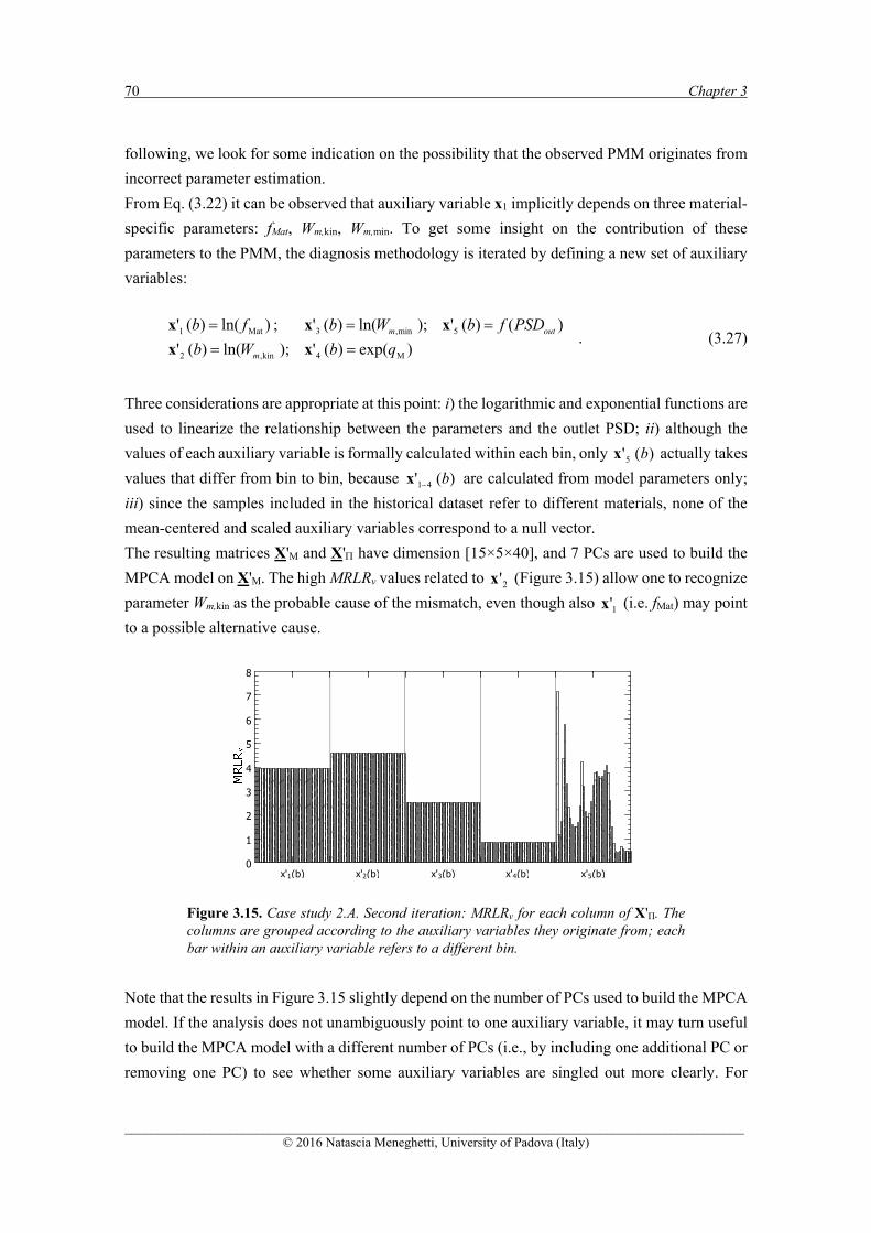
70 Chapter 3
______________________________________________________________________________________________ © 2016 Natascia Meneghetti, University of Padova (Italy)
following, we look for some indication on the possibility that the observed PMM originates from
incorrect parameter estimation.
From Eq. (3.22) it can be observed that auxiliary variable x1 implicitly depends on three material-
specific parameters: fMat, Wm,kin, Wm,min. To get some insight on the contribution of these
parameters to the PMM, the diagnosis methodology is iterated by defining a new set of auxiliary
variables:
)exp()(');ln()('
)()(');ln()(';)ln()('
M4kin,2
5min,3Mat1
qbWb
PSDfbWbfb
m
outm
xx
xxx . (3.27)
Three considerations are appropriate at this point: i) the logarithmic and exponential functions are
used to linearize the relationship between the parameters and the outlet PSD; ii) although the
values of each auxiliary variable is formally calculated within each bin, only )('5 bx actually takes
values that differ from bin to bin, because )(' 41 bx are calculated from model parameters only;
iii) since the samples included in the historical dataset refer to different materials, none of the
mean-centered and scaled auxiliary variables correspond to a null vector.
The resulting matrices X'M and X' have dimension [15×5×40], and 7 PCs are used to build the
MPCA model on X'M. The high MRLRv values related to 2'x (Figure 3.15) allow one to recognize
parameter Wm,kin as the probable cause of the mismatch, even though also 1'x (i.e. fMat) may point
to a possible alternative cause.
Figure 3.15. Case study 2.A. Second iteration: MRLRv for each column of X'Π. The columns are grouped according to the auxiliary variables they originate from; each bar within an auxiliary variable refers to a different bin.
Note that the results in Figure 3.15 slightly depend on the number of PCs used to build the MPCA
model. If the analysis does not unambiguously point to one auxiliary variable, it may turn useful
to build the MPCA model with a different number of PCs (i.e., by including one additional PC or
removing one PC) to see whether some auxiliary variables are singled out more clearly. For
0
1
2
3
4
5
6
7
8
x'1(b) x'2(b) x'3(b) x'4(b) x'5(b)
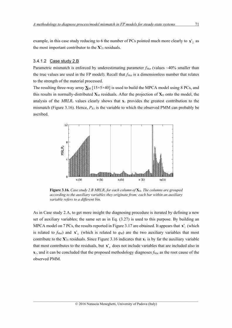
A methodology to diagnose process/model mismatch in FP models for steady-state systems 71
______________________________________________________________________________________________ © 2016 Natascia Meneghetti, University of Padova (Italy)
example, in this case study reducing to 6 the number of PCs pointed much more clearly to 2'x as
the most important contributor to the X' residuals.
3.4.1.2 Case study 2.B
Parametric mismatch is enforced by underestimating parameter fMat (values ~40% smaller than
the true values are used in the FP model). Recall that fMat is a dimensionless number that relates
to the strength of the material processed.
The resulting three-way array XM [15×5×40] is used to build the MPCA model using 8 PCs, and
this results in normally-distributed XM residuals. After the projection of XΠ onto the model, the
analysis of the MRLRv values clearly shows that x1 provides the greatest contribution to the
mismatch (Figure 3.16). Hence, PB,i is the variable to which the observed PMM can probably be
ascribed.
Figure 3.16. Case study 2.B MRLRv for each column of XΠ. The columns are grouped according to the auxiliary variables they originate from; each bar within an auxiliary variable refers to a different bin.
As in Case study 2.A, to get more insight the diagnosing procedure is iterated by defining a new
set of auxiliary variables; the same set as in Eq. (3.27) is used to this purpose. By building an
MPCA model on 7 PCs, the results reported in Figure 3.17 are obtained. It appears that 1'x (which
is related to fMat) and 4'x (which is related to qM) are the two auxiliary variables that most
contribute to the X' residuals. Since Figure 3.16 indicates that x1 is by far the auxiliary variable
that most contributes to the residuals, but 4'x does not include variables that are included also in
x1, and it can be concluded that the proposed methodology diagnoses fMat as the root cause of the
observed PMM.

72 Chapter 3
______________________________________________________________________________________________ © 2016 Natascia Meneghetti, University of Padova (Italy)
Figure 3.17. Case study 2.B. Second iteration: MRLRv for each column of X'Π. The columns are grouped according to the auxiliary variables they originate from; each bar within an auxiliary variable refers to a different bin.
3.4.1.3 Case study 2.C
Parametric mismatch is enforced by overestimating (by ~50%) the true q parameter. Note that q
denotes the power law exponent within the breakage function, and it depends on the mill rotational
velocity.
Application of the proposed methodology (with 9 PCs used to build the MPCA model) leads to
the results illustrated in Figure 3.18. Again, x1 is identified as the strongest contributor to the X
residuals. However note that, differently from Case studies 2.A and 2.B, auxiliary variable x5,
which is the variable on which the PMM is expected to show up, does not exhibit a significant
contribution to the residuals. Hence, this first iteration of the diagnosing methodology suggests
that for this case study the MRLRv index may not be able to identify the origin of the PPM, as the
PPM itself is not clearly noticeable from the residuals.
Figure 3.18. Case study 2.C MRLRc for each column of XΠ. The columns are grouped according to the auxiliary variables they originate from; each bar within an auxiliary variable refers to a different bin.
0
1
2
3
4
5
6
x'1(b) x'2(b) x'3(b) x'4(b) x'5(b)
MRL
R v

A methodology to diagnose process/model mismatch in FP models for steady-state systems 73
______________________________________________________________________________________________ © 2016 Natascia Meneghetti, University of Padova (Italy)
In fact, after building an MPCA model (on 7 PCs) on X'M and projecting X' onto it results in
Figure 3.19, no definitive conclusions can be taken in this case with respect to the origin of the
PMM: although the contribution of x'4 (hence qM) is somewhat larger than that of the other
auxiliary variables, this is not enough to unambiguously point to that parameter as the one that
needs to be adjusted to enhance the FP model performance. It is worth noticing that qM has a
smaller impact on the outlet PSD with respect to the other parameters analyzed, and this makes
the PMM diagnosis harder in this case study.
Figure 3.19. Case study 2.C. Second iteration: MRLRc for each column of X'Π. The columns are grouped according to the auxiliary variables they originate from; each bar within an auxiliary variable refers to a different bin.
3.5 Conclusions
In this Chapter, a methodology has been proposed to diagnose the causes of the process/model
mismatch that may arise when a first-principles process model is challenged against a set of
historical experimental data. The objective was to identify which model equations or model
parameters most contribute to the mismatch, without carrying out any additional experiment.
The methodology exploited the available historical dataset and a simulated dataset, generated by
the FP model using the same inputs as those of the historical dataset. Auxiliary variables were
defined as appropriate nonlinear combinations of the model variables and parameters and of the
process variables. The auxiliary variables were collected in two matrices, whose correlation
structure was compared using a multivariate statistical technique, namely principal component
analysis. Diagnostic indices were coupled to engineering judgment to pinpoint the model
equations or model parameters that most contributed to make the correlation structures of the two
matrices inconsistent, hence to determine the observed PMM.
Two simulated case studies at increasing level of complexity were used to assess the effectiveness
of the proposed methodology: a jacketed continuos stirred tank reactor and a solids milling unit.
0
1
2
3
x'1(b) x'2(b) x'3(b) x'4(b) x'5(b)

74 Chapter 3
______________________________________________________________________________________________ © 2016 Natascia Meneghetti, University of Padova (Italy)
In both cases, the proposed methodology was generally effective in diagnosing the root cause of
the observed mismatch.
There are several areas where further investigation should be carried out. First, appropriate
confidence limits should be defined when the residuals distribution is not found to be normal.
Additionally, the MRLRv index could be complemented with other diagnostic indices.
Furthermore, analyzing the shape of the MRLRv profiles (and not only their average values) might
prove useful to gain additional diagnostic indications. Finally, the effectiveness of the proposed
methodology should be assessed for a wider range of structural mismatches, as well as for a
combination of parametric and structural mismatches, and the methodology itself should be
challenged against real-world systems. Nevertheless, the proposed methodology provides a very
promising approach to the enhancement of FP models by systematic use of the information that
is hidden within historical databases. By facilitating the diagnosis of the PMM root causes, any
additional experimental effort, which may be needed to enhance the FP model performance, can
be targeted much more appropriately, and the overall need for experimental campaigns can
therefore be reduced.
______________________________________________________________________________________________ © 2016 Natascia Meneghetti, University of Padova (Italy)
Chapter 4
First-Principles Model Diagnosis in Batch Systems by Multivariate Statistical
Modeling*
In this Chapter, the methodology proposed in Chapter 3 to diagnose the root cause of the mismatch
in steady-states models is extended to dynamic models, considering a simulated batch drying
process and a simulated penicillin fermentation process to test the proposed methodology. The
likely sources of the mismatch are identified using a multivariate statistical model and analyzing
the model residuals as well as the scores shifts. The importance of considering the entire evolution
of a process in the diagnosis of a PMM is also discussed. Different examples are reported to
demonstrate the effectiveness of the proposed methodology.
4.1 Introduction
When a first-principles (FP) model is challenged against a historical dataset, the model outputs
may not match the historical evidence with the desired accuracy, and process/model mismatch
(PMM) occurs. In Chapter 3, a methodology has been proposed to diagnose the root causes of
PMM by exploiting the available historical dataset and a simulated dataset, generated by the FP
model using the same inputs as those of the historical dataset. A data-driven (DD) model (namely,
a multivariate statistical model) is used to analyze the correlation structure of the historical and
simulated datasets, and information about from where the PMM originates is obtained using
diagnostic indices and engineering judgment. The methodology was developed for steady-states
processes. However, for dynamic processes the diagnosis of an observed PMM is more difficult
because of the time-varying nature of the measurements, which imply data auto-correlation and
cross-correlation, as well as a more strongly nonlinear behavior that may be difficult to capture
using a linear multivariate model.
* Excerpts from this Chapter have been published in :Meneghetti, N., P. Facco, S. Bermingham, D. Slade, F. Bezzo, M. Barolo (2015). First-principles model diagnosis in batch systems by multivariate statistical modeling. In: Computer-Aided Chemical Engineering 37 (K.V. Gernaey, J.K. Huusom, R. Gani, Eds.), Elsevier, Amsterdam (The Netherlands), 437-442.
76 Chapter 4
______________________________________________________________________________________________ © 2016 Natascia Meneghetti, University of Padova (Italy)
In this Chapter, the PMM diagnosis methodology is extended to batch systems, using a simulated
semi-batch solids drying process and a simulated penicillin fermentation process as test beds. In
the first case study, multi-way principal component analysis (MPCA; Nomikos and MacGregor,
1994) is employed as a DD model, enhancing it with an orthogonal rotation (VARIMAX rotation)
of the principal directions (Magnus and Neudecker, 1999; Wang et al., 2005). In the second case
study, the comparison of the results obtained considering only the final measurements of a batch
or the entire trajectories is also provided. Two different examples for both case studies are
analyzed to discuss the ability of the proposed methodology to point to the FP model sections
needing improvement.
4.2 Case study 1
4.2.1 Process description and available data
A simulated lab-scale drying process is considered, in which hot dry air flows through a bed of
wet solid alumina granules, partially evaporating the water contained in the particles. The model
equations derive from the work of Burgschweiger and Tsostas (2002), and are solved in the
gSOLIDS® modeling environment (gSOLIDS®, Process Systems Enterprise Ltd, London, UK,
2014). The particle size distribution is discretized in 10 bins and no shrinkage of particles is
considered. The global mass and energy balances for the particulate phase and vapor phase
(indicated by subscripts p and vap, respectively) are:
pidryingout
pioutp
inpi
inp
pi RxFxFdt
dM,,,,
, , (4.1)
pdryingoutp
outp
inp
inp
p HhFhFdt
dH, , (4.2)
pidryingout
vapiout
vapin
vapiin
vap
vapi RxFxFdt
dM,,,,
, , (4.3)
pdryingoutvap
outvap
invap
invap
vap HhFhFdt
dH, , (4.4)
where F is the mass flowrate, h is the specific enthalpy, xi is the mass fraction of species i in the
solid phase (alumina or water) or in the vapor phase (dry air or water), and superscripts in and out
refer to the bed inlet and outlet, respectively. The drying rate pidryingR ,, is given by:
ibulkieqiciippidrying YYkAR ,,,,, , (4.5)
First-principles models diagnosis in batch systems by multivariate statistical modeling 77
______________________________________________________________________________________________ © 2016 Natascia Meneghetti, University of Padova (Italy)
and pdryingH , is the enthalpy change rate due to drying. In (4.5), Ap is the particle surface area
available for drying, ρi is the density of the gas phase, kc is the mass transfer coefficient, and ieqY ,
and ibulkY , are respectively the equilibrium and actual dry-basis moisture content of the water in
the gas phase. Finally, νi is the normalized single-particle drying rate, which can be estimated
from the experimental drying curve. The latter is a function of the normalized moisture content
ηi, which is in turn calculated from the dry basis moisture content Xi, the equilibrium dry-basis
moisture content Xeq,i (which is a function of the relative humidity i ), and the critical dry basis
moisture content Xcr,i. Details on the values of model parameters are reported in the original work
of Burgschweiger and Tsostas (2002). This FP model will be referred to as “the process” in the
following.
A set of N = 25 batches, representing the historical dataset, are simulated using different
combinations of the following measurable inputs: inlet solid mass flowrate ( inpF ), initial moisture
content (Xin), inlet mass flowrate ( invapF ), and air temperature ( in
vapT ). It is assumed that four
measurable outputs exist: moisture content in the granules (Xi), granules temperature ( outpT ), outlet
air temperature ( outvapT ), and outlet air relative humidity ( i ). The batch length is 1420s and the
measurement interval is 30 s; hence, T = 48 samples are available for each measured variable in
each batch.
The PMM diagnosis methodology is tested by considering two process models that use the same
set of equations as described above, but where two different parametric mismatches are purposely
introduced. These sets of equations and (wrong) parameters will be referred to as “the model” in
the following.
4.2.2 Proposed methodology
In order to diagnose the root-cause of an observed PMM, the framework proposed by in Chapter
3 is applied. However, appropriate adjustments are introduced to deal with dynamic data.
According to the proposed rationale, a DD model (namely, a latent variable model) is first
developed to model the correlation structure of appropriate combinations of the simulated process
variables, these combinations being suggested by the FP model structure. Then, it is assessed
whether the combinations of the same variables, but calculated from the historical measurements,
conform to this correlation structure. Finally, from the analysis of some model diagnostic indices,
engineering knowledge is used pinpoint the FP model sections that are mostly responsible for the
observed PMM. In detail, the following steps are followed (subscripts Π and M refer to the
process and to the model, respectively).
1. Auxiliary data designation. A set of V= 9 auxiliary variables is defined considering the model
equation terms that, according to engineering judgment, are expected to be possibly related
to the observed PMM:

78 Chapter 4
______________________________________________________________________________________________ © 2016 Natascia Meneghetti, University of Padova (Italy)
iieq
iici
vapiP
tnxtnxXtnx
Xtnxktnxtnx
TtnxtnxAtnx
),(),(),(
),(),(),(
),(),(),(
963
8,52
741
, (4.6)
where (n, t) of the [N×T] matrix Xv is indicated by ),( tnxv and represents the v-th auxiliary
variable evaluated at time t for batch n. In (4.6) i refers to water and α is the heat transfer
coefficient involved in the calculation of the energy balances. The simulated and historical
datasets are separately used to estimate the values of the auxiliary variables. The values taken
by the auxiliary variables throughout the whole batches are arranged in the [N×V×T] arrays
XM and XΠ, which are the model matrix and the process matrix, respectively.
Note that the values taken by some auxiliary variables (x1, x2, x4, x5 and x6) are bin-dependent.
However, only the bin including the largest number of particles is considered for their
calculation. Also note that variables Tvap, Xi and ϕi (which can be measured) are purposely
included in the auxiliary variable set (x7, x8 and x9) to make the available measurements
directly affect the correlation structures of XM and XΠ.
2. Data-driven model development. An MPCA model (Nomikos and MacGregor, 1994) is built
from XM. MPCA is equivalent to performing PCA (Jackson, 1991) on the [N×(V·T)] matrix
XM obtained by unfolding XM batch-wise. Also XΠ is unfolded (to XΠ), and both XM and XΠ
are autoscaled on the mean and standard deviation of XM. PCA decomposes XM as the sum
of A scores ti and A loadings pi, where A is the number of principal components (PCs) that
describe an adequate percentage of the dataset variability:
M
T
MMMM,M,M,2M2,M,1M1,M EPTEptptptX AA , (4.7)
where TM [N×A] is the scores matrix and PM [(V·T) ×A] is the loadings matrix In both
examples, 4 PCs are selected. Note however that the selected number of PCs can affect the
ability of the methodology to effectively diagnose an observed PMM. How to provide a
general guideline for the selection of A is still under investigation.
In this challenging case study, most of the auxiliary variables are very strongly correlated
and provide similar contributions along all latent directions, thus confounding the analysis.
In order to amplify the contribution of each auxiliary variable on one latent direction only,
the VARIMAX rotation is applied (Magnus and Neudecker 1999; Wang et al., 2005). This
technique uses an orthogonal rotation to transform the MPCA model space so that only a
subset of the auxiliary variables show high weight values along each PC. Upon VARIMAX
application, the residuals matrix EM is not modified, but can be calculated also from:
EPTX var,var, , (4.8)

First-principles models diagnosis in batch systems by multivariate statistical modeling 79
______________________________________________________________________________________________ © 2016 Natascia Meneghetti, University of Padova (Italy)
where Tvar,M and Pvar,M are (respectively) the scores and loadings matrices obtained by
application of the VARIMAX rotation.
3. Process matrix projection. XΠ is projected onto the rotated MPCA model space and the
residuals matrix EΠ is calculated as:
EPTXPXT TMvar,var,var,var, , , (4.9)
4. Mismatch diagnosis. The mismatch may appear in the MPCA model as a large residual value
or as a shift in the scores space (or both). For this reason, a mismatch analysis should evaluate
both these aspects.
The residuals analysis is performed by comparing EM and EΠ to identify the auxiliary
variables that are most responsible for the inconsistency in the correlation structures of UM
and UΠ. These auxiliary variables, together with engineering judgment, are used to pinpoint
which model sections are likely the cause of the observed PMM. In order to reduce the
residuals contribution due to the fraction of data variability not described by the MPCA
model, the results of residuals analysis are expressed using the mean residuals-to-limit ratio
(MRLR), i.e. the mean of the ratios between the residuals of each column of EΠ and the
corresponding 95 % confidence limit, calculated considering a normal distribution of the
residuals for each variable (Eq. 3.4, Chapter 3; Choi and Lee, 2005).
An analysis of the scores shift can be performed by jointly analyzing Tvar,M, Tvar,Π and Pvar,M.
For each PC, the scores shift is calculated as )( var,,varM,, aa tt , i.e., as the difference between
the model matrix scores and the process matrix scores. The rationale beyond this approach
is to identify the auxiliary variables that most affect the scores shift. These variables are
identified by analyzing the MPCA model loadings along the direction that most contributes
to the shift. To this purpose, the use of the VARIMAX rotation is particularly effective, as it
allows one to emphasize the contribution of a single auxiliary variable (or very few of them)
along each PC. The information obtained by this analysis may reveal particularly useful
when a small-dimension historical dataset is available.
4.2.2.1 Results for Example 1.A
The mismatch is forced by altering the value of the critical moisture content (which is involved
in the calculation of ηi) and results in a relative error of 1.6-17 % in the simulated final dry-basis
particle moisture content. Hence, to correctly diagnose the PMM, the proposed methodology
should point to auxiliary variable X4.
The residuals analysis (not reported for the sake of conciseness) cannot clearly point to the root
cause of the mismatch, since all auxiliary variables have similar and low values of MRLR (high
residuals are actually seen in X3 and X9, but this happens at the very beginning of the batch only).
The scores shift analysis is more effective, instead.

80 Chapter 4
______________________________________________________________________________________________ © 2016 Natascia Meneghetti, University of Padova (Italy)
Figure 4.1a reports the scores shifts for each batch together with the mean shifts through all
batches along each PC. By far the largest shifts are seen along PC2; hence, the auxiliary variables
having a significant weight along this direction are possibly related to the observed PMM. The
[1×(V∙T)] loadings pa,M,var are shown as black bars in Figure 4.1b. It can be seen that PC2 mainly
captures the variability due to model terms X2 and X3, as well as that due to outputs X7 and X9.
Hence, further investigation on the FP model should focus on the X2 and X3 terms. Model
inspection suggests that their values are strongly and directly correlated to X4. Therefore,
according to these considerations, to improve the FP model further investigation on model
sections X2, X3 and X4 should be done. The other model sections (including those representing
heat and mass transfer phenomena) are not likely sources of the observed PMM.
(a) (b)
Figure 4.1. Example 1. (a) Shift of ta,M,var from ta,Π,var for each batch (bars) and mean value of these differences (lines) for each PC. (b) Loadings for each PC obtained by applying the VARIMAX rotation to the MPCA model built on XM.
4.2.2.2 Results for Example 1.B
The mismatch is forced by changing the mass transfer coefficient kc, and results in a 1.3-37 %
error in the simulated final dry-basis particle moisture content. Hence, to correctly diagnose the
PMM, the proposed methodology should point to auxiliary variable X5.
Figure 4.2a reports the results obtained by the residuals analysis. Although, at the very beginning
of the batches, MRLR peaks for auxiliary variables X3 and X9, consistently high MRLR values
along the entire batch lengths are seen only on X1, X5 and X6. These latter auxiliary variables are
therefore regarded as the most responsible ones for the observed PMM. As X1, X5 and X6 refer to
the contact area and to the mass and heat transfer coefficients, their values are strongly correlated,
so that it is difficult to further discriminate their contribution to the PMM.
Figure 4.2b reports the scores shift for each PC. Although the main direction of the scores shift is
along PC1, this is clearly not dominant, because significant shifts occur also along the other
Scor
es s
hift
−2
−1
0
1
2
3
4
5
6
7
Batches25 25 25 25
PC1 PC2 PC3 PC4
−0,1
−0,05
0
0,05
0,1
0,15
0,2
Auxiliary variables1 3 5 7 9 1 3 5 7 9 1 3 5 7 9 1 3 5 7 9
PC1 PC2 PC3 PC4

First-principles models diagnosis in batch systems by multivariate statistical modeling 81
______________________________________________________________________________________________ © 2016 Natascia Meneghetti, University of Padova (Italy)
principal directions. We conclude that several auxiliary variables concur to the shift occurrence,
and the scores shift analysis does not effectively identify a likely PMM source.
To summarize, according to proposed methodology the observed mismatch is not related to model
sections X2, X3 or X4. Conversely, model sections X1, X5 and X6 should be investigated to
improve the FP model performance.
(a) (b)
Figure 4.2. Example 2. (a) MRLR values for each auxiliary variable. (b) Shift of ta,M,var from ta,Π,var for each batch (bars) and mean value of these differences (lines) for each PC.
4.3 Case study 2
4.3.1 Process description and available data
The second case study concerns a simulated fed-batch fermentation process, developed by using
a realistic dynamic model of penicillin fermentation. A detailed description of the process is
provided by Birol et al. (2002) and Çinar et al. (2003). The process involves two operating stages:
in the first stage the microorganisms grow in a batch culture (consuming oxygen and the initial
substrate) then, in the second stage, the synthesis of the penicillin is performed by operating in a
fed-batch mode. The penicillin is produced in a well-mixed bioreactor, where a control system
keeps the reactor temperature and pH at desired values. The mass balance for each element
(indicated by subscripts p for penicillin, s for substrate, x for biomass and l for dissolved oxygen)
and energy balance of the system are:
dt
dV
V
CCKC
dt
dC p
pxpp
p , (4.10)
dt
dV
V
C
V
FCmC
YC
Ydt
dC ssxxx
sp
pp
x
sx
s //
, (4.11)
−5
0
5
10
15
Batches25 25 25 25
PC1 PC2 PC3 PC4

82 Chapter 4
______________________________________________________________________________________________ © 2016 Natascia Meneghetti, University of Padova (Italy)
dt
dV
V
CC
dt
dC xx
x , (4.12)
dt
dV
V
CCCakCmC
YC
Ydt
dC lfinlllxox
op
pp
x
ox
l ,
*
//
, (4.13)
VCrdt
dV
V
Cr
dt
dQxq
xq 21 , (4.14)
where C stands for concentration, F for flowrate and V for volume. The specific growth rate μ and
the specific penicillin production rate μpp are expressed as:
p
finlfinxop
p
finl
Ifinsfinsp
fins
pppCCk
C
kCCk
C
,,
,
2
,,
, ./
, (4.15)
RT
E
d
RT
E
g
finlfinxox
finl
finsfinxx
finsxdg
ekekCCk
C
CCk
C
k
H
H
k...
][
][1 ,,
,
,,
,
2
1
. (4.16)
Details on the values of model parameters are reported in the original work of Birol et al. (2002).
Note that, this set of differential-algebraic equations represents only a part of the model
implemented in the simulator used to obtain the data (PenSim§) which also includes the pH and
temperature control algorithms. However, in this study it is assumed that the control system is not
affected by errors.
Two plants of different scales are considered. Plant A is a laboratory-scale plant with a culture
volume of 10 L, whereas plant B is a pilot-scale plant with an average culture volume of 100 L.
The two plants have been scaled maintaining the ratio P/V constant. The fermenter temperature
and pH are maintained at the desired value by a PID controller in both plants, and they use the
same settings as indicated by Birol et al. (2002). The reactor temperature is controlled by
manipulating the heating/cooling water flowrate in the reactor jacket, while pH is controlled by
adjusting the concentrated acid/base flowrate entering the reactor. Different initial conditions are
used to simulate the two plants in terms of substrate feed concentration and initial substrate
concentration, aeration rate, and agitation power (Table 4.1), whereas for all the other inputs the
values suggested by Birol et al. (2002) are considered.
It is assumed that the model used validated on the laboratory-scale plant, and that has poor
performance in the representation of the pilot-scale plant. In fact, two different errors have been
§ http://simulator.iit.edu/web/pensim/index.html

First-principles models diagnosis in batch systems by multivariate statistical modeling 83
______________________________________________________________________________________________ © 2016 Natascia Meneghetti, University of Padova (Italy)
introduced in the FP model used to describe the pilot-scale plant to force the presence of a PMM
(Example 2.a and 2.b).
Table 4.1. Case study 2: Values of the input variables used to generate the historical and simulated datasets.
Variables Measurement unit Initial values Substrate feed rate
concentration [g/L] 0.0431; 0.035; 0.037; 0.039;
0.045 Initial substrate concentration [g/L] 5; 8; 11; 17; 20
Aeration rate [L/h] 3; 4.4; 5.8; 7.2; 10 Agitation Power [W] 20; 32; 38; 44; 50
The trajectories of 26 different batches, carried out under different initial conditions in the pilot-
scale plant (namely by the model that simulates the real conditions of the system), have been
compared with the trajectories provided by the model under the same conditions (namely by the
model where an error has been introduced) actually revealing the presence of a PMM. Note that
if the same duration for each batch is maintained, different final concentrations of penicillin are
achieved for the 26 batches considered. Also note that, all the available measurements (Cx, Cp, Cs,
Cl, P (agitation power), V, T, H+(hydrogen ion concentration), Fs) are affected by noise.
For both examples, the analysis have been divided into two steps: first, only the measurements at
the end of the batches have been considered, thus reducing the analysis of the mismatch to that of
a steady-state system; then, the entire trajectories have been analyzed (Figure 4.3). This approach
permits one to assess the importance of considering the process dynamics. For both steps, the
same set of V= 10 auxiliary variables is considered:
xox
ss
RT
E
g
finlfinxox
finl
finsfinxx
finsxx
lxpp
RT
E
dxp
xxlll
CtnxmCtnx
CCtnxekCCk
C
CCk
C
k
H
H
kCtnx
CtnxCtnx
ekCtnxCKtnx
mCtnxCCaktnx
g
d
),(),(
),(...][
][1
),(
),(),(
),(;),(
),(),(
105
0,9
,,
,
,,
,
2
14
83
72
6
*
1
,(4.17)
where element (n, t) of the [N×T] matrix Xv is indicated by ),( tnxv and represents the v-th
auxiliary variable evaluated at time t for batch n. The simulated and historical datasets are
separately used to estimate the values of the auxiliary variables. The values taken by the auxiliary
variables throughout the whole batches are arranged in the [N×V×T] arrays XM and XΠ, which are
the model matrix and the process matrix, respectively.

84 Chapter 4
______________________________________________________________________________________________ © 2016 Natascia Meneghetti, University of Padova (Italy)
Note that some auxiliary variables (x8, x9 and x10) are constituted only by input and output
measurements, and are included in the dataset only to strengthen a different correlation structure
between XM and XΠ. Finally, since the temperature is maintained constant during the entire
process, the terms involved in Eq. (4.14) are not considered in the auxiliary variables set.
Figure 4.3. Case study 2.A. The analysis of the mismatch is split into two steps: in the first step only the measurements at the end of the batches have been considered, whereas in the second step the entire trajectories have been analyzed, by an MPCA model.
4.3.1.1 Results for Example 2.A
In this first example, it is assumed that a mismatch is forced by changing the parameter α (Eq.
4.18) in the calculation of mass transfer coefficient kla, thus assuming that the model
underestimates the mass transfer effectiveness (4.10).
V
Pfk gla . (4.18)
An average change of 90% of this coefficient leads to a variation in the final penicillin
concentration of the batches considered from 1 to 25%. However, note that in the calculation of
x1 of Eq. (4.17), parameter α is that assumed for the model, only the measured variables are
different in XM and XΠ.
In the first step of the analysis, XM and XΠ result to be 2-dimensional matrices [N×V×1], since
they are calculated considering the final measurements (t=300 h) available for the model and the
Isa
mpl
es
V auxiliaryvariables
T time instants
V ·T variables
X
auxiliaryvariable 1
auxiliaryvariable 2
auxiliaryvariable V
Isam
ples
UNFOLDING
X
Isam
ples
V auxiliaryvariables
X
Isam
ple
s
t=300 h X
T time instants V auxiliary
variables
Step 1 analysis att=300h
Step 2 analysis of the entiretrajectory

First-principles models diagnosis in batch systems by multivariate statistical modeling 85
______________________________________________________________________________________________ © 2016 Natascia Meneghetti, University of Padova (Italy)
process, respectively. Following the procedure proposed in Chapter 3 (Section 3.2), a PCA model
is built from XM (previously autoscaled), considering 2 PCs able to capture more than 90 % of
the variability of the data. Then XΠ (scaled on the mean and standard deviation of XM) is projected
onto the latent space described by XM. As stated in Section 4.3, the mismatch may appear in the
PCA model as a large residual value and/or as a shift in the scores space as shown in Figure 4.4a.
This representation clearly shows the different position of the two datasets, both on the score
plane (score shift) and from the score plane (high prediction residuals). The results of the residuals
analysis performed by comparing EM and EΠ through the MRLR index are shown in Figure 4.4b.
The first auxiliary variable (X1), which presents a value of the MRLR index significantly higher
than the other variables, is correctly identified as a possible cause of the mismatch (4.17).
In this case, the shift analysis (not reported for the sake of conciseness) does not permit to clearly
point to the root cause of the mismatch; not even the application of the VARIMAX rotation prevents
all auxiliary variables to have similar loadings on the first latent direction presenting the higher
scores shift.
(a) (b)
Figure 4.4. Case study 2.A. (a) Residuals in the scores space for each sample of the model matrix XM and of the process matrix XΠ and (b) MRLRv for each column of XΠ, calculated considering only the final measurements of each batch.
In the second step, XM and XΠ result to be 3-dimensional matrices [N×V×T], since they are
calculated considering the entire trajectories of the samples available for the model and the
process, respectively. Since the process involves a batch and a fed-batch stage, it has been
considered more appropriate to split the analysis of the batch trajectories into two parts, each
corresponding to the two operating stages. However, the time instant, where the switch from batch
mode to fed-batch mode occurs, differs from batch to batch. Therefore, a synchronization of the
batch trajectories before and after the switch point may be useful to adequately compare the
correlation structure of XM and XΠ. There are several synchronization techniques available in
1 2 3 4 5 6 7 8 9 100
10
20
30
40
50
Auxiliary variables
MR
LR
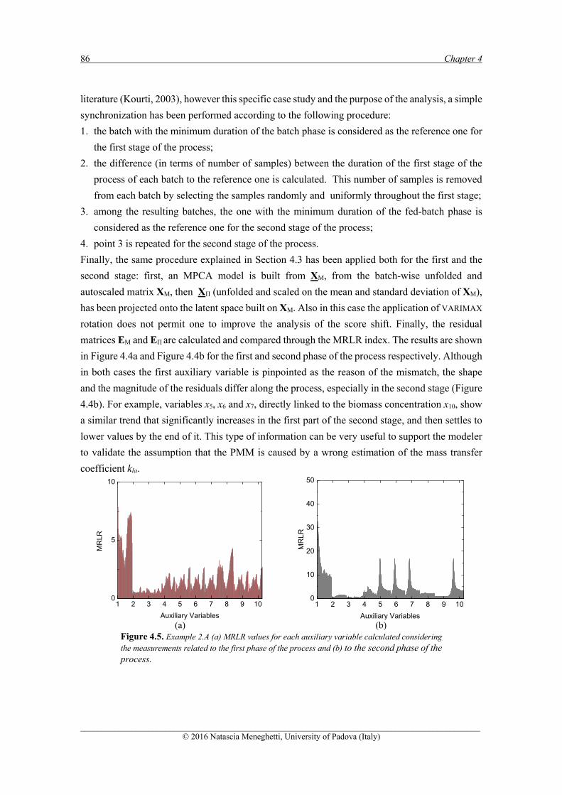
86 Chapter 4
______________________________________________________________________________________________ © 2016 Natascia Meneghetti, University of Padova (Italy)
literature (Kourti, 2003), however this specific case study and the purpose of the analysis, a simple
synchronization has been performed according to the following procedure:
1. the batch with the minimum duration of the batch phase is considered as the reference one for
the first stage of the process;
2. the difference (in terms of number of samples) between the duration of the first stage of the
process of each batch to the reference one is calculated. This number of samples is removed
from each batch by selecting the samples randomly and uniformly throughout the first stage;
3. among the resulting batches, the one with the minimum duration of the fed-batch phase is
considered as the reference one for the second stage of the process;
4. point 3 is repeated for the second stage of the process.
Finally, the same procedure explained in Section 4.3 has been applied both for the first and the
second stage: first, an MPCA model is built from XM, from the batch-wise unfolded and
autoscaled matrix XM, then XΠ (unfolded and scaled on the mean and standard deviation of XM),
has been projected onto the latent space built on XM. Also in this case the application of VARIMAX
rotation does not permit one to improve the analysis of the score shift. Finally, the residual
matrices EM and EΠ are calculated and compared through the MRLR index. The results are shown
in Figure 4.4a and Figure 4.4b for the first and second phase of the process respectively. Although
in both cases the first auxiliary variable is pinpointed as the reason of the mismatch, the shape
and the magnitude of the residuals differ along the process, especially in the second stage (Figure
4.4b). For example, variables x5, x6 and x7, directly linked to the biomass concentration x10, show
a similar trend that significantly increases in the first part of the second stage, and then settles to
lower values by the end of it. This type of information can be very useful to support the modeler
to validate the assumption that the PMM is caused by a wrong estimation of the mass transfer
coefficient kla.
(a) (b) Figure 4.5. Example 2.A (a) MRLR values for each auxiliary variable calculated considering the measurements related to the first phase of the process and (b) to the second phase of the process.
1 2 3 4 5 6 7 8 9 100
5
10
Auxiliary Variables
MR
LR
1 2 3 4 5 6 7 8 9 100
10
20
30
40
50
Auxiliary Variables
MR
LR
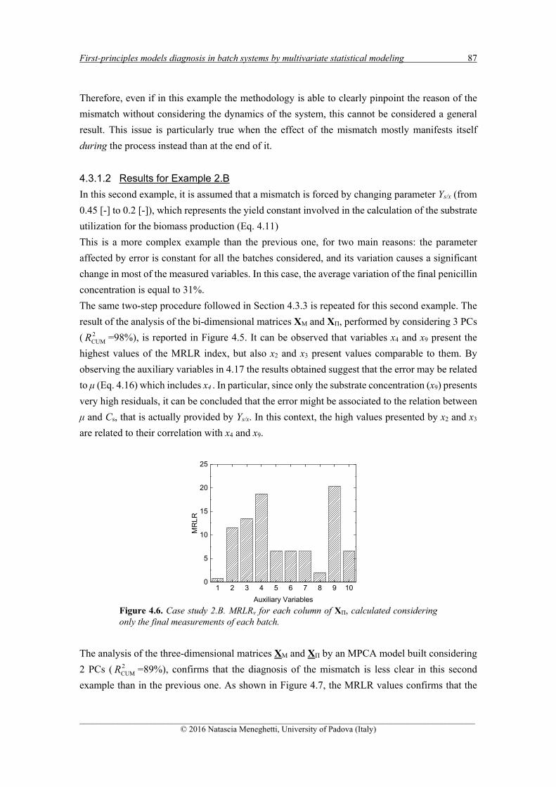
First-principles models diagnosis in batch systems by multivariate statistical modeling 87
______________________________________________________________________________________________ © 2016 Natascia Meneghetti, University of Padova (Italy)
Therefore, even if in this example the methodology is able to clearly pinpoint the reason of the
mismatch without considering the dynamics of the system, this cannot be considered a general
result. This issue is particularly true when the effect of the mismatch mostly manifests itself
during the process instead than at the end of it.
4.3.1.2 Results for Example 2.B
In this second example, it is assumed that a mismatch is forced by changing parameter Ys/x (from
0.45 [-] to 0.2 [-]), which represents the yield constant involved in the calculation of the substrate
utilization for the biomass production (Eq. 4.11)
This is a more complex example than the previous one, for two main reasons: the parameter
affected by error is constant for all the batches considered, and its variation causes a significant
change in most of the measured variables. In this case, the average variation of the final penicillin
concentration is equal to 31%.
The same two-step procedure followed in Section 4.3.3 is repeated for this second example. The
result of the analysis of the bi-dimensional matrices XM and XΠ, performed by considering 3 PCs
( 2CUMR =98%), is reported in Figure 4.5. It can be observed that variables x4 and x9 present the
highest values of the MRLR index, but also x2 and x3 present values comparable to them. By
observing the auxiliary variables in 4.17 the results obtained suggest that the error may be related
to μ (Eq. 4.16) which includes x4 . In particular, since only the substrate concentration (x9) presents
very high residuals, it can be concluded that the error might be associated to the relation between
μ and Cs, that is actually provided by Ys/x. In this context, the high values presented by x2 and x3
are related to their correlation with x4 and x9.
Figure 4.6. Case study 2.B. MRLRv for each column of XΠ, calculated considering only the final measurements of each batch.
The analysis of the three-dimensional matrices XM and XΠ by an MPCA model built considering
2 PCs ( 2CUMR =89%), confirms that the diagnosis of the mismatch is less clear in this second
example than in the previous one. As shown in Figure 4.7, the MRLR values confirms that the
1 2 3 4 5 6 7 8 9 100
5
10
15
20
25
Auxiliary Variables
MR
LR

88 Chapter 4
______________________________________________________________________________________________ © 2016 Natascia Meneghetti, University of Padova (Italy)
mismatch clearly affects x9, but neither in the first (Figure 4.7a) nor in the second phase (Figure
4.7b) of the process, a single term of the model can be unambiguously identified as the most
responsible of the PMM. However, the analysis of the MRLR values trend confirms that x5, x6,
and x7 are highly correlated (even collinear) with x10, and that, due the high values presented by
x4 and the end of the second phase, this variable may be most related to the PMM. Anyway, in
this case, further investigations are needed to validate this conclusion. In Appendix 4, a different
approach under investigation to solve this problem is presented.
Similar conclusions can be drown also when an error is introduced in the estimation of Ys/p. Due
to the strong correlation existing among the variables considered, it is very difficult to identify a
single cause of the PMM.
(a) (b) Figure 4.7. Example 2.B. (a) MRLR values for each auxiliary variable calculated considering the measurements related to the first phase of the process and (b) to the second phase of the process.
4.4 Conclusions
In this study, the methodology proposed in Chapter 3 to diagnose process/model mismatch has
been extended to dynamic systems using two realistic models as test beds: one for a batch drying
process and one for a penicillin fermentation process. The methodology exploits a set of historical
data and a simulated dataset, generated by the first-principles model using the same inputs as
those of the historical data set. Auxiliary variables were defined as appropriate nonlinear
combinations of the model variables and parameters, as well as of process measurements. A
multiway principal component analysis model was used to analyze the correlation structure of the
historical and simulated datasets. In the first case study, information on the root cause of the PMM
was obtained by the combined analysis of two diagnostic indices: the data-driven model residuals
and the data-driven model scores shifts. With respect to the scores shifts, an orthogonal rotation
of the principal axes was carried out in order to magnify the contribution of the most significant
auxiliary variables to the shifts. In the second case study, a combined analysis of the whole
1 2 3 4 5 6 7 8 9 100
10
Auxiliary Variables
MR
LR
1 2 3 4 5 6 7 8 9 100
5
10
15
20
Auxiliary Variables
MR
LR

First-principles models diagnosis in batch systems by multivariate statistical modeling 89
______________________________________________________________________________________________ © 2016 Natascia Meneghetti, University of Padova (Italy)
trajectories of the available batches and of the measurements taken at the end of each batch,
revealed the importance of considering the dynamics of the system in order to validate the results
obtained by the application of the methodology.
The results obtained show that the proposed methodology is able to direct the first-principles
model improvement efforts towards the model sections that are truly affected by modeling errors.
Further improvements should be directed to solve the problems encountered with strongly
correlated variables, which often make the diagnosis of the mismatch less clear.

______________________________________________________________________________________________ © 2016 Natascia Meneghetti, University of Padova (Italy)
Chapter 5
Bracketing the design space within the knowledge space in pharmaceutical
product development*
When a reliable first-principles model is not available for a new pharmaceutical product to be
developed, the design space (DS) is often found using experiments carried out within a domain
of input combinations (the so-called knowledge space; e.g. raw materials properties and process
operating conditions) that result from products that are similar to the new one, but have already
been developed. In this Chapter, a methodology is proposed that aims at segmenting the
knowledge space in such a way as to identify a subspace of it (called the experiment space) that
most likely brackets the DS, in order to limit the extension of the domain over which the
experiments should be carried out. The methodology relies on the exploitation of historical
information on products that have already been developed and are similar to the new one, and is
based on the inversion of a latent-variable model. Products characterized by a single equality
constraint specification are considered, and the effect of model prediction uncertainty is explicitly
accounted for.
5.1 Introduction
The Quality-by-Design (QbD) initiative launched by the United States Food and Drug
Administration (FDA) (FDA, 2004a) fosters the adoption of science-based (as opposed to
experience-based) methodologies to support the development of new pharmaceutical products,
with the purpose of building quality “by design” into the desired product, i.e. to consistently
deliver a product with the intended performance. The ultimate objective of the QbD initiative is
to promote product and process understanding in pharmaceutical development, in order to
increase both manufacturing flexibility and process robustness (intended as the ability of the
process to tolerate variability of materials and changes in the process conditions and equipment
without negative impact on product quality). Deep understanding on how the critical quality
* Facco, P., F. Dal Pastro, N. Meneghetti, F. Bezzo, M. Barolo (2015). Bracketing the design space within the knowledge space in pharmaceutical product development. Ind. Eng. Chem. Res., 54, 5128–5138.
92 Chapter 5
______________________________________________________________________________________________ © 2016 Natascia Meneghetti, University of Padova (Italy)
attributes and critical process parameters interact is required to achieve this ambitious objective,
and the key concept of design space (DS) was introduced to provide a science-based platform
where this interaction can be investigated.
According to the International Conference on Harmonization (ICH) Q8(R2) Guidance (ICH,
2009), the DS is “the multidimensional combination and interaction of input variables (e.g.,
material attributes) and process parameters that have been demonstrated to provide assurance of
quality”. The DS of the process that manufactures a given product (in short, the DS of that
product) is optionally proposed by the pharmaceutical company at the time of submission of that
product to the regulatory agency, and it is subject to regulatory assessment and approval.
“Working within the design space is not considered as a change” (ICH, 2009), and as such does
not require any further regulatory approval. This is a very important aspect, which offers a
pharmaceutical company the opportunity to continuously improve its manufacturing processes by
reducing the regulatory oversight. In fact, the materials properties and process parameters can be
changed by the company with no restrictions to maximize some performance metric, provided
that their combination falls within the approved DS. Moving outside the design space would
initiate a regulatory post-approval process, instead.
Some additional aspects of the ICH definition of DS are worth emphasizing. Firstly, the DS space
refers to multidimensional combinations of material attributes and process parameters (in this
study, material attributes and process parameters will be generally referred to as process inputs).
The fact that these input combinations are multidimensional implies that the DS should not be
described in terms of proven acceptable ranges for each input**. Instead, how these ranges interact
in a multidimensional space is the very matter of interest of the DS. Second, the input
combinations belonging to the DS should be demonstrated to fulfill some requirements.
“Demonstration” calls for the direct or indirect use of mathematical models to guide some form
of experimental activity, or to interpret or correlate the results obtained from experiments. Models
(either knowledge-driven or data-driven) are the battle-horse of process systems engineering,
which can therefore play a tremendously important role in pharmaceutical product and process
development (Gernaey et al., 2012 and Troup, and Georgakis 2013). Finally, ICH refers to
assurance of quality. Peterson (2008) and Pantelides et al. (2009) noted that, as the DS of a
product is calculated from a model and the model itself is subject to uncertainty, the DS
calculation is probabilistic. Any model-based technique used to calculate the DS of a product can
only determine the probability of a given combination of inputs to belong to the DS. Therefore,
it should be stated what probability is deemed sufficient to provide “assurance” of quality.
How the DS should be determined (or “developed”, following the ICH parlance) and how it
should be described in a submission is not strictly stated or recommended by the FDA. Graphical
** Interestingly, the regulatory documents are not entirely clear in this respect. In fact, while they state that “A combination of proven acceptable ranges does not constitute a design space”, they also state that in a submission “A design space can be described in terms of ranges of material attributes and process parameters” (ICH, 2009).

Bracketing the design space within the knowledge space in pharmaceutical product development 93
______________________________________________________________________________________________ © 2016 Natascia Meneghetti, University of Padova (Italy)
representations in the space of the inputs (such as response surface plots or contour plots) are
reported as demonstrating examples, but “more complex mathematical relationships (…) such as
components of a multivariate model” are accepted as well (ICH, 2009). It should be noted that
representing the DS by means of diagrams in the true input space sets a strong limitation with
respect to the multivariate nature of the DS. In fact, while a bivariate space can be easily captured
by a diagram, a trivariate one would be much harder to interpret at a glance, whereas an input
space of dimension larger than three would be impossible to represent graphically in the input
space. How to calculate the DS have been discussed in some studies. For example, Peterson
(2008) determined the DS using a multiple-response surface prediction model, and he discussed
the DS reliability using a Bayesian approach to account for both the model parameter uncertainty
and the correlation structure of the data. Pantelides et al. (2010) used a first-principles model to
identify the probabilistic DS for a batch reactor with input uncertainty. Following the same ideas,
Close et al. (2014) used a first-principles model coupled with stochastic simulations to generate
probabilistic process design spaces for a chromatography process. Chatzizacharia and
Hatziavramidis (2014) compared three different approaches (response surface, Bayesian, and
artificial neural network) to determine the DS under different data characteristics (complete data
with no uncertainty, data with high uncertainty, and missing data).
Knowledge-driven (i.e., first-principles) models can be extremely useful to describe the complex
and nonlinear relationships between materials properties, process conditions and critical quality
attributes that set the basis for the calculation of the DS. However, developing a reliable first-
principles model can be very challenging in a pharmaceutical industry context. In many cases, the
DS calculation exercise heavily relies on experimentation: a set of experiments is designed and
carried out, and a response (hyper)surface model is then used to fit the experimental evidence
(Troup, and Georgakis 2013; Chatzizacharia and Hatziavramidis, 2014). On some occasions, the
input domain for the designed experiments may be the same used for a set of historical products
that have already been developed and that are in some sense similar to the one under investigation.
This domain corresponds to the so-called knowledge space (MacGregor and Bruwer, 2008;
Jaeckle and Macgregor 1998) of the products already developed and is expected to include the
design space of the new product.†† Spanning by experiments the entire knowledge space may be
very demanding, especially if the number of inputs is large. The experimental effort would be
significantly reduced if one were able to find within which portion of the knowledge space the
DS is likely to lie. In fact, in this case a set of experiments would be designed and carried out
spanning the input combinations that belong to this subspace only. In this Chapter, a methodology
†† However, it should be acknowledged that a set of input combinations may exist, which are very different from any combination used in the manufacturing of historical products, but which would anyway ensure the desired product quality. This set would therefore belong to the DS of the new product, but not to the knowledge space of the historical products. The data-driven approach discussed in this study cannot provide information on this subset of the DS (Jaeckle and Macgregor 1998)

94 Chapter 5
______________________________________________________________________________________________ © 2016 Natascia Meneghetti, University of Padova (Italy)
is proposed that aims at segmenting the knowledge space in such a way as to define a subspace
wherein the DS is likely to be included, thus providing the developer a way to target his/her
experimental efforts within a much smaller domain of input combinations. This subspace will be
called the experiment space. Therefore, the objective is to develop a methodology that can return
an experiment space that is likely to bracket the design space, but is conveniently narrower than
the knowledge space.
To achieve this goal, a data-driven modeling approach is employed. Data-driven models are
usually much simpler to develop than knowledge-driven (first-principles) ones, but their
development requires a fairly large amount of data. This may not be an issue in pharmaceutical
development environments, where historical datasets on products already developed are often
available. Latent-variable (LV) modeling techniques, such as principal component analysis (PCA
Chapter 2, Section 2.1.1) and projection to latent structures (PLS, Chapter 2, Section 2.1.1), are
multivariate statistical tools that can optimally exploit historical datasets. Although these
techniques have long been used as process analytical technology tools only, their potential is much
greater than that. In fact, they are particularly useful to assist the practical implementation of QbD
paradigms, with several successful applications of interest for the pharmaceutical industry
(Tomba et al., 2013a). One particularly useful LV modeling approach is LV model inversion
(Jaeckle and Macgregor 1998; Jaeckle and Macgregor 2000). By inverting an LV model (say, a
PLS model) one can determine the set of inputs (namely, materials properties and process
conditions) that enable one to obtain an assigned output (namely, a product quality property).
Hence, PLS model inversion is strongly related to the determination of the DS of a given product
and could provide an indication of where the experiment space is located (Tomba et al., 2012).
However, since models are subject to uncertainty (Faber and Kowalski, 1997; Zhang and García-
Muñoz 2009), when a PLS model is inverted the uncertainty is backpropagated to the calculated
inputs, hence to the designated experiment space. In this study, we use a latent variable approach
based on PLS model inversion to locate the experiment space inside the knowledge space, under
uncertainty in the PLS model predictions and under the assumption that the desired new product
is characterized by one equality constraint specification. Note that the experiment space will be
identified in the latent variable space, which may enable a clear graphical representation of the
experiment space also when the number of process inputs is large. Within the context of this
study, the model inversion problem will be referred to as a product development problem.
The proposed methodology is tested on three simulated case studies. A nonlinear one-equation
model is first used to provide a clear representation of the true design space and its relationship
with the null space. Then, two systems of greater complexity (large number of inputs) and specific
interest for the pharmaceutical industry are investigated: a dry granulation process by roller
compaction and a wet granulation process.

Bracketing the design space within the knowledge space in pharmaceutical product development 95
______________________________________________________________________________________________ © 2016 Natascia Meneghetti, University of Padova (Italy)
5.2 Mathematical background
5.2.1 PLS model inversion
Usually a PLS model is used in its direct form (Chapter 2, Section 2.1.2); namely, given a set of
input data X [I×N] of I observations (samples) and N variables (e.g., raw materials properties,
process settings, operating conditions), the PLS model is used to predict an associated response
variable Y [I×M] of M responses (e.g., a product quality attribute) according the following model
structure:
ETPptptX
T
1 1
TTA
a
R
Aaaaaa , (5.1)
FTQptptY
T
1 1
TTA
a
R
Aaaaaa , (5.2)
WP
XWT
T . (5.3)
Where the meaning of the symbol is the same of Eqs. (2.10-14) of Chapter 2. When the i-th
observation xi [1×V] of X is projected onto the model, its score vector is:
WP
Wxt
Ti
i . (5.4)
Its prediction and the associated model residual are:
Tˆ Ptx ii , (5.5)
ˆiii uue . (5.6)
Two indices are used to assess the model performance when this observation is projected: the
Hotelling 2
iT statistic (Eq. 2.15) and and the residual SPEi statistic (Eq. 2.16). Under the
assumption of multinormally distributed observations, whether or not ui conforms to the
observations of the calibration dataset can be assessed by comparing 2
iT and iSPE to the
respective confidence limits 2limT (Eq. 2.18) and limSPE (Eq. 2.20). In this study, 95% confidence
limits for the T2 and SPE statistics are always used. Confidence limits can be also considered in
the latent space of the scores in the shape of an ellipsoid whose semi-axis of the a-th LV can be
calculated as in Eq. (2.18).
In this study, univariate responses (M=1) only are considered. Hence, matrix Y degenerates to a
vector y of dimension [N×1], Q degenerates to q [1×A], and F to f [N×1].

96 Chapter 5
______________________________________________________________________________________________ © 2016 Natascia Meneghetti, University of Padova (Italy)
In its inverse form (Chapter 2, Section 2.1.3) , the model can be used to suggest the combination
NEWx of inputs that are needed to obtain a product of desired quality DESy , provided that the
desired quality is (in some sense) similar to the quality of the products included in the historical
dataset (Jaeckle and MacGregor 1998; Jaeckle and MacGregor 2000b). The similarity can be
assessed by testing that DESy conforms to the correlation/covariance structure available in the
historical database that identifies the knowledge space (Jaeckle and MacGregor 2000a) and lies
within the region of variability spanned by the knowledge space (Jaeckle and MacGregor 2000b).
In this study, the analysis is limited to products characterized by a single quality attribute (i.e.,
1)rank( y ) assigned through an equality constraint (i.e., DESyy is the required quality
specification; extension to the case of inequality constraints is straightforward). As explained in
Chapter 2 (Section 2.1.3) assumed as RX the rank of the input matrix X, two cases can be outlined:
the dimension of the latent space of X is the same as the dimension of y (i.e., RX =1) or the
dimension of the latent space of X is greater than the one of y (i.e., RX>1; this is the most frequent
occurrence). In the first case, a unique solution NEWx to the model inversion problem (Eq. 2.28)
exists TNEWNEW Ptx , and from Eq. (5.5-6) NEWNEW xx and 0NEW e . In the second case, the
inversion problem is underdetermined and multiple solutions exist, that give rise to the null space
of dimension (RX - 1), which can be calculated analytically (Jaeckle and MacGregor 2000b) as
reported in Section 2.1.3.1. All the problems considered in this study are characterized by the
existence of a null space. A graphical interpretation of a one-dimensional null space is shown in
Figure 5.1, where the score space for the first two latent variables is reported. The circles represent
the historical data, and the dashed ellipse is the 95% confidence limit obtained from Eq. (2.18).
The projection NEWt of the direct model inversion solution is represented by the triangle. The null
space projection onto the score diagram is a straight line passing through NEWt : if the model is
not affected by uncertainty, all input combinations projecting onto this line are expected to yield
a product with the same quality DESy .
Figure 5.1. Graphical interpretation of the null space in the score space of the first two latent variables of a PLS model. The example model has V = 5 input variables and N = 100 observations.
-6 -4 -2 0 2 4 6-6
-4
-2
0
2
4
6
LV1 score
LV2
scor
e
calibrationtNEW
95% confidence limitnull space

Bracketing the design space within the knowledge space in pharmaceutical product development 97
______________________________________________________________________________________________ © 2016 Natascia Meneghetti, University of Padova (Italy)
The latent space spanned by the input combination projections that yield the products already
manufactured is the knowledge space. It is assumed that a likely projection of the knowledge
space onto the space of the first two LVs is the interior of the confidence ellipse shown in Figure
5.1. The input combinations that lie on the null space line, but do not belong to the knowledge
space, are not represented appropriately by the model. In the following, the words null space will
be referred to the subspace of it that is included within the knowledge space (in Figure 5.1, the
segment included within the ellipse).
Tomba et al. (2012) observed that there is a strong relation between the mathematical concept of
null space and the FDA concept of DS. If the product quality is characterized by equality
constraints only and no uncertainty affects the PLS model, from a practical standpoint the two
concepts are the same. However, if the PLS model is affected by uncertainty, when the model is
inverted the uncertainty is backpropagated to the calculated inputs, i.e. to the calculated null
space. Hence, the existence of uncertainty should be accounted for in the determination of the
experiment space.
5.2.2 Prediction uncertainty in PLS models
Consider a new observation obsx . Its regression through a PLS model generates the predicted
output obsy , which suffers from a mismatch with respect to the actual value obsy that would be
obtained by application of the input combination obsx to the real process. This mismatch is due
to the uncertainty that lie in the model. The main sources of uncertainty are the uncertainty on the
parameters in the model calibration (Martens and Martens, 2000), on the calibration data (Reis
and Saraiva, 2005), and on the predictions (Fernández Pierna et al., 2003; Bu et al., 2013). In this
study, only the prediction uncertainty is considered, although alternative methods exist (Faber,
2002; Reis and Saraiva 2012, Vanlaer et al., 2013).
To characterize the prediction uncertainty on obsy , the approach proposed by Faber and Kowalski
(1997) is followed, who accounted for the errors in the inputs, the errors in the responses, and the
bias in the calculation of the mean-squared prediction error. The same approach was lately drawn
on by Zhang and García-Muñoz (2009).
First, an estimation of the standard deviation s of the prediction error is calculated. Then,
assuming that the estimation error follows a t-statistic, the )%1(100 confidence interval (CI)
on obsy is calculated as:
sy dIobs ,2/tˆCI , (5.7)
where I is the number of the PLS model calibration samples, d is the number of degrees of freedom
used by the model, and is the significance level for the confidence interval. The wider the CI at
98 Chapter 5
______________________________________________________________________________________________ © 2016 Natascia Meneghetti, University of Padova (Italy)
a given significance level, the larger the prediction uncertainty. In this study, we refer to a 95 %
CI. The standard deviation s can be estimated as (Faber and Kowalski, 1997):
Ihs obs
11SE , (5.8)
where hobs is the leverage of the observation:
1
T1
Ih obsobs
obs
tt , (5.9)
SE is the standard error of calibration, which is evaluated as in Zhang and García-Muñoz (2009):
dI
yyI
iii
1
2ˆ
SE , (5.10)
and iy and iy are (respectively) the i-th measured output and the i-th estimated output of the
model calibration dataset. In this study, the number of degrees of freedom is set equal to the
number of latent variables of the PLS model, i.e. Ad (Krämer and Sugiyama, 2011). Other
degrees of freedom selection methods were tested (Van der Voet, 1999; Ye, 1998 ), with no major
changes in the results.
5.3 Bracketing the design space
Assume that historical datasets X and y are available, where X includes the input combinations
that have been used to manufacture products with quality characteristic y. It is required to estimate
the set REALx of process inputs leading to a new product of quality DESy not included in y. Several
different input combinations REALx may yield this product and, according to the ICH definition
and to the univariate equality constraint DESyy , the set REALX including all of these
combinations is the DS of product DESy . We indicate with REALX the subset of REALX whose
projections fall within the knowledge space and therefore that can in principle be described by
the PLS model relating X to y. We would like to estimate REALX by inverting the model. The
model estimate of a true input combination REALREAL Xx is NEWx .
If the model is not affected by uncertainty, the direct model inversion solution projects onto a
score vector NEWt that can move along the null space without affecting the product quality. Stated
differently, according to the PLS model there is an infinite number of input combinations NEWx
that can lead to a product with the same desired quality, and their projections all lie in the null

Bracketing the design space within the knowledge space in pharmaceutical product development 99
______________________________________________________________________________________________ © 2016 Natascia Meneghetti, University of Padova (Italy)
space. Hence, according to the PLS model, the DS of product DESy would be identified with the
null space. However, if the PLS model is affected by prediction uncertainty, DESy is predicted
with uncertainty; when the model is inverted, the prediction uncertainty is backpropagated to the
calculated inputs and therefore the null space calculation itself is affected by prediction
uncertainty. Hence, when prediction uncertainty is present, the DS is not necessarily the null
space.
From a practical point of view, the DS could be determined by carrying out a set of experiments
designed within the knowledge space, and then correlating the experimental results with (say) a
response surface model. However, determining the DS by experimentation within the entire
knowledge space would be impractical due to the number of experiments that may be needed to
account for the variability in all accessible inputs. The experimental effort could be significantly
reduced if the experimental domain were restricted to a subspace of the knowledge space within
which the DS is likely to lie. We call this subspace the experiment space, and in the following we
describe a methodology that is able to return an experiment space that is likely to bracket the
design space, but is conveniently narrower than the knowledge space.
5.3.1 Proposed knowledge space segmentation methodology
The knowledge space segmentation is carried out through the following steps.
Step 1. A PLS model relating X to y trough A latent variables is built using Eqs. (5.1) -
(5.3). Figure 5.1 provides a graphical representation of this model in the space of the first
two latent variables.
Step 2. Using Eqs. (2.28), the PLS model is inverted to determine the input variable
combination NEWx (from Eq. 5.5) that is expected to yield a product having the desired
quality DESy under no prediction uncertainty. The solution of the inversion problem is
obtained in terms of the score vector NEWt (triangle in Figure 5.1).
Step 3. The prediction uncertainty on DESy is evaluated as in Eqs. (5.7-5.10) at
significance level 05.0 , corresponding to %95)1(100 confidence. Figure
5.2a shows the probability density function of the t distribution centered on DESy with
)( AI degrees of freedom. The %95 CI for DESy is highlighted.
Step 4. The PLS model is inverted by direct inversion to project the y values belonging
to the 95% CI onto the latent space of the inputs. For convenience, the CI is discretized
in a subset whose scores TNEW are represented with magenta circles in Figure 5.2b.
Step 5. The null spaces associated to each score vector belonging to TNEW are calculated
(magenta lines in Figure 5.2c). The DS is expected to lie within the intersection between
these null spaces and the knowledge space (gray-shaded area in Figure 5.2d). This
segmented region of the knowledge space is therefore the designated experiment space.
Note that the wider the experiment space at a given confidence level, the wider the input
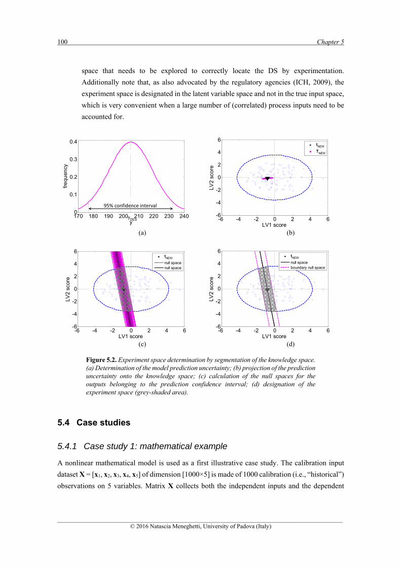
100 Chapter 5
______________________________________________________________________________________________ © 2016 Natascia Meneghetti, University of Padova (Italy)
space that needs to be explored to correctly locate the DS by experimentation.
Additionally note that, as also advocated by the regulatory agencies (ICH, 2009), the
experiment space is designated in the latent variable space and not in the true input space,
which is very convenient when a large number of (correlated) process inputs need to be
accounted for.
(a) (b)
(c) (d)
Figure 5.2. Experiment space determination by segmentation of the knowledge space. (a) Determination of the model prediction uncertainty; (b) projection of the prediction uncertainty onto the knowledge space; (c) calculation of the null spaces for the outputs belonging to the prediction confidence interval; (d) designation of the experiment space (grey-shaded area).
5.4 Case studies
5.4.1 Case study 1: mathematical example
A nonlinear mathematical model is used as a first illustrative case study. The calibration input
dataset X = [x1, x2, x3, x4, x5] of dimension [1000×5] is made of 1000 calibration (i.e., “historical”)
observations on 5 variables. Matrix X collects both the independent inputs and the dependent
170 180 190 200 210 220 230 2400
0.1
0.2
0.3
0.4
y
fre
quen
cy
yDES
95% confidence interval
-6 -4 -2 0 2 4 6-6
-4
-2
0
2
4
6
LV1 score
LV2
scor
e
tNEW
TNEW
-6 -4 -2 0 2 4 6-6
-4
-2
0
2
4
6
LV1 score
LV2
scor
e
tNEW
null spacenull space
-6 -4 -2 0 2 4 6-6
-4
-2
0
2
4
6
LV1 score
LV2
scor
e
tNEW
null spaceboundary null space
Bracketing the design space within the knowledge space in pharmaceutical product development 101
______________________________________________________________________________________________ © 2016 Natascia Meneghetti, University of Padova (Italy)
inputs. The independent inputs x1 and x2 are random Gaussian distributions. For any observation n, the dependent inputs 3,nx , 4,nx and 5,nx are defined as:
2,1,5,
22,4,
21,3,
nnn
nn
nn
xxx
xx
xx
(5.11)
The calibration response dataset y [1000×1] is built on the following model:
55443322110 xxxxxy kkkkkk , (5.12)
where: ]12.0;1.1;0064.0;022.0;3.4;0.21[];;;;;;[ 6543210 kkkkkkk .
Table 5.1 reports the calculated means and standard deviations for the x’s and for y included in
the historical datasets.
Table 5.1. Case study 1: characterization of the input and output calibration datasets.
Variable Mean Std. dev. x1 41.73 16.07 x2 11.13 2.97 x3 1999.15 1408.07 x4 132.63 66.93 x5 464.85 227.38 y 235.99 71.35
To assess the effectiveness of the knowledge space segmentation methodology, validation
datasets X* and y* are used, with X* [1000×5] and y* [1000×1].
5.4.2 Case study 2: dry granulation by roller compaction
The second case study concerns a simulated granulation process of microcrystalline cellulose by
roller compaction. “Historical” data from the roller compactor are obtained by simulating the
process with the model proposed by Johanson (1965) under the gSOLIDS® modeling environment
(Process Systems Enterprise Ltd, London, UK, 2013). The model predicts the intra-void fraction
of the solids out of the roller compactor (which is the product quality property y) by accounting
for the agglomeration between particles obtained from the mechanical pressure of two counter-
rotating rolls. Details on the roller compactor model can be found in the original reference
(Johanson, 1965).
The calibration and validation input matrices are X [90×8] and X* [22×8], respectively. The inputs
include raw materials properties (compressibility factor, friction angle between solid granulate

102 Chapter 5
______________________________________________________________________________________________ © 2016 Natascia Meneghetti, University of Padova (Italy)
and roller compactor, effective angle of friction, and springback factor) as well as some
characteristics and settings of the roller compactor (roller diameter, roller width, roller speed and
pressure force). A summary of the input variables characteristics is reported in Table 5.2. Note
that eight process inputs are considered, and they take discrete values.
The product quality data are collected in vectors y [90×1] and y* [22×1], respectively for the
calibration and the validation datasets.
Table 5.2. Case study 2: list of the input variables considered in the roller compactor model (columns 1-4), and characterization of the input calibration dataset (columns 5-6).
Input variable ID Symbol Measurement unit
Mean St. dev.
compressibility factor 1 K [-] 9.85 2.53 roller diameter 2 D [m] 0.40 0.07 roller width 3 W [m] 0.13 0.02 roller speed 4 vroll [rpm] 10.24 6.43 pressure force 5 Froll [kN] 13866.67 6951.19 friction angle between solid
granulate and roller compactor
FR [rad] 27.51 8.78
effective friction angle EFF [rad] 48.17 31.76 springback factor 8 Fsb [-] 0.11 0.03
The historical data refer to 5 different lots of microcrystalline cellulose (Table 5.3). The raw
materials properties are generated in such a way as to guarantee a meaningful physical behavior,
namely positive correlation between the friction angle FR and the effective friction angle EFF,
and negative correlation between the compressibility factor K and the springback factor Fsb. For
each processed lot, the variability of the raw materials properties is accounted for by adding white
noise with standard deviation m to the average property value (Table 5.3).
Table 5.3. Case study 2: properties of the historical raw materials lots processed in the roller compactors.
Lot no. K [-] FR [rad] EFF [rad] Fsb [-] σm
1 8.0 20.0 32.0 0.1250 0.4
2 9.0 30.0 48.0 0.1111 0.6
3 10.0 25.0 40.0 0.1000 0.7
4 14.0 40.0 64.0 0.0714 0.5
5 6.0 20.0 32.0 0.1667 0.4
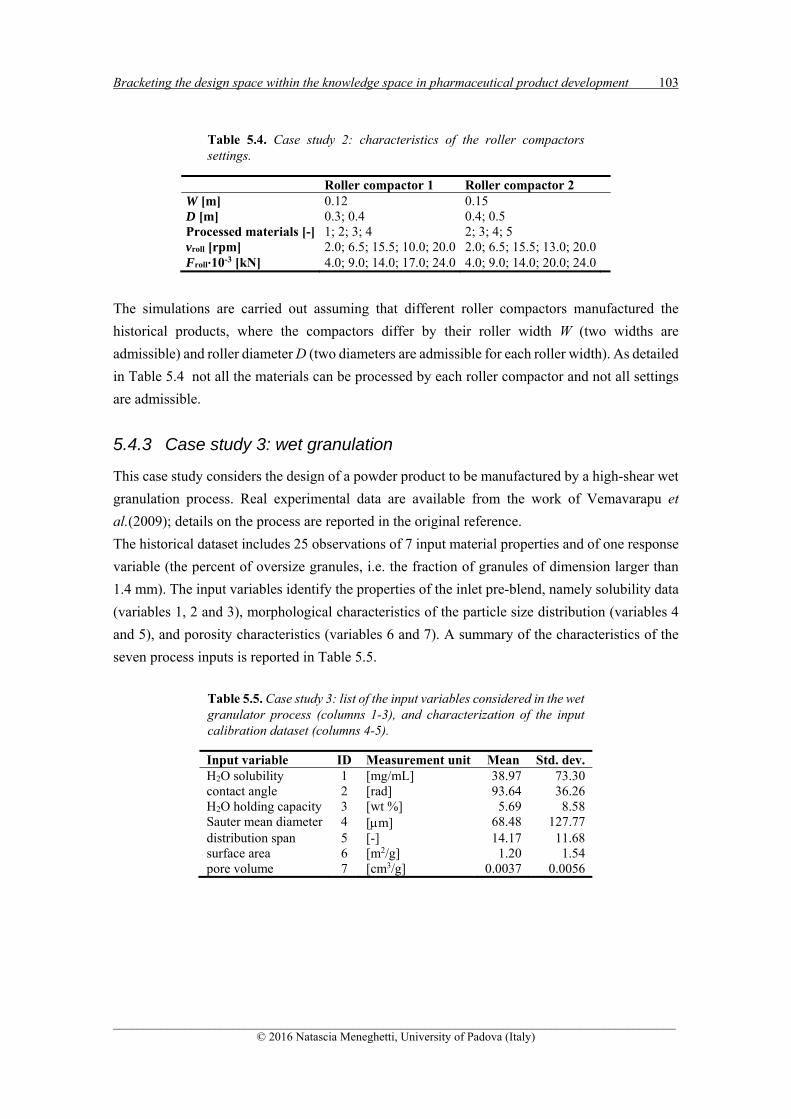
Bracketing the design space within the knowledge space in pharmaceutical product development 103
______________________________________________________________________________________________ © 2016 Natascia Meneghetti, University of Padova (Italy)
Table 5.4. Case study 2: characteristics of the roller compactors settings.
Roller compactor 1 Roller compactor 2 W [m] 0.12 0.15 D [m] 0.3; 0.4 0.4; 0.5 Processed materials [-] 1; 2; 3; 4 2; 3; 4; 5 vroll [rpm] 2.0; 6.5; 15.5; 10.0; 20.0 2.0; 6.5; 15.5; 13.0; 20.0 Froll∙10-3 [kN] 4.0; 9.0; 14.0; 17.0; 24.0 4.0; 9.0; 14.0; 20.0; 24.0
The simulations are carried out assuming that different roller compactors manufactured the
historical products, where the compactors differ by their roller width W (two widths are
admissible) and roller diameter D (two diameters are admissible for each roller width). As detailed
in Table 5.4 not all the materials can be processed by each roller compactor and not all settings
are admissible.
5.4.3 Case study 3: wet granulation
This case study considers the design of a powder product to be manufactured by a high-shear wet
granulation process. Real experimental data are available from the work of Vemavarapu et
al.(2009); details on the process are reported in the original reference.
The historical dataset includes 25 observations of 7 input material properties and of one response
variable (the percent of oversize granules, i.e. the fraction of granules of dimension larger than
1.4 mm). The input variables identify the properties of the inlet pre-blend, namely solubility data
(variables 1, 2 and 3), morphological characteristics of the particle size distribution (variables 4
and 5), and porosity characteristics (variables 6 and 7). A summary of the characteristics of the
seven process inputs is reported in Table 5.5.
Table 5.5. Case study 3: list of the input variables considered in the wet granulator process (columns 1-3), and characterization of the input calibration dataset (columns 4-5).
Input variable ID Measurement unit Mean Std. dev. H2O solubility 1 [mg/mL] 38.97 73.30 contact angle 2 [rad] 93.64 36.26 H2O holding capacity 3 [wt %] 5.69 8.58 Sauter mean diameter 4 [m] 68.48 127.77 distribution span 5 [-] 14.17 11.68 surface area 6 [m2/g] 1.20 1.54 pore volume 7 [cm3/g] 0.0037 0.0056

104 Chapter 5
______________________________________________________________________________________________ © 2016 Natascia Meneghetti, University of Padova (Italy)
5.5 Results and discussion for Case study 1
5.5.1 Development of a new product
A PLS model is first built using the calibration datasets. The number of LVs to be retained in the
model is determined by the scree test (§ 2.1.1.2) in such a way as to explain a sufficiently large
fraction of the variance not only of the product quality (to have good predictive power), but also
of the input variables (to obtain good predictive ability also in model inversion, Jaeckle and
MacGregor 2000b). Namely, using 2A LVs the model explains 96.1% of the variance of y
(94.8% with the first LV), and 98.3% of the variance of X (58.5% with the first LV). Note that,
since )rank(yA , a null space exists.
The problem of developing a product with 23.285DES y (not included in the historical dataset)
is addressed. The true DS REALX for this product is calculated from the first-principles model
assuming this model is a perfect representation of the true process. REALX is then projected onto
the PLS model space, resulting in the green line of Figure 5.3a; in the following, it will be referred
to this projection as to the true design space (TDS). Some issues deserve attention. Firstly, note
that since the actual process is nonlinear, the TDS is a curve. On the other hand, since PLS is a
linear modeling technique, it may have limited representativeness when the process variables are
related in a strongly nonlinear way. Secondly, some of the input combinations belonging to the
TDS may be projected beyond the 2limT limit or the SPElim limit of the model (e.g., in Figure 5.3a
the TDS projections exceeding 2limT lie outside the confidence ellipse). These input combinations
cannot be represented by PLS model inversion, regardless of the fact that the system is nonlinear
or not. Finally, note that some of the input combinations projecting onto the TDS may not be
achievable in practice, because of physical or operational constraints acting on the process.
(a) (b) Figure 5.3. Case study 1: designated experiment space (grey-shaded area) and projection of the true design space onto the PLS model space for the development of a product with (a) yDES = 285.23, and (b) yDES = 168.23.
-6 -4 -2 0 2 4 6-6
-4
-2
0
2
4
6
LV1 score
LV2
scor
e
tNEW
boundary null spacetrue design space
-6 -4 -2 0 2 4 6-6
-4
-2
0
2
4
6
LV1 score
LV2
scor
e
tNEW
boundary null spacetrue design space

Bracketing the design space within the knowledge space in pharmaceutical product development 105
______________________________________________________________________________________________ © 2016 Natascia Meneghetti, University of Padova (Italy)
The set NEWx of input variables that is expected to yield the desired new product is calculated by
PLS model direct inversion, assuming no model prediction uncertainty, obtaining
]96.609;33.173;41.2505;92.12;[47.56=NEW x . The related scores NEW t are plotted in the
model score space (triangle in Figure 5.3a). After accounting for the prediction uncertainty of the
PLS model, the knowledge space is segmented and the experiment space highlighted by the grey-
shaded area of Figure 5.3a is determined. It can be seen that the designated experiment space is a
narrow region of the knowledge space that effectively brackets large part of the TDS; namely, the
experiment space brackets the entire fraction of the TDS that lies within the knowledge space.
The experiments needed to experimentally determine the design space would therefore be carried
out using input combinations that project within the experiment space (not within the entire
knowledge space), thus significantly reducing the required experimental effort.
Figure 5.3b shows the designated experiment space for the development of a product with
23.168DES y , for which xNEW = [ 33.70; 8.65; 1302.50; 76.63; 265.17] is calculated. The
knowledge space segmentation if effective, as only a small fraction of the TDS included within
the confidence ellipse lies outside the designated experiment space, and the experiment space is
a very small fraction of the entire knowledge space.
5.5.2 Effect of the dimension of the calibration dataset on the experiment space
At assigned confidence (say, 95%), the PLS model prediction uncertainty depends on the model
calibration dataset, namely of the number and “quality” of the observations upon which the model
is built (i.e., on the amount of variability the calibration data are able to capture). Therefore, it is
interesting to study how the effectiveness of the proposed segmentation methodology changes
with the number of observations that are available to build the PLS model. As an example, we
consider the development of a product with 86.204DES y .
First, a graphical analysis is considered for three historical datasets, each comprising a different
number I of samples ( 10I , 100I and 1000I ). Obviously, three different PLS models can
be built from these datasets, and the designated experiment space is different in each case. Note
that although the actual DS of the product does not depend on the dimension of the historical
dataset, its projection onto the model latent space does, because this projection does depend on
the PLS model. Figure 5.4 qualitatively shows that increasing the dimension of the historical
dataset improves the knowledge space segmentation effectiveness, as a larger portion of the TDS
is bracketed by the designated experiment space.

106 Chapter 5
______________________________________________________________________________________________ © 2016 Natascia Meneghetti, University of Padova (Italy)
(a) (b)
(c) Figure 5.4. Case study 1, yDES = 204.86: designated experiment space (grey-shaded area) and projection of the true design space onto the PLS model space for historical datasets with (a) I = 10, (b) I = 100, and (c) I = 1000 samples.
This qualitative evaluation requires knowing the DS in advance, which is obviously not possible
in a real application. A quantitative evaluation, that does not require prior knowledge of the DS,
can be carried out as follows.
One randomly-selected sample is removed from the historical dataset (X; y), and the PLS model
is built without using this sample. Then, the validation dataset (X*; y*) is considered, and the
experiment space is determined for all products included in the dataset. Consider a sample
belonging to this dataset; the sample is characterized by a set *REALx of inputs and a related product
quality value *DESy . The projection *
REALt of *REALx onto the PLS model space is obtained from Eq.
(5.4) written in the form:
WP
Wxt
T
*REAL*
REAL . (5.13)
-6 -4 -2 0 2 4 6-6
-4
-2
0
2
4
6
LV1 score
LV2
scor
e
tNEW
boundary null spacetrue design space
-6 -4 -2 0 2 4 6-6
-4
-2
0
2
4
6
LV1 score
LV2
scor
e
tNEW
boundary null spacetrue design space
-6 -4 -2 0 2 4 6-6
-4
-2
0
2
4
6
LV1 score
LV2
scor
e
tNEW
boundary null spacetrue design space

Bracketing the design space within the knowledge space in pharmaceutical product development 107
______________________________________________________________________________________________ © 2016 Natascia Meneghetti, University of Padova (Italy)
For the experiment space designation to be effective, it is expected that (at least) *REALt lies within
with the designated experiment space for product *DESy . It is assumed that a wrong experiment
space designation has been obtained for a given product when at least one of the following
conditions is met: i) 2lim
*2REAL TT , but *
REALt is outside the experiment space; ii) 2lim
*2REAL TT ; iii)
lim*REAL SPESPE . Note that this approach is somewhat conservative, as conditions ii and iii are
related to inadequacy of the PLS model, rather than to ineffectiveness of the knowledge space
segmentation methodology. The operation is repeated for each sample of the validation dataset.
The fraction of validation samples, for which a wrong experiment space designation is obtained,
represents the frequency of wrong experiment space designation for a PLS model with )1( I
samples.
Then, a new iteration is carried out by removing two (instead of one) randomly-selected samples
from the historical dataset, and repeating the whole calculation.
By removing one additional sample at each iteration, the results illustrated in Figure 5.5 are
obtained (all PLS models related to the figure are built on 2 LVs). It can be seen that when the
model is built upon only very few calibration samples, the segmentation result is ineffective. For
example, if only 5 calibration samples are used, for ~86 % of the products to be designed the
proposed methodology is unable to correctly designate the experiment space. However, using 15
calibration samples is enough to reduce to ~9 % the percentage of wrong experiment space
designation, and this percentage does not substantially change even when a very large calibration
dataset is used. In a way, this measure provides the intrinsic capability of the available historical
dataset to serve as an effective source of information to bracket the design space of a new product.
Figure 5.5. Case study 1: effect of the number of model calibration samples on the frequency of occurrence of wrong experiment space designation.
Note that, generally speaking, the fewer the calibration samples, the more the results depend on
the quality of the calibration dataset. This means that, when too few samples are available to
calibrate the PLS model, the experiment space identified by the proposed methodology is
expected to be strongly dependent on each single calibration sample. To investigate this issue, we
101 102 1030
0.2
0.4
0.6
0.8
1
number of calibration samples
fre
que
ncy
of o
ccur
renc
e

108 Chapter 5
______________________________________________________________________________________________ © 2016 Natascia Meneghetti, University of Padova (Italy)
consider the problem of developing a product with 86.204DES y , and two different calibration
datasets: one with 5I samples and one with 20I samples (in both cases, the samples are
randomly selected from the entire historical dataset). A jackknife modeling technique is used
(Efron et al, 1983) to build one PLS model (with 2 LVs) for each of the N possible combinations
of 1I calibration samples, leaving out one of the original calibration samples at each iteration.
For comparison, the results from a model built on the entire set of I calibration samples are also
considered.
Figure 5.6a refers to the case with 5I available calibration samples, and shows that the
projection of NEWx onto the score space (i.e., NEWt ) changes significantly with the calibration
dataset. If all I samples are used to calibrate the model, NEWx projects onto the black triangle;
however, when 1I samples are used for calibration, I significantly different NEWx values are
obtained, each one projecting onto different score points (open triangles).
Figure 5.6a also shows the null spaces associated to each NEWt . It is apparent that the null spaces
are significantly different, implying that also the experiment spaces that can be designated are
very different. Stated differently, the fact that the calibration dataset is deficient implies that the
model prediction results are largely uncertain, and this in turn implies that there is a large
uncertainty in the designation of the experiment space.
(a) (b)
Figure 5.6. Case study 1, yDES = 204.86: effect of the dimension of the model calibration dataset on the designation of the experiment space: (a) jackknifing with I = 5 calibration samples; (a) jackknifing with I = 20 calibration samples.
Figure 5.6b refers instead to the calibration dataset with 20I . Clearly, the 1I solutions
obtained by model inversion all project very close to each other onto the score space, indicating
that the model inversion results do not strongly depend on the single calibration sample. The null
spaces almost overlap, implying that the experiment space designation is almost insensitive to the
calibration set.

Bracketing the design space within the knowledge space in pharmaceutical product development 109
______________________________________________________________________________________________ © 2016 Natascia Meneghetti, University of Padova (Italy)
5.6 Results and discussion for Case study 2
First, the effect of the dimension of the calibration dataset on the effectiveness of the experiment
space designation is studied for a PLS model with 2 LVs. The results reported in Figure 5.7 (which
refer to the entire validation dataset of 22 samples) are obtained. Similar general considerations
as in Case study 1 can be drawn: when the model is built on few calibration samples only, the
experiment space designation is ineffective. The uncertainty in the experiment space designation
decreases as more calibration samples become available. For this roller compaction process, about
30 calibration samples are needed to reduce to less than 20 % the fraction of incorrect experiment
space designations; using more than 40 calibration samples reduces to ~10 % the designation
errors.
Figure 5.7. Case study 2: effect of the number of model calibration samples on the occurrence of wrong experiment space designation.
The design of a process for the manufacturing a granulate with intra-void fraction of the solids
out of the roller compactor 6341.0DES y m3/m3 is now considered. We assume that 40 randomly
chosen samples are available to calibrate the model. For this Case study with a large number of
inputs, it is impractical to determine the TDS, as several inputs take discrete (rather than
continuous) values. For these reasons, the true inputs combinations that lead to the desired product
(i.e., the input combinations belonging to the DS) are found by trial-and-error. However, because
of the complexity of the problem, it is not possible to guarantee that all the input combinations
that can lead to DESy are found, the results obtained appear consistent with the knowledge that is
available from the historical database.
After building a PLS model with 2 LVs, application of the proposed methodology provides the
results of Figure 5.8 The knowledge space segmentation is effective: the designated experiment
space is a small fraction of the knowledge space and includes the TDS projections onto the score
space (green circles). The fact that these projections are clustered in a relatively narrow region of
the knowledge space reflects the fact that a product with the desired quality can be obtained by
processing only some of the available input materials with only some of the potential roller
10 20 30 40 50 60 70 80 900
0.2
0.4
0.6
0.8
1
number of calibration samples
fre
quen
cy o
f occ
uren
ce

110 Chapter 5
______________________________________________________________________________________________ © 2016 Natascia Meneghetti, University of Padova (Italy)
compactor settings. Note that, notwithstanding the fact that the system is subject to a large number
of inputs, a clear graphical representation of the multivariate experiment space is obtained.
Figure 5.8. Case study 2: designated experiment space (grey-shaded area) and projection of the true design space onto the PLS model space for the development of a product with yDES = 0.6341 m3/m3 (40 samples are used to calibrate the model).
5.7 Results and discussion for Case study 3
As discussed in Section 4.3, real experimental data are available for this wet granulation process.
Hence, the situation closely resembles a real one, where the TDS cannot be calculated in advance.
Furthermore, the available historical dataset comprises only 25 experimental samples. To
attenuate the data scarceness problem, a Monte Carlo approach is followed. Namely, 100
iterations are carried out in which the available observations are split into a calibration dataset of
20I observations (randomly selected at each iteration from the entire historical dataset),
whereas the remaining 5 observations are used to validate the knowledge space segmentation
results. The results presented are averaged throughout all the iterations of the Monte Carlo
procedure. Figure 5.9 shows that as few as 13 calibration samples are enough for this wet
granulation process to reduce the occurrence of wrong experiment space designation to a
negligible value.
Given the results of Figure 5.9, fifteen randomly selected samples are used to calibrate the PLS
model that relates the input material properties to the percentage of oversize granules. Figure 5.10,
which refers to the development of a granulate product characterized by 20DES y % oversize
granules, shows a typical knowledge space segmentation result. It is apparent that the proposed
methodology does a good job in bracketing within the experiment space at least the projection
tREAL of the true input combination. The fact that tREAL is close to the null space related to NEWt
provides indirect indication that the model predictions are not subject to a large uncertainty for
this problem.
-6 -4 -2 0 2 4 6-6
-4
-2
0
2
4
6
LV1 score
LV2
scor
e
tNEW
boundary null spacestrue design space

Bracketing the design space within the knowledge space in pharmaceutical product development 111
______________________________________________________________________________________________ © 2016 Natascia Meneghetti, University of Padova (Italy)
Figure 5.9. Case study 3: effect of the number of model calibration samples on the occurrence of wrong experiment space designation; the frequency of occurrence is averaged over 100 Monte Carlo simulations.
Figure 5.10. Case study 3: designated experiment space (grey-shaded area) for the development of a product characterized by 20 % of oversize granules (15 samples are used to calibrate the model).
5.8 Conclusions
A key element of the Quality-by-Design initiative is the determination of the design space for the
manufacturing of a pharmaceutical product. When this calculation cannot be assisted by the use
of a first-principles model, the DS determination heavily relies on experiments. In some cases,
the DS can be found using experiments designed within a domain of input combinations (e.g.
material properties and process conditions) that derive from the experience gained from products
that have already been developed and are similar to the new one under development. This domain
is the knowledge space and the related experimentation can be very demanding, especially if the
number of process inputs is large. Since the DS is only a subspace of the knowledge space, the
experimental effort could be reduced if one were able to find a narrower region within which
5 10 15 200
0,2
0,4
0,6
0,8
1
number of calibration samples
fre
que
ncy
of o
ccur
renc
e
-6 -4 -2 0 2 4 6-4
-2
0
2
4
LV1 score
LV2
scor
e
tNEW
tREAL
null spaceboundary null space

112 Chapter 5
______________________________________________________________________________________________ © 2016 Natascia Meneghetti, University of Padova (Italy)
designing and carrying out the experiments. This region, which we call the experiment space, is
inside the knowledge space and is likely to bracket the DS.
In this Chapter, a methodology has been proposed to determine the experiment space using
historical data on products already developed. By means of a latent-variable model inversion
approach, the knowledge space is segmented in such a way as to identify the experiment space in
the latent variable space of the model. The segmentation makes use of the concept of null space
and accounts for the existence of uncertainty in the model predictions.
Using three simulated case studies, the segmentation results have been shown to be effective, as
the designated experiment space includes the true DS and is much narrower than the knowledge
space. One additional advantage of the proposed methodology is that, being the experiment space
identified in a multivariate latent variable space, its graphical representation is clear also when
the number of process inputs is large.
The segmentation effectiveness is shown to depend on the number of samples available in the
historical dataset, but the appropriate number of samples does not necessarily need to be very
large. In this respect, a procedure has been suggested to test the intrinsic capability of the available
historical dataset to serve as an effective source of information to identify the experiment space.
Future investigations should be devoted to assess the effectiveness of a design-of-experiments
exercise carried out in the latent space with respect to the more common situation where the
experiments are designed directly in the true input space. Additionally, although model
uncertainty was explicitly accounted for, the proposed methodology only considered model
prediction uncertainty. Therefore, other forms of uncertainty (such as uncertainty on the model
parameters and on the calibration data) should be considered in future studies. Furthermore, this
study has considered only the case of products characterized by a single quality attribute.
However, quality is a truly multivariate property for many pharmaceutical products. How to
extend this methodology to the multivariate case represents an area open for further investigation.
______________________________________________________________________________________________ © 2016 Natascia Meneghetti, University of Padova (Italy)
Chapter 6
Knowledge management in secondary manufacturing by pattern recognition
techniques*
In this Chapter a methodology is proposed to systematically analyze large data historians of
secondary pharmaceutical manufacturing systems using pattern recognition techniques. The
objective is to develop an approach enabling to automatically retrieve operation-relevant
information that can assist the management in the periodic review of a manufactory system. The
proposed methodology allows one to automatically perform three tasks: the identification of
single batches within the entire data-sequence of the historical dataset, the identification of
distinct operating phases within each batch, and the characterization of a batch with respect to an
assigned multivariate set of operating characteristics. The approach is tested on two six-month
datasets of a commercial-scale granulation/drying system, where several millions of data entries
are recorded.
The Chapter is organized as follows: first, after the introduction of the problem, the proposed
methodology and the units analyzed are presented, then each step of the methodology is explained
in detail using one of the two available datasets, in order to demonstrate the practical application
of the methodology when no information about the products processed is available (section A).
Finally (Section B), the analysis is performed for both datasets also accounting for the information
available about the product manufacturing recipes.
6.1 Introduction
In the last decade, the pharmaceutical industry has been faced with unprecedented business
scenario changes. Many blockbuster drugs have been crossing the period of patent expiry and
fewer blockbusters are on the horizon. The development of new products is shifting towards more
complex therapeutic targets, and the patient base is narrower than that of preceding blockbusters
* Excerpts from this Chapter belong to: N. Meneghetti, P. Facco, F. Bezzo, C. Himawan, S. Zomer, M. Barolo, 2016, Knowledge management in secondary pharmaceutical manufacturing by mining of data historians – A proof-of-concept study. Submitted to Int. J. Pharm.

114 Chapter 6
______________________________________________________________________________________________ © 2016 Natascia Meneghetti, University of Padova (Italy)
(Kukura and Thien, 2011). Generic competition has become more and more aggressive (am Ende,
2011). Governments are taking radical measures to gain control over drug pricing (e.g. by
changing the copayment plans; Sadat et al., 2014). Given this scenario, the pharmaceutical
companies are striving to reduce costs to maintain competitiveness.
Primary pharmaceutical manufacturing is concerned with the production of active ingredients,
whereas secondary pharmaceutical manufacturing focuses in the production of dosage forms
(Bennett and Cole, 2003). Both primary and secondary manufacturing play a central role in cost
allocation. However, while on the one hand the pharma industry is very effective in discovering
new drugs, on the other hand its manufacturing efficiency is far behind the one of several other
sectors. Poor performance in manufacturing costs the pharma industry US$90 billion per year,
which is considered equivalent to the current development cost for 80–90 new drugs (The
Economist, 2005; Danese and Constantinou, 2007). Based on the annual reports of 17 “big
pharma” companies, it has been estimated that manufacturing costs amount to ~27% of the
revenues, largely exceeding the R&D expenses that are at ~17% (am Ende, 2011). Therefore,
even a fractional improvement in the quality of the manufacturing system can bring tremendous
competitive advantages to a company.
Though product quality targets are very severe, pharmaceutical manufacturing processes still
suffer for high variability. Continuous manufacturing is gaining more and more consideration,
but most active pharmaceutical ingredients and drug products are still manufactured batchwise.
Commercial manufacturing processes are often suboptimal, because they are conceived at the
development stage and get frozen close to product registration, with little or no attempt to
optimize them. Manufacturing cycle times are very variable, because out-of-specifications
(“exceptions”) during manufacturing need frequently be dealt with (Suresh and Basu, 2008). All
of these factors contribute to significantly decrease productivity and increase product costs.
With the advent of fast, cheap and reliable on-line measurement devices, product manufacturing
environments have now available large historical databases spanning several manufacturing
years. However, while being data rich, the pharma industry is also known to be information poor
(Politis and Rekkas, 2011). This is due to the fact that, due to data overload, the information
embedded in data historians is hidden and therefore remains largely unexploited. Indeed,
transforming data into knowledge is not a simple task. To clarify this issue, consider a typical
secondary manufacturing system. The ingredients are processed by a series of batch operations,
which eventually result in the final drug product. Each operation evolves through a series of
phases, which may involve exchange of heat and/or mass with the surroundings and are often
triggered by the operators. While a unit is processing the material, there may be short time
windows where the unit is stalled (e.g. for re-setting, quick maintenance, and the like). At the
conclusion of a batch, the equipment is possibly subject to maintenance and operation tests, then
cleaned and set in a hold position for the next operation. Each piece of equipment is equipped
with several sensors and hooked to a computer where sensor measurements (temperatures, flows,

Knowledge management in secondary manufacturing by pattern recognition techniques 115
______________________________________________________________________________________________ © 2016 Natascia Meneghetti, University of Padova (Italy)
torques, compression forces, etc.) are recorded along with some settings (position of switches,
controller set-points, etc.), for a total number of recordings on the order of a few tens at each time
instant per piece of equipment. Typically, the recordings are made continuously (i.e., at the
frequency of one set of recordings every few seconds) across an entire production campaign,
which may last several months and may possibly include different products. In most cases, the
data capture systems are meant to record data in a “passive” way only, i.e. without contextualizing
the operations around them. Therefore, the recordings typically include also data segments that
refer to temporary stalls of the equipment, where the time profiles of the recorded signals are
totally unrelated to the evolution of the operation within the equipment; not even when the
equipment is not processing material is the recording interrupted. The net result is that the amount
of data records that gets archived for a given production campaign is overwhelming, easily
reaching several millions of data entries. Additionally, the structure of the data capture systems
may be out of step with respect to the implementation of newer and increasingly sophisticated
data modeling and monitoring techniques, whose requirements were possibly not factored in at
the time of the systems installation. A mechanical update of the systems to this end might even
produce further disruption at significant cost for production. Periodic review of the historical
operational data by the company management is not easy, as the information is masked to a point
that even finding the start and end point of a batch may be difficult. Yet, there are several pieces
of information that are hidden in the historian and would be useful to know when reviewing a
production campaign, such as how many batches have been carried out in the campaign; which
factors characterize the evolution of the operating phases within each batch; whether and how
these factors have changed along the campaign; whether there have been some trends/drifts along
the campaign. Systematic review of these issues by science-driven methods would amount to
turning data into knowledge, and this can be a decisive step toward continuous improvement of
the manufacturing system. Note that, while the ultimate objective is to provide full
contextualization of the entire data historians for all the potential costumers (e.g., manufacturing
performance review teams, product development teams, equipment/maintenance engineers), even
an incremental improvement to progressively reduce existing gaps, where data cannot be fully
exploited, may lead to substantial savings.
In this Chapter, a methodology is proposed to systematically analyze large data historians of
secondary manufacturing systems using data mining techniques. The objective is to develop an
approach enabling to automatically retrieve operation-relevant information that can assist the
management in the periodic review of a manufactory system, thus improving process
understanding and contributing to reduce the occurrence of exceptions through systematic
identification of the variability sources. The approach is tested on two six-month datasets of a
commercial-scale granulation/drying system. The final result is an advanced process analytical
technology (PAT) tool that can assist the implementation of continuous improvement paradigms
within a quality-by-design framework (FDA 2004b).

116 Chapter 6
______________________________________________________________________________________________ © 2016 Natascia Meneghetti, University of Padova (Italy)
6.2 Proposed framework
Following the industrial parlance, the variables registered in manufacturing historians will be
named ‘tags’ in this study. The proposed methodology allows one to automatically perform the
following tasks:
Task 1: batch identification; namely, isolation of single batches within the entire data-sequence
of the historical dataset, depending on the characteristics of the available tags;
Task 2: phase identification; namely, identification of distinct operating phases within each
batch;
Task 3: batch characterization; namely, characterization of each batch with respect to an
assigned set of multivariate characteristics (e.g., length of a given phase, speed of a
given device, maximum or minimum temperature achieved, etc.) The methodology is
sketched in Figure 6.1. The three tasks are carried out sequentially and, depending on
the characteristics of the available tags, may involve alternative scenarios. In particular,
for the batch identification task (Task 2) two alternative scenarios are envisaged:
Scenario 1 refers to the situation where tags are available that are directly linked to the
length of a batch, whereas Scenario 2 refers to the more general case where these tags
do not exist; in this case, the Task 2 operations are carried out before the Task 1 ones.
Note that a preliminary exploratory analysis of the available data is suggested to select
the subset of tags suitable for the subsequent tasks, as well as to analyze the data
structure and the complexity of the system.

Knowledge management in secondary manufacturing by pattern recognition techniques 117
______________________________________________________________________________________________ © 2016 Natascia Meneghetti, University of Padova (Italy)
Figure 6.1 Flowchart of the proposed approach to analyze secondary manufacturing data historians for batch systems. Each block includes a reference to the section where the block operations are discussed.
6.2.1 Tag sources and possible data analysis scenarios
The available tags may derive from different sources, which should be clearly identified prior to
the analysis; therefore, interaction with the plant experts is fundamental at this stage. In this study,
four such sources were identified:
Source 1: measurement sensors. In this case, the tag values are registered in the form of real
numbers;
Source 2: calculations involving Source 1 variables;
Source 3: process settings (subject to operators’ adjustment). The tag values are recorded in
the form of integer positive numbers (0; 1; 2; …), representing the manually-driven
activation of a certain operation, or the current status of a piece of equipment;
Source 4: time span settings. The tag values are recorded in the form of real numbers
indicating the time elapsed from the operator-triggered start of a given event, to the current

118 Chapter 6
______________________________________________________________________________________________ © 2016 Natascia Meneghetti, University of Padova (Italy)
time instant (until event termination). Note that after the termination of a given event, the
relevant time span value is often recorded as a constant value equal to the total event duration.
In general, for a given manufacturing unit the available tags may not come from all sources;
additionally, the available tags may well change from unit to unit. For this reason, two possible
data analysis scenarios are considered in Figure 6.1, which depend on the tags available. Scenario
1 is preferred if tags indicating the status of the unit under investigation and/or the duration of all
its operating phases (Source 3 and 4 tags) are available; when such tags are not available, Scenario
2 is followed.
6.3 Manufacturing system and datasets
Two industrial secondary manufacturing units, both operating batchwise, were selected as test
beds for the proposed knowledge management methodology: a high-shear wet granulator and the
downstream fluid-bed dryer. Two consecutive six-month datasets were extracted from the
available historians, where data were recorded at a sampling rate of one data entry every 5 s, for
a total number of data entries on the order of 108. The available datasets are denoted as follows:
Dataset 1 collects the data recorded in the first production period analyzed;
Dataset 2 collects the data recorded in the second production period analyzed;
Dataset 2 presents the same number of observations as Dataset 1 (namely, 3,127,088 observations,
at a sampling rate of one data entry every 5 s).
In the first part of this Chapter the methodology is tested on Dataset 1, assuming that no
information is available about the product (or possibly products) manufactured. In the second
part, the analysis is repeated on the same dataset, but information about the manufacturing
recipe(s) is also used; additionally, Dataset 2 is also analyzed.
Note that the recorded data include time windows where a unit is in operation but temporary
stalled, as well as time windows where material is not being processed. Neither of these
occurrences are marked somehow in the historian. Note that the number of granulation and drying
batches included in the selected time window was not known a priori (namely, it was a piece of
information to be obtained by the proposed knowledge management method).
A description of each unit and a list of the tags recorded are reported in the following.
6.3.1 High-shear wet granulator: process description and operating phases
The high-shear wet granulator processes a powder feed to manufacture granular material with
assigned particle size distribution. The granule formation and size increase are obtained by
agglomeration, which is determined by adding a liquid combined with the action of an impeller

Knowledge management in secondary manufacturing by pattern recognition techniques 119
______________________________________________________________________________________________ © 2016 Natascia Meneghetti, University of Padova (Italy)
and a chopper. As schematically illustrated in Figure 6.2, four operating phases characterize the
typical evolution of a standard granulation batch:
Phase 1: dry mixing;
Phase 2: water addition;
Phase 3: wet massing;
Phase 4: discharge.
During Phase 1, the material is slowly charged into the unit and mixed by the impeller only. In
Phase 2 the aggregating agent is added and the chopper is activated. In Phase 3, changes in the
granule size and porosity are observed, causing an increase in the impeller power consumption.
Finally, when the granules reach an assigned size, the unit is emptied by opening a discharge
valve, and the material is sent to the dryer unit (Phase 4).
Figure 6.2 Granulation unit: description of the four operating phases of a standard batch.
Note that each operating phase may either represent an event related to the physical evolution of
the batch (e.g., wet massing) or an event triggered by the operators (e.g., solution addition,
discharge, etc.).
6.3.2 Fluid-bed dryer: process description and operating phases
The fluid bed dryer receives the material processed by the granulator as feed. The granulated
material moisture content is reduced by fluidizing the particles with an air stream until the final
product humidity or temperature reach a desired value. The complexity of the physical
mechanisms involved in the process, and the fact that product sampling requires stopping the
operation, make the analysis of the drying variable profiles more complex than that of the
granulator. Six operating phases can be identified for a standard drying batch (Figure 6.3):
Phase 1: pre-heating;
Dry-mixing phase
The feed materialis charged into
the unit
Solution addition
Wet-massingphase
Discharge
Phase 1 Phase 2 Phase 3 Phase 4
•The material ismixed by the impeller only
•No liquid ispresent or added
•The material ismixed by the impeller and the chopper
•A liquid isadded to agglomerate the material
•The material ismixed by the impelller and the chopper
•The viscosity of the productincreases
•The product isready to be sent to the dryer
•The dischargevalve is open

120 Chapter 6
______________________________________________________________________________________________ © 2016 Natascia Meneghetti, University of Padova (Italy)
Phase 2: charging;
Phase 3: constant drying rate;
Phase 4: falling drying rate;
Phase 5: cooling down;
Phase 6: discharge.
In Phase 1, the equipment is heated up. Then, while the material to be dried is gradually charged
(Phase 2), the solvent evaporates mainly from the particle surface (Phase 3), without significant
changes in the product temperature. During Phase 4, the product temperature increases due to the
slow diffusion of the liquid embedded in the particles toward the particle surface. Finally, the
material is cooled (Phase 5) and then discharged (Phase 6).
Figure 6.3. Drying unit: description of the six operating phases of a standard batch.
SECTION A – ANALYSIS OF DATASET 1 WITH NO PRODUCT INFORMATION AVAILABLE
6.4 Available data for Dataset 1
6.4.1 Granulation unit data
Thirty-four tags are available in the plant to monitor the granulation unit at any time instant.
Before further data processing, it may be useful or necessary to remove some tags from the
original dataset. The reasons for this may be different: for example, not all tags might be available
for all recorded batches, some tags may have been temporarily dismissed or be under
maintenance, some others may confound the analysis when used within the models that will be
described later (for more details refer to Section 6.6.3). Following this rationale, 11 tags were
retained to build the granulator dataset (Table 6.1), and they were organized in a granulator matrix
G [3127088×11], where each column represents one tag and each row (observation) reports the
Constantdrying rate
Materialcharging
Fallingdrying rate
Coolingdown
Discharge
Phase 5Phase 2 Phase 3 Phase 4
•The liquidembedded in the granulesevaporates
•The temperaturesincrease
•The product iscooled down
Pre-heating
Phase 1 Phase 6
•The granules are fluidized by an air stream
•Only the superficial liquid evaporates
•The product isready to be sent to the nextunit
•The materialexiting the granulator ischarged intothe fluid bed dryer
•The dryingchamber is pre-heated by an air stream at assigned temperature
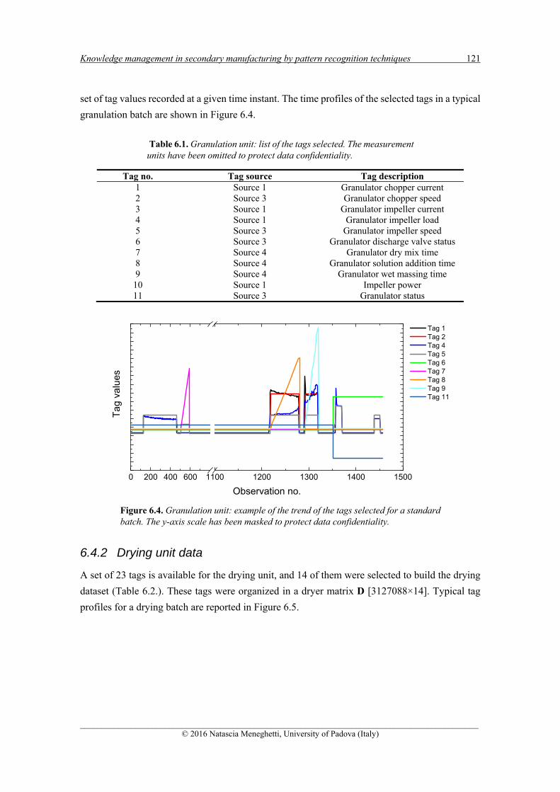
Knowledge management in secondary manufacturing by pattern recognition techniques 121
______________________________________________________________________________________________ © 2016 Natascia Meneghetti, University of Padova (Italy)
set of tag values recorded at a given time instant. The time profiles of the selected tags in a typical
granulation batch are shown in Figure 6.4.
Table 6.1. Granulation unit: list of the tags selected. The measurement units have been omitted to protect data confidentiality.
Tag no. Tag source Tag description 1 Source 1 Granulator chopper current 2 Source 3 Granulator chopper speed 3 Source 1 Granulator impeller current 4 Source 1 Granulator impeller load 5 Source 3 Granulator impeller speed 6 Source 3 Granulator discharge valve status 7 Source 4 Granulator dry mix time 8 Source 4 Granulator solution addition time 9 Source 4 Granulator wet massing time
10 Source 1 Impeller power 11 Source 3 Granulator status
Figure 6.4. Granulation unit: example of the trend of the tags selected for a standard batch. The y-axis scale has been masked to protect data confidentiality.
6.4.2 Drying unit data
A set of 23 tags is available for the drying unit, and 14 of them were selected to build the drying
dataset (Table 6.2.). These tags were organized in a dryer matrix D [3127088×14]. Typical tag
profiles for a drying batch are reported in Figure 6.5.
0 200 400 600 1100 1200 1300 1400 1500
Tag 1 Tag 2 Tag 4 Tag 5 Tag 6 Tag 7 Tag 8 Tag 9 Tag 11
Tag
val
ues
Observation no.

122 Chapter 6
______________________________________________________________________________________________ © 2016 Natascia Meneghetti, University of Padova (Italy)
Table 6.2. Drying unit: list of the tags selected. The measurement units have been omitted to protect data confidentiality.
Tag no. Tag source Tag description 1 Source 3 Dryer status 2 Source 1 Pressure difference 3 Source 4 Drying time 4 Source 3 Drying status 5 Source 1 Exhaust air temperature 6 Source 1 Inlet air humidity 7 Source 1 Inlet air moisture content 8 Source 1 Inlet air temperature 9 Source 1 Inlet air volume 10 Source 1 Inlet air fan speed 11 Source 1 Inlet air flap position 12 Source 1 Outlet air flap position 13 Source 4 Pre-heat time 14 Source 1 Product bed temperature
Figure 6.5. Drying unit: example of the trend of the tags selected for a standard batch. The y-axis scale has been masked to protect data confidentiality.
6.5 Exploratory data analysis
As a preliminary step of the proposed methodology, an exploratory data analysis is suggested to
investigate the correlation structure of the available data. The analysis requires visual
identification of a limited number B of batches included in the available datasets (G or D). This
operation may be time consuming, as the start and end point of the batches are not known a priori,
and therefore visual inspection of the datasets may be demanding. Note that, to avoid considering
batches that belong to a single production campaign (i.e., to a limited time frame), the batches
should be selected across the entire data historian. For generic batch b within this subset of data,
the available data are collected in matrix Vb [Ib×T], where Ib and T are the number of historical
0 200 1200 1400 1600 1800 2000 2200
Tag 3 Tag 5 Tag 8 Tag 9 Tag 10 Tag 13 Tag 14 Tag 15
Tag
val
ues
Observation no.

Knowledge management in secondary manufacturing by pattern recognition techniques 123
______________________________________________________________________________________________ © 2016 Natascia Meneghetti, University of Padova (Italy)
observations for the batch and the number of tags used, respectively. Then, the exploratory
analysis can be carried out as follows.
1. One batch of this subset, recognized as “standard” according to prior process knowledge, is
denoted as the reference batch, and the operating phases are visually identified for it. After data
pretreatment (namely, autoscaling), a principal component analysis (PCA; Chapter 2, Section
2.1.1) model is built on the reference batch.
2. The PCA model scores are examined to extract information about the relations among the
observations belonging to different operating phases. In fact, the observations belonging to the
same operating phase usually locate close in the scores space to form a cluster.
3. The remaining )1( B batches, denoted as validation batches, are projected onto the PCA
model space (note that each validation batch is autoscaled on its own mean and standard
deviation). Information about the degree of the batch-to-batch variability can be obtained by
analyzing the score patterns of the projected batches.
4. A few iterations of the procedure with different reference batches are suggested to assess the
consistency of the results obtained.
6.5.1 Results for the granulation unit
A PCA model or the granulator was built as indicated in step 1. Two PCs‡‡ (capturing ~63% of
the variability of the calibration data) were considered, but more may be used if a more accurate
analysis is required.
(a) (b) Figure 6.6. Granulation unit: (a) scores of the PCA model built on a reference batch; (b) projections of one representative validation batch onto the PCA model space. In (a), the calibration scores are marked with different colors according to the operating phase they belong to.
‡‡ Since the objectives of this preliminary analysis is only to evaluate how easily different operating phases can be discriminated, and whether the time trend of different batches is similar, it is suggested to use few PCs as possible. In fact, two PCs are often enough for this purpose.
-4 -2 0 2 4 6 8 10 12-8
-6
-4
-2
0
2
4
Sco
res
on P
C2
(18.
6%)
Scores on PC1 (44.4%)
Phase 1Phase 2Phase 3Phase 4Other
-4 -2 0 2 4 6 8 10 12-8
-6
-4
-2
0
2
4
Reference batch Validation batch
Sco
res
on P
C2
(18.
6%)
Scores on PC1 (44.4%)

124 Chapter 6
______________________________________________________________________________________________ © 2016 Natascia Meneghetti, University of Padova (Italy)
The model scores are reported in Figure 6.6a: the four operating phases characterizing a
granulation batch are apparent in the score space, meaning that each phase is characterized by a
unique combination of tag values that can be captured by the model. The same pattern is found
also for most validation batches; a projection of one representative validation batch onto the PCA
model space is shown in Figure 6.6b. The main conclusion for this analysis is that the batch-to-
batch variability is relatively limited for the granulation unit, even if the operators’ settings change
from batch to batch. Note that a standard PCA model loadings analysis (not reported here for the
sake of conciseness) can be used to identify the tags that most characterize each granulation phase.
6.5.2 Results for the drying unit
The pattern of the PCA scores resulting from the PCA model of a reference drying batch (Figure
6.7a) indicates that the drying process is more difficult to analyze. In contrast to the granulation
process, the clusters are not clearly distinguishable, suggesting that the identification of different
operating phases using the available tags may be difficult. Additionally, the projections of
different batches onto the PCA model space (a representative example is reported in Figure 6.7b)
reveals a much larger batch-to-batch variability.
(a) (b) Figure 6.7. Drying unit: (a) scores of the PCA model built on a reference batch; (b) projections of one representative validation batch onto the PCA model space. In (a), the calibration scores are marked with different colors according to the operating phases they belong to.
6.6 Batch identification and phase identification in Scenario 1
In this section, the procedure to automatically extract (from G or D) the observations belonging
to each single batch is presented. The objective is to screen each dataset in order to identify
segments of consecutive observations that all refer to the same granulation or drying batch. The
-8 -6 -4 -2 0 2 4
-4
-2
0
2
4
6
Sco
res
on P
C2
(1
9.5
%)
Scores on PC1 (47.3%)
Phase 1Phase 2Phase 3Phase 4Phase 5-6Other
-8 -6 -4 -2 0 2 4
-4
-2
0
2
4
6
Reference batch Validation batch
Sco
res
on P
C2
(19
.5%
)
Scores on PC1 (47.3%)

Knowledge management in secondary manufacturing by pattern recognition techniques 125
______________________________________________________________________________________________ © 2016 Natascia Meneghetti, University of Padova (Italy)
number of observations in these segments is not known a priori, and changes from batch to batch.
When one such segment is identified, the related observations are rearranged into a matrix Ob
[Ib×T] (OG,b or OD,b for the granulator or the drying, respectively), where the meaning of the
symbols is the same as in Section 6.5 . Note that, since the true batches may be separated by data
segments that are not directly related to actual product manufacturing, not all the observations in
G or D will eventually belong to one of the Ob matrices. The procedure discussed in this section
is based on direct tag analysis (Scenario 1); an alternative procedure that uses a pattern recognition
technique (Scenario 2) will be presented in Section 6.7 . Once all batches in G and D have been
singled out, the automatic identification of operating phases within each batch can be carried out
(Task 2). A procedure for carrying out this task is also presented in this section.
6.6.1 Tag-based batch identification
The simplest method that can be employed in order to recognize a batch within an historical
dataset makes use of those tags that can be directly related to the duration of the entire batch or
of its operating phases. The most convenient situation (which is actually encountered both in the
granulator and in the drier) is represented by the availability of one tag unambiguously indicating
when the manufacturing unit is (and is not) in operation (green path in Figure 6.8).
Figure 6.8. Tag-based batch identification: different alternatives are identified depending on the sources of the available tags. The orange path indicates the procedure followed to identify a granulation batch, whereas the green path was followed to identify a drying batch.
This tag can be directly used in a simple algorithm (not discussed here for the sake of conciseness)
that, based on the values the tag takes, recognizes whether or not the unit is in operation, and
Visual identification of a set of batches
Is there one tag indicating the
equipment status for the entire duration of
the batch?
Use this tag to identify a batch
YES
Is it possible to find two
or more tags which in sequence indicate the equipment status for the entire duration of
the batch?
NO
NOYES
Build a specific algorithm exploiting
these tags to identify a batch
Try an alternative method (phase-based identification method)

126 Chapter 6
______________________________________________________________________________________________ © 2016 Natascia Meneghetti, University of Padova (Italy)
consequently extracts the relevant data segments from G and D. If such a tag is not available,
alternative solutions exist as summarized by the orange path in Figure 6.8. Note that, in order to
be able to choose the appropriate path, a preliminary step is necessary to visually extract a set of
batches from the global dataset. To this purpose, the batches used for the preliminary exploratory
analysis (Sections 6.5.1 and 6.5.2) can be used. Some implementation issues that may arise
following the procedure proposed in Figure 6.8 will be discussed in Section 6.13 .
Note that, in general, not all of the batches identified can be considered as “standard”, because
some operating segments may be repeated twice in some batches, or they may last much longer
than in other batches. Therefore, regardless the scenario followed for batch identification, an
additional analysis is needed to discriminate between standard and non-standard batches (Figure
6.1). This topic (batch characterization) will be discussed in Section 6.8.
6.6.1.1 Results for the granulation unit
Since granulator Tag 11 (granulator status) indicates when the granulator is operating, this tag
can in principle be used for tag-based batch identification. However, this tag is active during the
first three operating phases only; therefore, an additional tag that remains active for the rest of the
batch is required (orange path in Figure 6.8). This tag exists and is Tag 6 (granulator discharge
valve). Therefore, a granulation batch b can be easily singled out from the G dataset using the
combination of Tag 11 and Tag 6.
A graphical representation of the results from this procedure is reported in Figure 6.9a for a small
subset of G: the grey-shaded areas correspond to the batch identified automatically. Using this
tag-based identification procedure, 90 different granulation batches were eventually identified.
6.6.1.2 Results for the drying unit
Using dryer Tag 1 (dryer status) is sufficient to identify the drying batches, as this tag is active
during the entire duration of the batch (green path in Figure 6.8). Eventually, ninety§§ different
drying batches were identified automatically. A graphical representation of the results of drying
batch identification is shown in Figure 6.9b. Note that the three batches marked by the grey
shading are separated by operational segments where all tag values (except Tag 1) change (Figure
6.9b), probably due to equipment testing; therefore, identifying the batch by analyzing the
trajectories of these tags would not be easy.
§§ The coincidence of this number with the number of batches identified for the granulation unit is accidental.
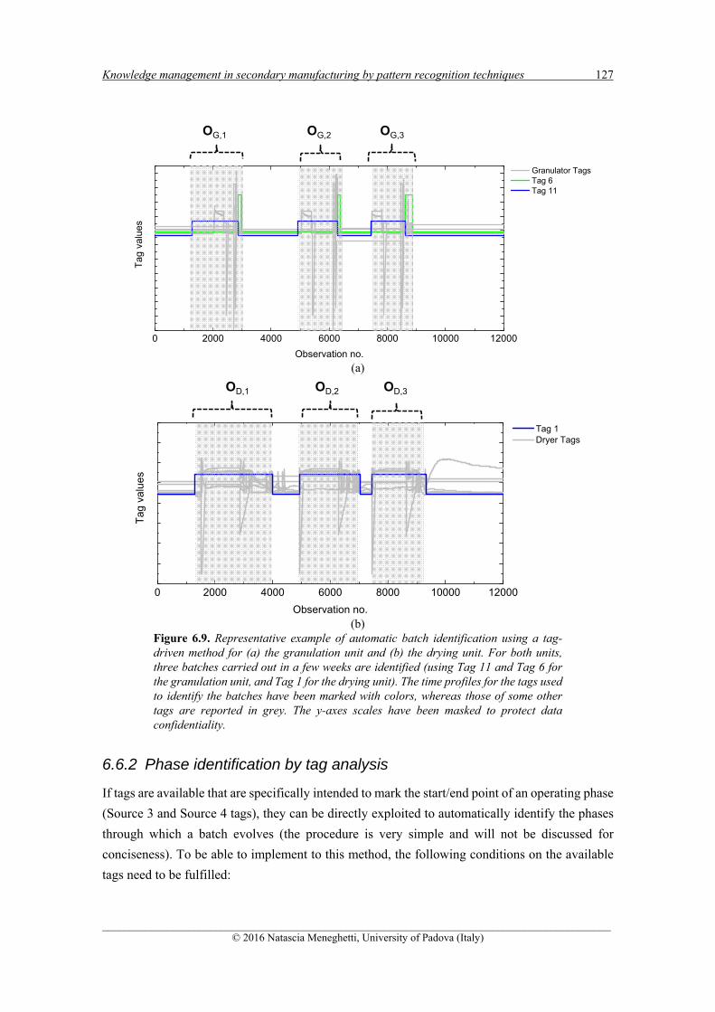
Knowledge management in secondary manufacturing by pattern recognition techniques 127
______________________________________________________________________________________________ © 2016 Natascia Meneghetti, University of Padova (Italy)
(a)
(b)
Figure 6.9. Representative example of automatic batch identification using a tag-driven method for (a) the granulation unit and (b) the drying unit. For both units, three batches carried out in a few weeks are identified (using Tag 11 and Tag 6 for the granulation unit, and Tag 1 for the drying unit). The time profiles for the tags used to identify the batches have been marked with colors, whereas those of some other tags are reported in grey. The y-axes scales have been masked to protect data confidentiality.
6.6.2 Phase identification by tag analysis
If tags are available that are specifically intended to mark the start/end point of an operating phase
(Source 3 and Source 4 tags), they can be directly exploited to automatically identify the phases
through which a batch evolves (the procedure is very simple and will not be discussed for
conciseness). To be able to implement to this method, the following conditions on the available
tags need to be fulfilled:
0 2000 4000 6000 8000 10000 12000
Tag
val
ues
Observation no.
Granulator Tags Tag 6 Tag 11
OG,1 OG,2 OG,3
0 2000 4000 6000 8000 10000 12000
Tag
val
ues
Observation no.
Tag 1 Dryer Tags
OD,1 OD,2 OD,3

128 Chapter 6
______________________________________________________________________________________________ © 2016 Natascia Meneghetti, University of Padova (Italy)
each operating phase must be defined by a tag;
the tags employed for phase identification must recorded for all batches.
This is the case of the granulation unit, for which phase identification can be easily done by
directly exploiting the following tags:
Tag 7 and Tag 5, indicating the duration of Phase 1;
Tag 8, indicating the duration of Phase 2;
Tag 9, indicating the duration of Phase 3;
Tag 6, indicating the duration of Phase 4.
However, this solution is not applicable to the drying unit, since there is only one tag (Tag 13)
that univocally marks the duration of an operating phase (namely the Pre-heating phase).
6.6.3 Phase identification by pattern recognition
In many manufacturing units, tags allowing one to easily identify the start and end instants for all
the phases that characterize a batch (Source 4 and Source 3 tags) may not be available for all
phases. In such instances, the batch phase identification problem can be transformed into a sample
classification problem, which is manageable even in the absence of sufficient number of these
tags. The task is therefore to assign each observation (sample) of a given batch Ob to a class
p( Pp ...,,2,1 ), the P classes being the operating phases characterizing that batch plus some
“inter-phases”, which are conveniently defined because on certain time periods some observations
may not be assignable to any operating phases, since they simply represent the intervals occurring
between two consecutive phases when ancillary operations are carried out (e.g., unit re-setting,
samplings etc.).
Both unsupervised methods (PCA, Chapter 2, Section 2.2.2) and supervised methods (linear
discriminant analysis; McLachlan ,2004); k-nearest neighbors (k-NN, Chapter 2, Section 2.2.1);
partial least-squares discriminant analysis (Barker and. Rayens, 2003) were tested to this purpose.
On average, k-NN showed a better performance for the case studies considered in this study, and
for this reason only the results obtained with this technique will be discussed.
The k-NN classification method allows one to classify an observation as belonging to one class
or to another, depending on the class attribution for an assigned number k of neighbors identified
according to a given distance criterion (detailed information about k-NN is reported in Chapter 2,
Section 2.2.1. The k-NN model is built from a set of calibration observations for which the class
assignment is known a priori and then used to classify new observations (e.g., an entire batch not
included in the calibration set). Therefore, to build the classification model one needs: i) defining
the calibration observations; ii) providing the class assignment for each of them.
Given batch b, for which Nb observations have to be assigned to P classes, the k-NN model
classification performance can be evaluated using three metrics (Ballabio and Todeschini, 2009):
error rate (ER), sensitivity (Snp), and specificity (Spp):
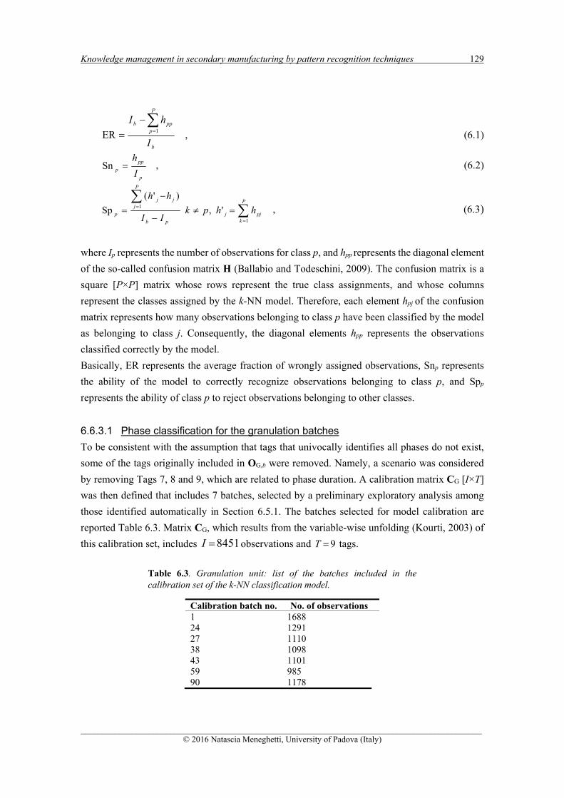
Knowledge management in secondary manufacturing by pattern recognition techniques 129
______________________________________________________________________________________________ © 2016 Natascia Meneghetti, University of Padova (Italy)
b
P
pppb
I
hI
1ER , (6.1)
p
pp
p I
hSn , (6.2)
P
kpjj
pb
P
jjj
p hhpkII
hh
1
1 ' ,
)'(
Sp , (6.3)
where Ip represents the number of observations for class p, and hpp represents the diagonal element
of the so-called confusion matrix H (Ballabio and Todeschini, 2009). The confusion matrix is a
square [P×P] matrix whose rows represent the true class assignments, and whose columns
represent the classes assigned by the k-NN model. Therefore, each element hpj of the confusion
matrix represents how many observations belonging to class p have been classified by the model
as belonging to class j. Consequently, the diagonal elements hpp represents the observations
classified correctly by the model.
Basically, ER represents the average fraction of wrongly assigned observations, Snp represents
the ability of the model to correctly recognize observations belonging to class p, and Spp
represents the ability of class p to reject observations belonging to other classes.
6.6.3.1 Phase classification for the granulation batches
To be consistent with the assumption that tags that univocally identifies all phases do not exist,
some of the tags originally included in OG,b were removed. Namely, a scenario was considered
by removing Tags 7, 8 and 9, which are related to phase duration. A calibration matrix CG [I×T]
was then defined that includes 7 batches, selected by a preliminary exploratory analysis among
those identified automatically in Section 6.5.1. The batches selected for model calibration are
reported Table 6.3. Matrix CG, which results from the variable-wise unfolding (Kourti, 2003) of
this calibration set, includes 8451I observations and 9T tags.
Table 6.3. Granulation unit: list of the batches included in the calibration set of the k-NN classification model.
Calibration batch no. No. of observations 1 1688 24 1291 27 1110 38 1098 43 1101 59 985 90 1178

130 Chapter 6
______________________________________________________________________________________________ © 2016 Natascia Meneghetti, University of Padova (Italy)
Note that assigning the correct class to each observation included in CG is a time consuming task,
because class assignment is done on the basis of a visual analysis of the time profiles of the tags
available for each observation. Appropriately selecting CG is therefore crucial, since CG should
include a limited subset of batches, which nevertheless represent well the entire variability of the
data historian. The explorative data analysis discussed in Section 6.5 can provide useful
information to this purpose.
Five classes were identified visually by analyzing the tag profiles for CG; an example of such
visual analysis is shown in Figure 6.10. These classes (Table 6.5) include the four granulation
phases (Section 6.3.1) as well as one inter-phase, which represents the interval between two
different operating phases when the impeller is off. Note that the actual operation of a given phase
may sometimes be different from batch to batch (e.g., depending of the product manufactured).
This does not represent a problem for phase recognition, provided that all the admissible tag
patterns are well represented in the calibration matrix.
Figure 6.10. Granulation unit: classes identified for a representative granulation batch of the calibration set (batch no.1); for clarity only a few tag profiles are indicated. The y-axes scale has been masked to protect data confidentiality.
A vector cG, whose elements represent the class assigned to each observation of the calibration
matrix, was defined to build the k-NN classification model, whose characteristics are summarized
in Table 6.4. Note that, in addition to the Euclidean distance, other distance criteria were tested,
with no major impact on the final results.
Table 6.4. Granulation unit: main characteristics of the k-NN model used for batch phase identification.
No. of neighbors (k) Distance criterion Data pre-treatment No. of classes (P) 5 Euclidean distance Autoscaling on Ob columns 5
Class i1
Clas
s 1
Clas
s 2
Clas
s 3
Clas
s 4
Class i1
Cla
ss i
0 4 8 800 1000 1200 1400 1600 1800
Tag
val
ues
Observation no.
Tag 2 Tag 4 Tag 5 Tag 6
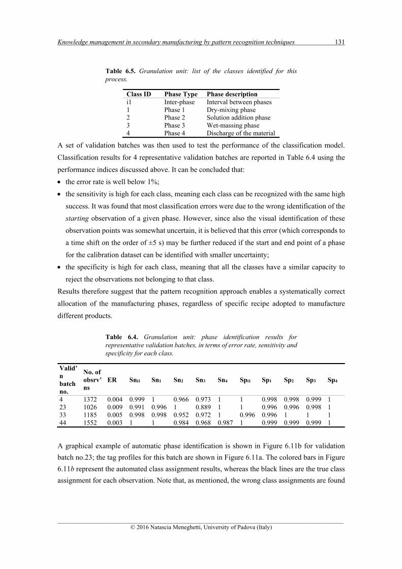
Knowledge management in secondary manufacturing by pattern recognition techniques 131
______________________________________________________________________________________________ © 2016 Natascia Meneghetti, University of Padova (Italy)
Table 6.5. Granulation unit: list of the classes identified for this process.
Class ID Phase Type Phase description i1 Inter-phase Interval between phases 1 Phase 1 Dry-mixing phase 2 Phase 2 Solution addition phase 3 Phase 3 Wet-massing phase 4 Phase 4 Discharge of the material
A set of validation batches was then used to test the performance of the classification model.
Classification results for 4 representative validation batches are reported in Table 6.4 using the
performance indices discussed above. It can be concluded that:
the error rate is well below 1%;
the sensitivity is high for each class, meaning each class can be recognized with the same high
success. It was found that most classification errors were due to the wrong identification of the
starting observation of a given phase. However, since also the visual identification of these
observation points was somewhat uncertain, it is believed that this error (which corresponds to
a time shift on the order of ±5 s) may be further reduced if the start and end point of a phase
for the calibration dataset can be identified with smaller uncertainty;
the specificity is high for each class, meaning that all the classes have a similar capacity to
reject the observations not belonging to that class.
Results therefore suggest that the pattern recognition approach enables a systematically correct
allocation of the manufacturing phases, regardless of specific recipe adopted to manufacture
different products.
Table 6.4. Granulation unit: phase identification results for representative validation batches, in terms of error rate, sensitivity and specificity for each class.
Valid’n batch no.
No. of obsrv’ns
ER Sni1 Sn1 Sn2 Sn3 Sn4 Spi1 Sp1 Sp2 Sp3 Sp4
4 1372 0.004 0.999 1 0.966 0.973 1 1 0.998 0.998 0.999 1 23 1026 0.009 0.991 0.996 1 0.889 1 1 0.996 0.996 0.998 1 33 1185 0.005 0.998 0.998 0.952 0.972 1 0.996 0.996 1 1 1 44 1552 0.003 1 1 0.984 0.968 0.987 1 0.999 0.999 0.999 1
A graphical example of automatic phase identification is shown in Figure 6.11b for validation
batch no.23; the tag profiles for this batch are shown in Figure 6.11a. The colored bars in Figure
6.11b represent the automated class assignment results, whereas the black lines are the true class
assignment for each observation. Note that, as mentioned, the wrong class assignments are found

132 Chapter 6
______________________________________________________________________________________________ © 2016 Natascia Meneghetti, University of Padova (Italy)
mainly at the very beginning of a true operating phase (e.g., see the blue bar around observation
no. 600 in Figure 6.11b).
(a)
(b)
Figure 6.11. Granulation unit, validation batch no.23: (a) representative tag profiles and (b) class assignment as obtained from the k-NN classification model. The classes assigned by the model are color-coded as indicated in the legend; the true class assignment is indicated by the black line.
6.6.3.2 Phase classification for the drying batches
The same procedure used for the granulator was applied to the drying unit. A calibration set was
defined using 8 batches among those identified in Table 6.5. Note that, since drying follows
granulation, the opening of the granulator discharge valve indicates not only the end of Phase 4
for the granulation process, but also that the material is starting to be charged into the drying unit,
i.e., the beginning of drying Phase 2. For this reason, Tag 6 of Table 6.1 (which is in fact pertinent
to the granulation process) was added as an additional column to D. We mention this simple trick
to stress that, although the data historian review can indeed be performed automatically, it is
nevertheless very important that, prior to the design of the data mining system, the datasets are
conveniently arranged according to engineering reasoning.
0 100 200 300 400 500 600 700 800 900 1000 1100
Tag
va
lues
Observation no.
0 100 200 300 400 500 600 700 800 900 1000 1100
i1
1
2
3
4
Cla
sse
s
Observation no.

Knowledge management in secondary manufacturing by pattern recognition techniques 133
______________________________________________________________________________________________ © 2016 Natascia Meneghetti, University of Padova (Italy)
Table 6.5. Drying unit: list of the batches included in the calibration set of the k-NN classification model.
Calibration batch no.
No. of observations
5 1195 21 1760 24 2067 58 2046 75 1359 78 2058 79 1892 87 1287
By analyzing the trends of the available tags for the calibration batches, 9 classes were eventually
defined as reported in Table 6.6. Five of them denote true operating phases, whereas the remaining
four classes represent recurrent events (not necessarily present in all batches), which were
classified as inter-phases.
Table 6.6. Drying unit: list of the classes identified for this process.
Class ID Phase Type Phase description i1 Inter-phase Break phase 1 Phase 1 Pre-heating phase i2 Inter-phase Break-phase after pre-heating phase 2 Phase 2 Charging phase 3 Phase 3 Constant-drying rate phase 4 Phase 4 Falling-drying-rate phase i3 Inter-phase Break phase related to the drying phase 5 Phase 5 Cooling-down and discharge phases i4 Inter-phase Break phase related to the cooling down phase
A graphical representation of the classes identified during model building is provided in Figure
6.12 for a typical calibration batch. Note that the discrimination between the constant drying rate
phase and the falling drying rate phase was uncertain for some calibration batches. For this reason,
it was assumed that the falling drying rate phase starts as soon as the temperatures of the exhaust
air and of the product start to increase. Furthermore, to simplify the analysis the cooling down
phase and the discharge phase were considered as a single phase. Details on the k-NN model built
for the drying unit are reported in Table 6.7. A summary of the automatic phase identification
results for four representative validation batches is reported in Table 6.8 and Table 6.9.
Table 6.7. Drying unit: main characteristics of the k-NN model used for the phase classification.
No. of neighbors Distance criterion Data pre-treatment No. of classes 7 Euclidean distance Autoscaling of Ob columns 9

134 Chapter 6
______________________________________________________________________________________________ © 2016 Natascia Meneghetti, University of Padova (Italy)
Figure 6.12. Drying unit: classes identified for a representative drying batch of the calibration set (batch no. 58); for clarity only a few tag profiles are indicated. The y-axes scale has been masked to protect data confidentiality.
The increase of the misclassified observations reflects the greater complexity of the phase
identification problem for the drying system. As anticipated by the preliminary exploratory
analysis, this is due to the larger variability experienced by the drying unit than by the granulation
one. Nevertheless, the classification model still exhibits very good performance:
the error rate ranges between 1.0% and 7.0%, with the largest ER value being obtained for a
very peculiar batch (no.73; Figure 6.13b-d), which was purposely included in the validation
dataset to provide a challenging test bed;
the sensitivity index indicates that, for all batches, the model does a very good job in class
attribution for classes 1, 2 3 and 5 (see Table 6.6 for class/phase correspondence). Bad model
performance is limited to class 6 assignment for validation batch no.6, and to class 4
assignment for validation batch no.73. However, it was found that also the visual identification
of the exact start and end point of these two phases is uncertain for both batches. Therefore,
the number of such misclassifications may probably be reduced if a clearer identification of
the operating phases can be provided;
the specificity index is satisfactorily high for all classes and all batches, meaning that all the
classes have the same ability to reject observations belonging to other classes.
Table 6.8. Drying unit: phase identification results for representative validation batches, in terms of error rate and sensitivity for each class.
Valid’n batch no.
No. of obsrv’ns
ER Sni1 Sn1 Sni2 Sn2 Sn3 Sn4 Sni3 Sn5 Sni4
2 2101 0.010 0.964 1 1 0.917 1 0.940 - 0.977 1 6 1269 0.021 0.996 1 1 0.989 0.947 0.125 0.949 0.956 - 38 4672 0.014 0.986 1 1 0.971 0.866 0.905 - 0.885 - 73 2371 0.070 0.979 1 0.975 0.385 0.787 0.913 - 0.925 0.964
0 100 200 1000 2000
Ta
g va
lues
Observation no.
Tag 3 Tag 7 Tag 8 Tag 9 Tag 10 Tag 13 Tag 14 Tag 15
Class 1
Class i2
Class 4
‐i1‐i3
Class i1
‐i4
Class 5
Class 2
‐3
Class 4
Class 3

Knowledge management in secondary manufacturing by pattern recognition techniques 135
______________________________________________________________________________________________ © 2016 Natascia Meneghetti, University of Padova (Italy)
Table 6.9. Drying unit: phase identification results for representative validation batches, in terms of specificity for each class.
Batch Spi1 Sp1 Spi2 Sp2 Sp3 Sp4 Spi3 Sp5 Spi4 2 0.997 1 0.999 1 0.997 0.999 0.998 0.999 1 6 0.988 1 0.999 0.999 0.995 0.996 1 0.999 1 38 0.997 1 0.999 1 0.998 0.998 0.995 0.999 1 73 0.952 1 1 0.987 0.998 0.983 0.992 0.997 0.996
(a) (b)
(c) (d) Figure 6.13. Drying unit. Upper diagrams: representative tag profiles for validation batch (a) no.38 and (b) no.73; lower diagrams: class assignment as obtained from the k-NN classification model for validation batch (c) no.38 and (d) no. 73 (phase identification is done on the basis of Table 8). In (c) and (d), the classes assigned by the model are color-coded as indicated in the legend; the true class assignment is indicated by the black line.
6.7 Batch identification and phase identification in Scenario 2
The availability of appropriate tags to carry out a tag-based batch identification procedure
(Section 6.6.1) cannot be considered as a standard occurrence in secondary manufacturing
environments. In fact, there might be units for which appropriate tags indicating the status of the
unit or the duration of the operating phases are not available (Scenario 2 in Figure 6.1). In this
section, an alternative methodology to identify single batches from historical datasets is presented.
This methodology, which we call phase-based batch identification, works jointly with a phase
identification procedure, and therefore requires to preliminarily identify the operating phases
within the D or G datasets (Section 6.7.1). This information is then used to reconstruct the
information needed to identify each single batch included in D or G (Section 6.7.2).
0 800 1600 2400 3200 4000 4800
Tag
val
ues
Observation no.0 600 1200 1800 2400
Ta
g va
lues
Observation no.

136 Chapter 6
______________________________________________________________________________________________ © 2016 Natascia Meneghetti, University of Padova (Italy)
As a demonstration example, the methodology will be applied to the granulation unit only (even
if, as discussed earlier, tag-based batch identification is actually possible for this unit).
6.7.1 Phase identification in the entire data historian
The identification of the operating phases within the data historian can be carried out using the
pattern recognition technique illustrated in Section 6.6.3 even if the batch segments are not
available. In fact, to build the k-NN classification model, one needs to i) visually identify the set
C of calibration batches within the data historian (G), and ii) assign each observation of C to a
class. Once the model is built, it can be used to classify each single observation remaining in the
historian, regardless of the fact that the observation has already been attributed to a batch or not.
The class assignments for all observations are then collected in vector c .
6.7.2 Phase-based batch identification
Since the phase identification operation is carried out observation-by-observation, by arranging
the observations in chronological order, the identification of sequences of operating phases
belonging to different batches can be obtained: the first observation included in c that belongs to
the first operating phase indicates the start of a batch, whereas the last observation classified as
belonging to the last operating phase indicates the end of that batch.
6.7.2.1 Results for the granulation unit
To be consistent with the assumption that leads to follow Scenario 2***, a different set of tags was
included in a new overall dataset G~
. Namely, some tags (which do relate to the batch length)
were removed from G. The tags removed are the number 7, 8, 9 and 11. Since only Tag 6
(granulator discharge valve) indicates the duration of the granulation Phase 4, this tag was not
removed.
The phase-based batch identification method was then applied to G~
matrix, thus identifying 315
different “batches”, i.e. many more than those (90) identified using the tag-based method (Section
6.6.1). To explain this difference, it should be noted that the historical data segments include
events (e.g., valve openings) that in some cases occur during a batch, whereas in some other are
totally unrelated to the batch operation. Since in most cases the correlation between tag values are
not very different in these two occurrences, phase misclassifications may well occur. This, in turn,
causes the wrong identification of these events as part of granulation batches that in fact do not
exist. However, the “spurious” batches can be easily detected by the batch characterization
procedure presented in the next section.
*** Scenario 2 refers to datasets for which no tags explicitly indicating the start and end observations of a batch are available. Therefore, for these datasets, the tag-based batch identification procedure of Scenario 1 cannot be implemented.

Knowledge management in secondary manufacturing by pattern recognition techniques 137
______________________________________________________________________________________________ © 2016 Natascia Meneghetti, University of Padova (Italy)
6.8 Batch characterization
The methods allowing one to identify the single batches within an overall data historian also
provide the number of different batches that have been carried out along the window spanned by
the historian. However, the batch identification methods cannot discriminate between “standard”
batches (i.e., batches whose tag profiles conform to an assigned standard, as for example those
reported in Figure 6.4 and Figure 6.5) and “non-standard” batches (i.e., batches that present a very
different time evolution). There are several reasons why a batch might be classified as non-
standard; among them: the presence of cleaning operations during a batch, the presence of
operating segments repeated twice or lasting much longer than for other batches, partial testing
on the equipment tests, or the processing of a new product. Note that the fact that a batch is
denoted as non-standard is not related to the quality of the manufactured product, but only to the
time evolution of the tags.
A method is proposed in this section to automatically detect those batches that present a time
evolution that is significantly different from the standard ones. The method can also be used to
characterize each batch depending on a set of features of industrial interest (e.g., duration of a
given operating phase, load to an impeller, etc.). This may be a simple way to further verify that
the manufactured product or associated process did not unexpectedly change characteristics over
time. As such, the proposed procedure may contribute to periodic product quality reviews.
6.8.1 Batch characterization by PCA and k-NN modeling
The method requires building a feature matrix F††† [B×V], where B is the total number of batches
identified for a given operation, and V is the number of feature variables purposely defined for
the unit where that operation is carried out. Each of these variables represents a specific feature
of the batch set (e.g., the duration of an operating phase, or the time-integral or average value of
some selected tags), which summarizes the dynamic evolution of the tags. Note that the values of
some feature variables may be the outcome of Task 1 or Task 2 calculations.
The characterization of a batch can be obtained through the following procedure:
1. F is split into two matrices, a calibration matrix (Fcal) and a validation matrix (Fval);
2. a PCA model is built from Fcal;
3. the model scores and loadings are analyzed in order to identify groups (clusters) of batches
with similar characteristics (see Chapter 2, Section 2.2.2). Each cluster is assigned to a different
class; the characteristics of each cluster can be highlighted by coupling a loadings plot analysis
to a visual inspection of the tag profiles for the batches included in the cluster;
††† Note that, in this Chapter F is used to denote the feature matrix and not the residual matrix F as in the previous Chapters.

138 Chapter 6
______________________________________________________________________________________________ © 2016 Natascia Meneghetti, University of Padova (Italy)
4. a k-NN classification model is built using the scores of the PCA model and the classes defined
at step 3;
5. Fval is projected onto the PCA model, and the position of each batch of the validation set is
analyzed in the score space. The batches that appear not to belong to any of the clusters
identified at step 3 are denoted as “non-standard”;
6. automatic characterization of the standard batches included in Fval is carried out using the k-
NN model.
Next, application of this procedure is discussed with reference to the granulation unit. Similar
results were obtained also for the drying unit.
6.8.1.1 Results for the granulation unit
The feature matrix FG was built using the features indicated in Table 6.10, where fG,v [B×1]
indicates the v-th feature variable (v = 1, 2, …, V). Note that, although fG,8 is expected to always
be zero, this variable was purposely included in the feature matrix in order to detect possible
inconsistencies in the recorded tag values.
Table 6.10. Granulation unit: feature variables defined for batch characterization.
Feature variable name Feature variable description fG,1 Duration of Phase 1 fG,2 Duration of Phase 2 fG,3 Duration of Phase 3 fG,4 Duration of Phase 4 fG,5 Average impeller speed in Phase 1 fG6 Average impeller speed in Phase 2 fG,7 Average impeller speed in Phase 3 fG,8 Average chopper speed in Phase 1 fG,9 Average chopper speed in Phase 2 fG10 Average chopper speed in Phase 3 fG,11 Maximum impeller load
It is important to remark that different sets of features may be defined and included in F, according
to the information that one wishes to extract from the available dataset.
A PCA model was built using a subset of FG that includes 83 batches; the model used 2 PCs,
capturing more than 73% of the data variability. The remaining 7 batches were used for model
validation.
Figure 6.14a shows that most granulation batches (circles) are clustered in similar areas of the
scores plane, with the exception of batches no. 51, 18, and possibly 69, which locate away from
the main clusters. These three calibration batches are therefore different from the other ones, and
as such they were denoted as non-standard. Analysis of the tag profiles for these batches revealed
that the non-standard designation was truly justified by operational reasons, namely:

Knowledge management in secondary manufacturing by pattern recognition techniques 139
______________________________________________________________________________________________ © 2016 Natascia Meneghetti, University of Padova (Italy)
batch 51 presented tag profiles that are strongly different from those usually found in standard
granulation operations;
in batch 18, Phase 1 was extremely prolonged;
in batch 69, Phase 1 was repeated twice.
(a) (b) Figure 6.14. Batch characterization in the granulation unit: (a) loadings and (b) scores of the PCA model built on the calibration feature matrix. The numbers in the symbols indicate the batch number.
The remaining calibration batches, which are visually grouped in four different clusters, were
denoted as standard. Analysis of the PCA model loadings (Figure 6.14b) provided the following
general considerations:
the position of a batch along PC1 is mainly related to the impeller speed, the chopper speed,
the duration of Phase 1 and the duration of Phase 3;
the position of a batch along PC2 is mainly related to the duration of Phase 2 and to the impeller
load.
Consequently, the main characteristics of each cluster were identified as reported in Table 6.11
The clusters (and related characteristics) served as the basis for the automatic characterization of
the validation batches.
Table 6.11. Granulation unit: characteristics of the 4 clusters defined to classify the calibration batches.
Batches included Batch characteristics
Cluster 1 15, 45, 46, 47,65, 84, 85, 89, Very long phase 2, low chopper speed, low
impeller load
Cluster 2 38, 39, 81, 82, 83 Long phase 2, low chopper speed, low impeller
load
Cluster 3 4, 5, 6, 23, 24, 78, 79, 80 Intermediate phase 2, low chopper speed, low
impeller load
Cluster 4 All the other batches Short phase 2, high chopper speed, high impeller
load, different duration of phase 1
-12 -6 -4 -2 0 2 4 6-12
-2
0
2
4
18
51
69
Sco
res
on P
C2
(21%
)
Scores on PC1 (52.8%)
Cluster 4
Cluster 1
Cluster 3
Cluster 2
f1 f2 f3 f4 f5 f6 f7 f8 f9 f10 f11-0.4
-0.2
0.0
0.2
0.4
0.6
Loa
din
gs PC1 PC2

140 Chapter 6
______________________________________________________________________________________________ © 2016 Natascia Meneghetti, University of Padova (Italy)
Projection of the validation data Fval,G onto the PCA model resulted in the red triangles of Figure
6.15.
Figure 6.15. Batch characterization in the granulation unit: projections on the scores plane of the 7 validation batches (red triangles). The numbers in the symbols indicate the batch number.
Three non-standard validation batches were identified, namely batches no. 52, 17, and possibly
8. Inspection of the relevant tag profiles confirmed that:
batch 52 presented tag profiles that are very different from those found in standard granulation
operations;
in batch 17, some operating phases were repeated twice;
in batch 8, Phase 1 was very long.
Note that, although class assignment for the standard validation batches was done by visual
inspection, assignment of these batches to the clusters identified in Figure 6.15 can be achieved
also automatically, by simply building a classification model (e.g., a k-NN one) for the scores of
the PCA model shown in Figure 6.15, and then using this classification model with the standard
validation batches. Excellent classification results were indeed obtained by using this approach.
SECTION B – COMPARISON OF DIFFERENT PRODUCTION
PERIODS USING RECIPE INFORMATION
6.9 Objectives of Section B
In the following Sections the analysis is carried out for both datasets assuming that information
about the products manufactured is available in the form of number of products and
manufacturing recipe.
-12 -6 -4 -2 0 2 4 6-12
-2
0
2
4
8
17
25
44
52
87
90S
core
s o
n P
C2
(21
%)
Scores on PC1 (52.8%)
Cluster 4
Cluster 1
Cluster 3
Cluster 2

Knowledge management in secondary manufacturing by pattern recognition techniques 141
______________________________________________________________________________________________ © 2016 Natascia Meneghetti, University of Padova (Italy)
In this second section, the same tags reported in Section 6.4.1 have been selected for the
granulation unit. For the drying unit instead, Tag no. 3, 6 and 7 have been removed from the set
reported in Section 6.4.2, and one more tag (related to the pressure difference) has been added, in
order to improve the classification performance (Section 6.11). For each dataset i, the
observations of the two datasets are arranged into two matrices (Gi and Di) whose characteristics
are reported in Table 6.12. In the two production periods analyzed, four different products were
manufactured. Using the available information about the manufacturing recipes may be
appropriate to better tune the data review activity. In this section of the analysis, the methodology
has been improved (Figure 6.16) using this new piece of information by modifying the batch
characterization step.
Table 6.12. Characteristics of the 2 datasets analysed in Part 2 for the granulation and the drying unit.
G1 D1 G2 D2 Unit Granulation Drying Granulation Drying Dataset Dataset 1 Dataset 1 Dataset 2 Dataset 2 Size 3127088×11 3127088×12 3127088×11 3127088×12
Figure 6.16. Flowchart of the modified approach to analyze historical manufacturing data. In this study, only the steps following the blue path have been considered.

142 Chapter 6
______________________________________________________________________________________________ © 2016 Natascia Meneghetti, University of Padova (Italy)
Namely, three additional steps have been considered (Figure 6.16) with the purpose of:
removing all the data segments that do not refer to actual drying/granulation batches (ancillary
operation removal);
grouping the identified batches in different clusters according to the product processed (cluster
identification);
characterizing each batch within each cluster in order to detect non-standard batches (batch
characterization within each cluster).
The objectives of this section are the following: i) testing the performance of the methodology by
also using the batch recipes as an information source (path marked in blue in Figure 6.16); ii)
evaluating the consistency of the two available datasets, namely assessing whether the features
characterizing a given batch operation have changed throughout the production periods analyzed.
6.10 Batch identification
Depending on the characteristics of the available tags, two methods were proposed (Section 6.2 )
to automatically recognize the start and end points of each batch within an historical dataset: tag-
based batch identification and phase-based batch identification. In this study, the tag-based batch
identification is used to identify the batches included in G2 and D2 using the same methodology
employed for G1 and D1 in Section 6.6.1. The observations belonging to a single drying or
granulation batch b are extracted and arranged into a new matrix Ob [Nb×T], where the meaning
of the symbols is the same as in Section 6.6.1.
6.10.1 Adjustments introduced in the tag-based batch identification
The tags available in G2 and D2 allow implementing the tag-based batch identification method for
both units. In fact, one or more tags exist that unambiguously indicate when the equipment is (and
is not) in operation.
In general, it is known a priori that some operations identified as single batches simply correspond
to equipment tests or cleaning operations. Thanks to the information acquired in the analysis of
Dataset 1 (Section 6.8 ) and to the new information available from the recipes, an additional
analysis has been included in the proposed methodology to discriminate between these auxiliary
operations and actual drying/granulation batches. This topic will be discussed in Section 6.12.1 .
For Dataset 1, an exploratory analysis of the batches identified by the tag-based batch
identification procedure in Dataset 1 revealed that some of the operations, which had originally
been recognized as separate batches, actually corresponded to the same batch that was interrupted
for a short time period. For this reason, a post-batch identification procedure was implemented in
Section 6.6.1 (both for the granulation unit and for the drying unit) in order to collect in the same
matrix Ob only the observations that can be considered as belonging to the same operation. For

Knowledge management in secondary manufacturing by pattern recognition techniques 143
______________________________________________________________________________________________ © 2016 Natascia Meneghetti, University of Padova (Italy)
Dataset 2 this post-batch identification procedure cannot be applied, since there are some cases
for which the gap between two consecutive data segments is less than a given threshold, but these
segments do refer to truly different operations (usually a drying/granulation batch and a
test/cleaning operation). Therefore, in order to apply the same procedure for both datasets, the
post-batch identification was not applied to Dataset 1. As a consequence the number of batches
identified in the following sections is different from those reported in Section 6.6.1.1 and 6.6.1.2
6.10.2.1 Results for the granulation unit
For the granulator, a granulation batch b can be easily singled out using the combination of Tag
11 and Tag 6. The relevant data were collected in matrix OG1,b and OG2,b. Using this tag-based
identification procedure, 99 different granulation batches were identified in G1 and 215 in G2.
6.10.2.2 Results for the drying unit
In this case, a single tag (Tag 1) is sufficient to recognize different drying operations, as this tag
is active during the entire duration of the batch. Eventually, 99 different OD1,b matrices and 214
OD2,b matrices were defined for D1 and for D2 respectively.
6.11 Phase identification
In this section, the classification method employed to automatically recognize the operating
phases characterizing a typical granulation/drying batch is tested on the batches identified within
G2 and D2. In particular the k-NN models used in Section 6.6.3 for the granulation and the drying
unit have been enhanced based on the information provided by the recipes of the product
manufactured during the time windows under investigation, thus permitting to relax some
assumptions previously considered for both units. Furthermore, in order to improve the reliability
of the results, the performance of these classification models are tested on larger validation sets
with respect to the validation sets considered above. Therefore, the objectives of this section are
mainly two: i) assessing the performance of the new classification models, thus defining the limit
of the analysis thanks to the availability of larger validation sets; ii) testing the ability of
recognizing different operating phases in batches carried out in different time windows.
For both units, a k-NN model, which is the same for all products, was defined to classify the
observations included in each Ob as belonging to one of the classes defined for each unit. The
classification model is built from a set of calibration observations belonging to Dataset 1 for which
the class assignment is known and therefore can be set a priori. The model is then used to classify
new observations, i.e. the observations included in the batches of Dataset 2 (or of Dataset 1, but

144 Chapter 6
______________________________________________________________________________________________ © 2016 Natascia Meneghetti, University of Padova (Italy)
not included in the calibration set). A subset‡‡‡ of these batches (validation set) is then selected
for each unit to test the model performance. The k-NN model classification performance is
evaluated using the three metrics defined in Section 6.6.3.
6.11.1 Phase identification in the granulation unit
6.11.1.1 Design of the classification model
The k-NN model used to recognize different operating phases in the granulation batches of
Dataset 1 has been updated according to the recipes provided for each of the four products
manufactured during the six months investigated. In particular, six classes (Table 6.13) were
considered instead of five as shown in Figure 6.17. These classes include the four operating phases
that characterize the granulation process and two inter-phases. The new inter-phase has been
introduced to better characterize the first part of the process, which differs according to the
product processed. A calibration matrix CG is defined by collecting 7 batches of Dataset 1 selected
by a preliminary exploratory analysis, including at least one batch for each of the 4 products
considered in this work. Note that, thanks to the availability of the recipes, a representative batch
for each manufactured product can be included in the calibration matrix. Matrix CG includes
8451I observations (each observation corresponds to 5 s) and 11T variables (tags). The
classification model characteristics are summarized in Table 6.14.
Figure 6.17. Granulation unit: classes identified for a representative granulation batch of the calibration set. The four operating phases (OPs) are coloured respectively in pink, orange, blue and green, whereas the inter-phases (IPs) are marked in grey. For clarity, a few tags only are reported. The y-axis scale has been masked to protect data confidentiality.
‡‡‡ Assigning the correct class to each single observation included in both calibration and validation dataset is a time consuming task, because class assignment is done on the basis of a visual analysis of the time profiles of the tags available for each observation. For this reason only a subset of the available batches is selected.
0 200 400 600 800 1000 1200
Tag
va
lues
No. observations
IP1 IP2 OP1 OP2 OP3 OP4

Knowledge management in secondary manufacturing by pattern recognition techniques 145
______________________________________________________________________________________________ © 2016 Natascia Meneghetti, University of Padova (Italy)
Table 6.13. Granulation unit: main characteristics of the k-NN model used for phase identification.
Table 6.14. Granulation unit: list and description of the classes identified for this process.
6.11.1.2 Phase identification for the validation batches
Only minor changes have been implemented in the classification model defined for the
granulation unit, so the results achieved for Dataset 1 are very similar to those presented in Section
6.6.3.1 . Hence, for the sake of conciseness, only the results obtained testing the classification
model on a set of batches of the new dataset (Dataset 2) are reported.
A set of 8 validation batches of Dataset 2 is used to test the performance of the classification
model. The classification results obtained for each validation batch are reported in Table 6.15,
whereas in Figure 6.18 a graphical representation of the results is provided by grouping all the
batches that present similar classification errors. The results obtained are very similar to those
achieved for Dataset 1 in Section 6.6.3.1 , where the wrong class assignments are found mainly
at the very beginning of a true operating phase. The error rate ER never exceeds 1%, meaning
that only an average of about 5 observations out of 990 are assigned to a wrong class. Moreover,
both the sensitivity and the specificity (the values calculated for this index have not been reported
here for conciseness) are high for each class.
Table 6.15. Granulation unit: phase identification results for the validation batches (Dataset 2), in terms of error rate and sensitivity for each class.
Valid’n batch no.
No. of obsrv’ns ER Sni1 Sni2 Sn1 Sn2 Sn3 Sn4
101 635 0.008 0.994 - 1 0.991 0.920 1 112 1722 0.002 1 0.999 0.988 0.984 0.977 1 132 2742 0.001 1.000 0.998 0.988 1 0.971 1 145 906 0.004 0.995 0.997 1 1 0.949 1 156 1172 0.003 0.998 1 0.988 0.984 0.971 1 178 1053 0.003 1 - 0.984 1 0.950 1 244 746 0.008 1 - 0.936 1 0.926 1 281 936 0.009 0.999 - 0.920 1 0.920 1
No. of neighbours Distance criterion Data pre-treatment No. of classes 5 Euclidean distance Autoscaling on Ob columns 6
Class no. Phase type Description i1 Inter-phase Interval between phases i2 Inter-phase Pre-Phase 1 1 Phase 1 Dry-mixing phase 2 Phase 2 Solution addition phase 3 Phase 3 Wet-massing phase 4 Phase 4 Discharge of the material

146 Chapter 6
______________________________________________________________________________________________ © 2016 Natascia Meneghetti, University of Padova (Italy)
Figure 6.18. Granulation unit: distribution of the classification errors calculated for 10 validation batches of Dataset 2.
6.11.2 Phase identification in the drying unit
6.11.2.1 Design of the classification model
The availability of the recipes for the four products manufactured during the time windows under
investigation strongly contributes to improve the identification of the operating phases that
characterize the drying unit, allowing one to:
discriminate between the cooling and discharge phase (Phase 5 and 6);
consider the presence of an additional inter phase related to the final phase of the batch;
recognize the different time evolution of the batches depending on the product manufactured.
However, no information is available to clearly discriminate between the falling and constant
drying rate, whose starting points remains uncertain.
The k-NN model used to identify the operating phases for the batches of Dataset 1 has been
modified considering a different number of classes and a different calibration set. In fact, by
analyzing the trends of the available tags jointly with the information included in the recipes
(duration of some phases, values of some tags), 10 classes were eventually defined as reported in
Table 6.16. Six of them denote true operating phases, whereas the remaining four classes represent
recurrent events (not necessarily present in all batches), which were classified as inter-phases. A
calibration matrix CD including 7 batches purposely selected to consider all the products
manufactured has been defined. This matrix includes 13886I observations (each observation
corresponds to 5 s) and 13T variables (tags), selected by engineering reasoning in such a way
as to minimize the classification errors.
0.0% 0.5% 1.0% 1.5% 2.0% 2.5% 3.0%0
1
2
3
4
5
6
7
No.
bat
ches
ER
mean=0.48%

Knowledge management in secondary manufacturing by pattern recognition techniques 147
______________________________________________________________________________________________ © 2016 Natascia Meneghetti, University of Padova (Italy)
Table 6.16. Drying unit: list and description of the classes identified for this process.
A graphical representation of the classes identified during model building is provided in Figure
6.19 for a typical calibration batch. Note that all tags related to phase duration were modified as
done for the granulation data. Details on the k-NN model built for the drying unit are reported in
Table 6.17.
Table 6.17. Drying unit: main characteristics of the k-NN model used for the phase classification.
Figure 6.19. Drying unit: classes identified for a representative drying batch of the calibration set. The six operating phases (OPs) are coloured respectively in red, pink, blue, orange, green and purple whereas the inter-phases (IPs) are marked in grey. For clarity, a few tags only are reported. The y-axis scale has been masked to protect data confidentiality.
0 200 400 600 800 1000 1200
Tag
val
ues
No. observations
OP1 IP1 OP2 OP3 OP4 OP5 IP2 OP6 IP3
Class no. Phase type Description i1 Inter-phase Break phase 1 Phase 1 Pre-heating phase i2 Inter-phase Break phase after the pre-heating phase 2 Phase 2 Charging phase 3 Phase 3 Constant-drying rate phase 4 Phase 4 Falling-drying rate phase i3 Inter-phase Break phase 5 Phase 5 Cooling-down 6 Phase 6 Discharge i4 Inter-phase Break phase related to the filter shaking
No. of neighbours Distance criterion Data pre-treatment No. of classes 5 Euclidean distance Autoscaling of Ob columns 10

148 Chapter 6
______________________________________________________________________________________________ © 2016 Natascia Meneghetti, University of Padova (Italy)
6.11.2.2 Phase classification for the validation batches of Dataset 1
The new k-NN model built for the drying unit is tested on a validation set of 10 batches belonging
to Dataset 1 in order to assess the effects of the adjustments introduced. A summary of the phase
identification results is reported in Table 6.18, from which it can be observed that:
the error rate ER ranges from 0.7% to 6.7%, with an average value of 2.4%, namely about 47
observations out of 2160 are assigned to a wrong class. A graphical representation of the results
obtained for this index is provided in Figure 6.20 by grouping all the batches that present
similar classification errors;
the sensitivity index Snp indicates that, for all batches, the model does a very good job in
classifying classes 1, 2, 3, 7, 8 and 9 (see Table 6.16 for class/phase correspondence). For some
batches the model is not able to correctly recognize the observations belonging to class 4, 5, 6
and 10. Anyway, it should be highlighted that for the batches that present a low value of
sensitivity index related to class 4, actually Phase 4 is very short and the temperature increasing
is not significant. The model is not able to correctly identify Phase 4 for all batches with the
same characteristics;
the specificity index has not been reported since it was observed that in general the values of
this index are satisfactorily high for all classes and all batches.
Table 6.18. Drying unit: phase identification results for the validation batches of Dataset 1, in terms of error rate and sensitivity for each class.
Valid’n
batch no.
No. of
obsrv’ns
ER Sni1 Sn1 Sni2 Sn2 Sn3 Sn4 Sni3 Sn5 Sn6 Sni4
5 1195 0.016 0.976 0.997 1.000 0.886 1.000 0.903 - 0.984 0.975 0.963 6 1269 0.027 0.988 1.000 1.000 0.979 1.000 0.125 - 0.895 0.956 0.882 16 1845 0.020 0.966 0.976 1.000 0.985 0.881 1.000 - - 1.000 0.783 26 2663 0.010 0.997 0.984 1.000 1.000 0.995 0.879 - - 0.983 0.889 27 1760 0.016 0.986 0.992 1.000 1.000 0.900 0.952 1.000 - 1.000 - 35 1500 0.067 0.994 1.000 1.000 0.983 0.637 0.980 - - 0.987 0.074 44 4672 0.014 0.996 0.992 1.000 0.971 0.819 0.983 - - 0.966 0.381 82 2371 0.037 0.994 0.984 0.905 0.682 0.848 0.982 0.986 - 0.969 0.958 87 2058 0.026 0.927 0.997 1.000 0.957 0.936 0.043 - 0.976 1.000 0.581 92 2269 0.007 1.000 0.992 1.000 0.977 1.000 0.939 - - 0.974 0.840

Knowledge management in secondary manufacturing by pattern recognition techniques 149
______________________________________________________________________________________________ © 2016 Natascia Meneghetti, University of Padova (Italy)
Figure 6.20. Drying unit: distribution of the classification errors calculated for 10 validation batches of Dataset 1.
6.11.2.3 Phase classification for the validation batches of Dataset 2
The same classification model is then used to recognize different operating phases in 13 batches
belonging to Dataset 2. A summary of the results is reported in Table 6.19. The error rate (Table
6.19) ranges from 2.1% to 12.5%. The average value (5.5%) is significantly higher than for the
batches of Dataset 1. Particularly, note that for some batches the sensitivity index is very low for
class 5 (Sn3) and 10 (Sni4).
Table 6.19. Drying unit: phase identification results for the validation batches of Dataset 2, in terms of error rate and sensitivity for each class.
Valid’n batch no.
No. of obsrv’ns
ER Sni1 Sn1 Sni2 Sn2 Sn3 Sn4 Sni3 Sn5 Sn6 Sni4
113 1609 0.037 0.939 1.000 1.000 0.972 0.869 0.988 - - 0.747 - 119 938 0.125 0.893 0.777 1.000 0.950 1.000 0.645 - - 0.927 0.632
125 1617 0.073 1.000 0.779 1.000 1.000 0.734 0.971 - - 0.790 0.667 131 755 0.096 0.926 0.967 1.000 0.968 0.376 0.988 - - 0.695 0.000 136 2793 0.069 0.806 0.992 1.000 0.960 0.474 0.990 0.920 - 0.500 1.000 176 1768 0.027 0.937 0.964 1.000 0.985 1.000 0.875 - 0.886 0.964 0.750 190 1882 0.049 0.892 0.992 0.998 1.000 0.710 0.991 0.968 - 0.957 0.667 209 2195 0.045 0.982 0.989 1.000 0.985 0.633 0.966 - - 0.968 0.476 213 1421 0.043 0.948 0.992 1.000 1.000 1.000 0.797 0.357 - 0.964 0.500 231 1236 0.047 0.862 1.000 1.000 1.000 0.989 0.818 - - 0.987 0.810 237 2133 0.045 0.919 0.857 1.000 0.965 0.917 0.990 0.996 - 0.784 0.231 243 2011 0.038 0.971 0.833 0.997 0.977 1.000 0.892 - - 0.906 0.826 261 1506 0.021 0.962 0.992 1.000 1.000 1.000 0.846 - - 0.944 0.962
In order to improve the results, a new classification model has been defined, considering a
different calibration matrix CD,2. Namely, the new CD,2 [10372×13] includes 7 batches of Dataset
0% 1% 2% 3% 4% 5% 6% 7% 8% 9% 10%0
1
2
3
4
5
6
No
. bat
che
s
ER
mean=2.4%

150 Chapter 6
______________________________________________________________________________________________ © 2016 Natascia Meneghetti, University of Padova (Italy)
2 and the same tags of CD . Details on the k-NN model built for the drying unit are reported in
Section 2.2.1. Note that k = 9 neighbours were used.
Table 6.20. Drying unit: main characteristics of the k-NN model used for the phase classification of Dataset 2.
A comparison of the results reported in Table 6.19 (referring to the classification performed with
the kNN model built considering a calibration set of Dataset 1) and Table 6.21 (referring to the
classification performed with the kNN model built considering a calibration set of Dataset 2)
demonstrate that the use of a different calibration set significantly improves the classification
performance§§§:
using CD,2 the error rate ER (Table 6.21) ranges from 1.3% to 4.9% , with an average value of
3.3%, namely about 59 observations out of 1760 are assigned to a wrong class. The ER
calculated using CD,2 results to be smaller for all the batches considered in the validation set,
apart from batch 113 and 237.
the comparison of the sensitivity index Snp indicates that with the new classification model the
classification errors for class 3 decrease but slightly increase for class 4 (note that for batch
176 in Table 6.21, Sn4 is low for the same reason of batches 6 and 86 of Dataset 1). This result
suggests that the calibration set could be optimized to reduce this error. Finally the
classification errors for class 10 remains high, indicating that the new model is also unable to
recognize this phase exactly. Note that usually this is a very short phase, where the variable
trend is very irregular.
These results lead to the conclusion that, across the time windows analyzed in this study, the
drying operation displays a higher variability than the granulation operation. Therefore, for certain
process, a classification model built on the basis of the batches performed in a given time window
may not be appropriate to reliably classify batches belonging to different time windows. A
graphical comparison of the ER calculated for each batch of the validation set of Dataset 2 is
reported in Figure 6.21.
§§§ The specificity index has not been reported for the same reasons explained for Dataset 1.
No. of neighbours Distance criterion Data pre-treatment No. of classes 9 Euclidean distance Autoscaling of Ob columns 10

Knowledge management in secondary manufacturing by pattern recognition techniques 151
______________________________________________________________________________________________ © 2016 Natascia Meneghetti, University of Padova (Italy)
Table 6.21. Drying unit: phase identification results for the validation batches, in terms of error rate and sensitivity for each class.
Valid’n batch no.
No. of obsrv’ns
ER Sni1 Sn1 Sni2 Sn2 Sn3 Sn4 Sni3 Sn5 Sn6 Sni4
113 1609 0.049 0.946 1.000 1.000 0.958 0.983 0.548 - - 0.716 - 119 938 0.044 0.982 0.893 1.000 0.950 0.930 0.984 - - 0.891 0.632 125 617 0.046 1.000 0.836 1.000 0.983 0.828 0.895 - - 0.967 0.533 131 1755 0.042 0.957 0.950 1.000 0.968 0.794 0.963 - - 0.841 0.000 136 2793 0.047 0.806 0.959 1.000 0.960 0.805 0.893 0.977 - 0.630 1.000 176 1768 0.019 0.969 1.000 1.000 0.955 1.000 0.313 - 0.935 0.973 0.750 190 1882 0.041 0.946 0.984 0.998 0.982 0.988 0.550 0.988 - 0.968 0.733 209 2195 0.013 0.994 0.989 1.000 0.985 0.982 0.980 - - 0.952 0.619 213 1421 0.030 0.960 0.992 1.000 1.000 1.000 0.967 0.000 - 0.982 0.467 231 1236 0.023 0.962 0.992 1.000 1.000 0.928 1.000 - - 0.974 0.810 237 2133 0.049 0.958 0.845 1.000 0.947 0.989 0.542 0.996 - 0.938 0.231 243 2011 0.016 0.987 0.975 0.997 0.977 0.944 0.985 - - 0.943 0.826 261 1506 0.013 0.984 0.992 1.000 1.000 1.000 0.915 - - 0.963 0.923
In Figure 6.22 the results of the phase classification performed with the new classification model
are reported for a batch that presents a very low value of ER (batch no. 261, Figure 6.22a) and for
a batch which presents an high value of ER (batch no.125, Figure 6.22b). Note that batch 125
presents a very peculiar variable trend: for this reason, some batches which present a similar
anomalous trend were purposely included in the validation set.
(a) (b) Figure 6.21. Drying unit: distribution of the classification errors calculated for 13 batches of Dataset 2: (a) using a k-NN model built on CD and (b) using a k-NN model built on CD,2.
0% 2% 4% 6% 8% 10% 12% 14% 16%0
1
2
3
4
5
6
7
8
No.
bat
ches
ER
mean=5.5%
0% 2% 4% 6% 8% 10% 12% 14% 16%0
1
2
3
4
5
6
7
8
No.
bat
ches
ER
mean=3.3%

152 Chapter 6
______________________________________________________________________________________________ © 2016 Natascia Meneghetti, University of Padova (Italy)
(a) (b)
Figure 6.22. Drying unit: representative tag profiles and class assignment as obtained from the k-NN classification model for (a) validation batch no.261 and (b) validation batch no.125.
6.12 Batch characterization
In Section 6.8 , principal component analysis was used to characterize each batch depending on
a set of features of industrial interest and to automatically detect those batches that present
different characteristics from the standard ones; these batches were denoted as “non-standard”
batches (i.e., batches that present a very different time evolution with respect to those recognized
as standard). The term “non-standard” has been used with reference to cleaning operations and
equipment tests, as well as for anomalous drying/granulation batches. However, a discrimination
between these two categories appears more appropriate, since the recipe availability can help one
to clearly discriminate between these two categories. Therefore, in this section the term ‘non-
standard’ will be used to refer only to those batches that present a different behavior from a
standard batch, but which are still recognizable as drying/granulation batches. For this reason, an
additional step has been introduced in the overall methodology to remove from the dataset to be
characterized all the operations that are not actual batches (Section 6.12.1 ).
In the two sections to follow, a batch characterization methodology is presented that can be
applied separately to the granulation unit and to the drying unit. In particular, PCA is used for
different purposes: i) to recognize different clusters of batches, each of which referring to one of
the products manufactured during the time window under investigation (cluster identification,
Section 6.12.2 ); ii) to characterize each batch with respect to the batches of the same cluster
(batch characterization within each cluster, Section 6.12.3 ).
0 300 600 900 1200 1500IP1
OP1IP2
OP2OP3OP4IP3
OP5OP6IP4
0 300 600 900 1200 1500
No. observations
Prediction real
ER=1.3%
Tag
val
ues
No. observations
0 200 400 600 800 1000 1200 1400 1600IP1
OP1IP2
OP2OP3OP4IP3
OP5OP6IP4
0 200 400 600 800 1000 1200 1400 1600
No. observations
Prediction real
ER=4.6%
Tag
val
ues
No. observations
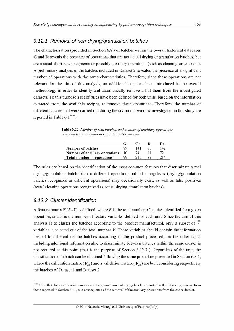
Knowledge management in secondary manufacturing by pattern recognition techniques 153
______________________________________________________________________________________________ © 2016 Natascia Meneghetti, University of Padova (Italy)
6.12.1 Removal of non-drying/granulation batches
The characterization (provided in Section 6.8 ) of batches within the overall historical databases
G and D reveals the presence of operations that are not actual drying or granulation batches, but
are instead short batch segments or possibly auxiliary operations (such as cleaning or test runs).
A preliminary analysis of the batches included in Dataset 2 revealed the presence of a significant
number of operations with the same characteristics. Therefore, since these operations are not
relevant for the aim of this analysis, an additional step has been introduced in the overall
methodology in order to identify and automatically remove all of them from the investigated
datasets. To this purpose a set of rules have been defined for both units, based on the information
extracted from the available recipes, to remove these operations. Therefore, the number of
different batches that were carried out during the six-month window investigated in this study are
reported in Table 6.1****.
Table 6.22. Number of real batches and number of ancillary operations removed from included in each datasets analyzed.
The rules are based on the identification of the most common features that discriminate a real
drying/granulation batch from a different operation, but false negatives (drying/granulation
batches recognized as different operations) may occasionally exist, as well as false positives
(tests/ cleaning operations recognized as actual drying/granulation batches).
6.12.2 Cluster identification
A feature matrix F [B×V] is defined, where B is the total number of batches identified for a given
operation, and V is the number of feature variables defined for each unit. Since the aim of this
analysis is to cluster the batches according to the product manufactured, only a subset of V
variables is selected out of the total number V. These variables should contain the information
needed to differentiate the batches according to the product processed; on the other hand,
including additional information able to discriminate between batches within the same cluster is
not required at this point (that is the purpose of Section 6.12.3 ). Regardless of the unit, the
classification of a batch can be obtained following the same procedure presented in Section 6.8.1,
where the calibration matrix ( calF ) and a validation matrix ( valF ) are built considering respectively
the batches of Dataset 1 and Dataset 2.
**** Note that the identification numbers of the granulation and drying batches reported in the following, change from those reported in Section 6.11, as a consequence of the removal of the ancillary operations from the entire dataset.
G1 G2 D1 D2 Number of batches 89 141 88 142 Number of ancillary operations 10 74 11 72 Total number of operations 99 215 99 214
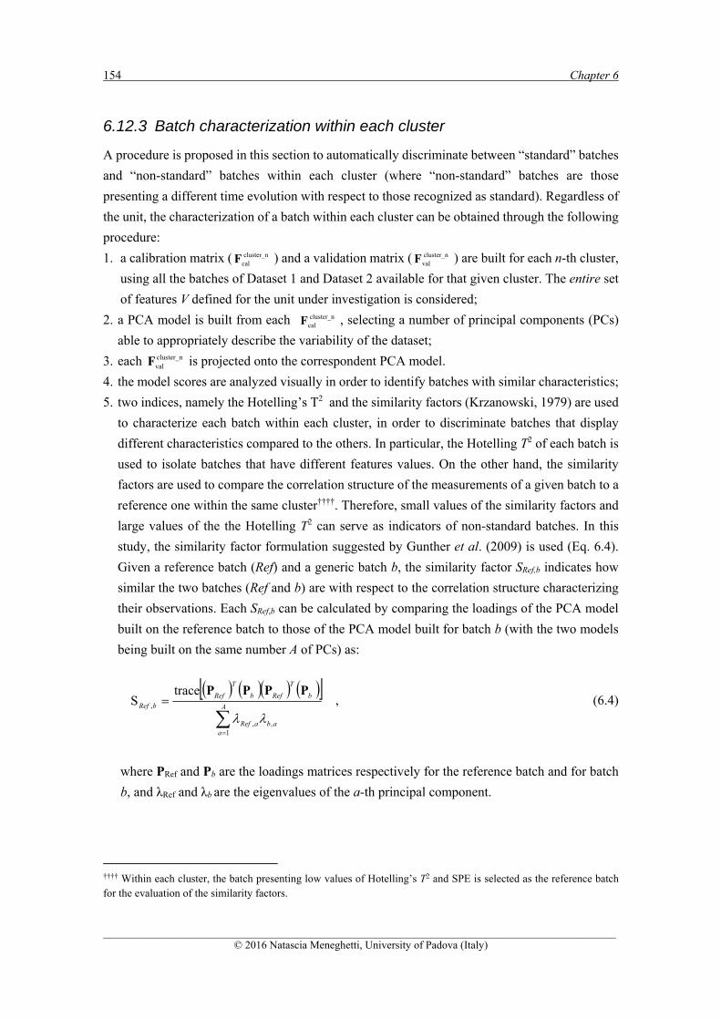
154 Chapter 6
______________________________________________________________________________________________ © 2016 Natascia Meneghetti, University of Padova (Italy)
6.12.3 Batch characterization within each cluster
A procedure is proposed in this section to automatically discriminate between “standard” batches
and “non-standard” batches within each cluster (where “non-standard” batches are those
presenting a different time evolution with respect to those recognized as standard). Regardless of
the unit, the characterization of a batch within each cluster can be obtained through the following
procedure:
1. a calibration matrix ( cluster_ncalF ) and a validation matrix ( cluster_n
valF ) are built for each n-th cluster,
using all the batches of Dataset 1 and Dataset 2 available for that given cluster. The entire set
of features V defined for the unit under investigation is considered;
2. a PCA model is built from each cluster_ncalF , selecting a number of principal components (PCs)
able to appropriately describe the variability of the dataset;
3. each cluster_nvalF is projected onto the correspondent PCA model.
4. the model scores are analyzed visually in order to identify batches with similar characteristics;
5. two indices, namely the Hotelling’s T2 and the similarity factors (Krzanowski, 1979) are used
to characterize each batch within each cluster, in order to discriminate batches that display
different characteristics compared to the others. In particular, the Hotelling T2 of each batch is
used to isolate batches that have different features values. On the other hand, the similarity
factors are used to compare the correlation structure of the measurements of a given batch to a
reference one within the same cluster††††. Therefore, small values of the similarity factors and
large values of the the Hotelling T2 can serve as indicators of non-standard batches. In this
study, the similarity factor formulation suggested by Gunther et al. (2009) is used (Eq. 6.4).
Given a reference batch (Ref) and a generic batch b, the similarity factor SRef,b indicates how
similar the two batches (Ref and b) are with respect to the correlation structure characterizing
their observations. Each SRef,b can be calculated by comparing the loadings of the PCA model
built on the reference batch to those of the PCA model built for batch b (with the two models
being built on the same number A of PCs) as:
A
aabaRef
b
T
Refb
T
Ref
bRef
1,,
,
traceS
PPPP , (6.4)
where PRef and Pb are the loadings matrices respectively for the reference batch and for batch
b, and λRef and λb are the eigenvalues of the a-th principal component.
†††† Within each cluster, the batch presenting low values of Hotelling’s T2 and SPE is selected as the reference batch for the evaluation of the similarity factors.

Knowledge management in secondary manufacturing by pattern recognition techniques 155
______________________________________________________________________________________________ © 2016 Natascia Meneghetti, University of Padova (Italy)
6.12.4 Results for the granulation unit
A set of features were identified to characterize the product manufactured by the granulation
process, as reported in Table 6.23.
Table 6.23. Granulation unit: feature variables defined for batch characterization.
Feature variable name Feature variable description fG,1 Duration of Phase 1 fG,2 Duration of Phase 2 fG,3 Duration of Phase 3 fG,4 Duration of Phase 4 fG,5 Average impeller speed in Phase 1 fG6 Average impeller speed in Phase 2 fG,7 Average impeller speed in Phase 3 fG,8 Maximum impeller load fG,9 Duration of the entire batch
6.12.4.1 Cluster identification
A subset of the above features, namely fG,1, fG,2, fG,3, fG,5, fG,6, and fG,7, are selected to build a
calibration matrix Gcal,F [89×6] and a validation matrix Gval,F [142×6]. According to the available
recipes, each feature assumes different and specific values for each product manufactured. Then,
Gcal,F was used to build a PCA model using 2 PCs, which captured more than 86% of the data
variability. Figure 6.23a shows how the granulation batches (circles) with similar characteristics
are located in the same area of the scores plane, forming four main clusters.
(a) (b) Figure 6.23. Batch characterization in the granulation unit: (a) scores of the PCA model built on the calibration feature matrix, and (b) projections of the validation feature matrix.
-7 -6 -5 -4 -3 -2 -1 0 1 2 3-5
-4
-3
-2
-1
0
1
2
3
12
3
456
7891011121314
15
16
17
1819202122
232425
26
2728
293031323334
353637
383940
414243
4445464748
4950
515253545556575859
606162
63
6465
666768697071
72
737475
767778
798081
828384
85
868788
PC
2 (1
3.7%
)
PC1 (73.2%)
Product 1 – Dataset 1Product 2 – Dataset 1Product 3 – Dataset 1Product 4 – Dataset 1
-7 -6 -5 -4 -3 -2 -1 0 1 2 3-5
-4
-3
-2
-1
0
1
2
3
89909192939495969798 99100
101
102103104105106107108109
110111
112113114115116117118
119
120121
122123
124
125
126127128129130
131132
133
134135136137138
139140141
142143144
145
146
147
148149150151152153154155156157158159160
161162
163
164
165166167168169170171172173174175176 177
178179180
181
182
183184
185186
187188189190191
192193194195196197
198199200201202203204205206207208209210211
212
213
214215216217218219220221222 223224225226227228
229230
PC
2 (
13.
7%
)
PC1 (73.2%)
Product 1 – Dataset 1 Product 1 – Dataset 2Product 2 – Dataset 1 Product 2 – Dataset 2Product 3 – Dataset 1 Product 3 – Dataset 2Product 4 – Dataset 1 Product 4 – Dataset 2
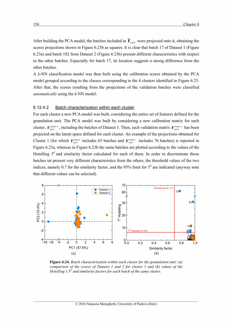
156 Chapter 6
______________________________________________________________________________________________ © 2016 Natascia Meneghetti, University of Padova (Italy)
After building the PCA model, the batches included in Gval,F were projected onto it, obtaining the
scores projections shown in Figure 6.23b as squares. It is clear that batch 17 of Dataset 1 (Figure
6.23a) and batch 182 from Dataset 2 (Figure 6.23b) present different characteristics with respect
to the other batches. Especially for batch 17, its location suggests a strong difference from the
other batches.
A k-NN classification model was then built using the calibration scores obtained by the PCA
model grouped according to the classes corresponding to the 4 clusters identified in Figure 6.23.
After that, the scores resulting from the projections of the validation batches were classified
automatically using the k-NN model.
6.12.4.2 Batch characterization within each cluster
For each cluster a new PCA model was built, considering the entire set of features defined for the
granulation unit. The PCA model was built by considering a new calibration matrix for each
cluster, n-clusterGcal,F , including the batches of Dataset 1. Then, each validation matrix n-cluster
Gval,F has been
projected on the latent space defined for each cluster. An example of the projections obtained for
Cluster 1 (for which cluster1Gcal,F includes 65 batches and cluster1
Gval,F includes 76 batches) is reported in
Figure 6.23a, whereas in Figure 6.23b the same batches are plotted according to the values of the
Hotelling T2 and similarity factor calculated for each of them. In order to discriminate those
batches tat present very different characteristics from the others, the threshold values of the two
indices, namely 0.7 for the similarity factor, and the 95% limit for T2 are indicated (anyway note
that different values can be selected).
(a) (b)
Figure 6.24. Batch characterization within each cluster for the granulation unit: (a) comparison of the scores of Dataset 1 and 2 for cluster 1 and (b) values of the Hotelling’s T2 and similarity factors for each batch of the same cluster.
-18 -16 -4 -2 0 2 4 6 8-4
-2
0
2
4
6
8 Dataset 1 Dataset 2
PC
2 (1
5.4
%)
PC1 (57.6%)
0.0 0.2 0.4 0.6 0.8 1.00
10
20
30
60
70
123789101112131416
17
1819202122262728293031
32
33
34
3536
37
4041424347484950
51
525354555657585960616264656667686970717273747584858699100101102103112113
114
115116117118119120121122123124
125
126127128129
130
131132134135136137138139
140141145146147148149150151152153154155156157158159160161162163177178179180185186187188189190191198199200201223224225226227228229230
Similarity factor = 0.7
T2 H
ote
llin
g
Similarity factor
T2 Hotelling limit 95%

Knowledge management in secondary manufacturing by pattern recognition techniques 157
______________________________________________________________________________________________ © 2016 Natascia Meneghetti, University of Padova (Italy)
The results for the first cluster (Figure 6.23b) suggest that the four batches that present large T2
values, are non-standard batches. A-posteriori analysis of the tag profiles of these batches, carried
out to investigate on the possible causes of the non-standard behavior, confirms that they actually
present some anomalies respect to the batches of the same cluster. Finally, in Figure 6.23a the
scores of Dataset 2 locate close to the scores of Dataset 1, indicating that the correlation structure
of the two datasets is very similar; stated differently, for each product the granulation process
conditions appear consistent across the investigated time frames.
6.12.5 Results for the drying unit
Similarly to the granulation unit, a set of features was defined to characterize the drying process
(Table 6.24).
Table 6.24. Drying unit: feature variables defined for batch characterization.
Feature variable name Feature variable description fD,1 Duration of Phase 1 fD,2 Duration of Phase 2 fD,3 Duration of Phase 3 fD,4 Duration of Phase 4 fD,5 Duration of Phase 5 fD,6 Average inlet air temperature before Phase 2 fD,7 Average inlet air temperature during Phase 3 fD,8 Maximum value of product bed temperature during Phase 4 fD,9 Average inlet air volume before Phase 2 fD,10 Duration of Phase 2+ Phase 3+ Phase 4+ Phase 5 fD,11 Duration of the entire batch
6.12.5.1 Cluster identification
A subset of the feature variables were selected to recognize different products, namely no. fD,1,
fD,6, fD,7, fD,8, and fD,9. A calibration matrix Fcal,D [88×5] was built considering the batches of
Dataset 1, whereas a validation matrix Fval,D [142×5] was built considering the batches of Dataset
2. The first one was used to build a PCA model considering 2 PCs (which captured more than the
75% of the variability of the data). Figure 6.25a shows that, like in the granulation unit, the batches
cluster in 4 clusters (i.e., 4 different products are identified). The projections of the validation
batches onto the PCA model are shown in Figure 6.25b as squares. The Dataset 2 batches locate
close to the four clusters identified for Dataset 1. As observed also for the granulation unit, some
batches locate far from the others, and this happens for both datasets. Anyway, the investigation
of how many and which batches present some anomalies respect to the others is the purpose of
the batch characterization analysis within each cluster (Section .6.12.3.4).

158 Chapter 6
______________________________________________________________________________________________ © 2016 Natascia Meneghetti, University of Padova (Italy)
(a) (b) Figure 6.25. Batch characterization in the drying unit: (a) scores of the PCA model built on the calibration feature matrix and (b) projections of the validation feature matrix.
6.12.5.2 Batch characterization within each cluster
Using Dataset 1, a PCA model was built for each cluster (i.e., product) using a new calibration
matrix ( n-clusterDcal,F ) for each cluster. The projections of the n-cluster
Dval,F matrices on the model space built
for each cluster, reveal the presence of a shift between the batches of the two datasets, which is
particularly apparent for cluster 1 (Figure 6.26a, where cluster1Dcal,F includes 65 batches and cluster1
Dval,F
includes 75 batches). By analyzing the model parameters and the feature values, it is possible to
identify the reasons of the shift observed that are mainly related to a different execution of the
drying phases.
The results obtained by pairing the indices used to identify non-standard batches (Figure 6.26b,
where the threshold for both indices is indicated) demonstrate the presence in cluster 1 of batches
presenting large T2 values and/or small similarity factor values. Actually, the analysis of the tag
profiles of these batches reveals that all of them, except for batch 159, present anomalous trends
and/or a different duration of an operating phase. Batch 159 does not present anomalies: it has
been erroneously recognized as a non-standard batch due to the misclassification of some samples
of phase 6.
The results obtained demonstrate the potential of the proposed methodology in revealing the
presence of some differences between the datasets analyzed, and in disclosing the causes of these
differences. However, some improvements should be considered further in order to prevent that
some batches are identified as non-standard when they are actually standard batches and vice
verse.
-10 -8 -2 0 2 4 6-7
-6
-3
-2
-1
0
1
2
3
123
4
56
7891011121314
15
1617
18
19
202122
23
2425
2627
28293031
32
33
34
3536
37 3839404142
43
444546
474849505152535455565758
59606162
63
6465666768
6970
7172737475
767778
798081
8283
848586
8788
PC
2 (2
3.9%
)
PC1 (52.4 %)
Product 1 – Dataset 1Product 2 – Dataset 1Product 3 – Dataset 1Product 4 – Dataset 1
Product 1 – Dataset 1 Product 1 – Dataset 2Product 2 – Dataset 1 Product 2 – Dataset 2Product 3 – Dataset 1 Product 3 – Dataset 2Product 4 – Dataset 1 Product 4 – Dataset 2
-10 -8 -2 0 2 4 6-7
-6
-3
-2
-1
0
1
2
3
89909192939495969798
99100101102
103
104105106107108109
110111
112113114115116117118119120121122123
124125126
127128129130131
132
133134
135136137138139140
141142143
144
145146147148
149
150151152153154155156157158
159
160
161
162
163
164165166167168169170171172173174175
176
177178179
180
181182183
184185186187
188189190
191192193194195196
197
198
199200
201202203204205206207208209210211212213214215216217
218
219220221
222
223
224225227228229230
PC
2 (2
3.9%
)PC1 (52.4 %)
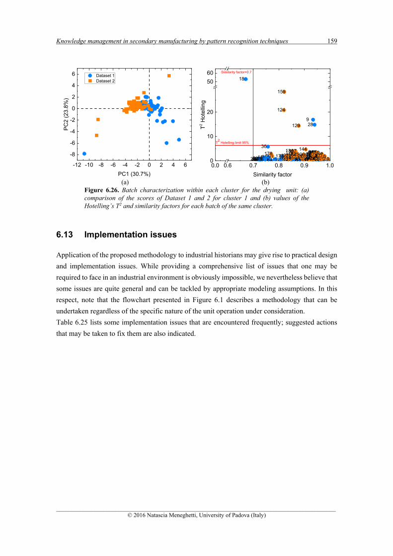
Knowledge management in secondary manufacturing by pattern recognition techniques 159
______________________________________________________________________________________________ © 2016 Natascia Meneghetti, University of Padova (Italy)
(a) (b) Figure 6.26. Batch characterization within each cluster for the drying unit: (a) comparison of the scores of Dataset 1 and 2 for cluster 1 and (b) values of the Hotelling’s T2 and similarity factors for each batch of the same cluster.
6.13 Implementation issues
Application of the proposed methodology to industrial historians may give rise to practical design
and implementation issues. While providing a comprehensive list of issues that one may be
required to face in an industrial environment is obviously impossible, we nevertheless believe that
some issues are quite general and can be tackled by appropriate modeling assumptions. In this
respect, note that the flowchart presented in Figure 6.1 describes a methodology that can be
undertaken regardless of the specific nature of the unit operation under consideration.
Table 6.25 lists some implementation issues that are encountered frequently; suggested actions
that may be taken to fix them are also indicated.
-12 -10 -8 -6 -4 -2 0 2 4 6
-8
-6
-4
-2
0
2
4
6 Dataset 1 Dataset 2
PC
2 (
23.8
%)
PC1 (30.7%)
0.0 0.6 0.7 0.8 0.9 1.00
10
20
50
60
1 23
78
9
1011 1213141617
18
19 202122 2627
28
2930 3132 333435
36
374041 42 4347 484950 51 525354 555657 585960 616264 656667 6869 7071 72 737475 84 8586
99 100101 102103112 113114115116117118119120 121122
123
124
125126127128
129
130131133134
135136137138139140
144145
146147 148 149150
151 152153154155156157158
159
160161
162176 177178 179184185186
187188189190
197198199200222 223224225 227228 229230230
Similarity factor=0.7
T2 H
ote
lling
Similarity factor
T2
Hotelling limit 95%

160 Chapter 6
______________________________________________________________________________________________ © 2016 Natascia Meneghetti, University of Padova (Italy)
Table 6.25. Possible solutions and recommendations to support the implementation of the suggested methodology.
Issue Suggested action
Preliminary analysis
A tag is not recorded for the entire dataset. If the tag is not helpful to identify an operating phase (Task 2), remove it from the dataset.
If the tag is helpful to visually identify an operating phase, keep the tag only to perform the visual identification of phases, then remove it from the dataset.
A tag is very noisy Filter its value; alternatively, remove the tag from the dataset if there are other tags providing similar information.
Task 1: batch identification
Some consecutive batches isolated by the tag-based batch identification method actually correspond to the same batch.
This is usually due to temporary stall of the unit. Adjust the batch identification algorithm so as to cross-check the values of identification-relevant tags, and disregard from the analysis the data segments that, following tag cross-check, can be attributed to stalled operation.
Task 2: phase identification
The classification results of the k-NN model are not satisfactory.
Select a different distance criterion or a different value for k.
Assess whether removing one or more tags or tag segments improves the k-NN model performance (this may be helpful especially for very noisy tags).
During model building, it is apparent that the tag profiles that refer to a given batch phase change across the dataset.
This usually corresponds to different manufactured products. Include all these products in the calibration dataset.
A true operating phase is difficult to be identified.
Consider including this phase with the previous or successive one.
The start/end point of a phase in a unit cannot be detected accurately by visual inspection.
If the unit (Unit A) follows or precedes a different unit (Unit B), try to exploit a tag of Unit B to mark the phase start/end point in Unit A.
How many inter-phases should be considered?
The inter-phases correspond to operational segments presenting visually different combinations of the tag profiles.
Task 3: batch characterization
The clusters identified by the PCA model are not representative of the true batch differences.
Consider using more PCs. Consider using different features in F.
How can a batch be marked as standard or non-standard?
An appropriate batch distance criterion may be considered (e.g., using k-NN modeling) to discriminate between standard and non-standard batches.
A group of batches has been wrongly recognized as non-standard.
Consider updating the calibration model including these batches.
Knowledge management in secondary manufacturing by pattern recognition techniques 161
______________________________________________________________________________________________ © 2016 Natascia Meneghetti, University of Padova (Italy)
6.14 Conclusions
In this Chapter, a methodology has been developed to retrieve operation-relevant information
from historical secondary manufacturing databases. The methodology allows one to automatically
perform three tasks: the identification (isolation) of single batches within the entire historical data
sequence, the identification of distinct operating phases within each batch, and the
characterization of a batch with respect to an assigned multivariate set of operating characteristics.
Fulfilment of these tasks can allow a company to increase the fraction of historical data that is
appropriately contextualized in full, which may lead to substantial savings in the life-cycle of a
product. Because the proposed methodology aims at assessing the consistency of operations over
a given time window(s) (e.g. monthly/quarterly) by providing visual diagnostics, it is naturally
positioned to rapidly identify potential areas of improvements. For example, the presence of
atypical phases in a unit operation, or in a more extreme case their absence, might relate either to
operators not following the correct procedure or to the system not responding as expected.
Similarly, the automated comparison between an extended number of batches might reveal subtler
offsets, e.g. relating to the effect of changes in the supply line for one of the ingredients over time,
which may not be immediately obvious otherwise. Conclusions drawn from the diagnostic charts
can therefore be used to assess the need to implement ameliorative activities or corrective and
preventing actions to avoid recurrence of undesirable events.
The methodology has been tested on two six-month datasets (Dataset 1 and Dataset 2) coming
from two industrial manufacturing units: a high-shear wet granulator and a fluid-bed dryer. First,
Dataset 1 has been analyzed demonstrating the potential of the methodology in handling different
type of data and units, using no information about the products processed. Then, the methodology
has been improved and tested on both datasets using new information coming from the recipes of
the products manufactured during the time windows investigated. The results demonstrate that
the methodology allows one to correctly recognize different operating phases for both units and
to correctly classify batches according to the product processed. Finally, the application of the
methodology permits also to reveal the presence of some differences in the process settings across
the two available datasets. Additional improvements may be considered in future applications: i)
a different metric/index may be identified to more properly detect anomalies in the batch
evolution and to avoid a wrong classification of actual standard batches as non-standard batches;
ii) the classification model may be enhanced by considering a larger calibration set; iii) the rules
defined to discriminate a true drying/granulation batch from a different (“ancillary”) operation
may be enhanced in order to reduce false negatives and false positives. However, the quality of
results and the generality of the approach indicate that there is a strong potential for extending the
method to larger historical datasets and different operations, thus making it an advanced PAT tool
that can assist the implementation of continuous improvement paradigms, targeting consistent
operation quality and easy monitoring of the entire manufacturing proces


______________________________________________________________________________________________ © 2016 Natascia Meneghetti, University of Padova (Italy)
Conclusions and future perspectives
Traditionally, the pharmaceutical industry has been subject to different attraction forces that led
to the development of a bipolar character along the years: if on the one hand more and more
cutting edge solutions were provided to respond to the rapid society evolution, on the other hand
the manufacturing environment fossilized on well-known experience-based procedures,
minimizing the interaction with the regulatory Agencies. Recently, market requirements have
forced a radical change in the pharmaceutical sector, which is moving towards a more efficient
industrial organization, based on a technologically advanced approach and on a more open
attitude with respect to academic collaborations and new markets. A decisive contribution to this
improvement has been provided by the new strategy adopted by the regulatory Agencies, which
realized the importance of fostering pharmaceutical innovation by the introduction of Quality-by-
Design (QbD) paradigms and by facilitating effective collaboration with the companies. The QbD
approach aims to build quality into a product by using a thorough understanding of the product
and process features and risks and by implementing appropriate strategies to control those risks.
The implementation of QbD paradigms relies on the use of a systematic scientific-based approach
that should support all the activities that characterize a pharmaceutical process; the knowledge
acquired during these activities should represent the base for continual process and product
improvement. From an engineering perspective, this represents the opportunity to adapt and
expand to the pharmaceutical applications the knowledge acquired in more mature sectors,
especially regarding process modeling activities (both knowledge-driven or data-driven).
However, the rapidly expansion of the use advanced modeling tools is somewhat limited by the
peculiar features of the pharmaceutical industry. The greater product complexity, low volume
multi-product productions and the strict regulatory oversight that characterize this sector, all
contribute to make the application of these advanced tools more challenging.
In this context, data-driven (DD) models have been demonstrated to be an optimal opportunity to
address several problems that characterize pharmaceutical development and manufacturing. In
this Dissertation, the potential of DD modeling, in particular of latent variable modeling and
pattern recognition techniques, has been exploited to develop general methodologies that aim to
strengthen the use process modeling (for example by facilitating first-principles model diagnosis)
and foster the use of the historical available data. Their application may support the practical
implementation of some fundamental elements of the QbD philosophy, from the definition of the
design space to the use of knowledge acquired throughout product lifecycle.
Table 1 summarizes the main achievements of the Dissertation, with indication of the application
considered and the data origin, as well as a reference to related papers that have been published
or submitted to journal or conferences.

164 Appendix A
______________________________________________________________________________________________ © 2016 Natascia Meneghetti, University of Padova (Italy)
T
able
1. S
umm
ary
of th
e m
ain
achi
evem
ents
of t
his
Dis
sert
atio
n, w
ith in
dica
tion
of th
e co
nsid
ered
app
licat
ion,
dat
a or
igin
an
d re
leva
nt r
efer
ence
s.
Ref
eren
ce
Men
eghe
tti,
N.,
P. F
acco
, F. B
ezzo
, M. B
arol
o (2
014)
. A m
etho
dolo
gy to
dia
gnos
e pr
oces
s/m
odel
mis
mat
ch i
n fi
rst-
prin
cipl
es m
odel
s. I
nd.
Eng
. C
hem
. R
es.,
53,
1400
2-14
013.
M
eneg
hetti
, N.,
P. F
acco
, F. B
ezzo
, M. B
arol
o (2
014)
. Dia
gnos
ing
proc
ess/
mod
el
mis
mat
ch i
n fi
rst-
prin
cipl
es m
odel
s by
lat
ent
vari
able
mod
elin
g. I
n: C
ompu
ter-
Aid
ed C
hem
ical
Eng
inee
ring
33
(J.J
. K
lem
eš,
P.S
. V
arba
nov,
P.Y
. L
iew
, E
ds.)
, E
lsev
ier,
Am
ster
dam
(T
he N
ethe
rlan
ds)
1897
-190
2.
Men
eghe
tti, N
., P
. Fac
co, S
. Ber
min
gham
, D. S
lade
, F. B
ezzo
, M. B
arol
o (2
015)
. F
irst
-pri
ncip
les
mod
el
diag
nosi
s in
ba
tch
syst
ems
by
mul
tiva
riat
e st
atis
tica
l m
odel
ing.
In:
Com
pute
r-A
ided
Che
mic
al E
ngin
eeri
ng 3
7 (K
.V.
Ger
naey
, J.
K.
Huu
som
, R. G
ani,
Eds
.), E
lsev
ier,
Am
ster
dam
(T
he N
ethe
rlan
ds),
437
-442
.
Facc
o, P
., F.
Dal
Pas
tro,
N. M
eneg
hett
i, F.
Bez
zo, M
. Bar
olo
(201
5). B
rack
etin
g th
e de
sign
sp
ace
wit
hin
the
know
ledg
e sp
ace
in
phar
mac
euti
cal
prod
uct
deve
lopm
ent.
Ind.
Eng
. Che
m. R
es.,
54, 5
128–
5138
.
Men
eghe
tti N
., P.
Fac
co,
F. B
ezzo
, C
. H
imaw
an,
S. Z
omer
, M
. B
arol
o, 2
015,
K
now
ledg
e m
anag
emen
t in
sec
onda
ry p
harm
aceu
tica
l m
anuf
actu
ring
by
min
ing
of d
ata
hist
oria
ns –
A p
roof
-of-
conc
ept s
tudy
, sub
mit
ted
to: I
nt.
J. P
harm
. M
eneg
hetti
N.,
P. F
acco
, F.
Bez
zo,
C.
Him
awan
, S.
Zom
er,
M.
Bar
olo,
201
6,
Aut
omat
ed D
ata
Rev
iew
in
Seco
ndar
y Ph
arm
aceu
tica
l M
anuf
actu
ring
by
Patte
rn
Rec
ogni
tion
T
echn
ique
s,
to
be
pres
ente
d at
: E
SC
AP
E
26,
26th
E
urop
ean
Sym
posi
um o
n C
ompu
ter-
Aid
ed P
roce
ss E
ngin
eeri
ng (
Por
toro
ž, S
love
nia,
12-
15
June
201
6).
Dat
a or
igin
Sim
ulat
ed
Sim
ulat
ed
Sim
ulat
ed a
nd
labo
rato
ry
(Vem
avar
apu
et a
l., 2
009)
Indu
stri
al
Ap
pli
cati
on
C
onti
nuou
s-st
irre
d ja
cket
ed
tank
rea
ctor
Mil
ling
D
ryin
g
Pen
icill
in
ferm
enta
tion
N
onli
near
one
-eq
uati
on m
odel
Dry
gra
nula
tion
by
rol
ler
com
pact
ion
W
et g
ranu
latio
n
G
ranu
lati
on u
nit
D
ryin
g un
it
Mai
n ac
hiev
emen
t
Gen
eral
met
hodo
logy
to
diag
nose
pro
cess
/mod
el
mis
mat
ch in
fir
st-
prin
cipl
es m
odel
s fo
r st
eady
-sta
te s
yste
ms
Gen
eral
met
hodo
logy
to
diag
nose
pro
cess
/mod
el
mis
mat
ch in
fir
st-
prin
cipl
es m
odel
s fo
r dy
nam
ic s
yste
ms
Met
hodo
logy
to s
peed
-up
desi
gn s
pace
iden
tifi
catio
n
Met
hodo
logy
to
auto
mat
ical
ly r
etri
eve
oper
atio
n-re
leva
nt
info
rmat
ion
in s
econ
dary
m
anuf
acto
ry s
yste
m
Ch
apte
r
Cha
pter
3
Cha
pter
4
Cha
pter
5
Cha
pter
6

On the interpretation of the latent variable model parameters 165
_____________________________________________________________________________________________ © 2016 Natascia Meneghetti, University of Padova (Italy)
With respect to first-principles models diagnosis, in Chapter 3 a methodology has been proposed
to improve first-principles steady-state models designed to describe steady-states systems for
which the presence of a process/model mismatch (PMM) has been observed. The aim of the
methodology is to diagnose the cause of the PMM by exploiting only the historical and simulated
data used to detect the presence of the PMM for the system under investigation, without carrying
out any additional experiment. A PCA model is used to compare the correlation structure of two
matrices, built considering a set of auxiliary variables calculated using the historical and a
simulated data. Appropriate diagnostic indices permit one to pinpoint the model equations or
model parameters that most contribute to the observed PMM.
In Chapter 4 the methodology has been modified to deal with dynamic models and to also consider
systems with strongly correlated variables. Different simulated case studies were used to assess
the effectiveness of the proposed methodology. The results obtained demonstrated that the
methodology is effective in diagnosing the model sections affected by modeling errors. By
facilitating the diagnosis of the PMM root causes, any additional experimental effort, which may
be needed to enhance the first-principles model performance, can be targeted much more
appropriately, and the overall need for experimental campaigns can therefore be reduced.
One of the main results of product and process understanding activities promoted by Quality-by-
Design initiative is the determination of the design space (DS) for the manufacturing of a
pharmaceutical product. The DS can be defined using first-principles models, when available,
alternatively, its determination relies on experiments. In Chapter 5 a methodology has been
proposed to support the determination of the design space using the historical data (e.g. material
properties and process conditions) on products already developed that are similar to the new one
under development; these historical data are often said to represent the knowledge space of the
system. The methodology aims to find a narrower region within the knowledge space, called
experiment space, within which the experiments needed to define the DS can be designed and
carried out, thus reducing the experimental effort usually required. By means of a latent-variable
model inversion approach, the knowledge space is segmented in such a way as to identify the
experiment space in the latent variable space of the model. The segmentation makes use of the
concept of null space and accounts for the existence of uncertainty in the model predictions.
Using three simulated case studies, it has been demonstrated that: i) the segmentation results are
effective; ii) the segmentation effectiveness depends on the number of samples available in the
historical dataset, but the appropriate number of samples does not necessarily need to be very
large; iii) the graphical representation of the experiment space identified in a multivariate latent
variable space is clear also when the number of process inputs is large.
Finally, in Chapter 6 a methodology was proposed to support the implementation of continual
improvement paradigms, by the periodic review of large manufacturing databases. In order to

166 Appendix A
______________________________________________________________________________________________ © 2016 Natascia Meneghetti, University of Padova (Italy)
retrieve operation-relevant information from historical secondary manufacturing databases, the
proposed methodology allows one to automatically carry out four tasks: i) the identification
(isolation) of single batches within the entire historical data sequence, ii) the identification of
distinct operating phases within each batch, iii) the characterization of a batch with respect to an
assigned multivariate set of operating characteristics, and iv) the comparison of batches carried
out in different time windows. Fulfilment of these tasks can allow a company to increase the
fraction of historical data that is appropriately contextualized in full in order to monitor the
evolution of the manufacturing campaigns over time and to detect possible exceptions, which may
lead to substantial savings in production. The methodology has been tested on two historical
datasets of two industrial manufacturing units (a high-shear wet granulator and a fluid-bed dryer).
The quality of results and the generality of the approach indicate that there is a strong potential
for extending the method to even larger historical datasets and to different operations.
In summary this Dissertation has shown how LVMs can be considered as an advanced flexible
tool whose potential can be exploited in many different applications. Thanks to their multivariate
nature, the possibility to handle large amount of data regardless their source and the ability of
investigate their correlation structure, DD models have been demonstrated to be a fundamental
PAT tool to support the implementation of QbD paradigms.
One of the main contributions of this Dissertation is the demonstration of the ‘‘power’’ of the
pharmaceutical process data. Manufacturing data should be considered not only as a means to
monitor the quality of product or the real-time performance of a manufacturing system, but also
as a fundamental source of information about the history of the process itself. This information
can be extracted and exploited to accomplish many objectives that lead to the realization of a
pharmaceutical quality system.
The studies carried out in this Dissertation have opened further perspectives, which could be
addressed in future research. For example, an interesting area open to further investigation is
the improvement of the methodology used to identify a PMM in Chapters 3 and 4. First, a general
procedure to systematically select proper auxiliary variables should be defined, as well as
appropriate confidence limits when the residuals distribution is found to be not normal.
Additionally, different diagnostic indices might be considered to better deal with the problem of
correlated auxiliary variables. Finally, the effectiveness of the proposed methodology should be
assessed for a combination of parametric and structural mismatches, and the methodology itself
should be challenged against real-world systems.
In the definition of the experiment space (Chapter 5), future studies should consider not only the
prediction uncertainty, but also other forms of uncertainty (such as uncertainty on the model
parameters and on the calibration data), as well as the manufacturing of products characterized
by a multivariate quality profile. Finally, future investigations should be devoted to assess the

On the interpretation of the latent variable model parameters 167
_____________________________________________________________________________________________ © 2016 Natascia Meneghetti, University of Padova (Italy)
effectiveness of a design-of-experiments exercise carried out in the latent space with respect to
the more common situation where the experiments are designed directly in the true input space.
Finally, the methodology developed to review large historical datasets (Chapter 6) can be further
improved according to different directions: i) a different metric/index might be identified to more
properly detect anomalies in the batch evolution and to avoid a misclassification of true standard
batches; ii) the rules defined to discriminate a true process batch from a different operation might
be enhanced in order to reduce false negatives and false positives.


______________________________________________________________________________________________ © 2016 Natascia Meneghetti, University of Padova (Italy)
Appendix A
On the interpretation of the latent variable model parameters
This Appendix reports some details on the interpretation of the parameters of a latent variable
model (LVM). In particular, some indications are provided on how to interpret the loading and
score diagrams in order to get information from the data (largely based on the Dissertations of
Tomba 2013 and Ottavian, 2014). The interpretation of the loading plots of the case study
considered in Chapter 6 is used as an example.
A.1 Interpretation of the scores and loading plots
PCA and PLS models (Chapter 2) are usually built not only for facilitate the analysis of large
multivariate datasets, by identifying a reduced number of latent variables describing the system,
but also to enhance understanding of the system itself. This can be achieved by analyzing the
correlation between variables and the similarities between samples. The advantage in using LVMs
to this purpose is due to the fact that the model parameters allow to interpret the correlation
structure in a straightforward way, facilitating also the identification of the mechanisms acting on
the system. Therefore, under a practical point of view, the analysis of the PCA and PLS
parameters is fundamental and it is done by considering plots of the scores and of the loadings of
the model. Although these plots can be reported in several ways, according to common practice
(which is adhered to in this Dissertation), the scores are reported as scatter plots, in which the
scores on a PC (or on a LV indifferently) are reported versus the scores on another PC. This is
usually done for the scores on the first LVs found by the model, because they explain most part
of the variability in the data. Bi-dimensional plots are usually used as they are easier to visualize
than three-dimensional ones. Figure A.1b reports an example of a score plot.
Loadings are usually reported as bar plots or as scatter plots. In the first case (which is the way
used in this Dissertation) a bar plot of the loadings of the original variables on each PC is reported,
as in Figure A.1a.
In general, loading plots are useful for two important reasons: i) understanding which are the
variables related to the data variability and which are not; ii) understanding if there are
correlations among the variables. Recalling the meaning of loadings in PCA and weights in PLS
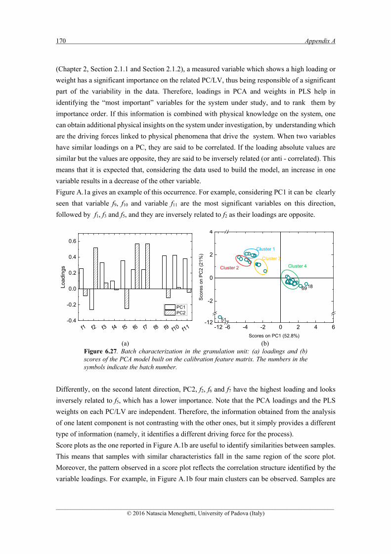
170 Appendix A
______________________________________________________________________________________________ © 2016 Natascia Meneghetti, University of Padova (Italy)
(Chapter 2, Section 2.1.1 and Section 2.1.2), a measured variable which shows a high loading or
weight has a significant importance on the related PC/LV, thus being responsible of a significant
part of the variability in the data. Therefore, loadings in PCA and weights in PLS help in
identifying the “most important” variables for the system under study, and to rank them by
importance order. If this information is combined with physical knowledge on the system, one
can obtain additional physical insights on the system under investigation, by understanding which
are the driving forces linked to physical phenomena that drive the system. When two variables
have similar loadings on a PC, they are said to be correlated. If the loading absolute values are
similar but the values are opposite, they are said to be inversely related (or anti - correlated). This
means that it is expected that, considering the data used to build the model, an increase in one
variable results in a decrease of the other variable.
Figure A.1a gives an example of this occurrence. For example, considering PC1 it can be clearly
seen that variable f9, f10 and variable f11 are the most significant variables on this direction,
followed by f1, f3 and f5, and they are inversely related to f2 as their loadings are opposite.
(a) (b) Figure 6.27. Batch characterization in the granulation unit: (a) loadings and (b) scores of the PCA model built on the calibration feature matrix. The numbers in the symbols indicate the batch number.
Differently, on the second latent direction, PC2, f2, f6 and f7 have the highest loading and looks
inversely related to f5, which has a lower importance. Note that the PCA loadings and the PLS
weights on each PC/LV are independent. Therefore, the information obtained from the analysis
of one latent component is not contrasting with the other ones, but it simply provides a different
type of information (namely, it identifies a different driving force for the process).
Score plots as the one reported in Figure A.1b are useful to identify similarities between samples.
This means that samples with similar characteristics fall in the same region of the score plot.
Moreover, the pattern observed in a score plot reflects the correlation structure identified by the
variable loadings. For example, in Figure A.1b four main clusters can be observed. Samples are
f1 f2 f3 f4 f5 f6 f7 f8 f9 f10 f11-0.4
-0.2
0.0
0.2
0.4
0.6
Load
ings
PC1 PC2
-12 -6 -4 -2 0 2 4 6-12
-2
0
2
4
18
51
69
Sco
res
on P
C2
(21%
)
Scores on PC1 (52.8%)
Cluster 4
Cluster 1
Cluster 3
Cluster 2

On the interpretation of the latent variable model parameters 171
_____________________________________________________________________________________________ © 2016 Natascia Meneghetti, University of Padova (Italy)
therefore grouped according to their similarities or differences in the variables that have the
highest loading on PC1 and PC2. By analyzing the loading plot, one can identify which these
variables are. Considering for example the first direction, samples having a high positive score
on PC1 as those included in cluster 4 will have higher values of f9, f10 and f11 and lower f2 values
on average. The situation is opposite in the case of samples with negative PC1 scores. A similar
analysis can be done also for the other PCs.

______________________________________________________________________________________________ © 2016 Natascia Meneghetti, University of Padova (Italy)
Appendix B
Details on the simulated processes analyzed in Chapter 3
This Appendix reports some details on the generation of the data used in the two examples
considered in Chapter 3: the CSTR system and the milling unit. For the second example, the
diagnostics of the MPCA model built for the first case study analyzed are also reported.
B.1 Generation of the historical dataset for Example 1
This Section provides the nominal values (Table B.1) of the parameters used to generate the
historical dataset for the CSTR system (“process Π”) analyzed in Example 1 (Section 3.3). The
ranges of the measured variables included in this dataset are also reported (Table B.2).
Table B.1. Nominal values of the parameters used to generate the historical dataset for Example 1.
Parameters Values A1,Π 20 kmol/(m3·s)A2,Π 10 kmol/(m3·s)
,Pc 4.186 kJ/(kg·K)
,,wPc 3.137 kJ/(kg·K) Ea1,Π 69.7 kJ/mol Ea2,Π 72 kJ/mol SΠ 32.98 m2
VR,Π 26.15 m3
,1H -59·103 J/mol
,2H -10·103 J/mol
,w 1000 kg/m3
800 kg/m3

174 Appendix B
______________________________________________________________________________________________ © 2016 Natascia Meneghetti, University of Padova (Italy)
Table B.2. Ranges of the measured variables included in the historical dataset for Example 1.
Measured variables Values inAC , [3 - 9] kmol/m3
outAC , [2.897 - 8.814] kmol /m3 inBC , [2 - 5] kmol /m3 outBC , [1.791 - 4.829] kmol /m3 inCC , 0 kmol /m3 outCC , [0.181 - 1.778] kmol /m3 inDC , 0 kmol /m3 outDC , [ 2.701·10-4 - 2.186·10-2] kmol /m3 Fj,Π [0.236 - 0.257] m3/s UΠ [0.2923 - 0.3035] kJ/(m2·s·K)
inT [292 - 298] K outT
[293.7 - 315.7] K
injT , [287.5 - 292.5] K outjT , [287.6 - 292.7] K
Fj,Π [0.236 - 0.257] m3/s
B.2 Generation of the historical dataset and diagnostics of the MPCA model for Example 2
This Section provides the nominal values (Table B.3 and B.4) of the parameters used to generate
the historical dataset for the mill system (“process ”) analyzed in Example 2 (Section 3.4), and
the eigenvalues λ, the explained variance R2 and its cumulated value 2cumR for each PC of the
MPCA model (Table B.5) built for Case study 2.A (Section 3.4.2.1).
Note that all parameters included in Table S3 (but kΠ andy ) are material-dependent. The ranges
of the measured variables included in this dataset are also reported.
Table B.3. Ranges of the measured variables included in the historical dataset for Example 2.
Measure variables Values ρbulk, Π [320-450] kg/m3
DinΠ [3-6]·10-3 mσin, Π [0.6-1]·10-3 m vΠ [30-80] m/s

Details on the simulated processes analyzed in Chapter 3 175
_____________________________________________________________________________________________ © 2016 Natascia Meneghetti, University of Padova (Italy)
Table B.4. Nominal values of the parameters used to generate the historical dataset for Example 2. The values in curly brackets refer to different materials. The values reported for parameter
kin,,mW refer to the range taken by the parameter for the entire set of materials.
Parameters Values cΠ {–0.052; –0.0422; –0.0325; –0.0226} [-] dΠ {4.42; 5.898; 5.51; 8.01} [-]
Mat,f {0.059; 0.095; 0.115; 0.125} [-]
kΠ 1 [-]
y’Π 2·10-5 m kin,,mW [1376.4 - 3808.9] J/kg
,min,mW {2.957; 3.427; 3.5; 3.541} Jm/kg
Table B.5. Case study 2.A. Diagnostics of the MPCA model on XM.
PC number
Eigenvalue of cov(XM)
R2 R2cum
1 83.84 42.56 42.56 2 68.28 34.66 77.22 3 20.13 10.22 87.44 4 11.93 6.05 93.49 5 5.57 2.83 96.32 6 3.01 1.53 97.84 7 1.68 0.85 98.69 8 1.24 0.63 99.33 9 0.76 0.39 99.71
10 0.31 0.16 99.87 11 0.15 0.08 99.94 12 0.08 0.04 99.99 13 0.02 0.01 99.99 14 0.01 0.01 100.00


______________________________________________________________________________________________ © 2016 Natascia Meneghetti, University of Padova (Italy)
Appendix C
An improved method to diagnose the cause of a process/model mismatch:
preliminary results
As highlighted in Chapter 3 and 4, strongly correlated auxiliary variables make the identification
of the mismatch particularly difficult, in the analysis of the residuals and/or of the score shifts.
For this reason, in this Appendix a preliminary solution to deal with strongly correlated variables
is presented, which exploits the methodology proposed by Rato and Reis (2015b) for fault
diagnosis purposes. A preliminary example of the results obtained is provided for the two
examples analyzed in Section 4.3 for the fermentation process.
C.1 An alternative approach to diagnose the cause of a PMM
The alternative approach proposed in this Appendix to identify which term of a first-principles
model might lead to a PMM is based on the use of partial correlation coefficients. The basic idea
in the use of partial correlation coefficients is to remove the effect of third-party variables before
checking for an association between the two designated variables. Therefore, considering 3
variables (x1, x2 and x3) the correlation between the first two is quantified, after conditioning upon
(i.e., controlling for, or holding constant) the third one, namely after the removal of the common
effect of x3 on x1 and x2 (Rato and Reis, 2014a).
Rato and Reis (2014a, 2014b, 2015a and 2015b) provide a detailed description and several
examples of the use of partial correlation coefficients for process monitoring purposes. In
particular, they suggest a number of sensitivity enhancing data transformations (SET) that can
maximize the detection ability of all monitoring procedures based on (partial or marginal)
correlation (Rato and Reis, 2014a). In their studies, they state that ‘‘even though partial
correlations do not provide information about the variables causality direction, they are still able
to discern if such connectivity does exist and in what degree it has changed. This characteristic,
coupled with their easy computation, makes them suitable for fault detection and diagnosis
purposes at the structural level’’. For this reason, the alternative approach proposed in this
Appendix to diagnose which term of a model is mostly related to the observed mismatch is based
on the fault diagnosis procedure introduced by Rato and Reis (2015b) with the purpose of

178 Appendix C
______________________________________________________________________________________________ © 2016 Natascia Meneghetti, University of Padova (Italy)
identifying a reduced set of variables that are closely related with the fault root cause. The authors
exploit the partial correlations ability to remove the effects of faulty variables in the data, under
the assumption that if a change on the variables relationships occurs, it is expected that the partial
correlation coefficients controlled by the variables associated with the root cause of the fault
remain close to their normal values, since the source of variability is being removed in such
circumstances (Rato and Reis, 2015b).
It should be highlighted that, the methodology proposed by Rato and Reis (2015b) refers to
continuous systems. In order to apply this methodology (only minor adjustments have been
introduced) to the purpose of our analysis, only the final measurements of N different batches are
considered, and for each of them B observations are simulated, which differ only for white noise.
Each batch has been carried out with different initial conditions for Cs, P, Fs, fg (for the meaning
of the symbols refer to Section 4.1). Appropriate solutions to consider the whole batch trajectories
are still under investigation.
The procedure proposed in this Appendix has been adapted from the one proposed by Rato and
Reis (2015b) and it is composed by 7 steps:
1. a set of V variables that represent only some measured variables (namely, the outputs of the
most important model equations) is defined. The measurements available for this set of
variables are collected in a historical matrix XΠ [N×M×B] and a simulated matrix XM
[N×V×B];
2. for each sample xM [V×B], the first-order partial correlation coefficients are calculated
considering all possible combination of pairs of variables in XM (for example, xi and xj)
controlled by a third variable (for example xk) as:
22,
11kjki
kjkiji
kji
rr
rrrr
xxxx
xxxxxx
xxx
, (C.1)
3. each partial correlation coefficient is normalized as:
21
1
rqN
wr , (C.2)
where ρ represents the population mean, N the number of samples, and q the order of the
partial correlation coefficient. In this analysis, q=1;
4. step 2 and 3 are repeated for XΠ, but normalizing each ri,j based on the ρ calculated for XM;
5. a matrix D‡‡‡‡ [V×V] is defined, where each row corresponds to a control variable, whereas
the j-th element of the k-th row is calculated as:
‡‡‡‡ Note that, in this Appendix matrix D assumes a different meaning respect to matrix D used in Chapter 6.

An improved method to diagnose the cause of a process/model mismatch: preliminary results 179
_____________________________________________________________________________________________ © 2016 Natascia Meneghetti, University of Padova (Italy)
))((,
,,
jkik
kjijk rwfd , (C.3)
where )( .kjirf 1 if CLrw r )( , and 0 otherwise. Since, thanks to the transformation of Eq.
(D.2), each )(rwr is normally distributed, therefore the CL (confidence limit) is calculated as:
)2/()( zwCL r , (C.4)
with z =2.58, corresponding to a threshold of 99%;
6. the squared norm of each row and column of matrix D is calculated to mark each variable as
RED, ORANGE and YELLOW, according to the rules reported in Table C.1. A variable is RED
when it presents the smallest value of the squared norm of the rows of D, and the largest value
of the norm of the columns of D. A variable is ORANGE when it presents the smallest value of
the squared norm of the rows of D, but the value of the norm of its column is smaller than the
largest one. Finally a variable is YELLOW when presents the largest value of the squared norm
the columns of D, but the value of the norm its row is larger than the smallest one;
Table C.1. Rules proposed by Rato and Reis (2015b) to marked a variable i as RED,
ORANGE or YELLOW.
RED yes yes
ORANGE yes no
YELLOW no yes
7. steps from 2-6 are repeated considering a new set of V variables composed by the terms of the
model involved in the calculation of the measured variables that demonstrated to be mostly
related to the mismatch.
According to Rato and Reis (2015b), when the variable related to the mismatch is controlled for,
the partial correlations calculated for the remaining pairs of variables should remain within the
control limits (low values of the norm of the columns of D). On the other hand, a variable
presenting high values of the norm of the rows of D indicates that it has suffered many changes
in correlation with the other variables. For this reason it is expected that most of the times, when
a variables is marked as red, it should be directly related with the cause of the mismatch, even if
also variables marked as ORANGE or YELLOW should also be checked.
22:),(min:),( ii DD 22
)(:,max)(:, ii DD
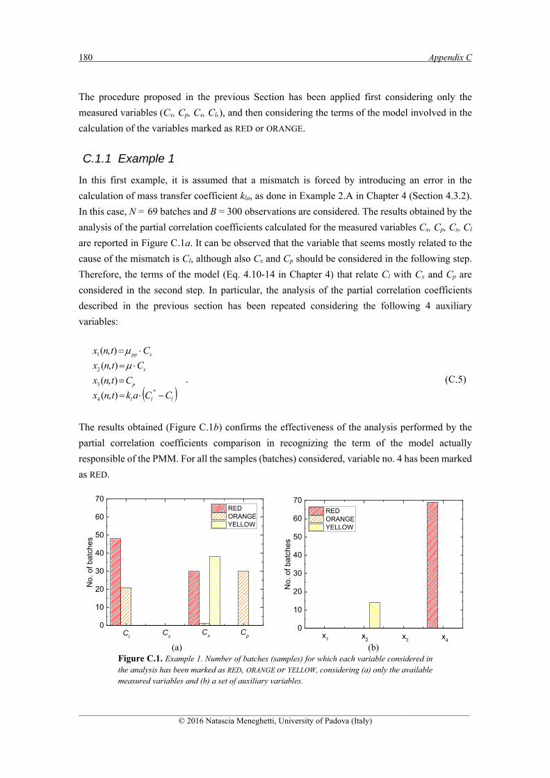
180 Appendix C
______________________________________________________________________________________________ © 2016 Natascia Meneghetti, University of Padova (Italy)
The procedure proposed in the previous Section has been applied first considering only the
measured variables (Cx, Cp, Cs, Cl,), and then considering the terms of the model involved in the
calculation of the variables marked as RED or ORANGE.
C.1.1 Example 1
In this first example, it is assumed that a mismatch is forced by introducing an error in the
calculation of mass transfer coefficient kla, as done in Example 2.A in Chapter 4 (Section 4.3.2).
In this case, N = 69 batches and B = 300 observations are considered. The results obtained by the
analysis of the partial correlation coefficients calculated for the measured variables Cx, Cp, Cs, Cl
are reported in Figure C.1a. It can be observed that the variable that seems mostly related to the
cause of the mismatch is Cl, although also Cx and Cp should be considered in the following step.
Therefore, the terms of the model (Eq. 4.10-14 in Chapter 4) that relate Cl with Cx and Cp are
considered in the second step. In particular, the analysis of the partial correlation coefficients
described in the previous section has been repeated considering the following 4 auxiliary
variables:
lll
p
x
xpp
CCaktnx
Ctnx
Ctnx
Ctnx
*
4
3
2
1
),(
),(
),(
),(
. (C.5)
The results obtained (Figure C.1b) confirms the effectiveness of the analysis performed by the
partial correlation coefficients comparison in recognizing the term of the model actually
responsible of the PMM. For all the samples (batches) considered, variable no. 4 has been marked
as RED.
(a) (b) Figure C.1. Example 1. Number of batches (samples) for which each variable considered in the analysis has been marked as RED, ORANGE or YELLOW, considering (a) only the available measured variables and (b) a set of auxiliary variables.
0
10
20
30
40
50
60
70
CxC
sCl
No.
of b
atch
es
RED ORANGE YELLOW
Cp
0
10
20
30
40
50
60
70
x4
x3
x1
No
. of b
atc
he
s
RED ORANGE YELLOW
x2

An improved method to diagnose the cause of a process/model mismatch: preliminary results 181
_____________________________________________________________________________________________ © 2016 Natascia Meneghetti, University of Padova (Italy)
C.1.2 Example 2
In this second example, it is assumed that a mismatch is forced by changing the parameter Ys/x
(from 0.45 [-] to 0.2 [-]), as done in Example 2.B in Chapter 4 (Section 4.2.5). In this case
N = 50 batches and B = 200 observations are considered. The results of the analysis of the partial
correlations coefficients calculated for the available measured variables are reported in Figure
C.2a. In this case, only Cx appears to be the measured variable mostly related with the mismatch,
whereas the relations with Cl does not appear to be affected by the mismatch. For this reason, in
the second step of the analysis the relations of Cx with Cs and Cp are investigated. Therefore the
new set of variables selected for the analysis is:
s
p
x
xpp
Ctnx
Ctnx
Ctnx
Ctnx
),(
),(
),(
),(
4
3
2
1
. (C.6)
The results obtained are reported in Figure C.2b. Since the amount of time that μ is marked as
RED is greater than for μpp, and since the correlation coefficients which involves Cs seems to be
affected by error more than those involving Cp, the results obtained suggest that the cause of the
mismatch is possibly due to the relation of x2 and x4, namely to Ys/x.
(a) (b) Figure C.2. Example 2. Number of batches (samples) for which each variable considered in the analysis has been marked as RED, ORANGE or YELLOW, considering (a) only the available measured variables and (b) a set of auxiliary variables.
Although in this section only preliminary results are presented, a significant margin of
improvement is expected upon further investigation. The final objective is to provide a robust tool
that, by exploiting the entire trajectory of the batches analyzed, is able to detect the cause of the
mismatch even with strongly correlated variables. To this purpose, further investigation is now
0
5
10
15
20
25
30
35
40
45
50
No.
of b
atch
es
RED ORANGE YELLOW
CxC
sC
l Cp
0
10
20
30
40
50
No
. of b
atc
hes
RED ORANGE YELLOW
x4
x3x
1x
2

182 Appendix C
______________________________________________________________________________________________ © 2016 Natascia Meneghetti, University of Padova (Italy)
focused on: i) adapting the solutions suggested by Rato and Reis (2015b) to enhance the accuracy
of the detection of a change in the correlation structure of the variables analyzed, especially with
time-dependent variables; ii) developing a robust procedure to identify appropriate sets of
auxiliary variables that can be analyzed with partial correlation coefficients; iii) analyzing the
effect of the number of available samples and of their features on the effectiveness of the
methodology.
______________________________________________________________________________________________ © 2016 Natascia Meneghetti, University of Padova (Italy)
References
am Ende, D.J., K. S. Bronk, J. Mustakis, G. O’Connor, C.L. Santa Maria, R. Nosal and T.J.N.
Watson (2007). API Quality by Design example from the Torcetrapib manufacturing process.
J. Pharm. Innov., 2, 71-86.
am Ende, D.J. (2011). Chemical engineering in the pharmaceutical industry: an introduction. In:
am Ende, D.J. (Ed.), Chemical Engineering in the Pharmaceutical Industry. R&D to
Manufacturing. John Wiley & Sons, Inc. New York, NJ.
Anderson, T. W., D. A. Darling (1952). Asymptotic Theory of Certain “Goodness of Fit” Criteria
Based on Stochastic Processes. Ann. Math. Stat., 23, 193–212.
Badwe, A. S., R. D. Gudi, R. S. Patwardhan, S. L. Shah, S. C. Patwardhan (2009). Detection of
Model-Plant Mismatch in MPC Applications. J. Process Control, 19, 1305–1313.
Ballabio D., R. Todeschini (2009). Multivariate classification for qualitative analysis. In Infrared
Spectroscopy for Food Quality Analysis and Control. Sun, D.W., Ed. Elsevier, Burlington,
MA, USA, pp. 83–104.
Barker M., W. Rayens (2003). Partial least squares for discrimination, J. Chemometr., 17, 166–
173.
Bennett B. and G. Cole (2003). Pharmaceutical production: an engineering guide, IChemE,
Rugby, UK.
Birol, G., C. Ündey, and A. Çinar (2002). A modular simulation package for fed - batch
fermentation: penicillin production. Computers Chem. Eng., 26, 1553-1565.
Bishop C.M. (2006). Pattern recognition and machine learning, Springer, New York (U.S.A.).
Boukouvala, F., F.J. Muzzio and M. Ierapetritou (2010). Design space of pharmaceutical
processes using data-driven-based methods. J. Pharm. Innov., 5, 119-137.
Box, G. E. P., and N. R. Draper (2007). Response surfaces, mixtures, and ridge analysis.
Hoboken, NJ Wiley.
Bu, D., B. Wan, G. McGeorge (2013). A Discussion on the Use of Prediction Uncertainty
Estimation of NIR Data in Partial Least Squares for Quantitative Pharmaceutical Tablet Assay
Methods. Chemom. Intell. Lab. Syst., 120, 84.
Burgschweiger J., E. Tsotsas (2002). Experimental investigation and modelling of continuous
fluidized bed drying under steady-state and dynamic conditions, Chem. Eng. Sci., 57, 5021–
5038.
Burnham, A, R. Viveros and J.F. MacGregor (1996). Frameworks for latent variable multivariate
regression. J. Chemom., 10, 31-45.
Burnham, A.J., J.F. MacGregor and R. Viveros (1999). Latent variable multivariate regression
modeling. Chemom. Intell. Lab. Syst., 48, 167-180.

184 References
______________________________________________________________________________________________ © 2016 Natascia Meneghetti, University of Padova (Italy)
Burt, J.L., A.D. Braem, A. Ramirez, B. Mudryk, L. Rossano, S. Tummala, (2011). Modelguided
design space development for a drug substance manufacturing process. J. Pharm. Innov. 6,
181–192.
Chatzizacharia, K. A., D. T. Hatziavramidis (2014). Design Space Approach for Pharmaceutical
Tablet Development. Ind. Eng. Chem. Res., 53, 12003.
Choi S. W. and I. B. Lee (2005). Multiblock PLS-based localized process diagnosis, J.Process
Control, 15, 295-306.
Çinar, A., S.J. Parukelar, C. Ündey, G. Birol (2003). Batch fermentation – Modeling, monitoring
and control. Marcel-Dekker, New York, NJ.
Close, E. J., J. R. Salm, D. G. Bracewell, E. Sorensen (2014). A Model Based Approach for
Identifying Robust Operating Conditions for Industrial Chromatography with Process
Variability. Chem. Eng. Sci., 116, 284.
Conlin, A.K., E.B. Martin and A.J. Morris (2000). Confidence limits for contribution plots. J.
Chemom., 14, 725-736.
Cook, J., M. T. Cruañes, M. Gupta, S. Riley, and J. Crison (2013). Quality-by-Design: Are We
There Yet?, AAPS PharmSciTech, 15, 140-148.
Cover, T. M., P.E. Hart (1967). Nearest neighbor pattern classification. IEEE Tran. Inf. Theory,
13, 21-27.
Danese, J., D. Constantinou (2007). Lean practices in a life sciences organization. Contract
Pharma. Available at: http://shows.contractpharma.com/articles/2007/10/lean-practices-in-
a-life-sciences-organization (Last accessed 26/01/2016).
Deloitte, (2015) Global life sciences outlook - Adapting in an era of transformation Deloitte
Touche Tohmatsu Limited’s life science and health care (DTTL LSHC), Available at:
http://www2.deloitte.com/it/it/pages/life-sciences-and-healthcare/articles/2015-global-life-
sciences-outlook.html (Last accessed 26/01/2016).
Dong, D. and T.J. McAvoy (1996), Nonlinear principal component analysis based on principal
curves and neural networks, Computers Chem. Eng., 20, 65-78.
Doymaz, F., J. Chen, J. A. Romagnoli, A. Palazoglu (2001). A Robust Strategy for Real-Time
Process Monitoring. J. Process Control, 11, 343–359.
Duda, R.O., P.E. Hart, D. G. Stork (2001). Pattern classification, 2nd Ed., John Wiley & Sons,
Inc., New York (U.S.A.).
Efron, B., G. Gong (1983). A Leisurely Look at the Bootstrap, the Jackknife, and Cross-
Validation. Am. Stat., 37, 36.
Eigenvector Research, (2015). PLS_Toolbox 8.0.2, Eigenvector Research, Inc., Wenatchee, WA,
USA.
Eriksson, L., E. Johansson, N. Kettaneh-Wold, J. Trygg, C. Wikström and S. Wold (2006). Multi-
and megavariate data analysis. Part I. Basic principles and applications. Umetrics AB, Umeå
(Sweden).

References 185
_____________________________________________________________________________________________ © 2016 Natascia Meneghetti, University of Padova (Italy)
EvaluatePharma (2015), EvaluatePharma World Preview 2015 Outlook to 2020, EvaluateTM Ltd.
Available at: http://www.evaluategroup.com/public/EvaluatePharma-Overview.aspx (Last
accessed 26/01/2016).
Faber, K., B. R. Kowalski (1997). Propagation of Measurement Errors for the Validation of
Predictions Obtained by Principal Component Regression and Partial Least Squares. J.
Chemom., 11, 181.
Faber, N. (Klaas) M. (2002). Uncertainty Estimation for Multivariate Regression Coefficients.
Chemom. Intell. Lab. Syst., 64, 169.
FDA (2004a). Pharmaceutical CGMPs for the 21st century – A risk based approach. Final report.
U.S. Department of Health and Human Services. U.S. Food and Drug Administration.
FDA (2004b). Guidance for industry. PAT - A framework for innovative pharmaceutical
development, manufacturing and quality assurance. Center for Drug Evaluation and
Research, U.S. Food and Drug Administration, Rockwille (MD), USA.
FDA (2006). Guidance for Industry - Quality Systems Approach to Pharmaceutical CGMP
Regulations. U.S. Department of Health and Human Services. U.S. Food and Drug
Administration.
Fernández Pierna, J. A., L. Jin,, F. Wahl, N. M. Faber, D. L. Massart (2003). Estimation of Partial
Least Squares Regression Prediction Uncertainty When the Reference Values Carry a Sizeable
Measurement Error. Chemom. Intell. Lab. Syst., 65, 281.
Flores-Cerillo, J. and J.F. MacGregor (2004). Control of batch product quality by trajectory
manipulation using LV models. J. Process Control, 14, 539-553.
Franceschini, G., S. Macchietto (2008). Model-Based Design of Experiments for Parameter
Precision: State of the Art. Chem. Eng. Sci., 63, 4846–4872.
Gabrielsson, J., N.-O. Lindberg and T. Lundstedt (2002). Multivariate methods in pharmaceutical
applications. J. Chemom., 16, 141-160.
Gani, R. Modelling for PSE and Product-Process Design. In Computer-Aided Chemical
Engineering; Proceedings of the 10th International Symposium on Process Systems
Engineering: Part A, Salvador de Bahia, Brazil, August 16-27, 2009; Brito Alves, R. M., Oller
Nascimento, C. A., Biscaia Jr, E. C., Eds.; Elsevier, 2009; 27, 7–12.
García-Muñoz S., S. Dolph and H.W. Ward II (2010). Handling uncertainty in the establishment
of a design space for the manufacture of a pharmaceutical product. Computers Chem. Eng., 34,
1098-1107.
García-Muñoz, S., T. Kourti, J.F. MacGregor, A.G. Mateos and G. Murphy (2003).
Troubleshooting of an industrial batch process using multivariate methods. Ind. Eng. Chem.
Res., 42, 3592-3601.
García-Muñoz, S., T. Kourti, J.F. MacGregor, F. Apruzzese and M. Champagne (2006).
Optimization of batch operating policies. Part I. Handling multiple solutions. Ind. Eng. Chem.
Res., 45, 7856-7866.
186 References
______________________________________________________________________________________________ © 2016 Natascia Meneghetti, University of Padova (Italy)
García-Muñoz, S., J.F. MacGregor and T. Kourti (2005). Product transfer between sites using
Joint-Y PLS. Chemom. Intell. Lab. Syst., 79, 101-114.
García-Muñoz, S., J.F. MacGregor, D. Neogi, B.E. Letshaw and S. Mehta (2008). Optimization
of batch operating policies. Part II. Incorporating process constraints and industrial
applications. Ind. Eng. Chem. Res., 47, 4202-4208.
García-Muñoz, S. and C.A. Oksanen (2010). Process modeling and control in drug development
and manufacturing. Computers Chem. Eng., 34, 1007-1008.
García-Muñoz, S., L. Zhang and M. Cortese (2009). Root cause analysis during process
development using Joint-Y PLS. Chemom. Intell. Lab. Syst., 95, 101-105.
Gautam, A., Pan, X. The changing model of big pharma: impact of key trends, Drug Discov Today
(2015), in Press. DOI: 10.1016/j.drudis.2015.10.002.
Gernaey, K.V., A.E. Cervera-Padrell and J.M. Woodley (2012). A perspective on PSE in
pharmaceutical process development and innovation. Computers Chem. Eng., 42, 15-29.
Gernaey, K.V., R. Gani (2010). A model-based systems approach to pharmaceutical product-
process design and analysis. Chem. Eng. Sci., 65, 5757-5769.
Geladi, P. and B. Kowalski (1986). Partial least-squares regression: a tutorial. Anal. Chim. Acta.,
185, 1-17.
Gunther, J. C., J. Baclaski, D. E. Seborg and J. S. Conner (2009). Pattern Matching in Batch
Bioprocesses - Comparisons Across Multiple Products and Operating Conditions. Computers
Chem. Eng., 33, 88-96.
Höskuldsson, A. (1988). PLS regression methods. J. Chemom., 2, 211-228.
Hotelling, H. (1933). Analysis of a complex of statistical variables into principal components. J.
Educ. Psycol., 24, 417-441.
Huang, J., G. Kaul, C. Cai, R. Chatlapalli, P. Hernandez-Abad, K. Ghosh, A. Nagi (2009). Quality
by design case study: an integrated approach to drug product and process development. Int. J.
Pharm., 382, 23-32.
ICH (1999). ICH harmonised tripartite guide. Specifications: test procedures and acceptance
criteria for new drug substances and new drug products: chemical substances. Q6A.
ICH (2005). ICH harmonised tripartite guide. Quality risk management Q9.
ICH (2008). ICH harmonised tripartite guide. Pharmaceutical quality system Q10.
ICH (2009). ICH harmonised tripartite guide. Pharmaceutical development Q8(R2).
ICH (2010). Quality implementation working group on Q8, Q9 and Q10. Questions & Answers
(R4).
ICH (2011). ICH quality implementation working group. Points to consider (R2). ICH-endorsed
guide for ICH Q8/Q9/Q10 implementation.
Jackson, J. E (1991). A user’s guide to principal components. John Wiley & Sons, Inc., New York
(U.S.A.).

References 187
_____________________________________________________________________________________________ © 2016 Natascia Meneghetti, University of Padova (Italy)
Jaeckle, C.M. and J.F. MacGregor (1998). Product design through multivariate statistical analysis
of process data. AIChE J., 44, 1105-1118.
Jaeckle, C.M. and J.F. MacGregor (2000a). Industrial application of product design through the
inversion of latent variable models. Chemom. Intell. Lab. Syst., 50, 199-210.
Jaeckle, C.M. and J.F. MacGregor (2000b). Product transfer between plants using historical
process data. AIChE J., 46, 1989-1997.
Johanson, J. R. (1965).A Rolling Theory for Granular Solids. J. Appl. Mech., 32, 842.
Johnson, R.A. and D. W. Wichern (2007). Applied multivariate statistical analysis (6th ed.).
Pearson Education, Inc., Upper Saddle River, NJ, (U.S.A).
Juran, JM. (1992). Juran on quality by design: the new steps for planning quality into goods and
services. New York: The Free Press, New York, (U.S.A.).
Kapsi, S.G., L.D. Castro, F.X. Muller, T.J. Wrzosek (2012). Development of a design space for a
unit operation: illustration using compression-mix blending process for the manufacture of a
tablet dosage form. J. Pharm. Innov., 7, 19-29.
Kashid, M. N., D. W. Agar and S. Turek (2007). CFD modelling of mass transfer with and without
chemical reaction in the liquid–liquid slug flowmicroreactor. Chem. Eng. Sci., 62, 5102–5109.
Ketterhagen, W.R., M.T. am Ende, B.C. Hancock (2009). Process modeling in the pharmaceutical
industry using the discrete element method. J Pharm Sci., 98, 442-470.
Kiparissides, A., C. Georgakis, A. Mantalaris, E. N. Pistikopoulos (2014). Design of In Silico
Experiments as a Tool for Nonlinear Sensitivity Analysis of Knowledge-Driven Models. Ind.
Eng. Chem. Res., 53, 7517−7525.
Klatt, K.-U., W. Marquardt, (2009). Perspectives for process systems engineering-Personal views
from academia and industry. Computers Chem. Eng., 33, 536-550.
Kourti, T. (2003). Multivariate Dynamic Data Modelling for Analysis and Statistical Process
Control of Batch Processes, Start –Ups and Grade Transitions, J. Chemom., 17, 93-109.
Kourti, T. (2005). Application of latent variable methods to process control and multivariate
statistical process control in industry. Int. J. Adapt. Control., 19, 213-246
Kourti, T. (2006). Process analytical technology beyond real-time analyzers: the role of
multivariate analysis. Crit. Rev. Anal. Chem., 36, 257-278.
Kourti, T., B. Davis (2012). The Business Benefit of Quality by Design (QbD). Pharm. Eng. Off.
Magazine of ISPE., 32,1-10.
Krämer, N., M. Sugiyama (2011). The Degrees of Freedom of Partial Least Squares Regression.
J. Am. Stat. Assoc., 106, 697.
Kremer, D.M. and B.C. Hancock (2006). Process simulation in the pharmaceutical industry: a
review of some basic physical models. J. Pharm. Sci., 95, 517-529.
Krzanowski, W. J. (1979). Between-Groups Comparison of Principal Components. J. Am. Stat.
Assoc., 74, 703-707.

188 References
______________________________________________________________________________________________ © 2016 Natascia Meneghetti, University of Padova (Italy)
Kukura, J.L., M.P. Thien (2011). Current challenges and opportunities in the pharmaceutical
industry. In: am Ende, D.J. (Ed.), Chemical Engineering in the Pharmaceutical Industry. R&D
to Manufacturing. John Wiley & Sons, Inc., New York, NJ, 21–27.
Laínez, J.M., E. Schaefer, G.V. Reklaitis (2012). Challenges and opportunities in enterprise-wide
optimization in the pharmaceutical industry. Computers Chem. Eng, 47, 19-28.
Lavine, B. K., C.E. Davidson (2006). Classification and Pattern Recognition, in Practical guide
to chemometrics, edited by Paul Gamperline, 2nd Edition, CRC press Taylor & Francis Group,
Boca Raton, FL, U.S.A.
López-Negrete de la Fuente, R., S. García-Muñoz and L.T. Biegler (2010). An efficient nonlinear
programming strategy for PCA models with incomplete data sets. J. Chemom., 24, 301-311.
Lourenço, V., D. Lochmann, G. Reich, J.C. Menezes, T. Herdling, J. Schewitz (2012). A quality
by design study applied to an industrial pharmaceutical fluid bed granulation. Euro. J. Pharm.
Biopharm. 81, 438–447.
Luyben, W. L., Chemical Reactor Design and Control, Wiley, New York , NJ, 2007.
MacGregor, J.F. and M-.J. Bruwer (2008). A framework for the development of design and
control spaces. J. Pharm. Innov., 3, 15-22.
MacGregor, J.F. and T. Kourti (1995). Statistical process control of multivariate processes.
Control Eng. Pract., 3, 403-414.
Magnus J.R. and H. Neudecker (1999). Matrix Differential Calculus with Applications in
Statistics and Econometrics, Revised Ed., John Wiley & Sons Inc., Chichester, (U.K.)
Mardia, K.V., J.T. Kent and J.M. Bibby (1979). Multivariate analysis. Academic Press Limited,
London (U.K.).
Marquardt, W., J. Morbach, A. Wiesner and A. Yang (2010). OntoCAPE: A re-usable ontology
for chemical process engineering. Springer-Verlag Berlin, Heildeberg.
Marquardt, W. (2005). Model-Based Experimental Analysis of Kinetic Phenomena in Multi-
Phase Reactive Systems. Chem. Eng. Res. Des., 83, 561–573.
Martens, H., M. Martens (2000). Modified Jack-Knife Estimation of Parameter Uncertainty in
Bilinear Modelling by Partial Least Squares Regression (PLSR). Food Qual. Prefer., 11, 5.
Martin, E. B., A. J. Morris (1996). Non-Parametric Confidence Bounds for Process Performance
Monitoring Charts. J. Process Control, 6, 349–358.
Mathworks (2015). Matlab 8.6. (R2015b). The MathWorks Inc., Natick, MA (U.S.A.).
McLachlan G. J. (2004). Discriminant Analysis and Statistical Pattern Recognition, John Wiley
& Sons, Inc., Hoboken, New Jersey, (U.S.A.)
Meyer, C.D. (2000). Matrix analysis and applied linear algebra. SIAM, Philadelphia, PA
(U.S.A.).
Mika, S., B. Scholkopf, A.J. Smola, K.-R. Muller, M. Scholz, G. Ratsch (1999). Kernel PCA and
de-noising in feature spaces. Adv. Neural. Inf. Process. Syst., 11, 536–542.

References 189
_____________________________________________________________________________________________ © 2016 Natascia Meneghetti, University of Padova (Italy)
Montgomery, D.C. (2005). Design and analysis of experiments. 6th edition. John Wiley & Sons,
Inc., New York (U.S.A.).
Morbach, J., A. Yang and W. Marquardt (2007). OntoCAPE – A large-scale ontology for
chemical process engineering. Eng. Appl. Artif. Intel. 20, 147–161.
Muteki, K., J.F. MacGregor and T. Ueda (2006). Rapid development of new polymer blends: the
optimal selection of materials and blend ratios. Ind. Eng. Chem. Res., 45, 4653-4660.
Nomikos, P. and J.F. MacGregor (1994). Monitoring Batch Processes Using Multiway Principal
Component Analysis. AIChE J., 40, 1361–1375.
Nomikos, P. and J.F. MacGregor (1995). Multivariate SPC charts for monitoring batch processes.
Technometrics, 37, 41-59.
Ottavian, M. (2014). Latent Variable Modeling to Assist Product Quality Characterization in the
Food and Pharmaceutical Industries. PhD Thesis, University of Padova (Italy).
Ottavian, M., E. Tomba, M. Barolo (2016). Advanced process decision making using multivariate
latent variable methods. In: Process Simulation and Data Modeling in Solid Oral Drug
Development and Manufacturing (M. G. Ierapetritou and R. Ramachandrean, Eds.), Springer,
New York (NJ), 159-189.
Pal, S. K. and P. Mitra, (2004) Pattern Recognition Algorithms for Data Mining, Chapman &
Hall CRC Press, Boca Raton, FL (U.S.A.).
Pantelides, C. C., M. Pinto, S. K. Bermingham (2010). Design Space Characterization Using
First-Principles Models. In; (Salt Lake City, UT), p paper no. 358b.
Pantelides, C. C. and J. G. Renfro (2013). The Online Use of First-Principles Models in Process
Operations: Review, Current Status and Future Needs. Comput. Chem. Eng., 51, 136–148.
Pantelides, C. C., N. Shah, C. S. Adjiman (2009).Comprehensive Quality by Design in
Pharmaceutical Development and Manufacture. In; Nashville (TN, U.S.A), p 417f.
Pantelides, C., Z. E. Urban (2004). Process Modeling Technology: A Critical Review of Recent
Developments. Proceedings of the 6th International Conference on Foundations of Computer-
Aided Process Design, Princeton, NJ, July 11-16, 2004; Floudas, C. A., Agrawal, R., Eds.;
CACHE Corp.: New York, 2004.
Peterson, J. J. (2008). A Bayesian Approach to the ICH Q8 Definition of Design Space. J.
Biopharm. Stat., 18, 959.
Politis, S. N. and Rekkas D. M. (2001). The Evolution of the Manufacturing Science and the
Pharmaceutical Industry, Pharm. Res., 28, 1779–1781.
Pomerantsev, A.L. and O.Y. Rodionova (2012). Process analytical technology: a critical view of
the chemometricians. J. Chemom., 26, 299-310.
Process Systems Enterprise Ltd. (2013) gSOLIDS®, version 3.0; Process Systems Enterprise Ltd:
London, UK.
Process Systems Enterprise Ltd. (2014) gSOLIDS®, version 4.0; Process Systems Enterprise Ltd:
London, UK.
190 References
______________________________________________________________________________________________ © 2016 Natascia Meneghetti, University of Padova (Italy)
Rafols, I., M. M. Hopkins, J. Hoekman, J. Siepel, A. O'Hare, A. Perianes-Rodríguez, P.
Nightingale (2012). Big Pharma, little science? A bibliometric perspective on Big Pharma's
R&D decline. Technol. Forecast. Soc., 81, 22–38.
Rantanen J. and Khinast J. (2015). The Future of Pharmaceutical Manufacturing Sciences. J.
Pharm. Sci., 104, 3612–3638.
Realpe, A. and C. Velázquez (2006). Pattern recognition for characterization of pharmaceutical
powders. Powder Technol., 169, 108-113.
Reis, M.S. and P. M. Saraiva (2005). Integration of Data Uncertainty in Linear Regression and
Process Optimization. AIChE J., 51, 3007.
Reis, M.S. and P. M. Saraiva (2012). Prediction of Profiles in the Process Industries. Ind. Eng.
Chem. Res., 51, 4254.
Rajalahti, T. and O.M. Kvalheim (2011). Multivariate data analysis in pharmaceutics: a tutorial
review. Int. J. Pharm., 417, 280-290.
Rato, T. J. and M. S. Reis (2014a). Sensitivity enhancing transformations for monitoring the
process correlation structure, J. Process Control, 24, 905-915.
Rato, T. J. and M. S. Reis (2014b). Non-causal data-driven monitoring of the process
correlation tructure: A comparison study with new methods, Computers Chem. Eng., 71,
307-322.
Rato, T. J. and M. S. Reis (2015a). On-line process monitoring using local measures of
association: Part I — Detection performance, Chemom. Intell. Lab. Syst., 142, 307-322.
Rato, T. J. and M. S. Reis (2015b) On-line process monitoring using local measures of association.
Part II: Design issues and fault diagnosis, Chemom. Intell. Lab. Syst., 142, 265-275.
Rogers, A. and M. Ierapetritou (2015). Challenges and opportunities in modeling pharmaceutical
manufacturing processes, Comput. Chem. Eng., 81, 32-39.
Roggo, Y., P. Chalus, L. Maurer, C. Lema-Martinez, A. Edmond, N. Jent (2007). A review of
near infrared spectroscopy and chemometrics in pharmaceutical technologies, J. Pharmaceut.
Biomed., 44, 683-700.
Rousseeuw, P.J. (1987) Silhouettes: A graphical aid to the interpretation and validation of cluster
analysis, J. Comput. Appl. Math., 20, 53-65.
Sadat, T., R. Russell, M. Stewart (2014). Shifting paths of pharmaceutical innovation:
Implications for the global pharmaceutical industry. Int. J. Knowl. Innov. Entrep., 2, 6-31.
Saltelli, A., S. Tarantola, F. Campolongo (2000). Sensitivity Analysis as an Ingredient of
Modeling. Stat. Sci., 15, 377–395.
Saltelli, A., M.Ratto, T. Andres, F. Campolongo, J. Cariboni, D.Gatelli, M. Saisana, S. Tarantola
(2008). Global Sensitivity Analysis: The Primer. John Wiley and Sons, Ltd, Chichester, (U.K).
Schölkopf, B., S. Mika, C.J.C. Burges, P. Knirsch, Müller, G. Rätsch, , A.J. Smola (1999). Input
space versus feature space in kernel-based methods. IEEE T. Neural Networ., 10, 1000–1016.

References 191
_____________________________________________________________________________________________ © 2016 Natascia Meneghetti, University of Padova (Italy)
Simon L. L. et al., 2015. Assessment of Recent Process Analytical Technology (PAT) Trends: A
Multiauthor Review, Org. Process Res. Dev., 19, 3−62.
Singh, R., K. V. Gernaey and R. Gani (2010). An ontological knowledge based system for
selection of process monitoring and analysis tools. Computers Chem. Eng., 34, 1137–1154.
Souihi, N., M. Josefson, P. Tajarobi, B. Gururajan, J. Trygg (2013). Design space estimation of
the roller compaction process. Ind. Eng. Chem. Res., 52, 12408–12419.
Stephanopoulos, G. and G. V. Reklaitis (2011). Process Systems Engineering: From Solvay to
Modern Bio- and Nanotechnology: A History of Development, Successes and Prospects for
the Future. Chem. Eng. Sci., 66, 4272–4306.
Streefland, M., P.F.G. Van Herpen, B. Van de Waterbeemd, L.A. Van der Pol, E.C. Beuvery, J.
Tramper, D.E. Martens, M. Toft (2009). A practical approach for exploration and modeling of
the design space of a bacterial vaccine cultivation process. Biotechnol. Bioeng., 104, 492–504.
Suresh, P. and P.K. Basu, (2008). Improving Pharmaceutical Product Development and
Manufacturing: Impact on Cost of Drug Development and Cost of Goods Sold of
Pharmaceuticals. J. Pharm. Innov., 3, 175-187.
The Economist. Quality manufacturing: a blockbuster opportunity for pharmaceuticals. The
Economist Intelligence Unit: London; 2005. Available at:
http://graphics.eiu.com/files/ad_pdfs/eiu_ORACLE_PHARMA_WP.pdf (Last accessed
07/27/2015).
Thirunahari, S., P. Shan Chow and R.B.H. Tan (2011). Quality by Design (QbD)-based
crystallization process development for the polymorphic drug tolbutamide. Cryst. Growth
Des., 11, 3027-3038.
Tomba, E., M. Barolo and S. García-Muñoz (2012). General framework for latent variable model
inversion for the design and manufacturing of new products. Ind. Eng. Chem. Res., 51, 12886-
12900.
Tomba, E. (2013). Latent Variable Modeling Approaches to Assist the Implementation of
Quality-by-Design Paradigms in Pharmaceutical Development and Manufacturing. PhD
Thesis, University of Padova (Italy)
Tomba, E., P. Facco, F. Bezzo, M. Barolo (2013a). Latent variable modeling to assist the
implementation of Quality-by-Design paradigms in pharmaceutical development and
manufacturing: A review. Int. J. Pharm, 457, 283-297.
Tomba, E., P. Facco, F. Bezzo, S. García-Muñoz (2013b). Exploiting historical databases to
design the target quality profile for a new product. Ind. Eng. Chem. Res. 52, 8260–8271.
Tomba, E., M. Barolo, S. García-Muñoz (2014). In silico product formulation design through
latent variable model inversion. Chem Eng Res Des, 92,534–544.
Troup, G. M. and C. Georgakis (2013). Process Systems Engineering Tools in the Pharmaceutical
Industry. Comput. Chem. Eng., 51, 157.

192 References
______________________________________________________________________________________________ © 2016 Natascia Meneghetti, University of Padova (Italy)
Valle, S., W. Li and S.J. Qin (1999). Selection of the number of principal components: the
variance of the reconstruction error criterion with a comparison to other methods. Ind. Eng.
Chem. Res., 38, 4389-4401.
Van der Voet, H. (1999). Pseudo-Degrees of Freedom for Complex Predictive Models: The
Example of Partial Least Squares. J. Chemom., 13, 195.
Vanlaer, J., G. Gins, J. F. M. Van Impe (2013). Quality Assessment of a Variance Estimator for
Partial Least Squares Prediction of Batch-End Quality. Comput. Chem. Eng., 52, 230.
Varmuza K., P. Filmozer (2009). Classification, Chapter 5. In: Introduction to Multivariate
Statistical Analysis in Chemometrics. CRC press Taylor & Francis Group, Boca Raton, FL,
U.S.A.
Vemavarapu, C., M. Surapaneni, M. Hussain, S. Badawy (2009). Role of Drug Substance
Material Properties in the Processibility and Performance of a Wet Granulated Product. Int. J.
Pharm., 374, 96.
Venkatasubramanian, V., C. Zhao, G. Joglekar, A. Jain, L. Hailemariam, P. Suresh, et al. (2006).
Ontological informatics infrastructure for pharmaceutical product development and
manufacturing. Computers Chem. Eng., 30, 1482–1496.
Vogel, L. and W. Peukert (2005). From Single Particle Impact Behaviour to Modelling of Impact
Mills. Chem. Eng. Sci., 60, 5164–5176.
Wang H., Q. Liu, Y. Tu, (2005). Interpretation of partial least-squares regression models with
VARIMAX rotation, Comput. Stat. Data Anal., 48, 207-219.
Wang, H., L. Xie, Z. Song (2012). A Review for Model Plant Mismatch Measures in Process
Monitoring. Chin. J. Chem. Eng., 20, 1039–1046.
Wassgren, C. and J. S. Curtis (2006). The application of computational modeling to
pharmaceutical materials science. MRS Bulletin, 31, 900–904.
Wise, B. M. and N. B. Gallagher (1996). The Process Chemometrics Approach to Process
Monitoring and Fault Detection. J. Process Control, 6, 329–348.
Wise, B.M., N.B. Gallagher, R. Bro, J.M. Shaver, W. Windig and R. Scott Koch (2006).
PLS_Toolbox Version 4.0 for use with MATLAB™. Eigenvector Research, Inc., Wenatchee,
WA (U.S.A.).
Wold, H. (1966). Estimation of principal components and related models by iterative least
squares. In Multivariate analysis, Academic Press Limited, New York (U.S.A.).
Wold, S. (1978). Cross-validatory estimation of the number of components in factor and principal
component models. Technometrics, 20, 397-405.
Wold, S., H. Martens and H. Wold (1983). The multivariate calibration problem in chemistry
solved by the PLS method. Lecture Notes in Math., 973, 286-293.
Woo, X.Y., R.B.H. Tan and R.D. Braatz (2009). Modeling and computational fluid dynamics -
population balance equation - micromixing simulation of impinging jet crystallizers. Cryst.
Growth Des., 9, 156-164.

References 193
_____________________________________________________________________________________________ © 2016 Natascia Meneghetti, University of Padova (Italy)
Woodcock J., (2013). FDA Check Up: Drug Development and Manufacturing Challenges.
Available at: http://www.fda.gov/NewsEvents/Testimony/ucm378343.htm (Last accessed
26/01/2016).
Yacoub, F. and J.F. MacGregor (2004). Product optimization and control in the latent variable
space of nonlinear PLS models. Chemom. Intell. Lab. Syst., 70, 63-74.
Yacoub, F. and J.F. MacGregor (2011). Robust processes through latent variable modeling and
optimization. AIChE J., 57, 1278-1287.
Ye, J. (1998). On Measuring and Correcting the Effects of Data Mining and Model Selection. J.
Am. Stat. Assoc., 93, 120.
Yu, L. X., G. Amidon, M. A. Khan, S. W. Hoag, J. Polli, G. K. Raju, J. Woodcock (2014).
Understanding Pharmaceutical Quality by Design. The AAPS Journal, 16, 771-783.
Yu L. X. and J. Woodcock (2015). FDA pharmaceutical quality oversight. Int. J. Pharm., 491, 2-
7.
Zacour, B.M., J.K. Drennen III and C.A. Anderson (2012a). Development of a statistical
tolerance-based fluid bed drying design space. J. Pharm. Innov., 7, 151-162.
Zacour, B.M., J.K. Drennen III and C.A. Andreson (2012b). Development of a fluid bed
granulation design space using critical quality attribute weighted tolerance intervals. J. Pharm.
Sci., 101, 2917-2929.
Zhang, L. and S. García-Muñoz (2009). A Comparison of Different Methods to Estimate
Prediction Uncertainty Using Partial Least Squares (PLS): A Practitioner’s Perspective.
Chemom. Intell. Lab. Syst., 97, 152.
Zomer, S., M. Gupta and A. Scott (2010). Application of multivariate tools in pharmaceutical
product development to bridge risk assessment to continuous verification in a quality by design
environment. J. Pharm. Innov., 5, 109-118.


______________________________________________________________________________________________ © 2016 Natascia Meneghetti, University of Padova (Italy)
Acknowledgements
There are many people to whom I would like to express my gratitude for their support and/or
contribution to this project during these three years.
First, I would like to thank my supervisor, Prof. Massimiliano Barolo, for his guidance, support,
encouragement, and especially for his patience. He helped me in my scientific, as well as, in my
professional and personal growth. I am also grateful to Prof. Fabrizio Bezzo and Dr. Pierantonio
Facco, for all the helpful discussions that enriched this Dissertation, which would not have been
possible without their fundamental contribution.
Thanks to Dr. Sean Bermingham for his support during my visit at Process Systems Enterprise,
and to all the kind colleagues I had the chance to meet and work with there. I am especially
grateful to Dr. David Slade, for his patience and his assistance in this work.
Thanks to Dr. Simeone Zomer for his support and enthusiasm during our collaboration.
Un enorme grazie a tutti gli amici del Cape-Lab e non: Riccardo, Andrea e Junaid, i migliori
compagni d’ufficio di sempre, grazie per la pazienza e lunghi e fruttuosi discorsi; Myriam, grazie
per il tuo entusiasmo e la capacità di farci sentire tutti uniti; Filippo, grazie non solo per il tuo
contributo in questa tesi, ma anche per darmi sempre un motivo per una genuina risata;
Pierantonio (di nuovo), grazie per tutte le nostre discussioni e per il grande esempio che mi offri
ogni giorno; grazie ad Amir, per il suo contributo in questo lavoro, e a tutti gli studenti del Cape-
Lab. Grazie a Chiara, Elena, Barbara, Elia, Ricardo, Martina e a tutti i magnifici amici che mi
hanno accompagnato in questa esperienza. Grazie a Matteo ed Emanuele, il vostro esempio è stato
molto utile per la mia formazione.
Grazie a Elisa e Mario, il vostro supporto e la vostra comprensione sono stati fondamentali in
questa esperienza. Grazie a Romina, Patrick e Grace, perché mi avete sempre fatto sentire la
vostra presenza e il vostro supporto.
Infine grazie Federico, non potevo trovare persona migliore per affrontare piccole e grandi sfide
di ogni giorno.