..........

.....

.....................................................................

.....

......

.....

.....

.

Solid state

Fulvio Ciriaco

March 9, 2014

crystals

nuclear motion

electronic structure

..........

.....

.....................................................................

.....

......

.....

.....

.

Crystals are model systems characterized by periodicity, i.e.invariance under translation. The 3, 2 and 1-dimensional crystal,therefor, must be invariant under all translation operations:

Tn1a1+n2a2+n3a3 Tn1a1+n2a2 Tn1a1

where ai are 3 independent vectors and ni are integers. This simpleproperty has many important consequences. Crystals are also oftenendowed with other (punctual) symmetries, not all of the symmetryoperations are however compatible with translational invariance.

..........

.....

.....................................................................

.....

......

.....

.....

.

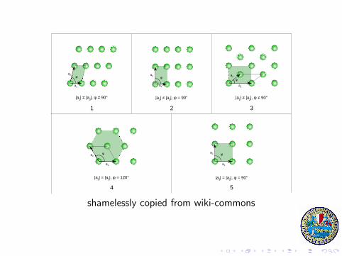
|a | = |a |, φ = 90°1 2|a | = |a |, φ = 120°1 2

a1

|a | ≠ |a |, φ = 90°1 2 |a | ≠ |a |, φ ≠ 90°1 2|a | ≠ |a |, φ ≠ 90°1 2

1 2 3

54

φ

a1

a2

φa2

φ

a1

a2

φ

a1

a2φ

a1

a2

shamelessly copied from wiki-commons

..........

.....

.....................................................................

.....

......

.....

.....

.

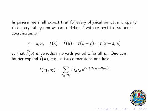
In general we shall expect that for every physical punctual propertyf of a crystal system we can redefine f with respect to fractionalcoordinates u:

x = uiai , f (x) = f (u) = f (u + n) = f (x + aini )

so that f (u) is periodic in u with period 1 for all ui . One canfourier expand f (u), e.g. in two dimensions one has:

f (u1, u2) =∑N1,N2

FN1N2e2πi(N1u1+N2u2)

..........

.....

.....................................................................

.....

......

.....

.....

.

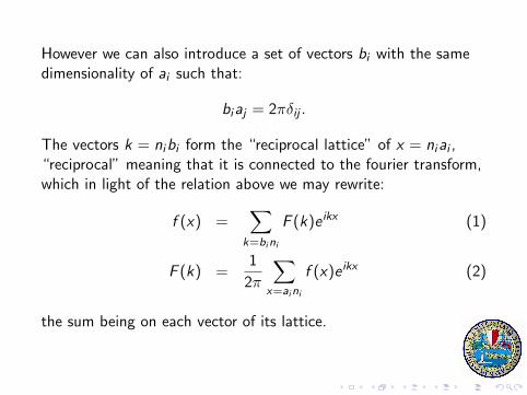
However we can also introduce a set of vectors bi with the samedimensionality of ai such that:

biaj = 2πδij .

The vectors k = nibi form the “reciprocal lattice” of x = niai ,“reciprocal” meaning that it is connected to the fourier transform,which in light of the relation above we may rewrite:

f (x) =∑

k=bini

F (k)e ikx (1)

F (k) =1

2π

∑x=aini

f (x)e ikx (2)

the sum being on each vector of its lattice.

..........

.....

.....................................................................

.....

......

.....

.....

.

Quantum eigenfunctions of the hamiltonian must satisfy symmetryrequirements in crystal, we are here concerned with theimplications of translational symmetry, i.e. the Bloch theorem.According to linear algebra, when two operators do commute withone another, it is always possible to find a set of vectors that areeigenvectors of both operators. Consequently, when one operator isthe Hamiltonian and the other one of the translation operatorsTx , x = niai :

[Tx ,H] = 0

that is how one expresses the fact that the potential has theperiodicity of the crystal, and therefore it must be possible to findthe H eigenfunctions ψ(r) so that:

Txψ(r) = ψ(r − x) = λxψ(r)

Tnxψ(r) = T nx ψ(r) = ψ(r − nx) = λnxψ(r)

for all integer values of n.

..........

.....

.....................................................................

.....

......

.....

.....

.

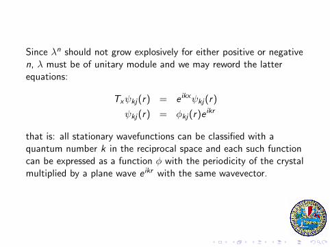
Since λn should not grow explosively for either positive or negativen, λ must be of unitary module and we may reword the latterequations:

Txψkj(r) = e ikxψkj(r)

ψkj(r) = ϕkj(r)eikr

that is: all stationary wavefunctions can be classified with aquantum number k in the reciprocal space and each such functioncan be expressed as a function ϕ with the periodicity of the crystalmultiplied by a plane wave e ikr with the same wavevector.

..........

.....

.....................................................................

.....

......

.....

.....

.

Nuclear motion constitutes an important part of crystal physics, itdictates sound propagation, heat transport, thermodynamicproperties and influences charge conduction, molecular adsorptionand several other processes.For brevity, we directly approach the quantum equations of motion,though consideration of the classical solutions provides someinsight.

..........

.....

.....................................................................

.....

......

.....

.....

.

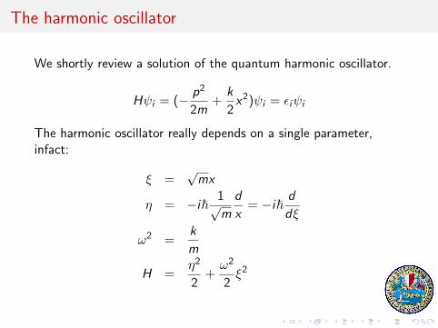
The harmonic oscillator

We shortly review a solution of the quantum harmonic oscillator.

Hψi = (− p2

2m+

k

2x2)ψi = ϵiψi

The harmonic oscillator really depends on a single parameter,infact:

ξ =√mx

η = −iℏ1√m

d

x= −iℏ

d

dξ

ω2 =k

m

H =η2

2+ω2

2ξ2

..........

.....

.....................................................................

.....

......

.....

.....

.

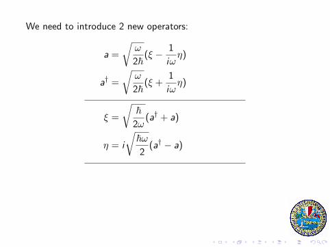
We need to introduce 2 new operators:

a =

√ω

2ℏ(ξ − 1

iωη)

a† =

√ω

2ℏ(ξ +

1

iωη)

ξ =

√ℏ2ω

(a† + a)

η = i

√ℏω2(a† − a)

[a, a†] =ω

2ℏ

(1

iω[ξ, η]− 1

iω[η, ξ]

)= 1

[a, a] = [a†, a†] = 0

..........

.....

.....................................................................

.....

......

.....

.....

.

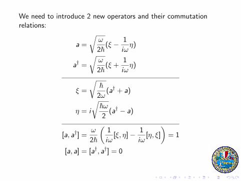
We need to introduce 2 new operators and their commutationrelations:

a =

√ω

2ℏ(ξ − 1

iωη)

a† =

√ω

2ℏ(ξ +

1

iωη)

ξ =

√ℏ2ω

(a† + a)

η = i

√ℏω2(a† − a)

[a, a†] =ω

2ℏ

(1

iω[ξ, η]− 1

iω[η, ξ]

)= 1

[a, a] = [a†, a†] = 0

..........

.....

.....................................................................

.....

......

.....

.....

.

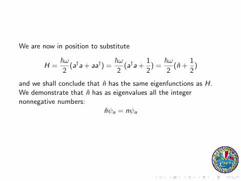
We are now in position to substitute

H =ℏω2(a†a+ aa†) =

ℏω2(a†a+

1

2) =

ℏω2(n +

1

2)

and we shall conclude that n has the same eigenfunctions as H.We demonstrate that n has as eigenvalues all the integernonnegative numbers:

nψn = nψn

..........

.....

.....................................................................

.....

......

.....

.....

.

1. the spectrum of n is nonnegative (left as an exercise)

2. naψn = a†aaψn = (aa† − 1)aψn = (n − 1)aψn

3. a†ψn = (n + 1)a†ψn, left as an exercise

4. ⟨aψn|aψn⟩ = ⟨ψn|n|ψn⟩ = n ⟨ψn|ψn⟩5. ⟨a†ψn|a†ψn⟩ = (n + 1) ⟨ψn|ψn⟩

points 2,3 connote a and a† as ladder operators, i.e.aψn =

√nψn−1 and a†ψn =

√n + 1ψn+1, where the

proportionality constants are deduced from points 4,5.Since the eigenvalues must all be positive, there must be aneigenfunction of a such that aψn = 0, hence n must be the integersequence obtainable by repeated application of a†.

..........

.....

.....................................................................

.....

......

.....

.....

.

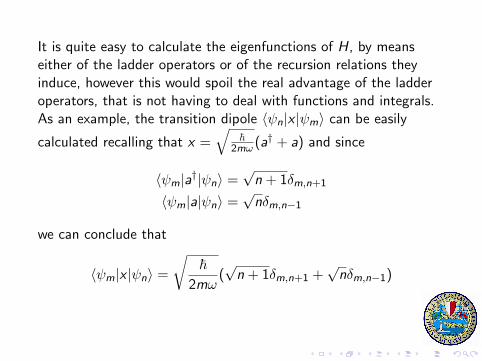
It is quite easy to calculate the eigenfunctions of H, by meanseither of the ladder operators or of the recursion relations theyinduce, however this would spoil the real advantage of the ladderoperators, that is not having to deal with functions and integrals.As an example, the transition dipole ⟨ψn|x |ψm⟩ can be easily

calculated recalling that x =√

ℏ2mω (a

† + a) and since

⟨ψm|a†|ψn⟩ =√n + 1δm,n+1

⟨ψm|a|ψn⟩ =√nδm,n−1

we can conclude that

⟨ψm|x |ψn⟩ =√

ℏ2mω

(√n + 1δm,n+1 +

√nδm,n−1)

..........

.....

.....................................................................

.....

......

.....

.....

.

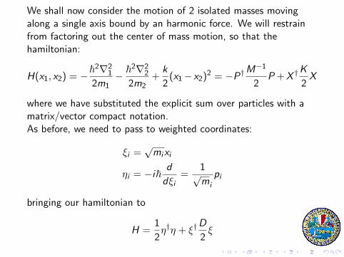
We shall now consider the motion of 2 isolated masses movingalong a single axis bound by an harmonic force. We will restrainfrom factoring out the center of mass motion, so that thehamiltonian:

H(x1, x2) = −ℏ2∇21

2m1− ℏ2∇2

2

2m2+

k

2(x1− x2)

2 = −P†M−1

2P+X †K

2X

where we have substituted the explicit sum over particles with amatrix/vector compact notation.As before, we need to pass to weighted coordinates:

ξi =√mixi

ηi = −iℏd

dξi=

1√mi

pi

bringing our hamiltonian to

H =1

2η†η + ξ†

D

2ξ

..........

.....

.....................................................................

.....

......

.....

.....

.

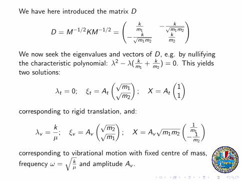
We have here introduced the matrix D

D = M−1/2KM−1/2 =

(km1

− k√m1m2

− k√m1m2

km2

)

We now seek the eigenvalues and vectors of D, e.g. by nullifyingthe characteristic polynomial: λ2 − λ( k

m1+ k

m2) = 0. This yields

two solutions:

λt = 0; ξt = At

(√m1√m2

); X = At

(11

)corresponding to rigid translation, and:

λv =k

µ; ξv = Av

(√m2√m1

); X = Av

√m1m2

( 1m1

− 1m2

)corresponding to vibrational motion with fixed centre of mass,

frequency ω =√

kµ and amplitude Av .

..........

.....

.....................................................................

.....

......

.....

.....

.

We have essentially factorized the hamiltonian into a set ofindependent motions:

H =1

2η†η + ξ†

D

2ξ = −

∇2At

2m−

∇2Av

2µ+

k

2A2v = Ht + Hv

by means of which we describe displacements and solutions interms of normal modes:

X ≡(x1x2

)= At

(11

)+ Av

( 1m1

− 1m2

)ψ(X ) = ϕt(At)ϕv (Av )

Htϕt(At) = ϵtϕt(At)

Hvϕv (Av ) = ϵvϕv (Av )

..........

.....

.....................................................................

.....

......

.....

.....

.

The generalization to a generic polyatomic molecule isstraightforward: from the hamiltonian

H =∑ p2i

2mi+

1

2

∑xikijxj

we pass to weighted coordinates ξi =√mixi :

H =1

2η†η + ξ†

D

2ξ

and upon diagonalization of D arrive at new collective coordinates(normal modes), 6 of which will be degenerate roto-translationmotions, (5 in the case of linear molecules) and the remainingrepresenting independent vibration.

X =3N∑

AiVi

where upon we factorize H into a set of 3N independent harmonichamiltonians

H =∑

Hi (Ai )

..........

.....

.....................................................................

.....

......

.....

.....

.

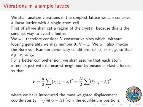
Vibrations in a simple lattice

We shall analyze vibrations in the simplest lattice we can conceive,a linear lattice with a single atom cell.First of all we shall cat a region of the crystal, because this is thesimplest way to avoid infinities.We will therefore consider N consecutive sites which, withoutloosing generality we may number 0..N − 1. We will also imposethe Born von Karman periodicity conditions, i.e. xi = xi+N , so thate.g. x0 = xN .For a better comprehension, we shall assume that each atominteracts just with its nearest neighbour by means of elastic forces,so that

V =k

2

∑l

(xl+1 − xl)2 =

D

2

∑l

(ξl+1 − ξl)2

where we have introduced the mass weighted displacementcoordinates ξl =

√m(xl − la) from the equilibrium positions.

..........

.....

.....................................................................

.....

......

.....

.....

.

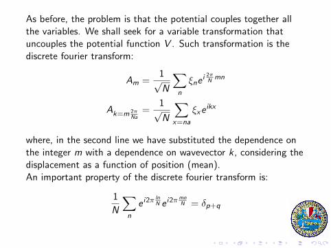
As before, the problem is that the potential couples together allthe variables. We shall seek for a variable transformation thatuncouples the potential function V . Such transformation is thediscrete fourier transform:

Am =1√N

∑n

ξnei 2πNmn

Ak=m 2πNa

=1√N

∑x=na

ξxeikx

where, in the second line we have substituted the dependence onthe integer m with a dependence on wavevector k, considering thedisplacement as a function of position (mean).An important property of the discrete fourier transform is:

1

N

∑n

e i2πlnN e i2π

mnN = δp+q

..........

.....

.....................................................................

.....

......

.....

.....

.

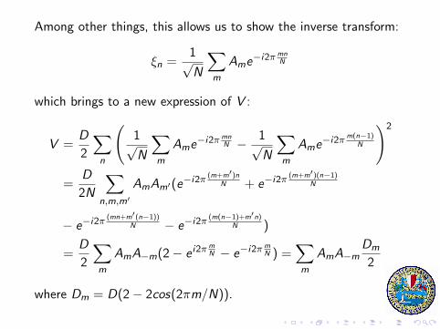
Among other things, this allows us to show the inverse transform:

ξn =1√N

∑m

Ame−i2πmn

N

which brings to a new expression of V :

V =D

2

∑n

(1√N

∑m

Ame−i2πmn

N − 1√N

∑m

Ame−i2πm(n−1)

N

)2

=D

2N

∑n,m,m′

AmAm′(e−i2π(m+m′)n

N + e−i2π(m+m′)(n−1)

N

− e−i2π (mn+m′(n−1))N − e−i2π (m(n−1)+m′n)

N )

=D

2

∑m

AmA−m(2− e i2πmN − e−i2πm

N ) =∑m

AmA−mDm

2

where Dm = D(2− 2cos(2πm/N)).

..........

.....

.....................................................................

.....

......

.....

.....

.

We apparently ended with V coupling the variables Am and A−m,however, since the displacement must be real, the constraintAm = A∗

−m must be satisfied, so that Am and A−m are indeed oneonly complex variable.The B operators:

Bm =1√N

∑n

ηne−i2πmn

N

are conjugates of the operators Am, that is they satisfy thecommutation relation [Bm,An] = iℏδmn. Therefore we can finallyrewrite the hamiltonian:

H =1

2

∑n

B2n + DnA

2n

i.e. a sum of oscillators with angular frequencyωm =

√D(2− 2cos(2πm/N)).

..........

.....

.....................................................................

.....

......

.....

.....

.

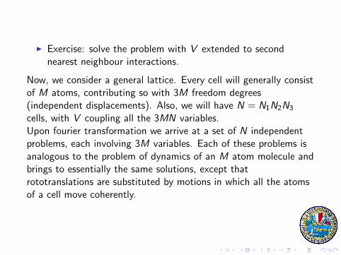
▶ Exercise: solve the problem with V extended to secondnearest neighbour interactions.

Now, we consider a general lattice. Every cell will generally consistof M atoms, contributing so with 3M freedom degrees(independent displacements). Also, we will have N = N1N2N3

cells, with V coupling all the 3MN variables.Upon fourier transformation we arrive at a set of N independentproblems, each involving 3M variables. Each of these problems isanalogous to the problem of dynamics of an M atom molecule andbrings to essentially the same solutions, except thatrototranslations are substituted by motions in which all the atomsof a cell move coherently.

..........

.....

.....................................................................

.....

......

.....

.....

.

-π/α 0 π/αk

ω

-π/α 0 π/αk

ω

-π/α 0 π/αk

ω

In simple crystals, left picture, a single curve appears in thedispersion plot. The value of ω(k = 0) is always 0. The slope dω

dkis the propagation speed for acoustic waves in the solid. In fact,the small k vibrations are what is perceived as sound. Actually,there are three acoustic branches, corresponding to 3 translationaldegrees in molecules. One of these represents longitudinal waves,the others transverse waves.In the case of cells with more atoms, the branches are 3M: 3acoustic and 3M − 3 so called optical phonons. The opticalphonons are analogous of molecular vibrations and exhibit thesame properties for IR excitation.

..........

.....

.....................................................................

.....

......

.....

.....

.

The rightmost picture, represents what happens when the cell isactually reducible. In this case, the branches exhibit degeneracy atthe boundary of the brillouin zone. Indeed the dispersion curveconstitutes a ”repeated representation” of the elementary celldispersion curves.

..........

.....

.....................................................................

.....

......

.....

.....

.

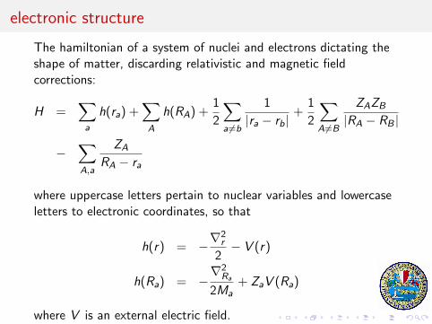
electronic structure

The hamiltonian of a system of nuclei and electrons dictating theshape of matter, discarding relativistic and magnetic fieldcorrections:

H =∑a

h(ra) +∑A

h(RA) +1

2

∑a =b

1

|ra − rb|+

1

2

∑A =B

ZAZB

|RA − RB |

−∑A,a

ZA

RA − ra

where uppercase letters pertain to nuclear variables and lowercaseletters to electronic coordinates, so that

h(r) = −∇2r

2− V (r)

h(Ra) = −∇2

Ra

2Ma+ ZaV (Ra)

where V is an external electric field.

..........

.....

.....................................................................

.....

......

.....

.....

.

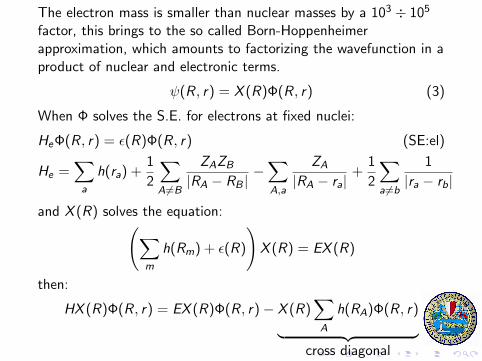
The electron mass is smaller than nuclear masses by a 103 ÷ 105

factor, this brings to the so called Born-Hoppenheimerapproximation, which amounts to factorizing the wavefunction in aproduct of nuclear and electronic terms.

ψ(R, r) = X (R)Φ(R, r) (3)

When Φ solves the S.E. for electrons at fixed nuclei:

HeΦ(R, r) = ϵ(R)Φ(R, r) (SE:el)

He =∑a

h(ra) +1

2

∑A=B

ZAZB

|RA − RB |−∑A,a

ZA

|RA − ra|+

1

2

∑a =b

1

|ra − rb|

and X (R) solves the equation:(∑m

h(Rm) + ϵ(R)

)X (R) = EX (R)

then:

HX (R)Φ(R, r) = EX (R)Φ(R, r)− X (R)∑A

h(RA)Φ(R, r)︸ ︷︷ ︸cross diagonal

..........

.....

.....................................................................

.....

......

.....

.....

.

So that X (R)Φ(R, r) solves the problem of nuclear and electronicmotion except for the “cross diagonal” term. The diabatic position,eq.3 requires knowing the electronic wavefunction at each nuclearposition. More commonly one adopts the “adiabatic” factorization

ψ(R, r) = X (R)Φ(R0, r) (4)

in which the electronic wavefunction pertains to fixed nuclearcoordinates R0, usually the lowest energy configuration.The “cross diagonal” correction term to the B.H. approximation issmall but fundamental, determining the shape of the wavefunctionnear the crossing points of adiabatic electronic wavefunctions.

..........

.....

.....................................................................

.....

......

.....

.....

.

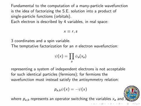
Fundamental to the computation of a many-particle wavefunctionis the idea of factorizing the S.E. solution into a product ofsingle-particle functions (orbitals).Each electron is described by 4 variables, in real space:

x ≡ r , s

3 coordinates and a spin variable.The temptative factorization for an n electron wavefunction:

ψ(x) =∏a

ϕa(xa)

representing a system of independent electrons is not acceptablefor such identical particles (fermions); for fermions thewavefunction must instead satisfy the antisymmetry relation:

pa,bψ(x) = −ψ(x)

where pa,b represents an operator switching the variables xa and xb.

..........

.....

.....................................................................

.....

......

.....

.....

.

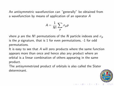
An antisymmetric wavefunction can “generally” be obtained froma wavefunction by means of application of an operator A

A =1

N!

∑p

σpp

vhere p are the N! permutations of the N particle indexes and σpis the p signature, that is 1 for even permutations, -1 for oddpermutations.It is easy to see that A will zero products where the same functionappears more than once and hence also any product where anorbital is a linear combination of others appearing in the sameproduct.The antisymmetrized product of orbitals is also called the Slaterdeterminant.

..........

.....

.....................................................................

.....

......

.....

.....

.

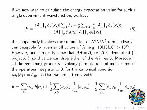
If we now wish to calculate the energy expectation value for such asingle determinant wavefunction, we have:

E =⟨A∏

a ϕa(xa)|∑

a ha +12

∑a,b

1rab

|A∏

a ϕa(xa)⟩⟨A∏

a ϕa(xa)|A∏

a ϕa(xa)⟩(5)

that apparently involves the summation of N!N!N2 terms, clearlyunmanagable for even small values of N: e.g. 10!10!102 > 1015.However, one can easily show that AA = A, i.e. A is idempotent (aprojector), so that we can drop either of the A in eq.5. Moreoverall the remaining products involving permutations of indexes not inthe operators integrate to 0, for the canonical condition⟨ϕa|ϕb⟩ = δab, so that we are left only with

E =∑a

⟨ϕa|h|ϕa⟩+1

2

∑a,b

⟨ϕaϕb|1

rab|ϕaϕb⟩−

1

2

∑a,b

⟨ϕaϕb|1

rab|ϕbϕa⟩

(6)

..........

.....

.....................................................................

.....

......

.....

.....

.

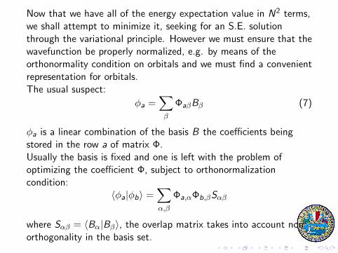
Now that we have all of the energy expectation value in N2 terms,we shall attempt to minimize it, seeking for an S.E. solutionthrough the variational principle. However we must ensure that thewavefunction be properly normalized, e.g. by means of theorthonormality condition on orbitals and we must find a convenientrepresentation for orbitals.The usual suspect:

ϕa =∑β

ΦaβBβ (7)

ϕa is a linear combination of the basis B the coefficients beingstored in the row a of matrix Φ.Usually the basis is fixed and one is left with the problem ofoptimizing the coefficient Φ, subject to orthonormalizationcondition:

⟨ϕa|ϕb⟩ =∑α,β

Φa,αΦb,βSαβ

where Sαβ = ⟨Bα|Bβ⟩, the overlap matrix takes into account nonorthogonality in the basis set.

..........

.....

.....................................................................

.....

......

.....

.....

.

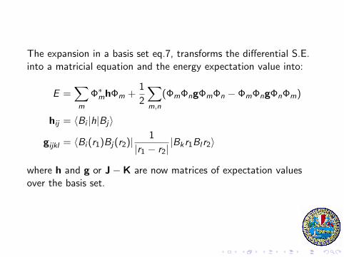
The expansion in a basis set eq.7, transforms the differential S.E.into a matricial equation and the energy expectation value into:

E =∑m

Φ∗mhΦm +

1

2

∑m,n

(ΦmΦngΦmΦn − ΦmΦngΦnΦm)

hij = ⟨Bi |h|Bj⟩

gijkl = ⟨Bi (r1)Bj(r2)|1

|r1 − r2||Bk r1Bl r2⟩

where h and g or J−K are now matrices of expectation valuesover the basis set.

..........

.....

.....................................................................

.....

......

.....

.....

.

Also, I wish to make sure that ⟨ϕi |ϕj⟩ = δij , which in my newrepresentation becomes:∑

mn

ΦimSmnΦnj = δij

so that we arrive at the lagrange function

L =∑m

Φ∗mhΦm +

1

2

∑m,n

(ΦmΦngΦmΦn − ΦmΦngΦnΦm)

+∑ij

ϵij(⟨Φi |S |Φj⟩ − δij)

..........

.....

.....................................................................

.....

......

.....

.....

.

We cannot directly solve this equation, but we can solve for:

L =∑m

Φ∗mhΦm +

1

2

∑m,n

(ΦmΦngΦmΦn − ΦmΦngΦnΦm)

+∑ij

ϵij(⟨Φi |S |Φj⟩ − δij)

=∑m

Φ∗mhΦm +

1

2

∑m,n

Φm(J−K)Φn +∑ij

ϵij(⟨Φi |S |Φj⟩ − δij)

where we have substituted the unknown inner Φ in the coulomband exchange expectation values with guessed values.

..........

.....

.....................................................................

.....

......

.....

.....

.

Now, making profit of some freedom in the choice of orbitals (thewavefunction does not change under unitary transformations ofoccupied orbitals), we can rearrange our problem:

L =∑m

Φ∗mFΦm +

∑i

ϵi (⟨Φi |S |Φi ⟩ − 1)

F = h+1

2(J−K)

FΦi = ϵiΦi

so that we remain with a diagonalization problem. We then willuse our solution for reevaluating the J and K matrices up to selfconsistency.

..........

.....

.....................................................................

.....

......

.....

.....

.

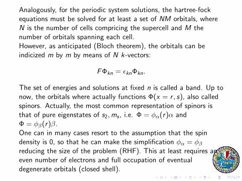
Analogously, for the periodic system solutions, the hartree-fockequations must be solved for at least a set of NM orbitals, whereN is the number of cells compricing the supercell and M thenumber of orbitals spanning each cell.However, as anticipated (Bloch theorem), the orbitals can beindicized m by m by means of N k-vectors:

FΦkn = ϵknΦkn.

The set of energies and solutions at fixed n is called a band. Up tonow, the orbitals where actually functions Φ(x = r , s), also calledspinors. Actually, the most common representation of spinors isthat of pure eigenstates of s2,ms , i.e. Φ = ϕα(r)α andΦ = ϕβ(r)β.One can in many cases resort to the assumption that the spindensity is 0, so that he can make the simplification ϕα = ϕβreducing the size of the problem (RHF). This at least requires aneven number of electrons and full occupation of eventualdegenerate orbitals (closed shell).

..........

.....

.....................................................................

.....

......

.....

.....

.

In any case one must face the problem of orbital occupation, whichusually is performed in energetic order, though no generaldemonstration actually exists that this brings to the lowest energyfor the system.

k

EF

E

k

EF

E

In the crystal the problem may be tougher, the bands possiblycrossing near the Fermi energy, separating the occupied from thefree bands at 0 K temperature.Solids are insulators when occupied and free bands are wellseparated, conductors when the density of states at the Fermienergy is not null, which may happen because the unit cell has anodd number of electrons or because band spreading is larger thanseparation.

..........

.....

.....................................................................

.....

......

.....

.....

.

electron correlation

While Hartree-Fock theory is surprisingly good, correlation maymake the difference in many cases. The monodeterminantalrepresentation turns out too restrictive even in closed shell systems.In solid state, most of modern computation makes use of densityfunctional theory, DFT, in the so called Kohn-Sham approach.The Kohn-Sham method applies the single determinantrepresentation to both obtain n-representable densities (densities ofsome n electron wavefunction) and to approximate the kineticenergy of the true wavefunction as expection values of the kineticoperator over occupied orbitals.

E = T + V + C + Exc

= −∑i

⟨ϕi |∇2

2|ϕi ⟩+

∫V (r)ρ(r)dr

+

∫∫ρ(r1)ρ(r2)

1

|r1 − r2|dr1dr2 +

∫Fxc [ρ(r)]dr