Dipartimento di Informatica eScienze dell�Informazione

Surface Reconstruction: Online Mosaicing and Modeling with

Uncertainty

by

Laura Papaleo

Theses Series DISI-TH-2004-XX

DISI, Universi tà d i Genova Via Dodecaneso, 35, 16146 Genova, I ta ly http://www.disi.unige.it

1

Università degli Studi di Genova Dipartimento di Informatica e

Scienze dell�Informazione

Dottorato di Ricerca in Informatica

Ph.D. Thesis in Computer Science

Surface Reconstruction: Online Mosaicing and Modeling with

Uncertainty

by

Laura Papaleo

March, 2004

2

Dottorato di Ricerca in Informatica Dipartimento di Informatica e Scienze dell�Informazione

Università degli Studi di Genova

DISI, Università di Genova Via Dodecaneso, 35

I-16146 Genova, Italy http://www.disi.unige.it/

Ph.D. Thesis in Computer Science Submitted by LAURA PAPALEO

DISI, Università di Genova papaleo@disi.unige.it

Date of submission: March 2004

Title Surface Reconstruction:

Online Mosaicing and Modeling with Uncertainty

Advisor: Prof. Enrico Puppo Dipartimento di Informatica e Scienze dell�Informazione

Università di Genova puppo@disi.unige.it

Ext Reviewers: Prof. Vittorio Murino Dipartimento Scientifico e Tecnologico

Università di Verona murino@sci.univr.it

Prof. Carlos Andújar Universitat Politecnica de Catalunya

andujar@lsi.upc.es

3

Abstract

A burst of research has been made during the last decade on 3D Reconstruction and several interesting and well-behave algorithms have been developed. However, as scanning technologies improve their performance, reconstruction methods have to tackle new problems such as working with datasets of large dimension and building meshes almost in real-time.

We pointed out a general need for formal analysis of the reconstruction problem and for methods which are able: (i) to elaborate huge and complex input datasets and to produce accurate results, (ii) to exploit all information provided by sensing devices, (iii) to transmit models quickly and accurately in order to visualize, search, and modify them using different devices (PDA, laptop, special devices, and so on).

This PhD dissertation addresses the problem of reconstruction from two different points of view: Online Mosaicing and Modeling with uncertainty .

Online Mosaicing: the Thesis presents a Data Analysis approach which on the fly, starting from multiple acoustic/optical range images, elaborates the acquired unknown object by mosaicing multiple single frame meshes.

In the context of the European ARROV project, we developed a 3D reconstruction pipeline, which provides a 3D model of an underwater scene from a sequence of range data captured by an acoustic camera mounted on board a Remotely Operated Vehicle (ROV). Our approach works on line by building the 3D model while the range images arrive from ROV. The method combines the range images in a sequence by minimizing the workload of the rendering system.

Modeling with uncertainty : The Thesis presents a general Surface Reconstruction framework which encapsulates the uncertainty of the sampled data, making no assumption on the shape of the surface to be reconstructed.

Starting from the input points (either points clouds or multiple range images), we construct an Estimated Existence Function (EEF) that models

4

the space in which the desired surface could exist and, by the extraction of EEF critical points, we reconstructs the surface. The final goal is the development of a generic framework able to adapt the result to different kind of additional information coming from sensors, such as sampling conditions, normals, local curvature, and reliability of the data.

5

To Franco, the sun that drives out winter from my heart-

6

Tell me and I will forget, Show me and I will remember, Let me do it and I will understand [Confucius]

7

Acknowledgments

I should say �Grazie� to many people for supporting me during these research years. Thanks to Enrico Puppo, who supports and suffer me, believing in my ideas, Giovanni Gallo and Alfredo Ferro, who suggested me to start this adventure and continue to sustain me. Franco, my husband and my best supporter in the world, who teaches me how organize my tasks and daily assists me in modeling my research offering me incredible ideas and realistic solutions.

Since life is not just work, here there are some people who render these years so special: Angelo, my best friend of which a little part inside me will never die. Chiara, Esther and �gli Enry�, who helped me in difficult decisions and in feeling better during hard periods of my research. My Bai� friends who facilitated my new life in Genova and Paolino because with his force taught me how life is short and wonderful and that we must live not simply exist.

Thanks also to all my new friends who helped me in living in a new department and in understanding its rules: Viviana, Davide, Francesca, Marco, Emanuele, Barbara, Paola, Giorgio, Giovanna, Gabriella.

Infine, grazie ai miei genitori , ai miei fratelli ed alla mia nonnina per aver creduto in me sempre e comunque, anche quando sembravo diversa, anche quando crescendo sembravo allontanarmi. Questa tesi la dedico a voi: siete sempre con me.

8

Table of Contents TABLE OF CONTENTS . . . . . . . . . . . . . . . . . . . . . . . . . . . . . . . . . . . . . . . . . . . . . . . . . . . . . . . . . . . . . . . . . . . . . . . . . . . . . . . . . . . . . . 8 1. INTRODUCTION .. . . . . . . . . . . . . . . . . . . . . . . . . . . . . . . . . . . . . . . . . . . . . . . . . . . . . . . . . . . . . . . . . . . . . . . . . . . . . . . . . . . . . . 10

1 .1 RE S E A R C H MO T I V A T I O N . . . . . . . . . . . . . . . . . . . . . . . . . . . . . . . . . . . . . . . . . . . . . . . . . . . . . . . . . . . . . . . . . . . . . .10 1.2 TH E S I S AI M A N D GO A L S . . . . . . . . . . . . . . . . . . . . . . . . . . . . . . . . . . . . . . . . . . . . . . . . . . . . . . . . . . . . . . . . . . . . . .12 1.3 TH E S I S STRU C T U R E . . . . . . . . . . . . . . . . . . . . . . . . . . . . . . . . . . . . . . . . . . . . . . . . . . . . . . . . . . . . . . . . . . . . . . . . . . . . .13

2. THE RECONSTRUCTION PROCESS . . . . . . . . . . . . . . . . . . . . . . . . . . . . . . . . . . . . . . . . . . . . . . . . . . . . . . . . . . 15 2 .1 AC Q U IS I T I O N A N D RE P R E S E N T A T I O N . . . . . . . . . . . . . . . . . . . . . . . . . . . . . . . . . . . . . . . . . . . . . . . . . . . . . .15 2.2 SC A N N I N G TE C H N I Q U E S . . . . . . . . . . . . . . . . . . . . . . . . . . . . . . . . . . . . . . . . . . . . . . . . . . . . . . . . . . . . . . . . . . . . . . .17 2.3 RE G I S T R A T I O N . . . . . . . . . . . . . . . . . . . . . . . . . . . . . . . . . . . . . . . . . . . . . . . . . . . . . . . . . . . . . . . . . . . . . . . . . . . . . . . . . . .21 2.4 IN T E G R A T I ON A P P R O A C HE S . . . . . . . . . . . . . . . . . . . . . . . . . . . . . . . . . . . . . . . . . . . . . . . . . . . . . . . . . . . . . . . . . .23

3. INTEGRATION: STATE-OF-THE-ART .. . . . . . . . . . . . . . . . . . . . . . . . . . . . . . . . . . . . . . . . . . . . . . . . . . . . . . 25 3 .1 CO M P U T A T I O N A L GE O ME T R Y APP R O A C H . . . . . . . . . . . . . . . . . . . . . . . . . . . . . . . . . . . . . . . . . . . . . . .25

3.1 .1 α-shape methods . . . . . . . . . . . . . . . . . . . . . . . . . . . . . . . . . . . . . . . . . . . . . . . . . . . . . . . . . . . . . . . . . . . . . . . . .26 3.1 .2 Sculpturing Methods . . . . . . . . . . . . . . . . . . . . . . . . . . . . . . . . . . . . . . . . . . . . . . . . . . . . . . . . . . . . . . . . . . . .31 3.1 .3 Medial Axis Methods . . . . . . . . . . . . . . . . . . . . . . . . . . . . . . . . . . . . . . . . . . . . . . . . . . . . . . . . . . . . . . . . . . .38 3.1 .4 Local Approaches . . . . . . . . . . . . . . . . . . . . . . . . . . . . . . . . . . . . . . . . . . . . . . . . . . . . . . . . . . . . . . . . . . . . . . .44

3 .2 VO L U M E T R IC ME T H O D S . . . . . . . . . . . . . . . . . . . . . . . . . . . . . . . . . . . . . . . . . . . . . . . . . . . . . . . . . . . . . . . . . . . . . . .59 3.2 .1 Grid-based approaches . . . . . . . . . . . . . . . . . . . . . . . . . . . . . . . . . . . . . . . . . . . . . . . . . . . . . . . . . . . . . . . .59 3.2 .2 Radial Basis Funct ion . . . . . . . . . . . . . . . . . . . . . . . . . . . . . . . . . . . . . . . . . . . . . . . . . . . . . . . . . . . . . . . . .68 3.2 .3 Deformable models and Level set Methods . . . . . . . . . . . . . . . . . . . . . . . . . . . . . . . . . . . . .80

4. ONLINE MOSAICING .. . . . . . . . . . . . . . . . . . . . . . . . . . . . . . . . . . . . . . . . . . . . . . . . . . . . . . . . . . . . . . . . . . . . . . . . . . . . . . . 86 4 .1 TH E ARROV PR OJ E C T . . . . . . . . . . . . . . . . . . . . . . . . . . . . . . . . . . . . . . . . . . . . . . . . . . . . . . . . . . . . . . . . . . . . . . . . .86 4.2 MO S A I C I N G F R O M MU L T I P L E RA N G E IM A G E S . . . . . . . . . . . . . . . . . . . . . . . . . . . . . . . . . . . . . . . . . .89 4.3 TH E ARROV RE C ON S TR U C T I O N P IP E L I N E . . . . . . . . . . . . . . . . . . . . . . . . . . . . . . . . . . . . . . . . . . . . . .90

4.3 .1 Data Capture . . . . . . . . . . . . . . . . . . . . . . . . . . . . . . . . . . . . . . . . . . . . . . . . . . . . . . . . . . . . . . . . . . . . . . . . . . . . . .93 4.3 .2 Data Pre-process ing . . . . . . . . . . . . . . . . . . . . . . . . . . . . . . . . . . . . . . . . . . . . . . . . . . . . . . . . . . . . . . . . . . . .96 4.3 .3 Regis trat ion . . . . . . . . . . . . . . . . . . . . . . . . . . . . . . . . . . . . . . . . . . . . . . . . . . . . . . . . . . . . . . . . . . . . . . . . . . . . . 103 4.3 .4 Geometric Fusion . . . . . . . . . . . . . . . . . . . . . . . . . . . . . . . . . . . . . . . . . . . . . . . . . . . . . . . . . . . . . . . . . . . . . . 104

4 .4 RE S U L T S . . . . . . . . . . . . . . . . . . . . . . . . . . . . . . . . . . . . . . . . . . . . . . . . . . . . . . . . . . . . . . . . . . . . . . . . . . . . . . . . . . . . . . . . . 112 5. MODELING WITH UNCERTAINTY .. . . . . . . . . . . . . . . . . . . . . . . . . . . . . . . . . . . . . . . . . . . . . . . . . . . . . . . . . 118

5 .1 MU L T I-S E N SO R S DA T A FU S I O N . . . . . . . . . . . . . . . . . . . . . . . . . . . . . . . . . . . . . . . . . . . . . . . . . . . . . . . . . . . 119 5.2 PR OB L E M DE F I N I T I O N A N D P R O P O S ED A P P R O A C H . . . . . . . . . . . . . . . . . . . . . . . . . . . . . . . . . . . 121

5.2 .1 Building the EEF Funct ion . . . . . . . . . . . . . . . . . . . . . . . . . . . . . . . . . . . . . . . . . . . . . . . . . . . . . . . . . 124 5.2 .2 Compute r idge points . . . . . . . . . . . . . . . . . . . . . . . . . . . . . . . . . . . . . . . . . . . . . . . . . . . . . . . . . . . . . . . . 126 5.2 .3 Building the mesh . . . . . . . . . . . . . . . . . . . . . . . . . . . . . . . . . . . . . . . . . . . . . . . . . . . . . . . . . . . . . . . . . . . . . 131

5 .3 TH E AL G OR IT H M . . . . . . . . . . . . . . . . . . . . . . . . . . . . . . . . . . . . . . . . . . . . . . . . . . . . . . . . . . . . . . . . . . . . . . . . . . . . . . 132 5.4 RE S U L T S . . . . . . . . . . . . . . . . . . . . . . . . . . . . . . . . . . . . . . . . . . . . . . . . . . . . . . . . . . . . . . . . . . . . . . . . . . . . . . . . . . . . . . . . . 134

6. CONCLUSIONS AND FUTURE WORKS .. . . . . . . . . . . . . . . . . . . . . . . . . . . . . . . . . . . . . . . . . . . . . . . . . . . 140 7. BIBLIOGRAPHY .. . . . . . . . . . . . . . . . . . . . . . . . . . . . . . . . . . . . . . . . . . . . . . . . . . . . . . . . . . . . . . . . . . . . . . . . . . . . . . . . . . . . 144

9

10

1. Introduction

This chapter first presents the motivation for the research and then introduces the proposed frameworks and their key components. The challenges in developing these frameworks are discussed, and the original contributions of this research are presented. Finally, the organization of the remainder of this dissertation is outlined to guide the reader through its details.

1.1 Research Motivation The problem of reconstructing 3D objects from sampled data has important applications in several fields among which virtual reality, animation, cultural heritage and reverse engineering are, maybe, the most popular [59]. In virtual reality, for example, generating an accurate 3D environment is essential for a human walk-through. In reverse engineering, 3D reconstruction is able to generate a CAD model from a real object. In robotic vision, a 3D simulation can help a robot to move in a unknown environment providing an correct mapping of the surrounding area. In image-guided surgery, 3D models reconstructed from CTs and MRIs can help a doctor to see anatomic structures and make an accurate diagnosis.

3D models are usually constructed from a set of measurements taken in 3D space. Laser range sensing and stereo vision are two popular methods for 3D measurement. Although stereo vision devices are much cheaper than laser range scanners, they are limited by measurement accuracy and range [86].

From an application-based point of view, two categories of tasks can be distinguished in 3D reconstruction: data analysis and surface reconstruction [64].

• Data Analysis means that nothing is known about the surface from which the data originate. The task is to find the most reasonable solutions among many possibilities.

11

• Surface Reconstruction means that the surface from which the data are sampled is known, say in form of a real model, and the goal is to get a computer-based description of this surface that is as accurate as possible. This knowledge may be used in the selection of a suitable algorithm.

A proper reconstruction of the desired surface in the latter case can only be expected if i t is sufficiently sampled. Sufficiency depends on the particular method of surface reconstruction. It might be formulated in form of sampling theorems, which should give sufficient conditions that can be easily checked. The necessity of these theorems is present almost in all the algorithms described in the state-of-the-art section (see Chapter 3): all of them, for working in a satisfactory manner, make strong assumptions on the goodness of the sampling dataset, but do not formally explain under what conditions this happens. Exceptions are the works of Attali [8] (which gives a morphology-based sampling theorem at least for the 2D case), Bernardini, Bajaj [12] and Amenta et al.[2].

If data are improperly sampled, a reconstruction method may cause artifacts, which have to be dealt with. A common artifact is the presence of holes and spurious surface boundaries in the model. Like in classical sampling theory, pre-filtering e.g. in the sense of depth-pass filtering may help to reduce artifacts at the costs of loss of details. Another possibility is interactive correction by the user that may be helpful if artifacts occur at some few isolated locations.

The opposite of insufficient sampling is that the sampling data are unnecessarily dense. This happens in particular if the surface is sampled with a uniform density. In that case, the sampling density required at fine details of the surface causes too many data points in regions of minor variation and often a simplification post-process is necessary.

The actual framework in 3D Reconstruction outlines a general request of formal analysis of the problem and a need of methods, which are able:

- to elaborate huge and complex input datasets and to produce accurate results

- to build models from input data which come with enriched properties (coordinates but also normal/curvature estimation on points, reliability of the data and so on.)

- to transmit these models quickly and accurately (via web, for example) in order to visualize, search, modify them using different devices (PDA, laptop, special devices, and so on)

12

This dissertation contributes to solving some problems in two different directions: on one hand, it presents a Data Analysis approach to online and offline mosaicing of multiple range images (in the context of the ARROV project [5]). On the other hand, it reports our investigation on innovative Surface Reconstruction Methods , which try to encapsulate uncertainty of the sampled data, making assumptions on the shape of the surface to be reconstructed.

1.2 Thesis Aim and Goals The use of three-dimensional digital models, in order to represent real objects and environments, is a powerful and smart solution: modeling is a creative but also cognitive strategy, which allows the users to visualize, modify and study 3D replica on a screen, far away from the real object, or to share representations of data and environments over the net.

A burst of research has been made during the last decade on 3D Reconstruction and several interesting and well-behave algorithms have been developed. However, as scanning technologies improve their performance, reconstruction methods have to tackle new problems such as working with datasets of large dimension and building meshes almost in real-time. An optimal reconstruction method should takes into account not only positional information of points (spatial coordinates) but also enriched properties which modern sensors often provide such estimations on normal and curvature on scanned points or reliability of the received input points.

This PhD dissertation addresses the problem of reconstruction from two different points of view: Online Mosaicing and Modeling with uncertainty .

Online Mosaicing: the Thesis presents a Data Analysis approach which on the fly, starting from multiple acoustic/optical range images, elaborates the acquired unknown object by mosaicing multiple single frame meshes.

In the context of the European ARROV project, we developed a 3D reconstruction pipeline that provides a 3D model of an underwater scene from a sequence of range data captured by an acoustic camera mounted on board a Remotely Operated Vehicle (ROV). Our approach works on line by building the 3D model while the range images arrive from ROV.

13

The method combines the range images in a sequence by minimizing the workload of the rendering system.

Modeling with uncertainty : The Thesis presents a general Surface Reconstruction framework which encapsulates the uncertainty of the sampled data, making no assumption on the shape of the surface to be reconstructed.

Starting from the input points (either points clouds or multiple range images), we construct an Estimated Existence Function (EEF) that models the space in which the desired surface could exist. The extraction of the EEF critical points by the use of a continuous method and a discrete one permits to reconstruct a surface, which correctly model the information given by the input. Moreover, the EEF can help/guide us in estimating the position and normal of missing data by exploiting spatial coherence.

The final goal is the development of a generic framework able to adapt the result to different kind of additional information (enriched data) coming from sensors, such as sampling conditions, normals, local curvature, and reliability of the data.

The implementation of both methods, based on space discretization by the use of a regular cell grid, has some advantages:

1. It can adapt the output resolution in order to fit system requirements

2. It can process large dataset progressively and successively merge all partial results

3. It can be simply parallelized.

1.3 Thesis Structure This section explains the structure of the thesis: Chapter 2 presents the general pipeline for 3D reconstruction problems treating acquisition devices and methodologies, registration methods integration approaches in general, while Chapter 3 presents our proposed taxonomy of the existing integration methods.

After these introductory Chapters, Chapter 4 presents the online 3D reconstruction pipeline we developed in the context of the European

14

Project ARROV [5] and Chapter 5 presents our novel approach for modeling with uncertainty in a Multi-Sensors Data Fusion framework.

Both Chapters 4 and 5 show the results of our algorithms applied to significant datasets: for the ARROV pipeline, we tested the method on input data coming from an acoustic sensor, while for the Multi-Sensors approach we used standard input dataset (Stanford bunny, Happy Buddha�). Finally, Chapter 6 concludes this Dissertation and lists future works and open problems.

15

2. The Reconstruction Process

The aim of this chapter is to introduce the standard reconstruction pipeline dealing with general concepts and methodologies for 3D data acquisition, registration and integration. It gives information on the different acquisition devices and on the standard registration techniques. Finally, i t makes an initial subdivision of the existing integration methods that will be treated in details in the next chapter.

2.1 Acquisition and Representation From an operative point of view, a digital 3D model is constructed with the definition of the following characteristics:

1. Geometry , description of the coordinates of vertices,

2. Connectivity , description of the relationships between vertices to form faces of the model

3. Photometry , colors attributes, normals or textures.

Given the acquired points of the observed object surface, the most common definition of the topology is given by the use of a triangular mesh , which allows a simple way of model representation, visualization and manipulation. But a model can be presented also by the use of surface patches, more flexible but also more mathematically complex, using, for example, NURBS .

The construction of 3D digital replicas requires performing a set of sequential and correlated phases that can be listed in the following order:

1. Acquisition Range sensors capture 3D surface measurements. Often, because of the sensor�s limited field of view or of the complexity of the object/scene to be scanned, multiple scans are required. Each view gives a set of 3D points on a certain given coordinates system (later in this chapter).

2. Registration In order to construct the entire model, the acquired data have to be

16

aligned transforming all the measurements into a common coordinate system. This operation has to be done with the minimal possible error.

3. Integration All data are merged to construct a single 3D surface model usually a triangle mesh. Successively some improvements on the model may be done, such as smoothing, simplification and so on (see chapter 3) for a complete taxonomy of the existing integration methods).

4. Color-Texture Processing Colors and reflectance properties have to be defined in order to extrapolate intrinsic physic object characteristics, which will be added to the synthetic model. Successively those reflectance values have to be added to the geometrical model, removing, for example, all the possible non-real shadings, or defining color for each screen pixel.

We are mainly interested in the Integration phase in which all the different correctly registered range images (or directly a cloud of points in space) are combined to construct an unambiguous topological model. The existing methods follow, essentially, two basic directions:

(1) Reconstruction from unorganized points (points cloud)

The main advantage of this type of approaches is that they are general and do not assume any knowledge of the object shape or topology [2], [3], [8], [9], [12], [14], [18], [19], [27], [31], [33], [34], [37], [44], [49], [51], [90], [106].

Unfortunately, for the same reasons, they are usually computationally expensive. Moreover, these methods work well in presence of smooth surfaces but not in the case of high curvature, zones and post processing operations are often necessary. To overcome these limitations, some methods (e.g. [44], [51]), start from a point cloud and extract additional information on the input (such as normals, k-neighbors set) inferring on proximity properties. Some others (e.g. [14] [90]), instead, consider point normals known a priori. In both cases those information are successively used in order to build a mesh as topologically correct as possible.

17

(2) Reconstruction using the underlying structure of the acquired points (range images, volumetric data, contour data)

Here, the underlying structure helps the method in the construction of the entire model [23], [26], [29], [52], [59], [75], [85], [101]. Normals, curvature, reliability of the data are strongly used in the integration phase. Unfortunately, some problems may arise in case of volumetric data: if the edge length of the cells grid is too big aliasing artifacts could be visible avoiding to obtain optimal result .

We now make a brief presentation on the existing scanning techniques and the existing methods on Registration of multiple range images. Finally, we concentrate on the existing Reconstruction Methods giving a initial taxonomy which will conclude this Chapter. In the next Chapter, instead, we will provide a complete survey on Integration Methods.

2.2 Scanning Techniques A complete description of the existing acquisition techniques is out of the scope of this work but a brief explanation can help in understanding existing methodologies and heuristics. For details, see for example [26], [28].

Depending on the techniques used, the output of a scanning process can be simply a set of points (unstructured data), but it can be also a profile, a range image or a volumetric output (structured data) [81]. Trying to provide taxonomy, the standard acquisition techniques can be roughly divided into two main categories [28] (Figure 1):

1. Acquisition by contact , which is performed by touching the object surface on each relevant side with an ad-hoc instrument. These instruments are quite slow and cannot be used on some typology of objects. Moreover, they do not provide information on object appearance.

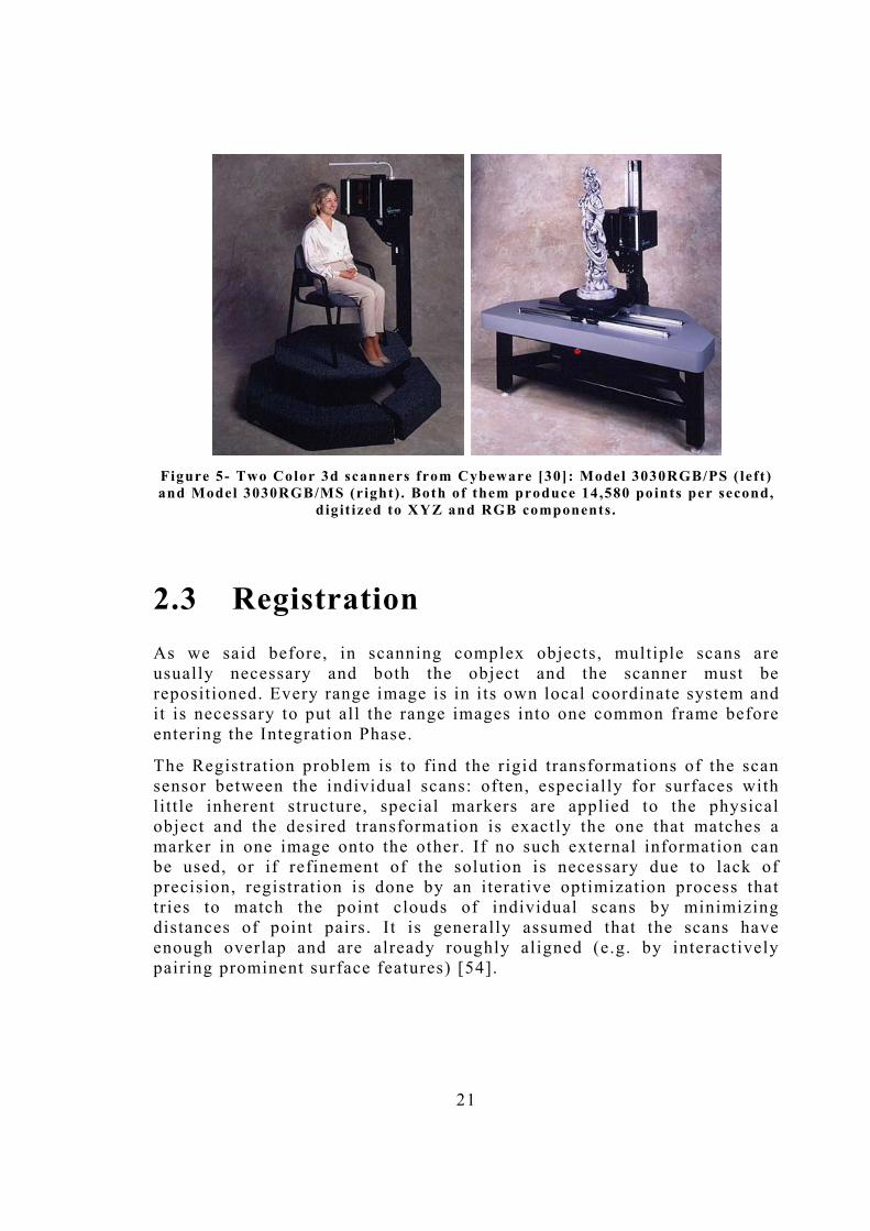
2. Acquisition without contact , which is performed by indirect techniques based on a certain energy source. The returned signal is measured by the use of digital cameras or special sensors. In this class, the optical and laser technologies are the most used (see Figure 5).

18

Shape Acquisition

Contact Non-contact

Non destructive Destructive Reflective Trasmissive

CMM Jointed arms Slicing Non optical Optical Industrial CT

Microwave radar Sonar

Figure 1 � Taxonomy of the exist ing Acquisit ion Techniques [28]

The optical technologies again can be divided into passive or active [28] (Figure 2). The last one (called also active sensing systems) can acquire data very fast and accurately: these are the reasons why they are the most popular existing technologies.

Passive optical systems are, in general, based (i) on acquisition of many RGB images taken from various points, (ii) on the reconstruction of object by contours and, finally, (iii) on integration of such contours for the reconstruction of the model 3D. These systems determine the object coordinates only by the use of information contained in the acquired images (for example, photogrammetry and acquisition by silhouette). They are extremely economic, simple to use and produce a complete model; on the contrary, the quality and accuracy of the produced model can be quite low.

Active optical systems are constituted by a source and a sensor, where the source emits a certain illuminant pattern and the sensor acquires returned marks reflected by the object surface.

19

Optical

Passive Active

Stereo

ImagingRadar Triangulation Active

stereoInterferometry

Shape fromshading

Shape fromsilhouettes

Depth fromfocus/defocus

Moire Holography

Figure 2 - Taxonomy of Optical scanning techniques [28]

The source scans regularly the space and the system returns a 2D matrix (range image), identifying the points on the surface. Among this type of systems we can list:

• Triangulation systems (Figure 3) where the object geometry is reconstructed by the use of three information: the pattern emission direction and the relative positions of both source and sensor (Figure 4). Either laser sources or light sources can be used as pattern emission sources. These systems reach a good level of accuracy, measuring many points in a small area and returning a 3D points cloud (x,y,z coordinates).

•

• Time of fl ight systems (imaging radar, interferometry, �) (Figure 3) which emit an impulse and use a sensor for measuring the time needed by this impulse to arrive at the surface and to come back at the device. They are, in general, less precise than triangulation ones but they can acquire wide surfaces on a single image. Moreover they tend to be more costly than triangulation-based sensors. In order to handle large bandwidths required by short pulses, sophisticated electronics that minimize sensitivity to variation in signal strength are needed [13].

20

Figure 3 - Autosynchronized scanner: dual-scan axis , equally used in

tr iangulat ion & t ime of f l ight systems [13] .

In conclusion, scanning works best with well�behaved surfaces, which are smooth and have low reflectance [28]. Triangulation scanners, for example, have the common problem of shadowing: due to the separation of light source and detector, parts of a non�convex object may not be reached by the light from the projector or may not be seen by the detector.

Figure 4 - Coded l ight approach example ( left) ful ly i l luminated scene taken prior to project ion of the stripe patterns, (r ight) grey scale image of a str ipe

pattern projected with a LCD projector. [13]

21

Figure 5- Two Color 3d scanners from Cybeware [30]: Model 3030RGB/PS ( left) and Model 3030RGB/MS (right) . Both of them produce 14,580 points per second,

digit ized to XYZ and RGB components.

2.3 Registration As we said before, in scanning complex objects, multiple scans are usually necessary and both the object and the scanner must be repositioned. Every range image is in its own local coordinate system and it is necessary to put all the range images into one common frame before entering the Integration Phase.

The Registration problem is to find the rigid transformations of the scan sensor between the individual scans: often, especially for surfaces with little inherent structure, special markers are applied to the physical object and the desired transformation is exactly the one that matches a marker in one image onto the other. If no such external information can be used, or if refinement of the solution is necessary due to lack of precision, registration is done by an iterative optimization process that tries to match the point clouds of individual scans by minimizing distances of point pairs. It is generally assumed that the scans have enough overlap and are already roughly aligned (e.g. by interactively pairing prominent surface features) [54].

22

The standard approach, for matching multiple range images, is to register them pair-wise using variants of the iterated closest point method (ICP) [25].

2.3.1.1 ICP ALGORITHM Let us suppose that we have two sets of 3D points which correspond to a single shape but are expressed in different reference frames. We will call one of these sets the data set V j , and the other the model set V i . Let G i j be the rigid transformation matrix (in homogeneous coordinates) that registers view j onto view i ,

V i = G i j ⋅Vj

The registration consist in finding the 3-D transformation G i j which, when applied to the data set V j , minimizes the distance between the two point sets. In general point correspondences are unknown.

For each point v from the set V j , there exists at least one point on the surface of V i which is closer to v than all other points in V i . This is the closest point. The basic idea behind the ICP algorithm is that, under certain conditions, closest points are a reasonable approximation to the true point correspondences.

The ICP algorithm can be summarized as follows [22]:

1. For each point in V j , compute its closest point in V i ;

2. With the correspondence from step 1, compute the incremental transformation G i j ;

3. Apply G i j to the data V j ;

4. If the change in total mean square error is less than a threshold, terminate. Else, goto step one.

For two point sets, the method determines a starting transformation and successively estimates correspondences between sample points. Then it updates the rigid transformation and repeats the first two steps until complete convergence. Ideally, the transformations are computed precisely and at the end all scans fit together perfectly. In practice, data are contaminated and have errors: surface points measured from different angles or distances result in slightly different sampled positions. So even with a good optimization procedure, i t is l ikely that the n-th scan will not fit to the first. Multiple iterations are necessary to find a global optimum and to distribute the error evenly.

23

In order to overcome of ICP problems, many variants to ICP have been proposed, including: the use of thresholds to limit the maximum distance between points [107], the use of closest points in the direction of the local surface normal, Least Median of Squares estimation [98], rejecting matching on the surface boundaries [101], or the use of the X84 outlier rejection rule to discard false correspondences on the basis of their distance [42].

Besl and McKay [15] proved that the ICP algorithm as presented above is guaranteed to converge monotonically to a local minimum of the Mean Square Error. As for step 2, efficient, non-iterative solutions to this problem (known as the point set registration problem) were compared in [61], and the one based on Singular Value Decomposition was found to be the best in terms of accuracy and stability. However, a detailed discussion of these methods is actually beyond the scope of this dissertation.

2.4 Integration approaches After data acquisition and registration phases, the next step is the generation of a single surface representation, usually an overall triangle mesh, from the acquired data. As we said before, general solutions should not assume any knowledge of the object shape or topology but possible approaches may strongly depend on the given type of input (e.g. point clouds, sections, multiple range images). It was quite difficult to determine a significant taxonomy of the existing surface reconstruction methods. Most of them, especially in the last few years, try to adopt hybrid solutions using different approaches in the same method.

Regardless the underlying structure of data, approaches can be divided into two groups [64], depending on whether they produce an:

1. Interpolation of the input data

2. Approximation of the input data

In the first case (interpolation), the vertices in the resulting mesh are the original sampled points. These methods, in some sense, rely on the accuracy of the input and use them as constraints for the construction of the final mesh [2], [3], [8], [9], [12], [18], [27], [31], [37], [44], [51], [90], [106].

24

The basic strategy under the interpolant approaches is to use the input points as the optimal geometric description of the scanned object, in other words as vertex set of the final mesh. In general a cloud of points with no other information is considered as input [37], [12], [18], [106], [31], [34] but, in some cases, also points clouds with additional information on the object structure or points proximity [2], [3], [8], [9] maybe processed. In addition, the modern scanning technologies often return the acquired points coordinates together with an estimation of the normal in each point: that is why some interpolant methods use also this information [90], [14], [44]. The interpolant methods can be divided into:

• Global Approaches that take into account the entire set of input points in order to derive an initial structure from which extract [12], [18], [31], [37], [90], [106] or on which construct [2], [3], [8], [9] the final mesh;

• Local Approaches, that build portions of mesh by inferring on local characteristics of the input points [14], [44], [101].

In the second case (approximation), the vertices in the resulting mesh can be different from the original sampled points.

The strategy of the approximation methods is to use the input points as guide for surface reconstruction. Especially for range data, an approximating rather than an interpolating mesh is desirable in order to get a result of moderate complexity [14], [23], [26], [29], [49], [50], [52]: in fact, in cases of input which comes with error, in the overlapping zones, where data are redundant, the error frequency is high and the interpolant methods can produce results with outliers. In these cases, approximation methods behave definitely better.

25

3. Integration: State-of-the-Art

Be curious always, for knowledge will not acquire you; you must acquire it

[Sudie Back]

This chapter tries to make an exhaustive description of the most representative 3D reconstructing methods developed in the last two decades. We have done our best to determine a good taxonomy of the existing methods. It was quite difficult because, especially in the last research years, many algorithms try to adopt hybrid solutions in order to get better results.

We divided the reconstruction methods into two main categories (and some of them into subcategories):

• Computational Geometry Approaches : a method belongs to this class if i t is based on computational geometry concepts (alpha-shapes, Delaunay Triangulation, Voronoi Diagram and Medial Axis and so on).

• Volumetric Approaches: they try to define a function in space and to build the final mesh inferring on the space occupied.

The remain part of this chapter is dedicated to the explanation of these categories with examples and (when possible) methods comparisons.

3.1 Computational Geometry Approach

We consider a method to belong to this class if i t basically takes into account the geometric structure of the object to be reconstructed and it is based upon computational geometry concepts (Voronoi Diagram, Delaunay Triangulation, Medial Axis, and so on). In the context of this macro-class, we can make another subdivision:

26

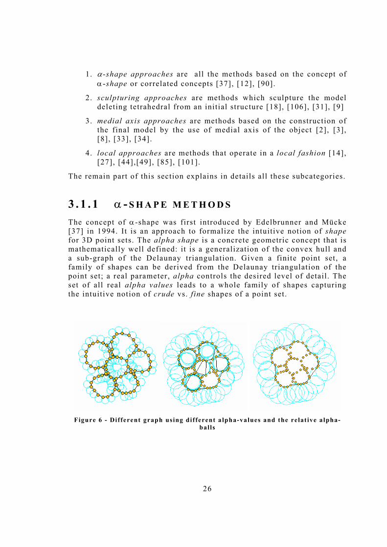
1. α-shape approaches are all the methods based on the concept of α-shape or correlated concepts [37], [12], [90].

2. sculpturing approaches are methods which sculpture the model deleting tetrahedral from an initial structure [18], [106], [31], [9]

3. medial axis approaches are methods based on the construction of the final model by the use of medial axis of the object [2], [3], [8], [33], [34].

4. local approaches are methods that operate in a local fashion [14], [27], [44],[49], [85], [101].

The remain part of this section explains in details all these subcategories.

3 . 1 . 1 α - S H A P E M E T H O D S The concept of α-shape was first introduced by Edelbrunner and Mücke [37] in 1994. It is an approach to formalize the intuitive notion of shape for 3D point sets. The alpha shape is a concrete geometric concept that is mathematically well defined: it is a generalization of the convex hull and a sub-graph of the Delaunay triangulation. Given a finite point set, a family of shapes can be derived from the Delaunay triangulation of the point set; a real parameter, alpha controls the desired level of detail. The set of all real alpha values leads to a whole family of shapes capturing the intuitive notion of crude vs. fine shapes of a point set.

Figure 6 - Different graph using different a lpha-values and the relat ive a lpha-

balls

27

For a given point set S⊂ℜd and 0≤α≤∞ , the α-complex Cα of S is a simplicial subcomplex of the Delaunay triangulation of S DT(S). Consider a simplex ∆T in DT(S): let be σT and µT the radius and the center of the circumsphere of ∆T respectively.

Given a certain α , ∆T in DT(S)is in Cα if

- σT<α and the σT-ball located at µT is empty (no points of S fall in its interior), or

- ∆T is a face of another simplex already in Cα .

The algorithm to obtain the alpha-shape Sα given an α is the following.

1. Compute the Delaunay triangulation of S , DT(S).

2. Determine Cα by inspecting all simplexes ∆T in DT(S): If the σT-ball around µT is empty and σT<α ( the alpha test) ∆T as a member of Cα , together with all i ts faces.

3. All d-simplexes of Cα make up the interior of Sα . All simplexes on the ∂Cα form boundary ∂Sα .

The main difficulty of this approach is, obviously, to find a suitable α-value: if i t is too small, holes and gaps can occur where not needed and if it is too big, cavities may not be preserved (Figure 7). Additionally, when the sampling density is variable, there might exist no α-value that provides a good reconstruction.

Figure 7 A model reconstructed using different ALPHA-values .

28

Moreover there are several problems with using α-shape, first because they were thought for reconstruction of a smooth surface. For example, in object with holes or sharp corners, the α-shape-based techniques may require quite some experimentation to find a α-value that produces the appropriate surface.

This method is quite old but it posed the basis for many other methods that try to improve it in performances and results.

An interesting tentative to improve the standard α-shape method in efficiency is the approach presented by Bajaj et al.[12] in 1996. The first part of an entire proposed reconstruction pipeline is based on the α-shapes concept, and the approach is capable of automatically selecting a α-value and improving the resulting mesh in areas of insufficient sampling.

First , the process extracts a triangle mesh from the data points; then decimates the mesh, while keeping the approximation error bounded. Finally, i t fi ts surface patches of degree three to the reduced mesh. Sharp edges, curvilinear creases and corners are automatically detected and reproduced in the final surface. The first phase of the pipeline can be summarized as follow:

• Compute the 3D Delaunay Triangulation of the points set

• Extract a connected subset of tetrahedra whose union (α-solid) represents the volume of the reconstructed object. The extraction of the α-solid is made up inferring if a tetrahedron is internal or external to the object.

o Start from one tetrahedron with a vertex at infinity marked as exterior ,

o Visit all adjacent tetrahedra, without crossing faces that belong to the α-shape (with an α-value set).

o Mark all reachable tetrahdra as exterior .

o Consider the marked tetrahedra set boundary.

! If it is not empty, one or more continuous shells of triangles form it.

o Start another search from all unmarked tetrahedra with faces on the boundary just computed.

29

o Mark as internal all tetrahedra that can be reached without traversing the α-shape faces.

o Repeat this procedure until all tetrahedra have been marked.

• Set to the α-solid Sα of S the union of all interior tetrahedra . The α-solid is a homogeneously three-dimensional object that can be computed from the underlying triangulation by traversing the adjacency graph [5].

A finite collection of different α-solids can be obtained, by varying α from the empty set to the convex hull of the point set (analogously to the α-shapes family). The tricky part is to choose the smallest α-value such that the relative α-solid is connected , all the data points are on its boundary or in its interior and its boundary is a two-manifold.

The algorithm always converges to a solution because the convex hull satisfies the searched requirements. Moreover, i t is proven that, if the sampling is sufficiently dense and uniform, it produces a good approximation of the object shape. In some cases, there could be some tetrahedra occluding small concave features: if they exist, some of the sampled points may lie inside the α -solid. So, the algorithm applies a particular sculpturing operation that removes:

1. All the tetrahedra that have a face on the boundary and the opposite vertex internal, or

2. Those tetrahedra that have two faces on the boundary and that satisfy the local smoothness criterion.

This criterion basically evaluates the dihedral angle formed by the two boundary faces and the sum (let us say Γ) of the dihedral angles formed by all adjacent boundary faces. Then it compute the sum (let us say ∆) of the dihedral angles formed by all boundary faces adjacent to the two faces of the tetrahedron that will become boundary after the removal operation. If Γ is bigger than ∆ the tetrahedron has to be removed because the local smoothness improves.

The second phase of the algorithm is basically the computation of a reduced polygonal mesh, which represents the data at the desired level of accuracy. This is performed by a vertex deletion scheme and is based on accumulated error bounds propagated from the original surface mesh through the successive reduced meshes. In the final step of the algorithm, the data are fitted with polygonal patches.

30

For each triangle of the reduced mesh, a surface patch is computed which interpolates its vertices and estimated vertex normals with the desired continuity conditions. This approach is able to produce good results in cases of complex objects and it is quite good from a complexity point of view.

Figure 8 - Some steps of the algorithm in [12]� among which there are the init ia l

Points Cloud (up-left) the f inal model (down-right)

In (1998), Teichmann and Capps [90] proposed an algorithm that tries to overcome the original limitations of α-shapes and allows reconstruction from a larger class of input point sets. Their approach introduces two extensions to the definition of α-shape:

1. Anisotropic Scaling : that allows the forbidden region to vary in shape and changes the triangulation accordingly.

2. Density Scaling: that varies the value of α depending on the local point density.

In the case of anisotropic scaling the existence of normals associated to the sampled points is assumed; if this information is not available it can

31

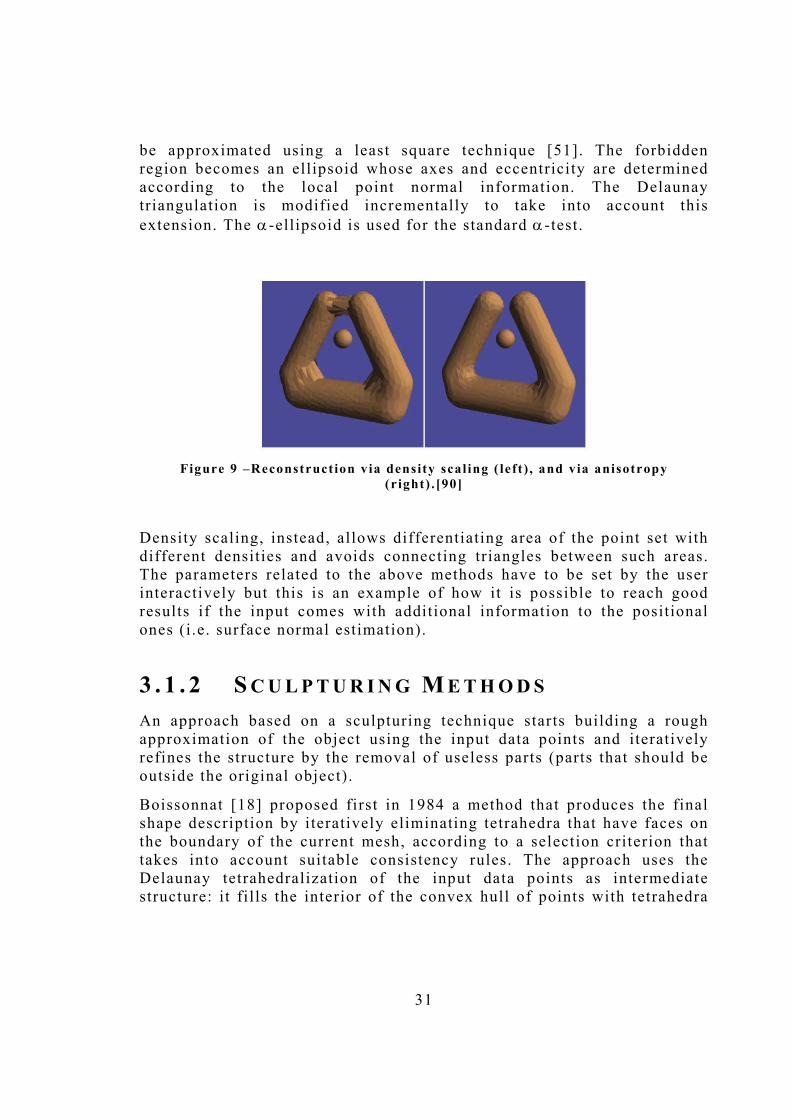
be approximated using a least square technique [51]. The forbidden region becomes an ellipsoid whose axes and eccentricity are determined according to the local point normal information. The Delaunay triangulation is modified incrementally to take into account this extension. The α-ellipsoid is used for the standard α-test .

Figure 9 �Reconstruct ion via density scal ing ( left ) , and via anisotropy

(r ight) . [90]

Density scaling, instead, allows differentiating area of the point set with different densities and avoids connecting triangles between such areas. The parameters related to the above methods have to be set by the user interactively but this is an example of how it is possible to reach good results if the input comes with additional information to the positional ones (i .e. surface normal estimation).

3 . 1 . 2 S C U L P T U R I N G M E T H O D S An approach based on a sculpturing technique starts building a rough approximation of the object using the input data points and iteratively refines the structure by the removal of useless parts (parts that should be outside the original object).

Boissonnat [18] proposed first in 1984 a method that produces the final shape description by iteratively eliminating tetrahedra that have faces on the boundary of the current mesh, according to a selection criterion that takes into account suitable consistency rules. The approach uses the Delaunay tetrahedralization of the input data points as intermediate structure: it fi lls the interior of the convex hull of points with tetrahedra

32

and then, if all the given points lie on the convex hull, provides a volumetric polyhedral representation of the object. Otherwise, Boissonnat proposed to eliminate tetrahedra until all the points are on the boundary of the resulting polyhedral shape or if the deletion of a tetrahedron does not improve the sum over certain decision values of all tetrahedra incident to the boundary of the polyhedron.

The sculpture step can be performed eliminating each time one tetrahedron: the removal is done in such a way that at every step, the boundary of the active shape does not violate the definition of polyhedron.

Basically, Boissonnat used the following criteria:

• Every tetrahedron with exactly three vertices on the boundary can be eliminated;

• Every tetrahedron with exactly five edges on the boundary can be eliminated;

• And every tetrahedron not satisfying the previous two rules cannot be eliminated.

Figure 10 - A model reconstructed using the Method in [18]

33

The main drawback of the Boissonnat algorithm is that the sculpturing process can stop before all the innermost vertices have been included into the boundary on the representation. Moreover it cannot reconstruct objects with holes and it is ambiguous in the sense that the result strongly depends on the order used for the tetrahedra elimination. But it has been the starting point for a lot of other interesting reconstruction approaches.

It is the case, for example, of the sculpturing approach proposed by Veltkamp (1992) in [106]. The algorithm uses a value called γ-indicator, associated to a sphere passing through three boundary points of a polyhedron which is positive or negative (see for an illustration of the 2D-case).

Its absolute value is computed as Rr

−1 , where r is the circle for the

boundary triangle and R the radius of the boundary tetrahedron. It is taken to be negative if the center of the sphere is on the inner side and positive if the center is on the outer side of the polyhedron. Note, that the γ-indicator is independent of the size of the boundary triangle (tetrahedron, respectively). Therefore, i t adapts to areas of changing point density. A removable face is a face with positive γ-indicator value.

Figure 11 �The γ - indicator in the 2D case

By the use of this concept, Veltkamp defines all the removable faces be faces with a positive γ-indicator. The proposed algorithm can be summarized as follows:

34

• Compute the Delaunay tetrahedralization of the given scattered data points.

• Store in a heap all the removable tetrahedra, sorted according to their γ-indicator values.

o A tetrahedron is removable or it is not, with respect to the same criteria Boissonnat uses.

• After having sorted and updated the heap, remove the tetrahedron with largest γ-indicator

• Update the boundary.

• Exit if all input points lie on the boundary or the heap is empty (no other removable tetrahedra should exist).

The main advantage of this approach is that the γ-indicator is considered variable in relation to the dataset density. Unfortunately, as in the previous case this method is still restricted to object without holes (i.e. genus zero).

Figure 12 - some steps of the reconstruct ion process in [106]

35

In 1998, De Floriani, Magillo, Puppo proposed an algorithm [31] and improved it in 2000 [32] that applies a sculpturing approach and can reconstruct objects with genus greater than zero. The algorithm has the following main steps:

• Read a set of scattered points in 3D space

• Build the Delaunay Tetrahedralization (DT) on them and perform mesh updates on the DT:

o Perform sculpturing operations through a sequence of α-tools triggered by the decreasing sequence l1 � lk of radius lengths of the circles inscribed in all triangles of the Delaunay tetrahedralization;

! Maintain a priority queue containing all the tetrahedra having at least one face on the boundary of the mesh, according to their corresponding α-values.

! Applies the l i - tool until the first tetrahedron in the queue has a α-value smaller than l i ,

! Iterate the process to a smaller l i +1-tool.

• Stop when there are no more tetrahedra to be removed or all the points lie on the boundary.

The application of an l i tool is basically the following:

• Given a tetrahedron t with an α-value larger or equal to l i ,

o If the deletion of t leaves the mesh valid: remove it .

o If the removal of t either disconnects the mesh or leaves some data points outside it: do not remove t , and delete it from the priority queue;

o If the removal of t introduces a non-manifold situation:

! try performing further sculpturing around the non-manifold edge or vertex, in the attempt of recovering validity.

• In case of success: a valid genus-varying update is performed that removes t together with some other tetrahedra;

• In case of failure for an unrecoverable violation of validity do not remove t but eliminate it from the priority queue;

36

• In case of failure because the α-tool is to big: do not remove immediately t , but change its α-value to the larger value among those that blocked the procedure.

The set of tetrahedra removed at each step defines the necessary mesh update : a sculpturing operation that removes, from a connected tetrahedral mesh T , a connected set of tetrahedra, T' .

T' must have at least one face on the external boundary of T and the tetrahedral mesh, resulting subtracting T' to T , have to be stil l connected. This is the main innovation with respect to the standard sculpturing method proposed by Boissonnat. While, at each step, only one tetrahedron is removed in [18], in [31], [32] more tetrahedra can be removed simultaneously, allowing genus-changing updates.

Figure 13 - A select ively sculptured mesh with ful l detai l at a box focus ( left) , na intermediate step (middle) and the f inal reconstructed chair (r ight) ( taken from

[32])

Another interesting approach is the one presented by Attene and Spagnuolo [9] in 2000. The method is based on sculpturing and on the use of some proprieties of geometric graphs. During the sculpturing operation, i t considers the Euclidean Minimum Spanning Tree (EMST) together with a geometric graph called the Extended Gabriel Hypergraph (EGH) as constraints.

As all the other sculpturing approaches, the algorithm starts building the Delaunay tetrahedralization DT of the initial dataset and iteratively removes tetrahedra until all vertices lie on the boundary. The main innovation is that the removal process is constrained to the EMST and to

37

the EGH. In particular, a tetrahedron T is considered removable (with constraints) if: (i) the basic sculpturing rules (the same as Boissonnat uses) are valid, (ii) in the case in which T has a unique face on the boundary, and this face does not belong to the EGH, (i i i) if T has two faces on the boundary, and they are not in the EGH and the common edge must not belong to the EMST.

When the process stops, the reconstructed surface is returned as output. The algorithm can be sketched as follow:

1. Read the input points and construct the relative initial DT and build the EMST and the EGH

2. Construct a heap H containing all removable (constraints on) tetrahedra sorted by longest boundary edge.

3. While the number of vertices on the boundary is less than the number of input vertices and the heap is not empty,

o Take the tetrahedron T in the heap root, remove it from the heap and if T is removable (with constraints) remove it also from the DT

o Insert all new removable (with constraints) tetrahedra into the heap.

o Repeat the removal operations considering the tetrahedra removable only with the basic sculpturing rules (constraints off).

4. Search for holes in the object.

o If the number of EMST edges on the boundary is less than the number of EMST vertices, fill the heap with those removable (constraints off) tetrahedra whose removal adds an EMST edge to the boundary.

o While the number of EMST edges on the boundary is less than the number of EMST vertices, perform remove operations (constraints off).

o If an edge e exists in the EMST graph that does not belong to the boundary and it is possible to create a hole according to e , create the hole put the constraints on and repeats the removal loop.

38

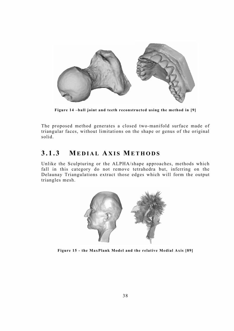
Figure 14 �ball jo int and teeth reconstructed using the method in [9]

The proposed method generates a closed two-manifold surface made of triangular faces, without limitations on the shape or genus of the original solid.

3 . 1 . 3 M E D I A L A X I S M E T H O D S Unlike the Sculpturing or the ALPHA/shape approaches, methods which fall in this category do not remove tetrahedra but, inferring on the Delaunay Triangulations extract those edges which will form the output triangles mesh.

Figure 15 - the MaxPlank Model and the relat ive Medial Axis [89]

39

It is the case of a series of works on surface reconstruction, starting from the object medial axis among which the methods of Amenta et al. are the most representative [2],[3] (but various other works have been published which follow the same ideas, see for example [43], [89], [88]).

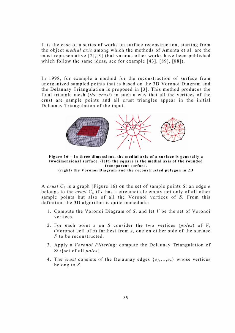
In 1998, for example a method for the reconstruction of surface from unorganized sampled points that is based on the 3D Voronoi Diagram and the Delaunay Triangulation is proposed in [3]. This method produces the final triangle mesh (the crust) in such a way that all the vertices of the crust are sample points and all crust triangles appear in the initial Delaunay Triangulation of the input.

Figure 16 � In three dimensions, the medial axis of a surface is general ly a twodimensional surface. ( left ) the square is the medial axis of the rounded

transparent surface. (r ight) the Voronoi Diagram and the reconstructed polygon in 2D

A crust CS is a graph (Figure 16) on the set of sample points S : an edge e belongs to the crust CS if e has a circumcircle empty not only of all other sample points but also of all the Voronoi vertices of S . From this definition the 3D algorithm is quite immediate:

1. Compute the Voronoi Diagram of S , and let V be the set of Voronoi vertices.

2. For each point s on S consider the two vertices (poles) of Vs (Voronoi cell of s) farthest from s , one on either side of the surface F to be reconstructed.

3. Apply a Voronoi Filtering: compute the Delaunay Triangulation of S∪{set of all poles}

4. The crust consists of the Delaunay edges {e1 ,�,en} whose vertices belong to S .

40

5. Apply Normal Filtering. In order to produce a piecewise-linear homeomorphic to F (see below).

6. Extract a manifold taking the outside surface of the remaining triangles on each connected component.

The normal filtering step is necessary because the crust is not always a manifold: it often contains four triangles of a very flat �sliver� tetrahedron. It throws away any triangles whose normals differ too much from the two vector connecting s to its poles . This simple approach cannot be applied when F is not smooth enough manifold without boundary. In that case the algorithm is not proven to be exact.

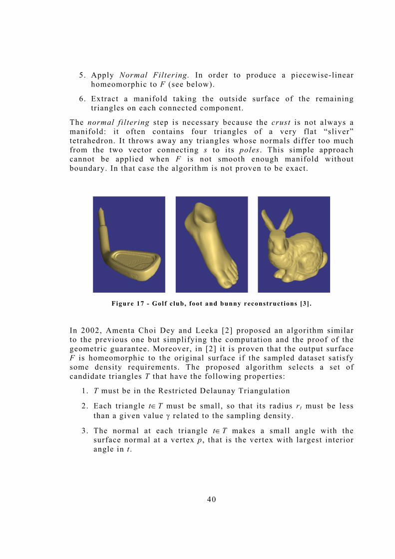
Figure 17 - Golf c lub, foot and bunny reconstruct ions [3] .

In 2002, Amenta Choi Dey and Leeka [2] proposed an algorithm similar to the previous one but simplifying the computation and the proof of the geometric guarantee. Moreover, in [2] i t is proven that the output surface F is homeomorphic to the original surface if the sampled dataset satisfy some density requirements. The proposed algorithm selects a set of candidate triangles T that have the following properties:

1. T must be in the Restricted Delaunay Triangulation

2. Each triangle t∈T must be small, so that i ts radius rt must be less than a given value γ related to the sampling density.

3. The normal at each triangle t∈T makes a small angle with the surface normal at a vertex p , that is the vertex with largest interior angle in t .

41

The selection of the candidate triangles set T uses the co-cone (Figure 18) relative to each sample point p and then extracts (at least in theory) a piecewise linear manifold from T . For an angle θ , the co-cone at a sample point p is defined to be the complement of the double cone with apex p making an angle of π/2-θ with the estimated normal line in p . The estimated normal line of a point p is the line that passes through p and its pole (the farthest point from p in its Voronoi cell).

Figure 18 - Co-cone in 2D and 3D

So the scheme of the algorithm is the following:

1. Compute the Delaunay Triangulation DT of the sample point set P and the Voronoi vertices dual to every tetrahedron.

2. ∀p∈P , find the pole v (the vector pv is the estimated normal of the surface in p) .

3. Consider an edge e in the Voronoi cell Vp , with its two endpoints w1 ,w2 .

o If the range of angles determined by the angle ∠vw1 and ∠vw2 intersects the range [π/2-θ , π/2+θ], the edge e is marked ok .

4. All those Delaunay triangles t dual to an edge e that has been marked ok by all i ts adjacent Voronoi cells are included as candidate triangles in T .

5. Apply a manifold extraction:

o Remove all those triangles incident to sharp edges (an edge e is defined sharp if the angle between any two consecutive

42

triangles around it is more than 3π/2 or if e has only one incident triangle).

o Extract the outer boundary of the set of triangles by applying a depth-first-walk along the outer boundary of each of its connected components.

For those input sets that do not satisfy the sampling conditions the authors use ad hoc heuristics in order to find an acceptable solution. The theoretical guarantee provided by the above algorithms [3][2] requires the sampled surfaces be smooth and have empty boundary. These algorithms may have serious problems if these conditions are not met.

In cases of surfaces with non-empty boundaries, an alternative approach is the one presented by Dey, Giesen, Leekha, and Wenger in [34]: it uses the co-cone approach for the reconstruction step and, for sufficiently dense samples, i t identifies all interior vertices. The boundary detection step (Figure 19) is invoked in the Co-cone algorithm and the Co-cone pruning step does not attempt to delete any triangle adjacent to a detected boundary vertex.

Figure 19 � the cat model without boundary detect ion ( left) and with boundary

detect ion (right) [34]

The definition of a vertex to be interior or boundary lies in the definition of f lat vertex that they give. A sampled point p is defined to be a flat vertex if the relative Voronoi cell Vp is long and thin in the direction of the pole vectors. They proved that, if the sampled point set P has certain

43

sampling properties, all the interior vertices are flat . Thus the definition of boundary vertex is straightforward: a vertex is boundary if i t is not flat

One side effect of the presented algorithm is that i t identifies the regions of undersampling . That is the case of the work in [33] that basically applies the same algorithm focusing the attention on the search of regions of undersampling. Using the definition of f lat vertices and the modified co-cone algorithm, Dey and Geisen first define the surface patches that are well sampled with the given samples. The boundaries of these surface patches identify the regions where dense sampling stops and undersampling begins.

Another interesting work, especially from a theoretical point of view, is the one of Attali [8] (1997), in which a precise formulation of the reconstruction problem is proposed. The solution is mathematically defined as a particular mesh called the normalized mesh. This solution has the property to be included inside the Delaunay Graph. Moreover a criterion to select boundary faces inside the Delaunay graph is proposed and it is proven to provide the exact solution in 2D with input a dataset that follows certain sampling conditions. Unfortunately, in 3D, this result cannot be extended and the criterion is not able to retrieve every necessary faces. For this reason the algorithm chooses ad hoc heuristics in order to complete the surface reconstruction phase.

The algorithm works as follows: given a set of points E on a surface S , E is a sampling path ε for S if any sphere with radius ε and center in S contains at least one sample point of E . The normalized mesh (the one that represents the object surface) starting from the sampled points E is the set of cells (segments in 2D and triangles in 3D) for which there exist a point m∈S such that

d(m ,cell1) = d(m , cell2) = � = d(m , E).

By definition, the normalized mesh is part of the Delaunay Diagram of E . The problem of reconstructing a mesh representing the object surface can be expressed in searching the normalized mesh of the points set E . In order to simplify the search of the normalized mesh Attali assumes that the shape S is an r-regular shape . It means that it is morphologically open and closed with respect to a disk of radius r>0.

An interesting characteristic of the 2D r-regular shape is that any circle passing through three distinct boundary points has radius greater than r and this property will be fundamental form the validity proof of the

44

algorithm. Unfortunately, the equivalent is not true for the 3D case. Inferring on angles formed by the Delaunay spheres (those spheres circumscribed to a Delaunay simplex), Attali proves that, in 2D, if ε< sin(π/8.r) is the set of edges for which the relative angles are less than π/2, it is the normalized mesh of S associated to E .

The beauty of the result is that there is no need to know the two parameters r and ε in order to compute the normalized mesh and the sampling path has no need to be close to zero in order to find the correct result . Unfortunately in 3D it may happen that some Delaunay spheres intersect the boundary without being tangent to it and, for this reasons, i t is impossible to minorate the radius of the spheres. So, at the end of the reconstruction process, some triangles may be missing and the surface can have holes depending on the sampling density. The surface needs to be closed adopting an ad hoc heuristic.

This method was the basis for other research of the same author together with other researchers: see for example [6] or [7] where the idea of Skeleton extraction was combined with methods, which improve the robustness.

Figure 20 � the skeleton (middle) the s implif ied skeleton by [6] (r ight) and the

reconstructed surface ( left)

3 . 1 . 4 L O C A L A P P R O A C H E S Reconstruction approaches in this class start with a seed and incrementally make it grow until the solution covers all the input data. The seed may be a triangle, an edge, a first range image or a wire frame approximation.

The paper of Soucy and Laurendau [85] in 1995, presents a general solution to the problem of reconstruction using a local approach. It tries

45

to integrate multiple range views computing a final connected surface model. It has been used in different modeling software packages, especially in the one of the InnovMetric Corporation called PolyWorks.

The method operates a re-parameterization of the input range images in order to reconstruct portions of surface representing, altogether, the entire object. It uses the concept of canonical subsets (called CS) of the Venn diagram formed by the input range images. A CS of K-range views is the set containing all points present in the K-range views AND not present in all the other range views.

Figure 21 - the exist ing CSs in case of three range images.

By modeling distinctly all the CS s of the Venn diagram, it is possible to obtain surface portions describing entirely the input object, with no overlapping parts between them. But this could be a problem in modeling the near-CSs border zones. For this reason, the method introduces the RCS subsets (redundant canonical subsets).

Let N be the number of input range images, and SV={V1, V2 ,�,VN} the set of all the input range images. All the input data are subdivided in RCS groups. Given a range images subset S j={V j 1 , V j 2 ,�, V j K}, with K<N an RCS associated to S j is defined to be a set containing all points common to the range view in S j .

Figure 22 - RCS sets start ing from V1, V2 and V3.

46

In this way, it is possible to model also the CSs border zones because same surface portions can be considered multiple times. A successive phase can discard the surface parts common to multiple RCSs. The algorithm examines all the range views starting from the intersection of all of them (K=N) until K=1. A point is common to different views if i t passes two tests:

• Spatial proximity test: which verifies if the point on a range view is sufficiently near to another range view;

• Surface visibility test: which verifies if a point on a range view is visible to another (i .e. the surface normals are quite similar oriented).

Each RCS subset is re-parameterized on a grid with normal vector the one obtained as weighted sum of the normal vectors of all the active range views.

1. At the beginning (K=N) the algorithm generates a surface.

2. At the next step (K=N-1),

o if the algorithm finds out a surface portion already taken into account, i t discards this portion (it has been reconstructed considering a greater number of multiple range views in a previous step).

3. At the end of the operation (K=1), thanks to the deletion of parts already examined, the algorithm obtains surface portions representing canonical subsets (not redundant).

Each CS represents all those points belonging to the intersection of K range views and belonging to no other range views. Thus the computed meshes cover the entire object and have no overlapping zones. The next step of the algorithm merges all the meshes by a Delaunay Triangulation.

The proposed method does not impose constraints on the topology of the observed surfaces, the position of the viewpoints, or the number of views that can be merged but it is assumed that accurate range views are available and that frame transformations between all pairs of views can be reliably computed. Unfortunately, constructing the Venn diagram is combinatorial in nature, thus computational intensive.

Another algorithm of this class is the one presented by Turk and Levoy in [101](1994). It is an incremental algorithm and as the one presented in

47

[85] works with multiple acquired range images and uses an integration technique coupled with geometric averaging to combine redundant data in the regions of overlap.

Both methods result in a local smoothing operation of data in correspondence of regions of redundancy. The main difference is in the order in which they perform the operations. Turk and Levoy [101] first stitch together two meshes at a time, trying to remove redundant parts in overlapping regions. Then, they use the vertices of the removed polygons to form a consensus of the surface shape in the regions of redundancy by moving the vertices of the final mesh. Instead, Soucy and Laurendeau [85] first combine redundant information in order to form a point set that is successively considered for stitching.

Going in details, the volumetric algorithm of Turk and Levoy acts in two steps: the one of creating a mesh reflecting the topology of the scanned object and the one relative to the vertex positions refinement by averaging the geometric details present in all scans. The main steps of the method can be summarized as follow:

• For each range images compute the triangle mesh: a triplet of points becomes a triangle in the final mesh if the edge lengths are below a given threshold.

• Align the mesh of triangles with each other using a modified iterated closest-point algorithm. The algorithm allows a user to align one range image with another on-screen. The traditional iterative closest point algorithm cannot be applied in this case because the point of one range images usually are not a subset of the points of the other.

o Given two meshes A and B , the modified ICP finds the nearest position on mesh A to each vertex on mesh B ;

o It discards pairs of point that are too far apart;

o It eliminates pairs in which either point is on the mesh boundary.

o It finds the rigid transformation that minimizes a weighted least-squared distance between the pairs of points and iterates this until convergence.

o Finally it performs the ICP on a more detailed mesh in the hierarchy.

48

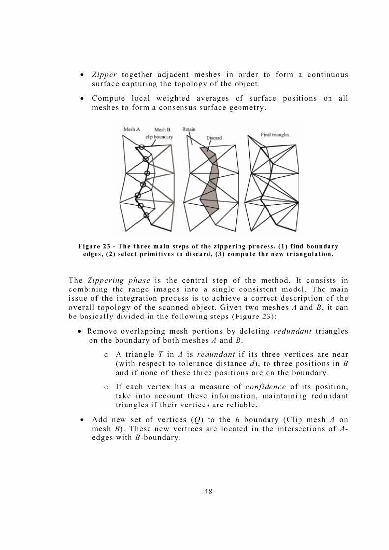
• Zipper together adjacent meshes in order to form a continuous surface capturing the topology of the object.

• Compute local weighted averages of surface positions on all meshes to form a consensus surface geometry.

Figure 23 - The three main steps of the zippering process. (1) f ind boundary

edges, (2) select primitives to discard, (3) compute the new triangulat ion.

The Zippering phase is the central step of the method. It consists in combining the range images into a single consistent model. The main issue of the integration process is to achieve a correct description of the overall topology of the scanned object. Given two meshes A and B , i t can be basically divided in the following steps (Figure 23):

• Remove overlapping mesh portions by deleting redundant triangles on the boundary of both meshes A and B .

o A triangle T in A is redundant if i ts three vertices are near (with respect to tolerance distance d), to three positions in B and if none of these three positions are on the boundary.

o If each vertex has a measure of confidence of its position, take into account these information, maintaining redundant triangles if their vertices are reliable.

• Add new set of vertices (Q) to the B boundary (Clip mesh A on mesh B). These new vertices are located in the intersections of A-edges with B-boundary.

49

• Split the triangles in B in order to incorporate the points of Q on the B-boundary

• Modify A: divide each A-border triangle in two parts:

o the one inside the B-boundary will be leftover;

o the one outside will be re-triangulated using all the vertices in the B-boundary and Q as constraints.

The clipping process may introduce small and thin triangles. The algorithm identifies these triangles (preferring those triangles with points in Q as vertices) and, by the use of a vertex deletion technique, removes them. In the last step of the algorithm, if needed, some characteristics are added for fine-tune the geometry of the mesh.

Figure 24 - an example of the zippering approach in 3D for the construct ion of a

phone ([101]) .

Neither methods [85],[101] deals with holes in the data resulting either from errors in sensor measurement, or from occluded parts. A hole-filling operator may be applied in a post-processing.

The idea of stitching surfaces together used by Soucy and Laurendau in [85], was of inspiration for the local approach developed by Heckel, Uva, Hamann and Joy in [49]. Like the methods in [27][14] this work uses a set of scattered points as input and reconstructs a triangulated surface model. It can be summarized in a two-step procedure:

50

1. Apply an adaptive clustering method [62] in order to produce a set of t i les (almost flat shapes), which locally approximate the unknown surface.

a. Each tile is associated to a cluster representative (a height field with respect to the best-fit plane defined by the tile).

2. Triangulate gaps between tiles by the use of a constrained Delaunay triangulation. This produces a valid geometrical and topological model.

The method computes distance estimate for each cluster which helps in the evaluation of the global error measurement. In the generation of tiles, the algorithm utilizes Principal Component Analysis (PCA) determining clusters of points that are nearly coplanar. In this way, each tile is computed starting from the boundary polygon of the convex hull of a set of points that have been projected into the best-fit plane.

Starting from a single cluster, an hierarchical clustering approach is used in order to slit i t if the error is too large. When this process stops, the obtained set of clusters partit ions the original data and all clusters satisfy a coplanarity condition.

Unfortunately this splitting process can fail to orient clusters correctly if the density of the surface samples is not sufficient. See, for example the case in which two different components of a surface are separated by a small distance: the algorithm will produce an unique cluster including points of both components, generating an incorrect triangulation.

While the process goes through, a connectivity graph, relating the boundary polygons of all clusters is computed and maintained. This graph will be used in order to generate a triangulation of the space between tiles. The method seems to be interesting if the density sampling varies according to the topological features of the scanned object. In fact, the algorithm can be able to build big clusters in case of �flat regions� and small clusters in proximity of �sharp features�.

In 1997, Hilton and Illingworth [50] proposed a method which is basically a local computational geometry approach. The algorithm takes as input a set of range images and returns, as always, a triangle mesh. Each triangle is constructed on the basis of the local information on surface topology. It i teratively creates new triangles from a list of

51

boundary edges, initialized with the three edges of a seed triangle, so that the growing mesh should eventually cover the entire implicit surface.

The marching triangles method relies on a prediction-correction step to compute new mesh vertices on the implicit surface. Although prediction correction methods work well for contours, difficulties arise when applied to surface, so this algorithm may fail at generating closed meshes for general implicit surfaces.

Starting from a set of points in 3D X={x0, �, xn} Hilton et al. use the property proven by Boissonnat [18] in order to model their method: Whenever the set of points X l ie on a manifold surface, the Delaunay triangulation is composed of triangles T such that there exists a sphere passing through the vertices of T that does not contain any other point of the set X .

(a) (b)

Figure 25 � the Marching Triangle step during the triangle creat ion and the verif icat ion of constraints [50]

Starting from a seed triangle on the implicit surface, the marching triangles algorithm iteratively find new triangles modeling the surface attaching them to the active boundary edges of the already triangulated surface in such a way that the Delaunay Property always holds.

During the computation, each triangle T has its relative normal nT and the associated circumcenter cT. At each step of the process the Triangle creation constraint must be satisfied:

52

• A triangle T(xk,xk+ 1,xp) can be added to the mesh boundary at edge e(xk,xk +1) if no other existing triangle intersects the sphere centered at cT circumscribing the triangle T(xk,xk +1,xp) with the same orientation (Figure 25-a). The orientation criterion of the triangle generation constraint allows the polygonization of implicit surfaces that exhibit thin folding sections (Figure 25-b)

In cases of triangulation of general implicit surface manifolds the algorithm keeps track of a list of boundary edges Le , which is initialized with the edges of the seed triangle. At each step, new triangles are tentatively created from candidate edges of the list Le . The overall algorithm may be written as follows iteratively analyzing each edge e(xk, xk +1) in the list:

1. From Le , i teratively create new triangles until no more triangles may be computed or unti l the list is empty.

• Create a new vertex x in the plane of the triangle T(xi ,xk xk +1) that contains the edge e(xk, xk + 1), This point will be used as a first guess in the computation of the surface vertex xp .

• Create a new surface vertex xp by projecting x onto the implicit surface following the gradient of the field function vf .

• Apply the Delaunay surface constraint to the new triangle T(xp,xk xk+1) and proceed as follows:

o If T(xp, xk, xk+ 1) passes the constraint, then add the triangle to the mesh and stack the edges e(xp,xk) and e(xp,xk +1) to the list of edges Le that need to be processed.

o If i t does not pass the constraint, check if one of the triangles T(xk - 1,xk,xk + 1) passes them, and modify the mesh accordingly if needed.

o Otherwise step over from the edge e(xk,xk+ 1).

2. Close the cracks that may appear in the polygonization.

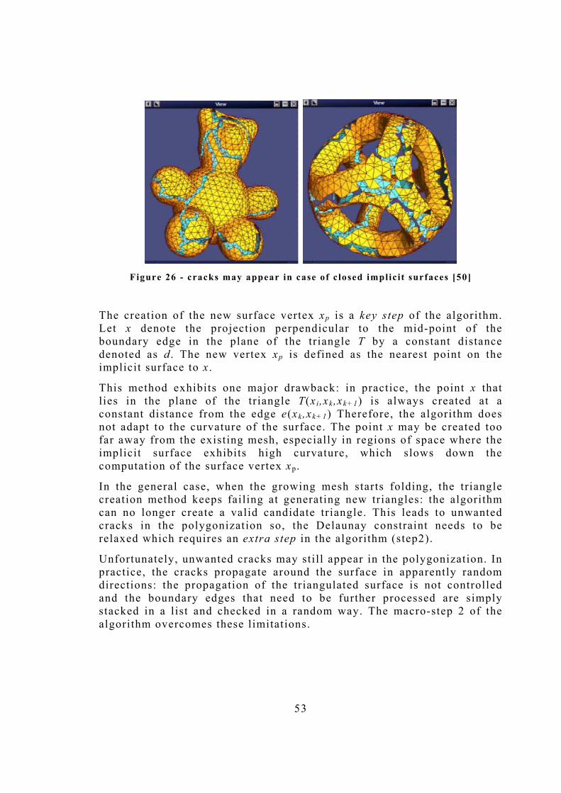
53

Figure 26 - cracks may appear in case of c losed implicit surfaces [50]

The creation of the new surface vertex xp is a key step of the algorithm. Let x denote the projection perpendicular to the mid-point of the boundary edge in the plane of the triangle T by a constant distance denoted as d . The new vertex xp is defined as the nearest point on the implicit surface to x .

This method exhibits one major drawback: in practice, the point x that lies in the plane of the triangle T(xi,xk,xk +1) is always created at a constant distance from the edge e(xk,xk+ 1) Therefore, the algorithm does not adapt to the curvature of the surface. The point x may be created too far away from the existing mesh, especially in regions of space where the implicit surface exhibits high curvature, which slows down the computation of the surface vertex xp.

In the general case, when the growing mesh starts folding, the triangle creation method keeps failing at generating new triangles: the algorithm can no longer create a valid candidate tr iangle. This leads to unwanted cracks in the polygonization so, the Delaunay constraint needs to be relaxed which requires an extra step in the algorithm (step2).

Unfortunately, unwanted cracks may still appear in the polygonization. In practice, the cracks propagate around the surface in apparently random directions: the propagation of the triangulated surface is not controlled and the boundary edges that need to be further processed are simply stacked in a list and checked in a random way. The macro-step 2 of the algorithm overcomes these limitations.

54

Differing from the above methods, which start from multiple range images the local approach presented in 1999 by Bernardini et al. starts from a set of unorganized point (together with the estimated normal on each point) [14]. It is the Ball-Pivoting Algorithm (BPA for short) and computes a triangle mesh following an advancing-front paradigm.

The method uses a ball radius ρ and locates three data points such that a ρ- ball touches them and do not contain other input data points. The triangle formed by these three vertices is called a seed triangle .

• Find a valid seed triangle:

o Pick an unused point σ and consider all pairs of points σa, σb in its neighborhood in order of distance from σ .

o Build σ , σa , σb as a potential seed checking that the triangle normal is pointing outward.

o Test that a ρ-ball with center in the outward half space touches all three vertices and contains no other points.

o Stop when a valid seed if found.

• Iteratively perform the ball pivot operation in order to find new triangles to be added to the mesh

o Keeping a ρ-ball in contact with two of the points in the active boundary, until i t touches another sampled point (Figure 27).

o Any time a new triangle is found, the boundary mesh (the active front) is updated and the ball-pivoting operations is performed around each edge of the new active front

• Stop when no other sampled points can be added in the data structure.

The updating of the active front is performed by two main operations:

- The join operation, when the pivot discovers a point σ i not yet used in the algorithm. It is the case in which a new triangle is added to the final mesh and two new edges are added to the active front while the old one is deleted (Figure 27- right). If the point σ i is already part of the mesh and is internal to it , the corresponding triangle cannot be added because of a non-manifold creation problem. The BPA marks the edge relative to the pivot

55

operation as boundary edge and continues in another direction. While, if σ i is belongs to the reconstructed mesh and to the active front, a test of non-manifold situation in adding the new triangle is performed. If the test returns ok the new triangle is added to the mesh.

- The glue operation: the join operation could create pairs of coincident edges with opposite orientation and the glue operation removes them from the active front leaving a new consistent front

Figure 27 - ( left) The bal l pivot ing operat ion, performed looking

at the coordinate system projected on the plane z=0. (Right) The jo in operat ion[14] .

Note that, in presence of noisy data the BPA can reconstruct artifacts such as small triangles sets lying close to the main surface. However, these triangles may be eliminated with a post-processing operation The BPA algorithm output (Figure 28) is a manifold subset of a ρ-shape of the input point set. Problems could arise in correct setting the ρ values but the BPA can be invoked multiple times with different ρ−values in order to improve the results.

Figure 28 - results of the BPA algorithm [14] .

56

An approach similar to the one presented above was proposed by Crossno and Angel [27], the same year. The Spiraling Edge algorithm produces a localized approximation to the surface by creating a star-shaped triangulation between a point and a subset of its nearest neighbors. This surface is successively extended by locally triangulating each of the points along the edge of the patch. The SE algorithm chooses as starting configuration a set of points generated by an isosurface algorithm. For this reason additional information related to the points also are generated: an estimated normal at each point, a list of each point�s neighbours, and a type classification for each point. In particular, type of the point is based on a point�s position relative to the boundaries of the volume data set from which the isosurface is taken.

• Interior points are not touching the volume boundaries

• Boundary points lie on the volume boundaries.

• Corner points lie along the intersections between multiple volume boundaries.

Figure 29 � Spiral ing Edge Algorithm: (Left) . A lobster. (Right) isosurface of an

electron density distribution in crystal l ine s i l icon

The SE algorithm uses the type classification to generate surface edges where the data set boundaries cut the surface so that it is possible to create open surfaces. It is a local approach in the sense that i t works locally to create a nearly planar triangulation between a point and its nearest neighbours. Under the assumptions that, except for boundary

57

points, the surface is closed, there are no non-manifold structures and there is only one point at any particular location, the SE algorithm grows a surface from single point until:

1. the surface encounters boundary points and stops growing in that direction, or

2. the surface fills until the edge ring reduces to a small hole that fi l ls itself in. So, boundary points have a special treatment.

When and edge ring becomes empty, the algorithm finishes a disconnected surface component. If all of the points have been used, the algorithm stops and the triangulation is completed; otherwise, it restarts from a new edge ring with a new point and its nearest neighbours (Figure 29).

Another local algorithm is the one presented by Gopi, Krishnan and Silva in 2000 [44]. Like the method presented above, this algorithm uses an advancing-front triangulation scheme and starts from a set of unorganized sampled points returning a manifold triangular mesh interpolating the input points. But unlike the BPA algorithm, which assumes vertex normal information available, here nothing is assumed about the geometry, topology or presence of boundaries in the dataset except that the input point set is sampled from a real manifold object.

The algorithm incrementally develops the output using the surface oriented proprieties of the input points and goes through four main steps:

1. Normal computation , using the closest neighbour information.

a. The normal vector in p is the vector that minimizes the variance of the dot product between itself and the vectors from p to its k-nearest neighbours (similar to the method presented in [51]).

2. Candidate point selection , choosing for each vertex p possible Delaunay neighbours in the final triangulation. This is done using a sampling criterion for all the possible neighbours.

a. Apply a distance criterion in order to prune down the search in spatial proximity of p .

58

b. Use the euclidean metric in order to accept only points that lie inside a sphere of influence with center in p .

c. Prune again the point set obtained by computing the height values of these points in p local tangent plane.

d. Remove all those points with the relative height value greater than a given threshold θ .

3. Delaunay neighbour computation , using a 2D local Delaunay triangulation around a sampled point p .

a. Map all the candidate points related to p (step 2) on the tangent plane at p by a rotation about an axis on the tangent plane.

b. Compute the Delaunay neighborhood from the mapped set of points around p .

4. Final triangulation considering all the neighbourhood relationships.

This algorithm seems to work well for all the practical models and its implementation is modular and is suitable for parallelization, but unfortunately it has some problems in the individuation of some special cases of holes.

Figure 30 - Some results of the spiral ing edge algorithm [44]

59

3.2 Volumetric Methods Methods, which fall in this category, build the final mesh analyzing the volume that contains the data. There are numerous methods belonging to this category, so an ulterior subdivision is necessary:

• Grid-based approaches, that use a grid to compute the final resulting mesh,

• Approaches which use Radial Basis Functions, and

• Approaches based on Deformable surfaces.

The remain part of this subsection tries to explain in details all these subcategories.

3 . 2 . 1 G R I D - B A S E D A P P R O A C H E S Those reconstruction approaches belonging to this sub-category use a cell discretization of the 3D space in order to reconstruct the desired surface. The used grid has importance also in relation to the resolution of the result and for the complexity of the overall procedure. These algorithms can handle large, unstructured data sets and seems to be robust in presence of noisy input data. Unfortunately, there is not any adaptive resolution. Vertices in output are uniformly distributed, regardless of highly curved or featureless areas of the surface. If one does not want to lose small features this will lead to complex, output meshes.

The first representative grid-based method is the one presented by Hoppe et al in 1992 [51], in 1996 the method of Curless and Levoy followed in [29] which has been used in the great Michelangelo project [59]. Both of them soon became reference points for the Surface Reconstruction approaches in general.

Going into details of each of the mentioned works, the paper of Hoppe et al [51] addresses the issue of reconstructing a surface starting from a set of unorganized points. The algorithm mainly consists of two stages (Figure 31):

1. Construct a signed distance function, which maps a 3D point to an estimated signed distance to the unknown surface. For each point in 3D the value of the signed distance function on it will be its distance from the closest point on the estimated oriented

60

tangent plane, multiplied by ±1 depending on which side of the surface the interesting point l ies:

a. Associate a tangent plane to each input sample point.

b. Orient each tangent plane. If the sampling is dense and the surface is smooth, ensure that for two near points xi,x j , the two associated normals ni ⋅nj are not only almost parallel, but also pointing in approximately the same direction, i .e. ni ⋅nj ≈+1.

c. Build a graph G≡(V ,E) in which each node represents a tangent plane and two nodes are connected by an edge if and only if the corresponding sample points are sufficiently close.

i . To connect different nodes, build a sort of enriched Euclidean Minimum Spanning Tree (EMST).

ii . The orientation is propagated by traversing the EMST with the cost of edge (si,s j) being 1-|ni ⋅nj | (favoring the propagation between samples with almost parallel normals).

2. Extract the zero-set using a modified Marching Cubes algorithm.

a. Visit only cubes that intersect the zero set by pushing onto queue only appropriate neighbors� cubes. In this way the signed distance function is evaluated only at points close to the data

To alleviate the problem of badly shaped triangles, the algorithm collapses small edges in a post-processing step using an aspect ratio criterion, to minimize the product of the edge length times the minimum inscribed radius of its two adjacent faces.

Figure 31 �The reconstructed model by Hoppe et al . (r ight) [51] .

The init ia l points cloud ( left) and the relat ive EMST (middle)

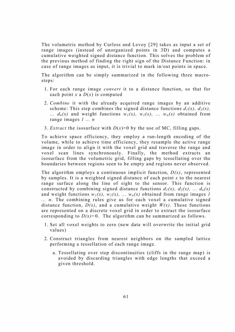
61

The volumetric method by Curless and Levoy [29] takes as input a set of range images (instead of unorganized points in 3D) and computes a cumulative weighted signed distance function. This solves the problem of the previous method of finding the right sign of the Distance Function: in case of range images as input, i t is trivial to mark in/out points in space.

The algorithm can be simply summarized in the following three macro-steps:

1. For each range image convert i t to a distance function, so that for each point x a D(x) is computed

2. Combine it with the already acquired range images by an additive scheme: This step combines the signed distance functions d1(x), d2(x), . . . dn(x) and weight functions w1(x), w2(x), . . . wn(x) obtained from range images 1 .. . n

3. Extract the isosurface with D(x)=0 by the use of MC, filling gaps.

To achieve space efficiency, they employ a run-length encoding of the volume, while to achieve time efficiency, they resample the active range image in order to align it with the voxel grid and traverse the range and voxel scan lines synchronously. Finally, the method extracts an isosurface from the volumetric grid, fi lling gaps by tessellating over the boundaries between regions seen to be empty and regions never observed.

The algorithm employs a continuous implicit function, D(x) , represented by samples. It is a weighted signed distance of each point x to the nearest range surface along the line of sight to the sensor. This function is constructed by combining signed distance functions d1(x), d2(x), . . . dn(x) and weight functions w1(x), w2(x), . . . wn(x) obtained from range images 1 . . . n . The combining rules give us for each voxel a cumulative signed distance function, D(x), and a cumulative weight W(x) . These functions are represented on a discrete voxel grid in order to extract the isosurface corresponding to D(x)=0. The algorithm can be summarized as follows.

1. Set all voxel weights to zero (new data will overwrite the initial grid values)

2. Construct triangles from nearest neighbors on the sampled lattice performing a tessellation of each range image.

a. Tessellating over step discontinuities (cliffs in the range map) is avoided by discarding triangles with edge lengths that exceed a given threshold.

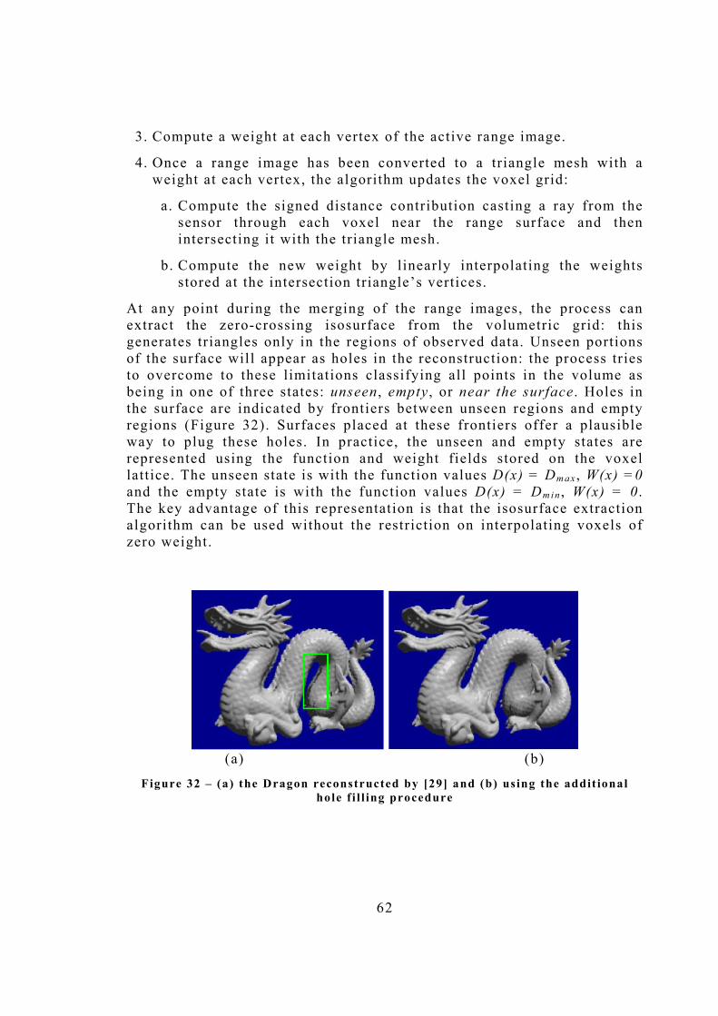
62

3. Compute a weight at each vertex of the active range image.

4. Once a range image has been converted to a triangle mesh with a weight at each vertex, the algorithm updates the voxel grid:

a. Compute the signed distance contribution casting a ray from the sensor through each voxel near the range surface and then intersecting it with the triangle mesh.

b. Compute the new weight by linearly interpolating the weights stored at the intersection triangle�s vertices.

At any point during the merging of the range images, the process can extract the zero-crossing isosurface from the volumetric grid: this generates triangles only in the regions of observed data. Unseen portions of the surface will appear as holes in the reconstruction: the process tries to overcome to these limitations classifying all points in the volume as being in one of three states: unseen , empty , or near the surface . Holes in the surface are indicated by frontiers between unseen regions and empty regions (Figure 32). Surfaces placed at these frontiers offer a plausible way to plug these holes. In practice, the unseen and empty states are represented using the function and weight fields stored on the voxel lattice. The unseen state is with the function values D(x) = Dm a x , W(x) =0 and the empty state is with the function values D(x) = Dm i n , W(x) = 0 . The key advantage of this representation is that the isosurface extraction algorithm can be used without the restriction on interpolating voxels of zero weight.

(a) (b)

Figure 32 � (a) the Dragon reconstructed by [29] and (b) using the addit ional hole f i l l ing procedure

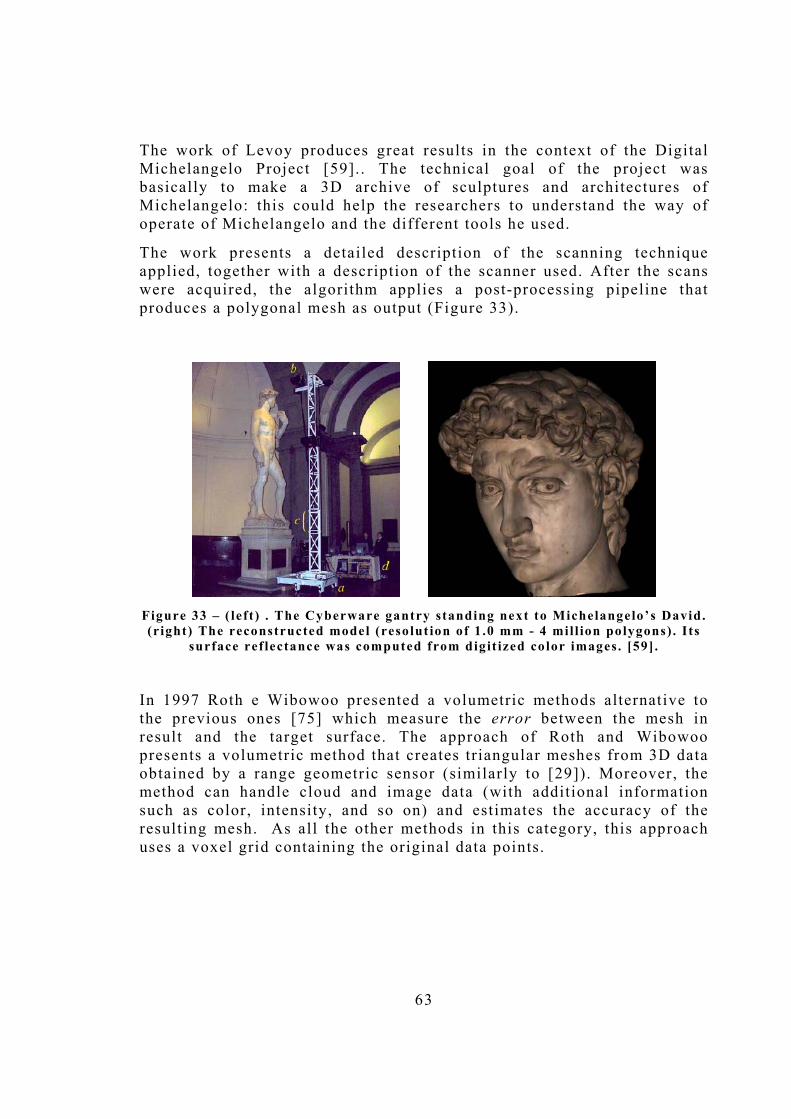
63

The work of Levoy produces great results in the context of the Digital Michelangelo Project [59].. The technical goal of the project was basically to make a 3D archive of sculptures and architectures of Michelangelo: this could help the researchers to understand the way of operate of Michelangelo and the different tools he used.

The work presents a detailed description of the scanning technique applied, together with a description of the scanner used. After the scans were acquired, the algorithm applies a post-processing pipeline that produces a polygonal mesh as output (Figure 33).

Figure 33 � ( left ) . The Cyberware gantry standing next to Michelangelo�s David. (right) The reconstructed model (resolut ion of 1 .0 mm - 4 mil l ion polygons) . Its

surface ref lectance was computed from digit ized color images. [59] .

In 1997 Roth e Wibowoo presented a volumetric methods alternative to the previous ones [75] which measure the error between the mesh in result and the target surface. The approach of Roth and Wibowoo presents a volumetric method that creates triangular meshes from 3D data obtained by a range geometric sensor (similarly to [29]). Moreover, the method can handle cloud and image data (with additional information such as color, intensity, and so on) and estimates the accuracy of the resulting mesh. As all the other methods in this category, this approach uses a voxel grid containing the original data points.

64

In order to efficiently access to different voxels hash table is constructed and because it is necessary to traverse the occupied voxels also a linked list is maintained to connect all the occupied voxels together.

The algorithm can be sketched as follow:

1. Set the voxel size, this can be made manually or automatically.

2. Add each data to the appropriate voxel in space

3. Compute the local normal at each point:

a. Given a point in the voxel grid, the algorithm finds the closet two neighboring points and then uses these three points for computing the relative normal

b. Orient all the normals by the use of a propagation technique.

c. Activate a normal smoothing process for improving the goodness of the data

4. Compute a distance function and run marching cubes to get the triangulation

a. For each voxel vertex the signed distance is computed by taking the weighted average of the signed distances of every points in the eight neighbouring voxels

b. Once all the values are computed then a linear interpolation process finds the intersection of the underlying surface with each edge of the voxel and each of these intersections is a vertex of the final triangulation

5. Close small holes. The method searches for hole loop in the triangulation.

a. A hole loop is a closed sequence of free edges (triangle edges not connected to other triangles).

b. Once a hole loop is founded, it must be triangulated

6. Remove small isolated triangle regions and compute mesh accuracy

Before acting the isolated triangle removing operation, they associate some additional information to each vertex � color, accuracy, intensity. This can be done by assigning to each triangle vertex the additional information of the closest input data. The removal of isolated regions (noise in the final model) is performed by the use of a 3D connectivity

65

algorithm that finds the size of each set of connected triangles in the mesh: the proposed heurist chooses to consider noise those connected triangle regions, containing fewer than a small number of triangles and it removes them.

Figure 34 � Two models created from image data (the elephant and dragon) [75]

The accuracy of the final mesh relative to the original 3D data points is computed considering for each point in a voxel the distance to the closest triangle that is part of the same voxel. Successively the algorithm finds the maximum of these closest distances: this value represents the maximum deviation of the triangular mesh from the original 3D data.

We conclude this section by presenting two methods that are not explicitly based on the computation of a distance function like the previous ones but share with them many characteristics, including the use of a grid to discretize 3d space.

The algorithm presented by Cignoni et al. [26] takes as input only range images, but makes use of an innovative marching algorithm and it is able to take into account the reliability of the input data points. The algorithm basically performs the following steps:

1. Locate the geometric intersections between each mesh built on a single range image and a virtual 3D reference grid;

2. Merge the corresponding intersections belonging to different range images;

66

3. Reconstruct the merged surface(s) on each cell of the grid containing intersections, by means of the Marching Intersections (MI) algorithm.

4. Close possible undesired holes on the surface.

The fusion of the multiple range maps by merging the corresponding intersections (step 2 and 3) has to be performed and the arrangement of the intersections data structures in a Marching Cubes [60] compliant manner has to be done: this means to ensure the existence of no more than one intersection on each virtual cell edge. For doing this, the algorithm fuses each couple of consecutive intersections belonging to different range maps looking at their sign.

Some removal operations are performed on the updated grid edge in order to ensure acceptable results: A removal action is performed on each pair of intersections, which lie on the same cell edge, belong to the same range map and have discordant signs.

Unfortunately, the fusion and removal operators are not sufficient to ensure that no more than one intersection lies on each virtual edge. In these situations, the algorithm maintains more intersections on a virtual edge and postpones their handling to the surface reconstruction step.

At the end of the merging process, the algorithm starts the surface reconstruction step by the use of the Marching Intersections (MI) reconstruction method. By the use of a standard MC look up table, i t performs an iterative visit of three data structures XY , XZ, YZ; and for each structure, the entries from left to right and from bottom to top are analyzed. The use of the MI algorithm permits to reconstruct most of the integrated surface(s).

Figure 35 � Two models bui lt using the Marching Intersect ions Algorithm [26]

67

However, a non-correct configuration can be obtained on some cells and a recovery action starts in order to close holes in the surface(s). The edges inserted into the appropriate list are analyzed: starting from a seed edge, the boundary of a hole is reconstructed by simply connecting edges with compatible extremes (Figure 35). The only hypothesis is that the boundary of the hole is simple and not self-intersecting.

Another interesting algorithm which uses a grid (not a regular grid but a octree space voxelization) is the one presented by Johnson Manduchi in 2002. The input is a set of 3D surface samples represented by measurement models derived from a sensor model and estimates of registration error.

Using a probabilistic rule, the method generates a surface probability function (SPF) that represents the probability that a volume contains the desired surface. The SPF is represented using an octree data structure; regions of space with samples of large covariance are stored at a coarser scale than regions of space containing samples with smaller covariance.

The approach builds first the SPF and its derivatives incrementally from the 3D samples: during SPF generation, changes to the SPF and its derivatives produced by each new sample are computed and stored in an octree structure.

For each measurement:

• Determine the octree level for inserting the measurement,

• Determine the nodes at this level near the measurement,

• Update the SPF terms for each node.

After all measurements have been added to the octree, the SPF and its derivatives are computed for each node.

The next step of the algorithm is ridge extraction : The ridge of the SPF will correspond to a 2D boundary representation of the surface. These ridge points are detected based on information stored in individual nodes of the octree. Each leaf node in the octree contains the SPF and its first and second order derivatives, which describe the local quadratic approximation to the SPF across the node. Almost all of the ridge points lie on a single surface while a few of the ridge points are outliers that can be eliminated removing ridge points with low surface probability. Finally, the method generates the resolution-integrated surface (a

68

triangle mesh), by the use of a variation of the marching triangles algorithm [50].

Figure 36- in sequence ( from top-left to bottom-right):

data, octree, ridge points , result ing mesh. (taken from [52])

3 . 2 . 2 R A D I A L B A S I S F U N C T I O N Methods that fall in this class try to reconstruct the surface of the scanned object by the use of implicit function in the form of Radial Basis Function. Differing from the previous methods, RBF-based approaches do not require that the data lie on any sort of regular grid.

About 20 years ago, in an extensive survey, Franke [41] identified radial basis functions as accurate methods to solve scattered data interpolation problems [95]. Given the set of k pair wise distinct points (also called centers) P={p1 , �pk}, pk∈ℜn of dimension n , and the set of values {h1,�,hk}, the problem is to find a function f: ℜn →ℜ such that ∀i f(pi)=hi . In order to obtain a radial basis function reconstruction of the point set P, a function f satisfying the equation

∑=

+=k

tii ppppf

1),()()( φωπ (3.1)

69

has to be found. In the equation (1), p,pi is the Euclidean distance, ω i are weights, φ:ℜ→ℜ is a basis function and π a degree one polynomial that accounts for the linear and constant portions of f .

∑=

+=n

t

ii pp

1

)(0)( πππ (3.2)

where p ( i ) is the i-th component of vector p . The basis function φ has to be conditionally positive definite [95], and some popular choices proposed in the literature are shown below:

• φ(r) =r and φ(r)=r3 the simplest polynomials, for fi t t ing functions of three variables;

• φ(r) = r2 log(r), typically for fi tting smooth functions of two variables;

• φ(r)=exp(-cr2), mainly for neural networks;

• φ(r) = √r2 +c2, for various applications, in particular fitting to topographical data;

• φ(r) = (1-r /α)4+(4 ⋅r/α +1) for r∈[0,α], the Wendland�s compactly supported radial basis functions with a support radius α instead of global as in the cases of the previous functions.

As we have an underdetermined system with k+n+1 unknowns variables and k equations, natural additional constraints for the coefficients r are added, so that

021 ===== ∑∑∑∑ i nii ii ii i πωπωπωω K

The equations above determine a linear system Ax=b with

( )

[ ] [ ]Tk

Tnk

jiij

Tij

hhhbx

ppPP

A

0,...0,0,,...,,,,...,,,,...,

,001001

210211 ==

=Φ

Φ=

ππππωω

φ (3.3)

The solution x is composed of the weights ω i and the polynomial coefficients π i and represents a solution also of the interpolation problem: ∀i f(pi)=hi .

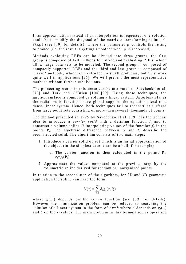
70

If an approximation instead of an interpolation is requested, one solution could be to modify the diagonal of the matrix A transforming it into A-8kπρΙ (see [19] for details), where the parameter ρ controls the fitting tolerance (i .e. the result is getting smoother when ρ is increased).

Methods exploiting RBFs can be divided into three groups: the first group is composed of fast methods for fitting and evaluating RBFs, which allow large data sets to be modeled. The second group is composed of compactly supported RBFs and the third and last group is composed of "naive" methods, which are restricted to small problems, but they work quite well in applications [95]. We will present the most representative methods without further subdivisions.

The pioneering works in this sense can be attributed to Savchenko et al. [79] and Turk and O�Brien [104],[99]. Using these techniques, the implicit surface is computed by solving a linear system. Unfortunately, as the radial basis functions have global support, the equations lead to a dense linear system. Hence, both techniques fail to reconstruct surfaces from large point sets consisting of more then several thousands of points.

The method presented in 1995 by Savchenko et al. [79] has the general idea to introduce a carrier solid with a defining function f c and to construct a volume spline U interpolating values of the function f c in the points P i . The algebraic difference between U and f c describe the reconstructed solid. The algorithm consists of two main steps:

1. Introduce a carrier solid object which is an initial approximation of the object (in the simplest case it can be a ball, for example)

a. The carrier function is then calculated in the points P i: ri=f c(P i)

2. Approximate the values computed at the previous step by the volumetric spline derived for random or unorganized points.

In relation to the second step of the algorithm, for 2D and 3D geometric application the spline can have the form:

∑+

=

=kN

iiii PxgxU

1),()( λ

where g i ( . .) depends on the Green function (see [79] for details). However the minimization problem can be reduced to searching the solution of a linear system in the form of Ax=b where A depends on gi(. .) and b on the ri values. The main problem in this formulation is operating

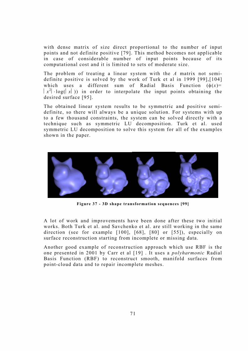
71

with dense matrix of size direct proportional to the number of input points and not definite positive [79]. This method becomes not applicable in case of considerable number of input points because of its computational cost and it is limited to sets of moderate size.

The problem of treating a linear system with the A matrix not semi-definite positive is solved by the work of Turk et al in 1999 [99],[104] which uses a different sum of Radial Basis Function (φ(x)= x2⋅ log(x)) in order to interpolate the input points obtaining the desired surface [95].

The obtained linear system results to be symmetric and positive semi-definite, so there will always be a unique solution. For systems with up to a few thousand constraints, the system can be solved directly with a technique such as symmetric LU decomposition. Turk et al . used symmetric LU decomposition to solve this system for all of the examples shown in the paper.

Figure 37 - 3D shape transformation sequences [99]

A lot of work and improvements have been done after these two initial works. Both Turk et al. and Savchenko et al . are stil l working in the same direction (see for example [100], [68], [80] or [55]), especially on surface reconstruction starting from incomplete or missing data.

Another good example of reconstruction approach which use RBF is the one presented in 2001 by Carr et al [19] . It uses a polyharmonic Radial Basis Function (RBF) to reconstruct smooth, manifold surfaces from point-cloud data and to repair incomplete meshes.

72

The method consists of three main steps:

1. Construct a signed distance function,

2. Fit an appropriate RBF to the distance function constructed at step 1.

3. Iso-surface the fitted RBF by the use of a Tetrahedra Marching Algorithm.

As usual, for the construction of a signed distance function, the method try to define a function f(P i )=0 if P i is a point on the surface and f(Q i )=d i if Q i is a point inside or outside the object: points outside the object are assigned positive values, while points inside the object are assigned negative values. The determination of the off-surface points is performed by projecting along surface normals. If these normals are not given as input, their approximation in each point can be made using method of normals approximation as the one presented in [51].

The next step of the algorithm is to fit an RBF to the distance function: given the set of zero-valued points and non-zero off-surface points, the problem is basically to approximate the signed-distance function f(x) by an interpolant function s(x). The method chooses an interpolant from the Beppo-Levi space of distributions on R3 [19], a space equipped with the rotation invariant semi-norm defined by:

∫ℜ

∂

∂∂

∂+

∂∂

∂+

∂∂

∂+

∂

∂+

∂

∂+

∂

∂=

3

2222222

2

22

2

22

2

22 )(2)(2)(2)()()( x

zyxs

zxxs

yxxs

zxs

yxs

xxss

This semi-norm measures in some way the energy of smoothness : functions with small semi-norm are smoother than those with a larger semi-norm. The smoothest interpolant is chosen and it is proven to be:

ssSs∈

= minarg*

The function is a particular form of a standard Radial Basis Function where the basis function is considered to be the biharmonic spline φ(z)=z and, for all the λ i , orthogonality conditions must hold:

0)(1

=∑=

N

iii xqλ for all polynomial q of degree almost m .

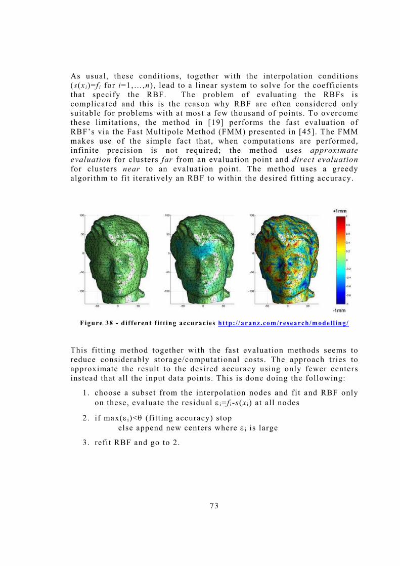
73

As usual, these conditions, together with the interpolation conditions (s(xi)=f i for i=1,�,n), lead to a linear system to solve for the coefficients that specify the RBF. The problem of evaluating the RBFs is complicated and this is the reason why RBF are often considered only suitable for problems with at most a few thousand of points. To overcome these limitations, the method in [19] performs the fast evaluation of RBF�s via the Fast Multipole Method (FMM) presented in [45]. The FMM makes use of the simple fact that, when computations are performed, infinite precision is not required; the method uses approximate evaluation for clusters far from an evaluation point and direct evaluation for clusters near to an evaluation point. The method uses a greedy algorithm to fit i teratively an RBF to within the desired fitting accuracy.

Figure 38 - different f it t ing accuracies http: / /aranz.com/research/model l ing/

This fitting method together with the fast evaluation methods seems to reduce considerably storage/computational costs. The approach tries to approximate the result to the desired accuracy using only fewer centers instead that all the input data points. This is done doing the following:

1. choose a subset from the interpolation nodes and fit and RBF only on these, evaluate the residual ε i=f i -s(x i ) at all nodes

2. if max(ε i )<θ (fitting accuracy) stop else append new centers where ε i is large

3. refit RBF and go to 2.

74

An RBF fitted to a set of surface data forms a solid model of an object. The surface is the locus of points where the RBF is zero. To visualize it , the approach applies a variation of the Marching Cube Algorithm; in particular a mesh optimisation scheme adapted from [97] is applied. It basically avoids thin and elongated triangles resulting in fewer triangles with better aspect ratios.

In conclusion, fast methods make it computationally possible to represent complicated objects of arbitrary topology by RBFs. The scale-independent, �smoothest interpolator� characterization of polyharmonic splines make RBFs particularly suited to fitting surfaces to non-uniformly sampled point-clouds and partial meshes that contain large irregular holes. Moreover, the functional nature of the RBF representation offers new possibilities for surface registration algorithms, mesh simplification, compression and smoothing algorithms. Unfortunately, the far field expansion has to be done for every radial basis function, and is very complex to implement.

Figure 39- A greedy algorithm iterat ively f its

an RBF to a point cloud result ing in fewer centers in the f inal funct ion [19]

Anyway, the method in [19] is a great representative of the reconstruction methods, which use Radial Basis Functions and implicit surfaces in general. The method presented in 2001 was the beginning of a great research frameworks [20] and companies like ARANZ [4] or FarField Technology Ltd [39] and has many applications in several fields.

75

But, using radially symmetric basis functions (like the one used in [19]) it is assumed that the desired surface should be everywhere locally symmetric. Nevertheless, such assumption is true only for planar regions and not for corners. Hence, reconstruction using isotropic basis is insufficient to reconstruct correctly object with sharp features.

The method presented by Dinh, Turk and Slabaugh [35], in 2001 tries to preserve sharp features using anisotropic basis functions. The output of the method is a surface sharper along edges and at corner points.

1. For each point, the algorithm determines the direction of anisotropy by performing principal component analysis (PCA) in a small relative neighborhood.

2. The resulting field of principle directions across the surface is smoothed through tensor filtering.

The approach starts from a volumetric representation of the surface consisting of red, green, and blue channels for each voxel. The status (color) of each voxel is computed through generalized voxel colouring algorithm that takes as input a 3D volume and a images set taken around the object and carves out voxels of the initial volume by splatting each voxel towards each camera and determining the consistency of the voxel color across the image. Basically, if the variance in color intensity is below a specified threshold θ , the voxel is kept as part of the object surface. Otherwise, i t is assigned a zero value.

For applying the RBF method, some constraint points have to be computed from the RBG points. The method uses an approach similar to [36] in order to sample the surface, interior, and exterior regions of the object (a previous characterization can be found also in [102], [46]).

Using the notion of free space (the region of space swept out by the collection of rays emanating from a camera towards surface points visible from that camera) and the a priori information about the cameras exterior points all around the object can be determined.

Surface points are defined by the voxel coloring dataset, while interior points are determined by traversing the volumetric data set along each major axis: all points occurring between pairs of surface voxels are marked as interior. Only voxels, which are marked as interior by two or more traversals, are kept as interior constraints.

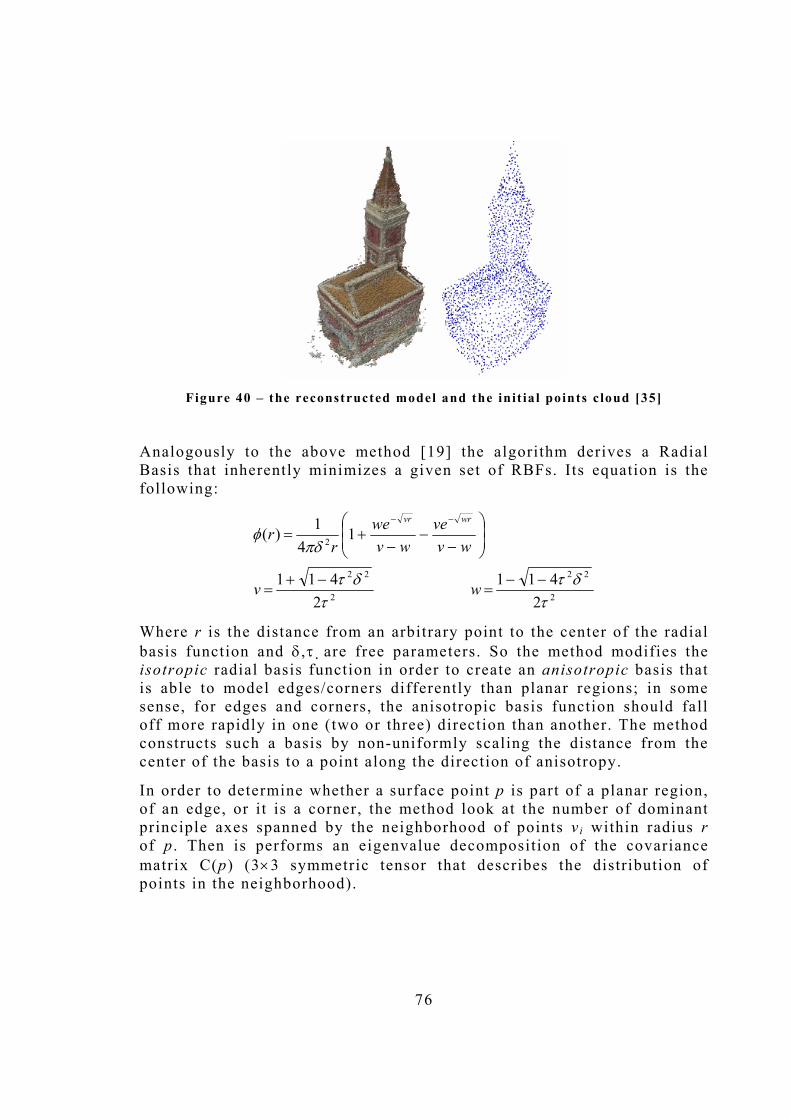
76

Figure 40 � the reconstructed model and the init ia l points cloud [35]

Analogously to the above method [19] the algorithm derives a Radial Basis that inherently minimizes a given set of RBFs. Its equation is the following:

2

22

2

22

2

2411

2411

14

1)(

τδτ

τδτ

πδφ

−−=

−+=

−−

−+=

−−

wv

wvve

wvwe

rr

wrvr

Where r is the distance from an arbitrary point to the center of the radial basis function and δ ,τ are free parameters. So the method modifies the isotropic radial basis function in order to create an anisotropic basis that is able to model edges/corners differently than planar regions; in some sense, for edges and corners, the anisotropic basis function should fall off more rapidly in one (two or three) direction than another. The method constructs such a basis by non-uniformly scaling the distance from the center of the basis to a point along the direction of anisotropy.

In order to determine whether a surface point p is part of a planar region, of an edge, or it is a corner, the method look at the number of dominant principle axes spanned by the neighborhood of points vi within radius r of p . Then is performs an eigenvalue decomposition of the covariance matrix C(p) (3×3 symmetric tensor that describes the distribution of points in the neighborhood).

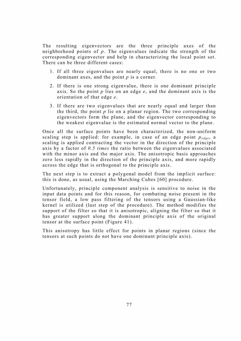
77

The resulting eigenvectors are the three principle axes of the neighborhood points of p . The eigenvalues indicate the strength of the corresponding eigenvector and help in characterizing the local point set. There can be three different cases:

1. If all three eigenvalues are nearly equal, there is no one or two dominant axes, and the point p is a corner.

2. If there is one strong eigenvalue, there is one dominant principle axis. So the point p l ies on an edge e , and the dominant axis is the orientation of that edge e .

3. If there are two eigenvalues that are nearly equal and larger than the third, the point p l ie on a planar region. The two corresponding eigenvectors form the plane, and the eigenvector corresponding to the weakest eigenvalue is the estimated normal vector to the plane.

Once all the surface points have been characterized, the non-uniform scaling step is applied: for example, in case of an edge point ped ge , a scaling is applied contracting the vector in the direction of the principle axis by a factor of 0.5 times the ratio between the eigenvalues associated with the minor axis and the major axis. The anisotropic basis approaches zero less rapidly in the direction of the principle axis, and more rapidly across the edge that is orthogonal to the principle axis.

The next step is to extract a polygonal model from the implicit surface: this is done, as usual, using the Marching Cubes [60] procedure.

Unfortunately, principle component analysis is sensitive to noise in the input data points and for this reason, for combating noise present in the tensor field, a low pass filtering of the tensors using a Gaussian-like kernel is utilized (last step of the procedure). The method modifies the support of the filter so that i t is anisotropic, aligning the filter so that i t has greater support along the dominant principle axis of the original tensor at the surface point (Figure 41).

This anisotropy has little effect for points in planar regions (since the tensors at such points do not have one dominant principle axis).

78

Figure 41 - Reconstruct ions of the noisy cube without tensor

f i l tering ( left) and with tensor f i ltering (r ight) .

Another method which uses implicit surface and Radial Basis Functions is the one presented by Laga et al in [58],[57]. The method takes a set of range data as input and constructs via RBF a polygonal model of the observed scene.

As usual, the entire object is modeled with a single implicit function and no restriction is made on the object geometry. The novelty is that they introduce a fast fi tt ing method of the RBF to the dataset via a center-number-reduction technique, which is not random (as in [19]) but uses a statistical analysis on the initial data.

The first idea is to define another basis for the subspace of the fitting functions which seems to be simpler than the others because lead to simpler matrices, the second idea is to reduce the points used to estimate f since the human perception is insensitive to small errors and scanning devices provide an over sampling of the object which results in redundant points [58]. The optimization process can be summarized as follow:

1. Select a subset A of S (input points, centers) as follows: for objects with sharp boundaries if a point and the set of its neighbors are lying approximatively on the same plane then they are reduced to 3 points only.

2. Fit the RBF to the subset A and evaluate the error at the points in S-A .

3. If the error is bigger than a threshold value θ add new points to A and repeat the step 2

4. Otherwise stop the fitt ing process.

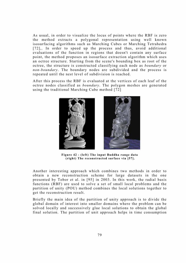
79

As usual, in order to visualize the locus of points where the RBF is zero the method extracts a polygonal representation using well known isosurfacing algorithms such as Marching Cubes or Marching Tetrahedra [72],. In order to speed up the process and thus, avoid additional evaluations of the function in regions that doesn't contain any surface point, the method proposes an isosurface extraction algorithm which uses an octree structure. Starting from the scene's bounding box as root of the octree, the structure is constructed classifying each node as boundary or non-boundary . The boundary nodes are subdivided and the process is repeated until the nest level of subdivision is reached.

After this process the RBF is evaluated at the vertices of each leaf of the octree nodes classified as boundary . The polygon meshes are generated using the traditional Marching Cube method [72]

Figure 42 - ( left) The input Buddha range data

(r ight) The reconstructed surface via [57] .

Another interesting approach which combines two methods in order to obtain a new reconstruction scheme for large datasets in the one presented by Tobor et al. in [95] in 2003. In this work, the radial basis functions (RBF) are used to solve a set of small local problems and the partition of unity (POU) method combines the local solutions together to get the reconstruction result.

Briefly the main idea of the partition of unity approach is to divide the global domain of interest into smaller domains where the problem can be solved locally and successively glue local solutions to obtain the global final solution. The partition of unit approach helps in time consumption

80

improvement dividing the time complexity in subroutine and rendering the BRF computation local instead of global. One novelty is that this method offers a high level of scalability as the data do not need to be completely stored in memory, but can be accessed sequentially from disk.

3 . 2 . 3 D E F O R M A B L E M O D E L S A N D L E V E L S E T M E T H O D S

The level set approach was originally introduced by Osher and Sethian in [69] to capture moving interfaces and has been used quite successfully in moving interface and free boundary problems as well as in image processing, image segmentation and elsewhere.

The level set method is based on a continuous formulation using Partial Differential Equations (PDE) and allows one to deform an implicit surface, which is usually the zero isocontour of a scalar (level set) function, according to various laws of motion depending on geometry, external forces, or a desired energy minimization [106].

In numerical computations, instead of explicitly tracking a moving surface one implicitly captures it by solving a PDE for the level set function on rectangular grids. The data structure is extremely simple and topological changes are handled easily [69]. The level set formulation works in any number of dimensions and the computation can easily be restricted to a narrow band near the zero level set. It is possible to locate or render the moving surface easily by interpolating the zero isosurface of the level set function.

Two key steps for the level set methods are: (1) Embed the surface as the zero isocontour of a scalar (level set) function. (2) Embed the motion in the system. For an exhaustive formulation of Level Set Methods and their development see also [84] [83] [82].

Sethian et al. basically presented a class of algorithms, called PSC schemes (Propagation of Surfaces under Curvature), for moving surfaces under their curvature. These algorithms rely on numerically solving Hamilton-Jacobi equations with viscous terms, using approximation techniques from hyperbolic conservation laws. The central idea is the formulation of the correct equation of motion for a front propagating with curvature-dependent speed [82] and by viewing the surface as a level set, topological complexities and changes in the moving front are

81

handled. They define a force function on the input data and make an initial seed grow following forces depending on point�s curvature and normals.

Another approach that goes in the same direction is the one presented by Chen and Medioni [23] in 1992. In their work, a balloon model is inflated starting from a set of registered range images.

The process terminates when the sphere (the balloon - Figure 43) reaches the shape of the object to be reconstructed. The vertices in the mesh are linked to their neighboring vertices through springs to simulate the surface tension. Unlike other dynamic models the balloon model is driven only by an applied inflation force towards the object surface from inside of the object, until the mesh elements reach the object surface (Figure 44).

The system includes an adaptive local triangle mesh subdivision scheme that results in an evenly distributed mesh. Since the approach is not based on global minimization, i t can handle complex, non-star-shaped objects without relying on a carefully selected initial state or encountering local minimum problem. It also allows to adapt the mesh surface to changes in local surface shapes and to handle holes present in the input data through adjusting certain system parameters adaptively.

The algorithm can be sketched as follow:

1. Select initial point inside the object

2. Construct an icosahedron shell at this location. The selection process is done manually and the size of the shell should be small enough so that i t is completely inside the object.

3. Let all the triangles on the initial mesh be front F0 and push it into the front queue Q , then until queue is empty, do the followings repeatedly:

• F =pop(Q) Pop the queue.

• Subdivide the triangles in F: for each vertex, whose 3D coordinates at time t is vi

t , do

o compute the internal force g i and external force f i with respect to the given deformable constraints

o compute the new vertex location v i t+t for the current iteration

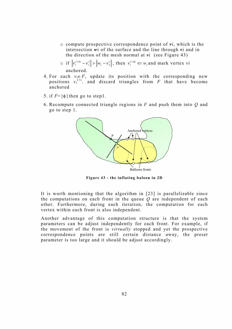
82

o compute prospective correspondence point of vi , which is the intersection wi of the surface and the line through vi and in the direction of the mesh normal at v i (see Figure 43)

o if tIi

ti

tti vwvv −>−∆+ , then i

tti wv ⇐∆+ and mark vertex vi

anchored. 4. For each vi∈F , update its position with the corresponding new

positions v it+ t . and discard triangles from F that have become

anchored

5. if F={φ}then go to step1.

6. Recompute connected triangle regions in F and push them into Q and go to step 1.

v

P

Balloons fronts

Anchored vertices

Figure 43 - the inf lat ing baloon in 2D

It is worth mentioning that the algorithm in [23] is parallelizable since the computations on each front in the queue Q are independent of each other. Furthermore, during each iteration, the computation for each vertex within each front is also independent.

Another advantage of this computation structure is that the system parameters can be adjust independently for each front. For example, if the movement of the front is virtually stopped and yet the prospective correspondence points are still certain distance away, the preset parameter is too large and it should be adjust accordingly.

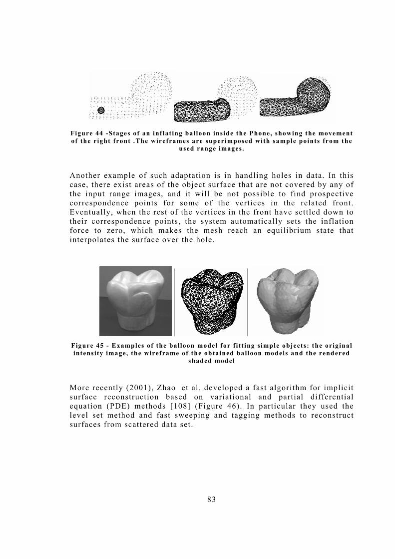
83

Figure 44 -Stages of an inf lat ing bal loon inside the Phone, showing the movement of the right front .The wireframes are superimposed with sample points from the

used range images.

Another example of such adaptation is in handling holes in data. In this case, there exist areas of the object surface that are not covered by any of the input range images, and it will be not possible to find prospective correspondence points for some of the vertices in the related front. Eventually, when the rest of the vertices in the front have settled down to their correspondence points, the system automatically sets the inflation force to zero, which makes the mesh reach an equilibrium state that interpolates the surface over the hole.

Figure 45 - Examples of the bal loon model for f i tt ing simple objects: the original intensity image, the wireframe of the obtained balloon models and the rendered

shaded model

More recently (2001), Zhao et al . developed a fast algorithm for implicit surface reconstruction based on variational and partial differential equation (PDE) methods [108] (Figure 46). In particular they used the level set method and fast sweeping and tagging methods to reconstruct surfaces from scattered data set.

84

The data set might consist of points, curves and/or surface patches. A weighted minimal surface-like model is constructed and its variational level set formulation is implemented.

The reconstructed surface is smoother than piecewise linear and has a natural scaling in the regularization that allows varying flexibility according to the local sampling density. As is usual with the level sets, this method can handle complicated topology and deformations, as well as noisy or highly non-uniform data sets easily.

There are three key numerical ingredients in the proposed implicit surface reconstruction.

1. First, an algorithm to compute the distance function to an arbitrary data set on rectangular grids is necessary.

2. Second, a good initial surface for the gradient flow has to be computed and

3. Third, a time dependent PDEs for the level set function has to be solved.

The distance function d(x) to an arbitrary data set S solves the following Eikonal equation: Sxxdxd ∈==∇ ,0)(,1)( From the PDE point of view, the characteristics of this Eikonal equation are straight lines that radiate from the data set. This reveals the causality property for the solution of the PDE, i .e. , the information propagates along straight lines from the data set, and the solution at a grid point should be determined only by its neighboring grid points that have smaller distance values. The algorithm uses different existing approaches that combine upwind differencing with Gauss-Seidel iterations of different sweeping order to solve the equation on rectangular grids (see [108] for more details).

Because a good initial surface is important for the efficiency of the PDE based method, the authors propose a fast tagging algorithm for characterizing interior , exterior and boundary surface points. As usual, the algorithm starts from any initial exterior region that is a subset of the true exterior region:

• All grid points that are not in the initial exterior region are labeled as interior points. Those interior grid points that have at least one exterior neighbor are labeled as temporary boundary points .

• The temporary boundary points are organized in a heapsort binary tree structure T sorting according to distance values di .

85

• Then the root RT of the heap (the temporary boundary point that has the largest distance) is extracted

• If RT with distance value dR has an interior neighbor wj with distance value dw≥ dR , this temporary boundary becomes a boundary point and the heap is re-sorted.

• Otherwise, RT becomes an exterior point, i t is thrown away from the heap T and the heap T is re-sorted according to distance values. None of RT neighbors are added to the heap.

• The procedure is repeated until the the maximum distance of the temporary boundary points is smaller than some tolerance θ (e.g. the size of a grid cell), which means all the temporary boundary points in the heap are close enough to the data set.

• Finally, all the remaining temporary boundary points are converted into final boundary points.

After the distance function is computed and the points have been categorized, the continuous deformation takes place using standard algorithms for the level set method [84].

Figure 46 � Final Reconstruct ion ( left) and a low resolut ion reconstruct ion

(right) [108]

86

4. Online Mosaicing

Virtual Reality is a way for humans to visualize, manipulate and interact with computers and extremely complex data

[Aukstakalnis S]

This chapter describes the work done in solving the problem of online mosaicing starting from multiple range images in the context of the European Project ARROV [5]. First, a brief introduction to the problem and the framework of the project are presented, next we present the details of the developed Data Analysis Pipeline and finally results are reported and open issues are outlined.

4.1 The ARROV Project The European ARROV project [5] has been founded from the European Community within the Fifth Framework Program, specific research, and technological development program "Competitive and Sustainable Growth".

It started in 2001 with duration of three years and aims at improving the applicability and performance of multifunctional Remotely Operated Vehicles (ROV) for the inspection, monitoring and survey of underwater environments and manmade installations. In particular, the project points at solving/improving the following activities:

• Surveying and monitoring of underwater structures , such as oil rigs, pipes, ship wrecks, and other submersed structure in general;

• Inspection of underwater installations , such as dams, dikes, docks, tanks, canals and tunnels (e.g., in hydro- and thermo-electric power plants), in order to detect causes of danger or damage;

• Surveillance for detection of oil and gas leakage from pipes, submersed tanks and wrecks;

87

• Control of unmanned industrial operations (e.g., pipe spool metrology).

At the state of the art, these problems are either solved through intervention of divers, which are consequently exposed to high risks; or addressed with insufficient reliability, because of the poor accuracy and quality of feedback provided by sensors on board an ROV.

The goal of the project has been achieved by the development of a novel integrated sensorial system , which exploits both optical and acoustical data to provide the ROV pilot with an augmented representation of the scene (augmented reality). The system will be also able to synthesize automatically a 3D model of the scene from sensorial data (model acquisition). Moreover, a unified man machine interface will be provided to control an ROV as well as the sensors mounted on board.

Figure 47 � The ARROV measurements system

Therefore, the main innovation of ARROV lies in the use of a compact set of imaging sensors (optical and acoustic cameras) aimed at the accurate 3D reconstruction of the surrounding environment, and in the

ROV sensor

Visualization Interface

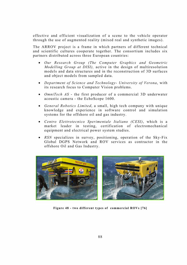
88

effective and efficient visualization of a scene to the vehicle operator through the use of augmented reality (mixed real and synthetic images).

The ARROV project is a frame in which partners of different technical and scientific cultures cooperate together. The consortium includes six partners distributed across three European countries:

• Our Research Group (The Computer Graphics and Geometric Modelling Group at DISI), active in the design of multiresolution models and data structures and in the reconstruction of 3D surfaces and object models from sampled data.

• Department of Science and Technology- University of Verona , with its research focus to Computer Vision problems.

• OmniTech AS - the first producer of a commercial 3D underwater acoustic camera - the EchoScope 1600.

• General Robotics Limited, a small, high tech company with unique knowledge and experience in software control and simulation systems for the offshore oil and gas industry.

• Centro Elettrotecnico Sperimentale Italiano (CESI) , which is a market leader in testing, certification of electromechanical equipment and electrical power system studies.

• RSN specializes in survey, positioning, operation of the Sky-Fix Global DGPS Network and ROV services as contractor in the offshore Oil and Gas Industry.

Figure 48 - two different types of commercial ROVs [76]

89

In conclusion, the augmented reality visualization system, developed in the context of the project ARROV, significantly contributes to reduce the cognitive load on teleoperators by providing cues that help prevent them getting lost and disoriented. Moreover and accurate 3D interpretation of data and automatic fault detection significantly contribute to improve surveillance and control of unmanned operations.

The role of our research group in the project was mainly the development of methods for Data Analysis starting from single or multiple range images able to satisfy real time requirements. Our methods have been integrated with the work done by the other academic partner (Department of Science and Technology- University of Verona) in acquisition and registration in order to produce the complete pipeline. I this chapter, we will present the entire pipeline going into more details for those parts which see our group as leader (Single Frame Reconstruction and Mosaicing).

4.2 Mosaicing from Multiple Range Images

Several steps are involved in reconstructing a 3D model and further scene analysis using multiple range images. In a general framework, a full 3D reconstruction of the observed environment requires scanning from different views [86]. The surface measured from each scan is recorded in a local coordinate system centered at the scanner. In order to integrate different views, all the surfaces must be registered into a global coordinate system (see Chapter 2 for details). In general, the challenges in automatic registration are how to efficiently find correspondences from two partially overlapped surfaces and robustly deal with the noise and different surface sampling resolutions [23],[25],[21].

Integrating surfaces from different views is a fusion process that weaves a whole surface from a set of overlapping surface patches. The integration process should be robust to surface noise and registration error. Usually, it is impossible to scan the whole object, so holes are left at regions where the laser cannot reach. These holes can be filled by space carving or by an automatic hole filling process after integration. The reconstructed surface may contain a number of parts. In many cases,

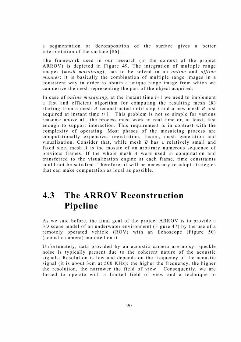
90

a segmentation or decomposition of the surface gives a better interpretation of the surface [86].

The framework used in our research (in the context of the project ARROV) is depicted in Figure 49. The integration of multiple range images (mesh mosaicing), has to be solved in an online and offline manner: i t is basically the combination of multiple range images in a consistent way in order to obtain a unique range image from which we can derive the mesh representing the part of the object acquired.

In case of online mosaicing , at the instant time t+1 we need to implement a fast and efficient algorithm for computing the resulting mesh (R) starting from a mesh A reconstructed until step t and a new mesh B just acquired at instant time t+1. This problem is not so simple for various reasons: above all , the process must work in real time or, at least, fast enough to support interaction. This requirement is in contrast with the complexity of operating. Most phases of the mosaicing process are computationally expensive: registration, fusion, mesh generation and visualization. Consider that, while mesh B has a relatively small and fixed size, mesh A is the mosaic of an arbitrary numerous sequence of previous frames. If the whole mesh A were used in computation and transferred to the visualization engine at each frame, time constraints could not be satisfied. Therefore, i t will be necessary to adopt strategies that can make computation as local as possible.

4.3 The ARROV Reconstruction Pipeline

As we said before, the final goal of the project ARROV is to provide a 3D scene model of an underwater environment (Figure 47) by the use of a remotely operated vehicle (ROV) with an Echoscope (Figure 50) (acoustic camera) mounted on it .

Unfortunately, data provided by an acoustic camera are noisy: speckle noise is typically present due to the coherent nature of the acoustic signals. Resolution is low and depends on the frequency of the acoustic signal (it is about 3cm at 500 KHz): the higher the frequency, the higher the resolution, the narrower the field of view. Consequently, we are forced to operate with a limited field of view and a technique to

91

reconstruct progressively the scene while the sensor is moving is necessary.

In our case: (i) the resolution is never better than some centimeters, unlike classic range data (e.g., from laser range finders); (ii) sensor position is not taken into account for view registration; (iii) the motion of the sensor is quite unstable, and cannot be controlled with precision in any real case, so acquired images from a fixed position may be different due to speckle and sensor floating. As a consequence, some previous solutions based on estimation of surface parameters cannot be taken into account due to the high uncertainty of data.

Texture Mapping

AR

ENGINE

Position

Arrov System

Calibration

Acoustic

Optic

Texture

Filtering Mosaic

Mesh Reconstruction

Registration 3D Model

Position Update

SyntheticPrimitives3D Model FittingMotion Tracking

Figure 49 - Arrov data process ing scheme

In order to achieve our goal, we developed, in collaboration with Department of Science and Technology- University of Verona a complete data processing pipeline (Figure 49), which starts from data acquisition,

92

and produces a geometric model of the observed scene, in the form of a mesh of triangles. This process can come in two versions:

• on-line , i .e. , processing occurs while new frames come from the sensor as the vehicle carrying it moves; and

• off-line , i .e. , processing is made after all frames have been collected.

The major differences between the two versions is that the on-line one needs to build the output progressively from a dataset that grows through time, and must do it within strict time constraints, in order to support navigation. The off-line version, on the contrary, can process all data together, taking a long time. We developed fast methods to support the on-line version, as well as refinements to improve the accuracy of the result in the off-line version.

This dissertation will concentrate on the on-line processing pipeline, which includes four stages: Data Capture , Data Pre-processing , Registration and Geometric Fusion .

1. Data capture , in which the acoustic camera produces a new range image;

2. Data Pre-Processing , in which data are pre-processed to eliminate outliers and a range image is processed to obtain a triangle mesh discarding small components;

3. Registration , in which all data corresponding to all frames are brought to the same coordinate system. In the on-line version this means just bringing the new frame to the coordinate system of all the previous frames;

4. Geometric fusion , in which geometries corresponding to the different frames are merged to form a single mesh representing the whole observed scene. In the on-line version this means to merge the geometry of the new frame into the mesh built on all previous frames.

Our research group actively participates at all the four stages but we were the leader in the context of the Recostruction steps (i .e. Pre-processing and Geometric Fusion). The remaining part of this section describes our reconstruction pipeline, going in details in those steps which have been developed mainly by our research group [22].

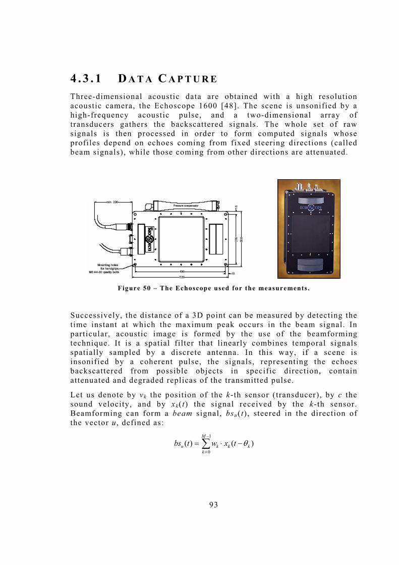
93

4 . 3 . 1 D A T A C A P T U R E Three-dimensional acoustic data are obtained with a high resolution acoustic camera, the Echoscope 1600 [48]. The scene is unsonified by a high-frequency acoustic pulse, and a two-dimensional array of transducers gathers the backscattered signals. The whole set of raw signals is then processed in order to form computed signals whose profiles depend on echoes coming from fixed steering directions (called beam signals), while those coming from other directions are attenuated.

Figure 50 � The Echoscope used for the measurements.

Successively, the distance of a 3D point can be measured by detecting the time instant at which the maximum peak occurs in the beam signal. In particular, acoustic image is formed by the use of the beamforming technique. It is a spatial filter that linearly combines temporal signals spatially sampled by a discrete antenna. In this way, if a scene is insonified by a coherent pulse, the signals, representing the echoes backscattered from possible objects in specific direction, contain attenuated and degraded replicas of the transmitted pulse.

Let us denote by vk the position of the k-th sensor (transducer), by c the sound velocity, and by xk( t) the signal received by the k-th sensor. Beamforming can form a beam signal, bsu(t), steered in the direction of the vector u , defined as:

)()(1

0kk

M

kku txwtbs θ−⋅= ∑

−

=

94

where wk are the weights assigned to each sensor, M is the number of transducers, and θ= (vk ⋅u)/c are the delays applied to each signal.

A common method to detect the scattering objects distances is to look for the maximum peak of the beam signal envelope [105]. Denoting by t* the time instant at which the maximum peak occurs, the related distance, r* (i .e. , range value) is easily derivable (i.e. , r*= c ⋅t*/2 if the pulse source is placed in the coordinate origin). According to the spherical scanning technology, range values are measured from each steering direction u(i j) where i and j are indices related to the elevation (tilt) and azimuth (pan) angles respectively.

Figure 51- Spherical scanning principle ( left) and subdivision

of the beams onto the acquiring volume (right) . Each beam is associated to a ( i ; j) coordinate of the range image

Figure 51.(left) shows a schema of the scanning principle. Figure 51.(right) shows a projection of the acquiring volume to the ZX plane, on which the sectors associated to each beam are marked. The minimum and maximum distances are also depicted.

Going into the details, the Echoscope carries out 64 measures for both ti lt and pan by defining a 64×64 range image ri j . The conversion from spherical coordinates to usual Cartesian coordinates is recovered by the use of the following equations [16]:

Acoust ic camera

alpha Visibi le area

Acoust ic beam

Acoust ic beam n.0

DISA DISB

x (or y)

z

Pan angle

tilt angle

sensor

range

Point (x,y,z)

xyz

95

)(tan)(tan

)(tan)(tan1)tan(

)(tan)(tan1)tan(

22

22

22

βα

βα

β

βα

α

jsjsrz

jsjsjsry

jsjsjsrx

ij

ij

ij

+=

++=

++=

where sα and sβ are increments of the elevation and the azimuth respectively. Figure 52 shows a range image acquired by the Echoscope and the related points cloud, which will be passed to the Pre-processing step of the pipeline.

There is a tradeoff between range resolution and field of view. Resolution depends on the frequency of the acoustic signal (it is about 5cm at 500KHz): roughly speaking, the higher is the frequency, the higher is the resolution, the narrower is the field of view.

Figure 52 � A range image acquired by the Echoscope 1600 ( left ) and the relat ive

cloud of points (r ight) . The scene consists of a pipe in underwater

Unfortunately, the acoustic image is affected by false reflections, caused by secondary lobes and by acquisition noise, which is modeled as speckle. Moreover, the intensity of the maximum peak can be used to generate another image, representing the reliability of the associate 3D measures, so that, in general, higher is the intensity, safer is the associate distance. A dramatic improvement of the range image quality can be

96

obtained by discarding points whose related intensity is lower than a threshold, depending on the secondary lobes [67], [66].

4 . 3 . 2 D A T A P R E - P R O C E S S I N G The next step of the Recostruction Pipeline is the reconstruction of a triangle mesh from a single range image just acquired by the 3D Echoscope. Our input basically consists of (Table 1):

1. a matrix I[i][j] describing a regular lattice (range image), whose entries (i ,j) describe either a point in space (x,y,z), or a vacancy,

2. a connectivity threshold (θ), used to evaluate whether or not two nodes in the lattice should be considered adjacent, and

3. the lateral resolution l of the sensor.

The output of the method is (Table 1):

1. an adjacency matrix A , containing the connection data for each entry in the input frame, and

2. a single frame mesh M=(V ,F), where V is a set of 3D vertices and F is a set of faces. The mesh structure contains also additional information such as face and vertex normals .

Input Output INPUT MATRIX Vertex I[]CONNECTIVITY THRESHOLD float t LATERAL RESOLUTION double l

ADJACENCY MATRIX Vertex A[] SINGLE FRAME MESH Mesh *M

Table 1 Input and output of the Single Frame Reconstruct ion Procedure

The method considers the points corresponding to non-vacant entries in the lattice, and connect them pairwise to form edges: cycles of three edges form triangles of the output mesh. A potential edge exists between each pair of points v≡(x1 ,y1 ,z1) and w≡(x2,y2 ,z2) if their radial distance is below some threshold (θ), depending from the following formula

θ<++−++ 22

22

22

21

21

21 zyxzyx .

97

We implemented an algorithm, which correctly reconstructs a triangle mesh from a range image as input. It can be divided into four main steps:

1. Find connections for non-vacant entries.

2. Recovery vacant entries

3. Improve connections: find feasible semi-diagonal

4. Generate the mesh

In the following, we will go into details of each step, showing results and pseudo-code of each sub-procedure.

Step 1 : Find connections for non-vacant entries

For each 2×2 block

43

21

vvvv

in the lattice where v1 is a non-vacant entry

(Figure 53.left) the procedure tries to find feasible edges. It first tests independently for horizontal and vertical connectivities (basically v1 ,v2 and v1 ,v3), successively it tests for the descending diagonal (v1,v4): if i t is found the procedure stops otherwise it checks the other diagonal searching for the connection between v3 and v2 .

Each time an adjacency is found, the procedure updates the adjacency vector. Starting from the range image in Figure 52.right, the result of the application of the first step is reported in Figure 53.right.

Figure 53 - 2x2 block test ing ( left) and the result applied on

a input range image (right)

98

// add elements to the 2x2 block for (i=0;i<(m_Height-1)*m_Width-1;i++) { // add a non vacant entry if the intensity of the relative vertex is // higher than a given threshold (IntThres) otherwise // add a vacant entry (NULL). Load(v0,v1,v2,v3,IntThres); // Test vertical adjacencies between non-vacant entries // if their radial distance is less than the input threshold m_RadThr if ((v1!=NULL && v3!=NULL) && (RaDist(v1,v3)< m_RadThr)) { // update the Adjacency Matrix for the output // update existence and adjacency fields UpdateAdjacencyMatrix(); } // Test vertical adjacencies between non-vacant entries // if their radial distance is less than the input threshold m_RadThr if ((v2!=NULL && v3!=NULL) && (RaDist(v2,v3) < m_RadThr)) UpdateAdjacencyMatrix(); // Test Diagonal Adjacencies between non-vacant entries: // ascending and descending -> first good is taken // if their radial distance is less than the input threshold m_RadThr if ((v0!= NULL && v3!=NULL) && (RaDist(v0,v3) < m_RadThr)) UpdateAdjacencyMatrix(); else if((v1!=NULL && v2!=NULL)&&(RaDist(v1,v2)<m_RadThr)) UpdateAdjacencyMatrix(); }

Table 2 - pseudo-code of the f irst step in the Single Frame Reconstruction procedure

Step 2 : Recovery vacant entries Once all the connections of step 1 from non vacant entries have been discovered, the method considers all the entries in the latt ice with no 3D point (vacant entries), as in case of a hole in the grid defined by the ARROV sensor.

For each vacant entry v (Figure 54.left) the procedure considers a 3×3 window Wv surrounding v and tests for connectivity between pairs of (non vacant) entries belonging to this Wv:

1. It tests vertical and horizontal adjacencies, checking existence and validity (a connection can exist only if it do not intersect any other already existing connection),

2. It tests the two diagonal adjacencies and validate each potential adjacency only if there are no existing edges crossing it .

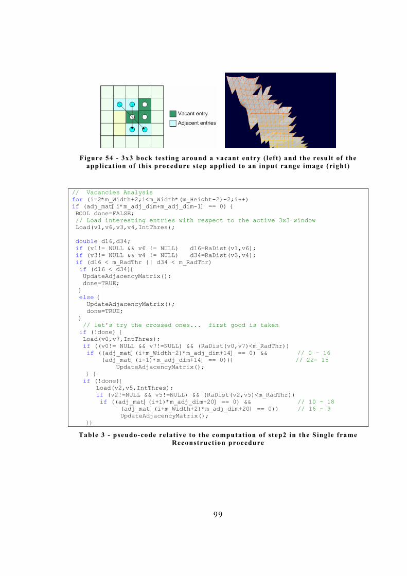
99

Figure 54 - 3x3 bock test ing around a vacant entry ( left) and the result of the

applicat ion of this procedure step applied to an input range image (right)

// Vacancies Analysis for (i=2*m_Width+2;i<m_Width*(m_Height-2)-2;i++) if (adj_mat[i*m_adj_dim+m_adj_dim-1] == 0) { BOOL done=FALSE; // Load interesting entries with respect to the active 3x3 window Load(v1,v6,v3,v4,IntThres); double d16,d34; if (v1!= NULL && v6 != NULL) d16=RaDist(v1,v6); if (v3!= NULL && v4 != NULL) d34=RaDist(v3,v4); if (d16 < m_RadThr || d34 < m_RadThr) if (d16 < d34){ UpdateAdjacencyMatrix(); done=TRUE; } else { UpdateAdjacencyMatrix(); done=TRUE; } // let's try the crossed ones... first good is taken if (!done) { Load(v0,v7,IntThres); if ((v0!= NULL && v7!=NULL) && (RaDist(v0,v7)<m_RadThr)) if ((adj_mat[(i+m_Width-2)*m_adj_dim+14] == 0) && // 0 - 16 (adj_mat[(i-1)*m_adj_dim+14] == 0)){ // 22- 15 UpdateAdjacencyMatrix(); } } if (!done){ Load(v2,v5,IntThres); if (v2!=NULL && v5!=NULL) && (RaDist(v2,v5)<m_RadThr)) if ((adj_mat[(i+1)*m_adj_dim+20] == 0) && // 10 - 18 (adj_mat[(i+m_Width+2)*m_adj_dim+20] == 0)) // 16 - 9 UpdateAdjacencyMatrix(); }}

Table 3 - pseudo-code relat ive to the computat ion of step2 in the Single frame Reconstruct ion procedure

100

The results demonstrated that this step is able to fil l some holes remained after the application of step_1 and to improve the result of the reconstruction (Figure 54). Unfortunately, too many holes remain in the final mesh and another step is necessary.

Step 3: Improve connections, find feasible semi-diagonals In order to improve the resulting mesh the method tries to find feasible semi-diagonal connections. For each 3×3 window in the input lattice we check for the possible eight semi-diagonal edges among the entries at the boundary of the window (Figure 55.right). At most two of the feasible semi-diagonal edges can coexist and the method searches for them (Table 4).

// Search for Horizontal Semi-Diagonals in a 3x3 block for (i=0;i<m_Width*(m_Height-1)-2;i++) { // first check BOOL done = FALSE; if (adj_mat[(i+1)*m_adj_dim+4] == 1) done = TRUE; else if ((adj_mat[(i+1)*m_adj_dim+5] == 1) || ((i>=m_Width) && (adj_mat[(i-m_Width+1)*m_adj_dim+5]==1))) done = TRUE; if (!done) { // descendant semi-diagonal Load (v0,v1,IntThres); if (v0!=NULL && v1!= NULL) if (CheckOnAdjacencyMatrix()) UpdateAdjacencyMatrix(); } if (!done) { // ascendant semidiag Load (v0,v1,IntThres); if(v0!=NULL && v1!=NULL) if(CheckOnAdjacencyMatrix()) { UpdateAdjacencyMatrix(); done = TRUE; } } } // Search for Vertical Semi-Diagonals for (i=0;i<m_Width*(m_Height-2)-1;i++) { // first check BOOL done = FALSE; if (adj_mat[(i+m_Width)*m_adj_dim+10]==1) done = TRUE; else if ((adj_mat[(i+m_Width+1)*m_adj_dim+23]==1)|| (adj_mat[(i+m_Width)*m_adj_dim+11]==1)) done = TRUE; if (!done) { // descendent semi-diagonal Load (v0,v1,IntThres); if (v0 != NULL && v1 != NULL) if(CheckOnAdjacencyMatrix()) { UpdateAdjacencyMatrix(); done = TRUE; if (!done) { // ascendant semi-diagonal Load (v0,v1,IntThres); if (v0!=NULL && v1!=NULL) if CheckOnAdjacencyMatrix()) { UpdateAdjacencyMatrix(); done = TRUE; } }}}

Table 4 � pseudo-code relat ive to the computat ion of step3 in the Single frame Reconstruct ion procedure.

101

Step 4: Mesh generation The last step of our procedure generates the final triangular mesh by forming faces as cycles of three edges (Figure 56).

For each location v in the lattice, the method scans the portion of adjacency list (that has been populated during the three steps above spanned) by the first 12 bits of the bit vector encoding it (Figure 55) (the remaining edges in the list will be considered from other vertices).

Figure 55 - the adjacency vector of an entry in the latt ice ( left) - a 3x3 block for

test ing for feasible semi-diagonals (r ight)

For each pair of consecutive edges in the list, a triangle of the mesh is generated. A filter can be also applied based on the perimeters of faces, to obtain a smoother distribution of face dimensions, and to overcome limitations due to the radial nature of the distance (used to test for point connectivity).

Figure 56 - the result of the applicat ion of the SingleFrameReconstruct ion()

procedure.

102

The procedure cuts also isolated vertices and computes the normal vectors for faces and vertices adding them to the mesh structure. The normal computation is split into two phases.

1. Compute normals for faces by taking the external product of two independent unit vectors lying on the face itself.

2. For each vertex, compute the relative normal by taking the vector sum of the faces� normals sharing the active vertex (the neighborhood faces of the vertex).

The connectivity information coming from the mesh is used to discard connected components smaller than a given size. This step, called size filter , greatly improves the quality of the acoustic images.

Figure 57 - Ti l ing of four meshes with different v isual ization options (from top-left to bottom-right: smooth, s imple faces, wireframe with curvature, wireframe

and s imple faces) .

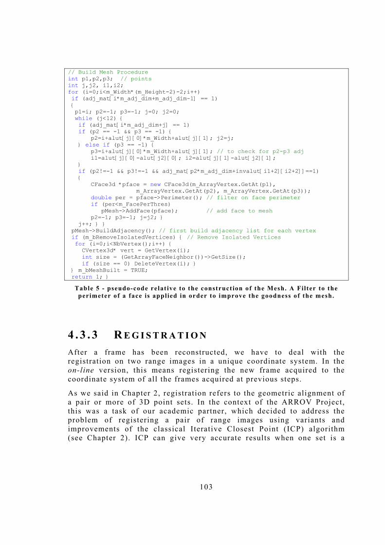
103

// Build Mesh Procedure int p1,p2,p3; // points int j,j2, i1,i2; for (i=0;i<m_Width*(m_Height-2)-2;i++) if (adj_mat[i*m_adj_dim+m_adj_dim-1] == 1) { p1=i; p2=-1; p3=-1; j=0; j2=0; while (j<12) { if (adj_mat[i*m_adj_dim+j] == 1) if (p2 == -1 && p3 == -1) { p2=i+alut[j][0]*m_Width+alut[j][1]; j2=j; } else if (p3 == -1) { p3=i+alut[j][0]*m_Width+alut[j][1]; // to check for p2-p3 adj i1=alut[j][0]-alut[j2][0]; i2=alut[j][1]-alut[j2][1]; } if (p2!=-1 && p3!=-1 && adj_mat[p2*m_adj_dim+invalut[i1+2][i2+2]]==1) { CFace3d *pface = new CFace3d(m_ArrayVertex.GetAt(p1), m_ArrayVertex.GetAt(p2), m_ArrayVertex.GetAt(p3)); double per = pface->Perimeter(); // filter on face perimeter if (per<m_FacePerThres) pMesh->AddFace(pface); // add face to mesh p2=-1; p3=-1; j=j2; } j++; } } pMesh->BuildAdjacency(); // first build adjacency list for each vertex if (m_bRemoveIsolatedVertices) { // Remove Isolated Vertices for (i=0;i<NbVertex();i++) { CVertex3d* vert = GetVertex(i); int size = (GetArrayFaceNeighbor())->GetSize(); if (size == 0) DeleteVertex(i); } } m_bMeshBuilt = TRUE; return 1; }

Table 5 - pseudo-code relat ive to the construct ion of the Mesh. A Filter to the perimeter of a face is applied in order to improve the goodness of the mesh.

4 . 3 . 3 R E G I S T R A T I O N After a frame has been reconstructed, we have to deal with the registration on two range images in a unique coordinate system. In the on-line version, this means registering the new frame acquired to the coordinate system of all the frames acquired at previous steps.

As we said in Chapter 2, registration refers to the geometric alignment of a pair or more of 3D point sets. In the context of the ARROV Project, this was a task of our academic partner, which decided to address the problem of registering a pair of range images using variants and improvements of the classical Iterative Closest Point (ICP) algorithm (see Chapter 2). ICP can give very accurate results when one set is a

104

subset of the other, but results deteriorate with pairs of partially overlapping range images. In this case, the overlapping surface portions must start very close to each other to ensure convergence, making the initial position a critical parameter [22].

Briefly, in order to be able to work on-line, ICP needs to be modified. In general, the speed enhancement of ICP algorithm can be achieved by: reducing the number of iterations necessary to converge and reducing the time spent at each iteration [21].

In the offline version, during the first phase a table is generated describing which frames overlap and successively, a global ICP is used, distributing registration errors evenly across all views [21].

4 . 3 . 4 G E O M E T R I C F U S I O N In general, the meshes built on the single frames, when represented in the same coordinate system, after registration, will freely overlap and intersect. Jumps, cracks and redundant surfaces will occur at overlaps (Figure 58). Thus, the simple collection of such meshes is not sufficient to give a final mosaic of the sensed objects. Meshes must undergo a process of geometric fusion , which produces a single mesh starting at the various registered meshes. If the fusion is to be done in off-line framework, algorithms proposed in [26], [29] serve well the purpose.

Here, we concentrate on the on-line version of the problem. In this case, at a given instant of time, a mesh A is given, which represents the mosaic obtained from all previous frames, and a new mesh B comes, which is built from the current frame as explained in Section 4.3.2.

The aim is to merge such meshes in a consistent way, in order to obtain a new mesh R , which represents the scene spanned by both A and B . This must be a fast process, since the system must support real time visualization of the mosaic at each frame. In particular, the output of the algorithm must be used to update the graphical system with the new primitives to be rendered. Unfortunately, this is not simply an incremental process in which new graphical primitives are added to the existing ones at each new frame. Indeed, the fusion operation may change the portion of A that overlaps with B (and it must overlap, otherwise registration would fail).

105

Figure 58 - some faces may overlap after mult iple s ingle frame meshes have been

added at the model .

This means that some primitives rendered in previous frames will have to be substituted with new ones. Eventually, this means that display lists used by the graphics system will have to be regenerated. This operation can be expensive if applied to the entire mesh, and it could slow down the system.

Because of observations above, we decided to modify the method of the Marching Intersection Algorithm (MIA) [26], which exhibits an interesting approach, since it allows a valid trade-off between speed and accuracy and, by the use of quality parameters, i t takes into account the reliability of input data.

As we already explained in Chapter 3, the original MIA is based on a volumetric approach that locates the geometric intersections between the meshes built on single frames and a virtual 3D reference grid. Intersections are first merged and the output mesh is found by joining intersection points that belong to edges of the same cell , through a scheme defined in a lookup table.

In order to make it applicable to an on-line setting , we have modified the algorithm to deal with a pre-computed mesh A (as explained before) which fits the reference grid (i .e. , i t has i ts vertices on grid edges, and each face is completely contained in a grid cell), and a new mesh B which intersects the grid properly. Furthermore, in order to support real time rendering , we have developed a lazy update strategy for display lists, which reduces the load per frame on the graphics system.

106

So the mosaicing algorithm can be divided into three main phases:

1. Rasterization and Intersection management

2. Fusion, with cleaning and removal operations

3. Mesh generation and Lazy Update

It takes as input:

• a single frame mesh SFM with time stamp t

• a registration matrix RM in homogeneous coordinates, which describes current position and orientation of the sensor in a global coordinate system

• a grid resolution value GR (positive real) representing the edge length of square cells in which 3D space is subdivided

• a fusion threshold value FT (positive real) representing the minimum distance between two vertices generated by different frames (The Fusion threshold is usually kept lower than grid resolution)

• an updating threshold value UT (positive real) representing the maximum number of changes in a mesh before a new list must be generated for visualization

The Fusion Procedure produces in output:

• a time stamp t (the same of the input)

• a list of meshes, in which each mesh represents a new portion of mosaic or a modified one, and has a name and the information on the number of triangles in that mesh

• a list of triangles where each triangle is a triple of points (each point represented in a global coordinate system with Cartesian coordinates (x, y,z)).

Phase 1: Rasterization and Intersection Management This part of the algorithm analyzes every face fq of one of the registered meshes, searching for intersections with the virtual underlying grid G (the other is the actual mosaic and therefore is already aligned at the grid).

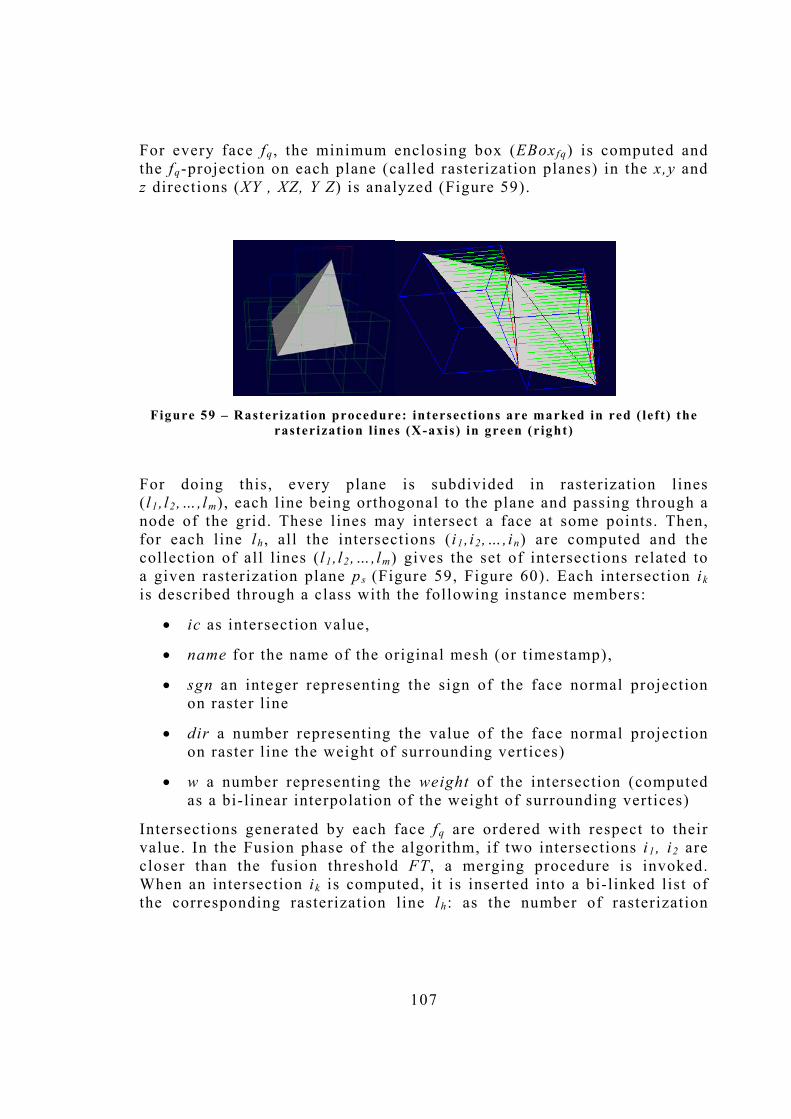
107

For every face fq , the minimum enclosing box (EBoxf q) is computed and the fq-projection on each plane (called rasterization planes) in the x,y and z directions (XY , XZ, Y Z) is analyzed (Figure 59).

Figure 59 � Rasterizat ion procedure: intersect ions are marked in red ( left) the

rasterizat ion l ines (X-axis) in green (right)

For doing this, every plane is subdivided in rasterization lines (l1, l2 ,�,lm), each line being orthogonal to the plane and passing through a node of the grid. These lines may intersect a face at some points. Then, for each line lh , all the intersections (i1,i2,�,in) are computed and the collection of all lines (l1 ,l2 ,�,lm) gives the set of intersections related to a given rasterization plane ps (Figure 59, Figure 60). Each intersection i k is described through a class with the following instance members:

• ic as intersection value,

• name for the name of the original mesh (or timestamp),

• sgn an integer representing the sign of the face normal projection on raster line

• dir a number representing the value of the face normal projection on raster line the weight of surrounding vertices)

• w a number representing the weight of the intersection (computed as a bi-linear interpolation of the weight of surrounding vertices)

Intersections generated by each face fq are ordered with respect to their value. In the Fusion phase of the algorithm, if two intersections i1, i2 are closer than the fusion threshold FT , a merging procedure is invoked. When an intersection i k is computed, it is inserted into a bi-linked list of the corresponding rasterization line lh : as the number of rasterization

108

lines is very big, we chose to represent a rasterization plane as an associative collection (hash table) of lists, keeping therefore only those structures containing real intersections.

Every time we instantiate a new list, i t is also added to a structure that contains all the updated or generated list of the current frame: this structure is a queue (FIFO type) that is scanned during the fusion phase.

Note that, we assume that underlying grid to have no bounds, that is, to be virtually infinite. Therefore we have to generate for each pair of coordinates a unique key as a function k=f(x,y) that describes the rasterization line: unfortunately it is quite difficult to find such a function. For sake of simplicity we chose k(x,y) = A ⋅x+y , where A is a constant (usually big). Of course, it is possible for collisions to occur, but for a medium sized mosaic this is quite unlikely.

Actually the hash function is defined in three dimensions as k(x,y,z)=A ·x+B ·y+C ·z and it is used both on the rasterization planes (setting z to zero) and on the whole 3-D mosaic for cell 's indexing purposes

Figure 60 - Cel ls , edges and intersect ion ( in red)

As we said before, each intersection (object) has a weight w , which measures the reliability of the data and it is used in the fusion phase. The weight is computed by linearly interpolating the intensity values of the vertices that describe the current face. If d0, d1, d2 are the distances of the intersection point from the vertices, and I0, I1, I2 are their intensities, then the weight w is defined as follow:

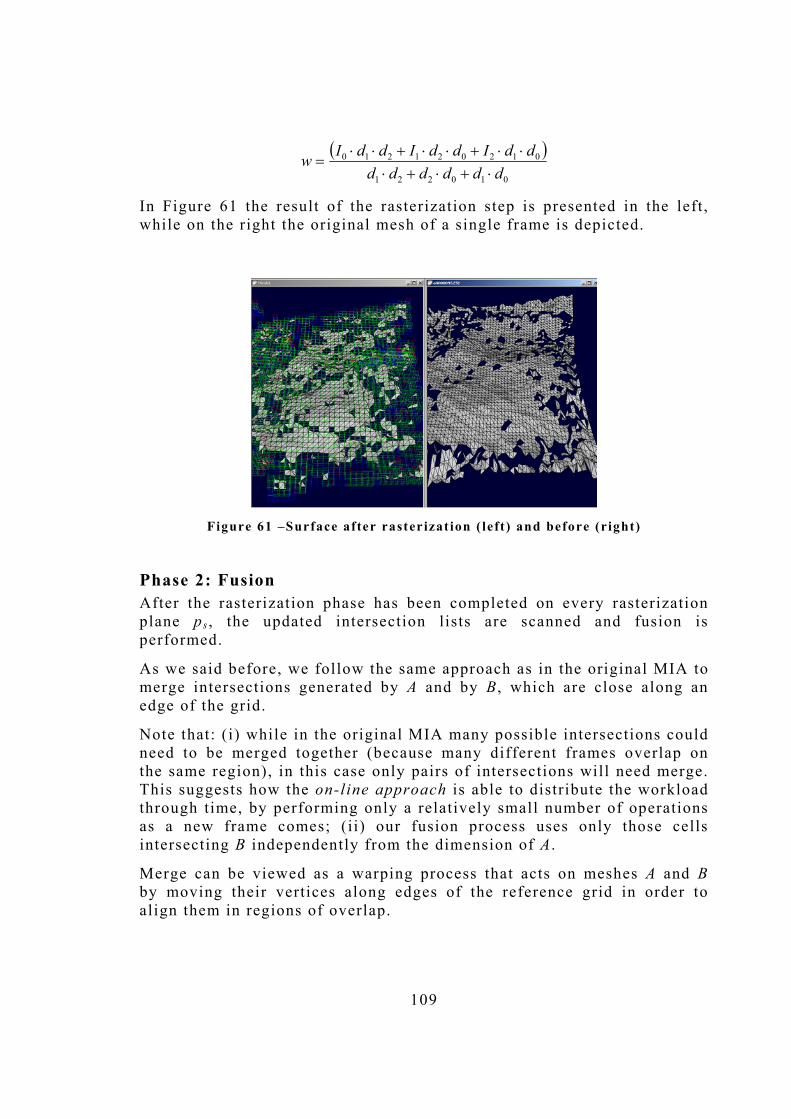
109

( )010221

012021210

ddddddddIddIddIw

⋅+⋅+⋅⋅⋅+⋅⋅+⋅⋅

=

In Figure 61 the result of the rasterization step is presented in the left, while on the right the original mesh of a single frame is depicted.

Figure 61 �Surface after raster izat ion ( left) and before (right)

Phase 2: Fusion After the rasterization phase has been completed on every rasterization plane ps , the updated intersection lists are scanned and fusion is performed.

As we said before, we follow the same approach as in the original MIA to merge intersections generated by A and by B , which are close along an edge of the grid.

Note that: (i) while in the original MIA many possible intersections could need to be merged together (because many different frames overlap on the same region), in this case only pairs of intersections will need merge. This suggests how the on-line approach is able to distribute the workload through time, by performing only a relatively small number of operations as a new frame comes; (ii) our fusion process uses only those cells intersecting B independently from the dimension of A .

Merge can be viewed as a warping process that acts on meshes A and B by moving their vertices along edges of the reference grid in order to align them in regions of overlap.

110

For every intersection lists (associated with a rasterization line lh), each couple of consecutive intersections i1 and i2 with different name (or timestamp - t1≠ t2) and concordant signs are merged together if their distance is shorter than the fusion threshold FT taking into account the reliability of the measurement:

( ) ( )( )

( )

});,(

;

;

{sgnsgn;,,

213

21

21

2211

2121

321

iiFusioniFTDif

dicic

D

wwdirwdirwd

ttifiiiIC

ii

ii

iiii

iiii

=<

−=

+⋅+⋅

=

=∧≠

The term d in the previous expression takes into account the fact that fusion is performed along the grid lines rather than on minimum distance direction. This operation corresponds to merge two concordant surfaces, which cross the same virtual cell edge.

If the two intersections i1 , i2 lie on different virtual cells, then the fusion operator performs a shift of the intersections toward the new average location.

During this operation, whenever we move from a virtual cell to another, a couple of artificial intersections are created on all the perpendicular virtual edges the intersection touches. When a new intersection is generated, the algorithm analyzes the other intersections on the same virtual edge in order to verify if a removal operation can be applied.

The removal operation is performed on the currently updated raster lines (l1,�,lq), that is where a new intersection has been created. A removal action (which removes two intersections from the current raster line) is performed on each pair of intersections (i1,i2) which:

- l ie on the same edge cell ec ,

- have the same name (or timestamp t i1=t i2), and

- have different signs sgn i1 ≠sgn i 2 .

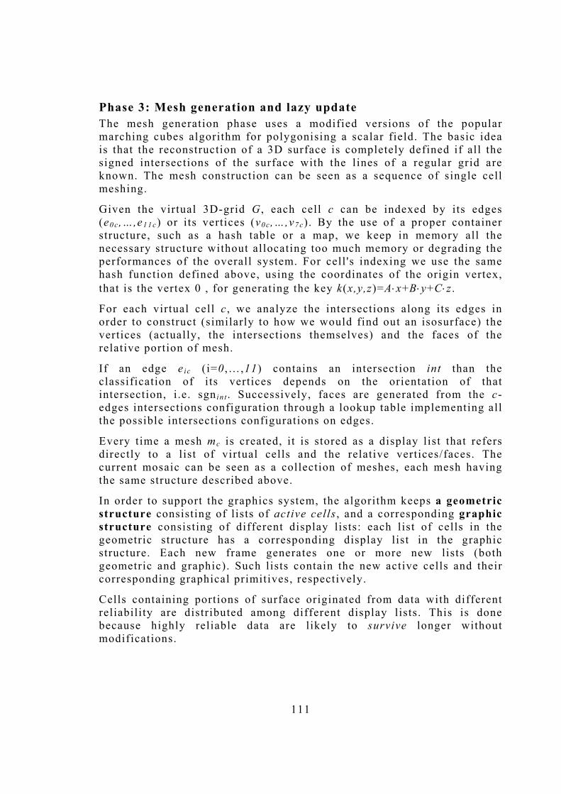
111

Phase 3: Mesh generation and lazy update The mesh generation phase uses a modified versions of the popular marching cubes algorithm for polygonising a scalar field. The basic idea is that the reconstruction of a 3D surface is completely defined if all the signed intersections of the surface with the lines of a regular grid are known. The mesh construction can be seen as a sequence of single cell meshing.

Given the virtual 3D-grid G , each cell c can be indexed by its edges (e0 c,�,e1 1c) or its vertices (v0c,�,v7 c). By the use of a proper container structure, such as a hash table or a map, we keep in memory all the necessary structure without allocating too much memory or degrading the performances of the overall system. For cell 's indexing we use the same hash function defined above, using the coordinates of the origin vertex, that is the vertex 0 , for generating the key k(x,y,z)=A ⋅x+B ⋅y+C ⋅z .

For each virtual cell c , we analyze the intersections along its edges in order to construct (similarly to how we would find out an isosurface) the vertices (actually, the intersections themselves) and the faces of the relative portion of mesh.

If an edge ei c (i=0 ,�,11) contains an intersection int than the classification of its vertices depends on the orientation of that intersection, i .e. sgn i n t . Successively, faces are generated from the c-edges intersections configuration through a lookup table implementing all the possible intersections configurations on edges.

Every time a mesh mc is created, it is stored as a display list that refers directly to a l ist of virtual cells and the relative vertices/faces. The current mosaic can be seen as a collection of meshes, each mesh having the same structure described above.

In order to support the graphics system, the algorithm keeps a geometric structure consisting of lists of active cells , and a corresponding graphic structure consisting of different display lists: each list of cells in the geometric structure has a corresponding display list in the graphic structure. Each new frame generates one or more new lists (both geometric and graphic). Such lists contain the new active cells and their corresponding graphical primitives, respectively.

Cells containing portions of surface originated from data with different reliability are distributed among different display lists. This is done because highly reliable data are likely to survive longer without modifications.

112

Old active cells that were modified by processing the new frame B are updated in the geometric structure, and each update increases a request value for the relative display list.

In order to speed-up the process of the on-line mosaicing, we decided to implement a lazy update approach of the display lists, giving out to the Viewer only the newly generated display lists and those display lists for which the amount of changes exceeds the update threshold UT .

So, meshes received by a Viewer at a given frame can be of two kinds:

• New mesh: a mesh that was generated in the current frame. In this case, this mesh must be added to the collection held by the Viewer.

• Modified mesh: a mesh that was generated in a previous frame and modified in the current frame. In this case, this mesh must substitute the mesh having the same name in the collection held by the Viewer. An empty mesh, i .e. , a mesh with zero triangles, means that the mesh with the same name must be deleted from the collection held by the Viewer.

A modified mesh can be discriminated from a new mesh on the basis of existence of his name in the collection of meshes that form the current mosaic.

4.4 Results The following section is dedicated to show results obtained for each subsection of the ARROV pipeline. In particular, we report images and function timings for the Registration and Geometric Fusion Steps. At the end of the section, conclusions and future works are listed.

Single Frame Reconstruction The single frame reconstruction algorithm has been successfully implemented and tested over 3D echoscope data (Figure 57, Figure 64). The results show that a good mesh reconstruction is obtained via a local analysis of the spatial properties of the 3D data, by exploiting the structure of the echoscope sensor.

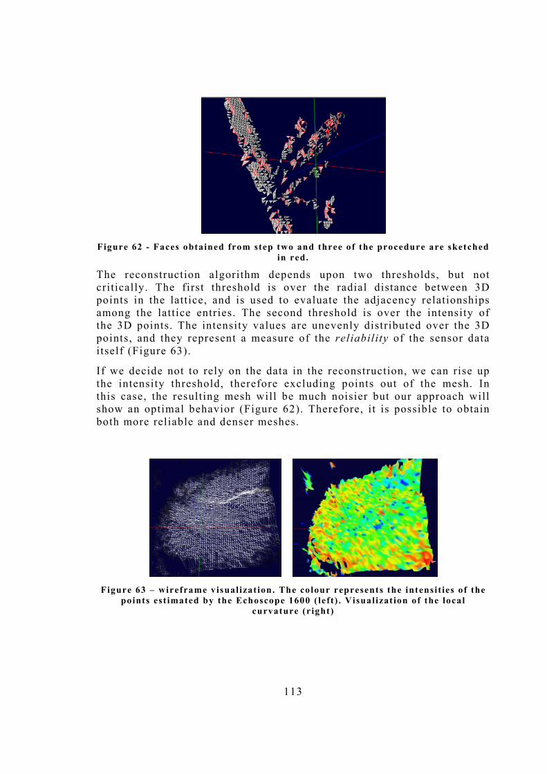
113

Figure 62 - Faces obtained from step two and three of the procedure are sketched

in red.

The reconstruction algorithm depends upon two thresholds, but not critically. The first threshold is over the radial distance between 3D points in the lattice, and is used to evaluate the adjacency relationships among the lattice entries. The second threshold is over the intensity of the 3D points. The intensity values are unevenly distributed over the 3D points, and they represent a measure of the reliability of the sensor data itself (Figure 63).

If we decide not to rely on the data in the reconstruction, we can rise up the intensity threshold, therefore excluding points out of the mesh. In this case, the resulting mesh will be much noisier but our approach will show an optimal behavior (Figure 62). Therefore, it is possible to obtain both more reliable and denser meshes.

Figure 63 � wireframe visual izat ion. The colour represents the intensit ies of the

points est imated by the Echoscope 1600 ( left) . Visualizat ion of the local curvature (right)

114

Figure 64 - four different frames reconstructed by the

SingleFrameReconstruction() procedure.

Geometric Fusion: Function Timing The following experimental results have been obtained by elaborating a 10-frame sequence showing an underwater pole structure. Timings have been computed by software profiling, on a P4 1.5GHz, with 392MB Ram, on 10 experiments.

We chose 7 different rasterization steps, from a coarse (step=50) to a fine (step=20) spatial resolution. Note that spatial resolution depends on the input data range, which is not normalized, and can vary from case to case. Therefore the value of step=20 means a very fine sampling of the meshes in the current sequence. As we can see the rasterization step affects the total number of the cells, which compose the mosaic, and thus every following computation phase.

Looking at the results, we can remark that the fusion stage does not represent a bottleneck for the mosaic procedure while rasterization does.

We should also stress that rasterization is strongly affected by the size of the original mesh, while the other stages particularly depend on the chosen rasterization step.

115

Raster Step( int)

Mosaic Cel ls (msec)

Raster izat ion (msec)

Cel l ' s Update (msec)

Fusion (msec)

Meshing (msec)

20 14670 587.8 476.6 35.9 1930.5

25 8505 280.9 330.3 29.5 1270.9

30 4343 195.7 247.9 27.5 814.9

35 4010 168.2 217.7 11.2 649.8

40 1521 105.7 134.1 8.6 408

45 1135 62.0 108.6 5.4 285.3

50 942 51.1 91.2 4.5 264.6

Table 6 � rasterizat ion steps, from a coarse (step = 50) to a f ine (step = 20) spat ial resolut ion and relat ive t iming form the reconstruction procedures

Figure 65 -Graphical t iming behavior of the reconstruction phases. ( left)

Rasterizat ion step (x axis) vs mosaic cel ls number (y axis) . (r ight) Time consumption vs rasterizat ion step: red (rasterizat ion), blue (cel l

update) , green (fusion), purple (meshing)

In conclusion, we presented a complete Data Analysis Framework developed in the context of the European ARROV project which supports real-time 3D scene reconstruction from a sequence of range data acquired by an acoustic camera (Echoscope 1600) mounted on a ROV.

The Single Frame Reconstruction algorithm depends upon two thresholds, but not crit ically (radial distance and intensity). The intensity values are unevenly distributed over the 3D points, and they represent a measure of the reliability of the sensor data itself (Figure 63).

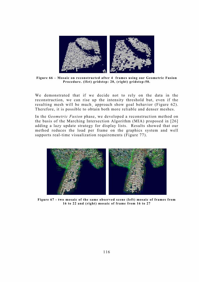
116

Figure 66 � Mosaic on reconstructed after 4 frames using our Geometric Fusion

Procedure. ( lfet) gridstep: 20, (r ight) gridstep:50.

We demonstrated that if we decide not to rely on the data in the reconstruction, we can rise up the intensity threshold but, even if the resulting mesh will be much¸ approach show goal behavior (Figure 62). Therefore, it is possible to obtain both more reliable and denser meshes.

In the Geometric Fusion phase, we developed a reconstruction method on the basis of the Marching Intersection Algorithm (MIA) proposed in [26] adding a lazy update strategy for display lists. Results showed that our method reduces the load per frame on the graphics system and well supports real-time visualization requirements (Figure 77).

Figure 67 - two mosaic of the same observed scene ( left) mosaic of frames from

16 to 22 and (right) mosaic of frame from 16 to 27

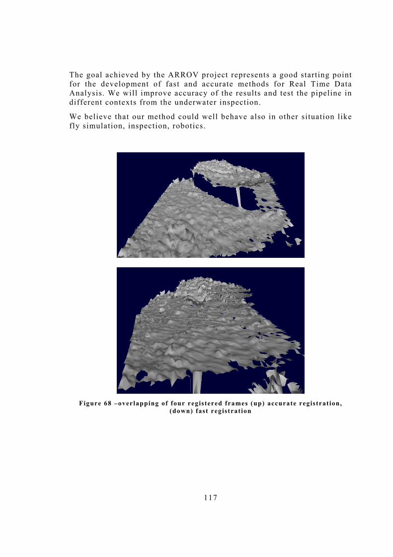
117

The goal achieved by the ARROV project represents a good starting point for the development of fast and accurate methods for Real Time Data Analysis. We will improve accuracy of the results and test the pipeline in different contexts from the underwater inspection.

We believe that our method could well behave also in other situation like fly simulation, inspection, robotics.

Figure 68 �overlapping of four registered frames (up) accurate registrat ion,

(down) fast registrat ion

118

5. Modeling with Uncertainty

The mismatch problem: we have a gray world but a black & white science

[Bart Kosko]

A proper Surface Reconstruction method can produce a good result if the object surface is sufficiently sampled. Sufficiency conditions are not so simple to determine. We showed that almost all the algorithms, described in the state-of-the-art section (Chapter 3), for working in a satisfactory manner, make strong assumptions on the goodness of the sampling dataset, but do not formally explain under what conditions this happens.

Exceptions can be found in the cases of Attali [8], which gives a formal definition of a sufficient sampling, of Bernardini, Bajaj [12] and of Amenta et al.[2]. If, from one side, sampling conditions analysis can lead to good theoretical (and practical) results, from the other side, it is interesting to use ALL the information coming from the modern sensors, integrating enriched data in a unique automatic system. Some methods try to overcome to sampling conditions limitations: the Zippering method of Turk et al. [101] that adds weights to the input data in order to merge meshes coming from different range images and the method of Cignoni et al. [26], which explicitly use a reliability value associated to each input points, are two examples.

In this sense goes our research, outlined in this Chapter: we will present a framework, in which we consider enriched measurements coming from different sensors that will be integrated. We use a set of measurements with some properties added to them and build the object surface approximating the input data points using the additional information. The dataset is considered enriched in the sense that it can have also: a model error on the spatial positions of points, a model error on the estimated normal vectors for each point, ad estimation of the reliability of each point and so on.

This chapter presents our results: first , a brief introduction to the problem is presented; then we outline the proposed method, showing results and, finally, we list future works and open Issues.

119

5.1 Multi-sensors Data Fusion Thanks to modern acquisition technologies, we can deal with heterogeneous enriched data1 that come from multiple acquisition devices. The problem is how to integrate all these information in a unique system in order to get significant results.

The framework in which we developed our method is a Multi-sensors Data Fusion framework in which the means and tools for the integration of data from multiple sensors are expressed. In this framework, it is possible to produce different data with different levels of precision also in cases in which data might be corrupted (Figure 69).

The basic concept of our approach is Uncertainty : lack of knowledge, which cannot be predicted and may be caused, e.g. from inadequate model etc. In case of multiple acquisition technologies, there are different types of uncertainty:

• Incompleteness: sensors possibly leave something out.

• Imprecision : sensors can provide only approximate information.

• Inconsistency: sensors data may not always agree with each other.

• Ambiguity: data from various sensors may be indistinguishable from one another.

The goal of a Multi-sensors Data Fusion Approach is to deal with uncertain sampled input dataset, to integrate them building a correct representation of these data in a common reference system.

We will consider 3D surface samples collected using different sensors of varying location and modality. Using measurement models, data collected from different sensors at different locations and resolutions can be combined in a formal way.

1 Not simply positional information (Cartesian coordinates) but also (for example) error, normal, curvature estimations.

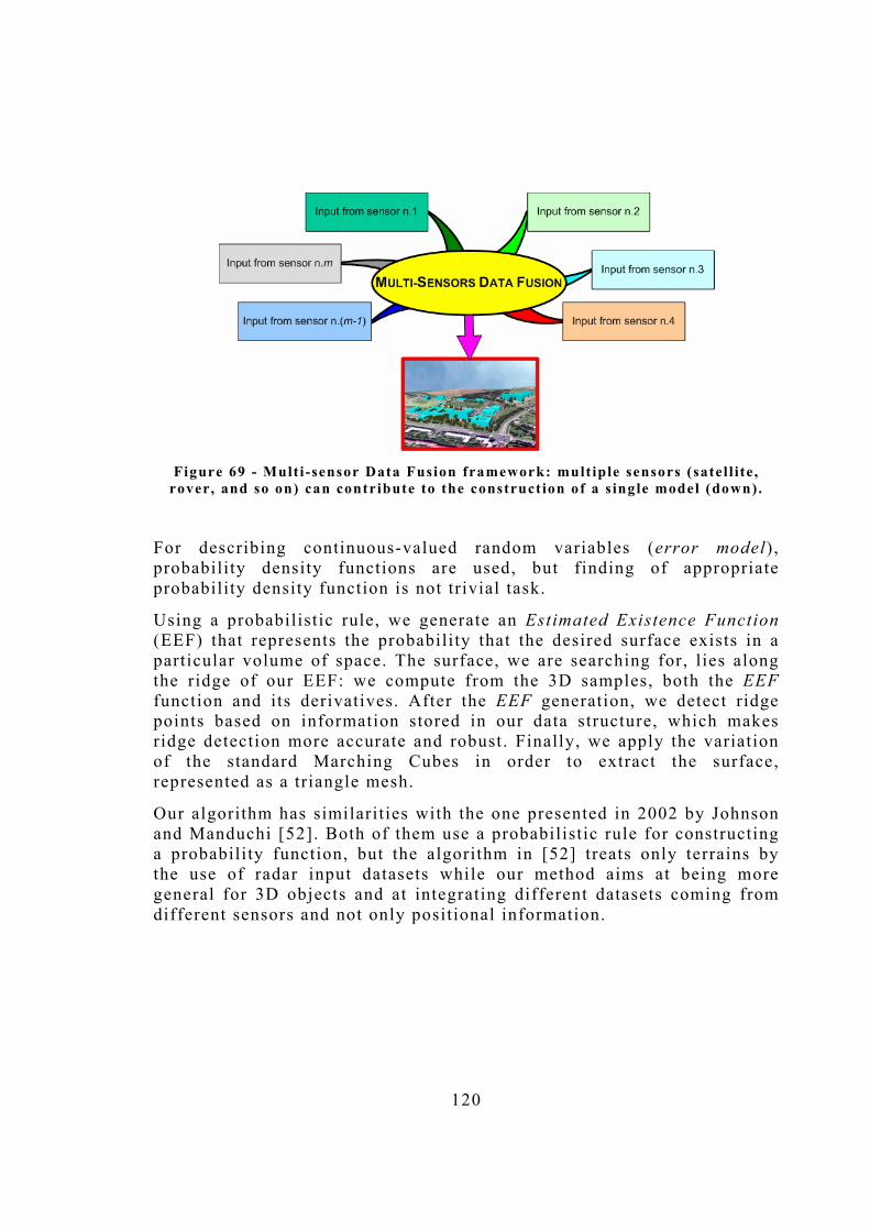
120

Figure 69 - Mult i-sensor Data Fusion framework: mult iple sensors (satel l ite ,

rover, and so on) can contribute to the construct ion of a s ingle model (down).

For describing continuous-valued random variables (error model), probability density functions are used, but finding of appropriate probability density function is not trivial task.

Using a probabilistic rule, we generate an Estimated Existence Function (EEF) that represents the probability that the desired surface exists in a particular volume of space. The surface, we are searching for, l ies along the ridge of our EEF: we compute from the 3D samples, both the EEF function and its derivatives. After the EEF generation, we detect ridge points based on information stored in our data structure, which makes ridge detection more accurate and robust. Finally, we apply the variation of the standard Marching Cubes in order to extract the surface, represented as a triangle mesh.

Our algorithm has similarities with the one presented in 2002 by Johnson and Manduchi [52]. Both of them use a probabilistic rule for constructing a probability function, but the algorithm in [52] treats only terrains by the use of radar input datasets while our method aims at being more general for 3D objects and at integrating different datasets coming from different sensors and not only positional information.

121

5.2 Problem Definition and proposed approach

From a mathematical point of view, the surface of a 3D object can be defined as a two-dimensional manifold that is compact, orientable and connected.

Our Surface Reconstruction problem can be formalized as follow:

Given a set of measurements V={µ1,�, µn} of an object (environment), coming from different sensors s1,�,sk. and a set of additional information M={M1,�,Mn} related to the given measurements in V, find a surface S⊂ℜ3 that approximates the observed object with bounded error ε.

Each Mi may contain properties related to the measurement µ i (e.g., RGB color of the measurement, geometric properties such as normal vector and local curvature) or measurement models (i .e, an error model, a reliability model, and so on).

Our idea is to define a Probability Density Function (PDF for short) for each measurement µ i integrating all the information present in the Mi. The PDF will indicate the degree of importance µ i in the building process of the desired surface F .

The PDFs related to measurements, help us in the construction of the Estimated Existence Function (EEF for short) and for building it , we define:

- Ux a suitable neighbourhood of a point x with x∈ℜ3

- P(µ is x) as the probability that µ measures a point in Ux

- P(x∈S) as P(S∩Ux ≠ ∅)

The probability P that, given a measurement µ , a point x is on the desired surface S of the observed object is

)()(

)()()(

xisPxisSxP

xisPxisSxPSxP

µµ

µµµ

⋅∈+

⋅∈=∈ (5.2.1)

122

If all the measurements come exactly from the surface than the probability that a given x measures the surface S at x is obviously 1 (maximum of information). If we have a generic point x and no measurements on it , we cannot infer anything on x. In this case, we adopt a conventional probability of ½ (minimum of information on x). Additionally, we have that:

)(1)( xisPxisP µµ −=

and from (5.2.1)

( )

( ))(121)(

)(121)(1)(

xMSxP

xisPxisPSxP

µµ

µµµ

+=∈

−+⋅=∈ (5.2.2)

where Mµ is the measurement model related to the measurement µ . The equation (5.2.2) shows that the probability P that a point x l ies on the surface S, given µ , is directly proportional to the value of the measurement model Mµ computed on x .

Given the input dataset in the form of n independent measurements µ1 ,�, µn , the Estimated Existence Function of a point x in space is the probability that x l ies on the desired surface S:

),,|()()( 1 nn SxPxPxEEF µµ K∈== (5.2.3)

( ) ( )

( ) ( )∏=

−−=−=

=+−=

=⋅∈

+⋅∈==

n

iii

ii

ii

iin

xisPianyforxisP

ianyforxisPianyforxisP

ianyforxisPianyforxisSxP

ianforxisPianforxisSxPxPxEEF

1

)(1211)(

211

)(21)(11

)()(

)()()()(

µµ

µµ

µµ

µµ

(5.2.4)

So we have:

∫=xU

dyyMxisP )()( µµ (5.2.5)

In cases of small Ux for each x , we can approximate the integral as follows:

123

)()()()( xEUxMdyyMxisP ix

Ui

x

≡≅= ∫ µµµ (5.2.6)

Where |Ux | is the volume of Ux . From equation (5.2.4), substituting symbols using (5.2.6) we have:

( ) ( )∏∏==

−−=−−==n

i

in

ii

n xExisPxPxEEF11

)(1211)(1

211)()( µ (5.2.7)

Equation (5.2.7) indicates our Estimated Existence Function for each point in space and how it depends on all the Models in M related to all the measurements µ in V . Once we have defined the EEF, we search for the characteristic points of the EEF , following the definition of Eberly et al [37] of a surface ridges on a volume.

For a rigorous definition of the ridge point of a function, we consider a function f(x ,y ,z):ℜ3"ℜ of class C2 . We indicate with f x , fy , f z the first partial derivatives of f regarding x ,y and z . The gradient of f is the carrier of the first partial derivatives of f , and it is defined as:

[ ]zyx ffff ,,=∇

A geometric interpretation of ∇f is that its direction is the direction of steepest ascent while the magnitude is the slope in that direction. Thus,

222

∂∂

+

∂∂

+

∂∂

=∇zf

yf

xff

describes the steepness of the hill t=f(x,y,z) at a point on the hill located at (x,y,z,f(x,y,z)).

The Hessian of f is a matrix having the second partial derivatives as entries.

=

zzzyzx

yzyyyx

xzxyxx

fffffffff

H

The Hessian H defines the curvature of f in a point x .

124

Let be [ ]321 ,, kkk and ( )TTT vvv 321 ,, respectively the eigenvalues and eigenvectors of �H where 321 kkk ≥≥ and v1 represents the direction of maximal changing of the gradient ∇ f . Positive (negative) values of ki corresponds to concavity (convexity) of the function f in the direction µ i .

A point x is a ridge point of type 3-1 (surface-on-a-volume) if 0)()(1 =∇⋅ xfxvT and 0)(1 >xk ; while it is a strong ridge point if:

0)()(1 =∇⋅ xfxvT , 0)(1 >xk and )()( 31 xkxk > (5.2.8)

This definition says that a point x in ℜ3 is a ridge point if the component of the gradient in the maximal changing direction is zero and the function is more concave than convex.

The set of points R={x∈ℜ3 | 0)()(1 =∇⋅ xfxvT and )()( 31 xkxk > } identifies the surface S we are searching for. If necessary, we can filter the set R choosing a new set R1⊆R such that R1={x∈ℜ3 | 0)()(1 =∇⋅ xfxvT ,

)()( 31 xkxk > and θ>)(xEEF } where θ is a suitable threshold.

5 . 2 . 1 B U I L D I N G T H E E E F F U N C T I O N We have derived the expression of the EEF function as follows:

( ) ( )∏∏==

−−=−−==n

i

in

ii

n xExisPxPxEEF11

)(1211)(1

211)()( µ

Under the hypothesis of n independent measurements µ1 ,�, µn . The independency of the measurements helps us in the definition of an incremental rule for the computation of the EEF which will speed the overall execution of the algorithm.

( ) )(211)(1

211)(

1

xfxExEEF nn

i

i −=−−= ∏=

where ( )∏=

−=n

i

in xExf1

)(1)(

So the Estimated Existence Function EEF(x) depends on a function fn(x) that can be computed incrementally. In fact:

( ) ( ) ( ) )()(1)(1)(1)( 11

1

xfxExExExf nin

i

iin −−

=

⋅−=−⋅−= ∏ (5.2.2.1)

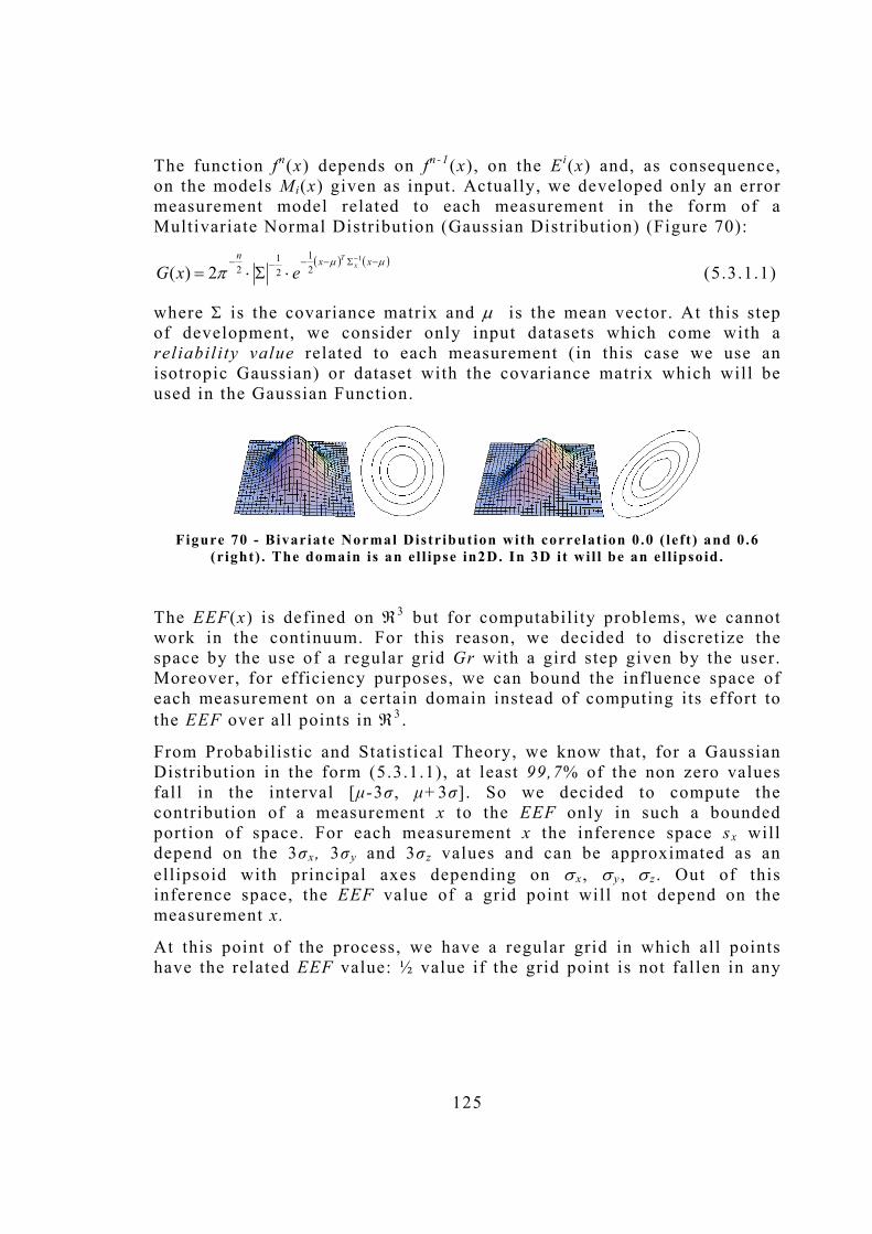
125

The function fn(x) depends on fn - 1(x), on the Ei(x) and, as consequence, on the models Mi(x) given as input. Actually, we developed only an error measurement model related to each measurement in the form of a Multivariate Normal Distribution (Gaussian Distribution) (Figure 70):

( ) ( )µµπ

−Σ−−−− −

⋅Σ⋅=xxn

xT

exG1

21

21

22)( (5.3.1.1)

where Σ is the covariance matrix and µ is the mean vector. At this step of development, we consider only input datasets which come with a reliability value related to each measurement (in this case we use an isotropic Gaussian) or dataset with the covariance matrix which will be used in the Gaussian Function.

Figure 70 - Bivariate Normal Distribution with correlat ion 0.0 ( left) and 0.6

(right) . The domain is an el l ipse in2D. In 3D it wil l be an el l ipsoid.

The EEF(x) is defined on ℜ3 but for computability problems, we cannot work in the continuum. For this reason, we decided to discretize the space by the use of a regular grid Gr with a gird step given by the user. Moreover, for efficiency purposes, we can bound the influence space of each measurement on a certain domain instead of computing its effort to the EEF over all points in ℜ3 .

From Probabilistic and Statistical Theory, we know that, for a Gaussian Distribution in the form (5.3.1.1), at least 99,7% of the non zero values fall in the interval [µ-3σ , µ+3σ]. So we decided to compute the contribution of a measurement x to the EEF only in such a bounded portion of space. For each measurement x the inference space sx will depend on the 3σx , 3σy and 3σ z values and can be approximated as an ellipsoid with principal axes depending on σx , σy , σ z . Out of this inference space, the EEF value of a grid point will not depend on the measurement x.

At this point of the process, we have a regular grid in which all points have the related EEF value: ½ value if the grid point is not fallen in any

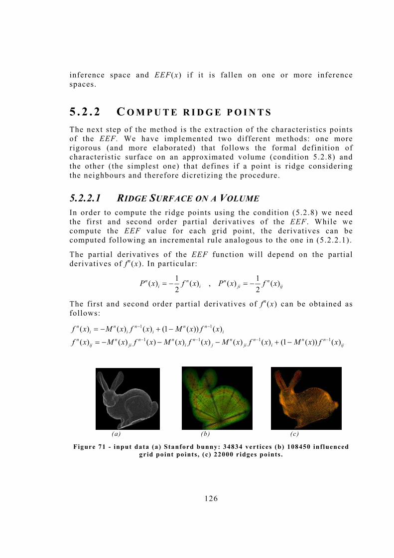
126

inference space and EEF(x) if it is fallen on one or more inference spaces.

5 . 2 . 2 C O M P U T E R I D G E P O I N T S The next step of the method is the extraction of the characteristics points of the EEF. We have implemented two different methods: one more rigorous (and more elaborated) that follows the formal definition of characteristic surface on an approximated volume (condition 5.2.8) and the other (the simplest one) that defines if a point is ridge considering the neighbours and therefore dicretizing the procedure.

5.2.2.1 RIDGE SURFACE ON A VOLUME In order to compute the ridge points using the condition (5.2.8) we need the first and second order partial derivatives of the EEF . While we compute the EEF value for each grid point, the derivatives can be computed following an incremental rule analogous to the one in (5.2.2.1).

The partial derivatives of the EEF function will depend on the partial derivatives of fn(x). In particular:

ijn

jin

in

in xfxPxfxP )(

21)(,)(

21)( −=−=

The first and second order partial derivatives of fn(x) can be obtained as follows:

ijnn

in

jin

jn

inn

jin

ijn

inn

in

in

in

xfxMxfxMxfxMxfxMxf

xfxMxfxMxf

)())(1()()()()()()()(

)())(1()()()(1111

11

−−−−

−−

−+−−−=

−+−=

(a) (b) (c)

Figure 71 - input data (a) Stanford bunny: 34834 vert ices (b) 108450 inf luenced grid point points , (c) 22000 ridges points .

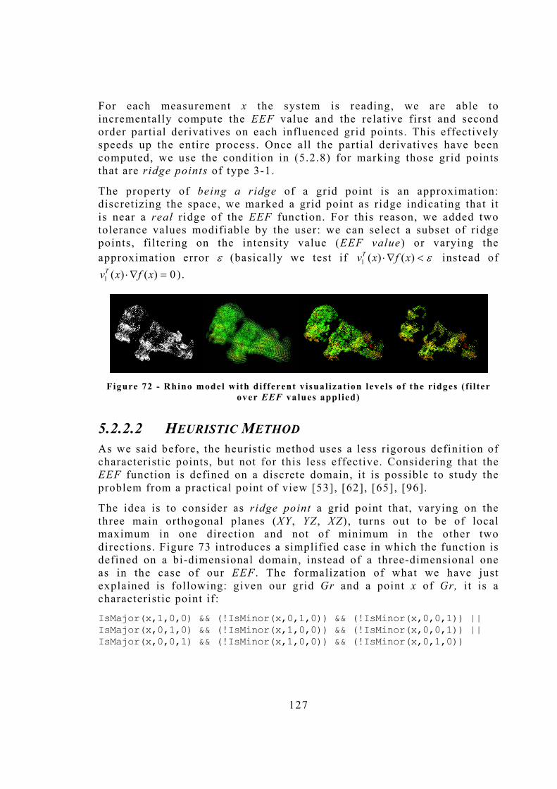
127

For each measurement x the system is reading, we are able to incrementally compute the EEF value and the relative first and second order partial derivatives on each influenced grid points. This effectively speeds up the entire process. Once all the partial derivatives have been computed, we use the condition in (5.2.8) for marking those grid points that are ridge points of type 3-1.

The property of being a ridge of a grid point is an approximation: discretizing the space, we marked a grid point as ridge indicating that it is near a real ridge of the EEF function. For this reason, we added two tolerance values modifiable by the user: we can select a subset of ridge points, filtering on the intensity value (EEF value) or varying the approximation error ε (basically we test if ε<∇⋅ )()(1 xfxvT instead of

0)()(1 =∇⋅ xfxvT ).

Figure 72 - Rhino model with different v isual izat ion levels of the ridges (f i lter

over EEF values applied)

5.2.2.2 HEURISTIC METHOD As we said before, the heuristic method uses a less rigorous definition of characteristic points, but not for this less effective. Considering that the EEF function is defined on a discrete domain, i t is possible to study the problem from a practical point of view [53], [62], [65], [96].

The idea is to consider as ridge point a grid point that, varying on the three main orthogonal planes (XY , YZ , XZ), turns out to be of local maximum in one direction and not of minimum in the other two directions. Figure 73 introduces a simplified case in which the function is defined on a bi-dimensional domain, instead of a three-dimensional one as in the case of our EEF . The formalization of what we have just explained is following: given our grid Gr and a point x of Gr, it is a characteristic point if:

IsMajor(x,1,0,0) && (!IsMinor(x,0,1,0)) && (!IsMinor(x,0,0,1)) || IsMajor(x,0,1,0) && (!IsMinor(x,1,0,0)) && (!IsMinor(x,0,0,1)) || IsMajor(x,0,0,1) && (!IsMinor(x,1,0,0)) && (!IsMinor(x,0,1,0))

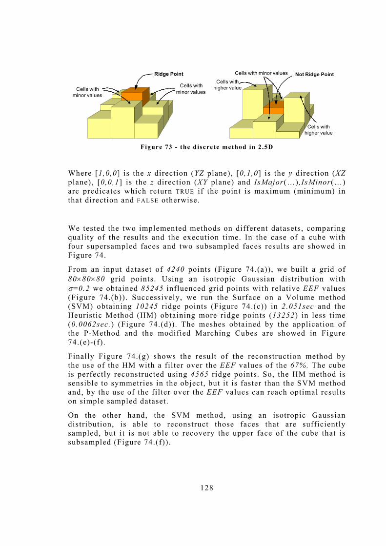
128

Ridge Point

Cells withminor valuesCells with

minor values

Cells with minor values Not Ridge PointCells with

higher value

Cells withhigher value

Figure 73 - the discrete method in 2.5D

Where [1,0,0] is the x direction (YZ plane), [0,1,0] is the y direction (XZ plane), [0,0,1] is the z direction (XY plane) and IsMajor(�) ,IsMinor(�) are predicates which return TRUE if the point is maximum (minimum) in that direction and FALSE otherwise.

We tested the two implemented methods on different datasets, comparing quality of the results and the execution time. In the case of a cube with four supersampled faces and two subsampled faces results are showed in Figure 74.

From an input dataset of 4240 points (Figure 74.(a)), we built a grid of 80×80×80 grid points. Using an isotropic Gaussian distribution with σ=0.2 we obtained 85245 influenced grid points with relative EEF values (Figure 74.(b)). Successively, we run the Surface on a Volume method (SVM) obtaining 10245 ridge points (Figure 74.(c)) in 2.051sec and the Heuristic Method (HM) obtaining more ridge points (13252) in less time (0.0062sec.) (Figure 74.(d)). The meshes obtained by the application of the P-Method and the modified Marching Cubes are showed in Figure 74.(e)-(f).

Finally Figure 74.(g) shows the result of the reconstruction method by the use of the HM with a filter over the EEF values of the 67%. The cube is perfectly reconstructed using 4565 ridge points. So, the HM method is sensible to symmetries in the object, but i t is faster than the SVM method and, by the use of the filter over the EEF values can reach optimal results on simple sampled dataset.

On the other hand, the SVM method, using an isotropic Gaussian distribution, is able to reconstruct those faces that are sufficiently sampled, but it is not able to recovery the upper face of the cube that is subsampled (Figure 74.(f)).

129

(a)

(b)

(c)

(d)

(e)

( f )

(g)

Figure 74 - Applicat ion of the SVM and HM methods on a cube input points , with isotropic gaussian distribution with s igms=0.2

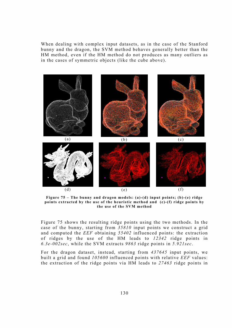
130

When dealing with complex input datasets, as in the case of the Stanford bunny and the dragon, the SVM method behaves generally better than the HM method, even if the HM method do not produces as many outliers as in the cases of symmetric objects (like the cube above).

(a)

(b)

(c)

(d) (e) (f)

Figure 75 � The bunny and dragon models: (a)-(d) input points; (b)-(e) ridge points extracted by the use of the heurist ic method and (c)-(f) r idge points by

the use of the SVM method

Figure 75 shows the resulting ridge points using the two methods. In the case of the bunny, starting from 35810 input points we construct a grid and computed the EEF obtaining 55402 influenced points: the extraction of ridges by the use of the HM leads to 12342 ridge points in 6.3e-002sec , while the SVM extracts 9863 ridge points in 5.921sec .

For the dragon dataset, instead, starting from 437645 input points, we built a grid and found 105600 influenced points with relative EEF values: the extraction of the ridge points via HM leads to 27463 ridge points in

131

0.125sec . , while the SVM extracts 14514 r idge points in definitely more seconds (12.75sec).

5 . 2 . 3 B U I L D I N G T H E M E S H Once all the ridges points have been computed, we need to build a final triangular mesh, which approximates the desired surface S . Our first idea was to march the cells of the grid, triangulating each triplet of ridge points. Unfortunately, this simple approach leads to too much approximating results (Figure 76): most of the marked ridges are on the desired surface but some of them are outliers.

Figure 76- results of the init ia l method without the use of the P-Method

In order to filter the set of ridges and to improve the result, we decided to implement a method that transmits the information of being a ridge from a vertex to an edge (or more edges). This is done with the application of a P-Method (Parabola-Method) which does the following:

! for each grid point gri , j , k in Gr , for each principal direction (x, y, z directions) (let us say con simplicity x direction)

o consider the parabola passing for the EEF values of the grid points gri - 1 , j , k , gri , j , k , gri+1 , j , k

o take the max (xm a x, ym a x, zma x) of the parabola (if it exists)

o consider the projection of this point: if i t falls in the interval [gri - 1 , j , k , gri , j , k] mark an intersection in this edge; if i t falls in

132

the interval [gri , j , k , gri +1 , j , k] mark an intersection in this edge. Otherwise do not mark and pass over.

The P-method works quite well for large datasets even if some outliers still remain. In any case, at the end of the procedure, we have the intersections in the edges of our grid and we can launch a modified Marching Cubes procedure [60] that starts directly from the intersections instead of the conditions on the vertices of a cell. This procedure definitely improved the results as showed in the next section of this chapter.

5.3 The Algorithm Out method can be divided into four macro-steps and summarized as follows: (Figure 77):

Figure 77 - our Surface Reconstruct ion Method

1. Read Dataset V and the properties set M

a. Build the Bounding Box of the input dataset: the procedure determines the relative minimum min≡(xm in ,ym i n,zm i n) and maximum max≡(xm a x, yma x,zma x) points. This is done fixing min=max as the first point, visiting all the input points and comparing the min (max) with the new point, updating min (max) if necessary.

b. Discretize the 3D space using a cell grid Gr on the Bounding Box

2. Compute EEF (incrementally) for each grid point g of Gr . For each point p in S

133

a. Find the inference space sp of p in space based on the model error given in input

b. Find the set of grid points in Gr (Grp) which fall in the inference space sp .

c. For each point g in Grp add the contribution of p to the EEFg value and to the partial derivatives (first and second order). The interface visualizes the influenced grid points with a normalized colour in the range [green, red] in relation to their EEF values (small_value"green, big_value"red) (Figure 78).

3. Extract Ridges:

a. CONTINOUS METHOD: For each grid point g in G , evaluate Hessian and Gradient of the EEF, compute eigenvalues and eigenvectors and mark all the grid points, which are ridge with respect to an error value.

b. DISCRETE METHOD: For each grid point g in G , if i t is maximal in one direction (x , y or z) and not minimum in the other two directions, mark it as ridge.

4. Build Mesh:

a. For each ridge point of the grid Gr find the intersection on four edges sharing it, applying the P-Method .

b. Extract the mesh using a modified Marching Cubes method, which starts directly from the intersection instead that from the vertex conditions.

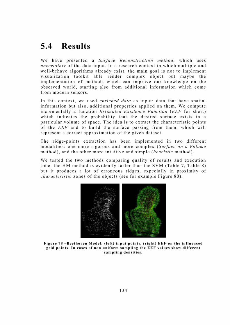
134

5.4 Results We have presented a Surface Reconstruction method , which uses uncertainty of the data input. In a research context in which multiple and well-behave algorithms already exist, the main goal is not to implement visualization toolkit able render complex object but maybe the implementation of methods which can improve our knowledge on the observed world, starting also from additional information which come from modern sensors.

In this context, we used enriched data as input: data that have spatial information but also, additional properties applied on them. We compute incrementally a function Estimated Existence Function (EEF for short) which indicates the probability that the desired surface exists in a particular volume of space. The idea is to extract the characteristic points of the EEF and to build the surface passing from them, which will represent a correct approximation of the given dataset.

The ridge-points extraction has been implemented in two different modalities: one more rigorous and more complex (Surface-on-a-Volume method), and the other more intuitive and simple (heuristic method).

We tested the two methods comparing quality of results and execution time: the HM method is evidently faster than the SVM (Table 7, Table 8) but it produces a lot of erroneous ridges, expecially in proximity of characteristic zones of the objects (see for example Figure 80).

Figure 78 �Beethoven Model: ( left) input points , (right) EEF on the inf luenced

grid points. In cases of non uniform sampling the EEF values show different sampling densit ies .

135

Another observation is that, our EEF strongly depends on the sampling condition of the initial dataset. In case of non uniform sampling (Figure 78) we found out more grid points with high EEF values in proximity of high density sampling (they will be influenced by numerous sampled points) and grid points with low EEF values in proximity of low density sampling (they will be influenced by less sampled points). This observation open a new research goal: to find different Probability Density Functions that are able to model dynamically the sampling quality of the input datasets.

Anyway, with the datasets we have used, our basic implementation of the algorithm shows acceptable results (see for example Figure 79 and Figure 80).

136

RID

GES

IN

TER

SEC

TIO

NS

MES

H

HM0.0 HM0.5 SVM0.0

INPUT POINTS EEF POINTS

Figure 79 � three different applications of our method to the stanford bunny dataset: Heurist ic Method with no f i l ter, Heurist ic method with 0.5 f i l ter and

Surface-on-a-volume method with no f i l ter

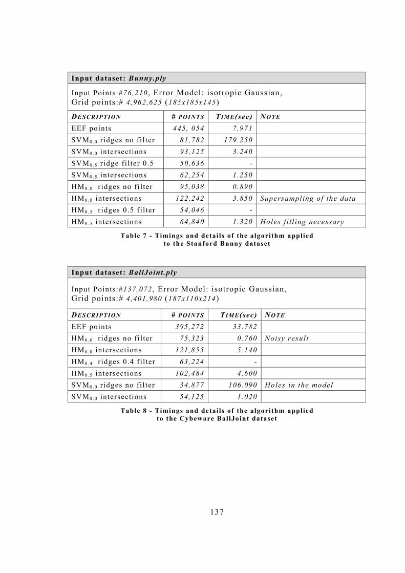
137

Input dataset: Bunny.ply

Input Points:#76,210 , Error Model: isotropic Gaussian, Grid points:# 4 ,962,625 (185x185x145)

DESCRIPTION # POINTS TIME(sec) NOTE EEF points 445, 054 7.971 SVM0 . 0 r idges no fi l ter 81,782 179.250 SVM0 . 0 intersections 93,125 3.240 SVM0 . 5 r idge fi l ter 0.5 50,636 - SVM0 . 5 intersections 62,254 1.250 HM0 . 0 r idges no fi l ter 95,038 0.890 HM0 . 0 intersections 122,242 3.850 Supersampling of the data HM0 . 5 r idges 0.5 f i l ter 54,046 - HM0 . 5 intersections 64,840 1.320 Holes f i l l ing necessary

Table 7 - Timings and detai ls of the algorithm applied to the Stanford Bunny dataset

Input dataset: BallJoint.ply

Input Points:#137,072 , Error Model: isotropic Gaussian, Grid points:# 4 ,401,980 (187x110x214)

DESCRIPTION # POINTS TIME(sec) NOTE EEF points 395,272 33.782 HM0 . 0 r idges no fi l ter 75,323 0.760 Noisy result HM0 . 0 intersections 121,855 5.140 HM0 . 4 r idges 0.4 f i l ter 63,224 - HM0 . 5 intersections 102,484 4.600 SVM0 . 0 r idges no fi l ter 34,877 106.090 Holes in the model SVM0 . 0 intersections 54,125 1.020

Table 8 - Timings and detai ls of the algorithm applied to the Cybeware BallJoint dataset

138

RID

GES

IN

TER

SEC

TIO

NS

MES

H

HM0.0 HM0.5 SVM0.0

INPUT POINTS EEF POINTS

Noise � filtering is necessary

Holes � post processing operation needed

Figure 80 - three different applicat ions of our method to the cybeware balljo int

dataset: Heurist ic Method with no f i l ter, Heurist ic method with 0.5 f i l ter and Surface-on-a-volume method with no f i l ter

139

Another observation is that our P-Method definitely improves the results of the final models, but at this stage is not able to remove completely outliers.

Finally, our method can be applied in an on-line setting as in the case of the method presented in the previous Chapter (Online Mosaicing). Our approach is a local approach: the incremental rule for the construction of the EEF and the choice of a Probabili ty Distribution (the Gaussian) which has a limited domain are fundamental properties, which render the method quite fast, local and incremental (but a code optimization is necessary).

140

6. Conclusions and Future Works

In this Dissertation, we have investigated two different topics related to 3D Reconstruction problems:

• We first presented a complete Data Analysis pipeline for the real-time reconstruction of underwater environments. This pipeline was developed in collaboration with the University of Verona, in the context of the European Project ARROV.

• Next, we presented a Surface Reconstruction method that encapsulates the uncertainty of the sampled data, making no assumptions on the shape of the surface to be reconstructed.

ARROV PIPELINE The Arrov Pipeline has lead to good results in relation to the types of input coming from the acoustic sensor. In fact, the acquired range images are noisy and at low resolution and present missing data. For these reasons, the Single Frame Reconstruction phase leads to triangular meshes with holes and the problem is present also in the Mosaicing Phase.

Part of these holes has been recovered by the use of a method, which searches for connections among entries in a 2x2 and 3x3 window.

The real time visualization requirement has been satisfied by the use of a Modified Marching Intersection Algorithm, which maintains a geometric structure consisting of l ists of active cells , and a corresponding graphic structure consisting of different display lists. In order to speed-up the process, the method lazily updates the display lists, giving out to the Viewer only the newly generated display lists and those display lists for which the amount of changes exceeds the update threshold.

Some future works can be done in order to optimize the pipeline and improve the results:

• The Marching Intersection Algorithm is sensitive to invalid cells configurations. We will improve the method trying to develop variants, which well-behave in cases of noisy data.

141

• It is necessary to improve the speed of the pipeline by optimizing the code.

• One important thing is that the pairwise registration of a subsequent frame can lead to error explosion, so sometimes a reset is needed. An improvement of the Registration Techniques is necessary: but this does not fall in the scope of this Dissertation.

The goal achieved by the ARROV project represents a good starting point for the development of fast and accurate methods for Real Time Data Analysis. We will improve accuracy of the results and test the pipeline in different contexts from the underwater inspection (robotics, Aerospatiale research, and so on ).

MODELING WITH UNCERTAINTY We have developed a general framework for building models starting from enriched data, which should arrive from multiple and different sensors.

The framework individuates a standard methodology which we have implemented in a basic version. In particular we choose a standard Gaussian Probability Distribution for the error model related to the input points, and we showed results implementing and applying two different methods (Surface-on-a-Volume and Heuristic) for the extraction of ridges.

Our proposed framework perfectly fits to the modern requirements of Surface Reconstruction Systems: it is oriented to the integration of different datasets and it can use all the information coming from modern acquisition systems.

Additionally, the process can be used to produce Multiresolution Triangle Meshes representing surfaces at different levels of accuracy and resolution. These meshes can be successively analyzed and manipulated in order to:

- on-line retrieve a model whose size and accuracy best fit the requirements of an application task real-time rendering (e.g., flight simulators, navigation in virtual environments)

- compress data (a lower resolution is used when it is sufficient)

- progressively transmit data (send a raw representation first, then add details where needed)

142

- reason across different levels of abstraction (e.g., from a raw to a refined representation in processing spatial queries)

For what concern the ridge extraction methods, both of them showed interesting results: the HM method finds more ridges than the SVM (some of them are redundant) but the filter over the EEF values help us in isolating significant ridges. The SVM method, instead, is more precise in results but definitely more slow: this is obvious because it makes computation on matrices and extraction of eigenvalues and eigenvectors, while the HM makes only comparisons on neighbor points.

Finally, as we said in the previous chapter, our method can be applied in an on-line setting as in the case of the method presented in the previous Chapter (Online Mosaicing): the incremental rule for the construction of the EEF and the choice of a Probabili ty Distribution (the Gaussian) which has a limited domain are fundamental properties which render the method fast, local and incremental.

Anyway, from an implementation as much as from a theoretical point of view, improvements are necessary in the future. For example:

• First, the filtering process applied to the EEF values is not always effective: in some cases, for removing outliers in some parts, we remove also significant ridges in other. The problem is that this filter is applied globally while it should be local : we are developing local filters that, inferring on neighbors of a ridge point, will decide if discard or maintain it .

• Next, we need to develop different probability density functions: we are studying which function cloud be the right one, also in relation to the type of input we are treating. In order to test the algorithm efficiently, we need to open and model datasets which come with an error model or a confidence value associated to each input point: actually we have not found such types of models available on the web, but a next step of our research will be to prove the method with the data coming from the acoustic sensor used in the ARROV project. These data have an estimation of the reliability associated to each input point and these reliability values can be used for the creation of the Probability Density Function and the EEF .

• Another improvement will be the integration of new models with the error model we have used: we are developing formalizations for

143

other types of additional data we can find in the output of the modern acquisition devices.

• Next, our final triangular mesh is not optimized but it is merely oriented to the simple visualization of the results. Additionally, we have to solve some problems we encountered during Mesh Extraction: in some cases the mesh is not correct and post processing operations are necessary. We are integrating standard algorithms for mesh improvement in order to develop a complete system of mesh creation/manipolation and visualization.

• Finally, the code must be optimized both in term of space and time complexity: for example, we are cleaning the data structures from useless properties.

144

7. Bibliography

[1] Aguilar Jose, A Dynamic Fuzzy-Cognitive-Map Approach based on Random Neural Networks , International Journal of Computational Cognition (ISSN 1542-5908) Volume 1, Number 4, pages 91-107, December 2003.

[2] Amenta N., Choi S., Dey Tamal K., Leekha N., A Simple Algorithm for Homeomorphic Surface Reconstruction , International Journal of Computational Geometry and Applications, vol.12 n.1-2, pp.125-141, 2002.

[3] Amenta. N, Bern M., Kamvysselis M., A new Voronoi-based Surface Reconstruction Algorithm . In Proceedings of ACM SIGGRAPH�98, pp.415-421, 1998

[4] ARANZ Applied Research Associates NZ Ltd is a research, design and development provider with particular expertise in 3D imaging. web sites: http://aranz.com.

[5] ARROV (Augmented Reality for Remotely Operated Vehicles based on 3D acoustical and optical sensors for underwater inspection and survey), Project Proposal, 2000.

[6] Attali D. and Lachaud J.-O., Delaunay conforming iso-surface; skeleton extraction and noise removal , Computational Geometry: Theory and Applications. 19(2-3): 175-189, 2001.

[7] Attali D. and Lachaud J.-O.. Constructing Iso-Surfaces Satisfying the Delaunay Constraint; Application to the Skeleton Computation . In Proc. 10th International Conference on Image Analysis and Processing (ICIAP'99), Venice, Italy, September 27-29, pages 382-387, 1999.

[8] Attali D., r-regular Shape Reconstruction from Unorganized Points. In Proceedings of the ACM Symposium on Computational Geometry, pp.248-253, 1997

[9] Attene M., Spagnuolo M., Automatic Surface Reconstruction from point sets in space . In EUROGRAPHICS 2000 Proceedings, pp. 457-465, Vol.19 n.3, 2000

145

[10] Aukstakalnis S. and Blatner D., Silicon Mirage: The Art and Science of V.R . ; Peachpit Press, Inc.; California; 1992

[11] Band, Lawrence E. Extraction of topographic networks from digital elevation data - Presented at the Eighteenth International Symposium on Remote Sensing of Environment, Paris, France, October 1-5, 1984

[12] Bajaj C.L.,Bernardini F., Chen J. , Schikore D. Automatic Reconstruction of 3D Cad Models . In Proceedings of Theory and Practice of Geometric Modelling, 1996

[13] Beraldin J. A., Blais F., Cournoyer L., Godin G. and Rioux M., Active 3D Sensing, Modelli E Metodi per lo studio e la conservazione dell 'architettura storica , University: Scola Normale Superiore, Pisa 10, NRC 44159, pp 22-46, 2000

[14] Bernardini F., Mittleman J., Rushmeier H., Silva C., Taubin G., The Ball-Pivoting Algorithm for Surface Reconstruction . In IEEE Transaction on Visualization and Computer Graphics, Vol.5n.4, pp.349-359, 1999

[15] Besl P. and McKay N.. A method for registration of 3-D shapes . IEEE Transactions on Pattern Analysis and Machine Intelligence, 14(2):239�256, February 1992.

[16] Besl P. J. . Range Imaging Sensors . General Motors Research Publications, March 1988.

[17] Blais G. and Levine M. D.. Registering multiview range data to create 3-D computer objects . IEEE Transactions on Pattern Analysis and Machine Intelligence, 17(8):820�824, 1995.

[18] Boissonnat J.D., Geometric Structures for Three-dimensional Shape Representation . ACM Transaction on Graphics, pp.266-286, Vol.3, 1984

[19] Carr J. C., Beatson R. K., Cherrie J.B. Mitchell T. J. , Fright W. R., McCallum B. C. and Evans T. R., Reconstruction and Representation of 3D Objects with Radial Basis Functions ACM SIGGRAPH 2001, Los Angeles, CA, pp67-76, 12-17, 2001.

[20] Carr J. C., Beatson R. K., McCallum B. C., Fright W. R, McLennan T. J. and Mitchell T. J. , Smooth surface reconstruction from noisy range data ACM GRAPHITE 2003, Melbourne, Australia, pp119-126, 11-19 February 2003.

146

[21] Castellani U., Fusiello A., Murino V., Registration of multiple acoustic range views for underwater scene reconstruction , Computer Vision and Image Understanding, Vol. 87, no. 3, pp. 78-89, 2002.

[22] Castellani U., Fusiello A., Murino V., Papaleo L., Pittore M., Puppo E., On-line 3D mosaicing from acoustical range data , 2004, [submitted for publishing].

[23] Chen Y. and Medioni G., Description of Complex Objects from Multiple Range Images Using an Inflating Baloon Model , CVIU Vol. 61, No. 3, May 1995, pp. 325-334.

[24] Chen Y. and Medioni G.. Object modeling by registration of multiple range images . Image and Vision Computing, 10(3):145�155, 1992.

[25] Chen Y., Medioni G., Object Modeling by Registration of Multiple Range Images . International Journal of Image and Vision Computing, vol.10 n.3, pp.145-155, 1992.

[26] Cignoni P., Montani C., Scopigno R and Rocchini C, The Marching Intersections algorithm for merging range images . Technical Report B4-61-00, I.E.I. - C.N.R., Pisa, Italy, June 2000.

[27] Crossno P., Angel E., Spiraling Edge: Fast Surface Reconstruction from Partially Organized Sample Points , Proceedings Visualization IEEE�99, pp.317-324, 24-29 October, 1999.

[28] Curless B., Bouguet J.Y., Debevec P., Levoy M., Nayar S., Seitz S . 3D Photography Course Notes , SIGGRAPH2000 July, Louisiana, 2000 (url: http://www-2.cs.cmu.edu/~seitz/course/3DPhoto.html ).

[29] Curless B., Levoy M . , A volumetric Method for building complex models from Range Images . Computer Graphics: Siggraph �96 Proceedings, pp.221-227, 1996.

[30] Cybeware Company http://www.cybeware.com

[31] De Floriani L., Magillo P., Puppo E., Managing the Level of Detail in 3D Shape Reconstruction and Representation . In Proceedings of the International Conference on Pattern Recognition, pp.389-391, 1998

147

[32] De L. Floriani, Magillo P., Puppo E., On-line Space Sculpturing for 3D Shape Manipulation , Proc. Int. Conference on Pattern Recognition, Barcelona, Spain, September 2000, Vol. 1, pp. 105-108, 2000.

[33] Dey T. K. Giesen J., Detecting undersampling in surface reconstruction - Symposium on Computational Geometry pp.257-263, 2001

[34] Dey Tamal K., Joachim Giesen, Naveen Leekha, and Rephael Wenger, Detecting Boundaries for Surface Reconstruction using co-cones . Int. J. Computer Graphics & CAD/CAM 16:141-159, 2001

[35] Dinh H.Q., Turk G., and Slabaugh G., Reconstructing Surfaces Using Anisotropic Basis Functions , International Conference on Computer Vision (ICCV) 2001

[36] Dinh, H. and G. Turk. Reconstructing Surfaces by Volumetric Regularization . Technical Report 00-26, Graphics, Visualization, and Usability, Georgia Institute of Technology, November, 2000.

[37] Eberly D., Gardner R., Morse B., Pizer S. and Scharlach C., Ridges for Image Analysis , Jour. Mathematical Imaging and Vision 4(4):353-373, 1994.

[38] Edelbrunner H., Mücke E.P., Three Dimensional alpha-Shape . ACM Transaction on Graphics, Vo.13 n.1, pp.43-72, 1994

[39] FarField Technology Ltd web site: http://www.farfieldtechnology.com/

[40] Farin G. E . . Curves and Surfaces for Computer Aided Geometric Design: A Practical Guide . Academic Press, Boston, Massachusetts, 2nd edition, 1990.

[41] Franke R . Scattered data interpolation: Tests of some methods . Mathematics of Computation, 38(157):181�200, 1982.

[42] Fusiello A., Castellani U., Ronchetti L., and Murino V.. Model acquisition by registration of multiple acoustic range views . In A. Heyden, G. Sparr, M. Nielsen, and P. Johansen, editors, Computer Vision - ECCV 2002, number 2351 in Lecture Notes in Computer Science, pages 805-819. Springer, 2002.

[43] Gao Shan, Lu Han-Qing, A Fast Algorithm for Delaunay based Surface Reconstruction, The 11-th International Conference in

148

Central Europe on Computer Graphics, Visualization and Computer Vision'2003, Plzen - Bory, Czech Republic, February 3 - 7, 2003

[44] Gopi M., Krishnan S., Silva C., Surface Reconstruction based on Lower Dimensional Localized Delaunay Triangulation , Proceedings of Eurographics 2000, Volume 19, N.3, pp. C467-C478, 2000.

[45] Greengard L. and Rokhlin V. A fast algorithm for particle simulations . J. Comput. Phys, 73:325�348, 1987.

[46] GVU Center Georgia Tech, Graphics Research Grupo, Variational Implicit Surfaces Web site: http://www.cc.gatech.edu/gvu/geometry/implicit/

[47] Hampel F., Rousseeuw P., Ronchetti E., and Stahel W.. Robust Statistics: the Approach Based on Influence Functions . Wiley Series in probability and mathematical statistics. John Wiley & Sons, 1986.

[48] Hansen R. K. and Andersen P. A.. A 3-D underwater acoustic camera - properties and applications. In P.Tortoliand L.Masotti , editors, Acoustical Imaging, pages 607�611. Plenum Press, 1996.

[49] Heckel B., Uva A.E., Hamann Bernd, Joy Kenneth I. , Surface reconstruction using adaptive clustering methods, Geometric Modelling: Dagstuhl 1999, Vol.14, Computing Suppl.- Series, pp. 199-218, 2001.

[50] Hilton A., Stoddart A., Illingworth J. and Windeatt T., Marching Triangles: Range Image Fusion for Complex Object Modeling . Proc. Int�l Conf. Image Processing (ICIP96), 1996.

[51] Hoppe H., DeRose T., Duchamp T., McDonald J., Stuetzle W., Surface Reconstruction From Unorganised Points . In Computer Graphics SIGGRAPH 92 Conference Proceedings, Vol.26, pp.71-78, 1992

[52] Johnson A.E., Manduchi R., Probabilistic 3D Data Fusion for Multiresolution Surface Generation , 1st International Symposium on 3D Data Processing, Visualization and Transmission, Padova, Italy, 2002.

149

[53] Johnston, E.G. and Rosenfeld, A. Digital Detection of Pits, Peaks, Ridges, and Ravines, SMC Volume 5, July, pp.472-480,1975.

[54] Kobbelt L., Bischoff S., Kähler K., Schneider R., Botsch M., Rössl C., Vorsatz J. , Geometric Modeling Based on Polygonal Meshes . Research Report n.MPI-I-2000-4-002, MPI Informatik, Saarbrücken, 2000.

[55] Kojekine N., Hagiwara I. , Savchenko V., Software Tools Using CSRBFs for Processing Scattered Data , International journal "Computers & Graphics" published by Elsevier Science, 27/2 pp. 309-317, 2003.

[56] Kosko B. Neural Networks and Fuzzy systems, A dynamic system approach to machine intelligence , Prentice Hall, New Jersey, 1992.

[57] Laga H., Piperakis R., Takahashi H., Nakajima M., 3D Object Reconstruction from Scanned Data using Radial Basis Functions and Volumetric Processing , Nicograph 2002 National Conference, Nagoya, Japan pp133-138,. October 2002.

[58] Laga H., Piperakis R., Takahashi H., Nakajima M., A Radial Basis Function Based Approach for 3D Object Modeling and Reconstruction , International Workshop on Advanced Image Technology IWAIT2003, Nagasaki, Japan, pp139-144. January 21-22, 2003.

[59] Levoy M., Pulli K., Curless B., Rusinkiewicz S., Koller D., Pereira L., Ginzton M., Anderson S., Davis J. , Ginsberg J. , Shade J., FulkD. The Digital Michelangelo Project: 3D Scanning of Large Statues . , Siggraph 2000, Computer Graphics Proceedings. Pp.131-144, 2000.

[60] Lorensen W.E. and Cline H.E., Marching Cubes: A High Resolution 3D Surface Construction Algorithm , Computer Graphics (Proceedings of SIGGRAPH '87), Vol. 21, No. 4, pp. 163-169 1987.

[61] Lorusso A, Eggert D. W., and Fisher R. B.. A comparison of four algorithms for estimating 3-D rigid transformations . Machine Vision and Applications, 9:272�290, 1997.

[62] Mark D. M., Automated detection of drainage networks from digital elevation models in AutoCarto IV: Proceedings Sixth

150

International Symposium on Computer Assisted Cartography, pp. 288�298, 1983.

[63] Manly B. Multivariate Statistical Methods , A Primer. Chapman & Hall, New York, New York, 1994.

[64] Mencl R., Müller. Interpolation and Approximation of Surfaces from Three Dimensional Scattered Data Points . In Proceedings of EUROGRAPHICS 98 State of the Art Reports, 1998.

[65] Monga, Olivier; Benayoun, Serge Using partial derivatives of 3D images to extract typical surface features , Computer Vision and Image Understanding: vol. 61(2); pp 171-189, 1995.

[66] Murino V. and Trucco A. Three-dimensional image generation and processing in underwater acoustic vision . Proceeding of the IEEE, 88(12):1903�1946, December 2000.

[67] Murino V., Trucco A., and Regazzoni C.. A probabilistic approach to the coupled reconstruction and restoration of underwater acoustic images. IEEE Transactions on Pattern Analysis and Machine Intelligence, 20(1):9�22, January 1998.

[68] Ohtake Y., Belyaev A., Alexa M., Turk G. and Seidel HP, Multi-level Partition of Unity Implicits , SIGGRAPH 2003

[69] Osher, S., and Sethian, J.A., Fronts Propagating with Curvature-Dependent Speed: Algorithms Based on Hamilton--Jacobi Formulations , Journal of Computational Physics, 79, pp. 12--49, 1988 URL: http://math.berkeley.edu/~sethian/levelexplain.html

[70] Papaleo L., 3D Object Reconstruction: Formal Analysis and Practical Applications , PhD Thesis Proposal, University of Genova, 2000.

[71] Papaleo L., Puppo E. , On-line Mosaicing and Visualization of 3D Meshes from Range Data , First Conference Eurographics Italian Chapter, Politecnico di Milano, 11-12 July 2002, 2002

[72] Poston T.,.Wong T.T, Heng P.A., Multiresolution Isosurface Extraction with Adaptive Skeleton Climbing , Eurographics'98 Vol.17 Number 3, 1998

[73] Pulli K., Surface Reconstruction and Display from Range and Color Data. PhD thesis, Department of Computer Science and Engineering, Univ. of Washington, December 1997.

151

[74] Remondino F., From Point Cloud to Surface: The Modeling and Visualization Problem . International Archives of the Photogrammetry, Remote Sensing and Spatial Information Sciences, Vol. XXXIV-5/W10 International Workshop on Visualization and Animation of Reality-based 3D Models, Tarasp-Vulpera, Switzerland, 24-28 February 2003.

[75] Roth G., Wibowoo D.E. An Efficient Volumetric Method for Building Closed Triangular Meshes from 3-D Image and Point . Graphics Interface, ED. W. Davis, M., Mantei V.,Klassen.1997.

[76] ROV.net � web resource of ROV technologies and Companies. [www.rov.net].

[77] Rusinkiewicz M. L. S.. Efficient variants of the ICP algorithm. In IEEE Int. Conf. on 3-D Imaging and Modeling, 3DIM �01, Quebec City (Canada), 2001.

[78] Samet H. The Design and Analysis of Spatial Data Structures. Addison-Wesley, Reading, Massachusetts, 1989.

[79] Savchenko V. V., Pasko A., Okunev O. G., and Kunii T. L.. Function representation of solids reconstructed from scattered surface points and contours . Computer Graphics Forum, 14(4):181�188, 1995.

[80] Savchenko V., N. Kojekine, An Approach to Blend Surfaces , Proceedings of CGI`2002 conference, Advances in Modeling, Animation and Rendering, J. Vince and R. Earnshaw (Eds) , June 24-28, pp. 139-150, 2002.

[81] Scopigno R., Andujar C., Goesele M., Lensch H., 3D Data Acquisition, Tutorial T1, Eurographics Conference, ISSN 1017-4565, September, 2002.

[82] Sethian, J.A., A Fast Marching Level Set Method for Monotonically Advancing Fronts , Proc. Nat. Acad. Sci. , 93, 4, pp.1591--1595, 1996

[83] Sethian, J.A., An Analysis of Flame Propagation, Ph.D. Dissertation, Dept. of Mathematics, University of California, Berkeley, CA, 1982.

[84] Sethian, J.A., Level Set Methods and Fast Marching Methods; Evolving Interfaces in Computational Geometry , Fluid

152

Mechanics, Computer Vision and Material Science , Cambridge University Press, 1999.

[85] Soucy M. and Laurendeau D., A General Surface Approach to the Integration of a Set of Range Views , IEEE Transactions on Pattern Analysis and Machine Intelligence, 17, 4, 344-358, 1995.

[86] Sun Yiyong, Surface Modeling and Analysis Using Range Images: Smoothing, Registration, Integration, and Segmentation , PhD Dissertation, Department of Electrical and Computer Engineering, University of Tennesse, 2003.

[87] Szeliski R. and Tonnesen D.. Surface modeling with oriented particle systems. Computer Graphics (SIGGRAPH'92), 26(2):185-194, July 1992.

[88] Tam, R. and Heidrich, W. Feature-Preserving Medial Axis Noise Removal . Lecture Notes in Computer Science (Proceedings of ECCV 2002), 2351:672�686, 2002.

[89] Tam, R. and Heidrich, W Shape Simplification Based on the Medial Axis Transform . In Proceedings of IEEE Visualization 2003, pp. 481�488, 2003.

[90] Teichmann M., Capps M., Surface Reconstruction with Anisotropic Density-Scaled Α Shape. Proceedings in IEEE Visualization�98, pp.18-23, 1998

[91] Terzopoulos D. and Fleischer K . . Modeling inelastic deformation: viscoelasticity, plasticity, fracture. Comput. Graph. (SIGGRAPH Proc.), pages 269--278, 1988

[92] Terzopoulos D., Kass, M. Witkin A., Snakes: Active contour models International Journal of Computer Vision, 1(4) , 321-331, 1987.

[93] Terzopoulos D., Witkin A., Kass M., Constraints on deformable models: Recovering 3D shape and nonrigid motion Artificial Intelligence, 36(1), 91-123, 1988.

[94] Terzopoulos D., Witkin A., Kass M., Symmetry-seeking models and 3D object reconstruction International Journal of Computer Vision, 1(3), 211-221, 1987.

[95] Tobor I. , Reuter P., Schlick C., Efficient Reconstruction of Large Scattered Geometric Datasets using the Partition of Unity and

153

Radial Basis Functions . Research Report RR-1301-03, LaBRI - Université Bordeaux, France. May, 2003

[96] Toriwaki, J.; Fukumura, T. Extraction of structural information from grey pictures Computer Graphics and Image Processing: vol. 7; pp 30-51, 1978.

[97] Treece G. M., Prager R.W., and Gee A. H.. Regularised marching tetrahedra: improved iso-surface extraction. Computers and Graphics, 23(4):583�598, 1999.

[98] Trucco E., Fusiello A., and Roberto V.. Robust motion and correspondence of noisy 3-D point sets withmissing data . Pattern Recognition Letters, 20(9):889�898, September 1999.

[99] Turk G. and O�Brien J. Shape transformation using variational implicit functions. Proceedings of ACM SIGGRAPH 99, pages 335�342, 1999.

[100] Turk G. and O'Brien J.F., Modelling with Implicit Surfaces that Interpolate. ACM Transactions on Graphics, Vol. 21, No. 4, pp. 855-873, October 2002.

[101] Turk G., Levoy M., Zippered Polygon Meshes from Range Images , In proceedings of ACM SIGGRAPH 94, pp.311-318, 1994

[102] Turk G., Yngve G. Creating Smooth Implicit Surfaces from Polygonal Meshes. Technical Report GIT-GVU-99-42, Graphics, Visualization, and Useability Center. Georgia Institute of Technology, 1999.

[103] Turk G., Yngve G.,. Robust creation of implicit surfaces from polygonal meshes. IEEE Transactions on Vizualization and Computer Graphics, 8(4):346--359, 2002.

[104] Turk G.and O�Brien J.. Variational implicit surfaces. Technical Report GIT-GVU-99-15, Georgia Institute of Technology, 1998.

[105] Urik R. J. . Principles of Underwater Sound . McGraw-Hill, 1983.

[106] Veltkamp R. C., Closed Object Boundaries from Scattered Points. PhD thesis, Center for Mathematics and Computer Science, Amsterdam, 1992

154

[107] Zhang Z.. Iterative point matching of free-form curves and surfaces. International Journal of Computer Vision, 13(2):119�152, 1994.

[108] Zhao H.K., Osher S., Fedkiw R.. Fast Surface Reconstruction Using the Level Set Method Proceedings of IEEE Workshop on Variational and Level Set Methods in Computer Vision (VLSM 2001), July, 2001