
Aspects of Electromagnetic Modelling for Multiple-Input...
106
UNIVERSIT ` A DEGLI STUDI DI PADOVA Dipartimento di Ingegneria Elettrica Scuola di Dottorato di Ricerca in Ingegneria Industriale Indirizzo di Ingegneria Elettrotecnica Ciclo XX Aspects of Electromagnetic Modelling for Multiple-Input-Multiple-Output Control of MHD Modes in RFX-mod Direttore della Scuola: Prof. Paolo F. Bariani Supervisore: Prof. Francesco Gnesotto Dottorando: Ing. Anton Soppelsa 31 Gennaio 2008
Transcript of Aspects of Electromagnetic Modelling for Multiple-Input...
UNIVERSITA DEGLI STUDI DI PADOVADipartimento di Ingegneria Elettrica
Scuola di Dottorato di Ricerca in Ingegneria IndustrialeIndirizzo di Ingegneria Elettrotecnica
Ciclo XX
Aspects of Electromagnetic Modellingfor Multiple-Input-Multiple-Output
Control of MHD Modes in RFX-mod
Direttore della Scuola: Prof. Paolo F. Bariani
Supervisore: Prof. Francesco Gnesotto
Dottorando: Ing. Anton Soppelsa
31 Gennaio 2008


To my Mother,tireless worker able to teach
the meaning of honesty and humility

Sommario
L’attivita di ricerca oggetto della presente discussione, e stata condotta nell’am-bito della Scuola di Dottorato in Ingegneria Industriale, indirizzo IngegneriaElettrica dell’Universita degli Studi di Padova. Oggetto primario dello studio,svoltosi nel settore della modellistica dei sistemi elettromagnetici, e l’analisidel sistema di controllo attivo per la stabilizzazione dei modi MHD del plasmanell’esperimento RFX-mod. Tre i risultati principali dell’attivita di ricerca:il primo e l’inquadramento dello specifico problema di controllo nell’ambitodella teoria unificata dei segnali, aspetto significativo al fine di fornire un solidoimpianto teorico dal quale procedere per sviluppare nuovi modelli e tecniche dicontrollo; il secondo e la realizzazione di un modello matematico dell’impiantobasato interamente su misure sperimentali che permette l’analisi della strut-tura del sistema, la simulazione del suo comportamento dinamico e lo sviluppodi schemi di controllo innovativi; il terzo infine e l’effettiva realizzazione di unnuovo algoritmo di controllo basato sul modello ricavato.
Il sistema preso in considerazione nel presente studio e composto da 192unita, ognuna delle quali comprende una bobina attiva, il suo alimentatore,tre sensori di campo radiale, rispettivamente toroidale e poloidale. Le bobineattive ed i sensori di campo radiale sono disposti ordinatamente in modo daricoprire due superfici toroidali e sono organizzati in 48 array poloidali di 4elementi ciascuno. Tra le bobine attive e i sensori di campo magnetico sonopresenti strutture metalliche di diverso spessore che sono sede di fenomenidissipativi dovuti alle correnti indotte dal sistema di controllo attivo e dalplasma stesso.
Durante la prima fase della ricerca si sono effettuate campagne sperimentaliper misurare il mutuo effetto delle correnti nelle bobine attive e l’effetto sulflusso magnetico misurato dai sensori radiali. I dati provenienti dalle campagnehanno permesso di risalire alla forma matematica della matrice delle mutueinduttanze delle bobine attive e di quella delle mutue induttanze tra bobineattive e sensori radiali. A causa della presenza delle strutture passive le matricinon sono costanti, ma variano al variare della frequenza. Per questo motivole campagne sperimentali sono state condotte studiando il comportamento

degli accoppiamenti in esame a diverse frequenze. Un modello del sistemadi controllo dei modi MHD del plasma e stato costruito sulla base di questedue matrici di trasferimento ed e stato completato con l’aggiunta del modellodegli alimentatori delle bobine attive. Cio e stato completato con la scrittura diopportune procedure Matlabr che hanno permesso di automatizzare il processodi calcolo a partire dall’acquisizione dei dati sperimentali e da alcune ipotesiriguardanti il numero di accoppiamenti significativi.
Successivamente il modello e stato sottoposto ad un’intesa attivita di val-idazione, comprendente verifiche del funzionamento in catena aperta, sia atensione impressa sia a corrente impressa, ed in catena chiusa. Si e constatatoche il modello riproduce con un’accuratezza del 5% i segnali sperimentali, chee sufficientement fedele da riprodurre correttamente l’intervallo di stabilita delsistema retroazionato e puo quindi venire usato con successo come strumentod’indagine di fenomeni marginalmente stabili.
L’analisi del modello ha evidenziato due importanti fenomeni. In primoluogo l’accoppiamento tra bobine attive e sensori radiali non e cosı localizzatocome postulato a priori e cio ha comportato il calcolo di un maggior numero diaccoppiamenti. In secondo luogo l’uniformita degli accoppiamenti risulta infe-riore alle aspettative, evidenziando che la presenza di disuniformita importantidelle strutture passive costituisce un limite alle massime prestazioni dinamichedel sistema nella configurazione attuale.
Nell’arco dell’ultimo anno di ricerca e stato realizzato un nuovo algoritmodi controllo basato sulla decomposizione a valori singolari del modello ricavatonegli anni precedenti. Risultati di simulazioni confermano che questo algoritmodi controllo e in grado di compensare le principali disomogeneita delle strutturepassive almeno fino a una frequenza limite, oltre la quale la potenza erogatadagli alimentatori non e piu sufficiente a contrastare gli effetti delle correntiindotte.
Parte dell’attivita di ricerca e stata svolta nell’ambito di una collaborazionetra il Consorzio RFX ed il laboratorio JET di Culham (UK) riguardante ilpotenziamento dell’amplificatore per il controllo dell’instabilita verticale diplasma. In tale ambito la presente attivita di ricerca hacontribuito alla real-izzazione della parte software del sistema di controllo del nuovo amplificatorerisonante.
Summary
The research activity object of the present dissertation has been carried out atthe Industrial Engeneering Doctoral School (Course of Electric Engeneering)of the University of Padova. The study concerned the electromagnetic systemsmodelling with regard on active control system analysis for the stabilizationof plasma MHD modes in the RFX-mod experiment. Three are the mainresults of the research activity. The first one is the inclusion of the specificproblem in the frame of the Unified Signal Theory, important in order to builda solid theoretical background from which starting developing new controlmodels and techniques. The second one is the production of a mathematicalmodel of the plant based exclusively on experimental measures. This allowthe system’s structure analysis, the simulation of its dynamic behaviour andthe development of innovative control schemes. The third one is the actualproduction of a new algorithm based on the developed model.
The system cosidered in the present study is made up by 192 units, each oneincluding an active coil, its power amplifier, three field sensors (respectivelyradial, toroidal and poloidal). The active coils and the radial sensors are laiddown in a regular manner and in this way they cover exactly the toroidalsurfaces they intersects. Both of them form a grid made of 48 poloidal arrays,each one consisting of 4 elements. Metallic structures of different thicknessare present in between the active coils and the magnetic field sensors, whichare interested by dissipative effects due to the induced currents by the activecontrol system and by the plasma.
During a first phase of the research, experimental campaigns have beenmade in order to measure quantitatively the mutual couplings between saddlecoils and the effect of their currents on the magnetic field measured by theradial sensors. Data collected during these campaigns allowed for the mathe-matical form of the active coils inductance matrix and the mutual inductancebetween active coils and sensors to be discovered. Due to the presence ofthe passive structures these matrices are not constant, but variable in the fre-quency domain. For this reason the campaigns have been carried out studyingthe behaviour of the couplings at different frequencies. A model of the cou-

plings has then been derived and used in the construction of a bigger modelcomprehensive of the active coils and power amplifier dynamics. The task hasbeen completed by writing convenient procedures in the Matlabr language,which allowed for an automated processing of the experimental data undersome simplifying hypothesis about the number of significative couplings.
Later the model has been intensively validated. Tests have been carriedout both in open loop and closed loop. The open loop tests have been madeby comparing the real and simulated outputs corresponding to the appliedvoltages and currents. The model was able to reproduce the output quantitieswith a 5% accuracy, to mimic the real closed loop stability range and has beenused with success as a tool to gain insight into marginally stable phenomena.
The model analysis evidenced a couple of important facts. The first is thatthe coupling between active coil and sensor is not so local as expected; thisrequired a great number of couplings to be considered. The second is that theuniformity of the couplings is less than expected. The presence of features,like the inner equatorial gap, ruining the uniformity of the passive structuresacts as a limit of the obtainable performance in the present configuration.
On the basis of the model a new control algorithm has been designed usingthe singular value decomposition. Simulation results confirm that this controlalgorithm is able to compensate the effects of the local features of the passivestructures till a limit frequency. Above that frequency the power required forthe compensation would exceed the capacity of the amplifiers.
Part of the research activity has been carried out in the frame of a collabo-ration between the Consorzio RFX and the EFDA-JET laboratory of Culham(UK) about the upgrade of the power amplifier of the plasma vertical insta-bility. Here the research has focused on the realisation of part of the softwarecontrol system of the new resonant amplifier.
Contents
1 Introduction 5
1.1 Structure of the Document . . . . . . . . . . . . . . . . . . . . . 5
1.2 Background . . . . . . . . . . . . . . . . . . . . . . . . . . . . . 5
1.2.1 Nuclear fusion . . . . . . . . . . . . . . . . . . . . . . . . 6
1.2.2 MHD theory and plasma instabilities . . . . . . . . . . . 7
1.2.3 Toroidal coordinate system . . . . . . . . . . . . . . . . . 9
1.2.4 Devices for the magnetically confined fusion . . . . . . . 11
1.2.5 RFX-mod . . . . . . . . . . . . . . . . . . . . . . . . . . 15
1.3 The active system for the control of MHD instabilities . . . . . . 19
1.3.1 Nomenclature . . . . . . . . . . . . . . . . . . . . . . . . 21
2 Analysis of the RFX-mod MHD system 23
2.1 Introduction . . . . . . . . . . . . . . . . . . . . . . . . . . . . . 23
2.2 Summary of the Unified Signal Theory . . . . . . . . . . . . . . 23
2.2.1 Regular groups . . . . . . . . . . . . . . . . . . . . . . . 24
2.2.2 Definition of signal . . . . . . . . . . . . . . . . . . . . . 25
2.2.3 Periodicity and cells . . . . . . . . . . . . . . . . . . . . 25
2.2.4 The Haar integral . . . . . . . . . . . . . . . . . . . . . . 26
2.2.5 Linear systems and convolution . . . . . . . . . . . . . . 27
2.2.6 Dual domains . . . . . . . . . . . . . . . . . . . . . . . . 28
2.2.7 Fourier transform . . . . . . . . . . . . . . . . . . . . . . 30
2.3 Time variant filtering . . . . . . . . . . . . . . . . . . . . . . . . 31
2.4 MHD system analysis . . . . . . . . . . . . . . . . . . . . . . . . 32
2.4.1 Block diagrams . . . . . . . . . . . . . . . . . . . . . . . 33
2.4.2 Domains definition . . . . . . . . . . . . . . . . . . . . . 34
2.4.3 Current distribution . . . . . . . . . . . . . . . . . . . . 35
2.4.4 Field interpolation . . . . . . . . . . . . . . . . . . . . . 37
2.4.5 Field sampling . . . . . . . . . . . . . . . . . . . . . . . 38
2.5 Conclusions . . . . . . . . . . . . . . . . . . . . . . . . . . . . . 48
1

CONTENTS
3 Model 513.1 Introduction . . . . . . . . . . . . . . . . . . . . . . . . . . . . . 513.2 Active Circuits Matrices . . . . . . . . . . . . . . . . . . . . . . 53
3.2.1 Experimental validation . . . . . . . . . . . . . . . . . . 573.3 Matrix of mutual inductances between active coils and sensors . 58
3.3.1 Evaluation of the 3D matrix elements . . . . . . . . . . . 593.3.2 Evaluation of the transfer function matrix . . . . . . . . 633.3.3 Experimental validation . . . . . . . . . . . . . . . . . . 65
3.4 Validation of the full open loop model . . . . . . . . . . . . . . . 663.5 Validation of the closed loop model . . . . . . . . . . . . . . . . 71
3.5.1 Stability analysis in virtual shell operation . . . . . . . . 713.6 Conclusions . . . . . . . . . . . . . . . . . . . . . . . . . . . . . 75
4 Pseudo-Decoupler 774.1 Introduction . . . . . . . . . . . . . . . . . . . . . . . . . . . . . 774.2 Previous design attempts . . . . . . . . . . . . . . . . . . . . . . 784.3 Projecting Decoupler . . . . . . . . . . . . . . . . . . . . . . . . 79
4.3.1 Projected model . . . . . . . . . . . . . . . . . . . . . . . 794.3.2 Decoupler synthesis . . . . . . . . . . . . . . . . . . . . . 804.3.3 Decoupler implementation . . . . . . . . . . . . . . . . . 80
4.4 Controller synthesis . . . . . . . . . . . . . . . . . . . . . . . . . 824.5 Simulation results . . . . . . . . . . . . . . . . . . . . . . . . . . 834.6 Conclusions . . . . . . . . . . . . . . . . . . . . . . . . . . . . . 84
5 Conclusions and further developments 89
A Technicalities 93
2
Acknowledgments
This Doctoral dissertation could not have been written without the aid ofmany colleagues and friends who constantly helped me in the research activity.I sincerely would like to thank them all and I regret not being able to mentioneveryone with the due precision. I am particularly grateful to Giuseppe Mar-chiori, with whom I share the authorship of many of the presented results, toMario Cavinato, Gabriele Manduchi, Cesare Taliercio, Lionello Marrelli, PaoloZanca for their precious suggestions, to my Advisor Prof. Francesco Gnesottoand my Tutor Adriano Luchetta for their useful guide, to Prof. James R.Drake of the Royal Institute of Technology and to Prof. Bernardo Brotas deCarvalho of the Instituto Superior Tecnico for their willingness to commentthis dissertation, to Filippo Sartori, Fabio Piccolo, Luca Zabeo for their sup-port while I was at the JET Laboratory, to the other PhD students CristianoTaccon, Fulvio Auriemma, Matteo Agostini, Federica Bonobo, Marco Gobbinfor their help in printing the dissertation copies and in submitting it to theUniversity office. Thanks to Prof. Giuseppe Chitarin for having provided thevalues of the mutual couplings between active coils and sensors at frequencyzero and to Ing. Antonio Masiello for having provided the analogous valuesfor the active coils couplings.
Most of all, I would like to thank my precious Marcella “Alpine Awareness”Morandini, her parents and all my Family, for the constant support they haveprovided and the patience they have showed, especially in the final steps ofthe writing.
3

Chapter 1
Introduction
1.1 Structure of the Document
The present document is the summary of the research carried out from January2005 to December 2007 at the Padova University Electrical Engineering Doc-torate School. The first chapter presents background material. After a shortintroduction to the research in the field of nuclear fusion, the description of thetoroidal coordinate system provides the pretext to introduce the terminologyused in the following sections. The Doctoral activity and the place where it hasbeen carried out are then presented. In the following chapters 2, 3, 4 results ofthe research are shown and discussed. These chapters cover different aspectsof the research. In chapter 2 theoretical backgrounds are given. In chapter 3the core result of the research is described. Chapter 4 deals with the imple-mentation of a software device that theoretically allows for an improvement ofperformance. Finally, chapter 5 is reserved for concluding remarks.
1.2 Background
The following subsection aims at providing some background information aboutthe nuclear fusion and the research in this field without any claim of complete-ness. The intention is to give the minimum information required for a betterunderstanding of the rest of the document. Publications covering the topics ofthis chapter at an introductory level are: [1] for a good review of the modernphysics of the magnetically confined plasmas, [2] for a description of the RFXmachine structure, [3] for a description of the RFX-mod peculiarities, [4] fora paper on the aspects of the RFX-mod MHD control system design, and [5]for a book covering the history of the magnetically confined fusion research.
5
1. INTRODUCTION
1.2.1 Nuclear fusion
Nuclear fusion is the process by which a couple of atomic nuclei join togetherto form a heavier one. When nuclei of light elements undergo a fusion reac-tion, some mass is lost in the process and energy is liberated according to theEinstein’s equation E = mc2.
Such nuclear reactions happen naturally in the stars, where high temper-ature and pressure allow hydrogen nuclei to get close enough for the strongforce to bind them together. In this case the gravitational force is responsibleof creating the conditions in which the fusion can occur; so the fusion reactionshappening in the stars are said to be gravitationally confined. The adjectivethermonuclear specifies that the electrical repulsion of nuclei carrying chargeof the same sign is won by means of their thermal energy. It is usually specifiedin contrast with the so called cold fusion, where the problem of winning theCoulomb Barrier is faced by means of other effects.
Among all the possible nuclear fusion reactions, the one that happens in themost favourable conditions is the fusion between deuterium 2
1H+ and tritium
31H
+ nuclei. This because the cross section for the reaction tritium-deuteriumis so that it can balance the radiative losses of a confined plasma with thegiven density at the lowest possible temperature.
Apart from the gravitational confinement, there are other two methodsto achieve the conditions of temperature and pressure which allow for thethermonuclear fusion reactions to happen. One is based on the momentumconservation and it is called inertial confinement, the other is based on theLorentz force and therefore it is called magnetic confinement.
The magnetically confined thermonuclear fusion relies on the fact that atthe working conditions the reactants are fully ionised. That is the gas of thereacting species is made entirely of electrons and positive ions freely movingin the space. Charged particles interact with the magnetic field through theLorentz’s force and for this reason they can actually be confined by a properlyshaped magnetic field. Macroscopically, a ionised gas at high temperature isa good conductor which can be interested by a flow of electric current. Theinteraction between this current and the surrounding magnetic field, giving riseto the confining force. A ionised gas macroscopically neutral is called plasma.
Research into the field of plasma physics began in the 1950s, with the pur-pose of developing a new commercially viable energy source and still continuesto this day. Since its beginning, the research activity in the field of mag-netically confined thermonuclear fusion has been carried out with the aid ofelectromechanical devices, able to confine plasma inside their vacuum cham-ber. The development of the plasma research in the field has been tightlylinked with the development of the machines used for the experiments. In the
6
1. INTRODUCTION
following years several machines, corresponding to several different magneticconfigurations, have been realised. The most successful of them were basedon a toroidal geometry. The size and complexity of such devices has growngradually from the initial major radius of about half a meter to the severalmeters of the current biggest devices.
The toroidal magnetic configurations presently used in the fusion researchare the Tokamak, the Stellarator and the Reversed Field Pinch (RFP). Allof them share the toroidal concept for their construction but the magneticconfiguration is rather different. In Tokamaks and Reversed Field Pinchesa toroidal current is induced in the plasma with a central solenoid and atoroidal field is applied with convenient toroidal field coils. The shape ofthe magnetic field is controlled to a higher degree with additional poloidalfield windings. However the two configurations differ because in Tokamas thetoroidal component of the magnetic field is much stronger than the poloidalcomponent, whereas in the Reversed Field Pinches they are of comparable size.Moreover the toroidal field change sign at a point between the plasma centreand the plasma edge. Stellarators are different because they do not require aninduced toroidal current in order to confine the plasma. This naturally allowsfor operations in steady state, but this configuration requires the design andrealisation of coils with complex, non-planar shapes.
Today the research in the field of magnetically confined thermonuclear fu-sion is carried out at Universities, Laboratories and Research Centres aroundthe world. The operating machines where it is possible to perform experimen-tal exploitation of magnetically confined plasmas are now a few tens and othermachines are currently being build. The research reported in this documenthas been carried out in two of these laboratories, namely the Reversed-FieldeXperiment (RFX), run by the Consorzio RFX in Padova, Italy and the JointEuropean Torus (JET), a project run in the framework of the European Fu-sion Development Agreement (EFDA) by the United Kingdom Atomic EnergyAgency (UKAEA) at Culham, in the United Kingdom. Presently, RFX andJET are the world biggest operating Reversed Field Pinch and Tokamak re-spectively.
1.2.2 MHD theory and plasma instabilities
The most simple physical model of the plasma behaviour is described by themagnetohydrodynamic (MHD) theory. This academic discipline studies thebehaviour of the electrically conducting fluids from a macroscopic point ofview. The starting point of the theory is a set of equations comprehensiveof the Navier-Stokes equations of fluid dynamics, the Maxwell’s equations ofelectromagnetism and a plasma state equation involving the thermodynamical
7
1. INTRODUCTION
quantities. Depending on the applications, this set of equations can be alreadytoo much to explain the fundamentals of the plasma dynamic in a magneticfield. In this case simplifying assumptions are made and special theories arederived. One of the most important simplifications is to consider the plasmaresistivity equal to zero. In this case the plasma becomes a perfect conductorable to freeze the magnetic field lines in their original configuration. In thiscase the name of the theory becomes ideal MHD. Depending on the workinghypothesis, other names are commonly in use. For example resistive MHD,where the plasma resistivity is considered, and two-fluid MHD, where the ionsand electrons are treated as different fluids.
However, even the most general MHD theory has limits. To be applicablethis model requires the distribution of the particles forming the fluid to beclose to Maxwellian. Even if the rate of Coulombian collisions in the plasmamultiplied by the time constant of the MHD phenomena is high, this hypothesisis not automatically verified. This happens because in fusion plasmas themean free path of the particles can be as big as tens of thousands of timesthe size of the machine itself. This should shed some light about the factthat there do exist macroscopical phenomena which cannot be explained bya fluid theory and therefore that there is the need of developing a kinetictheory able to take into account, for example, the effects of a non Maxwelliandistribution of the plasma particles. The ideal MHD is almost invariably thefirst model considered by experimental physicists and engineers because of itsideal simplicity, its ability of capturing many of the important properties ofplasma dynamics and being often also qualitatively accurate.
Ideal MHD theory is particularly useful, because in many cases it can beapplied to analyse the plasma behaviour in the neighbourhood of a given equi-librium state. The plasma is said to be in a equilibrium state if there are notnet forces accelerating macroscopically any part of the plasma itself. If theequilibrium is stable a small perturbation in the plasma configuration will bedamped out, if not it will grow, eventually causing the collapse of the magneticconfiguration, the lost of the confinement and the premature end of the dis-charge. The understanding of the plasma instabilities is therefore of primaryinterests for the realisation of stable devices to be used in the magneticallyconfined fusion research. The plasma instabilities which can be predicted byand analysed with the help of the MHD theory are called MHD instabilities.Examples of these instabilities, are the resistive wall mode (RWM) instabil-ity and the neoclassical tearing mode instability. The former is the instabilityarising in presence of a wall with finite conductivity while the plasma wouldhave been MHD stable in front of a perfectly conducting one, the latter isdue to the non-zero resistivity of the plasma. Examples of more trivially ex-
8
1. INTRODUCTION
plainable instabilities are the vertical instability that affects Tokamaks withelongated, non-circular plasma profiles, or the horizontal instability due to theinhomogeneity of the pressure at the surface.
1.2.3 Toroidal coordinate system
Toroidal surfaces are central to the theory of plasma confinement. Axial sym-metry is a feature pursued by engineers in system design as it allows for simpli-fied modelling, implementation, testing and commissioning. For these reasons,when possible, the structural components of the machines used in the fieldof the magnetically confined fusion are designed exploiting axial-symmetry.Cylindrical set of coordinates are therefore very common in the field of themagnetically confined fusion.
As the electrical machines used in this field of the plasma science aretoroidal in nature, beside the cylindrical coordinates a toroidal frame of refer-ence is also commonly used. In these coordinates a point
p = xi+ yj + zk (1.1)
in the three-dimensional Cartesian space V is labelled by the triplet (r, ϑ, ϕ)using the change of variables g : R3 → R3 defined by the equations
x(r, ϑ, ϕ) = (R0 + r cosϑ) cosϕ
y(r, ϑ, ϕ) = (R0 + r cosϑ) sinϕ
z(r, ϑ, ϕ) = r sinϑ.
(1.2)
and considering the mapping x = p g from R3 onto V .
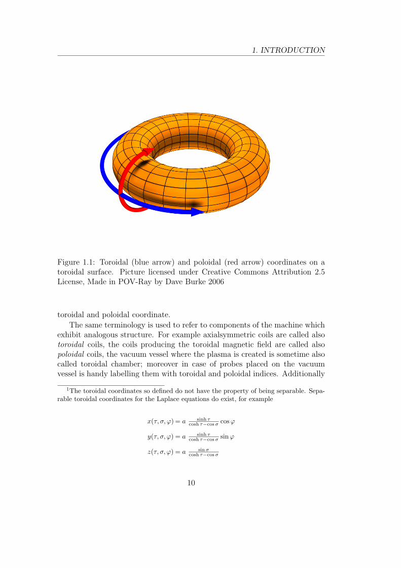
The variables r, ϑ, ϕ are called toroidal coordinates1, and ϑ and ϕ are re-spectively the poloidal and the toroidal angles, while r is the radial coordinateor radius. The positive number R0 is one of the most fundamental machineparameters: the nominal major radius. The coordinate surfaces of this map-ping are toroidal, conical and planar corresponding respectively to constant r,ϑ and ϕ. The planar coordinate surfaces are called poloidal planes. A visualdescription of a toroidal surface is reported in Figure 1.1. The black lines onthe surface are the intersections between the toroidal surface and the othercoordinate surfaces. The blue and red arrows show respectively the versus of
9
1. INTRODUCTION
Figure 1.1: Toroidal (blue arrow) and poloidal (red arrow) coordinates on atoroidal surface. Picture licensed under Creative Commons Attribution 2.5License, Made in POV-Ray by Dave Burke 2006
toroidal and poloidal coordinate.
The same terminology is used to refer to components of the machine whichexhibit analogous structure. For example axialsymmetric coils are called alsotoroidal coils, the coils producing the toroidal magnetic field are called alsopoloidal coils, the vacuum vessel where the plasma is created is sometime alsocalled toroidal chamber; moreover in case of probes placed on the vacuumvessel is handy labelling them with toroidal and poloidal indices. Additionally
1The toroidal coordinates so defined do not have the property of being separable. Sepa-rable toroidal coordinates for the Laplace equations do exist, for example
x(τ, σ, ϕ) = a sinh τcosh τ−cos σ cos ϕ
y(τ, σ, ϕ) = a sinh τcosh τ−cos σ sinϕ
z(τ, σ, ϕ) = a sin σcosh τ−cos σ
10
1. INTRODUCTION
the z axis, the xy plane and the circle r = 0 to be called, respectively, principalaxis, equatorial plane and secondary axis.
Some attention has to be made in the definition of the domain of thecoordinates change in order to attain its bijectivity. As a matter of fact, theinjectivity of such a mapping is guaranteed only if its domain is reduced to theregion U of the points (r, ϑ, ϕ) satisfying
−π < ϑ ≤ π−π < ϕ ≤ π
r > 0−r cosϑ < R0
(1.3)
In this case, the function g is not surjective any more as the the principaland secondary axes are not reached by the constrained coordinates. On theseregions, however, the Jacobian matrix of g would be singular and the cor-responding mapping x : U ⊂ R3 → V not regular. Instead, in the regionof V obtained removing the principal and secondary axes, the above toroidalcoordinates are orthogonal, defining an orthonormal basis as follows
ur(r, ϑ, ϕ) = −dxdr
(r, ϑ, ϕ)
uϑ(r, ϑ, ϕ) =1
r
dx
dϑ(r, ϑ, ϕ)
uϕ(r, ϑ, ϕ) =1
R0 + r cosϑ
dx
dϕ(r, ϑ, ϕ)
(1.4)
This basis is commonly used to represent vectorial quantities such as the totalmagnetic field produced by the set of active coils in the following form
b(r, ϑ, ϕ) = br(r, ϑ, ϕ)ur + bϑ(r, ϑ, ϕ)uϑ + bϕ(r, ϑ, ϕ)uϕ. (1.5)
1.2.4 Devices for the magnetically confined fusion
The devices used today by experimentalists of the magnetically confined fusionscience are large electrical machines, integrated with a number of auxiliarysystems. In the context of the magnetically confined fusion research all thedevices share a common conceptual design. The main components of thesemachines are: the vessel, the magnetic system, the heating and current drivesystems, the diagnostics and the control system.
The vessel
The region where the plasma is created is bounded by a ring shaped struc-ture which constitutes the vacuum vessel. The internal wall of the vessel is
11
1. INTRODUCTION
protected, totally or partially, by a cover of tiles called first wall. It is gen-erally constructed with elements or materials made up of atoms with a lowatomic number that are able to resist to a high thermal load like, for example,graphite, carbon fibre composites (CFC), or beryllium. The vacuum vessel isso called because inside the plasma an ultra-high vacuum is obtained beforestarting the operations in order to reduce the impurity density.
The magnetic system
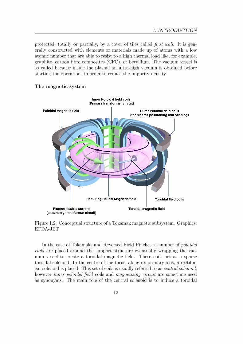
Figure 1.2: Conceptual structure of a Tokamak magnetic subsystem. Graphics:EFDA-JET
In the case of Tokamaks and Reversed Field Pinches, a number of poloidalcoils are placed around the support structure eventually wrapping the vac-uum vessel to create a toroidal magnetic field. These coils act as a sparsetoroidal solenoid. In the centre of the torus, along its primary axis, a rectilin-ear solenoid is placed. This set of coils is usually referred to as central solenoid,however inner poloidal field coils and magnetising circuit are sometime usedas synonyms. The main role of the central solenoid is to induce a toroidal
12
1. INTRODUCTION
electrical field in the plasma. The consequent loop voltage drives a toroidalcurrent in the plasma, which is called plasma current and which is anotherfundamental parameter of this kind of machines. The plasma current can besustained as long as the magnetising circuit is able to vary monotonically itscurrent. Toroidal coils are also placed conveniently outside the vacuum vessel,usually in the outer region. They are used for two tasks: to control the plasmaposition and to shape the plasma boundary. These toroidal coils are also calledfield shaping coils. A picture of the gross magnetic configuration in the caseof a Tokamak machine is presented in Figure 1.2.
Things are slightly different for Stellarators. In this case the central solenoidis not strictly required and the two toroidal and poloidal sets of coils are mergedin one single set of non planar coils. These kind of winding can be elicoidal-likeor even more complex. Other coils, local in nature, are the error field coils usedfor the correction of the field errors in the neighbouring of non-axialsymmetricfeatures of the machine or for a finer control of the plasma boundary.
The main material used in the construction of the machines magnetic sys-tem was, in the past, copper. Nowadays, in order to be able to control theplasma for a longer time, the coils of the magnetic system are usually madeof superconducting materials. This choice is essentially imposed by the factthat it is extremely difficult to design copper coils able to sustain the ohmicthermal load of the nominal current densities for the requested period of time.
Each one of these coils system is usually fed by a corresponding independentpower supply group. The characteristic of the power supplies vary dependingon the size of the machine and the length of the plasma discharge. Usually,in small and medium sized machines, the energy required for the operations isstored in mechanical, magnetic and electric accumulators which take it fromthe national power grid. The nominal power of the converters used to performthis task can be a fraction of the actual maximum power required by themachine operations. This approach needs a careful design of the energy storagesystems and of the converters. However, the most challenging power suppliesare those of big seized machines which operate with long discharge or in steadystate. These kind of power supplies require a careful engineering activity andnon-standard designs, as the mean power requested by these machines can beof the order of 500 MegaWatt.
Auxiliary heating and current drive systems
The most simple mechanism rising the plasma temperature is given by theOhm’s effect. The current induced in the plasma by the central solenoid fluxswing is also responsible for its temperature rise. However, as the plasma resis-tance decrease with the plasma temperature, this mechanism is not sufficient
13
1. INTRODUCTION
to reach the target temperature. For this reason other heating mechanism arerequired. These plasma auxiliary heating systems are based on the coupling ofelectromagnetic waves with the plasma at the ion, electron or hybrid cyclotronfrequency and on the injection into the plasma of a “current” of neutral parti-cles, usually hydrogen or deuterium atoms. The injection of neutral particlesrequires a device called neutral beam injector which is itself a system of thesame order of complexity than the machine. In machines like Tokamaks andRFP, which usually operates in a pulsed regimes, this system can also be usedas non inductive current drive system. By using these devices it is possible toincrease the length of the pulse beyond the limits imposed by the maximumamount of magnetic energy that can be stored in the central solenoid, possiblyreaching the steady state operational regime. Such heating system becomesthe primary heating facilities in machines without a central solenoid, as couldbe in Stellarators.
Diagnostics
Being experimental machines these kind of devices are usually filled up withdiagnostic equipment of several kind. The most commonly used are: magneticprobes (such as field probes and Rogowsky coils), temperature and pressuresensors, optic sensors, like infra red cameras, Thompson scattering, interfer-ometers and neutrons detectors.
The control system
All the machine subsystem can also be seen as information users. Many ofthem, like the diagnostic systems, are data producers, others, such as the poweramplifiers controlling the current in the coils, are data consumer and severalare both of them at the same time, for example all the controllers which processinput data producing output data. In this vision the devices of the subsystemsof the machine are components of a network where information flows from onenode to another. This flow needs to be controlled carefully. Data processingquality, that is the reliability and capability of the information processing, isof critical importance for the machine operations. Some of them are indeedsubject to strict, real-time, timing requirements.
Other systems
Apart from the subsystems described above there is a great number of othercomponents, sometimes called auxiliary system, which are essential for themachine operations. For example: the coils cooling system, the cryogenic
14

1. INTRODUCTION
system, the gas pumping and the vacuum system, eventually the cooling systemfor the conversion of the nuclear reactions energy.
In the past the coil cooling system has been implemented with standardtechnology, but the use of superconducting coils requires the set up of a cryo-genic system working at a temperature of about 4 Kelvin. The cryogenic sys-tem can also be used to implement the last component in the vacuum pumpingchain. Indeed this system can be implemented with lines made of a cryopump,a turbomolecular and a rotative pump connected in series. If the number offusion reactions become significant (as it should be in the case of the nextgeneration machines) the implementation of a system which takes care of thethe heat generated by the neutrons produced by the fusion reactions is alsorequired.
Despite its length, this list of subsystems is not exhaustive of all the com-ponents important for the realisation of a device for the study of the magnet-ically confined nuclear fusion. The present section aims at giving the idea ofthe complexity of such devices.
1.2.5 RFX-mod
Most of the doctoral research activity has been carried out at the RFX-modsite, in Padova, Italy. RFX-mod is currently the biggest RFP in the worldand it is run by the “Consorzio RFX”, an EURATOM-ENEA association.The machine, known in the past with the name “Reversed Field eXperiment”(RFX), started the operations in the 2004 after an upgrade triggered by a firethat in the 1999 destroyed part of its power supplies. Modifications appliedto the machine components have been thought to be important enough to bementioned in its name, so it has been changed to RFX-mod.
The structure of RFX-mod is essentially the one described in the previoussubsection. A slightly more descriptive illustration of the components of inter-est for the doctoral dissertation is given in the following one. The details ofthe major modifications of RFX-mod have been reported in the papers [3].
The main parameters of the RFX machine are listed in Table 1.1. Thevacuum vessel is a toroidal rigid structure made of INCONEL 625, composedof 72 elements welded together. Its inner surface is fully covered by graphitetiles, and be baked at temperatures between 350-400 C. The vessel majorradius is 2 m while its minor radius is 0.5 m. The vacuum vessel is also aninterface between the plasma and the outside. It is therefore equipped with 96ports for gas immission, vacuum pumping and diagnostic systems.
In RFX-mod the vacuum vessel is surrounded by a 3 mm thick coppershell. The purpose of this structure is to provide a passive stabilisation of thefast magnetohydrodynamical instabilities. This component, common in RFP
15
1. INTRODUCTION
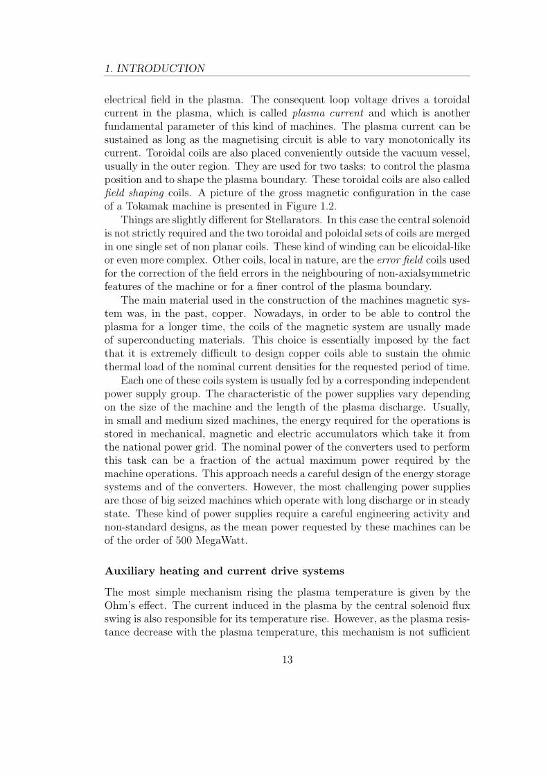
Figure 1.3: RFX-mod assembly.
machines, was not described in the general section, but, together with theactive control system of the MHD instabilities, it is one of the fundamentalcomponents for the present document. The shell is not uniform neither in thepoloidal direction, as an inner equatorial cut is present, nor in the toroidaldirection, as a poloidal gap and a region where the two edge of the shelltoroidally overlap are also present. The two gaps in the shell allow for thepenetration of the axialsymmetric toroidal field bϕ and the axialsymmetrictoroidal electric field.
Outside the stabilising shell, a toroidal structure provides the necessarymechanical support to the machine assembly, including 48 toroidal field coils,8+8 field shaping coils and 192 local coils called saddle coils. In Figure 1.3 thepicture of the vacuum vessel, shell and support structure assembly is presented.The saddle coils windings can be seen as the fourth element of the machinemagnetic subsystem, the magnetising circuit, the toroidal coils and the fieldshaping coils being the first three. Overall, the maximum peak power of anRFX-mod pulse requires 200 MVA to be taken from the 400 kV 50 Hz Italian
16
1. INTRODUCTION
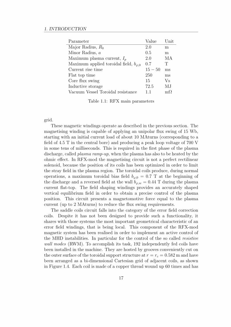
Parameter Value UnitMajor Radius, R0 2.0 mMinor Radius, a 0.5 mMaximum plasma current, Ip 2.0 MAMaximum applied toroidal field, bϕ,0 0.7 TCurrent rise time 15− 50 msFlat top time 250 msCore flux swing 15 VsInductive storage 72.5 MJVacuum Vessel Toroidal resistance 1.1 mΩ
Table 1.1: RFX main parameters
grid.
These magnetic windings operate as described in the previous section. Themagnetising winding is capable of applying an unipolar flux swing of 15 Wb,starting with an initial current load of about 10 MAturns (corresponding to afield of 4.5 T in the central bore) and producing a peak loop voltage of 700 Vin some tens of milliseconds. This is required in the first phase of the plasmadischarge, called plasma ramp-up, when the plasma has also to be heated by theohmic effect. In RFX-mod the magnetising circuit is not a perfect rectilinearsolenoid, because the position of its coils has been optimized in order to limitthe stray field in the plasma region. The toroidal coils produce, during normaloperations, a maximum toroidal bias field bϕ,0 = 0.7 T at the beginning ofthe discharge and a reversed field at the wall bϕ,w = 0.44 T during the plasmacurrent flat-top. The field shaping windings provides an accurately shapedvertical equilibrium field in order to obtain a precise control of the plasmaposition. This circuit presents a magnetomotive force equal to the plasmacurrent (up to 2 MAturns) to reduce the flux swing requirements.
The saddle coils circuit falls into the category of the error field correctioncoils. Despite it has not been designed to provide such a functionality, itshares with those systems the most important geometrical characteristic of anerror field windings, that is being local. This component of the RFX-modmagnetic system has been realised in order to implement an active control ofthe MHD instabilities. In particular for the control of the so called resistivewall modes (RWM). To accomplish its task, 192 independently fed coils havebeen installed in the machine. They are hosted by grooves conveniently cut onthe outer surface of the toroidal support structure at r = rc = 0.582 m and havebeen arranged as a bi-dimensional Cartesian grid of adjacent coils, as shownin Figure 1.4. Each coil is made of a copper thread wound up 60 times and has
17
1. INTRODUCTION
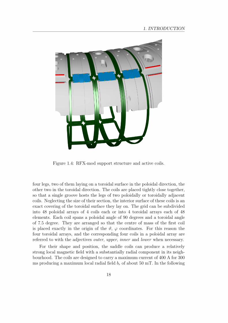
Figure 1.4: RFX-mod support structure and active coils.
four legs, two of them laying on a toroidal surface in the poloidal direction, theother two in the toroidal direction. The coils are placed tightly close together,so that a single groove hosts the legs of two poloidally or toroidally adjacentcoils. Neglecting the size of their section, the interior surface of these coils is anexact covering of the toroidal surface they lay on. The grid can be subdividedinto 48 poloidal arrays of 4 coils each or into 4 toroidal arrays each of 48elements. Each coil spans a poloidal angle of 90 degrees and a toroidal angleof 7.5 degree. They are arranged so that the centre of mass of the first coilis placed exactly in the origin of the ϑ, ϕ coordinates. For this reason thefour toroidal arrays, and the corresponding four coils in a poloidal array arereferred to with the adjectives outer, upper, inner and lower when necessary.
For their shape and position, the saddle coils can produce a relativelystrong local magnetic field with a substantially radial component in its neigh-bourhood. The coils are designed to carry a maximum current of 400 A for 300ms producing a maximum local radial field br of about 50 mT. In the following
18
1. INTRODUCTION
sections these coils will also be called active coils and radial field coils. Thiscan not lead to confusion because the study of this magnetic system is theprimary subject of the doctoral dissertation.
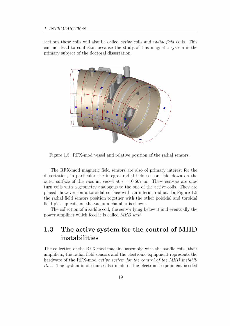
Figure 1.5: RFX-mod vessel and relative position of the radial sensors.
The RFX-mod magnetic field sensors are also of primary interest for thedissertation, in particular the integral radial field sensors laid down on theouter surface of the vacuum vessel at r = 0.507 m. These sensors are one-turn coils with a geometry analogous to the one of the active coils. They areplaced, however, on a toroidal surface with an inferior radius. In Figure 1.5the radial field sensors position together with the other poloidal and toroidalfield pick-up coils on the vacuum chamber is shown.
The collection of a saddle coil, the sensor lying below it and eventually thepower amplifier which feed it is called MHD unit.
1.3 The active system for the control of MHD
instabilities
The collection of the RFX-mod machine assembly, with the saddle coils, theiramplifiers, the radial field sensors and the electronic equipment represents thehardware of the RFX-mod active system for the control of the MHD instabil-ities. The system is of course also made of the electronic equipment needed
19
1. INTRODUCTION
for the acquisition and processing of the relevant control variables. From asystemic point of view three components can be identified:
1. The power amplifiers feeding the saddle coils
2. The electromagnetic system made of the active coils, the radial sensorsand the passive structures of the machine assembly
3. The control systems
These components are generally connected in a loop configuration: the voltagesat the ends of the power amplifiers are the inputs of the radial magnetic systemwhose outputs are the fluxes measured by the sensors. The flux values areprocessed by control algorithms and resulting quantities are sent back to thepower amplifiers as references or set points.
The details of the model of the amplifiers are not the subject of this disser-tation, and only the essential information will be given. The power amplifiersthemselves can be seen as a controlled dynamic system. They can operate inthree different modalities, depending on their parameter configuration. Theycan be voltage controlled, current controlled or flux controlled. In the first casethe power amplifiers control electronic interprets its input signals as a scaledvoltage reference and the electronic gates of the power supply unit are con-trolled so as to present the associated output voltage. In the second case, theinput signal is interpreted as a scaled current reference and the feedback con-troller implemented in the power amplifiers tries to drive a current followingthe reference. In the third case the, the input signal is interpreted as a fluxreference. The controlled error signal is the difference between the referenceand the flux measured by the underlying sensor.
The electromagnetic system is substantially inductive. It is made by 192coils which can be interested by a current flow (the active coils), and 192 coilswhich are used as sensors (the radial field sensors). This set of 384 coils canbe modelled as an ideal inductive 384-pole. That is the currents satisfy therelation [
v1(t)v2(t)
]=
[M11 M12
M21 M22
]d
dt
[i1(t)i2(t)
]+
[R11 00 R22
] [i1(t)i2(t)
](1.6)
where v and i denotes respectively voltage and current vector. The index 1refers to the active coils, index 2 to the sensors. Mij are partitions of a globalinductance matrix, while Rii are diagonal resistance matrices.
The voltage at the ends of the sensor coils is integrated to produce theflux measure. The integrating electronic is assumed to have a very small effect
20
1. INTRODUCTION
on the measured system so that the relation i2(t) = 0 is reasonable. Thisconsideration lead to the equations
v1(t) = M11ddti1(t) + R11i1(t)
ψ2(t) = M21i1(t)(1.7)
where ψ(t) is the flux vector measured by the radial field sensors.These equations, however, are correct only in a space free of passive struc-
tures. In their presence a linear multiple-input-multiple-output model of therelation between the input voltages and the output fluxes can still be derived,but require more effort in the modelling, and the resulting transfer matricesresult to be frequency dependent. This holds true even for the transfer func-tion matrix linking the input coil currents to the output flux vectors, whichwould be constant in the absence of passive structures.
The components M11 and M21 of the global inductance matrix have beencentral to this doctoral dissertation. A state space model of the transfer func-tion matrix M21(jω), called also M(jω) in the following, and a model of thetransfer function relating the saddle coils input voltages to the currents flowingin them has been derived. M11 plays a role in the latter derivation.
1.3.1 Nomenclature
A common naming convention has to be adopted for the clear identification ofeach entity in the set of the active coils and radial field sensors. In the caseof this system, however, more than one naming convention emerged, used onthe base of their convenience. At first sight labelling each coil naturally witha number from 1 to 192 following a particular geometrical order seems to bethe most clear solution. This also makes sense from the point of view of theimplementer of the control system, for whom each entity measure is a compo-nent of a vector stored somewhere in the controller memory. From other pointsof view, however, other naming conventions seems to be more adequate. Forexample when performing the spatial spectral analysis of a quantity measuredby the system2 the quantity itself is intrinsically bi-dimensional. In this caselabelling with pairs in the set 1, 2, . . . , 48× 1, 2, 3, 4 provides more insightof how things work. Other naming conventions are in use at the RFX sitein particular for the coils power amplifiers. These are in use because are themost obvious from the point of view of the power supply expert. The namingconventions more suitable for the present document are described below.
In the bi-dimensional nomenclature, to each sensor, active coil and relativeamplifier is assigned a pair of numbers from the set 1, 2, . . . , 48×1, 2, 3, 4.
2This kind of analysis will be described in the following chapter
21
1. INTRODUCTION
The first number in the pair is called toroidal index, the second poloidal index.The pair (1,1) is assigned to the sensor and active coil surrounding the halfline ϑ = 0, ϕ = 0. The pair (1,2) is assigned to the sensor and active coilsurrounding the half line described by ϑ = 1
2π, ϕ = 0 and so on. The pair
(2,2) is assigned to the coil and sensor linked to the ϑ = 12π, ϕ = 1
24π half line
and so on. In other words each coil is identified by two indices: the first one isthe index of a poloidal array whereas the second one is the index of a toroidalarray. The toroidal and poloidal indices are discrete coordinates correspondingto the continuous coordinates. The position of the “centre” of the (i, j) coil isϑ = (j− 1)π
2, ϕ = (i− 1) π
24. The nomenclature is extended also to the relative
coil power amplifier.In the progressive nomenclature to each sensor, active coil, and correspond-
ing amplifier is assigned a single number, called progressive index, varying from1 to 192. Mathematically the progressive index p can be calculated from thetoroidal index i and poloidal index j using the formula
p = 4(i− 1) + j. (1.8)
In other words the progressive nomenclature labels the sensors, coils and rel-ative amplifiers by counting them in poloidal major order. The toroidal andpoloidal indices can be calculated from the progressive index using the relations
i = floor (p− 1)/4 + 1j = mod (p− 1, 4) + 1.
(1.9)
22
Chapter 2
Analysis of the RFX-mod MHDsystem
2.1 Introduction
This chapter concerns the formal description of the RFX-mod active systemfor the control of the MHD instabilities and its analysis, from the point ofview of the System and Signal Theory. Particular attention has been paid tothe description of its intrinsic sampling mechanisms and in relation with thetoroidal geometry.
In the following section are introduced the mathematical language andthe tools needed to describe the active system from a systemic point of view,relaying on standard concepts of the System and Signal Theory. In particularthe language of the Unified Signal Theory developed by Professor GianfrancoCariolaro of the Padova University is used. After the most important conceptsof this theory have been recalled, the analysis of the sampling components ofthe system is presented. The analysis shows how the spatial harmonic contentof physical quantities such as the poloidal sheet current density Jp and theradial magnetic field br are affected by the sampling performed by the sensors.An integral parameter Λ, summarising the importance of the toroidal effect,is proposed.
2.2 Summary of the Unified Signal Theory
The Unified Signal Theory is an abstract formulation of signals and systems.It has been developed starting from few basic concepts, and it then resultsto be a general theory applicable to a wide class of signals and systems. Asthe reference textbook for the Unified Signal Theory is, at the moment, only
23
2. ANALYSIS OF THE RFX-MOD MHD SYSTEM
published in Italian language, in order to provide the reader with a generalunderstanding of the theory, a summary of it is presented in this section. Thereader should keep in mind, however, that the purpose of this summary is toprovide the information required to understand the specific analysis carried outin the rest of this dissertation, not to provide a complete survey of the UnifiedTheory. Further details of the theory, results and examples which are usefulfor its understanding, can be found in [6], which is the reference textbook ofthe Unified Signal Theory.
2.2.1 Regular groups
The key of the unification is the formal definition of signal, which is basedon algebraic structures called locally compact Abelian groups. The elements ofthis class are those mathematical objects which are, at the same time, both alocally compact topological space and an Abelian group with continuous groupoperation with respect of the topology [7]. Locally compact Abelian groupsare referred to, in the following, as regular groups for brevity1. In other wordsthe regular groups are the Abelian groups which, at the same time, are alsolocally compact topological spaces. The concept of regular group is logically atthe very bottom of the Unified Signal Theory and the study of the structuresof these groups is central to its development.
Elementary regular groups are R, Z and O. The latter is the trivial groupcontaining only the neutral element. Z(T ), the set nT : n ∈ Z, T ∈ (0,∞)is also a fundamental regular group. Other groups, denoted by U/S, are thoseobtained as quotients of a regular group U and one of its regular subgroupsS ⊂ U . A result of the topological group theory assures that the quotient groupformed in that way is always a regular group. Every group U can always berepresented as a quotient group by means of the trivial group, which is alwayscontained in every regular group. For example R can be expressed as R/Oand the trivial group as U/U for every group U . This means that the categoryof the quotient groups contains the one of the non-quotient groups. In thefollowing the word group is used to refer to the class of the quotient groups.Regular groups can also be constructed by taking the Cartesian product of tworegular groups. This fact has been used extensively in this chapter. Finallyregular groups can be constructed using isomorphisms between regular groups.
It is a fundamental result of Topology that
Theorem 2.2.1. Every regular group G is isomorphic to a group of Rm in the
1In should be stressed that in this context “regular” is merely a placeholder for thelocution “locally compact Abelian” and nothing else.
24
2. ANALYSIS OF THE RFX-MOD MHD SYSTEM
form
G ∼ Rp × (R/Z)q × Zr × Z/Z(N1)× · · · × Z/Z(Ns) (2.1)
for convenient p,q,r,s and N1, . . . , Ns ∈ N.
This theorem states that the structure of every possible regular group iscompletely known and having reference to the structure of simpler, elementarygroups. This theorem is used in the theory to develop the concepts of base,signature and representation of a regular group. These concepts are importantfor the development of the theory and in the characterisation of the regularsubgoups of Rn. However, for the purpose of this dissertation, their definitioncan be omitted.
2.2.2 Definition of signal
Equally important to the Unified Theory is the formal definition of signal,which, as has been mentioned before, relies on the concept of regular group.
Definition A signal is a function from a regular group U into the set of thecomplex numbers.
s : U → C (2.2)
Regular groups are important for the Unified Theory because they allowthe definition of a non-trivial operator acting on signals which is linear andinvariant to translations.
2.2.3 Periodicity and cells
Regular groups are also used in the Unified Theory to express the concept ofperiodicity. Formally, every regular sub-group P of a regular group U selectedfor this purpose is called periodicity of the group U . In general, signals withperiodicity P have the property that the signal value at u is the same of thesignal value at u+ p, for all the p ∈ P . That is,
s(u) = s(u+ p) ∀u ∈ U, ∀p ∈ P. (2.3)
The concept of periodicity is linked to the idea of cell, the generalisationof the period.
Definition A cell of the group U modulo P is a subset C of U so that
C + P = U (2.4)
25
2. ANALYSIS OF THE RFX-MOD MHD SYSTEM
and, for every p1, p2 ∈ P , the relation
(C + p1) ∩ (C + p2) = ∅ ⇔ p1 6= p2 (2.5)
holds. A cell of U modulo P is denoted with the symbol [U/P ).
In other words, the subsets family generated by shifting a cell [U/P ) of elementsin P a partition of U .
In the Unified Theory quotient groups are often interpreted as the couplegroup/modulo, instead of normal groups. This is possible because signalsdefined on U with periodicity P are always in a one to one correspondencewith the signals defined over the quotient group U/P . This correspondencecan easily be established making use of the following proposition, which isproved in the appendix.
Proposition 2.1. For every cell C = [U/P ) there exist a one to one mappingµ : C → U/P from C to the quotient group U/P .
2.2.4 The Haar integral
On every regular group U it is possible to define a measure, the Haar measure,from which an integral operator can be constructed. This operator is calledHaar integral and it is denoted, in this dissertation, by the usual integralsymbol, as shown in the equation below.∫
U
s(t)dt (2.6)
The Haar integral has the properties of being not identically zero for all signals,linear and invariant to a shift of the signal, that is obeying to the equation∫
U
s(t)dt =
∫U
s(t− u)dt, ∀u ∈ U. (2.7)
A fundamental result of the theory of locally compact groups is the proofof the existence and uniqueness of this integral.
Theorem 2.2.2. On every regular group it is possible to define a non-trivialintegral operator invariant to signal translations. This integral is unique up toa multiplicative constant.
By using this theorem an integral operator can quickly be checked to be acorrect Haar integral. Generally the Haar integral of a regular group is foundby checking if a given operator satisfies the above properties. For example the
26
2. ANALYSIS OF THE RFX-MOD MHD SYSTEM
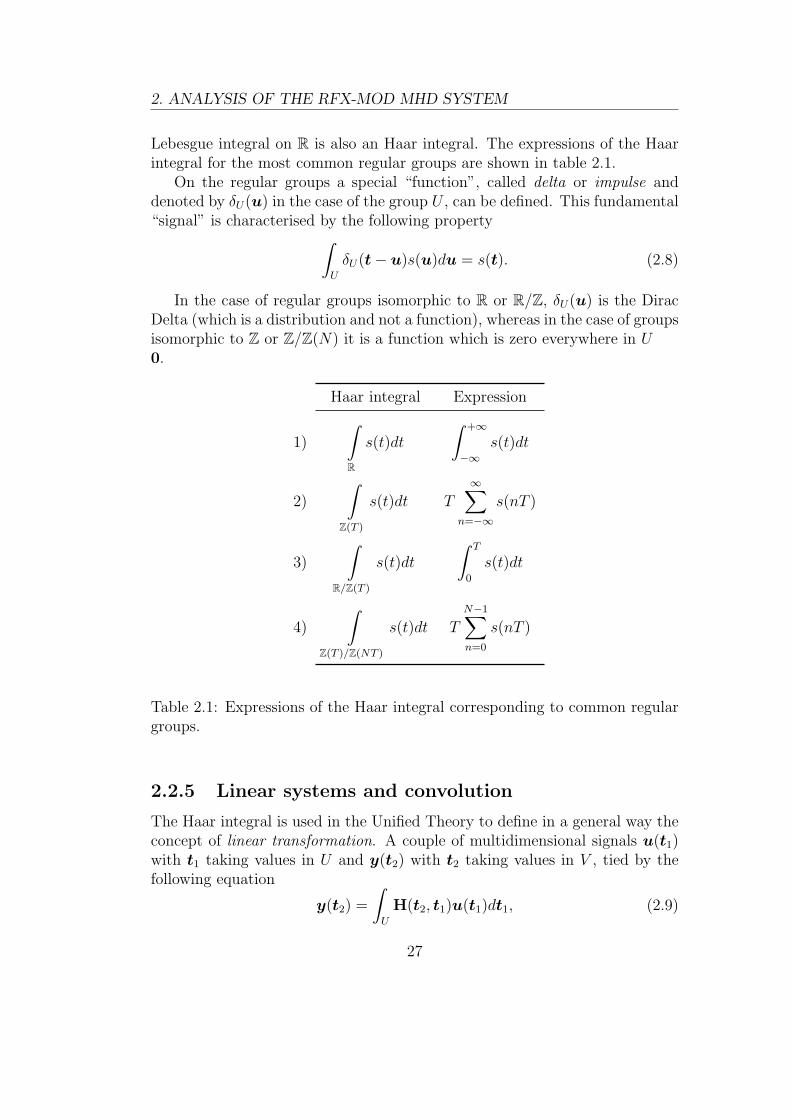
Lebesgue integral on R is also an Haar integral. The expressions of the Haarintegral for the most common regular groups are shown in table 2.1.
On the regular groups a special “function”, called delta or impulse anddenoted by δU(u) in the case of the group U , can be defined. This fundamental“signal” is characterised by the following property∫
U
δU(t− u)s(u)du = s(t). (2.8)
In the case of regular groups isomorphic to R or R/Z, δU(u) is the DiracDelta (which is a distribution and not a function), whereas in the case of groupsisomorphic to Z or Z/Z(N) it is a function which is zero everywhere in U0.
Haar integral Expression
1)
∫R
s(t)dt
∫ +∞
−∞s(t)dt
2)
∫Z(T )
s(t)dt T∞∑
n=−∞
s(nT )
3)
∫R/Z(T )
s(t)dt
∫ T
0
s(t)dt
4)
∫Z(T )/Z(NT )
s(t)dt TN−1∑n=0
s(nT )
Table 2.1: Expressions of the Haar integral corresponding to common regulargroups.
2.2.5 Linear systems and convolution
The Haar integral is used in the Unified Theory to define in a general way theconcept of linear transformation. A couple of multidimensional signals u(t1)with t1 taking values in U and y(t2) with t2 taking values in V , tied by thefollowing equation
y(t2) =
∫U
H(t2, t1)u(t1)dt1, (2.9)
27
2. ANALYSIS OF THE RFX-MOD MHD SYSTEM
are said to be, respectively, the input and the output of a linear transformationor system. The function matrix H(t2, t1) is defined over the Cartesian productU × V and it is called the kernel of the transformation.
The presented definition is the most general definition of linear system asit applies to variant, non-causal and multiple-input-multiple-output systems.The details of the use and meaning of such an operator depending on therelationship between the input domain U and the output domain V have beendeveloped in the framework of the Unified Theory and can be found in thebook [6].
In case the signals are not multidimensional the signals and the kernel ofthe above equation are written using normal letters instead of the bold ones,as below.
y(t2) =
∫U
h(t2, t1)u(t1)dt1 (2.10)
If the transformation kernel satisfies the following property
h(t2 + ∆t, t1 + ∆t) = h(t2, t1) (2.11)
for every ∆t ∈ U , which requires the domains U and V to share a commongroup operation, the system is called quasi invariant. If U and V are thesame group it is strictly invariant. The invariance of a transformation is animportant property which determines simplifications in the analysis of systems.Invariant counterparts of variant systems, for example, requires to define theirkernel in a group with half of the dimensions. Also the Fourier analysis of thesignals is simplified for invariant systems. Most of the results of the Systemand Signal Theory used in the engineering applications regards the class of theinvariant transformations. By letting ∆t = −t1 in the above equation, thekernel of an invariant transformation can always be written in the form2
h(t2 − t1) = h(t2 − t1,0). (2.12)
Despite the relevance of the invariant or quasi invariant transformations,for the present dissertation some results regarding the variant transformationare required. They are recalled in the next section and proved in the appendix.
2.2.6 Dual domains
The definition of dual of a regular group U is used in the development of ageneral Fourier analysis based on the topological group theory. Dual groups,
2When different functions are used for semantically equivalent purposes, if they can bediscriminated by the number or type of their arguments, they are denoted with the samesymbol.
28
2. ANALYSIS OF THE RFX-MOD MHD SYSTEM
Group Dual
1) U U
2) U1 × U2 U1 × U2
3) R R
4)R
Z(T )Z(1/T )
5) Z(T )R
Z(1/T )
6)Z(T )
Z(NT )
Z(1/NT )
Z(1/T )
7)R
Z(2π)× R
Z(2π)Z(1/2π)× Z(1/2π)
8)Z(2π/N1)
Z(2π)× Z(2π/N1)
Z(2π)
Z(1/2π)
Z(N1/2π)× Z(1/2π)
Z(N2/2π)
Table 2.2: Common regular groups and their duals. Parameter T ∈ R \ 0,N ∈ Z \ 0.
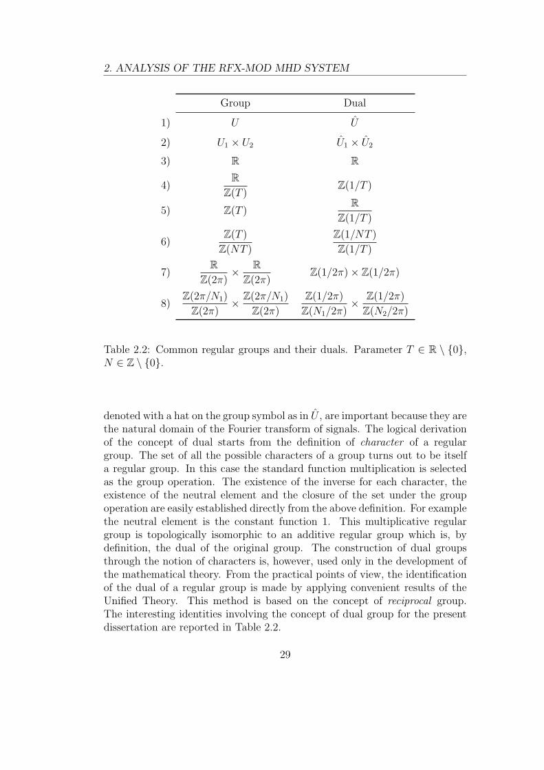
denoted with a hat on the group symbol as in U , are important because they arethe natural domain of the Fourier transform of signals. The logical derivationof the concept of dual starts from the definition of character of a regulargroup. The set of all the possible characters of a group turns out to be itselfa regular group. In this case the standard function multiplication is selectedas the group operation. The existence of the inverse for each character, theexistence of the neutral element and the closure of the set under the groupoperation are easily established directly from the above definition. For examplethe neutral element is the constant function 1. This multiplicative regulargroup is topologically isomorphic to an additive regular group which is, bydefinition, the dual of the original group. The construction of dual groupsthrough the notion of characters is, however, used only in the development ofthe mathematical theory. From the practical points of view, the identificationof the dual of a regular group is made by applying convenient results of theUnified Theory. This method is based on the concept of reciprocal group.The interesting identities involving the concept of dual group for the presentdissertation are reported in Table 2.2.
29

2. ANALYSIS OF THE RFX-MOD MHD SYSTEM
Signal Fourier transform
1) s(t) S(f)
2) s
(t− t0T
)Te−j2πf ·t0S(Tf)
3) s1(t)s2(t)
∫U
S1(f − ν)S2(ν)dν
4) δU(t) 1
5) 1 δU(f)
Table 2.3: Properties of the generalised Fourier transform.
2.2.7 Fourier transform
The generalised Fourier transform of a signal s over the domain U is definedas the following Haar integral
S(f) = F [s(t)](f) =
∫U
s(t)e−2πf ·tdt, (2.13)
where the variable f belongs to U , the dual of U .
In the Table 2.3 are presented some relationship between signal and Fouriertransform used in the rest of the document. The signals in the left column ofthe table are defined on the regular group U , therefore the Fourier transformson the right are defined on U . Signals are denoted with lowercase letterswhereas their Fourier transforms are denoted with the corresponding uppercaseletters. In the third and fourth rows of the table are recalled the formulas forthe Fourier transform of the shifted and stretched version of a signal and for theproduct of two signals. The last two rules are important relationship linkingidentity and Delta function on group and its dual.
Another important couple signal-transform used in the the following anal-ysis is
F [rect(t)](f) = sinc f, (2.14)
30
2. ANALYSIS OF THE RFX-MOD MHD SYSTEM
which relates the signals rect(t) and sinc(f) defined below.
rect(t) =
1 if |t| < 1
21
2if |t| = 1
2
0 if |t| > 1
2
t ∈ R, (2.15)
sinc(f) =sin(πf)
πff ∈ R. (2.16)
2.3 Time variant filtering
Some standard results of the Signal Theory about the invariant filtering have tobe extended to the non-invariant (or variant) case in order to be used in thefollowing calculations. A first proposition shows the mathematical relationbetween the Fourier transforms of signals which are connected by a variantfilter.
Proposition 2.2. Given a time variant system g(t1, t2) transforming the inputsignal u(t1) defined over the domain U into the corresponding output signalv(t2) defined over the same domain by the law
v(t2) =
∫U
g(t1, t2)u(t1)dt1 (2.17)
the Fourier transform of u(t1), v(t2) and g(t1, t2), respectively U(f1), V (f2)and G(f1,f2), are related by the equation
V (f2) =
∫U
G(−f1,f2)U(f1)df1 (2.18)
The importance of this result lays in the fact that the studied system isactually variant with respect of several aspects. The Fourier transform of theoutput signal is therefore obtained by the convolution of the Fourier transformof the input signal and the Fourier transform of the filter. This means thatthe harmonic content of the input signal is not only distorted by the variantfilter, but also new harmonic content can be introduced by the filter.
A second result shows the mathematical expression of the dual shape ofan invariant filter when it is treated with the variant theory. It is interestingbecause it is used in the definition of the parameter Λ given in the followingsection.
31
2. ANALYSIS OF THE RFX-MOD MHD SYSTEM
Proposition 2.3. Given a function g of two vectorial variables t1, t2 ∈ U suchthat for every d ∈ U g(t1 + d, t2 + d) = g(t1, t2), its Fourier transform is
G(f1,f2) = δU(f1 + f2)Gr(f2) = δI(f1 + f2)Gr(−f1) (2.19)
where
Gr(f2) =
∫U
g(0, τ )ej2πf2τdτ (2.20)
The proofs of these propositions can be found in the appendix.
2.4 MHD system analysis
In this analysis the RFX-mod active system for the control of the MHD insta-bilities, also referred to as the MHD system hereafter, has been considered. It isassumed to consist only of the 192 saddle coils, the machine passive structuresand the 192 radial field sensors. The intensities of the currents in the saddlecoils are supposed to be independent variables. This is reasonable, becausethey are independently fed by 192 power amplifiers.
The MHD system is seen as a particular magnetic field source with 192degree of freedom. Moreover, the resulting magnetic field is assumed to dependlinearly on the source currents. Such a device can be conveniently modelledas a dynamic system in the frame of the System Theory. However, instead ofdescribing the system from that point of view, in the following it is analysedusing the results of the Unified Signal Theory recalled in the previous section.
In the field of System Theory the MHD system would be classified as amulti-input-multi-output (MIMO) dynamic system. The 192 current intensi-ties would be the inputs of the system, whereas the 192 flux measures wouldbe its outputs. The values of these measures would be arranged in row vectors,respectively i(t) and ψ(t), and the linear dynamic relationship between themrepresented with the following integral transformation.
ψ(t) =
∫RM(u− t)i(u)dt (2.21)
The elements of the 192 × 192 matrix M(τ) would be real functions definedon R having the property of being causal impulse responses. The SystemTheory focuses on the structure of the mathematical representation of thedynamic system, that is on the shape of the function M(τ). The use of sucha representation is common, useful and it is at the base of the work describedin chapters 3 and 4. In spite of that, however, the approach described by the
32
2. ANALYSIS OF THE RFX-MOD MHD SYSTEM
M(·)i(t) ψ(t)
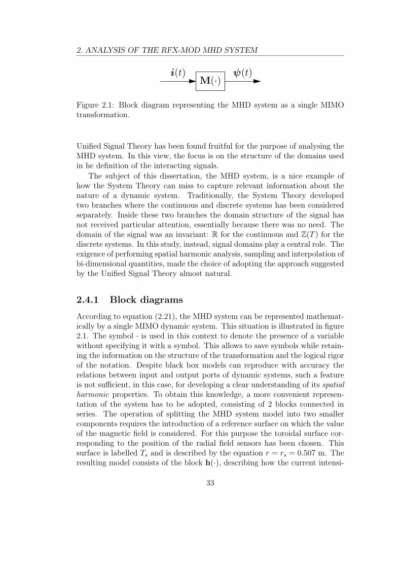
Figure 2.1: Block diagram representing the MHD system as a single MIMOtransformation.
Unified Signal Theory has been found fruitful for the purpose of analysing theMHD system. In this view, the focus is on the structure of the domains usedin he definition of the interacting signals.
The subject of this dissertation, the MHD system, is a nice example ofhow the System Theory can miss to capture relevant information about thenature of a dynamic system. Traditionally, the System Theory developedtwo branches where the continuous and discrete systems has been consideredseparately. Inside these two branches the domain structure of the signal hasnot received particular attention, essentially because there was no need. Thedomain of the signal was an invariant: R for the continuous and Z(T ) for thediscrete systems. In this study, instead, signal domains play a central role. Theexigence of performing spatial harmonic analysis, sampling and interpolation ofbi-dimensional quantities, made the choice of adopting the approach suggestedby the Unified Signal Theory almost natural.
2.4.1 Block diagrams
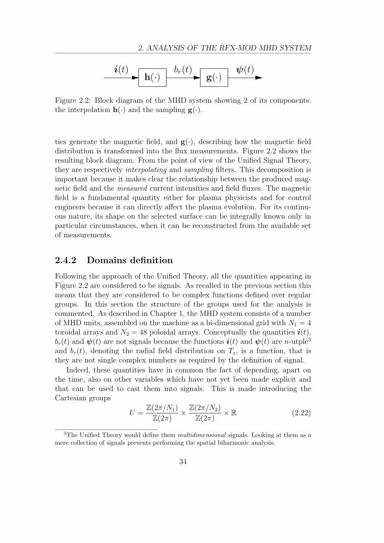
According to equation (2.21), the MHD system can be represented mathemat-ically by a single MIMO dynamic system. This situation is illustrated in figure2.1. The symbol · is used in this context to denote the presence of a variablewithout specifying it with a symbol. This allows to save symbols while retain-ing the information on the structure of the transformation and the logical rigorof the notation. Despite black box models can reproduce with accuracy therelations between input and output ports of dynamic systems, such a featureis not sufficient, in this case, for developing a clear understanding of its spatialharmonic properties. To obtain this knowledge, a more convenient represen-tation of the system has to be adopted, consisting of 2 blocks connected inseries. The operation of splitting the MHD system model into two smallercomponents requires the introduction of a reference surface on which the valueof the magnetic field is considered. For this purpose the toroidal surface cor-responding to the position of the radial field sensors has been chosen. Thissurface is labelled Ts and is described by the equation r = rs = 0.507 m. Theresulting model consists of the block h(·), describing how the current intensi-
33
2. ANALYSIS OF THE RFX-MOD MHD SYSTEM
h(·) g(·)i(t) b
r(t) ψ(t)
Figure 2.2: Block diagram of the MHD system showing 2 of its components:the interpolation h(·) and the sampling g(·).
ties generate the magnetic field, and g(·), describing how the magnetic fielddistribution is transformed into the flux measurements. Figure 2.2 shows theresulting block diagram. From the point of view of the Unified Signal Theory,they are respectively interpolating and sampling filters. This decomposition isimportant because it makes clear the relationship between the produced mag-netic field and the measured current intensities and field fluxes. The magneticfield is a fundamental quantity either for plasma physicists and for controlengineers because it can directly affect the plasma evolution. For its continu-ous nature, its shape on the selected surface can be integrally known only inparticular circumstances, when it can be reconstructed from the available setof measurements.
2.4.2 Domains definition
Following the approach of the Unified Theory, all the quantities appearing inFigure 2.2 are considered to be signals. As recalled in the previous section thismeans that they are considered to be complex functions defined over regulargroups. In this section the structure of the groups used for the analysis iscommented. As described in Chapter 1, the MHD system consists of a numberof MHD units, assembled on the machine as a bi-dimensional grid with N1 = 4toroidal arrays and N2 = 48 poloidal arrays. Conceptually the quantities i(t),br(t) and ψ(t) are not signals because the functions i(t) and ψ(t) are n-utple3
and br(t), denoting the radial field distribution on Ts, is a function, that isthey are not single complex numbers as required by the definition of signal.
Indeed, these quantities have in common the fact of depending, apart onthe time, also on other variables which have not yet been made explicit andthat can be used to cast them into signals. This is made introducing theCartesian groups
U =Z(2π/N1)
Z(2π)× Z(2π/N2)
Z(2π)× R (2.22)
3The Unified Theory would define them multidimensional signals. Looking at them as amere collection of signals prevents performing the spatial biharmonic analysis.
34
2. ANALYSIS OF THE RFX-MOD MHD SYSTEM
h(α, ξ, ·) g(ζ,α, ·)i(ξ, t)
U
br(α, t)
V
ψ(ζ, t)
U
Figure 2.3: Interpolating and sampling filters. Domain of the signals shownexplicitly.
and
V =R
Z(2π)× R
Z(2π)× R (2.23)
as domains for the above quantities. In both of them the first two factors areused to represent spatial coordinates while the last one is used to representthe time coordinate t. As this analysis is not focused on the behaviour of theMHD system with respect of the time, in the time dependence is sometimesdropped. This is acceptable because system is assumed to be time-invariantand it is meaningful, for the scope of the analysis, working at fixed time. Whenthis simplification is made the above domains become
UL =Z(2π/N1)
Z(2π)× Z(2π/N2)
Z(2π)(2.24)
and
VL =R
Z(2π)× R
Z(2π). (2.25)
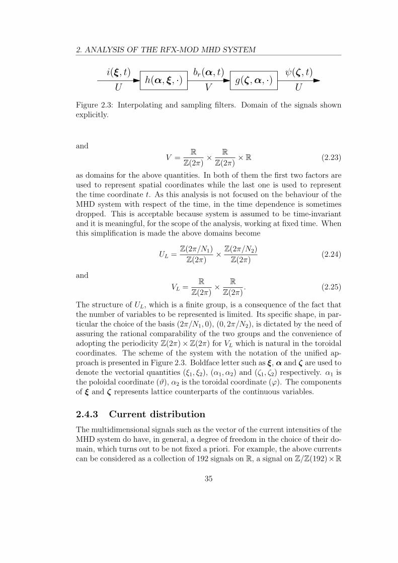
The structure of UL, which is a finite group, is a consequence of the fact thatthe number of variables to be represented is limited. Its specific shape, in par-ticular the choice of the basis (2π/N1, 0), (0, 2π/N2), is dictated by the need ofassuring the rational comparability of the two groups and the convenience ofadopting the periodicity Z(2π)×Z(2π) for VL which is natural in the toroidalcoordinates. The scheme of the system with the notation of the unified ap-proach is presented in Figure 2.3. Boldface letter such as ξ, α and ζ are used todenote the vectorial quantities (ξ1, ξ2), (α1, α2) and (ζ1, ζ2) respectively. α1 isthe poloidal coordinate (ϑ), α2 is the toroidal coordinate (ϕ). The componentsof ξ and ζ represents lattice counterparts of the continuous variables.
2.4.3 Current distribution
The multidimensional signals such as the vector of the current intensities of theMHD system do have, in general, a degree of freedom in the choice of their do-main, which turns out to be not fixed a priori. For example, the above currentscan be considered as a collection of 192 signals on R, a signal on Z/Z(192)×R
35
2. ANALYSIS OF THE RFX-MOD MHD SYSTEM
or a signal on U . The choice of the domain structure has to be made consid-ering other available information on the system such as the constraints on thetype of harmonic analysis, if any, that has to be performed on the signal. So,considering the examples just mentioned, in the first case no spatial harmonicanalysis is possible, because the domain is spatially unstructured4, in the sec-ond case a mono-dimensional spatial harmonic analysis is possible whereas inthe third a bi-dimensional spatial harmonic analysis become feasible.
The vector of the current intensities of the MHD system can be interpretedas a discrete bi-dimensional distribution in the sense that it is possible todevise a sampling scheme of a continuous bi-dimensional quantity where thecurrents turns out to be samples. This can be seen considering a continuouslaminar current density, Jp(α, t), on the toroidal surface Tc correspondingto the saddle coils radius rc = 0.582 m. The harmonic content of this bi-dimensional signal can be defined without ambiguities because the poloidal andtoroidal components are not independent assuming the current solenoidality5.Somehow arbitrarily, the harmonic content of Jp(α, t) is then defined to bethe one of its poloidal component. The current density is then sampled with aN1×N2 grid of sensors. Without entering the details, one way of implementingthis sampling system is considering a small arc, L(γ), as a reference boundaryfor the current measurement. This arc is placed on the toroidal surface Tc alongthe toroidal direction. Its length, l(γ), is an approximation of the toroidalwidth of the saddle coil section. A discrete variable ξ belonging to the groupset UL is used for the definition of the discrete signal and corresponds to thecontinuous variable γ taking values in VL. The probes are placed poloidallyat angles γ1 = ξ1 and centered toroidally at angles γ2 = ξ2 − π/N2.
In toroidal coordinates the measure of the current flowing through the arcis expressed by the following integral
i(ξ, t) =
∫L(ξ)
Jp(α, t)ndl. (2.26)
defining the function f(γ,α) as
f(γ,α) =R0
∆α2
(1 + ac cos(α1))δ(α1 − γ1) rect
(α2 − γ2 + π/N2
∆α2
)(2.27)
the currents can be expressed as a linear transformation which is a sampling
4From the harmonic analysis, in this case, is not possible to obtain more than a collectionof time frequency responses.
5This would not be the case if the current density had been tri-dimensional.
36
2. ANALYSIS OF THE RFX-MOD MHD SYSTEM
from VL to UL
i(ξ) =
∫∫VL
f(ξ,α)Jϑ(α)dα. (2.28)
In case the output quantity had been the mean current density<Jp(ξ)> thefilter would have been
f(ξ,α) =1
∆α2
1 + ac cos(α1)
1 + ac cos(ξ1)δ(α1 − ξ1) rect
(α2 − ξ2 − π/N2
∆α2
)(2.29)
and the linear transformation
<Jϑ>(ξ) =
∫∫VL
f(ξ,α)Jϑ(α)dα. (2.30)
2.4.4 Field interpolation
It is natural now modelling the relation between the discrete current distribu-tion i(ξ, t) and the flux distribution br(α, u) using the integral linear transfor-mation of the Unified Theory
br(α, u) =
∫U
h(α, u, ξ, t)i(ξ, t)dξ, (2.31)
with h(α, u, ξ, t) the kernel of the transformation. Assuming the time invari-ance of the system a slight simplification to the kernel can be made. It shouldbe pointed out however than assumption on the space invariance can not bemade. On a toroidal surface a field can not be invariant because, for example,it is possible to track changes in the position from the local surface curvature.In other words the coils or the sensors on the inner part of the toroidal surfaceare intrinsically different from the one on the outer surface. But apart of thiseffect, which could be advocated to be somewhat small for large aspect ratios,there still is the fact that the passive structures are not uniform. They presentclear dishomogeneities both in the poloidal direction, such as the shell innerequatorial gap, and in the toroidal direction, such as the shell overlapping re-gion, not to mention the load assembly diagnostic ports. This is a real sourceof invariance of the space coordinates.
The time invariance allows to reduce the dimension of the kernel domainso that it becomes h(α, ξ, τ)6. Making use of the bold notation for n-tuples,the linear transformation becomes
br(α, u) =
∫U
h(α, ξ, u− t)i(ξ, t)dξdt. (2.32)
37

2. ANALYSIS OF THE RFX-MOD MHD SYSTEM
Another form of this equation can be obtained by writing explicitly theHaar integrals on the domains. The resulting form is basically the one thatcould be obtained considering the system, instead of a single linear transfor-mation between multidimensional domains, as a a number of linear transfor-mations from R to V . Considering that two of the three components of thedomain U are lattices, that is U = UL × R with UL = Z(2π/N1)
Z(2π)× Z(2π/N2)
Z(2π), the
linear transformation can be written explicitly as
br(α, u) =4π2
N1N2
∑ξ∈UL
∫Rh(α, ξ, u− t)i(ξ, t)dt. (2.33)
The factor 4π2
N1N2can be absorbed in the kernel obtaining the representation
br(α, u) =∑ξ∈UL
∫Rhξ(α, u− t)iξ(t)dt, (2.34)
which is perhaps more common and generally accepted. The couple ξ can beseen as a “label” or an index for the elements which it applies to. The leadingfactor which appears in the above equation depends on the definition of theHaar integral on a lattices as the summation of the signal values times thelattice determinant.
A good estimate of the functions hξ(α, τ) can be calculated numericallyusing a time-harmonic solver of eddy currents problems. From the knowledgeof the frequency response of these distributions it is possible, in principle,to construct a state space model of harmonics produced by the active coilscurrents outside the sampling cell. That is of the saddle coils sidebands.
2.4.5 Field sampling
The measure of the radial magnetic field is performed by a set of N1 × N2
sensors laid down on a toroidal surface denoted with Ts. The sensors are widecoils, in the sense that their size is not negligible compared to the dimensionof the machine itself. The inner radius of Ts is rs = 0.507 m. The number
as =rs
R0
(2.35)
is a characteristic parameter of the sampling filter and is the inverse of theaspect radius of the toroidal surface Ts.
6Actually the new form of the kernel function is denoted with the same symbol of the oldform. The compact representation h is defined as h(α, ξ, t) = h(α, t, ξ, 0). The functionsare of course structurally different, but as they are different representations of the sametransformation and there is no risk of confusion, the same symbol has been used.
38

2. ANALYSIS OF THE RFX-MOD MHD SYSTEM
As in the case of the current distribution, the radial magnetic field br isrepresented as a signal on the regular group V . Again, the poloidal and toroidalcoordinates which are usually denoted with the letters ϑ and ϕ, are respectivelyreferred to, in this context, with α1 and α2.
The shape of the radial field br is influenced by currents in the active coils,Eddy currents in the passive structures and by the dynamics of the plasma. Forthis reason the radial field distribution is measured in real-time. This measureis carried out by the set of sensor described before. Despite the apparentlyhigh number of sensors which can be installed in the machine in order to takethis measure, it must be noted that performing the Fourier analysis on thesampled signal is not the same as performing it on the original signal. It hasalso to be noted that, in fact, the original signal is almost never accessible andall the Fourier analysis has to rely on the sampled signal.
Being the radial field measured by wide sensors, the type of sampling theyperform is peculiar and can be formalised with a sampling filter. The radialflux linked to a region of the toroidal surface Ts divided by the value of theregion area, gives the mean value of the radial field on that region and usingthe toroidal coordinates it can be expressed as
<br>(γ) =1
A(γ)
∫∫C(γ)
br(α)rsR0(1 + as cos(α1))dα. (2.36)
The region C(γ) is a rectangle with size 2π/N1 × 2π/N2 and center at γin the toroidal coordinate space. This region is mapped into the part of Ts
associated with the measure of the flux. Interestingly, this area is almost a cellof R2 modulo Z(2π/N1×2π/N2. Its area, A(γ), can be analytically calculatedand turns out to be
A(γ) =4π2
N1N2
rsR0 (1 + b cos(γ1)) . (2.37)
The parameter b is
b = as sinc(1/N1). (2.38)
Introducing the functions
∆(γ,α) = rect
(α1 − γ1
2π/N1
)rect
(α2 − γ2
2π/N2
)(2.39)
and
e(γ1, α1) =1 + as cos(α1)
1 + b cos(γ1)(2.40)
39
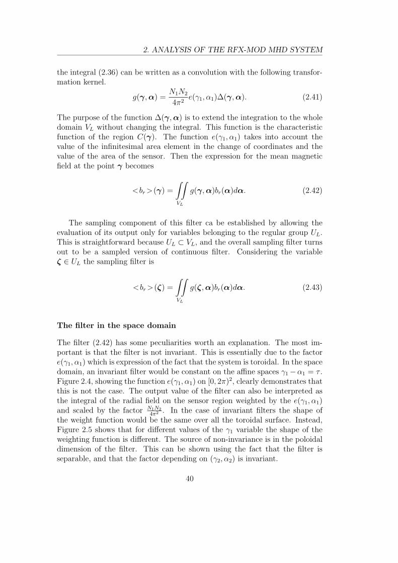
2. ANALYSIS OF THE RFX-MOD MHD SYSTEM
the integral (2.36) can be written as a convolution with the following transfor-mation kernel.
g(γ,α) =N1N2
4π2e(γ1, α1)∆(γ,α). (2.41)
The purpose of the function ∆(γ,α) is to extend the integration to the wholedomain VL without changing the integral. This function is the characteristicfunction of the region C(γ). The function e(γ1, α1) takes into account thevalue of the infinitesimal area element in the change of coordinates and thevalue of the area of the sensor. Then the expression for the mean magneticfield at the point γ becomes
<br>(γ) =
∫∫VL
g(γ,α)br(α)dα. (2.42)
The sampling component of this filter ca be established by allowing theevaluation of its output only for variables belonging to the regular group UL.This is straightforward because UL ⊂ VL, and the overall sampling filter turnsout to be a sampled version of continuous filter. Considering the variableζ ∈ UL the sampling filter is
<br>(ζ) =
∫∫VL
g(ζ,α)br(α)dα. (2.43)
The filter in the space domain
The filter (2.42) has some peculiarities worth an explanation. The most im-portant is that the filter is not invariant. This is essentially due to the factore(γ1, α1) which is expression of the fact that the system is toroidal. In the spacedomain, an invariant filter would be constant on the affine spaces γ1−α1 = τ .Figure 2.4, showing the function e(γ1, α1) on [0, 2π)2, clearly demonstrates thatthis is not the case. The output value of the filter can also be interpreted asthe integral of the radial field on the sensor region weighted by the e(γ1, α1)and scaled by the factor N1N2
4π2 . In the case of invariant filters the shape ofthe weight function would be the same over all the toroidal surface. Instead,Figure 2.5 shows that for different values of the γ1 variable the shape of theweighting function is different. The source of non-invariance is in the poloidaldimension of the filter. This can be shown using the fact that the filter isseparable, and that the factor depending on (γ2, α2) is invariant.
40
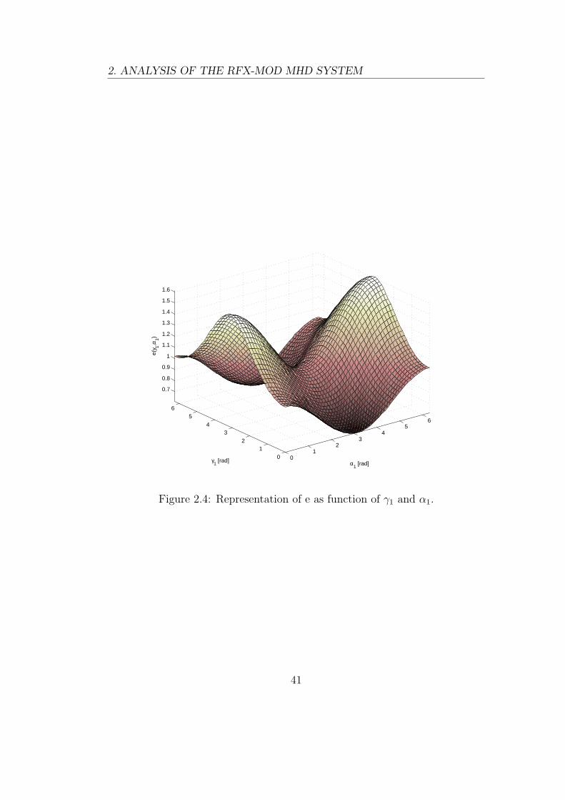
2. ANALYSIS OF THE RFX-MOD MHD SYSTEM
01
23
45
6
01
23
45
6
0.7
0.8
0.9
1
1.1
1.2
1.3
1.4
1.5
1.6
α1 [rad]γ
1 [rad]
e(γ 1,α
1)
Figure 2.4: Representation of e as function of γ1 and α1.
41
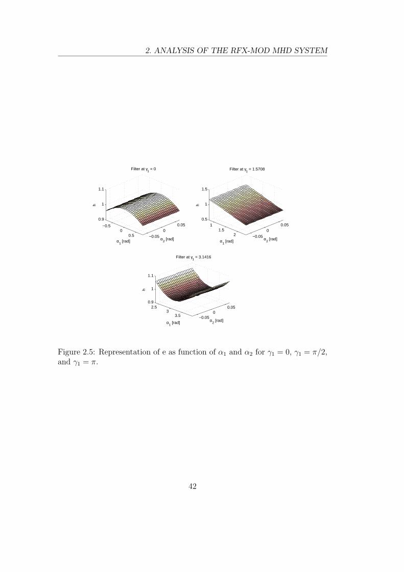
2. ANALYSIS OF THE RFX-MOD MHD SYSTEM
−0.50
0.5 −0.050
0.050.9
1
1.1
α2 [rad]
Filter at γ1 = 0
α1 [rad]
h
11.5
2 −0.050
0.050.5
1
1.5
α2 [rad]
Filter at γ1 = 1.5708
α1 [rad]
h
2.53
3.5 −0.050
0.050.9
1
1.1
α2 [rad]
Filter at γ1 = 3.1416
α1 [rad]
h
Figure 2.5: Representation of e as function of α1 and α2 for γ1 = 0, γ1 = π/2,and γ1 = π.
42
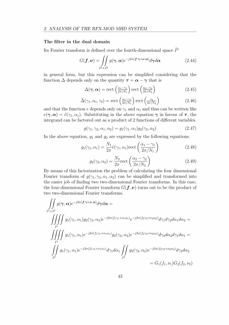
2. ANALYSIS OF THE RFX-MOD MHD SYSTEM
The filter in the dual domain
Its Fourier transform is defined over the fourth-dimensional space I2
G(f ,ν) =
∫∫I2×I2
g(γ,α)e−j2π(f ·γ+ν·α)dγdα (2.44)
in general form, but this expression can be simplified considering that thefunction ∆ depends only on the quantity τ = α− γ that is
∆(γ,α) = rect(
α1−γ1
2π/N1
)rect
(α2−γ2
2π/N2
)(2.45)
∆(γ1, α1, τ2) = rect(
α1−γ1
2π/N1
)rect
(τ2
2π/N2
)(2.46)
and that the function e depends only on γ1 and α1 and thus can be written likee(γ,α) = e(γ1, α1). Substituting in the above equation γ in favour of τ , theintegrand can be factored out as a product of 2 functions of different variables.
g(γ1, γ2, α1, α2) = g1(γ1, α1)g2(γ2, α2) (2.47)
In the above equation, g1 and g2 are expressed by the following equations.
g1(γ1, α1) =N1
2πe(γ1, α1)rect
(α1 − γ1
2π/N1
)(2.48)
g2(γ2, α2) =N2
2πrect
(α2 − γ2
2π/N2
)(2.49)
By means of this factorization the problem of calculating the four dimensionalFourier transform of g(γ1, γ2, α1, α2) can be simplified and transformed intothe easier job of finding two two-dimensional Fourier transforms. In this case,the four-dimensional Fourier transform G(f ,ν) turns out to be the product oftwo two-dimensional Fourier transforms.∫∫
I2×I2
g(γ,α)e−j2π(f ·γ+ν·α)dγdα =
∫∫∫∫I4
g1(γ1, α1)g2(γ2, α2)e−j2π(f1γ1+ν1α1)e−j2π(f2γ2+ν2α2)dγ1dγ2dα1dα2 =
∫∫∫∫I4
g1(γ1, α1)e−j2π(f1γ1+ν1α1)g2(γ2, α2)e
−j2π(f2γ2+ν2α2)dγ2dα2dγ1dα1 =
∫∫I2
g1(γ1, α1)e−j2π(f1γ1+ν1α1)dγ1dα1
∫∫I2
g2(γ2, α2)e−j2π(f2γ2+ν2α2)dγ2dα2
= G1(f1, ν1)G2(f2, ν2)
43
2. ANALYSIS OF THE RFX-MOD MHD SYSTEM
the integration of g2 is straightforward making the change of variable α2 =τ2 + γ2.
G2(f2, ν2) =
∫∫I2
g2(γ2, α2)e−j2π(f2γ2+ν2α2)dγ2dα2
=N2
2π
∫∫I2
rect
(τ2
2π/N2
)e−j2π(f2γ2+ν2τ2+ν2γ2)dγ2dτ2
=N2
2π
∫∫I2
rect
(τ2
2π/N2
)e−j2πν2τ2e−j2π(f2+ν2)γ2dγ2dτ2
=N2
2π
∫I
rect
(τ2
2π/N2
)e−j2πν2τ2
∫I
e−j2π(f2+ν2)γ2dγ2dτ2
= δI(f2 + ν2)N2
2π
∫I
rect
(τ2
2π/N2
)e−j2πν2τ2dτ2
= δI(f2 + ν2)sinc
(2π
N2
ν2
)The integration of g1 is a little bit more difficult but fortunately it can also becarried out in two steps,
G1(f1, ν1) =
∫∫I2
g1(γ1, α1)e−j2π(f1γ1+ν1α1)dγ1dα1
=N1
2π
∫∫I2
1 + a cos(α1)
1 + a sin(π/N1)π/N1
cos(γ1)·
· rect(α1 − γ1
2π/N2
)e−j2π(f1γ1+ν1α1)dγ1dα1
=N1
2π
∫I
e−j2πf1γ1
1 + a sin(π/N1)π/N1
cos(γ1)·
·∫I
(1 + a cos(α1)) rect
(α1 − γ1
2π/N2
)e−j2πν1α1dα1dγ1
considering that
F [ejαt](f) =
∫I
ejαte−j2πftdt = δI
(f − α
2π
)(2.50)
44
2. ANALYSIS OF THE RFX-MOD MHD SYSTEM
and that the Fourier transform of the product of two signals is equal to theconvolution of the respective Fourier transforms the integral
H(ν1, γ1) =
∫I
[1 + a cos(α1)] rect
(α1 − γ1
2π/N1
)e−j2πν1α1dα1 (2.51)
turns out to be the convolution of the following two signals
H1(ν1) =
∫I
[1 + a cos(α1)] e−j2πν1α1dα1 =
= δI(ν1) +a
2δI
(ν1 − 1
2π
)+a
2δI
(ν1 + 1
2π
)(2.52)
H2(ν1, γ1) =
∫I
rect
(α1 − γ1
2π/N1
)e−j2πν1α1dα1 =
=2π
N1
e−j2πν1γ1 sinc(
2πN1ν1
)(2.53)
that is
H(ν1, γ1) =
∫I
F2(τ, γ1)F1(ν1 − τ)dτ =
=2π
N1
e−j2πν1γ1
sinc
(2πN1ν1
)+a
2ejγ1 sinc
[2πN1
(ν1 − 1
2π
)]+
+a
2e−jγ1 sinc
[2πN1
(ν1 + 1
2π
)](2.54)
At this point the function G1(f1, ν1) has become
G1(f1, ν1) =N1
2π
∫I
e−j2πf1γ1
1 + b cos(γ1)H(ν1, γ1)dγ1 (2.55)
but, despite it is possible, in principle, to solve analytically the integral, thecalculations needed in order to get the closed form formula in the parametersb and f1 (remembering that 2πf1 ∈ Z) require an attention which is not worththe effort, especially considering the scope of the work. For this reason it hasbeen chosen to write the filter in terms of the function P (f1), defined as belowand computing numerically the rest of the calculation.
P (f1) =
∫I
e−j2πf1γ1
1 + b cos(γ1)dγ1 (2.56)
45
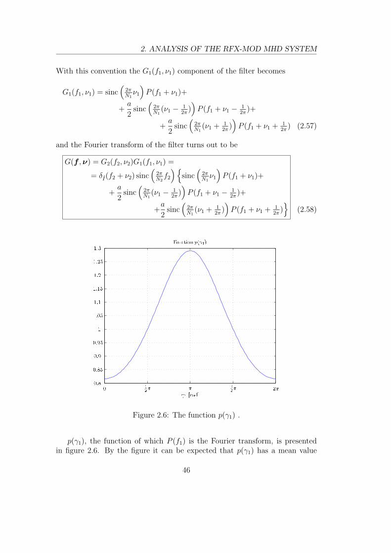
2. ANALYSIS OF THE RFX-MOD MHD SYSTEM
With this convention the G1(f1, ν1) component of the filter becomes
G1(f1, ν1) = sinc(
2πN1ν1
)P (f1 + ν1)+
+a
2sinc
(2πN1
(ν1 − 12π
))P (f1 + ν1 − 1
2π)+
+a
2sinc
(2πN1
(ν1 + 12π
))P (f1 + ν1 + 1
2π) (2.57)
and the Fourier transform of the filter turns out to be
G(f ,ν) = G2(f2, ν2)G1(f1, ν1) =
= δI(f2 + ν2) sinc(
2πN2f2
) sinc
(2πN1ν1
)P (f1 + ν1)+
+a
2sinc
(2πN1
(ν1 − 12π
))P (f1 + ν1 − 1
2π)+
+a
2sinc
(2πN1
(ν1 + 12π
))P (f1 + ν1 + 1
2π)
(2.58)
! "$#&% '
Figure 2.6: The function p(γ1) .
p(γ1), the function of which P (f1) is the Fourier transform, is presentedin figure 2.6. By the figure it can be expected that p(γ1) has a mean value
46
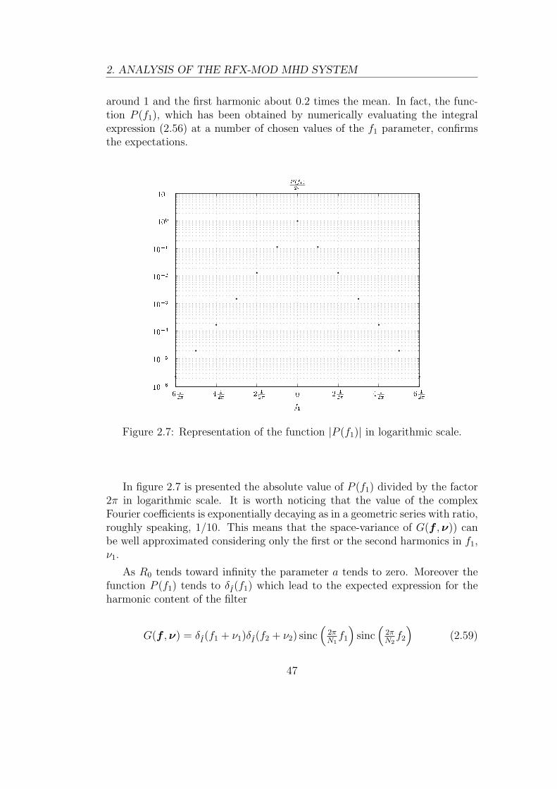
2. ANALYSIS OF THE RFX-MOD MHD SYSTEM
around 1 and the first harmonic about 0.2 times the mean. In fact, the func-tion P (f1), which has been obtained by numerically evaluating the integralexpression (2.56) at a number of chosen values of the f1 parameter, confirmsthe expectations.
Figure 2.7: Representation of the function |P (f1)| in logarithmic scale.
In figure 2.7 is presented the absolute value of P (f1) divided by the factor2π in logarithmic scale. It is worth noticing that the value of the complexFourier coefficients is exponentially decaying as in a geometric series with ratio,roughly speaking, 1/10. This means that the space-variance of G(f ,ν)) canbe well approximated considering only the first or the second harmonics in f1,ν1.
As R0 tends toward infinity the parameter a tends to zero. Moreover thefunction P (f1) tends to δI(f1) which lead to the expected expression for theharmonic content of the filter
G(f ,ν) = δI(f1 + ν1)δI(f2 + ν2) sinc(
2πN1f1
)sinc
(2πN2f2
)(2.59)
47
2. ANALYSIS OF THE RFX-MOD MHD SYSTEM
Analytical model Studied model
Is space invariant Is space variant
Makes a brutal approximation ofthe kernel (bi-dimensional rect)
Considers the actual flux density
Permits analytical calculationsRequires numerical evaluation ofthe kernel
Table 2.4: Differences between the analytical model used for the developmentof the sideband correction algorithm and the features of the system as studiedin the framework of the Unified Theory.
The parameter Λ
Considering the result of proposition 2.3 the parameter Λ defined as follows
Λ =
√√√√√√√∫
VL
δVL(f + ν)|G(f ,ν)|2dν∫VL
|G(f ,ν)|2dν, (2.60)
gives a measure of the degree of variance of a filter g on VL. This parameteris always a number between zero and one on the domain VL because the haarintegral is a summation. It is the square root of the ratio between the energyof the filter along the invariant subspace and the total energy of the filter.
2.5 Conclusions
The fact that the sampling performed by the radial field coils is space-varianthas some consequences on the signal reconstruction. Indeed the harmoniccontent of the input signal is distorted not only by a function multiplication,but by an integral linear transformation. This implies that the exponentialfunctions are not filter eigenfunctions as happens in the invariant case. It isworth spending some time comparing the features of this signal based modelwith those of the common cylindrical model used in the analytical developmentof the sideband correction algorithm.
This chapter shows that the Unified Signal Theory can be applied to givea detailed description of the behaviour of the MHD system and how to use itsresults to perform analyses of its components. This chapter shows that thereal MHD system presents more than one structural differences from the stan-dard cylindrical model usually used for the derivation of analytical formulas.
48
2. ANALYSIS OF THE RFX-MOD MHD SYSTEM
However, it does not provide a critique to the development of such a models,which often can be used to implement algorithms allowing an excellent perfor-mance of the machine. It provide a method which can be considered when theassumption made by more simple models become unacceptable. The result ofthis analysis is the detailed explanation, from the point of view of the UnifiedSignal Theory, of the relation between the physical quantities involved in theanalytical models and the actual information that is available for the real-timecontrol. The existence of this step should not be forgotten. The major dif-ference between a uniform cylindrical model and the model proposed in thischapter is the space variance. A weak source of space variance is the toroidalgeometry. This has an effect both on the radial field and current sampling.Much stronger source of spatial variance are the shell features such as gaps andports. The actual harmonic content of the field distribution generated by thesaddle coil currents can be estimated with a better accuracy performing nu-merical calculations using a Finite Element Model of the RFX-mode machineand an electromagnetic solver such as CARIDDI, for example. This result canhave an impact on the algorithm which compensates for the aliasing inducedby the radial field sampling.
49

Chapter 3
Model
3.1 Introduction
Summarising what said in the first chapter, the RFX-mod active system for thecontrol of the MHD instabilities consists of 192 active saddle coils, mounted soas to completely cover the outer toroidal surface of the stainless steel support-ing structure [4]. The radial component of the magnetic field is measured byan equal number of saddle probes, located on the projection of the active coilson the outer surface of the vessel. The shell is characterised by a poloidal gapand an inner equatorial gap to allow the penetration of the toroidal componentof the electric and magnetic field respectively.
A highly flexible real time control system was implemented, capable of per-forming bi-dimensional spatial Fourier analysis of the field components pro-ducing the corresponding harmonics characterized by the poloidal (m) andtoroidal (n) mode numbers [8]. Several control strategies were envisaged andhave been operating for one year with very good results in terms of quality ofthe magnetic boundary, bringing about a doubling of energy confinement timein pulses over 300 ms long [9]. The two main strategies are the “virtual shell”and the “mode control”. In the basic version of the former, the radial compo-nent of the magnetic field measured by each sensor is cancelled, in the latter,selected modes (RWM’s or tearing modes) of one field component can be eithersuppressed or actively stimulated. Up to now simple controllers equal for allthe coils have been used; a prospective exploitation of the system flexibilityasks for the design of a more sophisticated controller capable of an indepen-dent action on either selected modes or different coils taking into account thetoroidal geometry, the effect of the passive structures and other local features.
To this purpose a full electromagnetic dynamic model of the active controlsystem has been developed taking advantage of the experience gained on the
51
3. MODEL
other European RFP experiment T2R [10]. The model inputs are the voltagesapplied to each coil and its outputs the magnetic fluxes measured by the saddleprobes. Consistently with previous work in this field, it is also suited to the in-tegration with a dynamic model of the plasma RWM’s [11]. The developmentof such a requires the knowledge of the self and mutual coupling terms betweenactive coils and their resistance. The control scheme which uses the informa-tion provided by the radial field sensors requires the knowledge of the mutualcouplings between active coils and sensors. The presence of passive conductorssuch as the vacuum chamber, the shell and the supporting structure, eitherthe coupling and the dissipative factor depend on the frequency.
A preliminary campaign of measures allowed the acquisition of the datafor the calculation of the equivalent resistances and of the self and mutualcouplings of the active coils [12]. The values obtained have been arrangedin two three-dimensional matrices in order to save the information about thefrequency response. During the campaign C3, dedicated to the commissioningof the system, a series of vacuum shots has been performed to characterise theopen-loop frequency response of the system made up of the power amplifiersthe active coils and the sensors. A set of poloidal array has been selected asrepresentative of the different responses of the system due to the local featuresof the machine. During these experiments coils of different poloidal arrays havebeen fed at the same time in order to minimise the length of the campaign.The poloidal arrays have been selected trying to minimise cross effects on thesensors measurements, which would have lead to the wrong evaluation of thecouplings coefficients. Step and sinusoidal currents at different frequencieshave been impressed into the coils acting as inputs of the system. The datahave then been collected and analysed automating a procedure already used onT2R data. As previously made for the active coils data, a 3D matrix of com-plex coefficients has been constructed representing the amplitude and phaseof the couplings between active coils and sensors for each test frequency. Fortheir relative position, the couplings between the active coils and the sensorscome to depend more on the frequency than those of the active coils. Somevalidation tests evidenced that while constant matrices allowed to reproducewith sufficient accuracy the current dynamics, that was not possible for theradial fluxes at the sensors. Taking advantage of a MATLABr identificationroutine already used in the past with satisfying results [13], a matrix of ra-tional function approximating the dynamic response of the MHD system hasbeen obtained. For computational convenience, the transfer function matrixrepresentation of the system has been changed to an equivalent state spacemodel with constant matrices.
The dynamic system is necessary for the simulation of the overall system
52
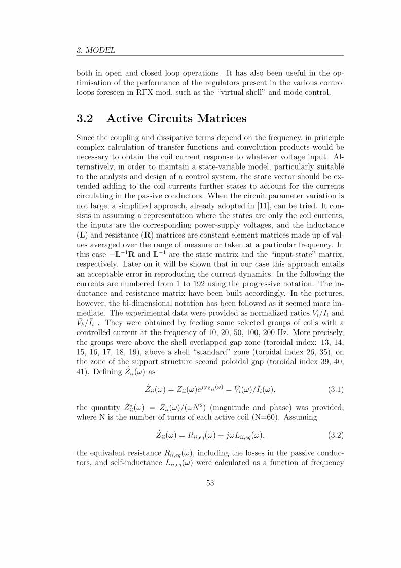
3. MODEL
both in open and closed loop operations. It has also been useful in the op-timisation of the performance of the regulators present in the various controlloops foreseen in RFX-mod, such as the “virtual shell” and mode control.
3.2 Active Circuits Matrices
Since the coupling and dissipative terms depend on the frequency, in principlecomplex calculation of transfer functions and convolution products would benecessary to obtain the coil current response to whatever voltage input. Al-ternatively, in order to maintain a state-variable model, particularly suitableto the analysis and design of a control system, the state vector should be ex-tended adding to the coil currents further states to account for the currentscirculating in the passive conductors. When the circuit parameter variation isnot large, a simplified approach, already adopted in [11], can be tried. It con-sists in assuming a representation where the states are only the coil currents,the inputs are the corresponding power-supply voltages, and the inductance(L) and resistance (R) matrices are constant element matrices made up of val-ues averaged over the range of measure or taken at a particular frequency. Inthis case −L−1R and L−1 are the state matrix and the “input-state” matrix,respectively. Later on it will be shown that in our case this approach entailsan acceptable error in reproducing the current dynamics. In the following thecurrents are numbered from 1 to 192 using the progressive notation. The in-ductance and resistance matrix have been built accordingly. In the pictures,however, the bi-dimensional notation has been followed as it seemed more im-mediate. The experimental data were provided as normalized ratios Vi/Ii andVk/Ii . They were obtained by feeding some selected groups of coils with acontrolled current at the frequency of 10, 20, 50, 100, 200 Hz. More precisely,the groups were above the shell overlapped gap zone (toroidal index: 13, 14,15, 16, 17, 18, 19), above a shell “standard” zone (toroidal index 26, 35), onthe zone of the support structure second poloidal gap (toroidal index 39, 40,41). Defining Zii(ω) as
Zii(ω) = Zii(ω)ejϕZii(ω) = Vi(ω)/Ii(ω), (3.1)
the quantity Z∗ii(ω) = Zii(ω)/(ωN2) (magnitude and phase) was provided,
where N is the number of turns of each active coil (N=60). Assuming
Zii(ω) = Rii,eq(ω) + jωLii,eq(ω), (3.2)
the equivalent resistance Rii,eq(ω), including the losses in the passive conduc-tors, and self-inductance Lii,eq(ω) were calculated as a function of frequency
53

3. MODEL
usign the following formulas
Rii,eq(ω) = ωN2Z∗ii(ω) cos(ϕZ∗
ii(ω)) (3.3)
Lii,eq(ω) = N2Z∗ii(ω) sin(ϕZ∗
ii(ω)). (3.4)
In some cases (for instance validation of FE model results) a decompositionwhich clearly separates pure resistive and inductive terms can be more use-ful. Such a decomposition can be derived introducing a complex inductanceLii(ω) = Lii(ω)ejϕLii
(ω) = Ψi(ω)/Ii(ω), whose aim is to account for the delayand attenuation of the resulting magnetic flux and the additional losses due tothe currents induced in the passive structures. Lii(ω) can be calculated fromits defining equation
Zii(ω) = Rii(ω) + jωLii(ω). (3.5)
Here Rii(ω) is the actual resistance of the i-th coil at the given frequency. Ifthe skin effect in the coil is neglected, the equation
Zii(ω) = Rii + jωLii(ω) (3.6)
is assumed, where Rii = Rii(ω)|ω=0. The amplitude of Lii(ω) can then beexpressed as
Lii(ω) =
√R2
ii(ω) + Z2ii(ω)− 2Rii(ω)Zii(ω) cos(ϕZii
(ω))
ω, (3.7)
and its phase ϕLii(ω) as:
ϕLii(ω) = atan2 (Rii(ω)− Zii(ω) cos(ϕZii
(ω)), Zii(ω) sin(ϕZii(ω))) . (3.8)
Now consider the case when the i-th coil is fed and the k-th coil voltage ismeasured:
Zki(ω) = Vk(ω)/Ii(ω). (3.9)
Again, the quantity Z∗ki(ω) = Zki(ω)/(ωN2) being available1, we calculate:
Rki,eq(ω) = ωN2Z∗ki(ω) cos(ϕZ∗
ki(ω)) (3.10)
Lki,eq(ω) = N2Z∗ki(ω) sin(ϕZ∗
ki(ω)). (3.11)
In this case the trans-impedance Zki(ω) is directly linked to the complexmutual inductance itself according to the equation Zki(ω) = jωLki(ω) , allthe dissipative effects in the passive conductors related to the k-th coil currentbeing taken into account.
1The actual available angle was αki = ϕZ∗ki
(ω)+π/2, thus the equations implemented inthe code are Rki,eq(ω) = ωN2Z∗
ki(ω) sin(αki(ω)) and Lki,eq(ω) = N2Z∗ki(ω) cos(αki(ω)).
54
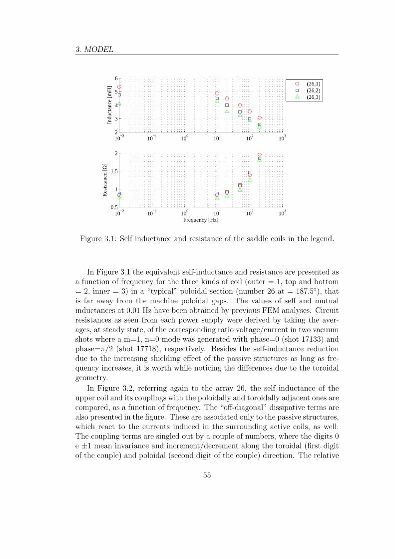
3. MODEL
10−2
10−1
100
101
102
103
2
3
4
5
6
Indu
ctan
ce [m
H]
10−2
10−1
100
101
102
103
0.5
1
1.5
2
Frequency [Hz]
Res
ista
nce
[Ω]
(26,1)(26,2)(26,3)
Figure 3.1: Self inductance and resistance of the saddle coils in the legend.
In Figure 3.1 the equivalent self-inductance and resistance are presented asa function of frequency for the three kinds of coil (outer = 1, top and bottom= 2, inner = 3) in a “typical” poloidal section (number 26 at = 187.5), thatis far away from the machine poloidal gaps. The values of self and mutualinductances at 0.01 Hz have been obtained by previous FEM analyses. Circuitresistances as seen from each power supply were derived by taking the aver-ages, at steady state, of the corresponding ratio voltage/current in two vacuumshots where a m=1, n=0 mode was generated with phase=0 (shot 17133) andphase=π/2 (shot 17718), respectively. Besides the self-inductance reductiondue to the increasing shielding effect of the passive structures as long as fre-quency increases, it is worth while noticing the differences due to the toroidalgeometry.
In Figure 3.2, referring again to the array 26, the self inductance of theupper coil and its couplings with the poloidally and toroidally adjacent ones arecompared, as a function of frequency. The “off-diagonal” dissipative terms arealso presented in the figure. These are associated only to the passive structures,which react to the currents induced in the surrounding active coils, as well.The coupling terms are singled out by a couple of numbers, where the digits 0e ±1 mean invariance and increment/decrement along the toroidal (first digitof the couple) and poloidal (second digit of the couple) direction. The relative
55
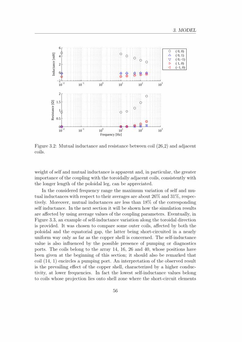
3. MODEL
10−2
10−1
100
101
102
103
−2
0
2
4
6
Indu
ctan
ce [m
H]
10−2
10−1
100
101
102
103
0
0.5
1
1.5
2
Frequency [Hz]
Res
ista
nce
[Ω]
( 0, 0)( 0, 1)( 0,−1)( 1, 0)(−1, 0)
Figure 3.2: Mutual inductance and resistance between coil (26,2) and adjacentcoils.
weight of self and mutual inductance is apparent and, in particular, the greaterimportance of the coupling with the toroidally adjacent coils, consistently withthe longer length of the poloidal leg, can be appreciated.
In the considered frequency range the maximum variation of self and mu-tual inductances with respect to their averages are about 26% and 31%, respec-tively. Moreover, mutual inductances are less than 18% of the correspondingself inductance. In the next section it will be shown how the simulation resultsare affected by using average values of the coupling parameters. Eventually, inFigure 3.3, an example of self-inductance variation along the toroidal directionis provided. It was chosen to compare some outer coils, affected by both thepoloidal and the equatorial gap, the latter being short-circuited in a nearlyuniform way only as far as the copper shell is concerned. The self-inductancevalue is also influenced by the possible presence of pumping or diagnosticsports. The coils belong to the array 14, 16, 26 and 40, whose positions havebeen given at the beginning of this section; it should also be remarked thatcoil (14, 1) encircles a pumping port. An interpretation of the observed resultis the prevailing effect of the copper shell, characterized by a higher conduc-tivity, at lower frequencies. In fact the lowest self-inductance values belongto coils whose projection lies onto shell zone where the short-circuit elements
56
3. MODEL
10−2
10−1
100
101
102
103
3
3.5
4
4.5
5
5.5
Indu
ctan
ce [m
H]
10−2
10−1
100
101
102
103
1
1.5
2
Frequency [Hz]
Res
ista
nce
[Ω]
(14,1)(16,1)(26,1)(40,1)
Figure 3.3: Self inductance and resistance of the coils in the external array.
number is higher, even though they span a cut of the supporting structure.Actually, the different toroidal pitch of the saddle coils and the short-circuitsystem bring about different “overlapping patterns” between coils and short-circuiting elements. Where the number of short-circuiting elements is higher,the better is the shell “equatorial continuity” approximated.
On the contrary, as the frequency increases, the outer conductor, i.e. thesupporting structure, becomes also an effective shield, except in the cut stretches,where the maximum values of coil self-inductances can then be found. An ex-ample of this behaviour can be seen in the figure, at low frequency, where thecoil with maximum inductance is (14,1), which surrounds a pumping port com-ing before the shell underlying edge without any short-circuiting elements, andthe coil with minimum inductance is (40,1), mounted onto the intersection ofthe structure poloidal and toroidal cuts, but where three shell short-circuitingelements are present. The self-inductance of this latter coil results less atten-uated at high frequencies.
3.2.1 Experimental validation
In order to validate the coupling terms and to assess the achievable accuracyin using constant element matrices some tests have been carried out. In Figure
57
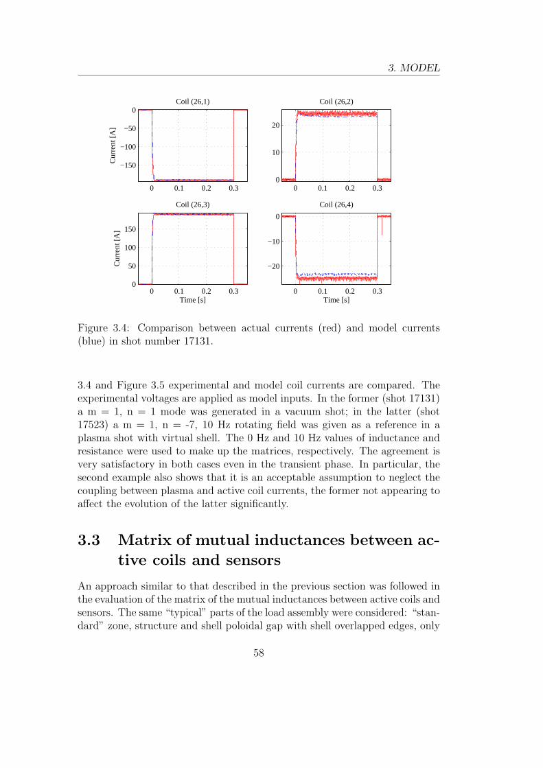
3. MODEL
0 0.1 0.2 0.3
−150
−100
−50
0Coil (26,1)
Cur
rent
[A]
0 0.1 0.2 0.30
10
20
Coil (26,2)
0 0.1 0.2 0.30
50
100
150
Coil (26,3)
Time [s]
Cur
rent
[A]
0 0.1 0.2 0.3
−20
−10
0
Coil (26,4)
Time [s]
Figure 3.4: Comparison between actual currents (red) and model currents(blue) in shot number 17131.
3.4 and Figure 3.5 experimental and model coil currents are compared. Theexperimental voltages are applied as model inputs. In the former (shot 17131)a m = 1, n = 1 mode was generated in a vacuum shot; in the latter (shot17523) a m = 1, n = -7, 10 Hz rotating field was given as a reference in aplasma shot with virtual shell. The 0 Hz and 10 Hz values of inductance andresistance were used to make up the matrices, respectively. The agreement isvery satisfactory in both cases even in the transient phase. In particular, thesecond example also shows that it is an acceptable assumption to neglect thecoupling between plasma and active coil currents, the former not appearing toaffect the evolution of the latter significantly.
3.3 Matrix of mutual inductances between ac-
tive coils and sensors
An approach similar to that described in the previous section was followed inthe evaluation of the matrix of the mutual inductances between active coils andsensors. The same “typical” parts of the load assembly were considered: “stan-dard” zone, structure and shell poloidal gap with shell overlapped edges, only
58
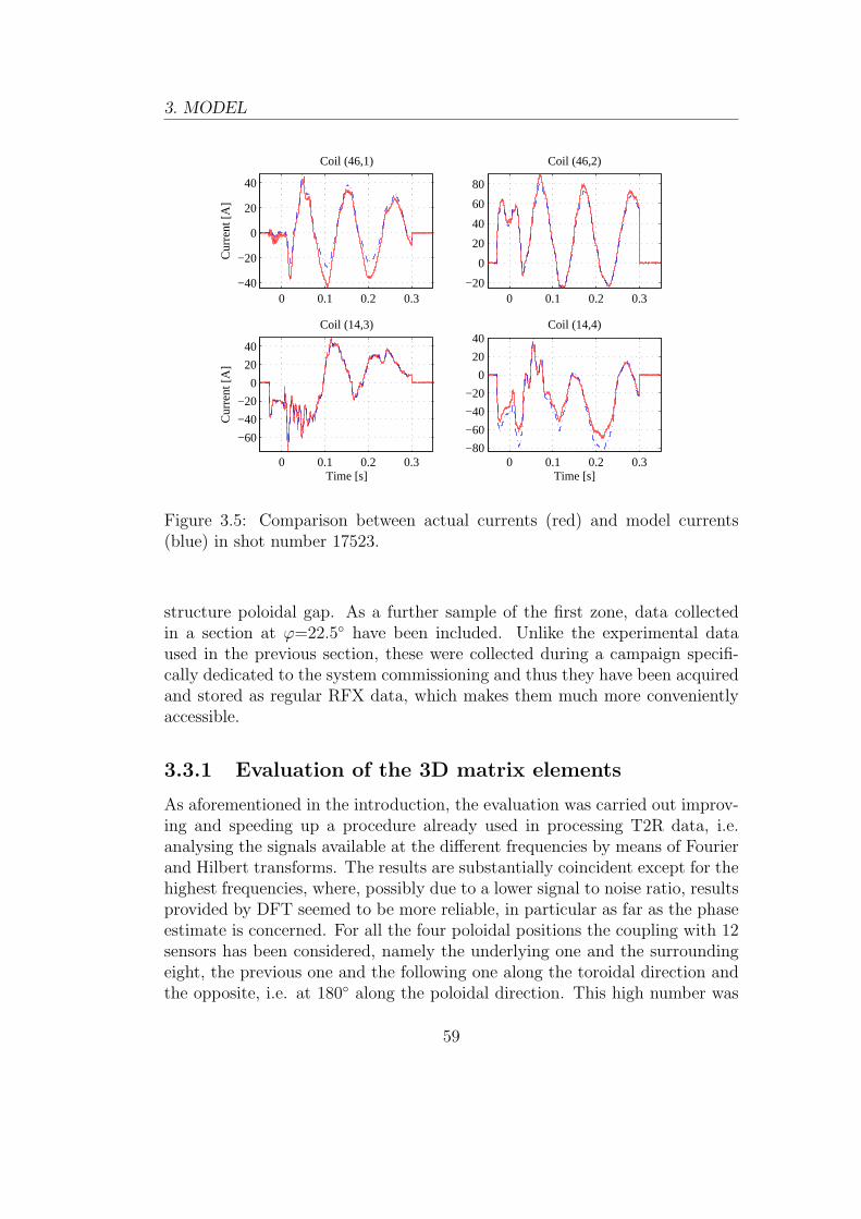
3. MODEL
0 0.1 0.2 0.3−40
−20
0
20
40
Coil (46,1)
Cur
rent
[A]
0 0.1 0.2 0.3−20
0
20
40
60
80
Coil (46,2)
0 0.1 0.2 0.3
−60
−40
−20
0
20
40
Coil (14,3)
Time [s]
Cur
rent
[A]
0 0.1 0.2 0.3−80
−60
−40
−20
0
20
40Coil (14,4)
Time [s]
Figure 3.5: Comparison between actual currents (red) and model currents(blue) in shot number 17523.
structure poloidal gap. As a further sample of the first zone, data collectedin a section at ϕ=22.5 have been included. Unlike the experimental dataused in the previous section, these were collected during a campaign specifi-cally dedicated to the system commissioning and thus they have been acquiredand stored as regular RFX data, which makes them much more convenientlyaccessible.
3.3.1 Evaluation of the 3D matrix elements
As aforementioned in the introduction, the evaluation was carried out improv-ing and speeding up a procedure already used in processing T2R data, i.e.analysing the signals available at the different frequencies by means of Fourierand Hilbert transforms. The results are substantially coincident except for thehighest frequencies, where, possibly due to a lower signal to noise ratio, resultsprovided by DFT seemed to be more reliable, in particular as far as the phaseestimate is concerned. For all the four poloidal positions the coupling with 12sensors has been considered, namely the underlying one and the surroundingeight, the previous one and the following one along the toroidal direction andthe opposite, i.e. at 180 along the poloidal direction. This high number was
59
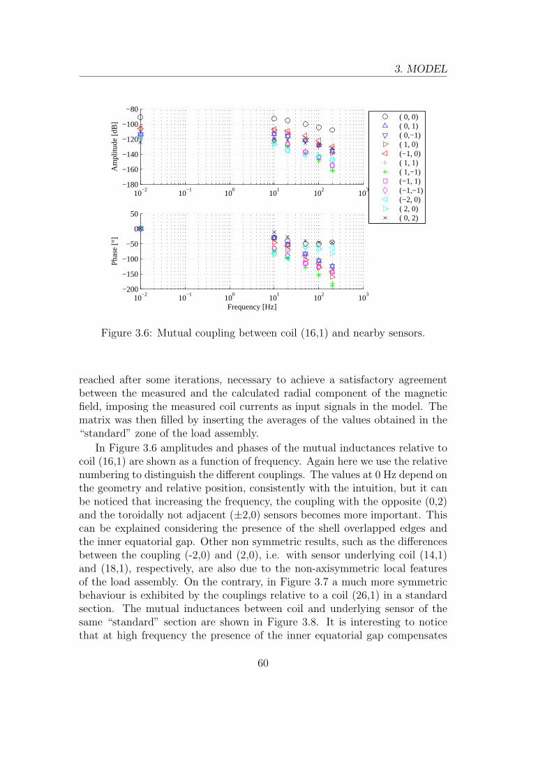
3. MODEL
10−2
10−1
100
101
102
103
−180
−160
−140
−120
−100
−80A
mpl
itude
[dB
]
10−2
10−1
100
101
102
103
−200
−150
−100
−50
0
50
Frequency [Hz]
Pha
se [°
]( 0, 0)( 0, 1)( 0,−1)( 1, 0)(−1, 0)( 1, 1)( 1,−1)(−1, 1)(−1,−1)(−2, 0)( 2, 0)( 0, 2)
Figure 3.6: Mutual coupling between coil (16,1) and nearby sensors.
reached after some iterations, necessary to achieve a satisfactory agreementbetween the measured and the calculated radial component of the magneticfield, imposing the measured coil currents as input signals in the model. Thematrix was then filled by inserting the averages of the values obtained in the“standard” zone of the load assembly.
In Figure 3.6 amplitudes and phases of the mutual inductances relative tocoil (16,1) are shown as a function of frequency. Again here we use the relativenumbering to distinguish the different couplings. The values at 0 Hz depend onthe geometry and relative position, consistently with the intuition, but it canbe noticed that increasing the frequency, the coupling with the opposite (0,2)and the toroidally not adjacent (±2,0) sensors becomes more important. Thiscan be explained considering the presence of the shell overlapped edges andthe inner equatorial gap. Other non symmetric results, such as the differencesbetween the coupling (-2,0) and (2,0), i.e. with sensor underlying coil (14,1)and (18,1), respectively, are also due to the non-axisymmetric local featuresof the load assembly. On the contrary, in Figure 3.7 a much more symmetricbehaviour is exhibited by the couplings relative to a coil (26,1) in a standardsection. The mutual inductances between coil and underlying sensor of thesame “standard” section are shown in Figure 3.8. It is interesting to noticethat at high frequency the presence of the inner equatorial gap compensates
60
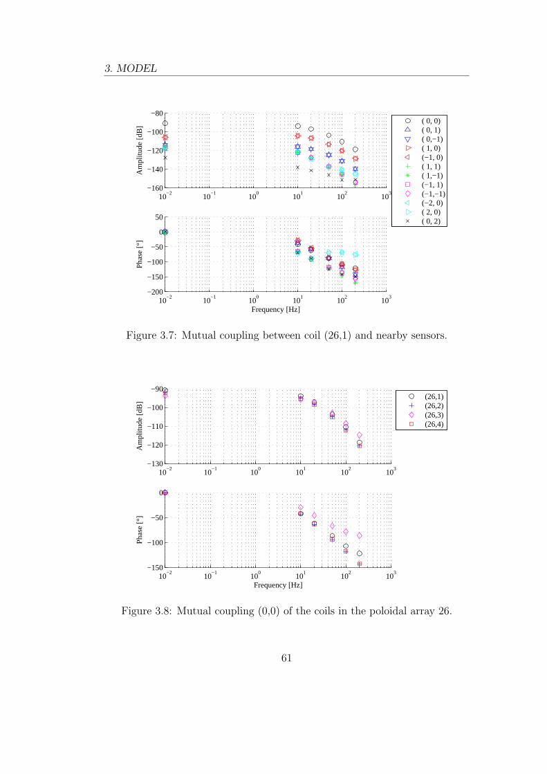
3. MODEL
10−2
10−1
100
101
102
103
−160
−140
−120
−100
−80
Am
plitu
de [d
B]
10−2
10−1
100
101
102
103
−200
−150
−100
−50
0
50
Frequency [Hz]
Pha
se [°
]
( 0, 0)( 0, 1)( 0,−1)( 1, 0)(−1, 0)( 1, 1)( 1,−1)(−1, 1)(−1,−1)(−2, 0)( 2, 0)( 0, 2)
Figure 3.7: Mutual coupling between coil (26,1) and nearby sensors.
10−2
10−1
100
101
102
103
−130
−120
−110
−100
−90
Am
plitu
de [d
B]
10−2
10−1
100
101
102
103
−150
−100
−50
0
Frequency [Hz]
Pha
se [°
]
(26,1)(26,2)(26,3)(26,4)
Figure 3.8: Mutual coupling (0,0) of the coils in the poloidal array 26.
61
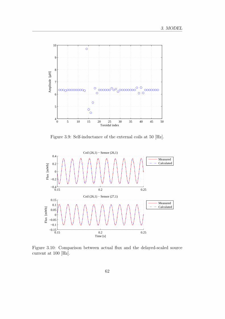
3. MODEL
0 5 10 15 20 25 30 35 40 45 504
5
6
7
8
9
10A
mpl
itude
[µH
]
Toroidal index
Figure 3.9: Self-inductance of the external coils at 50 [Hz].
0.15 0.2 0.25−0.4
−0.2
0
0.2
0.4
Flu
x [m
Wb]
Coil (26,1) − Sensor (26,1)
MeasuredCalculated
0.15 0.2 0.25−0.15
−0.1
−0.05
0
0.05
0.1
0.15
Time [s]
Flu
x [m
Wb]
Coil (26,1) − Sensor (27,1)
MeasuredCalculated
Figure 3.10: Comparison between actual flux and the delayed-scaled sourcecurrent at 100 [Hz].
62
3. MODEL
for the reduced size of the inner coil-sensor couple, the corresponding mutualinductance resulting larger than the others where the shielding of the passivestructures is more effective. A comprehensive view of (0,0)-coupling alongthe torus at 50 Hz is given in Figure 3.9. Apart from some small numericalvariations, the most significant differences are observed nearby the structureand shell poloidal gaps, as expected. In particular, (14,1) is the highest sincethere is no short-circuit element in the inner shell edge on its right side; on thecontrary the following three mutual inductances are the lowest, as the corre-sponding couples face the shell overlapped edges with the outer one regularlyshort-circuited. The deviations are lower in the section of the structure secondpoloidal gap; the largest two terms result (38,1) and (40,1), the former cou-ple encircling a pumping port and the latter spanning the poloidal gap. Theaverage values of the “standard” zone appear at the other positions.
In Figure 3.10, as an example of the accuracy in the mutual inductanceevaluation procedure, the measured and reproduced evolution of the magneticradial component in two positions are presented in a 100 Hz case: a very goodagreement can be observed.
3.3.2 Evaluation of the transfer function matrix
In order to build a model suitable to the control system analysis and theregulator design is required a block capable of providing the magnetic fieldas measured by the sensors in the presence of a general coil current input.Some preliminary tests using different constant term matrices, i.e. the samesimplified approach as in the case of the active coil inductance and resistancematrices, clearly demonstrated that this approach was not applicable due tothe strong dependence of the coupling terms on the frequency.
Thus a matrix whose elements are transfer functions was necessary. Onthe other hand, as mentioned in the introduction to section 2, a state vari-able representation is more convenient and numerically robust. Thus, first aMIMO transfer functions model was built and then a state space realizationwas worked out. In the past a procedure was developed to obtain the trans-fer function of the magnetic vertical component produced by the field shapingwindings currents inside the old thick conducting shell of RFX. Now it has beenupgraded and adapted to the automatic evaluation of the coil-sensor transferfunctions. It is based on a MATLABr toolbox routine providing the numer-ator and denominator coefficients of the transfer function which best fits ina least square sense an assigned set of experimental frequency response data.By inspection of the first results it was noticed that according to the couplecoil-sensor, a different number of zeros and poles of the transfer functions wasnecessary to achieve the best fitting. Nine mutual inductances were initially
63
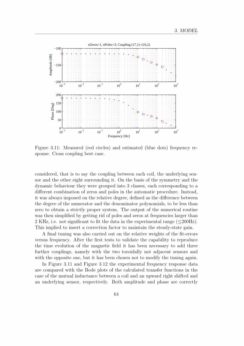
3. MODEL
10−3
10−2
10−1
100
101
102
103
−200
−150
−100nZeros=1, nPoles=3; Coupling (17,1)−(16,2)
Am
plitu
de [d
B]
10−3
10−2
10−1
100
101
102
103
0
50
100
150
200
Pha
se [D
eg]
Frequency [Hz]
Figure 3.11: Measured (red circles) and estimated (blue dots) frequency re-sponse. Cross coupling best case.
considered, that is to say the coupling between each coil, the underlying sen-sor and the other eight surrounding it. On the basis of the symmetry and thedynamic behaviour they were grouped into 3 classes, each corresponding to adifferent combination of zeros and poles in the automatic procedure. Instead,it was always imposed on the relative degree, defined as the difference betweenthe degree of the numerator and the denominator polynomials, to be less thanzero to obtain a strictly proper system. The output of the numerical routinewas then simplified by getting rid of poles and zeros at frequencies larger than2 KHz, i.e. not significant to fit the data in the experimental range (≤200Hz).This implied to insert a correction factor to maintain the steady-state gain.
A final tuning was also carried out on the relative weights of the fit-errorsversus frequency. After the first tests to validate the capability to reproducethe time evolution of the magnetic field it has been necessary to add threefurther couplings, namely with the two toroidally not adjacent sensors andwith the opposite one, but it has been chosen not to modify the tuning again.
In Figure 3.11 and Figure 3.12 the experimental frequency response dataare compared with the Bode plots of the calculated transfer functions in thecase of the mutual inductance between a coil and an upward right shifted andan underlying sensor, respectively. Both amplitude and phase are correctly
64
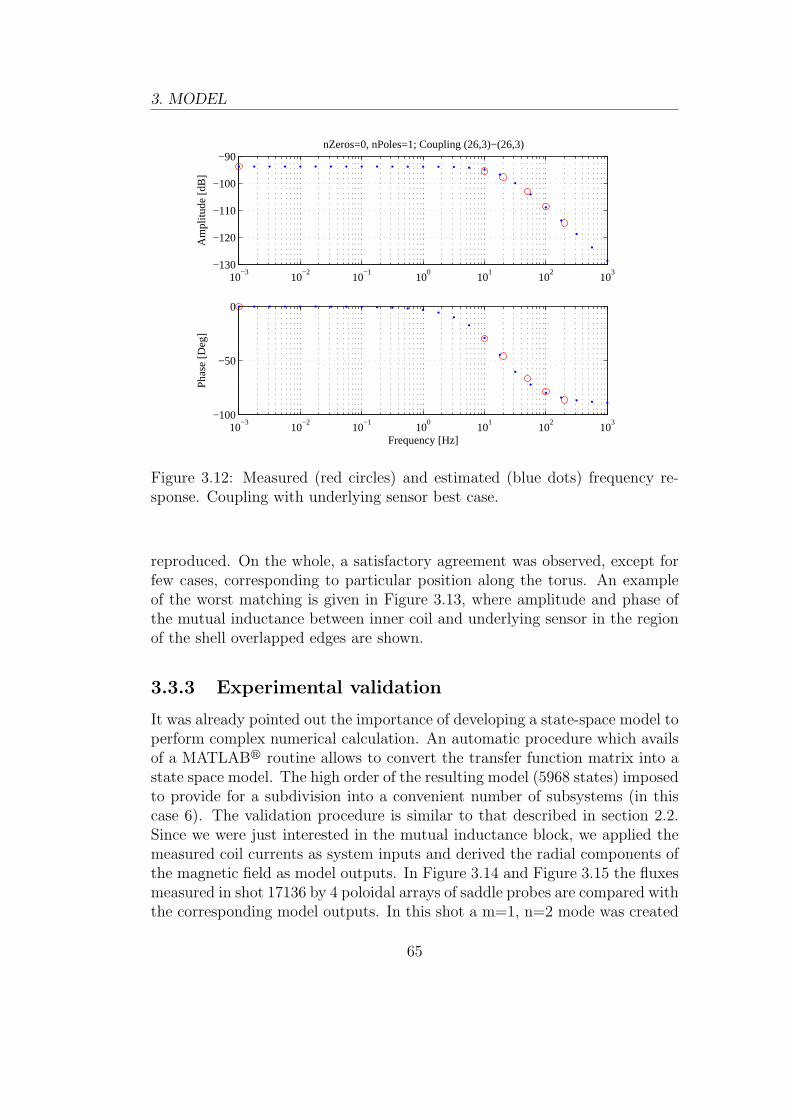
3. MODEL
10−3
10−2
10−1
100
101
102
103
−130
−120
−110
−100
−90nZeros=0, nPoles=1; Coupling (26,3)−(26,3)
Am
plitu
de [d
B]
10−3
10−2
10−1
100
101
102
103
−100
−50
0
Pha
se [D
eg]
Frequency [Hz]
Figure 3.12: Measured (red circles) and estimated (blue dots) frequency re-sponse. Coupling with underlying sensor best case.
reproduced. On the whole, a satisfactory agreement was observed, except forfew cases, corresponding to particular position along the torus. An exampleof the worst matching is given in Figure 3.13, where amplitude and phase ofthe mutual inductance between inner coil and underlying sensor in the regionof the shell overlapped edges are shown.
3.3.3 Experimental validation
It was already pointed out the importance of developing a state-space model toperform complex numerical calculation. An automatic procedure which availsof a MATLABr routine allows to convert the transfer function matrix into astate space model. The high order of the resulting model (5968 states) imposedto provide for a subdivision into a convenient number of subsystems (in thiscase 6). The validation procedure is similar to that described in section 2.2.Since we were just interested in the mutual inductance block, we applied themeasured coil currents as system inputs and derived the radial components ofthe magnetic field as model outputs. In Figure 3.14 and Figure 3.15 the fluxesmeasured in shot 17136 by 4 poloidal arrays of saddle probes are compared withthe corresponding model outputs. In this shot a m=1, n=2 mode was created
65
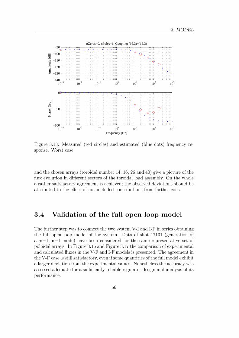
3. MODEL
10−3
10−2
10−1
100
101
102
103
−140
−130
−120
−110
−100
−90nZeros=0, nPoles=1; Coupling (16,3)−(16,3)
Am
plitu
de [d
B]
10−3
10−2
10−1
100
101
102
103
−100
−50
0
Pha
se [D
eg]
Frequency [Hz]
Figure 3.13: Measured (red circles) and estimated (blue dots) frequency re-sponse. Worst case.
and the chosen arrays (toroidal number 14, 16, 26 and 40) give a picture of theflux evolution in different sectors of the toroidal load assembly. On the wholea rather satisfactory agreement is achieved; the observed deviations should beattributed to the effect of not included contributions from farther coils.
3.4 Validation of the full open loop model
The further step was to connect the two system V-I and I-F in series obtainingthe full open loop model of the system. Data of shot 17131 (generation ofa m=1, n=1 mode) have been considered for the same representative set ofpoloidal arrays. In Figure 3.16 and Figure 3.17 the comparison of experimentaland calculated fluxes in the V-F and I-F models is presented. The agreement inthe V-F case is still satisfactory, even if some quantities of the full model exhibita larger deviation from the experimental values. Nonetheless the accuracy wasassessed adequate for a sufficiently reliable regulator design and analysis of itsperformance.
66
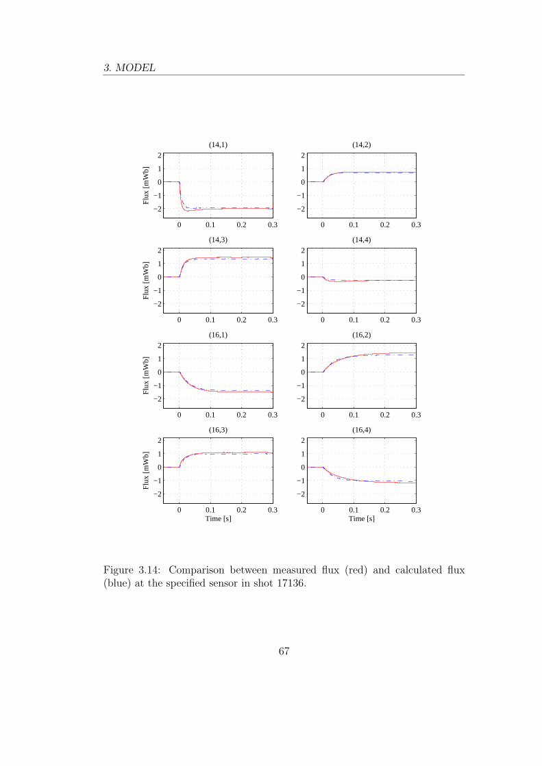
3. MODEL
0 0.1 0.2 0.3
−2
−1
0
1
2
Flu
x [m
Wb]
(14,1)
0 0.1 0.2 0.3
−2
−1
0
1
2
(14,2)
0 0.1 0.2 0.3
−2
−1
0
1
2
Flu
x [m
Wb]
(14,3)
0 0.1 0.2 0.3
−2
−1
0
1
2
(14,4)
0 0.1 0.2 0.3
−2
−1
0
1
2
Flu
x [m
Wb]
(16,1)
0 0.1 0.2 0.3
−2
−1
0
1
2
(16,2)
0 0.1 0.2 0.3
−2
−1
0
1
2
Flu
x [m
Wb]
Time [s]
(16,3)
0 0.1 0.2 0.3
−2
−1
0
1
2
Time [s]
(16,4)
Figure 3.14: Comparison between measured flux (red) and calculated flux(blue) at the specified sensor in shot 17136.
67
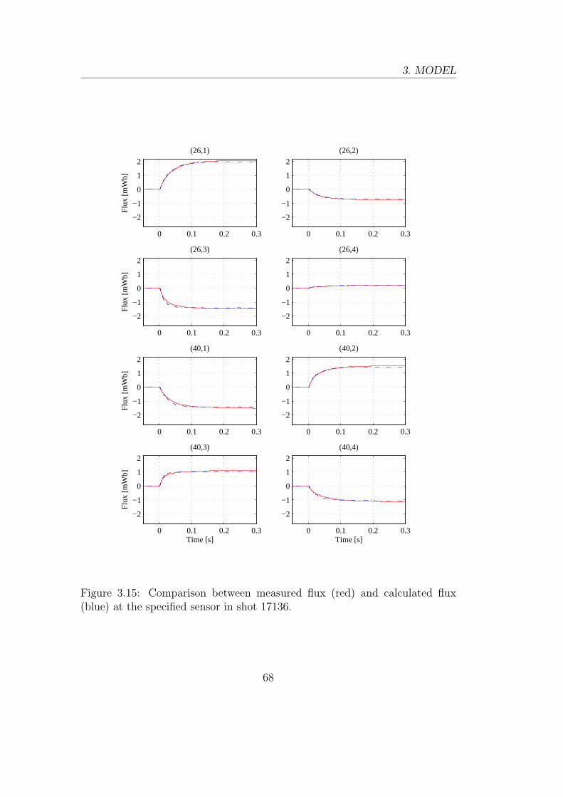
3. MODEL
0 0.1 0.2 0.3
−2
−1
0
1
2
Flu
x [m
Wb]
(26,1)
0 0.1 0.2 0.3
−2
−1
0
1
2
(26,2)
0 0.1 0.2 0.3
−2
−1
0
1
2
Flu
x [m
Wb]
(26,3)
0 0.1 0.2 0.3
−2
−1
0
1
2
(26,4)
0 0.1 0.2 0.3
−2
−1
0
1
2
Flu
x [m
Wb]
(40,1)
0 0.1 0.2 0.3
−2
−1
0
1
2
(40,2)
0 0.1 0.2 0.3
−2
−1
0
1
2
Flu
x [m
Wb]
Time [s]
(40,3)
0 0.1 0.2 0.3
−2
−1
0
1
2
Time [s]
(40,4)
Figure 3.15: Comparison between measured flux (red) and calculated flux(blue) at the specified sensor in shot 17136.
68
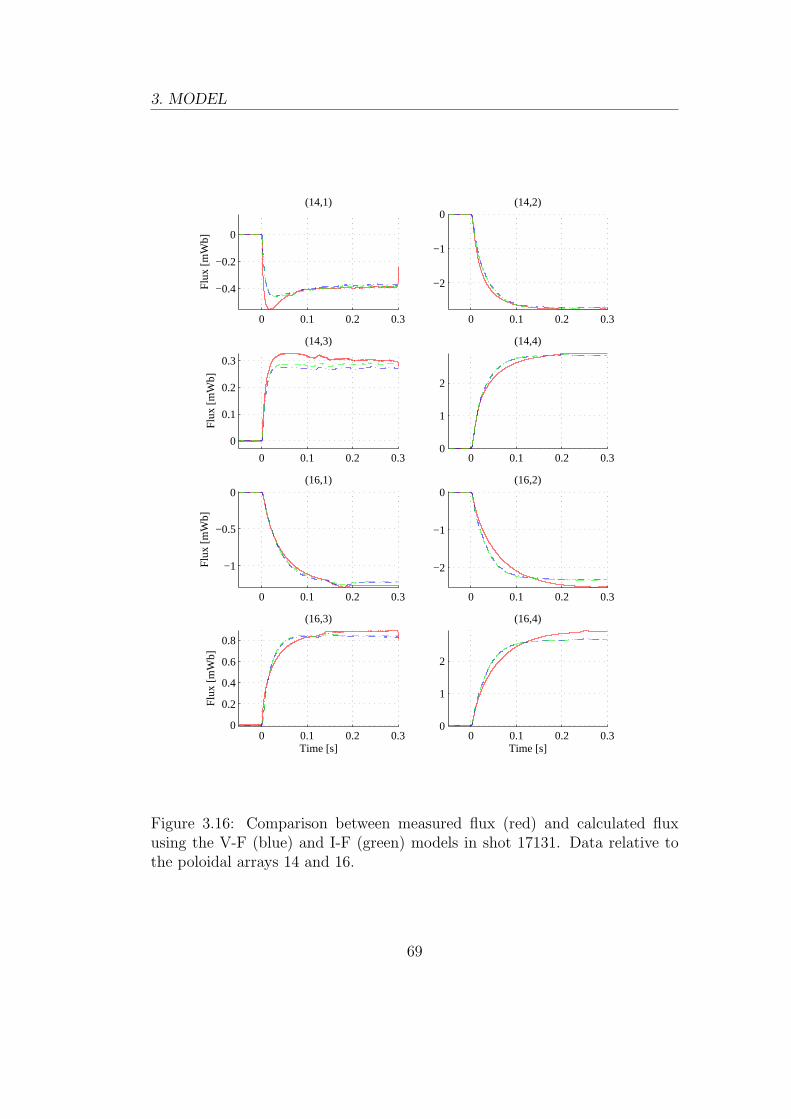
3. MODEL
0 0.1 0.2 0.3
−0.4
−0.2
0
Flu
x [m
Wb]
(14,1)
0 0.1 0.2 0.3
−2
−1
0(14,2)
0 0.1 0.2 0.3
0
0.1
0.2
0.3
Flu
x [m
Wb]
(14,3)
0 0.1 0.2 0.30
1
2
(14,4)
0 0.1 0.2 0.3
−1
−0.5
0
Flu
x [m
Wb]
(16,1)
0 0.1 0.2 0.3
−2
−1
0(16,2)
0 0.1 0.2 0.30
0.2
0.4
0.6
0.8
Flu
x [m
Wb]
Time [s]
(16,3)
0 0.1 0.2 0.30
1
2
Time [s]
(16,4)
Figure 3.16: Comparison between measured flux (red) and calculated fluxusing the V-F (blue) and I-F (green) models in shot 17131. Data relative tothe poloidal arrays 14 and 16.
69
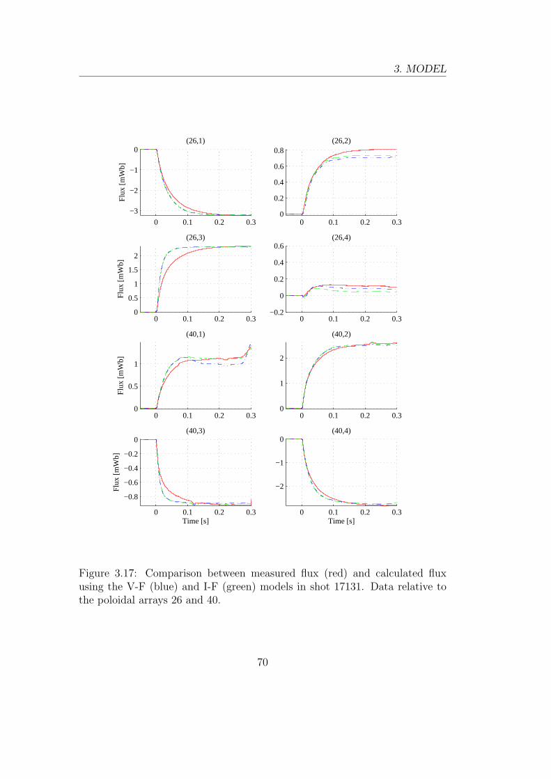
3. MODEL
0 0.1 0.2 0.3
−3
−2
−1
0
Flu
x [m
Wb]
(26,1)
0 0.1 0.2 0.30
0.2
0.4
0.6
0.8(26,2)
0 0.1 0.2 0.30
0.5
1
1.5
2
Flu
x [m
Wb]
(26,3)
0 0.1 0.2 0.3−0.2
0
0.2
0.4
0.6(26,4)
0 0.1 0.2 0.30
0.5
1
Flu
x [m
Wb]
(40,1)
0 0.1 0.2 0.30
1
2
(40,2)
0 0.1 0.2 0.3
−0.8
−0.6
−0.4
−0.2
0
Flu
x [m
Wb]
Time [s]
(40,3)
0 0.1 0.2 0.3
−2
−1
0
Time [s]
(40,4)
Figure 3.17: Comparison between measured flux (red) and calculated fluxusing the V-F (blue) and I-F (green) models in shot 17131. Data relative tothe poloidal arrays 26 and 40.
70
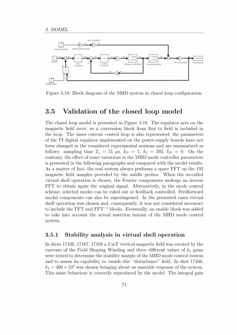
3. MODEL
y = Cx+Du
Volatages-Currents Model
PIx’ = Ax+Bu
-K-
Current
PI ControllerCurrents-Fluxes Model
Flux-->Field [T/Wb]Flux
PI Controller
192
192
192 192 192 192
192
192 192 192
192
192 192
Vertical disturbance (Field)
Field-->Flux [Wb/T]
192 192
Vertical Field Enable
Constant
Feedback Enable
PI
K*uK*u
-K-192
K*u-C-y = Cx+Du
x’ = Ax+BuB_model
To Workspace1
Figure 3.18: Block diagram of the MHD system in closed loop configuration.
3.5 Validation of the closed loop model
The closed loop model is presented in Figure 3.18. The regulator acts on themagnetic field error, so a conversion block from flux to field is included inthe loop. The inner current control loop is also represented; the parametersof the PI digital regulator implemented on the power-supply boards have notbeen changed in the considered experimental sessions and are summarized asfollows: sampling time Ts = 51 µs, kP = 1, kI = 392, kD = 0. On thecontrary, the effect of some variations in the MHD mode controller parametersis presented in the following paragraphs and compared with the model results.As a matter of fact, the real system always performs a space FFT on the 192magnetic field samples provided by the saddle probes. When the so-calledvirtual shell operation is chosen, the Fourier components undergo an inverseFFT to obtain again the original signal. Alternatively, in the mode controlscheme, selected modes can be ruled out or feedback controlled. Feedforwardmodal components can also be superimposed. In the presented cases virtualshell operation was chosen and, consequently, it was not considered necessaryto include the FFT and FFT−1 blocks. Eventually, an enable block was addedto take into account the actual insertion instant of the MHD mode controlsystem.
3.5.1 Stability analysis in virtual shell operation
In shots 17166, 17167, 17168 a 2 mT vertical magnetic field was created by thecurrents of the Field Shaping Winding and three different values of kI gainswere tested to determine the stability margin of the MHD mode control systemand to assess its capability to vanish this “disturbance” field. In shot 17166,kI = 400× 103 was chosen bringing about an unstable response of the system.This same behaviour is correctly reproduced by the model. The integral gain
71
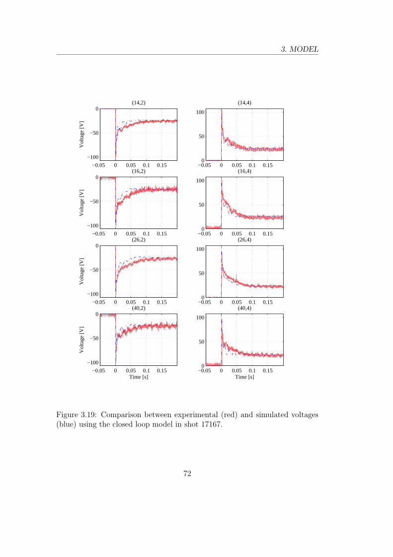
3. MODEL
−0.05 0 0.05 0.1 0.15
−100
−50
0
Vol
tage
[V]
(14,2)
−0.05 0 0.05 0.1 0.150
50
100
(14,4)
−0.05 0 0.05 0.1 0.15
−100
−50
0
Vol
tage
[V]
(16,2)
−0.05 0 0.05 0.1 0.150
50
100
(16,4)
−0.05 0 0.05 0.1 0.15
−100
−50
0
Vol
tage
[V]
(26,2)
−0.05 0 0.05 0.1 0.150
50
100
(26,4)
−0.05 0 0.05 0.1 0.15
−100
−50
0
Vol
tage
[V]
Time [s]
(40,2)
−0.05 0 0.05 0.1 0.150
50
100
Time [s]
(40,4)
Figure 3.19: Comparison between experimental (red) and simulated voltages(blue) using the closed loop model in shot 17167.
72
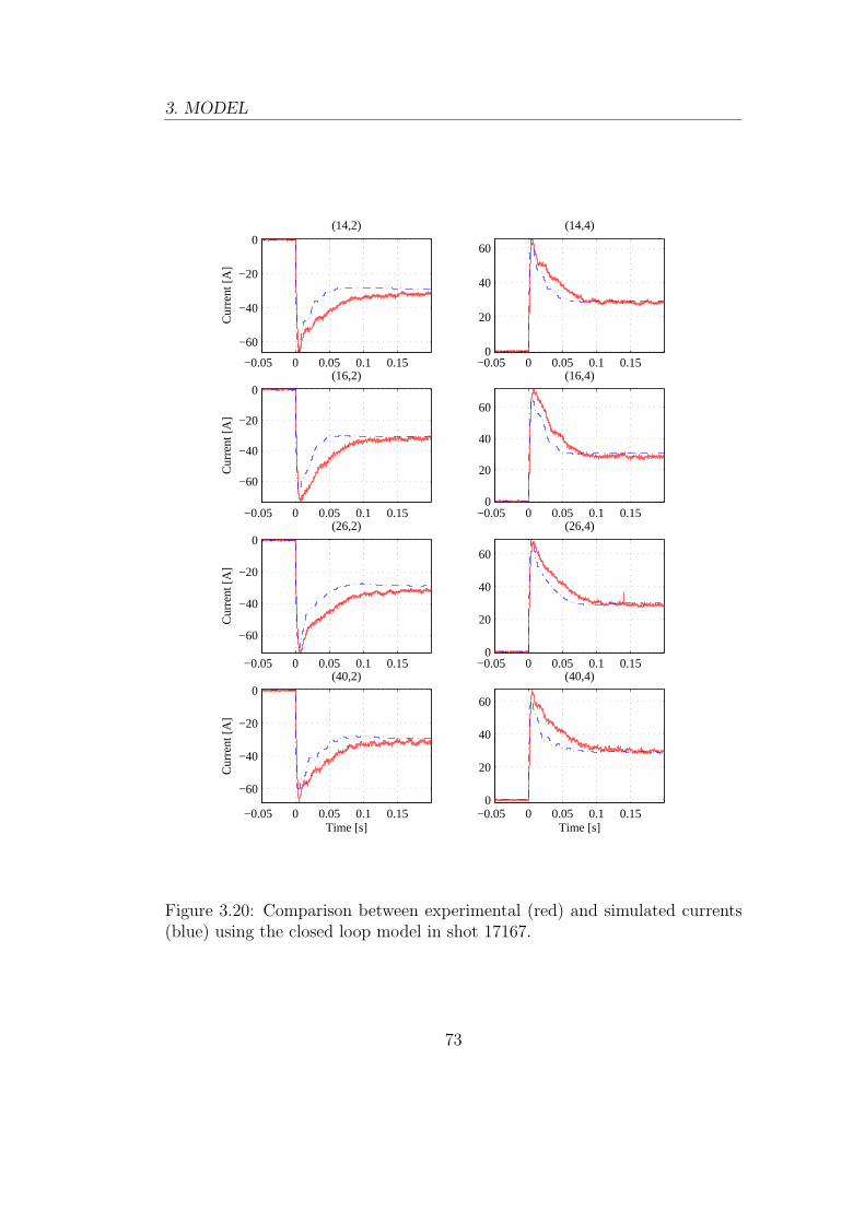
3. MODEL
−0.05 0 0.05 0.1 0.15
−60
−40
−20
0C
urre
nt [A
](14,2)
−0.05 0 0.05 0.1 0.150
20
40
60
(14,4)
−0.05 0 0.05 0.1 0.15
−60
−40
−20
0
Cur
rent
[A]
(16,2)
−0.05 0 0.05 0.1 0.150
20
40
60
(16,4)
−0.05 0 0.05 0.1 0.15
−60
−40
−20
0
Cur
rent
[A]
(26,2)
−0.05 0 0.05 0.1 0.150
20
40
60
(26,4)
−0.05 0 0.05 0.1 0.15
−60
−40
−20
0
Cur
rent
[A]
Time [s]
(40,2)
−0.05 0 0.05 0.1 0.150
20
40
60
Time [s]
(40,4)
Figure 3.20: Comparison between experimental (red) and simulated currents(blue) using the closed loop model in shot 17167.
73
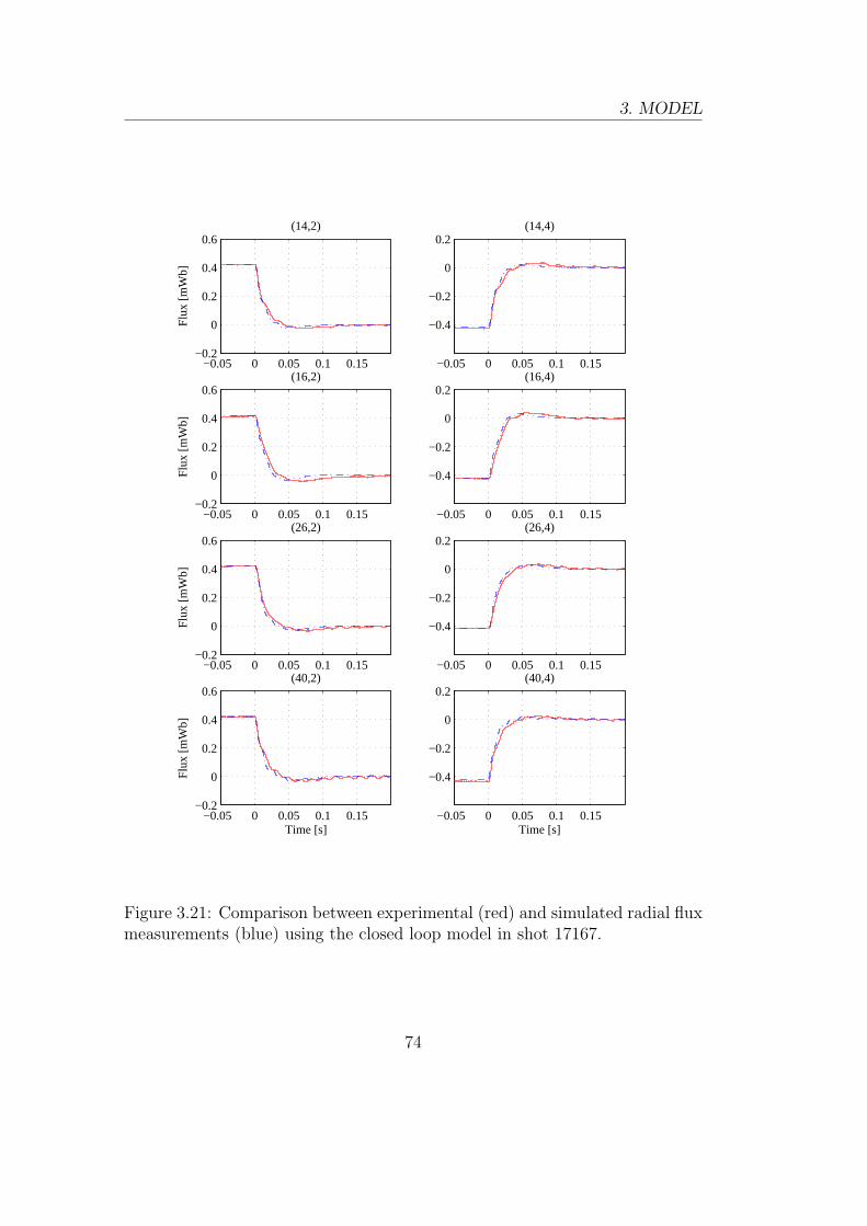
3. MODEL
−0.05 0 0.05 0.1 0.15−0.2
0
0.2
0.4
0.6
Flu
x [m
Wb]
(14,2)
−0.05 0 0.05 0.1 0.15
−0.4
−0.2
0
0.2(14,4)
−0.05 0 0.05 0.1 0.15−0.2
0
0.2
0.4
0.6
Flu
x [m
Wb]
(16,2)
−0.05 0 0.05 0.1 0.15
−0.4
−0.2
0
0.2(16,4)
−0.05 0 0.05 0.1 0.15−0.2
0
0.2
0.4
0.6
Flu
x [m
Wb]
(26,2)
−0.05 0 0.05 0.1 0.15
−0.4
−0.2
0
0.2(26,4)
−0.05 0 0.05 0.1 0.15−0.2
0
0.2
0.4
0.6
Flu
x [m
Wb]
Time [s]
(40,2)
−0.05 0 0.05 0.1 0.15
−0.4
−0.2
0
0.2
Time [s]
(40,4)
Figure 3.21: Comparison between experimental (red) and simulated radial fluxmeasurements (blue) using the closed loop model in shot 17167.
74
3. MODEL
kI was reduced to 40 × 103 in the following shot 17167, obtaining a stable,fairly prompt response. Again the model results satisfactorily agree with theexperimental ones not only in terms of the feedback controlled quantities butalso in terms of saddle coil voltages and currents. In Figure 3.19, 3.20 and 3.21voltages, currents and radial components of the magnetic fields are presentedalong with the corresponding experimental quantities.
3.6 Conclusions
A full electromagnetic model of the active control system of plasma MHDmodes in RFX-mod has been developed. An extensive series of validationtests proved the model capability to reproduce the system open and closedloop response in terms of evolution of the magnetic fluxes with satisfactoryaccuracy. Since all the model parameters have been derived from experimentaldata, the effects of the toroidal geometry, passive structures, and the presenceof non axialsymmetric features on the dynamics of the coil currents and theradial field are implicitly taken into account. The model should be a basic toolfor the design of more complex controllers to further improve the interactionwith the plasma modes by fully exploiting the real-time system flexibility.
75

Chapter 4
Pseudo-Decoupler
4.1 Introduction
Interest in real time control of the magnetic field perturbations in fusion de-vices has been growing in the last years because of the demanding stabilityrequirements associated with advanced scenarios. Experiments in the RFPconfiguration may play an important role in this framework: due to the richerharmonic content of the edge magnetic field perturbations compared to theTokamak, the RFP is a challenging test-bed for the development of edge mag-netic field control scenarios. RFX-mod has been designed with the aim ofextensive experimental activity in this field [4], the MHD system described inthe previous chapters being the tool for its exploitation.
Different control strategies acting either equally on all the radial magneticfield harmonic components (Virtual Shell) or selectively on subsets of them(Mode Control) have been implemented. Both led to a substantial improve-ment of the plasma confinement with a three-fold increase of the pulse lengthand have been routinely used ever since [9].
Various types of PID controllers of either the single sensor signals or themode components were designed according to Single-Input-Single-Output tech-niques. Such an approach was successful in controlling resistive wall modes(RWM) and in producing highly monochromatic static spectra. On the otherhand, the available PI regulator was less effective in the control of tearingmodes, being able to exert a rotating torque only up to 20-30 Hz [14]. Thiswas due to the high coupling of the active system, each coil affecting at leastone fourth of the total number of underlying sensors.
Thus a Multi-Input-Multi-Output approach to the control system designwas expected to be more adequate to meet the requirements given in terms ofspectral dynamic monochromaticity, reference tracking error and disturbance
77
4. PSEUDO-DECOUPLER
rejection. The MIMO model of the coils and sensors in the presence of thepassive structures, described in chapter 3, has been used in the design of anew control strategy. The high dimensionality of the problem was not a minorissue to cope with and some simplifying assumptions were adopted to carryout the design. Moreover, in the model simulations the plasma is assimilatedto an external disturbance and it can be neglected to investigate the maximumachievable performance in terms of stability margins and tracking capabilitywhich are limited mainly by the presence of the passive structures.
4.2 Previous design attempts
Up to now, the best achieved performances in RFX-mod have been obtainedwith a control system made up of 192 PID controllers that shared the valueof integral, proportional and derivative gains kI , kP and kD. Despite the useof PID controllers has several well understood advantages, this technique canfail to produce satisfying controllers, for example because the diagonal PIDstructure does not take into account most of the plant interactions.
Trying to move forward from the diagonal PID design, the use of optimaltechniques such as LQG, H∞ or pole placement have been considered. They allhave the major flaw in the need of the plant model, which is the starting pointof a long sequence of calculations, not always well conditioned, producing inmost cases a dynamic controller of nearly the same size as the model.
However, despite the great number of states, the model has also the peculiarstructure of having a block diagonal state matrix with a very small block sizeof maximum 3 and the other matrices of the state space representation largelysparse. After observing that the general purpose libraries of Matlabr failin performing the model reduction, specialised routines performing a modelreduction based on the truncation of the least Hankel singular values havebeen written. Using the specialised routines it has been possible to reducesignificantly the number of states to about 600. Unfortunately, the truncationdid not preserve the stability of the original model making it not directly usablefor the controller design.
After finding difficulties in the model reduction, optimal designs have beenabandoned in favour of a sub-optimal inverse-based decoupler design [15]. Afirst insight into the control problem was obtained designing a pre-compensatorbased on an approximation of the plant inverse calculated by taking into ac-count a small subset of the possible couplings. Unfortunately closed loopstability of the pre-compensated plant was not achievable with a satisfyingdisturbance rejection using this method. This suggested a different approachas described in the following paragraph.
78

4. PSEUDO-DECOUPLER
4.3 Projecting Decoupler
The approximated decoupler described in the above section evidenced someproblems when trying to increase the number of neighbours considered. Ex-perience on this point contributed in showing that the condition div B(t) = 0shall not be ignored when designing the compensator. So, a completely newdesign around the integral form of the above condition has been made.∫
Ts
b(t)dS =192∑i=1
∫Ti
b(t)dS =192∑i=1
ψi(t) = 0 (4.1)
In the above equations Ts is the whole toroidal surface covered with the 192measure coils each of area Ti and linked flux ψi(t).
4.3.1 Projected model
The above condition can be expressed in matricial form defining the vectorqH = [1, . . . , 1], where the superscript H denotes the conjugate transpose ofthe matrix. If a transfer function matrix G(jω) represents a dynamic systemwhose outputs are flux measures spanning exactly a closed surface, it satisfiesthe flux conservation condition if and only if qHG(jω) = 0H . This equationimplies that every transfer function matrix satisfying condition (4.1) can notbe full rank, and thus can not be invertible. The available model of the plant,despite its accuracy in reproducing the plant dynamics, actually does containapproximations for which the flux condition is not fulfilled. In particular onlya small number of couplings has been considered in the model [16].
A measure of how far is a model from meeting the flux condition can bederived considering the orthogonal projector
Q =qqH
qHq(4.2)
and its complementarP = I−Q, (4.3)
where I is the identity matrix. Using these two projectors it is possible todecompose the transfer function matrix into the parallel component G‖(jω)which satisfy equation (4.1) and the orthogonal G⊥(jω) component which doesnot. This follows from the fact that P + Q = I, considering that qHP = 0H
holds.
G(jω) = (P + Q)G(jω) = PG(jω) + QG(jω) = G‖(jω) + G⊥(jω) (4.4)
79
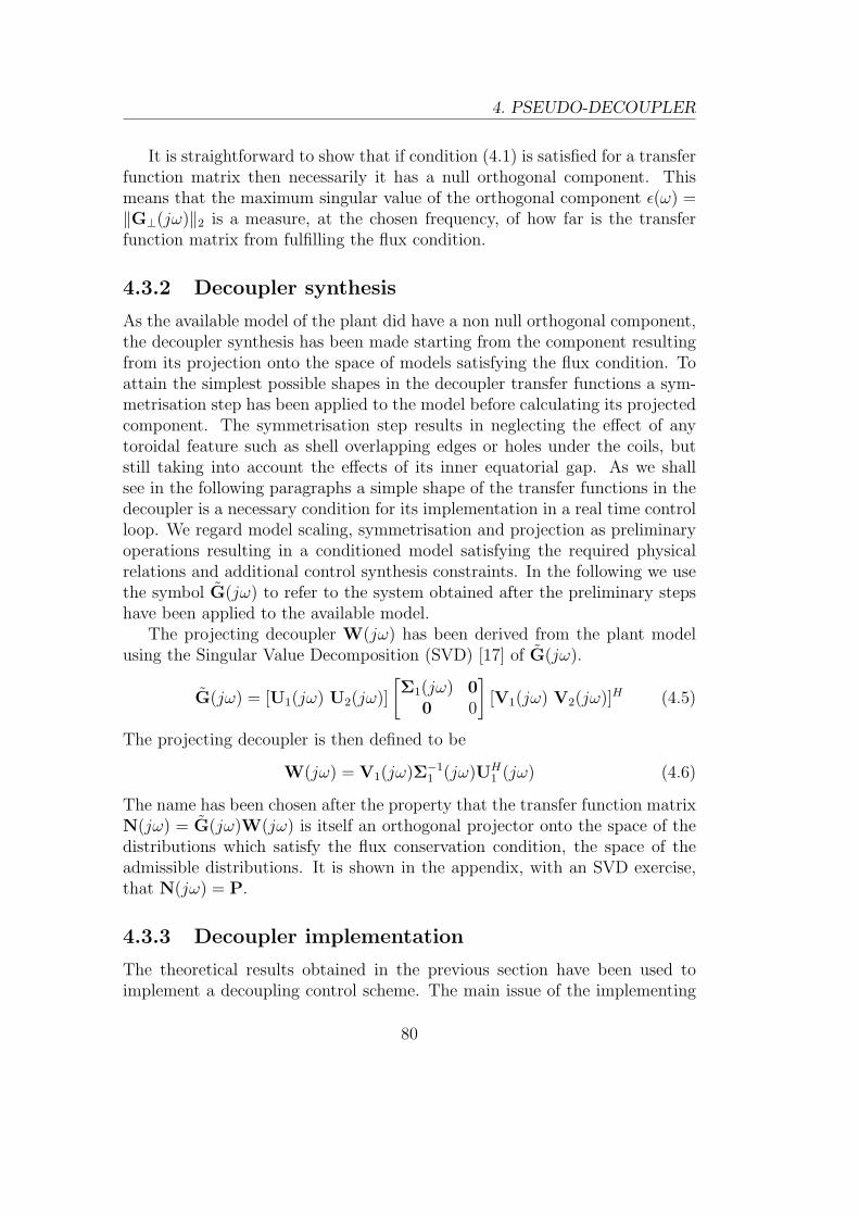
4. PSEUDO-DECOUPLER
It is straightforward to show that if condition (4.1) is satisfied for a transferfunction matrix then necessarily it has a null orthogonal component. Thismeans that the maximum singular value of the orthogonal component ε(ω) =‖G⊥(jω)‖2 is a measure, at the chosen frequency, of how far is the transferfunction matrix from fulfilling the flux condition.
4.3.2 Decoupler synthesis
As the available model of the plant did have a non null orthogonal component,the decoupler synthesis has been made starting from the component resultingfrom its projection onto the space of models satisfying the flux condition. Toattain the simplest possible shapes in the decoupler transfer functions a sym-metrisation step has been applied to the model before calculating its projectedcomponent. The symmetrisation step results in neglecting the effect of anytoroidal feature such as shell overlapping edges or holes under the coils, butstill taking into account the effects of its inner equatorial gap. As we shallsee in the following paragraphs a simple shape of the transfer functions in thedecoupler is a necessary condition for its implementation in a real time controlloop. We regard model scaling, symmetrisation and projection as preliminaryoperations resulting in a conditioned model satisfying the required physicalrelations and additional control synthesis constraints. In the following we usethe symbol G(jω) to refer to the system obtained after the preliminary stepshave been applied to the available model.
The projecting decoupler W(jω) has been derived from the plant modelusing the Singular Value Decomposition (SVD) [17] of G(jω).
G(jω) = [U1(jω) U2(jω)]
[Σ1(jω) 0
0 0
][V1(jω) V2(jω)]H (4.5)
The projecting decoupler is then defined to be
W(jω) = V1(jω)Σ−11 (jω)UH
1 (jω) (4.6)
The name has been chosen after the property that the transfer function matrixN(jω) = G(jω)W(jω) is itself an orthogonal projector onto the space of thedistributions which satisfy the flux conservation condition, the space of theadmissible distributions. It is shown in the appendix, with an SVD exercise,that N(jω) = P.
4.3.3 Decoupler implementation
The theoretical results obtained in the previous section have been used toimplement a decoupling control scheme. The main issue of the implementing
80
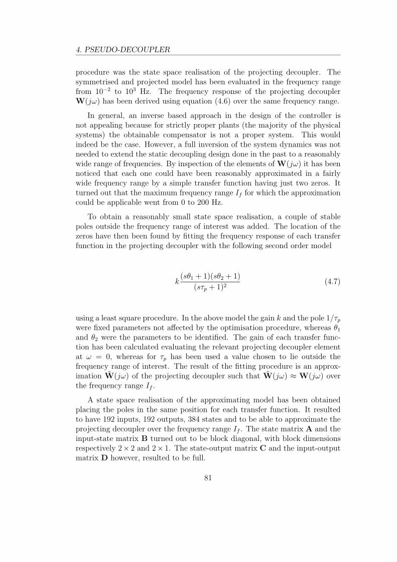
4. PSEUDO-DECOUPLER
procedure was the state space realisation of the projecting decoupler. Thesymmetrised and projected model has been evaluated in the frequency rangefrom 10−2 to 103 Hz. The frequency response of the projecting decouplerW(jω) has been derived using equation (4.6) over the same frequency range.
In general, an inverse based approach in the design of the controller isnot appealing because for strictly proper plants (the majority of the physicalsystems) the obtainable compensator is not a proper system. This wouldindeed be the case. However, a full inversion of the system dynamics was notneeded to extend the static decoupling design done in the past to a reasonablywide range of frequencies. By inspection of the elements of W(jω) it has beennoticed that each one could have been reasonably approximated in a fairlywide frequency range by a simple transfer function having just two zeros. Itturned out that the maximum frequency range If for which the approximationcould be applicable went from 0 to 200 Hz.
To obtain a reasonably small state space realisation, a couple of stablepoles outside the frequency range of interest was added. The location of thezeros have then been found by fitting the frequency response of each transferfunction in the projecting decoupler with the following second order model
k(sθ1 + 1)(sθ2 + 1)
(sτp + 1)2(4.7)
using a least square procedure. In the above model the gain k and the pole 1/τpwere fixed parameters not affected by the optimisation procedure, whereas θ1
and θ2 were the parameters to be identified. The gain of each transfer func-tion has been calculated evaluating the relevant projecting decoupler elementat ω = 0, whereas for τp has been used a value chosen to lie outside thefrequency range of interest. The result of the fitting procedure is an approx-imation W(jω) of the projecting decoupler such that W(jω) ≈ W(jω) overthe frequency range If .
A state space realisation of the approximating model has been obtainedplacing the poles in the same position for each transfer function. It resultedto have 192 inputs, 192 outputs, 384 states and to be able to approximate theprojecting decoupler over the frequency range If . The state matrix A and theinput-state matrix B turned out to be block diagonal, with block dimensionsrespectively 2× 2 and 2× 1. The state-output matrix C and the input-outputmatrix D however, resulted to be full.
81
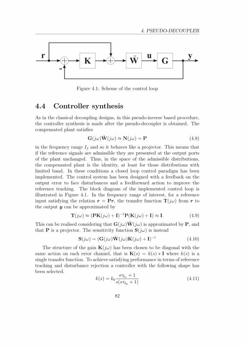
4. PSEUDO-DECOUPLER
GW!r u y
K-
Figure 4.1: Scheme of the control loop
4.4 Controller synthesis
As in the classical decoupling designs, in this pseudo-inverse based procedure,the controller synthesis is made after the pseudo-decoupler is obtained. Thecompensated plant satisfies
G(jω)W(jω) ≈ N(jω) = P (4.8)
in the frequency range If and so it behaves like a projector. This means thatif the reference signals are admissible they are presented at the output portsof the plant unchanged. Thus, in the space of the admissible distributions,the compensated plant is the identity, at least for those distributions withlimited band. In these conditions a closed loop control paradigm has beenimplemented. The control system has been designed with a feedback on theoutput error to face disturbances and a feedforward action to improve thereference tracking. The block diagram of the implemented control loop isillustrated in Figure 4.1. In the frequency range of interest, for a referenceinput satisfying the relation r = Pr, the transfer function T(jω) from r tothe output y can be approximated by
T(jω) ≈ (PK(jω) + I)−1P(K(jω) + I) ≈ I. (4.9)
This can be realised considering that G(jω)W(jω) is approximated by P, andthat P is a projector. The sensitivity function S(jω) is instead
S(jω) = (G(jω)W(jω)K(jω) + I)−1 (4.10)
The structure of the gain K(jω) has been chosen to be diagonal with thesame action on each error channel, that is K(s) = k(s) ∗ I where k(s) is asingle transfer function. To achieve satisfying performance in terms of referencetracking and disturbance rejection a controller with the following shape hasbeen selected.
k(s) = k0sτkz + 1
s(sτkp + 1)(4.11)
82
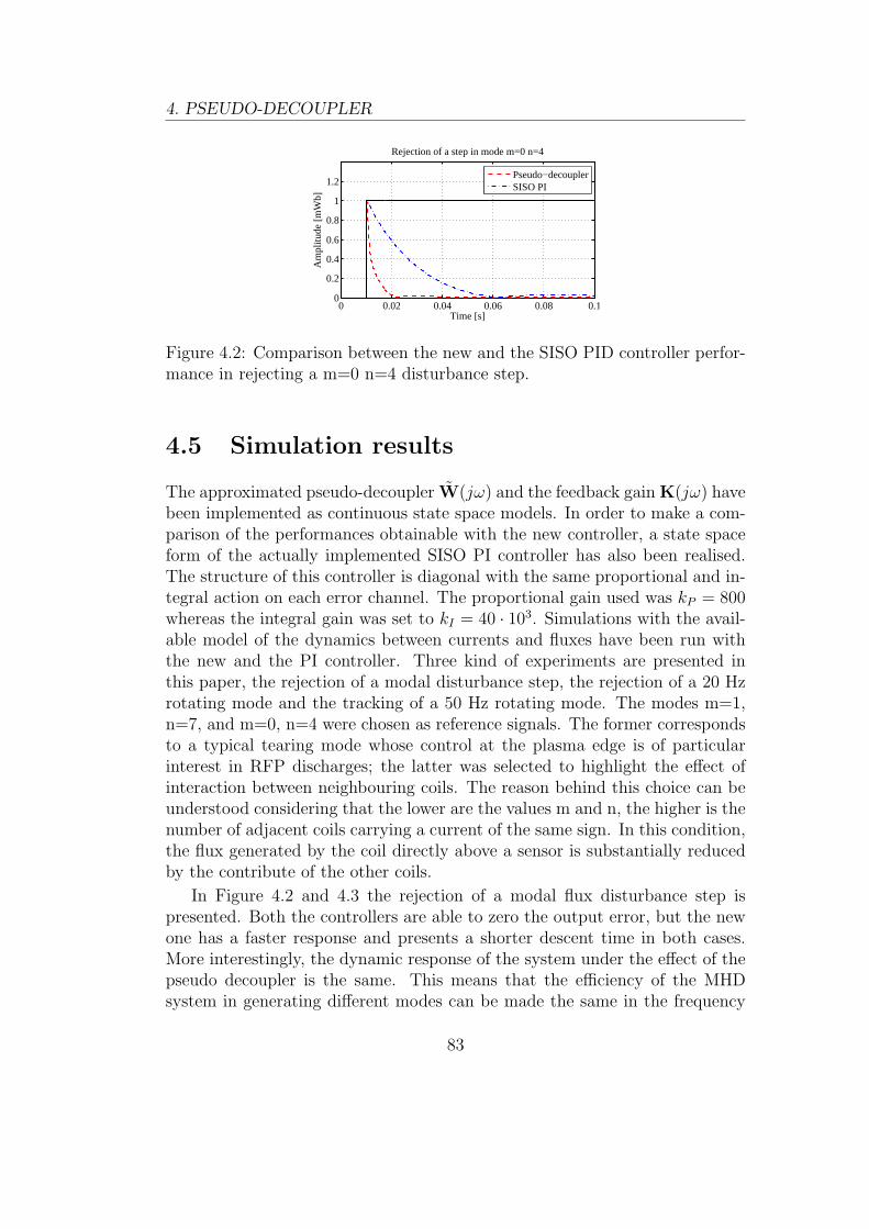
4. PSEUDO-DECOUPLER
0 0.02 0.04 0.06 0.08 0.10
0.2
0.4
0.6
0.8
1
1.2
Rejection of a step in mode m=0 n=4
Am
plitu
de [m
Wb]
Time [s]
Pseudo−decouplerSISO PI
Figure 4.2: Comparison between the new and the SISO PID controller perfor-mance in rejecting a m=0 n=4 disturbance step.
4.5 Simulation results
The approximated pseudo-decoupler W(jω) and the feedback gain K(jω) havebeen implemented as continuous state space models. In order to make a com-parison of the performances obtainable with the new controller, a state spaceform of the actually implemented SISO PI controller has also been realised.The structure of this controller is diagonal with the same proportional and in-tegral action on each error channel. The proportional gain used was kP = 800whereas the integral gain was set to kI = 40 · 103. Simulations with the avail-able model of the dynamics between currents and fluxes have been run withthe new and the PI controller. Three kind of experiments are presented inthis paper, the rejection of a modal disturbance step, the rejection of a 20 Hzrotating mode and the tracking of a 50 Hz rotating mode. The modes m=1,n=7, and m=0, n=4 were chosen as reference signals. The former correspondsto a typical tearing mode whose control at the plasma edge is of particularinterest in RFP discharges; the latter was selected to highlight the effect ofinteraction between neighbouring coils. The reason behind this choice can beunderstood considering that the lower are the values m and n, the higher is thenumber of adjacent coils carrying a current of the same sign. In this condition,the flux generated by the coil directly above a sensor is substantially reducedby the contribute of the other coils.
In Figure 4.2 and 4.3 the rejection of a modal flux disturbance step ispresented. Both the controllers are able to zero the output error, but the newone has a faster response and presents a shorter descent time in both cases.More interestingly, the dynamic response of the system under the effect of thepseudo decoupler is the same. This means that the efficiency of the MHDsystem in generating different modes can be made the same in the frequency
83
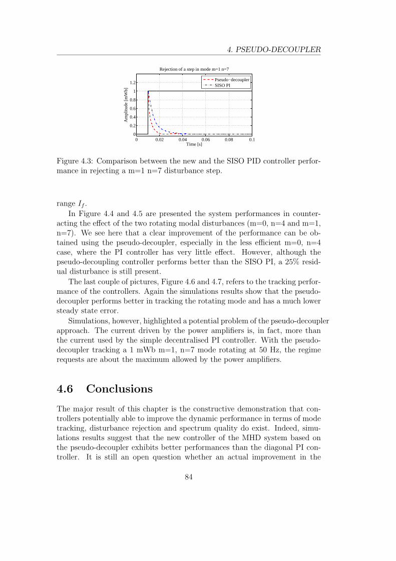
4. PSEUDO-DECOUPLER
0 0.02 0.04 0.06 0.08 0.10
0.2
0.4
0.6
0.8
1
1.2
Rejection of a step in mode m=1 n=7
Am
plitu
de [m
Wb]
Time [s]
Pseudo−decouplerSISO PI
Figure 4.3: Comparison between the new and the SISO PID controller perfor-mance in rejecting a m=1 n=7 disturbance step.
range If .
In Figure 4.4 and 4.5 are presented the system performances in counter-acting the effect of the two rotating modal disturbances (m=0, n=4 and m=1,n=7). We see here that a clear improvement of the performance can be ob-tained using the pseudo-decoupler, especially in the less efficient m=0, n=4case, where the PI controller has very little effect. However, although thepseudo-decoupling controller performs better than the SISO PI, a 25% resid-ual disturbance is still present.
The last couple of pictures, Figure 4.6 and 4.7, refers to the tracking perfor-mance of the controllers. Again the simulations results show that the pseudo-decoupler performs better in tracking the rotating mode and has a much lowersteady state error.
Simulations, however, highlighted a potential problem of the pseudo-decouplerapproach. The current driven by the power amplifiers is, in fact, more thanthe current used by the simple decentralised PI controller. With the pseudo-decoupler tracking a 1 mWb m=1, n=7 mode rotating at 50 Hz, the regimerequests are about the maximum allowed by the power amplifiers.
4.6 Conclusions
The major result of this chapter is the constructive demonstration that con-trollers potentially able to improve the dynamic performance in terms of modetracking, disturbance rejection and spectrum quality do exist. Indeed, simu-lations results suggest that the new controller of the MHD system based onthe pseudo-decoupler exhibits better performances than the diagonal PI con-troller. It is still an open question whether an actual improvement in the
84
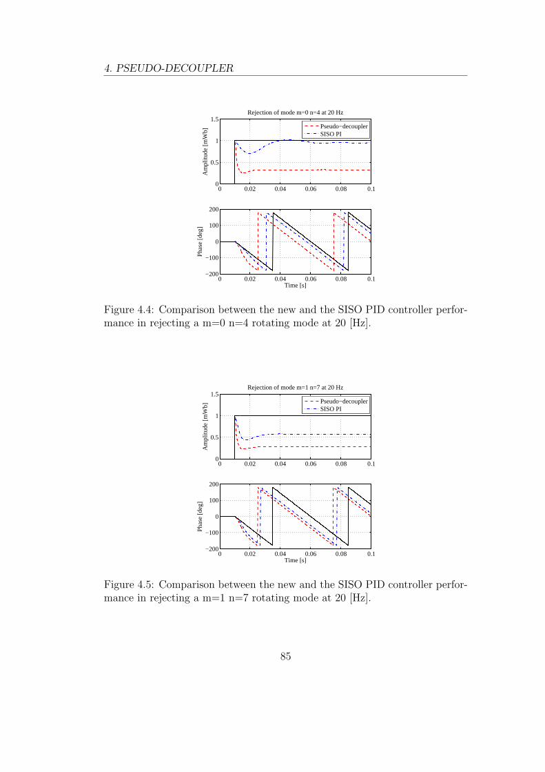
4. PSEUDO-DECOUPLER
0 0.02 0.04 0.06 0.08 0.10
0.5
1
1.5Rejection of mode m=0 n=4 at 20 Hz
Am
plitu
de [m
Wb]
Pseudo−decouplerSISO PI
0 0.02 0.04 0.06 0.08 0.1−200
−100
0
100
200
Pha
se [d
eg]
Time [s]
Figure 4.4: Comparison between the new and the SISO PID controller perfor-mance in rejecting a m=0 n=4 rotating mode at 20 [Hz].
0 0.02 0.04 0.06 0.08 0.10
0.5
1
1.5Rejection of mode m=1 n=7 at 20 Hz
Am
plitu
de [m
Wb]
Pseudo−decouplerSISO PI
0 0.02 0.04 0.06 0.08 0.1−200
−100
0
100
200
Pha
se [d
eg]
Time [s]
Figure 4.5: Comparison between the new and the SISO PID controller perfor-mance in rejecting a m=1 n=7 rotating mode at 20 [Hz].
85

4. PSEUDO-DECOUPLER
0 0.02 0.04 0.06 0.08 0.10
0.5
1
1.5Tracking of mode m=0 n=4 at 50 Hz
Am
plitu
de [m
Wb]
Pseudo−decouplerSISO PI
0 0.02 0.04 0.06 0.08 0.1−200
−100
0
100
200
Pha
se [d
eg]
Time [s]
Figure 4.6: Comparison between the new and the SISO PID controller perfor-mance in tracking a m=0 n=4 rotating mode at 50 [Hz].
0 0.02 0.04 0.06 0.08 0.10
0.5
1
1.5Tracking of mode m=1 n=7 at 50 Hz
Am
plitu
de [m
Wb]
Pseudo−decouplerSISO PI
0 0.02 0.04 0.06 0.08 0.1−200
−100
0
100
200
Pha
se [d
eg]
Time [s]
Figure 4.7: Comparison between the new and the SISO PID controller perfor-mance in tracking a m=1 n=7 rotating mode at 50 [Hz].
86

4. PSEUDO-DECOUPLER
performances is allowed by the limits of the power amplifiers or whether thesame performance can be achieved with a less current demanding controllerdesigned following different paradigms. However, the controller, obtained fol-lowing the pseudo-decoupler approach, is also an interesting benchmark forother control algorithms and an useful tool to gain insight into the intrinsiclimits of the active control system.
87

Chapter 5
Conclusions and furtherdevelopments
The research activity covered the analysis and modelling of an electromagneticMIMO dynamic system with 192 inputs and 192 outputs. It also coveredthe field of control system engineering with the implementation of a pseudo-decoupling control scheme which is also an example of the applicability of themodel.
The theoretical analysis of the active system for the control of MHD insta-bilities showed how the concepts of the Unified Signal Theory can be appliedto the analysis of this system. The use of the Unified Framework allows tograsp the essential features of the system. Its strong mathematical founda-tions provide a model for the understanding of the MHD control algorithmsand it can be used to establish a common background among physicists andengineers. The study allowed to highlight the structural difference between ax-ialsymmetric cylindrical models and the signal-based model of the same MHDsystem, the most important regarding the system spatial non-invariance. How-ever, it is not aimed at demoting the importance of analytical models, whichare understood to be essential to the development of the plasma physics andare always valuable in the implementation of algorithms often able to improvethe performance of the machine to an excellent level. Despite this mathe-matical analysis has not produced results of immediate practical relevance,it has been extremely useful in characterising the effect of sampling quanti-ties on a bi-dimensional toroidal manifold, in particular the spectral analysisof the flux sensors has been performed quantitatively. The work performedprovides methods which can be considered when the assumptions made bysimpler models become unacceptable, for example it could be used in the needof improving the actual sideband correction algorithm. In fact it takes intoaccount properties such as the spatial variance of the system, the frequency
89
5. CONCLUSIONS AND FURTHER DEVELOPMENTS
dependence of the field distribution and the conservation law of the magneticflux which are presently neglected in the sideband analytical calculations. Inparticular, the presence of shell local features such as gaps and ports is cause ofa strong spatial variance. A natural development of this study consists in thethe numerical calculation of the actual harmonic content of the field distribu-tion generated by the saddle coil currents. This task can be carried out usinga Finite Element Model of the machine active coils and passive structures anda electromagnetic solver such as CARIDDI, for example.
The activity of modelling the RFX-mod active control system for the con-trol of the MHD instabilities has been concluded producing a full electromag-netic model of the system whose state space representation consists of morethan 6000 states. The peculiarity of this model is the fact that it has beenderived almost entirely from experimental data. Extensive series of validationtests proved the model capability to reproduce the system open and closedloop response in terms of evolution of the magnetic fluxes with satisfactoryaccuracy. The same tests showed that the inductive effect of the plasma onthe currents in the active coils can be neglected. This can be used in the con-struction of models comprehensive of the plasma action because it allows tosimplify the problem. The derived model is capable of quantitative analysis ofthe relevant measured quantities and has been used with success in the studyof unstable phenomena which the MHD system had exhibited. In particular,the model is able to reproduce the stability range of the closed loop system,whose upper limit is not determined by an effect of the plasma but by theMHD system itself. Finally, since all the model parameters have been derivedfrom experimental data, the effects of the toroidal geometry, passive struc-tures, and the presence of non axialsymmetric features on the dynamics of thecoil currents and the radial field are implicitly taken into account. Recently, anew campaign of measures has been concluded and the integration of the newmeasures into the current model is ongoing. Despite it has been successfullyused up to now, the uge size of the model could be a limit to further develop-ments. Advanced model reduction techniques, able to deal with models of sizeten thousand, could be investigated, because preliminary reduction attemptssuggest that the model can be reduced to about one tenth of its original size.Apart of this activity, from the point of view of the modelling, it would be alsointeresting exploring ways to couple the MHD equations to this electromag-netic model of the machine in order to obtain a global model comprehensive ofthe plasma interactions suitable for the design of improved control algorithms.
Finally, the last results of the research is the development of a new con-troller for the MHD system. Its design has been done on the basis of thedata of the electromagnetic model which had just been developed. During the
90
5. CONCLUSIONS AND FURTHER DEVELOPMENTS
research activity several design techniques have been considered. The highdimensionality of the available model and the real-time constraints of the con-troller implementation seriously limited the usable design techniques. Finallya MIMO approach was followed based on a decoupling component togetherwith a controller designed with the classical loop shaping method. It shouldbe pointed out that the design method required the explicit use of the flux con-servation law in the controller derivation. This resulted in a pseudo-decouplercomponent instead of a full decoupling design whose properties have also beenalgebraically demonstrated. Simulation results confirm that such controllerscheme can improve the dynamic performance of the MHD control system interms of mode tracking, disturbance rejection and spectrum quality. Consider-ing these properties, the new controller based on the pseudo-decoupler exhibitsbetter performances than the diagonal PI controller. The real-time implemen-tation of the pseudo-decoupling algorithm is currently ongoing. Preliminarytests have been carried out on the crate hosting the computer board used inthe control system architecture of the RFX-mod MHD units and the EFDA-JET vertical stabilisation component. Early results suggest that it is possibleto implement the pseudo-decoupler algorithm on one node of the architecture(which consists of a Motorola VME5500 board equipped with a single PowerPCprocessor), this however has required a full exploitation of the board featuresat the lowest possible level (kernel level and/or hardware level). At the mo-ment an offline application of the pseudo-decoupler in the field of the errorfield correction is considered. In this application the MHD system is expectedto counteract the effect of the error fields induced by the magnetising winding.The pseudo-decoupler provides also a benchmark for other controllers. Apartfrom the pseudo-decoupler no other implemented controllers are known to havethe property of equalising the MHD system so as to achieve the same penetra-tion time constant for each spatial harmonic. In the field of the control systemengineering, an interesting application is the study of the technical feasibilityof real-time eddy currents calculation. It is still an open question whetherthe required performances are allowed by the limits of the power amplifiers orwhether the same performances can be achieved with a less current demandingcontroller designed following different paradigms.
91


Appendix A
Technicalities
In the following chapter are proved four propositions stated in the rest of thedissertation.
Proposition A.1. For every cell C = [U/P ) there exist a one to one mappingµ : C → U/P from C to the quotient group U/P .
Proof. Consider the restriction to C of the natural mapping from U into U/Pµ(c) : c ∈ C → c + P . Suppose (c1 + P ) ∩ (c2 + P ) 6= ∅. So there exist anelement u which belongs at the same time to (c1 + P ) and to (c2 + P ). Thatis there exist two elements, p1, p2 ∈ P , so that
u = c1 + p1 = c2 + p2. (A.1)
This equation also states that u is both in C + p1 and C + p2 so, from therelation (2.5) is possible to conclude that p1 = p2 and also c1 = c2. This provesthe map injectivity.
Every possible member of U/P can be expressed in the form u + P withu ∈ U . Equation (2.4) gives (C + P ) ∩ (u+ P ) = U ∩ (u+ P ) = u+ P . Thatis, for every u ∈ U , there exist a c ∈ C and p1, p2 ∈ S so that c+ p1 = u+ p2,which means that µ(c) = u+ P . This proves the map surjectivity.
Proposition A.2. Given a time variant system g(t1, t2) transforming the in-put signal u(t1) defined over the domain I into the corresponding output signalv(t2) defined over the same domain by the law
v(t2) =
∫I
u(t1)g(t1, t2)dt1 (A.2)
93
A. TECHNICALITIES
the Fourier transform of u(t1), v(t2) and g(t1, t2), respectively U(f1), V (f2)and G(f1,f2), are related by the equation
V (f2) =
∫I
U(f1)G(−f1,f2)df1 (A.3)
Proof. Considering that
U(f1) =
∫I
u(t1)e−j2πf1·t1dt1
and
G(f1,f2) =
∫∫I I
g(t1, t2)e−j2π(f1·t1+f2·t2)dt1dt2
equation (2.18) becomes
V (f2) =
∫I
∫I
u(t1)e−j2πf1·t1dt1
∫∫I I
g(t1, t2)e−j2π(−f1·t1+f2·t2)dt1dt2df1
=
∫∫∫∫I×I×I×I
u(t3)e−j2πf1·t3g(t1, t2)e
−j2π(−f1·t1+f2·t2)dt3dt1dt2df1
=
∫∫∫I×I×I
g(t1, t2)e−j2πf2·t2u(t3)
∫I
e−j2πf1·(t3−t1)df1dt3dt1dt2
=
∫∫I×I
g(t1, t2)e−j2πf2·t2
∫I
u(t3)δI(t3 − t1)dt3dt1dt2
=
∫I
e−j2πf2·t2∫I
u(t1)g(t1, t2)dt1dt2
=
∫I
v(t2)e−j2πf2·t2dt2
Proposition A.3. Given a function g of two vectorial variables t1, t2 ∈ I =G/P such that for every d ∈ I g(t1+d, t2+d) = g(t1, t2), its Fourier transformis
G(f1,f2) = δI(f1 + f2)Gr(f2) = δI(f1 + f2)Gr(−f1) (A.4)
where
Gr(f2) =
∫I
g(0, τ )ej2πf2τdτ (A.5)
94
A. TECHNICALITIES
Proof.
G(f1,f2) =
∫∫I×I
g(t1, t2)e−j2π(f1·t1+f2·t2)dt1dt2
=
∫∫I×I
g(0, τ )e−j2π(f1·t1+f2·t1+f2·τ ))dt1dτ
=
∫I
g(0, τ )e−j2πf2·τ∫I
e−j2π(f1+f2)·t1dt1dτ
=
∫I
g(0, τ )e−j2πf2·τ δI(f1 + f2)dτ
= δI(f1 + f2)
∫I
g(0, τ )e−j2πf2·τdτ
= δI(f1 + f2)Gr(f2)
The above chain of equations follows from the position τ = t2 − t1 substitut-ing t2 in favour of τ , whereas the second equation of the proposition followssubstituting t1 with τ in similar manner.
Proposition A.4. Considering the relations of section 4.3.2, that is
qH = [1, . . . , 1], qHG(jω) = 0H , (A.6)
Q =qqH
qHq, P = I−Q, (A.7)
G(jω) = U1(jω)Σ(jω)VH1 (jω) (A.8)
andW(jω) = V1(jω)Σ−1(jω)UH
1 (jω) (A.9)
thenG(jω)W(jω) = P (A.10)
for every ω ∈ R.
Proof. qHG(jω) = 0H implies that
qHG(jω)W(jω) = qHU1(jω)UH1 (jω) = 0H (A.11)
because U1(jω) is full rank. So q√qHq
can be used to complete the basis U1(jω)
to [U1(jω) q√qHq
]. Then
U1(jω)UH1 (jω) = [U1(jω) q√
qHq]
[I 00 0
][U1(jω) q√
qHq]H (A.12)
95

A. TECHNICALITIES
= [U1(jω) q√qHq
]
(I−
[0 00 1
])[U1(jω) q√
qHq]H = I−Q (A.13)
96
Bibliography
[1] Allen H. Boozer. Physics of magnetically confined plasmas. Reviews ofmodern physics, 76(4):1071–1141, October 2004.
[2] Topical issue on the rfx-experiment. Fusion Engineering and Design,25(4), January 1995.
[3] P. Zaccaria F. Gnesotto S. Ortolani A. Buffa M. Bagatin W. R. Baker S.Dal Bello P. Fiorentin L. Grando G. Marchiori D. Marcuzzi A. MasielloS. Peruzzo N. Pomaro P. Sonato, G. Chitarin and G. Serianni. Machinemodifications for active mhd control in rfx. Fusion Engineering and De-sign, 66-68:161–168, September 2003.
[4] A. Luchetta P. Sonato, R. Piovan. Control of non-axisymmetric magneticfields for plasma enhanced performances: The rfx contribution. FusionEngineering and Design, 74:97–107, November 2005.
[5] P. E. Stott C. M. Braams. Nuclear Fusion: half a century of magnetic con-finement research. Institute of Physics Publishing, Dirac House, TempleBack, Bristol, BS1 6BE, UK, first edition, 2002. ISBN 0750307056.
[6] Gianfranco Cariolaro. La teoria unificata dei segnali. UTET libreria,Torino (ITALY), 2nd edition, 1996.
[7] Leopoldo Nachbin. The Haar Integral. D. Van Nostrand Company, 120Alexander St., Princeton, New Jersey, USA, 1965.
[8] A. Luchetta G. Marchiori C. Taliercio M. Cavinato, G. Manduchi. Dis-tributed real time control in rfx-mod nuclear fusion experiment: Commis-sioning and first results. IEEE Transactions on Nuclear Science, 53:1015–1021, 2003.
[9] S. Ortolani and the RFX team. Active mhd control experiments in rfx-mod. Plasma Phys. Control. Fusion, 48:B371–B381, 2006.
97

BIBLIOGRAPHY
[10] P. R. Brunsell D. Yadikin G. Marchiori, A. Masiello. Open loop charac-terization of an active control system of mhd modes. Fusion Engineeringand Design, 74:555–560, 2005.
[11] A. Masiello R. Paccagnella G.Marchiori, M. Cavinato. Electromagneticmodeling for the active control of mhd modes in rfx. Fusion Engineeringand Design, 66–68:691–696, 2003.
[12] C. Taccon. Private communication.
[13] P. Zollino G. Chitarin, G. Marchiori. Computation and experimentalvalidation of the transfer functions of the local control coil system in rfx.Proceedings of the 17th Symposium on Fusion Engineering, vol.I:572–575,October 1997.
[14] S. Martini et al. Active mhd control at high currents in rfx-mod. NuclearFusion, 47(8):783–791, August 2007.
[15] I. Postlethwaite S. Skogestad. Multivariable feedback control. Jhon Wiley& Son, XX, xx edition, 1996. ISBN 0 471 94277 4.
[16] Anton Soppelsa Giuseppe Marchiori. Development and validation of anelectromagnetic model of the active control system of mhd modes in rfx-mod. Fusion Engineering and Design, 82:1015–1022, 2007.
[17] C. F. Van Loan G.H. Golub. Matrix computations. The Jhon HopkinsUniversity Press, 2715 North Charles Street, Baltimore, Maryland, 21218-4319, USA, third edition, 1996. ISBN 0 8018 5413 X.
98