
alla mia famiglia - unipd.ittesi.cab.unipd.it/39790/1/Tesi.pdf · alla mia famiglia. Contents ......
64
alla mia famiglia
Transcript of alla mia famiglia - unipd.ittesi.cab.unipd.it/39790/1/Tesi.pdf · alla mia famiglia. Contents ......

alla mia famiglia

Contents
1 SAR concepts 1
1.1 Spaceborne SAR geometry . . . . . . . . . . . . . . . . . . . . . . . 21.2 The Range Equation . . . . . . . . . . . . . . . . . . . . . . . . . . 31.3 SAR Signals . . . . . . . . . . . . . . . . . . . . . . . . . . . . . . . 4
1.3.1 SAR signal in Range Direction . . . . . . . . . . . . . . . . . 41.3.2 SAR signal in Azimuth Direction . . . . . . . . . . . . . . . 6
1.4 SAR resolution . . . . . . . . . . . . . . . . . . . . . . . . . . . . . 91.4.1 Range resolution . . . . . . . . . . . . . . . . . . . . . . . . 91.4.2 Azimuth resolution . . . . . . . . . . . . . . . . . . . . . . . 9
2 SAR GMTI concepts 11
2.1 Moving Targets . . . . . . . . . . . . . . . . . . . . . . . . . . . . . 112.1.1 Across-track velocity . . . . . . . . . . . . . . . . . . . . . . 112.1.2 Along-track velocity . . . . . . . . . . . . . . . . . . . . . . 12
2.2 Clutter . . . . . . . . . . . . . . . . . . . . . . . . . . . . . . . . . . 132.3 Multichannel SAR . . . . . . . . . . . . . . . . . . . . . . . . . . . 14
2.3.1 Dual Receive Antenna . . . . . . . . . . . . . . . . . . . . . 142.3.2 Toggle Modes . . . . . . . . . . . . . . . . . . . . . . . . . . 152.3.3 Toggle receive modes . . . . . . . . . . . . . . . . . . . . . . 152.3.4 Toggle on transmit modes . . . . . . . . . . . . . . . . . . . 16
2.4 GMTI Techniques . . . . . . . . . . . . . . . . . . . . . . . . . . . . 172.4.1 Displaced Phase Center Antenna . . . . . . . . . . . . . . . 172.4.2 Along Track Interferometry . . . . . . . . . . . . . . . . . . 182.4.3 STAP . . . . . . . . . . . . . . . . . . . . . . . . . . . . . . 18
3 Detection and Estimation Algorithm 23
3.1 Post Doppler STAP . . . . . . . . . . . . . . . . . . . . . . . . . . . 233.2 Detection . . . . . . . . . . . . . . . . . . . . . . . . . . . . . . . . 25
3.2.1 Constant False Alarm Rate Detector . . . . . . . . . . . . . 263.3 Along-Track velocity Estimation . . . . . . . . . . . . . . . . . . . . 29
4 Simulation Results 31
4.1 Simulated Scenario . . . . . . . . . . . . . . . . . . . . . . . . . . . 324.2 DRA results . . . . . . . . . . . . . . . . . . . . . . . . . . . . . . . 32
4.2.1 CNR . . . . . . . . . . . . . . . . . . . . . . . . . . . . . . . 334.2.2 SCNR . . . . . . . . . . . . . . . . . . . . . . . . . . . . . . 334.2.3 Detection Probability . . . . . . . . . . . . . . . . . . . . . . 35
iii

iv CONTENTS
4.2.4 Along-Track velocity estimation . . . . . . . . . . . . . . . . 374.3 TOGGLE modes results . . . . . . . . . . . . . . . . . . . . . . . . 39
4.3.1 CNR . . . . . . . . . . . . . . . . . . . . . . . . . . . . . . . 394.3.2 SCNR . . . . . . . . . . . . . . . . . . . . . . . . . . . . . . 394.3.3 Detection Probability . . . . . . . . . . . . . . . . . . . . . . 414.3.4 Along-Track velocity estimation . . . . . . . . . . . . . . . . 43
4.4 Analysis of the results . . . . . . . . . . . . . . . . . . . . . . . . . 46
5 Conclusions and future work 49

List of Figures
1.1 Synthetic aperture . . . . . . . . . . . . . . . . . . . . . . . . . . . 1
1.2 Spaceborne SAR geometry . . . . . . . . . . . . . . . . . . . . . . . 2
1.3 . . . . . . . . . . . . . . . . . . . . . . . . . . . . . . . . . . . . . . 4
1.4 Top-down view of antenna and accelerating target geometry for aspaceborne scenario . . . . . . . . . . . . . . . . . . . . . . . . . . . 5
1.5 Radar beam’s 3dB elevation beamwidth . . . . . . . . . . . . . . . 6
1.6 Azimuth beam pattern and its effect upon signal strength and dopplerfrequency, extracted from [9] . . . . . . . . . . . . . . . . . . . . . . 8
2.1 Azimuth cut of the impulse response function of a moving targetwith different constant across-track velocities . . . . . . . . . . . . . 12
2.2 Focused SAR image of three moving target with, from the left,vx =0m
s, vx = 10m
s, vx = 20m
s. . . . . . . . . . . . . . . . . . . . . . . . 13
2.3 Three virtual channel toggle on receive configuration of the antennafor the different pulses, the black triangles indicates the physicalcenters of the Tx or Rx antennas, the red diamonds indicates thetwo-way phase centers for each virtual channel . . . . . . . . . . . . 15
2.4 Four virtual channel toggle on receive configuration of the antennafor the different pulses, the black triangles indicates the physicalcenters of the Tx or Rx antennas, the red diamonds indicates thetwo-way phase centers for each virtual channel . . . . . . . . . . . . 16
2.5 Three virtual channels toggle on transmit mode configuration ofthe antenna for the different pulses, the black triangles indicatesthe physical centers of the Tx or Rx antennas, the red diamondsindicates the two-way phase centers for each virtual channel . . . . 17
2.6 DPCA principles, red diamonds indicates the 2-way phase center ofthe aft and fore antenna . . . . . . . . . . . . . . . . . . . . . . . . 17
2.7 power spectral density of the clutter in the angle-Doppler domain(ridge-like pattern of the clutter due to motion of the platform);extracted from [8] . . . . . . . . . . . . . . . . . . . . . . . . . . . 19
2.8 STAP beamformer, extracted from [8] . . . . . . . . . . . . . . . . . 20
3.1 Detection Algorithm . . . . . . . . . . . . . . . . . . . . . . . . . . 26
3.2 Comparison of the experimental Noise+Clutter PDF with a rayleighapproximated PDF for clutter (σ0 = −25dB, τc = 60ms) . . . . . . 27
3.3 Comparison of the experimental Noise+Clutter PDF with a rayleighapproximated PDF for clutter (σ0 = −15dB, τc = 32ms) . . . . . . 28
v

3.4 Comparison of the experimental Noise+Clutter PDF with a rayleighapproximated PDF for clutter (σ0 = −12dB, τc = 31ms) . . . . . . 28
4.1 A rendering of the PAZ satellite . . . . . . . . . . . . . . . . . . . . 31
4.2 DRA: SCNR as a function of Across-Track velocity for a 0dBm2
RCS target . . . . . . . . . . . . . . . . . . . . . . . . . . . . . . . 34
4.3 DRA: SCNR as a function of Along-Track velocity for a 0dBsm RCStarget . . . . . . . . . . . . . . . . . . . . . . . . . . . . . . . . . . 34
4.4 DRA: Pd as a function of Across-Track velocity for different RCS,Adapted Steering . . . . . . . . . . . . . . . . . . . . . . . . . . . . 35
4.5 DRA: Pd as a function of Across-Track velocity for different RCS,[1− 1] Steering . . . . . . . . . . . . . . . . . . . . . . . . . . . . . 36
4.6 DRA: Pd as a function of Along-Track velocity for different RCS,Adapted Steering . . . . . . . . . . . . . . . . . . . . . . . . . . . . 36
4.7 DRA: Pd as a function of Along-Track velocity for different RCS,[1− 1] Steering . . . . . . . . . . . . . . . . . . . . . . . . . . . . . 37
4.8 DRA: Pd as a function of Along+Across-Track velocity for differentRCS, Adapted Steering . . . . . . . . . . . . . . . . . . . . . . . . . 37
4.9 DRA: Pd as a function of Along+Across-Track velocity for differentRCS, [1− 1] Steering . . . . . . . . . . . . . . . . . . . . . . . . . . 38
4.10 DRA: Bank of filter OUTPUT for a 3ms
along-track moving target20dBsm RCS . . . . . . . . . . . . . . . . . . . . . . . . . . . . . . 38
4.11 DRA: Bank of filter OUTPUT for a 12ms
along-track moving target20dBsm RCS . . . . . . . . . . . . . . . . . . . . . . . . . . . . . . 39
4.12 TOGGLE: SCNR as a function of Across-Track velocity for a 0dBsm
RCS target . . . . . . . . . . . . . . . . . . . . . . . . . . . . . . . 41
4.13 TOGGLE: SCNR as a function of Along-Track velocity for a 0dBsm
RCS target . . . . . . . . . . . . . . . . . . . . . . . . . . . . . . . 42
4.14 TOGGLE: Pd as a function of Across-Track velocity for different RCS 42
4.15 TOGGLE: Pd as a function of Along-Track velocity for different RCS 43
4.16 TOGGLE: Pd as a function of Along+Across-Track velocity for dif-ferent RCS . . . . . . . . . . . . . . . . . . . . . . . . . . . . . . . . 43
4.17 TOGGLE: Bank of filter OUTPUT for a 3ms
along-track movingtarget 20dBsm RCS . . . . . . . . . . . . . . . . . . . . . . . . . . 44
4.18 TOGGLE: Bank of filter OUTPUT for a 12ms
along-track movingtarget 20dBsm RCS . . . . . . . . . . . . . . . . . . . . . . . . . . 44
4.19 DRA, SCNR as a function of Across-Track velocity for a 0dBsm
RCS target, different CNR . . . . . . . . . . . . . . . . . . . . . . 46
4.20 SCNR as a function of Across-Track velocity for a 0dBsm RCS target 47
vi

LIST OF TABLES vii
List of Tables
4.1 Parameters of SEOSAR/PAZ mission. . . . . . . . . . . . . . . . . 314.2 Characteristics of the sea clutter model used in the simulations . . . 324.3 DRA: CNR before and after STAP processing for adapted steering . 334.4 DRA: CNR before and after STAP processing for [1 -1] steering . . 334.5 DRA: estimated along track velocity for 20dBsm RCS target . . . . 404.6 TOGGLE: CNR before and after STAP processing for adapted steering 404.7 TOGGLE: estimated along track velocity for 20dBsm RCS target . 45

Ringraziamenti
E’ stato un percorso lungo e a volte complicato quello che mi ha portato fin quiora, e non sarebbe stato possibile senza l’incondizionato appoggio che fin dall’inizioho ricevuto da mio padre Lorenzo, da mia sorella Giulia e, sono sicuro, da miamadre Valeria che da lassù non ha mai smesso di credere in me. E’ a loro che vail mio ringraziamento più grande.
Ai miei nonni, Giuseppe e Cesarina, per l’affetto e l’aiuto che non mi hannomai fatto mancare.
Un ringraziamento speciale va poi a Federica, per la pazienza che da sempre haavuto con me e per i suoi incoraggiamenti ad andare sempre avanti, a non mollaremai anche quando tutto era più grigio, più insicuro.
Un ringraziamento a tutti i miei amici, in particolare Luca, Chiara, Giulio eJon che mi sono rimasti sempre vicino in questi anni.
ix

Introduction
The synthetic aperture radar principle has been discovered in the early 50th.Since then, a rapid development took place all over the world. Today, syntheticaperture radar (SAR) plays an important role in military applications and earth ob-servation. SAR systems offer advantages compared to competing sensors in infraredor visible spectral area, because of its day-and-night capability and the possibilityto penetrate clouds and rain. Typical applications of SAR in the earth observationare for example topographic mapping (2D and 3D), surface movements detection,vegetation monitoring. One application currently under evaluation is the use ofspaceborne SAR for traffic monitoring and maritime surveillance, and is in thisfield of application that this thesis gives its contribute. The maritime surveillancecould be of help to prevent for example the illegal immigration phenomena that isaffecting nowadays the southern Europe or can be used in piracy and illegal traffics(arms, toxic waste, etc) prevention. The European community has showed interestin this topic and has funded the NEWA (New EuropeanWAtcher) project in orderto investigate the problem of the detection of moving targets using spaceborneSAR.
This thesis is made in collaboration with the Department of Signal Theory andCommunications (TSC) of the Universitat Politècnica de Catalunya (UPC), whichparticipates in the NEWA project.
Objectives
The aim of this thesis is the study and implementation of a sub-optimal space-time adaptive processing technique and its integration in the SAR processing fordetection of moving targets in maritime scenario. A detection algorithm based onthis technique has been implemented and its performances have been evaluatedwith the SAR-GMTI simulator developed in the Department of Signal Theory andCommunications (TSC). The performances of this technique have been tested overdifferent sea conditions and for different types of modeled boats.
Organization
The thesis is organized as follows:
• In chapter 1 a review of Syntectic Aperture Radar (SAR) concepts is given.
xi

xii LIST OF TABLES
• In chapter 2 the Ground Moving Target Indicator concepts are given and thedifferent GMTI techniques are explained.
• In chapter 3 a sub-optimal space-time adaptive processing is studied and inte-grated in the SAR processing for detection of moving targets and estimationof their velocity.
• In chapter 4 the simulation results of the sub-optimal space-time adaptiveprocessing in maritime scenario are presented and commented.
• Chapter 5 summarizes the contributions of the thesis in line with some con-clusions and provides general hints for future work.
Chapter 1
SAR concepts
In spaceborne SAR the Radar is mounted in a satellite, typically flying in aLow Earth Orbit. In the monostatic configuration the signals are transmitter andreceived by the same antenna.
Antenna pattern illuminates a specific region on the earth surface, called beamfootprint, determined by the intersection of the antenna pattern and the earthsurface at a given incidence angle.
As the platform advances, pulse of electromagnetic energy are transmitted atregular intervals towards the ground, this pulses, after being reflected by theground, travel back to the Radar antenna where they are sampled according totheir bandwidth.
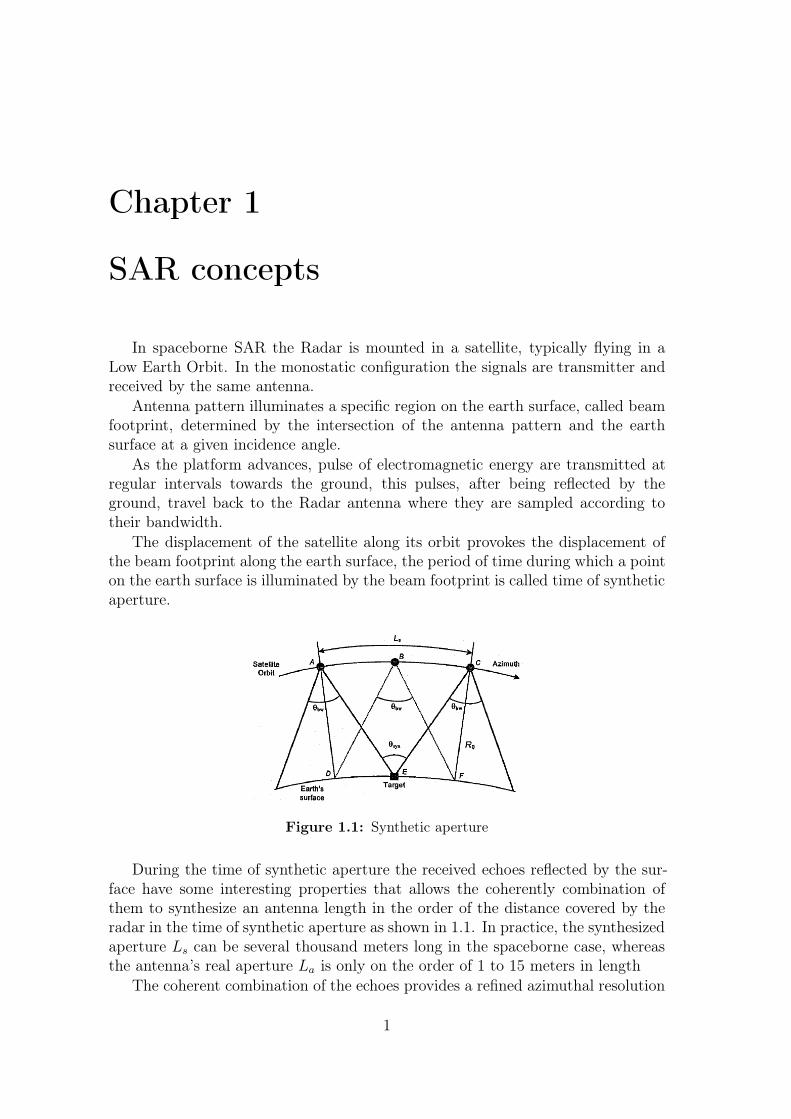
The displacement of the satellite along its orbit provokes the displacement ofthe beam footprint along the earth surface, the period of time during which a pointon the earth surface is illuminated by the beam footprint is called time of syntheticaperture.
Figure 1.1: Synthetic aperture
During the time of synthetic aperture the received echoes reflected by the sur-face have some interesting properties that allows the coherently combination ofthem to synthesize an antenna length in the order of the distance covered by theradar in the time of synthetic aperture as shown in 1.1. In practice, the synthesizedaperture Ls can be several thousand meters long in the spaceborne case, whereasthe antenna’s real aperture La is only on the order of 1 to 15 meters in length
The coherent combination of the echoes provides a refined azimuthal resolution
1
2 CHAPTER 1. SAR CONCEPTS
since the beamwidth is inversely proportional to the antenna aperture, independenton the range and frequency as happens in the Real aperture radars.
1.1 Spaceborne SAR geometry
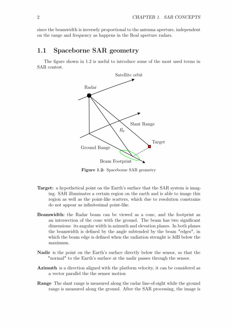
The figure shown in 1.2 is useful to introduce some of the most used terms inSAR contest.
Satellite orbit
Radar
Ground Range
R0
Slant Range
Target
Beam Footprint
Figure 1.2: Spaceborne SAR geometry
Target: a hypothetical point on the Earth’s surface that the SAR system is imag-ing. SAR illuminates a certain region on the earth and is able to image thisregion as well as the point-like scatters, which due to resolution constrainsdo not appear as infinitesimal point-like.
Beamwidth: the Radar beam can be viewed as a cone, and the footprint asan intersection of the cone with the ground. The beam has two significantdimensions: its angular width in azimuth and elevation planes. In both planesthe beamwidth is defined by the angle subtended by the beam "edges", inwhich the beam edge is defined when the radiation strenght is 3dB below themaximum.
Nadir is the point on the Earth’s surface directly below the sensor, so that the"normal" to the Earth’s surface at the nadir passes through the sensor.
Azimuth is a direction aligned with the platform velocity, it can be considered asa vector parallel the the sensor motion
Range The slant range is measured along the radar line-of-sight while the groundrange is measured along the ground. After the SAR processing, the image is
1.2. THE RANGE EQUATION 3
registered to the azimuth position of closest approach and the range axis isperpendicular to the azimuth axis.
Range of closest approach because of the motion of the platform the distancebetween the sensor and the target varies with time, when the range is aminimum it is called the range of closest approach, denoted by R0.
Zero Doppler plane the plane containing the sensor that’s perpendicular to theplatform velocity vector. When this plane crosses the target, the relativeradial velocity of the sensor with respect of the target is zero.
Ground range is the projection of the slant range onto the ground. Assumingthat the data is registered to zero Doppler, ground range is the directionorthogonal to the azimuth axis and parallel to the earth surface with itsorigin at the nadir point.
Squint angle is the angle between the slant range vector and the zero Dopplerplane, is an important component in the definition of the beam pointingdirection.
1.2 The Range Equation
It’s fundamental in the SAR processing to know how the slant range from thesensor to the target varies with time, this range history is described by the RangeEquation. When the sensor approaches the target the range decreases every pulsewhile after the sensor passes the target the range increases every pulse. In additionto the motion of the platform also the motion of the target (if present) has to betake into account.
This change in range mainly produces two consequences:
• a phase modulation from pulse to pulse that’s necessary to obtain fine az-imuth resolution.
• the received data to be skewed in the computer memory, this is called rangecell migration (RCM).
The following derivation of the range equation is made under the assumption ofa locally straight flight path, a flat earth’s surface and the absence of squint angleas shown in fig 1.3.
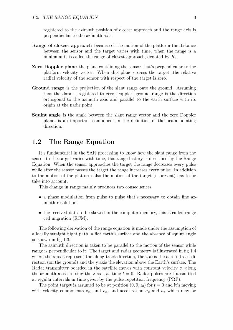
The azimuth direction is taken to be parallel to the motion of the sensor whilerange is perpendicular to it. The target and radar geometry is illustrated in fig 1.4where the x axis represent the along-track direction, the z axis the across-track di-rection (on the ground) and the y axis the elevation above the Earth’s surface. TheRadar transmitter boarded in the satellite moves with constant velocity vp alongthe azimuth axis crossing the z axis at time t = 0. Radar pulses are transmittedat regular intervals in time given by the pulse repetition frequency (PRF).
The point target is assumed to be at position (0, 0, z0) for t = 0 and it’s movingwith velocity components vx0 and vz0 and acceleration ax and az which may be

4 CHAPTER 1. SAR CONCEPTS
Satellite orbit
Earth Surfacevg
xg
vp
x0
(a) curved earth geometry.
vg
xg
vp
x0
(b) flat earth geometry.
Figure 1.3
considered constant over the observation period. The target height is assumed bezero.
We indicate with R0 =√
y20 +H2 the slant range at t = 0 and R(t) representthe range from sensor to target at any time t. The equation that describe thetemporal evolution of R(t) is given by[[14]]:
R(t) =
(
(
vx0+ax0
2t2+
˙ax06
t3−vpt)2
+(
z0+ vz0t+az0
2t2+
˙ay06t3)2
+H2
)1
2
(1.1)
where the dots indicate time derivatives of the target acceleration. Equation 2.9can be written as a second-order Taylor series expansion about broadside time t = 0taking into account that the accelerations could be considered constants over theperiod of observation.
R(t) ≈ R0 +z0vz0
R0t+
1
2R0
[
(vx0 − vp)2 + v2z0
(
1−z20R2
0
)
]
t2 (1.2)
1.3 SAR Signals
1.3.1 SAR signal in Range Direction
In the range direction the radar usually sends out a pulse with a linear Fre-quency Modulation characteristic:
spul(τ) = wr(τ) cos(
2πf0τ + πKrτ2)
(1.3)
where Kr is the FM rate of the range pulse and wr(τ) denotes the pulse envelopthat used to be approximately rectangular as expressed in equation 1.4 where Tr
is the pulse duration.
wr = rect( τ
Tr
)
(1.4)
1.3. SAR SIGNALS 5
replacemen
t < t0
t = t0 = 0
t > t0
Target,t < t0
Target,t = t0 = 0
Target,t > t0
R(t > t0)
R0
R(t < t0)
vx0, ax
vz0, az
vp
(0, H, 0)
(0, 0, y0)
x
yz
Figure 1.4: Top-down view of antenna and accelerating target geometry for a space-borne scenario
From now on we’ll refer to the time τ as the fast time because the range signaltravels at the speed of light while the azimuth signal is originated by the movementof the platform.
The instantaneous frequency of the signal spul(τ) varies with the fast time τ ,in fact if we take the derivative of the argument of the cosine we find that theinstantaneous frequency fi = f0 +Krτ .
When the sign of Kr is positive then the signal is called an up-chirp while in theother case corresponds to a down-chirp. This characteristic of the signal neitheraffects the structure of the SAR processing nor the quality of the processed image.
One very important parameter is the bandwidth of the signal, since the resolu-tion of the SAR image and the sampling requirements are directly dependent onit. The bandwidth of the signal spul(τ) is given by BW = ‖Kr‖Tr.
The demodulated signal is digitized at a sampling frequency Fr above theNyquist criterion. In practice the sampling frequency is chosen to oversamplethe signal by a factor that is called range oversampling ratio αos,r and is usuallybetween 1.1 and 1.2.
Let’s now analyze the received signal. The Radar beam has a certain beamwidthin the elevation plane, illuminating a section of the ground, lying between the "nearrange" and "far range" as indicated in figure 1.5.
The transmitted pulse travels at the speed of light towards the earth surface,at time t1 the pulse reaches the ground at the "near range" and after a fraction ofmillisecond the trailing edge of the pulse passes the "far range" point at time t2.
The reflected energy at any illumination instant is a convolution of the pulsewaveform and the ground reflectivity within the illuminated patch.

6 CHAPTER 1. SAR CONCEPTS
Nadir Near Range Far Range
Radar
θel
Figure 1.5: Radar beam’s 3dB elevation beamwidth
sr(τ) = gr(τ)⊗ spul(τ) (1.5)
This energy arrives back at the receiving antenna between times 2t1 and 2t2, thereceiver starts sampling a few milliseconds before 2t1 and ends a few millisecondsafter 2t2.
The distance between the near-range and far-range is called swath width, andcannot be chosen arbitrarily.
It’s very important for the elevation beam to be not too wide in relation to theinterpulse period because in this case range ambiguities may occur which resultfrom the mixing of reflected energy from consecutive pulses at the receiver.
1.3.2 SAR signal in Azimuth Direction
As the platform advances along its path, subsequent pulses are transmitted andreceived by the radar. These pulses are transmitted every PRI = 1
PRFwhere PRF
is defined as pulse repetition frequency.
SAR doppler frequency
During the data acquisition the signal is transmitted through the antenna, andthe resulting electromagnetic wave travels to the ground where it hits an objectand is reflected. The reflected wave travels back to the antenna and has the samewaveform as the transmitted signal but is much weaker and has a frequency shiftdue to the relative speed of the sensor and the object.
A given point in the ground passes through the whole antenna main beam asthe platform moves, varying its slant range. It is precisely this range variation,which induces a parabolic phase variation producing a frequency modulation inthe azimuth dimension similar to the transmitted chirp pulse.
The Doppler bandwidth is defined by the antenna mainlobe.
Pulse transmission and receiving
The transmitted pulses are equally spaced and are coherently transmitted, thatmeans that the start time and phase of each pulse is carefully controlled.
1.3. SAR SIGNALS 7
In the receiver chain the demodulator must maintain high time accuracy aswell. This coherency is an important property, necessary to obtain high azimuthresolution in SAR system.
During the echo window (radar not transmitting) the radar acquires the re-flected echoes. It’s a common rule to put some guards times between the transmis-sion windows and the receiving one to allow the system to switch and to preventunwanted superpositions between transmitted and received pulse.
Choice of PRF
The most important parameters to be taken into account when choosing a PRFare the followings:
Nyquist sampling rate The PRF should be larger than the significant azimuthsignal bandwidth. The azimuth oversampling factor αos,a is usually about 1.1to 1.4. If the PRF is too low than azimuth ambiguities caused by aliasingwill be troublesome.
Range swath width The sampling window con be up to 1PRF
− Tr seconds long,
corresponding to a slant range interval of(
1PRF
− Tr
)
c2
meters. The PRF
should be low enough so that most of all the near to far range interval illumi-nated by the beam falls within the receiver window. If the PRF is too largein relation to the echo duration, range ambiguities occur because of echoesfrom different pulses overlapping in the receive window.
Receive window timing The significant energy from the ground must arriveat the receiving antenna between the pulse times„ this concerns the starttime of the window. The start time is particulary affect by the PRF in thespaceborne case when a given transmitted pulse is not received until severalpulse intervals are elapsed.
Each of these criteria is in conflict with some of all of the other criteria, soa compromise is needed, especially in the spaceborne case. The tradeoff involvesmany of the SAR system parameters like platform height and velocity, operatingrange, radar wavelength, antenna length and range swath width.
Azimuth signal strength and doppler history
As the platform moves a target on the ground is illuminated by hundreds ofpulses. While the strength of the transmitted pulse is constant, the strength of theechoes is not constant because of two main causes:
• The azimuth beam pattern.
• The variation of the sensor-target distance.
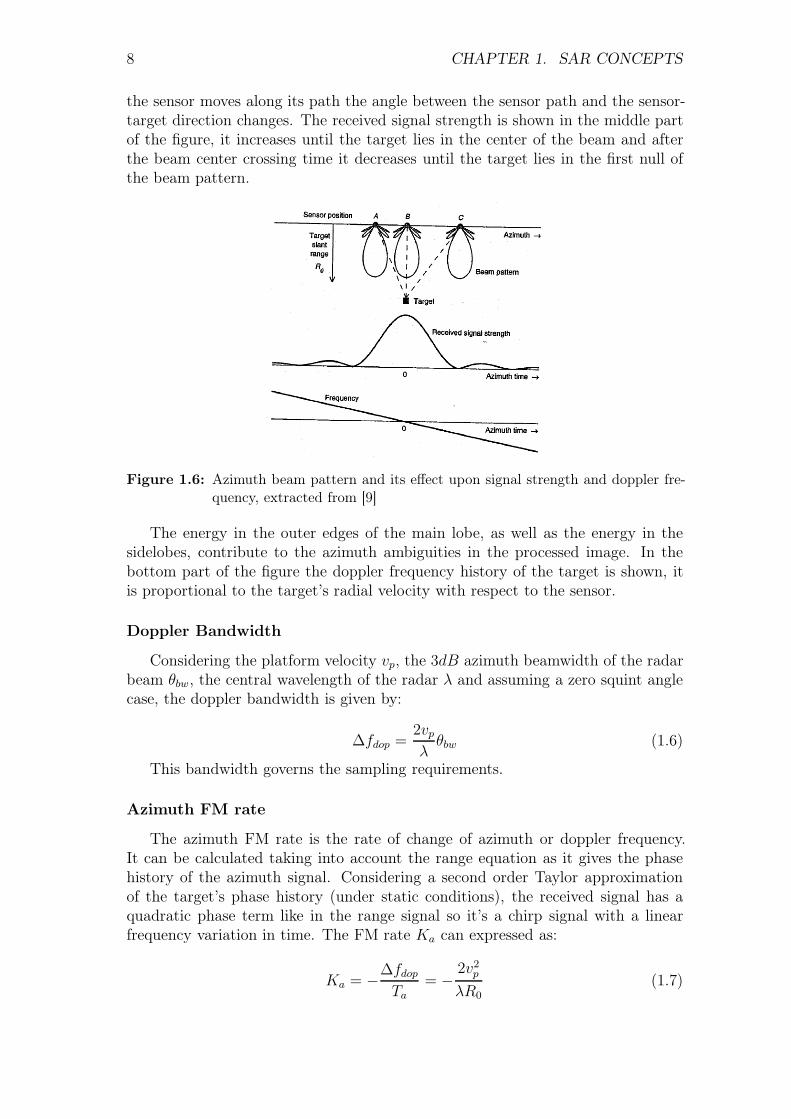
the first one is certainly the most effective. To explain this effects figure 1.6 canbe of help, in which an azimuth beam pattern for a zero squint angle is shown. As
8 CHAPTER 1. SAR CONCEPTS
the sensor moves along its path the angle between the sensor path and the sensor-target direction changes. The received signal strength is shown in the middle partof the figure, it increases until the target lies in the center of the beam and afterthe beam center crossing time it decreases until the target lies in the first null ofthe beam pattern.
Figure 1.6: Azimuth beam pattern and its effect upon signal strength and doppler fre-quency, extracted from [9]
The energy in the outer edges of the main lobe, as well as the energy in thesidelobes, contribute to the azimuth ambiguities in the processed image. In thebottom part of the figure the doppler frequency history of the target is shown, itis proportional to the target’s radial velocity with respect to the sensor.
Doppler Bandwidth
Considering the platform velocity vp, the 3dB azimuth beamwidth of the radarbeam θbw, the central wavelength of the radar λ and assuming a zero squint anglecase, the doppler bandwidth is given by:
∆fdop =2vpλ
θbw (1.6)
This bandwidth governs the sampling requirements.
Azimuth FM rate
The azimuth FM rate is the rate of change of azimuth or doppler frequency.It can be calculated taking into account the range equation as it gives the phasehistory of the azimuth signal. Considering a second order Taylor approximationof the target’s phase history (under static conditions), the received signal has aquadratic phase term like in the range signal so it’s a chirp signal with a linearfrequency variation in time. The FM rate Ka can expressed as:
Ka = −∆fdop
Ta= −
2v2pλR0
(1.7)
1.4. SAR RESOLUTION 9
where the minus sign comes from the fact that the change of the doppler fre-quency has a negative trend as shown in fig 1.6.
1.4 SAR resolution
The term resolution in radar contest is the capability of the radar to distinguishtwo targets that differ in their position on the ground. In SAR, fine azimuth andrange resolution is obtain applying a matched filter, there’s a lot of literature onthis subject and on pulse compression techniques of linear FM signals, here onlythe main results are reported.
1.4.1 Range resolution
In the range direction, the received signal has FM characteristics, inheritedfrom the transmitted pulse. High range resolution is obtained matched filtering thereturn signal with a reference transmitted chirp pulse. The resolution is inverselyproportional to the pulse bandwidth:
∆R =c
2B(1.8)
where c is the speed of light and B is the bandwidth of the transmitted signal.
1.4.2 Azimuth resolution
In the azimuth direction if we assume that the beamwidth is θbw ≈ 0.886λLa
(that’s an approximation based on a sinc-shape azimuth beam pattern) where La
is the antenna length, the azimuth resolution of the real aperture is given by theprojection of the beamwidth onto the ground:
∆Azuncomp = R0θbw =0.886λR0
La(1.9)
that could be of the order of several kilometers in the spaceborne case. Animproved resolution is achieved by means of the formation of the synthetic aperture(coherent integration of the pulses), such that the frequency modulated signal inthe azimuth dimension can be compressed using a matched filter approach (as inthe range dimension).
∆Az ≈ vp0.886
∆fdop≈
La
2(1.10)
The result is that the azimuth resolution is approximately half the antennalength independently of range, velocity and wavelength.

Chapter 2
SAR GMTI concepts
SAR systems provide bidimensional radar images of earth surface and they werenot originally devoted to extract information of moving targets. GMTI has the aimto detect moving targets, which may compete against what is called clutter thatis the static background scene in this case.
Before introducing the GMTI techniques is it necessary to understand the spec-tral characteristics of a moving target echo and the differences respect to a staticobject or clutter, which can be precisely exploited to detect and estimate the dif-ferent parameters of the moving targets.
2.1 Moving Targets
A moving single point target has a phase history different from a static point inthe scene; this difference due to its velocity and acceleration components appearsclear in the range equation:
R(t) ≈ R0 +z0vz0
R0
t +1
2R0
[
(vx0 − vp)2 + v2z0
(
1−z20R2
0
)
]
t2 (2.1)
This difference can be analyzed in the time or in the frequency domain, bothof them can be exploited by the detection and estimation techniques.
2.1.1 Across-track velocity
A non zero across-track velocity vz0 add the term z0vz0R0
t in the range equationequation 2.1. The moving target signal s(t), neglecting the accelerations can beexpressed as:
s(t) = Aexp(−j2βR(t)) ≈ Aexp(−j2β(R0 −vp
2R0t2))exp(−j2β
z0vz0
R0t) (2.2)
where β = 2πλ
is the wavenumber and A the amplitude of the pulse reflectedby the target. The first term of the signal s(t) has the same phase history ofa static target, whereas the second one due to the across-track velocity vz0 add alinear phase term that changes the instant frequency of the received signal (Doppler
11
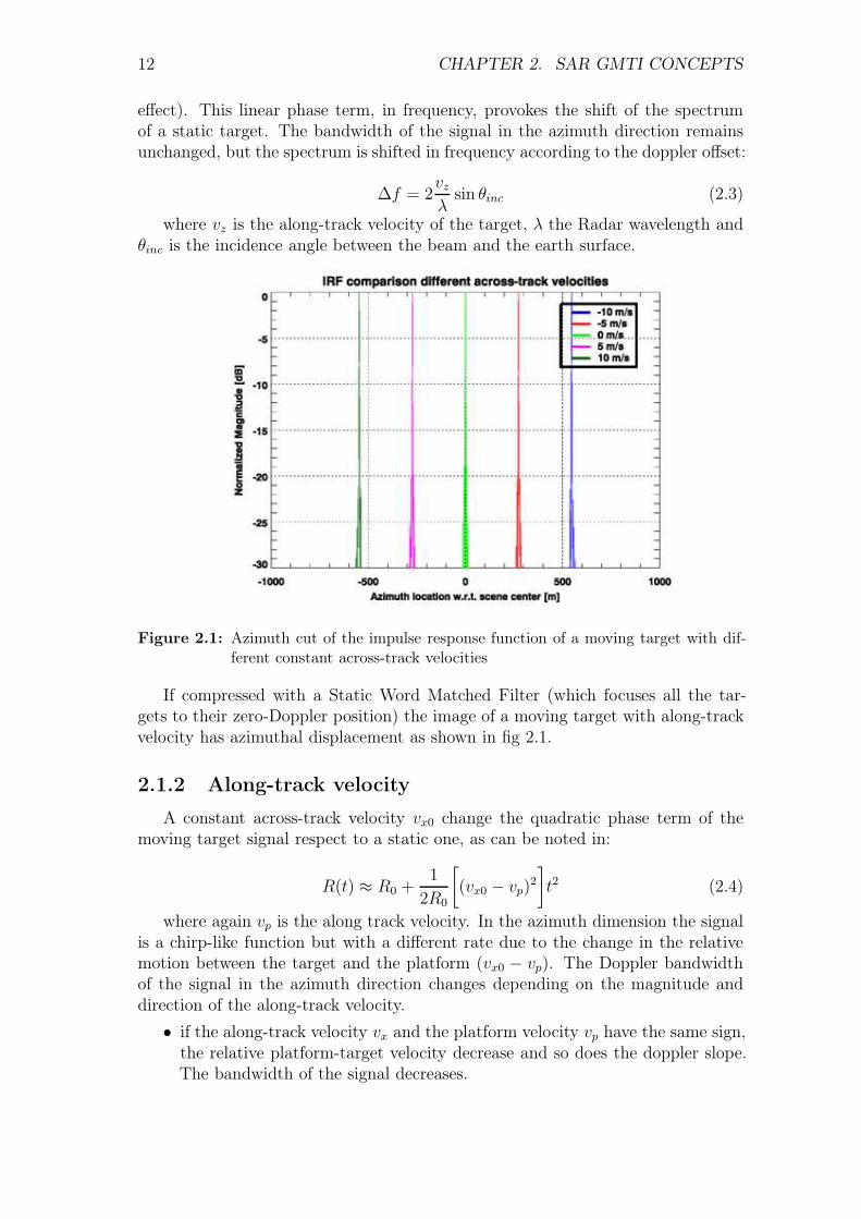
12 CHAPTER 2. SAR GMTI CONCEPTS
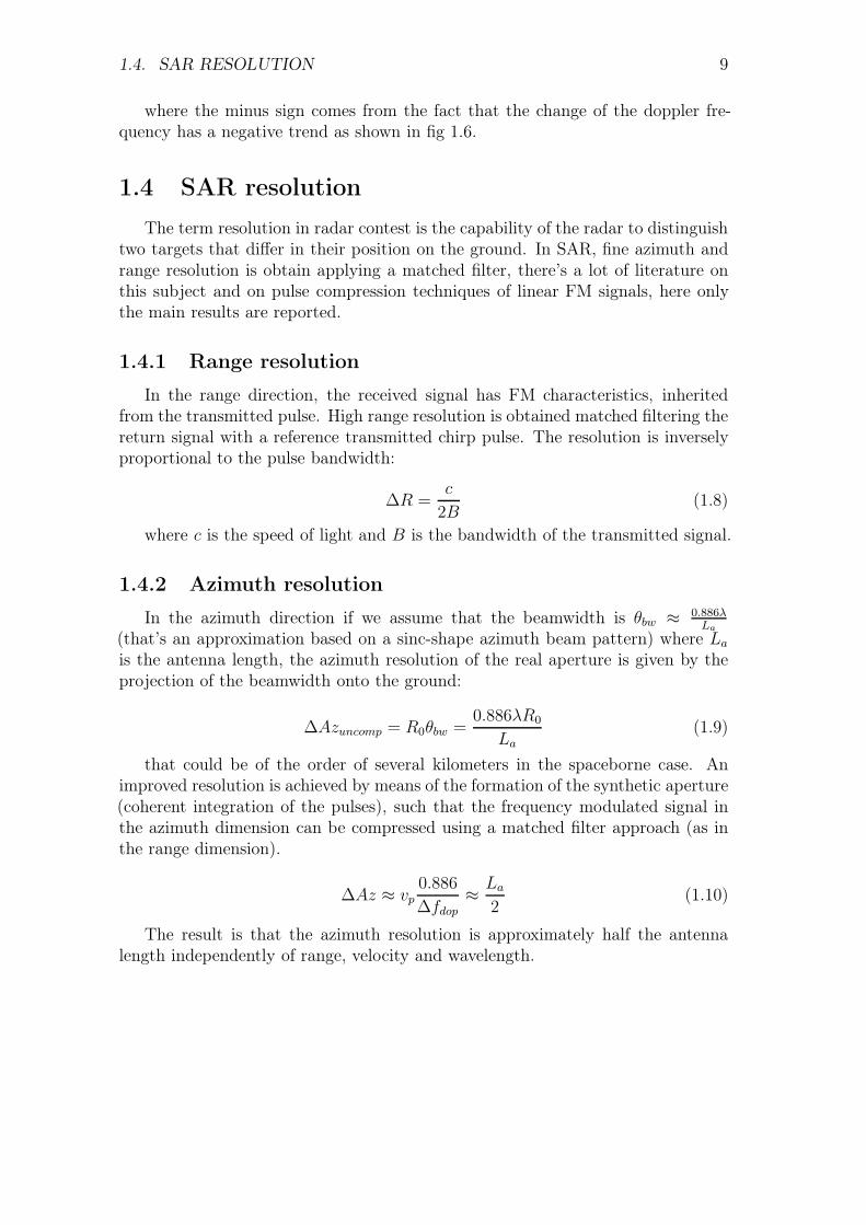
effect). This linear phase term, in frequency, provokes the shift of the spectrumof a static target. The bandwidth of the signal in the azimuth direction remainsunchanged, but the spectrum is shifted in frequency according to the doppler offset:
∆f = 2vz
λsin θinc (2.3)
where vz is the along-track velocity of the target, λ the Radar wavelength andθinc is the incidence angle between the beam and the earth surface.
Figure 2.1: Azimuth cut of the impulse response function of a moving target with dif-ferent constant across-track velocities
If compressed with a Static Word Matched Filter (which focuses all the tar-gets to their zero-Doppler position) the image of a moving target with along-trackvelocity has azimuthal displacement as shown in fig 2.1.
2.1.2 Along-track velocity
A constant across-track velocity vx0 change the quadratic phase term of themoving target signal respect to a static one, as can be noted in:
R(t) ≈ R0 +1
2R0
[
(vx0 − vp)2
]
t2 (2.4)
where again vp is the along track velocity. In the azimuth dimension the signalis a chirp-like function but with a different rate due to the change in the relativemotion between the target and the platform (vx0 − vp). The Doppler bandwidthof the signal in the azimuth direction changes depending on the magnitude anddirection of the along-track velocity.
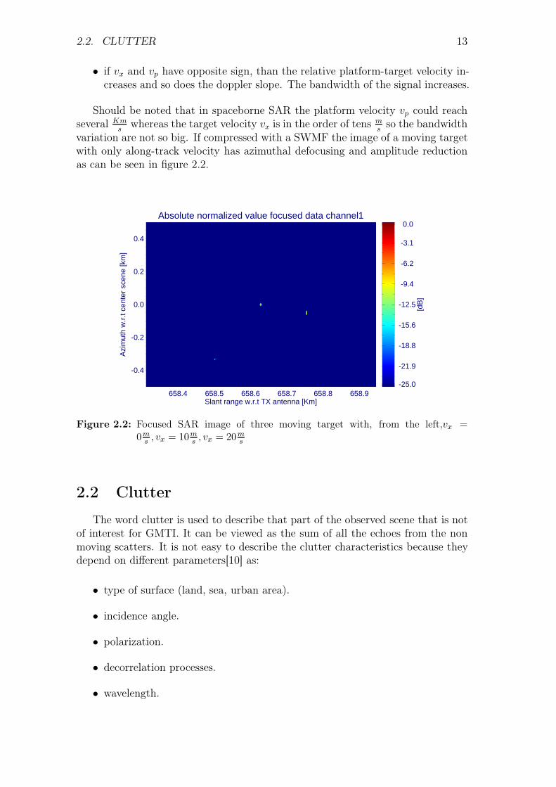
• if the along-track velocity vx and the platform velocity vp have the same sign,the relative platform-target velocity decrease and so does the doppler slope.The bandwidth of the signal decreases.
2.2. CLUTTER 13
• if vx and vp have opposite sign, than the relative platform-target velocity in-creases and so does the doppler slope. The bandwidth of the signal increases.
Should be noted that in spaceborne SAR the platform velocity vp could reachseveral Km
swhereas the target velocity vx is in the order of tens m
sso the bandwidth
variation are not so big. If compressed with a SWMF the image of a moving targetwith only along-track velocity has azimuthal defocusing and amplitude reductionas can be seen in figure 2.2.
Absolute normalized value focused data channel1
658.4 658.5 658.6 658.7 658.8 658.9Slant range w.r.t TX antenna [Km]
-0.4
-0.2
0.0
0.2
0.4
Azi
mut
h w
.r.t
cent
er s
cene
[km
]
-25.0
-21.9
-18.8
-15.6
-12.5
-9.4
-6.2
-3.1
0.0
[dB
]Figure 2.2: Focused SAR image of three moving target with, from the left,vx =
0ms , vx = 10m
s , vx = 20ms
2.2 Clutter
The word clutter is used to describe that part of the observed scene that is notof interest for GMTI. It can be viewed as the sum of all the echoes from the nonmoving scatters. It is not easy to describe the clutter characteristics because theydepend on different parameters[10] as:
• type of surface (land, sea, urban area).
• incidence angle.
• polarization.
• decorrelation processes.
• wavelength.

14 CHAPTER 2. SAR GMTI CONCEPTS
The clutter is commonly characterize by its backscattering coefficient σ0 (mea-sured in dBsm
sm) and its statistical properties. If we assume that the clutter dis-
tribution is spatially stationary, i.e. that the statistical properties are invariantwith azimuthal shifts, the clutter distribution is characterized by the covariancefunction:
Rz(τ) = E[p(t)p∗(t + τ)] (2.5)
where E denotes the expectation operator and p(t) is the clutter azimuthalreflectivity. This function depends on the spatial behavior of the clutter: it reflectsits smoothness or rapid changes in the reflectivity. In most cases, but not always,it will be appropriate to assume spatially white clutter, especially if many scatter-ers independent and identically distributed (from the central limit theorem) arecontained in each resolution cell.
2.3 Multichannel SAR
Different procedures have been proposed to detect moving targets with singlechannel SAR systems. In one of them the moving targets are detected becausetheir frequencies fall outside the main-beam clutter band.
The effectiveness of these procedures are quite limited becasuse the slowly mov-ing targets are completly masked by the clutter Doppler spectrum. Even in thecase of highly moving targets part of their doppler frequencies fall into the clutterband because in SAR system the PRF is limited as we have seen in chapter 1.Consequently is not possible to perform a good clutter cancelation by filtering infrequency domain.
This problems can be overcome using a multichannel SAR.
2.3.1 Dual Receive Antenna
The current implementation of SAR missions (Terrasar-X, Radarsat-2 and thefuture Spanish PAZ) are not specifically designed for the GMTI, they have insteadsome experimental GMTI modes of operation.
These missions have two physical receiver chains, therefore the maximum num-ber of channels that can be simultaneously recorded is set to two. These missionsare equipped with a highly flexible phased array antennas.
In the Dual Receive Antenna mode of operation the complete antenna is usedfor transmission but in receive the antenna is divided into two halves in along-track.The signals of both receiving antennas are sampled and recorded separately.
A direct consequence of this partitioning is that the azimuth pattern of the twohalved partitions are doubled in beamwidth compared to the complete antenna,this clearly impacts on the doppler bandwidth and indeed on the PRF choice. Ithas also to be kept in mind that the Rx gain is reduced by 3dB for a halved receiveantenna.
Anyway this impact is not so important because the two-way pattern has tobe considered for each channel where the smaller beamwidth of the transmissionantenna mitigate the broadening effects of the receiving one.

2.3. MULTICHANNEL SAR 15
This new spatial degree-of-freedom (DoF) provided by the second channel couldbe spent to suppress clutter or to perform a better estimation of the target param-eters, but the total number of DoF provided by the DRA are not enough to si-multaneously suppress the clutter and accurately estimate the target’s parameters,such as velocity and location.
2.3.2 Toggle Modes
Current platforms (or near future ones) are limited to two physical receivingchains for cost and practical reasons. The idea proposed by S.Chiu in[Chiu] isthat by doubling the pulse repetition frequency (PRF) of the radar it is possibleto generate one or two additional channels.
In the toggles modes , the flexibility on the array antenna’s programming, isexploited to generate additional virtual channels (three or four in the consideredcases) at different pulses.
In all the considered toggle modes the period of cyclical programming of theTX/RX schemes of the antenna is set to two. In order to avoid eventual clutterband aliasing the PRF have to be doubled.
2.3.3 Toggle receive modes
In the toggle receive modes the pulses are transmitted exploiting the full an-tenna aperture and the echoes are received using two alternating receiver excitationschemes.
Three virtual channel toggle on receive mode In figure 2.3 is shown apossible way to implement a three virtual channels channel toggle on receivescheme: during odd pulses the transmission is done with the whole antenna andthe backscattered signal is received with the two sub-apertures obtained splittingup the whole antenna in two equal parts; in the second pulse the signal is transmit-ted with the whole antenna and the backscattered signal is received with a singlecentered sub-aperture.
Figure 2.3: Three virtual channel toggle on receive configuration of the antenna for thedifferent pulses, the black triangles indicates the physical centers of the Txor Rx antennas, the red diamonds indicates the two-way phase centers foreach virtual channel
Some considerations have to be done for this mode of operation, in fact in orderto avoid aliasing problems the PRF has been doubled and this implies that to keepa power consumption similar to the DRA mode the energy-per-pulse have to be

16 CHAPTER 2. SAR GMTI CONCEPTS
Figure 2.4: Four virtual channel toggle on receive configuration of the antenna for thedifferent pulses, the black triangles indicates the physical centers of the Txor Rx antennas, the red diamonds indicates the two-way phase centers foreach virtual channel
reduced by the same amount the PRF is increased. The Signal to Clutter Ratio(SCR) doesn’t change because the energy of the clutter is dependent by the energyof the pulse, but the Signal to Noise Ratio (SNR) decrease.
Four virtual channels toggle receive mode In figure 2.4 is shown a possibleway to implement a four virtual channel toggle on receive scheme: during theodd pulses the transmission is done with the whole antenna and the backscatteredsignal is received with two sub-apertures obtained splitting up the whole antennain four equal parts and activating only two of them, in the even pulses the signal istransmitted with the whole antenna and the backscattered signal is received withtwo remaining sub-apertures.
In this mode of operation the SNR decrease even more respect the previousmode because of the reduced length of the receiving sub-apertures(the RX antennais a quarter of the TX).
2.3.4 Toggle on transmit modes
In the toggle on transmit mode the pulses are transmitted exploiting half ofthe antenna aperture, such that the transmission is cyclical (on the pulse basis)alternate from fore to aft parts. The echoes are received using two sub-aperturesof the full antenna (as in the Double Receive Antenna mode).
Three virtual channels toggle on transmit mode In figure 2.5 is shown apossible way to impleent a three virtual channels toggle on transmit scheme: duringodd pulses the transmission is done with half of the whole antenna (fore part) andthe backscattered signal is received with two sub-apertures; in the even pulses thesignal is transmitted with the aft part of the whole antenna and the backscatteredsignal is received with the same two sub-apertures as for odd pulses.
should clarify that is four times higher due to the cyclical approach (x2) anddue to the broader two-way pattern (x2)
In order to avoid aliasing problems in this mode, the PRF should be quadrupledbecause, in fact as in the other modes the cyclical approach need a doubled PRF,but here also the broader two-way pattern caused by the transmission with onepartitioned antenna needs to be taken into account because it increases the Dopplerband of the azimuth signal so that a quadrupled PRF is needed to avoid aliasing.
2.4. GMTI TECHNIQUES 17
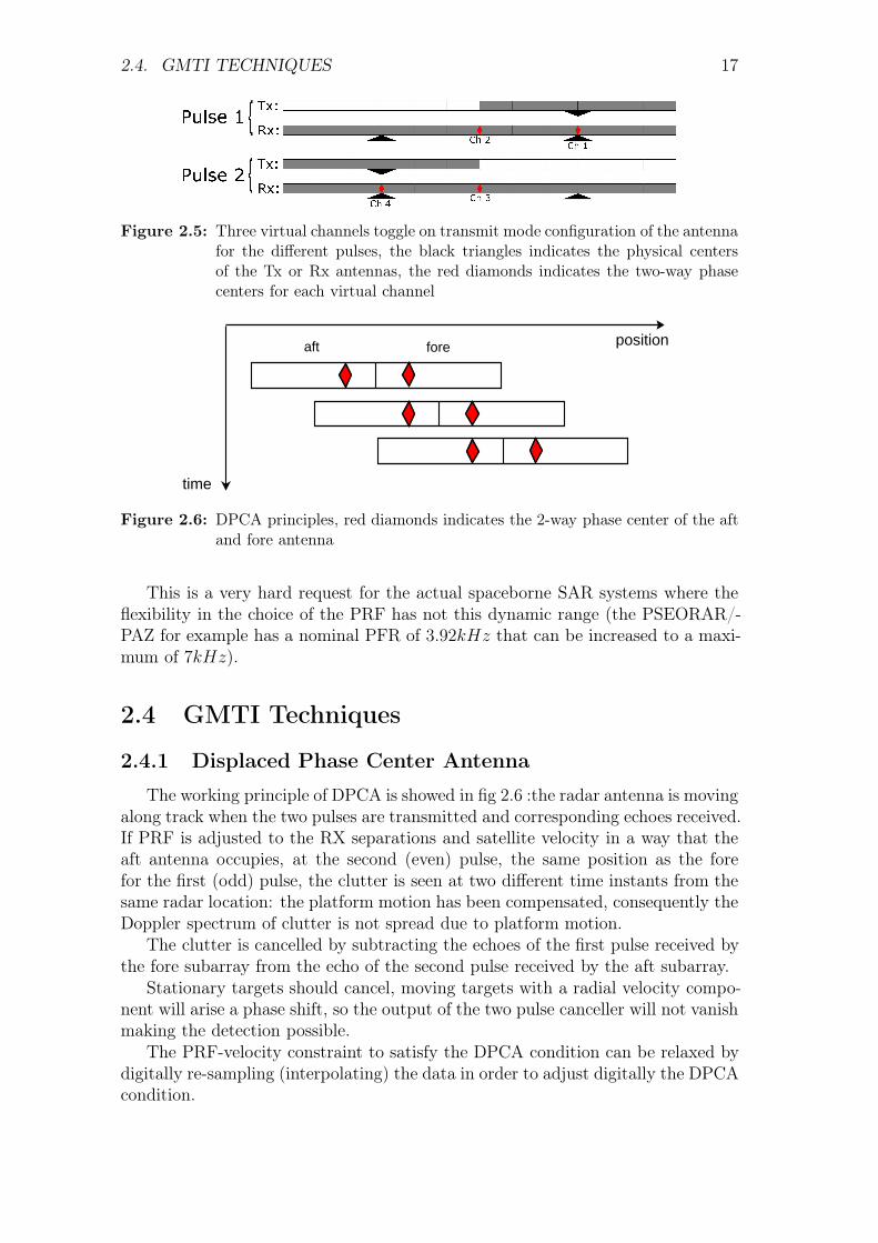
Figure 2.5: Three virtual channels toggle on transmit mode configuration of the antennafor the different pulses, the black triangles indicates the physical centersof the Tx or Rx antennas, the red diamonds indicates the two-way phasecenters for each virtual channel
aft fore position
time
Figure 2.6: DPCA principles, red diamonds indicates the 2-way phase center of the aftand fore antenna
This is a very hard request for the actual spaceborne SAR systems where theflexibility in the choice of the PRF has not this dynamic range (the PSEORAR/-PAZ for example has a nominal PFR of 3.92kHz that can be increased to a maxi-mum of 7kHz).
2.4 GMTI Techniques
2.4.1 Displaced Phase Center Antenna
The working principle of DPCA is showed in fig 2.6 :the radar antenna is movingalong track when the two pulses are transmitted and corresponding echoes received.If PRF is adjusted to the RX separations and satellite velocity in a way that theaft antenna occupies, at the second (even) pulse, the same position as the forefor the first (odd) pulse, the clutter is seen at two different time instants from thesame radar location: the platform motion has been compensated, consequently theDoppler spectrum of clutter is not spread due to platform motion.
The clutter is cancelled by subtracting the echoes of the first pulse received bythe fore subarray from the echo of the second pulse received by the aft subarray.
Stationary targets should cancel, moving targets with a radial velocity compo-nent will arise a phase shift, so the output of the two pulse canceller will not vanishmaking the detection possible.
The PRF-velocity constraint to satisfy the DPCA condition can be relaxed bydigitally re-sampling (interpolating) the data in order to adjust digitally the DPCAcondition.

18 CHAPTER 2. SAR GMTI CONCEPTS
The sensitivity of DPCA depends on the distance between the two antennas(considering the two-way pattern) that is called base-line, a longer base-line pro-vides higher sensitivity but at the same time leads to a comb of blind velocities(when the phase difference of the tho channels is an integer multiple of 2π)
2.4.2 Along Track Interferometry
In the Along-Track Interferometry, similar to the DPCA technique, two dis-placed antennas along-track are used. For each of the two channels a SAR image isgenerated, and in the azimuth compression the time delay between the two chan-nels is compensated (the two images are spatially co-registrated). Then if the firstimage is multiplied by the complex conjugate of the second, the remaining phaseis zero for non moving target and different from zero, otherwise.
If the two receiving antennas are separated in azimuth by a distance d, thenthe interferometric phase is approximately given by:
∆Φ = −2π
λdvr
vp(2.6)
where vr is the radial velocity of the target that is related to the across-trackvelocity vr = vacross−track sin θinc and θinc is the incident angle of the beam on theearth surface.
One shortcoming of ATI is that to get a high sensitivity, the two antennas haveto be separated far away and this is not a trivial task in a spaceborne platform.Having a large antenna separation on the other hand leads to a comb of blindvelocities (when the phase difference of the tho channels is an integer multiple of2π):
vblind = kvpλ
d(2.7)
where vp is the platform velocity and k is integer. These blind velocities thinout the interesting velocity range.
2.4.3 STAP
Space Time Adaptive Processing is the natural generalization of DPCA, in factit has the following features:
• generalization of DPCA for clutter cancellation.
• generalization of adaptive array of antennas for jammer nulling (mostly usedin military applications).
• freedom in shaping the null.
• fewer constraints on the spacing of the antenna elements.
• compensation of platform motion along (as DPCA) and orthogonal to thearray thus avoiding clutter spectral spreading.
2.4. GMTI TECHNIQUES 19
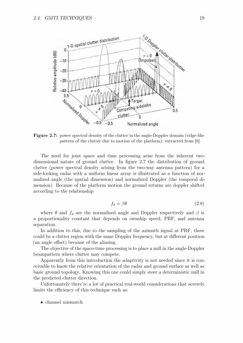
Figure 2.7: power spectral density of the clutter in the angle-Doppler domain (ridge-likepattern of the clutter due to motion of the platform); extracted from [8]
The need for joint space and time processing arise from the inherent two-dimensional nature of ground clutter. In figure 2.7 the distribution of groundclutter (power spectral density arising from the two-way antenna pattern) for aside-looking radar with a uniform linear array is illustrated as a function of nor-malized angle (the spatial dimension) and normalized Doppler (the temporal di-mension). Because of the platform motion the ground returns are doppler shiftedaccording to the relationship
fd = βθ (2.8)
where θ and fd are the normalized angle and Doppler respectively and β isa proportionality constant that depends on ownship speed, PRF, and antennaseparation.
In addition to this, due to the sampling of the azimuth signal at PRF, therecould be a clutter region with the same Doppler frequency, but at different position(an angle offset) because of the aliasing.
The objective of the space-time processing is to place a null in the angle-Dopplerbeampattern where clutter may compete.
Apparently from this introduction the adaptivity is not needed since it is con-ceivable to know the relative orientation of the radar and ground surface as well asbasic ground topology. Knowing this one could simply steer a deterministic null inthe predicted clutter direction.
Unfortunately there’re a lot of practical real-world considerations that severelylimits the efficiency of this technique such as:
• channel mismatch

20 CHAPTER 2. SAR GMTI CONCEPTS
Figure 2.8: STAP beamformer, extracted from [8]
• clutter heterogenity/nonstationarity
This real-world consideration give rise to the inherent need for adaptivity.In figure 2.8 the basic schematic architecture of a STAP beamformer is shown,
in which an M coherent pulses interval of an N elements antenna array is processed.As with an ordinary one-dimensional spatial-only beamforming, a two-dimensional
angle-Doppler (space-time) beampattern can be formed by a judicious selection ofa complex linear combiner weights wi.
Has been demonstrated that to maximize the response to a uniform narrowbandplane-wave corresponding to a given angle and Doppler the linear combiner weightvector w should be set equal to the anticipated structure of the desired signal s.
The result of this will be a two dimensional pattern (angle-Doppler) that hasthe peak in correspondence to the target (signal) of interest.
A linear combiner of this type has NM degrees of freedom, this means thatfor a desired angle-Doppler look direction s, we could also specify up to NM − 1"nulls".
If the set of NM angle-Doppler vectors s, j1, ....., jNM−1 is linearly indipendentthen a deterministic set of beamformer weights can be obtained from a linear setof equations:
w′s = 1w′j1 = 0
. . .
w′jNM−1 = 0
(2.9)
Unfortunately, due to the relative strength of potential interference (clutterand/or jamming) and the practical limitations on deterministic nulling, this ap-proach is unsustainable in practice.
Radar community has looked towards statistical signal processing for a meansof addressing the limitations of deterministic nulling. In particular clutter and jam-

2.4. GMTI TECHNIQUES 21
ming are treated as stochastic processes and the optimum space-time beamformeris derived via a statistical optimization procedure. Although there are many vari-ations on the theme, the basic underlying beamformer results is given by:
w = R−1s (2.10)
where R is the positive-definite NM ∗ NM dimensional covariance matrix as-sociated with the total interference (clutter, jamming, receiver noise).
It is possible to estimate R from sample data obtained in the normal course ofradar operation, it is this estimation of R on the fly that is the true basis for theinclusion of the word "adaptive" in STAP.


Chapter 3
Detection and Estimation Algorithm
The objective of this thesis is to implement and evaluate the performance of aSTAP processing scheme on a multichannel spaceborne GMTI SAR. This evalua-tion is based based on simulated SAR data for the future Spanish SEOSAR/PAZmission.
3.1 Post Doppler STAP
In spaceborne SAR the length of the synthetic aperture could be in the order ofseveral Km, and the number of azimuth samples that can be processed coherentlyM is indeed in the order of thousand.
A fully optimum STAP implementation would require the solution of a NM ×NM problem, where M is the number of pulses considered for the processing andN is the number of channels. The solution of such problem is not simple andhave a very high computational cost due to the inversion of the clutter plus noisecovariance matrix thas has dimensions NMxNM .
One efficient implementation suitable for SAR is Post-Doppler STAP in whichclutter cancellation is performed in the Doppler domain for each Doppler compo-nent using just the spatial degrees of freedom. The original NM×NM dimensionalproblem is split into M separates N ×N independent problems.
For a sufficiently long time base of the Fourier transform (in the case of space-borne SAR the length of the synthetic aperture), the frequency bins in the Dopplerdomain can be considered mutually independent [10].
The optimum spatial-only beamformer for each frequency ω is then given by:
w(ω) = R−1(ω)u(ω, ξ) (3.1)
where a(ω, ξ) is the expected steering vector (1×N) for the target on interestwith parameters ξ = [valong, vacross, x0] that the STAP should maximize and R isthe N ×N spectral power density matrix of clutter plus noise.
The model of the received signal from a target for a given channel i in time isgiven by:
si(t, ξ) = Di(ui(t, ξ))ej2βRi(t,ξ) (3.2)
23

24 CHAPTER 3. DETECTION AND ESTIMATION ALGORITHM
where Ri(t, ξ) is the slant range distance, β = 2πλ
is the wavenumber and ui(t, ξ)the direction history (directional cosine) from the i-th antenna to the moving tar-get on the ground. Di(u(t, ξ)) describes the two-way antenna pattern of the i− th
channel. In the far-field assumption, ui(t, ξ) = u(t, ξ), the distances can be rewrit-ten as Ri(t, ξ) = R(t, ξ)+u(t, ξ)d, where d is the spacing between the receivers andR(t, ξ) the slant range distance from any reference channel to the target. For theparticular case of a dual-receive channel the two dimensional signal vector becomes:
s(t, ξ) = ej2βR(t,ξ)
[
D1(u(t, ξ))D2(u(t, ξ))e
jβu(t,ξ)d
]
= ej2βR(t,ξ)a(u(t, ξ)) (3.3)
In array processing terminology the vector a(u) is called the steering vector.In post-Doppler STAP we process the signal in the Doppler domain so we areinterested in the fourier transform of (3.3) that can be written in analytical formas:
S(ω, ξ) = γ(ω)a(u(ω, ξ)) (3.4)
which can be expressed as the multiplication of the steering vector a(u(ω, ξ))by the fourier transform of the phase history signal of the target γ(ω).
The directional cosine u(ω, ξ) can be calculated as:
u(ω, ξ) =−(valong − vp)ω
2β[(valong − vp)2 + v2across]
+vacross
√
(valong − vp)2 + v2across
√
1−ω
2β√
(valong − vp)2 + v2across
(3.5)
The multiplication by the conjugate transpose of the steering vector in 3.7maximize the beamformer response for a given target with a directional cosinehistory u(t, ξ).
The spectral power density matrix R of clutter plus noise can be estimatedfrom a training data. For each Doppler frequency ω all the range bins can be usedin the estimation and hence the estimation possesses a very low variance:
R(ω) =1
k
Rmax∑
r=Rmin
x(r, ω)x∗(r, ω) (3.6)
where X(r, ω) is the vector of the received signal and k is the number of trainingvectors used for the estimation.
For a good estimation of R matrix, the training data over which the estimationis done should contain only clutter and noise, in the simulation the R matrix isestimated over a training data which contain only clutter and noise.
The process to invert this matrix is called the SMI (Sample Matrix Inversion)and the number of k training vectors to be used is higher than 2NM for the generalcase in order to obtain a degradation of the performance below 3dB comparedto ideal case of exactly knowledge of the matrix [see REF: Melvin: "A STAPoverview"]
3.2. DETECTION 25
Under this premise, the Signal Clutter Noise Ratio (SCNR) optimum filter fora particular frequency ω is given by:
y(ω) = wh(ω) ∗ x(ω) (3.7)
where H is the transpose conjugate operator.
The STAP filtering provides the clutter cancellation and the maximization ofthe signal of a particular target of interest but doesn’t compensates for the phasehistory of the target.
This last step required to concentrate the energy of a target signal is the azimuthcompression that is usually done in the range-Doppler domain by the multiplicationfor the complex conjugate of γ(ω). Generally there’s no a-priori information on thetarget characteristics hence in the compression the phase history of a static targetis used (SWMF).
3.2 Detection
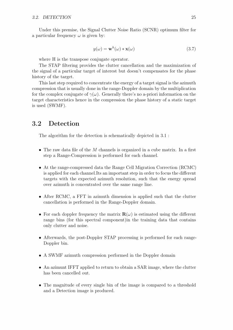
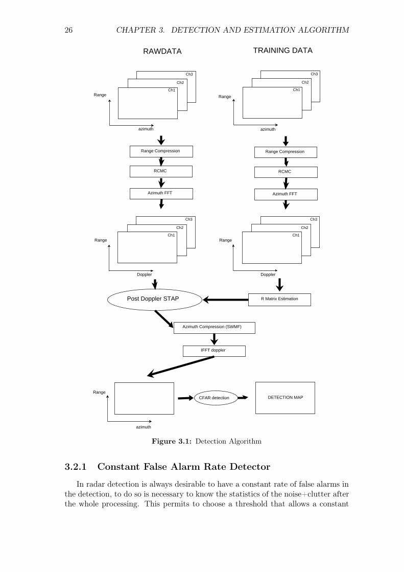
The algorithm for the detection is schematically depicted in 3.1 :
• The raw data file of the M channels is organized in a cube matrix. In a firststep a Range-Compression is performed for each channel.
• At the range-compressed data the Range Cell Migration Correction (RCMC)is applied for each channel.Its an important step in order to focus the differenttargets with the expected azimuth resolution, such that the energy spreadover azimuth is concentrated over the same range line.
• After RCMC, a FFT in azimuth dimension is applied such that the cluttercancellation is performed in the Range-Doppler domain.
• For each doppler frequency the matrix R(ω) is estimated using the differentrange bins (for this spectral component)in the training data that containsonly clutter and noise.
• Afterwards, the post-Doppler STAP processing is performed for each range-Doppler bin.
• A SWMF azimuth compression performed in the Doppler domain
• An azimunt IFFT applied to return to obtain a SAR image, where the clutterhas been cancelled out.
• The magnitude of every single bin of the image is compared to a thresholdand a Detection image is produced.
26 CHAPTER 3. DETECTION AND ESTIMATION ALGORITHM
Ch1
Ch2
Ch3
azimuth
Range
Range Compression
RCMC
Doppler
Azimuth FFT
Range
Doppler
Post Doppler STAP
IFFT doppler
CFAR detection
RAWDATA TRAINING DATA
Range
Range
azimuth
Ch1
Ch2
Ch3
Ch1
Ch2
Ch3
Ch1
Ch2
Ch3
Range Compression
RCMC
Azimuth FFT
Range
Azimuth Compression (SWMF)
azimuth
DETECTION MAP
R Matrix Estimation
Figure 3.1: Detection Algorithm
3.2.1 Constant False Alarm Rate Detector
In radar detection is always desirable to have a constant rate of false alarms inthe detection, to do so is necessary to know the statistics of the noise+clutter afterthe whole processing. This permits to choose a threshold that allows a constant

3.2. DETECTION 27
false alarm detection CFAR.Under the assumption of complex gaussian model for the clutter and noise,
and considering that the SAR operations in the process chain (range and azimuthcompression, STAP, RCMC) are linear processes the statistical model of clutterand noise at the end of the process will be also gaussian.
So under this assumption of complex gaussian model for the clutter and noise itturns out that the probability density function (pdf) of the magnitude is Rayleigh.
f(x, σ) =x
σ2e
x2
2σ (3.8)
where x is the magnitude and σ is the rayleigh parameter. In this case the thresholdcould be found using the theoretical cumulative distribution function of the rayleighdistribution:
th =√
− log(pfa)2σ2 (3.9)
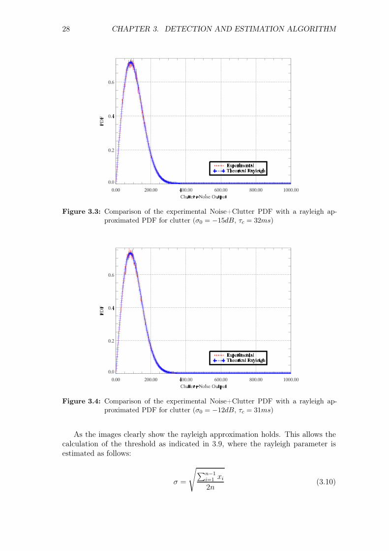
where pfa is the imposed probability of false alarm. To validate this hypothesisthe clutter+noise statistics has been computed and compared to a rayleigh approx-imation for the three different clutter scenario that will be used in the simulationsto model the sea clutter:
• σ0 = −25dB, decorrelation time τc = 60ms
• σ0 = −15dB, decorrelation time τc = 32ms
• σ0 = −12dB, decorrelation time τc = 31ms
Figure 3.2: Comparison of the experimental Noise+Clutter PDF with a rayleigh ap-proximated PDF for clutter (σ0 = −25dB, τc = 60ms)
28 CHAPTER 3. DETECTION AND ESTIMATION ALGORITHM
Figure 3.3: Comparison of the experimental Noise+Clutter PDF with a rayleigh ap-proximated PDF for clutter (σ0 = −15dB, τc = 32ms)
Figure 3.4: Comparison of the experimental Noise+Clutter PDF with a rayleigh ap-proximated PDF for clutter (σ0 = −12dB, τc = 31ms)
As the images clearly show the rayleigh approximation holds. This allows thecalculation of the threshold as indicated in 3.9, where the rayleigh parameter isestimated as follows:
σ =
√
∑n−1i=1 xi
2n(3.10)
3.3. ALONG-TRACK VELOCITY ESTIMATION 29
3.3 Along-Track velocity Estimation
The along-track velocity component of a moving vehicle can be derived indi-rectly by processing SAR data with varying frequency modulation (FM) rates andexploiting the specific behavior of the vehicle’s signal through the FM rate space[13].
In SAR processing the vehicles moving in along-track appear smeared in az-imuth direction, when nominal SAR azimuth focusing (SWMF) is performed. Along-track motion changes the relative velocity of sensor and vehicle resulting in a changeof the FM rate and consequently in a mismatch of the vehicle’s signal and the Sta-tionary Word Matched Filter. The extent of this defocusing is directly proportionalto the along track velocity of the target.
Re-sharpening of defocused moving targets in SAR images is achieved by vary-ing the FM rate of the matched filter. This allows estimating indirectly the along-track velocity component of the vehicle
In our case, the maximization of the peak energy in done not only varying theFM rate of the matched filter but also performing a post-Doppler STAP processingwith a steering vector adapted to the along-track velocity under test.

Chapter 4
Simulation Results
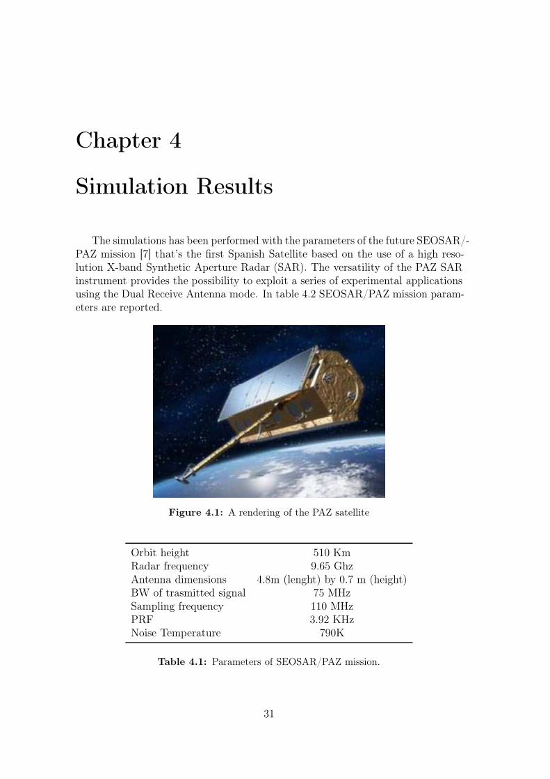
The simulations has been performed with the parameters of the future SEOSAR/-PAZ mission [7] that’s the first Spanish Satellite based on the use of a high reso-lution X-band Synthetic Aperture Radar (SAR). The versatility of the PAZ SARinstrument provides the possibility to exploit a series of experimental applicationsusing the Dual Receive Antenna mode. In table 4.2 SEOSAR/PAZ mission param-eters are reported.
Figure 4.1: A rendering of the PAZ satellite
Orbit height 510 KmRadar frequency 9.65 GhzAntenna dimensions 4.8m (lenght) by 0.7 m (height)BW of trasmitted signal 75 MHzSampling frequency 110 MHzPRF 3.92 KHzNoise Temperature 790K
Table 4.1: Parameters of SEOSAR/PAZ mission.
31

32 CHAPTER 4. SIMULATION RESULTS
4.1 Simulated Scenario
The simulations has been run over a 1km×1km sea scenario, to simulate thesea clutter the mean reflectivity coefficient σ0 for the gaussian distribution hasbeen extrapolated in the table compiled by Nathanson et al. in [5]. The temporaldecorrelation parameter τc is chosen according to the temporal decorrelation of thesea surface [6] by the approximation:
τc ∼= 3λ
uerf−1/2
(
2, 7x
u2
)
, (4.1)
where u is the wind speed, x is the spatial resolution in ground range and erf()is the Gauss error function. The sea specifications are in agreement to the WorldMeteorological Organization sea state code [15] and the Beaufort wind scale [15].
Sea State wind speed [ms] σ0 [dB] decorrelation time τc [ms]
0 1 −25 604 10 −15 326 16 −12 31
Table 4.2: Characteristics of the sea clutter model used in the simulations
The Radar Cross Section of the moving targets used in the simulations has beenchosen according to [12] in order to simulate the RCS of different types of boat:
0dBsm to simulate the echo return from of a small boat, like a speedboat (8m(length) x 2m (wide)).
10dBsm to simulate the echo return of a medium size boat, like a small fishingboat (15m (length) x 5m (wide)).
20dBsm to simulate the echo return of a big fishing vessel (60m (length) x 10m(wide)).
30dBsm to simulate the echo return of a ferry boat (100m (length) x 20m (wide)).
The simulation of a real echo return of a boat is not in the objective of thisproject and is generally very complicated, in the simulation a single point targetapproximation has been used. The velocity range considered for the simulation hasbeen chosen coherently to the field of application, in this case a marine scenario withmoving boats, so both the range of velocity has been limited to [−15, . . . ,+15]m
s.
4.2 DRA results
The first mode of operation used the simulation has been the Dual ReceiveAntenna. Before starting with the simulation of the moving target the three dif-ferent clutter scenario has been simulated and processed in order to estimate the
4.2. DRA RESULTS 33
threshold to be applied in the detection and the efficacy of the STAP in the clut-ter reduction. Two different type of steering vector have been used in the STAPalgorithm, the first one is the steering vector described in which is adapted to aspecifical target velocity, the second one is a fixed steering vector a = [1−1] that’sa sub-optimal solution to the problem proposed by Klemm in [11].
4.2.1 CNR
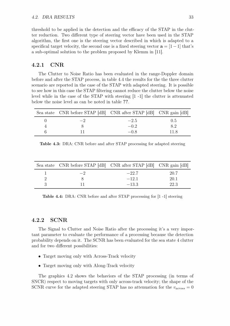
The Clutter to Noise Ratio has been evaluated in the range-Doppler domainbefore and after the STAP process, in table 4.4 the results for the the three clutterscenario are reported in the case of the STAP with adapted steering. It is possibleto see how in this case the STAP filtering cannot reduce the clutter below the noiselevel while in the case of the STAP with steering [1 -1] the clutter is attenuatedbelow the noise level as can be noted in table ??.
Sea state CNR before STAP [dB] CNR after STAP [dB] CNR gain [dB]
0 −2 −2.5 0.54 8 −0.2 8.26 11 −0.8 11.8
Table 4.3: DRA: CNR before and after STAP processing for adapted steering
Sea state CNR before STAP [dB] CNR after STAP [dB] CNR gain [dB]
1 −2 −22.7 20.72 8 −12.1 20.13 11 −13.3 22.3
Table 4.4: DRA: CNR before and after STAP processing for [1 -1] steering
4.2.2 SCNR
The Signal to Clutter and Noise Ratio after the processing it’s a very impor-tant parameter to evaluate the performance of a processing because the detectionprobability depends on it. The SCNR has been evaluated for the sea state 4 clutterand for two different possibilities:
• Target moving only with Across-Track velocity
• Target moving only with Along-Track velocity
The graphics 4.2 shows the behaviors of the STAP processing (in terms ofSNCR) respect to moving targets with only across-track velocity; the shape of theSCNR curve for the adapted steering STAP has no attenuation for the vacross = 0

34 CHAPTER 4. SIMULATION RESULTS
Figure 4.2: DRA: SCNR as a function of Across-Track velocity for a 0dBm2 RCS target
respect to the moving targets. On the other hand the application of the [1,−1]steering vector produce a more accentuated notch for velocities in the proximity ofzero.
Figure 4.3: DRA: SCNR as a function of Along-Track velocity for a 0dBsm RCS target
The behaviors of the STAP processing respect to the along-track velocity areshown in fig 4.3,the SCNR has its maximum for target velocities close to zero anddecreases as the velocity increases. This behavior appears to be dependent on theapplication of a SWMF for the compression after the STAP that causes defocusing
4.2. DRA RESULTS 35
of the target with valong different from zero and a consequent magnitude reduction.The application of the [1,−1] steering vector produce a similar shape of the curvebut placed almost 10dB below.
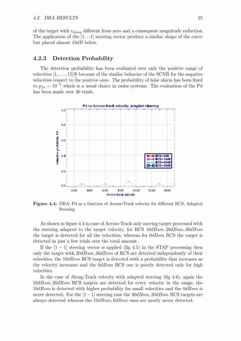
4.2.3 Detection Probability
The detection probability has been evaluated over only the positive range ofvelocities [1, . . . , 15]m
sbecause of the similar behavior of the SCNR for the negative
velocities respect to the positive ones. The probability of false alarm has been fixedto pfa = 10−5 which is a usual choice in radar systems. The evaluation of the Pdhas been made over 30 trials.
Figure 4.4: DRA: Pd as a function of Across-Track velocity for different RCS, AdaptedSteering
As shown in figure 4.4 in case of Across-Track only moving target processed withthe steering adapted to the target velocity, for RCS 10dBsm, 20dBsm, 30dBsm
the target is detected for all the velocities, whereas for 0dBsm RCS the target isdetected in just a few trials over the total amount.
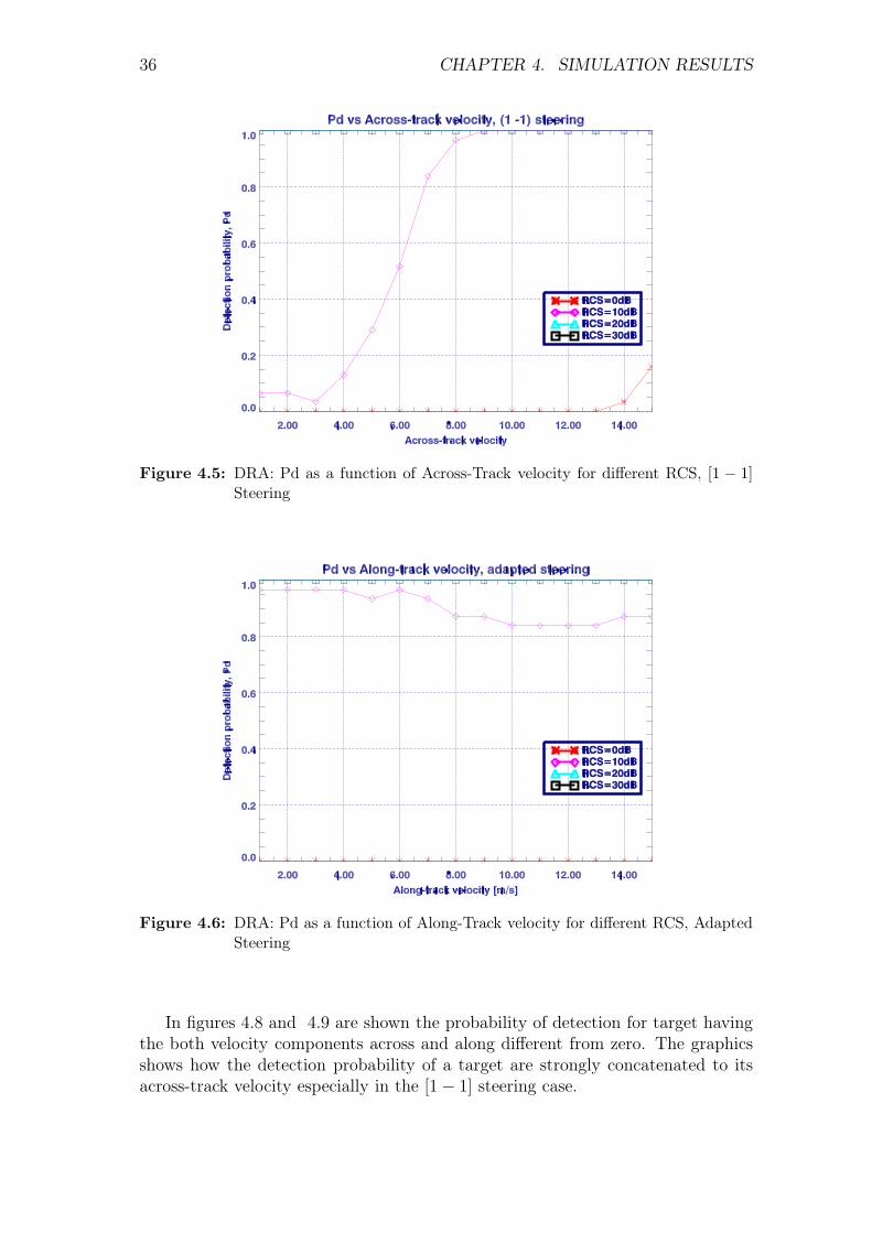
If the [1 − 1] steering vector is applied (fig 4.5) in the STAP processing thenonly the target with 20dBsm, 30dBsm of RCS are detected independently of theirvelocities, the 10dBsm RCS target is detected with a probability that increases asthe velocity increases and the 0dBsm RCS one is poorly detected only for highvelocities.
In the case of Along-Track velocity with adapted steering (fig 4.6), again the10dBsm, 20dBsm RCS targets are detected for every velocity in the range, the10dBsm is detected with higher probability for small velocities and the 0dBsm isnever detected. For the [1−1] steering case the 30dBsm, 20dBsm RCS targets arealways detected whereas the 10dBsm, 0dBsm ones are nearly never detected.
36 CHAPTER 4. SIMULATION RESULTS
Figure 4.5: DRA: Pd as a function of Across-Track velocity for different RCS, [1 − 1]Steering
Figure 4.6: DRA: Pd as a function of Along-Track velocity for different RCS, AdaptedSteering
In figures 4.8 and 4.9 are shown the probability of detection for target havingthe both velocity components across and along different from zero. The graphicsshows how the detection probability of a target are strongly concatenated to itsacross-track velocity especially in the [1− 1] steering case.

4.2. DRA RESULTS 37
Figure 4.7: DRA: Pd as a function of Along-Track velocity for different RCS, [1 − 1]Steering
Figure 4.8: DRA: Pd as a function of Along+Across-Track velocity for different RCS,Adapted Steering
4.2.4 Along-Track velocity estimation
The estimation of the Along-Track velocity is indirectly made, once a target hasbeen detected, using a bank of azimuth matched filter to azimuth line in which thetarget has been detected for a finite number of possible velocities. The estimatedalong-track velocity is the one that maximize output. In the estimation algorithmthe range of tested along-track velocities has been fixed as [−25, . . . ,+25]m
s.

38 CHAPTER 4. SIMULATION RESULTS
Figure 4.9: DRA: Pd as a function of Along+Across-Track velocity for different RCS,[1− 1] Steering
Two significative case are showed, in the first one a 20dBsm RCS target movingwith vacross = valong = 3m
sis processed whereas in the second a target with the
same RCS but vacross = valong = 11ms
is processed.
Figure 4.10: DRA: Bank of filter OUTPUT for a 3ms along-track moving target 20dBsm
RCS
In the first case ( 4.10) the velocity estimated applying a adapted steering vector(v̂along = 5m
s)is clearly much more reliable respect to the one estimated with the

4.3. TOGGLE MODES RESULTS 39
Figure 4.11: DRA: Bank of filter OUTPUT for a 12ms along-track moving target
20dBsm RCS
[1 − 1] steering vector (v̂along = −4ms) in the STAP process. In the second case
( 4.11)instead the two estimated velocity are both reliable (v̂along = 12ms
for theadapted steering, v̂along = 15m
sfor [1 -1] steering).
A complete table of the estimated velocity for different moving target could befound in 4.5.
4.3 TOGGLE modes results
In chapter two the possibility to generate an additional channel by exploitingthe flexibility in the programming of the radar antenna has been introduced. Thethree virtual channels toggle receive mode has been implemented in the simulatorand its performances has been evaluated.
4.3.1 CNR
The Clutter to Noise Ratio has been evaluated in the range-Doppler domainbefore and after the STAP process, in table 4.6 the results for the the three clutterscenario are reported for STAP with adapted steering. It is possible to see how inthis case the STAP filtering cannot reduce the clutter below the noise level as wasin the DRA case.
4.3.2 SCNR
Figure 4.12 shows the behaviors of the STAP processing with adapted steeringrespect to the across-track velocity, as in the DRA the static target with vacross = 0

40 CHAPTER 4. SIMULATION RESULTS
valong[ms] v̂along[
ms] ad. st. error [m
s] v̂along[
ms] [1 -1] st. error [m
s]
−15 −17 2 −12 3−14 −16 2 −16 2−13 −9 4 −15 2−12 −13 1 −15 3−11 −13 2 −13 2−10 −12 2 −13 3−9 −12 3 −12 3−8 −7 1 −13 5−7 −8 1 −11 4−6 −7 1 −8 2−5 −2 3 −9 4−4 −1 3 −9 5−3 −3 0 +1 4−2 0 2 3 5−1 +2 3 −4 30 +1 1 −4 4+1 +3 2 −4 5+2 +4 2 −5 7+3 +5 2 −4 7+4 +7 3 −1 5+5 +4 1 +2 3+6 +4 2 +1 5+7 +5 2 +4 3+8 +7 1 +4 4+9 +10 1 +7 2+10 +12 2 +9 1+11 +14 3 +13 2+12 +13 1 +15 3+13 +11 2 +16 3+14 +12 2 +12 2+15 +14 1 +13 2
Table 4.5: DRA: estimated along track velocity for 20dBsm RCS target
Sea state CNR before STAP [dB] CNR after STAP [dB] CNR gain [dB]
1 −5 −5.2 0.52 5 −0.7 4.33 8 −0.3 7.7
Table 4.6: TOGGLE: CNR before and after STAP processing for adapted steering

4.3. TOGGLE MODES RESULTS 41
is not strongly attenuated by the STAP respect to the the targets with highervacross.
Figure 4.12: TOGGLE: SCNR as a function of Across-Track velocity for a 0dBsm RCStarget
It can be noted that in along-track velocity (fig 4.13) the SCNR has its maxi-mum for target velocities close to zero and decreases as the velocity increases. Thisbehavior appears to be dependent on the application of a SWMF for the compres-sion after the STAP that causes defocusing of the target with vacross different fromzero and a consequent magnitude reduction.
4.3.3 Detection Probability
As in the DRA the detection probability has been evaluated over only thepositive range of velocities [1, . . . , 15]m
sbecause of the similar behavior of the SCNR
for the negative velocities respect to the positive ones. The probability of falsealarm has been fixed to pfa = 10−5. The evaluation of the Pd has been evaluatedover 30 trials.
In the case of moving target with only across-track velocity (fig 4.14), processedwith the adapted steering vector, for RCS 20dBsm, 30dBsm the target is detectedfor all the velocities, for 20dBsm RCS the estimated probability is very close toone, whereas for 0dBsm RCS the target is detected in just a few trials over thetotal amount.
In the case of Along-Track velocity with adapted steering (fig 4.15), again the30dBsm, 20dBsm RCS targets are detected for every velocity in the range, the10dBsm target detection probability decreases as the velocity increases,the 0dBsm
RCS target is never detected.Finally in figure 4.16 the probability of detection has been evaluated for target
having the both velocity components across and along different from zero. In this

42 CHAPTER 4. SIMULATION RESULTS
Figure 4.13: TOGGLE: SCNR as a function of Along-Track velocity for a 0dBsm RCStarget
Figure 4.14: TOGGLE: Pd as a function of Across-Track velocity for different RCS
case the defocusing effect due to the along-track velocity (as seen in the SCNR)seems to be dominant for velocities until 10m
sthen the effects of across-track ve-
locity becomes dominant.
4.3. TOGGLE MODES RESULTS 43
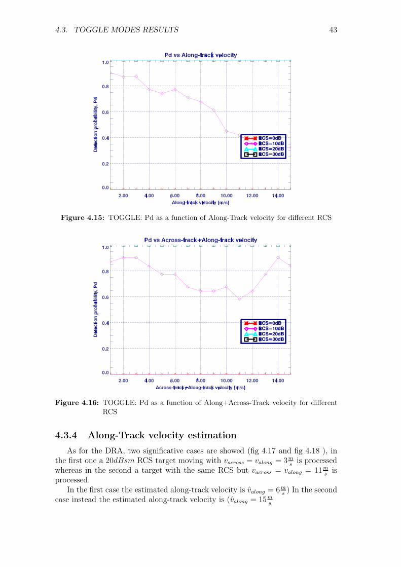
Figure 4.15: TOGGLE: Pd as a function of Along-Track velocity for different RCS
Figure 4.16: TOGGLE: Pd as a function of Along+Across-Track velocity for differentRCS
4.3.4 Along-Track velocity estimation
As for the DRA, two significative cases are showed (fig 4.17 and fig 4.18 ), inthe first one a 20dBsm RCS target moving with vacross = valong = 3m
sis processed
whereas in the second a target with the same RCS but vacross = valong = 11ms
isprocessed.
In the first case the estimated along-track velocity is v̂along = 6ms) In the second
case instead the estimated along-track velocity is (v̂along = 15ms

44 CHAPTER 4. SIMULATION RESULTS
Figure 4.17: TOGGLE: Bank of filter OUTPUT for a 3ms along-track moving target
20dBsm RCS
Figure 4.18: TOGGLE: Bank of filter OUTPUT for a 12ms along-track moving target
20dBsm RCS
A complete table of the estimated velocity for different moving targets couldbe found in 4.7.
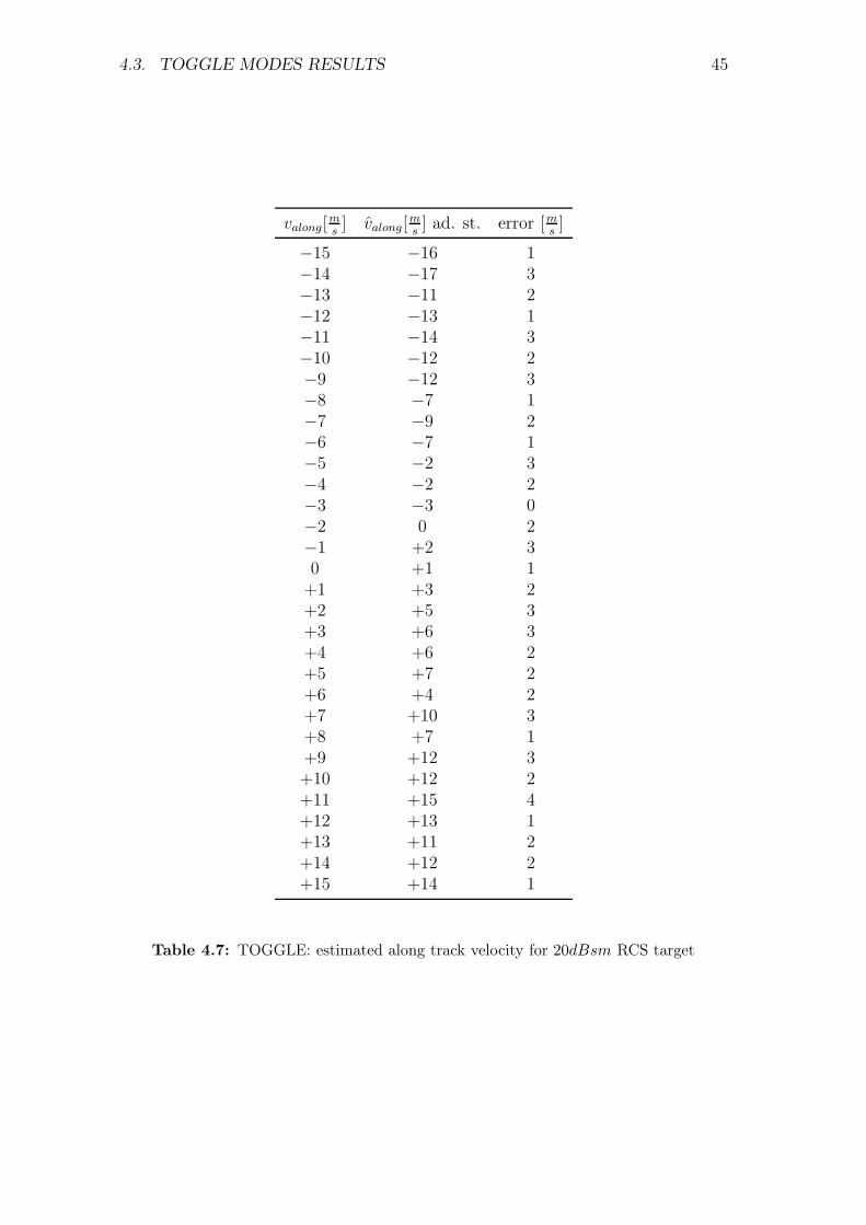
4.3. TOGGLE MODES RESULTS 45
valong[ms] v̂along[
ms] ad. st. error [m
s]
−15 −16 1−14 −17 3−13 −11 2−12 −13 1−11 −14 3−10 −12 2−9 −12 3−8 −7 1−7 −9 2−6 −7 1−5 −2 3−4 −2 2−3 −3 0−2 0 2−1 +2 30 +1 1+1 +3 2+2 +5 3+3 +6 3+4 +6 2+5 +7 2+6 +4 2+7 +10 3+8 +7 1+9 +12 3+10 +12 2+11 +15 4+12 +13 1+13 +11 2+14 +12 2+15 +14 1
Table 4.7: TOGGLE: estimated along track velocity for 20dBsm RCS target

46 CHAPTER 4. SIMULATION RESULTS
4.4 Analysis of the results
From the SCNR results appears clear that, for the simulated marine clutterscenario, the application of the STAP with the adapted steering vector don’t givean attenuation for the static target as would be desiderate in GMTI.
Experimental investigations has demonstrated that the cause of the problemrelies on the small Clutter-Noise-Ratio of 15dB of the simulated scenario in therange-Doppler domain at the moment of estimation of the spectral power densitymatrix R.
In figure 4.19 the SNCR after the processing for a target with only across-track velocity and for 2 different clutter backscatter coefficient (σ0 = 0dB andσ0 = 10dB), providing respectively a CNR improvement of 15dB and 20dB, isshown. Appears evident how the STAP filtering in this case is strongly attenuatingthe echoes from the static target.
Figure 4.19: DRA, SCNR as a function of Across-Track velocity for a 0dBsm RCStarget, different CNR
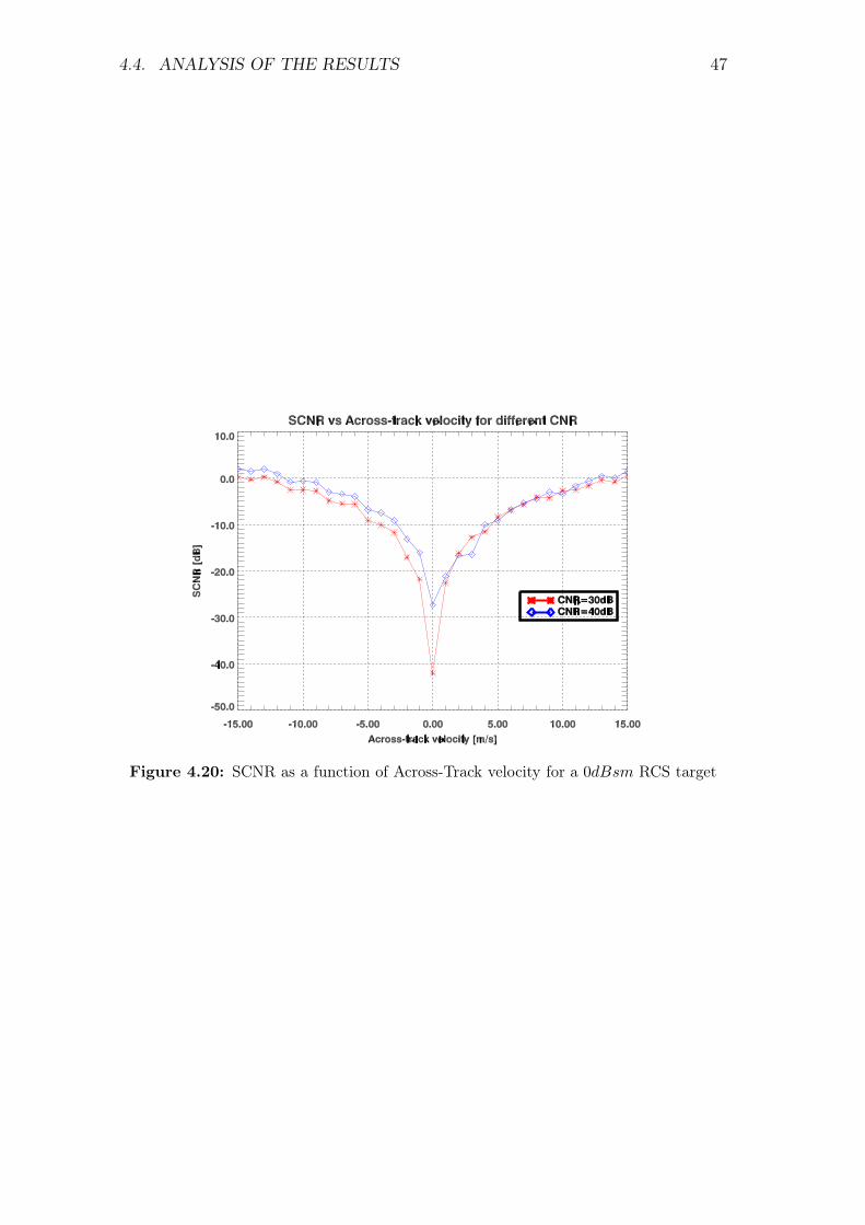
The results with the TOGGLE mode of operation are even better than whatfound for the DRA in terms of attenuation of the static target as fig 4.20 shows.
4.4. ANALYSIS OF THE RESULTS 47
Figure 4.20: SCNR as a function of Across-Track velocity for a 0dBsm RCS target

Chapter 5
Conclusions and future work
A post-Doppler STAP processing technique has been implemented and inte-grated in the SAR processing for detection of moving targets in maritime scenario.The performance of such technique has been evaluated with the integration ofthe algorithm in the SAR-GMTI simulator developed in the Department of SignalTheory and Communications (TSC). In simulation of the spaceborne SAR the pa-rameters of the future Spanish PAZ mission have been used. Two different mode ofoperation have been considered, the Dual Receive Antenna (DRA) that allows thecreation of two channel and a TOGGLE mode of operation that makes possible thecreation of an additional channel by doubling the pulse repetition frequency (PRF)and exploiting the flexibility in programming the array antenna. The performanceof the implemented technique has been evaluated in a maritime scenario and withthe simulation of four different types of boats.
In the DRA mode of operation, two different choice of steering vector in thepost-Doppler STAP have been used, the results obtained in the application ofthe technique to a marine clutter scenario have shown that a clutter reductionis provided by both possible choice of steering vector. For the adapted steeringcase the reduction of the clutter is lower respect the [1 -1] steering vector. In theTOGGLE mode of operation just the adapted steering vector has been considered(as the [1 -1] steering vector can only be applied with two channels) and a clutterreduction has been obtained.
The SCNR in the case of post-Doppler STAP with adapted steering is higherthan the one obtained with the [1 -1] steering and allows a better detection of themoving targets.
In the case of a static point-like target the results have shown that a betterCNR (respect to the one in the simulated maritime scenario) is required in orderto cancel it with the post-Doppler STAP.
The simulations have shown better detection probability in the case of adaptedsteering vector, of particular interest is the detection probability results obtainedfor moving targets with only along-track velocity, since generally with DPCA orATI processing techniques they are almost impossible to detect.
The along-track velocity estimation is better performed in the case of adaptedsteering with a maximum error of 4m
s.
The results obtained with the TOGGLE mode of operation have shown noappreciable improvements respect the DRA mode for the simulated scenarios.
49

50 CHAPTER 5. CONCLUSIONS AND FUTURE WORK
The future work in this field should be addressed in the study of a more realisticmodel for maritime clutter and in the creation of more detailed models of thedifferent type of boats in order to estimate in a better way the performance of theproposed technique.
Bibliography
[1] S. Barbarossa and A. Farina. “Space-time-frequency processing of syntheticaperture radar signals”. In: Aerospace and Electronic Systems, IEEE Trans-actions on 30.2 (1994), pp. 341 –358.
[2] D. Cerrutti-Maori and I. Sikaneta. “Optimum GMTI Processing for Space-based SAR/GMTI Systems -Theoretical Derivation-”. In: Proceedings of EU-SAR (2010).
[3] J.H.G. Ender. “Space-time-frequency processing of synthetic aperture radarsignals”. In: Electronics and Communication engineering jurnal (1999), pp. 29–38.
[4] J.H.G. Ender, C.H. Gierull, and D. Cerutti-Maori. “Improved Space-BasedMoving Target Indication via Alternate Transmission and Receiver Switch-ing”. In: Geoscience and Remote Sensing, IEEE Transactions on 46.12 (2008),pp. 3960 –3974.
[5] M. Cohen F. Nathanson J. Reilly. Radar Design Principles - Signal Process-ing and the Environment. SciTech Pub, 1999, Sea clutter table 134 –147.
[6] S.J. Frasier and A.J. Camps. “Dual-beam interferometry for ocean surfacecurrent vector mapping”. In: Geoscience and Remote Sensing, IEEE Trans-actions on 39.2 (2001), pp. 401 –414.
[7] A.S. Gonzalez et al. “PAZ instrument design and performance”. In: SyntheticAperture Radar (APSAR), 2011 3rd International Asia-Pacific Conferenceon. 2011, pp. 1 –4.
[8] J. Guerci. Space-Time Adaptive Processing for Radar. Artech House, USA,2003.
[9] Frank H. Wong Ian G. Cumming. Digital Processing of Synthetic ApertureRadar Data: Algorithms and Implementation. Artech House Publishers, 2005.
[10] R. Klemm. “Introduction to space-time adaptive processing”. In: Electronicsand Communication engineering jurnal (1999).
[11] R. Klemm. Principles of Space-Time Adaptive Processing. IEE Publisher,London UK, 2002.
[12] Gonzales O. Makhoul E. Broquetas E. “Evaluation of State-of-the-Art tech-niques for Future Spaceborne SAR system -Simulation Validation-”. In: (2011).
[13] G. Palubinskas et al. “Estimation of along-track velocity of road vehicles inSAR data”. In: Image and Signal Processing for Remote Sensing XI. 2005.
51

52 BIBLIOGRAPHY
[14] J.J. Sharma, C.H. Gierull, and M.J. Collins. “The influence of target accel-eration on velocity estimation in dual-channel SAR-GMTI”. In: Geoscienceand Remote Sensing, IEEE Transactions on 44.1 (2006), pp. 134 –147.
[15] World Meteorological Organization Manual on Codes, No 306. url: http://www.wmo.int/pages/p