A Maurizio e a mia mamma -...
177
Transcript of A Maurizio e a mia mamma -...


A Maurizio e a mia mamma

Riassunto
L’argomento di questa tesi sono i sistemi di particelle con interazione a campo medio e iprocessi nonlineari ottenuti come limiti di essi. Il lavoro è suddiviso in tre parti, in cuivengono analizzati modelli caratterizzati da tre diversi meccanismi di interazione. Nellaprima parte ci occupiamo di un’interazione tramite salti simultanei, che prende spunto daalcuni modelli apparsi recentemente in neuroscienze, dove gli autori trattano sistemi dineuroni in comunicazione l’uno con l’altro. Con l’obiettivo di generalizzare questo tipo dimodelli consideriamo un sistema di diffusioni con salti che interagiscono tra loro attraversola componente discontinua: ogni processo compie un salto principale con una certa fre-quenza e, contemporaneamente, forza tutte le altre particelle a compiere anch’esse un saltoche però è detto salto collaterale, in quanto viene riscalato rispetto alla taglia del sistema.Considerando diverse ipotesi sui coefficienti, ci concentriamo sulla propagazione del caostraiettoriale e sulla dimostrazione di esistenza e unicità delle soluzioni per la corrispon-dente SDE nonlineare. Nella seconda parte della tesi ci occupiamo di un’interazione ditipo asimmetrico. Definiamo un sistema dove ogni particella si muove secondo una passeg-giata aleatoria sui naturali, riflessa in zero e con un eventuale drift verso destra. In aggiuntec’è un’interazione asimmetrica, nel senso che ogni particella viene spinta a compiere movi-menti verso sinistra sotto l’influenza solo delle particelle che si trovano alla sua sinistra.Ci chiediamo come questo sistema, che in assenza di interazione è transiente, possa di-ventare ergodico a seconda della forza dell’interazione e studiamo i parametri critici sianel sistema ad N particelle che nel suo limite termodinamico. In particolare sfruttiamorisultati esistenti su diffusioni che interagiscono attraverso la funzione cumulativa empiricaper evidenziare le differenze date dalla dinamica discreta. Nella terza parte ci concentri-amo su una dinamica di Langevin per il modello di Curie-Weiss generalizzato alla qualeapplichiamo un termine di dissipazione. Questo approccio è stato precedentemente usatoper rompere la reversibilità nel modello di Curie-Weiss classico ed è stato dimostrato che,in quel caso, il sistema limite ammette una soluzione periodica. Il nostro lavoro confermal’emergenza di comportamenti periodici anche nel caso del Curie-Weiss generalizzato. Inparticolare, possiamo dimostrare che un’accurata scelta della funzione di interazione nelmodello di partenza è tale da dare luogo ad un sistema limite in cui coesistono molteplicisoluzioni periodiche stabili.

vi Riassunto

Abstract
In this thesis we study mean field interacting particle systems and their McKean-Vlasovlimiting processes, in particular we focus on three different interaction mechanisms, mainlyemerging from biological modelling. The first type of interaction is given by the so calledsimultaneous jumps. We consider a system of interacting jump-diffusion processes thatinteract by means of the discontinuous component: each particle performs a main jump andit simultaneously induces in all the other particles a simultaneous jump whose amplitudeis rescaled with the size of the system. This peculiar interaction is motivated by recentneuroscience models and here we depict a general framework for this type of processes. Wefocus on the well-posedness of the McKean-Vlasov limits of these particle systems underdifferent assumptions on the coefficients and we prove a pathwise propagation of chaosresult. The second interaction we consider is an asymmetric one. We describe a system ofbiased random walks on the positive integers, reflected at zero, where each particle mayperform a leftward jump with a rate proportional to the fraction of particles which arestrictly at its left. We study the critical interaction strength able to ensure ergodicity tothis system, that would be transient in absence of interaction. We compare this modelwith existing models of diffusions interacting through their CDF and we highlight theirdifferences, mainly caused by the presence of clusters of particles in the discrete model.The third interaction we account for is based on a dynamical version of the generalizedCurie-Weiss model. We modify a Langevin dynamics for this model with a dissipativeevolution of the interaction component, breaking the reversibility of the system. We provethat, in the mean field limit, this gives rise to stable limit cycles, explaining self-sustainedperiodic behaviors. In particular, we build a flexible model in which a suitable change inthe interaction function can result in a system which, in certain regimes of parameters,displays coexistence of stable periodic orbits.

viii Abstract

Introduction
Mean-field interacting particles were firstly introduced by Kac with the aim of micro-scopically justifying the spatially-homogeneous Boltzmann equation [56]. Since then, theyhave been extensively studied due to their flexibility and their connections with nonlinearPDE, starting from the seminal work of McKean [65] and in a great number of successiveworks [48, 81, 82, 84]. It is known that the complete graph of interactions among particlesand the symmetry of the evolution are not innocent assumptions and these models givean extremely simplified description of the physical phenomena they were introduced for.However, they have recently received more attention because they can be used to describecomplex systems coming from biology, social science and finance, where the mean-fieldassumption seems to be a reasonable one. This type of models consists in a microscopicand a macroscopic description of a phenomenon, in a way that the nonlinearity observedin the macroscopic behavior is explained by an interaction term at the microscopic level.If we consider a fixed number N of particles in this microscopic description, we say thatthis interaction is of mean field type because its intensity is of order O
(
1N
)
. Under suitableassumptions, it is possible to prove that systems of this type have the propagation of chaosproperty, see [83], i.e. when the particles start from i.i.d. initial conditions they maintainan asymptotic stochastic independence, despite the interaction. Indeed, when the size ofthe system N goes to infinity, particles tend to behave independently and distributed asthe correspondent nonlinear process characterizing the macroscopic description, which is aparticular type of time-inhomogeneous stochastic process, whose dynamics depends on thelaw of the process itself. Nonlinear processes arising as thermodynamic limits of mean-fieldinteracting particle systems, also called McKean-Vlasov processes, are non-trivial processesand the study of their features involves different techniques, usually not needed for clas-sical Markov processes. For instance, stopping times and compactness method are notuseful in the proof of well-posedness of the correspondent nonlinear SDE and differentapproaches are needed, [48, 49, 64]. Moreover, nonlinear processes display a much richerlong-time behavior than their correspondent particle systems, they may show stable oscil-latory laws [47, 79, 78] or multiple stationary measures, even a continuum of them [54].This thesis is divided into three parts, in which we focus on models that are characterizedby a specific type of interaction, each of them is of mean field type. These interactionsarise mainly from biological questions, but their peculiarities make them interesting ontheir own by a mathematical point of view.
ix

x Introduction
In the first part the key interaction is given by the so-called simultaneous jumps. Weconsider a N-particle system of jump-diffusions in R
d, for d > 1, that can interact witheach other by means of classical mean field interactions. We endow this system with anadditional interacting mechanism, inspired by neuroscience problems [29, 43, 75]: eachparticle performs a jump, that we call main jump with a certain rate and it simultaneouslyinduces in all the other particles a collateral jump, whose amplitude is of the order O
(
1N
)
.There is a dissimilarity in the treatment of the jump terms, since we expect that, in thelimit for N→ ∞, the main jump component is preserved while the collateral jump one, al-though simultaneous, collapses into an additional nonlinear drift term. Moreover, pathwisepropagation of chaos for interacting diffusions with jumps is less widespread in literaturethan the continuous case, probably because of the discontinuities in the paths and theimpossibility to use a compactness approach as in the proof of well-posedness for classicalSDE with jumps. Therefore in Chapter 1 and 2 we formally describe a general frameworkfor particle systems with simultaneous jumps, this is the model presented in [3, 4]. Wefocus on the issues of well-posedness of the correspondent nonlinear limit process and onthe proof of pathwise propagation of chaos by means of a coupling method. Being builtas a useful tool for modelling purposes, our model is very flexible and it can be adaptedto a wide class of processes, enclosing in the same framework nonlinear processes with un-bounded jump rates and with diffusive terms, that rarely appear in the mean field literature.
The second part of the thesis is focused on an interaction which is asymmetric. Weconsider a system of N one-dimensional random walks reflected at zero and with a positivebias. We add to this system an interaction that, for each particle, depends on the fractionof particles strictly below the particle itself and it forces the particle to move downward.The reason for this type of interaction comes from population dynamics. We interpret theposition of each particle on the line as the fitness level of an individual w.r.t. the environ-ment. We suppose that each individual has an intrinsic tendency to improve, given by thebiased random walk, but the influence of the individuals worse tham him may decrease itsfitness. For this model, presented in [2], the focus is on long-time behavior, rather thanon well-posedness of the nonlinear limit. Indeed, after having defined the mean field limitof this system, we aim to understand if this asymmetric interaction can ensure ergodicityto a system that would otherwise be transient. With respect to the first part, we areconsidering here a pure jump process and this plays a crucial role in the analysis of thecritical parameters. Indeed, in Chapter 3 we present a slight modification of the systemstudied in [54, 55, 74], that can be viewed as a continuous analogue of the simplest amongthe random walks with asymmetric interaction we aim to study in Chapter 4. However,most of the results in Chapter 3 strictly depend on the continuity of the space and thedynamics and they cannot be extended to the discrete model. We highlight in Chapter 4the differences given by the discontinuous dynamics and how these reflect in the criticalparameters of the model.
The third part of the thesis concerns an interaction coming from a generalized Curie-
xi
Weiss model [35, 37]. We build a particle system on RN that evolves in time according
to a Langevin dynamics, i.e. particles move continuously with the aim of minimizing theenergy coming from the Hamiltonian of the generalized Curie-Weiss model. We modifythis dynamics by providing the interaction term with a dissipative evolution. This is oneof the ways in which the reversibility of the model may be broken and it has been provenin [24, 26] that this approach gives rise to self-sustained periodic behaviors in the nonlinearlimit. The interest in models of interacting components able to capture collective periodicbehaviors is central in several fields, for instance neuroscience, ecology or social science.Indeed, macroscopic oscillatory behaviors are commonly observed in nature even if micro-scopically there is no tendency to behave periodically. With this in mind, we restrict theclass of models with dissipation we defined and we obtain a Gaussian process, which we areable to study completely. We prove that, by suitably modifying the interaction functionof the generalized Curie-Weiss model, we may recreate an interacting particle system thatshows as many stable limit cycles as we want. This confirms that the add of a dissipationterm in the time-evolution of the interaction favors the presence of self-sustained periodicbehavior for particle systems without any tendency to behave periodically. Moreover, witha suitable choice of the interaction function we have a model which is extremely flexibleand it is able to adapt to multiple situations.
In the following, let us describe precisely the structure of the thesis and the differentmodels we deal with.
Part I: models with simultaneous jumps
In Chapter 1 we define a general mean field model that is characterized by the feature ofsimultaneous jumps, explaining the motivation coming from neuroscience modelling. Weaim to understand if the peculiarity of the simultaneous jumps can create problems inthe proof of propagation of chaos in situations different from the ones presented in theneuroscience literature [29, 43, 75], for example in presence of a Brownian component.In this setting, every particle, besides its diffusive dynamics, can perform what we call amain jump, that is a jump of a certain amplitude with a certain rate. Every time thata particle performs this jump, it induces a jump in all the other particles’ trajectories,but the amplitude of these collateral jumps is rescaled according to the size of the system.We consider the McKean-Vlasov limit of this system and in Chapter 2 we prove pathwisepropagation of chaos via a coupling technique, under various sets of assumptions. Thisgive a rate of convergence for the W1 Wasserstein distance between the empirical measuresof the two systems on the space of trajectories D([0, T ],Rd).

xii Introduction
The microscopic and macroscopic dynamics
Fix N > 2 and let XN = (XN1 , . . . , XNN) ∈ R
d×N be the spatial positions of N differentparticles moving in R
d. We introduce the corresponding empirical measure
µNX.=1
N
N∑
i=1
δXNi .
We use the empirical measure to express classical mean field interactions, indeed we de-scribe the evolution of the vector of particles positions XN(t) as a jump diffusion processwhose coefficients depend on it. Moreover, we depict separately a general framework for thepeculiar interaction of mean field type represented by the simultaneous jumps. Therefore,the following coefficients characterize the i-th particle.
• The drift coefficient depends on the spatial position of the particle and on theother particles through the empirical measure, i.e. it is of the form
F(XNi (t), µNX (t))
for some function F : Rd ×M(Rd) → Rd common to all particles.
• The diffusion coefficient, equivalently, is written as
σ(XNi (t), µNX (t))
for σ : Rd ×M(Rd) → Rd×d1 , again the same for all particles.
• The main jump rate: particle i performs a main jump with rate
λ(XNi (t), µNX (t)),
for a positive function λ : Rd × M(Rd) → [0,∞). With this rate, the i-th particleperforms a main jump and simultaneously it induces in all the other particles acollateral jump.
• The main jump amplitude: particle i perform a main jump that is a randomvariable
ψ(XNi (t), µNX (t), h
Ni ) ,
for a function ψ : Rd×M(Rd)× [0,1] → Rd. Here hN is a random variable with values
in [0,1]N and its distribution is given by a symmetric measure νN.
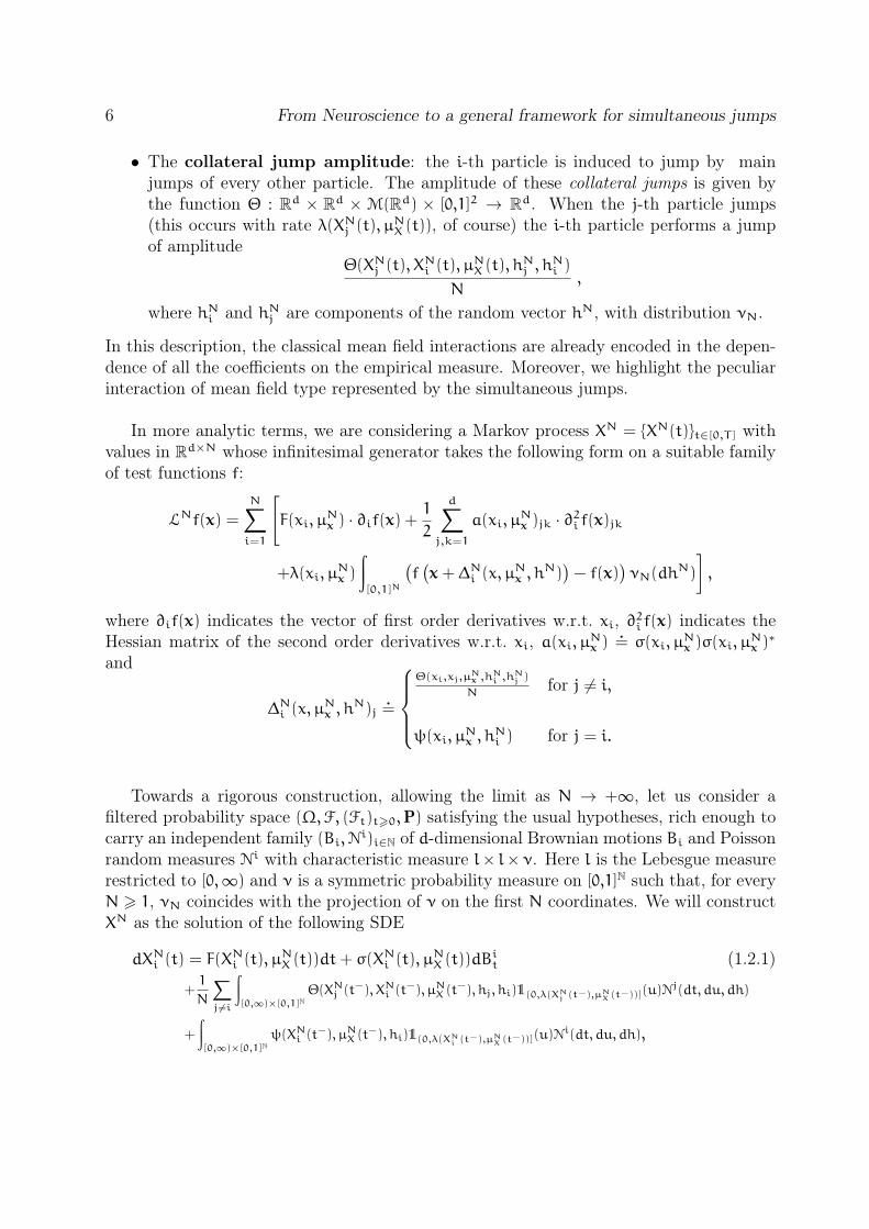
• The collateral jump amplitude: the i-th particle is induced to jump by mainjumps of every other particle. The amplitude of these collateral jumps is given bythe function Θ : Rd × R
d × M(Rd) × [0,1]2 → Rd. When the j-th particle jumps
(this occurs with rate λ(XNj (t), µNX (t)), of course) the i-th particle performs a jump
of amplitudeΘ(XNj (t), X
Ni (t), µ
NX (t), h
Nj , h
Ni )
N,
where hNi and hNj are components of the random vector hN, with distribution νN.

xiii
It is known that a process as XN is in correspondence with a McKean-Vlasov process, i.e.the process X whose law is the law of the solution of the nonlinear SDE:
dX(t) =
(
F(X(t), µt) +
⟨
µt, λ(·, µt)∫
[0,1]2Θ(·, X(t−), µt, h1, h2)ν2(dh1, dh2)
⟩)
dt
+σ(X(t), µt)dBt +
∫
[0,∞)×[0,1]Nψ(X(t−), µs, h1)1(0,λ(X(t−),µs)](u)N(dt, du, dh).
Here, B is a d1-dimensional Brownian motion and N an independent Poisson random mea-sure with characteristic measure dtduν(dh) on [0,∞)2 × [0,1]N. ν is a symmetric measureon [0,1]N such that each projection on N coordinates corresponds to νN. By 〈·, ·〉 we in-dicate the integral of a function on its domain with respect to a certain measure; thus,〈µ,φ〉 =
∫
Rdφ(y)µ(dy). The equation above is not a standard SDE since the law µt of the
solution appears as an argument of the coefficients. Processes of this type may be indi-cated as nonlinear processes and the nonlinearity stands in the fact that the coefficients ofthe SDE depend on the law of the process itself. Informally, we say that these nonlinearterms arise from the mean field interaction in the N particle system; in particular, noticethat the simultaneous jumps give rise to a nonlinear drift term. The collateral jumps,due to the rescaling via the size of the system, appear in the limit as being absorbedby an additional drift term, depending on the characteristic measure of the Poisson ran-dom measure N, that however is still present in the limit, due to the main jump component.
Well-posedness and propagation of chaos
Because of their peculiarity, well-posedness of nonlinear processes is a delicate issue, inparticular in presence of diffusion term and jump component and in literature we find afew examples of this type of processes [48, 49, 50, 67]. However, since classical diffusionprocesses with jumps are extremely used in various applications, it is natural to look fora flexible approach for the study of their nonlinear analogue in view of the use of particlesystems in different frameworks. For this reason, we dedicate Chapter 2 to the study ofthe nonlinear process that we presented under several sets of assumptions, always allowingfor unbounded jump rates.
In Section 2.1 we choose the most classical globally Lipschitz assumptions on all thecoefficients, both in the spatial and in the measure variables, w.r.t. the Euclidean andthe W1 Wasserstein distance. These conditions appear in [48], where well-posedness ofthe nonlinear process is proved. Therefore, we concentrate in the role of the simultaneousjumps and we study their role in the propagation of chaos, that is the connection betweenthe microscopic description and the macroscopic one. Let PN be the law of the particlesystem XN on D([0, T ],Rd)N and let µ the law of the nonlinear process X on D([0, T ],Rd).Intuitively, we say that there is propagation of chaos if, whenever the initial conditions ofthe particles XNi (0) are independent and distributed as µ0, then PN is µ-chaotic, i.e. for

xiv Introduction
any k > 1 and any φ1, . . . , φk ∈ Cb(D([0, T ],Rd))
limN→∞
〈PN, φ1 ⊗ · · · ⊗ φk ⊗ 1⊗ . . . 〉 =k∏
i=1
〈µ,φi〉.
This property states the asymptotic independence of the particles despite the interactionand it is often associate to a sort of Law of Large numbers. Indeed, it is equivalent to
µNXin law−→ µ
and when we say that we want to prove pathwise propagation of chaos we aim to give arate of convergence to zero of the distance between µNX and µ w.r.t. some distance betweenmeasures, in this case a W1 Wasserstein distance. Identifying the rate of propagation ofchaos for a particular interaction is useful also in view of approximation techniques forthe nonlinear process. Indeed, because of their nonlinearity, it is usually hard to simulatenumerically the evolution of a McKean-Vlasov process, but the propagation of chaos letus simulate its trajectories by means of the particle system [14, 15]. Of course the propaga-tion of chaos with a rate is a starting point to measure the accuracy of this approximation.In Section 1.2.4 we introduce an intermediate process that does not display the collateraljumps, instead it has an additional drift term depending on the empirical measure. Thisprocess helps in underlining the role of simultaneous jumps in the pathwise propagationof chaos. Indeed, we couple the two particle systems and in Proposition 2.1.1 we showthat the simultaneous jumps give a rate of convergence in W1 Wasserstein distance of theorder O
(
1√N
)
. After that, we couple the intermediate process with N independent copiesof the nonlinear process and in Proposition 2.1.2 we prove the property of propagation ofchaos along the lines of [48]. From these results it follows the Corollary 2.1.1, in whichpropagation of chaos for the particle system XN is proved.
In Section 2.2 we aim to extend the previous results to a more general set of assumptions.Therefore, it is natural to consider a class of systems with a superlinear drift term. In thisframework we can incorporate several existing mean field models with continuous pathsand extend them to a discontinuous setting [7, 28, 45]. The condition on the drift we aregoing to consider is the following:
(U) the drift coefficient F : Rd ×M(Rd) → Rd is of the form
F(x, α) = −OU(x) + b(x, α),
for all x ∈ Rd and all α ∈ M(Rd), where U is convex and C1, while the function b is
assumed to be globally Lipschitz in both variables.
All the other coefficients satisfy globally Lipschitz conditions on all variables. Nonlinearprocesses of this type with an unbounded jump rate seem to be new and we need to verifythe well-posedness of the correspondent SDE. We prove it in Theorem 2.2.1, by means
xv
of a contraction argument and of a Picard iteration. After that, with Proposition 2.2.1,Proposition 2.2.2 and Corollary 2.2.1, we confirm the results of Section 2.1 on pathwisepropagation of chaos under the assumption (U) on the drift coefficient. Notice that weneed to perform all the proofs in a L1 framework, instead of the classical L2 approachfor stochastic calculus. Indeed, we want to have at least globally Lipschitz conditions onthe rate function λ and the total jump amplitude, call it ∆N, and, when dealing withthe well-posedness of the nonlinear process, we will need to bound expectations of thesupremum over a time interval of an integral w.r.t. the Poisson random measure N. Inan L2 framework, this involves the corresponding compensated martingale N and it needsbounds of the following type, for X, Y ∈ R
d,∫∞
0
∫
[0,1]N‖∆N(X, h)1(0,λ(X)](u) − ∆
N(Y, h)1(0,λ(Y)](u)‖pduν(dh) 6 C‖X− Y‖p,
for p = 2. However, sometimes this may hold for p = 1, but not for p = 2, which justifiesthe choice of getting the L1 framework, where we do not need to compensate the processN. For instance, if ∆N is constant and λ is globally Lipschitz, the above inequality holdsfor p = 1 and not p = 2.
In Section 2.3 we focus on one of the neuroscience models that inspired the analysisof simultaneous jumps [75] and we slightly generalized it to a d-dimensional framework.Therefore we drop off the diffusive component and we consider the piecewise deterministicnonlinear Markov process that solves the following:
dX(t) =E [λ(X(t))]E [V]dt− X(t)dt
−
∫
[0,∞)×[0,1]N(X(t) −U(h1))1[0,λ(X(t)))(u)N(dt, du, dh),
with N Poisson random measure with characteristic measure l × ν × l. We see that thecontribution of the collateral jumps creates the additional drift term
E [λ(X(t))]E [V]dt.
While V and U are two bounded jump functions with values in Rd (they represents two
random variables with values in some bounded subsets of Rd, with abuse of notation wewill indicate as expectations their integrals w.r.t. the measure ν), we allow for a superlinearjump rate, of the form prescribed in [75].
(JR) The jump rate of each particle is a non-negative C1 function of its position, λ : Rd →R+, that is written as the sum of two functions:
λ(·) .= b(‖ · ‖) + h(·).- b is a C1, positive, non-decreasing function such that
b ′(r) 6 γb(r) + c
for some c > 0 and γ <1
5E[‖V‖] ;
xvi Introduction
- h : Rd → R is a C1 bounded function, i.e. there exists H > 0 such that ∀ x ∈ Rd,
‖h(x)‖ 6 H;
To control the jumps of the system when the jump rate is superlinear is particularlyhard, especially in the nonlinear case, where we cannot use any compactness method.Notice that, in [43], the authors succeed in proving well-posedness and propagation ofchaos with an explicit rate (the expected 1√
N) for a similar model and for weak moments
conditions on the initial values, by defining an ad-hoc distance based on the rate functionλ itself. In our study, we choose not to extend this powerful approach to our d-dimensionalmodel and to maintain the same structure of proofs of the previous sections. However, webelieve that the computations of [43] would work here and they would give results withoutthe restrictive hypothesis on the bounded support of initial condition that we require inTheorem 2.3.1, where we prove well-posedness of the nonlinear limit for bounded supportinitial conditions. In the following, by means of a priori bounds on the involved quantities,we end the study with Theorem 2.3.2, Theorem 2.3.3 and Corollary 2.3.1 in which we getpathwise propagation of chaos with the expected 1√
Nrate.
Part II: models with asymmetric interactions
In this part of the thesis we consider a particle system where the interaction is asymmet-ric and, if strong enough, it generates ergodicity in a system otherwise transient. Mainlyinspired by population models, in Chapter 4 we define and study a class of systems ofinteracting random walks on the positive integers, reflected in zero to which we add inter-actions that push each particle towards the origin. Previously, in Chapter 3, we describea continuous model which is a slight modification of the one in [54] and it represents thecontinuous analogue of one of the models of Chapter 4. Because of the continuity of thedynamics this model is completely solvable and we use it as a reference for the study ofthe discrete one.
Interacting random walks with asymmetric interaction
In Chapter 4 we consider a system of N particles on the non-negative integers N, whichwithout interaction evolve as independent random walks, with a drift towards infinity.The interaction induces jumps towards zero, whose size depends on the specific model weconsider, and whose rate is proportional to the fraction of particles that are in a lowerposition than the jumping particle. Let us describe the simplest model we consider. Thereis a fixed number N of particles on N, where each particle XNi , for i = 1, . . . ,N, makesjumps of size 1. If XNi > 0, then it goes to
XNi + 1 with rate 1+ δ,XNi − 1 with rate 1+ λ 1
N
∑Nk=1 1(X
Nk < X
Ni ).

xvii
If XNi = 0, then the only allowed jump is rightward. Here δ > 0 indicates a bias rightward,while λ 1
N
∑Nk=1 1(X
Nk < X
Ni ) is a bias leftward. We call this model the small jump model,
while in general we consider a larger class of models where the leftward jump inducedby the interaction term may have amplitude wider than 1. One interpretation of thesemodels is as follows. N individuals, each associated with an integer valued fitness, havean intrinsic tendency to improve their fitness in time. However, each individual mimickingonly the worse than him may worsen his fitness. Since the interaction is of mean field type,we associate to the particle system a nonlinear Markov process X(t)t>0 whose possibletransitions at time t > 0 are as follows:
X(t) + 1 with rate 1+ δ,X(t) − 1 with rate 1+ λµt[0, X(t)),
where µt is the law of X(t) and, as above, when X(t)=0, only the rightward jump is allowed.In Section 4.1 we define a larger class of models, roughly speaking such that the leftwardjump induced in the particle XNi may have amplitude between 1 and XNi itself. We provewell-posedness of the nonlinear process and the property of propagation of chaos, noticethat in some special cases this is a particular case of the one described in Chapter 1 and 2.
Then, the question is whether a strong interaction can prevent some individuals fromimproving forever, i.e. escape towards infinity. At the outset, we make two remarks whichwe illustrate in the small jump model at the level of the N particle system.
(i) The asymmetry in the drift produces an inhomogeneous system: the rightmost par-ticle, when alone on its site, has a net drift of about δ − λ, whereas the leftmostparticle has a positive drift δ.
(ii) Particles piled up at the same site do not interact, and this produces a tendency forpiles to spread rightward.
It is clear that, when λ = 0, for any N each particle system has no stationary measure.Indeed, it consists of random walks with a nonnegative drift δ > 0 and reflection at zero.Our aim is to estimate the critical interaction strength above which the system has astationary measure, we indicate it as
λ∗N(δ) and λ∗∞(δ)
for the N particle system and the nonlinear process, respectively. We focus on the simplemodel described above since it dominates all others in the class defined in Section 4.1 instochastic ordering. In particular, ergodicity of the small jump model implies ergodicityof all others. Moreover, in Chapter 3 we describe a model of interacting diffusions thatshares the same properties of the small jump model. This is an adaptation of the systemof particles interacting through their cumulative density function (CDF) defined in [54]. Inthis continuous case the critical interaction strength can be explicitly obtained for the N

xviii Introduction
particle system as well as for the nonlinear process. In Theorem 3.2.2 we prove the criticalvalue for the N particle system is
λ∗N,cont(δ) = 2δN
N− 1,
while in Theorem 3.2.3 it is proved that the nonlinear process has a critical interactionstrength that is
λ∗∞,cont(δ) = 2δ.
Unfortunately, the proofs of these results strictly depend on the continuity of the trajec-tories and we mainly use them to underline the differences with the discrete dynamics.Indeed, despite the same interacting mechanism, the continuous and the discrete modeldisplay a peculiar difference. In the discrete model the particles can form large clusters ona single site. When particles are on the same site, according to our description, they cannotinteract and this interferes with ergodicity. On the other hand, the interaction preventsthe particles from escaping to infinity and it favors the creations of clusters.
We dedicate Section 4.2 to the study of the long-time behavior and of the criticalinteraction strength for the N particle system. By means of a Lyapunov function, we provethat, for all δ > 0, there exists a critical value
λ∗up(δ).= 8δ2 + 12δ
such that for all N > 2, for all λ > λ∗up(δ) the process XN = (XN1 , . . . , XNN) described in
small jump model is exponentially ergodic and there exists a probability measure πN(SJ) onNN such that, for any initial condition XN(0),
‖PNx ((XN1 (t), . . . , XNN(t)) ∈ ·) − πN(SJ)‖TV 6 CN(x)(ρN)t, ∀ x ∈ N
N, ∀ t > 0,
where CN(x) is bounded, ρN < 1 and ‖ · ‖TV is the total variation norm. πN(SJ) is theunique stationary measure for the process (XN1 , . . . , X
NN). These are the results stated in
Theorem 4.2.1, in which we prove exponential ergodicity of the particle system under someassumptions and we give an upper bound on λ∗N(δ) which is uniform in N. On the otherhand, it is clear that for λ 6 δ the particle system is transient. By means of a linearLyapunov function, in Theorem 4.2.2 we establish a lower bound on λ∗N(δ). Indeed, thereexists
λ∗N,lower(δ).=(
1+ ρ(ε,N))
2δ, with ρ(ε,N).=
N2(δ+ 2)
N(N− 1)(δ+ 2) − 2δ− 1 −→ 0,
such that, for all λ < λ∗N,lower(δ), the process XN = (XN1 , . . . , XNN) is transient. This lower
bound in Theorem 4.2.2 is strictly greater than the critical value of the continuum model,highlighting the different role played by the occurrence of piles in our case. We believethat this difference is substantial and it gives rise to a non-trivial expression for λ∗∞(δ),
xix
unexpected by the analysis of the continuous model.
In Section 4.3 we study the stationary measures of the nonlinear process. In the contin-uous analogue this is done by directly solving the stationary Fokker-Planck equation andfinding that it has a unique solution. This is clearly harder in the discrete case, we couldnot find a way to prove uniqueness of the stationary measure and we define the criticalinteraction strength λ∗∞(δ) as the value above which the nonlinear process has at least onestationary measure. In Theorem 4.3.1 we prove the existence of at least one stationarydistribution by means of a transformation Γ in the space M(N), for which every stationarydistribution of the nonlinear process is a fixed point. This is an approach widely exploitedin the study of quasi-stationary distributions (QSD) in countable spaces, see [5, 40, 41].This gives an upper bound on the critical value that is
λ∗up(δ).= 4δ.
In Theorem 4.3.2 we give a simple lower bound on this value, saying that for λ 6 2δ thereis no stationary distribution at all.
In Section 4.4, we exploit a link with Jackson’s Networks [52] to give sharper estimateson the critical values. With a change of variables we study the dynamics of the gaps betweensuccessive particles and we compare it with a particular queueing system of Jackson’s type.This let us derive the exact form of
λ∗2(δ) = 2δ2 + 4δ
in Theorem 4.4.2. For N > 2 the applicability of this method is still an open problem;however in Section 4.4.3 we define, for each N > 3 a Jackson’s Network associated toour particle system. This suggests heuristic computation leading to conjecture the criticalinteraction strength for all values of N as follows. Fix N > 3, the process XN is ergodic ifand only if
(1+ δ)N <
N−1∏
k=1
(1+ λk
N).
Taking the limit asN goes to infinity, a natural conjecture is the critical interaction strengthfor the nonlinear process. Fix δ > 0, then for all λ such that
(1+1
λ) ln (1+ λ) − 1 > ln (1+ δ) ,
the nonlinear process X has at least one stationary measure.
Part III: generalized Curie-Weiss model
In Chapter 5 we analyze a particular type of dissipated interaction in a dynamical versionof the generalized Curie-Weiss model [35, 37], with the aim of proving the existence of self-sustained periodic behavior in its nonlinear limit. This interaction has already been proved
xx Introduction
to originate periodic behavior in a dynamical Curie-Weiss model [26] and in a diffusivemodel of cooperative behavior [24].
A dissipative dynamics for the generalized Curie-Weiss model
In Section 5.2 we define the dynamical process we are interested in. We recall that theCurie-Weiss model is defined as the sequence of probability measures on R
N, for N =
1,2, . . . , given by
PN,β(dx1, . . . , dxN) =1
ZN(β)exp
(
Nβg
(
N∑
i=1
xi
N
))
N∏
i=1
ρ(dxi),
where ρ is the symmetric probability measure on R representing the single-site distributionof a spin, g is the interaction function, β is the inverse absolute temperature of the modeland ZN(β) is the normalizing constant. For each N fixed, a Langevin dynamics associatedto the generalized Curie-Weiss model is a diffusion process XN with values in R
N such thatPN,β is its unique invariant measure. XN is solution to the following systems of SDE:
dXNi (t) =β
2g ′
(∑Nj=1 X
Nj (t)
N
)
dt−ρ ′(XNi (t))
2ρ(XNi (t))dt+ dBit,
where Bii=1,...,N is a family of independent 1-dimensional Brownian motions. This dy-namics represents an interacting particle system where each particle follows its own dy-namics (given by the last two terms on the right-hand side) and it experiences a mean
field interaction, which depends on the empirical mean of the system mN(t).=
∑Nj=1X
Nj (t)
N.
Following the approach in [24, 26], we suppose that the motion of each particle dependson a “perceived magnetization” instead of the empirical mean mN(t). To this aim, weintroduce the variables λNi , for i = 1, . . . ,N, representing the interaction felt by the spinXNi . This results in a stochastic process (XN, λN) with values in R
2N where, at everytime t > 0, XNt =
(
XN,1t , . . . , XN,Nt
)
is the vector of the spins of the N particles andλNt =
(
λN,1t , . . . , λN,Nt
)
is the vector of their “perceived magnetizations”. (XNt , λNt ) solves
the following system of SDE:
dXN,it = β2g ′(λN,it )dt−
ρ ′(XN,it )
2ρ(XN,it )dt+ dB1,it
dλN,it = −αλN,it dt+ 1N
∑Nj=1
(
β2g ′(λN,jt ) −
ρ ′(XN,jt )
2ρ(XN,jt )
)
dt+DdB2,it ,
i = 1, . . . ,N, for (B1,i, B2,ii=1,...,N a family of independent 2-dimensional Brownian mo-tions. The constants α,D > 0 are the dissipative and diffusive constants characterizingthe evolution of the “perceived magnetization”. The interactions are of mean field type; asusual, we define the correspondent nonlinear Markov process (X, λ) on R
2 as the solutionof the following nonlinear SDE:
dXt =β2g ′(λt)dt−
ρ ′(Xt)2ρ(Xt)
dt+ dB1t
dλt = −αλtdt+ 〈µt(x, l), β2g ′(l) − ρ ′(x)2ρ(x)
〉dt+DdB2tµt = Law(Xt, λt),

xxi
where B = (B1, B2) is a two dimensional Brownian motion. In Theorem 5.2.3 we provewell-posedness of this McKean-Vlasov process under some reasonable assumptions and inTheorem 5.2.4 we prove the correspondent property of propagation of chaos.
The Gaussian dynamics
In Section 5.3 we focus on a completely solvable model belonging to the class of modelsdescribed in Section 5.2. This has no diffusive component in the evolution of λ, i.e. D = 0,and the single-site distribution is normally distributed, i.e. ρ ∼ N(0, σ2). This simplificationleads to the nonlinear process (Xt, λt)t>0 solution of the following nonlinear SDE:
dXt =β2g ′(λt)dt−
Xt2σ2dt+ dBt,
dλtdt
= −αλt +β2g ′(λt) −
mt
2σ2,
µt = Law(Xt, λt) and mt = 〈µt(dx, dl), x〉,
for Bt Brownian motion. If λ0 is deterministic, the evolution of the “perceived magneti-zation” follows a deterministic dynamics, i.e. for all t > 0 the law of the process is suchthat
µt(dx, dλ) = νt(dx)× δλt(dλ).Moreover, the resulting process is a Gaussian process, specifically it is completely describedby the initial condition µ0 and the quantities (mt, Vt, λt)t>0, where Vt = Var[Xt]. In Sec-tion 5.3.1 we analyze the dynamics without dissipation, i.e. the nonlinear limit of theLangevin dynamics. In Proposition 5.3.1 we study the ODE that rules the evolution ofthe mean mt and we derive the set of the critical β, while in Theorem 5.3.1 we completelycharacterize the sets of stationary measures and the long-time behavior of the limitingLangevin dynamics.
In Section 5.3.2 we study the dynamics with dissipation, we reduce the problem to thestudy of the following system of ODE:
mt =
β2g ′(λt) −
mt
2σ2,
λt = −αλt +β2g ′(λt) −
mt
2σ2,
because the independence of the evolution of Vt let us consider a two-dimensional insteadof a three-dimensional system. With the simple change of variable y = 1
2σ2(λ−m), we get
the system yt = − α
2σ2λt,
λt = yt −(
α+ 12σ2
)
λt +β2g ′(λt),
which is a Liénard system. Among planar differential equations, the systems of Liénardtype have been extensively studied, in particular in relation to their limit cycles, [19, 22,46, 61, 71, 76]. A detailed and complete study of all Liénard systems, with necessary andsufficient conditions for the existence of exactly k > 0 limit cycles, is still an open problem.However, in literature we can find sufficient conditions for the existence of at least(or

xxii Introduction
exactly) k > 0 limit cycles, [22, 71]. In Theorem 5.3.2 we depict three possible phases ofthe evolution of (yt, λt) and we give sufficient conditions on the interaction function g andon the value of parameters for them to occur. In general, for an admissible interactionfunction g we observe the following situations.
i) We can always find a regime of the parameters in which the origin is a global attractorand no limit cycles are present.
ii) Under a simple condition on the derivative of the interaction function, we may finda critical value in which the origin looses its local stability and a stable limit cyclebifurcates from it.
iii) If the previous situation occurs and the interaction function is sufficiently regular atinfinity, we can find a regime in which there exists a unique limit cycles, which isattractive.
Then, Theorem 5.3.3 describes the stationary measure of the process (Xt, λt) and the in-variant sets of measures that characterize periodic solutions.
In Section 5.3.3 we highlight the flexibility of this model, since by a suitable choice ofthe interaction function g we can observe several interesting phases in the Liénard systemand, consequently, in the evolution of the nonlinear process (Xt, λt). In particular, weprove that it is possible to find an interaction function that allows, in certain regimes ofparameters, coexistence of periodic orbits. Indeed, the Liénard system may display thefollowing features.
a) More than one periodic orbit may coexist and they all revolve around the origin. Inthis case the outer one should be stable, the second should be unstable and then theyshould alternate.
b) Some periodic orbits may appear even when the origin is still locally stable. Theseorbits appear through global bifurcations (the Hopf bifurcation is a local one) andthey usually appear in pairs, the outer periodic orbit is stable, while the inner one isunstable.
In Proposition 5.3.2 we give sufficient conditions on the interaction function g such thatthe model admits a regime of parameters in which N limit cycles coexist. In Section 5.3.4we give an explicit example of two interaction functions that let us observe, in differentregimes of the parameters, the two particular situations above. For any α > 0, we couldfind the explicit critical value of β at which the Hopf bifurcation occurs, while we couldonly estimates the critical values at which the other phase transitions occur.
Contents
Riassunto v
Abstract vii
Introduction ix
I Models with simultaneous jumps 3
1 From Neuroscience to a general framework for simultaneous jumps 11.1 Interacting particle systems in Neuroscience . . . . . . . . . . . . . . . . . . 1
1.1.1 Mean field models in Neuroscience . . . . . . . . . . . . . . . . . . . . 21.1.2 Neuroscience models with simultaneous jumps . . . . . . . . . . . . . 3
1.2 Interacting particle systems with simultaneous jumps . . . . . . . . . . . . . 41.2.1 The microscopic dynamics . . . . . . . . . . . . . . . . . . . . . . . . 51.2.2 The macroscopic process . . . . . . . . . . . . . . . . . . . . . . . . . 71.2.3 Propagation of chaos . . . . . . . . . . . . . . . . . . . . . . . . . . . 91.2.4 The intermediate process . . . . . . . . . . . . . . . . . . . . . . . . . 10
2 Pathwise propagation of chaos for simultaneous jumps 132.1 Globally Lipschitz conditions on all coefficients . . . . . . . . . . . . . . . . . 13
2.1.1 Assumptions and well-posedness of the SDEs . . . . . . . . . . . . . 142.1.2 Propagation of chaos . . . . . . . . . . . . . . . . . . . . . . . . . . . 15
2.2 Non-globally Lipschitz drift . . . . . . . . . . . . . . . . . . . . . . . . . . . . 222.2.1 Assumptions and well-posedness of the particle systems . . . . . . . 232.2.2 Well-posedness of the McKean-Vlasov SDE . . . . . . . . . . . . . . 242.2.3 Propagation of chaos . . . . . . . . . . . . . . . . . . . . . . . . . . . 282.2.4 Some technical lemmas . . . . . . . . . . . . . . . . . . . . . . . . . . 29
2.3 Non-globally Lipschitz jump rate . . . . . . . . . . . . . . . . . . . . . . . . . 332.3.1 Assumptions and well-posedness of the particle system . . . . . . . . 332.3.2 Well-posedness of the McKean-Vlasov SDE . . . . . . . . . . . . . . 362.3.3 Propagation of Chaos . . . . . . . . . . . . . . . . . . . . . . . . . . . 382.3.4 Additional lemmas and proofs . . . . . . . . . . . . . . . . . . . . . . 42

xxiv Introduction
II Models with asymmetric interactions 53
3 A system of rank-based interacting diffusions 553.1 The model and propagation of chaos . . . . . . . . . . . . . . . . . . . . . . . 55
3.1.1 The particle system . . . . . . . . . . . . . . . . . . . . . . . . . . . . 563.1.2 Propagation of chaos and the nonlinear process . . . . . . . . . . . . 583.1.3 Pathwise propagation of chaos . . . . . . . . . . . . . . . . . . . . . . 62
3.2 Long-time behavior of the model . . . . . . . . . . . . . . . . . . . . . . . . . 643.2.1 Background: stability of Markov processes . . . . . . . . . . . . . . . 643.2.2 Exponential ergodicity of the particle systems . . . . . . . . . . . . . 663.2.3 Stationary distribution for the nonlinear process . . . . . . . . . . . . 693.2.4 Propagation of chaos for the stationary measures . . . . . . . . . . . 70
4 A system of random walks with asymmetric interaction 734.1 The model . . . . . . . . . . . . . . . . . . . . . . . . . . . . . . . . . . . . . 73
4.1.1 The particle system . . . . . . . . . . . . . . . . . . . . . . . . . . . . 734.1.2 The nonlinear processes . . . . . . . . . . . . . . . . . . . . . . . . . . 754.1.3 Propagation of chaos . . . . . . . . . . . . . . . . . . . . . . . . . . . 794.1.4 Motivation and examples . . . . . . . . . . . . . . . . . . . . . . . . . 83
4.2 Exponential ergodicity of the particle system . . . . . . . . . . . . . . . . . 874.2.1 Upper bound for the critical interaction strength in the particle system 904.2.2 Lower bound for the critical interaction strength in the particle system 96
4.3 Stationary measures for the nonlinear process . . . . . . . . . . . . . . . . . 994.3.1 Upper bound for the critical interaction strength in the nonlinear
process . . . . . . . . . . . . . . . . . . . . . . . . . . . . . . . . . . . 1004.3.2 Lower bound for the critical interaction strength in the nonlinear
process . . . . . . . . . . . . . . . . . . . . . . . . . . . . . . . . . . . 1034.4 The exact critical interaction strength . . . . . . . . . . . . . . . . . . . . . 104
4.4.1 Jackson networks . . . . . . . . . . . . . . . . . . . . . . . . . . . . . 1044.4.2 Exact study of gap process for N = 2 . . . . . . . . . . . . . . . . . . 1054.4.3 Some conjectures . . . . . . . . . . . . . . . . . . . . . . . . . . . . . 108
III Generalized Curie-Weiss model 113
5 Periodic behavior in a generalized Curie-Weiss model with dissipation 1155.1 Self-sustained periodic behavior . . . . . . . . . . . . . . . . . . . . . . . . . 1155.2 The model . . . . . . . . . . . . . . . . . . . . . . . . . . . . . . . . . . . . . 116
5.2.1 The Curie-Weiss model . . . . . . . . . . . . . . . . . . . . . . . . . . 1165.2.2 The generalized Curie-Weiss model . . . . . . . . . . . . . . . . . . . 1175.2.3 The Langevin dynamics for the generalized Curie-Weiss model . . . 1195.2.4 The dissipative dynamics . . . . . . . . . . . . . . . . . . . . . . . . 1205.2.5 The nonlinear process and propagation of chaos . . . . . . . . . . . . 121

1
5.3 Focus on the Gaussian dynamics . . . . . . . . . . . . . . . . . . . . . . . . . 1255.3.1 The case without dissipation, α = 0 . . . . . . . . . . . . . . . . . . . 1255.3.2 The case with dissipation, α > 0 . . . . . . . . . . . . . . . . . . . . . 1305.3.3 Coexistence of limit cycles . . . . . . . . . . . . . . . . . . . . . . . . 1345.3.4 A suitable interaction function for the coexistence of periodic orbits 135
Ringraziamenti 149

2 Contents

Part I
Models with simultaneous jumps
3

Chapter 1
From Neuroscience to a general
framework for simultaneous jumps
In this chapter we study an interacting particle system that displays a particular feature,that we indicate as the simultaneous jumps. This characteristic has recently appeared intoy models for interacting neurons, [29, 43, 75]. These models represent the spike of aneuron as a discontinuity in the evolution of its membrane potential. At the same timeeach spike induces collateral discontinuities in the membrane potential of all the otherneurons. Those ones are rescaled by the factor 1
N, where N is the size of the system,
as customary in mean field models. In the limit, these collateral jumps collapse into anadditional non-linear drift term while the spike component is preserved. This seems to bea new framework in mean field modelling, therefore we aim to depict a general descriptionof this class of models, giving to specialists a general and flexible class of models withsimultaneous jumps. In this chapter, we summarize the neuroscience models that haveinspired the study and we present at an informal level our general model.
1.1 Interacting particle systems in Neuroscience
Neurons are supposed to spread information by means of electrical impulses, called ac-tion potentials or spikes. A single neuron has its own membrane potential that varies dueto external stimuli, to interactions with other neurons and to its own dynamics. Whena neuron spikes its membrane potential is rapidly reset to a resting state and, at thesame time, other neurons in the network receive an excitatory or inhibitory influence.Recently, models describing networks of spiking neurons by means of the mean field ap-proach, typical of statistical mechanics, have become widespread in neuroscience. Due topeculiarities of the brain modelling, sometimes these models are raising questions that havetheir own interest outside the direct brain modelling. In particular, some recent works onpiecewise-deterministic Markov processes for the evolution of neurons membrane potentialhave displayed the interesting feature of simultaneous jumps that we are going to study inthe following sections.

2 From Neuroscience to a general framework for simultaneous jumps
1.1.1 Mean field models in Neuroscience
The mean field approach in neuroscience consists in describing large populations of neuronsof the same type by means of the behavior of a so-called “typical neuron”. The largenumber of neurons and of connections between them make indeed reasonable to describethe brain, a finite-size network, as the infinite-size limit of a system of particles in meanfield interactions, i.e. where the graph of interactions is complete. This approach originsin statistical mechanics, from the seminal work of Kac [56], in which the author builds amicroscopic system of interacting Markov processes, representing the molecules of a rarefiedgas, to justify the macroscopic description through the spatially homogeneous Boltzmannequation. The link between microscopic and macroscopic level is given by the propagationof chaos, see the well-known reference from Sznitmann [83]. Propagation of chaos basicallysays that, when the size of the system grows to infinity, the particles tends to de-correlate,despite their interaction. As observed by Galves and Löcherbach in [44], it is hard to finda systematical overview on the biological justification and experimental confirmation ofpropagation of chaos in the brain behavior, although the goodness of this approach seemsto be validated in Baladron et al. [7]. There the authors cite experimental results in[34], where de-correlation of neuronal firing in visual cortex is observed. Mean field modelsaccount for spikes with different approaches and we do not aim to be complete in describingthe extensive literature in this field. However, in the following we summarize some of theseapproaches.
• The conductance-based models describe in details the role of ions channels in the evo-lution of membrane potential of each neuron in the network. For instance, Hodgkin-Huxley and FitzHugh-Nagumo models associate to each neuron, respectively, a 4 anda 2 dimensional process, that takes into account the membrane potential, but alsoother variables, see [7] for analysis of networks of this type. These models consider theevolution of their quantities as continuous path processes, where the spikes are rapidchanges in the value of the membrane potential and the randomness is expressedby means of a Gaussian process. Usually this approach leads to extremely compli-cated expressions, however the continuity of paths helps in tackling the problem ofpropagation of chaos.
• Leaky integrate and fire models are widely studied in the neuroscience community andthey represent spikes as discontinuities in the evolution of the membrane potential.A single neuron’s membrane potential evolves according to an Ornstein-Uhlenbeckprocess starting from zero (chosen as the neuron’s resting state) and it spikes whenit reaches a certain fixed threshold. Then its potential is reset to zero (here is thediscontinuity) and the process starts again. In networks of leaky integrate and firemodels the interaction is given by the fact that, when a neuron spikes, all the othersreceive an additional drift (as a positive “kick”) of the order 1
N, if N is the size of
the network. The study of mean field limits for this type of networks requires non-standard techniques, because of the discontinuities given by the threshold and the

3
particular dependence of the nonlinear term on the law of the process itself, see [30]for a probabilistic study and [18, 20] for a PDE approach.
• Models with Poisson spikes account for the intrinsic randomness of spikes describingthem by means of inhomogeneous Poisson processes with a rate depending on themembrane potential. In this framework, the membrane potential is modelled by apiecewise deterministic Markov process and the interaction occurs through simulta-neous jumps. When a neuron spikes, randomly according to its rate, it is reset tozero as in leaky integrate and fire models, but instead of interacting with other neu-rons increasing their drifts, it makes their membrane potentials increase of a smallquantity, depending on the synaptic weight between them. In this way, the jumpsin the network are simultaneous and, even if some of them are of the order 1
N, they
may cause problems when letting the size N of the network going to infinity. Theliterature on mean field models with jumps is less rich then the one on continuousmodels, nevertheless in some recent papers the authors prove propagation of chaosfor models in this class, see [29, 43, 44, 75].
1.1.2 Neuroscience models with simultaneous jumps
Let us focus in the recent Poisson mean field models, displaying simultaneous jumps,[29, 43, 75]. These models describe the membrane potentials of neurons as quantities onthe positive real line. Let N > 1 be a fixed finite number of neurons in an homogeneousnetwork (i.e. where the neurons are all of the same type), we associate to each neuronan index i = 1, . . . ,N and we describe the membrane potential of the network with thestochastic process UN(t) =
(
UN1 (t), . . . , UNN(t)
)
∈ RN+ for every t > 0, where UNi (t) is the
membrane potential of the i-th neuron at time t. First of all, the membrane potential of aneuron exponentially decays towards the resting state (here it is 0) due to the leak current,a continuous flow of potential. Therefore neuron i has a drift proportional to
−UNi (t).
Then the neurons interact by means of electrical synapses and, through the gap-junctionchannels, they constantly communicate. This pushes the system towards the average po-tential value, that means that the i-th neuron has also a drift proportional to
N∑
j=1
UNj (t)
N−UNi (t).
Finally, chemical synapses cause fast-events, the spikes. A neuron spikes randomly accord-ing to a state dependent rate
λ(UNi (t)) > 0.
If λ(0) = 0, then it is supposed that there is no external stimuli, while a positive value in0 means that the neuron can spike even when it is at resting state, due to some external

4 From Neuroscience to a general framework for simultaneous jumps
input. When neuron i spikes, its membrane potential is reset at 0 by a jump of amplitude−UNi (t
−). Simultaneously, the non-spiking neurons receive an additional discrete influence,they increase their potential of a quantity depending on a stochastic synaptic efficacy. Thatresults in a jump of amplitude
Wi,j
N
of the membrane potential UNj (t−) when the i-th neuron spikes and this happens simul-
taneously for all j 6= i. The above description corresponds to a piecewise-deterministicMarkov evolution for the process UN, that is solution of the following system of SDEs. Forall i = 1, . . . ,N
dUNi (t) = − αUNi (t)dt− β
UNi (t) −
N∑
j=1
UNj (t)
N
dt−UNi (t−)
∫∞
0
1[0,λ(UNi (t−))](u)Ni(du, dt)
+∑
j 6=i
Wi,j
N
∫∞
0
1[0,λ(UNj (t−))](u)Nj(du, dt), (1.1.1)
where Nii=1,...,N is a family of independent Poisson random measures with characteristicmeasure l × l, for l the Lebesgue measure. In the papers [29, 43], the authors study thecase with α = 0 and Wi,j ≡ 1 for all i, j = 1, . . . ,N; while in [75] the authors study thecase of β = 0 and synaptic weights Wi,j = V i.i.d. positive bounded random variables.It is clear that the interactions here are all of mean field type, but while the one dueto electrical synapses is classical, the one given by chemical synapses is rather peculiar.Indeed these simultaneous jumps, one of which will remain in the limit, while the otherscollapse in a continuous term because of the rescaling of the order 1
N, seem to be new in
the mean field models framework. In the aforementioned papers, the authors succeed toprove propagation of chaos under super-linear hypothesis on the rate function λ.
1.2 Interacting particle systems with simultaneous jumps
In this section we describe a mean field model that can embed the feature of simultaneousjumps in a more general framework. The idea comes from the desire to understand if thepeculiarity of the simultaneous jumps can create problems in the proof of propagation ofchaos in situations different from the one described above, for example in presence of aBrownian component. In this setting, every particle, besides its diffusive dynamics, canperform what we call a main jump, that is a jump of a certain amplitude with a certainrate. Every time that a particle performs this jump, it induces a jump in all the otherparticles’ trajectories, but the amplitude of these collateral jumps is rescaled according tothe size of the system. We consider the McKean-Vlasov limit of this system and we want toprove pathwise propagation of chaos via a coupling technique that involves an intermediateprocess. This would give a rate of convergence for the W1 Wasserstein distance betweenthe empirical measures of the two systems on the space of trajectories D([0, T ],Rd). Westart at an informal level, introducing both the microscopic and the macroscopic dynamics

5
and illustrating the phenomenon of propagation of chaos. Well-posedness and convergencewill be shown under various assumptions in Chapter 2.
1.2.1 The microscopic dynamics
Fix N > 2 and let XN = (XN1 , . . . , XNN) ∈ R
d×N be the spatial positions of N differentparticles moving in R
d. We introduce the corresponding empirical measure
µNX.=1
N
N∑
i=1
δXNi .
When the time variable appears explicitly in XN(t), we write µNX (t) to indicate the timedependence of the empirical measure. Note that µNX (t) is an element of M(Rd), the set ofprobability measures on the Borel subsets of Rd.
The vector of particles positions XN(t) evolves as a jump diffusion process with thefollowing specifications for the i-th particle.
• The drift coefficient depends on the spatial position of the particle and on theother particles through the empirical measure, i.e. it is of the form
F(XNi (t), µNX (t))
for some function F : Rd ×M(Rd) → Rd common to all particles.
• The diffusion coefficient, equivalently, is written as
σ(XNi (t), µNX (t))
for σ : Rd ×M(Rd) → Rd×d1 , again the same for all particles.
• The main jump rate: particle i performs a main jump with rate
λ(XNi (t), µNX (t)),
for a positive function λ : Rd × M(Rd) → [0,∞). With this rate, the i-th particleperforms a main jump and simultaneously it induces in all the other particles acollateral jump.
• The main jump amplitude: particle i performs a main jump that is a randomvariable
ψ(XNi (t), µNX (t), h
Ni ) ,
for a function ψ : Rd×M(Rd)× [0,1] → Rd. Here hN is a random variable with values
in [0,1]N and its distribution is given by a symmetric measure νN.
6 From Neuroscience to a general framework for simultaneous jumps
• The collateral jump amplitude: the i-th particle is induced to jump by mainjumps of every other particle. The amplitude of these collateral jumps is given bythe function Θ : Rd × R
d × M(Rd) × [0,1]2 → Rd. When the j-th particle jumps
(this occurs with rate λ(XNj (t), µNX (t)), of course) the i-th particle performs a jump
of amplitudeΘ(XNj (t), X
Ni (t), µ
NX (t), h
Nj , h
Ni )
N,
where hNi and hNj are components of the random vector hN, with distribution νN.
In this description, the classical mean field interactions are already encoded in the depen-dence of all the coefficients on the empirical measure. Moreover, we highlight the peculiarinteraction of mean field type represented by the simultaneous jumps.
In more analytic terms, we are considering a Markov process XN = XN(t)t∈[0,T ] withvalues in R
d×N whose infinitesimal generator takes the following form on a suitable familyof test functions f:
LNf(x) =
N∑
i=1
[
F(xi, µNx) · ∂if(x) +
1
2
d∑
j,k=1
a(xi, µNx)jk · ∂2i f(x)jk
+λ(xi, µNx)
∫
[0,1]N
(
f(
x+ ∆Ni (x, µNx, hN)
)
− f(x))
νN(dhN)
]
,
where ∂if(x) indicates the vector of first order derivatives w.r.t. xi, ∂2i f(x) indicates theHessian matrix of the second order derivatives w.r.t. xi, a(xi, µNx )
.= σ(xi, µ
Nx)σ(xi, µ
Nx)∗
and
∆Ni (x, µNx, hN)j
.=
Θ(xi,xj,µNx,hNi ,h
Nj )
Nfor j 6= i,
ψ(xi, µNx, hNi ) for j = i.
Towards a rigorous construction, allowing the limit as N → +∞, let us consider afiltered probability space (Ω,F, (Ft)t>0,P) satisfying the usual hypotheses, rich enough tocarry an independent family (Bi,N
i)i∈N of d-dimensional Brownian motions Bi and Poissonrandom measures Ni with characteristic measure l× l×ν. Here l is the Lebesgue measurerestricted to [0,∞) and ν is a symmetric probability measure on [0,1]N such that, for everyN > 1, νN coincides with the projection of ν on the first N coordinates. We will constructXN as the solution of the following SDE
dXNi (t) = F(XNi (t), µ
NX (t))dt+ σ(X
Ni (t), µ
NX (t))dB
it (1.2.1)
+1
N
∑
j 6=i
∫
[0,∞)×[0,1]NΘ(XNj (t
−), XNi (t−), µNX (t
−), hj, hi)1(0,λ(XNj (t−),µN
X (t−))](u)Nj(dt, du, dh)
+
∫
[0,∞)×[0,1]Nψ(XNi (t
−), µNX (t−), hi)1(0,λ(XN
i (t−),µNX (t−))](u)N
i(dt, du, dh),
7
i = 1, . . . ,N. The existence and uniqueness of a solution starting from a vector of initialconditions
(
XN1 (0), . . . , XNN(0)
)
depends obviously on the assumptions on the coefficients,and we will specify sufficient conditions in the following chapter.
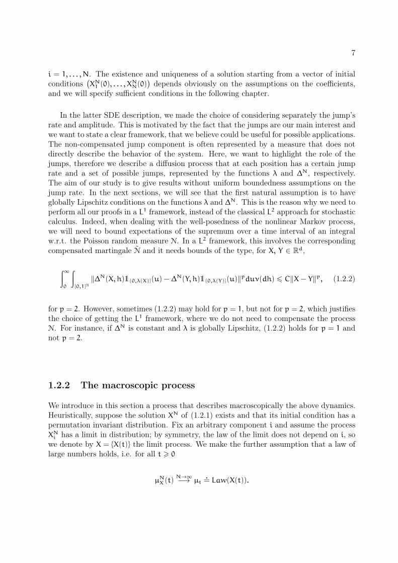
In the latter SDE description, we made the choice of considering separately the jump’srate and amplitude. This is motivated by the fact that the jumps are our main interest andwe want to state a clear framework, that we believe could be useful for possible applications.The non-compensated jump component is often represented by a measure that does notdirectly describe the behavior of the system. Here, we want to highlight the role of thejumps, therefore we describe a diffusion process that at each position has a certain jumprate and a set of possible jumps, represented by the functions λ and ∆N, respectively.The aim of our study is to give results without uniform boundedness assumptions on thejump rate. In the next sections, we will see that the first natural assumption is to haveglobally Lipschitz conditions on the functions λ and ∆N. This is the reason why we need toperform all our proofs in a L1 framework, instead of the classical L2 approach for stochasticcalculus. Indeed, when dealing with the well-posedness of the nonlinear Markov process,we will need to bound expectations of the supremum over a time interval of an integralw.r.t. the Poisson random measure N. In a L2 framework, this involves the correspondingcompensated martingale N and it needs bounds of the type, for X, Y ∈ R
d,
∫∞
0
∫
[0,1]N‖∆N(X, h)1(0,λ(X)](u) − ∆
N(Y, h)1(0,λ(Y)](u)‖pduν(dh) 6 C‖X− Y‖p, (1.2.2)
for p = 2. However, sometimes (1.2.2) may hold for p = 1, but not for p = 2, which justifiesthe choice of getting the L1 framework, where we do not need to compensate the processN. For instance, if ∆N is constant and λ is globally Lipschitz, (1.2.2) holds for p = 1 andnot p = 2.
1.2.2 The macroscopic process
We introduce in this section a process that describes macroscopically the above dynamics.Heuristically, suppose the solution XN of (1.2.1) exists and that its initial condition has apermutation invariant distribution. Fix an arbitrary component i and assume the processXNi has a limit in distribution; by symmetry, the law of the limit does not depend on i, sowe denote by X = X(t) the limit process. We make the further assumption that a law oflarge numbers holds, i.e. for all t > 0
µNX (t)N→∞−→ µt
.= Law(X(t)).

8 From Neuroscience to a general framework for simultaneous jumps
Then, we define the process X as the one with the law of the solution of the McKean-VlasovSDE:
dX(t) =
(
F(X(t), µt) +
⟨
µt, λ(·, µt)∫
[0,1]2Θ(·, X(t−), µt, h1, h2)ν2(dh1, dh2)
⟩)
dt (1.2.3)
+σ(X(t), µt)dBt +
∫
[0,∞)×[0,1]Nψ(X(t−), µs, h1)1(0,λ(X(t−),µs)](u)N(dt, du, dh).
Here, B is a d1-dimensional Brownian motion and N an independent Poisson randommeasure with characteristic measure dtduν(dh) on [0,∞)2 × [0,1]N as above. By 〈·, ·〉 weindicate the integral of a function on its domain with respect to a certain measure; thus,〈µ,φ〉 =
∫
Rdφ(y)µ(dy).
Existence and uniqueness of solutions to (1.2.3) starting from a given initial conditionX(0) will be discussed in the following sections. Note that (1.2.3) is not a standard SDEsince the law µt of the solution appears as an argument of its coefficients. Processes ofthis type may be indicated as nonlinear processes and the nonlinearity stands in the factthat the coefficients of the SDE depend on the law of the process itself. Informally, wesay that these nonlinear terms arise from the dependence, in the N particle system, onthe empirical measure; this is easy to see in most of the coefficients of (1.2.3). However,also the simultaneous jumps give rise to a nonlinear term: indeed, the collateral jumps,due to the rescaling via the size of the system, appear in the limit as being absorbed byan additional drift term, depending on the characteristic measure of the Poisson randommeasures Nii∈N.
A SDE of the type of (1.2.3) is often referred to as McKean-Vlasov SDE, as it iscustomary to call McKean-Vlasov equation the partial differential equation solved, in theweak form, by its law µt, that is
〈µt, φ〉− 〈µ0, φ〉 =∫ t
0
〈µs,L(µs)φ〉ds,
where
L(µt)φ(x).=F(x, µt)∂φ(x) +
1
2
d∑
j,k=1
a(x, µt)jk∂2φ(x)jk
+
⟨
µt, λ(·, µt)∫
[0,1]2Θ(·, x, µt, h1, h2)ν2(dh1, dh2)
⟩
∂φ(x)
+ λ(x, µt)
∫
[0,1]
(φ(x+ψ(x, µt, h1)) − φ(x))ν1(dh1).
Let us highlight that the Poisson random measures appearing in Equations (1.2.1) and(1.2.3), respectively, have characteristic measure defined on [0,∞)2× [0,1]N. The equationscould equivalently be stated in terms of Poisson random measures with characteristic mea-sures defined on [0,∞)2×[0,1]N (namely, l×l×νN) and on [0,∞)2×[0,1] (namely, l×l×ν1).
9
The reason for our seemingly unnatural choice is that it prepares for the coupling argumentwe will use below to establish propagation of chaos. We will need, for each N, a couplingof the N-particle system with N independent copies of the limit system.
1.2.3 Propagation of chaos
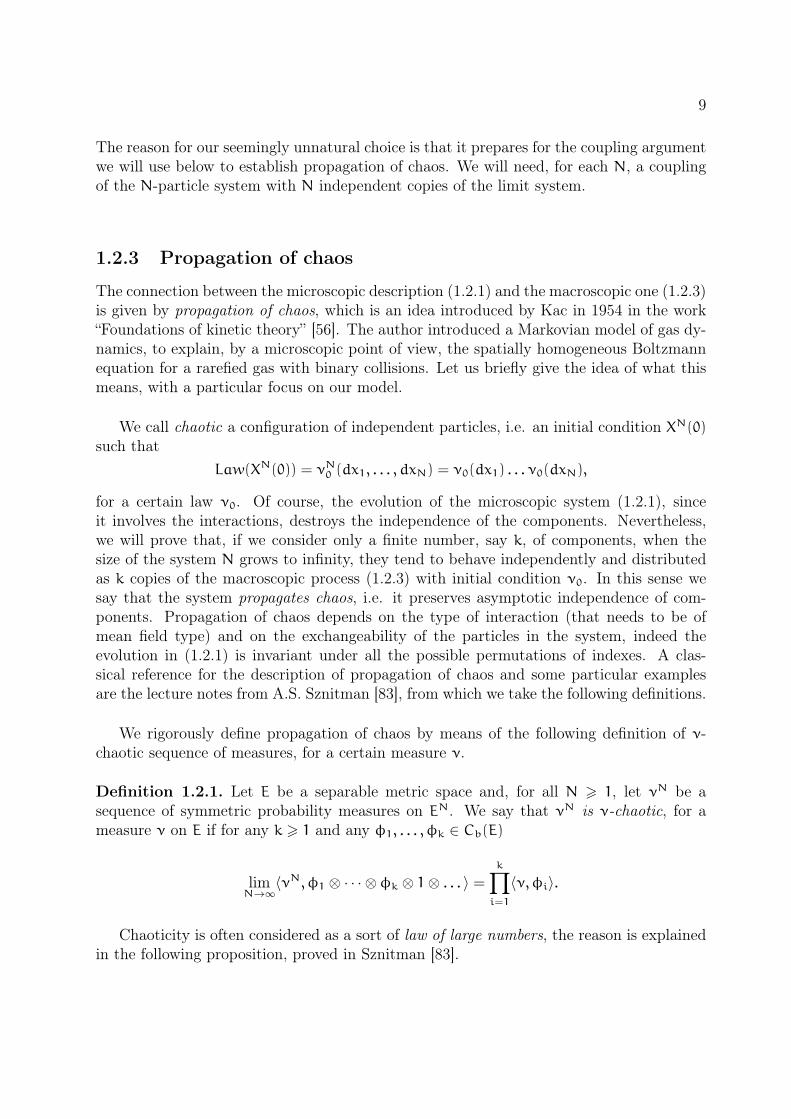
The connection between the microscopic description (1.2.1) and the macroscopic one (1.2.3)is given by propagation of chaos, which is an idea introduced by Kac in 1954 in the work“Foundations of kinetic theory” [56]. The author introduced a Markovian model of gas dy-namics, to explain, by a microscopic point of view, the spatially homogeneous Boltzmannequation for a rarefied gas with binary collisions. Let us briefly give the idea of what thismeans, with a particular focus on our model.
We call chaotic a configuration of independent particles, i.e. an initial condition XN(0)such that
Law(XN(0)) = νN0 (dx1, . . . , dxN) = ν0(dx1) . . . ν0(dxN),
for a certain law ν0. Of course, the evolution of the microscopic system (1.2.1), sinceit involves the interactions, destroys the independence of the components. Nevertheless,we will prove that, if we consider only a finite number, say k, of components, when thesize of the system N grows to infinity, they tend to behave independently and distributedas k copies of the macroscopic process (1.2.3) with initial condition ν0. In this sense wesay that the system propagates chaos, i.e. it preserves asymptotic independence of com-ponents. Propagation of chaos depends on the type of interaction (that needs to be ofmean field type) and on the exchangeability of the particles in the system, indeed theevolution in (1.2.1) is invariant under all the possible permutations of indexes. A clas-sical reference for the description of propagation of chaos and some particular examplesare the lecture notes from A.S. Sznitman [83], from which we take the following definitions.
We rigorously define propagation of chaos by means of the following definition of ν-chaotic sequence of measures, for a certain measure ν.
Definition 1.2.1. Let E be a separable metric space and, for all N > 1, let νN be asequence of symmetric probability measures on EN. We say that νN is ν-chaotic, for ameasure ν on E if for any k > 1 and any φ1, . . . , φk ∈ Cb(E)
limN→∞
〈νN, φ1 ⊗ · · · ⊗ φk ⊗ 1⊗ . . . 〉 =k∏
i=1
〈ν,φi〉.
Chaoticity is often considered as a sort of law of large numbers, the reason is explainedin the following proposition, proved in Sznitman [83].
10 From Neuroscience to a general framework for simultaneous jumps
Proposition 1.2.1. νN is ν-chaotic is equivalent to
µNX =1
N
N∑
i=1
δXiin law−→ δν,
where µNX is a random variable with values in M(E) (the space of probability measures onE), Xi indicates the canonical coordinates on EN and δν indicates the constant randomvariable ν in M(E).
In our case, we fix an arbitrary time horizon T > 0, and, for every N > 1, we denote byXN[0, T ] = (XN(t))t∈[0,T ] the random path of the solution to (1.2.1), up to time T . XN[0, T ]has law PNT on D([0, T ],Rd)N, i.e. the product of N times the Skorokhod space of càdlàgfunctions. At the same time we denote X[0, T ] = (X(t))t∈[0,T ] the random path of thesolution to (1.2.3), then X[0, T ] has a law QT on D([0, T ],Rd).
Definition 1.2.2. For every N > 1, let PN be the law of the solution of a particle systemon D(R+,Rd)N. We say that propagation of chaos holds if, whenever the sequence of initialconditions PN0 is Q0-chaotic, for a certain measure Q0 on R
d, then for all T > 0 the sequenceof laws PNT is QT -chaotic, where QT is a law on D([0, T ],Rd)N with initial condition Q0.
The approaches to prove propagation of chaos are essentially two, described in thefollowing.
i) There is a three-steps approach. First, the tightness of the sequence of empiricalmeasures µNX is proved. The second step consists in proving consistency of their limitpoints, i.e. the limit point of every convergent subsequence belongs to the set of mea-sures that solves the nonlinear limit. Lastly, the uniqueness of the measure solvingthe nonlinear limit is proved, ensuring that the limit of the sequence µNX is determin-istic. This method is extremely flexible, it can be used under weak hypothesis on thecoefficient but it does not provide any rate of convergence.
ii) An alternative approach consists in proving pathwise propagation of chaos, by meansof a coupling between the particle system and N independent copies of the limitprocess. This approach gives a (usually optimal) rate of convergence, but it is lessflexible than the previous one. It is mainly used when coefficients satisfy Lipschitzconditions, but it works also under some particular non-Lipschitz conditions.
In Chapter 2 we are interested in getting results on the model with simultaneous jumpswith the second approach. However, in the rest of the thesis, we will see the use of boththe approaches.
1.2.4 The intermediate process
As we mentioned, we are interested in proving pathwise propagation of chaos, with the aimof getting the rate of convergence due to the simultaneous jumps. The general strategy of
11
proof involves the introduction of an intermediate process YN = (YN(t))t∈[0,T ] with valuesin R
d×N. This Markov process YN can be given as the solution of the SDE
dYNi (t) =F(YNi (t), µ
NY (t))dt+ σ(Y
Ni (t), µ
Ni (t))dB
it (1.2.4)
+1
N
N∑
j=1
λ(YNj (t−), µNY (t−))
∫
[0,1]2Θ(YNj (t−), YNi (t−), µNY (t
−), h1, h2)ν2(dh1, dh2)dt
+
∫
[0,∞)×[0,1]Nψ(YNi (t
−), µNY (t−), h)1(0,λ(YNi (t−),µNi (t−))](u)N
i(dt, du, dh),
i = 1, . . . ,N, where again Bi are independent d-dimensional Brownian motions and Ni areindependent Poisson random measures with characteristic measure l×l×ν. It is immediateto see that the process YN differs from the original process XN in the jump terms; indeed,it does not have the collateral jumps anymore. Every particle still performs the main jumpwith rate given by the function λ, but this does not induce jumps in the other components.As in the macroscopic dynamics (1.2.3), the process YN has an additional drift term, thatdepends on the characteristic measure of Nii∈N and on the empirical measure µNY , because,of course, the term in the second line may be rewritten as
〈µNY (t), λ(·, µNY (t−))∫
[0,1]2Θ(·, YNi (t−), µNY (t
−), h1, h2)ν2(dh1, dh2)〉.
Therefore, the intermediate process YN displays only classical mean field interaction termsand the proof of propagation of chaos is easier than for XN. Furthermore, proving that thelaws of the two processes XN and YN get closer as N goes to infinity will help to quantifythe role of the simultaneous jumps and the rate at which they tend to collapse into thedrift term.
Let us briefly explain the coupling procedure that we will use in the following. Wecall it basic coupling and it is such that it maximizes the chance of two coupled particlesto jump together. We use the same Brownian motions and the same Poisson randommeasures in (1.2.1) and in (1.2.4), such that the processes XN and YN are coupled, i.e. theyare realized on the same probability space: it will not be hard to give conditions for theL1-convergence to zero of XN1 [0, T ]−Y
N1 [0, T ]. Thus, the fact that the law of XN is Q-chaotic
will follow if one shows that the law of YN is Q-chaotic. Since YN has no simultaneousjumps, this can be obtained along the lines of the classical approaches. As we said above,the intermediate process has the nice feature of highlighting the role of simultaneous jumpsin the rate of convergence in W1 Wasserstein distance of the empirical measure. Indeed bycomparing the empirical measures of XN and YN, we obtain that, under our assumptions,the rate of convergence due to the simultaneous jumps is of the order 1√
N, while the final
rate obviously depends on the moments of initial conditions and of the process itself, see[42].

12 From Neuroscience to a general framework for simultaneous jumps
Chapter 2
Pathwise propagation of chaos for
simultaneous jumps
In Section 1.2 of the previous chapter, we present at a heuristic level a general framework formean-field interacting particle systems with simultaneous jumps. In particular we describewhat we mean when we say that a particle system has simultaneous jumps and we highlightthe role of the microscopic, the intermediate and the macroscopic process. In this chapter,we formally prove pathwise propagation of chaos under various sets of assumptions.
2.1 Globally Lipschitz conditions on all coefficients
We start with the most natural among all the assumptions, i.e. classical Lipschitz condi-tions on all the coefficients. To state these conditions and the corresponding theorems, letus introduce a suitable metric on spaces of probability measures.
Definition 2.1.1 (Wp Wasserstein distance ). For p > 1, let (M,d) be a metric space, wecall Mp(M) be the space of probability on M with finite pth moment:
Mp(M) = µ ∈ M(M) :
∫
d(x, x0)pµ(dx) < +∞ for some x0 ∈M.
We equip this space with theWp Wasserstein metric defined as follows: for all µ, ν ∈Mp(M)
Wp(µ, ν).=
[
inf∫
M×Md(x, y)pπ(dx, dy); π has marginals µ and ν
]1/p
.
Therefore, in our case, let M1(Rd) be the space of probability on Rd with finite first
moment:
M1(Rd) = µ ∈ M(Rd) :
∫
‖x‖1µ(dx) < +∞.
14 Pathwise propagation of chaos for simultaneous jumps
This space is equipped with the W1 Wasserstein metric, that by abuse of notation weindicate as follows:
ρ(µ, ν).= inf
∫
Rd×Rd
‖x− y‖π(dx, dy); π has marginals µ and ν
= sup〈g, µ〉− 〈g, ν〉 : g : Rd → R, ‖g(x) − g(y)‖ 6 ‖x− y‖
,
where the equality in the latter row is called Kantorovich-Rubinstein duality and it char-acterized the Wp Wasserstein distance when p = 1, see [87]. We also consider a subset ofM(
D(
[0, T ],Rd))
, the set of the probability measures on D(
[0, T ],Rd)
:
M1(
D(
[0, T ],Rd)) .
=
α ∈ M(
D(
[0, T ],Rd))
:
∫
D
supt∈[0,T ]
‖x(t)‖α(dx) < +∞
,
and provide it with the W1 Wasserstein metric
ρT (α,β).= inf
∫
D×D
supt∈[0,T ]
‖x(t) − y(t)‖P(dx, dy); where P has marginals α and β
.
In what follows, we shall adopt a notion of chaoticity which is stronger than the one ofChapter 1.
Definition 2.1.2. Let XN = (XN1 , XN2 , . . . , X
NN) be a sequence of random vectors with com-
ponents XNi ∈ Rd (resp. XNi ∈ D
(
[0, T ],Rd)
). For µ ∈ M1(Rd) (resp. µ ∈ M1(
D(
[0, T ],Rd))
),we say that XN is µ-chaotic in W1 if its distribution is permutation invariant and, for eachk ∈ N, the law of the vector (XN1 , X
N2 , . . . , X
Nk ) converges to µ⊗k with respect to the metric
ρ (resp. ρT ).
Notice that in Definition 1.2.2 we consider weak convergence of the joint law of kcomponents, while in Definition 2.1.2 we consider convergence w.r.t. the metric ρ (or,respectively ρT ), that gives weak convergence together with the convergence of the firstmoment.
2.1.1 Assumptions and well-posedness of the SDEs
In the following we list the assumptions on the functions that we informally introducedin Section 1.2. In the L1-framework that we chose, these are very natural Lipschitz typeassumptions and they have the advantage that the proof of well-posedness of the involvedSDEs ((1.2.1),(1.2.3) and (1.2.4)) comes as a straightforward consequence of already well-known results on nonlinear diffusion with jumps, [48].
Assumption 2.1.1. (Li1) The classical global Lipschitz assumption on F and σ: ∃ LF, Lσ >0 such that, for all x, y ∈ R
d, all α, γ ∈ M1(Rd),
‖F(x, α) − F(y, γ)‖ 6 LF (‖x− y‖+ ρ(α, γ)) ,‖σ(x, α) − σ(y, γ)‖ 6 Lσ (‖x− y‖+ ρ(α, γ)) .
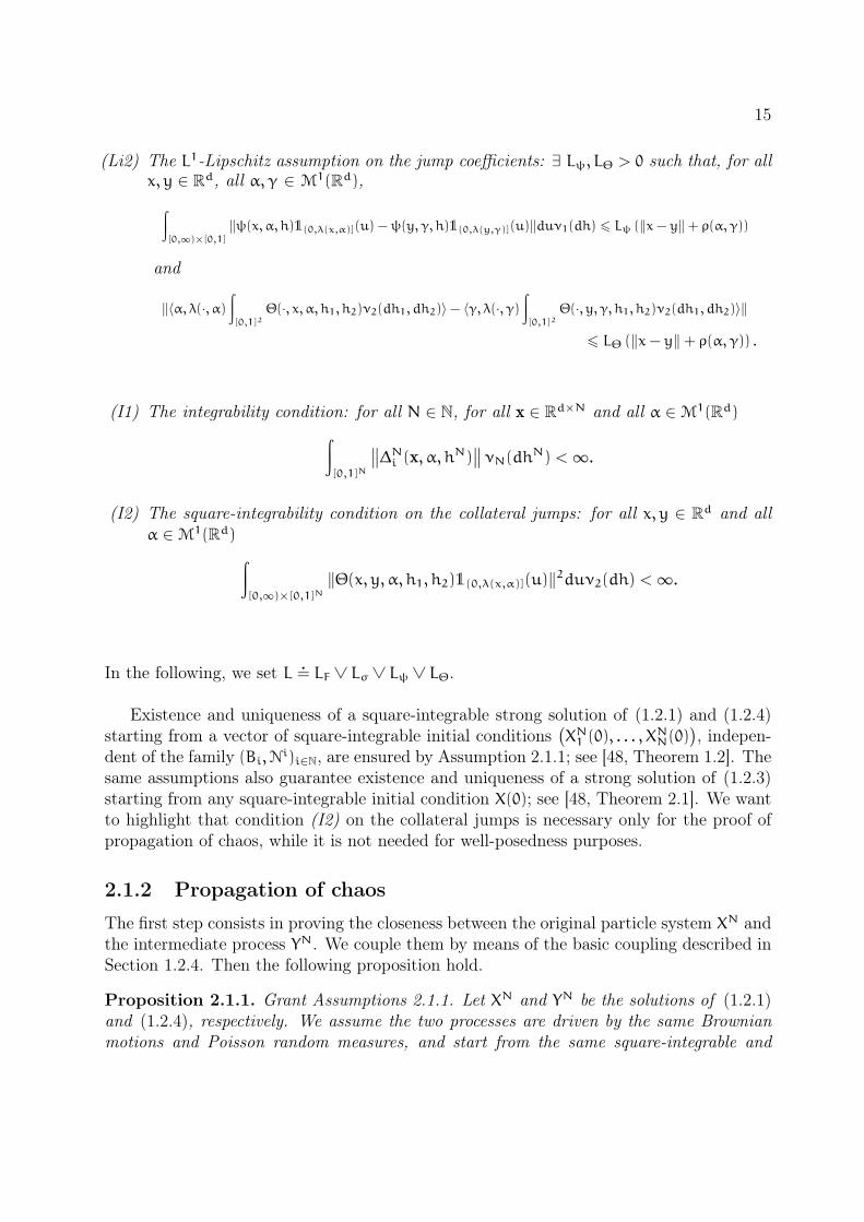
15
(Li2) The L1-Lipschitz assumption on the jump coefficients: ∃ Lψ, LΘ > 0 such that, for allx, y ∈ R
d, all α, γ ∈ M1(Rd),
∫
[0,∞)×[0,1]
‖ψ(x, α, h)1(0,λ(x,α)](u) −ψ(y, γ, h)1(0,λ(y,γ)](u)‖duν1(dh) 6 Lψ (‖x− y‖+ ρ(α, γ))
and
‖〈α, λ(·, α)∫
[0,1]2Θ(·, x, α, h1, h2)ν2(dh1, dh2)〉− 〈γ, λ(·, γ)
∫
[0,1]2Θ(·, y, γ, h1, h2)ν2(dh1, dh2)〉‖
6 LΘ (‖x− y‖+ ρ(α, γ)) .
(I1) The integrability condition: for all N ∈ N, for all x ∈ Rd×N and all α ∈ M1(Rd)
∫
[0,1]N
∥
∥∆Ni (x, α, hN)∥
∥νN(dhN) <∞.
(I2) The square-integrability condition on the collateral jumps: for all x, y ∈ Rd and all
α ∈ M1(Rd)
∫
[0,∞)×[0,1]N‖Θ(x, y, α, h1, h2)1(0,λ(x,α)](u)‖2duν2(dh) <∞.
In the following, we set L .= LF ∨ Lσ ∨ Lψ ∨ LΘ.
Existence and uniqueness of a square-integrable strong solution of (1.2.1) and (1.2.4)starting from a vector of square-integrable initial conditions
(
XN1 (0), . . . , XNN(0)
)
, indepen-dent of the family (Bi,N
i)i∈N, are ensured by Assumption 2.1.1; see [48, Theorem 1.2]. Thesame assumptions also guarantee existence and uniqueness of a strong solution of (1.2.3)starting from any square-integrable initial condition X(0); see [48, Theorem 2.1]. We wantto highlight that condition (I2) on the collateral jumps is necessary only for the proof ofpropagation of chaos, while it is not needed for well-posedness purposes.
2.1.2 Propagation of chaos
The first step consists in proving the closeness between the original particle system XN andthe intermediate process YN. We couple them by means of the basic coupling described inSection 1.2.4. Then the following proposition hold.
Proposition 2.1.1. Grant Assumptions 2.1.1. Let XN and YN be the solutions of (1.2.1)and (1.2.4), respectively. We assume the two processes are driven by the same Brownianmotions and Poisson random measures, and start from the same square-integrable and

16 Pathwise propagation of chaos for simultaneous jumps
permutation invariant initial condition. Then there exists a constant CT > 0 such that, foreach fixed i ∈ N, for all N > 1
E
[
supt∈[0,T ]
‖XNi (t) − YNi (t)‖]
6CT√N. (2.1.1)
Proof. To simplify notation, we adopt the following abbreviations:
Θi,j(XN(s−), h)
.= Θ(XNi (s
−), XNj (s−), µNX (s
−), hi, hj),
λi(XN(s−))
.= λ(XNi (s
−), µNX (s−)),
ψi(XN(s−), h)
.= ψ(XNi (s
−), µNX (s−), hi),
U.= [0,∞)× [0,1]N.
By permutation invariance of both the initial condition and the dynamics, we have, forevery t ∈ [0, T ],
E
[
sups∈[0,t]
‖XNi (s) − YNi (s)‖]
=1
N
N∑
j=1
E
[
sups∈[0,t]
‖XNj (s) − YNj (s)‖]
.
By the same reason we also have a coupling bound for the W1 distance of the empiricalmeasures of the two systems, i.e. for any t > 0
E[
ρ(
µNX (t), µNY (t)
)]
61
N
N∑
j=1
E[
‖XNj (t) − YNj (t)‖]
.
Fix t ∈ [0, T ], and set
Fi.= E
[∫ t
0
‖F(XNi (s), µNX (s)) − F(YNi (s), µNY (s))‖ds]
,
σi.= E
[
supr∈[0,t]
∥
∥
∥
∥
∫ r
0
(
σ(XNi (s), µNX (s)) − σ(Y
Ni (s), µ
NY (s))
)
dBis
∥
∥
∥
∥
]
,
Θi.= E
[
supr∈[0,t]
∥
∥
∥
∥
∥
1
N
∑
j6=i
∫
[0,r]×UΘj,i(X
N(s−), h)1(0,λj(XN(s−))](u)Nj(ds, du, dh)
−1
N
N∑
j=0
∫
[0,t]×UΘj,i(Y
N(s−), h)1(0,λj(YN(s−))](u)dsduν(dh)
∥
∥
∥
∥
∥
]
,
ψi.= E
[
supr∈[0,t]
∥
∥
∥
∥
∫
[0,r]×Uψi(X
N(s−), h)1(0,λi(XN(s−))](u)Ni(ds, du, dh)
−
∫
[0,r]×Uψi(Y
N(s−), h)1(0,λi(YN(s−))](u)Ni(ds, du, dh)
∥
∥
∥
∥
]
.

17
Note that all these quantities do not depend on i, that is therefore omitted in what follows.Then
E
[
sups∈[0,t]
‖XNi (s) − YNi (s)‖]
6 F+ σ+Θ+ψ. (2.1.2)
The term F can be easily bounded thanks to the Lipschitz condition (L1) and the couplingbound for the W1 Wasserstein metric, and we obtain
F 6 L
∫ t
0
E[
‖XNi (s) − YNi (s)‖]
ds+L
N
N∑
j=1
∫ t
0
E[
‖XNj (s) − YNj (s)‖]
ds.
The bound on σ, besides (Li1), involves the Burkholder-Davis-Gundy inequality, and weget, for some constant M not depending on N nor t,
σ 6ME
∫ t
0
(
‖XNi (s) − YNi (s)‖+1
N
N∑
j=1
‖XNj (s) − YNj (s)‖)2
ds
1/2
6M√tE
[
sups∈[0,t]
‖XNi (s) − YNi (s)‖+1
N
N∑
j=1
sups∈[0,t]
‖XNj (s) − YNj (s)‖]
.
The term Θ needs to be treated again with the Burkholder-Davis-Gundy inequality. Inwhat follows, we denote by Ni the compensated Poisson measure associated to Ni and it iscrucial the fact that Nii=1,...,N is a family of orthogonal martingales. First we compensatethe Poisson measures and we get
Θ 6 E
supr∈[0,t]
∥
∥
∥
∥
∥
∥
1
N
∑
j 6=i
∫
[0,r]×UΘj,i(X
N(s−), h)1[0,λj(XN(s−)))Nj(ds, du, dh)
∥
∥
∥
∥
∥
∥
+E
supr∈[0,t]
∥
∥
∥
∥
∥
∥
1
N
N∑
j=1
∫
[0,r]×UΘj,i(X
N(s−), h)1(0,λj(XN(s−))] −Θj,i(YN(s−), h)1(0,λj(YN(s−))]dsduν(dh)
∥
∥
∥
∥
∥
∥
+1
NE
[
supr∈[0,t]
∥
∥
∥
∥
∫
[0,r]×UΘi,i(X
N(s−), h)1(0,λi(XN(s−))]dsduν(dh)
∥
∥
∥
∥
]
.
The first term involves a sum of integrals w.r.t. orthogonal martingales and it is treatedwith Burkholder-Davis-Gundy inequality. Therefore, for a certain constant K > 0, theconstant L > 0 coming from condition (Li2) and a constant C > 0 not depending on N nor
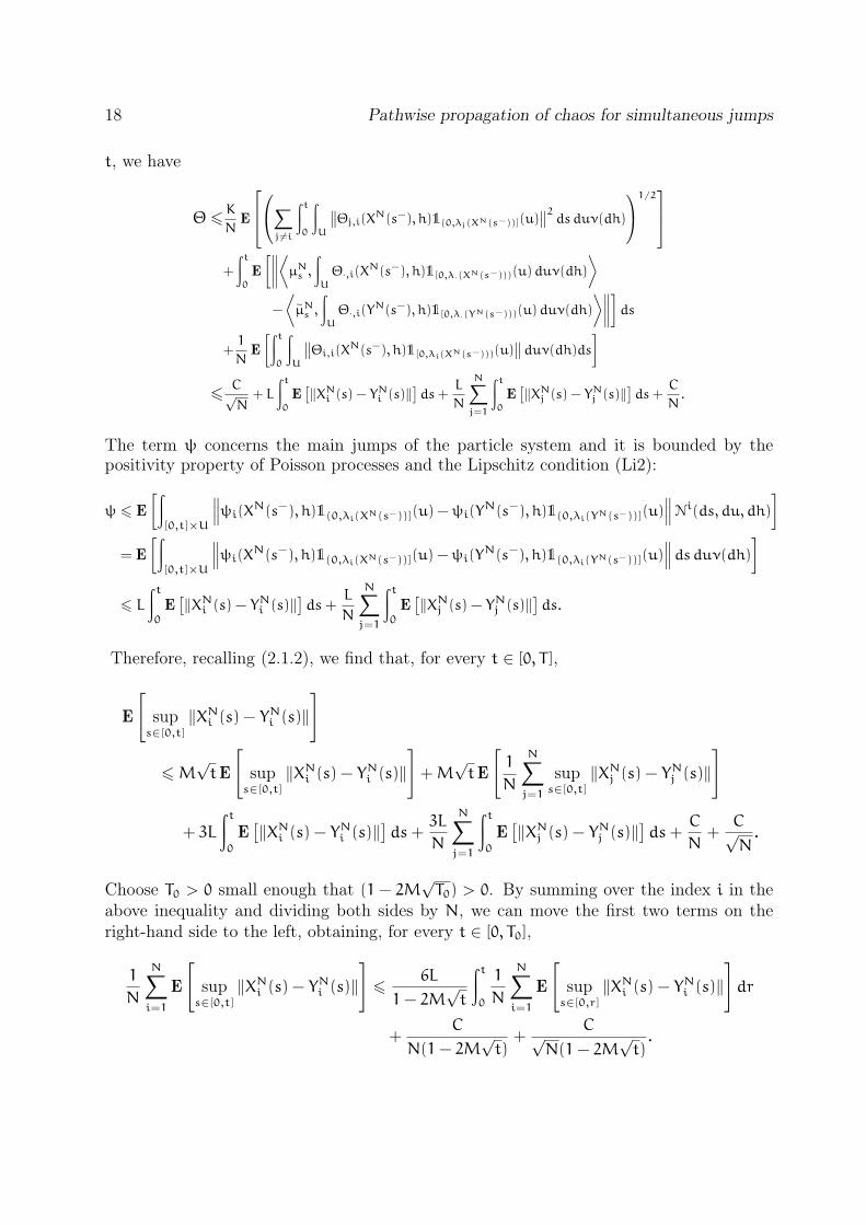
18 Pathwise propagation of chaos for simultaneous jumps
t, we have
Θ 6K
NE
∑
j 6=i
∫t
0
∫
U
∥
∥Θj,i(XN(s−), h)1(0,λj(XN(s−))](u)
∥
∥
2dsduν(dh)
1/2
+
∫t
0
E
[∥
∥
∥
∥
⟨
µNs ,
∫
U
Θ·,i(XN(s−), h)1[0,λ·(XN(s−)))(u)duν(dh)
⟩
−
⟨
µNs ,
∫
U
Θ·,i(YN(s−), h)1[0,λ·(YN(s−)))(u)duν(dh)
⟩∥
∥
∥
∥
]
ds
+1
NE
[∫t
0
∫
U
∥
∥Θi,i(XN(s−), h)1[0,λi(XN(s−)))(u)
∥
∥duν(dh)ds
]
6C√N
+ L
∫t
0
E[
‖XNi (s) − YNi (s)‖]
ds+L
N
N∑
j=1
∫t
0
E[
‖XNj (s) − YNj (s)‖]
ds+C
N.
The term ψ concerns the main jumps of the particle system and it is bounded by thepositivity property of Poisson processes and the Lipschitz condition (Li2):
ψ 6 E
[∫
[0,t]×U
∥
∥
∥ψi(XN(s−), h)1(0,λi(XN(s−))](u) −ψi(Y
N(s−), h)1(0,λi(YN(s−))](u)∥
∥
∥Ni(ds, du, dh)
]
= E
[∫
[0,t]×U
∥
∥
∥ψi(XN(s−), h)1(0,λi(XN(s−))](u) −ψi(Y
N(s−), h)1(0,λi(YN(s−))](u)∥
∥
∥dsduν(dh)
]
6 L
∫t
0
E[
‖XNi (s) − YNi (s)‖]
ds+L
N
N∑
j=1
∫t
0
E[
‖XNj (s) − YNj (s)‖]
ds.
Therefore, recalling (2.1.2), we find that, for every t ∈ [0, T ],
E
[
sups∈[0,t]
‖XNi (s) − YNi (s)‖]
6M√tE
[
sups∈[0,t]
‖XNi (s) − YNi (s)‖]
+M√tE
[
1
N
N∑
j=1
sups∈[0,t]
‖XNj (s) − YNj (s)‖]
+ 3L
∫ t
0
E[
‖XNi (s) − YNi (s)‖]
ds+3L
N
N∑
j=1
∫ t
0
E[
‖XNj (s) − YNj (s)‖]
ds+C
N+
C√N.
Choose T0 > 0 small enough that (1 − 2M√T0) > 0. By summing over the index i in the
above inequality and dividing both sides by N, we can move the first two terms on theright-hand side to the left, obtaining, for every t ∈ [0, T0],
1
N
N∑
i=1
E
[
sups∈[0,t]
‖XNi (s) − YNi (s)‖]
66L
1− 2M√t
∫ t
0
1
N
N∑
i=1
E
[
sups∈[0,r]
‖XNi (s) − YNi (s)‖]
dr
+C
N(1− 2M√t)
+C√
N(1− 2M√t).

19
An application of Gronwall’s lemma yields
1
N
N∑
i=1
E
[
supt∈[0,T0]
‖XNi (t) − YNi (t)‖]
6CT0√N
(2.1.3)
for some finite constant CT0 not depending on N. Recall that (2.1.3) holds on a timeinterval [0, T0] for T0 sufficiently small. If T0 is smaller than T , then we can repeat theprocedure of estimates on the interval [T0, (2T0) ∧ T ]. In this case, we find that, for everyt ∈ [T0, (2T0)∧ T ],
1
N
N∑
i=1
E
[
sups∈[T0,t]
‖XNi (s) − YNi (s)‖]
61
1− 2M√t− T0
(
1
N
N∑
i=1
E
[
sups∈[0,T0]
‖XNi (s) − YNi (s)‖])
+6L
1− 2M√t− T0
∫ t
T0
1
N
N∑
i=1
E
[
sups∈[T0,r]
‖XNi (s) − YNi (s)‖]
dr
+C
N(1− 2M√t− T0)
+C√
N(1− 2M√t− T0)
,
where the first term comes from a bound on the initial condition 1N
∑Ni=1 E
[
‖XNi (T0) − YNi (T0)‖]
.Hence, again thanks to Gronwall’s lemma, for some constant C2,T0 ,
1
N
N∑
i=1
E
[
sups∈[0,(2T0)∧T ]
‖XNi (s) − YNi (s)‖]
6C2,T0√N.
We proceed by induction until we cover, after finitely many steps, the entire interval [0, T ].By exchangeability of the laws of both the initial and the intermediate process, this yields,for i = 1, . . . ,N
E
[
sups∈[0,T ]
∥
∥XNi (s) − YNi (s)
∥
∥
]
6CT√N
and (2.1.1) holds.
In the next, we use a similar coupling technique and we show propagation of chaos forYN. In this case, for all N, we couple the process YN with N independent copies of theprocess X, solution of (1.2.3).
Proposition 2.1.2. Grant Assumptions 2.1.1. Let µ0 be a probability measure on Rd such
that∫‖x‖2µ0(dx) < +∞. For N ∈ N, let YN be a solution of Eq. (1.2.4) in [0, T ]. Assume
that YN(0) = (YN1 (0), . . . , YNN(0)), N ∈ N, form a sequence of square integrable random
vectors that is µ0-chaotic in W1. Let µ be the law of the solution of Eq. (1.2.3) in [0, T ]
with initial law P X(0)−1 = µ0. Then YN is µ-chaotic in W1.
Proof. In order to get the thesis, we set a coupling procedure. Let the processes YNi ,N ∈ N, i ∈ 1, . . . ,N be all defined on the filtered probability space (Ω,F, (Ft)t>0,P) withrespect to the family (Bi,N
i)i∈N of Brownian motions and Poisson random measures. Since

20 Pathwise propagation of chaos for simultaneous jumps
(YN(0)) is µ0-chaotic in W1 by hypothesis, we assume, as we may, that our stochastic basiscarries a triangular array (XNi (0))i∈1,...,N,N∈N of identically distributed R
d-valued randomvariables with common distribution µ0 such that (XNi (0))i∈1,...,N,N∈N and (Bi,N
i)i∈N areindependent, the sequence (XNi (0))i∈1,...,N is independent for each N, and
φN.= E
[∥
∥XNi (0) − YNi (0)
∥
∥
]
tends to zero as N→ ∞. For N ∈ N, i ∈ 1, . . . ,N, let XNi be the unique strong solution ofEq. (1.2.3) in [0, T ] with initial condition XNi (0), driving Brownian motion Bi and Poissonrandom measure Ni. Notice that the processes XN1 , . . . , X
NN are independent and identically
distributed for each N.
Because of the exchangeability of the system (1.2.4), the µ-chaoticity in W1 of thesequence YN is equivalent to
limN→∞
E[
ρT (µNY , µ)
]
= 0.
Moreover, by definition of the metric ρT , this follows from
limN→∞
E
[
supt∈[0,T ]
∥
∥XNi (t) − YNi (t)
∥
∥
]
= 0, (2.1.4)
for every fixed i ∈ N. However, the limit is the same by exchangeability of components.The term in (2.1.4) is bounded by
E
[
supt∈[0,T ]
‖YNi (t) − XNi (t)‖]
6 φN + F+ σ+ Θ+ ψ, (2.1.5)
where
F.= E
[∫T
0
‖F(YNi (s), µNY (s)) − F(XNi (s), µs)‖ds]
,
σ.= E
[
supt∈[0,T ]
∥
∥
∥
∥
∫ t
0
σ(YNi (s), µNY (s)) − σ(X
Ni (s), µs)dB
is
∥
∥
∥
∥
]
,
Θ.= E
[
supt∈[0,T ]
∥
∥
∥
∥
∫ t
0
⟨
µNY (s),
∫
U
Θ(·, YNi (s), µNY (s), h)1(0,λj(·,µNY (s))](u)duν2(dh)
⟩
ds
−
∫ t
0
∫
U
⟨
µs, Θ(·, XNi (s), µs, h)1(0,λj(·,µs)](u)duν(dh)⟩
ds
∥
∥
∥
∥
]
,
ψ.= E
[
supt∈[0,T ]
∥
∥
∥
∥
∫
[0,t]×Uψ(YNi (s
−), µNY (s), h)1(0,λ(YNi (s−),µNY (s−))](u)
−ψ(XNi (s−), µs− , h)1(0,λi(X
Ni (s−),µs−)](u)N
i(dt, du, dh)∥
∥
∥
]
.
The terms F, σ, and ψ are treated exactly as in Proposition 2.1.1, whereas the term Θonly requires the application of the Lipschitz condition (Li2). By mimicking the steps in

21
Proposition 2.1.1, there exists a T0 > 0 small enough and a constant CT0 > 0, independentof N, such that we can apply Gronwall’s Lemma and obtain
E
[
supt∈[0,T0]
‖YNi (t) − XNi (t)‖]
6 CT0
∫T0
0
E[
ρ(µNY (t), µt)]
dt+
√
∫T0
0
E[ρ(µNY (t), µt)2]dt+ φN
.
By triangular inequality, for every fixed t ∈ [0, T0],
E[
ρ(µNY (t), µt)]
6 E[
ρ(µNY (t), µNX(t))
]
+ E[
ρ(µNX(t), µt)
]
6 E
[
supt∈[0,T0]
‖YNi (t) − XNi (t)‖]
+ E[
ρ(µNX(t), µt)
]
.
Then, for a T0 sufficiently small, using again Gronwall Lemma, there exists a positiveconstant, depending on T0, that by abuse of notation we will indicate it again with CT0 > 0,such that
E
[
supt∈[0,T0]
‖YNi (t) − XNi (t)‖]
6 CT0
∫T0
0
E
[
ρ(µNX(t), µt)
]
dt+
√
∫T0
0
E
[
ρ(µNX(t), µt)2
]
dt+ φN
.
We see that the bound on (2.1.5) depends on the initial conditions and on E[
ρ(µNX(t), µt)
]
,that is the distance, at every fixed time t ∈ [0, T ], between the empirical measure of N i.i.d.copies of the solution of the process with law µ and the law µt itself. The rate of convergenceof empirical measures in Wasserstein distance depends on the moments of X(t) and on thedimension d, see [42, Theorem 1]. Since
supt∈[0,T ]
E[
X2i (t)]
< +∞,
it follows from [42] that, setting
βN.= supt∈[0,T ]
E[ρ(µNX(t), µt)],
we havelimN→∞
βN = 0.
Therefore, we know that there exists a constant CT0 > 0 such that, for N going to infinity,we have
E
[
supt∈[0,T0]
‖YNi (t) − XNi (t)‖]
6 CT0(
βN + φN)
.
Iterating this procedure as in Proposition 2.1.1, we extend the above result to [0, T ], i.e.
E
[
supt∈[0,T ]
‖YNi (t) − XNi (t)‖]
6 CT(
βN + φN)
.
for a suitable constant CT . This establishes µ-chaoticity of YN in W1.
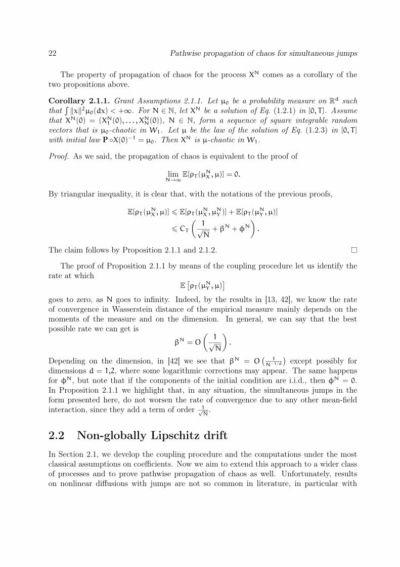
22 Pathwise propagation of chaos for simultaneous jumps
The property of propagation of chaos for the process XN comes as a corollary of thetwo propositions above.
Corollary 2.1.1. Grant Assumptions 2.1.1. Let µ0 be a probability measure on Rd such
that∫‖x‖2µ0(dx) < +∞. For N ∈ N, let XN be a solution of Eq. (1.2.1) in [0, T ]. Assume
that XN(0) = (XN1 (0), . . . , XNN(0)), N ∈ N, form a sequence of square integrable random
vectors that is µ0-chaotic in W1. Let µ be the law of the solution of Eq. (1.2.3) in [0, T ]
with initial law P X(0)−1 = µ0. Then XN is µ-chaotic in W1.
Proof. As we said, the propagation of chaos is equivalent to the proof of
limN→∞
E[ρT (µNX , µ)] = 0.
By triangular inequality, it is clear that, with the notations of the previous proofs,
E[ρT (µNX , µ)] 6 E[ρT (µ
NX , µ
NY )] + E[ρT (µ
NY , µ)]
6 CT
(
1√N
+ βN + φN)
.
The claim follows by Proposition 2.1.1 and 2.1.2.
The proof of Proposition 2.1.1 by means of the coupling procedure let us identify therate at which
E[
ρT (µNY , µ)
]
goes to zero, as N goes to infinity. Indeed, by the results in [13, 42], we know the rateof convergence in Wasserstein distance of the empirical measure mainly depends on themoments of the measure and on the dimension. In general, we can say that the bestpossible rate we can get is
βN = O
(
1√N
)
.
Depending on the dimension, in [42] we see that βN = O(
1N−1/d
)
except possibly fordimensions d = 1,2, where some logarithmic corrections may appear. The same happensfor φN, but note that if the components of the initial condition are i.i.d., then φN = 0.In Proposition 2.1.1 we highlight that, in any situation, the simultaneous jumps in theform presented here, do not worsen the rate of convergence due to any other mean-fieldinteraction, since they add a term of order 1√
N.
2.2 Non-globally Lipschitz drift
In Section 2.1, we develop the coupling procedure and the computations under the mostclassical assumptions on coefficients. Now we aim to extend this approach to a wider classof processes and to prove pathwise propagation of chaos as well. Unfortunately, resultson nonlinear diffusions with jumps are not so common in literature, in particular with

23
unbounded jump rates. Therefore, in the two following sections, we need to prove, besidesthe equivalent of Proposition 2.1.1, 2.1.2 and Corollary 2.1.1, also the well-posedness ofthe nonlinear process (1.2.3).
Let us start by relaxing the Lipschitz assumption on the drift, allowing as drift terms thegradients of general convex potentials. This includes relevant examples as those appearedin [28] and [45], extending them to the case with jumps.
2.2.1 Assumptions and well-posedness of the particle systems
The structure of this section recalls the one of Section 2.1.1, in the sense that we list theassumptions on the coefficients, that differ only in the condition of the drift function F.
Assumption 2.2.1. (U) The drift coefficient F : Rd ×M(Rd) → Rd is of the form
F(x, α) = −OU(x) + b(x, α),
for all x ∈ Rd and all α ∈ M(Rd), where U is convex and C1. The function b
is assumed to be globally Lipschitz in both variables: ∃ Lb > 0 such that, for allx, y ∈ R
d, all α, γ ∈ M1(Rd),
‖b(x, α) − b(y, γ)‖ 6 Lb (‖x− y‖+ ρ(α, γ)) .
(Li1) The classical global Lipschitz assumption on σ: ∃ Lσ > 0 such that, for all x, y ∈ Rd,
all α, γ ∈ M1(Rd),
‖σ(x, α) − σ(y, γ)‖ 6 Lσ (‖x− y‖+ ρ(α, γ)) .
(Li2) The L1-Lipschitz assumption on the jump coefficients: ∃ Lψ, LΘ > 0 such that, for allx, y ∈ R
d, all α, γ ∈ M1(Rd),
∫
[0,∞)×[0,1]
‖ψ(x, α, h)1(0,λ(x,α)](u) −ψ(y, γ, h)1(0,λ(y,γ)](u)‖duν1(dh) 6 Lψ (‖x− y‖+ ρ(α, γ))
and
‖〈α, λ(·, α)∫
[0,1]2Θ(·, x, α, h1, h2)ν2(dh1, dh2)〉− 〈γ, λ(·, γ)
∫
[0,1]2Θ(·, y, γ, h1, h2)ν2(dh1, dh2)〉‖
6 LΘ (‖x− y‖+ ρ(α, γ)) .
(I1) The integrability condition: for all N ∈ N, for all x ∈ Rd×N and all α ∈ M1(Rd)
∫
[0,1]N
∥
∥∆Ni (x, α, hN)∥
∥νN(dhN) <∞.

24 Pathwise propagation of chaos for simultaneous jumps
(I2) The square-integrability condition on the collateral jumps: for all x, y ∈ Rd and all
α ∈ M1(Rd)
∫
[0,∞)×[0,1]N‖Θ(x, y, α, h1, h2)1(0,λ(x,α)](u)‖2duν2(dh) <∞.
In the following, we set L .= Lb ∨ Lσ ∨ Lψ ∨ LΘ.
Condition (U) is a natural choice when one wants to relax globally Lipschitz conditionson coefficients. It induces a process whose trajectories are strongly constrained by the con-vex potential. This attracting drift, even when combined with an unbounded jump rate,should prevent the process from exploding in finite time. We will see that this is whathappens provided the jump rate is in some way “controllable”, as it is under the Lipschitzassumption (Li2).
We could not find a general result on SDE with unbounded jump’s rate and a non glob-ally Lipschitz condition on the drift coefficient, that could ensure existence and uniquenessof solutions to (1.2.1) and (1.2.4) under Assumption 2.2.1. Therefore, we prove sometechinical lemmas, that are gathered in Section 2.2.4.
2.2.2 Well-posedness of the McKean-Vlasov SDE
We mentioned that it is not easy to find results on SDE where the rate of jump is un-bounded and it is certainly much harder to find such results in the framework of nonlinearSDE. Indeed, the stopping time procedure that we use in the proof of Lemma 2.2.1 isnot suitable, since the coefficients depend on the law of the process itself. Thus, in thissection, we give a specific proof of well-posedness for nonlinear SDE belonging to this class.
Consider the stochastic differential equation
dX(t) =F(X(t), µt)dt+ σ(X(t), µt)dBt (2.2.1)
+
∫
[0,∞)×[0,1]Nψ(X(t−), µt− , h1)1(0,λ(X(t−),µt−)](u)N(dt, du, dh),
where µt = Law(X(t)), B is a d1-dimensional Brownian motion and N is a stationaryPoisson random measure with characteristic measure l× l× ν.
Theorem 2.2.1. Let the coefficients of the nonlinear SDE (2.2.1) satisfy Assumption 2.2.1.Then for all square integrable initial conditions X(0) ∈ R
d, Eq. (2.2.1) admits a uniquestrong solution.
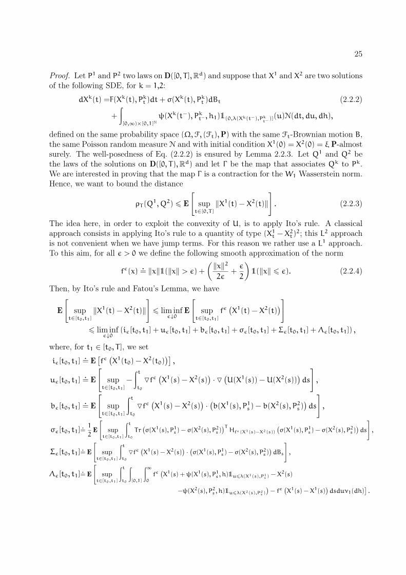
25
Proof. Let P1 and P2 two laws on D([0, T ],Rd) and suppose that X1 and X2 are two solutionsof the following SDE, for k = 1,2:
dXk(t) =F(Xk(t), Pkt )dt+ σ(Xk(t), Pkt )dBt (2.2.2)
+
∫
[0,∞)×[0,1]Nψ(Xk(t−), Pkt− , h1)1(0,λ(Xk(t−),Pk
t−)](u)N(dt, du, dh),
defined on the same probability space (Ω,F, (Ft),P) with the same Ft-Brownian motion B,the same Poisson random measure N and with initial condition X1(0) = X2(0) = ξ P-almostsurely. The well-posedness of Eq. (2.2.2) is ensured by Lemma 2.2.3. Let Q1 and Q2 bethe laws of the solutions on D([0, T),Rd) and let Γ be the map that associates Qk to Pk.We are interested in proving that the map Γ is a contraction for the W1 Wasserstein norm.Hence, we want to bound the distance
ρT (Q1, Q2) 6 E
[
supt∈[0,T ]
‖X1(t) − X2(t)‖]
. (2.2.3)
The idea here, in order to exploit the convexity of U, is to apply Ito’s rule. A classicalapproach consists in applying Ito’s rule to a quantity of type (X1t − X
2t)2; this L2 approach
is not convenient when we have jump terms. For this reason we rather use a L1 approach.To this aim, for all ε > 0 we define the following smooth approximation of the norm
fε(x).= ‖x‖1(‖x‖ > ε) +
(‖x‖22ε
+ε
2
)
1(‖x‖ 6 ε). (2.2.4)
Then, by Ito’s rule and Fatou’s Lemma, we have
E
[
supt∈[t0,t1]
‖X1(t) − X2(t)‖]
6 lim infε↓0
E
[
supt∈[t0,t1]
fε(
X1(t) − X2(t))
]
6 lim infε↓0
(iε[t0, t1] + uε[t0, t1] + bε[t0, t1] + σε[t0, t1] + Σε[t0, t1] +Λε[t0, t1]) ,
where, for t1 ∈ [t0, T ], we set
iε[t0, t1].= E
[
fε(
X1(t0) − X2(t0)
)]
,
uε[t0, t1].= E
[
supt∈[t0,t1]
−
∫ t
t0
Ofε(
X1(s) − X2(s))
· O(
U(X1(s)) −U(X2(s)))
ds
]
,
bε[t0, t1].= E
[
supt∈[t0,t1]
∫ t
t0
Ofε(
X1(s) − X2(s))
·(
b(X1(s), P1s) − b(X2(s), P2s)
)
ds
]
,
σε[t0, t1].=1
2E
[
supt∈[t0,t1]
∫t
t0
Tr(
σ(X1(s), P1s) − σ(X2(s), P2s)
)THfε(X1(s)−X2(s))
(
σ(X1(s), P1s) − σ(X2(s), P2s)
)
ds
]
,
Σε[t0, t1].= E
[
supt∈[t0,t1]
∫t
t0
Ofε(
X1(s) − X2(s))
·(
σ(X1(s), P1s) − σ(X2(s), P2s)
)
dBs
]
,
Λε[t0, t1].= E
[
supt∈[t0,t1]
∫t
t0
∫
[0,1]
∫∞
0
fε(
X1(s) +ψ(X1(s), P1s , h)1u6λ(X1(s),P1s )
− X2(s)
−ψ(X2(s), P2s , h)1u6λ(X2(s),P2s )
)
− fε(
X1(s) − X1(s))
dsduν1(dh)]
.
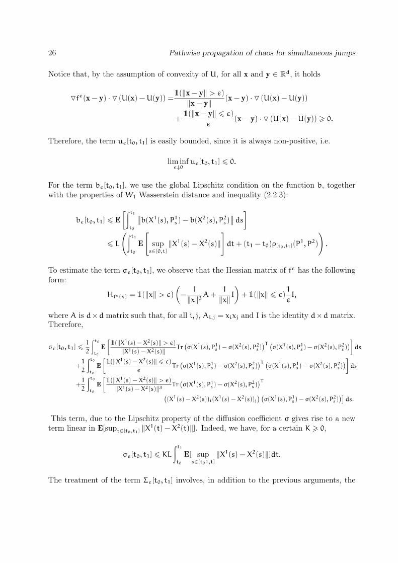
26 Pathwise propagation of chaos for simultaneous jumps
Notice that, by the assumption of convexity of U, for all x and y ∈ Rd, it holds
Ofε(x − y) · O (U(x) −U(y)) =1(‖x − y‖ > ε)
‖x − y‖ (x − y) · O (U(x) −U(y))
+1(‖x − y‖ 6 ε)
ε(x − y) · O (U(x) −U(y)) > 0.
Therefore, the term uε[t0, t1] is easily bounded, since it is always non-positive, i.e.
lim infε↓0
uε[t0, t1] 6 0.
For the term bε[t0, t1], we use the global Lipschitz condition on the function b, togetherwith the properties of W1 Wasserstein distance and inequality (2.2.3):
bε[t0, t1] 6 E
[∫ t1
t0
∥
∥b(X1(s), P1s) − b(X2(s), P2s)
∥
∥ds
]
6 L
(∫ t1
t0
E
[
sups∈[0,t]
‖X1(s) − X2(s)‖]
dt+ (t1 − t0)ρ[t0,t1](P1, P2)
)
.
To estimate the term σε[t0, t1], we observe that the Hessian matrix of fε has the followingform:
Hfε(x) = 1(‖x‖ > ε)(
−1
‖x‖3A+1
‖x‖I)
+ 1(‖x‖ 6 ε)1
εI,
where A is d×d matrix such that, for all i, j, Ai,j = xixj and I is the identity d×d matrix.Therefore,
σε[t0, t1] 61
2
∫t0
t0
E
[
1(‖X1(s) − X2(s)‖ > ε)‖X1(s) − X2(s)‖ Tr
(
σ(X1(s), P1s) − σ(X2(s), P2s)
)T (σ(X1(s), P1s) − σ(X
2(s), P2s))
]
ds
+1
2
∫t0
t0
E
[
1(‖X1(s) − X2(s)‖ 6 ε)
εTr(
σ(X1(s), P1s) − σ(X2(s), P2s)
)T (σ(X1(s), P1s) − σ(X
2(s), P2s))
]
ds
+1
2
∫t0
t0
E
[
1(‖X1(s) − X2(s)‖ > ε)‖X1(s) − X2(s)‖3 Tr
(
σ(X1(s), P1s) − σ(X2(s), P2s)
)T
(
(X1(s) − X2(s))i(X1(s) − X2(s))j
) (
σ(X1(s), P1s) − σ(X2(s), P2s)
)]
ds.
This term, due to the Lipschitz property of the diffusion coefficient σ gives rise to a newterm linear in E[supt∈[t0,t1]
‖X1(t) − X2(t)‖]. Indeed, we have, for a certain K > 0,
σε[t0, t1] 6 KL
∫ t1
t0
E[ sups∈[t01,t]
‖X1(s) − X2(s)‖]dt.
The treatment of the term Σε[t0, t1] involves, in addition to the previous arguments, the

27
Burkholder-Davis-Gundy inequalities and the global Lipschitz condition (Li1):
Σε[t0, t1] 6 C1 E
[(∫ t1
t0
∥
∥
∥
(
σ(X1(s), P1s) − σ(X2(s), P2s)
)T
(
σ(X1(s), P1s) − σ(X2(s), P2s)
)∥
∥ds)1/2
]
6 C1LE
(∫ t1
t0
sups∈[t0,t1]
‖X1(s) − X2(s)‖2dt+ (t1 − t0)ρ[t0,t1](P1, P2)2
)1/2
6 C1L√
(t1 − t0)
(
E
[
supt∈[t0,t1]
‖X1(t) − X2(t)‖]
+ ρ[t0,t1](P1, P2)
)
,
for some constant C1 not depending on t0, t1. To bound the term Λ[t0,t1], we make useof the properties of the process Λ(t)t∈[0,T ], of the W1 Wasserstein distance, as well ascondition (Li2) and monotone convergence theorem.
lim infε↓0
Λε[t0, t1] = E
[
supt∈[t0,t1]
∫t
t0
∫
[0,1]
∫∞
0
∥
∥
∥X1(s) +ψ(X1(s), P1s , h)1u6λ(X1(s),P1s) − X2(s)
−ψ(X2(s), P2s , h)1u6λ(X2(s),P2s)
∥
∥
∥− ‖X1(s) − X1(s)‖dsduν1(dh)]
6 E
[∫t1
t0
∫
[0,∞)×[0,1]
‖ψ(X1(s−), P1s− , h)1(0,λ(X1(s−),P1s−
)]
−ψ(X2(s−), P2s− , h)1(0,λ(X2(s−),P2s−
)]‖dsduν(dh)]
6 L
(∫t1
t0
E
[
sups∈[0,t]
‖X1(s) − X2(s)‖]
dt+ (t1 − t0)ρ[t0,t1](P1, P2)
)
.
Therefore,
E
[
supt∈[t0,t1]
‖X1(t) − X2(t)‖]
6E[
‖X1(t0) − X2(t0)‖]
+ L(
(K+ 1)(t1 − t0) + C1√t1 − t0
)
ρ[t0,t1](P1, P2)
+C1L√
(t1 − t0)E
[
supt∈[t0,t1]
‖X1(t) − X2(t)‖]
+L(1+ K)(t1 − t0)
∫ t1
t0
E
[
sups∈[0,t]
‖X1(s) − X2(s)‖]
dt.
By hypothesis, E [‖X(0) − Y(0)‖] = 0, then choose T0 > 0 such that 1 − C1L√T0 > 0.
Therefore we have
E
[
supt∈[0,T0∧T ]
‖X1(t) − X2(t)‖]
6L(1+ K)T0
1− C1L√T0
∫T0∧T
0
E
[
sups∈[0,t]
‖X1(s) − X2(s)‖]
dt
+L(
(1+ K)T0 + C1√T0)
1− C1L√T0
ρT0(P1, P2). (2.2.5)
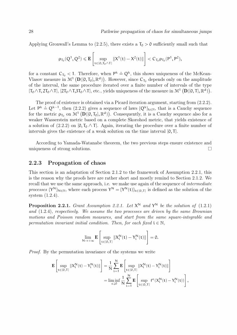
28 Pathwise propagation of chaos for simultaneous jumps
Applying Gronwall’s Lemma to (2.2.5), there exists a T0 > 0 sufficiently small such that
ρT0(Q1, Q2) 6 E
[
supt∈[0,T0∧T ]
‖X1(t) − X2(t)‖]
< CT0ρT0(P1, P2),
for a constant CT0 < 1. Therefore, when Pk .= Qk, this shows uniqueness of the McKean-Vlasov measure in M1
(
D([0, T0],Rd))
. However, since CT0 depends only on the amplitudeof the interval, the same procedure iterated over a finite number of intervals of the type[T0∧T, 2T0∧T ], [2T0∧T,3T0∧T ], etc., yields uniqueness of the measure in M1
(
D([0, T ],Rd))
.
The proof of existence is obtained via a Picard iteration argument, starting from (2.2.2).Let Pk .= Qk−1, then (2.2.2) gives a sequence of laws Qkk∈N, that is a Cauchy sequencefor the metric ρT0 on M1
(
D([0, T0],Rd))
. Consequently, it is a Cauchy sequence also for aweaker Wasserstein metric based on a complete Skorohod metric, that yields existence ofa solution of (2.2.2) on [0, T0 ∧ T ]. Again, iterating the procedure over a finite number ofintervals gives the existence of a weak solution on the time interval [0, T ].
According to Yamada-Watanabe theorem, the two previous steps ensure existence anduniqueness of strong solutions.
2.2.3 Propagation of chaos
This section is an adaptation of Section 2.1.2 to the framework of Assumption 2.2.1, thisis the reason why the proofs here are rather short and mostly remind to Section 2.1.2. Werecall that we use the same approach, i.e. we make use again of the sequence of intermediateprocesses YNN∈N, where each process YN = YN(t)t∈[0,T ] is defined as the solution of thesystem (1.2.4).
Proposition 2.2.1. Grant Assumption 2.2.1. Let XN and YN be the solution of (1.2.1)and (1.2.4), respectively. We assume the two processes are driven by the same Brownianmotions and Poisson random measures, and start from the same square-integrable andpermutation invariant initial condition. Then, for each fixed i ∈ N,
limN→+∞
E
[
supt∈[0,T ]
‖XNi (t) − YNi (t)‖]
= 0.
Proof. By the permutation invariance of the systems we write
E
[
supt∈[0,T ]
‖XNi (t) − YNi (t)‖]
=1
N
N∑
i=1
E
[
supt∈[0,T ]
‖XNi (t) − YNi (t)‖]
= lim infε↓0
1
N
N∑
i=1
E
[
supt∈[0,T ]
fε(XNi (t) − YNi (t))
]
,
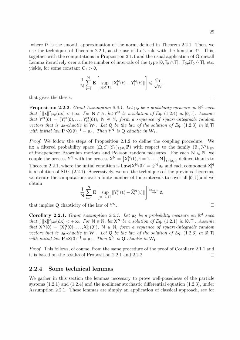
29
where fε is the smooth approximation of the norm, defined in Theorem 2.2.1. Then, weuse the techniques of Theorem 2.2.1, as the use of Ito’s rule with the function fε. This,together with the computations in Proposition 2.1.1 and the usual application of GronwallLemma iteratively over a finite number of intervals of the type [0, T0∧ T ], [T0,2T0∧ T ], etc.yields, for some constant CT > 0,
1
N
N∑
i=1
E
[
supt∈[0,T ]
‖XNi (t) − YNi (t)‖]
6CT√N,
that gives the thesis.
Proposition 2.2.2. Grant Assumption 2.2.1. Let µ0 be a probability measure on Rd such
that∫‖x‖2µ0(dx) < +∞. For N ∈ N, let YN be a solution of Eq. (1.2.4) in [0, T ]. Assume
that YN(0) = (YN1 (0), . . . , YNN(0)), N ∈ N, form a sequence of square-integrable random
vectors that is µ0-chaotic in W1. Let Q be the law of the solution of Eq. (1.2.3) in [0, T ]
with initial law P X(0)−1 = µ0. Then YN is Q chaotic in W1.
Proof. We follow the steps of Proposition 2.1.2 to define the coupling procedure. Wefix a filtered probability space (Ω,F, (Ft)t>0,P) with respect to the family (Bi,N
i)i∈N
of independent Brownian motions and Poisson random measures. For each N ∈ N, wecouple the process YN with the process XN =
XNi (t), i = 1, . . . ,N
t∈[0,T ]defined thanks to
Theorem 2.2.1, where the initial condition is Law(XN(0)) = ⊗Nµ0 and each component XNiis a solution of SDE (2.2.1). Successively, we use the techniques of the previous theorems,we iterate the computations over a finite number of time intervals to cover all [0, T ] and weobtain
1
N
N∑
i=1
E
[
supt∈[0,T ]
‖YNi (t) − XNi (t)‖]
N→∞→ 0,
that implies Q chaoticity of the law of YN.
Corollary 2.2.1. Grant Assumption 2.2.1. Let µ0 be a probability measure on Rd such
that∫‖x‖2µ0(dx) < +∞. For N ∈ N, let XN be a solution of Eq. (1.2.1) in [0, T ]. Assume
that XN(0) = (XN1 (0), . . . , XNN(0)), N ∈ N, form a sequence of square-integrable random
vectors that is µ0-chaotic in W1. Let Q be the law of the solution of Eq. (1.2.3) in [0, T ]
with initial law P X(0)−1 = µ0. Then XN is Q chaotic in W1.
Proof. This follows, of course, from the same procedure of the proof of Corollary 2.1.1 andit is based on the results of Proposition 2.2.1 and 2.2.2.
2.2.4 Some technical lemmas
We gather in this section the lemmas necessary to prove well-posedness of the particlesystems (1.2.1) and (1.2.4) and the nonlinear stochastic differential equation (1.2.3), underAssumption 2.2.1. These lemmas are simply an application of classical approach, see for

30 Pathwise propagation of chaos for simultaneous jumps
example Ikeda Watanabe [51], together with the trick used in the proof of Theorem 2.2.1.Well-posedness of equations (1.2.1) and (1.2.4) is clearly a consequence of Lemma 2.2.3,where there is no parametrizing measure, the state space of the process is R
N×d and wehave a finite number (precisely N) of Poisson integrals, instead of the one described in thestatement of the lemma.
Lemma 2.2.1. Consider the SDE parametrized by two measures α and β ∈ M(D([0, T ],Rd))
dX(t) =F(X(t), αt)dt+ σ(X(t−), αt)dBt (2.2.6)
+
∫
[0,∞)×[0,1]Nψ(Y(t−), αt− , h1)1(0,λ(Y(t−),αt−)](u)N(dt, du, dh),
with Law(Y) = β. If the coefficients satisfy Assumption 2.2.1, then for every α and β ∈M1(D([0, T ],Rd)), every square-integrable initial condition, there exists a unique strong so-lution to Eq. (2.2.6).
Moreover, let µ.= Law((X(t))t∈[0,T ]) be the law of the solution of (2.2.6) starting from
the square-integrable initial condition X(0) µ0-distributed, then µ ∈ M1(D([0, T ],Rd)).
Proof. Let B be an (Ft)-brownian motion, p be a (Ft)-stationary Poisson point processwith characteristic measure l × ν and ξ be a F0-measurable square-integrable r.v.. LetD.= s ∈ Dp s.t. p(s) ∈ Us = (0, λ(Y(s−), αs−)]×[0,1]×[0,1]×. . . . Let us call σ1 < σ2 < . . .
the elements of D. Each σn is an Ft -stopping time and limn→∞ σn = ∞ a.s.. Indeed, forevery T > 0 and for a fixed n ∈ N
∗,
P(σn 6 T) = P
(∫T
0
∫
[0,∞)×[0,1]N1(0,λ(Y(t−),αt−)](u)N(du, dh, dt) > n
)
6E [λ(Y(T), αT )]
n6CT
n,
for a certain constant CT . By Lemma 2.2.2, we get the claim. Then we start by showing∃! of a solution for (2.2.6) on [0, σ1]. Consider the equation
Z(t) = X(0) +
∫ t
0
F(Z(s), αs)ds+
∫ t
0
σ(Z(s−), αs)dBs. (2.2.7)
Existence and uniqueness of a strong solution for (2.2.7) are ensured by the classical Has-minskii’s test for non-explosion (see e.g. [66] with the Lyapunov function V(z) = ‖z‖2).The test’s conditions are guaranteed by the inequality
supα∈M1(Rd)
z · F(z, α) + tr(σ(z, α)σT (z, α)) 6 C(1+ ‖z‖2), (2.2.8)
for some C > 0, for all z ∈ Rd. Indeed, fix an α ∈ M1(Rd). Then, under (U) from
Assumption 2.2.1, we have
z · F(z, α) = −(z− 0) · (OU(z) − OU(0)) + z · OU(0) + z · b(z, α) 6 C(
‖z‖2 + 1)
,
due to the convexity of U and the linear growth of b. A similar bound is obtained forthe second summand in the l.h.s of (2.2.8), which has uniform quadratic growth in the z

31
variable. Then, for every integrable initial condition, there exists a unique strong solutionto (2.2.7). Let π1 be the projection defined as
π1 : [0,1]N × [0,∞) 7→ [0,1]
(h, u) → h1,
we define
X1(t) =
Z1(t) t ∈ [0, σ1),
Z1(σ−1 ) +ψ(Z1(σ−1 ), α(σ
−1 ), π1 p(σ1)) t = σ1,
(2.2.9)
where Z1(t)t>0 is solution of (2.2.7) with initial condition Z1(0) = ξ a.s.. We see thatX1(t) is solution of (2.2.6) for t ∈ [0, σ1]. We iterate the procedure by setting ξ .= X1(σ1),B.= (B(t + σ1) − B(σ1))t>0 and p .
= (p(t + σ1))t>0. We define X1(t) for t ∈ [0, σ1] as wedid for X1(t) in (2.2.9), where σ1 is the smallest time such that ps belongs to Uσ1+s andcoincides with σ2 − σ1. We define
X2(t) =
X1(t) t ∈ [0, σ1],
X1(t− σ1) t ∈ [σ1, σ2].
Clearly X2 is solution of (2.2.6) for t ∈ [0, σ2]. Since limn→∞ σn = ∞ a.s., we can iteratethis procedure to cover the entire time interval [0, T ].
To prove that the law µ of a solution of (2.2.6) belongs to M1(D([0, T ],Rd)), we will showthat there exists a filtered probability space (Ω,P, (Ft),F), with a Ft-Brownian motion B,an adapted Ft Poisson random measure N with characteristic measure l × l × ν and aF0-measurable initial condition X(0) µ0-distributed such that E
[
supt∈[0,T ] ‖X(t)‖]
< ∞.We consider the process X(t), for all t > 0, solution of (2.2.6). Now, we use the trick ofapplying Ito’s rule to the smooth approximation fε of ‖ · ‖ and taking the limit for ε ↓ 0, toexploit the properties of the potential function U. For the details of the approach, see theproof of Theorem 2.2.1. Then, for the properties of coefficients and quantities involved,there exist three positive constants D1, D2 and D3 s.t.
E
[
supt∈[0,T ]
‖X(t)‖]
6 E [‖X(0)‖] +D1T +D2T E
[
supt∈[0,T ]
‖Y(t)‖]
+D1
∫T
0
E
[
sups∈[0,t]
‖X(s)‖]
dt.
We apply Gronwall Lemma and we get the desired bound.
Lemma 2.2.2. Let σnn∈N∗ be a sequence of strictly increasing stopping times. If, for allT > 0, there exists a constant CT > 0 such that
P(σn 6 n) 6CT
n,
then limn→∞ σn = ∞ a.s..

32 Pathwise propagation of chaos for simultaneous jumps
Proof. We start by proving that, for all T > 0, there exists a measurable set ΛT withprobability one, such that for all ω ∈ ΛT , there exists n0(ω, T) and for all n > n0(ω, T) itholds σn(w) > T .
Let An.= σn2 6 T and A .
=
∞⋂
n=1
∞⋃
i=n
Ai, therefore we have
∞∑
n=1
P(An) 6
∞∑
n=1
CT
n2<∞
and for Borel Cantelli P(A) = 0. Let ΛT.= AC, then it has probability one and for all
ω ∈ ΛT there exists n0(ω, T) such that for all n > n0(ω, T) we have σn2 > T . Since the σnare increasing, we have the claim that there exists n0(ω, T) such that for all n > n0(ω, T),σn > T .Now, let Λ .
=⋂
T∈N
ΛT , then P(Λ) = 1 and for all ω ∈ Λ for all T > 0 there exists n0(ω, T)
s.t. for all n > n0(ω, T) then σn(ω) > T . This implies σn ∞ a.s..
We are now ready to prove the most important lemma of this section, the one thatallows us to prove well-posedness of SDE with jumps if the drift satisfies condition (U) andthat it is crucial in the proof of Theorem 2.2.1.
Lemma 2.2.3. Consider the SDE parametrized by a measure α ∈ M1(D([0, T ],Rd))
dX(t) =F(X(t), αt)dt+ σ(X(t), αt)dBt (2.2.10)
+
∫
[0,∞)×[0,1]Nψ(X(t−), αt− , h1)1(0,λ(X(t−),αt−)](u)N(dt, du, dh).
If the coefficients satisfy Assumption 2.2.1, then for every α ∈ M1(D([0, T ],Rd)) and everysquare-integrable initial condition, there exists a unique strong solution to Eq. (2.2.10).
Proof. First let X1 and X2 be two integrable stochastic processes on [0, T ] with values inRd. We define the map that associates the law of Xk to the law of the solution of
dYk(t) =F(Yk(t), αt)dt+ σ(Yk(t), αt)dBt (2.2.11)
+
∫
[0,∞)×[0,1]Nψ(Xk(t−), αt− , h1)1(0,λ(Xk(t−),αt−)](u)N(dt, du, dh),
that is well-defined for Lemma 2.2.1. With the same computation of the proof of Theo-rem 2.2.1, we get that, for a small enough T0 > 0, there exists a constant CT0 < 1 suchthat
E
[
supt∈[0,T0]
‖Y1(t) − Y2(t)‖]
6 CT0 E
[
supt∈[0,T0]
‖X1(t) − X2(t)‖]
.
This shows pathwise uniqueness for solution of (2.2.10). By means of (2.2.11), we define aPicard iteration argument that gives a sequence of laws Qnn∈N
on D([0, T ],Rd). Again,

33
there exists a T0 > 0 small enough such that Qnn∈Nis a Cauchy sequence for ρT0 and
hence for a weaker but complete Wasserstein metric on M1(D([0, T0],Rd)). Iterating the
procedure over a finite number of time intervals, to cover [0, T ], yields tweak existence ofa solution. The integrability property is proved as in the proof of Lemma 2.2.1. ThenYamada-Watanabe theorem concludes the proof.
Let us highlight that, in the proof of Lemma 2.2.3, we need to define the map bymeans of (2.2.11) and we could not straightly substitute Xk in the whole right-hand sideof (2.2.10). In fact, we need to control the jumps by means of a known process, but atthe same time, we need to have the same variable as argument of the drift coefficient toexploit the convexity of the potential function U.
2.3 Non-globally Lipschitz jump rate
In this section we want to extend our study to a class of systems in which the jump rateis super-linear. This is mainly motivated by the neuroscience models we introduced inSection 1.1.2, from which comes the inspiration of this study. In [29, 43, 75] the authorspresent two piece-wise deterministic Markov processes (PDMPs) of interacting neuronswith the feature of simultaneous jumps, that we summarized (at the microscopic level) in(1.1.1). In this section we extend the model to a d-dimensional framework and we slightlygeneralize the jumps’ amplitude and rate functions, but we neglect the term modellingelectrical synapses, by choosing β = 0. This results in a d-dimensional extension of themodel in [75].
2.3.1 Assumptions and well-posedness of the particle system
We consider, as the initial particle system, the PDMP XN solution of the following SDE:
dXNi (t) =−XNi (t)dt+1
N
∑
j6=i
∫
[0,∞]×[0,1]NV(hj, hi)1[0,λ(XNj (t)))(u)N
j(dt, du, dh)
−
∫
[0,∞)×[0,1]N
(
XNi (t) −U(hi))
1[0,λ(XNi (t)))(u)Ni(dt, du, dh) (2.3.1)
for all i = 1, . . . ,N. As before, (Ni)i∈N is an independent family of Poisson randommeasures Ni, each of them with characteristic measure l × l × ν. Remember that ν is asymmetric probability measure on [0,1]N such that it exists a consistent family of symmetricprobability measures (νN)N∈N
, each of them defined respectively on [0,1]N and coincidingwith the projections of ν on N coordinates.
Assumption 2.3.1. The coefficients of the system (2.3.1) obey the following properties:
(JR) the jump rate of each particle is a non-negative C1 function of its position, λ : Rd →R+, that is written as the sum of two functions:
λ(·) .= b(‖ · ‖) + h(·).

34 Pathwise propagation of chaos for simultaneous jumps
- b is a C1, positive, non-decreasing function such that
b ′(r) 6 γb(r) + c (2.3.2)
for some c > 0 and γ <1
5E[‖V‖] ;
- h : Rd → R is a C1 bounded function, i.e. there exists H > 0 such that ∀ x ∈ Rd,
‖h(x)‖ 6 H;
(JA) the jump amplitudes, V and U, are two bounded functions from respectively [0,1]2 and[0,1] to R
d (since they represents two random variables with values in some boundedsubsets of Rd, with abuse of notation we will indicate as expectations their integralsw.r.t. the measure ν ).
Notice that the form of the function b is exactly the one suggested by [75]. Theassumption
γ <1
5E[‖V‖]allows to obtain apriori bounds on the moments of λ(X(t)), where X(t) is the solution ofthe corresponding McKean-Vlasov equation, see (2.3.3), and it is used in the proofs of nextLemmas 2.3.4 and 2.3.5. It is interesting to notice that Assumption 2.3.1 allows to considernon-globally Lipschitz functions; in particular, this covers all the cases where b(r) is of theform rα, for α > 1. We also remark that the condition on b here is a little stronger thanin [75], due to the coupling method (vs. the martingale approach) in the proof, which inparticular allows to identify the rate of convergence, which is of the order O
(
1√N
)
. This
requires γ <1
KE[‖V‖] with K = 5 rather than K = 3, as in [75].
We will deal with initial conditions with bounded support and, if the function b isconvex, we could adapt our computations to include a drift towards the barycenter of thesystem, that would be an extention to the model in [43]. However, in [43], the authorssucceed in proving propagation of chaos with an explicit rate (namely, the expected 1√
N)
even for weaker conditions on the initial values, by defining an ad-hoc distance based onthe rate function λ itself. In our study, we choose not to extend this powerful approach toour d-dimensional model and to maintain the same structure of proofs of the previous sec-tions. However, we believe that the computations of [43] would work here and they wouldgive results without the restrictive hypothesis on the bounded support of initial conditionthat we require from Section 2.3.2 to the end of the chapter.
Let us start by proving well-posedness of (2.3.1), this relies on a truncation argumenton the function λ.
Lemma 2.3.1. Under Assumption 2.3.1, for every integrable initial condition XN(0) ∈Rd×N, the SDE (2.3.1) admits a unique solution.

35
Proof. The main issue is represented by the fact that the function λ is not bounded, neitherglobally Lipschitz continuous. For λ bounded or globally Lipschitz continuous, existenceand uniqueness of solutions for (2.3.1) are consequences of standard results, see [51].
Let us consider the truncate function λK .= λ∧ K, for K ∈ N, and the solution XN,K(t)
of (2.3.1) with the function λK instead of λ. This solution exists and it is unique for allt ∈ [0, T ]. By pathwise uniqueness, it holds XN,K(t) = XN,K+1(t) for all t ∈ τK, where
τK.= inf
t /‖XN,K(t)‖ > K
.
Therefore τK 6 τK+1 a.s. and there exists a pathwise unique solution X(t) to (2.3.1), de-fined for all t ∈ [0, τ), where τ .= supK∈N
τK. We are left to prove that P(τ > T) = 1.
Let us fix i ∈ 1, . . . ,N and ε > 0. We compute, by means of Ito’s formula, fε(XNi (t)),where fε is the function defined in (2.2.4). We get
fε(XNi (t)) 6 fε(XNi (0))
+∑
j6=i
∫t
0
∫
[0,1]N
∫∞
0
(
fε(
XNi (s) +V(hj, hi)
N
)
− fε(
XNi (s))
)
1(0,λ(XNj (s))](u)Nj(ds, du, dh)
+
∫t
0
∫
[0,1]N
∫∞
0
(
fε (U(hi)) − fε(
XNi (s)))
1(0,λ(XNi (s))](u)Ni(ds, du, dh),
that, of course, is bounded by the following expression
fε(XNi (t)) 6 fε(XNi (0)) +
1
N
N∑
j=1
∫t
0
∫
[0,1]N
∫∞
0
fε(
V(hj, hi))
1(0,λ(XNj (s))](u)Nj(ds, du, dh)
+
∫t
0
∫
[0,1]N
∫∞
0
(
fε (U(hi)) − fε(
XNi (s)))
1(0,λ(XNi (s))](u)Ni(ds, du, dh).
Summing on all i = 1, . . . ,N and taking expectation, by the application of Fatou’s Lemma,we get:
E
[
1
N
N∑
i=1
‖XNi (t)‖]
6 lim infε↓0
(
E
[
1
N
N∑
i=1
fε(XNi (0))
]
−
∫ t
0
E
[
1
N
N∑
i=1
fε(XNi (s))λ(XNi (s))
]
ds
+
∫ t
0
(E[fε(V)] + E[fε(U)])E
[
1
N
N∑
i=1
λ(XNi (s))
]
ds
)
Then, by monotone convergence, we have
E
[
1
N
N∑
i=1
‖XNi (t)‖]
6E
[
1
N
N∑
i=1
‖XNi (0)‖]
−
∫ t
0
E
[
1
N
N∑
i=1
‖XNi (s)‖λ(XNi (s))]
ds
+
∫ t
0
(E[‖V‖] + E[‖U‖])E
[
1
N
N∑
i=1
λ(XNi (s))
]
ds
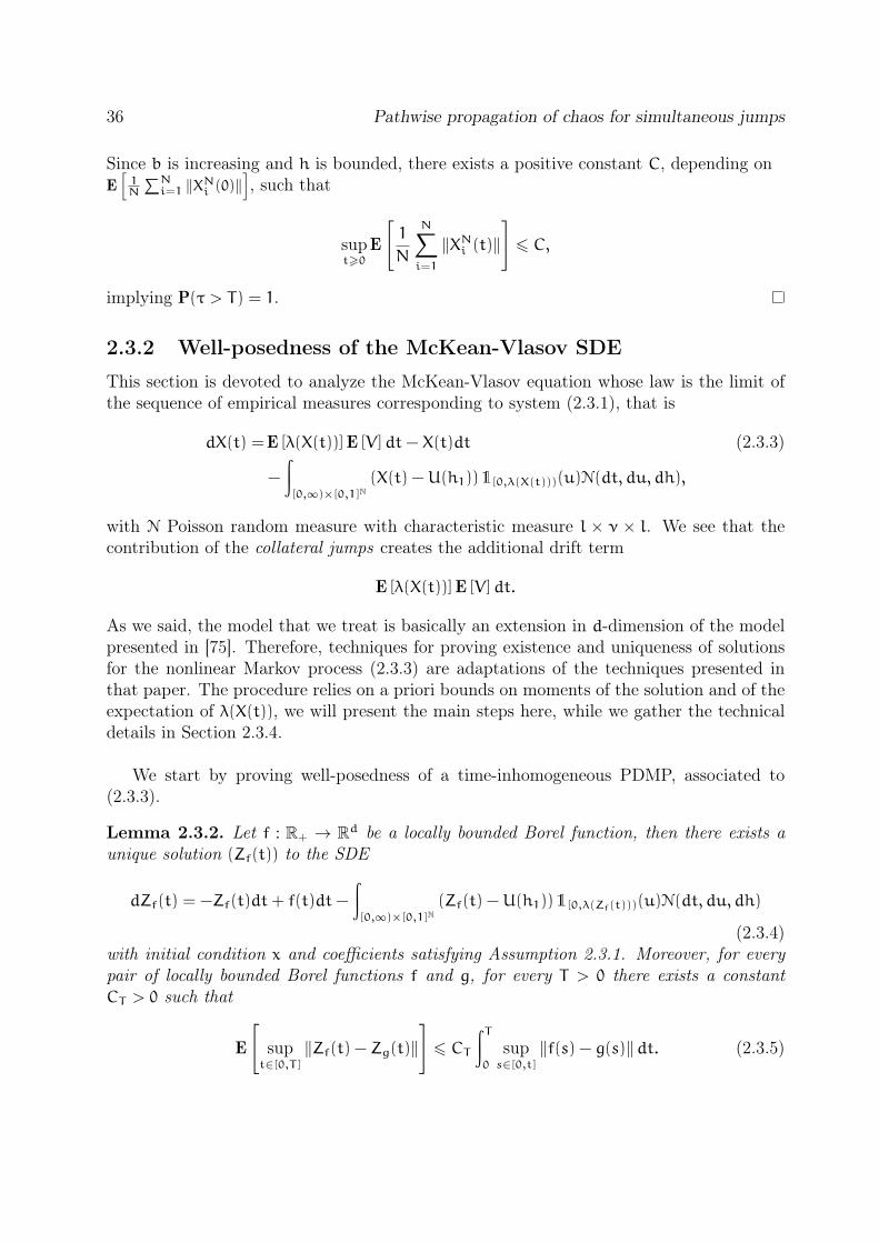
36 Pathwise propagation of chaos for simultaneous jumps
Since b is increasing and h is bounded, there exists a positive constant C, depending onE
[
1N
∑Ni=1 ‖XNi (0)‖
]
, such that
supt>0
E
[
1
N
N∑
i=1
‖XNi (t)‖]
6 C,
implying P(τ > T) = 1.
2.3.2 Well-posedness of the McKean-Vlasov SDE
This section is devoted to analyze the McKean-Vlasov equation whose law is the limit ofthe sequence of empirical measures corresponding to system (2.3.1), that is
dX(t) =E [λ(X(t))]E [V]dt− X(t)dt (2.3.3)
−
∫
[0,∞)×[0,1]N(X(t) −U(h1))1[0,λ(X(t)))(u)N(dt, du, dh),
with N Poisson random measure with characteristic measure l × ν × l. We see that thecontribution of the collateral jumps creates the additional drift term
E [λ(X(t))]E [V]dt.
As we said, the model that we treat is basically an extension in d-dimension of the modelpresented in [75]. Therefore, techniques for proving existence and uniqueness of solutionsfor the nonlinear Markov process (2.3.3) are adaptations of the techniques presented inthat paper. The procedure relies on a priori bounds on moments of the solution and of theexpectation of λ(X(t)), we will present the main steps here, while we gather the technicaldetails in Section 2.3.4.
We start by proving well-posedness of a time-inhomogeneous PDMP, associated to(2.3.3).
Lemma 2.3.2. Let f : R+ → Rd be a locally bounded Borel function, then there exists a
unique solution (Zf(t)) to the SDE
dZf(t) = −Zf(t)dt+ f(t)dt−
∫
[0,∞)×[0,1]N(Zf(t) −U(h1))1[0,λ(Zf(t)))(u)N(dt, du, dh)
(2.3.4)with initial condition x and coefficients satisfying Assumption 2.3.1. Moreover, for everypair of locally bounded Borel functions f and g, for every T > 0 there exists a constantCT > 0 such that
E
[
supt∈[0,T ]
‖Zf(t) − Zg(t)‖]
6 CT
∫T
0
sups∈[0,t]
‖f(s) − g(s)‖dt. (2.3.5)
37
It is clear that, if we choose the function f in a suitable way, i.e.
f(t).= E [λ(X(t))]E [V] ,
the solution Zf to (2.3.4) coincides with the solution X to (2.3.3). Then we derive a prioribounds for any solution of (2.3.3), that are necessary to perform the iteration that yields tothe existence and uniqueness of the nonlinear process itself. The following lemma providesthe required bounds.
Lemma 2.3.3. Suppose Assumption 2.3.1 is satisfied. Let X be a solution of (2.3.3) withintegrable initial condition X(0); then we have that supt>0 E [‖X(t)‖] < ∞. Moreover, forp = 1,2, 3, 4, if E [λp(X(0))] < ∞ then supt>0 E [λp(X(t))] 6 C < ∞, where C only dependson E [λp(X(0))] and on the parameters of equations (2.3.3).
Last, we prove well-posedness of the nonlinear PDMP (2.3.3).
Theorem 2.3.1 (Solution of the McKean-Vlasov equation). Under Assumption 2.3.1, forany initial condition X(0) with bounded support and independent of N, there exists a uniquestrong solution X(t)t∈[0,T ] for (2.3.3).
Let us sketch the idea of the proof. We prove well-posedness of a nonlinear process, inwhich we truncate the nonlinear drift term above a certain threshold. Since Lemma 2.3.3gives a priori bounds on the drift term itself, we can identify (2.3.3) with processes belongingto this class and we get the thesis.
Proof of Theorem 2.3.1. Fix a constant C > 0, and consider the following Picard iteration:ZC0 (t) ≡ X(0) and
dZCn(t) = −ZCn(t)dt+(
E[
λ(ZCn−1(t))]
∧ C)
E [V]dt
−∫
[0,∞)×[0,1]N
(
ZCn(t) −U(h1))
1[0,λ(ZCn(t)))(u)N(dt, du, dh),
ZCn(0) = X(0)
The following almost sure apriori bound is essentially obvious: for any n > 1
‖ZCn(t)‖ 6 K+ tCE[‖V‖],for a suitable K > 0 depending on the support of X(0) and the range of U(h). Indeed,when ‖ZC(t)‖ is large, the linear term −ZCn(t)dt as well as the jumps can only decreasethe norm. From Lemma 2.3.2 we now that there exists a constant CT such that
E
[
supt∈[0,T ]
‖ZCn+1(t) − ZCn(t)‖]
6 CT E [‖V‖]∫T
0
∥
∥E[
λ(ZCn(s))]
− E[
λ(ZCn−1(s))]∥
∥ds.
Thanks to the a.s. bounds on ‖ZCn(t)‖, we can exploit the local Lipschitzianity of λ andget, for a certain constant KT > 0,
E
[
supt∈[0,T ]
‖ZCn+1(t) − ZCn(t)‖]
6CT E [‖V‖]KT∫T
0
E
[
sups∈[0,t]
‖ZCn(s) − ZCn−1(s)‖]
dt
6 · · · 6 (KTCT E [‖V‖] T)nn!
E
[
sups∈[0,t]
‖ZC1 (s) − ZC0 (s)‖]
.

38 Pathwise propagation of chaos for simultaneous jumps
Therefore the sequence ZCnn∈N is a Cauchy sequence and its limit ZC is a solution of theSDE
dZC(t) = − ZC(t)dt+(
E[
λ(ZC(t))]
∧ C)
E [V]dt
−
∫
[0,∞)×[0,1]N
(
ZC(t−) −U(h1))
1[0,λ(ZC(t−)))(u)N(dt, du, dh).
By Lemma 2.3.3, we can choose C so that E[
λ(ZC(t))]
6 C for all t, so that ZC is indeed asolution of (2.3.3). Uniqueness is given by considering two solutions Z1 and Z2. Using theabove apriori bound, (2.3.5) and the Gronwall Lemma their equality follows from standardarguments.
2.3.3 Propagation of Chaos
As in the previous sections, we use the intermediate process YN(t)t∈[0,T ] that, in this case,is the solution of the system: for all i = 1, . . . ,N
dYNi (t) =−YNi (t)dt+1
N
N∑
j=1
E [V] λ(YNj (t))dt (2.3.6)
−
∫
[0,∞)×[0,1]N
(
YNi (t) −U(hi))
1[0,λ(YNi (t)))(u)Ni(dt, du, dh).
Well-posedness of (2.3.6) follows from Lemma 2.3.1. In order to use a coupling procedure toprove propagation of chaos, we need to set some a priori bounds on the involved quantities.
Lemma 2.3.4. For N > 0, under Assumption 2.3.1, let XN and YN be solutions, respec-tively, of (2.3.1) and (2.3.6), starting from initial conditions s.t. E
[
〈µNX (0), λ4(·)〉]
< ∞
and E[
〈µNY (0), λ4(·)〉]
<∞ . Then there exists a certain N0 > 0 such that it holds
supN>N0
supt>0
E[
〈µNX (t), λ4(·)〉]
<∞,
supN>N0
supt>0
E[
〈µNY (t), λ4(·)〉]
<∞.
Lemma 2.3.4 is crucial for proving that the number of jumps of the system in a compacttime interval is proportional to N with probability increasing with N. This bound is statedin the following lemma.
Lemma 2.3.5 (Bound on the number of jumps). Assume that Assumption 2.3.1 is satisfiedand that, for any N > 0, XN and YN are solutions, respectively, of (2.3.1) and (2.3.6),starting from initial conditions that are µ0-chaotic. Here µ0 is a probability measure onRd s.t. Eµ0
[
λ3(X)]
< ∞. Then, for any T > 0, there exists a positive constant HT and anatural number N0 > 0 such that, for certain positive constants KT and KT
P
(
CN(T)
N> HT
)
6KT
N
P
(∫T
0
〈µNY (s), λ〉ds > HT)
6KT
N,

39
for all N > N0. Here CN(T) is the number of jumps performed by system (2.3.1) up totime T .
The bounds on the number of collateral jumps and of the corresponding drift in acompact time interval plays a role in the proof of propagation of chaos, since they let usexploit the local Lipschitzianity of the function λ when we start from initial conditionswith bounded support. The proofs of these lemmas involve the form of the function λ andthey are in Section 2.3.4. In the following we state and prove the result on propagation ofchaos and also in this case, the simultaneous jumps result in a rate of the order 1√
N. As in
the previous sections, we start with the comparison between the particle system XN andthe intermediate system YN.
Theorem 2.3.2. Let Assumptions 2.3.1 be satisfied and let XN and YN be the solution, re-spectively, of (2.3.1) and (2.3.6) with permutation invariant initial condition with compactsupport XN(0) = YN(0) a.s. that are µ0-chaotic, with µ0 probability measure on R
d withcompact support. We assume the two processes are driven by the same Poisson randommeasures. Then, for each fixed i ∈ N,
limN→+∞
E
[
supt∈[0,T ]
‖XNi (t) − YNi (t)‖]
= 0.
Proof. As in previous sections, by permutation invariance of the initial conditions and ofthe dynamics, we have
E
[
supt∈[0,T ]
‖XNi (t) − YNi (t)‖]
=1
N
N∑
i=1
E
[
supt∈[0,T ]
‖XNi (t) − YNi (t)‖]
.
Let us start with
E
[
supt∈[0,T ]
‖XNi (t) − YNi (t)‖]
6 E
[∫T
0
∥
∥XNi (t) − YNi (t)
∥
∥dt
]
+ VXNi ,YNi(T) +UXNi ,Y
Ni(T),
where, for simplicity, we have set:
VXNi ,YNi(T)
.= E
supt∈[0,T ]
∥
∥
∥
∥
∥
∥
E[V]
N
N∑
j=1
∫t
0
λ(XNj (s)) − λ(YNj (s))ds−
E[V]
N
∫t
0
λ(XNi (s))ds
+1
N
∑
j6=i
∫t
0
∫
[0,1]N
∫∞
0
V(hi, hj)1[0,λ(XNj (s))(u)Nj(ds, du, dh)
∥
∥
∥
∥
∥
∥
;
UXNi ,YNi(T)
.= E
[
supt∈[0,T ]
∥
∥
∥
∥
−
∫t
0
∫
[0,1]N
∫∞
0
(XNi (s) −U(hi))1[0,λ(XNi (s)))(u)
−(YNi (s) −U(hi))1[0,λ(YNi (s)))(u)Ni(ds, du, dh)
∥
∥
∥
]
.
40 Pathwise propagation of chaos for simultaneous jumps
With the notation of Lemma 2.3.5, we consider the positive constant HT and the event
EN.=
CN(T)
N6 HT
∩∫T
0
〈µNY (s), λ〉ds 6 HT
,
such that P (EcN) → 0 for N→ ∞. Obviously, under the event EN, for all i = 1, . . . ,N, thequantities supt∈[0,T ] λ(X
Ni (t)) and supt∈[0,T ] λ(Y
Ni (t)) are uniformly bounded and we can
exploit local Lipschitzianity of λ (we will indicate its Lipschitz constant as LHT ). Thus, webound the first terms in VXNi ,YNi (T) in the following way:
E
supt∈[0,T ]
∥
∥
∥
∥
∥
∥
E[V]
N
N∑
j=1
∫t
0
λ(XNj (s)) − λ(YNj (s))ds
∥
∥
∥
∥
∥
∥
6E[‖V‖]N
N∑
j=1
E
[(∫T
0
LHT‖XNj (s) − YNj (s)‖ds
)
1EN
]
+E[‖V‖]E
∫T
0
1
N
N∑
j=1
|λ(XNj (s))|+ |λ(YNj (s))|ds
1ECN
6 LHTE[‖V‖]
∫T
0
1
N
N∑
j=1
E
[
sups∈[0,t]
‖XNj (s) − YNj (s)‖]
dt+
∫T
0
E[‖V‖]N
N∑
j=1
√
P(ECN)
√
E
[
|λ(XNj (s))|2]
ds
+
∫T
0
E[‖V‖]N
N∑
j=1
√
P(ECN)
√
E
[
|λ(YNj (s))|2]
ds
6 LHTE[‖V‖]
∫T
0
1
N
N∑
j=1
E
[
sups∈[0,t]
‖XNj (s) − YNj (s)‖]
dt+
∫T
0
E[‖V‖]√
P(ECN)
√
E[
〈µNX (s), |λ(·)|2〉]
ds
+
∫T
0
E[‖V‖]√
P(ECN)
√
E[
〈µNY (s), |λ(·)|2〉]
ds.
By Lemma 2.3.4 there exists N0 > 0 such that for all N > N0 supt>0 E[
〈µNX (s), |λ(·)|2〉]
andsupt>0 E
[
〈µNY (s), |λ(·)|2〉]
are bounded. By Lemma 2.3.5, there exists a constant KT > 0
such that P(ECN) 6KTN
. The second term in VNXNi ,Y
Ni(T) is bounded by exchangeability of
the XNi and by Lemma 2.3.4. Indeed, we have
E
[
supt∈[0,T ]
∥
∥
∥
∥
E[V]
N
∫ t
0
λ(XNi (s))ds
∥
∥
∥
∥
]
6E[V]
N
∫T
0
supt∈[0,T ]
E[
〈µNX (t), |λ(·)|〉]
dt.
To bound the third term we use Burkholder-Davis-Gundy inequality, the orthogonality ofthe martingales Njj∈N and Lemma 2.3.4.
E
[
supt∈[0,T ]
∥
∥
∥
∥
∥
1
N
N∑
j6=1
∫ t
0
∫ t
0
∫
[0,1]N
∫∞
0
V(hi, hj)1(0,λ(XNj (s))](u)Nj(ds, du, dh)
∥
∥
∥
∥
∥
]
6M
NE
(
N∑
j6=i
∫T
0
E[‖V‖2]λ(XNj (s))ds)1/2
6
√
E[‖V‖2]N
E
[
(∫T
0
〈µNX (t), λ(·)〉dt)1/2
]
.

41
Therefore we get that there exists three constants CT ,KT and MT such that, for all N > N0,
VNXNi ,Y
Ni(T) 6 CT
∫T
0
E
[
sups∈[0,t]
‖XN(s) − YN(s)‖2]
dt+KT√N
+MT
N.
With a similar argument, we get a bound of the same type for UXNi ,YNi (T).
1
N
N∑
i=1
UXNi ,YNi(T) 6 CT
∫T
0
1
N
N∑
i=1
‖XNi (t) − YNi (t)‖dt+ E
[
1ECN
∫T
0
1
N
N∑
i=1
‖XNi (t)‖λ(XNi (t))dt]
+ E
[
1ECN
∫T
0
1
N
N∑
i=1
‖YNi (t)‖λ(YNi (t))dt
]
+ E[‖U‖]E[
1ECN
∫T
0
1
N
N∑
i=1
λ(XNi (t))dt
]
+ E[‖U‖]E[
1ECN
∫T
0
1
N
N∑
i=1
λ(YNi (t))dt
]
.
As before, we wish to get a bound of the order O(
1√N
)
for the last terms. We do that
by means of Cauchy-Schwartz inequality, Lemma 2.3.4 and Lemma 2.3.5. We also exploitthat, by definition of λ , it holds ‖x‖ 6 Bλ(x) + c for a positive constant B and a constantc. Take, for instance, the second term of the right-hand side, it holds
E
[
1ECN
∫T
0
1
N
N∑
i=1
‖XNi (t)‖λ(XNi (t))dt]
6
∫T
0
√
P(ECN)
√
√
√
√
√E
(
1
N
N∑
i=1
‖XNi (s)‖λ(XNi (s)))2
ds
6 T
√
P(ECN)
√
√
√
√E
[
supt∈[0,T ]
〈µNX (t), ‖ · ‖2〉〈µNX (t), λ(·)2〉]
6 T
√
P(ECN)
√
√
√
√E
[
supt∈[0,T ]
〈µNX (t), λ(·)4〉]
.
The same holds for the remaining right-hand side terms. Thus, there exists two constantsCT and KT and a N0 > 0, such that for all N > N0 it holds
1
N
N∑
i=1
UXNi ,YNi (T) 6 CT
∫T
0
E
[
sups∈[0,t]
‖XN(s) − YN(s)‖]
dt+KT√N.
Thus, there exist three constants, that with abuse of notation we will indicate as CT ,KTand MT , depending only on T , and N0 > such that, for all N > N0 it holds
E
[
supt∈[0,T ]
‖XN(t) − YN(t)‖]
6 CT
∫T
0
E
[
sups∈[0,t]
‖XN(s) − YN(s)‖]
dt+KT√N
+MT
N.
By applying Gronwall lemma we get the thesis.
42 Pathwise propagation of chaos for simultaneous jumps
Theorem 2.3.3 (Propagation of Chaos for YN). Grant Assumptions 2.3.1. Let µ0 bea probability measure on R
d with compact support. For N ∈ N, let YN be a solution ofEq. (2.3.6) in [0, T ]. Assume that YN(0) = (YN1 (0), . . . , Y
NN(0)), N ∈ N, form a sequence of
compact support random vectors that is µ0-chaotic in W1. Let Q be the law of the solutionof Eq. (2.3.3) in [0, T ] with initial law P X(0)−1 = µ0. Then YN is Q chaotic in W1.
The proof of this theorem is a combination of the computations done for proving The-orem 2.3.2 and the coupling techniques for propagation of chaos used in the previoussections.
Proof of Theorem 2.3.3. We follow the steps of Proposition 2.1.2 and 2.2.2 to define thecoupling procedure. We fix a filtered probability space (Ω,F, (Ft)t>0,P) with respect to thefamily (Bi,N
i)i∈N of independent Brownian motions and Poisson random measures. Foreach N ∈ N, we couple the process YN with the process XN =
XNi (t), i = 1, . . . ,N
t∈[0,T ]
defined thanks to Theorem 2.2.1, where the initial condition is Law(XN(0)) = ⊗Nµ0 andeach component XNi is a solution of SDE (2.2.1). We start with
E
[
supt∈[0,T ]
‖YNi (t) − XNi (t)‖]
6 E
[∫T
0
∥
∥YNi (t) − XNi (t)
∥
∥dt
]
+UYNi ,XNi(T)
+ E
[
supt∈[0,T ]
∥
∥
∥
∥
∥
E[V]
N
N∑
j=1
∫ t
0
λ(YNj (s)) − E[λ(XNi (s))]ds
∥
∥
∥
∥
∥
]
,
where UYNi ,XNi (T) is defined as in the proof of Theorem 2.3.2. We use Lemma 2.3.3, 2.3.4and 2.3.5, together with local Lipschitzianity of λ and µ0-choaticity of the initial conditionsto get
1
N
N∑
i=1
E
[
supt∈[0,T ]
‖YNi (t) − XNi (t)‖]
N→∞→ 0,
that implies Q chaoticity of the law of YN.
As in the previous sections, these results imply propagation of chaos for XN, as thefollowing corollary states.
Corollary 2.3.1 (Propagation of Chaos for XN). Grant Assumptions 2.3.1. Let µ0 bea probability measure on R
d with compact support. For N ∈ N, let XN be a solution ofEq. (2.3.1) in [0, T ]. Assume that XN(0) = (XN1 (0), . . . , X
NN(0)), N ∈ N, form a sequence of
compact support random vectors that is µ0-chaotic in W1. Let Q be the law of the solutionof Eq. (2.3.3) in [0, T ] with initial law P X(0)−1 = µ0. Then XN is Q chaotic in W1.
2.3.4 Additional lemmas and proofs
We collect here the proofs of the various lemmas stated in Section 2.3 and some othertechnical result necessary for these proofs. First, we prove Lemma 2.3.2 and, thanksto two technical lemmas, we give the proof of Lemma 2.3.3, crucial for the existence
43
and uniqueness of solution of the nonlinear process (2.3.3). Then, we give the proofs ofLemma 2.3.4 and Lemma 2.3.5, that we use in the propagation of chaos section. Noticethat, the key ingredient here is represented by the fact that all the main jumps of theprocesses are such that they make the process go back inside a compact set (the supportof U). To exploit that, we need to apply Ito’s rule for a process with jumps (notice thathere we do not have a diffusion term). Since all the functions of interest (‖ · ‖ and λ(·))have singularities in the origin, we use the smooth approximation of the norm ‖ · ‖ definedin the proof of Theorem 2.2.1, for all ε > 0, we define
fε(x).= ‖x‖1(‖x‖ > ε) +
(‖x‖22ε
+ε
2
)
1(‖x‖ 6 ε).
We start with the proof of existence and uniqueness of solutions of (2.3.3) for compact sup-port initial condition. This proof relies on a straightforward adaptation of the arguments of[75] to our framework, therefore we write the proof of Lemma 2.3.2 only for completeness.
Proof of Lemma 2.3.2. We want to get an almost sure bound for ‖Zf(t)‖, in order to uselocally Lipschitzianity of λ in the following computations. Intuitively, the jumps have anincreasing role only if we are inside the support of the random variable U, otherwise theyforce the norm to decrease. Therefore, a.s., we can bound the process ‖Zf(t)‖ with thedeterministic expression
K0 +
∫ t
0
‖f(s)‖ds,
where K0.= max‖x‖, suph∈[0,1] ‖U(h)‖. This almost sure bound for ‖Zf(t)‖ and the con-
tinuity of the coefficients ensure the existence and uniqueness of a non-explosive solutionZf on [0, T ]. Let Zf and Zg two solutions of (2.3.4) corresponding to two different locallybounded Borellian functions f and g, we have
E
[
supt∈[0,T ]
‖Zf(t) − Zg(t)‖]
6
∫T
0
E
[
sups∈[0,t]
‖Zf(s) − Zg(s)‖]
ds+
∫T
0
sups∈[0,t]
‖f(s) − g(s)‖dt
+E
[∫T
0
∫
[0,1]×[0,∞)
∥
∥(Zf(s−) −U(h))1[0,λ(Zf(s−)))(u) − (Zg(s
−) −U(h))1[0,λ(Zg(s−)))(u)∥
∥dsduν1(dh)
]
.
The almost sure bounds on ‖Zf(t)‖ and ‖Zg(t)‖ let us define two positive constant bf,g(T)and Lf,g(T), such that we get
E
[
supt∈[0,T ]
‖Zf(t) − Zg(t)‖]
6
∫T
0
E
[
sups∈[0,t]
‖Zf(s) − Zg(s)‖]
ds+
∫T
0
sups∈[0,t]
‖f(s) − g(s)‖dt
+(bf,g(T) +H)
∫T
0
E
[
sups∈[0,t]
‖Zf(s) − Zg(s)‖]
ds
+Lf,g(T)
(
supt∈[0,T ]
‖Zf(t)‖) ∫T
0
E
[
sups∈[0,t]
‖Zf(s) − Zg(s)‖]
ds.
We apply now Gronwall lemma and we obtain (2.3.5).

44 Pathwise propagation of chaos for simultaneous jumps
The proof of Lemma 2.3.3 requires two technical lemmas adapted to our case from [75].
Lemma 2.3.6. Let x(t) be a non-negative C1 function on R+. If the following inequalityholds for any 0 6 s 6 t:
x(t) 6 x(s) − K
∫ t
s
xk(u)du+
∫ t
s
Pδ (x(u))du
where k, K > 0 and Pδ(·) is a polynomial of degree δ < k, then
supt>0
x(t) 6 C0 <∞.
Proof. Consider that for x→ ∞, then
−Kxk + Pδ(x) → −∞.
Therefore it exists a value C0 such that, as soon as the trajectory exceeds C0 > 0 itsderivative becomes strictly negative and the trajectory is forced toward zero. Thus, defining
C0 := maxC0, x(0),
we get the desired bound.
Lemma 2.3.7. If the function b satisfies the assumption (2.3.2), then for any ε > 0 andp ∈ [1,4+ 2ε], there exists a constant γ1 < (4+ 2ε)γ, c1 > 0 and a value η > 0, such that,for all a ∈ R
d with ‖a‖ 6 η and for all x ∈ Rd, it holds
|bp(‖x+ a‖) − bp(‖a‖)| 6 ‖a‖ (γ1bp(‖x‖) + c1) .
Proof. The proof of this lemma comes directly from Lemma 8 in the appendix of [75].
Notice that the constant γ1 < (4 + 2ε)γ, together with the condition of Lemma 2.3.6on the negativity of the coefficient K, cause the condition on γ w.r.t. E[‖V‖] in Assump-tion 2.3.1. This condition plays a crucial role in all the proofs of the boundedness for themoments of λ(X(t)) and of λ(XNi (t)) for all i. Now that we have stated these two results,we are ready to prove Lemma 2.3.3, that provides a priori uniform bounds on the firstmoment of the solution to (2.3.3) and on the moments of λ(X(t)).
Proof of Lemma 2.3.3. Fix ε > 0, by means of Ito’s rule, we have
E [fε(X(t))] 6 E [fε(X(0))] −
∫ t
0
E [‖X(s)‖1(‖X(s)‖ > ε)]ds
−
∫ t
0
E [ε1(‖X(s)‖ 6 ε)]ds+
∫ t
0
E [(E [‖V‖] + E [‖U‖] − fε(X(s)))h(X(s))]ds
+
∫ t
0
E [b(‖X(s)‖) (E [‖V‖] + E [‖U‖] − fε(X(s)))]ds.

45
For the monoticity assumption on b, we know that there exist Λ > 0 and β > 0 suchthat b(r) (E [‖V‖] + E [‖U‖] − r) 6 −Λr + β. Therefore, by Fatou’s lemma and monotoneconvergence theorem,
E [‖X(t)‖] 6 E [‖X(0)‖] +∫ t
0
[H (E [‖V‖] + E [‖U‖]) + β]ds−Λ∫ t
0
E [‖X(s)‖)]ds,
that gives the boundedness of supt>0 E[‖X(t)‖].
Let p = 1, clearly, to get a bound for E[λ(X(t))], it is sufficient to bound E [b(‖X(t)‖)].Thus, again, we use Ito’s rule to compute b(fε(X(t))) for ε > 0.
E [b(fε(X(t)))] 6 E [b(fε(X(0)))] −
∫t
0
E[
b ′(fε(X(s)))‖X(s)‖1(‖X(s)‖ > ε)]
ds
−
∫t
0
E
[
b ′(fε(X(s)))‖X(s)‖2ε
1(‖X(s)‖ 6 ε)
]
ds
+
∫t
0
E
[
b ′(fε(X(s)))E [b(‖X(s)‖)] X(s) · E[V]‖X(s)‖ 1(‖X(s)‖ > ε)]
ds
+H
∫t
0
E
[
b ′(fε(X(s)))X(s) · E[V]‖X(s)‖ 1(‖X(s)‖ > ε)
]
ds
+
∫t
0
E
[
b ′(fε(X(s)))E [b(‖X(s)‖)] X(s) · E[V]ε
1(‖X(s)‖ 6 ε)
]
ds
+H
∫t
0
E
[
b ′(fε(X(s)))X(s) · E[V]
ε1(‖X(s)‖ 6 ε)
]
ds
+
∫t
0
E [b(‖X(s)‖)]E [b(fε(U))]ds+
∫t
0
E [h(X(s))]E [b(fε(U))]ds
−
∫t
0
E [b(fε(X(s)))b(‖X(s)‖)]ds−∫t
0
E [b(fε(X(s)))]E [h(X(s))]ds.
Again we use Fatou’s lemma and monotone convergence theorem (indeed b(fε(·)) convergesmonotonically to b(‖ · ‖), thanks to the increasing property of b). Since b ′ is positive, wedisregard the two terms with minus sign in the first two rows, we use properties of b ′ tobound the remaining terms and we get
E [b(‖X(t)‖)] 6E [b(‖X(0)‖)] + (HcE [‖V‖] +HE [b(‖U‖)]) t+ (γE [‖V‖] − 1)∫t
0
E [b(‖X(s)‖)]2 ds
(cE [‖V‖] +HγE [‖V‖] + E [b(‖U‖)] +H)∫t
0
E [b(‖X(s)‖)]ds.
With Lemma 2.3.6 we conclude the boundedness for E [b(‖X(t)‖)]. The same argument isused to get a uniform bound for E [bp(‖X(t)‖)] when p = 2,3,4.
While the uniform bounds for E [‖X(t)‖] and E [b(‖X(t)‖)] are needed for the well-posedness of the nonlinear process itself, higher moments of λ are needed only for theproof of propagation of chaos. The same a priori bounds for the moments of λ appear

46 Pathwise propagation of chaos for simultaneous jumps
also in the case of the particle system. Their proof is similar to the nonlinear case, re-lies on Lemma 2.3.6 and Lemma 2.3.7, together with an argument based on orthogonalmartingales.
Proof of Lemma 2.3.4. We only prove it for µNX , then for µNY the steps are basically thesame. Fix δ > 0, of course it is sufficient to prove the boundedness of
supN>N0
supt>0
E[〈µNX (t), b4(fδ(·))〉].
Let us define for K > 0 the stopping time
τK := inft > 0 : 〈µNX (t), b5(fδ(·))〉 > K
.
Obviously the random variables 〈µNX (t∧τK), bp(fδ(·))〉 for 1 6 p 6 5 and 〈µNX (t∧τK), fδ(·)〉are integrable. Recall that, for all ε > 0, the process MN
ε (t)t>[0,T ] is a martingale; where,for t ∈ [0, T ] we have
MNε (t)
.= 〈µNX (t), fε(·)〉− 〈µNX (0), fε(·)〉
+1
N
N∑
i=1
(∫t
0
XNi (s) · XNi (s)‖XNi (s)‖
1(‖XNi (s)‖ > ε)ds+∫t
0
XNi (s) · XNi (s)ε
1(‖XNi (s)‖ 6 ε)ds
)
−1
N
N∑
i=1
∑
j 6=i
∫t
0
∫
[0,1]Nλ(XNj (s))
(
fε(
XNi (s) +V(hi, hj)
N
)
− fε(
XNi (s))
)
ν(dh)ds
−1
N
N∑
i=1
∫t
0
∫N
[0,1]
λ(XNi (s))(
fε (U(hi)) − fε(
XNi (s)))
ν(dh)ds.
Then, for the optional stopping theorem, it holds
E[
〈µNX (t∧ τK), fε(·)〉]
6 E[
µNX (0), fε(·)〉
]
− E
[∫t∧τK
0
〈µNX (s), ‖ · ‖1(‖ · ‖ > ε)〉ds]
−E
[∫t∧τK
0
〈µNX (s),‖ · ‖2ε
1(‖ · ‖ 6 ε)〉ds]
+NE
[∫t∧τK
0
〈µNX (s), λ(·)〉〈µNX (s),∫
[0,1]2fε(
·+ V(h1, h2)
N
)
− fε(·)ν2(dh)〉ds]
−E
[∫t∧τK
0
〈µNX (s), λ(·)∫
[0,1]
fε(
·+ V(h1, h1)
N
)
− fε(·)ν1(dh)〉ds]
+E
[∫t∧τK
0
E[fε(U)]〈µNX (s), λ(·)〉− 〈µNX (s), λ(·)fε(·)〉ds]
.
Again, we use the monotone convergence of fε(x) to ‖x‖, to get
E[
1(t 6 τK)〈µNX (t), ‖ · ‖〉]
6 lim infε↓0
E[
1(t 6 τK)〈µNX (t), fε(·)〉]
6 lim infε↓0
E[
〈µNX (t∧ τK), fε(·)〉]
.

47
By arguments close to the one in the proof of Lemma 2.3.3, there exists Λ > 0 and β > 0,such that we get the following inequality
E[
1(t 6 τK)〈µNX (t), ‖ · ‖〉]
6 E[
µNX (0), ‖ · ‖〉]
+
∫t
0
E
[
1(s 6 τK)〈µNX (s),(
E[‖V‖] + E[‖V‖]N
+ E[‖U‖] − ‖ · ‖)
λ(·)〉]
ds
6 E[
µNX (0), ‖ · ‖〉]
+
[
H
(
E[‖V‖] + E[‖V‖]N
+ E[‖U‖])
+ β
]
t−Λ
∫t
0
E[
1(s 6 τK)〈µNX (s), ‖ · ‖〉]
ds.
This, together with Lemma 2.3.6, gives the boundedness of
supt>0
E[
1(t 6 τK)〈µNX (t), ‖ · ‖〉]
.
Since this bound does not depend on K, letting K go to infinity gives the bound on
supt>0
E[
〈µNX (t), ‖ · ‖〉]
.
Now we apply the same argument to the martingale MNb4(t)t>[0,T ]. By deleting some of
the negative terms, applying Lemma 2.3.7 and repeating the previous steps, we obtain thefollowing bound
E[
1(τK 6 t)〈µNX (t), b4(‖ · ‖)〉]
6 E[
〈µNX (0), b4(‖ · ‖)〉]
+ γ1 E [‖V‖]∫t
0
E[
1(s 6 τK)〈µNX (s), b4(‖ · ‖)〉〈µNX (s), b(‖ · ‖)〉]
ds
+Hγ1 E [‖V‖]∫t
0
E[
1(s 6 τK)〈µNX (s), b4 (‖ · ‖)〉]
ds
+ c1 E [‖V‖]∫t
0
E[
1(s 6 τK)〈µNX (s), b(‖ · ‖)〉]
ds+ c1HE [‖V‖]∫t
0
E [1(s 6 τK)]ds
+ γ1E [‖V‖]N
∫t
0
E[
1(s 6 τK)〈µNX (s), b5(‖ · ‖)〉]
ds+ c1E [‖V‖]N
∫t
0
E[
1(s 6 τK)〈µNX (s), b(‖ · ‖)〉]
ds
+Hγ1E [‖V‖]N
∫t
0
E[
1(s 6 τK)〈µNX (s), b4(‖ · ‖)〉]
ds+ c1HE [‖V‖]N
∫t
0
E [1(s 6 τK)]ds
+ E[
b4(‖U‖)]
∫t
0
E[
1(s 6 τK)〈µNX (s), b(‖ · ‖)〉]
ds+ E[
b4(‖U‖)]
Ht
−
∫t
0
E[
1(s 6 τK)〈µNX (s), b5(‖ · ‖)〉]
ds+H
∫t
0
E[
1(s 6 τK)〈µNX (s), b4(‖ · ‖)〉]
ds.
48 Pathwise propagation of chaos for simultaneous jumps
By Hölder and Jensen inequalities, we get the following expression
E[
〈1(τK 6 t)µNX (t), b4(‖ · ‖)〉
]
6E[
〈µNX (0), b4(‖ · ‖)〉]
+ γ1 E [‖V‖]∫t
0
E[
1(s 6 τK)〈µNX (s), b4(‖ · ‖)〉]5/4
ds+Hγ1 E [‖V‖]∫t
0
E[
1(s 6 τK)〈µNX (s), b4 (‖ · ‖)〉]
ds
+ c1 E [‖V‖]∫t
0
E[
1(s 6 τK)〈µNX (s), b4(‖ · ‖)〉]1/4
ds+ c1HE [‖V‖] t
+ c1E [‖V‖]N
∫t
0
E[
1(s 6 τK)〈µNX (s), b4(‖ · ‖)〉]1/4
ds+Hγ1E [‖V‖]N
∫t
0
E[
1(s 6 τK)〈µNX (s), b4(‖ · ‖)〉]
ds
+
(
c1HE [‖V‖]N
+ E[
b4(‖U‖)]
)
t+ E[
b4(‖U‖)]
∫t
0
E
[
1(s 6 τK)〈µNX (s), b4(‖ · ‖)〉1/4]
ds
+H
∫t
0
E[
1(s 6 τK)〈µNX (s), b4(‖ · ‖)〉]
ds+
(
γ1E [‖V‖]N
− 1
) ∫t
0
E[
1(s 6 τK)〈µNX (s), b4(‖ · ‖)〉]5/4
ds,
where we have exploited the fact that(
γ1E[‖V‖]N
− 1)
< 0, for N large enough, and that
〈µNX (s), b5〉 > 〈µNX (s), b4〉5/4. Reordering, we get
E[
1(τK 6 t)〈µNX (t), b4(‖ · ‖)〉]
6〈E[
µNX (0), b4(‖ · ‖)〉
]
+
(
c1 E[‖V‖] + c1E[‖V‖]N
+ E[
b4(‖U‖)]
) ∫t
0
E[
1(s 6 τK)〈µNX (s), b4(‖ · ‖)〉]1/4
ds
+
(
Hγ1 E[‖V‖] +Hγ1E[‖V‖]N
+H
) ∫t
0
E[
1(s 6 τK)〈µNX (s), b4(‖ · ‖)〉]
ds
+
(
γ1 E [‖V‖] + γ1E [‖V‖]N
− 1
) ∫t
0
E[
1(s 6 τK)〈µNX (s), b4(‖ · ‖)〉]5/4
ds.
Since, by hypothesis, there exists N0 such that, for all N > N0 it holds
(
γ1 E [‖V‖] + γ1E [‖V‖]N
− 1
)
< 0,
we use Proposition 2.3.6 and this gives a bound on E[
1(t 6 τK)〈µNX (t), b4(‖ · ‖)〉]
indepen-dent of N and K; therefore letting K go to infinity proves the thesis.
As mentioned before, Lemma 2.3.4 plays a crucial role in the proof of Lemma 2.3.5,where we bound the number of jumps of a single particle for the particle system (2.3.1)and the contribution of the collateral drift term for the particle system (2.3.6).
Proof. of Lemma 2.3.5. We develop the computations for the proof just in the case of(2.3.1), since for the system (2.3.6) they are almost the same. Let us start by describingthe quantity CN(T), that is
CN(T) =
N∑
i=1
∫T
0
∫
[0,1]N
∫∞
0
1[0,λ(XNi (s))(u)Ni(ds, du, dh).
49
We can rewrite this quantity as the sum of orthogonal martingales, that we will indicateas MN(t), plus a term depending on the empirical measure, as follows:
CN(T)
N=1
N
N∑
i=1
∫T
0
∫
[0,1]N
∫∞
0
1[0,λ(XNi )(s)(u)Ni(ds, du, dh) +
∫T
0
〈µNX (s), λ(·)〉ds
.=MN(T) +
∫T
0
〈µNX (s), λ(·)〉ds.
Let us consider a positive constant HT > 0, then
P
(
CN(T)
N> HT
)
6 P(
MN(T) > HT)
+ P
(∫T
0
〈µNX (s), λ〉ds > HT)
.
Of course, since MN(t)t∈[0,T ] is a martingale, we have
P(
MN(T) > HT)
6E[MN(T)]
HT= 0.
Therefore, we want to get a bound for the probability P(∫T0〈µNX (s), λ〉ds > HT
)
. Let δ > 0be fixed, the first step consists in proving that there exists CT > 0 such that
E
[
supt∈[0,T ]
MNb,δ(t)
2
]
6 E[
〈MNb,δ(T)〉
]
6CT
N,
where MNb,δ(t)t∈[0,T ] is the martingale arising from the compensated Poisson measure in
the computation of 〈µNX (t), b(fδ(·))〉 with Ito rule, that is
MNb,δ(t)
.=1
N
N∑
i=1
∫ t
0
∫
[0,1]N
∫∞
0
1(0,λ(XNi (s))]
[
b(fδ(U(hi))) − b(fδ(XNi (s)))
+∑
j 6=ib
(
fδ(
XNj (s) +V(hi, hj)
N
))
− b(
fδ(
XNj (s)))
]
Ni(ds, du, dh)
and 〈MNb,δ(t)〉 is its quadratic variation. We use the fact that Nii=1,2... is a family of
orthogonal martingales, therefore
〈MNb,δ(t)〉 =
1
N2
N∑
i=1
∫ t
0
∫
[0,1]Nλ(XNi (s))
[
b(fδ(U(hi))) − b(fδ(XNi (s)))
+∑
j 6=ib
(
fδ(
XNj (s) +V(hi, hj)
N
))
− b(
fδ(
XNj (s)))
]2
ν(dh)ds.
Let us write
〈MNb,δ(t)〉
.=
1
N2
N∑
i=1
MNb,δ,i(t).

50 Pathwise propagation of chaos for simultaneous jumps
We fix i and we compute Mb,δ,i(t) as follows.
Mb,δ,i(t)6 2
∫t
0
∫
[0,1]Nb(fδ(XNi (s)))b
2(fδ(U)) +Hb2(fδ(U)) + b3(fδ(XNi (s))) +Hb2(fδ(XNi (s)))ν(dh)ds
+
∫t
0
∫
[0,1]Nb(fδ(XNi (s)))(N− 1)
∑
j6=i
(
fδ(V)
N(γ1b(f
δ(XNj (s))) + c1)
)2
ν(dh)ds
+
∫t
0
∫
[0,1]NH(N− 1)
∑
j6=i
(
fδ(V)
N(γ1b(f
δ(XNj (s))) + c1)
)2
ν(dh)ds
+2
∫t
0
∫
[0,1]Nb(fδ(XNi (s)))(b(f
δ(U)) − b(fδ(XNi (s))))∑
j 6=i
(
fδ(V)
N(γ1b(f
δ(XNj (s))) + c1)
)
ν(dh)ds
+2H
∫t
0
∫
[0,1]N(b(fδ(U)) − b(fδ(XNi (s))))
∑
j 6=i
(
fδ(V)
N(γ1b(f
δ(XNj (s))) + c1)
)
ν(dh)ds
Mb,δ,i(t)6
(
2HE[b2(fδ(U))] +Hc21 E[fδ(V)2]N− 1
N+ 2c1 E[b(fδ(U))]E[fδ(U)]H
)
t
+
(
2E[b2(fδ(U))] + c21 E[fδ(V)2]N− 1
N+ 2c1 E[b(fδ(U))]E[fδ(V)] + 2c1 E[fδ(V)]H
) ∫t
0
b(fδ(XNi (s)))ds
+(
2H+ 2c1 E[fδ(V)])
∫t
0
b2(fδ(XNi (s)))ds+
∫t
0
b3(fδ(XNi (s)))ds
+(
2γ1 E[b(fδ(U))]E[fδ(V)] + 2γ1 E[fδ(V)]H)
∫t
0
b(fδ(XNi (s)))〈µNX (s), b(fδ(·))〉ds
+γ21 E[fδ(V)2]N− 1
N
∫t
0
b(fδ(XNi (s)))〈µNX (s), b2(fδ(·))〉ds
+Hγ1 E[fδ(V)2]N− 1
N
∫t
0
〈µNX (s), b2(fδ(·))〉ds+ 2γ1 E[b(fδ(U))]E[fδ(V)]
∫t
0
〈µNX (s), b(fδ(·))〉ds
+2γ1 E[fδ(V)]
∫t
0
b2(fδ(XNi (s)))〈µNX (s), b(fδ(·))〉ds
Summing over all i = 1, . . . ,N and dividing by N2, we can find four positive constants K1,K2, K3 and K4 such that 〈MN
b (t)〉 is bounded by the expression
K1
Nt+
K2
N
∫t
0
〈µNX (s), b3(fδ(·))〉1/3ds+K3
N
∫t
0
〈µNX (s), b3(fδ(·))〉2/3ds+K4
N
∫t
0
〈µNX (s), b3(fδ(·))〉ds
Using the result of Lemma 2.3.4, we know that there exists a certain N0, such that theexpectation of all the terms involved is bounded uniformly in N > N0. Therefore, for suchN we have
E
[
supt∈[0,T ]
MNb,δ(t)
]
6CT
N.
By Chebychev and Doob inequalities this leads to
P
(
supt∈[0,T ]
MNb,δ(t) > 1
)
6 E
[
supt∈[0,T ]
(
MNb,δ(t)
)2
]
6 E[
〈MNb,δ(T)〉
]
6CT
N.
51
Now, we compute 〈µNX (t), b(fδ(·))〉 with Ito’s rule, that gives the following bound:
〈µNX (t), b(fδ(·))〉 6 〈µNX (0), b(fδ(·))〉+MNb,δ(t) +
(
E[fδ(V)]γ1
(
1+1
N
)
− 1
) ∫t
0
〈µNX (t), b2(fδ(·))〉ds
+
(
HE[fδ(V)]γ1
(
1+1
N
)
+H+ E[fδ(V)]c1
(
1+1
N
)
+ E[b2(fδ(U))]
) ∫t
0
〈µNX (t), b2(fδ(·))〉1/2ds
+H(
E[fδ(V)]c1 + E[b2(fδ(U))])
t.
Since, for hypothesis, b(fδ(·)) is integrable with respect to the law of X(0), for the law oflarge number, we know that
P(
〈µNX (0), b(fδ(·))〉 > 1+ E[b(fδ(X(0)))])
6Var
(
b(fδ(X(0))))
N.
Let us consider the event
〈µNX (0), b(fδ(·))〉 < 1+ E[b(fδ(X(0)))]
∪
supt∈[0,T ]
MNb,δ(t) < 1
,
that has a probability greater than 1−2CN
. Under this event, we apply Lemma 2.3.6 to geta bound for 〈µNX (T), b(fδ(·))〉. Since, for all δ > 0, λ(·) 6 b(fδ(·))+H a.s., this is equivalentto a bound for supt∈[0,T ]〈µNX (t), λ(·)〉, that leads to the existence of a positive constant KTsuch that
P
(∫T
0
〈µNX (s), λ〉ds > HT)
6KT
N,
and therefore to the desired bound for P(
CN(T)
N> HT
)
.

52 Pathwise propagation of chaos for simultaneous jumps
Part II
Models with asymmetric interactions
53

Chapter 3
A system of rank-based interacting
diffusions
In this chapter we study a slight modification of the particle system and the nonlinearprocess presented in [54], that we will use as a comparison for the system of interactingrandom walks that we study in Chapter 4. The proofs of this Chapter basically comesfrom the adaptations of known results to the case of a reflecting barrier in zero. Wemainly exploit the theory of competing Brownian particles, see for instance [8, 21, 80]and references therein, and the works on particles interacting through their cumulativedistribution function (CDF) [53, 54, 55, 74].
3.1 The model and propagation of chaos
We start from the model presented in [54, 53], in order to study the viscous scalar conser-vation law with flux function −A:
∂tFt(x) =
12∂xxFt(x) + ∂x(A(Ft(x))),
F0(x) = H ∗m(x),(3.1.1)
where m is a probability function on R, H(x) = 1(x > 0) is the Heaviside function and ∗indicates the spatial convolution. The authors study the correspondent nonlinear process:
dXt = −A ′(H ∗ Pt(Xt))dt+ dBt,Pt = Law(Xt),
m = Law(X0)
(3.1.2)
with B real Brownian motion independent from the initial condition X0. The two equationsare linked in the sense that H∗Pt(x) is the unique bounded weak solution of (3.1.1). In thischapter we choose a particular form of the function A and we add to (3.1.2) a reflectingbarrier in zero, in order to get useful results that will serve as basis of comparison for themodel presented in Chapter 4.

56 A system of rank-based interacting diffusions
3.1.1 The particle system
We consider a system of N particles, each of them moving on the positive half-line R+ with
a reflecting barrier in 0. Each particle evolves according to:
- an intrinsic dynamics given by a Brownian motion with a positive drift δ > 0;
- a rank-dependent interaction, that is an additional drift term depending on the pa-rameter λ > 0 and on the cumulative distribution function of the empirical measureµN.
The infinitesimal generator LN of the system acts on suitable C2 functions f : DN → R inthe following way:
LNf(x) =
N∑
i=1
1
2
∂2
∂x2if(x) +
(
δ−λ
N
N∑
k=1
1(xk 6 xi)
)
∂
∂xif(x),
whereDN
.= x ∈ R
N/ xi > 0 ∀ i = 1, . . . ,N
and the domain of the generator LN contains the following set of functions:
D(
LN)
⊇f ∈ C∞ : |ni(x)
T∇f(x)| = 0 for x ∈ ∂iDN, for i = 1, . . . ,N.
We indicate with ∂iDN a “face” of the boundary of DN, i.e.
∂iDN.= x ∈ DN : xi = 0 ,
and ni(x) is the inward normal vector to ∂iDN.
Let us indicate as XN(t) = (XN1 (t), . . . , XNN(t)) ∈ N
N the vector of the particles’ positionsat a fixed time t > 0 and the empirical measures as
µNt =1
N
N∑
i=1
δXNi (t).
Given an initial condition XN(0) ∈ DN, we say that the process XN is the solution to asystem on SDEs with reflection of ∂DN if the following holds:
- XN(t) ∈ DN for all t > 0;
- KN is a continuous adapted process with values in RN and finite variation on bounded
intervals, such that KN0 = 0 and for i = 1, . . . ,N,
XNi (t) = XNi (0) + Bit +
∫t
0
(
δ−λ
N
N∑
k=1
1(XNk (s) 6 XNi (s))
)
ds+ KNi (t),
KNi (t) =∫t0 1(X
Ni (s) = 0)dK
Ni (s),
(3.1.3)
where B is a N-dimensional Brownian motion.

57
Proposition 3.1.1. The system (3.1.3) of SDEs with reflection on ∂DN has a uniquestrong solution, for all measurable initial condition XN(0).
Proof. Fix a filtered probability space (Ω,F, Ft)t > 0,P), we know by [54, Proposition 1.3]that the non-reflected system (3.1.3) has a unique solution. Therefore, we may build a weaksolution to (3.1.3) pathwise with the local times in zero of the particles XNi (t)t>0 for everyi = 1, . . . ,N.
According to Yamada-Watanabe theorem, if we prove pathwise uniqueness, we obtainexistence and uniqueness of strong solutions. Let (XN1 (0), . . . , X
NN(0)) and (YN1 (0), . . . , Y
NN(0))
be two initial conditions and let (XN1 (t), . . . , XNN(t))t>0 and (YN1 (t), . . . , Y
NN(t))t>0 two so-
lutions of (3.1.3) coupled by means of the same Brownian motion. By Ito-Tanaka formula,we write:
N∑
i=1
(
XNi (t) − YNi (t)
)2=
N∑
i=1
(
XNi (0) − YNi (0)
)2
+2λ
∫t
0
N∑
i=1
(
XNi (s) − YNi (s)
)
1
N
N∑
j=1
1(YNj (s) 6 YNi (s)) −1
N
N∑
j=1
1(XNj (s) 6 XNi (s))
ds
+2
∫t
0
N∑
i=1
(
XNi (s) − YNi (s)
) (
1(XNi (s) = 0)dKNi,X(s) − 1(YNi (s) = 0)dKNi,Y(s)
)
.
While the last term is obviously less or equal than zero, by construction, the term in thesecond row is treated as in [54, Proposition 1.3]. We know that dP⊗ ds a.e. the positionsof the particles are distinct, therefore we find a unique permutation of indexes τXs (resp.τYs ) such that
XNτXs (1)(s) < XNτXs (2)
(s) < · · · < XNτXs (N)(s) ( resp. YNτYs (1)(s) < YNτYs (2)
(s) < · · · < YNτYs (N)(s) ).
Then we rewrite the argument of the second row integral as
N∑
i=1
i
N
((
XNτYs (i)(s) − YNτYs (i)
(s))
−(
XNτXs (i)(s) − YNτXs (i)
(s)))
. (3.1.4)
We exploit now a result on non decreasing sequences of real numbers [54, Lemma 1.4].
Lemma 3.1.1. For any pair of non decreasing sequences of real numbers (a(i))i=1,...,N and(b(i))i=1,...,N and any permutation of indexes τ ∈ SN
N∑
i=1
a(i)b(τ(i)) 6
N∑
i=1
a(i)b(i).
First, we consider the sequences (a(i))i=1,...,N =(
iN
)
i=1,...,N, (b(i))i=1,...,N
(
XNτXs (i)
(s))
i=1,...,N
and the permutation τ = (τXs )−1 τYs . Then, we apply the same result to the sequences

58 A system of rank-based interacting diffusions
(a(i))i=1,...,N =(
iN
)
i=1,...,N, (b(i))i=1,...,N =
(
YNτYs (i)
(s))
i=1,...,Nand the permutation τ =
(τYs )−1 τXs . This implies that (3.1.4) is less or equal than zero dP ⊗ ds a.e.. This implies
thatN∑
i=1
(
XNi (t) − YNi (t)
)2=
N∑
i=1
(
XNi (0) − YNi (0)
)2a.s.,
that implies pathwise uniqueness.
Let us highlight the following property of our system (3.1.3), that concerns collisionsof particles and it is simply implied by the results in [16].
Proposition 3.1.2. Fix a filtered probability space (Ω,F, Ftt>0,P) and an initial con-dition XN(0) = (XN1 (0), . . . , X
NN(0)), let (XN1 (t), . . . , X
NN(t))t>0 be the solution of (3.1.3).
Then the following hold:
i) a.s. there does not exists a t > 0 such that there is a triple collision at t, i.e.
XNi (t) = XNj (t) = X
Nh (t) for some i 6= j 6= h;
ii) a.s. there does not exists a t > 0 such that there are two or more simultaneouscollisions, i.e.
XNi (t) = XNj (t) and XNh (t) = X
Nk (t) for some i 6= j 6= h 6= k.
This proposition is a simple consequence of [16, Theorem 1.1] and it is crucial in thecomparison with the model on Chapter 4. Notice that the absence of triple collisions isalso a necessary condition for the strong existence of solutions to (3.1.3), that otherwisewould have only weak ones.
3.1.2 Propagation of chaos and the nonlinear process
The nonlinear process associated to the particle system (3.1.3) is the pair (Xt, Kt)t>0,solution to the following nonlinear SDE:
dXt = dBt + (δ− λH ∗ Pt(Xt))dt+ dKtKt =
∫t0 1(Xs = 0)dKs
Qt = Law(Xt, Kt) and Pt = Q X−1t
(3.1.5)
where B is a Brownian motion, independent from the initial condition (X0,0).
Theorem 3.1.1. The nonlinear SDE with reflection (3.1.5) admits a unique strong solutionfor all measurable initial conditions X0.

59
We prove existence and uniqueness of solutions to (3.1.5) by means of a propagation ofchaos result. Indeed, we build one weak solution to (3.1.5) taking the limit of a convergingsubsequence of empirical measures µNkt t>0. Therefore, we first want to show that thislimit exists (tightness of the sequence of empirical measures) and that it actually has thelaw of a solution of (3.1.5) (consistency of the limit). This, together with uniqueness ofsolutions to (3.1.5) proves propagation of chaos according to the first approach described inSection 1.2.3. Notice that the coefficients of (3.1.5) satisfies the globally Lipschitz conditionof Assumption 2.1.1, indeed the drift term is such that, for all x, y ∈ R
+ and α,β ∈ M(R+)
it holds
λ
∣
∣
∣
∣
∫x
0
dα−
∫y
0
dβ
∣
∣
∣
∣
6λ
∣
∣
∣
∣
∫x
0
dα−
∫y
0
dα
∣
∣
∣
∣
+ λ
∣
∣
∣
∣
∫y
0
dα−
∫y
0
dβ
∣
∣
∣
∣
6λ|x− y|+ λ sup‖f‖∈1−Lip
∣
∣
∣
∣
∫+∞
0
fdα−
∫+∞
0
fdβ
∣
∣
∣
∣
6λ(|x− y|+ ρ(α,β)).
We could simply adapt the results of Chapter 2 for well-posedness and propagation of chaosto the case of a reflecting barrier in zero, which is quite straightforward since we are indimension one (in higher dimension the problem would of course be harder). However, wechoose to highlight the other approach described in Section 1.2.3 and to use the martingaleproblem, which is defined as follows.
Definition 3.1.1. We say that the law Q on C(R+,R+)2 of any (Xt, Kt)t>0 satisfying(3.1.5) is the solution of the martingale problem correspondent to (3.1.5) if the followinghold:
i) Q (X0, K0)−1 = µ0 ⊗ δ0, for µ0 measure on [0,∞);
ii) ∀ φ ∈ C(R+,R)
φ (Xt − Kt) − φ (X0 − K0) −
∫ t
0
1
2φ ′′ (Xs − Ks) − (δ− λH ∗ Ps(Xs))φ ′ (Xs − Ks)ds
is a Q-martingale;
iii) ∀ t > 0∫t0dKs <∞ and Kt =
∫t01(Xs = 0)dKs Q-a.s..
Proposition 3.1.3. Fix a filtered probability space (Ω,F, Ftt>0,P) and an initial condi-tion XN(0) whose law is µ0-chaotic, for a law µ0 on R
+. Let (XN, KN)t>0 be the solutionto (3.1.3). Then:
a) the sequence of empirical measures
µN(X,K) =1
N
N∑
i=1
δ(XNi ,KNi )
is tight in M(
C(R+,R+)2)
;

60 A system of rank-based interacting diffusions
b) any limit point µ of µN(X,K) solves the martingale problem correspondent to (3.1.5).
Proof. a) The system is exchangeable, therefore, by a well-known result by Sznitman [83,Proposition 2.2], proving point i) is equivalent to proving the following:
the sequence (XN1 (t), KN(t))t>0 is tight in C(R+,R+)2.
By writing as YN(t)t>0 the evolution on R of the particle system without reflection, thesequence YN1 (t)t>0 is clearly tight. Then, the map associating to YN1 (t)t>0 the solution(XN1 (t), K
N1 (t))t>0 is continuous, see [60], and this gives the desired tightness.
b) Let Q∞ be a limit point of a converging subsequence µNk(X,K). We need to prove that
it satisfies Definition 3.1.1.Point i) is clearly satified, because the sequence of initial condition is µ0-chaotic.
For point ii) we follow the approach of Sznitman [81] and we define a functional
F : M(
C(R+,R+)2)
−→ R
that is zero on the solutions of the martingale problem defined in Definition 3.1.1. Let f∈ C∞(R,R), let g1, . . . , gh be continuous and bounded functions on R
2 and let 0 6 s1 6
· · · 6 sh 6 s 6 t be positive real numbers:
F(Q) = 〈Q,g1(xs1 , ks1) . . . gh(xsh , ksh)×[
f(xt − kt) − f(xs − ks) −
∫t
s
1
2f ′′(xr − kr) − (δ− λH ∗Qr(xr)) f ′(xr − kr)dr
]
〉.
Let us write
E[
F(µN(X,K))2]
= E
(
1
N
N∑
i=1
g1(XNi (s1), K
Ni (s1)) . . . gh(X
Ni (sh), K
Ni (sh))(M
if(t) −M
if(s))
)2
,
where, for all i = 1, . . . ,N
Mif(t)= f(X
Ni (t) − K
Ni (t)) − f(X
Ni (0) − K
Ni (0))
−
∫t
0
1
2f ′′(XNi (r) − K
Ni (r)) −
δ− λ1
N
N∑
j=1
1(XNj (r) 6 XNi (r))
f ′(XNi (r) − KNi (r))dr
are orthogonal martingales, i.e. 〈Mif,M
jf〉 = 0 for any i 6= j. Then, because of the orthogo-
nality of the martingales, we get, for a certain constant C > 0
limk→∞
E[
F(µNk(X,K))
2]
6 limk→∞
C
Nk2
Nk∑
i=1
E[〈Mif〉t − 〈Mi
f〉s] 6 limk→∞
C
Nk= 0.
61
We are left to prove that
EQ∞[F(Q)2] = lim
k→∞E[
F(µNk(X,K))
2]
.
This is a consequence of the fact that the functional F is continuous. Indeed let P∞ =
Q∞ X−1, then one can prove that P∞ does not weight points dt-a.e.. This implies that, ifwe call PN = µN(X,K) X−1, then H ∗ PN → H ∗ P∞ uniformly and therefore F is continuousin Q∞. This implies that F = 0 Q∞-a.s..
For point iii) we find that
EQ∞[KT ] 6 lim sup
k→∞
E[1
N
N∑
i=1
KNi (T)] = lim supk→∞
E[KN1 (T)] <∞,
this means that Q∞-a.s. for all T > 0 KT < ∞. Moreover, for any g positive continuousfunction with compact support in (0,∞)
EQ∞[
∫T
0
g(Xs)dKs] 6 lim supk→∞
E[1
N
N∑
i=1
∫T
0
g(XNi (s))dKNi (s)] = lim sup
k→∞
E[
∫T
0
g(XN1 (s))dKN1 (s)] = 0
and this means that Q∞-a.s. for all T > 0 KT =∫T01(Xs = 0)dKs.
Proof of Theorem 3.1.1. By Proposition 3.1.3, for any initial measure µ0 we get weak exis-tence of a solution, that is obtained as limit of the sequence of empirical measures µN(X,K).Uniqueness in law is given by uniqueness of solutions of the associated PDE, obtained in[54, 53]. By Yamada-Watanabe theorem, pathwise uniqueness ensures the thesis.
Fix a probability measure Q on C(R+,R+)2 and let Pt = Q X−1t be the flow of its first
coordinate time marginals. Let Γ be the map that associates to Q the solution (Xt, Kt)t>0to the SDE
dXt = dBt + (δ− λH ∗ Pt(Xt))dt+ dKtKt =
∫t0 1(Xs = 0)dKs.
Suppose that (X1t , K1t)t>0 and (X2t , K
2t)t>0 be two solutions, then by Ito-Tanaka formula we
have(
X1t − X2t
)2=(
X10 − X20
)2+2
∫t
0
λ(
X1s − X2s
) (
H ∗ Ps(X2s) −H ∗ Ps(X1s))
ds
+2
∫t
0
(
X1s − X2s
) (
1(X1s = 0)dK1s − 1(X2s = 0)dK
2s
)
.
Since H∗Pt(·) is non-decreasing, the second term in the right-hand side is a.s. less or equalthan zero and the same is true for the third term. This implies that, for all t > 0, a.s.
(
X1t − X2t
)26(
X10 − X20
)2.
Let Q be the unique law of a solution to (3.1.5), this implies pathwise uniqueness.

62 A system of rank-based interacting diffusions
3.1.3 Pathwise propagation of chaos
We know by Section 2.1, that for the system without reflection, it is possible to prove apathwise propagation of chaos. The problem of adding a reflecting barrier in zero, in di-mension one, can be handled easily and, following also the approach of [54, Theorem 1.5],we do the same in this case. To this aim we set the basic coupling procedure of Chapter 2between the particle system (XNt , K
Nt )t>0 solving (3.1.3) and N i.i.d. copies of the nonlinear
process solving (3.1.5). Notice that, since we do not have jump terms here, we adopt theclassical L2 approach of stochastic calculus, estimating the rate of convergence to zero ofthe W2 distance between the empirical measure and its mean field limit.
We fix a filtered probability space (Ω,F, Ftt>0,P) and let µ0 be a probability measureon R
+. For any N ∈ N let
(XN(t), KN(t))t>0 = (XN1 (t), KN1 (t), . . . , X
NN(t), K
NN(t))t>0
be solutions to (3.1.3), all defined on the same filtered probability space, with respect tothe family Bii∈N of one-dimensional independent Brownian motions with initial conditionsuch that, for all i = 1, . . . ,N, (XNi (0), K
Ni (0)) are independent and distributed as µ0 ⊗ δ0.
Let us define the vector
(Xt, Kt)t>0 = (X1t , K1t , . . . , X
Nt , K
Nt )t>0
such that, for any i = 1, . . . ,N the pair (Xit, Kit)t>0 is a solution to (3.1.5) with Brownian
motion Bi and initial condition (Xi0, Ki0) = (XNi (0), K
Ni (0)) a.s.. Now, for any N ∈ N, we
have coupled the solution to (3.1.3) with N independent copies of the solution to (3.1.5).The following result states the trajectorial propagation of chaos.
Theorem 3.1.2. For all t > 0, there exists a positive constant Ct <∞ such that
E[sups6t
(XN1 (s) − X1s)2] 6
Ct
N. (3.1.6)
Proof. We recall that, by exchangeability of the particle system, we write:
E[sups6t
(XN1 (s) − X1s)2] = E
[
sups6t
1
N
N∑
i=1
(XNi (s) − Xis)2
]
. (3.1.7)

63
We make use of the Ito-Tanaka formula to write:
N∑
i=1
(
XNi (t) − Xit
)2=
N∑
i=1
(
XNi (0) − Xi0
)2
+2λ
∫t
0
N∑
i=1
(
XNi (s) − Xis
)
1
N
N∑
j=1
1(Xjs 6 Xis) −
1
N
N∑
j=1
1(XNj (s) 6 XNi (s))
ds
+2λ
∫t
0
N∑
i=1
(
XNi (s) − Xis
)
H ∗ Ps(Xis) −1
N
N∑
j=1
1(Xjs 6 Xis)
ds
+2
∫t
0
N∑
i=1
(
XNi (s) − Xis
)(
1(XNi (s) = 0)dKNi (s) − 1(Xis = 0)dK
is
)
.
By the computations in the proof of Proposition 3.1.1, we get that the terms in the secondand fourth rows are a.s. less or equal than zero. We consider, for a fixed t > 0
E
(
H ∗ Ps(Xis) −1
N
N∑
j=1
1(Xjs 6 Xis)
)2
,
where the Xisi=1,...,N are i.i.d. random variables with common law Ps, H ∗ Ps(Xis) isuniformly distributed in [0,1] and E[1(Xjs 6 X
is)|X
is] = H ∗ Ps(Xis). This means that
E
(
H ∗ Ps(Xis) −1
N
N∑
j=1
1(Xjs 6 Xis)
)2
=1
NE[H ∗ Ps(Xis)(1−H ∗ Ps(Xis))] =
1
6N.
Then we have, by Cauchy-Schwarz inequality and previous computations,
E[sups6t
N∑
i=1
(
XNi (s) − Xis
)2] 6 E[
N∑
i=1
(
XNi (0) − Xi0
)2]
+2λ
∫t
0
√
√
√
√
√
√
E
supr6s
(
N∑
i=1
(XNi (r) − Xir)
)2
E
supr6s
H ∗ Pr(Xir) −1
N
N∑
j=1
1(Xjr 6 Xir)
2
ds
62λ√6
∫t
0
√
√
√
√
E
[
supr6s
N∑
i=1
(XNi (r) − Xir)2
]
ds.
This, by comparison with the ODE y = K√y, implies that there exists a Ct > 0 such that
E[sups6t
N∑
i=1
(
XNi (s) − Xis
)2] 6 Ct.
This, together with (3.1.7), implies (4.1.9).

64 A system of rank-based interacting diffusions
3.2 Long-time behavior of the model
In this section we study the stability properties of the model in Section 3.1. Of course,when λ = 0, the particle system (3.1.3) and its nonlinear limit (3.1.5) have no chance ofhaving a stationary measure, since they are just Brownian motions with a positive drift,reflected in zero. We are interested in finding under which conditions on λ the Markovprocesses have a stationary measure and whether they converge towards it as the time goesto infinity.
3.2.1 Background: stability of Markov processes
Let us introduce some mathematical background for the study of stability and long-timebehavior of Markov processes. We start with the definition of a distance between proba-bility measures, different from the Wasserstein distance defined in Chapter 2.
Definition 3.2.1 (Total variation distance). Let µ, ν be two probability measures on thesame Polish metric space (M,d), then the total variation distance between µ, ν is definedas follows:
‖µ− ν‖TV =1
2sup
∫
fdµ−
∫
fdν : ‖f‖∞ 6 1
= inf P(X 6= Y) : for a coupling (X, Y) s.t. Law(X) = µ; Law(Y) = ν .
Clearly the total variation distance is equivalent to the W1 Wasserstein distance whend(x, y) = 1(x 6= y) on M.
The stability of Markov processes has been extensively studied in literature, among theothers, let us cite the three well-known papers from Meyn and Tweedie [68, 69, 70]. Inparticular in [70] we find a criterion for exponential ergodicity of continuous-time Markovprocesses.
Definition 3.2.2 (Exponential ergodicity [70]). Let X = Xtt>0 be a Markov processwith values in a measurable space (E,E) and stationary measure π. We say that X isexponentially ergodic if there exist a positive constant β < 1 and a finite valued functionB such that
‖P (Xt ∈ ·) − π‖TV 6 B(x)βt for all t > 0, x ∈ E,when X0 = x a.s..
In [70] the authors give a Foster-Lyapunov criterion for exponential ergodicity, in thesense that they use the infinitesimal generator L of the Markov process and a Lyapunovfunction defined as follows.
Assumption 3.2.1 (Foster-Lyapunov condition). Let V : E → R+ a positive, measurablefunction in the domain D(L) of the generator of the Markov process X, that is norm-like,
65
i.e. the level sets x ∈ E : V(x) 6 K are precompact for each K > 0. The function V is suchthat there exist two positive constants γ > 0 and 0 < H <∞ such that
LV(x) 6 −γV(x) +H,
for all x ∈ E.
Any function V satisfying Assumption 3.2.1 is called Lyapunov function for the Markovprocess X, a terminology that comes from the theory of dynamical systems.
Theorem 3.2.1 (Theorem 6.1 in [70]). Let X = Xtt>0 be an irreducible and positiverecurrent Markov process with stationary measure π. Suppose that it exists a function Vsatisfying Assumption 3.2.1, then the process is exponentially ergodic, i.e. there exists twopositive constant β < 1 and C > 0 such that
‖P (Xt ∈ ·) − π‖TV 6 C(V(x) + 1)βt for all t > 0, x ∈ E,
when X0 = x a.s.. Moreover, we have the following estimate on π:
∫
E
V(x)π(dx) 6H
γ. (3.2.1)
Theorem 3.2.1 gives an estimate of rate of convergence of the law of the process towardsits stationary measure and it gives also an estimate on the stationary measure itself, withthe bound (3.2.1).
None of the results above with Lyapunov functions can be applied in the case of non-linear Markov processes, see [32]. Indeed, the infinitesimal generator of a McKean-Vlasovprocess does not even exist. However, if X is a McKean-Vlasov process, we can intuitivelydefine an operator Lµ that depends on a measure µ and such that, for all time t > 0
d
dtE[f(Xt)] = E[Lµtf(Xt)],
where µt = Law(Xt). The stability study for nonlinear Markov processes is highly non-trivial and it usually relies on some ad hoc procedures. The stationary measures areobtained by solving the stationary Fokker-Planck equation, which, by definition is actuallynonlinear. We find in literature different situations. In the case of [9, 63], the authorsprove the existence and uniqueness of a stationary measure and they prove it is attractive.The approach of [63] relies on the proof of a uniform (in time) propagation of chaos anda functional inequality (in this case a log-Sobolev inequality) for the N-particle systemstationary measure, with a constant that does not depend on N. The nonlinear modelin [43] has exactly two stationary measures and, under some reasonable conditions, theauthors prove that only one of these two is attractive. In [54], the authors prove that,under reasonable conditions, the process (3.1.2) has a continuum of stationary measures.In [55], the authors prove that each of these stationary measures attract solutions starting

66 A system of rank-based interacting diffusions
from its basin of attraction, the subset of probability measures with the same first moment.
We know that a mean field interacting particle system is characterized by the fact that,for all t > 0, the empirical measure of the particle system is such that
µN(t) → µt,
where µt is the law of a nonlinear Markov process, for which we may wonder whether itconverges to some stationary measure when t goes to infinity. At the same time, we knowthat, if the N particle system is ergodic, the empirical measure converges to the stationaryemprirical measure when the time goes to infinity, i.e.
µN(t) → µN∞.
Then, we study if the measure µN∞ has a weak limit when N grows to infinity, i.e. if thesequence of stationary measures is chaotic. This means that, in some situations, it ispossible to find a measure µ∞ such that the following diagram commutes:
µN(t)t→∞−−−→ µN∞
N→ ∞
y
y
N→ ∞
µt −−−→t→∞
µ∞
(3.2.2)
We will prove in the following that the model presented in Section 3.1 belongs to the classof models for which this study may be performed.
3.2.2 Exponential ergodicity of the particle systems
In this Section we fix N > 0 and we study the long time behavior of the system with Nparticles. We study the particle system along the lines of the work [72] on one-dimensionalBrownian particles with rank dependent drift. Indeed, we highlight that, by considering theincreasing reordering of the vector XN as YN = (YN1 , . . . , Y
NN), we can express the evolution
of our particle system as the process
dXNi (t) = dB1t +
N∑
k=1
(δ− λk− 1
N)1(XNi (t) = Y
Nk (t))dt+ dK
Ni (t). (3.2.3)
By classical results, this is equivalent to
YNi (t) = YNi (0) + (δ− λ i−1
N)t+ βit + V
i,i−1t − Vi,i+1t ,
Vi,i−1t =∫t01(YNi (s) = Y
Ni−1(s))dV
i,i−1s , for i = 2, . . . ,N,
V1,0t =∫t01(YN1 (s) = 0)dV
1,0s ,
Vi,i+1t =∫t01(YNi (s) = Y
Ni+1(s))dV
i,i+1s , for i = 1, . . . ,N− 1,
(3.2.4)
67
where βit =∑Nk=1
∫t01(XNk (s) = YNi (s))dB
ks is a Brownian motion. Weak existence and
uniqueness of solutions of a system like (3.2.4) is given by the theory of reflecting Brown-ian motions in polyhedra, see [72, 88]. Here we do not have any problem of well-posednessbecause (3.2.4) is simply a reordering of (3.2.3), for which Proposition 3.1.1 and Propo-sition 3.1.2 ensure existence and uniqueness of strong solutions. Let us state a Lemmafrom [72, Lemma 9], deduced by general results in [88], that is crucial for the study ofstationary distribution of (3.2.3).
Lemma 3.2.1. Let Z = Ztt>0 be a N-dimensional Brownian motion in a domain
ΛN =x ∈ R
N : bi(x) > 0 for i = 1, . . . ,N,
where bii=1,...,N are N linearly independent functionals. Let Z have identity covariancematrix, normal reflection at the boundaries and constant drift vector D such that
N∑
i=1
Dixi = −
N∑
i=1
aibi(x) for all x ∈ RN. (3.2.5)
The process Z has a stationary probability distribution if and only if ai > 0 for all i =1, . . . ,N. Moreover, in the stationary state (when it exists), the bi(Z) are independentexponential random variables with parameter 2ai and the process in its stationary state isreversible.
The proof of Lemma 3.2.1 is a particular case of [88, Theorem 1.2]. It is based onthe observation that Z is in duality with itself w.r.t. the measure ρ on the domain whosedensity is exp(2D · x). With the change of variable yi = bi(x) and the relation (3.2.5), wesee that the distribution of the bi(x) under ρ has joint density
∏Ni=1 exp(−2aiyi), which
has finite mass if and only if ai > 0 for all i = 1, . . . ,N.
Let us apply Lemma 3.2.1 to our case.
Theorem 3.2.2. The process XN, solution to (3.1.3), has a unique stationary distributionπN if and only if
λ > 2δN
N− 1. (3.2.6)
Moreover, this stationary distribution is such that the gaps
(YN1 , YN2 − YN1 , Y
N3 − YN2 , . . . , Y
NN − YNN−1)
are independent exponential random variables, respectively with parameter 2ai, where
ai =λ
2N
[
(N+ 1− i)
(
i−λ(2−N) + 2δN
λ
)]
. (3.2.7)
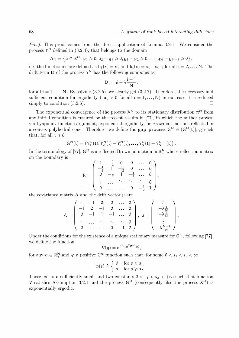
68 A system of rank-based interacting diffusions
Proof. This proof comes from the direct application of Lemma 3.2.1. We consider theprocess YN defined in (3.2.4), that belongs to the domain
ΛN =y ∈ R
N : y1 > 0, y2 − y1 > 0, y3 − y2 > 0, . . . , yN − yN−1 > 0,
i.e. the functionals are defined as b1(x) = x1 and bi(x) = xi−xi−1 for all i = 2, . . . ,N. Thedrift term D of the process YN has the following components:
Di = δ− λi− 1
N,
for all i = 1, . . . ,N. By solving (3.2.5), we clearly get (3.2.7). Therefore, the necessary andsufficient condition for ergodicity ( ai > 0 for all i = 1, . . . ,N) in our case it is reducedsimply to condition (3.2.6).
The exponential convergence of the process XN to its stationary distribution πN fromany initial condition is ensured by the recent results in [77], in which the author proves,via Lyapunov function argument, exponential ergodicity for Brownian motions reflected ina convex polyhedral cone. Therefore, we define the gap process GN
.= GN(t)t>0 such
that, for all t > 0
GN(t).=(
YN1 (t), YN2 (t) − Y
N1 (t), . . . , Y
NN(t) − Y
NN−1(t)
)
.
In the terminology of [77], GN is a reflected Brownian motion in RN+ whose reflection matrix
on the boundary is
R =
1 −12
0 0 . . . 0
−12
1 −12
0 . . . 0
0 −12
1 −12. . . 0
... . . .. . . . . . . . . 0
0 . . . . . . 0 −121
,
the covariance matrix A and the drift vector µ are
A =
1 −1 0 0 . . . 0
−1 2 −1 0 . . . 0
0 −1 1 −1 . . . 0... . . .
. . . . . . . . . 0
0 . . . . . . 0 −1 2
, µ =
δ
−λ 1N
−λ 2N
...−λN−1
N
.
Under the conditions for the existence of a unique stationary measure for GN, following [77],we define the function
V(g).= eaϕ(gTR−1g),
for any g ∈ RN+ and ϕ a positive C∞ function such that, for some 0 < s1 < s2 <∞
ϕ(s).=
0 for s 6 s1,s for s > s2.
There exists a sufficiently small and two constants 0 < s1 < s2 < +∞ such that functionV satisfies Assumption 3.2.1 and the process GN (consequently also the process XN) isexponentially ergodic.

69
3.2.3 Stationary distribution for the nonlinear process
The study of the invariant measures for the nonlinear process relies on the analysis of thecorrespondent stationary Fokker-Planck equation. Indeed, the nonlinear process (3.1.5)has a density function pt(x) that is the solution of the following PDE with boundaryconditions:
∂tpt(x) =12∂2xpt(x) + ∂x(λH ∗ pt(x) − δ)pt(x)) ∀ x > 0;
(δ− λH ∗ Pt(0))pt(0) = 12∂xpt(x)|x=0 ∀ t > 0.
Theorem 3.2.3. The process X, solution to (3.1.5), has a unique stationary measure π ifand only if
λ > 2δ.
The proof of this theorem follows the line of [54, Lemma 2.1], we sketch here the mainsteps.
Proof. Consider the stationary Fokker-Planck equation with boundary conditions
12∂2xπ+ ∂x(λH ∗ π− δ)π) = 0 ∀ x > 0;
(δ− λH ∗ π(0))π(0) = 12∂xπ(x)|x=0.
(3.2.8)
Then any probability measure π solving (3.2.8) in the weak sense is a stationary measurefor X. Let us consider a solution π to (3.2.8), that must be absolutely continuous w.r.t. theLebesgue measure, thanks to the regularizing effect of the second derivative. Therefore,we write (3.2.8) as
∂2xx(π− 2δH ∗ π+ λ(H ∗ π)2) = 0.Let f : R+ → R
+ be the density function of a solution of (3.2.8) and let F(x) =∫x0f(y)dy be
its cumulative distribution function, then F must be the solution of the following Cauchyproblem
dFdx
= 2δF− λF2 + β,
F(0) = 0,(3.2.9)
for certain constants β to be determined. The solution to (3.2.9) is of the following form:
F(x) =δ+
√
δ2 + βλ
λ
1− e−2x√δ2+βλ
1−δ+
√δ2+βλ
δ−√δ2+βλ
e−2x√δ2+βλ
. (3.2.10)
Therefore, we must find β such that limx→∞ F(x) = 1, that is β = λ − 2δ. For all δ, λ > 0there exists a unique solution F∞ to (3.2.9) with β = λ− 2δ
F(x) =1− e−2x(λ−δ)
1+ λλ−2δ
e−2x(λ−δ),
this F is the CDF of a probability measure if and only if dF(x)dx
> 0 for all x > 0, that meansif and only if λ > 2δ.
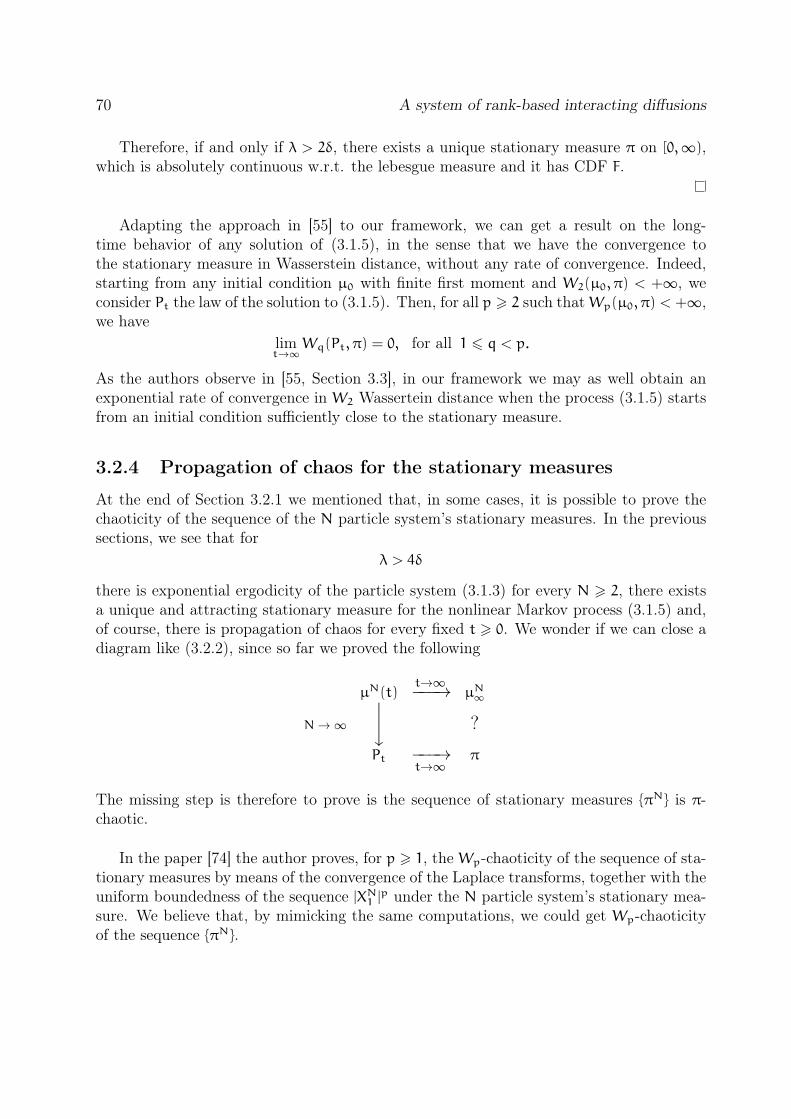
70 A system of rank-based interacting diffusions
Therefore, if and only if λ > 2δ, there exists a unique stationary measure π on [0,∞),which is absolutely continuous w.r.t. the lebesgue measure and it has CDF F.
Adapting the approach in [55] to our framework, we can get a result on the long-time behavior of any solution of (3.1.5), in the sense that we have the convergence tothe stationary measure in Wasserstein distance, without any rate of convergence. Indeed,starting from any initial condition µ0 with finite first moment and W2(µ0, π) < +∞, weconsider Pt the law of the solution to (3.1.5). Then, for all p > 2 such thatWp(µ0, π) < +∞,we have
limt→∞
Wq(Pt, π) = 0, for all 1 6 q < p.
As the authors observe in [55, Section 3.3], in our framework we may as well obtain anexponential rate of convergence in W2 Wassertein distance when the process (3.1.5) startsfrom an initial condition sufficiently close to the stationary measure.
3.2.4 Propagation of chaos for the stationary measures
At the end of Section 3.2.1 we mentioned that, in some cases, it is possible to prove thechaoticity of the sequence of the N particle system’s stationary measures. In the previoussections, we see that for
λ > 4δ
there is exponential ergodicity of the particle system (3.1.3) for every N > 2, there existsa unique and attracting stationary measure for the nonlinear Markov process (3.1.5) and,of course, there is propagation of chaos for every fixed t > 0. We wonder if we can close adiagram like (3.2.2), since so far we proved the following
µN(t)t→∞−−−→ µN∞
N→ ∞
y
?
Pt −−−→t→∞
π
The missing step is therefore to prove is the sequence of stationary measures πN is π-chaotic.
In the paper [74] the author proves, for p > 1, the Wp-chaoticity of the sequence of sta-tionary measures by means of the convergence of the Laplace transforms, together with theuniform boundedness of the sequence |XN1 |
p under the N particle system’s stationary mea-sure. We believe that, by mimicking the same computations, we could get Wp-chaoticityof the sequence πN.

71
Let us underline, that proving that the sequence of stationary measures πN is π-chaoticis equivalent to prove weak convergence of the sequence of stationary empirical measuresto π. Fix δ > 0 and λ > 4δ. The stationary measure π has density function:
f(x) =4(λ− δ)2(λ− 2δ)e−2(λ−δ)x
(λ− 2δ+ λe−2(λ−δ)x)2. (3.2.11)
If we call m∗ the median of the probability measure π, i.e. such that F(m∗) = 1/2, it isclear from (3.2.11) that
m∗ =1
2(λ− δ)log[
3λ− 4δ
λ− 2δ
]
.
At the level of N particle system, we know as well the median of the stationary empiricalmeasure µN∞, that is the position YNdN2 e
of the dN2eth ranked particle, where YN is the
reordered particle system (3.2.4) under πN. We know that, in the stationary regimes, YNdN2 eis the sum of dN
2e independent exponential random variables, with known parameters. For
instance, we can compute its mean and variance.
EπN [YNdN2 e
]=
dN2 e∑
i=1
1
2ai=
dN2 e∑
i=1
N
λ(N+ 1− i)(
i−λ(2−N)+2δN
λ
)
6N
λ(2N− 1) − 2δN
[
ln
(
N(
32λ− 2δ
)
− 2λ
N(λ− 2δ) − 2λ
)
+ ln(2) +O(
1
N
)
]
N→∞−→ 1
2(λ− δ)ln(
3λ− 4δ
λ− 2δ
)
= m∗
VarπN [YNdN2 e
]=
dN2 e∑
i=1
1
4a2i=
dN2 e∑
i=1
N2
λ2(N+ 1− i)2(
i−λ(2−N)+2δN
λ
)2
N→∞−→ 0
We can make the same computations for other quantiles of the measure π, comparedwith the quantiles of the stationary empirical measure µN∞, for which we know the explicitdistribution in terms of the independent gaps between successive particles. Therefore, forany p ∈ (0,1), the sequence of p-quantiles of the stationary empirical measure xNp , whichis a sequence of random variables, converges a.s. to the deterministic value xp, that is thep-quantile of π. The convergence of any p-quantile such that the pseudo inverse of thelimit CDF F−1(p) is continuous in p is equivalent to weak convergence. Since π admits adensity, we have that a.s. the sequence of stationary empirical measures converges weaklyto π.

72 A system of rank-based interacting diffusions
Chapter 4
A system of random walks with
asymmetric interaction
In this chapter we study a system of mean field interacting random walks on the positiveintegers, reflected at zero, presented in [2]. Each particle has a drift δ > 0 towards infinityand a parameter λ > 0 that tunes an interaction. This interaction is asymmetric in thesense that it pushes each particle towards the origin, but it depends on the number ofparticles at the left of the affected one. We are interested in studying the mean field limitof this model and its stability properties.
4.1 The model
In this section we describe all the details of the model we are interested in. As in the previ-ous chapters, we start with the description of the N particle system, then we heuristicallydescribe its mean field limit and we prove well-posedness and propagation of chaos.
4.1.1 The particle system
We fix N > 2 and we consider N particles, each of them moving on the nonnegative inte-gers. Let XN = (XN1 , . . . , X
NN) ∈ N
N be the vector of the particles’ positions. Each particlehas an intrinsic dynamics and it experiences an interaction.
- The intrinsic dynamics is given by a simple biased random walk, with jump ampli-tude one, independent of the other particles and reflected at zero. This is describedby 2 independent Poisson clocks for each particle, one with rate 1, governing thedownward jump and the other with rate 1+ δ, δ > 0, governing the upward jump.
- The interaction dynamics is tuned by a parameter λ > 0. Every pair of particles,for example
(XNi , XNj )
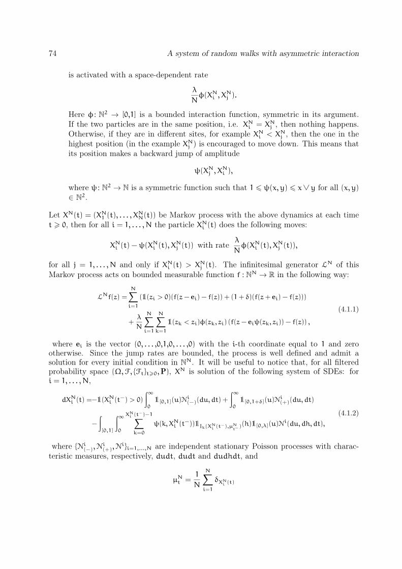
74 A system of random walks with asymmetric interaction
is activated with a space-dependent rate
λ
Nφ(XNi , X
Nj ).
Here φ : N2 → [0,1] is a bounded interaction function, symmetric in its argument.If the two particles are in the same position, i.e. XNi = XNj , then nothing happens.Otherwise, if they are in different sites, for example XNi < X
Nj , then the one in the
highest position (in the example XNj ) is encouraged to move down. This means thatits position makes a backward jump of amplitude
ψ(XNj , XNi ),
where ψ : N2 → N is a symmetric function such that 1 6 ψ(x, y) 6 x∨ y for all (x, y)∈ N
2.
Let XN(t) = (XN1 (t), . . . , XNN(t)) be Markov process with the above dynamics at each time
t > 0, then for all i = 1, . . . ,N the particle XNi (t) does the following moves:
XNi (t) −ψ(XNi (t), X
Nj (t)) with rate
λ
Nφ(XNi (t), X
Nj (t)),
for all j = 1, . . . ,N and only if XNi (t) > XNj (t). The infinitesimal generator LN of thisMarkov process acts on bounded measurable function f : NN → R in the following way:
LNf(z) =
N∑
i=1
(1(zi > 0)(f(z− ei) − f(z)) + (1+ δ)(f(z+ ei) − f(z)))
+λ
N
N∑
i=1
N∑
k=1
1(zk < zi)φ(zk, zi) (f(z− eiψ(zk, zi)) − f(z)) ,
(4.1.1)
where ei is the vector (0, . . . ,0,1,0, . . . ,0) with the i-th coordinate equal to 1 and zerootherwise. Since the jump rates are bounded, the process is well defined and admit asolution for every initial condition in N
N. It will be useful to notice that, for all filteredprobability space (Ω,F, Ftt>0,P), XN is solution of the following system of SDEs: fori = 1, . . . ,N,
dXNi (t) =−1(XNi (t−) > 0)
∫∞
0
1[0,1](u)Ni(−)(du, dt) +
∫∞
0
1[0,1+δ](u)Ni(+)(du, dt)
−
∫
[0,1]
∫∞
0
XNi (t−)−1∑
k=0
ψ(k, XNi (t−))1Ik(XNi (t−),µN
t−)(h)1[0,λ](u)N
i(du, dh, dt),
(4.1.2)
where Ni(−),Ni(+),N
ii=1,...,N are independent stationary Poisson processes with charac-teristic measures, respectively, dudt, dudt and dudhdt, and
µNt =1
N
N∑
i=1
δXNi (t)

75
indicates the empirical measures, as usual. The intervals are such that, for all k > 0 wehave
Ik(x, µ).=
(
k−1∑
y=0
φ(y, x)µ(y),
k∑
y=0
φ(y, x)µ(y)
]
and I0.= (0,φ(0, x)µ(0)].
4.1.2 The nonlinear processes
In this section we introduce, at a heuristic level, the nonlinear process, that stands forthe macroscopic description of the model presented in Section 4.1.1. As we said in theprevious chapters, heuristically the mean field limit is obtained under the assumption thatthere exists a law µt that is the weak limit of the sequence of empirical measures, i.e.
µNt t>0N→∞−→ µtt>0.
In this framework, let us consider the nonlinear SDE defined as follows
dX(t) = − 1(X(t−) > 0)
∫∞
0
1[0,1](u)N(−)(du, dt) +
∫∞
0
1[0,1+δ](u)N(+)(du, dt)
−
∫
[0,1]
∫∞
0
X(t−)−1∑
k=0
ψ(k, X(t−))1Ik(X(t−),µt−)(h)1[0,λ](u)N(du, dh, dt),
(4.1.3)
where µt = Law(X(t)), N(−),N(+),N are independent stationary Poisson processes withcharacteristic measures, respectively, dudt, dudt and dudhdt. The intervals Ik(x, µ) aredefined as in (4.1.2). The well-posedness of (4.1.3) for every initial condition supported onN will be proved together with the mean field limit, as in Chapter 3. Indeed, the existenceof a process that solves (4.1.3) is ensured by the tightness of the sequence of empiricalmeasures.
In order to ensure uniqueness of the nonlinear system, we require the backward jumpsto satisfy the following condition.
Assumption 4.1.1. There exists C < ∞ such that for all x, y ∈ N and α,β ∈ M(N)
probability measure on N
∣
∣
∣
∣
∣
x∨y−1∑
k=0
ψ(k, x∨ y) |Ik(x, α)∆Ik(y, α)|
∣
∣
∣
∣
∣
6 C|x− y|,
where for A,B two intervals of the real line A∆B.= A\B ∪ B\A and
∣
∣
∣
∣
∣
∣
∑
(x,y,z)∈A
α(y)α(z) − β(y)β(z)
∣
∣
∣
∣
∣
∣
6 C∑
x∈N
|α(x) − β(x)|,
where A.= (x, y, z) ∈ N
3 : z > x, z > y, z−ψ(y, z) = x.
76 A system of random walks with asymmetric interaction
Assumption 4.1.1 is rather technical; it resembles a Lipschitz-type condition on thecoefficients and it is sufficient for the proof of uniqueness via Gronwall inequalities, asthe following result shows. However, it is more general than any condition on jumps weconsidered in Chapter 2. Indeed, we can prove pathwise propagation of chaos only fora small subclass of models among the ones described here. This is the reason why weadopt the approach via the solution of the martingale problem, which is more flexible thanthe coupling procedure. In Section 4.1.4, we present a particular model of this class thatsatisfies Assumption 2.1.1 and for which pathwise propagation of chaos holds, with theexpected rate of 1√
N.
Proposition 4.1.1. Grant Assumption 4.1.1, then pathwise uniqueness holds for the non-linear SDE (4.1.3) in the class of processes with initial conditions supported on N.
Proof. Step 1: uniqueness in law. Let µ be the law of X and µt its time-marginal. Weconsider the following equation, for all x ∈ N
d
dtµt(x) =µt(x+ 1) − (1+ δ)µt(x) + 1(x > 0)((1+ δ)µt(x− 1) − µt(x))
+ λ
∑
(h,k)∈Ax
µt(h)µt(k)φ(h, k) − µt(x)
x−1∑
k=0
φ(k, x)µt(k)
,
(4.1.4)
where Ax.= (h, k) ∈ N
2 : h < k, k > x, k−ψ(h, k) = x. Since we are looking for processeswith initial condition supported on N, µ0 is a measure on N, thus the same is true for µtfor all t > 0 and (4.1.4) is actually the equation for the time evolution of the law µt. Setxk(t)
.= µt(k) for all k > 0, then (4.1.4) is equivalent to the following infinite dimensional
system of ODEs:
x0 = x1 − (1+ δ)x0 + λ∑
(h,k)∈A0
xhxkφ(h, k)
xn = xn+1 − xn + (1+ δ)(xn−1 − xn) + λ
∑
(h,k)∈An
xhxkφ(h, k) − xn
n−1∑
k=0
xkφ(k, x)
n = 1,2, . . .
(4.1.5)
Therefore, we are looking for the uniqueness of the solution of (4.1.5) in the subspace
M1 =x ∈ l1 s.t. ‖x‖1 = 1 and xi ∈ [0,1] ∀ i
.
Let x(t) and y(t) be two solutions of (4.1.5) with the same initial condition. Fix T > 0, wewant to prove that ‖x(t) − y(t)‖1 = 0 for all t ∈ [0, T ]. By a simple integration of (4.1.5)
77
and some bound, we get
‖x(t) − y(t)‖1 =∞∑
n=0
|xn(t) − yn(t)|
6‖x(0) − y(0)‖1 +∫t
0
(4+ 2δ)
∞∑
n=0
|xn(s) − yn(s)|ds
+λ
∫t
0
∞∑
n=0
∣
∣
∣
∣
∣
∣
∑
(h,k)∈An
xh(s)xk(s)φ(h, k) −
n−1∑
k=0
xn(s)xk(s)φ(k, n)
−
∑
(h,k)∈An
yh(s)yk(s)φ(h, k) −
n−1∑
k=0
yn(s)yk(s)φ(k, n)
∣
∣
∣
∣
∣
∣
ds.
Now the role of Assumption 4.1.1 is clear, since we have
‖x(t) − y(t)‖1 6‖x(0) − y(0)‖1 + 2(2+ δ)∫t
0
‖x(s) − y(s)‖1ds
+ λ
∫t
0
∞∑
n=0
|xn(s) − yn(s)|
∣
∣
∣
∣
∣
∞∑
k=n+1
xk(s) −
n−1∑
k=0
xk(s)
∣
∣
∣
∣
∣
ds
+ λ
∫t
0
∞∑
n=0
|yn(s)|
∣
∣
∣
∣
∣
∞∑
k=n+1
(xk(s) − yk(s)) −
n−1∑
k=0
(xk(s) − yk(s))
∣
∣
∣
∣
∣
ds
6‖x(0) − y(0)‖1 + 2(2+ δ+ (C+ 1)λ)
∫t
0
‖x(s) − y(s)‖1ds.
By applying Gronwall Lemma, since ‖x(0) − y(0)‖1 = 0, we get ‖x(t) − y(t)‖1 = 0 for allt ∈ [0, T ]. By the arbitrariness of T > 0, we get uniqueness for µ.
Step 2: pathwise uniqueness. We fix a stochastic basis (Ω,F, Ftt>0,P) and we considertwo solutions X1 = (X1(t))t>0 and X2 = (X2(t))t>0 driven by the same Poisson processesand such that a.s. X1(0) = X2(0) ∈ N. We know, by point i), that these two solutionscoincide in law, i.e. µ1 = µ2.
Fix T > 0, then we want to prove that E[
supt∈[0,T ] |X1(t) − X2(t)|
]
= 0.
E
[
supt∈[0,T ]
|X1(t) − X2(t)|
]
6 E
[∫T
0
∣
∣1(X1(t) > 0) − 1(X2(t) > 0)∣
∣dt
+λ
∫T
0
∫
[0,1]
∣
∣
∣
∣
∣
∣
X1(t)−1∑
k=0
ψ(k, X1(t))1Ik(X1(t),µ1(t))(h) −
X2(t)−1∑
k=0
ψ(k, X2(t))1Ik(X2(t),µ2(t))(h)
∣
∣
∣
∣
∣
∣
dhds
.
First, we know by the previous step that there is weak uniqueness, i.e. µ1(t) = µ2(t).Moreover, by hypothesis we have that |φ(·, ·)| 6 1. Therefore we perform the following
78 A system of random walks with asymmetric interaction
bound:
E
[
supt∈[0,T ]
|X1(t) − X2(t)|
]
6
∫T
0
E
[
sups∈[0,t]
|X1(t) − X2(t)|
]
dt
+ λ
∫T
0
E
|X1(t) − X2(t)|
X1(t)∧X2(t)−1∑
k=0
µ1(t)(k)
dt
+ λ
∫T
0
E
∣
∣
∣
∣
∣
∣
X1(t)∧X2(t)−1∑
k=0
ψ(k, X1(t))|Ik(X1(t), µ1t)∆Ik(X
2(t), µ1t)|
∣
∣
∣
∣
∣
∣
dt
+ λ
∫T
0
E
X1(t)∨X2(t)−1∑
k=X1(t)∧X2(t)
|X1(t)∨ X2(t) − k|µ1(t)(k)
dt.
We bound the third term in the right-hand side by means of Assumption 4.1.1. Then, weconsider the fourth term and, obviously, we have that, for all t > 0,
X1(t)∨X2(t)−1∑
k=X1(t)∧X2(t)
|X1(t)∨ X2(t) − k|µ1(t)(k) 6 |X1(t) − X2(t)|
X1(t)∨X2(t)−1∑
k=X1(t)∧X2(t)
µ1(t)(k).
Moreover, since µ1(t) is a probability measure for all t > 0, we recall that, obviously,
X1(t)∨X2(t)−1∑
k=0
µ1(t)(k) 6 1.
Therefore, we obtain
E
[
supt∈[0,T ]
|X1(t) − X2(t)|
]
6 (1+ (C+ 1)λ)
∫T
0
E
[
sups∈[0,t]
|X1(s) − X2(s)|
]
dt.
Now, we apply Gronwall Lemma and we get the thesis.
As we mentioned, weak existence of a solution to (4.1.3) is a consequence of propagationof chaos and it will be shown in the following section. Therefore, we end this section bystating the result on well-posedness of (4.1.3), but we postpone its proof to the end ofSection 4.1.3.
Theorem 4.1.1. Grant Assumption 4.1.1, then for every F0-measurable initial conditionX0 with values in N, there exists a unique strong solution to (4.1.3).

79
4.1.3 Propagation of chaos
In the proof of propagation of chaos for the particle system (4.1.2), we progress step bystep with the same approach of Section 3.1.2. This means that we first prove tightness andconsistency of the sequence of empirical measures. To this aim, let us define the martingaleproblem associated to (4.1.3).
Definition 4.1.1. We say that the law Q on D(R+,R+) of any (Xt)t>0 satisfying (4.1.3) isthe solution of the martingale problem correspondent to (4.1.3) if the following propertieshold.
i) Q X−10 = µ0, for µ0 measure on N.
ii) Let Lµ be the generator defined on every bounded function f by
Lµf(x) = 1(x > 0)(f(x−1)−f(x))+(1+δ)(f(x+1)−f(x))+λ
x−1∑
k=0
φ(k, x)µ(k)(f(x−ψ(k, x))−f(x)).
Then, for all f ∈ Cb, for all t > 0
Mft = f(Xt) − f(X0) −
∫ t
0
Lµsf(Xs)ds
is a Q-martingale, where µs = µ X−1s .
Proposition 4.1.2. Fix a filtered probability space (Ω,F, Ftt>0,P) and an initial con-dition XN(0) whose law is µ0-chaotic, for a law µ0 on N. Let XNt>0 be the solution to(4.1.2). Then:
a) the sequence of empirical measuresµN
is tight in M
(
D(R+)2)
;
b) any limit point µ of the sequence µN solves the martingale problem correspondent to(4.1.3).
Proof. a) We know that, under our conditions of exchangeability of the components, prov-ing point a) is equivalent to prove that the sequence of processes (XN1 (t))t>0, N > 2 istight in D(R+,R+), see [83]. To this aim, we use Aldous’s criterion, see [12], and we wantprove the two following statements.
i) For all T > 0,
limK↑∞
supN>1
P
(
supt∈[0,T ]
XN1 (t) > K
)
= 0.
ii) For all T > 0, ε > 0
limρ↓0
lim supN→∞
sup(S,S ′)∈AρT
P(
|XN1 (S) − XN1 (S
′)| > ε)
= 0,
where AρT.= (τ, τ ′) stopping times s.t. 0 6 τ 6 τ ′ 6 τ+ ρ 6 T a.s..

80 A system of random walks with asymmetric interaction
- Condition i) follows immediately from the fact that, if we fix T > 0, ∀ N > 1 we have
P
(
supt∈[0,T ]
XN1 (t) > K
)
6E[
supt∈[0,T ] |XN1 (t)|
]
K
(we take into account only the jumps on the right )
61
KE
[
supt∈[0,T ]
∫ t
0
∫∞
0
1[0,1+δ](u)Ni(+)(du, ds)
]
6(1+ δ)T
K.
- To prove condition ii), we know that
P(
|XN1 (S) − XN1 (S
′)| > ε)
6 P(
|XN1 (S) − XN1 (S
′)| > 0)
.
We write |XN1 (S) − XN1 (S
′)| by means of (4.1.2):
|XN1 (S) − XN1 (S
′)| 6
∣
∣
∣
∣
∣
−
∫S ′
S
1(XN1 (t−) > 0)
∫∞
0
1[0,1](u)N1(−)(du, dt)
∣
∣
∣
∣
∣
+
∣
∣
∣
∣
∣
∣
∫S′
S
∫
[0,1]
∫∞
0
XN1 (t−)−1∑
k=0
ψ(k, XN1 (t−))1Ik(XN
1 (t−),µNt−
)(h)1[0,λ](u)N1(du, dh, dt)
∣
∣
∣
∣
∣
∣
+
∣
∣
∣
∣
∣
∫S ′
S
∫∞
0
1[0,1+δ](u)N1(+)(du, dt)
∣
∣
∣
∣
∣
.= A−
(S,S ′) + B(S,S ′) +A+(S,S ′).
Since we have 3 terms involving only integrals with respect to Poisson random mea-sures, the probability of those terms being strictly greater than 0 is equal to theprobability that there is at least one jump in the time interval [S, S ′], therefore
P(A−(S,S ′) + B(S,S ′) +A
+(S,S ′) > 0) 6 P
(
A−(S,S ′) > 0
)
+ P(
B(S,S ′) > 0)
+ P
(
A+(S,S ′) > 0
)
6 P(A−(S,S′)
> 1) + P
(∫S′
S
∫1
0
∫∞
0
1[0,λ)(u)N1(du, dh, dt) > 1
)
+ P(A+(S,S′)
> 1)
6 E[A−(S,S′)
] + E
[∫S′
S
∫1
0
∫∞
0
1[0,λ)(u)N1(du, dh, dt)
]
+ E[A+(S,S′)
] 6 ρ(2+ λ+ δ).
By taking the limit for ρ ↓ 0 we get the thesis.
b) A probability measure Q ∈ M(D(R+,R+)) that is solution to the martingale problemdefined in Definition 4.1.1 must satisfy the two conditions i) and ii).
i) Clearly µ X−10 = µ0, since µ X−1
0 is the limit of the sequence 1N
∑Ni=1 δXNi (0) that,
by µ0-chaoticity clearly converges weakly to µ0.
81
ii) Step 1) As in Section 3.1.2, we follow the approach of Sznitman, [81], and we definea functional
F : M(D(R+,R+)) → R
that is zero on the measures satisfying this martingale problem defined in Defini-tion 4.1.1. Fix ϕ ∈ Cb, 0 6 s1 6 · · · 6 sq 6 s 6 t, g1, . . . , gq ∈ Cb and define
F(Q).= 〈Q,
(
φ(X(t)) − φ(X(s)) −
∫ t
s
LQuφ(X(u))du
)
g1(X(s1)) . . . gq(X(sq))〉.
We want to prove that for all Q limit point of µN, F(Q) = 0 a.s..
Step 2) We firstly prove that limN→∞ E[
F(µN)2]
= 0. We consider
E[
F(µN)2]
= E
[
1
N2
N∑
i=1
(Mϕit −Mϕi
s )2g21(XNi (s1)) . . . g
2q(X
Ni (sq))
]
+ E
[
1
N2
N∑
i6=j(Mϕi
t −Mϕis )(M
ϕjt −M
ϕjs )g1(X
Ni (s1))g1(X
Nj (s1)) . . .
]
,
where Mϕit = ϕ(XNi (t)) − ϕ(X
Ni (0)) −
∫t0LµN(u)ϕ(X
Ni (u))du for i = 1, . . . ,N are or-
thogonal martingales, i.e.
〈Mϕi ,Mϕj〉 = 0 for all i 6= j.
Indeed, by applying Ito’s rule for jump processes to ϕ(XNi (t))−ϕ(XNi (0)), we see that
Mϕit −Mϕi
s is simply the sum of integrals w.r.t. the three martingales Ni(−), Ni(+)
and Ni. Therefore, by hypothesis, it is orthogonal to Mϕjt −M
ϕjs for all j 6= i. We
also know how to rewrite the quadratic variation:
〈Mϕit −Mϕi
s 〉 =∫ t
s
∫∞
0
(
ϕ(XNi (r) + 1[0,1](u)) −ϕ(XNi (r))
)2dudr
+
∫ t
s
∫∞
0
(
ϕ(XNi (r) − 1[0,1](u)) −ϕ(XNi (r))
)21(XNi (r) > 0)dudr
+
∫t
s
∫∞
0
∫
[0,1]
ϕ
XNi (r) −
XNi (r)−1∑
k=0
ψ(k, XNi (r))1Ik(XNi (r),µN
r )(h)1[0,λ)(u)
−ϕ(XNi (r))
2
dhdudr.
Then, for a constant K > 0, depending on gii=1,...,q, and C > 0, depending on thefunction ϕ, we have
E[
F(µN)2]
6K
N2
N∑
i=1
E [〈Mϕit −Mϕi
s 〉] + K
N2
N∑
i6=jE[
〈Mϕit −Mϕi
s ,Mϕjt −M
ϕjs 〉]
6K
N2
N∑
i=1
C(2+ λ)(t− s) 6KC(2+ λ)(t− s)
N,
82 A system of random walks with asymmetric interaction
therefore limN→∞ E[
F(µN)2]
= 0.
Step 3) We are left to prove that E[
F(Q)2]
= limN→∞ E[
F(µN)2]
, from Sznitman[83] we know that it is sufficient to verify
Q (∆X(t) 6= 0 ∪ ∆X(s) 6= 0 ∪ ∆X(s1) 6= 0 ∪ · · · ∪ ∆X(sq) 6= 0) = 0 a.s.,
where ∆X(t) = X(t) − X(t−).
By contradiction, assume that there exists a t ∈ s1, . . . , sq, s, t such that Q(∆X(t) 6=0) > 0 with positive probability. That is, there exists a constant b > 0 such that theevent
E.= Q(∆X(t) > 0) > b
has positive probability. For every ε > 0 we can define the open set of D(R+,R+)
Dε.= x ∈ D(R+,R+) s.t. sup
s∈(t−ε,t+ε)
|∆xs| > 0
and the open set of M(D(R+,R+))
Pdε.= µ s.t. µ(Dε) > d.
We see that E ⊂ Q(Dεa) > d and, by Portmanteau theorem,
lim infN→∞
P(µN ∈ Pdε) > P(Q ∈ Pdε) > P(E) > 0.
We bound the term on the left-hand by means of
µN ∈ Pdε ⊂1
N
N∑
i=1
1(XNi performs at least one jump in (t− ε, t+ ε)) > d
.
Since the particle are exchangeable and their jump rates are constants, we have that
P(µN ∈ Pdε) 62ε(2+ λ+ δ)
d.
This leads to the contradiction
0 = lim infε↓0
lim infN→∞
P(µN ∈ Pdε) > P(E) > 0
and it proves continuity of F.
83
Weak uniqueness of solutions of the martingale problem in Definition 4.1.1 is proved inProposition 4.1.1, this implies that the limit of any convergent subsequence of µN is thesame deterministic element of the space M(D(R+,R+)). As we anticipated, the previousresults lead to the proof of the well-posedness of the nonlinear SDE (4.1.3).
Proof of Theorem 4.1.1. Existence of a weak solution to (4.1.3) is ensured by Proposi-tion 4.1.2. Indeed, for all initial condition µ0 ∈ M(N), we can construct a sequenceof processes XN = (XN(t))t>0. For all N > 2, each process has as initial condition(XN1 (0), . . . , X
NN(0)), where XNi (0) are i.i.d. random variables µ0-distributed and XN solves
(4.1.2). Then the limit of the sequence of empirical measures µNN>2 for N → ∞ is asolution to (4.1.3). Pathwise uniqueness of this solution is given by Proposition 4.1.1.By Yamada-Watanabe theorem, pathwise uniqueness together with weak existence givesexistence and uniqueness of strong solutions, see [57].
Finally we can state and prove a complete result of propagation of chaos, that is simplya consequence of the previous results.
Theorem 4.1.2 (Propagation of chaos). For every µ0 probability measure on N, let PN
∈ M(D(R+,R)N) be the law of the solution of system (4.1.2) with initial condition PN0 =
PN(XN0 )−1 that is µ0-chaotic. Then the sequence PN is µ-chaotic, where µ ∈ M(D(R+,R))
is the law of the unique solution of (4.1.3) with initial condition µ0.
Proof. We prove propagation of chaos with the tightness/consistency/uniqueness approach,see [81, 83].
- From Proposition 4.1.2, point i) we have tightness of the sequence of empirical mea-sures µNN∈N in M(D(R+,R+)).
- From Proposition 4.1.2, point ii) we have that any limit point of a converging subse-quence µNkk∈N is a solution of (4.1.3).
- In Proposition 4.1.1 we proved uniqueness of solution of (4.1.3), this let us concludethat the limit of the sequence of empirical measures is deterministic.
The three steps above imply the property of propagation of chaos for the particle system(4.1.2).
4.1.4 Motivation and examples
The class of models that we introduce in this chapter is motivated by genetics, indeed itcan be used as a description of the evolution of genetics traits. Our N particle system maybe interpreted as a population of N individuals. Each individual is characterized by itsfitness level, that is an integer number greater or equal than 0, that is the worst possiblefitness value. Each time that a particle moves, we imagine that the corresponding individ-ual dies and gives birth to a child whose fitness level is greater or smaller than its own.The individuals have an intrinsic tendency to improve (given by the biased random walk).

84 A system of random walks with asymmetric interaction
However, by mimicking the worst individual of the population (the one with lower fitnesslevel), they may give birth to a child that is much worse than themselves; this of coursecorresponds to the leftward jumps due to the asymmetric interaction.
Let us give some explicit examples of models belonging to this class, by specifying theinvolved functions.
The small jumps model
The simplest model in our class is such that the size of the jumps induced by the asymmetricinteraction is the minimal, i.e. they are of size 1. We refer to this model as the model withsmall jumps. In this case both the rate and the jump function are constantly equal to 1:for all x 6= y ∈ N
φ(x, y) = 1,
ψ(x, y) = 1.
Let us describe in details this model. For a fixed number N of particles on Z+, each particle
XNi , for i = 1, . . . ,N, makes the following moves: if XNi > 0, then it goes to
XNi + 1 with rate 1+ δ,XNi − 1 with rate 1+ λ 1
N
∑Nk=1 1(X
Nk < X
Ni ),
(4.1.6)
while when XNi = 0, the only allowed jump is the one upward. It is clear that here δ > 0
indicates a bias rightward, while λ 1N
∑Nk=1 1(X
Nk < X
Ni ) is a bias leftward. The infinitesimal
generator of (4.1.6) is given by
LN(SJ)f(z) =
N∑
i=1
(1(zi > 0)∇−i f(z) + (1+ δ)∇+
i f(z)) +λ
N
N∑
i=1
∇−i f(z)
N∑
k=1
1(zk < zi). (4.1.7)
Here ∇−i f(z) = f(z − ei) − f(z) and ∇+
i f(z) = f(z + ei) − f(z). We associate to (4.1.6) itscorrespondent nonlinear Markov process, that is a Markov process Xtt>0 whose possibiletransitions at time t > 0 are the following:
Xt + 1 with rate 1+ δ,Xt − 1 with rate 1+ λµt[0, Xt),
(4.1.8)
where µt = Law(Xt) and, as in (4.1.6), when Xt=0, only the upward jump is allowed.
Let us underline that this small jumps model has a direct link with the diffusion modeldescribed in Chapter 3, that may be seen as its continuous analogue. Each particle per-forms a random walk with a bias that depends on its rank with respect to all the others,with the same form of the drift in Chapter 3. Indeed, the rightmost particle, when aloneon its site, has a net drift of δ − λN−1
N, whereas the leftmost particle has a positive drift
85
δ. For this reason, we will use the continuous model as a basis for comparisons in theanalysis of the small jumps model. Despite their similarities, the two models display pecu-liar differences that emerge in the study of the long-time behavior. In the discrete modelparticles can form big clusters on a single site. By our rule, particles in the same site donot interact: thus the formation of clusters tends to prevent the stabilization of the process.
Before the study of the long-time behavior, motivated by Theorem 3.1.2, we look fora result of trajectorial propagation of chaos. To this aim, we define a coupling procedurebetween a Markov process defined by the generator (4.1.7) and N copies of the nonlinearMarkov process defined in (4.1.8). We fix a filtered probability space (Ω,F, Ftt>0,P) andlet µ0 be a probability measure on N. For any N ∈ N let
(XN(t), Xt)t>0 = (XN1 (t), X1t , . . . , X
NN(t), X
Nt )t>0
be a Markov process with initial conditions such that XNi (0) = Xi0 a.s., independent for all
i = 1, . . . ,N and µ0-distributed. Then, for all i = 1, . . . ,N, the pair (XNi (t), Xit) jumps in
the following positions:
(XNi (t) + 1, Xit + 1) with rate 1+ δ,
(XNi (t) − 1, Xit − 1) ” 1(XNi (t) > 0)1(X
it > 0) + λ
(
µNt [0, XNi (t))∧ µt[0, X
it))
,
(XNi (t) − 1, Xit) ” 1(XNi (t) > 0)1(X
it = 0) + λ
(
µNt [0, XNi (t)) − µt[0, X
it))
+,
(XNi (t), Xit − 1) ” 1(XNi (t) = 0)1(X
it > 0) + λ
(
µt[0, Xit) − µ
Nt [0, X
Ni (t))
)
+.
This is equivalent to the so-called basic coupling that we introduced in Chapter 1. Indeed,we assign to every pair of particles (XNi (t), X
it)t>0 the same Poisson clocks (the Poisson
random measures) and it maximizes the chances of the two particles to jump together. Ofcourse, this means that for any continuous and bounded function f : N2N → R
f(XN(t), Xt) − f(XN(0), X0) −
∫ t
0
Lµsf(XN(s), Xs)
is a martingale, where µt = Law(Xit) for any i = 1, . . . ,N and
Lµf(x, y)=N∑
i=1
(1+ δ)(f(x+ δi, y+ δi) − f(x, y))
+
[
1(xi > 0)1(yi > 0) + λ
(
1
N
N∑
k=1
1(xk < xi)∧ µ[0, yi)
)]
(f(x− δi, y− δi) − f(x, y))
+
[
1(xi > 0)1(yi = 0) + λ
(
1
N
N∑
k=1
1(xk < xi) − µ[0, yi)
)
+
]
(f(x− δi, y) − f(x, y))
+
[
1(xi = 0)1(yi > 0) + λ
(
µ[0, yi) −1
N
N∑
k=1
1(xk < xi)
)
+
]
(f(x, y− δi) − f(x, y)).
The following result states the trajectorial propagation of chaos, which is a consequence ofProposition 2.1.2.
86 A system of random walks with asymmetric interaction
Theorem 4.1.3. For all t > 0, there exists a positive constant Ct <∞ such that
E[sups6t
|XN1 (s) − X1s |] 6
Ct√N. (4.1.9)
Proof. Notice that the jump coefficients here satisfy Assumption 2.1.1, indeed, for allx, y ∈ N and α,β in M(N) it holds:
|−1(x > 0)λα[0, x) + 1(y > 0)λβ[0, y)| 6λ|α[0, x) − β[0, y)|+ 2λ|1(x = 0) − 1(y = 0)|
63λ|x− y|+ λρ(α,β).
Then, we use Proposition 2.1.2, and we get that, for all t > 0
E[sups6t
|XN1 (s) − X1s |] 6 βN,
where βN.= sups∈[0,t] E[ρ(µ
NXs, µs) is the W1 Wasserstein distance between the empirical
measure of the N copies of the nonlinear process (4.3.1) and its law. We know that thereexists a constant Ct > 0 such that βN 6
Ct√N
, which proves (4.1.9).
A branching and selection mechanism
Let us cite another interesting model belonging to our class of interacting random walks;we can relate this model to a branching-and-selection mechanism on the positive inte-gers. Branching and selection particle systems are popular models in population dynamics,starting from the work of Brunet and Derrida [17] and followed by many others, for in-stance [10, 33, 62]. This models are studied in relation to the Fisher-Kolmogorov PetrovskyPiscounov equation (F-KPP):
∂h
∂x= ∆h+ h(1− h),
for h = h(x, t), x ∈ R, t > 0.
In our case, we imagine that any individual reproduces with a rate λ and he givesbirth to a child. The fitness of this child is uniformly chosen among the ones of the otherindividuals. If the fitness of the newborn is strictly smaller than his parent’s one, the childkills him, on the other case the child does not survive. In the terminology we introduced,this means that, for all x 6= y ∈ N
φ(x, y) = 1,
ψ(x, y) = |x− y|.
It is natural, in this case, to imagine that the individuals are characterized by their unfitnessrather than their fitness, such that lower values are related to stronger genetic traits. Thismodel is clearly very interesting and we may develop its continuous-space analogue as we
87
did for the small jumps model. Of course, the continuous-space dynamics would not havecontinuous paths in this case, but each particle would behave according a diffusion withjumps. Following the approach of Chapter 3, we define the infinitesimal generator LN(BS)of the system on suitable C2 functions f : DN → R in the following way:
LN(BS)f(x) =
N∑
i=1
1
2
∂2
∂x2if(x) + δ
∂
∂xif(x) + λ
∫xi
0
(f(x− ei(xi − y)) − f(x))µN(dy),
the domain of the generator LN(BS) coincides with D(
LN)
from Chapter 3. Its mean fieldlimit is a process on R+ such that its law has a density µt that solves the following Fokker-Planck equation with boundary conditions
∂tµt(x) =
12∂2xµt(x) − δ∂xµt(x) + λµt(x)
∫∞
xµt(y)dy− λµt(x)
∫x0µt(y)dy ∀ x > 0;
δ∂xµt(x)|x=0 − λµt(0) =12∂2xµt(x)|x=0.
(4.1.10)Of course, integrating (4.1.10) from 0 to x, for all x > 0 and setting Ft(x) =
∫x0µt(y)dy its
CDF, we get the equivalence with the following:
∂tFt(x) =1
2∂2xFt(x) − δ∂xFt(x) + λFt(x)(1− Ft(x)),
for all x > 0 and Ft(x) = 0 for x 6 0, for all t > 0, that links this model with the F-KPPequation.
4.2 Exponential ergodicity of the particle system
In this Section we study the long time behavior of the system with N particles. The mainquestion we address is whether the asymmetric interaction can balance the drift to infinity,i.e. we want to understand if the interaction can ensure ergodicity in the N particle system.Clearly, when λ = 0, the model has no chance of having a stationary measure, because eachparticle perform a simple random walk with a nonnegative drift δ > 0 and reflection inzero. We aim to determine (or to give bounds to) the critical interaction strength
λ∗N(δ)
above which any system described in Section 4.1.1 has a stationary measure.
We restrict the analysis to the specific model with small jumps, defined by (4.1.6), sinceit stochastically dominates all the other model in the class we presented in Section 4.1.1,when the interaction function φ(x, y) ≡ 1. To this aim, following the approach in [58],we define the stochastic ordering between probability measures. Let X be a compactmetric space, in which we can define a partial order 6. Let M define the set of continuousfunctions on X, which are monotone, i.e.
M.= f : f(x) 6 f(y) for all x 6 y .
88 A system of random walks with asymmetric interaction
Definition 4.2.1 (Stochastic ordering). Let µ, ν be two probability measures on X, wesay that
µ νif and only if ∫
X
fdµ 6
∫
X
fdν
for all f ∈ M.
We say that a stochastic process Xtt>0 dominates another stochastic process Ytt>0if, whenever Law(Y0) Law(X0) then Law(Yt) Law(Xt), for all t > 0. In this sense,we have the following result on the model with small jumps w.r.t. all the other modelspresented in Section 4.1.
Proposition 4.2.1. Let PN and PNS be the law on D(R+,N) of the trajectories of the Markovprocesses described, respectively, by the generator (4.1.1) with φ(x, y) ≡ 1 and (4.1.7). Forany measure µ0 on N, if PN(0) PNS (0), then for all t > 0 PN(t) PNS (t).
A way to prove stochastic ordering between two measures µ ν consists in finding acoupling (X, Y) such that Law(X) = µ, Law(Y) = ν and
P(X 6 Y) = 1,
see Theorem 2.4 in [58]. We will use this equivalence in the proof, by finding a couplingthat preserves the order at any time t > 0.
Proof of Proposition 4.2.1. Let us fix one particular model among the ones defined in Sec-tion 4.1. We define the basic coupling procedure between this model and the model withsmall jumps, the coupling that maximizes the chances of two coupled particles to jumptogether. We fix a filtered probability space (Ω,F, Ftt>0,P) and let µ0 be a probabilitymeasure on N. For any N ∈ N let
(XN(t), YN(t)t>0 = (XN1 (t), YN1 (t), . . . , X
NN(t), Y
NN(t))t>0
be a Markov process with initial conditions such that XNi (0) 6 YNi (0) a.s., for all i =
1, . . . ,N. Then, for all i = 1, . . . ,N, the pair (XNi (t), YNi (t)) jumps in the following positions:
(XNi + 1, YNi + 1) with rate 1+ δ,
(XNi − 1, YNi − 1) ” 1(XNi > 0)1(YNi > 0),
(XNi − 1, YNi ) ” 1(XNi > 0)1(YNi = 0),
(XNi , YNi − 1) ” 1(XNi = 0)1(YNi > 0),
and for all j 6= i(XNi −ψ(XNi , X
Nj ), Y
Ni − 1) with rate λ
N
(
1(XNj 6 XNi )∧ 1(YNj 6 YNi ))
,
(XNi , YNi − 1) ” λ
N
(
1(YNj 6 YNi ) − 1(XNj 6 XNi ))
+,
(XNi −ψ(XNi , XNj ), Y
Ni ) ” λ
N
(
1(XNj 6 XNi ) − 1(YNj 6 YNi ))
+,
89
where we omit the time index for simplicity. This coupling is characterized by its owngenerator LN
(XN,YN). We aim to prove that, since P
(
XNi (0) 6 YNi (0), for i = 1, . . . ,N
)
= 1,then for all t > 0
P(
XNi (t) 6 YNi (t), for i = 1, . . . ,N
)
= 1.
Therefore, we consider the generator on the function 1(x1 6 y1, . . . , xN 6 yN), that sum-marize in the following few terms
LN(XN,YN)1 (x1 6 y1, . . . , xN 6 yN) =N∑
i=1
1 (xi = 1, yi = 0, xk 6 yk k 6= i)
+
N∑
i=1
∑
j6=i1 (xi − yi > ψ(xi, xj), xk 6 yk)
λ
N(1(xj 6 xi)∧ 1(yj 6 yi))
−
N∑
i=1
∑
j6=i1 (xi = yi, xk 6 yk)
λ
N(1(yj 6 yi) − 1(xj 6 xi))+
+
N∑
i=1
∑
j6=i1 (xi − yi > ψ(xi, xj), xk 6 yk)
λ
N(1(xj 6 xi) − 1(yj 6 yi))+.
Let us focus on the third term in the r.h.s., the one with a minus sign. Fix i = 1, . . . ,N andj 6= i, the first indicator function says that we are in the case xj 6 yj 6 yi = xi, but thentwo following indicators are both equal to 1, meaning that this term is zero. Therefore weproved that
LN(XN,YN)1 (x1 6 y1, . . . , xN 6 yN) > 0,
i.e. for all t > 0d
dtP(
XNi (t) > YNi (t), i = 1, . . . ,N
)
= E[
LN(XN,YN)1(
XNi (t) 6 YNi (t), i = 1, . . . ,N
)
]
> 0.
By hypothesis, this implies that, for all t > 0,
P(
XNi (t) > YNi (t), i = 1, . . . ,N
)
= P(
XNi (0) > YNi (0), i = 1, . . . ,N
)
= 1.
Proposition 4.2.1 implies that, for fixed N > 2, δ > 0 and λ > 0 such that the modelwith small jumps has a unique stationary measure, say πN(SJ), then every other modeldescribed in Section 4.1 has a stationary measure πN as well and πN πN(SJ). Then, welook for the critical interaction strength λ∗N(δ) for the small jumps model. Unfortunately,in contrast with the continuous analogue of Chapter 3, we could not obtain it in an explicitform and we give an upper and a lower bound for it. However, the lower bound has theinteresting feature of highlighting the difference between the continuous and the discretemodel, indeed we prove that
λ∗N(δ) > 2δN
N− 1,
where in the right-hand side of the inequality we have the exact critical value of thecontinuous model, obtained in Theorem 3.2.2.

90 A system of random walks with asymmetric interaction
4.2.1 Upper bound for the critical interaction strength in the par-
ticle system
In this section, by means of a Lyapunov function, we give an upper bound on λ∗N(δ). Thisupper bound is uniform in N > 2. We determine sufficient conditions for the assumptionsof Theorem 3.2.1 to hold and, therefore, this gives exponential ergodicity of the processXN.
Theorem 4.2.1. For all δ > 0, there exists a critical value
λ∗up(δ).= 8δ2 + 12δ
such that for all N > 2, for all λ > λ∗up(δ) the process XN = (XN1 , . . . , XNN) described in
(4.1.6) is exponentially ergodic. There exists a probability measure πN(SJ) on NN such that,
for any initial condition XN(0),
‖PNx ((XN1 (t), . . . , XNN(t)) ∈ ·) − πN(SJ)‖TV 6 CN(x)(ρN)t, ∀ x ∈ N
N, ∀ t > 0,
where CN(x) is bounded, ρN < 1 and ‖ · ‖TV is the total variation norm. πN(SJ) is the unique
stationary measure for the process (XN1 , . . . , XNN).
Our purpose is to prove Theorem 4.2.1 by means of a Lyapunov function. We choose afunction that is the product of two exponential functions, encoding two characteristics ofthe particle system: the center of mass and the height of the highest “pile” of particles. Bypile of particles we mean the number of particles in the same spatial position. A configu-ration x = (x1, . . . , xN) of NN shows piles as soon as there exists i 6= j such that xi = xj.In our dynamics the piles play a crucial role, since particles belonging to the same piledo not interact. When particles are widespread in the space, the asymmetric interactionfavors the moves that push particles one towards the other. However, when particles aregathered in the same position they do not feel the interaction and they tend to spreadrightward. This is a peculiarity of the discrete space model, since in the continuous onewe know from Proposition 3.1.2 that multiple collisions do not occur a.s.. This means thatthe highest possible pile is of height 2 and moreover it instantaneously disappears, whilein the discrete dynamics piles last for a certain amount of time.
The candidate Lyapunov function depends on two positive parameters α and β thatwe tune in order to satisfy the criterion. Let us define, for all x ∈ N
N
ψ(x) =1
N
N∑
i=1
eαxi ,
φ(x) = e+βN η,
where η .= maxv∈N
∑Ni=1 1(xi = v), that is the high of the highest pile of the configuration
x. Then, letVNα,β(x)
.= ψ(x)φ(x)
91
be our candidate Lyapunov function. We briefly describe the idea of the proof. We exploitthe multiplicative form of VNα,β(x) and the fact that we can write
LN(SJ)ψφ = ψLN(SJ)φ+ φLN(SJ)ψ+ 2ΓN(SJ)(φ,ψ),
where ΓN(SJ) is the operator carré du champ associated to LN(SJ), defined for every pair offunctions f, g
ΓN(SJ)(f, g) =1
2
[
LN(SJ)fg− fLN(SJ)g− gL
N(SJ)f
]
.
By the form of the jumps and of the involved functions, ΓN(SJ)(φ,ψ) can be bounded witha term proportional to
(eβ − 1)(eα − 1)VNα,β(x).
For α sufficiently small and β = Cα such that the constant C > 0 is admissible (here theadmissibility of C depends on the values of δ and λ ), we find γ > 0 and a constant H > 0
for whichLN(SJ)V
Nα,β(x) 6 −γVNα,β(x) +H,
i.e. the functio Vα,β satisfies Assumption 3.2.1. This prove the exponential ergodicitycriterion of Meyn and Tweedie, see Theorem 3.2.1.
We treat separately the terms LN(SJ)ψα(x), LN(SJ)φβ(x) and ΓN(SJ)(ψβ, φα)(x). We divide
the space NN into two unbounded subsets, such that we bound the values of LN(SJ)V
Nα,β(x)
with two different approaches. One subset of NN is the region of space such that where
there is one single tall pile of particles (by tall pile we intend that it contains morethen the half of particles), i.e. the region
ΛN.= x ∈ N
N : η(x) >N
2.
The other region is its complementary ΛCN, where the particles are widespread in dif-ferent positions, there may be a single pile taller than the others, but it does not containmore than half of the particles.
Proof of Theorem 4.2.1. Fix δ > 0 and N > 2. It is sufficient to prove that the exponentialergodicity criterion from Meyn and Tweedie, [70] holds for all values of λ greater thanλ∗up(δ).
Let α, β be two positive parameters, as we mentioned, we aim to bound the followingfunction
LN(SJ)VNα,β(x) = φ(x)L
N(SJ)ψ(x) +ψ(x)L
N(SJ)φ(x) + Γ
N(SJ)(φ,ψ)(x).
The bound on LN(SJ)ψα(x) relies basically on the following observation. It is possible
to give a lower bound on the quantity KN.= 1
N
∑Ni=1 µ
N[0, xi) in terms of η(x). Indeed,
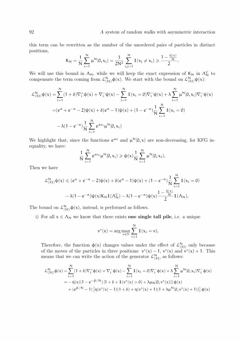
92 A system of random walks with asymmetric interaction
this term can be rewritten as the number of the unordered pairs of particles in distinctpositions,
KN =1
N
N∑
i=1
µN[0, xi) =1
2N2
N∑
i,j=1
1(xj 6= xi) >1−
η(x)
N
2.
We will use this bound in ΛN, while we will keep the exact expression of KN in ΛCN tocompensate the term coming from LN(SJ)φ(x). We start with the bound on LN(SJ)ψ(x):
LN(SJ)ψ(x) =
N∑
i=1
(1+ δ)∇+i ψ(x) +∇−
i ψ(x) −
N∑
i=1
1(xi = 0)∇−i ψ(x) + λ
N∑
i=1
µN[0, xi)∇−i ψ(x)
=(eα + e−α − 2)ψ(x) + δ(eα − 1)ψ(x) + (1− e−α)1
N
N∑
i=1
1(xi = 0)
− λ(1− e−α)1
N
N∑
i=1
eαxiµN[0, xi)
We highlight that, since the functions eαx and µN[0, x) are non-decreasing, for KFG in-equality, we have:
1
N
N∑
i=1
eαxiµN[0, xi) > ψ(x)1
N
N∑
i=1
µN[0, xi).
Then we have
LN(SJ)ψ(x) 6 (eα + e−α − 2)ψ(x) + δ(eα − 1)ψ(x) + (1− e−α)1
N
N∑
i=1
1(xi = 0)
− λ(1− e−α)ψ(x)KN1(ΛCN) − λ(1− e
−α)ψ(x)1−
η(x)
N
21(ΛN).
The bound on LN(SJ)φ(x), instead, is performed as follows.
i) For all x ∈ ΛN we know that there exists one single tall pile, i.e. a unique
v∗(x) = arg maxv∈N
N∑
i=1
1(xi = v).
Therefore, the function φ(x) changes values under the effect of LN(SJ) only becauseof the moves of the particles in three positions: v∗(x) − 1, v∗(x) and v∗(x) + 1. Thismeans that we can write the action of the generator LN(SJ) as follows:
LN(SJ)φ(x) =
N∑
i=1
(1+ δ)∇+i φ(x) +∇−
i φ(x) −
N∑
i=1
1(xi = 0)∇−i φ(x) + λ
N∑
i=1
µN[0, xi)∇−i φ(x)
= − η(x)(1− e−β/N) [1+ δ+ 1(v∗(x) > 0) + λµN[0, v∗(x))]φ(x)
+ (eβ/N − 1)[
η(v∗(x) − 1)(1+ δ) + η(v∗(x) + 1)(1+ λµN[0, v∗(x) + 1))]
φ(x)

93
Then, disregarding the non-positive term −η(x)(1 − e−β/N)1(v∗(x) > 0)φ(x) andbounding the number of particles η(k) in position k with (N− η(x)) for any k 6= ν∗(x),we have
LN(SJ)φ(x) 6
[
−η(x)
NN(1− e−β/N)(1+ δ) −
η(x)
NN(1− e−β/N)λµN[0, v∗(x))
+(N− η(x))λµN[0, v∗(x))(eβ/N − 1) + (1+ δ)(N− η(x))(eβ/N − 1)
+(N− η(x))(eβ/N − 1)λη(x)
N
]
φ(x).
ii) In the region ΛCN, we bound LN(SJ)φ(x) with the pessimistic assumption that everyjump increases φ(x) of the quantity (eβ/N − 1)φ(x), this means that we bound with
LN(SJ)φ(x) 6
(
N(2+ δ) + λ
N∑
i=1
µN[0, xi)
)
(eβ/N − 1)φ(x).
In the right-hand side the term∑Ni=1 µ
N[0, xi) = NKN appears and it will compensatethe same term coming from LN(SJ)ψ(x).
The carré du champ term ΓN(SJ)(φ,ψ)(x), because of the fixed jump amplitude of the process,is bounded as follows:
|ΓN(SJ)(ψ,φ)(x)| 6 N(2+ λ+ δ)(eα − 1)(eβ/N − 1)VNα,β(x).
Given these bounds, we want to identify if there exist λ, α, β positive such that
LN(SJ)VNα,β(x) 6 −γNV
Nα,β(x) +H,
for some constants γN > 0 and H > 0, that is the condition for the ergodicity criterionto hold. In the two complementary regions we have the following bounds, up to termsbounded by H = (1− e−α)eβ:A) for x ∈ ΛN:
LN(SJ)VNα,β(x) 6
[
(eα + e−α − 2) + δ(eα − 1) − λ(1− e−α)1−
η(x)N
2
−η(x)
NN(1− e−β/N)λµN[0, v∗(x)) + (N− η(x))λµN[0, v∗(x))(eβ/N − 1)
−η(x)
NN(1− e−β/N)(1+ δ) + (1+ δ)(N− η(x))(eβ/N − 1)
+(N− η(x))(eβ/N − 1)λη(x)
N+N(2+ δ+ λ)(eβ/N − 1)(eα − 1)
]
VNα,β(x);
B) for x ∈ ΛCN:
LN(SJ)VNα,β(x) 6
[
(eα + e−α − 2) + δ(eα − 1) − λ(1− e−α)KN
+(N(2+ δ) + λNKN) (eβ/N − 1) +N(2+ δ+ λ)(eβ/N − 1)(eα − 1)
]
VNα,β(x).

94 A system of random walks with asymmetric interaction
We want to make the two above parenthesis negative; we start by choosing β = Cα, for acertain C > 0 and to make α sufficiently small.
Let us look at point A). We can not say anything about the terms
−η(x)
NN(1− e−β/N)λµN[0, v∗(x)) + (N− η(x))λµN[0, v∗(x))(eβ/N − 1), (4.2.1)
but we know that, for β sufficiently small,
(1− e−β/N) ' (eβ/N − 1) ' β
N.
In this case, since η(x)
N> 12, the expression (4.2.1) is negative and we can neglect it. In the
same way, we disregard also the terms
N(2+ δ+ λ)(eβ/N − 1)(eα − 1) = o(α)
(eα + e−α − 2) = o(α).
We are left to find λ and C such that the expression
δ(eα − 1) − λ(1− e−α)1− ξ
2− ξN(1− e−β/N)(1+ δ) + (1+ δ)(1− ξ)N(eβ/N − 1) + (1− ξ)N(eβ/N − 1)λξ
is negative for all ξ ∈ (12,1]. Then, for α sufficiently small, this condition becomes
[
δ− (1− ξ)
(
λ
2− C(1+ λξ+ δ)
)
− Cξ(1+ δ)
]
α+ o(α) < 0,
for all ξ ∈ (1/2,1], that gives the conditions on C:
C 6
λ−4δλ
C >δ1+δ
.
Now we look at point B). Again, we neglect the terms
N(2+ δ+ λ)(eβ/N − 1)(eα − 1) + (eα + e−α − 2).
We look for conditions under which
δ(eα − 1) − λ(1− e−α)KN + (N(2+ δ) + λNKN) (eβ/N − 1)
is negative for all values assumed by KN when x ∈ ΛCN. This means, for α small,
[δ− λKN + C(2+ δ+ λKN)]α+ o(α) 6 0,
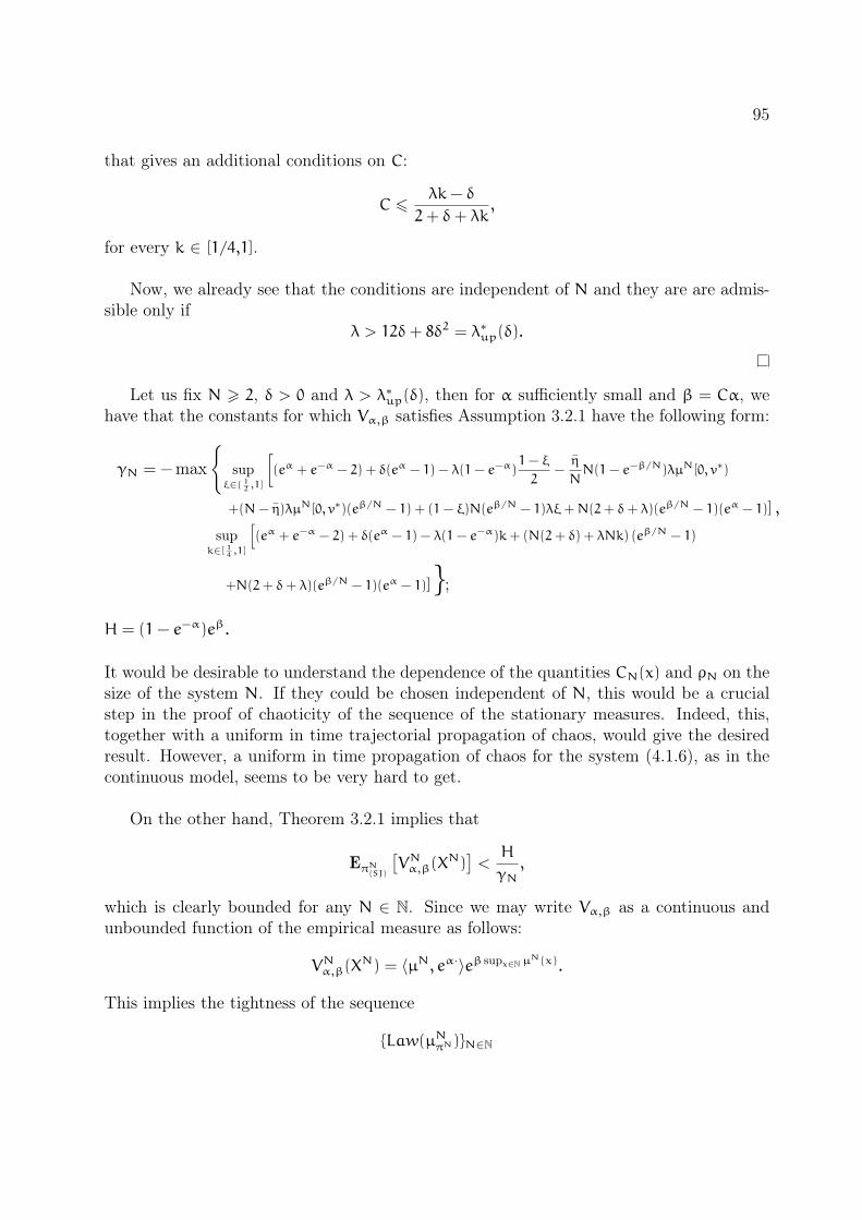
95
that gives an additional conditions on C:
C 6λk− δ
2+ δ+ λk,
for every k ∈ [1/4,1].
Now, we already see that the conditions are independent of N and they are are admis-sible only if
λ > 12δ+ 8δ2 = λ∗up(δ).
Let us fix N > 2, δ > 0 and λ > λ∗up(δ), then for α sufficiently small and β = Cα, wehave that the constants for which Vα,β satisfies Assumption 3.2.1 have the following form:
γN = −max
supξ∈( 1
2,1]
[
(eα + e−α − 2) + δ(eα − 1) − λ(1− e−α)1− ξ
2−η
NN(1− e−β/N)λµN[0, v∗)
+(N− η)λµN[0, v∗)(eβ/N − 1) + (1− ξ)N(eβ/N − 1)λξ+N(2+ δ+ λ)(eβ/N − 1)(eα − 1)] ,
supk∈[ 1
4,1]
[
(eα + e−α − 2) + δ(eα − 1) − λ(1− e−α)k+ (N(2+ δ) + λNk) (eβ/N − 1)
+N(2+ δ+ λ)(eβ/N − 1)(eα − 1)];
H = (1− e−α)eβ.
It would be desirable to understand the dependence of the quantities CN(x) and ρN on thesize of the system N. If they could be chosen independent of N, this would be a crucialstep in the proof of chaoticity of the sequence of the stationary measures. Indeed, this,together with a uniform in time trajectorial propagation of chaos, would give the desiredresult. However, a uniform in time propagation of chaos for the system (4.1.6), as in thecontinuous model, seems to be very hard to get.
On the other hand, Theorem 3.2.1 implies that
EπN(SJ)
[
VNα,β(XN)]
<H
γN,
which is clearly bounded for any N ∈ N. Since we may write Vα,β as a continuous andunbounded function of the empirical measure as follows:
VNα,β(XN) = 〈µN, eα·〉eβ supx∈N µ
N(x).
This implies the tightness of the sequence
Law(µNπN)N∈N

96 A system of random walks with asymmetric interaction
of the stationary empirical measures. Then, one may try to adopt the classical approach forthe proof of propagation of chaos, verifying that any limit point of a convergent subsequenceof µN
πNis stationary for the nonlinear process (4.3.1) and that the stationary measure of
(4.3.1) is unique.
4.2.2 Lower bound for the critical interaction strength in the par-
ticle system
The aim of this section is to highlight, by means of the lower bound for the critical interac-tion strength λ∗N(δ), the difference between the continuous model presented in Chapter 3and the small jumps model presented in Section 4.1.4.
As in Section 3.2.2, we consider the increasing reordering of the vector XN(t) that wenow call
(XN(1)(t), . . . , XN(N)(t)),
such that XN(1)(t) 6 XN(2)(t) 6 · · · 6 XN(N)(t) for all t > 0. According to the dynamics(4.1.6), the element XN(1)(t) perform an upward jump of amplitude 1 with rate 1 + δ, abackward jump of amplitude 1 with rate 1 and it is reflected when XN(1)(t) = 0 and whenXN(1)(t) = XN(2)(t). The same happens for XN(2)(t), with the difference that the rate ofbackward jump is 1+ λ 1
Nand the reflection is upward when when XN(2)(t) = X
N(1)(t) and it
is backward when XN(2)(t) = XN(3)(t). This is a random walk in a wedge, i.e. in the regionWN ⊂ N
N defined as
WN.=
x ∈ N
N s.t. 0 6 x1 6 x2 6 · · · 6 xN.
The dynamics in the interior of WN is the following, for all i = 1, . . . ,N
x→ x+ ei with rate 1+ δ,
x→ x− ei with rate 1+ λi− 1
N,
The dynamics at the boundaries of WN depends on which “face” of the wedge the point isin. For instance, fix an index i < N, an N− 1-dimensional “face” of the wedge is the subset
Bi,i+1.= x ∈ WN : xi = xi+1 and xj < xj+1 ∀ j 6= i.
The dynamics on Bi,i+1 is the same as the interior one for all jumps ±ej, j 6= i, i+ 1, whilethe difference is the following
x→ x+ ei+1 with rate 2(1+ δ),
x→ x− ei with rate 2(1+ λi− 1
N).

97
In the same way, we define the dynamics on all the other lower dimensional “faces” of thewedge, according to the dynamics (4.1.6) and the number of particles in the same position.
It is clear that these “faces” corresponds to configurations of particles that show somepiles of particles. For instance the N − 1-dimensional face Bi,i+1 corresponds to the setof configurations that display one single pile of particles of height 2 involving the ith and(i+ 1)th ranked particles. Therefore, we may identify the whole boundary of WN with theset of configurations with at least one pile of particles. We already mentioned that areexactly these “faces” that creates the main issue in understanding the stationary measure.Indeed, we defined (YN1 (t), . . . , Y
NN(t)) the process that evolves according to (3.2.4) in the
regionWN
.= y ∈ DN s.t. 0 6 y1 6 y2 6 · · · 6 yN .
We highlighted in Proposition 3.1.2 that, in this case, there is a.s. no triple collision. Thismeans that the non-smooth parts of the boundary of the wedge are of no importance andthat it is sufficient to consider reflection conditions on the hyperplanes of dimension N− 1
that bound the wedge and not on their edges. In the discrete case the piles of particlesactually matter and this is confirmed by the following result. We found, for all N > 2, alower bound for the critical value λ∗N(δ) that is strictly greater than the critical value forthe continuous space model, proved in Theorem 3.2.2. Therefore, in the random walk, thestrength of the interaction needed to get ergodicity is higher than in the diffusive case.
Theorem 4.2.2. For all N > 2 and for all δ > 0, there exists
λ∗N,lower(δ).=(
1+ ρ(ε,N))
2δ, with ρ(ε,N).=
N2(δ+ 2)
N(N− 1)(δ+ 2) − 2δ− 1 −→ 0, (4.2.2)
such that, for all λ < λ∗N,lower(δ), the process XN = (XN1 , . . . , XNN) generated by (4.1.6) is
transient.
It is clear that, for all fixed N > 2, this lower bound satisfies
λ∗N,lower(δ) > 2δN
N− 1,
i.e. it is strictly greater than the critical interaction strength of the continuous model foundin Theorem 3.2.2.
The proof of this lower bound is made by means of a Lyapunov function. We exploitthe following result on the transience of Markov chains, that is a simplified version ofTheorem 2.2.7 in [39].
Theorem 4.2.3 ( Theorem 2.2.7 in [39]). Let Xtt>0 an irreducible Markov process on acountable space X with infinitesimal generator L and bounded jumps. Suppose there existstwo positive constants ε,C > 0 and a positive function f such that AC
.= x ∈ X : f(x) > C 6=
∅ andLf(x) > ε for all x ∈ AC.
Then the process Xtt>0 is transient.

98 A system of random walks with asymmetric interaction
Therefore, we want to define a linear function f[N,λ,δ] : WN → R such that for allλ > λ∗N,lower(δ)
LNordf[N,λ,δ](x) > 0, (4.2.3)
for all x ∈ WN, where LNord is the generator of the reordered process (XN(1)(t), . . . , XN(N)(t)).
The idea for the construction of this Lyapunov function is the following. Firstly, we considerthe barycenter of the particle system
B(x) =
N∑
k=1
xk
as a candidate Lyapunov function. We see that, if λ < 2δ NN−1
,
LNordB(x) > 0
for all x ∈ WN. If the parameters satisfy this condition, the mean drift of the lowest bN2c
particles is positive, i.e. for k = 1, . . . , bN2c it holds
LNordxk > 0
for all x in the interior of WN. Then, we may consider, instead of the classic barycenter,a modification of it that gives more “weight” to the first particles. Therefore, we considerthe vector vε = (1+ ε,1,1,1, . . . ) and define the Laypunov function
fε(x) = 〈vε, x〉 = (1+ ε)x1 +
N∑
k=2
xk
for some ε > 0. We look for the maximal ε > 0 that improves the condition on λ, i.e. wewant to find if there exists ρ(ε,N) > 0 such that LNordfε(x) > 0 for all x ∈ WN, when
λ < 2δN
N− 1+ ρ(ε,N).
Proof of Theorem 4.2.2. We fix N > 2 and δ > 0, then we consider the N dimensionalvector vε = (1+ ε,1,1, . . . ,1) and the function fε(x) = 〈vε, x〉, defined on WN. For x in theinterior of WN the condition for (4.2.3) to hold is
Nδ+ ε− λN− 1
2> 0, (4.2.4)
our aim is to find an admissible ε > 0, that increases the maximal λ satisfying (4.2.3). Weneed to check the admissibility of ε in those regions of WN where the mean drift of the

99
first particle is negative, that are the regions where the first particle belongs to a pile. Letfirst consider the subsets
W(N,k) : = x ∈ WN : x1 = · · · = xk < xk+1,where the first particle belongs to a pile of exactly height k, for k = 2, . . . ,N. Then we saythat, for all k = 2, . . . ,N and for all x ∈ W(N,k), it holds
LNordfε(x) > Nδ− kε− λN− 1
2+ λ
k(k− 1)
2N.
Therefore we want to find the maximal ε > 0 such that
mink=2,...,N
Nδ− kε− λN− 1
2+ λ
k(k− 1)
2N> 0,
that isεmax =
λ
N(δ+ 2).
Substituting εmax, we get that (4.2.4) holds for all
λ <2N2(δ+ 2)δ
N(N− 1)(δ+ 2) − 2δ= λ∗N,lower(δ).
4.3 Stationary measures for the nonlinear process
Following the approach of Section 4.2, we focus on the stationary measures for the nonlinearprocess with small jumps, i.e. the process described in (4.1.8), that corresponds to thesolution X(t)t>0 of the following nonlinear SDE
dX(t) = −1(X(t−) > 0)
∫∞
0
1[0,1](u)N(−)(du, dt) +
∫∞
0
1[0,1+δ](u)N(+)(du, dt)
−
∫
[0,1]
∫∞
0
1[0,µt−([0,X(t−)))(h)1[0,λ](u)N(du, dh, dt), (4.3.1)
where µt = Law(X(t)) and N(−),N(+),N are independent stationary Poisson processeswith characteristic measures, respectively, dudt, dudt and dudhdt.
We know that the study of stationary measures for nonlinear processes is much moredifficult than the one for classical Markov processes. Motivated by the stability study of itscontinuous analogue in Theorem 3.2.3, we conjecture that a stationary measure for (4.3.1),when it exists, it should be unique. However, proving uniqueness of the stationary measurefor nonlinear processes is a delicate issue. For this reason, in this section we look for theexact critical value
λ∗(δ)
above which the nonlinear process (4.3.1) has at least one stationary measure. As inSection 4.2, we could not find the exact value λ∗(δ), so we give an upper and a lower boundfor it.

100 A system of random walks with asymmetric interaction
4.3.1 Upper bound for the critical interaction strength in the non-
linear process
In this section we give a sufficient condition for the existence of at least one stationarymeasure for the nonlinear process, solution to (4.3.1). This provides an upper bound forthe interaction strength λ∗(δ) and it is stated in the next theorem.
Theorem 4.3.1. For all δ > 0, there exists a value
λ∗up(δ).= 4δ
such that, for all λ > λ∗up(δ), the nonlinear process(4.3.1) has at least one stationarydistribution.
We prove the existence of at least one stationary distribution by means of a transfor-mation Γ in the space M(N), for which every stationary distribution of (4.3.1) is a fixedpoint. This is an approach widely exploited in the study of quasi-stationary distributions(QSD) in countable spaces, see [5, 40, 41].
We define a continuous time Markov chain on N, parametrized by a measure. Fix µ∈ M(N), then let Xµ(t)t>0 be the process with infinitesimal generator defined as follows.For f ∈ Cb, and x ∈ N
Lµf(x) = (1+ δ)(f(x+ 1) − f(x)) + 1(x > 0)(1+ λµ[0, x))(f(x− 1) − f(x)). (4.3.2)
It is clear that Xµ(t)t>0 is a birth and death process. Assuming λ > δ, for every measure µ,the process Xµ(t)t>0 is ergodic, and πµ denotes its unique stationary distribution. Definethe map
Γ : M(N) → M(N)
µ 7→ πµ,
Notice that, by definition, µ∗ is a stationary distribution for (4.3.1) if and only if it is afixed point of Γ .
Proof of Theorem 4.3.1. The proof of the upper bound consists of three steps. First wedefine an auxiliary map that stochastically dominates the map Γ , then we prove that thismap preserves a certain subset of M(N), finally we prove that Γ admits at least one fixedpoint in that subset.
Step 1. Givenm ∈ R+, consider the birth and death process with infinitesimal generator
Lmf(x) = (1+ δ)(f(x+ 1) − f(x)) + (1(x > 0) +λ
21(x > m))(f(x− 1) − f(x)),
Since we are assuming λ > 4δ (here λ > 2δ would suffice), this process is ergodic, andwe denote by πm its stationary distribution. We claim that for all µ ∈ M(N), we haveπµ πmed(µ), where med(µ) denotes the median of µ and is defined in Definition 4.2.1.
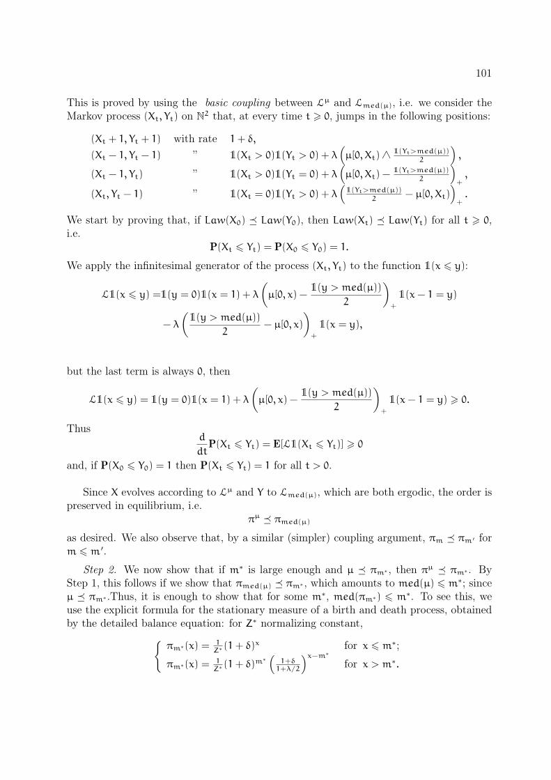
101
This is proved by using the basic coupling between Lµ and Lmed(µ), i.e. we consider theMarkov process (Xt, Yt) on N
2 that, at every time t > 0, jumps in the following positions:
(Xt + 1, Yt + 1) with rate 1+ δ,
(Xt − 1, Yt − 1) ” 1(Xt > 0)1(Yt > 0) + λ(
µ[0, Xt)∧1(Yt>med(µ))
2
)
,
(Xt − 1, Yt) ” 1(Xt > 0)1(Yt = 0) + λ(
µ[0, Xt) −1(Yt>med(µ))
2
)
+,
(Xt, Yt − 1) ” 1(Xt = 0)1(Yt > 0) + λ(
1(Yt>med(µ))
2− µ[0, Xt)
)
+.
We start by proving that, if Law(X0) Law(Y0), then Law(Xt) Law(Yt) for all t > 0,i.e.
P(Xt 6 Yt) = P(X0 6 Y0) = 1.
We apply the infinitesimal generator of the process (Xt, Yt) to the function 1(x 6 y):
L1(x 6 y) =1(y = 0)1(x = 1) + λ
(
µ[0, x) −1(y > med(µ))
2
)
+
1(x− 1 = y)
− λ
(
1(y > med(µ))
2− µ[0, x)
)
+
1(x = y),
but the last term is always 0, then
L1(x 6 y) = 1(y = 0)1(x = 1) + λ
(
µ[0, x) −1(y > med(µ))
2
)
+
1(x− 1 = y) > 0.
Thusd
dtP(Xt 6 Yt) = E[L1(Xt 6 Yt)] > 0
and, if P(X0 6 Y0) = 1 then P(Xt 6 Yt) = 1 for all t > 0.
Since X evolves according to Lµ and Y to Lmed(µ), which are both ergodic, the order ispreserved in equilibrium, i.e.
πµ πmed(µ)as desired. We also observe that, by a similar (simpler) coupling argument, πm πm ′ form 6 m ′.
Step 2. We now show that if m∗ is large enough and µ πm∗ , then πµ πm∗ . ByStep 1, this follows if we show that πmed(µ) πm∗ , which amounts to med(µ) 6 m∗; sinceµ πm∗ .Thus, it is enough to show that for some m∗, med(πm∗) 6 m∗. To see this, weuse the explicit formula for the stationary measure of a birth and death process, obtainedby the detailed balance equation: for Z∗ normalizing constant,
πm∗(x) = 1
Z∗ (1+ δ)x for x 6 m∗;
πm∗(x) = 1Z∗ (1+ δ)
m∗(
1+δ1+λ/2
)x−m∗
for x > m∗.

102 A system of random walks with asymmetric interaction
The desired inequality med(πm∗) 6 m∗ follows if we show that
πm∗ [0,m∗] > πm∗(m∗,∞).
Indeed, this is equivalent to
(1+ δ)bm∗c+1 − 1
δ> (1+ δ)bm
∗c 1+ δ
λ/2− δ
and, by simplifying,λ/2− 2δ
λ/2− δ>
1
(1+ δ)bm∗c+1 ,
which holds for m∗ sufficiently large.
Step 3. Define the set
Mm∗(N) : = µ ∈ M(N) : µ πm∗ ,
where m∗ has been determined in step 2. We have seen that the function Γ maps Mm∗ intoitself. Moreover, Mm∗ is clearly convex, and it is compact for the weak topology, beingclosed and tight. The existence of a fixed point follows from Schauder-Tychonov fixedpoint theorem if we show that Γ is continuous. Let µn → µ in Mm∗ . By the formula forthe stationary distribution of a birth and death process we have
πµn(x) =1
Z∗n
(1+ δ)k∏k−1h=0(1+ λµn[0, h))
,
with
Z∗n : =
∞∑
k=0
(1+ δ)k∏k−1h=0(1+ λµn[0, h))
.
Since(1+ δ)k
∏k−1h=0(1+ λµn[0, h))
6(1+ δ)k
∏k−1h=0(1+ λπm∗ [0, h))
,
by the Dominated Convergence Theorem
Z∗n → Z∗ :=
∞∑
k=0
(1+ δ)k∏k−1h=0(1+ λµ[0, h))
,
and πµn → πµ, which establishes continuity.
Let us underline the importance of this approach with the fixed point argument. Itgives an upper bound for the critical value λ∗∞(δ) which is linear in δ. Indeed, based on somebasic numerical computation, we have the feeling that the condition on λ is not quadraticin δ, as the one emerging from Theorem 4.2.1. Clearly the one found in Theorem 4.3.1 isnot optimal and in the following sections we propose conjectures for the critical interactionstrength in both the particle system and the nonlinear limit equation.

103
4.3.2 Lower bound for the critical interaction strength in the non-
linear process
In this section we give a simple lower bound for the critical value λ∗(δ). Although webelieve that λ∗(δ) should be strictly greater than its continuous analogue, we could notfind a way to prove it and the lower bound here coincides exactly with the continuouscritical interaction strength of Theorem 3.2.3.
Theorem 4.3.2. For all δ > 0, there exists a
λ∗lower(δ).= 2δ
such that, for all λ < λ∗lower(δ), there is no stationary distribution for the nonlinear pro-cess (4.3.1).
Proof. We show that, for λ 6 2δ, the nonlinear system has no stationary distributions.Let us remark, to begin with, that for λ 6 δ the conclusion is essentially obvious: indeed,the nonlinear Markov process can be coupled, monotonically from below, with a reflectedrandom walk with forward rate 1+ δ and backward rate 1+ λ, whose distribution at timet tends to concentrate in +∞ as t ↑ +∞, for any initial distribution.
So assume λ > δ, and suppose there exists a stationary distribution µ. The Markovprocess generated by Lµ in (4.3.2) has a strictly negative drift for sufficiently large positions;this implies that its stationary distribution, that is µ by assumption (because µ must bea fixed point of the map Γ), has tails not larger than exponentials. In particular, denotingby (Xt)t>0 the associated stationary process,
E(Xt) < +∞.
Moreover, denoting by id the identity map on N,
0 =d
dtE(Xt) = E [L
µid(Xt)] = δ− λ∑
x>0
µ[0, x)µ(x). (4.3.3)
But∑
x>0
µ[0, x)µ(x) =∑
x>0
µ[0, x− 1] (µ[0, x] − µ[0, x− 1])
=∑
x>0
(
µ2[0, x] − µ2[0, x− 1])
−∑
x>0
µ[0, x] (µ[0, x] − µ[0, x− 1])
= 1−∑
x>0
µ[0, x− 1] (µ[0, x] − µ[0, x− 1]) −∑
x>0
µ2(x)
which implies∑
x>0
µ[0, x)µ(x) <1
2.
Inserting this in (4.3.3), we get λ > 2δ, which completes the proof.
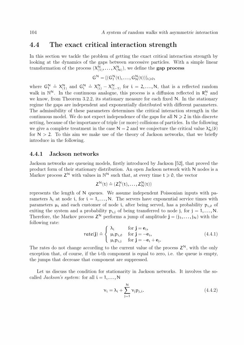
104 A system of random walks with asymmetric interaction
4.4 The exact critical interaction strength
In this section we tackle the problem of getting the exact critical interaction strength bylooking at the dynamics of the gaps between successive particles. With a simple lineartransformation of the process (XN(1), . . . , X
N(N)), we define the gap process
GN = (GN1 (t), . . . , GNN(t))t>0,
where GN1.= XN(1) and GNi
.= XN(i) − X
N(i−1) for i = 2, . . . ,N, that is a reflected random
walk in NN. In the continuous analogue, this process is a diffusion reflected in RN+ and
we know, from Theorem 3.2.2, its stationary measure for each fixed N. In the stationaryregime the gaps are independent and exponentially distributed with different parameters.The admissibility of these parameters determines the critical interaction strength in thecontinuous model. We do not expect independence of the gaps for all N > 2 in this discretesetting, because of the importance of triple (or more) collisions of particles. In the followingwe give a complete treatment in the case N = 2 and we conjecture the critical value λ∗N(δ)for N > 2. To this aim we make use of the theory of Jackson networks, that we brieflyintroduce in the following.
4.4.1 Jackson networks
Jackson networks are queueing models, firstly introduced by Jackson [52], that proved theproduct form of their stationary distribution. An open Jackson network with N nodes is aMarkov process ZN with values in N
N such that, at every time t > 0, the vector
ZN(t).= (ZN1 (t), . . . , Z
NN(t))
represents the length of N queues. We assume independent Poissonian inputs with pa-rameters λi at node i, for i = 1, . . . ,N. The servers have exponential service times withparameters µi and each customer of node i, after being served, has a probability pi,0 ofexiting the system and a probability pi,j of being transferred to node j, for j = 1, . . . ,N.Therefore, the Markov process ZN performs a jump of amplitude j = (j1, . . . , jN) with thefollowing rate:
rate(j).=
λi for j = ei,
µipi,0 for j = −ei,
µipi,j for j = −ei + ej.
(4.4.1)
The rates do not change according to the current value of the process ZN, with the onlyexception that, of course, if the i-th component is equal to zero, i.e. the queue is empty,the jumps that decrease that component are suppressed.
Let us discuss the condition for stationarity in Jackson networks. It involves the so-called Jackson’s system: for all i = 1, . . . ,N
νi = λi +
N∑
j=1
νjpj,i. (4.4.2)

105
Here, if we suppose to be in a stationary regime, the solution ν = (ν1, . . . , νN) of thesystem (4.4.2) represents the mean number of customers entering each node in a unit timeinterval, coming from the outside or from the other nodes. First, the system (4.4.2) admitsa solution if the spectral radius of the matrix pi,ji,j=1,dots,N is strictly less than one,i.e. every customer leaves the network with probability one. Then, we state whether astationary measure for the process with rates (4.4.1) exists in the following theorem, dueto Jackson [52].
Theorem 4.4.1. The Jackson network ZN with rates (4.4.1) is ergodic if and only if
νi < µi
for all i = 1, . . . ,N. In that case, the stationary measure is given by
πN,Jack(z) =
N∏
i=1
(
νi
µi
)zi
(1−νi
µi),
for all z ∈ NN.
In [38] the authors also prove exponential ergodicity of Jackson networks under thesame conditions of Theorem 4.4.1, by means of a linear Lyapunov function geometricallyconstructed.
4.4.2 Exact study of gap process for N = 2
Let us focus on the small jumps model (4.1.6) with N = 2. Its gap process G2 =
(G21(t), G22(t))t>0 is a reflected random walk in the positive quadrant. It jumps according
the following rates:
g s.t. g1 > 0, g2 > 0 → g + (1,−1) with rate 1+ δ
g + (0,−1) ” 1+ λ2
g + (−1,1) ” 1
g + (0,1) ” 1+ δ
g s.t. g1 = 0, g2 > 0 → g + (1,−1) ” 1+ δ
g + (0,−1) ” 1+ λ2
g + (0,1) ” 1+ δ
g s.t. g1 > 0, g2 = 0 → g + (−1,1) ” 2
g + (0,1) ” 2+ 2δ
(0,0) → (0,1) ” 2+ 2δ.
The following results gives the exact value of the critical interaction strength λ∗2(δ) and theexpression of the stationary measure for the model.
106 A system of random walks with asymmetric interaction
Theorem 4.4.2. The process G2 is exponentially ergodic if and only if λ > 2δ2 + 4δ.Moreover, when it exists, the unique stationary measure π2 has the following explicit form:
π2(0,0) =C2
π2(0, y) = C(
1+δ
1+ λ2
)y
y > 1,
π2(x,0) =C2
(
(1+δ)2
1+ λ2
)x
x > 1,
π2(x, y) = C(
(1+δ)2
1+ λ2
)x (1+δ
1+ λ2
)y
x > 1, y > 1,
for C.=2( λ2−δ)(
λ2−2δ−δ
2)
( λ2+δ2)(λ2+1)
.
The proof of exponential ergodicity is based on the link between the gap process G2 anda particular Jackson network. Indeed, because of the nature of the jumps of the gap processG2, notice that, except that for the “last gap”, the increase by one unit of a componentcauses the decrease by one unit of another. Therefore, we associate to the gap process G2
a two dimensional Jackson network. Let Z2 be such that its parameters take the followingvalues:
λ1 = 0, µ1 = 1, p1,0 = 0, p1,2 = 1,
λ2 = 1+ δ, µ2 = 2+λ2+ δ, p2,0 =
+ λ2
µ2, p2,1 =
1+δµ2.
(4.4.3)
The process Z2 defined in this way has the same jumps and the same rates of G2 in theinternal region N∗ × N∗, while has a slight difference in the rates on the boundaries.
In Figure 4.1 we see the admissible jumps of the gap process G2 and their rates. InFigure 4.2 we see that the admissible jumps of the Jackson network Z2 are the same ofG2 but the rates of the jumps performed from the x axis are halved w.r.t. the ones of G2.Therefore, it is easy to see that, if we consider the embedded Markov chain of each process,the two Markov chains have the same transition matrix. This implies that conditions onstationary measures and on ergodicity for one process are the same for the other and it isthe key of the following proof.
Proof of Theorem 4.4.2. Consider the 2 nodes Jackson network Z2 with same rates of G2
in the internal region, i.e. the one described by the parameters in (4.4.3). Let (ν1, ν2) bethe solution of the Jackson’s system (4.4.2), that here we write as:
ν1 = λ1 + ν2p2,1,
ν2 = λ2 + ν1p1,2.
We know from Theorem 4.4.1 that Z2 is ergodic if and only if νi < µi, for i=1,2. In ourcase this condition becomes
(1+δ)2
(1+ λ2 )< 1,
(1+δ)µ2(1+ λ
2 )< µ2,
that gives λ > 2δ2 + 4δ. As we mentioned, in [39], by the use of a Lyapunov function, theauthors prove that this is the necessary and sufficient condition for exponential ergodicity

107
2+ 2δ
(0,0)
2 2+ 2δ
1+ λ2
1+ δ
1+ δ
1
1+ δ1+ λ2
1+ δ
Figure 4.1: Gap process with rates when N = 2.
of the process Z2 and, consequently, for G2.
The invariant measure of the common embedded Markov chain has the following form:
η2(0,0) = 1+ δ
η2(0, y) =(
3+ 2δ+ λ2
)
(
1+δ
1+ λ2
)y
y > 1,
η2(x,0) = (2+ δ)(
(1+δ)2
1+ λ2
)x
x > 1,
η2(x, y) =(
4+ 2δ+ λ2
)
(
(1+δ)2
1+ λ2
)x (1+δ
1+ λ2
)y
x > 1, y > 1.
Then, for all (x, y) ∈ NN we divide η2(x, y) by the sum of G2-rates of exiting from (x, y)
and we normalize. Of course, the obtained measure coincide with the explicit form of π2.This is validated by verifying that π2 solves the stationary equation, i.e. for all boundedmeasurable functions f it holds:
∑
(x,y)∈N2
L2f(x, y)π2(x, y) = 0,
where L2 is the infinitesimal generator of G2.

108 A system of random walks with asymmetric interaction
1+ δ
(0,0)
1 1+ δ
1+ λ2
1+ δ
1+ δ
1
1+ δ1+ λ2
1+ δ
Figure 4.2: Associated Jackson network rates when N = 2.
Theorem 4.4.2 gives the exact critical value λ∗2(δ) for the ergodicity of the system andwe see that it is quadratic in δ. Moreover, the explicit expression of π2 proves that, in thestationary regime, the gaps G21 and G22 are independent. Notice that the lower bound onλ∗2(δ) obtained in Theorem 4.2.2 is optimal in this case.
4.4.3 Some conjectures
The link between the gap process and a Jackson network for N = 2 suggests an associationwith N nodes Jackson network for every fixed N. Unfortunately, when N > 3 the transitionmatrix of the embedded Markov chains of GN and ZN are not the same. However we canpropose a conjecture on the critical value λ∗N(δ) based on the properties of the associatedJackson network. First of all, let us define the Jackson network ZN to associate with thegap process GN, for a fixed N > 3. ZN must be such that the transition rates in the internalregion N
N∗ correspond to the ones of the gap process GN. For all i = 1, . . . ,N− 1
z → z− ei + ei+1 with rate 1+ λ i−1N,
z → z+ ei − ei+1 ” 1+ δ,
z → z− eN ” 1+ λN−1N,
z → z+ eN ” 1+ δ,
(4.4.4)

109
where ei is the vector (0, . . . ,0,1,0, . . . ,0) with the i-th coordinate equal to 1.
Proposition 4.4.1. Fix N > 3, the N node Jackson network ZN with transition rates(4.4.4) is ergodic if, and only if, we have
(1+ δ)N
N−1∏
k=1
(1+ λk
N)
< 1. (4.4.5)
Proof. The Jackson network ZN is such that
λN = 1+ δ,
λj = 0 for all j = 1, . . . ,N− 1,
µ1 = 0,
µj = 2+ δ+ λj−1N, for all j = 2, . . . ,N,
p1,2 = 1, p1,k = 0, for all k 6= 2,
pj,j+1 =1+λ j−1Nµj
, pj,j−1 =1+δµj
for all j = 2, . . . ,N− 1,
pj,k = 0 for all j = 2, . . . ,N− 1, and all k 6= j+ 1, j− 1,
pN,0 =1+λN−1
N
µN, pN,N−1 =
1+δµj
pN,k = 0 for all k 6= N,0.Let us recall the Jackson system:
νj = λj +
N∑
i=1
νipi,j, for j = 1, . . . ,N.
It is easy to verify that the solution (ν1, . . . , νN) of this is system has the following form:
νj = µj
N+1−j∏
k=1
(1+ δ)
(1+ λN−kN
), for all i = 1, . . . ,N,
that by classical result on Jackson networks gives the following condition:i∏
k=1
(1+ δ)
(1+ λN−kN
)< 1, for all i = 1, . . . ,N,
that is equivalent to (4.4.5).
Conjecture 4.4.1. Fix N > 3, the gap process GN is ergodic if, and only if,
(1+ δ)N
N−1∏
k=1
(1+ λk
N)
< 1.

110 A system of random walks with asymmetric interaction
This would give an exact critical value λ∗N(δ), i.e. for each N > 3 and each δ > 0 wouldbe the solution of
(1+ δ)N
N−1∏
k=1
(1+ λk
N)
= 1.
In the continuous framework, the sequence of critical values (that by abuse of notationwe indicate in the same way) λ∗N(δ) converges, as N goes to ∞ to the critical value λ∗∞(δ)
for the nonlinear process. In our case we could not understand if this can be true or not,since we do not even know if there is a value such that there exists a unique stationarymeasure. However we make a conjecture on the critical value for which there exists at leastone stationary measure based on the sequence λ∗N(δ).
Conjecture 4.4.2. Fix δ > 0, then for all λ such that
(1+1
λ) ln (1+ λ) − 1 > ln (1+ δ) ,
the nonlinear process (4.3.1) has at least one stationary measure.
Based on the comparison with the continuous model from Chapter 3, we conjecturealso that, when a stationary measure for (4.3.1) exists, then it is unique and that thechaoticity of the stationary measures holds true also in this case. The Lyapunov functionof Theorem 4.2.1 seems very promising in this direction, since it ensures the tightness ofthe sequence of empirical measures, as we observed at the end of Section 4.2.1. Indeed,given α > 0 from Theorem 4.2.1, there exists K .
= supNHγN
> 0 such that, for all N, thestationary measure πN(SJ) is such that
EπN(SJ)
[
∞∑
k=0
eαkµNXN(k)
]
< K, (4.4.6)
where µNXN
(·) = 1N
∑Ni=1 δXNi and Law(XN) = πN(SJ). Then we may wish to apply the
approach in [6], where the authors prove chaoticity of the stationary measures of theFleming-Viot particle system linked to the subcritical Galton-Watson process. Let usadapt this approach to our case. Fix δ > 0 and λ > λ∗up(δ), we wish to prove
limN→∞
EπNXN
[∥
∥µNXN(·) − π(·)∥
∥
TV
]
= 0, (4.4.7)
that implies weak convergence of the stationary empirical measures to the stationary mea-sure π of (4.3.1) identified in Theorem 4.3.1. Notice that (4.4.7) is equivalent to
limN→∞
EπNXN
[∣
∣µNXN(k) − π(k)∣
∣
]
= 0,
for all k ∈ N. Then fox k, by definition of stationary measure, we know that
EπN(SJ)
∣
∣µNXN(k) − π(k)∣
∣ = EπN(SJ)
∣
∣µNt (k) − π(k)∣
∣ ,
111
where µNt is the empirical measure of the process XN(t) such that Law(XN(0)) = πN(SJ). Letus also denote by µt(·, ν) the law at time t > 0 of the solution to (4.3.1), such that ν is thelaw of the initial condition. For any C > 0, we consider the following subset of NN
Sα(C).=
x ∈ NN :
∞∑
k=0
eαkµNx (k) 6 C, for µNx =1
N
N∑
i=1
δxi
.
Then it holds
EπN(SJ)
∣
∣µNt (k) − π(k)∣
∣ 6EπN(SJ)
[
1(
Sα(C)C)]
+ EπN(SJ)
[
1 (Sα(C))∣
∣µNt (k) − π(k)∣
∣
]
6 EπN(SJ)
[
1(
Sα(C)C)]
+ EπN(SJ)
[
1 (Sα(C))∣
∣µt(k, µNXN) − π(k)
∣
∣
]
+EπN(SJ)
[
1 (Sα(C))∣
∣µNt (k) − µt(k, µNXN)∣
∣
]
.
Let ε > 0, the first term is treated by means of (4.4.6), such that
EπN(SJ)
[
1
(
∞∑
h=0
eαhµNXN(h) > C
)]
6K
C
and we can choose C sufficiently large such that this term is smaller than ε3. Now, suppose
that we could prove that, for any initial condition ν belonging to the following set
Sα(C).=
ν ∈ M(N) :
∞∑
k=0
eαkν(k) 6 C
,
the (4.3.1) is ergodic, i.e. for all ν ∈ Sα(C)
limt→∞
‖µt(·, ν) − π(·)‖TV = 0.
Of course, in the event XN ∈ Sα(C) is equivalent to the event µNXN
∈ Sα(C). Thiswould let us choose t > 0 sufficiently large such that the second term is smaller than ε
3.
Then, for fixed C, t > 0 the pathwise propagation of chaos proved in Theorem 4.1.3, let uschoose N sufficiently large such that the third term is smaller than ε
3, as well. This would
prove (4.4.7). We conclude by highlighting that the missing step is the proof of ergodicityof (4.3.1), which seems to us a reasonable result, but not a trivial one.

112 A system of random walks with asymmetric interaction
Part III
Generalized Curie-Weiss model
113


Chapter 5
Periodic behavior in a generalized
Curie-Weiss model with dissipation
Among the interesting phenomena observed in complex systems, there is the occurrenceof rhythmic behaviors. It is natural to model this systems by means of large families ofinteracting units and one question is how periodic behaviors emerge in these systems whenthe single units have no tendency to behave periodically.
5.1 Self-sustained periodic behavior
In a particle system we say that we observe a self-sustained periodic behavior if there is aphase in which the evolution of the macroscopic law of the system has a stable limit cycle,without the action of any periodic force. Often this periodicity, even if easily detectable bynumerical simulations of the particles for large system’s size, it is a peculiarity of the ther-modynamic limit and it is quite hard to formally prove it, since it is an infinite dimensionalproblem. However, some recent works [27, 47] try to investigate the minimal hypothesisneeded to create self-sustained periodic behavior in mean field interacting particle systems.In this framework, one key step is to consider interactions that favor cooperation amongunits of the same type, but, opposed to the classical models originated from statisticalmechanics, the reversibility of the dynamics seems to be in contrast with the occurrence ofperiodic behavior [11, 47]. Therefore, different mechanisms that perturb classical reversiblemodels have been introduced.
• In [24, 26] the authors introduce particle systems where each particle has its own localfield that undergoes a diffusive and dissipative dynamics. The add of a dissipativeterm seems to be a useful tool to create stable periodic orbit in systems otherwisein equilibrium. The simplest model of this class is the dynamical Curie-Weiss modelwith a dissipative term studied in [26], which already displays an interesting behaviordue to the dissipation and the rise of a periodic orbit via a Hopf bifurcation. In [24]wefind a general way of introducing dissipation in systems of interacting diffusions,together with the study of the dissipative counterpart of the model by Dawson [28].

116 A generalized Curie-Weiss model with dissipation
• In [47] authors consider active rotators models, one among the others the stochasticKuramoto model. They propose different dynamics and interactions for which theyprove periodicity with a very general method. In particular adding a simple disorderin the initial phase of each rotator for the Kuramoto model, see [1, 23], gives originto oscillating behavior in the stationary solutions.
• The role of noise in the dynamics is crucial. It may induce periodicity in systemswhich cannot exhibit periodic solutions, giving rise to the phenomenon of noise-induced periodicity [27, 78, 86]. Moreover, noise has a role in enhancing periodicityin dynamical systems already proved to have limit cycles, a phenomenon known asexcitability by noise [24, 59].
• The add of a delay in the interactions is proved to give self-sustained periodicityin multi-populated models. In [85] a fixed time delay is sufficient to create stableoscillations in a bi-populated spin system with non-cooperative interaction. In [31] amulti-populated system of interacting Hawkes processes with a delay given by Erlangkernels is studied and sufficient conditions for the existence of at least one stable limitcycle are given.
• In [25] the interaction network between two populations is enough to generate peri-odicity, without the need of a delay in the interaction. In particular, it is a frustratedinteraction that, if strong enough, generates the limit cycles. By frustrated interac-tion we mean the situation in which one population “wants to copy” the other, butthis one has the tendency to behave oppositely to the first one.
The aim of this chapter is to extend the first approach to the so-called generalized Curie-Weiss model. We confirm that the dissipative interaction is able to give origin to self-sustained periodic behaviors in a wide class of mean field particle systems.
5.2 The model
In this section we build step-by-step the class of processes we are interested in. We startwith a brief description of the classical Curie-Weiss spin model and of the class of itsgeneralized counterpart; then we define a stochastic process related to this class and wedescribe how we can break its reversibility by means of the dissipative dynamics.
5.2.1 The Curie-Weiss model
The Curie-Weiss model origins as a mean field approximation of the Ising model for fer-romagnetism. In this case a magnet is modelled, at microscopic level, by a configurationof N spins; each spin takes values in the set −1,+1. We associate to each configurationσN ∈ −1,+1N an energy, by the Hamiltonian, which is a quadratic function of the mean

117
spin value:
HN(σN)
.= −
1
2N
(
N∑
i=1
σNi
)2
. (5.2.1)
For any inverse temperature β = 1T> 0 we define the probability measure, called the Gibbs
measure, on −1,+1N
PN,β(dσN1 . . . dσ
NN)
.=
1
ZN(β)e−βHN(σN),
where ZN(β).=
∑NσN∈−1,+1 e
−βHN(σN) is the normalizing constant. The Gibbs measuregives higher probability to configurations with minimal energy.
The Curie-Weiss model is defined as the sequence of probability measures PN,βN∈N∗
and it shows a phase transition, usually identified as a breakdown in the Law of LargeNumbers, see for example [36]. The previous means that the following weak limit holds:
∑Ni=1 σ
Ni
N
N→ ∞−−−−→δ0 for β 6 1,12(δm(β) + δ−m(β)) for β > 1,
(5.2.2)
for a certain increasing functionm(·) : (1,∞) → (0,1), called the spontaneous magnetization.Therefore, the value βc
.= 1 is a critical value for the Curie-Weiss. When β < βc (i.e. the
temperature is sufficiently high) we see that the spins behave as they were i.i.d. randomvariables with mean 0. On the other hand, when β > βc (i.e. for low temperature) thelimit of the empirical mean is a random variable.
5.2.2 The generalized Curie-Weiss model
A natural extension of the previous model is the so-called generalized Curie-Weiss model,see [37, 35]. The quadratic interaction function in (5.2.1) is replaced by a more generaleven function and the spin’s single site distribution in absence of interaction (that in theclassical Curie-Weiss is 1
2(δ−1 + δ1)) is some symmetric distribution on R. Therefore, we
consider a sequence of probability measures on RN, for N = 1,2, . . . , given by
PN,β(dx1, . . . , dxN) =1
ZN(β)exp
(
Nβg
(
N∑
i=1
xi
N
))
N∏
i=1
ρ(dxi), (5.2.3)
where ρ is the symmetric probability measure on R representing the single-site distributionof a spin, g is the interaction function, β is again the inverse absolute temperature ofthe model and ZN(β) is the normalizing constant. We summarize in the following someassuptions on these quantities, mainly coming from [35], that are sufficient for the existenceof such a model.
Assumption 5.2.1. The function g and the probability measure ρ satisfy the followingconditions.

118 A generalized Curie-Weiss model with dissipation
i) g : R → R>0 is an even, C2(R) function, strictly increasing on [0,∞) with g(0) = 0.It is two-sided real analytic, i.e. ∀ x ∈ R there exists δ > 0 and two real analyticfunctions g1 and g2 on (x− δ, x+ δ) such that
g : =
g1 on (x− δ, x]
g2 on [x, x+ δ).
ii) ρ is a symmetric Borel probability measure on R, absolutely continuous w.r.t. theLebesgue measure and, by abuse of notation, we denote its density function withρ(x).
iii) There exists a symmetric, nonconstant, convex function h on R such that
g(x) 6 h(x) for all x ∈ R,∫
R
eah(x)ρ(x)dx <∞ for all a > 0. (5.2.4)
The key function in the analysis of the asymptotic behavior of the sequence of measuresPN,β is the specific Gibbs free energy ψ(β), defined, for all β > 0, as
−βψ(β) = limN→∞
1
Nlog ZN(β).
This is known to be equivalent to the variational formula:
− βψ(β) = supu∈R
βg(u) − i(u), (5.2.5)
where i(u) is defined as the Legendre-Fenchel transform i(u) = supt∈Rtu − c(t) of the
quantity c(t) = log∫
Retxρ(dx), for all t ∈ R. The role of this formulation appears in the
following theorem, that is the main result of [35].
Theorem 5.2.1 (Theorem 1.2 in [35]). Suppose that Assumption 5.2.1 is satisfied. Thenthere exists a non-empty set of critical values
P.= 0 < β1 < β2 < . . . ,
whose elements are either finite or countably many and converging to infinity.
i) There exists a function m : (0,∞)\P −→ R+ such that
m(β)
= 0 for β < β1,> 0 for β ∈ (β1,∞)\P,
it is strictly increasing in (β1,∞)\P and real analytic on every connected subset of(0,∞)\P, but it is not the restriction of one real analytic function in any neighborhoodof a critical value βi.

119
ii) The function m is such that, for all β ∈ (0,∞)\P, the supremum in the formula(5.2.5) is attained at the points u = ±m(β) (of course, for β < β1 it is attained at0).
iii) For any N > 1, let (XN1 , . . . , XNN) be a random variable with values in R
N and distri-bution PN,β. Then the following weak limit holds:
∑Ni=1 X
Ni
N
N→ ∞−−−−→δ0 for β 6 β1,12(δm(β) + δ−m(β)) for β ∈ (β1,∞)\P.
Theorem 5.2.1 is true also for the classical Curie-Weiss model, where we have P = 1
and in (5.2.2) the value of the spontaneous magnetization is exactly the point at which thesupremum of (5.2.5) is attained, when ρ = 1
2(δ−1 + δ1). In general, the nature of phase
transitions of the generalized Curie-Weiss model may be of two type, depending on thecontinuity of the function m in the critical value.
Definition 5.2.1. We say that there is a phase transition for the generalized Curie-Weissmodel at the critical value β∗ if either one of the two following conditions is satisfied:
i) limβ↑β∗ m(β) < limβ↓β∗ m(β), in this case we have a first-order phase transition;
ii) limβ↑β∗ m(β) = limβ↓β∗ m(β), but limβ↓β∗ m ′(β) = +∞, in this case we have a second-order phase transition.
5.2.3 The Langevin dynamics for the generalized Curie-Weiss model
Let µ be a probability density on Rd, for d > 1, sufficiently regular, then the Langevin
dynamics Xtt>0 associated to µ is a diffusion process in Rd such that µ is its unique
stationary measure. We define this process as the solution of the following SDE
dXt =1
2∇ logµ (Xt)dt+ dBt, (5.2.6)
where B is a d-dimensional Brownian motion. Let us state a classical result on well-posedness and long-time behavior of Langevin diffusions.
Theorem 5.2.2. Let µ be a probability density function on Rd, for d > 1, such that logµ
∈ C2(Rd) and for all x ∈ Rd
xT∇ logµ(x) 6 C(1+ ‖x‖2),
for a certain C > 0. The SDE (5.2.6) admits a unique strong solution, for any square-integrable initial condition. Moreover, µ(x)dx is the unique stationary measure of (5.2.6)and, for all x ∈ R
d such that X0 = x a.s. then
limt→∞
‖Px(Xt ∈ ·) − µ(·)‖TV = 0.

120 A generalized Curie-Weiss model with dissipation
Therefore, for each N fixed, a Langevin dynamics associated to (5.2.3) is a diffusionprocess XN with values in R
N such that PN,β is its unique invariant measure, i.e. XN issolution to the following systems of SDE
dXNi (t) =β
2g ′
(∑Nj=1 X
Nj (t)
N
)
dt−ρ ′(XNi (t))
2ρ(XNi (t))dt+ dBit, (5.2.7)
where Bii=1,...,N is a family of independent 1-dimensional Brownian motions. The dynam-ics in (5.2.7) represents an interacting particle system where each particle follows its owndynamics, given by the last two terms on the right-hand side, and it experiences a mean
field interaction, which depends on the empirical mean of the system mN(t) : =∑Nj=1X
Nj (t)
N.
Assumption 5.2.2. The function g and the probability measure ρ satisfy the followingconditions.
i) g ′ is uniformly Lipschitz continuous, i.e. there exists a finite constant L > 0 suchthat for all x, y ∈ R
|g ′(x) − g ′(y)| 6 L|x− y|.
ii) We require log(ρ(x)) ∈ C2 and that there exists K > 0 s.t. for all x, y ∈ R
(x− y)
(
ρ ′(x)
ρ(x)−ρ ′(y)
ρ(y)
)
6 K(1+ (x− y)2). (5.2.8)
Assumptions 5.2.1 and 5.2.2 ensures well-posedness of (5.2.7) and, as we show later, ofits mean field limit; of course, in this case, Theorem 5.2.2 holds.
5.2.4 The dissipative dynamics
We aim to suitably modify the Langevin dynamics (5.2.7) in order to observe the emer-gence of self-sustained periodic behavior. Therefore, we choose to break reversibility byfollowing the approach in [24, 26], where the interaction in the particle system undergoesits own stochastic dynamics, characterized by a dissipative term.
We suppose that the motion of each particle depends on a “perceived magnetization”instead of the empirical mean mN(t). To this aim, we introduce the variables λNi , for i =1, . . . ,N, representing the interaction felt by the spin XNi . They evolve as the magnetizationof the system but they undergo a dissipative and diffusive evolution:
dλNi (t) = −αλNi (t)dt+DdB2,it + dmN(t),
where B2,ii=1,...,N are independent Brownian motions. This results in a stochastic process(XN, λN) with values in R
2N where, at every time t > 0, XN(t) =(
XN1 (t), . . . , XNN(t)
)
is the
121
vector of the spins of the N particles and λN =(
λN1 (t), . . . , λNN(t)
)
is the vector of the“perceived magnetizations”. The Markov process (XN(t), λN(t)) has infinitesimal generator
LNf(x, λ) =
N∑
i=1
[
1
2
(
βg ′(λi) −ρ ′(xi)
ρ(xi)
)
∂
∂xif(x, λ) +
1
2
∂2
∂x2if(x, λ)
+
(
1
2N
N∑
j=1
(
βg ′(λj) −ρ ′(xj)
ρ(xj)
)
− αλi
)
∂
∂λif(x, λ) +
D
2
∂2
∂λ2if(x, λ)
]
,
i.e. (XN(t), λN(t)) solves the following system of SDE:
dXN,it = β2g ′(λN,it )dt−
ρ ′(XN,it )
2ρ(XN,it )dt+ dB1,it
dλN,it = −αλN,it dt+ 1N
∑Nj=1
(
β2g ′(λN,jt ) −
ρ ′(XN,jt )
2ρ(XN,jt )
)
dt+DdB2,it ,(5.2.9)
i = 1, . . . ,N, for (B1,i, B2,ii=1,...,N a family of independent 2-dimensional Brownian mo-tions. Well-posedness of this system, under Assumptions 5.2.1 and 5.2.2 is a simple conse-quence of previous results.
This approach has been proved to break reversibility of the (otherwise reversible)Langevin dynamics in one particular case, in a way that collective periodic behavior oc-curs, see [24]. That model is a particular case of the framework we depicted in this section.Indeed, in [24] the authors consider the particle system (YN,it , λt), i = 1, . . . ,Nt>0 thatsolves the following, for i = 1, . . . ,N
dYN,it = (−(YN,it )3 + YN,it )dt− λtdt+ σdB
N,it
ddtλt = −(α− θ)λt − θE[−Y
3t + Yt],
where Bii=1,...,N are independent Brownian motions. By the change of variable X = Yσ,
we see that the previous system correspond to (5.2.9) with following specifications: β = θ,D = 0 and
g(x) =x2;
ρ(x) =1
Z∗ exp(
x2
2
(
1−x2σ2
2
))
, for Z∗ normalizing constant.
The model in [26] follows the same lines we described above, but since the state space isdiscrete the dynamics is given by a (slight modification of a) Glauber dynamics for theclassical Curie-Weiss.
5.2.5 The nonlinear process and propagation of chaos
The interactions in (5.2.11) are of mean field type and we define the correspondent nonlinearMarkov process (X, λ) on R
2 as the solution of the following nonlinear SDE:
dXt =β2g ′(λt)dt−
ρ ′(Xt)2ρ(Xt)
dt+ dB1t
dλt = −αλtdt+ 〈µt(x, l), β2g ′(l) − ρ ′(x)2ρ(x)
〉dt+DdB2tµt = Law(Xt, λt),
(5.2.10)

122 A generalized Curie-Weiss model with dissipation
where B = (B1, B2) is a two dimensional Brownian motion. Well-posedness of (5.2.10) isstated in the following theorem.
Theorem 5.2.3. The nonlinear process (5.2.10) is well-defined, i.e. there exists a uniquestrong solution for all square-integrable initial condition (X0, λ0) ∈ R
2.
The proof of Theorem 5.2.3 follows the approach via pathwise estimates we extensivelyused in Chapter 2. Notice that the drift coefficient of (5.2.10) satisfies Assumption 2.2.1 inits spatial coordinate, but not in the measure one. Indeed, it is not always true that, underAssumptions 5.2.1 and 5.2.2 it holds a Lipschitz condition w.r.t. to the W1 Wassersteindistance. This is because of the assumption (5.2.8), which implies that the nonlinearterm involves expectations of non-globally Lipschitz functions. However, we will follow thesame approach of Section 2.2, just adapting the proofs by means of an ad hoc treatmentof the mean field term. Indeed, the nonlinear term coincides with the time-derivativeof E[Xt], which drastically simplifies the situation. Due to the absence of jumps in thedynamics, we use the usual L2 approach. We fix a time T > 0 and wemake use of theW2 Wasserstein distance on the set M2(C([0, T ],R2)) of square-integrable measures: for allµ, ν ∈ M2(C([0, T ],R2))
W2,T (µ, ν)2 = inf
∫
supt∈[0,T ]
‖x(s) − y(s)‖2m(dx, dy),
with m ∈ M2(C([0, T ],R2)× C([0, T ],R2)), π1 m = µ, π2 m = ν
.
Proof of Theorem 5.2.3. Given any square-integrable law µ0 on R2, we define a map Γ that
associates to a measure Q ∈ M2(C([0, T ],R2)) the law of the solution (Xt, λt)t∈[0,T ] of theSDE
dXt =β2g ′(λt)dt−
ρ ′(Xt)2ρ(Xt)
dt+ dB1t
dλt = −αλtdt+ 〈Qt(dx, dl), β2g ′(l) − ρ ′(x)2ρ(x)
〉dt+DdB2t ,
that, for µ0 initial condition, admits a unique strong solution for classical results, see [51];of course a solution to (5.2.10) is a fixed point of Γ . We use a coupling argument to proveexistence (via a Picard iteration) and uniqueness of the fixed point of Γ . Let us startwith the proof of uniqueness, if Q1 and Q2 are two fixed point of Γ , i.e. two measuresin M2(C([0, T ],R2)) such that Q1 = Γ(Q1) and Q2 = Γ(Q2). We couple them as follows.Let (Ω,F, Ftt∈[0,T ],P) be a filtered probability space and Btt∈[0,T ] a two-dimensionalBrownian motion. Then we write
dX1t =
β2g ′(λ1t)dt−
ρ ′(X1t)2ρ(X1t)
dt+ dB1t
dλ1t = −αλ1tdt+ 〈Q1t(dx, dl), β2g ′(l) − ρ ′(x)2ρ(x)
〉dt+DdB2t ,
and dX2t =
β2g ′(λ2t)dt−
ρ ′(X2t)2ρ(X2t)
dt+ dB1t
dλ2t = −αλ2tdt+ 〈Q2t(dx, dl), β2g ′(l) − ρ ′(x)2ρ(x)
〉dt+DdB2t ,
123
where the initial conditions are (X10, λ10) = (X20, λ
20) a.s., µ0 distributed. We estimate the
distance between Q1 and Q2 by means of the above coupling, i.e.
W2,T (Q1, Q2) 6
√
√
√
√E
[
supt∈[0,T ]
(X1t − X2t)2 + (λ1t − λ
2t)2
]
.
The SDE for λ1 and λ2 is linear, then we write explicitly
λ1t − λ2t =
∫ t
0
eα(s−t)〈Q1s(dx, dl) −Q2s(dx, dl),β
2g ′(l) −
ρ ′(x)
2ρ(x)〉ds.
Notice that 〈Q1t(dx, dl) −Q2t(dx, dl), β2g ′(l) − ρ ′(x)2ρ(x)
〉 = ddt
E[
X1t − X2t
]
, that gives
λ1t − λ2t = E
[
X1t − X2t
]
− α
∫ t
0
E[
X1s − X2s
]
e−α(t−s)ds.
On the other hand, we use Ito’s formula to obtain
(X1t − X2t)2 = 2
∫ t
0
(X1s − X2s)
(
β
2g ′(λ1s) −
β
2g ′(λ1s) −
ρ ′(X1s)
2ρ(X1s)+ρ ′(X2s)
2ρ(X2s)
)
ds.
Therefore, there exists CT such that
E
[
supt∈[0,T ]
(X1t − X2t )2 + (λ1t − λ
2t )2
]
6 CT
∫T
0
E
[
supt∈[0,s]
(X1t − X2t )2 + (λ1t − λ
2t )2
]
ds,
and by Gronwall Lemma this gives W2,T (Q1, Q2) = 0. With a Picard iteration of the type
Qn = Γ(Qn−1) and with the above arguments, we obtain that
E
[
supt∈[0,T ]
(Xnt − Xn−1t )2 + (λnt − λn−1t )2
]
6L
∫T
0
E
[
supt∈[0,s]
(Xnt − Xn−1t )2 + (λnt − λn−1t )2
]
ds
+ α2T
∫T
0
W2,s(Qn−1, Qn−2)2ds,
that gives W2,T (Qn, Qn−1)2 6
(eLTTα2)n
n!
∫T0W2,s(Q
1, Q0)2ds, i.e. Qnn∈N is a Cauchy se-quence for W2,T and therefore for a weaker, but complete, metric on M2(C([0, T ],R2)).
We prove propagation of chaos for the particle system (5.2.9) with the same pathwiseapproach.
Theorem 5.2.4. Let (XN(t), λN(t))t>0 be the Markov process solution to (5.2.9) startingfrom i.i.d. initial conditions Law((XNi (0), λ
Ni (0))) = µ0 on R
2, where∫
R2(x2+λ2)µ0(dx, dλ) <
∞, and denote with PN its law on C([0, T ],R2N). Let (X(t), λ(t))t>0 be the solution to(5.2.10) with initial condition µ0, and denote with µ its law on C([0, T ],R2). Then, thesequence (PN)N∈N is µ-chaotic.

124 A generalized Curie-Weiss model with dissipation
As we said repeatedly in the previous chapters, by the exchangeability of the compo-nents and of the dynamics, it is well-known that this claim is implied by E
[
W2,T (µN, µ)
]
−→0as N→ +∞, where µN = 1
N
∑Ni=1 δ(XN,λN) (see [83]). Therefore, we apply this approach to
prove the theorem.
Proof of Theorem 5.2.4. On a filtered probability space (Ω,F, Ftt∈[0,T ],P), for anyN ∈ N,take a 2N-dimensional Brownian motion Btt∈[0,T ] and consider the coupled processes givenby
dXN,it = β2g ′(λN,it )dt−
ρ ′(XN,it )
2ρ(XN,it )dt+ dB1,it
dλN,it = −αλN,it dt+ 1N
∑Nj=1
(
β2g ′(λN,jt ) −
ρ ′(XN,jt )
2ρ(XN,jt )
)
dt+DdB2,it ,(5.2.11)
i = 1, . . . ,N, and
dXN,it = β
2g ′(λN,it )dt−
ρ ′(XN,it )
2ρ(XN,it )dt+ dB1,it
dλN,it = −αλN,it dt+ 〈µt(dx, dl), β2g ′(l) − ρ ′(x)2ρ(x)
〉dt+DdB2,it ,
i = 1, . . . ,N, where the initial conditions are (XN,i0 , λN,i0 ) = (XN,i0 , λN,i0 ) a.s., µ⊗N0 dis-
tributed. Let µN = 1N
∑Nj=1 δ(XN,j,λN,j), then, similarly to the proof of Theorem 5.2.3, it’s
easy to see that it holds
E[
W2,T (µN, µN)2
]
6E
[
supt∈[0,T ]
(XN,1t − XN,1t )2 + (λN,1t − λN,1t )2
]
6L
∫T
0
E
[
supt∈[0,s]
(XN,1t − XN,1t )2 + (λN,1t − λN,1t )2
]
ds
+ α2T
∫T
0
E[
W2,s(µN, µ)2
]
ds,
which, by an application of Gronwall’s Lemma, implies that there exists CT > 0 such that
E[
W2,T (µN, µN)2
]
6 CT
∫T
0
E[
W2,s(µN, µ)2
]
ds. (5.2.12)
Moreover, it is well known that E[
W2,T (µN, µ)
]
6 β(N) for some sequence β(N) such thatlimN→∞ β(N) = 0. Then, using (5.2.12), we have
E[
W2,T (µN, µ)2
]
6 E[
W2,T (µN, µN)2
]
+ E[
W2,T (µN, µ)2
]
6 CT
∫T
0
E[
W2,s(µN, µ)2
]
ds+ β(N) 6 KTβ(N)
for some KT > 0, which concludes the proof.

125
5.3 Focus on the Gaussian dynamics
The study of the stability and the long-time behavior of (5.2.10) is particularly hard andwe aim to focus on some particular cases. We choose as single site distribution of spinsthe Normal distribution with mean zero and variance σ2. As a consequence we restrictthe interaction function g to the class of functions such that, there exists a symmetric,nonconstant, convex function h on R with g(x) 6 h(x) for all x ∈ R and
∫
R
eah(x)e−x2
dx <∞ for all a > 0.
Moreover, let D = 0 and let us consider as initial condition measures of the form
µ0(dx, dλ) = ν0(dx)× δλ0(dλ),
where ν0 is a square-integrable measure on R and δλ0 is a Dirac delta centered in λ0 ∈ R.This drastically simplifies the treatment. The nonlinear process (X(t), λ(t))t>0 solution ofthe following nonlinear SDE:
dXt =β2g ′(λt)dt−
Xt2σ2dt+ dBt,
dλtdt
= −αλt +β2g ′(λt) −
mt
2σ2,
µt = Law(Xt, λt) and mt = 〈µt(dx, dl), x〉,(5.3.1)
for Bt Brownian motion. The evolution of the “perceived magnetization” follows a deter-ministic dynamics, i.e. for all t > 0 the law of the process is such that
µt(dx, dλ) = νt(dx)× δλt(dλ).
Moreover, the resulting process is a Gaussian process, specifically it is completely describedby the initial condition µ0 and the quantities (mt, Vt, λt)t>0, where Vt = Var[Xt]. In thefollowing we study the stability properties of (5.3.1) and to compare the behavior of theprocess with and without the dissipation in the perceived magnetization.
5.3.1 The case without dissipation, α = 0
We start with the stability study of (5.3.1) without the dissipative term. Let us underlinethat, in this case, the variable λt has the same evolution of mt, then if λ0 = E[X0] thenonlinear process (5.3.1) when α = 0, coincides with the nonlinear limit of a sequence ofparticle systems XN, each of them evolving according to the Langevin dynamics (5.2.7)w.r.t. the Gibbs measure PN,β. Therefore, we may consider this process as the dynamicalgeneralized Curie-Weiss model in the Gaussian case. We restrict the study to the followingsystem of ODE:
mt =β2g ′(mt) −
mt
2σ2
Vt = 1−Vtσ2.
(5.3.2)
126 A generalized Curie-Weiss model with dissipation
By independence of the two variables, we focus the attention on the one-dimensional ODEfor the evolution of mt. We define the function
fβ(x).= βg ′(x) −
x
σ2(5.3.3)
and notice that, for a fixed β > 0, the equilibrium points of (5.3.2) belong to the set(x, σ2), x ∈ Λ(β), where
Λ(β).= x ∈ R s.t. fβ(x) = 0.
We call phase transition any change in the number of equilibrium points, according tothe following definition.
Definition 5.3.1. We say that the system (5.3.2) has a phase transition in β∗ if, forany neighborhood of β∗ the cardinality of the set Λ(β) is not constant.
In the following proposition we study phase transitions and stability of the system 5.3.2,by focusing on its coordinate m, whose evolution and stability points are less trivial thanthe ones for V.
Proposition 5.3.1. Consider the dynamics
mt =β
2g ′(mt) −
mt
2σ2, (5.3.4)
for a fixed β > 0, the set of equilibrium points of (5.3.4) is given by Λ(β). Moreover, thereexists a nonempty set CV = 0 < β1 < β2 < · · · < βi < . . . of critical values for (5.3.4),that are either finite in number or countably many and divergent to infinity and such thatβ ∈ CV if and only if ∃ x R for which fβ(x) = 0 and f ′β(x) = 0.
• If β /∈ CV, let m∗ > 0 be a non-negative equilibrium point. Then the two points ±m∗
are asymptotically stable (resp. unstable) if there exists ε > 0 such that f ′β(y) < 0
(resp. > 0) for all y ∈ (m∗ − ε,m∗ + ε).
• If β ∈ CV, let m∗ > 0 be a non-negative equilibrium point such that f ′β(m∗) = 0.
If there exists ε > 0 such that fβ(x) > 0 for all x ∈ (m∗ − ε,m∗ + ε), then m∗ isasymptotically stable from the left and unstable from the right, while the oppositehappens for −m∗ (obviously everything is inverted if fβ(x) 6 0 for all x ∈ (m∗ −
ε,m∗ + ε)). The stability of all the other equilibrium points x∗ ∈ Λ(β) such thatf ′β(x
∗) 6= 0 follows the above description.
Proof. Obviously, since (5.3.4) can be rewritten as
mt =1
2fβ(mt),
its equilibrium points and their stability depend on the function fβ and on its zeros. It isclear that, since g ′ is globally Lipschitz continuous, for β sufficiently small the origin is the

127
only equilibrium points and it is a global attractor. Moreover, the set CV contains all thevalues of β such that the line y = x
σ2βis tangent to the graph y = g ′(x). By the property
(5.2.4) we get that the set CV is not empty, while its cardinality depends on the regularityof the function g. The stability of the equilibrium points of (5.3.4) follows from a standardanalysis of the sign of the function fβ.
By means of Proposition 5.3.1, we plan to study stability and long-time behavior of thesolution to (5.3.1) when α = 0. To this aim, we state and prove a lemma concerning thelong-time behavior of the following time-inhomogeneous SDE:
dYt = a(t)dt−
Yt2σ2dt+ dBt
Y0 ∈ L2(Ω)(5.3.5)
where a(t) is a deterministic function such that
limt→+∞
a(t) = a∗ ∈ R. (5.3.6)
The solution of (5.3.5) will be used as an auxiliary process to prove long-behavior of thesolution of (5.3.1). When α = 0, let Xtt>0 be the first component of a solution to (5.3.1)and Ytt>0 be the solution to (5.3.5). Then, if Law(X0) = Law(Y0) and
a(t) =
βg ′(mt)
2,
mt =β2g ′(mt) −
mt
2σ2,
with m0 = E[X0], then, for all t > 0
Law(Xt) = Law(Yt).
The same argument holds true when α > 0, replacing mt with λt.
Lemma 5.3.1. Let Yt be the solution of (5.3.5) and Pt(Y0, ·) be its law. Then,
limt→+∞
||Pt(Y0, ·) − νa∗(·)||TV = 0
where νa∗(dx) = 1√2πσ2
e(x−a∗)22σ2 dx.
Proof. First of all, notice that
limt→+∞
∣
∣
∣
∣
∫ t
0
es−t
2σ2 a(s)ds− a∗∣
∣
∣
∣
= 0. (5.3.7)
In fact, fix ε > 0, then by (5.3.6), there exists t∗ε such that |a(t) − a∗| < ε for any t > t∗ε.So,
∣
∣
∣
∣
∫ t
0
es−t
2σ2 a(s)ds− a∗∣
∣
∣
∣
6 e−t
2σ2
∫ t
0
es
2σ2 |a(s) − a∗|ds
= e−t
2σ2
∫ t∗ε
0
es
2σ2 |a(s) − a∗|ds+ e−t
2σ2
∫ t
t∗ε
es
2σ2 εσ2ds
6 e−t
2σ2 t∗εet∗ε2σ2 max
s∈[0,t∗ε]|a(s) − a∗|+
ε
2,
128 A generalized Curie-Weiss model with dissipation
then, taking t∗∗ε such that
e−t∗∗ε2σ2 t∗εe
t∗ε2σ2 max
s∈[0,t∗ε]|a(s) − a∗| <
ε
2,
for any t > t∗∗ε it holds that∣
∣
∣
∣
∫ t
0
es−t
2σ2 a(s)ds− a∗∣
∣
∣
∣
< ε
and (5.3.7) is proved. By the theory of linear stochastic differential equations it’s well-known that
(Yt|Y0 = y) ∼ N
(
ye−t
2σ2 +
∫ t
0
es−t
2σ2 a(s)ds, σ2(
1− e−t
σ2
)
)
,
then, if µ0(·) = Law(Y0),
||Pt(Y0, ·) − νa∗(·)||TV =
∫
R
||Pt(y, ·) − νa∗(·)||TVdν0(y)
=1
2
∫
R
∫
R
∣
∣
∣
∣
∣
∣
∣
∣
∣
∣
∣
∣
exp
(
x−ye− t2σ2 −
∫t0 e
s−t2σ2 a(s)ds
)2
2σ2(1−e− t2σ2 )
√
2πσ2(1− e−t
2σ2 )
−e
(x−a∗)22σ2√2πσ2
∣
∣
∣
∣
∣
∣
∣
∣
∣
∣
∣
∣
dxdν0(y)
which converges to 0 as t→ +∞ thanks to (5.3.7) and the Dominated Convergence Theo-rem.
We are now ready to prove the result on the stability points and long-time behavior ofthe Markov process (Xt, λt), which is solution to (5.3.1) when α = 0. Let us define whatwe mean by phase transition for this dynamical generalized Curie-Weiss model.
Definition 5.3.2. Let β∗ be a value such that, for any neighborhood of β∗, the numberof stationary measures for (5.3.1) when α = 0 is not constant. Then, we say that β∗ is aphase transition for the dynamical generalized Curie-Weiss model in the Gaussian case.
Theorem 5.3.1. The process (Xt, λt) described by (5.3.1) has a phase transition as de-fined in Definition 5.3.2, for any β ∈ CV. Fix β > 0, then (Xt, λt) has exactly Card(Λ(β))stationary solution given by the measures
µ∗m(dx, dl) =
1√2πσ2
e−(x−m)2
2σ2 dx× δm(dl)
for all m ∈ Λ(β). Moreover, for all µ0(dx, dλ) = ν0(dx)×δm0(dλ), square-integrable initial
conditions with m0 = 〈µ0, x〉
limt→∞
‖µt(·) − µ∗m(·)‖TV = 0, (5.3.8)
where m is the equilibrium point of (5.3.4) such that m0 belongs to the domain of attractionof m.

129
Proof. It is clear that the evolution given by (5.3.1) when α = 0must have a law µt(dx, dl) =νt(dx) × δmt
(dl) where δmtis a Dirac delta centered in mt =
∫
Ryνt(dy). Then the sta-
tionary Fokker-Planck gives
0 =1
2
d2
dx2ν∗(x) −
d
dx
[(
β
2g ′(m∗) −
x
2σ2
)
ν∗(x)
]
with m∗ =∫
Rxν∗(x)dx and µ∗(dx, dl) = ν∗(dx)δm∗(dl). Then, there exists K ∈ R such
thatd
dxν∗(x) = K+
(
β
2g ′(m∗) −
x
2σ2
)
ν∗(x).
Thus ν∗(x) solves a linear ODE, i.e. there exists C ∈ R such that
ν∗(x) = exp(βg ′(m)x−x2
2σ2)
(
C+ K
∫
R
exp(−βg ′(m)y+y2
2σ2)dy
)
.
Let us define the values of the constants:
• K = 0, indeed, when K 6= 0 ν∗(x) is not integrable;
• C =∫
Rexp(βg ′(m)x − x2
2σ2)dx, such that ν∗(x) is the density function of a random
variable.
The admissible functions ν∗ are such that
m∗ =
∫
R
xν∗(x)dx = βσ2g ′(m∗),
this identifies them as the ones corresponding to m∗ ∈ Λ(β).Now, let us prove the long-time behavior of µt for any square-integrable initial conditionof the type µ0 = ν0 × δm0
. As we said, this implies that µt = νt × δλt and λt = E[Xt] forall t > 0. We introduce an auxiliary process Yt, solution of
dYt = a(t)dt−Yt
2σ2dt+ dBt
with initial condition Y0 ∼ µ0 and a(t) = βg ′(λt)2
for all t > 0 . Denoting Pt(Y0, ·) = Law(Yt),it is clear that
‖Pt(Y0, ·) − νt(·)‖TV = 0,
for all t > 0. Then (5.3.8) follows directly from Lemma 5.3.1.
Let us compare the dynamical Curie-Weiss model we described here with its static coun-terpart. We recall that we are considering a situation in which the single site distributionof spin is Gaussian ∼ N(0, σ2). This implies that, in this case, (5.2.5) becomes
−βψ(β) = supx∈R
βg(x) −x2
2σ2
.

130 A generalized Curie-Weiss model with dissipation
According to Definition 5.2.1 and Theorem 5.2.1 the phase transitions of the generalizedCurie-Weiss model depend on the points in which the supremum of the function
Fβ(x).= βg(x) −
x2
2σ2
is attained. The dynamical approach does not differ too much in a sense that we are inter-ested in the local maxima and minima of the function Fβ(x) instead that in its supremum.Indeed, it is clear that the function fβ(x) defined in (5.3.3) coincides with the first deriva-tive of Fβ(x). According to Definition 5.3.2, a critical value a value β for the dynamicalmodel is such that, for any neighborhood of β, the number of minima and maxima of thefunction Fβ is not constant. It is clear that the two sets of critical values CV and P maybe very different, but it is interesting to keep in mind their link through the function Fβ .
5.3.2 The case with dissipation, α > 0
Let us now focus on the system in presence of a dissipative behavior for λt. We againreduce the problem to the study of a system of ODE, that is the following:
mt =
β2g ′(λt) −
mt
2σ2,
λt = −αλt +β2g ′(λt) −
mt
2σ2,
(5.3.9)
where, as before, the independence of the evolution of Vt let us consider a two-dimensionalinstead of a three-dimensional system. We consider a simple change of variable y = 1
2σ2(λ−
m), then we get the system
yt = − α
2σ2λt,
λt = yt −(
α+ 12σ2
)
λt +β2g ′(λt),
(5.3.10)
which is a Liénard system. The link with Liénard systems is important; indeed, amongplanar differential equations, the systems of this class have been extensively studied, inparticular in relation to their limit cycles, [19, 22, 46, 61, 71, 76]. A system of Liénard typehas the following form:
x = y−A(x),
y = −b(x),
for two suitable functions A, b. The usual hypothesis require that a = A ′ and b are C1
functions, b(0) = 0 and b(x)x > 0 for x small enough. A detailed and complete study ofall Liénard systems, with necessary and sufficient conditions for the existence of exactlyk > 0 limit cycles, is still an open problem. However, in literature we can find sufficientconditions for the existence of at least(or exactly) k > 0 limit cycles, [22, 71]. In thissetting, by a slight abuse of notation, we define the function
fα,β(x) : =
(
α+1
2σ2
)
x−β
2g ′(x);
131
of course, this generalizes (5.3.3), indeed f0,β = fβ. For any fixed triplet of parameters(α,β, σ2), it is clear that (5.3.10) is a Liénard system with A(x) = fα,β(x) and b(x) = α
2σ2x.
In this case, by phase transition we mean any change in the number or in the stabilityof equilibrium points and limit cycles of the ODE (5.3.10). In the following theorem wedepict three possible phases of the system and we give sufficient conditions for them tooccur.
i) We can always find a regime of the parameters in which the origin is a global attractorand there is not any limit cycle.
ii) Under a simple condition on the derivative of the interaction function, we may finda critical value in which the origin looses its local stability and a stable limit cyclebifurcates from it.
iii) If the previous situation occurs and the interaction function is sufficiently regular atinfinity, we can find a regime in which there exists a unique limit cycles, which isattractive.
Let us explain in details what are the conditions under which the above situations arepossible.
Theorem 5.3.2. Fix σ2 > 0 and α > 0 and consider the dynamical system (5.3.10) underAssumptions 5.2.1 and 5.2.2.
i) There exists β∗ > 0 such that ∀ β ∈ (0, β∗) the origin is a global attractor for (5.3.10).
ii) If g ′′(0) > 0, the origin looses stability via a Hopf bifurcation at the critical value
βH =2α+ 1
σ2
g ′′(0) .
iii) If g ′′(0) > 0 and there exists C > 0 such that for all x ∈ (C,∞) the function g ′(x)
is concave, then there exists a βUC such that for all β > βUC there exists a uniquelimit cycles for (5.3.10).
Proof. i) The strategy consists in finding a Lyapunov function (in the sense of dynamicalsystems, in contrast with Section 3.2.1) for the system (5.3.10). Let us consider the function
W(y, λ) =α
4σ2λ2 +
y2
2,
it is clear that
d
dtW(y(t), λ(t)) = −
α
2σ2λ
(
(α+1
2σ2)λ−
β
2g ′(λ)
)
= −α
2σ2λfα,β(λ). (5.3.11)
As in the proof of Proposition 5.3.1, the problem reduces to consider the intersection ofthe graph of the function
y = g ′(λ)
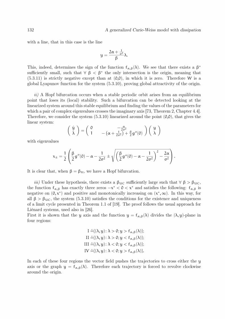
132 A generalized Curie-Weiss model with dissipation
with a line, that in this case is the line
y =2α+ 1
σ2
βλ.
This, indeed, determines the sign of the function fα,β(λ). We see that there exists a β∗
sufficiently small, such that ∀ β < β∗ the only intersection is the origin, meaning that(5.3.11) is strictly negative except than at (0,0), in which it is zero. Therefore W is aglobal Lyapunov function for the system (5.3.10), proving global attractivity of the origin.
ii) A Hopf bifurcation occurs when a stable periodic orbit arises from an equilibriumpoint that loses its (local) stability. Such a bifurcation can be detected looking at thelinearized system around this stable equilibrium and finding the values of the parameters forwhich a pair of complex eigenvalues crosses the imaginary axis [73, Theorem 2, Chapter 4.4].Therefore, we consider the system (5.3.10) linearized around the point (0,0), that gives thelinear system:
(
y
λ
)
=
(
0 − α2σ2
1 −(
α+ 12σ2
)
+ β2g ′′(0)
)(
y
λ
)
with eigenvalues
x± =1
2
β
2g ′′(0) − α−
1
2σ2±√
(
β
2g ′′(0) − α−
1
2σ2
)2
−2α
σ2
.
It is clear that, when β = βH, we have a Hopf bifurcation.
iii) Under these hypothesis, there exists a βUC sufficiently large such that ∀ β > βUC,the function fα,β has exactly three zeros −x∗ < 0 < x∗ and satisfies the following: fα,β isnegative on (0, x∗) and positive and monotonically increasing on (x∗,∞). In this way, forall β > βUC, the system (5.3.10) satisfies the conditions for the existence and uniquenessof a limit cycle presented in Theorem 1.1 of [19]. The proof follows the usual approach forLiénard systems, used also in [26].First it is shown that the y axis and the function y = fα,β(λ) divides the (λ, y)-plane infour regions:
I.=(λ, y) : λ > 0;y > fα,β(λ);
II.=(λ, y) : λ > 0;y < fα,β(λ);
III.=(λ, y) : λ < 0;y < fα,β(λ);
IV.=(λ, y) : λ < 0;y > fα,β(λ).
In each of these four regions the vector field pushes the trajectories to cross either the yaxis or the graph y = fα,β(λ). Therefore each trajectory is forced to revolve clockwisearound the origin.
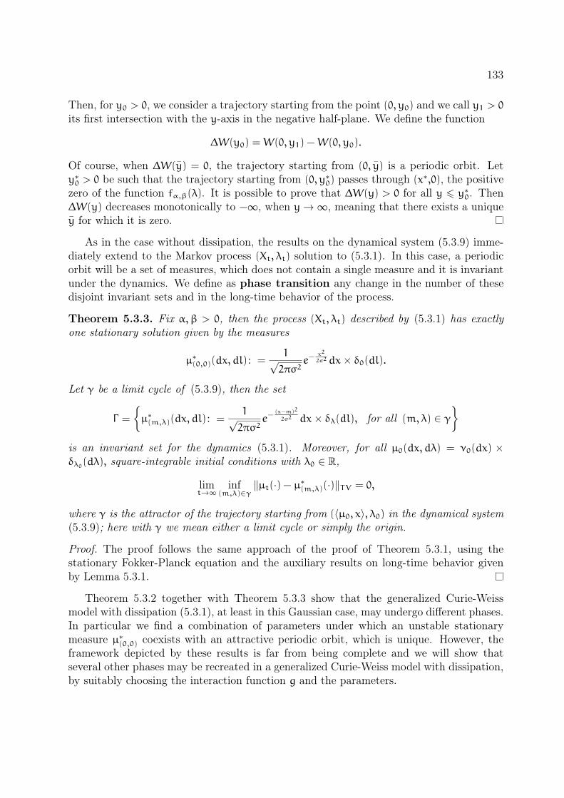
133
Then, for y0 > 0, we consider a trajectory starting from the point (0, y0) and we call y1 > 0its first intersection with the y-axis in the negative half-plane. We define the function
∆W(y0) =W(0, y1) −W(0, y0).
Of course, when ∆W(y) = 0, the trajectory starting from (0, y) is a periodic orbit. Lety∗0 > 0 be such that the trajectory starting from (0, y∗0) passes through (x∗,0), the positivezero of the function fα,β(λ). It is possible to prove that ∆W(y) > 0 for all y 6 y∗0. Then∆W(y) decreases monotonically to −∞, when y→ ∞, meaning that there exists a uniquey for which it is zero.
As in the case without dissipation, the results on the dynamical system (5.3.9) imme-diately extend to the Markov process (Xt, λt) solution to (5.3.1). In this case, a periodicorbit will be a set of measures, which does not contain a single measure and it is invariantunder the dynamics. We define as phase transition any change in the number of thesedisjoint invariant sets and in the long-time behavior of the process.
Theorem 5.3.3. Fix α,β > 0, then the process (Xt, λt) described by (5.3.1) has exactlyone stationary solution given by the measures
µ∗(0,0)(dx, dl) : =
1√2πσ2
e−x2
2σ2 dx× δ0(dl).
Let γ be a limit cycle of (5.3.9), then the set
Γ =
µ∗(m,λ)(dx, dl) : =
1√2πσ2
e−(x−m)2
2σ2 dx× δλ(dl), for all (m,λ) ∈ γ
is an invariant set for the dynamics (5.3.1). Moreover, for all µ0(dx, dλ) = ν0(dx) ×δλ0(dλ), square-integrable initial conditions with λ0 ∈ R,
limt→∞
inf(m,λ)∈γ
‖µt(·) − µ∗(m,λ)(·)‖TV = 0,
where γ is the attractor of the trajectory starting from (〈µ0, x〉, λ0) in the dynamical system(5.3.9); here with γ we mean either a limit cycle or simply the origin.
Proof. The proof follows the same approach of the proof of Theorem 5.3.1, using thestationary Fokker-Planck equation and the auxiliary results on long-time behavior givenby Lemma 5.3.1.
Theorem 5.3.2 together with Theorem 5.3.3 show that the generalized Curie-Weissmodel with dissipation (5.3.1), at least in this Gaussian case, may undergo different phases.In particular we find a combination of parameters under which an unstable stationarymeasure µ∗
(0,0) coexists with an attractive periodic orbit, which is unique. However, theframework depicted by these results is far from being complete and we will show thatseveral other phases may be recreated in a generalized Curie-Weiss model with dissipation,by suitably choosing the interaction function g and the parameters.

134 A generalized Curie-Weiss model with dissipation
5.3.3 Coexistence of limit cycles
When one introduces dissipation in a classical Curie-Weiss model [26], a Hopf bifurcationidentifies the transition from disorder to a phase in which a unique globally stable limitcycle is present. The model introduced here generalizes this scheme: as seen in Theorem5.3.2, a Hopf bifurcation may occur but, according to the form of the interaction functiong(x), the limiting dynamics may display a richer behavior. Let us summarize some of themost interesting situation that may occur in this model.
• More than one periodic orbit may coexist and they all revolve around the origin. Inthis case the outer one should be stable, the second should be unstable and then theyshould alternate.
• Some periodic orbits may appear even when the origin is still locally stable. Theseorbits appears through global bifurcations (the Hopf bifurcation is a local one) andthey usually appear in pairs, the outer periodic orbit is stable, while the inner one isunstable.
The number of limit cycles and their stability mainly depends on the function fα,β(x),which plays a key role in the study of a Liénard system such as (5.3.10). In general, sometools to determine the exact number of limit cycles in a Liénard system are available inliterature (see [22, 71] and references therein). However, their application may be cumber-some in a general setting, since several features of the function fα,β(x) should be studied,such as the position of its zeroes, its local minima and maxima, their height and so on.Nevertheless, playing with the form of the interaction function g, we can always create aGaussian Curie-Weiss model with dissipation with a customized number of phase transi-tions and of coexisting limit cycles.
Let us briefly underline the role of the function g in the occurrence of limit cycles inthe dynamics of (5.3.9). To this aim, we rewrite the Liénard system (5.3.10):
yt = − α
2σ2λt,
λt = yt − fα,β(λt).
In the rich literature on Liénard system, we see that the form of the function fα,β playsa fundamental role in the number of limit cycles of the system. In particular, from theresults in [71], we can state the following.
Proposition 5.3.2. Fix σ2, α > 0 and suppose that there exists a β∗ such that the followingconditions are satisfied:
i) the function fα,β∗ has N positive zeros x0 : = 0 < x1 < · · · < xN(< xN+1 a bound ) atwhich it changes sign;
ii) for every k = 1, . . . ,N there is a C1 mapping φk : [xk−1, xk] → [xk, xk+1] such that
φk(x)φ′k(x) > x and |fα,β∗(φk(x))| > |fα,β∗(x)|;
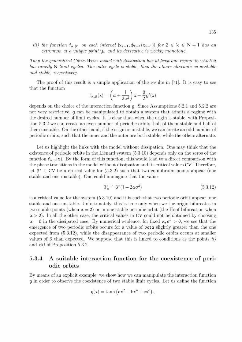
135
iii) the function fα,β∗ on each interval [xk−1, φk−1(xk−1)] for 2 6 k 6 N + 1 has anextremum at a unique point yk and its derivative is weakly monotone.
Then the generalized Curie-Weiss model with dissipation has at least one regime in which ithas exactly N limit cycles. The outer cycle is stable, then the others alternate as unstableand stable, respectively.
The proof of this result is a simple application of the results in [71]. It is easy to seethat the function
fα,β(x) =
(
α+1
2σ2
)
x−β
2g ′(x)
depends on the choice of the interaction function g. Since Assumptions 5.2.1 and 5.2.2 arenot very restrictive, g can be manipulated to obtain a system that admits a regime withthe desired number of limit cycles. It is clear that, when the origin is stable, with Proposi-tion 5.3.2 we can create an even number of periodic orbits, half of them stable and half ofthem unstable. On the other hand, if the origin is unstable, we can create an odd number ofperiodic orbits, such that the inner and the outer are both stable, while the others alternate.
Let us highlight the links with the model without dissipation. One may think that theexistence of periodic orbits in the Liénard system (5.3.10) depends only on the zeros of thefunction fα,β(x). By the form of this function, this would lead to a direct comparison withthe phase transitions in the model without dissipation and its critical values CV. Therefore,let β∗ ∈ CV be a critical value for (5.3.2) such that two equilibrium points appear (onestable and one unstable). One could immagine that the value
β∗α
.= β∗(1+ 2ασ2) (5.3.12)
is a critical value for the system (5.3.10) and it is such that two periodic orbit appear, onestable and one unstable. Unfortunately, this is true only when we the origin bifurcates intwo stable points (when α = 0) or in one stable periodic orbit (the Hopf bifurcation whenα > 0). In all the other case, the critical values in CV could not be obtained by choosingα = 0 in the dissipated case. By numerical evidence, for fixed α, σ2 > 0, we see that theemergence of two periodic orbits occurs for a value of beta slightly greater than the oneexpected from (5.3.12), while the disappearance of two periodic orbits occurs at smallervalues of β than expected. We suppose that this is linked to conditions as the points ii)and iii) of Proposition 5.3.2.
5.3.4 A suitable interaction function for the coexistence of peri-
odic orbits
By means of an explicit example, we show how we can manipulate the interaction functiong in order to observe the coexistence of two stable limit cycles. Let us define the function
g(x) = tanh(
ax2 + bx4 + cx6)
,

136 A generalized Curie-Weiss model with dissipation
with a, b, c suitable constants such that g stays strictly increasing on [0,∞). Fix σ2 > 0,then the pair (g, ρ), with ρ ∼ N(0, σ2) clearly satisfies Assumptions 5.2.1 and 5.2.2 and itdefines a generalized Curie-Weiss model. We consider two triplets of constants (1/2,−1,2)
and (1,1,0) in order to observe some particular regimes that do not exist for the classicalCurie-Weiss model with dissipation.
Case A: triplet(
12,−1,2
)
We see from Figure 5.1 the changes in the concavity of g ′(x). This causes, in the dynamicswithout dissipation, three critical values of β and the four following regimes:
- for β < β1 the origin is a global attractor;
- for β ∈ (β1, β2) the origin is locally stable, but there are four other equilibrium points−x2 < −x1 < 0 < x1 < x2, such that ±x2 are stable and ±x1 are unstable;
- for β ∈ (β2, β3) the origin becomes unstable and two additional stable equilibriumpoints appear, · · ·− x1 < −x3 < 0 < x3 < x1 . . . ;
- for β = β3 the pairs of equilibrium points x3, x1 and −x3,−x1 collapse and disap-pear, such that for β > β3 there are three equilibrium points −x2 < 0 < x2, the outertwo are stable and the origin is unstable.
Figure 5.1: The plot of the function g ′ and of lines y = 1βσ2x for different values of β. The
number of intersections gives the number of equilibrium points in the positive axes. Left:the case A. Right: the case B.
The exact critical values may be obtained numerically, and the behavior of the dy-namical system is clear from Proposition 5.3.1. As we expect, in this case the dissipateddynamics (5.3.9) actually shows four different regimes as well, but the critical values β1(α),β2(α), β3(α) are not straightforwardly obtained with the same procedure of the elementsof CV. To be precise, if β1 corresponds to the smallest value of β in which the line y = x
σ2β
is tangent to the graph of y = g ′(x), the value β1(α) is strictly greater than the smallest
value of β such that the line y =2α+ 1
σ2
βx is tangent to the graph of y = g ′(x). This means
that there exists a β∗ such that the line y =2α+ 1
σ2
β∗ x intersects the graph of y = g ′(x)

137
but any limit cycle occurs. Nevertheless, the system displays a regime of coexistence ofstable limit cycles. Let us better explain the four regimes that we observe in system (5.3.9)(actually the computations and the plots refer to system (5.3.10), since the link with thefunction fα,β is more clear in this case).
- For β < β1(α) the origin is a global attractor. Notice that, numerically we can seethat β1(α) is greater that the β∗ obtained in Theorem 5.3.2; indeed it is not necessarythat the function fα,β(x) is strictly greater than zero for all x > 0. It is reasonable tobelieve, see Figure 5.2(a), that for those β such that the negative part of the functionis “small enough” do not necessary give rose to a periodic orbit.
- For β ∈ (β1(α), β2(α)) the origin is locally stable and, through a global bifurcation,two periodic orbits have arised, the larger one is stable and the smaller one is unstable.Indeed, we can prove numerically that there exists a value β∗ ∈ (β1(α), β2(α)) suchthat the function fα,β∗ satisfies the conditions of Theorem A and B in [71] for theexistence of exactly two limit cycles. See Figure 5.2(b) in which we can observe thestable outer cycle and the attractivity of the origin.
- Notice that βH = β2(α) from Theorem 5.3.2. Therefore, for β ∈ (β2(α), β3(α)) weobserve two attractive limit cycles, a smaller one spreading from the origin (that isnow unstable) while the bigger one remains from the previous regime: see Figure5.2(c). The basin of attraction of the two stable orbits are separated by a thirdunstable periodic orbit. This is the regime in which we see the coexistence of twostable periodic orbits, one inside the other. The existence of this regime is again aconsequence of Theorem A and B in [71], because we can numerically find a β∗∗ thatsatisfies the hypothesis for the existence of exactly three limit cycles, two stable andone unstable.
- For β > β3(α) we see that only the largest periodic orbit has survived. Indeed, forin β3(α) the smallest stable orbit and the unstable one collapse and disappear. Ofcourse, we see that this β3(α) = βUC defined in Theorem 5.3.2; but from numericalevidence we suppose that for this value of β the function fα,β has more than onesingle zero in the positive half-line, but that the other two zeros are not distantenough to admit the existence of the two inner orbits. Of course when β is such thatthere exists a unique positive zero for fα,β, we analitically prove the existence anduniqueness of the limit cycle (see Theorem 5.3.2) while for lower values we can onlyshow it numerically, see Figure 5.2(d).
Case B: triplet (1,1,0)
We see in Figure 5.1 that the shape of g ′ basically allows three different regimes for thecase without dissipation. Indeed, in (5.3.2), the set CV has cardinality 2, i.e. we haveβ1 < β2 =
2σ2
. The three regimes are the following:
- for β < β1 the origin is a global attractor;

138 A generalized Curie-Weiss model with dissipation
- for β ∈ (β1, β2) there are five equilibrium points −x2 < −x1 < 0 < x1 < x2, where±x1 are unstable, while the others are stable;
- at β = β1 the two points ±x1 collapse in the origin that becomes unstable, such thatfor β > β1 the origin is unstable and the points ±x2 are stable.
We treat this example in the dissipated case (5.3.9) (by means of the Liénard system(5.3.10)). We expect three regimes and, in particular, we will observe an atypical behaviorat the Hopf bifurcation, where we will not have a small limit cycle bifurcating from theorigin, but the already existing stable limit cycle that becomes a global attractor. In Figure5.3 we compare the regimes immediately below and above the Hopf bifurcation.
- For β < β1(α), the origin is a global attractor. As is Case A the value β1(α) isstrictly greater than the value in which the line first touches the graph y = g ′(x).
- For β ∈ (β1(α), βH) the origin is stable and we have an unstable periodic orbitcontained in a stable periodic one. When β increase the inner orbit shrinks and theouter expands.
- For β = βH the Hopf bifurcation is such that the origin looses stability, but thishappens simultaneously to the collapse of the unstable periodic orbit on it. Therefore,after the bifurcation, we do not see the usual periodic orbit expanding form the originbecause the unique orbit is the stable one (from the previous regime) that becomesglobally stable.
This case is interesting because the Hopf bifurcation do not originates a small periodicorbit. However, the phenomenon is still a local one, because it is a small unstable orbitthat collapses on the origin changing its stability.
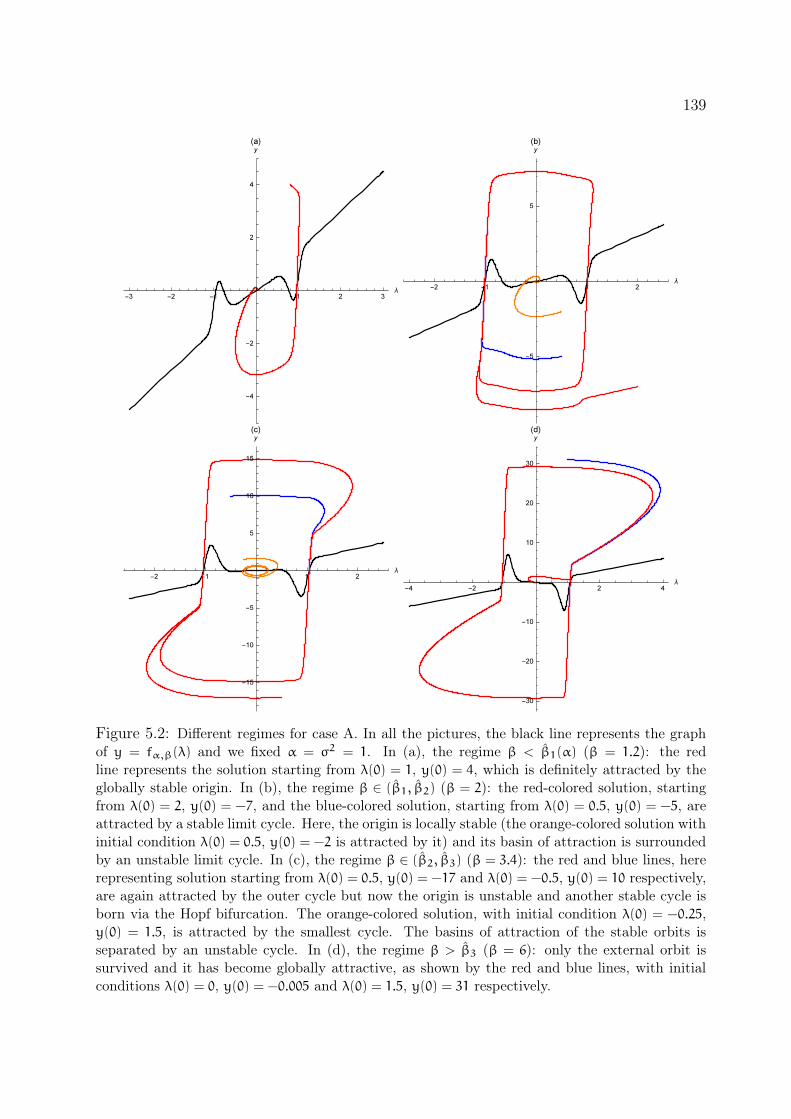
139
Figure 5.2: Different regimes for case A. In all the pictures, the black line represents the graphof y = fα,β(λ) and we fixed α = σ2 = 1. In (a), the regime β < β1(α) (β = 1.2): the redline represents the solution starting from λ(0) = 1, y(0) = 4, which is definitely attracted by theglobally stable origin. In (b), the regime β ∈ (β1, β2) (β = 2): the red-colored solution, startingfrom λ(0) = 2, y(0) = −7, and the blue-colored solution, starting from λ(0) = 0.5, y(0) = −5, areattracted by a stable limit cycle. Here, the origin is locally stable (the orange-colored solution withinitial condition λ(0) = 0.5, y(0) = −2 is attracted by it) and its basin of attraction is surroundedby an unstable limit cycle. In (c), the regime β ∈ (β2, β3) (β = 3.4): the red and blue lines, hererepresenting solution starting from λ(0) = 0.5, y(0) = −17 and λ(0) = −0.5, y(0) = 10 respectively,are again attracted by the outer cycle but now the origin is unstable and another stable cycle isborn via the Hopf bifurcation. The orange-colored solution, with initial condition λ(0) = −0.25,y(0) = 1.5, is attracted by the smallest cycle. The basins of attraction of the stable orbits isseparated by an unstable cycle. In (d), the regime β > β3 (β = 6): only the external orbit issurvived and it has become globally attractive, as shown by the red and blue lines, with initialconditions λ(0) = 0, y(0) = −0.005 and λ(0) = 1.5, y(0) = 31 respectively.

140 A generalized Curie-Weiss model with dissipation
Figure 5.3: Different regimes for case B close to the Hopf bifurcation. In both pictures, theblack line represents the graph of y = fα,β(λ) and we fixed α = σ2 = 1. In (a), the regimeβ ∈ (β1(α), βH) (β = 1.2): the situation is qualitatively the same of Figure 5.2(b). The red, blueand orange lines represent solution starting from λ(0) = 0.5, y(0) = −2, λ(0) = 0, y(0) = −1.5 andλ(0) = 0, y(0) = −0.8 respectively. In (b), the regime β > βH (β = 1.8): the system has undergonethrough a Hopf bifurcation but the stable limit cycle spreading from the origin is not presenthere, due to the collapse of the unstable cycle in the origin, leaving the outer orbit to becomeglobally attractive. The red-colored and blue-colored solutions have initial conditions λ(0) = 0,y(0) = −0.005 and λ(0) = 0, y(0) = 6 respectively.

Bibliography
[1] J. A. Acebrón, L. L. Bonilla, C. J. P. Vicente, F. Ritort, and R. Spigler. The Ku-ramoto model: A simple paradigm for synchronization phenomena. Reviews of modernphysics, 77(1):137, 2005.
[2] L. Andreis, A. Asselah, and P. Dai Pra. Ergodicity of a system of interacting randomwalks with asymmetric interaction. arXiv preprint arXiv:1702.02754, 2017.
[3] L. Andreis, P. Dai Pra, and M. Fischer. McKean-Vlasov limit for interacting systemswith simultaneous jumps. arXiv preprint arXiv:1704.01052, 2016.
[4] L. Andreis, P. Dai Pra, and M. Fischer. Simultaneous jumps in interacting particlesystems: from neuronal networks to a general framework. Submitted for publication,2017.
[5] A. Asselah and F. Castell. Existence of quasi-stationary measures for asymmetricattractive particle systems on zd. Annals of Applied Probability, 13(4):1569–1590,2003.
[6] A. Asselah, P. A. Ferrari, P. Groisman, and M. Jonckheere. Fleming–Viot selectsthe minimal quasi-stationary distribution: The Galton–Watson case. In Annales del’Institut Henri Poincaré, Probabilités et Statistiques, volume 52(2), pages 647–668.Institut Henri Poincaré, 2016.
[7] J. Baladron, D. Fasoli, O. Faugeras, and J. Touboul. Mean-field description andpropagation of chaos in networks of Hodgkin-Huxley and FitzHugh-Nagumo neurons.The Journal of Mathematical Neuroscience, 2(1):1, 2012.
[8] A. D. Banner, R. Fernholz, and I. Karatzas. Atlas models of equity markets. TheAnnals of Applied Probability, 15(4):2296–2330, 2005.
[9] S. Benachour, B. Roynette, and P. Vallois. Nonlinear self-stabilizing processes–II:Convergence to invariant probability. Stochastic processes and their applications,75(2):203–224, 1998.
[10] J. Bérard and J.-B. Gouéré. Brunet-Derrida behavior of branching-selection particlesystems on the line. Communications in Mathematical Physics, 298(2):323–342, 2010.
141

142 A generalized Curie-Weiss model with dissipation
[11] L. Bertini, G. Giacomin, and K. Pakdaman. Dynamical aspects of mean field planerotators and the Kuramoto model. Journal of Statistical Physics, 138(1-3):270–290,2010.
[12] P. Billingsley. Convergence of probability measures. Wiley, 1999.
[13] S. Bobkov and M. Ledoux. One-dimensional empirical measures, order statistics andkantorovich transport distances. preprint, 2014.
[14] M. Bossy and B. Jourdain. Rate of convergeance of a particle method for the solution ofa 1d viscous scalar conservation law in a bounded interval. The Annals of Probability,30(4):1797–1832, 2002.
[15] M. Bossy and D. Talay. Convergence rate for the approximation of the limit lawof weakly interacting particles: application to the burgers equation. The Annals ofApplied Probability, 6(3):818–861, 1996.
[16] C. Bruggeman and A. Sarantsev. Multiple collisions in systems of competing Brownianparticles. arXiv preprint arXiv:1309.2621, 2013.
[17] E. Brunet and B. Derrida. Shift in the velocity of a front due to a cutoff. PhysicalReview E, 56(3):2597, 1997.
[18] M. J. Cáceres, J. A. Carrillo, and B. Perthame. Analysis of nonlinear noisy inte-grate & fire neuron models: blow-up and steady states. The Journal of MathematicalNeuroscience, 1(1):1–33, 2011.
[19] T. Carletti and G. Villari. A note on existence and uniqueness of limit cycles forLiénard systems. Journal of mathematical analysis and applications, 307(2):763–773,2005.
[20] J. A. Carrillo, M. d. M. González, M. P. Gualdani, and M. E. Schonbek. Classical so-lutions for a nonlinear Fokker-Planck equation arising in computational neuroscience.Communications in Partial Differential Equations, 38(3):385–409, 2013.
[21] S. Chatterjee and S. Pal. A phase transition behavior for Brownian motions interactingthrough their ranks. Probability theory and related fields, 147(1-2):123–159, 2010.
[22] X. Chen, J. Llibre, and Z. Zhang. Sufficient conditions for the existence of at least nor exactly n limit cycles for the Liénard differential systems. Journal of DifferentialEquations, 242:11–23, 2007.
[23] F. Collet and P. Dai Pra. The role of disorder in the dynamics of critical fluctuationsof mean field models. Electron. J. Probab, 17(26):1–40, 2012.
[24] F. Collet, P. Dai Pra, and M. Formentin. Collective periodicity in mean-field modelsof cooperative behavior. Nonlinear Differential Equations and Applications NoDEA,22(5):1461–1482, 2015.
143
[25] F. Collet, M. Formentin, and D. Tovazzi. Rhythmic behavior in a two-populationmean-field Ising model. Physical Review E, 94(4):042139, 2016.
[26] P. Dai Pra, M. Fischer, and D. Regoli. A Curie-Weiss model with dissipation. Journalof Statistical Physics, 152(1):37–53, 2013.
[27] P. Dai Pra, G. Giacomin, and D. Regoli. Noise-induced periodicity: some stochasticmodels for complex biological systems. In Mathematical Models and Methods forPlanet Earth, pages 25–35. Springer, 2014.
[28] D. A. Dawson. Critical dynamics and fluctuations for a mean-field model of coopera-tive behavior. Journal of Statistical Physics, 31(1):29–85, 1983.
[29] A. De Masi, A. Galves, E. Löcherbach, and E. Presutti. Hydrodynamic limit forinteracting neurons. Journal of Statistical Physics, 158(4):866–902, 2014.
[30] F. Delarue, J. Inglis, S. Rubenthaler, and E. Tanré. Global solvability of a networkedintegrate-and-fire model of McKean–Vlasov type. The Annals of Applied Probability,25(4):2096–2133, 2015.
[31] S. Ditlevsen and E. Löcherbach. Multi-class oscillating systems of interacting neurons.Stochastic Processes and their Applications, 2016.
[32] P. Dupuis and M. Fischer. On the construction of Lyapunov functions for nonlinearmarkov processes via relative entropy. submitted for publication, 2011.
[33] R. Durrett and D. Remenik. Brunet–Derrida particle systems, free boundary problemsand Wiener—Hopf equations. The Annals of Probability, 39(6):2043–2078, 2011.
[34] A. S. Ecker, P. Berens, G. A. Keliris, M. Bethge, N. K. Logothetis, and A. S. Tolias.Decorrelated neuronal firing in cortical microcircuits. Science, 327(5965):584–587,2010.
[35] T. Eisele and R. S. Ellis. Multiple phase transitions in the generalized Curie-Weissmodel. Journal of statistical physics, 52(1-2):161–202, 1988.
[36] R. Ellis. Entropy, large deviations, and statistical mechanics. Springer, 2007.
[37] R. S. Ellis and C. M. Newman. Limit theorems for sums of dependent random vari-ables occurring in statistical mechanics. Zeitschrift für Wahrscheinlichkeitstheorie undverwandte Gebiete, 44(2):117–139, 1978.
[38] G. Fayolle, V. Malyshev, M. Menshikov, and A. Sidorenko. Lyapounov functions forJackson networks. Mathematics of operations research, 18(4):916–927, 1993.
[39] G. Fayolle, V. A. Malyshev, and M. V. MenÊźshikov. Topics in the constructive theoryof countable Markov chains. Cambridge university press, 1995.
144 A generalized Curie-Weiss model with dissipation
[40] P. Ferrari, H. Kesten, S. Martinez, and P. Picco. Existence of quasi-stationary distri-butions. A renewal dynamical approach. The Annals of Probability, pages 501–521,1995.
[41] P. A. Ferrari and N. Maric. Quasi stationary distributions and fleming-viot processesin countable spaces. Electron. J. Probab, 12(24):684–702, 2007.
[42] N. Fournier and A. Guillin. On the rate of convergence in Wasserstein distance of theempirical measure. Probability Theory and Related Fields, 162(3-4):707–738, 2015.
[43] N. Fournier and E. Löcherbach. On a toy model of interacting neurons. Annales del’Institut Henri Poincaré, Probabilités et Statistiques, 52(4):1844–1876, 2016.
[44] A. Galves and E. Löcherbach. Modeling networks of spiking neurons as interactingprocesses with memory of variable length. Journal de la Société Française de Statis-tique, 157(1):17–32, 2016.
[45] J. Garnier, G. Papanicolaou, and T.-W. Yang. Large deviations for a mean field modelof systemic risk. SIAM Journal on Financial Mathematics, 4(1):151–184, 2013.
[46] A. Gasull, H. Giacomini, and J. Llibre. New criteria for the existence and non-existenceof limit cycles in Liènard differential systems. Dynamical Systems, 24(2):171–185,2009.
[47] G. Giacomin and C. Poquet. Noise, interaction, nonlinear dynamics and the originof rhythmic behaviors. Brazilian Journal of Probability and Statistics, 29(2):460–493,2015.
[48] C. Graham. McKean-Vlasov Itô-Skorohod equations, and nonlinear diffusions withdiscrete jump sets. Stochastic processes and their applications, 40(1):69–82, 1992.
[49] C. Graham. Nonlinear diffusion with jumps. In Annales de l’IHP Probabilités etstatistiques, volume 28(3), pages 393–402, 1992.
[50] C. Graham and S. Méléard. Stochastic particle approximations for generalized boltz-mann models and convergence estimates. The Annals of probability, 25(1):115–132,1997.
[51] N. Ikeda and S. Watanabe. Stochastic differential equations and diffusion processes.Elsevier, 2014.
[52] J. R. Jackson. Jobshop-like queueing systems. Management science, 10(1):131–142,1963.
[53] B. Jourdain. Diffusion processes associated with nonlinear evolution equations forsigned measures. Methodology and computing in applied probability, 2(1):69–91, 2000.

145
[54] B. Jourdain and F. Malrieu. Propagation of chaos and Poincaré inequalities for asystem of particles interacting through their CDF. The Annals of Applied Probability,18(5):1706–1736, 2008.
[55] B. Jourdain and J. Reygner. Propagation of chaos for rank-based interacting diffusionsand long time behaviour of a scalar quasilinear parabolic equation. Stochastic partialdifferential equations: analysis and computations, 1(3):455–506, 2013.
[56] M. Kac. Foundations of Kinetic theory. In Proceedings of the Third Berkeley Sympo-sium on Mathematical Statistics and Probability, volume 3, pages 171–197, 1954.
[57] T. G. Kurtz. Weak and strong solutions of general stochastic models. ElectronicCommunications in Probability, 19(58):1–16, 2014.
[58] T. Liggett. Interacting particle systems, volume 276. Springer-Verlag Berlin Heidel-berg, 2012.
[59] B. Lindner, J. Garcıa-Ojalvo, A. Neiman, and L. Schimansky-Geier. Effects of noisein excitable systems. Physics reports, 392(6):321–424, 2004.
[60] P.-L. Lions and A.-S. Sznitman. Stochastic differential equations with reflectingboundary conditions. Communications on Pure and Applied Mathematics, 37(4):511–537, 1984.
[61] J. Llibre and X. Zhang. Limit cycles of the classical Liénard differential systems: Asurvey on the Lins Neto, de Melo and Pugh’s conjecture. Expositiones Mathematicae,2016.
[62] P. Maillard. Speed and fluctuations of N-particle branching brownian motion withspatial selection. Probability Theory and Related Fields, 166(3-4):1061–1173, 2016.
[63] F. Malrieu. Logarithmic sobolev inequalities for some nonlinear PDE’s. Stochasticprocesses and their applications, 95(1):109–132, 2001.
[64] F. Malrieu. Convergence to equilibrium for granular media equations and their eulerschemes. The Annals of Applied Probability, 13(2):540–560, 2003.
[65] H. P. McKean. A class of Markov processes associated with nonlinear parabolic equa-tions. Proceedings of the National Academy of Sciences, 56(6):1907–1911, 1966.
[66] H. P. McKean. Stochastic integrals, volume 353. American Mathematical Soc., 1969.
[67] S. Méléard. Asymptotic behaviour of some interacting particle systems; mckean-vlasov and boltzmann models. In Probabilistic models for nonlinear partial differentialequations, pages 42–95. Springer, 1996.
[68] S. P. Meyn and R. L. Tweedie. Stability of Markovian processes I: Criteria for discrete-time chains. Advances in Applied Probability, 24(03):542–574, 1992.
146 A generalized Curie-Weiss model with dissipation
[69] S. P. Meyn and R. L. Tweedie. Stability of Markovian processes II: Continuous-timeprocesses and sampled chains. Advances in Applied Probability, 25(3):487–517, 1993.
[70] S. P. Meyn and R. L. Tweedie. Stability of Markovian processes III: Foster-Lyapunovcriteria for continuous-time processes. Advances in Applied Probability, 25(3):518–548,1993.
[71] K. Odani. Existence of Exactly N Periodic Solutions for Liénard Systems. FunkcialajEkvacioj, 39:217–234, 1996.
[72] S. Pal and J. Pitman. One-dimensional brownian particle systems with rank-dependentdrifts. The Annals of Applied Probability, pages 2179–2207, 2008.
[73] L. Perko. Differential equations and dynamical systems, volume 7. Springer Science& Business Media, 2013.
[74] J. Reygner. Chaoticity of the stationary distribution of rank-based interacting diffu-sions. Electronic Communications in Probability, 20, 2015.
[75] P. Robert and J. Touboul. On the dynamics of random neuronal networks. Journalof Statistical Physics, 165(3):545–584, 2016.
[76] M. Sabatini and G. Villari. Limit cycle uniqueness for a class of planar dynamicalsystems. Applied mathematics letters, 19(11):1180–1184, 2006.
[77] A. Sarantsev. Reflected brownian motion in a convex polyhedral cone: Tail estimatesfor the stationary distribution. Journal of Theoretical Probability, pages 1–24, 2016.
[78] M. Scheutzow. Noise can create periodic behavior and stabilize nonlinear diffusions.Stochastic processes and their applications, 20(2):323–331, 1985.
[79] M. Scheutzow. Some examples of nonlinear diffusion processes having a time-periodiclaw. The Annals of Probability, pages 379–384, 1985.
[80] M. Shkolnikov. Competing particle systems evolving by interacting Lévy processes.The Annals of Applied Probability, 21(5):1911–1932, 2011.
[81] A.-S. Sznitman. Équations de type de Boltzmann, spatialement homogenes. Zeitschriftfür Wahrscheinlichkeitstheorie und verwandte Gebiete, 66(4):559–592, 1984.
[82] A.-S. Sznitman. Nonlinear reflecting diffusion process, and the propagation of chaosand fluctuations associated. Journal of functional analysis, 56(3):311–336, 1984.
[83] A.-S. Sznitman. Topics in propagation of chaos. In Ecole d’Eté de Probabilités deSaint-Flour XIX—1989, pages 165–251. Springer, 1991.
[84] H. Tanaka. Limit theorems for certain diffusion processes with interaction. North-Holland Mathematical Library, 32:469–488, 1984.

147
[85] J. Touboul. The hipster effect: When anticonformists all look the same. arXiv preprintarXiv:1410.8001, 2014.
[86] J. Touboul, G. Hermann, and O. Faugeras. Noise-induced behaviors in neural meanfield dynamics. SIAM Journal on Applied Dynamical Systems, 11(1):49–81, 2012.
[87] C. Villani. Optimal transport: old and new, volume 338. Springer-Verlag BerlinHeidelberg, 2008.
[88] R. J. Williams. Reflected brownian motion with skew symmetric data in a polyhedraldomain. Probability Theory and Related Fields, 75(4):459–485, 1987.

148 A generalized Curie-Weiss model with dissipation

Ringraziamenti
I would like to deeply thank my supervisor Paolo Dai Pra for his careful guidance andsupport. I will always be grateful for his great expertise, passion and patience, that havebeen milestones in my research experience and in the writing of this thesis.
A sincere thank goes to Amine Asselah for all the enriching discussions and usefulsuggestions. Moreover he gave us a great hospitality in Marseille, we spent an amazingand very productive time there. Thank you to Markus Fischer, for its knowledge and itscareful help, in particular in the first moments of my research experience. A thank to all theProbability and Finance group in Padova, for many useful comments and conversations;in particular thank you to Tiziano Vargiolu for giving me the opportunity to remain hereand letting me spend time in finishing this thesis.
A huge thank to my friend Daniele Tovazzi, who happened to be also my collaborator.Working with a close friend is something incredibly special, thank you for all the timespent together and for all your encouragement and support. I would like to thank also allthe people that I met during these years and that made this experience unique. When Istarted the PhD more than three years ago, I would have never imagined to meet so manypeople that I am now proud to call friends. I thank also my family, in which I clearlyinclude all my lifetime friends from Boves. I am grateful to my mother, for her endlesssupport and love. Finally, I will never be able to express all my gratitude to Maurizio forconstantly being by my side.