1

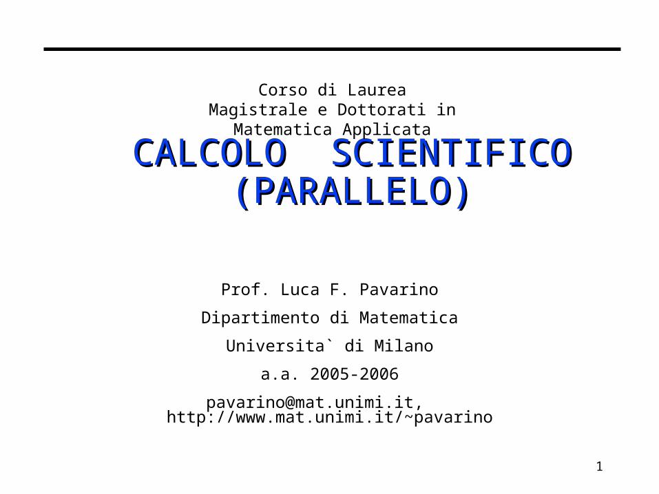
CALCOLO SCIENTIFICO CALCOLO SCIENTIFICO (PARALLELO)(PARALLELO)

Prof. Luca F. Pavarino

Dipartimento di Matematica

Universita` di Milano

a.a. 2005-2006

pavarino@mat.unimi.it, http://www.mat.unimi.it/~pavarino

Corso di Laurea Magistrale e Dottorati in Matematica Applicata

2

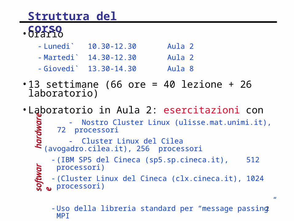
Struttura del corso

• Orario- Lunedi` 10.30-12.30 Aula 2

- Martedi` 14.30-12.30 Aula 2

- Giovedi` 13.30-14.30 Aula 8

• 13 settimane (66 ore = 40 lezione + 26 laboratorio)

• Laboratorio in Aula 2: esercitazioni con - Nostro Cluster Linux (ulisse.mat.unimi.it), 72 processori

- Cluster Linux del Cilea (avogadro.cilea.it), 256 processori

- (IBM SP5 del Cineca (sp5.sp.cineca.it), 512 processori)

- (Cluster Linux del Cineca (clx.cineca.it), 1024 processori)

- Uso della libreria standard per “message passing” MPI

- Uso della libreria parallela di calcolo scientifico PETSc dell’Argonne National Lab., basata su MPI

hardware

hardware

software

software

3

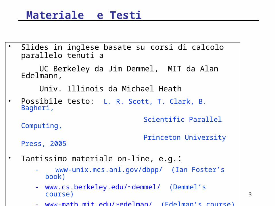
Materiale e Testi

• Slides in inglese basate su corsi di calcolo parallelo tenuti a

UC Berkeley da Jim Demmel, MIT da Alan Edelmann,

Univ. Illinois da Michael Heath

• Possibile testo: L. R. Scott, T. Clark, B. Bagheri,

Scientific Parallel Computing,

Princeton University Press, 2005

• Tantissimo materiale on-line, e.g.:- www-unix.mcs.anl.gov/dbpp/ (Ian Foster’s book)

- www.cs.berkeley.edu/~demmel/ (Demmel’s course)

- www-math.mit.edu/~edelman/ (Edelman’s course)

- www.cse.uiuc.edu/~heath/ (Heath’s course)

- www.cs.rit.edu/~ncs/parallel.html (Nan’s ref page)

4

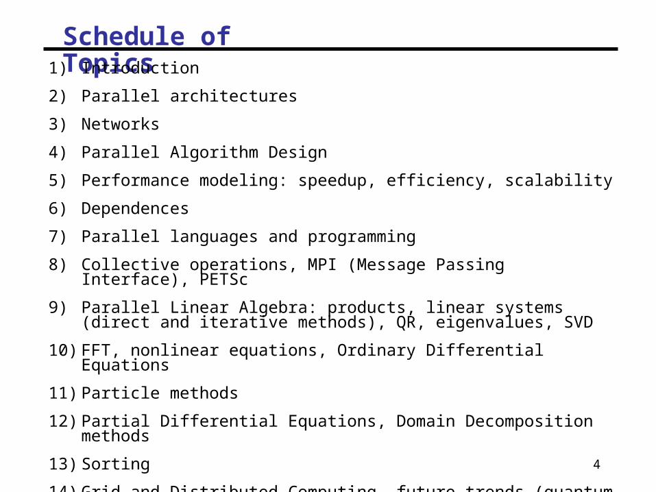
Schedule of Topics1) Introduction

2) Parallel architectures

3) Networks

4) Parallel Algorithm Design

5) Performance modeling: speedup, efficiency, scalability

6) Dependences

7) Parallel languages and programming

8) Collective operations, MPI (Message Passing Interface), PETSc

9) Parallel Linear Algebra: products, linear systems (direct and iterative methods), QR, eigenvalues, SVD

10) FFT, nonlinear equations, Ordinary Differential Equations

11) Particle methods

12) Partial Differential Equations, Domain Decomposition methods

13) Sorting

14) Grid and Distributed Computing, future trends (quantum computing, DNA computing,...)

5

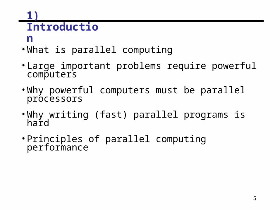
1) Introduction

• What is parallel computing

• Large important problems require powerful computers

• Why powerful computers must be parallel processors

• Why writing (fast) parallel programs is hard

• Principles of parallel computing performance

6

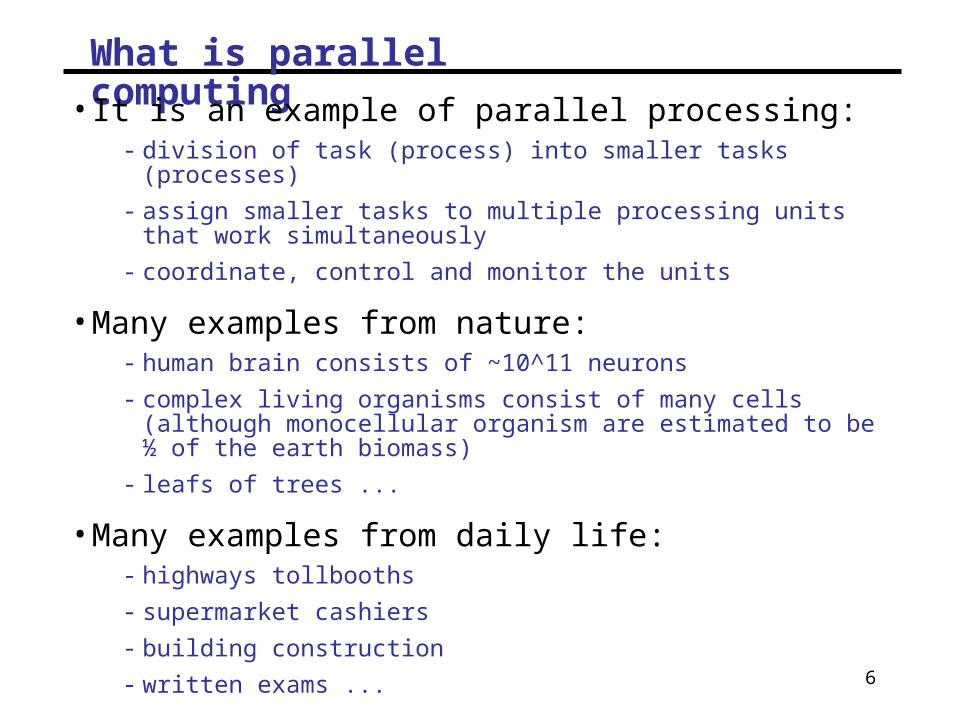
What is parallel computing

• It is an example of parallel processing:- division of task (process) into smaller tasks (processes)

- assign smaller tasks to multiple processing units that work simultaneously

- coordinate, control and monitor the units

• Many examples from nature:- human brain consists of ~10^11 neurons

- complex living organisms consist of many cells (although monocellular organism are estimated to be ½ of the earth biomass)

- leafs of trees ...

• Many examples from daily life:- highways tollbooths

- supermarket cashiers

- building construction

- written exams ...

7

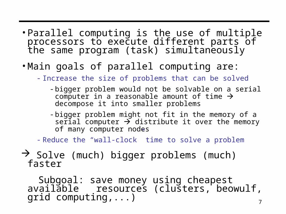
• Parallel computing is the use of multiple processors to execute different parts of the same program (task) simultaneously

• Main goals of parallel computing are:- Increase the size of problems that can be solved

- bigger problem would not be solvable on a serial computer in a reasonable amount of time decompose it into smaller problems

- bigger problem might not fit in the memory of a serial computer distribute it over the memory of many computer nodes

- Reduce the “wall-clock” time to solve a problem

Solve (much) bigger problems (much) faster

Subgoal: save money using cheapest available resources (clusters, beowulf, grid computing,...)

8

Why we need powerful computers

9

Simulation: The Third Pillar of Science

• Traditional scientific and engineering paradigm:1) Do theory or paper design.

2) Perform experiments or build system.

• Limitations:- Too difficult -- build large wind tunnels.

- Too expensive -- build a throw-away passenger jet.

- Too slow -- wait for climate or galactic evolution.

- Too dangerous -- weapons, drug design, climate experimentation.

• Computational science paradigm:3) Use high performance computer systems to simulate the

phenomenon- Based on known physical laws and efficient numerical methods.

10

Some Particularly Challenging Computations

• Science- Global climate modeling

- Astrophysical modeling

- Biology: Genome analysis; protein folding (drug design)

- Medicine: cardiac modeling, physiology, neurosciences

• Engineering- Crash simulation

- Semiconductor design

- Earthquake and structural modeling

• Business- Financial and economic modeling

- Transaction processing, web services and search engines

• Defense- Nuclear weapons -- test by simulations

- Cryptography

11

$5B World Market in Technical Computing

0%

10%

20%

30%

40%

50%

60%

70%

80%

90%

100%

1998 1999 2000 2001 2002 2003 Other

Technical Management andSupport

Simulation

Scientific Research and R&D

MechanicalDesign/Engineering Analysis

Mechanical Design andDrafting

Imaging

Geoscience and Geo-engineering

Electrical Design/EngineeringAnalysis

Economics/Financial

Digital Content Creation andDistribution

Classified Defense

Chemical Engineering

Biosciences

Source: IDC 2004, from NRC Future of Supercomputer Report

12

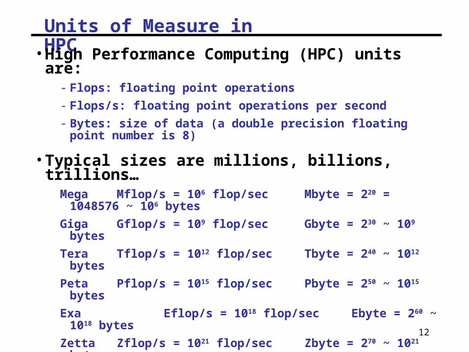
Units of Measure in HPC

• High Performance Computing (HPC) units are:- Flops: floating point operations

- Flops/s: floating point operations per second

- Bytes: size of data (a double precision floating point number is 8)

• Typical sizes are millions, billions, trillions…Mega Mflop/s = 106 flop/sec Mbyte = 220 = 1048576 ~ 106

bytes

Giga Gflop/s = 109 flop/sec Gbyte = 230 ~ 109 bytes

Tera Tflop/s = 1012 flop/sec Tbyte = 240 ~ 1012 bytes

Peta Pflop/s = 1015 flop/sec Pbyte = 250 ~ 1015 bytes

Exa Eflop/s = 1018 flop/sec Ebyte = 260 ~ 1018 bytes

Zetta Zflop/s = 1021 flop/sec Zbyte = 270 ~ 1021 bytes

Yotta Yflop/s = 1024 flop/sec Ybyte = 280 ~ 1024 bytes

13

Ex. 1: Global Climate Modeling Problem

• Problem is to compute:f(latitude, longitude, elevation, time)

temperature, pressure, humidity, wind velocity

• Atmospheric model: equation of fluid dynamics Navier-Stokes system of nonlinear partial differential equations

• Approach:- Discretize the domain, e.g., a measurement point every 1km

- Devise an algorithm to predict weather at time t+1 given t

• Uses:- Predict major events,

e.g., El Nino

- Use in setting air emissions standards

Source: http://www.epm.ornl.gov/chammp/chammp.html

14

Global Climate Modeling Computation

• One piece is modeling the fluid flow in the atmosphere- Solve Navier-Stokes problem

- Roughly 100 Flops per grid point with 1 minute timestep

• Computational requirements:- To match real-time, need 5x 1011 flops in 60 seconds ~ 8 Gflop/s

- Weather prediction (7 days in 24 hours) 56 Gflop/s

- Climate prediction (50 years in 30 days) 4.8 Tflop/s

- To use in policy negotiations (50 years in 12 hours) 288 Tflop/s

• To double the grid resolution, computation is at least 8x

• State of the art models require integration of atmosphere, ocean, sea-ice, land models, plus possibly carbon cycle, geochemistry and more

• Current models are coarser than this

15

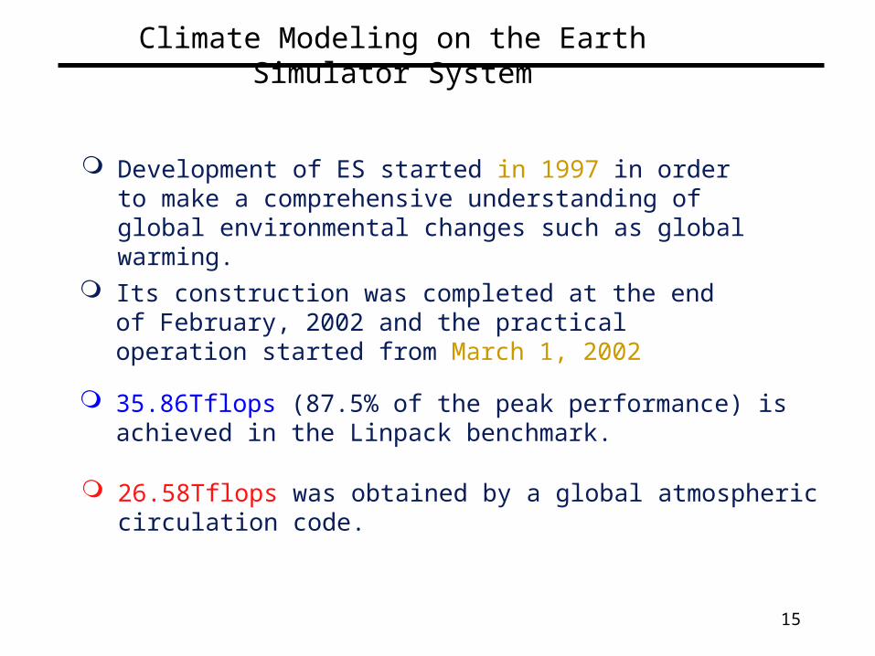
Climate Modeling on the Earth Simulator System

Development of ES started in 1997 in order to make a comprehensive understanding of global environmental changes such as global warming.

26.58Tflops was obtained by a global atmospheric circulation code.

35.86Tflops (87.5% of the peak performance) is achieved in the Linpack benchmark.

Its construction was completed at the end of February, 2002 and the practical operation started from March 1, 2002

16

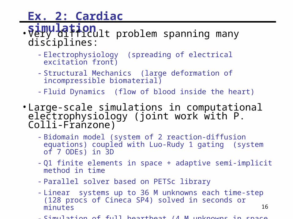
Ex. 2: Cardiac simulation

• Very difficult problem spanning many disciplines:- Electrophysiology (spreading of electrical excitation front)

- Structural Mechanics (large deformation of incompressible biomaterial)

- Fluid Dynamics (flow of blood inside the heart)

• Large-scale simulations in computational electrophysiology (joint work with P. Colli-Franzone)

- Bidomain model (system of 2 reaction-diffusion equations) coupled with Luo-Rudy 1 gating (system of 7 ODEs) in 3D

- Q1 finite elements in space + adaptive semi-implicit method in time

- Parallel solver based on PETSc library

- Linear systems up to 36 M unknowns each time-step (128 procs of Cineca SP4) solved in seconds or minutes

- Simulation of full heartbeat (4 M unknowns in space, thousands of time-steps) took more than 6 days on 25 procs of Cilea HP Superdome, now down to about 50 hours on 36 procs of our cluster

17

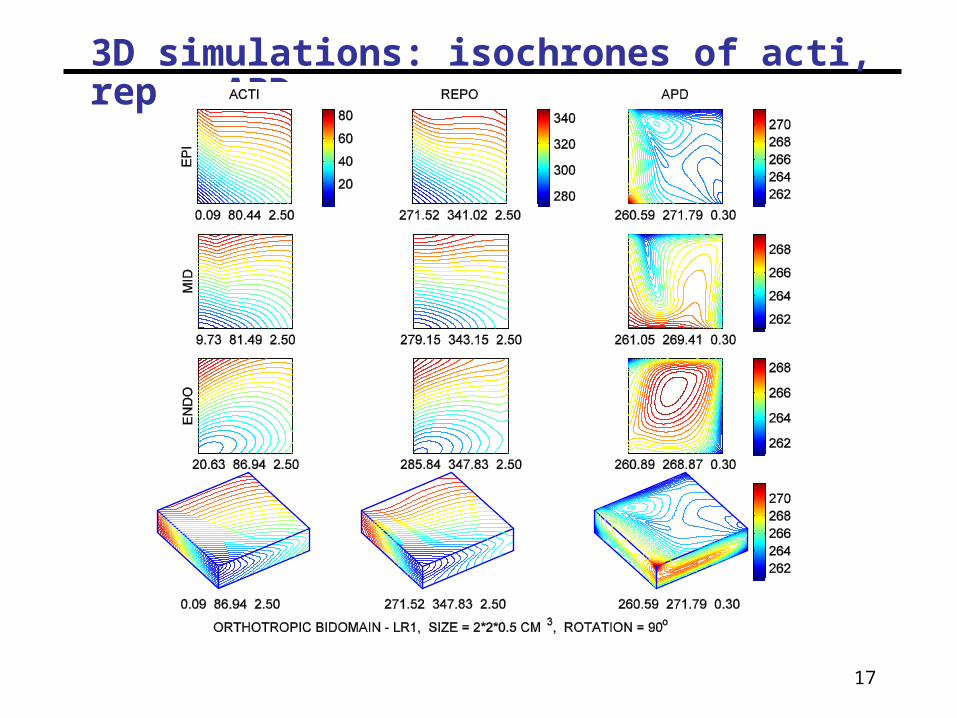
3D simulations: isochrones of acti, repo, APD

18

Activation and repolarization fronts

19

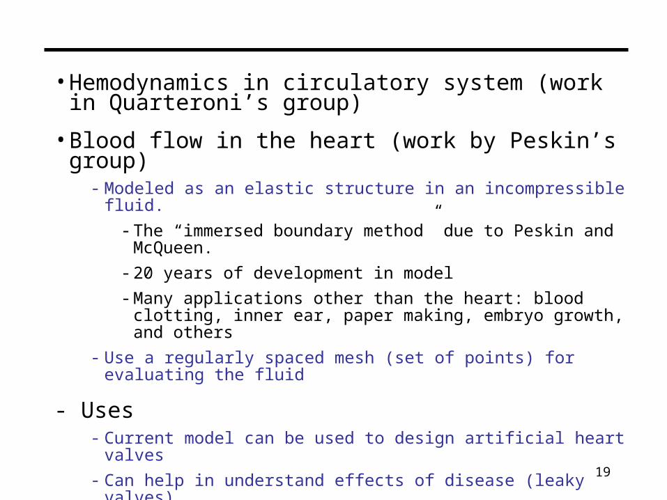
• Hemodynamics in circulatory system (work in Quarteroni’s group)

• Blood flow in the heart (work by Peskin’s group)- Modeled as an elastic structure in an incompressible fluid.

- The “immersed boundary method” due to Peskin and McQueen.

- 20 years of development in model

- Many applications other than the heart: blood clotting, inner ear, paper making, embryo growth, and others

- Use a regularly spaced mesh (set of points) for evaluating the fluid

- Uses- Current model can be used to design artificial heart valves

- Can help in understand effects of disease (leaky valves)

- Related projects look at the behavior of the heart during a heart attack

- Ultimately: real-time clinical work

20

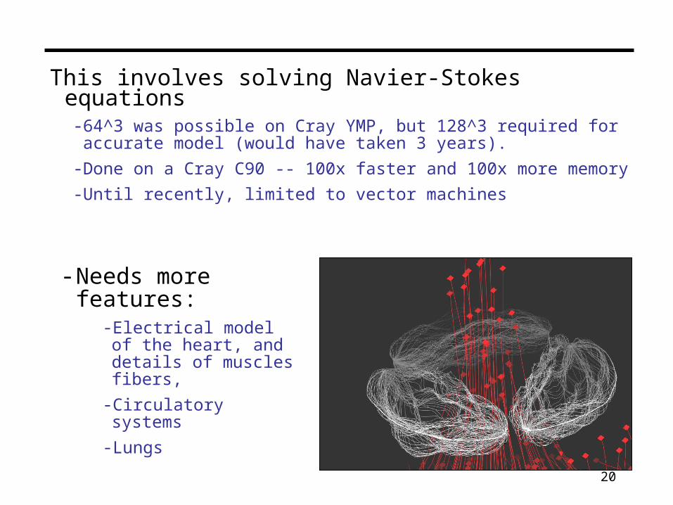
This involves solving Navier-Stokes equations- 64^3 was possible on Cray YMP, but 128^3 required for accurate model

(would have taken 3 years).

- Done on a Cray C90 -- 100x faster and 100x more memory

- Until recently, limited to vector machines

- Needs more features:- Electrical model of the heart, and details of muscles fibers,

- Circulatory systems

- Lungs

21

Ex. 3: Parallel Computing in Data Analysis

• Web search: - Functional parallelism: crawling, indexing, sorting

- Parallelism between queries: multiple users

- Finding information amidst junk

- Preprocessing of the web data set to help find information

• Google physical structure (2004 estimate): - about 63.272 nodes (126,544 cpus)

- 126.544 GB RAM

- 5,062 TB hard drive space

(This would make Google server farm one of the most powerful supercomputer in the world)

• Google index size (June 2005 estimate): - about 8 billion web pages, 1 billion images

22

- Note that the total Surface Web ( = publically indexable, i.e. reachable by web crawlers) has been estimated (Jan. 2005) at over 11.5 billion web pages.

- Invisible (or Deep) Web ( = not indexed by search engines; it consists of dynamic web pages, subscription sites, searchable databases) has been estimated (2001) at over 550 billion documents.

- Invisible Web not to be confused with Dark Web consisting of machines or network segments not connected to the Internet

• Data collected and stored at enormous speeds (Gbyte/hour)

- remote sensor on a satellite

- telescope scanning the skies

- microarrays generating gene expression data

- scientific simulations generating terabytes of data

- NSA analysis of telecommunications

23

Why powerful computers are

parallel

24

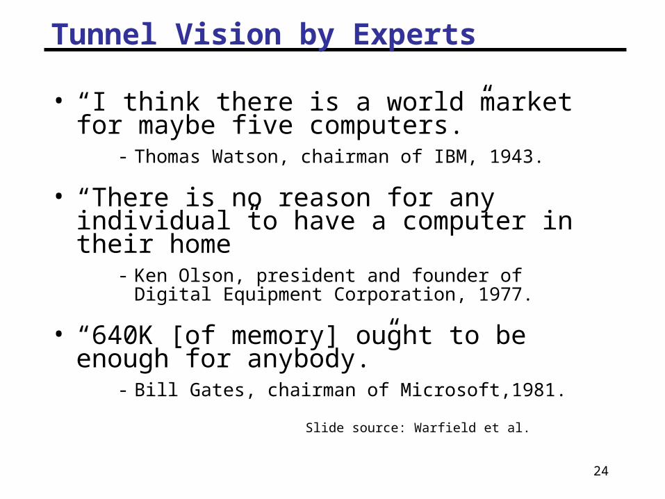
Tunnel Vision by Experts

• “I think there is a world market for maybe five computers.”

- Thomas Watson, chairman of IBM, 1943.

• “There is no reason for any individual to have a computer in their home”

- Ken Olson, president and founder of Digital Equipment Corporation, 1977.

• “640K [of memory] ought to be enough for anybody.”

- Bill Gates, chairman of Microsoft,1981.

Slide source: Warfield et al.

25

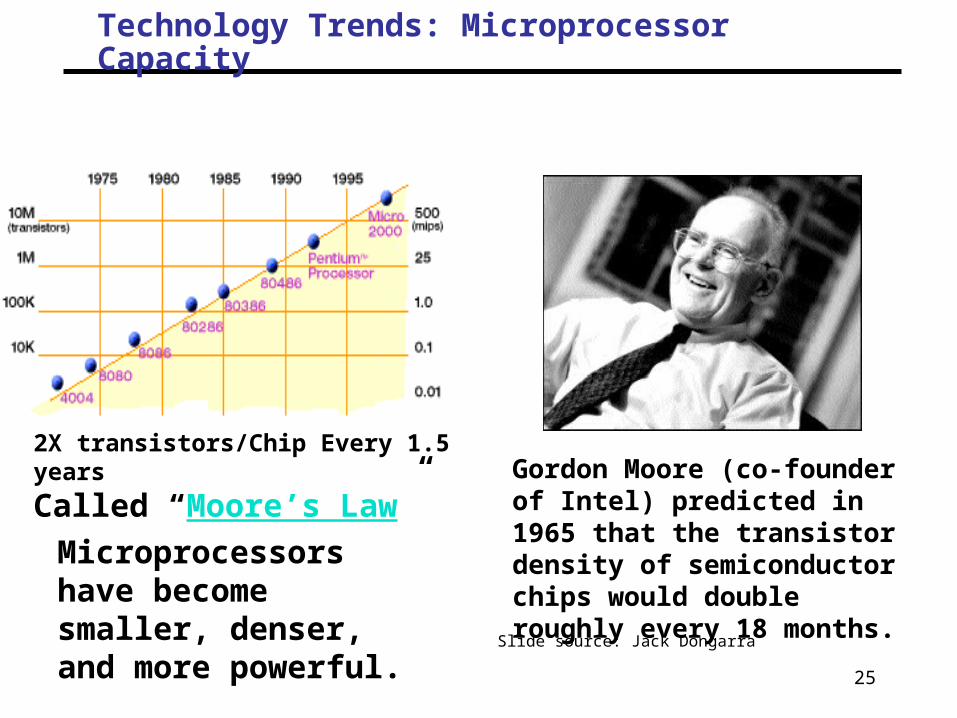
Technology Trends: Microprocessor Capacity

2X transistors/Chip Every 1.5 years

Called “Moore’s Law”

Moore’s Law

Microprocessors have become smaller, denser, and more powerful.

Gordon Moore (co-founder of Intel) predicted in 1965 that the transistor density of semiconductor chips would double roughly every 18 months.

Slide source: Jack Dongarra

26

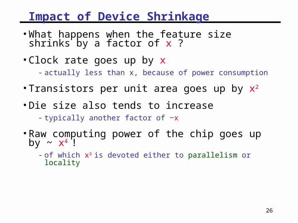
Impact of Device Shrinkage

• What happens when the feature size shrinks by a factor of x ?

• Clock rate goes up by x - actually less than x, because of power consumption

• Transistors per unit area goes up by x2

• Die size also tends to increase- typically another factor of ~x

• Raw computing power of the chip goes up by ~ x4 !- of which x3 is devoted either to parallelism or locality

27

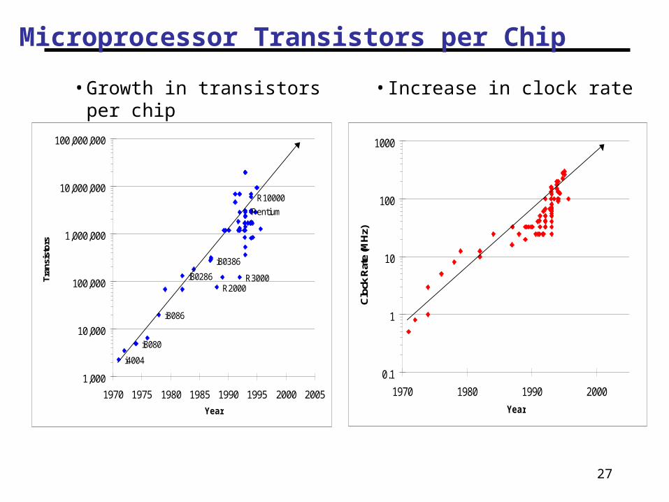
Microprocessor Transistors per Chip

i4004

i80286

i80386

i8080

i8086

R3000R2000

R10000

Pentium

1,000

10,000

100,000

1,000,000

10,000,000

100,000,000

1970 1975 1980 1985 1990 1995 2000 2005

Year

Tran

sist

ors

• Growth in transistors per chip

0.1

1

10

100

1000

1970 1980 1990 2000

Year

Clo

ck R

ate

(MH

z)

• Increase in clock rate

28

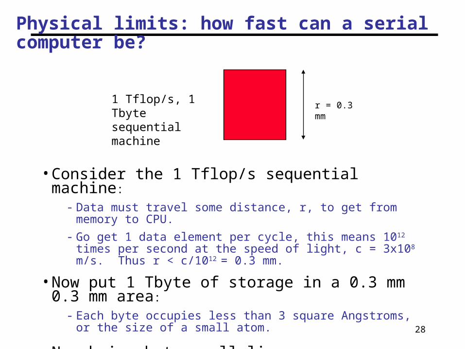
Physical limits: how fast can a serial computer be?

• Consider the 1 Tflop/s sequential machine:

- Data must travel some distance, r, to get from memory to CPU.

- Go get 1 data element per cycle, this means 1012 times per second at the speed of light, c = 3x108 m/s. Thus r < c/1012 = 0.3 mm.

• Now put 1 Tbyte of storage in a 0.3 mm 0.3 mm area:

- Each byte occupies less than 3 square Angstroms, or the size of a small atom.

• No choice but parallelism

r = 0.3 mm1 Tflop/s, 1 Tbyte sequential machine

29

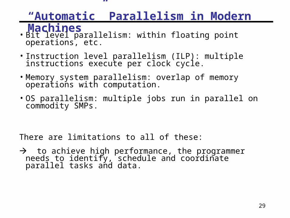
“Automatic” Parallelism in Modern Machines

• Bit level parallelism: within floating point operations, etc.

• Instruction level parallelism (ILP): multiple instructions execute per clock cycle.

• Memory system parallelism: overlap of memory operations with computation.

• OS parallelism: multiple jobs run in parallel on commodity SMPs.

There are limitations to all of these:

to achieve high performance, the programmer needs to identify, schedule and coordinate parallel tasks and data.

30

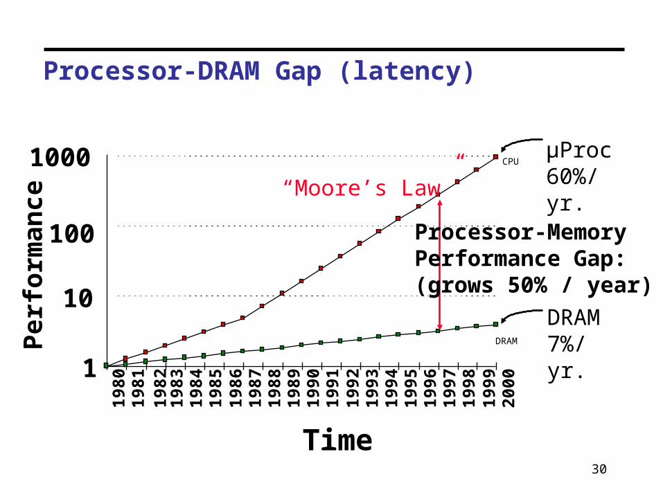
Processor-DRAM Gap (latency)

µProc60%/yr.

DRAM7%/yr.

1

10

100

1000

1980

1981

1983

1984

1985

1986

1987

1988

1989

1990

1991

1992

1993

1994

1995

1996

1997

1998

1999

2000

DRAM

CPU1982

Processor-MemoryPerformance Gap:(grows 50% / year)

Per

form

ance

Time

“Moore’s Law”

31

Principles of Parallel Computing

• Parallelism and Amdahl’s Law

• Finding and exploiting granularity

• Preserving data locality

• Load balancing

• Coordination and synchronization

• Performance modeling

All of these issues makes parallel programming harder than sequential programming.

32

Amdahl’s law: Finding Enough Parallelism

• Suppose only part of an application seems parallel

• Amdahl’s law- Let s be the fraction of work done sequentially, so

(1-s) is fraction parallelizable.

- P = number of processors.

Speedup(P) = Time(1)/Time(P)

<= 1/(s + (1-s)/P)

<= 1/s

Even if the parallel part speeds up perfectly, we may be limited by the sequential portion of code. Ex: if only s = 1%, then speedup <= 100 not worth it using more than p = 100 processors

33

Overhead of Parallelism

• Given enough parallel work, this is the most significant barrier to getting desired speedup.

• Parallelism overheads include:- cost of starting a thread or process- cost of communicating shared data- cost of synchronizing- extra (redundant) computation

• Each of these can be in the range of milliseconds (= millions of flops) on some systems

• Tradeoff: Algorithm needs sufficiently large units of work to run fast in parallel (i.e. large granularity), but not so large that there is not enough parallel work.

34

Locality and Parallelism

• Large memories are slow, fast memories are small.

• Storage hierarchies are large and fast on average.

• Parallel processors, collectively, have large, fast memories -- the slow accesses to “remote” data we call “communication”.

• Algorithm should do most work on local data.

ProcCache

L2 Cache

L3 Cache

Memory

Conventional Storage Hierarchy

ProcCache

L2 Cache

L3 Cache

Memory

ProcCache

L2 Cache

L3 Cache

Memory

potentialinterconnects

35

Load Imbalance

• Load imbalance is the time that some processors in the system are idle due to

- insufficient parallelism (during that phase).

- unequal size tasks.

• Examples of the latter- adapting to “interesting parts of a domain”.

- tree-structured computations.

- fundamentally unstructured problems

- Adaptive numerical methods in PDE (adaptivity and parallelism seem to conflict).

• Algorithm needs to balance load- but techniques the balance load often reduce locality

36

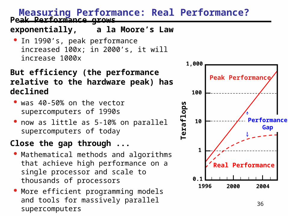
Measuring Performance: Real Performance?

0.1

1

10

100

1,000

2000 2004T

eraf

lop

s1996

Peak Performance grows exponentially, a la Moore’s Law

In 1990’s, peak performance increased 100x; in 2000’s, it will increase 1000x

But efficiency (the performance relative to the hardware peak) has declined

was 40-50% on the vector supercomputers of 1990s

now as little as 5-10% on parallel supercomputers of today

Close the gap through ... Mathematical methods and algorithms that

achieve high performance on a single processor and scale to thousands of processors

More efficient programming models and tools for massively parallel supercomputers

PerformanceGap

Peak Performance

Real Performance

37

Performance Levels

• Peak advertised performance (PAP)- You can’t possibly compute faster than this speed

• LINPACK - The “hello world” program for parallel computing

- Solve Ax=b using Gaussian Elimination, highly tuned

• Gordon Bell Prize winning applications performance- The right application/algorithm/platform combination plus years of work

• Average sustained applications performance- What one reasonable can expect for standard applications

When reporting performance results, these levels are often confused, even in reviewed publications

38

Performance Levels (for example on NERSC-3)

• Peak advertised performance (PAP): 5 Tflop/s

• LINPACK (TPP): 3.05 Tflop/s

• Gordon Bell Prize winning applications performance : 2.46 Tflop/s

- Material Science application at SC01

• Average sustained applications performance: ~0.4 Tflop/s

- Less than 10% peak!

39

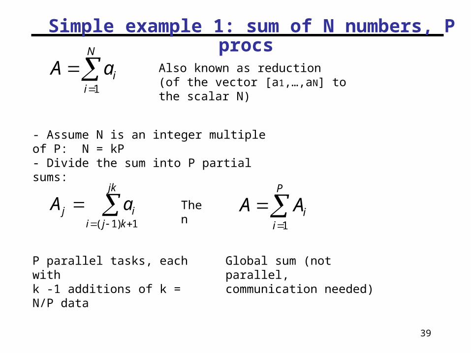
Simple example 1: sum of N numbers, P procs

jk

kjiij aA1)1(

N

iiaA

1

Also known as reduction (of the vector [a1,…,aN] to the scalar N)

- Assume N is an integer multiple of P: N = kP- Divide the sum into P partial sums:

Then

P

iiAA

1

P parallel tasks, each withk -1 additions of k = N/P data

Global sum (not parallel,communication needed)

40

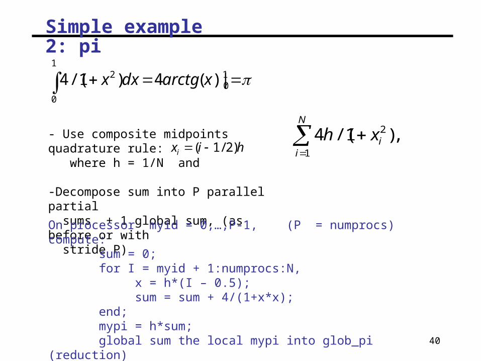
Simple example 2: pi

10

1

0

2 |)(4)1/(4 xarctgdxx

,)1/(41

2

N

iixh- Use composite midpoints quadrature rule:

where h = 1/N and

-Decompose sum into P parallel partial sums + 1 global sum, (as before or with stride P)

hixi )2/1(

On processor myid = 0,…,P-1, (P = numprocs) compute: sum = 0; for I = myid + 1:numprocs:N, x = h*(I – 0.5); sum = sum + 4/(1+x*x); end; mypi = h*sum; global sum the local mypi into glob_pi (reduction)

41

Simple example 3: prime number sieve

See exercise in class on Thursday Oct. 6, 2005

Simple example 4: Jacobi method for BVP

See exercise in class on Thursday Oct. 6, 2005