
Study of low p 0 T p CDF II in pp - Istituto Nazionale di ... Study of low p T D0 meson production...
111
Alma Mater Studiorum - Università di Bologna Facoltà di Scienze Matematiche Fisiche e Naturali Corso di Laurea Magistrale in Fisica Study of low p T D 0 meson production at CDF II in p ¯ p collisions at √ s = 900 GeV Relatore: Candidato: Dott. Stefano Zucchelli Elena Gramellini Correlatore: Dott. Manuel Mussini Anno Accademico 2010-2011 III Sessione
Transcript of Study of low p 0 T p CDF II in pp - Istituto Nazionale di ... Study of low p T D0 meson production...

Alma Mater Studiorum - Università di Bologna
Facoltà di Scienze Matematiche Fisiche e Naturali
Corso di Laurea Magistrale in Fisica
Study of low pT D0 meson production atCDF II in pp collisions at
√s = 900 GeV
Relatore: Candidato:
Dott. Stefano Zucchelli Elena Gramellini
Correlatore:
Dott. Manuel Mussini
Anno Accademico 2010-2011III Sessione

To the loving memory ofProf. Franco Rimondi

Contents
Introduction 5
1 Theory and motivation 71.1 The Standard Model . . . . . . . . . . . . . . . . . . . . . . . 71.2 Strong interaction theory: QCD . . . . . . . . . . . . . . . . . 9
1.2.1 QCD coupling constant . . . . . . . . . . . . . . . . . . 101.2.2 Lattice QCD and Effective Field Theory . . . . . . . . 12
1.3 Charm physics and D mesons . . . . . . . . . . . . . . . . . . 141.4 Charmed hadrons production and D0 cross section measure-
ments . . . . . . . . . . . . . . . . . . . . . . . . . . . . . . . 16
2 The Tevatron Collider and the CDF II experiment 202.1 The Tevatron Collider . . . . . . . . . . . . . . . . . . . . . . 20
2.1.1 Luminosity and center of mass energy . . . . . . . . . . 212.1.2 Proton and antiproton beams . . . . . . . . . . . . . . 222.1.3 The luminous region . . . . . . . . . . . . . . . . . . . 242.1.4 Tevatron status . . . . . . . . . . . . . . . . . . . . . . 24
2.2 The CDF II experiment . . . . . . . . . . . . . . . . . . . . . 252.2.1 Coordinates system and notations . . . . . . . . . . . . 272.2.2 Detector overview . . . . . . . . . . . . . . . . . . . . . 302.2.3 Tracking system . . . . . . . . . . . . . . . . . . . . . . 31
2.2.3.1 Layer ØØ (L ØØ) . . . . . . . . . . . . . . . 312.2.3.2 Silicon VerteX detector II (SVX II) . . . . . . 332.2.3.3 Intermediate Silicon Layer (ISL) . . . . . . . 352.2.3.4 Central Outer Tracker (COT) . . . . . . . . . 36
2

CONTENTS 3
2.2.3.5 Tracking performance. . . . . . . . . . . . . . 382.2.4 Other CDF II subdetectors . . . . . . . . . . . . . . . 412.2.5 Cherenkov Luminosity Counters (CLC) . . . . . . . . . 422.2.6 Trigger and Data AcQuisition (DAQ) system . . . . . . 43
2.2.6.1 Level 1 (L1) . . . . . . . . . . . . . . . . . . . 452.2.6.2 Level 2 (L2) and Level 3 (L3) . . . . . . . . . 46
2.2.7 Operations and data quality . . . . . . . . . . . . . . . 462.2.8 Event reconstruction and analysis framework . . . . . . 47
3 Data selection 493.1 Low energy scans . . . . . . . . . . . . . . . . . . . . . . . . . 49
3.1.1 Luminosity . . . . . . . . . . . . . . . . . . . . . . . . 493.2 Online . . . . . . . . . . . . . . . . . . . . . . . . . . . . . . . 50
3.2.1 Zero Bias trigger . . . . . . . . . . . . . . . . . . . . . 503.2.2 Minimum Bias trigger . . . . . . . . . . . . . . . . . . 513.2.3 Samples overlap . . . . . . . . . . . . . . . . . . . . . . 51
3.3 Offline . . . . . . . . . . . . . . . . . . . . . . . . . . . . . . . 513.3.1 Good Run List . . . . . . . . . . . . . . . . . . . . . . 51
3.4 D0 → Kπ at CDF II . . . . . . . . . . . . . . . . . . . . . . . 523.4.1 Measurement strategy . . . . . . . . . . . . . . . . . . 533.4.2 D0 → Kπ topology . . . . . . . . . . . . . . . . . . . . 54
4 Beam position reconstruction 564.1 Importance of beam reconstruction . . . . . . . . . . . . . . . 564.2 Reconstruction procedure . . . . . . . . . . . . . . . . . . . . 574.3 High Energy test . . . . . . . . . . . . . . . . . . . . . . . . . 594.4 Low energy beams . . . . . . . . . . . . . . . . . . . . . . . . 65
5 Monte Carlo samples 735.1 Monte Carlo simulation . . . . . . . . . . . . . . . . . . . . . . 735.2 Generation technique . . . . . . . . . . . . . . . . . . . . . . . 755.3 Samples . . . . . . . . . . . . . . . . . . . . . . . . . . . . . . 75
5.3.1 D0 → Kπ . . . . . . . . . . . . . . . . . . . . . . . . . 755.3.2 D0 → X . . . . . . . . . . . . . . . . . . . . . . . . . . 78

CONTENTS 4
5.4 Signal shapes . . . . . . . . . . . . . . . . . . . . . . . . . . . 805.4.1 Right Sign (RS) . . . . . . . . . . . . . . . . . . . . . . 815.4.2 Wrong Sign (WS) . . . . . . . . . . . . . . . . . . . . . 815.4.3 Background . . . . . . . . . . . . . . . . . . . . . . . . 86
6 Signal evidence 876.1 Base selection . . . . . . . . . . . . . . . . . . . . . . . . . . . 876.2 Evidence of the D0 signal . . . . . . . . . . . . . . . . . . . . 896.3 Fitting procedure . . . . . . . . . . . . . . . . . . . . . . . . . 916.4 D0 yield . . . . . . . . . . . . . . . . . . . . . . . . . . . . . . 92
7 Differential yields 957.1 Selection optimization . . . . . . . . . . . . . . . . . . . . . . 957.2 Optimized selection . . . . . . . . . . . . . . . . . . . . . . . . 987.3 Yields as a function of pT (D0) . . . . . . . . . . . . . . . . . . 99
Conclusions 104
Allegato: sommario in lingua italiana 107

Introduction
In this thesis a study of the D0 meson production in proton-antiprotoncollisions is presented. The data were collected with the CDF II detector atthe Tevatron Collider of the Fermi National Accelerator Laboratory. Thiswork is part of a specific effort by the CDF Collaboration to measure theinclusive differential cross section of prompt charmed mesons in the low pT
kinematic region.
The reconstruction of the neutral charmed meson (D0) at low momentaand at different energies gives the opportunity to enrich the knowledge of thebehavior of the strong interaction in the region where c-quark production isnearly in non-perturbative condition. In fact, the actual QCD theory cannotpredict the behavior of the strong interaction in the low transferred four-momentum region (low Q2) because of the running of the strong couplingconstant αs. In these kinematic conditions, αs is of the order of the unity,thus perturbative expansions are no longer permitted. Nowadays, some phe-nomenological models have been formulated, but they are usually able todescribe only few aspects of the observed physical quantities; however, theyfail in predicting the strong interaction behavior in its whole complexity. Ex-perimental studies in this region of interaction are crucial to overcome thetheoretical limitation and to model new theories.
An analysis published by the CDF Collaboration in 2003 probed a mini-mum pT of the D0 of only 5.5 GeV/c because of the biases introduced by thetrigger selection. In a recent study performed at the center of mass energyof 1.96 TeV, a lower limit of 1.5 GeV/c is reached using the Minimum Bias
5

INTRODUCTION 6
(MB) and Zero Bias (ZB) data samples so that no bias is introduced what-soever.This thesis, carried out within the Bologna research group, complements thatstudies as it concerns the analysis of the MB and ZB data samples collectedduring a low energy scan at the energy of 900 GeV in the center of mass.This work is the first measurement of D0 production ever performed in thelow pT range at this energy. The sample analyzed is the largest ever collectedby a hadron collider in these conditions.
The primary purpose of the present analysis is the measurement of theD0 raw yields as a function of the transverse momentum: the main step inthe measurement of the D0 production cross section. The decay channelused here is D0 → K−π+ (D0 → K+π−) because of its simple topology,its high reconstruction efficiency (all the produced particles are charged andtherefore observable in the tracking system) and its relatively high branchingratio (about 3.9%).
A preliminary task towards the measurement of the yields has been com-pleted during the thesis work: since the beam position was not recorded forthe runs of low energy scan, it has been reconstructed from data run-by-run.This was a necessary step to unfold the D0 signal whose signature is a sec-ondary vertex displaced from the beam of several microns. Finally the rawyields as a function of pT (D0) have been measured.
This thesis is composed of seven chapters. In the first one, a theoreticaloutline is given. The second one shortly describes the CDF detector withsome emphasis on the subdetectors used for this analysis. Chapter three de-scribes the data samples and the analysis strategy. Chapter four is dedicatedto the reconstruction of the beam position and chapter five to the preliminarydata simulations. In chapter six, the search of the signal is finalized and inchapter seven the measurement of the raw yields as a function of pT (D0) ispresented.

Chapter 1
Theory and motivation
1.1 The Standard Model
The Standard Model (SM) is a theory that describes the strong, electro-magnetic and weak interactions of the elementary particles in the frameworkof the quantum field theory. The weak and the electromagnetic interactionsare unified into the electroweak interaction.
The SM is a gauge theory based on the local group of symmetry
GSM = SU(3)C ⊗ SU(2)T ⊗ U(1)Y (1.1)
where the subscripts indicate the conserved charges: the strong charge,or color C, the weak isospin T (or rather its third component T3) and thehypercharge Y . These quantities are related to the electric charge Q throughthe Gell-Mann-Nishijima relation:
Q =Y
2+ T3. (1.2)
In the quantum field framework, the elementary particles correspond tothe irreducible representations of the GSM symmetry group. In particular,the particles with half-integer spin are called fermions and they are describedby the Fermi-Dirac statistics, whether the particles with integer spin arecalled bosons and they are described by the Bose-Einstein statistics. Thefundamental fermions and their quantum numbers are listed in Tab 1.1.
7

1.1 The Standard Model 8
Generation: I II III T3 Y Q
leptonic doublets(νeLeL
) (νµLµL
) (ντLτL
)1/2−1/2
-1 0−1
leptonic singlets eR µR τR 0 -2 -2
quark doublets(uLd′L
) (cLs′L
) (tLb′L
)1/2−1/2
1/3 2/3−1/3
quark singlets uRdR
cRs′R
tRb′R
0 4/3−2/3
2/3−1/3
Table 1.1: SM elementary fermions. The subscripts L and R indicate re-spectively the negative helicity (left-handed) and the positive helicity (right-handed).
Charged leptons interact via the weak and the electromagnetic forces,while neutrinos only interact via the weak force. Quarks can also interactvia the strong force; they are triplets of SU(3)C , that is they can exist in threedifferent colors: C = R, G, B. If one chooses a base where u, c and t quarksare simultaneously eigenstates of both the strong and the weak interactions,the remaining eigenstates are usually written as d, s and b for the stronginteraction and d′, s′ and b′ for the weak interaction, because the latter onesare the result of a Cabibbo rotation on the first ones.
The gauge group univocally determines the interactions and the numberof gauge bosons that carry them; the gauge bosons correspond to the gener-ators of the group: 8 gluons (g) for the strong interaction, a photon (γ) andthree bosons (W±, Z0) for the electroweak interaction.
A gauge theory by itself can not provide a description of massive particles,but it is experimentally well know that most of the elementary particles havenon-zero masses. The introduction of massive fields in the SM lagrangianwould make the theory non-renormalizable, and - so far - mathematicallyimpossible to handle. This problem is solved in the SM by the introductionof a scalar iso-doublet Φ(x), the Higgs field, see Tab 1.2, which gives masses

1.2 Strong interaction theory: QCD 9
to W+, W− and Z0 gauge bosons and to the fermions [1, 2].
T3 Y Q
Higgs doublet Φ(x) ≡(φ+(x)φ0(x)
)1/2−1/2
+1 10
Table 1.2: Higgs doublet and its third component of the weak isospin, hy-percharge and electric charge.
The existence of the Higgs boson has not been experimentally confirmedyet and the Higgs mass is one of the free parameters of the SM.
1.2 Strong interaction theory: QCD
The Quantum Chromodynamics (QCD) is the current theory used todescribe the strong interaction; it is based on the non-abelian SU(3) gaugegroup and it governs the dynamics of quarks and gluons.
QCD predictions are well tested at high energies where perturbative ap-proaches are possible because of the smallness of its coupling constant, αs,see sec. 1.2.1; on the other hand, in the low-energy region QCD becomes astrongly-coupled theory and a perturbative approach can not be applied.
In order to obtain a relativistic quantum field theory of interacting quarksand gluons, one should start from the QCD lagrangian density:
LQCD = −1
4Gµνa G
aµν +
∑f
qf [iγµDµ −mf ]qf (1.3)
where q stands for the quark field and f for the quark flavours relevant inthe interaction, while Gµν
a is the gluon field strength tensor, namely
Gµνa = ∂µAνa − ∂νAµa + gf bca A
µbA
νc , (1.4)
Dµ is the gauge covariant derivative, namely
Dµ = ∂µ − ig2Aµaλ
a, (1.5)

1.2 Strong interaction theory: QCD 10
Aµa is the gluon field, f bca are the antisymmetric structure constants and g aconstant related to αs via the formula αs = g2/4π.
Quarks and gluons are the fundamental degrees of freedom of the QCDtheory; they both carry color charge, so the gluons that mediate the stronginteraction can interact among themselves. Free quarks and gluons havenever been observed because of the confinement of the color charge. TheQCD field equations give rise to the complex world of nuclear and hadronicphysics, that is only qualitatively understood by now.
An intrinsic QCD scale, ΛQCD, is set through the standard process of therenormalization in quantum field theory; below the ΛQCD scale the standardperturbation theory is no longer valid because of the running of the couplingconstant.In principle, all the hadron masses could be evaluated in terms of ΛQCD,starting from a normalization parameter left free in the theory. The measuredvalue of the proton mass appears to be a suitable choice for the normalizationparameter because it is non-zero in virtue of the energy of the confined quarksand gluons [3].
There is no mathematical description of color confinement but, qualita-tively, this is believed to deal with the fact that the quark and gluon bilinearsqaqa and Ga
µνGµνa acquire non-zero vacuum expectation values. Even if the
QCD Lagrangian is well known and the strong interactions are understoodin principle, the features of low transferred momentum QCD phenomena arefar to be theoretically predicted. That is why experiments which test QCDin the non-perturbative regime are fundamental to improve our understand-ing of the strong interactions: they are the basis on which orient furthertheoretical and experimental researches.
1.2.1 QCD coupling constant
The qualitative understanding of QCD is based on the classical calculationof the dependence of the QCD coupling constant on the renormalization scaleof energy, µ. The simplest way to show this dependence is to define the so

1.2 Strong interaction theory: QCD 11
called β-function:
β(αs) ≡µ
2
∂α
∂µ= − β0
4πα2s −
β1
8π2α3s − ... (1.6)
whereβ0 = 11− 2
3nf (1.7)
β1 = 51− 19
3nf (1.8)
and nf is the number of active quarks, i.e. the quarks whose mass is lessthan µ. One introduces the arbitrary scale Λ to provide the µ dependence ofαs and solve the differential equation (1.6).A solution in the first order of approximation is the following [4]:
αs(µ2) =
4π
β0 ln(µ2/Λ2)+O
( ln[ln(µ2/Λ2)]
ln2(µ2/Λ2)]
). (1.9)
The solution (1.9) shows the two main properties of the theory: theasymptotic freedom
αsµ→+∞−→ 0 (1.10)
and the strong coupling scale below µ ∼ Λ.As one can see from Fig. 1.1, it is possible to roughly divide the physics
of the strong interaction into two regions as a function of the energy of theprocess: the perturbative QCD (high transferred momentum and little αs)and the non-perturbative QCD (low transferred momentum and high αs).
The predictions of the QCD in the perturbative region (pQCD), wherethe standard Feynman rules apply, have been well tested. In the perturbativeregime, the magnitude of the coupling constant is the fundamental parameterfor pQCD predictions. A multitude of phenomena, such as scaling violationsin deep inelastic scattering, high-energy hadron collisions, heavy-quarkonium(in particular bottomonium) decay, jet rates in e+e− collisions and in ep
collisions depends on the value of QCD coupling constant; for this reason, wecan then extrapolate the coupling constant value in a huge range of µ becausewe are able to measure it for many different processes. The different values

1.2 Strong interaction theory: QCD 12
QCD α (Μ ) = 0.1184 ± 0.0007s Z
0.1
0.2
0.3
0.4
0.5
αs (Q)
1 10 100Q [GeV]
Heavy Quarkoniae+e– Annihilation
Deep Inelastic Scattering
July 2009
Figure 1.1: The running of the strong coupling constant as a function of thetransferred momentum (i.e. scale of energy).
of αs for the different processes are listed in Fig. 1.2; they are consistentwith each other and their average value is [4]:
αs(m2Z0) = 0.1184± 0.0007. (1.11)
The non-perturbative regime area is quantitatively much less understood:it is the area of the strong nuclear forces and the hadronic resonances, wherewe still have several unresolved questions.
1.2.2 Lattice QCD and Effective Field Theory
The theoretical approaches to the non-perturbative QCD region are essen-tially two: the Lattice QCD (LQCD) and the Effective Field Theory (EFT).

1.2 Strong interaction theory: QCD 13
0.11 0.12 0.13
α (Μ )s Z
Quarkonia (lattice)
DIS F2 (N3LO)
τ-decays (N3LO)
DIS jets (NLO)
e+e– jets & shps (NNLO)
electroweak fits (N3LO)
e+e– jets & shapes (NNLO)
Υ decays (NLO)
Figure 1.2: Summary of αs(mZ0) measurements and world average value.
LQCD is a numerical approach. The theoretical idea underlying thisframework is to discretize QCD equations of motion on a 4-dimentional space-time lattice and to solve them by a large scale of numerical simulations onbig computers. The discretization is removed by letting the lattice spacingtend to zero; the continuum is then restored.Even if LQCD theoretical principles were originally proposed in 1974, thisapproach has made enormous progress over the last decades, mainly due tothe empowerment of the computer technology.
An EFT is a model equivalent to QCD in a certain energy range that canbe formulated under a series of approximations. One typical approximationis the assumption of negligible mass of the up, down and strange quarkswith respect to ΛQCD [5]. An EFT can in some cases provide a solutionin calculation from QCD where several dynamical scales are involved; forexample combining LQCD with EFT technique has turned out to be a verypowerful method. In recent years a variety of EFTs with quark and gluondegrees of freedom have been developed.

1.3 Charm physics and D mesons 14
1.3 Charm physics and D mesons
The D mesons family is a family of hadrons containing the c quark. It isformed by the D0, D+, D∗+ and Ds mesons and their antiparticles.
The existence of hadrons with the charm quantum number had beenpredicted in 1963 because the existence of a further quark was necessaryto perform the normalization of the weak interactions in the framework ofnon-abelian gauge theories [6, 7].
In order to keep the theory consistent and manage consequent possibleanomalies, the main features of charm quarks (c) were predicted to be asfollows:
• c quarks have the same coupling as u quarks, but their mass is muchheavier, namely about 2 GeV/c2;
• they form charged and neutral hadrons, of which (in the C = 1 sector)three mesons and four baryons decay only weakly with lifetimes roughly10−13 s (they are considered indeed stable);
• charm decay produces direct leptons and preferentially strange hadrons.
The researches on the charm physics during the last 50 years have shownhow these assumptions were extraordinary reliable.
c quark occupies a unique place among up-type quarks, because it is theonly up-type quarks whose hadronization (and the consequent decay) can bestudied. This is due to the fact that, on the heavy side of the spectrum, thet quark decays before it can hadronize, while on the lighter side, the u quarkcan be considered stable. u quark forms only two kinds of neutral hadronwhich decay weakly, neutrons and pions: the decay of the former is due tothe weak decay of quark d and, in the latter, quark and antiquark of the firstfamily annihilate each other.
The charm is an up-type quark, so loop diagrams do not involve theheavy top quark; the SM prediction for charm hadronization and decay isthen smaller by many orders of magnitude than the down-type correspondingprocesses. Intermediate meson-states are expected to contribute at the 10−3

1.3 Charm physics and D mesons 15
level and thus overshadow the short-distance contributions. As mentioned,SM physics lowers the probability to observe loop-mediated processes; on thecontrary, new physics may enhance them and it could be easier to detect inthe charm system than in the bottom system. Experimentally, charm showsmore distinct signatures than the B-system because c branching fractionsinto fully reconstructed modes are up to the 10 % level, while the productof branching ratios to fully reconstruct a b decay is typically at the 10−4
level. Very specific tags are present in the charm decay; for example, in theD∗+ → D0π+ decay, the slow pion tags the D0 flavor at production with anefficiency of almost 100 %.
Mixing of the neutral mesons can occur in the charm system throughbox-diagram, just like the kaon and the B systems. These box-diagram caninvolve only d, s and b quarks because c quark is an up-type quark, thus,again, the large contribution of the heavy t quark is missing.
In the charm framework, the mixing of neutral mesons is studied in thecase of D0 − D0 oscillations. The mixing is describe in terms of two pa-rameters: xD ≡ ∆MD
ΓDand yD ≡ ∆ΓD
2ΓD, where ∆MD is the mass difference
between D0 and D0 (∆MD ≤ 1.3 × 10⁻¹³ GeV) and ∆ΓD is the differencebetween their decay rate. The box-diagram predictions for xD and yD are atthe 10−5 level [8]. New physics should have a little effect on ∆ΓD, but mayhave significant contributions to ∆MD up to values of xD at the 1 % level.Contributions from non-perturbative QCD tend to increase ∆ΓD but the ef-fect on ∆MD is small. An observation of the xD at the percent level togetherwith a strong limit on yD at the 10−3 level would be a strong indication fornew physics.
The LHCb collaboration recently announced preliminary evidence for CPviolation in D0 meson decays [9]. They reported a 3.5σ evidence for a non-zero value of the difference between the time-integrated CP asymmetries inthe decays D0 → K+K− and D0 → π+π−. They evaluated ∆aCP to be∆aCP ≡ aK+K− - aπ+π− = −(0.82± 0.21± 0.11)%, where:
aK+K− =Γ(D0 → K+Ki−)− Γ(D0 → K+K−)
Γ(D0 → K+K−) + Γ(D0 → K+K−)(1.12)

1.4 Charmed hadrons production and D0 cross section measurements 16
andaπ+π− =
Γ(D0 → π+π−)− Γ(D0 → π+π−)
Γ(D0 → π+π−) + Γ(D0 → π+π−). (1.13)
The CDF Collaboration is going to publish a similar result soon.
1.4 Charmed hadrons production and D0 crosssection measurements
Recently, thorough experimental and theoretical studies have been madeabout the inclusive production of charmed hadrons (Xc) at hadron collid-ers. Important results on the charm physics come from the PHENIX andthe STAR experiments at the BNL Relativistic Heavy Ion Collider (RHIC).Both collaborations reported the measure of non-photonic electron produc-tion through charm and bottom decays in pp, dAu and AuAu collisions at√s = 200 GeV [11, 12]. The STAR Collaboration also presented mid-rapidity
open charm spectra from direct reconstruction of decays in dAu collisions andindirect e+e− measurements via charm semileptonic decays in pp and dAucollisions at the center of mass energy,
√s, of 200 GeV [13]. The main disad-
vantage of these results is that RHIC data only covered a very limited low-pTrange.
The latest result concerning the charm physics is the measurement of theinclusive open charm production in p-p and Pb-Pb collision performed bythe ALICE collaboration [14]. A preliminary measurement of the D0, D∗+
and D+ differential cross sections at√s = 7 TeV was released. The total
charm production cross section was estimate using the extrapolation of theD meson cross section measurements to the full kinematic phase space. Fig1.3 shows the pp → cc cross section as a function of centre of mass energyfor various experiments.
In 2003, the CDF Collaboration published the measurements of the dif-ferential cross sections for the inclusive production of charmed hadrons as afunction of the transverse momentum for pT ≥ 5.5 GeV/c [10], at
√s = 1.97
TeV. Fig. 1.4 shows CDF differential cross section measurements for the

1.4 Charmed hadrons production and D0 cross section measurements 17
Figure 1.3: Total charm production cross section as a function of centre ofmass energy for various experiments [14].
mesons of the D family.From the theoretical point of view, the cross section for the inclusive produc-tion of Xc mesons can be calculated by the convolution of universal partondistribution functions (PDFs) and universal fragmentation functions (FFs)with calculable hard-scattering cross sections via perturbative approach. Thenon-perturbative part in the form of PDFs and FFs is input by fits fromother processes. The PDFs and FFs are universal, so unique predictions forthe cross section of the inclusive production of heavy-flavored hadrons areguaranteed.The results of this method in the case of Xc production at the energy avail-able at the Tevatron [15, 16] were compared to CDF results and a not sogood agreement between theory and experiment was found. The experimen-tal central data points tend to overlap the central theoretical prediction inmost of the considered pT range, but in the lower end of the spectrum, theytend to overshoot the prediction, even by a factor of about 1.5. For all meson

1.4 Charmed hadrons production and D0 cross section measurements 18
species, the experimental and theoretical uncertainties overlap.
Figure 1.4: The differential cross section measurements for the mesons of theD family at
√s = 1.97. The inner bars represent the statistical uncertainties;
the outer bars are the quadratic sum of the statistical and systematic uncer-tainties. The solid and dashed curves are the theoretical predictions, withuncertainties indicated by the shaded bands. No prediction was available forthe D+
S production.
The measurement of the D0 meson inclusive differential production crosssection extended to the low pT range (1.5 ≤ pT ≤ 9.5 GeV/c) is going to bepublished soon. The results of this measurement are shown in Fig. 1.5.
New measurements in the region where αs becomes too big for perturba-tive calculation and the color confinement behavior is not well understoodare crucial to understand and model non-perturbative QCD. With this work,we want to extend the previous CDF published measurement of D0 → Kπ
cross section to low pT and lower center of mass energy, in order to providean important information about the non-perturbative region.
During the years of operation, the Tevatron collider collected about 10
fb−1 of data at√s = 1.96 TeV. Before the final shut down, additional scans at
lower center of mass energies were performed:√s = 300 GeV and
√s = 900
GeV. To this day, the Tevatron sample with√s = 900 GeV is the largest
sample at this center of mass energy ever collected in a hadronic collider:

1.4 Charmed hadrons production and D0 cross section measurements 19
Figure 1.5: D0 meson inclusive differential production cross section at√s = 1.97 TeV as a function of the transverse momentum (only statisti-
cal uncertainties are shown).
this give us the chance to perform the measurement of the D0 productioncross section at two different energies.
The Tevatron experimental setup guarantees the uniqueness of this mea-surement: in fact, even if LHC experiments are able to probe the same pTrange and can run at the same energy, the different initial state means dif-ferent conditions, implying the possible existence of other processes in theunknown region under exam.

Chapter 2
The Tevatron Collider and theCDF II experiment
2.1 The Tevatron Collider
In the following paragraphs, we will briefly describe the default config-uration of the Tevatron Collider. This configuration has been used duringalmost the whole duration of the Tevatron operation. For this analysis, weused a data sample collected with a special configuration; the differences be-tween the two configurations will be discussed in the next chapter.
The Tevatron Collider is a high energy accelerator located at the FermiNational Accelerator Laboratory (FNAL or Fermilab), about 50 km Westfrom Chicago, Illinois, US.This collider is a circular superconducting magnets synchrotron, with a 1 kmradius. The Tevatron makes bunches of protons (p) collide against bunchesof antiprotons (p) with the same energy: during the years of operation, theTevatron collected events with a center of mass energy of
√s = 1.96 TeV,
√s = 1.8 TeV,
√s = 900 GeV and
√s = 300 GeV. In order to reach the final
energy in the collision, protons and antiprotons are prepared and acceleratedin several steps, which are shown in Fig.2.1.
20

2.1 The Tevatron Collider 21
Figure 2.1: View of the Fermilab Tevatron collider.
2.1.1 Luminosity and center of mass energy
The center of mass energy,√s, and the instantaneous luminosity, L,
are the key parameters that determine the performance of a collider. Inthe measurement of the cross section of a given process, the luminosity isfundamental because it is the coefficient of proportionality between the rateof the process, R, and its cross section σ:
R [events s−1] = L [cm2s−1]× σ[cm2]. (2.1)
It is important to notice in equation 2.1 how the rate is achieved: it isthe product of σ, which is set by the physics of the process, and L, that ispurely due to the machine.
The expected number of events produced, n, in a finite time ∆T is ob-tained by the time integration of the rate; the cross section is constant in

2.1 The Tevatron Collider 22
time, so the introduction of the time integral of the luminosity (integratedluminosity) is very usefull, because we can write
n(∆T ) = σ
∫∆T
L(t) dt. (2.2)
As mentioned above, L is purely due to the machine, and, assuming anideal head-on pp collision, it is defined as follows in collider experiments:
L = 10−5 NpNpBfβγ
2πβ∗√
(εp + εp)x(εp + εp)yH(σz/β
∗) [1030cm−2s−1], (2.3)
where Np and Np are the average number of protons (Np ≈ 2.78× 10¹²) andantiprotons (Np ≈ 8.33 × 10¹¹) in a bunch, B is the number of circulatingbunches in the ring (B = 36), f is the frequency (f = 47.713 kHz), εp andεp are the 95% normalized emittances of the beams (εp ≈ 18π mm mrad andεp ≈ 1π mm mrad after the injection) and H is an empiric factor, function ofthe ratio between the longitudinal r.m.s. width of the bunch (σz ≈ 60 cm)and “beta function”1 calculated at the interaction point (β∗ ≈ 30 cm).
The production of p has a low efficiency; the creation of collimated p
bunches and their transfer through the subsequent accelerator stages aredifficult: that is why Np is the strongest limiting factor of the Tevatron lu-minosity.
The accessible phase space for the production of resonances in the finalstate is set by the center of mass energy,
√s; indeed,
√s determines the
upper limit for the masses of the particles produced in the pp collision.The highest value of
√s reached by the Tevatron Collider is 1.96 TeV. Further
details about the Tevatron Collider can be found in [17].
2.1.2 Proton and antiproton beams
The process of protons acceleration develops in gradual stages of acceler-ation. Gaseous hydrogen is ionized in order to form H− ions; these ions, afterbeing boosted to 750 keV by a Cockroft-Walton accelerator, are injected to
1The beta function (or betatron function) is the function that parametrize all the linearproperties of the beam.

2.1 The Tevatron Collider 23
the Linac linear accelerator that increases their energy up to 400 MeV. Then,H− ions pass through a carbon foil and lose the two electrons. The resultingprotons are then injected into a rapid cycling synchrotron, called Booster;at this stage protons reach 8 GeV of energy and are compacted into bunches.The next stage of acceleration is the Main Injector, a synchrotron whichaccelerates the bunches up to 250 GeV. In the Main Injector, several bunchesare merged into one and used for the injection in the last stage.The resulting bunches are then transferred to the Tevatron. The protons areforced on an approximately circular orbit by a magnetic field of 5.7 T andthey reach the final energy.
Bunches of protons are used also for the production of the antiprotons.When protons bunches in the Main Injector reach 120 GeV, some of them aredeviated to a nickel or copper target. Collisions produce spatially wide-spreadbunches of antiprotons which are then focused into a beam via a cylindricallithium lens that separates p from other charged interaction products. Thebunch structure of the emerging antiprotons is similar to that of the incidentprotons.The antiprotons bunches are stored in the Debuncher storage ring. In theDebuncher, stochastic cooling stations reduce the spread of the p momentum,but a constant energy of 8 GeV is maintained.At the end of this process, the antiprotons are stored in the Accumulator(see Fig. 2.1), where they are further cooled and stored until the cycles of theDebuncher are completed. The p are injected into the Main Injector whentheir current is sufficient to create 36 bunches with the required density. Inthe Main Injector, the energy of p reaches 150 GeV. They are then transferredto the Tevatron where 36 bunches of protons are already circulating in theopposite direction and they reach the final energy.
During the run, the antiproton production and storage does not stop.When the antiproton stack is sufficiently large (' 4 × 10¹² antiprotons) andthe circulating beams are degraded, the detector high-voltages are switchedoff, the store is dumped and a new one begins.
The dead time between beam abortion and a new store is typically about

2.1 The Tevatron Collider 24
2 hr. During this time, calibrations of the sub-detectors and test runs withcosmics are usually performed.
2.1.3 The luminous region
The pp collisions take place at two interaction points: DØ, where thehomonym detector is locates, and BØ, home of CDF II. Special quadrupolemagnets are located at both extremities of the detectors along the beam pipein order to maximize the luminosity at the interaction points by reducing thetransversal section of the beams. On the longitudinal plane, i.e. along thebeam axis, the distribution of the interaction region fits roughly a Gaussian(σz ≈ 28 cm) and its center is shifted on the nominal interaction point bythe fine tuning of the squeezers. The beam profile in the transverse plane isalmost a circumference; its distribution fits roughly two Gaussian with a rmsof σT ≈ 28 µm.
Only when the beam profile is narrow enough and the conditions aresafely stable, the detectors are turned on and the data acquisition starts.
The bunches cross every 396 ns.The “pile up”, i.e. the number of overlapping interactions for each bunch
crossing, is a function of the instantaneous luminosity and follows a Poissondistribution (see Fig. 2.2). The average pile up is approximately 10 when theluminosity is at its peak (L ≈ 3× 1032[cm−2s−1]). The luminosity decreasesexponentially during the run-time, because of the beam-gas and beam-halointeractions.
2.1.4 Tevatron status
From February 2002 to February 2010, at the center of mass energy√s =
1.96 TeV, about 6.7 fb−1 were recorded on tape and the luminosity was, atthe beginning of a run, on average about 3.8 × 1032[cm−2s−1], with peaks at4 × 1032[cm−2s−1] (See Fig.2.3).
The trend of Tevatron’s integrated and initial luminosity as function of

2.2 The CDF II experiment 25
Figure 2.2: Average number of interactions per crossing as a function ofthe luminosity (cm−2s−1) and of the number of bunches circulating in theTevatron.
store number2 is shown in Fig. 2.4. The total amount of data collectedduring the Tevatron activity is about 10.3 fb−1 (“acquired” on tape about 8.5fb−1).
2.2 The CDF II experiment
In the following paragraphs, we will describe the coordinates system andprincipal notations of the CDF II experiment. An overview of the wholedetector and a description of the subtdetectors used in this analysis are thenpresented.
The CDF II detector is a large multi purpose solenoidal magnetic spec-trometer equipped with a tracking system, full coverage projective calorime-
2The store number is progressive in time, so the luminosity as a function of the storenumber is, in practice, the trend of the luminosity over the time.

2.2 The CDF II experiment 26
Figure 2.3: Initial luminosity as a function of store number.
Figure 2.4: Integrated luminosity as a function of store number.
ters and fine-grained muon detectors. The aim of the detector is to determineenergy, momentum and, whenever possible, the identity of a broad range ofparticles produced in the pp collisions.
CDF original facility was commissioned in 1985, but the detector hasbeen constantly improved during its activity. After 1995, the operation ofthe upgraded detector is generally referred to as Run II. Both 2-D and 3-D

2.2 The CDF II experiment 27
representations of CDF II detector are shown in Fig.s 2.5 and 2.6.
Figure 2.5: View of one half of the CDF II detector in the longitudinalsection.
2.2.1 Coordinates system and notations
The Fig. 2.7, shows the right-handed Cartesian coordinates system em-ployed in CDF II. The origin of the frame is assumed to coincide with theBØ nominal interaction point and with the center of the drift chamber.
The proton direction (east) defines the positive z-axis which lies alongthe nominal beam line. The (x, y) plane is therefore perpendicular to bothprotons and antiprotons beams. The positive y-axis points vertically upwardand the positive x-axis points radially outward with respect to the centerof the ring, in the horizontal plane of the Tevatron. Neither the protons

2.2 The CDF II experiment 28
Figure 2.6: 3D view of the CDF II detector.
Figure 2.7: CDF II Cartesian coordinates system.
beam nor the antiprotons beam is polarized. As a consequence, the resultingphysical observations are invariant under rotations around the z-axis. Thisinvariance makes a description of the detector geometry in cylindrical (r, φ, z)
coordinates system very convenient. Throughout this thesis,we use the wordlongitudinal to indicate the positive direction of the the z-axis and the wordtransverse to indicate the plane perpendicular to the proton direction, i.e.(x, y) ≡ (r, φ) plane.
Protons and antiprotons are composite particles, so the actual interaction

2.2 The CDF II experiment 29
occurs individually between their partons, that is between gluons, valence orsea quarks. Even if the energy of the colliding (anti)proton is well know,each parton carries a fraction of the (anti)proton momentum which is notmeasurable on an event-by-event basis. The momenta of the colliding par-tons along z can be thus very different: as a consequence, the center-of-massof the parton-level interaction may gain a large speed in the longitudinalcomponent.
In collision experiments, the variable rapidity is often used. Rapidity isdefined in Eq. 2.4
y =1
2ln[E + p · cos(θ)E − p · cos(θ)
], (2.4)
where (E, ~p) is the energy-momentum four-vector of the particle. Rapidityis invariant under z boosts and it can be used as an unit of relativisticphase-space. It transforms linearly under a z boost to an inertial frame withspeed β. In fact, y → y′ ≡ y + tanh−1(β), therefore y is invariant sincedy ≡ dy′. However, from the definition 2.4 it is clear that the measurementof the rapidity requires a detector capable of accurately measuring energyand identifying particles, because of the mass term entering E. In order toput mass out of the equation, when the ultrarelativistic (p � m) limit issatisfied, it is preferred to use the approximate expression η instead of y,usually valid for products of high-energy collisions:
yp�m−−−→ η +O(m2/p2), (2.5)
in fact, the pseudo-rapidity η is only function of θ:
η = −ln tan(θ
2
). (2.6)
As already mentioned, along the z-axis, the actual interaction region isdistributed around the nominal interaction point with about 28 cm r.m.swidth, so it is necessary to distinguish the detector pseudo-rapidity, ηdet,measured with respect to the (0,0,0) nominal interaction point, from theparticle pseudo-rapidity, η, measured with respect to the position of the realvertex where the particle originated.

2.2 The CDF II experiment 30
An other commonly used variable is the transverse component of themomentum with respect to the beam axis (pT )
~pT ≡ (px, py)→ pT ≡ p · sin(θ). (2.7)
2.2.2 Detector overview
A comprehensive description of the detector and its subsystems is givenin [18].
As one can see in Fig. 2.5, CDF II is an approximately cylindric assemblyof sub-detectors. Its dimensions are about 15 m in length, about 15 m indiameter and its weight about 5000 ton.
An accurate description of the final state’s particle in energetic hadroniccollisions is quantitatively well obtained by the use of (pseudo)rapidity, trans-verse component of the momentum and azimuthal angle around this axis:this is the reason for the CDF II cylindrical symmetry both in the azimuthalplane and in the forward (z > 0) – backward (z < 0) directions.
Each CDF II sub-system is designed to perform a different task. Theprincipal subsystems are listed below from the inner to the outer of thedetector:
• Tracking system: it performs the 3-D reconstruction of charged trackspath throught an integrated system consisting of three silicon innersubdetectors and a large outer drift chamber, all contained in a super-conducting solenoid.
• Time Of Flight system: it is a cylindrical array made of scintillatingbars that allows particle identification via the time of flight method.The TOF is also contained in the solenoid.
• Calorimeters: outside the solenoid, electromagnetic and hadronic calori-meters measure respectively the energy of photons and electrons and

2.2 The CDF II experiment 31
the energy of hadronic particles using the shower sampling technique.The basic structure consists of alternating layers of passive absorberand plastic scintillator.
• Muon system: it is CDF II outermost system and performs muonsidentification. It consists in scintillating counters and drift tubes.
The set of all these components guarantees the possibility of CDF II toperform a wide range of measurements, including high resolution trackingof charged particle, electron and muon identification, low momentum π/K
separation, precise secondary vertices proper time measurements, finely seg-mented sampling of energy flow coming from final state hadrons, electronsor photons, identification of neutrinos via transverse energy imbalance.
Another fundamental feature of CDF II is the capability to monitor theinstantaneous luminosity. This is achieved by the use of Cherenkov Lumi-nosity Counters (CLC).
CDF II solenoid produces a solenoidal magnetic field of 1.4 T in the regionwith r ≤ 150 cm and |z| ≤ 250 cm.
The detector is conventionally divided into two main sections of pseudo-rapidity: the central region, where the tracking is contained, and the forwardregion. In the following, if not otherwise stated, we shall refer to the cen-tral region as the volume contained in |ηdet| < 1, while the forward regionindicates the detector volume comprised in 1 < |ηdet| < 3.6.
2.2.3 Tracking system
Fig. 2.8 shows CFD II tracking apparatus: the three-dimensional track-ing of charged particle is performed through an integrated system consistingof three silicon inner subdetectors (LØØ, SVX II and ISL ) and a large outerdrift chamber (COT). These subdetectors are all contained in the supercon-ducting solenoid.
2.2.3.1 Layer ØØ (L ØØ)
The layer of the microvertex silicon detector closest to the beam pipeis Layer ØØ (LØØ) (see Fig. 2.9). It consists of single-sided, radiation-

2.2 The CDF II experiment 32
Figure 2.8: Elevation view of one quadrant of the inner portion of the CDFII detector showing the tracking volume surrounded by the solenoid and theforward calorimeters.
2.2 cm
Figure 2.9: LØØ arrangement in transversal view.
tolerant, AC-coupled silicon strip detectors.LØØ covers longitudinally theberyllium beam pipe along 80 cm. Layer ØØ provides excellent coveragewith minimal material inside the tracking volume, improving the impactparameter resolution and the B-tagging efficiencies.

2.2 The CDF II experiment 33
The silicon sensors of LØØ can be biased to very high voltages that man-tain a good signal-to-noise ratio even after high integrated radiation dose(O(5 MRad)).
The sensors are installed at radii of 1.35 cm and 1.62 cm in direct contactwith the beam pipe. The proximity to the beam pipe, which guarantees highresolution measurements of the primary and decay vertexes, is allowed bythe radiation hardness of such sensors.
The LØØ strips are located parallel to the beam axis and provide thefirst sampling of tracks in the r−φ plane. The resolution of the r−φ impactpoint for charged particles is about 10 µm.
The LØØ mass is about 0.01 · X0 in the region with the cooling pipes,while it reduces to 0.006 ·X0 in the region with sensors only.
2.2.3.2 Silicon VerteX detector II (SVX II)
The Silicon VerteX detector II (SVX II) is a fine resolution silicon mi-crostrip vertex detector which provides five 3D samplings of tracks in thetransversal region between 2.4 and 10.7 cm from the beam (see Fig. 2.8).
Fig. 2.10a shows SVX II geometry: the detector is cylindrical, coaxialwith the beam and segmented along z into three 32 cm long mechanicalbarrels. The total length of 96 cm assures a complete geometrical coveragewithin |ηdet| < 2.
Each barrel comprises 12 azimuthal wedges each of which subtends ap-proximately 30◦. In order to allow the wedge-to-wedge alignment, the edgesof two adjacent wedges slightly overlap. Each wedge consists of 5 concen-tric and equally spaced silicon layers sensors installed at radii 2.45 (3.0), 4.1(4.6), 6.5 (7.0), 8.2 (8.7) and 10.1 (10.6) cm from the beam as shown in Fig.2.10b3.
Independent readout units, called ladders host sensors in a layer. Eachladder is composed by two double sided rectangular 7.5 cm long sensors and
3Half of the wedges are closer to the beam than the other half because their edgesmust overlap. The numbers in brackets indicate the distance from the beam of the furtherwedges’ layers.

2.2 The CDF II experiment 34
(a)
(b)
Figure 2.10: (a) SVX II view in the (r, φ) plane. (b) view of SVX II threeinstrumented mechanical barrels.
by the read out electronics unit.SVX II active surface consists of double-sided, AC-coupled silicon sensors.
In each sensor’s side, the different possible orientations of strips are three:
- strips oriented parallel to the beam axis, called r − φ (axial).
- strips rotated by 1.2◦ with respect to the beam axis, called Small AngleStereo (SAS).

2.2 The CDF II experiment 35
- strips oriented in the transverse plane, called 90◦ stereo.
All the five layers have axial strips on one side, three have 90◦ stereo onthe other side and two have SAS strips.
A radiation-hard front-end chip, called SVX3D, collects the charge pulsefrom the strips. Only signals above a threshold are processed: SVX3D op-erates readout in “sparse-mode”. When a channel is over the threshold, thesignal of the neighbor channels is also processed in order to cluster the hits.
SVX II single hit efficiency greater than 99% and the measured averagesignal-to-noise ratio is S/N ≥ 10, while the resolutions of the impact pa-rameter for central high momentum tracks are σφ < 35 µm and σz < 60µm.
The average mass of SVX II corresponds to 0.05 ·X0.
2.2.3.3 Intermediate Silicon Layer (ISL)
On the outside of SVX II, an other silicon tracker is placed: the Interme-diate Silicon Layer detector, ISL (see Fig. 2.11). ISL covers the polar regionof |ηdet| < 2, the same region covered by SVX II.
Figure 2.11: View of ISL three instrumented mechanical barrels.

2.2 The CDF II experiment 36
ISL can be roughly divided in three regions: a central region and two for-ward regions. The central region consists of a single layer of silicon installedover a cylindrical barrel at radius of 22 cm, while the forward regions consistof two layers of silicon installed on concentric barrels at radii of 20 and 28cm. In order to match SVX II wedge, each silicon layer of ISL is azimuthallydivided into 30◦ wedge.
By analogy with SVX II, ISL basic readout unit is the ISL ladder. Themain difference between these two types of ladders is that ISL ladder is madewith three sensors wire bonded in series, instead of the SVX II two. Thus, theresulting total active length of ISL ladder is 25 cm. ISL sensors are doublesided AC-coupled, with axial strips on one side and SAS strips on the other.The sensors dimensions are 5.7×7.5 cm2 wide and 300 µm thick. As in SVXII, the charge pulse from each strip is read by SVX3D chips.
ISL average mass is 0.02 ·X0 for normally incident particles.
2.2.3.4 Central Outer Tracker (COT)
Fig.2.12 shows the outermost tracking subdetector of CDF II: a largeopen cell drift chamber called the Central Outer Tracker (COT).
The COT is a cylindrical detector, coaxial with the beam and it extendsradially, within the central region, between the radius of 40 cm and 138 cmfrom z-axis.
The chamber contains 96 radial layers of wires arranged into 8 superlayers(SL), see Figure 2.12. Each SL contains 12 sense wires (anode) spaced 0.762cm apart, so it samples the path of a charged particle at twelve radii. Thewires of the 8 SL are not oriented all in the same way: in order to reconstructthe path of a charged particle in the r − z volume, the wires of four SL areoriented parallely to the beam axis (axial SL) and the wires of the remainingfour SL are oriented either +3◦ or -3◦ with respect to the beamline (stereoSL). The axial SL are radially interleaved with the stereo SL.Each superlayer is azimuthally segmented into open drift cells. Figure 2.13shows the view of a drift cell: a row of 12 sense wires alternating with 13potential wires. The potential wires optimize the electric field intensity inthe SL controlling the gain on the sense wires. The field panel closes the

2.2 The CDF II experiment 37
Figure 2.12: A 1/6 section of the COT end-plate. The enlargement shows indetails the slot were wire planes (sense) and field sheet (field) are installed.
cell along the azimuthal direction and defines the fiducial volume of a cell:it is the cathode of the detection circuit. Mylar strips carrying field-shapingwires, called shaper panels, close mechanically and electrostatically the cellsat the radial extremities. The electric field strength in the cell is 2.5 kV/cm.
In the chamber, the crossed electrical and magnetic field as well as thecharacteristics of the gas mixture cause an angular shift of the particle driftpath. In order to balance this shift, the wire planes are 35◦ azimuthal tiltedwith respect the radial direction. The tilted-cell geometry shows other bene-fits: the calibration of the drift-velocity is easier and the left-right ambiguityfor tracks coming from the origin is removed. An overview of the COT maincharacteristics is presented in Tab 2.1.
A preamplifier shapes and amplifies the analog pulses from the COT sensewires. To perform the dE/dx measures, the discriminated differential output

2.2 The CDF II experiment 38
SL252 54 56 58 60 62 64 66
R
Potential wires
Sense wires
Shaper wires
Bare Mylar
Gold on Mylar (Field Panel)
R (cm)
Figure 2.13: A view of an axial section of three cells in super-layer 2. Thearrow shows the radial direction.
Gas Mixture Ar(50%)/Ethane(35%)/CF4(15%)Electron drift speed about 100 µm/nsMaximum drift time about 100 ns
Track efficiency 99%Single hit resolution σhit ' 140 µm
pt resolution σpT /p2T ' 0.0015 c/GeV
Mass 0.016 ·X0 for normally incident particle
Table 2.1: COT characteristics.
is used because it encodes charge information in its width. A TDC is usedto record the leading and trailing edges of the signals in 1 ns bins.
2.2.3.5 Tracking performance.
In the tracking system, a uniform axial magnetic field is present, so thetrajectory of a charged particle produced in the interaction point with non-zero velocity is described by an helix with the axis parallel to the magneticfield.

2.2 The CDF II experiment 39
Fig. 2.14 shows a view of the helix parametrization, which requires thedefinition of five parameters:
• C: signed helix half-curvature, defined as C ≡ Q2R
, where Q is the signof the electric charge of the particle and R is the radius of the helix.The relation between C and the transverse momentum is: pT = cB
2|C|
(where B is the intensity of the magnetic field).
• ϕ0: direction of the track at the point of closest approach to the beam.
• d0: signed impact parameter, i.e. the distance between helix and theorigin at closest approach, defined as
d0 ≡ Q · (√x2c + y2
c −R), (2.8)
where (xc, yc) are the coordinates of the primary vertex of interactionin the transverse plane.
• cot(θ): cotangent of the polar angle at closest approach distance. Thisis directly related to the longitudinal component of the momentum:pz = pT · cot(θ).
• z0: z position of the point of closest approach to the origin.
The trajectory of a charged particle satisfies the following equations:
x = r · sin(ϕ)− (r + d0) · sin(ϕ0) (2.9)
y = −r · cos(ϕ) + (r + d0) · cos(ϕ0) (2.10)
z = z0 + s · cot(θ) (2.11)
where s is the projected length along the track, r = 1/2C and ϕ = 2Cs+ϕ0.When a charged particle passes through the tracking system, the detector
reconstructs, along the physical trajectory of the particle, a set of spatialmeasurements (“hits”) by clustering and pattern-recognition algorithms. In

2.2 The CDF II experiment 40
Figure 2.14: View of the helix parametrization
order to reconstruct the trajectory, the hits are fitted with a helical fit, whichdetermines the five above parameters and finally define a “track” object.The helical fit takes into account non-uniformities of the magnetic field andscattering in the detector material.
Only tracks reconstructed with both silicon and COT hits (SVX+COTtracks) were used for this analysis. The track fitting for all SVX+COT tracksstarts with the fit in the COT: the fit is then extrapolated inward to the sil-icon. In the COT the track density is lower than in the silicon, because ofits greater radial dimension, consequently the probability of hits accidentalcombination in the track reconstruction is smaller. This way of performingthe fit is fast and efficient; the resulting tracks have high purities.
COT performance. The COT efficiency for tracks is typically 99% andall the COT channels worked properly until the last the Tevatron run. Cos-mic rays are exploited to mantain the internal alignments of the COT cellswithin 10 µm. The wires mechanical curvatures effects due to gravitationaland electrostatic forces are kept under control within 0.5% by equalizing the

2.2 The CDF II experiment 41
difference of E/p between electrons and positrons as a function of cot(θ).The single-hit resolution is about 140 µm, including a 75 µm contributionfrom the uncertainty on the measurement of the pp interaction time. Thetypical resolutions on track parameters for tracks fit with no silicon informa-tion or beam constraint are listed in Tab 2.2
resolution valueσpT /p
2T 0.0015 c/GeV
σϕ0 0.035◦
σd0 250 µmσθ 0.17◦
σz0 0.3 cm
Table 2.2: COT resolution on track parameters.
Performance with the silicon detectors. The reconstruction of the hitsin the silicon detector is fundamental to improve the impact parameter res-olution of tracks. In fact, with the measure in the silicon, the resolutionmay reach σd0 ≈ 20 µm (not including the transverse beam size)4. Thisvalue and the value of the transverse beam size ( σT ≈ 28 µ) are ones of themost important factors for the study of the transverse decay-lengths of heavyflavors. In fact, these resolutions are sufficiently small with respect to thetypical transverse decay-lengths (a few hundred microns) to allow separationbetween the decay vertices and the primary vertices of the collisions.
With the use of the silicon tracker, also the stereo resolutions are im-proved up to σθ ≈ 0.06◦, and σz0 ≈ 70 µm. On the contrary, the transversemomentum and the azimuthal resolutions remain approximately the same ofCOT-Only tracks.
2.2.4 Other CDF II subdetectors
For an accurate description of the CDF II subdetectors not used in thisanalysis (TOF system, calorimeters and muon system) see [18].
4The smallness of σd0 depend on the number and radial distance of the silicon hits.

2.2 The CDF II experiment 42
2.2.5 Cherenkov Luminosity Counters (CLC)
The luminosity (L) is a fundamental parameter to measure the physicalprocesses cross sections.
Given the the average number of inelastic interactions per bunch crossing(< N >), the luminosity is inferred according to:
L =< N > ·fb.c.
σTOT(2.12)
where fb.c. is the bunch-crossing frequency and σTOT is the total pp cross-section at
√s = 1.96 TeV. fb.c. is precisely known from the Tevatron radio
frequency. The total cross section at√s = 1.96 TeV is calculated from the
averaged CDF and E8115 luminosity-independent measurements at√s = 1.8
5E811 is an experiment about p-p elastic scattering, situated at hall EØ of the Tevatronbeam line.
Figure 2.15: Views of the CLC system in the longitudinal and transverseplans.

2.2 The CDF II experiment 43
TeV [19, 20] and extrapolated to√s = 1.96. Its value is σTOT = 81.90± 2.30
mb [21].
The measurement of < N > is performed at CDF through the CherenkovLuminosity Counters (CLC). These sub-detectors are two separate modules,symmetrically placed in CDF II forward and backward regions: they coverthe 3.7 ≤ |ηdet| . 4.7 range (see Fig. 2.15).
Each module is composed by conical Cherenkov counters arranged in threeconcentric layers around the beam-pipe. The Cherenkov counters point tothe nominal interaction region; they are 48 thin, 110–180 cm long, filled withisobutane.
CLC Cherenkov angle, θC = 3.4◦, determines the momentum thresholdsfor light emission: 9.3 MeV/c for electrons and 2.6 GeV/c for charged pions.In the CLC, the signal due to the pp interaction is generally larger than thesignal due to the beam halo or to secondary interactions because promptcharged particles from the pp interaction are more likely to walk through thefull counter length. Moreover, different particle multiplicities entering thecounters cause distinct peaks in the signal amplitude distribution. For thisreasons, the CLC measurement of < N > has 4.4% relative uncertainty inthe luminosity range 1031 ≤ L ≤ 1032 [cm−2s−1]. Combining this accuracywith the relative uncertainty on the inelastic pp cross-section, one finds thatthe instantaneous luminosity is inferred with 5.8% relative uncertainty.
2.2.6 Trigger and Data AcQuisition (DAQ) system
An event is written on tape when at least one of the CDF II triggersfires. Events are grouped into runs that are progressively labeled with aRun Number ; a run is a period of continuous operation of the CDF II DataAcquisition (DAQ).
Starting from partial information provided by the detector in real time,the trigger system discards the uninteresting events. The production crosssection of physics of interest is way smaller than the total pp inelastic one.The task of separating the great majority of background events from the

2.2 The CDF II experiment 44
Figure 2.16: Functional block diagram of the CDF II system.
fraction of interesting events is fundamental.The writing of events on permanent memories has a maximum rate of
about 100 Hz, while the Tevatron has an average collision rate of about1.7 MHz, due to the 396 ns interbunch spacing; the CDF II trigger reducesthis acquisition rate, without losing the majority of events with a physicalinterest.
The CDF II trigger is a multi-stage system: it is divided into three levels,as one can see in Fig. 2.16. Each level has more accurate detector informationand more time for processing than the previous one; thus, it can choosewhether discarding the event received from the previous level or sending itto the next level. The detector front-end electronics sends data directly toLevel-1; an event is permanently stored to memory if it passes the Level-3.
The read-out of the entire detector takes about 2 ms on average. Whenthe trigger is busy processing an event, it cannot record other events: thiscauses the so called trigger deadtime. At the maximum luminosity, the per-centage of events rejected because of the trigger deadtime is around 5%.

2.2 The CDF II experiment 45
2.2.6.1 Level 1 (L1)
Level 1 (L1) stage has the same clock of the Tevatron (about 1.7 MHz).Afully pipelined front-end electronics for the whole detector is employed: every396 ns, the buffer of a 42-cell long pipeline is written with the signal of eachCDF II channel. This method gives L1 more time to make its decision beforethe buffer is cleared and the data are lost: 396×42 ns ' 16 µs.
L1 makes its decision processing on a simplified subset of data. A custom-designed hardware reconstructs coarse information from the COT, the calo-rimeters and the muon system, using three parallel streams. For each event,two-dimensional tracks in the transverse plane, the total energy and and thepresence of muon are identified; these physical objects are called “primitives”,because of their low resolution.
In the decision stage, the information from the “primitives” is analyzedand more sophisticated objects, like muons, electrons or jets are formed.
The COT channels are processed by the eXtremely Fast Tracker (XFT).In time with the L1 decision, XFT custom processor identifies two-dimensionaltracks in the (r, φ) plan of the COT. In order to do so, short segments of trackare firstly identified by a pattern matching. Then, if a coincidence betweensegments crossing four super-layers is found, they are linked together intofull-length, two-dimensional tracks. The pattern matching consists in com-paring a possible segment with a set of about 2,400 predetermined patterns.These patterns are determined by the correspondence to all tracks with pT &
1.5 GeV/c originating from the beam line.At L ≈ 1032 [cm−2s−1], the track-finding efficiency and the fake-rate with
respect to the off-line tracks are measured to be respectively 96% and 3%for tracks with pT & 1.5 GeV/c. Of course, this parameters depend on theinstantaneous luminosity. For these 2-D tracks, the observed momentumresolution is σpT /p2
T ≈ 0.017 c/GeV.To keep or to reject an event, different combinations of requirements on
the reconstructed objects can be submitted to L1.

2.2 The CDF II experiment 46
2.2.6.2 Level 2 (L2) and Level 3 (L3)
The Level-2 (L2) trigger fulfills two subsequent tasks, the Event buildingand the Decision.L2 detector information is more complete than L1 detector information; thus,the Event building reconstructs the event with L2 information. The Eventbuilding process in parallel the calorimetric information and the trackinginformation. Its clock is 10 µs.
Decision combines the outputs from L1 and L2 in order to decide whetheror not an event is sent to Level-3.The maximum decision-making time (latency) of L2 is 20 µs for each eventand the output rate is about 300 Hz.
Level-3 (L3) is exclusively software-based. At L3, the events selected byL2 are reconstructed, with full detector resolution. L3 codes and the offlinereconstruction codes are very similar to each other.
About 191 trigger paths can be implemented at L3: the trigger path isthe tool to define any particular sequence of L1, L2 and L3 selections. Anevent that satisfied all the 3 levels requests is flagged with a particular triggerpath. Two events with different trigger paths fulfill different level requests,even if same level request can be used by the two trigger paths.Once the event is fully reconstructed and the integrity of its data is checked,L3 decides whether or not the event is written on tape.The size of an event is typically about 150 kbytes. The maximum storagerate is about 20 Mbyte/s.At the end of the three stages, the event output rate is about 75 Hz.
2.2.7 Operations and data quality
During the runs, the operation of the detector and the quality of theon-line data taking was continuously controlled.
The main causes of data taking inefficiencies are two. At the beginningof the runs, the detector was not empowered since the beam was proved tobe stable. In addition, problems related to trigger dead time, to detector or

2.2 The CDF II experiment 47
to DAQ may occur. The average data-taking efficiency was about 85%.Quality inspections were applied on each run in order to guarantee homo-
geneous data-taking conditions. The running condition must undergo somephysics-quality standards; for these reasons, the fractions of data valid forphysics analysis were certified for each run.
The data-taking was immediately stopped if a malfunction of the detectorwas registered. Then, corrupted data are more likely contained in very shortruns that are usually excluded on-line from physics analysis.
The CLC were operative during the whole data-taking of the physics-quality data, thus an accurate integrated luminosity measurement has beenguaranteed; a set of luminosity and beam-monitor probe quantities wereconstantly controlled to be within the expected ranges during the data taking.On-line, shift operators ensured that L1, L2 and L3 triggers work correctly.The operators also controlled other higher level quantities to be within theexpected ranges.
After the recording on tape of the data, all the data manipulations arereferred to as off-line processes.
2.2.8 Event reconstruction and analysis framework
The events collected by the DAQ and the simulated samples are storedon tapes and analyzed with the Production reconstruction program.
The production process is the main off-line operation: high-level physicsobjects (e.g. tracks, vertices, muons, electrons, jets, etc.) are reconstructedby a centralized analysis from low-level information (e.g hits in the trackingsubdetectors, muon stubs, fired calorimeter towers, etc.).
Precise information about the detector such as calibrations, beam-linepositions, alignment constants, masks of malfunctioning detector-channels,etc. etc. and more sophisticated algorithms are available during the produc-tion. After the production, the size of an event typically increases of the 20%because of the added information.The production processing of all the data sets has been repeated every timethat improved detector information or new reconstruction algorithms became

2.2 The CDF II experiment 48
available.Off-line, the exclusion of runs with software crashes during the productionor with generic problems takes place.
Analysis groups creates a set of ntupes in order to reduce the total amountof data to a smaller data-set of interest.
The ROOT framework [24] is used to create these ntuples. The ROOTframework is a tool of analysis written in C++ and commonly used by sev-eral HEP experiments; it is the same environment used for all the analysespreformed at CDF.
The ntuples used in this work are the Standard Ntuples (Stntuples) thatare used by the QCD group by default. Stntuples contains the events col-lected by the triggers suitable for this analysis.

Chapter 3
Data selection
3.1 Low energy scans
With a view to the final shut down, the Tevatron collider performed aseries of scans at lower center of mass energies, especially addressed to QCDstudies.
The data taking lasted a week and collected data at two different centerof mass energies:
√s = 900 GeV and
√s = 300 GeV. The sample at the
energy of√s = 900 GeV is the largest sample ever collected at a hadronic
collider in these experimental conditions; these are the data used for thepresent analysis.The main features of these runs operation remained the same as the defaultoperation, but some configuration were changed. The number of bunches perrun was decreased to 3 bunches of protons and 3 bunches of antiprotons. Theinstantaneous luminosity decreased as well. The decreasing of the luminosityentails a diminishing of the pile up: for the low energy runs the pile up isapproximately zero. In addition, the trigger tables were optimized for QCDstudies in these new configurations.
3.1.1 Luminosity
As described in Sec. 2.2.5, the rate of the inelastic pp events measuredby the CLCs provides the instantaneous luminosity.
The CLCs measure the average number of primary interactions, < N >;
49

3.2 Online 50
this quantity is related to the instantaneous luminosity L as stated in Eq.2.12. In the low energy scan, the Tevatron average bunch crossing rate fb.c.is about 48 kHz, while the total pp cross section at the energy of 900 GeV isdetermined according to data provided by the Particle Data Group [4, 25].
The total, elastic and inelastic cross sections at the energy of 900 GeVare listed in Tab. 3.1. At this center of mass energy, the total cross sectionis estimated by performing a linear interpolation [21].
√s 900 GeV
σel. (mb) 13.7 ± 1.4 ± 0.0σinel. (mb) 51.6 ± 1.6 ± 2.3σTOT (mb) 65.3 ± 0.7 ± 2.3
Table 3.1: Elastic, inelastic and total cross section for pp scattering at√s =
900 GeV [25]. The first uncertainty is statistical, the second systematic.
3.2 Online
The events used in this analysis are collected with the ZEROBIAS (ZB)and the MINBIAS (MB) trigger paths; the features of these trigger pathsare described in detail in the following sections. With these two paths, notrigger-related bias is introduced in the measured variables. On the contrary,in the published CDF measurement of the D0 cross section [10], a triggerselection with hard requests in terms of the transverse momentum of thedecay products was used: because of this bias, the minimum pT (D0) was setto 5.5 GeV/c.
3.2.1 Zero Bias trigger
The first trigger path used to collect events for this analysis is the ZEROBIAS.Any bunch crossing fires L1, but its rate is reduced by a prescale factor tolimit its output to disk. No further requests are applied at L2 and L3. Thistrigger path do not use any CDF II sub-detector to fire; L1 fires whether ornot a hard scattering collision occurs. The data taking depends exclusivelyon the Tevatron bunch crossing frequency. The combination of the prescale

3.3 Offline 51
factor and the bunch cross rate gives a final output rate at L3 of about 50Hz. About 6.6 millions of events were collected by this path.
3.2.2 Minimum Bias trigger
The second path used is MINBIAS. Unlike the ZEROBIAS, the MINBIAS re-quires at least an inelastic pp collision to trigger an event. At L1, CherenkovLuminosity Counters (CLC) are exploited to check if a collision occurs:MINBIAS requires the coincidence of a signal1 in at least one East CLC andone West CLC. No further requests are applied at L2 and L3.The output rate at each trigger level is limited by prescale factors: theircombination gives a final output rate at L3 of about 400 Hz.About 46.6 millions of events are collected by this path.
3.2.3 Samples overlap
During the data taking, all CDF trigger paths operate at the same time;then, events might be triggered by both our paths, appearing twice in thedata sample. However, considering the effect of the prescale, the sampleoverlapping has a negligible effect on our analysis key variables with respectto their uncertainties; we find an overlap of the order of one event every10,000. Our analysis checks for these occurrences and filters out the duplicateevents.
3.3 Offline
3.3.1 Good Run List
In Sec. 2.2.7 we described the standard CDF data-quality requirementsthat define which runs can be used for physics analyses. The “good” runs aregrouped in the so called Good Run List (GRL).Several GRLs are released by the analysis groups, depending on which sub-detectors properly worked during the data-taking. The official list that con-tains only runs where SVX II and the COT were working properly is used for
1 The minimum threshold for claiming a CLC signal is 250 ADC counts.

3.4 D0 → Kπ at CDF II 52
this analysis, because only SVX+COT tracks were employed. In fact, on onehand COT stand-alone tracking do not provide a sufficient impact parameterresolution of our aim; on the other hand, silicon stand-alone tracking is usefulin the region 1 ≤ |η| ≤ 2, where the COT coverage is incomplete. In thisanalysis, however, we reject tracks with |η| > 1, because the reconstructionefficiency is too low. In the central region of interest, only track with a pT< 0.28 GeV/c have SVX-Only informations, but this pT value is well belowour minimum request.
The ZB and MB sample are reduced after the GRL request: to about 6.0millions (ZB sample) and to about 42.0 millions (MB sample).
3.4 D0 → Kπ at CDF II
The aim of this work is to identify the signal of the D0 mesons decayin the channel D0 → Kπ; with this notation, we consider both the chargedconjugated: D0 → K−π+ and D0 → K+π−. This is the first step to measurethe differential production cross section, defined as follows:
dσD0→kπ
dpT(pT ; |y| ≤ 1) =
ND0+ND0
2(pT )
L · εtrig · εrec(pT ) ·Br(D0 → Kπ)
∣∣∣|y|≤1
(3.1)
where:
• ND0 and ND0 are the yields of the D0 and D0 signals. Experimentally,we count the sum of D0 and D0 yields. We assume charge invariancein the production process through strong interaction, thus the crosssection for D0 mesons only is the average cross section for D0 and D0
mesons.
• |y| ≤ 1 is the range of rapidity considered.
• L is the integrated luminosity of the data sample.
• εtrig is the trigger efficiency.

3.4 D0 → Kπ at CDF II 53
• εrec is the global efficiency of the reconstruction of our candidates. Thisparameter accounts for the geometrical and kinematical acceptances aswell as the detector reconstruction efficiency of the signal.
• Br(D0 → Kπ) is the decay branching ratio of the channel studied.
We refer to the decay products, K and π, as the D0 “daughters”.
3.4.1 Measurement strategy
The D0 → Kπ channel represents one of the simplest topology that wecan study at CDF II to detect this charmed neutral meson: D0 → Kπ has arelatively high branching ratio (about 3.9 %) and it is fully detected by thetracking system (the daughters are two charged particles). We are then ableto identify this heavy meson concealed by a background of light particles(mainly pions and kaons) several orders of magnitude larger.
To unfold the D0 signal from the background we apply the followingprocedure for each event:
• apply quality requirements on the tracks, in terms of hits producedinside the tracking system (see Sec. 6.1) to reduce the contaminationof fake reconstructions;
• combine together all the possible couples of the selected tracks withopposite charges;
• require geometrical conditions between the two considered tracks toreduce the combinations coming from unrelated tracks;
• fit the tracks’ helices looking for an intersection point. If the fit returnsa possible common origin for them, a D0 candidate is defined;
• select only candidates with a decay vertex displaced from the primaryvertex of interaction (to reduce the combinatorial background) and inthe rapidity region of interest.

3.4 D0 → Kπ at CDF II 54
We then evaluate the candidate’s invariant mass and study its distributionfor all the candidates found in the sample; we search a signal at the expectedD0 mass (about 1.864 GeV/c2). More details of the measurement strategywill be described in Sec. 6.1.
3.4.2 D0 → Kπ topology
The D0 lifetime is τ ∼ 410 · 10−15 s, that correspond to a decay length ofcτ ∼ 123 µm. Thus, the D0 travels a path, away from the primary vertex ofthe pp collision that originates it, that is measured thanks to the resolutionof the silicon tracker SVX II (see Section 2.2.3.2).
Figure 3.1: Scheme of the topology of the D0 decay in the transverse planefor the K−π+ channel .
Fig. 3.1 shows the topology of the D0 → K−π+ decay. The figure alsoshows some of the fundamental quantities used in this analysis:
• ~xpri, the primary vertex, is the point where the pp collision takes place.It is the D0 origin vertex.
• ~pT , the transverse momentum, is the projection of the momentum vec-tor to the transverse plane (we refer to its magnitude as pT ).

3.4 D0 → Kπ at CDF II 55
• ~xsec, the secondary vertex, is the D0 decay vertex.
• Lxy, the transverse decay length, is the signed distance between theprimary and the secondary vertices projected to the transverse plane.It is defined as follows:
Lxy =(~xsec − ~xpri) · ~pT
pT(3.2)
where ~pT = (px; py; 0)
• d0, the impact parameter, is the signed distance between the originvertex and the helix of a daughter at their closest approach. It isdefined as stated in Eq. 2.8.
• ∆z0, the longitudinal distance, is the difference in the z coordinate ofthe two daughters at their closest approach to the beam, (not shownin figure, see Sec. 2.2.3.5).
• ∆ϕ0, the transverse opening angle, is the difference of the ϕ0 angle ofthe two daughters at their closest approach to the beam, (not shownin figure, see Sec. 2.2.3.5).

Chapter 4
Beam position reconstruction
4.1 Importance of beam reconstruction
The beam position reconstruction is mandatory in order to extract theD0 signal from the combinatorial background; for this task, the main stepconsists in performing a selection able to distinguish between prompt andsecondary particles. Thanks to the spatial resolution of the CDF II trackingsystem (see Sec. 2.2.3.5), we can identify the particles produced in the D0
decay from the prompt mesons produced in the event by looking at theirimpact parameter. The impact parameter is closely related to the beamposition. In fact, the impact parameter of a track, d0, is the distance in thetransverse plane between the track and the primary vertex; it is defined asstated in Eq. 2.8 .
The pp interaction happens on the beam trajectory, so we can identify thecoordinates of the primary vertex of interaction (xc, yc, zc) with the beamposition at the zc coordinate of the vertex. We exploit this assumption toevaluate the beam position. Once the beam position is found, the d0 valuefor each track comes straight from the definition 2.8. It is then clear thatthe definition of the beam position affects the reconstruction of d0, becomingcrucial for our analysis.
For the high energy runs (√s = 1.96 TeV), the beam position is recon-
structed by the CDF offline software; however, this information is missingfor the low energy runs (
√s = 900 GeV).
56

4.2 Reconstruction procedure 57
In what follows, we describe the procedure we applied to obtain the para-meterization of the beam for the runs used in this analysis; we tested ourprocedure against some high energy runs to be sure that our result is com-patible with the official one.
4.2 Reconstruction procedure
The transverse profile of the luminous region inside CDF can be describedby two Gaussian functions in x and y. The mean of these Gaussians definesthe beam position. Their width is approximately σT ≈ 28 µm. Unfortunately,the beam is not centered with respect to the detector nor parallel to thedetector z-axis. The dependence of the x and y position of the beam on z
can be described, at a first order of approximation, by a linear function:
x =dx
dz· z + x0 y =
dy
dz· z + y0, (4.1)
where x0 and y0 are the position of the beam at z = 0 (“offset”) in thetransverse plane, while dx
dzand dy
dzare the slopes of the beam in the 0xz and
0yz planes, respectively.Generally, run by run the orbits of protons and antiprotons beams vary alittle; we have then to fit the beam position independently for each run.
As can be found in [26], two different algorithms can be used to obtainthe beam position.The first algorithm is based on the 3D reconstruction of the primary vertices1.The beam line will be described by the straight line that best fits theirpositions. The reconstruction of the beam position in the high energy runsis obtained using this algorithm.The second algorithm is instead based directly on tracks2. If the beam wasin its nominal position (x0 = 0, y0 = 0, dx
dz= 0, dy
dz= 0), the distribution of the
tracks’ impact parameter would be (to a first order approximation) a gaussiancentered in d0 = 0 and flat in ϕ0, because the production of the tracks withinthe collision is invariant for rotation on the z-axis. The beam offset and slope
1We further refer to this algorithm as the vertices algorithm2We further refer to this algorithm as the d0 − ϕ0 algorithm.

4.2 Reconstruction procedure 58
Figure 4.1: Scheme of the correlation between the impact parameter and theangle ϕ0 of a track.
affect the raw d0 versus ϕ0 distribution and a correlation between the twovariables arises. This correlation comes from a rototranslation of the beamwith respect to the “ideal” spatial reference system described before.
As can be seen in Fig. 4.1, the impact parameter d0 of a track comingfrom a primary vertex at (xc, yc) can be parameterized to the first order usingthe track parameterization of CDF [27]:
d0(xc, yc, ϕ0) = −xc sinϕ0 + yc cosϕ0. (4.2)
Introducing the z position and exploiting the equations 4.1, we write theimpact parameter as a function of the 4 parameters that describe the beamline:
d0(z, ϕ0) = −x0 sinϕ0 + y0 cosϕ0 − z ·dx
dzsinϕ0 + z · dy
dzcosϕ0. (4.3)

4.3 High Energy test 59
To obtain x0, y0, dxdz ,dydz, we have to do what follows:
• sample the z coordinate into several ranges;
• for each range:
– select only tracks that satisfy minimal quality requests:
∗ SVX II small angle stereo hits ≥ 1;
∗ SVX II stereo hits ≥ 2;
∗ SVX II axial hits ≥ 3;
∗ COT stereo hits ≥ 25;
∗ COT axial hits ≥ 25;
∗ pT ≥ 0.9 GeV/c;
∗ |η| ≤ 1.2.
– plot the d0-ϕ0 distribution for the selected tracks;
– fit the distribution using the parameterization on Eq. 4.4
d0(x, y, ϕ0) = −x sinϕ0 + y cosϕ0, (4.4)
• plot the x and y obtained through the fits as a function of z (the centerof each range is used);
• fit both x and y distributions with a line (see Eq. 4.3).
4.3 High Energy test
We tested our procedure on four (arbitrarily chosen) high energy runs (seeTab. 4.1), comparing our result with the official beam line measurement.
We decided to divide the z-range into 12 equal sub-ranges, 8 cm longfrom -48 to 48 cm. For each sub-range, all the tracks with the correspondingz0 that pass the quality requirements are used in the d0-ϕ0 plots. Fig. 4.2shows an example of d0-ϕ0 distributions in six ranges within 0 < z ≤ 48 cm.
Some of the plots in Fig. 4.2 show blank areas, e.g. in Fig. 4.2 (f), alarge blank strip is visible between 100◦ < ϕ0 < 130◦. This blanks are due

4.3 High Energy test 60
(a) (b)
(c) (d)
(e) (f)
Figure 4.2: d0 versus ϕ0 in 6 z sub-ranges, run 289274.

4.3 High Energy test 61
RunNumber Maximum Luminosity Integrated Luminosity MB Events289274 249.036 ×1030 cm−2 s−1 6,191.039 nb−1 860,362289331 308.152 ×1030 cm−2 s−1 6,874.450 nb−1 1,024,869289384 178.287 ×1030 cm−2 s−1 3,758.349 nb−1 499,942289461 295.268 ×1030 cm−2 s−1 6,655.777 nb−1 980,190
Table 4.1: Maximum, integrated luminosity and number of events triggeredfor the four high energy runs used in the test.
to blind spots in the detector tracking.
For each scatter plot, the projection of each ϕ0 bin on the d0-axis is de-scribed, to a first order approximation, by a gaussian function. For eachscatter plot, we fill a corresponding “profile” plot with the mean value of d0
in each ϕ0 bin, assigning the gaussian width as the associated uncertainty.We fit these new plots instead of fitting the scatter plots. Fig. 4.3 showsthe application of this method on the scatter plot (b) of Fig. 4.2. The fit ofthe profile plot is performed using Eq. 4.4; x and y are the free parametersthat give the beam position in the transverse plane at the center of the cor-responding z sub-range.
The parameters x and y of each sub-range are then plotted versus z andthe beam profile in 0xz and 0yz planes is found. Fig. 4.4 shows the beamposition in the 0xz and 0yz planes for the four considered runs; the blackcontinuous lines represent the results of our fits; the black dashed lines showthe systematic uncertainty due to the beam transverse width. The red linesrepresent the beam positions reconstructed by the official algorithm.
For each run, our result is compatible with the official one: the offset iswithin 8 microns (well below the minimal transverse width of the beam ≈ 28
µm ) and the slope is in perfect agreement.The procedure is therefore proved to be reliable and has been adopted in thisanalysis for the low energy scans.

4.3 High Energy test 62
Figure 4.3: Comparison between the d0 versus ϕ0 scatter plot and the d0
versus ϕ0 profile in 8 < z ≤ 16 cm region, run 289274.

4.3 High Energy test 63
z [cm]-50 0 50
x [c
m]
-0.16
-0.14
-0.12
Beam Position in 0xz Plane RunNum 289274
0.0006±p0 = -0.1405
0.00002±p1 = 0.00048
Beam Position in 0xz Plane RunNum 289274
(a) Run 289274 beam position in 0xz plane.
z [cm]-50 0 50
y [c
m]
0.11
0.12
0.13
0.14
0.15
0.16Beam Position in 0yz Plane RunNum 289274
0.00017±p0 = 0.13050
0.000006±p1 = -0.000134
(b) Run 289274 beam position in 0yz plane.
z [cm]-50 0 50
x [c
m]
-0.16
-0.14
Beam Position in 0xz Plane RunNum 289331
0.0005±p0 = -0.1465
0.00002±p1 = 0.00047
Beam Position in 0xz Plane RunNum 289331
(c) Run 289331 beam position in 0xz plane.
z [cm]-50 0 50
y [c
m]
0.11
0.12
0.13
0.14
0.15
0.16Beam Position in 0yz Plane RunNum 289331
0.00019±p0 = 0.12860
0.000007±p1 = -0.000148
(d) Run 289331 beam position in 0yz plane.
Figure 4.4: Beam position in 0xz and 0yz planes and comparison with theofficial reconstruction for the four runs under exam. The black continuouslines represent the results of our fits; the black dashed lines show the system-atic uncertainty due to the beam width. The red lines represent the beamposition reconstructed by the official algorithm.

4.3 High Energy test 64
z [cm]-50 0 50
x [c
m]
-0.16
-0.14
Beam Position in 0xz Plane RunNum 289384
0.0006±p0 = -0.1458
0.00002±p1 = 0.00047
Beam Position in 0xz Plane RunNum 289384
(e) Run 289384 beam position in 0xz plane.
z [cm]-50 0 50
y [c
m]
0.11
0.12
0.13
0.14
0.15
0.16Beam Position in 0yz Plane RunNum 289384
0.00018±p0 = 0.12859
0.000007±p1 = -0.000148
(f) Run 289384 beam position in 0yz plane.
z [cm]-50 0 50
x [c
m]
-0.16
-0.14
Beam Position in 0xz Plane RunNum 289461
0.0006±p0 = -0.1469
0.00002±p1 = 0.00048
Beam Position in 0xz Plane RunNum 289461
(g) Run 289461 beam position in 0xz plane.
z [cm]-50 0 50
y [c
m]
0.11
0.12
0.13
0.14
0.15
0.16Beam Position in 0yz Plane RunNum 289461
0.00017±p0 = 0.12869
0.000006±p1 = -0.000137
(h) Run 289461 beam position in 0yz plane.
Figure 4.4: Beam position in 0xz and 0yz planes and comparison with theofficial reconstruction for the four runs under exam. The black continuouslines represent the results of our fits; the black dashed lines show the system-atic uncertainty due to the beam width. The red lines represent the beamposition reconstructed by the official algorithm.
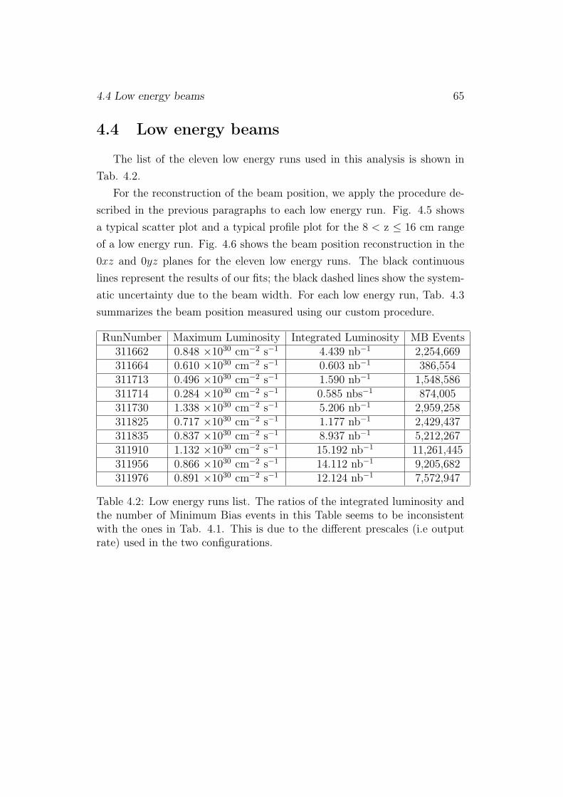
4.4 Low energy beams 65
4.4 Low energy beams
The list of the eleven low energy runs used in this analysis is shown inTab. 4.2.
For the reconstruction of the beam position, we apply the procedure de-scribed in the previous paragraphs to each low energy run. Fig. 4.5 showsa typical scatter plot and a typical profile plot for the 8 < z ≤ 16 cm rangeof a low energy run. Fig. 4.6 shows the beam position reconstruction in the0xz and 0yz planes for the eleven low energy runs. The black continuouslines represent the results of our fits; the black dashed lines show the system-atic uncertainty due to the beam width. For each low energy run, Tab. 4.3summarizes the beam position measured using our custom procedure.
RunNumber Maximum Luminosity Integrated Luminosity MB Events311662 0.848 ×1030 cm−2 s−1 4.439 nb−1 2,254,669311664 0.610 ×1030 cm−2 s−1 0.603 nb−1 386,554311713 0.496 ×1030 cm−2 s−1 1.590 nb−1 1,548,586311714 0.284 ×1030 cm−2 s−1 0.585 nbs−1 874,005311730 1.338 ×1030 cm−2 s−1 5.206 nb−1 2,959,258311825 0.717 ×1030 cm−2 s−1 1.177 nb−1 2,429,437311835 0.837 ×1030 cm−2 s−1 8.937 nb−1 5,212,267311910 1.132 ×1030 cm−2 s−1 15.192 nb−1 11,261,445311956 0.866 ×1030 cm−2 s−1 14.112 nb−1 9,205,682311976 0.891 ×1030 cm−2 s−1 12.124 nb−1 7,572,947
Table 4.2: Low energy runs list. The ratios of the integrated luminosity andthe number of Minimum Bias events in this Table seems to be inconsistentwith the ones in Tab. 4.1. This is due to the different prescales (i.e outputrate) used in the two configurations.

4.4 Low energy beams 66
Figure 4.5: Comparison between the d0 versus ϕ0 scatter plot and the d0
versus ϕ0 profile in 8 < z ≤ 16 cm region, run 311714.
z [cm]-50 0 50
x [c
m]
-0.06
-0.04
-0.02
Beam Position in 0xz Plane RunNum 311662
0.0006±p0 = -0.0426
0.00002±p1 = 0.00052
Beam Position in 0xz Plane RunNum 311662
(a) Run 311662 beam position in 0xz plane.
z [cm]-50 0 50
y [c
m]
0.14
0.16
0.18
Beam Position in 0yz Plane RunNum 311662
0.00009±p0 = 0.16297
0.000004±p1 = -0.000009
Beam Position in 0yz Plane RunNum 311662
(b) Run 311662 beam position in 0yz plane.
Figure 4.6: Beam position in 0xz and 0yz planes for low energy runs. Theblack continuous lines represent the results of our fits; the black dashed linesshow the systematic uncertainty due to the beam width.

4.4 Low energy beams 67
z [cm]-50 0 50
x [c
m]
-0.06
-0.04
-0.02
Beam Position in 0xz Plane RunNum 311664
0.0006±p0 = -0.0448
0.00002±p1 = 0.00052
Beam Position in 0xz Plane RunNum 311664
(c) Run 311664 beam position in 0xz plane.
z [cm]-50 0 50
y [c
m]
0.14
0.16
0.18
Beam Position in 0yz Plane RunNum 311664
0.00008±p0 = 0.16576
0.000003±p1 = -0.000010
Beam Position in 0yz Plane RunNum 311664
(d) Run 311664 beam position in 0yz plane.
z [cm]-50 0 50
x [c
m]
-0.06
-0.04
-0.02
Beam Position in 0xz Plane RunNum 311699
0.0006±p0 = -0.0435
0.00002±p1 = 0.00052
Beam Position in 0xz Plane RunNum 311699
(e) Run 311699 beam position in 0xz plane.
z [cm]-50 0 50
y [c
m]
0.14
0.16
0.18
Beam Position in 0yz Plane RunNum 311699
0.00010±p0 = 0.16465
0.000004±p1 = -0.000017
Beam Position in 0yz Plane RunNum 311699
(f) Run 311699 beam position in 0yz plane.
Figure 4.6: Beam position in 0xz and 0yz planes for low energy runs. Theblack continuous lines represent the results of our fits; the black dashed linesshow the systematic uncertainty due to the beam width.

4.4 Low energy beams 68
z [cm]-50 0 50
x [c
m]
-0.06
-0.04
-0.02
Beam Position in 0xz Plane RunNum 311713
0.0006±p0 = -0.0432
0.00002±p1 = 0.00052
Beam Position in 0xz Plane RunNum 311713
(g) Run 311713 beam position in 0xz plane.
z [cm]-50 0 50
y [c
m]
0.14
0.16
0.18
Beam Position in 0yz Plane RunNum 311713
0.00009±p0 = 0.16420
0.000004±p1 = -0.000013
Beam Position in 0yz Plane RunNum 311713
(h) Run 311713 beam position in 0yz plane.
z [cm]-50 0 50
x [c
m]
-0.14
-0.12
-0.10Beam Position in 0xz Plane RunNum 311714
0.0006±p0 = -0.1255
0.00002±p1 = 0.00052
Beam Position in 0xz Plane RunNum 311714
(i) Run 311714 beam position in 0xz plane.
z [cm]-50 0 50
y [c
m]
0.14
0.16
0.18
Beam Position in 0yz Plane RunNum 311714
0.00010±p0 = 0.16301
0.000004±p1 = -0.000012
Beam Position in 0yz Plane RunNum 311714
(j) Run 311714 beam position in 0yz plane.
Figure 4.6: Beam position in 0xz and 0yz planes for low energy runs. Theblack continuous lines represent the results of our fits; the black dashed linesshow the systematic uncertainty due to the beam width.

4.4 Low energy beams 69
z [cm]-50 0 50
x [c
m]
-0.14
-0.12
-0.10
Beam Position in 0xz Plane RunNum 311730
0.0006±p0 = -0.1250
0.00002±p1 = 0.00051
Beam Position in 0xz Plane RunNum 311730
(k) Run 311730 beam position in 0xz plane.
z [cm]-50 0 50
y [c
m]
0.14
0.16
0.18
Beam Position in 0yz Plane RunNum 311730
0.00009±p0 = 0.16178
0.000004±p1 = -0.000019
Beam Position in 0yz Plane RunNum 311730
(l) Run 311730 beam position in 0yz plane.
z [cm]-50 0 50
x [c
m]
-0.14
-0.12
-0.10
Beam Position in 0xz Plane RunNum 311825
0.0006±p0 = -0.1234
0.00002±p1 = 0.00052
Beam Position in 0xz Plane RunNum 311825
(m) Run 311825 beam position in 0xz plane.
z [cm]-50 0 50
y [c
m]
0.14
0.16
0.18
Beam Position in 0yz Plane RunNum 311825
0.00009±p0 = 0.16345
0.000004±p1 = -0.000013
Beam Position in 0yz Plane RunNum 311825
(n) Run 311825 beam position in 0yz plane.
Figure 4.6: Beam position in 0xz and 0yz planes for low energy runs. Theblack continuous lines represent the results of our fits; the black dashed linesshow the systematic uncertainty due to the beam width.

4.4 Low energy beams 70
z [cm]-50 0 50
x [c
m]
-0.14
-0.12
-0.10
Beam Position in 0xz Plane RunNum 311835
0.0006±p0 = -0.1226
0.00002±p1 = 0.00052
Beam Position in 0xz Plane RunNum 311835
(o) Run 311835 beam position in 0xz plane.
z [cm]-50 0 50
y [c
m]
0.14
0.16
0.18
Beam Position in 0yz Plane RunNum 311835
0.00007±p0 = 0.16366
0.000003±p1 = -0.000014
Beam Position in 0yz Plane RunNum 311835
(p) Run 311835 beam position in 0yz plane.
z [cm]-50 0 50
x [c
m]
-0.14
-0.12
-0.10
Beam Position in 0xz Plane RunNum 311910
0.0006±p0 = -0.1205
0.00002±p1 = 0.00050
Beam Position in 0xz Plane RunNum 311910
(q) Run 311910 beam position in 0xz plane.
z [cm]-50 0 50
y [c
m]
0.14
0.16
0.18
Beam Position in 0yz Plane RunNum 311910
0.00007±p0 = 0.16110
0.000003±p1 = -0.000043
Beam Position in 0yz Plane RunNum 311910
(r) Run 311910 beam position in 0yz plane.
Figure 4.6: Beam position in 0xz and 0yz planes for low energy runs. Theblack continuous lines represent the results of our fits; the black dashed linesshow the systematic uncertainty due to the beam width.

4.4 Low energy beams 71
z [cm]-50 0 50
x [c
m]
-0.14
-0.12
-0.10
Beam Position in 0xz Plane RunNum 311956
0.0006±p0 = -0.1229
0.00002±p1 = 0.00050
Beam Position in 0xz Plane RunNum 311956
(s) Run 311956 beam position in 0xz plane.
z [cm]-50 0 50
y [c
m]
0.14
0.16
0.18
Beam Position in 0yz Plane RunNum 311956
0.00007±p0 = 0.16413
0.000003±p1 = -0.000041
Beam Position in 0yz Plane RunNum 311956
(t) Run 311956 beam position in 0yz plane.
z [cm]-50 0 50
x [c
m]
-0.14
-0.12
-0.10
Beam Position in 0xz Plane RunNum 311976
0.0006±p0 = -0.1212
0.00002±p1 = 0.00050
Beam Position in 0xz Plane RunNum 311976
(u) Run 311976 beam position in 0xz plane.
z [cm]-50 0 50
y [c
m]
0.14
0.16
0.18
Beam Position in 0yz Plane RunNum 311976
0.00008±p0 = 0.16395
0.000003±p1 = -0.000042
Beam Position in 0yz Plane RunNum 311976
(v) Run 311976 beam position in 0yz plane.
Figure 4.6: Beam position in 0xz and 0yz planes for low energy runs. Theblack continuous lines represent the results of our fits; the black dashed linesshow the systematic uncertainty due to the beam width.

4.4 Low energy beams 72
Run
#x
0±σx
0[cm]
dxdz±σdxdz[rad
]y 0±σy0[cm]
dydz±σdydz[rad]
3116
62(−
4.26±
0.06
)·1
0−2
(5.2±
0.2)·1
0−4
1.62
97·1
0−1±
9·1
0−5
(−0.
9±
0.4)·1
0−5
3116
64(−
4.48±
0.06
)·1
0−2
(5.2±
0.2)·1
0−4
1.65
76·1
0−1±
8·1
0−5
(−1.
0±
0.3)·1
0−5
3116
99(−
4.35±
0.06
)·1
0−2
(5.2±
0.2)·1
0−4
1.64
65·1
0−1±
10·1
0−5
(−1.
7±
0.4)·1
0−5
3117
13(−
4.32±
0.06
)·1
0−2
(5.2±
0.2)·1
0−4
1.64
20·1
0−1±
10·1
0−5
(−1.
3±
0.4)·1
0−5
3117
14(−
12.5
5±
0.06
)·1
0−2
(5.2±
0.2)·1
0−4
1.64
30·1
0−1±
10·1
0−5
(−1.
2±
0.4)·1
0−5
3117
30(−
12.5
0±
0.06
)·1
0−2
(5.1±
0.2)·1
0−4
1.61
78·1
0−1±
9·1
0−5
(−1.
9±
0.4)·1
0−5
3118
25(−
12.3
3±
0.06
)·1
0−2
(5.2±
0.2)·1
0−4
1.63
45·1
0−1±
9·1
0−5
(−1.
3±
0.4)·1
0−5
3118
35(−
12.2
6±
0.06
)·1
0−2
(5.2±
0.2)·1
0−4
1.63
66·1
0−1±
7·1
0−5
(−1.
4±
0.3)·1
0−5
3119
10(−
12.0
5±
0.06
)·1
0−2
(5.0±
0.2)·1
0−4
1.61
10·1
0−1±
7·1
0−5
(−4.
3±
0.3)·1
0−5
3119
56(−
12.2
9±
0.06
)·1
0−2
(5.0±
0.2)·1
0−4
1.64
13·1
0−1±
7·1
0−5
(−4.
1±
0.3)·1
0−5
3119
76(−
12.1
2±
0.06
)·1
0−2
(5.0±
0.2)·1
0−4
1.63
95·1
0−1±
7·1
0−5
(−4.
2±
0.2)·1
0−5
Table4.3:
Fittedbe
ampo
sition
san
dtheirstatisticalu
ncertainties
forlow
energy
runs.

Chapter 5
Monte Carlo samples
5.1 Monte Carlo simulation
In complex experiments like CDF II, the detector acceptance and thedetector expected response to the passage of a particle are often simulated viaMonte Carlo (MC) techniques. It is impossible, in fact, to analytically predictthe detector behavior because of the complexity of its geometry and becauseof the huge number of variables to consider. MC simulation techniques areuseful numerical methods that allow, e.g., to estimate the fraction of eventsescaping from the detector acceptance or to predict the functional form of aparticular signal.
In HEP experiments, MC techniques can be generally divided into threekinds: generation simulation, detector simulation and trigger simulation. Inthis analysis we do not need the trigger simulation.The generation simulation incorporates, for this analysis, all the physicalprocesses involved in the pp collision. The collision is simulated from theinitial interaction up to the final formation of the hadronic state.The detector simulation is the simulation of the passage of the MC producedparticles inside the detector geometry. The detector simulation also providesthe generation of the signals collected by the subdetectors, their read out,etc..The final result of a complete MC simulation is a sample of simulated datathat has the same format as data, allowing their analysis with the same anal-
73

5.1 Monte Carlo simulation 74
ysis frameworks.
Different types of generators are used in CDF Monte Carlo samples; inthis analysis we used BGenerator [22].
BGenerator is used in the CDF B Monte Carlo (BMC). BMC generatessamples of hadrons containing a quark b or a quark c (e.g. D mesons). Aftergenerating the hadrons, BGenerator forces them to decay into a particularfinal state. At the end, the decay products are propagated within the CDFII detector simulation. The joint distribution of transverse momentum andpseudo-rapidity for the different hadrons are the input information of theBGenerator.The interactions between the particles and the different materials of thedetector are also reproduced. The different signals that the particles producein all the subdetectors are then simulated. The version 3 of the GEANTpackage [23] models the detector geometry and material for the standardCDF II simulation.
Some sub-detectors are simulated by specific packages rather than byGEANT. For the silicon detectors, a parametric model, tuned on data, sim-ulates the charge deposition: it accounts for the Landau distribution, pro-duction of δ rays, capacitive charge sharing between neighboring strips andnoise, etc.
The off-line database is used to tune the simulation. The configuration ischanged on a run by run basis (position and slope of the beam line, relativemis-alignments between subdetectors, trigger table used, etc.) and local ortemporary inefficiencies of the silicon tracker (active coverage, noisy channels,etc.) are taken into account. In this way, a detailed simulation of the realruns is available and it is possible to match the distribution of data and MCin any given sample.

5.2 Generation technique 75
5.2 Generation technique
We exploit MC techniques to simulate the shapes of the signals.We simulate the D0 → Kπ decay channel for the signal and all the other D0
decay channels for the physical background. Through this simulation, we areable to interpret the invariant K−π+ mass distribution obtained from data.
As input for the BMC, we used the rapidity distribution versus the trans-verse momentum (y–pT ) for the mesons to be generated in the ranges [-1.3;1.3]×[0; 15] GeV/c. A shape that describes the phenomenological distribu-tion in the y–pT range is used.
In order to reproduce the same characteristics of our data sample, wedo not perform any trigger simulations. The MC events follow the samereconstruction chain as data: we also perform the same candidate selectionused for the data (see Sec. 6.1).
5.3 Samples
For our purpose, we simulate two different MC sample, the D0 → Kπ
sample and the D0 → X sample.
5.3.1 D0 → Kπ
For this sample, we generate D0 and D0 and force them to decay into Kπonly (D0 → K−π+ and D0 → K+π−).
Fig. 5.1 shows the resulting invariant K−π+ mass plot. For each candi-date D0, we assume that the negative track is a kaon and the positive trackis a pion and we sum their four-momenta to evaluate the invariant mass.The plot is composed by the sum of two structures, both centered at theexpected D0 mass (mD0 ' 1.864 GeV/c2): a narrow peak with a width ofabout 8 MeV/c2 and a wider one with a width of about 80 MeV/c2. In theD0 candidate reconstruction, we always assign the mass of the kaon to thenegative track. Thus, when a D0 is produced, we fail the mass assignment ofthe tracks. The narrow peak in Fig. 5.1 represents the D0 → K−π+ signal

5.3 Samples 76
Figure 5.1: Invariant K−π+ mass of candidates reconstructed in the D0 →Kπ MC sample, linear scale (Top). Invariant K−π+ mass of candidatesreconstructed in the D0 → Kπ MC sample, logarithmic scale (Bottom).

5.3 Samples 77
that we obtain when we have the Right Sign (RS) assignment of the masses:the kaon mass (mK− ' 494 MeV/c2) is assigned to the negative track andthe pion mass (mπ+ ' 139 MeV/c2) to the positive track. The wide peakrepresents the D0 → K+π− signal that we obtain every time we have theWrong Sign (WS) assignment of the masses.
D0 → K+π−
D0→K−π
+
Figure 5.2: D0 → Kπ MC sample: 2D invariant mass plot of candidateswith K+π− assignment in the y axis versus K−π+ assignment in the x axis.
We plot the two possible Kπ invariant mass assignments in a 2D scatterplot: K+π− versus K−π+. As one can see in Fig. 5.2, the two signals aredistinctly separate: the generated D0 are represented by the horizontal bulkof candidates, while the generated D0 are represented by the vertical one.Fig. 5.1 is in fact the projection of the 2D plot of Fig. 5.2 on the horizontalaxis.
We use this MC sample not only to understand how the signals (D0 andD0) appear in the invariant K−π+ mass plots, but also to study the signals

5.3 Samples 78
shapes as a function of pT (see Sec. 5.4) and to perform the fit of the yielddescribed in Chapt. 6.
5.3.2 D0 → X
For this sample, we simulate the main D0 decay channels that could affectthe invariant K−π+ mass distribution.
Fig. 5.3 shows the resulting invariant K−π+ mass plot. The plot stillshows the RS and the WS peaks, but several other structures are visible atdifferent invariant mass ranges.
Plotting again the two mass assignments on a 2D scatter plot (Fig. 5.4),these structures are well visible and their origin is cleared; each structurecorresponds to a different decay channel, described in what follows:
• D0 → KK decays: in the mass assignment, we assume that the positivetrack is due to a pion. In this case we underestimate the candidate’smass (left-bottom region of the plot);
• D0 → ππ decays: in the mass assignment, we assume that the negativetracks is due to a kaon. In this case we overestimate the candidate’smass (right-top region of the plot);
• multibody D0 decays: we underestimate the candidate mass (left-bottom region of the plot), because we evaluate it using only two tracks(e.g. we miss additional particles, daughters of the D0);
• combinatorial: the random combination of tracks that accidentally sat-isfy our selection and form a fake candidate are visible as a large diag-onal band in the plot.
We use this MC sample not only to understand how the different D0
decay channels appear in the invariant K−π+ mass plots; in fact, this MCalso shows that from mK−π+ ≥ 1.8 GeV/c2 the only components that enterthe plot are RS, WR and combinatorial background. The tails from otherdecay channels in this range are negligible with respect to the uncertaintiesexpected from the fit.

5.3 Samples 79
]2-mass [GeV/c-K+πInvariant 1.5 2.0
2C
andi
date
s pe
r 5
MeV
/c
0
5000
10000
15000 total-K+π →0D-π+ K→
0D
-π+π →0D-K+ K→0D
multibody→D
CDF Monte Carlo
total-K+π →0D-π+ K→
0D
-π+π →0D-K+ K→0D
multibody→D
]2-mass [GeV/c-K+πInvariant 1.5 2.0
2C
andi
date
s pe
r 5
MeV
/c
1
10
210
310
410total
-K+π →0D-π+ K→
0D
-π+π →0D-K+ K→0D
multibody→D
CDF Monte Carlo
Figure 5.3: Top: Invariant K−π+ mass of candidates reconstructed in theD0 → X MC sample, linear scale. Bottom: Invariant K−π+ mass of candi-dates reconstructed in the D0 → X MC sample, logarithmic scale.

5.4 Signal shapes 80
]2-mass [GeV/c-π+Invariant K1.5 2.0
]2-m
ass
[GeV
/c-
K+ πIn
varia
nt
1.5
2.0
1
10
210
310
410
510
-1 = 5.94 fbL dt∫CDF Run II Preliminary
D0 → K−π+
D0→K
+π−
D0 → ππ
D0 → KK
Multib
ody
Com
bina
toric
s
Figure 5.4: 2D invariant mass plot of candidates with K+π− assignment inthe y axis vsK−π+ assignment in the x axis. The plot shows data collected byhigh-pT triggers; we are showing these data instead of our MC sample becausethey give a better view of the distribution thanks to the huge statistics andthe presence of the combinatorial component (the BMC simulates exclusivelythe D0 decays and not the whole event).
5.4 Signal shapes
The statistics in our data allow us to measure the D0 yields as a functionof pT (D0). We divide the pT range from 0.5 to 6.5 GeV/c in bins of 1 GeV/c.We then analyze the shapes of the RS and WS separately for each bin. Theshapes obtained from the MC sample are then fixed and used to fit the data.

5.4 Signal shapes 81
5.4.1 Right Sign (RS)
We parameterize the mass line shape of the RS candidates with a sum oftwo Gaussians. The probability density function is then defined as follows:
℘RS(m; ~θRS) = g ·G(m;m1, σ1) + (1− g) ·G(m;m2, σ2) (5.1)
where:
• ~θRS is the vector of parameters. It is defined as ~θRS = {g,m1,m2, σ1, σ2}and it is extracted by fitting the simulated invariant K−π+ mass dis-tribution when a D0 is generated;
• g is the relative fraction of the Gaussian labeled with the index 1 withrespect to the sum of the two Gaussians;
• G represents the parameterization of the gaussian functions. It is de-fined as follows:
G(m;µ, σ) =1
σ√
2πe−
(m−µ)2
2σ2 ; (5.2)
• m1(2) and σ1(2) are, respectively, the mean and the width of the Gaus-sian 1 (2 );
The results of the parameterization for each bin of pT (D0) between 0.5 GeV/cand 6.5 GeV/c are shown in Fig. 5.5. D0 candidates from the D0 → Kπ MCsample are used for this fits.
From these simulations, we infer that the RS signal width is almostcostant throughout the all pT (D0) range under exam.
5.4.2 Wrong Sign (WS)
We parameterize the mass line shape of the WS candidates with the samepdf used for the RS:
℘WS(m; ~θWS) = g ·G(m;m1, σ1) + (1− g) ·G(m;m2, σ2) (5.3)

5.4 Signal shapes 82
(a) 0.5 ≤ pT (D0) < 1.5 GeV/c (b) 1.5 ≤ pT (D0) < 2.5 GeV/c
(c) 2.5 ≤ pT (D0) < 3.5 GeV/c (d) 3.5 ≤ pT (D0) < 4.5 GeV/c
Figure 5.5: D0 → Kπ MC sample: invariant K−π+ mass distribution for theRS candidates in 1 GeV/c intervals of pT (D0).

5.4 Signal shapes 83
(e) 4.5 ≤ pT (D0) < 5.5 GeV/c (f) 5.5 ≤ pT (D0) < 6.5 GeV/c
Figure 5.5: D0 → Kπ MC sample: invariant K−π+ mass distribution for theRS candidates in 1 GeV/c intervals of pT (D0).
The results of the parameterization for each bin of pT (D0) for the WRare shown in Fig. 5.6. D0 candidates from the D0 → Kπ MC sample areused for this fits.
At lower masses, a long tail due to a soft photon emission is present. Forthe fit shapes, we do not take into account the radiative tail because thiscorrection is minimal with respect to the measurement uncertainties.
We notice that the WS signal width has a clear dependence on the pT (D0),unlike the RS shapes. The width of the distribution increases with the mo-mentum.

5.4 Signal shapes 84
(a) 0.5 ≤ pT (D0) < 1.5 GeV/c (b) 1.5 ≤ pT (D0) < 2.5 GeV/c
(c) 2.5 ≤ pT (D0) < 3.5 GeV/c (d) 3.5 ≤ pT (D0) < 4.5 GeV/c
Figure 5.6: Invariant K−π+ mass distribution for the WS candidates in 1GeV/c intervals of pT (D0).
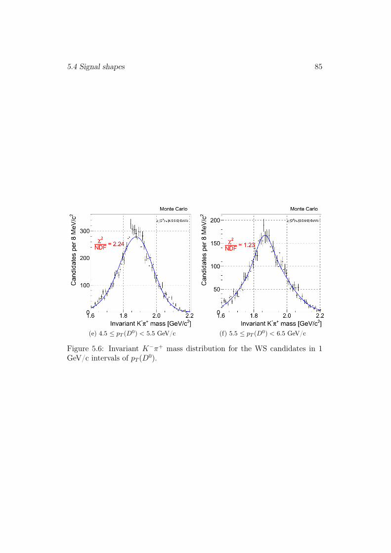
5.4 Signal shapes 85
(e) 4.5 ≤ pT (D0) < 5.5 GeV/c (f) 5.5 ≤ pT (D0) < 6.5 GeV/c
Figure 5.6: Invariant K−π+ mass distribution for the WS candidates in 1GeV/c intervals of pT (D0).

5.4 Signal shapes 86
5.4.3 Background
Unrelated couples of tracks can accidentally satisfy our selection require-ments on candidates, generating a combinatorial background.
From the MC simulation, we observe that the the signal is spread on alarge invariant mass range around the expected D0 mass value because of theWS candidates. Thus, we can’t rely on the sidebands of the data invariantmass plot to parametrize it. In addition to that the MC does not simulatethe whole event, but only the signal.
We extract the combinatorial background trend directly from data byforcing the reconstruction of fake candidates. We repeat exactly our selec-tion but using couples of tracks of the same sign (SS). We find that a de-creasing exponential shape is a good parameterization for the combinatoricstrend. Fig. 5.7 shows the invariant K±π± mass plot for the SS candidates,integrated over all the pT range.
Figure 5.7: Invariant K±π± mass distribution for Same Sign candidates ofthe data sample. The distribution is integrated over the whole pT (D0) range.

Chapter 6
Signal evidence
6.1 Base selection
We discuss here the data selection which leads to the measurement of D0
candidates in the sample. The two fundamental parameters of the selectionare the daughters’ impact parameter, d0, and the D0 transverse decay length,Lxy; these parameters both depend on the beam position. In the following,we use the d0 and Lxy referred to the beam measurement performed in Chap.4.
The method to reconstruct the D0 candidates consists in evaluating the in-variant mass of any possible combination of two tracks (with opposite charge)reconstructed in each event, assuming that they are a K and a π.
To suppress fake tracks, we apply some selection criteria, specifically stud-ied for this task. We select tracks only in the η and pT ranges where the re-construction efficiency of the tracking system is maximum. We also requirea minimum impact parameter of the tracks in order to reduce the number ofthe tracks coming from the primary vertex of interaction and maximize thenumber of tracks coming from a secondary vertex.
The requests for the single track are the following:
• SVX II small angle stereo hits ≥ 1;
• SVX II stereo hits ≥ 2;
• SVX II axial hits ≥ 3;
87

6.1 Base selection 88
• COT stereo hits ≥ 25;
• COT axial hits ≥ 25;
• |η| ≤ 1.2;
• pT ≥ 0.7 GeV/c;
• 60 µm ≤ |d0| ≤ 1.0 mm;
The first six requests represent a base "quality" selection of the tracksused in what follows. To fix the values of these parameters, we take into ac-count the tracking system specification: in fact, these values assure the lowestcontamination of fake reconstructed tracks. The requirements on transversemomentum and on impact parameter are preliminarly set after the study oftheir distributions in MC events. Each possible pair of tracks that passedthe above selection is then required to meet the following additional criteria:
• q1 · q2 < 0;
• d0,1 · d0,2 < 0;
• 2◦ ≤ ∆ϕ0 = |ϕ0,1 − ϕ0,2| ≤ 90◦;
• ∆z0 = |z0,1 − z0,2| ≤ 6 mm;
where we label the parameters relative to the negative track with (1) andthe ones relative to the positive track with (2); q1 and q2 are the daughters’charges. The first two requirements are two constraints set by the decaygeometry and kinematics. We make requests on ∆ϕ0 studying its distributionin MC events in order to take into account tracking resolution (∆ϕ0 ≥ 2◦)and kinematics of the decay channel (∆ϕ0 ≤ 90◦).
For each couple, we assign the masses to the tracks in the hypothesis thatthe negative track represents the kaon and the positive track represents thepion. We set the z coordinate of the primary vertex to be the average of thetracks z0; the x and y coordinates are then obtained from those of the beamafter evaluating the beam position in the transverse plane at that z.

6.2 Evidence of the D0 signal 89
Then, we fit each pair of tracks, looking for a possible common originpoint displaced by the primary vertex.
The fitter looks for a possible intersection point between the two tracksin the transverse plane. The fit converges only if the longitudinal distancebetween the two helices is within a certain threshold. The fitter returnsthe candidate’s decay vertex position and the resulting χ2/ndf of the fit,referred to as χ2 in what follows. We then apply the following selection onthe reconstructed candidates:
• Lxy ≥ 300 µm;
• |y(D0)| ≤ 1;
• χ2 ≤ 9;
where y(D0) is the candidate’s rapidity; its value represents the rapidityrange we are interested in. The values of the decay length and χ2 are fixedat first studying their distributions in MC events.
6.2 Evidence of the D0 signal
We plot the invariant K−π+ mass distribution for the candidates selectedas described above, looking for a structure in the D0 mass region: Fig. 6.1shows the resulting distribution.This plot represents the first evidence of the D0 signal and, in general, of thecharm production in a pp collider experiment at
√s = 900 GeV.
The distribution shows a peak at the expectedD0 mass,mD0 ' 1.864 GeV/c2.

6.2 Evidence of the D0 signal 90
Figure 6.1: InvariantK−π+ mass distribution of ZB plus MB events obtainedwith the discussed selection.

6.3 Fitting procedure 91
6.3 Fitting procedure
In order to find the D0 yield, we need to perform a fit of the invariantK−π+ mass distribution of the selected candidates.
The bins of the invariant K−π+ mass plots have a constant width of 8MeV/c2; the fit range is [m0;mmax] = [1.8 ; 2.4] GeV/c2, as described in Sec.5.3.2.
We assume a Poisson distribution for the number of events in each bin,nb, because the bin contents represent counts. We define f(m,p) to be theprobability density function used to perform the fit and p to be the vector ofthe fit parameters. The fitted bin content is fb(p); in the equations we referto fb(p) as fb for sake of simplicity. Thus, the histogram likelihood resultsto be the following:
Lb(p) =M∏b=1
(fb)nbe−fb
nb!, (6.1)
giving
Fb(p) = −2 lnLb(p) = −2M∑b=1
(nb ln fb − fb − lnnb!). (6.2)
∑Mb=1 fb is the fitted contents of all bins.
∑Mb=1 lnnb! is independent of p and
does not alter the fit result. Ignoring this term, we perform the fit minimizingthe following function:
Fb(p) = −2 lnLb(p) = −2M∑b=1
nb ln fb + 2M∑b=1
fb. (6.3)
With respect to a χ2 fit, the likelihood method has the advantage oftreating correctly the empty bins and use them in the fitting procedure.
In our case, the parameter vector is p = (nS, nB, q), where nS and nBare respectively the signal and background yields, while q is the slope of theexponential used for the combinatorics.The fit function is defined as follows:
f(m; p) = nS · ℘sig(m) + nB · ℘bkg(m; q). (6.4)

6.4 D0 yield 92
℘sig(m) is the Probability Density Function (pdf ) of the signals; it is definedas follows:
℘sig(m) = fRS · ℘RS(m) + (1− fRS) · ℘WR(m); (6.5)
where fRS is the fraction of RS candidates with respect to the number of D0
and D0 candidates. We set its value to 0.5 assuming the C-invariance of thestrong interaction production. ℘RS(m) and ℘WR(m) are fixed in shape andcentral value by the fit of the corresponding MC (see Sec. 5.4).℘bkg(m) is the pdf of the background. It is defined as follows:
℘bkg(m; q) =e−q·m∫ mmax
m0e−q·mdm
. (6.6)
The yield is defined as the integral of the RS plus the WS fit functions;in this manner, the yield represents the number of D0 and D0 found.
6.4 D0 yield
We now fit theK−π+ mass distribution for all the candidates with pT (D0)
greater than 1.5 GeV/c and calculate the yield relative to the base selectiondescribed in Sec. 6.1. Fig. 6.2 shows the results of the fit.
We compare the D0 yield in the 900 GeV sample with the one in the1.96 TeV. This comparison is possible because the data were collected by thesame detector and the same selection configuration is applied. We neglecthere minor differences in the reconstruction efficiencies that may arise due tothe different center of mass energies and that will need more detailed studies.We choose the selection described in Sec. 6.1. For each sample, we normalizethe invariant K−π+ mass plot to the number of events in the sample. Theresulting plots are shown in Fig. 6.3
In the low energy sample we obtain one third of candidates per millionof events with respect to the high energy one. This reduction is due to thedifference of the D0 cross sections at the different energies: the ratio between

6.4 D0 yield 93
Figure 6.2: InvariantK−π+ mass distribution of ZB plus MB events obtainedwith the discussed selection. The blue line represents the result of the fit; thecombinatorial background (red) and the WS (green) contributions are alsoshown.
the high and the low energy distributions is consistent with what is expectedfrom a rough extrapolation of the total cc cross section (see Fig.1.3).

6.4 D0 yield 94
(a) Normalized yield at√s = 1.97 TeV. (b) Normalized yield at
√s = 900 GeV.
Figure 6.3: Comparison between the invariant K−π+ mass plots, normalizedto the number of events in the sample, obtained in the high energy sample(left) and in the low energy sample (right).

Chapter 7
Differential yields
7.1 Selection optimization
The requirements described in the previous chapter were set in order tounfold the D0 signal from the background, considering all the candidateswith pT ≥ 1.5 GeV/c. If the D0 production is studied as a function of theD0 transverse momentum, this selection is not guaranteed to be the best oneas a function of pT (D0).
Thus, instead of considering all the candidates with pT ≥ 1.5 GeV/c, wedivide the pT (D0) range in bins of 1 GeV/c and we perform an optimizationprocedure of the selection independently in each pT (D0) bin.Since the MC simulation does not correctly reproduce the background, wedecided to use a pure data-driven optimization.
The aim of the optimization procedure is to reduce the statistical un-certainty associated with the signal for each pT (D0) bin. In order to do so,we define a figure of merit that accounts for the signal combined with thebackground and we find the selection that maximizes it, independently foreach bin.
We define the signal S as the integral of the RS and WS fit functionsin the mass range mD0± 16 MeV/c2, i.e. mD0 ± 2σmD0
; we define the back-ground B as the integral of the background fit function in the same range.
95

7.1 Selection optimization 96
In order to avoid eventual statistical biases in the selection, we proceedas follows:
• the sample is split into two mutually exclusive subsamples, A and B,using a random criterion. We choose to fill the subsample A with theevents with even event number and B with the ones with odd eventnumber, obtaining independent subsamples of approximately the samesize.
• We independently apply the same optimization steps on both the sub-samples:
1. we measure the signal events SAi and the background events BAiwhich satisfy the i-th selection configuration in subsample A byperforming a fit of the candidates invariant mass distribution;
2. we choose the figure-of-merit
f(SAi ,BAi ) =SAi√SAi + BAi
and we maximize it over the space of configurations built by allcombinations of requirements. We chose this figure of merit be-cause it gives an estimate of how much the signal is unlikely to bea background fluctuation;
3. the selection configuration corresponding to the maximum of fdefines the set of requirements optimized in sample A;
4. we repeat steps 2-3 in the sample B;
• we obtain the final sample by applying to the subsample B the require-ments optimized in subsample A and viceversa. Since a backgroundfluctuation is not likely to happen in the same mass range for indepen-dent samples, we obtain a sample of candidates that can be consideredstatistically unbiased and optimized.

7.2 Optimized selection 97
We use the variables listed in Tab. 7.1 to built a 5D matrix of selectionconfiguration. To built the matrix, we differentiate the selection on eachsingle variable for several different values, referred to as “steps”. The numberof steps considered for each variable and its range is listed in the table.
Variable Range Number of stepspT of the daughters [0.7; 1.0] GeV/c i = 4d0 of the daughters [0; 160] µm j = 10∆z0 of the daughters [0.2; 0.7] cm k = 6χ2 of the candidate [2; 12] l = 10Lxy of the candidate [0; 340] µm m = 10
Table 7.1: Variables used in the optimization procedure; we report the rangemapped and the number of steps used.
A selection configuration is defined as:
• pT ≥ pT,i ;
• |d0| ≥ |d0,j| ;
• |∆z0| ≤ |∆z0,k|;
• χ2 ≤ χ2l ;
• Lxy ≥ Lxy,m,
where pT,i, d0,j, ∆z0,k, χ2l and Lxy,m are the different values corresponding to
the different steps of each single variable selection.We map the figure of merit over every possible combination of require-
ments on the five variables. Each configuration is coded with a single num-ber (C) where every digit represents the considered step for each variable:C = ijklm.
Fig. 7.1 shows a typical plot of the figure of merit versus the configura-tion number. Several peaks are visible: the highest one represents the bestselection for the considered pT (D0) bin.

7.2 Optimized selection 98
Figure 7.1: Figure of merit versus the configuration number for sample A, inthe range 1.5 ≤ pT ≤ 2.5 GeV/c.
7.2 Optimized selection
We apply the same optimization procedure considering all the candidateswith pT (D0) ≥ 1.5 GeV/c and we obtain the optimized integrated selection;thus, for each bin of pT , we compare this selection with the one optimized inthe single bin in order to check if the bin by bin optimization is actually thebest way to discriminate the signal. As we expected, Fig. 7.2 shows that thefigure of merit obtained with the bin by bin selection is higher or equal tothe one obtained with the integrated selection for each bin.
For the measurement of the D0 yields as a function of pT , we decided toconsider only the bins with a figure of merit & 3, where the separation of thesignal from the background is larger. Thus, we considered the pT range from0.5 GeV/c to 6.5 GeV/c.

7.3 Yields as a function of pT (D0) 99
Figure 7.2: Comparison of the figures of merit for the selection optimizedon the whole pT spectrum (red) and for the selection optimized bin by bin(blue).
7.3 Yields as a function of pT (D0)
Fig. 7.3 shows the results of the fits on data in each pT (D0) bin. The blueline represents the result of the fit; the combinatorial background (red) andthe WS (green) contributions are also shown.
It is important to highlight that we are able to measure the D0 signal inthe 0.5 ≤ pT (D0) ≤ 1.5 GeV/c bin, as shown in Fig. 7.3 (a), only because ofthe of MB and ZB bias triggers and because we unfold the signal from thebackground via the bin by bin optimization procedure.
Summing the yield for each pT (D0) bin, even if the selections are differentfor each pT (D0) bin, we obtain an estimate of the number of D0 and D0 inthe studied range 0.5 ≤ pT (D0) ≤ 6.5 GeV/c.Fig. 7.4 shows the fitted D0 yields as a function of pT and Tab. 7.2 summa-rizes the fit results.

7.3 Yields as a function of pT (D0) 100
(a) 0.5 ≤ pT (D0) < 1.5 GeV/c
(b) 1.5 ≤ pT (D0) < 2.5 GeV/c
Figure 7.3: Invariant K−π+ mass fit of data in 1 GeV/c intervals of pT (D0).The blue line represents the result of the fit; the combinatorial background(red) and the WS (green) contributions are also shown.

7.3 Yields as a function of pT (D0) 101
(c) 2.5 ≤ pT (D0) < 3.5 GeV/c
(d) 3.5 ≤ pT (D0) < 4.5 GeV/c
Figure 7.3: Invariant K−π+ mass fit of data in 1 GeV/c intervals of pT (D0).The blue line represents the result of the fit; the combinatorial background(red) and the WS (green) contributions are also shown.

7.3 Yields as a function of pT (D0) 102
(e) 4.5 ≤ pT (D0) < 5.5 GeV/c
(f) 5.5 ≤ pT (D0) < 6.5 GeV/c
Figure 7.3: Invariant K−π+ mass fit of data in 1 GeV/c intervals of pT (D0).The blue line represents the result of the fit; the combinatorial background(red) and the WS (green) contributions are also shown.

7.3 Yields as a function of pT (D0) 103
Figure 7.4: Yields as a function of pT obtained with the bin by bin optimiza-tion.
pT [GeV/c] Yield σY ield σY ield/Yield0.5 – 1.5 24 9 38%1.5 – 2.5 156 37 24%2.5 – 3.5 116 36 31%3.5 – 4.5 53 12 23%4.5 – 5.5 66 19 29%5.5 – 6.5 58 13 22%Total 473 58 12%
Table 7.2: pT (D0) range, correspondent yield and uncertainties.

Conclusions
In this analysis, we presented a study of the D0 meson production at√s
= 900 GeV in the Minimum Bias and Zero Bias samples collected by theCDF experiment at the Tevatron Collider. Our study belongs to a series ofexperimental QCD studies in the kinematic conditions where the perturba-tive QCD does no longer apply and the behavior of the strong interactionsis not well understood.
The D0 yields as a function of pT has been measured. Specifically, weevaluated the raw yield of the D0 meson in the decay channel D0 → K−π+
(D0 → K+π−) as a function of the D0 transverse momentum in the range0.5 ≤ pT ≤ 6.5 GeV/c.A preliminary step was also completed. We developed a procedure to recon-struct the beam and we successfully reconstructed its position for the lowenergy runs. The beam position we measured can be further exploited byother analyses of the collaboration.We successfully unfolded the D0 signal from the background, thus complet-ing the main step toward the measurement of the D0 differential productioncross section. This result is of particular importance since such measurementis likely to remain the only one of its kind for several years.
Our result is consistent with what is expected from a rough extrapolationof the total cc cross section measurement performed at different energies.
104

Bibliography
[1] P. W. Higgs, Broken Symmetries, Massless Particles And Gauge
F ields, Phys. Lett. 12 (1964) 132.
[2] P. W. Higgs, Broken Symmetries, Massless Particles And Gauge
F ields, Phys. Lett. 13 (1964) 508.
[3] M. R. Pennington, Swimming with quarks, http://arxiv.org/pdf/hep-ph/0504262
[4] K. Nakamura et al. [Particle Data Group], J. Phys. G 37, 075021 (2010).
[5] A.V. Manohar and M. B. Wise, Camb. Monogr. Part. Phys. Nucl. Phys.Cosmol. 10, 1 (2000).
[6] G. ’t Hooft, Nucl. Phys. B 44, 461 (1972).
[7] B. W. Lee, Phys. Rev. D 5, 823 (1972).
[8] Ikaros I. Y. Bigi, Charm physics - like Botticelli in the Sistine chapel,hep- ph/0107102 (2001).
[9] G. Isidori et al. [LHCb Collaboration], arXiv:1111.4987v1 [hep-ph],(2011).
[10] D. Acosta et al. [CDF Collaboration], Phys. Rev. Lett. 91, 241804(2003).
[11] A. Adare et al [PHENIX Collaboration], Phys. Rev. Lett. 97, 252002(2006).
105

BIBLIOGRAPHY 106
[12] J. Adams et al. [STAR Collaboration], Phys. Rev. Lett. 94, 062301(2005).
[13] B. I. Abelev et al. [STAR Collaboration], Phys. Rev. Lett. 98, 192301(2007).
[14] R. Bala, for the ALICE Collaboration, arXiv:1201.0729v1 [nucl-ex],(2012).
[15] B. A. Kniehl, G. Kramer, I. Schienbein and H. Spiesberger, AIP Conf.Proc. 792, 867 (2005).
[16] B. A. Kniehl, G. Kramer, I. Schienbein and H. Spiesberger, Phys. Rev.Lett. 96, 012001 (2006).
[17] Fermilab Beam Division, Run II Handbook and Operations RookieBooks.
[18] R. Blair et al. [CDF Collaboration], The CDFII Detector : Technical
Design Report, FERMILAB-Pub-96/390-E (1996).
[19] D. Acosta et al., CDF note 6052, 2002.
[20] S. Klimenko, J. Konigsberg and T. Liss, CDF note 6314, 2003.
[21] N. Goldschmidt CDF note 10650, 2011.
[22] K. Anikeev, P. Christoph and P. Murat, Description of Bgenerator II,CDF note 5092, 1999.
[23] R. Brun et al., GEANT: Simulation Program For Particle Physics Ex-periments. User Guide and Reference Manual, 1978.
[24] R. Brun et al., ROOT object oriented data analysis framework.,http://root.cern.ch.
[25] http://pdg.lbl.gov/2011/hadronic-xsections/
[26] H. Stadie et al., CDF note 6327, 2003.
[27] H. Wenzel et al., CDF note 1924, 1993.

Allegato: sommario in linguaitaliana
In questo lavoro di tesi è presentato uno studio della produzione delmesone D0 nelle collisioni protone-antiprotone. I dati in analisi sono statiraccolti dall’esperimento CDF II presso il collisionatore di protoni e antipro-toni Tevatron sito al Fermi National Accelerator Laboratory. Questo lavorofa parte di uno specifico sforzo da parte della collaborazione CDF per mis-urare la sezione d’urto differenziale dei mesoni contenenti quark di tipo charmnella regione cinematica dei bassi momenti trasversi.
Lo studio della produzione dei mesoni D0 a basso momento transverso adifferenti energie nel centro di massa è un’opportunità per arricchire l’attualeconoscenza sul comportamento dell’interazione forte nella regione in cui laproduzione del quark c avviene in condizioni non perturbative. L’attuale teo-ria di cromodinamica quantistica (QCD) infatti non è in grado di descrivere ilcomportamento dell’interazione forte nella regione dei bassi quadri-momentitransferiti (basso Q2), a causa del running della costante di accoppiamentoαS. In queste condizioni cinematiche, αS è dell’ordine dell’unità, quindi leteorie pertubative non sono applicabili. Studi sperimentali in questa regionesono fondamentali per superare la limitazione teorica e fornire spunti pernuovi modelli.
Il mio lavoro di tesi, supportato dal gruppo di ricerca CDF Bologna, èun’estensione dei precedenti lavori della collaborazione CDF sui mesoni D0
e concerne l’analisi del campione di dati raccolto all’energia di 900 GeV nel
107

BIBLIOGRAPHY 108
centro di massa durante il cosidetto “Low Energy Scan”. Si è per la primavolta osservata la produzione di D0 a basso momento trasverso a questaenergia. Il campione di eventi analizzato è il più numeroso mai raccolto adun collisionatore adronico in queste condizioni sperimentali.
Obiettivo primario dell’analisi è stato la misura del numero diD0 prodottiin funzione del loro momento trasverso. Si è selezionato il canale di decadi-mento D0 → K−π+ (D0 → K+π−) per la sua semplice topologia, la suabuona efficienza di ricostruzione (entrambi i prodotti di decadimento sonocarichi e visibili dall’apparato di tracciamento di CDF) e per il BrancingRatio relativamente alto (circa 3.9%).
E’ stato necessario effettuare una misura preliminare per poter finalizzareanalisi: poiché per i run a bassa energia la posizione del fascio non era stataricostruita, si è dovuto studiare una procedura ad hoc per tale ricostruzione.La posizione del fascio è stata quindi ricostruira indipendentemente per ognirun: potranno beneficiare del risultato ottenuto anche altre analisi della col-laborazione. La necessità di questa misura è data dal fatto che la segnaturadel decadimento dei mesoni D0 è un vertice secondario distante dal verticeprimario di interazione diversi micron. E’ stato quindi possibile estrarre ilsegnale di D0 dal fondo costituito da mesoni leggeri e misurarne il numeroin funzione del momento trasverso nell’intervallo fra 0.5 GeV/c e 6.5 GeV/c.La misura del numero di D0 in tale intervallo di pT è stata possibile gra-zie all’utilizzo degli eventi raccolti dai trigger di Minimum Bias e di ZeroBias e grazie anche alla procedura di ottimizzazione della selezione studiatanell’analisi.
La tesi si articola in sette capitoli. Nel primo viene presentata una breveintroduzione teorica, mentre nel secondo viene descritto l’apparato sperimen-tale. Il capitolo tre descrive il campione utilizzato e la strategia d’analisi. Ilcapitolo quattro è dedicato alla procedura di ricostruzione della posizionedel fascio ed ai suoi risultati per i run considerati. Nel capitolo cinque sonodescritte le tecniche di simulazione Monte Carlo utilizzate per l’analisi pre-liminare dei dati. Nel capitolo sei viene presentata l’evidenza del segnale diD0. Nel settimo capitolo è illustrata la misura del numero di D0 prodotti infunzione del loro momento trasverso.

Acknowledgements
A un uomo gentile e onesto va il mio primo ringraziamento: al Prof.Franco Rimondi. E’ stato lui a volere fortemente questa analisi, a volermiin questo gruppo ed io non posso che essergli riconoscente per il fatto che,nonostante tutte le difficoltà, ho concluso un lavoro che mi ha reso un fisicomigliore e mi ha dato la possibilità di conoscere un manipolo straordinariodi persone che, veramente, “buttano il cuore oltre l’ostacolo”. E’ stato lui,insieme a Milena, a darmi l’opportunità di “scoprire l’America” ed il suoanomalo, ma straordinario ambiente di lavoro. Con lui è iniziato questomio lungo viaggio chiamato tesi e ora, insieme alla gioia della finalizzazione,rimane un retrogusto amaro.
Il suddetto “manipolo straordinario” è il gruppo CDF Bologna. Per averraccolto un pesante testimone, ringrazio il dott. Stefano Zucchelli che haavuto il cuore e la volontà di completare insieme a me questo lavoro.Ringrazio il dott. Manuel Mussini, che, con infinita pazienza e tempra in-stancabile, per questi mesi mi ha preso per mano e mi ha guidato lungotutta l’analisi: senza di lui avrei continuato a proiettare grafici a caso e adisperarmi ogni quindici minuti. In questi mesi è stato per me un grandeinsegnante e un amico. Quanto gli devo non è neanche numerabile....Ringrazio anche il dott. Niccolò Moggi per aver accettato di correggere lamia tesi nonostante non fosse suo compito, nonostante l’influenza e nonos-tante la mancanza di sonno; i suoi preziosi consigli sono stati quanto maigraditi.Infine ringrazio la dott.ssa Milena Deninno per il suo apporto a questo lavoro,ma soprattutto perché non è da tutti essere sorridenti e gentili anche nellapiù buia delle ore.

BIBLIOGRAPHY 110
Ringrazio gang di Cottonwood: Vitolino che mi ha dato un tetto soprala testa, Phede che mi ha contagiato con la sforzite, Colò per gli abbraccigratuiti, Pisotti perché è completamente matto e Vittorio, perché se va malec’è sempre l’industria. Poi ancora Jen, Elettra e Céline, perché le donne chevestono al contrario han capito tutto dalla vita. Grazie per non avermi fattomai sentire sola nello sconfinato Yankee-continente. I luv u, pipol.
Ringrazio l’Ele-di-Milano perché è pur essendo continuamente super im-pegnate siamo riuscite a trovare uno strano equilibrio a distanza per coltivarela nostra stupenda amicizia. Non era facile.
Ringrazio l’Elisa perché essere certe persone non è affatto facile e lei ciriesce alla grandissima. Sei una roccia e sei per me un’ispirazione.
Ringrazio la Fede perché tutti i giorni mi fa scoprire chi sono e chi vogliodiventare.
Ringrazio Luca perché è mio fratello e in famiglia ci si ama nonostantetutte le malefatte, i giudizi e le foto col pizzetto.
Ringrazio tutti i miei amici, fra cui in particolare Vinci, Sotti, Marquez,Giova, la Tasso, Edo, la Viola, Brogna, Sighi, Giacomo, gli Ornitorinchi, isemiotici in genere e le regaz del basket perché se cinque anni di fisica nonmi hanno trasformato in una nerd irrecuperabile è soprattutto merito loro.
Ringrazio il mio topo perché cresciamo ogni giorno insieme, perché misopporta quando sclero, perché mi ha dettato le correzioni di questa tesiall’una di notte, perché dopo quasi due anni che viviamo a Bologna non saancora qual è il nostro ripiano del frigo, ma ha sempre riconosciuto cosa èbene per noi. Nelle cose importanti sei la mia guida. Andiamo bene...
Infine ringrazio la mia mamma, perché è la mia mamma e nessuno trannelei sa cosa questo comporti...