Smooth surfaces from bilinear patches: discrete affineminimal surfaces

Florian Kaferbock

Institut fur Diskrete Mathematik und Geometrie, Technische Universitat WienWiedner Hauptstr. 8–10/104, A-1040 Wien, Austria

Helmut Pottmann

King Abdullah University of Science and TechnologyThuwal 23955, Saudi Arabia

Abstract

Motivated by applications in freeform architecture, we study surfaces whichare composed of smoothly joined bilinear patches. These surfaces turn out to bediscrete versions of negatively curved affine minimal surfaces and share manyproperties with their classical smooth counterparts. We present computationaldesign approaches and study special cases which should be interesting for thearchitectural application.

Keywords: Discrete differential geometry, affine minimal surface, asymptoticnet, architectural geometry, fabrication-aware design

1. Introduction

Freeform structures constitute one of the major trends in contemporary ar-chitecture. While we have plenty of ways to handle the pure digital shapemodeling tasks, the realization of a complex shape at the large architecturalscale is still a challenge. A significant number of problems to be solved arerooted in Geometric Design: Ideally, architects should use systems which gen-erate only those shapes that can be efficiently built with the chosen materialand fabrication technology. Such an approach to digital design may be calledfabrication-aware design. The present paper attempts to make a contribution inthis direction. It also continues along the lines of recent research which re-vealed a close connection between the design and construction of architecturalfreeform structures and discrete differential geometry. It turned out that practi-cal requirements make certain discrete surface representations, such as meshes

Email addresses: fkaeferboeck@geometrie.tuwien.ac.at (Florian Kaferbock),helmut.pottmann@kaust.edu.sa (Helmut Pottmann)

Preprint submitted to CAGD February 8, 2013

with planar faces and offset properties, very attractive for architectural applica-tions. In fact, the architectural application led to the formulation of some newconcepts in discrete differential geometry [2, 3].

Some architects aim at architectural structures which exhibit smooth freeformskins. However, smooth architectural freeform hulls are a big challenge. Sincethey have to be composed of panels and the production of the panels needs tobe feasible, one has to compose smooth surfaces from simple types of surfacepatches (panels). If one aims at smoothness, planar panels are not suitable.One can replace planar panels with developable panels, in particular cylindri-cal and conical ones. This led to the introduction of developable strip models.They may be viewed as semi-discrete structures and provide a link betweenthe smooth and fully discrete setting [17]. However, while being smooth alongstrips, the arising structures still exhibit kinks between adjacent strips. Panel-ing freeform surfaces with an algorithm that allows one to control the trade-offbetween smoothness and construction cost has been addressed by Eigensatzet al. [8]. None of these methods will be able to generate a general smoothfreeform surface.

In this paper, we pursue a different direction: Prescribing a simple type ofpanels, namely bilinear patches, we ask for those surfaces which can be generatedby smoothly joining these bilinear patches. Bilinear patches are parts of hyper-bolic paraboloids and have been widely used in architecture, where they arecalled hypar shells. The actual construction exploits their geometric properties:They contain two families of straight lines and are also translational surfaces.To the best of our knowledge, there is no built structure so far where bilinearpatches have been joined in a nontrivial way to obtain a smooth surface.

It is clear that smoothly joined negatively curved patches will only generatemodels of negatively curved surfaces. The shape limitation is even stronger.We will show here that smooth surfaces from bilinear patches are discrete affineminimal surfaces with indefinite metric. They agree with the surfaces of Craizeret al. [6] who did not point to the fact that their quad meshes, when filled bypatches of hyperbolic paraboloids, do in fact generate smooth surfaces. Wewill complement the work of Craizer et al. by a different approach, a study ofimportant special cases and their relations to the classical geometric literature,and in particular by proposing methods for computational design of thesesurfaces.

1.1. Previous workNegatively curved smooth surfaces from ruled surface strips, but not bilin-

ear patches, have already been addressed by S. Flory et al. [9, 10, 11]. Thiswork can be seen as contribution to the computation of semidiscrete asymp-totic parameterizations; for a mathematical study of this topic, we refer to workby J. Wallner [26]. A rather surprising result has been achieved by E. Huhnen-Venedey and T. Rorig [12]: They showed that discrete asymptotic parameteriza-tions, namely quad meshes with planar vertex stars (A-nets) can be extended tosmooth surfaces via rational bilinear patches (under a certain condition on theway the quad strips in the mesh are twisted). Thus, they showed that rational

2

bilinear patches (general ruled quadrics) can be joined to smooth surfaces. Thiswork has not yet been fully exploited for architectural design, and it is not easyto directly extract our special case of bilinear patches. From a purely theoreticalperspective, the work of Rorig and Huhnen-Venedey relates via Lie’s famousline-sphere transformation to another result on smooth surfaces from simplepatches: A circular mesh (quad mesh all whose quads possess a circumcircle)can be extended to a continuously differentiable surface by appropriately fill-ing the quads with patches of Dupin cyclides [4]. The relation between circularmeshes and surfaces consisting of cyclidic patches was further extended tocircular arc structures and volume structures for architectural applications [5].

As soon as we will have established the relation to discrete affine minimalsurfaces, we will mention the key references on this topic. Due to the closerelation of our work to discrete differential geometry, we would like to point tothe monograph by Bobenko and Suris [2] which provides an excellent accountof this rapidly expanding field.

From the perspective of CAGD, our paper discusses smooth patchworksfrom Bezier patches of degree (1,1), and thus it may be seen as a simple, but sofar not yet studied contribution to geometrically continuous patchworks.

1.2. Contributions and overviewThe contributions of the present paper are as follows:

1. In section 2, we show that smoothly joined bilinear patches are discretemodels of negatively curved affine minimal surfaces. Based only on thesmooth joining of bilinear patches, we derive a construction of discreteaffine minimal surfaces from discrete translational surfaces. This con-struction features a correspondence between quads which is similar tothe discrete Christoffel duality used for the generation of discrete Eu-clidean minimal surfaces (see e.g. [2]).

2. Section 3 employs these findings for the design of smooth surfaces frombilinear patches and provides tools for exploring the possible shapes.

3. Hyperbolic paraboloids possess excellent structural properties when theiraxis is vertical. Thus, in section 4, we study the case where all bilinearpatches have a vertical axis. The corresponding surfaces are discrete coun-terparts to improper affine spheres. Viewing the constant axis direction asisotropic direction in isotropic 3-space, the surfaces possess constant rela-tive curvature (the isotropic counterpart to Gaussian curvature) and theycan be kinematically generated as translational surfaces via so-called Clif-ford translation. This generalizes results by K. Strubecker [25] on smoothsurfaces of constant relative curvature to the discrete setting.

2. Joining bilinear patches smoothly

We are interested in designing a quad mesh with regular topology andvertices fi j, i = 1, . . . ,M, j = 1, . . . ,N, so that the bilinear patches Pi j determinedby each quad fi j, fi+1, j, fi+1, j+1, fi, j+1 join smoothly. We will denote the edges

3

fi jfi+1, j of the mesh rows by e1i j and the column edges fi jfi, j+1 by e2

i j. Note that abilinear patch (hyperbolic paraboloid) Pi j carries two families of straight lines,which we call the e1-regulus (containing e1

i j, e1i, j+1) and the e2-regulus (containing

e2i j, e

2i+1, j). The lines in each regulus are parallel to a plane (directing plane) E1

i j

and E2i j, respectively. The direction which is parallel to both directing planes

is the axis direction ai j of the paraboloid; it is parallel to the vector fi j − fi+1, j +fi+1, j+1 − fi, j+1.

Clearly, smoothness requires that the edges through each vertex are copla-nar, i.e., the mesh is a so-called asymptotic mesh or A-net [2], a discrete coun-terpart to the network of asymptotic curves on a smooth negatively curvedsurface. Our considerations will be based on the following elementary fact:

Lemma 1. Two bilinear patches Pi, j and Pi+1, j join smoothly along a common edgee2

i+1, j = fi+1, jfi+1, j+1 if and only if

1. the edges at the common vertices fi+1, j and fi+1, j+1 are co-planar and2. the three edges e2

i, j, e2i+1, j, e

2i+2, j are parallel to a plane.

The latter property implies that the reguli determined by the common edge have acommon directing plane.

Proof. For the two bilinear patches to join smoothly means that along theircommon edge their respective tangential planes coincide, which are spannedby the patches’ rulings. If we let

f (λ, µ) := det(λe1

i j + µe1i, j+1, e

2i+1, j, λe1

i+1, j + µe1i+1, j+1

)then clearly the tangential planes at (1 − t)fi+1, j + tfi+1, j+1 coincide if and onlyif f (1 − t, t) = 0. Expansion shows f (λ, µ) = λ2 f (1, 0) + λµC + µ2 f (0, 1), whereC ∈ R is independent of λ, µ. f (1, 0) = f (0, 1) = 0 is just the first property (A-netcondition). Thus f (λ, µ) = λµC = −λµ f (−1, 1), therefore f (1 − t, t) = 0 ∀t ⇔f (−1, 1) = 0, which is the second property. �

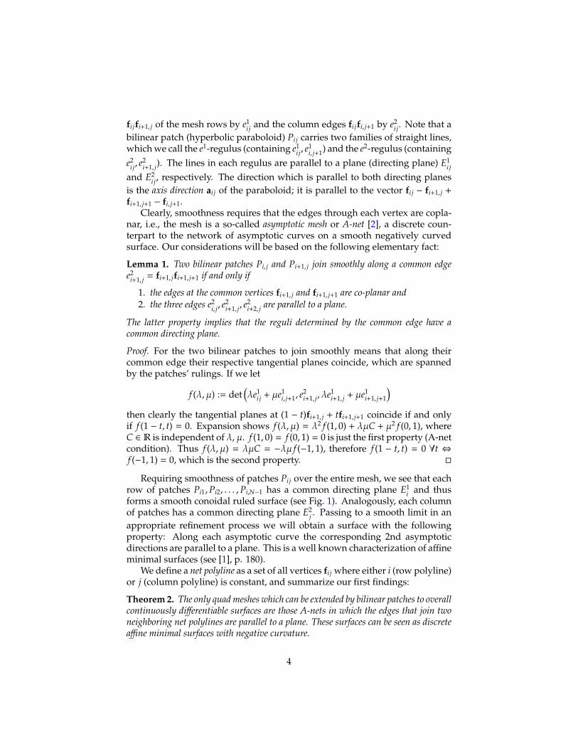
Requiring smoothness of patches Pi j over the entire mesh, we see that eachrow of patches Pi1,Pi2, . . . ,Pi,N−1 has a common directing plane E1

i and thusforms a smooth conoidal ruled surface (see Fig. 1). Analogously, each columnof patches has a common directing plane E2

j . Passing to a smooth limit in anappropriate refinement process we will obtain a surface with the followingproperty: Along each asymptotic curve the corresponding 2nd asymptoticdirections are parallel to a plane. This is a well known characterization of affineminimal surfaces (see [1], p. 180).

We define a net polyline as a set of all vertices fi j where either i (row polyline)or j (column polyline) is constant, and summarize our first findings:

Theorem 2. The only quad meshes which can be extended by bilinear patches to overallcontinuously differentiable surfaces are those A-nets in which the edges that join twoneighboring net polylines are parallel to a plane. These surfaces can be seen as discreteaffine minimal surfaces with negative curvature.

4

fi jfi jfi jfi jfi jfi jfi jfi jfi jfi jfi jfi jfi jfi jfi jfi jfi jfi jfi jfi jfi jfi jfi jfi jfi jfi jfi jfi jfi jfi jfi jfi jfi j

fi, j+1fi, j+1fi, j+1fi, j+1fi, j+1fi, j+1fi, j+1fi, j+1fi, j+1fi, j+1fi, j+1fi, j+1fi, j+1fi, j+1fi, j+1fi, j+1fi, j+1fi, j+1fi, j+1fi, j+1fi, j+1fi, j+1fi, j+1fi, j+1fi, j+1fi, j+1fi, j+1fi, j+1fi, j+1fi, j+1fi, j+1fi, j+1fi, j+1fi+1, jfi+1, jfi+1, jfi+1, jfi+1, jfi+1, jfi+1, jfi+1, jfi+1, jfi+1, jfi+1, jfi+1, jfi+1, jfi+1, jfi+1, jfi+1, jfi+1, jfi+1, jfi+1, jfi+1, jfi+1, jfi+1, jfi+1, jfi+1, jfi+1, jfi+1, jfi+1, jfi+1, jfi+1, jfi+1, jfi+1, jfi+1, jfi+1, j

fi+1, j+1fi+1, j+1fi+1, j+1fi+1, j+1fi+1, j+1fi+1, j+1fi+1, j+1fi+1, j+1fi+1, j+1fi+1, j+1fi+1, j+1fi+1, j+1fi+1, j+1fi+1, j+1fi+1, j+1fi+1, j+1fi+1, j+1fi+1, j+1fi+1, j+1fi+1, j+1fi+1, j+1fi+1, j+1fi+1, j+1fi+1, j+1fi+1, j+1fi+1, j+1fi+1, j+1fi+1, j+1fi+1, j+1fi+1, j+1fi+1, j+1fi+1, j+1fi+1, j+1

Pi jPi jPi jPi jPi jPi jPi jPi jPi jPi jPi jPi jPi jPi jPi jPi jPi jPi jPi jPi jPi jPi jPi jPi jPi jPi jPi jPi jPi jPi jPi jPi jPi j

(i) planar vertices (A-net)

E2jE2jE2jE2jE2jE2jE2jE2jE2jE2jE2jE2jE2jE2jE2jE2jE2jE2jE2jE2jE2jE2jE2jE2jE2jE2jE2jE2jE2jE2jE2jE2jE2j E1

iE1iE1iE1iE1iE1iE1iE1iE1iE1iE1iE1iE1iE1iE1iE1iE1iE1iE1iE1iE1iE1iE1iE1iE1iE1iE1iE1iE1iE1iE1iE1iE1i

ai jai jai jai jai jai jai jai jai jai jai jai jai jai jai jai jai jai jai jai jai jai jai jai jai jai jai jai jai jai jai jai jai j

fi jfi jfi jfi jfi jfi jfi jfi jfi jfi jfi jfi jfi jfi jfi jfi jfi jfi jfi jfi jfi jfi jfi jfi jfi jfi jfi jfi jfi jfi jfi jfi jfi j

fi, j+1fi, j+1fi, j+1fi, j+1fi, j+1fi, j+1fi, j+1fi, j+1fi, j+1fi, j+1fi, j+1fi, j+1fi, j+1fi, j+1fi, j+1fi, j+1fi, j+1fi, j+1fi, j+1fi, j+1fi, j+1fi, j+1fi, j+1fi, j+1fi, j+1fi, j+1fi, j+1fi, j+1fi, j+1fi, j+1fi, j+1fi, j+1fi, j+1fi+1, jfi+1, jfi+1, jfi+1, jfi+1, jfi+1, jfi+1, jfi+1, jfi+1, jfi+1, jfi+1, jfi+1, jfi+1, jfi+1, jfi+1, jfi+1, jfi+1, jfi+1, jfi+1, jfi+1, jfi+1, jfi+1, jfi+1, jfi+1, jfi+1, jfi+1, jfi+1, jfi+1, jfi+1, jfi+1, jfi+1, jfi+1, jfi+1, j

fi+1, j+1fi+1, j+1fi+1, j+1fi+1, j+1fi+1, j+1fi+1, j+1fi+1, j+1fi+1, j+1fi+1, j+1fi+1, j+1fi+1, j+1fi+1, j+1fi+1, j+1fi+1, j+1fi+1, j+1fi+1, j+1fi+1, j+1fi+1, j+1fi+1, j+1fi+1, j+1fi+1, j+1fi+1, j+1fi+1, j+1fi+1, j+1fi+1, j+1fi+1, j+1fi+1, j+1fi+1, j+1fi+1, j+1fi+1, j+1fi+1, j+1fi+1, j+1fi+1, j+1

(ii) conoidal strips

Figure 1: Characterization of a quad mesh which can be extended to a smoothsurface by filling its faces with bilinear patches: (i) All vertex stars have tobe planar. (ii) The edges joining any two neighboring net polygons have tobe parallel to a plane. Therefore, on the smoothly extended surface, the stripbetween two neighboring net polygons contains a continuous family of straightline segments all of which are parallel to that plane and thus the strip defines aconoidal ruled surface.

Our discrete affine minimal surfaces agree with the ones which Craizer et al.[6] derived recently. There, the surfaces are found by discretizing a well-knownconstruction of smooth affine minimal surfaces from translational surfaces aris-ing as co-normal fields. We will now continue the geometric considerationsbased on smoothly joined patches Pi j and arrive at this construction in a purelygeometric way.

Let us first consider a single bilinear patch P := Pi j, and for simplicity callits vertices v1 := fi j, v2 := fi, j+1, v3 := fi+1, j+1 and v4 := fi+1, j,. Each vertex has anormal with direction vector

ni = λ(vi − vi−1) × (vi+1 − vi), (1)

where indices are taken modulo 4. Vectors ni represent the vertices of a paral-lelogram NP, since opposite edges are parallel,

ni+1 − ni = λ(vi+1 − vi) × (vi+2 − vi−1) = ni+2 − ni−1. (2)

Moreover, (2) shows that each edge of NP is orthogonal to a pair of oppositeedges of P and thus it is orthogonal to a directing plane of P.

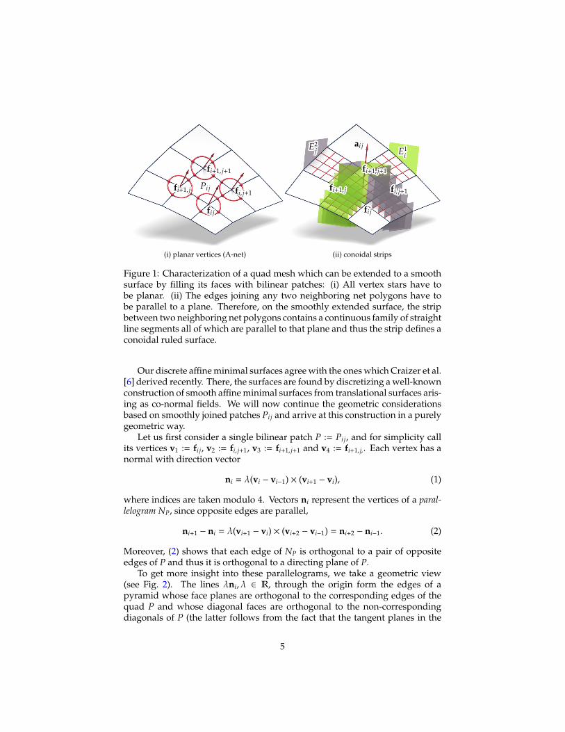
To get more insight into these parallelograms, we take a geometric view(see Fig. 2). The lines λni, λ ∈ R, through the origin form the edges of apyramid whose face planes are orthogonal to the corresponding edges of thequad P and whose diagonal faces are orthogonal to the non-correspondingdiagonals of P (the latter follows from the fact that the tangent planes in the

5

end points of one diagonal of P intersect in the other diagonal). One cantransfer these orthogonality relations into an arbitrarily chosen plane Π asfollows: We intersect the normal pyramid with Π, resulting in a quad N∗ =n∗1, . . . ,n

∗

4. Also, we project the quad P orthogonally onto Π, resulting in a quadP∗ = v∗1, . . . ,v

∗

4. Then, the resulting two quads have the following property:corresponding edges are orthogonal and non-corresponding diagonals are orthogonal.This reminds us of Christoffel dual quads where corresponding edges and non-corresponding diagonals are parallel (see[2], p. 48); we will therefore speakof Christoffel orthogonal quads or briefly C-orthogonal quads. The definition ofC-orthogonality is not restricted to planar quads. Obviously, also the quad Pitself is C-orthogonal to NP.

v1v1v1v1v1v1v1v1v1v1v1v1v1v1v1v1v1v1v1v1v1v1v1v1v1v1v1v1v1v1v1v1v1

v2v2v2v2v2v2v2v2v2v2v2v2v2v2v2v2v2v2v2v2v2v2v2v2v2v2v2v2v2v2v2v2v2

v3v3v3v3v3v3v3v3v3v3v3v3v3v3v3v3v3v3v3v3v3v3v3v3v3v3v3v3v3v3v3v3v3

v4v4v4v4v4v4v4v4v4v4v4v4v4v4v4v4v4v4v4v4v4v4v4v4v4v4v4v4v4v4v4v4v4

n1n1n1n1n1n1n1n1n1n1n1n1n1n1n1n1n1n1n1n1n1n1n1n1n1n1n1n1n1n1n1n1n1n2n2n2n2n2n2n2n2n2n2n2n2n2n2n2n2n2n2n2n2n2n2n2n2n2n2n2n2n2n2n2n2n2n3n3n3n3n3n3n3n3n3n3n3n3n3n3n3n3n3n3n3n3n3n3n3n3n3n3n3n3n3n3n3n3n3

n4n4n4n4n4n4n4n4n4n4n4n4n4n4n4n4n4n4n4n4n4n4n4n4n4n4n4n4n4n4n4n4n4

v∗1v∗1v∗1v∗1v∗1v∗1v∗1v∗1v∗1v∗1v∗1v∗1v∗1v∗1v∗1v∗1v∗1v∗1v∗1v∗1v∗1v∗1v∗1v∗1v∗1v∗1v∗1v∗1v∗1v∗1v∗1v∗1v∗1

v∗2v∗2v∗2v∗2v∗2v∗2v∗2v∗2v∗2v∗2v∗2v∗2v∗2v∗2v∗2v∗2v∗2v∗2v∗2v∗2v∗2v∗2v∗2v∗2v∗2v∗2v∗2v∗2v∗2v∗2v∗2v∗2v∗2

v∗3v∗3v∗3v∗3v∗3v∗3v∗3v∗3v∗3v∗3v∗3v∗3v∗3v∗3v∗3v∗3v∗3v∗3v∗3v∗3v∗3v∗3v∗3v∗3v∗3v∗3v∗3v∗3v∗3v∗3v∗3v∗3v∗3

v∗4v∗4v∗4v∗4v∗4v∗4v∗4v∗4v∗4v∗4v∗4v∗4v∗4v∗4v∗4v∗4v∗4v∗4v∗4v∗4v∗4v∗4v∗4v∗4v∗4v∗4v∗4v∗4v∗4v∗4v∗4v∗4v∗4

n∗1n∗1n∗1n∗1n∗1n∗1n∗1n∗1n∗1n∗1n∗1n∗1n∗1n∗1n∗1n∗1n∗1n∗1n∗1n∗1n∗1n∗1n∗1n∗1n∗1n∗1n∗1n∗1n∗1n∗1n∗1n∗1n∗1n∗2n∗2n∗2n∗2n∗2n∗2n∗2n∗2n∗2n∗2n∗2n∗2n∗2n∗2n∗2n∗2n∗2n∗2n∗2n∗2n∗2n∗2n∗2n∗2n∗2n∗2n∗2n∗2n∗2n∗2n∗2n∗2n∗2

n∗3n∗3n∗3n∗3n∗3n∗3n∗3n∗3n∗3n∗3n∗3n∗3n∗3n∗3n∗3n∗3n∗3n∗3n∗3n∗3n∗3n∗3n∗3n∗3n∗3n∗3n∗3n∗3n∗3n∗3n∗3n∗3n∗3

n∗4n∗4n∗4n∗4n∗4n∗4n∗4n∗4n∗4n∗4n∗4n∗4n∗4n∗4n∗4n∗4n∗4n∗4n∗4n∗4n∗4n∗4n∗4n∗4n∗4n∗4n∗4n∗4n∗4n∗4n∗4n∗4n∗4

PPPPPPPPPPPPPPPPPPPPPPPPPPPPPPPPP

P∗P∗P∗P∗P∗P∗P∗P∗P∗P∗P∗P∗P∗P∗P∗P∗P∗P∗P∗P∗P∗P∗P∗P∗P∗P∗P∗P∗P∗P∗P∗P∗P∗

ΠΠΠΠΠΠΠΠΠΠΠΠΠΠΠΠΠΠΠΠΠΠΠΠΠΠΠΠΠΠΠΠΠ

N∗N∗N∗N∗N∗N∗N∗N∗N∗N∗N∗N∗N∗N∗N∗N∗N∗N∗N∗N∗N∗N∗N∗N∗N∗N∗N∗N∗N∗N∗N∗N∗N∗

Figure 2: The normals vectors ni at the vertices vi of a bilinear patch P definea pyramid with vertex at the origin (left). The intersection N∗ with a plane Πand the orthogonal projection P∗ of P onto Π are Christoffel orthogonal quads:corresponding edges and non-corresponding diagonals are orthogonal.

Let us choose the plane Π orthogonal to the axis of P (i.e., orthogonal to thevector v1 + v3−v2−v4); this leads to two Christoffel-orthogonal parallelogramsP∗ and N∗. The edges of the projected quad P∗ are parallel to the directingplanes of P, those of N∗ are orthogonal to the directing planes. Hence, N∗ is theparallelogram NP from above.

If we now take two adjacent quads of an affine minimal net, we can choosethe slicing planes (the value λ per bilinear patch) so that the correspondingnormal parallelograms NP share a common edge: This edge is orthogonal to

6

the common directing plane of the two smoothly joined bilinear patches (cf.Lemma 1). Proceeding with this argument we find a translational net n of normalsassociated with the affine minimal net f. For completeness, we mention thatthe patch dependent scaling factor λ shall be taken as reciprocal value of theaffine surface area of the corresponding bilinear patch [6], i.e.,

λ = 1/√

det(f2 − f1, f3 − f1, f4 − f1). (3)

For our main purposes, namely the design of affine minimal nets f, we donot need these factors, since we take the reverse direction. Starting from atranslational net n with vertices

ni j = n1i + n2

j , (4)

we can directly compute the corresponding C-orthogonal net A from the or-thogonality relations (also known as discrete Lelieuvre equations),

fi+1, j − fi j = ni j × ni+1, j, fi, j+1 − fi j = ni, j+1 × ni j. (5)

The system of these equations is very easily seen to be integrable: The twoways for obtaining fi+1, j+1 from fi j (either via fi+1, j or fi, j+1), are the same,

fi+1, j+1 − fi, j = ni+1, j+1 × ni+1, j + ni j × ni+1, j = ni, j+1 × ni+1, j+1 + ni, j+1 × ni j,

which follows by insertion from (4) (see also [6]). Summarizing, we obtain thefollowing theorem by Craizer et al. [6], to which we have added the interpre-tation via C-orthogonality and provided a more geometric interpretation basedon smoothly joined bilinear patches:

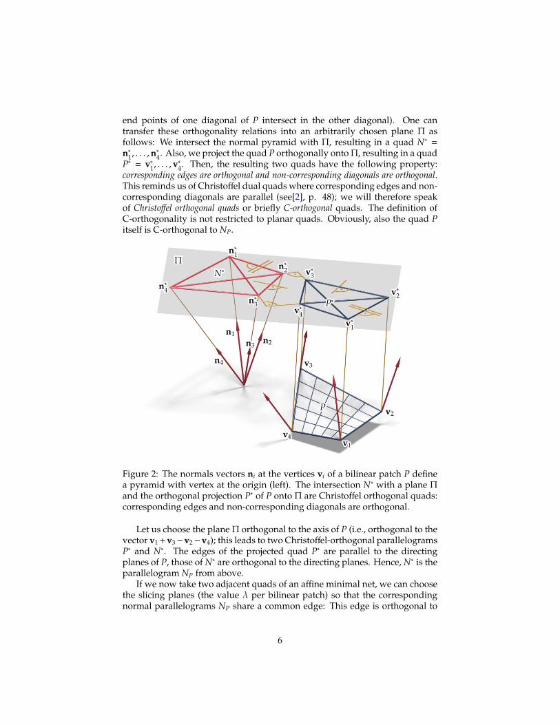
Theorem 3. Any smooth surface from bilinear patches (discrete affine minimal net f)can be constructed from a translational net n (4) that is star-shaped with respect to theorigin as a Christoffel orthogonal net with help of the Lelieuvre equations (5).

The reason why we require a star-shaped translational mesh is illustratedby Fig. 3. We point out that ni, j (defined through equations (1) and (3)) areEuclidean normal vectors at the vertices fi j of f, but they are not unit vectors.Sometimes called co-normals or Lelieuvre normals, they define a translationalnet whose projection onto the unit sphere (centered at the origin) gives thefamiliar discrete Gaussian image of f (see Fig. 7, left column).

As discussed above, the relation of C-orthogonality also holds between theorthogonal projection of the mesh f onto a plane Π and the planar section of thenormal image in Π. The latter arises as a central projection of the translationalmesh n from the origin onto Π. We may actually rotatate that section by a rightangle in Π and obtain a pair of Christoffel dual meshes:

Corollary 4. The orthogonal projection of a discrete affine minimal net f onto anyplane Π yields a mesh whose Christoffel dual mesh may be viewed as perspective imageof the translational net n associated with f according to Theorem (3).

7

origin = light source

nnnnnnnnnnnnnnnnnnnnnnnnnnnnnnnnn

fffffffffffffffffffffffffffffffff

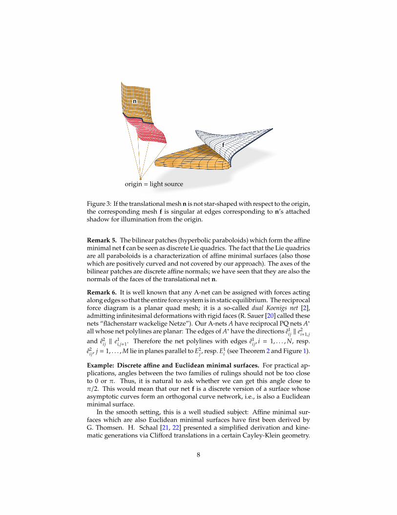
Figure 3: If the translational mesh n is not star-shaped with respect to the origin,the corresponding mesh f is singular at edges corresponding to n’s attachedshadow for illumination from the origin.

Remark 5. The bilinear patches (hyperbolic paraboloids) which form the affineminimal net f can be seen as discrete Lie quadrics. The fact that the Lie quadricsare all paraboloids is a characterization of affine minimal surfaces (also thosewhich are positively curved and not covered by our approach). The axes of thebilinear patches are discrete affine normals; we have seen that they are also thenormals of the faces of the translational net n.

Remark 6. It is well known that any A-net can be assigned with forces actingalong edges so that the entire force system is in static equilibrium. The reciprocalforce diagram is a planar quad mesh; it is a so-called dual Koenigs net [2],admitting infinitesimal deformations with rigid faces (R. Sauer [20] called thesenets “flachenstarr wackelige Netze”). Our A-nets A have reciprocal PQ nets A∗

all whose net polylines are planar: The edges of A∗ have the directions e1i j ‖ e2

i+1, j

and e2i j ‖ e1

i, j+1. Therefore the net polylines with edges e1i j, i = 1, . . . ,N, resp.

e2i j, j = 1, . . . ,M lie in planes parallel to E2

j , resp. E1i (see Theorem 2 and Figure 1).

Example: Discrete affine and Euclidean minimal surfaces. For practical ap-plications, angles between the two families of rulings should not be too closeto 0 or π. Thus, it is natural to ask whether we can get this angle close toπ/2. This would mean that our net f is a discrete version of a surface whoseasymptotic curves form an orthogonal curve network, i.e., is also a Euclideanminimal surface.

In the smooth setting, this is a well studied subject: Affine minimal sur-faces which are also Euclidean minimal surfaces have first been derived byG. Thomsen. H. Schaal [21, 22] presented a simplified derivation and kine-matic generations via Clifford translations in a certain Cayley-Klein geometry.

8

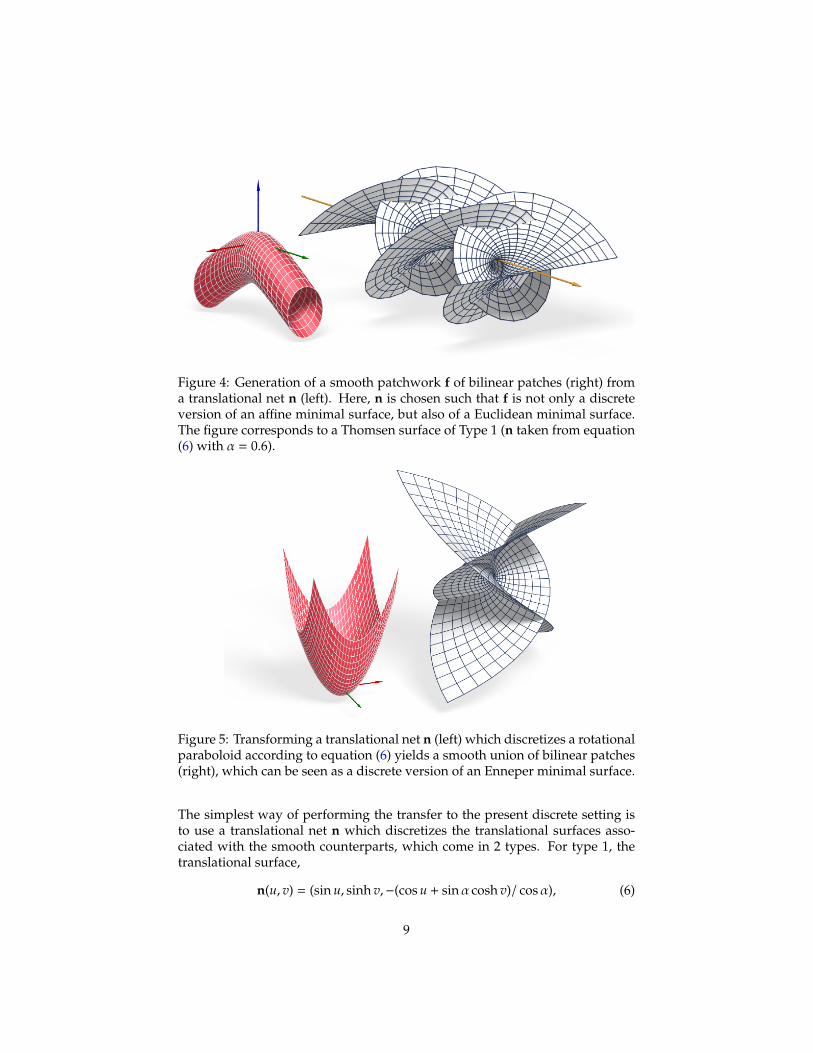
Figure 4: Generation of a smooth patchwork f of bilinear patches (right) froma translational net n (left). Here, n is chosen such that f is not only a discreteversion of an affine minimal surface, but also of a Euclidean minimal surface.The figure corresponds to a Thomsen surface of Type 1 (n taken from equation(6) with α = 0.6).

Figure 5: Transforming a translational net n (left) which discretizes a rotationalparaboloid according to equation (6) yields a smooth union of bilinear patches(right), which can be seen as a discrete version of an Enneper minimal surface.

The simplest way of performing the transfer to the present discrete setting isto use a translational net n which discretizes the translational surfaces asso-ciated with the smooth counterparts, which come in 2 types. For type 1, thetranslational surface,

n(u, v) = (sin u, sinh v,−(cos u + sinα cosh v)/ cosα), (6)

9

is generated by translating an ellipse along a branch of a hyperbola; α is aconstant, 0 < α < π/2. The surface is symmetric with respect to the planesx = 0 and y = 0, and the ellipse and hyperbola in these symmetry planespossess the origin as focal point. For type 2, n is a rotational paraboloid withthe origin as focal point generated by translating two parabolae along eachother,

n(u, v) = (u, v,u2 + v2−

14 ). (7)

Here, the corresponding minimal surface is the well-known Enneper surface.Discretization of these translational surfaces can be performed by evaluation

on an axis-aligned grid in the (u, v)-parameter plane. The translational nets nand the associated A-nets f derived from them according to Theorem 3 areshown in Figures 4 and 5, respectively.

3. Surface design and shape exploration

fffffffffffffffffffffffffffffffff

nnnnnnnnnnnnnnnnnnnnnnnnnnnnnnnnn

fffffffffffffffffffffffffffffffff

nnnnnnnnnnnnnnnnnnnnnnnnnnnnnnnnn

ooooooooooooooooooooooooooooooooo ooooooooooooooooooooooooooooooooo

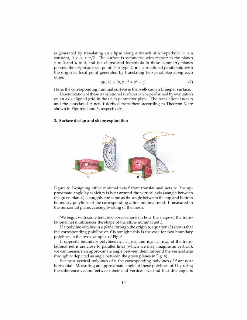
Figure 6: Designing affine minimal nets f from translational nets n: The ap-proximate angle by which n is bent around the vertical axis (=angle betweenthe green planes) is roughly the same as the angle between the top and bottomboundary polylines of the corresponding affine minimal mesh f measured inthe horizontal plane, causing twisting of the mesh.

We begin with some tentative observations on how the shape of the trans-lational net n influences the shape of the affine minimal net f.

If a polyline of n lies in a plane through the origin o, equation (5) shows thatthe corresponding polyline on f is straight; this is the case for two boundarypolylines in the two examples of Fig. 6.

If opposite boundary polylines n11, . . . ,n1N and nM1, . . . ,nMN of the trans-lational net n are close to parallel lines (which we may imagine as vertical),we can measure an approximate angle between them (around the vertical axisthrough o; depicted as angle between the green planes in Fig. 6).

For near vertical polylines of n the corresponding polylines of f are nearhorizontal. Measuring an approximate angle of those polylines of f by usingthe difference vectors between their end vertices, we find that this angle is

10

roughly the same as the one at the translational net. This rotation around thevertical axis from the bottom boundary to the top boundary polyline causes atwisting of f (see Fig. 6).

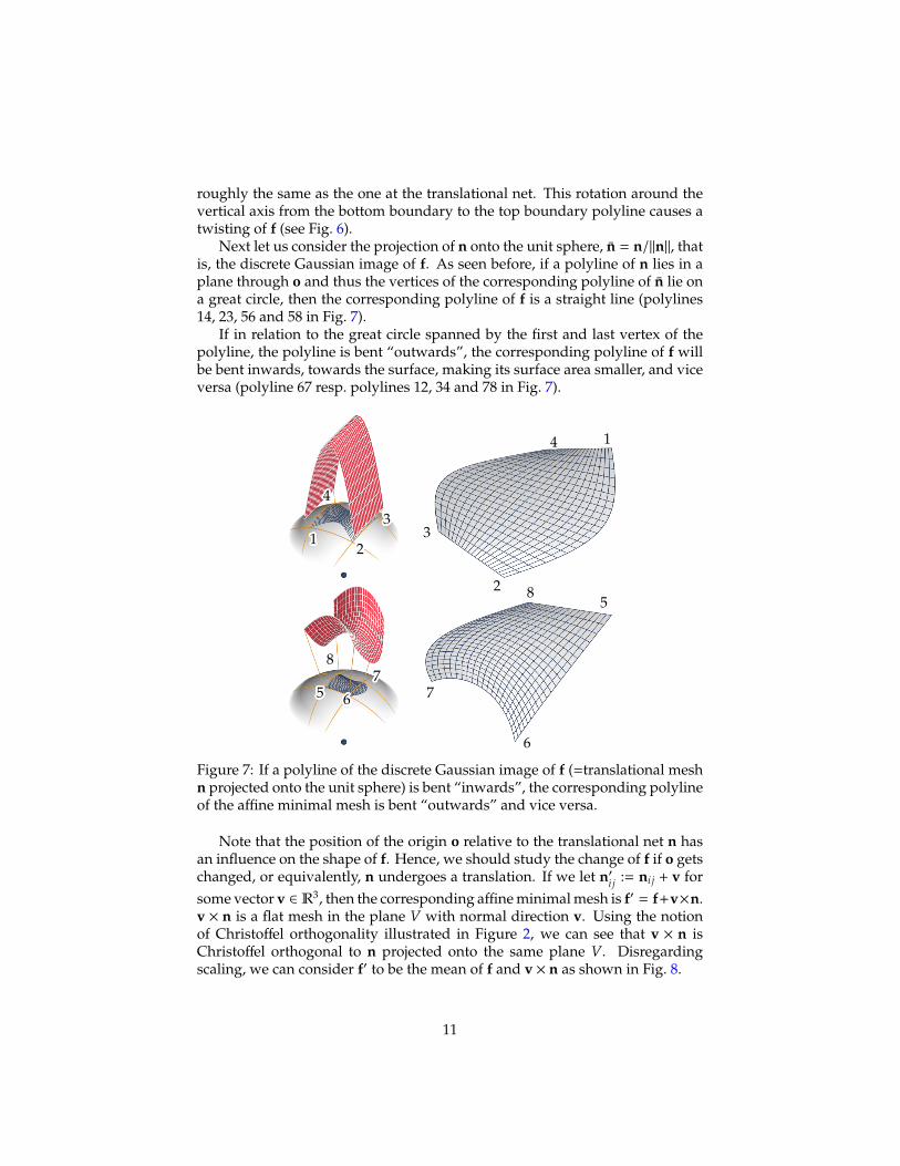
Next let us consider the projection of n onto the unit sphere, n = n/‖n‖, thatis, the discrete Gaussian image of f. As seen before, if a polyline of n lies in aplane through o and thus the vertices of the corresponding polyline of n lie ona great circle, then the corresponding polyline of f is a straight line (polylines14, 23, 56 and 58 in Fig. 7).

If in relation to the great circle spanned by the first and last vertex of thepolyline, the polyline is bent “outwards”, the corresponding polyline of f willbe bent inwards, towards the surface, making its surface area smaller, and viceversa (polyline 67 resp. polylines 12, 34 and 78 in Fig. 7).

111111111111111111111111111111111 222222222222222222222222222222222

333333333333333333333333333333333

444444444444444444444444444444444

111111111111111111111111111111111

222222222222222222222222222222222

333333333333333333333333333333333

444444444444444444444444444444444

555555555555555555555555555555555 666666666666666666666666666666666

777777777777777777777777777777777888888888888888888888888888888888

555555555555555555555555555555555

666666666666666666666666666666666

777777777777777777777777777777777

888888888888888888888888888888888

Figure 7: If a polyline of the discrete Gaussian image of f (=translational meshn projected onto the unit sphere) is bent “inwards”, the corresponding polylineof the affine minimal mesh is bent “outwards” and vice versa.

Note that the position of the origin o relative to the translational net n hasan influence on the shape of f. Hence, we should study the change of f if o getschanged, or equivalently, n undergoes a translation. If we let n′i j := ni j + v forsome vector v ∈ R3, then the corresponding affine minimal mesh is f′ = f+v×n.v × n is a flat mesh in the plane V with normal direction v. Using the notionof Christoffel orthogonality illustrated in Figure 2, we can see that v × n isChristoffel orthogonal to n projected onto the same plane V. Disregardingscaling, we can consider f′ to be the mean of f and v × n as shown in Fig. 8.

11

nnnnnnnnnnnnnnnnnnnnnnnnnnnnnnnnn

n′n′n′n′n′n′n′n′n′n′n′n′n′n′n′n′n′n′n′n′n′n′n′n′n′n′n′n′n′n′n′n′n′

fffffffffffffffffffffffffffffffff

f′f′f′f′f′f′f′f′f′f′f′f′f′f′f′f′f′f′f′f′f′f′f′f′f′f′f′f′f′f′f′f′f′

v × nv × nv × nv × nv × nv × nv × nv × nv × nv × nv × nv × nv × nv × nv × nv × nv × nv × nv × nv × nv × nv × nv × nv × nv × nv × nv × nv × nv × nv × nv × nv × nv × n

vvvvvvvvvvvvvvvvvvvvvvvvvvvvvvvvv

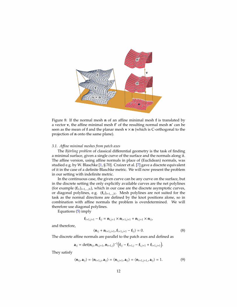
Figure 8: If the normal mesh n of an affine minimal mesh f is translated bya vector v, the affine minimal mesh f′ of the resulting normal mesh n′ can beseen as the mean of f and the planar mesh v × n (which is C-orthogonal to theprojection of n onto the same plane).

3.1. Affine minimal meshes from patch axesThe Bjorling problem of classical differential geometry is the task of finding

a minimal surface, given a single curve of the surface and the normals along it.The affine version, using affine normals in place of (Euclidean) normals, wasstudied e.g. by W. Blaschke [1, § 70]. Craizer et al. [7] gave a discrete equivalentof it in the case of a definite Blaschke metric. We will now present the problemin our setting with indefinite metric.

In the continuous case, the given curve can be any curve on the surface, butin the discrete setting the only explicitly available curves are the net polylines(for example (fi1)i=1,...,N), which in our case are the discrete asymptotic curves,or diagonal polylines, e.g. (fii)i=1,...,N. Mesh polylines are not suited for thetask as the normal directions are defined by the knot positions alone, so incombination with affine normals the problem is overdetermined. We willtherefore use diagonal polylines.

Equations (5) imply

fi+1, j+1 − fi j = ni, j+1 × ni+1, j+1 + ni, j+1 × ni j,

and therefore,〈ni j + ni+1, j+1, fi+1, j+1 − fi j〉 = 0. (8)

The discrete affine normals are parallel to the patch axes and defined as

ai j = det(ni j,ni, j+1,ni+1, j)−1(fi j − fi+1, j − fi, j+1 + fi+1, j+1

).

They satisfy

〈ni j, ai j〉 = 〈ni+1, j, ai j〉 = 〈ni, j+1, ai j〉 = 〈ni+1, j+1,, ai j〉 = 1. (9)

12

This together with (8) gives us three equations for ni+1, j+1,(ai j, ai+1, j+1 − ai j, fi+1, j+1 − fi j

)· ni+1, j+1 = (1, 0,−〈ni j, fi+1, j+1 − fi j〉)T, (10)

which have a unique solution provided that

det(ai j, ai+1, j+1 − ai j, fi+1, j+1 − fi j

), 0. (11)

This is the same assumption as is made in the continuous case [1, § 70, eq. (55)].

Theorem 7. Suppose nets f and a are given along the diagonal, that is, fii and aii areknown. Suppose further that the regularity condition (11) is satisfied.

Then there is a three-parameter family of affine minimal meshes f, normal meshesn and face axes a. These affine minimal meshes can be constructed by first calculatingthe normals along the diagonal nii by solving the systems of linear equations (10), thenthe off-center diagonals by

ni+1,i := 12

(nii + ni+1,i+1 − aii × (fi+1,i+1 − fii)

), (12)

and then all the others by ni j + ni+1, j+1 − ni+1, j − ni, j+1 = 0.Finally the mesh f is constructed from the mesh n by the Lelieuvre equations (5).

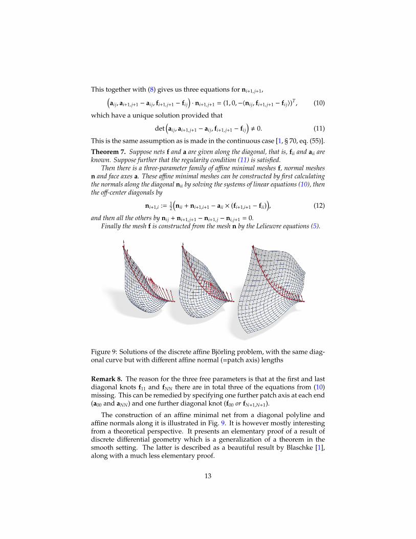
Figure 9: Solutions of the discrete affine Bjorling problem, with the same diag-onal curve but with different affine normal (=patch axis) lengths

Remark 8. The reason for the three free parameters is that at the first and lastdiagonal knots f11 and fNN there are in total three of the equations from (10)missing. This can be remedied by specifying one further patch axis at each end(a00 and aNN) and one further diagonal knot (f00 or fN+1,N+1).

The construction of an affine minimal net from a diagonal polyline andaffine normals along it is illustrated in Fig. 9. It is however mostly interestingfrom a theoretical perspective. It presents an elementary proof of a result ofdiscrete differential geometry which is a generalization of a theorem in thesmooth setting. The latter is described as a beautiful result by Blaschke [1],along with a much less elementary proof.

13

3.2. Affine minimal meshes from diagonal strips

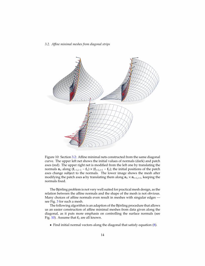
Figure 10: Section 3.2: Affine minimal nets constructed from the same diagonalcurve. The upper left net shows the initial values of normals (dark) and patchaxes (red). The upper right net is modified from the left one by translating thenormals nii along (fi−1,i−1 − fii) × (fi+1,i+1 − fii); the initial positions of the patchaxes change subject to the normals. The lower image shows the mesh aftermodifying the patch axes a by translating them along nii × ni+1,i+1, keeping thenormals fixed.

The Bjorling problem is not very well suited for practical mesh design, as therelation between the affine normals and the shape of the mesh is not obvious.Many choices of affine normals even result in meshes with singular edges —see Fig. 3 for such a mesh.

The following algorithm is an adaption of the Bjorling procedure that allowsus an easier construction of affine minimal meshes from data given along thediagonal, as it puts more emphasis on controlling the surface normals (seeFig. 10). Assume that fii are all known.

• Find initial normal vectors along the diagonal that satisfy equation (8).

14

• Design the normal directions along the diagonal by translating the niialong (fi−1,i−1 − fii) × (fi+1,i+1 − fii). This keeps (8) valid.

• After that, initial patch axes aii are calculated by

aii :=nii〈ni+1,i+1 − nii,ni+1,i+1〉 − ni+1,i+1〈ni+1,i+1 − nii,nii〉

‖nii‖2‖ni+1,i+1‖

2 − 〈nii,ni+1,i+1〉2 .

This makes sure that equation (9) holds, that is 〈aii,nii〉 = 〈aii,ni+1,i+1〉 = 1.

• Design the affine normal directions by translating them along nii×ni+1,i+1,keeping the conditions above.

• Construct the rest of the mesh according to the Bjorling procedure (sec-tion 3.1).

3.3. Affine minimal meshes from zigzag polygonsThere is another method of constructing affine minimal meshes from diag-

onal data using a zigzag polygon.Assume that f11, f12, f22, f23, . . . , fN−1,N, fNN are known. The normal directions

at these knots can easily be calculated, as there are two known edges emanatingfrom each knot, except for the first and last knot. There the missing second edgescan be defined for example by specifying one further knot beyond each end,namely f01 and fN,N+1.

A knot fi+1,i lies in the knot planes of both fii and fi+1,i+1. It can be freelychosen anywhere on those planes’ intersection line. Once one such knot isfixed, all the others follow uniquely by imposing the properties of an affineminimal mesh, A-net and conoidal strips, see Theorem 2.

Let us summarize these facts:

Theorem 9. Let f11, f12, f22, f23, . . . , fN−1,N, fNN be a polygon in R3 together withnormal directions at the first and last vertex n11 ⊥ f12 − f11 and nNN ⊥ fN−1,N − fNN.Then there is a one-parameter family of affine minimal meshes f that extends the givenpolygon and has the given normal directions at the corners (1, 1) and (N,N).

Remark 10. A suitable zigzag polygon can be constructed by a continuouscurve c : R→ R3 and a fixed vector v ∈ R3 as

fii := c(i) + v and fi,i+1 := c(i + 12 ) − v.

It is also important to note that the torsions of column and row polygons havedifferent signs. The given zigzag polygon has to reflect that fact. For example,if the curve c is planar (as in Fig. 11) this means it cannot have inflection points.

15

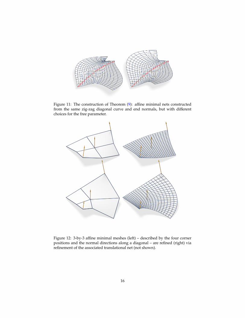
Figure 11: The construction of Theorem (9): affine minimal nets constructedfrom the same zig-zag diagonal curve and end normals, but with differentchoices for the free parameter.

Figure 12: 3-by-3 affine minimal meshes (left) – described by the four cornerpositions and the normal directions along a diagonal – are refined (right) viarefinement of the associated translational net (not shown).

16

3.4. Affine minimal meshes by refinementArchitectural designs often do not exhibit shape variations on a fine scale.

Hence it is feasible and good practice to design the shape on a coarser scaleand then compute the final shape via refinement, of course ensuring that theconstraints are also met after refinement. This approach has been successfullydemonstrated for planar quad meshes (see e.g. [13, 16]) and can also be adaptedto the current setting. We just present a simple version in order to demonstratethe basic principle.

An affine minimal mesh with 3-by-3 vertices has 18 degrees of freedom,which can be specified in a variety of ways. We can for example prescribe thepositions of the four corners (f11, f31, f13f33) and the directions of the normalsalong a diagonal (the directions of n11, n22 and n33).

This very simple affine minimal mesh can now be refined by refining theassociated translational net n, which is an easy task: One simply refines itsgenerating net polylines ni1 and n1 j, by any curve refinement method (e.g.interpolatory subdivision).

The resulting refined affine minimal surface fr will satisfy the given normaldirections but not the corner positions. If those are of higher importance, themesh can be affinely transformed to match the corners (as in Fig. 12), but thiswill cause slight deviations in the normal directions.

Remark 11. In essence, affine minimal nets are special types of constrainedmeshes. Therefore, designing, editing and exploring the shapes of affine mini-mal nets can also be based on the constrained mesh exploration framework ofYang et al. [28].

4. Smoothly joined bilinear patches with parallel axes

Let us now study those affine-minimal nets all whose bilinar patches possessthe same axis direction. We imagine this direction to be vertical, parallel to thez-axis of a Cartesian system. This special case is motivated by a practical per-spective because of the superior statics properties of hyperboloic paraboloidswith vertical axis. We aim here at some simple insights for the design of thesesurfaces and at an understanding of their quite interesting geometry. Thestructural analysis of the overall smooth surface is left for future work.

Let us start with some remarks on prior work and the theory. Since theparaboloid axes are discrete affine normals, our surfaces are discrete improperaffine spheres and have been studied as such by Matsuura and Urakawa [14].However, these authors as well as Craizer et al. [6] did not pursue our approach,namely looking at these surfaces from the perspective of isotropic geometry.Defining the z-direction as isotropic direction in an isotropic space, the surfacesappear as isotropic counterparts to the discrete surfaces of constant Gaussiancurvature of Sauer [19] and Wunderlich [27]. They are discrete versions ofsmooth surfaces studied already by Darboux and later by Strubecker [25], whofirst realized the advantages of using isotropic geometry. We will refrain from

17

a detailed study, but we want to sketch the main results and demonstrate howeasily they follow from our geometric framework.

4.1. Construction from planar translational nets

mmmmmmmmmmmmmmmmmmmmmmmmmmmmmmmmm

mmmmmmmmmmmmmmmmmmmmmmmmmmmmmmmmm

mmmmmmmmmmmmmmmmmmmmmmmmmmmmmmmmm

mmmmmmmmmmmmmmmmmmmmmmmmmmmmmmmmm

fffffffffffffffffffffffffffffffff

f′

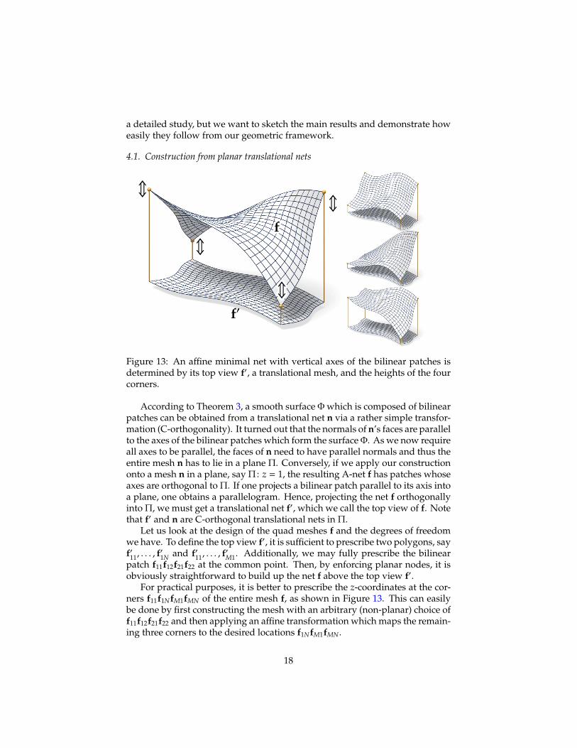
Figure 13: An affine minimal net with vertical axes of the bilinear patches isdetermined by its top view f′, a translational mesh, and the heights of the fourcorners.

According to Theorem 3, a smooth surface Φ which is composed of bilinearpatches can be obtained from a translational net n via a rather simple transfor-mation (C-orthogonality). It turned out that the normals of n’s faces are parallelto the axes of the bilinear patches which form the surface Φ. As we now requireall axes to be parallel, the faces of n need to have parallel normals and thus theentire mesh n has to lie in a plane Π. Conversely, if we apply our constructiononto a mesh n in a plane, say Π : z = 1, the resulting A-net f has patches whoseaxes are orthogonal to Π. If one projects a bilinear patch parallel to its axis intoa plane, one obtains a parallelogram. Hence, projecting the net f orthogonallyinto Π, we must get a translational net f′, which we call the top view of f. Notethat f′ and n are C-orthogonal translational nets in Π.

Let us look at the design of the quad meshes f and the degrees of freedomwe have. To define the top view f′, it is sufficient to prescribe two polygons, sayf′11, . . . , f

′

1N and f′11, . . . , f′

M1. Additionally, we may fully prescribe the bilinearpatch f11f12f21f22 at the common point. Then, by enforcing planar nodes, it isobviously straightforward to build up the net f above the top view f′.

For practical purposes, it is better to prescribe the z-coordinates at the cor-ners f11f1NfM1fMN of the entire mesh f, as shown in Figure 13. This can easilybe done by first constructing the mesh with an arbitrary (non-planar) choice off11f12f21f22 and then applying an affine transformation which maps the remain-ing three corners to the desired locations f1NfM1fMN.

18

4.2. Some basics of isotropic geometryThe geometry of the nets f becomes interesting if we employ isotropic geom-

etry, which has been systematically developed by Strubecker [25, 23, 24] in the1940s (see also the mongraph by Sachs [18]). It is based on the following groupG6 of affine transformations (x, y, z) 7→ (x′, y′, z′) in R3,

x′ = a + x cosφ − y sinφ,y′ = b + x sinφ + y cosφ, (13)z′ = c + c1x + c2y + z,

called isotropic congruence transformations (i-motions). Obviously, motions inisotropic space I3 appear as Euclidean motions in the top view.

The 5-parameter subgroup of those i-motions which appear as translationsin the top view (φ = 0) can be represented as commutative product of two3-parameter groups of so-called Clifford translations,

x′ = a + x,y′ = b + y, (14)z′ = c + εbx − εay + z, ε = ±1;

one speaks of right translations for ε = 1 and left translations for ε = −1.Many metric properties in isotropic 3-space I3 (invariants under G6) are

Euclidean invariants in the top view. For example, the i-distance of two pointsx j = (x j, y j, z j), j = 1, 2, is defined as Euclidean distance of their top views x′j,

‖x1 − x2‖i :=√

(x1 − x2)2 + (y1 − y2)2. (15)

Two points (x, y, z j) with the same top view are called parallel points; they havei-distance zero, but they need not agree. Since the i-metric (15) degeneratesalong z-parallel lines, these are called isotropic lines. Isotropic angles betweenstraight lines are measured as Euclidean angles in the top view.

Isotropic geometry enjoys a metric duality. It may be realized by the polaritywith respect to the isotropic unit sphere Σ : 2z = x2 + y2, which maps the pointp = (p1, p2, p3) to the plane

P : z = p1x + p2y − p3. (16)

Points p and q = (q1, q2, q3) with i-distance d (from (15)) are mapped to planesP and Q : z = q1x + q2y − q3. The i-angle σ of the two planes P,Q, defined asσ2 = (p1 − q1)2 + (p2 − q2)2, equals the point distance d.

Curvature theory of surfaces: A surface Φ without isotropic (z-parallel) tangentplanes can be written in explicit form, Φ : z = f (x, y). Defining an isotropicGauss map from Φ to the isotropic unit sphere Σ via parallel tangent planes,one finds that the derivative of this map (isotropic Weingarten map) is describedby the Hessian ∇2 f of f . Its eigenvalues are called i-principal curvatures. The

19

corresponding orthogonal directions r1, r2 are the eigenvectors of ∇2 f . With thei-principal curvatures κ1, κ2 one defines isotropic curvature (or relative curvature)

K = κ1κ2 = det(∇2 f ) = fxx fyy − f 2xy, (17)

and isotropic mean curvature H,

2H = κ1 + κ2 = trace(∇2 f ) = fxx + fyy = ∆ f . (18)

4.3. Viewing smoothly joined bilinear patches with parallel axes as surfaces in isotropicspace

Let us consider the constant axis direction of the bilinear patches in ourspecial A-nets f as isotropic direction in isotropic space. Simple properties ofthese patches in isotropic geometry, along with the fact that they are smoothlyjoined, will allow us to derive remarkable geometric properties of the nets f.These appear as discrete counterparts to known results in the smooth case.

A bilinear patch f1, . . . , f4 whose top view is a parallelegram may be called askew parallelogram (isogram) in isotropic geometry. Opposite edges have thesame isotropic length, say s1 and s2, respectively. The tangent planes at the endpoints of opposite edges form the same isotropic angle (due to the isotropicaxial symmetry of the patch with respect to the istropic line which joins thecenters of the patch digonals). Let σi, i = 1, 2, be the isotropic angle formed bythe tangent planes at the end points of an edge of length si. A simple elementarycalculation then shows that

σ1 : s1 = −σ2 : s2 =: τ. (19)

Since neighboring patches share tangent planes, the ratio σi : si is constant alongeach row or column polygon in the net; it is τ for one family and −τ for theother. Obviously, the ratio σi : si is a suitable definition of discrete isotropic torsionof a polygon, and thus we can state that the A-nets under consideration possesstwo families of discrete asymptotic curves with constant isotropic torsion ±τ. Clearlythe nets are isotropic Chebyshev nets and, for example with arguments as givenby Wunderlich [27] in the Euclidean case, one finds that the nets are discretecounterparts of surfaces with constant isotropic relative curvature K = −τ2 = const.

To see that the A-nets are also Clifford translational surfaces, we just needto have a look at a single patch Pi j. It is a Clifford surface in isotropic geometryand hence, there is a Clifford translation which maps two opposite boundariesonto each other, say (fi j, fi, j+1) 7→ (fi+1, j, fi+1, j+1). It can be extended to a one-parameter group which maps the entire surface defined by the patch in itself.As an isotropic motion, it keeps isotropic angles and distances. Thus, it alsomaps the patch Pi, j+1 which joins Pi, j smoothly along the edge (fi, j+1, fi+1, j+1)in itself. Continuing in this way, we see that the entire polygon fi,1, . . . , fi,N ismapped to the next polygon fi+1,1, . . . , fi+1,N. This proves the following result,extending the main result of Strubecker [25] to the discrete case:

20

Theorem 12. Affine minimal nets formed by bilinear patches whose axes are parallelpossess remarkable geometric properties if the axis direction is seen as isotropic directionin isotropic 3-space: The nets are discrete surfaces of constant relative curvatureK = −τ2 and may be generated as Clifford translational nets whose generating polygonshave constant isotropic torsion ±τ; each of these polygons lies in a linear line complex.

The latter statement follows easily from the fact that a linear line complexwith isotropic axis has the following property: Two points on a straight lineof the complex, apart at a distance s, have null planes whose angle σ is p · s, pbeing the parameter of the complex. Obviously, polygons whose edges lie insuch complexes are exactly those which possess constant isotropic torsion (forthe smooth limit case, see [25]; for the geometry of linear line complexes, seee.g. [15]).

These considerations also reveal the shape limitations of the A-nets f underconsideration. We see that the net polylines within the same family have verysimilar shape, as they are related by special affine maps (isotropic Cliffordtranslations).

Conclusion and future workMotivated by applications in architecture, we have shown that gluing bi-

linear patches together in a smooth way leads to interesting discrete versionsof affine minimal surfaces which share a lot of essential properties with theirclassical counterparts. We have addressed the design of these patchworks andalso contributed new results to discrete affine minimal surfaces.

A natural path for future work is to use slightly more general patchesthan just bilinear ones for forming smooth surfaces, but keeping in mind thesimple contructability of the patches in view of architectural applications. Inparticular, we plan to address the global optimization and shape design ofpatchworks from rational bilinear patches (introduced by Huhnen-Venedeyand Rorig [12]). Moreover, one should couple fabrication-aware shape designwith other important issues such as structural considerations. For example, wehad motivated section 4 with structural properties of the individual panels, butdid not yet care about the structural properties of the entire surface. This needsfurther study.

AcknowledgmentsThis research was supported by grants No. 23735-N13 and I 706-N26 (SFB/

Transregio Geometry and Discretization) of the Austrian Science Fund (FWF).We thank Johannes Wallner for sharing with us his insights and for excellentcomments on earlier versions of this paper.

References

[1] W. Blaschke, Vorlesungen uber Differentialgeometrie, Vol. 2, Springer,1923.

21

[2] A. I. Bobenko, Yu. Suris, Discrete differential geometry: Integrable Struc-ture, American Math. Soc., 2008.

[3] A. I. Bobenko, H. Pottmann, J. Wallner, A curvature theory for discretesurfaces based on mesh parallelity, Math. Annalen 348 (2010) 1–24.

[4] A. I. Bobenko, E. Huhnen-Venedey, Curvature line parametrized surfacesand orthogonal coordinate systems. Discretization with Dupin cyclides,Geom. Dedicata To appear.

[5] P. Bo, H. Pottmann, M. Kilian, W. Wang, J. Wallner, Circular arc structures,ACM Trans. Graphics 30 (2011) #101,1–11, proc. SIGGRAPH.

[6] M. Craizer, H. Anciaux, T. Lewiner, Discrete affine minimal surfaces withindefinite metric, Differential Geometry and its Applications 28 (2010)158–169.

[7] M. Craizer, T. Lewiner, R. Teixeira, Cauchy Problems for Discrete AffineMinimal Surfaces, Archivum Mathematicum, 48(1), p.1-14, 2012.

[8] M. Eigensatz, M. Kilian, A. Schiftner, N. Mitra, H. Pottmann, M. Pauly, Pan-eling architectural freeform surfaces, ACM Trans. Graphics 29 (4) (2010)#45,1–10, proc. SIGGRAPH.

[9] S. Flory, Constrained matching of point clouds and surfaces, Ph.D. thesis,Vienna University of Technology (2010).

[10] S. Flory, H. Pottmann, Ruled surfaces for rationalization and design inarchitecture, Proc. ACADIA (2010) 103–109.

[11] S. Flory, Y. Nagai, F. Isvoranu, H. Pottmann, J. Wallner, Ruled free forms, in:L. Hesselgren, S. Sharma, J. Wallner, N. Baldassini, P. Bompas, J. Raynaud(Eds.), Advances in Architectural Geometry, Springer, 2012, pp. 57–66.

[12] E. Huhnen-Venedey, T. Rorig, Discretization of asymptotic line parametri-zations using hyperboloid surface patches, arXiv preprint 1112.3508 (2011).

[13] Y. Liu, H. Pottmann, J. Wallner, Y.-L. Yang, W. Wang, Geometric modelingwith conical meshes and developable surfaces, ACM Trans. Graphics 25 (3)(2006) 681–689.

[14] N. Matsuura, H. Urakawa, Discrete improper affine spheres, J. Geometryand Physics 45 (2003) 164–183.

[15] H. Pottmann, J. Wallner, Computational Line Geometry, Springer, 2001.

[16] H. Pottmann, Y. Liu, J. Wallner, A. Bobenko, W. Wang, Geometry of multi-layer freeform structures for architecture, ACM Trans. Graphics 26 (3)(2007) #65,1–11.

22

[17] H. Pottmann, A. Schiftner, P. Bo, H. Schmiedhofer, W. Wang, N. Bal-dassini, J. Wallner, Freeform surfaces from single curved panels, ACMTrans. Graphics 27 (3) (2008) #76, 1–10, proc. SIGGRAPH.

[18] H. Sachs, Isotrope Geometrie des Raumes, Vieweg, 1990.

[19] R. Sauer, Parallelogrammgitter als Modelle pseudospharischer Flachen,Math. Z. 52 (1950) 611–622.

[20] R. Sauer, Differenzengeometrie, Springer, 1970.

[21] H. Schaal, Die Affinminimalflachen von G. Thomsen, Arch. Math. 24 (1973)208–217.

[22] H. Schaal, Neue Erzeugungen der Minimalflachen von G. Thomsen,Monaths. Math. 77 (1973) 433–461.

[23] K. Strubecker, Differentialgeometrie des isotropen Raumes I: Theorie derRaumkurven, Sitzungsber. Akad. Wiss. Wien, Abt. IIa 150 (1941) 1–53.

[24] K. Strubecker, Differentialgeometrie des isotropen Raumes III: Flachen-theorie, Math. Zeitschrift 48 (1942) 369–427.

[25] K. Strubecker, Differentialgeometrie des isotropen Raumes II: Die Flachenkonstanter Relativkrummung K = rt − s2, Math. Zeitschrift 47 (1942) 743–777.

[26] J. Wallner, On the semidiscrete differential geometry of A-surfaces andK-surfaces, J. Geometry 103 (2012) 161–176.

[27] W. Wunderlich, Zur Differenzengeometrie der Flachen konstanter negati-ver Krummung, Sitz. Ost. Ak. Wiss 160 (1951) 41–77.

[28] Y. Yang, Y. Yang, H. Pottmann, N. Mitra, Shape space exploration of con-strained meshes, ACM Trans. Graphics 30, proc. SIGGRAPH Asia.

23