
Rivista di statistica ufficiale 2-3-2008 · biregionale macro/mesoeconomico Renato Paniccià,...
87
rivista di statistica ufficiale rivista di statistica ufficiale Istituto nazionale di Statistica n.2-3 2008 Temi trattati File Concatenation of Survey Data: a Computer Intensiven Approach to Sampling Weights Estimation Marco Ballin, Marco Di Zio, Marcello D’Orazio, Mauro Scanu, Nicola Torelli Monthly Income As a Core Social Variable: Evidence From the Italian EU SILC Survey Marco Di Marco The integration of the non-profit sector in a Social Accounting Matrix: methodological issues, empirical evidences and employment effects for Italy Giovanni Cerulli L’impatto delle politiche fiscali attraverso l’integrazione fra un modello di microsimulazione ed un modello biregionale macro/mesoeconomico Renato Paniccià, Nicola Sciclone
Transcript of Rivista di statistica ufficiale 2-3-2008 · biregionale macro/mesoeconomico Renato Paniccià,...
rivista
di statistica
ufficiale
riv
ista
di s
tatis
tica u
ffic
iale
Istituto nazionale
di Statistica
n.2-3 - 2008
n.2-32008La Rivista di Statistica Ufficiale accoglie lavori che hanno come
oggetto la misurazione e la comprensione dei fenomeni sociali,demografici, economici ed ambientali, la costruzione di sistemiinformativi e di indicatori come supporto per le decisionipubbliche e private, nonché le questioni di natura metodologica,tecnologica e istituzionale connesse ai processi di produzione delleinformazioni statistiche e rilevanti ai fini del perseguimento dei finidella statistica ufficiale.La Rivista di Statistica Ufficiale si propone di promuovere lacollaborazione tra il mondo della ricerca scientifica, gli utilizzatoridell’informazione statistica e la statistica ufficiale, al fine dimigliorare la qualità e l’analisi dei dati.La pubblicazione nasce nel 1992 come collana di monografie“Quaderni di Ricerca ISTAT”. Nel 1999 la collana viene affidata adun editore esterno e diviene quadrimestrale con la denominazione“Quaderni di Ricerca - Rivista di Statistica Ufficiale”. L’attualedenominazione, “Rivista di Statistica Ufficiale”, viene assunta apartire dal n. 1/2006 e l’Istat torna ad essere editore in proprio dellapubblicazione.
1B012009001000000
€ 10,00ISSN 1828-1982
Temi trattati
File Concatenation of Survey Data: a ComputerIntensiven Approach to Sampling Weights EstimationMarco Ballin, Marco Di Zio, Marcello D’Orazio,Mauro Scanu, Nicola Torelli
Monthly Income As a Core Social Variable:Evidence From the Italian EU SILC SurveyMarco Di Marco
The integration of the non-profit sector in a SocialAccounting Matrix: methodological issues, empiricalevidences and employment effects for ItalyGiovanni Cerulli
L’impatto delle politiche fiscali attraverso l’integrazionefra un modello di microsimulazione ed un modellobiregionale macro/mesoeconomicoRenato Paniccià, Nicola Sciclone

n.2-32008
Temi trattati
File Concatenation of Survey Data: a ComputerIntensiven Approach to Sampling Weights EstimationMarco Ballin, Marco Di Zio, Marcello D’Orazio,Mauro Scanu, Nicola Torelli
Monthly Income As a Core Social Variable:Evidence From the Italian EU SILC SurveyMarco Di Marco
The integration of the non-profit sector in a SocialAccounting Matrix: methodological issues, empiricalevidences and employment effects for ItalyGiovanni Cerulli
L’impatto delle politiche fiscali attraverso l’integrazionefra un modello di microsimulazione ed un modellobiregionale macro/mesoeconomicoRenato Paniccià, Nicola Sciclone
5
13
33
65
Direttore responsabile: Patrizia Cacioli Coordinatore scientifico: Giulio Barcaroli per contattare la redazione o per inviare lavori scrivere a: Segreteria del Comitato di redazione delle pubblicazioni scientifiche c/o Gilda Sonetti Istat - Via Cesare Balbo, 16 - 00184 Roma e-mail: [email protected]
rivista di statistica ufficiale n. 2-3/2008 Periodico quadrimestrale ISSN 1828-1982 Registrazione presso il Tribunale di Roma n. 339 del 19 luglio 2007 Istituto nazionale di statistica Servizio Editoria Via Cesare Balbo, 16 - Roma Videoimpaginazione: Carlo Calvaresi Stampa: presso il Centro stampa dell’Istat Via Tuscolana 1788 - Roma Marzo 2010 - Copie 350 Si autorizza la riproduzione a fini non commerciali e con citazione della fonte

RIVISTA DI STATISTICA UFFICIALE N.2-3/2008
ISTITUTO NAZIONALE DI STATISTICA 5
File Concatenation of Survey Data: a Computer Intensive Approach to Sampling Weights Estimation1
Marco Ballin2, Marco Di Zio3, Marcello D’Orazio4, Mauro Scanu5, Nicola Torelli6
Abstract
File concatenation is an approach that can be used to integrate two (or more) sources of data which refer to the same target population. It consists in considering the concatenation of the two files as a unique data set. Although this approach seems to be natural in an integration procedure, it is not generally adopted, especially when data are obtained by means of different complex sampling designs. In fact, it requires the computation of the sampling weights for the concatenated data set and this can be often a very hard task. To this aim, some simplifying assumptions are adopted: for instance, when large population and simple survey designs are concerned, it can be reasonable to assume that the chance that a unit is included in both the samples is negligible. This assumption can be questioned when different and complex survey designs are adopted. This is, for instance, the case of enterprise surveys where survey designs with probability proportional to size selection are often considered and the probability of including in both the samples the same units is far from being negligible. In this paper we propose a method to deal with the problem of computing sampling weights of a concatenated sample in a general sampling design context. The method is a computer intensive approach and its applicability to real cases is shown by computing the weights of a data set obtained by concatenating two agricultural Istat surveys: the Farm Structural Survey and the Farm Economic Accounts Survey. Keywords: data fusion, data integration, missing data. 1. Introduction
Statistical matching techniques (D’Orazio et al, 2006) are aimed to combine information available in two distinct data sources referred to the same target population. It is often the case that the two datasets, A and B, contain data collected in two independent sample surveys of size An and Bn respectively and such that (i) the two samples contain
distinct units (the samples do not overlap); (ii) the two samples contain information on some variables X (common variables), while other variables are observed distinctly in one of the two samples, say, Y in A and Z in B. Rubin (1986) proposes a procedure for statistical matching, called file concatenation, where all the units of the two archives are
1 Il presente lavoro è stato svolto nell’ambito del Progetto PRIN 2007 “Uso efficiente dell’informazione ausiliaria per il disegno e la stima in indagini complesse: aspetti metodologici e applicativi per la produzione di statistiche ufficiali” 2 Ricercatore (Istat): [email protected] 3 Ricercatore (Istat): [email protected] 4 Ricercatore (Istat): [email protected] 5 Ricercatore (Istat): [email protected] 6 Professore (Università di Trieste): [email protected]
FILE CONCATENATION OF SURVEY DATA: A COMPUTER INTENSIVE APPROACH TO SAMPLING WEIGHTS ESTIMATION
ISTITUTO NAZIONALE DI STATISTICA 6
concatenated so that a unique data set is obtained. Statistical matching consists in doing inferences on this combined data set, taking into account the missing items in the variables Y and Z. When we concatenate two sample surveys, the procedure should involve the computation of concatenated weights for the records of the union of the two sample surveys. The basic idea of Rubin is that the new sampling weights can be derived by using the simplifying assumption that the probability of including a unit in both the samples is negligible. Rubin’s procedure has been thoroughly reviewed by Moriarity and Scheuren (2003) who noted “The notion of file concatenation is appealing. However […] on a close examination it seems to have limited applicability” (p. 71). In fact, in many cases, when different and complex survey designs are adopted in the two surveys and when the probability that a unit belongs to both the samples is far from being negligible, computation of weights according to Rubin’s procedure could be inappropriate.
In this paper, we will show how to evaluate sampling weights for a concatenated file in complex sampling designs by appropriately adapting the computational intensive approach presented by Fattorini (2006), thus facing the problem of the applicability of file concatenation. In order to show the feasibility of the proposed technique, we will apply the procedure to the concatenation of data collected in two important Italian surveys: the Farm Structural Survey (hereafter FSS) and the survey on the economic structure of the farms (FADN). The two surveys are designed to investigate different phenomena: structure of the farm is the focus of the first, economic accounts of the second. Combining information from the two sources is of potential great interest. For these surveys a stratified random sampling is considered but the design variables are not the same. In both the surveys largest farms have non negligible probability of being included in the sample. Moreover, the sampling designs used are not independent as in the Rubin’s standard approach.
The paper is organized as follows: Section 2 describes main features of the two surveys, in Section 3 the problem of estimating concatenation weights is presented, and in Section 4 the computation strategy for their estimation is considered. Some preliminary results and concluding remarks are presented respectively in Section 5 and Section 6. 2. The FSS and FADN Surveys
The Farm Structural Survey is carried out on farms every two years. Its main objective is to investigate the principal phenomena like crops, livestock, machinery and equipment, labour force, holder’s family characteristics. More specifically the FSS used for this study, has been carried out at the end of the agricultural year 2003 (November 2002 - October 2003). The target population of the survey is defined as the set of farms which in the agricultural year 2003 have the following characteristics:
• the Utilized Agricultural Area (UAA) is one hectare or more, or; • the UAA is less than one hectare if they produce a certain proportion for sale (2500 €)
or if their production unit has exceeded a given physical threshold.
Sampling units have been selected according to a stratified sample design with a “take all” stratum (all the units in the take all stratum are selected into the sample) containing the largest farms. The total sample size is 55030. Among these, 53000 units have been selected from the target population (consiting of 2,1 million of farms) and about 2000 units have
RIVISTA DI STATISTICA UFFICIALE N.2-3/2008
ISTITUTO NAZIONALE DI STATISTICA 7
been selected from the set of other small units (0,5 millions of farms) enumerated by the Census in 2001. Furthermore all farms resulting from a splitting or a merging of a sampling unit have been added to the sample by the interviewers.
The stratification of units has been carried out as follows:
• the take all stratum has been defined using the size of the farms expressed in terms of UAA, Livestock Size Unit (LSU) and Economic Size Unit (ESU) of each unit;
• the reference population has been stratified according to location (region or province), dimension (UAA, LSU and ESU) and typology of the agricultural holdings;
• the remaining units of the population list have been stratified using the region code. The FADN collects data on the economic structure and results of the farms, as costs, added
value, employment labour cost, household income, etc. The target population consists of those farms whose UAA is at least one hectare or with the UAA less than one hectare but being large in terms of economic dimension (more than 2066 € of the production is sold).
According to the previous definition, the reference population consists of 2.1 millions of units. The sample is selected according to a stratified random sample with a take all stratum containing the largest farms in terms of ESU. Stratification has been defined with respect to region or province code, typology classification (first digit), ESU classes, working day classes. The sample consists of 20317 units.
The selection of the units in the two surveys is negatively coordinated, in order to reduce the response burden. This negative coordination is made possible by attaching the same random number to each unit of the sampling frame. This procedure is described below, where for the sake of simplicity, we refer to the intersection of stratum r in FADN and stratum s in FSS.
1. Assign a permanent random number between zero and one to each unit in the census
frame of the Italian farms. 2. Order these units according to the permanent random number. 3. Select rn units with the lowest random numbers among the rN units in stratum r. Add
0.5 to each permanent number (those units with new random number greater than 1 are shifted by subtracting 1).
4. Select the sn units with the lowest random numbers among the sN units in stratum s. The overlap between the two surveys resulted in 1624 farms. Among these, 1593 farms
belong to the take all stratum of FSS.
3. File concatenation of the FADN and FSS files Rubin’s original proposal suggests to concatenate the two survey data files A and B and
to compute a new inclusion probability for each unit in the concatenated file:
BA,iB,iA,iBA,i ∩∪ π−π+π=π , BA nn,.,i += K21 (3.1)
Under the hypothesis of negligible chance of a non empty intersection of the two samples ( 0=π ∩BA,i ), the inclusion probability for the ith unit in the union of the two samples A and B is:
FILE CONCATENATION OF SURVEY DATA: A COMPUTER INTENSIVE APPROACH TO SAMPLING WEIGHTS ESTIMATION
ISTITUTO NAZIONALE DI STATISTICA 8
B,iA,iBA,i π+π≅π ∪ , BA nn,.,i += K21 (3.2)
This simplified expression requires the computation of the inclusion probability of the records in A under the survey design in B, as well as the inclusion probability of the records in B under the survey design in A. This computation requires that the design variables used in each survey are available for both the surveys and this is rather unusual. For this reason the approach proposed by Rubin has been seldom applied.
As illustrated in Section 2, in our case survey design variables are available for all the units in the target population for both the FADN and the FSS, and consequently they represent a natural framework for the application of concatenated weights proposed by Rubin. Nontheless, the two survey designs imply some not negligible intersections; hence, the simplified concatenated weights in (3.2) cannot be used. For this reason, the inclusion probability of a generic unit i in the union of the two surveys has to be computed as:
FSSFADN,iFSS,iFADN,iFSSFADN,i ∩∪ π−π+π=π (3.3)
where FSSFADN,i ∩π is the probability that both the samples include the ith unit. Given that both the surveys use a stratified random sampling and that these variables are available in both the surveys, FADN,iπ and FSS,iπ can be easily derived, on the contrary it is more difficult to compute the probability that a population unit is included in both the samples, because the two samples are not independent but they are negatively coordinated in order to avoid as much as possible the overlap. In practice, the overlap is negligible for small farms but can not be avoided for large farms that in both the surveys have probability close or equal to 1 to be included in the sample. In the next section, we propose to use a simulation strategy that allows computation of FSSFADNi ∩,π and hence of the concatenated weights. 4. Empirical weights
The direct computation of the sampling weights is not straightforward. We decided to estimate them by means of a Monte Carlo approach. The idea of evaluating sampling weights in complex survey designs via computer intensive methods is introduced in Fattorini (2006). Consider population P consisting of N units listed in the sampling frame. Fattorini suggests to estimate the first and second order inclusion probabilities according to the following scheme.
1. Draw M independent samples (
Ms,,s,s K21) from the population P according to the
survey design. 2. Estimate the first order inclusion probabilities iπ ( 0>πi ) through the empirical
inclusion probabilities ( ) ( )11 ++=π MX~ii ( N,,,i K21= ), where ( )∑ =
∈=M
t tti siIX1
is the number of times unit i is included in the M samples.
3. Estimate the second order inclusion probabilities ikπ ( 0>πik ) through the empirical inclusion probabilities ( ) ( )11 ++=π MX~
ikik ( ki;N,,,k,i ≠= K21 ), where ikX is the number of times units i and k are jointly included in the M samples.
RIVISTA DI STATISTICA UFFICIALE N.2-3/2008
ISTITUTO NAZIONALE DI STATISTICA 9
In practice, the computation of the empirical inclusion probabilities is based on a Monte Carlo approach that is generally used to approximate the expected value of a function g of a random variable (r.v.) Y through the computation of g in a finite number of points. In the discrete case, denoting with )(yfY the probability mass function of the r.v. Y, the Monte
Carlo estimate of [ ] ∑ ∈=
Yy Y yfyggE )()((Y) is given by:
∑ ==
n
i in ygnyg~1
)()1()( (4.1)
where iy ( n,,,i K21= ) are n observations drawn independently from )(yfY . The strong law of large numbers implies that )(yg~n converges almost surely to ))(( YgE as n increases. Hence, the first order inclusion probabilities may be written as
)()( iii Esp δ=δ=π ∑S (4.2)
where iδ is 1 when the ith unit is included in the sample s and 0 otherwise, S is the sample space, and )(sp is the probability of the sample s according to the chosen sampling design. The definition of the first order inclusion probabilities as expected values underpins the Fattorini’s approach and justifies the convergence of the empirical inclusion probabilities to the first order inclusion probabilities.
As far as the second order probabilities are concerned, the reasoning is similar by noting that the expected value is ( ) ( )kikiik Esp δδ=δδ=π ∑S
. 5. Evaluation of the empirical weights for FSS and FADN survey
In the concatenation file task we are dealing with, the main problem is the computation of the probability that a unit i is included in both the FSS sample and the FADN sample. Analogously to the previous case, this probability may be written as an expected value
( ) ( )iFSSFADNiFSSFADN,i Es,sp δ=δ=π ∑∩ S (5.1)
and, following Fattorini’s approach, it may be evaluated by repeating M times the procedure of drawing the FADN and FSS samples from the given sampling frame. At each iteration a couple of samples ( t,FSSt,FADN s,s ) is selected using their own sampling design. The estimation of the inclusion probabilities exploits a very simple and intuitive idea: i.e. to estimate a probability by means of observed relative frequencies. In our case, we estimate the probability FSSFADN,i ∩π that the ith unit is included at the same time in FADN and FSS samples by counting the number of times that the ith unit appears in both of the samples in the M iterations.
To clarify how the inclusion probabilities can be computed a detailed description of the procedure is given below: 1. Iterate M times the following procedure: (i) draw a sample from P using sampling
design of the FADN survey and (ii) draw a sample from P using sampling design of the FSS survey;
FILE CONCATENATION OF SURVEY DATA: A COMPUTER INTENSIVE APPROACH TO SAMPLING WEIGHTS ESTIMATION
ISTITUTO NAZIONALE DI STATISTICA 10
2. estimate the probabilities FSSFADN,i ∩π ( 0>π ∩FSSFADN,i ) through the following expression:
11
++
=π ∩∩ M
X~ FSSFADN,iFSSFADN,i , N,,,i K21= (5.2)
being FSSFADN,iX ∩ the number of times unit i is included at the same time in both the samples:
( )∑=
∩ ∈∩∈=M
ttFSStFADNtFSSFADNi sisiIX
1,,, N,,,i K21= (5.3)
A final comment on the use of empirical inclusion probabilities is about their impact on
the estimates. As analysed in Fattorini (2006) in the case of the Horvitz-Thompson estimator, the use of empirical inclusion probabilities instead of true inclusion probabilities, implies a further source of variability that should be taken into account when computing the reliability of an estimate.
In order to determine an optimal value for M, we can refer to the theory of simple random sampling with replacement (SRSWR). In SRSWR ( ) ( ) MpppV iii −= 1 . Denoting as 0V the desired variance, it follows that the optimal value of M is (Cochran, 1977, pp. 75-76):
( ) 00 1 VppM ii −= (5.4)
If it is considered that the maximum value for the numerator is 0.25 ( 50.pi = ) the highest value for 0M is 0250 V. . Hence, with 000100 .V = it follows that 25000 =M . Sometimes,
it may be more convenient to work with the relative error ii pVr 0= . In this case
( ) 22iii ppVr = and, consequently:
( )i
i
i pp
rM −= 11
20 (5.5)
It is easy to verify that requiring a small relative error, say 0250.r = , in estimating a rare event, say 050.p ≤ , leads to a marked increase of 0M : 304000 ≥M . 5.1 Some preliminary results
The procedure shown in the previous Section has been used to estimate the FSSFADN,i ∩π ( N,,,i K21= ) through the expression (5.2) by a series of 3000=M iterations. We can distinguish three cases.
First, for the units belonging to the FSS take all stratum and to FADN take all stratum we have 1=π FADN,i and 1=π FSS,i , hence, given that:
FSSFADN,iFSS,iFADN,iFSSFADN,i ∩∪ π−π+π=π and , 10 ≤π< ∪FSSFADN,i
RIVISTA DI STATISTICA UFFICIALE N.2-3/2008
ISTITUTO NAZIONALE DI STATISTICA 11
we do not need the Monte Carlo procedure to conclude that in this case 1=π ∩FSSFADN,i and 1=π ∪FSSFADN,i . This overlapping has been encountered for 6979 units in the whole
sampling frame consisting of about 2.6 million of units. For those units not belonging to the FSS take all stratum ( 1<π FSS,i ) and to the FADN
take all stratum ( 1<π FADN,i ), due to negative coordination of the two samples, FSSFADN,i ∩π has been estimated using the Monte Carlo experiment. These probabilities resulted almost always equal to zeros. In this case we can conclude that the FSSFADN,i ∩π can be computed according to the approximate expression (3.2).
For those units that do not fulfill the previous conditions (2121 out of 2.6 million of units in the frame) we can assume that 0>π ∩FSSFADN,i . These probabilities have been estimated using the Monte Carlo procedure. The procedure seems quite efficient and the difference between the empirical probabilities computed at 2000th iteration and at the end (i.e. after 3000 iterations) leads to a change of the fourth decimal value of FSSFADN,i
~∩π .
6. Concluding remarks
File concatenation is a valuable strategy for dealing with statistical matching of data collected in two sample surveys referred to the same target population: it allows to adjust sample weights of the concatenated files overcoming the classical debate between constrained and unconstrained statistical matching (see again D’Orazio et al. 2006) and, moreover, as noted above, one can envisage the use of the concatenated file also for a more efficient estimate of data collected in both the surveys. In fact, the empirical survey weights can be used for two objectives: (i) estimate the totals of those variables which are present on both A and B on the concatenated file and (ii) use the concatenated file for statistical matching purposes, as a partially observed file (Rubin,1986). In this case, appropriate imputation procedures can be used in order to get a complete sample, where joint analyses on the distinct variables collected in A and B become possible. Note that there is a trade-off between the two previous objectives. As a matter of fact, in our case the larger the overlap between FADN and FSS, the more information is available for statistical matching purposes. On the contrary, the larger the overlap between FADN and FSS, the lower is the gain in precision expected from the concatenated file.
File concatenation has been seldom used in practice mainly for problems connected with evaluation of sampling weights of the units in the two samples. File concatenation is not straightforward when, as is often the case with enterprises surveys, the probability of including a unit in both the samples can not be considered negligible. In this paper a proposal for estimating concatenation weights by using computational intensive techniques is presented and evaluated with reference to two important surveys on farms. In this example, the sample designs are negatively coordinated to reduce respondent burden and, even if the number of units included in both the samples is small (if compared to the population size), the proportion of units in the overlapping sample is quite large.
Future research will consider strategies for using this overlap sample to evaluate and alleviate the conditional independence assumption in a statistical matching problem. In principle it could be useful to design two surveys allowing that a limited sample of units are included in both the surveys.
FILE CONCATENATION OF SURVEY DATA: A COMPUTER INTENSIVE APPROACH TO SAMPLING WEIGHTS ESTIMATION
ISTITUTO NAZIONALE DI STATISTICA 12
On the other hand further researches have to be devoted to study the problem of concatenating the respondents to two sample surveys. Usually, this problem is treated by increasing the respondent design weights by estimating (directly or indirectly) the propensity to respond. In the case of file concatenation, a more complex procedure is needed to correct the BA,i ∪π in order to take nonresponse into account. Moreover the problem of variables with imputed values or with a non negligible fraction of measurement error has to be investigated. Obviously, the integration of two data sources can not be really useful when one of the target variables in one of the two data sources is not reliable due to a high fraction of imputed values. References Cochran W.G. (1977), Sampling Techniques, 3rd Edition. Wiley, New York. D’Orazio M., Di Zio M., Scanu M. (2006), Statistical Matching: Theory and Practice,
Wiley, New York. Fattorini L. (2006), “Applying the Horwitz-Thompson criterion in complex designs: a
computer-intensive perspective for estimating inclusion probabilities”, Biometrika, vol. 93, pp. 269-278.
Moriarity C., Scheuren F. (2003), “A note on Rubin’s Statistical matching using file concatenation with adjusted weights and multiple imputations”, Journal of Business and Economic Statistics, vol. 21, pp. 65-73
Rubin D.B. (1986), “Statistical matching using file concatenation with adjusted weights and multiple imputations”, Journal of Business and Economic Statistics, vol. 4, pp. 87-94.
RIVISTA DI STATISTICA UFFICIALE N.2-3/2008
ISTITUTO NAZIONALE DI STATISTICA 13
Monthly Income As a Core Social Variable: Evidence From the Italian EU SILC Survey
Marco Di Marco1
Abstract
Though monthly income cannot be expected to be an accurate measure of annual income, it may nevertheless lead to an acceptable classification of the households if it ranks them properly, from the poorest to the richest. To explore this issue, a question about monthly household income has been added to the Italian EU SILC survey, in order to compare the results with the annual income. It turns out that, whilst the level of monthly income is a poor predictor of the level of yearly income, the rank of monthly income may lead to an acceptable classification of the households into quintiles, though some would be misplaced in the ‘wrong’ groups. Further improvements may come from econometric techniques. A quantile regression analysis shows that the ranks of monthly income could be used as predictors of the ranks of yearly incomes (rather than as substitutes). In the case of the Italian EU SILC, this permits to avoid a significant proportion of misplacements. Keywords: income measurement; quantile regression 1. Monthly income as a core social variable
The measurement of household monthly income by the means of a single question in a survey questionnaire raises interesting methodological issues. Though it cannot be expected to be accurate, such a measure may nevertheless lead to an acceptable classification of the households. In a sociological survey, this classification would be a suitable substitute for the deciles (quintiles) that would be obtained through a more complex and accurate measure of households’ incomes. In order to setup an European System of Social Statistics, EUROSTAT is presently considering to introduce a list of ‘core social variables’ in most of the European social surveys2. A core variable on income is envisaged to obtain a proxy of the economic well-being of the respondent. The crucial methodological question is whether monthly income ranks the households properly, from the poorest to the richest. If this turns out to be the case, the rankings could be used to classify the households into ten (five) groups. To explore this issue, a simple question about net monthly household income has been added to the 2005 edition of the Italian EU SILC survey. After the imputation of the missing values, the collected monthly income has been equivalised by the ‘modified OECD’ equivalence scale and then used to group the households into deciles (quintiles). This grouping has been compared to the deciles (quintiles) obtained by sorting the households by the equivalent
1 Ricercatore (Istat), e-mail: [email protected] 2 EUROSTAT (2007), Glaude (2008)

MONTHLY INCOME AS A CORE SOCIAL VARIABLE: EVIDENCE FROM THE ITALIAN EU SILC SURVEY
ISTITUTO NAZIONALE DI STATISTICA 14
disposable income per year, also collected in the EU SILC survey by a detailed set of questions3. The rest of this paper focuses on the comparisons of the two income variables (Sections 2 – 4) and on an econometric analysis of their difference (Section 5).
2. Monthly household incomes in the Italian EU SILC questionnaire
In the PAPI questionnaire of the Italian EU SILC (2005 edition) a simple question asked about monthly household incomes perceived in 2004:
In 2004, what has been the net total monthly income of your household? If the respondent was not able to answer, an ancillary question asked about an
approximate amount, to be selected from a pre-printed list. The households’ acceptance has been positive (Table 1). Only 3.5 percent of the interviewed households refused both questions. About 80 percent of the answers were given as exact amounts and 16.5 percent as approximate values. Of the exact amounts reported, 165 were found to be outliers (0.7 percent of total households).
Table 1 - Answers to the monthly income question (households)
Unweighted weighted
N % N %
Collected values 21,251 96.46 22,738,741 96.47
- exact amounts (a) 17,605 79.91 18,952,771 80.41
- approximate closest values 3,646 16.55 3,785,970 16.06
Missing values 781 3.54 832,653 3.53
Total 22,032 100.00 23,571,394 100.00
Source: Italian EU SILC (2005 edition) Note: (a) Including 165 outliers (0.7% of total households)
A two-stage editing & imputation procedure has been applied to the answers4: (i) in the first stage, the 3,646 approximate ‘closest’ values have been smoothed and
joined to the 17,605 exact amounts to form together the 21,251 collected values of the monthly income variable. The 781 missing values were included in the same variable, too. Afterwards, 165 outliers have been cancelled5. The smoothing of the approximate values has been achieved through the following steps: (a) the variable coding the approximate values has been ‘filled up’ by setting, for each valid exact value collected, the corresponding closest value; (b) the same variable has been used as a regressor in a multiple regression model conceived to impute the missing values of the variable coding the exact amounts. At this first stage, the model has been applied exclusively to the subset of valid
3 EUROSTAT (2007b) contains an extensive description of the EU SILC project. 4 The procedure has been devised and implemented, using the software SAS and IveWare, by Silvano Vitaletti. 5 Precisely, the exact amounts lower than 140 and greater than 15,250 euros have been cancelled.

RIVISTA DI STATISTICA UFFICIALE N.2-3/2008
ISTITUTO NAZIONALE DI STATISTICA 15
cases (i.e. to the exact and approximate amounts, excluding the outliers). Therefore, the imputed values of the first stage are, simply, the smoothed approximate values. These imputed/smoothed values have been constrained to lie within brackets built around the corresponding approximate closest values6.
Figure 1 - Frequency distribution of monthly non-equivalent incomes, before and after the imputation
of missing values (percent of households)
0
2
4
6
8
10
12
14
200 1200 2200 3200 4200 5200 6200 7200 8200 9200 10200 11200 12200 13200
euro
%
before imputation (but after smoothing and removal of outliers)
after imputation (of missing and outliers)
before after before after N 21,086 22,032 90th percentile 3,000 3,047 Mean 1,864 1,803 75th percentile 2,200 2,200 CV 2,868 2,737 50th percentile 1,500 1,400 Standard deviation 53,452 49,352 25th percentile 1,000 1,000 10th percentile 650 700
Source: Italian EU SILC (2005 edition)
(ii) In the second stage another multiple regression model, extended to all 22,032 cases,
has been applied to impute the 781 missing values and the 165 outliers of the monthly income variable resulting from the first stage. The imputation process of the second stage has slightly increased the peak of the frequency distribution, corresponding to monthly incomes between 900 and 1,400 euros (Figure 1). The mean, the median and the variance
6 The income variables have been transformed in natural logs before the imputation (and converted back after the imputation).
MONTHLY INCOME AS A CORE SOCIAL VARIABLE: EVIDENCE FROM THE ITALIAN EU SILC SURVEY
ISTITUTO NAZIONALE DI STATISTICA 16
have been lowered, though by a small measure. Except for the median, the main percentiles have been left substantially unchanged. The main covariates for the imputation of monthly incomes, taken from the EU SILC survey, are the household characteristics (age, sex, education, employment status of components…), the characteristics of the dwelling (type, size, tenure status, location…), the durables possessed (car, satellite TV, dishwasher…) and some subjective assessments of the economic situation of the household (e.g. the ability to make ends meet). It is important to highlight that yearly household income has not been included in the covariates for the imputation of the missing values of monthly income. Thus, the imputation process has not directly induced an artificial increase of the correlation between the two variables7.
3. Monthly and yearly equivalent household incomes
The scatterplot of the equivalent yearly incomes Y against the equivalent monthly incomes MY clearly shows a recognisable pattern between the two variables (Figure 2). In fact, a large amount of data run above and parallel to the ‘annualised’ monthly income line Y=12.MY. The pattern is the effect of multiplicative as well as additive factors. The main positive multiplicative factor is related to those extra payments given to employees as additional monthly wages, like the ‘thirteenth’ that is paid in December to most of the Italian dependent workers8. The negative multiplicative factors are often associated with unemployment spells of any of the household members in the income reference year. The additive factors, on their turn, correspond often to neglected components of total income (e.g. capital incomes, deliberate and unintentional under-reporting, transfers to and from other households, occasional and irregular receipts and losses) 9.
Overall, the positive (multiplicative and additive) factors outbalance the negative ones. Indeed, the mean of Y is 14.8 times greater than the mean of MY, and exceeds by 3,132 euros the mean of the annualised monthly income 12.MY. For most households (82.0 percent) yearly income is not greater than 24 times the monthly income MY and not lower than 6.MY (Table 2, shaded areas in the left panel). At the same time, for the 88.4 percent of households, the difference between the yearly income and the annualised monthly income 12.MY lies between -6,000 and +15,000 euros, as is shown by the shaded areas in the right panel of Table 2.
7 However, many of the covariates used for the imputation of the missing monthly incomes have also been used for the imputation of some components of the yearly incomes. 8 Many categories of workers are also paid a ‘fourteenth’ wage in July, before the summer holidays. 9 In the Italian EU SILC, the under-reporting of yearly household incomes is minimised by comparing the survey data with the administrative ones, after a record linkage with the respondents’ tax and social security files. To see whether it could be a good proxy for the yearly income, monthly income has not been submitted to the same procedure.
RIVISTA DI STATISTICA UFFICIALE N.2-3/2008
ISTITUTO NAZIONALE DI STATISTICA 17
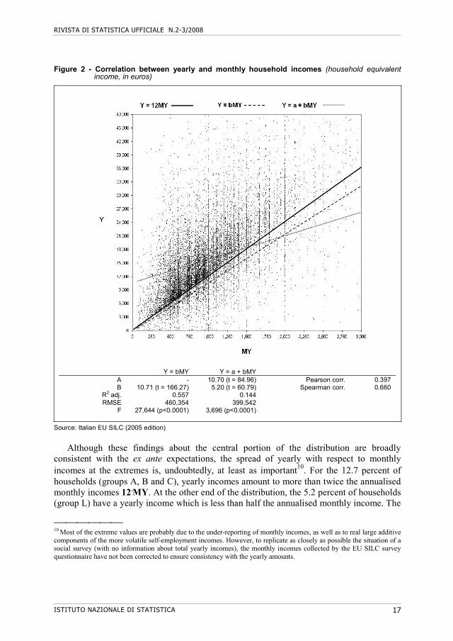
Figure 2 - Correlation between yearly and monthly household incomes (household equivalent income, in euros)
Y = bMY Y = a + bMY A - 10.70 (t = 84.96) Pearson corr. 0.397 B 10.71 (t = 166.27) 5.20 (t = 60.79) Spearman corr. 0.660
R2 adj. 0.557 0.144 RMSE 460,354 399,542
F 27,644 (p<0.0001) 3,696 (p<0.0001)
Source: Italian EU SILC (2005 edition)
Although these findings about the central portion of the distribution are broadly
consistent with the ex ante expectations, the spread of yearly with respect to monthly incomes at the extremes is, undoubtedly, at least as important10. For the 12.7 percent of households (groups A, B and C), yearly incomes amount to more than twice the annualised monthly incomes 12.MY. At the other end of the distribution, the 5.2 percent of households (group L) have a yearly income which is less than half the annualised monthly income. The
10 Most of the extreme values are probably due to the under-reporting of monthly incomes, as well as to real large additive components of the more volatile self-employment incomes. However, to replicate as closely as possible the situation of a social survey (with no information about total yearly incomes), the monthly incomes collected by the EU SILC survey questionnaire have not been corrected to ensure consistency with the yearly amounts.

MONTHLY INCOME AS A CORE SOCIAL VARIABLE: EVIDENCE FROM THE ITALIAN EU SILC SURVEY
ISTITUTO NAZIONALE DI STATISTICA 18
proportion of extreme values is large and, thereby, highly influential on the association between Y and MY. The ‘Pearson’ measure of linear correlation (0.38) and the poor fit of the two-way linear regressions indicate that the influence of extreme values is definitely negative. Moreover, multiplicative and additive factors overlap and it would be awkward to disentangle them by a two-way, simple model. Only a more accurate model, including additional explanatory variables could possibly improve the situation. A further discussion of this point will be presented in Section 5, below.
Table 2 - Yearly incomes by ‘additive’ and ‘multiplicative’ classes of monthly income (percent of households)
'multiplicative' classes of MY
lower upper %
A 28MY 8.31
B 26MY 28MY 1.83
C 24MY 26MY 2.60
D 22MY 24MY 3.34
E 20MY 22MY 4.64
F 18MY 20MY 6.88
G 16MY 18MY 10.63
H 14MY 16MY 18.82
I 12MY 14MY 23.38
J 9MY 12MY 9.98
K 6MY 9MY 4.35
L 6MY 5.24
Total 100
'additive' classes of MY
lower upper %
M 15,000+12MY 5.95
N 10,000+12MY 15,000+12MY 6.31
O 8,000+12MY 10,000+12MY 4.89
P 6,000+12MY 8,000+12MY 7.92
Q 4,000+12MY 6,000+12MY 11.74
R 2,000+12MY 4,000+12MY 17.96
S 12MY 2,000+12MY 25.66
T -1,000+12MY 12MY 4.76
U -2,000+12MY -1,000+12MY 3.02
V -2,000+12MY -4,000+12MY 3.95
W -4,000+12MY -6,000+12MY 2.16
Z -6,000+12MY 5.66
Total 100
Source: Italian EU SILC (2005 edition)
RIVISTA DI STATISTICA UFFICIALE N.2-3/2008
ISTITUTO NAZIONALE DI STATISTICA 19
The remarkable finding, at this stage of the analysis, is that the amount of monthly income cannot be used as a proxy for the amount of yearly income without further information and, noticeably, a detailed econometric model.
The same conclusion could have been reached by observing that any straight line or curve lying above the annualised monthly income line Y=12.MY (as it should, given the location of most data points) would rule out a large part of households (19.6 percent) who are positioned below that line. A more encouraging result is that the ‘Spearman’ correlation between the ranks of Y and MY (0.66) is substantially higher than the ‘Pearson’ correlation (0.40) between levels. Section 4 will therefore focus on the correlation between the ranks of Y and MY.
4. Ranking the households by monthly and yearly incomes
To compare the rankings obtained from different measures of income, a suitable variable is the fractional rank. When all the N households are sorted in ascending order of the income Y, the (weighted) fractional rank RY of each household j is defined as11:
N
1ii
j
1ii
w
w
YR (1)
The concept is well-known in the literature about inequality, as the fractional rank represents one of the coordinates of the Lorenz curve and appears in the computation of the Gini index. Besides, the deciles (or quintiles) may be computed directly from the fractional ranks. For example, all the households whose fractional rank is lower than 0.10 belong to the first decile of the distribution.
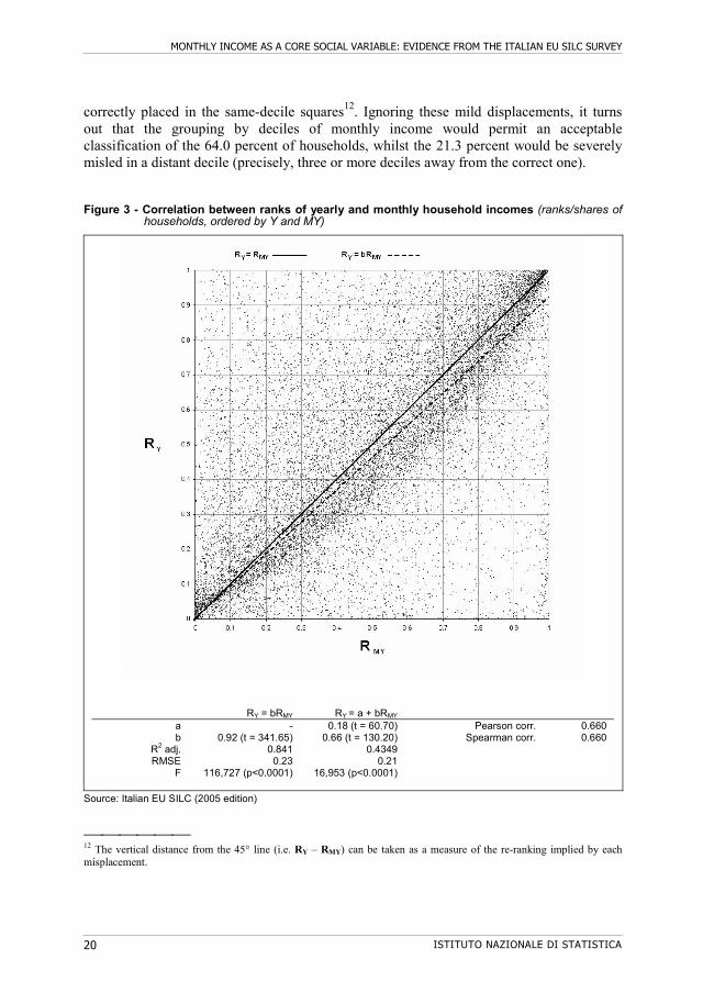
As expected, the scatterplot of RY against RMY looks better than that relating to levels (Figure 3). The data points seem running away from the NW and SE corners to gather towards the 45° line, which is the locus of equal ranks, halving the ten ‘same-decile’ squares (as well as the five ‘same-quintile’ ones). Furthermore, the estimated slope of the linear regression RY = b.RMY (0.92) is close to that of the 45° line. The 29.3 percent of households belong to the same decile of both distributions (Table 3). In fact, with the sole exception of the tenth decile, less than 50 percent of the households of any other decile of Y belong to the same decile of MY.
Re-ranking is impressive in the central part of the distribution: more than 75 percent of the households in the fourth, fifth, sixth and seventh deciles of yearly income are in a different decile of monthly income. As a consequence, when grouping by deciles, misclassified cases amount to 70.7 percent of the total. However, 34.7 percent of households are found in adjacent deciles where, as the visual inspection of Figure 3 confirms, a large number of data points lie as close to the 45° line as many other points
11 In the formula, to simplify the notation, the j superscript to RY has been omitted.
MONTHLY INCOME AS A CORE SOCIAL VARIABLE: EVIDENCE FROM THE ITALIAN EU SILC SURVEY
ISTITUTO NAZIONALE DI STATISTICA 20
correctly placed in the same-decile squares12. Ignoring these mild displacements, it turns out that the grouping by deciles of monthly income would permit an acceptable classification of the 64.0 percent of households, whilst the 21.3 percent would be severely misled in a distant decile (precisely, three or more deciles away from the correct one).
Figure 3 - Correlation between ranks of yearly and monthly household incomes (ranks/shares of households, ordered by Y and MY)
RY = bRMY RY = a + bRMY a - 0.18 (t = 60.70) Pearson corr. 0.660 b 0.92 (t = 341.65) 0.66 (t = 130.20) Spearman corr. 0.660
R2 adj. 0.841 0.4349 RMSE 0.23 0.21
F 116,727 (p<0.0001) 16,953 (p<0.0001)
Source: Italian EU SILC (2005 edition)
12 The vertical distance from the 45° line (i.e. RY – RMY) can be taken as a measure of the re-ranking implied by each misplacement.

RIVISTA DI STATISTICA UFFICIALE N.2-3/2008
ISTITUTO NAZIONALE DI STATISTICA 21
Table 3 - Households by deciles of yearly and monthly income (percent of total households)
1st 2nd 3rd 4th 5th 6th 7th 8th 9th 10th all
10th 0.3 0.2 0.2 0.2 0.3 0.4 0.6 0.9 1.9 5.1 10.0
9th 0.2 0.2 0.3 0.4 0.4 0.6 0.9 1.8 3.2 2.1 10.0
8th 0.2 0.3 0.4 0.5 0.7 0.9 1.4 2.4 2.5 0.7 10.0
7th 0.4 0.4 0.5 0.6 0.9 1.2 2.1 2.5 1.0 0.4 10.0
6th 0.5 0.5 0.7 0.8 1.2 2.0 2.6 1.1 0.5 0.3 10.0
5th 0.5 0.7 0.9 1.2 1.9 2.4 1.2 0.6 0.3 0.3 10.0
4th 0.7 1.0 1.3 2.2 2.7 1.2 0.5 0.3 0.1 0.2 10.0
3rd 1.1 1.5 2.5 2.6 0.8 0.5 0.4 0.2 0.1 0.3 10.0
2nd 1.6 3.6 2.5 0.8 0.5 0.3 0.2 0.1 0.1 0.2 10.0
1st 4.5 1.8 0.8 0.7 0.4 0.6 0.3 0.2 0.3 0.5 10.0
all 10.0 10.0 10.0 10.0 10.0 10.0 10.0 10.0 10.0 10.0 100.0
deciles of MYd
ec
iles
of
Y
In the same deciles
64.0
In adjacent deciles
29.3
=
+
34.7
In a distant decile21.3
Source: Italian EU SILC (2005 edition)
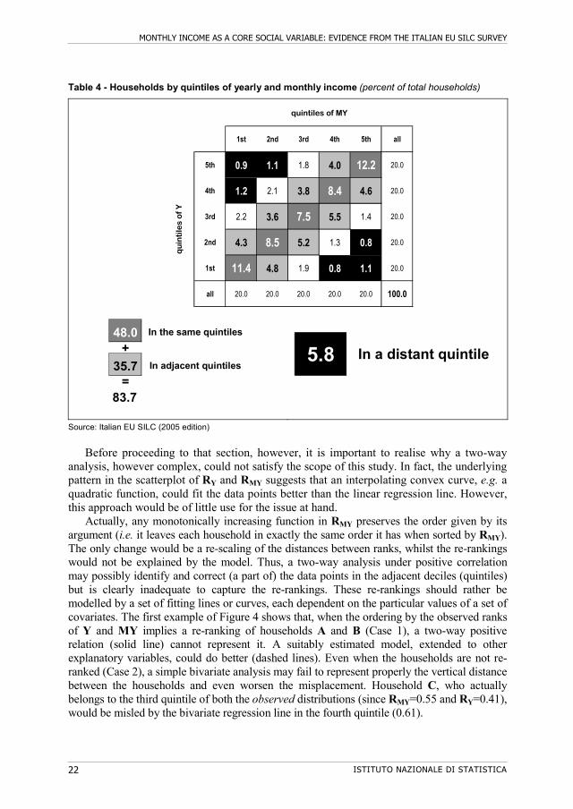
The quintiles of Y and MY are more consistent between them (Table 4). Actually, the
48.0 percent of house holds belong to the same quintiles. Moreover, adding the mildly re-ranked households (misplaced in the adjacent quintiles), the percent of acceptable classifications reaches 83.7 of the total. The households severely misplaced in distant quintiles are the 5.8 percent.
For the Italian case, two main conclusions have been reached at this stage of the analysis: (i) it is better to rely upon the correlation between the ranks of the yearly and monthly income variables than on the weaker correlation between their levels; (ii) the grouping by quintiles implies less severe misplacements than the grouping by deciles. Further improvements may reasonably come from an econometric study of the misplacements, relating the differences between the ranks of the two income variables to additional information about the households. The next section discusses the relation between Y and MY, conditional on additional explanatory variables, by the means of a quantile regression analysis.
MONTHLY INCOME AS A CORE SOCIAL VARIABLE: EVIDENCE FROM THE ITALIAN EU SILC SURVEY
ISTITUTO NAZIONALE DI STATISTICA 22
Table 4 - Households by quintiles of yearly and monthly income (percent of total households)
1st 2nd 3rd 4th 5th all
5th 0.9 1.1 1.8 4.0 12.2 20.0
4th 1.2 2.1 3.8 8.4 4.6 20.0
3rd 2.2 3.6 7.5 5.5 1.4 20.0
2nd 4.3 8.5 5.2 1.3 0.8 20.0
1st 11.4 4.8 1.9 0.8 1.1 20.0
all 20.0 20.0 20.0 20.0 20.0 100.0
quintiles of MY
qu
inti
les
of
Y
5.8 In a distant quintile
Source: Italian EU SILC (2005 edition)
Before proceeding to that section, however, it is important to realise why a two-way
analysis, however complex, could not satisfy the scope of this study. In fact, the underlying pattern in the scatterplot of RY and RMY suggests that an interpolating convex curve, e.g. a quadratic function, could fit the data points better than the linear regression line. However, this approach would be of little use for the issue at hand.
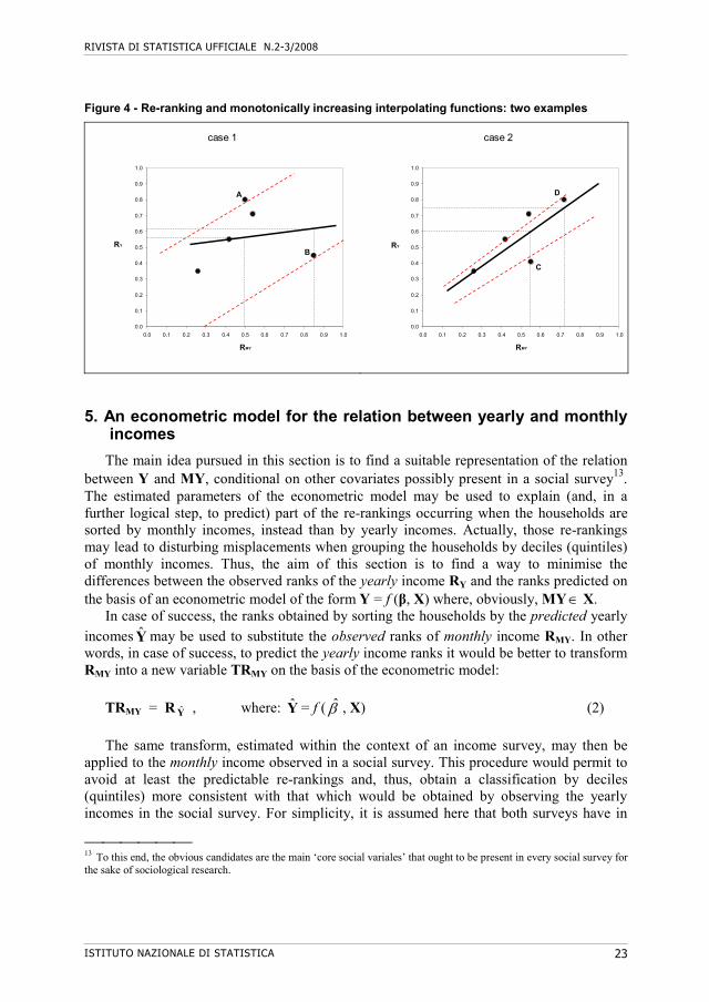
Actually, any monotonically increasing function in RMY preserves the order given by its argument (i.e. it leaves each household in exactly the same order it has when sorted by RMY). The only change would be a re-scaling of the distances between ranks, whilst the re-rankings would not be explained by the model. Thus, a two-way analysis under positive correlation may possibly identify and correct (a part of) the data points in the adjacent deciles (quintiles) but is clearly inadequate to capture the re-rankings. These re-rankings should rather be modelled by a set of fitting lines or curves, each dependent on the particular values of a set of covariates. The first example of Figure 4 shows that, when the ordering by the observed ranks of Y and MY implies a re-ranking of households A and B (Case 1), a two-way positive relation (solid line) cannot represent it. A suitably estimated model, extended to other explanatory variables, could do better (dashed lines). Even when the households are not re-ranked (Case 2), a simple bivariate analysis may fail to represent properly the vertical distance between the households and even worsen the misplacement. Household C, who actually belongs to the third quintile of both the observed distributions (since RMY=0.55 and RY=0.41), would be misled by the bivariate regression line in the fourth quintile (0.61).
= 83.7
48.0 In the same quintiles
+ 35.7 In adjacent quintiles
RIVISTA DI STATISTICA UFFICIALE N.2-3/2008
ISTITUTO NAZIONALE DI STATISTICA 23
Figure 4 - Re-ranking and monotonically increasing interpolating functions: two examples
case 1
0.0
0.1
0.2
0.3
0.4
0.5
0.6
0.7
0.8
0.9
1.0
0.0 0.1 0.2 0.3 0.4 0.5 0.6 0.7 0.8 0.9 1.0
RMY
RY
A
B
case 2
0.0
0.1
0.2
0.3
0.4
0.5
0.6
0.7
0.8
0.9
1.0
0.0 0.1 0.2 0.3 0.4 0.5 0.6 0.7 0.8 0.9 1.0
RMY
RY
D
C
5. An econometric model for the relation between yearly and monthly incomes
The main idea pursued in this section is to find a suitable representation of the relation between Y and MY, conditional on other covariates possibly present in a social survey13. The estimated parameters of the econometric model may be used to explain (and, in a further logical step, to predict) part of the re-rankings occurring when the households are sorted by monthly incomes, instead than by yearly incomes. Actually, those re-rankings may lead to disturbing misplacements when grouping the households by deciles (quintiles) of monthly incomes. Thus, the aim of this section is to find a way to minimise the differences between the observed ranks of the yearly income RY and the ranks predicted on the basis of an econometric model of the form Y = f (β, X) where, obviously, MY X.
In case of success, the ranks obtained by sorting the households by the predicted yearly
incomes Y may be used to substitute the observed ranks of monthly income RMY. In other words, in case of success, to predict the yearly income ranks it would be better to transform RMY into a new variable TRMY on the basis of the econometric model:
TRMY = R Y , where: Y = f ( , X) (2)
The same transform, estimated within the context of an income survey, may then be
applied to the monthly income observed in a social survey. This procedure would permit to avoid at least the predictable re-rankings and, thus, obtain a classification by deciles (quintiles) more consistent with that which would be obtained by observing the yearly incomes in the social survey. For simplicity, it is assumed here that both surveys have in
13 To this end, the obvious candidates are the main ‘core social variales’ that ought to be present in every social survey for the sake of sociological research.
MONTHLY INCOME AS A CORE SOCIAL VARIABLE: EVIDENCE FROM THE ITALIAN EU SILC SURVEY
ISTITUTO NAZIONALE DI STATISTICA 24
common the same population, the sampling designs, the patterns of non-response and anything else that could otherwise bring about differences in their comparative representativeness.
A useful econometric tool to model the re-rankings is the quantile regression analysis14. For a specific quantile τ of a dependent variable y, with K explanatory variables and an
intercept in the model, quantile regression finds the K+1 vector )(ˆ , called regression
quantile, by solving the minimisation problem:
n
iii xy
1
)'(min)(ˆ , with: ))0(()( zIzz , 10 (3)
where I(.) is the indicator function, valued ‘1’ for negative residuals and ‘0’ otherwise.
The solution minimises the sum of the residuals (each weighted by the τ function) just as the standard OLS regression minimises the sum of squared residuals. Except for that difference, the core of the model is linear and the estimated parameters can be interpreted in a familiar way. They show the influence of each explanatory variable on the pτ = τ.100th percentile of the distribution of the dependent variable. Since y can be predicted at every percentile of its distribution, quantile regression is widely used when it is thought that both the spread and the ‘median’ tendency could be explained by the regressors in X. When such an analysis is performed for every percentile, the entire set of regression quantiles is called a quantile process and is denoted as: )1,0(:)( .
The explanatory variables considered in the model are built on the basis of core social variables like sex, age, education, employment status etc.. They are all put in a dichotomous format and thus enter the model as dummies. Except for the geographical area, represented by the variable southisland, the other dummies count the number of adults per household having a given characteristic (i.e. they are measured at the household level, as the prefix ‘h’ to their names indicates). The only variables referred to children are: (i) hagelt15_one, which takes the ‘1’ value for those households where there is exactly one individual younger than 15 years (and ‘0’ otherwise) and (ii): hagelt15_2more , taking the ‘1’ value when there are two or more children aged less than 15 years.
14 Quantile regression has been introduced by Koenker and Bassett (1978). The basic concepts can be found in Koenker and Hallock (2001) and in Cade and Noon (2003). For an application to wage inequality see Angrist et al. (2004), whilst a detailed description is in Koenker (2005). The SAS users may download an experimental version of the QUANTREG procedure (and the related handbook) from the website: http://sas.support.com (see also Chen, 2005).
RIVISTA DI STATISTICA UFFICIALE N.2-3/2008
ISTITUTO NAZIONALE DI STATISTICA 25
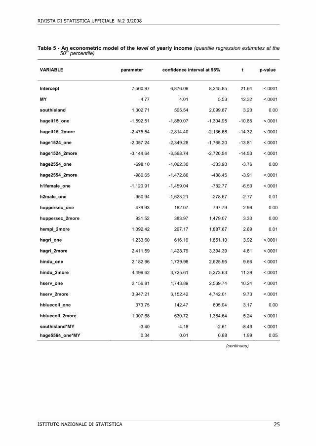
Table 5 - An econometric model of the level of yearly income (quantile regression estimates at the 50th percentile)
VARIABLE parameter confidence interval at 95% t p-value
Intercept 7,560.97 6,876.09 8,245.85 21.64 <.0001
MY 4.77 4.01 5.53 12.32 <.0001
southisland 1,302.71 505.54 2,099.87 3.20
0.00
hagelt15_one -1,592.51 -1,880.07 -1,304.95 -10.85 <.0001
hagelt15_2more -2,475.54 -2,814.40 -2,136.68 -14.32 <.0001
hage1524_one -2,057.24 -2,349.28 -1,765.20 -13.81 <.0001
hage1524_2more -3,144.64 -3,568.74 -2,720.54 -14.53 <.0001
hage2554_one -698.10 -1,062.30 -333.90 -3.76
0.00
hage2554_2more -980.65 -1,472.86 -488.45 -3.91 <.0001
h1female_one -1,120.91 -1,459.04 -782.77 -6.50 <.0001
h2male_one -950.94 -1,623.21 -278.67 -2.77
0.01
huppersec_one 479.93 162.07 797.79 2.96
0.00
huppersec_2more 931.52 383.97 1,479.07 3.33
0.00
hempl_2more 1,092.42 297.17 1,887.67 2.69
0.01
hagri_one 1,233.60 616.10 1,851.10 3.92 <.0001
hagri_2more 2,411.59 1,428.79 3,394.39 4.81 <.0001
hindu_one 2,182.96 1,739.98 2,625.95 9.66 <.0001
hindu_2more 4,499.62 3,725.61 5,273.63 11.39 <.0001
hserv_one 2,156.81 1,743.89 2,569.74 10.24 <.0001
hserv_2more 3,947.21 3,152.42 4,742.01 9.73 <.0001
hbluecoll_one 373.75 142.47 605.04 3.17
0.00
hbluecoll_2more 1,007.68 630.72 1,384.64 5.24 <.0001
southisland*MY -3.40 -4.18 -2.61 -8.49 <.0001
hage5564_one*MY 0.34 0.01 0.68 1.99 0.05
(continues)
MONTHLY INCOME AS A CORE SOCIAL VARIABLE: EVIDENCE FROM THE ITALIAN EU SILC SURVEY
ISTITUTO NAZIONALE DI STATISTICA 26
Table 5 (continued) - An econometric model of the level of yearly income (quantile regression estimates at the 50th percentile)
VARIABLE parameter confidence interval at 95% t p-value
hage5564_2more*MY 0.83 0.41 1.26 3.86
0.00
h2male_one*MY 1.04 0.34 1.75 2.90
0.00
h2male_2more*MY 0.96 0.47 1.46 3.80
0.00
hlowedu_one*MY -0.53 -0.90 -0.15 -2.76
0.01
hlowedu_2more*MY -0.97 -1.48 -0.46 -3.75
0.00
huniv_one*MY 1.79 1.38 2.20 8.60 <.0001
huniv_2more*MY 2.44 1.69 3.19 6.39 <.0001
hempl_one*MY 1.06 0.61 1.51 4.60 <.0001
hself_1more*MY -0.88 -1.34 -0.41 -3.70
0.00
hunem_1more*MY -1.68 -2.27 -1.08 -5.49 <.0001
hhighskill_one*MY 1.80 1.46 2.14 10.33 <.0001
hhighskill_2more*MY 3.28 2.56 3.99 9.00 <.0001
hclerks_one*MY 1.55 1.22 1.89 9.04 <.0001
hclerks_2more*MY 2.87 2.43 3.32 12.64 <.0001
hlowskill_1more*MY 0.21 -0.17 0.58 1.08 0.28
For all the count variables, the omitted category is always referred to the households with
no individuals with the specified characteristic. Household size has been omitted, being indirectly represented by the set of other regressors. An exception has been made for gender indicators, for which distinct variables have been devised for single-person households15. The variables h1female_no (reference group) and h1female_one indicate adult single women (in one-person households), whilst the variables h2female_no, h2female_one, h2female_2more count the adult women present in households with two or more components. Single adult men are perfectly represented by the h1female_no variable and can thus be taken as the benchmark (i.e. omitted) group for the h1female_one dummy16.
The meaning of the dummies should be clear from their names. The variables for the profession are related to the 1st-digit ISCO88 classification: highskill (ISCO = 1, 2) - clerks (ISCO = 3, 4, 5) - bluecoll (ISCO = 6, 7, 8) - lowskill (ISCO = 9). Those for the educational attainment (lowedu – uppersec - univ) are referred to the ISCED classification.
15 Single women are a peculiar group, mainly composed of old widowers, and have been treated separately to reduce the variance of the estimated parameters of the gender indicators. 16 For similar reasons, there is no need to insert a variable for the ‘no adult men’ case in single households.
RIVISTA DI STATISTICA UFFICIALE N.2-3/2008
ISTITUTO NAZIONALE DI STATISTICA 27
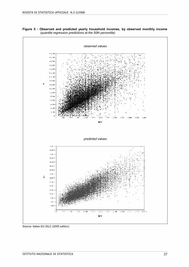
Figure 5 - Observed and predicted yearly household incomes, by observed monthly income (quantile regression predictions at the 50th percentile)
observed values
predicted values
Source: Italian EU SILC (2005 edition)
MONTHLY INCOME AS A CORE SOCIAL VARIABLE: EVIDENCE FROM THE ITALIAN EU SILC SURVEY
ISTITUTO NAZIONALE DI STATISTICA 28
The strategy of model selection has looked primarily at the 95 percent confidence intervals of the estimated parameters and at the Student’s t, in order to avoid too large prediction errors. These latter would introduce additional undesired misplacements, whilst the scope of the present exercise is precisely the opposite: to avoid the re-rankings induced by the use of the observed monthly income as the ordering variable. The second choice has concerned the insertion of the covariates as ‘additive’ or ‘multiplicative’ factors17. After a sequence of trials, it emerged that only for the geographical dummy both the additive and the multiplicative influences can be separately represented by the model. For each of the other variables, the retained form (additive or multiplicative) is the one that corresponds to the lower standard error of the parameter.
Many interaction terms have proved to be not statistically significant (e.g. southisland *empl does not add explanatory power to the regression). The interplay amongst so many variables correlated between them may lead to multicollinearity (e.g. the group: lowskill - lowedu – unem; and the group: agegt65 – retiredoth - lowedu). For this reason, some variables are parsimoniously represented by a single ‘one or more’ dummy (suffix: _1more) instead of the pair ‘exactly one’ (_one) and ‘two or more’ (_2more). Besides, the variables agegt65 and retiredoth have been dropped in order to retain lowskill and lowedu.
Given the main goal of the present study, a detailed explanation of the econometric results seems out of the scope. For the time being, they may be summarised graphically: the multivariate model permits to form a ‘cloud’ of predicted values that reproduces a significant part of the spread of the observed values (Figure 5).
The households may now be sorted by the predicted yearly incomes Y and grouped into deciles and quintiles (Table 6). The worst re-rankings are those occurring at the NW and SE corners, corresponding to households placed in the top quintile of a distribution and in the bottom quintile of the other. An important finding of the econometric exercise is that the grouping by predicted incomes has considerably reduced these extreme misplacements (with respect to the ordering by observed monthly incomes shown in Table 3). The worst misplacements amount to 2.0 percent when ranking by MY (precisely, 1.1 percent in the SE corner and 0.9 percent in the NW one, in Table 3) and only to 0.7 percent when the households are sorted by Y (0.3 percent in the SE corner and 0.4 percent in the NW one, in Table 6). Moreover, the percentage of households placed in the two opposite NW and SE decile squares has been reduced from 0.8 to 0.1 percent. That is, the econometric predictions have almost completely avoided re-placements from the richest decile of a distribution to the poorest of the other and vice versa.
Besides, the percentage of households misplaced in distant deciles (displayed as black cells in Tables 3 and 6) has also been reduced from 21.3 to 19.2 percent. The analogous reduction for what concerns quintiles is from 5.8 to 3.4 percent. Therefore, when the grouping is by quintiles, the use of predicted Y permits to avoid more than the 40 percent of the misplacements in distant quintiles, whilst the analogous gain when grouping by deciles is about 10 percent.
17 Geometrically, the distinction is between an additive influence on the height of the ‘cloud’ of predicted points and a multiplicative one, affecting its slope.

RIVISTA DI STATISTICA UFFICIALE N.2-3/2008
ISTITUTO NAZIONALE DI STATISTICA 29
Table 6 - Households by deciles and quintiles of predicted and observed yearly equivalent incomes (percent of total households)
1st 2nd 3rd 4th 5th 6th 7th 8th 9th 10th all
10th 0.0 0.1 0.1 0.2 0.4 0.4 0.7 1.1 1.7 5.3 10.0
9th 0.0 0.1 0.1 0.3 0.4 0.8 1.2 1.6 2.9 2.5 10.0
8th 0.1 0.2 0.3 0.4 0.6 1.2 1.5 2.2 2.6 1.0 10.0
7th 0.2 0.3 0.5 0.6 1.0 1.5 2.1 2.3 1.3 0.4 10.0
6th 0.3 0.6 0.6 1.0 1.6 1.8 1.9 1.3 0.7 0.2 10.0
5th 0.5 0.8 1.0 1.4 2.2 1.6 1.3 0.7 0.3 0.2 10.0
4th 0.9 1.2 1.9 2.0 1.7 1.2 0.6 0.4 0.1 0.2 10.0
3rd 1.3 1.9 2.1 2.1 1.1 0.8 0.3 0.2 0.1 0.1 10.0
2nd 2.2 3.1 2.0 1.4 0.5 0.3 0.2 0.1 0.1 0.1 10.0
1st 4.5 1.9 1.4 0.7 0.6 0.4 0.3 0.1 0.1 0.1 10.0
all 10.0 10.0 10.0 10.0 10.0 10.0 10.0 10.0 10.0 10.0 100.0
deciles of PREDICTED Y
de
cile
s o
f Y
In the same deciles
61.9
In adjacent deciles
28.0
=
+
33.8
In a distant decile19.2
1st 2nd 3rd 4th 5th all
5th 0.3 0.7 2.0 4.6 12.5 20.0
4th 0.7 1.7 4.2 8.1 5.2 20.0
3rd 2.1 4.1 7.2 5.2 1.5 20.0
2nd 5.2 8.0 4.8 1.5 0.5 20.0
1st 11.6 5.5 1.8 0.7 0.4 20.0
all 20.0 20.0 20.0 20.0 20.0 100.0
quintiles of PREDICTED Y
qu
inti
les
of Y
86.1
47.4 In the same quintiles
+
38.7 In adjacent quintiles
=
3.4 In a distant quintile
Source: Italian EU SILC (2005 edition) Disappointingly, the ordering by predicted incomes has slightly lowered the number of
households placed in the same deciles (from 29.3 percent when ranking by MY to 28.0 percent when ranking by Y ) and in the adjacent deciles as well (from 34.7 to 33.8 percent). Therefore, for what concerns the deciles, the acceptable classifications are reduced from 64.0 to 61.9 percent when MY is replaced by Y as the ordering variable. Nonetheless, the opposite result is found for quintiles: the acceptable classifications (i.e. in the same or adjacent quintiles) has increased from 83.7 to 86.1 percent of total households. The reason for this mixed result is easy to understand: the econometric model entails its own
MONTHLY INCOME AS A CORE SOCIAL VARIABLE: EVIDENCE FROM THE ITALIAN EU SILC SURVEY
ISTITUTO NAZIONALE DI STATISTICA 30
misplacements, due to prediction errors. With respect to deciles, the ordering by quintiles ‘sterilizes’ all the prediction errors greater than 0.10 and lower than 0.20 while, at the same time, permits to avoid a larger proportion of the extreme misplacements induced by the MY ranking.
To sum up, when compared to the ordering by observed monthly incomes, the grouping by predicted values of yearly incomes implies a lower percentage of extreme misplacements and, furthermore, reduces the proportion of households misled in distant deciles (quintiles). In addition, if the household are grouped by quintiles, the ranking by predicted values also permits an increase in the percent of acceptable classifications.
6. Conclusions
The comparison of monthly vs. yearly incomes, both collected in the 2005 Italian EU SILC survey, shows that:
(i) the observed amount of monthly income turns out to be a poor predictor of the amount of yearly income. Therefore, the collected monthly income should not be used as a simple proxy for yearly income without further information and more accurate econometric techniques.
(ii) The correlation between the ranks of the yearly and monthly income variables is substantially higher than the correlation of their levels. Therefore, the observed rank of monthly income may lead to an acceptable classification of the households into deciles or quintiles. However, a large part of the households are not found exactly in the same deciles of both distributions. The grouping by quintiles of monthly income entails a lower percentage of misplacements than the grouping by deciles.
(iii) Further improvements may come from an econometric study of the differences between the observed levels and ranks of the two income variables, relating them to additional information about the households, taken from core social variables. An exploratory quantile regression analysis of the Italian EU SILC data shows that, with respect to the ordering given by the observed monthly incomes, the classification by (ranks of) predicted yearly incomes permits to avoid a large proportion of extreme misplacements. Furthermore, the percentage of households misled in distant deciles or quintiles is considerably reduced. Finally, if the household are grouped by quintiles, the ranking by predicted values also permits an increase in the percent of acceptable classifications (i.e. in the same or adjacent quintiles).
RIVISTA DI STATISTICA UFFICIALE N.2-3/2008
ISTITUTO NAZIONALE DI STATISTICA 31
References
Angrist, J., V. Chernozhukov and I. Fernandez-Val (2004), “Quantile Regression Under Misspecification, With An Application to the U.S. Wage Structure”, NBER Working Paper Series, n. 10428
Cade, B.S. and B.R. Noon, B.R. (2003), “A gentle introduction to quantile regression for ecologists”, Frontiers in Ecology and the Environment, vol. 1, p. 412-420
Chen, C. (2005), “An Introduction to Quantile Regression and the QUANTREG Procedure”, Proceedings of the Thirtieth Annual SAS Users Group International Conference, Paper 21330, SAS Institute Inc., Cary (North Carolina, USA)
EUROSTAT (2007a), Task Force on Core Social Variables – Final Report, European Communities, Luxembourg
EUROSTAT (2007b), Comparative EU Statistics on Income and Living Conditions: Issues and Challenges, European Communities, Luxembourg
Glaude, M. (2008), “Measuring Critical Social Issues The European experience”, New Directions in Social Statistics, Seminar of the United Nations Statistics Department, February, New York (http://unstats.un.org/unsd/statcom/new_directions_seminar.htm)
Koenker, R. (2005), Quantile Regression, Cambridge University Press, New York
Koenker, R. and G. Bassett (1978), “Regression Quantiles”, Econometrica, vol. 46, p. 33-50
Koenker, R. and K.F. Hallock (2001), “Quantile Regression”, Journal of Economic Perspectives, vol. 15, p. 143-156

RIVISTA DI STATISTICA UFFICIALE N.2-3/2008
ISTITUTO NAZIONALE DI STATISTICA 33
The integration of the non-profit sector in a Social Accounting Matrix: methodological issues, empirical
evidences and employment effects for Italy
Giovanni Cerulli1
Sommario
Questo lavoro presenta una Matrice di Contabilità Sociale (SAM) per l’Italia che include, per la prima volta, un conto economico per il settore non-profit (o “terzo settore”). L’anno di riferimento è il 1999. Nella prima parte dell’articolo si considera la definizione statistica di settore non-profit ed il modo in cui esso è stato integrato in un modello SAM. Vengono poi presentati i principali risultati dell’analisi. Due tipi di risultati sono considerati, riferiti rispettivamente al commento dei principali coefficienti descrittivi della SAM e ad una semplice analisi di simulazione per testare l’impatto della politica fiscale (spesa e trasferimenti pubblici) sul livello di occupazione generato da e attraverso l’attività del terzo settore. Abstract
This work presents a Social Accounting Matrix (SAM) for Italy including, for the first time, an economic account of the non-profit sector (or “third sector”). The year it refers to is 1999. In the first part of this article I address statistical definition of the non-profit sector and how I include it in the SAM framework. I then go on to set out the main results of my analysis. Two kinds of results will be considered, referring respectively to comment on the principal descriptive coefficients of the SAM, and to a simple simulation analysis to test the impact of fiscal policy (public expenditure and public transfers) on the level of employment generated within and through the third sector activity. Keywords: Social Accounting Matrix, non-profit sector, national accounts 1. Introduction
The recent rise of non-profit (or third sector) organizations in modern economies has fostered the development of a huge theoretical and empirical literature centered on explaining the rationale for the existence of this kind of institutions operating within a large number of social markets such as child care, assistance for aged people, environmental protection, sport activities, and so on (Marcon-Mellano, 2000).
From a theoretical perspective, various approaches have been proposed to account for this unexpected rise. The “demand side” approach, probably the most explored stream of research, focused on the ability of non-profit organizations to be more efficient than other
1 Ceris-CNR, Istituto di Ricerca sull’Impresa e lo Sviluppo, e-mail: [email protected].

THE INTEGRATION OF THE NON-PROFIT SECTOR IN A SOCIAL ACCOUNTING MATRIX.…
ISTITUTO NAZIONALE DI STATISTICA 34
agencies in responding to specific failures in markets whose structural characteristics are long far from a perfectly competitive structure. Weisbrod (1975; 1988), for example, suggests that in the case of public and quasi-public goods, the non-profit provision is explained by the quantity/quality rationing set by for-profit firms (through the “free-riding” mechanism) and the governmental agencies (according to the “median voter” supply). Hansmann (1980; 1989), on the contrary, focuses on the emergence of non-profit sector when strong “asymmetric information” between producers and consumers is at work. Indeed, by means of the “non-distribution constraint” (NDC), non-profit organizations are able to fit the market, being the NDC a special contractual arrangement able to reduce the agency costs generated by post-contractual opportunism within firm-consumer relationship.
The “supply side” approach, on the contrary, focuses on the emergence of non-profit organizations as entrepreneurial activities. James (1989), for example, suggests that non-profit organizations are the preferred institutions elected by government agencies to delegate part of production of many services. It occurs fundamentally for two reasons. Firstly, non-profit organizations are particularly suitable to meet citizens’ differentiated preferences (language, religion, race, etc.). Secondly, non-profit organization are able to lower costs since they typically make use of voluntary labor and/or donations. Defourny (2001), by contrast, starts from the tradition of the European co-operative movement and goes on to point out that the non-profit sector historically has arisen principally as an innovation promoter in the more traditional social markets. Taking a Shumpeterian approach, he shows the marked capacity of the third sector to innovate through: (a) new combinations of productive processes, (b) production of new (and qualitatively new) commodities and services, (c) new organizational patterns, (d) new productive factors, such as voluntary labor (e) new forms of enterprise, and finally (f) new forms of transaction and exchange.
Other important contributions point their attention to the third sector organizations as intermediary structures between market economic and state agencies political interests (Van Til, 1998; Bauer, 1990; Evers-Wintersberger, 1990). Indeed, non-profit organizations are able to promote collective self-organized form of organization and participation closely connected, especially at local level, to the direct beneficiaries of services (Laville, 1997; Borzaga-Mittone, 1995; Lombardi et al., 1999). In this sense, the increasing partnership between public and non-profit organizations, through the vigorous process of contracting-out welfare services, is constituting and shaping that new model known as “welfare mix” (Ascoli-Pasquinelli, 1993). A system of welfare mix arises when the provision of public, quasi-public and social goods and services are entrusted to institutional typologies characterized by a different allocation of the property rights on operating surplus, governmental, non-profit and for-profit institutions being the typical organizational forms we find in modern economies (Ben Ner-Van Hoomissen,1991).
While there seems to be broad agreement on the need for transition to a more pluralistic and heterogeneous system of welfare, we still lack the macroeconomic statistical and policy tools for more searching, more scientific analysis of the effects of economic development of the non-profit sector within the welfare mix taking into account not only ”efficiency” considerations, but also ”employment” performance. A Social Accounting Matrix (SAM), explicitly including the non-profit sector and ranging over the entire productive structure of the Italian welfare mix, appears an appropriate methodological tool to reach our aims. In fact, once the appropriate partitioning of its sections has been defined, a SAM allows us to capture

RIVISTA DI STATISTICA UFFICIALE N.2-3/2008
ISTITUTO NAZIONALE DI STATISTICA 35
all the interactions existing between the circular income flow and the socio-economic behaviors of the economic institutional actors. In particular, a SAM allows for both descriptive analysis of the state of ”linkages” between the different economic sectors and normative analysis through the design of specific theoretical models to utilize for simple simulative tests. For the latter use, the SAM provides a powerful device to evaluate the impact of public policies on future sets of welfare mixes, on the incentive mechanisms and, above all, on the level of employment generated through third sector socio-economic activity.
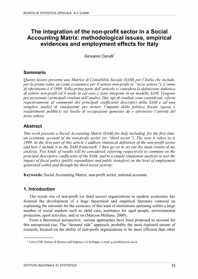
The paper is organized as follows. We start by the statistical definition of non-profit sector showing the methodology to derive a first estimation of a non-profit satellite account to integrate in the SAM (section 2 and subsection 2.1); we then go on by presenting general remarks on SAM (section 3) and the proposed SAM of this paper (section 4 and subsections); then results are set out (section 5 and subsections) and conclusions follow (section 6). 2. The statistical definition of non-profit sector2
A good starting point for statistical definition of the non-profit sector is the System of National Accounts (SNA-93), which defines non-profit institutions as: “legal or social entities created for the purpose of producing goods and services whose status does not permit them to be a source of income, profit or other financial gain for the units that establish, control of finance them” (SNA, 1993, 4.54).
This broad definition, based solely on the “non distribution constraint”, is provided in order to identify the non-profit units. Nevertheless, it is particularly suited to homogeneous treatment of the sector. The SNA in fact specifies that: “it is important to distinguish between NPIs engaged in market and non market production as this affects the sector of the economy to which an NPI is allocated. NPIs do no necessarily engage in non-market production” (SNA, 1993, 4.57). Adopting this approach it can be observed that NPIs are present in each of five residence sectors distinguished by the SNA, namely:
1. Non Financial Corporations (S11) 2. Financial Corporations (S12) 3. General Government (S13) 4. Households (S14) 5. Non-Profit Institutions Serving Households (S15) This classification refers to the sector in which NPIs will be computed and is primarily
dependent on the market or non-market production feature of the unit. On this aspect, the European System of Accounts (ESA) states that:
“in order to determine the type of producer and the sector for the private NPIs, a 50%
criterion should be applied: a) if more than 50% of production costs are covered by sales, the institutional unit is a market producer and classified to the non-financial and financial
2 This paragraph is heavily drawn on Messina-Riccioni (2000).
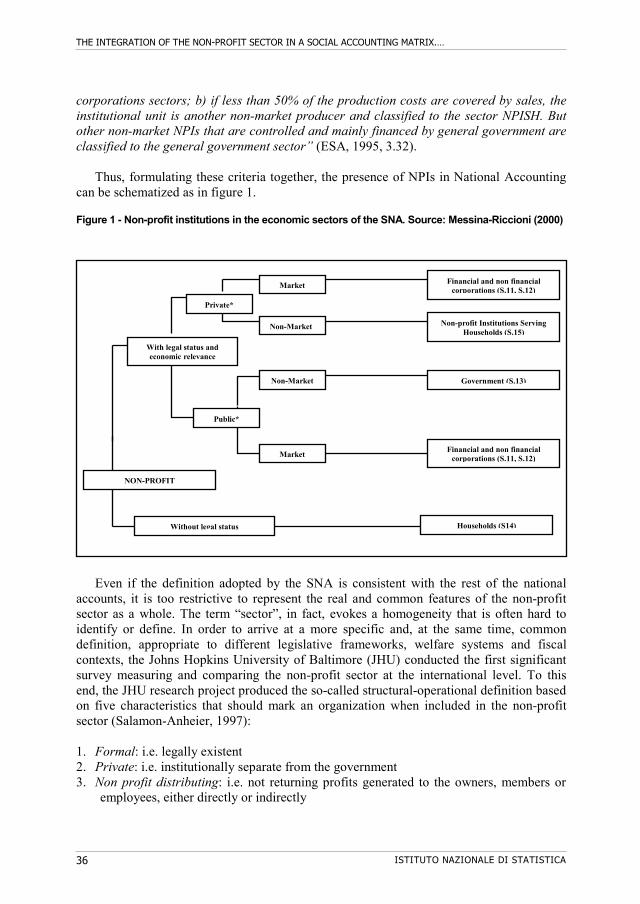
THE INTEGRATION OF THE NON-PROFIT SECTOR IN A SOCIAL ACCOUNTING MATRIX.…
ISTITUTO NAZIONALE DI STATISTICA 36
corporations sectors; b) if less than 50% of the production costs are covered by sales, the institutional unit is another non-market producer and classified to the sector NPISH. But other non-market NPIs that are controlled and mainly financed by general government are classified to the general government sector” (ESA, 1995, 3.32).
Thus, formulating these criteria together, the presence of NPIs in National Accounting
can be schematized as in figure 1. Figure 1 - Non-profit institutions in the economic sectors of the SNA. Source: Messina-Riccioni (2000)
Even if the definition adopted by the SNA is consistent with the rest of the national accounts, it is too restrictive to represent the real and common features of the non-profit sector as a whole. The term “sector”, in fact, evokes a homogeneity that is often hard to identify or define. In order to arrive at a more specific and, at the same time, common definition, appropriate to different legislative frameworks, welfare systems and fiscal contexts, the Johns Hopkins University of Baltimore (JHU) conducted the first significant survey measuring and comparing the non-profit sector at the international level. To this end, the JHU research project produced the so-called structural-operational definition based on five characteristics that should mark an organization when included in the non-profit sector (Salamon-Anheier, 1997):
1. Formal: i.e. legally existent 2. Private: i.e. institutionally separate from the government 3. Non profit distributing: i.e. not returning profits generated to the owners, members or
employees, either directly or indirectly
Households (S14)
Financial and non financial corporations (S.11, S.12)
Non-profit Institutions Serving Households (S.15)
Financial and non financial corporations (S.11, S.12)
Market
Non-Market
Non-Market
Market
Public*
Private*
NON-PROFIT
Without legal status
Government (S.13)
With legal status and economic relevance
RIVISTA DI STATISTICA UFFICIALE N.2-3/2008
ISTITUTO NAZIONALE DI STATISTICA 37
4. Self-governing: i.e. maintaining autonomy in decision making processes and equipped to control their own activities
5. Voluntary: i.e. involving some meaningful degree of voluntary participation, either in the actual conduct of the agency activities or in the management of its affairs.
Figure 2 - Relationship between JHU and SNA. Source: Messina-Riccioni (2000)
One of the most important advantages of the structural-operational definition is that it
allows for: “the examination of a wide assortment of characteristics and features” as well as “focused attention on particular subjects of the non-profit sector that are of particular interest” (Salamon-Anheier, 1997, p. 28).
This definition, however, is not without its disadvantages. For instance, it overlooks the functional features typical of the non-profit sector, failing to take into consideration the important distinction between non-profit institutions that are mutual or public benefit oriented.
Nevertheless, it is a good starting point for empirical analysis. The Italian National Statistical Institute (ISTAT), in fact, used precisely this definition for the “first census of non-profit institutions in Italy” for 1999 (ISTAT, 2001a). This definition will be therefore employed in the SAM proposed in this work. Finally, figure 2 shows the type of relationship existing between the SNA and JHU definitions.
Coming to the Italian context, although there has been a great deal of debate on the definition, main approach and classification to be adopted when studying the non-profit
Non
mar
ket
Structural/operational definition (JHU)
The Third Sector (NETS)
Mar
ket
Public Private
General Government
Financial or non financial corporations
Nonprofit Institutions Serving Households
THE INTEGRATION OF THE NON-PROFIT SECTOR IN A SOCIAL ACCOUNTING MATRIX.…
ISTITUTO NAZIONALE DI STATISTICA 38
sector, there is a general agreement as to the minimum requisites for the legal typologies of organizations to be included in the non-profit sector in Italy, which in fact the ISTAT census automatically incorporates in its definition (ISTAT, 2001a). The main typologies are: Associations, Foundations, Non governmental organizations (NGOs), Voluntary organizations, Non-profit organizations of social utility (ONLUS’s). Then there are a series of other non-profit entities deemed to be in a borderline situation, but included in the census too. They are: Social cooperatives (type A and B), I.P.A.B., Banking foundations, Institutions of patronage, political parties, trade unions and religious organizations (see Messina-Riccioni (2000) and Lunaria (1999) for details). 2.1 A satellite account for the non-profit sector to integrate in the SAM
The structural-operational definition, despite its generality, allows for consistent linkage with the SNA accounts. This aspect proves very important as a meaningful step forward in the direction of constructing a satellite account for the non-profit sector3. At the present time, we have yet to see “official” assessments of a satellite account for the non-profit sector, although the scientific community has been showing increasing interest in the issue over the last few years. In Europe, for instance, several pilot-experiments have started in order to assess a satellite account following the methodology provided by the Global Non-profit Information System Project, a research project coordinated by the Statistical Bureau of the United Nations jointly with the Johns Hopkins University and London School of Economics4.
The data considered by the ISTAT census of non-profit institutions can be used for initial assessment of a satellite account to integrate in a SAM. The census presents 7 items for the non-profit revenues (or resources) and 8 items for the non-profit expenditures.
Table 1 shows the “entries” and the “expenditures” in the SAM structure. If, now, we consider the difference between revenues and expenditures for the non-profit sector (i.e., its economic balance), we obtain:
S = E − U = [K+ + TR+ + C + G + AC] − [CI + W + K− + I + TR−].
The total production (Z) is equal to:
Z = CI +W + K−
where W + K- = VA is the value added. Substituting and reorganizing it in the previous expression we have that:
S = [K+ + TR+] − {[Z − (C + G + AC)] + TR−-}.
3 The SNA recommends constructing a satellite account for all those institutional sectors that are not immediately
visible in official statistics. An interesting survey on the issues involved in the construction of a satellite account for the non-profit sector was performed, in the case of Belgium, by Sybille Mertens (2000).
4 See, in particular, the fundamental contribution of Mertens (2004) who provided the first satellite account for the third sector in Belgium, and for general methodological aspects: United Nations-Johns Hopkins University-London School of Economics (2001), Anheier-Salamon (1998), Anheier-Rudney (1996) and, for the Italy, Messina-Riccioni (2000) and Cuicchio-Malizia-Zamaro (2001).

RIVISTA DI STATISTICA UFFICIALE N.2-3/2008
ISTITUTO NAZIONALE DI STATISTICA 39
Table 1 - Variables of the economic account of non-profit sector to introduce in the SAM
RESOURCES (E)
EXPENDITURES (U)
K+ = Property income received
TR+= Transfers (capital and current) received
C = Households consumption G = Public consumption AC= Other consumptions
CI = Intermediate Costs W = Remuneration of employees K−= Property incomes (paid)
I=Investments TR−= Transfers (capital and current)
This represents the item of entries and expenditures we find in our SAM. It is useful to observe that, in the previous relation, we have that: Z − (C + G + AC) = CNP = Non-profit non-market production. The last step consists in an assessment of the variables in table 1 starting from the variables we find in the ISTAT census. For this purpose I itemize it in the following scheme5: RESOURCES: 1. ENTRATE DI FONTE PUBBLICA (PUBLIC REVENUES) (a) Sussidi e contributi a titolo gratuito (Subsidies and contributions) (E1) (b) Ricavi per contratti e/o convenzioni (Sales of goods and services) (E2) 2. ENTRATE DI FONTE PRIVATA (PRIVATE REVENUES) (a) Quote associative (Subscriptions from members) (E3) (b) Ricavi da vendita di beni e servizi (Sales of goods and services) (E4) (c) Donazioni (Donations) (E5) (d) Redditi finanziari e patrimoniali (Financial revenues) (E6) (e) Altre entrate di fonte privata (Other private revenues) (E7) Table 2 - Table to pass from the variables of the ISTAT non-profit institutions census to the flows
to introduce in the SAM
RESOURCES EXPENDITURES
K+ = E6+E3 TR+= E1+E5
C = E4 G = E2 AC=E7
CI = U4+U3 W = U1+U2 K− = U(8)
I = U7 TR− = U5+U6
5 See ISTAT (2001a, pp. 227-228).
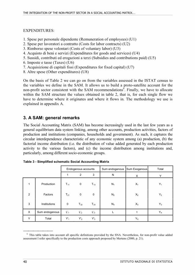
THE INTEGRATION OF THE NON-PROFIT SECTOR IN A SOCIAL ACCOUNTING MATRIX.…
ISTITUTO NAZIONALE DI STATISTICA 40
EXPENDITURES: 1. Spese per personale dipendente (Remuneration of employees) (U1) 2. Spese per lavoratori a contratto (Costs for labor contracts) (U2) 3. Rimborso spese volontari (Costs of voluntary labor) (U3) 4. Acquisto di beni e servizi (Expenditures for goods and services) (U4) 5. Sussidi, contributi ed erogazioni a terzi (Subsidies and contributions paid) (U5) 6. Imposte e tasse (Taxes) (U6) 7. Acquisizione di capitali fissi (Expenditures for fixed capital) (U7) 8. Altre spese (Other expenditures) (U8) On the basis of Table 2 we can go on from the variables assessed in the ISTAT census to the variables we define in the SAM. It allows us to build a proto-satellite account for the non-profit sector consistent with the SAM recommendations6. Finally, we have to allocate within the SAM structure the values obtained in table 2, that is, for each single flow we have to determine where it originates and where it flows in. The methodology we use is explained in appendix A. 3. A SAM: general remarks
The Social Accounting Matrix (SAM) has become increasingly used in the last few years as a general equilibrium data system linking, among other accounts, production activities, factors of production and institutions (companies, households and government). As such, it captures the circular interdependence characteristic of any economic system among (a) production, (b) the factorial income distribution (i.e. the distribution of value added generated by each production activity to the various factors), and (c) the income distribution among institutions and, particularly, among different socio-economic groups. Table 3 - Simplified schematic Social Accounting Matrix
Endogenous accounts Sum endogenous Sum Exogenous Total
1 2 3 N X Y
1 Production T11 0 T13 N1 X1 Y1
2 Factors T21 0 0 N2 X2 Y2
3 Institutions 0 T32 T33 N3 X3 Y3
X Sum endogenous L'1 L'2 L'3 L t YX
Y Total Y'1 Y'2 Y'3 YX
6 This table takes into account all specific definitions provided by the SNA. Nevertheless, for non-profit value added
assessment I refer specifically to the production costs approach proposed by Mertens (2000, p. 21).
RIVISTA DI STATISTICA UFFICIALE N.2-3/2008
ISTITUTO NAZIONALE DI STATISTICA 41
The SAM is a square matrix involving various sets of accounts, which represent the whole of the production and institutional sectors of a given economy. Each account consists of a row (to record resources) and a column (to record expenses). For convenience of presentation, the sequence number of an account in the matrix is the same by row as by column. This presentation of accounts implies that a SAM might be viewed as a Double-Entry Table of transactions where the total sum per row is equal to the total sum per column. The verification of identity for all accounts is symptomatic of the resources-expenses (supplies-uses) equilibrium at the level of each economic agent, product or factor market, production sector, institution and at the level of the whole economy.
Roughly speaking, the SAM has two main functions: on the one hand, it is recognized as a descriptive and synoptic framework of an economy, while on the other hand it is used as a modeling database (Pyatt, 1988). In fact, under certain assumptions, such as excess capacity (i.e. availability of unused resources) and fixed prices, the SAM can be used as the basis for simple modeling. More specifically, the effects of endogenous injections on the whole economic system can be explored with multiplier analysis, which requires partitioning the SAM into “endogenous” and “exogenous” accounts. Typically, the former include (i) factors, (ii) institutions (companies and households) and (iii) production activities, while the exogenous accounts consist of (iv) government, (v) capital, and (vi) rest of the world (Defourny-Thorbecke, 1984). Table 3 shows the partitions and the transformations (matrices) involving endogenous and exogenous accounts. Following table 3 it can be demonstrated that it is possible to establish a relationship between endogenous incomes (yn) and exogenous accounts (X) by multiplying injections (X) by a multiplier matrix Ma:
yn = Ma · X.
In my analysis I will consider only government as exogenous to assess the effect of “public expenditure” and “public transfers” on the level of activity and employment of the non-profit sector.
4. A SAM for welfare mix: the integration of non-profit sector
Thanks to the flexibility of the SAM it is possible to establish a particular portioning of its sections in order to pursue specific aims of analysis. Introducing an economic account into a SAM framework is a worthwhile exercise from many points of view7. In fact, considering in the first place only the input-output scheme of this sector, it may well prove interesting to analyse the composition of its costs of production (i.e. costs of intermediate consumptions, employees’ remuneration, property incomes, fixed capital, etc.) and the composition of the demand flows from institutions purchasing non-profit goods and services. This is very useful to assess the level of labour and capital intensity, calculate some measures of vertical integration, assess the degree of dependence on public expenditure and, finally, establish the share of non-profit production
7 The early works on this subject, by Young (1993) and Anheier-Rudnay (1998), introduced the non-profit sector in an
Input-Output scheme as a separate, aggregate sector of the economy; in these works neither partitioning according to the ISIC classification of economic activities, nor structured welfare mix analysis for the non-profit sector was considered. Furthermore, performing their analysis solely with the construction of an I-O table, they were unable to capture the redistributing role played by the non-profit sector in the economy. On the other hand, there is an interesting work dealing with the useful consequences of introducing the non-profit sector in a SAM framework by Timpano (1997).

THE INTEGRATION OF THE NON-PROFIT SECTOR IN A SOCIAL ACCOUNTING MATRIX.…
ISTITUTO NAZIONALE DI STATISTICA 42
bought by other institutions (market production) and the remaining share computed as self-purchase (non-market production).
In this respect, analysis of the transfers matrix offers the opportunity to examine the mechanisms of financing non-market production: the role played by the Public Administration as “subsidies provider” and those played by Households and Companies as “donors” appears central to this SAM section.
Furthermore, since one of the main tasks of this work is to highlight the structure of the Italian “welfare mix” system and the effects of increasing development of a non-profit sector within it, I propose partitioning the SAM “production” section in three sectors (government, for-profit companies and non-profit companies). In this way it is easier to make comparison among the three institutional typologies and also to test the economic theories explicating the rationale of the welfare mix institutional composition. Finally I believe that a structure thus organized allows for evaluation of possible modifications of the Italian welfare mix system with the simple simulation model illustrated in the previous section.
4.1 The structure of proposed SAM
On the basis of our aims, I present in this section the theoretical framework of the proposed SAM. I will begin by illustrating the ad hoc partition of the SAM structure:
1. Production
I distinguish between two kinds of production: the Social Production: referring to the traditional welfare branches of production,
namely: (1) “Education, Research and Development”, (2) “Health and Social Works”, (3) “Membership Organizations” and (4) “Recreational and Cultural Activities”;
the Rest of Production: referring to all the remaining branches of the economy.
Partitioning in the three institutional typologies is made only for the social branches. The rest of the economy is presented aggregately.
2. Factors
The only factors considered are labor and capital, although it might well prove interesting to consider also the volunteer labor factor for the non-profit sector.
3. Institutions
I consider five institutional categories: (a) Public Administration (PA), (b) Non-Profit Sector (NPO), (c) Companies (FIRMS), (d) Households (HOUS), and (e) Rest of the World (RofW).
Finally, this SAM presents section 4.BALANCES and 6.TOTAL ENTRIES for all the
operators defined above. As pointed out above, the definition of an economic account for non-profit institutions
presents some specific problems since the SNA does not provide it in the sequence of national accounts. Nevertheless, it is possible to build a satellite account for the non-profit sector consistent with the other institutional accounts. In fact, starting from the first Italian non-profit institution census it is not difficult to obtain an initial satellite account for the non-profit sector to introduce into the SAM structure.
RIVISTA DI STATISTICA UFFICIALE N.2-3/2008
ISTITUTO NAZIONALE DI STATISTICA 43
The proposed “theoretical” SAM can be seen in appendix B. It shows the principal macroeconomic variables I considered along the five non-nil sub-matrices of the SAM. Each variable represents a “double index flow” (ij) where “i” is the sector of the economy where this flow originates and “j” the sector of the economy it flows into.
In the “Production” section we find, starting from the top, the intermediate exchanges matrix. In this scheme, to be taken as an example, only two “welfare branches” (i.e. “Education” and “Health”) are considered, and these branches alone are divided into three sub-branches. The generic element of this matrix is indicated with the notation: xij.
The matrix of factorial redistribution of value added is shared on the basis of capital factor costs (consumption of fixed capital (D) and gross operating surplus (P)) and labor factor costs (wages and salaries (W), employers’ social contributions (OS) and, if available, volunteer labor costs (WV ).
Next (in vertical order) in the “Production” section we come to net indirect taxes on production (T) and Imports (IM). Finally, with Z is indicated the saleable production of each branch.
The functional redistribution of Value Added matrix (VA), transforms the distribution of value added from “factorial” to “functional”. It is worth noting that salaries and wages go aggregately to Households while total social contributions go to the Public Administration (PA).
The matrix of final flows is particularly significant in this representation because the welfare branches are typically oriented to final consumption. Starting with the first row, we can see how the non-profit production of “education” is allocated among institutional consumers. A portion of this production is purchased by the “Production” section as intermediate consumption (x1.). Another share (G1) is purchased by the government sector, corresponding to the typical case of “contracting partnerships” between state and non-profit firms. The term (C1), on the other hand, correspond to the Households’ consumption of non-profit educational goods and services, while (EXP1) are exports (i.e. non-profit educational consumption of the “Rest of the World”). If we sum up these variables, we obtain the market production of the “non-profit educational branch”. This is the portion of production that passes through the price system, or in other words that is subject to the usual market constraints (i.e., competition, existence of a fee, etc.): [Market Production] = x1. + G1 + C1 + EXP1.
Nevertheless, not all the non-profit production passes through the prices system. Accountably there exists a fraction of non-profit production sold without significant price and financed by transfers. This is called non-market production and in our scheme it corresponds to C1
NPO: it is purchased directly by the non-profit sector as “self-consumption”. On the basis of these specifications we can express the total non-profit production (Z1) summing up the two components defined above: Z1 = [x1. + G1 + C1 + EXP1] + [C1
NPO].
The second row of this scheme shows the allocation of final demand for the “for-profit firms” (FPOs) still in the “education” branch. As can readily be seen, all its production is considered as “market”.
Finally, in the third row we see the final allocation for public companies (GOV) providing educational services to the entire community. It will be noted that the public companies also include a “non-market” component in their production (G3
n). This part
THE INTEGRATION OF THE NON-PROFIT SECTOR IN A SOCIAL ACCOUNTING MATRIX.…
ISTITUTO NAZIONALE DI STATISTICA 44
represents the flow of goods and services provided to Households directly, with no corresponding money flow (i.e. without price). In the SNA system it is a “social transfer” and is financed by taxation. On the other hand, variable (C3) indicates the monetary value of educational public services purchased directly by Households (i.e. market production); so we have that: (fee) (social transfer) Z3 = C3 + G3
n
where we set that (x.3) and (EXP3) are equal to zero. Furthermore it is useful to observe that the vertical sum of the three cells of GOV (in the branch “education”) correspond to the total public expenditure on “education”:
GEduc = G1 + G2 + G3
n.
In the “Total Production” row related to this matrix we find, respectively, the total public expenditure (G), investment of the non-profit sector (INPO), total household consumption (C) and total exports (EXP).
We now go on to consider the matrix of inter-institutional transfers where ID indicates the value of direct taxation, TRij the unilateral transfer from operator “j” to operator “i” and DON the flows of donations. In this work no distinction is made between current and capital transfers.
Finally, the row related to BALANCES presents, for each institution, the difference between total entries and total exits. For the Public Administration this represents its surplus or deficit (D), while for the Rest of the World it is the balance of payments (B) and for the other institutions it represents the saving (Sj) (which can be either positive or negative). Sums of balances are equal to zero. At the end of this scheme Ej
T indicates the total entries of institution “j”. It is helpful to bear in mind that sums per rows are equal to sums per columns given that: ET = UT + [ET − UT] = UT + S. 5. Results
In the following section I will present the principal results of my work. The SAM performed (i.e. the assessed or empirical SAM) is shown in appendix C. The year referred to is 1999. In the first subsection I provide in concise form the main descriptive results obtained with calculation of the SAM coefficients. Subsequently I set out the results of a simple simulative model obtained considering the Public Administration as “exogenous”. Particular stress will be placed on the macroeconomic linkage between fiscal policy (public expenditure and public transfers) and employment effects in the non-profit sector. It must, however, be pointed out that only some of the descriptive and normative aspects of this SAM will be presented in the following sections.
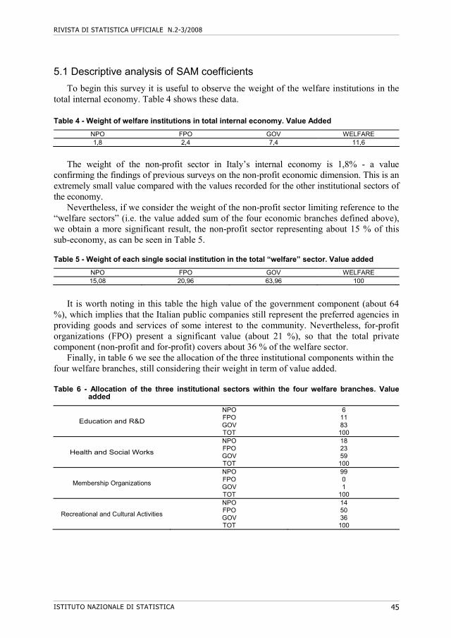
RIVISTA DI STATISTICA UFFICIALE N.2-3/2008
ISTITUTO NAZIONALE DI STATISTICA 45
5.1 Descriptive analysis of SAM coefficients
To begin this survey it is useful to observe the weight of the welfare institutions in the total internal economy. Table 4 shows these data. Table 4 - Weight of welfare institutions in total internal economy. Value Added
NPO FPO GOV WELFARE 1,8 2,4 7,4 11,6
The weight of the non-profit sector in Italy’s internal economy is 1,8% - a value
confirming the findings of previous surveys on the non-profit economic dimension. This is an extremely small value compared with the values recorded for the other institutional sectors of the economy.
Nevertheless, if we consider the weight of the non-profit sector limiting reference to the “welfare sectors” (i.e. the value added sum of the four economic branches defined above), we obtain a more significant result, the non-profit sector representing about 15 % of this sub-economy, as can be seen in Table 5.
Table 5 - Weight of each single social institution in the total “welfare” sector. Value added
NPO FPO GOV WELFARE 15,08 20,96 63,96 100
It is worth noting in this table the high value of the government component (about 64
%), which implies that the Italian public companies still represent the preferred agencies in providing goods and services of some interest to the community. Nevertheless, for-profit organizations (FPO) present a significant value (about 21 %), so that the total private component (non-profit and for-profit) covers about 36 % of the welfare sector.
Finally, in table 6 we see the allocation of the three institutional components within the four welfare branches, still considering their weight in term of value added.
Table 6 - Allocation of the three institutional sectors within the four welfare branches. Value
added
Education and R&D
NPO FPO GOV TOT
6 11 83 100
Health and Social Works
NPO FPO GOV TOT
18 23 59 100
Membership Organizations
NPO FPO GOV TOT
99 0 1
100
Recreational and Cultural Activities
NPO FPO GOV TOT
14 50 36 100

THE INTEGRATION OF THE NON-PROFIT SECTOR IN A SOCIAL ACCOUNTING MATRIX.…
ISTITUTO NAZIONALE DI STATISTICA 46
It will immediately be observed that the non-profit sector is largely predominant in the “Membership Organizations” branch, where it covers 99 % of the entire value added of the branch. Here, in fact, we find the largest share of the NPISH (non-profit institutions serving households) which represent, generally speaking, the vast, heterogeneous world of associations. The “Education and R&D” branch shows the smallest presence of non-profit institutions (6 %) while showing an overwhelming presence of public provision (83 %). Considerable incidence of non-profit institutions can be seen in the “Health and Social Works” (18 %) and “Recreational and cultural activities” (14%) branches, where, significantly, for-profit institutions reach a weight of 50 %.
To conclude this section, it can be said that: the more “private” goods and services’ attributes there are, the smaller is the public provision and, vice versa, the more “collective” good and services’ attributes there are, the smaller is the private provision. 5.1.1 The matrix of costs
Having analysed the institutional composition of the welfare mix, I now go on to focus on survey of the “costs structure” for each institutional typology. In this section I am particularly interested in the measurement of labour and capital intensity of each institutions. This is useful to identify the specific differences emerging in the way these three institutions “do welfare”.
Table 7 - Institutional Composition of SAM production costs split into: compensations of
employees (W), gross operating surplus (P), intermediate costs (CI), net indirect taxation plus imports (IIN+IMP)
CI W P IIN+IMP Totale
Education and R&D
NPO FPO GOV
0,32 0,35 0,12
0,53 0,33 0,78
0,12 0,27 0,07
0,03 0,04 0,03
1 1 1
Health and Social Works
NPO FPO GOV
0,31 0,28 0,33
0,54 0,04 0,60
0,14 0,66 0,03
0,02 0,02 0,04
1 1 1
Membership Organizations
NPO FPO GOV
0,34 -
0,28
0,37 -
0,61
0,26 -
0,08
0,02 -
0,03
1 1 1
Recreational and Cultural Activities
NPO FPO GOV
0,47 0,30 0,28
0,25 0,08 0,28
0,25 0,16 0,41
0,03 0,46 0,04
1 1 1
With table 7 we can compare the structural costs of institutions within the four welfare
branches defined above. As is immediately evident, the non-profit sector shows a high “labour intensity” coefficient in all branches. In fact, the level of the W coefficient (i.e. compensations of employees) reaches a value of 54 % of total costs in the “Health and Social Works” branch. This is followed respectively by the “Education and R&D” branch (with a value of 53 %), the “Membership Organizations” branch (with a value of 37 %) and, finally, the “Recreational and Cultural Activities” branch (with a value of 25 %). In the row of the for-profit sector we find the results inverted, with a marked degree of “capital intensity” coefficients and low labour factor costs. In particular we can observe that the maximum incidence of capital costs here appears in the “Health and Social Works” branch, with a value of 66 % of total costs. The government component, on the other hand, always presents the more “labour intensive” structure with W values generally exceeding 50 % of
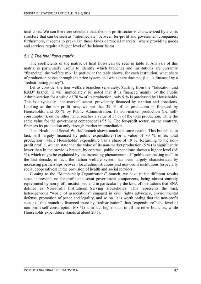
RIVISTA DI STATISTICA UFFICIALE N.2-3/2008
ISTITUTO NAZIONALE DI STATISTICA 47
total costs. We can therefore conclude that: the non-profit sector is characterized by a costs structure that can be seen as “intermediate” between for-profit and government companies; furthermore, it seems to prevail in those kinds of “social markets” where providing goods and services require a higher level of the labour factor. 5.1.2 The final flows matrix
The coefficients of the matrix of final flows can be seen in table 8. Analysis of this matrix is particularly useful to identify which branches and institutions are currently “financing” the welfare mix. In particular the table shows, for each institution, what share of production passes through the price system and what share does not (i.e., is financed by a “redistributing policy”).
Let us consider the four welfare branches separately. Starting from the “Education and R&D” branch, it will immediately be noted that it is financed mainly by the Public Administration for a value of 78 % of its production; only 9 % is purchased by Households. This is a typically “non-market” sector, prevalently financed by taxation and donations. Looking at the non-profit row, we see that 39 % of its production in financed by Households, and 35 % by Public Administration. Its non-market production (i.e. self-consumption), on the other hand, reaches a value of 35 % of the total production, while the same value for the government component is 95 %. The for-profit sector, on the contrary, finances its production only through market intermediation.
The “Health and Social Works” branch shows much the same results. This branch is, in fact, still largely financed by public expenditure (for a value of 80 % of its total production), while Households’ expenditure has a share of 19 %. Returning to the non-profit profile, we can state that the value of its non-market production (5 %) is significantly lower than in the previous branch; by contrast, public expenditure shows a higher level (65 %), which might be explained by the increasing phenomenon of “public contracting out”: in the last decade, in fact, the Italian welfare system has been largely characterized by increasing partnerships between local administrations and non-profit institutions (especially social cooperatives) in the provision of health and social services.
Coming to the “Membership Organizations” branch, we have rather different results since it presents no for-profit and scant government components, being almost entirely represented by non-profit institutions, and in particular by the kind of institutions that SNA defined as Non-Profit Institutions Serving Households. This represents the vast, heterogeneous “world of associations” engaged in civil rights advocacy, environmental defense, promotion of peace and legality, and so on. It is worth noting that the non-profit sector of this branch is financed more by “redistribution” than “expenditure”: the level of non-profit self consumption (68 %) is in fact higher than in all the other branches, while Households expenditure stands at about 20 %.
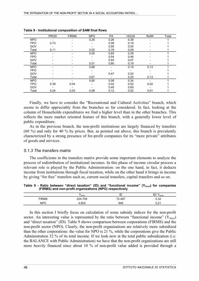
THE INTEGRATION OF THE NON-PROFIT SECTOR IN A SOCIAL ACCOUNTING MATRIX.…
ISTITUTO NAZIONALE DI STATISTICA 48
Table 8 - Institutional composition of SAM final flows
PROD FIRMS NPO PA HOUS RofW Total NPO FPO GOV Total
- 0,73
- 0,11
- - - -
0,35 - -
0,02
0,26 0,08 0,95 0,78
0,39 0,19 0,05 0,09
- - - -
1 1 1 1
NPO FPO GOV Total
- - - -
- - - -
0,05 - -
0,01
0,65 0,54 0,93 0,80
0,29 0,46 0,07 0,19
- - - -
1 1 1 1
NPO FPO GOV Total
- - - -
- - - -
0,68 - -
0,67
- -
0,47 -
0,19 -
0,53 0,20
0,13 - -
0,13
1 1 1 1
NPO FPO GOV Total
- 0,39
- 0,24
- 0,04
- 0,03
0,60 - -
0,08
0,06 0,02 0,40 0,12
0,34 0,52 0,60 0,52
- 0,02
- 0,01
1 1 1 1
Finally, we have to consider the “Recreational and Cultural Activities” branch, which
seems to differ appreciably from the branches so far considered. In fact, looking at the column of Households expenditures we find a higher level than in the other branches. This reflects the more market oriented feature of this branch, with a generally lower level of public expenditure.
As in the previous branch, the non-profit institutions are largely financed by transfers (60 %) and only for 40 % by prices. But, as pointed out above, this branch is prevalently characterized by a strong presence of for-profit companies for its “more private” attributes of goods and services. 5.1.3 The transfers matrix
The coefficients in the transfers matrix provide some important elements to analyze the process of redistribution of institutional incomes. In this phase of income circular process a relevant role is played by the Public Administration: on the one hand, in fact, it deducts income from institutions through fiscal taxation, while on the other hand it brings in income by giving “for free” transfers such as, current social transfers, capital transfers and so on. Table 9 - Ratio between “direct taxation” (ID) and “functional income” (Yfunct) for companies
(FIRMS) and non-profit organizations (NPO) respectively
Yfunct ID ID/ Yfunct
FIRMS
NPO
224.709
4.603
72.497
949
0,32
0,21
In this section I briefly focus on calculation of some subsidy indices for the non-profit
sector. An interesting value is represented by the ratio between “functional income” (Yfunct) and “direct taxation” (ID). Table 9 shows comparison between corporations (FIRMS) and the non-profit sector (NPO). Clearly, the non-profit organizations are relatively more subsidized than the other corporations: the value for NPO is 21 %, while the corporations give the Public Administration 32 % of its total income. If we look now at the total public subsidization (i.e. the BALANCE with Public Administration) we have that the non-profit organizations are still more heavily financed since about 10 % of non-profit value added is provided through a

RIVISTA DI STATISTICA UFFICIALE N.2-3/2008
ISTITUTO NAZIONALE DI STATISTICA 49
positive balance with the public administration. On the contrary, the value for corporations is negative (-0,11). Moreover, it is worth noting that the “total SAM balance” for the non-profit sector is positive, amounting to 12 % of its total value added. Table 10 - Ratio between “balance with Public Administration” (SPA) and “value added” (VA) for
FIRMS and NPO
PILpm SPA SPA/PILpm
FIRMS 2.091.850 -52.095 -0,02
NPO 36.315 +3.872 +0,11
What, however, is to be said of the redistributing role played by the non-profit sector?
With the transfers matrix we can calculate a “solidarity index” related to the non-profit sector, which we can identify in the share of non-profit production that does not pass through the prices system but is transferred directly “for free” to the final consumers (i.e., non-market production). This part of production is financed through the subsidization we find in this matrix. Table 11 presents comparison with the government sector.
The last row of the table shows that 36 % of the non-profit production is “non-market production”, so we can conclude that the non-profit organizations not only operate and have to survive in a competitive environment (led by the prices system), but also play a significant “redistributing role” allowing people to access the same social goods and services regardless of their income level8.
5.2 Simulation analysis: the employment effects of fiscal policy
As we observed above, the non-profit sector shows a markedly labor intensive productive structure. Furthermore, we also saw that it presents strong linkage with the public sector financing through expenditure and transfers a reliable part of its production. Starting from this point, a step forward is to consider, in a simple simulating model, the effects of government fiscal policy on non-profit sector employment capacity. In this sense, we can calculate, through the SAM viewed as a “policy model”, the value of elasticity between “public expenditure”, “public transfers” and “non-profit income”. Furthermore, it seems particularly useful to compare these results with those regarding the for-profit component of the welfare mix (both being “private institutions”). Nevertheless, before setting out the results obtained in simulation analysis, it seems worthwhile to keep in mind the hypothesis underlying the SAM as a “policy model”, that is:
1. fixed prices; 2. unutilised productive capacity; 3. constant multipliers.
8 This is the precise definition of “universal provision” of social commodities (see Barbetta, 1996).
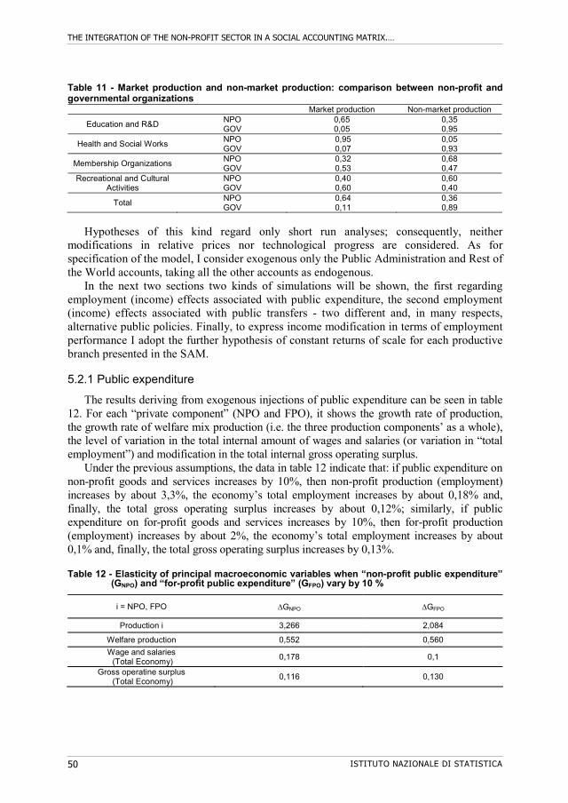
THE INTEGRATION OF THE NON-PROFIT SECTOR IN A SOCIAL ACCOUNTING MATRIX.…
ISTITUTO NAZIONALE DI STATISTICA 50
Table 11 - Market production and non-market production: comparison between non-profit and governmental organizations Market production Non-market production
Education and R&D NPO GOV
0,65 0,05
0,35 0,95
Health and Social Works NPO GOV
0,95 0,07
0,05 0,93
Membership Organizations NPO GOV
0,32 0,53
0,68 0,47
Recreational and Cultural Activities
NPO GOV
0,40 0,60
0,60 0,40
Total NPO GOV
0,64 0,11
0,36 0,89
Hypotheses of this kind regard only short run analyses; consequently, neither
modifications in relative prices nor technological progress are considered. As for specification of the model, I consider exogenous only the Public Administration and Rest of the World accounts, taking all the other accounts as endogenous.
In the next two sections two kinds of simulations will be shown, the first regarding employment (income) effects associated with public expenditure, the second employment (income) effects associated with public transfers - two different and, in many respects, alternative public policies. Finally, to express income modification in terms of employment performance I adopt the further hypothesis of constant returns of scale for each productive branch presented in the SAM. 5.2.1 Public expenditure
The results deriving from exogenous injections of public expenditure can be seen in table 12. For each “private component” (NPO and FPO), it shows the growth rate of production, the growth rate of welfare mix production (i.e. the three production components’ as a whole), the level of variation in the total internal amount of wages and salaries (or variation in “total employment”) and modification in the total internal gross operating surplus.
Under the previous assumptions, the data in table 12 indicate that: if public expenditure on non-profit goods and services increases by 10%, then non-profit production (employment) increases by about 3,3%, the economy’s total employment increases by about 0,18% and, finally, the total gross operating surplus increases by about 0,12%; similarly, if public expenditure on for-profit goods and services increases by 10%, then for-profit production (employment) increases by about 2%, the economy’s total employment increases by about 0,1% and, finally, the total gross operating surplus increases by 0,13%. Table 12 - Elasticity of principal macroeconomic variables when “non-profit public expenditure”
(GNPO) and “for-profit public expenditure” (GFPO) vary by 10 %
i = NPO, FPO GNPO GFPO
Production i 3,266 2,084
Welfare production 0,552 0,560
Wage and salaries (Total Economy)
0,178 0,1
Gross operatine surplus (Total Economy)
0,116 0,130
RIVISTA DI STATISTICA UFFICIALE N.2-3/2008
ISTITUTO NAZIONALE DI STATISTICA 51
We can conclude that: even if the non-profit sector is smaller than the for-profit sector it produces more extensive multiplicative effects in the total internal economy (and, in particular, in total rate of growth in employment).
This emerges more strongly if we consider the “absolute changes” in public expenditure, as shown in table 13 where we compare the performance of the three components. Finally, table 14 shows the effects of public expenditure for each non-profit welfare branch. As will immediately be seen, “Health and Social Works” proves the most dynamic branch with a growth rate of about 6,6% and a growth rate in total employment of about 1,7%. Immediately after it come the “Education and R&D”, “Membership Organizations” and “Recreational and Cultural Activities” branches respectively. 5.2.2 Public transfers
In this section we consider the employment effects of public transfers. As a first step it seems useful to compare the non-profit multiplicative effects relative to public transfers and public expenditure. Table 15 shows the results. The multiplicative effects of public expenditure are strictly higher than the effects of public transfers. Only the surplus (SNPO) increases more by transfers than by public expenditure. Table 16 illustrates the growth rate for non-profit welfare branches when public transfers increase by 10 %. We can observe that the more reactive branch is “Membership Organizations” (2,133), immediately followed by the “Recreational and Cultural Activities” (1,897), “Education and R&D” (1,124) and “Health and Social Works” (0,182) branches. Table 13 - Sectoral growth and total employment variation (%) when public expenditure stands at
1.000 for each institutional branch (FPO, NPO, GOV)
Sectoral growth Total employment GNPO = 1.000 1,831 0,1
GFPO = 1.000 1,134 0,05
GGOV = 1.000 0,504 0,123
The analysis set out above indicates that: within the Italian non-profit sector there exist
two different components, the first refers to those organizations more engaged in the market system; they present the common form of “entrepreneurial institutions” (such as the social cooperatives) typically linked to the public administrations through solid and constant partnerships; they are active especially in those sectors of the economy mainly characterized by a very large presence of merit, public and quasi-public goods and services (education services, daily care services, etc.).
The second component is essentially characterized by institutions of a less entrepreneurial, market oriented nature. They develop and grow mainly as a consequence of public subsidization. Italian NPISH operating in the field of environment protection, civil rights advocacy, arts and sports promotion and so on are largely present in this component.
THE INTEGRATION OF THE NON-PROFIT SECTOR IN A SOCIAL ACCOUNTING MATRIX.…
ISTITUTO NAZIONALE DI STATISTICA 52
6. Conclusions
The purpose and originality of this work lies in building a Social Accounting Matrix for the Italian welfare mix (on 1999 data) where the non-profit sector has been explicitly integrated. Thus the statistical-economic aim of this work can be considered largely fulfilled, despite difficulties in finding and systemizing data and information. Further analysis would serve to fill out the picture more completely, but it can be seen yet as a good panorama of the Italian welfare mix system. I believe this work represents three major steps forward from the previous surveys dealing with this subject:
1. The SAM presented previously effectively sums up the state of interactions among the
different institutional bodies acting in the Italian welfare mix system involved in the production, allocation and redistribution of resources. It offers a synoptic-descriptive scheme allowing for a more simplified reading of the data (it is only a 24x24 squared matrix) and a deeper knowledge of the “links” existing between the welfare mix and the rest of the economic system. Furthermore, the division of the social branches into the three components for-profit, non-profit and government, represents an absolute novelty in the literature. In fact, this aspect allows for immediate comparison among the dimensions, productive structure and other economic features characterizing the ways the three institutional components “do welfare”.
Table 14 - Sectoral growth and employment variation in non-profit welfare branches when public
expenditure increases by 10 % for each branch
GNPO = 10% Sectoral growth Total employment
Education and R&D 2,630 0,026
Health and Social Works 6,577 0,167
Membership Organizations 1,298 0,017
Recreational and Cultural Activities 0,588 0,005
Table 15 - Comparison between multiplicative effects of public expenditure and transfers in non-
profit growth rate and employment
NPO rate of growth Total employment NPO surplus variation TRNPO = 10% 1,129 0,063 3,130
GNPO = 10% 3,366 0,178 0,081
2. Another original aspect of this work is the way It introduces non-profit sector within the
SAM. Utilizing the ISTAT first census of Italian non-profit institutions, I have been able to build an initial economic account for non-profit sector to be integrated in the other institutional economic accounts (households, firms, etc.). This aspect can be seen as an initial assessment of a “satellite account” for the non-profit sector although it needs to be improved and extended by further analysis. Furthermore, the choice to consider the non-profit sector within the welfare mix system gives us a more significant representation of this sector for the purposes of comparison with the rest of the economy9.
9 It is interesting to note that several studies consider the non-profit sector comparing it to the total rest of the Italian
economy, whose non-profit is about 2 %. This leads to considering it not economically significant. However, considering the non-profit sector within the welfare sector, where it represents about 15 %, restores significance to our analysis.
RIVISTA DI STATISTICA UFFICIALE N.2-3/2008
ISTITUTO NAZIONALE DI STATISTICA 53
Table 16 - Effects of public transfers on growth in the non-profit welfare branches
TRNPO = 10% NPO sectoral rate of growth Education and R&D 1,124
Health and Social Works 0,182 Membership Organizations 2,133
Recreational and Cultural Activities 1,897
3. The last original element characterizing this contribution that I wish to draw attention to
is the use of SAM as a tool for policy planning. In fact, at the beginning of this work I noted that in the literature there was an absolute lack of a “macroeconomic policy tool” for the non-profit sector. This fact was partly explained by the quite total absence of reliable data sources before the ISTAT non-profit institution census. Furthermore, since there are no significant time series data for non-profit variables (useful, eventually, to estimate policy functional relations), building a SAM represented the only way to obtain a policy tool considering just one year of measurement (that is, 1999).
Clearly, this work also presents some limits, consisting in: (a) the scarcity of certain
data sources (several variables, such as “social contributions”, were not assessed in the ISTAT non-profit census); (b) a static version of simulating model (as a “Leontievian methodology”) and, finally, (c) the fixed prices hypothesis. Further analysis will be able to overcome these limits and propose useful extensions and improvements.
Finally, let us summarize the principal results we obtain in this work. For this purpose I claim to consider only some indicators of the SAM structure, thus: 1. with a share of value added of about 15% the third sector represents a significant
institutional agent in the Italian welfare mix; 2. if we compare the non-profit sector with the for-profit sector of the Italian welfare mix,
the non-profit sector proves the main partner chosen by the public administration in the process of “contracting out” the provision of social goods and services. In fact, the share of public expenditure for the non-profit sector is about 32 %, while it is about 20 % for the for-profit one;
3. within the “private sector” of the welfare mix, the non-profit sector is basically characterized by a strong labor intensive productive structure (the share of labor costs is 44 % of total costs for the non-profit sector while it is 12 % for the for-profit sector). This depends on the typical way the non-profit organizations “do welfare”: they prevail in that kind of social markets mainly characterized by elements such as relation, proximity, trust and so on, that require a major level of labour force instead of capital goods;
4. non-profit organizations provide about the 36 % of their production without charging significant fees. Thus, it plays a significant “redistribution role” in the Italian welfare economy;
5. finally, through the construction of a normative model, we tested the effects of fiscal policies (public expenditure and public transfers) on the level of non-profit activity and on the level of total employment. Even if the two policies are very different and alternative in many respects, they lead to claim that: the global employment effects generated through the non-profit activity is twice as high as that generated through for-profit sector activity; thus, the third sector appears to be a good tool for policy makers, also to address the problem of unemployment still existing in our society.
THE INTEGRATION OF THE NON-PROFIT SECTOR IN A SOCIAL ACCOUNTING MATRIX.…
ISTITUTO NAZIONALE DI STATISTICA 54
These are the main results of our analysis. As a consequence, we can conclude this article claiming that: development of the non-profit sector in modern economies (and especially in the Italian case) can be seen as a good strategy to take into account both the need for increasing externalization of the traditional public provision of social goods and services, and effectiveness in terms of solidarity and employment performance. Nevertheless, the non-profit sector can be legitimated to take on this role only if its ability to attract donations and voluntary labor and its economic activity pattern will be able to continue to exalt the perception of its “social utility” regards as the social preferences.
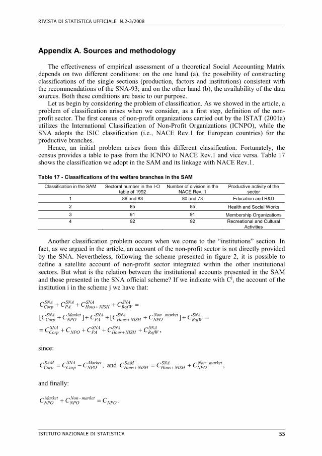
RIVISTA DI STATISTICA UFFICIALE N.2-3/2008
ISTITUTO NAZIONALE DI STATISTICA 55
Appendix A. Sources and methodology
The effectiveness of empirical assessment of a theoretical Social Accounting Matrix depends on two different conditions: on the one hand (a), the possibility of constructing classifications of the single sections (production, factors and institutions) consistent with the recommendations of the SNA-93; and on the other hand (b), the availability of the data sources. Both these conditions are basic to our purpose.
Let us begin by considering the problem of classification. As we showed in the article, a problem of classification arises when we consider, as a first step, definition of the non-profit sector. The first census of non-profit organizations carried out by the ISTAT (2001a) utilizes the International Classification of Non-Profit Organizations (ICNPO), while the SNA adopts the ISIC classification (i.e., NACE Rev.1 for European countries) for the productive branches.
Hence, an initial problem arises from this different classification. Fortunately, the census provides a table to pass from the ICNPO to NACE Rev.1 and vice versa. Table 17 shows the classification we adopt in the SAM and its linkage with NACE Rev.1. Table 17 - Classifications of the welfare branches in the SAM
Classification in the SAM Sectoral number in the I-O table of 1992
Number of division in the NACE Rev. 1
Productive activity of the sector
1 86 and 83 80 and 73 Education and R&D
2 85 85 Health and Social Works
3 91 91 Membership Organizations 4 92 92 Recreational and Cultural
Activities
Another classification problem occurs when we come to the “institutions” section. In
fact, as we argued in the article, an account of the non-profit sector is not directly provided by the SNA. Nevertheless, following the scheme presented in figure 2, it is possible to define a satellite account of non-profit sector integrated within the other institutional sectors. But what is the relation between the institutional accounts presented in the SAM and those presented in the SNA official scheme? If we indicate with Cj
i the account of the institution i in the scheme j we have that:
[ ] [ ]
,
SNA SNA SNA SNACorp PA Hous NISH RofW
SNA Market SNA SNA Non market SNACorp NPO PA Hous NISH NPO RofW
SNA SNA SNA SNACorp NPO PA Hous NISH RofW
C C C C
C C C C C C
C C C C C
since:
,SAM SNA MarketCorp Corp NPOC C C and ,SAM SNA Non market
Hous NISH Hous NISH NPOC C C
and finally:
Market Non marketNPO NPO NPOC C C .
THE INTEGRATION OF THE NON-PROFIT SECTOR IN A SOCIAL ACCOUNTING MATRIX.…
ISTITUTO NAZIONALE DI STATISTICA 56
Fortunately, the ISTAT census provides the economic variables of non-profit institutions according to its market and non-market component, so that we have no great difficulty in implementing the expression set out above. The previous considerations ensure the consistency of the SAM sections and eliminate the problem of “duplication” in institutional accounts of the SAM. We now have to consider the problem of estimating the theoretical SAM (see appendix B).
Let us begin with the methodology adopted to construct the Input-Output Table included in the SAM. For each branch defined as a “welfare branch” and illustrated in table 17, we have to extract the non-profit (NPO), for-profit (FPO), and government (GOV) component. For this purpose, we first write the following simple relation:
i i i iNPO GOV FPOX X X X ,
where i indicates the generic “welfare branch”. From this relation we can calculate estimation of the for-profit component as follows:
ˆnpo
i i i iFPO NA PAASA
X X X X , where: 1. i
NAX is derived by the national accounting assessments (see, in particular: ISTAT, 2001b; ISTAT, 2000b; MTBPE, 2000; and ISTAT, 2000c); 2. npo
iSA
X results by the satellite account of non-profit sector derived from the ISTAT census of non-profit institutions (see: ISTAT, 2001a). See the methodology set out in the article; 3. i
PAAX is obtained utilizing the data contained in the public administration accounts (see: ISTAT, 2000a; ISTAT, 2002b).
As regards the matrix of transfers, a standard construction methodology can be found in Zelli (1994), where the basic source is the non-financial accounts for institutional sectors (see: ISTAT, 2001c). It is not possible to explain here all the methodology followed to build this matrix, but it can be useful to describe the basic steps: 1. we start from the “non-financial accounts for institutional sectors” and, for each
institution, we build a more aggregated economic account distinguishing between entries and expenditures (that is, we have to re-construct all the “secondary distribution of income account”);
2. once we have obtained this account, for each flow in entries and in expenditures we have to establish precisely which institution it goes into and which institution it comes from;
RIVISTA DI STATISTICA UFFICIALE N.2-3/2008
ISTITUTO NAZIONALE DI STATISTICA 57
3. finally, we have to verify the consistency of these allocations noting whether the “balance” is respected for each institution (bearing in mind that the sum of all the institutions’ balances must come to zero); It is worth noting that this procedure also allows us to construct the functional income matrix .
Although these methodologies are statistically consistent, some of estimation problems
can arise, and ad hoc hypotheses must therefore be formulated. For a better understanding of this issue, let us consider separately the five SAM non-nil matrices10: 1. matrix of intermediate exchanges: there are no reliable sources for the data of this
matrix, and we must therefore hypothesize it as a nil-matrix. Furthermore, we consider that all the intermediate services and goods of the welfare branches are purchased in the fifth global branch called: “Rest of the Economy” (RofE);
2. matrix of primary costs: this does not present particular problems of estimation. Nevertheless, as the ISTAT census does not provide relevant variables such as the “social contributions” and the “consumption of fixed capital”, we consider only the “gross” remunerations of productive factors (labor and capital);
3. matrix of final flows: there being significant informative lacunae in the available sources, it is impossible to assess all the variables presented in the appendix B. The first significant lacuna we find in the non-profit census consists in the fact that it does not distinguish between the part of non-profit production purchased by the households and the part purchased by the firms (in the “production” section of the SAM). Hence, we choose to hypothesize that the households purchase all the non-profit private consumption. The same problem arises with government final uses. In this case, too, the official statistics only provide the distinction between “market” and “non-market production” without specifying the typology of the market production purchasers; as in the previous case, we took it that the households purchase all the government market production. With further analysis and new statistical surveys these limitations can be overcome, but in any case we believe that the markedly “final oriented nature” of the goods and services produced by the four welfare branches (and the three institutional typologies) considered in the SAM should not largely modify our analysis. In this respect we can assume our hypothesis to be sufficiently “robust”. Clearly, if a branch presented non-nil intermediate consumptions, we chose to identify them as goods and services produced solely by the for-profit institutions;
4. transfers matrix: in this matrix, too, we can find some lacunae in the data. As in the case of consumption, the ISTAT census again fails to differentiate between transfers “to” and “from” corporations, and transfers “to” and “from” households. These transfers are principally represented by donations so that we decided to consider them all as coming from households. Another limitation is the lack of distinction between capital and current transfers, since the census does not perform this kind of division;
5. functional distribution matrix: this matrix does not present any problems of assessment. We find all the functional incomes following the standard SNA methods.
10 To follow this part better, see the theoretical SAM scheme in appendix B.
THE INTEGRATION OF THE NON-PROFIT SECTOR IN A SOCIAL ACCOUNTING MATRIX.…
ISTITUTO NAZIONALE DI STATISTICA 58
Finally, various other estimation problems arise from the incompleteness of official statistics publications. In fact, “complete accountability” does not obtain for all the institutional typologies: except for the “Health and Social Works”, complete government accountability does not obtain for the other social branches. In particular we encountered some problems with the government component of the “Education and R&D” and “Recreational and Cultural Activities” branches. Fortunately we were able to reconstruct this basic information with cross-comparison of the data available in various ISTAT publications on the ISTAT web site (ISTAT, 2002a; 2002b).
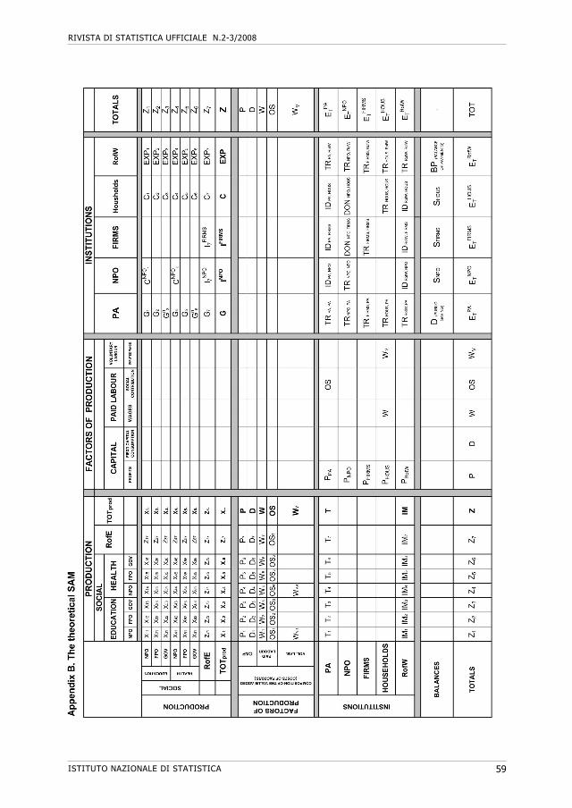
RIVISTA DI STATISTICA UFFICIALE N.2-3/2008
ISTITUTO NAZIONALE DI STATISTICA 59
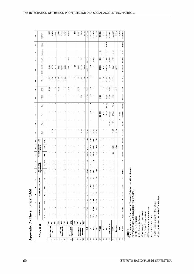
THE INTEGRATION OF THE NON-PROFIT SECTOR IN A SOCIAL ACCOUNTING MATRIX.…
ISTITUTO NAZIONALE DI STATISTICA 60
RIVISTA DI STATISTICA UFFICIALE N.2-3/2008
ISTITUTO NAZIONALE DI STATISTICA 61
References
Anheier H.K., Rudney G. (1996), “Satellite Accounts for Nonprofit Institutions: A proposal”, Paper prepared for the Second Biannual Research Conference of ISTR, Mexico City, July.
Anheier H.K., Rudnay G. (1998), “An input-output analysis of the nonprofit sector in the USA and Germany”, Annals of public and cooperative economics, vol. 69, n. 1, March.
Anheier H.K., Salamon L.M. (1998), “Nonprofit Institutions and the Household Sector” in: “Household Accounting: Experiences in the Use of Concepts and their Compilation”, vol. 1: “Household Sector Accounts”, United Nations Statistics Division, Studies in Methods, Series F, n.75, Handbook of National Accounting, New York.
Ascoli U., Pasquinelli S. (eds) (1993), Il welfare mix. Stato sociale e terzo settore, Franco Angeli, Milano.
Barbetta G. (1996), Senza scopo di lucro, Il Mulino, Bologna.
Bauer R. (1990), “Voluntary welfare associations in Germany and the United States: theses on the historical development of intermediary systems”, Voluntas, vol. 1, n. 1, Manchester United Press, Manchester.
Ben-Ner A., Van Hoomissen T. (1991), “Non-profit organizations in the mixed economy”, Annals of Public and Cooperative Economics, vol. 62, pp. 519-550 .
Borzaga C., Mittone L. (1997), “The multi-stakeholders versus the non-profit organisation”, Discussion paper n. 7, University of Trento.
Cuicchio S., Malizia R., Zamaro N. (2001), “The Handbook on Nonprofit Institutions. Report on the Italian Pilot Test Results”, Roma, mimeo.
Defourny J., Thorbecke E. (1984), “Structural path analysis and multiplier decomposition within a social accounting matrix framework”, Economic Journal, vol. 94, pp. 111-136.
Defourny J. (2001), “From the third sector to the social enterprise”, in Borzaga C., Defourny J. (eds.), The Emergence of social enterprise, Routledge, London.
Eurostat (1995), European system of accounts, Luxembourg.
Evers A., Wintersberger H. (eds.) (1990), “Shifts in the welfare mix. Their impact on work, social services and welfare policies”, Frankfurt/Boulder Campus/Westview.
Hansmann H. (1980), “The role of non-profit enterprise”, Yale Law Journal, vol. 89, pp. 835-901.
Hansmann H. (1989), “The two non-profit sectors: fee for services versus donative organizations”, in Hodgkinson V.A., Lyman R.W. (eds), The future of the non-profit sector, Jossey-Bass Publishers, San Francisco.
ISTAT (2000a), “Conti economici consolidati delle Amministrazioni Pubbliche e della protezione sociale”, in MTBPE (2000), vol. I.
ISTAT (2000b), “Tavola intersettoriale dell’economia italiana - anno 1992”, Informazioni, n. 22.
ISTAT (2000c), “Contabilità nazionale. Tomo 1. Conti economici nazionali anni 1982-98”, Informazioni, n. 4.
THE INTEGRATION OF THE NON-PROFIT SECTOR IN A SOCIAL ACCOUNTING MATRIX.…
ISTITUTO NAZIONALE DI STATISTICA 62
ISTAT (2001a), “Istituzioni non-profit in Italia. I risultati della prima rilevazione censuaria -Anno 1999”, Informazioni, n.50.
ISTAT (2001b), Compendio statistico italiano 2000, ISTAT.
ISTAT (2001c), “Conti economici non-finanziari per settore istituzionale – 1999”, in ISTAT (2002b).
ISTAT (2002a), Data banks, database accessed at the website www.istat.it.
ISTAT (2002b), Economy, database accessed at the website www.istat.it.
James E. (1989), The non-profit Sector in international perspective, Oxford University Press, New York/Oxford.
Laville J.L. (1994), L’economie solidaire, Desclée de Brouwer, Paris.
Lombardi E. et al. (1999), “Working in the third sector. Handbook on work organisation in social enterprise”, Lunaria.
Lunaria (1999), “New employment opportunities in third sector”, University of Rome La Sapienza.
Marcon G., Mellano M. (eds.) (2000), The Economics of the Third Sector. Size, structure and Political Economy, Editrice La Sapienza.
Mertens S. (2000), “A satellite account of Non-profit organizations: principles and lessons from a pilot test in Belgium”, Working Draft, Centre of Social Economy, University of Liège.
Mertens S. (2004), “Le compte satellite des associations en Belgique”, Revue internationale de l'économie sociale, n. 292, pp. 42-58.
Messina A., Riccioni S. (2000), “The economic account of non-profit institutions serving households”, Paper presented at the XV° Voorburg Group meeting on service statistics, Madrid, 18-22 September.
MTBPE - Ministero del Tesoro, del Bilancio e della Programmazione Economica (2000), “Relazione generale sulla situazione economica del paese – 1999”, vol. I, II, III.
Pyatt G. (1988), “A SAM approach to modelling”, Journal of policy modelling, vol.10, n. 3.
Salamon L.M., Anheier H.K. (1997), “Defining the non-profit sector. A cross national analysis”, Manchester University Press, Manchester.
Timpano F. (1997), “Il non-profit e le matrici di contabilità sociale”, dattiloscritto, Facoltà di Economia, Università Cattolica di Piacenza.
United Nations (1993), System of national accounts, N.Y..
United Nations, Johns Hopkins University, London School of Economics (2001), “Handbook on Nonprofit Institutions in the System of National Accounts”, mimeo, New York.
Van Til J. (1988), “Mapping the third sector. Voluntarism in a changing social economy”, The Foundation Center, New York.
Weisbrod B.A. (1975), “Toward a theory of the voluntary non-profit sector in a three sector economy”, in Phelps E. (ed.), Altruism, morality and economic theory, Russel Sage Foundation, N.Y.

RIVISTA DI STATISTICA UFFICIALE N.2-3/2008
ISTITUTO NAZIONALE DI STATISTICA 63
Weisbrod B.A. (1988), The Non-profit Economy, Harvard University Press, Cambridge, Massachusetts.
Young P.C. (1993), Non-profit institutions in an input-output framework, Voluntas, vol. 4, n. 4.
Zelli R. (1994), “Costruzione di una SAM con il ricorso ai dati di contabilità nazionale: un’applicazione per l’Italia”, Dipartimento di contabilità nazionale e analisi dei processi sociali, Università degli studi di Roma La Sapienza, Ricerche, n. 8.


RIVISTA DI STATISTICA UFFICIALE N.2-3/2008
ISTITUTO NAZIONALE DI STATISTICA 65
L’impatto delle politiche fiscali attraverso l’integrazione fra un modello di micro simulazione ed un modello biregionale macro/mesoeconomico1
Renato Paniccià2, Nicola Sciclone 3,
Sommario
L’articolo ha per obiettivo la quantificazione degli impatti distributivi e sulla crescita di politiche fiscali attraverso l’utilizzo dell’integrazione fra un modello di microsimulazione dei redditi familiari ed un modello macro/meso economico basata su una SAM biregionale Toscana-Resto d’Italia. Lo scopo di tale integrazione è superare i limiti dei due strumenti quantitativi: da un lato i modelli di microsimulazione non colgono le interazioni fra settori instituzionali mentre la modellizzazione macro/meso non stima in modo completo gli effetti distributivi diretti delle politiche fiscali. In questo articolo i due modelli sono interrelati in modo simultaneo a differenza del link recursivo utilizzato nella maggior parte degli studi presenti in letteratura. Il caso di studio è costituto dall’introduzione di un’ipotetica flat tax ed i risultati dell’impatto, derivati dall’utilizzo del modello integrato, mostrano una maggiore completezza rispetto alle stime fornite dall’utilizzo separato dei due modelli. Abstract
This study aims at testing an integrated model to estimating the economic impact of fiscal policies. The integration relies on linking a micro simulation model and a macro/meso model based on a biregional SAM (Tuscany-Rest of Italy). This connection represents an attempt to overcome the limits of both models, when they are separately running. Indeed micro models do not take into account all the interactions amongst institutional sectors while macro/meso models estimates those flows but they are not able to capture the direct effects on income distribution within households properly. In this article the two models have been connected simultaneously, unlike the majority of the approaches found in the literature, where this linkage has been performed recursively. The integrated model has been utilized to estimate the impact on both income distribution and growth of a flat income tax rate reform. The exercise has shown that the linked model provides a more complete impact estimate than the results coming from the two models running separately.
1 Questo articolo costituisce un aggiornamento del lavoro “Un approccio micro-macro alla stima dell’impatto regionale e nazionale di politiche fiscali” di R.Paniccià e N.Sciclone, presente in: Il Finanziamento del Settore Pubblico a cura di G.Brosio e G.Muraro F. Angeli 2006. I cambiamenti principali hanno riguardato: i) l’anno di riferimento (2003 in luogo del 2002) ii) il dataset micro (Eu-Silc in luogo della rilevazione Banca d’Italia) iii) una nuova stima della funzione del consumo iv) l’utilizzo delle matrici Supply and Use nella parte I-O della SAM.
Gli autori desiderano ringraziare Stefano Casini Benvenuti, Renata Targetti Lenti e Dino Martellato per gli utili suggerimenti ad una versione preliminare dell’articolo presentata al convegno sulle matrici di contabilità sociale organizzato a Roma da ISCONA il 30-3-2007. Resta la sola responsabilità degli autori riguardo il contenuto dell’articolo.
2 Ricercatore (Istituto Regionale Programmazione Economica della Toscana), e-mail: [email protected]. 3 Ricercatore (Istituto Regionale Programmazione Economica della Toscana), e-mail: [email protected].
L’IMPATTO DELLE POLITICHE FISCALI ATTRAVERSO L’INTEGRAZIONE FRA UN MODELLO DI MICROSIMULAZIONE…
ISTITUTO NAZIONALE DI STATISTICA 66
Introduzione
L’impatto di politiche fiscali è solitamente condotto adottando due diversi tipi di approccio. Il primo, basato su modelli di microsimulazione (sempre più utilizzati negli anni recenti) ha per obiettivo la quantificazione degli impatti distributivi e delle diverse misurazioni di povertà. Ciò deriva dalla natura stessa dei modelli di microsimulazione: essi operano in contesti di equilibrio parziale e stimano principalmente gli effetti diretti delle politiche fiscali, escludendo dalla quantificazione i feed backs (effetti indiretti) dovuti all’interazione con gli altri settori istituzionali. L’approccio macro/mesoeconomico è interessato soprattutto all’impatto sulla crescita ed all’effetto sull’equilibrio macroeconomico interno ed esterno. I modelli macro/meso presentano il vantaggio della coerenza contabile e della quantificazione di (quasi) tutte le relazioni fra i settori istituzionali; tuttavia essi trascurano, o colgono solo in parte (distribuzione between groups) la causalità innescata dai cambiamenti distributivi direttamente connessi alla politica fiscale. Il presente lavoro sperimenta un approccio che integra, non solo contabilmente, ma soprattutto nell’analisi d’impatto, il modello di microsimulazione microReg con un modello mesoeconomico che origina da una matrice di contabilità sociale (SAM) biregionale Toscana-Resto d’Italia. L’esercizio utilizzato per testare questa integrazione riguarda la valutazione dell’impatto, sulla distribuzione dei redditi e sulla crescita, di una riforma del sistema di tassazione ispirata al modello flat tax rate. L’integrazione proposta costituisce un tentativo di superare i limiti che i modelli micro e macro presentano quando sono impiegati, l’uno, separatamente dall’altro. Essa dovrebbe quindi consentire di catturare gli effetti moltiplicativi (modello meso) derivanti da uno shock esogeno -come potrebbe essere considerata una riforma fiscale- preservando e capitalizzando le micro informazioni sulla distribuzione dei redditi familiari (modello micro), al fine di pervenire ad una stima completa e non distorta dell’effetto diretto. Il paper è organizzato in cinque sezioni. Nella prima sarà svolta una rassegna dei principali approcci di integrazione micro-macro proposti dalla letteratura; nella sezione successiva si presenterà il modello di microsimulazione; nella terza sezione si descriveranno il modello macroeconomico basato sulla SAM e la procedura di integrazione contabile utilizzata. Nella quarta sezione si illustrerà la procedura di integrazione modellistica mentre nella quinta si utilizzerà tale procedura per stimare l’impatto redistributivo e sulla crescita di una politica fiscale flat tax per la Toscana ed il Resto d’Italia.

RIVISTA DI STATISTICA UFFICIALE N.2-3/2008
ISTITUTO NAZIONALE DI STATISTICA 67
1. Il quadro metodologico
I tentativi di integrare – nel campo dell’analisi distributiva- i modelli micro con quelli macro hanno registrato negli ultimi anni un significativo incremento.
Le sollecitazioni all’attuazione di tale integrazione provengono da due direzioni. In primo luogo dalla critica all’utilizzo dell’ipotesi dell’agente rappresentativo nei
modelli macroeconomomici (Blinder 1975, Stoker 1986), soprattutto nella specificazione della stima e nell’utilizzo delle equazioni aggregate del consumo delle famiglie, poiché il processo di aggregazione (e quindi la distribuzione) dei singoli agenti non è neutrale nella stima dell’aggregato macroeconomico. In secondo luogo dalla citata incompletezza dell’impatto proveniente dai modelli di microsimulazione.
I tentativi di integrazione si distinguono, da un lato, per la natura endogena o esogena della distribuzione within-groups e, dall’altro, per le caratteristiche recursive o simultanee dell’interazione micro-macro.
Il primo esempio, forse tra i più conosciuti in letteratura, di integrazione con distribuzione within-groups esogena è quello di Adelman e Robinson (1978), ripreso successivamente da Dervis et al. (1982). Esso è basato sul concetto di Representative Household (RH4) e le caratteristiche principali sono così sintetizzabili: i) i modelli macro/meso sono CGE (Computable General Equilibrium Model) ii) le informazioni tratte dalle indagini sui bilanci familiari sono utilizzate per stimare una distribuzione within, attraverso la stima dei parametri di una funzione di probabilità (spesso lognormale o beta5). La suddetta distribuzione è tuttavia esogena, con i valori medi del reddito o del consumo che si distribuiscono within RH forniti dal modello CGE.
Una estensione di questo approccio, che ha il vantaggio di endogenizzare la distribuzione within, è quello presentato nei modelli 123PRSP (Devarajan, Go 2005) e IMMPA (Agenor et al. 2003), nei quali le famiglie del campione sono inserite nel CGE. Il sistema è recursivo nel senso macro-micro: infatti, il modello CGE6 fornisce le variazioni dei redditi che vengono assegnate uniformemente alle famiglie secondo caratteristiche specifiche di aggregazione (ad esempio, stato del capofamiglia).
Nella recente proposta metodologica di Bourguignon et al. (2002) il focus non è invece nel modulo macroeconomico, bensì in quello di microsimulazione: infatti la soluzione del modello CGE fornisce un vettore di prezzi, salari e variabili relative all’occupazione, che il modello di microsimulazione utilizza per generare variazioni nei salari, nei redditi da lavoro autonomo e nello status occupazionale, in modo coerente con il set di macro variabili generato dal modello CGE. In questo schema non si prevedono feed backs micro-macro; tuttavia esso ha il vantaggio di endogenizzare, come nei citati modelli 123PRSP e IMMPA, la distribuzione del reddito within-groups. Bourguignon et al. dimostrano –nel loro lavoro- anche la rilevanza di tale endogenizzazione nel determinare la variazione degli indici di disuguaglianza in risposta a shocks esogeni7.
4 Una RH corrisponde ad una aggregazione di famiglie definite secondo una particolare caratteristica (sociale,
geografica, demografica, ecc.). Per una rassegna su gli ultimi sviluppi metodologici si rinvia a Lofgren et al (2005) 5 Normalmente vengono utilizzate distribuzioni lognormali, ma in Decaluwè et al. (1999), ad esempio, sono state
utilizzate funzioni beta 6 Una rassegna abbastanza esaustiva dei metodi di integrazione macro-micro recursivi basati su CGE si trova in Essama
et al. (2005). 7 Fra gli esercizi svolti vi è la stima dell’impatto di una svalutazione: nello scenario “balanced closure”, utilizzando una
distribuzione within-groups esogena, si ha un incremento del Gini di 0,6 punti, mentre utilizzando la versione within groups endogena tale indice diminuisce addirittura di 1,1 punti.
L’IMPATTO DELLE POLITICHE FISCALI ATTRAVERSO L’INTEGRAZIONE FRA UN MODELLO DI MICROSIMULAZIONE…
ISTITUTO NAZIONALE DI STATISTICA 68
La simultaneità ed endogenizzazione della distribuzione intra-gruppo della simulazione micro-macro può essere invece rintracciata in tre differenti modellizzazioni.
Un primo esempio è quello di Savard (2003), nel quale un modello CGE fornisce un vettore di prezzi al modello micro, che a sua volta restituisce al CGE la variazione aggregata delle funzioni di spesa.
Una integrazione simultanea è utilizzata, nel modello MOSED della Banca d’Italia (Brandolini et al. 1993): in questo caso il modello di microsimulazione sostituisce l’equazione del consumo del modello macroeconometrico. Il tentativo nasce dall’esigenza di tener conto, nella specificazione di tale equazione, dell’effetto distributivo8 che è riconosciuto come significativo nella determinazione del consumo aggregato. Il modello macroeconometrico a sua volta fornisce al modello micro le componenti di reddito da attribuire uniformemente alla singole famiglie, in base a caratteristiche coerenti con le variabili macro.
Un tentativo di integrazione simile è stato introdotto infine da Cameron, Ezzeddin (2000). Il modello macro utilizzato è del tipo Input-Output dove reddito disponibile e consumo delle famiglie vengono endogenizzati tramite un modello di microsimulazione.
Quest’ultimo approccio in particolare costituirà il punto di riferimento utilizzato nell’esercizio proposto. 2. Il modello di microsimulazione
Il modello di microsimulazione impiegato nel presente lavoro9 (microReg) si colloca nella famiglia dei modelli statici: nel confronto fra lo scenario a legislazione vigente e gli scenari simulati, non sono pertanto previsti cambiamenti né della struttura della popolazione né del comportamento degli operatori. L’obiettivo è quello di ricostruire la distribuzione dei redditi al lordo dell’imposizione diretta e quindi valutare l’impatto dei principali provvedimenti di politica economica sui bilanci individuali e familiari. .
Il modello utilizza come basa campionaria l’indagine sui redditi e le condizioni di vita (EU-SILC) condotta nel 2004 dall’Istat.
La soluzione utilizzata per lordizzare i redditi netti consiste nella costruzione del seguente algoritmo iterativo:
i) alla prima iterazione (s=1) ad ogni osservazione i del campione è associata una stima del reddito lordo, sfruttando la seguente relazione
[1])si,t(1
ionarioynettocampylordo
con i=1,…n individui; s=1
8 Un filone di questo approccio che risponde alla critica sull’utilizzo dell’agente rappresentativo mutua all’interno di
alcune funzione del modello macroeconometrico i parametri distributivi che consentono di inglobare nella funzione del consumo l’effetto distributivo. Una applicazione di tale filone si può trovare ad esempio in Golinelli e Mantovani (1992).
9 Per una esauriente descrizione ed una successiva applicazione del modello si rinvia a Maitino- Sciclone (2008) e Sciclone (2008)

RIVISTA DI STATISTICA UFFICIALE N.2-3/2008
ISTITUTO NAZIONALE DI STATISTICA 69
tt si , è l’aliquota media (rapporto fra imposta netta e reddito lordo) fissata
arbitrariamente, anche se naturalmente ad un valore prossimo a quello vero, ed uguale per
tutti gli individui10.
ii) al reddito lordo così ricavato, sempre nella prima iterazione (s=1), è applicata tutta la normativa fiscale, deduzioni e detrazioni incluse, in modo da ottenere un nuovo valore del reddito netto ( oRegynettomicr )
[2] )t-(1 ylordooRegynettomicr si,is,i i=1,..n individui; s=1
con ts ,it aliquota media effettiva ottenuta dalla applicazione di tutte le regole di
esazione11 iii) infine, sempre nella prima iterazione (s=1), oRegynettomicr è posto a confronto con
ionarioynettocamp .
[3] (ynettocampionarioi,s-ynettomicroRegi,s) = controllo
Se i due valori del reddito netto, quello campionario e quello microsimulato, non sono sufficientemente vicini allora si procede -iterando- ad una nuova stima del reddito lordo (s>1), correggendo come segue il valore dell’aliquota media dell’equazione [1]
[4] )gReoynettomicr
ionarioynettocamp*(tt
i
i
1s,ii,s s>1
La procedura si arresta quando per tutte le osservazioni campionarie la differenza fra i
valori originali e microsimulati del reddito netto (controllo) è, in valore assoluto, inferiore a 20 euro. Nei casi in cui l’algoritmo non converga12 dopo un certo numero di iterazioni, scelto arbitrariamente13, la procedura parte con un differente valore -estratto casualmente da una distribuzione uniforme definita nell’intervallo 0-1 – dell’aliquota media nell’eq. [1]. Le seguenti tabelle confrontano, a fini di validazione, i dati che si ottengono da microReg con
10 L’informazione sull’aliquota media può essere desunta dai dati del Ministero delle Finanze o ricavata da altri modelli
di microsimulazione 11 In altri termini, ad ogni osservazione corrisponderà un diverso valore dell’aliquota media (che non sarà più quella
iniziale), in funzione dei valori dell’irpef netta ricavati dall’applicazione delle regole fiscali e del reddito lordo stimato nella prima iterazione.
12 A causa della complessità e non linearità del sistema fiscale, ad un unico valore del reddito netto possono corrispondere più valori del reddito lordo.
13 Nel nostro caso 1.000 iterazioni
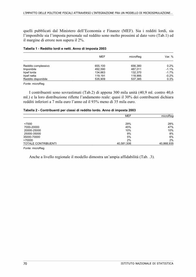
L’IMPATTO DELLE POLITICHE FISCALI ATTRAVERSO L’INTEGRAZIONE FRA UN MODELLO DI MICROSIMULAZIONE…
ISTITUTO NAZIONALE DI STATISTICA 70
quelli pubblicati dal Ministero dell’Economia e Finanze (MEF). Sia i redditi lordi, sia l’imponibile sia l’imposta personale sul reddito sono molto prossimi al dato vero (Tab.1) ed il margine di errore non supera il 2%.
Tabella 1 - Reddito lordi e netti. Anno di imposta 2003
MEF microReg Var. %
Reddito complessivo 655,100 656,380 0.2%Imponibile 492,590 487,011 -1.1%Irpef lorda 134,663 132,370 -1.7%Irpef netta 119,191 118,995 -0.2%Reddito disponibile 535,909 537,385 0.3%
Fonte: microReg
I contribuenti sono sovrastimati (Tab.2) di appena 300 mila unità (40,9 ml. contro 40,6
ml.) e la loro distribuzione riflette l’andamento reale: quasi il 30% dei contribuenti dichiara redditi inferiori a 7 mila euro l’anno ed il 93% meno di 35 mila euro.
Tabella 2 - Contribuenti per classi di reddito lordo. Anno di imposta 2003
MEF microReg
<7000 29% 28% 7000-20000 45% 47% 20000-25000 10% 10% 25000-35000 9% 8%35000-70000 5% 6%>70000 2% 2%TOTALE CONTRIBUENTI 40,581,506 40,868,935
Fonte: microReg Anche a livello regionale il modello dimostra un’ampia affidabilità (Tab. .3).
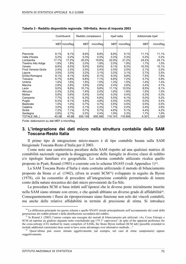
RIVISTA DI STATISTICA UFFICIALE N.2-3/2008
ISTITUTO NAZIONALE DI STATISTICA 71
Tabella 3 - Reddito disponibile regionale. 100=Italia. Anno di imposta 2003
Contribuenti Reddito complessivo Irpef netta Addizionale Irpef
MEF microReg MEF microReg MEF microReg MEF microReg
Piemonte 8,1% 8,1% 8,6% 8,8% 8,9% 9,1% 11,1% 11,1%Valle d'Aosta 0,2% 0,2% 0,3% 0,3% 0,3% 0,3% 0,2% 0,2%Lombardia 17,1% 17,2% 20,4% 19,8% 22,9% 21,2% 24,4% 24,1%Trentino Alto Adige 1,9% 1,8% 2,0% 1,9% 2,0% 1,9% 1,7% 1,5%Veneto 8,6% 8,5% 9,0% 8,6% 9,1% 8,3% 10,3% 10,1%Friuli Venezia Giulia 2,4% 2,3% 2,5% 2,4% 2,5% 2,5% 2,1% 2,0%Liguria 3,0% 3,0% 3,2% 3,1% 3,2% 3,1% 2,7% 2,5%Emilia Romagna 8,1% 8,1% 8,9% 9,1% 9,3% 9,8% 7,5% 7,6%Toscana 6,7% 6,8% 6,8% 7,1% 6,8% 7,2% 5,7% 5,9%Umbria 1,6% 1,6% 1,5% 1,5% 1,3% 1,5% 1,4% 1,4%Marche 2,8% 2,8% 2,6% 2,6% 2,4% 2,6% 3,4% 4,7%Lazio 9,0% 8,8% 10,1% 9,8% 11,1% 10,5% 8,5% 8,1%Abruzzo 2,3% 2,2% 1,9% 2,0% 1,6% 1,8% 1,5% 1,5%Molise 0,6% 0,6% 0,4% 0,4% 0,3% 0,4% 0,3% 0,3%Campania 7,7% 8,1% 6,3% 6,8% 5,5% 6,1% 5,0% 5,2%Puglia 6,2% 6,1% 4,8% 4,8% 4,0% 4,0% 5,0% 4,4%Basilicata 1,0% 1,0% 0,7% 0,7% 0,5% 0,5% 0,5% 0,5%Calabria 3,0% 3,0% 2,1% 2,3% 1,7% 2,0% 2,4% 2,6%Sicilia 7,2% 7,1% 5,7% 5,7% 4,8% 5,1% 4,4% 4,2%Sardegna 2,6% 2,7% 2,2% 2,4% 1,9% 2,3% 1,7% 1,9%TOTALE (ML.) 40,58 40,86 655.100 656.380 119.191 118.995 6.301 6.526
Fonte: elaborazioni su dati MEF e microReg 3. L’integrazione dei dati micro nella struttura contabile della SAM
Toscana-Resto Italia
Il primo tipo di integrazione micro-macro è di tipo contabile basata sulla SAM biregionale Toscana-Resto d’Italia per il 2003.
Come noto una caratteristica peculiare della SAM rispetto ad una qualsiasi matrice di contabilità nazionale riguarda la disaggregazione delle famiglie in diverse classi di reddito e/o tipologie familiare e/o geografiche. Lo schema contabile utilizzato ricalca quello proposto in Pyatt, Round (1985) e coerente con lo schema SNA93 (vedi Appendice 1)14.
La SAM Toscana Resto d’Italia è stata costruita utilizzando il metodo di bilanciamento proposto da Stone et al. (1942), (d'ora in avanti SCM15) sviluppato in seguito da Byron (1978), ciò ha consentito di procedere all’integrazione contabile permettendo di tenere conto della natura stocastica dei dati micro provenienti da Eu-Silc.
La procedura SCM si basa infatti sull’iipotesi che le diverse poste inizialmente inserite nella SAM siano stimate con errore, e che quindi abbiano un diverso grado di affidabilità16. Conseguentemente i flussi da riproporzionare siano funzione non solo dei vincoli contabili, ma anche delle relative affidabilità in termini di precisione di stima. Si introduce
14 La differenza principale tra questo schema e quello SNA93 risiede principalmente nell’accorpamento dei conti della generazione dei redditi primari e della distribuzione secondaria del reddito.
15 In Round J. (2003) l’autore compie una rassegna dei metodi di bilanciamento più utilizzati: rAs, Cross Entropy e SCM ed esprime un giudizio alquanto netto concludendo (pg 179 3° capoverso)”..In spite of the apparent preference for the cross-entropy (CE) method by many compilers of SAMs, the Stone Byron method (SCM ndr) (possible extended to include additional constraints) does seem to have some advantages over alternative methods…”
16 Quest’ultima può essere stimata oggettivamente (ad esempio, nel caso di stime campionarie) oppure soggettivamente.

L’IMPATTO DELLE POLITICHE FISCALI ATTRAVERSO L’INTEGRAZIONE FRA UN MODELLO DI MICROSIMULAZIONE…
ISTITUTO NAZIONALE DI STATISTICA 72
esplicitamente il concetto di varianza e covarianza relativa, associata al set iniziale di conti da bilanciare, come determinate del processo di aggiustamento. La procedura SCM consiste nell’applicazione del metodo dei minimi quadrati generalizzati al seguente problema: dato un sistema di conti T (vettorizzazione t) soggetto a vincoli k, secondo la matrice di aggregazione G:
[5] tGk
Utilizzando le stime iniziali T(0) si avrà:
[6] )0(tGk
dove è il vettore dei residui contabili. Si assume che le stime iniziali T(0) siano non
distorte ed abbiano le seguente caratteristiche
[7]
VE
E
tt
)'(
0)(
)1()0(
L’applicazione dei minimi quadrati generalizzati porterà allora alla stima di un vettore
t*(1) che soddisfi i vincoli contabili in [7] e sia il più vicino possibile ai dati effettivi t(1). Lo stimatore in grado di produrre tale stima è il seguente:
[8] kGVGGVtGGVGGVIt 11 )'(')0())'('()1(
Si dimostra che tale stimatore è BLU, e la sua varianza è data da:
[9] VGGVGGVVV 1)'(' Un problema cruciale a questo punto è quello di definire la matrice V che determina, per
ciascun flusso in T(0), il range di aggiustamento17 e che è, a sua volta, funzione inversa del grado di attendibilità della stima preliminare. A tale proposito, i valori della SAM derivati dai conti economici regionali e nazionali hanno attendibilità alta ed in alcuni casi varianza nulla; mentre i dati provenienti dal Eu-Silc avranno una varianza derivata dalle stime campionarie.
Così, i dati micro, una volta inseriti nello schema contabile SAM, subiranno un aggiustamento che è funzione della varianza campionaria e dei vincoli macroeconomici.
17 Per una descrizione della procedura di bilanciamento utilizzata dall’IRPET nella costruzione delle tavole Input-
Output multiregionali, si veda Casini e Paniccià 2002.
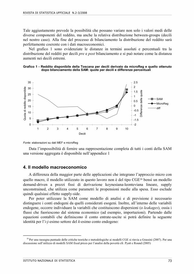
RIVISTA DI STATISTICA UFFICIALE N.2-3/2008
ISTITUTO NAZIONALE DI STATISTICA 73
Tale aggiustamento prevede la possibilità che possano variare non solo i valori medi delle diverse componenti del reddito, ma anche la relativa distribuzione between-groups (decili nel nostro caso). Alla fine del processo di bilanciamento la distribuzione del reddito sarà perfettamente coerente con i dati macroeconomici.
Nel grafico 1 sono evidenziate le distanze in termini assoluti e percentuali tra la distribuzione del redditi per decili pre e post bilanciamento e si può notare come la distanza aumenti nei decili estremi.
Grafico 1 - Reddito disponibile della Toscana per decili derivato da microReg e quello ottenuto
dopo bilanciamento della SAM: quote per decili e differenze percentuali
Fonte: elaborazioni su dati MEF e microReg
Data l’impossibilità di fornire una rappresentazione completa di tutti i conti della SAM una versione aggregata è disponibile nell’appendice 1 4. Il modello macroeconomico
A differenza della maggior parte delle applicazioni che integrano l’approccio micro con quello macro, il modello utilizzato in questo lavoro non è del tipo CGE18 bensì un modello demand-driven a prezzi fissi di derivazione keynesiana-leonteviana lineare, supply unconstrained, che utilizza come parametri le propensioni medie alla spesa. Esso esclude quindi qualsiasi effetto supply-side.
Per poter utilizzare la SAM come modello di analisi e di previsione è necessario distinguere i conti endogeni da quelli considerati esogeni. Inoltre, all’interno delle variabili endogene, occorre individuare la variabili che costituiscono dispersioni (o leakages), ossia i flussi che fuoriescono dal sistema economico (ad esempio, importazioni). Partendo dalle equazioni contabili che definiscono il conto entrate-uscite si potrà definire la seguente identità per l’i-j-esimo settore del k-esimo conto endogeno:
18 Per una rassegna puntuale delle critiche teoriche e metodologiche ai modelli CGE si rinvia a Grassini (2007). Per una
discussione sull’utilizzo di modelli SAM fixed prices per l’analisi della povertà cfr. Pyatt e Round (2005)
0
5
10
15
20
25
30
35
1 2 3 4 5 6 7 8 9 10
Decili
Quo
ta d
i red
dito
dis
poni
bile
-2
-1.5
-1
-0.5
0
0.5
1
1.5
2
2.5
Diff
eren
ze d
elle
quo
te
SAM
MicroReg
diff

L’IMPATTO DELLE POLITICHE FISCALI ATTRAVERSO L’INTEGRAZIONE FRA UN MODELLO DI MICROSIMULAZIONE…
ISTITUTO NAZIONALE DI STATISTICA 74
[10]
n
1k
m
1j
f
1h
d
1j
n
1k
m
1i
s
1l
f
1hjlhjikihjikj leakendogexogendog
dove:
endog = variabile endogena simultanea
exog = variabile esogena
leak = leakages
n = totale conti endogeni
m = totale settori endogeni del j-esimo/ k-esimo conto endogeno
f = totale conti esogeni
p = totale settori endogeni del h-esimo conto esogeno
s = totali conti leakages
In analogia con la simbologia impiegata nei modelli Input-Output si può definire:
[11] Pksij= Tksij/Tj
come la propensione media di spesa del settore j-esimo del conto k-esimo nei confronti del settore i-esimo del conto s-esimo. Il modello può quindi definirsi nella sua forma strutturale nel modo seguente:
[12] endog
eendog
Mleak
xogPendog
La prima relazione strutturale definisce le risorse e gli impieghi dei conti endogeni
simultanei, mentre la seconda relazione stabilisce il livello dei conti leakages in funzione dei conti endogeni. Il sistema quindi in forma ridotta avrà la seguente specificazione:
[13] xogPIendog 1 e
Ai fini dell’analisi previsiva e strutturale assume particolare importanza la matrice (I-P),
che contiene i parametri in forma ridotta del modello o, più comunemente, i moltiplicatori. Al pari del modello I-O essi quantificano gli effetti diretti ed indiretti di variazioni nelle variabili esogene su quelle endogene ed a fortiori sulle dispersioni.
RIVISTA DI STATISTICA UFFICIALE N.2-3/2008
ISTITUTO NAZIONALE DI STATISTICA 75
5. L’integrazione modellistica microReg-SAM
L’esercizio che si propone si basa su un uso integrato dei due modelli appena descritti: quello micro (microReg) e quello macro/meso SAM based.
Come accennato nei paragrafo 2 l’integrazione, prendendo spunto dai lavori di Cameron, Ezzedin (2000) e Brandolini et al. (1993), si concretizzerà nella sostituzione del blocco macro/meso endogeno della spesa della famiglie residenti, basato sulle propensioni medie, con le relazioni desunte dal modello di microsimulazione.
Per operare compiutamente tale sostituzione necessita la presenza in microReg di una funzione del consumo che stimi la spesa totale delle famiglie residenti una volta definito il reddito disponibile. L’indagine Eu-Silc non contiene informazioni sulla spesa delle famiglie per cui, provvisoriamente, in attesa di poter disporre di una procedura di matching affidabile con l’indagine ISTAT sui consumi delle famiglie, si è utilizzata l’elasticità consumo–reddito stimata attraverso l’utilizzo di un diverso dataset (vedi appendice 2)
L’integrazione micro-macro funzionerà quindi nel modo seguente. Si ipotizzi una variazione del regime fiscale: microReg calcolerà l’impatto diretto di tale manovra sul reddito disponibile e con essa, tramite una funzione econometrica (vedi appendice 2), la conseguente variazione della spesa delle famiglie residenti. Tale spesa sarà poi aggregata per decili e disaggregata per funzioni di spesa e quindi passata come iniezione esogena al modello macroeconomico, che a sua volta, stimerà la conseguente attivazione di reddito primario settoriale, distinto nelle componenti dipendente ed autonoma e per tipologia professionale.
Il modello SAM quindi restituirà a microReg la variazione media dei redditi primari così disaggregata, che sarà quindi assegnata opportunamente ai percettori di reddito di microReg. Una volta compiuta tale operazione sarà possibile calcolare un nuovo reddito disponibile, che attraverso la funzione econometrica produrrà una nuova stima del consumo aggregato dei residenti. La procedura di calcolo si arresterà quando la variazione del reddito disponibile raggiungerà un valore minimo
Una operazione preliminare allo svolgimento dell’integrazione è la sintonizzazione del modello micro con i dati mesoconomici in termini classificatori e numerici. Questa operazione era già stata svolta, nel senso micromacro, dal bilanciamento avvenuto al momento della stima della SAM; si tratta ora quindi di procedere in senso inverso, poiché anche i dati all’interno del modello micro devono essere aggiustati attraverso un processo di grossing up con quelli macro al fine di rendere la scambio di dati non generatore di distorsioni.
5.1 L’integrazione: una trattazione formale
Se si specifica in modo più dettagliato il modello SAM riportato nell’equazione [12] sostituendo le relazioni derivanti da microReg alle corrispettive equazioni macro, si potrà scrivere la seguente forma strutturale di un modello multiregionale:
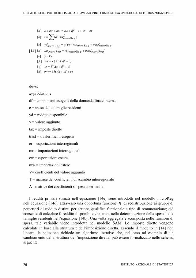
L’IMPATTO DELLE POLITICHE FISCALI ATTRAVERSO L’INTEGRAZIONE FRA UN MODELLO DI MICROSIMULAZIONE…
ISTITUTO NAZIONALE DI STATISTICA 76
[14]
)(][
)(][
)(][
][
)(][
)(][
)(][
][
ReReRe
ReReRe
Re
cdfAxMmwh
cdfAxTerg
cdfAxTmrf
Vxye
trasfytaxd
trasftaxyydc
ydcb
ewercdfAxmwmrxa
gmicrogmicrogmicro
gmicrogmicrogmicro
gmicro
dove:
x=produzione
df = componenti esogene della domanda finale interna
c = spesa delle famiglie residenti
yd = reddito disponibile
y = valore aggiunto
tax = imposte dirette
trasf = trasferimenti esogeni
er = esportazioni interregionali
mr = importazioni interregionali
ew = esportazioni estere
mw = importazioni estere
V= coefficienti del valore aggiunto
T = matrice dei coefficienti di scambio interregionale
A= matrice dei coefficienti si spesa intermedia
I redditi primari stimati nell’equazione [14e] sono introdotti nel modello microReg
nell’equazione [14c], attraverso una opportuna funzione di redistribuzione ai gruppi di
percettori di reddito distinti per settore, qualifica funzionale e tipo di remunerazione; ciò consente di calcolare il reddito disponibile che entra nella determinazione della spesa delle famiglie residenti nell’equazione [14b]. Una volta aggregata e scomposta nelle funzioni di spesa, tale variabile viene introdotta nel modello SAM. Le imposte dirette vengono calcolate in base alla struttura dell’imposizione diretta. Essendo il modello in [14] non lineare, la soluzione richiede un algoritmo iterativo che, nel caso ad esempio di un cambiamento della struttura dell’imposizione diretta, può essere formalizzato nello schema seguente:
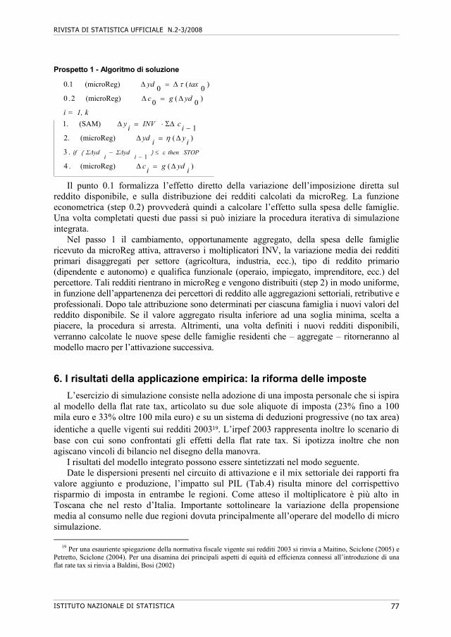
RIVISTA DI STATISTICA UFFICIALE N.2-3/2008
ISTITUTO NAZIONALE DI STATISTICA 77
Prospetto 1 - Algoritmo di soluzione
Il punto 0.1 formalizza l’effetto diretto della variazione dell’imposizione diretta sul reddito disponibile, e sulla distribuzione dei redditi calcolati da microReg. La funzione econometrica (step 0.2) provvederà quindi a calcolare l’effetto sulla spesa delle famiglie. Una volta completati questi due passi si può iniziare la procedura iterativa di simulazione integrata.
Nel passo 1 il cambiamento, opportunamente aggregato, della spesa delle famiglie ricevuto da microReg attiva, attraverso i moltiplicatori INV, la variazione media dei redditi primari disaggregati per settore (agricoltura, industria, ecc.), tipo di reddito primario (dipendente e autonomo) e qualifica funzionale (operaio, impiegato, imprenditore, ecc.) del percettore. Tali redditi rientrano in microReg e vengono distribuiti (step 2) in modo uniforme, in funzione dell’appartenenza dei percettori di reddito alle aggregazioni settoriali, retributive e professionali. Dopo tale attribuzione sono determinati per ciascuna famiglia i nuovi valori del reddito disponibile. Se il valore aggregato risulta inferiore ad una soglia minima, scelta a piacere, la procedura si arresta. Altrimenti, una volta definiti i nuovi redditi disponibili, verranno calcolate le nuove spese delle famiglie residenti che – aggregate – ritorneranno al modello macro per l’attivazione successiva.
6. I risultati della applicazione empirica: la riforma delle imposte
L’esercizio di simulazione consiste nella adozione di una imposta personale che si ispira al modello della flat rate tax, articolato su due sole aliquote di imposta (23% fino a 100 mila euro e 33% oltre 100 mila euro) e su un sistema di deduzioni progressive (no tax area) identiche a quelle vigenti sui redditi 200319. L’irpef 2003 rappresenta inoltre lo scenario di base con cui sono confrontati gli effetti della flat rate tax. Si ipotizza inoltre che non agiscano vincoli di bilancio nel disegno della manovra.
I risultati del modello integrato possono essere sintetizzati nel modo seguente. Date le dispersioni presenti nel circuito di attivazione e il mix settoriale dei rapporti fra
valore aggiunto e produzione, l’impatto sul PIL (Tab.4) risulta minore del corrispettivo risparmio di imposta in entrambe le regioni. Come atteso il moltiplicatore è più alto in Toscana che nel resto d’Italia. Importante sottolineare la variazione della propensione media al consumo nelle due regioni dovuta principalmente all’operare del modello di micro simulazione.
19 Per una esauriente spiegazione della normativa fiscale vigente sui redditi 2003 si rinvia a Maitino, Sciclone (2005) e Petretto, Sciclone (2004). Per una disamina dei principali aspetti di equità ed efficienza connessi all’introduzione di una flat rate tax si rinvia a Baldini, Bosi (2002)
)((microReg).4
.3
)((microReg)2.1
(SAM)1.
)0
(0
(microReg)2.0
)0
(0
(microReg)0.1
1
iydg
ic
iy
iyd
icINV
iy
k1,=i
ydgc
taxyd
STOPthenεi
ΣΔydi
ΣΔydif
)(
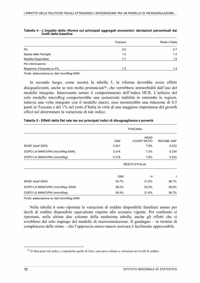
L’IMPATTO DELLE POLITICHE FISCALI ATTRAVERSO L’INTEGRAZIONE FRA UN MODELLO DI MICROSIMULAZIONE…
ISTITUTO NAZIONALE DI STATISTICA 78
Tabella 4 - L’impatto della riforma sui principali aggregati economici: deviazioni percentuali dai livelli della baseline
Toscana Resto d’Italia
PIL 0.8 0.7
Spesa delle Famiglie 1.5 1.4
Reddito Disponibile 1.7 1.5
Per informazione
Risparmio d’Imposta su PIL 1.5 1.4
Fonte: elaborazione su dati microReg-SAM
In secondo luogo, come mostra la tabella 5, la riforma dovrebbe avere effetti
disegualizzanti, anche se non molto pronunciati20, che verrebbero ammorbiditi dall’uso del modello integrato. Interessante notare il comportamento dell’indice HCR, L’utilizzo del solo modello microReg comporterebbe una sostanziale stabilità in entrambe le regioni, tuttavia una volta integrato con il modello macro, esso mostrerebbe una riduzione di 0,5 punti in Toscana e del 1% nel resto d’Italia in virtù di una maggiore importanza del growth effect nel determinare la variazione di tale indice.
Tabella 5 - Effetti della flat rate tax sui principali indici di disuguaglianza e povertà
TOSCANA
GINIHEAD
COUNT RATIO INCOME GAP
BASE (Irpef 2003) 0,301 7,8% 0,233
DOPO LA MANOVRA (microReg-SAM) 0,316 7,3% 0.234
DOPO LA MANOVRA (microReg) 0.318 7,8% 0.233
RESTO D'ITALIA
GINI H I
BASE (Irpef 2004) 34,7% 21,6% 38,7%
DOPO LA MANOVRA (microReg -SAM) 36,2% 20,5% 38,8%
DOPO LA MANOVRA (microReg) 36,4% 21,6% 38,7%
Fonte: elaborazione su dati microReg-SAM
Nella tabella 6 sono riportate le variazioni di reddito disponibile familiare annuo per
decili di reddito disponibile equivalente rispetto allo scenario vigente. Per confronto si riportano, nelle ultime due colonne della medesima tabella, anche gli effetti che si avrebbero dal solo impiego del modello di microsimulazione. Il guadagno – in termini di completezza delle stime – che l’approccio micro-macro assicura è facilmente apprezzabile.
20 D’altra parte tali indici, e soprattutto quello di Gini, sono poco elastici a variazioni nei livelli di reddito.
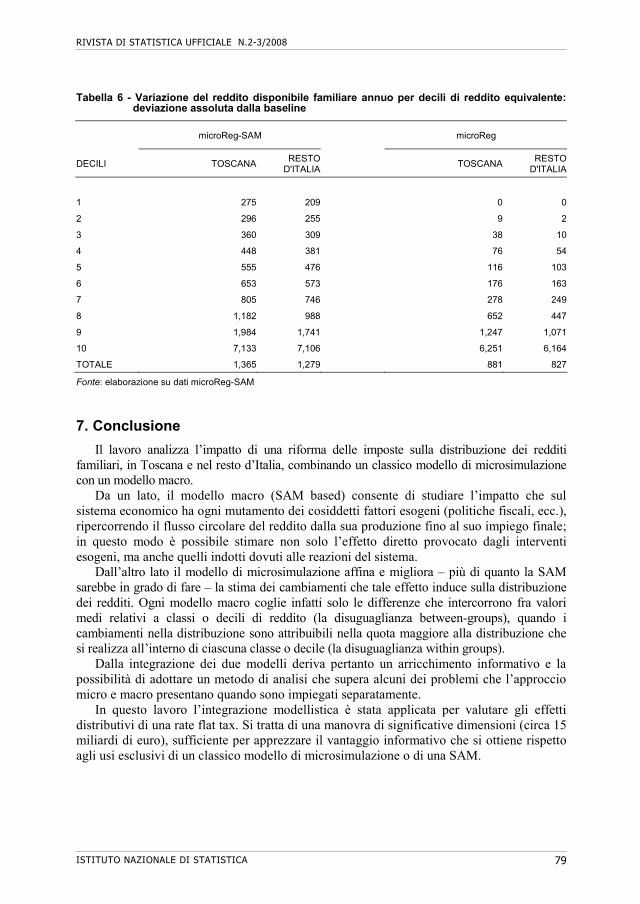
RIVISTA DI STATISTICA UFFICIALE N.2-3/2008
ISTITUTO NAZIONALE DI STATISTICA 79
Tabella 6 - Variazione del reddito disponibile familiare annuo per decili di reddito equivalente: deviazione assoluta dalla baseline
microReg-SAM microReg
DECILI TOSCANARESTO
D'ITALIATOSCANA
RESTO D'ITALIA
1 275 209 0 0
2 296 255 9 2
3 360 309 38 10
4 448 381 76 54
5 555 476 116 103
6 653 573 176 163
7 805 746 278 249
8 1,182 988 652 447
9 1,984 1,741 1,247 1,071
10 7,133 7,106 6,251 6,164
TOTALE 1,365 1,279 881 827
Fonte: elaborazione su dati microReg-SAM
7. Conclusione
Il lavoro analizza l’impatto di una riforma delle imposte sulla distribuzione dei redditi familiari, in Toscana e nel resto d’Italia, combinando un classico modello di microsimulazione con un modello macro.
Da un lato, il modello macro (SAM based) consente di studiare l’impatto che sul sistema economico ha ogni mutamento dei cosiddetti fattori esogeni (politiche fiscali, ecc.), ripercorrendo il flusso circolare del reddito dalla sua produzione fino al suo impiego finale; in questo modo è possibile stimare non solo l’effetto diretto provocato dagli interventi esogeni, ma anche quelli indotti dovuti alle reazioni del sistema.
Dall’altro lato il modello di microsimulazione affina e migliora – più di quanto la SAM sarebbe in grado di fare – la stima dei cambiamenti che tale effetto induce sulla distribuzione dei redditi. Ogni modello macro coglie infatti solo le differenze che intercorrono fra valori medi relativi a classi o decili di reddito (la disuguaglianza between-groups), quando i cambiamenti nella distribuzione sono attribuibili nella quota maggiore alla distribuzione che si realizza all’interno di ciascuna classe o decile (la disuguaglianza within groups).
Dalla integrazione dei due modelli deriva pertanto un arricchimento informativo e la possibilità di adottare un metodo di analisi che supera alcuni dei problemi che l’approccio micro e macro presentano quando sono impiegati separatamente.
In questo lavoro l’integrazione modellistica è stata applicata per valutare gli effetti distributivi di una rate flat tax. Si tratta di una manovra di significative dimensioni (circa 15 miliardi di euro), sufficiente per apprezzare il vantaggio informativo che si ottiene rispetto agli usi esclusivi di un classico modello di microsimulazione o di una SAM.
L’IMPATTO DELLE POLITICHE FISCALI ATTRAVERSO L’INTEGRAZIONE FRA UN MODELLO DI MICROSIMULAZIONE…
ISTITUTO NAZIONALE DI STATISTICA 80
Riferimenti bibliografici
ADELMAN I, ROBINSON S. (1978), “Income distribution policy in developing countries: a case study of Korea”, Oxford University Press
AGENOR P., IZQUIERDO A., FOFACK H., (2002) “IMMPA: a quantitative macroeconomic framework for analysis”, World Bank
BLINDER A.S. (1975), “Distribution effects and the aggregate distribution consumption function”, Journal of Political Economy n.83
BRANDOLINI A., BRUNO G. e GUISO L., (1993), “MOSED Simulation models of distributive effects: first report”, Mimeo, Banca d’Italia
CANNARI A., D’ALESSIO G. (2003), “La distribuzione del reddito e della ricchezza nelle regioni italiane”, Temi di Discussione 482, Banca d’Italia
BOURGUIGNON F., ROBILLARD S., ROBINSON S. (2003), Representative vs. real households in the macroeconomic modelling of inequality, DIAL document de travail
CAMERON G., EZZEDDIN R. (2000), “Integrating input-output and tax microsimulation models” in Mitton L. Sutherland H., Weeks M. (eds), Microsimulation modelling for policy analysis, Cambridge University Press
COADY D. e HARRIS R., (2001), A regional general equilibrium model of the welfare impact of cash transfers, Paper 76, IFPRI
CASINI BENVENUTI S., PANICCIA’ R. (2002), “A multi-regional Input-Output model for Italy: methodology and first results”, IRPET WP 22.2003
DECALUWé L, PATRY A., SAVARD L., TOERBECKE E. (1999), “Poverty Analysis within a General Equilibrium framework”, WP 99-06, CREFA Univ de Laval
DEVARAJAN S., GO D.S., (2005), 123PRSP Model, in Bourguignon F., Ferreira L (eds.) The impact of economic policies on poverty and income distribution, Oxford University Press
DA SILVA. L, ESSAMA-NSSAH B. e SAMAKE’ I (2005), Linking aggregate Macroconsistency Models to Household survey: a Poverty Analysis Macroeconomic Simulator, or PAMS, in Bourguignon F., Ferreira L (eds.) The impact of economic policies on poverty and income distribution, Oxford University Press
DEATON A., (1997), The analysis of household surveys, World Bank
DERVIS K, de MELO J, and ROBINSON S. (1982), General Equilibrium models for development policy, Cambridge University Press
ESSAMA-NSSAH B., (2005), “The Poverty and Distribution Impact of Macroeconomic Shocks and Policies: a Review of Modelling Approaches”, WB Policy Research WP 3682
GRASSINI M., (2007) “Rowing along the CGE Modelling Mainstream”, Studi e Note di Economia, n.3.
LATTARULO P., PANICCIÀ R., SCICLONE N. (2002), La distribuzione del reddito in Toscana. Un approccio integrato micro e macro, IRPET WP 21.2003
LOFGREN H., ROBINSON S, el-SAID M. (2005), Poverty and Inequality analysis in a general equilibrium framework: The Representative Household approach, in Bourguignon F., Ferreira L (eds.) The impact of economic policies on poverty and income distribution, Oxford University Press
RIVISTA DI STATISTICA UFFICIALE N.2-3/2008
ISTITUTO NAZIONALE DI STATISTICA 81
MAITINO M.L, SCICLONE N., (2005), Dall’Irpef all’Ire: gli effetti distributivi e di gettito in Toscana, in Ricchezza e Povertà (a cura di), Baldi P., Lemmi A., Sciclone N, Franco Angeli
MAITINO M.L, SCICLONE N., (2008), Il modello di microsimulazione multiregionale dell'Irpet Microreg”, Working Paper n.604, Società Italiana di Economia Pubblica
MITTON L. SUTHERLAND H., WEEKS M. (2000), Microsimulation modelling for policy analysis, Cambridge University Press
PETRETTO A., SCICLONE N. (2004), Gli effetti distributivi della riforma dell’IRE: una analisi per la Toscana, Note di Economia n.2
PYATT G., ROUND J.I. (1985),Social Accounting Matrices: a basis for planning, The World Bank, Washington
PYATT G., ROUND J., (2005), Multiplier Effects and Reduction of Poverty, in d Janvry A., Kanbur R., (2006) Poverty, Inequality and Development, Springer
ROUND J.I. (2003), “Constructing SAMs for development policy analysis: lessons learned and challenges ahead”, Economic System Research n.2
REDMOND G., SUTHERLAND H., WILSON M. (1998), The Arithmetic of Tax and Social Security Reform, Cambridge University Press
SAVARD L., (2003) “Poverty and Incombe Distribution in a CGE-household Sequential Model”, International Development Research Centre, Dakar
SCICLONE N., (2008), “La manovra di bilancio per il 2008 sulle famiglie italiane”, (2008), Working Paper n.605, Società Italiana di Economia Pubblica
STOKER T.M (1986), “Simple tests of distributional effects on macroeconomic equations”, Journal of Political Economy,n.4
SUTHERLAND H. (ed.), (2001), “Final report. Euromod: an integrated European Benefit-tax model”, Working papers Euromod, n. EM9/01
TARGETTI LENTI R. (1989), “Income distribution and the structure of the economic system: a SAM approach”, in Dagum C., Zenga M. (eds), Income and wealth distribution, inequality and poverty, Springer-Verlag
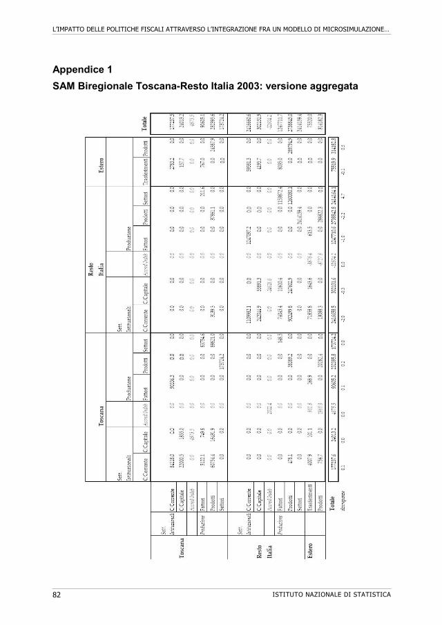
L’IMPATTO DELLE POLITICHE FISCALI ATTRAVERSO L’INTEGRAZIONE FRA UN MODELLO DI MICROSIMULAZIONE…
ISTITUTO NAZIONALE DI STATISTICA 82
Appendice 1
SAM Biregionale Toscana-Resto Italia 2003: versione aggregata
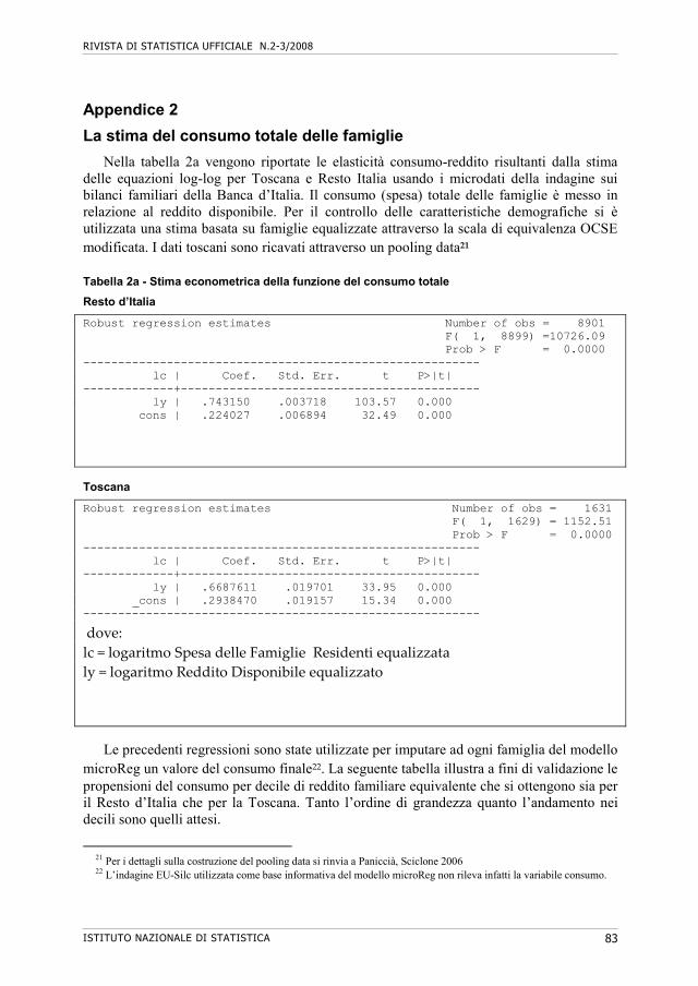
RIVISTA DI STATISTICA UFFICIALE N.2-3/2008
ISTITUTO NAZIONALE DI STATISTICA 83
Appendice 2
La stima del consumo totale delle famiglie
Nella tabella 2a vengono riportate le elasticità consumo-reddito risultanti dalla stima delle equazioni log-log per Toscana e Resto Italia usando i microdati della indagine sui bilanci familiari della Banca d’Italia. Il consumo (spesa) totale delle famiglie è messo in relazione al reddito disponibile. Per il controllo delle caratteristiche demografiche si è utilizzata una stima basata su famiglie equalizzate attraverso la scala di equivalenza OCSE modificata. I dati toscani sono ricavati attraverso un pooling data21
Tabella 2a - Stima econometrica della funzione del consumo totale
Resto d’Italia
Robust regression estimates Number of obs = 8901 F( 1, 8899) =10726.09 Prob > F = 0.0000 --------------------------------------------------------- lc | Coef. Std. Err. t P>|t| -------------+------------------------------------------- ly | .743150 .003718 103.57 0.000 cons | .224027 .006894 32.49 0.000
Toscana
Robust regression estimates Number of obs = 1631 F( 1, 1629) = 1152.51 Prob > F = 0.0000 --------------------------------------------------------- lc | Coef. Std. Err. t P>|t| -------------+------------------------------------------- ly | .6687611 .019701 33.95 0.000 _cons | .2938470 .019157 15.34 0.000 --------------------------------------------------------- dove: lc = logaritmo Spesa delle Famiglie Residenti equalizzata ly = logaritmo Reddito Disponibile equalizzato
Le precedenti regressioni sono state utilizzate per imputare ad ogni famiglia del modello
microReg un valore del consumo finale22. La seguente tabella illustra a fini di validazione le propensioni del consumo per decile di reddito familiare equivalente che si ottengono sia per il Resto d’Italia che per la Toscana. Tanto l’ordine di grandezza quanto l’andamento nei decili sono quelli attesi.
21 Per i dettagli sulla costruzione del pooling data si rinvia a Paniccià, Sciclone 2006 22 L’indagine EU-Silc utilizzata come base informativa del modello microReg non rileva infatti la variabile consumo.
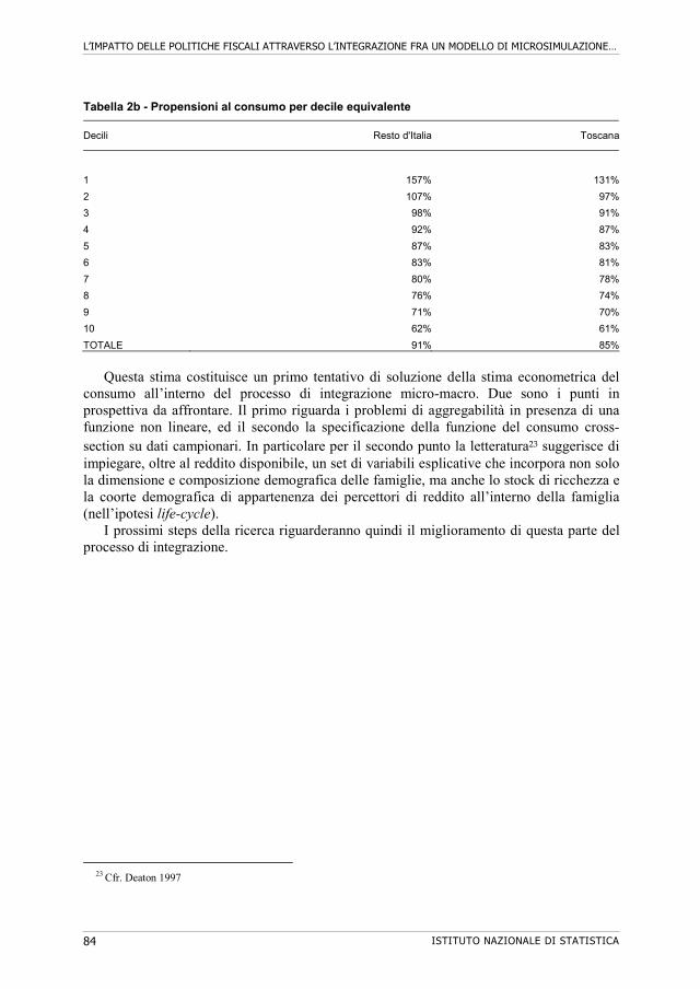
L’IMPATTO DELLE POLITICHE FISCALI ATTRAVERSO L’INTEGRAZIONE FRA UN MODELLO DI MICROSIMULAZIONE…
ISTITUTO NAZIONALE DI STATISTICA 84
Tabella 2b - Propensioni al consumo per decile equivalente
Decili Resto d'Italia Toscana
1 157% 131%
2 107% 97%
3 98% 91%
4 92% 87%
5 87% 83%
6 83% 81%
7 80% 78%
8 76% 74%
9 71% 70%
10 62% 61%
TOTALE 91% 85%
Questa stima costituisce un primo tentativo di soluzione della stima econometrica del
consumo all’interno del processo di integrazione micro-macro. Due sono i punti in prospettiva da affrontare. Il primo riguarda i problemi di aggregabilità in presenza di una funzione non lineare, ed il secondo la specificazione della funzione del consumo cross-section su dati campionari. In particolare per il secondo punto la letteratura23 suggerisce di impiegare, oltre al reddito disponibile, un set di variabili esplicative che incorpora non solo la dimensione e composizione demografica delle famiglie, ma anche lo stock di ricchezza e la coorte demografica di appartenenza dei percettori di reddito all’interno della famiglia (nell’ipotesi life-cycle).
I prossimi steps della ricerca riguarderanno quindi il miglioramento di questa parte del processo di integrazione.
23 Cfr. Deaton 1997
RIVISTA DI STATISTICA UFFICIALE
ISTITUTO NAZIONALE DI STATISTICA 85
Norme redazionali
La Rivista di Statistica Ufficiale pubblica contributi originali nella sezione “Temi trattati” ed eventuali discussioni a largo spettro nella sezione “Interventi”. Possono essere pubblicati articoli oggetto di comunicazioni a convegni, riportandone il riferimento specifico. Gli articoli devono essere fatti pervenire al Comitato di redazione delle pubblicazioni scientifiche Istat corredati, a parte, da una nota informativa dell’Autore contenente: appartenenza ad istituzioni, attività prevalente, qualifica, indirizzo, casella di posta elettronica, recapito telefonico e l’autorizzazione alla pubblicazione firmata dagli Autori. Ogni articolo prima della pubblicazione dovrà ricevere il parere favorevole di un referente scelto tra gli esperti dei diversi temi affrontati. Gli originali, anche se non pubblicati, non si restituiscono.
Per l’impaginazione dei lavori gli autori sono tenuti a conformarsi rigorosamente agli standard editoriali fissati dal Comitato di redazione e contenuti nel file Template.doc disponibile on line o su richiesta. In base a tali standard la lunghezza dei contributi originali per entrambe le sezioni dovrà essere limitata entro le 30-35 pagine.
Tutti i lavori devono essere corredati di un sommario nella lingua in cui sono redatti (non più di 12 righe); quelli in italiano dovranno prevedere anche un Abstract in inglese. La bibliografia, in ordine alfabetico per autore, deve essere riportata in elenco a parte alla fine dell’articolo. Quando nel testo si fa riferimento ad una pubblicazione citata nell’elenco, si metta in parentesi tonda il nome dell’autore, l’anno di pubblicazione ed eventualmente la pagina citata. Ad esempio (Bianchi, 1987, Rossi, 1988, p. 55). Quando l’autore compare più volte nello stesso anno l’ordine verrà dato dall’aggiunta di una lettera minuscola accanto all’anno di pubblicazione. Ad esempio (Bianchi, 1987a, 1987b).
Nella bibliografia le citazioni di libri e articoli vanno indicate nel seguente modo. Per i libri: cognome dell’autore seguito dall’iniziale in maiuscolo del nome, il titolo in corsivo dell’opera, l’editore, il luogo di edizione e l’anno di pubblicazione. Per gli articoli: dopo l’indicazione dell’autore si riporta il titolo tra virgolette, il titolo completo in corsivo della rivista, il numero del fascicolo e l’anno di pubblicazione. Nei riferimenti bibliografici non si devono usare abbreviazioni.
Nel testo dovrà essere di norma utilizzato il corsivo per le parole in lingua straniera e il corsivo o grassetto per quei termini o locuzioni che si vogliano porre in particolare evidenza (non vanno adoperati, per tali scopi, il maiuscolo, la sottolineatura o altro).
Gli articoli pubblicati impegnano esclusivamente gli Autori, le opinioni espresse non implicano alcuna responsabilità da parte dell’Istat.
La proprietà letteraria degli articoli pubblicati spetta alla Rivista di statistica ufficiale. E’ vietata a norma di legge la riproduzione anche parziale senza autorizzazione e senza
citarne la fonte. Per contattare il Comitato di redazione delle pubblicazioni scientifiche Istat e per inviare
lavori: [email protected]. Oppure scrivere a: Comitato di redazione delle pubblicazioni scientifiche C/O Gilda Sonetti Via Cesare Balbo, 16 00184 Roma

rivista
di statistica
ufficiale
riv
ista
di s
tatis
tica u
ffic
iale
Istituto nazionale
di Statistica
n.1 - 2008
n.12008
La Rivista di Statistica Ufficiale accoglie lavori che hanno comeoggetto la misurazione e la comprensione dei fenomeni sociali,demografici, economici ed ambientali, la costruzione di sistemiinformativi e di indicatori come supporto per le decisionipubbliche e private, nonché le questioni di natura metodologica,tecnologica e istituzionale connesse ai processi di produzione delleinformazioni statistiche e rilevanti ai fini del perseguimento dei finidella statistica ufficiale.La Rivista di Statistica Ufficiale si propone di promuovere lacollaborazione tra il mondo della ricerca scientifica, gli utilizzatoridell’informazione statistica e la statistica ufficiale, al fine dimigliorare la qualità e l’analisi dei dati.La pubblicazione nasce nel 1992 come collana di monografie“Quaderni di Ricerca ISTAT”. Nel 1999 la collana viene affidata adun editore esterno e diviene quadrimestrale con la denominazione“Quaderni di Ricerca - Rivista di Statistica Ufficiale”. L’attualedenominazione, “Rivista di Statistica Ufficiale”, viene assunta apartire dal n. 1/2006 e l’Istat torna ad essere editore in proprio dellapubblicazione.
1B
01
20
09
003
00
00
00
€ 10,00ISSN 1828-1982
Temi trattati
Statistical Criteria to Manage Non-respondents’Intensive Follow Up in Surveys Repeated along TimeRoberto Gismondi, Andrea Carone
Multiplier Decomposition, Inequality and Povertyin a SAM FrameworkMarisa Bottiroli Civardi, Renata Targetti Lenti
Estimation of Poverty Rates for the Italian Populationclassified by Household Type and Administrative RegionClaudio Ceccarelli, Enrico Fabrizi,Maria Rosaria Ferrante, Silvia Pacei