
Quantum Biology. Simulazioni di trasferimento di … Mater Studiorum Università di Bologna Scuola...
72
Alma Mater Studiorum · Università di Bologna Scuola di Scienze Corso di Laurea Magistrale in Fisica Quantum Biology. Simulazioni di trasferimento di energia in una struttura dimerica Relatore: Prof.sa Beatrice Fraboni Correlatore: Dott. Javier Prior Arce Presentata da: Adriano Macarone Palmieri Sessione II Anno Accademico 2013/2014
Transcript of Quantum Biology. Simulazioni di trasferimento di … Mater Studiorum Università di Bologna Scuola...

Alma Mater Studiorum · Università di Bologna
Scuola di Scienze
Corso di Laurea Magistrale in Fisica
Quantum Biology. Simulazioni ditrasferimento di energia in una struttura
dimerica
Relatore:
Prof.sa Beatrice Fraboni
Correlatore:
Dott. Javier Prior Arce
Presentata da:
Adriano Macarone Palmieri
Sessione II
Anno Accademico 2013/2014

2

Indice
1 Introduction/Abstract 5
1.1 Abstract . . . . . . . . . . . . . . . . . . . . . . . . . . . . . . . . . . 5
1.2 Introduction . . . . . . . . . . . . . . . . . . . . . . . . . . . . . . . . 6
1.3 Biological Introduction . . . . . . . . . . . . . . . . . . . . . . . . . . . 7
1.3.1 Electronic energy transfer in Photosyntetic complex . . . . . . 11
1.3.2 Phonon-assisted electron tunneling & olfaction . . . . . . . . . 12
1.3.3 Magneto reception in birds . . . . . . . . . . . . . . . . . . . . 13
2 Dynamical Simulation of 1-D Quantum Many body Systems 15
2.1 Introduction . . . . . . . . . . . . . . . . . . . . . . . . . . . . . . . . 15
2.2 1D Quantum Systems . . . . . . . . . . . . . . . . . . . . . . . . . . 16
2.2.1 Definition . . . . . . . . . . . . . . . . . . . . . . . . . . . . . 16
2.2.2 Basic Properties of 1D quantum systems . . . . . . . . . . . . 17
2.2.3 Schmidt decomposition . . . . . . . . . . . . . . . . . . . . . . 17
2.3 Matrix Product Representation . . . . . . . . . . . . . . . . . . . . . 19
2.3.1 Schmidt decomposition and canonical form . . . . . . . . . . . 20
2.4 Calculations with MPS . . . . . . . . . . . . . . . . . . . . . . . . . . 22
2.4.1 Density matrices . . . . . . . . . . . . . . . . . . . . . . . . . 22
2.4.2 Two-sites gates . . . . . . . . . . . . . . . . . . . . . . . . . . 23
3 Time Evolving Block Decimation 27
3.0.3 Suzuki-Trotter sweeps . . . . . . . . . . . . . . . . . . . . . . 28
3.1 Errors In TEBD . . . . . . . . . . . . . . . . . . . . . . . . . . . . . . 29
3

4 INDICE
3.1.1 Trotter error . . . . . . . . . . . . . . . . . . . . . . . . . . . . 293.1.2 Truncation error . . . . . . . . . . . . . . . . . . . . . . . . . 30
4 Mapping between system-reservoir & semi-infinite discrete chains 33
4.1 Introduction . . . . . . . . . . . . . . . . . . . . . . . . . . . . . . . . 334.1.1 System Reservoir structure . . . . . . . . . . . . . . . . . . . . 354.1.2 Applications . . . . . . . . . . . . . . . . . . . . . . . . . . . . 38
5 Photosynthesis networks transport 43
5.1 The phonon antenna mechanism . . . . . . . . . . . . . . . . . . . . 435.1.1 Non equilibrium long lived coherences . . . . . . . . . . . . . 455.1.2 Last overview on EET principles . . . . . . . . . . . . . . . . 45
5.2 TEBD simulation for Dimeric system . . . . . . . . . . . . . . . . . . 475.2.1 Introduction . . . . . . . . . . . . . . . . . . . . . . . . . . . . 475.2.2 Model parameters . . . . . . . . . . . . . . . . . . . . . . . . . 485.2.3 The Adolf-Rengel optical spectral . . . . . . . . . . . . . . . . 485.2.4 the recoherence and the fundamental role of non-equilibrium
vibrational structure . . . . . . . . . . . . . . . . . . . . . . . 515.2.5 the coupling with environment . . . . . . . . . . . . . . . . . . 525.2.6 Additional random noise . . . . . . . . . . . . . . . . . . . . . 535.2.7 entanglement Measures: Von Newman entropy . . . . . . . . . 575.2.8 The Double Environment . . . . . . . . . . . . . . . . . . . . 64
6 Conclusion 69

Capitolo 1Introduction/Abstract
1.1 Abstract
La quantum biology (QB) è un campo di ricerca emergente che cerca di affronta-re fenomeni quantistici non triviali all’interno dei contesti biologici dotandosi di datisperimentali di esplorazioni teoriche e tecniche numeriche. I sistemi biologici sonoper definizione sistemi aperti, caldi,umidi e rumorosi, e queste condizioni sono perloro imprenscindibili; si pensa sia un sistema soggetto ad una veloce decoerenza chesopprime ogni dinamica quantistica controllata. La QB, tramite i principi di noiseassisted transport e di antenna fononica sostiene che la presenza di un adeguatolivello di rumore ambientale aumenti l’efficienza di un network di trasporto,inoltrese all’interno dello spettro ambientale vi sono specifici modi vibrazionali persistentisi hanno effetti di risonanza che rigenerano la coerenza quantistica. L’interazioneambiente-sistema è di tipo non Markoviano,non perturbativo e di forte non equi-librio, ed il rumore non è trattato come tradizionale rumore bianco. La tecnicanumerica che per prima ha predetto la rigenerazione della coerenza all’interno diquesti network proteici è stato il TEBD, Time Evolving Block Decimation, unoschema numerico che permette di simulare sistemi 1-D a molti corpi, caratterizzatida interazioni di primi vicini e leggermente entangled. Tramite gli algoritmi numericidi Orthopol l’hamiltoniana spin-bosone viene proiettata su una catena discreta 1-D,tenendo conto degli effetti di interazione ambiente-sistema contenuti nello spettro(ilquale determina la dinamica del sistema).Infine si esegue l’evoluzione dello stato.
5
6 CAPITOLO 1. INTRODUCTION/ABSTRACT
1.2 Introduction
The recently born approach towards some biological effects and their new ty-pe of description it’s demonstrating to be quite challenging both theoretically andexperimentally. Recently the numerical approach of TEBD (Time Evolving BlockDecimation), inherited from quantum information, has assisted the idea (and so-me experimental data) that typical quantum effects like the presence of coherenceand local entanglement play an important, even if partly still unclear, role in somebiological effects like the EET. Moreover the theoretical and numerical challenge tointerpret and modeling these phenomena, the great difficulties given from the experi-mental data and their complex interpretation, at the light of our current knowledgesis still quite great. To begin with, biological systems are, almost by definition, opensystems, as they need to be continuously supplied with energy to maintain the outof equilibrium state that life represents. Open systems, however, especially warm,wet and noisy biological systems, are subject to environmental fluctuations that areusually expected to result in fast decoherence and, as a result, the suppression ofwell controlled quantum dynamics. Thus quantum phenomena may at first sightseem unlikely to play a significant role in biology. These quantum phenomena arenot merely a by-product of the underlying quantum nature of chemical bonds butare actually exploited by biological systems to enhance performance and achievenovel functionalities. The extreme consequence of the basic principle of phononantenna have been found to underlie the fruitful interplay between vibrational en-vironments and coherent quantum dynamics, which will provide an understandingwhy optimal transport performance in proteic complex can arise at intermediatenoise levels.Let’s take two closely spaced energy levels are separated from a thirdlevel to which excitations should be delivered. They are subject to dephasing noisefrom an environment with a finite bandwidth that exhibits a maximum. A coherentinteraction between the upper two energy levels leads to dressed states |±〉 withan energy splitting which, if matched to the maximum of the environment spectraldensity, will optimize transport from the upper to the lower level. As will be shownin the data chapter, the presence of sharp resonant peak into the spectra that, as in

1.3. BIOLOGICAL INTRODUCTION 7
the case of EET , if it matches enough the difference in energy between two differentexciton produce a further tuning effect that will give raise to the reborn of the cohe-rence in the system. Theoretically the most simple model is the Spin-Boson Model(SBM) one of the simplest non-trivial models of open-system dynamics. This modeldescribes a single two-level system (TLS) coupled linearly to the coordinates of anenvironment consisting of a continuum of harmonic oscillators and despite its sim-plicity, this model shows a rich array of non-Markovian dynamical phenomena thatfor picoseconds time become of relevant importance. This non Markovian backwardeffects of interaction due to the system environment coupling are the key elementof the lasting of coherence into the system. Mapping the spin-boson model exactlyonto a 1D system permits the deployment of the time-adaptive density matrix whererenormalization group (t-DMRG), to which TEBD belongs, technique to integratethe time evolution of the full system-environment dynamics efficiently
1.3 Biological Introduction
Following early speculations concerning the potential role of quantum physics inbiology, recent progress in science and technology has led to the rapid emergence ofa new direction of research whose aim is the experimental and theoretical explora-tion of quantum effects in biology (see [1][2]) which are taking place on length andtimescales that allow quantum dynamics and environmental fluctuations to enteran intricate and fruitful interplay. To begin with, biological systems are, almost bydefinition, open systems, as they need to be continuously supplied with energy tomaintain the out of equilibrium state that life represents. Open systems, however,especially warm, wet and noisy biological systems, are subject to environmental fluc-tuations that are usually expected to result in fast decoherence and, as a result, thesuppression of well controlled quantum dynamics. Thus quantum phenomena mayat first sight seem unlikely to play a significant role in biology. There are argumentshowever to counter this pessimistic view. At the level of molecular complexes andproteins, processes that are of fundamental importance for biological function can
8 CAPITOLO 1. INTRODUCTION/ABSTRACT
be very fast (taking place within picoseconds) and well localised (extending across afew nanometers, the size of proteins) and may therefore exhibit quantum phenomenabefore the environment has had an opportunity to destroy them. Furthermore, earlywork in quantum information science, for example, has shown that thermal noise instationary non-equilibrium systems may in fact support the existence of quantumcoherence and entanglement [3]. Hence the possible existence of significant quan-tum dynamics is not only a question of sufficiently short length and time scales butmay also depend on a constructive interplay between a quantum dynamical systemand its environment such that quantum correlations are not simply washed out orsuppressed but may in fact be enhanced or regenerated by the interaction with theenvironment. These arguments suggest that quantum effects in biology are possi-ble at the right length- and time scales. We do expect however that in the courseof evolution Nature will have learnt to make use of quantum phenomena only ifthese enable or make more efficient a useful biological function that provides anevolutionary advantage. It is indeed well established from a quantum informationperspective that pure quantum dynamics of multi-component systems can provi-de qualitative performance improvements over classical systems for example wheretransport is concerned. This provides further support for the expectation that na-ture has developed non-trivial quantum phenomena in the dynamics of biologicalsystems, possibly supported by their environment whose presence and influence isunavoidable. These quantum phenomena are not merely a by-product of the un-derlying quantum nature of chemical bonds but are actually exploited by biologicalsystems to enhance performance and achieve novel functionalities. The clear demon-stration that Nature makes use of quantum effects would bring about the necessityfor a significant change of thinking for biologists as they would be required to graspquantum concepts in order to understand some fundamental biological processes. Asabove stated when the biological system seems to take advantage from local quan-tum properties and are able to handle them despite the presence of a surroundingwhich, in truth, as we’ll be better explained in chapter 4, can become a resourcefor the permanence and reborn of quantum properties, instead of the cause of thedeath of these physical elements. Being so, we can start to think to apply technique

1.3. BIOLOGICAL INTRODUCTION 9
Figura 1.1: dimensions & correlated biological phenomena and complexity

10 CAPITOLO 1. INTRODUCTION/ABSTRACT
typical of the many body system into these kind of contests, but taking in mind thatthe biological system can be treated uniquely as Open Quantum System and takingin account of the very fast (picosecond time scale) time setting of these transientphenomena,the perturbative approximation cannot suits our necessities.
Open Quantum Systems–Thanks to the insights of quantum physics some unre-solved biological phenomena today can be deal with a new approach whereas the oldclassical interpretations have seemed so far to fail. The energy transport mechanismof clorosomes or into the reaction center of the leafs systems will be developed inthe next chapter (see chapter 4) , but today the quantum approach is trying to shedlight also onto other different biological phenomena. Needless to say the key com-ponent supporting this interpretation is the presence of a environment composed ofvibration or spins that can be handled by the system in order to take advantagein sustaining it’s quantum properties.Differently from the thermal fluctuations thatit’s exploited from classical systems in order to overcome potential barrier (a me-chanism present in protein folding e.g.) the benefits of environment onto quantumsystem is less evident and experimentally tasking to explore.
[ Structured active Environment]Structured active Environment
As repetitively claimed the environment is not a passive element and in biologicalcontest possess a well define,organized structure.These kinds of environment are nota simple source of white noise and cannot be represented as a small perturbationof any dynamics. All the informations of the environment effect are encoded insideits spectra.The environmental spectral densities (e.g. see chapter 5) describing theirinteraction with the system tend to display two principal structures:
1. a broad smooth back- ground which has a short memory time and interactswith the system mainly through its fluctuations, i.e. causing noise,
2. sharp defined features corresponding to long-lived vibrational motion
the latter ones can lead to quasi-coherent dynamical non-equilibrium exchangesbetween system and environment. The first smooth vibrational component of theenvironment is due to the protein environment and noise processes caused by the

1.3. BIOLOGICAL INTRODUCTION 11
solvents,while the sharp features originate from long lived vibration belonging tomolecules inside the protein scaffold. This reachness leads to a non-Markovian andbeing the environment neither too much nor to weakly coupled compared to theintra-systems dynamics, the total dynamics is also a non-perturbative one. Mo-reover we must stress a fundamental concept: biological system can survive onlycontinuously managing an out-of-equilibrium state.
1.3.1 Electronic energy transfer in Photosyntetic complex
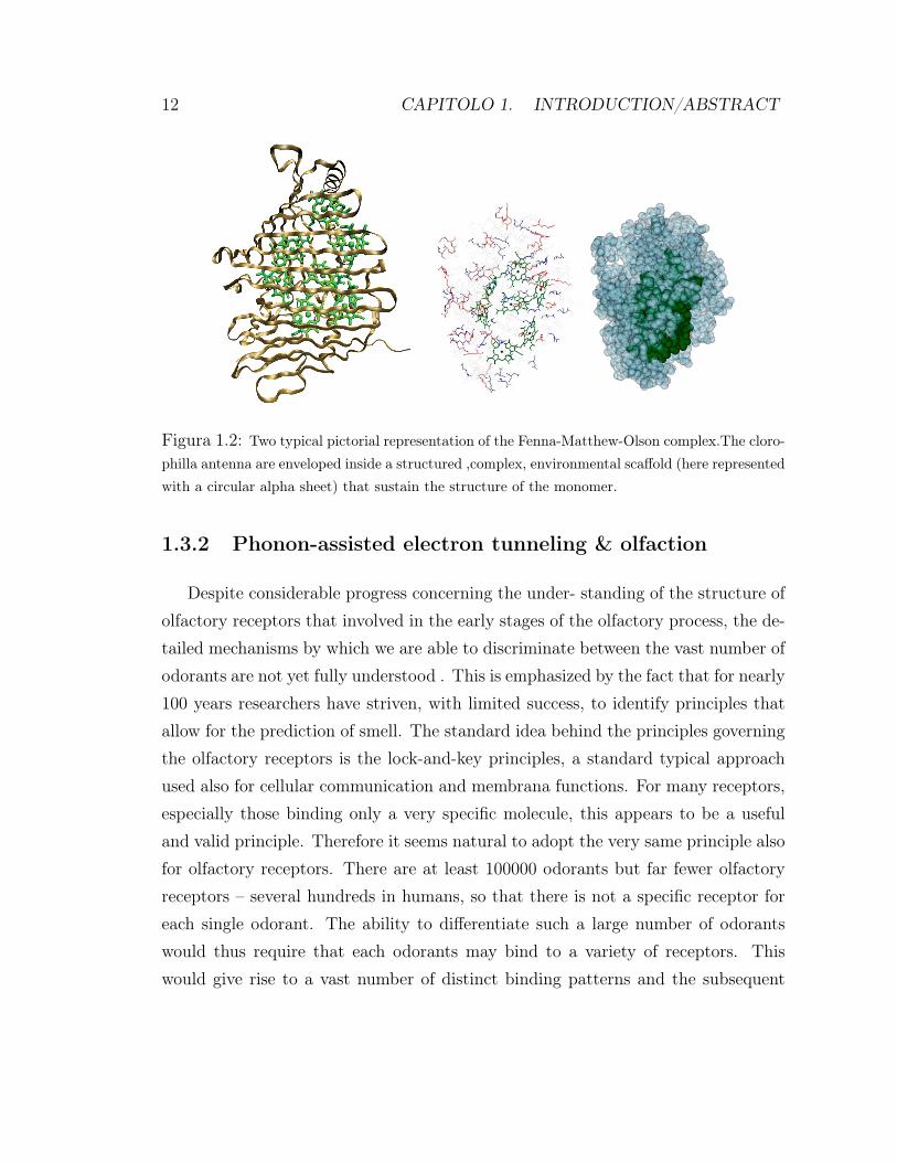
In physical terms an organised structured like that of the well studied FMOantenna complex is no more than a transport network assigned to the convey ofelectronic excitations (excitons) , that is composed of a set of highly absorptiveentities such bacteriochlorophyll molecules each of which may support an electronicexcitation (a Frenkel exciton). The protein scaffold role is to display them into thespace into a specific geometry,somebody has also argued that the protein scaffoldmay give a further help to the transport ability of the network with little variations inthe inter-antenna distance and so modifying the dipolar strength between antennasin order to improve the tuning between them. The full Hamiltonian describing theexciton- vibrational interaction as well as the exciton-exciton interaction is given byH = Hex +HI +HB where
Hex =N∑n=1
En|n〉〈n|+1
2
∑m 6=n
(|m〉〈n|+ h.c.) (1.1)
HB =∑i,k
}ωka†ikaik (1.2)
HI =1
2
∑n
(∑k
√Snkωk(ank + ank†)|n〉〈n|+ h.c.) (1.3)
with |n〉 the excitation on site n,Jmn the dipolar interaction between excitationson different sites, ank, a†nk the bosonic destruction and creation operators for kth
independent vibrational mode coupled to site n. In the end Snk is the Huang-Rhysfactor which determined the strength coupling between exciton and vibration mode.
12 CAPITOLO 1. INTRODUCTION/ABSTRACT
Figura 1.2: Two typical pictorial representation of the Fenna-Matthew-Olson complex.The cloro-philla antenna are enveloped inside a structured ,complex, environmental scaffold (here representedwith a circular alpha sheet) that sustain the structure of the monomer.
1.3.2 Phonon-assisted electron tunneling & olfaction
Despite considerable progress concerning the under- standing of the structure ofolfactory receptors that involved in the early stages of the olfactory process, the de-tailed mechanisms by which we are able to discriminate between the vast number ofodorants are not yet fully understood . This is emphasized by the fact that for nearly100 years researchers have striven, with limited success, to identify principles thatallow for the prediction of smell. The standard idea behind the principles governingthe olfactory receptors is the lock-and-key principles, a standard typical approachused also for cellular communication and membrana functions. For many receptors,especially those binding only a very specific molecule, this appears to be a usefuland valid principle. Therefore it seems natural to adopt the very same principle alsofor olfactory receptors. There are at least 100000 odorants but far fewer olfactoryreceptors – several hundreds in humans, so that there is not a specific receptor foreach single odorant. The ability to differentiate such a large number of odorantswould thus require that each odorants may bind to a variety of receptors. Thiswould give rise to a vast number of distinct binding patterns and the subsequent

1.3. BIOLOGICAL INTRODUCTION 13
sensation of smell, nonetheless an clear explication hasn’t been experimentally foun-ded yet. Moreover has been noticed in recent experiments that Drosophila flies arecapable of discriminating between molecules in their hydrogenated and their deu-terated form and, importantly, are able to generalize from deuterated molecules toother molecules that exhibit a vibrational modes similar in frequency to the Carbon-Deuterium stretch mode. These observations sustain the alternative theory basedon the physical-vibrational properties of the molecules rather then the standardchemical lock-and key mechanism. The physical mechanism besides the olfactoryphenomena should be, as proposed by Luca Turin, the inelastic electron tunnelingspectroscopy, which allows to recognize the vibrational spectra of a molecula. In thenew perspective of noise assisted quantum effects the are the environmental phononwho supported the the inelastic electron tunneling; there is on the one hand thetunneling process of a massive particle, here the electron, and on the other handthe fact that a vibrational mode, that is a quantized harmonic oscillator, can onlytake up energy in discrete quanta proportional to the relevant vibrational frequencyωodor. It is the second aspect that makes it possible for this process to discrimina-te effectively between different vibrational modes and thus between the vibrationalfingerprints of different molecules.
1.3.3 Magneto reception in birds
Despitethe navigation and orientation ability of lot of mammals,birds reptilesand amphibians is well documented, the mechanism behind this magneto sense oflot of creatures it actually unclear. Recently behavioral experiments with birdssuch as the Euro- pean robin to study avian magneto-reception have led to theobservation that the process of avian magneto- reception depends on the wavelengthof the ambient light and can be disrupted by very weak external oscillating magneticfields. These combined with independent experiments of magnetic field effects onradical pair reaction at a earth magnetic fields provides evidences that support theidea that the chemical compass (which is composed free radicals) may be involved inmagneto reception. A donor-acceptor pair is initially in its electronic ground state
14 CAPITOLO 1. INTRODUCTION/ABSTRACT
characterized by a paired electron in a singlet state. Absorption of a photon inducesan electron transfer of a single electron from the donor to the acceptor thus creatinga radical pair, that is, two molecules with an unpaired electron each. For simplicitywe assume that the electronic spin state remains unaffected in this step so that theelectrons remain in a singlet state. At this stage no magnetic field sensitivity can beexpected as the spin singlet state is rotationally symmetric and hence insensitive tothe orientation and magnitude of the external magnetic field. To break the symmetryis the nuclear spin environment of the donor and acceptor moleculas. Due to thedistance dependence of the dipolar interaction between electron and nuclear spin theunpaired electrons on donor and acceptor see dominantly uncorrelated interactionswhich induce symmetry- breaking transitions from the singlet to the triplet manifold.
Capitolo 2
Dynamical Simulation of 1-D
Quantum Many body Systems
2.1 Introduction
Biological systems are not so strictly bounded systems, they best suite the de-finition of slightly entangled systems, but even if they’re not a standard strongly-correlated systems as the usual ones utilized in condensed matter physics (e.g. Bose-einstein condensate) as demonstrated by Vidal into they’re works it’s always possibleto perform a classical simulation of the evolution of the quantum state that descri-bed these type of states if the computational cost it’s not exponential ; so somespecific quantum evolutions can be efficiently simulated by a classical computer ,and therefore cannot yield an exponential computational speed-up. TEBD makesuse of a classical computer, pure-state quantum dynamics of n entangled qubits,whenever only a restricted amount of entanglement is present in the system. Con-sider, a pure state |Φ〉 ∈ H⊗n2 of an n-qubit system. Let A denote a subset of the nqubits and B the rest of them. The Schmidt decomposition (SD) of |Φ〉 with respectto the partition A:B reads
|Ψ〉 =
χA∑α=1
λα|Φ[A]α 〉 ⊗ |Φ[B]
α 〉 (2.1)
15

16CAPITOLO 2. DYNAMICAL SIMULATION OF 1-D QUANTUM MANY BODY SYSTEMS
where the vector |Φ[A]α 〉, |Φ[B]
α 〉 is an eigenvector with eigenvalue |λα〉>0 of the re-duced density matrix ρ[A], ρ[B] whereas the coefficient λα follows from the relation〈Φ[A]
α |Ψ〉 = λα|Φ[B]α . The Schmidt rank χA is a natural measure of the entanglement
between the qubits in A and those in B. Accordingly, we quantify the entanglementof state |Ψ〉 by χ
χ ≡ maxA
χA (2.2)
that is, by the maximal Schmidt rank over all possible bi-partite splittings A:B ofthe n qubits. We shall say that |Psi〉 is only slighlty entangled if χ is small. Inparticular, here we are interested in sequences of states |Ψn〉 of an increasing numbern of qubits (corresponding, say, to quantum computations with increasingly largeinputs). In such a context we consider χ to be small if it grows at most polynomiallywith n, χn = poly(n). If through a pure-state quantum computation χn is upperbounded by poly(n), then the computation can be classically simulated with poly(n)memory space and computational time, and so reproducible
2.2 1D Quantum systems
2.2.1 Definition
To begin we consider a quantum system composed of M subsystems (or sites)each with an identical local finite d-dimensional Hilbert space Hd spanned by states|j〉 The full state space of this system H = H⊗Md is then spanned by the productbasis of these local states |J[1,M ]〉 = |j1〉|j2〉⊗···|jM〉 and has dimension D = d whichgrows exponentially withM . An arbitrary state |Ψ〉 of the system can be expandedin this basis as
|Ψ〉 =∑|j[1,M ]〉
cj1,j2···jM |J[1,M ]〉 (2.3)
with D complex amplitudes cj1,j2···jM . While we have imposed a sequential labellingto the subsystems we have not yet made any real constraint on the dimension ofthe system. Indeed, the actual geometry of the system is only truly revealed bythe range and pattern (with respect to the labelling) of interactions between the

2.2. 1D QUANTUM SYSTEMS 17
underlying subsystems as determined by the Hamiltonian1 of the system. Thus,to restrict our considerations to a genuine 1D quantum system the Hamiltonian Hgoverning the system must have short-ranged interactions only.
2.2.2 Basic Properties of 1D quantum systems
The knowledge of how entanglement is distributed within a 1D system permitsa parametrisation of low-lying excitation for 1D quantum system[8]. We considerthe 1D quantum Ising model with a transverse magnetic field
HIsing = −J(M−1∑
i=1
σxi σxi+1 + g
M∑i=1
σzi
)(2.4)
since it is exactly solvable. We ’ll consider two important properties of the groundstate. Firstly, the spin-spin correlations as a function of the distance between thespins l which are of the form
Cabl = 〈σai σbi+l〉 − 〈σai 〉〈σbi+l〉 (2.5)
Since correlation functions Cabl vanish for all product spin states a change in their
behaviour is a signature of a corresponding change in the structure of entanglementin the ground state. The second relevant property is the entanglement entropy SL ofa contiguous block of L spins, which is calculated from the block’s reduced densitymatrix ρL = trM−L(|Ψgs〉〈Ψgl|) via the von-Neumann entropy
SL = −tr(ρLlog2ρL
)(2.6)
and directly measures the amount of entanglement between the block and the restof the chain.
2.2.3 Schmidt decomposition
The essential mathematical tool we use to build a more efficient formulation isthe Schmidt decomposition. Starting from an arbitrary state |Ψ〉 in the Hilbert spaceH of an M-site system, we begin by bipartitioning this system into two subsystems

18CAPITOLO 2. DYNAMICAL SIMULATION OF 1-D QUANTUM MANY BODY SYSTEMS
A and B which are composed of some subset of m and M −m sites respectively. Byusing some orthonormal basis |iA〉 spanning the dm-dimensional Hilbert space HA
and similarly |jB〉spanning the dM−m dimensional Hilbert space HB this arbitrarystate can be expressed as
|Ψ〉 =dm∑i=1
dM−m∑j=1
Cij|iA〉 ⊗ |jB〉 (2.7)
The amplitudes Cij of this expansion can then be interpreted as the elements of a(dm × dM−m) matrix C. We then perform a standard operation of linear algebra,called the singular-value-decomposition (SVD), which breaks C up into the productC = UDV , where U and V are (dm × dm)and (dM−m × dM−m)unitary matricesand D is a (dm × dM−m)diagonal matrix whose elements are real and non-negative. We denote the diagonal elements of D as λα = Dαα, and the number of non-zeroλα’s as χ. This operation then brings the expansion into the form of a Schmidtdecomposition as
|Ψ〉 =
χ∑α=1
λα
( dm∑i=1
Uiα|i〉A)⊗( dM−m∑
j=1
Vαj|j〉B)
=
χ∑α=1
λα|φ[A]α 〉 ⊗ |φ[B]
α 〉 (2.8)
Since the unitary matrices U and V act solely on the corresponding subspaces, HA
andHB, respectively, they have been used to construct the orthonormal bases, calledSchmidt states, {|φ[A]
α 〉} and {|φ[A]α }which span χ-dimensional subspaces of HA and
HB respectively. The diagonal elements λα are called the Schmidt coefficients whichwe take from now on as being arranged in descending order so λα > λα + 1 andsatisfy
∑α λ
2α = 1, while χ is called the Schmidt rank. The reduced density matrices
for the two subsystems ρA = trB(|Ψ〉〈Ψ|)and ρB = trA(|Ψ〉〈Ψ|) then follow from theSchmidt decomposition as
ρA =
χ∑α=1
λ2α|φ[A]α 〉〈φ[A]
α | ; ρB =
χ∑α=1
λ2α|φ[B]α 〉〈φ[B]
α | (2.9)

2.3. MATRIX PRODUCT REPRESENTATION 19
which immediately demonstrates that both ρA and ρB are diagonal in their respectiveSchmidt basis and have identical spectra. Important physical quantities follow fromthe nature of the spectrum {λ2α}. In particular it allows entanglement between thetwo subsystems to be measured via the entropy S[A|B], introduced earlier as SL,which is computed via the Shannon entropy of spectrum
S[A|B] = −χ∑α=1
λ2α log2 λ2α (2.10)
Thus, with the total system in a pure state, entanglement between the two subsy-stems appears as entropy in the resulting reduced density matrices.
2.3 Matrix Product Representation
The ground states of 1D systems have a several unique properties, so we nowcome to the question of how to exploit these. The approach w will pursue is basedon parameterising the state in the form
|Ψ〉 =∑J[1,M ]
f(A[1]j1A[2]j2 · · · A[M ]jM
)|J[1,M ]〉 (2.11)
where A[M ]jM are a set of d complex matrices of dimension (χm−1×χm) labelledby the physical index jm. Each site m of the system therefore has a matrix assignedto it dependent on which physical basis state|jm〉 it is in. The full set of amplitudescj1j2···jM for the state are then encoded into specific products of such matrices andextracted by the function f(·) which maps (χ0 × χM) matrices to scalars. For thisreason Eq. (2.11) is called a matrix product representation.The exact form of thefunction f(·) depends on the boundary conditions. In the case of periodic boundaryconditions (PBC) the matrix product representation of a state is
|Ψ〉 =∑J[1,M ]
tr(A[1]j1A[2]j2 · · · A[M ]jM
)|J[1,M ]〉 (2.12)

20CAPITOLO 2. DYNAMICAL SIMULATION OF 1-D QUANTUM MANY BODY SYSTEMS
where the function f(·) is a conventional matrix trace. For open boundary conditions(OBC) the expansion is
|Ψ〉 =∑J[1,M ]
⟨Φ0|A[1]j1A[2]j2 · · · A[M ]jM |ΦM
⟩|J[1,M ]〉 (2.13)
where |Φ0〉 and |ΦM〉 1are boundary states in the vector spaces Cχ0 and CχM , re-spectively. In this case the function f(·) is then equivalent to the scalar-productwith these boundary states. Will make use of this properties.
2.3.1 Schmidt decomposition and canonical forms
Till now we have made no constraints on the form of the matrices A[m]jm . Thisnot only makes this description difficult to interpret, it also makes them harder tohandle numerically, but using the insertion of the identity (a gauge freedom) of anynon-singular square (χm× χm) matrix X along with its inverseX−1 into the matrixproduct sinceA[m]jmA[m+1]jm+1 = (A[m]jmX−1)(XA[m+1]jm+1) we can solve this lack.To begin we consider a system with OBC and split it after site k into two contiguousblocks L = 1, · · ·, kand R = k + 1, · · ·,M . Using the gauge freedom we redefine thematrix A[k]jk as A[k]jk → A[k]jkD−1 where D is a diagonal (χk×χk) matrix with realelements λαk , and correspondingly introduce it into the product as
M∏m=1
A[m]jm →( k∏m=1
A[m]jm)D( M∏m′=k+1
A[m′]j′m
)(2.14)
By inserting the resolution of the identity∑
αk|αk〉〈αk| for the vector spaces Cχk
, on both sides of the diagonal matrix D the matrix product representation of |Ψ〉can then be readily split up into the form
|Ψ〉 =
χk∑alpha=1
λαk |φ[L]αk〉|φ[R]
αk〉 (2.15)
1Note that for numerical calculation we can set χ0 = 1 and χM = 1 for convenience

2.3. MATRIX PRODUCT REPRESENTATION 21
where the states of the blocks R and L are
|φ[L]αk〉 =
∑J[1,k]
⟨Φ0|A[1]j1A[2]j2 · · · A[k]jk |αk
⟩|J[1,k]〉 (2.16)
|φ[R]αk〉 =
∑J[k+1,M ]
⟨αk|A[k+1]jk+1 · · · A[M ]jM |ΦM
⟩|J[k+1,M ]〉 (2.17)
The corresponding scalar-products of these block states are
〈φ[L]αk|φ[L]αk〉 =
∑J[1,k]
⟨αk|(A[k]jk)† · · · (A[1]j1)†|αk
⟩⟨Φ0|A[1]j1 · · · A[k]jk |βk
⟩〈φ[R]
αk|φ[R]αk〉 =
∑J[k+1,M ]
⟨ΦM |(A[M ]jM )† · · · (A[k+1]jk+1)†|αk
⟩⟨βk|A[k+1]jk+1 · · · A[M ]jM |ΦM
⟩The splitting of the state introduce another question : the right and left handednessof the matrixes of our state. we introduce the notation A← and A→ to signify whenan A matrix obeys the corresponding left or righthanded orthonormality constraint.The importance of distinguishing them will be clear in next chapters (especially forhandling numerical errors). For the boundary we impose
d∑j1=1
(A[1]j1← )†|Φ0〉〈Φ0|A[1]j1
← = 1 lefthanded (2.18)
d∑jM=1
A[M ]jM→ |ΦM〉〈φM |(A[M ]jM
→ )† = 1 righthanded (2.19)
To ensure ourseleves Eq. (2.15) to be a Schmidt decomposition of |Ψ〉 we imposeto the A matrices of the left ([L]) and right ([R])side to obey one of the followingconstraints.
d∑j1=1
(A[1]j1← )†A[1]j1
← = 1 lefthanded (2.20)
d∑jm=1
A[M ]jM→ (A[M ]jM
→ )† = 1 righthanded (2.21)
If Eq. (2.20) applies to all matrices A[m]jm with 1 < m ≤ k, then the left blockstates |Φ[A]
αk 〉 orthonormality can be established,by its successive use (after using the

22CAPITOLO 2. DYNAMICAL SIMULATION OF 1-D QUANTUM MANY BODY SYSTEMS
boundary 2.20). The same occurs for the right block states |Φ[B]αk 〉, after applying
Eq. (2.21).Finally, we now require |Ψ〉 to be normalised, which is equivalent totr(D2) = 1 =
∑αkλ2αk = 1, allowing the diagonal matrix D to be identified with
the matrix of Schmidt coefficients√
Λ[k].
2.4 Calculations with MPS
2.4.1 Density matrices
In order to produce any measure it’s necessary define the reduced density ope-rators of a small subset of sites, such as ρk for a single site k or ρkl for two sites kand l, and expectation values of the form 〈Ψ|O1 ⊗O2 · · ·OM |Ψ〉 where {Oj}Mj=1 areoperators acting in the Hillbert space Hj of site j. For convenience the descriptiongiven for the rest of this section utilises MPS with PBC and unconstrained matrices.To begin the full density operator ρ = |Ψ〉〈Ψ| of the system is given by
ρ =∑J[1,M ]
∑I[1,M ]
tr( M∏m=1
A[m]jm)tr( M∏m=1
A∗[m]jm)|J[1,M ]〉〈I[1,M ]| (2.22)
after using tr(XY Z)∗ = tr(X∗Y ∗Z∗).By applying the matrix identitiestr(X)tr(Y ) =
tr(X ⊗ Y ) = tr(Y ⊗X)and (ABC)⊗ (XY Z) =(A⊗X)(B ⊗ Y )(C ⊗ Z)we obtaina more compact form
ρ =∑J[1,M ]
∑I[1,M ]
tr( M∏m=1
E[m]jmim)|J[1,M ]〉〈I[1,M ]| (2.23)
where E[m]jmim = A[m]jm ⊗ A∗[m]im . To normalize the state we trace out all thephysical sites as tr(ρ) = 〈Ψ|Ψ〉 = tr(
∏Mm=1 I
[m]) where the contraction of the physicalindices labelling the set of matrix E[m]jmim is called the “transfer” matrix and isdenoted as I[m] =
∏djm=1E
[m]jmjm . By leaving out one site k from this trace weobtain the reduced density operator
ρk =d∑
jk=1
d∑ik=1
tr([ k−1∏
m=1
I [m]]E[k]jkik
[ M∏m′=k+1
I∗[m′]])|jm〉〈im| (2.24)

2.4. CALCULATIONS WITH MPS 23
which is reproduced in fig(2.1). Expressions for the reduced density operators oflarger numbers of sites then follow a similar form as a trace of products of appropriatesets of I [m] and E[m]jmim matrices
〈Ψ|O1 ⊗O2 ⊗ · · ·OM |Ψ〉 = tr( M∏m=1
O[m])
(2.25)
with the observable matrices being defined as
O[m] =d∑
jm=1
d∑im=1
〈jm|Om|im〉E[m]jmim (2.26)
and noting that whenever Om = [1]m then O[m] = I [m].
2.4.2 Two-sites gates
Now we can move forward the essential core method of the TEBD algorithm,precisely how to update them after applying two-site gates. To begin we need onlyconsider an MPS with the initial form
ρk =∑J[1,M ]
〈Φ0|( k−1∏m=1
A[m]jmjm′←
)Ξjkjk+1
( M∏m′=k+2
A[m′])|Φm〉|J[1,M ]〉 (2.27)
where the A matrices are orthonormalised. The central set of matrices Θjkjk+1
spanning the two sites is defined in one of three ways
Ξjkjk+1
√
Λk−1A[k]jk→ A[k+1]jk+1
→ Left ,
A[k]jk←√
ΛkA[k+1]jk+1→ Center
A[k]jk← A[k+1]jk+1
←√
Λk+1 Right
(2.28)
depending on where the twist in the handedness is located. Since the remainingmatrix products give orthonormalised left and right Schmidt states the state can beexpressed in the basis
|Ψ〉 =∑
[k,k+1]
χk−1∑αk−1=1
χk+1∑αk+k1=1
〈αk−1|Ξjkjk+1|αk+1〉|L[k−1]αk−1〉|jl〉|jjk+1
〉|R[k+1]αk+1〉 (2.29)

24CAPITOLO 2. DYNAMICAL SIMULATION OF 1-D QUANTUM MANY BODY SYSTEMS
Figura 2.1: (a) The graphical representation of the full density matrixρ = |Ψ〉〈Ψ| of the system with PBC. The shadedtriangular object represents the matrices A[m]jm . (b) Tracing out all sites, aside from site m, is equivalent to contracting (joining)all the appropriate physical indices. The remaining (uncontracted) indices im and jm are then the rows and columns of the densitymatrix ρm .The shaded objects represent the matrices E[m]jmim and I[m] .

2.4. CALCULATIONS WITH MPS 25
Figura 2.2: (a) An observable O acting on one site. (b) The graphical representation of the matrix O[m] formed by contractionwith O. (c) The contraction of indices required for the computation of 〈OmOm+l〉.
The utility of this two-site-two-block form is that the physical basis of sites k andk + 1 appear explicitly and we may now apply exactly an arbitrary transformation
G =∑
J[k,k+1]
∑I[k,k+1]
Gjkjk+1
ikik+1|jk〉|ik+1〉〈ik+1|〈jk+1| (2.30)
on these two sites directly. This transformation mixes up the set of Θjkjk+1matricesas
Θjjjk+a =∑ik,k+1
Gjkjk+1
ikik+1Ξik,ik+1 (2.31)
giving the new state |Ψ′〉 = G|Ψ〉 in the same basis as
|Ψ′〉 =∑
[k,k+1]
χk−1∑αk−1=1
χk+1∑αk+k1=1
〈αk−1|Θjkjk+1|αk+1〉|L[k−1]αk−1〉|jl〉|jjk+1
〉|R[k+1]αk+1〉 (2.32)
which is shown in Fig. (a). In a similar way to Ξjkjk+1 the new quantity Θjkjk+1 isa set of d2(χk−1 × χk+1) matrices indexed by the two physical indices jk and jk+1.This matrix represents a set of anomalous two-site matrices in our MPS. To bringthe decomposition back into a standard MPS form we need to factorise Θjkjk+1 . Atechnical description of this procedure can be found in the mathematical extra.

26CAPITOLO 2. DYNAMICAL SIMULATION OF 1-D QUANTUM MANY BODY SYSTEMS

Capitolo 3
Time Evolving Block Decimation
As stated at the beginning the biological system are slightly entangled one so weonly consider Hamiltonians with nearest neighbouring interactions,therefor we havean explicit 1D geometry. The most general form of Hamiltonian we shall consider is
For OBC it is convenient both for notation and for calculations to reformulateH(t) in terms of time-dependent two-site operators as
Hj,j+1 =1
2
k1∑ν=1
cνj (t)hνj +
k2∑ν=1
cνj (t)hνj,j+1+
1
2
k1∑ν=1
cνj+1(t)hj+1ν 1 ≤ j ≤M−1 (3.1)
which are defined symmetrically about site j, aside from at the boundaries where
H1,2(t) =
k1∑ν=1
cνj (t)hνj +
k2∑ν=1
cνj (t)hνj,j+1 +
1
2
k1∑ν=1
cνj+1(t)hj+1ν
HM−1,M(t) =
k1∑ν=1
cνj (t)hνj +
k2∑ν=1
cνj (t)hνj,j+1 +
1
2
k1∑ν=1
cνj+1(t)hj+1ν
giving in total H(t) =∑M−1
j=1 Hj,j+1(t). We search for the dynamical evolutionof a system given by the integration of dimensionless time-dependent Schrodingerequation ıδt|Ψ(t)〉 = H(t)|Ψ〉. For the case of a time-independent Hamiltonian H
this equation admits a formal solution |Ψ(t)〉 = exp(−iHt) |Ψ〉. Numerical calculationsproceed by discretising the total time T into T/δt steps where δt ≤ 1 as tn = (n−1)δt
with n = (1, · · ·, T/δt), obtaining the time-evolution operatorU(t) as the product
27
28 CAPITOLO 3. TIME EVOLVING BLOCK DECIMATION
U(t) =∏t
n=1 exp(−iH(tn)δt) connecting the initial state|Ψ〉 to the state |Ψ(t)〉. Thecomputation of Un is further aided by the nearest neighbour hypothesis,the latterenables H(tn) to be summed up into two operators H(tn) = F +G where
F =∑oddj
Hj,j+1(tn) and G =∑
evenj+1
Hj,j+1(tn) (3.2)
leaving Un = exp[−i(F + G)δt]. Since no two terms within either F or G involvethe same sites they all commute amongst themselves. Given that the exponentialof each operators alone can be calculated exactly as the product of unitaries whichact exclusively on two neighbouring sites
e−iFδt =∏oddj
e−iHj,j+1(tn)δt and e−iGδt =∏evenj
e−iHj,j+1(tn)δt (3.3)
The complications in computing the unitary Un fully arise from the fact that Fand G do not in general commute. Thanks the Suzuki-Trotter expansion we ensurethe preservation of the norm of the state and we can overcome the problem of thecommutation of the exponential of our evolution operators.
The simplest and more common expansion follows by assuming F and G commu-te and constitutes a first-order expansion of Un in δt as Un = exp(−iFδt)exp(−iGδt)+O(δt2). If instead we define the symmetric product
s(F,G, y) = e−12iFye−iGye−
12iFy (3.4)
then a second-order expansion follows as Un = s(F,G, δt) + O(δtt3). Important toset: Trotter error is not the only source of error and in most cases is actually theleast important. For this reason using higher-order expansions can even becomecounter-productive.
3.0.3 Suzuki-Trotter sweeps
The suzuki Trotter decomposition is performed applying a two-site gate to aneven and odd sites. In order to start the ST sweep and apply the gate operator we
3.1. ERRORS IN TEBD 29
have to ensure that the handedness of all matrices A of the initial state is the same,for example left-handed : A[1]j1
← A[2]j2← · · ·A[M ]jM
← . Given that we can apply to the twosites (eq 2.28,2.29) the gate of the formula 2.30 in order to compute the n− th timestep evolution of Fj,j+1 or Gj+1,j+2. Problem lies in the fact that after applying theunitary gate the updated matrix A[k] posses the correct handedness (←)while theA[k + 1] doesn’t(→), but it can be flipped to A′[k+1]
← via a right division by√
Λ[k+1]
and a left multiplication by√
Λ[k]. Despite it’s facility, this operation it’s numericalunstable being the value of
√Λ[k+1] very small. This means that a tentative of higher
our precision in the simulation raising the value of χ, if excessive, will enhance thenumerical instability. In every case this problem can be solved by applying the gatesin sequential zip.For example, in the case of a second-order decomposition actingon a state which is entirely lefthanded we apply the gates within exp(−iFδt) fromleft-to-right as
e−12iFδt = e−
12iH1,2(tn)δt(12,3)e
− 12iH3,4(tn)δt · (3.5)
·(14,5) · · · (1M−2,M−1)e−12iHM−1,M (tn)δt
where explicit identity operations k,k+1 have been inserted in between the usualunitaries. The purpose of the identity operations is to shift the twist in handednessone site to the right making the decomposition compatible for the next gate. We thendo precisely the same, but in the opposite direction, when applying exp(−iGδt), andfinally after applying the last zip exp(−iFδt) our MPS will be entirely righthanded.We remark here that this kind of zipping is very close to the finite-system sweepsused in DMRG.
3.1 Errors in TEBD
3.1.1 Trotter Error
For any single time-step δt the Trotter error εδt will be of order εδt ≈ (δt)p+1 fora pth- order expansion. To evolve the state to some final time T we need to performT/δt time steps, and denote the state after these steps as |Ψst〉. If the exact time-

30 CAPITOLO 3. TIME EVOLVING BLOCK DECIMATION
evolved state is |Ψ(T )〉 then the Suzuki-Trotter overlap error isεst = 1 − |〈Ψ(T )|Ψst〉 |. It has been found from numerical evidence [9] that εst ≈MT (δt)p and therefore scales linearly with the overall evolution time T and thesystem size M. This error is controlled entirely by δt and so requires δt << 1.
3.1.2 Truncation error
The most important source of error in TEBD is the truncation of this Sch-midt decomposition to include only the χ Schmidt states with the largest Sch-midt coefficients. This source of errors derive from the truncation approxima-tion of the state |Ψ〉 = |Ψtr〉 − |Ψres〉, with |Ψtr〉 =
∑χαmλ[m]αm |L
[m]αm〉|R
[m]αm〉 and
|Ψ⊥〉 =∑
αm>χλ[m]αm|L
[m]αm〉|R
[m]αm〉.
At the first step we have εm = 1 − |〈Ψ|Ψres〉| =∑
αm>χ(λ
[m]αm)2. At the next
step we will decompose the state |Ψres〉 in the same way obtaining a total errorεm+1 = 1− |〈Ψ|Ψ′res〉 = 1− (1− εm+1 − εm). So moving along all the sites the finaltruncation error will be εtr =
∑M−1m=1 εm which is additive in the individual truncation
errors. In practise the degradation of the norm of the MPS is a good measure ofthe truncation error and we might tolerate it becoming 10−6.
The runaway time was empirically found to increase with χ, but decreases withthe number of two- site gates applied and with M. Obtaining an accurate simulationfor a desired time therefore requires a careful balancing of δt and the order of theSuzuki-Trotter expansion.
Here a graph of the effects of the runaway time effects for an application of 1000two-site gate application
Here we can see the direct effect of the refinement of the value of our basis troughthe rising of the χ parameter inside our simulation. As stated above a low value ofthe Schmidt basis will give raise to numerical instability for a very low run awaytime. A χ value of 30 just show to better preserve the norm (and so the dynamics)from great instability.

3.1. ERRORS IN TEBD 31
chi5-20-30.png
Figura 3.1: Populations for AR spectra + delta 180cm−1; rising up of population caused bytruncation error at a valuable runaway time for small χ and different effects on the dynamics bythe truncation error

32 CAPITOLO 3. TIME EVOLVING BLOCK DECIMATION
Capitolo 4
Mapping between system-reservoir quantum models and
semi-infinite discrete chains
4.1 Introduction
All quantum systems encountered in nature experience random perturbationsdue to their coupling to degrees of freedom of their local environments. Informationabout these degrees of freedom are not normally accessible, and to correctly predictthe results of experiments, these degrees of freedom must be averaged over. Thisaveraging introduces qualitatively new features into the otherwise unitary dynamicsof the quantum system, and typically induces an effectively irreversible dynamicswhich drives the system towards an equilibrium with its environment.For quantumsystems, this evolution towards equilibrium not only involves energy transfer to theenvironment, but can also cause the loss of coherence in the system state, oftenon a much faster timescale than the energy relaxation. This latter process of de-coherence destroys quantum mechanical effects arising from the existence of phasecoherence in the state of the system, and must be a part of the total correct dyna-mics of every phenomena description.. The most simple model is the Spin-BosonModel (SBM) one of the simplest non-trivial models of open-system dynamics. Thismodel describes a single two-level system (TLS) coupled linearly to the coordinatesof an environment consisting of a continuum of harmonic oscillators and despite itssimplicity, this model shows a rich array of non-Markovian dynamical phenomena
33

34CAPITOLO 4. MAPPING BETWEEN SYSTEM-RESERVOIR & SEMI-INFINITE DISCRETE CHAINS
that for so short time events can became of relevant importance. In the case ofQuantum Biology this non Markovian backward effects of interaction due to thesystem environment coupling are the key element of the lasting of coherence intothe system (see next chapter).The action of the orthogonal polynomials is to pro-ject by unitary transformation the Hamiltonian into the normal vibrational modescoordinates and produce the 1D chain useful for our dynamical simulation withoutany need of discretisation.
Figura 4.1: pictorial representation of the back scattering effect behind the reborn of coherenceinto the system for an inhomogenous chain
As depicted in fig (3.1) the type of chain product from the projection operatorisn’t translationally invariant, in this way optical effect of reflection can take placeand produce back scattering energy that will come back into the system. Subsysteminitially injects excitations (shown as wave packets) into inhomogenous region ofthe chain. Scattering from inhomogeneity causes back action of excitations on thesystem at later times and leads to memory effects and non-Markovian subsystemdynamics. At long times (yellow dots), after multiple scattering the energy landscapesmooths , excitations penetrate into the homogenous region and propagate awayfrom the system without backscattering. This leads to irreversible and Markovian

4.1. INTRODUCTION 35
excitation absorption by the environment. The inhomogeneity of the chain enter intothe local hamiltonian modifying the energy local parameters of the system througha sort of
4.1.1 System Reservoir structure
The observables in an open quantum system are affected by the unavoidableinteraction with the environment. This environment may be described by an infinitenumber (often called a reservoir) of bosonic or femionic modes labeled by some realnumber. The internal dynamics of the reservoir is given by some Hamiltonian of theform
Hres =
∫ xmax
0
dxg(x)a†xax (4.1)
where in a physical context x could represent some continuous real variable such asthe momentum of each mode, and xmax the maximum value of it which is presentin the reservoir (it could be infinity). In this picture g(x) represents the dispersionrelation of the reservoir which relates the oscillator frequency to the variable x. Thecreation and annihilation operators satisfy the continuum bosonic [ax, a
†y] = δ(x−y)
or fermionic {ax, a†y} = δ(x?y) commutation rules. We assume that the frequenciesg(x) and momenta x of the reservoir are bounded. The internal dynamics of theopen quantum system are described by a un- specified local Hamiltonian operatorHloc and we assume that the interaction between the system and the reservoir isgiven by a linear coupling
v =
∫ xmax
0
dhh(x)A(a†xax) (4.2)
where A is The internal dynamics of the open quantum system are described by aun- specified local Hamiltonian operator Hloc and we assume that the interactionbetween the system and the reservoir is given by a linear coupling.
H = Hloc +Hres + V = Hloc +
∫ xmax
0
dxg(x)a†xax +
∫ xmax
0
dxh(x)A(a†x + ax) (4.3)
It has been shown that the dynamics induced in the quantum system by its inte-raction with the reservoir is completely determined by a positive function of the
36CAPITOLO 4. MAPPING BETWEEN SYSTEM-RESERVOIR & SEMI-INFINITE DISCRETE CHAINS
energy (or frequency ω) of the oscillators called the spectral density J(ω). For thecontinuum model of the reservoir we are considering, this function is given by
J(ω) = πh2[g−1(ω)]dg−1((ω)
dω(4.4)
where g−1[g(x)] = g[g−1(x)] = x. Physically dg−1((ω)dω
can be interpreted as dω thenumber of quanta with frequencies between ω and ω + δω as δω → 0 it representsthe density of states of the reservoir in frequency space. The spectral function thusdescribes the overall strength of the interaction of the system with the reservoirmodes of frequency ω. This physical introduction motivate the next mathematicaldefinition.Definition. It’s defined as spectral density of a reservoir as a real non- negativeand integrable function J(ω) inside of its (real positive) domain, which could bethe entire half-line ω ∈ [0,∞). Of course, given only a spectral density J(ω)), thedispersion relation g(x) and the coupling function h(x) are not uniquely defined. Weshall make use of this freedom to implement a particularly simple transformation ofthe bosonic modes, and we will chose the dispersion function to be linear g(x) = gx.Our main theorem isTheorem 3.1 A system linearly coupled with a reservoir characterized by a spectraldensity J(ω) is unitarily equivalent to semi-infinite chain with only nearest-neighborsinteractions, where the system only couples to the first site in the chain. In otherwords, there exist an unitary operator Un(x) such that the countably infinite set ofnew operators
b†n =
∫ xmax
0
dxUn(x)a†x
satisfy the corresponding commutation relations [bn, b†m] = δnm for bosons, and
{bn, b†m} = δnm for fermions, with transformed Hamiltonian
H ′ =
∫ xmax
0
dxUn(x)H = Hloc+c0A(b0+b†0)+∞∑n=0
ωnb†nbn+tnb
†n+1bn+tb†nbn+1 (4.5)
where c0, tn, ωn are real constants.Proof. The proof is by construction. Since J(ω) is positive, h(x) is real, this defines

4.1. INTRODUCTION 37
the measure dµ(x) = h2(x)dx. Then write
Un(x) = h(x)p(x) = h(x)πn||πn||
(x) (4.6)
where pn(x) are some set of orthonormal polynomials with respect to the measuredµ(x) = h2(x)dx with support on [0, xmax]. Then it is clear that Un(x) is unitary(actually orthogonal as it is also a real transformation) in the sense of∫ xmax
0
dxUn(x)U?m(x) =
∫ xmax
0
dxUn(x = Um(x) =
∫ xmax
0
pn(x)pm(x) = δnm (4.7)
so the inverse transformation is just
a†x =∑n
Un(x)b†n (4.8)
Moreover for bosons
[bn, b†m] =
∫ xmax
0
∫ xmax
0
dxdx′Un(x)Um(x′)[ax, ax′†]
=
∫ xmax
0
∫ xmax
0
dxdx′Un(x)Um(x′)δ(x− x′)
=
∫ xmax
0
dxUn(x)Um(x) = δnm
and similarly it is proved that {bn, bdaggerm} = δnm for fermions. It remains to de-termine the structure of the transformed Hamiltonian H, note that V is transformedlike:
V = A∑n
∫ xmax
0
dxh(x)Un(x)(bn + b†n) = A∑n
∫ xmax
0
dxh2(x)πn(x)
||πn||(bn + b†n)
since for monic polynomials π0(x) = 1 we find
V = A∑n
∫ xmax
0
dxh2(x)πn(x)
||πn||(bn + b†n)
= A∑n
||πn||2σn0||πn||
(bn + b†n) = ||π0||A(b0 + b†0)

38CAPITOLO 4. MAPPING BETWEEN SYSTEM-RESERVOIR & SEMI-INFINITE DISCRETE CHAINS
so c0 = ||π0||. For the Hres term, note that with the choice of lineaer dispersionfunction g(x) = gx for the spectral density J(ω) one obtains
Hres =∑n,m
∫ xmax
0
dxg(x)Un(x)Um(x)b†nbm
=∑n,m
∫ xmax
0
dxh2(x)g(x)pn(x)pm(x)b†nbm
= g∑n,m
∫ xmax
0
dxxh2(x)pn(x)pm(x)b†nbm
With the recurrence relation we substitute the value of xpn(x) in the above integralto find
H ′res = g∑n,m
∫ xmax
0
dxh2(x)[ 1
Cnpn+1(x) +
AnCn
pn(x) +Bn
Cnpn−1(x)
]pm(x)b†nbm (4.9)
then orthonormality yields
H ′res = g∑n
1
Cnb†nbn+1 +
AnCn
b†bbn +bn+1
Cn+1
b†n+1bn
= g∑n
√βn+1b
†nbn+1 + αb†nbn +
√βn+1b
†n+1bn
where we have used the relation between monic and orthogonal recurrence coeffi-cients. So finally we have
ωn = gαn
tn = g√βn+1
4.1.2 Applications
As a prototypical example let us consider the spin-boson Hamiltonian whichdescribes the interaction of a TLS with an environment of harmonic oscillators
HSB = Hloc +
∫ xMAX
0
dxg(x)a†xax +1
2σ3
∫ xMAX
0
dxh(x)(a†xax) (4.10)
where ax are bosonic operators, and the local Hamiltonina of the spin is ginve by
hloc =1
2ησ1 +
1
2εσ3 (4.11)

4.1. INTRODUCTION 39
where σ1, σ2 are the corresponding Pauli matrices. Firstly we will consider spectralfunctions bounded by a hard cut-off at an energy ωc, hence the cut-off xmax =
g?1(ωc) appearing in the integrals in, which are usually parameterized as
J(ω) = 2παω1−sc ωs(ω − ωc) (4.12)
where α is the dimensionless coupling strength of the system-bath interaction andθ(ω − ωc) denotes the Heaviside step function. In the SBM literature, spectralfunctions with s > 1 are referred to as super-ohmic, s = 1 as Ohmic, and s < 1 assub-Ohmic. According to and our convention in taking linear dispersion relations,this continuous spectral function is related to the Hamiltonian parameters by
g(x) = ωcx h(x) =√
2αωcxs/2 (4.13)
With this choice of g(x) and h(x), xmax = 1 and absorbing the common factor ωc√
2α
in the system operator A = ωc√
2ασ3, the following matrix elements generate themapping onto the chain
Un = xs/2P (0,s)n (x) (4.14)
here P (0,s)n = P
(0,s)(x)N−1n
n is a (normalized) shifted Jacobi polynomial (from support [-1,1] to support [0,1]) . The straight calculation can can be found in the mathematicalextras What we care in our simulation is the final result
ωn = ωc(2n+ 1 + s) (4.15)
tn = ωc√
(n+ 1)(n+ s+ 1) (4.16)
that once introduced into our simulation performed the variation in local site energiesand hopping along the chain of normal modes. In this way we reproduce the local sitevariation energy of the (quantum) system and the tunneling parameters along thechain to reproduce the dynamics of the OQS. Obviously in a simulation the setting ofparameters can affect enormously the final result, and in order to correctly describethe dynamic simulation of a system we must be aware of these effects. The two most

40CAPITOLO 4. MAPPING BETWEEN SYSTEM-RESERVOIR & SEMI-INFINITE DISCRETE CHAINS
Figura 4.2: backward propagation effects on the population dynamcs on sites 1 of the clorophillaantenna of theBb820 RC, in the initial state as exciton state, due to different chain lenght. Initialvalueχ= 30, number of bosons=9
significant one are the variation of the total number of boson parameter applied inour simulation and the total length of the chain we used in our modellisation.
In figure 3.1 we can see the great difference in the dynamics behaviours betweentoo much short chains (15 and 20 sites) which produce unavoidable border effect(that resemble a lot the numerical instability of figure 2.3 for short appearances ofthe runaway time) and longer chains (we can see great difference just starting witha chain of length 100).
while here in fig 3.3 we can see how little variation doesn’t produce any particulardifference for certain time evolution. Usually the greater the number of projectionthe better, if not the only problem connected are numerical one, in the maintenanceof numerical stability in the ORTHOPOL connected with the use of Stieltjes integralin order to produce our desiderata new energies and tunnelings values. So we alwaysmust make the correct compromise between parameters’ value inside the numerical

4.1. INTRODUCTION 41
Figura 4.3: backward propagation effects on the population on sites 1 of the clorophilla antennaof theBb820 RC for comparable length chain.initial valueχ= 30, number of bosons=9
possibilities ours tools permit us. A shorter chain will not be affected from numericalinstability connected to the Stieltjes integrations but will suffer of great bordereffects, while in the other case the dynamics will not suffer borders effects butshould be wrecked from previous instabilities.
Here we can check the numerical difference between physical systems treatedwith a different number of bosons, but with same χ and length of 200

42CAPITOLO 4. MAPPING BETWEEN SYSTEM-RESERVOIR & SEMI-INFINITE DISCRETE CHAINS
Figura 4.4: dynamics with different boson number for the modellisation of the phononenvironment.χ=30 chain lenght of 200
Capitolo 5
Photosynthesis network transport
5.1 The phonon antenna mechanism
The extreme consequence of the basic principle of phonon antenna have beenfound to underlie the fruitful interplay between vibrational environments and cohe-rent quantum dynamics, which will provide an understanding why optimal transportperformance in proteic complex can arise at intermediate noise levels. As examplelet’s use a 3 sites network where site 2 whose excitation energy, position and orienta-tion, and hence dipolar interaction strength with sites 1 and 3 we are free to choose.We assume that site 3 provides the zero of excitation energy, the question that wewould like to answer concerns the optimal choice of excitation energy, position andorientation of site 2 or in other words the optimal choice of the excitation energy ofsite 2 and its dipolar coupling strengths to sites 1 and 3 As such, this question cannotbe answered unambiguously as we are missing a crucial piece of information, namelythat of the structure of the environmental fluctuations. This structure is characteri-zed by the spectral density of the environment which is a combination of the densityof environmental modes and their individual coupling strength to the system. Let’sassume that the environmental spectral density has a single maximum , roughly asdepicted in fig.(4.1). We finds that the optimal position of site 2 is close to site 1such that it exhibits a strong coherent dipolar interaction and close in excitation
43

44 CAPITOLO 5. PHOTOSYNTHESIS NETWORKS TRANSPORT
energy. these have been found by numerical results, now we can rationalize its originand thereby arrive at a very useful design principle of phonon antenna. Indeed, the
Figura 5.1: In the upper figure, two closely spaced energy levels are separated from a third level to which excitations should bedelivered. They are subject to dephasing noise from an environment with a finite bandwidth that exhibits a maximum. A coherentinteraction between the upper two energy levels leads to dressed states |±〉 with an energy splitting which, if matched to the maximumof the environment spectral density, will optimize transport from the upper to the lower level. Hence the dressed states act as anantenna to harvest environmental fluctuations to enhance transport.
strong coherent dipolar interaction between sites 1 and 2 suggests that we move toa new basis made up of the eigenstates of the coherent part of the dynamics of thesetwo sites, that is the excitonic states of that system (for quantum opticians, the dres-sed state). This change of picture leads us to rewrite the Hamiltonian that describesthe system-environment interactionHI = 1
2
∑n
(∑h
√Snhωk(anh + a†nh|n〉〈n| in the
excitonic basis of eigenstates |en〉 of eq. (1), so that |i〉 =∑
nCin|en〉 and the coupling
terms
HI =1
2
∑n,m
(Qn,m|en〉〈em|+ h.c.) (5.1)
where
Qn,m =∑i,k
√SkwkC
inC
im(aik + a†ik) (5.2)
This leads us to two insights. Firstly, in the exciton basis the action of the depha-sing noise now leads to transitions between excitons, that is amplitude noise, which

5.1. THE PHONON ANTENNA MECHANISM 45
facilitates transport towards the lower of the two exciton states. Secondly, the twoexcitons (dressed states) are separated by an energy difference that is related tothe coherent dipolar coupling strength and the energy difference of sites 1 and 2.The dominant contribution to the transition between these excitons (dressed states)arises from those environmental modes whose frequency closely matches the energydifference between dressed states. Indeed, it was found that the physically impor-tant relaxation pathway between sites 1 and 3 is mediated by pigments which arespectrally and spatially positioned by the protein to efficiently sample the spectralfunction of the proteins fluctuations
5.1.1 Non equilibrium long lived coherences
Experimental observations employing ultrafast 2-D spectroscopy on various pho-tosynthetic complexes exhibited long-lived oscillatory features which were interpre-ted as evidence for long-lived electronic coherence in the systems under investigation[11][10]. Under this hypothesis electronic coherence appear to exhibit lifetimes thatcan reach the picosecond range thus exceeding expectations from condensed mattersystems at least tenfold
5.1.2 Last overview on EET principles
The discovery of long-lived coherence between the singly excited electronic statesof photosynthetic antenna complexes has necessitated both a rethinking of energytransfer in biological systems and, more broadly, a reconsideration of the role of thesurrounding environment and of coherent dynamics in the condensed phase. The-se “persistent coherences” unexpectedly outlive coherences between the constituentsingly excited states and the electronic ground state. An ever-growing body of workdemonstrates the persistence of electronic coherence during energy transfer in amultitude of antenna complexes across broad phylogenic boundaries , and coheren-ce within the Fenna-Matthews-Olson complex (FMO) has been shown to be robustto vibronic and structural modifications . This remarkable generality suggests thatpersistent electronic coherences may be a general property of any system of dense-

46 CAPITOLO 5. PHOTOSYNTHESIS NETWORKS TRANSPORT
ly packed chromophores arranged in a nearly static relative geometry and coupledto a common bath. Despite numerous observations of persistent electronic cohe-rence in photosynthetic systems, no clear microscopic mechanism for the survivalof these coherences has been experimentally verified. Theoretical efforts to dissectthe atomistic mechanism are complicated by the size and complexity of photosyn-thetic light-harvesting systems. Consequently, many competing models have beenintroduced to explain the observed quantum beating. These models invoke a broadrange of physical mechanisms, including vibrational coherences , vibronic excitons,nonadiabatic couplings , correlated protein motion , nonsecular coupling betweencoherence and population , and long-range dielectric fluctuations [10]
The higher lying electronic levels, representing the various exciton eigenstatesof the electronic system, are not excited even at room temperature as the excita-tion energy is in the range of eV. The initial (fast) injection of an exciton, eithercoherently or incoherently, populates one of the exciton states of the system andcreates a sudden force on the electrons and nuclei and thus change their equilibriumpositions . Now the environment will start to react to these forces which initia-tes transient oscillations of the modes at approximately their natural frequency wk.The continuous background of the spectral density will relax very rapidly into thenew equilibrium state as it contains a broad range of frequencies and thus posses-ses a very short correlation time. The well-defined long-lived vibrational mode willoscillate for a considerable time (which can be up to several picoseconds) and willinteract with the electronic system. This in turn leads to oscillations between diffe-rent exciton states. We make an observation: these oscillations will have the largestamplitude between those exciton states whose energy difference is nearly resonantwith the frequency of the vibrational mode.
5.2. TEBD SIMULATION FOR DIMERIC SYSTEM 47
5.2 TEBD simulation for Dimeric system
5.2.1 Introduction
We have to keep in mind that one of the key messages of the preceding sections isthe special role of the interplay between the quantum dynamics of a system and itsenvironment, in particular when this environment does not merely represent whitenoise but possesses structure, and this is a typical characteristic of the biologicaltype of environment. Furthermore, it has become clear that the optimal operatingregime for quantum bio dynamics tends to favour parameter ranges in which theinteraction between system components is comparable to the interaction of thesesystem components and their environment. Both features are not well modeled bythe traditional perturbative treatments that lead to master equations of Lindblad, Redfield or modified Red-field type . Indeed the essential importance of the non-Markovian nature of the system-environment interaction calls for the developmentof non-perturbative methods that can accurately, certifiably and efficiently modelthe resulting dynamics. From a numerical point of view it’s important to rememberthat also for a standard model of open quantum system, as the just well commentedspin-boson system, the dynamic induced in the quantum system it’s strictly corre-lated to the structure of the distribution to which is coupled, which modellise allthe information about the interaction between the quantum system and the envi-ronment. For the continuum model of the reservoire that we are considering i.e.choosing g(x) = x this function is given by
J(ω) = πh2(ω) (5.3)
In other words the spectral function thus describes the overall strength of the inte-raction of the system with the reservoir modes of frequency ω. Despite it’s relativesimplicity, the dynamic of this model it’s not exactly solveable and so we have toresort to numerical methods. This is even more true when the environmental spec-tral function exhibits considerable structure or when the coupling strength betweensystem and environment lies in a non perturbative regime. This is exactly the set of

48 CAPITOLO 5. PHOTOSYNTHESIS NETWORKS TRANSPORT
hypothesis we are moving on with our modelization, and even more. WE must re-membering the reach and well structured environment of a biological system coupledto a quantum system that lies inevitably in a non perturbative regime, however evenif the weighth2(x) is a complicated function, families of orthogonal polynomials canbe found by using very stable numerical algorithms such as the ORTHOPOL pac-kage; in this way we are able to obtain a 1D system.This is the key that permit thedeployment of the time-adaptive density matrix renormalization group (t-DMRG)technique to integrate the time evolution of the full system-environment dynamicsefficiently.So now thank the interplay of this two methods we are able to coupleour system (in this case our dimeric system) to environment which show differentproperties onto each site or adding also the local static-Gaussian- disorder in thesite energies of the dimer,another quantity of of a certain relevance being used inthe calculation for the optical spectra absorption of these proteic systems citeAR.
All this element, thanks to possibility to obtain a numerical precise simulationof the dynamics, concur to the simulation of a more and more realistic biologicalenvironment able to take advantage of it’s quantum local properties.
5.2.2 Model parameters
All the data and simulations have been performed onto the modelisation of aproteic dimer (synthetic one or not). The quantum initial state used as initial stateof the antenna sistem in the dimer was 1√
2
(|e〉1 + |e〉2
)(exciton state). The study
on our dimeric system has been carried on zero temperature effect, so it meansno thermal state is present, only the effect of the environmental spectral functionhave been taken into account into the simulations.The time scale is expressed 1/ 5.3picosecond.
5.2.3 The Adolf-Rengel optical spectral
As stated above all the information of the interaction between the reservoirephonon bath and the local quantum system lies into the spectral density function

5.2. TEBD SIMULATION FOR DIMERIC SYSTEM 49
J(ω) of the exciton-vibrational coupling defined as
J(ω) =∑ε
gεδ(ω − ωε) (5.4)
which is also a key quantity in the expressions for optical spectra and the rateconstants for exciton relaxation discussed below. IN the standard theory and cal-culation the value J(ω) is assumed independent on the site index m; i.e., the samelocal modulation of site energies by the vibrational dynamics is assumed. As wewill see through TEBD simulation it’s possible to introduce the effect of differentenvironment for each site, giving raise so to a broader variety of dynamics.
We will not undergo all the calculations developed to find the analytical form ofthe optical spectra, but we will check ourselves to the peculiar aspect of it.
The optical linear absorption is obtained from the dipole-dipole correlation func-tion as explained in detail in Renger and Marcus
α(ω) ∝⟨∑
M
|µM |2DM(ω)⟩dis
(5.5)
where DM(ω) is the lineshape function and 〈 〉dis the denotes an average overstatic disorder in site energies. A Gaussian distribution function of width (FWHM)∆dis is assumed for these energies. The lineshape function DM(ω) was obtainedusing a non-Markovian density matrix approach [13] . It is given as
DM(ω) = Re
∫ ∞0
dteı(ω−ω)teGM (t)−GM (0)et/τ (5.6)
The value DM(ω) contains both vibrational sidebands GM(t) and the lifetimebroadening by the dephasing time τM .Both these quantities are related to J(ω).OF importance is the quantity GM(t) which is defined as
G(t) =
∫ ∞0
dw[(1 + n(ω)J(ω)e−ıωt + n(ω)J(ω)eıωt] (5.7)
Where n(ω) is the mean number of vibrational quanta with energy ~ω that areexcited at given temperature T.

50 CAPITOLO 5. PHOTOSYNTHESIS NETWORKS TRANSPORT
The ω source is shifted from the purely electronic transition frequency ωM dueto the exciton-vibrational coupling
ω = ωM − γMMEλ~
+∑N 6=M
γMNCIm(ωMN) (5.8)
Here above appears another important quantities, the local reorganization energyEλ defined as
Eλ = ~∫ ∞0
dωωJ(ω) (5.9)
In the present model, the spectral density J(ω) contains both a broad low fre-quency contribution S0J0(ω) by the protein vibrations with Huang-Rhys factor S0
and a single effective high-energy vibrational mode of the pigments with Huang-Rhysfactor SH :
J(ω) = S0J0(ω) + SHδ(ω − ωH) (5.10)
For the normalized low-frequency function J0(ω) we assume that it has the sameform as the spectral density, extracted recently [13] from 1.6 oK fluorescence li-ne narrowing spectra of B777-complexes. The final lineshape function DM(ω) sobecome
DM(ω) = e−SHγMMRe
∫ ∞0
dt∞∑k=0
(γMMSH)k
k!xeı(ω− ˆωM+)teG
0M (t)−G0
M (0)e−t/τM (5.11)
We obtained the typical figure.With Orthopol has been reproduced the shape of theAR figure summing the two part of the (5.2)
With TEBD it’s also possible to handle the term ω of the purely electronictransition frequencies(or energies), of the final function DM(ω) , introducing asupplementary source of Gaussian static disorder into the local site energies.
Taking in account all the previous statements about structure environment andphonon antenna tuned on resonant peaks , we can add sharp delta function ontothis standard function in order to take in account for all the resonant, local, typicalphenomena. This is a first ,basic,example of different environments that act ondifferent sites.

5.2. TEBD SIMULATION FOR DIMERIC SYSTEM 51
0 0.2 0.4 0.6 0.8 10
10
20
30
40
50
60
70
80
90
100
Figura 5.2: Normalised standard Adolf Rengel distribution without delta. The delta peakintroduced for the simulations appear at point 0.18 and 0.36
5.2.4 the recoherence and the fundamental role of non-equilibrium
vibrational structure
The phonon antenna mechanism is at the basis of the fundamental role of thereborn of coherence inside the quantum local site of our system. Locally the systemtaking advantage of non equilibrium quantum properties in the pico second timescale when the presence of a structured environment produce peaked value for thephonon energies which are resonant (approximately of the same value) with thedifference in energy of two exciton (in the case of the dimer, the only two present).
As we can see the presence of the noisy environment does not destroy totallythe coherence into the system, but the sharp resonant peak permits the continuousregeneration of that coherence into the sites population for a very longer time. Bothvalues more or less asimptotically verge at the same plateau value for very longtime of the state evolution,as expected. The plateau limit is a consequence of thepresence of the phonon both into with the local systems are inserted.

52 CAPITOLO 5. PHOTOSYNTHESIS NETWORKS TRANSPORT
Figura 5.3: Population in the dimer site 1 obtained with a standard Adolf-Rengel distributionand with a standard with delta peak in 180cm−1
5.2.5 the coupling with the environment
The environment plays a fundamental role into these type of system, so anotheruseful quantities of relevance is the strength coupling between the system and theenvironmnt. As we can easily expect variation into this value produce great variationinto the dynamics of the system.The presence of the resonant peak will alwayssupport the reborn of the coherence in a way or another,but because of the differentvalue of the value of the coupling with the environment, the population dynamicswill move from a more dumped one or to toward a more isolated dumped Raby-likesystem that show an oscillatory behave (see the oscillatory term into equation (4) )
As we can see from figure 5.4 the presence of delta always substains the rebornof coherences inside the system, but the coupling with the environment greatlymodify the dynamics. A strong coupling with the bath produce, as expected, astrong dumping that appears in a double exponential decay and second a plateau inthe value of population lower, while a weaker coupling first of all induce an higher
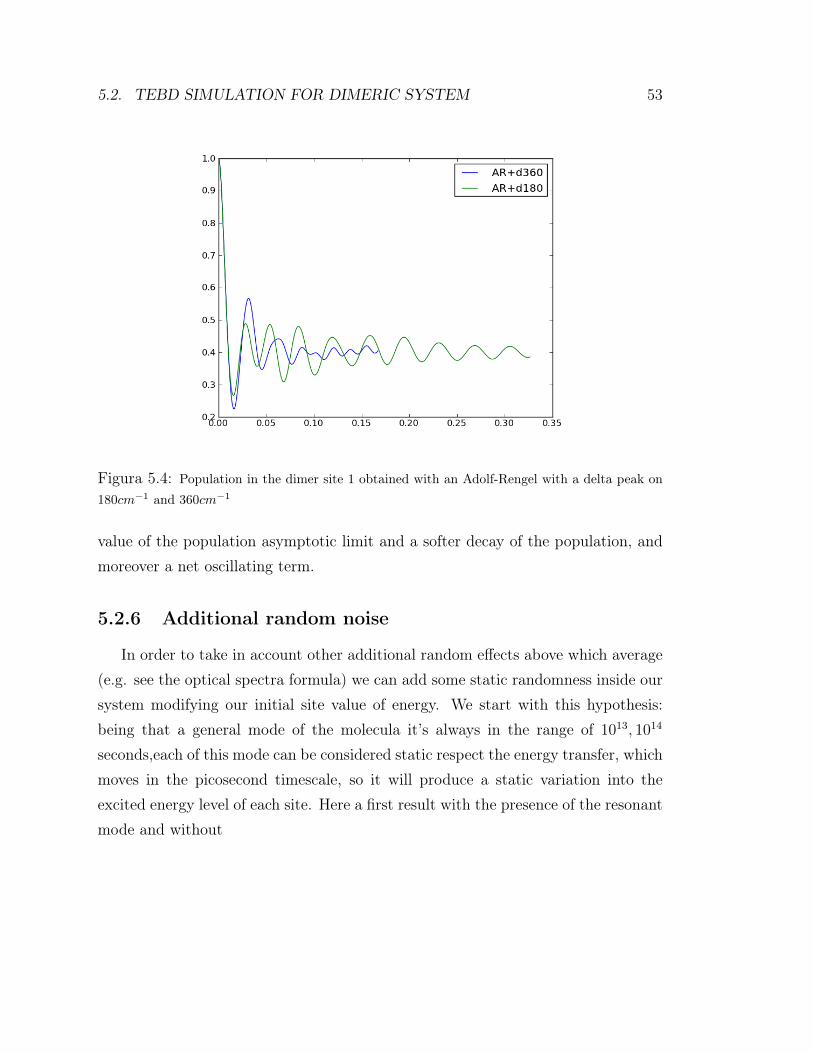
5.2. TEBD SIMULATION FOR DIMERIC SYSTEM 53
Figura 5.4: Population in the dimer site 1 obtained with an Adolf-Rengel with a delta peak on180cm−1 and 360cm−1
value of the population asymptotic limit and a softer decay of the population, andmoreover a net oscillating term.
5.2.6 Additional random noise
In order to take in account other additional random effects above which average(e.g. see the optical spectra formula) we can add some static randomness inside oursystem modifying our initial site value of energy. We start with this hypothesis:being that a general mode of the molecula it’s always in the range of 1013, 1014
seconds,each of this mode can be considered static respect the energy transfer, whichmoves in the picosecond timescale, so it will produce a static variation into theexcited energy level of each site. Here a first result with the presence of the resonantmode and without

54 CAPITOLO 5. PHOTOSYNTHESIS NETWORKS TRANSPORT
Figura 5.5: Different dynamics resulting from different strength coupling with theenvironment
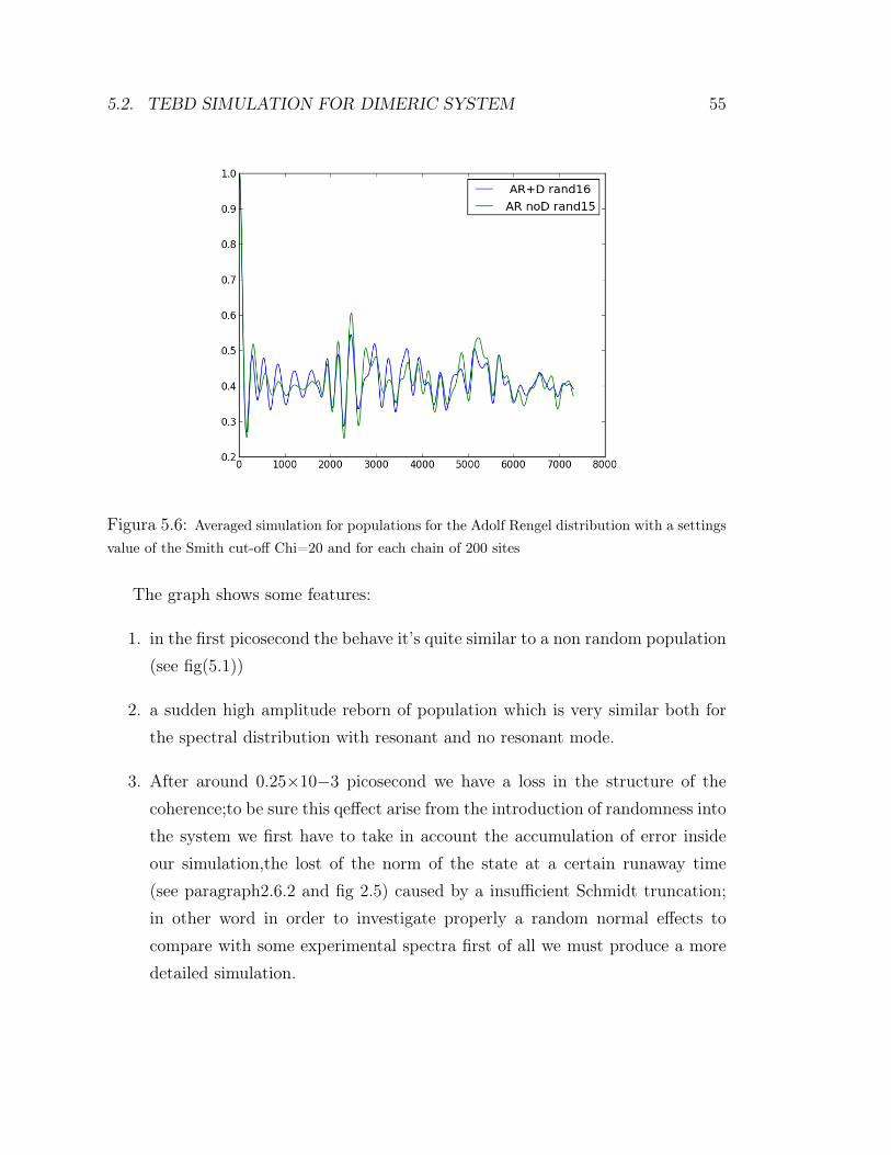
5.2. TEBD SIMULATION FOR DIMERIC SYSTEM 55
Figura 5.6: Averaged simulation for populations for the Adolf Rengel distribution with a settingsvalue of the Smith cut-off Chi=20 and for each chain of 200 sites
The graph shows some features:
1. in the first picosecond the behave it’s quite similar to a non random population(see fig(5.1))
2. a sudden high amplitude reborn of population which is very similar both forthe spectral distribution with resonant and no resonant mode.
3. After around 0.25×10⁻³ picosecond we have a loss in the structure of thecoherence;to be sure this qeffect arise from the introduction of randomness intothe system we first have to take in account the accumulation of error insideour simulation,the lost of the norm of the state at a certain runaway time(see paragraph2.6.2 and fig 2.5) caused by a insufficient Schmidt truncation;in other word in order to investigate properly a random normal effects tocompare with some experimental spectra first of all we must produce a moredetailed simulation.

56 CAPITOLO 5. PHOTOSYNTHESIS NETWORKS TRANSPORT
(a)
Higher energie antennacm−1 lower energie antenna cm−1
1051.2219117333091 993.54086116839031062.7355617394030 995.68011484761441050.6039684374250 1000.0405186140791057.9278694405500 1004.41711387939541047.2970555313029 1003.4329063001351052.2562514848751 1010.77419601896851065.2139014795459 996.98323604228381051.005637134137 994.6951834486741
(b)
Higher energie antenna cm−1 lower energie antenna cm−1
1053.2913431155830 998.68627144512941052.6506925406741 1001.5695317802491029.3402825750420 1002.71966231225781037.1049564797320 1009.16291904166581059.4935570340319 1005.63908489018211052.8911763378601 1001.88017637360361062.8445222092330 993.93108508055831
Then we have refined our simulation in a more proper way,using a standard set ofrandom number for both the spectral distribution and rising the numerical precisionsetting the value of the Schmidt cut-off Chi=38 to be sure to avoid the runaway timeeffects,and in order to take also in account border effects,a value of a total chainlength of 480 sites ( normal mode). Here the set of random number putted into theenergy sites parameter for each simulation
and the new populations graph (5.7) which shows how the artifact effects disap-pear after the correction.

5.2. TEBD SIMULATION FOR DIMERIC SYSTEM 57
Figura 5.7: Averaged simulation for populations for the Adolf Rengel distribution with a settingsvalue of the Smith cut-off Chi=38 and for each chain of 240 sites
5.2.7 Entanglement Measure: Von Newman entropy
The TEBD techniques possesses another powerful advantage which is the possi-bility to produce during our temporal evolution a direct, full, dynamical landscapeof the terms of the total Schmidt decomposition of the state that derive from theapplication of the SVD for each time evolution on the total state; in this way we areable to obtain a direct measure of the two-blocks(subsystems) Von Newman entropyevaluated in each inter-site value (as stated in chapter 1 the tensor into which theλ are putted it’s the matrix of basis transformation from one local site of the chainto another).
AS we can infer from image the difference in Entanglement production in thetwo time step consider,it’s quite a few but present. Of a certain relevance is thepresence of a peak in fig(5.6,5.7) in the inter-site near the central part of the chain,more precisely where lay the (protein antenna) system, .Despite we may expect thispeaks follows from the contribute of the presence of the delta into the distribution

58 CAPITOLO 5. PHOTOSYNTHESIS NETWORKS TRANSPORT
Figura 5.8: Adolf-Rengel spectral distribution + delta 180 cm−1 Von Newmann Entorpy graphfor a timestep of 2000-2024

5.2. TEBD SIMULATION FOR DIMERIC SYSTEM 59
Figura 5.9: Standard Adolf-Rengel Von Newmann Entorpy graph for a timestep of 2000-2024
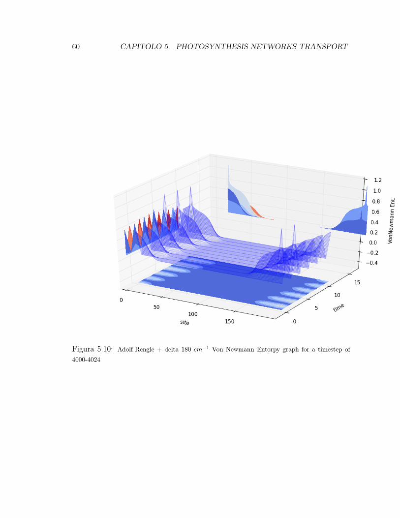
60 CAPITOLO 5. PHOTOSYNTHESIS NETWORKS TRANSPORT
Figura 5.10: Adolf-Rengle + delta 180 cm−1 Von Newmann Entorpy graph for a timestep of4000-4024
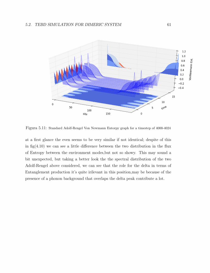
5.2. TEBD SIMULATION FOR DIMERIC SYSTEM 61
Figura 5.11: Standard Adolf-Rengel Von Newmann Entorpy graph for a timestep of 4000-4024
at a first glance the even seems to be very similar if not identical; despite of thisin fig(4.10) we can see a little difference between the two distribution in the fluxof Entropy between the environment modes,but not so showy. This may sound abit unexpected, but taking a better look the the spectral distribution of the twoAdolf-Rengel above considered, we can see that the role for the delta in terms ofEntanglement production it’s quite irilevant in this position,may be because of thepresence of a phonon background that overlaps the delta peak contribute a lot.

62 CAPITOLO 5. PHOTOSYNTHESIS NETWORKS TRANSPORT
Figura 5.12: Graphical difference between the Von Newmann Entropy obtained without theresonant peak and resonant peak at 180cm−1
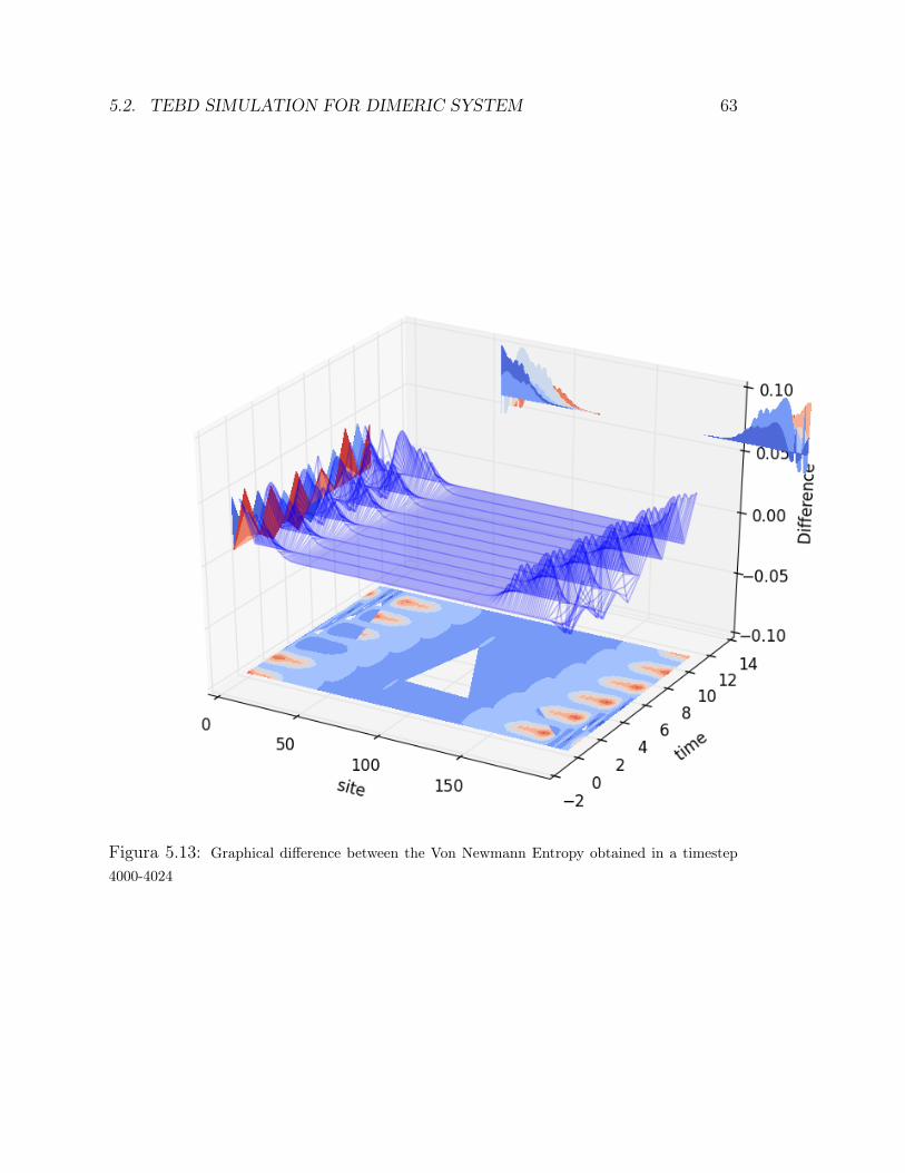
5.2. TEBD SIMULATION FOR DIMERIC SYSTEM 63
Figura 5.13: Graphical difference between the Von Newmann Entropy obtained in a timestep4000-4024
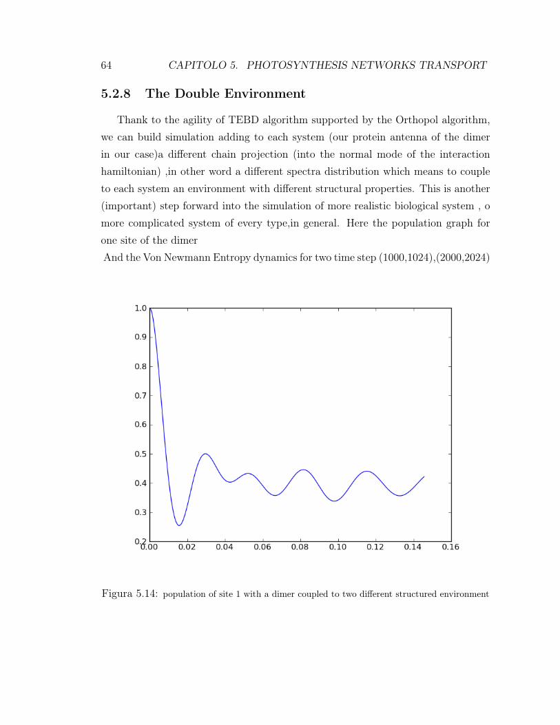
64 CAPITOLO 5. PHOTOSYNTHESIS NETWORKS TRANSPORT
5.2.8 The Double Environment
Thank to the agility of TEBD algorithm supported by the Orthopol algorithm,we can build simulation adding to each system (our protein antenna of the dimerin our case)a different chain projection (into the normal mode of the interactionhamiltonian) ,in other word a different spectra distribution which means to coupleto each system an environment with different structural properties. This is another(important) step forward into the simulation of more realistic biological system , omore complicated system of every type,in general. Here the population graph forone site of the dimerAnd the Von Newmann Entropy dynamics for two time step (1000,1024),(2000,2024)
Figura 5.14: population of site 1 with a dimer coupled to two different structured environment

5.2. TEBD SIMULATION FOR DIMERIC SYSTEM 65
Figura 5.15: population of site 1 with a dimer couplde to two different structured environment

66 CAPITOLO 5. PHOTOSYNTHESIS NETWORKS TRANSPORT
Figura 5.16: population of site 1 with a dimer couplde to two different structured environment

5.2. TEBD SIMULATION FOR DIMERIC SYSTEM 67
As we can see the presence of two different environment produce another dyna-mics more, into the flux of entanglement along the chain. The population dynamicsshows the maintenance of the persistent oscillation due to the phonon antenna effect,even if only one environment site contributes to it. This shows a certain robustnessof this phenomenology whereas a quantum system can take advantage of it. Onthe other hand the entanglement (Von newmann entropy) present a very peculiarbehavior showing a non diffusive behavior.

68 CAPITOLO 5. PHOTOSYNTHESIS NETWORKS TRANSPORT
Capitolo 6
Conclusion
The aim of this thesis. First the presentation of the numerical outcome concer-ning the local population dynamics of the excitons inside the antenna sites of ourdimeric system via our TEBD algorithm, at the light of the paradigms of the quan-tum biology above exposed. Thank to the principles of the noisy assisted transport,an intermediate degree of environmental noise which, as demonstrated into quan-tum network simulation, sustains the flux along a general transport chain , and thephonon antenna principle, which explains how the system take advantage of somespecific long lived environmental vibrational modes, is possible shed light into thedeeper mechanism of how a coherent transport of energy along the chain of an ex-citonic system (a chain composed of two level systems of protein in excited statewhich produce site Frenkel excitons). As shown in fig 5.5 the coupling strenght withthe environment produce a great variation into the dynamic of the local population,so only an intermediate level of noise is permitted in order to obtain performantdynamics; higher level of noisy will produced an unavoidable quantity of dephasingthat will suppress the coherence while on the other hand a too low level of noise willgive raise to a stronger effect of localization (Anderson effect) which will obstructthe transport dynamics Alongside with this principle, as is evident in fig 5.3, thephonon antenna principle that lasts for time of the order of the picosecond; a timescale which permit to the transport chain the transport of energy without losses.
Second aim was an overview of the technique, it’s methods , and its potential in
69
70 CAPITOLO 6. CONCLUSION
order to present its agility in showing some global features like the Von Newmannand how modifications to the structure of the objects modeled can be easily handledwith the numerical tool of the TEBD. Thank to the ORTHOPOL algorithm thatmakes use of the orthonormal polynomials we can map an open system of the typeof continuous spin-boson model into a (theoretically) semi infinite chain of normalmodes. Being the spectral function the description of the overall strength of theinteraction of the system with the reservoir modes of frequency ω we can producethe new energy parameters for the chain, and the associated hopping parametersof the 1-D projected chain, in order to simulate in the TEBD code the system-environment interaction. This straightforward technique shows the potential of afull non-equilibrium, non-perturbative, non-Markovian (inhomogeneous chain) de-scription of the system-environment dynamics. The agility of the TEBD techniquealso permit us the visualization of global information as the von Newmann entropyof the 1-D chain for every time step.It is even possible easily inserting static localrandom effect or modification in the conformational structure of our dimer, thatfrom an informational point of view means the contemporary use of different envi-ronmental spectras. This agility makes straightforward simulation of more and morecomplicated structures, far beyond a simple dimeric structure. This will be anothervery useful trait in the future for the modeling of more structured and reach proteincomplexes as the FMO and others even more complicated as the Photosystem IIlight harvesting systems.

Bibliografia
[1] M. Mohseni, Y. Omar, G.S. Engel, and M.B. Plenio (eds.), Quantum effects inbiology, Cambridge Univer- sity Press, Cambridge 2013.
[2] Proceedings of the 22nd Solvay Conference in Chem- istry on ”Quantum Effectsin Chemistry and Biology, Procedia Chemistry 3 (2011).
[3] L. Hartmann, W. Du?r and H.J. Briegel, Steady state en- tanglement in openand noisy quantum systems at high temperature, Phys. Rev. A 74 (2006),052304.
[4] Blankenship, R. Molecular Mechanisms of Photosynthesis (Wiley-Blackwell,2002)
[5] Van Amerongen, H., Valkunas, L. & van Grondelle, R. Photosynthetic Excitons(World Scientific, 2000)
[6] Matsuzaki, S., Zazubovich, V., Rätsep, M., Hayes, J. & Small, G. Energytransfer kinetics and low energy vibrational structure of the three lowest energyQy-states of the Fenna-Matthews-Olson antenna complex. J. Phys. Chem. B104, 9564–9572 (2000).
[7] R. P. Feynman, Opt. News 11, 11 (1985): Found. Phys. 16 507 (1986); Int. J.Theor. Phys. 21, 467 (1982).
[8] G. Vidal, Phys. Rev. Lett. 98, 070201 (2007)
[9] G. Vidal, Phys. Rev. Lett. 93, 040502 (2004)
71

72 BIBLIOGRAFIA
[10] Engineering Coherence Among Excited States in Synthetic HeterodimerSystems
[11] E. Collini, C. Wong, K. Wilk, P. Curmi, P. Brumer, and G. Scholes, Coherentlywired light-harvesting in photo- synthetic marine algae at ambient temperature,Nature 463 (2010), pp. 644 - 649.
[12] S.F. Huelga, A. Rivas, and M.B. Plenio, Non- Markovianity assisted SteadyState Entanglement, Phys. Rev. Lett. 108 (2012), 160402.
[13] On the relation of protein dynamics and exciton relaxation in pigment-proteincomplexes: an estimation of the spectral density and a theory for the calculationof optical spectra