POLITECNICO DI MILANO Como Campus · con la pazienza, la comprensione e il sacrificio. ... BigEar...
156
POLITECNICO DI MILANO Como Campus M.Sc. in Computer Science and Engineering Department of Electronics, Information and Bioengineering BigEar: A LOW COST WIRELESS DISTRIBUTED AUDIO CAPTURING SYSTEM FOR UBIQUITOUS AUTOMATIC SPEECH RECOGNITION Advisor: Prof. Fabio Salice Tutor: Eng. Hassan Saidinejad Master Graduation Thesis of: Stefano Gorla, ID 745603 Academic Year 2014-2015
Transcript of POLITECNICO DI MILANO Como Campus · con la pazienza, la comprensione e il sacrificio. ... BigEar...
POLITECNICO DI MILANOComo Campus
M.Sc. in Computer Science and EngineeringDepartment of Electronics, Information and Bioengineering
BigEar: A LOW COST WIRELESS DISTRIBUTED AUDIO CAPTURINGSYSTEM FOR UBIQUITOUS AUTOMATIC SPEECH RECOGNITION
Advisor: Prof. Fabio SaliceTutor: Eng. Hassan Saidinejad
Master Graduation Thesis of:Stefano Gorla, ID 745603
Academic Year 2014-2015


POLITECNICO DI MILANOPolo Regionale di Como
Corso di Laurea Magistrale in Ingegneria InformaticaDipartmento di Elettronica, Informazione e Bioingegneria
BigEar: SISTEMA A BASSO COSTO, WIRELESS, DISTRIBUITO DIACQUISIZIONE AUDIO PER IL RICONOSCIMENTO AUTOMATICO DEL
PARLATO
Relatore: Prof. Fabio SaliceTutore: Ing. Hassan Saidinejad
Tesi di Laurea di:Stefano Gorla, matricola 745603
Anno Accademico 2014-2015

Ai miei genitori,che mi hanno sempre sostenuto
con la pazienza, la comprensione e il sacrificio.

Acknowledgements
First of all I would like to thank Prof. Fabio Salice deeply, for his valuable and helpful advice, support
and encouragements during this work. Special thanks to Eng. Ashkan Saidinejad for his useful and
important tutoring. Without their support and their help, the pages of this work would be white.
Also I have to mention the names of Prof. Augusto Sarti and Prof. Giuseppe Bertuccio for their
willingness; a special thank to Eng. Marco Leone and Eng. Carlo Bernaschina for their help in the
prototype realization and implementation.
Thanks to Emanuele De Bernardi, Fabio Veronese, Simone Mangano, who shared with me important
moments of social brainstorming, but also lunch breaks and a lot of coffee.
During my long study career, I met many people, and many of them shared part of my journey. I
want to thank first my family, dad and mom, my brother Marco with his wife Sonia, my nephews Anna
and Giulia, my sisters Elena with her husband Pietro and Agnese, with Eleonora, Lucrezia and of course
in our hearts Mauro.
Thank you to the people with whom I share my passions: my choir, the diocesan school of music,
don Rinaldo, don Simone, don Nicholas, Celeste, Andrea and Carlo; Filippo, Laura and the friends from
Castel San Pietro. Thanks to Rita, Ugo and the friends of AdFontes for their infectious enthusiasm.
Thank you to the Non-violent guys group, to the Benzoni’s family, and to don Felice Rainoldi: not only
an outstanding teacher but specially a true friend.
Thank you to the music: a strange world where you can escape, but where, as always, are the best
inspirations.The final thank goes to Paola. Thank you for having always believed in me and for giving me day
by day the right encouragement to continue my work in many hard times. Thank you.
i

Abstract
THE ageing of world’s population will raise the demand and challenges of elderly care in comingyears. Several approaches have been devised to deal with the needs of older people proactively.Assistive domotics represents a relatively recent effort in this direction; in particular, Vocal Inter-
action can be a favored way to control the smart home environment, providing that the interface fulfillsrequirements of transparency and unobtrusiveness. Absence of intrusive devices induces a more natu-ral interaction model in which there is no need to wear a microphone or to issue commands to specific“hotspots” of the dwelling.
From these assumptions, a wireless, modular and low-cost speech capturing system has been imple-mented, in which a set of wireless audio sensors send captured data to a Base Station, which in turn isresponsible for aggregating received data in order to rebuild the speech captured distributely by BigEarAudio Sensors. The reconstruction algorithm performs a first stage of energy and delay analysis of theaudio streams coming from the sensors; this stage is needed for compensating energy and delay dif-ferences due to different source-sensors distances. Then, the streams are superposed in order to mergeeach contribution into a unique output stream. Each sensor generates an audio stream that, depending onnetwork interaction model, will be not complete, presenting thus sequences of silence (holes). Holes inthe reconstructed signal drastically decrease the accuracy of the speech recognition procedure. AlthoughBigEar system, working with the best network parameters, ensures high chances for a successful speechrecognition, four different methods have been used to repair the audio signal before sending it to thespeech recognition block.
BigEar architecture has been simulated by means of a MATLAB-based simulator that allows to studythe whole system behavior, from the environment (room) acoustic simulation up to Network Interactionprotocol. Once best parameters are pointed out by the simulation, a real-world prototype has beenrealized.
From Results Analysis it can be seen that BigEar can be identified as a minimum cost, wirelessand distributed system. Moreover, ubiquitous approach allows Data Intelligence mechanisms, e.g. per-forming a coarse-grain localization - using sensor signal power and delays information - in order to addinformative content that could disambiguate context-free vocal commands (“Turn off the light” or - bet-ter - “Turn off this light” could be integrated with localization information in order to determine whichlight has to be switched off).
iii

Sommario
L’INVECCHIAMENTO della popolazione mondiale nei prossimi anni causerà l’accrescimento del-la domanda e le relative sfide nella cura degli anziani. Sono stati studiati numerosi approcciper far fronte alle esigenze delle persone meno giovani. La domotica assistiva rappresenta
un passo - seppur relativamente recente - in questa direzione; in particolare, l’interazione vocale puòessere una via preferenziale per controllare l’ambiente domestico gestito dalla domotica, a patto chel’interfaccia uomo-macchina soddisfi requisiti di trasparenza e non-intrusività. L’assenza di dispositi-vi invasivi induce a una interazione più naturale in cui non sia necessario indossare un microfono oimpartire comandi attraverso specifici punti di ascolto dell’abitazione.
A partire da queste premesse è stato implementato un sistema modulare, senza fili e a basso costo dicattura del parlato in cui un insieme di sensori audio invia i dati acquisiti a una Base Station, la qualeprovvede ad assemblare i dati ricevuti in modo da ricostruire il parlato precedentemente acquisito, inmodo distribuito, dai sensori. L’algoritmo di ricostruzione esegue anzitutto l’analisi energetica e dei ri-tardi dei flussi audio; questa operazione è necessaria alla compensazione delle differenze energetiche edei ritardi dovuti alle distanze tra i sensori e la sorgente. Dopodiché, i flussi audio vengono sovrappostiin modo da fondere i singoli contributi in un unico flusso audio. A seconda del modello di interazionedi rete, ogni sensore genera un flusso audio che presenta sequenze di silenzio (buchi). I buchi nel segna-le ricostruito diminuiscono drasticamente l’accuratezza della procedura di riconoscimento del parlato.Sebbene il sistema BigEar, quando configurato per operare con i migliori parametri di rete, assicuri alteprobabilità affinché il riconoscimento dia risultati positivi, sono stati testati quattro diversi metodi perriparare il segnale audio prima che esso venga inviato al blocco di riconoscimento del parlato.
L’architettura è stata testata tramite un simulatore basato su codice MATLAB che permette di studiareil comportamento dell’intero sistema, dalla simulazione acustica dell’ambiente fino ai protocolli usati perle interazioni di rete. A partire dai parametri ottimi indicati dal simulatore è stato realizzato un prototiporeale.
Dall’analisi dei risultati si può notare che BigEar può essere identificato quale sistema a costo mi-nimo, senza fili e modulare. Inoltre, l’approccio distribuito al problema permette meccanismi di In-telligenza dei Dati, ad esempio eseguendo una localizzazione sommaria della sorgente (sfruttando leinformazioni di ritardo e di energia del segnale) che permetta di aggiungere contenuto informativo ingrado di disambiguare comandi vocali privi di contesto (i comandi “Spegni la luce” o - meglio - “Spegniquesta luce” potrebbero essere integrati con una localizzazione in grado di determinare quale luce debbaessere spenta).
v

Contents
Acknowledgements i
Abstract iii
Sommario v
1 Introduction 11.1 BRIDGe - Behaviour dRift compensation for autonomous and InDependent livinG . . . 11.2 Ubiquitous Computing . . . . . . . . . . . . . . . . . . . . . . . . . . . . . . . . . . . 21.3 BigEar Application . . . . . . . . . . . . . . . . . . . . . . . . . . . . . . . . . . . . . 31.4 Related Works . . . . . . . . . . . . . . . . . . . . . . . . . . . . . . . . . . . . . . . . 31.5 Structure of the Dissertation . . . . . . . . . . . . . . . . . . . . . . . . . . . . . . . . 5
2 BigEar Architecture 72.1 Overview of the System . . . . . . . . . . . . . . . . . . . . . . . . . . . . . . . . . . . 72.2 Wixel Programmable USB Wireless Module . . . . . . . . . . . . . . . . . . . . . . . . 82.3 Audio Interface . . . . . . . . . . . . . . . . . . . . . . . . . . . . . . . . . . . . . . . 9
2.3.1 Physical Characteristics of the Typical Situation . . . . . . . . . . . . . . . . . . 92.3.2 Sensitivity of the microphone . . . . . . . . . . . . . . . . . . . . . . . . . . . 112.3.3 ADC characteristics . . . . . . . . . . . . . . . . . . . . . . . . . . . . . . . . 12
2.4 BigEar Receiver and Base station . . . . . . . . . . . . . . . . . . . . . . . . . . . . . . 132.5 Network Protocols . . . . . . . . . . . . . . . . . . . . . . . . . . . . . . . . . . . . . 14
2.5.1 ALOHA Protocol . . . . . . . . . . . . . . . . . . . . . . . . . . . . . . . . . . 16
3 BigEar Modeling and Simulation 193.1 Overview . . . . . . . . . . . . . . . . . . . . . . . . . . . . . . . . . . . . . . . . . . 193.2 Audio Model . . . . . . . . . . . . . . . . . . . . . . . . . . . . . . . . . . . . . . . . 20
3.2.1 Physical Model . . . . . . . . . . . . . . . . . . . . . . . . . . . . . . . . . . . 213.2.2 MCROOMSIM toolbox . . . . . . . . . . . . . . . . . . . . . . . . . . . . . . 23
3.3 Sensors network model . . . . . . . . . . . . . . . . . . . . . . . . . . . . . . . . . . . 273.3.1 Radio Transmission Model . . . . . . . . . . . . . . . . . . . . . . . . . . . . . 303.3.2 N-buffer Internal Model . . . . . . . . . . . . . . . . . . . . . . . . . . . . . . 32
vii
Capitolo 0. Sommario
4 Signal Reconstruction and Repair 354.1 Overview . . . . . . . . . . . . . . . . . . . . . . . . . . . . . . . . . . . . . . . . . . 354.2 Energy Compensation . . . . . . . . . . . . . . . . . . . . . . . . . . . . . . . . . . . . 39
4.2.1 Bias Removal . . . . . . . . . . . . . . . . . . . . . . . . . . . . . . . . . . . . 394.2.2 Normalization . . . . . . . . . . . . . . . . . . . . . . . . . . . . . . . . . . . 40
4.3 Streams Superposition . . . . . . . . . . . . . . . . . . . . . . . . . . . . . . . . . . . 414.3.1 Weighted Sum of Contributions . . . . . . . . . . . . . . . . . . . . . . . . . . 414.3.2 Holes Replacement . . . . . . . . . . . . . . . . . . . . . . . . . . . . . . . . . 41
4.4 Cross-correlation . . . . . . . . . . . . . . . . . . . . . . . . . . . . . . . . . . . . . . 424.4.1 Cross-correlation Drawbacks . . . . . . . . . . . . . . . . . . . . . . . . . . . . 434.4.2 Envelopes Cross-correlation . . . . . . . . . . . . . . . . . . . . . . . . . . . . 44
4.5 Healing Signal Fragmentation . . . . . . . . . . . . . . . . . . . . . . . . . . . . . . . 464.5.1 B-Spline Interpolation . . . . . . . . . . . . . . . . . . . . . . . . . . . . . . . 464.5.2 Noise Addition . . . . . . . . . . . . . . . . . . . . . . . . . . . . . . . . . . . 474.5.3 Packet Loss Concealing . . . . . . . . . . . . . . . . . . . . . . . . . . . . . . 474.5.4 LSAR - Least Squares Auto-Regressive Interpolation . . . . . . . . . . . . . . . 484.5.5 Audio inpainting . . . . . . . . . . . . . . . . . . . . . . . . . . . . . . . . . . 494.5.6 Healing methods comparison . . . . . . . . . . . . . . . . . . . . . . . . . . . . 50
4.6 Summary . . . . . . . . . . . . . . . . . . . . . . . . . . . . . . . . . . . . . . . . . . 51
5 BigEar Implementation 535.1 Overview . . . . . . . . . . . . . . . . . . . . . . . . . . . . . . . . . . . . . . . . . . 535.2 Hardware Setup . . . . . . . . . . . . . . . . . . . . . . . . . . . . . . . . . . . . . . . 54
5.2.1 BigEar Audio Capture Board . . . . . . . . . . . . . . . . . . . . . . . . . . . . 545.2.2 BigEar Receiver . . . . . . . . . . . . . . . . . . . . . . . . . . . . . . . . . . 57
5.3 Software Implementation . . . . . . . . . . . . . . . . . . . . . . . . . . . . . . . . . . 595.3.1 BigEar Audio Sensor . . . . . . . . . . . . . . . . . . . . . . . . . . . . . . . . 595.3.2 BigEar Input Calibration . . . . . . . . . . . . . . . . . . . . . . . . . . . . . . 665.3.3 BigEar Receiver . . . . . . . . . . . . . . . . . . . . . . . . . . . . . . . . . . 675.3.4 BigEar Base Station . . . . . . . . . . . . . . . . . . . . . . . . . . . . . . . . 67
6 BigEar Results Analysis 756.1 Overview . . . . . . . . . . . . . . . . . . . . . . . . . . . . . . . . . . . . . . . . . . 756.2 Metrics Definition . . . . . . . . . . . . . . . . . . . . . . . . . . . . . . . . . . . . . . 76
6.2.1 Reconstructed Signal Metrics . . . . . . . . . . . . . . . . . . . . . . . . . . . 766.2.2 Software Performance Metrics . . . . . . . . . . . . . . . . . . . . . . . . . . . 77
6.3 Simulation Setup . . . . . . . . . . . . . . . . . . . . . . . . . . . . . . . . . . . . . . 786.4 On-field Setup . . . . . . . . . . . . . . . . . . . . . . . . . . . . . . . . . . . . . . . . 786.5 Results Discussion . . . . . . . . . . . . . . . . . . . . . . . . . . . . . . . . . . . . . 80
6.5.1 Reconstructed Signal Comparison . . . . . . . . . . . . . . . . . . . . . . . . . 806.5.2 Software Performance Tests . . . . . . . . . . . . . . . . . . . . . . . . . . . . 836.5.3 Coarse-grain localization . . . . . . . . . . . . . . . . . . . . . . . . . . . . . . 87
7 Conclusions and Future Work 897.1 Conclusions . . . . . . . . . . . . . . . . . . . . . . . . . . . . . . . . . . . . . . . . . 897.2 Strengths and Weaknesses . . . . . . . . . . . . . . . . . . . . . . . . . . . . . . . . . 90
7.2.1 Strengths . . . . . . . . . . . . . . . . . . . . . . . . . . . . . . . . . . . . . . 907.2.2 Weaknesses . . . . . . . . . . . . . . . . . . . . . . . . . . . . . . . . . . . . . 91
7.3 Future Work . . . . . . . . . . . . . . . . . . . . . . . . . . . . . . . . . . . . . . . . . 91
viii
A TI CC2511 MCU Key features 93A.1 CC2511F32 Logic Scheme . . . . . . . . . . . . . . . . . . . . . . . . . . . . . . . . . 94A.2 CC2511F32 Radio Packet format . . . . . . . . . . . . . . . . . . . . . . . . . . . . . . 95
B BigEar simulator MATLAB implementation 97B.1 Radio Transmission Model . . . . . . . . . . . . . . . . . . . . . . . . . . . . . . . . . 97B.2 N-Buffer Internal Model . . . . . . . . . . . . . . . . . . . . . . . . . . . . . . . . . . 98B.3 Signal Reconstruction block . . . . . . . . . . . . . . . . . . . . . . . . . . . . . . . . 99
C BigEar Reconstruction MATLAB Script 103
D Cross-correlation convergence test 107
E BigEar Implementation schematics and pictures 111E.1 BigEar Audio Capture board . . . . . . . . . . . . . . . . . . . . . . . . . . . . . . . . 111E.2 BigEar Receiver . . . . . . . . . . . . . . . . . . . . . . . . . . . . . . . . . . . . . . . 112E.3 BigEar Audio Capture application . . . . . . . . . . . . . . . . . . . . . . . . . . . . . 113E.4 BigEar Input Calibration . . . . . . . . . . . . . . . . . . . . . . . . . . . . . . . . . . 117E.5 BigEar Receiver application . . . . . . . . . . . . . . . . . . . . . . . . . . . . . . . . 118E.6 BigEar SerialPort application GUI . . . . . . . . . . . . . . . . . . . . . . . . . . . . . 120
F BigEar Simulation 121F.1 Simulation setups . . . . . . . . . . . . . . . . . . . . . . . . . . . . . . . . . . . . . . 121
G Datasheets 125G.1 Kingstone KECG2738PBJ-A Electret Microphone . . . . . . . . . . . . . . . . . . . . 125G.2 Linear Technology LT1013 Dual Precision Op Amp . . . . . . . . . . . . . . . . . . . . 127
Bibliography 133
ix

List of Figures
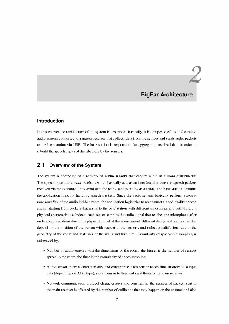
2.1 Overview of the BigEar architecture . . . . . . . . . . . . . . . . . . . . . . . . . . . . 82.2 Wixel module pinout and components . . . . . . . . . . . . . . . . . . . . . . . . . . . 82.3 CC2511 ADC Block diagram . . . . . . . . . . . . . . . . . . . . . . . . . . . . . . . . 132.4 BigEar Receiver Logic . . . . . . . . . . . . . . . . . . . . . . . . . . . . . . . . . . . 142.5 BigEar Application Reconstruction Logic . . . . . . . . . . . . . . . . . . . . . . . . . 152.6 Aloha vs. Slotted Aloha throughput . . . . . . . . . . . . . . . . . . . . . . . . . . . . 17
3.1 Architecture model . . . . . . . . . . . . . . . . . . . . . . . . . . . . . . . . . . . . . 203.2 Geometry of wave propagation from a point source x1 to a listening point x2 . . . . . . . 213.3 Point-to-point spherical wave simulator . . . . . . . . . . . . . . . . . . . . . . . . . . 213.4 Law of reflection . . . . . . . . . . . . . . . . . . . . . . . . . . . . . . . . . . . . . . 223.5 Geometry of an acoustic reflection caused by “multipath” propagation . . . . . . . . . . 223.6 Image source method using two walls, one source and one listening point. . . . . . . . . 243.7 MCROOMSIM Data flow from configuration stage to the end of simulation . . . . . . . 263.8 Simulation and reconstruction flowchart . . . . . . . . . . . . . . . . . . . . . . . . . . 293.9 Flowchart of the radio transmission model . . . . . . . . . . . . . . . . . . . . . . . . . 313.10 Buffer Frames sliding . . . . . . . . . . . . . . . . . . . . . . . . . . . . . . . . . . . . 333.11 Flowchart of the N-buffer model . . . . . . . . . . . . . . . . . . . . . . . . . . . . . . 34
4.1 Flowchart of the signal reconstruction block . . . . . . . . . . . . . . . . . . . . . . . . 374.2 Alignment of audio packets considering their timestamp . . . . . . . . . . . . . . . . . 374.3 Flowchart of the correlation analysis block . . . . . . . . . . . . . . . . . . . . . . . . . 384.4 Representation of a holey signal . . . . . . . . . . . . . . . . . . . . . . . . . . . . . . 394.5 How summation of different biases might influence the reconstructed signal . . . . . . . 404.6 Harmonic distortion due to unweighted sum of contributions . . . . . . . . . . . . . . . 424.7 Cross-correlation test between noisy and holey signals . . . . . . . . . . . . . . . . . . 454.8 Cross-correlation analysis and alignment on signal’s envelopes . . . . . . . . . . . . . . 464.9 B-Spline method for healing reconstructed signal . . . . . . . . . . . . . . . . . . . . . 474.10 G.711.I Frame erasure concealment algorithm . . . . . . . . . . . . . . . . . . . . . . . 484.11 Gabor spectrograms of original, reconstructed and inpainted streams . . . . . . . . . . . 51
5.1 BigEar Audio Capture Board Biasing circuit . . . . . . . . . . . . . . . . . . . . . . . . 545.2 BigEar Audio Capture Board Signal Conditioning stage . . . . . . . . . . . . . . . . . . 56
xi
List of Figures
5.3 LT1013 OpAmp Voltage VS. Frequency Gain . . . . . . . . . . . . . . . . . . . . . . . 565.4 Frequency response of the simulated signal conditioning circuit . . . . . . . . . . . . . . 585.5 Flowcharts of the BigEar Audio Capture application . . . . . . . . . . . . . . . . . . . . 605.6 Signal and Saturation LED indicators policy . . . . . . . . . . . . . . . . . . . . . . . . 635.7 BigEar Data field structure . . . . . . . . . . . . . . . . . . . . . . . . . . . . . . . . . 645.8 Flowchart of the BigEar Receiver application . . . . . . . . . . . . . . . . . . . . . . . 675.9 BigEar SerialPort raw file formats . . . . . . . . . . . . . . . . . . . . . . . . . . . . . 685.10 BigEar SerialPort Capture flowchart . . . . . . . . . . . . . . . . . . . . . . . . . . . . 695.11 BigEar SerialPort Raw-to-CSV decoding . . . . . . . . . . . . . . . . . . . . . . . . . 715.12 BigEar SerialPort Class Diagram . . . . . . . . . . . . . . . . . . . . . . . . . . . . . . 725.13 BigEar Reconstructor Flowchart . . . . . . . . . . . . . . . . . . . . . . . . . . . . . . 73
6.1 Reconstructed signal metrics plotted as a function of TmaxDelay parameter . . . . . . 816.2 Fill_ratio as a function of TmaxDelay . . . . . . . . . . . . . . . . . . . . . . . . . 826.3 BigEar Reconstructor RPR metric . . . . . . . . . . . . . . . . . . . . . . . . . . . . . 856.4 BigEar Capture Board Application timing analysis . . . . . . . . . . . . . . . . . . . . 856.5 BigEar Reconstructor PAR metric . . . . . . . . . . . . . . . . . . . . . . . . . . . . . 866.6 Signal power vs. alignment delay plot for coarse-grain localization . . . . . . . . . . . . 88
G.1 . . . . . . . . . . . . . . . . . . . . . . . . . . . . . . . . . . . . . . . . . . . . . . . 136
xii
List of Tables
2.1 Physical characterization of the Typical Situation . . . . . . . . . . . . . . . . . . . . . 112.2 ADC: Speed of Conversion VS. Decimation Rate . . . . . . . . . . . . . . . . . . . . . 13
4.1 Noise Addition for Speech Signal Repair . . . . . . . . . . . . . . . . . . . . . . . . . . 484.2 Healing methods comparison . . . . . . . . . . . . . . . . . . . . . . . . . . . . . . . . 52
5.1 Design Choices for Signal Conditioning stage . . . . . . . . . . . . . . . . . . . . . . . 585.2 BigEar Audio Capture application Design Choices and Parameters . . . . . . . . . . . . 66
6.1 BigEar Simulator parameters . . . . . . . . . . . . . . . . . . . . . . . . . . . . . . . . 79
xiii

1Introduction
QUALITY of life depends heavily on the efficiency, comfort and cosiness of the place an individual
calls “home”. Thus, a wide range of products and systems have been invented in the past to
advance human control over the entire living space. Domotics is a field specializes in specific
automation techniques for private homes, often referred to as “home automation” or “smart home tech-
nology”. In essence, home environment control and automation extend the various techniques typically
used in building automation, such as light and climate control, control of doors and window shutters,
surveillance systems, etc. through the networking of ICT in the home environment, including the inte-
gration of household appliances and devices. Such solutions are not only offering comfort and security,
but when serving an elderly or a person with disability (a fragile person in general) can leverage safety
and individual independence. Assistive domotics represents a relatively recent effort in this direction
that further specializes in the needs of people with disability, older persons, and people with little or no
technical affinity, and which seeks to offer such residents new levels of safety, security and comfort, and
thereby the chance to prolong their safe staying at home.
The ageing of world’s population will raise the demand and challenges of elderly care in coming
years. Based on a study of the US census, the number of people aged over 65 will increase by 101
percent between 2000 and 2030, at a rate of 2.3 percent each year; during that same period, the number
of family members who can provide support for them will increase by only 25 percent, at a rate of
0.8 percent each year. Several approaches have been devised to deal with the needs of older people
proactively.
1.1 BRIDGe - Behaviour dRift compensation for autonomous and InDe-
pendent livinG
The BRIDGe1 (Behaviour dRift compensation for autonomous InDependent livinG) project [17], being
done at Politecnico di Milano - Polo di Como, aims to build strong connections between a person living
independently at home and his or her social environment (family, caregivers, social services, and so on)
1atg.deib.polimi.it/projects
1
Chapter 1. Introduction
by implementing a system that provides focused interventions according to the user’s needs.
The target of Bridge are people with mild cognitive or physical impairments and, more generally,
fragile people whose weakness threatens their autonomy, health or other important aspects of life. Fragile
people need for mutual reassurance: they typically want to be independent and autonomous, but they also
know that often somebody else must be present to help them with unexpected needs.
At Bridge’s core is a wireless sensor-actuator network that supports house control and user behavior
detection through a rich and flexible communication system between the person and his or her social
environment, aimed at reassuring both the family and the user.
One of the simpler ways the user can adopt for meeting his needs is to ask someone to do something:
ask to switch off the light, to unlock the door, to increase the room temperature, etc. Inhabitants of the
“smart home” can vocally control some parts of a dwelling (lights, doors, principal gate, and so on) by
means of issuing commands to a Vocal Command Interface (VCI).
The inhabitant starts by activating the VCI, which is continuously listening and waiting for the per-
sonalized activation keyword. Activation is confirmed to the user through a vocal message, and the VCI
is now ready to receive the inhabitant’s vocal command (for example, “turn on the light in the kitchen”).
The vocal command is analyzed in an ad hoc application and the result of the interaction is the execution
of the vocal command.
1.2 Ubiquitous Computing
Ubiquitous computing is a paradigm in which the processing of information is linked with each activity or
object as encountered. It involves connecting electronic devices, including embedding microprocessors
to communicate information. Devices that use ubiquitous computing have constant availability and are
completely connected.
Ubiquitous computing is one of the keys to success of Bridge system: the more the sensors network is
unobtrusive and transparent with respect to the interaction of the elder with his environment, the greater
is the sense of autonomy and independence felt by the user.
In case of vocal interaction, a ubiquitous approach to the problem requires that the interaction
take place as transparent as possible: no need to wear a microphone or to issue commands to specific
“hotspots” of the dwelling. Absence of intrusive devices induces a more natural interaction model that
generates in turn several positive aspects in chain:
Learning curve performance: Elderly user has no need to wear devices in order to perform human-
computer interaction; he/she only need to ask someone to perform an action. In this way, the
learning process will not present the typical high barrier that arouses when the user approaches an
interaction model foreign to his user experience.
Technology acceptance: According to the Technology Acceptance Model [2], the two most important
attitudinal factors in explaining acceptance and usage of a new technology are perceived usefulness
and perceived ease of use. Perceived usefulness is described as “the degree to which a person
2
1.3. BigEar Application
believes that using the particular technology would enhance his/her job performance”. Perceived
ease of use is defined as “the extent to which a person believes that using a technology is free of
effort”. Lacks in ease of use, in particular when dealing with elderly, can demotivate the user and
bring him to consider a technology as useless or misleading. “Why do I have to wear a mobile
phone for switching off the light? It would be easier if I could use a remote control directly”.
Mastering of the living enviroment: As permanent medical devices can reduce the perceived quality
of life, so intrusive assistive technologies can be perceived as a gilded cage that lowers the sense
of freedom and induces the user to feel a stranger in his own house. Ubiquitous and transparent
systems can help elderly or injured people to feel masters of their home.
1.3 BigEar Application
Target of this work is to model, realize and implement a distributed speech capturing system that meets
the expectations of ubiquitousness and transparency described above. Behind the acronym BigEar (uBiq-
uitous wIreless low-budGet spEech cApturing inteRface) is an audio acquisition system built following
Wireless Sensor Network [3] requirements:
Minimum cost: The adopted technology (hardware and software) has to consider the economical pos-
sibilities of the people according to the paradigm: “a good but costly solution is not a solution at
all”.
Wireless: The absence of power and/or signal cables is a strong requirement in order to lower costs
for house adaptation. Moreover, wireless systems can ensure a higher degree of flexibility and
configurability than wired systems.
Distributed: The key for pervasiveness is distributed computing; according to definition, [7, p. 2] the
devices concur in building a result whose information content is more than the sum of single contri-
bution. Moreover, sensors are completely independent and an eventual failure will not completely
compromise the result of the sensor network collaboration.
Modular: The system should be implemented using a modular approach in order to be scalable and
quickly configurable for matching environment characteristics and user’s needs.
Responsive: Speech recognition should be immediate, so speed of processing is a crucial requirement
in order to give the user an immediate feedback; assistive domotic interaction has to be as fast as
possible since the user don’t wait for Microsoft Window’s Hourglass.
1.4 Related Works
Literature focusing on Wireless Low-Cost Speech Capturing systems is limited. In general, the approach
to the subject tends to emphasize one aspect (such as audio quality) at the expense of others (such as
flexibility) and none of the examined projects can be considered as low cost.
3
Chapter 1. Introduction
SWEET-HOME Project
The SWEET-HOME project [15] aims at designing a smart home system based on audio technology
focusing on three main aspects: to provide assistance via natural man-machine interaction (voice and
tactile command), to ease social e-inclusion and to provide security reassurance by detecting situations
of distress. The targeted smart environments in which speech recognition must be performed thus include
multi-room homes with one or more microphones per room set near the ceiling.
To achieve the project goals, a smart home was set up. It is a thirty square meters suite flat including
a bathroom, a kitchen, a bedroom and a study; in order to acquire audio signals, seven microphones were
set in the ceiling. All of the microphones were connected to a dedicated PC embedding an 8-channel
input audio card.
Strength The approach to multi-channel audio alignment proposed by the paper is the same adopted in
the BigEar Reconstruction Algorithm (Ch. 4); it is based on the alignment of each audio channel
with the one with the highest SNR.
Weaknesses The use of a multichannel audio card requires dedicated hardware increases costs and
reduces flexibility. Moreover, a wired approach is hard to implement since it requires to fix wires
onto walls or into existing electrical pipes.
Wireless Sensor Networks for Voice Capture in Ubiquitous Home Environ-
ments
The work introduces a voice capture application using a hierarchical wireless sensor network: nodes in
the same area belong to the same group of nodes (cluster); in each cluster there is a special node that
coordinates the cluster activities (clusterhead). Each clusterhead collects audio data from their cluster
nodes and relays it to a base station instantiated by a personal computer. Each node is instantiated by a
MicaZ mote.
In order to capture audio signals from the environment, sensor nodes have a high sensitivity micro-
phone, which is initially used to detect the presence of human voice in the environment; to do so, audio
signal is continuously sensed using a sampling frequency of 2 kHz and if the sensed signal intensity
exceeds a predetermined threshold, the node would send a notification through its wireless interface to
the clusterhead, that in turn is asked to send a capture command to the sensor node. Then the sensor
node enters into a High Frequency Sampling (HFS) mode to capture three seconds of audio and store
each sample in the on-board EEPROM. Once the node finishes sampling, it would exit the HFS mode
and would transfer the audio data to the clusterhead node which in turn would relay it to the base station
where a more resourceful computer would process speech recognition tasks.
The High Frequency Sampling state comprehends shutting down the communications interface and
sampling audio through the microphone using a sampling frequency of 8 kHz. The microphone in the
motes is wired to a 10-bit resolution ADC, but only earlier 8 bit samples were used. It was imperative to
shut down the communications interface to be able to sample at such frequency because both components
4
1.5. Structure of the Dissertation
cannot be enabled simultaneously due to the fact that these nodes have a resource-limited microcontroller
on-board.
For speech recognition, VR Stamp Toolkit from Sensory Inc. are used. The VR Stamp toolkit is an
off the shelf tool that uses neural network-based algorithms for voice pattern matching. It consists of a
daughterboard with an integrated RSC-4128 speech processor, 1 Mbit flash memory and a 128 kB serial
EEPROM for data, this board is attached to the base station (PC) via USB port.
Strength The Low Frequency Sampling (LFS) state allows power saving and extends battery life.
Weaknesses The system is not full real-time since speech recognition starts after that 3 seconds of
audio data are recorded and sent; MicaZ motes have limited lifetime since on-board EEPROM can
bear a number of read/write operations that is far less than in RAM memory; The system is very
expensive since each MicaZ mote costs about 80 $2, at which other costs have to be added for the
microphones and for the VR Stamp toolkit.
1.5 Structure of the Dissertation
This work is organized as follows: in Chapter 2 the proposed Architecture of BigEar system is described,
focusing on the characterization of the context of use, on the features of the Wixel prototyping board (core
of the system) and on the communication protocol between the components of the system. The following
Chapter illustrates the simplified model that allows to investigate the architecture capabilities by means of
a simulation environment. The core of the system is represented by the BigEar Reconstruction Algorithm
described in Chapter 4; in that chapter all of the methods used for reconstructing a speech signal starting
from the audio data captured by each sensor are described. Then, a real-world working prototype of the
system has been built following the guidelines and the design choices discussed in Chapter 5. The audio
data captured by means of the BigEar Prototype have been compared with the ones generated by the
simulator, and results of this comparison are discussed in Chapter 6. Finally, in Chapter 7 final remarks
conclude the dissertation and look out over the future works.
2Quotation: first quarter of 2015
5

2BigEar Architecture
Introduction
In this chapter the architecture of the system is described. Basically, it is composed of a set of wireless
audio sensors connected to a master receiver that collects data from the sensors and sends audio packets
to the base station via USB. The base station is responsible for aggregating received data in order to
rebuild the speech captured distributedly by the sensors.
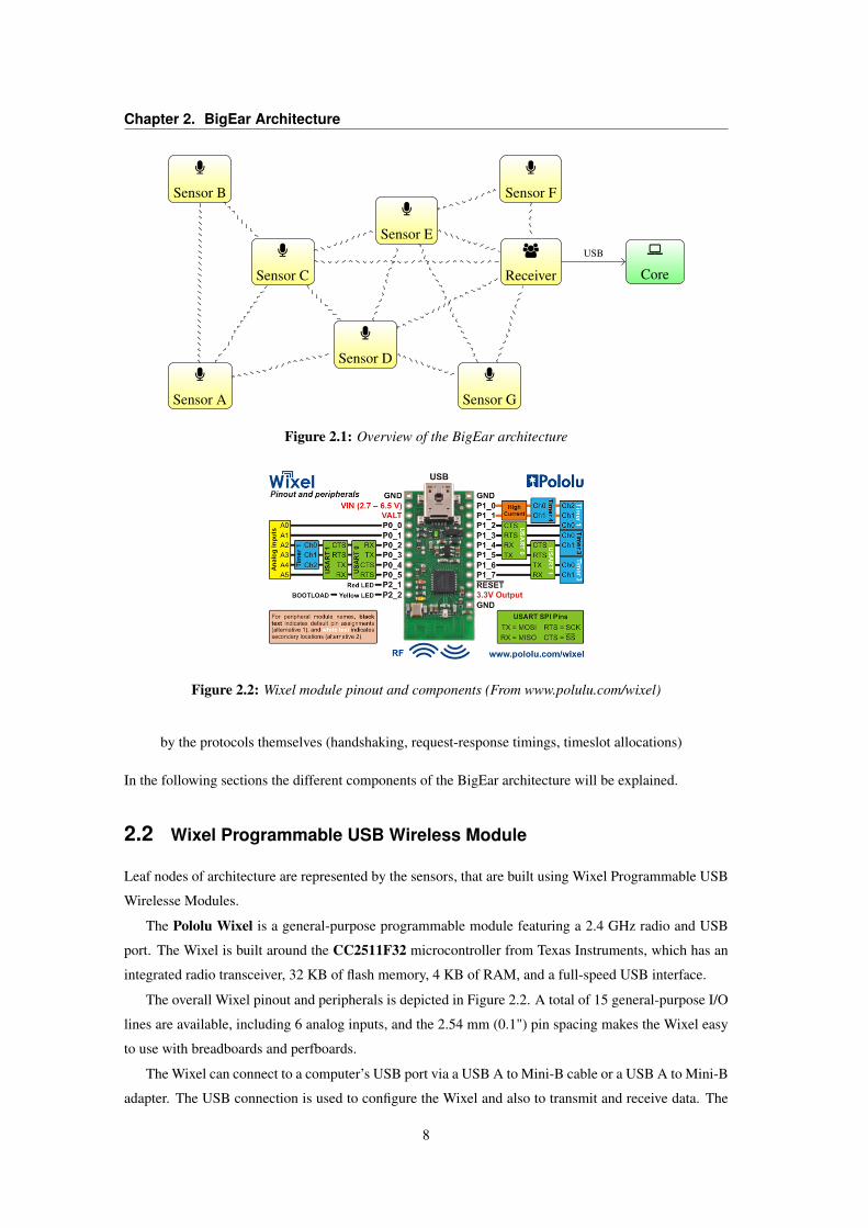
2.1 Overview of the System
The system is composed of a network of audio sensors that capture audio in a room distributedly.
The speech is sent to a main receiver, which basically acts as an interface that converts speech packets
received via radio channel into serial data for being sent to the base station. The base station contains
the application logic for handling speech packets. Since the audio sensors basically perform a space-
time sampling of the audio inside a room, the application logic tries to reconstruct a good-quality speech
stream starting from packets that arrive to the base station with different timestamps and with different
physical characteristics. Indeed, each sensor samples the audio signal that reaches the microphone after
undergoing variations due to the physical model of the environment: different delays and amplitudes that
depend on the position of the person with respect to the sensors, and reflections/diffusions due to the
geometry of the room and materials of the walls and furniture. Granularity of space-time sampling is
influenced by:
• Number of audio sensors w.r.t the dimensions of the room: the bigger is the number of sensors
spread in the room, the finer is the granularity of space sampling.
• Audio sensor internal characteristics and constraints: each sensor needs time in order to sample
data (depending on ADC type), store them in buffers and send them to the main receiver.
• Network communication protocol characteristics and constraints: the number of packets sent to
the main receiver is affected by the number of collisions that may happen on the channel and also
7
Chapter 2. BigEar Architecture
§
Sensor A
§
Sensor B
§
Sensor C
§
Sensor D
§
Sensor E
§
Sensor F
§
Sensor G
u
Receiver
Core
USB
Figure 2.1: Overview of the BigEar architecture
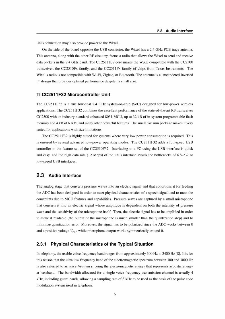
Figure 2.2: Wixel module pinout and components (From www.polulu.com/wixel)
by the protocols themselves (handshaking, request-response timings, timeslot allocations)
In the following sections the different components of the BigEar architecture will be explained.
2.2 Wixel Programmable USB Wireless Module
Leaf nodes of architecture are represented by the sensors, that are built using Wixel Programmable USB
Wirelesse Modules.
The Pololu Wixel is a general-purpose programmable module featuring a 2.4 GHz radio and USB
port. The Wixel is built around the CC2511F32 microcontroller from Texas Instruments, which has an
integrated radio transceiver, 32 KB of flash memory, 4 KB of RAM, and a full-speed USB interface.
The overall Wixel pinout and peripherals is depicted in Figure 2.2. A total of 15 general-purpose I/O
lines are available, including 6 analog inputs, and the 2.54 mm (0.1") pin spacing makes the Wixel easy
to use with breadboards and perfboards.
The Wixel can connect to a computer’s USB port via a USB A to Mini-B cable or a USB A to Mini-B
adapter. The USB connection is used to configure the Wixel and also to transmit and receive data. The
8
2.3. Audio Interface
USB connection may also provide power to the Wixel.
On the side of the board opposite the USB connector, the Wixel has a 2.4 GHz PCB trace antenna.
This antenna, along with the other RF circuitry, forms a radio that allows the Wixel to send and receive
data packets in the 2.4 GHz band. The CC2511F32 core makes the Wixel compatible with the CC2500
transceiver, the CC2510Fx family, and the CC2511Fx family of chips from Texas Instruments. The
Wixel’s radio is not compatible with Wi-Fi, Zigbee, or Bluetooth. The antenna is a “meandered Inverted
F” design that provides optimal performance despite its small size.
TI CC2511F32 Microcontroller Unit
The CC2511F32 is a true low-cost 2.4 GHz system-on-chip (SoC) designed for low-power wireless
applications. The CC2511F32 combines the excellent performance of the state-of-the-art RF transceiver
CC2500 with an industry-standard enhanced 8051 MCU, up to 32 kB of in-system programmable flash
memory and 4 kB of RAM, and many other powerful features. The small 6x6 mm package makes it very
suited for applications with size limitations.
The CC2511F32 is highly suited for systems where very low power consumption is required. This
is ensured by several advanced low-power operating modes. The CC2511F32 adds a full-speed USB
controller to the feature set of the CC2510F32. Interfacing to a PC using the USB interface is quick
and easy, and the high data rate (12 Mbps) of the USB interface avoids the bottlenecks of RS-232 or
low-speed USB interfaces.
2.3 Audio Interface
The analog stage that converts pressure waves into an electric signal and that conditions it for feeding
the ADC has been designed in order to meet physical characteristics of a speech signal and to meet the
constraints due to MCU features and capabilities. Pressure waves are captured by a small microphone
that converts it into an electric signal whose amplitude is dependent on both the intensity of pressure
wave and the sensitivity of the microphone itself. Then, the electric signal has to be amplified in order
to make it readable (the output of the microphone is much smaller than the quantization step) and to
minimize quantization error. Moreover, the signal has to be polarized since the ADC works between 0
and a positive voltage Vref while microphone output works symmetrically around 0.
2.3.1 Physical Characteristics of the Typical Situation
In telephony, the usable voice frequency band ranges from approximately 300 Hz to 3400 Hz [8]. It is for
this reason that the ultra low frequency band of the electromagnetic spectrum between 300 and 3000 Hz
is also referred to as voice frequency, being the electromagnetic energy that represents acoustic energy
at baseband. The bandwidth allocated for a single voice-frequency transmission channel is usually 4
kHz, including guard bands, allowing a sampling rate of 8 kHz to be used as the basis of the pulse code
modulation system used in telephony.
9
Chapter 2. BigEar Architecture
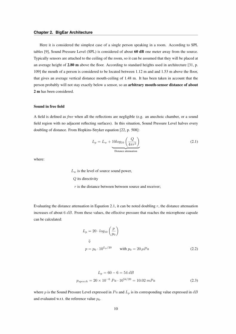
Here it is considered the simplest case of a single person speaking in a room. According to SPL
tables [9], Sound Pressure Level (SPL) is considered of about 60 dB one meter away from the source.
Typically sensors are attached to the ceiling of the room, so it can be assumed that they will be placed at
an average height of 2.80 m above the floor. According to standard heights used in architecture [31, p.
109] the mouth of a person is considered to be located between 1.12 m and and 1.53 m above the floor,
that gives an average vertical distance mouth-ceiling of 1.48 m. It has been taken in account that the
person probably will not stay exactly below a sensor, so an arbitrary mouth-sensor distance of about
2 m has been considered.
Sound in free field
A field is defined as free when all the reflections are negligible (e.g. an anechoic chamber, or a sound
field region with no adjacent reflecting surfaces). In this situation, Sound Pressure Level halves every
doubling of distance. From Hopkins-Stryker equation [22, p. 508]:
Lp = Lw + 10log10
(Q
4πr2
)︸ ︷︷ ︸
Distance attenuation
(2.1)
where:
Lw is the level of source sound power,
Q its directivity
r is the distance between between source and receiver;
Evaluating the distance attenuation in Equation 2.1, it can be noted doubling r, the distance attenuation
increases of about 6 dB. From these values, the effective pressure that reaches the microphone capsule
can be calculated:
Lp = 20 · log10(p
p0
)⇓
p = p0 · 10Lp/20 with p0 = 20µPa (2.2)
Lp = 60− 6 = 54 dB
pspeech = 20× 10−6 Pa · 1054/20 = 10.02 mPa (2.3)
where p is the Sound Pressure Level expressed in Pa and Lp is its corresponding value expressed in dB
and evaluated w.r.t. the reference value p0.
10
2.3. Audio Interface
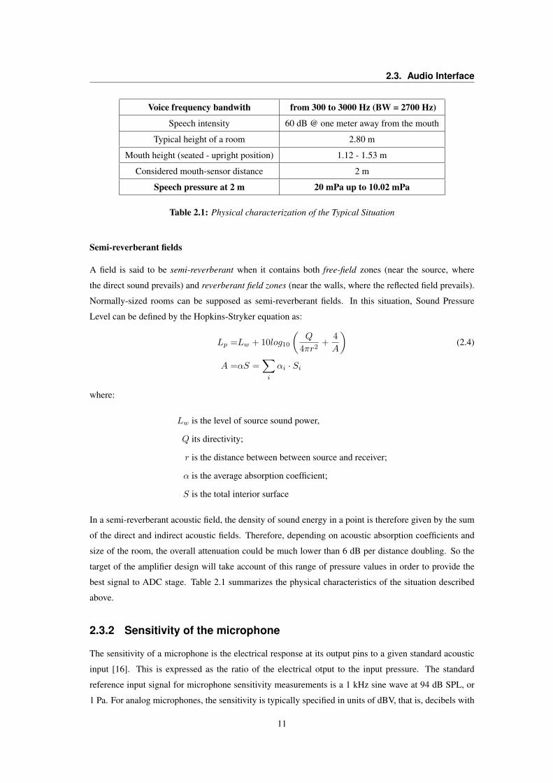
Voice frequency bandwith from 300 to 3000 Hz (BW = 2700 Hz)
Speech intensity 60 dB @ one meter away from the mouth
Typical height of a room 2.80 m
Mouth height (seated - upright position) 1.12 - 1.53 m
Considered mouth-sensor distance 2 m
Speech pressure at 2 m 20 mPa up to 10.02 mPa
Table 2.1: Physical characterization of the Typical Situation
Semi-reverberant fields
A field is said to be semi-reverberant when it contains both free-field zones (near the source, where
the direct sound prevails) and reverberant field zones (near the walls, where the reflected field prevails).
Normally-sized rooms can be supposed as semi-reverberant fields. In this situation, Sound Pressure
Level can be defined by the Hopkins-Stryker equation as:
Lp =Lw + 10log10
(Q
4πr2+
4
A
)(2.4)
A =αS =∑i
αi · Si
where:
Lw is the level of source sound power,
Q its directivity;
r is the distance between between source and receiver;
α is the average absorption coefficient;
S is the total interior surface
In a semi-reverberant acoustic field, the density of sound energy in a point is therefore given by the sum
of the direct and indirect acoustic fields. Therefore, depending on acoustic absorption coefficients and
size of the room, the overall attenuation could be much lower than 6 dB per distance doubling. So the
target of the amplifier design will take account of this range of pressure values in order to provide the
best signal to ADC stage. Table 2.1 summarizes the physical characteristics of the situation described
above.
2.3.2 Sensitivity of the microphone
The sensitivity of a microphone is the electrical response at its output pins to a given standard acoustic
input [16]. This is expressed as the ratio of the electrical otput to the input pressure. The standard
reference input signal for microphone sensitivity measurements is a 1 kHz sine wave at 94 dB SPL, or
1 Pa. For analog microphones, the sensitivity is typically specified in units of dBV, that is, decibels with
11
Chapter 2. BigEar Architecture
reference to 1.0 V rms. Analog microphones sensitivity can be measured with mV/Pa units:
SdBV = 20 ∗ log10(SmV/Pa
OutREF
)where OutREF = 1000 mV/Pa reference output voltage
(2.5)
⇓
SmV/Pa = OutREF · 10SdBV /20 (2.6)
Microphones used for the prototypes have a sensitivity of -38 dB, so we can derive the sensitivity of
them expressed in mV/Pa units:
SdBV = −38 dB
SmV/Pa = 1000 mV/Pa · 10−38/20 = 12.59 mV/Pa (2.7)
Using equations 2.3 and 2.7 we can assert that in presence of a typical speech signal, the microphone
capsule will produce an output signal whose amplitude will be:
Vmic = pspeech · SmV/Pa = 10.02× 10−3 Pa · 12.59mV/Pa = 0.126 mV (2.8)
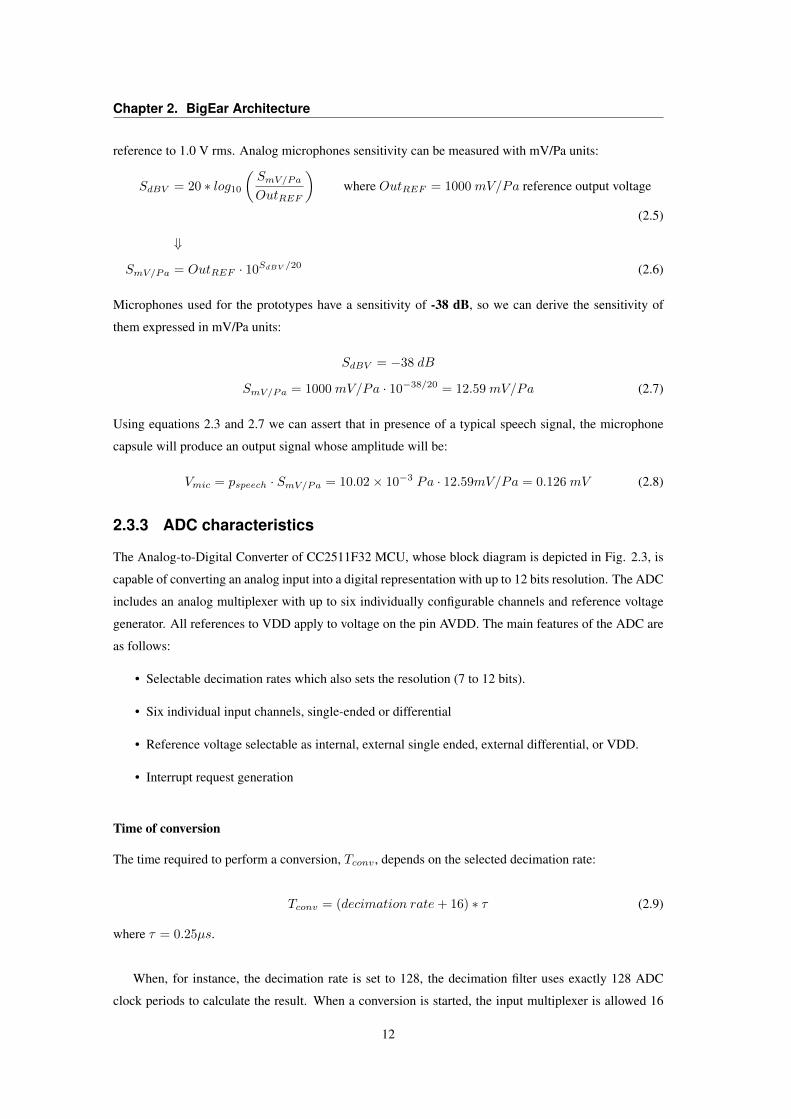
2.3.3 ADC characteristics
The Analog-to-Digital Converter of CC2511F32 MCU, whose block diagram is depicted in Fig. 2.3, is
capable of converting an analog input into a digital representation with up to 12 bits resolution. The ADC
includes an analog multiplexer with up to six individually configurable channels and reference voltage
generator. All references to VDD apply to voltage on the pin AVDD. The main features of the ADC are
as follows:
• Selectable decimation rates which also sets the resolution (7 to 12 bits).
• Six individual input channels, single-ended or differential
• Reference voltage selectable as internal, external single ended, external differential, or VDD.
• Interrupt request generation
Time of conversion
The time required to perform a conversion, Tconv , depends on the selected decimation rate:
Tconv = (decimation rate+ 16) ∗ τ (2.9)
where τ = 0.25µs.
When, for instance, the decimation rate is set to 128, the decimation filter uses exactly 128 ADC
clock periods to calculate the result. When a conversion is started, the input multiplexer is allowed 16
12
2.4. BigEar Receiver and Base station
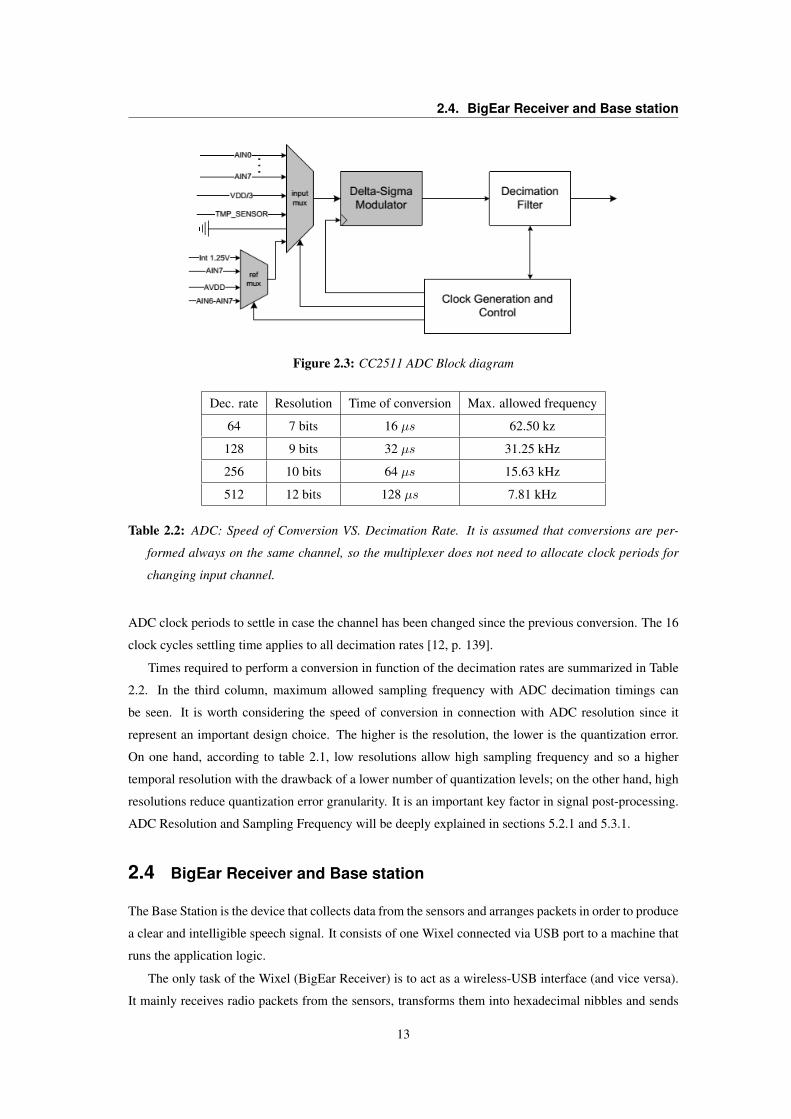
Figure 2.3: CC2511 ADC Block diagram
Dec. rate Resolution Time of conversion Max. allowed frequency
64 7 bits 16 µs 62.50 kz
128 9 bits 32 µs 31.25 kHz
256 10 bits 64 µs 15.63 kHz
512 12 bits 128 µs 7.81 kHz
Table 2.2: ADC: Speed of Conversion VS. Decimation Rate. It is assumed that conversions are per-
formed always on the same channel, so the multiplexer does not need to allocate clock periods for
changing input channel.
ADC clock periods to settle in case the channel has been changed since the previous conversion. The 16
clock cycles settling time applies to all decimation rates [12, p. 139].
Times required to perform a conversion in function of the decimation rates are summarized in Table
2.2. In the third column, maximum allowed sampling frequency with ADC decimation timings can
be seen. It is worth considering the speed of conversion in connection with ADC resolution since it
represent an important design choice. The higher is the resolution, the lower is the quantization error.
On one hand, according to table 2.1, low resolutions allow high sampling frequency and so a higher
temporal resolution with the drawback of a lower number of quantization levels; on the other hand, high
resolutions reduce quantization error granularity. It is an important key factor in signal post-processing.
ADC Resolution and Sampling Frequency will be deeply explained in sections 5.2.1 and 5.3.1.
2.4 BigEar Receiver and Base station
The Base Station is the device that collects data from the sensors and arranges packets in order to produce
a clear and intelligible speech signal. It consists of one Wixel connected via USB port to a machine that
runs the application logic.
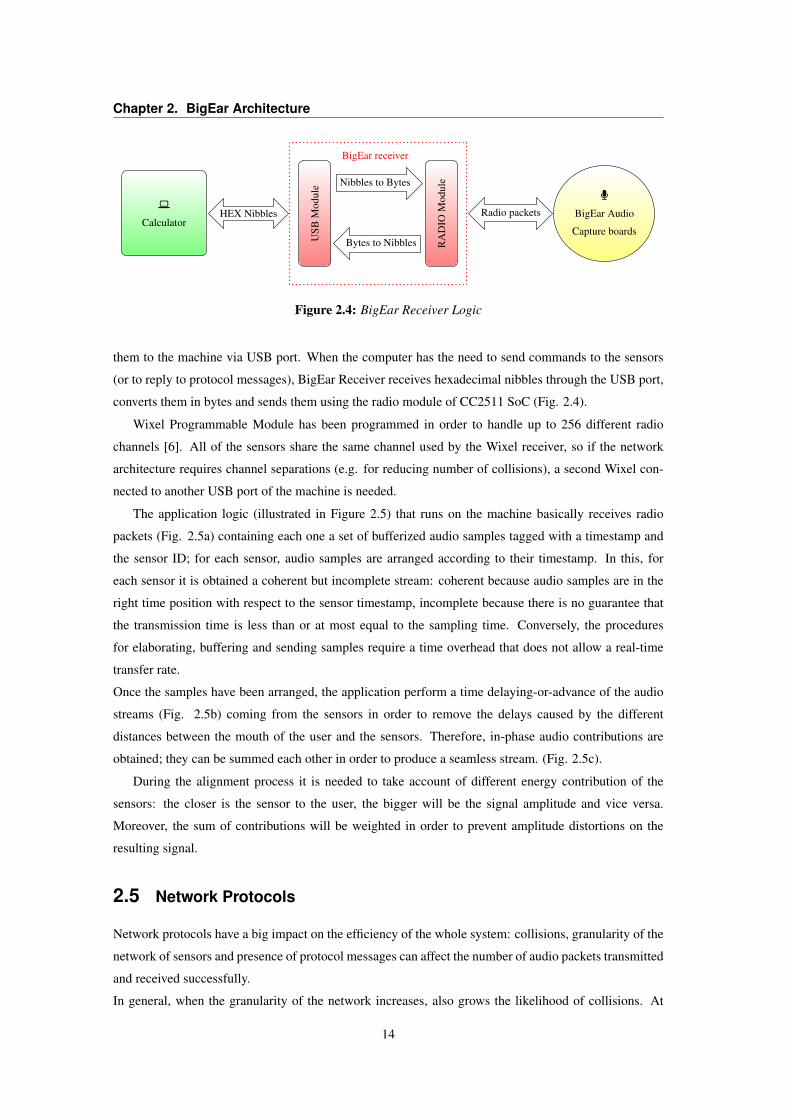
The only task of the Wixel (BigEar Receiver) is to act as a wireless-USB interface (and vice versa).
It mainly receives radio packets from the sensors, transforms them into hexadecimal nibbles and sends
13
Chapter 2. BigEar Architecture
USB
Mod
ule Nibbles to Bytes
Bytes to Nibbles RA
DIO
Mod
ule
HEX Nibbles Radio packets
BigEar receiver
Calculator
§
BigEar Audio
Capture boards
Figure 2.4: BigEar Receiver Logic
them to the machine via USB port. When the computer has the need to send commands to the sensors
(or to reply to protocol messages), BigEar Receiver receives hexadecimal nibbles through the USB port,
converts them in bytes and sends them using the radio module of CC2511 SoC (Fig. 2.4).
Wixel Programmable Module has been programmed in order to handle up to 256 different radio
channels [6]. All of the sensors share the same channel used by the Wixel receiver, so if the network
architecture requires channel separations (e.g. for reducing number of collisions), a second Wixel con-
nected to another USB port of the machine is needed.
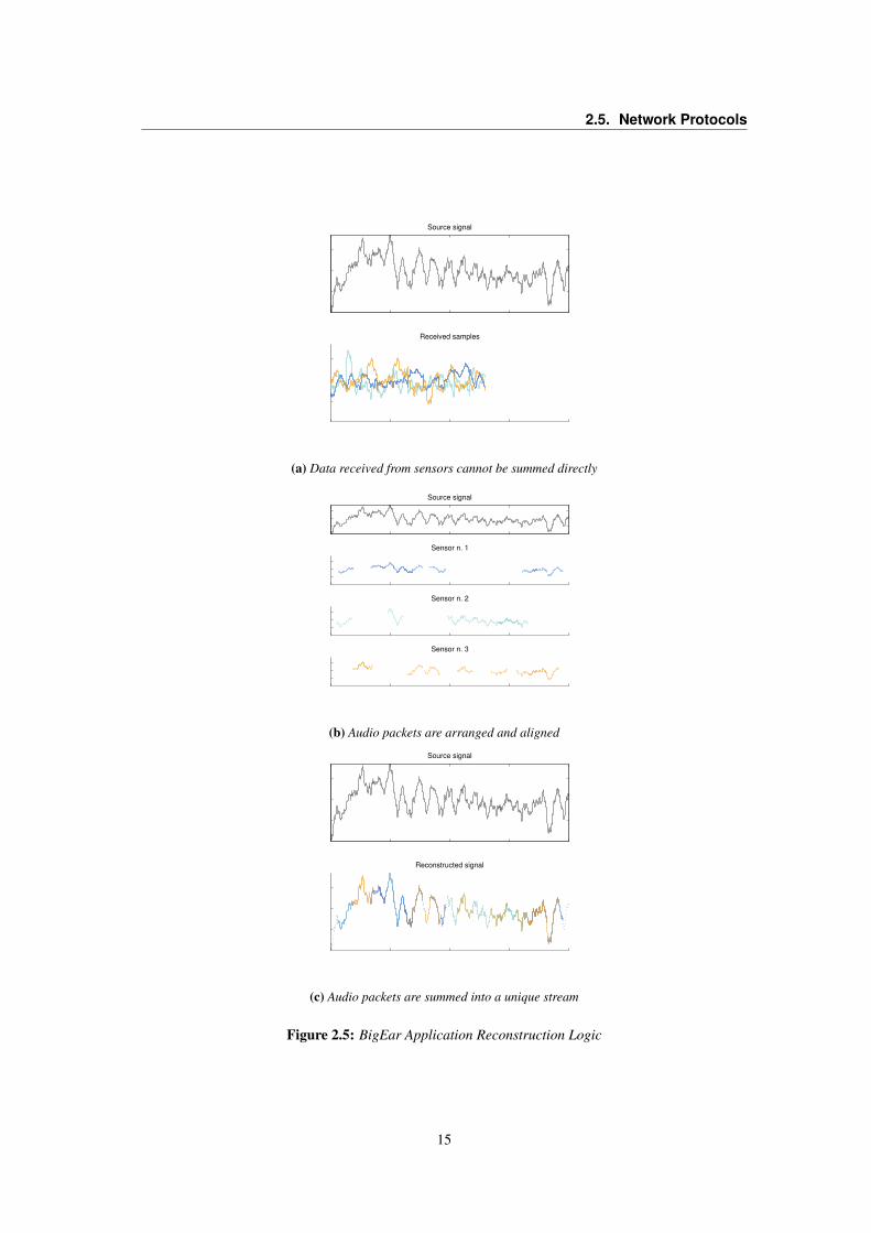
The application logic (illustrated in Figure 2.5) that runs on the machine basically receives radio
packets (Fig. 2.5a) containing each one a set of bufferized audio samples tagged with a timestamp and
the sensor ID; for each sensor, audio samples are arranged according to their timestamp. In this, for
each sensor it is obtained a coherent but incomplete stream: coherent because audio samples are in the
right time position with respect to the sensor timestamp, incomplete because there is no guarantee that
the transmission time is less than or at most equal to the sampling time. Conversely, the procedures
for elaborating, buffering and sending samples require a time overhead that does not allow a real-time
transfer rate.
Once the samples have been arranged, the application perform a time delaying-or-advance of the audio
streams (Fig. 2.5b) coming from the sensors in order to remove the delays caused by the different
distances between the mouth of the user and the sensors. Therefore, in-phase audio contributions are
obtained; they can be summed each other in order to produce a seamless stream. (Fig. 2.5c).
During the alignment process it is needed to take account of different energy contribution of the
sensors: the closer is the sensor to the user, the bigger will be the signal amplitude and vice versa.
Moreover, the sum of contributions will be weighted in order to prevent amplitude distortions on the
resulting signal.
2.5 Network Protocols
Network protocols have a big impact on the efficiency of the whole system: collisions, granularity of the
network of sensors and presence of protocol messages can affect the number of audio packets transmitted
and received successfully.
In general, when the granularity of the network increases, also grows the likelihood of collisions. At
14
2.5. Network Protocols
Source signal
Received samples
(a) Data received from sensors cannot be summed directly
Source signal
Sensor n. 1
Sensor n. 2
Sensor n. 3
(b) Audio packets are arranged and aligned
Source signal
Reconstructed signal
(c) Audio packets are summed into a unique stream
Figure 2.5: BigEar Application Reconstruction Logic
15
Chapter 2. BigEar Architecture
the same time the number of service messages for implementing synchronization mechanisms have to
be increased in order to reduce the number of collision. This can be done at the expense of the channel
availability and software complexity. CC2511 does not offer either Carrier Sense nor Collision Detection,
so the scenario can be seen as a pure broadcast domain. Moreover, each Wixel receives everything is
being transmitted on its channel, and each transmission reaches every Wixel that is listening on the same
radio channel.
2.5.1 ALOHA Protocol
The simplest protocol that can be adopted in this scenario is Aloha [1]; This name refers to a simple
communications scheme in which each source (transmitter) in a network sends data whenever there is
a frame to send. Aloha specifies also that if the frame successfully reaches the destination (receiver),
the next frame is sent; otherwise if the frame fails to be received at the destination, it is sent again.
Since audio data are time-dependent, for BigEar application purposes it is worthless to retransmit audio
packets, so the transmitter-side application will not wait for any acknowledgment from the base station.
Advantages:
• It doesn’t need any protocol or service message.
• Adapts to varying number of stations.
Disadvantages:
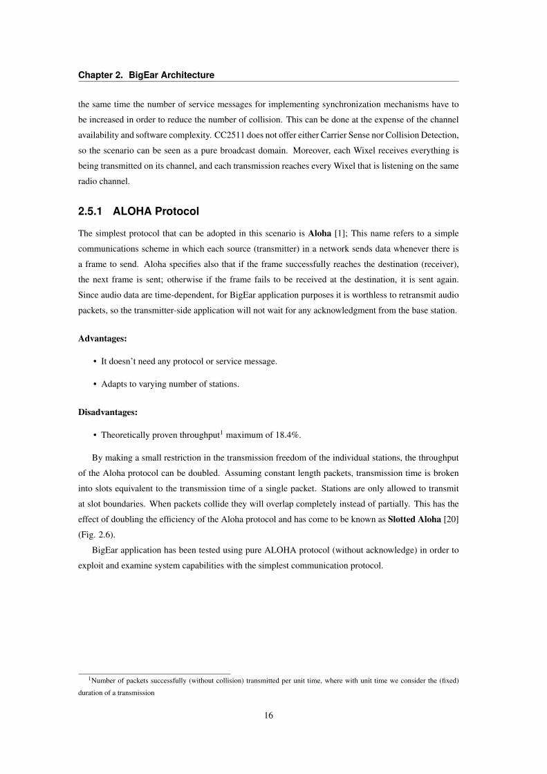
• Theoretically proven throughput1 maximum of 18.4%.
By making a small restriction in the transmission freedom of the individual stations, the throughput
of the Aloha protocol can be doubled. Assuming constant length packets, transmission time is broken
into slots equivalent to the transmission time of a single packet. Stations are only allowed to transmit
at slot boundaries. When packets collide they will overlap completely instead of partially. This has the
effect of doubling the efficiency of the Aloha protocol and has come to be known as Slotted Aloha [20]
(Fig. 2.6).
BigEar application has been tested using pure ALOHA protocol (without acknowledge) in order to
exploit and examine system capabilities with the simplest communication protocol.
1Number of packets successfully (without collision) transmitted per unit time, where with unit time we consider the (fixed)
duration of a transmission
16
2.5. Network Protocols
Figure 2.6: Aloha vs. Slotted Aloha throughput
17

3BigEar Modeling and Simulation
Introduction
In this chapter the methods and structures used for simulating the entire architecture within its envi-
ronment are described. Dissertation starts illustrating the physical model of the propagation of a sound
within a room and tools used for simulating it, then it continues describing a model that simulate the
behavior of the network of sensors arranged in the room.
3.1 Overview
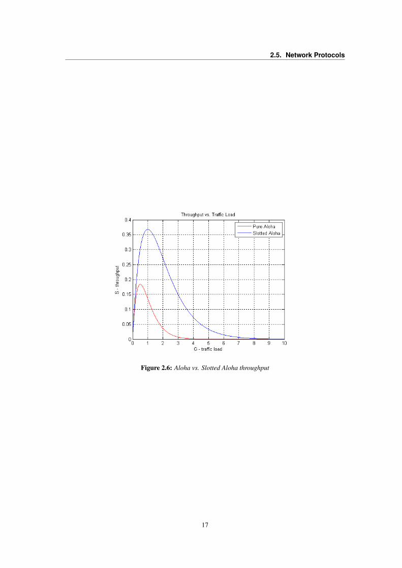
Figure 3.1 shows a schematic representation of BigEar simulator. It is composed of four interconnected
modules, at the end of which it is possible to withdraw the reconstructed signal.
The Audio model block consists in the simulation of the environment: room dimensions (and op-
tionally other parameters such as reflection and diffraction coefficients of walls), location of the sensors
and of the audio source are set. Then an audio file is provided as input. The block produces as many
audio streams as there are sensors. Each stream differs from the others in terms of amplitude, delay and
diffusion, which change depending on the acoustics characteristics of the room and the positions of the
sensor and the source.
The second block, Radio network model, simulates the behavior of transmitters according to a
choosen network protocol. In the simplest case of ALOHA protocol (See 2.5.1), it simulates random
instants of transmission of each transmitter and tags each packet as received or collided. This kind of
information is important because it affects the behavior of the following block that models the internal
buffer structure of the sensors.
N-buffer model block implements the buffering system internal to each transmitter. In real world,
data are continuously sampled and buffered by each transmitter in order to be ready to send them when
needed; during the simulation, instead, the time instants in which transmission occurs are known, but it is
needed to model the buffering structures in order to know what are the data ready for being transmitted.
This block produces in output the audio samples packed as if they were coming from real transmitters:
19

Chapter 3. BigEar Modeling and Simulation
Audio
Model
Fs
Room
Source
Sensor positions
N-Buffer model
Radio network model
Signal
Reconstruction
block
Model and Sensors
parameters
Reconstructed
signal
Sensor Model
Audio
streams
Output
packets
Rad
iotim
ings
and
Col
lisio
nfla
gsFigure 3.1: Architecture model
each packet contains the ID of the transmitter, the timestamp of the first sample1 of the packet and a
number of samples that corresponds to the frame size of each buffer.
The fourth block has been reported here for completeness but it will be discussed in chapter 4. It
concerns the reconstruction of the source signal starting from output of the previous block.
3.2 Audio Model
In order to create an audio model of the typical use case it is needed to do some assumptions about the
typical environment where the system will work. The room model assumed is a rectangular enclosure,
a three-dimensional space bounded by six surfaces (walls, ceiling and floor). In section 3.2.2 this type
of room will be also called “empty shoebox”. Each room surface has its own absorption and scattering
(diffusion) coefficients. The scattering coefficients set the ratio as a function of frequency between the
amount of specular and diffuse reflection. Sound scattering due to furniture and other objects in the
room can be approximated by higher levels of overall room diffuseness. This type of room has been
chosen because it is the most common shape of room, and also because of its ease of modeling and
computability.
Other assumptions concern directivity of source and sensors. It is assumed that directivity of the source
can be negligible because in small-medium rooms the reflections give a big contribution to the diffusion
of the sound. Small microphone capsules have omnidirectional polar pattern so directionality factors can
be neglected.
1Timestamps of other samples can be inferred summing τi = i · 1Fs
where i is the (0-based) the index of ith sample in the
packet
20
3.2. Audio Model
x1
x2
r12
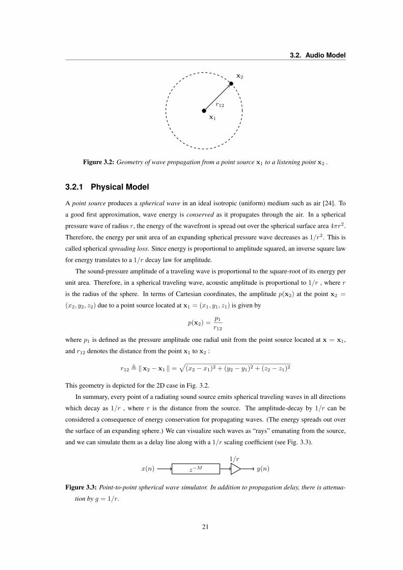
Figure 3.2: Geometry of wave propagation from a point source x1 to a listening point x2 .
3.2.1 Physical Model
A point source produces a spherical wave in an ideal isotropic (uniform) medium such as air [24]. To
a good first approximation, wave energy is conserved as it propagates through the air. In a spherical
pressure wave of radius r, the energy of the wavefront is spread out over the spherical surface area 4πr2.
Therefore, the energy per unit area of an expanding spherical pressure wave decreases as 1/r2. This is
called spherical spreading loss. Since energy is proportional to amplitude squared, an inverse square law
for energy translates to a 1/r decay law for amplitude.
The sound-pressure amplitude of a traveling wave is proportional to the square-root of its energy per
unit area. Therefore, in a spherical traveling wave, acoustic amplitude is proportional to 1/r , where r
is the radius of the sphere. In terms of Cartesian coordinates, the amplitude p(x2) at the point x2 =
(x2, y2, z2) due to a point source located at x1 = (x1, y1, z1) is given by
p(x2) =p1r12
where p1 is defined as the pressure amplitude one radial unit from the point source located at x = x1,
and r12 denotes the distance from the point x1 to x2 :
r12 , ‖x2 − x1 ‖ =√
(x2 − x1)2 + (y2 − y1)2 + (z2 − z1)2
This geometry is depicted for the 2D case in Fig. 3.2.
In summary, every point of a radiating sound source emits spherical traveling waves in all directions
which decay as 1/r , where r is the distance from the source. The amplitude-decay by 1/r can be
considered a consequence of energy conservation for propagating waves. (The energy spreads out over
the surface of an expanding sphere.) We can visualize such waves as “rays” emanating from the source,
and we can simulate them as a delay line along with a 1/r scaling coefficient (see Fig. 3.3).
x(n) z−M1/r
y(n)
Figure 3.3: Point-to-point spherical wave simulator. In addition to propagation delay, there is attenua-
tion by g = 1/r.
21
Chapter 3. BigEar Modeling and Simulation
f i
θi
fr
θr
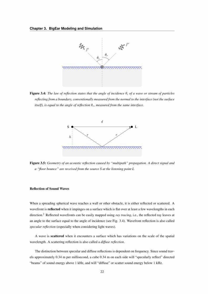
Figure 3.4: The law of reflection states that the angle of incidence θi of a wave or stream of particles
reflecting from a boundary, conventionally measured from the normal to the interface (not the surface
itself), is equal to the angle of reflection θr, measured from the same interface.
h
S L
d
r r
Figure 3.5: Geometry of an acoustic reflection caused by “multipath” propagation. A direct signal and
a “floor bounce” are received from the source S at the listening point L
Reflection of Sound Waves
When a spreading spherical wave reaches a wall or other obstacle, it is either reflected or scattered. A
wavefront is reflected when it impinges on a surface which is flat over at least a few wavelengths in each
direction.2 Reflected wavefronts can be easily mapped using ray tracing, i.e., the reflected ray leaves at
an angle to the surface equal to the angle of incidence (see Fig. 3.4). Wavefront reflection is also called
specular reflection (especially when considering light waves).
A wave is scattered when it encounters a surface which has variations on the scale of the spatial
wavelength. A scattering reflection is also called a diffuse reflection.
The distinction between specular and diffuse reflections is dependent on frequency. Since sound trav-
els approximately 0.34 m per millisecond, a cube 0.34 m on each side will “specularly reflect” directed
“beams” of sound energy above 1 kHz, and will “diffuse” or scatter sound energy below 1 kHz.
22
3.2. Audio Model
Room Acoustics
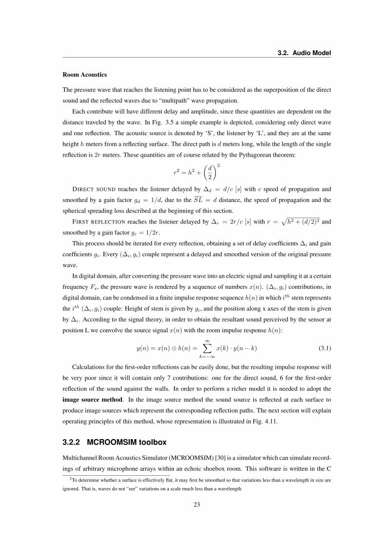
The pressure wave that reaches the listening point has to be considered as the superposition of the direct
sound and the reflected waves due to “multipath” wave propagation.
Each contribute will have different delay and amplitude, since these quantities are dependent on the
distance traveled by the wave. In Fig. 3.5 a simple example is depicted, considering only direct wave
and one reflection. The acoustic source is denoted by ‘S’, the listener by ‘L’, and they are at the same
height h meters from a reflecting surface. The direct path is d meters long, while the length of the single
reflection is 2r meters. These quantities are of course related by the Pythagorean theorem:
r2 = h2 +
(d
2
)2
DIRECT SOUND reaches the listener delayed by ∆d = d/c [s] with c speed of propagation and
smoothed by a gain factor gd = 1/d, due to the SL = d distance, the speed of propagation and the
spherical spreading loss described at the beginning of this section.
FIRST REFLECTION reaches the listener delayed by ∆r = 2r/c [s] with r =√h2 + (d/2)2 and
smoothed by a gain factor gr = 1/2r.
This process should be iterated for every reflection, obtaining a set of delay coefficients ∆i and gain
coefficients gi. Every (∆i, gi) couple represent a delayed and smoothed version of the original pressure
wave.
In digital domain, after converting the pressure wave into an electric signal and sampling it at a certain
frequency Fs, the pressure wave is rendered by a sequence of numbers x(n). (∆i, gi) contributions, in
digital domain, can be condensed in a finite impulse response sequence h(n) in which ith stem represents
the ith (∆i, gi) couple: Height of stem is given by gi, and the position along x axes of the stem is given
by ∆i. According to the signal theory, in order to obtain the resultant sound perceived by the sensor at
position L we convolve the source signal x(n) with the room impulse response h(n):
y(n) = x(n)⊗ h(n) =
∞∑k=−∞
x(k) · y(n− k) (3.1)
Calculations for the first-order reflections can be easily done, but the resulting impulse response will
be very poor since it will contain only 7 contributions: one for the direct sound, 6 for the first-order
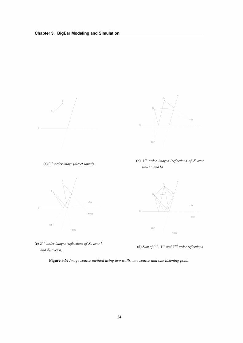
reflection of the sound against the walls. In order to perform a richer model it is needed to adopt the
image source method. In the image source method the sound source is reflected at each surface to
produce image sources which represent the corresponding reflection paths. The next section will explain
operating principles of this method, whose representation is illustrated in Fig. 4.11.
3.2.2 MCROOMSIM toolbox
Multichannel Room Acoustics Simulator (MCROOMSIM) [30] is a simulator which can simulate record-
ings of arbitrary microphone arrays within an echoic shoebox room. This software is written in the C2To determine whether a surface is effectively flat, it may first be smoothed so that variations less than a wavelength in size are
ignored. That is, waves do not “see” variations on a scale much less than a wavelength
23
Chapter 3. BigEar Modeling and Simulation
(a) 0th order image (direct sound)(b) 1st order images (reflections of S over
walls a and b)
(c) 2nd order images (reflections of Sa over b
and Sb over a)(d) Sum of 0th, 1st and 2nd order reflections
Figure 3.6: Image source method using two walls, one source and one listening point.
24
3.2. Audio Model
programming language. The software is freely available from the authors.
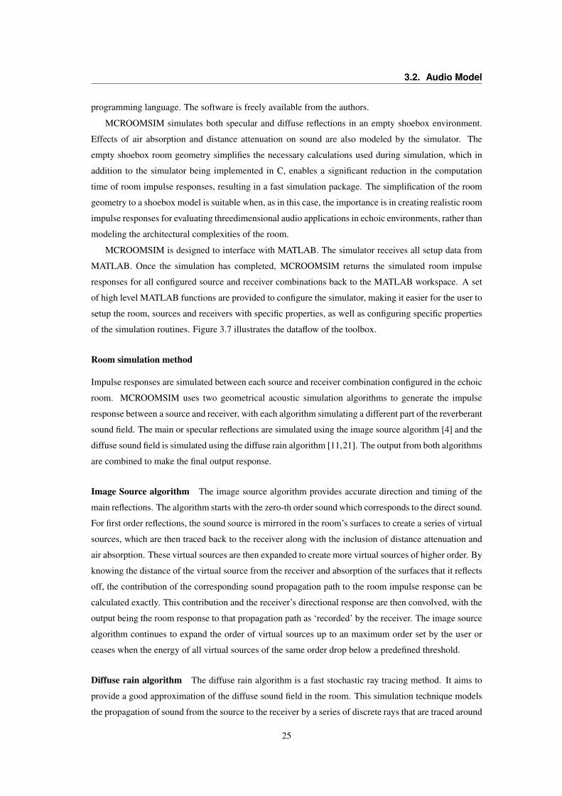
MCROOMSIM simulates both specular and diffuse reflections in an empty shoebox environment.
Effects of air absorption and distance attenuation on sound are also modeled by the simulator. The
empty shoebox room geometry simplifies the necessary calculations used during simulation, which in
addition to the simulator being implemented in C, enables a significant reduction in the computation
time of room impulse responses, resulting in a fast simulation package. The simplification of the room
geometry to a shoebox model is suitable when, as in this case, the importance is in creating realistic room
impulse responses for evaluating threedimensional audio applications in echoic environments, rather than
modeling the architectural complexities of the room.
MCROOMSIM is designed to interface with MATLAB. The simulator receives all setup data from
MATLAB. Once the simulation has completed, MCROOMSIM returns the simulated room impulse
responses for all configured source and receiver combinations back to the MATLAB workspace. A set
of high level MATLAB functions are provided to configure the simulator, making it easier for the user to
setup the room, sources and receivers with specific properties, as well as configuring specific properties
of the simulation routines. Figure 3.7 illustrates the dataflow of the toolbox.
Room simulation method
Impulse responses are simulated between each source and receiver combination configured in the echoic
room. MCROOMSIM uses two geometrical acoustic simulation algorithms to generate the impulse
response between a source and receiver, with each algorithm simulating a different part of the reverberant
sound field. The main or specular reflections are simulated using the image source algorithm [4] and the
diffuse sound field is simulated using the diffuse rain algorithm [11,21]. The output from both algorithms
are combined to make the final output response.
Image Source algorithm The image source algorithm provides accurate direction and timing of the
main reflections. The algorithm starts with the zero-th order sound which corresponds to the direct sound.
For first order reflections, the sound source is mirrored in the room’s surfaces to create a series of virtual
sources, which are then traced back to the receiver along with the inclusion of distance attenuation and
air absorption. These virtual sources are then expanded to create more virtual sources of higher order. By
knowing the distance of the virtual source from the receiver and absorption of the surfaces that it reflects
off, the contribution of the corresponding sound propagation path to the room impulse response can be
calculated exactly. This contribution and the receiver’s directional response are then convolved, with the
output being the room response to that propagation path as ‘recorded’ by the receiver. The image source
algorithm continues to expand the order of virtual sources up to an maximum order set by the user or
ceases when the energy of all virtual sources of the same order drop below a predefined threshold.
Diffuse rain algorithm The diffuse rain algorithm is a fast stochastic ray tracing method. It aims to
provide a good approximation of the diffuse sound field in the room. This simulation technique models
the propagation of sound from the source to the receiver by a series of discrete rays that are traced around
25
Chapter 3. BigEar Modeling and Simulation
Proceedings of the International Symposium on Room Acoustics, ISRA 2010 29–31 August 2010, Melbourne, Australia
the size, frequency dependent absorption and scatteringcoefficients of the walls/ceilings, room temperature andhumidity.
2. General simulation options: here the user is providedwith an opportunity to configure various features of thesimulator such as the maximum order that the imagesource algorithm will iterate up to, the minimum energythreshold for virtual image sources or rays, etc.
3. Receiver setup: the number of receivers to simulate, theirlocations, orientation, number of channels and directivity.For receivers with custom directivity, a list of directionalgains or impulse responses along with the matchingdirection list is also included here.
4. Source setup: same as the receiver setup with the limita-tion that sources can only be single channel.
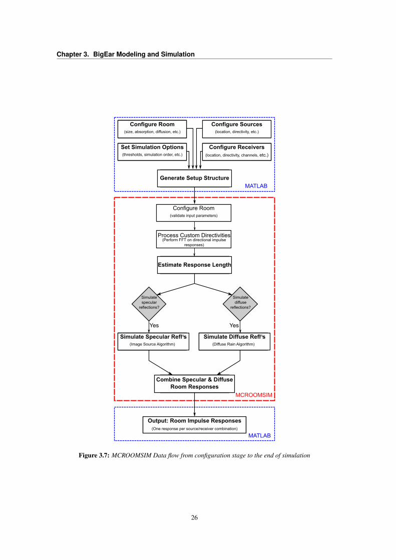
Once the MCROOMSIM function is invoked, MATLAB com-bines all of the data, including all user-defined directional re-sponses (if provided), into a single structure which it then passesto MCROOMSIM. Once the simulation has completed, all ofthe room impulse response data are provided as output to theMATLAB workspace. The output of MCROOMSIM is a timedomain room impulse response for each source and receivercombination. In the case of a multichannel receiver array, aseparate response is provided for each channel.
Flow Of Software
Once the input configuration data is received by MCROOMSIM,the simulator first performs a validity check on the parametersto ensure that the configuration is not erroneous. Once this hascompleted successfully, the simulator uses these parameters toconfigure itself. All operations are performed in the frequencydomain, which improves efficiency of convolutions. Thereforeif a source or receiver has custom directivity defined with di-rectional impulse responses, MCROOMSIM transforms theseresponses into the frequency domain. Next the simulator es-timates the maximum possible length for the room impulseresponse by calculating the longest time for the virtual sourcesto decay below the energy threshold, as set in the simulationgeneral options. This is performed so that simulation memorycan be pre-allocated.
MCROOMSIM can be configured to run in one of three ways:specular only simulation, diffuse only simulation or both. Thesimulation algorithms are then executed to generate the roomimpulse responses between the defined sources and receivers.Each algorithm outputs its results in the time domain, so thereis no need for transformation. If both algorithms have beenexecuted then the outputs of each will be combined to create theoverall room impulse responses. Upon completion, the resultingsimulated room impulse responses are provided as output to theMATLAB workspace. Fig. 1 highlights the flow of the softwarefrom configuration to the end of simulation.
EXAMPLE APPLICATIONS OF THE SOFTWARE
Realistic in-room microphone array simulation
Microphone arrays are used in many three-dimensional audioapplications. Some examples include spatial sound reproduc-tion [2], measurement and analysis of directional properties ofreverberant sound fields using beamforming techniques [8] orplane wave decomposition [9]. In all of these situations MC-ROOMSIM can be used to generate realistic three-dimensionalroom impulse responses for the microphone array under test. Allthat is needed are the anechoic directional impulses responsesof the microphone array and the properties of the room undersimulation, i.e. size, location of source(s), location of micro-phone array, etc. Moreover, sources with specific directivitypatterns can also be simulated in the system, enabling the user
Configure Room(size, absorption, diffusion, etc.)
Configure Room(size, absorption, diffusion, etc.)
Configure Room(size, absorption, diffusion, etc.)
Configure Room(size, absorption, diffusion, etc.)
Configure Room(size, absorption, diffusion, etc.)
Configure Sources(location, directivity, etc.)
Configure Room(size, absorption, diffusion, etc.)
Configure Room(size, absorption, diffusion, etc.)
Configure Room(size, absorption, diffusion, etc.)
Set Simulation Options(thresholds, simulation order, etc.)
Configure Room(size, absorption, diffusion, etc.)
Configure Room(size, absorption, diffusion, etc.)
Configure Room(size, absorption, diffusion, etc.)
Configure Receivers(location, directivity, channels, etc.)
Configure Room(size, absorption, diffusion, etc.)
Configure Room(size, absorption, diffusion, etc.)
Configure Room(size, absorption, diffusion, etc.)
Generate Setup Structure
MATLAB
Configure Room(validate input parameters)
Configure Room(size, absorption, diffusion, etc.)
Configure Room(size, absorption, diffusion, etc.)
Configure Room(size, absorption, diffusion, etc.)
Estimate Response Length
Simulatespecular
reflections?
Simulatediffuse
reflections?
Configure Room(size, absorption, diffusion, etc.)
Configure Room(size, absorption, diffusion, etc.)
Configure Room(size, absorption, diffusion, etc.)
Simulate Specular Refl s(Image Source Algorithm)
n Configure Room(size, absorption, diffusion, etc.)
Configure Room(size, absorption, diffusion, etc.)
Configure Room(size, absorption, diffusion, etc.)
Simulate Diffuse Refl s(Diffuse Rain Algorithm)
n
Yes Yes
Configure Room(size, absorption, diffusion, etc.)
Configure Room(size, absorption, diffusion, etc.)
Configure Room(size, absorption, diffusion, etc.)
Combine Specular & Diffuse Room Responses
MCROOMSIM
Output: Room Impulse Responses(One response per source/receiver combination)
MATLAB
Process Custom Directivities(Perform FFT on directional impulse
responses)
Figure 1: The flow of the MCROOMSIM software is shownfrom the configuration stage to the end of simulation, where thesimulated room impulse responses are returned to the MATLABworkspace.
to compare the effects of various sources on the reverberantsound field.
3D Binaural rendering of echoic sound scenes
MCROOMSIM can be used to directly simulate realistic Bin-aural Room Impulse Responses (BRIRs). This is done by con-figuring the simulation software with a pair of sensors whosedirectional impulse responses are anechoic head related impulseresponses (HRIRs) measured for a number of directions in thefree-field for the particular user. This is useful for quickly gen-erating 3D BRIRs for many environments, without the needof performing time consuming recordings within each environ-ment. From this the user could then for instance listen to the3D reverberant sound fields created by sources with differentdirectivities.
ISRA 2010 3
Figure 3.7: MCROOMSIM Data flow from configuration stage to the end of simulation
26
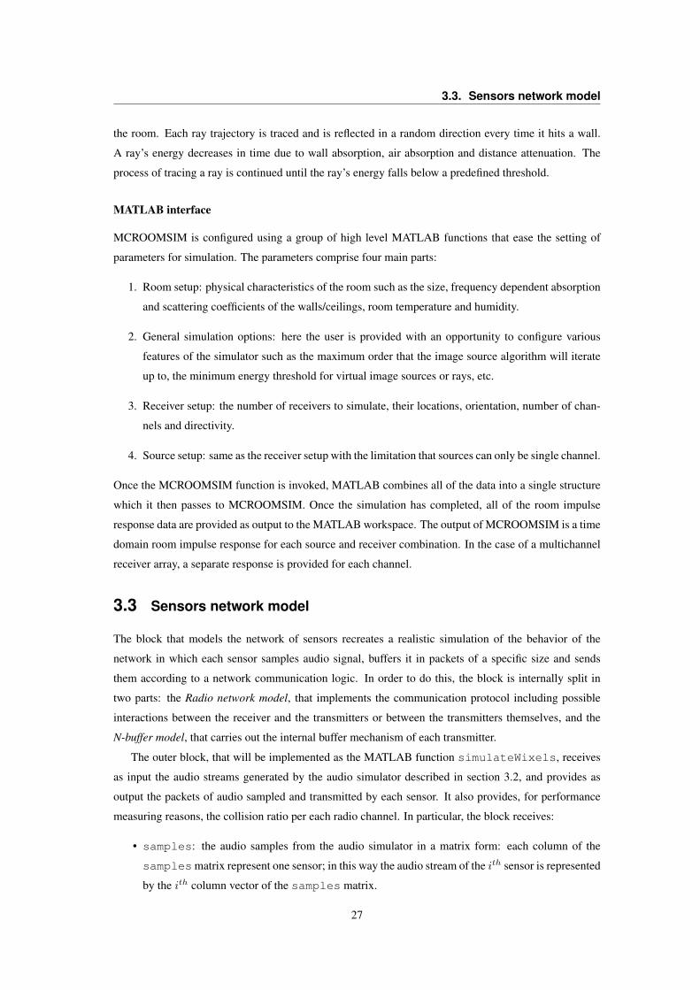
3.3. Sensors network model
the room. Each ray trajectory is traced and is reflected in a random direction every time it hits a wall.
A ray’s energy decreases in time due to wall absorption, air absorption and distance attenuation. The
process of tracing a ray is continued until the ray’s energy falls below a predefined threshold.
MATLAB interface
MCROOMSIM is configured using a group of high level MATLAB functions that ease the setting of
parameters for simulation. The parameters comprise four main parts:
1. Room setup: physical characteristics of the room such as the size, frequency dependent absorption
and scattering coefficients of the walls/ceilings, room temperature and humidity.
2. General simulation options: here the user is provided with an opportunity to configure various
features of the simulator such as the maximum order that the image source algorithm will iterate
up to, the minimum energy threshold for virtual image sources or rays, etc.
3. Receiver setup: the number of receivers to simulate, their locations, orientation, number of chan-
nels and directivity.
4. Source setup: same as the receiver setup with the limitation that sources can only be single channel.
Once the MCROOMSIM function is invoked, MATLAB combines all of the data into a single structure
which it then passes to MCROOMSIM. Once the simulation has completed, all of the room impulse
response data are provided as output to the MATLAB workspace. The output of MCROOMSIM is a time
domain room impulse response for each source and receiver combination. In the case of a multichannel
receiver array, a separate response is provided for each channel.
3.3 Sensors network model
The block that models the network of sensors recreates a realistic simulation of the behavior of the
network in which each sensor samples audio signal, buffers it in packets of a specific size and sends
them according to a network communication logic. In order to do this, the block is internally split in
two parts: the Radio network model, that implements the communication protocol including possible
interactions between the receiver and the transmitters or between the transmitters themselves, and the
N-buffer model, that carries out the internal buffer mechanism of each transmitter.
The outer block, that will be implemented as the MATLAB function simulateWixels, receives
as input the audio streams generated by the audio simulator described in section 3.2, and provides as
output the packets of audio sampled and transmitted by each sensor. It also provides, for performance
measuring reasons, the collision ratio per each radio channel. In particular, the block receives:
• samples: the audio samples from the audio simulator in a matrix form: each column of the
samplesmatrix represent one sensor; in this way the audio stream of the ith sensor is represented
by the ith column vector of the samples matrix.
27
Chapter 3. BigEar Modeling and Simulation
• Model: the structure containing all of the parameters that characterize a transmitter:
– FRAMES: the number of frames of which the buffer system is composed of
– FRAME_SIZE: the number of samples that can be stored in a frame
– Tbusy: the duration of a radio transmission, expressed in milliseconds
– TmaxDelay: the maximum allowed delay for a radio transmission (when we assume a
network protocol belonging to ALOHA family of protocols)
– Fs: the sampling frequency of the sensor
• Sensors: the structure that describe individual characteristics of sensors: their position in the room,
their radio channel and their name.
– X, Y, Z: column vectors containing coordinates of the sensors
– Channel: column vector containing radio channel of the sensor
– Name: (optional) column vector containing names of the sensors
while the outputs are represented by these data:
• output: M-by-N matrix where M is the number of samples in output obtained by theN th sensor
• positions: M-by-N in which the position in time (expressed as sample index) of the ith sample
transmitted by the jth sensor are specified
• collisionRatioPerChannel: a vector in the each ith element represents the collision ratio
within the ith channel
The collision ratio is a performance metric that someway measures protocol robustness. It is calculated
as following:
Cr(i) =Nlost(i)
Ntotal(i)(3.2)
where i represents the ith channel, supposing that the network exploits different radio channels in order
to reduce the number of collisions, Nlost represents the number of packets lost for collisions on ith
channel and Ntotal represents the total number of packets that have been transmitted on ith channel.
The simulateWixels block (see dashed box in Fig 3.8) performs the network simulation apply-
ing a communication model to the transmitters that belong to the same broadcast domain. It is possible
to split the broadcast domain into several sub domains exploiting the capability of CC2511 radio to work
on different 2.4 GHz carriers. In this way it is possible to reduce the number of collisions decreasing
the number of transmitters that share the same carrier. So, simulateWixels first divide the sensor
set into K subsets, and then for each subset it calls the generateCalls block, described in section
3.3.1, in order to obtain two matrices: times and valid_flags. In the times matrix each column
represents a transmitter; each element in a column is a number corresponding to a time instant (expressed
in milliseconds from the beginning of the simulation) in which the transmitter starts to transmit a packet.
28
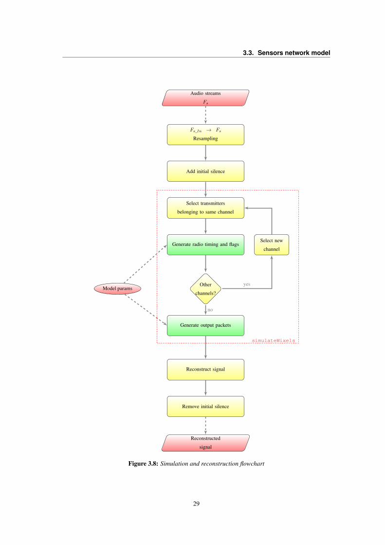
3.3. Sensors network model
Fs_In → Fs
Resampling
Audio streams
Fs
Add initial silence
Select transmitters
belonging to same channel
Generate radio timing and flags
Other
channels?
Select new
channel
Generate output packets
Model params
Reconstruct signal
Remove initial silence
Reconstructed
signal
simulateWixels
no
yes
Figure 3.8: Simulation and reconstruction flowchart
29
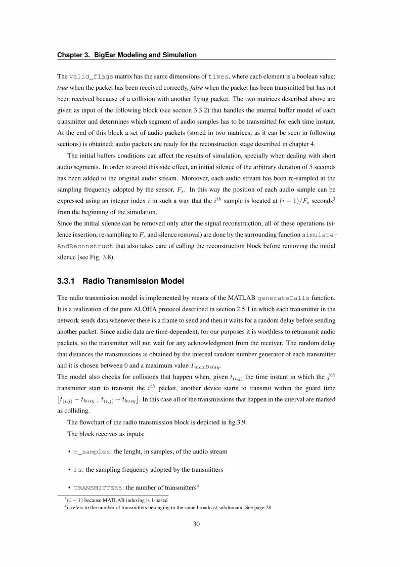
Chapter 3. BigEar Modeling and Simulation
The valid_flags matrix has the same dimensions of times, where each element is a boolean value:
true when the packet has been received correctly, false when the packet has been transmitted but has not
been received because of a collision with another flying packet. The two matrices described above are
given as input of the following block (see section 3.3.2) that handles the internal buffer model of each
transmitter and determines which segment of audio samples has to be transmitted for each time instant.
At the end of this block a set of audio packets (stored in two matrices, as it can be seen in following
sections) is obtained; audio packets are ready for the reconstruction stage described in chapter 4.
The initial buffers conditions can affect the results of simulation, specially when dealing with short
audio segments. In order to avoid this side effect, an initial silence of the arbitrary duration of 5 seconds
has been added to the original audio stream. Moreover, each audio stream has been re-sampled at the
sampling frequency adopted by the sensor, Fs. In this way the position of each audio sample can be
expressed using an integer index i in such a way that the ith sample is located at (i − 1)/Fs seconds3
from the beginning of the simulation.
Since the initial silence can be removed only after the signal reconstruction, all of these operations (si-
lence insertion, re-sampling toFs and silence removal) are done by the surrounding function simulate-
AndReconstruct that also takes care of calling the reconstruction block before removing the initial
silence (see Fig. 3.8).
3.3.1 Radio Transmission Model
The radio transmission model is implemented by means of the MATLAB generateCalls function.
It is a realization of the pure ALOHA protocol described in section 2.5.1 in which each transmitter in the
network sends data whenever there is a frame to send and then it waits for a random delay before sending
another packet. Since audio data are time-dependent, for our purposes it is worthless to retransmit audio
packets, so the transmitter will not wait for any acknowledgment from the receiver. The random delay
that distances the transmissions is obtained by the internal random number generator of each transmitter
and it is chosen between 0 and a maximum value TmaxDelay.
The model also checks for collisions that happen when, given t(i,j) the time instant in which the jth
transmitter start to transmit the ith packet, another device starts to transmit within the guard time[t(i,j) − tbusy , t(i,j) + tbusy
]. In this case all of the transmissions that happen in the interval are marked
as colliding.
The flowchart of the radio transmission block is depicted in fig.3.9.
The block receives as inputs:
• n_samples: the lenght, in samples, of the audio stream
• Fs: the sampling frequency adopted by the transmitters
• TRANSMITTERS: the number of transmitters4
3(i− 1) because MATLAB indexing is 1-based4it refers to the number of transmitters belonging to the same broadcast subdomain. See page 28
30
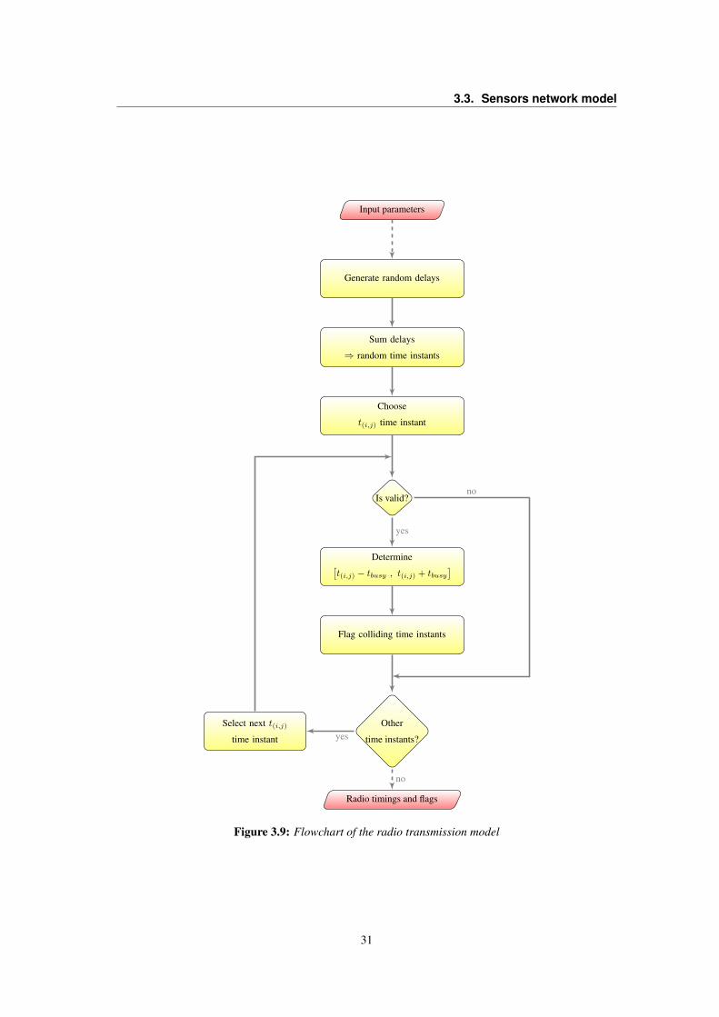
3.3. Sensors network model
Generate random delays
Input parameters
Sum delays
⇒ random time instants
Choose
t(i,j) time instant
Is valid?
Determine[t(i,j) − tbusy , t(i,j) + tbusy
]
Flag colliding time instants
Other
time instants?
Radio timings and flags
Select next t(i,j)time instant
yes
yes
no
no
Figure 3.9: Flowchart of the radio transmission model
31
Chapter 3. BigEar Modeling and Simulation
• Tbusy: the duration of a radio transmission, expressed in milliseconds
• TmaxDelay: the maximum allowed delay between two transmissions.
and produce as outputs:
• call_time: M-by-N matrix; each (i,j) element represent the ith time instant in which the jth
transmitter starts to transmit
• call_valid_flag: M-by-N matrix of boolean elements; each (i,j) element is false (invalid) if
the ith packet transmitted by the jth transmitter has collided.
3.3.2 N-buffer Internal Model
The transmitter-side application can be seen as divided in two parts: the sampler and the transmitter.
The sampler (as illustrated in section 5.3.1) continuously samples data and stores them into a framed
buffer. Then the transmitter, at proper time, checks if there is at least one full frame for sending the
packet to the receiver. These two parts are in such a way isolated from one another since sampler is
ruled by a timer interrupt routine and transmission procedure is called in the main loop. In order to know
which segment of audio samples has to be transmitted for each time instant we have to model the internal
behavior of buffers of each transmitter. This is the role of the N-buffer block, implemented by means of
the generateTransmitterOutputs MATLAB function.
Multiple buffering allows the sensor to work simultaneously on read and write sides: the interrupt
routine acquires the signal and stores samples into the write frame, pointed by the irs_idx index,
while the main loop can read from the read frame, pointed by the main_idx index.
Frames are handled by means of incrementing pointers: the condition main_idx = irs_idx
states that main loop would try reading from the same frame in which the interrupt routine is writing
data, but it is not possible to do this: this condition, indeed, occurs when all of the buffer have been
emptied by previous readings, so there are no frames ready to be processed.
When a frame is completely read, the main loop increments main_idx index by means of a modulo
operation:
main_idx = (main_idx + 1) % FRAMES_NUMBER
The same operation is done by the interrupt routine: once the frame is full and there is another free frame
to fill, index is incremented by mean of:
irs_idx = (irs_idx + 1) % FRAMES_NUMBER
In this way the temporal consequentiality of the frames is preserved. In case the transmission takes place
after ∆t > Tframe · FRAMES, the last frame (the one with most recent data) slides towards rights
(following an ideal temporal axis pointing to the right) in order to keep itself updated. This mechanism
makes sure that if the transmissions are spaced ∆t > Tframe · FRAMES each other, we in output
32
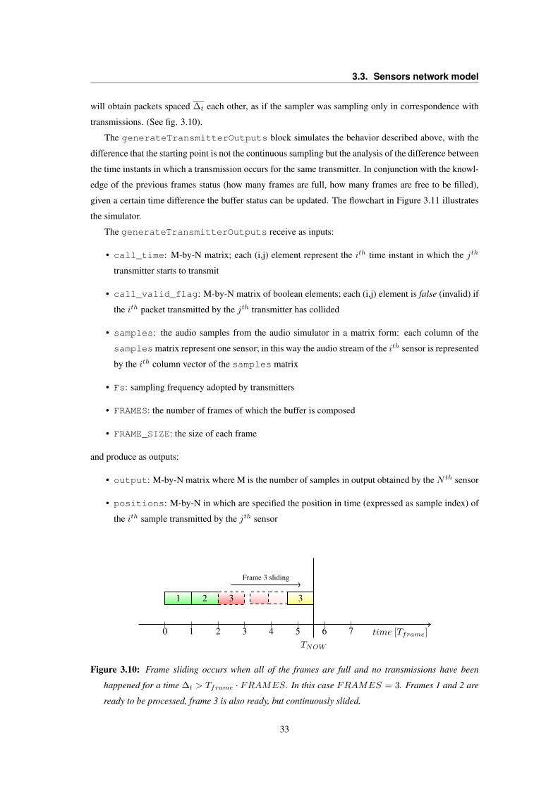
3.3. Sensors network model
will obtain packets spaced ∆t each other, as if the sampler was sampling only in correspondence with
transmissions. (See fig. 3.10).
The generateTransmitterOutputs block simulates the behavior described above, with the
difference that the starting point is not the continuous sampling but the analysis of the difference between
the time instants in which a transmission occurs for the same transmitter. In conjunction with the knowl-
edge of the previous frames status (how many frames are full, how many frames are free to be filled),
given a certain time difference the buffer status can be updated. The flowchart in Figure 3.11 illustrates
the simulator.
The generateTransmitterOutputs receive as inputs:
• call_time: M-by-N matrix; each (i,j) element represent the ith time instant in which the jth
transmitter starts to transmit
• call_valid_flag: M-by-N matrix of boolean elements; each (i,j) element is false (invalid) if
the ith packet transmitted by the jth transmitter has collided
• samples: the audio samples from the audio simulator in a matrix form: each column of the
samplesmatrix represent one sensor; in this way the audio stream of the ith sensor is represented
by the ith column vector of the samples matrix
• Fs: sampling frequency adopted by transmitters
• FRAMES: the number of frames of which the buffer is composed
• FRAME_SIZE: the size of each frame
and produce as outputs:
• output: M-by-N matrix where M is the number of samples in output obtained by theN th sensor
• positions: M-by-N in which are specified the position in time (expressed as sample index) of
the ith sample transmitted by the jth sensor
time [Tframe]0 1 2 3 4 5 6 7
1 2 3 3
TNOW
Frame 3 sliding
Figure 3.10: Frame sliding occurs when all of the frames are full and no transmissions have been
happened for a time ∆t > Tframe · FRAMES. In this case FRAMES = 3. Frames 1 and 2 are
ready to be processed, frame 3 is also ready, but continuously slided.
33
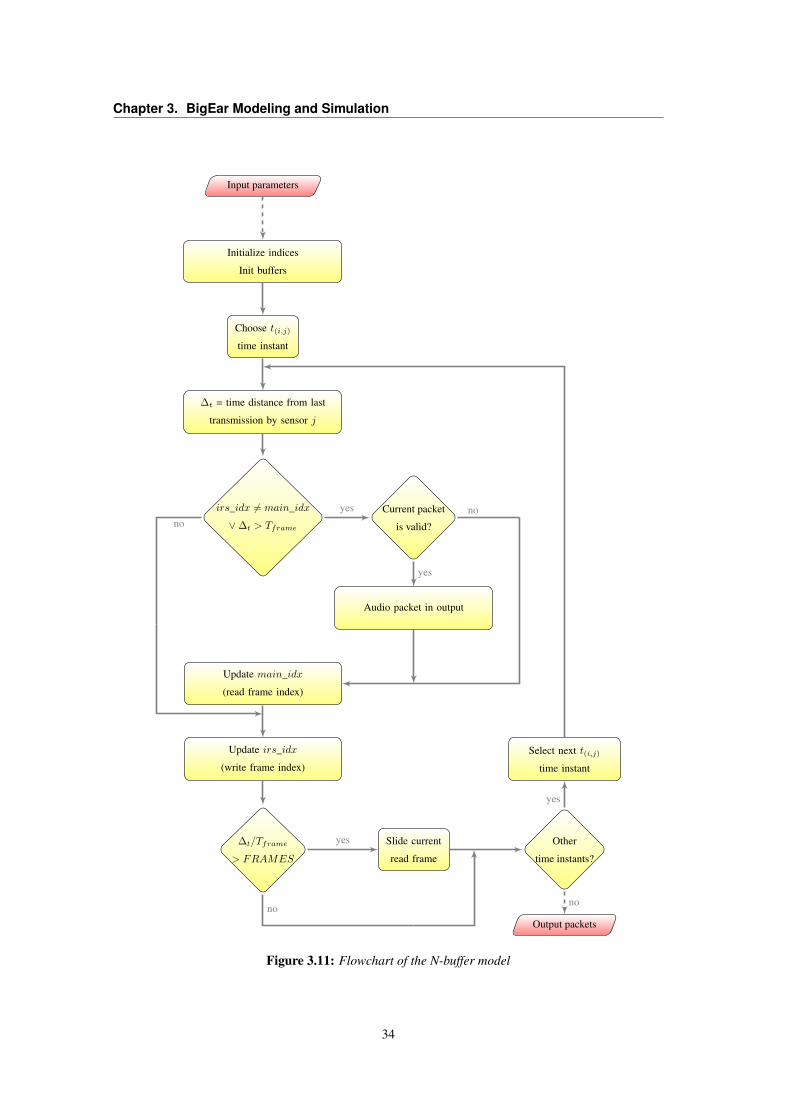
Chapter 3. BigEar Modeling and Simulation
Initialize indices
Init buffers
Input parameters
Choose t(i,j)time instant
∆t = time distance from last
transmission by sensor j
irs_idx 6= main_idx
∨ ∆t > Tframe
Current packet
is valid?
Audio packet in output
Update main_idx
(read frame index)
Update irs_idx
(write frame index)
∆t/Tframe
> FRAMES
Slide current
read frame
Other
time instants?
Output packets
Select next t(i,j)time instant
yesno
no
yes
yes
no
yes
no
Figure 3.11: Flowchart of the N-buffer model
34
4Signal Reconstruction and Repair
Introduction
Once the audio signal has been acquired by the sensors and sent to the base station, audio packets need
to be arranged and summed in such a way to make the audio signal suitable for speech recognition. This
is the role of the signal reconstruction block. First, the streams coming from sensors are built using
timestamp information given by each audio packet; then, the streams are aligned in order to reduce
the delay due to the distance of the speech source with respect to the position of the sensors. When
the signals are properly aligned they can be superposed with several summing or replacing methods in
order to preserve the signal energy and not to introduce energy variations due to the different number of
contributions that are summed at the same time. Since reconstructed signal is given by the superposition
of audio packets sampled by different sensors at random time instants, it can be affected by sequences of
empty samples. These holes influence the result of the speech recognition algorithm, so they have to be
removed by means of healing methods that generate segments of signal coherent with the information
content of the audio stream.
4.1 Overview
Each transmitter transmits a number of audio packets per time unit that is influenced by two factors:
• Audio sensor internal characteristics and constraints: each sensor needs time in order to sample
data, store them in buffers and send them to the main receiver.
• Network communication protocol characteristics and constraints: the number of packets sent to
the main receiver is affected by the number of collisions that may happen on the channel and also
by the protocols themselves (handshaking, request-response timings, timeslot allocations).
Audio streams generated by each transmitter contain a number of samples that is proportional to the
transmission rate fTX of the sensor. Defining Fill_ratio as the number of audio samples received over
35
Chapter 4. Signal Reconstruction and Repair
the system uptime it is possible to write:
Fill_ratio = Tframe · fTX (4.1)
where fTX =number of packets
total timeand Tframe = FRAME_SIZE
Fs.
Fill_ratio tends to 1 (complete audio stream) when Tframe and fTX tend to be respectively one the
reciprocal of the other, i.e., when the average time distance between adjacent transmissions equals the
duration of the audio packet. Using random access protocols like ALOHA family (section 2.5.1), this
optimal condition is hard to reach so the audio streams collected by the base station will be characterized
by 0 < Fill_ratio < 1. If Fill_ratio = 1 then there are no holes in the reconstructed speech signal.
The higher is the Fill_ratio, the lower is the number of artifacts generated by holes in the reconstructed
signals.
The flowchart at Fig. 4.1 illustrates the operation performed by the signal reconstruction block. It
receives in input the audio samples from the sensors. According to previous stages (see 3.3.2) each
audio sample is represented by a couple (audioPackets(i,j),positions(i,j)): each element of the
matrix audioPackets represents the ith audio sample transmitted by the jth sensor. Position in time of
the given sample is specified in positions(i,j). Using position information, audio samples are correctly
spaced on the sensor’s timeline (see Fig. 4.2). The time instants in which no audio samples are present
are 0-filled.
Audio packets have been preventively unbiased in order to remove effects of input signal polarization.
Then, audio streams are normalized in order to have signals of comparable amplitudes. Although it is
an unnecessary step for applying cross-correlation, it is a needed transformation in order to obtain audio
streams with equal energy contributions.
The alignment of audio streams is obtained by using the cross-correlation function [19]. In order to
apply it efficiently, the audio streams are processed according to their informative contribution: they are
sorted by their normalized power in descending order to allow the cross-correlation algorithm to work
in the best condition. Once a couple of streams has been aligned, it is summed in order to generate a
“superstream” whose information content is the sum of the single contributions.
Delays applied for stream alignment are proportional to the distance between the source and the
sensor. Due to sound propagation laws, the closer is the sensor to the source, the lower will be the time
of arrival of pressure wave to the microphone. The same holds for normalized power of signals: the
closer is the sensor to the source, the higher will be the power of captured audio signal; so alignment
delays and normalized power of signals give information about the localization of the source.
At the end of the process a global stream is built and returned by the block, whose flowchart is
illustrated in Fig. 4.3. In addition to the output stream and to some statistic data and metrics that will be
discussed in Chapter 6, the block also produces a vector of the same length of the output stream in which
each element totalCoverage(i) maps the coverage of each sample output(i), that is the number of
audio packets that have been superposed in order to obtain that sample. totalCoverage contains values
totalCoverage(i) ∈ [0, N ], where N is the number of sensors; totalCoverage(i) = 0 means that
36

4.1. Overview
Generate coverage map
Input parameters
Unbias audio samples
a(i,j) = a(i,j) −∑Nk=1
a(k,j)
N
Normalize audio samples
a(i,j) =a(i,j)
max1≤k≤N
a(k,j)
Time-align audio samples
(Creation of partials)
Correlation analysis(See Fig. 4.3)
Update coverage map
Reconstructed signal
Figure 4.1: Flowchart of the signal reconstruction block
t1,2 t2,2 t3,2 t4,2
t1,1 t2,1 t3,1 t4,1
Sens
or1
Sens
or2
time
Figure 4.2: Alignment of audio packets considering their timestamp
37
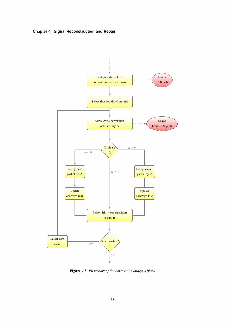
Chapter 4. Signal Reconstruction and Repair
Sort partials by their
in-band normalized power
Power
of Signals
Select first couple of partials
Apply cross-correlation,
obtain delay ∆
Delays
between Signals
Evaluate
∆
Delay first
partial by ∆
Delay second
partial by ∆
Update
coverage map
Update
coverage map
Policy-driven superposition
of partials
Other partials?Select next
partial
∆ < 0
∆ > 0
∆ = 0
yes
no
Figure 4.3: Flowchart of the correlation analysis block
38
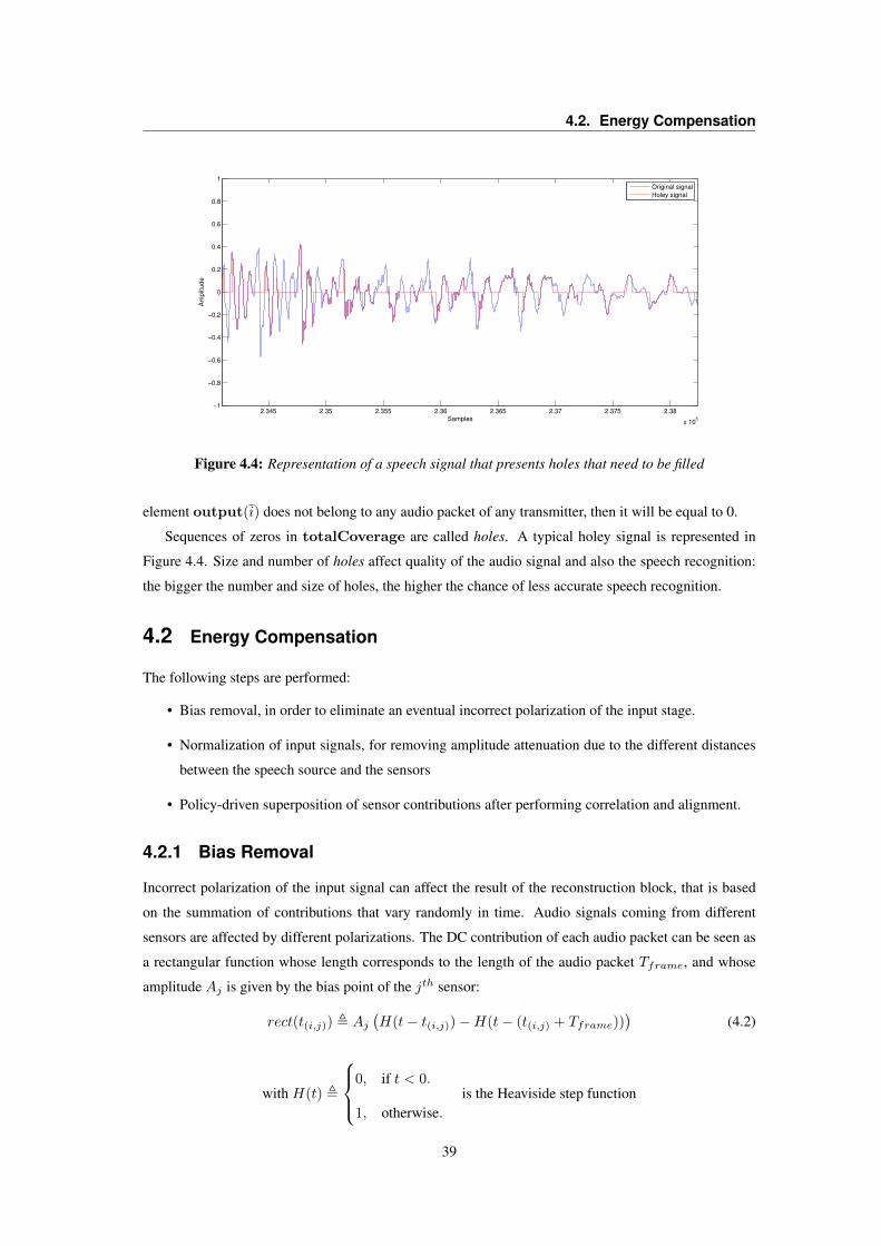
4.2. Energy Compensation
2.345 2.35 2.355 2.36 2.365 2.37 2.375 2.38
x 105
−1
−0.8
−0.6
−0.4
−0.2
0
0.2
0.4
0.6
0.8
1
Samples
Am
plit
ud
e
Original signal
Holey signal
Figure 4.4: Representation of a speech signal that presents holes that need to be filled
element output(i) does not belong to any audio packet of any transmitter, then it will be equal to 0.
Sequences of zeros in totalCoverage are called holes. A typical holey signal is represented in
Figure 4.4. Size and number of holes affect quality of the audio signal and also the speech recognition:
the bigger the number and size of holes, the higher the chance of less accurate speech recognition.
4.2 Energy Compensation
The following steps are performed:
• Bias removal, in order to eliminate an eventual incorrect polarization of the input stage.
• Normalization of input signals, for removing amplitude attenuation due to the different distances
between the speech source and the sensors
• Policy-driven superposition of sensor contributions after performing correlation and alignment.
4.2.1 Bias Removal
Incorrect polarization of the input signal can affect the result of the reconstruction block, that is based
on the summation of contributions that vary randomly in time. Audio signals coming from different
sensors are affected by different polarizations. The DC contribution of each audio packet can be seen as
a rectangular function whose length corresponds to the length of the audio packet Tframe, and whose
amplitude Aj is given by the bias point of the jth sensor:
rect(t(i,j)) , Aj(H(t− t(i,j))−H(t− (t(i,j) + Tframe))
)(4.2)
with H(t) ,
0, if t < 0.
1, otherwise.is the Heaviside step function
39
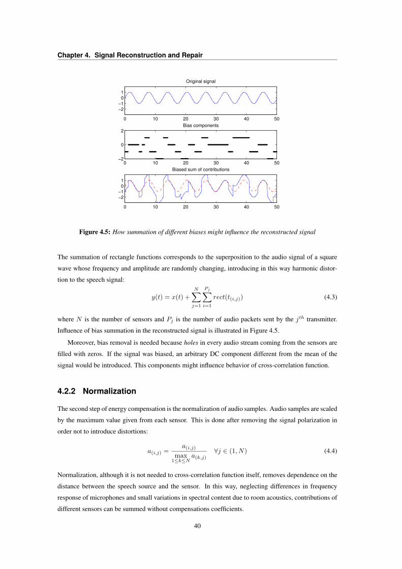
Chapter 4. Signal Reconstruction and Repair
0 10 20 30 40 50
−2
−1
0
1
Original signal
0 10 20 30 40 50−2
0
2Bias components
0 10 20 30 40 50
−2
−1
0
1
Biased sum of contributions
Figure 4.5: How summation of different biases might influence the reconstructed signal
The summation of rectangle functions corresponds to the superposition to the audio signal of a square
wave whose frequency and amplitude are randomly changing, introducing in this way harmonic distor-
tion to the speech signal:
y(t) = x(t) +
N∑j=1
Pj∑i=1
rect(t(i,j)) (4.3)
where N is the number of sensors and Pj is the number of audio packets sent by the jth transmitter.
Influence of bias summation in the reconstructed signal is illustrated in Figure 4.5.
Moreover, bias removal is needed because holes in every audio stream coming from the sensors are
filled with zeros. If the signal was biased, an arbitrary DC component different from the mean of the
signal would be introduced. This components might influence behavior of cross-correlation function.
4.2.2 Normalization
The second step of energy compensation is the normalization of audio samples. Audio samples are scaled
by the maximum value given from each sensor. This is done after removing the signal polarization in
order not to introduce distortions:
a(i,j) =a(i,j)
max1≤k≤N
a(k,j)∀j ∈ (1, N) (4.4)
Normalization, although it is not needed to cross-correlation function itself, removes dependence on the
distance between the speech source and the sensor. In this way, neglecting differences in frequency
response of microphones and small variations in spectral content due to room acoustics, contributions of
different sensors can be summed without compensations coefficients.
40
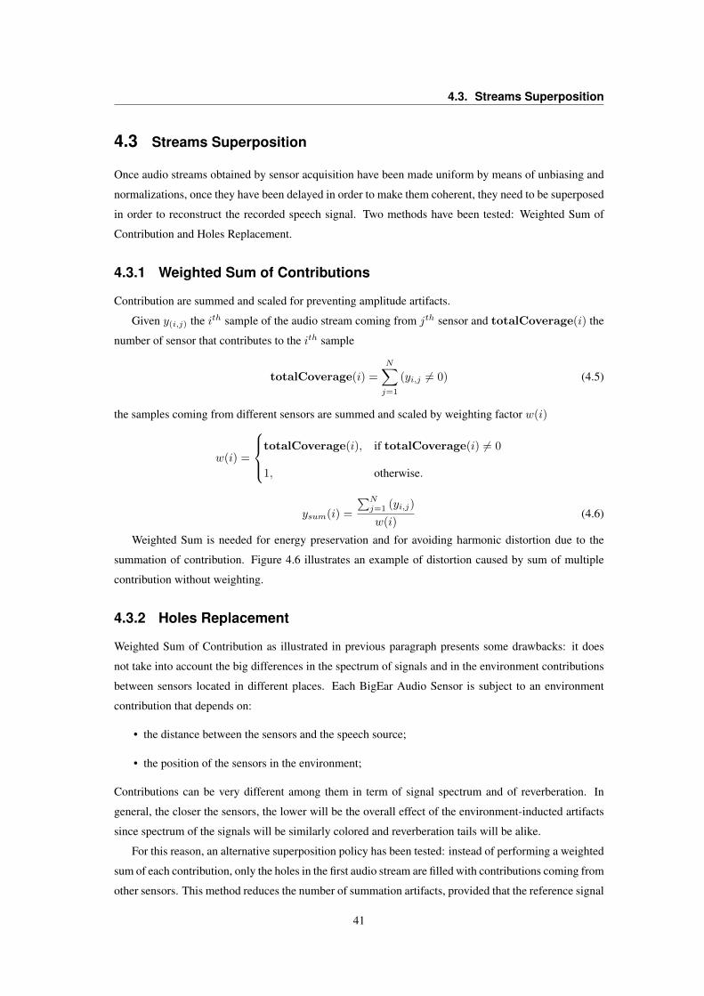
4.3. Streams Superposition
4.3 Streams Superposition
Once audio streams obtained by sensor acquisition have been made uniform by means of unbiasing and
normalizations, once they have been delayed in order to make them coherent, they need to be superposed
in order to reconstruct the recorded speech signal. Two methods have been tested: Weighted Sum of
Contribution and Holes Replacement.
4.3.1 Weighted Sum of Contributions
Contribution are summed and scaled for preventing amplitude artifacts.
Given y(i,j) the ith sample of the audio stream coming from jth sensor and totalCoverage(i) the
number of sensor that contributes to the ith sample
totalCoverage(i) =
N∑j=1
(yi,j 6= 0) (4.5)
the samples coming from different sensors are summed and scaled by weighting factor w(i)
w(i) =
totalCoverage(i), if totalCoverage(i) 6= 0
1, otherwise.
ysum(i) =
∑Nj=1 (yi,j)
w(i)(4.6)
Weighted Sum is needed for energy preservation and for avoiding harmonic distortion due to the
summation of contribution. Figure 4.6 illustrates an example of distortion caused by sum of multiple
contribution without weighting.
4.3.2 Holes Replacement
Weighted Sum of Contribution as illustrated in previous paragraph presents some drawbacks: it does
not take into account the big differences in the spectrum of signals and in the environment contributions
between sensors located in different places. Each BigEar Audio Sensor is subject to an environment
contribution that depends on:
• the distance between the sensors and the speech source;
• the position of the sensors in the environment;
Contributions can be very different among them in term of signal spectrum and of reverberation. In
general, the closer the sensors, the lower will be the overall effect of the environment-inducted artifacts
since spectrum of the signals will be similarly colored and reverberation tails will be alike.
For this reason, an alternative superposition policy has been tested: instead of performing a weighted
sum of each contribution, only the holes in the first audio stream are filled with contributions coming from
other sensors. This method reduces the number of summation artifacts, provided that the reference signal
41
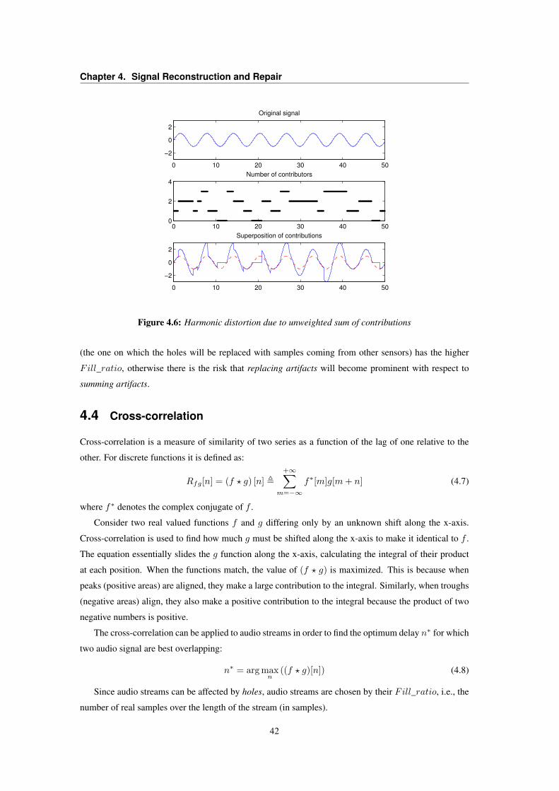
Chapter 4. Signal Reconstruction and Repair
0 10 20 30 40 50
−2
0
2
Original signal
0 10 20 30 40 500
2
4Number of contributors
0 10 20 30 40 50
−2
0
2
Superposition of contributions
Figure 4.6: Harmonic distortion due to unweighted sum of contributions
(the one on which the holes will be replaced with samples coming from other sensors) has the higher
Fill_ratio, otherwise there is the risk that replacing artifacts will become prominent with respect to
summing artifacts.
4.4 Cross-correlation
Cross-correlation is a measure of similarity of two series as a function of the lag of one relative to the
other. For discrete functions it is defined as:
Rfg[n] = (f ? g) [n] ,+∞∑
m=−∞f∗[m]g[m+ n] (4.7)
where f∗ denotes the complex conjugate of f .
Consider two real valued functions f and g differing only by an unknown shift along the x-axis.
Cross-correlation is used to find how much g must be shifted along the x-axis to make it identical to f .
The equation essentially slides the g function along the x-axis, calculating the integral of their product
at each position. When the functions match, the value of (f ? g) is maximized. This is because when
peaks (positive areas) are aligned, they make a large contribution to the integral. Similarly, when troughs
(negative areas) align, they also make a positive contribution to the integral because the product of two
negative numbers is positive.
The cross-correlation can be applied to audio streams in order to find the optimum delay n∗ for which
two audio signal are best overlapping:
n∗ = arg maxn
((f ? g)[n]) (4.8)
Since audio streams can be affected by holes, audio streams are chosen by their Fill_ratio, i.e., the
number of real samples over the length of the stream (in samples).
42
4.4. Cross-correlation
The MATLAB function [r, lags] = xcorr (x, y) takes in input two sequences x and y,
slides y along the x-axis and calculate the summation of x*y ad each position. The function returns
two vectors: r, that contains cross-correlation results, and lags, that contains the lags at which the
correlations are computed. So, the delay that maximize correlation can be found at lags(i), where i
denotes the position at which r is maximum.
A negative delay implies that the second stream has to be anticipated, a positive delay states that the
second stream has to be delayed, and a zero value delay is returned when two streams are already aligned.
4.4.1 Cross-correlation Drawbacks
A first drawback of cross-correlation function is that it has to operate on superposable audio segments
since it works on signals’ similarity. If audio segments are not superposables, the result stream will be
incoherent since cross-correlation suggest the best way to superpose them.
The second drawback is represented by the inability of the cross-correlation function in discrimi-
nating between the true signal and noise or holes. Cross-correlation function operates on signals that,
for their origin, are noisy and holey. If holes and noise are negligibles, cross-correlation gives expected
results. Conversely, e.g., if holes are much bigger than the signal itself, cross-correlation will produce
wrong results since it returns the delay value for which the holes will be at their best superposed. There-
fore it is needed to analyze the behavior of cross-correlation in function of size and number of holes in
the input signals. The test procedure has been performed in the following way:
1. Load an audio file x
2. Select a fixed ∆ delay (in samples)
• Test correlation by changing dimension of holes
1. Set a fixed τ average time distance between holes
2. Determine number of holes N = b(length(x)/τ · Fs − 1)e
3. Set M = maximum size of holes
4. Create two copies of the original stream; delay by ∆ the second copy
5. Hole the two signals with N holes randomly spaced over all the length of the signals. Each
ith hole has size di ∼ U([0,M ])
6. Apply cross-correlation function Rfg[n] = (f ? g) [n] ,∑+∞m=−∞ f∗[m]g[m+ n]
7. ∆m = arg maxn ((f ? g)[n])
8. Plot the difference |∆ − ∆m|, where ∆m is the measured delay that maximizes cross-
correlation between the two signals.
9. Increase M
10. Repeat steps 4 to 9.
43
Chapter 4. Signal Reconstruction and Repair
• Test correlation by changing number of holes
1. Set fixed d = size of holes
2. Set τ average time distance between holes
3. Determine number of holes N = b(length(x)/τ · Fs − 1)e
4. Create two copies of the original stream; delay by ∆ the second copy
5. Hole the two signals with N holes randomly spaced over all the length of the signals. Each
holes has fixed d size.
6. Apply cross-correlation function Rfg[n] = (f ? g) [n] ,∑+∞m=−∞ f∗[m]g[m+ n]
7. ∆m = arg maxn ((f ? g)[n])
8. Plot the difference |∆ − ∆m|, where ∆m is the measured delay that maximizes cross-
correlation between the two signals.
9. Decrease τ
10. Repeat steps 3 to 9.
Figure 4.7 plots the results of the convergence test. It can be noted that cross-correlation function
works correctly for
di|τ=3 ms ≤ 6.5 ms since di ∼ U([0,M ]) and M |τ=3 ms ≤ 13 ms
and
τ |M=12 ms =length of the stream [seconds]
number of holes≥ 4 ms
where di|τ=3 ms is the average size of the holes evaluated with constant average time distance between
holes τ = 3 ms, and τ |M=12 ms is the average time distance between holes evaluated with holes whose
size is constant within the uniform range [0, 12 ms].
The values described above, as it can be seen in Chapter 6, are evaluated at borderline system condi-
tions, so the cross-correlation convergence is reached.
4.4.2 Envelopes Cross-correlation
As illustrated in Section 4.4.1, if sequence of zeros (holes) are much bigger than the signal itself, or if
the signal is subject to particular type of noises such as impulse trains, the Cross-correlation function
would produce wrong results. To overcome this problem, instead of applying Cross-correlation function
directly on noisy or holey signals, it has been applied to the positive envelopes of the signals themselves.
A positive envelope is a particular representation of a signal that evidences the shape of the signal. It
is obtained with these steps:
1. Generate a copy of the original signal whose negative samples are truncated at 0;
2. Filter the signal with a Low-pass filter having very low cutoff frequency.
44
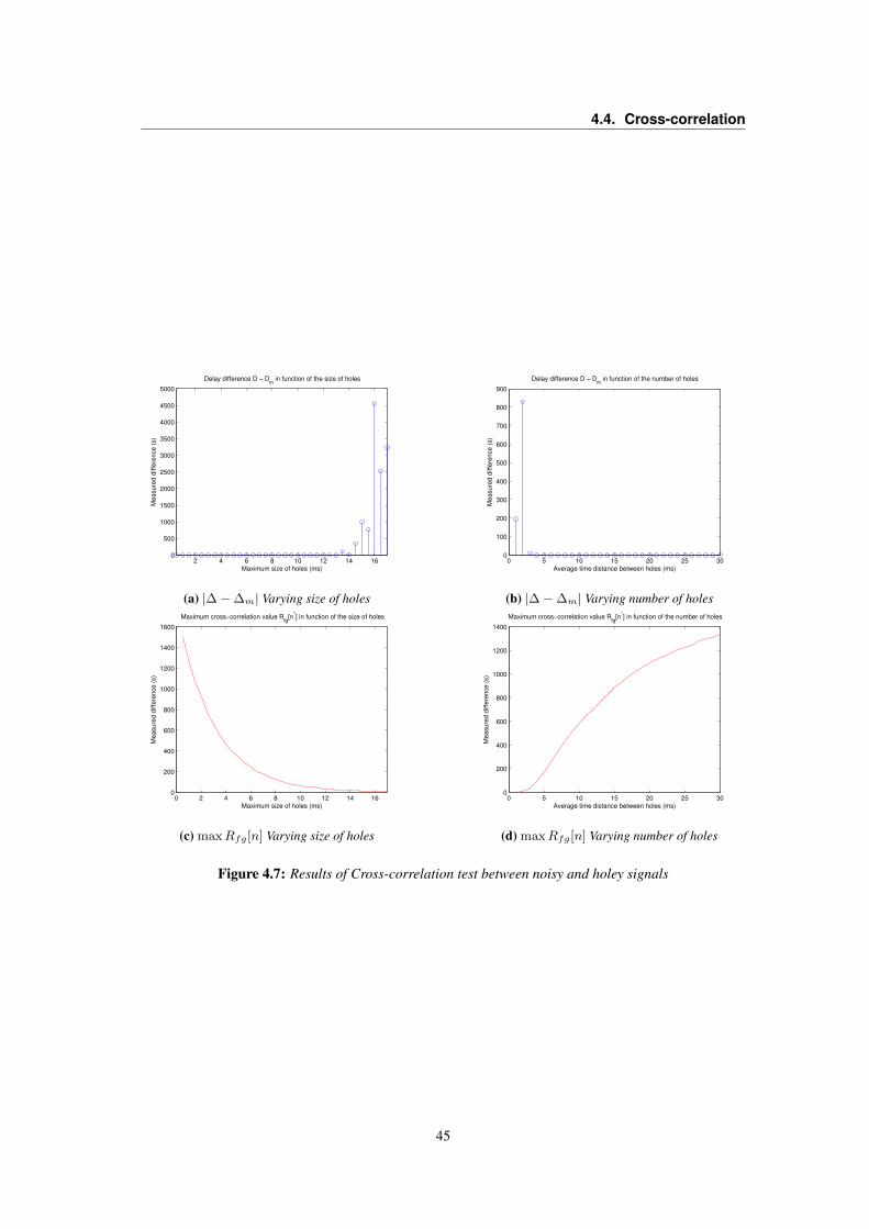
4.4. Cross-correlation
2 4 6 8 10 12 14 160
500
1000
1500
2000
2500
3000
3500
4000
4500
5000
Delay difference D − Dm
in function of the size of holes
Maximum size of holes (ms)
Me
asu
red
diffe
ren
ce
(s)
(a) |∆−∆m| Varying size of holes
0 5 10 15 20 25 300
100
200
300
400
500
600
700
800
900
Delay difference D − Dm
in function of the number of holes
Average time distance between holes (ms)
Me
asu
red
diffe
ren
ce
(s)
(b) |∆−∆m| Varying number of holes
0 2 4 6 8 10 12 14 160
200
400
600
800
1000
1200
1400
1600
Maximum cross−correlation value Rfg
[n*] in function of the size of holes
Maximum size of holes (ms)
Me
asu
red
diffe
ren
ce
(s)
(c) maxRfg[n] Varying size of holes
0 5 10 15 20 25 300
200
400
600
800
1000
1200
1400
Maximum cross−correlation value Rfg
[n*] in function of the number of holes
Average time distance between holes (ms)
Me
asu
red
diffe
ren
ce
(s)
(d) maxRfg[n] Varying number of holes
Figure 4.7: Results of Cross-correlation test between noisy and holey signals
45
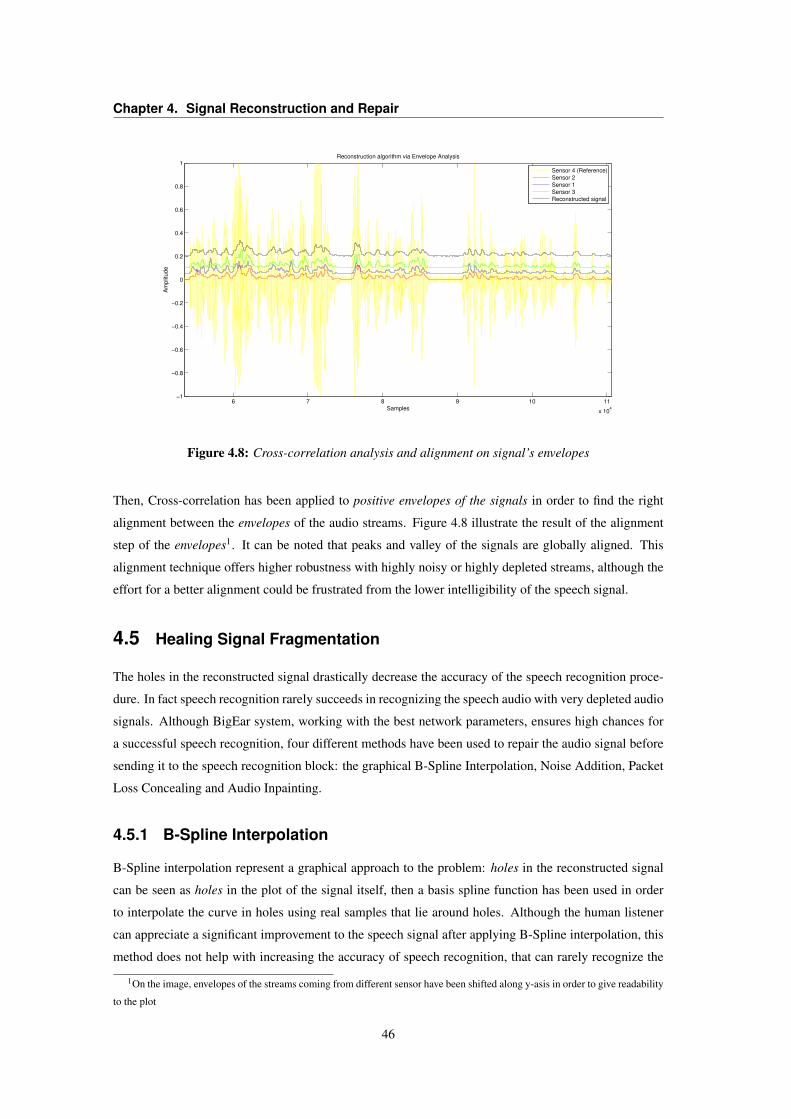
Chapter 4. Signal Reconstruction and Repair
6 7 8 9 10 11
x 104
−1
−0.8
−0.6
−0.4
−0.2
0
0.2
0.4
0.6
0.8
1
Samples
Am
plit
ude
Reconstruction algorithm via Envelope Analysis
Sensor 4 (Reference)
Sensor 2
Sensor 1
Sensor 3
Reconstructed signal
Figure 4.8: Cross-correlation analysis and alignment on signal’s envelopes
Then, Cross-correlation has been applied to positive envelopes of the signals in order to find the right
alignment between the envelopes of the audio streams. Figure 4.8 illustrate the result of the alignment
step of the envelopes1. It can be noted that peaks and valley of the signals are globally aligned. This
alignment technique offers higher robustness with highly noisy or highly depleted streams, although the
effort for a better alignment could be frustrated from the lower intelligibility of the speech signal.
4.5 Healing Signal Fragmentation
The holes in the reconstructed signal drastically decrease the accuracy of the speech recognition proce-
dure. In fact speech recognition rarely succeeds in recognizing the speech audio with very depleted audio
signals. Although BigEar system, working with the best network parameters, ensures high chances for
a successful speech recognition, four different methods have been used to repair the audio signal before
sending it to the speech recognition block: the graphical B-Spline Interpolation, Noise Addition, Packet
Loss Concealing and Audio Inpainting.
4.5.1 B-Spline Interpolation
B-Spline interpolation represent a graphical approach to the problem: holes in the reconstructed signal
can be seen as holes in the plot of the signal itself, then a basis spline function has been used in order
to interpolate the curve in holes using real samples that lie around holes. Although the human listener
can appreciate a significant improvement to the speech signal after applying B-Spline interpolation, this
method does not help with increasing the accuracy of speech recognition, that can rarely recognize the
1On the image, envelopes of the streams coming from different sensor have been shifted along y-asis in order to give readability
to the plot
46
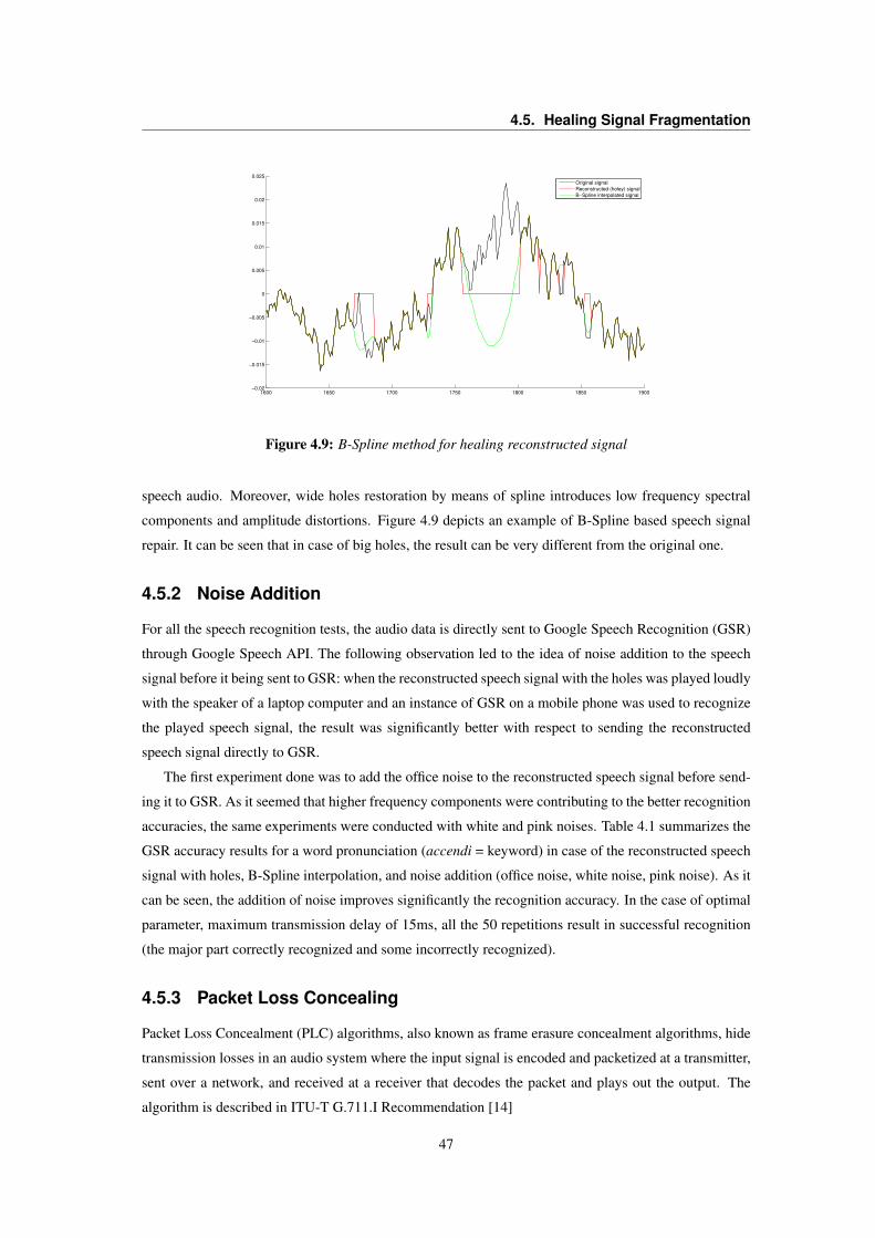
4.5. Healing Signal Fragmentation
1600 1650 1700 1750 1800 1850 1900−0.02
−0.015
−0.01
−0.005
0
0.005
0.01
0.015
0.02
0.025
Original signal
Reconstructed (holey) signal
B−Spline interpolated signal
Figure 4.9: B-Spline method for healing reconstructed signal
speech audio. Moreover, wide holes restoration by means of spline introduces low frequency spectral
components and amplitude distortions. Figure 4.9 depicts an example of B-Spline based speech signal
repair. It can be seen that in case of big holes, the result can be very different from the original one.
4.5.2 Noise Addition
For all the speech recognition tests, the audio data is directly sent to Google Speech Recognition (GSR)
through Google Speech API. The following observation led to the idea of noise addition to the speech
signal before it being sent to GSR: when the reconstructed speech signal with the holes was played loudly
with the speaker of a laptop computer and an instance of GSR on a mobile phone was used to recognize
the played speech signal, the result was significantly better with respect to sending the reconstructed
speech signal directly to GSR.
The first experiment done was to add the office noise to the reconstructed speech signal before send-
ing it to GSR. As it seemed that higher frequency components were contributing to the better recognition
accuracies, the same experiments were conducted with white and pink noises. Table 4.1 summarizes the
GSR accuracy results for a word pronunciation (accendi = keyword) in case of the reconstructed speech
signal with holes, B-Spline interpolation, and noise addition (office noise, white noise, pink noise). As it
can be seen, the addition of noise improves significantly the recognition accuracy. In the case of optimal
parameter, maximum transmission delay of 15ms, all the 50 repetitions result in successful recognition
(the major part correctly recognized and some incorrectly recognized).
4.5.3 Packet Loss Concealing
Packet Loss Concealment (PLC) algorithms, also known as frame erasure concealment algorithms, hide
transmission losses in an audio system where the input signal is encoded and packetized at a transmitter,
sent over a network, and received at a receiver that decodes the packet and plays out the output. The
algorithm is described in ITU-T G.711.I Recommendation [14]
47
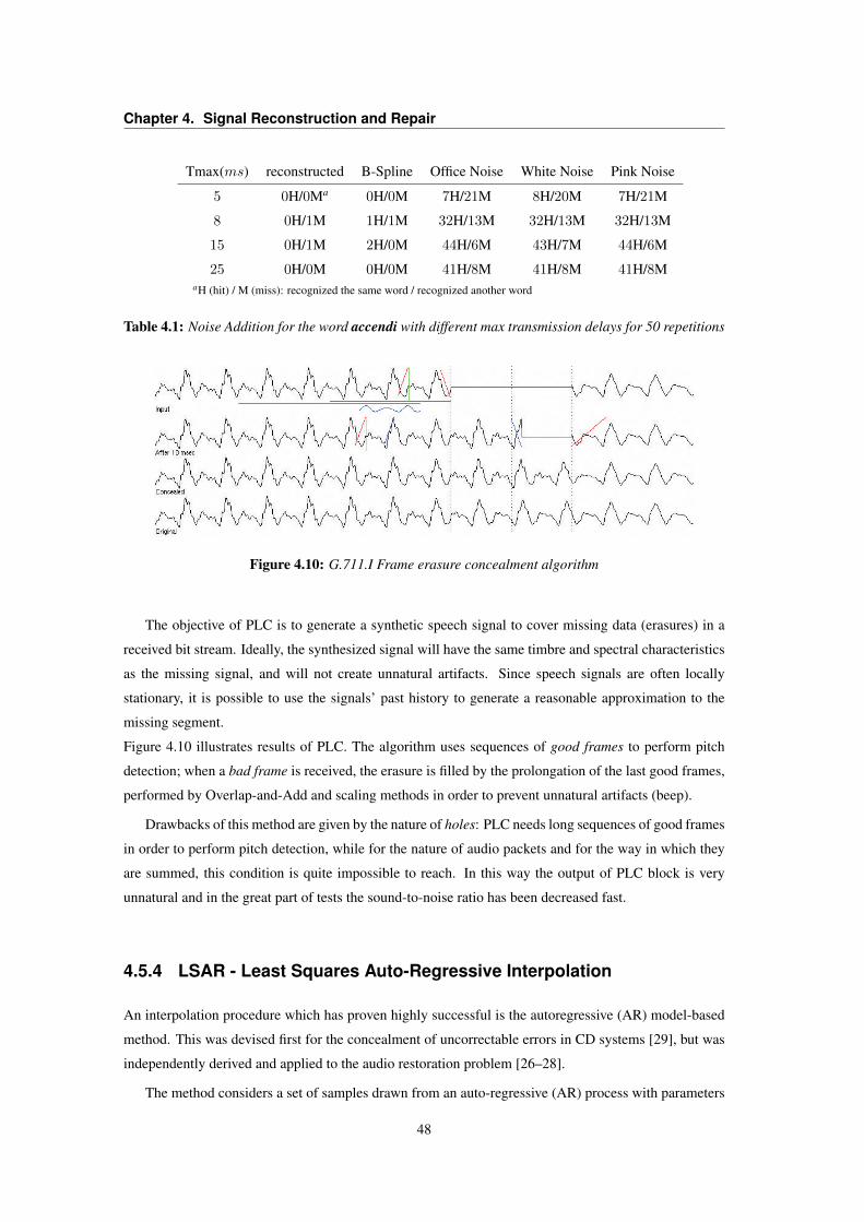
Chapter 4. Signal Reconstruction and Repair
Tmax(ms) reconstructed B-Spline Office Noise White Noise Pink Noise
5 0H/0Ma 0H/0M 7H/21M 8H/20M 7H/21M
8 0H/1M 1H/1M 32H/13M 32H/13M 32H/13M
15 0H/1M 2H/0M 44H/6M 43H/7M 44H/6M
25 0H/0M 0H/0M 41H/8M 41H/8M 41H/8MaH (hit) / M (miss): recognized the same word / recognized another word
Table 4.1: Noise Addition for the word accendi with different max transmission delays for 50 repetitions
Figure 4.10: G.711.I Frame erasure concealment algorithm
The objective of PLC is to generate a synthetic speech signal to cover missing data (erasures) in a
received bit stream. Ideally, the synthesized signal will have the same timbre and spectral characteristics
as the missing signal, and will not create unnatural artifacts. Since speech signals are often locally
stationary, it is possible to use the signals’ past history to generate a reasonable approximation to the
missing segment.
Figure 4.10 illustrates results of PLC. The algorithm uses sequences of good frames to perform pitch
detection; when a bad frame is received, the erasure is filled by the prolongation of the last good frames,
performed by Overlap-and-Add and scaling methods in order to prevent unnatural artifacts (beep).
Drawbacks of this method are given by the nature of holes: PLC needs long sequences of good frames
in order to perform pitch detection, while for the nature of audio packets and for the way in which they
are summed, this condition is quite impossible to reach. In this way the output of PLC block is very
unnatural and in the great part of tests the sound-to-noise ratio has been decreased fast.
4.5.4 LSAR - Least Squares Auto-Regressive Interpolation
An interpolation procedure which has proven highly successful is the autoregressive (AR) model-based
method. This was devised first for the concealment of uncorrectable errors in CD systems [29], but was
independently derived and applied to the audio restoration problem [26–28].
The method considers a set of samples drawn from an auto-regressive (AR) process with parameters
48
4.5. Healing Signal Fragmentation
a. Excitation vector e can be written in terms of the data vector:
e = Ax
= A(U x(i) + K x−(i))
= A(i)x(i) + A−(i)x−(i)
where x has been re-expressed in terms of its partitions: x(i) is the column-wise partition of uncorrupted
samples of the audio signal - taken from both sides around the corrupt segment, and x−(i) is the column-
wise partition of corrupted samples of the audio signal.
Thus, the estimated unknown audio partition can be obtaind by minimizing the cost function E with
respect to the unknown vector x−(i):
E =
N∑n=P+1
e2n = eTe
The least squares (LS) interpolator is now obtained as the interpolated data vector x(i) which mini-
mizes the sum squared prediction error E, since E can be regarded as a measure of the goodness of ‘fit’
of the data to the AR model. In other words, the solution is found as that unknown data vector x(i) which
minimizes E:
xLS(i) = arg minx(i)E
that can be solved for x(i), obtaining [10]:
xLS(i) = −(AT
(i)A(i)
)−1AT
(i)A−(i)x(i)
This solution for the missing data involves solution of a set of l linear equations, where l is the number
of missing samples in the block. Although the approximation is accurate even in bad audio conditions,
speed of processing does not allow a real-time usage.
4.5.5 Audio inpainting
Inpainting is the process of reconstructing lost or deteriorated parts of images, videos or sounds [23].
Inpainting is rooted in the restoration of images. Traditionally, inpainting has been done by professional
restorers. The underlying methodology of their work is as follows:
• The global picture determines how to fill in the gap. The purpose of inpainting is to restore the
unity of the work.
• The structure of the gap surroundings is supposed to be continued into the gap. Contour lines that
arrive at the gap boundary are prolonged into the gap.
• The different regions inside a gap, as defined by the contour lines, are filled with colors matching
for those of its boundary.
• The small details are painted, i.e. “texture” is added.
49
Chapter 4. Signal Reconstruction and Repair
This method can be migrated in the sound world using different kinds of analysis such as the evolu-
tion of the spectrum in time or the analysis of formants edges.
UNLocBoX toolbox
The UNLocBoX [18] is a toolbox designed to solve convex optimization problems of the form
minx∈R
f1(x) + f2(x) (4.9)
where the fi are lower semi-continuous convex functions from RN to (−∞,+∞]. When both f1 and
f2 are smooth functions, gradient descent methods can be used to solve 4.9; however, gradient descent
methods cannot be used to solve 4.9 when f1 and/or f2 are not smooth. In order to solve such problems
more generally, in the toolbox several algorithms are implemented, falling into the class of proximal
splitting algorithms.
The term proximal refers to their use of proximity operators, which are generalizations of convex
projection operators. The proximity operator of a lower semi-continuous convex function f : RN → R
is defined by
proxf (x) , arg miny∈R
1
2‖x− y‖22 + f(y)
. (4.10)
Note that the minimization problem in 4.10 has a unique solution for every x ∈ RN , so proxf : RN →RN is well-defined. The proximity operator is a useful tool because x∗ is a minimizer in 4.9 if and only
if for any γ > 0,
x∗ = proxγ(f1+f2)(x∗). (4.11)
The term splitting refers to the fact that the proximal splitting algorithms do not directly evaluate
the proximity operator proxγ(f1+f2)(x), but rather try to find a solution to 4.11 through sequences of
computations involving the proximity operators proxγf1(x) and proxγf2(x) separately.
In order to test the toolbox, the demo MATLAB script proposed by the authors has been modified
in order to load BigEar data; then, the script tries to solve the sound inpainting problem expressed as in
4.12:
arg minx‖AG∗x− b‖2 + τ‖x‖1 (4.12)
where b is the signal at the non-holey part, A an operator representing the mask selecting the non-holey
part of the signal and G∗ is the Gabor synthesis operation. Here the general assumption is that the signal
is sparse in the Gabor domain.
This is the healing method that gives best results; indeed, the accuracy of the repaired speech signals
with inpainting is the same as the original signals (see Fig. 4.11a). However, the main drawback of the
inpainting method is its time complexity that makes it inappropriate for “real-time”speech recognition
for domotic control.
4.5.6 Healing methods comparison
A comparison of healing methods has been performed. Excluding Packet Loss Concealing (Section
4.5.3) because of its strong dependence on the nature of holes, and Noise Addition since it cannot be
50
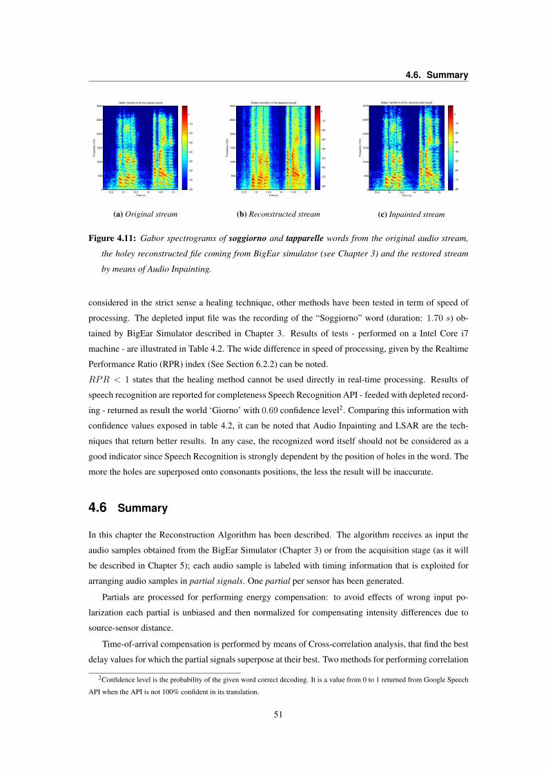
4.6. Summary
Time (s)
Fre
qu
en
cy (
Hz)
Gabor transform of the original sound
12.5 13 13.5 14 14.5 150
500
1000
1500
2000
2500
3000
−80
−70
−60
−50
−40
−30
−20
−10
0
(a) Original stream
Time (s)
Fre
qu
en
cy (
Hz)
Gabor transform of the depleted sound
12.5 13 13.5 14 14.5 150
500
1000
1500
2000
2500
3000
−80
−70
−60
−50
−40
−30
−20
−10
0
(b) Reconstructed stream
Time (s)
Fre
quency (
Hz)
Gabor transform of the reconstructed sound
12.5 13 13.5 14 14.5 150
500
1000
1500
2000
2500
3000
−80
−70
−60
−50
−40
−30
−20
−10
0
(c) Inpainted stream
Figure 4.11: Gabor spectrograms of soggiorno and tapparelle words from the original audio stream,
the holey reconstructed file coming from BigEar simulator (see Chapter 3) and the restored stream
by means of Audio Inpainting.
considered in the strict sense a healing technique, other methods have been tested in term of speed of
processing. The depleted input file was the recording of the “Soggiorno” word (duration: 1.70 s) ob-
tained by BigEar Simulator described in Chapter 3. Results of tests - performed on a Intel Core i7
machine - are illustrated in Table 4.2. The wide difference in speed of processing, given by the Realtime
Performance Ratio (RPR) index (See Section 6.2.2) can be noted.
RPR < 1 states that the healing method cannot be used directly in real-time processing. Results of
speech recognition are reported for completeness Speech Recognition API - feeded with depleted record-
ing - returned as result the world ‘Giorno’ with 0.69 confidence level2. Comparing this information with
confidence values exposed in table 4.2, it can be noted that Audio Inpainting and LSAR are the tech-
niques that return better results. In any case, the recognized word itself should not be considered as a
good indicator since Speech Recognition is strongly dependent by the position of holes in the word. The
more the holes are superposed onto consonants positions, the less the result will be inaccurate.
4.6 Summary
In this chapter the Reconstruction Algorithm has been described. The algorithm receives as input the
audio samples obtained from the BigEar Simulator (Chapter 3) or from the acquisition stage (as it will
be described in Chapter 5); each audio sample is labeled with timing information that is exploited for
arranging audio samples in partial signals. One partial per sensor has been generated.
Partials are processed for performing energy compensation: to avoid effects of wrong input po-
larization each partial is unbiased and then normalized for compensating intensity differences due to
source-sensor distance.
Time-of-arrival compensation is performed by means of Cross-correlation analysis, that find the best
delay values for which the partial signals superpose at their best. Two methods for performing correlation
2Confidence level is the probability of the given word correct decoding. It is a value from 0 to 1 returned from Google Speech
API when the API is not 100% confident in its translation.
51
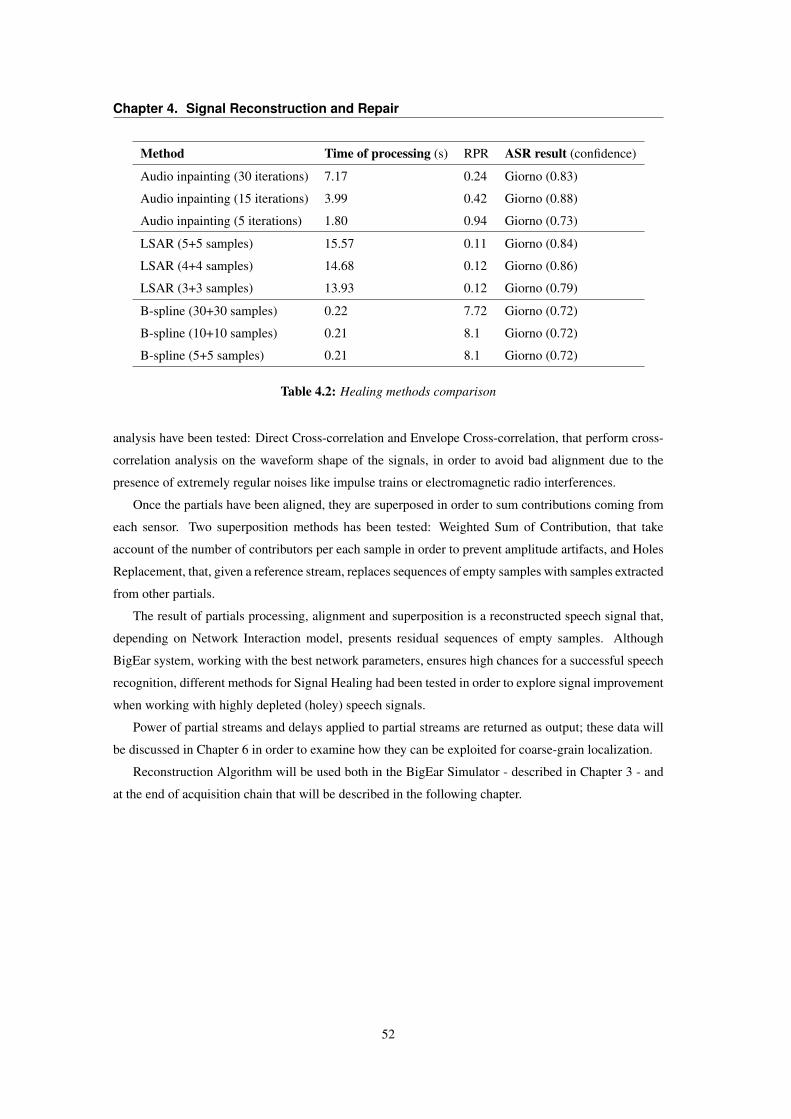
Chapter 4. Signal Reconstruction and Repair
Method Time of processing (s) RPR ASR result (confidence)
Audio inpainting (30 iterations) 7.17 0.24 Giorno (0.83)
Audio inpainting (15 iterations) 3.99 0.42 Giorno (0.88)
Audio inpainting (5 iterations) 1.80 0.94 Giorno (0.73)
LSAR (5+5 samples) 15.57 0.11 Giorno (0.84)
LSAR (4+4 samples) 14.68 0.12 Giorno (0.86)
LSAR (3+3 samples) 13.93 0.12 Giorno (0.79)
B-spline (30+30 samples) 0.22 7.72 Giorno (0.72)
B-spline (10+10 samples) 0.21 8.1 Giorno (0.72)
B-spline (5+5 samples) 0.21 8.1 Giorno (0.72)
Table 4.2: Healing methods comparison
analysis have been tested: Direct Cross-correlation and Envelope Cross-correlation, that perform cross-
correlation analysis on the waveform shape of the signals, in order to avoid bad alignment due to the
presence of extremely regular noises like impulse trains or electromagnetic radio interferences.
Once the partials have been aligned, they are superposed in order to sum contributions coming from
each sensor. Two superposition methods has been tested: Weighted Sum of Contribution, that take
account of the number of contributors per each sample in order to prevent amplitude artifacts, and Holes
Replacement, that, given a reference stream, replaces sequences of empty samples with samples extracted
from other partials.
The result of partials processing, alignment and superposition is a reconstructed speech signal that,
depending on Network Interaction model, presents residual sequences of empty samples. Although
BigEar system, working with the best network parameters, ensures high chances for a successful speech
recognition, different methods for Signal Healing had been tested in order to explore signal improvement
when working with highly depleted (holey) speech signals.
Power of partial streams and delays applied to partial streams are returned as output; these data will
be discussed in Chapter 6 in order to examine how they can be exploited for coarse-grain localization.
Reconstruction Algorithm will be used both in the BigEar Simulator - described in Chapter 3 - and
at the end of acquisition chain that will be described in the following chapter.
52
5BigEar Implementation
Introduction
In this chapter the implementation of the system is described. In the first section the hardware implemen-
tation is illustrated, whose prominent part is the represented by audio interface design. This part focuses
on physical aspects of the signal that it is needed to be acquired and on interface constraints between the
signal conditioning stage and the MCU. In the second part of the chapter, the application logic will be
described starting from leaves of the system, represented by the audio sensors, and arriving to the Base
Station that deals with data collection and audio reconstruction.
5.1 Overview
As already mentioned in Chapter 2, the system is composed of a set of audio sensors that perform a space-
time sampling of a room. Before sampling, the audio signal converted by each microphone capsule has to
be amplified and biased in order to match to ADC characteristics. Each audio sensor samples the signal
and packs data into frames in order to send them to the receiver. The multi-buffer internal structure of
each transmitter allows an efficient application logic in which the sampling stage is managed by means of
a timer-handled interrupt routine, and the network logic is handled by the main loop of the applications.
Network structure can be layered onto several radio channels in order to reduce the number of collision.
A separate BigEar Receiver is needed for each radio channel.
Once the packets arrive to the BigEar receiver, they are converted in hexadecimal nibbles and serially
sent to the Base Station by means of the USB port. The Base Station, in its experimental form, is
composed of an acquisition application that listens to each BigEar Receiver connected to the USB ports
of the machine and stores data into a local raw data file. When the acquisition stage is stopped by the
user, raw data are converted into CSV format in order to feed a MATLAB script that reconstructs the
audio data by means of the reconstruction method described in Chapter 4.
53
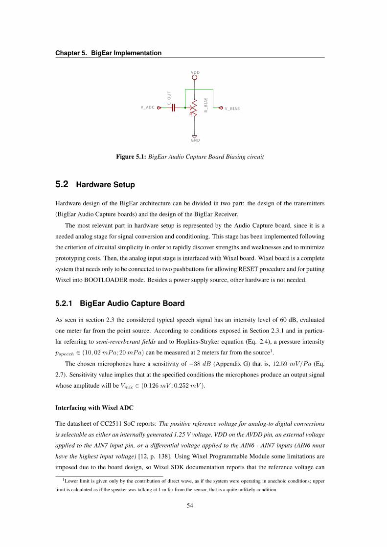
Chapter 5. BigEar Implementation
VDD
GND
R_BIAS
V_ADC V_BIAS
C_OUT
Figure 5.1: BigEar Audio Capture Board Biasing circuit
5.2 Hardware Setup
Hardware design of the BigEar architecture can be divided in two part: the design of the transmitters
(BigEar Audio Capture boards) and the design of the BigEar Receiver.
The most relevant part in hardware setup is represented by the Audio Capture board, since it is a
needed analog stage for signal conversion and conditioning. This stage has been implemented following
the criterion of circuital simplicity in order to rapidly discover strengths and weaknesses and to minimize
prototyping costs. Then, the analog input stage is interfaced with Wixel board. Wixel board is a complete
system that needs only to be connected to two pushbuttons for allowing RESET procedure and for putting
Wixel into BOOTLOADER mode. Besides a power supply source, other hardware is not needed.
5.2.1 BigEar Audio Capture Board
As seen in section 2.3 the considered typical speech signal has an intensity level of 60 dB, evaluated
one meter far from the point source. According to conditions exposed in Section 2.3.1 and in particu-
lar referring to semi-reverberant fields and to Hopkins-Stryker equation (Eq. 2.4), a pressure intensity
pspeech ∈ (10, 02 mPa; 20 mPa) can be measured at 2 meters far from the source1.
The chosen microphones have a sensitivity of −38 dB (Appendix G) that is, 12.59 mV/Pa (Eq.
2.7). Sensitivity value implies that at the specified conditions the microphones produce an output signal
whose amplitude will be Vmic ∈ (0.126 mV ; 0.252 mV ).
Interfacing with Wixel ADC
The datasheet of CC2511 SoC reports: The positive reference voltage for analog-to digital conversions
is selectable as either an internally generated 1.25 V voltage, VDD on the AVDD pin, an external voltage
applied to the AIN7 input pin, or a differential voltage applied to the AIN6 - AIN7 inputs (AIN6 must
have the highest input voltage) [12, p. 138]. Using Wixel Programmable Module some limitations are
imposed due to the board design, so Wixel SDK documentation reports that the reference voltage can
1Lower limit is given only by the contribution of direct wave, as if the system were operating in anechoic conditions; upper
limit is calculated as if the speaker was talking at 1 m far from the sensor, that is a quite unlikely condition.
54
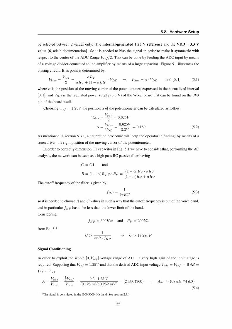
5.2. Hardware Setup
be selected between 2 values only: The internal-generated 1.25 V reference and the VDD = 3.3 V
value [6, adc.h documentation]. So it is needed to bias the signal in order to make it symmetric with
respect to the center of the ADC Range Vref/2. This can be done by feeding the ADC input by means
of a voltage divider connected to the amplifier by means of a large capacitor. Figure 5.1 illustrates the
biasing circuit. Bias point is determined by:
Vbias =Vref
2=
αRVαRV + (1− α)RV
· VDD ⇒ Vbias = α · VDD α ∈ [0, 1] (5.1)
where α is the position of the moving cursor of the potentiometer, expressed in the normalized interval
[0, 1], and VDD is the regulated power supply (3.3 V) of the Wixel board that can be found on the 3V3
pin of the board itself.
Choosing vref = 1.25V the position α of the potentiometer can be calculated as follow:
Vbias =Vref
2= 0.625V
α =VbiasVDD
=0.625V
3.3V= 0.189 (5.2)
As mentioned in section 5.3.1, a calibration procedure will help the operator in finding, by means of a
screwdriver, the right position of the moving cursor of the potentiometer.
In order to correctly dimension C1 capacitor in Fig. 5.1 we have to consider that, performing the AC
analysis, the network can be seen as a high pass RC passive filter having
C = C1 and
R = (1− α)RV //αRV =(1− α)RV · αRV(1− α)RV + αRV
The cutoff frequency of the filter is given by
fHP =1
2πRC(5.3)
so it is needed to choose R and C values in such a way that the cutoff frequency is out of the voice band,
and in particular fHP has to be less than the lower limit of the band.
Considering
fHP < 300Hz2 and RV = 200kΩ
from Eq. 5.3:
C >1
2πR · fHP⇒ C > 17.28nF
Signal Conditioning
In order to exploit the whole [0, Vref ] voltage range of ADC, a very high gain of the input stage is
required. Supposing that Vref = 1.25V and that the desired ADC input voltage Vadc = Vref − 6 dB =
1/2 · Vref :
A =VadcVmic
=12Vref
Vmic=
0.5 · 1.25 V
(0.126 mV ; 0.252 mV )= (2480; 4960) ⇒ AdB ≈ (68 dB; 74 dB)
(5.4)2The signal is considered in the [300 3000] Hz band. See section 2.3.1.
55
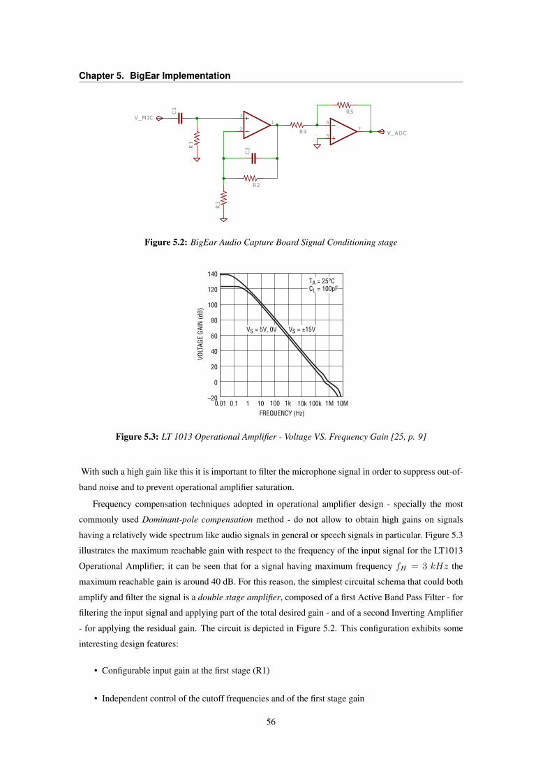
Chapter 5. BigEar Implementation
R3
R 2
C1
C2
R 5
R42
31 6
57
R1
V_M IC
V_ADC
Figure 5.2: BigEar Audio Capture Board Signal Conditioning stage
FREQUENCY (Hz)0.01 0.1
VOLT
AGE
GAIN
(dB)
1M 10M1 10 100 1k 10k 100k
140
120
100
80
60
40
20
0
–20
VS = ±15VVS = 5V, 0V
TA = 25°CCL = 100pF
Figure 5.3: LT 1013 Operational Amplifier - Voltage VS. Frequency Gain [25, p. 9]
With such a high gain like this it is important to filter the microphone signal in order to suppress out-of-
band noise and to prevent operational amplifier saturation.
Frequency compensation techniques adopted in operational amplifier design - specially the most
commonly used Dominant-pole compensation method - do not allow to obtain high gains on signals
having a relatively wide spectrum like audio signals in general or speech signals in particular. Figure 5.3
illustrates the maximum reachable gain with respect to the frequency of the input signal for the LT1013
Operational Amplifier; it can be seen that for a signal having maximum frequency fH = 3 kHz the
maximum reachable gain is around 40 dB. For this reason, the simplest circuital schema that could both
amplify and filter the signal is a double stage amplifier, composed of a first Active Band Pass Filter - for
filtering the input signal and applying part of the total desired gain - and of a second Inverting Amplifier
- for applying the residual gain. The circuit is depicted in Figure 5.2. This configuration exhibits some
interesting design features:
• Configurable input gain at the first stage (R1)
• Independent control of the cutoff frequencies and of the first stage gain
56

5.2. Hardware Setup
• Variable overall gain (replacing R5 with a variable resistor)
The parameters that drive the signal conditioning stage are:
Acb = 1 +R2
R3+R5
R4Overall gain, omitting the phase inversion due to the second stage. (5.5)
fL =1
2π R1 C1Cutoff frequency of the High Pass filter given from C1 and R1. (5.6)
fH =1
2π R2 C2Cutoff frequency of the Low Pass retroaction network C2//R2. (5.7)
According to technical specifications of the Microphone and of the Operational Amplifier chosen for the
realization of the prototype - described in Appendices G.1 and G.2 - the following design choices have
been implemented:
• Since the microphone has an Output Impedance Zout = 2.2 kΩ, thenR1 Zout, so the chosen
value for R1 is 120 kΩ.
• The first stage amplifies the microphone signal with a partial gain of about 34 dB, so the chosen
values for R2 and R3 are respectively 100 kΩ and 2.2 kΩ.
• The residual gain varies from 0 up to 40 dB and can be set by the operator by means of a variable
feedback resistor, so R4 = 1 kΩ and R5 is replaced by a series of a 1 kΩ resistor with a 100 kΩ
potentiometer.
• The first stage perform filtering at fL u 300 Hz and fH u 3 kHz; in order to reach these
cutoff frequencies the selected values are C1 = 4.7 nF and C2 = 470 pF .
• Since the whole circuit will be powered from a battery source, the input pins of the Operational
Amplifier that in Figure 5.2 are referenced to ground need to be referenced to Vcc/2 in order to
prevent the use of a dual supply.
Table 5.1 summarize the design choices and their effects on the circuit. The circuit has been tested
using PSpice - the well-known analog electronic circuit simulator - before its realization in order to
verify the frequency response of the system. Results are depicted in Figure 5.4; it can be seen that
simulation results are close to the desired behavior both in frequency response and in-band gain. Then,
the prototypes have been realized with the addition of power decoupling capacitors and the power supply
circuit for the microphone. The complete schematic and a picture of the realized prototype can be found
in Appendix E.1.
5.2.2 BigEar Receiver
The Hardware design of the BigEar Receiver is limited to a simple board that hosts the Wixel module
and connects it with two pushbuttons for allowing RESET procedure and for putting Wixel into BOOT-
LOADER mode. Since the Receiver is connected to a PC by means of a USB port, BigEar Receiver is
directly powered by means of the USB connection.
57
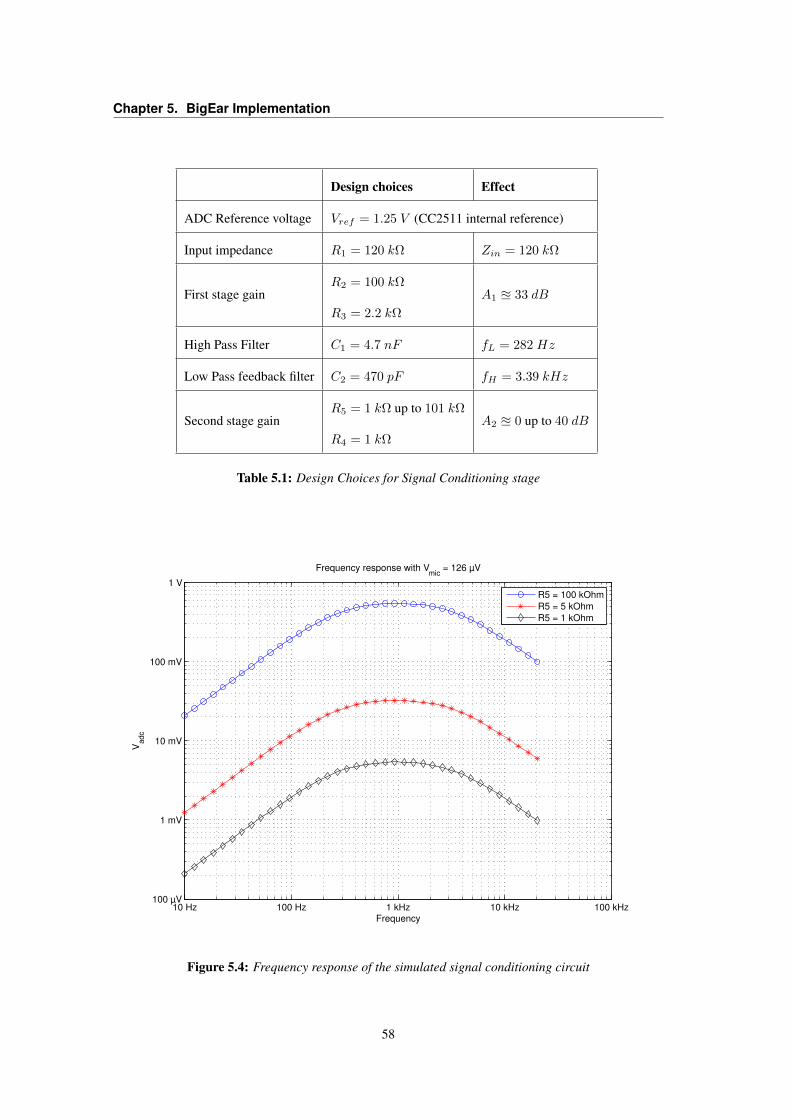
Chapter 5. BigEar Implementation
Design choices Effect
ADC Reference voltage Vref = 1.25 V (CC2511 internal reference)
Input impedance R1 = 120 kΩ Zin = 120 kΩ
First stage gainR2 = 100 kΩ
R3 = 2.2 kΩ
A1 u 33 dB
High Pass Filter C1 = 4.7 nF fL = 282 Hz
Low Pass feedback filter C2 = 470 pF fH = 3.39 kHz
Second stage gainR5 = 1 kΩ up to 101 kΩ
R4 = 1 kΩ
A2 u 0 up to 40 dB
Table 5.1: Design Choices for Signal Conditioning stage
10 Hz 100 Hz 1 kHz 10 kHz 100 kHz100 µV
1 mV
10 mV
100 mV
1 V
Frequency
Vadc
Frequency response with Vmic
= 126 µV
R5 = 100 kOhm
R5 = 5 kOhm
R5 = 1 kOhm
Figure 5.4: Frequency response of the simulated signal conditioning circuit
58
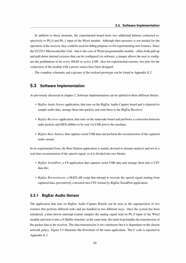
5.3. Software Implementation
In addition to these elements, the experimental board hosts two additional buttons connected re-
spectively to P0_0 and P0_1 input of the Wixel module. Although their presence is not needed for the
operation of the receiver, they could be used for debug purposes or for experimenting new features. Since
the CC2511 Microcontroller Unit - that is the core of Wixel programmable module - offers both pull-up
and pull-down internal resistors that can be configured via software, a jumper allows the user to config-
ure the pushbuttons to be active HIGH or active LOW. Also for experimental reasons, two pins for the
connection of the module with a power source have been designed.
The complete schematic and a picture of the realized prototype can be found in Appendix E.2.
5.3 Software Implementation
As previously discussed in chapter 2, Software implementation can be splitted in three different blocks:
• BigEar Audio Sensor application, that runs on the BigEar Audio Capture board and is depicted to
sample audio data, arrange them into packets and send them to the BigEar Receiver;
• BigEar Receiver application, that runs on the namesake board and performs a conversion between
radio packets and HEX nibbles to be sent via USB port to the machine;
• BigEar Base Station, that captures serial USB data and perform the reconstruction of the captured
audio stream.
In its experimental form, the Base Station application is mainly devoted to streams analysis and not to a
real-time reconstruction of the speech signal, so it is divided into two blocks:
• BigEar SerialPort, a C# application that captures serial USB data and arrange them into a CSV
data file;
• BigEar Reconstructor, a MATLAB script that attempt to recreate the speech signal starting from
captured data, preventively converted into CSV format by BigEar SerialPort application.
5.3.1 BigEar Audio Sensor
The application that runs on BigEar Audio Capture Boards can be seen as the superposition of two
routines that perform different tasks and are handled in two different ways. Once the system has been
initialized, a time-driven interrupt routine samples the analog signal read on P0_0 input of the Wixel
module and store it into a N-Buffer structure; at the same time, the main loop handles the transmission of
the packet data to the receiver. The data transmission is not continuous but it is dependent on the chosen
network policy. Figure 5.5 illustrates the flowcharts of the main application. The C code is reported in
Appendix E.3.
59
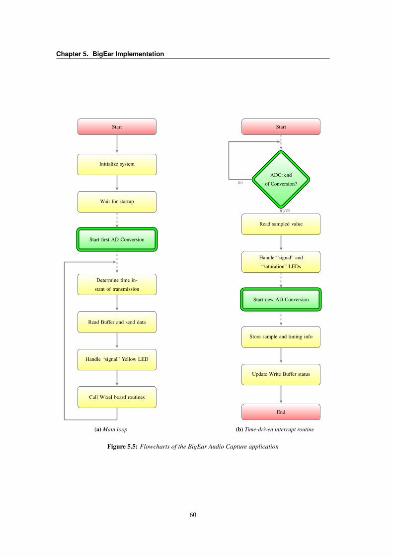
Chapter 5. BigEar Implementation
Start
Initialize system
Wait for startup
Start first AD Conversion
Determine time in-
stant of transmission
Read Buffer and send data
Handle “signal” Yellow LED
Call Wixel board routines
(a) Main loop
Start
ADC: end
of Conversion?
Read sampled value
Handle “signal” and
“saturation” LEDs
Start new AD Conversion
Store sample and timing info
Update Write Buffer status
End
yes
no
(b) Time-driven interrupt routine
Figure 5.5: Flowcharts of the BigEar Audio Capture application
60
5.3. Software Implementation
N-Buffer Data Storage
In order to efficiently store data before sending them to the receiver, audio samples are written and
arranged in frames. In paragraph Samples Processing and Transmission it will be explained that each
frame contains 20 consecutive samples, and each frame is in turn arranged into an array of 3 elements.
In this way it is possible to bufferize data without conflicts related to reading and writing simultaneously
in the same memory location. The reading index irs_index and the writing index main_index are
written respectively from the Sampling Routine and from the Main loop, so - checking that irs_index
!= main_index - it will never happen that the main loop access a frame that is empty or incomplete.
Furthermore, each frame is capable to store not only the sample value but also timing information in
order to perform a good reconstruction of the samples positions in time.
Time-driven Sampling Routine
Sampling routine needs to be called periodically with frequency fs. In order to choose fs value, Nyquist-
Shannon Theorem states that in order to prevent aliasing, sampling frequency must be higher than upper
limit of the band of the signal. Since, as illustrated in Section 4.1, one of the goals of the Signal Recon-
struction stage is to prevent holes in the reconstructed speech signal, minimizing fs means to maximize
the sample duration and then to maximize audioPackets overlapping likelihood. So the design choice is
to select fs ' 6 kHz.
Flowchart 5.5b illustrates the work of the Sampling routine that samples the P0_0 input and store
data into the buffers. The function is handled like an Interrupt Service Routine raised by the internal
T3 timer of the Microcontroller. T3 is a 8-bit timer which supports typical timer/counter functions such
as output compare and PWM functions [12, p. 126]. It consists of an 8-bit counter that increments
(or decrements) at each active clock edge. The frequency of the active clock edges is given by internal
registers CLKCON.TICKSPD and T3CTL.DIV. With the default value of CLKCON.TICKSPD (initial-
ized by the Wixel SDK libraries) and setting the prescaler T3CTL.DIV at its maximum value (128), the
frequency of each active edge is ftick = 187.5 kHz.
In order to obtain a sampling frequency fs ' 6 kHz it is needed to set the timer to work in Modulo
Mode [12, p. 127] and to set the register T3CC0 to a value N such that:
fs =ftickN
and then:
N =
⌊ftickfs
⌋=
⌊187.5 kHz
6 kHz
⌋= 31
Some empirical tests have been performed with the help of a Logical Analyzer in order to verify the
value and the stability of the sampling frequency. During this tests it has been discovered that the best
value for T3CC0 is N = 30, that gives as result a sampling frequency of fs = 6.04± 0.005 kHz.
The routine, basically, reads from the ADCH+ADCL registers the result of the AD conversion and
stores it using the already described N-Buffer structure. For each sample it is needed to know exact
the timing information in order to perform a precise in-time reconstruction of the speech signal. Wixel
61
Chapter 5. BigEar Implementation
SDK exposes the uint32 getMs() function that returns a 32-bit unsigned integer that represents the
number of milliseconds that have elapsed since the system was initialized; the time distance between
two samples sampled at fs = 6.04 kHz is 0.166 ms so the granularity of 1 millisecond is not sufficient.
In order to obtain a higher precision, in addiction to the timestamp expressed in millisecond, the value
of T4CNT register is stored. This register contains the value of the T4 counter used by the system for
incrementing the milliseconds counter. The T4 counter is programmed to operate in Modulo Mode and
to count up to 187, in such a way that each millisecond the Timer raises an Interrupt, whose Service
Routine simply increments by 1 the milliseconds counter. In this way, storing T4CNT value means
storing a fractional part of millisecond expressed as units of 1/187 ms.
Another function of the Interrupt Service Routine is to handle the yellow and the red LEDs, used as
level indicators as illustrated in Figure 5.6:
• Signal LED: When the amplitude of the sample is greater than -6 dB3, yellow LED is switched on;
• Saturation LED: When the amplitude of the sample is equal to 0 dB, red LED is switched on.
The handling of Saturation LED requires only a simple check, while the handling of Signal LED requires
to set a boolean flag that will be checked in the main loop for switching on the yellow LED. This
limitation is due to the fact that the Yellow LED shares the same GPIO pin on CC2511 MCU with
the BOOTLDR button, so it is not possible to modify the configuration of that specific pin during the
execution of an Interrupt Service Routine, otherwise Wixel will interpret the state change as a BTLDR
request.
ADC Improved Reading
Wixel SDK provides the function uint16 adcRead(uint8 channel) that perform an Analog-
to-Digital Conversion and returns the sampled value. It is a blocking function and its use within the
Interrupt Service Routine described above causes strong dependences on the speed of the CPU. Indeed,
as illustrated in table 2.2, the use of adcRead for performing a 12-bit reading will lock the application
for 128 µs; this means that working at fs = 6.04 kHz only (166 − 128) µs = 38 µs remain for data
storage, processing and transmission. To overcome this problem an unlocking method has been adopted,
exploiting the capability of ADC to perform conversions without any interaction from the CPU.
The unlocking method consists in three steps (highligted in Figure 5.5):
1. Set ADC Registers before main loop starts
2. In the Sampling routine, wait for the end of the conversion before reading sampled value
3. After saving the data, rearm ADC
Since a 12-bit conversion lasts 128 µs < 166 µs, the Sampling routine will never wait for the end of the
conversion (except for the very first AD conversion). Moreover since ADC is rearmed by a time-driven
3With respect to 0 dB as the maximum amplitude value
62

5.3. Software Implementation
0 20 40 60 80 100 120 140 160 180 200
0 dB
−6 dB
− inf
− 6 dB
0 dB
Samples
Am
plit
ud
eSignal / Saturation LED Handling Thresholds
Saturation limit
Signal threshold
Figure 5.6: Signal and Saturation LED indicators policy
routine, all of the ADC samplings will be synchronized with the same granularity and precision of T3
timer.
The use of 12-bit conversion causes a +6 dB increment the SNR Ratio with respect to the use of
10-bit conversion.
Given M the ADC resolution in bits:
vqn =Vref2M
If M = 10 and Vref = 1.25 V 4:
v10qn =1.25 V
210= 1.221 mV
SNR10 =Vrmsv10qn
Increasing ADC resolution to M = 12 and according to ADC Conversion Results limitations illustrated
in CC2511 datasheet [12, p. 139]:
v12qn =1.25 V
212/2= 0.610 mV
v12qn =1
2
(v10qn)
and so
SNR12 =Vrmsv12qn
=Vrms
12
(v10qn) = 2 · Vrms
v10qnu SNR10 + 6 dB (5.8)
4See Table 5.1.
63
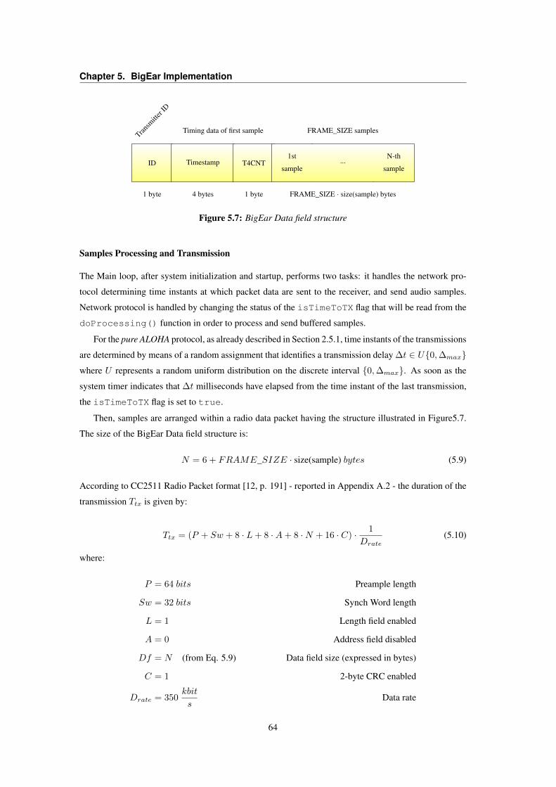
Chapter 5. BigEar Implementation
ID Timestamp T4CNT1st
sample...
N-th
sample
1 byte 4 bytes 1 byte FRAME_SIZE · size(sample) bytes
Transm
itter ID
Timing data of first sample FRAME_SIZE samples
Figure 5.7: BigEar Data field structure
Samples Processing and Transmission
The Main loop, after system initialization and startup, performs two tasks: it handles the network pro-
tocol determining time instants at which packet data are sent to the receiver, and send audio samples.
Network protocol is handled by changing the status of the isTimeToTX flag that will be read from the
doProcessing() function in order to process and send buffered samples.
For the pure ALOHA protocol, as already described in Section 2.5.1, time instants of the transmissions
are determined by means of a random assignment that identifies a transmission delay ∆t ∈ U0,∆maxwhere U represents a random uniform distribution on the discrete interval 0,∆max. As soon as the
system timer indicates that ∆t milliseconds have elapsed from the time instant of the last transmission,
the isTimeToTX flag is set to true.
Then, samples are arranged within a radio data packet having the structure illustrated in Figure5.7.
The size of the BigEar Data field structure is:
N = 6 + FRAME_SIZE · size(sample) bytes (5.9)
According to CC2511 Radio Packet format [12, p. 191] - reported in Appendix A.2 - the duration of the
transmission Ttx is given by:
Ttx = (P + Sw + 8 · L+ 8 ·A+ 8 ·N + 16 · C) · 1
Drate(5.10)
where:
P = 64 bits Preample length
Sw = 32 bits Synch Word length
L = 1 Length field enabled
A = 0 Address field disabled
Df = N (from Eq. 5.9) Data field size (expressed in bytes)
C = 1 2-byte CRC enabled
Drate = 350kbit
sData rate
64
5.3. Software Implementation
As it can be seen in the next paragraph, in order to reduce packet size and to decrease transmission
duration each 16-bit sample is compressed to an 8-bit µ-Law sample. An important design choice is to
correctly dimension FRAME_SIZE, i.e. the number of samples stored in one frame and transmitted
by means of a single transmission. The idea is to exploit the minimum granularity of 1 ms in time
handling functions in order to transmit the maximum amount of data without overstepping that value.
From Equations 5.10 and 5.9, the maximum number of samples per frame FRAME_SIZEmax can be
derived as:
FRAME_SIZEmax : Ttx ≤ 1 ms
FRAME_SIZEmax ≤⌊
1
8(Drate − 168 bits)
⌋FRAME_SIZEmax ≤ 22 (5.11)
FRAME_SIZE = 20 has been chosen in order to keep a small guard time. Indeed:
Ttx
∣∣∣∣∣∣FRAME_SIZE=20
= 0.9371 ms
µ-Law Compression and Expansion
The CC2511F32 SoC provides an industry standard I2S interface. The application exploit the capability
of the I2S interface to perform fast5 µ-Law Compressions or Expansions in order to efficiently code audio
samples.
µ-Law is an audio compression scheme (codec) defined by Consultative Committee for International
Telephony And Telegraphy (CCITT) G.711 Recommendation [13] which compress 16-bit linear PCM
data down to eight bits of logarithmic data. The compression process is logarithmic: the compression
ratio increases as the sample signals increase. In other words, the larger sample signals are compressed
more than the smaller sample signals. This causes the quantization noise to increase as the sample signal
increases. A logarithmic increase in quantization noise throughout the dynamic range of an input sample
signal keeps the SNR constant throughout this dynamic range.
Analog µ-Law compression For a given input x, the equation for µ-Law encoding is:
F (x) = sgn(x)ln(1 + µ|x|)
ln(1 + µ)− 1 ≤ x ≤ 1 (5.12)
Analog µ-Law expansion µ-Law expansion is then given by the inverse equation:
F−1(y) = sgn(y)(1/µ)((1 + µ)|y| − 1) − 1 ≤ y ≤ 1 (5.13)
The digital counterparts of the described equations are defined in ITU-T Recommendation G.711. [13]
5CC2511 I2S interface µ-Law compression and expansion take one clock cycle to perform.
65
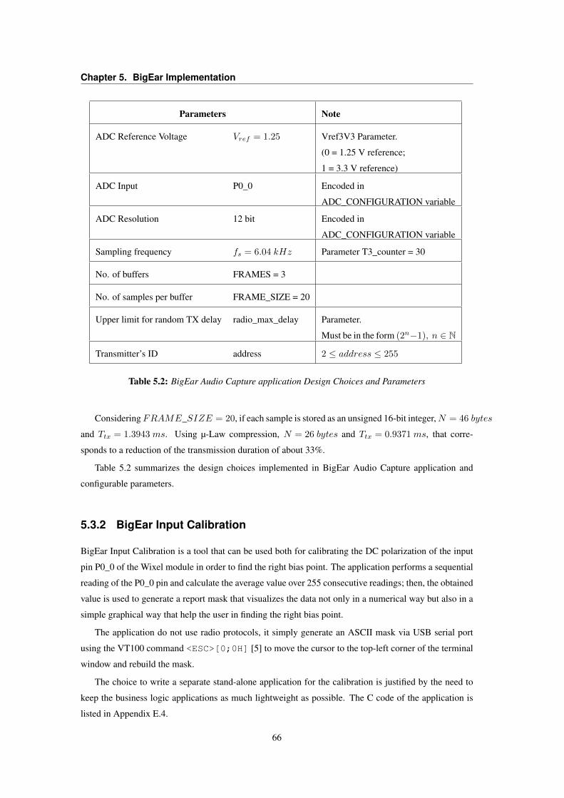
Chapter 5. BigEar Implementation
Parameters Note
ADC Reference Voltage Vref = 1.25 Vref3V3 Parameter.
(0 = 1.25 V reference;
1 = 3.3 V reference)
ADC Input P0_0 Encoded in
ADC_CONFIGURATION variable
ADC Resolution 12 bit Encoded in
ADC_CONFIGURATION variable
Sampling frequency fs = 6.04 kHz Parameter T3_counter = 30
No. of buffers FRAMES = 3
No. of samples per buffer FRAME_SIZE = 20
Upper limit for random TX delay radio_max_delay Parameter.
Must be in the form (2n−1), n ∈ N
Transmitter’s ID address 2 ≤ address ≤ 255
Table 5.2: BigEar Audio Capture application Design Choices and Parameters
ConsideringFRAME_SIZE = 20, if each sample is stored as an unsigned 16-bit integer,N = 46 bytes
and Ttx = 1.3943 ms. Using µ-Law compression, N = 26 bytes and Ttx = 0.9371 ms, that corre-
sponds to a reduction of the transmission duration of about 33%.
Table 5.2 summarizes the design choices implemented in BigEar Audio Capture application and
configurable parameters.
5.3.2 BigEar Input Calibration
BigEar Input Calibration is a tool that can be used both for calibrating the DC polarization of the input
pin P0_0 of the Wixel module in order to find the right bias point. The application performs a sequential
reading of the P0_0 pin and calculate the average value over 255 consecutive readings; then, the obtained
value is used to generate a report mask that visualizes the data not only in a numerical way but also in a
simple graphical way that help the user in finding the right bias point.
The application do not use radio protocols, it simply generate an ASCII mask via USB serial port
using the VT100 command <ESC>[0;0H] [5] to move the cursor to the top-left corner of the terminal
window and rebuild the mask.
The choice to write a separate stand-alone application for the calibration is justified by the need to
keep the business logic applications as much lightweight as possible. The C code of the application is
listed in Appendix E.4.
66
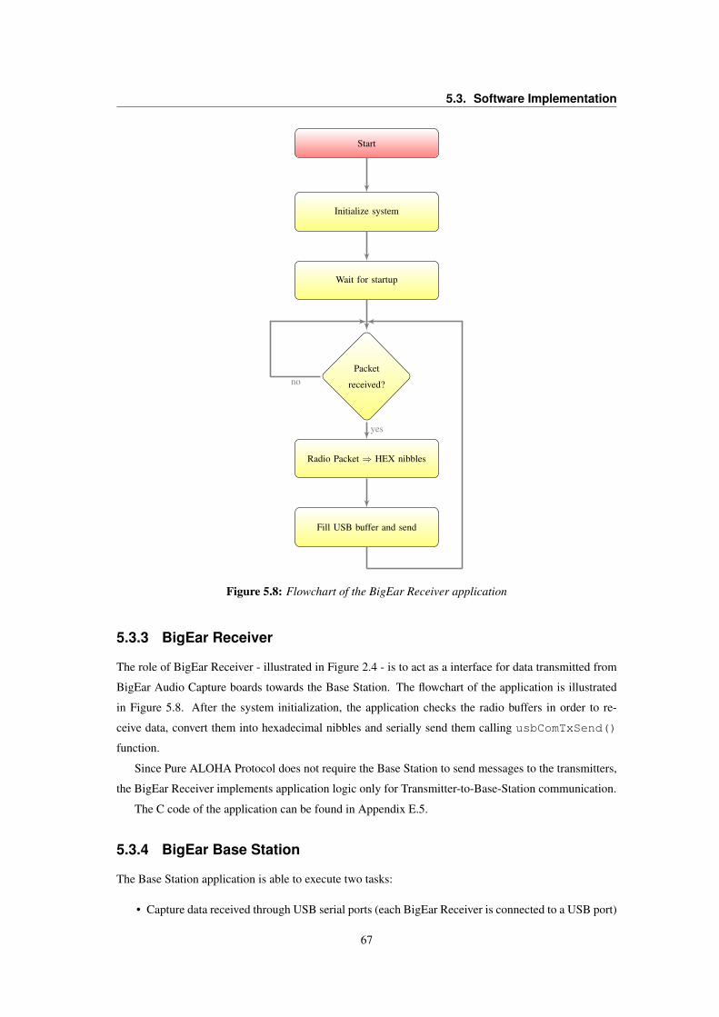
5.3. Software Implementation
Start
Initialize system
Wait for startup
Packet
received?
Radio Packet ⇒ HEX nibbles
Fill USB buffer and send
yes
no
Figure 5.8: Flowchart of the BigEar Receiver application
5.3.3 BigEar Receiver
The role of BigEar Receiver - illustrated in Figure 2.4 - is to act as a interface for data transmitted from
BigEar Audio Capture boards towards the Base Station. The flowchart of the application is illustrated
in Figure 5.8. After the system initialization, the application checks the radio buffers in order to re-
ceive data, convert them into hexadecimal nibbles and serially send them calling usbComTxSend()
function.
Since Pure ALOHA Protocol does not require the Base Station to send messages to the transmitters,
the BigEar Receiver implements application logic only for Transmitter-to-Base-Station communication.
The C code of the application can be found in Appendix E.5.
5.3.4 BigEar Base Station
The Base Station application is able to execute two tasks:
• Capture data received through USB serial ports (each BigEar Receiver is connected to a USB port)
67
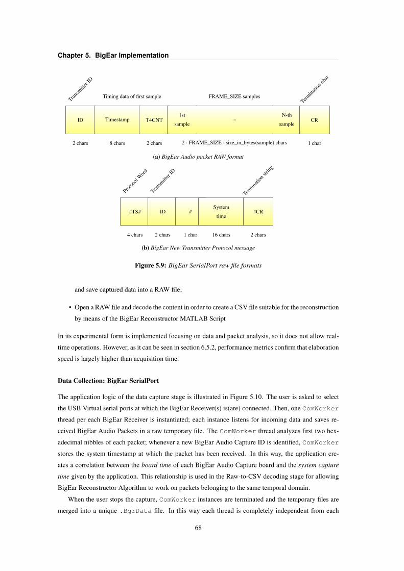
Chapter 5. BigEar Implementation
ID Timestamp T4CNT1st
sample...
N-th
sampleCR
2 chars 8 chars 2 chars 2 · FRAME_SIZE · size_in_bytes(sample) chars 1 char
Transm
itter ID
Timing data of first sample FRAME_SIZE samplesTerm
inatio
n char
(a) BigEar Audio packet RAW format
#TS# ID #System
time#CR
4 chars 2 chars 1 char 16 chars 2 chars
Protoc
olW
ord
Transm
itter ID
Termina
tion str
ing
(b) BigEar New Transmitter Protocol message
Figure 5.9: BigEar SerialPort raw file formats
and save captured data into a RAW file;
• Open a RAW file and decode the content in order to create a CSV file suitable for the reconstruction
by means of the BigEar Reconstructor MATLAB Script
In its experimental form is implemented focusing on data and packet analysis, so it does not allow real-
time operations. However, as it can be seen in section 6.5.2, performance metrics confirm that elaboration
speed is largely higher than acquisition time.
Data Collection: BigEar SerialPort
The application logic of the data capture stage is illustrated in Figure 5.10. The user is asked to select
the USB Virtual serial ports at which the BigEar Receiver(s) is(are) connected. Then, one ComWorker
thread per each BigEar Receiver is instantiated; each instance listens for incoming data and saves re-
ceived BigEar Audio Packets in a raw temporary file. The ComWorker thread analyzes first two hex-
adecimal nibbles of each packet; whenever a new BigEar Audio Capture ID is identified, ComWorker
stores the system timestamp at which the packet has been received. In this way, the application cre-
ates a correlation between the board time of each BigEar Audio Capture board and the system capture
time given by the application. This relationship is used in the Raw-to-CSV decoding stage for allowing
BigEar Reconstructor Algorithm to work on packets belonging to the same temporal domain.
When the user stops the capture, ComWorker instances are terminated and the temporary files are
merged into a unique .BgrData file. In this way each thread is completely independent from each
68
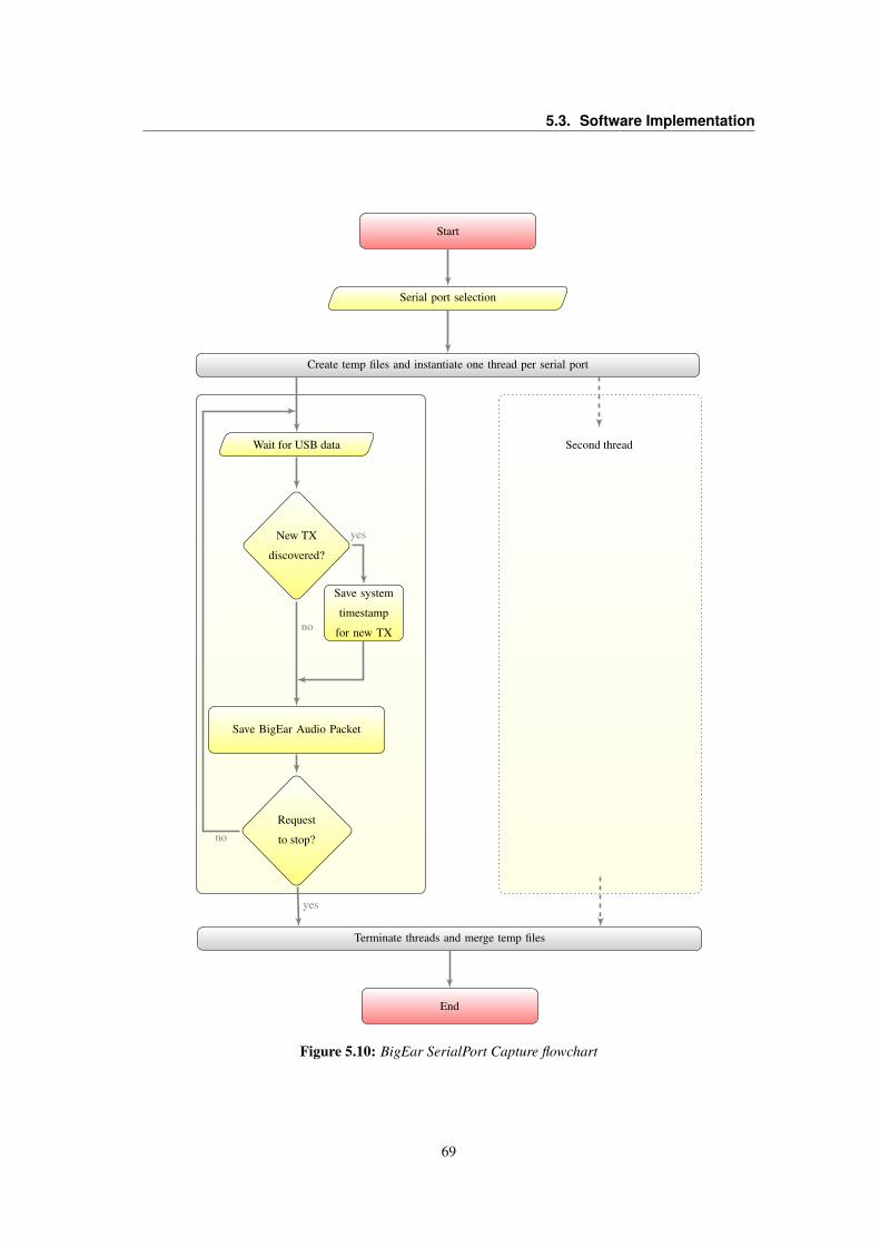
5.3. Software Implementation
Start
Serial port selection
Create temp files and instantiate one thread per serial port
Wait for USB data
New TX
discovered?
Save system
timestamp
for new TX
Save BigEar Audio Packet
Request
to stop?
Terminate threads and merge temp files
End
Second thread
yes
yes
no
no
Figure 5.10: BigEar SerialPort Capture flowchart
69
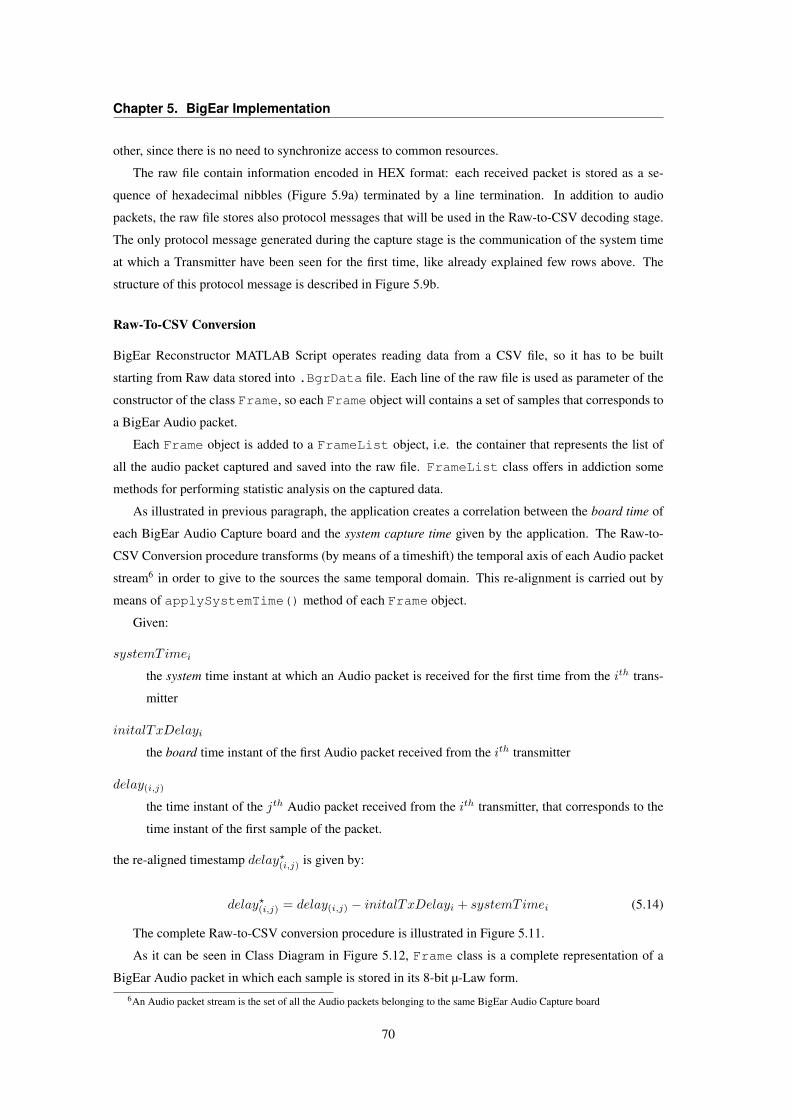
Chapter 5. BigEar Implementation
other, since there is no need to synchronize access to common resources.
The raw file contain information encoded in HEX format: each received packet is stored as a se-
quence of hexadecimal nibbles (Figure 5.9a) terminated by a line termination. In addition to audio
packets, the raw file stores also protocol messages that will be used in the Raw-to-CSV decoding stage.
The only protocol message generated during the capture stage is the communication of the system time
at which a Transmitter have been seen for the first time, like already explained few rows above. The
structure of this protocol message is described in Figure 5.9b.
Raw-To-CSV Conversion
BigEar Reconstructor MATLAB Script operates reading data from a CSV file, so it has to be built
starting from Raw data stored into .BgrData file. Each line of the raw file is used as parameter of the
constructor of the class Frame, so each Frame object will contains a set of samples that corresponds to
a BigEar Audio packet.
Each Frame object is added to a FrameList object, i.e. the container that represents the list of
all the audio packet captured and saved into the raw file. FrameList class offers in addiction some
methods for performing statistic analysis on the captured data.
As illustrated in previous paragraph, the application creates a correlation between the board time of
each BigEar Audio Capture board and the system capture time given by the application. The Raw-to-
CSV Conversion procedure transforms (by means of a timeshift) the temporal axis of each Audio packet
stream6 in order to give to the sources the same temporal domain. This re-alignment is carried out by
means of applySystemTime() method of each Frame object.
Given:
systemTimei
the system time instant at which an Audio packet is received for the first time from the ith trans-
mitter
initalTxDelayi
the board time instant of the first Audio packet received from the ith transmitter
delay(i,j)
the time instant of the jth Audio packet received from the ith transmitter, that corresponds to the
time instant of the first sample of the packet.
the re-aligned timestamp delay?(i,j) is given by:
delay?(i,j) = delay(i,j) − initalTxDelayi + systemTimei (5.14)
The complete Raw-to-CSV conversion procedure is illustrated in Figure 5.11.
As it can be seen in Class Diagram in Figure 5.12, Frame class is a complete representation of a
BigEar Audio packet in which each sample is stored in its 8-bit µ-Law form.6An Audio packet stream is the set of all the Audio packets belonging to the same BigEar Audio Capture board
70
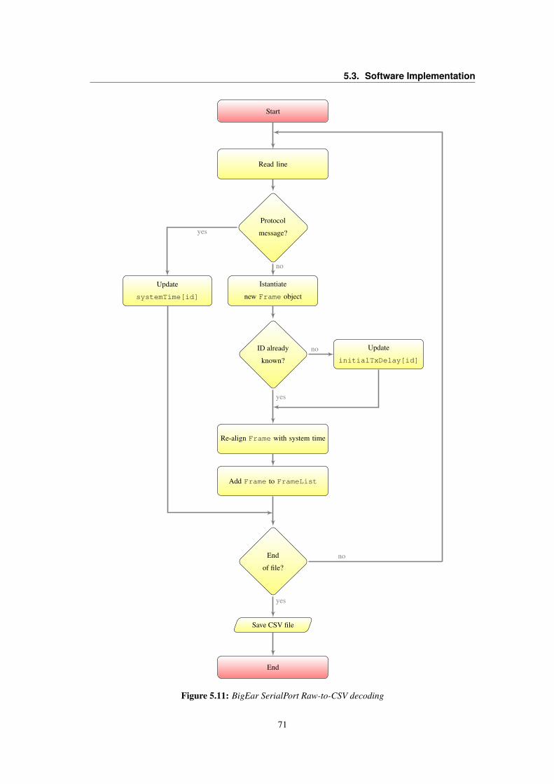
5.3. Software Implementation
Start
Read line
Protocol
message?
Istantiate
new Frame object
Update
systemTime[id]
ID already
known?
Update
initialTxDelay[id]
Re-align Frame with system time
Add Frame to FrameList
End
of file?
Save CSV file
End
yes
no
no
yes
yes
no
Figure 5.11: BigEar SerialPort Raw-to-CSV decoding
71
Chapter 5. BigEar Implementation
uLaw- expandedValue : int[ ]
+ GetExpandedValue : int
ComWorker- comPort : SerialPort
- DataCounter : uint
- known : bool[ ]
- port : string
- shouldStop : bool
- stream : FileStream
- sw : StopWatch
+ DoWork : void
+ GetDataCounter : uint
+ RequestStop : void
Frame- msFract : byte
- Source : byte
+ StartingMillisecond : uint
- samples : byte[ ]
+ ApplySystemTime : void
+ GetDelayOfSample : double
+ GetFrameCSV : string
+ GetSample : int
+ GetSamplesCSV : string
FrameList- avgFramesDistance : double[ ]
- finalDelay : uint[ ]
- framesTransmitted : uint[ ]
- hasBeenSeen : bool[ ]
- initialDelay : uint[ ]
+ Add : void
+ Clear : void
+ GetAvgFrameDistance : double
+ GetFramesTransmitted : uint
+ GetInitialDelayOfSource : uint
+ GetMaxDuration : float
+ HasBeenSeen : bool
+ Remove : bool
+ ToString : string
0..*
Figure 5.12: BigEar SerialPort Class Diagram
When the getSample(byte index) method is called to return the value of the indexth sample, the
method returns the expanded 16-bit value. The expansion is performed by means of a lookup table (see
uLaw class in Figure 5.12). Moreover, the Frame class exposes the getSamplesCSV() method that
returns the Comma-Separated-Value representation of the Frame.
BigEar SerialPort application GUI is reported in Appendix E.6.
Audio Reconstruction: BigEar Reconstructor MATLAB Script
The MATLAB Script devoted to the speech reconstruction prepares audio data for being processed by
means of the Reconstruction block already discussed in Chapter 4. Starting from CSV file generated
during the previous stage, the script builds audioPackets and positions matrices in which each
audioPackets(i,j) element represents the ith audio sample transmitted by the jth sensor. Position
in time of the given sample is specified in positions(i,j).
After data setup, the reconstruct function is called and the reconstructed signal is filtered by means
of a Third-order Type I Chebyschev filter (passband ripple) in order to suppress out-of-band noises and
artifacts. At the end of signal processing part, some statistics data are generated in order to analyze
performance data. The list of the metrics and statistical measures will be discussed in Section 6.2. The
Flowchart of BigEar Reconstructor MATLAB Script is illustrated in Figure 5.13.
72
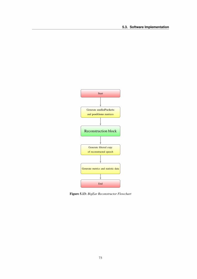
5.3. Software Implementation
Start
Generate audioPackets
and positions matrices
Reconstruction block
Generate filtered copy
of reconstructed speech
Generate metrics and statistic data
End
Figure 5.13: BigEar Reconstructor Flowchart
73

6BigEar Results Analysis
Introduction
In this chapter the results of the simulation of the system and the measures obtained by real prototype are
discussed. After the definition of the metrics adopted and after the description of the experimental setups,
the consistency between the theoretical model - implemented in the BigEar Simulator - and the real-
world implementation of the prototypes will be shown; then, reconstructed signal metrics are discussed
focusing on relevant properties such as the number of holes and the overlapping between contributors.
Finally, software metrics allow to evaluate robustness of the system in term of speed of processing and
of quality of the reconstruction.
6.1 Overview
Once the system has been implemented and the prototype realized, in order to examine the system
behavior some metrics are needed in order to perform a direct comparison between the data captured
by means of the BigEar prototype and the data obtained by means of the BigEar Simulator described
in Chapter 3; the defined metrics are related to those speech signal characteristics that are identified as
relevant or critic for the application.
One of the critical aspects is represented by the holeyness of the reconstructed speech signal. As
already seen, since reconstructed signal is paying by the superposition of audio packets sampled by
different sensors at random time instants, it can be affected by sequences of empty samples. These
holes influence the result of the speech recognition algorithm, so defined metrics help in finding best
parameters and best working conditions.
Parameters for the best speech signal in output are not evaluated only looking at the number of
holes in the reconstructed stream, but also giving attention to the degree of overlapping between the
audio streams received from the transmitters and to the quality of the reconstruction since superposition
algorithms affect the quality of the final result. Another important factor is the speed of processing:
reconstruction algorithms has to be fast in order to be used - in future - in real-time audio capture.
75
Chapter 6. BigEar Results Analysis
6.2 Metrics Definition
In order to compare the audio speech signal generated by the BigEar Simulator with audio stream cap-
tured and reconstructed by means of the prototypes described in Chapter 5, some metrics have been
defined. These measures characterize the results in terms of quality of the reconstructed speech signal
and in term of the amount of informative contribution given by each BigEar Audio Capture board. Other
metrics are used to measure software performances.
6.2.1 Reconstructed Signal Metrics
The metrics defined in this sections provide quality measures concerning the reconstructed speech signal.
As already mentioned in Section 4.5, the success of speech recognition is influenced by the number and
the size of holes in the reconstructed signal. Moreover, the BigEar Reconstruction algorithm convergence
is influenced by the amount of information that can be overlapped for the Cross-correlation alignment.
Fill ratio
Fill_ratio =No. of samples
Nwhere N = Length of the stream (in samples) (6.1)
Already defined in Eq. 4.1. Referring to the reconstructed signal, it represents the amount of
samples with respect to the total length of the stream. The more the value is close to 1, the more
the reconstructed signal is complete.
Numer of holes
NoH =No. of 0-ed sequences in totalCoverage
N(6.2)
Size of holes
SoH = Average size of 0-ed sequences in totalCoverage (6.3)
In conjunction with NoH , this metric characterize the distribution of empty samples (holes) into
the reconstructed signal. In case of constant Fill_ratio, SoH andNoH allow to compare whether
empty samples are gathered into few big blocks or diffused into many small blocks.
Support factor
Sf = E [totalCoverage0] where totalCoverage0 = ti ∈ totalCoverage : ti 6= 0(6.4)
Sf gives a measure of the contribution of each single transmitter to the construction of the final
speech signal. Sf ∈ (0, NTX ] where NTX is the number of transmitters. The higher Sf , the
higher the overlapping of the streams obtained by the different transmitters.
76
6.2. Metrics Definition
Support factor standard deviation
σSf =
√√√√ 1
N
N∑i=1
(ti − Sf)2 where ti ∈ totalCoverage0 (6.5)
σSf measures the dispersion of totalCoverage0. σSf close to 0 indicates that the number of
contributors per sample tends to be very close to Sf while a high σSf indicates that the number of
contributors is volatile.
6.2.2 Software Performance Metrics
Each BigEar Audio Capture board samples a signal that is the summation of the direct sound and of the
environment contributions given by the room reflections, so each audio stream is more or less different
from others. Where two or more streams are superposed, at the beginning and at the end of the over-
lapping areas artifacts are generated (see section 4.3.2). While it is impossible to estimate the scope of
the artifacts, it is possible to count the positions on which an artifact could be generated. The higher the
number of potential artifacts, the higher the probability to degrade the speech quality.
Potential Artifacts Ratio
Aws =
NTX∑k=1
edgeskN
(6.6)
where edgesk = 2 ·NoHk
and NoHk = no. of holes in the stream produced by kth sensor
Ahr =
NTX∑k=1
(edgesk − edgesh<kk
)N
(6.7)
where edgesh<kk = edges in the kth stream covered by samples of previous streams
Since number of potential artifacts is dependent on the chosen superposition policy, two different
calculation methods are needed. Aws is the metric used for Weighted Sum reconstruction; in this
case the method considers all the edges in each stream since all of the contributions are summed
up. On the other hand, reconstruction by Holes Replacement starts from a given stream (selected
by means of signal power analysis) and only samples that are needed to fill the holes are taken
from the other streams (See Section 4.3.2); in this case, therefore, Ahr takes into account, for each
stream, only the edges that are not covered by samples given by the previous steps.
Realtime Performance Ratio
RPR =∆Trec∆Telab
=(length of reconstructed signal) · 1
Fs
∆Telab(6.8)
77
Chapter 6. BigEar Results Analysis
The Realtime Performance Ratio measures the ability of the system to operate in real time, giving
a ratio between the duration of the reconstructed stream and the time needed to process data. This
measure is dependent on the number of transmitters since the higher the number of transmitters,
the higher the data flow. So the metric can be used as a global tradeoff parameter:
RPR > 1 states that the whole system is able to bufferize, send and process data faster than
sampling.
6.3 Simulation Setup
Simulations have been performed using BigEar Simulator described Chapter 3 and changing some pa-
rameters in order to study system behavior under different configurations. The fixed parameters are
given by design choices illustrated in Chapter 5, while the parameters that have been changed are the
ones related to:
• Number of BigEar Capture boards used for acquisition
• BigEar Audio Capture boards positions in the room
• Radio channel configuration of each BigEar Audio Capture board (how many transmitters com-
municating on the same radio channel, as seen in Section 2.4)
• Maximum delay between adjacent transmission of the same transmitter (See ALOHA Protocol
Family, Section 2.5.1)
Table 6.1 summarize parameters given to BigEar Simulator for performing its work. It can be noted
that selected values for TMAXDELAY parameter are the same values that can be used in the BigEar Audio
Capture Board Application, as illustrated in Table 5.2. For each simulation parameters set, in order
to give statistical relevance to data, a number of 50 experiments have been performed using a speech
signal of a duration of 16 seconds. Transmitters positions and channel configurations are summarized in
Appendix F.
From these simulations, Statistic data and Metrics have been calculated according to Section 6.2.1
and plotted onto charts that will be discussed in Section 6.5.
6.4 On-field Setup
Once the prototypes have been realized, they have been tested for checking the correct realization. Then,
in order to set the overall gain and to find the right bias point at the interface between the amplifier stage
and the P0_0 input of the Wixel board (Section 5.2.1), each transmitter has been calibrated using BigEar
Input Calibration application (Section 5.3.2).
On-field tests have been divided in two stages: Near-field and Far-field tests.
78
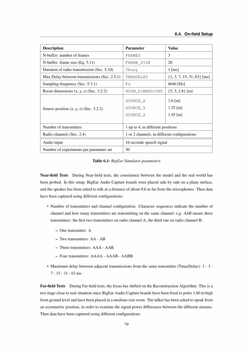
6.4. On-field Setup
Description Parameter Value
N-buffer: number of frames FRAMES 3
N-buffer: frame size (Eq. 5.11) FRAME_SIZE 20
Duration of radio transmission (Sec. 5.10) Tbusy 1 [ms]
Max Delay between transmissions (Sec. 2.5.1) TMAXDELAY 1, 3, 7, 15, 31, 63 [ms]
Sampling frequency (Sec. 5.3.1) Fs 6040 [Hz]
Room dimensions (x, y, z) (Sec. 3.2.2) ROOM_DIMENSIONS 5, 3, 2.8 [m]
Source position (x, y, z) (Sec. 3.2.2)
SOURCE_X
SOURCE_Y
SOURCE_Z
3.6 [m]
1.25 [m]
1.45 [m]
Number of transmitters 1 up to 4, in different positions
Radio channels (Sec. 2.4) 1 or 2 channels, in different configurations
Audio input 16 seconds speech signal
Number of experiments per parameter set 50
Table 6.1: BigEar Simulator parameters
Near-field Tests During Near-field tests, the consistence between the model and the real world has
been probed. In this setup, BigEar Audio Capture boards were placed side by side on a plane surface,
and the speaker has been asked to talk at a distance of about 0.6 m far from the microphones. Then data
have been captured using different configurations:
• Number of transmitters and channel configuration. Character sequences indicate the number of
channel and how many transmitters are transmitting on the same channel; e.g. AAB means three
transmitters: the first two transmitters on radio channel A, the third one on radio channel B:
– One transmitter: A
– Two transmitters: AA - AB
– Three transmitters: AAA - AAB
– Four transmitters: AAAA - AAAB - AABB
• Maximum delay between adjacent transmissions from the same transmitter (TmaxDelay): 1 - 3 -
7 - 15 - 31 - 63 ms
Far-field Tests During Far-field tests, the focus has shifted on the Reconstruction Algorithm. This is a
test stage close to real situation since BigEar Audio Capture boards have been fixed to poles 1.60 m high
from ground level and have been placed in a medium-size room. The talker has been asked to speak from
an asymmetric position, in order to examine the signal power differences between the different streams.
Then data have been captured using different configurations:
79
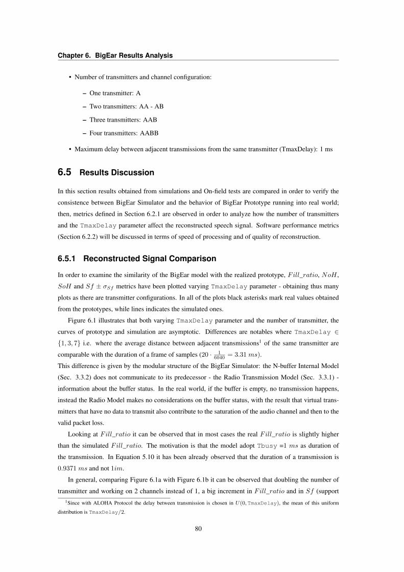
Chapter 6. BigEar Results Analysis
• Number of transmitters and channel configuration:
– One transmitter: A
– Two transmitters: AA - AB
– Three transmitters: AAB
– Four transmitters: AABB
• Maximum delay between adjacent transmissions from the same transmitter (TmaxDelay): 1 ms
6.5 Results Discussion
In this section results obtained from simulations and On-field tests are compared in order to verify the
consistence between BigEar Simulator and the behavior of BigEar Prototype running into real world;
then, metrics defined in Section 6.2.1 are observed in order to analyze how the number of transmitters
and the TmaxDelay parameter affect the reconstructed speech signal. Software performance metrics
(Section 6.2.2) will be discussed in terms of speed of processing and of quality of reconstruction.
6.5.1 Reconstructed Signal Comparison
In order to examine the similarity of the BigEar model with the realized prototype, Fill_ratio, NoH ,
SoH and Sf ± σSf metrics have been plotted varying TmaxDelay parameter - obtaining thus many
plots as there are transmitter configurations. In all of the plots black asterisks mark real values obtained
from the prototypes, while lines indicates the simulated ones.
Figure 6.1 illustrates that both varying TmaxDelay parameter and the number of transmitter, the
curves of prototype and simulation are asymptotic. Differences are notables where TmaxDelay ∈1, 3, 7 i.e. where the average distance between adjacent transmissions1 of the same transmitter are
comparable with the duration of a frame of samples (20 · 16040 = 3.31 ms).
This difference is given by the modular structure of the BigEar Simulator: the N-buffer Internal Model
(Sec. 3.3.2) does not communicate to its predecessor - the Radio Transmission Model (Sec. 3.3.1) -
information about the buffer status. In the real world, if the buffer is empty, no transmission happens,
instead the Radio Model makes no considerations on the buffer status, with the result that virtual trans-
mitters that have no data to transmit also contribute to the saturation of the audio channel and then to the
valid packet loss.
Looking at Fill_ratio it can be observed that in most cases the real Fill_ratio is slightly higher
than the simulated Fill_ratio. The motivation is that the model adopt Tbusy =1 ms as duration of
the transmission. In Equation 5.10 it has been already observed that the duration of a transmission is
0.9371 ms and not 1im.
In general, comparing Figure 6.1a with Figure 6.1b it can be observed that doubling the number of
transmitter and working on 2 channels instead of 1, a big increment in Fill_ratio and in Sf (support1Since with ALOHA Protocol the delay between transmission is chosen in U(0,TmaxDelay), the mean of this uniform
distribution is TmaxDelay/2.
80
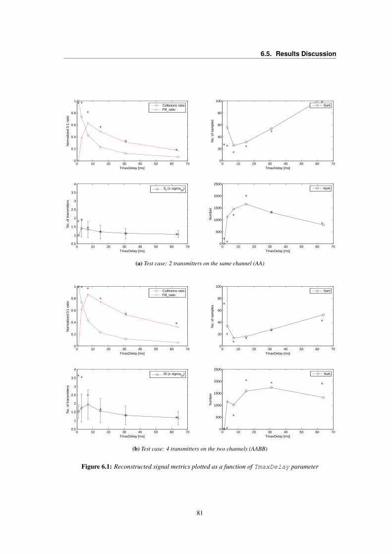
6.5. Results Discussion
0 10 20 30 40 50 60 700
0.2
0.4
0.6
0.8
1
TmaxDelay [ms]
Nor
mal
ized
0:1
rat
io
Collisions ratioFill_ratio
0 10 20 30 40 50 60 700
20
40
60
80
100
TmaxDelay [ms]
No.
of s
ampl
es
SoH
0 10 20 30 40 50 60 700.5
1
1.5
2
2.5
3
3.5
4
TmaxDelay [ms]
No.
of t
rans
mitt
ers
S
f (± sigma
Sf)
0 10 20 30 40 50 60 700
500
1000
1500
2000
2500
TmaxDelay [ms]
Num
ber
NoH
(a) Test case: 2 transmitters on the same channel (AA)
0 10 20 30 40 50 60 700
0.2
0.4
0.6
0.8
1
TmaxDelay [ms]
Nor
mal
ized
0:1
rat
io
Collisions ratioFill_ratio
0 10 20 30 40 50 60 700
20
40
60
80
100
TmaxDelay [ms]
No.
of s
ampl
es
SoH
0 10 20 30 40 50 60 700.5
1
1.5
2
2.5
3
3.5
4
TmaxDelay [ms]
No.
of t
rans
mitt
ers
Sf (± sigma
Sf)
0 10 20 30 40 50 60 700
500
1000
1500
2000
2500
TmaxDelay [ms]
Num
ber
Noh
(b) Test case: 4 transmitters on the two channels (AABB)
Figure 6.1: Reconstructed signal metrics plotted as a function of TmaxDelay parameter
81
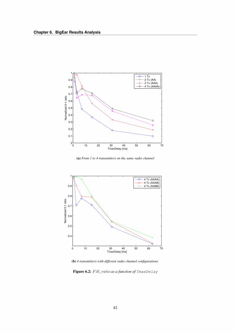
Chapter 6. BigEar Results Analysis
0 10 20 30 40 50 60 700
0.1
0.2
0.3
0.4
0.5
0.6
0.7
0.8
0.9
1
TmaxDelay [ms]
No
rma
lize
d 0
:1 r
atio
1 Tx
2 Tx (AA)
3 Tx (AAA)
4 Tx (AAAA)
(a) From 1 to 4 transmitters on the same radio channel
0 10 20 30 40 50 60 70
0.4
0.5
0.6
0.7
0.8
0.9
1
TmaxDelay [ms]
No
rma
lize
d 0
:1 r
atio
4 Tx (AAAA)
4 Tx (AAAB)
4 Tx (AABB)
(b) 4 transmitters with different radio channel configurations
Figure 6.2: Fill_ratio as a function of TmaxDelay
82
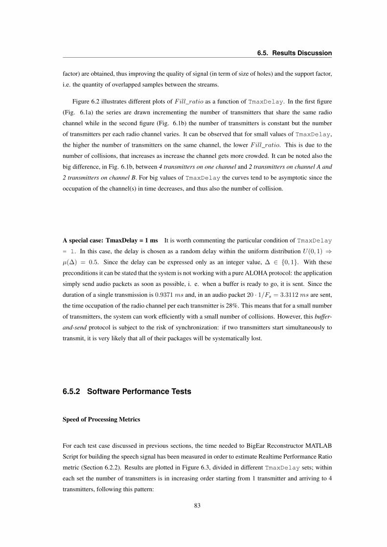
6.5. Results Discussion
factor) are obtained, thus improving the quality of signal (in term of size of holes) and the support factor,
i.e. the quantity of overlapped samples between the streams.
Figure 6.2 illustrates different plots of Fill_ratio as a function of TmaxDelay. In the first figure
(Fig. 6.1a) the series are drawn incrementing the number of transmitters that share the same radio
channel while in the second figure (Fig. 6.1b) the number of transmitters is constant but the number
of transmitters per each radio channel varies. It can be observed that for small values of TmaxDelay,
the higher the number of transmitters on the same channel, the lower Fill_ratio. This is due to the
number of collisions, that increases as increase the channel gets more crowded. It can be noted also the
big difference, in Fig. 6.1b, between 4 transmitters on one channel and 2 transmitters on channel A and
2 transmitters on channel B. For big values of TmaxDelay the curves tend to be asymptotic since the
occupation of the channel(s) in time decreases, and thus also the number of collision.
A special case: TmaxDelay = 1 ms It is worth commenting the particular condition of TmaxDelay
= 1. In this case, the delay is chosen as a random delay within the uniform distribution U(0, 1) ⇒µ(∆) = 0.5. Since the delay can be expressed only as an integer value, ∆ ∈ 0, 1. With these
preconditions it can be stated that the system is not working with a pure ALOHA protocol: the application
simply send audio packets as soon as possible, i. e. when a buffer is ready to go, it is sent. Since the
duration of a single transmission is 0.9371 ms and, in an audio packet 20 · 1/Fs = 3.3112 ms are sent,
the time occupation of the radio channel per each transmitter is 28%. This means that for a small number
of transmitters, the system can work efficiently with a small number of collisions. However, this buffer-
and-send protocol is subject to the risk of synchronization: if two transmitters start simultaneously to
transmit, it is very likely that all of their packages will be systematically lost.
6.5.2 Software Performance Tests
Speed of Processing Metrics
For each test case discussed in previous sections, the time needed to BigEar Reconstructor MATLAB
Script for building the speech signal has been measured in order to estimate Realtime Performance Ratio
metric (Section 6.2.2). Results are plotted in Figure 6.3, divided in different TmaxDelay sets; within
each set the number of transmitters is in increasing order starting from 1 transmitter and arriving to 4
transmitters, following this pattern:
83
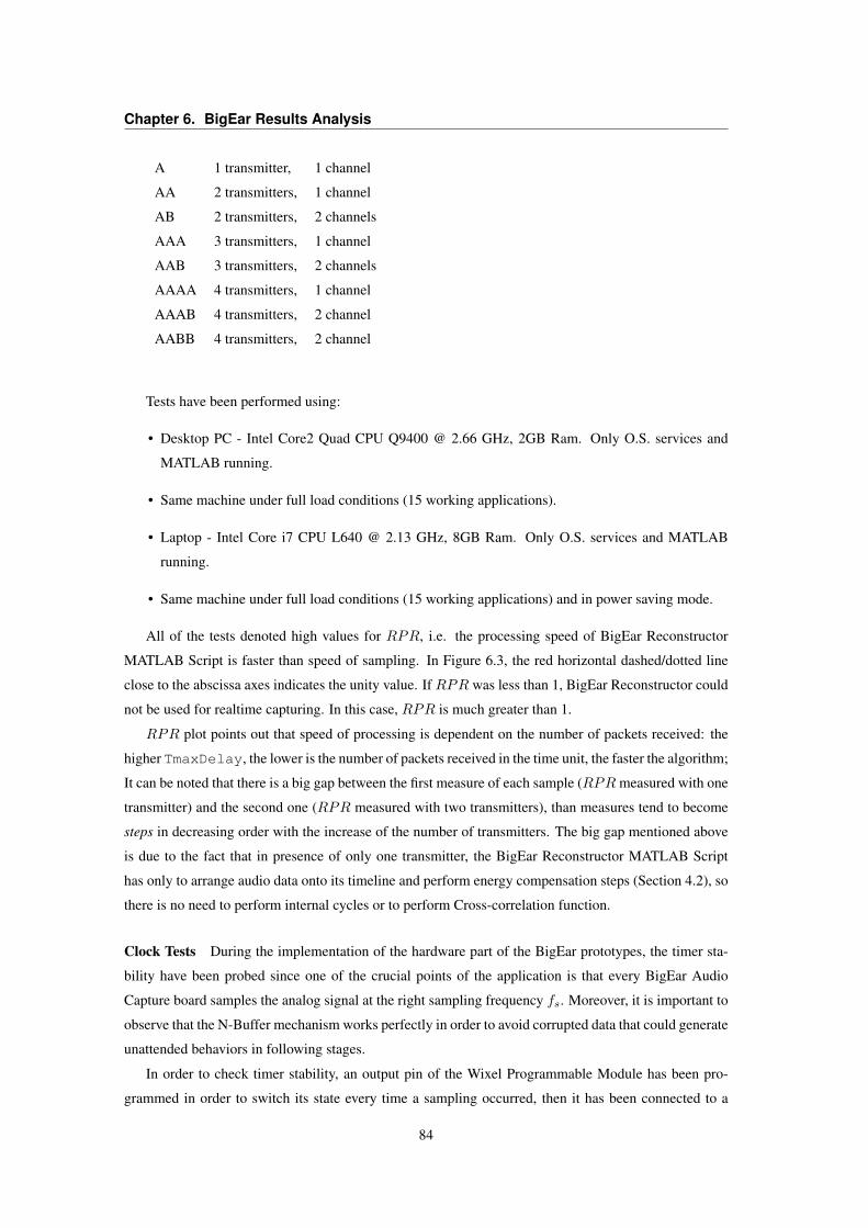
Chapter 6. BigEar Results Analysis
A 1 transmitter, 1 channel
AA 2 transmitters, 1 channel
AB 2 transmitters, 2 channels
AAA 3 transmitters, 1 channel
AAB 3 transmitters, 2 channels
AAAA 4 transmitters, 1 channel
AAAB 4 transmitters, 2 channel
AABB 4 transmitters, 2 channel
Tests have been performed using:
• Desktop PC - Intel Core2 Quad CPU Q9400 @ 2.66 GHz, 2GB Ram. Only O.S. services and
MATLAB running.
• Same machine under full load conditions (15 working applications).
• Laptop - Intel Core i7 CPU L640 @ 2.13 GHz, 8GB Ram. Only O.S. services and MATLAB
running.
• Same machine under full load conditions (15 working applications) and in power saving mode.
All of the tests denoted high values for RPR, i.e. the processing speed of BigEar Reconstructor
MATLAB Script is faster than speed of sampling. In Figure 6.3, the red horizontal dashed/dotted line
close to the abscissa axes indicates the unity value. If RPR was less than 1, BigEar Reconstructor could
not be used for realtime capturing. In this case, RPR is much greater than 1.
RPR plot points out that speed of processing is dependent on the number of packets received: the
higher TmaxDelay, the lower is the number of packets received in the time unit, the faster the algorithm;
It can be noted that there is a big gap between the first measure of each sample (RPR measured with one
transmitter) and the second one (RPR measured with two transmitters), than measures tend to become
steps in decreasing order with the increase of the number of transmitters. The big gap mentioned above
is due to the fact that in presence of only one transmitter, the BigEar Reconstructor MATLAB Script
has only to arrange audio data onto its timeline and perform energy compensation steps (Section 4.2), so
there is no need to perform internal cycles or to perform Cross-correlation function.
Clock Tests During the implementation of the hardware part of the BigEar prototypes, the timer sta-
bility have been probed since one of the crucial points of the application is that every BigEar Audio
Capture board samples the analog signal at the right sampling frequency fs. Moreover, it is important to
observe that the N-Buffer mechanism works perfectly in order to avoid corrupted data that could generate
unattended behaviors in following stages.
In order to check timer stability, an output pin of the Wixel Programmable Module has been pro-
grammed in order to switch its state every time a sampling occurred, then it has been connected to a
84
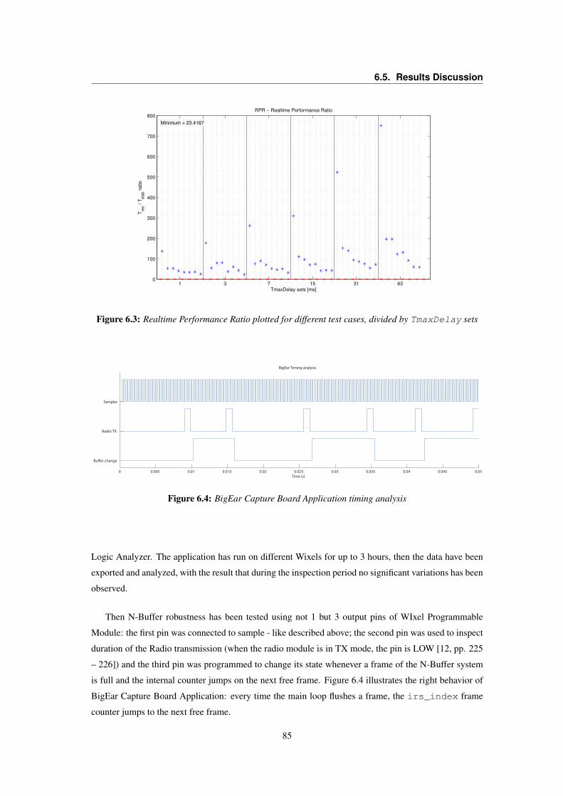
6.5. Results Discussion
1 3 7 15 31 630
100
200
300
400
500
600
700
800
TmaxDelay sets [ms]
RPR − Realtime Performance Ratio
Minimum = 23.4167
Tre
c /
Tela
b r
atio
Figure 6.3: Realtime Performance Ratio plotted for different test cases, divided by TmaxDelay sets
0 0.005 0.01 0.015 0.02 0.025 0.03 0.035 0.04 0.045 0.05
Buer change
Radio TX
Sampler
BigEar Timing analysis
Time (s)
Figure 6.4: BigEar Capture Board Application timing analysis
Logic Analyzer. The application has run on different Wixels for up to 3 hours, then the data have been
exported and analyzed, with the result that during the inspection period no significant variations has been
observed.
Then N-Buffer robustness has been tested using not 1 but 3 output pins of WIxel Programmable
Module: the first pin was connected to sample - like described above; the second pin was used to inspect
duration of the Radio transmission (when the radio module is in TX mode, the pin is LOW [12, pp. 225
– 226]) and the third pin was programmed to change its state whenever a frame of the N-Buffer system
is full and the internal counter jumps on the next free frame. Figure 6.4 illustrates the right behavior of
BigEar Capture Board Application: every time the main loop flushes a frame, the irs_index frame
counter jumps to the next free frame.
85
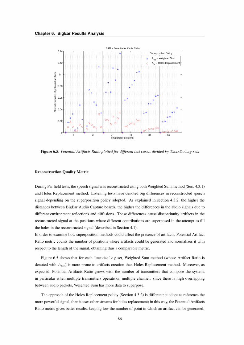
Chapter 6. BigEar Results Analysis
1 3 7 15 31 630
0.02
0.04
0.06
0.08
0.1
0.12
0.14
TmaxDelay sets [ms]
PAR − Potential Artifacts Ratio
No
rma
lize
d r
atio
of
po
ten
tia
l a
rtifa
cts
Aws
− Weighted Sum
Ahr
− Holes Replacement
Superposition Policy
Figure 6.5: Potential Artifacts Ratio plotted for different test cases, divided by TmaxDelay sets
Reconstruction Quality Metric
During Far field tests, the speech signal was reconstructed using both Weighted Sum method (Sec. 4.3.1)
and Holes Replacement method. Listening tests have denoted big differences in reconstructed speech
signal depending on the superposition policy adopted. As explained in section 4.3.2, the higher the
distances between BigEar Audio Capture boards, the higher the differences in the audio signals due to
different environment reflections and diffusions. These differences cause discontinuity artifacts in the
reconstructed signal at the positions where different contributions are superposed in the attempt to fill
the holes in the reconstructed signal (described in Section 4.1).
In order to examine how superposition methods could affect the presence of artifacts, Potential Artifact
Ratio metric counts the number of positions where artifacts could be generated and normalizes it with
respect to the length of the signal, obtaining thus a comparable metric.
Figure 6.5 shows that for each TmaxDelay set, Weighted Sum method (whose Artifact Ratio is
denoted with Aws) is more prone to artifacts creation than Holes Replacement method. Moreover, as
expected, Potential Artifacts Ratio grows with the number of transmitters that compose the system,
in particular when multiple transmitters operate on multiple channel: since there is high overlapping
between audio packets, Weighted Sum has more data to superpose.
The approach of the Holes Replacement policy (Section 4.3.2) is different: it adopt as reference the
more powerful signal, then it uses other streams for holes replacement; in this way, the Potential Artifacts
Ratio metric gives better results, keeping low the number of point in which an artifact can be generated.
86

6.5. Results Discussion
6.5.3 Coarse-grain localization
As mentioned in Chapter 4, power of signals and delays applied for streams alignment are related to
the distance between the source and the distance between sensors, so if the position of BigEar Audio
Capture Boards is known, those information can be exploited for coarse-grain localization of the source.
Figure 6.6 shows the relation between signal power and delay used for streams alignment. In order to
give significance to the graphical representation of data, values have been normalized between 0 and
1; furthermore, since delay grows with distance while power decreases, a flipped version of the delay
(called advance) has been plotted:
advance[i] = 1− delay[i]
max(delay)
It can be noted that alignment delays and power of signals provide coherent information that can be used
for source localization.
87
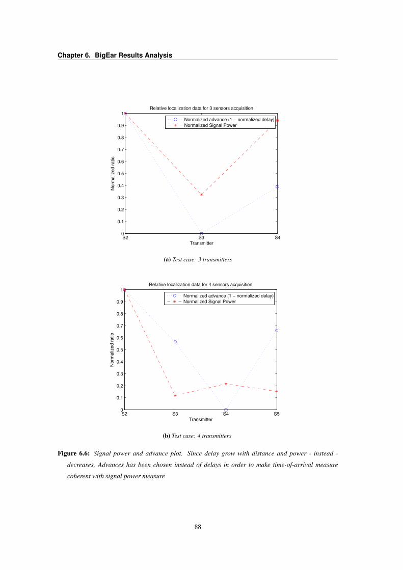
Chapter 6. BigEar Results Analysis
S2 S3 S40
0.1
0.2
0.3
0.4
0.5
0.6
0.7
0.8
0.9
1
Transmitter
No
rma
lize
d r
atio
Relative localization data for 3 sensors acquisition
Normalized advance (1 − normalized delay)
Normalized Signal Power
(a) Test case: 3 transmitters
S2 S3 S4 S50
0.1
0.2
0.3
0.4
0.5
0.6
0.7
0.8
0.9
1
Transmitter
No
rma
lize
d r
atio
Relative localization data for 4 sensors acquisition
Normalized advance (1 − normalized delay)
Normalized Signal Power
(b) Test case: 4 transmitters
Figure 6.6: Signal power and advance plot. Since delay grow with distance and power - instead -
decreases, Advances has been chosen instead of delays in order to make time-of-arrival measure
coherent with signal power measure
88
7Conclusions and Future Work
7.1 Conclusions
In this work of thesis, starting from requirements of Minimum costs, Wireless, Distribution and Modu-
larity, the prototype of a voice capture application has been introduced.
BigEar application has been implemented based on a distributed Wireless Sensor Network that per-
form a space-time audio sampling of an environment. Core of the application is Base Station, that is the
device devoted to data collection. Wireless Sensor Network can be multi-layered by the use of multiple
radio channels; for each radio channel a BigEar Receiver acts as interface between the Base Station and
the BigEar Audio Capture Boards belonging to the same layer.
In order to analyze and evaluate architecture features, a simulator has been implemented. The BigEar
Simulator adopts an interaction model composed of different sequential blocks: Audio Model block per-
forms a physical characterization of the speech signal captured by each sensor; Sensor Network Model
simulates the behavior of the architecture by means of a Network Interaction Model and an N-Buffer
Internal Model, which account respectively for handling the time instants each sensor transmits audio
Packet, and for simulating the behavior of the internal buffering system of each transmitter.
Once audio packets have been received by BigEar Base Station, they need to be superposed in order
to build a unique speech signal from the contributions of each sensor. Superposition is performed by the
Reconstruction Block that exploits Cross-correlation function for finding the right time alignment of the
audio data. Before superposing, audio packets need to get unbiased and normalized for compensating
intensity differences due to the different sensor-source distances and for correcting wrong sensor calibra-
tions. Then, two different methods have been tested for the superposition of samples: Weighted Sum of
samples is robust in term of local issues handling (like saturation of the input stage) at the expense of a
higher number of discontinuity points (artifacts); conversely, Holes Replacement method is less prone to
artifacts generation, but additional methods are required for handling local issues. Reconstructed speech
signal is subject to the presence of sequences of empty samples (holes) that could influence Speech
Recognition stage. Several methods have been tested in order to fill these sequences.
The system has been implemented for examining the real-world behavior of the previously modeled
89

Chapter 7. Conclusions and Future Work
architecture. BigEar Audio Capture board has been implemented using a cheap microphone and a signal
conditioning circuit composed of a double stage operational amplifier having a fixed band-pass filter
and a variable overall gain. The application running on each BigEar Capture module allows to perform
ADC readings at full 12-bit resolution and is able to compress each 12-bit sample into an 8-bit µLaw
compressed sample, optimizing data rate and incrementing Quantization SNR. The BigEar Receiver
application acts as a wireless-USB dongle between BigEar Audio Capture modules and BigEar Base
Station. Finally, BigEar Base Station has been implemented as a modular application in order to focus
on debug and testing purposes.
7.2 Strengths and Weaknesses
Result analysis has exposed strengths and weaknesses of the BigEar system. Strengths can be related
with Minimum costs, Wireless, Distribution and Modularity requirements discussed in Section .
7.2.1 Strengths
Minimum cost
Low costs can be seen from different points of view:
• Architecture is based on Wixel Prototyping boards, whose cost is around 20 $ each one; costs
for speech acquisition circuit is under 10 $ per board1;
• BigEar Simulator can be used to perform an a-priori analysis in order to identify best param-
eters (no. of sensors, position of sensors, no. of channels, software-configurable parameters)
for a specific use case, minimizing production and installation costs.
Wireless
The use of wireless transmission between nodes gives to the system flexibility and fast reconfig-
urability, while it reduces efforts for house adaptation eliminating need for signal or power cables.
Distributed
The distributed approach overcomes issues related to sensors temporary failures and, in particular
with local signal problems like saturation.
Data Intelligence
Ubiquitous approach allows Data Intelligence mechanisms in integration with BRIDGe architec-
ture, e.g. performing a coarse-grain localization in order to add informative content that could dis-
ambiguate context-free vocal commands (“Turn off the light” or - better - “Turn off this light” could
be integrated with localization information in order to determine which light has to be switched
off).
1Quotations: second quarter of 2015
90
7.3. Future Work
Modular
Whole architecture is scalable and it can be easily reconfigured by adding or removing sensors
from the sensor network.
Responsive
Software Performance Metrics shows that BigEar Reconstructor algorithm - even though in its
experimental form - can perform real-time speech reconstruction, so responsivity of the system is
related to speed of Automatic Speech Recognition algorithms.
7.2.2 Weaknesses
Hardware-related weaknesses are represented by the presence of electrical noise generated by the Wixel
antenna and through the Wixel VIN pin - despite the presence of decoupling capacitors, and the lack
of mechanisms for preventing long-term sensor clock drift that can cause time warping and long-term
misalignments between audio streams.
A Model related weakness can be identified in the lack of a backward communication mechanism
between the Radio Transmission Model and the N-Buffer Model used in BigEar Simulator; this is the
cause of big differences between the simulated data and real world measures when 0 < TmaxDelay <
N · 1/Fs.From the Reconstruction point of view, an aspect to take into account is the generation of superpo-
sition artifacts when dealing with signals having big differences in spectral content (e.g. signals coming
from sensors away from each other); moreover, Audio Inpainting method for healing reconstructed signal
(by heuristic filling of sequence of empty samples) need to be optimized for a real-time use.
7.3 Future Work
Buffered reconstruction
BigEar Reconstructor is a monolithic algorithm implemented for experimental purposes; Actually,
the algorithm operates off-line on a CSV file that contains audio data preventively captured. It
needs to be implemented in order to perform on-line reconstruction.
Reconstructed Signal Processing
In order to neutralize effects of superposition artifacts, Filtering or Far-field Speech Processing
methods can be integrated into BigEar Reconstructor algorithm; moreover, periodical training
stages can be adopted for identifying physical and spectral characteristics of the ambient noise.
Network Interaction Models and Protocols
The Network Interaction Model could be extended to other network protocol than pure ALOHA
family in order to explore how Reconstructed Signal Metrics are influenced by different Network
Interactions. In particular, different Network Protocols might help in reducing superposition arti-
facts; furthermore, Network Protocol could include synchronization mechanisms to prevent sensor
clock drift.
91

Chapter 7. Conclusions and Future Work
I2S Interface Library
Texas Instrument CC2511F SoC provides an industry standard I2S interface. The I2S interface
can be used to transfer digital audio samples between the CC2510Fx/CC2511Fx and an external
audio device, so it would be possible to replace the signal conditioning analog stage with a Single-
chip digital microphone. Wixel SDK, at the time of writing this work, does not expose any library
in this direction.
BRIDGe Integration
Once BigEar System will be implemented for real-time operations, it is needed to implement the
interface that allows BigEar to feed Automatic Speech Recognition applications.
92
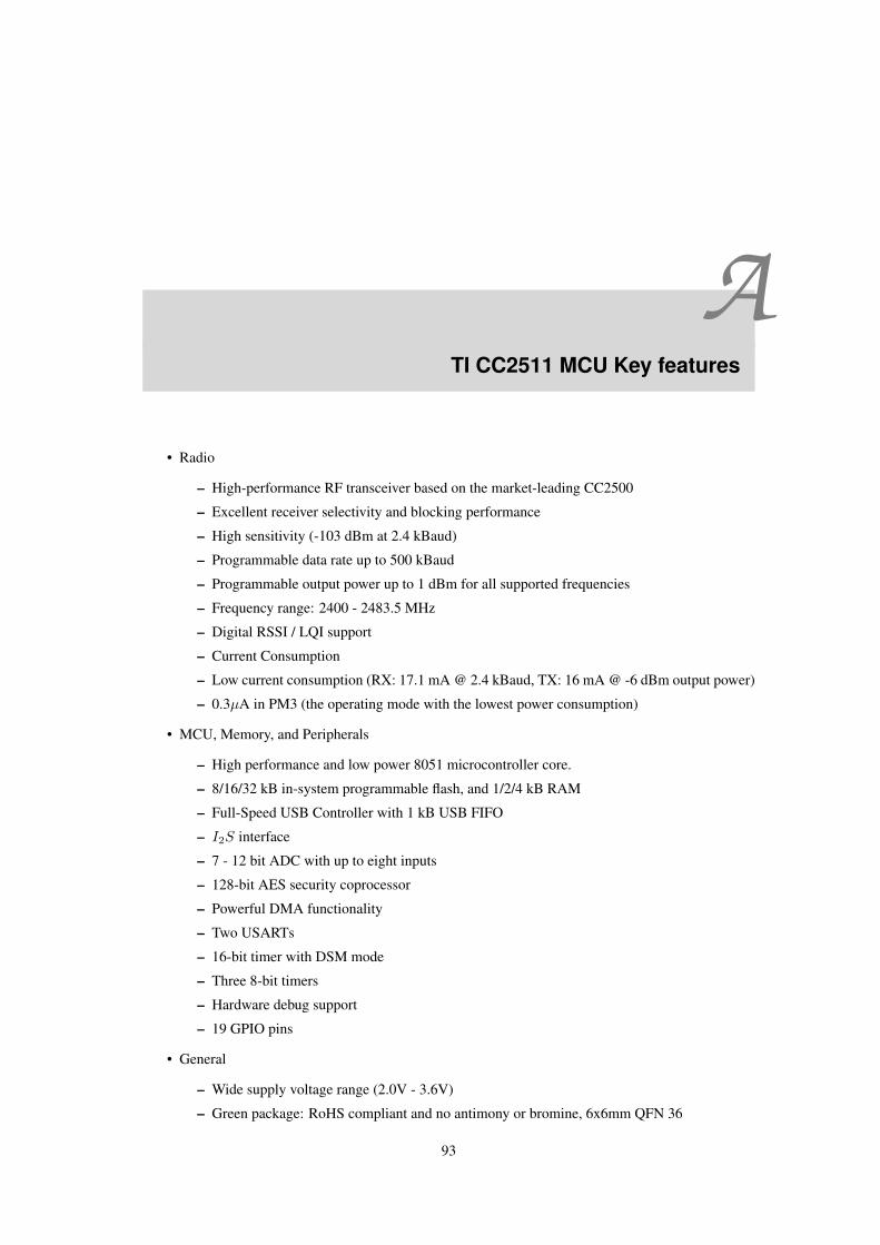
ATI CC2511 MCU Key features
• Radio
– High-performance RF transceiver based on the market-leading CC2500
– Excellent receiver selectivity and blocking performance
– High sensitivity (-103 dBm at 2.4 kBaud)
– Programmable data rate up to 500 kBaud
– Programmable output power up to 1 dBm for all supported frequencies
– Frequency range: 2400 - 2483.5 MHz
– Digital RSSI / LQI support
– Current Consumption
– Low current consumption (RX: 17.1 mA @ 2.4 kBaud, TX: 16 mA @ -6 dBm output power)
– 0.3µA in PM3 (the operating mode with the lowest power consumption)
• MCU, Memory, and Peripherals
– High performance and low power 8051 microcontroller core.
– 8/16/32 kB in-system programmable flash, and 1/2/4 kB RAM
– Full-Speed USB Controller with 1 kB USB FIFO
– I2S interface
– 7 - 12 bit ADC with up to eight inputs
– 128-bit AES security coprocessor
– Powerful DMA functionality
– Two USARTs
– 16-bit timer with DSM mode
– Three 8-bit timers
– Hardware debug support
– 19 GPIO pins
• General
– Wide supply voltage range (2.0V - 3.6V)
– Green package: RoHS compliant and no antimony or bromine, 6x6mm QFN 36
93
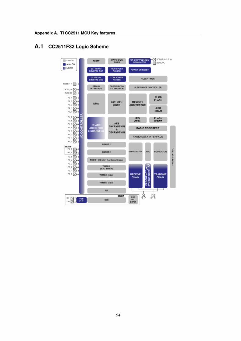
Appendix A. TI CC2511 MCU Key features
A.1 CC2511F32 Logic Scheme
94
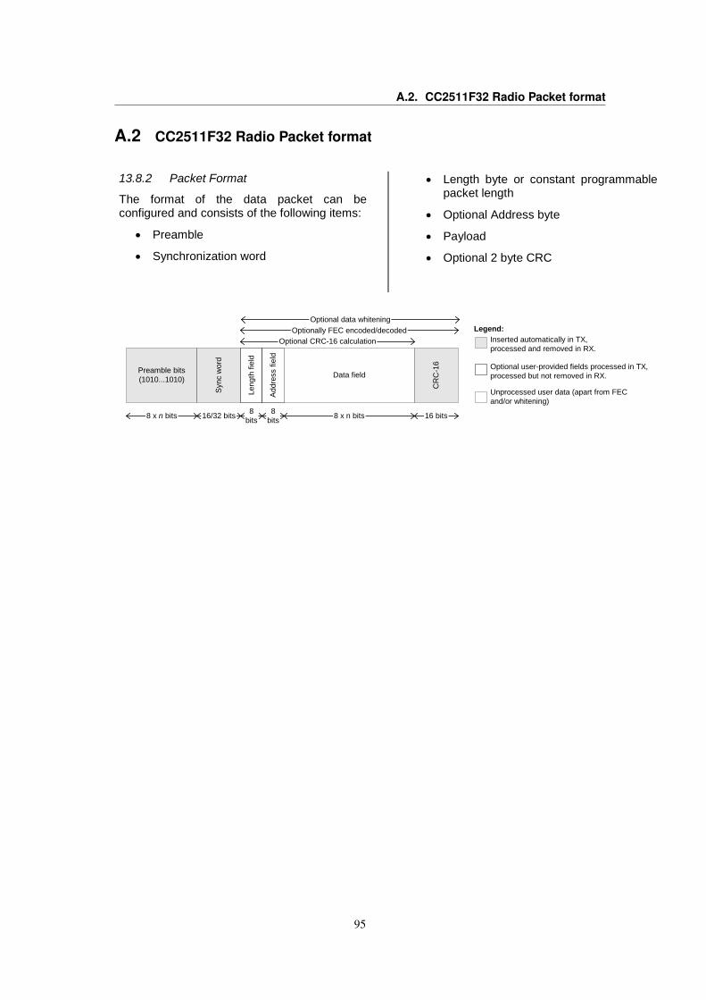
A.2. CC2511F32 Radio Packet format
A.2 CC2511F32 Radio Packet format
CC2510Fx / CC2511Fx
SWRS055G Page 191 of 236
XOR-ed with a 9-bit pseudo-random (PN9) sequence before being transmitted as shown in Figure 50. At the receiver end, the data are XOR-ed with the same pseudo-random sequence. This way, the whitening is reversed,
and the original data appear in the receiver. The PN9 sequence is reset to all 1’s.
Data whitening can only be used when PKTCTRL0.CC2400_EN=0 (default).
TX_OUT[7:0]
TX_DATA
8 7 6 5 4 3 2 1 0
7 6 5 4 3 2 1 0
The first TX_DATA byte is shifted in before doing the XOR-operation providing the first TX_OUT[7:0] byte. The second TX_DATA byte is then shifted in before doing the XOR-operation providing the second TX_OUT[7:0] byte.
Figure 50: Data Whitening in TX Mode
13.8.2 Packet Format
The format of the data packet can be configured and consists of the following items:
• Preamble
• Synchronization word
• Length byte or constant programmable packet length
• Optional Address byte
• Payload
• Optional 2 byte CRC
Preamble bits(1010...1010)
Syn
c w
ord
Leng
th fi
eld
Add
ress
fiel
d
Data field
CR
C-1
6
Optional CRC-16 calculationOptionally FEC encoded/decoded
8 x n bits 16/32 bits 8bits
8bits 8 x n bits 16 bits
Optional data whiteningLegend:
Inserted automatically in TX,processed and removed in RX.
Optional user-provided fields processed in TX,processed but not removed in RX.
Unprocessed user data (apart from FECand/or whitening)
Figure 51: Packet Format
CC2511F8 - Not Recommended for New Designs
95

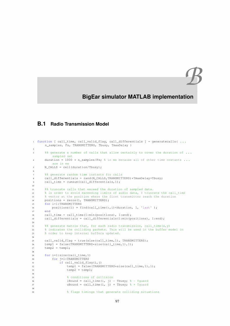
BBigEar simulator MATLAB implementation
B.1 Radio Transmission Model
1 function [ call_time, call_valid_flag, call_differentials ] = generatecalls( ...n_samples, Fs, TRANSMITTERS, Tbusy, TmaxDelay )
2
3 %% generate a number of calls that allow certainly to cover the duration of ...sampled set
4 duration = 1000 * n_samples/Fs; % in ms because all of other time costants ...are in ms
5 N_CALLS = ceil(duration/Tbusy);6
7 %% generate random time instants for calls8 call_differentials = rand(N_CALLS,TRANSMITTERS)*TmaxDelay+Tbusy;9 call_time = cumsum(call_differentials,1);
10
11 %% truncate calls that exceed the duration of sampled data.12 % in order to avoid exceeding limits of audio data, I truncate the call_time13 % vector at the position where the first transmitter reach the duration14 positions = zeros(1, TRANSMITTERS);15 for i=1:TRANSMITTERS16 positions(i) = find(call_time(:,i)<duration, 1, 'last' );17 end18 call_time = call_time(1:min(positions), 1:end);19 call_differentials = call_differentials(1:min(positions), 1:end);20
21 %% generate matrix that, for each radio transmission, call_time(x,y)22 % indicates the colliding packets. This will be used in the buffer model in23 % order to keep internal buffers updated.24
25 call_valid_flag = true(size(call_time,1), TRANSMITTERS);26 temp1 = false(TRANSMITTERS*size(call_time,1),1);27 temp2 = temp1;28
29 for i=1:size(call_time,1)30 for j=1:TRANSMITTERS31 if call_valid_flag(i,j)32 temp1 = false(TRANSMITTERS*size(call_time,1),1);33 temp2 = temp1;34
35 % conditions of collision36 lBound = call_time(i, j) - Tbusy; % - Tguard37 uBound = call_time(i, j) + Tbusy; % + Tguard38
39 % flags timings that generate colliding situations
97
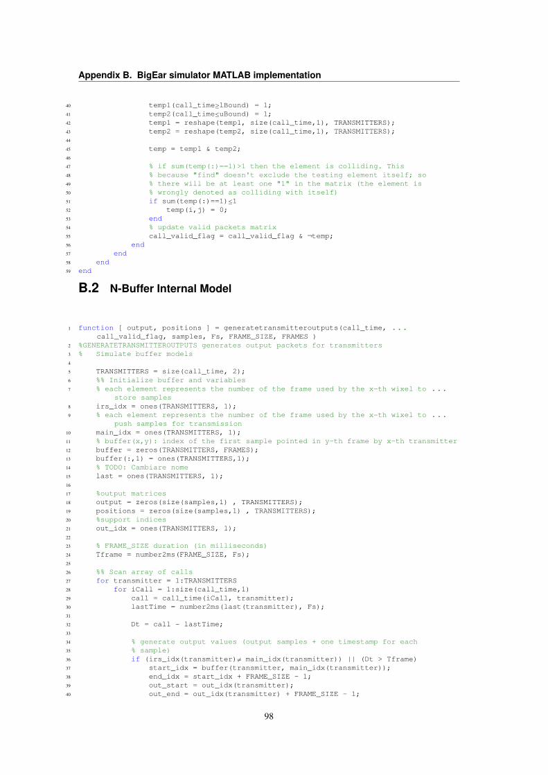
Appendix B. BigEar simulator MATLAB implementation
40 temp1(call_time≥lBound) = 1;41 temp2(call_time≤uBound) = 1;42 temp1 = reshape(temp1, size(call_time,1), TRANSMITTERS);43 temp2 = reshape(temp2, size(call_time,1), TRANSMITTERS);44
45 temp = temp1 & temp2;46
47 % if sum(temp(:)==1)>1 then the element is colliding. This48 % because "find" doesn't exclude the testing element itself; so49 % there will be at least one "1" in the matrix (the element is50 % wrongly denoted as colliding with itself)51 if sum(temp(:)==1)≤152 temp(i,j) = 0;53 end54 % update valid packets matrix55 call_valid_flag = call_valid_flag & ¬temp;56 end57 end58 end59 end
B.2 N-Buffer Internal Model
1 function [ output, positions ] = generatetransmitteroutputs(call_time, ...call_valid_flag, samples, Fs, FRAME_SIZE, FRAMES )
2 %GENERATETRANSMITTEROUTPUTS generates output packets for transmitters3 % Simulate buffer models4
5 TRANSMITTERS = size(call_time, 2);6 %% Initialize buffer and variables7 % each element represents the number of the frame used by the x-th wixel to ...
store samples8 irs_idx = ones(TRANSMITTERS, 1);9 % each element represents the number of the frame used by the x-th wixel to ...
push samples for transmission10 main_idx = ones(TRANSMITTERS, 1);11 % buffer(x,y): index of the first sample pointed in y-th frame by x-th transmitter12 buffer = zeros(TRANSMITTERS, FRAMES);13 buffer(:,1) = ones(TRANSMITTERS,1);14 % TODO: Cambiare nome15 last = ones(TRANSMITTERS, 1);16
17 %output matrices18 output = zeros(size(samples,1) , TRANSMITTERS);19 positions = zeros(size(samples,1) , TRANSMITTERS);20 %support indices21 out_idx = ones(TRANSMITTERS, 1);22
23 % FRAME_SIZE duration (in milliseconds)24 Tframe = number2ms(FRAME_SIZE, Fs);25
26 %% Scan array of calls27 for transmitter = 1:TRANSMITTERS28 for iCall = 1:size(call_time,1)29 call = call_time(iCall, transmitter);30 lastTime = number2ms(last(transmitter), Fs);31
32 Dt = call - lastTime;33
34 % generate output values (output samples + one timestamp for each35 % sample)36 if (irs_idx(transmitter)6= main_idx(transmitter)) || (Dt > Tframe)37 start_idx = buffer(transmitter, main_idx(transmitter));38 end_idx = start_idx + FRAME_SIZE - 1;39 out_start = out_idx(transmitter);40 out_end = out_idx(transmitter) + FRAME_SIZE - 1;
98
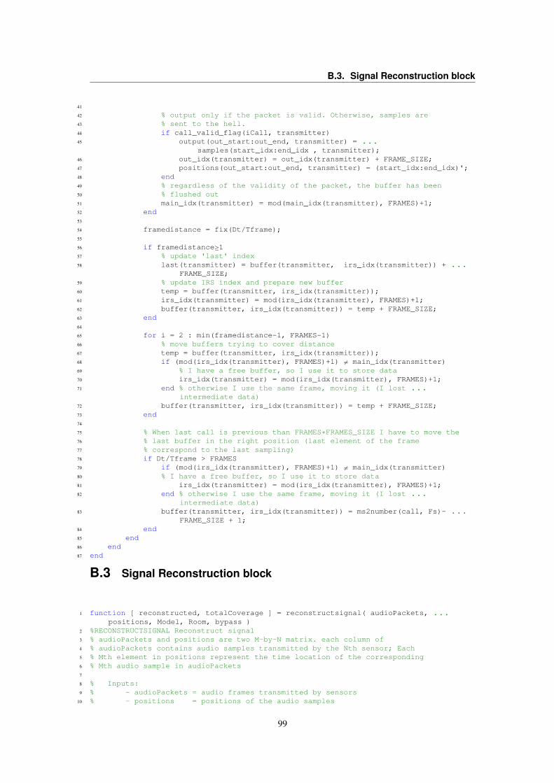
B.3. Signal Reconstruction block
41
42 % output only if the packet is valid. Otherwise, samples are43 % sent to the hell.44 if call_valid_flag(iCall, transmitter)45 output(out_start:out_end, transmitter) = ...
samples(start_idx:end_idx , transmitter);46 out_idx(transmitter) = out_idx(transmitter) + FRAME_SIZE;47 positions(out_start:out_end, transmitter) = (start_idx:end_idx)';48 end49 % regardless of the validity of the packet, the buffer has been50 % flushed out51 main_idx(transmitter) = mod(main_idx(transmitter), FRAMES)+1;52 end53
54 framedistance = fix(Dt/Tframe);55
56 if framedistance≥157 % update 'last' index58 last(transmitter) = buffer(transmitter, irs_idx(transmitter)) + ...
FRAME_SIZE;59 % update IRS index and prepare new buffer60 temp = buffer(transmitter, irs_idx(transmitter));61 irs_idx(transmitter) = mod(irs_idx(transmitter), FRAMES)+1;62 buffer(transmitter, irs_idx(transmitter)) = temp + FRAME_SIZE;63 end64
65 for i = 2 : min(framedistance-1, FRAMES-1)66 % move buffers trying to cover distance67 temp = buffer(transmitter, irs_idx(transmitter));68 if (mod(irs_idx(transmitter), FRAMES)+1) 6= main_idx(transmitter)69 % I have a free buffer, so I use it to store data70 irs_idx(transmitter) = mod(irs_idx(transmitter), FRAMES)+1;71 end % otherwise I use the same frame, moving it (I lost ...
intermediate data)72 buffer(transmitter, irs_idx(transmitter)) = temp + FRAME_SIZE;73 end74
75 % When last call is previous than FRAMES*FRAMES_SIZE I have to move the76 % last buffer in the right position (last element of the frame77 % correspond to the last sampling)78 if Dt/Tframe > FRAMES79 if (mod(irs_idx(transmitter), FRAMES)+1) 6= main_idx(transmitter)80 % I have a free buffer, so I use it to store data81 irs_idx(transmitter) = mod(irs_idx(transmitter), FRAMES)+1;82 end % otherwise I use the same frame, moving it (I lost ...
intermediate data)83 buffer(transmitter, irs_idx(transmitter)) = ms2number(call, Fs)- ...
FRAME_SIZE + 1;84 end85 end86 end87 end
B.3 Signal Reconstruction block
1 function [ reconstructed, totalCoverage ] = reconstructsignal( audioPackets, ...positions, Model, Room, bypass )
2 %RECONSTRUCTSIGNAL Reconstruct signal3 % audioPackets and positions are two M-by-N matrix. each column of4 % audioPackets contains audio samples transmitted by the Nth sensor; Each5 % Mth element in positions represent the time location of the corresponding6 % Mth audio sample in audioPackets7
8 % Inputs:9 % - audioPackets = audio frames transmitted by sensors
10 % - positions = positions of the audio samples
99
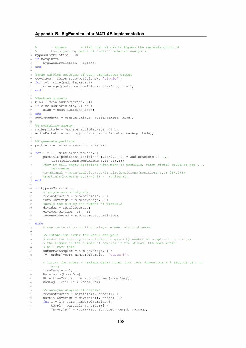
Appendix B. BigEar simulator MATLAB implementation
11 % - bypass = flag that allows to bypass the reconstruction of12 % the signal by means of crosscorrelation analysis.13 bypassCorrelation = 0;14 if nargin==515 bypassCorrelation = bypass;16 end17
18 %%map samples coverage of each transmitter output19 coverage = zeros(size(positions), 'single');20 for i=1: size(audioPackets,2)21 coverage(positions(positions(:,i)>0,i),i) = 1;22 end23
24 %%unbias signals25 bias = mean(audioPackets, 2);26 if size(audioPackets, 2) == 127 bias = mean(audioPackets);28 end29 audioPackets = bsxfun(@minus, audioPackets, bias);30
31 %% normalize energy32 maxAmplitude = max(abs(audioPackets),[],1);33 audioPackets = bsxfun(@rdivide, audioPackets, maxAmplitude);34
35 %% generate partials36 partials = zeros(size(audioPackets));37
38 for i = 1 : size(audioPackets,2)39 partials(positions(positions(:,i)>0,i),i) = audioPackets(1: ...
size(positions(positions(:,i)>0)),i);40 %try to fill empty positions with mean of partials, since signal could be not ...
zero-mean41 %avgSignal = mean(audioPackets(1: size(positions(positions(:,i)>0)),i));42 %partials(coverage(:,i)==0,i) = avgSignal;43 end44
45 if bypassCorrelation46 % simple sum of signals:47 reconstructed = sum(partials, 2);48 totalCoverage = sum(coverage, 2);49 %scale the sum by the number of partials50 divider = totalCoverage;51 divider(divider==0) = 1;52 reconstructed = reconstructed./divider;53
54 else55 % use correlation to find delays between audio streams56
57 %% estabilish order for xcorr analysis58 % order for testing xcorrelation is given by number of samples in a stream.59 % the bigger is the number of samples in the stream, the more xcorr60 % will work fine.61 numberOfSamples = sum(coverage, 1);62 [¬, order]=sort(numberOfSamples, 'descend');63
64 % limits for xcorr = maximum delay given from room dimensions + 2 seconds of ...margin
65 timeMargin = 2;66 Ds = norm(Room.Dim);67 Dt = timeMargin + Ds / SoundSpeed(Room.Temp);68 maxLag = ceil(Dt * Model.Fs);69
70 %% analyze couples of streams71 reconstructed = partials(:, order(1));72 partialCoverage = coverage(:, order(1));73 for i = 2 : size(numberOfSamples,2)74 temp2 = partials(:, order(i));75 [acor,lag] = xcorr(reconstructed, temp2, maxLag);
100
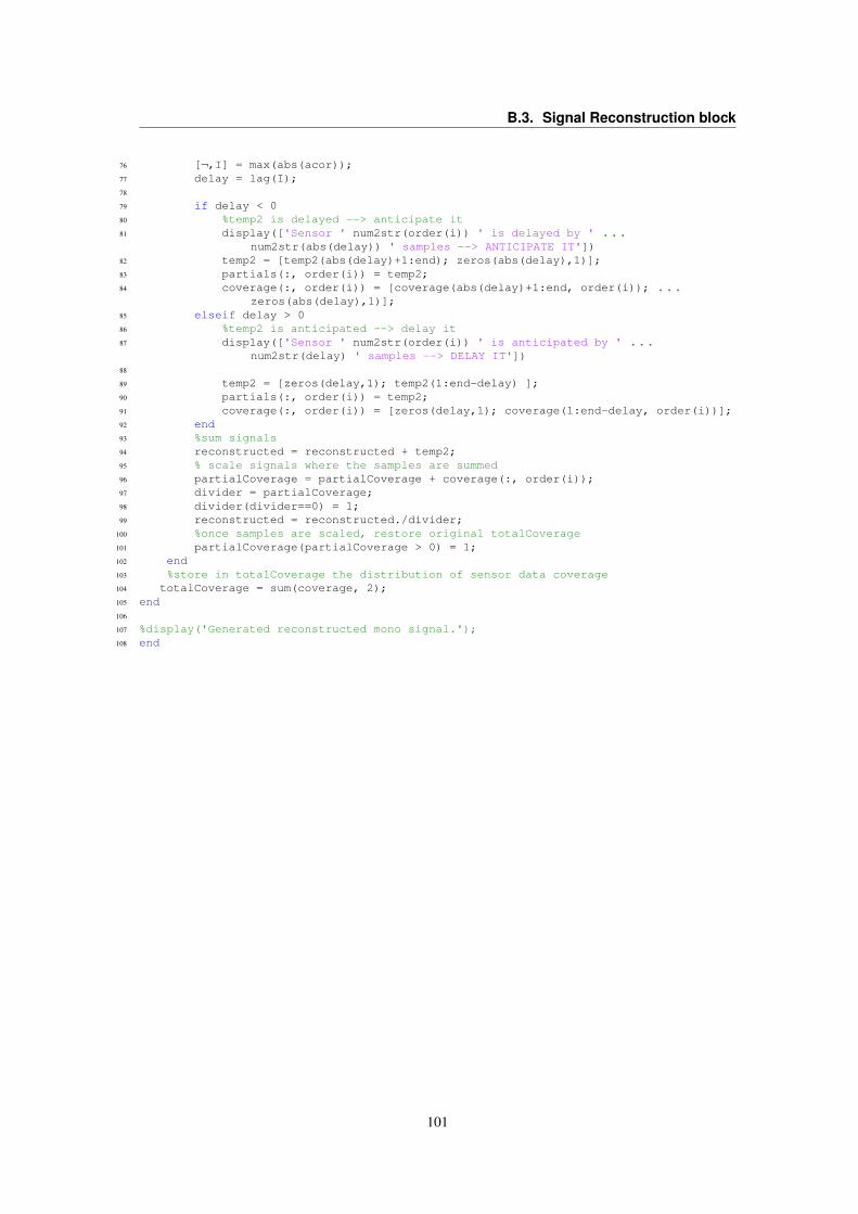
B.3. Signal Reconstruction block
76 [¬,I] = max(abs(acor));77 delay = lag(I);78
79 if delay < 080 %temp2 is delayed --> anticipate it81 display(['Sensor ' num2str(order(i)) ' is delayed by ' ...
num2str(abs(delay)) ' samples --> ANTICIPATE IT'])82 temp2 = [temp2(abs(delay)+1:end); zeros(abs(delay),1)];83 partials(:, order(i)) = temp2;84 coverage(:, order(i)) = [coverage(abs(delay)+1:end, order(i)); ...
zeros(abs(delay),1)];85 elseif delay > 086 %temp2 is anticipated --> delay it87 display(['Sensor ' num2str(order(i)) ' is anticipated by ' ...
num2str(delay) ' samples --> DELAY IT'])88
89 temp2 = [zeros(delay,1); temp2(1:end-delay) ];90 partials(:, order(i)) = temp2;91 coverage(:, order(i)) = [zeros(delay,1); coverage(1:end-delay, order(i))];92 end93 %sum signals94 reconstructed = reconstructed + temp2;95 % scale signals where the samples are summed96 partialCoverage = partialCoverage + coverage(:, order(i));97 divider = partialCoverage;98 divider(divider==0) = 1;99 reconstructed = reconstructed./divider;
100 %once samples are scaled, restore original totalCoverage101 partialCoverage(partialCoverage > 0) = 1;102 end103 %store in totalCoverage the distribution of sensor data coverage104 totalCoverage = sum(coverage, 2);105 end106
107 %display('Generated reconstructed mono signal.');108 end
101

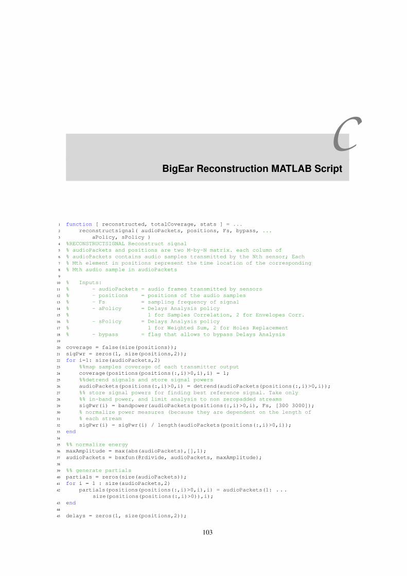
CBigEar Reconstruction MATLAB Script
1 function [ reconstructed, totalCoverage, stats ] = ...2 reconstructsignal( audioPackets, positions, Fs, bypass, ...3 aPolicy, sPolicy )4 %RECONSTRUCTSIGNAL Reconstruct signal5 % audioPackets and positions are two M-by-N matrix. each column of6 % audioPackets contains audio samples transmitted by the Nth sensor; Each7 % Mth element in positions represent the time location of the corresponding8 % Mth audio sample in audioPackets9
10 % Inputs:11 % - audioPackets = audio frames transmitted by sensors12 % - positions = positions of the audio samples13 % - Fs = sampling frequency of signal14 % - aPolicy = Delays Analysis policy15 % 1 for Samples Correlation, 2 for Envelopes Corr.16 % - sPolicy = Delays Analysis policy17 % 1 for Weighted Sum, 2 for Holes Replacement18 % - bypass = flag that allows to bypass Delays Analysis19
20 coverage = false(size(positions));21 sigPwr = zeros(1, size(positions,2));22 for i=1: size(audioPackets,2)23 %%map samples coverage of each transmitter output24 coverage(positions(positions(:,i)>0,i),i) = 1;25 %%detrend signals and store signal powers26 audioPackets(positions(:,i)>0,i) = detrend(audioPackets(positions(:,i)>0,i));27 %% store signal powers for finding best reference signal. Take only28 %% in-band power, and limit analysis to non zeropadded streams29 sigPwr(i) = bandpower(audioPackets(positions(:,i)>0,i), Fs, [300 3000]);30 % normalize power measures (because they are dependent on the length of31 % each stream32 sigPwr(i) = sigPwr(i) / length(audioPackets(positions(:,i)>0,i));33 end34
35 %% normalize energy36 maxAmplitude = max(abs(audioPackets),[],1);37 audioPackets = bsxfun(@rdivide, audioPackets, maxAmplitude);38
39 %% generate partials40 partials = zeros(size(audioPackets));41 for i = 1 : size(audioPackets,2)42 partials(positions(positions(:,i)>0,i),i) = audioPackets(1: ...
size(positions(positions(:,i)>0)),i);43 end44
45 delays = zeros(1, size(positions,2));
103
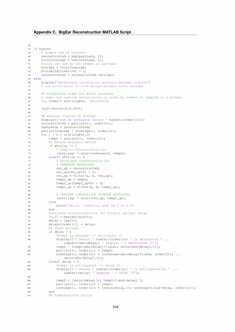
Appendix C. BigEar Reconstruction MATLAB Script
46
47 if bypass48 % simple sum of signals:49 reconstructed = sum(partials, 2);50 totalCoverage = sum(coverage, 2);51 %scale the sum by the number of partials52 divider = totalCoverage;53 divider(divider==0) = 1;54 reconstructed = reconstructed./divider;55 else56 display('Performing correlation analysis between signals')57 % use correlation to find delays between audio streams58
59 %% estabilish order for xcorr analysis60 % order for testing xcorrelation is given by number of samples in a stream.61 [¬, order]= sort(sigPwr, 'descend');62
63 [a,b]=butter(2,0.004);64
65 %% analyze couples of streams66 display(['Use as reference Sensor ' num2str(order(1))])67 reconstructed = partials(:, order(1));68 reference = reconstructed;69 partialCoverage = coverage(:, order(1));70 for i = 2 : size(sigPwr,2)71 temp2 = partials(:, order(i));72 %% Delays Analysis method73 if aPolicy == 174 % Samples Crosscorrelation75 [acor,lag] = xcorr(reference, temp2);76 elseif aPolicy == 277 % Envelopes Crosscorrelation78 % GENERATE ENVELOPES79 rec_up = reconstructed;80 rec_up(rec_up<0) = 0;81 rec_up = filter(a, b, rec_up);82 temp2_up = temp2;83 temp2_up(temp2_up<0) = 0;84 temp2_up = filter(a, b, temp2_up);85
86 % PERFORM CORRELATION BETWEEN ENVELOPES87 [acor,lag] = xcorr(rec_up, temp2_up);88 else89 error('Error. \naPolicy must be 1 or 2.')90 end91 %evaluate crosscorrelation for findinf optimal delay92 [¬,I] = max(abs(acor));93 delay = lag(I);94 delays(order(i)) = delay;95 %% shift streams96 if delay < 097 %temp2 is delayed --> anticipate it98 display(['* Sensor ' num2str(order(i)) ' is delayed by ' ...
num2str(abs(delay)) ' samples --> ANTICIPATE IT'])99 temp2 = [temp2(abs(delay)+1:end); zeros(abs(delay),1)];
100 partials(:, order(i)) = temp2;101 coverage(:, order(i)) = [coverage(abs(delay)+1:end, order(i)); ...
zeros(abs(delay),1)];102 elseif delay > 0103 %temp2 is anticipated --> delay it104 display(['* Sensor ' num2str(order(i)) ' is anticipated by ' ...
num2str(delay) ' samples --> DELAY IT'])105
106 temp2 = [zeros(delay,1); temp2(1:end-delay) ];107 partials(:, order(i)) = temp2;108 coverage(:, order(i)) = [zeros(delay,1); coverage(1:end-delay, order(i))];109 end110 %% Superposition policy
104
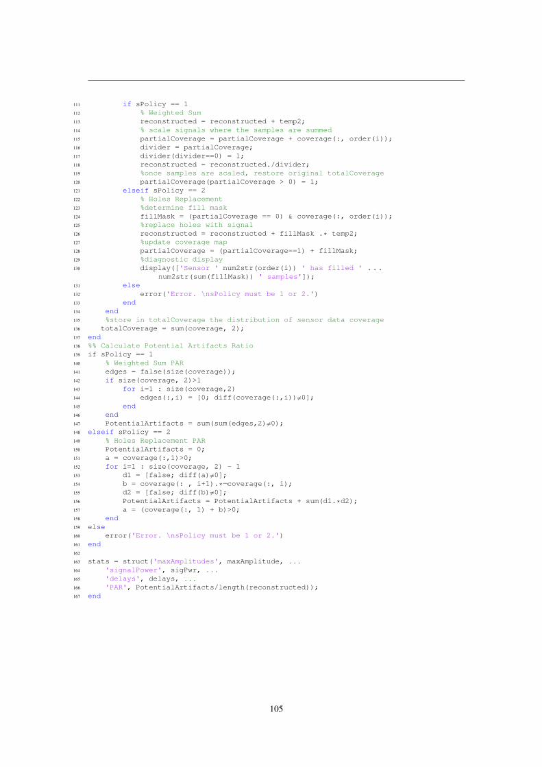
111 if sPolicy == 1112 % Weighted Sum113 reconstructed = reconstructed + temp2;114 % scale signals where the samples are summed115 partialCoverage = partialCoverage + coverage(:, order(i));116 divider = partialCoverage;117 divider(divider==0) = 1;118 reconstructed = reconstructed./divider;119 %once samples are scaled, restore original totalCoverage120 partialCoverage(partialCoverage > 0) = 1;121 elseif sPolicy == 2122 % Holes Replacement123 %determine fill mask124 fillMask = (partialCoverage == 0) & coverage(:, order(i));125 %replace holes with signal126 reconstructed = reconstructed + fillMask .* temp2;127 %update coverage map128 partialCoverage = (partialCoverage==1) + fillMask;129 %diagnostic display130 display(['Sensor ' num2str(order(i)) ' has filled ' ...
num2str(sum(fillMask)) ' samples']);131 else132 error('Error. \nsPolicy must be 1 or 2.')133 end134 end135 %store in totalCoverage the distribution of sensor data coverage136 totalCoverage = sum(coverage, 2);137 end138 %% Calculate Potential Artifacts Ratio139 if sPolicy == 1140 % Weighted Sum PAR141 edges = false(size(coverage));142 if size(coverage, 2)>1143 for i=1 : size(coverage,2)144 edges(:,i) = [0; diff(coverage(:,i))6=0];145 end146 end147 PotentialArtifacts = sum(sum(edges,2)6=0);148 elseif sPolicy == 2149 % Holes Replacement PAR150 PotentialArtifacts = 0;151 a = coverage(:,1)>0;152 for i=1 : size(coverage, 2) - 1153 d1 = [false; diff(a)6=0];154 b = coverage(: , i+1).*¬coverage(:, i);155 d2 = [false; diff(b)6=0];156 PotentialArtifacts = PotentialArtifacts + sum(d1.*d2);157 a = (coverage(:, 1) + b)>0;158 end159 else160 error('Error. \nsPolicy must be 1 or 2.')161 end162
163 stats = struct('maxAmplitudes', maxAmplitude, ...164 'signalPower', sigPwr, ...165 'delays', delays, ...166 'PAR', PotentialArtifacts/length(reconstructed));167 end
105

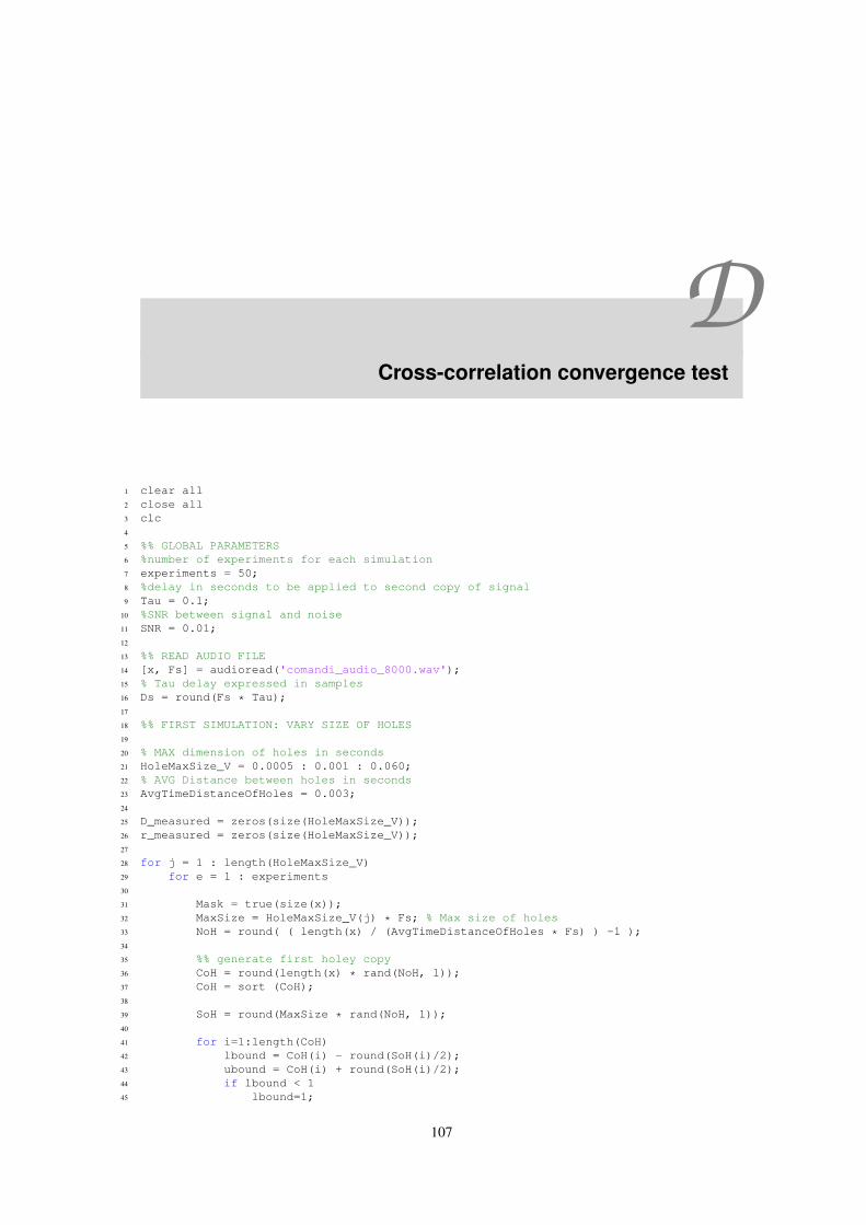
DCross-correlation convergence test
1 clear all2 close all3 clc4
5 %% GLOBAL PARAMETERS6 %number of experiments for each simulation7 experiments = 50;8 %delay in seconds to be applied to second copy of signal9 Tau = 0.1;
10 %SNR between signal and noise11 SNR = 0.01;12
13 %% READ AUDIO FILE14 [x, Fs] = audioread('comandi_audio_8000.wav');15 % Tau delay expressed in samples16 Ds = round(Fs * Tau);17
18 %% FIRST SIMULATION: VARY SIZE OF HOLES19
20 % MAX dimension of holes in seconds21 HoleMaxSize_V = 0.0005 : 0.001 : 0.060;22 % AVG Distance between holes in seconds23 AvgTimeDistanceOfHoles = 0.003;24
25 D_measured = zeros(size(HoleMaxSize_V));26 r_measured = zeros(size(HoleMaxSize_V));27
28 for j = 1 : length(HoleMaxSize_V)29 for e = 1 : experiments30
31 Mask = true(size(x));32 MaxSize = HoleMaxSize_V(j) * Fs; % Max size of holes33 NoH = round( ( length(x) / (AvgTimeDistanceOfHoles * Fs) ) -1 );34
35 %% generate first holey copy36 CoH = round(length(x) * rand(NoH, 1));37 CoH = sort (CoH);38
39 SoH = round(MaxSize * rand(NoH, 1));40
41 for i=1:length(CoH)42 lbound = CoH(i) - round(SoH(i)/2);43 ubound = CoH(i) + round(SoH(i)/2);44 if lbound < 145 lbound=1;
107

Appendix D. Cross-correlation convergence test
46 end47 if ubound > length(x)48 ubound = length(x);49 end50 Mask(lbound : ubound) = 0;51 end52 y1 = x .* Mask;53
54 %% generate second holey copy55 Mask = true(size(x));56 CoH = round(length(x) * rand(NoH, 1));57 CoH = sort (CoH);58
59 SoH = round(MaxSize * rand(NoH, 1));60
61 for i=1:length(CoH)62 lbound = CoH(i) - round(SoH(i)/2);63 ubound = CoH(i) + round(SoH(i)/2);64 if lbound < 165 lbound=1;66 end67 if ubound > length(x)68 ubound = length(x);69 end70 Mask(lbound : ubound) = 0;71 end72 y2 = x .* Mask;73
74 %% delay second signal75 y2d = [zeros(Ds,1); y2(1 : end - Ds)];76
77 %% noise signals78 noiseAmplitude = max(abs(y1)) * SNR;79 y1n = y1 + noiseAmplitude * randn(size(y1));80 scale = max(abs(x))/max(abs(y1n));81 y1n = y1n .* scale;82
83 noiseAmplitude = max(abs(y2d)) * SNR;84 y2n = y2d + noiseAmplitude * randn(size(y2d));85 scale = max(abs(x))/max(abs(y2n));86 y2n = y2n .* scale;87
88 %% perform correlation89 [r, lags] = xcorr(y1n,y2n);90 [¬, I] = max(abs(r));91 %save measured data92 D_m = lags(I);93
94 D_measured(j) = D_measured(j) + D_m / experiments;95 r_measured(j) = r_measured(j) + max(abs(r)) / experiments;96 end97 end98 D_measured = abs(D_measured);99 D_difference = abs(D_measured - Ds);
100
101 figure102 stem(HoleMaxSize_V.*1000, D_difference);103 title ('Delay difference D - D_m in function of the size of holes')104 xlabel('Maximum size of holes (ms)')105 ylabel('Measured difference (s)')106 figure107 plot(HoleMaxSize_V.*1000, r_measured, 'r');108 title ('Maximum cross-correlation value R_f_g[n^*] in function of the size of holes')109 xlabel('Maximum size of holes (ms)')110 ylabel('Measured difference (s)')111
112 %% SECOND SIMULATION: VARY AVERAGE TIME DISTANCE BETWEEN HOLES113
108

114 HoleMaxSize = 0.012; % MAX dimension of holes in seconds115 AvgTimeDistanceOfHoles_V = 0.030 : -0.001 : 0.001;116
117 %% read audio file118 [x, Fs] = audioread('comandi_audio_8000.wav');119 Ds = round(Fs * Tau);120
121 D_measured = zeros(size(AvgTimeDistanceOfHoles_V));122 r_measured = zeros(size(AvgTimeDistanceOfHoles_V));123
124 for j = 1 : length(AvgTimeDistanceOfHoles_V)125 for e = 1 : experiments126
127 Mask = true(size(x));128 MaxSize = HoleMaxSize * Fs; % Max size of holes129 NoH = round( ( length(x) / (AvgTimeDistanceOfHoles_V(j) * Fs) ) -1 );130
131 %% generate first holey copy132 CoH = round(length(x) * rand(NoH, 1));133 CoH = sort (CoH);134
135 SoH = round(MaxSize * rand(NoH, 1));136
137 for i=1:length(CoH)138 lbound = CoH(i) - round(SoH(i)/2);139 ubound = CoH(i) + round(SoH(i)/2);140 if lbound < 1141 lbound=1;142 end143 if ubound > length(x)144 ubound = length(x);145 end146 Mask(lbound : ubound) = 0;147 end148 y1 = x .* Mask;149
150 %% generate second holey copy151 Mask = true(size(x));152 CoH = round(length(x) * rand(NoH, 1));153 CoH = sort (CoH);154
155 SoH = round(MaxSize * rand(NoH, 1));156
157 for i=1:length(CoH)158 lbound = CoH(i) - round(SoH(i)/2);159 ubound = CoH(i) + round(SoH(i)/2);160 if lbound < 1161 lbound=1;162 end163 if ubound > length(x)164 ubound = length(x);165 end166 Mask(lbound : ubound) = 0;167 end168 y2 = x .* Mask;169
170 %% delay second signal171 y2d = [zeros(Ds,1); y2(1 : end - Ds)];172
173 %% noise signals174
175 noiseAmplitude = max(abs(y1)) * SNR;176 y1n = y1 + noiseAmplitude * randn(size(y1));177 scale = max(abs(x))/max(abs(y1n));178 y1n = y1n .* scale;179
180 noiseAmplitude = max(abs(y2d)) * SNR;181 y2n = y2d + noiseAmplitude * randn(size(y2d));
109
Appendix D. Cross-correlation convergence test
182 scale = max(abs(x))/max(abs(y2n));183 y2n = y2n .* scale;184
185 %% perform correlation186 [r, lags] = xcorr(y1n,y2n);187 [¬, I] = max(abs(r));188 %save measured data189 D_m = lags(I);190
191 D_measured(j) = D_measured(j) + D_m / experiments;192 r_measured(j) = r_measured(j) + max(abs(r)) / experiments;193 end194 end195 D_measured = abs(D_measured);196 D_difference = abs(D_measured - Ds);197
198 figure199 stem(AvgTimeDistanceOfHoles_V.*1000, D_difference);200 title ('Delay difference D - D_m in function of the number of holes')201 xlabel('Average time distance between holes (ms)')202 ylabel('Measured difference (s)')203 figure204 plot(AvgTimeDistanceOfHoles_V.*1000, r_measured, 'r');205 title ('Maximum cross-correlation value R_f_g[n^*] in function of the number of ...
holes')206 xlabel('Average time distance between holes (ms)')207 ylabel('Measured difference (s)')
110
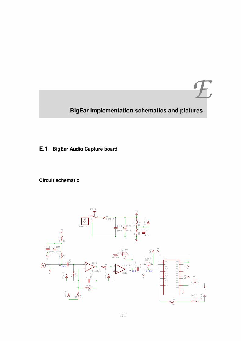
EBigEar Implementation schematics and pictures
E.1 BigEar Audio Capture board
Circuit schematic
Sp iceO rder 1 Sp iceO rder 2
GND
Vin
P0_0
P0_1
P0_2
P0_3
P0_4
P0_5
VALT
P2_1
P2_2
GND
P1_0
P1_1
P1_2
P1_3
P1_4
P1_5
P1_6
P1_7
RST
3.3v
GND
82
2k2
2k2
100k
100n 100u
100u
4.7
n
47
0p
F
22
0u
1N4007
V-
+3
V3
+3
V3
V -
V+
1k +3
V3
V -
200k
100k
V-
1k
1k
LT1013N
LT1013N
12
0k
100n
V+
10
k1
0k
V -
VC
C/2
VC
C/2
VC
C/2
V -VC
C/2
4 .7u
V-
V+
R8
R7
R3
R 2
C1IC C2IC
C2M
C1
C2
C_
OU
T
D 1
W 1
R6
BATTERY
12
R_BIAS
A E
S
12
R5_VAR
1 3
2
RST
12
BOOT
12
PW R1
23
1
R5_FIX
R4
IC1A
2
31
IC1B
6
57
R1
C 1M
R1
0R
9
C 3
+
+
1 3
+
V_m ic
V_adc V_b ias
111

Appendix E. BigEar Implementation schematics and pictures
Circuit prototype
E.2 BigEar Receiver
BigEar Receiver schematic
GND
Vin
P0_0
P0_1
P0_2
P0_3
P0_4
P0_5
VALT
P2_1
P2_2
GND
P1_0
P1_1
P1_2
P1_3
P1_4
P1_5
P1_6
P1_7
RST
3.3v
GND
VC
C
VC
C
1k
BA
TT
ER
Y
GND
GND
GND
GND
GND
W 1
11
22
RST
11
22
BOOTLDRR1
B1
+-
JP1
123
11
22
P0_0
11
22
P0_1
Jum per on 3-2: active H IGH
Jum per on 1-2: active LOW
BigEar Receiver prototype
112
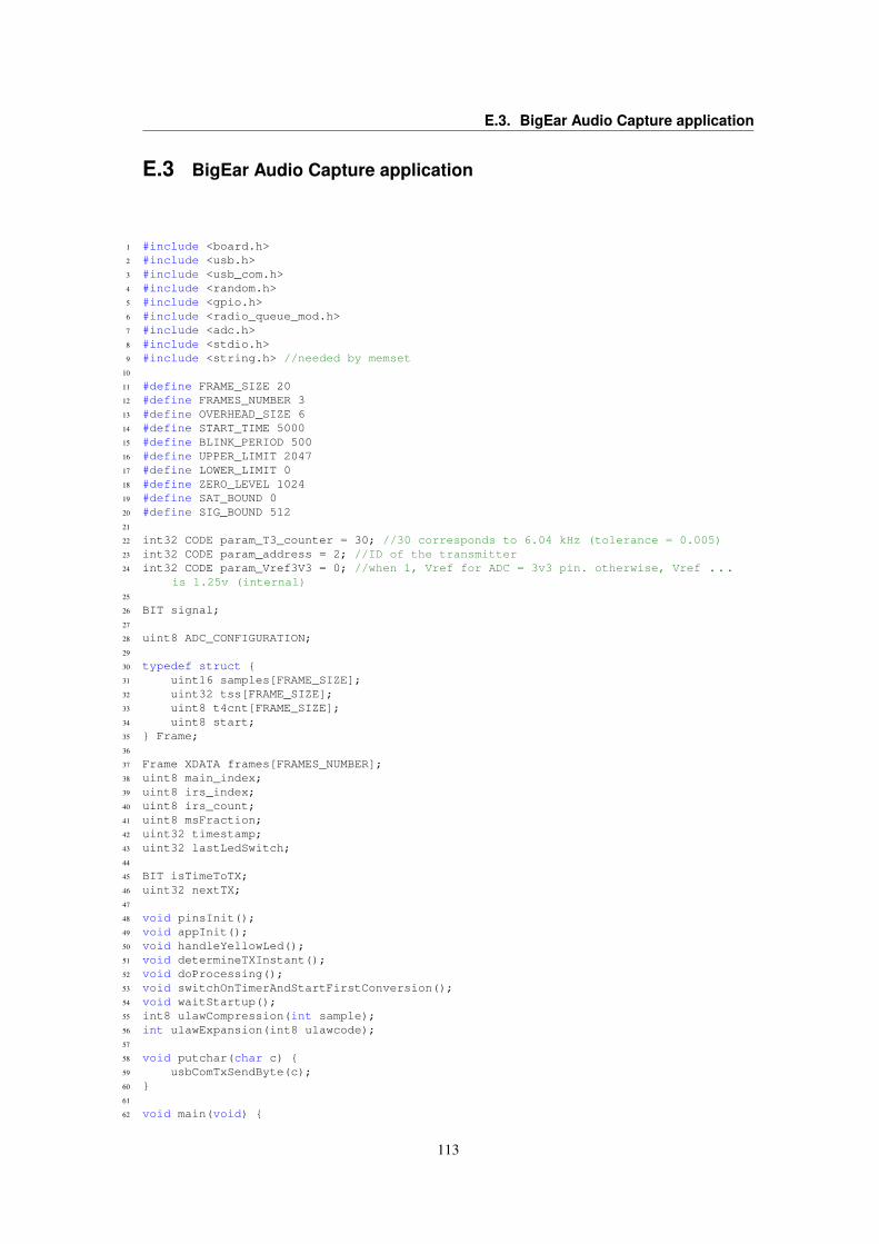
E.3. BigEar Audio Capture application
E.3 BigEar Audio Capture application
1 #include <board.h>2 #include <usb.h>3 #include <usb_com.h>4 #include <random.h>5 #include <gpio.h>6 #include <radio_queue_mod.h>7 #include <adc.h>8 #include <stdio.h>9 #include <string.h> //needed by memset
10
11 #define FRAME_SIZE 2012 #define FRAMES_NUMBER 313 #define OVERHEAD_SIZE 614 #define START_TIME 500015 #define BLINK_PERIOD 50016 #define UPPER_LIMIT 204717 #define LOWER_LIMIT 018 #define ZERO_LEVEL 102419 #define SAT_BOUND 020 #define SIG_BOUND 51221
22 int32 CODE param_T3_counter = 30; //30 corresponds to 6.04 kHz (tolerance = 0.005)23 int32 CODE param_address = 2; //ID of the transmitter24 int32 CODE param_Vref3V3 = 0; //when 1, Vref for ADC = 3v3 pin. otherwise, Vref ...
is 1.25v (internal)25
26 BIT signal;27
28 uint8 ADC_CONFIGURATION;29
30 typedef struct 31 uint16 samples[FRAME_SIZE];32 uint32 tss[FRAME_SIZE];33 uint8 t4cnt[FRAME_SIZE];34 uint8 start;35 Frame;36
37 Frame XDATA frames[FRAMES_NUMBER];38 uint8 main_index;39 uint8 irs_index;40 uint8 irs_count;41 uint8 msFraction;42 uint32 timestamp;43 uint32 lastLedSwitch;44
45 BIT isTimeToTX;46 uint32 nextTX;47
48 void pinsInit();49 void appInit();50 void handleYellowLed();51 void determineTXInstant();52 void doProcessing();53 void switchOnTimerAndStartFirstConversion();54 void waitStartup();55 int8 ulawCompression(int sample);56 int ulawExpansion(int8 ulawcode);57
58 void putchar(char c) 59 usbComTxSendByte(c);60 61
62 void main(void)
113
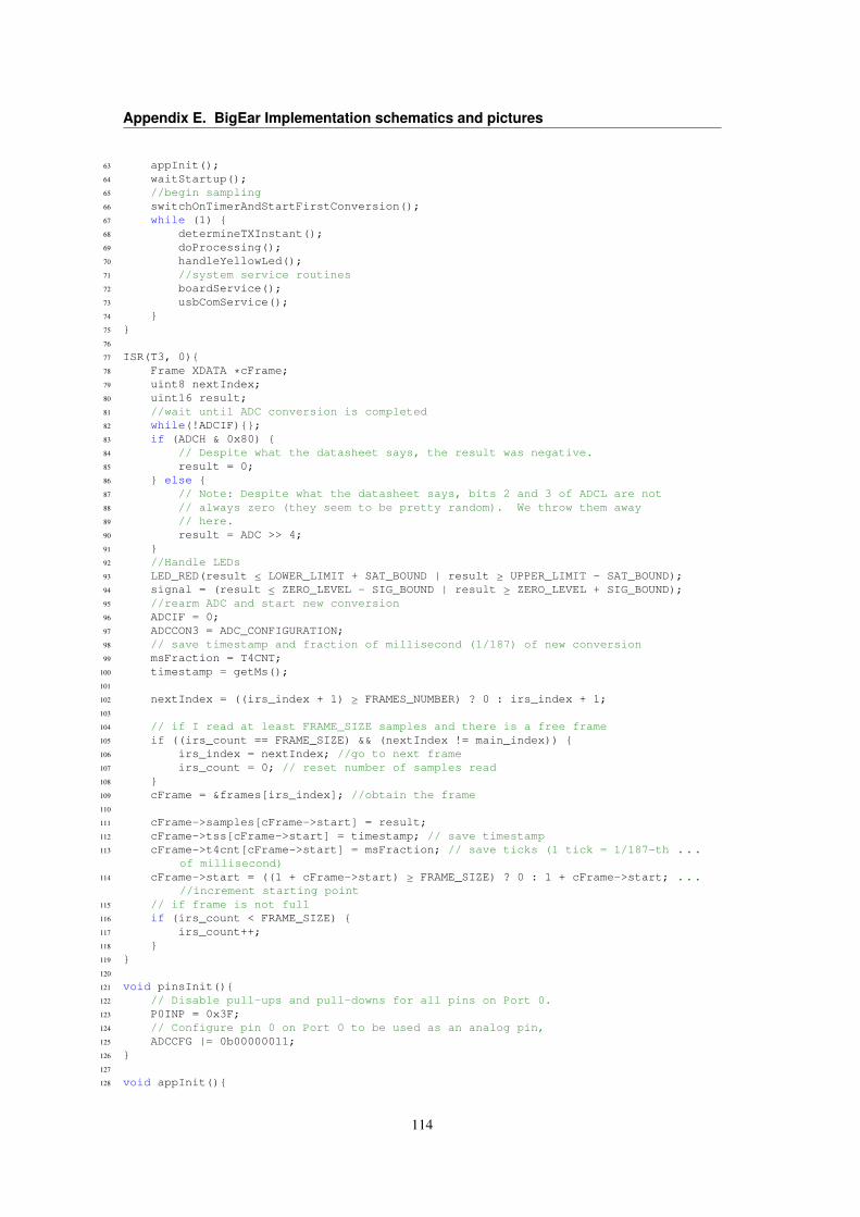
Appendix E. BigEar Implementation schematics and pictures
63 appInit();64 waitStartup();65 //begin sampling66 switchOnTimerAndStartFirstConversion();67 while (1) 68 determineTXInstant();69 doProcessing();70 handleYellowLed();71 //system service routines72 boardService();73 usbComService();74 75 76
77 ISR(T3, 0)78 Frame XDATA *cFrame;79 uint8 nextIndex;80 uint16 result;81 //wait until ADC conversion is completed82 while(!ADCIF);83 if (ADCH & 0x80) 84 // Despite what the datasheet says, the result was negative.85 result = 0;86 else 87 // Note: Despite what the datasheet says, bits 2 and 3 of ADCL are not88 // always zero (they seem to be pretty random). We throw them away89 // here.90 result = ADC >> 4;91 92 //Handle LEDs93 LED_RED(result ≤ LOWER_LIMIT + SAT_BOUND | result ≥ UPPER_LIMIT - SAT_BOUND);94 signal = (result ≤ ZERO_LEVEL - SIG_BOUND | result ≥ ZERO_LEVEL + SIG_BOUND);95 //rearm ADC and start new conversion96 ADCIF = 0;97 ADCCON3 = ADC_CONFIGURATION;98 // save timestamp and fraction of millisecond (1/187) of new conversion99 msFraction = T4CNT;
100 timestamp = getMs();101
102 nextIndex = ((irs_index + 1) ≥ FRAMES_NUMBER) ? 0 : irs_index + 1;103
104 // if I read at least FRAME_SIZE samples and there is a free frame105 if ((irs_count == FRAME_SIZE) && (nextIndex != main_index)) 106 irs_index = nextIndex; //go to next frame107 irs_count = 0; // reset number of samples read108 109 cFrame = &frames[irs_index]; //obtain the frame110
111 cFrame->samples[cFrame->start] = result;112 cFrame->tss[cFrame->start] = timestamp; // save timestamp113 cFrame->t4cnt[cFrame->start] = msFraction; // save ticks (1 tick = 1/187-th ...
of millisecond)114 cFrame->start = ((1 + cFrame->start) ≥ FRAME_SIZE) ? 0 : 1 + cFrame->start; ...
//increment starting point115 // if frame is not full116 if (irs_count < FRAME_SIZE) 117 irs_count++;118 119 120
121 void pinsInit()122 // Disable pull-ups and pull-downs for all pins on Port 0.123 P0INP = 0x3F;124 // Configure pin 0 on Port 0 to be used as an analog pin,125 ADCCFG |= 0b00000011;126 127
128 void appInit()
114
E.3. BigEar Audio Capture application
129 //init vars130 main_index = 0;131 irs_index = 0;132 irs_count = 0;133 memset(frames, 0, sizeof(frames));134 signal = 0;135 //init system136 systemInit();137 usbInit();138 pinsInit();139 randomSeedFromAdc();140 radioQueueInit();141 //init ADC configuration142 if (param_Vref3V3 !=0 )143 //use external 3V3 pin as Vref144 ADC_CONFIGURATION = 0b10110000;145 else146 //use internal REF147 ADC_CONFIGURATION = 0b00110000;148 // 10 = 3V3 (AVDD) ref. **------149 // 00 = 1V25 int. ref. **------150 // 11 = 12 bit resol. --**----151 // 0000 = AIN0 (P0_0) ----****152 153
154 void handleYellowLed()155 if (getMs() - lastLedSwitch > BLINK_PERIOD && signal == 0)156 lastLedSwitch = getMs();157 LED_YELLOW_TOGGLE();158 159 else160 if (signal==1)161 LED_YELLOW(signal);162 163
164 void determineTXInstant()165 if (getMs() > nextTX)166 isTimeToTX = 1;167 nextTX = getMs() + (randomNumber() & param_radio_max_delay);168 169 170
171 void doProcessing()172 uint8 XDATA * txBuf;173 // There is a frame ready for being sent174 if (main_index != irs_index) 175 if ((isTimeToTX == 1) && (txBuf = radioQueueTxCurrentPacket()))176 Frame XDATA *cFrame = &frames[main_index];177 uint8 i;178 int out;179 uint32 XDATA * ptrTimeStamp = (uint32 XDATA *) &txBuf[2];180 uint8 XDATA * ptrData = (uint8 XDATA *) &txBuf[7];181 //set source address182 *(txBuf + 1) = param_address;183 //timestamp of the first sample184 *(ptrTimeStamp) = cFrame->tss[cFrame->start];185 //fraction of timestamp of the first sample186 *(txBuf + 6) = cFrame->t4cnt[cFrame->start];187 //samples188 for (i=0; i<FRAME_SIZE; i++)189 uint8 index;190 index = i + cFrame->start;191 if (index ≥ FRAME_SIZE)192 index -= FRAME_SIZE;193 //maximize signal in order to exploit u-Law compression194 out = (cFrame->samples[index] << 5) - 32767;195 *(ptrData + i) = ulawCompression(out);196
115
Appendix E. BigEar Implementation schematics and pictures
197 //radio content length198 *txBuf = OVERHEAD_SIZE + FRAME_SIZE;199 //send packet200 radioQueueTxSendPacket();201 isTimeToTX = 0;202 //Flush frame203 main_index = (main_index + 1 ≥ FRAMES_NUMBER) ? 0 : main_index + 1;204 205 206 207
208 void switchOnTimerAndStartFirstConversion()209 T3CC0 = param_T3_counter;210 // DIV=111: 1:128 prescaler211 // START=1: Start the timer212 // OVFIM=1: Enable the overflow interrupt.213 // CLR = 0: Disable counter reset214 // MODE=10: Modulo215 T3CTL = 0b11111010;216 T3IE = 1; // Enable Timer 3 interrupt. (IEN1.T3IE=1)217 EA = 1; // Globally enable interrupts (IEN0.EA=1).218 // save timestamp and fraction of millisecond (1/187) of the beginning of the ...
conversion219 msFraction = T4CNT;220 timestamp = getMs();221 //start first AD conversion of P0_0222 ADCIF = 0;223 ADCCON3 = ADC_CONFIGURATION;224 225
226 void waitStartup() 227 uint32 appStart, lastLedSwitch;228 //wait for START_TIME milliseconds blinking RED led229 LED_RED(1);230 LED_YELLOW(1);231 appStart = getMs();232 lastLedSwitch = appStart;233 while (getMs() - appStart < START_TIME) 234 if (getMs() - lastLedSwitch > BLINK_PERIOD) 235 lastLedSwitch = getMs();236 LED_RED_TOGGLE();237 238 boardService();239 usbComService();240 241 LED_RED(0);242 LED_YELLOW(0);243 //save led switch timer244 lastLedSwitch = getMs();245 //determine instant of next (first) transmission246 nextTX = getMs() + (randomNumber() & param_radio_max_delay);247 isTimeToTX = 0;248 249
250 // Enable mu-law compression(I2SCFG0.ULAWE cleared & I2SCFG0.ULAWC set)251 // Write uncompressed data to I2SDATH:I2SDATL registers. Result in I2SDATH252 int8 ulawCompression(int sample) 253 I2SCFG0 = 0x10;254 I2SDATL = (uint8) sample;255 I2SDATH = (uint8) (sample >> 8);256 return I2SDATH;257 258
259 // Enable mu-law expansion (I2SCFG0.ULAWE set & I2SCFG0.ULAWC cleared)260 // Write compressed data to I2SDATH register. Result in I2SDATH:I2SDATL261 int ulawExpansion(int8 ulawcode) 262 uint16 expandedValue;263 I2SCFG0 = 0x20;
116
E.4. BigEar Input Calibration
264 I2SDATH = ulawcode;265 expandedValue = I2SDATL;266 expandedValue |= I2SDATH << 8;267 return expandedValue;268
E.4 BigEar Input Calibration
1 #include <board.h>2 #include <usb.h>3 #include <usb_com.h>4 #include <gpio.h>5 #include <adc.h>6 #include <stdio.h>7 #include <string.h> //needed by memset8
9 #define FRAME_SIZE 25510 #define BLINK_PERIOD 50011 uint32 lastLedSwitch;12
13 int32 CODE param_Vref3V3 = 0;14 int32 CODE param_ADCTolerance = 2;15 uint8 ADC_CHANNEL;16
17 void pinsInit();18 void doProcessing();19
20 void putchar(char c) 21 usbComTxSendByte(c);22 23
24 void main(void) 25 //init system26 systemInit();27 usbInit();28 pinsInit();29 //adc configuration30 if (param_Vref3V3 !=0 )31 //use external 3V3 pin as Vref32 ADC_CHANNEL = 0 | ADC_REFERENCE_VDD | ADC_BITS_12;33 else34 //use 3V3 pin35 ADC_CHANNEL = 0 | ADC_REFERENCE_INTERNAL | ADC_BITS_12;36 //begin37 lastLedSwitch = getMs();38 while (1) 39 doProcessing();40 if (getMs() - lastLedSwitch > BLINK_PERIOD) 41 lastLedSwitch = getMs();42 LED_RED_TOGGLE();43 44 boardService();45 usbComService();46 47 48
49 void pinsInit()50 // Disable pull-ups and pull-downs for all pins on Port 0.51 P0INP = 0x3F;52 // Configure pin 0 on Port 0 to be used as an analog pin,53 ADCCFG |= 0b00000011;54 55
56 void printBar(const char * name, uint16 adcResult)57 58 uint8 i, width;
117
Appendix E. BigEar Implementation schematics and pictures
59
60 printf("%-4s %4d mV |", name, adcConvertToMillivolts(adcResult));61 width = adcResult >> 5;62 for(i = 0; i < width; i++) putchar('#'); 63 for(; i < 63; i++) putchar(' '); 64 putchar('|');65 putchar('\r');66 putchar('\n');67 68
69 void doProcessing()70 if (usbComTxAvailable() ≥ 128)71 uint8 i;72 int32 val;73 val = 0;74 //calibrate ADC75 adcSetMillivoltCalibration(adcReadVddMillivolts());76 //sample77 for (i = 0; i<FRAME_SIZE; i++)78 val += adcRead(ADC_CHANNEL);79 80 val /= FRAME_SIZE;81 //led yellow ON when the signal is correctly biased82 LED_YELLOW( (1024-val) > -param_ADCTolerance && (1024-val) < ...
param_ADCTolerance );83 printf("\x1B[0;0H"); // VT100 command for "go to 0,0"84 printBar("P0_0", val);85 printf("Measured = %8lu. Difference: %5ld", val, 1024-val);86 87
E.5 BigEar Receiver application
1 #include <board.h>2 #include <usb.h>3 #include <usb_com.h>4 #include <random.h>5 #include <gpio.h>6 #include <radio_queue_mod.h>7 #include <stdio.h>8
9 #define FRAME_SIZE 2010 #define FRAMES_NUMBER 311 #define OVERHEAD_SIZE 612 #define TERMINATION_SIZE 213 #define START_TIME 500014 #define BLINK_PERIOD 50015
16 uint32 lastLedSwitch;17 /* *** RADIO PDU STRUCT ***/18 typedef struct 19 uint8 length;20 uint8 source;21 uint32 timestamp;22 uint8 msFract;23 uint8 sample[FRAME_SIZE];24 radioPacket;25
26 void doProcessing();27 void waitStartup();28 void uint8ToHex(char *buf, uint8 val);29 void uint32ToHex(char *buf, uint32 val);30
31 void main(void) 32 //init system33 systemInit();
118
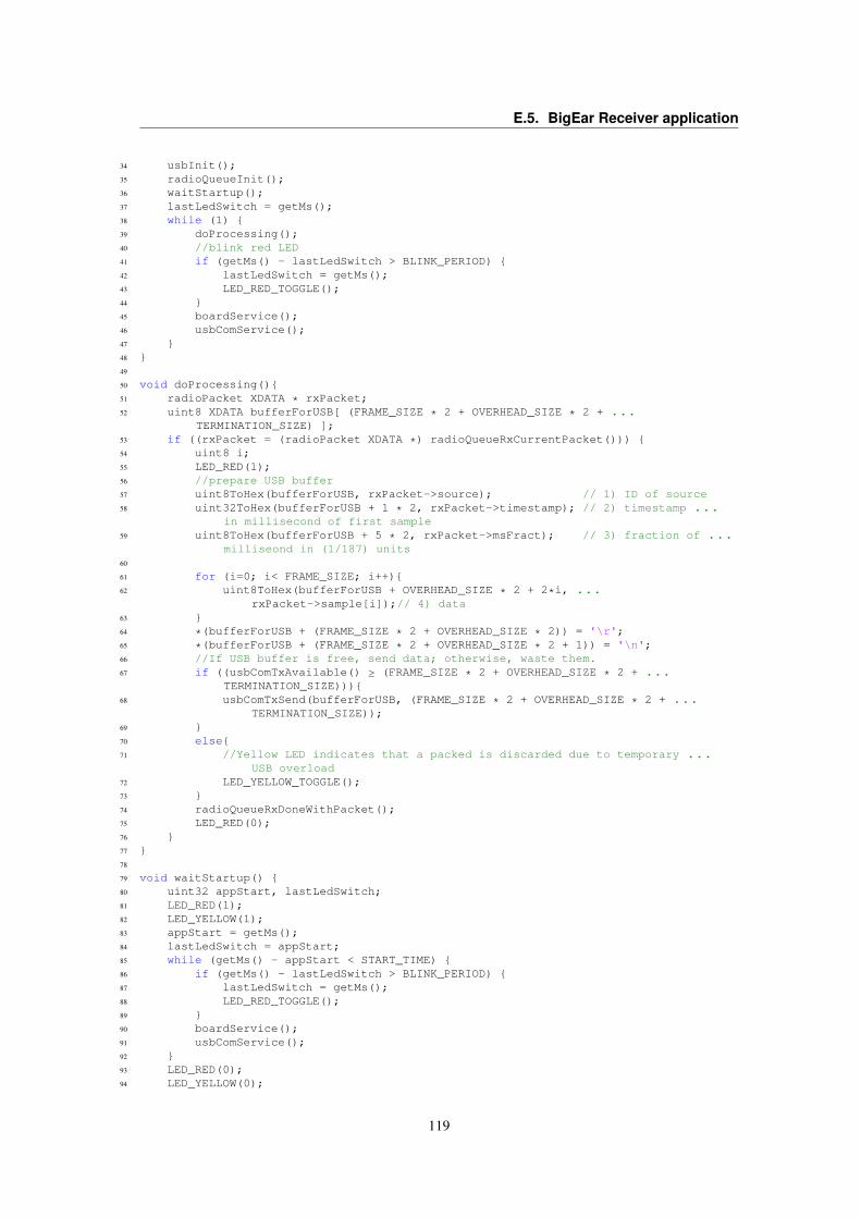
E.5. BigEar Receiver application
34 usbInit();35 radioQueueInit();36 waitStartup();37 lastLedSwitch = getMs();38 while (1) 39 doProcessing();40 //blink red LED41 if (getMs() - lastLedSwitch > BLINK_PERIOD) 42 lastLedSwitch = getMs();43 LED_RED_TOGGLE();44 45 boardService();46 usbComService();47 48 49
50 void doProcessing()51 radioPacket XDATA * rxPacket;52 uint8 XDATA bufferForUSB[ (FRAME_SIZE * 2 + OVERHEAD_SIZE * 2 + ...
TERMINATION_SIZE) ];53 if ((rxPacket = (radioPacket XDATA *) radioQueueRxCurrentPacket())) 54 uint8 i;55 LED_RED(1);56 //prepare USB buffer57 uint8ToHex(bufferForUSB, rxPacket->source); // 1) ID of source58 uint32ToHex(bufferForUSB + 1 * 2, rxPacket->timestamp); // 2) timestamp ...
in millisecond of first sample59 uint8ToHex(bufferForUSB + 5 * 2, rxPacket->msFract); // 3) fraction of ...
milliseond in (1/187) units60
61 for (i=0; i< FRAME_SIZE; i++)62 uint8ToHex(bufferForUSB + OVERHEAD_SIZE * 2 + 2*i, ...
rxPacket->sample[i]);// 4) data63 64 *(bufferForUSB + (FRAME_SIZE * 2 + OVERHEAD_SIZE * 2)) = '\r';65 *(bufferForUSB + (FRAME_SIZE * 2 + OVERHEAD_SIZE * 2 + 1)) = '\n';66 //If USB buffer is free, send data; otherwise, waste them.67 if ((usbComTxAvailable() ≥ (FRAME_SIZE * 2 + OVERHEAD_SIZE * 2 + ...
TERMINATION_SIZE)))68 usbComTxSend(bufferForUSB, (FRAME_SIZE * 2 + OVERHEAD_SIZE * 2 + ...
TERMINATION_SIZE));69 70 else71 //Yellow LED indicates that a packed is discarded due to temporary ...
USB overload72 LED_YELLOW_TOGGLE();73 74 radioQueueRxDoneWithPacket();75 LED_RED(0);76 77 78
79 void waitStartup() 80 uint32 appStart, lastLedSwitch;81 LED_RED(1);82 LED_YELLOW(1);83 appStart = getMs();84 lastLedSwitch = appStart;85 while (getMs() - appStart < START_TIME) 86 if (getMs() - lastLedSwitch > BLINK_PERIOD) 87 lastLedSwitch = getMs();88 LED_RED_TOGGLE();89 90 boardService();91 usbComService();92 93 LED_RED(0);94 LED_YELLOW(0);
119
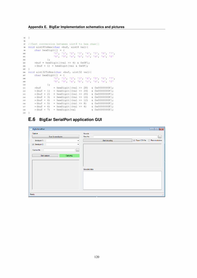
Appendix E. BigEar Implementation schematics and pictures
95 96
97 //fast conversion between uint8 to hex char[]98 void uint8ToHex(char *buf, uint8 val)99 char hexDigit[] =
100 '0', '1', '2', '3', '4', '5', '6', '7',101 '8', '9', 'a', 'b', 'c', 'd', 'e', 'f'102 ;103 *buf = hexDigit[(val >> 4) & 0x0F];104 *(buf + 1) = hexDigit[val & 0x0F];105 106 void uint32ToHex(char *buf, uint32 val)107 char hexDigit[] = 108 '0', '1', '2', '3', '4', '5', '6', '7',109 '8', '9', 'a', 'b', 'c', 'd', 'e', 'f'110 ;111 *buf = hexDigit[(val >> 28) & 0x0000000F];112 *(buf + 1) = hexDigit[(val >> 24) & 0x0000000F];113 *(buf + 2) = hexDigit[(val >> 20) & 0x0000000F];114 *(buf + 3) = hexDigit[(val >> 16) & 0x0000000F];115 *(buf + 4) = hexDigit[(val >> 12) & 0x0000000F];116 *(buf + 5) = hexDigit[(val >> 8) & 0x0000000F];117 *(buf + 6) = hexDigit[(val >> 4) & 0x0000000F];118 *(buf + 7) = hexDigit[val & 0x0000000F];119
E.6 BigEar SerialPort application GUI
120
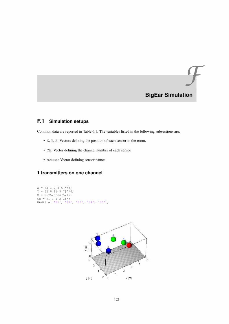
FBigEar Simulation
F.1 Simulation setups
Common data are reported in Table 6.1. The variables listed in the following subsections are:
• X, Y, Z: Vectors defining the position of each sensor in the room.
• CH: Vector defining the channel number of each sensor
• NAMES: Vector defining sensor names.
1 transmitters on one channel
X = [2 1 2 8 6]'/3;Y = [2 8 11 3 7]'/4;Z = 2.75*ones(5,1);CH = [1 1 1 2 2]';NAMES = ['S1'; 'S2'; 'S3'; 'S4'; 'S5'];
121
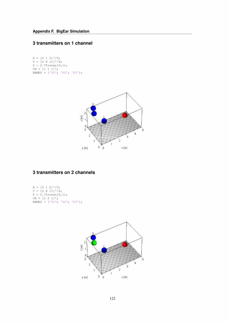
Appendix F. BigEar Simulation
3 transmitters on 1 channel
X = [2 1 2]'/3;Y = [2 8 11]'/4;Z = 2.75*ones(3,1);CH = [1 1 1]';NAMES = ['S1'; 'S2'; 'S3'];
3 transmitters on 2 channels
X = [2 1 2]'/3;Y = [2 8 11]'/4;Z = 2.75*ones(3,1);CH = [1 2 1]';NAMES = ['S1'; 'S2'; 'S3'];
122

F.1. Simulation setups
4 transmitters on 1 channel
X = [2 1 2 8]'/3;Y = [2 8 11 3]'/4;Z = 2.75*ones(4,1);CH = [1 1 1 1 ]';NAMES = ['S1'; 'S2'; 'S3'; 'S4'];
4 transmitters on 2 channels
X = [2 1 2 8]'/3;Y = [2 8 11 3]'/4;Z = 2.75*ones(4,1);CH = [1 2 1 2 ]';NAMES = ['S1'; 'S2'; 'S3'; 'S4'];
123
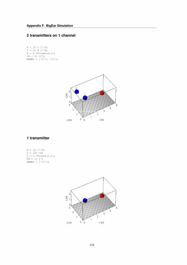
Appendix F. BigEar Simulation
2 transmitters on 1 channel
X = [2 1 ]'/3;Y = [2 8 ]'/4;Z = 2.75*ones(2,1);CH = [1 1]';NAMES = ['S1'; 'S2'];
1 transmitter
X = [2 ]'/3;Y = [2]'/4;Z = 2.75*ones(1,1);CH = [1 ]';NAMES = ['S1'];
124
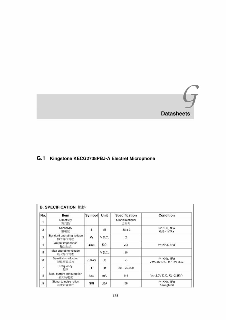
GDatasheets
G.1 Kingstone KECG2738PBJ-A Electret Microphone
125
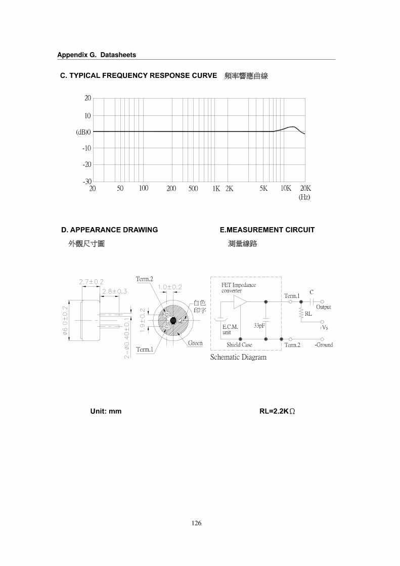
Appendix G. Datasheets
126
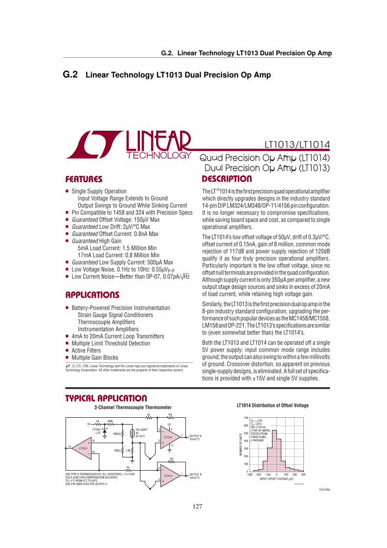
G.2. Linear Technology LT1013 Dual Precision Op Amp
G.2 Linear Technology LT1013 Dual Precision Op Amp
LT1013/LT1014
10134fd
Typical applicaTion
DescripTion
Quad Precision Op Amp (LT1014)Dual Precision Op Amp (LT1013)
The LT ®1014 is the first precision quad operational amplifier which directly upgrades designs in the industry standard 14-pin DIP LM324/LM348/OP-11/4156 pin configuration. It is no longer necessary to compromise specifications, while saving board space and cost, as compared to single operational amplifiers.
The LT1014’s low offset voltage of 50µV, drift of 0.3µV/°C, offset current of 0.15nA, gain of 8 million, common mode rejection of 117dB and power supply rejection of 120dB qualify it as four truly precision operational amplifiers. Particularly important is the low offset voltage, since no offset null terminals are provided in the quad configuration. Although supply current is only 350µA per amplifier, a new output stage design sources and sinks in excess of 20mA of load current, while retaining high voltage gain.
Similarly, the LT1013 is the first precision dual op amp in the 8-pin industry standard configuration, upgrading the per-formance of such popular devices as the MC1458/MC1558, LM158 and OP-221. The LT1013’s specifications are similar to (even somewhat better than) the LT1014’s.
Both the LT1013 and LT1014 can be operated off a single 5V power supply: input common mode range includes ground; the output can also swing to within a few millivolts of ground. Crossover distortion, so apparent on previous single-supply designs, is eliminated. A full set of specifica-tions is provided with ±15V and single 5V supplies.
FeaTures
applicaTions
n Single Supply Operation Input Voltage Range Extends to Ground Output Swings to Ground While Sinking Currentn Pin Compatible to 1458 and 324 with Precision Specsn Guaranteed Offset Voltage: 150µV Max n Guaranteed Low Drift: 2µV/°C Maxn Guaranteed Offset Current: 0.8nA Maxn Guaranteed High Gain 5mA Load Current: 1.5 Million Min 17mA Load Current: 0.8 Million Minn Guaranteed Low Supply Current: 500µA Maxn Low Voltage Noise, 0.1Hz to 10Hz: 0.55µVP-Pn Low Current Noise—Better than 0P-07, 0.07pA/√Hz
n Battery-Powered Precision Instrumentation Strain Gauge Signal Conditioners Thermocouple Amplifiers Instrumentation Amplifiersn 4mA to 20mA Current Loop Transmittersn Multiple Limit Threshold Detectionn Active Filtersn Multiple Gain Blocks
–
+LT1014
1
4
11
2
3
5V5V
1M4k
OUTPUT A10mV/°C
–
+LT1014
7
6
5
1M
OUTPUT B10mV/°C
4k
1.8k
YSI 440075kAT 25°C
260Ω
1684Ω
299k3k
LT10041.2V
14
12
13–
+LT1014
USE TYPE K THERMOCOUPLES. ALL RESISTORS = 1% FILM.COLD JUNCTION COMPENSATION ACCURATE TO ±1°C FROM 0°C TO 60°C.USE 4TH AMPLIFIER FOR OUTPUT C.
LT1014 Distribution of Offset Voltage3-Channel Thermocouple Thermometer
INPUT OFFSET VOLTAGE (µV)–300 0 200–200 –100 100 300
NUM
BER
OF U
NITS
700
600
500
400
300
200
100
0
VS = ±15VTA = 25°C425 LT1014s(1700 OP AMPS)TESTED FROM THREE RUNS J PACKAGE
1013/14 TA02
L, LT, LTC, LTM, Linear Technology and the Linear logo are registered trademarks of Linear Technology Corporation. All other trademarks are the property of their respective owners.
127
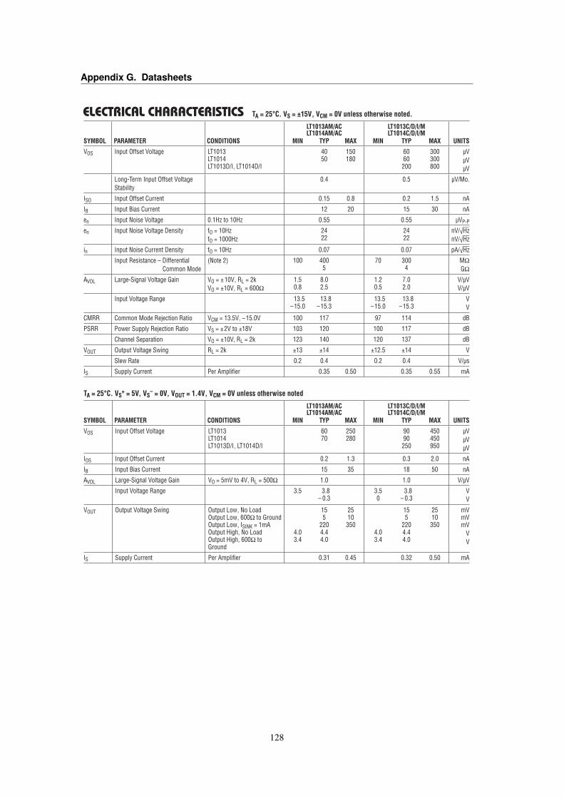
Appendix G. DatasheetsLT1013/LT1014
10134fd
elecTrical characTerisTics
SYMBOL PARAMETER CONDITIONS
LT1013AM/AC LT1014AM/AC
LT1013C/D/I/M LT1014C/D/I/M
UNITSMIN TYP MAX MIN TYP MAX
VOS Input Offset Voltage LT1013 LT1014 LT1013D/I, LT1014D/I
40 50
150 180
60 60
200
300 300 800
µV µV µV
Long-Term Input Offset Voltage Stability
0.4 0.5 µV/Mo.
ISO Input Offset Current 0.15 0.8 0.2 1.5 nA
IB Input Bias Current 12 20 15 30 nA
en Input Noise Voltage 0.1Hz to 10Hz 0.55 0.55 µVP-P
en Input Noise Voltage Density fO = 10Hz fO = 1000Hz
24 22
24 22
nV/√Hz nV/√Hz
in Input Noise Current Density fO = 10Hz 0.07 0.07 pA/√Hz
Input Resistance – Differential Common Mode
(Note 2) 100 400 5
70 300 4
MΩ GΩ
AVOL Large-Signal Voltage Gain VO = ±10V, RL = 2k VO = ±10V, RL = 600Ω
1.5 0.8
8.0 2.5
1.2 0.5
7.0 2.0
V/µV V/µV
Input Voltage Range 13.5 –15.0
13.8 –15.3
13.5 –15.0
13.8 –15.3
V V
CMRR Common Mode Rejection Ratio VCM = 13.5V, –15.0V 100 117 97 114 dB
PSRR Power Supply Rejection Ratio VS = ±2V to ±18V 103 120 100 117 dB
Channel Separation VO = ±10V, RL = 2k 123 140 120 137 dB
VOUT Output Voltage Swing RL = 2k ±13 ±14 ±12.5 ±14 V
Slew Rate 0.2 0.4 0.2 0.4 V/µs
IS Supply Current Per Amplifier 0.35 0.50 0.35 0.55 mA
TA = 25°C. VS = ±15V, VCM = 0V unless otherwise noted.
SYMBOL PARAMETER CONDITIONS
LT1013AM/AC LT1014AM/AC
LT1013C/D/I/M LT1014C/D/I/M
UNITSMIN TYP MAX MIN TYP MAX
VOS Input Offset Voltage LT1013 LT1014 LT1013D/I, LT1014D/I
60 70
250 280
90 90
250
450 450 950
µV µV µV
IOS Input Offset Current 0.2 1.3 0.3 2.0 nA
IB Input Bias Current 15 35 18 50 nA
AVOL Large-Signal Voltage Gain VO = 5mV to 4V, RL = 500Ω 1.0 1.0 V/µV
Input Voltage Range 3.5 3.8 – 0.3
3.5 0
3.8 – 0.3
V V
VOUT Output Voltage Swing Output Low, No Load Output Low, 600Ω to Ground Output Low, ISINK = 1mA Output High, No Load Output High, 600Ω to Ground
4.0 3.4
15 5
220 4.4 4.0
25 10
350
4.0 3.4
15 5
220 4.4 4.0
25 10
350
mV mV mV
V V
IS Supply Current Per Amplifier 0.31 0.45 0.32 0.50 mA
TA = 25°C. VS+ = 5V, VS
– = 0V, VOUT = 1.4V, VCM = 0V unless otherwise noted
128
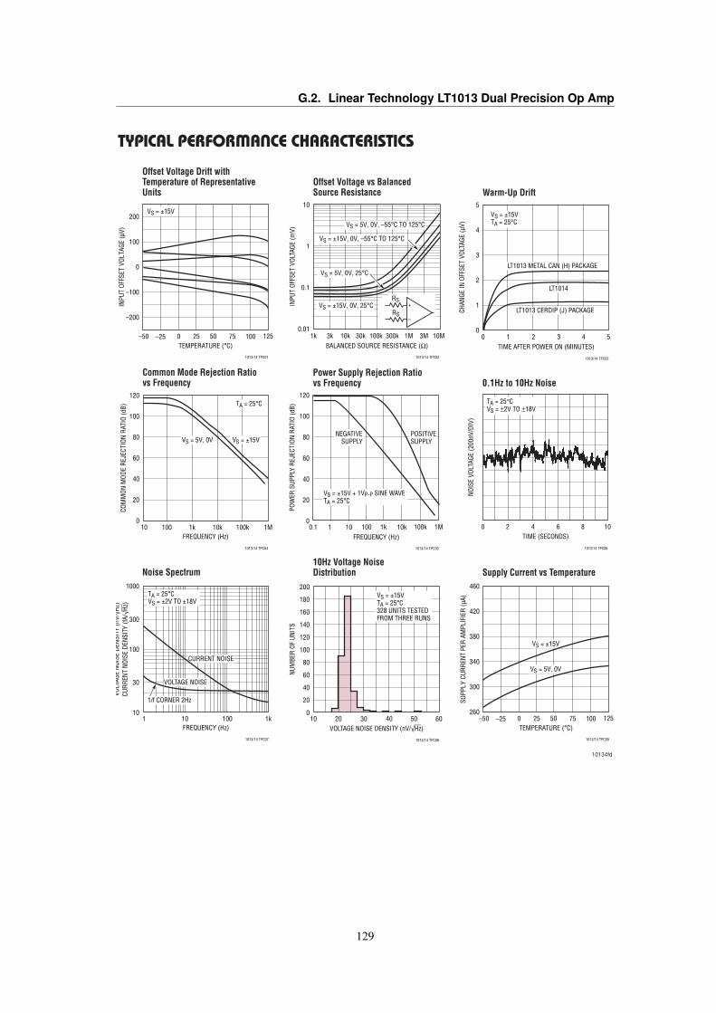
G.2. Linear Technology LT1013 Dual Precision Op AmpLT1013/LT1014
10134fd
Typical perForMance characTerisTics
Offset Voltage Drift with Temperature of Representative Units
TEMPERATURE (°C)–50
INPU
T OF
FSET
VOL
TAGE
(µV)
200
100
0
–100
–200
0 50 75–25 25 100 125
VS = ±15V
1013/14 TPC01
TIME AFTER POWER ON (MINUTES)0
CHAN
GE IN
OFF
SET
VOLT
AGE
(µV)
5
4
3
2
1
041 2 3 5
VS = ±15VTA = 25°C
LT1013 CERDIP (J) PACKAGE
LT1013 METAL CAN (H) PACKAGE
LT1014
1013/14 TPC03
Warm-Up Drift
BALANCED SOURCE RESISTANCE (Ω)1k 3k 10k 30k 100k 300k 1M 3M 10M
INPU
T OF
FSET
VOL
TAGE
(mV)
10
1
0.1
0.01
VS = 5V, 0V, –55°C TO 125°C
VS = ±15V, 0V, –55°C TO 125°C
VS = 5V, 0V, 25°C
VS = ±15V, 0V, 25°C
–
+RS
RS
1013/14 TPC02
Offset Voltage vs Balanced Source Resistance
Common Mode Rejection Ratio vs Frequency 0.1Hz to 10Hz Noise
Power Supply Rejection Ratio vs Frequency
FREQUENCY (Hz)10
COM
MON
MOD
E RE
JECT
ION
RATI
O (d
B)
120
100
80
60
40
20
0100 1k 10k 100k 1M
VS = 5V, 0V VS = ±15V
TA = 25°C
1013/14 TPC04
FREQUENCY (Hz)0.1
POW
ER S
UPPL
Y RE
JECT
ION
RATI
O (d
B)
120
100
80
60
40
20
0100 10k1 10 1k 100k 1M
POSITIVESUPPLY
NEGATIVESUPPLY
VS = ±15V + 1VP-P SINE WAVETA = 25°C
1013/14 TPC05
TIME (SECONDS)0
NOIS
E VO
LTAG
E (2
00nV
/DIV
)
82 4 6 10
TA = 25 CVS = 2V TO 18V
1013/14 TPC06
10Hz Voltage Noise DistributionNoise Spectrum Supply Current vs Temperature
FREQUENCY (Hz)1
VOLT
AGE
NOIS
E DE
NSIT
Y (n
V/√H
z)CU
RREN
T NO
ISE
DENS
ITY
(fA/√Hz
)
1000
100
10
300
30
10 100 1k
CURRENT NOISE
VOLTAGE NOISE
1/f CORNER 2Hz
TA = 25°CVS = ±2V TO ±18V
1013/14 TPC07
VOLTAGE NOISE DENSITY (nV/√Hz)10
NUM
BER
OF U
NITS
200
180
160
140
120
100
80
60
40
20
05020 30 40 60
VS = ±15VTA = 25°C328 UNITS TESTEDFROM THREE RUNS
1013/14 TPC08
TEMPERATURE (°C)–50
SUPP
LY C
URRE
NT P
ER A
MPL
IFIE
R (µ
A)
460
420
380
340
300
2600 50 75–25 25 100 125
VS = ±15V
VS = 5V, 0V
1013/14 TPC09
129
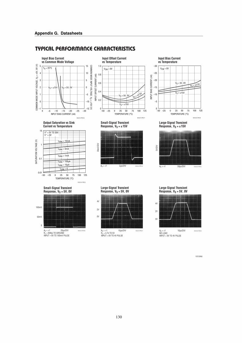
Appendix G. DatasheetsLT1013/LT1014
10134fd
Typical perForMance characTerisTics
INPUT BIAS CURRENT (nA)0CO
MM
ON M
ODE
INPU
T VO
LTAG
E, V
S =
+5V,
0V
(V)
5
4
3
2
1
0
–1
COMM
ON MODE INPUT VOLTAGE, V
S = ±15V (V)
15
10
5
0
–5
–10
–15–5 –10 –15 –20 –25 –30
TA = 25°C
VS = 5V, 0VVS = ±15V
1013/14 TPC10
Input Bias Current vs Common Mode Voltage
TEMPERATURE (°C)–50
INPU
T BI
AS C
URRE
NT (n
A)
–30
–25
–20
–15
–10
–5
025 75–25 0 50 100 125
VCM = 0V
VS = 5V, 0V
VS = ±15V
VS = ±2.5V
1013/14 TPC12
TEMPERATURE (°C)–50
INPU
T OF
FSET
CUR
RENT
(nA)
1.0
0.8
0.6
0.4
0.2
00 50 75–25 25 100 125
VCM = 0V
VS = 5V, 0VVS =
±2.5V
VS = ±15V
1013/14 TPC11
Input Bias Current vs Temperature
Large-Signal Transient Response, VS = ±15V
5V/D
IV
AV = +1 50µs/DIV 1013/14 TPC15
Large-Signal Transient Response, VS = 5V, 0V
AV = +1 10µs/DIV 1013/14 TPC18
NO LOADINPUT = 0V TO 4V PULSE
4V
2V
0V
Small-Signal Transient Response, VS = ±15V
20m
V/DI
V
AV = +1 2µs/DIV 1013/14 TPC14
Large-Signal Transient Response, VS = 5V, 0V
AV = +1 10µs/DIV 1013/14 TPC17
RL = 4.7k TO 5VINPUT = 0V TO 4V PULSE
4V
2V
0V
Output Saturation vs Sink Current vs Temperature
TEMPERATURE (°C)–50 –25 0 25 50 75 100 125
SATU
RATI
ON V
OLTA
GE (V
)
10
1
0.1
0.01
V+ = 5V TO 30VV– = 0V
ISINK = 10mA
ISINK = 5mA
ISINK = 1mA
ISINK = 100µAISINK = 10µA
ISINK = 0
1013/14 TPC13
AV = +1 20µs/DIV 1013/14 TPC16
RL = 600Ω TO GROUNDINPUT = 0V TO 100mV PULSE
Small-Signal Transient Response, VS = 5V, 0V
100mV
50mV
0
Input Offset Current vs Temperature
130
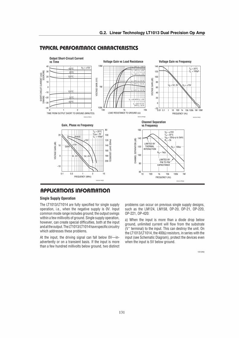
G.2. Linear Technology LT1013 Dual Precision Op AmpLT1013/LT1014
10134fd
Typical perForMance characTerisTics
Voltage Gain vs Frequency
FREQUENCY (Hz)0.01 0.1
VOLT
AGE
GAIN
(dB)
1M 10M1 10 100 1k 10k 100k
140
120
100
80
60
40
20
0
–20
VS = ±15VVS = 5V, 0V
TA = 25°CCL = 100pF
1013/14 TPC21
LOAD RESISTANCE TO GROUND (Ω)100
100k
VOLT
AGE
GAIN
(V/V
)
1M
10M
1k 10k
VO = 20mV TO 3.5VWITH VS = 5V, 0V
TA = 25°C, VS = ±15V
TA = –55°C, VS = ±15V
TA = 125°C, VS = ±15V
TA = –55°C, VS = 5V, 0V
TA = 25°C, VS = 5V, 0V
TA = 125°C, VS = 5V, 0V
VO = ±10V WITH VS = ±15V
1013/14 TPC20
Output Short-Circuit Current vs Time
TIME FROM OUTPUT SHORT TO GROUND (MINUTES)0
SHOR
T-CI
RCUI
T CU
RREN
T (m
A)SI
NKIN
G
SOUR
CING
1 2
40
30
20
10
0
–10
–20
–30
–403
–55°C
25°C
25°C
125°C
125°C
–55°C VS = ±15V
1013/14 TPC19
Voltage Gain vs Load Resistance
Gain, Phase vs FrequencyChannel Separation vs Frequency
applicaTions inForMaTion
FREQUENCY (MHz)0.1 0.3
VOLT
AGE
GAIN
(dB)
20
10
0
–10
PHASE SHIFT (DEGREES)80
100
120
140
160
180
200
1 3 10
TA = 25°CVCM = 0VCL = 100pFPHASE
±15V
5V, 0V
±15V
5V, 0V
GAIN
1013/14 TPC22
FREQUENCY (Hz)10
CHAN
NEL
SEPA
RATI
ON (d
B)
160
140
120
100
80
60100k100 1k 10k 1M
LIMITED BYTHERMAL
INTERACTIONRS = 1kΩ
RS = 100Ω
VS = ±15VTA = 25°CVIN = 20Vp-p to 5kHzRL = 2k
LIMITED BYPIN TO PIN
CAPACITANCE
1013/14 TPC23
Single Supply Operation
The LT1013/LT1014 are fully specified for single supply operation, i.e., when the negative supply is 0V. Input common mode range includes ground; the output swings within a few millivolts of ground. Single supply operation, however, can create special difficulties, both at the input and at the output. The LT1013/LT1014 have specific circuitry which addresses these problems.
At the input, the driving signal can fall below 0V—in-advertently or on a transient basis. If the input is more than a few hundred millivolts below ground, two distinct
problems can occur on previous single supply designs, such as the LM124, LM158, OP-20, OP-21, OP-220, OP-221, OP-420:
a) When the input is more than a diode drop below ground, unlimited current will flow from the substrate (V – terminal) to the input. This can destroy the unit. On the LT1013/LT1014, the 400Ω resistors, in series with the input (see Schematic Diagram), protect the devices even when the input is 5V below ground.
131


Bibliography
[1] Norman Abramson. The aloha system: another alternative for computer communications. InProceedings of the November 17-19, 1970, fall joint computer conference, pages 281–285. ACM,1970.
[2] Dennis A. Adams, R. Ryan Nelson, and Peter A. Todd. Perceived usefulness, ease of use, and usageof information technology: A replication. MIS Q., 16(2):227–247, June 1992.
[3] I. F. Akyildiz, W. Su, Y. Sankarasubramaniam, and E. Cayirci. Wireless sensor networks: a survey.Computer Networks, 38:393–422, 2002.
[4] Jont B. Allen and David A.’ Berkley. Image method for efficiently simulating small room acoustics.The Journal of the Acoustical Society of America, 65(4):943–950, 1979.
[5] ASCII-Table.com. Ansi escape sequences - vt100 / vt52. http://ascii-table.com/ansi-escape-sequences-vt-100.php.
[6] Pololu corp. Wixel sdk documentation. http://pololu.github.io/wixel-sdk/.
[7] George Coulouris, Jean Dollimore, Tim Kindberg, and Gordon Blair. Distributed Systems: Con-cepts and Design. Pearson, fifth edition, 2012.
[8] Federal Standard. 1037c. telecommunications: Glossary of telecommunication terms. Institute forTelecommunications Sciences, 7, 1996.
[9] Galen Carol Audio. Decibel (loudness) comparison chart. http://www.gcaudio.com/resources/howtos/loudness.html.
[10] Simon Godsill and Peter Rayner. Digital audio restoration. Department of Engineering, Universityof Cambridge, pages 1–71, 1997.
[11] Renate Heinz. Binaural room simulation based on an image source model with addition of statisticalmethods to include the diffuse sound scattering of walls and to predict the reverberant tail. AppliedAcoustics, 38(2–4):145 – 159, 1993.
[12] Texas Instruments. Low-power soc (system-on-chip) with mcu, memory, 2.4 ghz rf transceiver, andusb (rev. g). http://www.ti.com/lit/ds/symlink/cc2511.pdf, 2013.
[13] International Telecommunication Union. ITU-T recommendation G.711 – Pulse Code Modulation(PCM) of Voice Frequencies. Technical report, 1993.
[14] International Telecommunication Union. ITU-T recommendation G.711 appendix I – A High Qual-ity Low-Complexity Algorithm for Packet Loss Concealment. Technical report, 1999.
133
Bibliography
[15] Benjamin Lecouteux, Michel Vacher, and François Portet. Distant Speech Recognition in aSmart Home: Comparison of Several Multisource ASRs in Realistic Conditions. In InternationalSpeech Communication Association, editor, Interspeech 2011 Florence, pages 2273–2276, Flo-rence, Italy, August 2011. 4 pages.
[16] Jerad Lewis. Understanding microphone sensitivity. Analog Dialogue, pages 46–05, 2012.
[17] S. Mangano, H. Saidinejad, F. Veronese, S. Comai, M. Matteucci, and F. Salice. Bridge: Mutualreassurance for autonomous and independent living. Intelligent Systems, IEEE, 30(4):31–38, July2015.
[18] Nathanael Perraudin, David Shuman, Gilles Puy, and Pierre Vandergheynst. Unlocbox a matlabconvex optimization toolbox using proximal splitting methods. arXiv preprint arXiv:1402.0779,2014.
[19] Matthew Rhudy, Brian Bucci, Jeffrey Vipperman, Jeffrey Allanach, and Bruce Abraham. Micro-phone array analysis methods using cross-correlations. In ASME 2009 International MechanicalEngineering Congress and Exposition, pages 281–288. American Society of Mechanical Engineers,2009.
[20] Lawrence G Roberts. Aloha packet system with and without slots and capture. ACM SIGCOMMComputer Communication Review, 5(2):28–42, 1975.
[21] Dirk Schroeder, Philipp Dross, and Michael Vorlaender. A fast reverberation estimator for virtualenvironments. In Audio Engineering Society Conference: 30th International Conference: Intelli-gent Audio Environments, Mar 2007.
[22] Douglas Self. Audio engineering explained. Taylor & Francis, 2009.
[23] Jianhong Shen. Inpainting and the fundamental problem of image processing. SIAM news, 36(5):1–4, 2003.
[24] Julius O. Smith. Physical Audio Signal Processing. http://ccrma.stanford.edu/-˜jos/pasp/, accessed 2015. online book, 2010 edition.
[25] Linear Technology. LT1013/1014 quad precision op amp (lt1014) – dual precision op amp (lt1013).http://cds.linear.com/docs/en/datasheet/10134fd.pdf, 2013.
[26] Saeed V Vaseghi. Algorithms for restoration of archived gramophone recordings. PhD thesis,University of Cambridge, 1988.
[27] Saeed V Vaseghi and Peter JW Rayner. A new application of adaptive filters for restoration ofarchived gramophone recordings. In Acoustics, Speech, and Signal Processing, 1988. ICASSP-88.,1988 International Conference on, pages 2548–2551. IEEE, 1988.
[28] SV Vaseghi and PJW Rayner. Detection and suppression of impulsive noise in speech communica-tion systems. IEE Proceedings I (Communications, Speech and Vision), 137(1):38–46, 1990.
[29] Raymond NJ Veldhuis, Lodewijk B Vries, et al. Adaptive interpolation of discrete-time signalsthat can be modeled as autoregressive processes. Acoustics, Speech and Signal Processing, IEEETransactions on, 34(2):317–330, 1986.
[30] Andrew Wabnitz, Nicolas Epain, Craig Jin, and André van Schaik. Room acoustics simulationfor multichannel microphone arrays. In Proceedings of the International Symposium on RoomAcoustics, 2010.
[31] L. Zevi. Il nuovissimo manuale dell’architetto. Mancosu Editore, 20 edition, 2003.
134

u B iquitous w I reless low-bud G et spe E ch c A pturing inte R face