
Finite element modeling of flow/compression-induced...
58
1 ALMA MATER STUDIORUM - UNIVERSITÀ DI BOLOGNA CAMPUS DI CESENA SCUOLA DI INGEGNERIA E ARCHITETTURA CORSO DI LAUREA MAGISTRALE IN INGEGNERIA BIOMEDICA Finite element modeling of flow/compression-induced deformation of alginate scaffolds for bone tissue engineering Bioingegneria molecolare e cellulare Relatore: Tesi di laurea magistrale di : Prof. Emanuele D. Giordano Antonio Vasile Tegas Correlatori Prof. Paolo Gargiulo Ing. Joseph Lovecchio III sessione Anno Accademico 2014/2015
Transcript of Finite element modeling of flow/compression-induced...
1
ALMA MATER STUDIORUM - UNIVERSITÀ DI BOLOGNA
CAMPUS DI CESENA
SCUOLA DI INGEGNERIA E ARCHITETTURA
CORSO DI LAUREA MAGISTRALE IN INGEGNERIA BIOMEDICA
Finite element modeling of flow/compression-induced
deformation of alginate scaffolds for bone tissue
engineering
Bioingegneria molecolare e cellulare
Relatore: Tesi di laurea magistrale di :
Prof. Emanuele D. Giordano Antonio Vasile Tegas
Correlatori
Prof. Paolo Gargiulo
Ing. Joseph Lovecchio
III sessione
Anno Accademico 2014/2015

2
“The optimal operating conditions of a bioreactor should not
be determined through a trial and error approach,but should
be instead defined by integrating experimental data and
computational models”
Cit. Wendt et al. [1]

3
Abstract
Trauma or degenerative diseases such as osteonecrosis may determine bone loss whose recover is promised by a
„tissue engineering“ approach. This strategy involves the use of stem cells, grown onboard of adequate
biocompatible/bioreabsorbable hosting templates (usually defined as scaffolds) and cultured in specific dynamic
environments afforded by differentiation-inducing actuators (usually defined as bioreactors) to produce
implantable tissue constructs.
The purpose of this thesis is to evaluate, by finite element modeling of flow/compression-induced deformation,
alginate scaffolds intended for bone tissue engineering.
This work was conducted at the Biomechanics Laboratory of the Institute of Biomedical and Neural Engineering
of the Reykjavik University of Iceland.
In this respect, Comsol Multiphysics 5.1 simulations were carried out to approximate the loads over alginate 3D
matrices under perfusion, compression and perfusion+compression, when varyingalginate pore size and
flow/compression regimen.
The results of the simulations show that the shear forces in the matrix of the scaffold increase coherently with
the increase in flow and load, and decrease with the increase of the pore size.
Flow and load rates suggested for proper osteogenic cell differentiation are reported.
4
INDEX
1 Introduction 6
1.1 Computational Fluid Dynamics and Modelling 7
1.2 Fluid dynamics 8
1.2.1 Reynolds number 9
1.2.2 Mach number 9
1.2.3 Newtonian fluids 10
1.2.4 Non-Newtonian fluids 11
1.2.5 The conservation equations for mass 11
1.2.6 The law of conservation of momentum 12
1.3 Considerations about bone hierarchy and scaffold properties 14
1.3.1 Bone hierarchy 14
1.3.2 Scaffold design 20
1.3.2.1 Parameters 22
1.3.2.2 Synthetic polymer materials 25
1.3.2.2 Natural polymer materials 26
1.3.2.3 Hybrid materials 27
1.3.2.4 Hydrogel materials 28
1.3.2.5 Metallic materials 30
2. Material and methods 33
2.1 Comsol Multiphysics 5.1 33
2.2 Finite element method 33
2.3 Model 36
3. Results and discussion 38
4. Conclusions 49
Appendix 49
Bibliography 56

5
6
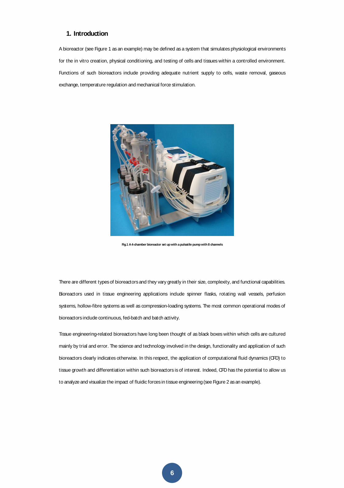
1. Introduction
A bioreactor (see Figure 1 as an example) may be defined as a system that simulates physiological environments
for the in vitro creation, physical conditioning, and testing of cells and tissues within a controlled environment.
Functions of such bioreactors include providing adequate nutrient supply to cells, waste removal, gaseous
exchange, temperature regulation and mechanical force stimulation.
Fig.1 A 4-chamber bioreactor set up with a pulsatile pump with 8 channels
There are different types of bioreactors and they vary greatly in their size, complexity, and functional capabilities.
Bioreactors used in tissue engineering applications include spinner flasks, rotating wall vessels, perfusion
systems, hollow-fibre systems as well as compression-loading systems. The most common operational modes of
bioreactors include continuous, fed-batch and batch activity.
Tissue engineering-related bioreactors have long been thought of as black boxes within which cells are cultured
mainly by trial and error. The science and technology involved in the design, functionality and application of such
bioreactors clearly indicates otherwise. In this respect, the application of computational fluid dynamics (CFD) to
tissue growth and differentiation within such bioreactors is of interest. Indeed, CFD has the potential to allow us
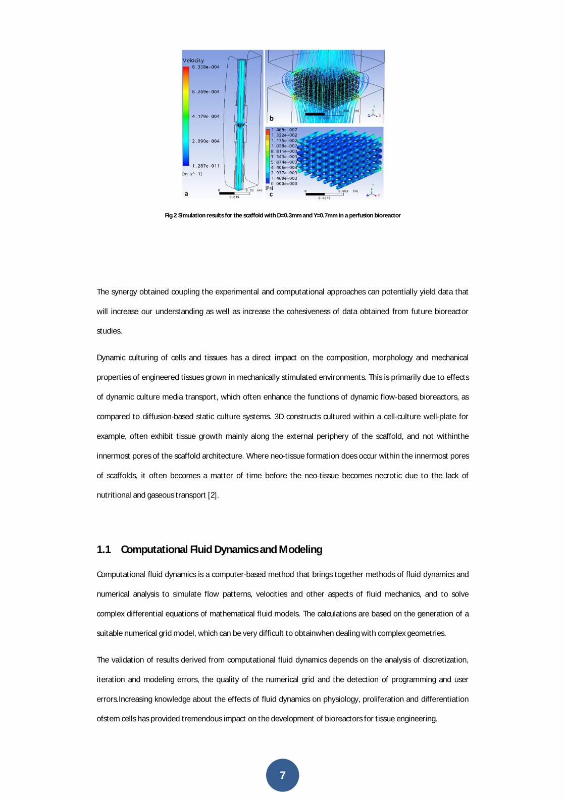
to analyze and visualize the impact of fluidic forces in tissue engineering (see Figure 2 as an example).
7
Fig.2 Simulation results for the scaffold with D=0.3mm and Y=0.7mm in a perfusion bioreactor
The synergy obtained coupling the experimental and computational approaches can potentially yield data that
will increase our understanding as well as increase the cohesiveness of data obtained from future bioreactor
studies.
Dynamic culturing of cells and tissues has a direct impact on the composition, morphology and mechanical
properties of engineered tissues grown in mechanically stimulated environments. This is primarily due to effects
of dynamic culture media transport, which often enhance the functions of dynamic flow-based bioreactors, as
compared to diffusion-based static culture systems. 3D constructs cultured within a cell-culture well-plate for
example, often exhibit tissue growth mainly along the external periphery of the scaffold, and not withinthe
innermost pores of the scaffold architecture. Where neo-tissue formation does occur within the innermost pores
of scaffolds, it often becomes a matter of time before the neo-tissue becomes necrotic due to the lack of
nutritional and gaseous transport [2].
1.1 Computational Fluid Dynamics and Modeling
Computational fluid dynamics is a computer-based method that brings together methods of fluid dynamics and
numerical analysis to simulate flow patterns, velocities and other aspects of fluid mechanics, and to solve
complex differential equations of mathematical fluid models. The calculations are based on the generation of a
suitable numerical grid model, which can be very difficult to obtainwhen dealing with complex geometries.
The validation of results derived from computational fluid dynamics depends on the analysis of discretization,
iteration and modeling errors, the quality of the numerical grid and the detection of programming and user
errors.Increasing knowledge about the effects of fluid dynamics on physiology, proliferation and differentiation
ofstem cells has provided tremendous impact on the development of bioreactors for tissue engineering.
8
New advances in the theoretical background and application technologies of fluid dynamics such as
computational fluid dynamics can help to improve design and construction of modern bioreactors. By computer
simulation of flow vectors, velocity distribution and pressure gradients, problems of bioreactor design such as
turbulent flow patterns can be identified prior to the experimental testing phase of the prototype.
Computational fluid dynamics allows adjusting the bioreactor design for optimal culture conditions of specific
stem cells and tissue-engineering constructs. Modern software for computational fluid dynamics can achieve
three-dimensional fluid dynamics models, which help to design even more precise bioreactor models for tissue
engineering [3].
Bioreactors allowing direct perfusion of culture medium through tissue-engineeredconstructs may overcome
diffusion limitations associated with static culturing, and may provide flow-mediated mechanical stimuli. The
hydrodynamic stress imposed on cells in these systems will depend not only on the culture medium flow rate but
also on the scaffold three dimensional (3D) micro-architecture.
The goal is to perform computational fluid dynamics (CFD) simulations of the flow of culture medium with the
aim of predicting the shear stress acting on cells adhering on the scaffold walls, as a function of various
parameters that can be set in a tissue-engineering experiment [5]: scaffold material, geometry, pore
size,porosity, Young’s modulus, efficient nutrient delivery, and dissolution rate and mechanical stimulation.
Previous research has shown that bone regeneration during fracture healing and osteochondral defect repair can
be simulated using mechano-regulation algorithms based on computing strain and/or fluid flow in the
regenerating tissue.
The mechano-regulation algorithm employed determines tissue differentiation both in terms of the prevailing
biophysical stimulus and number of precursor cells, where cell number is computed based on a three-
dimensional random-walk approach. The simulations predict that all three design variables have a critical effect
on the amount of bone regenerated, but not in an intuitive way: in a low load environment, a higher porosity and
higher stiffness but a medium dissolution rate gives the greatest amount of bone whereas in a high load
environment the dissolution rate should be lower otherwise the scaffold will collapse—at lower initial porosities
however, higher dissolution rates can be sustained. Besides showing that scaffolds may be optimized to suit the
site-specific loading requirements, the results open up a new approach for computational simulations in tissue
engineering [4].
1.2 Fluid dynamics
The speed of a flow affects its properties in a number of ways. At low enough speeds, the inertia of the fluid may
be ignored and we have creeping flow. This regime is of importance in flows containing small particles
(suspensions), in flows through porous media or in narrow passages (coating techniques, micro-devices). As the
9
speed is increased, inertia becomes important but each fluid particle follows a smooth trajectory; the flow is then
said to be laminar. Further increases in speed may lead to instability thateventually produces a more random
type of flow that is called turbulent; the process of laminar-turbulent transition is an important area in its own
right [5].
1.2.1 Reynolds number
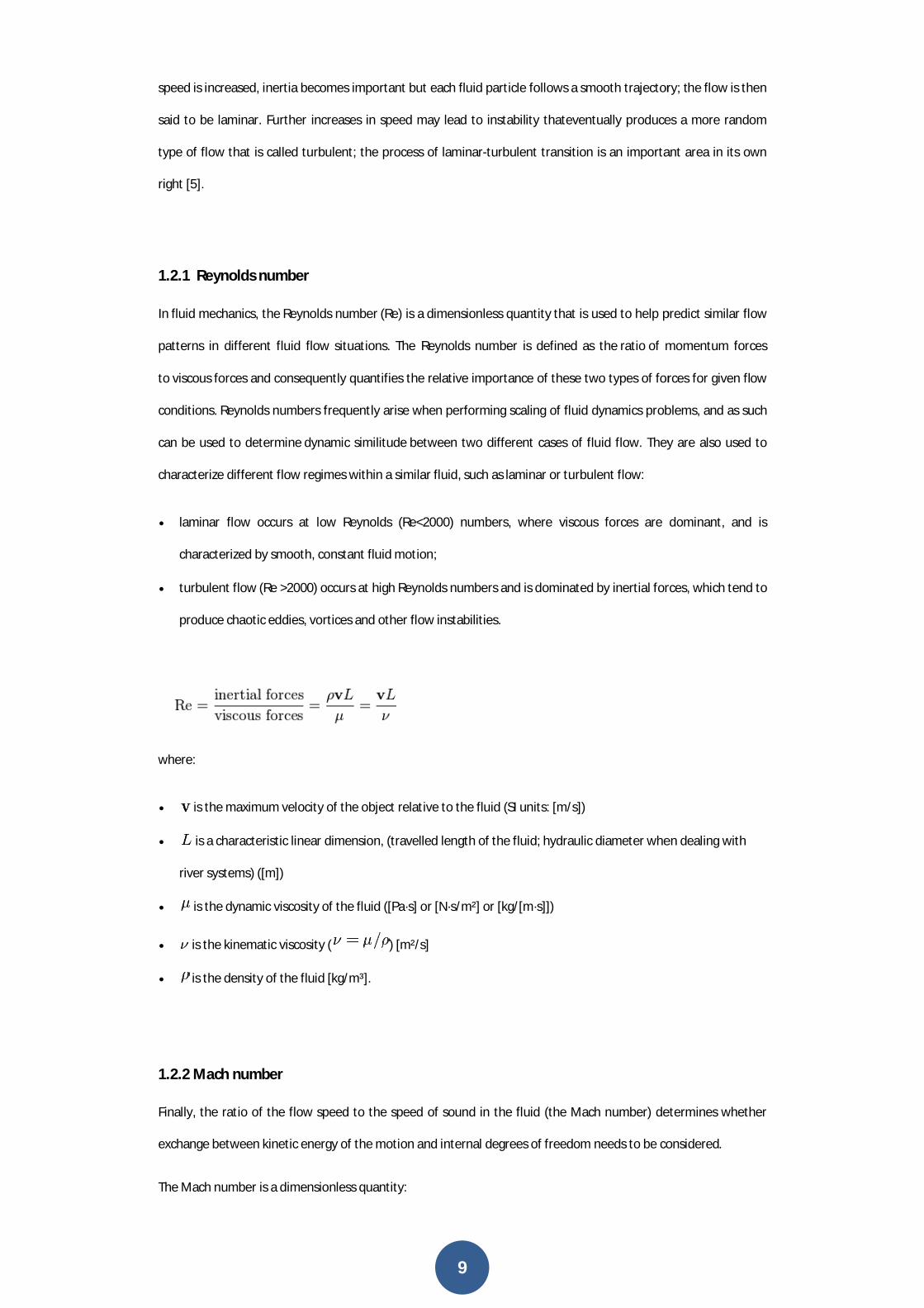
In fluid mechanics, the Reynolds number (Re) is a dimensionless quantity that is used to help predict similar flow
patterns in different fluid flow situations. The Reynolds number is defined as the ratio of momentum forces
to viscous forces and consequently quantifies the relative importance of these two types of forces for given flow
conditions. Reynolds numbers frequently arise when performing scaling of fluid dynamics problems, and as such
can be used to determine dynamic similitude between two different cases of fluid flow. They are also used to
characterize different flow regimes within a similar fluid, such as laminar or turbulent flow:
laminar flow occurs at low Reynolds (Re<2000) numbers, where viscous forces are dominant, and is
characterized by smooth, constant fluid motion;
turbulent flow (Re >2000) occurs at high Reynolds numbers and is dominated by inertial forces, which tend to
produce chaotic eddies, vortices and other flow instabilities.
where:
is the maximum velocity of the object relative to the fluid (SI units: [m/s])
is a characteristic linear dimension, (travelled length of the fluid; hydraulic diameter when dealing with
river systems) ([m])
is the dynamic viscosity of the fluid ([Pa·s] or [N·s/m²] or [kg/[m·s]])
is the kinematic viscosity ( ) [m²/s]
is the density of the fluid [kg/m³].
1.2.2 Mach number
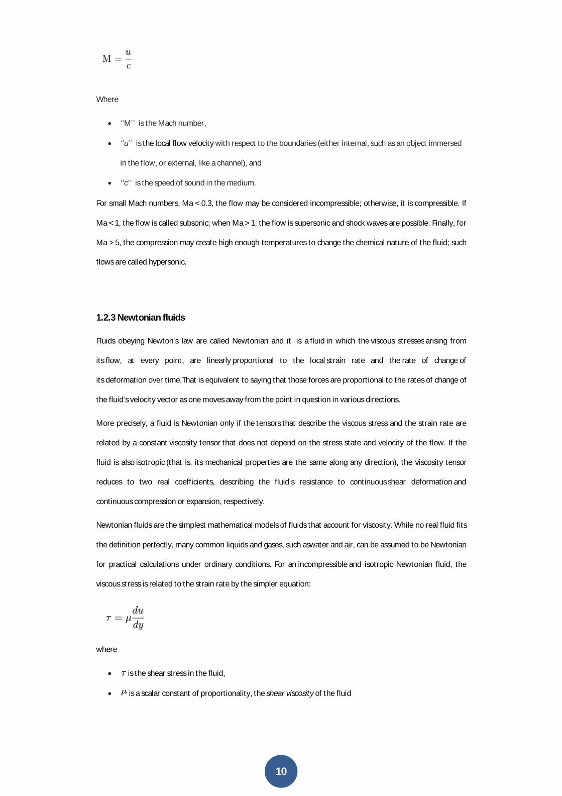
Finally, the ratio of the flow speed to the speed of sound in the fluid (the Mach number) determines whether
exchange between kinetic energy of the motion and internal degrees of freedom needs to be considered.
The Mach number is a dimensionless quantity:
speed is increased, inertia becomes important but each fluid particle follows a smooth trajectory; the flow is then
ity thateventually produces a more random
turbulent transition is an important area in its own
that is used to help predict similar flow
of momentum forces
forces and consequently quantifies the relative importance of these two types of forces for given flow
Reynolds numbers frequently arise when performing scaling of fluid dynamics problems, and as such
between two different cases of fluid flow. They are also used to
numbers, where viscous forces are dominant, and is
occurs at high Reynolds numbers and is dominated by inertial forces, which tend to
en dealing with
Finally, the ratio of the flow speed to the speed of sound in the fluid (the Mach number) determines whether
exchange between kinetic energy of the motion and internal degrees of freedom needs to be considered.
10
Where
‘’M’’ is the Mach number,
‘’u’’ is the local flow velocity with respect to the boundaries (either internal, such as an object immersed
in the flow, or external, like a channel), and
‘’c’’ is the speed of sound in the medium.
For small Mach numbers, Ma < 0.3, the flow may be considered incompressible; otherwise, it is compressible. If
Ma < 1, the flow is called subsonic; when Ma > 1, the flow is supersonic and shock waves are possible. Finally, for
Ma > 5, the compression may create high enough temperatures to change the chemical nature of the fluid; such
flows are called hypersonic.
1.2.3 Newtonian fluids
Fluids obeying Newton's law are called Newtonian and it is a fluid in which the viscous stresses
its flow, at every point, are linearly proportional to the local strain rate and the rate of change
its deformation over time.That is equivalent to saying that those forces are proportional to the rates of change of
the fluid's velocity vector as one moves away from the point in question in various directions.
More precisely, a fluid is Newtonian only if the tensors that describe the viscous stress and the strain rate are
related by a constant viscosity tensor that does not depend on the stress state and velocity of the flow. If the
fluid is also isotropic (that is, its mechanical properties are the same along any direction), the viscosity tensor
reduces to two real coefficients, describing the fluid's resistance to continuous shear deformation
continuous compression or expansion, respectively.
Newtonian fluids are the simplest mathematical models of fluids that account for viscosity. While no real fluid fits
the definition perfectly, many common liquids and gases, such aswater and air, can be assumed to be Newtonian
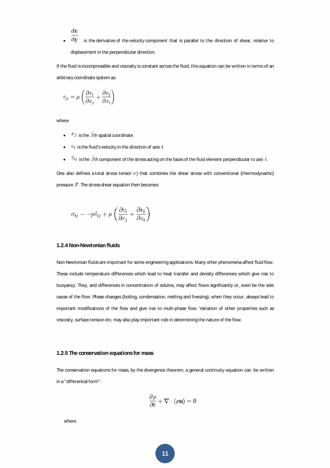
for practical calculations under ordinary conditions. For an incompressible and isotropic Newtonian fluid, the
viscous stress is related to the strain rate by the simpler equation:
where
is the shear stress in the fluid,
is a scalar constant of proportionality, the shear viscosity of the fluid
with respect to the boundaries (either internal, such as an object immersed
For small Mach numbers, Ma < 0.3, the flow may be considered incompressible; otherwise, it is compressible. If
Ma < 1, the flow is called subsonic; when Ma > 1, the flow is supersonic and shock waves are possible. Finally, for
reate high enough temperatures to change the chemical nature of the fluid; such
viscous stresses arising from
rate of change of
over time.That is equivalent to saying that those forces are proportional to the rates of change of
ous stress and the strain rate are
that does not depend on the stress state and velocity of the flow. If the
(that is, its mechanical properties are the same along any direction), the viscosity tensor
shear deformation and
of fluids that account for viscosity. While no real fluid fits
, can be assumed to be Newtonian
and isotropic Newtonian fluid, the
11
is the derivative of the velocity component that is parallel to the direction of shear, relative to
displacement in the perpendicular direction.
If the fluid is incompressible and viscosity is constant across the fluid, this equation can be written in terms of an
arbitrary coordinate system as:
where
is the th spatial coordinate
is the fluid's velocity in the direction of axis
is the th component of the stress acting on the faces of the fluid element perpendicular to axis
One also defines a total stress tensor ) that combines the shear stress with conventional (thermodynamic)
pressure . The stress-shear equation then becomes
1.2.4 Non-Newtonian fluids
Non-Newtonian fluids are important for some engineering applications. Many other phenomena affect fluid flow.
These include temperature differences which lead to heat transfer and density differences which give rise to
buoyancy. They, and differences in concentration of solutes, may affect flows significantly or, even be the sole
cause of the flow. Phase changes (boiling, condensation, melting and freezing), when they occur, always lead to
important modifications of the flow and give rise to multi-phase flow. Variation of other properties such as
viscosity, surface tension etc. may also play important role in determining the nature of the flow.
1.2.5 The conservation equations for mass
The conservation equations for mass, by the divergence theorem, a general continuity equation can
in a "differential form":
where
component that is parallel to the direction of shear, relative to
and viscosity is constant across the fluid, this equation can be written in terms of an
th component of the stress acting on the faces of the fluid element perpendicular to axis .
) that combines the shear stress with conventional (thermodynamic)
Newtonian fluids are important for some engineering applications. Many other phenomena affect fluid flow.
differences which give rise to
buoyancy. They, and differences in concentration of solutes, may affect flows significantly or, even be the sole
cause of the flow. Phase changes (boiling, condensation, melting and freezing), when they occur, always lead to
phase flow. Variation of other properties such as
viscosity, surface tension etc. may also play important role in determining the nature of the flow.
, a general continuity equation can be written
12
ρ is fluid density,
t is time,
u is the flow velocity vector field.
In this context, this equation is also one of the Euler equations (fluid dynamics). The
equations form a vector continuity equation describing the conservation of linear momentum
written in a "differential form" in a closed system (one that does not exchange any matter with its
surroundings and is not acted on by external forces) the total momentum is constant.
1.2.6 The law of conservation of momentum
This fact, known as the law of conservation of momentum, is implied by Newton's laws of motion
for example, that two particles interact. Because of the third law, the forces between the
opposite. If the particles are numbered 1 and 2, the second law states
and .
Therefore
with the negative sign indicating that the forces oppose. Equivalently
If the velocities of the particles are u1 and u2 before the interaction, and afterwards they are v1 and
This law holds no matter how complicated the force is between particles. Similarly, if there are several particles,
the momentum exchanged between each pair of particles adds up to zero, so the total change in momentum is
. The Navier–Stokes
linear momentum that can be
(one that does not exchange any matter with its
Newton's laws of motion. Suppose,
for example, that two particles interact. Because of the third law, the forces between them are equal and
and v2, then
This law holds no matter how complicated the force is between particles. Similarly, if there are several particles,
the momentum exchanged between each pair of particles adds up to zero, so the total change in momentum is
13
zero. This conservation law applies to all interactions, including collisions and separations caused by explosive
forces.
They are non-linear, coupled, and difficult to solve. It is difficult to prove by the existing mathematical tools that a
unique solution exists for particular boundary conditions. Experience shows that theincomprensibleNavier-Stokes
equations (convective form):
describe the flow of a Newtonian fluid accurately.
where:
is the kinematic viscosity
The incompressible Navier–Stokes equations is the fundamental equation of hydraulics. The domain for this
equation is commonly a 3 or less euclidean space, for which an orthogonal coordinate reference frame is usually
set to explicit the system of scalar partial derivative equations to be solved. In 3D orthogonal coordinate systems
are 3: Cartesian, cylindrical, and spherical.
These flows are important for studying the fundamentals of fluid dynamics, but their practical relevance is
limited. In all cases in which such a solution is possible, many terms in the equations are zero. For other flows
some terms are unimportant and we may neglect them; this simplification introduces an error. In most cases,
even the simplified equations cannot be solved analytically; one has to use numerical methods. The computing
effort may be much smaller than for the full equations, which is a justification for simplifications. It list below
some flow types for which the equations of motion can be simplified.
Discretization errors can be reduced by using more accurate interpolation or approximations or by applying the
approximations to smaller regions but this usually increases the time and cost of obtaining the solution.
Compromise is usually needed. We shall present some schemes in detail but shall also point out ways of creating
more accurate approximations [6].
14
1.2 Consideration about bone hierarchy and scaffold properties
1.3.1 Bone Hierarchy
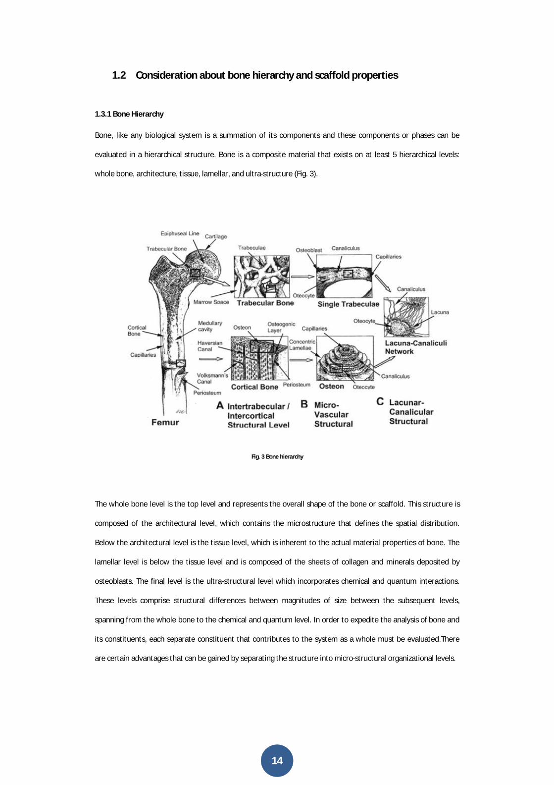
Bone, like any biological system is a summation of its components and these components or phases can be
evaluated in a hierarchical structure. Bone is a composite material that exists on at least 5 hierarchical levels:
whole bone, architecture, tissue, lamellar, and ultra-structure (Fig. 3).
Fig. 3 Bone hierarchy
The whole bone level is the top level and represents the overall shape of the bone or scaffold. This structure is
composed of the architectural level, which contains the microstructure that defines the spatial distribution.
Below the architectural level is the tissue level, which is inherent to the actual material properties of bone. The
lamellar level is below the tissue level and is composed of the sheets of collagen and minerals deposited by
osteoblasts. The final level is the ultra-structural level which incorporates chemical and quantum interactions.
These levels comprise structural differences between magnitudes of size between the subsequent levels,
spanning from the whole bone to the chemical and quantum level. In order to expedite the analysis of bone and
its constituents, each separate constituent that contributes to the system as a whole must be evaluated.There
are certain advantages that can be gained by separating the structure into micro-structural organizational levels.
15
At the hierarchical level, it is easy to compare different structures and tissues. Additionally, it is much simpler to
define characteristic levels to use for analysis. Each level depends on the lower levels to provide function and
structural support for the top levels (Table 1).
Table 1 Bone Hierarchy Levels
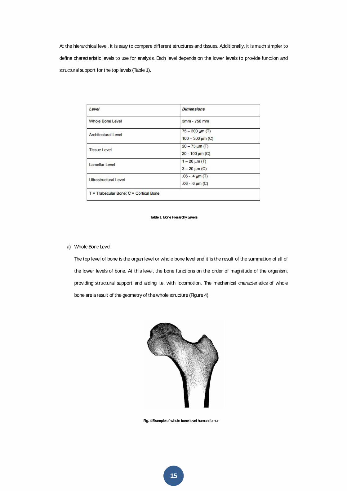
a) Whole Bone Level
The top level of bone is the organ level or whole bone level and it is the result of the summation of all of
the lower levels of bone. At this level, the bone functions on the order of magnitude of the organism,
providing structural support and aiding i.e. with locomotion. The mechanical characteristics of whole
bone are a result of the geometry of the whole structure (Figure 4).
Fig. 4 Example of whole bone level human femur
16
At this hierarchical level, the bone may interact with other bones, joints, or muscles in the body.
Optimization at this level is as a result of the need of the organism for strength in the whole bone, and
not as a result of localized stress concentrations. Shape changes that occur at this level are minimal and
the mechanical strength of the structure is a result of the total geometry of the bone and the distribution
of the tissue. Remodeling that may occur at lower levels is measured as percent increase or decrease in
mass in the overall bone.
b) Architectural Level
The architectural level of bone relates to the characteristic micro-architecture of bone tissue, specifically
cortical or trabecular bone. One step below the global structure is the architecture which serves to
provide mechanical stability to the entire global structure of bone. The optimized architecture of bone
shares the overall load of the entire organ and is distributed throughout the osteons and/or trabeculae. It
is at this level that the effects of remodeling are seen as a change in geometry or architecture and in the
apparent mechanical properties. Depending on the type of bone, trabecular or cortical, two different
architectures will arise. Trabecular bone, contained in the end of long bones and the site of bone marrow
synthesis, exhibits anisotropy as a result of its rod and plateorganization. Cortical bone is highly compact
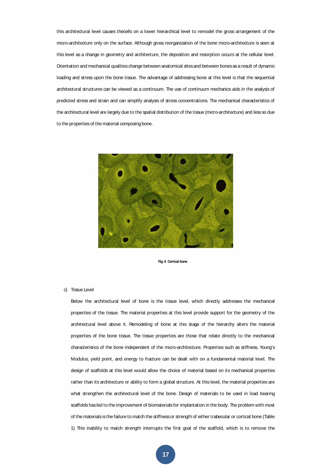
and orthotropic due to the circular nature of the osteons that make up its structure. One illustration of
the micro-architectural differences between the two architectures is that cortical bone contains only
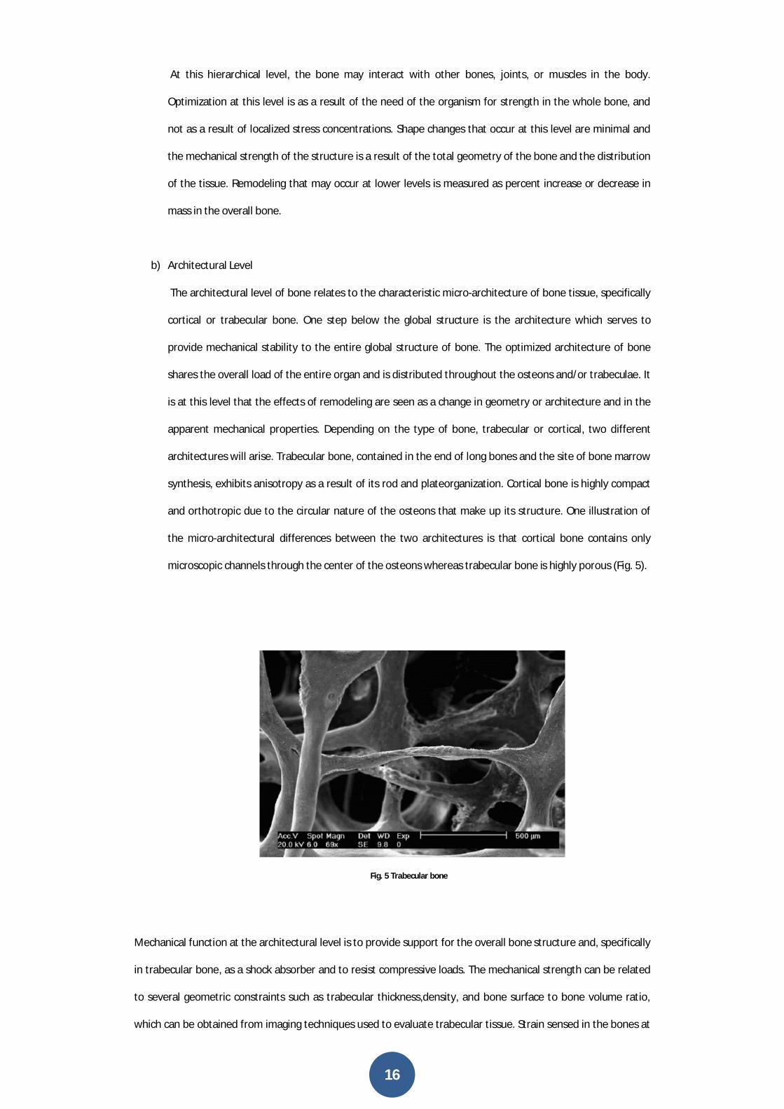
microscopic channels through the center of the osteons whereas trabecular bone is highly porous (Fig. 5).
Fig. 5 Trabecular bone
Mechanical function at the architectural level is to provide support for the overall bone structure and, specifically
in trabecular bone, as a shock absorber and to resist compressive loads. The mechanical strength can be related
to several geometric constraints such as trabecular thickness,density, and bone surface to bone volume ratio,
which can be obtained from imaging techniques used to evaluate trabecular tissue. Strain sensed in the bones at
17
this architectural level causes thecells on a lower hierarchical level to remodel the gross arrangement of the
micro-architecture only on the surface. Although gross reorganization of the bone micro-architecture is seen at
this level as a change in geometry and architecture, the deposition and resorption occurs at the cellular level.
Orientation and mechanical qualities change between anatomical sites and between bones as a result of dynamic
loading and stress upon the bone tissue. The advantage of addressing bone at this level is that the sequential
architectural structures can be viewed as a continuum. The use of continuum mechanics aids in the analysis of
predicted stress and strain and can simplify analysis of stress concentrations. The mechanical characteristics of
the architectural level are largely due to the spatial distribution of the tissue (micro-architecture) and less so due
to the properties of the material composing bone.
Fig. 6 Cortical bone
c) Tissue Level
Below the architectural level of bone is the tissue level, which directly addresses the mechanical
properties of the tissue. The material properties at this level provide support for the geometry of the
architectural level above it. Remodeling of bone at this stage of the hierarchy alters the material
properties of the bone tissue. The tissue properties are those that relate directly to the mechanical
characteristics of the bone independent of the micro-architecture. Properties such as stiffness, Young’s
Modulus, yield point, and energy to fracture can be dealt with on a fundamental material level. The
design of scaffolds at this level would allow the choice of material based on its mechanical properties
rather than its architecture or ability to form a global structure. At this level, the material properties are
what strengthen the architectural level of the bone. Design of materials to be used in load bearing
scaffolds has led to the improvement of biomaterials for implantation in the body. The problem with most
of the materials is the failure to match the stiffness or strength of either trabecular or cortical bone (Table
1) This inability to match strength interrupts the first goal of the scaffold, which is to remove the
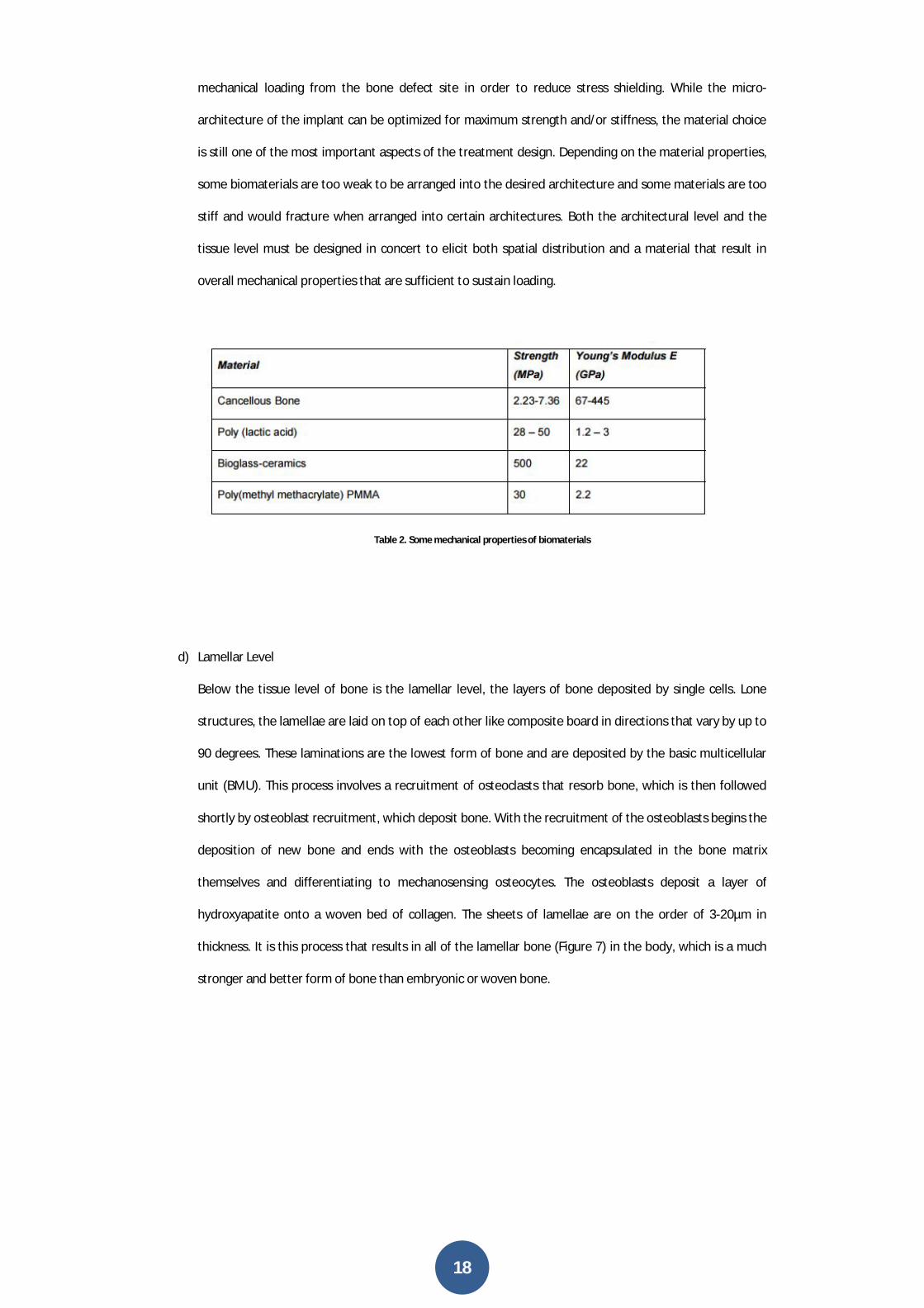
18
mechanical loading from the bone defect site in order to reduce stress shielding. While the micro-
architecture of the implant can be optimized for maximum strength and/or stiffness, the material choice
is still one of the most important aspects of the treatment design. Depending on the material properties,
some biomaterials are too weak to be arranged into the desired architecture and some materials are too
stiff and would fracture when arranged into certain architectures. Both the architectural level and the
tissue level must be designed in concert to elicit both spatial distribution and a material that result in
overall mechanical properties that are sufficient to sustain loading.
Table 2. Some mechanical properties of biomaterials
d) Lamellar Level
Below the tissue level of bone is the lamellar level, the layers of bone deposited by single cells. Lone
structures, the lamellae are laid on top of each other like composite board in directions that vary by up to
90 degrees. These laminations are the lowest form of bone and are deposited by the basic multicellular
unit (BMU). This process involves a recruitment of osteoclasts that resorb bone, which is then followed
shortly by osteoblast recruitment, which deposit bone. With the recruitment of the osteoblasts begins the
deposition of new bone and ends with the osteoblasts becoming encapsulated in the bone matrix
themselves and differentiating to mechanosensing osteocytes. The osteoblasts deposit a layer of
hydroxyapatite onto a woven bed of collagen. The sheets of lamellae are on the order of 3-20µm in
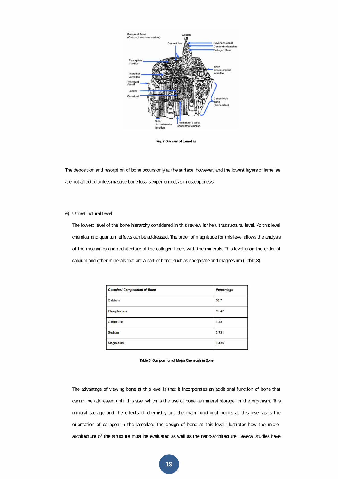
thickness. It is this process that results in all of the lamellar bone (Figure 7) in the body, which is a much
stronger and better form of bone than embryonic or woven bone.
19
Fig. 7 Diagram of Lamellae
The deposition and resorption of bone occurs only at the surface, however, and the lowest layers of lamellae
are not affected unless massive bone loss is experienced, as in osteoporosis.
e) Ultrastructural Level
The lowest level of the bone hierarchy considered in this review is the ultrastructural level. At this level
chemical and quantum effects can be addressed. The order of magnitude for this level allows the analysis
of the mechanics and architecture of the collagen fibers with the minerals. This level is on the order of
calcium and other minerals that are a part of bone, such as phosphate and magnesium (Table 3).
Table 3. Composition of Major Chemicals in Bone
The advantage of viewing bone at this level is that it incorporates an additional function of bone that
cannot be addressed until this size, which is the use of bone as mineral storage for the organism. This
mineral storage and the effects of chemistry are the main functional points at this level as is the
orientation of collagen in the lamellae. The design of bone at this level illustrates how the micro-
architecture of the structure must be evaluated as well as the nano-architecture. Several studies have

20
been completed on the difference in mechanical properties as a result of the collagen orientation and the
amount of mineral deposition on the collagen beds. The degree of mineralization will affect the final
stiffness of the bone itself as well as the overall ash content [7].
1.3.2 Scaffold design
A scaffold for hard tissue reconstruction is a three dimensional construct, which is used as a support structure
allowing the tissues/cells to adhere, proliferate and differentiate to form a healthy bone/tissue for restoring the
functionality. In almost all the clinical cases, scaffolds for hard tissue repair in a load-bearing area are not
temporary, but permanent. They most retain theirshape, strength and biological integrity through the process of
regeneration/repair of the damaged bone tissue.
Bone replacement constructs for bone defects reconstructions would need to be biocompatible with surrounding
tissue, radiolucent, easily shaped or molded to fit perfectly into the bone defect, nonallergic and non-
carcinogenic, strong enough to endure trauma, stable over time, able to maintain its volume and
osteoconductive (able to support bone growth and encourage the ingrowth of surrounding bone). Apart from the
above-mentioned material requirements, the structural requirements expected for the possible candidate for
bone scaffold are numerous, ranging from the maximum feasible porosity to the porous architecture itself. Pore
size and interconnectivity are important in that they can affect how much cells can penetrate and grow into the
scaffold and what quantity of materials and nutrients can be transported into and out of the scaffold and
vascularization.
Fig. 8 Bone specimen and tissue engineered scaffold
Physiologically, previous research has shown that the optimum pore size for promoting bone ingrowth is in the
range of 100-500 m [7]. However, the scientific community has not reached yet a consensus regarding the
optimal pore size for bone ingrowth. From a mechanical perspective, scaffold materials aimed for the repair of
structural tissues should provide mechanical support in order to preserve tissue volume and ultimately to

21
facilitate tissue regeneration. The most critical mechanical properties to be matched by the scaffold are bone
loading stiffness, strength and fatigue strength [8].
In addition to matching bone stiffness, the scaffold should also match or exceed the strength of natural bone. The
scaffold must resist physiological forces within the implantation site and should have sufficient strength and
stiffness to function for a period until in vivo tissue ingrowth has filled the scaffold matrix. An equal or excess
strength ensures that the scaffold has equivalent or better load bearing capabilities than natural bone. For last,
for a nonresorbable scaffold, it is very important to consider the fatigue strength, since the scaffold will be
exposed to cyclic loading during the rest of the patient’s life.
In the scaffold design, surface properties including: topography, surface energy, chemical composition, surface
wettability, surface bioactivity, etc., must all be considered, taking into account that in a complex porous 3-D
scaffold the surface is not just the outside surface, but also the internal 3-D surfaces. For example, the
modification of scaffolds materials with bioactive molecules is a technique to tailor the scaffold bioactivity.
In addition, reduction of micromotion can be obtained by appropriately tailoring the material surface of the
scaffold. The development of the required interface is not only highly influenced by surface chemistry, but also
more specifically by nanometer and micrometer scale topographies. The surface roughness is found to influence
the cell morphology and growth.
On the other hand, to program scaffolds with biological structures, cells and growth factors need to be integrated
into the scaffold fabrication for bone tissue engineering, so that the bioactive molecules can be released from the
scaffold in order to stimulate or modulate new tissue formation. Through surface modifications the metallic
scaffold surface can be tailored to improve the adhesion of cells and adsorption of biomolecules in order to
stimulate the bone formation and to facilitate faster healing. Currently, a significant research effort is aimed at
the biochemical modification of metallic surfaces.
The goal of the biochemical surface modification is to immobilize proteins, enzymes or peptides on biomaterials
for the purpose of inducing specific cell and tissue responses, or in other words, to control the tissue-scaffold
interface with molecules delivered directly to the interface [9].
Computed-aided tissue engineering enables the application of advanced computer aided technologies and
biomechanical engineering principles to derive systematic solutions for the designing and fabrication of
patientspecific scaffold [10].
The prediction of desired mechanical characteristics for bone scaffolds based on similar bone modeling steps. If
we take a look at bone tissue of one species (i.e. humans) in particular, we generally differentiate only between
trabecular and cortical bone. Previous studies on the mechanical properties of bone tissue, however, have
revealed that trabecular bone material properties vary significantly between anatomic sites. Nevertheless, it was
found that the tissue properties of trabecular and cortical bone from different anatomical sites are comparable.
22
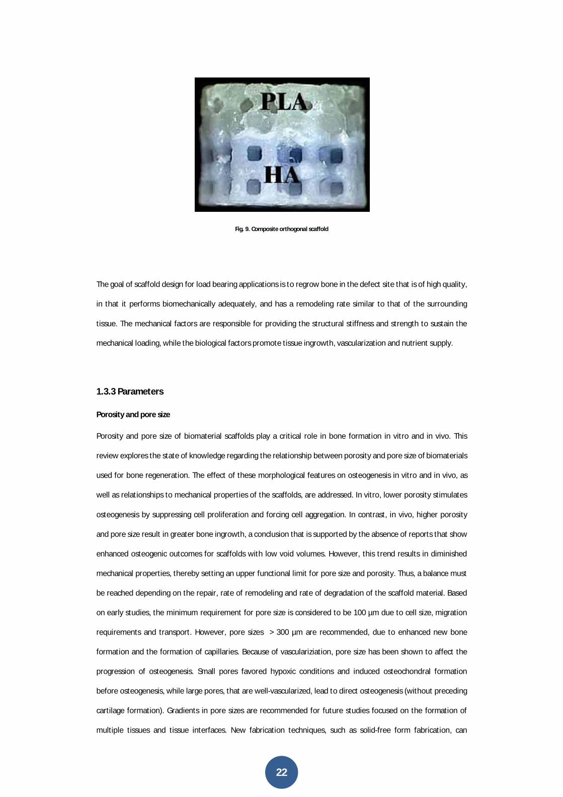
Fig. 9. Composite orthogonal scaffold
The goal of scaffold design for load bearing applications is to regrow bone in the defect site that is of high quality,
in that it performs biomechanically adequately, and has a remodeling rate similar to that of the surrounding
tissue. The mechanical factors are responsible for providing the structural stiffness and strength to sustain the
mechanical loading, while the biological factors promote tissue ingrowth, vascularization and nutrient supply.
1.3.3 Parameters
Porosity and pore size
Porosity and pore size of biomaterial scaffolds play a critical role in bone formation in vitro and in vivo. This
review explores the state of knowledge regarding the relationship between porosity and pore size of biomaterials
used for bone regeneration. The effect of these morphological features on osteogenesis in vitro and in vivo, as
well as relationships to mechanical properties of the scaffolds, are addressed. In vitro, lower porosity stimulates
osteogenesis by suppressing cell proliferation and forcing cell aggregation. In contrast, in vivo, higher porosity
and pore size result in greater bone ingrowth, a conclusion that is supported by the absence of reports that show
enhanced osteogenic outcomes for scaffolds with low void volumes. However, this trend results in diminished
mechanical properties, thereby setting an upper functional limit for pore size and porosity. Thus, a balance must
be reached depending on the repair, rate of remodeling and rate of degradation of the scaffold material. Based
on early studies, the minimum requirement for pore size is considered to be 100 µm due to cell size, migration
requirements and transport. However, pore sizes > 300 µm are recommended, due to enhanced new bone
formation and the formation of capillaries. Because of vasculariziation, pore size has been shown to affect the
progression of osteogenesis. Small pores favored hypoxic conditions and induced osteochondral formation
before osteogenesis, while large pores, that are well-vascularized, lead to direct osteogenesis (without preceding
cartilage formation). Gradients in pore sizes are recommended for future studies focused on the formation of
multiple tissues and tissue interfaces. New fabrication techniques, such as solid-free form fabrication, can
23
potentially be used to generate scaffolds with morphological and mechanical properties more selectively
designed to meet the specificity of bone repair needs. Although increased porosity and pore size facilitate bone
ingrowth, the result is a reduction in mechanical properties, since this compromises the structural integrity of the
scaffold. The differences of bone tissues in morphological (pore size and porosity) and mechanical properties, as
well as gradient features of adsorbed cytokines, set challenges for fabricating biomaterial scaffolds that can meet
the requirements set by the specific site of application. Other researchers have proposed a computational
algorithm, based on topology optimization, that paired different porosities with scaffold geometries for certain
mechanical properties. Prototypes of the designed scaffold architectures can be fabricated with techniques, such
as solid-free form fabrication techniques. The versatility provided by this technique will allow the fabrication of
implants with different porosities, pore sizes and mechanical properties that can mimic the complex architecture
of bone-specific sites to optimize bone tissue regeneration [11].
Young’s modulus
The cells within each lattice differentiate based on the stimuli calculated by the mechano-regulation algorithm.
The mechanical properties are calculated using the rule of mixtures. The rule of mixtures accounts for both the
number and phenotype of cells within each element and therefore the material properties will change gradually
towards the phenotype determined by the stimulus.
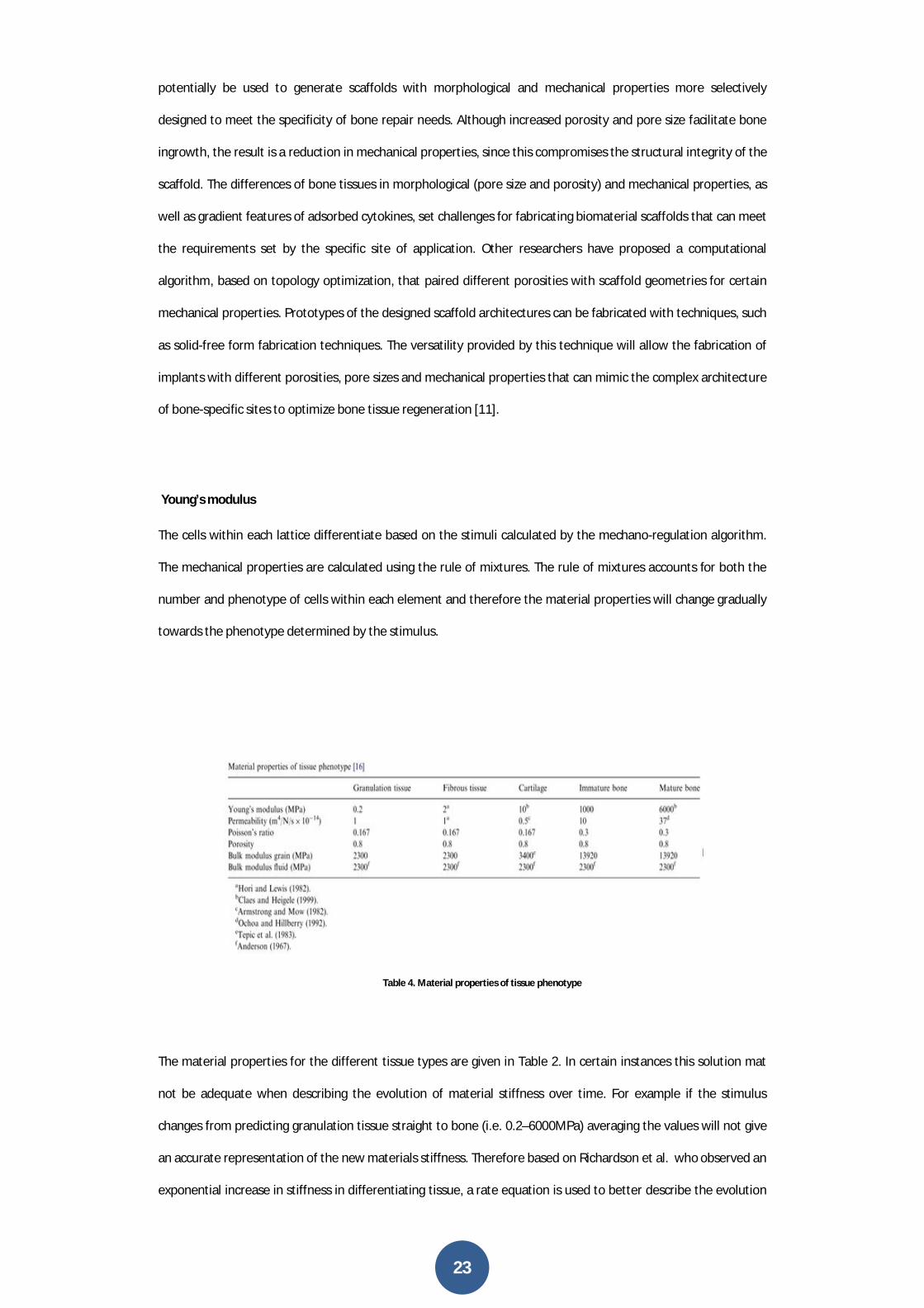
Table 4. Material properties of tissue phenotype
The material properties for the different tissue types are given in Table 2. In certain instances this solution mat
not be adequate when describing the evolution of material stiffness over time. For example if the stimulus
changes from predicting granulation tissue straight to bone (i.e. 0.2–6000MPa) averaging the values will not give
an accurate representation of the new materials stiffness. Therefore based on Richardson et al. who observed an
exponential increase in stiffness in differentiating tissue, a rate equation is used to better describe the evolution
24
of the Young’s modulus of the regenerating tissue. The equation of describing the variation of the Young’s
modulus is of the form:
Where Ei represents the Young’s modulus for tissue phenotype i (where i is fibrous tissue, cartilage, immature or
mature bone), t is the time and Ki and βi are two parameters regulating the shape of the exponential curve. The
values of Ki and βihave been set so that the Young’s modulus of tissue phenotype i increases in 60 days from the
initial value of 0.2MPa, typical of granulation tissue to the final values reported up (Table 2).
The time is based on the age of the cell; therefore the rate equation starts locally after the deposition of a certain
tissue type [12].
Degradation rate
Scaffolds fabricated from biomaterials with a high degradation rate should not have high porosities (>90%), since
rapid depletion of the biomaterial will compromise the mechanical and structural integrity before substitution by
newly formed bone. In contrast, scaffolds fabricated from biomaterials with low degradation rates and robust
mechanical properties can be highly porous, because the higher pore surface area interacting with the host tissue
can accelerate degradation due to macrophages via oxidation and/or hydrolysis [13].
1.3.4 Synthetic polymer materials
Biodegradable synthetic polymers offer a number of advantages over other materials for developing scaffolds in
tissue engineering. The key advantages include the ability to tailor mechanical properties and degradation
kinetics to suit various applications. Synthetic polymers are also attractive because they can be fabricated into
various shapes with desired pore morphologic features conducive to tissue in-growth. Furthermore, polymers
can be designed with chemical functional groups that can induce tissue in-growth. Biodegradable synthetic
polymers such as poly(glycolic acid), poly(lactic acid) and their copolymers, poly(p-dioxanone), and copolymers of
trimethylene carbonate and glycolide have been used in a number of clinical applications. Among the families of
synthetic polymers, the polyesters have been attractive for these applications because of their ease of
degradation by hydrolysis of ester linkage, degradation products being resorbed through the metabolic pathways
in some cases and the potential to tailor the structure to alter degradation rates. These requirements range from
the ability of scaffold to provide mechanical support during tissue growth and gradually degrade to
biocompatible products to more demanding requirements such as the ability to incorporate cells, growth factors
etc and provide osteoconductive and osteoinductive environments [14].

25
Polylactic acid (PLA)
Thepolylactic acid (PLA) is completely degradable. A factorial experimental design was applied to optimise
scaffold composition prior to simultaneous microtomography and micromechanical testing. Synchrotron X-ray
microtomography combined with in situ micromechanical testing was performed to obtain three-dimensional
(3D) images of the scaffolds under compression.
Fig. 10 PLA scaffold
The experimental design reveals that larger glass particle and pore sizes reduce the stiffness of the scaffolds, and
that the porosity is largely unaffected by changes in pore sizes or glass weight content. The porosity ranges
between 93% and 96.5%, and the stiffness ranges between 50 and 200 kPa [15].
PMMA
Poly (methyl methacrylate) (PMMA) is a polymer largely used in biomedical applications. It has a good degree of
compatibility with human tissues. A relevant biomedical application of PMMA is represented by the production
of porous scaffolds to be used as controlled release devices for pharmaceutical products [16]. The drug release
from a scaffold is controlled by different mass transfer mechanisms, such as diffusion, erosion, swelling or
osmosis. It depends also on the material properties (composition, porosity, roughness, wettability and water
uptake) and on the drug properties, such as its solubility and molecular weight.
26
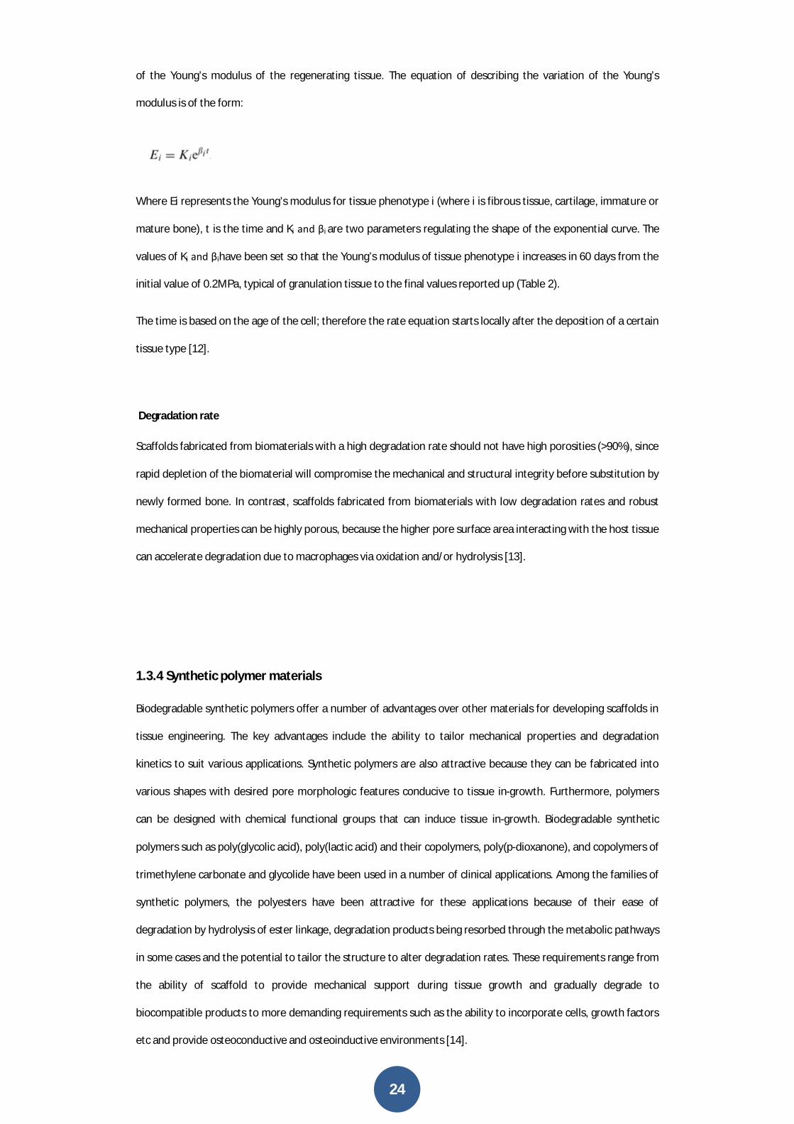
Fig. 11 PMMA scaffold
it suffers from the fact that it is not degraded and that its high curing temperatures can cause necrosis of the
surrounding tissue [17].
1.3.5 Natural polymer materials
The collagen is the most abundant protein in mammals. It provides structural and mechanical support to tissues
and organs,and fulfill biomechanical functions in bone, cartilage, skin, tendon, and ligament. Collagen scaffolds
have been used in numerous medical applications: drug delivery, hemostatic pads, skin substitutes, soft tissue
augmentation, suturing and as tissue engineering substrate.Collagen scaffolds are processed in a variety of
forms.24 Thin sheets and gels are substrates for smooth muscle,renal hepatic,endothelialand epithelial
cells, while sponges are often used to engineer skeletal tissues such as cartilage,tendon and bone. Collagen is
biodegradable and has low or negligible antigenicity [18].
Forms of collagen type I, commonly extracted from bovine tendon, are biocompatible and adequate scaffolds for
tissue engineering in terms of mechanical properties, pore structure, permeability, hydrophilicity and in
vivo stability. Several immunological studies (animal models) of injectable collagen gels and implanted collagen
sponges, confirm little or no antibodies to collagen type I are detected.Collagen type I has been shown to support
osteoblast, osteoclast, and chondrocyte attachment, proliferation, and differentiation in vitroas well as in vivo
[19].
27
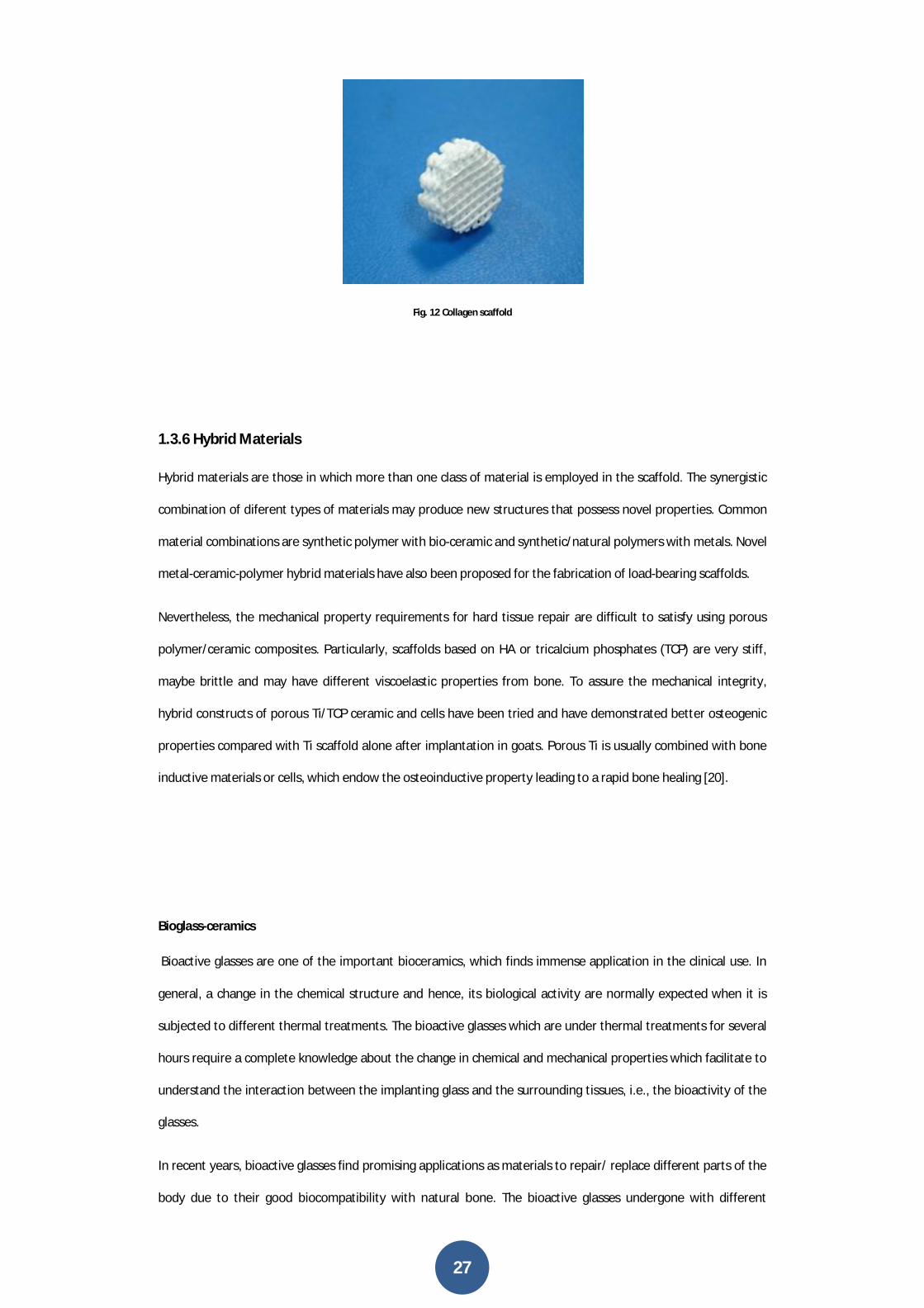
Fig. 12 Collagen scaffold
1.3.6 Hybrid Materials
Hybrid materials are those in which more than one class of material is employed in the scaffold. The synergistic
combination of diferent types of materials may produce new structures that possess novel properties. Common
material combinations are synthetic polymer with bio-ceramic and synthetic/natural polymers with metals. Novel
metal-ceramic-polymer hybrid materials have also been proposed for the fabrication of load-bearing scaffolds.
Nevertheless, the mechanical property requirements for hard tissue repair are difficult to satisfy using porous
polymer/ceramic composites. Particularly, scaffolds based on HA or tricalcium phosphates (TCP) are very stiff,
maybe brittle and may have different viscoelastic properties from bone. To assure the mechanical integrity,
hybrid constructs of porous Ti/TCP ceramic and cells have been tried and have demonstrated better osteogenic
properties compared with Ti scaffold alone after implantation in goats. Porous Ti is usually combined with bone
inductive materials or cells, which endow the osteoinductive property leading to a rapid bone healing [20].
Bioglass-ceramics
Bioactive glasses are one of the important bioceramics, which finds immense application in the clinical use. In
general, a change in the chemical structure and hence, its biological activity are normally expected when it is
subjected to different thermal treatments. The bioactive glasses which are under thermal treatments for several
hours require a complete knowledge about the change in chemical and mechanical properties which facilitate to
understand the interaction between the implanting glass and the surrounding tissues, i.e., the bioactivity of the
glasses.
In recent years, bioactive glasses find promising applications as materials to repair/ replace different parts of the
body due to their good biocompatibility with natural bone. The bioactive glasses undergone with different
28
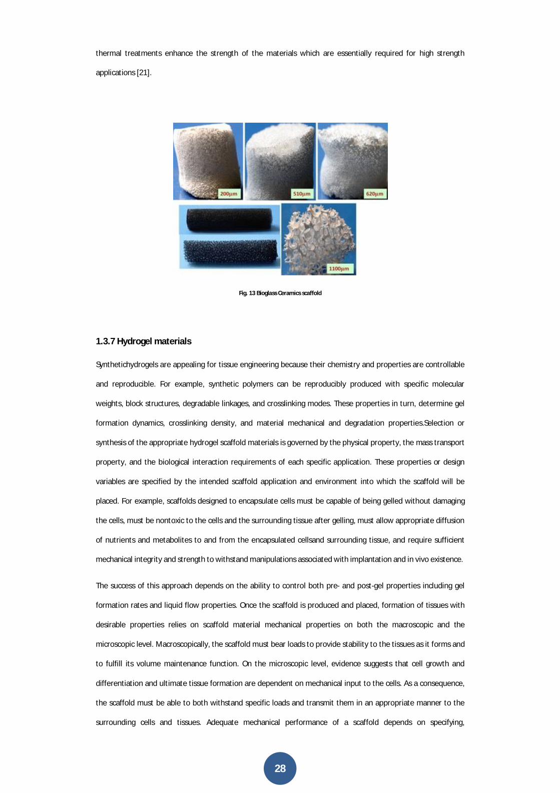
thermal treatments enhance the strength of the materials which are essentially required for high strength
applications [21].
Fig. 13 Bioglass Ceramics scaffold
1.3.7 Hydrogel materials
Synthetichydrogels are appealing for tissue engineering because their chemistry and properties are controllable
and reproducible. For example, synthetic polymers can be reproducibly produced with specific molecular
weights, block structures, degradable linkages, and crosslinking modes. These properties in turn, determine gel
formation dynamics, crosslinking density, and material mechanical and degradation properties.Selection or
synthesis of the appropriate hydrogel scaffold materials is governed by the physical property, the mass transport
property, and the biological interaction requirements of each specific application. These properties or design
variables are specified by the intended scaffold application and environment into which the scaffold will be
placed. For example, scaffolds designed to encapsulate cells must be capable of being gelled without damaging
the cells, must be nontoxic to the cells and the surrounding tissue after gelling, must allow appropriate diffusion
of nutrients and metabolites to and from the encapsulated cellsand surrounding tissue, and require sufficient
mechanical integrity and strength to withstand manipulations associated with implantation and in vivo existence.
The success of this approach depends on the ability to control both pre- and post-gel properties including gel
formation rates and liquid flow properties. Once the scaffold is produced and placed, formation of tissues with
desirable properties relies on scaffold material mechanical properties on both the macroscopic and the
microscopic level. Macroscopically, the scaffold must bear loads to provide stability to the tissues as it forms and
to fulfill its volume maintenance function. On the microscopic level, evidence suggests that cell growth and
differentiation and ultimate tissue formation are dependent on mechanical input to the cells. As a consequence,
the scaffold must be able to both withstand specific loads and transmit them in an appropriate manner to the
surrounding cells and tissues. Adequate mechanical performance of a scaffold depends on specifying,
29
characterizing, and controlling the material mechanical properties including elasticity, compressibility,
viscoelastic behavior, tensile strength, and failure strain.
Hydrogel mechanical properties are also affected by the crosslinker type and density. The mechanical strength of
ionically crosslinked alginate hydrogels increases when the ion concentration is increased and when divalent ions
that have a higher affinity for alginate are used for crosslinking. Similarly, the mechanical shear modulus of
covalently crosslinked alginate is dependent on the crosslinker density. In addition to the polymer and crosslinker
characteristics, gel swelling usually results in a decrease in the mechanical strength of hydrogels.
Hydrogel degradation and dissolution usually lead to a weakening of the gels unless tissue ingrowth acts to
strengthen them or these properties are decoupled. The desired kinetics for scaffold degradation depends on
the tissue engineering application. Degradation is essential in many small and large molecule release applications
and in functional tissue regeneration applications. However, it may not be warranted if the application is related
to cell encapsulation for immunoisolation.
Ideally, the rate of scaffold degradation should mirror the rate of new tissue formation or be adequate for the
controlled release of bioactive molecules. For hydrogels, there are three basic degradation mechanisms:
hydrolysis, enzymatic cleavage, and dissolution. Most of the synthetichydrogels are degraded through hydrolysis
of ester linkages. As hydrolysis occurs at a constant rate in vivo and in vitro, the degradation rate of hydrolytically
labile gels (e.g. PEG-PLA copolymer) can be manipulated by the composition of the material but not the
environment.
The success of scaffolds for tissue engineering are typically coupled to the appropriate transport of gases,
nutrients, proteins, cells, and waste products into, out of, and/or within the scaffold. Here, the primary mass
transport property of interest, at least initially, is diffusion. In a scaffold, the rate and distance a molecule diffuses
depend on both the material and molecule characteristics and interactions. Gel properties such as polymer
fraction, polymer size, and crosslinker concentration determine the gels nanoporous structure.Materials used to
form gels engineered to exist in the body must simultaneously promote desirable cellular functions for a specific
application (i.e. adherence, proliferation, differentiation) and tissue development, while not eliciting a severe and
chronic inflammatory response.
Hydrogel forming polymers are generally designed to be nontoxicto the cells they are delivering and to the
surrounding tissue. Both collagen and HA are major components of the native ECM and tissues. Both should
theoretically interact favorably with the body, provided that they have not been contaminated during processing
and that there are no cross-species immunological issues (both are typically derived from bovine sources).
Alginate
30
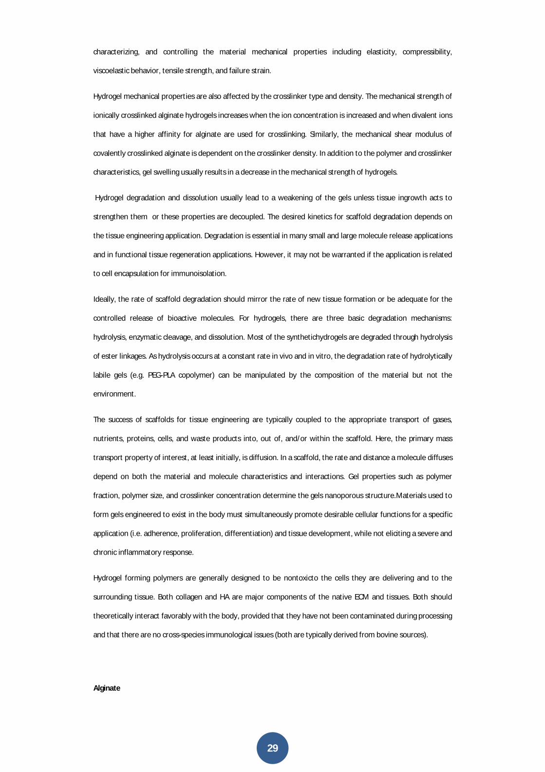
Alginate gel beads are commonly formed by dripping sodium or potassium alginate solution into an aqueous
solution of calcium ions typically made from calcium chloride (CaCl2 ). The fast gelation rate with CaCl2 results in
varying crosslinking density and a polymer concentration gradient within the gel bead. In contrast, CaCO3 has
very low solubility in pure water, allowing its uniform distribution in alginate solution before gelation occurs.
[22].
Fig. 14Alginate scaffold
1.3.8 Metallic materials
To date there are several biocompatible metallic materials that are frequently used as implanting materials in
dental and orthopedic surgery to replace damaged bone or to provide support for healing bones or bone defects.
However, the main disadvantage of metallic biomaterials is their lack of biological recognition on the material
surface. To overcome this restraint, surface coating or surface modification presents a way to preserve the
mechanical properties of established biocompatible metals improving the surface biocompatibility. Moreover, in
order to enhance communication between cells, facilitating their organization within the porous scaffold; it is
desired to integrate cell-recognizable ligands and signaling growth factors on the surface of the scaffolds. Indeed,
biofactors that influence cell proliferation, differentiation, migration, morphologies and gene expression can be
incorporated in the scaffold design and fabrication to enhance cell growth rate and direct cell functions. Another
limitation of the current metallic biomaterials is the possible release of toxic metallic ions and/or particles
through corrosion or wear possible that lead to inflammatory cascades and allergic reactions, which reduce the
biocompatibility and cause tissue loss. A proper treatment of the material surface may help to avoid this problem
and create a direct bonding with the tissue. On the other hand, depending on the materials properties, some
metallic materials are too weak to be arranged into the desired architecture with a controlled porous structure
and some metals are too stiff and would fracture when arranged into certain architectures. Each metallic
31
material possesses different processing requirements and the degree of processability of each metal to form a
scaffold is variable also [23].
Titanium and Titanium Alloys
Titanium is found to be well tolerated and nearly an inert material in the human body environment. In an optimal
situation titanium is capable of osseointegration with bone. In addition, titanium forms a very stable passive layer
of TiO2 on its surface and provides superior biocompatibility. Even if the passive layer is damaged, the layer is
immediately rebuilt. In the case of titanium, the nature of the oxide film that protects the metal substrate from
corrosion is of particular importance and its physicochemical properties such as crystallinity, impurity
segregation, etc., have been found to be quite relevant. Titanium alloys show superior biocompatibility when
compared to the stainless steels and Cr-Co alloys.Titanium-aluminum-vanadium alloys (ASTM F136, ASTM F1108
and ASTM F1472)
In general, porous titanium and titanium alloys exhibit good biocompatibility. One method to overcome one
problem is the use of hydroxyapatite to provide the necessary bioactivity to the titanium mesh cage with a
porous network to facilitate osteoconduction. Moreover, despite the great advances in complete tissue
engineered oral and maxillofacial structures, the current gold standard for load bearing defect sites such as
mandible, maxilla and craniofacial reconstruction remains titanium meshes and titanium 3-D scaffolds. On the
other hand, Ti and its alloys are not ferromagnetic and do not cause harm to the patient in magnetic resonance
imaging (MRI) units. Titanium osseointegration can be potentially improved by loading the scaffold with specific
growth factors. In applications where there are existing gaps, such as craniofacial reconstruction or augmentation
of bone or peri-implant defects, increased regeneration of bone, often has been accomplished with delivery of
TGF- and BMP-2 via titanium scaffold. The latter growth factors are capable to elicit specific cellular responses
leading to rapid new tissue formation. Stem cells have also been cultured in vitro onto titanium scaffolds to
induce the formation of calcified nodules in order to increase the production of mineralized extracellular matrix
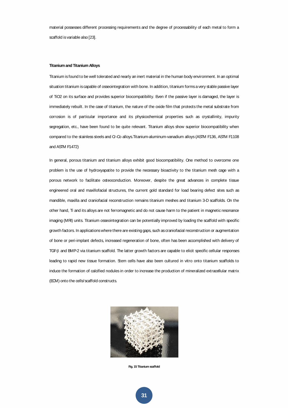
(ECM) onto the cells/scaffold constructs.
Fig. 15 Titanium scaffold

32
Porous titanium and titanium alloys have been shown to possess excellent mechanical properties as permanent
orthopedic implants under load-bearing conditions. Many basic scientific preclinical and clinical studies support
the utility of Ti scaffolds. For marginal bone defects and bone augmentation Ti foams allow for bone ingrowth
through interconnected porous. On the other hand, titanium fiber-mesh is a useful scaffold material that
warrants further investigation as a clinical tool for bone reconstructive surgery. In vitro, titanium fiber-mesh acts
as a scaffold for the adhesion and the osteoblastic differentiation of progenitor cells. In vivo, the material reveals
itself to be osteoconductive, demonstrating encouraging results [24].
33
1.3 MATERIALS AND METHODS
1.4.1 COMSOL Multiphysics5.1
COMSOL Multiphysics5.1 is a general-purpose software platform, based on advanced numerical methods, for
modeling and simulating physics-based problems by physics interfaces and tools for electrical, mechanical,
fluid flow, and chemical applications. Comsol use the finite element method to give approximate solutions to
diffrential equation(PDEs). This method requires a problem defined in geometrical space (or domain), to be
subdivided into a finite number of smaller region (a mesh) [25].
1.4.2 Finite element method
The main feature of the finite element method is the discretization by creating a grid (mesh) made up of
primitives (finite element) in coded form (triangles and quadrangles in 2D domains, hexahedrons and
tetrahedrons for 3D domains). On each element characterized by this basic form, the solution of the problem is
assumed to be expressed by the linear combination of the basis functions of said functions or functions of the
form (shape functions). Sometimes the function is approximated, and not necessarily the exact values of the
function will be those calculated in the points, but the values that provide the least error on the entire
solution.
The typical example is the one that refers to polynomial functions, so that the overall solution of the problem
is approximated with a polynomial function to pieces. The number of coefficients that identifies the solution on
each element is thus linked to the degree of the polynomial chosen. This, in turn, governs the accuracy of the
numerical solution found.In its original form, and still more widespread, the finite element method is used to
solve problems resting on linear constitutive laws.To arrive at the model to the final elements follow the basic
steps, each of which involves the insertion of errors in the final solution.
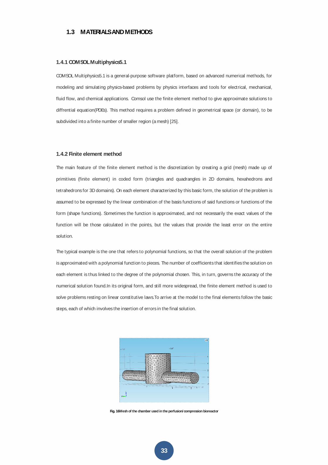
Fig. 16Mesh of the chamber used in the perfusion/compression bioreactor
34
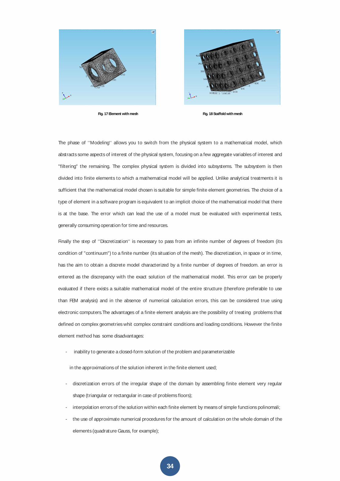
Fig. 17 Element with mesh Fig. 18 Scaffold with mesh
The phase of ‘‘Modeling‘‘ allows you to switch from the physical system to a mathematical model, which
abstracts some aspects of interest of the physical system, focusing on a few aggregate variables of interest and
"filtering" the remaining. The complex physical system is divided into subsystems. The subsystem is then
divided into finite elements to which a mathematical model will be applied. Unlike analytical treatments it is
sufficient that the mathematical model chosen is suitable for simple finite element geometries. The choice of a
type of element in a software program is equivalent to an implicit choice of the mathematical model that there
is at the base. The error which can lead the use of a model must be evaluated with experimental tests,
generally consuming operation for time and resources.
Finally the step of ‘‘Discretization‘‘ is necessary to pass from an infinite number of degrees of freedom (its
condition of "continuum") to a finite number (its situation of the mesh). The discretization, in space or in time,
has the aim to obtain a discrete model characterized by a finite number of degrees of freedom. an error is
entered as the discrepancy with the exact solution of the mathematical model. This error can be properly
evaluated if there exists a suitable mathematical model of the entire structure (therefore preferable to use
than FEM analysis) and in the absence of numerical calculation errors, this can be considered true using
electronic computers.The advantages of a finite element analysis are the possibility of treating problems that
defined on complex geometries whit complex constraint conditions and loading conditions. However the finite
element method has some disadvantages:
- inability to generate a closed-form solution of the problem and parameterizable
in the approximations of the solution inherent in the finite element used;
- discretization errors of the irregular shape of the domain by assembling finite element very regular
shape (triangular or rectangular in case of problems floors);
- interpolation errors of the solution within each finite element by means of simple functions polinomali;
- the use of approximate numerical procedures for the amount of calculation on the whole domain of the
elements (quadrature Gauss, for example);
35
- calculation errors related to the limited number of significant digits with which a computer works and
consequent truncation of the decimal numerical quantities.
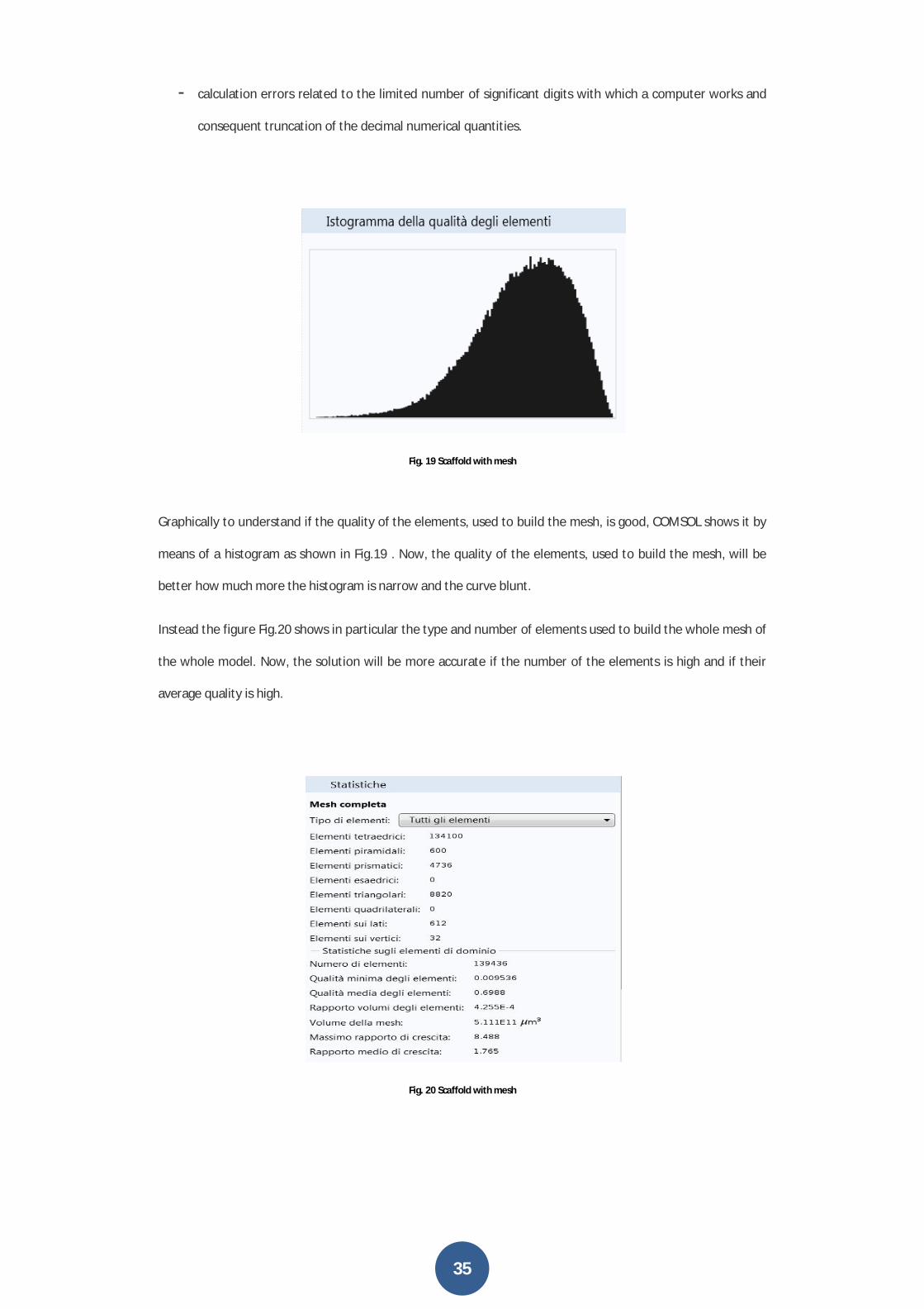
Fig. 19 Scaffold with mesh
Graphically to understand if the quality of the elements, used to build the mesh, is good, COMSOL shows it by
means of a histogram as shown in Fig.19 . Now, the quality of the elements, used to build the mesh, will be
better how much more the histogram is narrow and the curve blunt.
Instead the figure Fig.20 shows in particular the type and number of elements used to build the whole mesh of
the whole model. Now, the solution will be more accurate if the number of the elements is high and if their
average quality is high.
Fig. 20 Scaffold with mesh

36
1.4.3 Model
The model geometry has been designed in this way:
- cylindrical room with diameter of 7.0 mm and height 9.0 mm;
- input and output pipe with diameter equal to 3.2 mm and length 10.5 mm;
- Scaffold built as a 4X4X4 matrix homogeneous porosity 0.8;
- Radius size between 56.6 µm to 115.18µm
Fig. 21 Model
Fig. 22 Scaffold
The model requires the elastic modulus (E),the coefficient of poisson (ν) and density(d) to characterize the type
of material used for the scaffold
In this study I used physics interfaces and toolsfor mechanical and fluid flow application:
- Laminar Flow (Re<2000 and Ma<3) in stationary condition, that is founded about of conservation of
mass and momentum. The flow is hypothesized incompressible because I considered a water flow.
- Solid Mechanics, that consider deformation, strain and stress in a build subjected to a load.
37
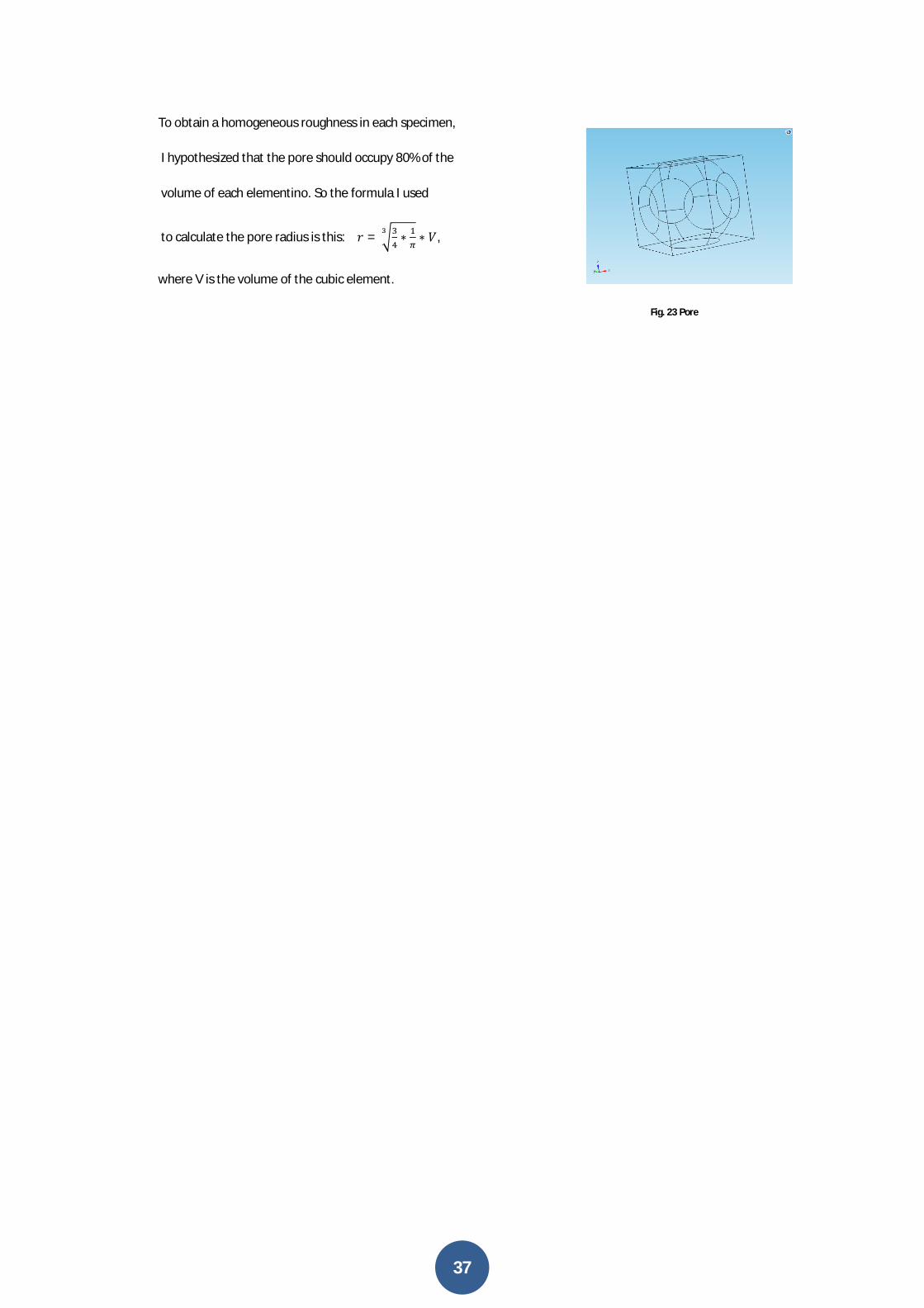
To obtain a homogeneous roughness in each specimen,
I hypothesized that the pore should occupy 80% of the
volume of each elementino. So the formula I used
to calculate the pore radius is this: 푟 = ∗ ∗ 푉,
where V is the volume of the cubic element.
Fig. 23 Pore
38
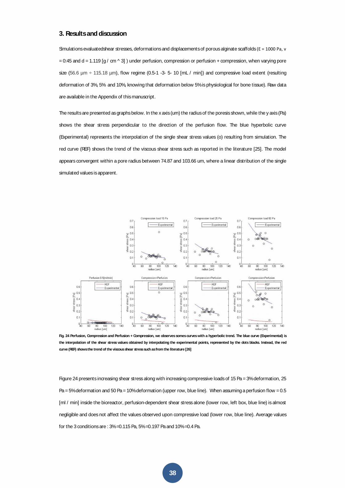
3. Results and discussion
Simulations evaluatedshear stresses, deformations and displacements of porous alginate scaffolds (E = 1000 Pa, ν
= 0:45 and d = 1.119 [g / cm ^ 3] ) under perfusion, compression or perfusion + compression, when varying pore
size (56.6 µm ÷ 115.18 µm), flow regime (0.5-1 -3- 5- 10 [mL / min]) and compressive load extent (resulting
deformation of 3%, 5% and 10%, knowing that deformation below 5% is physiological for bone tissue). Raw data
are available in the Appendix of this manuscript.
The results are presented as graphs below. In the x axis (um) the radius of the poresis shown, while the y axis (Pa)
shows the shear stress perpendicular to the direction of the perfusion flow. The blue hyperbolic curve
(Experimental) represents the interpolation of the single shear stress values (o) resulting from simulation. The
red curve (REF) shows the trend of the viscous shear stress such as reported in the literature [25]. The model
appears convergent within a pore radius between 74.87 and 103.66 um, where a linear distribution of the single
simulated values is apparent.
Fig. 24 Perfusion, Compression and Perfusion + Compression, we observes somes curves with a hyperbolic trend. The blue curve (Experimental) is
the interpolation of the shear stress values obtained by interpolating the experimental points, represented by the dots blacks. Instead, the red
curve (REF) shows the trend of the viscous shear stress such as from the literature [26]
Figure 24 presents increasing shear stress along with increasing compressive loads of 15 Pa = 3% deformation, 25
Pa = 5% deformation and 50 Pa = 10% deformation (upper row, blue line). When assuming a perfusion flow = 0.5
[ml / min] inside the bioreactor, perfusion-dependent shear stress alone (lower row, left box, blue line) is almost
negligible and does not affect the values observed upon compressive load (lower row, blue line). Average values
for the 3 conditions are : 3% =0.115 Pa, 5% =0.197 Pa and 10% =0.4 Pa.
39
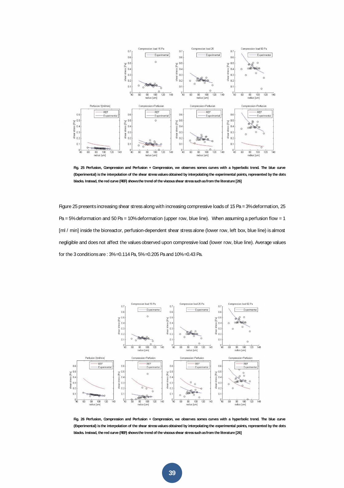
Fig. 25 Perfusion, Compression and Perfusion + Compression, we observes somes curves with a hyperbolic trend. The blue curve
(Experimental) is the interpolation of the shear stress values obtained by interpolating the experimental points, represented by the dots
blacks. Instead, the red curve (REF) shows the trend of the viscous shear stress such as from the literature [26]
Figure 25 presents increasing shear stress along with increasing compressive loads of 15 Pa = 3% deformation, 25
Pa = 5% deformation and 50 Pa = 10% deformation (upper row, blue line). When assuming a perfusion flow = 1
[ml / min] inside the bioreactor, perfusion-dependent shear stress alone (lower row, left box, blue line) is almost
negligible and does not affect the values observed upon compressive load (lower row, blue line). Average values
for the 3 conditions are : 3% =0.114 Pa, 5% =0.205 Pa and 10% =0.43 Pa.
Fig. 26 Perfusion, Compression and Perfusion + Compression, we observes somes curves with a hyperbolic trend. The blue curve
(Experimental) is the interpolation of the shear stress values obtained by interpolating the experimental points, represented by the dots
blacks. Instead, the red curve (REF) shows the trend of the viscous shear stress such as from the literature [26]
40
Figure 26 presents increasing shear stress along with increasing compressive loads of 15 Pa = 3% deformation, 25
Pa = 5% deformation and 50 Pa = 10% deformation (upper row, blue line). When assuming a perfusion flow = 3
[ml / min] inside the bioreactor, perfusion-dependent shear stress alone (lower row, left box, blue line) is almost
negligible and does not affect the values observed upon compressive load (lower row, blue line). Average values
for the 3 conditions are : 3% =0.069 Pa, 5% =0.16 Pa and 10% =0.589 Pa.
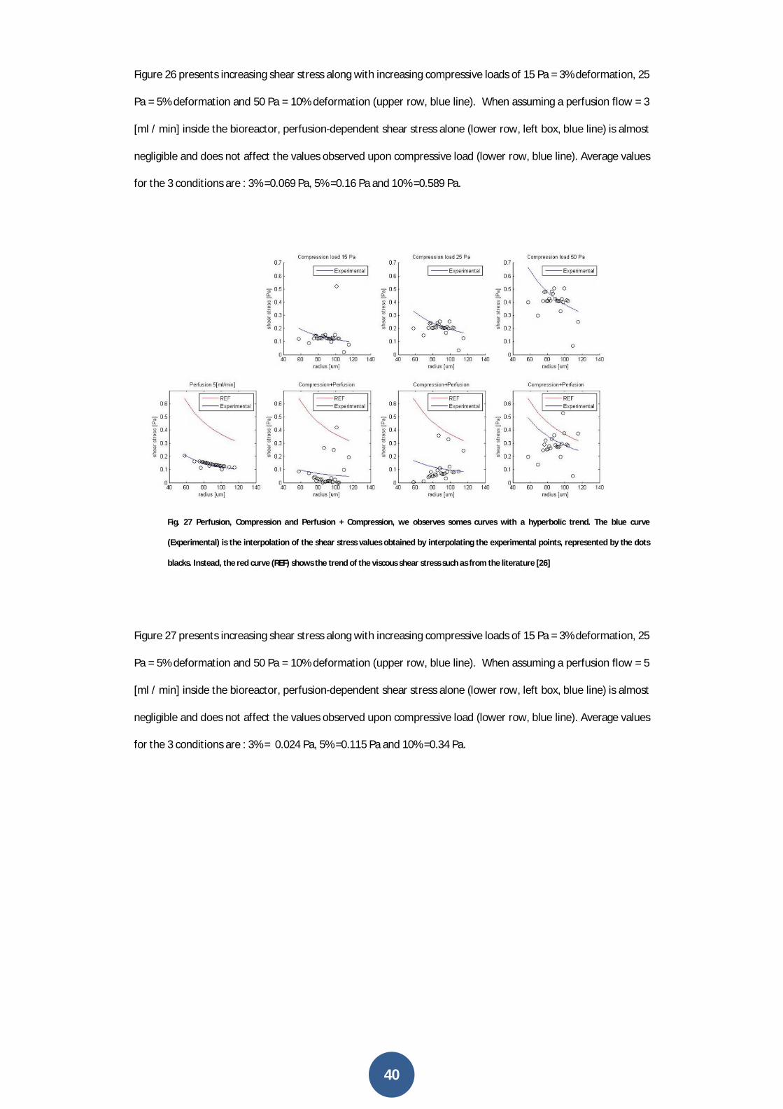
Fig. 27 Perfusion, Compression and Perfusion + Compression, we observes somes curves with a hyperbolic trend. The blue curve
(Experimental) is the interpolation of the shear stress values obtained by interpolating the experimental points, represented by the dots
blacks. Instead, the red curve (REF) shows the trend of the viscous shear stress such as from the literature [26]
Figure 27 presents increasing shear stress along with increasing compressive loads of 15 Pa = 3% deformation, 25
Pa = 5% deformation and 50 Pa = 10% deformation (upper row, blue line). When assuming a perfusion flow = 5
[ml / min] inside the bioreactor, perfusion-dependent shear stress alone (lower row, left box, blue line) is almost
negligible and does not affect the values observed upon compressive load (lower row, blue line). Average values
for the 3 conditions are : 3% = 0.024 Pa, 5% =0.115 Pa and 10% =0.34 Pa.
41
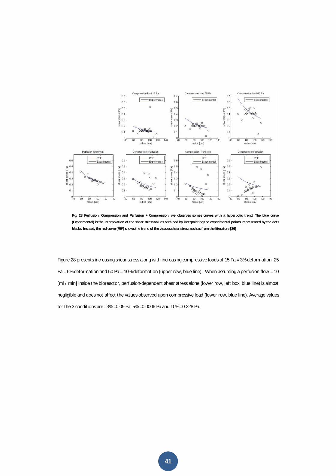
Fig. 28 Perfusion, Compression and Perfusion + Compression, we observes somes curves with a hyperbolic trend. The blue curve
(Experimental) is the interpolation of the shear stress values obtained by interpolating the experimental points, represented by the dots
blacks. Instead, the red curve (REF) shows the trend of the viscous shear stress such as from the literature [26]
Figure 28 presents increasing shear stress along with increasing compressive loads of 15 Pa = 3% deformation, 25
Pa = 5% deformation and 50 Pa = 10% deformation (upper row, blue line). When assuming a perfusion flow = 10
[ml / min] inside the bioreactor, perfusion-dependent shear stress alone (lower row, left box, blue line) is almost
negligible and does not affect the values observed upon compressive load (lower row, blue line). Average values
for the 3 conditions are : 3% =0.09 Pa, 5% =0.0006 Pa and 10% =0.228 Pa.
42
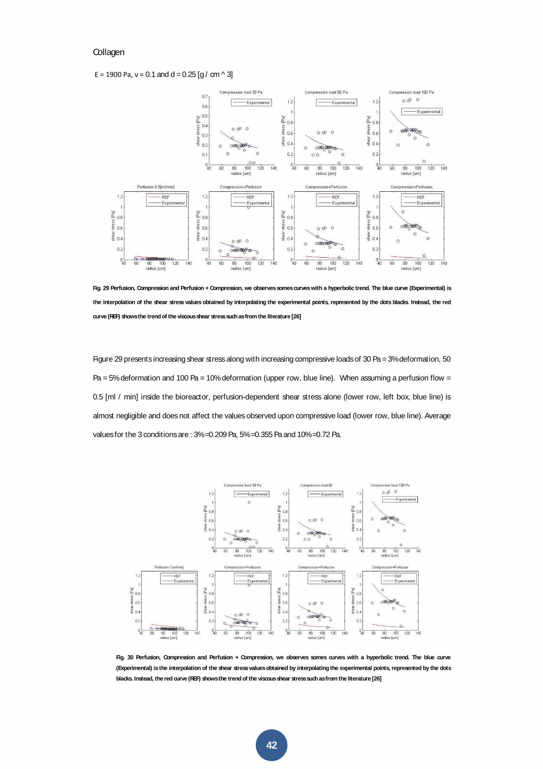
Collagen
E = 1900 Pa, ν = 0.1 and d = 0.25 [g / cm ^ 3]
Fig. 29 Perfusion, Compression and Perfusion + Compression, we observes somes curves with a hyperbolic trend. The blue curve (Experimental) is
the interpolation of the shear stress values obtained by interpolating the experimental points, represented by the dots blacks. Instead, the red
curve (REF) shows the trend of the viscous shear stress such as from the literature [26]
Figure 29 presents increasing shear stress along with increasing compressive loads of 30 Pa = 3% deformation, 50
Pa = 5% deformation and 100 Pa = 10% deformation (upper row, blue line). When assuming a perfusion flow =
0.5 [ml / min] inside the bioreactor, perfusion-dependent shear stress alone (lower row, left box, blue line) is
almost negligible and does not affect the values observed upon compressive load (lower row, blue line). Average
values for the 3 conditions are : 3% =0.209 Pa, 5% =0.355 Pa and 10% =0.72 Pa.
Fig. 30 Perfusion, Compression and Perfusion + Compression, we observes somes curves with a hyperbolic trend. The blue curve
(Experimental) is the interpolation of the shear stress values obtained by interpolating the experimental points, represented by the dots
blacks. Instead, the red curve (REF) shows the trend of the viscous shear stress such as from the literature [26]
43
Figure 30 presents increasing shear stress along with increasing compressive loads of 30 Pa = 3% deformation, 50
Pa = 5% deformation and 100 Pa = 10% deformation (upper row, blue line). When assuming a perfusion flow = 1
[ml / min] inside the bioreactor, perfusion-dependent shear stress alone (lower row, left box, blue line) is almost
negligible and does not affect the values observed upon compressive load (lower row, blue line). Average values
for the 3 conditions are : 3% = 0.218 Pa, 5% =0.379 Pa and 10% =0.781 Pa.
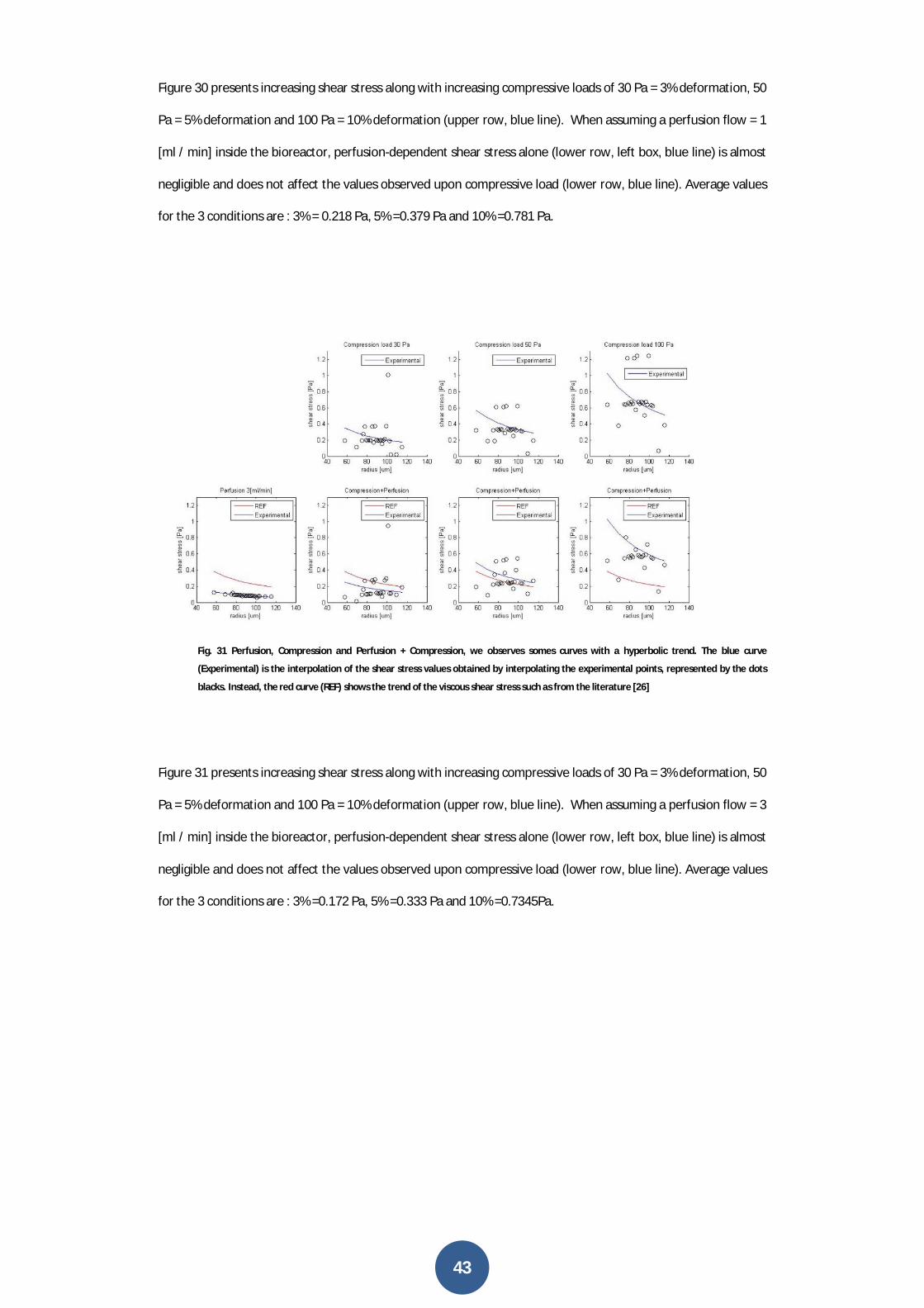
Fig. 31 Perfusion, Compression and Perfusion + Compression, we observes somes curves with a hyperbolic trend. The blue curve
(Experimental) is the interpolation of the shear stress values obtained by interpolating the experimental points, represented by the dots
blacks. Instead, the red curve (REF) shows the trend of the viscous shear stress such as from the literature [26]
Figure 31 presents increasing shear stress along with increasing compressive loads of 30 Pa = 3% deformation, 50
Pa = 5% deformation and 100 Pa = 10% deformation (upper row, blue line). When assuming a perfusion flow = 3
[ml / min] inside the bioreactor, perfusion-dependent shear stress alone (lower row, left box, blue line) is almost
negligible and does not affect the values observed upon compressive load (lower row, blue line). Average values
for the 3 conditions are : 3% =0.172 Pa, 5% =0.333 Pa and 10% =0.7345Pa.

44
Fig. 32 Perfusion, Compression and Perfusion + Compression, we observes somes curves with a hyperbolic trend. The blue curve
(Experimental) is the interpolation of the shear stress values obtained by interpolating the experimental points, represented by the dots
blacks. Instead, the red curve (REF) shows the trend of the viscous shear stress such as from the literature [26]
Figure 32 presents increasing shear stress along with increasing compressive loads of 30 Pa = 3% deformation, 50
Pa = 5% deformation and 100 Pa = 10% deformation (upper row, blue line). When assuming a perfusion flow = 5
[ml / min] inside the bioreactor, perfusion-dependent shear stress alone (lower row, left box, blue line) is almost
negligible and does not affect the values observed upon compressive load (lower row, blue line). Average values
for the 3 conditions are : 3% = 0.125 Pa, 5% =0.286 Pa and 10% =0.6888 Pa.
Fig. 33 Perfusion, Compression and Perfusion + Compression, we observes somes curves with a hyperbolic trend. The blue curve
(Experimental) is the interpolation of the shear stress values obtained by interpolating the experimental points, represented by the dots
blacks. Instead, the red curve (REF) shows the trend of the viscous shear stress such as from the literature [26]
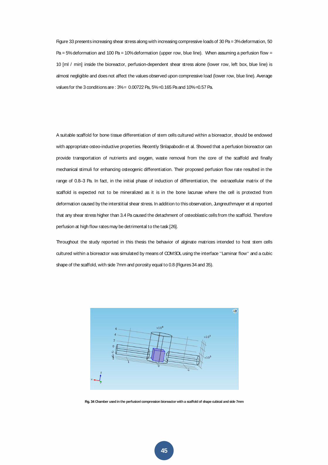
45
Figure 33 presents increasing shear stress along with increasing compressive loads of 30 Pa = 3% deformation, 50
Pa = 5% deformation and 100 Pa = 10% deformation (upper row, blue line). When assuming a perfusion flow =
10 [ml / min] inside the bioreactor, perfusion-dependent shear stress alone (lower row, left box, blue line) is
almost negligible and does not affect the values observed upon compressive load (lower row, blue line). Average
values for the 3 conditions are : 3% = 0.00722 Pa, 5% =0.165 Pa and 10% =0.57 Pa.
A suitable scaffold for bone tissue differentiation of stem cells cultured within a bioreactor, should be endowed
with appropriate osteo-inductive properties. Recently Sinlapabodin et al. Showed that a perfusion bioreactor can
provide transportation of nutrients and oxygen, waste removal from the core of the scaffold and finally
mechanical stimuli for enhancing osteogenic differentiation. Their proposed perfusion flow rate resulted in the
range of 0.8–3 Pa. In fact, in the initial phase of induction of differentiation, the extracellular matrix of the
scaffold is expected not to be mineralized as it is in the bone lacunae where the cell is protected from
deformation caused by the interstitial shear stress. In addition to this observation, Jungreuthmayer et al reported
that any shear stress higher than 3.4 Pa caused the detachment of osteoblastic cells from the scaffold. Therefore
perfusion at high flow rates may be detrimental to the task [26].
Throughout the study reported in this thesis the behavior of alginate matrices intended to host stem cells
cultured within a bioreactor was simulated by means of COMSOL using the interface ‘‘Laminar flow‘‘ and a cubic
shape of the scaffold, with side 7mm and porosity equal to 0.8 (Figures 34 and 35).
Fig. 34 Chamber used in the perfusion/compression bioreactor with a scaffold of shape cubical and side 7mm
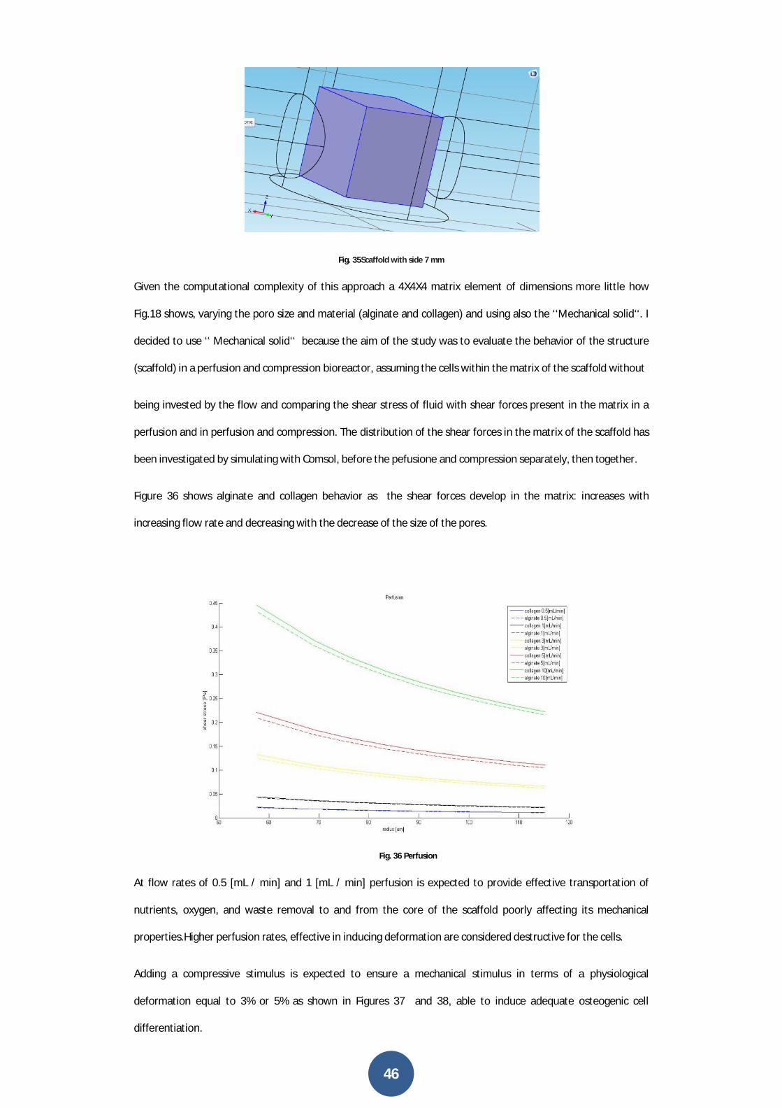
46
Fig. 35Scaffold with side 7 mm
Given the computational complexity of this approach a 4X4X4 matrix element of dimensions more little how
Fig.18 shows, varying the poro size and material (alginate and collagen) and using also the ‘‘Mechanical solid‘‘. I
decided to use ‘‘ Mechanical solid‘‘ because the aim of the study was to evaluate the behavior of the structure
(scaffold) in a perfusion and compression bioreactor, assuming the cells within the matrix of the scaffold without
being invested by the flow and comparing the shear stress of fluid with shear forces present in the matrix in a
perfusion and in perfusion and compression. The distribution of the shear forces in the matrix of the scaffold has
been investigated by simulating with Comsol, before the pefusione and compression separately, then together.
Figure 36 shows alginate and collagen behavior as the shear forces develop in the matrix: increases with
increasing flow rate and decreasing with the decrease of the size of the pores.
Fig. 36 Perfusion
At flow rates of 0.5 [mL / min] and 1 [mL / min] perfusion is expected to provide effective transportation of
nutrients, oxygen, and waste removal to and from the core of the scaffold poorly affecting its mechanical
properties.Higher perfusion rates, effective in inducing deformation are considered destructive for the cells.
Adding a compressive stimulus is expected to ensure a mechanical stimulus in terms of a physiological
deformation equal to 3% or 5% as shown in Figures 37 and 38, able to induce adequate osteogenic cell
differentiation.
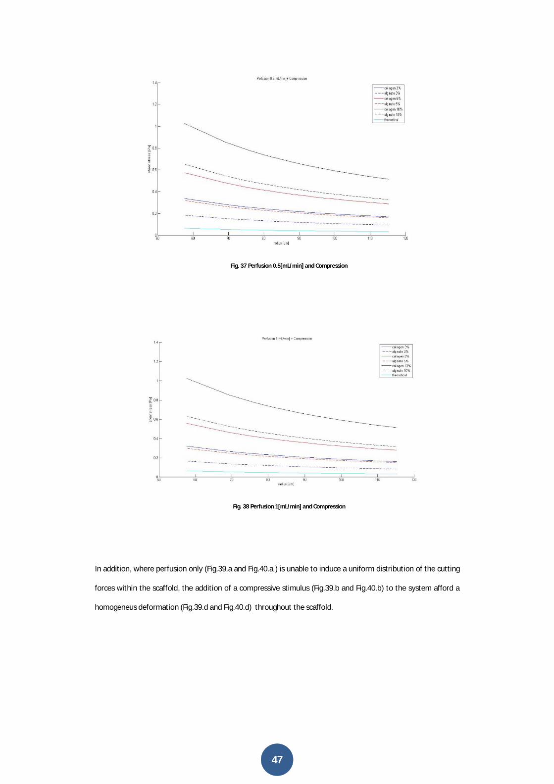
47
Fig. 37 Perfusion 0.5[mL/min] and Compression
Fig. 38 Perfusion 1[mL/min] and Compression
In addition, where perfusion only (Fig.39.a and Fig.40.a ) is unable to induce a uniform distribution of the cutting
forces within the scaffold, the addition of a compressive stimulus (Fig.39.b and Fig.40.b) to the system afford a
homogeneus deformation (Fig.39.d and Fig.40.d) throughout the scaffold.
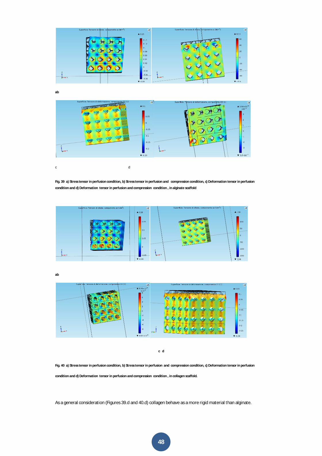
48
ab
c d
Fig. 39 a) Stress tensor in perfusion condition, b) Stress tensor in perfusion and compression condition, c) Deformation tensor in perfusion
condition and d) Deformation tensor in perfusion and compression condition , in alginate scaffold
ab
c d
Fig. 40 a) Stress tensor in perfusion condition, b) Stress tensor in perfusion and compression condition, c) Deformation tensor in perfusion
condition and d) Deformation tensor in perfusion and compression condition , in collagen scaffold.
As a general consideration (Figures 39.d and 40.d) collagen behave as a more rigid material than alginate.

49
4. Conclusions
A blend of 0.5-1 mL/min flow, expected to provides effective transportation of nutrients, oxygen, and waste
removal to and from the core of the scaffold and a compressive 3% and 5% deformation of the 3D matrix is
suggested as the suitable approach to induceosteogenic cell differentiation.
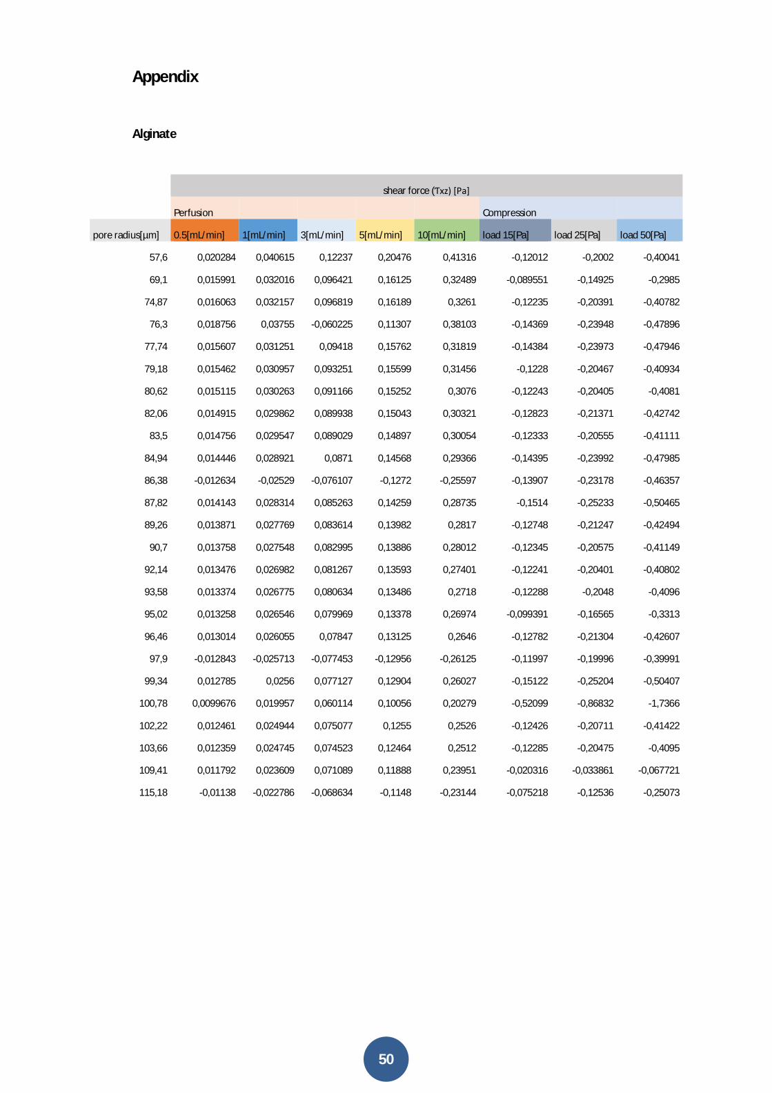
50
Appendix
Alginate
shear force (Ƭxz) [Pa]
Perfusion Compression
pore radius[µm] 0.5[mL/min] 1[mL/min] 3[mL/min] 5[mL/min] 10[mL/min] load 15[Pa] load 25[Pa] load 50[Pa]
57,6 0,020284 0,040615 0,12237 0,20476 0,41316 -0,12012 -0,2002 -0,40041
69,1 0,015991 0,032016 0,096421 0,16125 0,32489 -0,089551 -0,14925 -0,2985
74,87 0,016063 0,032157 0,096819 0,16189 0,3261 -0,12235 -0,20391 -0,40782
76,3 0,018756 0,03755 -0,060225 0,11307 0,38103 -0,14369 -0,23948 -0,47896
77,74 0,015607 0,031251 0,09418 0,15762 0,31819 -0,14384 -0,23973 -0,47946
79,18 0,015462 0,030957 0,093251 0,15599 0,31456 -0,1228 -0,20467 -0,40934
80,62 0,015115 0,030263 0,091166 0,15252 0,3076 -0,12243 -0,20405 -0,4081
82,06 0,014915 0,029862 0,089938 0,15043 0,30321 -0,12823 -0,21371 -0,42742
83,5 0,014756 0,029547 0,089029 0,14897 0,30054 -0,12333 -0,20555 -0,41111
84,94 0,014446 0,028921 0,0871 0,14568 0,29366 -0,14395 -0,23992 -0,47985
86,38 -0,012634 -0,02529 -0,076107 -0,1272 -0,25597 -0,13907 -0,23178 -0,46357
87,82 0,014143 0,028314 0,085263 0,14259 0,28735 -0,1514 -0,25233 -0,50465
89,26 0,013871 0,027769 0,083614 0,13982 0,2817 -0,12748 -0,21247 -0,42494
90,7 0,013758 0,027548 0,082995 0,13886 0,28012 -0,12345 -0,20575 -0,41149
92,14 0,013476 0,026982 0,081267 0,13593 0,27401 -0,12241 -0,20401 -0,40802
93,58 0,013374 0,026775 0,080634 0,13486 0,2718 -0,12288 -0,2048 -0,4096
95,02 0,013258 0,026546 0,079969 0,13378 0,26974 -0,099391 -0,16565 -0,3313
96,46 0,013014 0,026055 0,07847 0,13125 0,2646 -0,12782 -0,21304 -0,42607
97,9 -0,012843 -0,025713 -0,077453 -0,12956 -0,26125 -0,11997 -0,19996 -0,39991
99,34 0,012785 0,0256 0,077127 0,12904 0,26027 -0,15122 -0,25204 -0,50407
100,78 0,0099676 0,019957 0,060114 0,10056 0,20279 -0,52099 -0,86832 -1,7366
102,22 0,012461 0,024944 0,075077 0,1255 0,2526 -0,12426 -0,20711 -0,41422
103,66 0,012359 0,024745 0,074523 0,12464 0,2512 -0,12285 -0,20475 -0,4095
109,41 0,011792 0,023609 0,071089 0,11888 0,23951 -0,020316 -0,033861 -0,067721
115,18 -0,01138 -0,022786 -0,068634 -0,1148 -0,23144 -0,075218 -0,12536 -0,25073
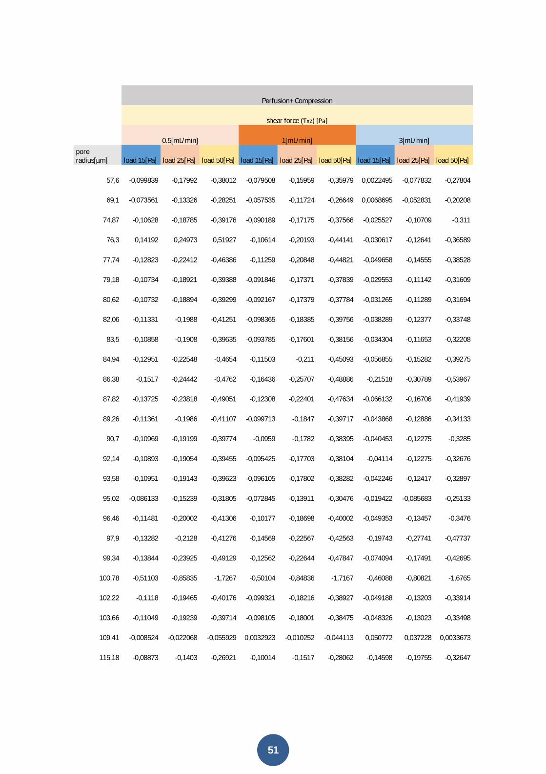
51
Perfusion+ Compression
shear force (Ƭxz) [Pa]
0.5[mL/min] 1[mL/min] 3[mL/min]
pore radius[µm] load 15[Pa] load 25[Pa] load 50[Pa] load 15[Pa] load 25[Pa] load 50[Pa] load 15[Pa] load 25[Pa] load 50[Pa]
57,6 -0,099839 -0,17992 -0,38012 -0,079508 -0,15959 -0,35979 0,0022495 -0,077832 -0,27804
69,1 -0,073561 -0,13326 -0,28251 -0,057535 -0,11724 -0,26649 0,0068695 -0,052831 -0,20208
74,87 -0,10628 -0,18785 -0,39176 -0,090189 -0,17175 -0,37566 -0,025527 -0,10709 -0,311
76,3 0,14192 0,24973 0,51927 -0,10614 -0,20193 -0,44141 -0,030617 -0,12641 -0,36589
77,74 -0,12823 -0,22412 -0,46386 -0,11259 -0,20848 -0,44821 -0,049658 -0,14555 -0,38528
79,18 -0,10734 -0,18921 -0,39388 -0,091846 -0,17371 -0,37839 -0,029553 -0,11142 -0,31609
80,62 -0,10732 -0,18894 -0,39299 -0,092167 -0,17379 -0,37784 -0,031265 -0,11289 -0,31694
82,06 -0,11331 -0,1988 -0,41251 -0,098365 -0,18385 -0,39756 -0,038289 -0,12377 -0,33748
83,5 -0,10858 -0,1908 -0,39635 -0,093785 -0,17601 -0,38156 -0,034304 -0,11653 -0,32208
84,94 -0,12951 -0,22548 -0,4654 -0,11503 -0,211 -0,45093 -0,056855 -0,15282 -0,39275
86,38 -0,1517 -0,24442 -0,4762 -0,16436 -0,25707 -0,48886 -0,21518 -0,30789 -0,53967
87,82 -0,13725 -0,23818 -0,49051 -0,12308 -0,22401 -0,47634 -0,066132 -0,16706 -0,41939
89,26 -0,11361 -0,1986 -0,41107 -0,099713 -0,1847 -0,39717 -0,043868 -0,12886 -0,34133
90,7 -0,10969 -0,19199 -0,39774 -0,0959 -0,1782 -0,38395 -0,040453 -0,12275 -0,3285
92,14 -0,10893 -0,19054 -0,39455 -0,095425 -0,17703 -0,38104 -0,04114 -0,12275 -0,32676
93,58 -0,10951 -0,19143 -0,39623 -0,096105 -0,17802 -0,38282 -0,042246 -0,12417 -0,32897
95,02 -0,086133 -0,15239 -0,31805 -0,072845 -0,13911 -0,30476 -0,019422 -0,085683 -0,25133
96,46 -0,11481 -0,20002 -0,41306 -0,10177 -0,18698 -0,40002 -0,049353 -0,13457 -0,3476
97,9 -0,13282 -0,2128 -0,41276 -0,14569 -0,22567 -0,42563 -0,19743 -0,27741 -0,47737
99,34 -0,13844 -0,23925 -0,49129 -0,12562 -0,22644 -0,47847 -0,074094 -0,17491 -0,42695
100,78 -0,51103 -0,85835 -1,7267 -0,50104 -0,84836 -1,7167 -0,46088 -0,80821 -1,6765
102,22 -0,1118 -0,19465 -0,40176 -0,099321 -0,18216 -0,38927 -0,049188 -0,13203 -0,33914
103,66 -0,11049 -0,19239 -0,39714 -0,098105 -0,18001 -0,38475 -0,048326 -0,13023 -0,33498
109,41 -0,008524 -0,022068 -0,055929 0,0032923 -0,010252 -0,044113 0,050772 0,037228 0,0033673
115,18 -0,08873 -0,1403 -0,26921 -0,10014 -0,1517 -0,28062 -0,14598 -0,19755 -0,32647
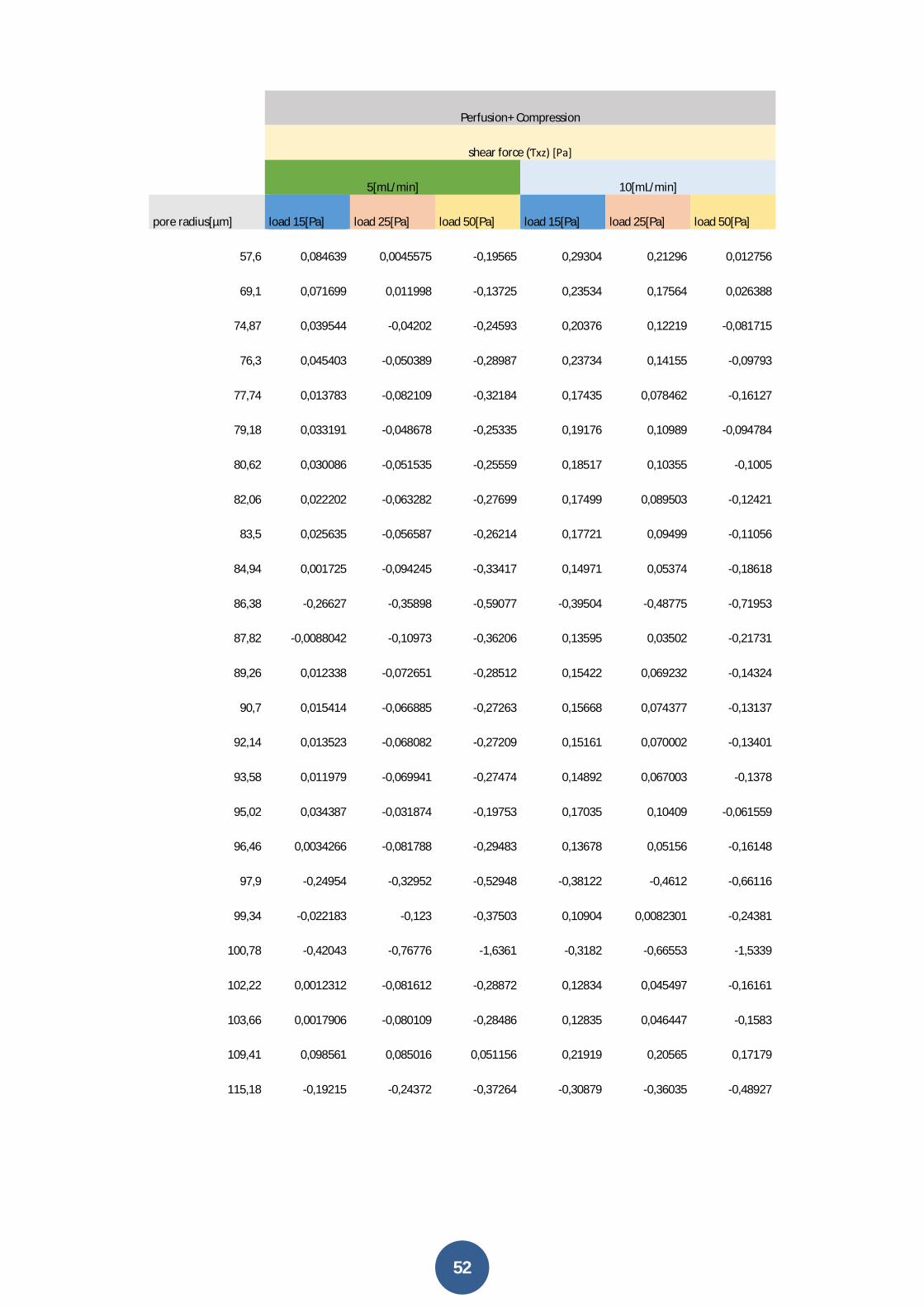
52
Perfusion+ Compression
shear force (Ƭxz) [Pa]
5[mL/min] 10[mL/min]
pore radius[µm] load 15[Pa] load 25[Pa] load 50[Pa] load 15[Pa] load 25[Pa] load 50[Pa]
57,6 0,084639 0,0045575 -0,19565 0,29304 0,21296 0,012756
69,1 0,071699 0,011998 -0,13725 0,23534 0,17564 0,026388
74,87 0,039544 -0,04202 -0,24593 0,20376 0,12219 -0,081715
76,3 0,045403 -0,050389 -0,28987 0,23734 0,14155 -0,09793
77,74 0,013783 -0,082109 -0,32184 0,17435 0,078462 -0,16127
79,18 0,033191 -0,048678 -0,25335 0,19176 0,10989 -0,094784
80,62 0,030086 -0,051535 -0,25559 0,18517 0,10355 -0,1005
82,06 0,022202 -0,063282 -0,27699 0,17499 0,089503 -0,12421
83,5 0,025635 -0,056587 -0,26214 0,17721 0,09499 -0,11056
84,94 0,001725 -0,094245 -0,33417 0,14971 0,05374 -0,18618
86,38 -0,26627 -0,35898 -0,59077 -0,39504 -0,48775 -0,71953
87,82 -0,0088042 -0,10973 -0,36206 0,13595 0,03502 -0,21731
89,26 0,012338 -0,072651 -0,28512 0,15422 0,069232 -0,14324
90,7 0,015414 -0,066885 -0,27263 0,15668 0,074377 -0,13137
92,14 0,013523 -0,068082 -0,27209 0,15161 0,070002 -0,13401
93,58 0,011979 -0,069941 -0,27474 0,14892 0,067003 -0,1378
95,02 0,034387 -0,031874 -0,19753 0,17035 0,10409 -0,061559
96,46 0,0034266 -0,081788 -0,29483 0,13678 0,05156 -0,16148
97,9 -0,24954 -0,32952 -0,52948 -0,38122 -0,4612 -0,66116
99,34 -0,022183 -0,123 -0,37503 0,10904 0,0082301 -0,24381
100,78 -0,42043 -0,76776 -1,6361 -0,3182 -0,66553 -1,5339
102,22 0,0012312 -0,081612 -0,28872 0,12834 0,045497 -0,16161
103,66 0,0017906 -0,080109 -0,28486 0,12835 0,046447 -0,1583
109,41 0,098561 0,085016 0,051156 0,21919 0,20565 0,17179
115,18 -0,19215 -0,24372 -0,37264 -0,30879 -0,36035 -0,48927
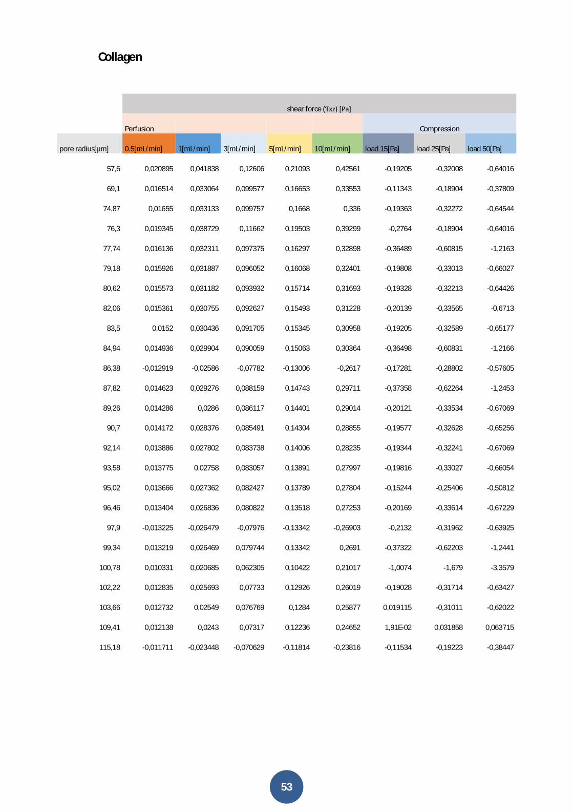
53
Collagen
shear force (Ƭxz) [Pa]
Perfusion Compression
pore radius[µm] 0.5[mL/min] 1[mL/min] 3[mL/min] 5[mL/min] 10[mL/min] load 15[Pa] load 25[Pa] load 50[Pa]
57,6 0,020895 0,041838 0,12606 0,21093 0,42561 -0,19205 -0,32008 -0,64016
69,1 0,016514 0,033064 0,099577 0,16653 0,33553 -0,11343 -0,18904 -0,37809
74,87 0,01655 0,033133 0,099757 0,1668 0,336 -0,19363 -0,32272 -0,64544
76,3 0,019345 0,038729 0,11662 0,19503 0,39299 -0,2764 -0,18904 -0,64016
77,74 0,016136 0,032311 0,097375 0,16297 0,32898 -0,36489 -0,60815 -1,2163
79,18 0,015926 0,031887 0,096052 0,16068 0,32401 -0,19808 -0,33013 -0,66027
80,62 0,015573 0,031182 0,093932 0,15714 0,31693 -0,19328 -0,32213 -0,64426
82,06 0,015361 0,030755 0,092627 0,15493 0,31228 -0,20139 -0,33565 -0,6713
83,5 0,0152 0,030436 0,091705 0,15345 0,30958 -0,19205 -0,32589 -0,65177
84,94 0,014936 0,029904 0,090059 0,15063 0,30364 -0,36498 -0,60831 -1,2166
86,38 -0,012919 -0,02586 -0,07782 -0,13006 -0,2617 -0,17281 -0,28802 -0,57605
87,82 0,014623 0,029276 0,088159 0,14743 0,29711 -0,37358 -0,62264 -1,2453
89,26 0,014286 0,0286 0,086117 0,14401 0,29014 -0,20121 -0,33534 -0,67069
90,7 0,014172 0,028376 0,085491 0,14304 0,28855 -0,19577 -0,32628 -0,65256
92,14 0,013886 0,027802 0,083738 0,14006 0,28235 -0,19344 -0,32241 -0,67069
93,58 0,013775 0,02758 0,083057 0,13891 0,27997 -0,19816 -0,33027 -0,66054
95,02 0,013666 0,027362 0,082427 0,13789 0,27804 -0,15244 -0,25406 -0,50812
96,46 0,013404 0,026836 0,080822 0,13518 0,27253 -0,20169 -0,33614 -0,67229
97,9 -0,013225 -0,026479 -0,07976 -0,13342 -0,26903 -0,2132 -0,31962 -0,63925
99,34 0,013219 0,026469 0,079744 0,13342 0,2691 -0,37322 -0,62203 -1,2441
100,78 0,010331 0,020685 0,062305 0,10422 0,21017 -1,0074 -1,679 -3,3579
102,22 0,012835 0,025693 0,07733 0,12926 0,26019 -0,19028 -0,31714 -0,63427
103,66 0,012732 0,02549 0,076769 0,1284 0,25877 0,019115 -0,31011 -0,62022
109,41 0,012138 0,0243 0,07317 0,12236 0,24652 1,91E-02 0,031858 0,063715
115,18 -0,011711 -0,023448 -0,070629 -0,11814 -0,23816 -0,11534 -0,19223 -0,38447

54
Perfusion+ Compression
shear force (Ƭxz) [Pa]
0.5[mL/min] 1[mL/min] 3[mL/min]
poreradius[µm] load 15[Pa] load 25[Pa] load 50[Pa] load 15[Pa] load 25[Pa] load 50[Pa] load 15[Pa] load 25[Pa] load 50[Pa]
57,6 -0,17115 -0,29918 -0,61926 -0,15021 -0,27824 -0,59832 -0,065989 -0,19402 -0,5141
69,1 -0,096912 -0,17253 -0,36157 -0,080362 -0,15598 -0,34502 -0,013849 -0,089466 -0,27851
74,87 -0,17708 -0,30617 -0,62889 -0,1605 -0,28959 -0,61231 -0,093876 -0,22296 -0,54569
76,3 0,2589 0,44512 0,91069 -0,23767 -0,42194 -0,88262 -0,15978 -0,34405 -0,80472
77,74 -0,34876 -0,59202 -1,2002 -0,33258 -0,57584 -1,184 -0,26752 -0,51078 -1,1189
79,18 -0,18215 -0,31421 -0,64434 -0,16619 -0,29825 -0,62838 -0,10203 -0,23408 -0,56422
80,62 -0,1777 -0,30656 -0,62868 -0,1621 -0,29095 -0,61308 -0,099345 -0,2282 -0,55033
82,06 -0,18603 -0,32029 -0,65594 -0,17063 -0,30489 -0,64054 -0,10876 -0,24302 -0,57867
83,5 -0,18033 -0,31069 -0,63657 -0,1651 -0,29545 -0,62134 -0,10383 -0,23418 -0,56007
84,94 -0,35005 -0,59337 -1,2017 -0,33508 -0,5784 -1,1867 -0,27493 -0,51825 -1,1266
86,38 -0,18573 -0,30094 -0,58897 -0,19867 -0,31388 -0,60191 -0,25063 -0,36584 -0,65387
87,82 -0,35896 -0,60801 -1,2306 -0,34431 -0,59336 -1,216 -0,28542 -0,53448 -1,1571
89,26 -0,18692 -0,32106 -0,6564 -0,17261 -0,30674 -0,64209 -0,11509 -0,24923 -0,58457
90,7 -0,1816 -0,31211 -0,63839 -0,16739 -0,2979 -0,62418 -0,11028 -0,24079 -0,56707
92,14 -0,17956 -3,09E-01 -0,63092 -0,16564 -0,2946 -0,61701 -0,1097 -0,23867 -0,56107
93,58 -0,18439 -0,31649 -0,64676 -0,17058 -0,30269 -0,63296 -0,1151 -0,24721 -0,57748
95,02 -0,13877 -0,2404 -0,49446 -0,12507 -0,2267 -0,48076 -0,07001 -0,17163 -0,4257
96,46 -0,18828 -0,32274 -0,65888 -0,17485 -0,30931 -0,64545 -0,12086 -0,25532 -0,59147
97,9 -0,205 -0,33285 -0,65247 -0,21825 -0,3461 -0,66573 -0,27153 -0,39938 -0,71901
99,34 -0,36 -0,60881 -1,2308 -0,34675 -0,59556 -1,2176 -0,29348 -0,54229 -1,1643
100,78 -0,99704 -1,6686 -3,3476 -0,98669 -1,6583 -3,3372 -0,94507 -1,6166 -3,2956
102,22 -0,17745 -0,3043 -0,62144 -0,16459 -0,29144 -0,60858 -0,11295 -0,23981 -0,55694
103,66 -0,17333 -0,29738 -0,60749 -0,16058 -0,28462 -0,59473 -0,1093 -0,23334 -0,54345
109,41 0,031252 0,043995 0,075853 0,043415 0,056158 0,088015 0,092285 0,10503 0,13689
115,18 -0,13028 -0,20933 -0,40696 -0,14202 -0,22107 -0,41869 -0,1892 -0,26825 -0,46587
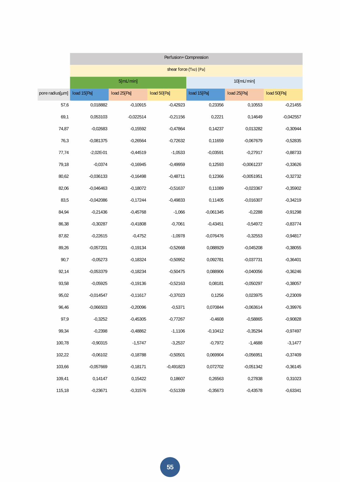
55
Perfusion+ Compression
shear force (Ƭxz) [Pa]
5[mL/min] 10[mL/min]
pore radius[µm] load 15[Pa] load 25[Pa] load 50[Pa] load 15[Pa] load 25[Pa] load 50[Pa]
57,6 0,018882 -0,10915 -0,42923 0,23356 0,10553 -0,21455
69,1 0,053103 -0,022514 -0,21156 0,2221 0,14649 -0,042557
74,87 -0,02683 -0,15592 -0,47864 0,14237 0,013282 -0,30944
76,3 -0,081375 -0,26564 -0,72632 0,11659 -0,067679 -0,52835
77,74 -2,02E-01 -0,44519 -1,0533 -0,03591 -0,27917 -0,88733
79,18 -0,0374 -0,16945 -0,49959 0,12593 -0,0061237 -0,33626
80,62 -0,036133 -0,16498 -0,48711 0,12366 -0,0051951 -0,32732
82,06 -0,046463 -0,18072 -0,51637 0,11089 -0,023367 -0,35902
83,5 -0,042086 -0,17244 -0,49833 0,11405 -0,016307 -0,34219
84,94 -0,21436 -0,45768 -1,066 -0,061345 -0,2288 -0,91298
86,38 -0,30287 -0,41808 -0,7061 -0,43451 -0,54972 -0,83774
87,82 -0,22615 -0,4752 -1,0978 -0,076476 -0,32553 -0,94817
89,26 -0,057201 -0,19134 -0,52668 0,088929 -0,045208 -0,38055
90,7 -0,05273 -0,18324 -0,50952 0,092781 -0,037731 -0,36401
92,14 -0,053379 -0,18234 -0,50475 0,088906 -0,040056 -0,36246
93,58 -0,05925 -0,19136 -0,52163 0,08181 -0,050297 -0,38057
95,02 -0,014547 -0,11617 -0,37023 0,1256 0,023975 -0,23009
96,46 -0,066503 -0,20096 -0,5371 0,070844 -0,063614 -0,39976
97,9 -0,3252 -0,45305 -0,77267 -0,4608 -0,58865 -0,90828
99,34 -0,2398 -0,48862 -1,1106 -0,10412 -0,35294 -0,97497
100,78 -0,90315 -1,5747 -3,2537 -0,7972 -1,4688 -3,1477
102,22 -0,06102 -0,18788 -0,50501 0,069904 -0,056951 -0,37409
103,66 -0,057669 -0,18171 -0,491823 0,072702 -0,051342 -0,36145
109,41 0,14147 0,15422 0,18607 0,26563 0,27838 0,31023
115,18 -0,23671 -0,31576 -0,51339 -0,35673 -0,43578 -0,63341

56
Bibliography
[1] Cit. Wendt et al. Literature Review, 2008, Chapter 2.
[2]H. Singh and D. W. Hutmacher, Bioreactor Studies and Computational Fluid Dynamics 2008,Page 3
[3] Gregory N. Bancroft, Vassilios I. Sikavitsas, and Antonios G. Mikos, Advances in Biochemical Engineering/
Biotechnology also Electronically Fluid Dynamics in Bioreactor Design,Topics in Tissue Engineering,2008, Volume
3, Pages 549-550;
[4] M.T. Raimondi*, F. Boschetti, F. Migliavacca, M. Cioffi and G. Dubini , Micro Fluid Dynamics in Three
Dimensional Engineered Cell Systems in Bioreactors, , Topics in Tissue Engineering 2005, Volume 2, Page 296;
[5] Computational Methods for Fluid Dynamics, Joel H. Ferziger, Milovan Peric, Springer, 2002 Page 3;
[6] Damien P. Byrne , Damien Lacroix , Josep A. Planell , Daniel J. Kelly , Patrick J. Prendergast, Simulation of
tissue differentiation in a scaffold as a function of porosity, Young’s modulus and dissolution rate: Application of
mechanobiological models in tissue engineering 2007, Page 3
[7] M.A.K. Liebschner* and M.A. Wettergreen, Optimization of Bone Scaffold Engineering for Load Bearing
Applications, , Topics in Tissue Engineering 2003. Eds. N. Ashammakhi & P. Ferretti, Page 5-8;
[8] Mieczyslaw Jurczyk, Bionanomaterials for Dental Applications, 2012 Page 428;
[9] David A. Puleo,Rena Bizios, Biological Interactions on Materials Surfaces: Understanding and Controlling
Pages 87-98;
[10] Damien P Byrne, Damien Lacroix , Josep A. Planell, Patrick J. Prendergast, Daniel J. Kelly, Simulation of tissue
differentiation in a scaffold as a function of porosity, Young's modulus and dissolution rate: Application of
mechanobiological models in tissue engineering ,Page 6
[11] osteogenesis Vassilis Karageorgiou, David Kaplan, Porosity of 3D biomaterial scaffolds and, 2005,Volume 26,
Issue 27, Pages 5474–5491
[12] Binil Starly, Biomimetic design and fabrication of tissue engineered scaffolds using computer aided tissue
engineering, Thesis Submitted to the Faculty of Drexel University by Binil Starly in partial fulfillment of the
requirements for the degree of Doctor of Philosophy June 2006;
[13] Gerjon Hannink, J.J. Chris Arts, Bioresorbability, porosity and mechanical strength of bone substitutes: What
is optimal for bone regeneration?,2008 Page 3
[14] Vassilis Karageorgiou, David Kaplan, Porosity of 3D biomaterial scaffolds and osteogenesis, 2005,
Biomaterials Pages 5474–5491;
[15] Charles-Harris M1, del Valle S, Hentges E, Bleuet P, Lacroix D, Planell JA, Mechanical and structural
characterisation of completely degradable polylactic acid/calcium phosphate glass scaffolds,Biomaterials. 2007
4429-38.;
57
[16] Pathiraja Gunatillake and Raju Adhikar, P A Gunatillake & R Adhikari,Biodegradable synthetic polymers for
tissue engineering, Vol. 5. 2003 (pages 1-16);
[17] Stefano Cardea*, Lucia Baldino, Iolanda De Marco, Ernesto Reverchon,Generation of Loaded PMMA
Scaffolds Using Supercritical CO2 Assisted Phase Separation materials science and engineering, biomimetic
materials, sensors and systems, 2015,vol. 59. Pages.480-487;
[18] Stefano Cardea*, Lucia Baldino, Iolanda De Marco, Ernesto Reverchon, Generation of Loaded PMMA
Scaffolds Using Supercritical CO2 Assisted Phase Separation, materials science and engineering, Biomimetic
Materials, sensors and systems, 2015, vol. 59. Pages.480-487;
[19] Serafim M. Oliveira, MS, PhD, Rushali A. Ringshia, MS, Racquel Z. LeGeros, PhD, Elizabeth Clark, MS, Michael
J. Yost, PhD, Louis Terracio, PhD, and Cristina C. Teixeira, DMD, MS, PhD, Journal of Biomedical Materials
Research Part A, An improved Collagen Scaffold for Skeletal Regeneration, 2010,Volume 94A, pages 371–379;
[20] E. Reverchon*, S. cardea, E. Schiavo Rappo,Loaded polymeric membranes formation using a supercritical
fluids assisted process,2009, The Journal of Supercritical Fluids, Pages 484–492;
[21] Liam C. Palmer, Christina J. Newcomb, Stuart R. Kaltz, Erik D. Spoerkeand Samuel I. Stupp, Biomimetic
Systems for Hydroxyapatite Mineralization Inspired By Bone and Enamel, 2008, Chemical Review;
[22] Huaping Tan 1 and Kacey G. Marra, Injectable, Biodegradable Hydrogels for Tissue Engineering
Applications,2010,Materials, Pages 8-9
[23] Kelly Alvarez 1 and Hideo Nakajima,Metallic Scaffolds for Bone Regeneration,2009, Materials, Pages 5-9;
[24] Rajendran V, Nishara Begum, Fatma El-batal and M. A.Zooz, Ultrasonic characterisation of SiO2-Na2O-CaO-
P2O 5 bioglass ceramics for biomedical application, 2013 New Journal of Glass and Ceramics, Pages 15-20;
[25] https://www.comsol.com/comsol-multiphysics;
[26] Catherine K. Kuo, Peter X. Ma, Ionically crosslinked alginate hydrogels as scaffolds for tissue engineering:
Part 1. Structure, gelation rate and mechanical properties, , Biomaterials 2001; 511-21;
[27] Salita Sinlapabodin, Phakdee Amornsudthiwat, Siriporn Damrongsakkul, Sorada Kanokpanont, An axial
distribution of seeding, proliferation, and osteogenic differentiation of MC3T3-E1 cells and rat bone marrow-
derived mesenchymal stem cells across a 3D Thai silk fibroin/gelatin/ hydroxyapatite scaffold in a perfusion
bioreactor, materials science and engineering c, 2015, Pages 5-9 ;
[28] J. Lovecchio et al., Assement of perfusion bioreactor system using X-ray-uCT technology and 3D modelling
methods., Tissue Eng Regen Med-2014 , 207-208;

58
Ringraziamenti
Ringrazio il prof. Emanuele Domenico Giordano, il prof. Paolo Gargiulo e in particolare Josephe Lovecchio per
l‘aiuto sempre attento e preciso che hanno saputo darmi e per la competenza con cui mi hanno indirizzato nelle
occosioni di dubbio durante il lavoro di tesi.