Poligoni,  Poliedri  e  Volumi  

Poligoni  

•  Un  poligono  è  una  figura  con  n  la5,  definita  da  un  insieme  ordinato  di  almeno  3  pun5  nel  piano,  nel  quale  ogni  punto  è  collegato  al  successivo  (e  l’ul5mo  al  primo)  con  un  segmento  di  re>a.  

•  Due  ver5ci  si  dicono  adiacen5  se  sono  uni5  da  un  lato  

•  Un  poligono  è  semplice  se  ogni  coppia  di  la5  non  consecu5vi  non  ha  pun5  in  comune  

•  Un  poligono  semplice  divide  il  piano  in  due  par5:  l’area  interna  al  poligono  e  quella  esterna  

Poligoni  

Poligoni  

•  Un  ver5ce  di  un  poligono  è  convesso  se  l’angolo  interiore  è  minore  di  180°  

•  Se  l’angolo  è  maggiore,  il  ver5ce  si  dice  concavo  •  Un  poligono  è  convesso  se  per  ogni  coppia  di  pun5  interni  al  poligono,  la  congiungente  è  interna  al  poligono  

•  Un  poligono  che  non  è  convesso  è  concavo  •  Un  poligono  con  uno  o  più  ver5ci  concavi  è  concavo,  ma  un  poligono  con  solo  ver5ci  convessi  non  è  necessariamente  convesso  

•  Il  triangolo  è  l’unico  poligono  sempre  convesso  

Poligoni  

•  I  poligoni  convessi  possono  essere  vis5  come  un  so>oinsieme  dell’conce>o  di  insieme  dei  pun*  convessi  nel  piano  

•  Un  insieme  di  pun5  convessi  è  un  insieme  di  pun5  in  cui  qualsiasi  linea  tra  due  pun5  è  cos5tuita  da  pun5  dell’insieme  

•  Dato  un  insieme  di  pun5  S,  il  guscio  convesso  (convex  hull)  di  S,  denotato  con  CH(S)  è  il  più  piccolo  insieme  di  pun5  convessi  che  con5ene  S  

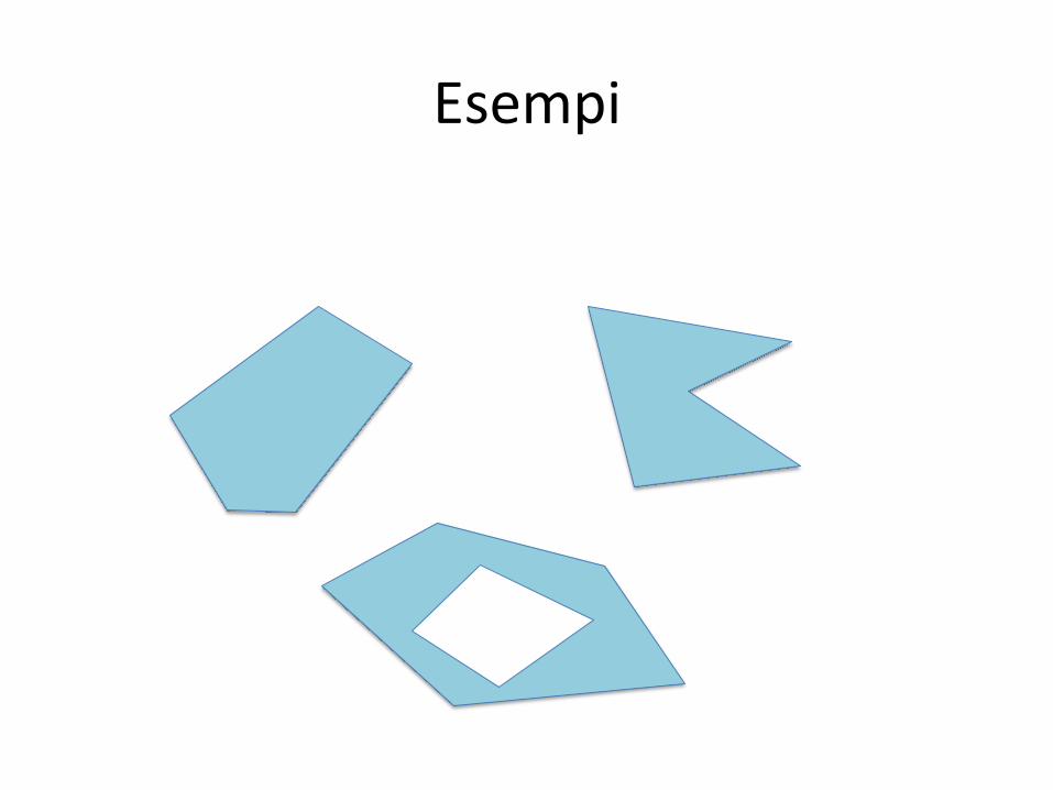
Esempi  

Test  di  Convessità  su  Quadrilateri  

•  Spesso,  oltre  ai  triangoli,  all’interno  di  una  mesh  vi  sono  anche  quadrilateri.  

•  Il  test  di  convessità  su  un  quadrilatero  può  essere  fa>o  in  maniera  semplice  rispe>o  ad  un  test  di  un  poligono  ad  n  la5  

•  Assumendo  che  i  ver5ci  del  quadrilatero  ABCD  siano  co-­‐planari,  occorre  testare  che  le  due  diagonali  giacciano  nell’interno  del  quadrilatero  

•  Tale  test  è  equivalente  al  fa>o  che  le  due  diagonali  si  intersechino  

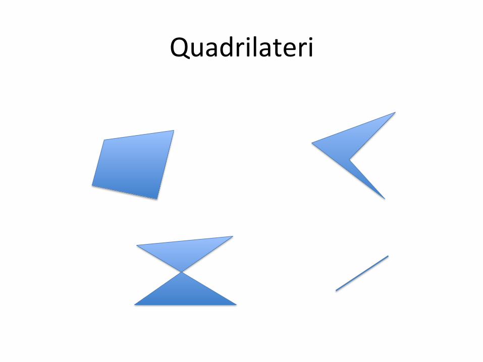
Quadrilateri  

Test  di  convessità  su  quadrilateri  

•  Mediante  considerazioni  geometriche,  si  dimostra  che  un  test  equivalente  a  quelli  precedentemente  elenca5,  consiste  nel  verificare  che  l’avvolgimento  dei  due  triangoli  ABD  e  BDC  sia  opposto,  ovvero  –  (BD  x  BA)  (BD  x  BC)  <  0  –  (AC  x  AD)  (AC  x  AB)  <  0  

Test  di  convessità  su  poligoni  

•  Per  poligoni  con  numero  di  ver5ci  maggiore  di  4  occorre  controllare  che  per  ogni  lato  del  poligono,  gli  altri  ver5ci  giacciano  tuZ  da  una  parte  rispe>o  al  lato.  

•  La  complessità  di  tale  algoritmo  è  O(n^2)  •  Altri  test  sono  più  veloci  ma  possono  dare  risulta5  erra5  – zig-­‐zag  – angoli  interni  <  180°  

Poliedri  

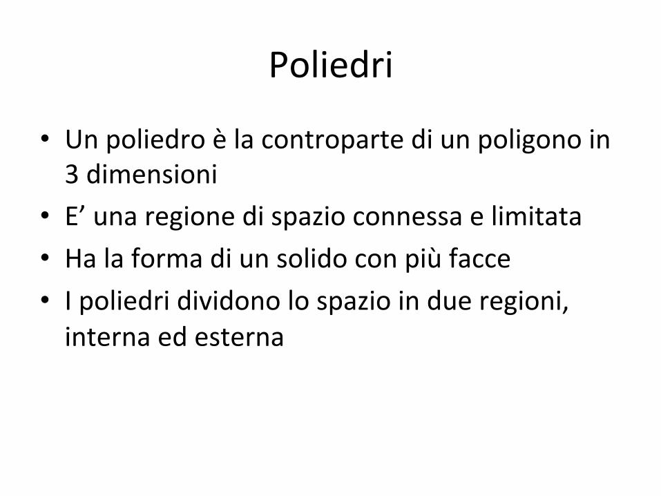
•  Un  poliedro  è  la  controparte  di  un  poligono  in  3  dimensioni  

•  E’  una  regione  di  spazio  connessa  e  limitata  •  Ha  la  forma  di  un  solido  con  più  facce  •  I  poliedri  dividono  lo  spazio  in  due  regioni,  interna  ed  esterna  

 

Politopi  

•  Un  poliedro  convesso  è  definito  anche  un  politopo.  

•  Come  un  poligono,  i  politopi  possono  essere  defini5  come  l’intersezione  di  un  numero  finito  di  semispazi  

Simplesso  

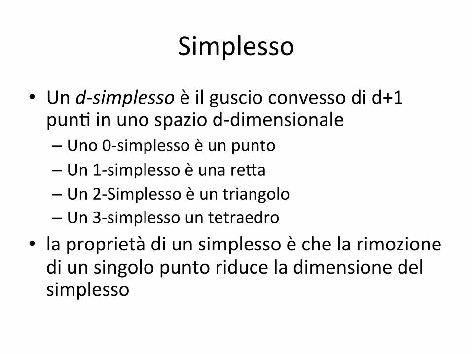
•  Un  d-­‐simplesso  è  il  guscio  convesso  di  d+1  pun5  in  uno  spazio  d-­‐dimensionale  – Uno  0-­‐simplesso  è  un  punto  – Un  1-­‐simplesso  è  una  re>a  – Un  2-­‐Simplesso  è  un  triangolo  – Un  3-­‐simplesso  un  tetraedro  

•  la  proprietà  di  un  simplesso  è  che  la  rimozione  di  un  singolo  punto  riduce  la  dimensione  del  simplesso    

Computazione  dei  gusci  convessi  

•  I  gusci  convessi  possono  essere  u5lizza5  come  volumi  per  geometrie  di  collisione  

•  Diversi  algoritmi  per  la  computazione  di  ques5  sono  sta5  propos5  

Andrew’s  Algorithm  

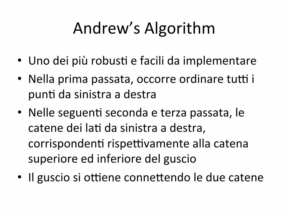
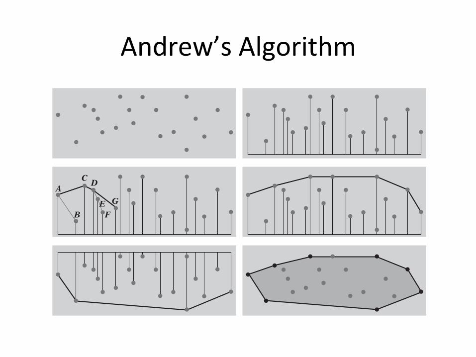
•  Uno  dei  più  robus5  e  facili  da  implementare  •  Nella  prima  passata,  occorre  ordinare  tuZ  i  pun5  da  sinistra  a  destra  

•  Nelle  seguen5  seconda  e  terza  passata,  le  catene  dei  la5  da  sinistra  a  destra,  corrisponden5  rispeZvamente  alla  catena  superiore  ed  inferiore  del  guscio  

•  Il  guscio  si  oZene  conne>endo  le  due  catene  

Andrew’s  Algorithm  3.9 Computing Convex Hulls 65

A

B

C D

EF

G

Figure 3.22 Andrew’s algorithm. Top left: the point set. Top right: the points sorted (lexi-cographically) from left to right. Middle left: during construction of the upper chain. Middleright: the completed upper chain. Lower left: the lower chain. Lower right: the two chainstogether forming the convex hull.

Two of them are briefly described in the next two sections: Andrew’s algorithm andthe Quickhull algorithm.

3.9.1 Andrew’s Algorithm

One of the most robust and easy to implement 2D convex hull algorithms is Andrew’salgorithm [Andrew79]. In its first pass, it starts by sorting all points in the given pointset from left to right. In subsequent second and third passes, chains of edges fromthe leftmost to the rightmost point are formed, corresponding to the upper and lowerhalf of the convex hull, respectively. With the chains created, the hull is obtained bysimply connecting the two chains end to end. The process is illustrated in Figure 3.22.The main step lies in the creation of the chains of hull edges. To see how one of thechains is formed, consider the partially constructed upper chain of points, as shownin the middle left-hand illustration. To simplify the presentation, it is assumed thereare not multiple points of the same x coordinate (this assumption is lifted further on).

Initially, the two leftmost points, A and B, are taken to form the first edge of thechain. The remaining points are now processed in order, considered one by one foraddition to the hull chain. If the next point for consideration lies to the right of the

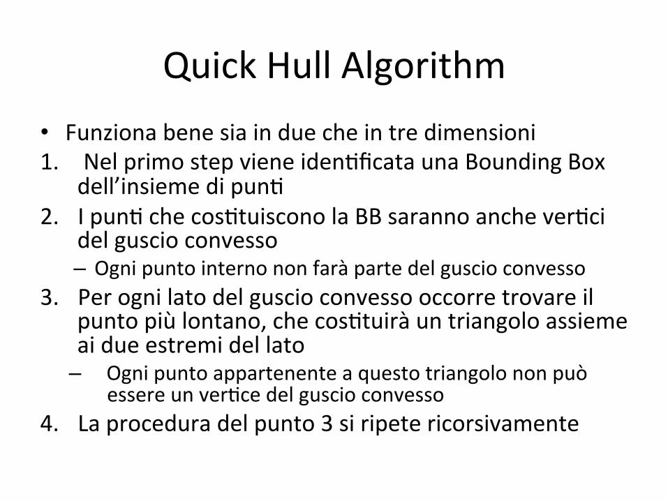
Quick  Hull  Algorithm  •  Funziona  bene  sia  in  due  che  in  tre  dimensioni  1.   Nel  primo  step  viene  iden5ficata  una  Bounding  Box  

dell’insieme  di  pun5  2.  I  pun5  che  cos5tuiscono  la  BB  saranno  anche  ver5ci  

del  guscio  convesso  –  Ogni  punto  interno  non  farà  parte  del  guscio  convesso  

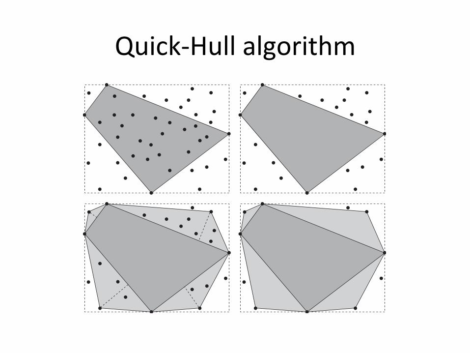
3.  Per  ogni  lato  del  guscio  convesso  occorre  trovare  il  punto  più  lontano,  che  cos5tuirà  un  triangolo  assieme  ai  due  estremi  del  lato  –  Ogni  punto  appartenente  a  questo  triangolo  non  può  

essere  un  ver5ce  del  guscio  convesso  4.  La  procedura  del  punto  3  si  ripete  ricorsivamente  

Quick-­‐Hull  algorithm  3.9 Computing Convex Hulls 67

Figure 3.23 First steps of the Quickhull algorithm. Top left: the four extreme points (on thebounding box of the point set) are located. Top right: all points inside the region formed bythose points are deleted, as they cannot be on the hull. Bottom left: for each edge of theregion, the point farthest away from the edge is located. Bottom right: all points inside thetriangular regions so formed are deleted, and at this point the algorithm proceeds recursivelyby locating the points farthest from the edges of these triangle regions, and so on.

endpoints of the edge, these new points form a triangular region. Just as before, anypoints located inside this region cannot be on the hull and can be discarded (Figure3.23, bottom right). The procedure now recursively repeats the same procedure foreach new edge that was added to the hull, terminating the recursion when no pointslie outside the edges.

Although the preceding paragraph completes the overall algorithm description,two minor complications must be addressed in a robust implementation. The firstcomplication is that the initial hull approximation may not always be a quadrilateral.If an extreme point lies, say, in the bottom left-hand corner, the initial shape mayinstead be a triangle. If another extreme point lies in the top right-hand corner,it may be a degenerate hull, consisting of only two points. To avoid problems, animplementation must be written to handle an initial hull approximation of a variablenumber of edges. The second complication is that there might not be a single unique

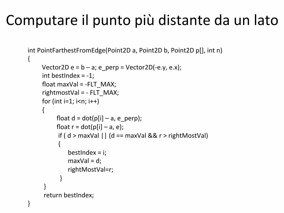
Computare  il  punto  più  distante  da  un  lato  

int  PointFarthestFromEdge(Point2D  a,  Point2D  b,  Point2D  p[],  int  n)  {  

 Vector2D  e  =  b  –  a;  e_perp  =  Vector2D(-­‐e.y,  e.x);                    int  bestIndex  =  -­‐1;                    float  maxVal  =  -­‐FLT_MAX;                    rightmostVal  =  -­‐  FLT_MAX;                    for  (int  i=1;  i<n;  i++)                    {                                      float  d  =  dot(p[i]  –  a,  e_perp);                                      float  r  =  dot(p[i]  –  a,  e);                                        if  (  d  >  maxVal  ||  (d  ==  maxVal  &&  r  >  rightMostVal)                                        {                                                    bestIndex  =  i;                                                    maxVal  =  d;                                                    rightMostVal=r;                                          }                      }                      return  bestIndex;  }    

Bounding  Volumes  

•  Un  Bounding  Volume  è  un  volume  che  incapsula  uno  o  più  oggeZ  di  natura  più  complessa.  

•  L’idea  è  quella  di  u5lizzare  tali  volumi  più  semplici,  come  sfere  o  parallelepipedi,  per  compiere  dei  test  di  sovrapposizione.  

•  Usandoli,  è  possibile  computare  velocemente  una  mancata  sovrapposizione  

Cara>eris5che  Desiderabili  

•  test  di  intersezione  poco  costoso  in  termini  computazionali  

•  Aderenza  stre>a  con  la  geometria  •  Semplice  da  calcolare  •  Poca  memoria  richiesta  

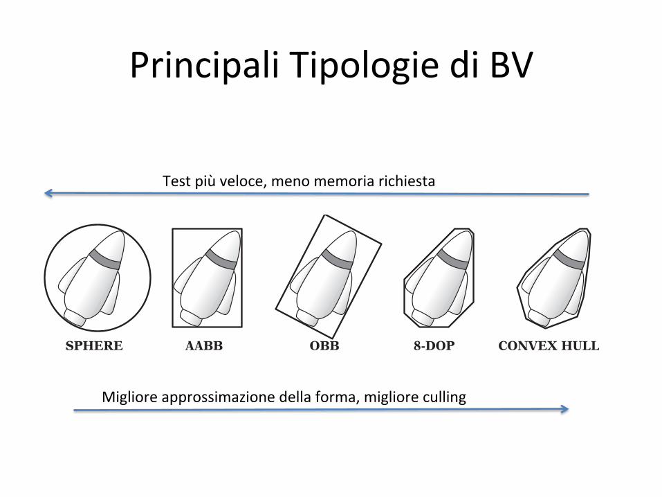
Principali  Tipologie  di  BV  4.2 Axis-aligned Bounding Boxes (AABBs) 77

BETTER BOUND, BETTER CULLING

FASTER TEST, LESS MEMORY

SPHERE AABB OBB 8-DOP CONVEX HULL

Figure 4.2 Types of bounding volumes: sphere, axis-aligned bounding box (AABB), orientedbounding box (OBB), eight-direction discrete orientation polytope (8-DOP), and convex hull.

point inclusion, ray intersection with the volume, and intersection with planes andpolygons.

Bounding volumes are typically computed in a preprocessing step rather than atruntime. Even so, it is important that their construction does not negatively affectresource build times. Some bounding volumes, however, must be realigned at runtimewhen their contained objects move. For these, if the bounding volume is expensiveto compute realigning the bounding volume is preferable (cheaper) to recomputingit from scratch.

Because bounding volumes are stored in addition to the geometry, they shouldideally add little extra memory to the geometry. Simpler geometric shapes require lessmemory space. As many of the desired properties are largely mutually exclusive, nospecific bounding volume is the best choice for all situations. Instead, the best optionis to test a few different bounding volumes to determine the one most appropriatefor a given application. Figure 4.2 illustrates some of the trade-offs among five ofthe most common bounding volume types. The given ordering with respect to betterbounds, better culling, faster tests, and less memory should be seen as a rough, ratherthan an absolute, guide. The first of the bounding volumes covered in this chapter isthe axis-aligned bounding box, described in the next section.

4.2 Axis-aligned Bounding Boxes (AABBs)

The axis-aligned bounding box (AABB) is one of the most common bounding volumes.It is a rectangular six-sided box (in 3D, four-sided in 2D) categorized by having itsfaces oriented in such a way that its face normals are at all times parallel with theaxes of the given coordinate system. The best feature of the AABB is its fast overlapcheck, which simply involves direct comparison of individual coordinate values.

Migliore  approssimazione  della  forma,  migliore  culling  

Test  più  veloce,  meno  memoria  richiesta  

Axis  Aligned  Bounding  Box  

•  Un  parallelepipedo  orientato  in  maniera  tale  da  avere  le  facce  orientate  normali  agli  assi  del  sistema  di  riferimento  

•  La  sua  cara>eris5ca  è  la  rapidità  con  cui  si  può  computare  un  test  di  sovrapposizione  

•  Il  test  coinvolge  semplicemente  la  comparazione  di  valori  di  coordinate  

Implementazione  78 Chapter 4 Bounding Volumes

(a) (b) (c)

Figure 4.3 The three common AABB representations: (a) min-max, (b) min-widths, and(c) center-radius.

There are three common representations for AABBs (Figure 4.3). One is by theminimum and maximum coordinate values along each axis:

// region R = {(x, y, z) | min.x<=x<=max.x, min.y<=y<=max.y, min.z<=z<=max.z }struct AABB {

Point min;Point max;

};

This representation specifies the BV region of space as that between the two oppos-ing corner points: min and max. Another representation is as the minimum cornerpoint min and the width or diameter extents dx, dy, and dz from this corner:

// region R = {(x, y, z) | min.x<=x<=min.x+dx, min.y<=y<=min.y+dy, min.z<=z<=min.z+dz}struct AABB {

Point min;float d[3]; // diameter or width extents (dx, dy, dz)

};

The last representation specifies the AABB as a center point C and halfwidthextents or radii rx, ry, and rz along its axes:

// region R = {(x, y, z) | |c.x-x|<=rx, |c.y-y|<=ry, |c.z-z|<=rz }struct AABB {

Point c; // center point of AABBfloat r[3]; // radius or halfwidth extents (rx, ry, rz)

};

struct  AABB  {        Point  min;        Point  max;  };  

struct  AABB  {        Point  min;        float  d[3];  };  

struct  AABB  {        Point  center;        float  radius[3];  };  

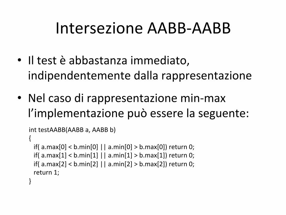
Intersezione  AABB-­‐AABB  

•  Il  test  è  abbastanza  immediato,  indipendentemente  dalla  rappresentazione  

 

int  testAABB(AABB  a,  AABB  b)  {        if(  a.max[0]  <  b.min[0]  ||  a.min[0]  >  b.max[0])  return  0;        if(  a.max[1]  <  b.min[1]  ||  a.min[1]  >  b.max[1])  return  0;        if(  a.max[2]  <  b.min[2]  ||  a.min[2]  >  b.max[2])  return  0;        return  1;  }  

•  Nel  caso  di  rappresentazione  min-­‐max  l’implementazione  può  essere  la  seguente:  

 

Computare  ed  aggiornare  le  AABB  

•  Per  il  test  di  overlap  è  necessario  che  le  due  AABB  siano  nello  stesso  sistema  di  riferimento  

•  Può  essere  quello  di  tenere  entrambe  le  AABB  in  world  space  oppure  di  trasformare  una  AABB  nello  spazio  locale  dell’altra  

•  Efficienza  ed  accuratezza  

Sfere  

•  Altro  bounding  volume  molto  comune  •  Sono  anche  invarian5  alle  rotazioni  •  Dal  punto  di  vista  della  memoria,  è  il  bounding  volume  meno  costoso  

struct  Sphere  {  

 Point  c;                    float  radius;  }  

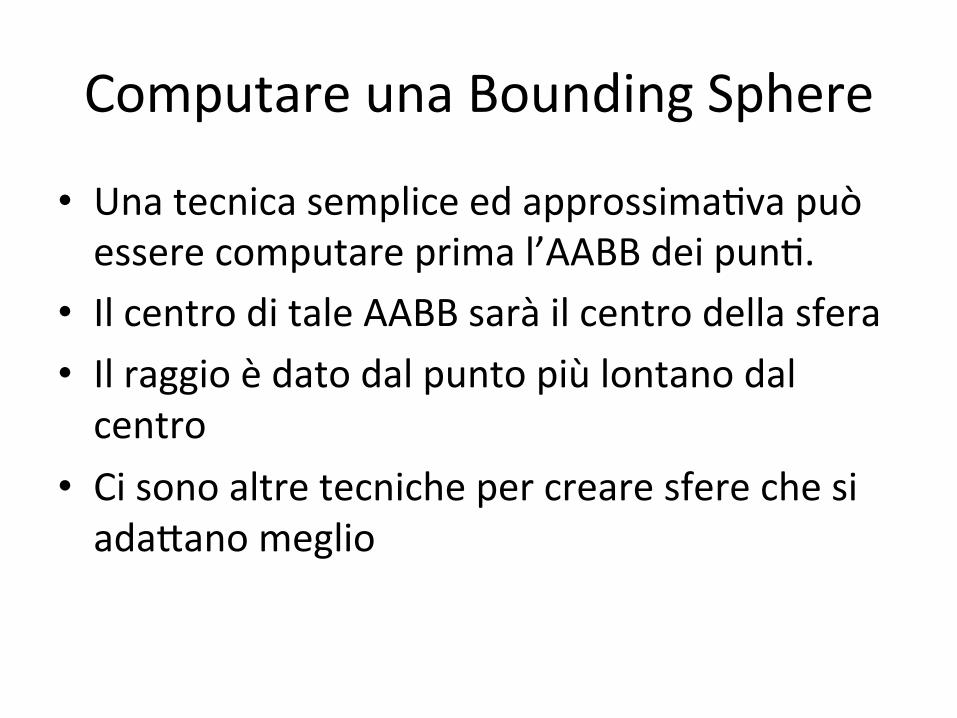
Computare  una  Bounding  Sphere  

•  Una  tecnica  semplice  ed  approssima5va  può  essere  computare  prima  l’AABB  dei  pun5.    

•  Il  centro  di  tale  AABB  sarà  il  centro  della  sfera  •  Il  raggio  è  dato  dal  punto  più  lontano  dal  centro  

•  Ci  sono  altre  tecniche  per  creare  sfere  che  si  ada>ano  meglio  

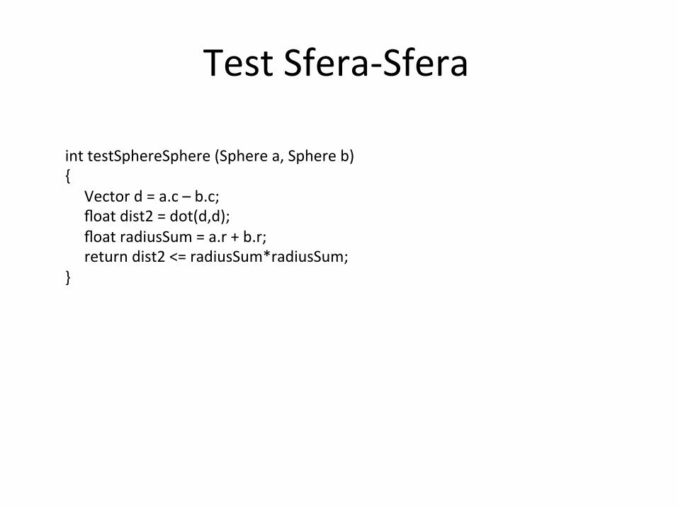
Test  Sfera-­‐Sfera  

int  testSphereSphere  (Sphere  a,  Sphere  b)  {            Vector  d  =  a.c  –  b.c;            float  dist2  =  dot(d,d);            float  radiusSum  =  a.r  +  b.r;            return  dist2  <=  radiusSum*radiusSum;  }  

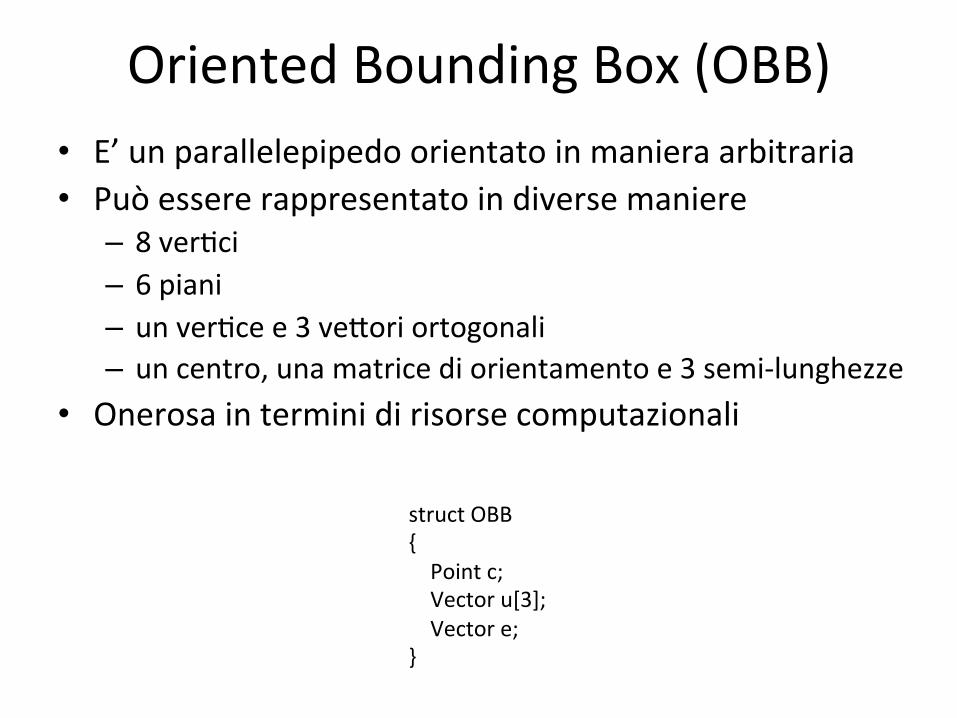
Oriented  Bounding  Box  (OBB)  •  E’  un  parallelepipedo  orientato  in  maniera  arbitraria  •  Può  essere  rappresentato  in  diverse  maniere  –  8  ver5ci  –  6  piani  –  un  ver5ce  e  3  ve>ori  ortogonali  –  un  centro,  una  matrice  di  orientamento  e  3  semi-­‐lunghezze  

•  Onerosa  in  termini  di  risorse  computazionali  

struct  OBB  {          Point  c;          Vector  u[3];          Vector  e;  }