ISTITUTO DI ANALISI DEI SISTEMI ED INFORMATICA

CONSIGLIO NAZIONALE DELLE RICERCHE

M. Roma

DYNAMIC SCALING BASED PRECONDITIONING

FOR TRUNCATED NEWTON METHODS

IN LARGE SCALE UNCONSTRAINED OPTIMIZATION:

THE COMPLETE RESULTS

R. 579 Dicembre 2002

Massimo Roma - Dipartimento di Informatica e Sistemistica “A. Ruberti”, Universita diRoma “La Sapienza”, via Buonarroti 12 - 00185 Roma, Italy and Istituto di Analisi deiSistemi ed Informatica del CNR “A. Ruberti”, viale Manzoni 30 - 00185 Roma, Italy.Email : roma@dis.uniroma1.it URL: www.dis.uniroma1.it/ ˜ roma.

This work was supported by Progetto FIRB “Ottimizzazione non lineare su larga scala”

Istituto di Analisi dei Sistemi ed Informatica, CNRviale Manzoni 3000185 ROMA, Italy

tel. ++39-06-77161fax ++39-06-7716461email: iasi@iasi.rm.cnr.itURL: http://www.iasi.rm.cnr.it

Abstract

This paper deals with the preconditioning of truncated Newton methods for the solution oflarge scale nonlinear unconstrained optimization problems. We focus on preconditioners whichcan be naturally embedded in the framework of truncated Newton methods, i.e. which can bebuilt without storing the Hessian matrix of the function to be minimized, but only based uponinformation on the Hessian obtained by the product of the Hessian matrix times a vector. Inparticular we propose a diagonal preconditioning which enjoys this feature and which enablesus to examine the effect of diagonal scaling on truncated Newton methods. In fact, this newpreconditioner carries out a scaling strategy and it is based on the concept of equilibration ofthe data in linear systems of equations. An extensive numerical testing has been performedshowing that the diagonal preconditioning strategy proposed is very effective. In fact, on mostproblems considered, the resulting diagonal preconditioned truncated Newton method performsbetter than both the unpreconditioned method and the one using an automatic preconditionerbased on limited memory quasi–Newton updating (PREQN) recently proposed in [23].

Key words: truncated Newton method, conjugate gradient method, preconditioning, row–column scaling, equilibrated matrix.

3.

1. Introduction

This paper deals with large scale nonlinear unconstrained optimization problems, i.e. problemsof finding a local minimizer of a real valued function f : IRn −→ IR, namely

min f(x)

x ∈ IRn

where the number of variables n is large. The function f is assumed to be twice continuouslydifferentiable.

The growing interest in solving large scale problems is mainly due to the fact that in many anddifferent contexts and applications such problems arise very frequently. Moreover, as well known,efficiently solving unconstrained problems is very important in the framework of constrainedoptimization too, for instance when a penalty–barrier approach is used.

Among the existing methods in large scale unconstrained optimization (see, e.g. [28] [31]for a survey) the truncated Newton methods represent one of the most powerful, reliable andflexible tool for solving large scale problems. In fact, they have a solid convergence theory, theyretain the good Newton–like convergence properties exhibiting an excellent rate of convergence;moreover, they are robust and efficient also in solving “difficult problems” as highly nonlinearand ill–conditioned problems. Moreover truncated Newton methods have been successfully usedin solving real world problems arising in many applications and several algorithmic enhancementshave been developed and studied in the last years, too (see the excellent survey of truncatedNewton methods [25] recently published by Nash and the references reported therein).

Although truncated Newton methods have been widely studied and extensively tested a num-ber of important open questions still exist (see [28] Section 3.2) and motivate this work. Oneof these open questions addresses the formulation of an effective preconditioning strategy whichenables to improve the behaviour of a truncated Newton method in tackling large scale prob-lems. In this paper this question is considered, focusing on “general purpose” preconditionerssuitable within the truncated Newton method framework, that is preconditioners which do notrequire the explicit knowledge of the Hessian matrix. The information about the Hessian matrixare gained only by means of a routine which provides us with the matrix–vector products of theHessian matrix times a vector, i.e. by using a tool already required by any truncated Newtonmethod implementation. Of course, this makes this kind of preconditioners also suitable withindiscrete truncated Newton methods where these matrix–vector products are approximated byfinite differences [29]. Moreover, we focus our attention on preconditioners which are also “dy-namic”, i.e. which change during the iterations of the method.

Very few preconditioners enjoying all these features have been developed up to now. Themost recent and efficient proposal of such a preconditioner is due to Morales and Nocedal [23]which proposed an automatic preconditioning strategy based on limited memory quasi–Newtonupdating.

In this work we propose a diagonal preconditioning strategy which enjoys all these desiredfeatures. It is based on the equilibration of data in linear systems and it consists of scalingthe column vectors of the Hessian matrix. Generally speaking, column scaling is carried outby dividing each column of the matrix by the norm of the column, where different norms maybe considered. Equilibrating matrices is a topic of great importance in the numerical solutionof linear systems, and, as far as the author is aware, it has not yet been fully exploited as auseful tool for building good “general purpose” preconditioners for truncated Newton methods,

4.

even though the optimal properties of the scaled matrices—in terms of condition numbers—were well known since thirty year ago (see, e.g. [35], [5]). The need of equilibrating matricesin solving linear systems arising from real world problems is, in general, very evident; in fact,many times, these matrices have entries that vary over many orders of magnitude and their arevery spread. In this case, a simple diagonal scaling would greatly reduce the condition numberof the matrices. These general considerations are of fundamental importance in the frameworkof truncated Newton methods, since at each iteration of these methods a linear system must be(approximately) solved.

We embedded the diagonal preconditioner proposed within a linesearch based implementationof truncated Newton method and firstly, to check its reliability, we numerically tested it on asome real problems arising as finite dimensional approximation models taken form the MINPACK-

2 collection [1]. Then we performed an extensive numerical testing on a very large set of testproblems of the CUTE collection [6]. The results obtained confirmed our expectation: in factthis preconditioning strategy revealed inexpensive and very effective, reducing both the numberof conjugate gradient iterations and the CPU time needed for solving most of the problemsconsidered with respect to the unpreconditioned method. Moreover, a comparison with theresults obtained on the same set of test problems by using the automatic preconditioner based onlimited memory quasi–Newton updating PREQN proposed in [23] has been performed. Also fromthis comparison it is clearly pointed out the efficiency of the proposed diagonal preconditioner.

The paper is organized as follows: in Section 2 truncated Newton methods are briefly recalledpointing out those questions which are still considered open problems and, in particular, con-cerning preconditioning. In Section 3 the new diagonal preconditioning strategy is describedand in Section 4 the results of the extensive numerical investigation are reported.

Throughout the paper the following notations are used: g(x) = ∇f(x) denotes the gradientand H(x) = ∇2f(x) the Hessian matrix of the function f . Moreover, ‖v‖p denotes the `p–normof a vector v ∈ IRn and for a n×n matrix A, ‖A‖p denotes the induced matrix norm. Moreover,

κp(A) = ‖A‖p

∥∥A−1∥∥

p denotes the condition number of A in the `p–norm.

2. Preconditioned truncated Newton methods

In this section, truncated Newton methods (TN) are briefly recalled, focusing on their ma-jor components and in particular on preconditioning (a more precise description of truncatedNewton methods can be found in [11] or, e.g., in the survey paper [25]).

As well known, given a guess xk of a solution x?, the truncated Newton method is based onthe quadratic model of the objective function f given by

qk(d) = f(xk) + g(xk)T d +

1

2dT H(xk)d (2.1)

and it is defined by iterations of the form

xk+1 = xk + dk

where the search direction dk is obtained by approximately minimizing the quadratic model ofthe objective function (2.1) over IRn. Of course, whenever the Hessian matrix H(xk) is positivedefinite, to minimize the quadratic model qk is equivalent to solve the linear system

H(xk)d = −g(xk). (2.2)

5.

A good convergence rate of the method is still ensured by using a particular trade-off rule betweenthe computational burden required to solve the system (2.2) and the accuracy with which it issolved [10]. A natural measure of this accuracy is the relative residual. In the truncatedNewton methods an approximation of the Newton direction dk is computed by applying aniterative method for approximately solving the linear system (2.2) and “truncating” the iterateswhenever a required accuracy is achieved [11]. To this aim, the most frequently used algorithmis the linear conjugate gradient method (CG) since it is an efficient iterative method for solvingpositive definite linear systems.

The components of a truncated Newton method are several, providing the method with agreat flexibility. In particular three key aspects for the overall efficiency of a truncated Newtonmethod can be still considered open problems (see [28] Section 3.2): i) the formulation of aneffective “truncation criterion” for the inner loop; ii) how to handle the case when the Hessianmatrix is not positive definite; iii) the formulation and handling of a preconditioner to acceleratethe convergence in the inner CG iterates.

In this paper we concentrate on preconditioning, which is considered one of the most importantissues of the current research on truncated Newton methods. As well known preconditioningthe inner CG iterations can considerably accelerate the convergence of the conjugate gradientmethod affecting the overall efficiency of a truncated Newton method. In fact, the convergencerate of the CG inner iterations is based on the condition number and the number of distincteigenvalues of the Hessian matrix H(xk) (see, e.g. [13]). In particular, the larger the conditionnumber, the slower the convergence of the method is; moreover, the more the eigenvalues areclustered, the sooner the error is reduced. Preconditioning enables to reduce either the conditionnumber and the number of distinct eigenvalues thus accelerating the convergence of the CGmethod. A scheme of the Preconditioned Conjugate Gradient (PCG) algorithm applied to thesolution of the system (2.2) is the following (see, e.g. [13] [18] [14]):

Preconditioned Conjugate Gradient AlgorithmPCG(M)

Given d0 = 0 and M−1, set r0 = g(xk), z0 = M−1r0 and p0 = −z0.

For i = 0, 1, 2, . . ., until convergence, perform the iteration

di+1 = di + αipi

ri+1 = ri + αiH(xk)pi

where αi =riT zi

piT H(xk)pi

zi+1 = M−1ri+1 (2.3)

pi+1 = −zi+1 + βipi

where βi =ri+1T

zi+1

riT zi

6.

As well knonw, this PCG algorithm is obtained by applying the CG method to the transformedsystem Hkd = −gk, where Hk = CH(xk)C

T , d = C−T d, gk = Cg(xk) and C is a non-singular matrix. The matrix M = (CCT )−1 is the preconditioner and, due to similarity, Hk

and H(xk)M−1 have the same conditioning. The computational burden of the PCG algorithm

is more expensive than the unpreconditioned one, but it is now the matrix H(xk)M−1 which

determines the convergence properties of the PCG method. More precisely the convergencedepends on the condition number κ2(H(xk)M

−1) and on the number of distinct eigenvalues ofH(xk)M

−1.

It is out of the scope of this paper to discuss the well known features of preconditioning or tosurvey the very broad field of preconditioners (see, e.g. [4] [14] [36] [2] [21] for some references).We only mention in the sequel of this section the main preconditioning strategies up to nowproposed in the framework of truncated Newton methods.

A preconditioning strategy which has been successfully used within truncated Newton methodsis based on the incomplete (modified) Cholesky factorization [19] [33] [7]. It is a valuable choicesince it is “general purpose” and a great reduction of the number of the inner CG iterationscan be obtained. However, unfortunately, it requires the knowledge of the Hessian matrix.Another approach is based on efficiently exploiting the problem structure when it exists; inparticular, many large scale problems possess the so called “partial separability” property, i.e.the objective function can be written as sum of simpler functions and this property can beexploited for defining “ad hoc” preconditioners [9].

In the context of truncated Newton methods, a first key point in developing an efficient precon-ditioning strategy for solving the sequence of systems (2.2) is to use a “dynamic preconditioner”,i.e. a preconditioner which changes with the outer iterations. In particular, since at each outeriteration k the Hessian matrix changes, consequently the preconditioner should be changed.One possibility is to define, at each outer iteration k, a new preconditioner on the basis of theinformation gained during the solution of the system at the (k − 1)–th iteration. This idea isnot new, and its importance, as a challenge topic in large scale optimization, has already beenclearly pointed out (see [28] Section 3.2).

Another key point is the availability of a preconditioner which can be effectively used withina truncated Newton method that is, which does not require to store and handle any matrix. Byusing this kind of preconditioners, the PCG algorithm is still free from the storage and handlingof the Hessian matrix, like the unpreconditioned CG algorithm. Of course this feature is enjoyedby a preconditioner which can be built by using only information on the Hessian matrix obtainedby performing products of the Hessian matrix times a vector. We remark that preconditionersof this kind can be used within discrete Newton methods [29] or when automatic differentiation[15] is used.

The first proposal of a preconditioned truncated Newton method which satisfies both theserequirements was performed in [24]. It is based on a two–step limited memory BFGS updating;in particular, a diagonal scaling which uses a diagonal approximation of the Hessian matrix, ob-tained by means of BFGS updating is defined. This preconditioning strategy has been embeddedin a discrete truncated Newton method which has been numerically tested and compared withother methods for large scale unconstrained optimization [26].

Recently, an automatic preconditioning based on m–step limited memory quasi–Newton up-dating has been proposed [23] [22]. This is a dynamic preconditioner which does not requirethe explicit knowledge of the Hessian matrix, too. This preconditioner has been numericallytested within a discrete Newton method and in the solution of linear systems arising in somefinite element models; the results obtained in the solution of large scale unconstrained optimiza-

7.

tion problems indicate that this preconditioning strategy enables to reduce the number of CGinner iterations but it is expensive, due to the considerable computational cost of building andhandling the preconditioner. This makes this particular preconditioner suited for problems forwhich the matrix–vector products of the Hessian matrix times a vector are expensive to com-pute. However, today this automatic preconditioning technique seems to be the best proposalwithin the class of dynamic preconditioners that we are considering.

3. Diagonal Preconditioning Truncated Newton Methods

On the basis of the remarks contained in the previous section, we now focus on diagonal pre-conditioning techniques since they can be efficiently used in the context of truncated Newtonmethods. In fact, we propose a diagonal preconditioner which possesses the desired featureswhich makes its use appealing within a truncated Newton methods. Before going into details,we briefly report the main features of a generic diagonal preconditioner considering the solutionof a generic linear system As = b where A is a n × n nonsingular symmetric matrix and aij

denotes its entries. First of all, we recall the well known concept of equilibrated matrix whichwill be used in the sequel

Definition 3.1. A matrix A is said row (column) equilibrated if all its rows (columns) havethe same length in some norm and it is said equilibrated if all its rows and columns have thesame length in some norm.

Diagonal preconditioning is the simplest form of preconditioning and it is very inexpensive tohandle. The matrix M is chosen as a diagonal matrix

M = diag{d1 . . . dn} =

d1 0. . .

0 dn

where di ∈ IR, di > 0, i = 1, . . . , n. This preconditioning corresponds to a scaling of thecolumns of the matrix A, aiming at obtaining a system with a column equilibrated matrix, thatis a better conditioned system. Analogously a system with a row equilibrated matrix can beconsidered, while it is more complicated to obtain an equilibrated matrix. The advantages ofhaving linear systems with equilibrated matrix is well known and its importance in numericalnumerical analysis is witnessed by the number of papers devoted to this topic (see, e.g., [12] [34][32] and the references therein). Moreover, there exist algorithms for equilibrating a matrix in aspecific norm; some examples were proposed in [8], [30], [32]. Furthermore, optimality propertiesof scaling in `p–norm equilibrating the rows or the columns for minimizing the condition numberare considered in [17] Section 7.3.

Note that to apply the preconditioned conjugate gradient method with this diagonal pre-conditioner, corresponds to apply the CG method to the system with the transformed matrix

D−1AD−1 where D = diag{d1

2

1 , . . . , d1

2

n}.

It is well known that diagonal preconditioning presents some very good features; in fact itwould greatly reduce the condition number of the matrix and it does not destroy the sparsity ofthe matrix; moreover it requires a minimal additional work and it is suitable to handle practicalproblems whose matrices entries frequently vary over many orders of magnitude.

8.

A choice which is “optimal” with respect to diagonal preconditioners is to use the diagonalof the matrix A as diagonal preconditioner matrix (Jacobi preconditioner); in fact this choiceenables to minimize the condition number of the matrix of the transformed system with respectto all the diagonal preconditioners. In fact, the following result holds [35] (see also, e.g., [14][17] [21] ):

Theorem 3.2. Let A be a n × n symmetric positive definite matrix. Let Dn denote the set of

n × n nonsingular diagonal matrices and ∆ = diag{a1

2

11, . . . , a1

2

nn}. Then

κ2(∆−1A∆−1) ≤ p min

D∈Dn

κ2(D−1AD−1),

where p is the maximum number of non-zero elements in any row of A.

It is important to note that, even in this special case of the Jacobi preconditioner no resultsconcerning the variation of the condition number or the eigenvalue distribution—and hence apossible improvement of the convergence rate—is available. In fact, Theorem 3.2 states onlythe existence of a lower bound but does not provide us with information about the variationof the condition number of the transformed system. This result, however, states that this kindof preconditioner is effective for sparse matrices. As regards the numerical efficiency of Jacobipreconditioner, it is known that it typically works well whenever the matrix A is very diagonallydominant.

Simple diagonal scaling of the variables has been already proved to be very effective in thecontext of L–BFGS methods [20] and within partitioned quasi–Newton methods [16] especiallyin tackling large scale problems. Moreover in [3] the effect of diagonal scaling with projectedgradient methods for bound constrained problems has been investigated.

We can conclude these brief general considerations on diagonal scaling claiming that, evenif there exist cases in which diagonal preconditioning does not lead to an improvement of theconditioning, however, in many cases an improvement, even if small, is observed and thereforethe use of a diagonal preconditioning is usually recommended.

Now we investigate the possibility to define and efficiently use a diagonal preconditioningstrategy within truncated Newton methods. In particular, we note that it corresponds to ascaling of the Hessian matrix which appears in the sequence of linear systems (2.2) and, aswell known, to have “good” scaling in defining algorithms is always very important, even if thealgorithm we are dealing with is a scaling invariant algorithm as the Newton method. Morein details, as already observed, diagonal preconditioning corresponds to an equilibration of thedata in the large linear systems to be solved at each iteration of the truncated Newton method.

A classical approach for row (column) scaling is to divide each row (column) by the norm ofthe row (column) vector. The most commonly used norms are the `1–norm and the `∞–norm.To scale matrices such that the norm of all rows (or columns) are equal to one is an heavy taskfrom the computational point of view, and this should be the reason for which, as far as theauthor is aware, this numerical tool has not yet been fully exploited for building preconditionerin the context of truncated Newton methods, tackling large scale problems. In fact to computethe norm of each row (or column) of the Hessian matrix at each outer iteration of the methodis computationally too expensive and thus impracticable, whichever norm is chosen. Also theuse of the diagonal of the Hessian matrix itself as diagonal preconditioner is not practicable toderive efficiently by means of a routine which provides the product of the Hessian matrix timesa vector.

9.

On the basis of these remarks, we propose a strategy based on columns scaling of the Hessianmatrix H(xk) in the solution of the systems (2.2) and, in particular, we focus on an equilibrationstrategy which uses the `1–norm.

In the sequel of this section, for the sake of simplicity, we remove the dependency on kand hence we refer to the system Hd = −g. Let hij , i, j = 1, . . . , n, denote the entries ofthe Hessian matrix H and for each j = 1, . . . , n let wj ∈ IRn defined by wj = Hej , whereej = (0, . . . , 1, . . . , 0)T is the j-th unit vector, that is, for each column j, wj denote the columnvectors of the matrix H (which are also the row–vectors for the symmetry). We consider thediagonal preconditioning generated by the matrix

D = diag

{‖w1‖

1

2

1 , . . . , ‖wn‖1

2

1

}=

‖w1‖

1

2

1 0. . .

0 ‖wn‖1

2

1

Obviously, in terms of the preconditioning matrix, this corresponds to choose

M = diag{‖w1‖1, . . . , ‖wn‖1

},

and it results that the matrix HM−1 is a column equilibrated matrix in the `1–norm.

It is now important to analyze the condition number and the eigenvalues distribution of thepreconditioned matrix to check if the use of such a preconditioner leads to a better conditionedsystem. Note that the (unsymmetric) matrix HM−1 and the (symmetric) matrix M−1/2HM−1/2

are similar and hence they have the same eigenvalues. Firstly we address to the conditionnumber of the preconditioned matrix showing that the particular column scaling proposed hasa very important feature, since it is an optimal column scaling strategy. In fact, the followingproposition holds.

Proposition 3.3. If H is nonsingular and Dn denotes the set of n × n nonsingular diagonalmatrices, then

κ1(HM−1) ≤ minD∈Dn

κ1(HD).

Proof: The results immediately follows from Theorem 7.5 in [17].

Therefore the proposed column scaling is the best column scaling in terms of condition numberin `1–norm and due to the well known norm equivalence on a finite–dimensional space, it ispossible to establish a relation between the condition number in `1–norm and in `2–norm, whichdiffer by at most a constant that depends on the dimension n.

As regards the eigenvalues distribution of the preconditioned matrix, by exploiting the factthat the matrix HM−1 is column equilibrated in the `1–norm, it is possible to prove the followingresult.

Proposition 3.4. Let ρ(HM−1) = max{ |λi| : λi eigenvalues of HM−1} be the spectral radiusof the matrix HM−1. Then it results

ρ(HM−1) ≤ 1.

10.

Proof: The result can be obtained by observing that for a square matrix A it results ρ(A) ≤‖A‖p for every `p–norm. In fact, we have

ρ(HM−1) ≤ ‖HM−1‖1 = 1,

where the last equality follows from the fact that ‖HM−1ej‖1 = 1 for all j = 1, . . . , n, i.e. allthe columns of HM−1 have unitary `1–norm.

The result stated in this proposition shows how the use of the proposed preconditioner enablesto have clustered eigenvalues and hence the PCG iterates are expected to converge quickly.

Now, we prove a general result concerning diagonal preconditioning.

Proposition 3.5. Let D = diag{d1, . . . , dn} be a n×n diagonal matrix with dj > 0, j = 1, . . . , nand z ∈ IRn such that Hz = Dz. Then the matrix D−1/2HD−1/2 admits an eigenvalue equal toone and the corresponding eigenvector is given by v = D1/2z.

Proof: Since Hz = Dz, we have

D−1/2HD−1/2v = D−1/2Hz = D1/2z = v

that is, v is an eigenvector of D−1/2HD−1/2 corresponding to the eigenvalue equal to one.

By applying this proposition, assuming that H is a nonnegative matrix, i.e. hij ≥ 0 for alli, j = 1, . . . , n, it is possible to said more about the eigenvalues of the preconditioned matrixM−1/2HM−1/2. In fact, the following result holds.

Proposition 3.6. If H is a nonnegative matrix, the preconditioned matrix M−1/2HM−1/2 ad-mits an eigenvalue equal to one, and the corresponding eigenvector is given by v = M 1/2e, wheree = (1, . . . , 1)T .

Proof: It is enough to apply Proposition 3.5 with z = e. In fact, in this case, the equalityHe = Me holds.

Proposition 3.4 shows that the proposed preconditioner correspond to normalize the precondi-tioned matrix in such a way that its largest eigenvalue is less than or equal to one. Moreover, ifthe Hessian is a nonnegative matrix, Proposition 3.6 implies that the largest eigenvalue of thepreconditioned matrix is equal to one.

Finally, Proposition 3.5 shows that this diagonal preconditioner can be viewed as a particularcase of a more general setting in which in the definition of the preconditioner M , the vector e inHe = Me is replaced with any vector z ∈ IRn provided that Hz = Mz. However, note that if avector different from e is used in the equality He = Me, the optimal properties of the `1–normscaling do not necessarily hold, even if H is a nonnegative matrix.

Our aim is now to embed this diagonal preconditioning strategy in the framework of truncatedNewton methods, but it is not straightforward, since the matrix H is not available. In order toobtain information on the `1–norm of the columns of the Hessian matrix we propose to use theonly tool available in this context for providing us with information on the Hessian matrix, that

11.

is the routine for the product of H times a vector. In fact, we observe that an estimate of the`1–norm of the columns of the Hessian matrix can be obtained as follows: for each j-th column,j = 1, . . . , n let us consider

σj = |n∑

i=1

hij |. (3.1)

These quantities have the following properties:

• they are a lower estimate of the `1–norm of the j-th column vector;

• due to the symmetry of H, all the σj , j = 1, . . . , n, can be very easily computed by meansof the product of the Hessian matrix H times the vector e = (1, 1, . . . , 1)T . In fact, bytaking the absolute value of each component of the vector resulting from this product,we obtain all the σj . Therefore, only one call to the routine which provides us with theproduct of the Hessian matrix times a vector is enough to compute all the σj .

Obviously, for each column j for which hij ≥ 0 for all i = 1, . . . , n, we have σj = ‖wj‖1.

Therefore, if H is a nonnegative matrix, then it results σj = ‖wj‖1, for all j = 1, . . . , n.

The quantities (3.1) can be used to build the diagonal preconditioner defined by the followingdiagonal positive definite matrix

M = diag{σ1, . . . , σn} =

σ1 0. . .

0 σn

(3.2)

where, for j = 1, . . . n,

σj =

σj if σj > δ

1 otherwise

with δ > 0 small.

By using this diagonal preconditioning, each column of the matrix is scaled by a quantitywhich represents an estimate of the `1–norm of the column vectors and no scaling is performedin correspondence of those columns for which σj is small.

The proposed diagonal preconditioner has the following important features:

• the explicit knowledge of the Hessian matrix is not required, but only a routine whichprovides the product of the Hessian matrix times a vector is needed, enabling its usewithin a truncated Newton method;

• it carries out a “dynamical” preconditioning technique, i.e. the preconditioner changesfrom one outer iterate to the next, thus overcoming the drawback of having the samepreconditioner during the solution of each of the sequence of Newton’s systems (2.2),whereas the Hessian matrix can change drastically;

• the solution of the auxiliary system (2.3) needed to compute the preconditioned residualis very inexpensive;

12.

• the additional cost of preconditioning is essentially due to one additional call, at eachouter iteration, to the subroutine which provides the matrix–vector product of the Hessianmatrix times the vector e = (1, . . . , 1)T .

This diagonal preconditioner represents a useful tool that can be viewed as a “dynamic scaling”since it is derived from dynamic preconditioning and scaling and we name it DSPREC.

We note that if the Hessian matrix H is a nonnegative matrix, the quantities σj in (3.1)are the `1–norm of the j-th column vector and therefore the results stated in Proposition 3.3,Proposition 3.4 and Proposition 3.6 apply; in this case this diagonal preconditioner posses theimportant theoretical properties stated. Otherwise, as it occurs in most cases when dealingwith preconditioning, in the general setting, it is impossible to derive results which apply toany matrix. Therefore, since we are interested in “general purpose” preconditioner, the bestassessment tool is represented by an extensive numerical study.

4. Numerical experiments

If a wide numerical investigation is usually considered an essential tool for assessing the efficiencyof an algorithm, it is so much important in dealing with preconditioning strategies when, asoften occurs, some choices are mainly based on numerical experiments rather than on solidtheoretical results. Keeping in mind the central role of the numerical experiments in evaluatingthe effectiveness of different preconditioning strategies, we have been trying to perform a veryextensive numerical testing. To this aim we embedded the proposed preconditioning strategy ina linesearch–based truncated Newton method. Our implementation of the method is now brieflydescribed.

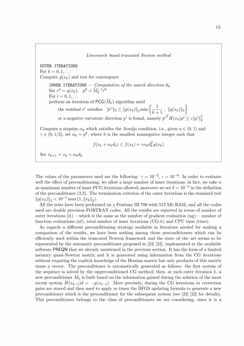
A preconditioned conjugate gradient algorithm is used for computing the search direction,terminating the inner PCG iterations whenever the residual–based criterion is satisfied or anegative curvature direction is encountered [11]. This criterion is preferred here with respect tothe quadratic model–based criterion proposed in [27] since it allows to easily control the rate ofconvergence of the truncated Newton method. The method is outlined in the following scheme:

13.

Linesearch–based truncated Newton method

OUTER ITERATIONS

For k = 0, 1, . . .Compute g(xk) and test for convergence

INNER ITERATIONS — Computation of the search direction dk

Set r0 = g(xk), p0 = M−10 r0

For i = 0, 1, . . .perform an iteration of PCG(Mk) algorithm until

the residual ri satisfies ‖ri‖2 ≤ ‖g(xk)‖2min

{1

k + 1, ‖g(xk)‖2

}

or a negative curvature direction pi is found, namely piT H(xk)pi ≤ ε‖pi‖

2

2

Compute a stepsize αk which satisfies the Armijo condition, i.e., given η ∈ (0, 1) andγ ∈ (0, 1/2), set αk = ηh, where h is the smallest nonnegative integer such that

f(xk + αkdk) ≤ f(xk) + γαkdTk g(xk)

Set xk+1 = xk + αkdk

The values of the parameters used are the following: γ = 10−3, ε = 10−6. In order to evaluatewell the effect of preconditioning, we allow a large number of inner iterations, in fact, we take nas maximum number of inner PCG iterations allowed; moreover we set δ = 10−6 in the definitionof the preconditioner (3.2). The termination criterion of the outer iterations is the standard test‖g(xk)‖2

< 10−5 max (1, ‖xk‖2).

All the tests have been performed on a Pentium III 700 with 512 Mb RAM, and all the codesused are double precision FORTRAN codes. All the results are reported in terms of number ofouter iterations (it) —which is the same as the number of gradient evaluation (ng)— number offunction evaluations (nf), total number of inner iterations (CG-it) and CPU time (time).

As regards a different preconditioning strategy available in literature needed for making acomparison of the results, we have been seeking among those preconditioners which can beefficiently used within the truncated Newton framework and the state–of–the–art seems to berepresented by the automatic preconditioner proposed in [23] [22], implemented in the availablesoftware PREQN that we already mentioned in the previous section. It has the form of a limitedmemory quasi-Newton matrix and it is generated using information from the CG iterationswithout requiring the explicit knowledge of the Hessian matrix but only products of this matrixtimes a vector. The preconditioner is automatically generated as follows: the first system ofthe sequence is solved by the unpreconditioned CG method; then, at each outer iteration k, anew preconditioner Mk is built based on the information gained during the solution of the mostrecent system H(xk−1)d = −g(xk−1). More precisely, during the CG iterations m correctionpairs are stored and then used to apply m times the BFGS updating formula to generate a newpreconditioner which is the preconditioner for the subsequent system (see [23] [22] for details).This preconditioner belongs to the class of preconditioners we are considering, since it is a

14.

dynamic preconditioner which exploits only the matrix–vector product of the Hessian matrixtimes a vector as information on the Hessian matrix and therefore a coherent comparison of theresults can be performed.

We embedded the preconditioner PREQN within our implementation of the linesearch–basedtruncated Newton method using the “uniform sampling” strategy for selecting the m vectorspairs, with m = 8 and refreshing the preconditioner at each outer iteration. In fact, accordingto the authors and to our numerical experiences, this seems to be the best choice. Note that theimplementation we use is different from that used in [23]; in fact the method we implemented isnot discrete, i.e. it does not uses finite differences for approximating the product of the Hessiantimes a vector; moreover we use a different truncation criterion of the inner iterations and adifferent linesearch procedure. A common feature is to terminate the inner iterations whenevera negative curvature direction is encountered; moreover the same stopping test for the outeriterations is used.

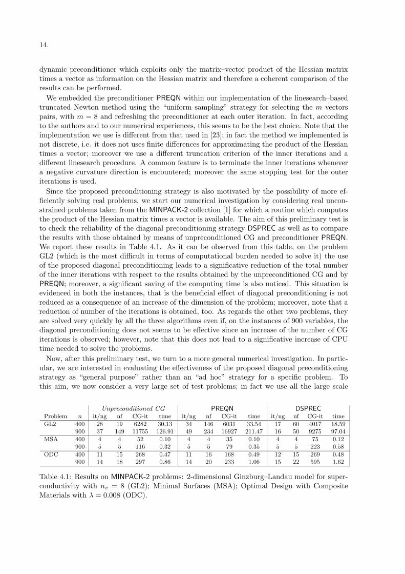
Since the proposed preconditioning strategy is also motivated by the possibility of more ef-ficiently solving real problems, we start our numerical investigation by considering real uncon-strained problems taken from the MINPACK-2 collection [1] for which a routine which computesthe product of the Hessian matrix times a vector is available. The aim of this preliminary test isto check the reliability of the diagonal preconditioning strategy DSPREC as well as to comparethe results with those obtained by means of unpreconditioned CG and preconditioner PREQN.We report these results in Table 4.1. As it can be observed from this table, on the problemGL2 (which is the most difficult in terms of computational burden needed to solve it) the useof the proposed diagonal preconditioning leads to a significative reduction of the total numberof the inner iterations with respect to the results obtained by the unpreconditioned CG and byPREQN; moreover, a significant saving of the computing time is also noticed. This situation isevidenced in both the instances, that is the beneficial effect of diagonal preconditioning is notreduced as a consequence of an increase of the dimension of the problem; moreover, note that areduction of number of the iterations is obtained, too. As regards the other two problems, theyare solved very quickly by all the three algorithms even if, on the instances of 900 variables, thediagonal preconditioning does not seems to be effective since an increase of the number of CGiterations is observed; however, note that this does not lead to a significative increase of CPUtime needed to solve the problems.

Now, after this preliminary test, we turn to a more general numerical investigation. In partic-ular, we are interested in evaluating the effectiveness of the proposed diagonal preconditioningstrategy as “general purpose” rather than an “ad hoc” strategy for a specific problem. Tothis aim, we now consider a very large set of test problems; in fact we use all the large scale

Unpreconditioned CG PREQN DSPREC

Problem n it/ng nf CG-it time it/ng nf CG-it time it/ng nf CG-it time

GL2 400 28 19 6282 30.13 34 146 6031 33.54 17 60 4017 18.59900 37 149 11755 126.91 49 234 16927 211.47 16 50 9275 97.04

MSA 400 4 4 52 0.10 4 4 35 0.10 4 4 75 0.12900 5 5 116 0.32 5 5 79 0.35 5 5 223 0.58

ODC 400 11 15 268 0.47 11 16 168 0.49 12 15 269 0.48900 14 18 297 0.86 14 20 233 1.06 15 22 595 1.62

Table 4.1: Results on MINPACK-2 problems: 2-dimensional Ginzburg–Landau model for super-conductivity with nv = 8 (GL2); Minimal Surfaces (MSA); Optimal Design with CompositeMaterials with λ = 0.008 (ODC).

15.

10 20 30 40 50 60 70 80 90

−20

0

20

40

60

80

100

120

140

160

10 20 30 40 50 60 70 80 90−1

0

1

2

3

4

5

6

7

8

9

10

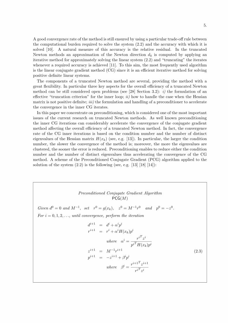
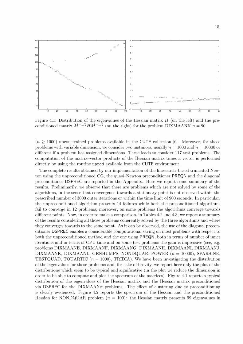
Figure 4.1: Distribution of the eigenvalues of the Hessian matrix H (on the left) and the pre-conditioned matrix M−1/2HM−1/2 (on the right) for the problem DIXMAANK n = 90

(n ≥ 1000) unconstrained problems available in the CUTE collection [6]. Moreover, for thoseproblems with variable dimension, we consider two instances, usually n = 1000 and n = 10000 ordifferent if a problem has assigned dimensions. These leads to consider 117 test problems. Thecomputation of the matrix–vector products of the Hessian matrix times a vector is performeddirectly by using the routine uprod available from the CUTE environment.

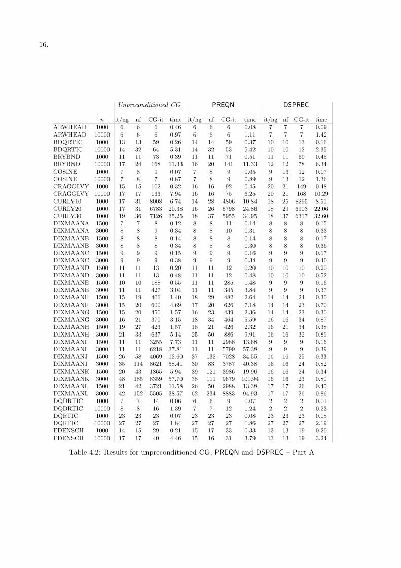
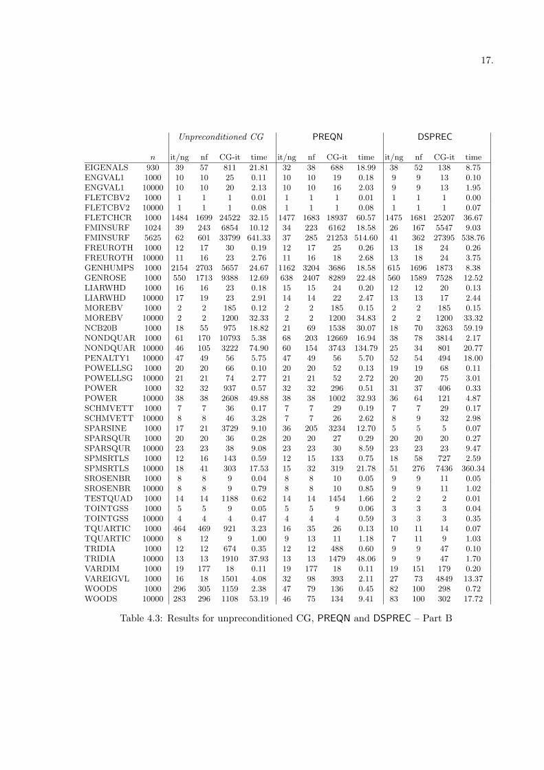
The complete results obtained by our implementation of the linesearch–based truncated New-ton using the unpreconditioned CG, the quasi–Newton preconditioner PREQN and the diagonalpreconditioner DSPREC are reported in the Appendix. Here we report some summary of theresults. Preliminarily, we observe that there are problems which are not solved by some of thealgorithms, in the sense that convergence towards a stationary point is not observed within theprescribed number of 3000 outer iterations or within the time limit of 900 seconds. In particular,the unpreconditioned algorithm presents 14 failures while both the preconditioned algorithmsfail to converge in 12 problems; moreover, on some problems the algorithms converge towardsdifferent points. Now, in order to make a comparison, in Tables 4.2 and 4.3, we report a summaryof the results considering all those problems coherently solved by the three algorithms and wherethey converges towards to the same point. As it can be observed, the use of the diagonal precon-ditioner DSPREC enables a considerable computational saving on most problems with respect toboth the unpreconditioned method and the one using PREQN, both in terms of number of inneriterations and in terms of CPU time and on some test problems the gain is impressive (see, e.g.problems DIXMAANE, DIXMAANF, DIXMAANG, DIXMAANH, DIXMAANI, DIXMAANJ,DIXMAANK, DIXMAANL, GENHUMPS, NONDQUAR, POWER (n = 10000), SPARSINE,TESTQUAD, TQUARTIC (n = 1000), TRIDIA). We have been investigating the distributionof the eigenvalues for these problems and, for sake of brevity, we report here only the plot of thedistributions which seem to be typical and significative (in the plot we reduce the dimension inorder to be able to compute and plot the spectrum of the matrices). Figure 4.1 reports a typicaldistribution of the eigenvalues of the Hessian matrix and the Hessian matrix preconditionedvia DSPREC for the DIXMAANα problems. The effect of clustering due to preconditioningis clearly evidenced. Figure 4.2 reports the spectrum of the Hessian and the preconditionedHessian for NONDQUAR problem (n = 100): the Hessian matrix presents 99 eigenvalues in

16.

Unpreconditioned CG PREQN DSPREC

n it/ng nf CG-it time it/ng nf CG-it time it/ng nf CG-it time

ARWHEAD 1000 6 6 6 0.46 6 6 6 0.08 7 7 7 0.09ARWHEAD 10000 6 6 6 0.97 6 6 6 1.11 7 7 7 1.42BDQRTIC 1000 13 13 59 0.26 14 14 59 0.37 10 10 13 0.16BDQRTIC 10000 14 32 64 5.31 14 32 53 5.42 10 10 12 2.35BRYBND 1000 11 11 73 0.39 11 11 71 0.51 11 11 69 0.45BRYBND 10000 17 24 168 11.33 16 20 141 11.33 12 12 78 6.34COSINE 1000 7 8 9 0.07 7 8 9 0.05 9 13 12 0.07COSINE 10000 7 8 7 0.87 7 8 9 0.89 9 13 12 1.36CRAGGLVY 1000 15 15 102 0.32 16 16 92 0.45 20 21 149 0.48CRAGGLVY 10000 17 17 133 7.94 16 16 75 6.25 20 21 168 10.29CURLY10 1000 17 31 8008 6.74 14 28 4806 10.84 18 25 8295 8.51CURLY20 1000 17 31 6783 20.38 16 26 5798 24.86 18 29 6903 22.06CURLY30 1000 19 36 7126 35.25 18 37 5955 34.95 18 37 6317 32.60DIXMAANA 1500 7 7 8 0.12 8 8 11 0.14 8 8 8 0.15DIXMAANA 3000 8 8 9 0.34 8 8 10 0.31 8 8 8 0.33DIXMAANB 1500 8 8 8 0.14 8 8 8 0.14 8 8 8 0.17DIXMAANB 3000 8 8 8 0.34 8 8 8 0.30 8 8 8 0.36DIXMAANC 1500 9 9 9 0.15 9 9 9 0.16 9 9 9 0.17DIXMAANC 3000 9 9 9 0.38 9 9 9 0.34 9 9 9 0.40DIXMAAND 1500 11 11 13 0.20 11 11 12 0.20 10 10 10 0.20DIXMAAND 3000 11 11 13 0.48 11 11 12 0.48 10 10 10 0.52DIXMAANE 1500 10 10 188 0.55 11 11 285 1.48 9 9 9 0.16DIXMAANE 3000 11 11 427 3.04 11 11 345 3.84 9 9 9 0.37DIXMAANF 1500 15 19 406 1.40 18 29 482 2.64 14 14 24 0.30DIXMAANF 3000 15 20 600 4.69 17 20 626 7.18 14 14 23 0.70DIXMAANG 1500 15 20 450 1.57 16 23 439 2.36 14 14 23 0.30DIXMAANG 3000 16 21 370 3.15 18 34 464 5.59 16 16 34 0.87DIXMAANH 1500 19 27 423 1.57 18 21 426 2.32 16 21 34 0.38DIXMAANH 3000 21 33 637 5.14 25 50 886 9.91 16 16 32 0.89DIXMAANI 1500 11 11 3255 7.73 11 11 2988 13.68 9 9 9 0.16DIXMAANI 3000 11 11 6218 37.81 11 11 5799 57.38 9 9 9 0.39DIXMAANJ 1500 26 58 4069 12.60 37 132 7028 34.55 16 16 25 0.33DIXMAANJ 3000 35 114 8621 58.41 30 83 3787 40.38 16 16 24 0.82DIXMAANK 1500 20 43 1865 5.94 39 121 3986 19.96 16 16 24 0.34DIXMAANK 3000 48 185 8359 57.70 38 111 9679 101.94 16 16 23 0.80DIXMAANL 1500 21 42 3721 11.58 26 50 2988 13.38 17 17 26 0.40DIXMAANL 3000 42 152 5505 38.57 62 234 8883 94.93 17 17 26 0.86DQDRTIC 1000 7 7 14 0.06 6 6 9 0.07 2 2 2 0.01DQDRTIC 10000 8 8 16 1.39 7 7 12 1.24 2 2 2 0.23DQRTIC 1000 23 23 23 0.07 23 23 23 0.08 23 23 23 0.08DQRTIC 10000 27 27 27 1.84 27 27 27 1.86 27 27 27 2.19EDENSCH 1000 14 15 29 0.21 15 17 33 0.33 13 13 19 0.20EDENSCH 10000 17 17 40 4.46 15 16 31 3.79 13 13 19 3.24

Table 4.2: Results for unpreconditioned CG, PREQN and DSPREC – Part A

17.

Unpreconditioned CG PREQN DSPREC

n it/ng nf CG-it time it/ng nf CG-it time it/ng nf CG-it time

EIGENALS 930 39 57 811 21.81 32 38 688 18.99 38 52 138 8.75ENGVAL1 1000 10 10 25 0.11 10 10 19 0.18 9 9 13 0.10ENGVAL1 10000 10 10 20 2.13 10 10 16 2.03 9 9 13 1.95FLETCBV2 1000 1 1 1 0.01 1 1 1 0.01 1 1 1 0.00FLETCBV2 10000 1 1 1 0.08 1 1 1 0.08 1 1 1 0.07FLETCHCR 1000 1484 1699 24522 32.15 1477 1683 18937 60.57 1475 1681 25207 36.67FMINSURF 1024 39 243 6854 10.12 34 223 6162 18.58 26 167 5547 9.03FMINSURF 5625 62 601 33799 641.33 37 285 21253 514.60 41 362 27395 538.76FREUROTH 1000 12 17 30 0.19 12 17 25 0.26 13 18 24 0.26FREUROTH 10000 11 16 23 2.76 11 16 18 2.68 13 18 24 3.75GENHUMPS 1000 2154 2703 5657 24.67 1162 3204 3686 18.58 615 1696 1873 8.38GENROSE 1000 550 1713 9388 12.69 638 2407 8289 22.48 560 1589 7528 12.52LIARWHD 1000 16 16 23 0.18 15 15 24 0.20 12 12 20 0.13LIARWHD 10000 17 19 23 2.91 14 14 22 2.47 13 13 17 2.44MOREBV 1000 2 2 185 0.12 2 2 185 0.15 2 2 185 0.15MOREBV 10000 2 2 1200 32.33 2 2 1200 34.83 2 2 1200 33.32NCB20B 1000 18 55 975 18.82 21 69 1538 30.07 18 70 3263 59.19NONDQUAR 1000 61 170 10793 5.38 68 203 12669 16.94 38 78 3814 2.17NONDQUAR 10000 46 105 3222 74.90 60 154 3743 134.79 25 34 801 20.77PENALTY1 10000 47 49 56 5.75 47 49 56 5.70 52 54 494 18.00POWELLSG 1000 20 20 66 0.10 20 20 52 0.13 19 19 68 0.11POWELLSG 10000 21 21 74 2.77 21 21 52 2.72 20 20 75 3.01POWER 1000 32 32 937 0.57 32 32 296 0.51 31 37 406 0.33POWER 10000 38 38 2608 49.88 38 38 1002 32.93 36 64 121 4.87SCHMVETT 1000 7 7 36 0.17 7 7 29 0.19 7 7 29 0.17SCHMVETT 10000 8 8 46 3.28 7 7 26 2.62 8 9 32 2.98SPARSINE 1000 17 21 3729 9.10 36 205 3234 12.70 5 5 5 0.07SPARSQUR 1000 20 20 36 0.28 20 20 27 0.29 20 20 20 0.27SPARSQUR 10000 23 23 38 9.08 23 23 30 8.59 23 23 23 9.47SPMSRTLS 1000 12 16 143 0.59 12 15 133 0.75 18 58 727 2.59SPMSRTLS 10000 18 41 303 17.53 15 32 319 21.78 51 276 7436 360.34SROSENBR 1000 8 8 9 0.04 8 8 10 0.05 9 9 11 0.05SROSENBR 10000 8 8 9 0.79 8 8 10 0.85 9 9 11 1.02TESTQUAD 1000 14 14 1188 0.62 14 14 1454 1.66 2 2 2 0.01TOINTGSS 1000 5 5 9 0.05 5 5 9 0.06 3 3 3 0.04TOINTGSS 10000 4 4 4 0.47 4 4 4 0.59 3 3 3 0.35TQUARTIC 1000 464 469 921 3.23 16 35 26 0.13 10 11 14 0.07TQUARTIC 10000 8 12 9 1.00 9 13 11 1.18 7 11 9 1.03TRIDIA 1000 12 12 674 0.35 12 12 488 0.60 9 9 47 0.10TRIDIA 10000 13 13 1910 37.93 13 13 1479 48.06 9 9 47 1.70VARDIM 1000 19 177 18 0.11 19 177 18 0.11 19 151 179 0.20VAREIGVL 1000 16 18 1501 4.08 32 98 393 2.11 27 73 4849 13.37WOODS 1000 296 305 1159 2.38 47 79 136 0.45 82 100 298 0.72WOODS 10000 283 296 1108 53.19 46 75 134 9.41 83 100 302 17.72

Table 4.3: Results for unpreconditioned CG, PREQN and DSPREC – Part B

18.

0 10 20 30 40 50 60 70 80 90 1000

200

400

600

800

1000

1200

1400

10 20 30 40 50 60 70 80 90 1000

1

2

3

4

5

6

7

8

9

10

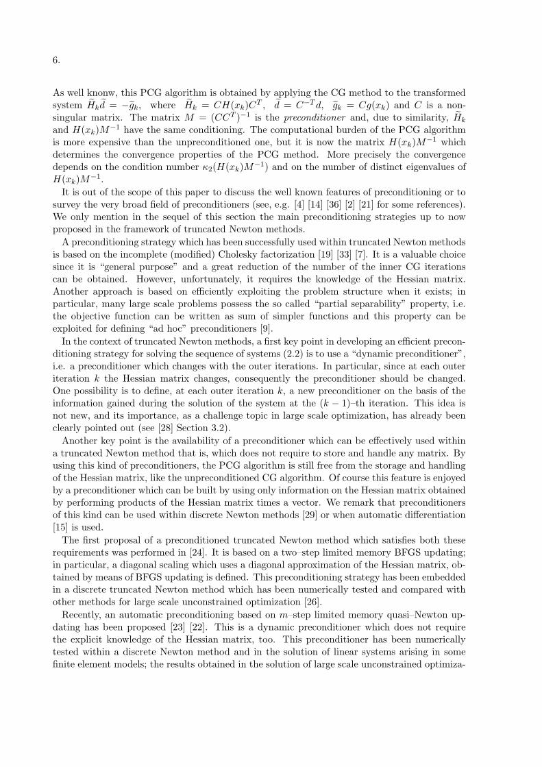
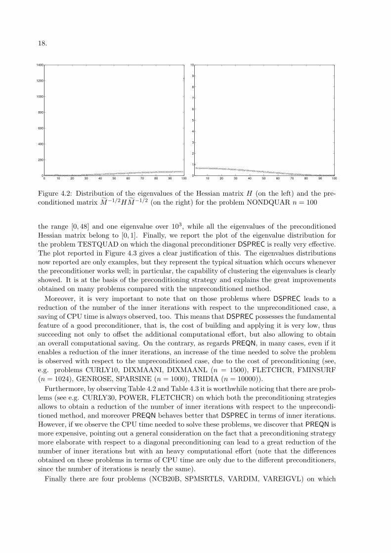
Figure 4.2: Distribution of the eigenvalues of the Hessian matrix H (on the left) and the pre-conditioned matrix M−1/2HM−1/2 (on the right) for the problem NONDQUAR n = 100

the range [0, 48] and one eigenvalue over 103, while all the eigenvalues of the preconditionedHessian matrix belong to [0, 1]. Finally, we report the plot of the eigenvalue distribution forthe problem TESTQUAD on which the diagonal preconditioner DSPREC is really very effective.The plot reported in Figure 4.3 gives a clear justification of this. The eigenvalues distributionsnow reported are only examples, but they represent the typical situation which occurs wheneverthe preconditioner works well; in particular, the capability of clustering the eigenvalues is clearlyshowed. It is at the basis of the preconditioning strategy and explains the great improvementsobtained on many problems compared with the unpreconditioned method.

Moreover, it is very important to note that on those problems where DSPREC leads to areduction of the number of the inner iterations with respect to the unpreconditioned case, asaving of CPU time is always observed, too. This means that DSPREC possesses the fundamentalfeature of a good preconditioner, that is, the cost of building and applying it is very low, thussucceeding not only to offset the additional computational effort, but also allowing to obtainan overall computational saving. On the contrary, as regards PREQN, in many cases, even if itenables a reduction of the inner iterations, an increase of the time needed to solve the problemis observed with respect to the unpreconditioned case, due to the cost of preconditioning (see,e.g. problems CURLY10, DIXMAANI, DIXMAANL (n = 1500), FLETCHCR, FMINSURF(n = 1024), GENROSE, SPARSINE (n = 1000), TRIDIA (n = 10000)).

Furthermore, by observing Table 4.2 and Table 4.3 it is worthwhile noticing that there are prob-lems (see e.g. CURLY30, POWER, FLETCHCR) on which both the preconditioning strategiesallows to obtain a reduction of the number of inner iterations with respect to the unprecondi-tioned method, and moreover PREQN behaves better that DSPREC in terms of inner iterations.However, if we observe the CPU time needed to solve these problems, we discover that PREQN ismore expensive, pointing out a general consideration on the fact that a preconditioning strategymore elaborate with respect to a diagonal preconditioning can lead to a great reduction of thenumber of inner iterations but with an heavy computational effort (note that the differencesobtained on these problems in terms of CPU time are only due to the different preconditioners,since the number of iterations is nearly the same).

Finally there are four problems (NCB20B, SPMSRTLS, VARDIM, VAREIGVL) on which

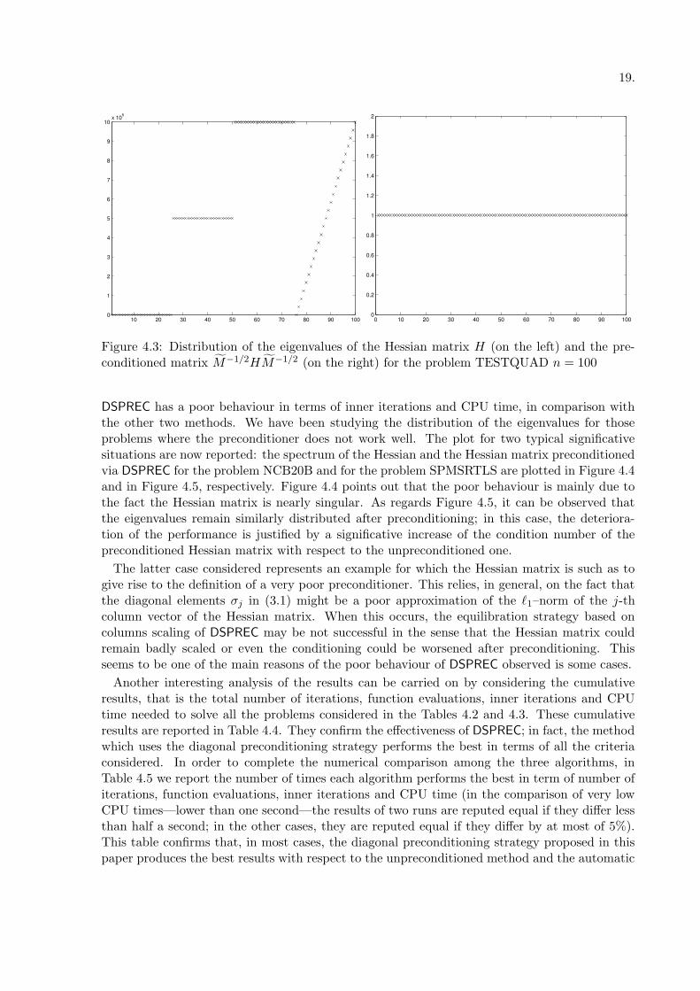
19.

10 20 30 40 50 60 70 80 90 1000

1

2

3

4

5

6

7

8

9

10x 105

0 10 20 30 40 50 60 70 80 90 1000

0.2

0.4

0.6

0.8

1

1.2

1.4

1.6

1.8

2

Figure 4.3: Distribution of the eigenvalues of the Hessian matrix H (on the left) and the pre-conditioned matrix M−1/2HM−1/2 (on the right) for the problem TESTQUAD n = 100

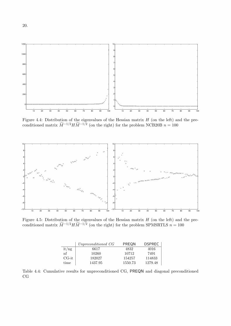
DSPREC has a poor behaviour in terms of inner iterations and CPU time, in comparison withthe other two methods. We have been studying the distribution of the eigenvalues for thoseproblems where the preconditioner does not work well. The plot for two typical significativesituations are now reported: the spectrum of the Hessian and the Hessian matrix preconditionedvia DSPREC for the problem NCB20B and for the problem SPMSRTLS are plotted in Figure 4.4and in Figure 4.5, respectively. Figure 4.4 points out that the poor behaviour is mainly due tothe fact the Hessian matrix is nearly singular. As regards Figure 4.5, it can be observed thatthe eigenvalues remain similarly distributed after preconditioning; in this case, the deteriora-tion of the performance is justified by a significative increase of the condition number of thepreconditioned Hessian matrix with respect to the unpreconditioned one.

The latter case considered represents an example for which the Hessian matrix is such as togive rise to the definition of a very poor preconditioner. This relies, in general, on the fact thatthe diagonal elements σj in (3.1) might be a poor approximation of the `1–norm of the j-thcolumn vector of the Hessian matrix. When this occurs, the equilibration strategy based oncolumns scaling of DSPREC may be not successful in the sense that the Hessian matrix couldremain badly scaled or even the conditioning could be worsened after preconditioning. Thisseems to be one of the main reasons of the poor behaviour of DSPREC observed is some cases.

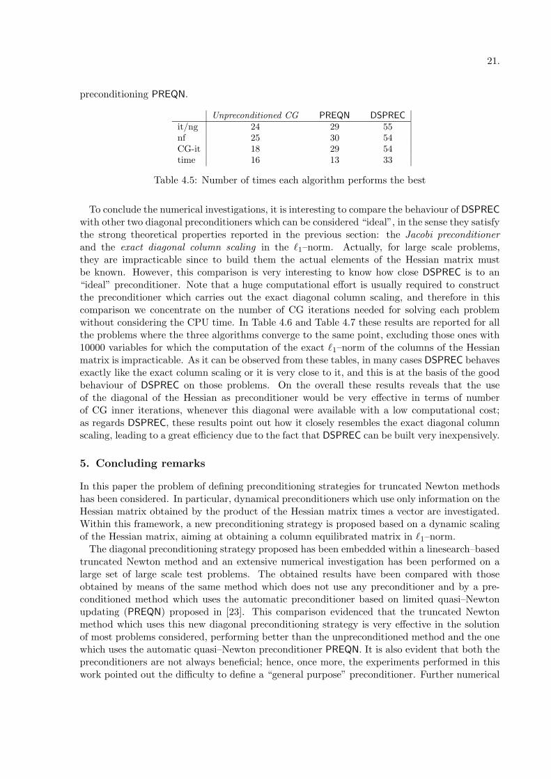
Another interesting analysis of the results can be carried on by considering the cumulativeresults, that is the total number of iterations, function evaluations, inner iterations and CPUtime needed to solve all the problems considered in the Tables 4.2 and 4.3. These cumulativeresults are reported in Table 4.4. They confirm the effectiveness of DSPREC; in fact, the methodwhich uses the diagonal preconditioning strategy performs the best in terms of all the criteriaconsidered. In order to complete the numerical comparison among the three algorithms, inTable 4.5 we report the number of times each algorithm performs the best in term of number ofiterations, function evaluations, inner iterations and CPU time (in the comparison of very lowCPU times—lower than one second—the results of two runs are reputed equal if they differ lessthan half a second; in the other cases, they are reputed equal if they differ by at most of 5%).This table confirms that, in most cases, the diagonal preconditioning strategy proposed in thispaper produces the best results with respect to the unpreconditioned method and the automatic

20.

10 20 30 40 50 60 70 80 90 100

0

200

400

600

800

1000

1200

10 20 30 40 50 60 70 80 90 100

0

1

2

3

4

5

6

7

8

9

10

Figure 4.4: Distribution of the eigenvalues of the Hessian matrix H (on the left) and the pre-conditioned matrix M−1/2HM−1/2 (on the right) for the problem NCB20B n = 100

10 20 30 40 50 60 70 80 90 100−10

−8

−6

−4

−2

0

2

4

6

8

10

10 20 30 40 50 60 70 80 90 100−10

−8

−6

−4

−2

0

2

4

6

8

10

Figure 4.5: Distribution of the eigenvalues of the Hessian matrix H (on the left) and the pre-conditioned matrix M−1/2HM−1/2 (on the right) for the problem SPMSRTLS n = 100

Unpreconditioned CG PREQN DSPREC

it/ng 6617 4832 4016nf 10260 10712 7491CG-it 182027 154257 114833time 1437.95 1550.73 1279.48

Table 4.4: Cumulative results for unpreconditioned CG, PREQN and diagonal preconditionedCG

21.

preconditioning PREQN.

Unpreconditioned CG PREQN DSPREC

it/ng 24 29 55nf 25 30 54CG-it 18 29 54time 16 13 33

Table 4.5: Number of times each algorithm performs the best

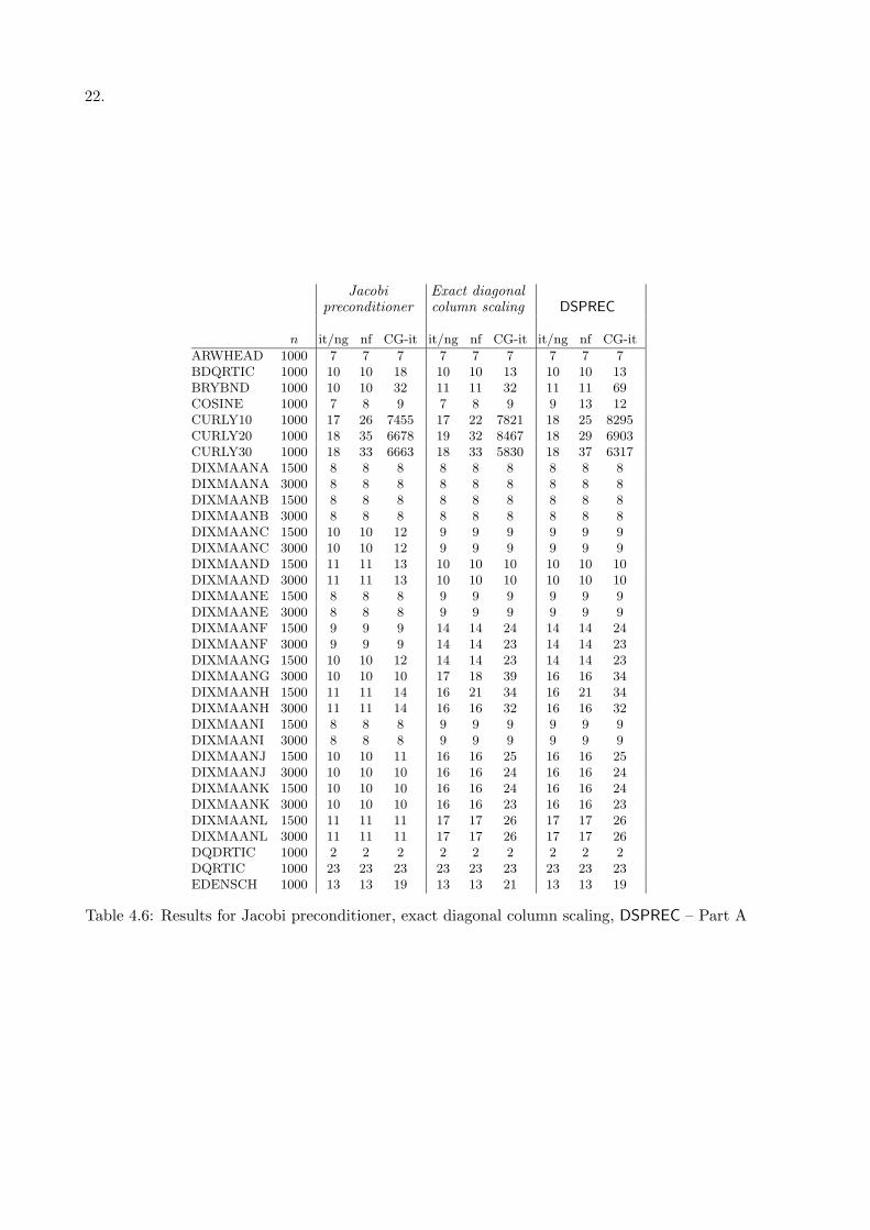
To conclude the numerical investigations, it is interesting to compare the behaviour of DSPREC

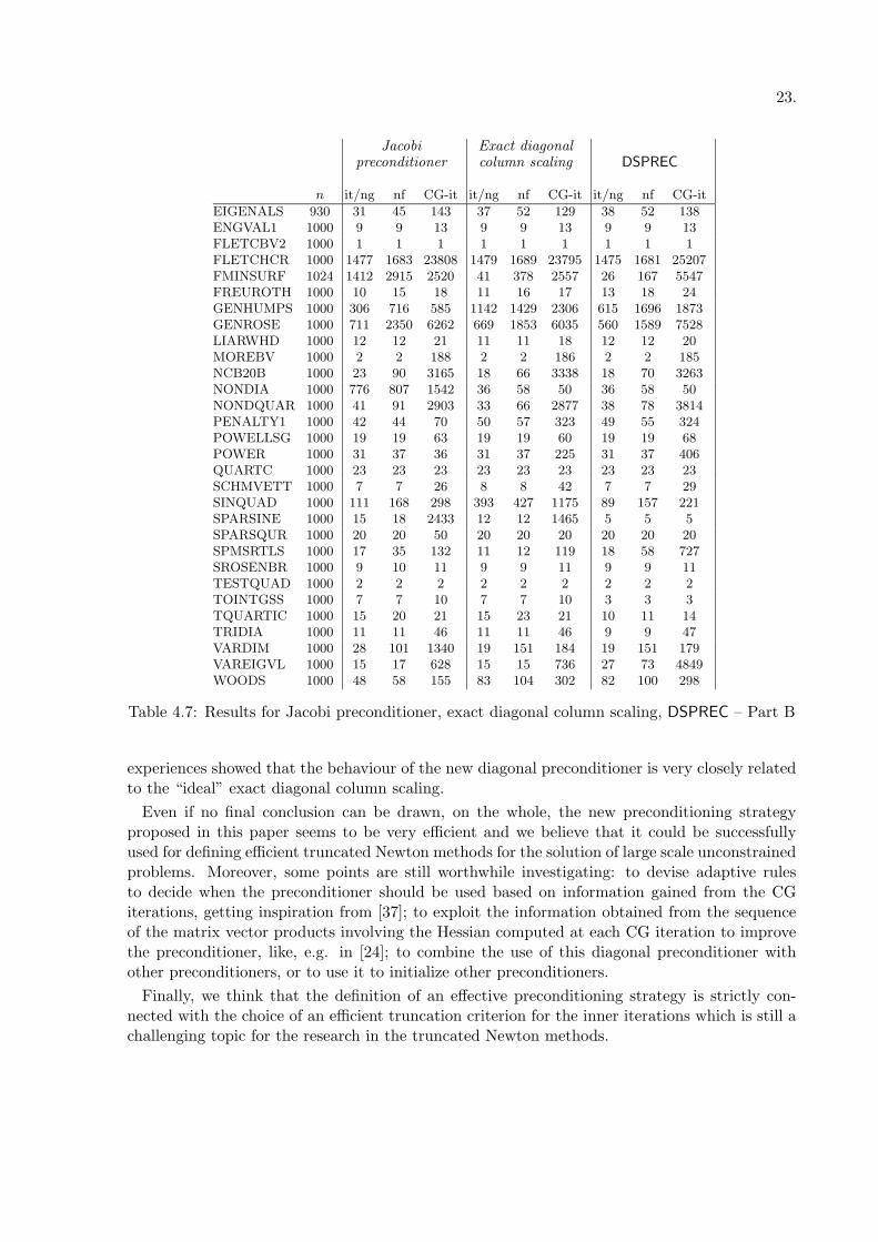
with other two diagonal preconditioners which can be considered “ideal”, in the sense they satisfythe strong theoretical properties reported in the previous section: the Jacobi preconditionerand the exact diagonal column scaling in the `1–norm. Actually, for large scale problems,they are impracticable since to build them the actual elements of the Hessian matrix mustbe known. However, this comparison is very interesting to know how close DSPREC is to an“ideal” preconditioner. Note that a huge computational effort is usually required to constructthe preconditioner which carries out the exact diagonal column scaling, and therefore in thiscomparison we concentrate on the number of CG iterations needed for solving each problemwithout considering the CPU time. In Table 4.6 and Table 4.7 these results are reported for allthe problems where the three algorithms converge to the same point, excluding those ones with10000 variables for which the computation of the exact `1–norm of the columns of the Hessianmatrix is impracticable. As it can be observed from these tables, in many cases DSPREC behavesexactly like the exact column scaling or it is very close to it, and this is at the basis of the goodbehaviour of DSPREC on those problems. On the overall these results reveals that the useof the diagonal of the Hessian as preconditioner would be very effective in terms of numberof CG inner iterations, whenever this diagonal were available with a low computational cost;as regards DSPREC, these results point out how it closely resembles the exact diagonal columnscaling, leading to a great efficiency due to the fact that DSPREC can be built very inexpensively.

5. Concluding remarks

In this paper the problem of defining preconditioning strategies for truncated Newton methodshas been considered. In particular, dynamical preconditioners which use only information on theHessian matrix obtained by the product of the Hessian matrix times a vector are investigated.Within this framework, a new preconditioning strategy is proposed based on a dynamic scalingof the Hessian matrix, aiming at obtaining a column equilibrated matrix in `1–norm.

The diagonal preconditioning strategy proposed has been embedded within a linesearch–basedtruncated Newton method and an extensive numerical investigation has been performed on alarge set of large scale test problems. The obtained results have been compared with thoseobtained by means of the same method which does not use any preconditioner and by a pre-conditioned method which uses the automatic preconditioner based on limited quasi–Newtonupdating (PREQN) proposed in [23]. This comparison evidenced that the truncated Newtonmethod which uses this new diagonal preconditioning strategy is very effective in the solutionof most problems considered, performing better than the unpreconditioned method and the onewhich uses the automatic quasi–Newton preconditioner PREQN. It is also evident that both thepreconditioners are not always beneficial; hence, once more, the experiments performed in thiswork pointed out the difficulty to define a “general purpose” preconditioner. Further numerical

22.

Jacobi Exact diagonalpreconditioner column scaling DSPREC

n it/ng nf CG-it it/ng nf CG-it it/ng nf CG-it

ARWHEAD 1000 7 7 7 7 7 7 7 7 7BDQRTIC 1000 10 10 18 10 10 13 10 10 13BRYBND 1000 10 10 32 11 11 32 11 11 69COSINE 1000 7 8 9 7 8 9 9 13 12CURLY10 1000 17 26 7455 17 22 7821 18 25 8295CURLY20 1000 18 35 6678 19 32 8467 18 29 6903CURLY30 1000 18 33 6663 18 33 5830 18 37 6317DIXMAANA 1500 8 8 8 8 8 8 8 8 8DIXMAANA 3000 8 8 8 8 8 8 8 8 8DIXMAANB 1500 8 8 8 8 8 8 8 8 8DIXMAANB 3000 8 8 8 8 8 8 8 8 8DIXMAANC 1500 10 10 12 9 9 9 9 9 9DIXMAANC 3000 10 10 12 9 9 9 9 9 9DIXMAAND 1500 11 11 13 10 10 10 10 10 10DIXMAAND 3000 11 11 13 10 10 10 10 10 10DIXMAANE 1500 8 8 8 9 9 9 9 9 9DIXMAANE 3000 8 8 8 9 9 9 9 9 9DIXMAANF 1500 9 9 9 14 14 24 14 14 24DIXMAANF 3000 9 9 9 14 14 23 14 14 23DIXMAANG 1500 10 10 12 14 14 23 14 14 23DIXMAANG 3000 10 10 10 17 18 39 16 16 34DIXMAANH 1500 11 11 14 16 21 34 16 21 34DIXMAANH 3000 11 11 14 16 16 32 16 16 32DIXMAANI 1500 8 8 8 9 9 9 9 9 9DIXMAANI 3000 8 8 8 9 9 9 9 9 9DIXMAANJ 1500 10 10 11 16 16 25 16 16 25DIXMAANJ 3000 10 10 10 16 16 24 16 16 24DIXMAANK 1500 10 10 10 16 16 24 16 16 24DIXMAANK 3000 10 10 10 16 16 23 16 16 23DIXMAANL 1500 11 11 11 17 17 26 17 17 26DIXMAANL 3000 11 11 11 17 17 26 17 17 26DQDRTIC 1000 2 2 2 2 2 2 2 2 2DQRTIC 1000 23 23 23 23 23 23 23 23 23EDENSCH 1000 13 13 19 13 13 21 13 13 19

Table 4.6: Results for Jacobi preconditioner, exact diagonal column scaling, DSPREC – Part A

23.

Jacobi Exact diagonalpreconditioner column scaling DSPREC

n it/ng nf CG-it it/ng nf CG-it it/ng nf CG-it

EIGENALS 930 31 45 143 37 52 129 38 52 138ENGVAL1 1000 9 9 13 9 9 13 9 9 13FLETCBV2 1000 1 1 1 1 1 1 1 1 1FLETCHCR 1000 1477 1683 23808 1479 1689 23795 1475 1681 25207FMINSURF 1024 1412 2915 2520 41 378 2557 26 167 5547FREUROTH 1000 10 15 18 11 16 17 13 18 24GENHUMPS 1000 306 716 585 1142 1429 2306 615 1696 1873GENROSE 1000 711 2350 6262 669 1853 6035 560 1589 7528LIARWHD 1000 12 12 21 11 11 18 12 12 20MOREBV 1000 2 2 188 2 2 186 2 2 185NCB20B 1000 23 90 3165 18 66 3338 18 70 3263NONDIA 1000 776 807 1542 36 58 50 36 58 50NONDQUAR 1000 41 91 2903 33 66 2877 38 78 3814PENALTY1 1000 42 44 70 50 57 323 49 55 324POWELLSG 1000 19 19 63 19 19 60 19 19 68POWER 1000 31 37 36 31 37 225 31 37 406QUARTC 1000 23 23 23 23 23 23 23 23 23SCHMVETT 1000 7 7 26 8 8 42 7 7 29SINQUAD 1000 111 168 298 393 427 1175 89 157 221SPARSINE 1000 15 18 2433 12 12 1465 5 5 5SPARSQUR 1000 20 20 50 20 20 20 20 20 20SPMSRTLS 1000 17 35 132 11 12 119 18 58 727SROSENBR 1000 9 10 11 9 9 11 9 9 11TESTQUAD 1000 2 2 2 2 2 2 2 2 2TOINTGSS 1000 7 7 10 7 7 10 3 3 3TQUARTIC 1000 15 20 21 15 23 21 10 11 14TRIDIA 1000 11 11 46 11 11 46 9 9 47VARDIM 1000 28 101 1340 19 151 184 19 151 179VAREIGVL 1000 15 17 628 15 15 736 27 73 4849WOODS 1000 48 58 155 83 104 302 82 100 298

Table 4.7: Results for Jacobi preconditioner, exact diagonal column scaling, DSPREC – Part B

experiences showed that the behaviour of the new diagonal preconditioner is very closely relatedto the “ideal” exact diagonal column scaling.

Even if no final conclusion can be drawn, on the whole, the new preconditioning strategyproposed in this paper seems to be very efficient and we believe that it could be successfullyused for defining efficient truncated Newton methods for the solution of large scale unconstrainedproblems. Moreover, some points are still worthwhile investigating: to devise adaptive rulesto decide when the preconditioner should be used based on information gained from the CGiterations, getting inspiration from [37]; to exploit the information obtained from the sequenceof the matrix vector products involving the Hessian computed at each CG iteration to improvethe preconditioner, like, e.g. in [24]; to combine the use of this diagonal preconditioner withother preconditioners, or to use it to initialize other preconditioners.

Finally, we think that the definition of an effective preconditioning strategy is strictly con-nected with the choice of an efficient truncation criterion for the inner iterations which is still achallenging topic for the research in the truncated Newton methods.

24.

Appendix

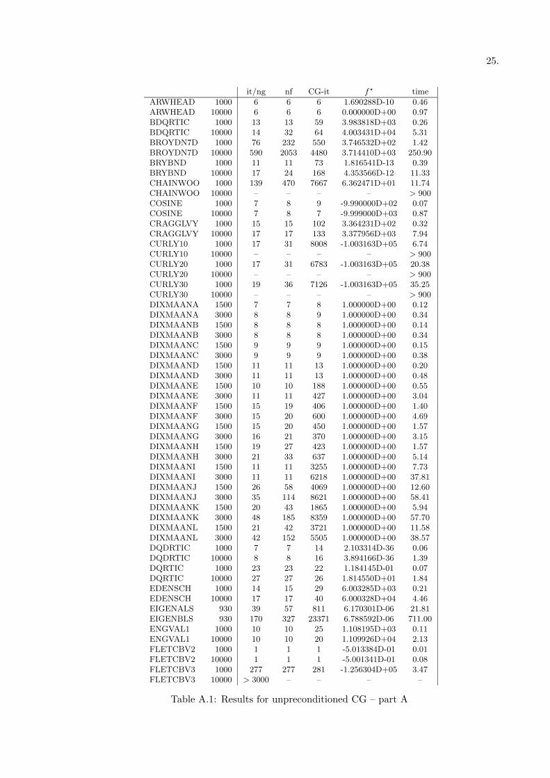
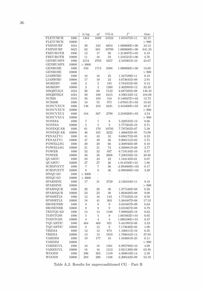
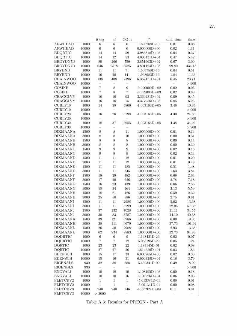
In this Appendix we report the complete numerical results obtained by the linesearch basedtruncated Newton method which uses

• the unpreconditioned CG (Tables A.1 and A.2),

• the preconditioner PREQN [23] (Tables A.3 and A.4)

• the diagonal preconditioning strategy proposed in this paper (Tables A.5 and A.6).

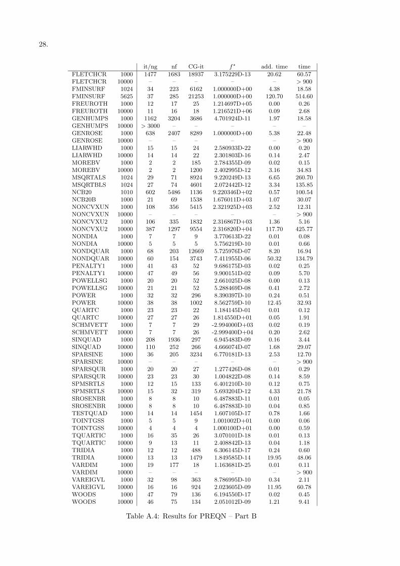
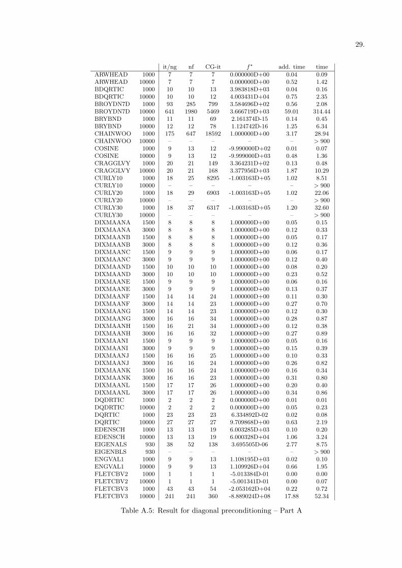
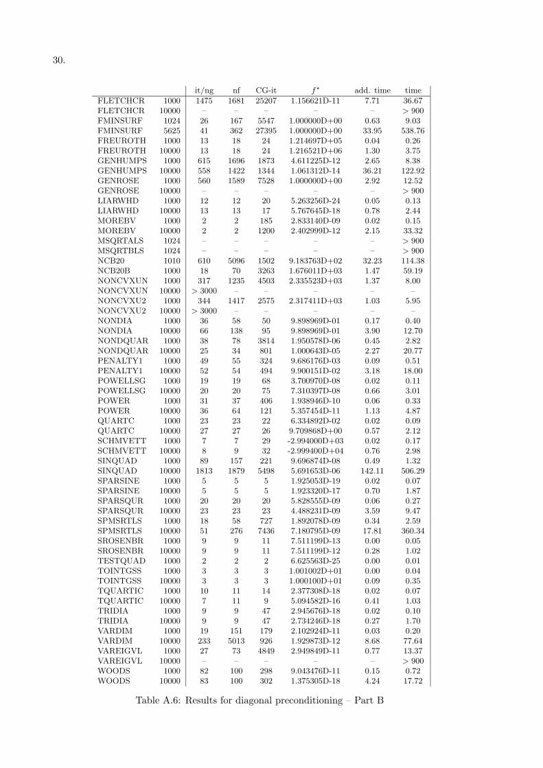
All the results are reported in terms of number of outer iterations (it) —which is the same asthe number of gradient evaluation (ng)— number of function evaluations (nf), total number ofinner iterations (CG-it) and CPU time (time); moreover the optimal function value obtained isreported (f?). Finally, for the methods which uses a preconditioner, the additional time dueto preconditioning, i.e. the total time needed to computed the preconditioned residual at eachinner iteration is reported.

25.

it/ng nf CG-it f? time

ARWHEAD 1000 6 6 6 1.690288D-10 0.46ARWHEAD 10000 6 6 6 0.000000D+00 0.97BDQRTIC 1000 13 13 59 3.983818D+03 0.26BDQRTIC 10000 14 32 64 4.003431D+04 5.31BROYDN7D 1000 76 232 550 3.746532D+02 1.42BROYDN7D 10000 590 2053 4480 3.714410D+03 250.90BRYBND 1000 11 11 73 1.816541D-13 0.39BRYBND 10000 17 24 168 4.353566D-12 11.33CHAINWOO 1000 139 470 7667 6.362471D+01 11.74CHAINWOO 10000 – – – – > 900COSINE 1000 7 8 9 -9.990000D+02 0.07COSINE 10000 7 8 7 -9.999000D+03 0.87CRAGGLVY 1000 15 15 102 3.364231D+02 0.32CRAGGLVY 10000 17 17 133 3.377956D+03 7.94CURLY10 1000 17 31 8008 -1.003163D+05 6.74CURLY10 10000 – – – – > 900CURLY20 1000 17 31 6783 -1.003163D+05 20.38CURLY20 10000 – – – – > 900CURLY30 1000 19 36 7126 -1.003163D+05 35.25CURLY30 10000 – – – – > 900DIXMAANA 1500 7 7 8 1.000000D+00 0.12DIXMAANA 3000 8 8 9 1.000000D+00 0.34DIXMAANB 1500 8 8 8 1.000000D+00 0.14DIXMAANB 3000 8 8 8 1.000000D+00 0.34DIXMAANC 1500 9 9 9 1.000000D+00 0.15DIXMAANC 3000 9 9 9 1.000000D+00 0.38DIXMAAND 1500 11 11 13 1.000000D+00 0.20DIXMAAND 3000 11 11 13 1.000000D+00 0.48DIXMAANE 1500 10 10 188 1.000000D+00 0.55DIXMAANE 3000 11 11 427 1.000000D+00 3.04DIXMAANF 1500 15 19 406 1.000000D+00 1.40DIXMAANF 3000 15 20 600 1.000000D+00 4.69DIXMAANG 1500 15 20 450 1.000000D+00 1.57DIXMAANG 3000 16 21 370 1.000000D+00 3.15DIXMAANH 1500 19 27 423 1.000000D+00 1.57DIXMAANH 3000 21 33 637 1.000000D+00 5.14DIXMAANI 1500 11 11 3255 1.000000D+00 7.73DIXMAANI 3000 11 11 6218 1.000000D+00 37.81DIXMAANJ 1500 26 58 4069 1.000000D+00 12.60DIXMAANJ 3000 35 114 8621 1.000000D+00 58.41DIXMAANK 1500 20 43 1865 1.000000D+00 5.94DIXMAANK 3000 48 185 8359 1.000000D+00 57.70DIXMAANL 1500 21 42 3721 1.000000D+00 11.58DIXMAANL 3000 42 152 5505 1.000000D+00 38.57DQDRTIC 1000 7 7 14 2.103314D-36 0.06DQDRTIC 10000 8 8 16 3.894166D-36 1.39DQRTIC 1000 23 23 22 1.184145D-01 0.07DQRTIC 10000 27 27 26 1.814550D+01 1.84EDENSCH 1000 14 15 29 6.003285D+03 0.21EDENSCH 10000 17 17 40 6.000328D+04 4.46EIGENALS 930 39 57 811 6.170301D-06 21.81EIGENBLS 930 170 327 23371 6.788592D-06 711.00ENGVAL1 1000 10 10 25 1.108195D+03 0.11ENGVAL1 10000 10 10 20 1.109926D+04 2.13FLETCBV2 1000 1 1 1 -5.013384D-01 0.01FLETCBV2 10000 1 1 1 -5.001341D-01 0.08FLETCBV3 1000 277 277 281 -1.256304D+05 3.47FLETCBV3 10000 > 3000 – – – –

Table A.1: Results for unpreconditioned CG – part A

26.

it/ng nf CG-it f? time

FLETCHCR 1000 1484 1699 24522 1.855475D-11 32.15FLETCHCR 10000 – – – – > 900FMINSURF 1024 39 243 6854 1.000000D+00 10.12FMINSURF 5625 62 601 33799 1.000000D+00 641.33FREUROTH 1000 12 17 30 1.214697D+05 0.19FREUROTH 10000 11 16 23 1.216521D+06 2.76GENHUMPS 1000 2154 2703 5657 2.165901D-10 24.67GENHUMPS 10000 > 3000 – – – –GENROSE 1000 550 1713 9388 1.000000D+00 12.69GENROSE 10000 – – – – > 900LIARWHD 1000 16 16 23 1.347339D-11 0.18LIARWHD 10000 17 19 23 3.673645D-09 2.91MOREBV 1000 2 2 185 2.784355D-09 0.12MOREBV 10000 2 2 1200 2.402995D-12 32.33MSQRTALS 1024 26 69 5122 6.687495D-08 148.33MSQRTBLS 1024 30 100 6415 4.590134D-12 184.08NCB20 1010 56 103 510 9.146927D+02 13.73NCB20B 1000 18 55 975 1.676011D+03 18.82NONCVXUN 1000 148 410 8231 2.341600D+03 10.47NONCVXUN 10000 – – – – > 900NONCVXU2 1000 184 567 2799 2.316926D+03 4.54NONCVXU2 10000 – – – – > 900NONDIA 1000 7 7 8 5.328525D-12 0.06NONDIA 10000 5 5 5 5.777204D-10 0.71NONDQUAR 1000 61 170 10793 7.797202D-07 5.38NONDQUAR 10000 46 105 3222 1.406633D-05 74.90PENALTY1 1000 41 43 52 9.686175D-03 0.23PENALTY1 10000 47 49 56 9.900151D-02 5.75POWELLSG 1000 20 20 66 2.308946D-08 0.10POWELLSG 10000 21 21 74 4.560881D-08 2.77POWER 1000 32 32 937 6.719134D-10 0.57POWER 10000 38 38 2608 7.236558D-10 49.88QUARTC 1000 23 23 22 1.184145D-01 0.07QUARTC 10000 27 27 26 1.814550D+01 1.86SCHMVETT 1000 7 7 36 -2.994000D+03 0.17SCHMVETT 10000 8 8 46 -2.999400D+04 3.28SINQUAD 1000 > 3000 – – – –SINQUAD 10000 > 3000 – – – –SPARSINE 1000 17 21 3729 2.120104D-11 9.10SPARSINE 10000 – – – – > 900SPARSQUR 1000 20 20 36 1.277448D-08 0.28SPARSQUR 10000 23 23 38 1.004828D-08 9.08SPMSRTLS 1000 12 16 143 1.775335D-10 0.59SPMSRTLS 10000 18 41 303 5.384487D-08 17.53SROSENBR 1000 8 8 9 3.831667D-09 0.04SROSENBR 10000 8 8 9 3.831667D-08 0.79TESTQUAD 1000 14 14 1188 7.998922D-18 0.62TOINTGSS 1000 5 5 9 1.001002D+01 0.05TOINTGSS 10000 4 4 4 1.000100D+01 0.47TQUARTIC 1000 464 469 921 5.441991D-08 3.23TQUARTIC 10000 8 12 9 7.172640D-05 1.00TRIDIA 1000 12 12 674 1.166811D-16 0.35TRIDIA 10000 13 13 1910 1.780044D-14 37.93VARDIM 1000 19 177 18 1.163681D-25 0.11VARDIM 10000 – – – – > 900VAREIGVL 1000 16 18 1501 6.995798D-10 4.08VAREIGVL 10000 16 16 1212 2.921130D-09 63.30WOODS 1000 296 305 1159 4.389618D-14 2.38WOODS 10000 283 296 1108 6.200442D-09 53.19

Table A.2: Results for unpreconditioned CG – Part B

27.

it/ng nf CG-it f? add. time time

ARWHEAD 1000 6 6 6 1.690288D-10 0.01 0.08ARWHEAD 10000 6 6 6 0.000000D+00 0.02 1.11BDQRTIC 1000 14 14 59 3.983818D+03 0.04 0.37BDQRTIC 10000 14 32 53 4.003431D+04 0.47 5.42BROYDN7D 1000 80 266 750 3.851963D+02 0.67 3.00BROYDN7D 10000 646 2518 6525 3.801124D+03 99.80 434.13BRYBND 1000 11 11 71 1.505758D-16 0.04 0.51BRYBND 10000 16 20 141 1.968983D-16 1.84 11.33CHAINWOO 1000 138 408 7396 6.362471D+01 6.45 23.71CHAINWOO 10000 – – – – – > 900COSINE 1000 7 8 9 -9.990000D+02 0.02 0.05COSINE 10000 7 8 7 -9.999000D+03 0.02 0.89CRAGGLVY 1000 16 16 92 3.364231D+02 0.09 0.45CRAGGLVY 10000 16 16 75 3.377956D+03 0.85 6.25CURLY10 1000 14 28 4806 -1.003163D+05 3.48 10.84CURLY10 10000 – – – – – > 900CURLY20 1000 16 26 5798 -1.003163D+05 4.30 24.86CURLY20 10000 – – – – – > 900CURLY30 1000 18 37 5955 -1.003163D+05 4.38 34.95CURLY30 10000 – – – – – > 900DIXMAANA 1500 8 8 11 1.000000D+00 0.01 0.14DIXMAANA 3000 8 8 10 1.000000D+00 0.00 0.31DIXMAANB 1500 8 8 8 1.000000D+00 0.00 0.14DIXMAANB 3000 8 8 8 1.000000D+00 0.00 0.30DIXMAANC 1500 9 9 9 1.000000D+00 0.02 0.16DIXMAANC 3000 9 9 9 1.000000D+00 0.02 0.34DIXMAAND 1500 11 11 12 1.000000D+00 0.01 0.20DIXMAAND 3000 11 11 12 1.000000D+00 0.01 0.48DIXMAANE 1500 11 11 285 1.000000D+00 0.51 1.48DIXMAANE 3000 11 11 345 1.000000D+00 1.63 3.84DIXMAANF 1500 18 29 482 1.000000D+00 0.66 2.64DIXMAANF 3000 17 20 626 1.000000D+00 2.78 7.18DIXMAANG 1500 16 23 439 1.000000D+00 0.66 2.36DIXMAANG 3000 18 34 464 1.000000D+00 2.13 5.59DIXMAANH 1500 18 21 426 1.000000D+00 0.59 2.32DIXMAANH 3000 25 50 886 1.000000D+00 2.75 9.91DIXMAANI 1500 11 11 2988 1.000000D+00 5.02 13.68DIXMAANI 3000 11 11 5799 1.000000D+00 22.05 57.38DIXMAANJ 1500 37 132 7028 1.000000D+00 11.11 34.55DIXMAANJ 3000 30 83 3787 1.000000D+00 14.10 40.38DIXMAANK 1500 39 121 3986 1.000000D+00 6.00 19.96DIXMAANK 3000 38 111 9679 1.000000D+00 37.73 101.94DIXMAANL 1500 26 50 2988 1.000000D+00 2.93 13.38DIXMAANL 3000 62 234 8883 1.000000D+00 32.73 94.93DQDRTIC 1000 6 6 9 1.148421D-26 0.02 0.07DQDRTIC 10000 7 7 12 5.053195D-29 0.05 1.24DQRTIC 1000 23 23 22 1.184145D-01 0.02 0.08DQRTIC 10000 27 27 26 1.814550D+01 0.03 1.86EDENSCH 1000 15 17 33 6.003285D+03 0.02 0.33EDENSCH 10000 15 16 31 6.000328D+04 0.16 3.79EIGENALS 930 32 38 688 5.439341D-09 0.39 18.99EIGENBLS 930 – – – – – > 900ENGVAL1 1000 10 10 19 1.108195D+03 0.00 0.18ENGVAL1 10000 10 10 16 1.109926D+04 0.06 2.03FLETCBV2 1000 1 1 1 -5.013384D-01 0.00 0.01FLETCBV2 10000 1 1 1 -5.001341D-01 0.00 0.08FLETCBV3 1000 240 240 246 -4.997924D+04 0.11 3.01FLETCBV3 10000 > 3000 – – – – –

Table A.3: Results for PREQN - Part A

28.

it/ng nf CG-it f? add. time time

FLETCHCR 1000 1477 1683 18937 3.175229D-13 20.62 60.57FLETCHCR 10000 – – – – – > 900FMINSURF 1024 34 223 6162 1.000000D+00 4.38 18.58FMINSURF 5625 37 285 21253 1.000000D+00 120.70 514.60FREUROTH 1000 12 17 25 1.214697D+05 0.00 0.26FREUROTH 10000 11 16 18 1.216521D+06 0.09 2.68GENHUMPS 1000 1162 3204 3686 4.701924D-11 1.97 18.58GENHUMPS 10000 > 3000 – – – – –GENROSE 1000 638 2407 8289 1.000000D+00 5.38 22.48GENROSE 10000 – – – – – > 900LIARWHD 1000 15 15 24 2.580933D-22 0.00 0.20LIARWHD 10000 14 14 22 2.301803D-16 0.14 2.47MOREBV 1000 2 2 185 2.784355D-09 0.02 0.15MOREBV 10000 2 2 1200 2.402995D-12 3.16 34.83MSQRTALS 1024 29 71 8924 9.220249D-13 6.65 260.70MSQRTBLS 1024 27 74 4601 2.072442D-12 3.34 135.85NCB20 1010 602 5486 1136 9.220346D+02 0.57 100.54NCB20B 1000 21 69 1538 1.676011D+03 1.07 30.07NONCVXUN 1000 108 356 5415 2.321925D+03 2.52 12.31NONCVXUN 10000 – – – – – > 900NONCVXU2 1000 106 335 1832 2.316867D+03 1.36 5.16NONCVXU2 10000 387 1297 9554 2.316820D+04 117.70 425.77NONDIA 1000 7 7 9 3.770613D-22 0.01 0.08NONDIA 10000 5 5 5 5.756219D-10 0.01 0.66NONDQUAR 1000 68 203 12669 5.725976D-07 8.20 16.94NONDQUAR 10000 60 154 3743 7.411955D-06 50.32 134.79PENALTY1 1000 41 43 52 9.686175D-03 0.02 0.25PENALTY1 10000 47 49 56 9.900151D-02 0.09 5.70POWELLSG 1000 20 20 52 2.661025D-08 0.00 0.13POWELLSG 10000 21 21 52 5.288469D-08 0.41 2.72POWER 1000 32 32 296 8.390397D-10 0.24 0.51POWER 10000 38 38 1002 8.562759D-10 12.45 32.93QUARTC 1000 23 23 22 1.184145D-01 0.01 0.12QUARTC 10000 27 27 26 1.814550D+01 0.05 1.91SCHMVETT 1000 7 7 29 -2.994000D+03 0.02 0.19SCHMVETT 10000 7 7 26 -2.999400D+04 0.20 2.62SINQUAD 1000 208 1936 297 6.945483D-09 0.16 3.44SINQUAD 10000 110 252 266 4.666074D-07 1.68 29.07SPARSINE 1000 36 205 3234 6.770181D-13 2.53 12.70SPARSINE 10000 – – – – – > 900SPARSQUR 1000 20 20 27 1.277426D-08 0.01 0.29SPARSQUR 10000 23 23 30 1.004822D-08 0.14 8.59SPMSRTLS 1000 12 15 133 6.401210D-10 0.12 0.75SPMSRTLS 10000 15 32 319 5.693204D-12 4.33 21.78SROSENBR 1000 8 8 10 6.487883D-11 0.01 0.05SROSENBR 10000 8 8 10 6.487883D-10 0.04 0.85TESTQUAD 1000 14 14 1454 1.607105D-17 0.78 1.66TOINTGSS 1000 5 5 9 1.001002D+01 0.00 0.06TOINTGSS 10000 4 4 4 1.000100D+01 0.00 0.59TQUARTIC 1000 16 35 26 3.070101D-18 0.01 0.13TQUARTIC 10000 9 13 11 2.408842D-13 0.04 1.18TRIDIA 1000 12 12 488 6.306145D-17 0.24 0.60TRIDIA 10000 13 13 1479 1.849585D-14 19.95 48.06VARDIM 1000 19 177 18 1.163681D-25 0.01 0.11VARDIM 10000 – – – – – > 900VAREIGVL 1000 32 98 363 8.786995D-10 0.34 2.11VAREIGVL 10000 16 16 924 2.023605D-09 11.95 60.78WOODS 1000 47 79 136 6.194550D-17 0.02 0.45WOODS 10000 46 75 134 2.051012D-09 1.21 9.41

Table A.4: Results for PREQN – Part B

29.

it/ng nf CG-it f? add. time time

ARWHEAD 1000 7 7 7 0.000000D+00 0.04 0.09ARWHEAD 10000 7 7 7 0.000000D+00 0.52 1.42BDQRTIC 1000 10 10 13 3.983818D+03 0.04 0.16BDQRTIC 10000 10 10 12 4.003431D+04 0.75 2.35BROYDN7D 1000 93 285 799 3.584696D+02 0.56 2.08BROYDN7D 10000 641 1980 5469 3.666719D+03 59.01 314.44BRYBND 1000 11 11 69 2.161374D-15 0.14 0.45BRYBND 10000 12 12 78 1.124742D-16 1.25 6.34CHAINWOO 1000 175 647 18592 1.000000D+00 3.17 28.94CHAINWOO 10000 – – – – – > 900COSINE 1000 9 13 12 -9.990000D+02 0.01 0.07COSINE 10000 9 13 12 -9.999000D+03 0.48 1.36CRAGGLVY 1000 20 21 149 3.364231D+02 0.13 0.48CRAGGLVY 10000 20 21 168 3.377956D+03 1.87 10.29CURLY10 1000 18 25 8295 -1.003163D+05 1.02 8.51CURLY10 10000 – – – – – > 900CURLY20 1000 18 29 6903 -1.003163D+05 1.02 22.06CURLY20 10000 – – – – – > 900CURLY30 1000 18 37 6317 -1.003163D+05 1.20 32.60CURLY30 10000 – – – – – > 900DIXMAANA 1500 8 8 8 1.000000D+00 0.05 0.15DIXMAANA 3000 8 8 8 1.000000D+00 0.12 0.33DIXMAANB 1500 8 8 8 1.000000D+00 0.05 0.17DIXMAANB 3000 8 8 8 1.000000D+00 0.12 0.36DIXMAANC 1500 9 9 9 1.000000D+00 0.06 0.17DIXMAANC 3000 9 9 9 1.000000D+00 0.12 0.40DIXMAAND 1500 10 10 10 1.000000D+00 0.08 0.20DIXMAAND 3000 10 10 10 1.000000D+00 0.23 0.52DIXMAANE 1500 9 9 9 1.000000D+00 0.06 0.16DIXMAANE 3000 9 9 9 1.000000D+00 0.13 0.37DIXMAANF 1500 14 14 24 1.000000D+00 0.11 0.30DIXMAANF 3000 14 14 23 1.000000D+00 0.27 0.70DIXMAANG 1500 14 14 23 1.000000D+00 0.12 0.30DIXMAANG 3000 16 16 34 1.000000D+00 0.28 0.87DIXMAANH 1500 16 21 34 1.000000D+00 0.12 0.38DIXMAANH 3000 16 16 32 1.000000D+00 0.27 0.89DIXMAANI 1500 9 9 9 1.000000D+00 0.05 0.16DIXMAANI 3000 9 9 9 1.000000D+00 0.15 0.39DIXMAANJ 1500 16 16 25 1.000000D+00 0.10 0.33DIXMAANJ 3000 16 16 24 1.000000D+00 0.26 0.82DIXMAANK 1500 16 16 24 1.000000D+00 0.16 0.34DIXMAANK 3000 16 16 23 1.000000D+00 0.31 0.80DIXMAANL 1500 17 17 26 1.000000D+00 0.20 0.40DIXMAANL 3000 17 17 26 1.000000D+00 0.34 0.86DQDRTIC 1000 2 2 2 0.000000D+00 0.01 0.01DQDRTIC 10000 2 2 2 0.000000D+00 0.05 0.23DQRTIC 1000 23 23 23 6.334892D-02 0.02 0.08DQRTIC 10000 27 27 27 9.709868D+00 0.63 2.19EDENSCH 1000 13 13 19 6.003285D+03 0.10 0.20EDENSCH 10000 13 13 19 6.000328D+04 1.06 3.24EIGENALS 930 38 52 138 3.695505D-06 2.77 8.75EIGENBLS 930 – – – – – > 900ENGVAL1 1000 9 9 13 1.108195D+03 0.02 0.10ENGVAL1 10000 9 9 13 1.109926D+04 0.66 1.95FLETCBV2 1000 1 1 1 -5.013384D-01 0.00 0.00FLETCBV2 10000 1 1 1 -5.001341D-01 0.00 0.07FLETCBV3 1000 43 43 54 -2.053162D+04 0.22 0.72FLETCBV3 10000 241 241 360 -8.889024D+08 17.88 52.34

Table A.5: Result for diagonal preconditioning – Part A

30.

it/ng nf CG-it f? add. time time

FLETCHCR 1000 1475 1681 25207 1.156621D-11 7.71 36.67FLETCHCR 10000 – – – – – > 900FMINSURF 1024 26 167 5547 1.000000D+00 0.63 9.03FMINSURF 5625 41 362 27395 1.000000D+00 33.95 538.76FREUROTH 1000 13 18 24 1.214697D+05 0.04 0.26FREUROTH 10000 13 18 24 1.216521D+06 1.30 3.75GENHUMPS 1000 615 1696 1873 4.611225D-12 2.65 8.38GENHUMPS 10000 558 1422 1344 1.061312D-14 36.21 122.92GENROSE 1000 560 1589 7528 1.000000D+00 2.92 12.52GENROSE 10000 – – – – – > 900LIARWHD 1000 12 12 20 5.263256D-24 0.05 0.13LIARWHD 10000 13 13 17 5.767645D-18 0.78 2.44MOREBV 1000 2 2 185 2.833140D-09 0.02 0.15MOREBV 10000 2 2 1200 2.402999D-12 2.15 33.32MSQRTALS 1024 – – – – – > 900MSQRTBLS 1024 – – – – – > 900NCB20 1010 610 5096 1502 9.183763D+02 32.23 114.38NCB20B 1000 18 70 3263 1.676011D+03 1.47 59.19NONCVXUN 1000 317 1235 4503 2.335523D+03 1.37 8.00NONCVXUN 10000 > 3000 – – – – –NONCVXU2 1000 344 1417 2575 2.317411D+03 1.03 5.95NONCVXU2 10000 > 3000 – – – – –NONDIA 1000 36 58 50 9.898969D-01 0.17 0.40NONDIA 10000 66 138 95 9.898969D-01 3.90 12.70NONDQUAR 1000 38 78 3814 1.950578D-06 0.45 2.82NONDQUAR 10000 25 34 801 1.000643D-05 2.27 20.77PENALTY1 1000 49 55 324 9.686176D-03 0.09 0.51PENALTY1 10000 52 54 494 9.900151D-02 3.18 18.00POWELLSG 1000 19 19 68 3.700970D-08 0.02 0.11POWELLSG 10000 20 20 75 7.310397D-08 0.66 3.01POWER 1000 31 37 406 1.938946D-10 0.06 0.33POWER 10000 36 64 121 5.357454D-11 1.13 4.87QUARTC 1000 23 23 22 6.334892D-02 0.02 0.09QUARTC 10000 27 27 26 9.709868D+00 0.57 2.12SCHMVETT 1000 7 7 29 -2.994000D+03 0.02 0.17SCHMVETT 10000 8 9 32 -2.999400D+04 0.76 2.98SINQUAD 1000 89 157 221 9.696874D-08 0.49 1.32SINQUAD 10000 1813 1879 5498 5.691653D-06 142.11 506.29SPARSINE 1000 5 5 5 1.925053D-19 0.02 0.07SPARSINE 10000 5 5 5 1.923320D-17 0.70 1.87SPARSQUR 1000 20 20 20 5.828555D-09 0.06 0.27SPARSQUR 10000 23 23 23 4.488231D-09 3.59 9.47SPMSRTLS 1000 18 58 727 1.892078D-09 0.34 2.59SPMSRTLS 10000 51 276 7436 7.180795D-09 17.81 360.34SROSENBR 1000 9 9 11 7.511199D-13 0.00 0.05SROSENBR 10000 9 9 11 7.511199D-12 0.28 1.02TESTQUAD 1000 2 2 2 6.625563D-25 0.00 0.01TOINTGSS 1000 3 3 3 1.001002D+01 0.00 0.04TOINTGSS 10000 3 3 3 1.000100D+01 0.09 0.35TQUARTIC 1000 10 11 14 2.377308D-18 0.02 0.07TQUARTIC 10000 7 11 9 5.094582D-16 0.41 1.03TRIDIA 1000 9 9 47 2.945676D-18 0.02 0.10TRIDIA 10000 9 9 47 2.734246D-18 0.27 1.70VARDIM 1000 19 151 179 2.102924D-11 0.03 0.20VARDIM 10000 233 5013 926 1.929873D-12 8.68 77.64VAREIGVL 1000 27 73 4849 2.949849D-11 0.77 13.37VAREIGVL 10000 – – – – – > 900WOODS 1000 82 100 298 9.043476D-11 0.15 0.72WOODS 10000 83 100 302 1.375305D-18 4.24 17.72

Table A.6: Results for diagonal preconditioning – Part B

31.

Acknowledgments

The author wish to thank Stefano Lucidi for his many constructive comments and suggestions.Thanks also to Giovanni Fasano for helpful discussions and for carefully reading a preliminaryversion of this paper.

References

[1] B. Averick, R. Carter, J. More, and G. Xue, “The MINPACK-2 test problems collection,”preprint MCS-P153-0692, Argonne National Laboratoty, Argonne, IL, 1992.

[2] O. Axelsson, Iterative solution methods. Cambridge: Cambridge University Press, 1994.

[3] J. Barlow and G. Toraldo, “The effect of diagonal scaling on projected gradient methods forbound constrained quadratic programming problems,” Optimization Methods and Software,vol. 5, pp. 235–245, 1995.

[4] R. Barret, M. Berry, T. Chan, J. Demmel, J. Donato, J. Dongarra, V. Eijkhout, R. Pozo,C. Romine, and H. Van der Vorst, Templates for the solution of linear systems: buildingblocks for iterative methods. Philadelphia, PA: SIAM, 1994.

[5] F. Bauer, “Optimally scaled matrices,” Numerische Mathematik, vol. 5, pp. 73–87, 1963.

[6] I. Bongartz, A. Conn, N. I. M. Gould, and P. L. Toint, “CUTE: Constrained and un-constrained testing environment,” ACM Transaction on Mathematical Software, vol. 21,pp. 123–160, 1995.

[7] A. Bouaricha, J. More, and Z. Wu, “Preconditioning Newton’s method,” Technical ReportCRPC–TR98762, Center for Research on Parallel Computing, Rice University, Houston,TX, 1998.

[8] J. Bunch, “Equilibration of symmetric matrices in the max-norm,” Journal of ACM, vol. 18,pp. 566–572, 1971.

[9] M. J. Dayde, J.-Y. L’Excellent, and N. I. M. Gould, “Element–by–element precondition-ers for large–scale partially separable optimization problems,” SIAM Journal on ScientificComputing, vol. 18, pp. 1767–1787, 1997.

[10] R. Dembo, S. Eisenstat, and T. Steihaug, “Inexact Newton methods,” SIAM Journal onNumerical Analysis, vol. 19, pp. 400–408, 1982.

[11] R. Dembo and T. Steihaug, “Truncated-Newton algorithms for large-scale unconstrainedoptimization,” Mathematical Programming, vol. 26, pp. 190–212, 1983.

[12] I. S. Duff, A. M. Erisman, and J. K. Reid, Direct methods for sparse matrices. London:Oxford University Press, 1986.

[13] G. Golub and C. Van Loan, Matrix Computations. Baltimore: The John Hopkins Press,1996. Third edition.

[14] A. Greenbaum, Iterative methods for solving linear systems. Philadelphia, PA: SIAM, 1997.

32.

[15] A. Griewank, “On automatic differentiation,” in Mathematical programming: Recent De-velopments and Applications (M. Iri and K. Tanake, eds.), pp. 83–108, Kluwer AcademicPublishers, 1989.

[16] A. Griewank and P. L. Toint, “Partitioned variable metric updates for large structuredoptimization problems,” Numerische Mathematik, vol. 39, pp. 119–137, 1982.

[17] N. Higham, Accuracy and stability of numerical algorithms. Philadelphia, PA: SIAM, 2002.Second edition.

[18] C. T. Kelley, Iterative methods for linear and nonlinear equations. Philadelphia, PA: SIAM,1995.

[19] C.-J. Lin and J. More, “Incomplete Cholesky factorization with limited memory,” SIAMJournal on Scientific Computing, vol. 21, pp. 24–45, 1999.

[20] D. Liu and J. Nocedal, “On the limited memory BFGS method for large scale optimization,”Mathematical Programming, vol. 45, pp. 503–528, 1989.

[21] G. Meurant, Computer solution of large linear systems. Amsterdam: North Holland, Else-vier, 1999.

[22] J. L. Morales and J. Nocedal, “Algorithm PREQN: Fortran 77 subroutine for preconditioningthe conjugate gradient method,” ACM Transaction on Mathematical Software, vol. 27,pp. 83–91, 2001.

[23] J. Morales and J. Nocedal, “Automatic preconditioning by limited memory quasi–Newtonupdating,” SIAM Journal on Optimization, vol. 10, pp. 1079–1096, 2000.

[24] S. Nash, “Preconditioning of truncated-Newton methods,” SIAM Journal on Scientific andStatistical Computing, vol. 6, pp. 599–616, 1985.

[25] S. Nash, “A survey of truncated-Newton methods,” Journal of Computational and AppliedMathematics, vol. 124, pp. 45–59, 2000.

[26] S. Nash and J. Nocedal, “A numerical study of the limited memory BFGS method and thetruncated-Newton method for large scale optimization,” SIAM Journal on Optimization,vol. 1, pp. 358–372, 1991.

[27] S. Nash and A. Sofer, “Assessing a search direction within a truncated-Newton method,”Operations Research Letter, vol. 9, pp. 219–221, 1990.

[28] J. Nocedal, “Large scale unconstrained optimization,” in The state of the art in NumericalAnalysis (A. Watson and I. Duff, eds.), (Oxford), pp. 311–338, Oxford University Press,1997.

[29] D. O’Leary, “A discrete Newton algorithm for minimizing a function of many variables,”Mathematical Programming, vol. 23, pp. 20–33, 1982.

[30] B. Parlett and T. Landis, “Methods for scaling to double stochastic form,” Linear Algebraand Applications, vol. 48, pp. 53–79, 1982.

33.

[31] M. Roma, “Large scale unconstrained optimization,” in Encyclopedia of Optimization(C. Floudas and P. Pardalos, eds.), vol. III, pp. 143–150, Kluwer Academic Publishers,2001.

[32] D. Ruiz, “A scaling algorithm to equilibrate both rows and columns norms in matrices,”Techical Report RAL–TR–2001–034, Computational Sciences and Engineering Department,Rutherford Appleton Laboratory, Oxon, UK, 2001. Submitted to Linear Algebra and Ap-plications.

[33] T. Schlick, “Modified Cholesky factorization for sparse preconditioners,” SIAM Journal onScientific Computing, vol. 14, pp. 424–445, 1993.

[34] M. H. Schneider and S. Zenios, “A comparative study of algorithms for matrix balancing,”Operations Research, vol. 38, pp. 439–455, 1990.

[35] A. Van der Sluis, “Condition number and equilibration of matrices,” Numerische Mathe-matik, vol. 14, pp. 14–23, 1969.

[36] H. Van Der Vorst and K. Dekker, “Conjugate gradient type methods and preconditioning,”Journal of Computational and Applied Mathematics, vol. 24, pp. 73–87, 1988.

[37] W. Wang and D. O’Leary, “Adaptative use of iterative methods in predictor–correctorinterior point methods for linear programming,” Numerical Algorithms, vol. 25, pp. 387–406, 2000.