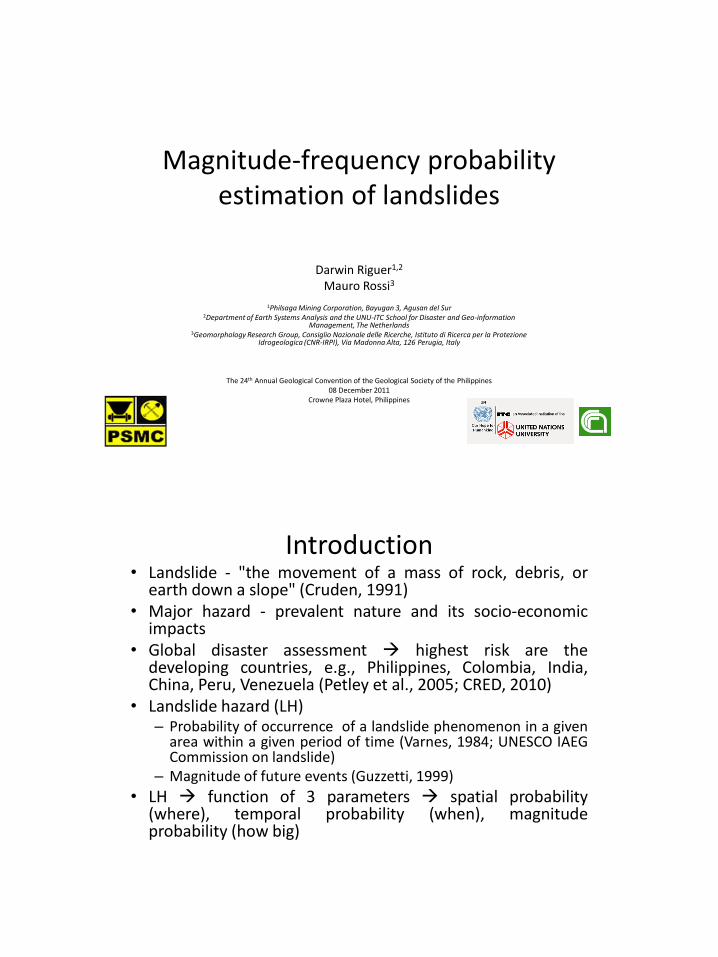
Magnitude-frequency probability estimation of landslides

Darwin Riguer1,2

Mauro Rossi3

1Philsaga Mining Corporation, Bayugan 3, Agusan del Sur

2Department of Earth Systems Analysis and the UNU-ITC School for Disaster and Geo-information Management, The Netherlands

3Geomorphology Research Group, Consiglio Nazionale delle Ricerche, Istituto di Ricerca per la Protezione Idrogeologica (CNR-IRPI), Via Madonna Alta, 126 Perugia, Italy

The 24th Annual Geological Convention of the Geological Society of the Philippines 08 December 2011

Crowne Plaza Hotel, Philippines

Introduction • Landslide - "the movement of a mass of rock, debris, or

earth down a slope" (Cruden, 1991) • Major hazard - prevalent nature and its socio-economic

impacts • Global disaster assessment highest risk are the

developing countries, e.g., Philippines, Colombia, India, China, Peru, Venezuela (Petley et al., 2005; CRED, 2010)

• Landslide hazard (LH) – Probability of occurrence of a landslide phenomenon in a given

area within a given period of time (Varnes, 1984; UNESCO IAEG Commission on landslide)

– Magnitude of future events (Guzzetti, 1999)

• LH function of 3 parameters spatial probability (where), temporal probability (when), magnitude probability (how big)

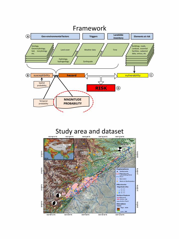
Framework

Earthquake

Hydrology, hydrogeology

Geology, Geomorphology, Soil, morphology etc.

Land cover Weather data Time

Buildings, roads, Landuse, essential facilities, cadastral data, census, etc

Geo-environmental factors Triggers Landslide inventory

Elements at risk

susceptibility vulnerability

RISK

A

B C

D

hazard

Temporal probability

MAGNITUDE PROBABILITY

Spatial probability

Study area and dataset

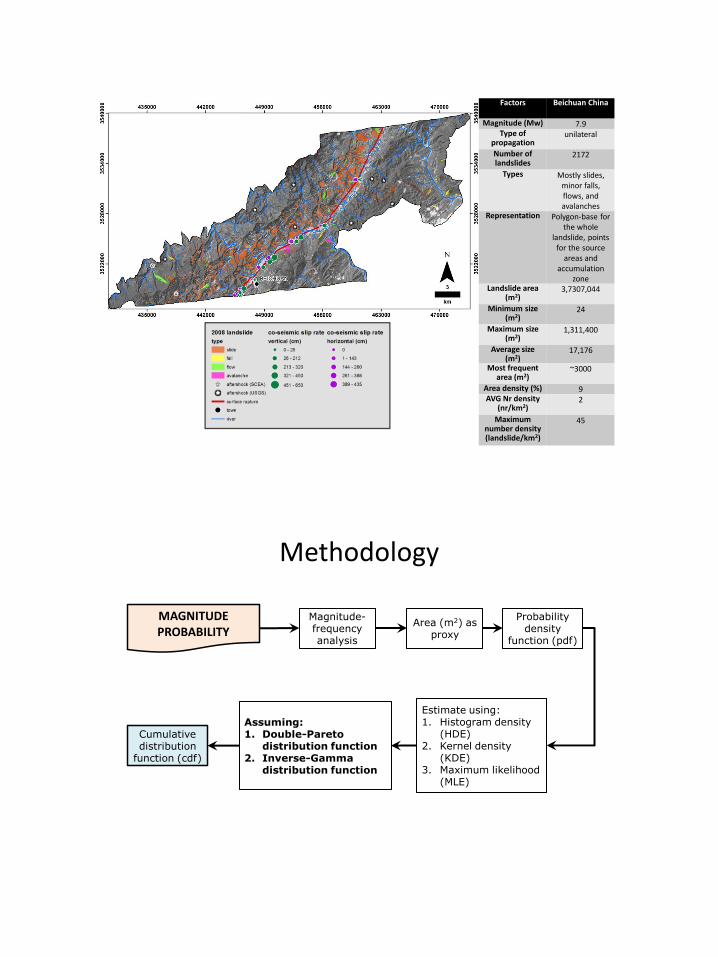
Factors

Beichuan China

Magnitude (Mw) 7.9 Type of

propagation unilateral

Number of landslides

2172

Types Mostly slides, minor falls, flows, and avalanches

Representation Polygon-base for the whole

landslide, points for the source

areas and accumulation

zone Landslide area

(m2) 3,7307,044

Minimum size (m2)

24

Maximum size (m2)

1,311,400

Average size (m2)

17,176

Most frequent area (m2)

~3000

Area density (%) 9 AVG Nr density

(nr/km2) 2

Maximum number density (landslide/km2)

45

Methodology

MAGNITUDE PROBABILITY

Magnitude-frequency analysis

Area (m2) as proxy

Probability density

function (pdf)

Estimate using: 1. Histogram density

(HDE) 2. Kernel density

(KDE) 3. Maximum likelihood

(MLE)

Assuming: 1. Double-Pareto

distribution function 2. Inverse-Gamma

distribution function

Cumulative distribution

function (cdf)

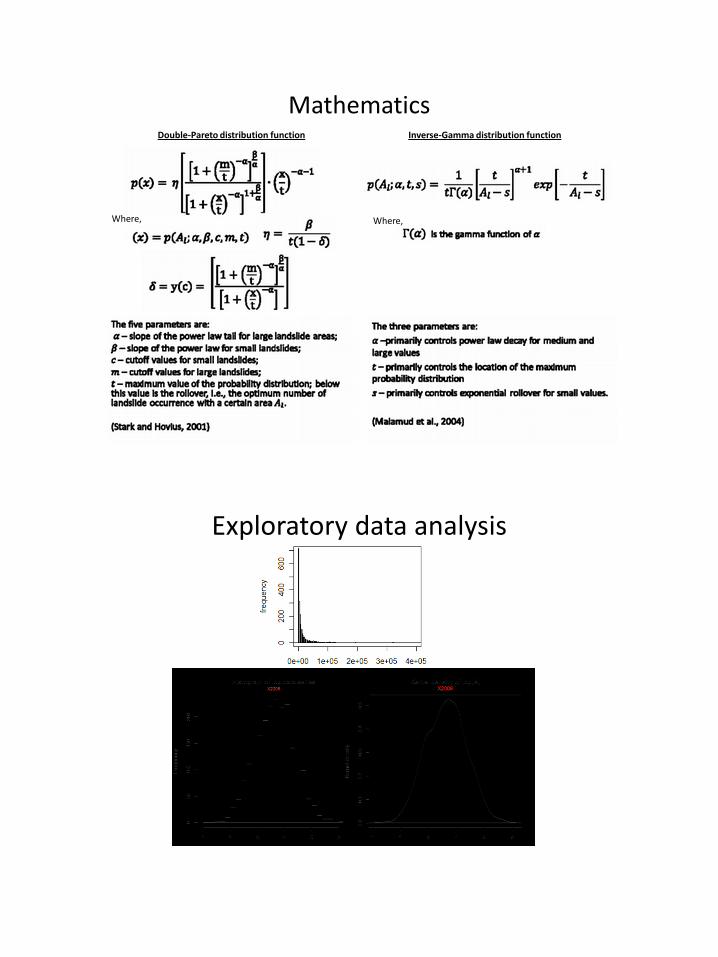
Mathematics

Where,

Double-Pareto distribution function

Where,

Inverse-Gamma distribution function

Exploratory data analysis

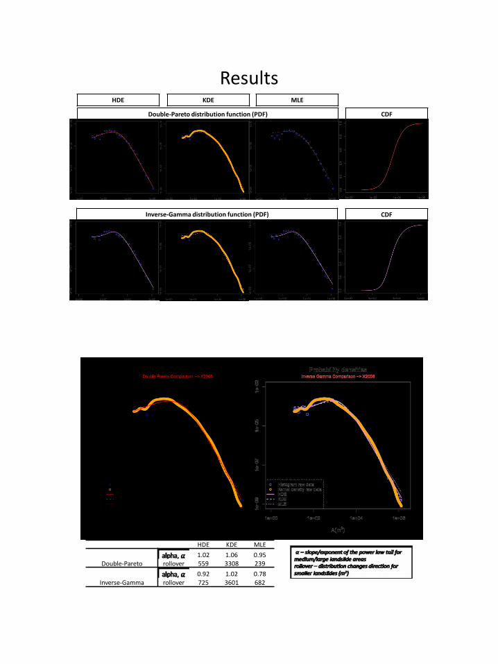
Results

Double-Pareto distribution function (PDF) CDF

Inverse-Gamma distribution function (PDF) CDF

HDE KDE MLE

AL(m2)

Probability Density (m2)

Probability, P[AL]

AL(m2)

AL(m2)

Probability Density (m2)

Probability, P[AL]

AL(m2)

HDE KDE MLE

Double-Pareto 1.02 1.06 0.95

rollover 559 3308 239

Inverse-Gamma 0.92 1.02 0.78

rollover 725 3601 682

Conclusion and future works

• Magnitude probability PDF CDF

• Perform test(s) on:

– Philippine dataset (Phivolcs, MGB, local agencies, NGO’s, etc.)

– relation between event-based landslide distribution patterns and geo-environmental factors for 2 earthquakes happening in the same area

• Create a generic software matlab, extension in ArcGIS, binary code in GRASS-GIS

• Can be applied to ore deposit size (?)

Difficulties and limitations

• Lack of sufficient data for pre-landslide events

– Inadequate

– Different spatial and temporal resolutions

– Event not in congruence with the source data

– Triggering event doesn’t exhibit systematic patterns

• Limitations in landslide inventory maps

– Inconsistencies in landslide densities

– Inaccurate estimation of size-frequency distributions

END

Thank you

Theoretical considerations and framework • Landslides leave discernible signs that can be recognized, classified, and mapped through various

methods: (1) field survey, (2) stereoscopic aerial photos and (3) satellite imagery (Rib and Liang, 1978; Varnes, 1978; Crozier, 1984; Hansen, 1984; Hutchinson, 1988; Turner and Schuster, 1996).

• Mechanical laws govern landslides and therefore they do not occur randomly or by chance. As a consequence, landslides can be analyzed empirically, statistically or in a deterministic way (Hutchinson, 1988; Crozier, 1986; Dietrich et al., 1995). It follows therefore that knowledge on landslides can be generalized (Aleotti and Chowdhury, 1999; Guzzetti et al., 1999).

• The morphological signature of a landslide (Pike, 1988) depends on the type (i.e., fall, flow, slide, complex, translational, rotational, etc.) and the rate of movement of the slope failure (Pašek, 1975; Varnes, 1978; Hansen, 1984; Hutchinson, 1988; Cruden and Varnes, 1996; Dikau et al., 1996).

• The principle of uniformitarianism holds that the present is the key to the past, thus the present is a key to the future (Varnes et al., 1984; Carrara et al., 1991; Hutchinson, 1995; Aleotti and Chowdhury, 1999; Guzzetti et al., 1999).

• The identification of landslides, including the type of data and the techniques that make data collection feasible, is dependent on scale-related input data (van Westen, 1993; Mantovani, et al., 1996; Soeters and van Westen, 1996).

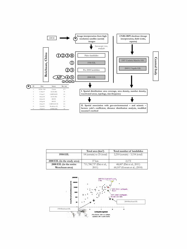
Paleo-landslides

1958 EIL

2008 EIL

Pre-2008 landslides 2009 L’Aquila EIL

1997 Umbria-Marche EIL

Image interpretation from high

resolution satellite (aerial)

images

Beic

hu

an

, C

hin

a

Cen

tral Ita

ly

CNRI-IRPI database (image

interpretation, field works,

reports)

I. Spatial distribution: area coverage, area density, number density,

reactivated areas, typology, size-frequency

II. Spatial association with geo-environmental – and seismic –

factors: yule’s coefficient, distance distribution analysis, modified

meunier’s method

ID Date Sensor Res. (m)

1 20 Dec 1968 Corona 2.75

2 31 Mar 07 ALOS (MS) 10

3 19 Apr 07 CARTOSAT1 2.5

4 04 Jun 08 ALOS (MS) 10

5 04 Jun 08 SPOT5 5

6 24 Sep 08 SPOT5 2.5

7 24 Jan 09 CARTOSAT (P) 2.5

8 31-Jul-09 Worldview (P) 0.5

9 19 Jul 10 ASTER (MS) 15

1 2

*

* DEM

3 8

2 3

1

Steroscopic view,

anaglyph

8 9 7 6

5 4 AP

Total area (km2) Total number of landslides

1958 EIL 18 (certain) to 25 (total) 2,210 (certain) - 3,154 (total)

2008 EIL (in the study area) 37 km 2,172

2008 EIL (in the entire

Wenchuan area)

711,780,737 (Dai et al.,

2011)

48,007 (Dai et al., 2011)

60,107 (Gorum et al., (2010)

1958 Beichuan EIL

2008 Beichuan EIL

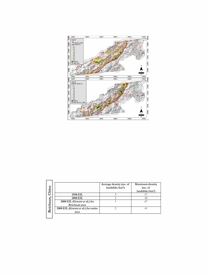
Average density (no. of

landslide/km2)

Maximum density

(no. of

landslide/km2)

1958 EIL 3 57

2008 EIL 2 44

2008 EIL (Gorum et al.) for

Beichuan area

1 67

2008 EIL (Gorum et al.) for entire

area

2 41

Beic

hu

an

, C

hin

a

• Reactivation

700 landslides reactivated; 102,914,407 m2

3113

36 5

1940

46 179

7 0

500

1000

1500

2000

2500

3000

3500

slide flow fall avalanche

freq

uen

cy

landslide type

1958 EIL

2008 EIL

Optimum distance to

CSFR

4.8 km to hanging wall;

1 km to footwall

3.3 km to hanging wall;

2.9 km meters to

footwall

12 km from CSFR 11.5 km from CSFR

Optimum elevation

(m)

1000 1300 300 700

Optimum slope (°) 23 38 9 17

Associated slope

aspect(s)

SE, SSE, SSW, SW,

WSW

NE, ENE, ESES, SE,

SSE, SSW, SW

SE, SSE, SSW, SW,

WSW, WNW

NNE, NE, ENE, ESE

Nearer to ridge or

stream

ridge ridge ridge ridge

Associated lithology Longmaxi (Phyllite,

schist, slate with

sandstone and

limestone ); Maoxian

group (Phyllite,schist,

slate with sandstone

and limestone);

Ordovician

(Limestone, muddy

limestone intercalated

with slate); Cambrian

(Sandstone and

siltstone intercalated

with slate)

Quaternary alluvium;

Ordovician

(Limestone, muddy

limestone intercalated

with slate); Cambrian

(Sandstone and

siltstone intercalated

with slate)

Paleogene- Upper

Cretaceous ( Limestones

and pelagic limestones

marl); Jurassic

(Limestones and

sometimes neritic

dolomites and from

platform); Cretaceous –

Jurassic (Micritic

limestones and pelagic

micrite clay) ;

Jurassic(Limestones,

limestones marl and

marl, limestones flint,

pelagic limestones)

Paleogene (Limestones

and biodetric and

neritic limestones and

of platform); middle

lower Miocene

(Organogenic

limestones,

calcarenite);

Pleistocene and

Pliocene (Lacustrine

deposits and fluvial)

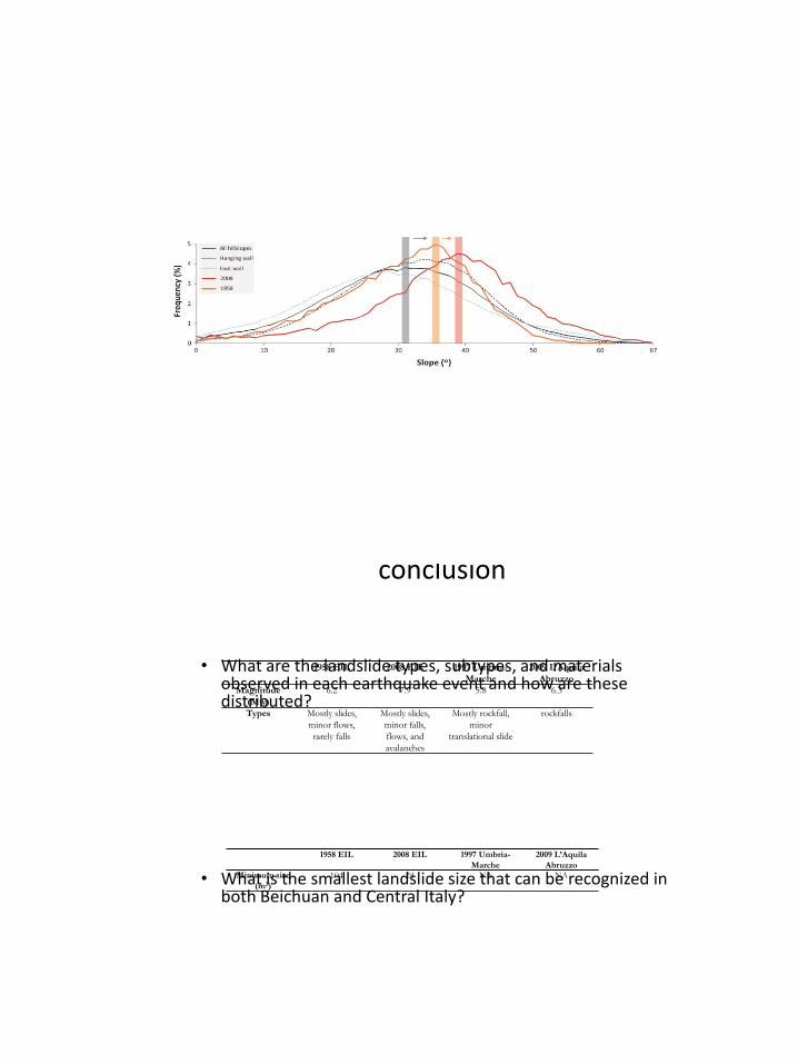
conclusion

• What are the landslide types, subtypes, and materials observed in each earthquake event and how are these distributed?

• What is the smallest landslide size that can be recognized in both Beichuan and Central Italy?

1958 EIL 2008 EIL 1997 Umbria-

Marche

2009 L’Aquila

Abruzzo

Magnitude

(Mw)

6.2 7.9 5.8 6.3

Types Mostly slides,

minor flows,

rarely falls

Mostly slides,

minor falls,

flows, and

avalanches

Mostly rockfall,

minor

translational slide

rockfalls

Minimum size

(m2) 104 24 NA NA

1958 EIL 2008 EIL 1997 Umbria-

Marche

2009 L’Aquila

Abruzzo

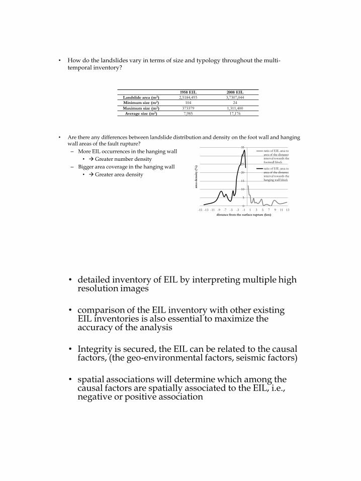
• How do the landslides vary in terms of size and typology throughout the multi-temporal inventory?

• Are there any differences between landslide distribution and density on the foot wall and hanging

wall areas of the fault rupture?

– More EIL occurrences in the hanging wall

• Greater number density

– Bigger area coverage in the hanging wall

• Greater area density

1958 EIL 2008 EIL

Landslide area (m2) 2,5184,493 3,7307,044

Minimum size (m2) 104 24

Maximum size (m2) 373379 1,311,400

Average size (m2) 7,985 17,176

0

5

10

15

20

25

30

35

-15 -13 -11 -9 -7 -5 -3 -1 1 3 5 7 9 11 13

are

a d

en

sity

(%

)

distance from the surface rupture (km)

ratio of EIL area to area of the distance interval towards the footwall block

ratio of EIL area to area of the distance interval towards the hanging wall block

• detailed inventory of EIL by interpreting multiple high resolution images

• comparison of the EIL inventory with other existing EIL inventories is also essential to maximize the accuracy of the analysis

• Integrity is secured, the EIL can be related to the causal factors, (the geo-environmental factors, seismic factors)

• spatial associations will determine which among the causal factors are spatially associated to the EIL, i.e., negative or positive association

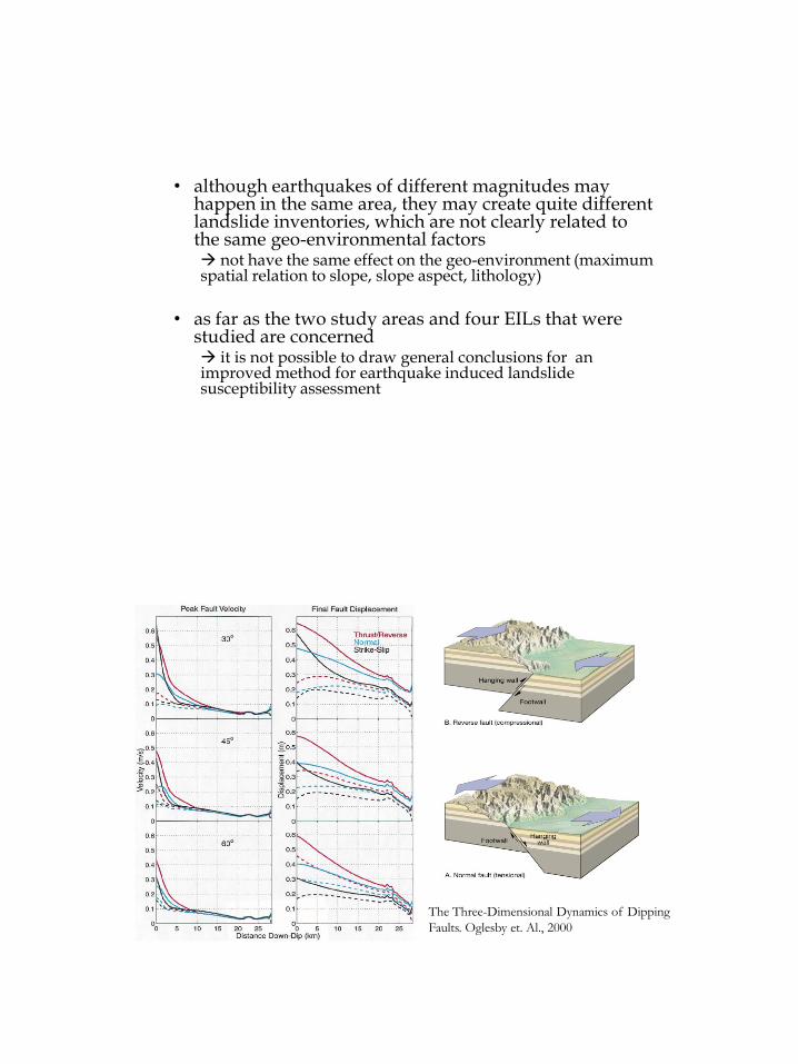
• although earthquakes of different magnitudes may happen in the same area, they may create quite different landslide inventories, which are not clearly related to the same geo-environmental factors not have the same effect on the geo-environment (maximum spatial relation to slope, slope aspect, lithology)

• as far as the two study areas and four EILs that were

studied are concerned it is not possible to draw general conclusions for an improved method for earthquake induced landslide susceptibility assessment

The Three-Dimensional Dynamics of Dipping

Faults. Oglesby et. Al., 2000

• END

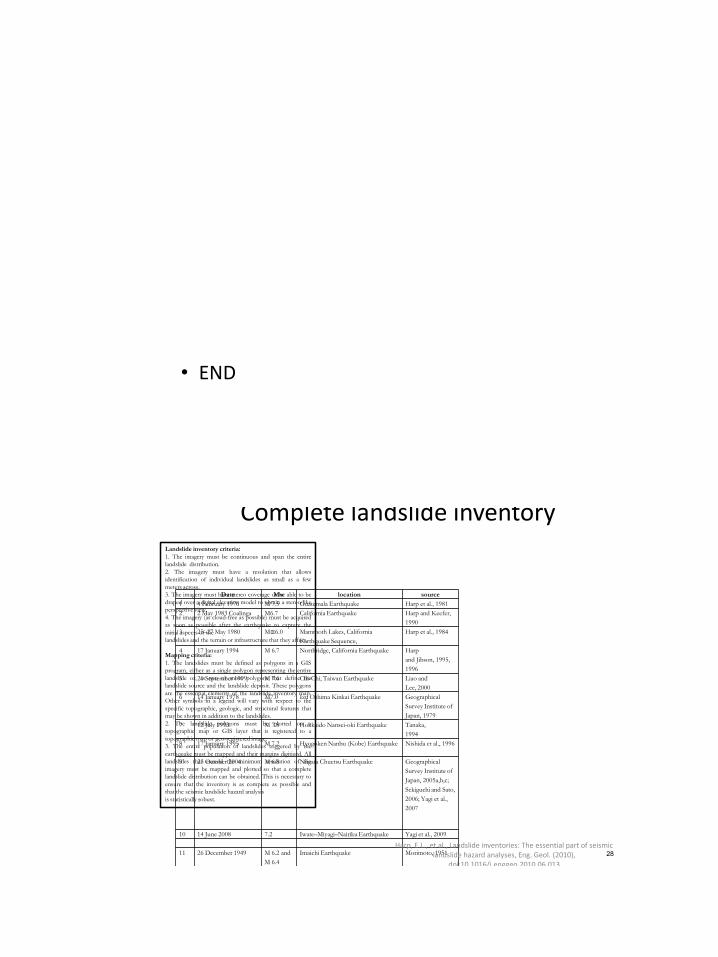
Complete landslide inventory

Date Mw location source

1 4 February 1976 M 7.5 Guatemala Earthquake Harp et al., 1981

2 2 May 1983 Coalinga M6.7 California Earthquake Harp and Keefer,

1990

3 25–27 May 1980 M≅6.0 Mammoth Lakes, California

Earthquake Sequence,

Harp et al., 1984

4 17 January 1994 M 6.7 Northridge, California Earthquake Harp

and Jibson, 1995,

1996

5 21 September 1999 M 7.6 Chi-Chi, Taiwan Earthquake Liao and

Lee, 2000

6 14 January 1978 M7.0 Izu Oshima Kinkai Earthquake Geographical

Survey Institute of

Japan, 1979

7 12 July 1993 M 7.8 Hokkaido Nansei-oki Earthquake Tanaka,

1994

8 17 January 1995 M 7.2 Hyogoken Nanbu (Kobe) Earthquake Nishida et al., 1996

9 23 October 2004 M 6.8 Niigata Chuetsu Earthquake Geographical

Survey Institute of

Japan, 2005a,b,c;

Sekiguchi and Sato,

2006; Yagi et al.,

2007

10 14 June 2008 7.2 Iwate–Miyagi–Nairiku Earthquake Yagi et al., 2009

11 26 December 1949 M 6.2 and

M 6.4

Imaichi Earthquake Morimoto, 1951

12 6 May 1976 M 6.4 Friuli, Italy Earthquake Govi, 1977a,b

Harp, E.L., et al., Landslide inventories: The essential part of seismic landslide hazard analyses, Eng. Geol. (2010),

doi:10.1016/j.enggeo.2010.06.013

Landslide inventory criteria:

1. The imagery must be continuous and span the entire

landslide distribution.

2. The imagery must have a resolution that allows

identification of individual landslides as small as a few

meters across.

3. The imagery must have stereo coverage or be able to be

draped over a digital elevation model to obtain a stereo-like

perspective view.

4. The imagery (as cloud-free as possible) must be acquired

as soon as possible after the earthquake to capture the

initial aspects of the

landslides and the terrain or infrastructure that they affect.

Mapping criteria:

1. The landslides must be defined as polygons in a GIS

program, either as a single polygon representing the entire

landslide or, as two or more polygons that define the

landslide source and the landslide deposit. These polygons

are the essential elements of the landslide inventory map.

Other symbols in a legend will vary with respect to the

specific topographic, geologic, and structural features that

may be shown in addition to the landslides.

2. The landslide polygons must be plotted on a

topographic map or GIS layer that is registered to a

topographic map or geo-registered image.

3. The entire population of landslides triggered by the

earthquake must be mapped and their margins digitized. All

landslides that exceed the minimum resolution of the

imagery must be mapped and plotted so that a complete

landslide distribution can be obtained. This is necessary to

ensure that the inventory is as complete as possible and

that the seismic landslide hazard analysis

is statistically robust.

28

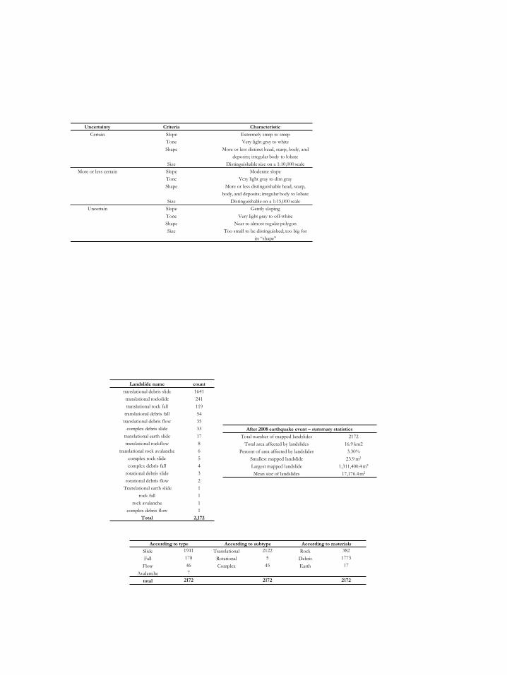
Uncertainty Criteria Characteristic

Certain Slope Extremely steep to steep

Tone Very light gray to white

Shape More or less distinct head, scarp, body, and

deposits; irregular body to lobate

Size Distinguishable size on a 1:10,000 scale

More or less certain Slope Moderate slope

Tone Very light gray to dim gray

Shape More or less distinguishable head, scarp,

body, and deposits; irregular body to lobate

Size Distinguishable on a 1:15,000 scale

Uncertain Slope Gently sloping

Tone Very light gray to off-white

Shape Near to almost regular polygon

Size Too small to be distinguished; too big for

its “shape”

Landslide name count

translational debris slide 1641

translational rockslide 241

translational rock fall 119

translational debris fall 54

translational debris flow 35

complex debris slide 33

translational earth slide 17

translational rockflow 8

translational rock avalanche 6

complex rock slide 5

complex debris fall 4

rotational debris slide 3

rotational debris flow 2

Translational earth slide 1

rock fall 1

rock avalanche 1

complex debris flow 1

Total 2,172

According to type According to subtype According to materials

Slide 1941 Translational 2122 Rock 382

Fall 178 Rotational 5 Debris 1773

Flow 46 Complex 45 Earth 17

Avalanche 7

total 2172 2172 2172

After 2008 earthquake event – summary statistics

Total number of mapped landslides 2172

Total area affected by landslides 16.9 km2

Percent of area affected by landslides 3.30%

Smallest mapped landslide 23.9 m2

Largest mapped landslide 1,311,400.4 m2

Mean size of landslides 17,176.4 m2

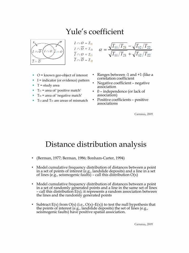
Yule’s coefficient

• Ranges between -1 and +1 (like a correlation coefficient

• Negative coefficient – negative association

• 0 – independence (or lack of association)

• Positive coefficients – positive associations

O = known geo-object of interest

I = indicator (or evidence) pattern

T = study area

T11 = area of ‘positive match’

T22 = area of ‘negative match’

T12 and T21 are areas of mismatch

Carranza, 2009

Distance distribution analysis

• (Berman, 1977; Berman, 1986; Bonham-Carter, 1994)

• Model cumulative frequency distribution of distances between a point in a set of points of interest (e.g., landslide deposits) and a line in a set of lines (e.g., seismogenic faults) – call this distribution O(x)

• Model cumulative frequency distribution of distances between a point in a set of randomly generated points and a line in the same set of lines – call this distribution E(x); it represents a random association between the lines and the randomly generated points

• Subtract E(x) from O(x) (i.e., O(x)–E(x)) to test the null hypothesis that the points of interest (e.g., landslide deposits) the set of lines (e.g., seismogenic faults) have positive spatial association.

Carranza, 2009

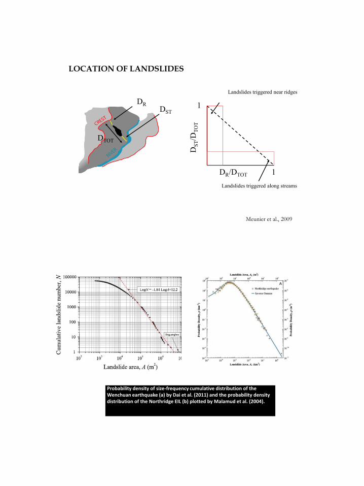
DS

T/D

TO

T

DR/DTOT

1

1

Landslides triggered near ridges

Landslides triggered along streams

LOCATION OF LANDSLIDES

DST

DR

DTOT

Meunier et al., 2009

Probability density of size-frequency cumulative distribution of the Wenchuan earthquake (a) by Dai et al. (2011) and the probability density distribution of the Northridge EIL (b) plotted by Malamud et al. (2004).

Fatal landslide examples from Beichuan town. a, General view of the Beichuan town after the earthquake. b-c Pre- and post-photos of Beichuan Middle-school rock avalanche. This landslide caused 700 deaths. d-e, Pre- and post-photos of Wang Jiayan landslide which caused almost 1700 deaths. (pre-earthquake photographs courtesy of Chengdu University of Technology).

Visual interpretation element applied to image interpretation of landslides and other associated features. 1 – color difference between the landslide and its surrounding environment that is vegetation; 2 – texture difference between a coarser and smoother landslide; 3 – lath-like patterns of cropfields; 4 – shape difference of a lobular landslide compared to a very irregular outline; 5 – size difference between a relatively smaller landslide to a bigger one; 6 – association of river deposits in river bends

Morphological element aids in interpreting landslides. The use of stereoscopic views helps visualize the topography in three dimension therefore making landslides more apparent.1 – landslide triggered near ridges; 2 – landslides triggered at mid-slopes; 3 – landslides triggered very near the river.