
E cient State Estimation in Power Networks for Reactive ...tesi.cab.unipd.it/42731/1/Tesi.pdfA...
75
Universit` a degli Studi di Padova DIPARTIMENTO DI INGEGNERIA DELL’INFORMAZIONE Corso di Laurea in Ingegneria dell’Automazione Tesi di Laurea Magistrale Efficient State Estimation in Power Networks for Reactive Power Losses Compensation Candidato Alberto Di Vittorio Relatore prof. Ruggero Carli Anno Accademico 2012-2013
Transcript of E cient State Estimation in Power Networks for Reactive ...tesi.cab.unipd.it/42731/1/Tesi.pdfA...

Universita degli Studi di Padova
DIPARTIMENTO DI INGEGNERIA DELL’INFORMAZIONE
Corso di Laurea in Ingegneria dell’Automazione
Tesi di Laurea Magistrale
Efficient State Estimation in PowerNetworks for Reactive Power Losses
Compensation
Candidato
Alberto Di VittorioRelatore
prof. Ruggero Carli
Anno Accademico 2012-2013


Sebbene questa tesi sia solo il frutto degli ultimi miei sei mesi di lavoro,quando viene conclusa, stampata e presa in mano essa non può fare a meno dirappresentare, dentro di te, il simbolo della fine del tuo periodo uiversitario.Un periodo nel quale questo percorso di studi ti ha accompagnato giornodopo giorno, senza lasciarti mai. Gioie, soddisfazioni, conquiste, e anchequalche grossa batosta. Ebbene, ora sembra davvero arrivato il capolinea.Sperando che questo capolinea non sia altro che il trampolino di lancio perl’entrata nel mondo del lavoro, non posso fare a meno di menzionare e diringraziare tutte le persone che hanno reso possibile quasto mio traguardo,alcune con un supporto permanente e altre anche con un semplice gesto.
- Grazie innanzitutto ad Ilaria, la mia fantastica compagna di vita, cheha condiviso con me ogni gioia e ogni traguardo e ha cercato di nonfarmi perdere autostima, voglia e fiducia in me stesso nei momenti diforte abbattimento;
- Grazie a mamma e papà, sempre i primi a credere in me e a spronarmiper tirare fuori il massimo in ogni ambito;
- Grazie ai miei nonni Elena, Gianni, Gino e Rita, per avermi fattosentire un nipote speciale anche quando io non mi sentivo tale.
- Grazie a Diego e Wally, non solo semplici compagni universitari maamici, non solo persone con cui studiare, interrogarsi e migliorarsi, macon cui condividere una passione;
- Grazie a Lele e Diane (e Samuel), compagni e sposi novelli;
- Grazie a Tod, per avermi dato molto più di una mano in questa tesi;
- Grazie al prof. Ruggero Carli, per essere stato sempre disponibile neimiei confronti durante questo lavoro di tesi;
- Grazie a tutti i membri della mitica squadra di calcetto "Futsal3G",Luigino in primis;
- Grazie alla città di Lisbona, luogo che per me ricoprirà sempre unaposizione speciale;
- Grazie a tutti i parenti e gli amici, italiani e non, che in questi cinqueanni mi sono stati vicino anche solo con un semplice gesto o pensiero;
- Grazie alla musica, vero rifugio di serenità e divertimento che mai arrivaalla saturazione;
- Grazie a te, perché se stai leggendo questa tesi significa che pensi possaessere un lavoro interessante.

Contents
1 Introduction 71.1 Extended Abstract . . . . . . . . . . . . . . . . . . . . . . . . 71.2 State of the Art . . . . . . . . . . . . . . . . . . . . . . . . . . 101.3 Short summary . . . . . . . . . . . . . . . . . . . . . . . . . . 12
2 Grid Modeling 152.1 Grid Components . . . . . . . . . . . . . . . . . . . . . . . . . 15
2.1.1 Transmission Lines . . . . . . . . . . . . . . . . . . . . 152.1.2 Shunt Capacitors or Reactors . . . . . . . . . . . . . . 162.1.3 Transformers . . . . . . . . . . . . . . . . . . . . . . . 162.1.4 Loads and Generators . . . . . . . . . . . . . . . . . . 16
2.2 Network Model . . . . . . . . . . . . . . . . . . . . . . . . . . 172.3 Smart Grid Model . . . . . . . . . . . . . . . . . . . . . . . . 17
2.3.1 Mathematical Preliminaries . . . . . . . . . . . . . . . 172.3.2 Model . . . . . . . . . . . . . . . . . . . . . . . . . . . 17
2.4 Testing setup: IEEE test Feeders . . . . . . . . . . . . . . . . 21
3 State Estimation and Reactive Power Compensation 233.1 Model and Estimation Problem Formulation . . . . . . . . . . 23
3.1.1 Model . . . . . . . . . . . . . . . . . . . . . . . . . . . 233.1.2 Estimation Problem Formulation . . . . . . . . . . . . 243.1.3 Model Linearization . . . . . . . . . . . . . . . . . . . 253.1.4 Closed Form Solution . . . . . . . . . . . . . . . . . . 273.1.5 HTR−1H structure . . . . . . . . . . . . . . . . . . . . 28
3.2 Reactive Power Compensation . . . . . . . . . . . . . . . . . . 283.2.1 Problem Formulation . . . . . . . . . . . . . . . . . . . 283.2.2 Dual decomposition . . . . . . . . . . . . . . . . . . . 293.2.3 Distributed algorithm . . . . . . . . . . . . . . . . . . 303.2.4 Estimation and RPC . . . . . . . . . . . . . . . . . . . 32
4 Distributed Estimation Algorithms 354.1 Multi Area Decomposition . . . . . . . . . . . . . . . . . . . . 354.2 Alternating Direction Multiplier Method . . . . . . . . . . . . 37
5
6 CONTENTS
4.2.1 ADMM classical . . . . . . . . . . . . . . . . . . . . . 374.2.2 ADMM scalable with Projector matrices . . . . . . . . 394.2.3 ADMM scalable and compact . . . . . . . . . . . . . . 414.2.4 Convergence of ADMM scalable . . . . . . . . . . . . . 44
4.3 Jacobi approximate algorithm . . . . . . . . . . . . . . . . . . 47
5 Testing results 515.1 Noise sizing . . . . . . . . . . . . . . . . . . . . . . . . . . . . 525.2 Performances of the algorithms . . . . . . . . . . . . . . . . . 53
5.2.1 About Centralized Estimation . . . . . . . . . . . . . . 535.2.2 Tests setup . . . . . . . . . . . . . . . . . . . . . . . . 545.2.3 Performances for default values of noise standard de-
viations . . . . . . . . . . . . . . . . . . . . . . . . . . 545.2.4 Performances for σ = 10−4 . . . . . . . . . . . . . . . . 585.2.5 Performances for σ = 10−3 . . . . . . . . . . . . . . . . 595.2.6 Performances for σ = 5 · 10−3 . . . . . . . . . . . . . . 605.2.7 Performances for σ = 3 · 10−2 . . . . . . . . . . . . . . 615.2.8 Performances for σ = 5 · 10−2 . . . . . . . . . . . . . . 625.2.9 Performances for σ = 10−1 . . . . . . . . . . . . . . . . 635.2.10 Jacobi algorithm on a 6-areas divided grid . . . . . . . 645.2.11 Performances adding saturation constraints to each
power line . . . . . . . . . . . . . . . . . . . . . . . . . 66
6 Conclusion 696.1 Results achieved . . . . . . . . . . . . . . . . . . . . . . . . . 696.2 Possible future developments . . . . . . . . . . . . . . . . . . 70
A Proof of equations 4.5 and 4.6 71

Chapter 1
Introduction
1.1 Extended Abstract
In the last decade the electric grid has been undergoing a deep renovationprocess toward the a so-called smart grid featuring larger hosting capability,widespread penetration of renewable energy sources, higher quality of theservice and reliability. In particular, the modernization of the low voltageand medium voltage power distribution network consists in the deploymentof a large amount of information and communication technologies (ICT),in the form of dispersed measurement, monitoring, and actuation devices.From the environmental point of view, in particular, it is talked about greentechnology, that is, smart tech capable to exploit sustainable source of energy.
Among the many different aspects of this transition, we focus on the con-trol of the microgenerators inside a smart microgrid ([1], [2]). A microgridis a portion of the low-voltage power distribution network that is managedautonomously from the rest of the network, in order to achieve better qual-ity of the service, improve efficiency, and pursue specific economic interests.Together with the loads connected to the microgrid (both residential and in-dustrial customers), we also have microgeneration devices (solar panels, com-bined heat-and-power plants, micro wind turbines, etc.). These devices areconnected to the microgrid via electronic interfaces (inverters), whose maintask is to enable the injection of the produced power into the microgrid. Oneexample in this sense is the coordinated control of the power inverters of themicrogeneration devices connected to the low voltage grid. When properlycontrolled, these devices can provide valuable ancillary services like reactivepower compensation, voltage support, automatic generation control, optimalpower flow computation, etc. ([3], [4]). In this work we consider the prob-lem of optimal reactive power compensation (RPC). Loads belonging to themicrogrid may require a sinusoidal current which is not in phase with volt-age. A convenient description for this, consists in saying that they demandreactive power together with active power, associated with out-of-phase and
7

8 CHAPTER 1. INTRODUCTION
in-phase components of the current, respectively. Reactive power is not a"real" physical power, meaning that there is no energy conversion involvednor fuel costs to produce it. Like active power flows, reactive power flowscontribute to power losses on the lines, cause voltage drop, and may lead togrid instability. It is therefore preferable to minimize reactive power flowsby producing it as close as possible to the users that need it.
For example, the reactive power compensation strategy proposed in [5]consists in an iterative tuning of the amount of reactive power injected bythe microgenerators, with the objective of minimizing power distributionlosses across the grid. The proposed procedure requires that microgeneratorsperform voltage phasor measurements at their own point of connection tothe grid. These measurements are then shared with other microgeneratorsvia a communication channel, and processed in a distributed way. Based onthe result of this processing, each microgenerators then updates the amountof reactive power injected into the grid, actuating the system. Because ofthe inherent communication part, this strategy belongs to the wide class ofnetworked control systems [7].
One of the main bottleneck in the actuaction of this kind of control strate-gies in the low voltage power distribution network is the need for accuratevoltage phasor measurements across the grid. Specifically, to achieve the aimof control is necessary to handle with the voltage phasor at every node1 ofthe grid, namely the state of the grid.
Phasor measurement units (PMU) can provide these measurements, buttheir cost is generally unacceptable for large scale deployment. In particular,time synchronization between different PMUs is a major technological issue,and it is generally tackled via a GPS module that can provide timestampingof the data.
The first contribution of this thesis consists in evaluating the effects ofPMU measurement errors for measurement-driven control strategies, adopt-ing the reactive power control proposed in [5] as a prototype. Then wepresent two distributed estimation algorithms capable of improving the qual-ity of the voltage measurements via exchange of data with other PMUs andvia distributed processing of the raw data.
We assume that the power distribution grid is divided into a number ofareas. The PMUs beloning to each area transmit their voltage measurementsto an area monitor. Area monitors can communicate and they are instructedto process the collected measurement in a distributed way.
Similar algorithms have already been proposed in the literature, espe-cially for medium voltage and high voltage power grids, see [6], [7], [8], [9][10]. The two solutions proposed, however, exhibit some notable originalfeatures which make them particularly suited for the scenario of low voltage
1A Node can represent either an household appliance in a domestic microgrid or anentire house demand in a urban grid.
1.1. EXTENDED ABSTRACT 9
power distribution grids:
• they only require measurements that can be performed by the devicesat their point of connection, instead of power flow and current mea-surements on the power lines, which are generally not available in lowvoltage grids;
• the computational effort is very limited and remains constant if thegrid grows in size;
• they are completely leader-less (no grid supervisor is present).
In order to present the two proposed distributed algorithms, we first in-troduce a model for the power grid, which includes a convenient modellingof the measurement errors in which time sync error are explicitly considered.Based on this model, we detail the least-square problem that has to be solvedin order to find the maximum-likelyhood estimation of the grid state. For thesolution of such optimization problem, we propose two different approaches.The first approach is a distributed implementation of the Alternating Direc-tion Method of Multipliers ([11]). This contribution is of particular interestper se: we show how ADMM can be implemented in a scalable way [12],in which every agent is only required to store a portion of the entire stateof the systems. The second approach is a distributed Jacobi-like algorithm.The algorithm is completely leader-less, and each monitor has to solve anextremely simple optimization problem, for which a closed form solution isprovided.
Finally, it is studied the behaviour of these two estimation algorithmtogether with the reactive power compensation one. In the last example it isshown how are the estimation algorithm performances in the reactive powercompensation for a grid constrained: we added upper and lower bounds tothe reactive power that each compensator can exchange with the remainingnetwork ([13]) These box constraints complicate the initial problem, butdraw the model closer to the real microgrid. We will show that, using theestimate state, it leads to an optimal behaviour.
10 CHAPTER 1. INTRODUCTION
1.2 State of the Art
Since Power Networks State Estimation represents the starting point to im-plement a desirable network control, it has been fully treated in literature.Firstly it has been analyzed through centralized techniques. Afterwards re-searchers focused on distributed solution since the increasing in network size,the always more relevant computational effort, the networks topology pri-vacy and the robustness to failures become strictly urgent.
The main aim of the estimation is to adequately filter the raw measure-ments with the purpose to achieve a better knowledge of a desire quantity,namely the state. This is very important due to the fact that measurementscould be very noisy. Therefore, they cannot be straightly used to control thenetwork. Indeed, presence of outliers, measurement errors and noisy mea-sures, corrupting the real value of the state, make absolutely unusable thecontrol. As a byproduct, the estimation could be efficiently used to do faultdetection and bad data detection. This is, respectively, to detect fault of thenetwork and to identify particularly bad measures (outliers), for instance,due to instrumentation faults or corruption through the connection lines.
In [14] the authors firstly present the principal electric components to in-troduce a suitable network model. Secondly, it is fully explained the central-ized weighted least squares estimation supposing to deal with measurementsaffected by gaussian noise.
In [15], [16] e [17] it is firstly developed an exact network model, secondlyan approximated one and finally the authors deal with the implementationof a centralized static least square estimation modeling the noise as a gaus-sian random variable. Finally it is suggested how to implement a real-timeversion of the algorithm proposed and a bad data detection.
In [6] the authors proposed a multi area distributed two-level estimation.Firstly the single area, using just inner measures, estimates its own knowl-edge of the state. Secondly, a central unit deals with the task of coordinatethe single areas estimations via an additional set of pseudo-measurementstake by Phasor Measurement Units (PMUs). Similar method is describedboth in [7] and [8].
In [18] it is proposed a technique that, after a preliminary decompositionof the net in smaller subnetworks, place the measurement units with the aimof optimizing their number and costs.
In [9], similar to the two-level implementation of [6], [7] and [8], the au-thor proposes a method to deal with a distributed state estimation via only

1.2. STATE OF THE ART 11
local measures. Thanks to the exchange of borders information betweenneighboring areas and a central coordination unit it is finally reached thewide range estimation.
In [10] a complete leader-less algorithm is proposed. Coordination andestimation are carried out only via local exchange of information.
In [11] the authors develop a fully distributed mean square algorithm.This leads a Wireless Sensor Network (WSN), in which the algorithm istested, to adaptively reach the state estimation with single-hop neighborsexchanges of messages. The optimization problem is solved exploiting theAlternating Direction Method of Multipliers (ADMM).
In [19] an approach able to parallelize optimal power flow is presented.The proposed distributed scheme can be use to coordinate an heterogeneouscollection of utilities. Three mathematical decomposition coordination meth-ods are introduced to implement the proposed distributed sheme: the Auxil-iary Problem Principle (APP); the Predictor-Corrector Proximal MultiplierMethod (PCPM); the Alternating Direction Method (ADM).
In [12] is proposed a modification of the standard Alternating DirectionMultiplier Method formulation in order to obtain a scalable version. Theresulting algorithm is completely distributed and scalable.
In [5] the authors firstly propose an appropriate model for a low volt-age microgrid, secondly they develop a completely distributed algorithm toappropriately command a sub set of microgenerators to achieve an optimaldistribution losses minimization.
12 CHAPTER 1. INTRODUCTION
1.3 Short summary
This thesis is organized as follows:
• Chapter 2 presents the general model for the electric grid on wichwe have based the work. Consecutively, is presented a specific lowvoltage microgrid model suitable either for the estimation topic or forthe reactive power compensation formulation.
• Chapter 3 presents the problem to deal with. Specifically it formu-lates the estimation problem and its importance related to the reactivepower compensation. A centralized solution to the problem is devel-oped.
• Chapter 4 introduces and develops two completely distributed and scal-able technique to achieve the target. Specifically, firstly an ADMMbased solution is developed and proved. Secondly, a Jacobi-like algo-rithm is proposed.
• Chapter 5 presents a full set of tests to validate the algorithms pro-posed.
• Chapter 6 gathers the main features of the work done and gives someideas on what can be done in future.

1.3. SHORT SUMMARY 13
Notations
A. State variables
vi Magnitude of the voltage at the ith node.
θi Phase of the voltage at the ith node.
V Vector containing all voltages’ magnitude.
Θ Vector containing all voltages’ phase.
ii Magnitude of the current at the ith node.
φi Phase of the current at the ith node.
I Vector containing the magnitude of the current.
Φ Vector containing all currents’ phase.
xi Real of the voltage at the ith node.
yi Imaginary of the voltage at the ith node .
X Vector containing all the real parts.
Y Vector containing all the imaginary parts.
X = [X Y ]T Vector of all the state variables.
B. Measures
vmi Magnitude of the voltage at the ith node.
θmi Phase of the voltage at the ith node.
V m Vector containing all the magnitude of the voltages measured.
Θm Vector containing all the phases of the voltages measured.
si Real of the voltage at the ith node.
ri Imaginary of the voltage at the ith node.
S Vector of the real parts of the voltage.
R Vector of the imaginary parts of the voltage.
imi Magnitude of the current at the ith node.
φmi Phase of the current at the ith node.
hi Real of the current at the ith node.

14 CHAPTER 1. INTRODUCTION
ki Imaginary of the current at the ith node.
H Vector of the real part.
K Vector of the real part.
C. Standard deviations
σv Standard deviation of the voltage magnitude error.
σθ Standard deviation of the voltage phase error.
σi Standard deviation of the current magnitude error.
σφ Standard deviation of the current phase error.
D. Functions
J(·) Objective Cost Function.
f(·) Current magnitude nonlinear function of the state.
g(·) Current phase nonlinear function of the state.
|·| Both the absolute value of a quantity or the cardinality of a set dependingon the context.
·T Transpose of a vector or matrix.
· Complex conjugate of a complex quantity.
·∗ Both complex conjugate and transpose.
E. Matrixes and Vectors
In Identity matrix ∈ Rnxn.
1 Vector whose element are all equal to one.
1i Canonical vector whose elements are all equal to zero except for that inposition i.

Chapter 2
Grid Modeling
In this chapter we introduce in a general way an electric grid, starting fromthe principal components. Atfer have described a commonly adopted modelof an electric grid ([14]) we present the specific model on which we will focusin this thesis ([5]).
2.1 Grid Components
An electric grid consists of a series of electric components such as trans-mission lines, loads, generators, transformers and capacitors. It is usuallyassumed the power system to operate in the steady state under balance con-ditions. This implies that all bus loads and branch flows will be three phaseand balanced, all transmission lines are fully transposed and all other seriesor shut devices are symmetrical in the three phases [14]. These assumptionsallow the use of the single phase positive sequence equivalent circuit for mod-eling the entire system. The following component models are commonly usedin representing the network.
2.1.1 Transmission Lines
Transmission lines are usually represented by a two-port π-model character-ized by a series impedance of R + jX and a total line charging susceptanceof j2B corresponding to the equivalent circuit of figure 2.1
2.2 Component Modeling and Assumptions
Power system is assumed to operate in the steady state under balancedconditions. This implies that all bus loads and branch power flows willbe three phase and balanced, all transmission lines are fully transposed,and all other series or shunt devices are symmetrical in the three phases.These assumptions allow the use of single phase positive sequence equivalentcircuit for modeling the entire power system. The solution that will beobtained by using such a network model, will also be the positive sequencecomponent of the system state during balanced steady state operation. Asin the case of the power flow, all network data as well as the networkvariables, are expressed in the per unit system. The following componentmodels will thus be used in representing the entire network.
2.2.1 Transmission Lines
Transmission lines are represented by a two-port 7r-model whose parameterscorrespond to the positive sequence equivalent circuit of transmission lines.A transmission line with a positive sequence series impedance of .R+j f andtotal line charging susceptance of j23, will be modelled by the equivalentcircuit shown in Figure 2.1.
Figure 2.1. Equivaient circuit for a transmission tine
2.2.2 Shunt Capacitors or Reactors
Shunt capacitors or reactors which may be used for voltage and/or reactivepower control, are represented by their per phase susceptance at the corre-sponding bus. The sign of the susceptance value will determine the type ofthe shunt element. It will be positive or negative corresponding to a shuntcapacitor or reactor respectively.
2.2.3 Tap Changing and Phase Shifting Transformers
Transformers with off-nominal but in-phasc taps, can be modeled as seriesimpedances in scries with ideal transformers as shown in Figure 2.2. The
Copyright 2004 by Marcel Dekker, Inc. All Rights Reserved.
Figure 2.1: Equivalent circuit for a transmission line
15
16 CHAPTER 2. GRID MODELING
2.1.2 Shunt Capacitors or Reactors
Shunt devices are represented by their susceptance at the corresponding buswhose sign determines the type of shunt element. They can be used for volt-age and/or reactive power control.
Consider an admittance Y = jB characterized the susceptance B
B =
ωL− 1ωC
the sign of B determines the type of shunt element so a positive value cor-responds to a capacitor, alternatively a negative one to a reactor.
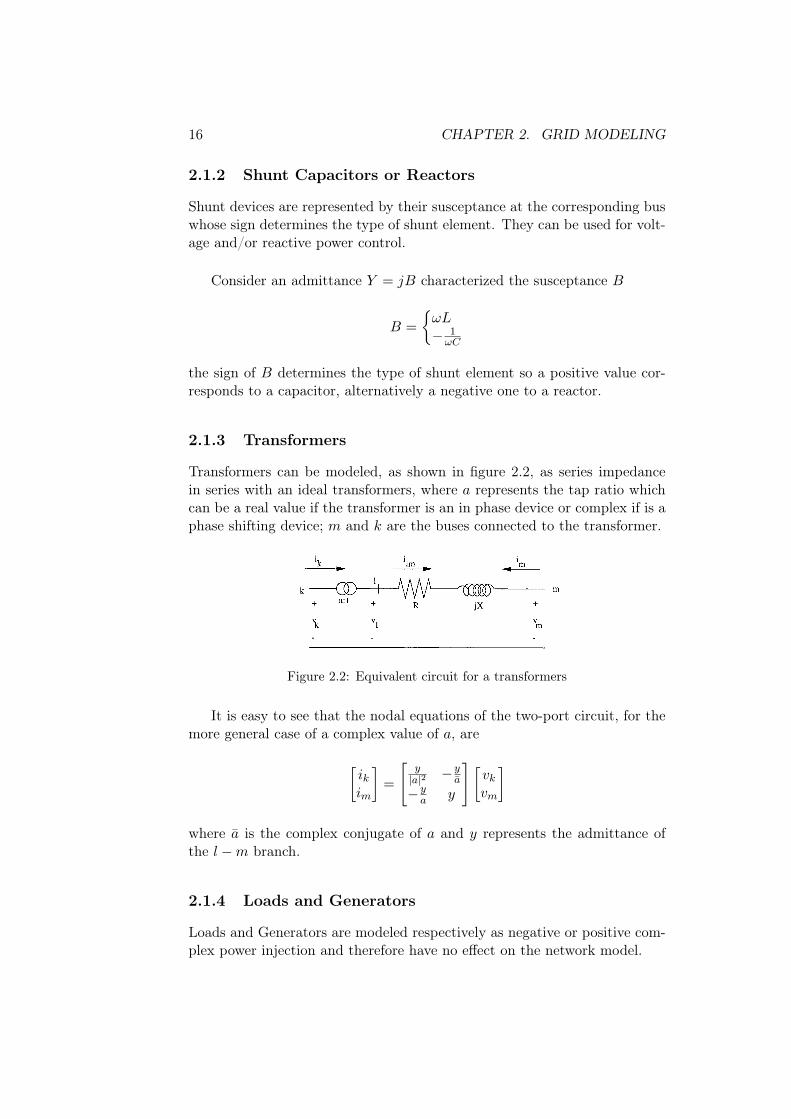
2.1.3 Transformers
Transformers can be modeled, as shown in figure 2.2, as series impedancein series with an ideal transformers, where a represents the tap ratio whichcan be a real value if the transformer is an in phase device or complex if is aphase shifting device; m and k are the buses connected to the transformer.two transformer terminal buses m and /c are commonly designated as the
impedance side and the tap side bus respectively.
Figure 2.2. Equivatent circuit for an off-nominat tap transformer
The nodal equations of the two port circuit of Figure 2.2 can be derivedby first expressing the current flows ^ and i at each end of the seriesbranch R + jJf. Denoting the admittance of this branch ^ — m by y, theterminal current injections will be given by:
(2.1)
Substituting for rn and
the final form will be obtained as follows:
(2.2)
where a is the in phase tap ratio. Figure 2.3 shows the corresponding twoport equivalent circuit for the above set of nodal equations.
Figure 2.3. Equivatent circuit of an in-phase tap changer
For a phase shifting transformer where the off-nominal tap value a, iscomplex, the equations will slightly change as:
Copyright 2004 by Marcel Dekker, Inc. All Rights Reserved.
Figure 2.2: Equivalent circuit for a transformers
It is easy to see that the nodal equations of the two-port circuit, for themore general case of a complex value of a, are
[ikim
]=
[y|a|2 −y
a
−ya y
] [vkvm
]
where a is the complex conjugate of a and y represents the admittance ofthe l −m branch.
2.1.4 Loads and Generators
Loads and Generators are modeled respectively as negative or positive com-plex power injection and therefore have no effect on the network model.
2.2. NETWORK MODEL 17
2.2 Network Model
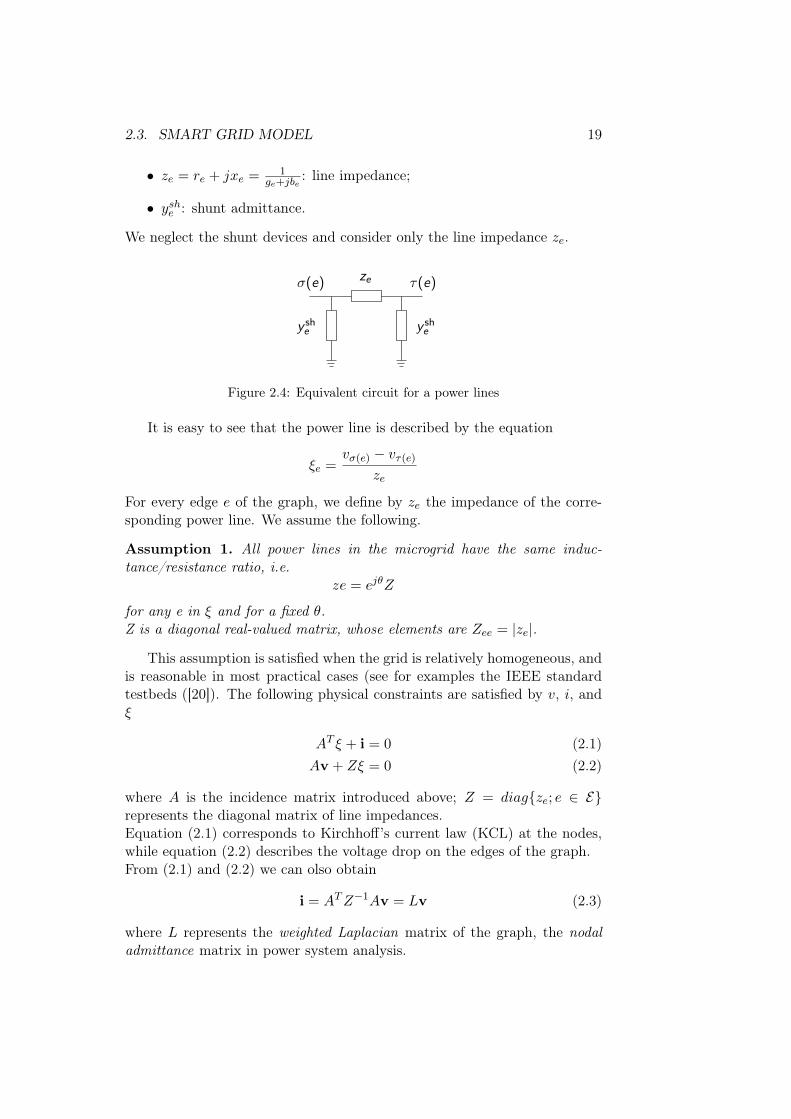
Modelling each component as above, we can build the general network modelof the system, that is the admittance matrix Y describing the Kirchhoff’scurrent law at each bus:
I =
i1...iN
=
Y11 · · · Y1N...
...YN1 · · · YNN
v1
...vN
= Y V
where ik is the current injection and vk is voltage phasor, both at bus k;Ykm is the (m, k) entry of the Y matrix representing the total admittancebetween nodes m and k.
2.3 Smart Grid Model
For our specific problem, the model built is a bit different from the generalone, and almost similar to the one described in [5].
2.3.1 Mathematical Preliminaries
Let G = (V, E , σ, τ) be a directed graph, where V is the set of nodes (|V| = n),E is the set of edges (|E| = r) and σ, τ : E → V are two functions such thatthe edge e ∈ E goes from node σ(e) to node τ(e).Two edges e, e′ are said to be consecutive if
σ(e), τ(e) ∩ σ(e′), τ(e′)
is not empty. A path is a sequence of consecutive edges. It is possible todescribe the graph through its incidence matrix A ∈ Rr×n defined as follows:
Aei =
-1 if i = σ(e);1 if i = τ(e);0 otherwise.
A graph is connected if exists a path connecting every pair of nodes. If thisis the case the vector 1 is the only one owning to the null space ker(A).
2.3.2 Model
Let us firstly define a smart grid (or microgrid depending on its dimensions)as a portion of the power distribution network, described above, that isconnected to the power transmission network in one point, the PCC (pointof common coupling), and hosts a number of loads and power generators.We consider the grid as a directed graph G = (V, E) whose edges E represent

18 CHAPTER 2. GRID MODELING
5
Ele
ctri
cne
twor
kG
raph
mod
elC
ontr
ol
uv
iv
ξe
ze
v
σ(e) τ(e)
e
0
Ci
Cj
Ck
Figure 1. Schematic representation of the microgrid model. In the lower panel a circuit representation is given, where black
diamonds are microgenerators, white diamonds are loads, and the left-most element of the circuit represents the PCC. The
middle panel illustrates the adopted graph representation for the same microgrid. Circled nodes represent compensators (i.e.
microgenerators and the PCC). The upper panel shows how the compensators can be divided into overlapping clusters in order
to implement the control algorithm proposed in Section IV. Each cluster is provided with a supervisor with some computational
capability.
number y = |y|ej∠y whose absolute value |y| corresponds to the signal root-mean-square value, and
whose phase ∠y corresponds to the phase of the signal with respect to an arbitrary global reference.
In this notation, the steady state of a microgrid is described by the following system variables (see
Figure 1, lower panel):
• u ∈ Cn, where uv is the grid voltage at node v;
• ι ∈ Cn, where ιv is the current injected by node v;
April 15, 2012 DRAFT
Figure 2.3: Lower Panel: Electric point of view for the grid. Black diamonds rep-resent loads, while white diamonds represent microgenerators.Upper panel: graph interpretation of the grid. Circled nodes correspondto microgenerators.
the power lines and nodes V both the loads and generators. Figure 2.3 showsthe correspondence between the electric and graph formulation for the grid.
We limit our study to the steady state behavior of the system, as mentionabove. This let us represent all the signal via a complex number y = |y|ej∠y,since they are sinusoidal wave of the same frequency. The absolute value|y| represents the signal root mean square and the argument ∠y representsits phase with respect to an arbitrary global reference (usually that of thePCC).The notation introduced above let us define the steady state of the systemas:
• v = V ejΘ ∈ Cn, where viejθi is the complex voltage of the ith node;
• i = IejΦ ∈ Cn, where iiejφi is the complex current of the ith node;
• ξ ∈ Cr, where ξe is the current flowing in the edge e.
It is useful to highlight the electric component specifically considered in ourmodel clarifying the differences existing between our model and that of sec-tion 2.1.
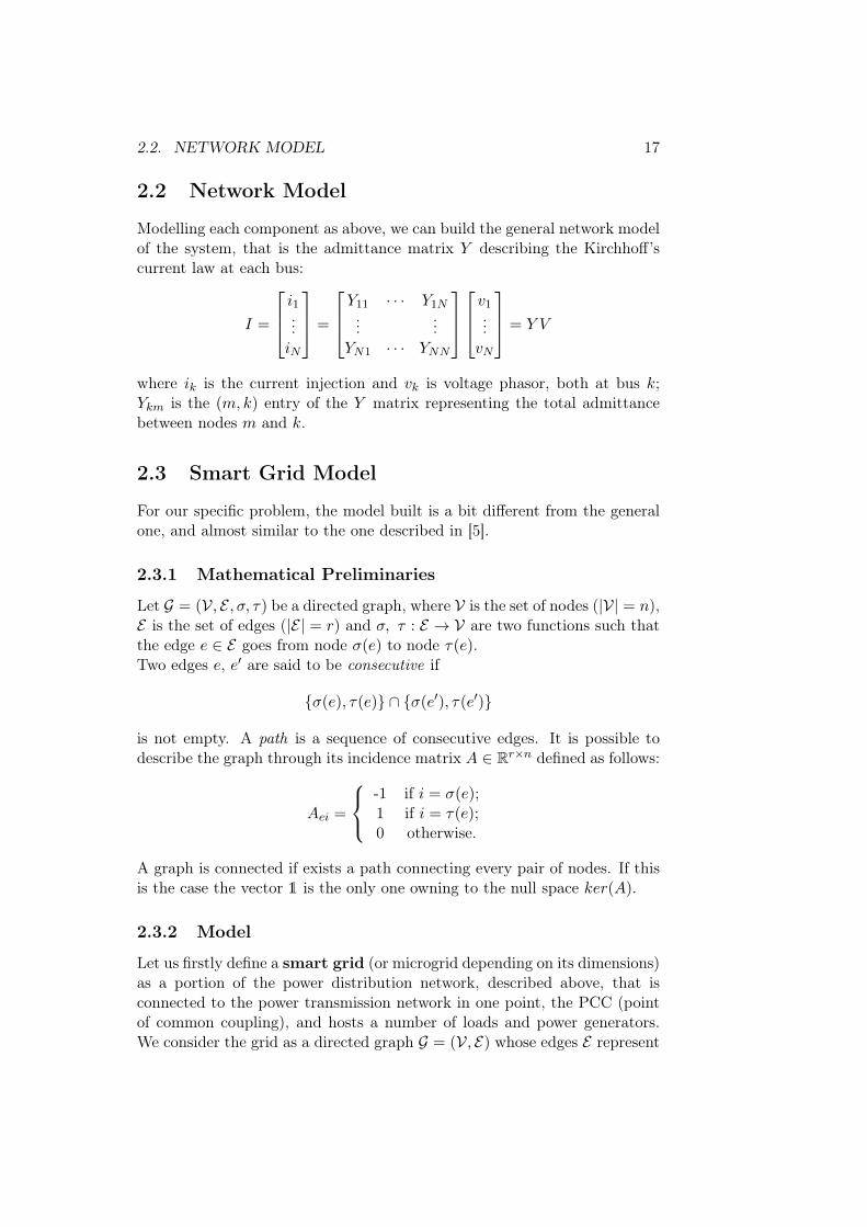
Power lines are commonly described via the π-model characterized by,see figure 2.4,
2.3. SMART GRID MODEL 19
• ze = re + jxe = 1ge+jbe
: line impedance;
• yshe : shunt admittance.
We neglect the shunt devices and consider only the line impedance ze.
Network elements: power lines
The most commonly adopted model for power lines is the π-model.
Power lines are described by their seriesimpedance
ze = re + jxe =1
ge + jbe, re , xe > 0
while we neglect shunt admittances.
σ(e) τ(e)ze
y she y sh
e
Power line equation
ξe =uσ(e) − uτ(e)
ze
Figure 2.4: Equivalent circuit for a power lines
It is easy to see that the power line is described by the equation
ξe =vσ(e) − vτ(e)
ze
For every edge e of the graph, we define by ze the impedance of the corre-sponding power line. We assume the following.
Assumption 1. All power lines in the microgrid have the same induc-tance/resistance ratio, i.e.
ze = ejθZ
for any e in ξ and for a fixed θ.Z is a diagonal real-valued matrix, whose elements are Zee = |ze|.
This assumption is satisfied when the grid is relatively homogeneous, andis reasonable in most practical cases (see for examples the IEEE standardtestbeds ([20]). The following physical constraints are satisfied by v, i, andξ
AT ξ + i = 0 (2.1)Av + Zξ = 0 (2.2)
where A is the incidence matrix introduced above; Z = diagze; e ∈ Erepresents the diagonal matrix of line impedances.Equation (2.1) corresponds to Kirchhoff’s current law (KCL) at the nodes,while equation (2.2) describes the voltage drop on the edges of the graph.From (2.1) and (2.2) we can olso obtain
i = ATZ−1Av = Lv (2.3)
where L represents the weighted Laplacian matrix of the graph, the nodaladmittance matrix in power system analysis.
20 CHAPTER 2. GRID MODELING
The PCC (point of common coupling) is modeled as a constant voltagegenerator
vPCC = VNejθ0 = V0 (2.4)
where VN is the nominal voltage and θ0 is an arbitrary fixed angle. In thepower system analysis terminology, node 0 is then a slack bus with fixedvoltage magnitude and angle.
Differently from PCC, Loads are considered to require a given amount ofactive and reactive power for example depending on the voltage amplitude vi.Examples of this are constant impedance loads and constant power loads. Todescribe in a unique way all different loads considered it is useful to exploitthe exponential model in which each node (except the PCC) is modeled viaa law relating the voltage vi and current ii. Specifically
viii = si
∣∣∣ viVN
∣∣∣ηi (2.5)
where si is the nominal complex power and ηi is a characteristic parameter.More specifically si is the value of the complex power that the node wouldinject into the grid if the voltage at its point of connection is equal to VN .The quantities
pv := <(sv) and qv := =(sv) (2.6)
are denoted as active and reactive power, respectively. The complex powersv corresponding to grid loads are such that pv < 0, meaning that posi-tive active power is supplied to the device; on the other hand, are such thatpv ≥ 0, as positive active power is injected into the grid. The parameterηi identify the device typology: for example constant power, constant cur-rent and constant impedance loads are described respectively by ηi = 0, 1, 2.See that generators fit this model for a parameter ηi = 0.
Finally, dealing with a low voltage power distribution network, trans-formers, both tap changers and phase shifters, are neglected.
The three equations (2.4), (2.5) and (2.3) individuate a system of nonlinear equation to be solved to determine the steady state of the grid startingfrom the knowledge of the grid topology (identify by L) and the power de-mand required by the nodes. This topic is extensively covered in literatureknown as Power Flow Analysis. To our purpose is completely indifferenthow the grid is solved and we will assume on the following to exploit somealgorithm that performs it.

2.4. TESTING SETUP: IEEE TEST FEEDERS 21
2.4 Testing setup: IEEE test Feeders
Here are presented the specific tests setup used through this thesis. Allalgorithm presented in the following has been tested on either one or both theIEEE37 or IEEE123 [20] Radial Distribution Test Feeder. More specificallythe graphs describing the mentioned test feeder are presented in figure 2.5.
The Institute of Electrical and Electronics Engineers, Inc.
IEEE 37 Node Test Feeder
(a) 37 nodes test feeder graph
The Institute of Electrical and Electronics Engineers, Inc.
IEEE 123 Node Test Feeder
(b) 123 nodes test feeder graph
Figure 2.5: Test Feeders graphs

22 CHAPTER 2. GRID MODELING

Chapter 3
State Estimation and ReactivePower Compensation
This chapter is divided in two parts, both of crucial importance dor thisthesis. In the first part we introduce and develop the estimation problem foran electric power grid. In the second one, we provide a formulation for thereactive power compensation problem.
3.1 Model and Estimation Problem Formulation
3.1.1 Model
Consider a graph G = (V, E) representing the grid, as described in chapter2, where V is the set of n nodes and E is the set of r edges.It is assumed that every node can measure its current and voltage dividedinto magnitude and phase, i.e.,
vmi = vi + evi ; evi ∼ N (0, σ2v);
θmi = θi + eθi ; eθi ∼ N (0, σ2θ);
imi = ii + eii ; eii ∼ N (0, σ2i );
φmi = φi + eφi ; eφi ∼ N (0, σ2φ);
where evi , eθi , eii and eφi represent the error introduced by the measureitself1. All the measurements are assumed to be independent from eachother. Collecting all the measurements in vectors one can write
V m := V + eV ;Θm := Θ + eΘ;Im := I + eI ;Φm := Φ + eΦ
1In a real set up every node of the grid is equipped by a PMU(Phasor MeasurementUnit).
23

24CHAPTER 3. STATE ESTIMATION ANDREACTIVE POWER COMPENSATION
where, we recall, (see notations page 13)
V m =
vm1...vmN
;V =
v1...vN
; eV =
ev1...evN
;
and where Θm, Θ, eΘ, Im, I, eI , Φm, Φ and eΦ are defined similarly.Now let us define the noise vector e = [eV eΘ eI eΦ]T . Then the correlationmatrix R for the noise is
R = E[eeT ] =
σ2vIn
σ2θIn
σ2i In
σ2φIn
We define the state of the grid as the voltage magnitude and phase at
every node. Then, it is well known thatV m = V + eV ;Θm = Θ + eΘ;Im = f(V,Θ) + eI ;Φm = g(V,Θ) + eΦ
(3.1)
where, generally, f(·) and g(·) represent non linear current’s dependance onthe state.
Assumption 2. Measurements are taken all at the same time instant. There-fore there is no synchronization noise.
In this thesis it is not considered, but it is not very difficult to includealso the synchronization noise in this model. (see [21])
3.1.2 Estimation Problem Formulation
In general, we can say that the state estimation problem in an electric grid isreduced as a Weighted Least Squares Problem (see [14],[17]). Following thisway, we can define this cost function depending on the measurements
J(V,Θ) =[V m Θm Im Φm
]R−1
V m
Θm
Im
Φm
(3.2)
that is, explicitly,
J(V,Θ) =
n∑i=1
1
σ2v
(vmi − vi)2 +1
σ2θ
(θmi − θi)2 +1
σ2i
(imi − f(V,Θ))2 +
+1
σ2φ
(φmi − g(V,Θ))2

3.1. MODEL AND ESTIMATION PROBLEM FORMULATION 25
Eventually, if measurements of other nature are available, i.e. power (realand reactive) injected, power flow exc..., they can be added to expression in(3.2).As a matter of fact, we want to underline that a novelty of this work staysjust in discarding them and using only current and voltage measures.
In order to estimate the state, we have to find the value (V , Θ) of (V,Θ)that minimizes the objective cost function, that is, to find the solution forthe optimization problem
minV,Θ
J(V,Θ) (3.3)
The nonlinear dependance of I and Φ on V and Θ drives the aboveoptimization problem into the nonlinear unconditioned class of problems.To solve it we can find a lot of techniques in the literature. For instance, allmethods based on the augmented Lagrangian technique.However, this kind of algorithm may suffer of one of these disadvantages:
• the algorithm does non converge;
• the algorithm converge to a local but not global minima;
• the algorithm converge to the global minima but it requires a very longrunning time to achieve the convergence.
In this thesis, in order to deal with the optimization problem in (3.3), wepursue an approach based on a suitable linearized model of the electric grid.Interestingly we will see how the linear model leads to a convenient closedform solution.
3.1.3 Model Linearization
In the previous chapter we exploited the relation between complex valuecurrent and voltage of the grid
i = Lu (3.4)
where L = ATZ−1A represents the admittance matrix of the grid; being Aand Z, respectively, the incidence and inductance matrix of the grid (seechapter 2).
The basic idea to obtain a linear model is based on expressing the quanti-ties of interest as function either of the real or imaginary part of the voltage,instead of the actual representation, based on magnitude and phase. Split-ting relation (3.4) into real and imaginary part we can obtain, for a singlenode, (see page 13)
h+ jk = [<(L) + j=(L)] ∗ (s+ jr) = [<(L)s−=(L)r] + j[=(L)s+ <(L)r]
26CHAPTER 3. STATE ESTIMATION ANDREACTIVE POWER COMPENSATION
that can be rewritten in a matrix form as[hk
]=
[<(L) −=(L)=(L) <(L)
] [sr
]Collecting all nodes values, the whole measures model becomes (see notationspage 13)
SRHK
=
In 00 In<(L) −=(L)=(L) <(L)
[XY]
+
eSeReHeK
Z = H · X + e (3.5)
where eS , eR, eH and eK denotes the noises of the measures with re-spect to the real and imaginary parts; Z denotes the measures vector and Hdenotes the model matrix and e the noises vector.
Note that (3.5) represents a suitable linear model for the measures withrespect to the new state variables, that are the real and imaginary partof the nodes voltage.
To manage correctly this new representation, it is necessary to expressthe noise in a suitable form, starting from the knowledge of the standard de-viation of magnitude and phase measures. The noise expressed in this newform is, in fact, textbfno more uncorrelated because, in general, part of themagnitude and phase noise will be reprojected into both real and imaginarypart.
In order to understand this fact consider two generic vectors
x = ρejψ = ρ(cosψ + j sinψ);
x = ρejψ = (ρ+ δρ)ej(ψ+δψ) = (ρ+ δρ)(cos(ψ + δψ) + j sin(ψ + δψ))
where, clearly, δρ and δψ represent a sort of error affecting the exact valuesρ and ψ. It is possible to rewrite x, exploiting some trigonometric relations,as
x = ρ(cosψ + j sinψ) cos δψ + δρ(cosψ + j sinψ) cos δψ −−ρ(sinψ − j cosψ) sin δψ − δρ(sinψ − j cosψ) sin δψ
To simplify the expression above we assume δψ small enough and, usingthe McLaurin expansion for the sine and cosine functions, we get
x ' ρ(cosψ + j sinψ)(
1− δψ2
2
)+ δρ(cosψ + j sinψ)
(1− δψ2
2
)−
−ρ(sinψ − j cosψ)δψ − δρ(sinψ − j cosψ)δψ
3.1. MODEL AND ESTIMATION PROBLEM FORMULATION 27
Finally, taking a first order approximation, we get
x ' ρ(cosψ + j sinψ) + δρ(cosψ + j sinψ)− ρ(sinψ − j cosψ)δψ
' x+ (δρ cosψ − ρ sinψ δψ) + j(δρ sinψ + ρ cosψ δψ)
that can be rewritten in a matrix form as
x ' x+
[cosψ − sinψsinψ cosψ
] [δρρ δψ
](3.6)
Equation (3.6) highlights the approximation exploited to project the errormeasured in phase and magnitude into real and imaginary component.
Managing our error variables in a similar way, we can obtain (see [21])the new noise correlation matrix:
R =
σ2<(V )In σ<(V )=(V )In σ<(V )<(I)In σ<(V )=(I)In
σ=(V )<(V )In σ2=(V )In σ=(V )<(I)In σ=(V )=(I)In
σ<(I)<(V )In σ<(I)=(V )In σ2<(I)In σ<(I)=(I)In
σ=(I)<(V )In σ=(I)=(V )In σ=(I)<(I)In σ2=(I)In
where for all i ∈ 1...n, the diagonal block are equal to
σ2<(V ) = σ2
v cos2 θ + σ2θ(v
mi )2 sin2 θ;
σ2=(V ) = σ2
v sin2 θ + σ2θ(v
mi )2 cos2 θ;
σ2<(I) = σ2
i cos2 φ+ σ2φ(imi )2 sin2 φ;
σ2=(I) = σ2
i cos2 φ+ σ2φ(imi )2 cos2 φ;
representing the autocorrelation between quantities. The cross correlationbetween the real and imaginary part of the voltage is
σ<(V )=(V ) =(σ2v − σ2
θ(vmi )2
)sin θ cos θ = σ=(V )<(V ).
Similarly the correlation between real and imaginary part of the current is
σ<(I)=(I) =(σ2i − σ2
φ(imi )2)
sinφ cosφ = σ=(I)<(I).
3.1.4 Closed Form Solution
Consider the linear model in (3.5), i.e,
Z = HX + e
It is possible to rewrite the objective cost function J(V,Θ) as
J(X) =[Z −HX
]TR−1
[Z −HX
](3.7)

28CHAPTER 3. STATE ESTIMATION ANDREACTIVE POWER COMPENSATION
This cost function, being a linear function of the decision variable X, reducesto the classical linear weighted least squares problem. It is well known that,if the matrix (HTR−1H) is not singular, then the optimal solution X can beobtain in a closed form as
X = (HTR−1H)−1HTR−1Z (3.8)
Dealing with Gaussian additive noise this solution coincides with the maxi-mum likelihood estimation.
3.1.5 HTR−1H structure
This matrix does not assume a suitable form to be studied with some al-gebraic method. Anyway, a deep empirical analysis shows not only its in-vertibility but moreover its definite positivity as well. This assure the appli-cability of the algorithm proposed in most of the practical situations. (see[21])
3.2 Reactive Power Compensation
As explained in the Introduction, reactive power compensation is one of thekey-problems in which are involved the electric grids. Now we want to presenta control strategy similar to the one in [5]. Nevertheless, differently from [5],we will not suppose to have perfect measurements, but instead we want todeal with our noise measurements. Of course we cannot use them directlyin the algorithm, because raw data are usually subject to these problems:
• they are too inaccurate;
• they can collect outliers.
This leads to the use of filter data able to let the control algorithm efficientlywork.To this point of view, the estimation represents the filtering of the measure-ments to achieve a better knowledge of the real state of the grid. It is thefirst necessary step to deal with a good control strategy.
Let us introduce the optimal reactive power flow problem, exploitingwhat done in [5], to better understand it.
3.2.1 Problem Formulation
The metric, for the optimality of reactive power flows, is considered to bethe active power losses on the power lines. The total active power losses on

3.2. REACTIVE POWER COMPENSATION 29
the edges are then equal to
J ,∑e∈E|ξe|2<(ze) = uT<(L)u
It is assumed to be possible to command only a subset C ⊂ V of the nodesof the grid, named compensators. A part of them is assumed to be equippedwith some sort of intelligence, as shown in figure 3.1 (uupper panel). In ad-dition to this, we can work only on the amount of reactive power injected,as the decision on the amount of active power follows imperative economiccriteria.
The problem of optimal reactive power injection at the compensators canbe expressed as a quadratic, linearly constrained problem, in the form
minq
J(q), where J(q) =1
2qTRe(X)q (3.9)
subject to 1T q = 0
qv = Im(sv), v ∈ V \ C,Im(sv), v ∈ V \ C being the nominal amount of reactive power injected bythe nodes that cannot be commanded.The challenging part to solving the problem is that each node has only localinformation.
To appropriately drive the microgenerators, the algorithm provided in [5]implements a distributed optimal reactive power compensation. Specificallythe microgenerators are assumed to be organized into overlapping groups,namely clusters, each of which coordinated by a cluster header equipped withsome intelligence unit (see figure 3.1).
3.2.2 Dual decomposition
In order to derive a control strategy to solve the ORPF problem, we apply thetool of dual decomposition to (3.9). While problem (3.9) might not be convexin general, we rely on the result presented in [22], which shows that zeroduality gap holds for the ORPF problems, under some conditions that arecommonly verified in practice. Based on this result, we use an approximateexplicit solution of the nonlinear equations to derive a dual ascent algorithmthat can be implemented by the agents. In order to present the approximatesolution, we need the following technical lemma.
Lemma 3. Let L be the complex valued Laplacian L := ATZ−1A. Thereexists a unique symmetric matrix X ∈ Cn×n such that
XL = I − 11T0X10 = 0
(3.10)

30CHAPTER 3. STATE ESTIMATION ANDREACTIVE POWER COMPENSATION5
Ele
ctri
cne
twor
kG
raph
mod
elC
ontr
ol
uv
iv
ξe
ze
v
σ(e) τ(e)
e
0
Ci
Cj
Ck
Figure 1. Schematic representation of the microgrid model. In the lower panel a circuit representation is given, where black
diamonds are microgenerators, white diamonds are loads, and the left-most element of the circuit represents the PCC. The
middle panel illustrates the adopted graph representation for the same microgrid. Circled nodes represent compensators (i.e.
microgenerators and the PCC). The upper panel shows how the compensators can be divided into overlapping clusters in order
to implement the control algorithm proposed in Section IV. Each cluster is provided with a supervisor with some computational
capability.
number y = |y|ej∠y whose absolute value |y| corresponds to the signal root-mean-square value, and
whose phase ∠y corresponds to the phase of the signal with respect to an arbitrary global reference.
In this notation, the steady state of a microgrid is described by the following system variables (see
Figure 1, lower panel):
• u ∈ Cn, where uv is the grid voltage at node v;
• ι ∈ Cn, where ιv is the current injected by node v;
April 15, 2012 DRAFT
Figure 3.1: Different schematic view of the grid. upper panel: division of mi-crogenerators into overlapping clusters to implement the distributedalgorithm. middle panel: graph representation. Circled nodes rep-resent microgenerators. lower panel: circuit representation. Blackdiamonds are microgenerators and white are loads.
where, we recall, [10]v = 1 for v = 0, and 0 otherwise and I is the identitymatrix.
This matrix X depends only on the topology of the microgrid power linesand on their impedance.The effective impedance, Zeffuv, of the power lines for every pair of nodes (u,v) can be represented by the following:
|Z|effuv = (1u − 1v)TX(1u − 1v) (3.11)
3.2.3 Distributed algorithm
The algorithm proposed in [5] is based only on a local knowledge, thereforeany central controller is not needed. The algorithm can be distributed acrossthe agents of the microgrid, that consist in decomposing the optimizationproblem into smaller issues.

3.2. REACTIVE POWER COMPENSATION 31
All the compensators are divided into ` possibly overlapping sets C1, . . . , C`,with
⋃`i=1 Ci = C and the nodes of the same set, called cluster, are able to
communicate to each other, and they are therefore capable of coordinatingtheir actions and sharing their measurements.The proposed optimization algorithm consists of the following repeated steps:
1. a set Ci(t) is chosen at a certain discrete time t = 0, 1, 2, . . . wherei(t) ∈ 1, . . . , `;
2. the agents in Ci(t), by coordinating their actions and communicating,determine the new feasible state that minimizes J(q), solving the op-timization subproblem in which all the nodes that are not in Ci(t) keeptheir states constant;
3. the agents in Ci(t) actuate the system by updating their state (theinjected reactive power).
Partitioning q as
q =
[qCqV\C
]where qC ∈ Rm are the controllable components and qV\C ∈ Rm−n are notcontrollable. According to this partition of q, it is possible also the partitionof the matrix
<(X) =
[M NN Q
](3.12)
Introduced also the matrices m×m
Ω :=1
2m
∑h,k∈C
(1h − 1k)(1h − 1k)T = I − 1
m11T ,
Ωi :=1
2|Ci|∑h,k∈Ci
(1h − 1k)(1h − 1k)T =
= diag(1Ci)−1
|Ci|1Ci1
TCi
When the cluster Ci is fired its nodes perform th optimization:
qopt,iC := arg minq′C∈qC+Si
J(q′C , qV\C) = qC − (ΩiMΩi)#∇J, (3.13)
where∇J = MqC +NqV\C = [Re(X)q]C ∈ Rm (3.14)
is the gradient of J(qC , qV\C) with respect to the decision variables qC .This is computed via a distributed way:if h /∈ Ci then
[qopt,iC
]h
= qh, if instead h ∈ Ci then:[qopt,iC
]h
= qh −∑k∈Ci
[(ΩiMΩi)
#]hk
[∇J ]k (3.15)
32CHAPTER 3. STATE ESTIMATION ANDREACTIVE POWER COMPENSATION
The Hessian matrix can be computed a priori thanks only to local knowl-edge of the mutual effective impedances between pairs compensators.Defining Reff
hk = <(Zeffhk) through some computation is obteined that:
ΩiMΩi = −1
2ΩiR
effΩi. (3.16)
Assume that nodes in Ci can measure the grid voltage at their point ofconnection. Each agent k ∈ Ci compute
ν(i)k :=
1
|Ci|∑v∈Ci|uv||uk| sin(∠uk − ∠uv − θ) (3.17)
After some computations is it possible to write the estimate gradient as:
[∇J ]k = − cos θ(Im(1TkXs)) (3.18)
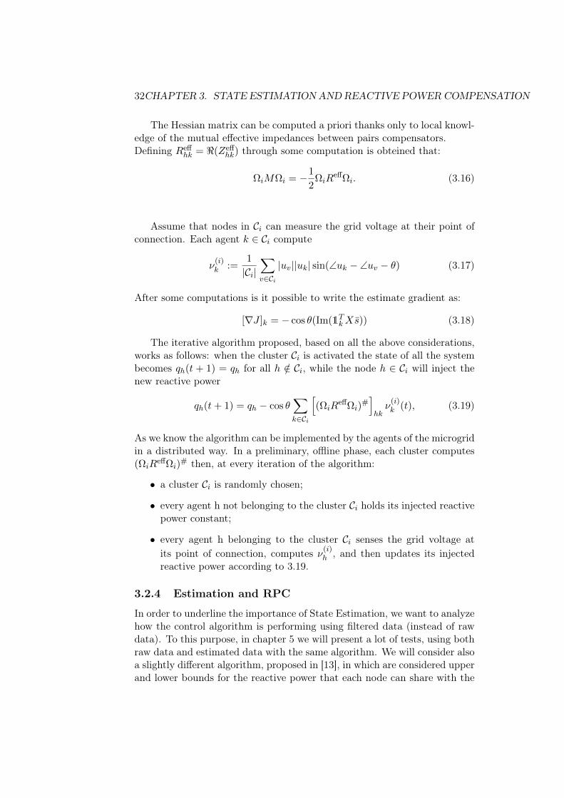
The iterative algorithm proposed, based on all the above considerations,works as follows: when the cluster Ci is activated the state of all the systembecomes qh(t + 1) = qh for all h /∈ Ci, while the node h ∈ Ci will inject thenew reactive power
qh(t+ 1) = qh − cos θ∑k∈Ci
[(ΩiR
effΩi)#]hkν
(i)k (t), (3.19)
As we know the algorithm can be implemented by the agents of the microgridin a distributed way. In a preliminary, offline phase, each cluster computes(ΩiR
effΩi)# then, at every iteration of the algorithm:
• a cluster Ci is randomly chosen;
• every agent h not belonging to the cluster Ci holds its injected reactivepower constant;
• every agent h belonging to the cluster Ci senses the grid voltage atits point of connection, computes ν(i)
h , and then updates its injectedreactive power according to 3.19.
3.2.4 Estimation and RPC
In order to underline the importance of State Estimation, we want to analyzehow the control algorithm is performing using filtered data (instead of rawdata). To this purpose, in chapter 5 we will present a lot of tests, using bothraw data and estimated data with the same algorithm. We will consider alsoa slightly different algorithm, proposed in [13], in which are considered upperand lower bounds for the reactive power that each node can share with the

3.2. REACTIVE POWER COMPENSATION 33
others. Thanks to those test, we will be able to show that the performancesof the algorithm using the estimated state are comparable to those obtainedusing the grid real state (with no noise), while raw measurements cause analgorithm behaviour totally undesirable.

34CHAPTER 3. STATE ESTIMATION ANDREACTIVE POWER COMPENSATION

Chapter 4
Distributed EstimationAlgorithms
We now propose two completely distributed and scalable algorithms inorder to solve the estimation problem presented in the previous chapter. Thefirst one is the ADMM Estimator, for which we will prove the convergenceto the optimal value, while the second is the Jacobi-approximate Estimator,a faster distributed algorithm, very useful if there is the concrete possibilityto employ better resources in some grid measurements.
Before describing the distributed algorithms, however, it is importantto investigate on why it is preferable to implement this kind of algorithmsrespect to the centralized ones. There are a lot of advantages, not only fromthe economical point of view, in managing whatever problem, if it is possible,in a distributed way:
• we can avoid the huge computational effort, growing with the grid size,of a centralized algorithm. Distributed algorithm are much "lighter"from the computational point of view.
• we do not need to employ a central intelligence with which supervise theentire grid, as for a distributed algorithm is sufficient a local knowledge.
• from the robustness point of view, imagine that an error occurs duringthe running of the centralized algorithm. Then the entire procedurefails and no information will be computed. In a distributed algorithmdifferent procedures are computed separately (often in an asynchronousway), so the robustness is improved a lot.
4.1 Multi Area Decomposition
Let us introduce a decomposition for the grid suitable for the algorithmsthat are going to be presented.
35

36 CHAPTER 4. DISTRIBUTED ESTIMATION ALGORITHMS
Let us divide the grid into m non overlapping subset. Each subset rep-resents a microgrid. Adjacent areas are supposed to be connected throughtie lines, called border lines, as shown in figure 4.1.
Figure 4.1: Grid divided into non overlapping areas
For each area a ∈ [1, ...,m] we have:
Xa internal state;
Za internal measures;
La internal inductance matrix (describing the internal topology);
Let Ωa ⊂ [1, ...,m] be the subset of adjacent areas of a.Then, for each b ∈ Ωa we have:
Zab measures of the nodes of area b that direct communicate with somenode of area a;
Lab inductance matrix between area a and b ∈ Ωa (describes the communi-cation topology).
Figure 4.2 well explain the quantities introduced.
Figure 4.2: Information relating two adjacent areas

4.2. ALTERNATING DIRECTION MULTIPLIER METHOD 37
4.2 Alternating Direction Multiplier Method
The first solution we propose is based on the Alternating Direction MultiplierMethod (ADMM). This is an optimization technique based on the iterativesolution of an augmented Lagrangian problem.
It is well known from the literature that the the classical ADMM, be-cause of its structure, can be implemented in a distributed way. However,the flow of informations through different areas do not concern only localinformations, but global informations. This is a crucial point, that does notmake the algorithm scalable.
The novelty of our solution is based on [12] and on [21]. We will show howto implement a local and scalable ADMM algorithm to solve the estimationproblem, and moreover we will show a complete proof about its convergenceto the solution of the equation (3.8).
Let us firstly introduce the classical ADMM procedure. Afterwards wewill present the scalable solution proposed.
4.2.1 ADMM classical
Considering the system 3.5, let us introduce a new notation, more suitablefor the ADMM algorithm that we are going to show, imposing
m =
m(1)
...m(N)
≡ Z; A =
A11 · · · A1N...
...AN1 · · · ANN
≡ H;
X =
x1...xN
≡ X; R =
R1
. . .RN
≡ R.It is possible to define the quadratic function, based on these new matri-
ces, more specifically on each row or block of rows,
fi(X) =( N∑j=1
Aijxj −m(i))TR−1i
( N∑j=1
Aijxj −m(i))
Collecting all function fi, ∀i = 1 . . . N , is easy to get
F (X) =
N∑i=1
fi(X) =(AX −m
)TR−1
(AX −m
)(4.1)
whose optimal solution, X, is the well known
X =(ATR−1A
)−1ATR−1m
38 CHAPTER 4. DISTRIBUTED ESTIMATION ALGORITHMS
Let us define X(i), i ∈ [1, . . . , N ], as the ith copy of the vector X, owningto area i. Thanks to this it is possible to rewrite the minimization problemreferred to equation in (4.1) as
minimizeX(1)···X(N)
N∑i=1
fi(X(i)
)s.t. X(i) = X(j) ∀j ∈ Ni ∪ i
where Ni represents the subset of indices of areas adjacent to area i, butexcluding area i itself.
It is then possible to solve the minimization problem through the aug-mented Lagrangian technique, introducing some redundant bonds that allowus to manage the solution with the ADMM algorithm, as
minimizeX(1)···X(N)
N∑i=1
fi(X(i)
)s.t. X(i) = zij ; X
(i) = zji ∀j ∈ Ni ∪ i
The correspondent Lagrangian function is
L =N∑i=1
fi(X(i)
)+
N∑i=1
∑j∈Ni∪i
λTij(X(i) − zij
)+ µTij
(X(i) − zji
)+
+c
2
N∑i=1
∑j∈Ni∪i
||X(i) − zij ||2 + ||X(i) − zji||2
This function can be solved through ADMM algorithm, which consistsof three main updating steps:
1. λij(t) = λij(t− 1) + c
(X(i)(t)− zij(t)
)µij(t) = µij(t− 1) + c
(X(i)(t)− zji(t)
) (4.2)
2.X(i)(t+ 1) = arg min
X(i)
L(X, z(t), λ(t), µ(t)) (4.3)
3.zij(t+ 1) = arg min
zijL(X(t+ 1), z, λ(t), µ(t)) (4.4)
With some manipulations of the updating step (proof is reported in theappendix A) it is possible to rewrite the algorithm in a simpler way consistingof only two updating step:
1.λij(t) = λij(t− 1) +
c
2
(X(i)(t)−X(j)(t)
)(4.5)
4.2. ALTERNATING DIRECTION MULTIPLIER METHOD 39
2.X(i)(t+ 1) = arg min
X(i)
L(X,λ(t)) (4.6)
In this algorithm every area estimates the entire grid state, therefore theflow of informations between areas is global and not local.
We are interested, instead, in a kind of algorithm in which every area isable to compute its inner state X(i) in a distributed and local fashion, i.e.only from the knowledge of its adjacent areas state.
4.2.2 ADMM scalable with Projector matrices
The first formulation we propose is the one in [21]. Let us start from theusual state of the art formulation of ADMM minimization problem
minimizeX(1)···X(N)
N∑i=1
fi(X(i)
)s.t. X(i) = zij ; X
(i) = zji ∀i = 1 . . . N, ∀j ∈ Ni
(4.7)We remind that X(1), . . . , X(N) are local copies of X
X =
x1...xN
where xi represents the inner state of area i.
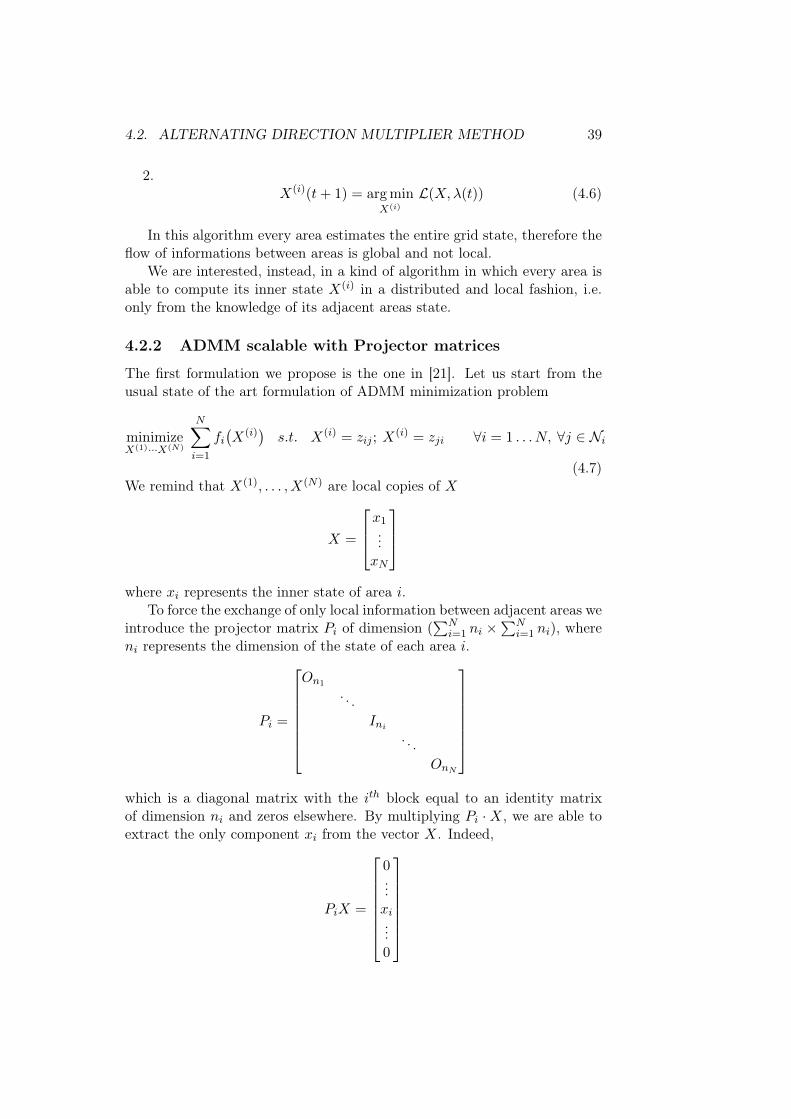
To force the exchange of only local information between adjacent areas weintroduce the projector matrix Pi of dimension (
∑Ni=1 ni ×
∑Ni=1 ni), where
ni represents the dimension of the state of each area i.
Pi =
On1
. . .Ini
. . .OnN
which is a diagonal matrix with the ith block equal to an identity matrixof dimension ni and zeros elsewhere. By multiplying Pi ·X, we are able toextract the only component xi from the vector X. Indeed,
PiX =
0...xi...0
40 CHAPTER 4. DISTRIBUTED ESTIMATION ALGORITHMS
Similarly it is possible to define the joint projector
Pij =
Pi i = j
Pi + Pj i 6= j
Note that, using the projector matrices, it is possible to rewrite the initialproblem as
minimizeX(1)···X(N)
N∑i=1
fi(X(i)
)(4.8)
s.t. PijX(i) = Pijzij ; PijX
(i) = Pijzji ∀i = 1 . . . N, ∀j ∈ Ni
where the P matrices forces to involve only local information between adja-cent areas.
From the previous proofs it is known that:
• λij(t) = λij(t− 1) + c2
(X(i)(t)−X(j)(t)
);
• zij(t) = X(i)(t)+X(j)(t)2 ;
• λij(t) = µij(t) = −λji(t) = −µji(t) ∀t;
In addition, it is known that zij = zji, and so it is possible to rewrite theLagrangian as
L(X, z, λ) =N∑i=1
fi(X(i)
)+
N∑i=1
∑j∈Ni∪i
[2λTijPij
(X(i)−zij
)+c(X(i)−zij)TPij(X(i)−zij)
]By eliminating the constant terms and using the previous equations, we get
X(i)(t+1) = arg minX(i)
fi(X
(i))+∑
j∈Ni∪iX(i)TPij
(2λij(t)+cX
(i)−2czij(t))
Finally, through the first order optimality condition, we can obtain the op-timal updating step in a closed form solution
X(i)(t+ 1) =(A(i)TR−1
i A(i) + cMi
)−1[A(i)TR−1
i m(i) + U (i)(t)− Λ(i)(t)]
where
Mi =∑
j∈Ni∪iPij
Λ(i)(t) = Miλij(t)
U (i)(t) = cMizij(t)
Note that

4.2. ALTERNATING DIRECTION MULTIPLIER METHOD 41
• if Pi = I ∀i = 1 . . . N, the algorithm turn to be equal to classicalimplementation (4.7);
• This particular formulation of ADMM is completey local. Indeed, inMi, Ui, Λi is considered only local information, (terms depending onj ∈ Ni), so the remaining parts of the vector could be neglected in thecomputation. This makes the algorithm fully scalable and local;
4.2.3 ADMM scalable and compact
By inspecting the Pi matrices, it is easy to note that each one of them is asparse matrix. Indeed the larger part of its components is equal to 0 dueto the non-communication between non-adjacent areas. Now we want tore-write this scalable algorithm in a more compact way, considering only thecomponents really involved in the minimization each time. Given
X(i) =
x(i)1...x
(i)N
as a local copy of X owning to area i, the quadratic function we have tominimize is
fi(X(i)) =
( ∑j∈Ni∪i
Aijx(i)j −m(i)
)TR−1i
( ∑j∈Ni∪i
Aijx(i)j −m(i)
)hence we can write
fi(X(i)) = fi(x
(i)j ) ∀j ∈ Ni ∪ i
We define the vector Y (i), that collects in a compact way all the statesuseful for area i, that are x(i)
i and all the x(i)j ∀j ∈ Ni
Y (i) =
x(i)i
x(i)j
j∈Ni
To be precise, this notation does not respect the sorting of the vector com-ponents, because i = 1 . . . N . Formally we should write
Y (i) =
x
(i)j1...
x(i)j|Ni|+1
i ∈ j1, . . . , j|Ni|+1
but the previous notation is much simpler and clear, so we will use that one,generalizing for every i = 1 . . . N .

42 CHAPTER 4. DISTRIBUTED ESTIMATION ALGORITHMS
Now it is possible to rewrite the initial problem as
minimizeY (1)···Y (N)
N∑i=1
fi(Y (i)
)(4.9)
s.t. x(i)j = x
(j)j ; x
(i)i = x
(j)i ∀i = 1, . . . , N, ∀j ∈ Ni
Applying the ADMM procedure to this problem and exploiting the first orderoptimality conditions, one can obtain the closed form solution, which is equalto
Y (i)(t+ 1) =[(A(i)TR−1
i A(i) + cMi
)]−1[A(i)TR−1
i m(i) + U (i)(t)− Λ(i)(t)]
where
• A is obtained due to "compacting" the matrix A(i), considering onlynon-zero columns, that are Aij columns with j ∈ Ni.(ex. A(i) = [Ai1 0 Ai3 Ai4 0 · · · 0] =⇒ A(i) = [Ai1 Ai3 Ai4]);
• Mi is obtained due to "compacting" the term Mi =∑
j∈NiPij into a
matrix of dimension |Ni + 1| × |Ni + 1|, with |Ni| + 1 in the positioncorresponding to index i and 1 in the position corresponding to indexesj, j ∈ Ni;
The other terms involved in the minimization are
U (i)(t) =
u(i)i (t)
u(i)j (t)
j∈Ni
=
c2
∑j∈Ni
(x
(i)i (t) + x
(j)i (t)
)c2
(x
(i)j (t) + x
(j)j (t)
)j∈Ni
Λ(i)(t) =
λ(i)i (t)
λ(i)j (t)
j∈Ni
=
λ(i)i (t− 1) + c
2
∑j∈Ni
(x
(i)i (t)− x(j)
i (t))
λ(i)j (t− 1) + c
2
(x
(i)j (t)− x(j)
j (t))
j∈Ni
In order to show explicitly the distributed and asynchronous propertiesof this algorithm, we provide the explicit ADMM procedure for this formu-lation.
First of all we can write the minimization problem adding to the con-straints some redundant variables that allow as to manage the solution withthe ADMM algorithm:
minimizeY (1)···Y (N)
N∑i=1
fi(Y (i)
)(4.10)
s.t. x(i)i = z
(i,j)i ; x
(i)j = z
(i,j)j
x(i)i = z
(j,i)i ; x
(i)j = z
(j,i)j ∀i = 1, . . . , N, ∀j ∈ Ni

4.2. ALTERNATING DIRECTION MULTIPLIER METHOD 43
This formulation leads to a Lagrangian function equal to
L =
N∑i=1
fi(Y (i)
)+
∑j∈Ni∪i
[λ
(i,j)i
(x
(i)i − z
(i,j)i
)+ λ
(i,j)j
(x
(i)j − z
(i,j)j
)]+
+∑
j∈Ni∪i
[µ
(i,j)i
(x
(i)i − z
(j,i)i
)+ µ
(i,j)j
(x
(i)j − z
(j,i)j
)]+
+c
2
∑j∈Ni∪i
[||x(i)
i − z(i,j)i ||2 + ||x(i)
j − z(i,j)j ||2 + ||x(i)
i − z(j,i)i ||2 + ||x(i)
j − z(j,i)j ||2
]
The ADMM updating steps are:
1. λ
(i,j)i (t) = λ
(i,j)i (t− 1) + c
(x
(i)i (t)− z(i,j)
i (t))
λ(i,j)j (t) = λ
(i,j)j (t− 1) + c
(x
(i)j (t)− z(i,j)
j (t))
µ(i,j)i (t) = µ
(i,j)i (t− 1) + c
(x
(i)i (t)− z(j,i)
i (t))
µ(i,j)j (t) = µ
(i,j)j (t− 1) + c
(x
(i)j (t)− z(j,i)
j (t)) (4.11)
2.Y (i)(t+ 1) = argmin
Y (i)
L(Y (i), z(t), λ(t), µ(t)) (4.12)
3.z(t+ 1) = argmin
zL(Y (i)(t+ 1), z, λ(t), µ(t)) (4.13)
where, in the last two steps, for λ, µ and z we mean respectively all thevariables λ(∗,∗)
∗ , µ(∗,∗)∗ and z(∗,∗)
∗ involved in the lagrangian term.We suppose that node i has in memory:
Y (i)(t) =
x(i)i (t)
x(i)j (t)
j∈Ni
; Z(i)(t) :=
z(i,j)i (t)
z(i,j)j (t)
j∈Ni
Λ(i)(t) =
λ(i,j)i (t)
λ(i,j)j (t)
j∈Ni
; M(i)(t) :=
µ(i,j)i (t)
µ(i,j)j (t)
j∈Ni
Before doing step (4.11), it is clear that we need a sharing, and hence a
communication between neighbour nodes, because of the usage of the termsz
(j,i)i and z(j,i)
j , that are in the memory of the node j but not in the i’s one.Thanks to this, by inspecting the lagrangian function it is easy to note
that the minimization step in (4.12) can be done asynchronously by thealgorithm, because the terms involved in the minimization belong all to thearea i.
44 CHAPTER 4. DISTRIBUTED ESTIMATION ALGORITHMS
Finally, before doing step (4.13), asynchronously as before, we need asharing between neighbour areas again. Indeed, considering for example theminimization in which are involved the terms z(i,j)
j , we have
z(i,j)j (t+ 1) = argmin
z(i,j)j
L(Y (t+ 1), z(i,j)j , λ(t), µ(t))
Discarding terms that are not depending on z(i,j)j , the minimization becomes
z(i,j)j (t+ 1) = argmin
z(i,j)j
λ
(i,j)j (t)
(x
(i)j (t+ 1)− z(i,j)
j (t+ 1))
+c
2||x(i)
j (t+ 1)− z(i,j)j (t+ 1)||2 +
+µ(j,i)j (t)
(x
(j)j (t+ 1)− z(i,j)
j (t+ 1))
+c
2||x(j)
j (t+ 1)− z(i,j)j (t+ 1)||2
exploiting the first order optimality condition, we obtain
z(i,j)j (t+ 1) =
x(i)j (t+ 1) + x
(j)j (t+ 1)
2−λ
(i,j)j (t) + µ
(j,i)j (t)
2c
From this it is clear that we need to know the termsx
(j)j (t + 1)
j∈Ni
andµ
(j,i)j (t)
j∈Ni
. With a similar process it is easy to demonstrate that in the
computation of the variables z(j,i)j it is necessary to know the terms x(j)
j (t+1)
and λ(j,i)j (t). Therefore we need a sharing of these terms, because they are
not in the memory of the node i.We have shown a fundamental property: this algorithm works completely
in ad asynchronous way, hence the minimization steps are completely sepa-rable in a distributed way.
4.2.4 Convergence of ADMM scalable
In this subsection we will show that the ADMM scalable converges to theoptimal solution for the problem 4.1. The proof exploits the work done in[23], which treats problems in the form
minimizex,z
F (x) +G(z) (4.14)
subject to Ax+Bz = c
with variables x ∈ Rn and z ∈ Rm, where A ∈ Rp×n, B ∈ Rp×m andc ∈ Rp.
We know that, from [23], under these assumptions the algorithm con-verges to the optimal value for (4.14), that is:
p∗ = infF (x) +G(z) | Ax+Bz = c
4.2. ALTERNATING DIRECTION MULTIPLIER METHOD 45
After formulating the augmented Lagrangian
Lρ(x, z, λ) = F (x) +G(z) + λT (Ax+Bz − c) + (ρ/2)||Ax+Bz − c||22
we can write the ADMM iterations, that are
λk := λk−1 + ρ(Axk +Bzk − c)xk+1 := argmin
xLρ(x, zk, λk)
zk+1 := argminz
Lρ(xk+1, z, λk)
where ρ > 0.
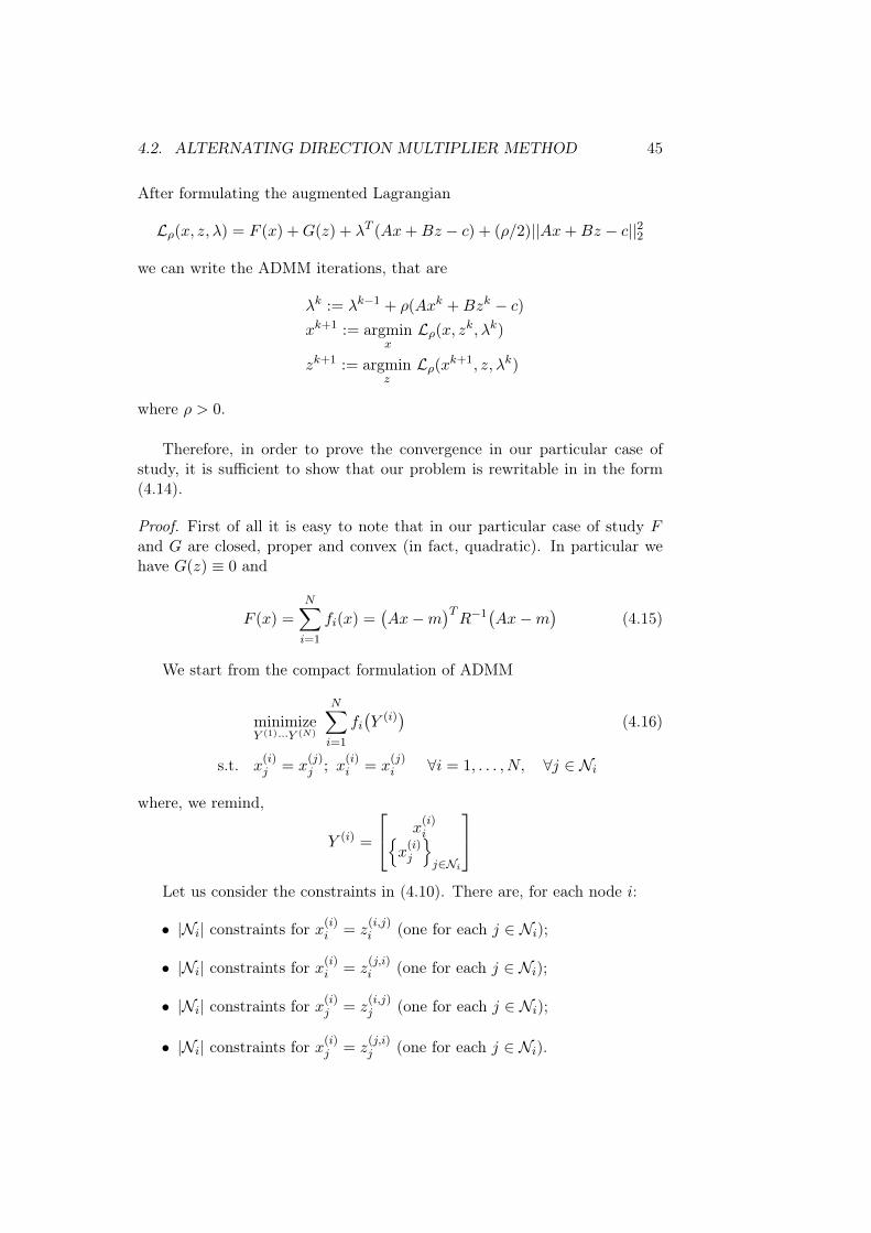
Therefore, in order to prove the convergence in our particular case ofstudy, it is sufficient to show that our problem is rewritable in in the form(4.14).
Proof. First of all it is easy to note that in our particular case of study Fand G are closed, proper and convex (in fact, quadratic). In particular wehave G(z) ≡ 0 and
F (x) =N∑i=1
fi(x) =(Ax−m
)TR−1
(Ax−m
)(4.15)
We start from the compact formulation of ADMM
minimizeY (1)···Y (N)
N∑i=1
fi(Y (i)
)(4.16)
s.t. x(i)j = x
(j)j ; x
(i)i = x
(j)i ∀i = 1, . . . , N, ∀j ∈ Ni
where, we remind,
Y (i) =
x(i)i
x(i)j
j∈Ni
Let us consider the constraints in (4.10). There are, for each node i:
• |Ni| constraints for x(i)i = z
(i,j)i (one for each j ∈ Ni);
• |Ni| constraints for x(i)i = z
(j,i)i (one for each j ∈ Ni);
• |Ni| constraints for x(i)j = z
(i,j)j (one for each j ∈ Ni);
• |Ni| constraints for x(i)j = z
(j,i)j (one for each j ∈ Ni).

46 CHAPTER 4. DISTRIBUTED ESTIMATION ALGORITHMS
Let us define
Z(i) =
z
(i,j)i
j∈Ni
z(j,i)i
j∈Ni
z(i,j)j
j∈Ni
z(j,i)j
j∈Ni
Z(i) has dimension 4|Ni| × 1. Let us define moreover
A(i) =
1 0...
. . .1 0
1 0...
. . .1 0
0 1...
. . .0 1
0 1...
. . .0 1
; B(i) = −I4|Ni|
Each block of A(i) has dimension |Ni| × |Ni|+ 1. Using these new variablesit is possible to write in a compact way all the 4|Ni| constraints of (4.10):
A(i)Y (i) +B(i)Z(i) = 0 (4.17)
By collecting all A(i), B(i), Y (i) and Z(i) we can define
A =
A(1)
...A(N)
; B =
B(1)
...B(N)
x =
Y(1)
...Y (N)
; z =
z
(1,j)1
j∈N1
z(j,1)1
j∈N1
...z
(N,j)N
j∈NN
z(j,N)N
j∈NN
(4.18)
and obtain directly the formulation Ax+Bz = c as in 4.14, with c = 0.
4.3. JACOBI APPROXIMATE ALGORITHM 47
4.3 Jacobi approximate algorithm
Before seeing the reactive power compensation algorithms with the ADMMestimation, we want to present briefly a new approximate Jacobi-like algo-rithm, distributed and faster than ADMM. This algorithm, differently fromADMM, does not converge to the optimal solution, but it can have a highpractical relevance if we are able to make some measurements more accuratethan the others.
For a deeper mathematical analysis of the Jacobi algorithm we remindto [21].
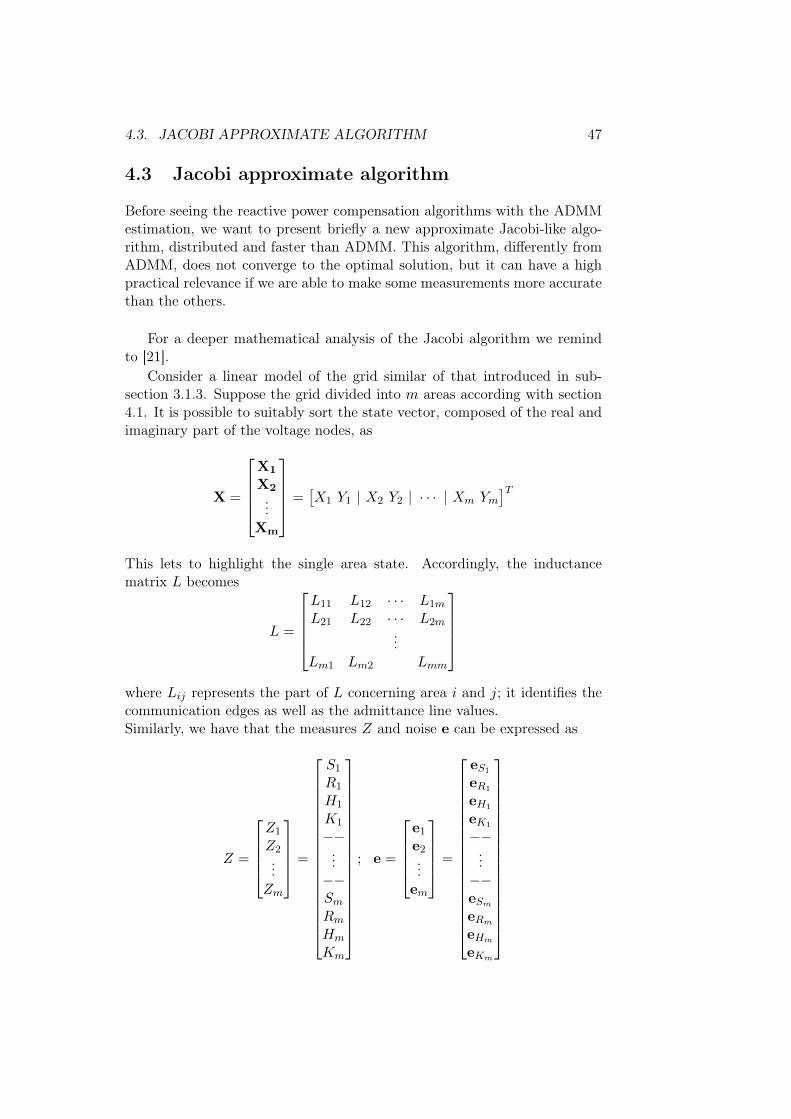
Consider a linear model of the grid similar of that introduced in sub-section 3.1.3. Suppose the grid divided into m areas according with section4.1. It is possible to suitably sort the state vector, composed of the real andimaginary part of the voltage nodes, as
X =
X1
X2...
Xm
=[X1 Y1 | X2 Y2 | · · · | Xm Ym
]T
This lets to highlight the single area state. Accordingly, the inductancematrix L becomes
L =
L11 L12 · · · L1m
L21 L22 · · · L2m...
Lm1 Lm2 Lmm
where Lij represents the part of L concerning area i and j; it identifies thecommunication edges as well as the admittance line values.Similarly, we have that the measures Z and noise e can be expressed as
Z =
Z1
Z2...Zm
=
S1
R1
H1
K1
−−...−−SmRmHm
Km
; e =
e1
e2...em
=
eS1
eR1
eH1
eK1
−−...−−eSm
eRm
eHm
eKm

48 CHAPTER 4. DISTRIBUTED ESTIMATION ALGORITHMS
It follows a correlation matrix R, for the noise vector e, equal to
R = E[eeT ] =
R1
R2
. . .Rm
Ri has a structure similar to that seen in section 3.1.3 but it concernes onlymeasurements taken from the same area.
Accordingly to the state sorting, the matrix of model (3.5) will be char-acterized by a similar structure. Specifically
H =
H1...Hm
Thanks to this sorting it is then possible to outline a specific linear model
for every area i ∈ [1, . . . ,m] of the form
Zi = HiX + ei = HiiXi +∑j 6=iHijXj + ei;
Note that the matrix model is equal to
Hi =[Hi1 · · · Hii · · · Him
]
=
0 00 0
<(Li1) −=(Li1)=(Li1) <(Li1)
· · ·Ini 00 Ini
<(Lii) −=(Lii)=(Lii) <(Lii)
· · ·0 00 0
<(Lim) −=(Lim)=(Lim) <(Lim)
whose block Hii is relative to the inner state and blocks Hij to other areasstate.
Distributed Solution
In section 3.1.4 it has been shown that the optimal global solution to thecentralized problem is equal to
X =(HTR−1H
)−1HTR−1Z
Exploiting the Jacobi procedure, the closed form solution, in a Jacobipoint of view, can be rewritten as
Xi(t+ 1) =(HTiiR−1
ii Hii)−1HTiiR−1
ii
(Zi −
∑j 6=iHijXj(t)
)(4.19)

4.3. JACOBI APPROXIMATE ALGORITHM 49
The iterative step described by equation (4.19) shows how the single areastate estimation depends on its inner measures and its border nodes estima-tion.
This let us handling only with local informations and to implement acompletely distributed algorithm:
1. each area i receive the border estimated state form adjacent areasj ∈ Ωi;
2. estimates its inner state using equation 4.19;
3. sends to area j the estimated value of node i ∈ Ωj .
The idea that make this algorithm "competitive" in estimation scenariois to measure with a more accurate instrument the border nodes of each area.In this way we reduce the error in border measurements. As they are crucialfor a correct estimation, we will show a big set of simulation showing thatthis algorithm performs a very good estimation and therefore has a goodbehaviour applied to the reactive power compensation algorithm.

50 CHAPTER 4. DISTRIBUTED ESTIMATION ALGORITHMS
Chapter 5
Testing results
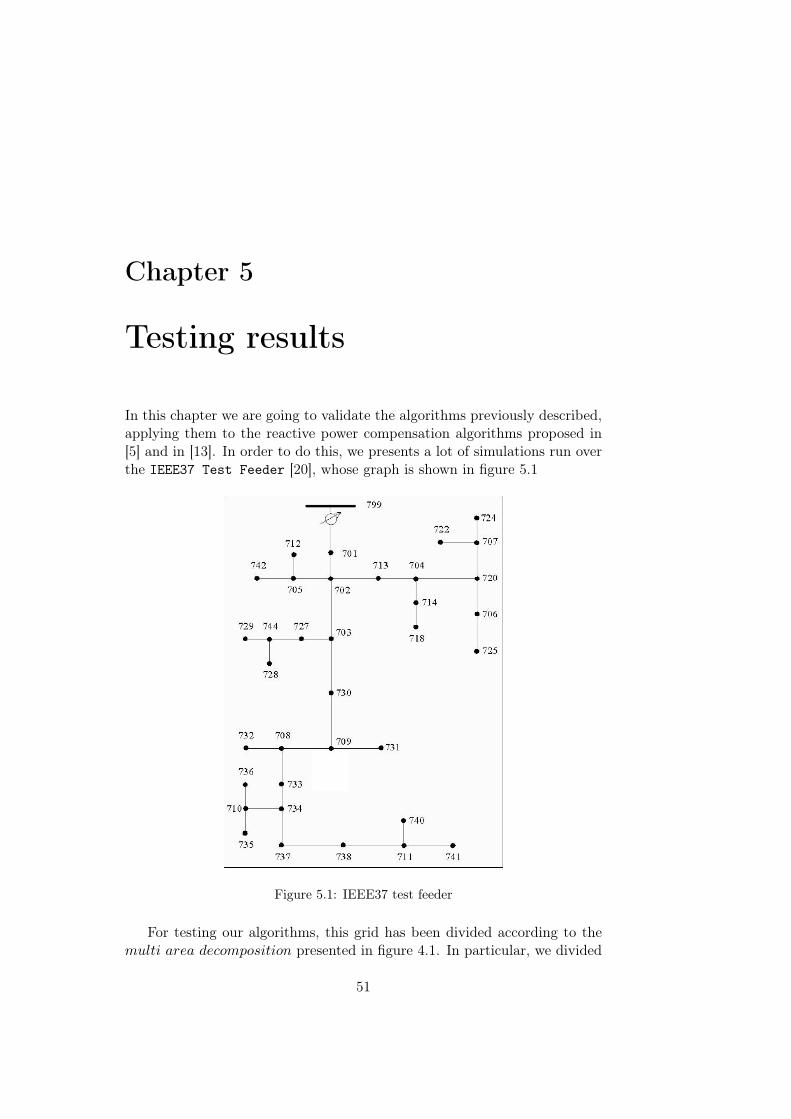
In this chapter we are going to validate the algorithms previously described,applying them to the reactive power compensation algorithms proposed in[5] and in [13]. In order to do this, we presents a lot of simulations run overthe IEEE37 Test Feeder [20], whose graph is shown in figure 5.1
Figure 5.1: IEEE37 test feeder
For testing our algorithms, this grid has been divided according to themulti area decomposition presented in figure 4.1. In particular, we divided
51
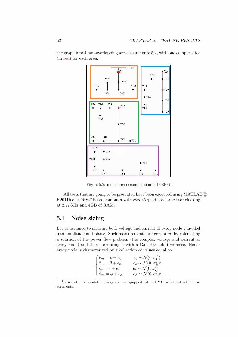
52 CHAPTER 5. TESTING RESULTS
the graph into 4 non-overlapping areas as in figure 5.2, with one compensator(in red) for each area.
Figure 5.2: multi area decomposition of IEEE37
All tests that are going to be presented have been executed using MATLAB©R2011b on aWin7 based computer with core i5 quad-core processor clockingat 2.27GHz and 4GB of RAM.
5.1 Noise sizing
Let us assumed to measure both voltage and current at every node1, dividedinto amplitude and phase. Such measurements are generated by calculatinga solution of the power flow problem (the complex voltage and current atevery node) and then corrupting it with a Gaussian additive noise. Henceevery node is characterized by a collection of values equal to:
vm = v + ev; ev ∼ N (0, σ2V );
θm = θ + eθ; eθ ∼ N (0, σ2Θ);
im = i+ ei; ei ∼ N (0, σ2I );
φm = φ+ eφ; eφ ∼ N (0, σ2Φ);
1In a real implementation every node is equipped with a PMU, which takes the mea-surements.

5.2. PERFORMANCES OF THE ALGORITHMS 53
More specifically, as default standard deviation values, it is assumed that:
• σV = 10−2PCCV oltageAmplitue[V olt]: it means to let the measures tohave a standard deviation equal to 1% the PCC voltage amplitude. Tobetter understand it for a PCC voltage amplitude of 4.16KV it meansto have a measurement error of ' 10V on average;
• σI = 10−2imax[Ampere]: as seen for the voltage measures, it meansto let the current amplitude measurement being equal to 1% of themaximum current on average;
• σθ = σφ = 10−2[rad]: for a 50Hz signal it means to measure a phasewith an almost maximum error of ' 100µs.
These values are chosen as standard values, it is just a convention. How-ever, simulations have been executed for several values, greater and smallerthan the standard ones, to highlight the algorithms performances in differentsituations.
It should be underlined that using smaller values of standard deviationsimplies better or equal but absolutely not worse performances of the algo-rithms. Similarly, using greater values of standard deviations implies worseor equal but absolutely not better performances.
In order to a better comprehension and to make the reader able to matchimmediately the performances, tests will be grouped according to the stan-dard deviation values, considering both algorithms in the same analysis.
5.2 Performances of the algorithms
5.2.1 About Centralized Estimation
The centralized estimation is the starting point of our study. It represents theoptimal global solution to the estimation problem, that is the solution to theequation 3.8. This estimator assumes the presence of a central unit over theentire network, which is able to collect and process all nodes measurements.
In this thesis we are not going to analyze the behaviour of the centralestimation (for centralized simulations see [21]), we will just consider it as theoptimal solution Xopt, and we will use it in order to test the performancesof the different distributed estimations. In fact, the variable introducedto understand immediately the estimation performance is ||Xopt −Xestim||,where Xestim means the entire state obtained by collecting the distributedsolutions. This variable is our choice to express the distance between ourdistributed solution and the optimal one. Formally, we have:
||Xopt −Xestim|| =
√√√√ n∑i=1
(xopti − xestimi )2

54 CHAPTER 5. TESTING RESULTS
where xopti and xestimi are the single components respectively of Xopt and ofXestim and n is the number of agents composing the state involved in theestimation.
5.2.2 Tests setup
As mentioned above, we will consider both algorithms in the same moment,in order to better understand the comparison of their performances. Forthe ADMM estimation we will consider three times same algorithm, eachtime with a different (increasing) number of iterations, to observe how thesolution can change simply reducing the number of ADMM iterations. Testsproposed will consider:
• ADMM estimation with 10 iterations;
• ADMM estimation with 100 iterations;
• ADMM estimation with 1000 iterations;
• Jacobi-like algorithm with 2 iterations;
The last choice is imposed, because in every simulation we noted that thestate computed using the Jacobi algorithm, after the second iteration, re-mains constant whatever is the number of iterations. This behaviour isprobably due to Matlab approximation. Executing the simulation, indeed,a warning inform us that results can be inaccurate because of the structureof the error matrix R.
The following tests are made up in this way: we will first present thebehaviour only of the estimation algorithm, analyzing the distance betweenthe optimal solution. Then we will apply the 4 different configurations to thereactive power compensation algorithm, in order to see if the compensationis acceptable or not.
To be precise, we have to highlight a convention applied in RPC al-gorithm. In order to better plotting the results of the compensation withADMM and JACOBI, we supposed to compute the initial losses after havingestimated the state. If you want to know the initial losses before estimating,you can consider the value related to noisy measurements. As the measure-ments trend is sometimes completely undesirable, we will zoom the mostsignificant part of the graphics. Therefore in some cases it will not be pos-sible to see the measurements trend, or part of it.
5.2.3 Performances for default values of noise standard de-viations
Let us compare our algorithms for default values of standard deviations (seesection 5.1). Considering only the ADMM algorithm, in figure 5.3 we canfind the performances for each number of iterations.
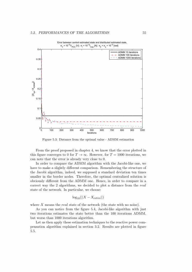
5.2. PERFORMANCES OF THE ALGORITHMS 55
0 100 200 300 400 500 600 700 800 900 10000
0.05
0.1
0.15
0.2
0.25
0.3
0.35
0.4
Error between central estimated state and distributed estimated state, σV = 10−2VPCC [V]; σI = 10−2Imax [A]; σθ = σφ = 10−2 [rad]
Iterations
||Xop
t−XA
DM
M||
ADMM 10 iterationsADMM 100 iterationsADMM 1000 iterations
Figure 5.3: Distance from the optimal value - ADMM estimation
From the proof proposed in chapter 4, we know that the error plotted inthis figure converges to 0 for T →∞. However, for T = 1000 iterations, wecan note that the error is already very close to 0.
In order to compare the ADMM algorithm with the Jacobi-like one, wehave to make a slightly different comparison. Remembering the structure ofthe Jacobi algorithm, indeed, we supposed a standard deviation ten timessmaller in the border nodes. Therefore, the optimal centralized solution isobviously different from the ADMM one. Hence, in order to compare in acorrect way the 2 algorithms, we decided to plot a distance from the realstate of the network. In particular, we choose:
log10(||X −Xestim||)
where X means the real state of the network (the state with no noise).As you can notice from the figure 5.4, Jacobi-like algorithm with just
two iterations estimates the state better than the 100 iterations ADMM,but worse than 1000 iterations algorithm.
Let us then apply these estimation techniques to the reactive power com-pensation algorithm explained in section 3.2. Results are plotted in figure5.5.
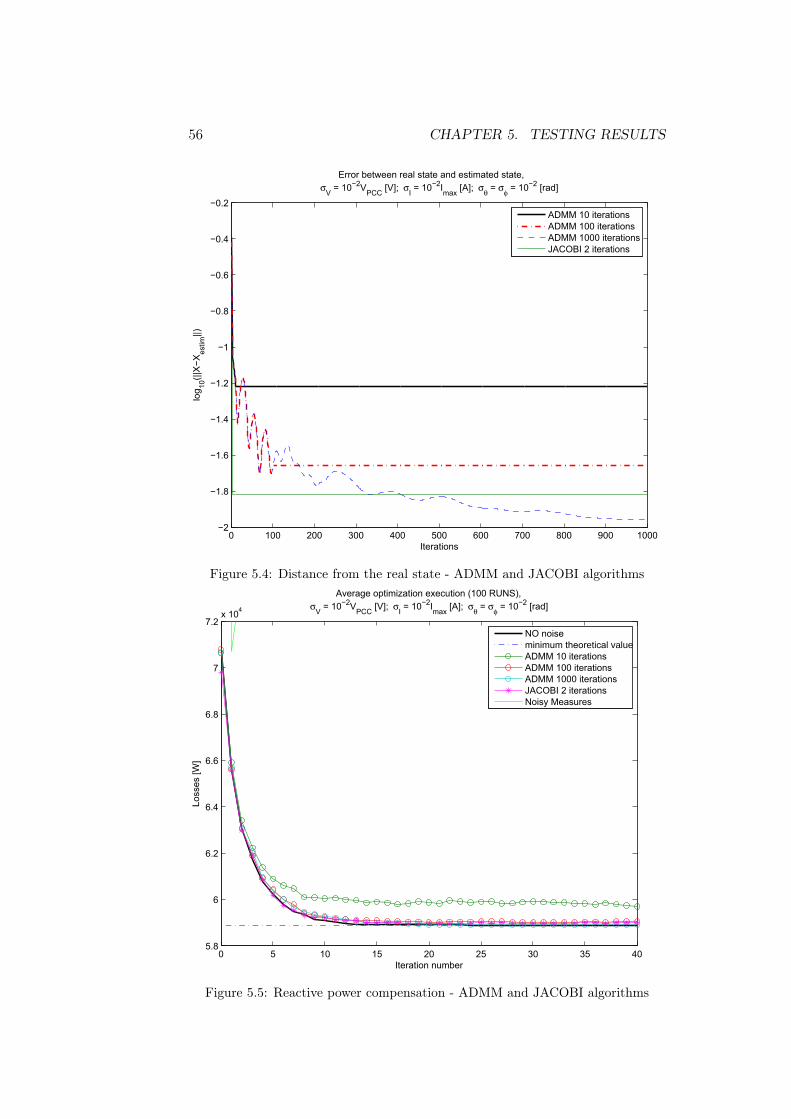
56 CHAPTER 5. TESTING RESULTS
0 100 200 300 400 500 600 700 800 900 1000−2
−1.8
−1.6
−1.4
−1.2
−1
−0.8
−0.6
−0.4
−0.2
Error between real state and estimated state,σV = 10−2VPCC [V]; σI = 10−2Imax [A]; σθ = σφ = 10−2 [rad]
Iterations
log 10
(||X
−Xes
tim||)
ADMM 10 iterationsADMM 100 iterationsADMM 1000 iterationsJACOBI 2 iterations
Figure 5.4: Distance from the real state - ADMM and JACOBI algorithms
0 5 10 15 20 25 30 35 405.8
6
6.2
6.4
6.6
6.8
7
7.2x 10⁴
Loss
es [W
]
Iteration number
Average optimization execution (100 RUNS), σV = 10−2VPCC [V]; σI = 10−2Imax [A]; σθ = σφ = 10−2 [rad]
NO noiseminimum theoretical valueADMM 10 iterationsADMM 100 iterationsADMM 1000 iterationsJACOBI 2 iterationsNoisy Measures
Figure 5.5: Reactive power compensation - ADMM and JACOBI algorithms
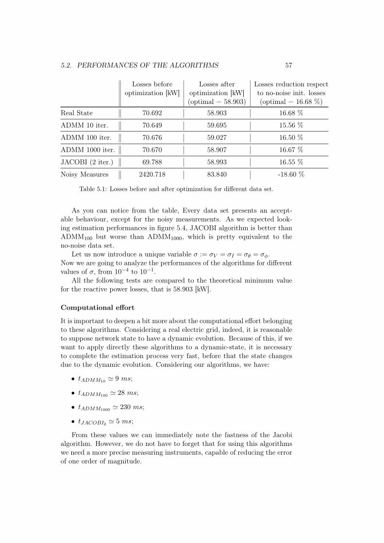
5.2. PERFORMANCES OF THE ALGORITHMS 57
Losses before Losses after Losses reduction respectoptimization [kW] optimization [kW] to no-noise init. losses
(optimal = 58.903) (optimal = 16.68 %)
Real State 70.692 58.903 16.68 %
ADMM 10 iter. 70.649 59.695 15.56 %
ADMM 100 iter. 70.676 59.027 16.50 %
ADMM 1000 iter. 70.670 58.907 16.67 %
JACOBI (2 iter.) 69.788 58.993 16.55 %
Noisy Measures 2420.718 83.840 -18.60 %
Table 5.1: Losses before and after optimization for different data set.
As you can notice from the table, Every data set presents an accept-able behaviour, except for the noisy measurements. As we expected look-ing estimation performances in figure 5.4, JACOBI algorithm is better thanADMM100 but worse than ADMM1000, which is pretty equivalent to theno-noise data set.
Let us now introduce a unique variable σ := σV = σI = σθ = σφ.Now we are going to analyze the performances of the algorithms for differentvalues of σ, from 10−4 to 10−1.
All the following tests are compared to the theoretical minimum valuefor the reactive power losses, that is 58.903 [kW].
Computational effort
It is important to deepen a bit more about the computational effort belongingto these algorithms. Considering a real electric grid, indeed, it is reasonableto suppose network state to have a dynamic evolution. Because of this, if wewant to apply directly these algorithms to a dynamic-state, it is necessaryto complete the estimation process very fast, before that the state changesdue to the dynamic evolution. Considering our algorithms, we have:
• tADMM10 ' 9 ms;
• tADMM100 ' 28 ms;
• tADMM1000 ' 230 ms;
• tJACOBI2 ' 5 ms;
From these values we can immediately note the fastness of the Jacobialgorithm. However, we do not have to forget that for using this algorithmswe need a more precise measuring instruments, capable of reducing the errorof one order of magnitude.
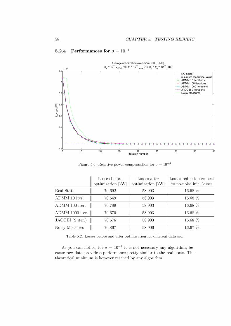
58 CHAPTER 5. TESTING RESULTS
5.2.4 Performances for σ = 10−4
0 5 10 15 20 25 30 35 405.8
6
6.2
6.4
6.6
6.8
7
7.2x 10⁴
Iteration number
Loss
es [W
]
Average optimization execution (100 RUNS), σV = 10−4VPCC [V]; σI = 10−4Imax [A]; σθ = σφ = 10−4 [rad]
NO noiseminimum theoretical valueADMM 10 iterationsADMM 100 iterationsADMM 1000 iterationsJACOBI 2 iterationsNoisy Measures
Figure 5.6: Reactive power compensation for σ = 10−4
Losses before Losses after Losses reduction respectoptimization [kW] optimization [kW] to no-noise init. losses
Real State 70.692 58.903 16.68 %
ADMM 10 iter. 70.649 58.903 16.68 %
ADMM 100 iter. 70.789 58.903 16.68 %
ADMM 1000 iter. 70.670 58.903 16.68 %
JACOBI (2 iter.) 70.676 58.903 16.68 %
Noisy Measures 70.867 58.906 16.67 %
Table 5.2: Losses before and after optimization for different data set.
As you can notice, for σ = 10−4 it is not necessary any algorithm, be-cause raw data provide a performance pretty similar to the real state. Thetheoretical minimum is however reached by any algorithm.

5.2. PERFORMANCES OF THE ALGORITHMS 59
5.2.5 Performances for σ = 10−3
0 5 10 15 20 25 30 35 405.8
6
6.2
6.4
6.6
6.8
7
7.2x 10⁴
Iteration number
Loss
es [W
]
Average optimization execution (100 RUNS), σV = 10−3VPCC [V]; σI = 10−3Imax [A]; σθ = σφ = 10−3 [rad]
NO noiseminimum theoretical valueADMM 10 iterationsADMM 100 iterationsADMM 1000 iterationsJACOBI 2 iterationsNoisy Measures
Figure 5.7: Reactive power compensation for σ = 10−3
Losses before Losses after Losses reduction respectoptimization [kW] optimization [kW] to no-noise init. losses
Real State 70.692 58.903 16.68 %
ADMM 10 iter. 71.046 58.912 16.66 %
ADMM 100 iter. 70.756 58.904 16.67 %
ADMM 1000 iter. 70.703 58.903 16.68 %
JACOBI (2 iter.) 70.660 58.903 16.68 %
Noisy Measures 70.867 59.174 16.29 %
Table 5.3: Losses before and after optimization for different data set.
For σ = 10−3 all data sets up to ADMM10 are well performing, onlynoisy measurements deviate a bit from the optimal value.
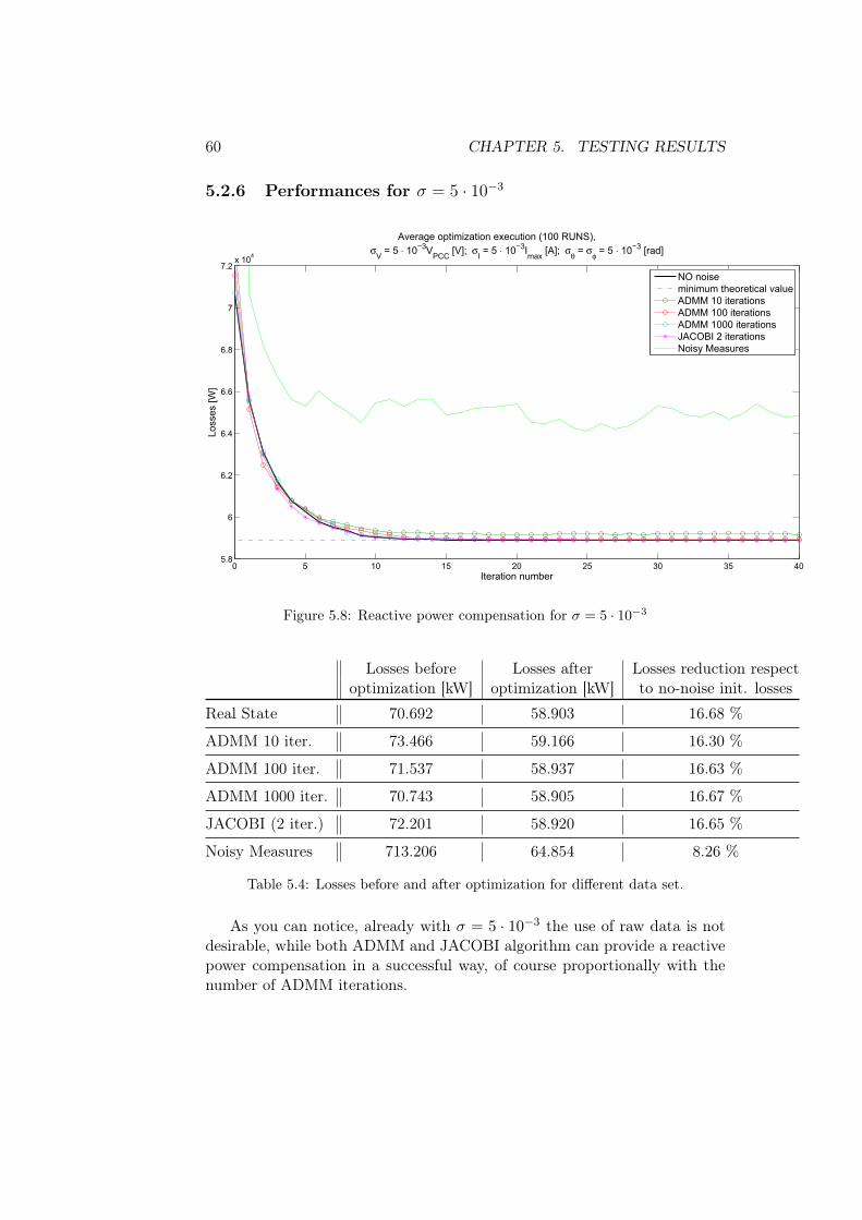
60 CHAPTER 5. TESTING RESULTS
5.2.6 Performances for σ = 5 · 10−3
0 5 10 15 20 25 30 35 405.8
6
6.2
6.4
6.6
6.8
7
7.2x 10⁴
Iteration number
Loss
es [W
]
Average optimization execution (100 RUNS), σV = 5 ⋅ 10−3VPCC [V]; σI = 5 ⋅ 10−3Imax [A]; σθ = σφ = 5 ⋅ 10−3 [rad]
NO noiseminimum theoretical valueADMM 10 iterationsADMM 100 iterationsADMM 1000 iterationsJACOBI 2 iterationsNoisy Measures
Figure 5.8: Reactive power compensation for σ = 5 · 10−3
Losses before Losses after Losses reduction respectoptimization [kW] optimization [kW] to no-noise init. losses
Real State 70.692 58.903 16.68 %
ADMM 10 iter. 73.466 59.166 16.30 %
ADMM 100 iter. 71.537 58.937 16.63 %
ADMM 1000 iter. 70.743 58.905 16.67 %
JACOBI (2 iter.) 72.201 58.920 16.65 %
Noisy Measures 713.206 64.854 8.26 %
Table 5.4: Losses before and after optimization for different data set.
As you can notice, already with σ = 5 · 10−3 the use of raw data is notdesirable, while both ADMM and JACOBI algorithm can provide a reactivepower compensation in a successful way, of course proportionally with thenumber of ADMM iterations.
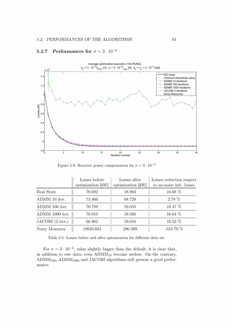
5.2. PERFORMANCES OF THE ALGORITHMS 61
5.2.7 Performances for σ = 3 · 10−2
0 5 10 15 20 25 30 35 405.8
6
6.2
6.4
6.6
6.8
7
7.2
7.4
x 104
Iteration number
Loss
es [W
]
Average optimization execution (100 RUNS), σV = 3 ⋅ 10−2VPCC [V]; σI = 3 ⋅ 10−2Imax [A]; σθ = σφ = 3 ⋅ 10−2 [rad]
NO noiseminimum theoretical valueADMM 10 iterationsADMM 100 iterationsADMM 1000 iterationsJACOBI 2 iterationsNoisy Measures
Figure 5.9: Reactive power compensation for σ = 3 · 10−2
Losses before Losses after Losses reduction respectoptimization [kW] optimization [kW] to no-noise init. losses
Real State 70.692 58.903 16.68 %
ADMM 10 iter. 73.466 68.728 2.78 %
ADMM 100 iter. 70.789 59.050 16.47 %
ADMM 1000 iter. 70.810 58.926 16.64 %
JACOBI (2 iter.) 66.902 59.016 16.52 %
Noisy Measures 19820.694 290.399 -310.79 %
Table 5.5: Losses before and after optimization for different data set.
For σ = 3 · 10−2, value slightly bigger than the default, it is clear that,in addition to raw data, even ADMM10 become useless. On the contrary,ADMM100, ADMM1000 and JACOBI algorithms still present a good perfor-mance.
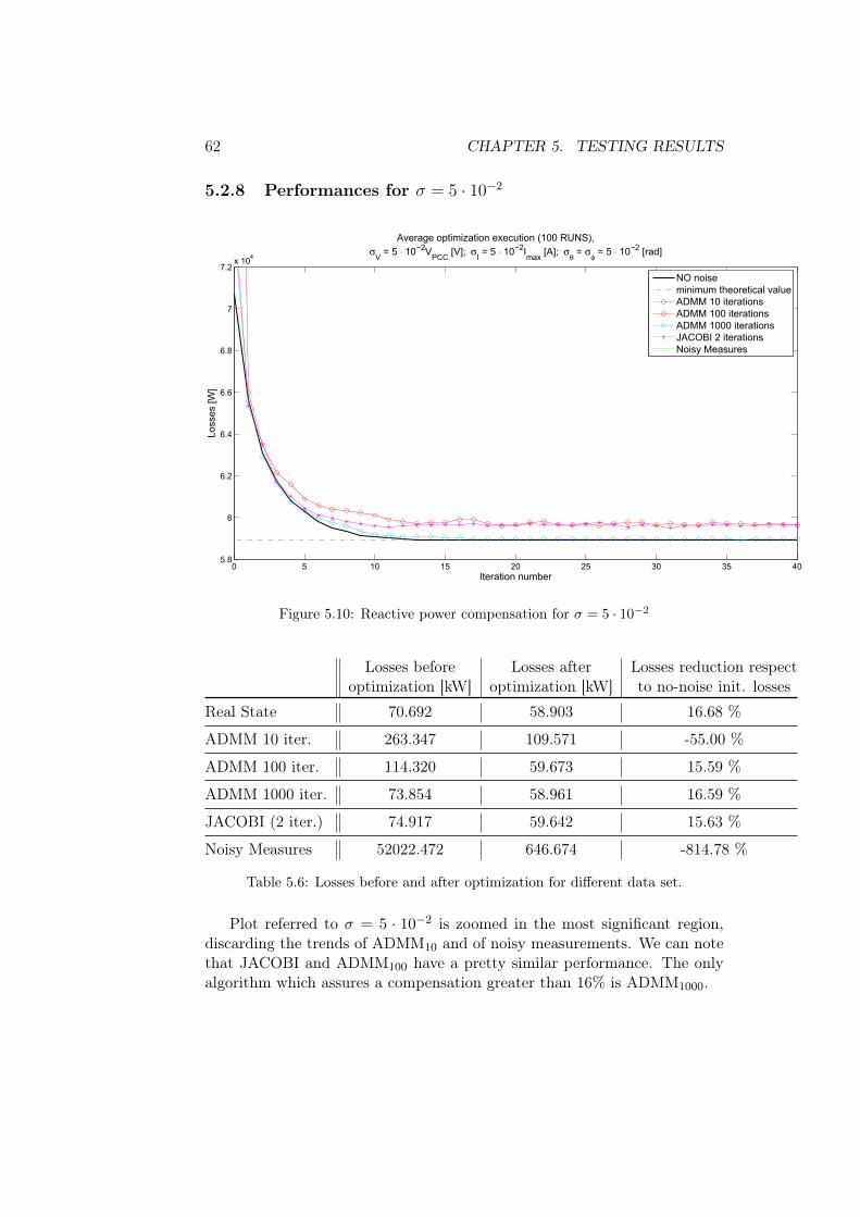
62 CHAPTER 5. TESTING RESULTS
5.2.8 Performances for σ = 5 · 10−2
0 5 10 15 20 25 30 35 405.8
6
6.2
6.4
6.6
6.8
7
7.2x 10⁴
Iteration number
Loss
es [W
]
Average optimization execution (100 RUNS), σV = 5 ⋅ 10−2VPCC [V]; σI = 5 ⋅ 10−2Imax [A]; σθ = σφ = 5 ⋅ 10−2 [rad]
NO noiseminimum theoretical valueADMM 10 iterationsADMM 100 iterationsADMM 1000 iterationsJACOBI 2 iterationsNoisy Measures
Figure 5.10: Reactive power compensation for σ = 5 · 10−2
Losses before Losses after Losses reduction respectoptimization [kW] optimization [kW] to no-noise init. losses
Real State 70.692 58.903 16.68 %
ADMM 10 iter. 263.347 109.571 -55.00 %
ADMM 100 iter. 114.320 59.673 15.59 %
ADMM 1000 iter. 73.854 58.961 16.59 %
JACOBI (2 iter.) 74.917 59.642 15.63 %
Noisy Measures 52022.472 646.674 -814.78 %
Table 5.6: Losses before and after optimization for different data set.
Plot referred to σ = 5 · 10−2 is zoomed in the most significant region,discarding the trends of ADMM10 and of noisy measurements. We can notethat JACOBI and ADMM100 have a pretty similar performance. The onlyalgorithm which assures a compensation greater than 16% is ADMM1000.
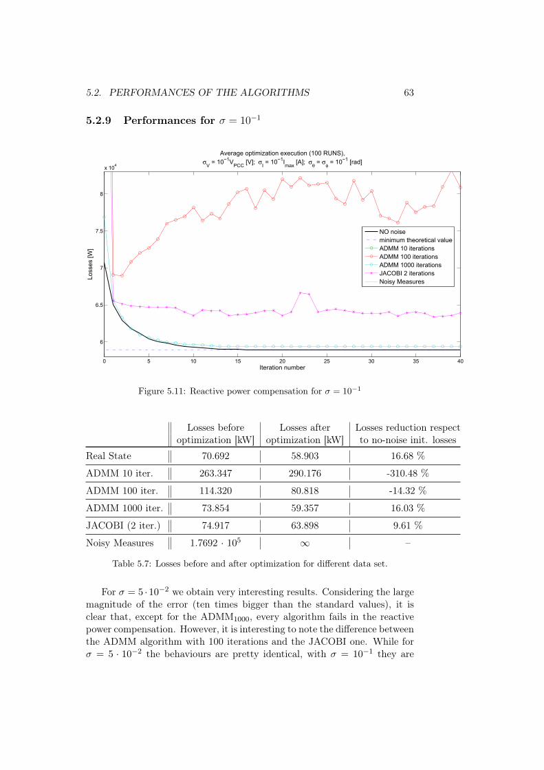
5.2. PERFORMANCES OF THE ALGORITHMS 63
5.2.9 Performances for σ = 10−1
0 5 10 15 20 25 30 35 40
6
6.5
7
7.5
8
x 104
Iteration number
Loss
es [W
]
Average optimization execution (100 RUNS), σV = 10−1VPCC [V]; σI = 10−1Imax [A]; σθ = σφ = 10−1 [rad]
NO noiseminimum theoretical valueADMM 10 iterationsADMM 100 iterationsADMM 1000 iterationsJACOBI 2 iterationsNoisy Measures
Figure 5.11: Reactive power compensation for σ = 10−1
Losses before Losses after Losses reduction respectoptimization [kW] optimization [kW] to no-noise init. losses
Real State 70.692 58.903 16.68 %
ADMM 10 iter. 263.347 290.176 -310.48 %
ADMM 100 iter. 114.320 80.818 -14.32 %
ADMM 1000 iter. 73.854 59.357 16.03 %
JACOBI (2 iter.) 74.917 63.898 9.61 %
Noisy Measures 1.7692 · 105 ∞ –
Table 5.7: Losses before and after optimization for different data set.
For σ = 5 ·10−2 we obtain very interesting results. Considering the largemagnitude of the error (ten times bigger than the standard values), it isclear that, except for the ADMM1000, every algorithm fails in the reactivepower compensation. However, it is interesting to note the difference betweenthe ADMM algorithm with 100 iterations and the JACOBI one. While forσ = 5 · 10−2 the behaviours are pretty identical, with σ = 10−1 they are
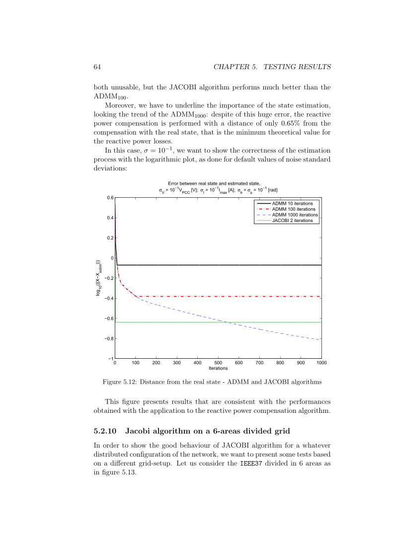
64 CHAPTER 5. TESTING RESULTS
both unusable, but the JACOBI algorithm performs much better than theADMM100.
Moreover, we have to underline the importance of the state estimation,looking the trend of the ADMM1000: despite of this huge error, the reactivepower compensation is performed with a distance of only 0.65% from thecompensation with the real state, that is the minimum theoretical value forthe reactive power losses.
In this case, σ = 10−1, we want to show the correctness of the estimationprocess with the logarithmic plot, as done for default values of noise standarddeviations:
0 100 200 300 400 500 600 700 800 900 1000−1
−0.8
−0.6
−0.4
−0.2
0
0.2
0.4
0.6
Error between real state and estimated state,σV = 10−1VPCC [V]; σI = 10−1Imax [A]; σθ = σφ = 10−1 [rad]
Iterations
log 10
(||X
−Xes
tim||)
ADMM 10 iterationsADMM 100 iterationsADMM 1000 iterationsJACOBI 2 iterations
Figure 5.12: Distance from the real state - ADMM and JACOBI algorithms
This figure presents results that are consistent with the performancesobtained with the application to the reactive power compensation algorithm.
5.2.10 Jacobi algorithm on a 6-areas divided grid
In order to show the good behaviour of JACOBI algorithm for a whateverdistributed configuration of the network, we want to present some tests basedon a different grid-setup. Let us consider the IEEE37 divided in 6 areas asin figure 5.13.
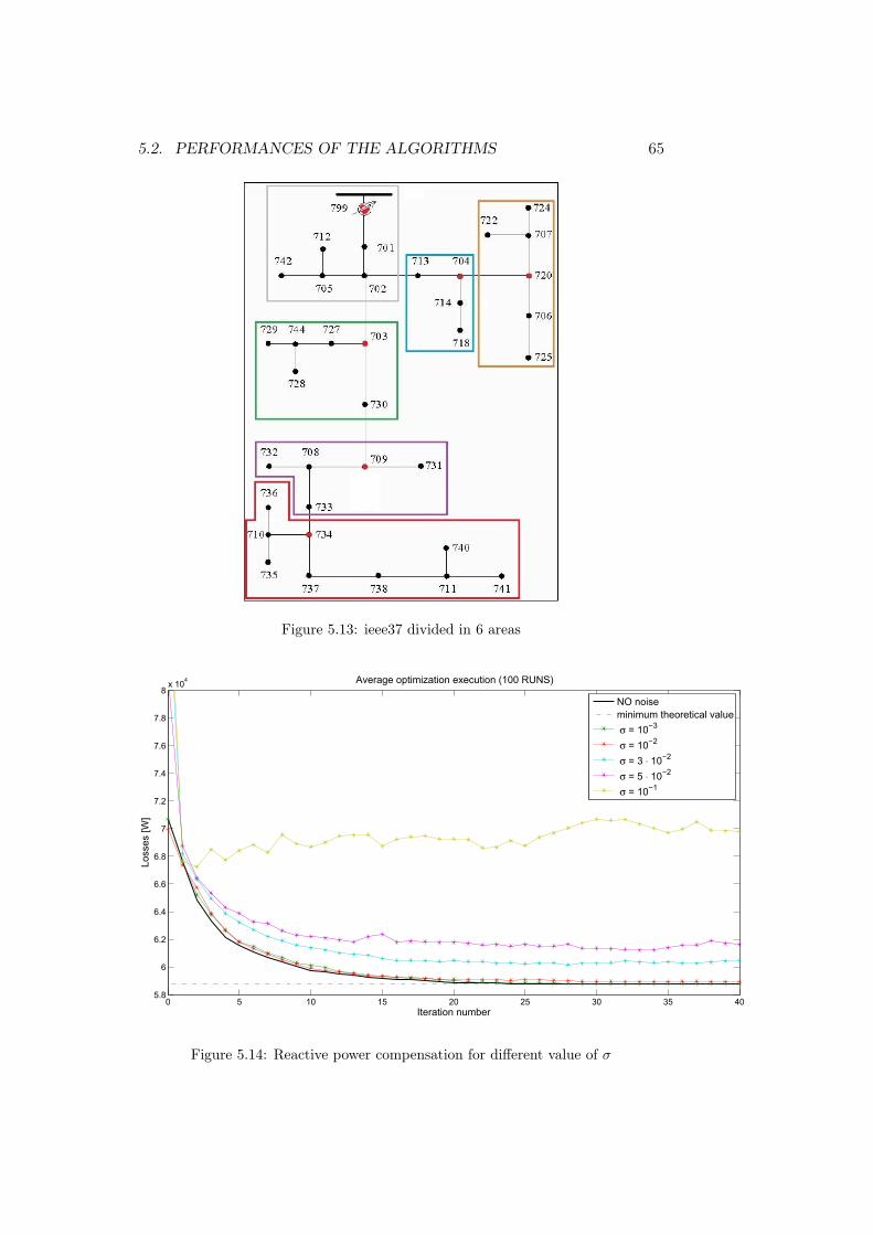
5.2. PERFORMANCES OF THE ALGORITHMS 65
Figure 5.13: ieee37 divided in 6 areas
0 5 10 15 20 25 30 35 405.8
6
6.2
6.4
6.6
6.8
7
7.2
7.4
7.6
7.8
8x 10⁴
Iteration number
Loss
es [W
]
Average optimization execution (100 RUNS)
NO noiseminimum theoretical value σ = 10−3
σ = 10−2
σ = 3 ⋅ 10−2
σ = 5 ⋅ 10−2
σ = 10−1
Figure 5.14: Reactive power compensation for different value of σ

66 CHAPTER 5. TESTING RESULTS
This setup presents one compensator for each area, and so 6 compen-sators (nodes in red). Let us compare the performances of the algorithm fordifferent values of σ. Minimum theoretical value for losses is 58.769 [kW].Results are shown in figure 5.14
Losses before Losses after Losses reduction respectoptimization [kW] optimization [kW] to no-noise init. losses
Real State 70.692 58.769 16.87 %
σ = 10−3 70.692 58.771 16.86 %
σ = 10−2 69.940 58.943 16.62 %
σ = 3 · 10−2 88.980 60.487 14.44 %
σ = 5 · 10−2 81.780 61.615 12.84 %
σ = 10−1 91.313 69.782 1.29 %
Table 5.8: Losses before and after optimization for different data set.
Looking at the table and comparing results with the ones obtained beforewith a 4-areas configuration, we can state that performances are substantiallyequivalent.
5.2.11 Performances adding saturation constraints to eachpower line
Now we want to apply ADMM and JACOBI estimation strategies to a reac-tive power compensation algorithms with saturation constraints, treated in[13]. In this algorithm we added power saturation constraints to each powerline. In [13] it has been demonstrated that in this new configuration thealgorithm does not reach always the optimal value because it can stop in alocal minimum, different from the global one. Then it has been implementeda multi-hop strategy in order to reach anyway the optimal value. We willshow that the problem of non-convergence is present even with the estima-tion algorithms, and moreover that ADMM and JACOBI performances withthe multi-hop strategy are pretty equal to the no-noise state ones.
We will analyze the algorithms for default value of noise standard devia-tions, that is σ = 10−2, in the 4-areas configuration of IEEE 37 test feeder.
Let us start highlighting the behaviour without the multi-hop strategy.Every algorithm does not reach the theoretical minimum value o f reactivepower losses, as shown in figure 5.15. We did not consider the performanceusing raw measurements because it is completely undesirable.

5.2. PERFORMANCES OF THE ALGORITHMS 67
0 5 10 15 20 25 30 35 40 45 50
1.16
1.18
1.2
1.22
1.24
1.26
1.28
x 105
Iteration number
Loss
es [W
]
Average optimization execution (100 RUNS), σV = 10−2VPCC [V]; σI = 10−2Imax [A]; σθ = σφ = 10−2 [rad]
NO noiseminimum theoretical valueADMM 10 iterationsADMM 100 iterationsADMM 1000 iterationsJACOBI 2 iterations
Figure 5.15: Behaviour with saturation constraints on power lines
Losses before Losses after Losses reduction respectoptimization [kW] optimization [kW] to no-noise init. losses
(optimal = 115.227) (optimal = 14.45 %)
Real State 134.693 127.040 5.68 %
ADMM 10 iter. 134.498 127.728 5.17 %
ADMM 100 iter. 134.391 127.460 5.37 %
ADMM 1000 iter. 134.047 127.250 5.53 %
JACOBI (2 iter.) 136.588 128.020 4.95 %
Table 5.9: Losses before and after optimization with saturation constraints

68 CHAPTER 5. TESTING RESULTS
Introducing the multi-hop strategy, instead, both algorithms improvetheir performances and approach the optimal value, as shown in figure 5.16.
0 50 100 150
1.16
1.18
1.2
1.22
1.24
1.26
1.28
x 105
Iteration number
Loss
es [W
]
Average optimization execution (100 RUNS), σV = 10−2VPCC [V]; σI = 10−2Imax [A]; σθ = σφ = 10−2 [rad]
NO noiseminimum theoretical valueADMM 10 iterationsADMM 100 iterationsADMM 1000 iterationsJACOBI 2 iterations
Figure 5.16: Behaviour with saturation constraints and multi-hop strategy
Losses before Losses after Losses reduction respectoptimization [kW] optimization [kW] to no-noise init. losses
(optimal = 115.227) (optimal = 14.45 %)
Real State 134.693 115.227 14.45 %
ADMM 10 iter. 136.052 115.330 14.38 %
ADMM 100 iter. 136.973 115.240 14.44 %
ADMM 1000 iter. 134.565 115.229 14.45 %
JACOBI (2 iter.) 137.285 115.227 14.45 %
Table 5.10: Losses before and after optimization with multi-hop strategy
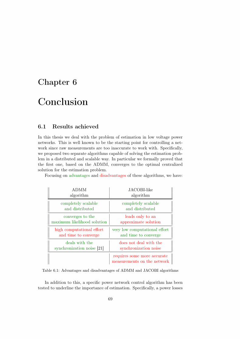
Chapter 6
Conclusion
6.1 Results achieved
In this thesis we deal with the problem of estimation in low voltage powernetworks. This is well known to be the starting point for controlling a net-work since raw measurements are too inaccurate to work with. Specifically,we proposed two separate algorithms capable of solving the estimation prob-lem in a distributed and scalable way. In particular we formally proved thatthe first one, based on the ADMM, converges to the optimal centralizedsolution for the estimation problem.
Focusing on advantages and disadvantages of these algorithms, we have:
ADMM JACOBI-likealgorithm algorithm
completely scalable completely scalableand distributed and distributed
converges to the leads only to anmaximum likelihood solution approximate solution
high computational effort very low computational effortand time to converge and time to converge
deals with the does not deal with thesynchronization noise [21] synchronization noise
requires some more accuratemeasurements on the network
Table 6.1: Advantages and disadvantages of ADMM and JACOBI algorithms
In addition to this, a specific power network control algorithm has beentested to underline the importance of estimation. Specifically, a power losses
69

70 CHAPTER 6. CONCLUSION
reduction through reactive power compensation algorithm, with and withoutsaturation constraints ([5],[13]) has been chosen as prototype. The simula-tions show how using the estimated state, respect to the raw measurements,improves much more the performances, making them comparable with thoseobtained using the exact state value. The measurements, instead, leads toan undesirable behaviour.
6.2 Possible future developments
This thesis can be an interesting starting point to analyze in a deeper waypower networks with noisy measurements. We suggest some future develop-ments that can be inspected starting from our results:
1. Study how the dynamic behaviour of a power grid can affect theseresult, and eventually find a solution to dynamically estimate the stateof the network, i.e. with extended Kalman filter.
2. In order to apply the Jacobi-like algorithm to a real netweork, it can beinteresting to focus on measuring instruments available at the moment,understand if it is possible to buy instruments capable of measuringthe voltages with a fixed order of magnitude of the error, and which iseventually the price of these instruments.
3. Compare the algorithms presented in this thesis with other distributedalgorithms that are rising in the literature, i.e. Newton-Raphson basedalgorithms, in order to understand which algorithm is best suited fora particular controlling problem.

Appendix A
Proof of equations 4.5 and 4.6
Lemma 4. For each time instant t, the updating step of zij in the ADMMalgorithm is
zij(t+ 1) =1
2c
(λij(t) + µji(t) + c
(X(i)(t+ 1) +X(j)(t+ 1)
))(A.1)
Proof. Starting from 4.4 we have:
zij(t+ 1) = arg minzij
L(X(t+ 1), z, λ(t), µ(t))
= arg minzij
−(λTij(t) + µTji(t))zij +
c
2
[||X(i)(t+ 1)− zij ||2 + ||X(j)(t+ 1)− zij ||2
]because all the other components does not depend on zij .
Through the first order optimality condition we have
−λij(t)− µji(t)− c(X(i)(t+ 1)− zij
)− c(X(j)(t+ 1)− zij
)= 0
and hence
zij(t+ 1) =1
2c
(λij(t) + µji(t) + c
(X(i)(t+ 1) +X(j)(t+ 1)
))
Lemma 5. In general it is true that
λij(−1) = −µji(−1) =⇒ λij(t) = −µji(t) ∀t
Proof. The proof is done by induction. The base case is trivial, due toa simple initialization λij(−1) = −µji(−1) = 0. Then, substituting theexpression of zij(t) obtained in A.1 in 4.2 we haveλij(t) = λij(t− 1) + c
2
(X(i)(t)−X(j)(t)
)− 1
2
(λij(t− 1) + µji(t− 1)
)µji(t) = µji(t− 1) + c
2
(X(j)(t)−X(i)(t)
)+ 1
2
(λij(t− 1) + µji(t− 1)
)71

72 APPENDIX A. PROOF OF EQUATIONS 4.5 AND 4.6
By summing these equations we obtain
λij(t) + µji(t) = λij(t− 1) + µji(t− 1) +c
2· 0.
Applying the inductive hypothesis, the thesis follows.
Now, by substituting this equivalence in the zij equation we obtain
zij(t) =X(i)(t) +X(j)(t)
2
Because of this, by simply substituting this expression in equations 4.2,4.3 and 4.4, we can discard both zij and µij terms, obtaining the new for-mulation for the ADMM algorithm described in equations 4.5 and 4.6.

Bibliography
[1] J. A. Lopes, C. L. Moreira, and A. G. Madureira, “Defining controlstrategies for microgrids islanded operation,” IEEE Trans. Power Syst.,vol. 21, no. 2, pp. 916–924, May 2006.
[2] T. C. Green, C. L. Prodanović, and A. G. Madureira, “Control ofinverter-based micro-grids,” Electr. Pow. Syst. Res., vol. 77, no. 9, pp.1204–1213, Jul 2007.
[3] F. Katiraei and M. R. Iravani, “Power management strategies for a mi-crogrid with multiple distributed generation units,” IEEE Trans. PowerSyst., vol. 21, no. 4, pp. 1821–1831, Nov 2006.
[4] M. Prodanović, K. De Brabandere, J. Van den Keybus, T. Green, andJ. Driesen, “Harmonic and reactive power compensation as ancillaryserivces in inveerter-based distributed generation,” IET Gener. Transm.Distrib., vol. 1, no. 3, pp. 432–438, 2007.
[5] S. Bolognani and S. Zampieri, “A distributed control strategyfor reactive power compensation in smart microgrids,” arXiv,vol. arXiv:1106.5626v2 [math.OC], Oct. 2011. [Online]. Available:http://arxiv.org/abs/1106.5626
[6] G. Valverde and V. Terzja, “Pmu-based multi-area state estimation withlow data exchange,” Innovative Smart Grid Technologies ConferenceEurope (ISGT Europe), 2010 IEEE PES, pp. 1–7, October 2010.
[7] L. Zhao and A. Abur, “Multiarea state estimation using synchronizedphasor measurements,” Ieee Transaction on Power System, vol. 20,no. 2, pp. 611–617, May 2005.
[8] W. Jiang, V. Vittal, and G. T. Heydt, “A distributed state estimator uti-lizing synchronized phasor measurements,” Ieee Transaction on PowerSystem, vol. 22, no. 2, pp. 563–571, May 2007.
[9] G. N. Korres, “A distributed multiarea state estimation,” Ieee Transac-tion on Power System, vol. 26, no. 1, pp. 73–84, February 2011.
73
74 BIBLIOGRAPHY
[10] A. J. Conejo, S. de la Torre, and M. Canas, “An optimization ap-proach to multiarea state estimation,” Ieee Transaction on Power Sys-tem, vol. 22, no. 1, pp. 213–221, February 2007.
[11] G. Mateos, I. D. Schizas, and G. B. Giannaakis, “Performance analysisof the consensus-based distributed lms algorithm,” EURASIP Journalon Advances in Signal Processing, October 2009.
[12] T. Erseghe, “A distributed and scalable processing method based uponadmm,” Ieee Signal Processing Letters, vol. 19, pp. 563–566, 2012.
[13] S. Bolognani, A. Carron, A. Di Vittorio, and D. Romeres, “Distributedmulti-hop reactive power compensation in smart micro-grids subject tosaturation constraints,” 2012.
[14] A. Abur and A. G. Exposito, Power System State Estimation, theoryand implementation. Marcel Dekker, 2004.
[15] F. C. Schweppe and D. B. Rom, “Power system static-state estimation,part i: Exact model,” Transaction on Power Apparatus and Systems,vol. Pas-89, no. 1, pp. 120–125, January 1970.
[16] ——, “Power system static-state estimation, part ii: Approxiamtemodel,” Transaction on Power Apparatus and Systems, vol. Pas-89,no. 1, pp. 125 – 130, January 1970.
[17] ——, “Power system static-state estimation, part iii: Implementation,”Transaction on Power Apparatus and Systems, vol. Pas-89, no. 1, pp.130 – 135, January 1970.
[18] C. Rakpenthai, S. Premrudeepreechacharn, S. Uatrongjit, and N. R.R. Watson, “Measurement placement for power system state estima-tion using decomposition technique,” Electric Power System Research,vol. 75, pp. 41–49, 2005.
[19] B. H. Kim and R. Baldick, “A comparison of distributed optimal powerflow algorithm,” Ieee Transaction on Power System, vol. 15, no. 2, pp.599–604, May 2000.
[20] W. H. Kersting, “Radial distribution test feeders,” Transaction on PowerSystems, vol. 6, no. 3, pp. 975–985, August 1991.
[21] M. Todescato, “Distributed algorithms for state estimation in a lowvoltage distribution network,” Master’s thesis, Oct 2012.
[22] J. Lavaei and S. H. Low, “Zero duality gap in optimal power flow prob-lem,” IEEE Trans. on Power Syst., 2011.

BIBLIOGRAPHY 75
[23] S. Boyd, N. Parikh, E. Chu, B. Peleato, and J. Eckstein,Distributed Optimization and Statistical Learning via the AlternatingDirection Method of Multipliers, 2010, vol. 3. [Online]. Available:www.stanford.edu/~boyd/papers/pdf/admm_distr_stats.pdf


![Estimate of Causality Between Cortical Spatial Patterns During … · 2011. 8. 14. · level [Babiloni et al., 2005; Astolfi et al., 2005]. However, the causality estimation from](https://static.fdocumenti.com/doc/165x107/6131b4541ecc51586944e73b/estimate-of-causality-between-cortical-spatial-patterns-during-2011-8-14-level.jpg)