IN BIOINGEGNERIA - unibo.itamsdottorato.unibo.it/1695/1/Tassani_Simone_Tesi.pdf · IN BIOINGEGNERIA...
142
Alma Mater Studiorum – Università di Bologna DOTTORATO DI RICERCA IN BIOINGEGNERIA Ciclo XXI Settore scientifico disciplinare di afferenza: ING-IND/34 TITOLO TESI "ANALISI DELLA RESISTENZA OSSEA: TECNICHE MICROTOMOGRAFICHE" "EVALUATION OF BONE STRENGTH: MICROTOMOGRAPHIC TECHNIQUES" Presentata da: Ing. SIMONE TASSANI Coordinatore Dottorato: Relatore: Prof. Angelo Cappello Prof. Luca Cristofolini Co-relatore: Dott. Fabio Baruffaldi Bologna, Marzo 2009
Transcript of IN BIOINGEGNERIA - unibo.itamsdottorato.unibo.it/1695/1/Tassani_Simone_Tesi.pdf · IN BIOINGEGNERIA...
AAllmmaa MMaatteerr SSttuuddiioorruumm –– UUnniivveerrssiittàà ddii BBoollooggnnaa
DOTTORATO DI RICERCA
IN BIOINGEGNERIA
Ciclo XXI
Settore scientifico disciplinare di afferenza: ING-IND/34
TITOLO TESI
"ANALISI DELLA RESISTENZA OSSEA: TECNICHE MICROTOMOGRAFICHE"
"EVALUATION OF BONE STRENGTH: MICROTOMOGRAPHIC TECHNIQUES"
Presentata da: Ing. SIMONE TASSANI
Coordinatore Dottorato: Relatore: Prof. Angelo Cappello Prof. Luca Cristofolini
Co-relatore: Dott. Fabio Baruffaldi
Bologna, Marzo 2009


Content
3
CONTENT
Content ..................................................................................................... 3
Sommario ..................................................................................................... 7
Summary ................................................................................................... 13
Chapter 1 Bone and bone strength .............................................................. 19
1.1 Bone: the human skeleton .................................................................. 19
1.2 Bone morphology .............................................................................. 21
1.2.1 Bone composition ...................................................................... 21
1.3 Cortical and Trabecular bone ............................................................. 22
1.3.1 Cortical Bone ............................................................................. 23
1.3.2 Trabecular Bone ......................................................................... 25
1.4 Bone development and turnover ........................................................ 26
1.4.1 Bone cells ................................................................................... 27
Osteoblasts: ........................................................................................... 27
Bone-lining cells: .................................................................................. 28
Osteocytes: ............................................................................................ 28
Osteoclasts: ........................................................................................... 29
1.4.2 Bone resorption .......................................................................... 29
1.4.3 Bone formation .......................................................................... 29
1.4.4 Modeling .................................................................................... 30
1.4.5 Remodeling ................................................................................ 30
1.4.6 The mechanostat hypothesis ...................................................... 32
1.5 Osteoarthritis ...................................................................................... 33
1.6 Bone Strength .................................................................................... 34
1.6.1 Bone Quantity ............................................................................ 35
1.6.2 Bone Quality .............................................................................. 35
Bone structure ....................................................................................... 35
Tissue quality ........................................................................................ 37
Chapter 2 Micro-CT imaging for quantification of bone structure ............ 39
2.1 Principal imaging techniques applied on bone .................................. 39
Content
4
2.1.1 About tomography ..................................................................... 39
2.1.2 Computed tomography (CT) ...................................................... 39
2.1.3 MicroCT ..................................................................................... 40
2.2 Quantification of trabecular bone ...................................................... 42
2.3 Traditional 2D histomorphometric methods ...................................... 43
2.3.1 Bone Volume Fraction, BV/TV ................................................. 45
2.3.2 Bone Surface Density, BS/TV, (mm/mm2) ............................... 45
2.3.3 Trabecular Thickness, Tb.Th, (µm) ........................................... 46
2.3.4 Trabecular Number, Tb.N, (1/mm) ............................................ 46
2.3.5 Trabecular Separation, Tb.Sp, (µm) .......................................... 47
2.4 Methods based on 3D reconstructions ............................................... 47
2.4.1 Model independent thickness, Tb.Th*, (µm) ............................. 48
2.4.2 Model independent separation, Tb.Sp*, (µm) ........................... 49
2.4.3 Structure Model Index, SMI ...................................................... 49
2.4.4 3D Connectivity ......................................................................... 50
2.4.5 Mean Intercept Length, MIL ..................................................... 51
2.4.6 Degree of anisotropy, DA .......................................................... 52
2.5 Application for the imaging and quantification of trabecular bone
structure ......................................................................................................... 53
2.5.1 Acquisition of the projection data .............................................. 53
2.5.2 Cross-section reconstruction ...................................................... 54
2.5.3 Segmentation of the images and calculation of the
histomophometric parameters ........................................................................ 55
Chapter 3 Reliability of the Measurement device: Quality control protocol
for IN-VITRO micro-computed tomography ....................................................... 59
3.1 Introduction ........................................................................................ 60
3.2 Material and Methods ........................................................................ 61
3.2.1 MicroCT scanner settings and image processing. ..................... 64
3.2.2 Application of the in-vitro microCT QC protocol ..................... 64
Acceptance/status test: .......................................................................... 64
Periodic time monitoring: ..................................................................... 65

Content
5
“Noise” test: .......................................................................................... 65
“Uniformity” test:.................................................................................. 66
“Accuracy” test: .................................................................................... 68
Statistical Analysis: ............................................................................... 71
3.3 Results ................................................................................................ 72
3.3.1 “Noise” test: ............................................................................... 72
3.3.2 “Uniformity” test: ...................................................................... 72
3.3.3 “Accuracy” test: ......................................................................... 73
3.4 Discussion .......................................................................................... 75
3.4.1 “Noise” test ................................................................................ 75
3.4.2 “Uniformity” test ....................................................................... 76
3.4.3 “Accuracy” test .......................................................................... 77
Chapter 4 Analysis of bone structure 1. Mechanical testing of cancellous
bone from the femoral head:experimental errors due to off-axis measurements 79
4.1 Introduction ........................................................................................ 80
4.2 Materials and Methods ....................................................................... 81
4.2.1 Samples ...................................................................................... 81
4.2.2 Extraction of cylindrical specimens ........................................... 81
4.2.3 Micro-tomography ..................................................................... 84
4.2.4 Mechanical testing ..................................................................... 85
4.2.5 Ashing ........................................................................................ 86
4.2.6 Hardness ..................................................................................... 87
4.2.7 Selection of the control group .................................................... 87
4.2.8 Statistical analysis ...................................................................... 88
4.3 Results ................................................................................................ 88
4.4 Discussion .......................................................................................... 91
Chapter 5 Analysis of bone structure 2. Mechanical strength of
osteoarthritic cancellous bone depends on trabecular structure and its local
variations ................................................................................................... 95
5.1 Introduction ........................................................................................ 96
5.2 Materials and Methods ....................................................................... 97

Content
6
5.2.1 Bone samples ............................................................................. 97
5.2.2 Extraction of cancellous bone cylinders .................................... 97
5.2.3 Micro-CT scanning .................................................................... 98
Models: ................................................................................................ 100
5.2.4 Mechanical testing ................................................................... 101
5.2.5 Statistical analyses ................................................................... 102
5.3 Results .............................................................................................. 102
5.4 Discussion ........................................................................................ 104
Chapter 6 Analysis of bone structure 3. three-dimensional trabecular bone
anisotropy in hip arthritis: the clinical application. ........................................... 109
6.1 Introduction ...................................................................................... 110
6.2 Materials and Methods ..................................................................... 111
6.2.1 Bone specimens: ...................................................................... 111
6.2.2 MicroCT examination: ............................................................. 112
6.2.3 Statistical analysis: ................................................................... 115
6.3 Results .............................................................................................. 115
6.4 Discussion ........................................................................................ 117
Chapter 7 Analysis of tissue quality. Volume to density relation in bone
tissue. ................................................................................................. 121
7.1 Introduction ...................................................................................... 122
7.2 Materials and Methods ..................................................................... 123
7.2.1 Specimen extraction ................................................................. 123
7.2.2 Micro-CT analysis ................................................................... 124
7.2.3 Ashing procedure ..................................................................... 125
7.2.4 Statistical analysis .................................................................... 126
7.3 Results .............................................................................................. 126
7.4 Discussion ........................................................................................ 127
Conclusions ................................................................................................. 129
References ................................................................................................. 132
Ringraziamenti ................................................................................................. 141
Sommario
7
SOMMARIO
La presente tesi descrive i risultati della ricerca svolta nell’ambito di un
Dottorato in Bioingegneria. L’argomento della ricerca è stato l’uso di immagini
microtomografiche di provini di tessuto osseo per la stima della resistenza
meccanica del tessuto. Lo studio si è principalmente concentrato sull’osso
trabecolare umano, ma è stato avviato anche uno studio sull’osso corticale. Il
lavoro è stato svolto presso il Laboratorio di Tecnologia Medica (LTM)
dell’Istituto Ortopedico Rizzoli (IOR, Bologna, Italia).
Osso trabecolare e corticale sono le principali strutture presenti in tutte le ossa
di mammifero. Comunque, l’intero sistema scheletrico risulta una struttura molto
più complicata. In tutti i vertebrati lo scheletro svolge tre ruoli principali;
supporto, protezione ed omeostasi del calcio. Queste funzioni interagiscono con il
tipo e la quantità di movimento, e tendono a modificare la struttura ossea allo
scopo di soddisfare i requisiti (supporto, protezione ed omeostasi del calcio) del
ruolo ricoperto dall’osso. Questa è un’iterazione circolare, dove il ruolo di
modellamento e rimodellamento delle cellule ossee è molto importante, anche se
non completamente compreso. Fondamenti relativi la struttura ossea e l’iterazione
biologica sono riportati nel Capitolo 1. In questo capitolo vengono inoltre
introdotti i concetti principali relativi il comportamento meccanico dell’osso.
Infatti, l’integrità meccanica delle ossa è una condizione necessaria per il supporto
e la protezione, inoltre interagisce pesantemente con l’omeostasi del calcio.
Fratture legate all’invecchiamento, come le fratture dell’anca, vertebrali o del
polso, sono un problema socio economico importante legato all’aumento della
popolazione anziana [1]. Una migliore comprensione dei meccanismi di frattura
potrebbe aiutare lo sviluppo di nuove strategie per la prevenzione e trattamento
degli eventi traumatici.
In questa tesi, è stato deciso di approcciare lo studio della resistenza ossea
partendo dalla definizione di due macro-classi, che descrivano le principali
componenti responsabili per la resistenza a frattura del tessuto osseo: quantità e
qualità ossea. La densitometria ossea è l’attuale standard clinico (attraverso l’uso
Sommario
8
di analisi DEXA) per la misura della quantità ossea. Molti studi hanno
ampiamente dimostrato che la quantità di tessuto osseo è correlata con le proprietà
meccaniche di elasticità e frattura. Comunque, i modelli presentati in letteratura,
includendo informazioni sulla mera quantità di tessuto, hanno spesso mostrato
limitazioni nella descrizione del comportamento meccanico del tessuto osseo.
Recenti studi hanno sottolineato che la struttura ossea e la mineralizzazione del
tessuto giocano un importante ruolo nella caratterizzazione meccanica del tessuto
osseo. Per questa ragione, nella presente tesi, la classe definita come qualità ossea
è stata studiata dividendola in due sottoclassi: struttura e qualità ossea.
Variazioni nella struttura ossea partono dal livello cellulare, ma coinvolgono
tutti i livelli, raggiungendo la macro-scala dell’intero segmento osseo, e
coinvolgendo sia strutture corticali che trabecolari. Le micro strutture del tessuto
osseo sono risultate essere una importante meso-scala per la trasmissione delle
modifiche a livello cellulare fino al livello di organo (i.e., il segmento osseo
intero). Per questa ragione la microtomografia computerizzata (micro-CT) è un
potente strumento per lo studio dell’architettura ossea.
La micro-CT fu introdotta nei tardi anni ’80 ed è basata sugli stessi principi
della comune tomografia computerizzata [2, 3]. Anche se i principi di
funzionamento della micro-CT sono ormai consolidati, ed è usata da molti
ricercatori da ormai 20 anni, non è ancora uno “strumento di analisi standard”.
Inoltre molte analisi svolte usando la micro-CT necessitano ancora di essere
confrontati e validati con “gonden standards” riconosciuti. I principali strumenti
per la quantificazione della struttura ossea attraverso l’uso della micro-CT sono
riportati nel Capitolo 2.
I ricercatori hanno cominciato ad utilizzare l’analisi micro-CT diversi anni fa
ed oggi è possibile confrontare molte acquisizioni differenti e fare studi su
campioni ampi e con grande variabilità. Comunque l’affidabilità a lungo termine
di strumenti micro-CT non è mai stata valutata sebbene sia un parametro
fondamentale per il confronto di acquisizioni ottenute durante studi effettuati in
periodi differenti.

Sommario
9
Date queste premesse la necessità di un protocollo di controllo di qualità
(quality control QC) risulta evidente. Per questo motivo LTM, avendo iniziato
l’attività di acquisizione nel 2002 ed avendo sino ad oggi sviluppato studi su più
di duecento volumi ricostruiti, ha deciso di sviluppare questo protocollo.
Il protocollo è stato progettato allo scopo di effettuare un controllo periodico
delle prestazioni micro-CT e per assicurare l’accuratezza dello strumento durante
il tempo. Questo protocollo di QC è riportato nel Capitolo 3, ed è ispirato alla
pratica clinica, dove le apparecchiature TAC vengono controllate periodicamente.
Comunque alcuni nuovi controlli morfometrici sono stati progettati in quanto i
controlli clinici sono mirati allo studio della densità ossea, mentre la più diffusa
analisi micro-CT è quella morfometria. In questa maniera la consistenza nel
tempo delle misure strutturali è stata garantita, assicurando la corretta analisi della
micro struttura ossea.
Il primo passo per l’analisi della struttura ossea è stata la prova meccanica a
compressione di provini di osso trabecolare. Questi provini sono stati estratti con
una direzione principale delle trabecole nota (main trabecular direction, MTD). Lo
scopo è stato quello di verificare se un disallineamento tra la direzione di carico e
la MTD, da qui in avanti chiamato off-axis angle, ha un effetto significativo sul
comportamento a compressione dell’osso trabecolare. In questo lavoro, presentato
estensivamente nel Capitolo 4, è stata definita una procedura per il controllo della
MTD ed i risultati dimostrano un importante effetto dell’off-axis angle sul
comportamento a compressione dell’osso trabecolare.
La sopra menzionata procedura per il controllo dell’MTD ha reso possibile
l’inizio di un nuovo metodo di analisi della resistenza ossea, controllando
l’influenza della struttura [4]. Perilli et al., usando provini con un off-axis angle
inferiore a 10 gradi, ha concluso che, a causa dell’eterogeneità dell’osso
trabecolare, possono esistere regioni locali caratterizzate da una microarchitettura
differente, dove l’osso è più debole e conseguentemente è più facile che vada
incontro a collasso meccanico. Sono a conoscenza dell’autore solo pochi lavori
che introducono l’importanza dell’analisi locale. Sottolineando che la quantità
ossea locale (i.e., il volume che contiene il valore minimo di quantità ossea), può

Sommario
10
essere un forte predittore delle proprietà meccaniche. Comunque l’importanza
della quantità ossea locale è fortemente legata al controllo della struttura ossea.
Per questa ragione il secondo passo nello studio della meccanica del tessuto è
stato quello di identificare quale parametro strutturale, tra i diversi presentati in
letteratura, potesse essere integrato alle informazioni di quantità ossea, allo scopo
di meglio descrivere e predire le proprietà meccaniche dell’osso. Lo scopo di
questa parte dello studio, presentata nel Capitolo 5, è stato quello di organizzare i
parametri strutturali più usati all’interno di un modello di caratterizzazione
meccanica dell’osso trabecolare. Lo scopo è stato quello di presentare un modello
di analisi indipendente dall’intrinseca variazione della struttura trabecolare interna
al provino.
In questa parte del lavoro è stata ancora una volta dimostrata l’importanza di
considerare l’off-axis angle. Inoltre l’analisi locale è stata confermata come un
potente strumento per la caratterizzazione meccanica del tessuto osseo. Uno
svantaggio di questo lavoro è stato l’uso di soli provini artrosici. D’altra parte
questo ha però permesso di studiare approfonditamente questa patologia.
Infatti è stato possibile studiare il coinvolgimento di modifiche strutturali
durante lo svilupparsi dell’osteoartrosi. Lo scopo principale è stato quello di
valutare se l’osteoartrosi ha qualche tipo di influenza sulla micro struttura
dell’osso trabecolare (vedere Capitolo 6). Lo studio ha evidenziato una variazione
del grado di anisotropia nell’osso artrosico comparato con un campione appaiato
di provini non patologici, con un aumentato orientamento delle trabecole lungo la
direzione di carico. Questo risultato ha diverse implicazioni cliniche che hanno
suggerito la proposta di alcuni trattamenti.
L’ultima parte di questa tesi è stata mirata all’introduzione dello studio sulla
qualità del tessuto, col significato di qualità del materiale che compone la
struttura ossea. La qualità del tessuto è un argomento molto complesso e molti
metodi differenti possono essere usati per studiarla su diversi livelli. Comunque
uno degli approcci più frequenti all’analisi della qualità del tessuto è lo studio
della sua mineralizzazione. La micro-CT è uno strumento privilegiato per lo
studio della mineralizzazione del tessuto a causa dello stretto legame tra la densità

Sommario
11
ossea e l’assorbimento dei raggi x. Comunque lo studio della densità del tessuto
attraverso l’uso di tecniche microtomografiche è un campo emergente, e la
differenza tra densità dell’osso e densità del tessuto non è ancora completamente
chiara. In questo ultimo studio (Capitolo 7) la densità ossea, o densità delle ceneri,
è stata definita come il rapporto tra la massa del provino incenerito ed il volume
geometrico dello stesso provino prima dell’incenerimento. La relazione tra densità
ossea e quantità ossea è stata studiata sia per l’osso trabecolare che per quello
corticale. È stato trovato che un singolo modello di regressione lineare è capace di
descrivere questa relazione per entrambi i tessuti. Questo significa che la densità
del tessuto, rapporto tra la densità delle ceneri e la quantità ossea, può essere
considerato un valore costante per entrambi i tipi di tessuto. In questo lavoro la
differenza tra densità ossea e densità del tessuto è stata sottolineata.
In conclusione questa tesi presenta una approfondita analisi della struttura
ossea e propone una integrazione tra informazioni di struttura e quantità nello
studio della resistenza ossea. Inoltre l’analisi della qualità del tessuto è stata
introdotta. La comprensione di come la qualità del tessuto possa essere coinvolta
nella caratterizzazione della resistenza ossea e di come possa essere integrata con
informazioni di quantità ossea e struttura, dovrebbe essere il successivo passo di
future ricerche. Inoltre le informazioni relative la micro struttura dovrebbero
essere incluse in differenti livelli di analisi, dal cellulare al livello di organo, in
modo da avere un approccio più completo alla meccanica dell’osso.

12

Summary
13
SUMMARY
The present thesis describes the results of the research performed throughout a
Ph.D in Bioengineering. The topic of the research was the use of
microtomographic images of bone tissue specimens in order to estimate the
mechanical resistance of the tissue. The study was mainly focused on human
cancellous bone, but a study on cortical tissue was also started. The work was
carried out at the Laboratorio di Tecnologia Medica (LTM) of Istituto Ortopedico
Rizzoli (IOR, Bologna, Italy).
Trabecular and cortical bone are the main structures present in all skeletal
bones in mammals. However, the whole skeletal system has a much more
complex structure. In all vertebrates the skeleton performs three main functions;
support, protection and homeostasis of calcium. These functions interact with the
type and amount of movement, and tend to change the structure of the bone tissue
in order to fulfil the requirements (support, protection and homeostasis of
calcium) of a bone’s role. This is a circular interaction, where the role of bone
cells in modelling and remodelling the structure is very important, even if not yet
completely understood. Basics about bone structures and biological interactions
are presented in Chapter 1. In this chapter the main concepts about the mechanical
behaviour of bone are also introduced. In fact, mechanical integrity of bones is a
necessary condition for support and protection, moreover strongly interacting with
the homeostasis of calcium. Age-related bone fractures, such as fractures of the
hip, spine, or wrist, are a significant social and economic problem in the
increasingly elder population [1]. A better understanding of the underlying
mechanism of those fractures would help the development of strategies for
prevention and treatment of traumatic events.
In this thesis, it was decided to approach the study of bone strength by defining
two macro-classes, which describe the main components responsible for the
resistance to fracture of bone tissue: quantity and quality of bone. Bone
densitometry is the current clinical standard (using DEXA analysis) for measuring
bone quantity. Several research studies have amply demonstrated that the amount

Summary
14
of tissue is correlated with its mechanical properties of elasticity and fracture.
However, the models presented in the literature, including information on the
mere quantity of tissue, have often been limited in describing the mechanical
behaviour of bone tissue. Recent investigations have underlined that bone
structure and tissue mineralization also play an important role in the mechanical
characterization of bone tissue. For this reason, in the present thesis, the class
defined as bone quality was mainly investigated by splitting it into two sub-
classes: bone structure; and tissue quality.
Variation in the bone structure starts from the cell level but involves every
level, reaching the macro-scale of the whole bone segment, and involving both
cortical and trabecular structures. The micro structures of bone tissue resulted to
be an important meso-scale for transmitting the cellular-level modifications to the
organ level (i.e. whole bone segment). For this reason the micro-computed
tomography (micro-CT) is a powerful tool in the study of bone architecture.
Micro-CT was pioneered in the late 1980’s and is based on the same basic
principles as the common computed tomography [2, 3]. Even if micro-CT
principles are consolidated, and it has been used as a research tool for almost 20
years, it is not yet a “standard analysis device”. Moreover many analyses
performed using micro-CT still need to be compared and validated with
recognized “golden standards”. The main tools for the quantification of bone
structure with the use of micro-CT analysis are reported in Chapter 2.
Researchers began using micro-CT analyses several years ago and nowadays it
is possible to compare several different acquisitions and to make studies on wide
and greatly variable specimen samples. However reliability over time of micro-
CT devices has never been assessed although it is a fundamental parameter in
order to compare acquisitions coming from studies at different time points.
Given this premises the need for a quality control (QC) protocol became
evident. That is why LTM, having started to acquire bone specimen in 2002 and
having until now performed studies on more than two hundred reconstructed
volumes, decided to develop such a protocol.
Summary
15
The protocol was designed in order to periodically control the micro-CT
performance and to assure the device accuracy along the years. This QC protocol,
reported in Chapter 3, was inspired from the clinical practice where CT devices
are periodically controlled. However some new morphometric controls had to be
designed because standard clinical controls are aimed to study bone density while
the most used micro-CT analysis is bone morphometry. In this way the
consistency over time of the structural measurement was guaranteed, ensuring a
correct analysis of bone micro structure.
The first step of the analysis of bone structure was to mechanically test bone
trabecular specimens under compression. These specimens were extracted with a
known main trabecular direction (MTD). The aim was to verify whether a
misalignment between the testing direction and the MTD, hereinafter called off-
axis angle, had a significant effect on the compressive behaviour of cancellous
bone. In this work, presented extensively in Chapter 4, a procedure to control the
MTD was defined and the results demonstrated a great effect of the off-axis angle
on the compressive behaviour of trabecular bone.
The above mentioned procedure of MTD control made it possible to start a
new analysis of bone strength, controlling the structural influence [4]. Perilli et al.,
using samples with off-axis angle inferior to 10 degrees, concluded that, due to
the heterogeneity of cancellous bone, there may exist local regions characterized
by a different microarchitecture, where the bone is weaker and consequently is
more likely to fail. To the author’s knowledge only a few articles have introduced
the importance of local analysis, highlighting that the local bone quantity (i.e.
volume containing the minimum quantity), can be a strong predictor of
mechanical properties. However the importance of local bone quantity is tightly
bound to the control of bone structure.
For this reason the second step of the mechanical study was to identify which
structural parameters, among the several presented in the literature, could be
integrated with the information about quantity, in order to better describe and
predict the mechanical properties of bone. The aim of this part of the study,
presented in 0 was to arrange the most used structural parameters in a consistent
Summary
16
model of mechanical characterization of trabecular bone. The purpose was to
present a method of analysis independent of the intrinsic variation of the
trabecular structure within a specimen.
In this part of the work the importance of considering off-axis angle was once
again demonstrated. Moreover the local analysis was confirmed to be a powerful
tool for the mechanical characterization of bone tissue. A drawback of this work
was the use of only osteoarthitic specimens. However, on the other hand this fact
made it possible to study this pathology in depth.
In fact the involvement of structural modifications during the development of
osteoarthritis was investigated. The principal aimed was to assess whether
osteoarthritis has some kind of influence on micro structure of trabecular bone
(see 0). The study highlighted a variation in the degrees of anisotropy in
osteoarthritic bone compared to a matched group of non pathologic specimens,
with an increased orientation of the trabecular framework along the load direction.
This result has several clinical implications and some treatments were proposed.
The last part of this thesis was aimed to introduce the study of tissue quality, in
the meaning of quality of the material that constitute the bone structures. Quality
of the tissue is a very complex issue and many different methods can be used to
study it at several different levels. However, one frequent approach to the analysis
of tissue quality is the study of its mineralization. Micro-CT is a privileged
instrument for the study of tissue mineralization due to the tight link between
bone density and x-ray absorption. However the study of tissue density by means
of microtomographic techniques is an emerging field, and the difference between
bone density and tissue density is not yet completely clear. In this last study (0)
bone density, or ash density, was defined as the ratio between the mass of the
ashed specimen and the geometrical volume of the specimen before ashing. The
relation between bone density and bone quantity was studied both for trabecular
and cortical bone. It was found that one single linear regression model was able to
describe this relation for both tissues. This means that the tissue density, ratio
between ash density and bone quantity, can be assumed to be a constant value for
Summary
17
both kind of tissues. In this work the difference between bone density and tissue
density was highlighted.
In conclusion the current thesis presents an in depth analysis of bone structure
and proposes an integration between bone structure and bone quantity
information, in the studies concerning bone strength. Moreover the analysis of
tissue quality is introduced. The understanding of the tissue quality involvement
in characterization of bone strength and its integration with bone quantity and
structure should be the next step for future research. Moreover, information about
micro structure should be included at different levels of analysis, from cellular to
organ level, in order to have a complete approach to the bone mechanics.

18

Chapter 1
19
CHAPTER 1 BONE AND BONE STRENGTH
Bone strength was the object of the present study. However in order to
understand how the bone tissue reacts to mechanical loads it is important to
briefly introduce the skeletal system, the bones of which is composed, and
distinguish between cortical bone and trabecular bone
1.1 Bone: the human skeleton
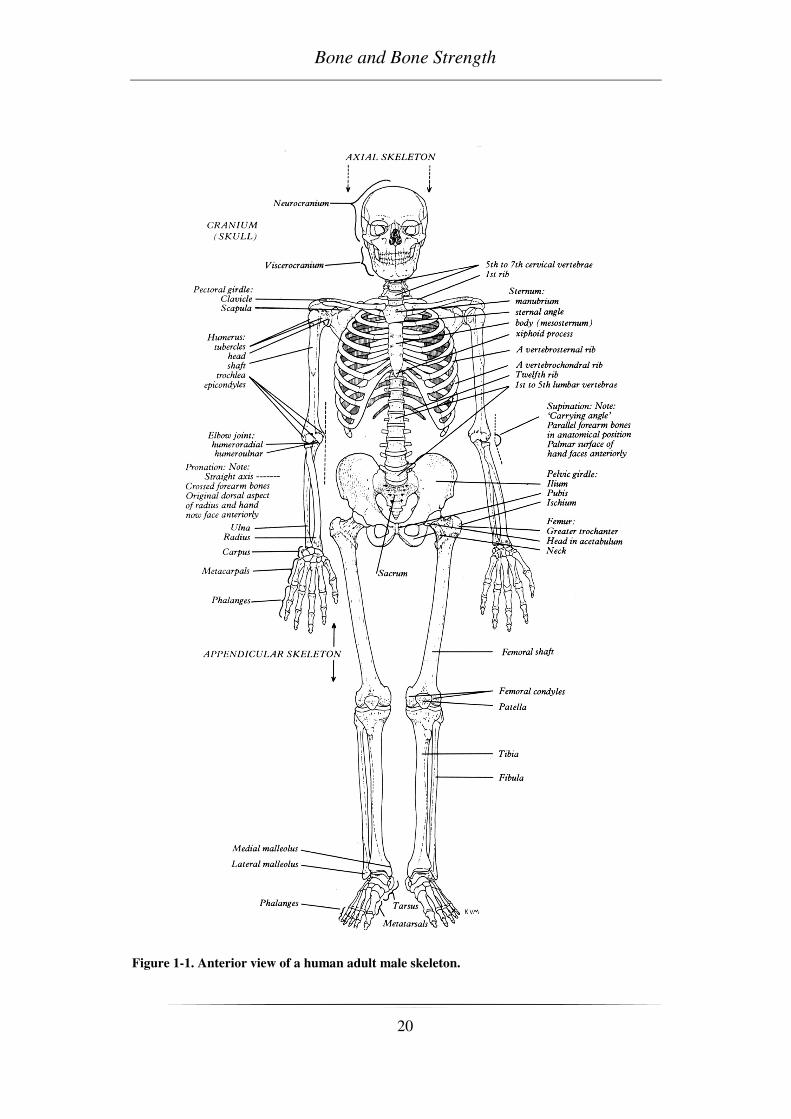
The skeletal system, showed in Figure 1-1, comprehends not only individual
bones, but also others connective tissue. [5, 6]. In this work we will discuss
mainly bone tissue. However a brief description about cartilages is below
presented due to the importance of this tissue in the later described pathology:
osteoarthritis.
Cartilage is widely present in embryo and fetus, in which acts as a precursor of
the adult skeleton and is the main centre of skeletal growth. In adulthood performs
two main functions: to keep the shape (e.g. hears, nose) and to cover the articular
surface decreasing the surface friction. In fact one important property of
cartilaginous tissue is to present a very low friction coefficient.
Bones are the main constituent of the skeleton and differs from the soft tissue
(i.e. cartilage, ligaments and tendons) in rigidity and hardness. Bones are
important to the body both biomechanically and metabolically. The skeletal tissue
performs three main functions for the life of any vertebrate; support, protection
and homeostasis of calcium. In fact the rigidity and hardness of bone enable the
skeleton to maintain the shape of the body and support it, to transmit muscular
forces from one part of the body to another during movement, to protect the soft
tissues of the cranial, thoracic and pelvic cavities, to supply the framework for the
bone marrow. The mineral content of bone serves as a reservoir for ions,
particularly calcium, and also contributes to the regulation of extracellular fluid
composition, mainly ionized calcium ion concentration.
Bone and Bone Strength
20
Figure 1-1. Anterior view of a human adult male skeleton.

Chapter 1
21
1.2 Bone morphology
Bones vary in shape and can be grouped because of their gross appearance into
long, short, flat and irregular bones [6]:
• Long bones: the limbs, as femur, tibia, humerus
• Flat bones: e.g. cranial vault, scapulae, pelvis
• Short bones: e.g. carpus, tarsus
• Irregular bones: any element not easily assigned to the former groups
A typical example of the macroscopic morphology of bone can be given by the
long bones. As described in Figure 1-2, they consist of a cylindrical shaft (or
diaphysis) and two wider and rounder ends, the epiphyses. Conical regions, called
the metaphyses, connect the diaphysis with the epiphysis. Most bones have the
ends wider than their central part, with the joints covered by articular cartilage.
Figure 1-2 Schematic representation of human femur.
1.2.1 Bone composition
Bone matrix is composed of approximately 28% by weight of organic matter,
from 60% of inorganic substance and the remaining 12% of water (38.4% in
volume organic matter, 37.7% mineral and 23.9% water) [7].

Bone and Bone Strength
22
The mineral is largely impure hydroxyapatite, Ca6(PO4)6(OH)2, containing
carbonate, citrate, fluoride and strontium. The organic matrix consists of 90%
collagen and about 10% noncollagenous proteins. From a mechanical point of
view, the bone matrix is comparable to a composite material: the organic matrix is
responsible to give toughness to the bone, while the inorganic matrix has the
function to stiffen and strengthen the bone [5].
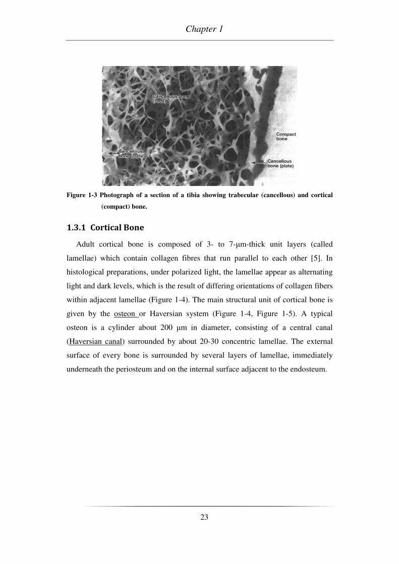
1.3 Cortical and Trabecular bone
Bones are composed in general of two basic structures, i.e. cortical and trabecular,
or cancellous, bone (Figure 1-3) [5]. Cortical bone is solid compact bone, containing
microscopic channels. Approximately 80% of the skeletal mass in the adult skeleton
is cortical bone. However, due to the different structures, trabecular bone fill the
bigger volume. Cortical bone forms the outer wall of all bones, being largely
responsible for the supportive and protective function of the skeleton. The remaining
20% of the bone mass is cancellous bone, a lattice of plates and rods having typical
mean thicknesses ranging from 50 µm to 300 µm known as trabecula, found in the
inner parts of the skeleton.
The diaphysis is composed mainly of cortical bone. The epiphysis and metaphysis
contain mostly cancellous bone, with a thin outer shell of cortical bone. During
growing, the epiphysis is separated from the metaphysis by a plate of hyaline
cartilage, known as the epiphyseal plate or growth plate. The growth plate and the
adjacent cancellous bone of the metaphysis constitute a region where cancellous bone
production and elongation of the cortex occours. In the adult, the cartilaginous growth
plate is replaced by cancellous bone, which causes the epiphysis to become fused to
the metaphysis.
Chapter 1
23
Figure 1-3 Photograph of a section of a tibia showing trabecular (cancellous) and cortical
(compact) bone.
1.3.1 Cortical Bone
Adult cortical bone is composed of 3- to 7-µm-thick unit layers (called
lamellae) which contain collagen fibres that run parallel to each other [5]. In
histological preparations, under polarized light, the lamellae appear as alternating
light and dark levels, which is the result of differing orientations of collagen fibers
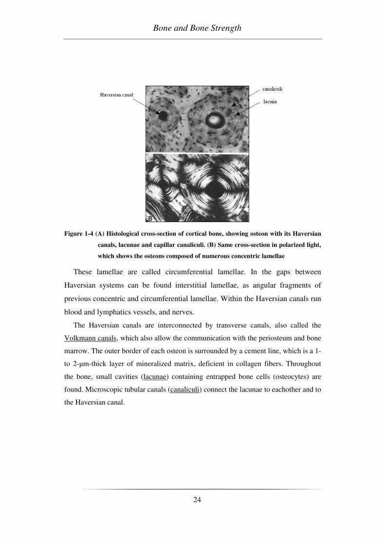
within adjacent lamellae (Figure 1-4). The main structural unit of cortical bone is
given by the osteon or Haversian system (Figure 1-4, Figure 1-5). A typical
osteon is a cylinder about 200 µm in diameter, consisting of a central canal
(Haversian canal) surrounded by about 20-30 concentric lamellae. The external
surface of every bone is surrounded by several layers of lamellae, immediately
underneath the periosteum and on the internal surface adjacent to the endosteum.
Bone and Bone Strength
24
Figure 1-4 (A) Histological cross-section of cortical bone, showing osteon with its Haversian
canals, lacunae and capillar canaliculi. (B) Same cross-section in polarized light,
which shows the osteons composed of numerous concentric lamellae
These lamellae are called circumferential lamellae. In the gaps between
Haversian systems can be found interstitial lamellae, as angular fragments of
previous concentric and circumferential lamellae. Within the Haversian canals run
blood and lymphatics vessels, and nerves.
The Haversian canals are interconnected by transverse canals, also called the
Volkmann canals, which also allow the communication with the periosteum and bone
marrow. The outer border of each osteon is surrounded by a cement line, which is a 1-
to 2-µm-thick layer of mineralized matrix, deficient in collagen fibers. Throughout
the bone, small cavities (lacunae) containing entrapped bone cells (osteocytes) are
found. Microscopic tubular canals (canaliculi) connect the lacunae to eachother and to
the Haversian canal.

Chapter 1
25
Figure 1-5 Scheme of a portion of a long bone shaft, showing details of cortical bone.
1.3.2 Trabecular Bone
The trabecular bone has not Havers systems, but consists of an array of
interconnected beams (trabecule), of a thickness less than 0.2 mm and variable in
shape (Figure 1-6). Each trabecula is constituted by a packages of parallel
lamellae. Usually a package of lamellae is up to 1 mm long and 50-60 microns in
section.
According to the site of analysis is possible to find trabecular bone with
different characteristics. The quantity of trabecular bone can widely vary within
different anatomical sites. This leads to great differences in bone density.
Moreover the orientation of the trabecular structure is tightly bonded to the
anatomical site and its mechanical role. In fact the correlation between the
trabecular orientation and the load direction was already showed in literature [8,
9]; trabecular structure result to be mainly oriented along the primary load
direction. However load direction depends by the motion, therefore trabecular
structure can became very complex.
In order to classify structure that can be very different, and to obtain some
quantitative information, some models were developed [10].

Bone and Bone Strength
26
Figure 1-6 A: vertical section of trabbecular bone from lumbar vertebra. B: single trabecula
leaving from the endosteal wall.
Such models, assumed that the trabecular bone could be made by parallel
planes (Plate like structure) or cylindrical interconnected rods (Rod like structure).
These models were widely used before the development of 3D high resolution
analysis, but are still used every time only 2D imaging is possible, and will be
describe in the next chapter.
The trabecular bone is compliant and less strong than cortical bone, generally
because of its discontinuous structure. Consequently it gives a smaller contribute
to the rigidity of the bone. Moreover can show greater variability in mechanical
behaviour than cortical bone, due to its greater structural irregularity. However we
must not underestimate his role:
• It stiffens the structure connecting the outer shell of cortical bone;
• It supports the layer of the cortex and distributes the loads in the case of
lateral impacts;
• It supports the articular cartilage and act as shock-absorber during loads;
• It transfers and distributes the load to the surrounding cortical bone;
• It protects the cave bones from phenomena of instability (buckling).
1.4 Bone development and turnover
In normal conditions, bone is characterized by a balanced coexistence of
resorptive and appositional processes. The main characters of these processes are
the bone cells. Even if they represent a not influential part of the whole skeletal

Chapter 1
27
weight they are responsible for all the processes of bone resoption, formation,
modeling and remodeling. It is still not clear what really drive them behaviour,
however the scientific community agrees to the hypothesis that the development
of a particular structure, during remodelling process, can be a reaction to
mechanical loads.
1.4.1 Bone cells
The major cellular elements of bone can be grouped in [5, 11]:
• osteoblasts
• bone-lining cells
• osteocytes
• osteoclasts
Osteoblasts:
Osteoblasts are bone-forming cells that synthesize and secrete unmineralized
bone matrix (the osteoid). They seem to participate in the calcification and
resorption of bone and to regulate the flux of calcium and phosphate in and out of
bone. Osteoblasts occur as a layer of contiguous cells which in their active state
are cuboidal (15 to 30 µm thick). Bone formation occurs in two stages: matrix
formation followed by mineralization, denoted by deposition of crystals of
hydroxyapatite.
• Their life cycle can be summarized as follows [5, 11, 12] the birth from a
progenitor cell
• the differentiation from stem cells to osteoblasts and participation in
elaborating matrix and calcifying units
• either returning to the pre-osteoblast pool, transform into bone-lining cell
and burial as osteocytes, or death.
The development of osteoblasts and osteoclasts are inseparably linked on a
molecular basis. Both are derived from precursor cells originating in bone marrow
(with osteoblasts from multipotent mesenchymal stem cells, while osteoclasts

Bone and Bone Strength
28
from hemaiopoietic cells of the monocyte/macrophage lineage), and osteoblast
differerentiation is a prerequisite for osteoclast development [5].
Bone-lining cells:
Bone-lining cells are believed to be derived from osteoblasts that have become
inactive, or osteoblast precursors that have ceased activity or differentiated and
flattened out on bone surfaces. Bone-lining cells occupy the majority of the adult
bone surface. They serve as an ion barrier separating fluids percolating through
the osteocyte and lacunar canalicular system from the interstitial fluids. Bone-
lining cells are also involved in osteoclastic bone resorption, by digesting the
surface osteoid and subsequently allow the osteoclast access to mineralized tissue.
Furthermore, it has been postulated that the 3D-networks of bone-lining cells and
osteocytes are able to sense the shape of the bone, together with its reaction to
stress and strain, and to transmit these sensations as signals to the bone surface for
new bone formation/resorption.
Osteocytes:
During bone formation, some osteoblasts are left behind in the newly formed
osteoid as osteocytes when the bone formation moves on. The osteoblasts
embedded in lacunae differentiate into osteocytes. In mature bone osteocytes are
the most abundant cell type. They are found to be about ten times more than
osteoblasts in normal human bone. Mature osteocytes posses a cell body that has
the shape of an ellipsoid, with the longest axis (25 µm) parallel to the surrounding
bone lamella. The osteocytes are thought to be the cells best placed to sense the
magnitude and distribution of strains. They are thought both to respond to changes
in mechanical strain and to respond to fluid flow to transduce information to
surface cells, via the canalicular processes and the communicating gap junctions.
Osteocytes play a key role in homeostatic, morphogenetic and restructuring
process of bone mass that constitute the regulation of mineral and architecture [5].
Chapter 1
29
Osteoclasts:
Osteoclasts are bone-resorbing cells, which contain one to more than 50 nuclei
and range in diameter from 20 to over 100 µm. Their role is to resorb bone, by
solubilizing both the mineral and the organic component of the matrix. The
signals for the selection of sites to be resorbed are unknown. Biphoshponates,
calcitonin and estrogen are commonly used to inhibit resorption. These are
believed to act by inhibiting the formation and activity of osteoclats and
promoting osteoclasts apoptosis.
1.4.2 Bone resorption
The actual mechanism for the activation of osteoclast bone resorption is still
unclear. Osteoclasts begin to erode the bone while coming in contact with the
surface of bone. During this activity osteoclasts form cavities (Howship’s
lacunae) in cancellous bone, and cutting cones or resorption cavities in cortical
bone. The resorption process occurs in two steps, which occur essentially
simultaneosly: dissolution of mineral and enzymic digestion of organic
macromolecules.
1.4.3 Bone formation
Bone formation occurs in two phases: matrix synthesis followed by
extracellular mineralization. The osteoblasts begin to deposit a layer of bone
matrix, referred to as the osteoid seam. After about 5 to 10 days, the osteoid seam
reaches a level of approximately 70% of its mineralization. The complete
mineralization takes about 3 to 6 months in both cortical and trabecular bone.
Bone formation is a complex process regulated by hormones (e.g. Parathyroid
hormones) and growth factors (e.g. Transforming Growth Factor-β).
The building of bone as a functional organ is an important process, as bone
constantly enlarges, renews and develops itself in time. In the same time it adapts
itself to support protection, mechanical needs and numerous metabolic and
hematopoietic activities [6, 13, 14].

Bone and Bone Strength
30
In this thesis, the normal growing of long bones will be addressed only briefly.
It is just mentioned that this growth follows a cartilaginous model, involving the
growth through the epiphyseal plates, the metaphyseal spongiosa growth, and the
circumferential growth of the bone shaft. This chapter is more focused in the
modeling and remodeling process, which play an important role both for normal
bone growth as also for the adaptation processes that occur in pathological
modification of bone (e.g. osteoporosis, osteoarthritis).
1.4.4 Modeling
In general, growth and modelling are linked together [5]. Modeling allows the
development of normal architecture during growth, controlling the shape, size,
strength and anatomy of bones and joints. It increases the outside cortex and
marrow cavity diameters, gives shape to the ends of long bones, drifts trabeculae
and cortices, enlarges the cranial vault and changes the cranial curvature. During
normal growth, periostal bone is added faster by formation drifts than endosteal
bone is removed by resorption drifts. This process is regulated so that the
cylindrical shaft markedly expands in diameter, whereas the thickness of the wall
and the marrow cavity slowly increase.
Modeling controls also the modulation of the bone architecture and mass when
the mechanical condition changes [15]. For example, bone surfaces can be moved
to respond to mechanical requirements. A coordinate action of bone resorption
and formation of one side of the periosteal and endosteal surfaces can move the
entire shaft to the right or left, allowing some bones to grow eccentrically [16].
1.4.5 Remodeling
Remodelling can be defined as a process that produces and maintains bone that
is biomechanically and metabolically competent [5]. At infancy, the immature
(woven) bone at the metaphysis is structurally inferior to mature bone. In adult
bone, the quality (e.g. mechanical properties) of bone deteriorates with time.
Thus, as many other tissues, bone must replace or renew itself. This replacement
of immature and old bone occurs by a process called remodeling, which is a

Chapter 1
31
sequence of resorption followed by formation of new lamellar bone [15]. The
remodeling characterizes the whole life of bones. For normal rates of periodic
bone replacement (bone turnover), cancellous bone has a mean age of 1 to 4 years,
while cortical bone about 20 years.
The remodeling has both positive and negative effects on bone quality on the
tissue level. It allows to remove microdamage, replace dead and hypermineralized
bone, adapt the microarchitecture to local stresses. But remodeling may also
perforate or remove trabeculae, increase cortical bone porosity, decrease cortical
width and possibly reduce bone strength.
The group of bone cells that carries out one quantum of bone turnover,
osteoclast, osteoblast and their progenitors, is called a bone remodeling unit
(BRU). The life cycle of a unit can be summarized in the following stages:
resting, activation, resorption, reversal (coupling), formation, mineralization and
back to resting.
Resting:
About 80% of the cancellous and cortical bone surfaces (periosteal and
endosteal) and about 95% of the intracortical bone surfaces in large adult animals
(including humans) are inactive with respect to bone remodeling stage, at any
given time. These inactive surfaces are covered by bone-lining cells and a thin
endosteal membrane.
Activation:
As activation is defined the conversion of the quiescent bone surface to
resorption activity. Which factor initiates this process is unknown. However,
activation is believed to occur partly in response to local structural or
biomechanical stimuli. The remodeling cycle necessitates the recruitment of
osteoclasts and the mean for them to access the bone surface.
Resorption:
Osteoclasts begin to erode bone, forming cavities.
Reversal:
The 1- to 2- week interval between completion of resorption and the beginning
of bone formation is called reversal.

Bone and Bone Strength
32
Formation and mineralization:
Bone formation occurs, through matrix synthesis followed by extracellular
mineralization.
Bone turnover depends both on the surface-restricted activation frequency and
on the surface-to-volume ratio. The activation frequency is the inverse of the time
interval between consecutive cycles of remodeling at the same site. The surface-
to-volume ratio of cancellous bone is about 5- to 10 times bigger than in cortical
bone.
There are studies showing that remodeling does differ in different parts of the
skeleton and also in different parts of a given bone at any moment. Possible
reasons are that where microdamage occurs, BRU-based remodeling increases to
try to repair it. Usually, such regions are highly loaded sites, like the epiphyseal
spongiosa (Burr et al. (1985); Cowin (2001)). Another reason could be, that
during growth parts of the skeleton accumulated more bone than actually needed
for mechanical usage, which will increase remodeling-dependent bone loss (Frost
& Jee (1994); Cowin (2001)). In the adult bone the bone remodeling provides a
mechanism for the skeleton to adapt to its mechanical environment, due to
inactivity or to hypervigorous activity. These phenomena are grouped together as
biomechanical-driven remodeling. Conversely, it is sustained that there exist
genetically driven remodeling or stochastic remodeling that prevents fatigue
damage. This hypothesis is highly disputed [5, 17, 18].
1.4.6 The mechanostat hypothesis
By observing the variation in trabecular architecture, Wolff formulated a law
[19], which links trabecular architecture to mechanical usage by adaptation Wolff
stated that the architecture is related to mechanical usage “in accordance with
mechanical laws”, but without specifying these laws. The mechanostat hypothesis
was introduced by Frost [20, 21] to explain how mechanical usage regulates bone
mass and architecture. It is based on the idea that there exists an effective strain
that induces a response to change the bone mass and strength. The mechanism
would behave like a thermostat in a house. In this concept, depending on the

Chapter 1
33
mechanical usage of bone, signals are transmitted to the modeling and remodeling
system, which actively alter bone mass and shape.
1.5 Osteoarthritis
Figure 1-7 The degeneration of hip osteoarthrosis is represented.
The abnormal function of the processes previously described can lead to the
development of several pathologies. One in particular is reported here as
introduction because object of study later in this thesis: the osteoarthritis (OA).
The OA, also known as degenerative articular disease, is the result of a gradual
erosion of the articular cartilage in joints. The joints most affected are the knee,
the hip and hand. The knee and hand are affected more frequently in women and
the hip in men. The hip osteoarthritis is a very common disease. The most
important risk factor in the genesis of this pathology is represented by age.
Osteoarthritis (OA) was defined as the 4th leading cause of Years Lost due to
Disability in the study “Global Burden of Disease 2000”, published in the World
Health Report 2002 [22]. This disease places an enormous demand on orthopaedic
services. Understanding the development of this disease is important to improve
the medical approaches to OA. Nevertheless, information about this pathology is
still incomplete and its comprehension is a challenge not yet resolved. For these
reasons the study of OA was part of the present work, and it will be discussed in 0
and 0.

Bone and Bone Strength
34
1.6 Bone Strength
The anatomical introduction about bone gave us an idea about how complex
the mechanisms involving bone tissue are. It results logical to argue that is not
possible to find one single parameter able to fully describe the mechanical
properties of bone.
In this thesis it was decided to approach the study of bone strength by defining
two macro-classes describing the main components responsible for the resistance
to fracture of bone: quantity and quality of bone. The class defined as bone quality
was mainly studied, therefore was splitting it into two sub-classes named bone
structure and tissue quality (Figure 1-8).
Figure 1-8 All the sub-classes defining bone strength are represented.
The study was focused on trabecular bone tissue due to its greater variability
and only in the last chapter the cortical bone was approached. Therefore bone
structure refers to the micro structure of trabecular bone. On the other hand the
study of tissue quality is aimed to the evaluation of the material by which
trabecular and cortical bone are constitute.

Chapter 1
35
1.6.1 Bone Quantity
The study of trabecular bone quantity is the current clinical standard measure
for so-called bone densitometry, and research studies have amply demonstrated
that the amount of tissue is correlated with its mechanical properties of elasticity
and fracture. It represents the volume of mineralized tissue presented in the
analyzed area and give not information about the distribution of the matter. For
this reason the models presented in the literature, including information on the
mere quantity of tissue, have often been limited in describing the mechanical
behaviour of bone tissue. Recent investigations have underlined that also the
bone-structure and the tissue-mineralization play an important role in the
mechanical characterization of bone tissue
Nonetheless the bone quantity results the main parameter in clinical practice
for the assessment of bone strength. Moreover in research studies it is still
recognized as the most representative parameter. In the present thesis bone
quantity was not focused. Its role is consolidated and do not need further study.
Aim of this work was to identify which parameters can join the information about
quantity in order to fully describe bone strength.
1.6.2 Bone Quality
Bone quality is a generic name to describe every parameter is not bone
quantity. It is important to underline that quantity cannot completely explain the
mechanical behaviour of bone tissue, but at the same time a definition of what
quality means is needed. On the basis of what was previously described about
bone cells and bone remodeling we decided to split the study of bone quality in
two sub-classes: bone structure and tissue quality.
Bone structure
Analysis of bone structure was the principal topic of the present thesis. The
whole study was focused on trabecular structure due to its high heterogeneity and,
therefore, high impact on mechanical behaviour of this tissue. Moreover, form the
Bone and Bone Strength
36
clinical point of view, trabecular tissue represents an important structure for the
bone integrity during age.
The first step into the analysis of bone structure was to mechanically test in
compression bone trabecular specimens. These specimens were extracted with a
known main trabecular direction (MTD).The aim was to verify whether a
misalignment between the testing direction and the MTD, later called off-axis
angle, has a significant effect on the compressive behaviour of cancellous bone. In
this work, presented extensively in Chapter 4, procedures for the control of the
MTD were defined and the results demonstrated a great effect of the off-axis
angle on the compressive behaviour of trabecular bone. This angle should be
reduced as much as possible, in any case measured and controlled, and always
reported together with the mechanical parameters of cancellous bone.
The developed procedures for the MTD control gave the possibility to manage
the variability of trabecular bone framework. In this way was possible to start a
new analysis of bone strength, controlling the structural influence [4]. Perilli et al.
concluded that, due to the heterogeneity of cancellous bone, there may exist
regions characterized by a different microarchitecture, where the bone is weaker
and consequently is more likely to fail. These regions mostly contain minimum
amount of bone quantity, which were found to predict ultimate stress better than
average bone quantity. To the author’s knowledge few articles introduced the
importance of local analysis [4, 23], highlighting how the local bone quantity,
area with minimum quantity, can be a strong predictor of mechanical properties.
However quantity can be a strong predictor only when bone structure is controlled
by the limitation of the off-axis angle. Only controlling the bone structure it is
possible to fully describe mechanical properties by means of local bone quantity.
For this reason the second step of the mechanical study was to identify which
structural parameters, among the several presented in the literature, could be
integrated with the information about quantity, in order to better describe and
predict the mechanical properties of bone. The aim of this part of the study,
presented in 0, was to arrange the most used structural parameter in a consistent
model of mechanical characterization of trabecular bone. The purpose was to

Chapter 1
37
present a method of analysis independent of the presence of high structural
variation within a single specimen.
In this part of the work the importance of considering off-axis angle was once
again demonstrated. The researcher should decide to apply the preferred form of
control; to include off-axis angle in its models or to test only specimen with
known MTD, but he should not ignore this problem. Moreover the local analysis
was confirmed to be a powerful tool for the mechanical characterization of bone
tissue. On the one hand this work was limited by the use of osteoarthritic
specimens. On the other hand we had the possibility to study in depth this
pathology.
In fact, because of the significant relation between structure and mechanics,
the involvement of structural modifications during the development of
osteoarthritis was investigated. This kind of study, fully presented in 0, was aimed
to assess whether the osteoarthritis have some kind of influence on micro structure
of the trabecular bone. The study highlighted a variation in degrees of anisotropy
in osteoarthritic bone compared to a matched group of non pathologic specimens.
In particular a major orientation of MTD of the trabecular framework along the
load direction was found. This situation could be driven by a changing in lifestyle,
reduction in dynamic range of motion of the hip, of osteoarthritic patients due to
antalgic gait.
Tissue quality
Quality of the tissue is a very complex issue and many different methods can
be used to study it at several different levels. As we did for bone quality, this class
could be divided in many sub-classes(e.g. lamellar structure, metabolic activity of
bone cells, composition of bone matrix). However a frequent approach to the
analysis of tissue quality is the study of its mineralization.
The last part of this thesis is aimed to introduce the study of tissue quality and
it is presented extensively in the 0. Microtomography is a privileged tool for the
study of tissue mineralization due to the tightly link between bone density and x-
ray absorption. However the study of tissue density by means of micro-CT is an

Bone and Bone Strength
38
emerging field, and difference between bone density and tissue density is not yet
completely clear. In this last study we define bone density, or ash density, as the
ratio between the mass of the ashed samples and the geometrical volume of the
specimen. The relation between bone density and bone quantity was studied both
for trabecular and cortical bone.

Chapter 2
39
CHAPTER 2 MICRO-CT IMAGING FOR
QUANTIFICATION OF BONE STRUCTURE
As explained in Chapter 1 variation of the structure starts from cell level but
involve every level, reaching the macro-scale of the whole bone segment, and
involve both cortical and trabecular structures. The micro-structures of bone tissue
resulted to be an important meso-scale to transmit the cellular-level modifications
to the organ level of the whole bone segment. For this reason the micro-computed
tomography (micro-CT) result to be a powerful tool in the study of bone quality.
In this chapter the basic principles of micro-CT analysis and the techniques of
bone structure quantifications will be described.
2.1 Principal imaging techniques applied on bone
2.1.1 About tomography
The word “tomography” originates from two Greek words: “tomos” (τόµος),
which means “slice”, and “graphein” (γράφειν), which means “to write”.
In medical imaging, tomography usually refers to cross-sectional imaging of an
object from either transmission or reflection data, collected by illuminating the
objects from many different directions [24]. The first tomographic application in
medical field utilized X-rays, but also other radiation sources can be used, as
gamma-rays in the case of the Single Photon Emission Tomography, for example
[25]From a purely mathematical standpoint, the solution to the problem how to
reconstruct a function from its projections dates back to the paper of Radon in
1917 [26]. The current systems in tomographic imaging originated with
Hounsfield’s invention in 1972 [27], who shared the Nobel prize with Allan
Cormack [28], who independently discovered some of the algorithms.
2.1.2 Computed tomography (CT)
X-ray Computed tomography (usually referred to as simply computed
tomography) is based on the projection data obtained from the attenuation of X-

Micro-CT Imaging for Quantification of Bone Structure
40
rays. X-rays originated from a source interact with the object to be imaged and
emerge as projection data. These projection data are the result of the interaction
between the radiation used for imaging and the substance of which the object is
composed. Using algorithms for the back-calculation of these projection data,
cross-sections of the imaged object can be reconstructed.
Different CT scanner configurations were developed with time, by which either
the X-ray sources or the detector system are moving, the number of detectors are
augmented, with the principal aim to reduce scan-time [24]. However, the basic
principles are still similar: all reconstructed cross-section images are based on the
attenuation coefficients of the examined object. With a proper calibration, it is
possible to convert the cross-section images in density images, for example in
Hounsfield Units [24]. However, with clinical systems using polychromatic X-ray
sources, limitations arise because of the X-ray energy spectrum (beam hardening
artifact). Special software and hardware calibration procedures were developed, to
counteract these artifacts. Another type of artifact is given by the partial volume
effect, due to mismatch of the spatial resolution of the measuring system and the
examined structural dimensions. These can be neglected only if spatial resolution
is much higher than the structural dimensions. Standard hospital-based systems
have typically a limited in-plane resolution, with a slice thickness which can
hardly be reduced to no more than 1mm. Thus, it is difficult to use such standard
equipment for the imaging of the bone microstructure. However, by using special
setups for in-vitro imaging of bone biopsies, in plane resolutions of 150 µm were
reported, with a slice thickness of 330 µm [29, 30].
2.1.3 MicroCT
MicroCT was pioneered in the late 1980’s and is based on the same basic
principles as the common computed tomography [2, 3]. In general, the system
consists of a microfocus tube which generates a cone-beam of X-rays, a rotating
specimen holder on which is mounted the object, and a detector system which
acquires the images. One of the main differences to medical CT is that during
microCT scanning, the source-detector geometry is fixed, while images are taken
Chapter 2
41
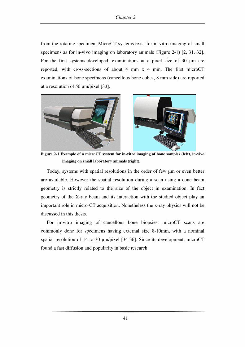
from the rotating specimen. MicroCT systems exist for in-vitro imaging of small
specimens as for in-vivo imaging on laboratory animals (Figure 2-1) [2, 31, 32].
For the first systems developed, examinations at a pixel size of 30 µm are
reported, with cross-sections of about 4 mm x 4 mm. The first microCT
examinations of bone specimens (cancellous bone cubes, 8 mm side) are reported
at a resolution of 50 µm/pixel [33].
Figure 2-1 Example of a microCT system for in-vitro imaging of bone samples (left), in-vivo
imaging on small laboratory animals (right).
Today, systems with spatial resolutions in the order of few µm or even better
are available. However the spatial resolution during a scan using a cone beam
geometry is strictly related to the size of the object in examination. In fact
geometry of the X-ray beam and its interaction with the studied object play an
important role in micro-CT acquisition. Nonetheless the x-ray physics will not be
discussed in this thesis.
For in-vitro imaging of cancellous bone biopsies, microCT scans are
commonly done for specimens having external size 8-10mm, with a nominal
spatial resolution of 14-to 30 µm/pixel [34-36]. Since its development, microCT
found a fast diffusion and popularity in basic research.
Micro-CT Imaging for Quantification of Bone Structure
42
2.2 Quantification of trabecular bone
Cancellous bone can be studied at different hierarchical levels, from the
ultrastructure of collagen and mineral to macroscopic apparent density [37-41].
The architecture of cancellous bone is studied at the scale of individual trabeculae,
at a resolution in the range from of 20 µm to 50µm [5].
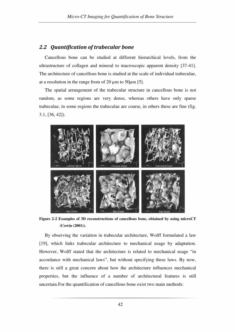
The spatial arrangement of the trabecular structure in cancellous bone is not
random, as some regions are very dense, whereas others have only sparse
trabeculae, in some regions the trabeculae are coarse, in others these are fine (fig.
3.1, [36, 42]).
Figure 2-2 Examples of 3D reconstructions of cancellous bone, obtained by using microCT
(Cowin (2001)).
By observing the variation in trabecular architecture, Wolff formulated a law
[19], which links trabecular architecture to mechanical usage by adaptation.
However, Wolff stated that the architecture is related to mechanical usage “in
accordance with mechanical laws”, but without specifying these laws. By now,
there is still a great concern about how the architecture influences mechanical
properties, but the influence of a number of architectural features is still
uncertain.For the quantification of cancellous bone exist two main methods:
Chapter 2
43
1) traditional 2D histomorphometric methods
2) methods based on 3D reconstructions
There exist also other methods, such as those based on texture analysis of plain
radiographs, but these will not be discussed [43]
2.3 Traditional 2D histomorphometric methods
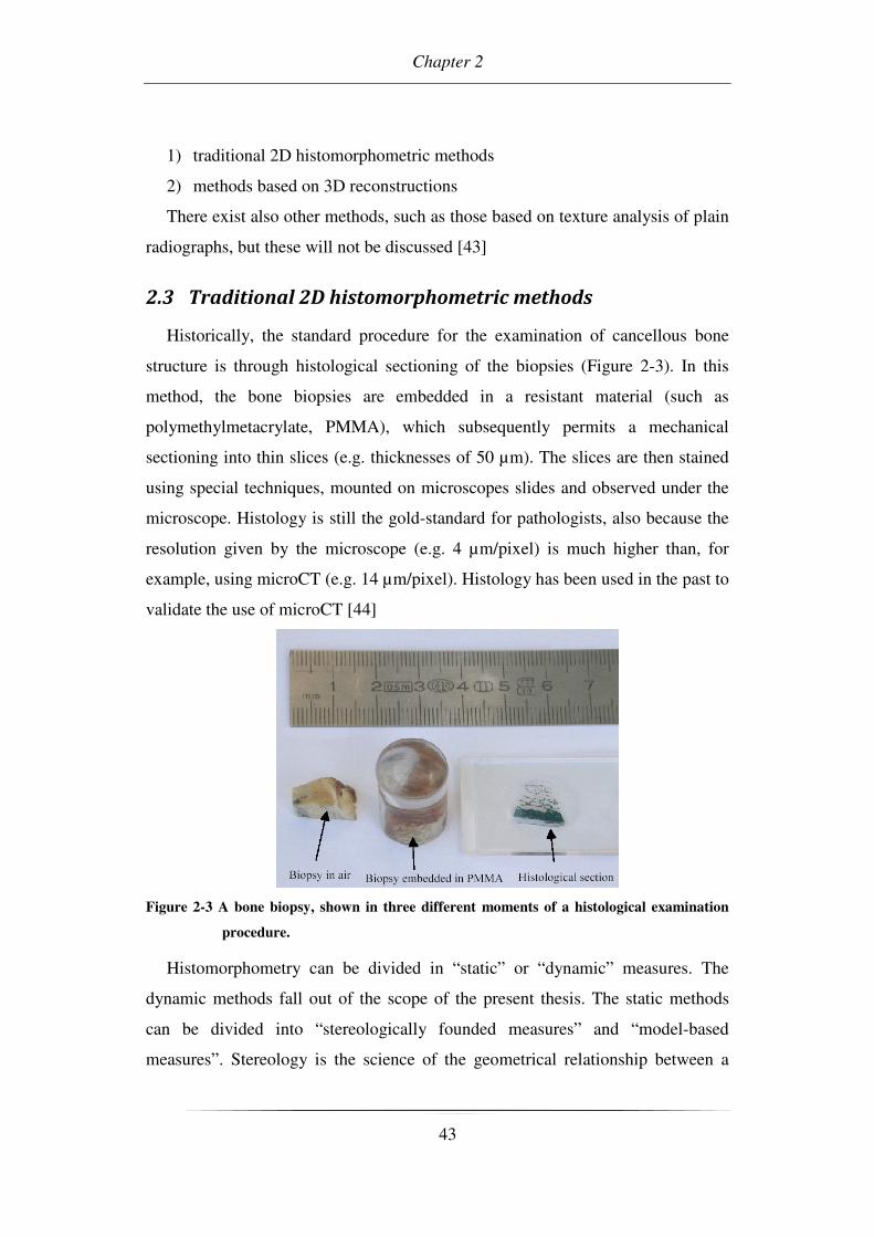
Historically, the standard procedure for the examination of cancellous bone
structure is through histological sectioning of the biopsies (Figure 2-3). In this
method, the bone biopsies are embedded in a resistant material (such as
polymethylmetacrylate, PMMA), which subsequently permits a mechanical
sectioning into thin slices (e.g. thicknesses of 50 µm). The slices are then stained
using special techniques, mounted on microscopes slides and observed under the
microscope. Histology is still the gold-standard for pathologists, also because the
resolution given by the microscope (e.g. 4 µm/pixel) is much higher than, for
example, using microCT (e.g. 14 µm/pixel). Histology has been used in the past to
validate the use of microCT [44]
Figure 2-3 A bone biopsy, shown in three different moments of a histological examination
procedure.
Histomorphometry can be divided in “static” or “dynamic” measures. The
dynamic methods fall out of the scope of the present thesis. The static methods
can be divided into “stereologically founded measures” and “model-based
measures”. Stereology is the science of the geometrical relationship between a
Micro-CT Imaging for Quantification of Bone Structure
44
structure that exists in three dimensions and the images of that structure given in
2D [45]. These 2D images can be obtained by various means, as through
microscope images of sections of the structure, which are mainly used by
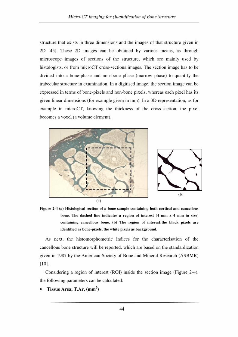
histologists, or from microCT cross-sections images. The section image has to be
divided into a bone-phase and non-bone phase (marrow phase) to quantify the
trabecular structure in examination. In a digitised image, the section image can be
expressed in terms of bone-pixels and non-bone pixels, whereas each pixel has its
given linear dimensions (for example given in mm). In a 3D representation, as for
example in microCT, knowing the thickness of the cross-section, the pixel
becomes a voxel (a volume element).
Figure 2-4 (a) Histological section of a bone sample containing both cortical and cancellous
bone. The dashed line indicates a region of interest (4 mm x 4 mm in size)
containing cancellous bone. (b) The region of interest:the black pixels are
identified as bone-pixels, the white pixels as background.
As next, the histomorphometric indices for the characterisation of the
cancellous bone structure will be reported, which are based on the standardization
given in 1987 by the American Society of Bone and Mineral Research (ASBMR)
[10].
Considering a region of interest (ROI) inside the section image (Figure 2-4),
the following parameters can be calculated:
• Tissue Area, T.Ar, (mm2)
Chapter 2
45
It is the total area of the region of interest (ROI) in examination, which is the
sum of the elemental areas of the bone-pixels and non-bone pixels.
• Tissue Volume, TV, (mm3)
The total volume of interest in examination, i.e. in the case of a stack of slices,
the volume of interest represented by the sum of all voxels.
• Bone Area, B.Ar, (mm2)
The sum of all pixels marked as bone inside the ROI.
• Bone Volume, BV, (mm3)
The sum of all voxels marked as bone inside the volume of interest.
• Bone Perimeter, B.Pm, (mm)
The sum of the bordering pixels marked as bone inside the ROI.
• Bone Surface, BS, (mm2)
The surface area of the structure marked as bone inside the volume of interest.
2.3.1 Bone Volume Fraction, BV/TV
volumetissue
volumebonetrabecular
TV
BV=
Eq. 2-1
The bone volume fraction in a single slice is equivalent to the fraction
B.Ar/T.Ar. It has to be noticed, that when reporting BV/TV as a percentage, the
equation Eq. 2-1 has to be multiplied by 100.
2.3.2 Bone Surface Density, BS/TV, (mm/mm2)
volumetissue
surfacebonetrabecular
TV
BS=
Eq. 2-2
In a single slice, the BS/TV is equivalent to BS/TV = ((4/π) * (B.Pm/T.Ar)),
which is correct for isotropic structures. For human cancellous bone, such as the
iliac crest, it has been experimentally determined that BS/TV = (1.199 *
(B.Pm/T.Ar)) [10].
The previously presented parameters are model independent, also called
“primary indices”, as these are calculated directly on the image or volume in
examination.

Micro-CT Imaging for Quantification of Bone Structure
46
There are also “model-dependent indices“ or “secondary indices” for the
quantification of trabecular bone architecture, which are indirect calculations
based on areas and perimeters. These model-dependent methods are aimed at
determining properties of the trabecular architecture that are assumed to be related
to mechanical properties [5]. As hint in chapter 1.3.2 it is possible to distinguish
between two models: plate-model and rod-model
Figure 2-5 Plate and Rod models used for the calculation of anatomical-structure indexes.
The most widely used is the plate model, which assumes that all the trabecular
bone is organized in infinite plates, with a certain thickness (Tb.Th), separation
(Tb.Sp), and number per unit length (Tb.N). Formerly, these parameters contained
the word “plate” (e.g. MTPT, mean trabecular plate thickness) within their
terminology, which was unfortunately eliminated following the standardization.
Thus, reporting these parameters, it has to be explicit mentioned which model is
used [46].
2.3.3 Trabecular Thickness, Tb.Th, (µm)
BS
BV
PmB
ArBThTb 2
.
.
199.1
2. ==
(plate model) Eq. 2-3
The trabecular thickness gives the thickness of the trabeculae, assuming a plate
model.
2.3.4 Trabecular Number, Tb.N, (1/mm)
TV
BS
ArT
PmBNTb
2
1
.
.
2
199.1. ==
(plate model) Eq. 2-4

Chapter 2
47
The trabecular number (or trabecular density) is the number of plates traversed
by a line of unit length perpendicular to the plates.
2.3.5 Trabecular Separation, Tb.Sp, (µm)
ThTbNTb
SpTb ..
1. −=
(plate model) Eq. 2-5
Trabecular separation is defined as the distance between edges of the
trabeculae.
2.4 Methods based on 3D reconstructions
The recommendations worked out by the ASBMR were developed to interpret
2D sections, with the third dimension taken into account by model assumptions.
However, the error made by making the wrong model assumption can be
considerable.
With the development of 3D-imaging techniques, such as microCT, it was
possible to develop new image tools that take full advantage of all three
dimensions [46]. As an example, such procedures are given by the direct surface
and volume determination. The bone surface area (BS) can thus be calculated by
using the marching cubes algorithm, to triangulate the mineralised bone surface
[47] (Figure 2-6). Tetrahedrons are then used to calculate the bone volume (BV)
of the triangulated surface. Using the direct-techniques, it is then possible to
calculate parameters such as the model independent thickness, model independent
separation, structure model index, 3D-connectivity, mean intercept length and
degree of anisotropy.
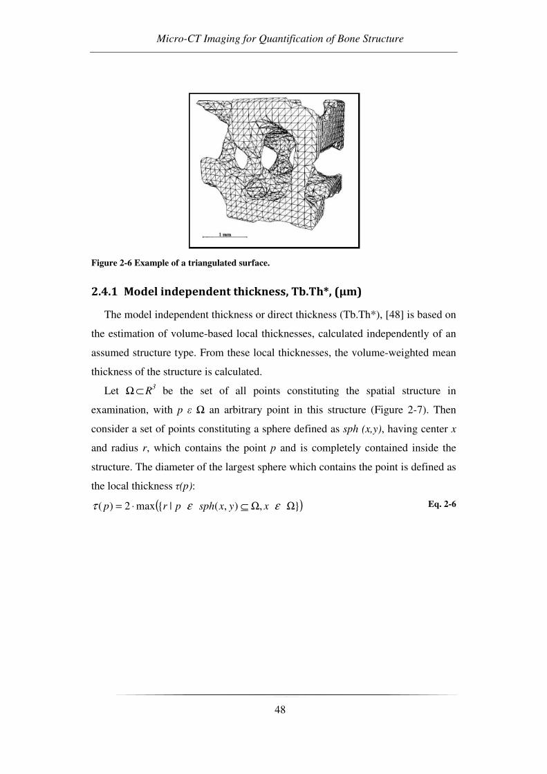
Micro-CT Imaging for Quantification of Bone Structure
48
Figure 2-6 Example of a triangulated surface.
2.4.1 Model independent thickness, Tb.Th*, (µm)
The model independent thickness or direct thickness (Tb.Th*), [48] is based on
the estimation of volume-based local thicknesses, calculated independently of an
assumed structure type. From these local thicknesses, the volume-weighted mean
thickness of the structure is calculated.
Let Ω⊂ R3 be the set of all points constituting the spatial structure in
examination, with p ε Ω an arbitrary point in this structure (Figure 2-7). Then
consider a set of points constituting a sphere defined as sph (x,y), having center x
and radius r, which contains the point p and is completely contained inside the
structure. The diameter of the largest sphere which contains the point is defined as
the local thickness τ(p):
( ),),(|max2)( ΩΩ⊆⋅= εετ xyxsphprp Eq. 2-6

Chapter 2
49
Figure 2-7 containing the point p and having maximum radius, entirely enclosed in the
structure Ω. Thus, the local thickness τ(p) in the point p is equal to the diameter
of the sphere (from [48]).
As an example, in the case of an ideal cylinder with infinite length, all points in
the structure will have the same local thickness value corresponding to the
diameter of the cylinder.
The arithmetic mean value of the local thicknesses, taken over all points in the
3D structure, gives the mean thickness τ of the structure (eq. (3.7)), which is also
noted as Tb.Th* in the examination of trabecular bone:
xdxVol ∫∫∫ΩΩ
= 3)()(
1ττ , ∫∫∫Ω=Ω xdVol 3)(
Eq. 2-7
2.4.2 Model independent separation, Tb.Sp*, (µm)
The Tb.Sp* [48] is calculated with the same procedure as used for the Tb.Th*,
but this time the voxels representing non-bone parts are filled with maximal
spheres. The separation is thus the thickness of the marrow cavities.
2.4.3 Structure Model Index, SMI
The structure model index (SMI, [49]estimates the characteristic form in terms
of plates and rods composing the 3D-structure (Figure 2-5). It assumes the values

Micro-CT Imaging for Quantification of Bone Structure
50
0, 3 and 4 for ideal plates, rods and spheres respectively. Mixed structures
composed of both rods and plates have SMI-values lying between 0 and 3.
Given the structure volume V and the structure surface , the structure model
index is calculated as:
S
VSSMI
'6 ⋅=
Eq. 2-8
where S is defined as the structure derivative of the volume with respect to a
linear measure r and S’ denotes the structure surface area derived with respect to
r:
r
VS
∂
∂= ,
r
SS
∂
∂='
Eq. 2-9
For the implementation, the surface area S(r) is found by triangulation of the
structure surface using the Marching Cube method. [47]Then structure thickening
is simulated by displacing the triangulated surface by a small distance ∆r in its
normal direction and recalculating the surface area S(r+∆r). The derivative of the
surface area is then calculated as:
r
rSrrS
r
SS
∆
−∆+=
∂
∂=
)()('
Eq. 2-10
where the magnitude of the displacement ∆r, i.e. the thickening of the
structure, is chosen so that it is more than an order of magnitude smaller than the
voxel side length.
2.4.4 3D Connectivity
Connectivity is defined as a measure of the degree to which a structure is
multiple connected. Thus, for a network, it reports the maximal number of
branches that can be broken, before the structure is separated in two parts. In the
discipline of topology there are a full set of theorems for handling the connectivity
of cancellous bone. Recently it was found that no functional relationship exists
between connectivity and elastic properties of trabecular bone. However, a
connectivity-loss during a bone atrophy-bone re-growth cycle primarly reflects
Chapter 2
51
trabecular breakage, which is related to a loss of mechanical stiffness [50]. A
complete description of this parameter can be found in the work of Odgaard [51].
2.4.5 Mean Intercept Length, MIL
Whitehouse provided a detailed description of cancellous bone architectural
anisotropy using the mean intercept length (MIL) method [52]. The MIL method
is based on placing an equispaced linear grid with orientation Θ onto a structure
and counting the number of intersections I between the grid and the bone-marrow
interface. Thus, at a given orientation ω of the grid, the mean intercept length
MIL(Θ) (i.e. the mean length between two consecutive intersections) is the total
line length L divided by the number of intersections I(Θ):
)()(
Θ=Θ
I
LMIL
Eq. 2-11
Whitehouse noticed, that collecting the mean intercept length on cancellous
bone sections at various orientations of the grid, and plotting the values of
MIL(Θ) in a polar diagram, a figure approximating an ellipse was generated. The
main axis of the ellipse indicated the main orientation of the bone-marow
interface, i.e. of the cancellous bone structure.
A generalization of this observation into 3D space would result in an ellipsoid
(Figure 2-8). Harrigan and Mann noted that this could be expressed as the
quadratic form of a second-rank tensor M [53]. The MIL fabric tensor E was
defined by Cowin as the inverse square root of M [54, 55]. The advantage of
using the MIL fabric tensor E is that larger values of E will be associated with
larger values of Young’s modulus, and that the eigenvalues of E are the MIL
values in the main orientations (for details see Cowin 2001, [5].

Micro-CT Imaging for Quantification of Bone Structure
52
Figure 2-8 Example of the MIL method on cancellous bone, to obtain the average orientation
of the trabeculae in3D; (a) A linear grid is applied on a bone section. The
intersections per total length line at the bone-marrowinterface are counted, with
varying angle Θ of the grid. Reporting these values in a polar plot, an ellipse
isgenerated. (b) In 3D, (i.e. varying also the angle Φ), this generates an ellipsoid.
The principal axes of the ellipsoid indicate the main orientations of the bone-
marrow interface in 3D (from [5]).
However a normalization of the fabric tensor E was proposed [56] in order to
present the tensor as independent of the quantity. Therefore in the present thesis
was used the normalization of tensor the eigenvalues, as reported in Eq. 2-12
1=++ kji HHH
kji
ii
EEE
EH
++=
Eq. 2-12
2.4.6 Degree of anisotropy, DA
In the case of an anisotropic structure (Figure 2-8), the polar plot of MIL gives
an ellipsoid, with the principal axes of the ellipsoid representing the main
trabecular orientation. The ratio between the lengths of the principal axes gives an
information about the anisotropy of the structure, i.e. the degree of anisotropy
[57]:
min
max
MIL
MILDA =
When the analyzed is a 3D one it is possible to compute the DA in three
dimensions making the ratio between the three main axes of the ellipsoid.
Conversely, a polar plot of the MIL of an ideal isotropic structure will be
represented by a sphere, giving DA=1.

Chapter 2
53
2.5 Application for the imaging and quantification of
trabecular bone structure
The typical procedure for microCT imaging and quantification of cancellous
bone structure is composed of three steps:
• Acquisition of the projection data.
• The cross-section reconstruction
• Segmentation of the images and calculation of the
histomorphometric/structural parameters
The bone samples examined by microCT are usually of cylindrical or
parallelepiped shape, with a diameter or side length in the order of 5-10 mm
(Figure 2-9).
Figure 2-9 (Left) Example of a parallelepiped-shaped cancellous bone biopsy, obtained from
a human femoralneck. (Right) Example of a cancellous bone biopsy embedded in
PMMA.
2.5.1 Acquisition of the projection data
The bone sample is put on the rotation stage into the microCT scanner (Figure
2-10). The microCT scan of the frontal images of cancellous bone samples is done
typically with the source set at 50 kVp, 200 µA, using the 1 mm-Al filter for beam
hardening minimization. With 5.9 s exposure time, 0.45° rotation step, a complete
acquisition over 185° lasts two hours. Figure 2-11 shows a frontal X-ray
projection (image size 20 mm x 20 mm, 19.5 µm/pixel) of a cylindrical cancellous

Micro-CT Imaging for Quantification of Bone Structure
54
bone biopsy (diameter 10 mm) obtained from the human femoral neck, embedded
in PMMA.
Figure 2-10 (Left) Picture of the microCT imaging system installed at LTM-IOR and used
for the present thesis. (Right) Specimen chamber, showing a cancellous bone
biopsy positioned on the rotation stage.
Figure 2-11 Frontal X-ray projection obtained by microCT of a cylindrical bone biopsy,
diameter10mm, embedded in PMMA (pixel size 19.5 µm).
2.5.2 Cross-section reconstruction
From the frontal projection data it is then possible to reconstruct the cross-
section images of the object, using the software “Cone_rec” (Skyscan, Belgium),
which is based on the cone beam algorithm [58]. The reconstruction of 100 slices
takes about 30 minutes, using the built-in double-processor option (software
“Cone_rec”, Skyscan, Belgium).
The original cross-section images are given in 16-bit floating-point values. The
software used for the calculation of the histomorphometric calculations (“3D-
Calculator”, Skyscan, Belgium) is optimised for bitmap files (bmp, 256

Chapter 2
55
greylevels). Thus, for the calculations of the histomorphometric parameters, the
floating-point images are converted into bmp images. The conversion is done by
assigning to the floating-point value which represents air (floating point value=
0.000) the bmp value 255 (white), and to the maximum floating-point value
representing bone (floating point value= 1.500) the bmp value 0 (black). The
floating-point values in-between are then scaled linearly. An example of a cross-
section image is given in Figure 2-12.
Figure 2-12 (Left) Cross-section image of the cylindrical bone biopsy, 10mm diameter,
embedded inPMMA (pixel size 19.5µm), with a squared region of interest (6mm
x 6mm) selected in the center.(Right) Enlargement of the squared region of
interest extracted from the cross-section image.
2.5.3 Segmentation of the images and calculation of the
histomophometric parameters
For the calculation of the histomophometric parameters, the greylevel image
has to be previoulsy segmented into a bone and non-bone phase. This process,
also called “segmentation”, “thresholding” or “binarization”, has as a result an
image composed only of black or white pixels. In the example shown below
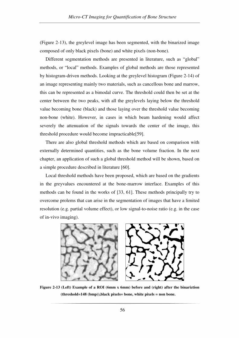
Micro-CT Imaging for Quantification of Bone Structure
56
(Figure 2-13), the greylevel image has been segmented, with the binarized image
composed of only black pixels (bone) and white pixels (non-bone).
Different segmentation methods are presented in literature, such as “global”
methods, or “local” methods. Examples of global methods are those represented
by histogram-driven methods. Looking at the greylevel histogram (Figure 2-14) of
an image representing mainly two materials, such as cancellous bone and marrow,
this can be represented as a bimodal curve. The threshold could then be set at the
center between the two peaks, with all the greylevels laying below the threshold
value becoming bone (black) and those laying over the threshold value becoming
non-bone (white). However, in cases in which beam hardening would affect
severely the attenuation of the signals towards the center of the image, this
threshold procedure would become impracticable[59].
There are also global threshold methods which are based on comparison with
externally determined quantities, such as the bone volume fraction. In the next
chapter, an application of such a global threshold method will be shown, based on
a simple procedure described in literature [60].
Local threshold methods have been proposed, which are based on the gradients
in the greyvalues encountered at the bone-marrow interface. Examples of this
methods can be found in the works of [33, 61]. These methods principally try to
overcome prolems that can arise in the segmentation of images that have a limited
resolution (e.g. partial volume effect), or low signal-to-noise ratio (e.g. in the case
of in-vivo imaging).
Figure 2-13 (Left) Example of a ROI (6mm x 6mm) before and (right) after the binariztion
(threshold=148 (bmp)),black pixels= bone, white pixels = non bone.

Chapter 2
57
Figure 2-14 Example of a greylevel histogram of a cancellous bone image embedded in
PMMA.
Once the image has been segmented, the histomorphometric parameters can be
calculated. The software used in the preset thesis (software “3D-Calculator”,
Skyscan) permits the calculation of the classical 2D-histomorphometric
parameters (e.g. BV/TV, Tb.Th, Tb.N, Tb.Sp) as well as the direct 3D parameters
(e.g. SMI, MIL, Connectivity) over a volume of interest.
A 3D representation obtained from a stack of microCT cross-sections is given
in Figure 2-14.
Figure 2-15 (Left) stack of binarized microCT imagesof cancellous bone structre (binarized
ROIs), (Right) a 3D representation.
The presented procedure is an example of how cancellous bone samples can be
characterized using microCT.
Micro-CT Imaging for Quantification of Bone Structure
58
Researchers who have begun micro-CT analyses several years ago, now have
the possibility to compare several different acquisitions and to make studies on
wide specimen samples and with great variability. However reliability over time
of micro-CT devices was never assessed while it is a fundamental parameter in
order to compare acquisitions coming from different studies over time. The LTM
starting to acquire bone specimen in 2002 and could now study more than two
hundred reconstructed volumes. For this reason a quality control (QC) protocol
was realized in order to periodically control micro-CT performance and to assure
the device accuracy along years (Chapter 3).

Chapter 3 Reliability of the Measurement Device
59
CHAPTER 3 RELIABILITY OF THE
MEASUREMENT DEVICE: QUALITY CONTROL
PROTOCOL FOR IN-VITRO MICRO-COMPUTED
TOMOGRAPHY
The study presented in this chapter is subject of the paper:
Rossella Stoico, Simone Tassani, Egon Perilli, Fabio Baruffali,
Marco Viceconti.
Quality control protocol for IN-VITRO micro-computed tomography.
To be submitted to “Journal of Microscopy”
The author of the this thesis was main investigator of the present article
together with Rossella Stoico. However she practically performed micro-CT
acquisitions and wrote the article, therefore she was selected as first author.
MicroCT was pioneered in the late 1980’s and is based on the same basic
principles as the common computed tomography [2, 3]. However reliability over
time of micro-CT devices was never assessed. For this reason a quality control
(QC) protocol was realized and described in order to periodically control micro-
CT performance.
Quality Control Protocol for in-vitro Micro-Computed Tomography
60
3.1 Introduction
Quality control (QC) is a process applied to ensure a certain level of quality in
a product or service. The level of quality of a measuring instrument is connected
to the accuracy of the measurement. Therefore, quality control is a process
employed to verify the accuracy of the measurements of the instrument over the
time according to commonly accepted standards of quality.
X-ray micro-computed tomography (microCT) is a non-destructive
investigation method with widespread use in different research fields, such as
industry, science and medical research. It is a three-dimensional measuring
method with high spatial resolution that does not require special preparation of the
specimen. The accuracy needed in microCT investigations should suggest the
systematic application of QC protocols, but that issue has been poorly addressed
in the literature.
Conversely, with the use of X-rays in medicine a periodic quality control of the
measuring instruments is applied to assure the quality of diagnostic accuracy and
in particular their safety for patients and operators. In medical CT, which is
commonly used in clinical practice, the QC protocols are set to ensure diagnostic
accuracy and reduce the risk of X-ray exposure to patients and operators
according to a specific indication of standard of quality, for example international
directive 97/43/EURATOM. In the literature there are many studies about the
application of QC protocols in medical CT. The American Association of
Physicists in Medicine (AAPM) and Institute of Physics and Engineering in
Medicine (IPEM) proposed QC protocols in medical CT based on international
directive [62, 63] to ensure the quality of diagnostic accuracy. These QC protocols
are about the control of the most important medical CT characteristics, such as
image detail and noise [64], uniformity and linearity of CT numbers, spatial and
high/low contrast resolution and dose evaluation. The QC protocols are performed
by the use of phantoms designed with tissue-equivalent inserts according to
specific clinical application [65-73].

Chapter 3 Reliability of the Measurement Device
61
MicroCT is based on the same physical principles of medical CT and is applied
widely in medical research, especially in the histomorphometric characterization
of bone tissue. To the best of the authors’ knowledge only few applications of QC
protocols for microCT have been reported in the literature, and their concern is
mainly in densitometry. They are based on the use of solid and liquid calibration
phantoms, to evaluate the quality of the bone mineral density measures [74, 75].
Recently, a QC phantom was designed, to evaluate the performance of an in-vivo
micro-computed tomographic system, operated at 150-µm resolution [76]. The in-
vivo tomographic system is used to investigate small animals, such as mice or rats
for pre-clinical analysis. For this reason the proposed QC tests are aimed at
evaluating spatial resolution, geometric accuracy, CT number accuracy, linearity,
noise and image uniformity [76] and to assure that measurements are not affected
by scanner drift. However, that phantom cannot be used for in-vitro microCT
evaluation of quality level because the inserts of that phantom are chosen to
control the most important parameters of pre-clinical analysis concerning in
particular tissue-density discrimination. On the other hand, the in-vitro microCT
system is used especially for morphometric analysis and a morphometric phantom
is required. Moreover, an accuracy test concerning morphometric measurements
has never been proposed.
The aim of the present work is to propose a QC protocol for in-vitro microCT,
by adapting the QC protocols of medical CT. The QC tests proposed in this study
can be adapted and applied to various applications of in-vitro microCT. The
proposed QC protocol was applied to a widespread research field such as the
histomorphometric characterization of bone tissue.
3.2 Material and Methods
A QC protocol for in-vitro microCT is proposed. It was inspired by QC
protocols used in medical CT (IPEM guidelines), that ensure a level of quality
suitable for clinical practice [63]. The presented QC protocol is summarized in
Table 3-1 The proposed QC protocol for in-vitro microCT. Three tests were
proposed: 1) “noise” and 2) “uniformity” tests performed by the use of a water
Quality Control Protocol for in-vitro Micro-Computed Tomography
62
phantom; 3) “accuracy” test performed by the use of a morphometric calibrated
phantom.
The presented tests are based on the use of baseline values (baseline, B.L.) and
control charts. The baseline values are measured during an acceptance/status test,
and represent the reference values for the control charts, which are subsequently
used to monitor the specific parameters over time. The tests are based on the use
of two specific calibration phantoms: a water phantom, and a morphometric
calibration phantom.
The application of the QC protocol for in-vitro microCT is related to the
particular use of the X-ray measuring instrument. In fact, whereas the procedures
and QC parameters in the noise and uniformity tests were directly inspired by
IPEM indications and based on the use of a water phantom, for the accuracy test
the calibration phantom had to reproduce materials, structure and dimensions of
the object of investigation, that is, trabecular bone specimens. With this aim, a
proper morphometric calibration phantom was used, as described later [77].
Moreover, a new procedure for the evaluation of the accuracy of morphometric
measurements was introduced.
In the acceptance/status test both phantoms were scanned five consecutive
times to calculate the reference value (baseline, B.L.). The B.L. was used as the
reference value for data collection charts. Each scan was performed on a different
day for five consecutive days, and the phantom was repositioned in the microCT
each time. The QC phantoms have to be scanned by always keeping the same
scanner setting. A periodic time monitoring of one month was proposed, to
control whether measurements showed any scanner drift.
If a periodic measure is out of the upper and lower limits defined for each
specific adopted chart, then this measure is defined as “out of control”. The QC
protocol proposed in this study suggests that if a measure is out of the upper and
lower control limits, an intervention, e.g. maintenance service, is required.
The data collection method for the noise test was inspired by the IPEM
indications, whereas for the uniformity and accuracy tests a new method was
proposed. In particular, for the uniformity test two approaches were considered:

Chapter 3 Reliability of the Measurement Device
63
the data collection method inspired by IPEM indication and a novel method.
These methods were applied and compared to evaluate the most suitable data
collection method for the QC protocol
Phantoms Noise/Uniformity test: Water or soft-tissue equivalent
Accuracy test: morphometric calibration phantom (materials,
dimensions and geometries known)
Procedure Noise test: circular region of interest (ROI) in proportion to the
area of the water phantom positioned according IPEM procedure
[63] on the reconstructed grey-level images in the central part of
the water phantom (Figure 3-1).
Uniformity test: central circular ROI in proportion of the area
of the water phantom and four peripheral ones positioned
according to IPEM procedure on the reconstructed grey-level
images in the central part of the water phantom [63] (Figure
3-2).
Accuracy test: shape and dimension of the ROI had to be
selected to contain the whole object of interest; a threshold value
was used to calculate the parameters on reconstructed grey-level
images
QC parameters Noise test: standard deviation of grey levels of the ROI
averaged on five consecutive cross sections reconstruction.
Uniformity test: difference in grey levels calculated between
average density of the circular central ROI and average density
of the four circular peripheral ones; the difference in grey levels
averaged on the same five consecutive cross sections
reconstruction.
Accuracy test: root mean square error (RMSE) calculated
between measured values and baseline (B.L).
Baseline Noise/Uniformity/Accuracy tests: B.L. calculated during
acceptance/status test.

Quality Control Protocol for in-vitro Micro-Computed Tomography
64
Data collecting
method
Noise test: chart with tolerance range according to the indication
of IPEM guidelines (± 20% of the B.L.) [63]
Uniformity/Accuracy test: Shewart control chart [78].
Time
monitoring
Noise/Uniformity/Accuracy tests: monthly
Maintenance
Service
Noise/Uniformity/Accuracy tests: intervention, e.g.
maintenance service request in case of “out of control”
situations: measure out of upper and lower control limits of the
specific chart adopted.
Table 3-1 The proposed QC protocol for in-vitro microCT
3.2.1 MicroCT scanner settings and image processing.
The QC protocol was applied on a Skyscan in-vitro microCT model 1072
(Skyscan, Kontich, Belgium). The scanning parameters were 50kVp, 200µA,
rotation step 0.45°. A 1-mm aluminium filter was used to reduce the beam
hardening effect. The exposure time was set at 5.9 s averaged by two frames. The
magnification was set to 16x with a pixel size of 19.5µm and a field of view
(FOV) of 20x20mm.
A filtered back-projection algorithm Feldkamp [58] was used for cross-section
reconstruction (software Cone-Rec v.2.9, Skyscan). The reconstructed
tomographic images were saved in 8-bit format (256 grey levels) and 1024x1024
pixels in size.
3.2.2 Application of the in-vitro microCT QC protocol
Acceptance/status test:
The acceptance/status test was performed on both the water phantom and the
morphometric phantom in 2004, from which the baseline (B.L.) was calculated for
each parameter.
Chapter 3 Reliability of the Measurement Device
65
Periodic time monitoring:
The periodic time monitoring started three years after the acceptance/status test
to verify if the measurements showed any scanner drift after about 1800 work-
hours of the X-ray tube. All the measures described in the QC protocol were
performed monthly, for 15 months.
“Noise” test:
The noise test was performed by using the water phantom. The phantom
consists of a cylindrical plastic vessel with an 18-mm outer diameter, 14-mm
inner diameter and 44-mm height. A series of five consecutive cross sections were
reconstructed in the central height of the water phantom.
According IPEM indications, the ROI area corresponds to 500 mm2 because a
standard-size soft tissue-equivalent phantom is used for the application of QC
protocols in medical CT. In in-vitro microCT systems, the water phantom
dimensions can be chosen according to the available FOV size. In this case the
ROI size was chosen to be 10% of the area of the inner water phantom area. Then
it was positioned in the center of the five consecutive cross sections.
The QC parameter “noise” was calculated as the standard deviation of the grey
levels averaged on five consecutive cross-sections (average SD). The B.L. was
used to establish the quality control chart with an upper noise limit (UNL) and
lower noise limit (LNL) as ± 20% of B.L. respectively, according to IPEM
indications [63].
Image-Pro Plus v.4.5.1.22 (The Proven Solution, Media Cybernetics, Inc.)
image analysis software was used to calculate the average SD in grey levels in the
circular ROI for the “noise” test (Figure 3-1) as described in field Procedure in
Table 3-1.

Quality Control Protocol for in-vitro Micro-Computed Tomography
66
Figure 3-1 Circular ROI area, positioning for the noise test. This procedure was inspired by
IPEM guidelines [63]
“Uniformity” test:
For the uniformity test the water phantom and the five consecutive grey level
images of the noise test were used. A circular ROI, the same as used for the noise
test, was positioned in the center of the water phantom and four circular ones,
with the same dimensions, were positioned in the peripheral location (Figure 3-2).
The QC parameter “uniformity” was calculated as the difference in grey levels
between average density of the circular central ROI and the average density of all
four circular peripheral ones. This difference was averaged on five consecutive
cross sections.
Image-Pro Plus v.4.5.1.22 (The Proven Solution, Media Cybernetics, Inc.)
image analysis software was used to calculate the average difference in grey
levels for the “uniformity” test (Figure 3-2) as described in the field Procedure in
Table 3-1 The proposed QC protocol for in-vitro microCT.

Chapter 3 Reliability of the Measurement Device
67
Concerning the data collection method, two different approaches were
considered to choose the most suitable monitoring data method for the proposed
QC protocol. In one case the upper uniformity limit (UUL) and lower uniformity
limit (LUL) were represented by ± 1.5% of B.L. respectively, which are the
tolerance limits defined by IPEM guidelines [63]. In the second case, the upper
control limit (UCL) and the lower control limit (LCL) were represented as ± 3 *
mean moving range (MR) divided by 1.128, that are the tolerance limits defined
by the “Shewart control chart for single measures” [78]. The MR is the absolute
difference between each pair of consecutive measures. The 1.128 value is the
reference value for measures with a sample size equal to two [78]. The mean MR
was calculated by the first five acquisitions of 2004.
Figure 3-2 The uniformity test procedure inspired by IPEM guidelines. Images in grey levels
were used. The ROI was the same as that used for the noise test and was
positioned in the central part (2a) and in four peripheral locations (2b, 2c, 2d,
2e) of the water phantom.

Quality Control Protocol for in-vitro Micro-Computed Tomography
68
“Accuracy” test:
IPEM guidelines do not contain any accuracy test for morphometric
measurements. However, the research interest in in-vitro microCT was actually in
morphometric characterization of trabecular bone tissue. Thus, a dedicated
protocol was developed and applied, based on a morphometric calibration
phantom. The main characteristic of a phantom for accuracy test in morphometry
is to reproduce the typical 3D structure of the analysed specimen: e.g. the
trabecular bone framework.
A previously published physical 3D phantom with calibrated aluminium (Al)-
inserts was chosen [77] for the application of the proposed QC protocol (Table
3-1). The phantom was designed in cylindrical shape (13 mm diameter x 23mm
height). The Al-inserts were of different geometries (foils, wires, meshes and
spheres) and calibrated thickness to reproduce the typical thickness of trabecular
bone structure [77]. The objects of the calibration phantom are four foils of 20±3,
50±7.5, 100±10 and 250±25 µm in thickness, four wires of 20±2, 50±5, 125±12.5
and 250±25 µm in thickness, a small horizontal and a vertical mesh composed of
100±10 µm thick wires, a horizontal mesh of bigger external size and four spheres
of 1000±50 µm in diameter embedded in polymethylmethacrylate (PMMA)
(Figure 3-3). The Al material was used because its X-ray attenuation coefficient is
very similar to the bone tissue (µAl(60keV)=0.75cm-1; µBone(60keV)=0.60cm-1)
[79].
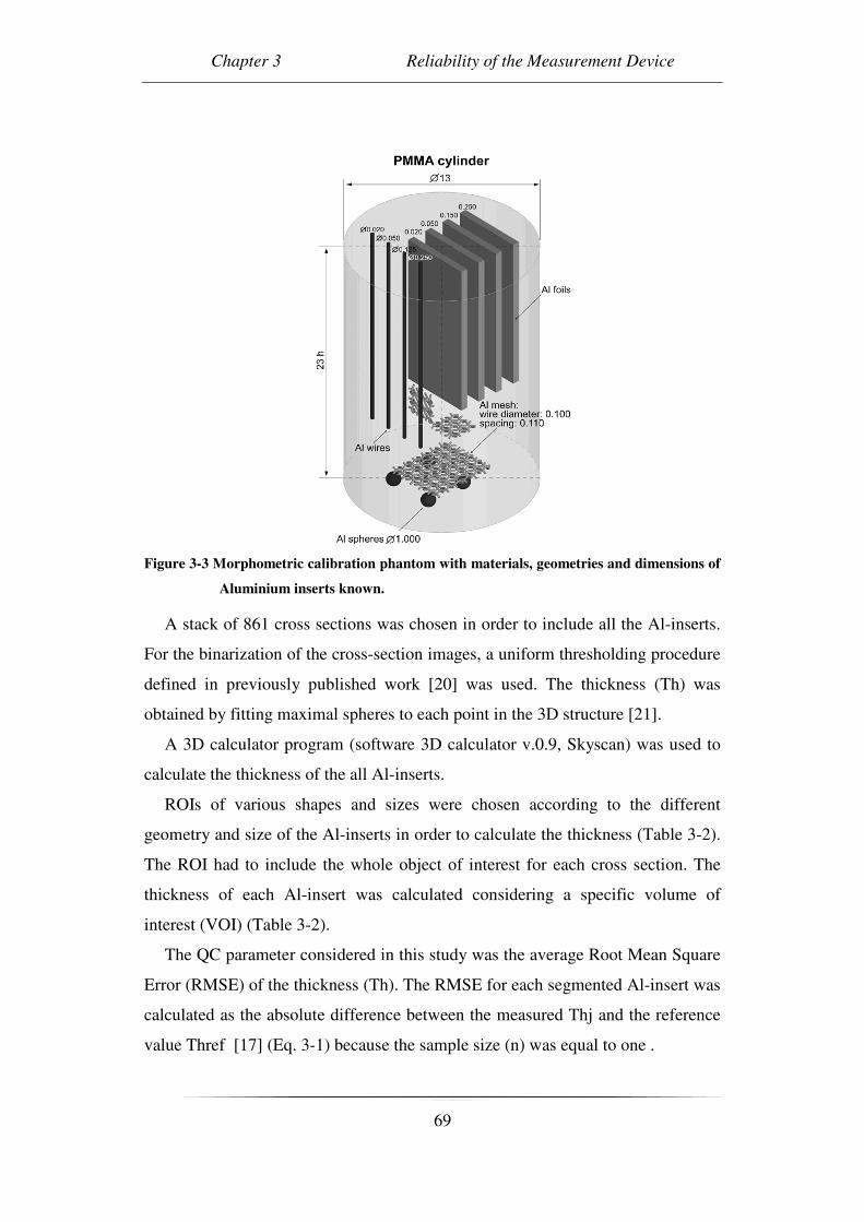
Chapter 3 Reliability of the Measurement Device
69
Figure 3-3 Morphometric calibration phantom with materials, geometries and dimensions of
Aluminium inserts known.
A stack of 861 cross sections was chosen in order to include all the Al-inserts.
For the binarization of the cross-section images, a uniform thresholding procedure
defined in previously published work [20] was used. The thickness (Th) was
obtained by fitting maximal spheres to each point in the 3D structure [21].
A 3D calculator program (software 3D calculator v.0.9, Skyscan) was used to
calculate the thickness of the all Al-inserts.
ROIs of various shapes and sizes were chosen according to the different
geometry and size of the Al-inserts in order to calculate the thickness (Table 3-2).
The ROI had to include the whole object of interest for each cross section. The
thickness of each Al-insert was calculated considering a specific volume of
interest (VOI) (Table 3-2).
The QC parameter considered in this study was the average Root Mean Square
Error (RMSE) of the thickness (Th). The RMSE for each segmented Al-insert was
calculated as the absolute difference between the measured Thj and the reference
value Thref [17] (Eq. 3-1) because the sample size (n) was equal to one .
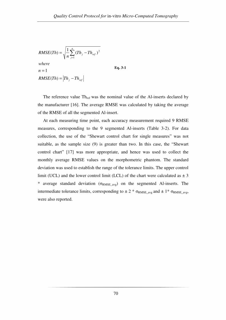
Quality Control Protocol for in-vitro Micro-Computed Tomography
70
refj
n
jrefj
ThThThRMSE
n
where
ThThn
ThRMSE
−=
=
−= ∑=
)(
1
)(1
)(1
2
Eq. 3-1
The reference value Thref was the nominal value of the Al-inserts declared by
the manufacturer [16]. The average RMSE was calculated by taking the average
of the RMSE of all the segmented Al-insert.
At each measuring time point, each accuracy measurement required 9 RMSE
measures, corresponding to the 9 segmented Al-inserts (Table 3-2). For data
collection, the use of the “Shewart control chart for single measures” was not
suitable, as the sample size (9) is greater than two. In this case, the “Shewart
control chart” [17] was more appropriate, and hence was used to collect the
monthly average RMSE values on the morphometric phantom. The standard
deviation was used to establish the range of the tolerance limits. The upper control
limit (UCL) and the lower control limit (LCL) of the chart were calculated as ± 3
* average standard deviation (σRMSE_avg) on the segmented Al-inserts. The
intermediate tolerance limits, corresponding to ± 2 * σRMSE_avg and ± 1* σRMSE_avg,
were also reported.

Chapter 3 Reliability of the Measurement Device
71
Al-inserts ROI size
(mm2 – pixel)
ROI shape VOI (ROI size x
#slices)
Wire (20 µm) Not segmented Not segmented Not segmented
Foil (20 µm) Not segmented Not segmented Not segmented
Wire (50 µm) Not segmented Not segmented Not segmented
Foil (50 µm) 5.4x1.6 – 275x80 rectangular 275x80 x 281
Mesh
(small horizontal)
5.8x5.8 – 300x300 square 300x300 x 31
Mesh
(big horizontal)
9.7x9.7 – 500x500 square 500x500 x 26
Mesh
(small vertical)
5.4x1.6 – 275x80 rectangular 275x80 x 191
Foil (100 µm) 5.4x1.6 – 275x80 rectangular 275x80 x 281
Wire (125 µm) 0.9x0.9 – 48x48 square 48x48 x 576
Foil (250 µm) 5.4x1.6 – 275x80 rectangular 275x80 x 281
Wire (250 µm) 0.9x0.9 – 48x48 square 48x48 x 576
Spheres 5.8x5.8 – 300x300 square 300x300 x 61
Table 3-2 The different ROI sizes and shapes and specific VOI used for thickness calculation
of the segmented Al-inserts
Statistical Analysis:
All the measures of the QC protocol were processed by the statistical test C,
with the null hypothesis that the collected data were randomly distributed. This
test is very flexible for verifying the null hypothesis, however without
considerations about the alternative hypothesis (Eq. 3-2) [80].
tsmeasuremenXXX
where
XX
XX
C
nii
n
ii
n
iii
=
−
−
−=
+
=
−
=+
∑
∑
,...,,
)(*2
)(1
1
1
2
1
1
21
Eq. 3-2
The measures were collected monthly over 15 months for each test. The data
were then divided into 3 groups, with each group containing the measures of 5
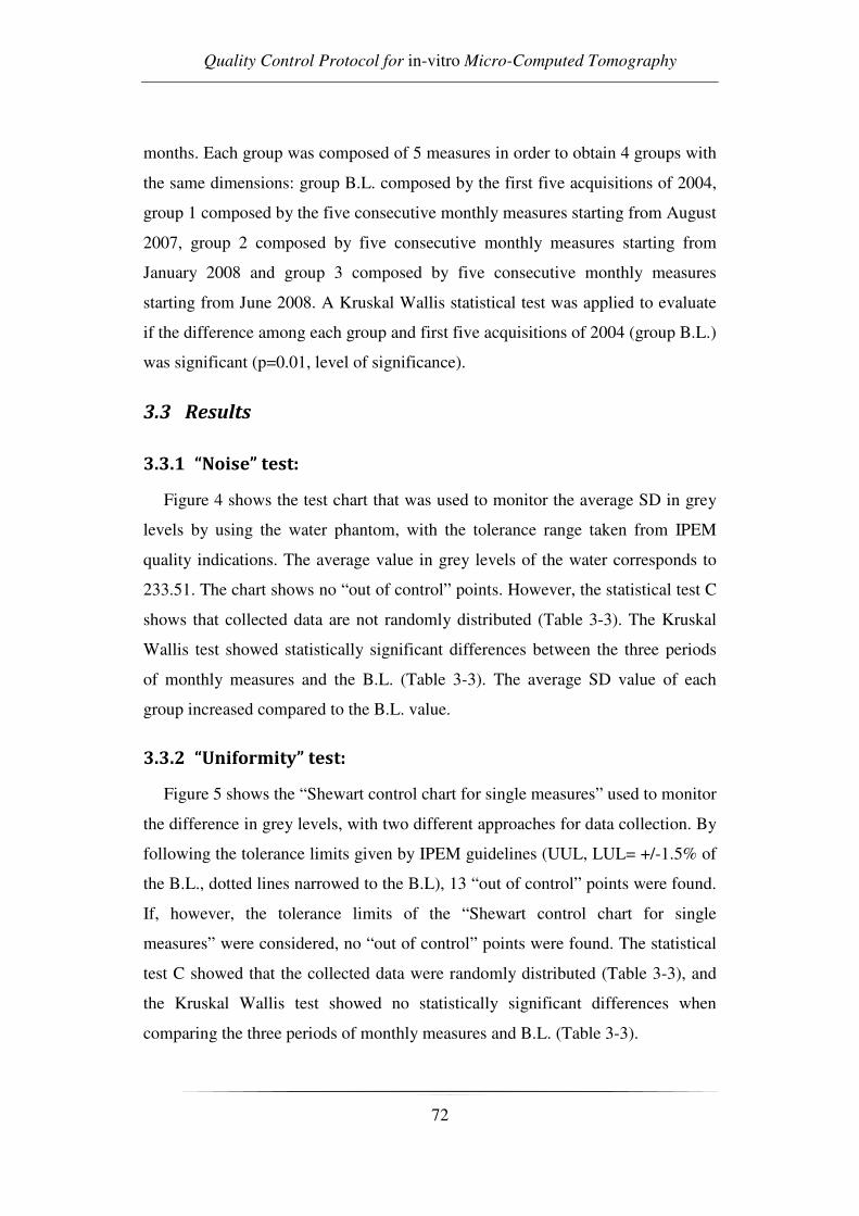
Quality Control Protocol for in-vitro Micro-Computed Tomography
72
months. Each group was composed of 5 measures in order to obtain 4 groups with
the same dimensions: group B.L. composed by the first five acquisitions of 2004,
group 1 composed by the five consecutive monthly measures starting from August
2007, group 2 composed by five consecutive monthly measures starting from
January 2008 and group 3 composed by five consecutive monthly measures
starting from June 2008. A Kruskal Wallis statistical test was applied to evaluate
if the difference among each group and first five acquisitions of 2004 (group B.L.)
was significant (p=0.01, level of significance).
3.3 Results
3.3.1 “Noise” test:
Figure 4 shows the test chart that was used to monitor the average SD in grey
levels by using the water phantom, with the tolerance range taken from IPEM
quality indications. The average value in grey levels of the water corresponds to
233.51. The chart shows no “out of control” points. However, the statistical test C
shows that collected data are not randomly distributed (Table 3-3). The Kruskal
Wallis test showed statistically significant differences between the three periods
of monthly measures and the B.L. (Table 3-3). The average SD value of each
group increased compared to the B.L. value.
3.3.2 “Uniformity” test:
Figure 5 shows the “Shewart control chart for single measures” used to monitor
the difference in grey levels, with two different approaches for data collection. By
following the tolerance limits given by IPEM guidelines (UUL, LUL= +/-1.5% of
the B.L., dotted lines narrowed to the B.L), 13 “out of control” points were found.
If, however, the tolerance limits of the “Shewart control chart for single
measures” were considered, no “out of control” points were found. The statistical
test C showed that the collected data were randomly distributed (Table 3-3), and
the Kruskal Wallis test showed no statistically significant differences when
comparing the three periods of monthly measures and B.L. (Table 3-3).

Chapter 3 Reliability of the Measurement Device
73
3.3.3 “Accuracy” test:
Figure 6 shows the application of “Shewart control chart” to monitor the
average RMSE parameter of the segmented Al-inserts of the morphometric
calibration phantom. The chart shows no “out of control” points. The statistical
test C showed that the collected data were randomly distributed (Table 3-3), and
the Kruskal Wallis test showed no statistically significant differences between the
three periods of monthly measures and B.L. (Table 3-3).
Figure 3-4 “Noise” test chart: Noise test chart of the average SD in grey levels of a ROI area
in proportion of the water phantom area. The tolerance range (UNL (upper
noise limit) = +20% B.L., LNL (lower noise limit) = -20% B.L.) was calculated in
accordance with IPEM guidelines.

Quality Control Protocol for in-vitro Micro-Computed Tomography
74
Figure 3-5 “Uniformity” test chart: “Shewart control chart for single measures” (UCL =
upper control limit, LCL = lower control limit) of the difference in grey levels,
procedure indicated by IPEM. The dotted lines (UUL (upper uniformity limit) =
+15% B.L., LUL (lower uniformity limit) = -15% B.L.) narrowed to B.L. were
the tolerance limits suggested by IPEM guidelines.
Figure 3-6: “Accuracy” test chart: “Shewart control chart” (UCL = upper control limit,
LCL = lower control limit) for the average RMSE parameter calculated by using
the Al-calibration phantom. The UCL and LCL were calculated as ± 3*σRMSE_avg.

Chapter 3 Reliability of the Measurement Device
75
Group
B.L. Group 1 Group 2 Group 3
Test C
p
Kruskal
Wallis
p
Water phantom
“Noise” test:
Average SD in
grey levels
3.35 ± 0.02
3.52 ± 0.05
3.56 ± 0.02
3.51 ± 0.05
< 0.01 < 0.01
“Uniformity” test:
Difference in grey
levels
-0.98 ± 0.06
-0.90 ± 0.10
-0.96 ± 0.04
-0.90 ± 0.12
0.73 0.30
Al-calibration phantom
“Accuracy” test:
Average RMSE in
Th (µm)
19.59 ± 5.25
20.05 ± 1.34
20.28 ± 1.82
19.79 ± 2.67
0.93 0.84
Table 3-3 Mean and SD of the most important selected parameters for the CQ protocol
application on water and Al-calibration phantoms. The mean of each group
composed of five consecutive monthly measures and B.L. was calculated. The p
value (p = 0.01, level of significance) of Test C and the Kruskal Wallis statistical
test are shown.
3.4 Discussion
In the present work a QC protocol for in-vitro microCT was defined and
applied. It was inspired by QC protocols commonly used in medical CT. The QC
protocol proposed was applied in a particular medical research field, which is the
morphometric characterization of trabecular bone specimens. For this purpose
suitable phantoms were used.
Quality control charts were used to collect and monitor the monthly measures
of selected QC parameters. The procedure of “noise” and “uniformity” tests was
taken from IPEM guidelines and adapted to microCT, whereas a new procedure
for morphometric accuracy was introduced. The data and analysis over a 15-
month application of the QC protocol were presented.
3.4.1 “Noise” test
Monthly noise measures were in accordance with tolerance limits defined by
international guidelines for medical CT (± 20% of B.L.). However, the collected
Quality Control Protocol for in-vitro Micro-Computed Tomography
76
data were not randomly distributed, and were in the upper part of the tolerance
range (Figure 3-4). Moreover, statistically significant differences between B.L.
and each group of five consecutive monthly measures were found (Table 3-3),
with the noise (average SD in grey levels) after 3 years found to increase,
compared to B.L. These results can be considered an indication of a changing
condition. Although the values were not found out of the upper and lower noise
limits of the chart, a maintenance service was required to verify the cause of these
results. The maintenance service reproduces the same tests performed during
acceptance/status tests to verify the performances of the mechanical components
of microCT, the X-ray tube and the CCD camera after three years’ working.
3.4.2 “Uniformity” test
Two different approaches to collect the data were applied. The first approach
was based on the tolerance range suggested by IPEM guidelines (± 1.5% of B.L.).
However, this was not suitable to monitor uniformity data stored in 8-bit format
(256 grey levels) images. In fact, the tomographic images in medical CT, for
which the IPEM guidelines are designed, are stored in a 12-bit format, which give
a much higher grey level range (4096 grey levels). The tolerance range of the
difference in grey levels between the central ROI (233.52 GL) and peripheral
ROIs (234.50 GL) was a limitation because of the small dispersion of the grey
levels around B.L (UUL = -0.97, LUL = -0.99, Figure 4). The consequence was to
observe 13 out of control points in the uniformity chart. But statistical C and
Kruskal Wallis tests showed no “out of control” condition. To save images in a
larger bit format might be a solution. However, these images are more difficult to
manage and process. On the other hand, the concern in the present paper was to
observe how the variability of the average SD (“noise” test) and difference in grey
levels (“uniformity” test) influenced the morphometric measurements. For this
purpose the grey level images for “noise” and “uniformity” tests were to be
reconstructed in the same bit format of grey level images for “accuracy” tests (8
bit).

Chapter 3 Reliability of the Measurement Device
77
A second approach for data collection in uniformity measurements was
introduced and applied, which was based on the “Shewart control chart for single
measures”. This chart showed no “out of control” points for uniformity
measurements (Figure 3-5).
Considering the outcomes of the statistical test C, the data were randomly
distributed, and there were no statistically significant differences between each
group of five consecutive monthly measures and B.L. (Kruskal Wallis, Table 3-3).
This outcome is consistent with that of the “Shewart control chart for single
measurements”, which can be considered the most suitable approach to collect the
data in uniformity measurements.
3.4.3 “Accuracy” test
A Shewart control chart was used to monitor the average RMSE for the QC
parameters of the morphometric calibration phantom, where no “out of control”
points were observed. The deviations from the nominal values in thickness
(RMSE values), were about the pixel size used for the tomographic acquisition
(B.L. = 19. 59, Table 3-3). All the monthly measures were within one standard
deviation, randomly distributed (Figure 3-6), with no significant differences
between each period of five consecutive monthly measures and B.L. (Table 3-3).
Thus, the results of the morphometric accuracy test shows that the performance of
the microCT system can be considered not “out of control”.
In conclusion a QC protocol in in-vitro microCT was proposed and applied
successfully. The protocol, inspired by IPEM guidelines, was adapted to monitor
the performance of in-vitro microCT in a common application field, which is
trabecular bone histomorphometry. The “noise” and “uniformity” tests were
performed by using a water phantom. For the “accuracy” test a physical phantom
for the calibration of morphometric measurements in 3D was used. Three years
after measuring baseline values, the application of the QC protocol showed that
the quality level of the microCT scanner used was not “out of control” concerning
accuracy and uniformity. The noise showed a slight but significant increase over
the years, which however can be considered negligible, as it had no effect on the

Quality Control Protocol for in-vitro Micro-Computed Tomography
78
outcome in histomorphometry. However, the systematic increase in monthly
measures compared to B.L. can be interpreted as a changing condition in the
performance of the X-ray tube and CCD camera of the microCT system. A
maintenance service to control the performance of mechanical components of
microCT after three years’ working is suggested.

Chapter 4 Analysis of Bone Structure 1
79
CHAPTER 4 ANALYSIS OF BONE STRUCTURE 1.
MECHANICAL TESTING OF CANCELLOUS
BONE FROM THE FEMORAL
HEAD:EXPERIMENTAL ERRORS DUE TO OFF-
AXIS MEASUREMENTS
The study presented in this chapter is subject of the paper:
Caroline Öhman, Massimiliano Baleani, Egon Perilli, Enrico Dall’Ara,
Simone Tassani, Fabio Baruffaldi and Marco Viceconti
Mechanical testing of cancellous bone from the femoral head: experimental errors
due to off-axis measurements
Published on Journal of Biomechanics.
The author of the this thesis focused his study on the design of the micro-CT
procedures and performed the acquisitions.
The first step into the analysis of bone structure was to assess if the mean
trabecular orientation could influence the structure strength.
Mechanical Testing of Cancellous Bone from the Femoral Head: Experimental
Errors due to Off-Axis Measurements
80
4.1 Introduction
Cancellous bone is a porous material that presents various structural
anisotropies depending on the specific anatomical site [3, 81, 82]. The tissue
structure has been shown to range from nearly transverse isotropic, (e.g. human
vertebra), to orthotropic (e.g. human calcaneus)[42].
A mathematical model to describe the structure of cancellous bone in two
dimensions, using images from a scanning electron microscope, was proposed by
Whitehouse et al.[52]. He found that the polar diagram representing the measured
mean intercept lengths in different directions is an ellipse. Harrigan and Mann
[53] extended this model to three dimensions, introducing the use of a second rank
symmetric tensor to describe the degree of orientation in orthotropic materials.
Cowin [54]expanded the use of tensors, showing that there is a theoretical
relationship between the fourth rank elasticity tensor of a porous, anisotropic,
linear-elastic material and a second rank symmetric tensor. The latter, referred to
as the ‘fabric’ tensor characterises the arrangement of the microstructural
components of the material. Several studies[83-85] have been done to confirm the
theory of Cowin [54]. In those studies, the three-dimensional structure of
cancellous bone specimens was obtained by means of microtomographic images.
The structural anisotropy was expressed in terms of a fabric tensor. From this
tensor the structural main directions were calculated. The mechanical principal
directions were estimated with finite element simulations. The structural main
directions predicted well the mechanical principal directions with differences of
only a few degrees (from 1.4° to 3.8°).
Several experimental studies have been performed to assess the mechanical
behaviour in three orthogonal directions of cancellous bone [40, 42, 57, 86].
Those studies confirmed an orthotropic or transversely isotropic behaviour of the
cancellous bone. However, little effort has been made to experimentally
investigate the effect of the load direction with respect to the main trabecular
direction (MTD), hereafter called ‘off-axis angle’, on the measurement of the
mechanical behaviour of cancellous bone. A theoretical study [9], to estimate the
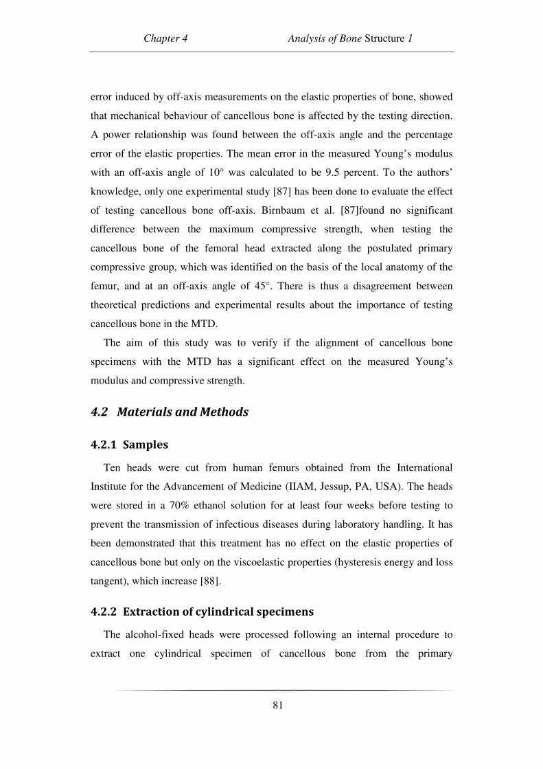
Chapter 4 Analysis of Bone Structure 1
81
error induced by off-axis measurements on the elastic properties of bone, showed
that mechanical behaviour of cancellous bone is affected by the testing direction.
A power relationship was found between the off-axis angle and the percentage
error of the elastic properties. The mean error in the measured Young’s modulus
with an off-axis angle of 10° was calculated to be 9.5 percent. To the authors’
knowledge, only one experimental study [87] has been done to evaluate the effect
of testing cancellous bone off-axis. Birnbaum et al. [87]found no significant
difference between the maximum compressive strength, when testing the
cancellous bone of the femoral head extracted along the postulated primary
compressive group, which was identified on the basis of the local anatomy of the
femur, and at an off-axis angle of 45°. There is thus a disagreement between
theoretical predictions and experimental results about the importance of testing
cancellous bone in the MTD.
The aim of this study was to verify if the alignment of cancellous bone
specimens with the MTD has a significant effect on the measured Young’s
modulus and compressive strength.
4.2 Materials and Methods
4.2.1 Samples
Ten heads were cut from human femurs obtained from the International
Institute for the Advancement of Medicine (IIAM, Jessup, PA, USA). The heads
were stored in a 70% ethanol solution for at least four weeks before testing to
prevent the transmission of infectious diseases during laboratory handling. It has
been demonstrated that this treatment has no effect on the elastic properties of
cancellous bone but only on the viscoelastic properties (hysteresis energy and loss
tangent), which increase [88].
4.2.2 Extraction of cylindrical specimens
The alcohol-fixed heads were processed following an internal procedure to
extract one cylindrical specimen of cancellous bone from the primary
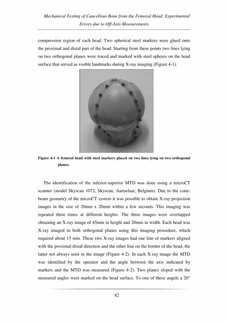
Mechanical Testing of Cancellous Bone from the Femoral Head: Experimental
Errors due to Off-Axis Measurements
82
compression region of each head. Two spherical steel markers were glued onto
the proximal and distal part of the head. Starting from these points two lines lying
on two orthogonal planes were traced and marked with steel spheres on the head
surface that served as visible landmarks during X-ray imaging (Figure 4-1).
Figure 4-1 A femoral head with steel markers placed on two lines lying on two orthogonal
planes.
The identification of the inferior-superior MTD was done using a microCT
scanner (model Skyscan 1072, Skyscan, Aartselaar, Belgium). Due to the cone-
beam geometry of the microCT system it was possible to obtain X-ray projection
images in the size of 20mm x 20mm within a few seconds. This imaging was
repeated three times at different heights. The three images were overlapped
obtaining an X-ray image of 45mm in height and 20mm in width. Each head was
X-ray imaged in both orthogonal planes using this imaging procedure, which
required about 15 min. These two X-ray images had one line of markers aligned
with the proximal-distal direction and the other line on the border of the head, the
latter not always seen in the image (Figure 4-2). In each X-ray image the MTD
was identified by the operator and the angle between the axis indicated by
markers and the MTD was measured (Figure 4-2). Two planes sloped with the
measured angles were marked on the head surface. To one of these angels a 20°

Chapter 4 Analysis of Bone Structure 1
83
offset was added to assure a misalignment of the specimen axis with the MTD.
These specimens were referred to as ‘misaligned’. Therefore, the two intersection
points of these planes defined an axis misaligned with 20° to the MTD in the
head. The proximal part, about 5 mm thick, and the distal part of the head were
cut perpendicularly to this direction using a diamond saw, obtaining a head slice
of 26 mm. Finally, a 10 mm cylinder was extracted from the head slice by means
of a holed diamond-coated milling cutter with the slice immersed in water. The
specimen height and diameter were measured.
Figure 4-2 Two orthogonal X-ray images of a femoral head (19.5 mm/pixel, 45mm_20mm)
used to identify the main direction of the trabeculae. The steel spheres that serve
as landmarks are clearly visible. The MTD defined by the operator is also
indicated.
A preliminary study was done to evaluate the accuracy of the extraction
method. Assuming the MTD (the direction in which the cylinder must be
extracted) to be correctly identified, the described experimental procedure allows
extracting a specimen with a misalignment error lower than 5° from the chosen
direction. Unfortunately, the operator introduces an additional error in choosing
the MTD. Considering both the inaccuracies, the described procedure assures an
overall misalignment error in extracting a cylindrical specimen along the MTD
lower than 10°.
Mechanical Testing of Cancellous Bone from the Femoral Head: Experimental
Errors due to Off-Axis Measurements
84
4.2.3 Micro-tomography
The cylindrical specimens underwent micro-tomographic analysis. During
microCT scanning each sample was placed vertically into a polyethylene cylinder
filled with Ringer’s solution. The scanner operated at a voltage of 50kVp, a
current of 200µA, and with a 1mm-thick aluminium filter for beam hardening
reduction [77]. An image acquisition process was done for a rotation over 185°.
For each specimen, 1024 microCT cross sections (total height 20mm) were
reconstructed using a filtered back-projection algorithm [2, 58] (software
“cone_rec”, Skyscan, Aartselaar, Belgium). Each reconstructed cross-section was
saved as an 8-bit greylevel image, 1024x1024 pixels in size, isotropic voxel size
19.5µm. For each bone sample, the stack of microCT cross-sections was then
binarized using a global threshold procedure (Perilli, et al., 2006). The following
structural parameters were calculated for each specimen (software “3D-
Calculator”, Skyscan, Aartselaar, Belgium): bone volume fraction (BV/TV),
trabecular thickness (Tb.Th) and trabecular separation (Tb.Sp), following the
recommendations of the American Society of Bone and Mineral Research [10].
The structure model index (SMI) was calculated as described in other reports [49,
77]. The mean intercept length (MIL) was calculated to quantify the misalignment
of the MTD from the cylinder axis [83]. Due to the used specimen extraction
protocol, it was assumed that the MTD (that corresponds to the orientation of the
maximum MIL eigenvector) was aligned along the vertical axis of the scanned
bone cylinder. Thus, the angular deviation from the vertical axis (z-axis) of the
eigenvector relative to the maximum MIL was defined as ‘off-axis angle’ (Figure
4-312:25 PM).

Chapter 4 Analysis of Bone Structure 1
85
Figure 4-3 X-ray images (19.5 µm/pixel, 20mm×20 mm) of two samples obtained with the
microCT. On the left a specimen extracted along the main axis of the trabecular
structure. On the right a specimen extracted with an off-axis angle of 201.
4.2.4 Mechanical testing
The cylindrical specimen was cemented directly onto the testing machine
(Mod. 8502, Instron Corp., Canton, MA, USA) to ensure the alignment of the
cylindrical specimen with the machine axis. The free length of the bone cylinder
after fixation was 20mm. Before testing the bone specimen was kept at room
temperature in Ringer’s solution for one additional hour. The whole procedure
was performed within 24 hours with the specimen continuously immersed in
Ringer’s solution to assure the re-hydrolysing of the tissue. Strain measurements
were done with an extensometer (Mod. 2620-601, Instron Corp., Canton, MA,
USA) attached with two rubber bands directly to the central part of the cylinder
(Figure 4-4). This technique allows an accurate measurement of the tissue strain
since its measurement is unaffected by the end effects [89]. Thereafter the
specimen was compressively loaded to failure in displacement control. The strain
rate was set to 0.01s-1 [90] [57] [91].

Mechanical Testing of Cancellous Bone from the Femoral Head: Experimental
Errors due to Off-Axis Measurements
86
Figure 4-4 Set-up of the mechanical test.
The ultimate stress was defined as the first point on the load-elongation curve
where the slope was zero [90, 92, 93]. The Young’s modulus was identified as the
slope of the linear part of the calculated stress-strain curve [90].
4.2.5 Ashing
After testing, the endcaps were removed and the specimen was reduced to ash
by burning the tissue in a muffle furnace at 650°C for 24 hours. The burning
temperature was preliminary set by ashing five specimens initially at 600°C and
then increasing the temperature with 50°C for each following cycle. After each
cycle the muffle furnace was turned off and the specimens were left inside for
additionally 24 hours to reach room temperature and thereafter the ash weight was
measured. The ash weight reduction (-1.8%) was significant when increasing the
temperature from 600 to 650°C while further increasing the temperature did not
cause a significant reduction. Therefore, this temperature was set for the ashing
procedure. The ash density of the specimen was defined as the ash weight divided
by the specimen volume [94-96].

Chapter 4 Analysis of Bone Structure 1
87
4.2.6 Hardness
The quality of the bone tissue was assessed by hardness tests. Each head was
cut in two pieces across the hole left after the extraction of the cylindrical
specimen. One part was grinded increasing the sandpaper number up to 2000 grit
and then the surface was polished by means of a napped cloth impregnated with
diamond pastes, starting with a grain size of 6mm and finishing with 1mm. All
polishing was done under constant water irrigation. The hardness measurements
were obtained performing micro-indentations on the wet tissue by means of a
Vickers diamond micro-indenter (Leica VMHT). A 25gf load was applied to the
bone specimen for 15 seconds. 30 micro-indentations were performed on the
surface along each border of the hole (always leaving a distance of about 1mm
from the border and a relative distance of about 3mm between each indentation).
Thus, 60 hardness measurements were collected from each femoral head. All
indentations where one diagonal was >15% longer than the other were ignored,
according to Hodgskinson[97]. To the remaining measurements the Chauvenet
criterion was applied, excluding abnormal values.
4.2.7 Selection of the control group
When the micro-tomography analysis was finished, each ‘misaligned’
specimen was paired with a specimen selected from an internal database. The
criterion used was to pair the ‘misaligned’ specimen with the one in the database
that had the closest BV/TV (Figure 4-5).
Figure 4-5 The BV/TV of all the paired specimens and the percentual difference between
them.
Mechanical Testing of Cancellous Bone from the Femoral Head: Experimental
Errors due to Off-Axis Measurements
88
This criterion was applied since it has been shown that the BV/TV is one of the
parameters which best predict the mechanical properties of cancellous bone [57,
81]. The specimens from the database were referred to as ‘aligned’ since the extra
20° was not added in the extracting procedure. Therefore in these cases the
extraction direction should be aligned with the MTD. In the ‘aligned’ cases, the
absolute value of the off-axis angle was considered since the effect of an off-axis
angle from the MTD is independent of the sign.
4.2.8 Statistical analysis
An unpaired t-test was used to investigate whether there were differences in the
calculated parameters between the two groups. A regression analysis was done for
the Young’s modulus versus the BV/TV and the ultimate stress versus the
BV/TV. The same plots were also reported splitting the data in ‘aligned’ and
‘misaligned’ groups. The coefficient of determination (R2) was calculated for each
regression. The regression lines of the split groups were analysed by analysis of
covariance (ANOVA).
4.3 Results
All results from the tests for the two groups are summarised in Table 1. No
statistical significant difference was found between the two groups in BV/TV and
age. Instead, as expected, a significant difference was found between the
misalignment angles (p<0.001). The tissue structure and quality of the two groups
were not different since no statistically significant differences were found between
calculated histomorphometric parameters (SMI, Tb.Th, and Tb.Sp), hardness or
ash density of the bone tissue, whereas a significant difference was found between
the two groups in Young’s modulus (p=0.01) and ultimate stress (p=0.03).
Additionally, the mechanical properties were significant correlated with
BV/TV (p<0.001 for all the correlations). In Figure 4-6 a linear regression
between BV/TV and Young’s modulus is shown.

Chapter 4 Analysis of Bone Structure 1
89
Parameter Aligned Misaligned p-value
BV/TV (%)a 26.6(±7.6) 26.4(±8.3) 0.96
Age (years) 73.5(±8.0) 69.8(±7.5) 0.30
Off-axis angle (°) 6.1(±3.3) 21.6(±6.6) <0.001
SMI 0.42(±0.59) 0.38(±0.59) 0.87
Tb.Th (µm) 139(±21) 132(±25) 0.55
Tb.Sp (µm) 402(±100) 414(±181) 0.85
Hardness (HV) 32.5(±2.9) 31.1(±3.1) 0.30
Young’s modulus (GPa)
2.73(±1.06) 1.59(±0.66)b 0.01
Ultimate stress (MPa) 18.0(±6.4) 11.2(±6.4) 0.03
Ash density (mg/mm3)
0.30(±0.07)c 0.31(±0.08)c 0.71
Table 4-1 The results from all the tests performed on cancellous bone specimens for the
‘aligned’ and ‘misaligned’ groups. aThe BV/TV value was used to pair the
specimens. bIn one case Young’s modulus data were lost.
cIn two cases, one
aligned and one misaligned, the ash density was impossible to measure because
pieces of the specimens were lost.
Figure 4-6 The linear regression of Young’s modulus versus BV/TV, above all specimens
together and below split in the ‘aligned’ and ‘misaligned’ groups.

Mechanical Testing of Cancellous Bone from the Femoral Head: Experimental
Errors due to Off-Axis Measurements
90
Figure 4-7 The linear regression of ultimate stress versus BV/TV, above the ‘aligned’ and
‘misaligned’ groups together and below split.
The upper graph shows the two groups together and in the one below the two
groups are separated. The same goes for Figure 4-7 where a linear regression
between BV/TV and ultimate stress is shown. In both cases the R2 value increases
when the groups are separated. In the case with BV/TV versus Young’s modulus
R2 increases from 0.41 (all specimens) to 0.60 (aligned) and 0.58 (misaligned).
The R2 value for BV/TV versus ultimate stress increases from 0.68 (all
specimens) to 0.94 (aligned) and 0.80 (misaligned). Referring to the two
regression lines calculated for the split groups, there was no significant difference
between the slopes of the two regression lines for BV/TV versus Young’s
modulus (p=0.16) neither for BV/TV versus ultimate stress (p=0.34). Conversely,
a significant distance between the two lines was found in both cases (p=0.003 and
p=<0.001 for Young’s modulus versus BV/TV and for ultimate stress versus
BV/TV, respectively).
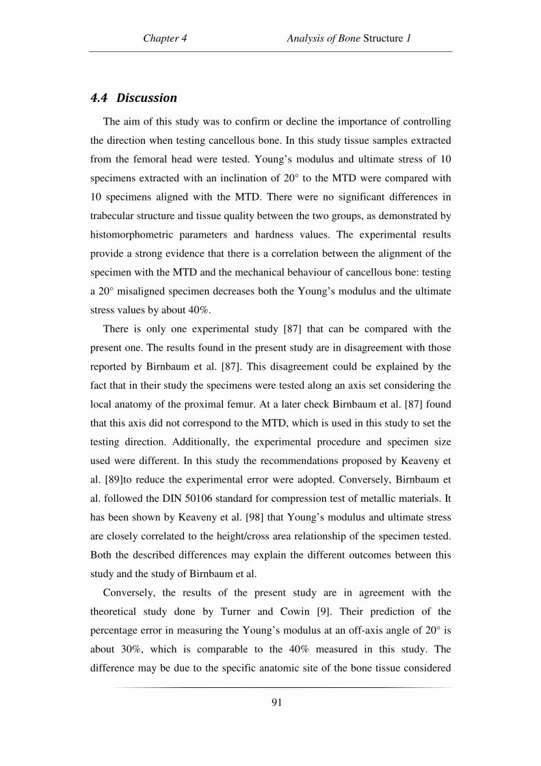
Chapter 4 Analysis of Bone Structure 1
91
4.4 Discussion
The aim of this study was to confirm or decline the importance of controlling
the direction when testing cancellous bone. In this study tissue samples extracted
from the femoral head were tested. Young’s modulus and ultimate stress of 10
specimens extracted with an inclination of 20° to the MTD were compared with
10 specimens aligned with the MTD. There were no significant differences in
trabecular structure and tissue quality between the two groups, as demonstrated by
histomorphometric parameters and hardness values. The experimental results
provide a strong evidence that there is a correlation between the alignment of the
specimen with the MTD and the mechanical behaviour of cancellous bone: testing
a 20° misaligned specimen decreases both the Young’s modulus and the ultimate
stress values by about 40%.
There is only one experimental study [87] that can be compared with the
present one. The results found in the present study are in disagreement with those
reported by Birnbaum et al. [87]. This disagreement could be explained by the
fact that in their study the specimens were tested along an axis set considering the
local anatomy of the proximal femur. At a later check Birnbaum et al. [87] found
that this axis did not correspond to the MTD, which is used in this study to set the
testing direction. Additionally, the experimental procedure and specimen size
used were different. In this study the recommendations proposed by Keaveny et
al. [89]to reduce the experimental error were adopted. Conversely, Birnbaum et
al. followed the DIN 50106 standard for compression test of metallic materials. It
has been shown by Keaveny et al. [98] that Young’s modulus and ultimate stress
are closely correlated to the height/cross area relationship of the specimen tested.
Both the described differences may explain the different outcomes between this
study and the study of Birnbaum et al.
Conversely, the results of the present study are in agreement with the
theoretical study done by Turner and Cowin [9]. Their prediction of the
percentage error in measuring the Young’s modulus at an off-axis angle of 20° is
about 30%, which is comparable to the 40% measured in this study. The
difference may be due to the specific anatomic site of the bone tissue considered
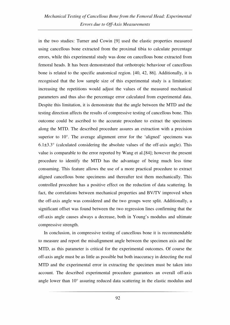
Mechanical Testing of Cancellous Bone from the Femoral Head: Experimental
Errors due to Off-Axis Measurements
92
in the two studies: Turner and Cowin [9] used the elastic properties measured
using cancellous bone extracted from the proximal tibia to calculate percentage
errors, while this experimental study was done on cancellous bone extracted from
femoral heads. It has been demonstrated that orthotropic behaviour of cancellous
bone is related to the specific anatomical region. [40, 42, 86]. Additionally, it is
recognised that the low sample size of this experimental study is a limitation:
increasing the repetitions would adjust the values of the measured mechanical
parameters and thus also the percentage error calculated from experimental data.
Despite this limitation, it is demonstrate that the angle between the MTD and the
testing direction affects the results of compressive testing of cancellous bone. This
outcome could be ascribed to the accurate procedure to extract the specimens
along the MTD. The described procedure assures an extraction with a precision
superior to 10°. The average alignment error for the ‘aligned’ specimens was
6.1±3.3° (calculated considering the absolute values of the off-axis angle). This
value is comparable to the error reported by Wang et al.[84]; however the present
procedure to identify the MTD has the advantage of being much less time
consuming. This feature allows the use of a more practical procedure to extract
aligned cancellous bone specimens and thereafter test them mechanically. This
controlled procedure has a positive effect on the reduction of data scattering. In
fact, the correlations between mechanical properties and BV/TV improved when
the off-axis angle was considered and the two groups were split. Additionally, a
significant offset was found between the two regression lines confirming that the
off-axis angle causes always a decrease, both in Young’s modulus and ultimate
compressive strength.
In conclusion, in compressive testing of cancellous bone it is recommendable
to measure and report the misalignment angle between the specimen axis and the
MTD, as this parameter is critical for the experimental outcomes. Of course the
off-axis angle must be as little as possible but both inaccuracy in detecting the real
MTD and the experimental error in extracting the specimen must be taken into
account. The described experimental procedure guarantees an overall off-axis
angle lower than 10° assuring reduced data scattering in the elastic modulus and

Chapter 4 Analysis of Bone Structure 1
93
compressive strength of the cancellous bone measured along the selected testing
direction.

94
Chapter 5 Analysis of Bone Structure 2
95
CHAPTER 5 ANALYSIS OF BONE STRUCTURE 2.
MECHANICAL STRENGTH OF
OSTEOARTHRITIC CANCELLOUS BONE
DEPENDS ON TRABECULAR STRUCTURE AND
ITS LOCAL VARIATIONS
The study presented in this chapter is subject of the paper:
Simone Tassani, Caroline Öhman, Davide Monari, Massimiliano Baleani, Luca
Cristofolini, Fabio Baruffaldi and Marco Viceconti
Global and local level analysis to describe the mechanical behaviour of
osteoarthritic trabecular bone.
To be submitted to Journal of Biomechanics.
The second step of the mechanical study was to identify which structural
parameters, among the several presented in the literature, could be integrated with
the information about quantity, in order to better describe and predict the
mechanical properties of bone

Mechanical Strength of Osteoarthritic Cancellous Bone Depends on
Trabecular Structure and Its Local Variation
96
5.1 Introduction
Osteoarthritis (OA) is widely studied to clarify its eziopathogenesis. Although
this is still not clear, it has been demonstrated that OA involves both cartilage and
trabecular bone tissue [93, 99-101]. Furthermore, it has been found that changes
in trabecular tissue leads to changes in mechanical properties, e.g. bone strength
[99, 102].
Along the years, a great number of studies have used microtomographic
(micro-CT) analyses to estimate trabecular bone structure [4, 33, 103-105]. Many
of those studies have indicated bone volume fraction (BV/TV) as the most
representative parameter of mechanical properties [57, 81, 106, 107]. However,
BV/TV cannot describe all variations in mechanical properties by itself [81, 82].
To improve the predictions of mechanical properties of cancellous bone two
different strategies have been used: 1) emphasising the influence of structural
anisotropy [42, 57, 108, 109]; 2) stressing the highly heterogeneous characteristics
of trabecular bone [4, 23]. The developed functions of the former strategy
included values from the fabric tensor, e.g. mean intercept length [42, 57],
normalised eigenvalues [110], indexes of anisotropy [57, 103, 110] Conversely,
the latter one suggested the use of the minimum value of BV/TV in its predictions
[4, 23].
Using both these strategies, some of the studies obtained good determination
coefficients (R2≥0.90). However, these studies did not directly face the influence
of the off-axis angle, i.e. angle between testing directions and principal orientation
axes of the trabeculae. This angle has been proved to have a significant effect on
the mechanical properties of cancellous bone, both theoretically [9] and
experimentally [8]. To avoid the data scattering an off-axis angle creates, some
studies [4, 110] controlled this angle and used only specimens with a small off-
axis angle. Another study [23] used specimens from the vertebrae, which can be
supposed to have the main trabecular direction coinciding with the longitudinal
anatomical axis, and hence minimising the off-axis angel effect. However, other
studies [42, 108] did not control or take into account the off-axis angle and

Chapter 5 Analysis of Bone Structure 2
97
consequently, the results from those predictions were not as good (R2<0.82).
Conversely, Goulet et al. [57] predicted well (R2 up to 0.92) ultimate strength
using BV/TV combined with mean intercept length (MIL) and degree of
anisotropy (DA). However, in that study no significant difference was found
among the three anatomical directions (anterior-posterior, medial-lateral, inferior-
superior), which has been proven by several other studies [42, 81, 90, 111]
To the authors’ knowledge no study has tried to combine the two strategies and
directly taking into account the off-axis angle. Furthermore, the previous studies
did not verify the independence of the parameters that were used.
The aim of the present study was to verify whether predictions of OA bone
strength would improve taken into account not only BV/TV but also the most
representative parameters characterising the anisotropic nature of cancellous bone
and whether using local minimums would further improve the predictions.
5.2 Materials and Methods
5.2.1 Bone samples
Twenty-five human femoral heads were obtained from subjects having severe
primary coxarthritis, undergoing total hip arthroplasty. A written informed
consent was obtained from all subjects.
To minimise the risk of transmission of infectious diseases the femoral heads
were stored in a 70% ethanol solution for at least four weeks before proceeding. It
has been found that this storage method does not significantly alter the elastic
mechanical properties of human bone tissue [88].
5.2.2 Extraction of cancellous bone cylinders
Following a previously validated protocol, a cylindrical specimen containing
cancellous bone from the principal compressive region was extracted from each
femoral head [8]. Shortly, this protocol uses X-rays images obtained by microCT
(desktop microCT system, Skyscan model 1072, Skyscan, Kontich, Belgium) to
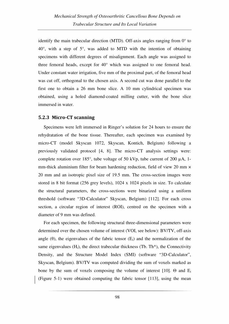
Mechanical Strength of Osteoarthritic Cancellous Bone Depends on
Trabecular Structure and Its Local Variation
98
identify the main trabecular direction (MTD). Off-axis angles ranging from 0° to
40°, with a step of 5°, was added to MTD with the intention of obtaining
specimens with different degrees of misalignment. Each angle was assigned to
three femoral heads, except for 40° which was assigned to one femoral head.
Under constant water irrigation, five mm of the proximal part, of the femoral head
was cut off, orthogonal to the chosen axis. A second cut was done parallel to the
first one to obtain a 26 mm bone slice. A 10 mm cylindrical specimen was
obtained, using a holed diamond-coated milling cutter, with the bone slice
immersed in water.
5.2.3 Micro-CT scanning
Specimens were left immersed in Ringer’s solution for 24 hours to ensure the
rehydratation of the bone tissue. Thereafter, each specimen was examined by
micro-CT (model Skyscan 1072, Skyscan, Kontich, Belgium) following a
previously validated protocol [4, 8]. The micro-CT analysis settings were:
complete rotation over 185°, tube voltage of 50 kVp, tube current of 200 µA, 1-
mm-thick aluminium filter for beam hardening reduction, field of view 20 mm ×
20 mm and an isotropic pixel size of 19.5 mm. The cross-section images were
stored in 8 bit format (256 grey levels), 1024 x 1024 pixels in size. To calculate
the structural parameters, the cross-sections were binarized using a uniform
threshold (software “3D-Calculator” Skyscan, Belgium) [112]. For each cross
section, a circular region of interest (ROI), centred on the specimen with a
diameter of 9 mm was defined.
For each specimen, the following structural three-dimensional parameters were
determined over the chosen volume of interest (VOI, see below): BV/TV, off-axis
angle (θ), the eigenvalues of the fabric tensor (Ei) and the normalization of the
same eigenvalues (Hi), the direct trabecular thickness (Tb. Th*), the Connectivity
Density, and the Structure Model Index (SMI) (software “3D-Calculator”,
Skyscan, Belgium). BV/TV was computed dividing the sum of voxels marked as
bone by the sum of voxels composing the volume of interest [10]. Θ and Ei
(Figure 5-1) were obtained computing the fabric tensor [113], using the mean

Chapter 5 Analysis of Bone Structure 2
99
intercept length (MIL) technique [42, 52, 113]. Hi where computed using the
normalization proposed by Turner et al. [56, 110]. The parameter Tb.Th*, which
gives a model-independent thickness of the 3D structure, was calculated using the
sphere-fitting method [48]. The parameter SMI is a topological index, giving an
estimate of the characteristic form in terms of plates and rods composing the 3D
structure. For ideal plates and rods the index assumes respectively the values 0
and 3, whereas for a mixed structure the SMI-index lies in between 0 and 3 [49].
Connectivity density is a parameter to measure the degree of multiple connection,
and hence reports the maximal number of branches that can be broken in a
network before the structure is separated into two parts [51].
Figure 5-1 The fabric ellipsoid is shown. Θ represents the off-axis angle while the three
eigenvectors are shown as red arrows. Eigenvalues (Ei ) are represented by the
length of the arrows.

Mechanical Strength of Osteoarthritic Cancellous Bone Depends on
Trabecular Structure and Its Local Variation
100
Models:
To improve the correlation between mechanical properties, measured along one
direction, and tissue characteristics, bone strength was studied as a function of
three independent parameters. Hence, not only BV/TV was taken into
consideration but also combinations of BV/TV, θ and Hi. In this way three models
were proposed.
• M1=BV/TV ×·cos(θ), where cos(θ) is the component of the eigenvector ‘z’
projected along the specimen axis. The here presented model is the
modulus of a vector, with the direction of the eigenvector ‘z’ and the
modulus of the bone mass, but projected along the test axis.
• M2=BV/TV·× Hz, where Hz is the fabric tensor eigenvalue closest to the
specimen axis, normalized as described by Turner et al. [110]. It represents
the influence of the structural orientation and bone mass. The orientation
of such a vector is the closest to the ‘z’ axis but is not projected on it.
• M3=BV/TV·× cos(θ)·Hz. This last model is the modulus of a vector
representing the influence of the structural orientation and bone mass, but
projected along the test axis.
Cos(θ) and Hz were chosen because in the literature they were indicated as the
most relevant parameter in the description of the mechanical behaviour [8, 57,
108, 110], and moreover they were supposed to be independent of BV/TV [110].
Both statements were verified by means of statistical approach.
The three models were computed using two different approaches, general
analysis and local analysis.
General analysis consisted in calculating the parameters over the whole
specimen volume. The VOI used, was composed of a stack of 991 consecutive
ROIs, resulting in a cylindrical VOI of 9 mm in diameter and 19.3 mm in height
[4].
Local analysis was computed along the whole specimen height using a sliding
VOI of 1mm in height with a step of about 20µm. At every step, BV/TV was
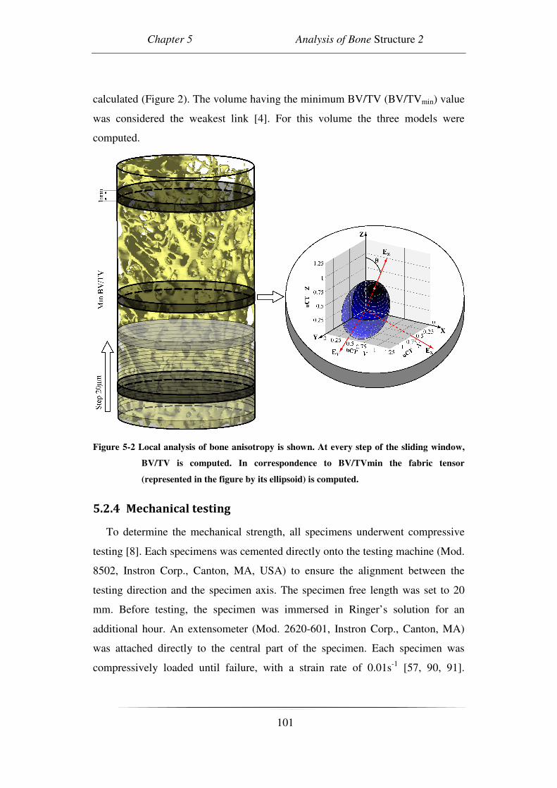
Chapter 5 Analysis of Bone Structure 2
101
calculated (Figure 2). The volume having the minimum BV/TV (BV/TVmin) value
was considered the weakest link [4]. For this volume the three models were
computed.
Figure 5-2 Local analysis of bone anisotropy is shown. At every step of the sliding window,
BV/TV is computed. In correspondence to BV/TVmin the fabric tensor
(represented in the figure by its ellipsoid) is computed.
5.2.4 Mechanical testing
To determine the mechanical strength, all specimens underwent compressive
testing [8]. Each specimens was cemented directly onto the testing machine (Mod.
8502, Instron Corp., Canton, MA, USA) to ensure the alignment between the
testing direction and the specimen axis. The specimen free length was set to 20
mm. Before testing, the specimen was immersed in Ringer’s solution for an
additional hour. An extensometer (Mod. 2620-601, Instron Corp., Canton, MA)
was attached directly to the central part of the specimen. Each specimen was
compressively loaded until failure, with a strain rate of 0.01s-1 [57, 90, 91].

Mechanical Strength of Osteoarthritic Cancellous Bone Depends on
Trabecular Structure and Its Local Variation
102
Ultimate stress (σu) was calculated from the first point on the load-extensometer
displacement curve where the slope was zero [90, 92, 93].
5.2.5 Statistical analyses
A stepwise analysis was used to verify the statistic significance of every
morphometric parameter and a correlation matrix was used to control the
independence of the parameters to BV/TV. A linear regression was plotted for σu
versus a parameter representing tissue characteristics (BV/TV, M1, M2 or M3).
The regressions were plotted for parameters calculated both in general and local
analyses. The determination coefficients and the regression residuals were
analysed to investigate the descriptive power of the models. ANOVA and Sheffe’s
post hoc tests were used to evaluate eventual differences in residuals among the
models within each kind of analysis (general or local), while a paired t-test was
used to directly compare the global analysis residuals to the ones of local analysis.
5.3 Results
The extracted specimens had minimal differences between the set “off-axis
angle” and the effective one (mean error=0,9°; max error=2,1°). The stepwise
analysis identified 4 parameters significantly related to the σu. In order of
significance: BV/TV, cos(θ), Hz, SMI. By means of a correlation matrix the
independence of cos(θ) and Hz by BV/TV was verified. Conversely, SMI resulted
significantly correlated to BV/TV (r=-0,888).
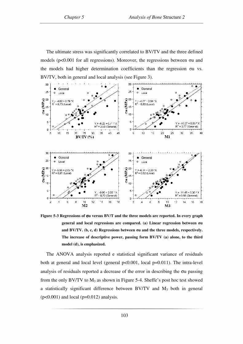
Chapter 5 Analysis of Bone Structure 2
103
The ultimate stress was significantly correlated to BV/TV and the three defined
models (p<0.001 for all regressions). Moreover, the regressions between σu and
the models had higher determination coefficients than the regression σu vs.
BV/TV, both in general and local analysis (see Figure 3).
Figure 5-3 Regressions of σσσσu versus BV/T and the three models are reported. In every graph
general and local regressions are compared. (a) Linear regression between σu
and BV/TV. (b, c, d) Regressions between σu and the three models, respectively.
The increase of descriptive power, passing form BV/TV (a) alone, to the third
model (d), is emphasized.
The ANOVA analysis reported e statistical significant variance of residuals
both at general and local level (general p<0.001, local p=0.011). The intra-level
analysis of residuals reported a decrease of the error in describing the σu passing
from the only BV/TV to M3 as shown in Figure 5-4. Sheffe’s post hoc test showed
a statistically significant difference between BV/TV and M3 both in general
(p<0.001) and local (p=0.012) analysis.

Mechanical Strength of Osteoarthritic Cancellous Bone Depends on
Trabecular Structure and Its Local Variation
104
Figure 5-4 The absolute residual values are shown. The inter-level analysis showed a
decrease of error passing from only BV/TV to M3. The intra-level analysis report
a difference between global and local. In particular, the local level analysis
showed a smaller error than the global one.
The paired t-test results are shown in Figure 4. The error found in local
analysis was always smaller than the one found in general analysis. Although, the
difference found in M1 and M3 was not statistically significant.
5.4 Discussion
Several previous studies have found that changes in mechanical properties of
trabecular bone were related to the development of OA [99, 102]. However,
mechanical characterization of trabecular bone tissue resulted a difficult issue due
to the influence of the three-dimensional structure and the heterogeneity of the
analyzed tissue.
The aim of this study was to indentify a model predicting the strength of
trabecular tissue considering its anisotropy, the non homogeneity and the real
direction testing.
In the present study the proposed models improved the description of the
mechanical strength. The improvement was enhanced by the increase of
determination coefficient and the residuals reduction. This was found in both
general and local analyses. In particular, M3 resulted significantly different from
BV/TV in both analyses. This result is mechanically reasonable and points out the
Chapter 5 Analysis of Bone Structure 2
105
dependence of bone strength of bone mass, trabecular orientation and the
difference between main trabecular direction and test axis (off-axis angle).
In comparison with other studies [42, 57, 108, 109] M3 showed a clear
improvement in the phenomenon description. In fact, the application of the model
reported by Turner (1992) using the data from the general analysis resulted in a
smaller coefficient of determination (r2=0.77). The direct comparison with
Majumdar et al. (1998) and Matsuura et al. (2007) is more complex since the
former reported only the regression coefficient and the latter did not include the
equation of the model used. However, the values reported appear lower than the
ones found in the present study (Majumdar et al., r=0.82 and Matsuura et al.,
r2=0.72). It can be suppose that the main reason of such a result to be the inclusion
of the off-axis angle among the studied parameters. In fact the inclusion of Fabric
parameters was already proposed in literature, however the difference between the
MTD and the load direction was often ignored. Conversely, Goulet et al. [57]
found a high determination coefficient for the description of ultimate strength
(r2=0.92) without including the off axis angle in the model. However, a direct
comparison between that study and the present one is difficult due to the
logarithmic model used in the former study. Moreover, in the model of Goulet et
al. (1994) MIL was combined with BV/TV even though the former is know to
depend on the latter [110]. Furthermore, no significant difference was found
among the three anatomical directions (anterior-posterior, medial-lateral, inferior-
superior), which has been proven by several other studies [42, 81, 90, 111].
A novel technique of local analysis was presented. A reduced sliding VOI was
used to obtain morphometric parameters from small portions of a single specimen
Local analysis always showed a better determination coefficient and a reduced
error in comparison to the general one. However, in M1 and M3 the residual
difference was not statistically significant. Nonetheless, local analyses were
always more precise, i.e. higher determination coefficient and lower residual
error, and the outcome is close to a significant result (p=0.077). Hence, the non
significant result could be due to the limited sample size. Moreover, local analyses
permit studying highly heterogeneous structures, taking into consideration the
Mechanical Strength of Osteoarthritic Cancellous Bone Depends on
Trabecular Structure and Its Local Variation
106
influence of such variability on the mechanical properties, as reported in the
literature [4, 23].
In this study, it is shown how the introduction of uncontrolled off-axis angles
can increase the noise in the analysis of σu. The accuracy of the strategy proposed
in the literature [4], where the off-axis angle was controlled and limited under 10°,
strongly decreased. The results of the present study demonstrate that the off-axis
angle has to be controlled, either by including it in the models or by only using
specimens which are aligned with the testing axis. Testing cancellous bone
specimen without controlling the off-axis angle can lead to uncontrollable results.
The determination coefficient of the best model proposed in the present study
(M3) was comparable to the one reported by Perilli et al. (2008). This is not
surprising since:
- in that study the specimen were aligned therefore the effect of the off-axis
angle was minimised;
- due to the minimization of the off-axis angle the specimens where always
tested along H1 (i.e. Hz=H1; H1 the major of the three eigenvalues H1>H2>H3). In
this way also the variability of the eigenvalue was minimized.
-in that study the sample size was twice the present one.
Two limitations of the study are the reduced sample size and the assumption to
have a homogeneous trabecular structure inside the VOI of analysis. This
assumption could result unacceptable, especially in transition zones close to
cortical bone. This problem was strongly reduced along the z axis of the specimen
by the use of a sliding window with a narrow step (20µm). However it could still
be present along the others axis, i.e. the cross section could be not homogeneous.
Moreover, only one anatomical site was investigated while a multisite analysis
could complete the model. Finally, the parameters were selected following a
mechanical rational, among the best results presented in literature and were
verified by means of a statistical step wise test. Nevertheless, the presented
models are just a few of the possible combinations. The existence of more
complex, but also more complete models cannot be excluded.

Chapter 5 Analysis of Bone Structure 2
107
It is still unclear how the knowledge about microstructure can be useful in the
assessment of bone macro-fractures. A previous study [114] claimed that
structural information cannot necessarily improve the prediction of whole bone
strength beyond that of bone mass or areal density. However, in that study
structural information were measured on one forearm, whereas densitometric
measures and bone strength were assessed on the contralateral one. Conversely, in
the present study the influence of microstructure in the assessment of bone
strength is not questionable.
In conclusion, in the present study the importance of considering structural
parameter was yet again shown. Numerous structural parameters describing the
3D framework of trabecular bone were presented in literature, but only a few of
them resulted really involved in the mechanical resistance of the bone structure. In
particular, in the present study the bone strength was found to be a function of
only three parameters (BV/TV, Hz and θ) of the seven assessed.
Moreover, two different techniques were used ,general and local analyses. It
was confirmed that the local analysis could better describe the mechanical
behaviour of the highly heterogenic framework of the cancellous bone.

108

Chapter 6 Analysis of Bone Structure 3
109
CHAPTER 6 ANALYSIS OF BONE STRUCTURE 3.
THREE-DIMENSIONAL TRABECULAR BONE
ANISOTROPY IN HIP ARTHRITIS: THE
CLINICAL APPLICATION.
The study presented in this chapter is subject of the paper:
Simone Tassani, Francesco Traina, Egon Perilli, Fabio Baruffaldi,
Marco Viceconti
Three-dimensional trabecular bone anisotropy in hip arthritis.
To be submitted to Journal of Orthopaedic Research.
The involvement of structural modifications during the development of
osteoarthritis was investigated. This aspect was analyzed because of the
significant relation between bone structure and mechanics, The study was aimed
to assess whether osteoarthritis have some kind of influence on micro structure of
the trabecular bone.

Three-Dimensional Trabecular Bone Anisotropy in Hip Arthritis: the Clinical
Application
110
6.1 Introduction
Hip osteoarthritis is one of the most common arthritis disease with a prevalence
ranging from 0.9% to 27% with a mean of 8.0% and a standard deviation of
7.0%[115]. Hip osteoarthritis is usually treated with a total hip replacement
placing an important demand on the Health Care System. In early stages hip
arthritis is approached with less invasive surgical techniques such as hip
arthroscopy or cartilage remodelling after hip dislocation or non surgical
procedures [116]. Nevertheless, information about osteoarthritis pathogenesis is
still incomplete and its full comprehension is still a challenge.
Different structural and mechanical properties of cancellous bone were found
between arthritic and non-pathologic bone along the years. The most often
reported finding is the increased level of bone mineral density (BMD) [93, 117,
118] in osteoarthritic (OA) patients, in contrast to controls. The exact mechanism
used by the human metabolism to achieve this augmentation of material is still an
open question. Apart from the increased amount of bone, differences in the
structural parameters of cancellous bone in OA are also reported in the literature
[119, 120]. In particular, Kamibayashi et al. [101] reported a change in the
principal trabecular orientation in the tibial plateau in OA. They found the
structure to be more perpendicular to the articular surface in OA than in the
control group.
The relation between amount of bone and structural parameters was already
reported in both non-pathologic [121] and OA [122] bone.
The importance of studying trabecular bone structure has been highlighted over
the years by the correlations found between bone anisotropy and mechanical
properties [54, 83, 123]. However, a possible implication of a modification of
degrees of anisotropy (DA) in OA bone, in comparison with non-pathologic bone,
has been scarcely investigated. The DA could have a pivot role in the
pathogenesis of osteoarthritis. A better understanding of hip osteoarthritis
pathogenesis could lead to less invasive and expensive treatments and could
improve prophylactic treatments.

Chapter 6 Analysis of Bone Structure 3
111
The aim of the present study was to investigate whether there were structural
differences, in particular in the DAs, between OA and the non-pathologic control
bone using groups paired by age and BV/TV. The bone specimens were extracted
from human femoral heads. The anisotropic parameters were computed using the
MIL method by means of X-ray micro-computed tomography (microCT).
6.2 Materials and Methods
6.2.1 Bone specimens:
The bone specimens originated from the femoral heads of two groups of
Caucasian donors, i.e. a non-pathological group (control group), and an OA
group. For the control group, 22 femoral heads were obtained from deceased
persons without musculoskeletal disorders (16 males, 6 females, age 70±10)
thanks to a donor program (International Institute for the Advance of Medicine,
Jessup, PA, USA).
The 22 osteoarthritic specimens originated from patients undergoing hip
replacement (12 males, 10 females, age 70±9) due to severe osteoarthritis, being
part of an ongoing study on osteoarthritis [8, 124]. A written informed consent
was obtained from the patients.
In order to compare anisotropic characteristics of the control bone specimens
with the OA ones, the OA specimens were selected from an internal database
[124]. These OA specimens were selected to have a distribution of age and
BV/TV similar to the control group, to reduce possible influences of these
parameters on the trabecular framework [36, 57, 104, 121, 122]. The method used
to compute the BV/TV is explained later (see MicroCT examination).
The following procedure for the specimen preparation and microCT
examination was applied to both the groups.
The heads were stored in a 70% ethanol solution for at least four weeks before
carrying out the tests, to prevent the transmission of infective diseases during
laboratory handling. A cylindrical trabecular bone specimen was retrieved from
the primary compression region of each head, as described in previous studies [4,

Three-Dimensional Trabecular Bone Anisotropy in Hip Arthritis: the Clinical
Application
112
8]. Using a diamond saw under constant water irrigation, a 26-mm-thick bone
slice was obtained, about 5 mm from the articular surface of the femoral head. A
hollow diamond-coated milling cutter, with the slice immersed in water, was used
to extract a cylindrical trabecular bone specimen (height 26 mm diameter 10 mm,
see Figure 6-1) [4, 8].
Figure 6-1 A human femoral head, with the inscribed 26mm thick bone slice, is shown. The
bone slice was cut out from the primary compressive region of the head, and
then the cylinder was drilled out from the slice
6.2.2 MicroCT examination:
Specimens were examined by microCT (model Skyscan 1072, Skyscan,
Kontich, Belgium) with a previously described protocol [4, 8, 124]. The microCT
scan settings were: complete rotation over 185°, tube voltage of 50 kVp, tube
current of 200 µA, 1-mm-thick aluminium filter for beam hardening reduction,
field of view 20 mm × 20 mm and an isotropic pixel size of 19.5 µm. The cross-
section images were reconstructed using a filtered back-projection algorithm
(software “Cone_rec”, Skyscan, Belgium) [2, 58], and storing each cross-section
as an 8-bit image (256 grey levels), 1024 x 1024 pixels in size. To calculate the
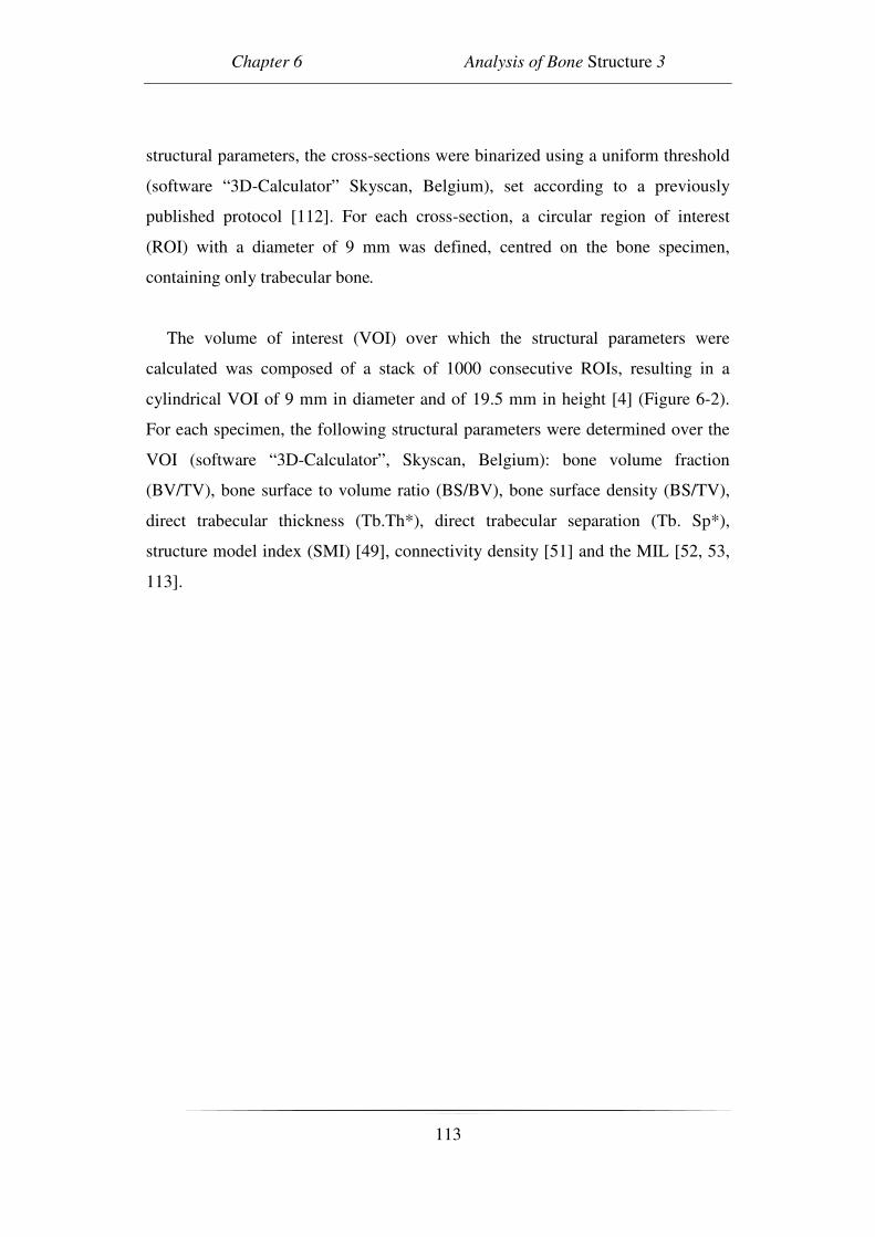
Chapter 6 Analysis of Bone Structure 3
113
structural parameters, the cross-sections were binarized using a uniform threshold
(software “3D-Calculator” Skyscan, Belgium), set according to a previously
published protocol [112]. For each cross-section, a circular region of interest
(ROI) with a diameter of 9 mm was defined, centred on the bone specimen,
containing only trabecular bone.
The volume of interest (VOI) over which the structural parameters were
calculated was composed of a stack of 1000 consecutive ROIs, resulting in a
cylindrical VOI of 9 mm in diameter and of 19.5 mm in height [4] (Figure 6-2).
For each specimen, the following structural parameters were determined over the
VOI (software “3D-Calculator”, Skyscan, Belgium): bone volume fraction
(BV/TV), bone surface to volume ratio (BS/BV), bone surface density (BS/TV),
direct trabecular thickness (Tb.Th*), direct trabecular separation (Tb. Sp*),
structure model index (SMI) [49], connectivity density [51] and the MIL [52, 53,
113].
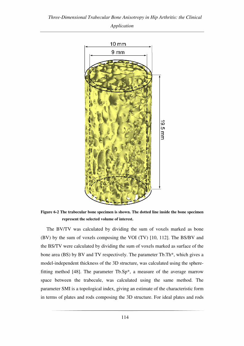
Three-Dimensional Trabecular Bone Anisotropy in Hip Arthritis: the Clinical
Application
114
Figure 6-2 The trabecular bone specimen is shown. The dotted line inside the bone specimen
represent the selected volume of interest.
The BV/TV was calculated by dividing the sum of voxels marked as bone
(BV) by the sum of voxels composing the VOI (TV) [10, 112]. The BS/BV and
the BS/TV were calculated by dividing the sum of voxels marked as surface of the
bone area (BS) by BV and TV respectively. The parameter Tb.Th*, which gives a
model-independent thickness of the 3D structure, was calculated using the sphere-
fitting method [48]. The parameter Tb.Sp*, a measure of the average marrow
space between the trabecule, was calculated using the same method. The
parameter SMI is a topological index, giving an estimate of the characteristic form
in terms of plates and rods composing the 3D structure. For ideal plates and rods

Chapter 6 Analysis of Bone Structure 3
115
the index assumes respectively the values 0 and 3, whereas for a mixed structure
the SMI-index lies in between 0 and 3. Connectivity density is a parameter to
measure the degree of multiple connection, and hence reports the maximal
number of branches that can be broken in a network before the structure is
separated into two parts [51]. The maximum, average, and minimum mean
intercept lengths, MIL1, MIL2, MIL3 respectively, were determined. These
represent the primary, secondary and tertiary direction of the MIL ellipsoid.
The degrees of anisotropy (DA) were defined and calculated [42, 57] as:
DA1= MIL1/MIL3
DA2= MIL2/MIL3
DA3= MIL1/MIL2
6.2.3 Statistical analysis:
A comparison in age, DAs and the other structural parameters was made
between the control specimens and the OA specimens.
Some of the data did not follow a normal distribution (Shapiro-Wilk test,
p<0.05 for age and connectivity density in the control group, and for SMI and Tb.
Th* in the OA group). Thus, a Mann-Whitney non-parametric test was used to
perform the comparison.
Differences were deemed to be statistically significant at a probability of
p<0.05.
For statistical analysis the software StatView (StatView version 5.0.1, SAS
institute inc. , Cary, NC, USA) was used.
6.3 Results
All results from the comparison analysis on the two groups are summarized in
Table 6-1. Mean values and standard deviations are shown for each group,
together with the related p value.

Three-Dimensional Trabecular Bone Anisotropy in Hip Arthritis: the Clinical
Application
116
Parameter Control group OA group P value
Agea 70 (±10) 70 (±9) 0.707
BV/TV (%) a 31 (±7) 29 (±6) 0.534
BS/BV (mm-1) 12.1 (±1.9) 11.9 (±1,8) 0.778
BS/TV (mm-1) 3.6 (±0.4) 3.4 (±0.5) 0.231
Tb. Th* (µm) 266 (±35) 279 (±45) 0.453
Tb.Sp* (µm) 726 (±89) 789 (±148) 0.290
SMI 0.03 (±0.85) 0.22 (±0.42) 0.481
Connectivity density 3.9 (±2.8) 4.0 (±2.1) 0.622
DA1 1.50 (±0.12) 1.59 (±0.13) 0.021§
DA2 1.14 (±0.05) 1.10 (±0.06) 0.018§
DA3 1.31 (±0.09) 1.45 (±0.13) <0.001§
Table 6-1 Comparison in age and structural parameters on trabecular bone specimens
between OA and control subjects (N= 22 specimens per group). Mean values ±±±±
standard deviations are shown for each group, together with the related p value.
a BV/TV and age values were used to pair the groups.
§ statistical significance
p<0.05
No statistically significant differences were found in age and BV/TV between
control and OA specimens, as these parameters were used to match the two
groups. No statistically significant differences were found in any of the other
examined structural parameters either (BS/BV, BS/TV, Tb.Th*, Tb. Sp*, SMI,
connectivity density), with the only exception being anisotropy. In fact,
significant differences between the two groups were found in DA1, DA2 and
DA3. In particular, the OA specimens had larger DA1 and DA3 values than the
control specimens (+7%, p<0.05, and +11%, p<0.01, respectively). Thus, the
trabeculae in the OA specimens were more oriented along the primary direction
(MIL1) of the MIL ellipsoid than those of the control specimens (Figure 6-3). On
the other hand, DA2 in the OA group was lower (-4%, p<0.05). Thus, in the plane
orthogonal to the primary direction, the distribution of the trabeculae in the OA
specimens was more isotropic than in the control specimens.
Chapter 6 Analysis of Bone Structure 3
117
Figure 6-3 3-D reconstruction of cylindrical specimens of control (a) and OA (b) cancellous
bone, from micro-CT scans. The MIL ellipsoid for control and OA samples is
shown in (c) and (d) respectively . The reported specimen showed comparable
BV/TV (control 32%; OA 30%) but different degrees of anisotropy (control
DA3=1.3; OA DA3=1.7)
6.4 Discussion
In this study femoral trabecular bone specimens obtained from the human
femoral heads of non-pathologic patients and patients in severe primary OA
conditions were analyzed. A three-dimensional analysis of the structure was
performed with the aim of comparing the three-dimensional framework of the
control and OA specimens.
No statistically significant difference was found in BS/BV, BS/TV, Tb.Th*, Tb
Sp*, SMI, nor in Connectivity Density, between control and OA specimens.
However, differences in DAs were found, suggesting alterations in the spatial
organization of the trabeculae for the OA group. In particular, as the DA1 and
DA3 in the OA group were found to increase when compared to the control
group, the OA specimens had the trabeculae more oriented along the primary
direction than the control cohorts (Figure 6-3). It is important to underline how

Three-Dimensional Trabecular Bone Anisotropy in Hip Arthritis: the Clinical
Application
118
parameters previously pointed out as indicator of structural changing, as Tb.Th*,
SMI and Connectivity Density, did not show any statistical difference.
Moreover the results shown in the present work are in agreement with similar
findings in the literature [101, 125]. Kamibayashi et al. [101] analysed the human
proximal tibia founding an orientation of the trabeculae more perpendicular to the
articular surface in the late OA group than in the control group. However the used
technique was limited to bi-dimensional analysis of a small portion of the tibial
plateau. In the present study a three-dimensional approach was used on a bigger
and more representative specimen of femoral head. Nonetheless it is reasonable to
expect, that the more vertical orientation of the trabeculae in the tibial plateau
found in that study corresponds to the increase of trabecular orientation along the
MIL1 shown in the present study.
Bettica et al. [126] reported a greater biological activity in progressive OA
(which is the phase in which the OA evolves), with respect to normal bone.
Indeed, the present results, together with those of Kamibayashi and Bettica,
suggest the existence of a remodelling activity, detected by changes in anisotropy
and highlighting a three-dimensional reorientation of the trabecular structure.
In a previous study on early knee OA, Day et al. reported a disruption of the
correlation between apparent stiffness and BV/TV [102]. The here presented
results suggest a possible role of DA variation in the description of mechanical
properties.
The link between structure orientation and mechanical properties is well
described in the literature [54, 83, 123, 127, 128] It is well known how a more
oriented structure can result a stiffer one.
The bone adapt to the applied load during everyday life [129, 130]., a change
on bone loading due to OA could lead to a structure reorientation.
Differences in gait between non-pathologic and OA patients were widely
analyzed in the literature [131-134]. In particular, as reported by Hurwitz et al
[135], there is a reduction in dynamic range of motion of the hip, due to antalgic
gait. This could modify the biomechanics of the joint, leading the patient to load
his hip in the only position in which he does not feel pain, and consequently drive

Chapter 6 Analysis of Bone Structure 3
119
the trabecular framework remodelling along preferred orientations, which might
explain the more anisotropic specimens found in OA in the present study.
However, this study did not analyse gait experimentally as it was not the aim of
the study, and further researches are needed to confirm this hypothesis.
Nonetheless, if a modification of the load during everyday life could be the
cause of the change in trabecular orientation here presented, lifestyle interventions
should be the treatment. Aquatic therapy or other kind of physical treatment was
found to have a statistically significant effect in the reduction of pain and
functional improvement [136, 137].
In conclusion, the presented study found differences of trabecular anisotropy
between OA and control specimens. This suggests the presence of a bone
remodelling activity, in terms of reorientation of the trabeculae in OA. The OA
trabecular framework resulted in a more oriented structure along the primary
direction. On the other hand other structural parameter did not exhibit any
statistical difference between groups matched in BV/TV.
This reorientation might take place after the development of cartilage
abnormalities [99] and could be consequence of the changes in joint function and
gait of the patients, associated with OA. In our opinion treatment of OA should
address at least three different bone problems: reduced tissue modulus, increasing
of volume fraction and reorientation of the trabecular framework. While the first
and the second should probably be treated by means of drugs, the latter should be
treated by lifestyle interventions and physical therapy [136, 137] because we
believe that without return to mechanical normality attempts at healing fail.

120
Chapter 7 Analysis of Tissue Quality
121
CHAPTER 7 ANALYSIS OF TISSUE QUALITY.
VOLUME TO DENSITY RELATION IN BONE
TISSUE.
The study presented in this chapter is subject of the paper:
Simone Tassani, Caroline Öhman, Massimiliano Baleani, Fabio Baruffaldi and
Marco Viceconti
Volume to density relation in bone tissue: the importance of morphometric
phantoms in micro-ct analyses
Micro-CT is a privileged instrument for the study of tissue mineralization due
to the tightly link between bone density and x-ray absorption. However the study
of tissue density by means of microtomographic techniques is an emerging field,
and the difference between bone density and tissue density is not yet completely
clear. In this last part of the study the relation between bone density and bone
quantity was studied both for trabecular and cortical bone. It was found that one
single linear regression model was able to describe this relation in both the tissues.

Volume to Density Relation in Bone Tissue
122
7.1 Introduction
Analysis of bone material properties is an important issue for the mechanical
characterization of the bone tissue. Furthermore, a correct description of the
material properties of cortical and trabecular bone is a critical topic for the
implementation of computational models.
Several studies in the literature [93] have investigated the influence of bone
composition and tissue properties on its mechanical properties.
Some studies have indicated the degree of porosity as the only difference
between cortical and trabecular bone tissue [81]. This suggestion would simplify
the predictions of mechanical properties of bone tissue since it would become a
function of only bone quantity and structure.
Conversely, a boomerang like distribution of tissue mineral densities in the
elephant femur was recently suggested[138]. In that work, cortical bone with low
porosity showed a high mineral content increasing the porosity the mineral
content decreased coming to a minimum value in the zone between cortical and
trabecular bone. However, once passed to trabecular bone an increase in porosity
caused an increase in mineral content as well. The authors state that the reported
effect is real and not an experimental artefact. If that effect should be verified also
in human bone the use of densitometry as a diagnostic tool could became
questionable.
However, the method used in that study has been pointed out to have practical
problems in its accuracy [139] due to difficulties in measuring the wet density of
trabecular bone. In fact, cleaning all bone porosities from bone marrow, which
implies that all porosities must be open, is not a trivial issue. Moreover, the same
problem could also be present in the analysis of cortical tissue where the porosity
can range from 5 to 20% [113, 138].
The aim of the present study was to verify the mineral density distribution in
both cortical and trabecular bone using micro computed tomography (micro-CT)
analysis to avoid the above-mentioned problems.

Chapter 7 Analysis of Tissue Quality
123
7.2 Materials and Methods
Cortical and trabecular bone specimens were extracted, acquired by means of
micro-CT and finally ashed. In this work the bone volume fraction (BV/TV) was
calculate using the micro-CT while the mineral content was defined weighting
gravitometrically the ash mass of the specimens. Tissue Mineral Density (TMD)
was defined as the ratio between ash density and bone volume [74]
7.2.1 Specimen extraction
The lower limbs of two female donors without muscoloskeletal disease were
obtained from the European project LHDL. The samples had been embalmed
using the modified Dankmeyer’s method [140]. It has been found that bone
mineral density is not affected by formalin fixation [141, 142].
Tibias and femurs were cut into slices perpendicular to the longitudinal axis of
the bone. The diaphyses were cut into 20-mm slices whereas the epiphyses were
cut into 26-mm slices. Cylindrical specimens of cortical bone, with a diameter of
2.8 mm and a height of 20 mm, were extracted from the diaphysial slices by
means of a holed diamond-coated milling cutter. Cylindrical specimens of
trabecular bone, with a diameter of 10 mm and a height of 26 mm, were extracted
from the epiphysial slices, i.e. femoral head, greater trochanter, femoral condyles,
tibial plateau and distal tibia, by means of a holed diamond-coated milling cutter.
The femoral specimens were extracted following a previous published protocol
[8]. During specimen extraction the bone slice was immersed in water.
Seventy nine bone specimens (62 trabecular and 17 cortical) where extracted.
The specimens where extracted from different sites of the lower limbs (see Figure
7-1) in order to perform an inter-site analysis. Moreover, in order to increase the
sample size for an inter-subject analysis, 19 specimens used for another study [8]
were added to the present study.
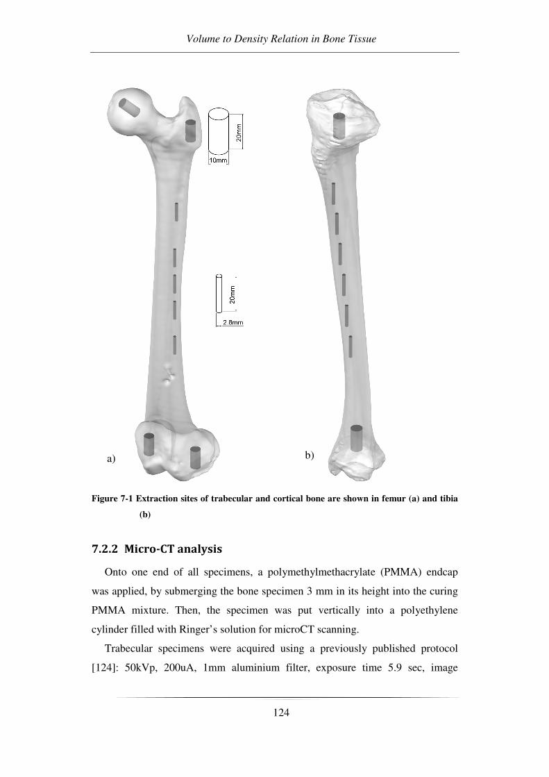
Volume to Density Relation in Bone Tissue
124
Figure 7-1 Extraction sites of trabecular and cortical bone are shown in femur (a) and tibia
(b)
7.2.2 Micro-CT analysis
Onto one end of all specimens, a polymethylmethacrylate (PMMA) endcap
was applied, by submerging the bone specimen 3 mm in its height into the curing
PMMA mixture. Then, the specimen was put vertically into a polyethylene
cylinder filled with Ringer’s solution for microCT scanning.
Trabecular specimens were acquired using a previously published protocol
[124]: 50kVp, 200uA, 1mm aluminium filter, exposure time 5.9 sec, image
a) b)
Chapter 7 Analysis of Tissue Quality
125
averaged on 2 projections, rotation 180 degree, rotation step 0.9°, field of view 20
mm × 20 mm and an isotropic pixel size of 19.5 µm. The cross-section images
were stored in 8 bit format (256 grey levels), 1024 x 1024 pixels in size. For each
cross section, a circular region of interest (ROI), centred on the specimen with a
diameter of 9 mm was defined. The VOI used, was composed of a stack of 991
consecutive ROIs, resulting in a cylindrical VOI of 9 mm in diameter and 19.3
mm in height.
Cortical specimen were acquired using the following protocol: 80kVp 150µA
1mm aluminium filter, exposure time 5.9 sec, image averaged on 2 projections,
rotation 180 degree, rotation step 0.9°, field of view 8 mm × 8 mm and an
isotropic pixel size of 8µm. In order to acquire the whole specimen using the
described resolution two acquisition were performed for every cortical specimen
in order to obtain a field of view of 8x14mm. The cross-section images were
stored in 8 bit format (256 grey levels), 1024 x 1024 pixels in size. For each cross
section, a circular region of interest (ROI), centred on the specimen with a
diameter of 2,52 mm was defined. The VOI used, was composed of a stack of
1747 consecutive ROIs, resulting in a cylindrical VOI of 2,52 mm in diameter and
14 mm in height.
BV/TV was calculated for both trabecular and cortical specimens using two
different global thresholds. The two thresholds were selected by means of two
morphometric phantoms representative of the analyzed tissue .
7.2.3 Ashing procedure
After the micro-CT analysis, the cement endcaps were removed and the
specimens were reduced to ash by burning the bone tissue in a muffle furnace at
650°C for 24 hours. The muffle furnace was then turned off and the specimens
were left inside for additionally 24 hours to reach room temperature and thereafter
the ash weight was measured [8]. The ash density of the specimen was defined as
the ash weight divided by the specimen volume [94-96]. The volume of the bone
specimen was determined from the diameter and total height.

Volume to Density Relation in Bone Tissue
126
7.2.4 Statistical analysis
Linear regressions between Ash density and BV/TV and between TMD and
BV/TV were plotted. The normality of the distributions for cortical and trabecular
TMD was verified by means of a Shapiro-Wilk test. Moreover, a unpaired student
t-test was performed to investigate any difference between TMD of trabecular and
cortical bone specimens.
7.3 Results
TMD remained relatively constant for the whole range of BV/TV analysed
(Figure 7-2) showing only an increase in the TMD in the low range of BV/TV.
0
0.2
0.4
0.6
0.8
1
1.2
1.4
1.6
1.8
2
0.00 0.20 0.40 0.60 0.80
TM
D (
g/c
m3)
Figure 7-2 TMD distribution of cortical and trabecular bone
Moreover, the T-test showed no statistical difference between TMD in cortical
and trabecular bone specimen (p=0,89). In fact, only one linear regression curve
could describe the relation between Ash density and BV/TV, as shown in Figure
7-3.
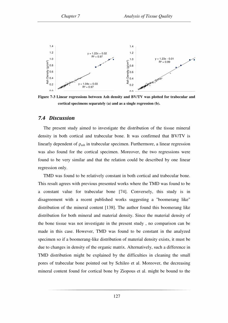
Chapter 7 Analysis of Tissue Quality
127
y = 1.04x + 0.03R² = 0.97
y = 1.22x + 0.02R² = 0.97
0.0
0.2
0.4
0.6
0.8
1.0
1.2
1.4A
sh
De
nsity
(g/c
m3)
y = 1.23x - 0.01R² = 0.99
0.0
0.2
0.4
0.6
0.8
1.0
1.2
1.4
Ash
Density
(g/c
m3)
Figure 7-3 Linear regressions between Ash density and BV/TV was plotted for trabecular and
cortical specimens separately (a) and as a single regression (b).
7.4 Discussion
The present study aimed to investigate the distribution of the tissue mineral
density in both cortical and trabecular bone. It was confirmed that BV/TV is
linearly dependent of ρash in trabecular specimen. Furthermore, a linear regression
was also found for the cortical specimen. Moreover, the two regressions were
found to be very similar and that the relation could be described by one linear
regression only.
TMD was found to be relatively constant in both cortical and trabecular bone.
This result agrees with previous presented works where the TMD was found to be
a constant value for trabecular bone [74]. Conversely, this study is in
disagreement with a recent published works suggesting a "boomerang like"
distribution of the mineral content [138]. The author found this boomerang like
distribution for both mineral and material density. Since the material density of
the bone tissue was not investigate in the present study , no comparison can be
made in this case. However, TMD was found to be constant in the analyzed
specimen so if a boomerang-like distribution of material density exists, it must be
due to changes in density of the organic matrix. Alternatively, such a difference in
TMD distribution might be explained by the difficulties in cleaning the small
pores of trabecular bone pointed out by Schileo et al. Moreover, the decreasing
mineral content found for cortical bone by Ziopous et al. might be bound to the

Volume to Density Relation in Bone Tissue
128
porosity of this tissue resulting in cleaning problems similar to those of trabecular
bone.
The present study was in agreement with a clinical study about densitometry
[139]. In fact, Schileo et al. proposed a single linear distribution between ash
density and mineral density measured with clinical CT. However, clinical CT does
not have the resolution to calculate TMD and the resulted index is a combination
of TMD and quantity of bone i.e. Bone Mineral Density. Furthermore, the here
presented results suggest that the clinical outcome might be a linear expression of
bone quantity due to the constant distribution of TMD. This result is important
especially for computational models where TMD could be selected as a fixed
material parameter for both trabecular and cortical bone.
One limitation of the present study is related to the low number of donors for
cortical tissue. TMD could be directly measured using micro-CT analysis by
means of a densitometric calibration [74, 143]. However, this approach is strongly
calibration dependent and there is still a need of a definition of an accurate
calibration procedure. On the other hand, gravitometric measures are easy to
assess and the calculation of BV/TV is validated procedure [112].
One interesting result is that the distribution of the TMD was wider for
specimens having a low BV/TV. This effect could be related to the increasing
error in computing BV/TV using a global threshold while the ratio decrease due to
partial volume effect [77].
In conclusion, no significant difference was found in TMD between trabecular
and cortical bone. In contrast with some “boomerang-like” results, this study
suggest that the TMD is relatively constant in both cortical and trabecular
specimens.

Conclusions
129
CONCLUSIONS
The present Ph.D research described micro-CT techniques for the evaluation of
bone strength, with particular regard to cancellous bone. Bone tissue
microarchitecture and density were measured to estimate its mechanical
behaviour.
The reliability of the micro-CT device was studied and verified. This was not a
granted result because Quality Control protocols were never reported for micro-
CT devices. However this study permits the future combined study of many bone
specimens acquired using the same protocol, during different study over time.
Moreover the developed Quality Control protocol permits the periodical control of
the device and can avoid future “out of control” situations.
The evaluation of bone strength was assessed by the study of different bone
characteristics such as bone quantity, bone structure and tissue quality. Bone
quantity is recognized to be the main actor in the determination of bone strength.
However models involving information about the mere quantity resulted weak in
this direction. The presented studies underlined the importance to control
information about quantity in order to identify the right parameters about
structure. In fact along the years the so called “structural parameters” have
strongly increased in number but the relationship with mechanical characteristics
is not clear. In particular the dependence of structural from quantity parameter is
often neglected. In chapter 5 and 6 the dependence of many structural parameter
from BV/TV was underlined and only two parameters were identified as best and
independent descriptors of the structure: off-axis angle and the normalized fabric
tensor eigenvalue. The researcher should not ignore the influence of bone
structure. He can decide to control the global structure testing only specimen with
a given direction, or to include bone structure parameters in the analysis.
The clinical application of structural analysis was also studied. The dependence
between structure and function was suggested and some clinical treatments were
proposed.
Conclusions
130
The study of tissue quality suggests cortical and trabecular bone to have the
same tissue density. This statement has several practical implications. First of all
the clinical application: clinical densitometric analysis resulting in decrease “bone
density” could indicate a decrease of bone quantity, while the material by which
bone is made maintain the same density. This assumption is suggested for healthy
bone. From literature it is known that some pathology can vary the tissue density,
i.e. osteoarthritis, however could be hypothesized to be a constant in trabecular
and cortical bone within a defined bone condition, e.g. osteoarthritis, osteoporosis
or non pathological bone. Moreover, the importance of morphometric analysis in
micro-CT density study is underlined. In fact the identification of bone volume is
mandatory to assess the density of bone tissue.
In conclusion the present Ph.D research aimed at evaluating bone strength. The
main parameters involved in mechanical characterization of bone tissue were
analyzed. Bone quantity was confirmed to play an important role in the evaluation
of bone strength. Among the several structural parameters reported in literature,
only two were identified as describers of the bone structure. Last but not least,
tissue density was found not to be a variable within a defined bone condition.
The here presented analyses showed the results of inductive procedure.
However, this study demonstrates that it is now possible to develop a validated
deductive model .

131

References
132
REFERENCES
1. Genant, H.K., et al., Interim report and recommendations of the World Health Organization Task-Force for Osteoporosis. Osteoporos Int, 1999. 10(4): p. 259-64.
2. Sasov, A. and D. Van Dyck, Desktop X-ray microscopy and microtomography. J Microsc, 1998. 191(Pt 2): p. 151-8.
3. Feldkamp, L.A., et al., The direct examination of three-dimensional bone architecture in vitro by computed tomography. J Bone Miner Res, 1989. 4(1): p. 3-11.
4. Perilli, E., et al., Dependence of mechanical compressive strength on local variations in microarchitecture in cancellous bone of proximal human femur. J Biomech, 2008. 41(2): p. 438-46.
5. Cowin, S.C., Bone Mechanics Handbook. Second edition. 2001: CRC Press, Boca Raton, USA.
6. Williams, P.L., Gray's anatomy. 38th edition. 1995: Churchill Livingstone, London, UK.
7. Black, J. and G. Hastings, Handbook of biomaterial properties, : Chapman & Hall.
8. Ohman, C., et al., Mechanical testing of cancellous bone from the femoral head: Experimental errors due to off-axis measurements. J Biomech, 2007.
9. Turner, C.H. and S.C. Cowin, Errors induced by off-axis measurement of the elastic properties of bone. J Biomech Eng, 1988. 110(3): p. 213-5.
10. Parfitt, A.M., et al., Bone histomorphometry: standardization of nomenclature, symbols, and units. Report of the ASBMR Histomorphometry Nomenclature Committee. J Bone Miner Res, 1987. 2(6): p. 595-610.
11. Malluche, H.H.F., M. C. , Atlas of mineralized bone histology. 1986: Karger AG, Basel, Switzerland.
12. Weiss, L., Cell and tissue biology. 1990: Urban & Schwarzenberg, Baltimore.
13. Frost, H.M., Intermediary organization of skeleton. 1984: CRC Press, Boca Raton, USA.
14. Hancox, N.M., The biology of bone. 1972: Campridge University Press, Cambridge.
15. Currey, J.D., The many adaptations of bone. J Biomech, 2003. 36(10): p. 1487-95.
16. Currey, J.D., What should bones be designed to do? Calcif Tissue Int, 1984. 36 Suppl 1: p. S7-10.
17. Burr, D.B., et al., Bone remodeling in response to in vivo fatigue microdamage. J Biomech, 1985. 18(3): p. 189-200.
18. Frost, H.M. and W.S. Jee, Perspectives: a vital biomechanical model of the endochondral ossification mechanism. Anat Rec, 1994. 240(4): p. 435-46.

References
133
19. Wolff, J., Über die innere Architektur der Knochen und ihre Bedeutung für die Frage vom Knochenwachstum. . Virchows Arch. Anat. Physiol. Klin. Med. , 1870. 50: p. 389-453.
20. Frost, H.M., Bone "mass" and the "mechanostat": a proposal. Anat Rec, 1987. 219(1): p. 1-9.
21. Frost, H.M., Introduction to a new skeletal physiology. 1995: Pajaro Group, Pueblo Vol. I and II.
22. WHO (2002) The World Health report 2002. Reducing Risks, Promoting Healthy Life. Volume,
23. Nazarian, A., et al., The interaction of microstructure and volume fraction in predicting failure in cancellous bone. Bone, 2006. 39(6): p. 1196-202.
24. Kak, A.C. and M. Slaney, Principles of computerized tomographic imaging. . 1999: New York, USA, IEEE Press.
25. Krane, S., Introductory nuclear physics. 1988: John Wiley & Sons, USA. 26. Radon, J., Űber die Bestimmung von Funktionen durch ihre Integralwerte
längs gewisser Mannigfaltigkeiten. . Berichte Saechsischer Akademie der Wissenschaften 1917. 69: p. 262-267.
27. Hounsfield, G.N., Computerized transverse axial scanning (tomography). 1. Description of system. Br J Radiol, 1973. 46(552): p. 1016-22.
28. Cormack, A.M., Reconstruction of densities from their projections, with applications in radiological physics. Phys Med Biol, 1973. 18(2): p. 195-207.
29. Cendre, E., et al., High-resolution computed tomography for architectural characterization of human lumbar cancellous bone: relationships with histomorphometry and biomechanics. Osteoporosis International, 1999. 10(5): p. 353-60.
30. Mitton, D., et al., Mechanical properties of ewe vertebral cancellous bone compared with histomorphometry and high-resolution computed tomography parameters. Bone, 1998. 22(6): p. 651-8.
31. Ruegsegger, P., B. Koller, and R. Muller, A microtomographic system for the nondestructive evaluation of bone architecture. Calcif Tissue Int, 1996. 58(1): p. 24-9.
32. David, V., et al., Noninvasive in vivo monitoring of bone architecture alterations in hindlimb-unloaded female rats using novel three-dimensional microcomputed tomography. J Bone Miner Res, 2003. 18(9): p. 1622-31.
33. Kuhn, J.L., et al., Evaluation of a microcomputed tomography system to study trabecular bone structure. J Orthop Res, 1990. 8(6): p. 833-42.
34. Thomsen, J.S., et al., Stereological measures of trabecular bone structure: comparison of 3D micro computed tomography with 2D histological sections in human proximal tibial bone biopsies. J Microsc, 2005. 218(Pt 2): p. 171-9.
35. Nagele, E., et al., Technical considerations for microstructural analysis of human trabecular bone from specimens excised from various skeletal sites. Calcif Tissue Int, 2004. 75(1): p. 15-22.

References
134
36. Hildebrand, T., et al., Direct three-dimensional morphometric analysis of human cancellous bone: microstructural data from spine, femur, iliac crest, and calcaneus. J Bone Miner Res, 1999. 14(7): p. 1167-74.
37. Wang, X., et al., Age-related changes in the collagen network and toughness of bone. Bone, 2002. 31(1): p. 1-7.
38. Hoffler, C.E., et al., Heterogeneity of bone lamellar-level elastic moduli. Bone, 2000. 26(6): p. 603-9.
39. Aerssens, J., et al., Variations in trabecular bone composition with anatomical site and age: potential implications for bone quality assessment. J Endocrinol, 1997. 155(3): p. 411-21.
40. Ciarelli, M.J., et al., Evaluation of orthogonal mechanical properties and density of human trabecular bone from the major metaphyseal regions with materials testing and computed tomography. Journal of Orthopaedic Research, 1991. 9(5): p. 674-82.
41. Ding, M., et al., Age-related variations in the microstructure of human tibial cancellous bone. J Orthop Res, 2002. 20(3): p. 615-21.
42. Majumdar, S., et al., High-resolution magnetic resonance imaging: three-dimensional trabecular bone architecture and biomechanical properties. Bone, 1998. 22(5): p. 445-54.
43. Chappard, D., et al., Comparison insight bone measurements by histomorphometry and microCT. J Bone Miner Res, 2005. 20(7): p. 1177-84.
44. Muller, R., et al., Morphometric analysis of human bone biopsies: a quantitative structural comparison of histological sections and micro-computed tomography. Bone, 1998. 23(1): p. 59-66.
45. Russ, J.C. and R. Dehoff, Practical stereology. 1999: Second edition, Plenum Press, New York, USA.
46. Odgaard, A., Three-dimensional methods for quantification of cancellous bone architecture. Bone, 1997. 20(4): p. 315-28.
47. Lorensen, W.E. and H.E. Cline, MARCHING CUBES: A HIGH RESOLUTION 3D SURFACE CONSTRUCTION ALGORITHM. Computer Graphics (ACM), 1987. 21(4): p. 163-169.
48. Hildebrand, T. and P. Ruegsegger, A new method for the model-independent assessment of thickness in three-dimensional images. Journal of Microscopy, 1997. 185: p. 67.
49. Hildebrand, T. and P. Ruegsegger, Quantification of Bone Microarchitecture with the Structure Model Index. Comput Methods Biomech Biomed Engin, 1997. 1(1): p. 15-23.
50. Kinney, J.H. and A.J. Ladd, The relationship between three-dimensional connectivity and the elastic properties of trabecular bone. J Bone Miner Res, 1998. 13(5): p. 839-45.
51. Odgaard, A. and H.J. Gundersen, Quantification of connectivity in cancellous bone, with special emphasis on 3-D reconstructions. Bone, 1993. 14(2): p. 173-82.
52. Whitehouse, W.J., The quantitative morphology of anisotropic trabecular bone. J Microsc, 1974. 101(Pt 2): p. 153-68.

References
135
53. Harrigan, T.P. and R.W. Mann, Characterization of microstructural anisotropy in orthotropic materials using a second rank tensor. Journal of Materials Science, 1984. 19(3): p. 761.
54. Cowin, S.C., The relationship between the elasticity tensor and the fabric tensor. Mechanics of Materials, 1985. 4(2): p. 137.
55. Cowin, S.C., Wolff's law of trabecular architecture at remodeling equilibrium. J Biomech Eng, 1986. 108(1): p. 83-8.
56. Homminga, J., et al., The dependence of the elastic properties of osteoporotic cancellous bone on volume fraction and fabric. J Biomech, 2003. 36(10): p. 1461-7.
57. Goulet, R.W., et al., The relationship between the structural and orthogonal compressive properties of trabecular bone. J Biomech, 1994. 27(4): p. 375-89.
58. Feldkamp, L.A., L.C. Davis, and J.W. Kress, Practical cone-beam algorithm. J. Opt. Soc. Am. A, 1984.
59. Dufresne, T., Segmentation techniques for analysis of bone by three-dimensional computed tomographic imaging. Technol Health Care, 1998. 6(5-6): p. 351-9.
60. Ding, M., A. Odgaard, and I. Hvid, Accuracy of cancellous bone volume fraction measured by micro-CT scanning. J Biomech, 1999. 32(3): p. 323-6.
61. Waarsing, J.H., et al., Detecting and tracking local changes in the tibiae of individual rats: a novel method to analyse longitudinal in vivo micro-CT data. Bone, 2004. 34(1): p. 163-9.
62. Quality Control In Diagnostic Radiology. 2002, The American Association of Physicists in Medicine (AAPM).
63. Recommended standards for the performance testing of diagnostic X-ray imaging systems. 2005, Institute of Physics and Engineering in Medicine (IPEM).
64. Sprawls, P., AAPM tutorial. CT image detail and noise. Radiographics, 1992. 12(5): p. 1041-6.
65. Birnbaum, B.A., et al., Renal cyst pseudoenhancement: evaluation with an anthropomorphic body CT phantom. Radiology, 2002. 225(1): p. 83-90.
66. Funama, Y., et al., Radiation dose reduction without degradation of low-contrast detectability at abdominal multisection CT with a low-tube voltage technique: phantom study. Radiology, 2005. 237(3): p. 905-10.
67. Huda, W., et al., An approach for the estimation of effective radiation dose at CT in pediatric patients. Radiology, 1997. 203(2): p. 417-22.
68. Kalender, W.A., A phantom for standardization and quality control in spinal bone mineral measurements by QCT and DXA: design considerations and specifications. Med Phys, 1992. 19(3): p. 583-6.
69. Kalender, W.A., et al., The European Spine Phantom--a tool for standardization and quality control in spinal bone mineral measurements by DXA and QCT. Eur J Radiol, 1995. 20(2): p. 83-92.
70. Kalender, W.A. and C. Suess, A new calibration phantom for quantitative computed tomography. Med Phys, 1987. 14(5): p. 863-6.

References
136
71. Ko, J.P., et al., Small pulmonary nodules: volume measurement at chest CT--phantom study. Radiology, 2003. 228(3): p. 864-70.
72. Olerud, H.M., J.B. Olsen, and A. Skretting, An anthropomorphic phantom for receiver operating characteristic studies in CT imaging of liver lesions. Br J Radiol, 1999. 72(853): p. 35-43.
73. Ruegsegger, P. and W.A. Kalender, A phantom for standardization and quality control in peripheral bone measurements by PQCT and DXA. Phys. Med. Biol. , 1993. 38(12): p. 1963.
74. Kazakia, G.J., et al., Assessment of bone tissue mineralization by conventional x-ray microcomputed tomography: comparison with synchrotron radiation microcomputed tomography and ash measurements. Med Phys, 2008. 35(7): p. 3170-9.
75. Nazarian, A., et al., Quantitative micro-computed tomography: A non-invasive method to assess equivalent bone mineral density. Bone, 2008. 43(2): p. 302-11.
76. Du, L.Y., et al., A quality assurance phantom for the performance evaluation of volumetric micro-CT systems. Phys Med Biol, 2007. 52(23): p. 7087-108.
77. Perilli, E., et al., A physical phantom for the calibration of three-dimensional X-ray microtomography examination. J Microsc, 2006. 222(Pt 2): p. 124-34.
78. Montgomery, D.C., Introduction to Statistical Quality Control. 2006, Milano: The McGraw-Hill Companies, S.r.l., Publishing Group Italia.
79. Hubbell, J.H., Tables of X-Ray Mass Attenuation Coefficients NISTIR 5632, NIST, Gaithersburg, MD, USA.
80. L.C.Young, On Randomness in ordered sequences. Annals of Mathematical Statistics, 1941. 12: p. 293-300.
81. Gibson, L.J., Biomechanics of cellular solids. J Biomech, 2005. 38(3): p. 377-99.
82. Gibson, L.J., The mechanical behaviour of cancellous bone. Journal of Biomechanics, 1985. 18(5): p. 317-28.
83. Odgaard, A., et al., Fabric and elastic principal directions of cancellous bone are closely related. J Biomech, 1997. 30(5): p. 487-95.
84. Wang, X., X. Liu, and G.L. Niebur, Preparation of on-axis cylindrical trabecular bone specimens using micro-CT imaging. J Biomech Eng, 2004. 126(1): p. 122-5.
85. Zysset, P.K., et al., Mechanical properties of human trabecular bone lamellae quantified by nanoindentation. Technology and Health Care, 1998. 6(5-6): p. 429-32.
86. Augat, P., et al., Anisotropy of the elastic modulus of trabecular bone specimens from different anatomical locations. Medical Engineering and Physics, 1998. 20(2): p. 124-31.
87. Birnbaum, K., et al., Material properties of trabecular bone structures. Surgical - Radiologic Anatomy, 2001. 23(6): p. 399-407.

References
137
88. Linde, F. and H.C. Sorensen, The effect of different storage methods on the mechanical properties of trabecular bone. J Biomech, 1993. 26(10): p. 1249-52.
89. Keaveny, T.M., et al., Systematic and random errors in compression testing of trabecular bone [published erratum appears in J Orthop Res 1999 Jan;17(1):151]. Journal of Orthopaedic Research, 1997. 15(1): p. 101-10.
90. Ciarelli, T.E., et al., Variations in three-dimensional cancellous bone architecture of the proximal femur in female hip fractures and in controls. J Bone Miner Res, 2000. 15(1): p. 32-40.
91. Linde, F., I. Hvid, and F. Madsen, The effect of specimen geometry on the mechanical behaviour of trabecular bone specimens. J Biomech, 1992. 25(4): p. 359-68.
92. Brown, S.J., et al., Regional differences in mechanical and material properties of femoral head cancellous bone in health and osteoarthritis. Calcif Tissue Int, 2002. 71(3): p. 227-34.
93. Li, B. and R.M. Aspden, Composition and mechanical properties of cancellous bone from the femoral head of patients with osteoporosis or osteoarthritis. J Bone Miner Res, 1997. 12(4): p. 641-51.
94. Kaneko, T.S., et al., Mechanical properties, density and quantitative CT scan data of trabecular bone with and without metastases. Journal of Biomechanics, 2004. 37(4): p. 523-30.
95. Les, C.M., et al., Stiff and strong compressive properties are associated with brittle post-yield behavior in equine compact bone material. Journal of Orthopaedic Research, 2002. 20(3): p. 607-14.
96. Lespessailles, E., et al., Biomechanical properties of human os calcanei: relationships with bone density and fractal evaluation of bone microarchitecture. Journal of Biomechanics, 1998. 31(9): p. 817-24.
97. Hodgskinson, R., J.D. Currey, and G.P. Evans, Hardness, an indicator of the mechanical competence of cancellous bone. Journal of Orthopaedic Research, 1989. 7(5): p. 754-8.
98. Keaveny, T.M., et al., Trabecular bone modulus and strength can depend on specimen geometry. Journal of Biomechanics, 1993. 26(8): p. 991-1000.
99. Ding, M., A. Odgaard, and I. Hvid, Changes in the three-dimensional microstructure of human tibial cancellous bone in early osteoarthritis. J Bone Joint Surg Br, 2003. 85(6): p. 906-12.
100. Dequeker, J. and O. Johnell, Osteoarthritis protects against femoral neck fracture: the MEDOS study experience. Bone, 1993. 14 Suppl 1: p. S51-6.
101. Kamibayashi, L., et al., Changes in mean trabecular orientation in the medial condyle of the proximal tibia in osteoarthritis. Calcif Tissue Int, 1995. 57(1): p. 69-73.
102. Day, J.S., et al., A decreased subchondral trabecular bone tissue elastic modulus is associated with pre-arthritic cartilage damage. J Orthop Res, 2001. 19(5): p. 914-8.

References
138
103. Goldstein, S.A., R. Goulet, and D. McCubbrey, Measurement and significance of three-dimensional architecture to the mechanical integrity of trabecular bone. Calcif Tissue Int, 1993. 53 Suppl 1: p. S127-32; discussion S132-3.
104. Muller, R. and P. Ruegsegger, Micro-tomographic imaging for the nondestructive evaluation of trabecular bone architecture. Stud Health Technol Inform, 1997. 40: p. 61-79.
105. Ding, M. and I. Hvid, Quantification of age-related changes in the structure model type and trabecular thickness of human tibial cancellous bone. Bone, 2000. 26(3): p. 291-5.
106. Snyder, B.D., et al., Role of trabecular morphology in the etiology of age-related vertebral fractures. Calcif Tissue Int, 1993. 53 Suppl 1: p. S14-22.
107. Helgason, B., et al., Mathematical relationships between bone density and mechanical properties: a literature review. Clin Biomech (Bristol, Avon), 2008. 23(2): p. 135-46.
108. Matsuura, M., et al., The role of fabric in the quasi-static compressive mechanical properties of human trabecular bone from various anatomical locations. Biomech Model Mechanobiol, 2007.
109. Turner, C.H., On Wolff's law of trabecular architecture. J Biomech, 1992. 25(1): p. 1-9.
110. Turner, C.H., et al., The fabric dependence of the orthotropic elastic constants of cancellous bone. J Biomech, 1990. 23(6): p. 549-61.
111. Mittra, E., C. Rubin, and Y.X. Qin, Interrelationship of trabecular mechanical and microstructural properties in sheep trabecular bone. J Biomech, 2005. 38(6): p. 1229-37.
112. Perilli, E., et al., MicroCT examination of human bone specimens: effects of polymethylmethacrylate embedding on structural parameters. J Microsc, 2007. 225(Pt 2): p. 192-200.
113. Cowin, S.C. and M.M. Mehrabadi, Identification of the elastic symmetry of bone and other materials. J Biomech, 1989. 22(6-7): p. 503-15.
114. Lochmuller, E.M., et al., Measurement of trabecular bone microstructure does not improve prediction of mechanical failure loads at the distal radius compared with bone mass alone. Calcif Tissue Int, 2008. 83(4): p. 293-9.
115. Dagenais, S., S. Garbedian, and E.K. Wai, Systematic review of the prevalence of radiographic primary hip osteoarthritis. Clin Orthop Relat Res, 2009. 467(3): p. 623-37.
116. Misso, M.L., et al., Quality and consistency of clinical practice guidelines for diagnosis and management of osteoarthritis of the hip and knee: a descriptive overview of published guidelines. Med J Aust, 2008. 189(7): p. 394-9.
117. Dequeker, J., et al., Inverse relationship osteoarthritis-osteoporosis: what is the evidence? What are the consequences? Br J Rheumatol, 1996. 35(9): p. 813-8.

References
139
118. Nevitt, M.C., et al., Radiographic osteoarthritis of the hip and bone mineral density. The Study of Osteoporotic Fractures Research Group. Arthritis Rheum, 1995. 38(7): p. 907-16.
119. Fazzalari, N.L. and I.H. Parkinson, Femoral trabecular bone of osteoarthritic and normal subjects in an age and sex matched group. Osteoarthritis Cartilage, 1998. 6(6): p. 377-82.
120. Fazzalari, N.L., J. Darracott, and B. Vernon-Roberts, Histomorphometric changes in the trabecular structure of a selected stress region in the femur in patients with osteoarthritis and fracture of the femoral neck. Bone, 1985. 6(3): p. 125-33.
121. Parkinson, I.H. and N.L. Fazzalari, Interrelationships between structural parameters of cancellous bone reveal accelerated structural change at low bone volume. J Bone Miner Res, 2003. 18(12): p. 2200-5.
122. Fazzalari, N.L., et al., Assessment of cancellous bone quality in severe osteoarthrosis: bone mineral density, mechanics, and microdamage. Bone, 1998. 22(4): p. 381-8.
123. Kabel, J., et al., Constitutive relationships of fabric, density, and elastic properties in cancellous bone architecture. Bone, 1999. 25(4): p. 481-6.
124. Perilli, E., et al., Structural parameters and mechanical strength of cancellous bone in the femoral head in osteoarthritis do not depend on age. Bone, 2007. 41(5): p. 760-8.
125. Podsiadlo, P., et al., Differences in trabecular bone texture between knees with and without radiographic osteoarthritis detected by fractal methods. Osteoarthritis Cartilage, 2008. 16(3): p. 323-9.
126. Bettica, P., et al., Evidence for increased bone resorption in patients with progressive knee osteoarthritis: longitudinal results from the Chingford study. Arthritis Rheum, 2002. 46(12): p. 3178-84.
127. Tsubota, K. and T. Adachi, Changes in the fabric and compliance tensors of cancellous bone due to trabecular surface remodeling, predicted by a digital image-based model. Comput Methods Biomech Biomed Engin, 2004. 7(4): p. 187-92.
128. Brandt, K.D., P. Dieppe, and E. Radin, Etiopathogenesis of osteoarthritis. Med Clin North Am, 2009. 93(1): p. 1-24.
129. Biewener, A.A., et al., Adaptive changes in trabecular architecture in relation to functional strain patterns and disuse. Bone, 1996. 19(1): p. 1-8.
130. Keaveny, T.M., et al., Biomechanics of trabecular bone. Annu Rev Biomed Eng, 2001. 3: p. 307-33.
131. Tanaka, Y., Gait analysis of patients with osteoarthritis of the hip and the those with total hip arthroplasty. Biomed Mater Eng, 1998. 8(3-4): p. 187-96.
132. Nakamura, H., Gait analysis in coxarthrosis. Kurume Med J, 1999. 46(1): p. 1-7.
133. Frosi, G., et al., [Physiopathology and biomechanics of hip osteoarthritis]. Reumatismo, 2001. 53(4): p. 271-279.

References
140
134. Watelain, E., et al., Pelvic and lower limb compensatory actions of subjects in an early stage of hip osteoarthritis. Arch Phys Med Rehabil, 2001. 82(12): p. 1705-11.
135. Hurwitz, D.E., et al., Gait compensations in patients with osteoarthritis of the hip and their relationship to pain and passive hip motion. J Orthop Res, 1997. 15(4): p. 629-35.
136. Hunter, D.J. and G.H. Lo, The management of osteoarthritis: an overview and call to appropriate conservative treatment. Med Clin North Am, 2009. 93(1): p. 127-43.
137. Lane, N.E., Clinical practice. Osteoarthritis of the hip. N Engl J Med, 2007. 357(14): p. 1413-21.
138. Zioupos, P., R.B. Cook, and J.R. Hutchinson, Some basic relationships between density values in cancellous and cortical bone. Journal of Biomechanics, 2008. 41(9): p. 1961-8.
139. Schileo, E., et al., An accurate estimation of bone density improves the accuracy of subject-specific finite element models. Journal of Biomechanics, 2008. 41(11): p. 2483-91.
140. Van Sint Jan, S. and M. Rooze, The thenar muscles. New findings. Surgical - Radiologic Anatomy, 1992. 14(4): p. 325-9.
141. Edmondston, S.J., et al., Formalin fixation effects on vertebral bone density and failure mechanics: an in-vitro study of human and sheep vertebrae. Clinical Biomechanics, 1994. 9(3): p. 175-179.
142. Boskey, A.L., M.L. Cohen, and P.G. Bullough, hard tissue biochemistry: a comparison of fresh-frozen and formalin-fixed tissue samples. Calcif Tissue Int., 1982. 34(4): p. 328-31.
143. Burghardt, A.J., et al., Quantitative assessment of bone tissue mineralization with polychromatic micro-computed tomography. Calcif Tissue Int, 2008. 83(2): p. 129-38.

Ringraziamenti
141
RINGRAZIAMENTI
Conti alla mano questa è la quarta tesi che svolgo sempre presso lo stesso
laboratorio. È rimasta veramente poca gente da ringraziare. Nella mia tesi
precedente scrivevo:
“Volevo ringraziare tutto il Laboratorio di Tecnologia Medica per avermi
fornito l’irripetibile (spero) possibilità di svolgere presso i loro locali un numero
di tesi e tirocini sufficienti al completamento della carriera accademica di almeno
3 laureandi”.
Oltre a ripetere i doverosi ringraziamenti a tutto il laboratorio che ha continuato
a sopportarmi per altri 3 anni, non posso fare a meno di soffermarmi su quel
“spero” e pensare che forse non lo speravo veramente visto che ho finito per
scriverne un’altra. Potrei ringraziare gli “ultimi” arrivati che hanno condiviso con
me gli ultimi deliranti momenti di questa ricerca. Le biologhe che odiano gli
ingegneri ogni volta che fanno domande tipo “ma tanto, quanto?”, ma in fondo li
adorano. Gli ingegneri che odiano le biologhe quando fanno le cose a caso (per i
nostri standard) ma senza di loro perderebbero il contatto con la realtà… e anche i
fisici che odiano e amano (spero) solo me che sono l’ingegnere del gruppo. È il
caso di ringraziare ancora una volta i miei genitori che, come tre anni fa, ancora
non capiscono bene cosa io stia facendo, ma pazienza. Forse, dopo dodici anni di
frequentazione è anche arrivato il momento di ringraziare i miei professori che
scientificamente mi hanno insegnato veramente tanto, e me lo potevo aspettare,
ma qualcosa me lo hanno insegnato anche dal punto di vista umano, e questo me
lo aspettavo meno.
Dopo tutti questi anni è forse veramente arrivato il momento di camminare con
le mie gambe. Allora non mi resta che ringraziare l’unica persona che da troppo
tempo sta aspettando che io cammini con lei.
Περίµενε λίγο ακόµα αγάπη µου. Θα έρθω.
Forlì 16 Marzo 2009
Simone

References
142