
Frascati - Formulary of statistics with R
923
Formulario di Statistica con http://cran.r-project.org/other-docs.html http://www.r-project.org/ Fabio Frascati 1 R version 2.7.0 (2008-04-22) Work in progress! 6 settembre 2008 1 Fabio Frascati, Laurea in Statistica e Scienze Economiche conseguita presso l’Università degli Studi di Firenze, [email protected]
description
It is a good manual with over 400 R commands. It provides formulas support
Transcript of Frascati - Formulary of statistics with R

Formulario di Statistica con
http://cran.r-project.org/other-docs.html
http://www.r-project.org/
Fabio Frascati1
R version 2.7.0 (2008-04-22)Work in progress!
6 settembre 2008
1Fabio Frascati, Laurea in Statistica e Scienze Economiche conseguita presso l’Università degli Studi di Firenze,[email protected]

É garantito il permesso di copiare, distribuire e/o modificare questo documento seguen-do i termini della Licenza per Documentazione Libera GNU, Versione 1.1 o ogni versionesuccessiva pubblicata dalla Free Software Foundation. La Licenza per DocumentazioneLibera GNU è consultabile su Internet:originale in inglese:
http://www.fsf.org/licenses/licenses.html#FDL
e con traduzione in italiano:
http://www.softwarelibero.it/gnudoc/fdl.it.html
La creazione e distribuzione di copie fedeli di questo articolo è concessa a patto che lanota di copyright e questo permesso stesso vengano distribuiti con ogni copia. Copiemodificate di questo articolo possono essere copiate e distribuite alle stesse condizionidelle copie fedeli, a patto che il lavoro risultante venga distribuito con la medesimaconcessione.
Copyright © 2005 Fabio Frascati
ii
INDICE
Indice
Indice iii
I Matematica ed algebra lineare vii
1 Background 11.1 Operatori matematici . . . . . . . . . . . . . . . . . . . . . . . . . . . . . . . . . . . . . . . . . . . 11.2 Operatori relazionali . . . . . . . . . . . . . . . . . . . . . . . . . . . . . . . . . . . . . . . . . . . . 51.3 Operatori logici . . . . . . . . . . . . . . . . . . . . . . . . . . . . . . . . . . . . . . . . . . . . . . . 71.4 Funzioni di base . . . . . . . . . . . . . . . . . . . . . . . . . . . . . . . . . . . . . . . . . . . . . . 91.5 Funzioni insiemistiche . . . . . . . . . . . . . . . . . . . . . . . . . . . . . . . . . . . . . . . . . . 121.6 Funzioni indice . . . . . . . . . . . . . . . . . . . . . . . . . . . . . . . . . . . . . . . . . . . . . . . 151.7 Funzioni combinatorie . . . . . . . . . . . . . . . . . . . . . . . . . . . . . . . . . . . . . . . . . . 171.8 Funzioni trigonometriche dirette . . . . . . . . . . . . . . . . . . . . . . . . . . . . . . . . . . . . . 191.9 Funzioni trigonometriche inverse . . . . . . . . . . . . . . . . . . . . . . . . . . . . . . . . . . . . 211.10Funzioni iperboliche dirette . . . . . . . . . . . . . . . . . . . . . . . . . . . . . . . . . . . . . . . 221.11Funzioni iperboliche inverse . . . . . . . . . . . . . . . . . . . . . . . . . . . . . . . . . . . . . . . 241.12Funzioni esponenziali e logaritmiche . . . . . . . . . . . . . . . . . . . . . . . . . . . . . . . . . . 251.13Funzioni di successione . . . . . . . . . . . . . . . . . . . . . . . . . . . . . . . . . . . . . . . . . . 291.14Funzioni di ordinamento . . . . . . . . . . . . . . . . . . . . . . . . . . . . . . . . . . . . . . . . . 331.15Funzioni di troncamento e di arrotondamento . . . . . . . . . . . . . . . . . . . . . . . . . . . . . 361.16Funzioni avanzate . . . . . . . . . . . . . . . . . . . . . . . . . . . . . . . . . . . . . . . . . . . . . 391.17Funzioni sui numeri complessi . . . . . . . . . . . . . . . . . . . . . . . . . . . . . . . . . . . . . 471.18Funzioni cumulate . . . . . . . . . . . . . . . . . . . . . . . . . . . . . . . . . . . . . . . . . . . . . 501.19Funzioni in parallelo . . . . . . . . . . . . . . . . . . . . . . . . . . . . . . . . . . . . . . . . . . . . 521.20Funzioni di analisi numerica . . . . . . . . . . . . . . . . . . . . . . . . . . . . . . . . . . . . . . . 531.21Costanti . . . . . . . . . . . . . . . . . . . . . . . . . . . . . . . . . . . . . . . . . . . . . . . . . . . 591.22Miscellaneous . . . . . . . . . . . . . . . . . . . . . . . . . . . . . . . . . . . . . . . . . . . . . . . 62
2 Vettori, Matrici ed Arrays 752.1 Creazione di Vettori . . . . . . . . . . . . . . . . . . . . . . . . . . . . . . . . . . . . . . . . . . . . 752.2 Creazione di Matrici . . . . . . . . . . . . . . . . . . . . . . . . . . . . . . . . . . . . . . . . . . . . 842.3 Operazioni sulle Matrici . . . . . . . . . . . . . . . . . . . . . . . . . . . . . . . . . . . . . . . . . . 992.4 Fattorizzazioni di Matrici . . . . . . . . . . . . . . . . . . . . . . . . . . . . . . . . . . . . . . . . . 1352.5 Creazione di Arrays . . . . . . . . . . . . . . . . . . . . . . . . . . . . . . . . . . . . . . . . . . . . 143
II Statistica Descrittiva 147
3 Misure ed indici statistici 1493.1 Minimo e massimo . . . . . . . . . . . . . . . . . . . . . . . . . . . . . . . . . . . . . . . . . . . . . 1493.2 Campo di variazione e midrange . . . . . . . . . . . . . . . . . . . . . . . . . . . . . . . . . . . . . 1503.3 Media aritmetica, geometrica ed armonica . . . . . . . . . . . . . . . . . . . . . . . . . . . . . . . 1533.4 Mediana e quantili . . . . . . . . . . . . . . . . . . . . . . . . . . . . . . . . . . . . . . . . . . . . . 1553.5 Differenza interquartile e deviazione assoluta dalla mediana . . . . . . . . . . . . . . . . . . . . 1583.6 Asimmetria e curtosi . . . . . . . . . . . . . . . . . . . . . . . . . . . . . . . . . . . . . . . . . . . 1593.7 Coefficiente di variazione . . . . . . . . . . . . . . . . . . . . . . . . . . . . . . . . . . . . . . . . . 1643.8 Scarto quadratico medio e deviazione standard . . . . . . . . . . . . . . . . . . . . . . . . . . . . 1663.9 Errore standard . . . . . . . . . . . . . . . . . . . . . . . . . . . . . . . . . . . . . . . . . . . . . . 1673.10Varianza e devianza . . . . . . . . . . . . . . . . . . . . . . . . . . . . . . . . . . . . . . . . . . . . 1683.11Covarianza e codevianza . . . . . . . . . . . . . . . . . . . . . . . . . . . . . . . . . . . . . . . . . 1703.12Matrice di varianza e covarianza . . . . . . . . . . . . . . . . . . . . . . . . . . . . . . . . . . . . . 1723.13Correlazione di Pearson, Spearman e Kendall . . . . . . . . . . . . . . . . . . . . . . . . . . . . . 175
iii
INDICE
3.14Media e varianza pesate . . . . . . . . . . . . . . . . . . . . . . . . . . . . . . . . . . . . . . . . . . 1883.15Momenti centrati e non centrati . . . . . . . . . . . . . . . . . . . . . . . . . . . . . . . . . . . . . 2023.16Connessione e dipendenza in media . . . . . . . . . . . . . . . . . . . . . . . . . . . . . . . . . . 2073.17Sintesi di dati . . . . . . . . . . . . . . . . . . . . . . . . . . . . . . . . . . . . . . . . . . . . . . . . 2143.18Distribuzione di frequenza . . . . . . . . . . . . . . . . . . . . . . . . . . . . . . . . . . . . . . . . 2273.19Istogramma . . . . . . . . . . . . . . . . . . . . . . . . . . . . . . . . . . . . . . . . . . . . . . . . . 2303.20Variabili casuali discrete . . . . . . . . . . . . . . . . . . . . . . . . . . . . . . . . . . . . . . . . . 2363.21Variabili casuali continue . . . . . . . . . . . . . . . . . . . . . . . . . . . . . . . . . . . . . . . . . 2383.22Logit . . . . . . . . . . . . . . . . . . . . . . . . . . . . . . . . . . . . . . . . . . . . . . . . . . . . . 2453.23Serie storiche . . . . . . . . . . . . . . . . . . . . . . . . . . . . . . . . . . . . . . . . . . . . . . . . 2473.24Valori mancanti . . . . . . . . . . . . . . . . . . . . . . . . . . . . . . . . . . . . . . . . . . . . . . 2523.25Miscellaneous . . . . . . . . . . . . . . . . . . . . . . . . . . . . . . . . . . . . . . . . . . . . . . . 254
4 Analisi Componenti Principali (ACP) 2614.1 ACP con matrice di covarianza di popolazione . . . . . . . . . . . . . . . . . . . . . . . . . . . . . 2614.2 ACP con matrice di covarianza campionaria . . . . . . . . . . . . . . . . . . . . . . . . . . . . . . 2644.3 ACP con matrice di correlazione di popolazione . . . . . . . . . . . . . . . . . . . . . . . . . . . . 2694.4 ACP con matrice di correlazione campionaria . . . . . . . . . . . . . . . . . . . . . . . . . . . . . 273
5 Analisi dei Gruppi 2815.1 Indici di distanza . . . . . . . . . . . . . . . . . . . . . . . . . . . . . . . . . . . . . . . . . . . . . . 2815.2 Criteri di Raggruppamento . . . . . . . . . . . . . . . . . . . . . . . . . . . . . . . . . . . . . . . . 285
III Statistica Inferenziale 291
6 Test di ipotesi parametrici 2936.1 Test di ipotesi sulla media con uno o due campioni . . . . . . . . . . . . . . . . . . . . . . . . . . 2936.2 Test di ipotesi sulla media con uno o due campioni (summarized data) . . . . . . . . . . . . . . 3136.3 Test di ipotesi sulla varianza con uno o due campioni . . . . . . . . . . . . . . . . . . . . . . . . 3316.4 Test di ipotesi su proporzioni . . . . . . . . . . . . . . . . . . . . . . . . . . . . . . . . . . . . . . . 3376.5 Test di ipotesi sull’omogeneità delle varianze . . . . . . . . . . . . . . . . . . . . . . . . . . . . . 348
7 Analisi della varianza (Anova) 3517.1 Simbologia . . . . . . . . . . . . . . . . . . . . . . . . . . . . . . . . . . . . . . . . . . . . . . . . . 3517.2 Modelli di analisi della varianza . . . . . . . . . . . . . . . . . . . . . . . . . . . . . . . . . . . . . 3517.3 Comandi utili in analisi della varianza . . . . . . . . . . . . . . . . . . . . . . . . . . . . . . . . . 357
8 Confronti multipli 3738.1 Simbologia . . . . . . . . . . . . . . . . . . . . . . . . . . . . . . . . . . . . . . . . . . . . . . . . . 3738.2 Metodo di Tukey . . . . . . . . . . . . . . . . . . . . . . . . . . . . . . . . . . . . . . . . . . . . . . 3738.3 Metodo di Bonferroni . . . . . . . . . . . . . . . . . . . . . . . . . . . . . . . . . . . . . . . . . . . 3818.4 Metodo di Student . . . . . . . . . . . . . . . . . . . . . . . . . . . . . . . . . . . . . . . . . . . . . 383
9 Test di ipotesi su correlazione ed autocorrelazione 3859.1 Test di ipotesi sulla correlazione lineare . . . . . . . . . . . . . . . . . . . . . . . . . . . . . . . . 3859.2 Test di ipotesi sulla autocorrelazione . . . . . . . . . . . . . . . . . . . . . . . . . . . . . . . . . . 402
10 Test di ipotesi non parametrici 40910.1Simbologia . . . . . . . . . . . . . . . . . . . . . . . . . . . . . . . . . . . . . . . . . . . . . . . . . 40910.2Test di ipotesi sulla mediana con uno o due campioni . . . . . . . . . . . . . . . . . . . . . . . . 40910.3Test di ipotesi sulla mediana con più campioni . . . . . . . . . . . . . . . . . . . . . . . . . . . . 43210.4Test di ipotesi sull’omogeneità delle varianze . . . . . . . . . . . . . . . . . . . . . . . . . . . . . 43610.5Anova non parametrica a due fattori senza interazione . . . . . . . . . . . . . . . . . . . . . . . 43910.6Test di ipotesi su una proporzione . . . . . . . . . . . . . . . . . . . . . . . . . . . . . . . . . . . . 44310.7Test di ipotesi sul ciclo di casualità . . . . . . . . . . . . . . . . . . . . . . . . . . . . . . . . . . . 44610.8Test di ipotesi sulla differenza tra parametri di scala . . . . . . . . . . . . . . . . . . . . . . . . . 450
11 Tabelle di contingenza 45311.1Simbologia . . . . . . . . . . . . . . . . . . . . . . . . . . . . . . . . . . . . . . . . . . . . . . . . . 45311.2Test di ipotesi per tabelle di contingenza 2 righe per 2 colonne . . . . . . . . . . . . . . . . . . . 45311.3Test di ipotesi per tabelle di contingenza n righe per k colonne . . . . . . . . . . . . . . . . . . . 46611.4Comandi utili per le tabelle di contingenza . . . . . . . . . . . . . . . . . . . . . . . . . . . . . . . 469
iv
INDICE
12 Test di ipotesi sull’adattamento 47712.1Test di ipotesi sulla distribuzione normale . . . . . . . . . . . . . . . . . . . . . . . . . . . . . . . 47712.2Funzioni di adattamento normale . . . . . . . . . . . . . . . . . . . . . . . . . . . . . . . . . . . . 49512.3Test di ipotesi su una distribuzione generica . . . . . . . . . . . . . . . . . . . . . . . . . . . . . 497
IV Modelli Lineari 503
13 Regressione lineare semplice 50513.1Simbologia . . . . . . . . . . . . . . . . . . . . . . . . . . . . . . . . . . . . . . . . . . . . . . . . . 50513.2Stima . . . . . . . . . . . . . . . . . . . . . . . . . . . . . . . . . . . . . . . . . . . . . . . . . . . . 50613.3Adattamento . . . . . . . . . . . . . . . . . . . . . . . . . . . . . . . . . . . . . . . . . . . . . . . . 51913.4Diagnostica . . . . . . . . . . . . . . . . . . . . . . . . . . . . . . . . . . . . . . . . . . . . . . . . . 525
14 Regressione lineare multipla 53714.1Simbologia . . . . . . . . . . . . . . . . . . . . . . . . . . . . . . . . . . . . . . . . . . . . . . . . . 53714.2Stima . . . . . . . . . . . . . . . . . . . . . . . . . . . . . . . . . . . . . . . . . . . . . . . . . . . . 53814.3Adattamento . . . . . . . . . . . . . . . . . . . . . . . . . . . . . . . . . . . . . . . . . . . . . . . . 56714.4Diagnostica . . . . . . . . . . . . . . . . . . . . . . . . . . . . . . . . . . . . . . . . . . . . . . . . . 580
15 Regressione lineare semplice pesata 59915.1Simbologia . . . . . . . . . . . . . . . . . . . . . . . . . . . . . . . . . . . . . . . . . . . . . . . . . 59915.2Stima . . . . . . . . . . . . . . . . . . . . . . . . . . . . . . . . . . . . . . . . . . . . . . . . . . . . 60015.3Adattamento . . . . . . . . . . . . . . . . . . . . . . . . . . . . . . . . . . . . . . . . . . . . . . . . 61315.4Diagnostica . . . . . . . . . . . . . . . . . . . . . . . . . . . . . . . . . . . . . . . . . . . . . . . . . 621
16 Regressione lineare multipla pesata 63316.1Simbologia . . . . . . . . . . . . . . . . . . . . . . . . . . . . . . . . . . . . . . . . . . . . . . . . . 63316.2Stima . . . . . . . . . . . . . . . . . . . . . . . . . . . . . . . . . . . . . . . . . . . . . . . . . . . . 63416.3Adattamento . . . . . . . . . . . . . . . . . . . . . . . . . . . . . . . . . . . . . . . . . . . . . . . . 65416.4Diagnostica . . . . . . . . . . . . . . . . . . . . . . . . . . . . . . . . . . . . . . . . . . . . . . . . . 666
V Modelli Lineari Generalizzati 685
17 Regressione Logit 68717.1Simbologia . . . . . . . . . . . . . . . . . . . . . . . . . . . . . . . . . . . . . . . . . . . . . . . . . 68717.2Stima . . . . . . . . . . . . . . . . . . . . . . . . . . . . . . . . . . . . . . . . . . . . . . . . . . . . 68817.3Adattamento . . . . . . . . . . . . . . . . . . . . . . . . . . . . . . . . . . . . . . . . . . . . . . . . 70017.4Diagnostica . . . . . . . . . . . . . . . . . . . . . . . . . . . . . . . . . . . . . . . . . . . . . . . . . 707
18 Regressione Probit 72118.1Simbologia . . . . . . . . . . . . . . . . . . . . . . . . . . . . . . . . . . . . . . . . . . . . . . . . . 72118.2Stima . . . . . . . . . . . . . . . . . . . . . . . . . . . . . . . . . . . . . . . . . . . . . . . . . . . . 72218.3Adattamento . . . . . . . . . . . . . . . . . . . . . . . . . . . . . . . . . . . . . . . . . . . . . . . . 73418.4Diagnostica . . . . . . . . . . . . . . . . . . . . . . . . . . . . . . . . . . . . . . . . . . . . . . . . . 741
19 Regressione Log-log complementare 75519.1Simbologia . . . . . . . . . . . . . . . . . . . . . . . . . . . . . . . . . . . . . . . . . . . . . . . . . 75519.2Stima . . . . . . . . . . . . . . . . . . . . . . . . . . . . . . . . . . . . . . . . . . . . . . . . . . . . 75619.3Adattamento . . . . . . . . . . . . . . . . . . . . . . . . . . . . . . . . . . . . . . . . . . . . . . . . 76919.4Diagnostica . . . . . . . . . . . . . . . . . . . . . . . . . . . . . . . . . . . . . . . . . . . . . . . . . 776
20 Regressione di Cauchy 78920.1Simbologia . . . . . . . . . . . . . . . . . . . . . . . . . . . . . . . . . . . . . . . . . . . . . . . . . 78920.2Stima . . . . . . . . . . . . . . . . . . . . . . . . . . . . . . . . . . . . . . . . . . . . . . . . . . . . 79020.3Adattamento . . . . . . . . . . . . . . . . . . . . . . . . . . . . . . . . . . . . . . . . . . . . . . . . 80220.4Diagnostica . . . . . . . . . . . . . . . . . . . . . . . . . . . . . . . . . . . . . . . . . . . . . . . . . 809
21 Regressione di Poisson 82321.1Simbologia . . . . . . . . . . . . . . . . . . . . . . . . . . . . . . . . . . . . . . . . . . . . . . . . . 82321.2Stima . . . . . . . . . . . . . . . . . . . . . . . . . . . . . . . . . . . . . . . . . . . . . . . . . . . . 82421.3Adattamento . . . . . . . . . . . . . . . . . . . . . . . . . . . . . . . . . . . . . . . . . . . . . . . . 83621.4Diagnostica . . . . . . . . . . . . . . . . . . . . . . . . . . . . . . . . . . . . . . . . . . . . . . . . . 842
v

INDICE
22 Regressione Gamma 85522.1Simbologia . . . . . . . . . . . . . . . . . . . . . . . . . . . . . . . . . . . . . . . . . . . . . . . . . 85522.2Stima . . . . . . . . . . . . . . . . . . . . . . . . . . . . . . . . . . . . . . . . . . . . . . . . . . . . 85622.3Adattamento . . . . . . . . . . . . . . . . . . . . . . . . . . . . . . . . . . . . . . . . . . . . . . . . 86722.4Diagnostica . . . . . . . . . . . . . . . . . . . . . . . . . . . . . . . . . . . . . . . . . . . . . . . . . 871
23 Regressione di Wald 87923.1Simbologia . . . . . . . . . . . . . . . . . . . . . . . . . . . . . . . . . . . . . . . . . . . . . . . . . 87923.2Stima . . . . . . . . . . . . . . . . . . . . . . . . . . . . . . . . . . . . . . . . . . . . . . . . . . . . 88023.3Adattamento . . . . . . . . . . . . . . . . . . . . . . . . . . . . . . . . . . . . . . . . . . . . . . . . 89123.4Diagnostica . . . . . . . . . . . . . . . . . . . . . . . . . . . . . . . . . . . . . . . . . . . . . . . . . 895
VI Appendice 903
A Packages 905
B Links 907
Bibliografia 909
Indice analitico 911
vi

Parte I
Matematica ed algebra lineare
vii


Capitolo 1
Background
1.1 Operatori matematici
+
• Package: base
• Description: addizione
• Example:
> 1 + 2
[1] 3
> x <- c(1, 2, 3, 4, 5)> y <- c(1.2, 3.4, 5.2, 3.5, 7.8)> x + y
[1] 2.2 5.4 8.2 7.5 12.8
> x <- c(1, 2, 3, 4, 5)> x + 10
[1] 11 12 13 14 15
–
• Package: base
• Description: sottrazione
• Example:
> 1.2 - 6.7
[1] -5.5
> x <- c(1, 2, 3, 4, 5)> y <- c(1.2, 3.4, 5.2, 3.5, 7.8)> x - y
[1] -0.2 -1.4 -2.2 0.5 -2.8
> x <- c(1, 2, 3, 4, 5)> x - 10
[1] -9 -8 -7 -6 -5
1
Background
> Inf - Inf
[1] NaN
> --3
[1] 3
*
• Package: base
• Description: moltiplicazione
• Example:
> 2.3 * 4
[1] 9.2
> x <- c(1.2, 3.4, 5.6, 7.8, 0, 9.8)> 3 * x
[1] 3.6 10.2 16.8 23.4 0.0 29.4
> x <- c(1, 2, 3, 4, 5, 6, 7)> y <- c(-3.2, -2.2, -1.2, -0.2, 0.8, 1.8, 2.8)> x * y
[1] -3.2 -4.4 -3.6 -0.8 4.0 10.8 19.6
/
• Package: base
• Description: rapporto
• Example:
> 21/7
[1] 3
> x <- c(1.2, 3.4, 5.6, 7.8, 0, 9.8)> x/2
[1] 0.6 1.7 2.8 3.9 0.0 4.9
> 2/0
[1] Inf
> -1/0
[1] -Inf
> 0/0
2
1.1 Operatori matematici
[1] NaN
> Inf/Inf
[1] NaN
> Inf/0
[1] Inf
> -Inf/0
[1] -Inf
> x <- c(1, 2, 3, 4, 5, 6, 7)> y <- c(-3.2, -2.2, -1.2, -0.2, 0.8, 1.8, 2.8)> y/x
[1] -3.20 -1.10 -0.40 -0.05 0.16 0.30 0.40
**
• Package: base
• Description: elevamento a potenza
• Example:
> 2**4
[1] 16
> x <- c(1.2, 3.4, 5.6, 7.8, 0.0, 9.8)> x**2
[1] 1.44 11.56 31.36 60.84 0.00 96.04
> x <- c(1, 2, 3, 4)> y <- c(-3.2, -2.2, -1.2, -0.2)> y**x
[1] -3.2000 4.8400 -1.7280 0.0016
3
Background
ˆ
• Package: base
• Description: elevamento a potenza
• Example:
> 2^4
[1] 16
> x <- c(1.2, 3.4, 5.6, 7.8, 0, 9.8)> x^2
[1] 1.44 11.56 31.36 60.84 0.00 96.04
> x <- c(1, 2, 3, 4)> y <- c(-3.2, -2.2, -1.2, -0.2)> y^x
[1] -3.2000 4.8400 -1.7280 0.0016
%/%
• Package: base
• Description: quoziente intero della divisione
• Example:
> 22.6%/%3.4
[1] 6
> 23%/%3
[1] 7
%%
• Package: base
• Description: resto della divisione (modulo)
• Example:
> 22.6%%3.4
[1] 2.2
> 23%%3
[1] 2
4
1.2 Operatori relazionali
1.2 Operatori relazionali
<
• Package: base
• Description: minore
• Example:
> 1 < 2
[1] TRUE
> x <- c(0.11, 1.2, 2.3, 4.5)> x < 2.4
[1] TRUE TRUE TRUE FALSE
>
• Package: base
• Description: maggiore
• Example:
> 3 > 1.2
[1] TRUE
> x <- c(0.11, 1.2, 2.3, 4.5)> x > 2.4
[1] FALSE FALSE FALSE TRUE
<=
• Package: base
• Description: minore od uguale
• Example:
> 3.4 <= 8.5
[1] TRUE
> x <- c(0.11, 1.2, 2.3, 4.5)> x <= 2.4
[1] TRUE TRUE TRUE FALSE
5
Background
>=
• Package: base
• Description: maggiore od uguale
• Example:
> 3.4 >= 5.4
[1] FALSE
> x <- c(0.11, 1.2, 2.3, 5.4)> x >= 5.4
[1] FALSE FALSE FALSE TRUE
!=
• Package: base
• Description: diverso
• Example:
> 2 != 3
[1] TRUE
> x <- c(0.11, 1.2, 2.3, 5.4)> x != 5.4
[1] TRUE TRUE TRUE FALSE
==
• Package: base
• Description: uguale
• Example:
> 4 == 4
[1] TRUE
> x <- c(0.11, 1.2, 2.3, 5.4)> x == 5.4
[1] FALSE FALSE FALSE TRUE
> TRUE == 1
[1] TRUE
> FALSE == 0
[1] TRUE
6
1.3 Operatori logici
1.3 Operatori logici
&
• Package: base
• Description: AND termine a termine
• Example:
> 1 & 5
[1] TRUE
> x <- c(0.11, 1.2, 2.3, 4.5, 0)> x & 3
[1] TRUE TRUE TRUE TRUE FALSE
&&
• Package: base
• Description: AND si arresta al primo elemento che soddisfa la condizione
• Example:
> 1 && 5
[1] TRUE
> x <- c(0.11, 1.2, 2.3, 4.5, 0)> x && 3
[1] TRUE
> x <- c(0, 1.2, 2.3, 4.5, 0)> x && 3
[1] FALSE
|
• Package: base
• Description: OR termine a termine
• Example:
> 5 | 0
[1] TRUE
> x <- c(0.11, 1.2, 2.3, 4.5, 0)> x | 0
[1] TRUE TRUE TRUE TRUE FALSE
7
Background
||
• Package: base
• Description: OR si arresta al primo elemento che soddisfa la condizione
• Example:
> 5 || 0
[1] TRUE
> x <- c(0.11, 1.2, 2.3, 4.5, 0)> x || 3
[1] TRUE
> x <- c(0, 1.2, 2.3, 4.5, 0)> x || 0
[1] FALSE
xor()
• Package: base
• Description: EXCLUSIVE OR termine a termine
• Example:
> xor(4, 5)
[1] FALSE
> x <- c(0.11, 1.2, 2.3, 4.5, 0)> xor(x, 3)
[1] FALSE FALSE FALSE FALSE TRUE
!
• Package: base
• Description: NOT
• Example:
> !8
[1] FALSE
> x <- c(0.11, 1.2, 2.3, 4.5, 0)> !x
[1] FALSE FALSE FALSE FALSE TRUE
8
1.4 Funzioni di base
1.4 Funzioni di base
sum()
• Package: base
• Input:
x vettore numerico di dimensione n
• Description: somma
• Formula:n∑i=1
xi
• Example:
> x <- c(1.2, 2, 3)> 1.2 + 2 + 3
[1] 6.2
> sum(x)
[1] 6.2
> x <- c(1.2, 3.4, 5.1, 5.6, 7.8)> 1.2 + 3.4 + 5.1 + 5.6 + 7.8
[1] 23.1
> sum(x)
[1] 23.1
prod()
• Package: base
• Input:
x vettore numerico di dimensione n
• Description: prodotto
• Formula:n∏i=1
xi
• Example:
> x <- c(1, 2, 3.2)> 1 * 2 * 3.2
[1] 6.4
> prod(x)
[1] 6.4
> x <- c(1.2, 3.4, 5.1, 5.6, 7.8)> 1.2 * 3.4 * 5.1 * 5.6 * 7.8
9
Background
[1] 908.8934
> prod(x)
[1] 908.8934
abs()
• Package: base
• Input:
x valore numerico
• Description: valore assoluto
• Formula:
|x | =
x se x > 00 se x = 0−x se x < 0
• Example:
> abs(x = 1.3)
[1] 1.3
> abs(x = 0)
[1] 0
> abs(x = -2.3)
[1] 2.3
> abs(x = 3 + 4i)
[1] 5
> Mod(x = 3 + 4i)
[1] 5
• Note: Equivale alla funzione Mod().
10
1.4 Funzioni di base
sign()
• Package: base
• Input:
x valore numerico
• Description: segno
• Formula:
sign(x) =
1 se x > 00 se x = 0−1 se x < 0
• Example:
> sign(x = 1.2)
[1] 1
> sign(x = 0)
[1] 0
> sign(x = -1.2)
[1] -1
sqrt()
• Package: base
• Input:
x valore numerico tale che x > 0
• Description: radice quadrata
• Formula: √x
• Example:
> sqrt(x = 2)
[1] 1.414214
> sqrt(x = 3.5)
[1] 1.870829
> sqrt(x = -9)
[1] NaN
> sqrt(x = -9 + 0i)
[1] 0+3i
11
Background
1.5 Funzioni insiemistiche
union()
• Package: base
• Input:
x vettore alfanumerico di dimensione n
y vettore alfanumerico di dimensione m
• Description: unione
• Formula:x ∪ y
• Example:
> x <- c(1, 2, 3, 4, 5, 6, 7, 8, 9, 10)> y <- c(1, 2, 6, 11)> union(x, y)
[1] 1 2 3 4 5 6 7 8 9 10 11
> x <- c("a", "b", "c", "d", "e", "f", "g")> y <- c("a", "e", "f", "h")> union(x, y)
[1] "a" "b" "c" "d" "e" "f" "g" "h"
intersect()
• Package: base
• Input:
x vettore alfanumerico di dimensione n
y vettore alfanumerico di dimensione m
• Description: intersezione
• Formula:x ∩ y
• Example:
> x <- c(1, 2, 3, 4, 5, 6, 7, 8, 9, 10)> y <- c(1, 2, 6, 11)> intersect(x, y)
[1] 1 2 6
> x <- c("a", "b", "c", "d", "e", "f", "g")> y <- c("a", "e", "f", "h")> intersect(x, y)
[1] "a" "e" "f"
12
1.5 Funzioni insiemistiche
setdiff()
• Package: base
• Input:
x vettore alfanumerico di dimensione ny vettore alfanumerico di dimensione m
• Description: differenza
• Formula:x \ y
• Example:
> x <- c(1, 2, 3, 4, 5, 6, 7, 8, 9, 10)> y <- c(1, 2, 6, 11)> setdiff(x, y)
[1] 3 4 5 7 8 9 10
> x <- c("a", "b", "c", "d", "e", "f", "g")> y <- c("a", "e", "f", "h")> setdiff(x, y)
[1] "b" "c" "d" "g"
is.element()
• Package: base
• Input:
el valore x alfanumericoset vettore y alfanumerico di dimensione n
• Description: appartenenza di x all’insieme y
• Formula:x ∈ y
• Example:
> x <- 2> y <- c(1, 2, 6, 11)> is.element(el = x, set = y)
[1] TRUE
> x <- 3> y <- c(1, 2, 6, 11)> is.element(el = x, set = y)
[1] FALSE
> x <- "d"> y <- c("a", "b", "c", "d", "e", "f", "g")> is.element(el = x, set = y)
[1] TRUE
> x <- "h"> y <- c("a", "b", "c", "d", "e", "f", "g")> is.element(el = x, set = y)
[1] FALSE
13
Background
%in%
• Package: base
• Input:
x valore alfanumerico
y vettore alfanumerico di dimensione n
• Description: appartenenza di x all’insieme y
• Formula:x ∈ y
• Example:
> x <- 2> y <- c(1, 2, 6, 11)> x %in% y
[1] TRUE
> x <- 3> y <- c(1, 2, 6, 11)> x %in% y
[1] FALSE
> x <- "d"> y <- c("a", "b", "c", "d", "e", "f", "g")> x %in% y
[1] TRUE
> x <- "h"> y <- c("a", "b", "c", "d", "e", "f", "g")> x %in% y
[1] FALSE
setequal()
• Package: base
• Input:
x vettore alfanumerico di dimensione n
y vettore alfanumerico di dimensione m
• Description: uguaglianza
• Formula:
x = y ⇔{x ⊆ yy ⊆ x
• Example:
> x <- c(1, 4, 5, 6, 8, 77)> y <- c(1, 1, 1, 4, 5, 6, 8, 77)> setequal(x, y)
[1] TRUE
14
1.6 Funzioni indice
> x <- c("a", "b")> y <- c("a", "b", "a", "b", "a", "b", "a")> setequal(x, y)
[1] TRUE
1.6 Funzioni indice
which()
• Package: base
• Input:
x vettore numerico di dimensione n
• Description: indici degli elementi di x che soddisfano ad una condizione fissata
• Example:
> x <- c(1.2, 4.5, -1.3, 4.5)> which(x > 2)
[1] 2 4
> x <- c(1.2, 4.5, -1.3, 4.5)> which((x >= -1) & (x < 5))
[1] 1 2 4
> x <- c(1.2, 4.5, -1.3, 4.5)> which((x >= 3.6) | (x < -1.6))
[1] 2 4
> x <- c(1.2, 4.5, -1.3, 4.5)> x[x < 4]
[1] 1.2 -1.3
> x[which(x < 4)]
[1] 1.2 -1.3
which.min()
• Package: base
• Input:
x vettore numerico di dimensione n
• Description: indice del primo elemento minimo di x
• Example:
> x <- c(1.2, 1, 2.3, 4, 1, 4)> min(x)
[1] 1
15
Background
> which(x == min(x))[1]
[1] 2
> which.min(x)
[1] 2
> x <- c(1.2, 4.5, -1.3, 4.5)> min(x)
[1] -1.3
> which(x == min(x))[1]
[1] 3
> which.min(x)
[1] 3
which.max()
• Package: base
• Input:
x vettore numerico di dimensione n
• Description: indice del primo elemento massimo di x
• Example:
> x <- c(1.2, 1, 2.3, 4, 1, 4)> max(x)
[1] 4
> which(x == max(x))[1]
[1] 4
> which.max(x)
[1] 4
> x <- c(1.2, 4.5, -1.3, 4.5)> max(x)
[1] 4.5
> which(x == max(x))[1]
[1] 2
> which.max(x)
[1] 2
16
1.7 Funzioni combinatorie
1.7 Funzioni combinatorie
choose()
• Package: base
• Input:
n valore naturale
k valore naturale tale che 0 ≤ k ≤ n
• Description: coefficiente binomiale
• Formula: (n
k
)=
n !k ! (n− k) !
• Example:
> n <- 10> k <- 3> prod(1:n)/(prod(1:k) * prod(1:(n - k)))
[1] 120
> choose(n = 10, k = 3)
[1] 120
> n <- 8> k <- 5> prod(1:n)/(prod(1:k) * prod(1:(n - k)))
[1] 56
> choose(n = 8, k = 5)
[1] 56
lchoose()
• Package: base
• Input:
n valore naturale
k valore naturale tale che 0 ≤ k ≤ n
• Description: logaritmo naturale del coefficiente binomiale
• Formula:
log(n
k
)• Example:
> n <- 10> k <- 3> log(prod(1:n)/(prod(1:k) * prod(1:(n - k))))
[1] 4.787492
> lchoose(n = 10, k = 3)
17

Background
[1] 4.787492
> n <- 8> k <- 5> log(prod(1:n)/(prod(1:k) * prod(1:(n - k))))
[1] 4.025352
> lchoose(n = 8, k = 5)
[1] 4.025352
factorial()
• Package: base
• Input:
x valore naturale
• Description: fattoriale
• Formula:
x !
• Example:
> x <- 4> prod(1:x)
[1] 24
> factorial(x = 4)
[1] 24
> x <- 6> prod(1:x)
[1] 720
> factorial(x = 6)
[1] 720
18
1.8 Funzioni trigonometriche dirette
lfactorial()
• Package: base
• Input:
x valore naturale
• Description: logaritmo del fattoriale in base e
• Formula:log(x !)
• Example:
> x <- 4> log(prod(1:x))
[1] 3.178054
> lfactorial(x = 4)
[1] 3.178054
> x <- 6> log(prod(1:x))
[1] 6.579251
> lfactorial(x = 6)
[1] 6.579251
1.8 Funzioni trigonometriche dirette
sin()
• Package: base
• Input:
x valore numerico
• Description: seno
• Formula:sin(x)
• Example:
> sin(x = 1.2)
[1] 0.932039
> sin(x = pi)
[1] 1.224606e-16
19
Background
cos()
• Package: base
• Input:
x valore numerico
• Description: coseno
• Formula:cos(x)
• Example:
> cos(x = 1.2)
[1] 0.3623578
> cos(x = pi/2)
[1] 6.123032e-17
tan()
• Package: base
• Input:
x valore numerico
• Description: tangente
• Formula:
tan(x) =sin(x)cos(x)
• Example:
> tan(x = 1.2)
[1] 2.572152
> tan(x = pi)
[1] -1.224606e-16
> tan(x = 2.3)
[1] -1.119214
> sin(x = 2.3)/cos(x = 2.3)
[1] -1.119214
20
1.9 Funzioni trigonometriche inverse
1.9 Funzioni trigonometriche inverse
asin()
• Package: base
• Input:
x valore numerico tale che |x| ≤ 1
• Description: arcoseno di x, espresso in radianti nell’intervallo tra −π / 2 e π / 2
• Formula:arcsin(x)
• Example:
> asin(x = 0.9)
[1] 1.119770
> asin(x = -1)
[1] -1.570796
acos()
• Package: base
• Input:
x valore numerico tale che |x| ≤ 1
• Description: arcocoseno di x, espresso in radianti nell’intervallo tra 0 e π
• Formula:arccos(x)
• Example:
> acos(x = 0.9)
[1] 0.4510268
> acos(x = -1)
[1] 3.141593
atan()
• Package: base
• Input:
x valore numerico
• Description: arcotangente di x, espressa in radianti nell’intervallo tra −π / 2 e π / 2
• Formula:arctan(x)
• Example:
> atan(x = 0.9)
21
Background
[1] 0.7328151
> atan(x = -34)
[1] -1.541393
atan2()
• Package: base
• Input:
y valore numerico di ordinatax valore numerico di ascissa
• Description: arcotangente in radianti dalle coordinate x e y specificate, nell’intervallo tra −π e π
• Formula:arctan(x)
• Example:
> atan2(y = -2, x = 0.9)
[1] -1.147942
> atan2(y = -1, x = -1)
[1] -2.356194
1.10 Funzioni iperboliche dirette
sinh()
• Package: base
• Input:
x valore numerico
• Description: seno iperbolico
• Formula:
sinh(x) =ex − e−x
2• Example:
> x <- 2.45> (exp(x) - exp(-x))/2
[1] 5.751027
> sinh(x = 2.45)
[1] 5.751027
> x <- 3.7> (exp(x) - exp(-x))/2
[1] 20.21129
> sinh(x = 3.7)
[1] 20.21129
22
1.10 Funzioni iperboliche dirette
cosh()
• Package: base
• Input:
x valore numerico
• Description: coseno iperbolico
• Formula:
cosh(x) =ex + e−x
2
• Example:
> x <- 2.45> (exp(x) + exp(-x))/2
[1] 5.83732
> cosh(x = 2.45)
[1] 5.83732
> x <- 3.7> (exp(x) + exp(-x))/2
[1] 20.23601
> cosh(x = 3.7)
[1] 20.23601
tanh()
• Package: base
• Input:
x valore numerico
• Description: tangente iperbolica
• Formula:
tanh(x) =sinh(x)cosh(x)
=e2 x − 1e2 x + 1
• Example:
> x <- 2.45> (exp(2 * x) - 1)/(exp(2 * x) + 1)
[1] 0.985217
> tanh(x = 2.45)
[1] 0.985217
> x <- 3.7> (exp(2 * x) - 1)/(exp(2 * x) + 1)
[1] 0.9987782
23
Background
> tanh(x = 3.7)
[1] 0.9987782
> tanh(x = 2.3)
[1] 0.9800964
> sinh(x = 2.3)/cosh(x = 2.3)
[1] 0.9800964
1.11 Funzioni iperboliche inverse
asinh()
• Package: base
• Input:
x valore numerico
• Description: inversa seno iperbolico
• Formula:arcsinh(x)
• Example:
> asinh(x = 2.45)
[1] 1.628500
> asinh(x = 3.7)
[1] 2.019261
acosh()
• Package: base
• Input:
x valore numerico tale che x ≥ 1
• Description: inversa coseno iperbolico
• Formula:arccosh(x)
• Example:
> acosh(x = 2.45)
[1] 1.544713
> acosh(x = 3.7)
[1] 1.982697
24
1.12 Funzioni esponenziali e logaritmiche
atanh()
• Package: base
• Input:
x valore numerico tale che |x| < 1
• Description: inversa tangente iperbolica
• Formula:
arctanh(x) =12
log(
1 + x
1− x
)• Example:
> x <- 0.45> 0.5 * log((1 + x)/(1 - x))
[1] 0.4847003
> atanh(x = 0.45)
[1] 0.4847003
> x <- 0.7> 0.5 * log((1 + x)/(1 - x))
[1] 0.8673005
> atanh(x = 0.7)
[1] 0.8673005
1.12 Funzioni esponenziali e logaritmiche
exp()
• Package: base
• Input:
x valore numerico
• Description: esponenziale
• Formula:ex
• Example:
> exp(x = 1.2)
[1] 3.320117
> exp(x = 0)
[1] 1
25
Background
expm1()
• Package: base
• Input:
x valore numerico
• Description: esponenziale
• Formula:ex − 1
• Example:
> x <- 1.2> exp(x) - 1
[1] 2.320117
> expm1(x = 1.2)
[1] 2.320117
> x <- 0> exp(x) - 1
[1] 0
> expm1(x = 0)
[1] 0
log2()
• Package: base
• Input:
x valore numerico tale che x > 0
• Description: logaritmo di x in base 2
• Formula:log2(x)
• Example:
> log2(x = 1.2)
[1] 0.2630344
> log2(x = 8)
[1] 3
> log2(x = -1.2)
[1] NaN
26
1.12 Funzioni esponenziali e logaritmiche
log10()
• Package: base
• Input:
x valore numerico tale che x > 0
• Description: logaritmo di x in base 10
• Formula:log10(x)
• Example:
> log10(x = 1.2)
[1] 0.07918125
> log10(x = 1000)
[1] 3
> log10(x = -6.4)
[1] NaN
log()
• Package: base
• Input:
x valore numerico tale che x > 0
base il valore b tale che b > 0
• Description: logaritmo di x in base b
• Formula:logb(x)
• Example:
> log(x = 2, base = 4)
[1] 0.5
> log(x = 8, base = 2)
[1] 3
> log(x = 0, base = 10)
[1] -Inf
> log(x = 100, base = -10)
[1] NaN
27
Background
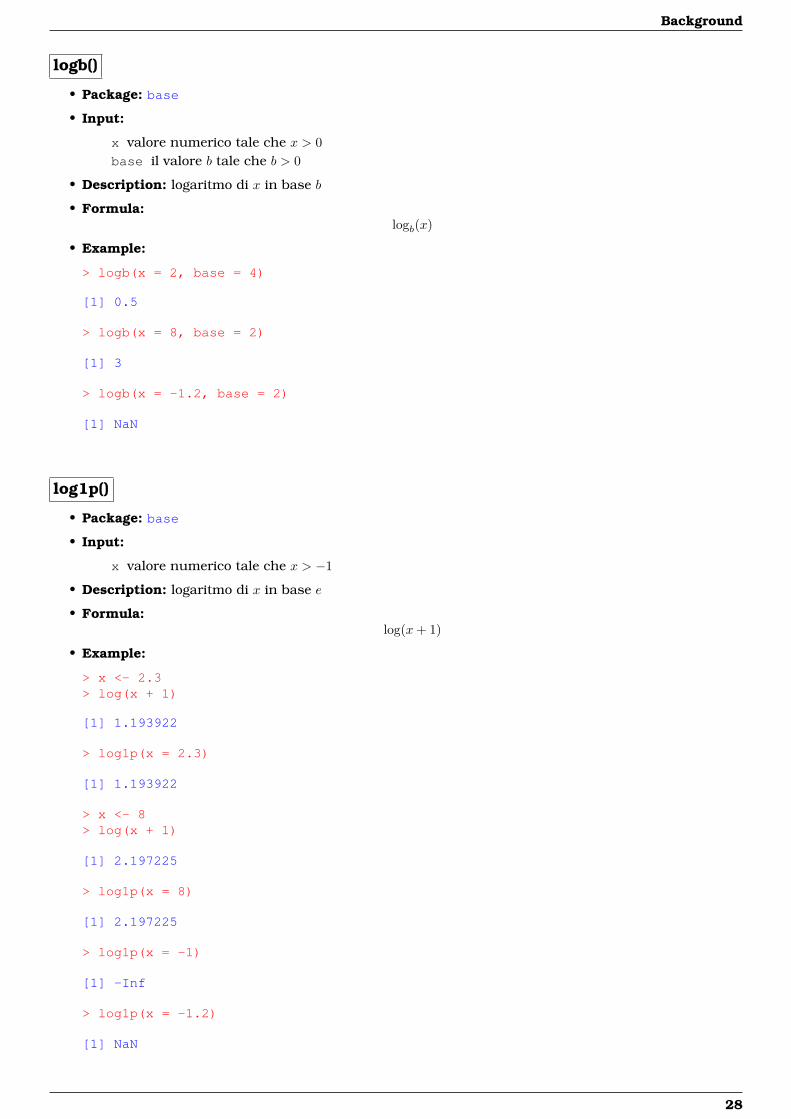
logb()
• Package: base
• Input:
x valore numerico tale che x > 0base il valore b tale che b > 0
• Description: logaritmo di x in base b
• Formula:logb(x)
• Example:
> logb(x = 2, base = 4)
[1] 0.5
> logb(x = 8, base = 2)
[1] 3
> logb(x = -1.2, base = 2)
[1] NaN
log1p()
• Package: base
• Input:
x valore numerico tale che x > −1
• Description: logaritmo di x in base e
• Formula:log(x+ 1)
• Example:
> x <- 2.3> log(x + 1)
[1] 1.193922
> log1p(x = 2.3)
[1] 1.193922
> x <- 8> log(x + 1)
[1] 2.197225
> log1p(x = 8)
[1] 2.197225
> log1p(x = -1)
[1] -Inf
> log1p(x = -1.2)
[1] NaN
28

1.13 Funzioni di successione
1.13 Funzioni di successione
:
• Package: base
• Description: successione con intervallo unitario
• Example:
> 1:10
[1] 1 2 3 4 5 6 7 8 9 10
> 1:10.2
[1] 1 2 3 4 5 6 7 8 9 10
> 1.1:10.2
[1] 1.1 2.1 3.1 4.1 5.1 6.1 7.1 8.1 9.1 10.1
> 1:5 + 1
[1] 2 3 4 5 6
> 1:(5 + 1)
[1] 1 2 3 4 5 6
rep()
• Package: base
• Input:
x vettore alfanumerico di dimensione n
times ogni elemento del vettore viene ripetuto lo stesso numero times di volte
length.out dimensione del vettore risultato
each ogni elemento del vettore viene ripetuto each volte
• Description: replicazioni
• Example:
> rep(x = 2, times = 5)
[1] 2 2 2 2 2
> rep(x = c(1, 2, 3), times = 5)
[1] 1 2 3 1 2 3 1 2 3 1 2 3 1 2 3
> rep(x = c(8.1, 6.7, 10.2), times = c(1, 2, 3))
[1] 8.1 6.7 6.7 10.2 10.2 10.2
> rep(x = c(1, 2, 3), each = 2)
[1] 1 1 2 2 3 3
29

Background
> rep(x = c(1, 2, 3), length.out = 7)
[1] 1 2 3 1 2 3 1
> rep(x = TRUE, times = 5)
[1] TRUE TRUE TRUE TRUE TRUE
> rep(x = c(1, 2, 3, 4), each = 3, times = 2)
[1] 1 1 1 2 2 2 3 3 3 4 4 4 1 1 1 2 2 2 3 3 3 4 4 4
• Note: Il parametro each ha precedenza sul parametro times.
rep.int()
• Package: base
• Input:
x vettore alfanumerico di dimensione n
times ogni elemento del vettore viene ripetuto lo stesso numero times di volte
• Description: replicazioni
• Example:
> rep.int(x = 2, times = 5)
[1] 2 2 2 2 2
> rep.int(x = c(1, 2, 3), times = 5)
[1] 1 2 3 1 2 3 1 2 3 1 2 3 1 2 3
> rep.int(x = c(1, 2, 3), times = c(1, 2, 3))
[1] 1 2 2 3 3 3
> rep.int(x = TRUE, times = 5)
[1] TRUE TRUE TRUE TRUE TRUE
30

1.13 Funzioni di successione
sequence()
• Package: base
• Input:
nvec vettore numerico x di valori naturali di dimensione n
• Description: serie di sequenze di interi dove ciascuna sequenza termina con i numeri naturali passaticome argomento
• Example:
> n1 <- 2> n2 <- 5> c(1:n1, 1:n2)
[1] 1 2 1 2 3 4 5
> sequence(nvec = c(2, 5))
[1] 1 2 1 2 3 4 5
> n1 <- 6> n2 <- 3> c(1:n1, 1:n2)
[1] 1 2 3 4 5 6 1 2 3
> sequence(nvec = c(6, 3))
[1] 1 2 3 4 5 6 1 2 3
seq()
• Package: base
• Input:
from punto di partenza
to punto di arrivo
by passo
length.out dimensione
along.with vettore di dimensione n per creare la sequenza di valori naturali 1, 2, . . . , n
• Description: successione
• Example:
> seq(from = 1, to = 3.4, by = 0.4)
[1] 1.0 1.4 1.8 2.2 2.6 3.0 3.4
> seq(from = 1, to = 3.4, length.out = 5)
[1] 1.0 1.6 2.2 2.8 3.4
> seq(from = 3.4, to = 1, length.out = 5)
[1] 3.4 2.8 2.2 1.6 1.0
31
Background
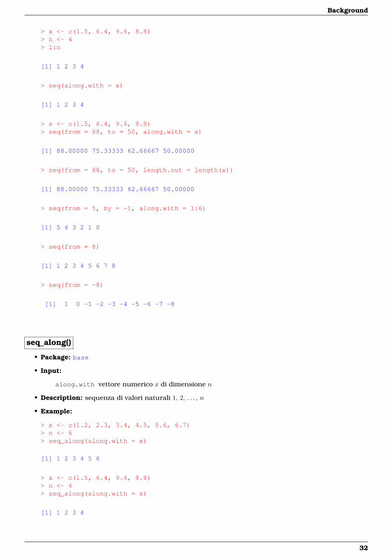
> x <- c(1.5, 6.4, 9.6, 8.8)> n <- 4> 1:n
[1] 1 2 3 4
> seq(along.with = x)
[1] 1 2 3 4
> x <- c(1.5, 6.4, 9.6, 8.8)> seq(from = 88, to = 50, along.with = x)
[1] 88.00000 75.33333 62.66667 50.00000
> seq(from = 88, to = 50, length.out = length(x))
[1] 88.00000 75.33333 62.66667 50.00000
> seq(from = 5, by = -1, along.with = 1:6)
[1] 5 4 3 2 1 0
> seq(from = 8)
[1] 1 2 3 4 5 6 7 8
> seq(from = -8)
[1] 1 0 -1 -2 -3 -4 -5 -6 -7 -8
seq_along()
• Package: base
• Input:
along.with vettore numerico x di dimensione n
• Description: sequenza di valori naturali 1, 2, . . . , n
• Example:
> x <- c(1.2, 2.3, 3.4, 4.5, 5.6, 6.7)> n <- 6> seq_along(along.with = x)
[1] 1 2 3 4 5 6
> x <- c(1.5, 6.4, 9.6, 8.8)> n <- 4> seq_along(along.with = x)
[1] 1 2 3 4
32
1.14 Funzioni di ordinamento
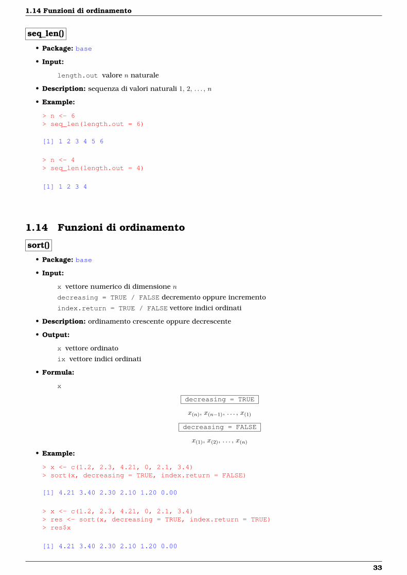
seq_len()
• Package: base
• Input:
length.out valore n naturale
• Description: sequenza di valori naturali 1, 2, . . . , n
• Example:
> n <- 6> seq_len(length.out = 6)
[1] 1 2 3 4 5 6
> n <- 4> seq_len(length.out = 4)
[1] 1 2 3 4
1.14 Funzioni di ordinamento
sort()
• Package: base
• Input:
x vettore numerico di dimensione n
decreasing = TRUE / FALSE decremento oppure incremento
index.return = TRUE / FALSE vettore indici ordinati
• Description: ordinamento crescente oppure decrescente
• Output:
x vettore ordinato
ix vettore indici ordinati
• Formula:
x
decreasing = TRUE
x(n), x(n−1), . . . , x(1)
decreasing = FALSE
x(1), x(2), . . . , x(n)
• Example:
> x <- c(1.2, 2.3, 4.21, 0, 2.1, 3.4)> sort(x, decreasing = TRUE, index.return = FALSE)
[1] 4.21 3.40 2.30 2.10 1.20 0.00
> x <- c(1.2, 2.3, 4.21, 0, 2.1, 3.4)> res <- sort(x, decreasing = TRUE, index.return = TRUE)> res$x
[1] 4.21 3.40 2.30 2.10 1.20 0.00
33
Background
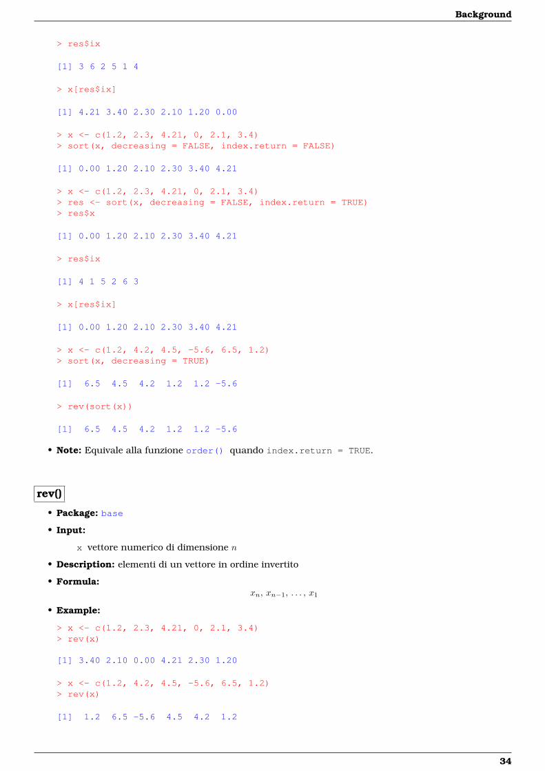
> res$ix
[1] 3 6 2 5 1 4
> x[res$ix]
[1] 4.21 3.40 2.30 2.10 1.20 0.00
> x <- c(1.2, 2.3, 4.21, 0, 2.1, 3.4)> sort(x, decreasing = FALSE, index.return = FALSE)
[1] 0.00 1.20 2.10 2.30 3.40 4.21
> x <- c(1.2, 2.3, 4.21, 0, 2.1, 3.4)> res <- sort(x, decreasing = FALSE, index.return = TRUE)> res$x
[1] 0.00 1.20 2.10 2.30 3.40 4.21
> res$ix
[1] 4 1 5 2 6 3
> x[res$ix]
[1] 0.00 1.20 2.10 2.30 3.40 4.21
> x <- c(1.2, 4.2, 4.5, -5.6, 6.5, 1.2)> sort(x, decreasing = TRUE)
[1] 6.5 4.5 4.2 1.2 1.2 -5.6
> rev(sort(x))
[1] 6.5 4.5 4.2 1.2 1.2 -5.6
• Note: Equivale alla funzione order() quando index.return = TRUE.
rev()
• Package: base
• Input:
x vettore numerico di dimensione n
• Description: elementi di un vettore in ordine invertito
• Formula:xn, xn−1, . . . , x1
• Example:
> x <- c(1.2, 2.3, 4.21, 0, 2.1, 3.4)> rev(x)
[1] 3.40 2.10 0.00 4.21 2.30 1.20
> x <- c(1.2, 4.2, 4.5, -5.6, 6.5, 1.2)> rev(x)
[1] 1.2 6.5 -5.6 4.5 4.2 1.2
34
1.14 Funzioni di ordinamento
order()
• Package: base
• Input:
x vettore numerico di dimensione ndecreasing = TRUE / FALSE decremento oppure incremento
• Description: restituisce la posizione di ogni elemento di x se questo fosse ordinato in maniera decre-scente oppure crescente
• Example:
> x <- c(1.2, 2.3, 4.21, 0, 2.1, 3.4)> order(x, decreasing = FALSE)
[1] 4 1 5 2 6 3
> x <- c(1.2, 2.3, 4.21, 0, 2.1, 3.4)> order(x, decreasing = TRUE)
[1] 3 6 2 5 1 4
> x <- c(1.6, 6.8, 7.7, 7.2, 5.4, 7.9, 8, 8, 3.4, 12)> sort(x, decreasing = FALSE)
[1] 1.6 3.4 5.4 6.8 7.2 7.7 7.9 8.0 8.0 12.0
> x[order(x, decreasing = FALSE)]
[1] 1.6 3.4 5.4 6.8 7.2 7.7 7.9 8.0 8.0 12.0
rank()
• Package: base
• Input:
x vettore numerico di dimensione nties.method = "average" / "first" / "random" / "max" / "min" metodo da utilizzare inpresenza di ties
• Description: rango di x ossia viene associato ad ogni elemento del vettore x il posto occupato nellostesso vettore ordinato in modo crescente
• Example:
> x <- c(1.2, 2.3, 4.5, 2.3, 4.5, 6.6, 1.2, 3.4)> rank(x, ties.method = "average")
[1] 1.5 3.5 6.5 3.5 6.5 8.0 1.5 5.0
> x <- c(1.2, 2.3, 4.21, 0, 2.1, 3.4)> rank(x, ties.method = "average")
[1] 2 4 6 1 3 5
> x <- c(1.2, 4.2, 4.5, -5.6, 6.5, 1.2)> rank(x, ties.method = "first")
[1] 2 4 5 1 6 3
• Note: Solo per ties.method = "average" e ties.method = "first" la somma del vettore finalerimane uguale a n (n+ 1) / 2.
35
Background
1.15 Funzioni di troncamento e di arrotondamento
trunc()
• Package: base
• Input:
x valore numerico
• Description: tronca la parte decimale
• Formula:[x ]
• Example:
> trunc(x = 2)
[1] 2
> trunc(x = 2.999)
[1] 2
> trunc(x = -2.01)
[1] -2
floor()
• Package: base
• Input:
x valore numerico
• Description: arrotonda all’intero inferiore
• Formula:
bxc =
x se x è intero[x ] se x è positivo non intero[x ] − 1 se x è negativo non intero
• Example:
> floor(x = 2)
[1] 2
> floor(x = 2.99)
[1] 2
> floor(x = -2.01)
[1] -3
36
1.15 Funzioni di troncamento e di arrotondamento
ceiling()
• Package: base
• Input:
x valore numerico
• Description: arrotonda all’intero superiore
• Formula:
dxe =
x se x è intero[x ] + 1 se x è positivo non intero[x ] se x è negativo non intero
• Example:
> ceiling(x = 2)
[1] 2
> ceiling(x = 2.001)
[1] 3
> ceiling(x = -2.01)
[1] -2
round()
• Package: base
• Input:
x valore numerico
digits valore naturale n
• Description: arrotonda al numero di cifre specificato da n
• Example:
> pi
[1] 3.141593
> round(x = pi, digits = 4)
[1] 3.1416
> exp(1)
[1] 2.718282
> round(x = exp(1), digits = 3)
[1] 2.718
37
Background
signif()
• Package: base
• Input:
x valore numerico
digits valore naturale n
• Description: arrotonda al numero di cifre significative specificate da n
• Example:
> pi
[1] 3.141593
> signif(x = pi, digits = 4)
[1] 3.142
> exp(1)
[1] 2.718282
> signif(x = exp(1), digits = 3)
[1] 2.72
fractions()
• Package: MASS
• Input:
x oggetto numerico
• Description: trasforma un valore decimale in frazionario
• Example:
> fractions(x = 2.3)
[1] 23/10
> fractions(x = 1.34)
[1] 67/50
> x <- matrix(data = c(1.2, 34, 4.3, 4.2), nrow = 2, ncol = 2,+ byrow = FALSE)> x
[,1] [,2][1,] 1.2 4.3[2,] 34.0 4.2
> fractions(x)
[,1] [,2][1,] 6/5 43/10[2,] 34 21/5
38
1.16 Funzioni avanzate
rational()
• Package: MASS
• Input:
x oggetto numerico
• Description: approssimazione razionale
• Example:
> matrice <- matrix(data = c(1.2, 34, 4.3, 4.2), nrow = 2, ncol = 2,+ byrow = FALSE)> matrice
[,1] [,2][1,] 1.2 4.3[2,] 34.0 4.2
> det(matrice)
[1] -141.16
> solve(matrice) %*% matrice
[,1] [,2][1,] 1.000000e+00 -2.303930e-17[2,] 2.428613e-17 1.000000e+00
> rational(x = solve(matrice) %*% matrice)
[,1] [,2][1,] 1 0[2,] 0 1
1.16 Funzioni avanzate
gamma()
• Package: base
• Input:
x valore numerico tale che x > 0
• Description: funzione gamma
• Formula:
Γ(x) =∫ +∞
0
ux−1 e−u du
• Example:
> gamma(x = 3.45)
[1] 3.146312
> gamma(x = 5)
[1] 24
39
Background
lgamma()
• Package: base
• Input:
x valore numerico tale che x > 0
• Description: logaritmo naturale della funzione gamma
• Formula:log (Γ(x))
• Example:
> log(gamma(x = 3.45))
[1] 1.146231
> lgamma(x = 3.45)
[1] 1.146231
> log(gamma(x = 5))
[1] 3.178054
> lgamma(x = 5)
[1] 3.178054
digamma()
• Package: base
• Input:
x valore numerico tale che x > 0
• Description: funzione digamma
• Formula:
Ψ(x) =d
dxlog (Γ(x))
• Example:
> digamma(x = 2.45)
[1] 0.6783387
> digamma(x = 5.3)
[1] 1.570411
40
1.16 Funzioni avanzate
trigamma()
• Package: base
• Input:
x valore numerico tale che x > 0
• Description: derivata prima della funzione digamma
• Formula:d
dxΨ(x)
• Example:
> trigamma(x = 2.45)
[1] 0.5024545
> trigamma(x = 5.3)
[1] 0.2075909
psigamma()
• Package: base
• Input:
x valore numerico tale che x > 0
deriv valore naturale n
• Description: derivata n-esima della funzione digamma
• Formula:dn
dxΨ(x)
• Example:
> psigamma(x = 2.45, deriv = 0)
[1] 0.6783387
> digamma(x = 2.45)
[1] 0.6783387
> psigamma(x = 5.3, deriv = 1)
[1] 0.2075909
> trigamma(x = 5.3)
[1] 0.2075909
41
Background
beta()
• Package: base
• Input:
a valore numerico tale che a > 0
b valore numerico tale che b > 0
• Description: funzione beta
• Formula:
B(a, b) =Γ(a) Γ(b)Γ(a+ b)
=∫ 1
0
ua−1 (1− u)b−1 du
• Example:
> a <- 3.45> b <- 2.3> gamma(a) * gamma(b)/gamma(a + b)
[1] 0.04659344
> beta(a = 3.45, b = 2.3)
[1] 0.04659344
> a <- 5> b <- 4> gamma(a) * gamma(b)/gamma(a + b)
[1] 0.003571429
> beta(a = 5, b = 4)
[1] 0.003571429
lbeta()
• Package: base
• Input:
a valore numerico tale che a > 0
b valore numerico tale che b > 0
• Description: logaritmo naturale della funzione beta
• Formula:log (B(a, b))
• Example:
> a <- 3.45> b <- 2.3> log(gamma(a) * gamma(b)/gamma(a + b))
[1] -3.066296
> lbeta(a = 3.45, b = 2.3)
[1] -3.066296
42
1.16 Funzioni avanzate
> a <- 5> b <- 4> log(gamma(a) * gamma(b)/gamma(a + b))
[1] -5.63479
> lbeta(a = 5, b = 4)
[1] -5.63479
fbeta()
• Package: MASS
• Input:
x valore numerico tale che x > 0 e x < 1
a valore numerico tale che a > 0
b valore numerico tale che b > 0
• Description: funzione beta
• Formula:xa−1 (1− x)b−1
• Example:
> x <- 0.67> a <- 3.45> b <- 2.3> x^(a - 1) * (1 - x)^(b - 1)
[1] 0.08870567
> fbeta(x = 0.67, a = 3.45, b = 2.3)
[1] 0.08870567
> x <- 0.12> a <- 5> b <- 4> x^(a - 1) * (1 - x)^(b - 1)
[1] 0.0001413100
> fbeta(x = 0.12, a = 5, b = 4)
[1] 0.0001413100
43
Background
sigmoid()
• Package: e1071
• Input:
x valore numerico
• Description: funzione sigmoide
• Formula:S(x) = (1 + e−x)−1 =
ex
1 + ex
• Example:
> x <- 3.45> (1 + exp(-x))^(-1)
[1] 0.9692311
> sigmoid(x = 3.45)
[1] 0.9692311
> x <- -1.7> (1 + exp(-x))^(-1)
[1] 0.1544653
> sigmoid(x = -1.7)
[1] 0.1544653
dsigmoid()
• Package: e1071
• Input:
x valore numerico
• Description: derivata prima della funzione sigmoide
• Formula:d
dxS(x) =
ex
(1 + ex)2=
ex
1 + ex
(1− ex
1 + ex
)= S(x) (1− S(x))
• Example:
> x <- 3.45> exp(x)/(1 + exp(x))^2
[1] 0.02982214
> dsigmoid(x = 3.45)
[1] 0.02982214
> x <- -1.7> exp(x)/(1 + exp(x))^2
[1] 0.1306057
> dsigmoid(x = -1.7)
[1] 0.1306057
44
1.16 Funzioni avanzate
d2sigmoid()
• Package: e1071
• Input:
x valore numerico
• Description: derivata seconda della funzione sigmoide
• Formula:
d2
dxS(x) =
ex (1− ex)(1 + ex)3
=ex
1 + ex
(1− ex
1 + ex
) (1
1 + ex− ex
1 + ex
)= S2(x) (1− S(x)) (e−x − 1)
• Example:
> x <- 3.45> (exp(x) * (1 - exp(x)))/(1 + exp(x))^3
[1] -0.02798695
> d2sigmoid(x = 3.45)
[1] -0.02798695
> x <- -1.7> (exp(x) * (1 - exp(x)))/(1 + exp(x))^3
[1] 0.09025764
> d2sigmoid(x = -1.7)
[1] 0.09025764
besselI()
• Package: base
• Input:
x valore numerico tale che x > 0
nu valore naturale
• Description: funzione BesselI
• Example:
> besselI(x = 2.3, nu = 3)
[1] 0.3492232
> besselI(x = 1.6, nu = 2)
[1] 0.3939673
45
Background
besselJ()
• Package: base
• Input:
x valore numerico tale che x > 0nu valore naturale
• Description: funzione BesselJ
• Example:
> besselJ(x = 2.3, nu = 3)
[1] 0.1799789
> besselJ(x = 1.6, nu = 2)
[1] 0.2569678
besselK()
• Package: base
• Input:
x valore numerico tale che x > 0nu valore naturale
• Description: funzione BesselK
• Example:
> besselK(x = 2.3, nu = 3)
[1] 0.3762579
> besselK(x = 1.6, nu = 2)
[1] 0.4887471
besselY()
• Package: base
• Input:
x valore numerico tale che x > 0nu valore naturale
• Description: funzione BesselY
• Example:
> besselY(x = 2.3, nu = 3)
[1] -0.8742197
> besselY(x = 1.6, nu = 2)
[1] -0.8548994
46
1.17 Funzioni sui numeri complessi
1.17 Funzioni sui numeri complessi
complex()
• Package: base
• Input:
real parte reale αimaginary parte immaginaria β
modulus modulo rargument argomento φ
• Description: numero complesso
• Formula:
α+ i β = r (cos(φ) + i sin(φ))
α = r cos(φ)
β = r sin(φ)
r =√α2 + β2
φ = arctan(β
α
)• Example:
> complex(real = 1, imaginary = 3)
[1] 1+3i
> complex(modulus = Mod(1 + 3i), argument = Arg(1 + 3i))
[1] 1+3i
> complex(real = -3, imaginary = 4)
[1] -3+4i
> complex(modulus = Mod(-3 + 4i), argument = Arg(-3 + 4i))
[1] -3+4i
Re()
• Package: base
• Input:
x numero complesso
• Description: parte reale
• Formula:α
• Example:
> Re(x = 2 + 3i)
[1] 2
> Re(x = -3 + 4i)
[1] -3
47
Background
Im()
• Package: base
• Input:
x numero complesso
• Description: parte immaginaria
• Formula:β
• Example:
> Im(x = -2 + 3i)
[1] 3
> Im(x = 3 - 4i)
[1] -4
Mod()
• Package: base
• Input:
x numero complesso
• Description: modulo
• Formula:r =
√α2 + β2
• Example:
> x <- 2 + 3i> sqrt(2^2 + 3^2)
[1] 3.605551
> Mod(x = 2 + 3i)
[1] 3.605551
> x <- -3 + 4i> sqrt((-3)^2 + 4^2)
[1] 5
> Mod(x = -3 + 4i)
[1] 5
> x <- 3 + 4i> sqrt(3^2 + 4^2)
[1] 5
> Mod(x = 3 + 4i)
48
1.17 Funzioni sui numeri complessi
[1] 5
> abs(x = 3 + 4i)
[1] 5
• Note: Equivale alla funzione abs().
Arg()
• Package: base
• Input:
x numero complesso
• Description: argomento
• Formula:
φ = arctan(β
α
)• Example:
> x <- 2 + 3i> atan(3/2)
[1] 0.9827937
> Arg(x = 2 + 3i)
[1] 0.9827937
> x <- 4 + 5i> atan(5/4)
[1] 0.8960554
> Arg(x = 4 + 5i)
[1] 0.8960554
Conj()
• Package: base
• Input:
x numero complesso
• Description: coniugato
• Formula:α− i β
• Example:
> Conj(x = 2 + 3i)
[1] 2-3i
> Conj(x = -3 + 4i)
[1] -3-4i
49
Background
is.real()
• Package: base
• Input:
x valore numerico
• Description: segnalazione di valore numerico reale
• Example:
> is.real(x = 2 + 3i)
[1] FALSE
> is.real(x = 4)
[1] TRUE
is.complex()
• Package: base
• Input:
x valore numerico
• Description: segnalazione di valore numerico complesso
• Example:
> is.complex(x = 2 + 3i)
[1] TRUE
> is.complex(x = 4)
[1] FALSE
1.18 Funzioni cumulate
cumsum()
• Package: base
• Input:
x vettore numerico di dimensione n
• Description: somma cumulata
• Formula:i∑
j=1
xj ∀ i = 1, 2, . . . , n
• Example:
> x <- c(1, 2, 4, 3, 5, 6)> cumsum(x)
[1] 1 3 7 10 15 21
50
1.18 Funzioni cumulate
> x <- c(1, 2.3, 4.5, 6.7, 2.1)> cumsum(x)
[1] 1.0 3.3 7.8 14.5 16.6
cumprod()
• Package: base
• Input:
x vettore numerico di dimensione n
• Description: prodotto cumulato
• Formula:i∏
j=1
xj ∀ i = 1, 2, . . . , n
• Example:
> x <- c(1, 2, 4, 3, 5, 6)> cumprod(x)
[1] 1 2 8 24 120 720
> x <- c(1, 2.3, 4.5, 6.7, 2.1)> cumprod(x)
[1] 1.0000 2.3000 10.3500 69.3450 145.6245
cummin()
• Package: base
• Input:
x vettore numerico di dimensione n
• Description: minimo cumulato
• Formula:min(x1, x2, . . . , xi) ∀ i = 1, 2, . . . , n
• Example:
> x <- c(3, 4, 3, 2, 4, 1)> cummin(x)
[1] 3 3 3 2 2 1
> x <- c(1, 3, 2, 4, 5, 1)> cummin(x)
[1] 1 1 1 1 1 1
51
Background
cummax()
• Package: base
• Input:
x vettore numerico di dimensione n
• Description: massimo cumulato
• Formula:max(x1, x2, . . . , xi) ∀ i = 1, 2, . . . , n
• Example:
> x <- c(1, 3, 2, 4, 5, 1)> cummax(x)
[1] 1 3 3 4 5 5
> x <- c(1, 3, 2, 4, 5, 1)> cummax(x)
[1] 1 3 3 4 5 5
1.19 Funzioni in parallelo
pmin()
• Package: base
• Input:
x vettore numerico di dimensione n
y vettore numerico di dimensione n
• Description: minimo in parallelo
• Formula:min(xi, yi) ∀ i = 1, 2, . . . , n
• Example:
> x <- c(1.2, 2.3, 0.11, 4.5)> y <- c(1.1, 2.1, 1.3, 4.4)> pmin(x, y)
[1] 1.10 2.10 0.11 4.40
> x <- c(1.2, 2.3, 0.11, 4.5)> y <- c(1.1, 2.1, 1.1, 2.1)> pmin(x, y)
[1] 1.10 2.10 0.11 2.10
52
1.20 Funzioni di analisi numerica
pmax()
• Package: base
• Input:
x vettore numerico di dimensione n
y vettore numerico di dimensione n
• Description: massimo in parallelo
• Formula:max(xi, yi) ∀ i = 1, 2, . . . , n
• Example:
> x <- c(1.2, 2.3, 0.11, 4.5)> y <- c(1.1, 2.1, 1.3, 4.4)> pmax(x, y)
[1] 1.2 2.3 1.3 4.5
> x <- c(1.2, 2.3, 0.11, 4.5)> y <- c(1.1, 2.1, 1.1, 2.1)> pmax(x, y)
[1] 1.2 2.3 1.1 4.5
1.20 Funzioni di analisi numerica
optimize()
• Package: stats
• Input:
f funzione f(x)
lower estremo inferiore
upper estremo superiore
maximum = TRUE / FALSE massimo oppure minimo
tol tolleranza
• Description: ricerca di un massimo oppure di un minimo
• Output:
minimum punto di minimo
maximum punto di massimo
objective valore assunto dalla funzione nel punto individuato
• Formula:
maximum = TRUE
maxx
f(x)
maximum = FALSE
minx
f(x)
• Example:
53
Background
> f <- function(x) x * exp(-x^3) - (log(x))^2> optimize(f, lower = 0.3, upper = 1.5, maximum = TRUE, tol = 1e-04)
$maximum[1] 0.8374697
$objective[1] 0.4339975
> f <- function(x) (x - 0.1)^2> optimize(f, lower = 0, upper = 1, maximum = FALSE, tol = 1e-04)
$minimum[1] 0.1
$objective[1] 7.70372e-34
> f <- function(x) dchisq(x, df = 8)> optimize(f, lower = 0, upper = 10, maximum = TRUE, tol = 1e-04)
$maximum[1] 5.999999
$objective[1] 0.1120209
optim()
• Package: stats
• Input:
par valore di partenza
fn funzione f(x)
method = "Nelder-Mead" / "BFGS" / "CG" / "L-BFGS-B" / "SANN" metodo di ottimizzazio-ne
• Description: ottimizzazione
• Output:
par punto di ottimo
value valore assunto dalla funzione nel punto individuato
• Example:
> f <- function(x) x * exp(-x^3) - (log(x))^2> optim(par = 1, fn = f, method = "BFGS")$par
[1] 20804.91
> optim(par = 1, fn = f, method = "BFGS")$value
[1] -98.86214
> f <- function(x) (x - 0.1)^2> optim(par = 1, fn = f, method = "BFGS")$par
[1] 0.1
54
1.20 Funzioni di analisi numerica
> optim(par = 1, fn = f, method = "BFGS")$value
[1] 7.70372e-34
> f <- function(x) dchisq(x, df = 8)> optim(par = 1, fn = f, method = "BFGS")$par
[1] 0.0003649698
> optim(par = 1, fn = f, method = "BFGS")$value
[1] 5.063142e-13
> nLL <- function(mu, x) {+ z <- mu * x+ lz <- log(z)+ L1 <- sum(lz)+ L2 <- mu/2+ LL <- -(L1 - L2)+ LL+ }> x <- c(1.2, 3.4, 5.6, 6.1, 7.8, 8.6, 10.7, 12, 13.7, 14.7)> optim(par = 10000, fn = nLL, method = "CG", x = x)$par
[1] 9950.6
> optim(par = 10000, fn = nLL, method = "CG", x = x)$value
[1] 4863.693
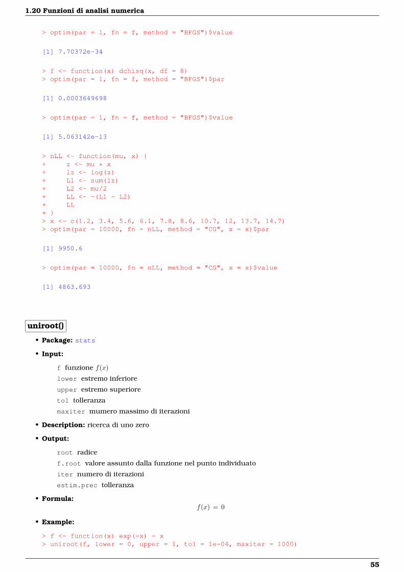
uniroot()
• Package: stats
• Input:
f funzione f(x)
lower estremo inferiore
upper estremo superiore
tol tolleranza
maxiter mumero massimo di iterazioni
• Description: ricerca di uno zero
• Output:
root radice
f.root valore assunto dalla funzione nel punto individuato
iter numero di iterazioni
estim.prec tolleranza
• Formula:f(x) = 0
• Example:
> f <- function(x) exp(-x) - x> uniroot(f, lower = 0, upper = 1, tol = 1e-04, maxiter = 1000)
55
Background
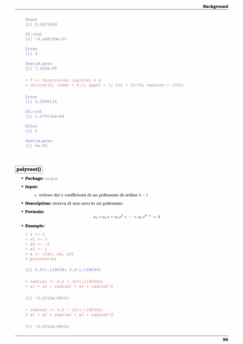
$root[1] 0.5671439
$f.root[1] -9.448109e-07
$iter[1] 3
$estim.prec[1] 7.425e-05
> f <- function(x) log10(x) + x> uniroot(f, lower = 0.1, upper = 1, tol = 1e-04, maxiter = 1000)
$root[1] 0.3990136
$f.root[1] 1.279136e-06
$iter[1] 5
$estim.prec[1] 5e-05
polyroot()
• Package: stats
• Input:
a vettore dei k coefficienti di un polinomio di ordine k − 1
• Description: ricerca di uno zero in un polinomio
• Formula:a1 + a2 x+ a3 x
2 + · · ·+ ak xk−1 = 0
• Example:
> k <- 3> a1 <- 3> a2 <- -2> a3 <- 2> a <- c(a1, a2, a3)> polyroot(a)
[1] 0.5+1.118034i 0.5-1.118034i
> radice1 <- 0.5 + (0+1.118034i)> a1 + a2 * radice1 + a3 * radice1^2
[1] -5.0312e-08+0i
> radice2 <- 0.5 - (0+1.118034i)> a1 + a2 * radice2 + a3 * radice2^2
[1] -5.0312e-08+0i
56

1.20 Funzioni di analisi numerica
> k <- 4> a1 <- 3> a2 <- -2> a3 <- 2> a4 <- -1> a <- c(a1, a2, a3, a4)> polyroot(a)
[1] 0.094732+1.283742i 0.094732-1.283742i 1.810536+0.000000i
> radice1 <- 0.09473214 + (0+1.283742i)> a1 + a2 * radice1 + a3 * radice1^2 + a4 * radice1^3
[1] 7.477461e-07-5.808714e-07i
> radice2 <- 0.09473214 - (0+1.283742i)> a1 + a2 * radice2 + a3 * radice2^2 + a4 * radice2^3
[1] 7.477461e-07+5.808714e-07i
> radice3 <- 1.81053571 + (0+0i)> a1 + a2 * radice3 + a3 * radice3^2 + a4 * radice3^3
[1] 1.729401e-08+0i
D()
• Package: stats
• Input:
expr espressione contenente la funzione f(x) da derivare
name variabile x di derivazione
• Description: derivata simbolica al primo ordine
• Formula:d
dxf(x)
• Example:
> D(expr = expression(exp(-x) - x), name = "x")
-(exp(-x) + 1)
> D(expr = expression(x * exp(-a)), name = "x")
exp(-a)
57
Background
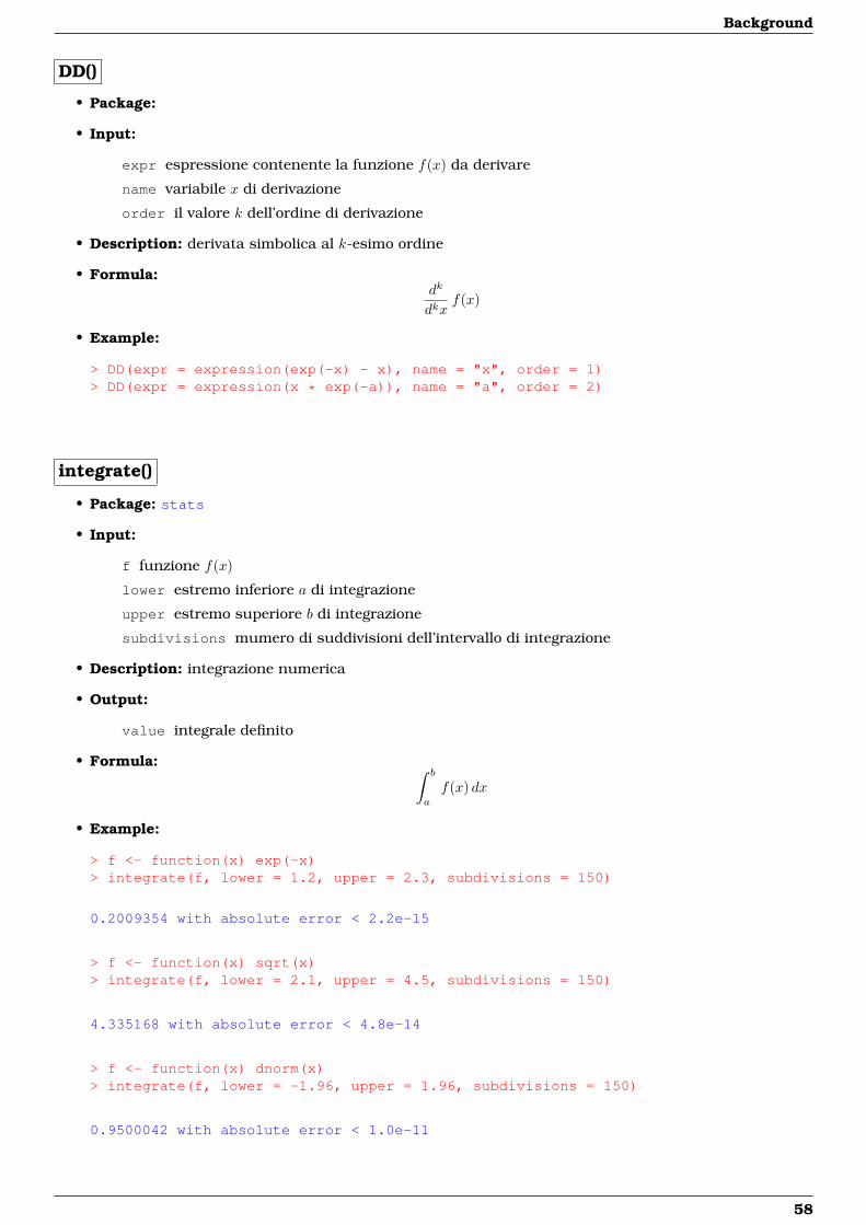
DD()
• Package:
• Input:
expr espressione contenente la funzione f(x) da derivare
name variabile x di derivazione
order il valore k dell’ordine di derivazione
• Description: derivata simbolica al k-esimo ordine
• Formula:dk
dkxf(x)
• Example:
> DD(expr = expression(exp(-x) - x), name = "x", order = 1)> DD(expr = expression(x * exp(-a)), name = "a", order = 2)
integrate()
• Package: stats
• Input:
f funzione f(x)
lower estremo inferiore a di integrazione
upper estremo superiore b di integrazione
subdivisions mumero di suddivisioni dell’intervallo di integrazione
• Description: integrazione numerica
• Output:
value integrale definito
• Formula: ∫ b
a
f(x) dx
• Example:
> f <- function(x) exp(-x)> integrate(f, lower = 1.2, upper = 2.3, subdivisions = 150)
0.2009354 with absolute error < 2.2e-15
> f <- function(x) sqrt(x)> integrate(f, lower = 2.1, upper = 4.5, subdivisions = 150)
4.335168 with absolute error < 4.8e-14
> f <- function(x) dnorm(x)> integrate(f, lower = -1.96, upper = 1.96, subdivisions = 150)
0.9500042 with absolute error < 1.0e-11
58

1.21 Costanti
1.21 Costanti
pi
• Package: base
• Description: pi greco
• Formula:π
• Example:
> pi
[1] 3.141593
> 2 * pi
[1] 6.283185
Inf
• Package:
• Description: infinito
• Formula:±∞
• Example:
> 2/0
[1] Inf
> -2/0
[1] -Inf
> 0^Inf
[1] 0
> exp(-Inf)
[1] 0
> 0/Inf
[1] 0
> Inf - Inf
[1] NaN
> Inf/Inf
[1] NaN
> exp(Inf)
[1] Inf
59
Background
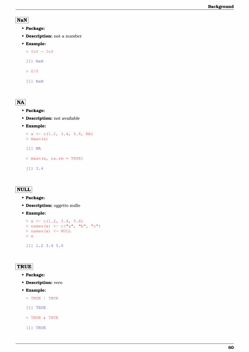
NaN
• Package:
• Description: not a number
• Example:
> Inf - Inf
[1] NaN
> 0/0
[1] NaN
NA
• Package:
• Description: not available
• Example:
> x <- c(1.2, 3.4, 5.6, NA)> mean(x)
[1] NA
> mean(x, na.rm = TRUE)
[1] 3.4
NULL
• Package:
• Description: oggetto nullo
• Example:
> x <- c(1.2, 3.4, 5.6)> names(x) <- c("a", "b", "c")> names(x) <- NULL> x
[1] 1.2 3.4 5.6
TRUE
• Package:
• Description: vero
• Example:
> TRUE | TRUE
[1] TRUE
> TRUE & TRUE
[1] TRUE
60

1.21 Costanti
T
• Package: base
• Description: vero
• Example:
> T
[1] TRUE
> T & T
[1] TRUE
FALSE
• Package:
• Description: falso
• Example:
> FALSE | TRUE
[1] TRUE
> FALSE & TRUE
[1] FALSE
F
• Package: base
• Description: falso
• Example:
> F
[1] FALSE
> F | T
[1] TRUE
61

Background
1.22 Miscellaneous
list()
• Package: base
• Description: creazione di un oggetto lista
• Example:
> x <- c(7.8, 6.6, 6.5, 7.4, 7.3, 7, 6.4, 7.1)> y <- c(4.5, 5.4, 6.1, 6.1, 5.4)> lista <- list(x = x, y = y)> lista
$x[1] 7.8 6.6 6.5 7.4 7.3 7.0 6.4 7.1
$y[1] 4.5 5.4 6.1 6.1 5.4
> lista[1]
$x[1] 7.8 6.6 6.5 7.4 7.3 7.0 6.4 7.1
> lista$x
[1] 7.8 6.6 6.5 7.4 7.3 7.0 6.4 7.1
> lista[[1]]
[1] 7.8 6.6 6.5 7.4 7.3 7.0 6.4 7.1
> lista[[1]][1]
[1] 7.8
> lista[2]
$y[1] 4.5 5.4 6.1 6.1 5.4
> lista$y
[1] 4.5 5.4 6.1 6.1 5.4
> lista[[2]]
[1] 4.5 5.4 6.1 6.1 5.4
> lista[[2]][1]
[1] 4.5
> x <- c(1, 2.3, 4.5, 6.7, 8.9)> y <- c(154, 109, 137, 115, 140)> z <- c(108, 115, 126, 92, 146)> lista <- list(x = x, y = y, z = z)> lista
62

1.22 Miscellaneous
$x[1] 1.0 2.3 4.5 6.7 8.9
$y[1] 154 109 137 115 140
$z[1] 108 115 126 92 146
> lista[1]
$x[1] 1.0 2.3 4.5 6.7 8.9
> lista$x
[1] 1.0 2.3 4.5 6.7 8.9
> lista[[1]]
[1] 1.0 2.3 4.5 6.7 8.9
> lista[[1]][1]
[1] 1
> lista[2]
$y[1] 154 109 137 115 140
> lista$y
[1] 154 109 137 115 140
> lista[[2]]
[1] 154 109 137 115 140
> lista[[2]][1]
[1] 154
> lista[3]
$z[1] 108 115 126 92 146
> lista$z
[1] 108 115 126 92 146
> lista[[3]]
[1] 108 115 126 92 146
> lista[[3]][1]
63
Background
[1] 108
> x <- c(1, 2, 3)> y <- c(11, 12, 13, 14, 15)> lista <- list(x, y)> lista
[[1]][1] 1 2 3
[[2]][1] 11 12 13 14 15
> names(lista)
NULL
> x <- c(1, 2, 3)> y <- c(11, 12, 13, 14, 15)> lista <- list(A = x, B = y)> lista
$A[1] 1 2 3
$B[1] 11 12 13 14 15
> names(lista)
[1] "A" "B"
lapply()
• Package: base
• Input:
x oggetto lista
FUN funzione
• Description: applica la funzione FUN ad ogni elemento di lista
• Example:
> vec1 <- c(7.8, 6.6, 6.5, 7.4, 7.3, 7, 6.4, 7.1)> mean(vec1)
[1] 7.0125
> vec2 <- c(4.5, 5.4, 6.1, 6.1, 5.4)> mean(vec2)
[1] 5.5
> x <- list(vec1 = vec1, vec2 = vec2)> lapply(x, FUN = mean)
64
1.22 Miscellaneous
$vec1[1] 7.0125
$vec2[1] 5.5
> vec1 <- c(1, 2.3, 4.5, 6.7, 8.9)> sd(vec1)
[1] 3.206556
> vec2 <- c(154, 109, 137, 115, 140)> sd(vec2)
[1] 18.61451
> vec3 <- c(108, 115, 126, 92, 146)> sd(vec3)
[1] 20.19406
> x <- list(vec1 = vec1, vec2 = vec2, vec3 = vec3)> lapply(x, FUN = sd)
$vec1[1] 3.206556
$vec2[1] 18.61451
$vec3[1] 20.19406
.Last.value
• Package: base
• Description: ultimo valore calcolato
• Example:
> 2 + 4
[1] 6
> .Last.value
[1] "stats" "graphics" "grDevices" "utils" "datasets" "methods"[7] "base"
> 3 * 4^4.2
[1] 1013.382
> .Last.value
[1] "stats" "graphics" "grDevices" "utils" "datasets" "methods"[7] "base"
65
Background
identical()
• Package: base
• Description: uguaglianza tra due oggetti
• Example:
> u <- c(1, 2, 3)> v <- c(1, 2, 4)> if (identical(u, v)) print("uguali") else print("non uguali")
[1] "non uguali"
> u <- c(1, 2, 3)> v <- c(1, 3, 2)> identical(u, v)
[1] FALSE
any()
• Package: base
• Input:
x vettore numerico di dimensione n
• Description: restituisce TRUE se almeno un elemento del vettore soddisfa ad una condizione fissata
• Example:
> x <- c(3, 4, 3, 2, 4, 1)> x < 2
[1] FALSE FALSE FALSE FALSE FALSE TRUE
> any(x < 2)
[1] TRUE
> x <- c(1, 2, 3, 4, 5, 6, 7, 8)> x > 4
[1] FALSE FALSE FALSE FALSE TRUE TRUE TRUE TRUE
> any(x > 4)
[1] TRUE
66
1.22 Miscellaneous
all()
• Package: base
• Input:
x vettore numerico di dimensione n
• Description: restituisce TRUE se tutti gli elementi del vettore soddisfano ad una condizione fissata
• Example:
> x <- c(3, 4, 3, 2, 4, 1)> x < 2
[1] FALSE FALSE FALSE FALSE FALSE TRUE
> all(x < 2)
[1] FALSE
> x <- c(1, 2, 3, 4, 5, 6, 7, 8)> x > 4
[1] FALSE FALSE FALSE FALSE TRUE TRUE TRUE TRUE
> all(x > 4)
[1] FALSE
match()
• Package: base
• Input:
x vettore numerico di dimensione n
table vettore numerico y di dimensione m
nomatch alternativa da inserire al posto di NA
• Description: per ogni elemento di x restituisce la posizione della prima occorrenza in y
• Example:
> x <- c(1, 1, 1, 2, 2, 2, 3, 3, 3, 4, 4, 4, 5, 5, 5)> match(x, table = c(2, 4), nomatch = 0)
[1] 0 0 0 1 1 1 0 0 0 2 2 2 0 0 0
> x <- c(1, 1, 1, 2, 2, 2, 3, 3, 3, 4, 4, 4, 5, 5, 5)> match(x, table = c(2, 4), nomatch = NA)
[1] NA NA NA 1 1 1 NA NA NA 2 2 2 NA NA NA
> match(x = c(-3, 3), table = c(5, 33, 3, 6, -3, -4, 3, 5, -3),+ nomatch = NA)
[1] 5 3
67
Background
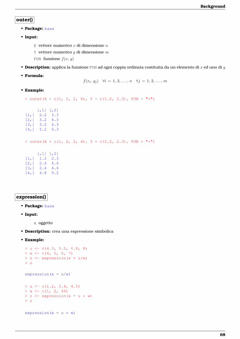
outer()
• Package: base
• Input:
X vettore numerico x di dimensione n
Y vettore numerico y di dimensione m
FUN funzione f(x, y)
• Description: applica la funzione FUN ad ogni coppia ordinata costituita da un elemento di x ed uno di y
• Formula:f(xi, yj) ∀i = 1, 2, . . . , n ∀j = 1, 2, . . . , m
• Example:
> outer(X = c(1, 2, 2, 4), Y = c(1.2, 2.3), FUN = "+")
[,1] [,2][1,] 2.2 3.3[2,] 3.2 4.3[3,] 3.2 4.3[4,] 5.2 6.3
> outer(X = c(1, 2, 2, 4), Y = c(1.2, 2.3), FUN = "*")
[,1] [,2][1,] 1.2 2.3[2,] 2.4 4.6[3,] 2.4 4.6[4,] 4.8 9.2
expression()
• Package: base
• Input:
x oggetto
• Description: crea una espressione simbolica
• Example:
> u <- c(4.3, 5.5, 6.8, 8)> w <- c(4, 5, 6, 7)> z <- expression(x = u/w)> z
expression(x = u/w)
> u <- c(1.2, 3.4, 4.5)> w <- c(1, 2, 44)> z <- expression(x = u * w)> z
expression(x = u * w)
68
1.22 Miscellaneous
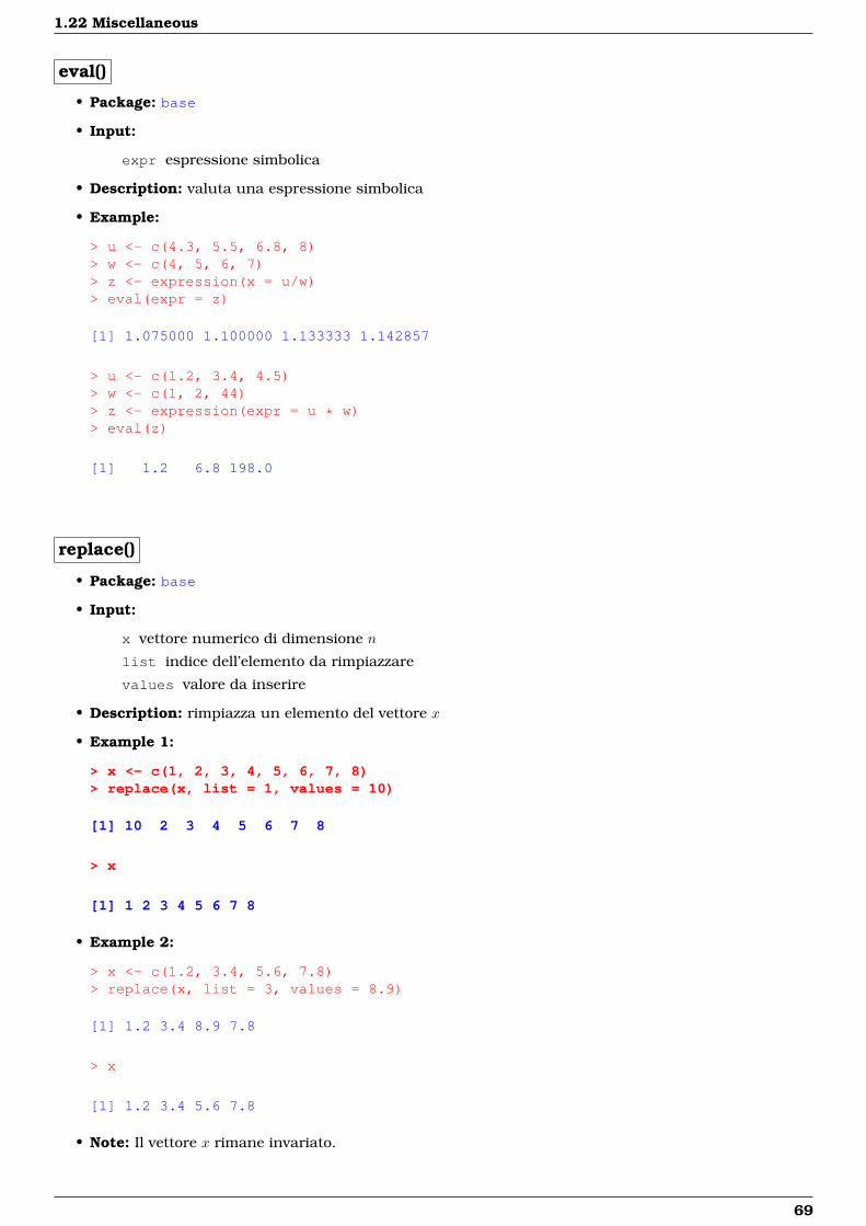
eval()
• Package: base
• Input:
expr espressione simbolica
• Description: valuta una espressione simbolica
• Example:
> u <- c(4.3, 5.5, 6.8, 8)> w <- c(4, 5, 6, 7)> z <- expression(x = u/w)> eval(expr = z)
[1] 1.075000 1.100000 1.133333 1.142857
> u <- c(1.2, 3.4, 4.5)> w <- c(1, 2, 44)> z <- expression(expr = u * w)> eval(z)
[1] 1.2 6.8 198.0
replace()
• Package: base
• Input:
x vettore numerico di dimensione n
list indice dell’elemento da rimpiazzare
values valore da inserire
• Description: rimpiazza un elemento del vettore x
• Example 1:
> x <- c(1, 2, 3, 4, 5, 6, 7, 8)> replace(x, list = 1, values = 10)
[1] 10 2 3 4 5 6 7 8
> x
[1] 1 2 3 4 5 6 7 8
• Example 2:
> x <- c(1.2, 3.4, 5.6, 7.8)> replace(x, list = 3, values = 8.9)
[1] 1.2 3.4 8.9 7.8
> x
[1] 1.2 3.4 5.6 7.8
• Note: Il vettore x rimane invariato.
69
Background
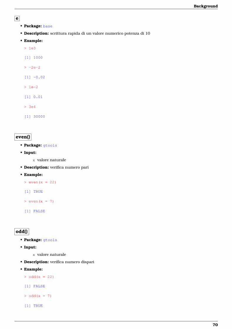
e
• Package: base
• Description: scrittura rapida di un valore numerico potenza di 10
• Example:
> 1e3
[1] 1000
> -2e-2
[1] -0.02
> 1e-2
[1] 0.01
> 3e4
[1] 30000
even()
• Package: gtools
• Input:
x valore naturale
• Description: verifica numero pari
• Example:
> even(x = 22)
[1] TRUE
> even(x = 7)
[1] FALSE
odd()
• Package: gtools
• Input:
x valore naturale
• Description: verifica numero dispari
• Example:
> odd(x = 22)
[1] FALSE
> odd(x = 7)
[1] TRUE
70
1.22 Miscellaneous
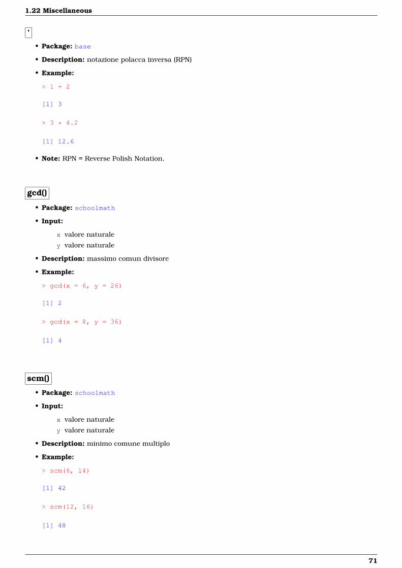
’
• Package: base
• Description: notazione polacca inversa (RPN)
• Example:
> 1 + 2
[1] 3
> 3 * 4.2
[1] 12.6
• Note: RPN = Reverse Polish Notation.
gcd()
• Package: schoolmath
• Input:
x valore naturale
y valore naturale
• Description: massimo comun divisore
• Example:
> gcd(x = 6, y = 26)
[1] 2
> gcd(x = 8, y = 36)
[1] 4
scm()
• Package: schoolmath
• Input:
x valore naturale
y valore naturale
• Description: minimo comune multiplo
• Example:
> scm(6, 14)
[1] 42
> scm(12, 16)
[1] 48
71
Background
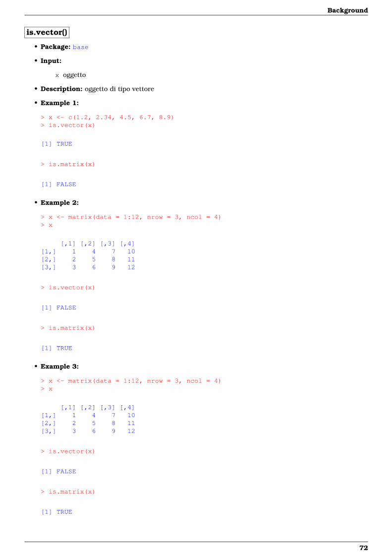
is.vector()
• Package: base
• Input:
x oggetto
• Description: oggetto di tipo vettore
• Example 1:
> x <- c(1.2, 2.34, 4.5, 6.7, 8.9)> is.vector(x)
[1] TRUE
> is.matrix(x)
[1] FALSE
• Example 2:
> x <- matrix(data = 1:12, nrow = 3, ncol = 4)> x
[,1] [,2] [,3] [,4][1,] 1 4 7 10[2,] 2 5 8 11[3,] 3 6 9 12
> is.vector(x)
[1] FALSE
> is.matrix(x)
[1] TRUE
• Example 3:
> x <- matrix(data = 1:12, nrow = 3, ncol = 4)> x
[,1] [,2] [,3] [,4][1,] 1 4 7 10[2,] 2 5 8 11[3,] 3 6 9 12
> is.vector(x)
[1] FALSE
> is.matrix(x)
[1] TRUE
72
1.22 Miscellaneous
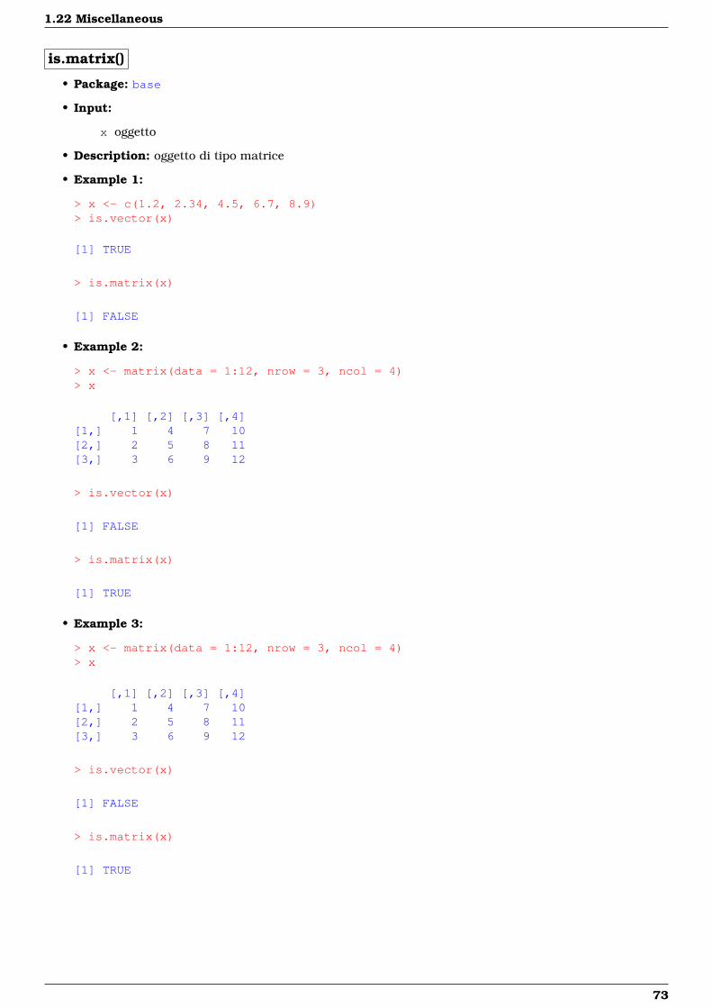
is.matrix()
• Package: base
• Input:
x oggetto
• Description: oggetto di tipo matrice
• Example 1:
> x <- c(1.2, 2.34, 4.5, 6.7, 8.9)> is.vector(x)
[1] TRUE
> is.matrix(x)
[1] FALSE
• Example 2:
> x <- matrix(data = 1:12, nrow = 3, ncol = 4)> x
[,1] [,2] [,3] [,4][1,] 1 4 7 10[2,] 2 5 8 11[3,] 3 6 9 12
> is.vector(x)
[1] FALSE
> is.matrix(x)
[1] TRUE
• Example 3:
> x <- matrix(data = 1:12, nrow = 3, ncol = 4)> x
[,1] [,2] [,3] [,4][1,] 1 4 7 10[2,] 2 5 8 11[3,] 3 6 9 12
> is.vector(x)
[1] FALSE
> is.matrix(x)
[1] TRUE
73


Capitolo 2
Vettori, Matrici ed Arrays
2.1 Creazione di Vettori
c()
• Package: base
• Input:
... oggetti da concatenare
recursive = TRUE / FALSE concatenazione per oggetti di tipo list()
• Description: funzione di concatenazione
• Example:
> x <- c(1.2, 3.4, 5.6, 7.8)> x
[1] 1.2 3.4 5.6 7.8
> x <- c(x, 9.9)> x
[1] 1.2 3.4 5.6 7.8 9.9
> x <- c(1.2, 3.4, 5.6, 7.8)> x
[1] 1.2 3.4 5.6 7.8
> x[5] <- 9.9> x
[1] 1.2 3.4 5.6 7.8 9.9
> x <- c("a", "b")> x
[1] "a" "b"
> x <- c("a", "b")> x
[1] "a" "b"
> x <- c("a", "b", "a", "a", "b")> x
75
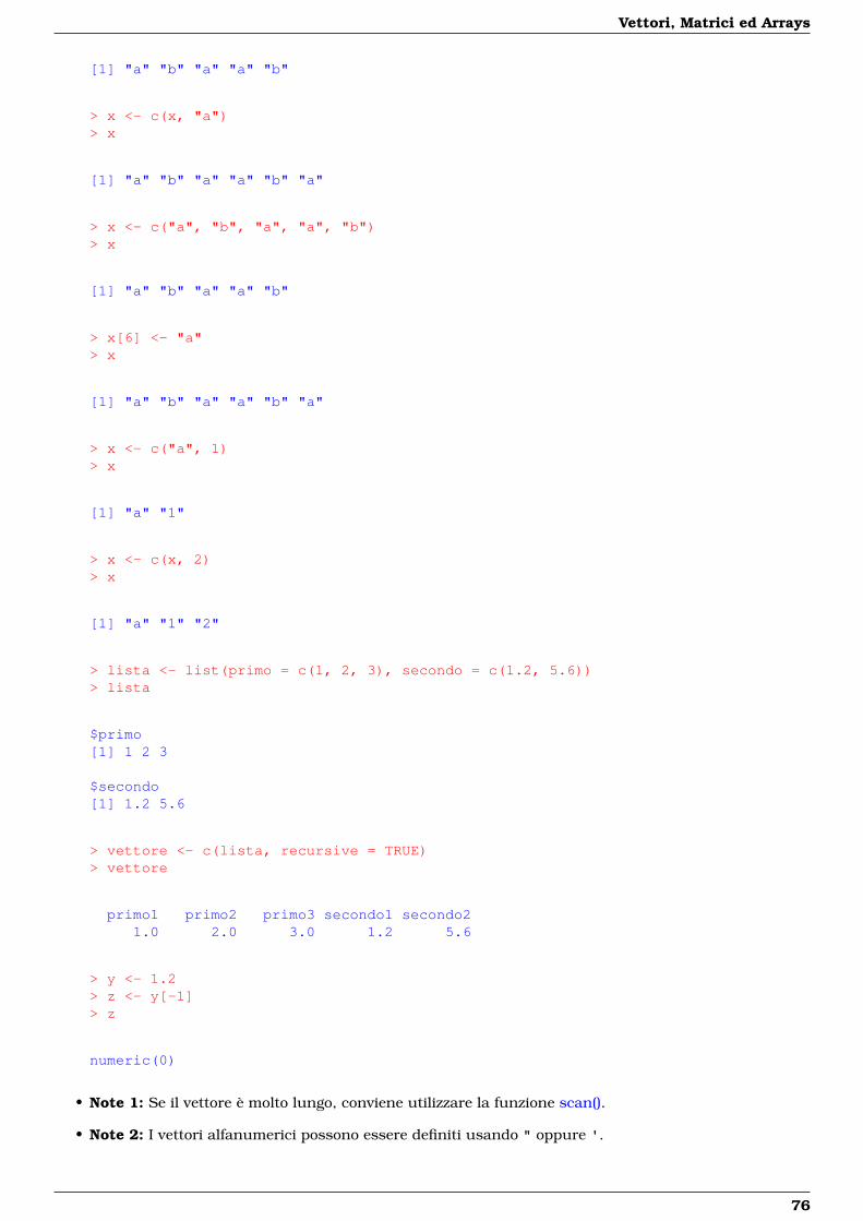
Vettori, Matrici ed Arrays
[1] "a" "b" "a" "a" "b"
> x <- c(x, "a")> x
[1] "a" "b" "a" "a" "b" "a"
> x <- c("a", "b", "a", "a", "b")> x
[1] "a" "b" "a" "a" "b"
> x[6] <- "a"> x
[1] "a" "b" "a" "a" "b" "a"
> x <- c("a", 1)> x
[1] "a" "1"
> x <- c(x, 2)> x
[1] "a" "1" "2"
> lista <- list(primo = c(1, 2, 3), secondo = c(1.2, 5.6))> lista
$primo[1] 1 2 3
$secondo[1] 1.2 5.6
> vettore <- c(lista, recursive = TRUE)> vettore
primo1 primo2 primo3 secondo1 secondo21.0 2.0 3.0 1.2 5.6
> y <- 1.2> z <- y[-1]> z
numeric(0)
• Note 1: Se il vettore è molto lungo, conviene utilizzare la funzione scan().
• Note 2: I vettori alfanumerici possono essere definiti usando " oppure '.
76

2.1 Creazione di Vettori
scan()
• Package: base
• Input:
what = double(0) / "character" tipo dei dati numerico oppure carattere
• Description: creazione di un vettore
• Example:
> x <- scan(what = double(0))> x <- scan(what = "character")
[ ]
• Package: base
• Input:
x vettore alfanumerico di dimensione n
• Description: estrazione di elementi da un vettore
• Example:
> x <- c(1.2, 3.4, 5.6, 7.8, 9, 9.9)> x
[1] 1.2 3.4 5.6 7.8 9.0 9.9
> x[2]
[1] 3.4
> x[c(1, 3, 4)]
[1] 1.2 5.6 7.8
> x[1:3]
[1] 1.2 3.4 5.6
> x[-c(1:3)]
[1] 7.8 9.0 9.9
> x[-(1:3)]
[1] 7.8 9.0 9.9
> x[x %in% c(1.2, 7.8)]
[1] 1.2 7.8
> x[x > 6.3]
[1] 7.8 9.0 9.9
> x[x > 6.3 & x < 9.7]
77
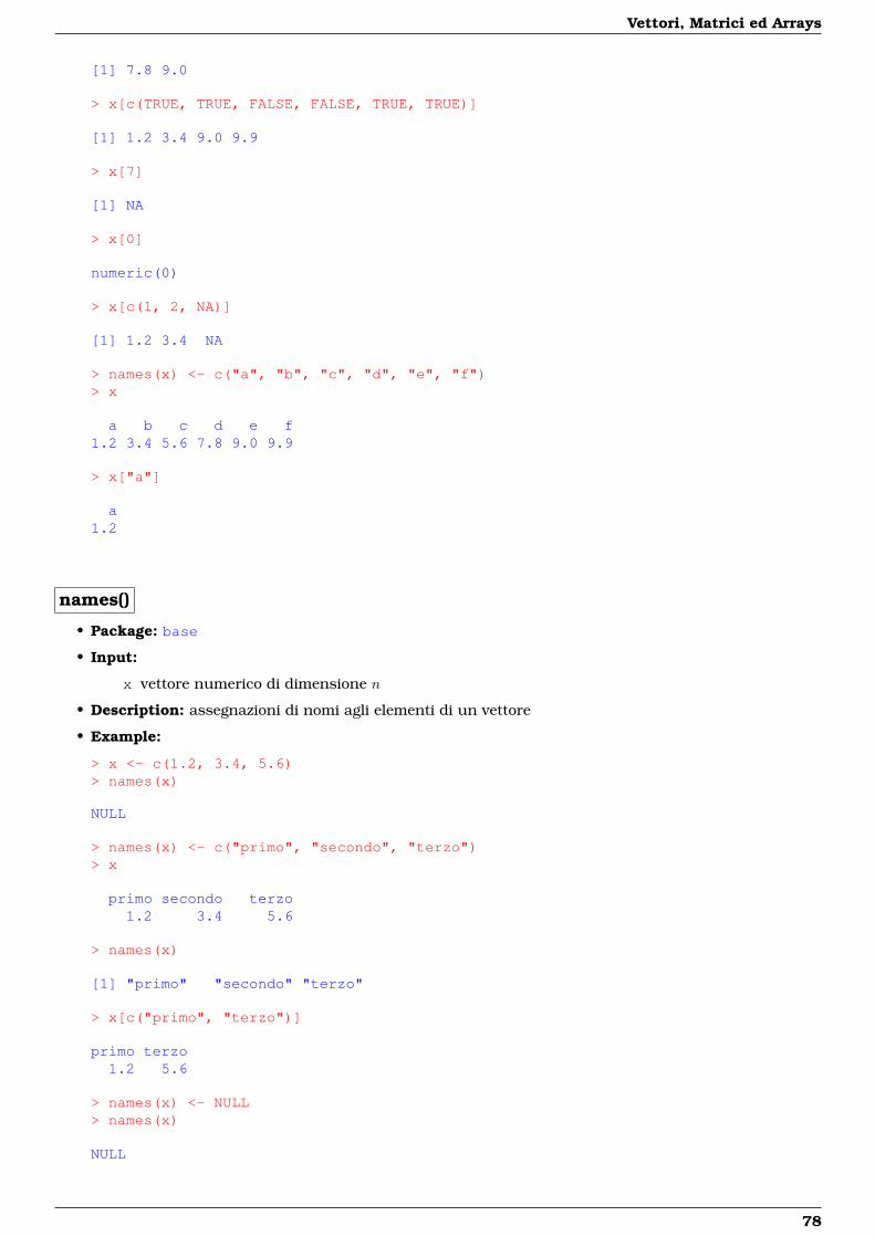
Vettori, Matrici ed Arrays
[1] 7.8 9.0
> x[c(TRUE, TRUE, FALSE, FALSE, TRUE, TRUE)]
[1] 1.2 3.4 9.0 9.9
> x[7]
[1] NA
> x[0]
numeric(0)
> x[c(1, 2, NA)]
[1] 1.2 3.4 NA
> names(x) <- c("a", "b", "c", "d", "e", "f")> x
a b c d e f1.2 3.4 5.6 7.8 9.0 9.9
> x["a"]
a1.2
names()
• Package: base
• Input:
x vettore numerico di dimensione n
• Description: assegnazioni di nomi agli elementi di un vettore
• Example:
> x <- c(1.2, 3.4, 5.6)> names(x)
NULL
> names(x) <- c("primo", "secondo", "terzo")> x
primo secondo terzo1.2 3.4 5.6
> names(x)
[1] "primo" "secondo" "terzo"
> x[c("primo", "terzo")]
primo terzo1.2 5.6
> names(x) <- NULL> names(x)
NULL
78

2.1 Creazione di Vettori
vector()
• Package: base
• Input:
mode = "numeric" / "complex" / "logical" tipo di oggetto
length valore n della dimensione
• Description: inizializzazione di un vettore di dimensione n
• Example:
> x <- vector(mode = "numeric", length = 5)> x
[1] 0 0 0 0 0
> x <- vector(mode = "complex", length = 3)> x
[1] 0+0i 0+0i 0+0i
> x <- vector(mode = "logical", length = 4)> x
[1] FALSE FALSE FALSE FALSE
numeric()
• Package: base
• Input:
length dimensione
• Description: inizializzazione di un vettore numerico di dimensione n
• Example:
> x <- numeric(length = 5)> x
[1] 0 0 0 0 0
> x <- numeric(length = 4)> x
[1] 0 0 0 0
79
Vettori, Matrici ed Arrays
complex()
• Package: base
• Input:
length dimensione
• Description: inizializzazione di un vettore complesso di dimensione n
• Example:
> x <- complex(length = 5)> x
[1] 0+0i 0+0i 0+0i 0+0i 0+0i
> x <- complex(length = 4)> x
[1] 0+0i 0+0i 0+0i 0+0i
logical()
• Package: base
• Input:
length dimensione
• Description: inizializzazione di un vettore logico di dimensione n
• Example:
> x <- logical(length = 5)> x
[1] FALSE FALSE FALSE FALSE FALSE
> x <- logical(length = 4)> x
[1] FALSE FALSE FALSE FALSE
head()
• Package: utils
• Input:
x vettore numerico di dimensione mn numero di elementi
• Description: seleziona i primi n elementi
• Example:
> x <- c(1.2, 3.2, 3.3, 2.5, 5, 5.6)> head(x, n = 2)
[1] 1.2 3.2
> x <- c(4.5, 6.7, 8.9, 7.7, 11.2)> head(x, n = 3)
[1] 4.5 6.7 8.9
80
2.1 Creazione di Vettori
tail()
• Package: utils
• Input:
x vettore numerico di dimensione m
n numero di elementi
• Description: seleziona gli ultimi n elementi
• Example:
> x <- c(1.2, 3.2, 3.3, 2.5, 5, 5.6)> tail(x, n = 3)
[1] 2.5 5.0 5.6
> x <- c(4.5, 6.7, 8.9, 7.7, 11.2)> tail(x, n = 2)
[1] 7.7 11.2
%o%
• Package: base
• Input:
x vettore numerico di dimensione n
y vettore numerico di dimensione m
• Description: prodotto esterno
• Formula:xi yj ∀i = 1, 2, . . . , n ∀j = 1, 2, . . . , m
• Example:
> x <- c(1, 2, 3, 4)> n <- 4> y <- c(1.2, 3.4)> m <- 2> x %o% y
[,1] [,2][1,] 1.2 3.4[2,] 2.4 6.8[3,] 3.6 10.2[4,] 4.8 13.6
> x <- c(3, 4, 7)> n <- 3> y <- c(1.1, 2.2, 3.3)> m <- 3> x %o% y
[,1] [,2] [,3][1,] 3.3 6.6 9.9[2,] 4.4 8.8 13.2[3,] 7.7 15.4 23.1
81
Vettori, Matrici ed Arrays
append()
• Package: base
• Input:
x vettore numerico di dimensione n
values valore v numerico
after valore j naturale
• Description: aggiunge un elemento ad un vettore
• Formula:
after ≤ 0
v, x1, x2, . . . , xn
after ≥ n
x1, x2, . . . , xn, v
1 ≤ after ≤ n− 1
x1, x2, . . . , xj , v, xj+1, xj+2, . . . , xn
• Example:
> x <- c(1.2, 3.4, 5.6)> append(x, values = 6, after = -2)
[1] 6.0 1.2 3.4 5.6
> x <- c(1.2, 3.4, 5.6)> append(x, values = 6, after = 2)
[1] 1.2 3.4 6.0 5.6
> x <- c(1.2, 3.4, 5.6)> append(x, values = 6, after = 7)
[1] 1.2 3.4 5.6 6.0
sapply()
• Package: base
• Input:
X vettore numerico di dimensione n
FUN funzione scelta
• Description: applica FUN ad ogni elemento del vettore X
• Example:
> sapply(X = c(1.2, 3.2, 4.5, 6.7), FUN = sin)
[1] 0.93203909 -0.05837414 -0.97753012 0.40484992
> sapply(X = c(1.2, 3.2, 4.5, 6.7), FUN = log)
82
2.1 Creazione di Vettori
[1] 0.1823216 1.1631508 1.5040774 1.9021075
> a <- c(2, 4, 7, 3, 5, 2, 9, 0)> X <- c(2, 4, 6)> myfun <- function(x) which(a > x)> sapply(X, FUN = myfun)
[[1]][1] 2 3 4 5 7
[[2]][1] 3 5 7
[[3]][1] 3 7
> x <- c(1.5, 6.4, 9.6, 8.8, 7.7, 2.2, 4.8)> sapply(X = 1:5, FUN = function(i) sample(x, size = 3, replace = FALSE))
[,1] [,2] [,3] [,4] [,5][1,] 9.6 8.8 2.2 1.5 7.7[2,] 1.5 9.6 9.6 7.7 9.6[3,] 8.8 6.4 7.7 9.6 6.4
> x <- matrix(data = c(2, 3, 4, 5, 5, 4, 1, 3, 4, 7, 6, 5, 12,+ 13, 4, 11, 21, 10, 9, 7), nrow = 4, ncol = 5)> x
[,1] [,2] [,3] [,4] [,5][1,] 2 5 4 12 21[2,] 3 4 7 13 10[3,] 4 1 6 4 9[4,] 5 3 5 11 7
> fattore <- factor(c(1, 2, 2, 1), labels = letters[1:2])> fattore
[1] a b b aLevels: a b
> sapply(X = 1:ncol(x), FUN = function(i) tapply(x[, i], INDEX = fattore,+ FUN = mean))
[,1] [,2] [,3] [,4] [,5]a 3.5 4.0 4.5 11.5 14.0b 3.5 2.5 6.5 8.5 9.5
> myfun <- function(x) prod(1:x)> sapply(X = 1:5, myfun)
[1] 1 2 6 24 120
> x <- c(1.1, 2.3, 4.5, 6.7, 8.9, 3.4, 5.6, 6.7)> y <- c(1.5, 6.4, 9.6, 8.8, 8.86, 7.8, 8.6, 8.6)> sumsq <- function(b, xv = x, yv = y) {+ yhat <- 1.2 + b * xv+ sum((yv - yhat)^2)+ }> b <- seq(0, 2, by = 0.05)> sapply(X = b, FUN = sumsq)
83

Vettori, Matrici ed Arrays
[1] 367.20560 339.53785 313.06340 287.78225 263.69440 240.79985 219.09860[8] 198.59065 179.27600 161.15465 144.22660 128.49185 113.95040 100.60225
[15] 88.44740 77.48585 67.71760 59.14265 51.76100 45.57265 40.57760[22] 36.77585 34.16740 32.75225 32.53040 33.50185 35.66660 39.02465[29] 43.57600 49.32065 56.25860 64.38985 73.71440 84.23225 95.94340[36] 108.84785 122.94560 138.23665 154.72100 172.39865 191.26960
subset()
• Package: base
• Input:
x vettore numerico di dimensione n
subset selezione
• Description: sottoinsieme del vettore x
• Example 1:
> x <- c(7.8, 6.6, 6.5, 7.4, 7.3, 7, 6.4, 7.1, 6.7, 7.6, 6.8)> subset(x, subset = x > 7.5)
[1] 7.8 7.6
• Example 2:
> x <- c(7.8, 6.6, 6.5, 6.6)> subset(x, subset = x == 6.6)
[1] 6.6 6.6
2.2 Creazione di Matrici
matrix()
• Package: base
• Input:
data vettore numerico di dimensione nm
nrow numero n di righe
ncol numero m di colonne
byrow = TRUE / FALSE elementi disposti per riga oppure per colonna
dimnames etichette di riga e di colonna
• Description: definizione di una matrice
• Example:
> n <- 2> m <- 3> x <- c(1, -0.2, 3, 1.1, -0.3, 3.2)> A <- matrix(data = x, nrow = n, ncol = m, byrow = TRUE)> A
[,1] [,2] [,3][1,] 1.0 -0.2 3.0[2,] 1.1 -0.3 3.2
84
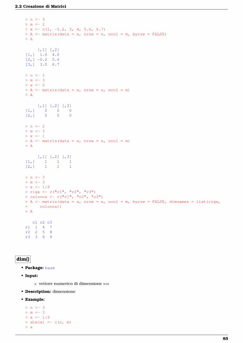
2.2 Creazione di Matrici
> n <- 3> m <- 2> x <- c(1, -0.2, 3, 4, 5.6, 6.7)> A <- matrix(data = x, nrow = n, ncol = m, byrow = FALSE)> A
[,1] [,2][1,] 1.0 4.0[2,] -0.2 5.6[3,] 3.0 6.7
> n <- 2> m <- 3> x <- 0> A <- matrix(data = x, nrow = n, ncol = m)> A
[,1] [,2] [,3][1,] 0 0 0[2,] 0 0 0
> n <- 2> m <- 3> x <- 1> A <- matrix(data = x, nrow = n, ncol = m)> A
[,1] [,2] [,3][1,] 1 1 1[2,] 1 1 1
> n <- 3> m <- 3> x <- 1:9> riga <- c("r1", "r2", "r3")> colonna <- c("c1", "c2", "c3")> A <- matrix(data = x, nrow = n, ncol = m, byrow = FALSE, dimnames = list(riga,+ colonna))> A
c1 c2 c3r1 1 4 7r2 2 5 8r3 3 6 9
dim()
• Package: base
• Input:
x vettore numerico di dimensione nm
• Description: dimensione
• Example:
> n <- 3> m <- 3> x <- 1:9> dim(x) <- c(n, m)> x
85
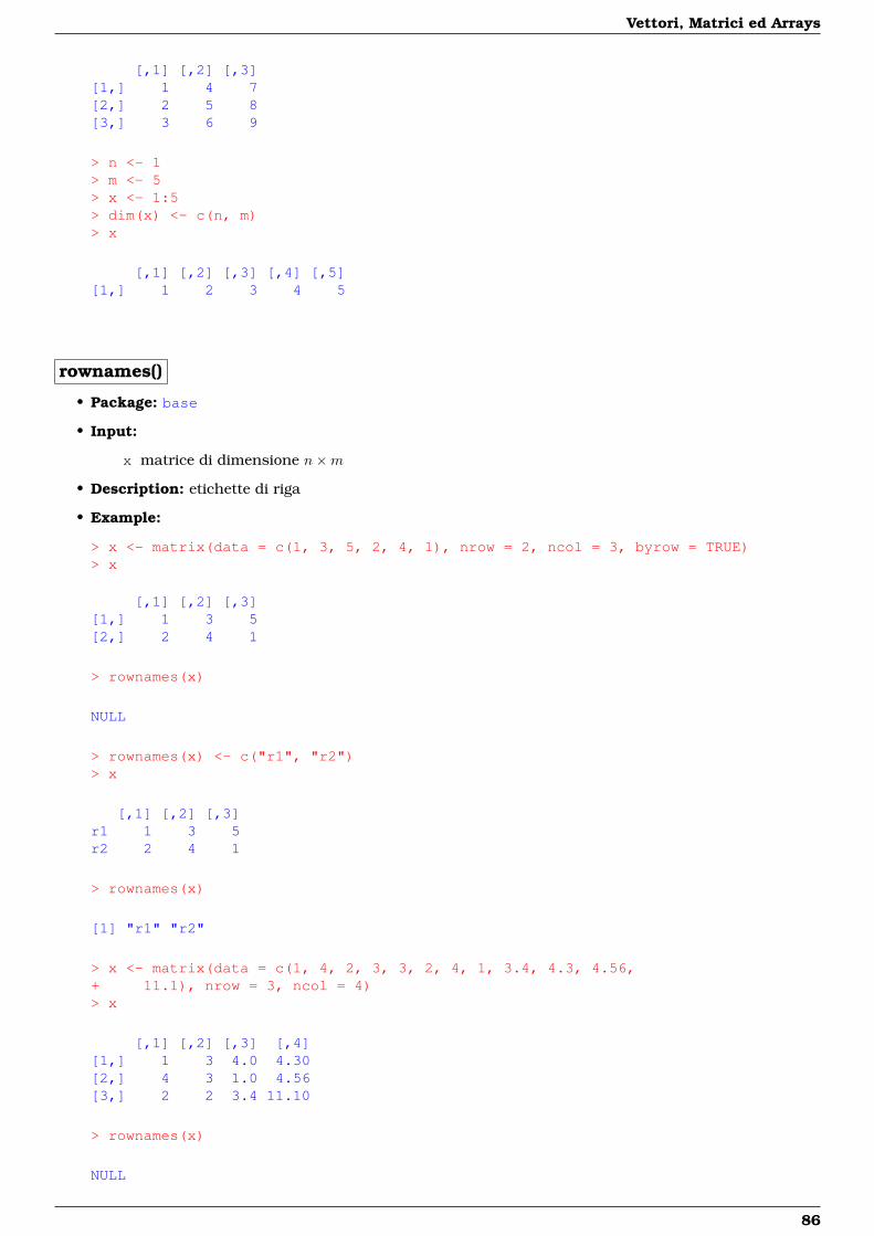
Vettori, Matrici ed Arrays
[,1] [,2] [,3][1,] 1 4 7[2,] 2 5 8[3,] 3 6 9
> n <- 1> m <- 5> x <- 1:5> dim(x) <- c(n, m)> x
[,1] [,2] [,3] [,4] [,5][1,] 1 2 3 4 5
rownames()
• Package: base
• Input:
x matrice di dimensione n×m
• Description: etichette di riga
• Example:
> x <- matrix(data = c(1, 3, 5, 2, 4, 1), nrow = 2, ncol = 3, byrow = TRUE)> x
[,1] [,2] [,3][1,] 1 3 5[2,] 2 4 1
> rownames(x)
NULL
> rownames(x) <- c("r1", "r2")> x
[,1] [,2] [,3]r1 1 3 5r2 2 4 1
> rownames(x)
[1] "r1" "r2"
> x <- matrix(data = c(1, 4, 2, 3, 3, 2, 4, 1, 3.4, 4.3, 4.56,+ 11.1), nrow = 3, ncol = 4)> x
[,1] [,2] [,3] [,4][1,] 1 3 4.0 4.30[2,] 4 3 1.0 4.56[3,] 2 2 3.4 11.10
> rownames(x)
NULL
86
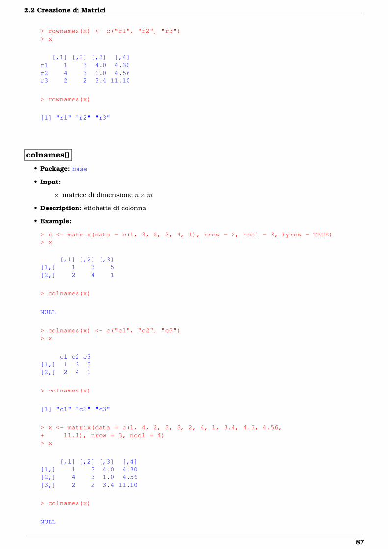
2.2 Creazione di Matrici
> rownames(x) <- c("r1", "r2", "r3")> x
[,1] [,2] [,3] [,4]r1 1 3 4.0 4.30r2 4 3 1.0 4.56r3 2 2 3.4 11.10
> rownames(x)
[1] "r1" "r2" "r3"
colnames()
• Package: base
• Input:
x matrice di dimensione n×m
• Description: etichette di colonna
• Example:
> x <- matrix(data = c(1, 3, 5, 2, 4, 1), nrow = 2, ncol = 3, byrow = TRUE)> x
[,1] [,2] [,3][1,] 1 3 5[2,] 2 4 1
> colnames(x)
NULL
> colnames(x) <- c("c1", "c2", "c3")> x
c1 c2 c3[1,] 1 3 5[2,] 2 4 1
> colnames(x)
[1] "c1" "c2" "c3"
> x <- matrix(data = c(1, 4, 2, 3, 3, 2, 4, 1, 3.4, 4.3, 4.56,+ 11.1), nrow = 3, ncol = 4)> x
[,1] [,2] [,3] [,4][1,] 1 3 4.0 4.30[2,] 4 3 1.0 4.56[3,] 2 2 3.4 11.10
> colnames(x)
NULL
87
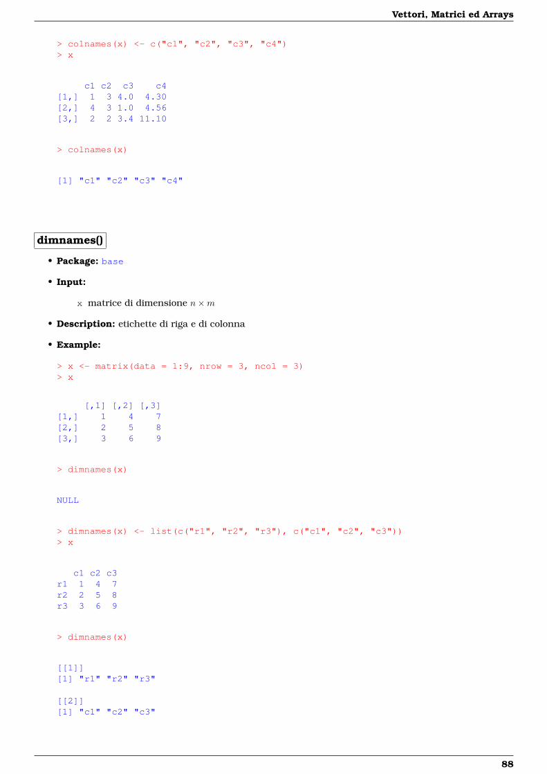
Vettori, Matrici ed Arrays
> colnames(x) <- c("c1", "c2", "c3", "c4")> x
c1 c2 c3 c4[1,] 1 3 4.0 4.30[2,] 4 3 1.0 4.56[3,] 2 2 3.4 11.10
> colnames(x)
[1] "c1" "c2" "c3" "c4"
dimnames()
• Package: base
• Input:
x matrice di dimensione n×m
• Description: etichette di riga e di colonna
• Example:
> x <- matrix(data = 1:9, nrow = 3, ncol = 3)> x
[,1] [,2] [,3][1,] 1 4 7[2,] 2 5 8[3,] 3 6 9
> dimnames(x)
NULL
> dimnames(x) <- list(c("r1", "r2", "r3"), c("c1", "c2", "c3"))> x
c1 c2 c3r1 1 4 7r2 2 5 8r3 3 6 9
> dimnames(x)
[[1]][1] "r1" "r2" "r3"
[[2]][1] "c1" "c2" "c3"
88
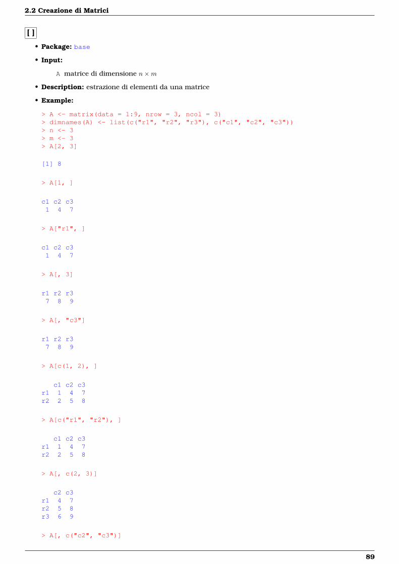
2.2 Creazione di Matrici
[ ]
• Package: base
• Input:
A matrice di dimensione n×m
• Description: estrazione di elementi da una matrice
• Example:
> A <- matrix(data = 1:9, nrow = 3, ncol = 3)> dimnames(A) <- list(c("r1", "r2", "r3"), c("c1", "c2", "c3"))> n <- 3> m <- 3> A[2, 3]
[1] 8
> A[1, ]
c1 c2 c31 4 7
> A["r1", ]
c1 c2 c31 4 7
> A[, 3]
r1 r2 r37 8 9
> A[, "c3"]
r1 r2 r37 8 9
> A[c(1, 2), ]
c1 c2 c3r1 1 4 7r2 2 5 8
> A[c("r1", "r2"), ]
c1 c2 c3r1 1 4 7r2 2 5 8
> A[, c(2, 3)]
c2 c3r1 4 7r2 5 8r3 6 9
> A[, c("c2", "c3")]
89

Vettori, Matrici ed Arrays
c2 c3r1 4 7r2 5 8r3 6 9
> A[-1, ]
c1 c2 c3r2 2 5 8r3 3 6 9
> A[, -3]
c1 c2r1 1 4r2 2 5r3 3 6
> A[A[, "c2"] > 4.1, ]
c1 c2 c3r2 2 5 8r3 3 6 9
> x[x > 3]
[1] 4 5 6 7 8 9
> A <- matrix(data = c(1.2, 3.4, 5.6, 7.8, 9.1), nrow = 1, ncol = 5)> is.matrix(A)
[1] TRUE
> myvec <- A[1, ]> is.vector(myvec)
[1] TRUE
> myvec2 <- A[, 1]> is.vector(myvec2)
[1] TRUE
> myvec3 <- A[1, , drop = FALSE]> is.vector(myvec3)
[1] FALSE
> is.matrix(myvec3)
[1] TRUE
90
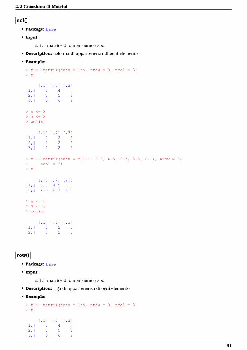
2.2 Creazione di Matrici
col()
• Package: base
• Input:
data matrice di dimensione n×m
• Description: colonna di appartenenza di ogni elemento
• Example:
> x <- matrix(data = 1:9, nrow = 3, ncol = 3)> x
[,1] [,2] [,3][1,] 1 4 7[2,] 2 5 8[3,] 3 6 9
> n <- 3> m <- 3> col(x)
[,1] [,2] [,3][1,] 1 2 3[2,] 1 2 3[3,] 1 2 3
> x <- matrix(data = c(1.1, 2.3, 4.5, 6.7, 8.8, 6.1), nrow = 2,+ ncol = 3)> x
[,1] [,2] [,3][1,] 1.1 4.5 8.8[2,] 2.3 6.7 6.1
> n <- 2> m <- 3> col(x)
[,1] [,2] [,3][1,] 1 2 3[2,] 1 2 3
row()
• Package: base
• Input:
data matrice di dimensione n×m
• Description: riga di appartenenza di ogni elemento
• Example:
> x <- matrix(data = 1:9, nrow = 3, ncol = 3)> x
[,1] [,2] [,3][1,] 1 4 7[2,] 2 5 8[3,] 3 6 9
91
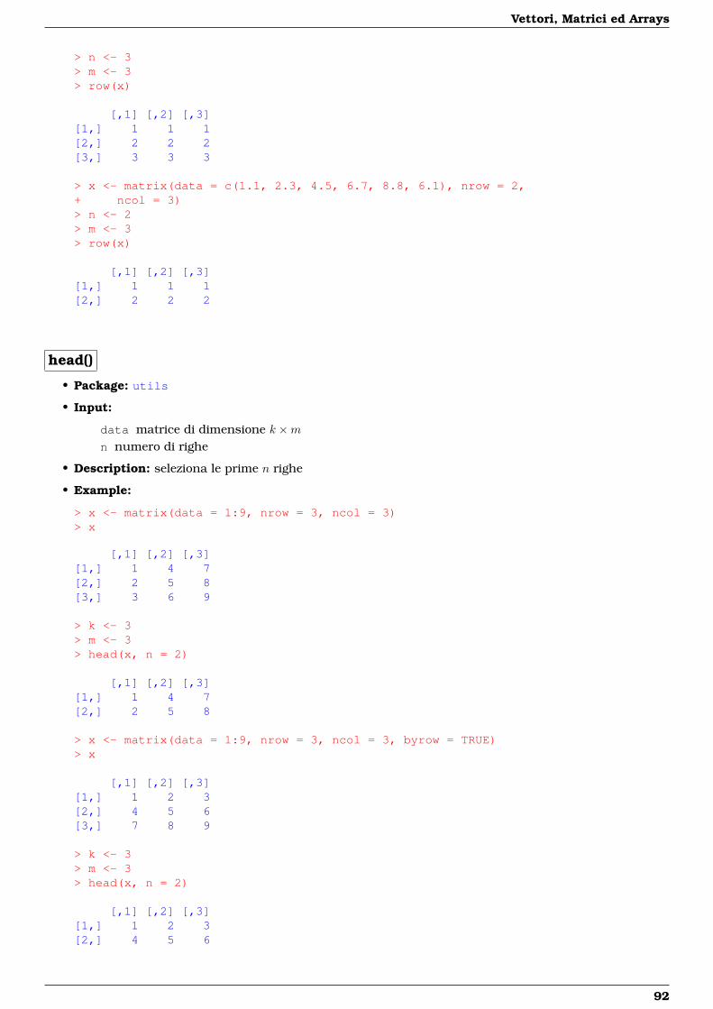
Vettori, Matrici ed Arrays
> n <- 3> m <- 3> row(x)
[,1] [,2] [,3][1,] 1 1 1[2,] 2 2 2[3,] 3 3 3
> x <- matrix(data = c(1.1, 2.3, 4.5, 6.7, 8.8, 6.1), nrow = 2,+ ncol = 3)> n <- 2> m <- 3> row(x)
[,1] [,2] [,3][1,] 1 1 1[2,] 2 2 2
head()
• Package: utils
• Input:
data matrice di dimensione k ×mn numero di righe
• Description: seleziona le prime n righe
• Example:
> x <- matrix(data = 1:9, nrow = 3, ncol = 3)> x
[,1] [,2] [,3][1,] 1 4 7[2,] 2 5 8[3,] 3 6 9
> k <- 3> m <- 3> head(x, n = 2)
[,1] [,2] [,3][1,] 1 4 7[2,] 2 5 8
> x <- matrix(data = 1:9, nrow = 3, ncol = 3, byrow = TRUE)> x
[,1] [,2] [,3][1,] 1 2 3[2,] 4 5 6[3,] 7 8 9
> k <- 3> m <- 3> head(x, n = 2)
[,1] [,2] [,3][1,] 1 2 3[2,] 4 5 6
92
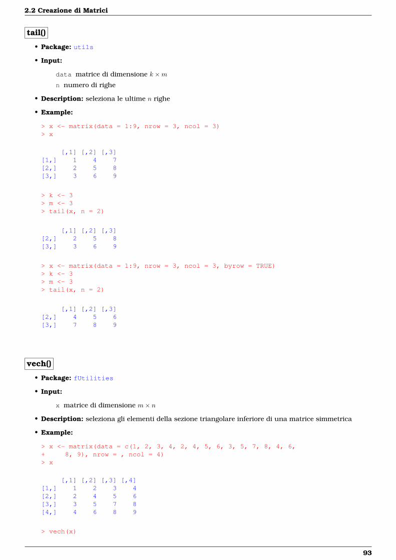
2.2 Creazione di Matrici
tail()
• Package: utils
• Input:
data matrice di dimensione k ×mn numero di righe
• Description: seleziona le ultime n righe
• Example:
> x <- matrix(data = 1:9, nrow = 3, ncol = 3)> x
[,1] [,2] [,3][1,] 1 4 7[2,] 2 5 8[3,] 3 6 9
> k <- 3> m <- 3> tail(x, n = 2)
[,1] [,2] [,3][2,] 2 5 8[3,] 3 6 9
> x <- matrix(data = 1:9, nrow = 3, ncol = 3, byrow = TRUE)> k <- 3> m <- 3> tail(x, n = 2)
[,1] [,2] [,3][2,] 4 5 6[3,] 7 8 9
vech()
• Package: fUtilities
• Input:
x matrice di dimensione m× n
• Description: seleziona gli elementi della sezione triangolare inferiore di una matrice simmetrica
• Example:
> x <- matrix(data = c(1, 2, 3, 4, 2, 4, 5, 6, 3, 5, 7, 8, 4, 6,+ 8, 9), nrow = , ncol = 4)> x
[,1] [,2] [,3] [,4][1,] 1 2 3 4[2,] 2 4 5 6[3,] 3 5 7 8[4,] 4 6 8 9
> vech(x)
93
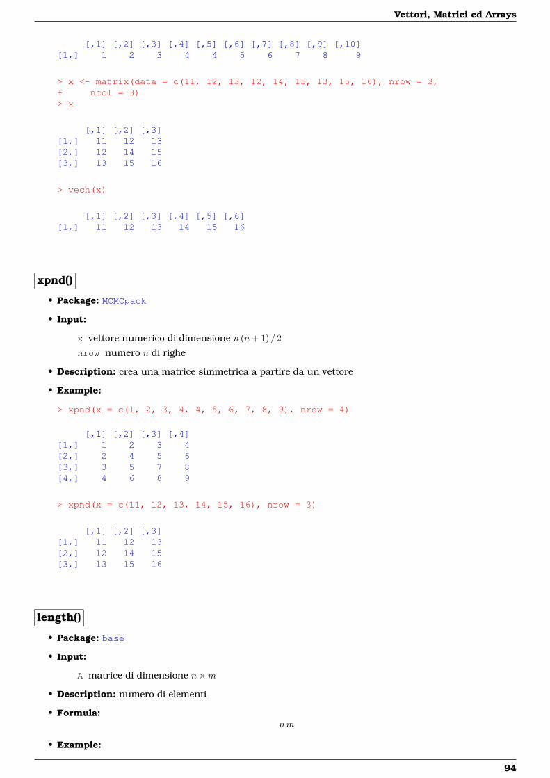
Vettori, Matrici ed Arrays
[,1] [,2] [,3] [,4] [,5] [,6] [,7] [,8] [,9] [,10][1,] 1 2 3 4 4 5 6 7 8 9
> x <- matrix(data = c(11, 12, 13, 12, 14, 15, 13, 15, 16), nrow = 3,+ ncol = 3)> x
[,1] [,2] [,3][1,] 11 12 13[2,] 12 14 15[3,] 13 15 16
> vech(x)
[,1] [,2] [,3] [,4] [,5] [,6][1,] 11 12 13 14 15 16
xpnd()
• Package: MCMCpack
• Input:
x vettore numerico di dimensione n (n+ 1) / 2
nrow numero n di righe
• Description: crea una matrice simmetrica a partire da un vettore
• Example:
> xpnd(x = c(1, 2, 3, 4, 4, 5, 6, 7, 8, 9), nrow = 4)
[,1] [,2] [,3] [,4][1,] 1 2 3 4[2,] 2 4 5 6[3,] 3 5 7 8[4,] 4 6 8 9
> xpnd(x = c(11, 12, 13, 14, 15, 16), nrow = 3)
[,1] [,2] [,3][1,] 11 12 13[2,] 12 14 15[3,] 13 15 16
length()
• Package: base
• Input:
A matrice di dimensione n×m
• Description: numero di elementi
• Formula:nm
• Example:
94

2.2 Creazione di Matrici
> A <- matrix(data = 1:9, nrow = 3, ncol = 3)> A
[,1] [,2] [,3][1,] 1 4 7[2,] 2 5 8[3,] 3 6 9
> n <- 3> m <- 3> n * m
[1] 9
> length(A)
[1] 9
> A <- matrix(data = c(1.2, 4.5, 2.3, 3.1), nrow = 2, ncol = 2)> A
[,1] [,2][1,] 1.2 2.3[2,] 4.5 3.1
> n <- 2> m <- 2> n * m
[1] 4
> length(A)
[1] 4
cbind()
• Package: base
• Input:
A matrice di dimensione n×mB matrice di dimensione n× k
• Description: unisce due matrici accostandole per colonna
• Example:
> A <- matrix(data = c(9.9, 1, 12), nrow = 3, ncol = 1)> A
[,1][1,] 9.9[2,] 1.0[3,] 12.0
> B <- matrix(data = 1:3, nrow = 3, ncol = 1)> B
95
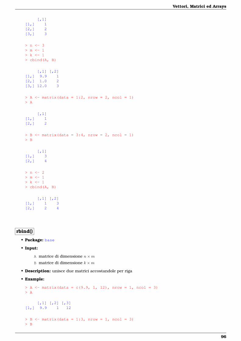
Vettori, Matrici ed Arrays
[,1][1,] 1[2,] 2[3,] 3
> n <- 3> m <- 1> k <- 1> cbind(A, B)
[,1] [,2][1,] 9.9 1[2,] 1.0 2[3,] 12.0 3
> A <- matrix(data = 1:2, nrow = 2, ncol = 1)> A
[,1][1,] 1[2,] 2
> B <- matrix(data = 3:4, nrow = 2, ncol = 1)> B
[,1][1,] 3[2,] 4
> n <- 2> m <- 1> k <- 1> cbind(A, B)
[,1] [,2][1,] 1 3[2,] 2 4
rbind()
• Package: base
• Input:
A matrice di dimensione n×mB matrice di dimensione k ×m
• Description: unisce due matrici accostandole per riga
• Example:
> A <- matrix(data = c(9.9, 1, 12), nrow = 1, ncol = 3)> A
[,1] [,2] [,3][1,] 9.9 1 12
> B <- matrix(data = 1:3, nrow = 1, ncol = 3)> B
96
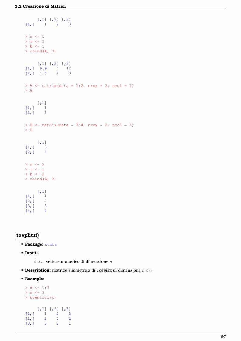
2.2 Creazione di Matrici
[,1] [,2] [,3][1,] 1 2 3
> n <- 1> m <- 3> k <- 1> rbind(A, B)
[,1] [,2] [,3][1,] 9.9 1 12[2,] 1.0 2 3
> A <- matrix(data = 1:2, nrow = 2, ncol = 1)> A
[,1][1,] 1[2,] 2
> B <- matrix(data = 3:4, nrow = 2, ncol = 1)> B
[,1][1,] 3[2,] 4
> n <- 2> m <- 1> k <- 2> rbind(A, B)
[,1][1,] 1[2,] 2[3,] 3[4,] 4
toeplitz()
• Package: stats
• Input:
data vettore numerico di dimensione n
• Description: matrice simmetrica di Toeplitz di dimensione n× n
• Example:
> x <- 1:3> n <- 3> toeplitz(x)
[,1] [,2] [,3][1,] 1 2 3[2,] 2 1 2[3,] 3 2 1
97
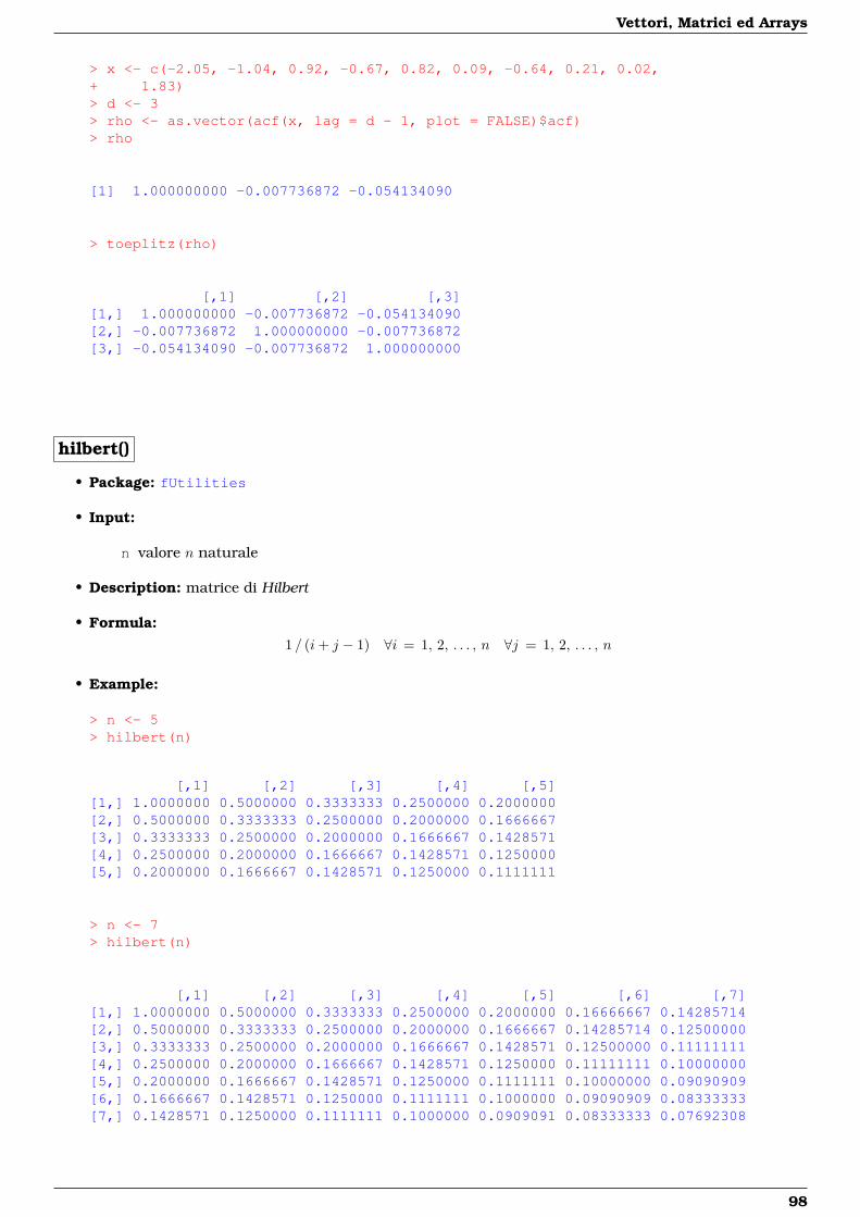
Vettori, Matrici ed Arrays
> x <- c(-2.05, -1.04, 0.92, -0.67, 0.82, 0.09, -0.64, 0.21, 0.02,+ 1.83)> d <- 3> rho <- as.vector(acf(x, lag = d - 1, plot = FALSE)$acf)> rho
[1] 1.000000000 -0.007736872 -0.054134090
> toeplitz(rho)
[,1] [,2] [,3][1,] 1.000000000 -0.007736872 -0.054134090[2,] -0.007736872 1.000000000 -0.007736872[3,] -0.054134090 -0.007736872 1.000000000
hilbert()
• Package: fUtilities
• Input:
n valore n naturale
• Description: matrice di Hilbert
• Formula:1 / (i+ j − 1) ∀i = 1, 2, . . . , n ∀j = 1, 2, . . . , n
• Example:
> n <- 5> hilbert(n)
[,1] [,2] [,3] [,4] [,5][1,] 1.0000000 0.5000000 0.3333333 0.2500000 0.2000000[2,] 0.5000000 0.3333333 0.2500000 0.2000000 0.1666667[3,] 0.3333333 0.2500000 0.2000000 0.1666667 0.1428571[4,] 0.2500000 0.2000000 0.1666667 0.1428571 0.1250000[5,] 0.2000000 0.1666667 0.1428571 0.1250000 0.1111111
> n <- 7> hilbert(n)
[,1] [,2] [,3] [,4] [,5] [,6] [,7][1,] 1.0000000 0.5000000 0.3333333 0.2500000 0.2000000 0.16666667 0.14285714[2,] 0.5000000 0.3333333 0.2500000 0.2000000 0.1666667 0.14285714 0.12500000[3,] 0.3333333 0.2500000 0.2000000 0.1666667 0.1428571 0.12500000 0.11111111[4,] 0.2500000 0.2000000 0.1666667 0.1428571 0.1250000 0.11111111 0.10000000[5,] 0.2000000 0.1666667 0.1428571 0.1250000 0.1111111 0.10000000 0.09090909[6,] 0.1666667 0.1428571 0.1250000 0.1111111 0.1000000 0.09090909 0.08333333[7,] 0.1428571 0.1250000 0.1111111 0.1000000 0.0909091 0.08333333 0.07692308
98
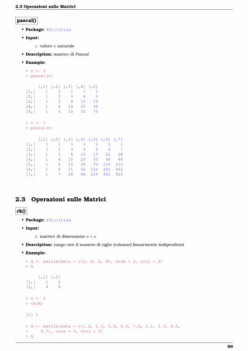
2.3 Operazioni sulle Matrici
pascal()
• Package: fUtilities
• Input:
n valore n naturale
• Description: matrice di Pascal
• Example:
> n <- 5> pascal(n)
[,1] [,2] [,3] [,4] [,5][1,] 1 1 1 1 1[2,] 1 2 3 4 5[3,] 1 3 6 10 15[4,] 1 4 10 20 35[5,] 1 5 15 35 70
> n <- 7> pascal(n)
[,1] [,2] [,3] [,4] [,5] [,6] [,7][1,] 1 1 1 1 1 1 1[2,] 1 2 3 4 5 6 7[3,] 1 3 6 10 15 21 28[4,] 1 4 10 20 35 56 84[5,] 1 5 15 35 70 126 210[6,] 1 6 21 56 126 252 462[7,] 1 7 28 84 210 462 924
2.3 Operazioni sulle Matrici
rk()
• Package: fUtilities
• Input:
A matrice di dimensione n× n
• Description: rango cioé il numero di righe (colonne) linearmente indipendenti
• Example:
> A <- matrix(data = c(1, 4, 2, 8), nrow = 2, ncol = 2)> A
[,1] [,2][1,] 1 2[2,] 4 8
> n <- 2> rk(A)
[1] 1
> A <- matrix(data = c(1.2, 2.3, 4.5, 6.5, 7.6, 1.1, 2.3, 4.5,+ 6.7), nrow = 3, ncol = 3)> A
99
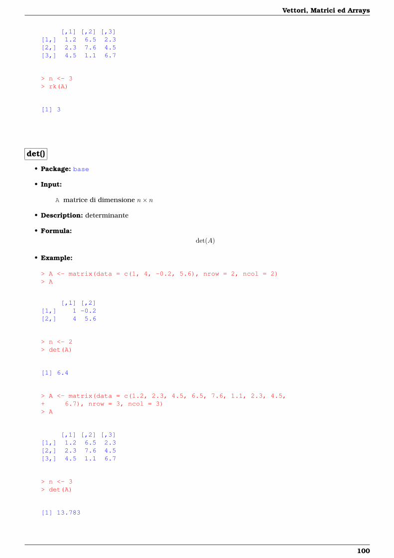
Vettori, Matrici ed Arrays
[,1] [,2] [,3][1,] 1.2 6.5 2.3[2,] 2.3 7.6 4.5[3,] 4.5 1.1 6.7
> n <- 3> rk(A)
[1] 3
det()
• Package: base
• Input:
A matrice di dimensione n× n
• Description: determinante
• Formula:det(A)
• Example:
> A <- matrix(data = c(1, 4, -0.2, 5.6), nrow = 2, ncol = 2)> A
[,1] [,2][1,] 1 -0.2[2,] 4 5.6
> n <- 2> det(A)
[1] 6.4
> A <- matrix(data = c(1.2, 2.3, 4.5, 6.5, 7.6, 1.1, 2.3, 4.5,+ 6.7), nrow = 3, ncol = 3)> A
[,1] [,2] [,3][1,] 1.2 6.5 2.3[2,] 2.3 7.6 4.5[3,] 4.5 1.1 6.7
> n <- 3> det(A)
[1] 13.783
100
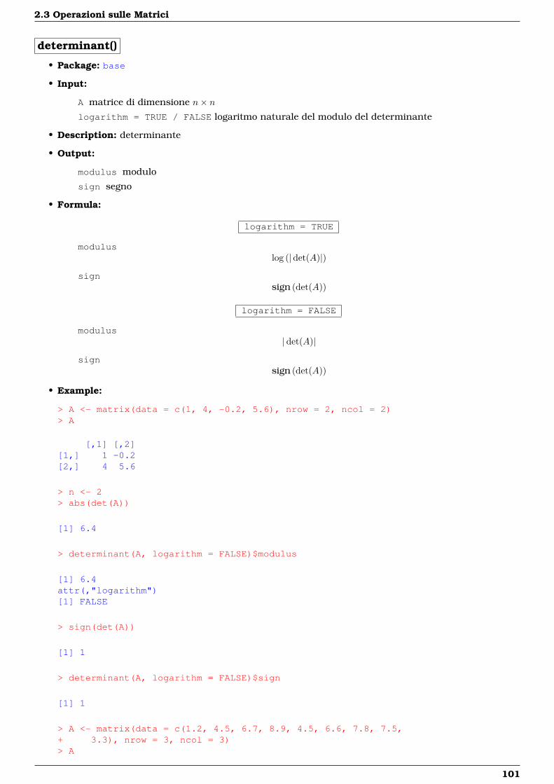
2.3 Operazioni sulle Matrici
determinant()
• Package: base
• Input:
A matrice di dimensione n× nlogarithm = TRUE / FALSE logaritmo naturale del modulo del determinante
• Description: determinante
• Output:
modulus modulo
sign segno
• Formula:
logarithm = TRUE
moduluslog (|det(A)|)
signsign (det(A))
logarithm = FALSE
modulus|det(A)|
signsign (det(A))
• Example:
> A <- matrix(data = c(1, 4, -0.2, 5.6), nrow = 2, ncol = 2)> A
[,1] [,2][1,] 1 -0.2[2,] 4 5.6
> n <- 2> abs(det(A))
[1] 6.4
> determinant(A, logarithm = FALSE)$modulus
[1] 6.4attr(,"logarithm")[1] FALSE
> sign(det(A))
[1] 1
> determinant(A, logarithm = FALSE)$sign
[1] 1
> A <- matrix(data = c(1.2, 4.5, 6.7, 8.9, 4.5, 6.6, 7.8, 7.5,+ 3.3), nrow = 3, ncol = 3)> A
101
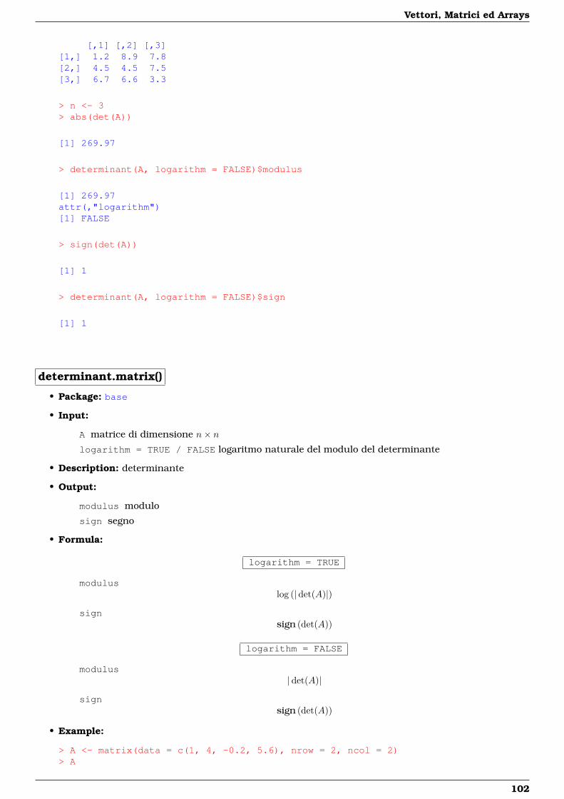
Vettori, Matrici ed Arrays
[,1] [,2] [,3][1,] 1.2 8.9 7.8[2,] 4.5 4.5 7.5[3,] 6.7 6.6 3.3
> n <- 3> abs(det(A))
[1] 269.97
> determinant(A, logarithm = FALSE)$modulus
[1] 269.97attr(,"logarithm")[1] FALSE
> sign(det(A))
[1] 1
> determinant(A, logarithm = FALSE)$sign
[1] 1
determinant.matrix()
• Package: base
• Input:
A matrice di dimensione n× nlogarithm = TRUE / FALSE logaritmo naturale del modulo del determinante
• Description: determinante
• Output:
modulus modulo
sign segno
• Formula:
logarithm = TRUE
moduluslog (|det(A)|)
signsign (det(A))
logarithm = FALSE
modulus|det(A)|
signsign (det(A))
• Example:
> A <- matrix(data = c(1, 4, -0.2, 5.6), nrow = 2, ncol = 2)> A
102
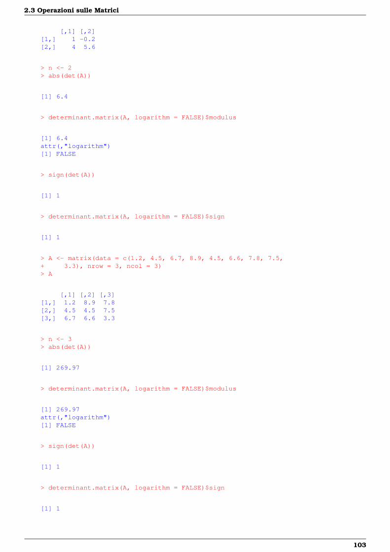
2.3 Operazioni sulle Matrici
[,1] [,2][1,] 1 -0.2[2,] 4 5.6
> n <- 2> abs(det(A))
[1] 6.4
> determinant.matrix(A, logarithm = FALSE)$modulus
[1] 6.4attr(,"logarithm")[1] FALSE
> sign(det(A))
[1] 1
> determinant.matrix(A, logarithm = FALSE)$sign
[1] 1
> A <- matrix(data = c(1.2, 4.5, 6.7, 8.9, 4.5, 6.6, 7.8, 7.5,+ 3.3), nrow = 3, ncol = 3)> A
[,1] [,2] [,3][1,] 1.2 8.9 7.8[2,] 4.5 4.5 7.5[3,] 6.7 6.6 3.3
> n <- 3> abs(det(A))
[1] 269.97
> determinant.matrix(A, logarithm = FALSE)$modulus
[1] 269.97attr(,"logarithm")[1] FALSE
> sign(det(A))
[1] 1
> determinant.matrix(A, logarithm = FALSE)$sign
[1] 1
103
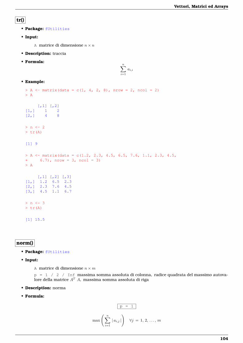
Vettori, Matrici ed Arrays
tr()
• Package: fUtilities
• Input:
A matrice di dimensione n× n
• Description: traccia
• Formula:n∑i=1
ai,i
• Example:
> A <- matrix(data = c(1, 4, 2, 8), nrow = 2, ncol = 2)> A
[,1] [,2][1,] 1 2[2,] 4 8
> n <- 2> tr(A)
[1] 9
> A <- matrix(data = c(1.2, 2.3, 4.5, 6.5, 7.6, 1.1, 2.3, 4.5,+ 6.7), nrow = 3, ncol = 3)> A
[,1] [,2] [,3][1,] 1.2 6.5 2.3[2,] 2.3 7.6 4.5[3,] 4.5 1.1 6.7
> n <- 3> tr(A)
[1] 15.5
norm()
• Package: fUtilities
• Input:
A matrice di dimensione n×mp = 1 / 2 / Inf massima somma assoluta di colonna, radice quadrata del massimo autova-lore della matrice AT A, massima somma assoluta di riga
• Description: norma
• Formula:
p = 1
max
(n∑i=1
| ai,j |
)∀j = 1, 2, . . . , m
104
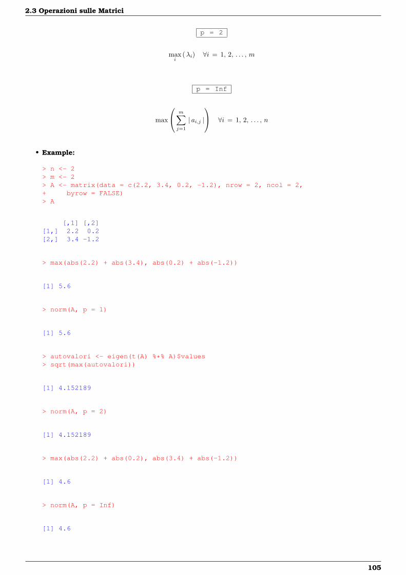
2.3 Operazioni sulle Matrici
p = 2
maxi
(λi) ∀i = 1, 2, . . . , m
p = Inf
max
m∑j=1
| ai,j |
∀i = 1, 2, . . . , n
• Example:
> n <- 2> m <- 2> A <- matrix(data = c(2.2, 3.4, 0.2, -1.2), nrow = 2, ncol = 2,+ byrow = FALSE)> A
[,1] [,2][1,] 2.2 0.2[2,] 3.4 -1.2
> max(abs(2.2) + abs(3.4), abs(0.2) + abs(-1.2))
[1] 5.6
> norm(A, p = 1)
[1] 5.6
> autovalori <- eigen(t(A) %*% A)$values> sqrt(max(autovalori))
[1] 4.152189
> norm(A, p = 2)
[1] 4.152189
> max(abs(2.2) + abs(0.2), abs(3.4) + abs(-1.2))
[1] 4.6
> norm(A, p = Inf)
[1] 4.6
105
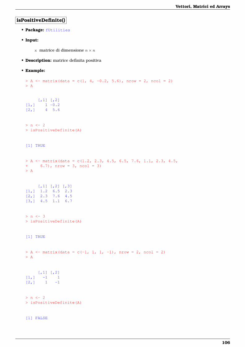
Vettori, Matrici ed Arrays
isPositiveDefinite()
• Package: fUtilities
• Input:
x matrice di dimensione n× n
• Description: matrice definita positiva
• Example:
> A <- matrix(data = c(1, 4, -0.2, 5.6), nrow = 2, ncol = 2)> A
[,1] [,2][1,] 1 -0.2[2,] 4 5.6
> n <- 2> isPositiveDefinite(A)
[1] TRUE
> A <- matrix(data = c(1.2, 2.3, 4.5, 6.5, 7.6, 1.1, 2.3, 4.5,+ 6.7), nrow = 3, ncol = 3)> A
[,1] [,2] [,3][1,] 1.2 6.5 2.3[2,] 2.3 7.6 4.5[3,] 4.5 1.1 6.7
> n <- 3> isPositiveDefinite(A)
[1] TRUE
> A <- matrix(data = c(-1, 1, 1, -1), nrow = 2, ncol = 2)> A
[,1] [,2][1,] -1 1[2,] 1 -1
> n <- 2> isPositiveDefinite(A)
[1] FALSE
106
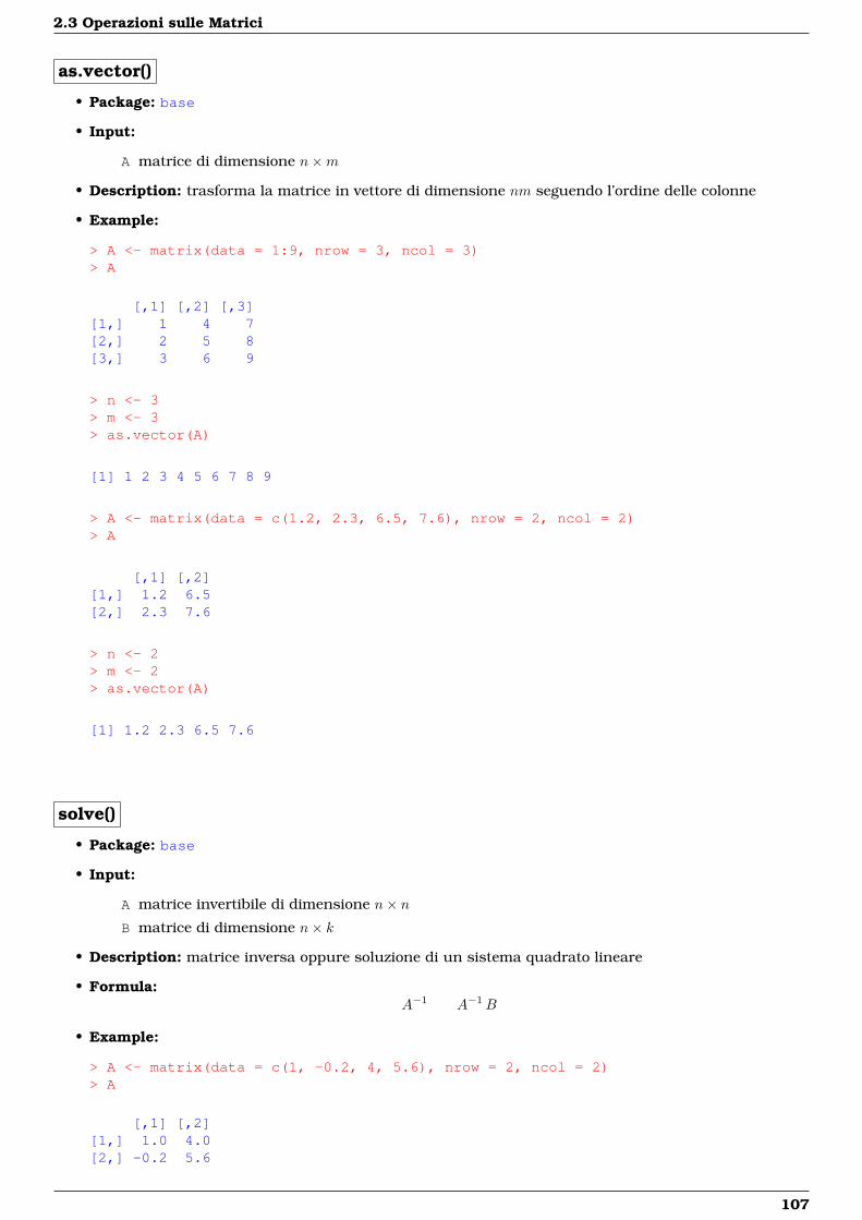
2.3 Operazioni sulle Matrici
as.vector()
• Package: base
• Input:
A matrice di dimensione n×m
• Description: trasforma la matrice in vettore di dimensione nm seguendo l’ordine delle colonne
• Example:
> A <- matrix(data = 1:9, nrow = 3, ncol = 3)> A
[,1] [,2] [,3][1,] 1 4 7[2,] 2 5 8[3,] 3 6 9
> n <- 3> m <- 3> as.vector(A)
[1] 1 2 3 4 5 6 7 8 9
> A <- matrix(data = c(1.2, 2.3, 6.5, 7.6), nrow = 2, ncol = 2)> A
[,1] [,2][1,] 1.2 6.5[2,] 2.3 7.6
> n <- 2> m <- 2> as.vector(A)
[1] 1.2 2.3 6.5 7.6
solve()
• Package: base
• Input:
A matrice invertibile di dimensione n× nB matrice di dimensione n× k
• Description: matrice inversa oppure soluzione di un sistema quadrato lineare
• Formula:A−1 A−1B
• Example:
> A <- matrix(data = c(1, -0.2, 4, 5.6), nrow = 2, ncol = 2)> A
[,1] [,2][1,] 1.0 4.0[2,] -0.2 5.6
107
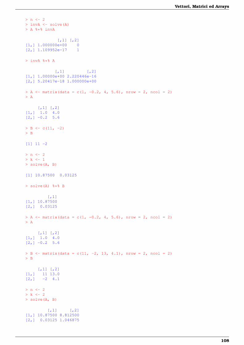
Vettori, Matrici ed Arrays
> n <- 2> invA <- solve(A)> A %*% invA
[,1] [,2][1,] 1.000000e+00 0[2,] 1.109952e-17 1
> invA %*% A
[,1] [,2][1,] 1.00000e+00 2.220446e-16[2,] 5.20417e-18 1.000000e+00
> A <- matrix(data = c(1, -0.2, 4, 5.6), nrow = 2, ncol = 2)> A
[,1] [,2][1,] 1.0 4.0[2,] -0.2 5.6
> B <- c(11, -2)> B
[1] 11 -2
> n <- 2> k <- 1> solve(A, B)
[1] 10.87500 0.03125
> solve(A) %*% B
[,1][1,] 10.87500[2,] 0.03125
> A <- matrix(data = c(1, -0.2, 4, 5.6), nrow = 2, ncol = 2)> A
[,1] [,2][1,] 1.0 4.0[2,] -0.2 5.6
> B <- matrix(data = c(11, -2, 13, 4.1), nrow = 2, ncol = 2)> B
[,1] [,2][1,] 11 13.0[2,] -2 4.1
> n <- 2> k <- 2> solve(A, B)
[,1] [,2][1,] 10.87500 8.812500[2,] 0.03125 1.046875
108
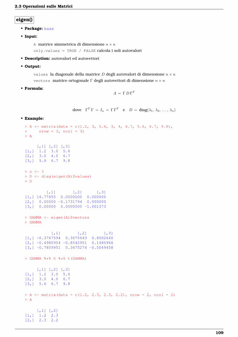
2.3 Operazioni sulle Matrici
eigen()
• Package: base
• Input:
A matrice simmetrica di dimensione n× nonly.values = TRUE / FALSE calcola i soli autovalori
• Description: autovalori ed autovettori
• Output:
values la diagonale della matrice D degli autovalori di dimensione n× nvectors matrice ortogonale Γ degli autovettori di dimensione n× n
• Formula:A = ΓD ΓT
dove ΓT Γ = In = Γ ΓT e D = diag(λ1, λ2, . . . , λn)
• Example:
> A <- matrix(data = c(1.2, 3, 5.6, 3, 4, 6.7, 5.6, 6.7, 9.8),+ nrow = 3, ncol = 3)> A
[,1] [,2] [,3][1,] 1.2 3.0 5.6[2,] 3.0 4.0 6.7[3,] 5.6 6.7 9.8
> n <- 3> D <- diag(eigen(A)$values)> D
[,1] [,2] [,3][1,] 16.77455 0.0000000 0.000000[2,] 0.00000 -0.1731794 0.000000[3,] 0.00000 0.0000000 -1.601373
> GAMMA <- eigen(A)$vectors> GAMMA
[,1] [,2] [,3][1,] -0.3767594 0.3675643 0.8502640[2,] -0.4980954 -0.8542951 0.1485966[3,] -0.7809951 0.3675274 -0.5049458
> GAMMA %*% D %*% t(GAMMA)
[,1] [,2] [,3][1,] 1.2 3.0 5.6[2,] 3.0 4.0 6.7[3,] 5.6 6.7 9.8
> A <- matrix(data = c(1.2, 2.3, 2.3, 2.2), nrow = 2, ncol = 2)> A
[,1] [,2][1,] 1.2 2.3[2,] 2.3 2.2
109
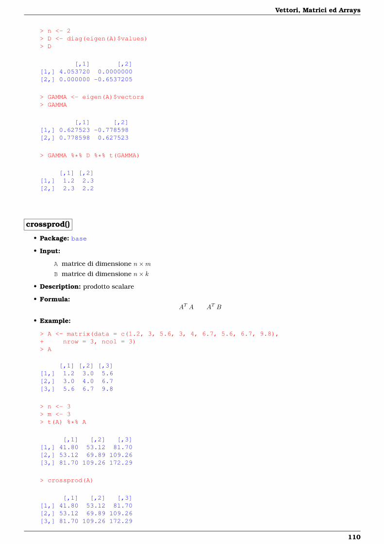
Vettori, Matrici ed Arrays
> n <- 2> D <- diag(eigen(A)$values)> D
[,1] [,2][1,] 4.053720 0.0000000[2,] 0.000000 -0.6537205
> GAMMA <- eigen(A)$vectors> GAMMA
[,1] [,2][1,] 0.627523 -0.778598[2,] 0.778598 0.627523
> GAMMA %*% D %*% t(GAMMA)
[,1] [,2][1,] 1.2 2.3[2,] 2.3 2.2
crossprod()
• Package: base
• Input:
A matrice di dimensione n×mB matrice di dimensione n× k
• Description: prodotto scalare
• Formula:AT A AT B
• Example:
> A <- matrix(data = c(1.2, 3, 5.6, 3, 4, 6.7, 5.6, 6.7, 9.8),+ nrow = 3, ncol = 3)> A
[,1] [,2] [,3][1,] 1.2 3.0 5.6[2,] 3.0 4.0 6.7[3,] 5.6 6.7 9.8
> n <- 3> m <- 3> t(A) %*% A
[,1] [,2] [,3][1,] 41.80 53.12 81.70[2,] 53.12 69.89 109.26[3,] 81.70 109.26 172.29
> crossprod(A)
[,1] [,2] [,3][1,] 41.80 53.12 81.70[2,] 53.12 69.89 109.26[3,] 81.70 109.26 172.29
110
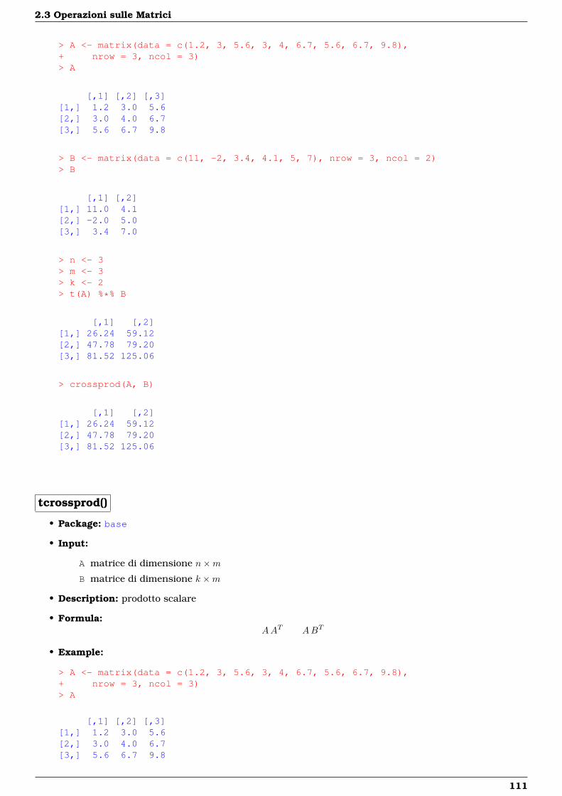
2.3 Operazioni sulle Matrici
> A <- matrix(data = c(1.2, 3, 5.6, 3, 4, 6.7, 5.6, 6.7, 9.8),+ nrow = 3, ncol = 3)> A
[,1] [,2] [,3][1,] 1.2 3.0 5.6[2,] 3.0 4.0 6.7[3,] 5.6 6.7 9.8
> B <- matrix(data = c(11, -2, 3.4, 4.1, 5, 7), nrow = 3, ncol = 2)> B
[,1] [,2][1,] 11.0 4.1[2,] -2.0 5.0[3,] 3.4 7.0
> n <- 3> m <- 3> k <- 2> t(A) %*% B
[,1] [,2][1,] 26.24 59.12[2,] 47.78 79.20[3,] 81.52 125.06
> crossprod(A, B)
[,1] [,2][1,] 26.24 59.12[2,] 47.78 79.20[3,] 81.52 125.06
tcrossprod()
• Package: base
• Input:
A matrice di dimensione n×mB matrice di dimensione k ×m
• Description: prodotto scalare
• Formula:AAT ABT
• Example:
> A <- matrix(data = c(1.2, 3, 5.6, 3, 4, 6.7, 5.6, 6.7, 9.8),+ nrow = 3, ncol = 3)> A
[,1] [,2] [,3][1,] 1.2 3.0 5.6[2,] 3.0 4.0 6.7[3,] 5.6 6.7 9.8
111
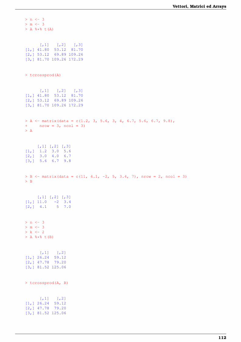
Vettori, Matrici ed Arrays
> n <- 3> m <- 3> A %*% t(A)
[,1] [,2] [,3][1,] 41.80 53.12 81.70[2,] 53.12 69.89 109.26[3,] 81.70 109.26 172.29
> tcrossprod(A)
[,1] [,2] [,3][1,] 41.80 53.12 81.70[2,] 53.12 69.89 109.26[3,] 81.70 109.26 172.29
> A <- matrix(data = c(1.2, 3, 5.6, 3, 4, 6.7, 5.6, 6.7, 9.8),+ nrow = 3, ncol = 3)> A
[,1] [,2] [,3][1,] 1.2 3.0 5.6[2,] 3.0 4.0 6.7[3,] 5.6 6.7 9.8
> B <- matrix(data = c(11, 4.1, -2, 5, 3.4, 7), nrow = 2, ncol = 3)> B
[,1] [,2] [,3][1,] 11.0 -2 3.4[2,] 4.1 5 7.0
> n <- 3> m <- 3> k <- 2> A %*% t(B)
[,1] [,2][1,] 26.24 59.12[2,] 47.78 79.20[3,] 81.52 125.06
> tcrossprod(A, B)
[,1] [,2][1,] 26.24 59.12[2,] 47.78 79.20[3,] 81.52 125.06
112
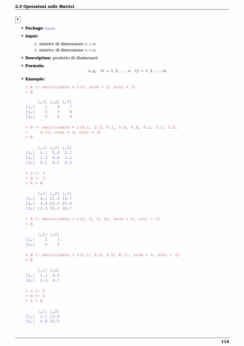
2.3 Operazioni sulle Matrici
*
• Package: base
• Input:
A matrice di dimensione n×mB matrice di dimensione n×m
• Description: prodotto di Hadamard
• Formula:xi yj ∀i = 1, 2, . . . , n ∀j = 1, 2, . . . , m
• Example:
> A <- matrix(data = 1:9, nrow = 3, ncol = 3)> A
[,1] [,2] [,3][1,] 1 4 7[2,] 2 5 8[3,] 3 6 9
> B <- matrix(data = c(4.1, 2.3, 4.1, 5.4, 4.6, 4.2, 2.1, 3.2,+ 4.3), nrow = 3, ncol = 3)> B
[,1] [,2] [,3][1,] 4.1 5.4 2.1[2,] 2.3 4.6 3.2[3,] 4.1 4.2 4.3
> n <- 3> m <- 3> A * B
[,1] [,2] [,3][1,] 4.1 21.6 14.7[2,] 4.6 23.0 25.6[3,] 12.3 25.2 38.7
> A <- matrix(data = c(1, 2, 3, 5), nrow = 2, ncol = 2)> A
[,1] [,2][1,] 1 3[2,] 2 5
> B <- matrix(data = c(1.1, 2.3, 4.5, 6.7), nrow = 2, ncol = 2)> B
[,1] [,2][1,] 1.1 4.5[2,] 2.3 6.7
> n <- 2> m <- 2> A * B
[,1] [,2][1,] 1.1 13.5[2,] 4.6 33.5
113
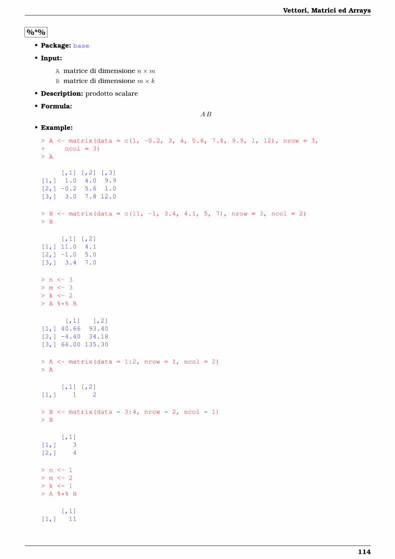
Vettori, Matrici ed Arrays
%*%
• Package: base
• Input:
A matrice di dimensione n×mB matrice di dimensione m× k
• Description: prodotto scalare
• Formula:AB
• Example:
> A <- matrix(data = c(1, -0.2, 3, 4, 5.6, 7.8, 9.9, 1, 12), nrow = 3,+ ncol = 3)> A
[,1] [,2] [,3][1,] 1.0 4.0 9.9[2,] -0.2 5.6 1.0[3,] 3.0 7.8 12.0
> B <- matrix(data = c(11, -1, 3.4, 4.1, 5, 7), nrow = 3, ncol = 2)> B
[,1] [,2][1,] 11.0 4.1[2,] -1.0 5.0[3,] 3.4 7.0
> n <- 3> m <- 3> k <- 2> A %*% B
[,1] [,2][1,] 40.66 93.40[2,] -4.40 34.18[3,] 66.00 135.30
> A <- matrix(data = 1:2, nrow = 1, ncol = 2)> A
[,1] [,2][1,] 1 2
> B <- matrix(data = 3:4, nrow = 2, ncol = 1)> B
[,1][1,] 3[2,] 4
> n <- 1> m <- 2> k <- 1> A %*% B
[,1][1,] 11
114
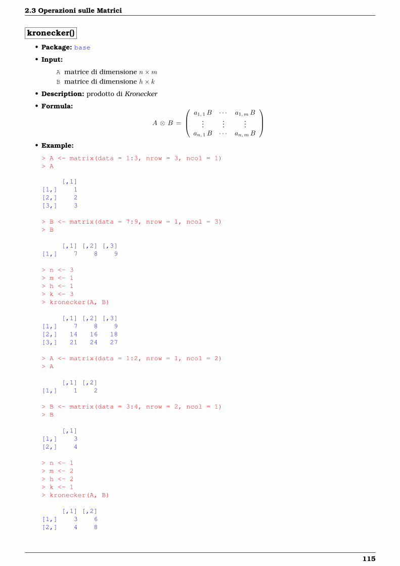
2.3 Operazioni sulle Matrici
kronecker()
• Package: base
• Input:
A matrice di dimensione n×mB matrice di dimensione h× k
• Description: prodotto di Kronecker
• Formula:
A ⊗ B =
a1, 1B · · · a1,mB...
......
an, 1B · · · an,mB
• Example:
> A <- matrix(data = 1:3, nrow = 3, ncol = 1)> A
[,1][1,] 1[2,] 2[3,] 3
> B <- matrix(data = 7:9, nrow = 1, ncol = 3)> B
[,1] [,2] [,3][1,] 7 8 9
> n <- 3> m <- 1> h <- 1> k <- 3> kronecker(A, B)
[,1] [,2] [,3][1,] 7 8 9[2,] 14 16 18[3,] 21 24 27
> A <- matrix(data = 1:2, nrow = 1, ncol = 2)> A
[,1] [,2][1,] 1 2
> B <- matrix(data = 3:4, nrow = 2, ncol = 1)> B
[,1][1,] 3[2,] 4
> n <- 1> m <- 2> h <- 2> k <- 1> kronecker(A, B)
[,1] [,2][1,] 3 6[2,] 4 8
115
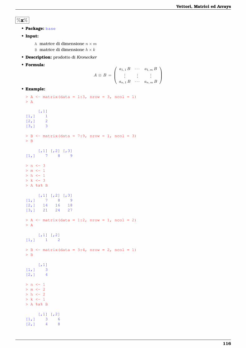
Vettori, Matrici ed Arrays
%x%
• Package: base
• Input:
A matrice di dimensione n×mB matrice di dimensione h× k
• Description: prodotto di Kronecker
• Formula:
A ⊗ B =
a1, 1B · · · a1,mB...
......
an, 1B · · · an,mB
• Example:
> A <- matrix(data = 1:3, nrow = 3, ncol = 1)> A
[,1][1,] 1[2,] 2[3,] 3
> B <- matrix(data = 7:9, nrow = 1, ncol = 3)> B
[,1] [,2] [,3][1,] 7 8 9
> n <- 3> m <- 1> h <- 1> k <- 3> A %x% B
[,1] [,2] [,3][1,] 7 8 9[2,] 14 16 18[3,] 21 24 27
> A <- matrix(data = 1:2, nrow = 1, ncol = 2)> A
[,1] [,2][1,] 1 2
> B <- matrix(data = 3:4, nrow = 2, ncol = 1)> B
[,1][1,] 3[2,] 4
> n <- 1> m <- 2> h <- 2> k <- 1> A %x% B
[,1] [,2][1,] 3 6[2,] 4 8
116
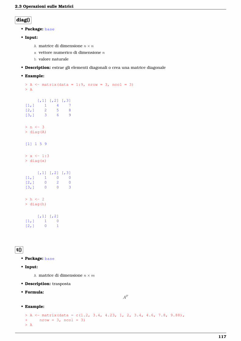
2.3 Operazioni sulle Matrici
diag()
• Package: base
• Input:
A matrice di dimensione n× nx vettore numerico di dimensione n
h valore naturale
• Description: estrae gli elementi diagonali o crea una matrice diagonale
• Example:
> A <- matrix(data = 1:9, nrow = 3, ncol = 3)> A
[,1] [,2] [,3][1,] 1 4 7[2,] 2 5 8[3,] 3 6 9
> n <- 3> diag(A)
[1] 1 5 9
> x <- 1:3> diag(x)
[,1] [,2] [,3][1,] 1 0 0[2,] 0 2 0[3,] 0 0 3
> h <- 2> diag(h)
[,1] [,2][1,] 1 0[2,] 0 1
t()
• Package: base
• Input:
A matrice di dimensione n×m
• Description: trasposta
• Formula:AT
• Example:
> A <- matrix(data = c(1.2, 3.4, 4.23, 1, 2, 3.4, 4.6, 7.8, 9.88),+ nrow = 3, ncol = 3)> A
117
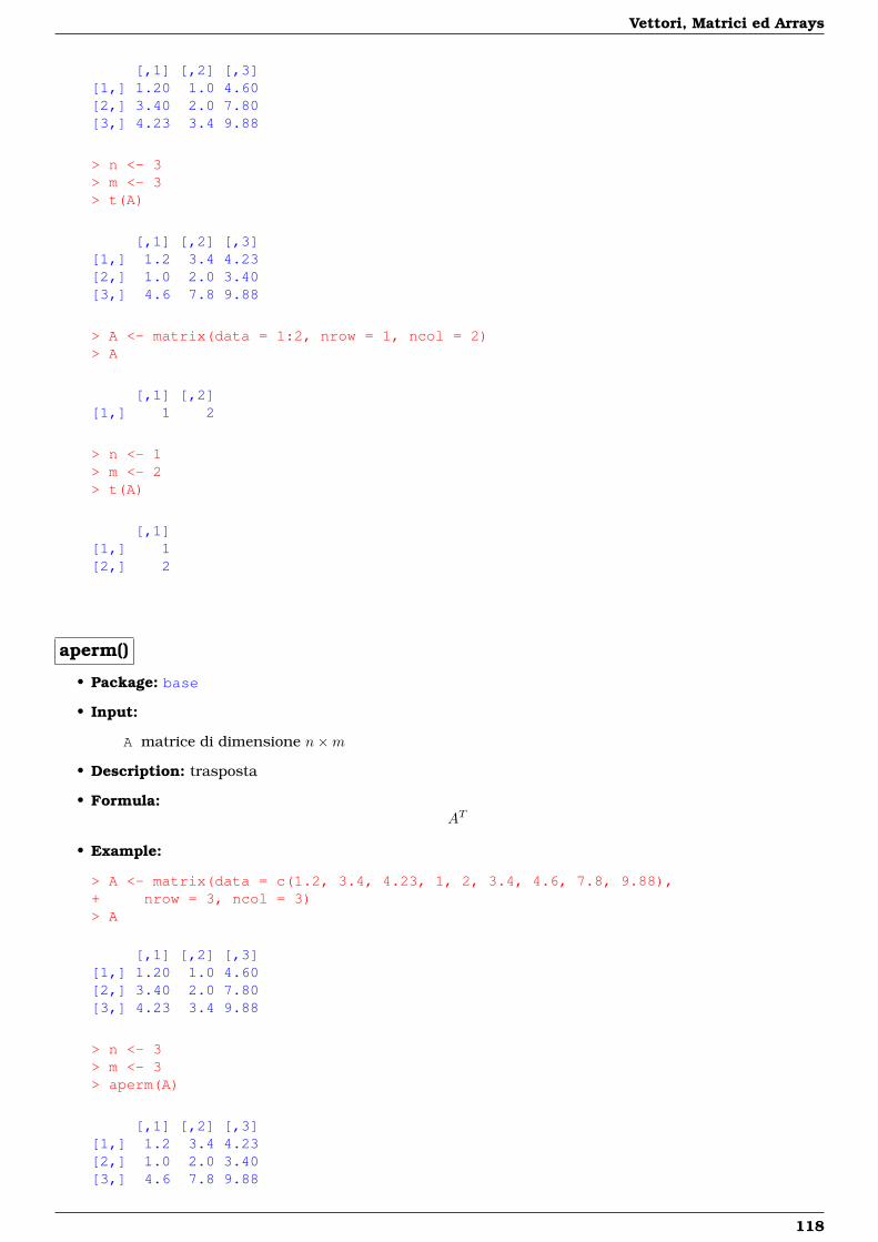
Vettori, Matrici ed Arrays
[,1] [,2] [,3][1,] 1.20 1.0 4.60[2,] 3.40 2.0 7.80[3,] 4.23 3.4 9.88
> n <- 3> m <- 3> t(A)
[,1] [,2] [,3][1,] 1.2 3.4 4.23[2,] 1.0 2.0 3.40[3,] 4.6 7.8 9.88
> A <- matrix(data = 1:2, nrow = 1, ncol = 2)> A
[,1] [,2][1,] 1 2
> n <- 1> m <- 2> t(A)
[,1][1,] 1[2,] 2
aperm()
• Package: base
• Input:
A matrice di dimensione n×m
• Description: trasposta
• Formula:AT
• Example:
> A <- matrix(data = c(1.2, 3.4, 4.23, 1, 2, 3.4, 4.6, 7.8, 9.88),+ nrow = 3, ncol = 3)> A
[,1] [,2] [,3][1,] 1.20 1.0 4.60[2,] 3.40 2.0 7.80[3,] 4.23 3.4 9.88
> n <- 3> m <- 3> aperm(A)
[,1] [,2] [,3][1,] 1.2 3.4 4.23[2,] 1.0 2.0 3.40[3,] 4.6 7.8 9.88
118

2.3 Operazioni sulle Matrici
> A <- matrix(data = 1:2, nrow = 1, ncol = 2)> A
[,1] [,2][1,] 1 2
> n <- 1> m <- 2> t(A)
[,1][1,] 1[2,] 2
dim()
• Package: base
• Input:
A matrice di dimensione n×m
• Description: numero di righe e di colonne
• Formula:n m
• Example:
> A <- matrix(data = c(1, -0.2, 3, 4, 5.6, 7.8, 9.9, 1, 12), nrow = 3,+ ncol = 3)> A
[,1] [,2] [,3][1,] 1.0 4.0 9.9[2,] -0.2 5.6 1.0[3,] 3.0 7.8 12.0
> dim(A)
[1] 3 3
> A <- matrix(data = c(1.2, 2.3, 6.5, 7.6), nrow = 2, ncol = 2)> A
[,1] [,2][1,] 1.2 6.5[2,] 2.3 7.6
> n <- 2> m <- 2> dim(A)
[1] 2 2
119
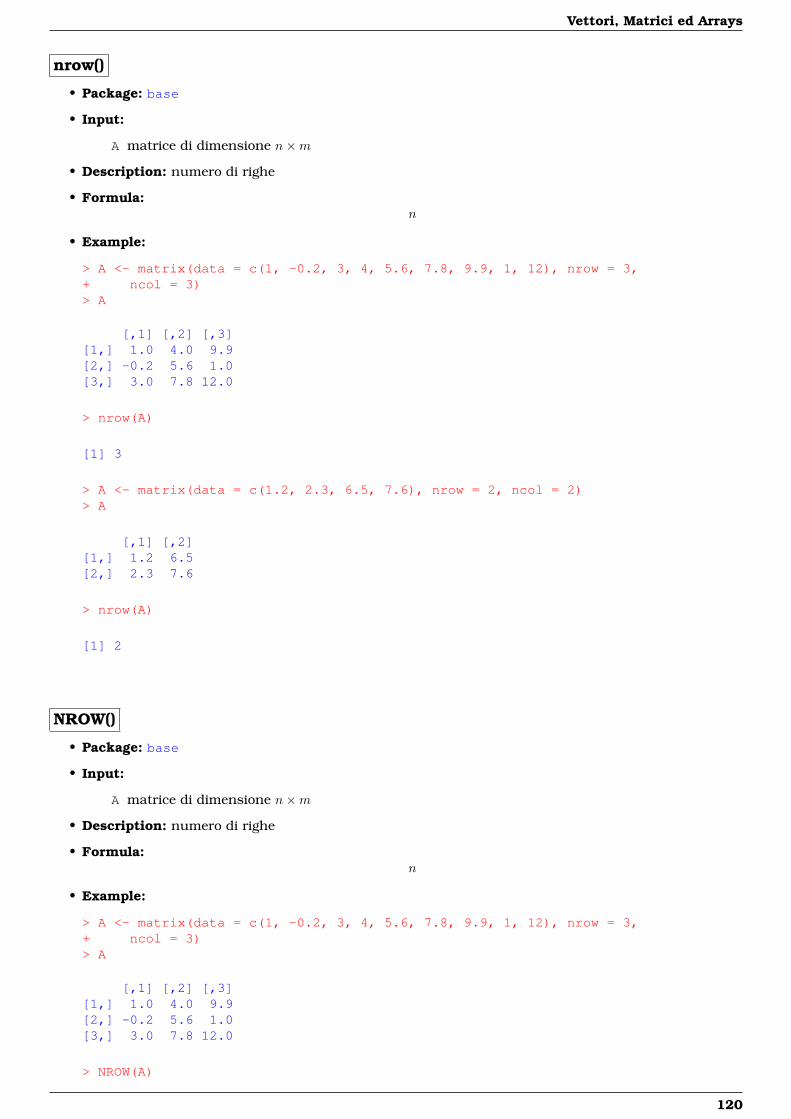
Vettori, Matrici ed Arrays
nrow()
• Package: base
• Input:
A matrice di dimensione n×m
• Description: numero di righe
• Formula:n
• Example:
> A <- matrix(data = c(1, -0.2, 3, 4, 5.6, 7.8, 9.9, 1, 12), nrow = 3,+ ncol = 3)> A
[,1] [,2] [,3][1,] 1.0 4.0 9.9[2,] -0.2 5.6 1.0[3,] 3.0 7.8 12.0
> nrow(A)
[1] 3
> A <- matrix(data = c(1.2, 2.3, 6.5, 7.6), nrow = 2, ncol = 2)> A
[,1] [,2][1,] 1.2 6.5[2,] 2.3 7.6
> nrow(A)
[1] 2
NROW()
• Package: base
• Input:
A matrice di dimensione n×m
• Description: numero di righe
• Formula:n
• Example:
> A <- matrix(data = c(1, -0.2, 3, 4, 5.6, 7.8, 9.9, 1, 12), nrow = 3,+ ncol = 3)> A
[,1] [,2] [,3][1,] 1.0 4.0 9.9[2,] -0.2 5.6 1.0[3,] 3.0 7.8 12.0
> NROW(A)
120
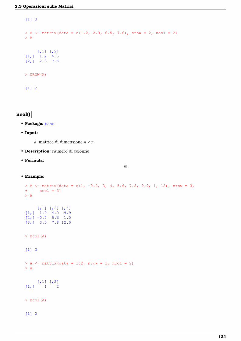
2.3 Operazioni sulle Matrici
[1] 3
> A <- matrix(data = c(1.2, 2.3, 6.5, 7.6), nrow = 2, ncol = 2)> A
[,1] [,2][1,] 1.2 6.5[2,] 2.3 7.6
> NROW(A)
[1] 2
ncol()
• Package: base
• Input:
A matrice di dimensione n×m
• Description: numero di colonne
• Formula:m
• Example:
> A <- matrix(data = c(1, -0.2, 3, 4, 5.6, 7.8, 9.9, 1, 12), nrow = 3,+ ncol = 3)> A
[,1] [,2] [,3][1,] 1.0 4.0 9.9[2,] -0.2 5.6 1.0[3,] 3.0 7.8 12.0
> ncol(A)
[1] 3
> A <- matrix(data = 1:2, nrow = 1, ncol = 2)> A
[,1] [,2][1,] 1 2
> ncol(A)
[1] 2
121
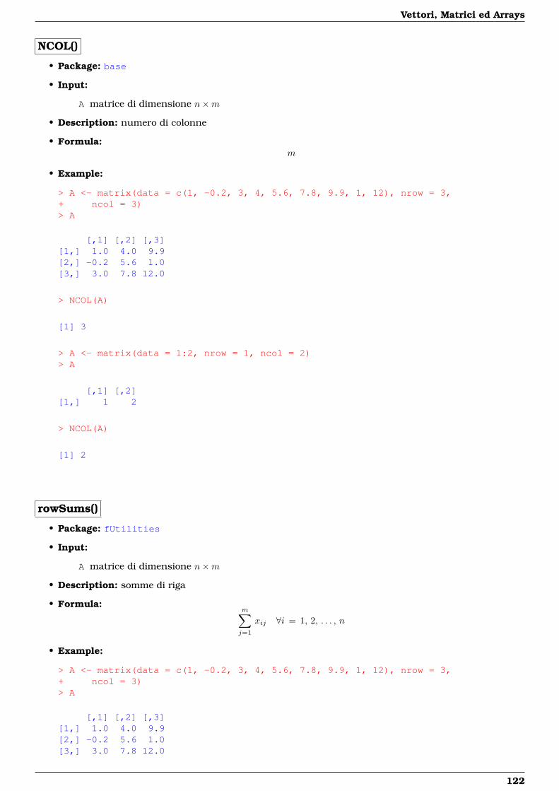
Vettori, Matrici ed Arrays
NCOL()
• Package: base
• Input:
A matrice di dimensione n×m
• Description: numero di colonne
• Formula:m
• Example:
> A <- matrix(data = c(1, -0.2, 3, 4, 5.6, 7.8, 9.9, 1, 12), nrow = 3,+ ncol = 3)> A
[,1] [,2] [,3][1,] 1.0 4.0 9.9[2,] -0.2 5.6 1.0[3,] 3.0 7.8 12.0
> NCOL(A)
[1] 3
> A <- matrix(data = 1:2, nrow = 1, ncol = 2)> A
[,1] [,2][1,] 1 2
> NCOL(A)
[1] 2
rowSums()
• Package: fUtilities
• Input:
A matrice di dimensione n×m
• Description: somme di riga
• Formula:m∑j=1
xij ∀i = 1, 2, . . . , n
• Example:
> A <- matrix(data = c(1, -0.2, 3, 4, 5.6, 7.8, 9.9, 1, 12), nrow = 3,+ ncol = 3)> A
[,1] [,2] [,3][1,] 1.0 4.0 9.9[2,] -0.2 5.6 1.0[3,] 3.0 7.8 12.0
122
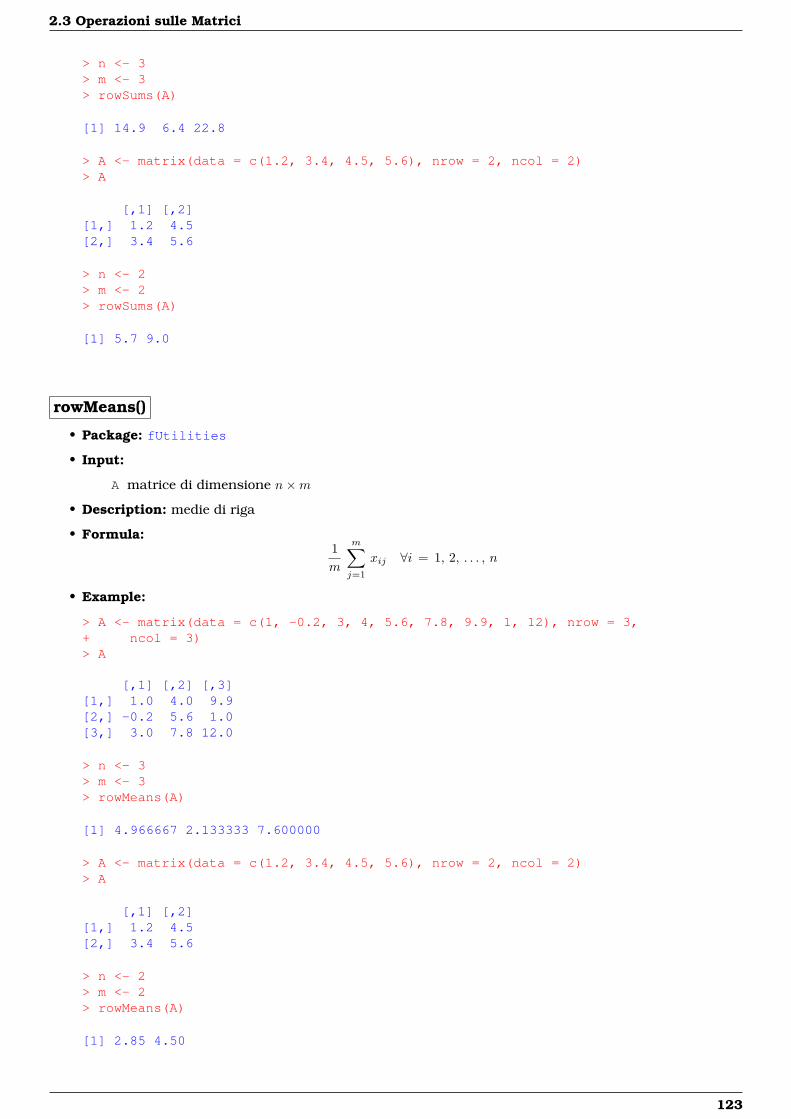
2.3 Operazioni sulle Matrici
> n <- 3> m <- 3> rowSums(A)
[1] 14.9 6.4 22.8
> A <- matrix(data = c(1.2, 3.4, 4.5, 5.6), nrow = 2, ncol = 2)> A
[,1] [,2][1,] 1.2 4.5[2,] 3.4 5.6
> n <- 2> m <- 2> rowSums(A)
[1] 5.7 9.0
rowMeans()
• Package: fUtilities
• Input:
A matrice di dimensione n×m
• Description: medie di riga
• Formula:1m
m∑j=1
xij ∀i = 1, 2, . . . , n
• Example:
> A <- matrix(data = c(1, -0.2, 3, 4, 5.6, 7.8, 9.9, 1, 12), nrow = 3,+ ncol = 3)> A
[,1] [,2] [,3][1,] 1.0 4.0 9.9[2,] -0.2 5.6 1.0[3,] 3.0 7.8 12.0
> n <- 3> m <- 3> rowMeans(A)
[1] 4.966667 2.133333 7.600000
> A <- matrix(data = c(1.2, 3.4, 4.5, 5.6), nrow = 2, ncol = 2)> A
[,1] [,2][1,] 1.2 4.5[2,] 3.4 5.6
> n <- 2> m <- 2> rowMeans(A)
[1] 2.85 4.50
123
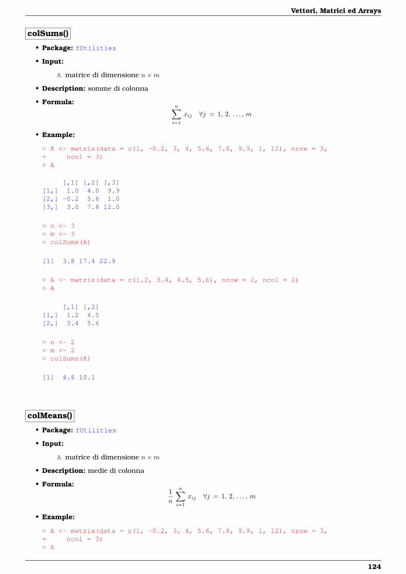
Vettori, Matrici ed Arrays
colSums()
• Package: fUtilities
• Input:
A matrice di dimensione n×m
• Description: somme di colonna
• Formula:n∑i=1
xij ∀j = 1, 2, . . . , m
• Example:
> A <- matrix(data = c(1, -0.2, 3, 4, 5.6, 7.8, 9.9, 1, 12), nrow = 3,+ ncol = 3)> A
[,1] [,2] [,3][1,] 1.0 4.0 9.9[2,] -0.2 5.6 1.0[3,] 3.0 7.8 12.0
> n <- 3> m <- 3> colSums(A)
[1] 3.8 17.4 22.9
> A <- matrix(data = c(1.2, 3.4, 4.5, 5.6), nrow = 2, ncol = 2)> A
[,1] [,2][1,] 1.2 4.5[2,] 3.4 5.6
> n <- 2> m <- 2> colSums(A)
[1] 4.6 10.1
colMeans()
• Package: fUtilities
• Input:
A matrice di dimensione n×m
• Description: medie di colonna
• Formula:1n
n∑i=1
xij ∀j = 1, 2, . . . , m
• Example:
> A <- matrix(data = c(1, -0.2, 3, 4, 5.6, 7.8, 9.9, 1, 12), nrow = 3,+ ncol = 3)> A
124
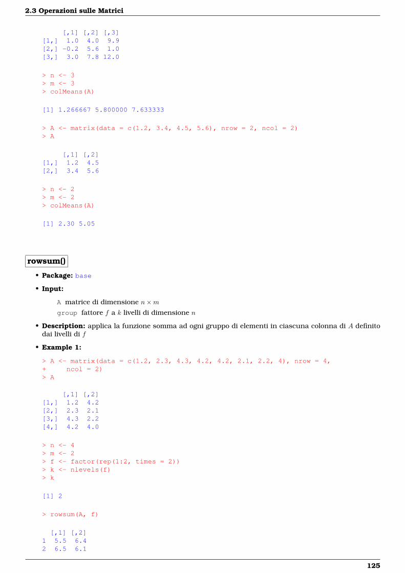
2.3 Operazioni sulle Matrici
[,1] [,2] [,3][1,] 1.0 4.0 9.9[2,] -0.2 5.6 1.0[3,] 3.0 7.8 12.0
> n <- 3> m <- 3> colMeans(A)
[1] 1.266667 5.800000 7.633333
> A <- matrix(data = c(1.2, 3.4, 4.5, 5.6), nrow = 2, ncol = 2)> A
[,1] [,2][1,] 1.2 4.5[2,] 3.4 5.6
> n <- 2> m <- 2> colMeans(A)
[1] 2.30 5.05
rowsum()
• Package: base
• Input:
A matrice di dimensione n×mgroup fattore f a k livelli di dimensione n
• Description: applica la funzione somma ad ogni gruppo di elementi in ciascuna colonna di A definitodai livelli di f
• Example 1:
> A <- matrix(data = c(1.2, 2.3, 4.3, 4.2, 4.2, 2.1, 2.2, 4), nrow = 4,+ ncol = 2)> A
[,1] [,2][1,] 1.2 4.2[2,] 2.3 2.1[3,] 4.3 2.2[4,] 4.2 4.0
> n <- 4> m <- 2> f <- factor(rep(1:2, times = 2))> k <- nlevels(f)> k
[1] 2
> rowsum(A, f)
[,1] [,2]1 5.5 6.42 6.5 6.1
125
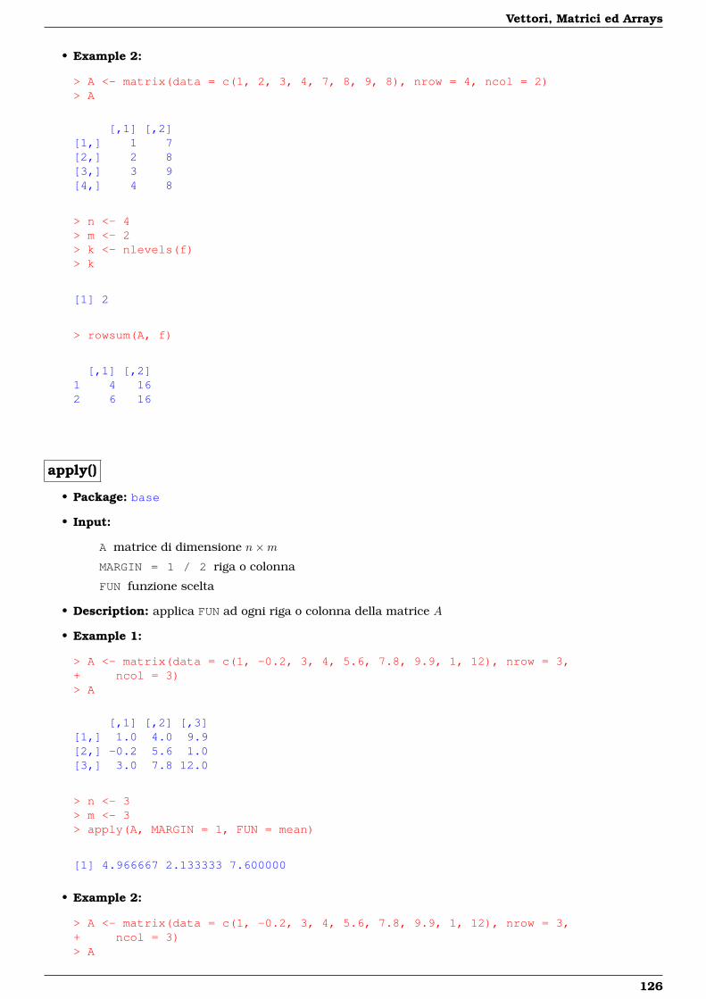
Vettori, Matrici ed Arrays
• Example 2:
> A <- matrix(data = c(1, 2, 3, 4, 7, 8, 9, 8), nrow = 4, ncol = 2)> A
[,1] [,2][1,] 1 7[2,] 2 8[3,] 3 9[4,] 4 8
> n <- 4> m <- 2> k <- nlevels(f)> k
[1] 2
> rowsum(A, f)
[,1] [,2]1 4 162 6 16
apply()
• Package: base
• Input:
A matrice di dimensione n×mMARGIN = 1 / 2 riga o colonna
FUN funzione scelta
• Description: applica FUN ad ogni riga o colonna della matrice A
• Example 1:
> A <- matrix(data = c(1, -0.2, 3, 4, 5.6, 7.8, 9.9, 1, 12), nrow = 3,+ ncol = 3)> A
[,1] [,2] [,3][1,] 1.0 4.0 9.9[2,] -0.2 5.6 1.0[3,] 3.0 7.8 12.0
> n <- 3> m <- 3> apply(A, MARGIN = 1, FUN = mean)
[1] 4.966667 2.133333 7.600000
• Example 2:
> A <- matrix(data = c(1, -0.2, 3, 4, 5.6, 7.8, 9.9, 1, 12), nrow = 3,+ ncol = 3)> A
126
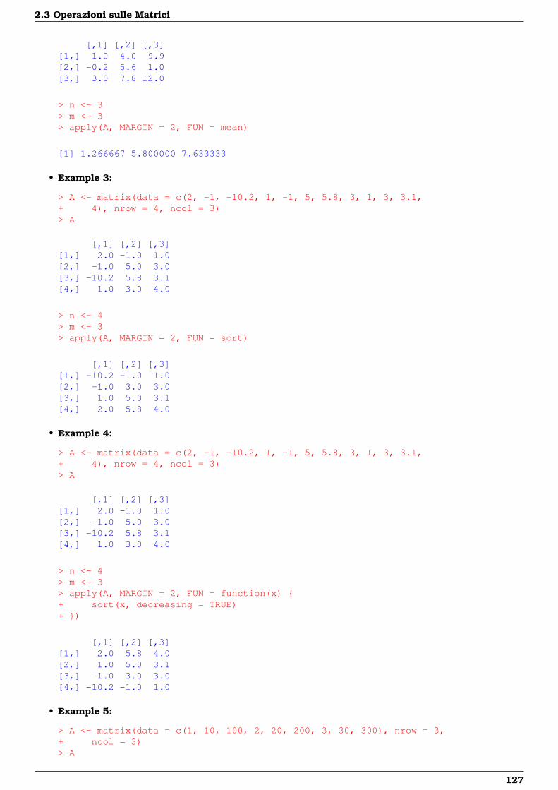
2.3 Operazioni sulle Matrici
[,1] [,2] [,3][1,] 1.0 4.0 9.9[2,] -0.2 5.6 1.0[3,] 3.0 7.8 12.0
> n <- 3> m <- 3> apply(A, MARGIN = 2, FUN = mean)
[1] 1.266667 5.800000 7.633333
• Example 3:
> A <- matrix(data = c(2, -1, -10.2, 1, -1, 5, 5.8, 3, 1, 3, 3.1,+ 4), nrow = 4, ncol = 3)> A
[,1] [,2] [,3][1,] 2.0 -1.0 1.0[2,] -1.0 5.0 3.0[3,] -10.2 5.8 3.1[4,] 1.0 3.0 4.0
> n <- 4> m <- 3> apply(A, MARGIN = 2, FUN = sort)
[,1] [,2] [,3][1,] -10.2 -1.0 1.0[2,] -1.0 3.0 3.0[3,] 1.0 5.0 3.1[4,] 2.0 5.8 4.0
• Example 4:
> A <- matrix(data = c(2, -1, -10.2, 1, -1, 5, 5.8, 3, 1, 3, 3.1,+ 4), nrow = 4, ncol = 3)> A
[,1] [,2] [,3][1,] 2.0 -1.0 1.0[2,] -1.0 5.0 3.0[3,] -10.2 5.8 3.1[4,] 1.0 3.0 4.0
> n <- 4> m <- 3> apply(A, MARGIN = 2, FUN = function(x) {+ sort(x, decreasing = TRUE)+ })
[,1] [,2] [,3][1,] 2.0 5.8 4.0[2,] 1.0 5.0 3.1[3,] -1.0 3.0 3.0[4,] -10.2 -1.0 1.0
• Example 5:
> A <- matrix(data = c(1, 10, 100, 2, 20, 200, 3, 30, 300), nrow = 3,+ ncol = 3)> A
127
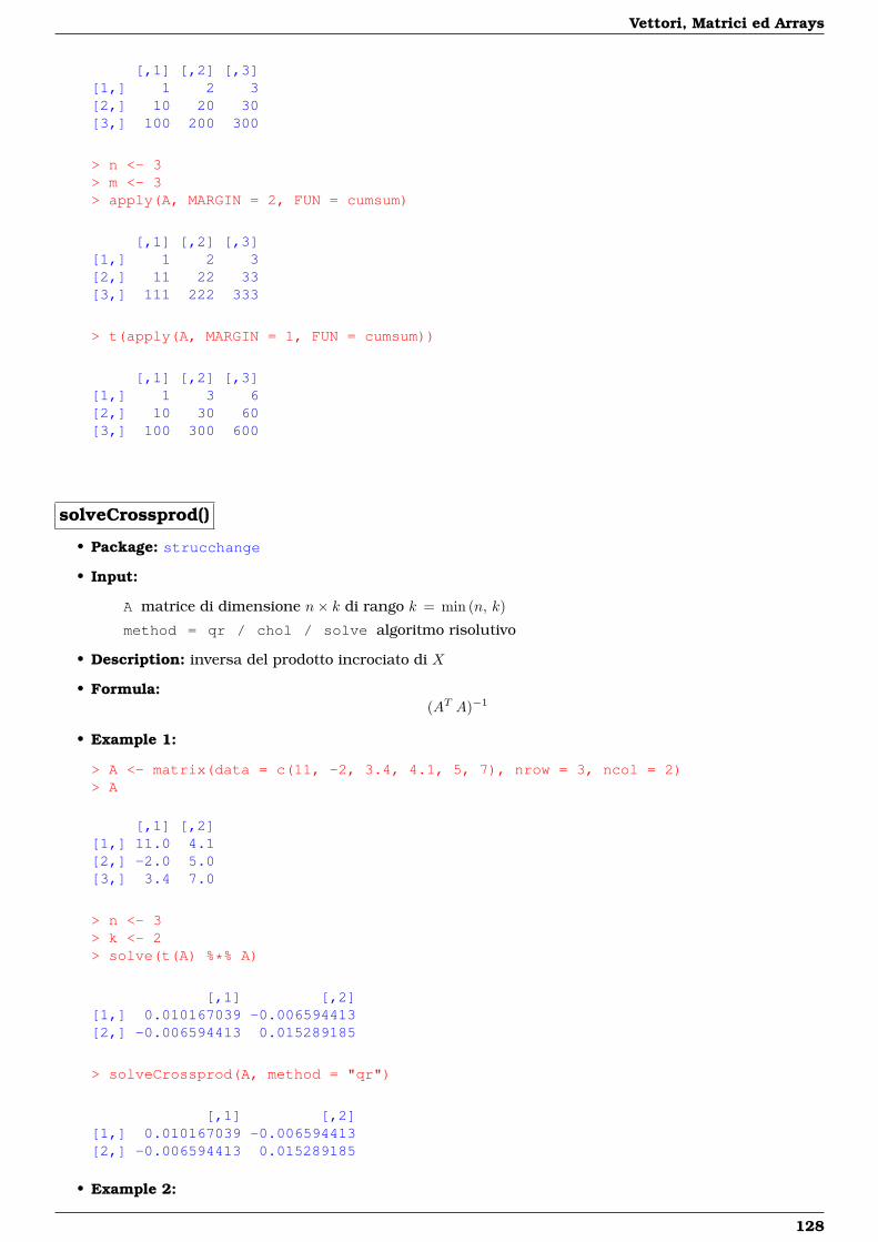
Vettori, Matrici ed Arrays
[,1] [,2] [,3][1,] 1 2 3[2,] 10 20 30[3,] 100 200 300
> n <- 3> m <- 3> apply(A, MARGIN = 2, FUN = cumsum)
[,1] [,2] [,3][1,] 1 2 3[2,] 11 22 33[3,] 111 222 333
> t(apply(A, MARGIN = 1, FUN = cumsum))
[,1] [,2] [,3][1,] 1 3 6[2,] 10 30 60[3,] 100 300 600
solveCrossprod()
• Package: strucchange
• Input:
A matrice di dimensione n× k di rango k = min (n, k)
method = qr / chol / solve algoritmo risolutivo
• Description: inversa del prodotto incrociato di X
• Formula:(AT A)−1
• Example 1:
> A <- matrix(data = c(11, -2, 3.4, 4.1, 5, 7), nrow = 3, ncol = 2)> A
[,1] [,2][1,] 11.0 4.1[2,] -2.0 5.0[3,] 3.4 7.0
> n <- 3> k <- 2> solve(t(A) %*% A)
[,1] [,2][1,] 0.010167039 -0.006594413[2,] -0.006594413 0.015289185
> solveCrossprod(A, method = "qr")
[,1] [,2][1,] 0.010167039 -0.006594413[2,] -0.006594413 0.015289185
• Example 2:
128
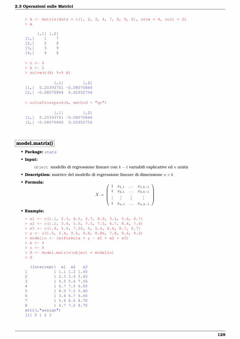
2.3 Operazioni sulle Matrici
> A <- matrix(data = c(1, 2, 3, 4, 7, 8, 9, 8), nrow = 4, ncol = 2)> A
[,1] [,2][1,] 1 7[2,] 2 8[3,] 3 9[4,] 4 8
> n <- 4> k <- 2> solve(t(A) %*% A)
[,1] [,2][1,] 0.25393701 -0.08070866[2,] -0.08070866 0.02952756
> solveCrossprod(A, method = "qr")
[,1] [,2][1,] 0.25393701 -0.08070866[2,] -0.08070866 0.02952756
model.matrix()
• Package: stats
• Input:
object modello di regressione lineare con k − 1 variabili esplicative ed n unità
• Description: matrice del modello di regressione lineare di dimensione n× k
• Formula:
X =
1 x1, 1 . . . x1, k−1
1 x2, 1 . . . x2, k−1
......
......
1 xn, 1 . . . xn, k−1
• Example:
> x1 <- c(1.1, 2.3, 4.5, 6.7, 8.9, 3.4, 5.6, 6.7)> x2 <- c(1.2, 3.4, 5.6, 7.5, 7.5, 6.7, 8.6, 7.6)> x3 <- c(1.4, 5.6, 7.56, 6, 5.4, 6.6, 8.7, 8.7)> y <- c(1.5, 6.4, 9.6, 8.8, 8.86, 7.8, 8.6, 8.6)> modello <- lm(formula = y ~ x1 + x2 + x3)> k <- 4> n <- 8> X <- model.matrix(object = modello)> X
(Intercept) x1 x2 x31 1 1.1 1.2 1.402 1 2.3 3.4 5.603 1 4.5 5.6 7.564 1 6.7 7.5 6.005 1 8.9 7.5 5.406 1 3.4 6.7 6.607 1 5.6 8.6 8.708 1 6.7 7.6 8.70attr(,"assign")[1] 0 1 2 3
129
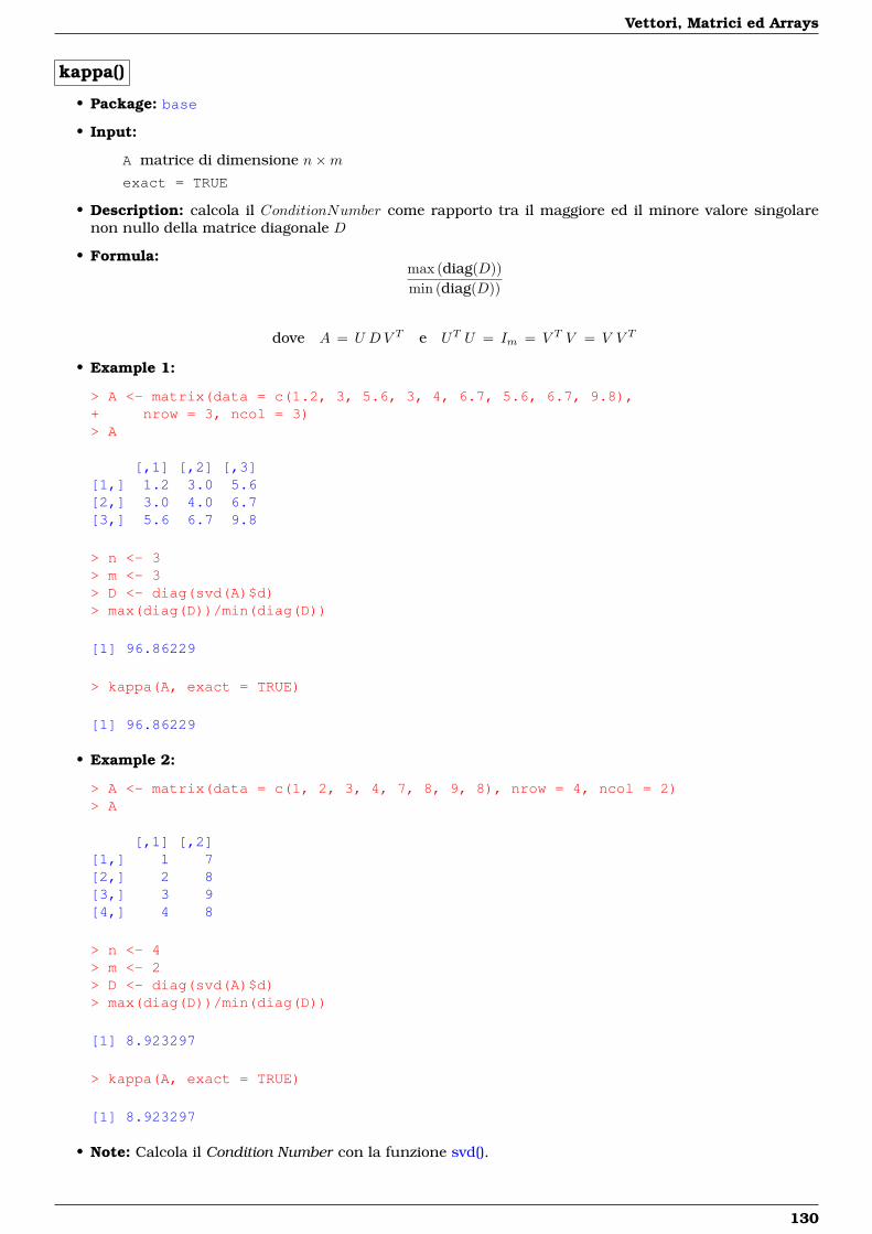
Vettori, Matrici ed Arrays
kappa()
• Package: base
• Input:
A matrice di dimensione n×mexact = TRUE
• Description: calcola il ConditionNumber come rapporto tra il maggiore ed il minore valore singolarenon nullo della matrice diagonale D
• Formula:max (diag(D))min (diag(D))
dove A = U DV T e UT U = Im = V T V = V V T
• Example 1:
> A <- matrix(data = c(1.2, 3, 5.6, 3, 4, 6.7, 5.6, 6.7, 9.8),+ nrow = 3, ncol = 3)> A
[,1] [,2] [,3][1,] 1.2 3.0 5.6[2,] 3.0 4.0 6.7[3,] 5.6 6.7 9.8
> n <- 3> m <- 3> D <- diag(svd(A)$d)> max(diag(D))/min(diag(D))
[1] 96.86229
> kappa(A, exact = TRUE)
[1] 96.86229
• Example 2:
> A <- matrix(data = c(1, 2, 3, 4, 7, 8, 9, 8), nrow = 4, ncol = 2)> A
[,1] [,2][1,] 1 7[2,] 2 8[3,] 3 9[4,] 4 8
> n <- 4> m <- 2> D <- diag(svd(A)$d)> max(diag(D))/min(diag(D))
[1] 8.923297
> kappa(A, exact = TRUE)
[1] 8.923297
• Note: Calcola il Condition Number con la funzione svd().
130
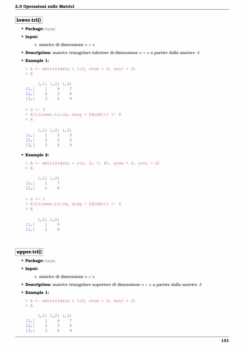
2.3 Operazioni sulle Matrici
lower.tri()
• Package: base
• Input:
A matrice di dimensione n× n
• Description: matrice triangolare inferiore di dimensione n× n a partire dalla matrice A
• Example 1:
> A <- matrix(data = 1:9, nrow = 3, ncol = 3)> A
[,1] [,2] [,3][1,] 1 4 7[2,] 2 5 8[3,] 3 6 9
> n <- 3> A[t(lower.tri(A, diag = FALSE))] <- 0> A
[,1] [,2] [,3][1,] 1 0 0[2,] 2 5 0[3,] 3 6 9
• Example 2:
> A <- matrix(data = c(1, 2, 7, 8), nrow = 2, ncol = 2)> A
[,1] [,2][1,] 1 7[2,] 2 8
> n <- 2> A[t(lower.tri(A, diag = FALSE))] <- 0> A
[,1] [,2][1,] 1 0[2,] 2 8
upper.tri()
• Package: base
• Input:
A matrice di dimensione n× n
• Description: matrice triangolare superiore di dimensione n× n a partire dalla matrice A
• Example 1:
> A <- matrix(data = 1:9, nrow = 3, ncol = 3)> A
[,1] [,2] [,3][1,] 1 4 7[2,] 2 5 8[3,] 3 6 9
131
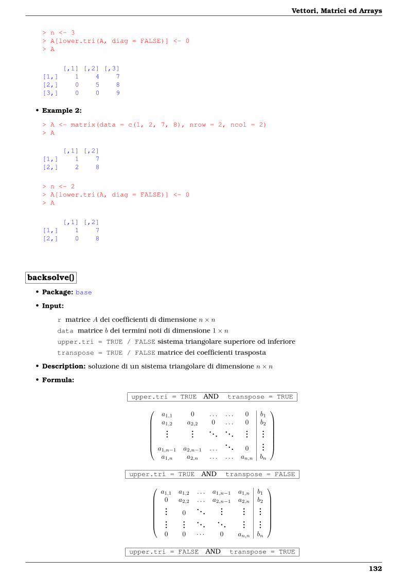
Vettori, Matrici ed Arrays
> n <- 3> A[lower.tri(A, diag = FALSE)] <- 0> A
[,1] [,2] [,3][1,] 1 4 7[2,] 0 5 8[3,] 0 0 9
• Example 2:
> A <- matrix(data = c(1, 2, 7, 8), nrow = 2, ncol = 2)> A
[,1] [,2][1,] 1 7[2,] 2 8
> n <- 2> A[lower.tri(A, diag = FALSE)] <- 0> A
[,1] [,2][1,] 1 7[2,] 0 8
backsolve()
• Package: base
• Input:
r matrice A dei coefficienti di dimensione n× ndata matrice b dei termini noti di dimensione 1× nupper.tri = TRUE / FALSE sistema triangolare superiore od inferiore
transpose = TRUE / FALSE matrice dei coefficienti trasposta
• Description: soluzione di un sistema triangolare di dimensione n× n
• Formula:
upper.tri = TRUE AND transpose = TRUE
a1,1 0 . . . . . . 0 b1a1,2 a2,2 0 . . . 0 b2...
.... . . . . .
......
a1,n−1 a2,n−1 . . .. . . 0
...a1,n a2,n . . . . . . an,n bn
upper.tri = TRUE AND transpose = FALSE
a1,1 a1,2 . . . a1,n−1 a1,n b10 a2,2 . . . a2,n−1 a2,n b2... 0
. . ....
......
......
. . . . . ....
...0 0 · · · 0 an,n bn
upper.tri = FALSE AND transpose = TRUE
132
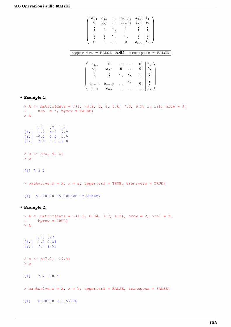
2.3 Operazioni sulle Matrici
a1,1 a2,1 . . . an−1,1 an,1 b10 a2,2 . . . an−1,2 an,2 b2... 0
. . ....
......
......
. . . . . ....
...0 0 · · · 0 an,n bn
upper.tri = FALSE AND transpose = FALSE
a1,1 0 . . . . . . 0 b1a2,1 a2,2 0 . . . 0 b2...
.... . . . . .
......
an−1,1 an−1,2 . . .. . . 0
...an,1 an,2 . . . . . . an,n bn
• Example 1:
> A <- matrix(data = c(1, -0.2, 3, 4, 5.6, 7.8, 9.9, 1, 12), nrow = 3,+ ncol = 3, byrow = FALSE)> A
[,1] [,2] [,3][1,] 1.0 4.0 9.9[2,] -0.2 5.6 1.0[3,] 3.0 7.8 12.0
> b <- c(8, 4, 2)> b
[1] 8 4 2
> backsolve(r = A, x = b, upper.tri = TRUE, transpose = TRUE)
[1] 8.000000 -5.000000 -6.016667
• Example 2:
> A <- matrix(data = c(1.2, 0.34, 7.7, 4.5), nrow = 2, ncol = 2,+ byrow = TRUE)> A
[,1] [,2][1,] 1.2 0.34[2,] 7.7 4.50
> b <- c(7.2, -10.4)> b
[1] 7.2 -10.4
> backsolve(r = A, x = b, upper.tri = FALSE, transpose = FALSE)
[1] 6.00000 -12.57778
133
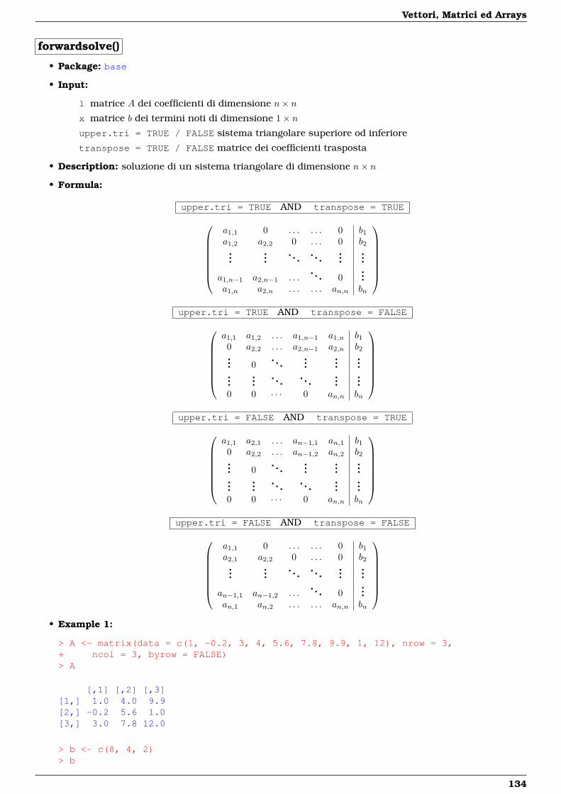
Vettori, Matrici ed Arrays
forwardsolve()
• Package: base
• Input:
l matrice A dei coefficienti di dimensione n× nx matrice b dei termini noti di dimensione 1× nupper.tri = TRUE / FALSE sistema triangolare superiore od inferiore
transpose = TRUE / FALSE matrice dei coefficienti trasposta
• Description: soluzione di un sistema triangolare di dimensione n× n
• Formula:
upper.tri = TRUE AND transpose = TRUE
a1,1 0 . . . . . . 0 b1a1,2 a2,2 0 . . . 0 b2...
.... . . . . .
......
a1,n−1 a2,n−1 . . .. . . 0
...a1,n a2,n . . . . . . an,n bn
upper.tri = TRUE AND transpose = FALSE
a1,1 a1,2 . . . a1,n−1 a1,n b10 a2,2 . . . a2,n−1 a2,n b2... 0
. . ....
......
......
. . . . . ....
...0 0 · · · 0 an,n bn
upper.tri = FALSE AND transpose = TRUE
a1,1 a2,1 . . . an−1,1 an,1 b10 a2,2 . . . an−1,2 an,2 b2... 0
. . ....
......
......
. . . . . ....
...0 0 · · · 0 an,n bn
upper.tri = FALSE AND transpose = FALSE
a1,1 0 . . . . . . 0 b1a2,1 a2,2 0 . . . 0 b2...
.... . . . . .
......
an−1,1 an−1,2 . . .. . . 0
...an,1 an,2 . . . . . . an,n bn
• Example 1:
> A <- matrix(data = c(1, -0.2, 3, 4, 5.6, 7.8, 9.9, 1, 12), nrow = 3,+ ncol = 3, byrow = FALSE)> A
[,1] [,2] [,3][1,] 1.0 4.0 9.9[2,] -0.2 5.6 1.0[3,] 3.0 7.8 12.0
> b <- c(8, 4, 2)> b
134
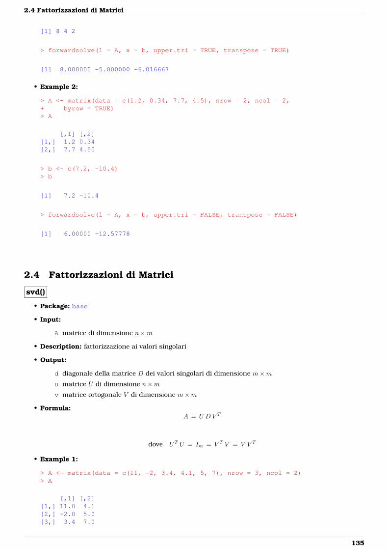
2.4 Fattorizzazioni di Matrici
[1] 8 4 2
> forwardsolve(l = A, x = b, upper.tri = TRUE, transpose = TRUE)
[1] 8.000000 -5.000000 -6.016667
• Example 2:
> A <- matrix(data = c(1.2, 0.34, 7.7, 4.5), nrow = 2, ncol = 2,+ byrow = TRUE)> A
[,1] [,2][1,] 1.2 0.34[2,] 7.7 4.50
> b <- c(7.2, -10.4)> b
[1] 7.2 -10.4
> forwardsolve(l = A, x = b, upper.tri = FALSE, transpose = FALSE)
[1] 6.00000 -12.57778
2.4 Fattorizzazioni di Matrici
svd()
• Package: base
• Input:
A matrice di dimensione n×m
• Description: fattorizzazione ai valori singolari
• Output:
d diagonale della matrice D dei valori singolari di dimensione m×mu matrice U di dimensione n×mv matrice ortogonale V di dimensione m×m
• Formula:A = U DV T
dove UT U = Im = V T V = V V T
• Example 1:
> A <- matrix(data = c(11, -2, 3.4, 4.1, 5, 7), nrow = 3, ncol = 2)> A
[,1] [,2][1,] 11.0 4.1[2,] -2.0 5.0[3,] 3.4 7.0
135
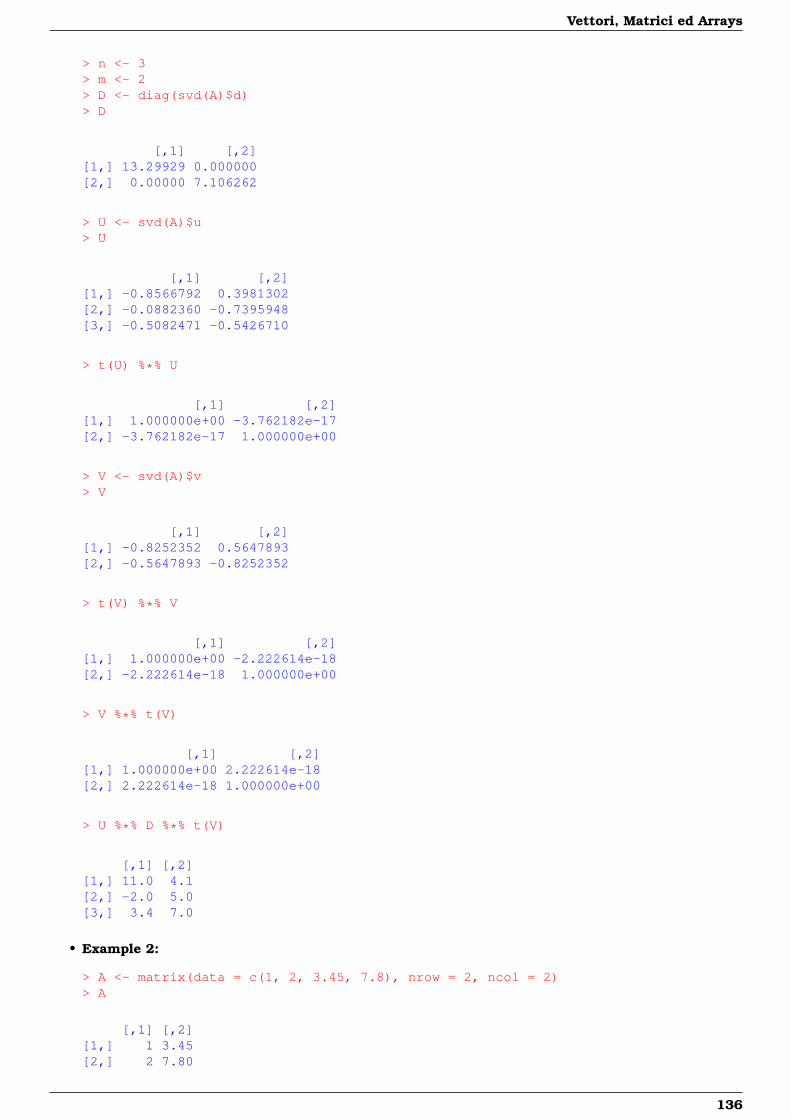
Vettori, Matrici ed Arrays
> n <- 3> m <- 2> D <- diag(svd(A)$d)> D
[,1] [,2][1,] 13.29929 0.000000[2,] 0.00000 7.106262
> U <- svd(A)$u> U
[,1] [,2][1,] -0.8566792 0.3981302[2,] -0.0882360 -0.7395948[3,] -0.5082471 -0.5426710
> t(U) %*% U
[,1] [,2][1,] 1.000000e+00 -3.762182e-17[2,] -3.762182e-17 1.000000e+00
> V <- svd(A)$v> V
[,1] [,2][1,] -0.8252352 0.5647893[2,] -0.5647893 -0.8252352
> t(V) %*% V
[,1] [,2][1,] 1.000000e+00 -2.222614e-18[2,] -2.222614e-18 1.000000e+00
> V %*% t(V)
[,1] [,2][1,] 1.000000e+00 2.222614e-18[2,] 2.222614e-18 1.000000e+00
> U %*% D %*% t(V)
[,1] [,2][1,] 11.0 4.1[2,] -2.0 5.0[3,] 3.4 7.0
• Example 2:
> A <- matrix(data = c(1, 2, 3.45, 7.8), nrow = 2, ncol = 2)> A
[,1] [,2][1,] 1 3.45[2,] 2 7.80
136
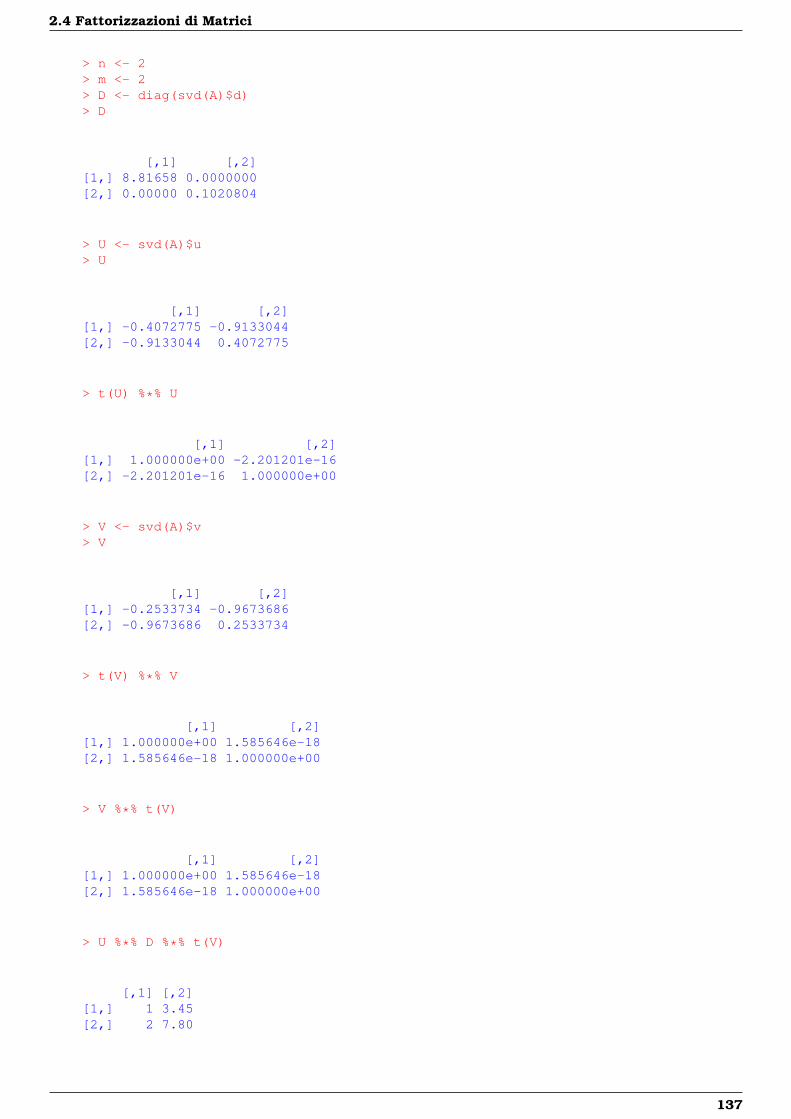
2.4 Fattorizzazioni di Matrici
> n <- 2> m <- 2> D <- diag(svd(A)$d)> D
[,1] [,2][1,] 8.81658 0.0000000[2,] 0.00000 0.1020804
> U <- svd(A)$u> U
[,1] [,2][1,] -0.4072775 -0.9133044[2,] -0.9133044 0.4072775
> t(U) %*% U
[,1] [,2][1,] 1.000000e+00 -2.201201e-16[2,] -2.201201e-16 1.000000e+00
> V <- svd(A)$v> V
[,1] [,2][1,] -0.2533734 -0.9673686[2,] -0.9673686 0.2533734
> t(V) %*% V
[,1] [,2][1,] 1.000000e+00 1.585646e-18[2,] 1.585646e-18 1.000000e+00
> V %*% t(V)
[,1] [,2][1,] 1.000000e+00 1.585646e-18[2,] 1.585646e-18 1.000000e+00
> U %*% D %*% t(V)
[,1] [,2][1,] 1 3.45[2,] 2 7.80
137
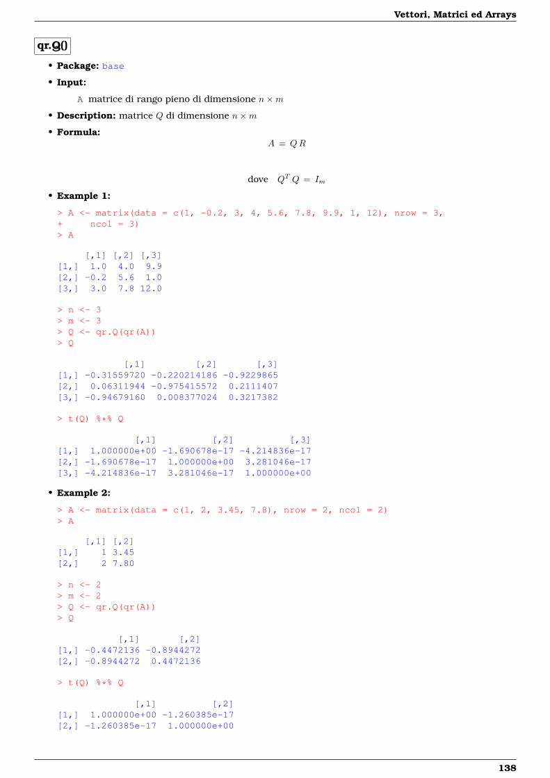
Vettori, Matrici ed Arrays
qr.Q()
• Package: base
• Input:
A matrice di rango pieno di dimensione n×m
• Description: matrice Q di dimensione n×m
• Formula:A = QR
dove QT Q = Im
• Example 1:
> A <- matrix(data = c(1, -0.2, 3, 4, 5.6, 7.8, 9.9, 1, 12), nrow = 3,+ ncol = 3)> A
[,1] [,2] [,3][1,] 1.0 4.0 9.9[2,] -0.2 5.6 1.0[3,] 3.0 7.8 12.0
> n <- 3> m <- 3> Q <- qr.Q(qr(A))> Q
[,1] [,2] [,3][1,] -0.31559720 -0.220214186 -0.9229865[2,] 0.06311944 -0.975415572 0.2111407[3,] -0.94679160 0.008377024 0.3217382
> t(Q) %*% Q
[,1] [,2] [,3][1,] 1.000000e+00 -1.690678e-17 -4.214836e-17[2,] -1.690678e-17 1.000000e+00 3.281046e-17[3,] -4.214836e-17 3.281046e-17 1.000000e+00
• Example 2:
> A <- matrix(data = c(1, 2, 3.45, 7.8), nrow = 2, ncol = 2)> A
[,1] [,2][1,] 1 3.45[2,] 2 7.80
> n <- 2> m <- 2> Q <- qr.Q(qr(A))> Q
[,1] [,2][1,] -0.4472136 -0.8944272[2,] -0.8944272 0.4472136
> t(Q) %*% Q
[,1] [,2][1,] 1.000000e+00 -1.260385e-17[2,] -1.260385e-17 1.000000e+00
138
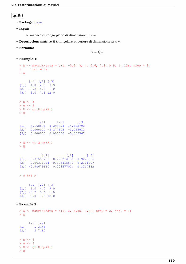
2.4 Fattorizzazioni di Matrici
qr.R()
• Package: base
• Input:
A matrice di rango pieno di dimensione n×m
• Description: matrice R triangolare superiore di dimensione m×m
• Formula:A = QR
• Example 1:
> A <- matrix(data = c(1, -0.2, 3, 4, 5.6, 7.8, 9.9, 1, 12), nrow = 3,+ ncol = 3)> A
[,1] [,2] [,3][1,] 1.0 4.0 9.9[2,] -0.2 5.6 1.0[3,] 3.0 7.8 12.0
> n <- 3> m <- 3> R <- qr.R(qr(A))> R
[,1] [,2] [,3][1,] -3.168596 -8.293894 -14.422792[2,] 0.000000 -6.277843 -3.055012[3,] 0.000000 0.000000 -5.065567
> Q <- qr.Q(qr(A))> Q
[,1] [,2] [,3][1,] -0.31559720 -0.220214186 -0.9229865[2,] 0.06311944 -0.975415572 0.2111407[3,] -0.94679160 0.008377024 0.3217382
> Q %*% R
[,1] [,2] [,3][1,] 1.0 4.0 9.9[2,] -0.2 5.6 1.0[3,] 3.0 7.8 12.0
• Example 2:
> A <- matrix(data = c(1, 2, 3.45, 7.8), nrow = 2, ncol = 2)> A
[,1] [,2][1,] 1 3.45[2,] 2 7.80
> n <- 2> m <- 2> R <- qr.R(qr(A))> R
139
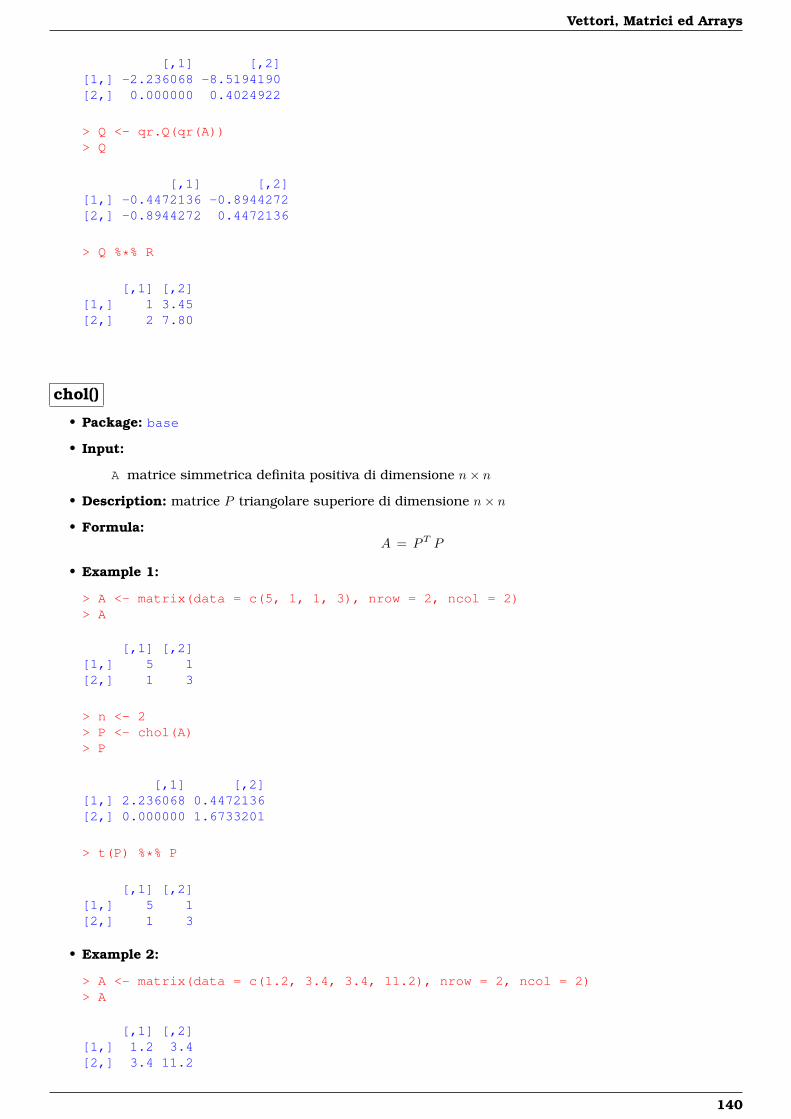
Vettori, Matrici ed Arrays
[,1] [,2][1,] -2.236068 -8.5194190[2,] 0.000000 0.4024922
> Q <- qr.Q(qr(A))> Q
[,1] [,2][1,] -0.4472136 -0.8944272[2,] -0.8944272 0.4472136
> Q %*% R
[,1] [,2][1,] 1 3.45[2,] 2 7.80
chol()
• Package: base
• Input:
A matrice simmetrica definita positiva di dimensione n× n
• Description: matrice P triangolare superiore di dimensione n× n
• Formula:A = PT P
• Example 1:
> A <- matrix(data = c(5, 1, 1, 3), nrow = 2, ncol = 2)> A
[,1] [,2][1,] 5 1[2,] 1 3
> n <- 2> P <- chol(A)> P
[,1] [,2][1,] 2.236068 0.4472136[2,] 0.000000 1.6733201
> t(P) %*% P
[,1] [,2][1,] 5 1[2,] 1 3
• Example 2:
> A <- matrix(data = c(1.2, 3.4, 3.4, 11.2), nrow = 2, ncol = 2)> A
[,1] [,2][1,] 1.2 3.4[2,] 3.4 11.2
140
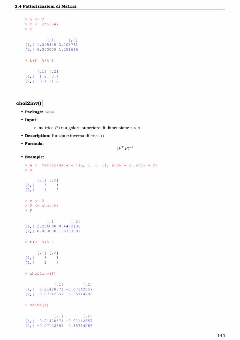
2.4 Fattorizzazioni di Matrici
> n <- 2> P <- chol(A)> P
[,1] [,2][1,] 1.095445 3.103761[2,] 0.000000 1.251666
> t(P) %*% P
[,1] [,2][1,] 1.2 3.4[2,] 3.4 11.2
chol2inv()
• Package: base
• Input:
P matrice P triangolare superiore di dimensione n× n
• Description: funzione inversa di chol()
• Formula:(PT P )−1
• Example:
> A <- matrix(data = c(5, 1, 1, 3), nrow = 2, ncol = 2)> A
[,1] [,2][1,] 5 1[2,] 1 3
> n <- 2> P <- chol(A)> P
[,1] [,2][1,] 2.236068 0.4472136[2,] 0.000000 1.6733201
> t(P) %*% P
[,1] [,2][1,] 5 1[2,] 1 3
> chol2inv(P)
[,1] [,2][1,] 0.21428571 -0.07142857[2,] -0.07142857 0.35714286
> solve(A)
[,1] [,2][1,] 0.21428571 -0.07142857[2,] -0.07142857 0.35714286
141
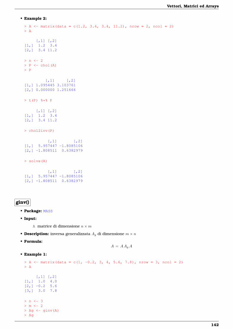
Vettori, Matrici ed Arrays
• Example 2:
> A <- matrix(data = c(1.2, 3.4, 3.4, 11.2), nrow = 2, ncol = 2)> A
[,1] [,2][1,] 1.2 3.4[2,] 3.4 11.2
> n <- 2> P <- chol(A)> P
[,1] [,2][1,] 1.095445 3.103761[2,] 0.000000 1.251666
> t(P) %*% P
[,1] [,2][1,] 1.2 3.4[2,] 3.4 11.2
> chol2inv(P)
[,1] [,2][1,] 5.957447 -1.8085106[2,] -1.808511 0.6382979
> solve(A)
[,1] [,2][1,] 5.957447 -1.8085106[2,] -1.808511 0.6382979
ginv()
• Package: MASS
• Input:
A matrice di dimensione n×m
• Description: inversa generalizzata Ag di dimensione m× n
• Formula:A = AAg A
• Example 1:
> A <- matrix(data = c(1, -0.2, 3, 4, 5.6, 7.8), nrow = 3, ncol = 2)> A
[,1] [,2][1,] 1.0 4.0[2,] -0.2 5.6[3,] 3.0 7.8
> n <- 3> m <- 2> Ag <- ginv(A)> Ag
142

2.5 Creazione di Arrays
[,1] [,2] [,3][1,] 0.007783879 -0.4266172 0.302297558[2,] 0.035078001 0.1553743 -0.001334379
> A %*% Ag %*% A
[,1] [,2][1,] 1.0 4.0[2,] -0.2 5.6[3,] 3.0 7.8
• Example 2:
> A <- matrix(data = c(1.2, 3.4, 3.4, 11.2), nrow = 2, ncol = 2)> A
[,1] [,2][1,] 1.2 3.4[2,] 3.4 11.2
> n <- 2> m <- 2> Ag <- ginv(A)> Ag
[,1] [,2][1,] 5.957447 -1.8085106[2,] -1.808511 0.6382979
> A %*% Ag %*% A
[,1] [,2][1,] 1.2 3.4[2,] 3.4 11.2
2.5 Creazione di Arrays
array()
• Package: base
• Input:
data vettore numerico
dim dimensione
dimnames etichette di dimensione
• Description: creazione
• Example:
> etichette <- list(c("A", "B"), c("a", "b"), c("X", "Y"))> myarray <- array(data = 1:8, dim = c(2, 2, 2), dimnames = etichette)> myarray
143
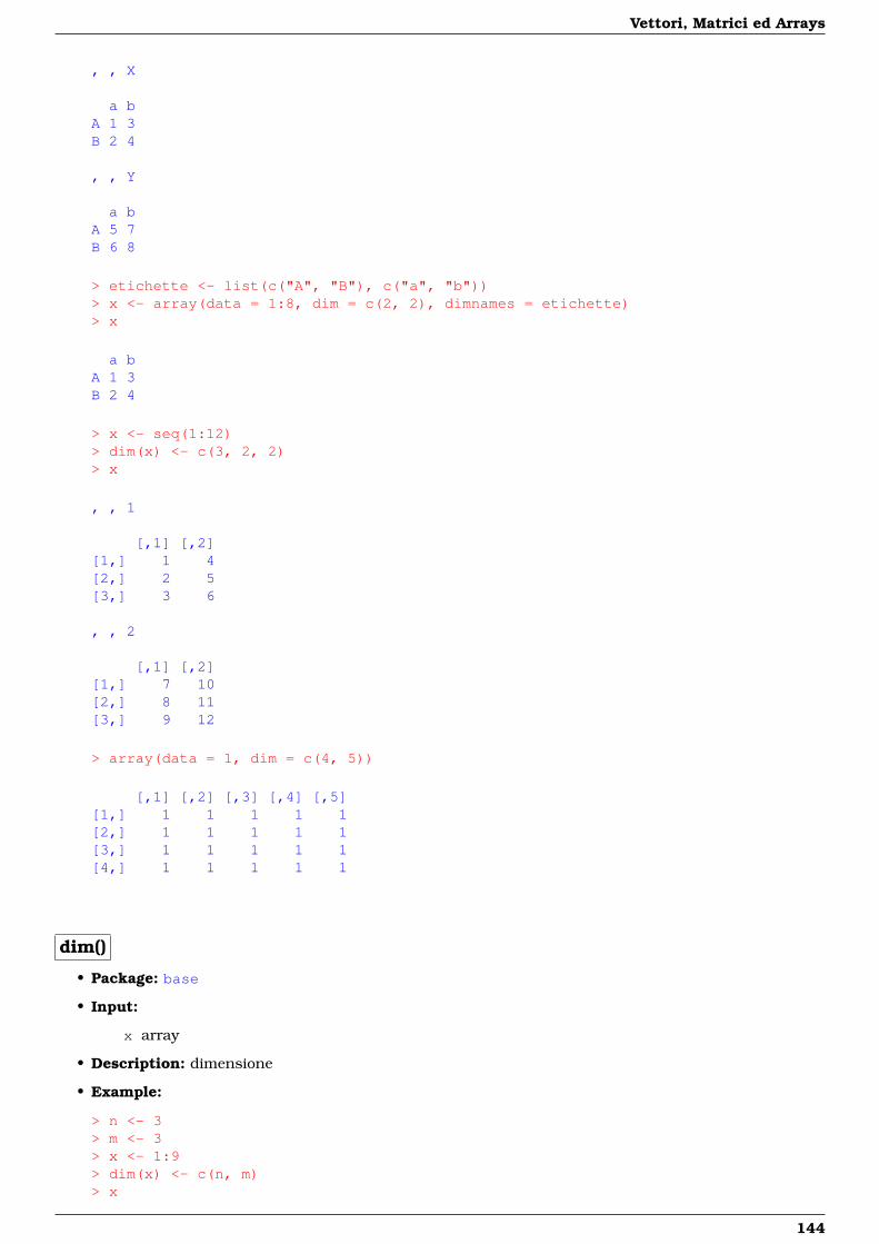
Vettori, Matrici ed Arrays
, , X
a bA 1 3B 2 4
, , Y
a bA 5 7B 6 8
> etichette <- list(c("A", "B"), c("a", "b"))> x <- array(data = 1:8, dim = c(2, 2), dimnames = etichette)> x
a bA 1 3B 2 4
> x <- seq(1:12)> dim(x) <- c(3, 2, 2)> x
, , 1
[,1] [,2][1,] 1 4[2,] 2 5[3,] 3 6
, , 2
[,1] [,2][1,] 7 10[2,] 8 11[3,] 9 12
> array(data = 1, dim = c(4, 5))
[,1] [,2] [,3] [,4] [,5][1,] 1 1 1 1 1[2,] 1 1 1 1 1[3,] 1 1 1 1 1[4,] 1 1 1 1 1
dim()
• Package: base
• Input:
x array
• Description: dimensione
• Example:
> n <- 3> m <- 3> x <- 1:9> dim(x) <- c(n, m)> x
144
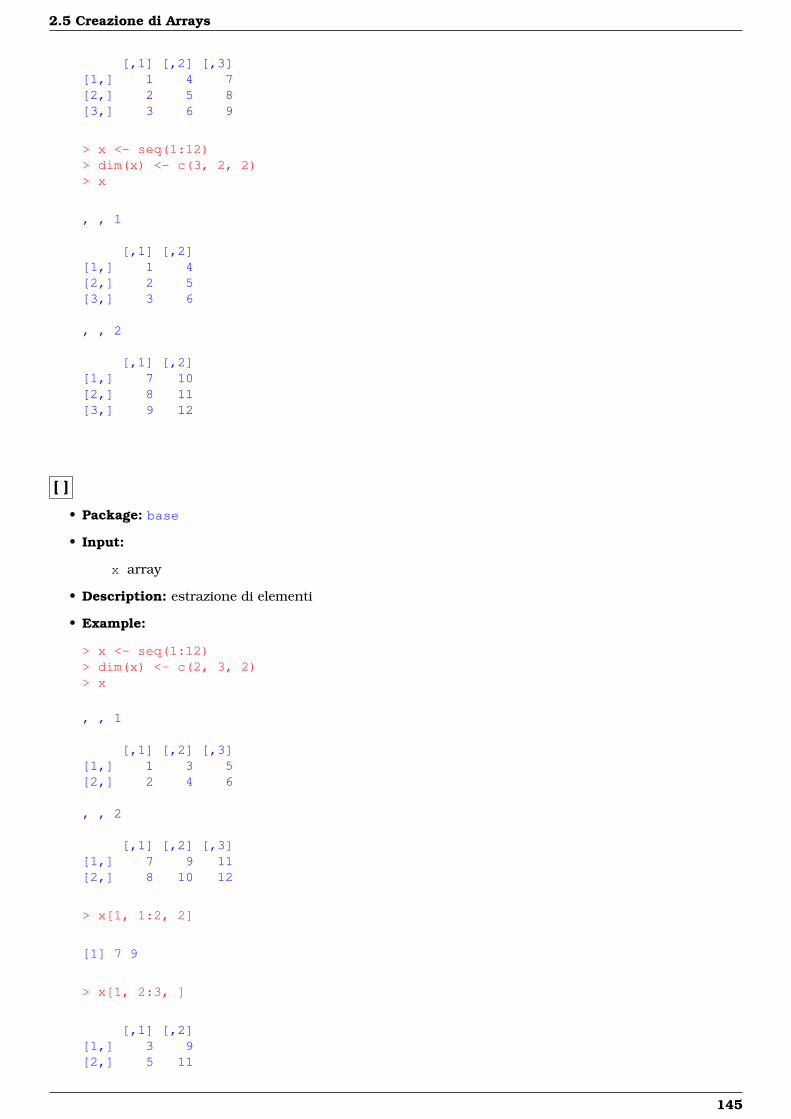
2.5 Creazione di Arrays
[,1] [,2] [,3][1,] 1 4 7[2,] 2 5 8[3,] 3 6 9
> x <- seq(1:12)> dim(x) <- c(3, 2, 2)> x
, , 1
[,1] [,2][1,] 1 4[2,] 2 5[3,] 3 6
, , 2
[,1] [,2][1,] 7 10[2,] 8 11[3,] 9 12
[ ]
• Package: base
• Input:
x array
• Description: estrazione di elementi
• Example:
> x <- seq(1:12)> dim(x) <- c(2, 3, 2)> x
, , 1
[,1] [,2] [,3][1,] 1 3 5[2,] 2 4 6
, , 2
[,1] [,2] [,3][1,] 7 9 11[2,] 8 10 12
> x[1, 1:2, 2]
[1] 7 9
> x[1, 2:3, ]
[,1] [,2][1,] 3 9[2,] 5 11
145

Vettori, Matrici ed Arrays
> x[1, 2:3, , drop = FALSE]
, , 1
[,1] [,2][1,] 3 5
, , 2
[,1] [,2][1,] 9 11
dimnames()
• Package: base
• Input:
x array
• Description: etichette di dimensione
• Example:
> x
, , 1
[,1] [,2] [,3][1,] 1 3 5[2,] 2 4 6
, , 2
[,1] [,2] [,3][1,] 7 9 11[2,] 8 10 12
> dimnames(x) <- list(letters[1:2], LETTERS[1:3], c("primo", "secondo"))> x
, , primo
A B Ca 1 3 5b 2 4 6
, , secondo
A B Ca 7 9 11b 8 10 12
146
Parte II
Statistica Descrittiva
147

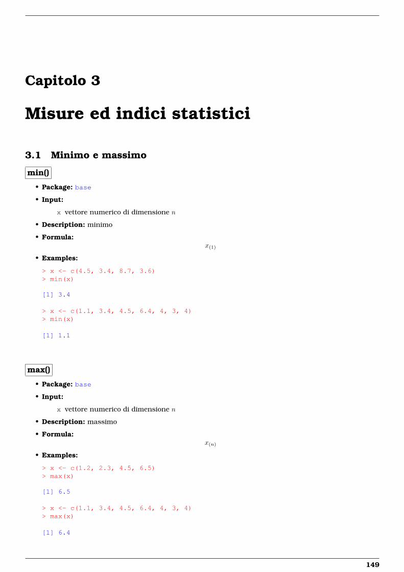
Capitolo 3
Misure ed indici statistici
3.1 Minimo e massimo
min()
• Package: base
• Input:
x vettore numerico di dimensione n
• Description: minimo
• Formula:x(1)
• Examples:
> x <- c(4.5, 3.4, 8.7, 3.6)> min(x)
[1] 3.4
> x <- c(1.1, 3.4, 4.5, 6.4, 4, 3, 4)> min(x)
[1] 1.1
max()
• Package: base
• Input:
x vettore numerico di dimensione n
• Description: massimo
• Formula:x(n)
• Examples:
> x <- c(1.2, 2.3, 4.5, 6.5)> max(x)
[1] 6.5
> x <- c(1.1, 3.4, 4.5, 6.4, 4, 3, 4)> max(x)
[1] 6.4
149

Misure ed indici statistici
3.2 Campo di variazione e midrange
range()
• Package: base
• Input:
x vettore numerico di dimensione n
• Description: minimo e massimo
• Formula:x(1) x(n)
• Examples:
> x <- c(1, 1.2, 3.4, 0.8)> min(x)
[1] 0.8
> max(x)
[1] 3.4
> range(x)
[1] 0.8 3.4
> x <- c(1.2, 3.4, 4.5, 6.4, 4, 3, 4)> min(x)
[1] 1.2
> max(x)
[1] 6.4
> range(x)
[1] 1.2 6.4
range2()
• Package: sigma2tools
• Input:
x vettore numerico di dimensione n
• Description: campo di variazione
• Formula:x(n) − x(1)
• Examples:
> x <- c(1, 1.2, 3.4, 0.8)> min(x)
[1] 0.8
150

3.2 Campo di variazione e midrange
> max(x)
[1] 3.4
> max(x) - min(x)
[1] 2.6
> range2(x)
[1] 2.6
> x <- c(1.2, 3.4, 4.5, 6.4, 4, 3, 4)> min(x)
[1] 1.2
> max(x)
[1] 6.4
> max(x) - min(x)
[1] 5.2
> range2(x)
[1] 5.2
midrange()
• Package: sigma2tools
• Input:
x vettore numerico di dimensione n
• Description: midrange
• Formula: (x(1) + x(n)
)/ 2
• Examples:
> x <- c(1, 1.2, 3.4, 0.8, 1.77, 7.8)> min(x)
[1] 0.8
> max(x)
[1] 7.8
> (min(x) + max(x))/2
[1] 4.3
> midrange(x)
151
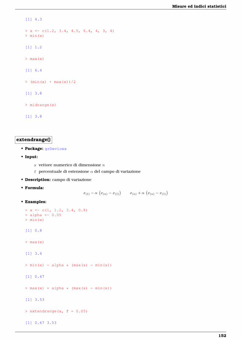
Misure ed indici statistici
[1] 4.3
> x <- c(1.2, 3.4, 4.5, 6.4, 4, 3, 4)> min(x)
[1] 1.2
> max(x)
[1] 6.4
> (min(x) + max(x))/2
[1] 3.8
> midrange(x)
[1] 3.8
extendrange()
• Package: grDevices
• Input:
x vettore numerico di dimensione n
f percentuale di estensione α del campo di variazione
• Description: campo di variazione
• Formula:x(1) − α
(x(n) − x(1)
)x(n) + α
(x(n) − x(1)
)• Examples:
> x <- c(1, 1.2, 3.4, 0.8)> alpha <- 0.05> min(x)
[1] 0.8
> max(x)
[1] 3.4
> min(x) - alpha * (max(x) - min(x))
[1] 0.67
> max(x) + alpha * (max(x) - min(x))
[1] 3.53
> extendrange(x, f = 0.05)
[1] 0.67 3.53
152

3.3 Media aritmetica, geometrica ed armonica
> x <- c(1.2, 3.4, 4.5, 6.4, 4, 3, 4)> alpha <- 0.05> min(x)
[1] 1.2
> max(x)
[1] 6.4
> min(x) - alpha * (max(x) - min(x))
[1] 0.94
> max(x) + alpha * (max(x) - min(x))
[1] 6.66
> extendrange(x, f = 0.05)
[1] 0.94 6.66
3.3 Media aritmetica, geometrica ed armonica
mean()
• Package: base
• Input:
x vettore numerico di dimensione n
trim il valore di α con 0 ≤ α ≤ 0.5 che rappresenta la percentuale di osservazioni più basse e piùalte che deve essere esclusa dal calcolo della media aritmetica
• Description: media α-trimmed
• Formula:
xα =
x se α = 0
1n−2 bnαc
∑n−bnαci=bnαc+1 x(i) se 0 < α < 0.5
Q0.5(x) se α = 0.5
• Examples:
> x <- c(1, 1.2, 3.4, 0.8, 10.2, 9.3, 7.34)> n <- 7> sum(x)/n
[1] 4.748571
> mean(x, trim = 0)
[1] 4.748571
> x <- c(1, 1.2, 3.4, 0.8, 10.2, 9.3, 7.34)> x <- sort(x)> x
153
Misure ed indici statistici
[1] 0.80 1.00 1.20 3.40 7.34 9.30 10.20
> n <- 7> alpha <- 0.26> sum(x[(floor(n * alpha) + 1):(n - floor(n * alpha))])/(n - 2 *+ floor(n * alpha))
[1] 4.448
> mean(x, trim = 0.26)
[1] 4.448
> x <- c(1, 1.2, 3.4, 0.8, 10.2, 9.3, 7.34)> median(x)
[1] 3.4
> mean(x, trim = 0.5)
[1] 3.4
mean.g()
• Package: labstatR
• Input:
x vettore numerico di elementi positivi di dimensione n
• Description: media geometrica
• Formula:
xG =
(n∏i=1
xi
)1 / n
= exp
(1n
n∑i=1
log(xi)
)
• Examples:
> x <- c(1.2, 2.3, 4.5, 6.5)> n <- 4> prod(x)^(1/n)
[1] 2.997497
> mean.g(x)
[1] 2.997497
> x <- c(1.2, 3.4, 4.5, 6.4, 4, 3, 4)> n <- 7> prod(x)^(1/n)
[1] 3.434782
> mean.g(x)
[1] 3.434782
154
3.4 Mediana e quantili
mean.a()
• Package: labstatR
• Input:
x vettore numerico di elementi non nulli di dimensione n
• Description: media armonica
• Formula:
xA =
(1n
n∑i=1
1xi
)−1
• Examples:
> x <- c(1.2, 2.3, 4.5, 6.5)> 1/mean(1/x)
[1] 2.432817
> mean.a(x)
[1] 2.432817
> x <- c(1.2, 3.4, 4.5, 6.4, 4, 3, 4)> 1/mean(1/x)
[1] 2.992404
> mean.a(x)
[1] 2.992404
3.4 Mediana e quantili
median()
• Package: stats
• Input:
x vettore numerico di dimensione n
• Description: mediana
• Formula:
Q0.5(x) =
x(n+1
2 ) se n è dispari
0.5(x(n2 ) + x(n2 +1)
)se n è pari
• Examples:
> x <- c(1.2, 0.34, 5.6, 7.4, 2.1, 3.2, 9.87, 10.1)> x <- sort(x)> x
[1] 0.34 1.20 2.10 3.20 5.60 7.40 9.87 10.10
> n <- 8> 0.5 * (x[n/2] + x[n/2 + 1])
155
Misure ed indici statistici
[1] 4.4
> median(x)
[1] 4.4
> x <- c(1.2, 0.34, 5.6, 7.4, 2.1, 3.2, 9.87)> x <- sort(x)> x
[1] 0.34 1.20 2.10 3.20 5.60 7.40 9.87
> n <- 7> x[(n + 1)/2]
[1] 3.2
> median(x)
[1] 3.2
• Note: Equivale alla funzione quantile() quando questa è calcolata in probs = 0.5.
quantile()
• Package: stats
• Input:
x vettore numerico di dimensione n
probs valore p di probabilità
• Description: quantile al (100 p)%
• Formula:
Qp(x) =
x(α) se α è intero
x(bαc) + (α− bαc)(x(bαc+1) − x(bαc)
)se α non è intero
dove α = 1 + (n− 1) p
• Examples:
> x <- c(1.2, 2.3, 0.11, 4.5, 2.3, 4.55, 7.8, 6.6, 9.9)> x <- sort(x)> x
[1] 0.11 1.20 2.30 2.30 4.50 4.55 6.60 7.80 9.90
> n <- 9> p <- 0.25> alpha <- 1 + (n - 1) * p> alpha
[1] 3
> x[alpha]
[1] 2.3
156
3.4 Mediana e quantili
> quantile(x, probs = 0.25)
25%2.3
> x <- c(1.2, 2.3, 0.11, 4.5)> x <- sort(x)> x
[1] 0.11 1.20 2.30 4.50
> n <- 4> p <- 0.34> alpha <- 1 + (n - 1) * p> alpha
[1] 2.02
> x[floor(alpha)] + (alpha - floor(alpha)) * (x[floor(alpha) ++ 1] - x[floor(alpha)])
[1] 1.222
> quantile(x, probs = 0.34)
34%1.222
> x <- c(1.2, 4.2, 4.5, -5.6, 6.5, 1.2)> x <- sort(x)> n <- 6> p <- 0.68> alpha <- 1 + (n - 1) * p> alpha
[1] 4.4
> x[floor(alpha)] + (alpha - floor(alpha)) * (x[floor(alpha) ++ 1] - x[floor(alpha)])
[1] 4.32
> quantile(x, probs = 0.68)
68%4.32
• Note 1: Equivale alla funzione median() quando probs = 0.5.
• Note 2: Equivale alla funzione min() quando probs = 0.
• Note 3: Equivale alla funzione max() quando probs = 1.
157
Misure ed indici statistici
3.5 Differenza interquartile e deviazione assoluta dalla mediana
IQR()
• Package: stats
• Input:
x vettore numerico di dimensione n
• Description: differenza interquartile
• Formula:IQR(x) = Q0.75(x)−Q0.25(x)
• Examples:
> x <- c(1, 1.2, 3.4, 0.8, 10.2, 9.3, 7.34)> diff(quantile(x, probs = c(0.25, 0.75)))
75%7.22
> IQR(x)
[1] 7.22
> x <- c(1.2, 3.4, 4.5, 6.4, 4, 3, 4)> diff(quantile(x, probs = c(0.25, 0.75)))
75%1.05
> IQR(x)
[1] 1.05
• Note: Calcola i quartili con la funzione quantile().
mad()
• Package: stats
• Input:
x vettore numerico di dimensione n
center parametro rispetto al quale si effettuano gli scarti
constant il valore α della costante positiva
• Description: deviazione assoluta dalla mediana
• Formula:αQ0.5 ( |x− center(x) | )
• Examples:
> x <- c(1.2, 3.4, 4.5, 6.4, 4)> alpha <- 1.23> alpha * median(abs(x - median(x)))
[1] 0.738
> mad(x, center = median(x), constant = 1.23)
158
3.6 Asimmetria e curtosi
[1] 0.738
> x <- c(1, 1.2, 3.4, 0.8, 10.2, 9.3, 7.34)> alpha <- 1.55> alpha * median(abs(x - mean(x)))
[1] 5.810286
> mad(x, center = mean(x), constant = 1.55)
[1] 5.810286
> x <- c(1.2, 4.2, 4.5, -5.6, 6.5, 1.2)> alpha <- 2.42> alpha * median(abs(x - mean(x)))
[1] 5.687
> mad(x, center = mean(x), constant = 2.42)
[1] 5.687
• Note: Per default vale constant = 1.4826 = 1 /Φ−1(0.75) e center = median(x).
3.6 Asimmetria e curtosi
skew()
• Package: labstatR
• Input:
x vettore numerico di dimensione n
• Description: asimmetria nella popolazione
• Formula:
γ3 =1n
n∑i=1
(xi − xσx
)3
• Examples:
> x <- c(1, 2.3, 4.5, 6.7, 8.9)> sigmax <- sqrt(mean((x - mean(x))^2))> mean((x - mean(x))^3/sigmax^3)
[1] 0.1701538
> skew(x)
[1] 0.1701538
> x <- c(1.2, 3.4, 5.2, 3.4, 4.4)> sigmax <- sqrt(mean((x - mean(x))^2))> mean((x - mean(x))^3/sigmax^3)
[1] -0.5845336
> skew(x)
[1] -0.5845336
159
Misure ed indici statistici
skewness()
• Package: fBasics
• Input:
x vettore numerico di dimensione n
• Description: asimmetria campionaria
• Formula:
γ3 =1n
n∑i=1
(xi − xsx
)3
• Examples:
> x <- c(1, 2.3, 4.5, 6.7, 8.9)> mean((x - mean(x))^3/sd(x)^3)
[1] 0.1217521
> skewness(x)
[1] 0.1217521attr(,"method")[1] "moment"
> x <- c(1.2, 3.4, 5.2, 3.4, 4.4)> mean((x - mean(x))^3/sd(x)^3)
[1] -0.4182582
> skewness(x)
[1] -0.4182582attr(,"method")[1] "moment"
skewness()
• Package: e1071
• Input:
x vettore numerico di dimensione n
• Description: asimmetria campionaria
• Formula:
γ3 =1n
n∑i=1
(xi − xsx
)3
• Examples:
> x <- c(1, 2.3, 4.5, 6.7, 8.9)> mean((x - mean(x))^3/sd(x)^3)
[1] 0.1217521
> skewness(x)
160
3.6 Asimmetria e curtosi
[1] 0.1217521attr(,"method")[1] "moment"
> x <- c(1.2, 3.4, 5.2, 3.4, 4.4)> mean((x - mean(x))^3/sd(x)^3)
[1] -0.4182582
> skewness(x)
[1] -0.4182582attr(,"method")[1] "moment"
kurt()
• Package: labstatR
• Input:
x vettore numerico di dimensione n
• Description: kurtosi nella popolazione
• Formula:
γ4 =1n
n∑i=1
(xi − xσx
)4
• Examples:
> x <- c(1, 2.3, 4.5, 6.7, 8.9)> sigmax <- sqrt(mean((x - mean(x))^2))> mean((x - mean(x))^4/sigmax^4)
[1] 1.623612
> kurt(x)
[1] 1.623612
> x <- c(1.2, 3.4, 5.2, 3.4, 4.4)> sigmax <- sqrt(mean((x - mean(x))^2))> mean((x - mean(x))^4/sigmax^4)
[1] 2.312941
> kurt(x)
[1] 2.312941
161
Misure ed indici statistici
kurtosis()
• Package: fBasics
• Input:
x vettore numerico di dimensione n
• Description: kurtosi campionaria
• Formula:
γ4 =1n
n∑i=1
(xi − xsx
)4
− 3
• Examples:
> x <- c(1, 2.3, 4.5, 6.7, 8.9)> mean((x - mean(x))^4/sd(x)^4) - 3
[1] -1.960889
> kurtosis(x)
[1] -1.960889attr(,"method")[1] "excess"
> x <- c(1.2, 3.4, 5.2, 3.4, 4.4)> mean((x - mean(x))^4/sd(x)^4) - 3
[1] -1.519718
> kurtosis(x)
[1] -1.519718attr(,"method")[1] "excess"
kurtosis()
• Package: e1071
• Input:
x vettore numerico di dimensione n
• Description: kurtosi campionaria
• Formula:
γ4 =1n
n∑i=1
(xi − xsx
)4
− 3
• Examples:
> x <- c(1, 2.3, 4.5, 6.7, 8.9)> mean((x - mean(x))^4/sd(x)^4) - 3
[1] -1.960889
> kurtosis(x)
162

3.6 Asimmetria e curtosi
[1] -1.960889attr(,"method")[1] "excess"
> x <- c(1.2, 3.4, 5.2, 3.4, 4.4)> mean((x - mean(x))^4/sd(x)^4) - 3
[1] -1.519718
> kurtosis(x)
[1] -1.519718attr(,"method")[1] "excess"
geary()
• Package:
• Input:
x vettore numerico di dimensione n
• Description: kurtosi secondo Geary
• Formula:
γG4 =1n
n∑i=1
|xi − x |σx
• Examples:
> x <- c(1, 2.3, 4.5, 6.7, 8.9)> sigmax <- sqrt(mean((x - mean(x))^2))> mean(abs(x - mean(x))/sigmax)
[1] 0.8702836
> geary(x)
[1] 0.8702836
> x <- c(1.2, 3.4, 5.2, 3.4, 4.4)> sigmax <- sqrt(mean((x - mean(x))^2))> mean(abs(x - mean(x))/sigmax)
[1] 0.7629055
> geary(x)
[1] 0.7629055
163
Misure ed indici statistici
3.7 Coefficiente di variazione
var.coeff()
• Package: ineq
• Input:
x vettore numerico di dimensione n
square = TRUE / FALSE quadrato
• Description: coefficiente di variazione nella popolazione
• Formula:
square = FALSE
CVx = σx / x
square = TRUE
CV 2x = (σx / x)2
• Examples:
> x <- c(1, 1.2, 3.4, 0.8)> sigmax <- sqrt(mean((x - mean(x))^2))> sigmax/mean(x)
[1] 0.6555055
> var.coeff(x, square = FALSE)
[1] 0.6555055
> x <- c(1.2, 3.4, 4.5, 6.4, 4, 3, 4)> sigmax <- sqrt(mean((x - mean(x))^2))> (sigmax/mean(x))^2
[1] 0.1484087
> var.coeff(x, square = TRUE)
[1] 0.1484087
cv()
• Package: labstatR
• Input:
x vettore numerico di dimensione n
• Description: coefficiente di variazione nella popolazione
• Formula:
CVx = σx / | x | =
√n− 1n
cvx
• Examples:
164
3.7 Coefficiente di variazione
> x <- c(1, 1.2, 3.4, 0.8)> sigmax <- sqrt(mean((x - mean(x))^2))> sigmax/abs(mean(x))
[1] 0.6555055
> cv(x)
[1] 0.6555055
> x <- c(1.2, 3.4, 4.5, 6.4, 4, 3, 4)> sigmax <- sqrt(mean((x - mean(x))^2))> sigmax/abs(mean(x))
[1] 0.3852385
> cv(x)
[1] 0.3852385
cv2()
• Package: sigma2tools
• Input:
x vettore numerico di dimensione n
• Description: coefficiente di variazione campionario
• Formula:
cvx = sx / | x | =√
n
n− 1CVx
• Examples:
> x <- c(1, 1.2, 3.4, 0.8)> sd(x)/abs(mean(x))
[1] 0.7569126
> cv2(x)
[1] 0.7569126
> x <- c(1.2, 3.4, 4.5, 6.4, 4, 3, 4)> sd(x)/abs(mean(x))
[1] 0.4161051
> cv2(x)
[1] 0.4161051
165
Misure ed indici statistici
3.8 Scarto quadratico medio e deviazione standard
sigma()
• Package: sigma2tools
• Input:
x vettore numerico di dimensione n
• Description: scarto quadratico medio
• Formula:
σx =
(1n
n∑i=1
(xi − x)2
)1 / 2
=
√1nssx =
√n− 1n
sx
• Examples:
> x <- c(1, 2.3, 4.5, 6.7, 8.9)> sqrt(mean((x - mean(x))^2))
[1] 2.868031
> sigma(x)
[1] 2.868031
> x <- c(1.2, 2.3, 4.5, 6.5)> sqrt(mean((x - mean(x))^2))
[1] 2.041292
> sigma(x)
[1] 2.041292
sd()
• Package: stats
• Input:
x vettore numerico di dimensione n
• Description: deviazione standard
• Formula:
sx =
(1
n− 1
n∑i=1
(xi − x)2
)1 / 2
=
√1
n− 1ssx =
√n
n− 1σx
• Examples:
> x <- c(1, 2.3, 4.5, 6.7, 8.9)> n <- 5> sqrt(sum((x - mean(x))^2)/(n - 1))
[1] 3.206556
> sd(x)
[1] 3.206556
166
3.9 Errore standard
> x <- c(1.3, 4.2, 3.3, 8.7)> n <- 4> sqrt(sum((x - mean(x))^2)/(n - 1))
[1] 3.127699
> sd(x)
[1] 3.127699
3.9 Errore standard
popstderror()
• Package: sigma2tools
• Input:
x vettore numerico di dimensione n
• Description: errore standard nella popolazione
• Formula:
SEx = σx /√n =
√n− 1n
sex
• Examples:
> x <- c(1, 1.2, 3.4, 0.8)> n <- 4> sigmax <- sqrt(sum((x - mean(x))^2)/n)> sigmax/sqrt(n)
[1] 0.5244044
> popstderror(x)
[1] 0.5244044
> x <- c(1.2, 3.4, 4.5, 6.4, 4, 3, 4)> n <- 7> sigmax <- sqrt(sum((x - mean(x))^2)/n)> sigmax/sqrt(n)
[1] 0.5512245
> popstderror(x)
[1] 0.5512245
167
Misure ed indici statistici
stderror()
• Package: sigma2tools
• Input:
x vettore numerico di dimensione n
• Description: errore standard campionario
• Formula:
sex = sx /√n =
√n
n− 1SEx
• Examples:
> x <- c(1, 1.2, 3.4, 0.8)> n <- 4> sd(x)/sqrt(n)
[1] 0.6055301
> stderror(x)
[1] 0.6055301
> x <- c(1.2, 3.4, 4.5, 6.4, 4, 3, 4)> n <- 7> sd(x)/sqrt(n)
[1] 0.5953905
> stderror(x)
[1] 0.5953905
3.10 Varianza e devianza
sigma2()
• Package: labstatR
• Input:
x vettore numerico di dimensione n
• Description: varianza nella popolazione
• Formula:
σ2x =
1n
n∑i=1
(xi − x)2 =1n
n∑i=1
x2i − x2 =
1nssx =
n− 1n
s2x
• Examples:
> x <- c(1, 2.3, 4.5, 6.7, 8.9)> mean((x - mean(x))^2)
[1] 8.2256
> sigma2(x)
[1] 8.2256
168
3.10 Varianza e devianza
> x <- c(1.2, 2.3, 4.5, 6.5)> mean((x - mean(x))^2)
[1] 4.166875
> sigma2(x)
[1] 4.166875
var()
• Package: fUtilities
• Input:
x vettore numerico di dimensione n
• Description: varianza campionaria
• Formula:
s2x =
1n− 1
n∑i=1
(xi − x)2 =1
n− 1
n∑i=1
x2i −
n
n− 1x2 =
1n− 1
ssx =n
n− 1σ2x
• Examples:
> x <- c(1, 2.3, 4.5, 6.7, 8.9)> n <- 5> sum((x - mean(x))^2)/(n - 1)
[1] 10.282
> var(x)
[1] 10.282
> x <- c(1.2, 3.4, 5.6, 3.7, 7.8, 8.5)> n <- 6> sum((x - mean(x))^2)/(n - 1)
[1] 7.826667
> var(x)
[1] 7.826667
169
Misure ed indici statistici
ssdev()
• Package: sigma2tools
• Input:
x vettore numerico di dimensione n
• Description: devianza
• Formula:
ssx =n∑i=1
(xi − x)2 =n∑i=1
x2i − n x2 = (n− 1) s2
x = nσ2x
• Examples:
> x <- c(1, 1.2, 3.4, 0.8)> sum((x - mean(x))^2)
[1] 4.4
> ssdev(x)
[1] 4.4
> x <- c(1.2, 2.3, 4.5, 6.5)> sum((x - mean(x))^2)
[1] 16.6675
> ssdev(x)
[1] 16.6675
3.11 Covarianza e codevianza
COV()
• Package: labstatR
• Input:
x vettore numerico di dimensione n
y vettore numerico di dimensione n
• Description: covarianza nella popolazione
• Formula:
σxy =1n
n∑i=1
(xi − x) (yi − y) =1n
n∑i=1
xi yi − x y =1nssxy =
n− 1n
sxy
• Examples:
> x <- c(1, 2.3, 4.5, 6.7, 8.9)> y <- c(1.2, 3.4, 4.5, 6.4, 4)> mean((x - mean(x)) * (y - mean(y)))
[1] 3.298
> COV(x, y)
[1] 3.298
170
3.11 Covarianza e codevianza
> x <- c(1.2, 3.4, 5.6, 7.5, 7.7, 7.8)> y <- c(1.1, 2.3, 4.4, 5.1, 2.9, 8.7)> mean((x - mean(x)) * (y - mean(y)))
[1] 4.442222
> COV(x, y)
[1] 4.442222
cov()
• Package: fUtilities
• Input:
x vettore numerico di dimensione n
y vettore numerico di dimensione n
• Description: covarianza campionaria
• Formula:
sxy =1
n− 1
n∑i=1
(xi − x) (yi − y) =1
n− 1
n∑i=1
xi yi −n
n− 1x y =
1n− 1
ssxy =n
n− 1σxy
• Examples:
> x <- c(1, 2.3, 4.5, 6.7, 8.9)> y <- c(1.3, 4.2, 3.3, 8.7, 3.7)> n <- 5> sum((x - mean(x)) * (y - mean(y)))/(n - 1)
[1] 4.4535
> cov(x, y)
[1] 4.4535
> x <- c(1.5, 6.4, 6.3, 6.7, 7.5, 4.5, 4.2, 7.8)> y <- c(1.2, 3.4, 4.5, 6.4, 4, 3, 4, 3.4)> n <- 8> sum((x - mean(x)) * (y - mean(y)))/(n - 1)
[1] 1.970893
> cov(x, y)
[1] 1.970893
171
Misure ed indici statistici
codev()
• Package: sigma2tools
• Input:
x vettore numerico di dimensione n
y vettore numerico di dimensione n
• Description: codevianza
• Formula:
ssxy =n∑i=1
(xi − x) (yi − y) =n∑i=1
xi yi − n x y = (n− 1) sxy = nσxy
• Examples:
> x <- c(1.5, 6.4, 6.3, 6.7, 7.5)> y <- c(1.2, 3.4, 4.5, 6.4, 4)> sum((x - mean(x)) * (y - mean(y)))
[1] 14.03
> codev(x, y)
[1] 14.03
> x <- c(1.2, 3.4, 5.6, 7.5, 7.7, 7.8)> y <- c(1.1, 2.3, 4.4, 5.1, 2.9, 8.7)> sum((x - mean(x)) * (y - mean(y)))
[1] 26.65333
> codev(x, y)
[1] 26.65333
3.12 Matrice di varianza e covarianza
sigma2m()
• Package: sigma2tools
• Input:
x matrice di dimensione n× k le cui colonne corrispondono ai vettori numerici x1, x2, . . . , xk
• Description: matrice di covarianza non corretta
• Formula:sxixj =
1n
(xi − xi)T (xj − xj) ∀ i, j = 1, 2, . . . , k
• Examples:
> k <- 2> x1 <- c(1.3, 4.6, 7.7, 8.4, 12.4)> x2 <- c(1.2, 3.4, 4.5, 6.4, 4)> n <- 5> (n - 1) * var(x1)/n
[1] 13.9576
172
3.12 Matrice di varianza e covarianza
> (n - 1) * var(x2)/n
[1] 2.832
> (n - 1) * cov(x1, x2)/n
[1] 4.21
> x <- cbind(x1, x2)> sigma2m(x)
x1 x2x1 13.9576 4.210x2 4.2100 2.832
> k <- 3> x1 <- c(1.1, 3.6, 7.4, 6.8, 9.8, 7.6, 3.8)> x2 <- c(5.6, 7.54, 7.3, 3.5, 6.45, 5.4, 3.4)> x3 <- c(2.8, 8.5, 6.4, 7.8, 98.6, 7.5, 5.7)> n <- 7> (n - 1) * var(x1)/n
[1] 7.670612
> (n - 1) * var(x2)/n
[1] 2.380869
> (n - 1) * var(x3)/n
[1] 1042.793
> (n - 1) * cov(x1, x2)/n
[1] 0.5416122
> (n - 1) * cov(x1, x3)/n
[1] 56.06959
> (n - 1) * cov(x2, x3)/n
[1] 11.56516
> x <- cbind(x1, x2, x3)> sigma2m(x)
x1 x2 x3x1 7.6706122 0.5416122 56.06959x2 0.5416122 2.3808694 11.56516x3 56.0695918 11.5651633 1042.79265
• Note: Naturalmente vale che sxixi = s2xi ∀ i = 1, 2, . . . , k.
173
Misure ed indici statistici
Var()
• Package: car
• Input:
x matrice di dimensione n× k le cui colonne corrispondono ai vettori numerici x1, x2, . . . , xk
diag = TRUE / FALSE varianze campionarie o matrice di covarianza
• Description: matrice di covarianza
• Formula:
diag = TRUE
s2xi =
1n− 1
(xi − xi)T (xi − xi) ∀ i = 1, 2, . . . , k
diag = FALSE
sxixj =1
n− 1(xi − xi)T (xj − xj) ∀ i, j = 1, 2, . . . , k
• Examples:
> k <- 2> x1 <- c(0.5, -0.1, 0.2, -1.9, 1.9, 0.7, -1.5, 0, -2.5, 1.6, 0.2,+ -0.3)> x2 <- c(1, 4, 10, 2.1, 3.5, 5.6, 8.4, 12, 6.5, 2, 1.2, 3.4)> n <- 12> var(x1)
[1] 1.734545
> var(x2)
[1] 12.89295
> cov(x1, x2)
[1] -1.070909
> x <- cbind(x1, x2)> Var(x, diag = TRUE)
x1 x21.734545 12.892955
> Var(x, diag = FALSE)
x1 x2x1 1.734545 -1.070909x2 -1.070909 12.892955
> k <- 3> x1 <- c(1.2, 3.4, 5.6, 7.5, 7.7)> x2 <- c(1.1, 2.1, 4.2, 5.3, 3.3)> x3 <- c(1, 2.6, 7.6, 7.7, 7.7)> n <- 5> var(x1)
[1] 7.717
174
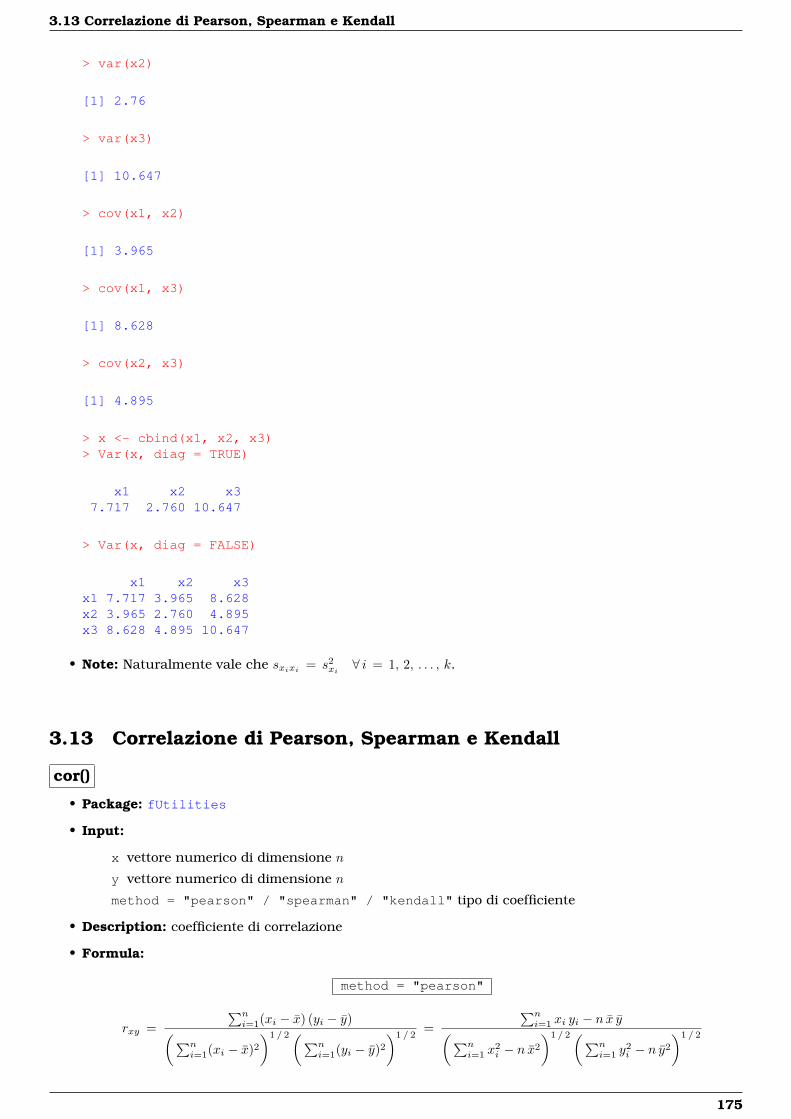
3.13 Correlazione di Pearson, Spearman e Kendall
> var(x2)
[1] 2.76
> var(x3)
[1] 10.647
> cov(x1, x2)
[1] 3.965
> cov(x1, x3)
[1] 8.628
> cov(x2, x3)
[1] 4.895
> x <- cbind(x1, x2, x3)> Var(x, diag = TRUE)
x1 x2 x37.717 2.760 10.647
> Var(x, diag = FALSE)
x1 x2 x3x1 7.717 3.965 8.628x2 3.965 2.760 4.895x3 8.628 4.895 10.647
• Note: Naturalmente vale che sxixi = s2xi ∀ i = 1, 2, . . . , k.
3.13 Correlazione di Pearson, Spearman e Kendall
cor()
• Package: fUtilities
• Input:
x vettore numerico di dimensione n
y vettore numerico di dimensione n
method = "pearson" / "spearman" / "kendall" tipo di coefficiente
• Description: coefficiente di correlazione
• Formula:
method = "pearson"
rxy =∑ni=1(xi − x) (yi − y)(∑n
i=1(xi − x)2
)1 / 2(∑ni=1(yi − y)2
)1 / 2=
∑ni=1 xi yi − n x y(∑n
i=1 x2i − n x2
)1 / 2(∑ni=1 y
2i − n y2
)1 / 2
175
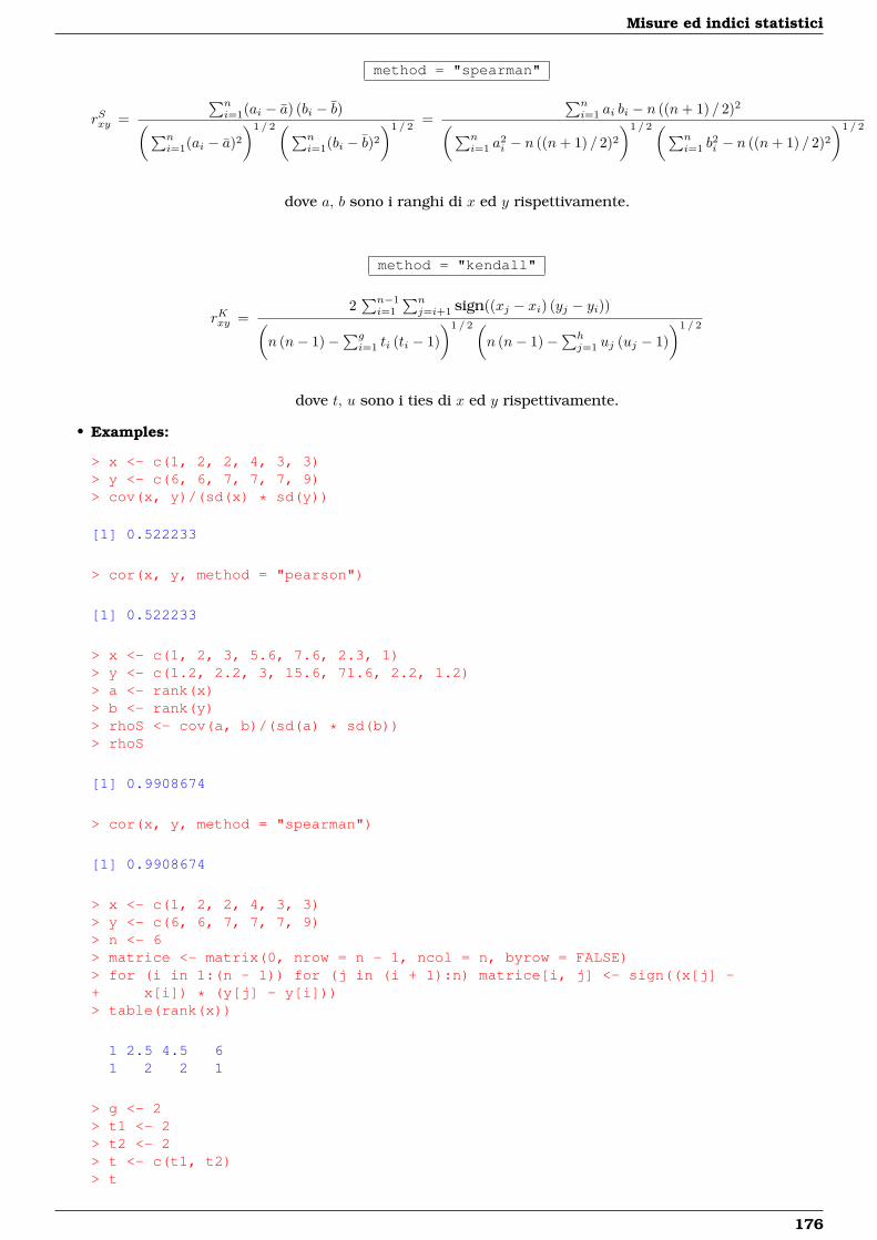
Misure ed indici statistici
method = "spearman"
rSxy =∑ni=1(ai − a) (bi − b)(∑n
i=1(ai − a)2
)1 / 2(∑ni=1(bi − b)2
)1 / 2=
∑ni=1 ai bi − n ((n+ 1) / 2)2(∑n
i=1 a2i − n ((n+ 1) / 2)2
)1 / 2(∑ni=1 b
2i − n ((n+ 1) / 2)2
)1 / 2
dove a, b sono i ranghi di x ed y rispettivamente.
method = "kendall"
rKxy =2∑n−1i=1
∑nj=i+1 sign((xj − xi) (yj − yi))(
n (n− 1)−∑gi=1 ti (ti − 1)
)1 / 2(n (n− 1)−
∑hj=1 uj (uj − 1)
)1 / 2
dove t, u sono i ties di x ed y rispettivamente.
• Examples:
> x <- c(1, 2, 2, 4, 3, 3)> y <- c(6, 6, 7, 7, 7, 9)> cov(x, y)/(sd(x) * sd(y))
[1] 0.522233
> cor(x, y, method = "pearson")
[1] 0.522233
> x <- c(1, 2, 3, 5.6, 7.6, 2.3, 1)> y <- c(1.2, 2.2, 3, 15.6, 71.6, 2.2, 1.2)> a <- rank(x)> b <- rank(y)> rhoS <- cov(a, b)/(sd(a) * sd(b))> rhoS
[1] 0.9908674
> cor(x, y, method = "spearman")
[1] 0.9908674
> x <- c(1, 2, 2, 4, 3, 3)> y <- c(6, 6, 7, 7, 7, 9)> n <- 6> matrice <- matrix(0, nrow = n - 1, ncol = n, byrow = FALSE)> for (i in 1:(n - 1)) for (j in (i + 1):n) matrice[i, j] <- sign((x[j] -+ x[i]) * (y[j] - y[i]))> table(rank(x))
1 2.5 4.5 61 2 2 1
> g <- 2> t1 <- 2> t2 <- 2> t <- c(t1, t2)> t
176
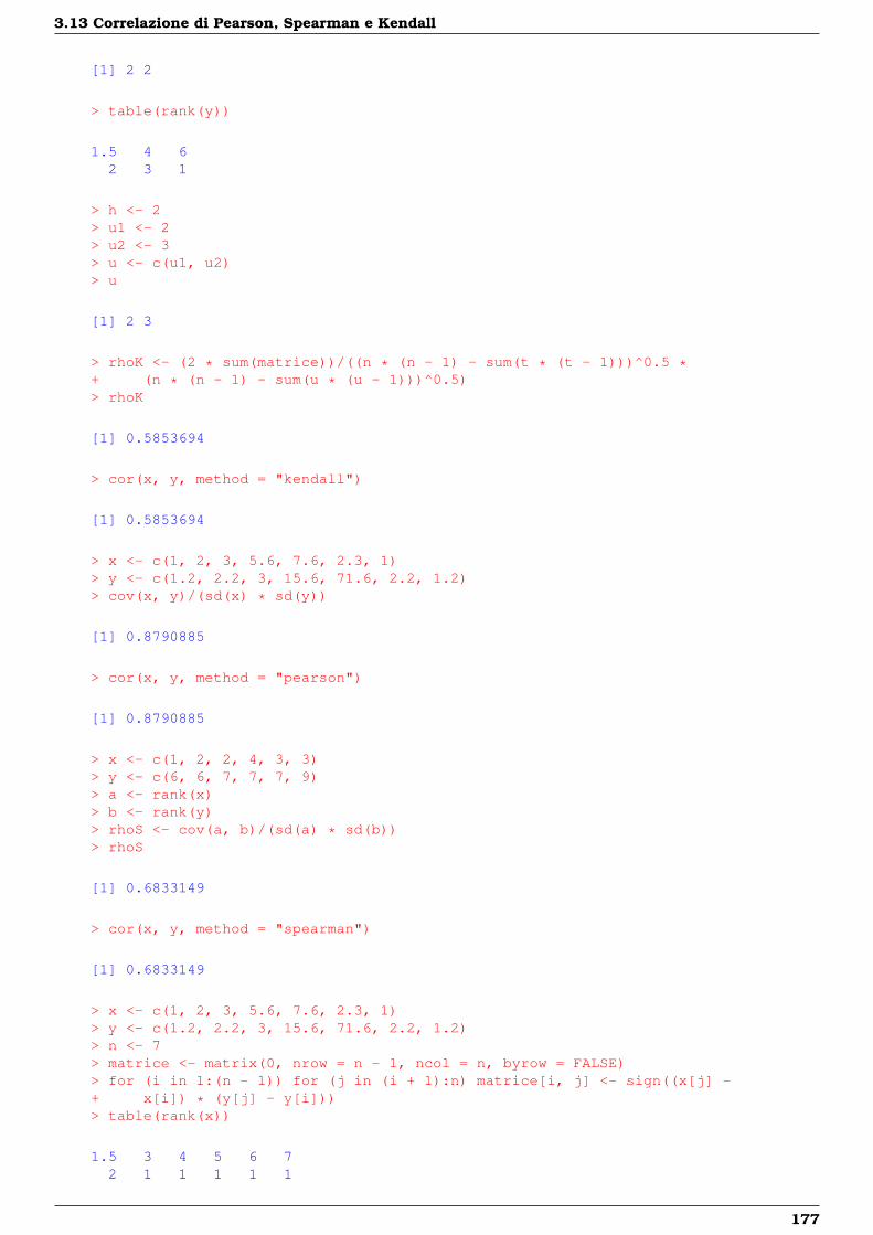
3.13 Correlazione di Pearson, Spearman e Kendall
[1] 2 2
> table(rank(y))
1.5 4 62 3 1
> h <- 2> u1 <- 2> u2 <- 3> u <- c(u1, u2)> u
[1] 2 3
> rhoK <- (2 * sum(matrice))/((n * (n - 1) - sum(t * (t - 1)))^0.5 *+ (n * (n - 1) - sum(u * (u - 1)))^0.5)> rhoK
[1] 0.5853694
> cor(x, y, method = "kendall")
[1] 0.5853694
> x <- c(1, 2, 3, 5.6, 7.6, 2.3, 1)> y <- c(1.2, 2.2, 3, 15.6, 71.6, 2.2, 1.2)> cov(x, y)/(sd(x) * sd(y))
[1] 0.8790885
> cor(x, y, method = "pearson")
[1] 0.8790885
> x <- c(1, 2, 2, 4, 3, 3)> y <- c(6, 6, 7, 7, 7, 9)> a <- rank(x)> b <- rank(y)> rhoS <- cov(a, b)/(sd(a) * sd(b))> rhoS
[1] 0.6833149
> cor(x, y, method = "spearman")
[1] 0.6833149
> x <- c(1, 2, 3, 5.6, 7.6, 2.3, 1)> y <- c(1.2, 2.2, 3, 15.6, 71.6, 2.2, 1.2)> n <- 7> matrice <- matrix(0, nrow = n - 1, ncol = n, byrow = FALSE)> for (i in 1:(n - 1)) for (j in (i + 1):n) matrice[i, j] <- sign((x[j] -+ x[i]) * (y[j] - y[i]))> table(rank(x))
1.5 3 4 5 6 72 1 1 1 1 1
177
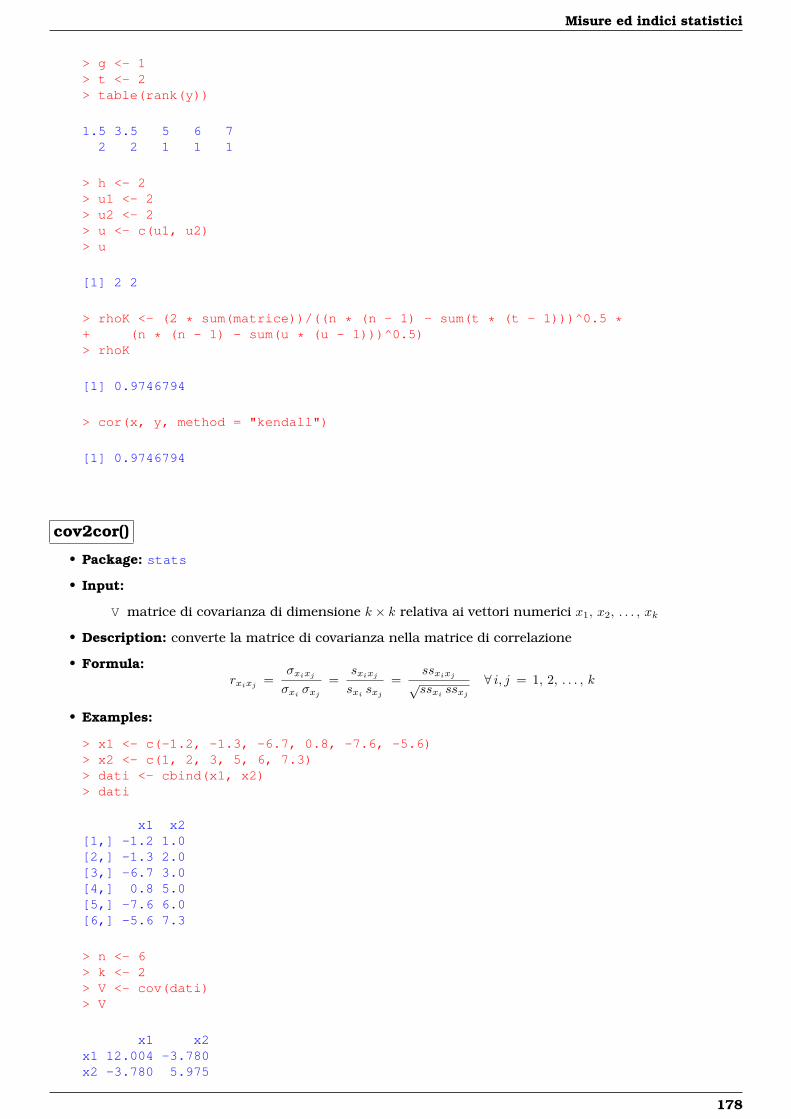
Misure ed indici statistici
> g <- 1> t <- 2> table(rank(y))
1.5 3.5 5 6 72 2 1 1 1
> h <- 2> u1 <- 2> u2 <- 2> u <- c(u1, u2)> u
[1] 2 2
> rhoK <- (2 * sum(matrice))/((n * (n - 1) - sum(t * (t - 1)))^0.5 *+ (n * (n - 1) - sum(u * (u - 1)))^0.5)> rhoK
[1] 0.9746794
> cor(x, y, method = "kendall")
[1] 0.9746794
cov2cor()
• Package: stats
• Input:
V matrice di covarianza di dimensione k × k relativa ai vettori numerici x1, x2, . . . , xk
• Description: converte la matrice di covarianza nella matrice di correlazione
• Formula:rxixj =
σxixjσxi σxj
=sxixjsxi sxj
=ssxixj√ssxi ssxj
∀ i, j = 1, 2, . . . , k
• Examples:
> x1 <- c(-1.2, -1.3, -6.7, 0.8, -7.6, -5.6)> x2 <- c(1, 2, 3, 5, 6, 7.3)> dati <- cbind(x1, x2)> dati
x1 x2[1,] -1.2 1.0[2,] -1.3 2.0[3,] -6.7 3.0[4,] 0.8 5.0[5,] -7.6 6.0[6,] -5.6 7.3
> n <- 6> k <- 2> V <- cov(dati)> V
x1 x2x1 12.004 -3.780x2 -3.780 5.975
178
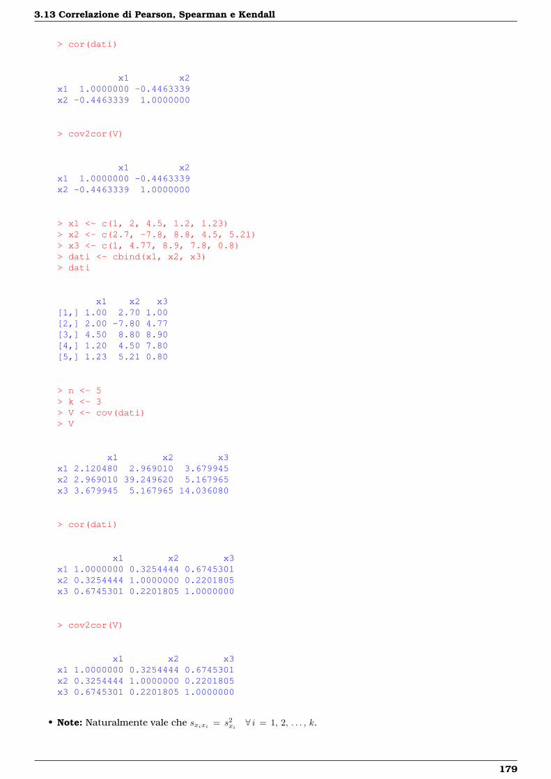
3.13 Correlazione di Pearson, Spearman e Kendall
> cor(dati)
x1 x2x1 1.0000000 -0.4463339x2 -0.4463339 1.0000000
> cov2cor(V)
x1 x2x1 1.0000000 -0.4463339x2 -0.4463339 1.0000000
> x1 <- c(1, 2, 4.5, 1.2, 1.23)> x2 <- c(2.7, -7.8, 8.8, 4.5, 5.21)> x3 <- c(1, 4.77, 8.9, 7.8, 0.8)> dati <- cbind(x1, x2, x3)> dati
x1 x2 x3[1,] 1.00 2.70 1.00[2,] 2.00 -7.80 4.77[3,] 4.50 8.80 8.90[4,] 1.20 4.50 7.80[5,] 1.23 5.21 0.80
> n <- 5> k <- 3> V <- cov(dati)> V
x1 x2 x3x1 2.120480 2.969010 3.679945x2 2.969010 39.249620 5.167965x3 3.679945 5.167965 14.036080
> cor(dati)
x1 x2 x3x1 1.0000000 0.3254444 0.6745301x2 0.3254444 1.0000000 0.2201805x3 0.6745301 0.2201805 1.0000000
> cov2cor(V)
x1 x2 x3x1 1.0000000 0.3254444 0.6745301x2 0.3254444 1.0000000 0.2201805x3 0.6745301 0.2201805 1.0000000
• Note: Naturalmente vale che sxixi = s2xi ∀ i = 1, 2, . . . , k.
179
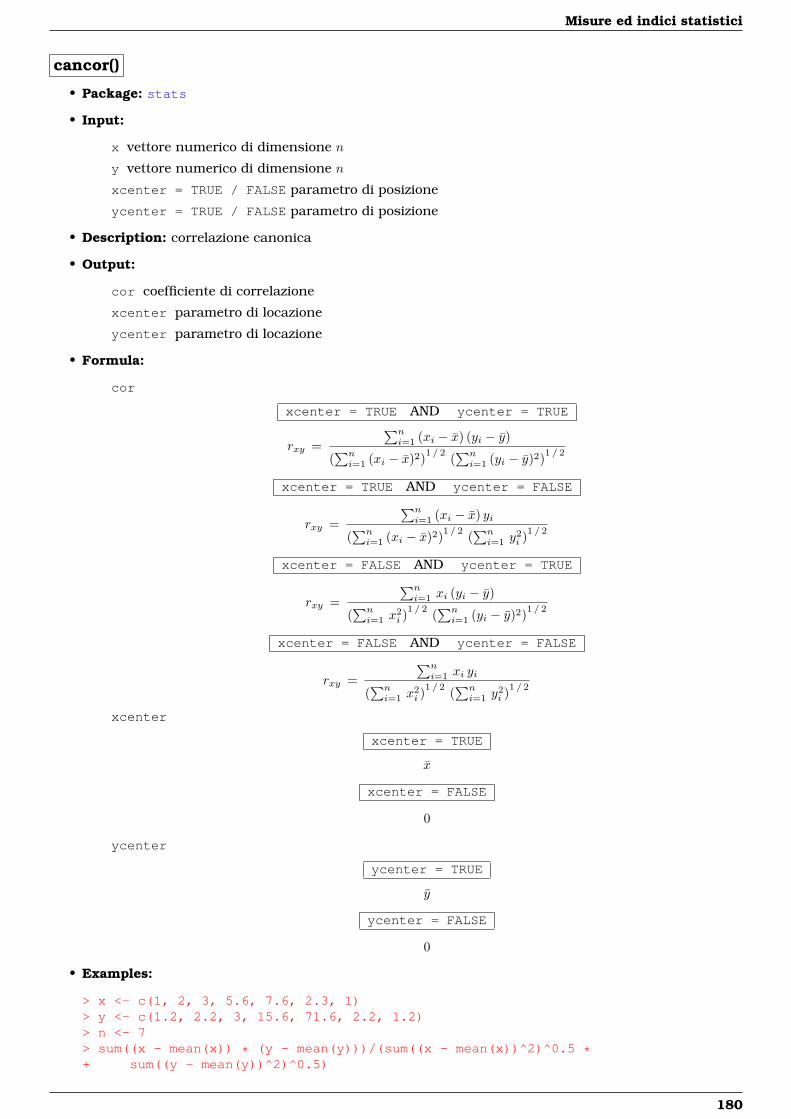
Misure ed indici statistici
cancor()
• Package: stats
• Input:
x vettore numerico di dimensione n
y vettore numerico di dimensione n
xcenter = TRUE / FALSE parametro di posizione
ycenter = TRUE / FALSE parametro di posizione
• Description: correlazione canonica
• Output:
cor coefficiente di correlazione
xcenter parametro di locazione
ycenter parametro di locazione
• Formula:
cor
xcenter = TRUE AND ycenter = TRUE
rxy =∑ni=1 (xi − x) (yi − y)
(∑ni=1 (xi − x)2)1 / 2 (
∑ni=1 (yi − y)2)1 / 2
xcenter = TRUE AND ycenter = FALSE
rxy =∑ni=1 (xi − x) yi
(∑ni=1 (xi − x)2)1 / 2 (
∑ni=1 y
2i )1 / 2
xcenter = FALSE AND ycenter = TRUE
rxy =∑ni=1 xi (yi − y)
(∑ni=1 x
2i )
1 / 2 (∑ni=1 (yi − y)2)1 / 2
xcenter = FALSE AND ycenter = FALSE
rxy =∑ni=1 xi yi
(∑ni=1 x
2i )
1 / 2 (∑ni=1 y
2i )1 / 2
xcenter
xcenter = TRUE
x
xcenter = FALSE
0
ycenter
ycenter = TRUE
y
ycenter = FALSE
0
• Examples:
> x <- c(1, 2, 3, 5.6, 7.6, 2.3, 1)> y <- c(1.2, 2.2, 3, 15.6, 71.6, 2.2, 1.2)> n <- 7> sum((x - mean(x)) * (y - mean(y)))/(sum((x - mean(x))^2)^0.5 *+ sum((y - mean(y))^2)^0.5)
180
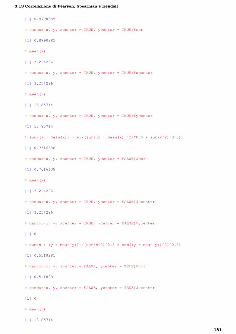
3.13 Correlazione di Pearson, Spearman e Kendall
[1] 0.8790885
> cancor(x, y, xcenter = TRUE, ycenter = TRUE)$cor
[1] 0.8790885
> mean(x)
[1] 3.214286
> cancor(x, y, xcenter = TRUE, ycenter = TRUE)$xcenter
[1] 3.214286
> mean(y)
[1] 13.85714
> cancor(x, y, xcenter = TRUE, ycenter = TRUE)$ycenter
[1] 13.85714
> sum((x - mean(x)) * y)/(sum((x - mean(x))^2)^0.5 * sum(y^2)^0.5)
[1] 0.7616638
> cancor(x, y, xcenter = TRUE, ycenter = FALSE)$cor
[1] 0.7616638
> mean(x)
[1] 3.214286
> cancor(x, y, xcenter = TRUE, ycenter = FALSE)$xcenter
[1] 3.214286
> cancor(x, y, xcenter = TRUE, ycenter = FALSE)$ycenter
[1] 0
> sum(x * (y - mean(y)))/(sum(x^2)^0.5 * sum((y - mean(y))^2)^0.5)
[1] 0.5118281
> cancor(x, y, xcenter = FALSE, ycenter = TRUE)$cor
[1] 0.5118281
> cancor(x, y, xcenter = FALSE, ycenter = TRUE)$xcenter
[1] 0
> mean(y)
[1] 13.85714
181
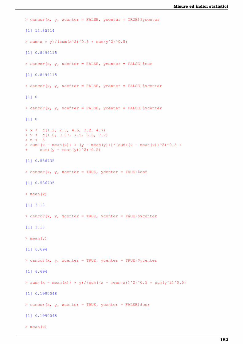
Misure ed indici statistici
> cancor(x, y, xcenter = FALSE, ycenter = TRUE)$ycenter
[1] 13.85714
> sum(x * y)/(sum(x^2)^0.5 * sum(y^2)^0.5)
[1] 0.8494115
> cancor(x, y, xcenter = FALSE, ycenter = FALSE)$cor
[1] 0.8494115
> cancor(x, y, xcenter = FALSE, ycenter = FALSE)$xcenter
[1] 0
> cancor(x, y, xcenter = FALSE, ycenter = FALSE)$ycenter
[1] 0
> x <- c(1.2, 2.3, 4.5, 3.2, 4.7)> y <- c(1.8, 9.87, 7.5, 6.6, 7.7)> n <- 5> sum((x - mean(x)) * (y - mean(y)))/(sum((x - mean(x))^2)^0.5 *+ sum((y - mean(y))^2)^0.5)
[1] 0.536735
> cancor(x, y, xcenter = TRUE, ycenter = TRUE)$cor
[1] 0.536735
> mean(x)
[1] 3.18
> cancor(x, y, xcenter = TRUE, ycenter = TRUE)$xcenter
[1] 3.18
> mean(y)
[1] 6.694
> cancor(x, y, xcenter = TRUE, ycenter = TRUE)$ycenter
[1] 6.694
> sum((x - mean(x)) * y)/(sum((x - mean(x))^2)^0.5 * sum(y^2)^0.5)
[1] 0.1990048
> cancor(x, y, xcenter = TRUE, ycenter = FALSE)$cor
[1] 0.1990048
> mean(x)
182
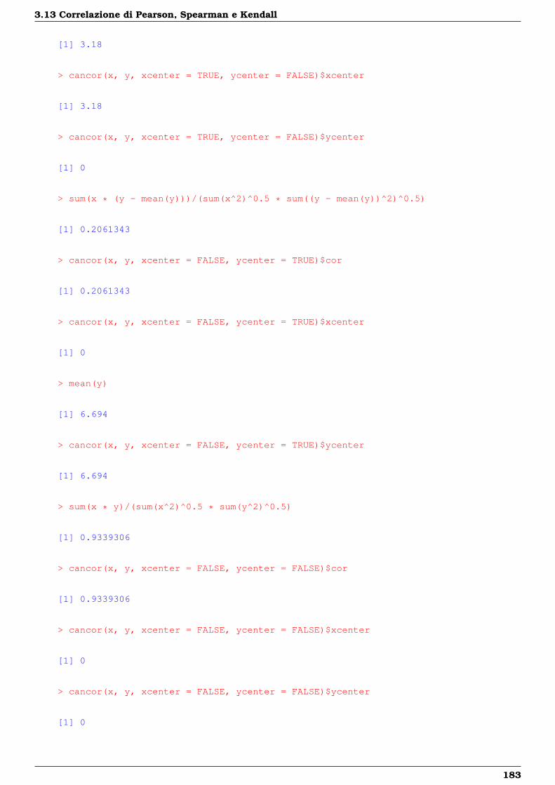
3.13 Correlazione di Pearson, Spearman e Kendall
[1] 3.18
> cancor(x, y, xcenter = TRUE, ycenter = FALSE)$xcenter
[1] 3.18
> cancor(x, y, xcenter = TRUE, ycenter = FALSE)$ycenter
[1] 0
> sum(x * (y - mean(y)))/(sum(x^2)^0.5 * sum((y - mean(y))^2)^0.5)
[1] 0.2061343
> cancor(x, y, xcenter = FALSE, ycenter = TRUE)$cor
[1] 0.2061343
> cancor(x, y, xcenter = FALSE, ycenter = TRUE)$xcenter
[1] 0
> mean(y)
[1] 6.694
> cancor(x, y, xcenter = FALSE, ycenter = TRUE)$ycenter
[1] 6.694
> sum(x * y)/(sum(x^2)^0.5 * sum(y^2)^0.5)
[1] 0.9339306
> cancor(x, y, xcenter = FALSE, ycenter = FALSE)$cor
[1] 0.9339306
> cancor(x, y, xcenter = FALSE, ycenter = FALSE)$xcenter
[1] 0
> cancor(x, y, xcenter = FALSE, ycenter = FALSE)$ycenter
[1] 0
183
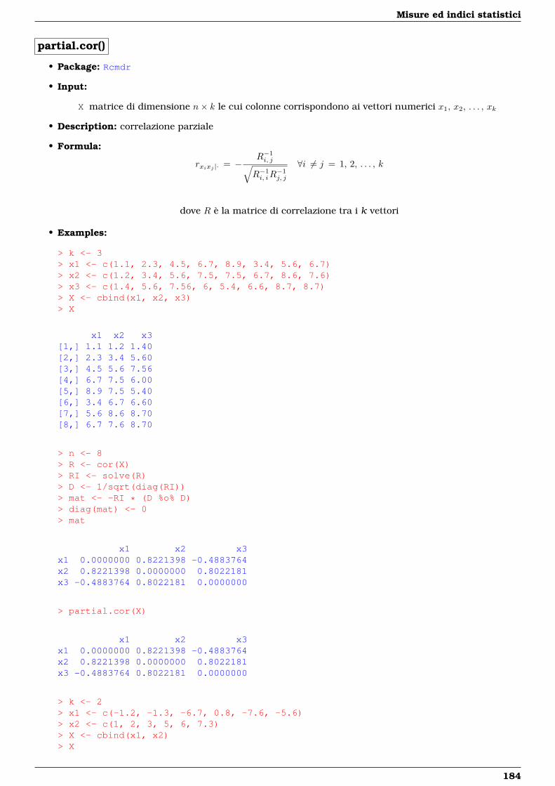
Misure ed indici statistici
partial.cor()
• Package: Rcmdr
• Input:
X matrice di dimensione n× k le cui colonne corrispondono ai vettori numerici x1, x2, . . . , xk
• Description: correlazione parziale
• Formula:
rxixj |· = −R−1i, j√
R−1i, iR
−1j, j
∀i 6= j = 1, 2, . . . , k
dove R è la matrice di correlazione tra i k vettori
• Examples:
> k <- 3> x1 <- c(1.1, 2.3, 4.5, 6.7, 8.9, 3.4, 5.6, 6.7)> x2 <- c(1.2, 3.4, 5.6, 7.5, 7.5, 6.7, 8.6, 7.6)> x3 <- c(1.4, 5.6, 7.56, 6, 5.4, 6.6, 8.7, 8.7)> X <- cbind(x1, x2, x3)> X
x1 x2 x3[1,] 1.1 1.2 1.40[2,] 2.3 3.4 5.60[3,] 4.5 5.6 7.56[4,] 6.7 7.5 6.00[5,] 8.9 7.5 5.40[6,] 3.4 6.7 6.60[7,] 5.6 8.6 8.70[8,] 6.7 7.6 8.70
> n <- 8> R <- cor(X)> RI <- solve(R)> D <- 1/sqrt(diag(RI))> mat <- -RI * (D %o% D)> diag(mat) <- 0> mat
x1 x2 x3x1 0.0000000 0.8221398 -0.4883764x2 0.8221398 0.0000000 0.8022181x3 -0.4883764 0.8022181 0.0000000
> partial.cor(X)
x1 x2 x3x1 0.0000000 0.8221398 -0.4883764x2 0.8221398 0.0000000 0.8022181x3 -0.4883764 0.8022181 0.0000000
> k <- 2> x1 <- c(-1.2, -1.3, -6.7, 0.8, -7.6, -5.6)> x2 <- c(1, 2, 3, 5, 6, 7.3)> X <- cbind(x1, x2)> X
184
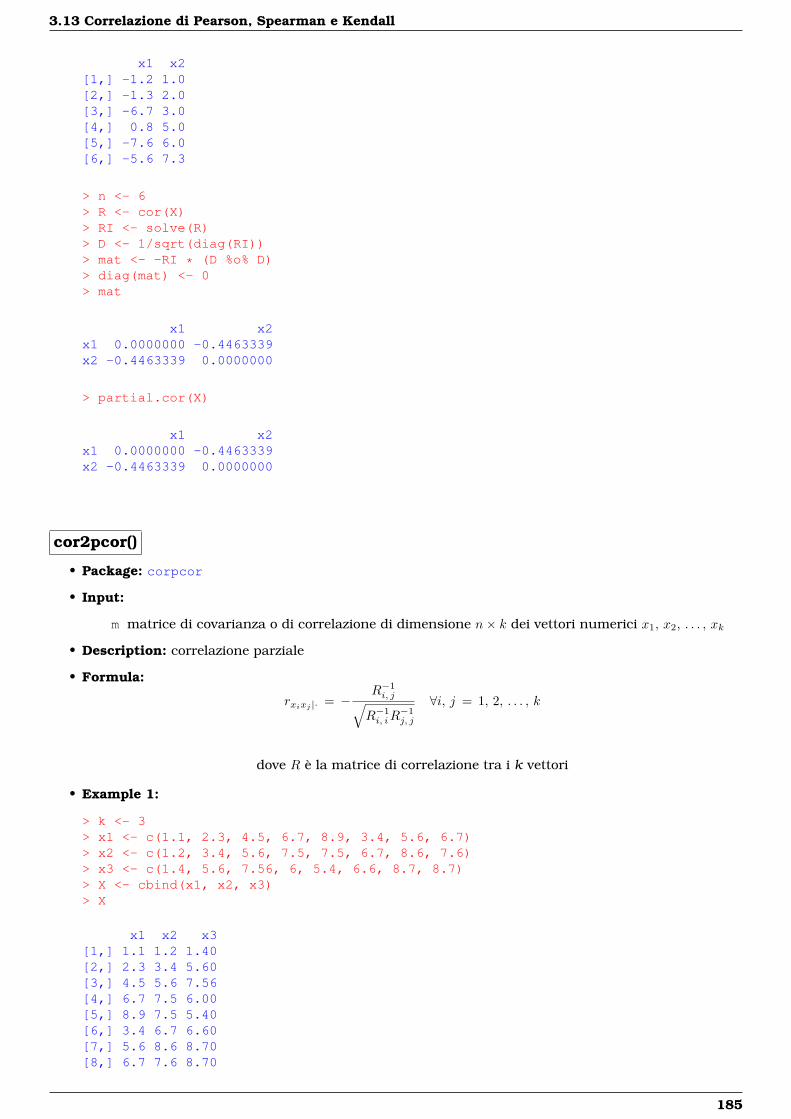
3.13 Correlazione di Pearson, Spearman e Kendall
x1 x2[1,] -1.2 1.0[2,] -1.3 2.0[3,] -6.7 3.0[4,] 0.8 5.0[5,] -7.6 6.0[6,] -5.6 7.3
> n <- 6> R <- cor(X)> RI <- solve(R)> D <- 1/sqrt(diag(RI))> mat <- -RI * (D %o% D)> diag(mat) <- 0> mat
x1 x2x1 0.0000000 -0.4463339x2 -0.4463339 0.0000000
> partial.cor(X)
x1 x2x1 0.0000000 -0.4463339x2 -0.4463339 0.0000000
cor2pcor()
• Package: corpcor
• Input:
m matrice di covarianza o di correlazione di dimensione n× k dei vettori numerici x1, x2, . . . , xk
• Description: correlazione parziale
• Formula:
rxixj |· = −R−1i, j√
R−1i, iR
−1j, j
∀i, j = 1, 2, . . . , k
dove R è la matrice di correlazione tra i k vettori
• Example 1:
> k <- 3> x1 <- c(1.1, 2.3, 4.5, 6.7, 8.9, 3.4, 5.6, 6.7)> x2 <- c(1.2, 3.4, 5.6, 7.5, 7.5, 6.7, 8.6, 7.6)> x3 <- c(1.4, 5.6, 7.56, 6, 5.4, 6.6, 8.7, 8.7)> X <- cbind(x1, x2, x3)> X
x1 x2 x3[1,] 1.1 1.2 1.40[2,] 2.3 3.4 5.60[3,] 4.5 5.6 7.56[4,] 6.7 7.5 6.00[5,] 8.9 7.5 5.40[6,] 3.4 6.7 6.60[7,] 5.6 8.6 8.70[8,] 6.7 7.6 8.70
185
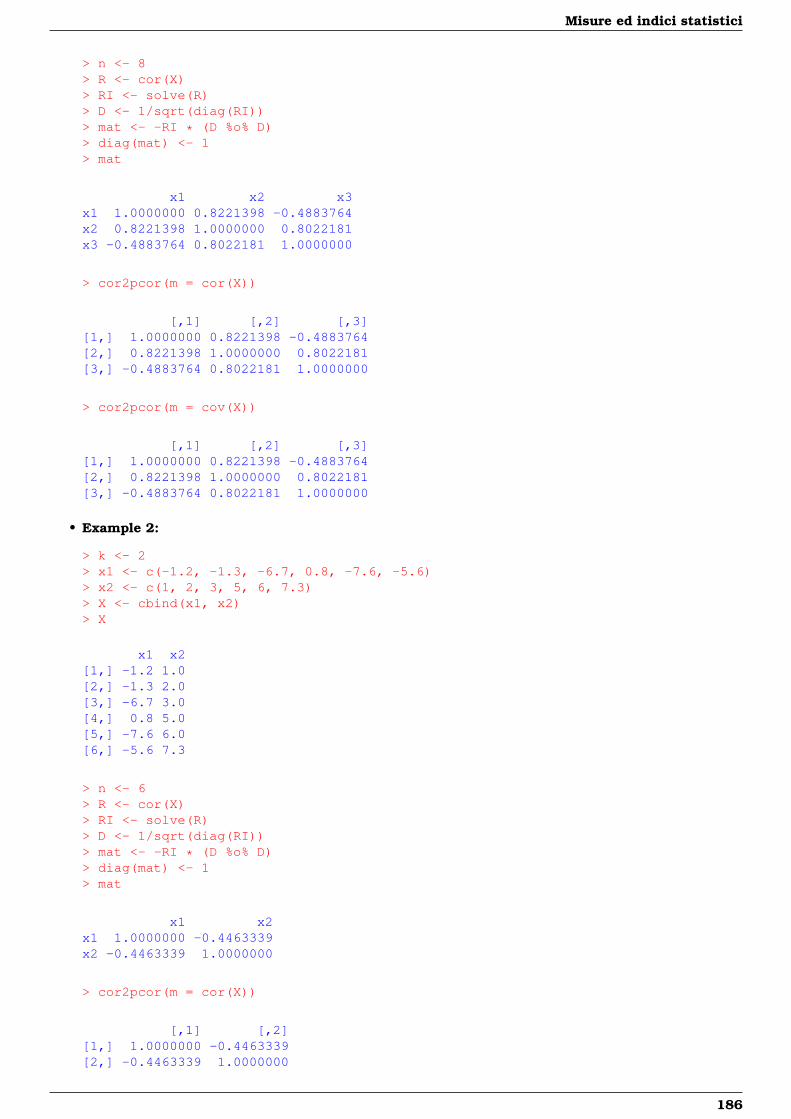
Misure ed indici statistici
> n <- 8> R <- cor(X)> RI <- solve(R)> D <- 1/sqrt(diag(RI))> mat <- -RI * (D %o% D)> diag(mat) <- 1> mat
x1 x2 x3x1 1.0000000 0.8221398 -0.4883764x2 0.8221398 1.0000000 0.8022181x3 -0.4883764 0.8022181 1.0000000
> cor2pcor(m = cor(X))
[,1] [,2] [,3][1,] 1.0000000 0.8221398 -0.4883764[2,] 0.8221398 1.0000000 0.8022181[3,] -0.4883764 0.8022181 1.0000000
> cor2pcor(m = cov(X))
[,1] [,2] [,3][1,] 1.0000000 0.8221398 -0.4883764[2,] 0.8221398 1.0000000 0.8022181[3,] -0.4883764 0.8022181 1.0000000
• Example 2:
> k <- 2> x1 <- c(-1.2, -1.3, -6.7, 0.8, -7.6, -5.6)> x2 <- c(1, 2, 3, 5, 6, 7.3)> X <- cbind(x1, x2)> X
x1 x2[1,] -1.2 1.0[2,] -1.3 2.0[3,] -6.7 3.0[4,] 0.8 5.0[5,] -7.6 6.0[6,] -5.6 7.3
> n <- 6> R <- cor(X)> RI <- solve(R)> D <- 1/sqrt(diag(RI))> mat <- -RI * (D %o% D)> diag(mat) <- 1> mat
x1 x2x1 1.0000000 -0.4463339x2 -0.4463339 1.0000000
> cor2pcor(m = cor(X))
[,1] [,2][1,] 1.0000000 -0.4463339[2,] -0.4463339 1.0000000
186
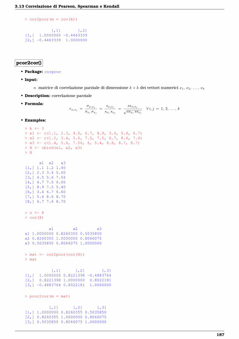
3.13 Correlazione di Pearson, Spearman e Kendall
> cor2pcor(m = cov(X))
[,1] [,2][1,] 1.0000000 -0.4463339[2,] -0.4463339 1.0000000
pcor2cor()
• Package: corpcor
• Input:
m matrice di correlazione parziale di dimensione k × k dei vettori numerici x1, x2, . . . , xk
• Description: correlazione parziale
• Formula:rxixj =
σxixjσxi σxj
=sxixjsxi sxj
=ssxixj√ssxi ssxj
∀ i, j = 1, 2, . . . , k
• Examples:
> k <- 3> x1 <- c(1.1, 2.3, 4.5, 6.7, 8.9, 3.4, 5.6, 6.7)> x2 <- c(1.2, 3.4, 5.6, 7.5, 7.5, 6.7, 8.6, 7.6)> x3 <- c(1.4, 5.6, 7.56, 6, 5.4, 6.6, 8.7, 8.7)> X <- cbind(x1, x2, x3)> X
x1 x2 x3[1,] 1.1 1.2 1.40[2,] 2.3 3.4 5.60[3,] 4.5 5.6 7.56[4,] 6.7 7.5 6.00[5,] 8.9 7.5 5.40[6,] 3.4 6.7 6.60[7,] 5.6 8.6 8.70[8,] 6.7 7.6 8.70
> n <- 8> cor(X)
x1 x2 x3x1 1.0000000 0.8260355 0.5035850x2 0.8260355 1.0000000 0.8066075x3 0.5035850 0.8066075 1.0000000
> mat <- cor2pcor(cor(X))> mat
[,1] [,2] [,3][1,] 1.0000000 0.8221398 -0.4883764[2,] 0.8221398 1.0000000 0.8022181[3,] -0.4883764 0.8022181 1.0000000
> pcor2cor(m = mat)
[,1] [,2] [,3][1,] 1.0000000 0.8260355 0.5035850[2,] 0.8260355 1.0000000 0.8066075[3,] 0.5035850 0.8066075 1.0000000
187
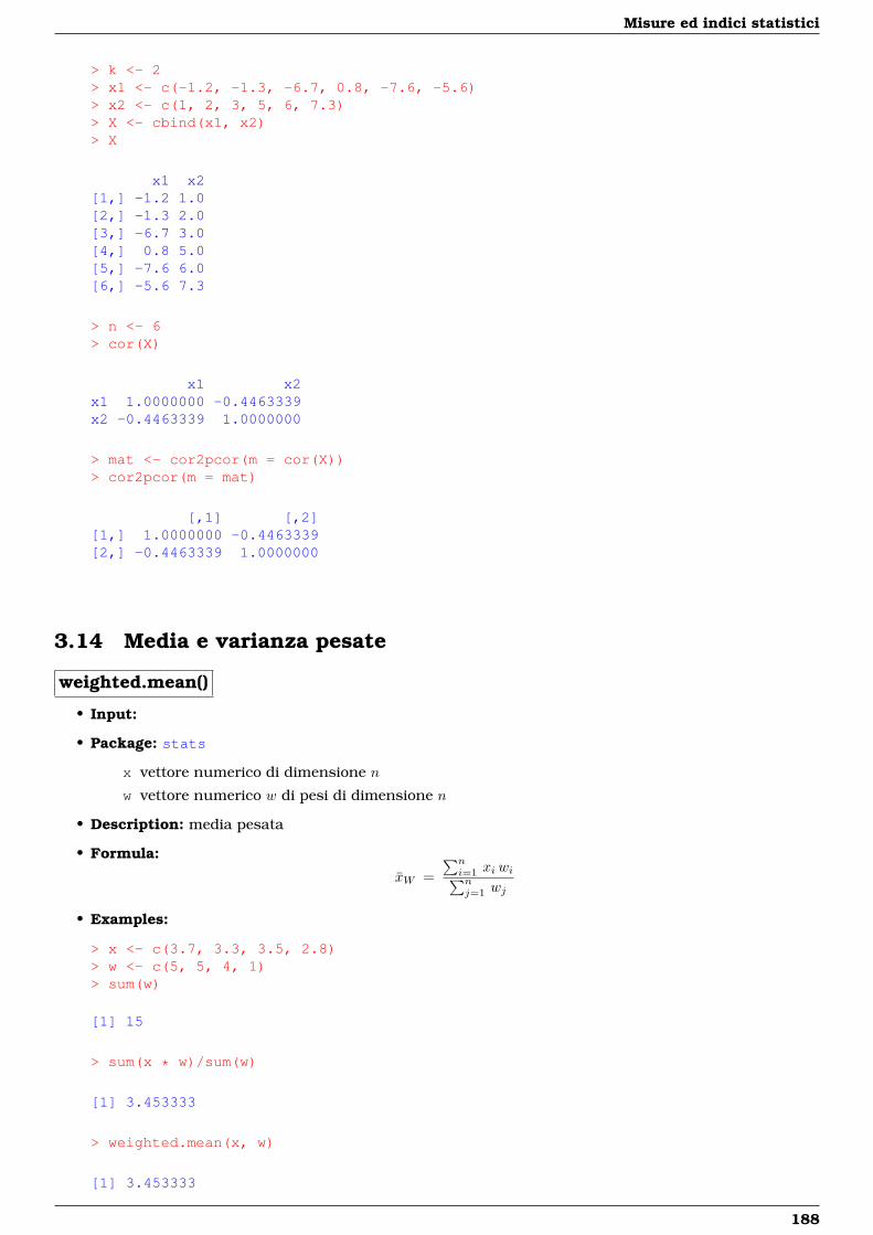
Misure ed indici statistici
> k <- 2> x1 <- c(-1.2, -1.3, -6.7, 0.8, -7.6, -5.6)> x2 <- c(1, 2, 3, 5, 6, 7.3)> X <- cbind(x1, x2)> X
x1 x2[1,] -1.2 1.0[2,] -1.3 2.0[3,] -6.7 3.0[4,] 0.8 5.0[5,] -7.6 6.0[6,] -5.6 7.3
> n <- 6> cor(X)
x1 x2x1 1.0000000 -0.4463339x2 -0.4463339 1.0000000
> mat <- cor2pcor(m = cor(X))> cor2pcor(m = mat)
[,1] [,2][1,] 1.0000000 -0.4463339[2,] -0.4463339 1.0000000
3.14 Media e varianza pesate
weighted.mean()
• Input:
• Package: stats
x vettore numerico di dimensione n
w vettore numerico w di pesi di dimensione n
• Description: media pesata
• Formula:
xW =∑ni=1 xi wi∑nj=1 wj
• Examples:
> x <- c(3.7, 3.3, 3.5, 2.8)> w <- c(5, 5, 4, 1)> sum(w)
[1] 15
> sum(x * w)/sum(w)
[1] 3.453333
> weighted.mean(x, w)
[1] 3.453333
188
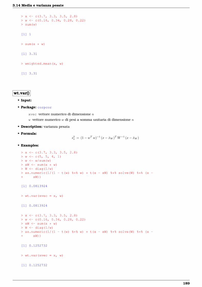
3.14 Media e varianza pesate
> x <- c(3.7, 3.3, 3.5, 2.8)> w <- c(0.16, 0.34, 0.28, 0.22)> sum(w)
[1] 1
> sum(x * w)
[1] 3.31
> weighted.mean(x, w)
[1] 3.31
wt.var()
• Input:
• Package: corpcor
xvec vettore numerico di dimensione n
w vettore numerico w di pesi a somma unitaria di dimensione n
• Description: varianza pesata
• Formula:s2x = (1− wT w)−1 (x− xW )T W−1 (x− xW )
• Examples:
> x <- c(3.7, 3.3, 3.5, 2.8)> w <- c(5, 5, 4, 1)> w <- w/sum(w)> xW <- sum(x * w)> W <- diag(1/w)> as.numeric(1/(1 - t(w) %*% w) * t(x - xW) %*% solve(W) %*% (x -+ xW))
[1] 0.0813924
> wt.var(xvec = x, w)
[1] 0.0813924
> x <- c(3.7, 3.3, 3.5, 2.8)> w <- c(0.16, 0.34, 0.28, 0.22)> xW <- sum(x * w)> W <- diag(1/w)> as.numeric(1/(1 - t(w) %*% w) * t(x - xW) %*% solve(W) %*% (x -+ xW))
[1] 0.1252732
> wt.var(xvec = x, w)
[1] 0.1252732
189
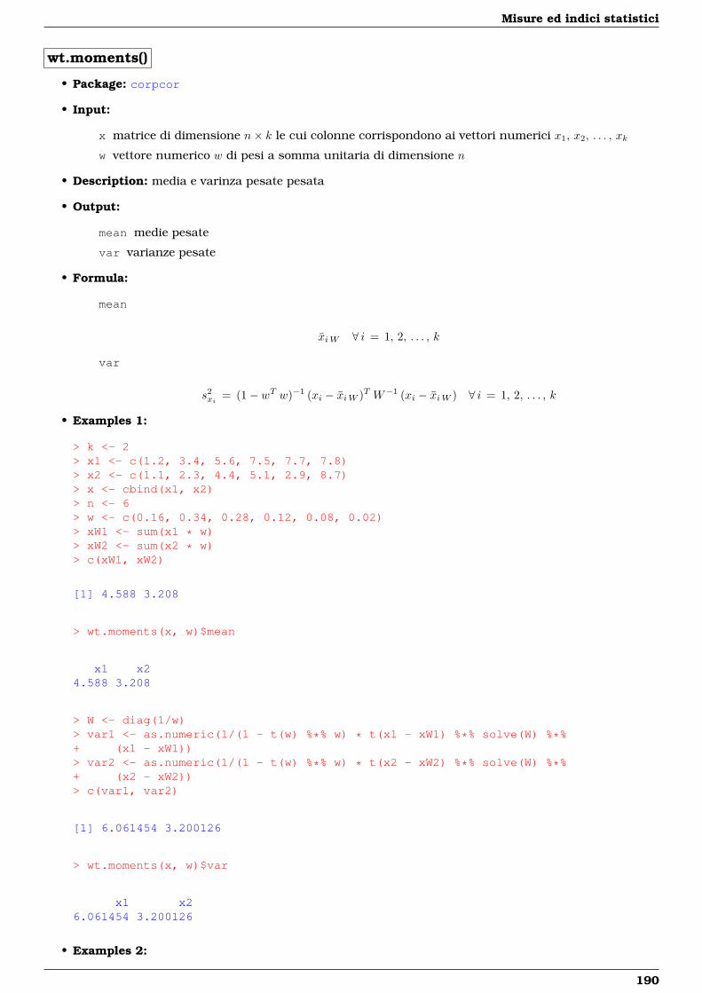
Misure ed indici statistici
wt.moments()
• Package: corpcor
• Input:
x matrice di dimensione n× k le cui colonne corrispondono ai vettori numerici x1, x2, . . . , xk
w vettore numerico w di pesi a somma unitaria di dimensione n
• Description: media e varinza pesate pesata
• Output:
mean medie pesate
var varianze pesate
• Formula:
mean
xiW ∀ i = 1, 2, . . . , k
var
s2xi = (1− wT w)−1 (xi − xiW )T W−1 (xi − xiW ) ∀ i = 1, 2, . . . , k
• Examples 1:
> k <- 2> x1 <- c(1.2, 3.4, 5.6, 7.5, 7.7, 7.8)> x2 <- c(1.1, 2.3, 4.4, 5.1, 2.9, 8.7)> x <- cbind(x1, x2)> n <- 6> w <- c(0.16, 0.34, 0.28, 0.12, 0.08, 0.02)> xW1 <- sum(x1 * w)> xW2 <- sum(x2 * w)> c(xW1, xW2)
[1] 4.588 3.208
> wt.moments(x, w)$mean
x1 x24.588 3.208
> W <- diag(1/w)> var1 <- as.numeric(1/(1 - t(w) %*% w) * t(x1 - xW1) %*% solve(W) %*%+ (x1 - xW1))> var2 <- as.numeric(1/(1 - t(w) %*% w) * t(x2 - xW2) %*% solve(W) %*%+ (x2 - xW2))> c(var1, var2)
[1] 6.061454 3.200126
> wt.moments(x, w)$var
x1 x26.061454 3.200126
• Examples 2:
190
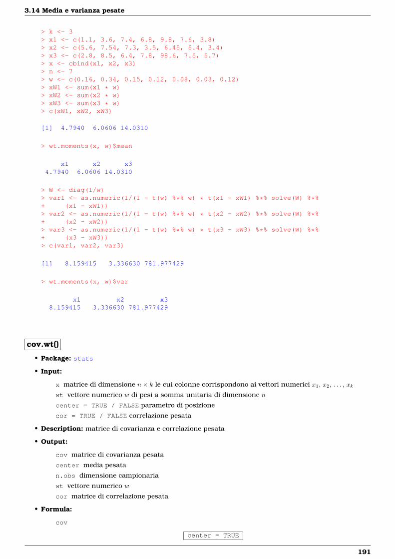
3.14 Media e varianza pesate
> k <- 3> x1 <- c(1.1, 3.6, 7.4, 6.8, 9.8, 7.6, 3.8)> x2 <- c(5.6, 7.54, 7.3, 3.5, 6.45, 5.4, 3.4)> x3 <- c(2.8, 8.5, 6.4, 7.8, 98.6, 7.5, 5.7)> x <- cbind(x1, x2, x3)> n <- 7> w <- c(0.16, 0.34, 0.15, 0.12, 0.08, 0.03, 0.12)> xW1 <- sum(x1 * w)> xW2 <- sum(x2 * w)> xW3 <- sum(x3 * w)> c(xW1, xW2, xW3)
[1] 4.7940 6.0606 14.0310
> wt.moments(x, w)$mean
x1 x2 x34.7940 6.0606 14.0310
> W <- diag(1/w)> var1 <- as.numeric(1/(1 - t(w) %*% w) * t(x1 - xW1) %*% solve(W) %*%+ (x1 - xW1))> var2 <- as.numeric(1/(1 - t(w) %*% w) * t(x2 - xW2) %*% solve(W) %*%+ (x2 - xW2))> var3 <- as.numeric(1/(1 - t(w) %*% w) * t(x3 - xW3) %*% solve(W) %*%+ (x3 - xW3))> c(var1, var2, var3)
[1] 8.159415 3.336630 781.977429
> wt.moments(x, w)$var
x1 x2 x38.159415 3.336630 781.977429
cov.wt()
• Package: stats
• Input:
x matrice di dimensione n× k le cui colonne corrispondono ai vettori numerici x1, x2, . . . , xk
wt vettore numerico w di pesi a somma unitaria di dimensione n
center = TRUE / FALSE parametro di posizione
cor = TRUE / FALSE correlazione pesata
• Description: matrice di covarianza e correlazione pesata
• Output:
cov matrice di covarianza pesata
center media pesata
n.obs dimensione campionaria
wt vettore numerico w
cor matrice di correlazione pesata
• Formula:
cov
center = TRUE
191
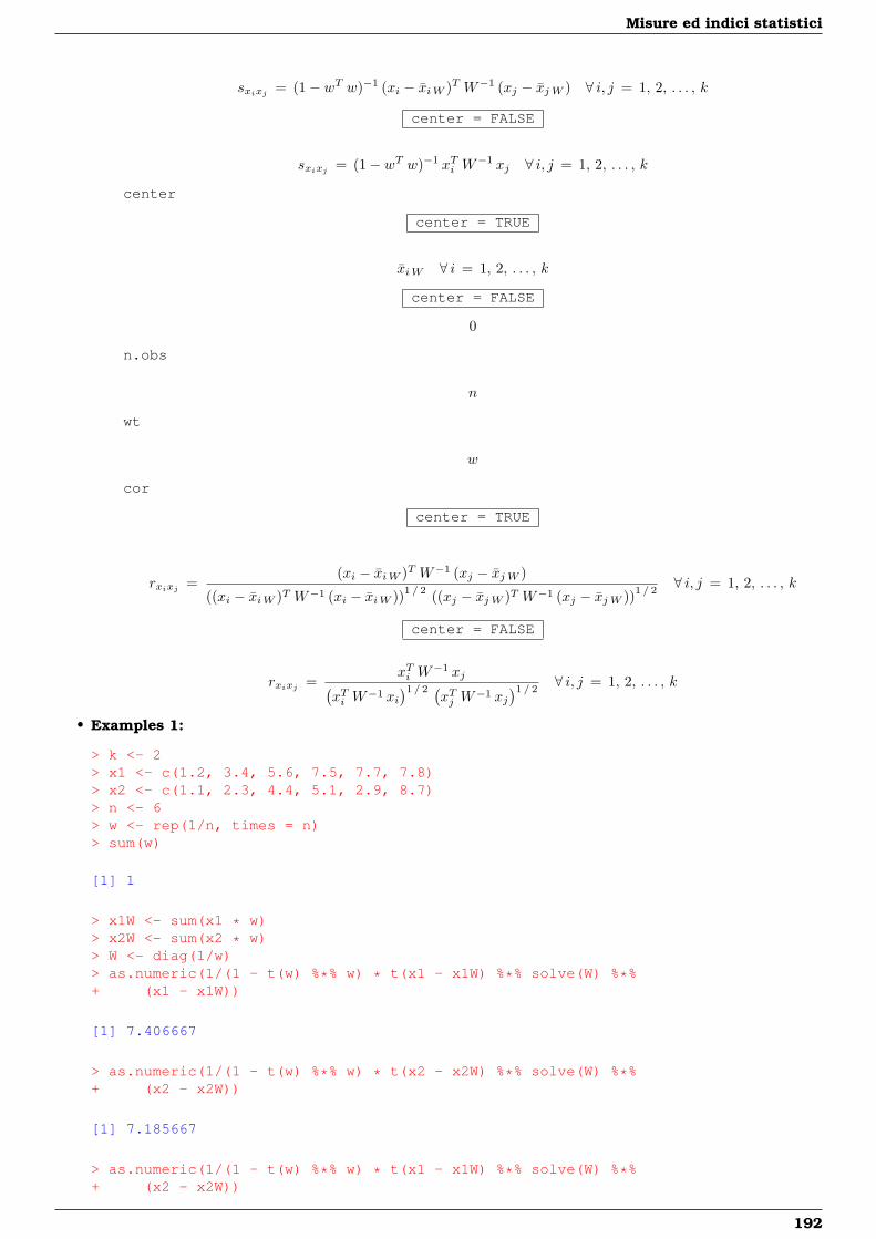
Misure ed indici statistici
sxixj = (1− wT w)−1 (xi − xiW )T W−1 (xj − xj W ) ∀ i, j = 1, 2, . . . , k
center = FALSE
sxixj = (1− wT w)−1 xTi W−1 xj ∀ i, j = 1, 2, . . . , k
center
center = TRUE
xiW ∀ i = 1, 2, . . . , k
center = FALSE
0
n.obs
n
wt
w
cor
center = TRUE
rxixj =(xi − xiW )T W−1 (xj − xj W )
((xi − xiW )T W−1 (xi − xiW ))1 / 2 ((xj − xj W )T W−1 (xj − xj W ))1 / 2∀ i, j = 1, 2, . . . , k
center = FALSE
rxixj =xTi W
−1 xj(xTi W
−1 xi)1 / 2 (
xTj W−1 xj
)1 / 2∀ i, j = 1, 2, . . . , k
• Examples 1:
> k <- 2> x1 <- c(1.2, 3.4, 5.6, 7.5, 7.7, 7.8)> x2 <- c(1.1, 2.3, 4.4, 5.1, 2.9, 8.7)> n <- 6> w <- rep(1/n, times = n)> sum(w)
[1] 1
> x1W <- sum(x1 * w)> x2W <- sum(x2 * w)> W <- diag(1/w)> as.numeric(1/(1 - t(w) %*% w) * t(x1 - x1W) %*% solve(W) %*%+ (x1 - x1W))
[1] 7.406667
> as.numeric(1/(1 - t(w) %*% w) * t(x2 - x2W) %*% solve(W) %*%+ (x2 - x2W))
[1] 7.185667
> as.numeric(1/(1 - t(w) %*% w) * t(x1 - x1W) %*% solve(W) %*%+ (x2 - x2W))
192
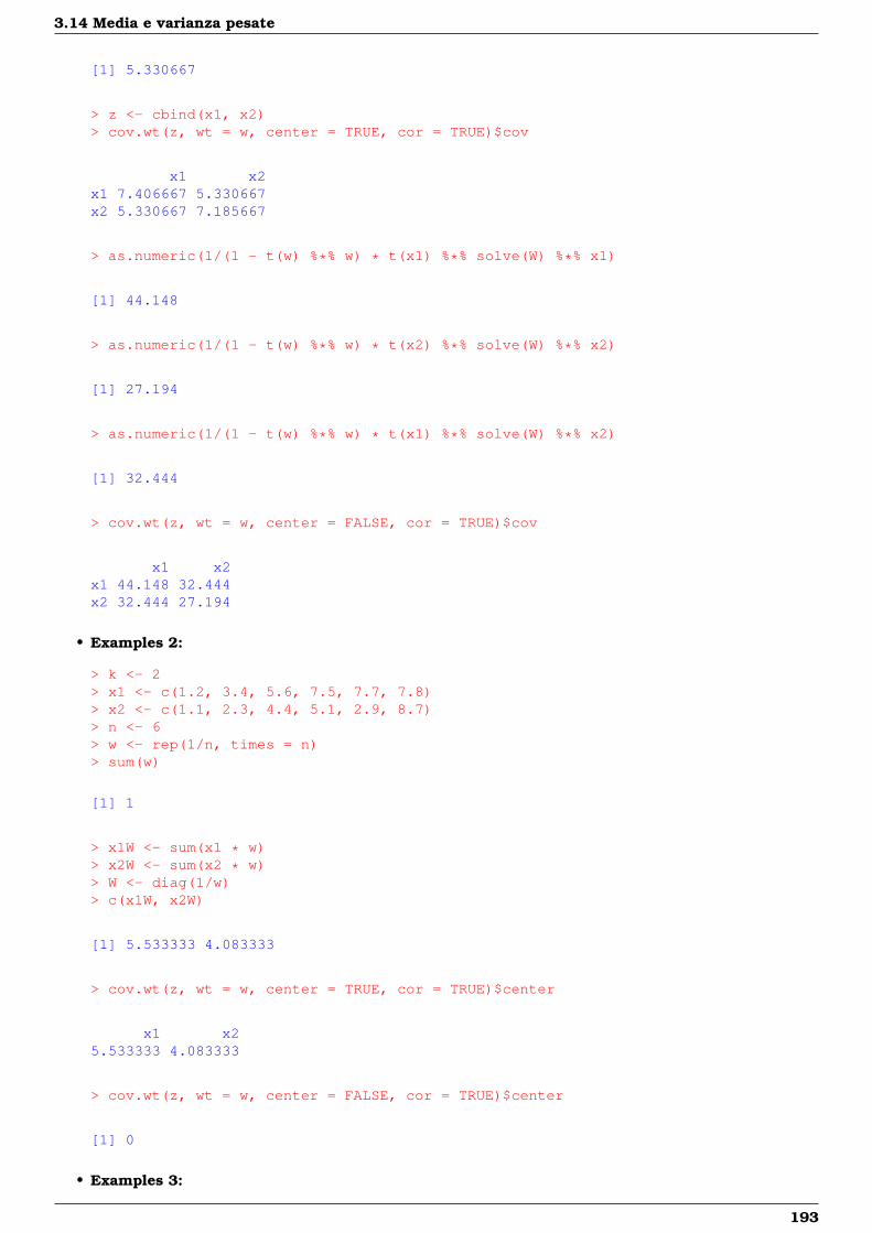
3.14 Media e varianza pesate
[1] 5.330667
> z <- cbind(x1, x2)> cov.wt(z, wt = w, center = TRUE, cor = TRUE)$cov
x1 x2x1 7.406667 5.330667x2 5.330667 7.185667
> as.numeric(1/(1 - t(w) %*% w) * t(x1) %*% solve(W) %*% x1)
[1] 44.148
> as.numeric(1/(1 - t(w) %*% w) * t(x2) %*% solve(W) %*% x2)
[1] 27.194
> as.numeric(1/(1 - t(w) %*% w) * t(x1) %*% solve(W) %*% x2)
[1] 32.444
> cov.wt(z, wt = w, center = FALSE, cor = TRUE)$cov
x1 x2x1 44.148 32.444x2 32.444 27.194
• Examples 2:
> k <- 2> x1 <- c(1.2, 3.4, 5.6, 7.5, 7.7, 7.8)> x2 <- c(1.1, 2.3, 4.4, 5.1, 2.9, 8.7)> n <- 6> w <- rep(1/n, times = n)> sum(w)
[1] 1
> x1W <- sum(x1 * w)> x2W <- sum(x2 * w)> W <- diag(1/w)> c(x1W, x2W)
[1] 5.533333 4.083333
> cov.wt(z, wt = w, center = TRUE, cor = TRUE)$center
x1 x25.533333 4.083333
> cov.wt(z, wt = w, center = FALSE, cor = TRUE)$center
[1] 0
• Examples 3:
193
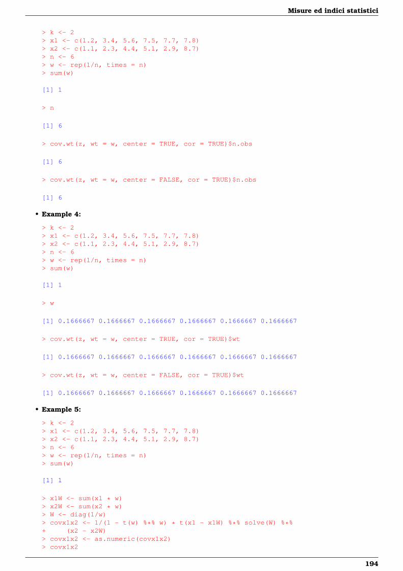
Misure ed indici statistici
> k <- 2> x1 <- c(1.2, 3.4, 5.6, 7.5, 7.7, 7.8)> x2 <- c(1.1, 2.3, 4.4, 5.1, 2.9, 8.7)> n <- 6> w <- rep(1/n, times = n)> sum(w)
[1] 1
> n
[1] 6
> cov.wt(z, wt = w, center = TRUE, cor = TRUE)$n.obs
[1] 6
> cov.wt(z, wt = w, center = FALSE, cor = TRUE)$n.obs
[1] 6
• Example 4:
> k <- 2> x1 <- c(1.2, 3.4, 5.6, 7.5, 7.7, 7.8)> x2 <- c(1.1, 2.3, 4.4, 5.1, 2.9, 8.7)> n <- 6> w <- rep(1/n, times = n)> sum(w)
[1] 1
> w
[1] 0.1666667 0.1666667 0.1666667 0.1666667 0.1666667 0.1666667
> cov.wt(z, wt = w, center = TRUE, cor = TRUE)$wt
[1] 0.1666667 0.1666667 0.1666667 0.1666667 0.1666667 0.1666667
> cov.wt(z, wt = w, center = FALSE, cor = TRUE)$wt
[1] 0.1666667 0.1666667 0.1666667 0.1666667 0.1666667 0.1666667
• Example 5:
> k <- 2> x1 <- c(1.2, 3.4, 5.6, 7.5, 7.7, 7.8)> x2 <- c(1.1, 2.3, 4.4, 5.1, 2.9, 8.7)> n <- 6> w <- rep(1/n, times = n)> sum(w)
[1] 1
> x1W <- sum(x1 * w)> x2W <- sum(x2 * w)> W <- diag(1/w)> covx1x2 <- 1/(1 - t(w) %*% w) * t(x1 - x1W) %*% solve(W) %*%+ (x2 - x2W)> covx1x2 <- as.numeric(covx1x2)> covx1x2
194
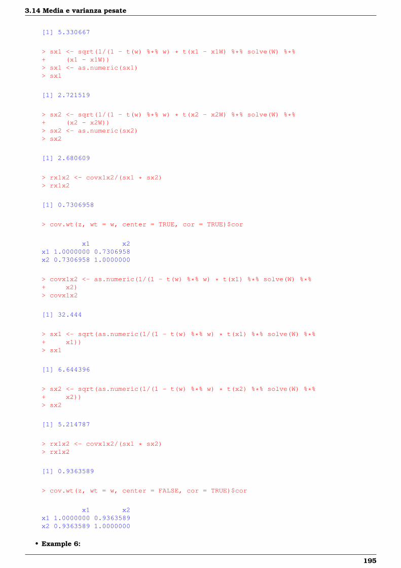
3.14 Media e varianza pesate
[1] 5.330667
> sx1 <- sqrt(1/(1 - t(w) %*% w) * t(x1 - x1W) %*% solve(W) %*%+ (x1 - x1W))> sx1 <- as.numeric(sx1)> sx1
[1] 2.721519
> sx2 <- sqrt(1/(1 - t(w) %*% w) * t(x2 - x2W) %*% solve(W) %*%+ (x2 - x2W))> sx2 <- as.numeric(sx2)> sx2
[1] 2.680609
> rx1x2 <- covx1x2/(sx1 * sx2)> rx1x2
[1] 0.7306958
> cov.wt(z, wt = w, center = TRUE, cor = TRUE)$cor
x1 x2x1 1.0000000 0.7306958x2 0.7306958 1.0000000
> covx1x2 <- as.numeric(1/(1 - t(w) %*% w) * t(x1) %*% solve(W) %*%+ x2)> covx1x2
[1] 32.444
> sx1 <- sqrt(as.numeric(1/(1 - t(w) %*% w) * t(x1) %*% solve(W) %*%+ x1))> sx1
[1] 6.644396
> sx2 <- sqrt(as.numeric(1/(1 - t(w) %*% w) * t(x2) %*% solve(W) %*%+ x2))> sx2
[1] 5.214787
> rx1x2 <- covx1x2/(sx1 * sx2)> rx1x2
[1] 0.9363589
> cov.wt(z, wt = w, center = FALSE, cor = TRUE)$cor
x1 x2x1 1.0000000 0.9363589x2 0.9363589 1.0000000
• Example 6:
195
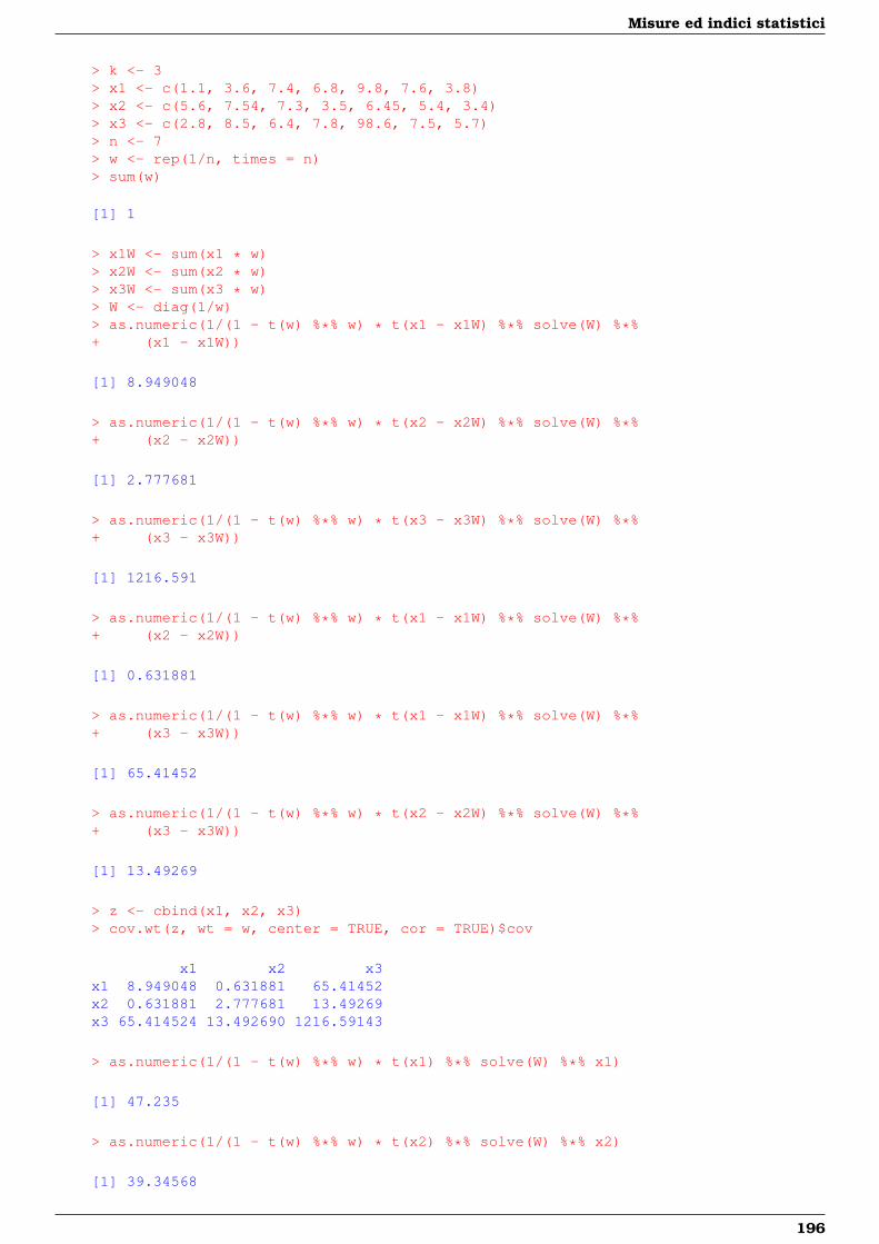
Misure ed indici statistici
> k <- 3> x1 <- c(1.1, 3.6, 7.4, 6.8, 9.8, 7.6, 3.8)> x2 <- c(5.6, 7.54, 7.3, 3.5, 6.45, 5.4, 3.4)> x3 <- c(2.8, 8.5, 6.4, 7.8, 98.6, 7.5, 5.7)> n <- 7> w <- rep(1/n, times = n)> sum(w)
[1] 1
> x1W <- sum(x1 * w)> x2W <- sum(x2 * w)> x3W <- sum(x3 * w)> W <- diag(1/w)> as.numeric(1/(1 - t(w) %*% w) * t(x1 - x1W) %*% solve(W) %*%+ (x1 - x1W))
[1] 8.949048
> as.numeric(1/(1 - t(w) %*% w) * t(x2 - x2W) %*% solve(W) %*%+ (x2 - x2W))
[1] 2.777681
> as.numeric(1/(1 - t(w) %*% w) * t(x3 - x3W) %*% solve(W) %*%+ (x3 - x3W))
[1] 1216.591
> as.numeric(1/(1 - t(w) %*% w) * t(x1 - x1W) %*% solve(W) %*%+ (x2 - x2W))
[1] 0.631881
> as.numeric(1/(1 - t(w) %*% w) * t(x1 - x1W) %*% solve(W) %*%+ (x3 - x3W))
[1] 65.41452
> as.numeric(1/(1 - t(w) %*% w) * t(x2 - x2W) %*% solve(W) %*%+ (x3 - x3W))
[1] 13.49269
> z <- cbind(x1, x2, x3)> cov.wt(z, wt = w, center = TRUE, cor = TRUE)$cov
x1 x2 x3x1 8.949048 0.631881 65.41452x2 0.631881 2.777681 13.49269x3 65.414524 13.492690 1216.59143
> as.numeric(1/(1 - t(w) %*% w) * t(x1) %*% solve(W) %*% x1)
[1] 47.235
> as.numeric(1/(1 - t(w) %*% w) * t(x2) %*% solve(W) %*% x2)
[1] 39.34568
196
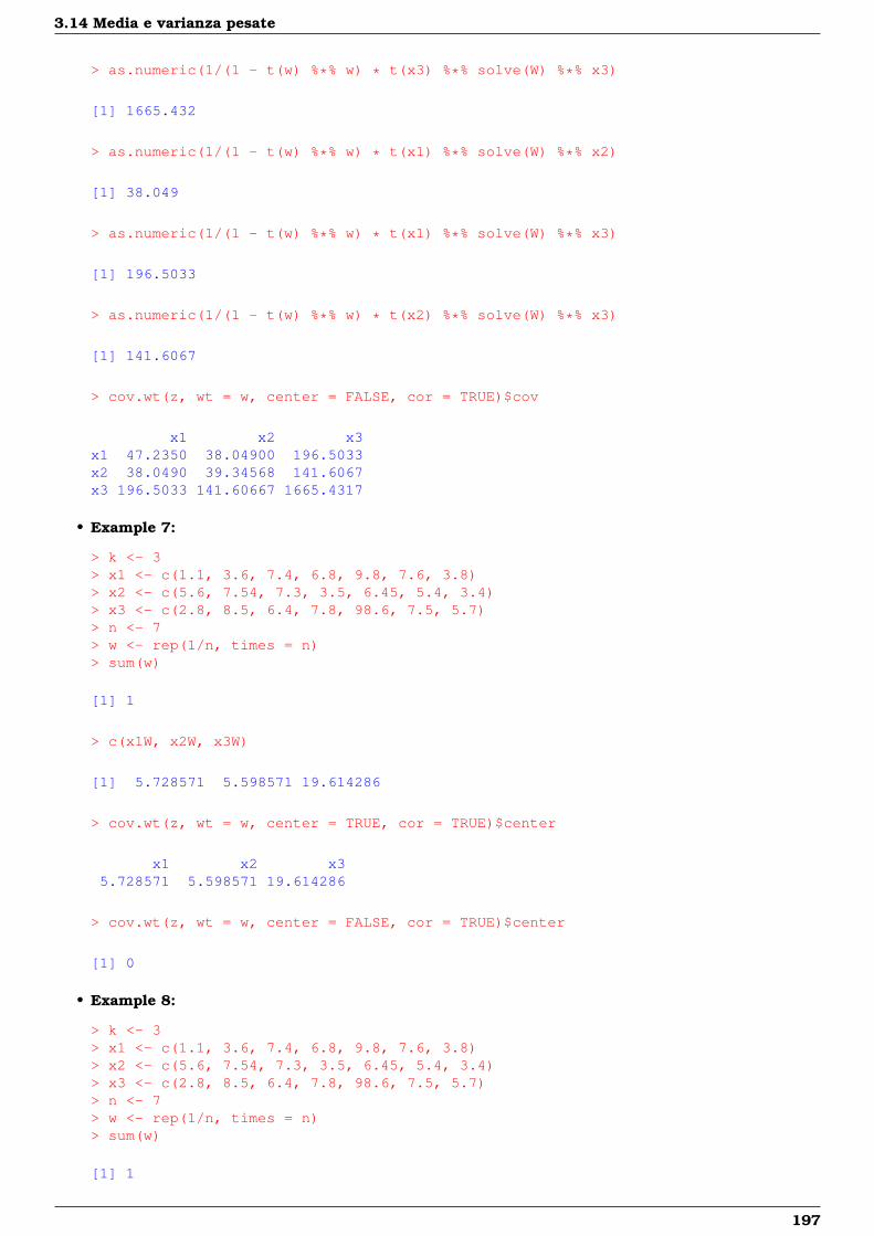
3.14 Media e varianza pesate
> as.numeric(1/(1 - t(w) %*% w) * t(x3) %*% solve(W) %*% x3)
[1] 1665.432
> as.numeric(1/(1 - t(w) %*% w) * t(x1) %*% solve(W) %*% x2)
[1] 38.049
> as.numeric(1/(1 - t(w) %*% w) * t(x1) %*% solve(W) %*% x3)
[1] 196.5033
> as.numeric(1/(1 - t(w) %*% w) * t(x2) %*% solve(W) %*% x3)
[1] 141.6067
> cov.wt(z, wt = w, center = FALSE, cor = TRUE)$cov
x1 x2 x3x1 47.2350 38.04900 196.5033x2 38.0490 39.34568 141.6067x3 196.5033 141.60667 1665.4317
• Example 7:
> k <- 3> x1 <- c(1.1, 3.6, 7.4, 6.8, 9.8, 7.6, 3.8)> x2 <- c(5.6, 7.54, 7.3, 3.5, 6.45, 5.4, 3.4)> x3 <- c(2.8, 8.5, 6.4, 7.8, 98.6, 7.5, 5.7)> n <- 7> w <- rep(1/n, times = n)> sum(w)
[1] 1
> c(x1W, x2W, x3W)
[1] 5.728571 5.598571 19.614286
> cov.wt(z, wt = w, center = TRUE, cor = TRUE)$center
x1 x2 x35.728571 5.598571 19.614286
> cov.wt(z, wt = w, center = FALSE, cor = TRUE)$center
[1] 0
• Example 8:
> k <- 3> x1 <- c(1.1, 3.6, 7.4, 6.8, 9.8, 7.6, 3.8)> x2 <- c(5.6, 7.54, 7.3, 3.5, 6.45, 5.4, 3.4)> x3 <- c(2.8, 8.5, 6.4, 7.8, 98.6, 7.5, 5.7)> n <- 7> w <- rep(1/n, times = n)> sum(w)
[1] 1
197
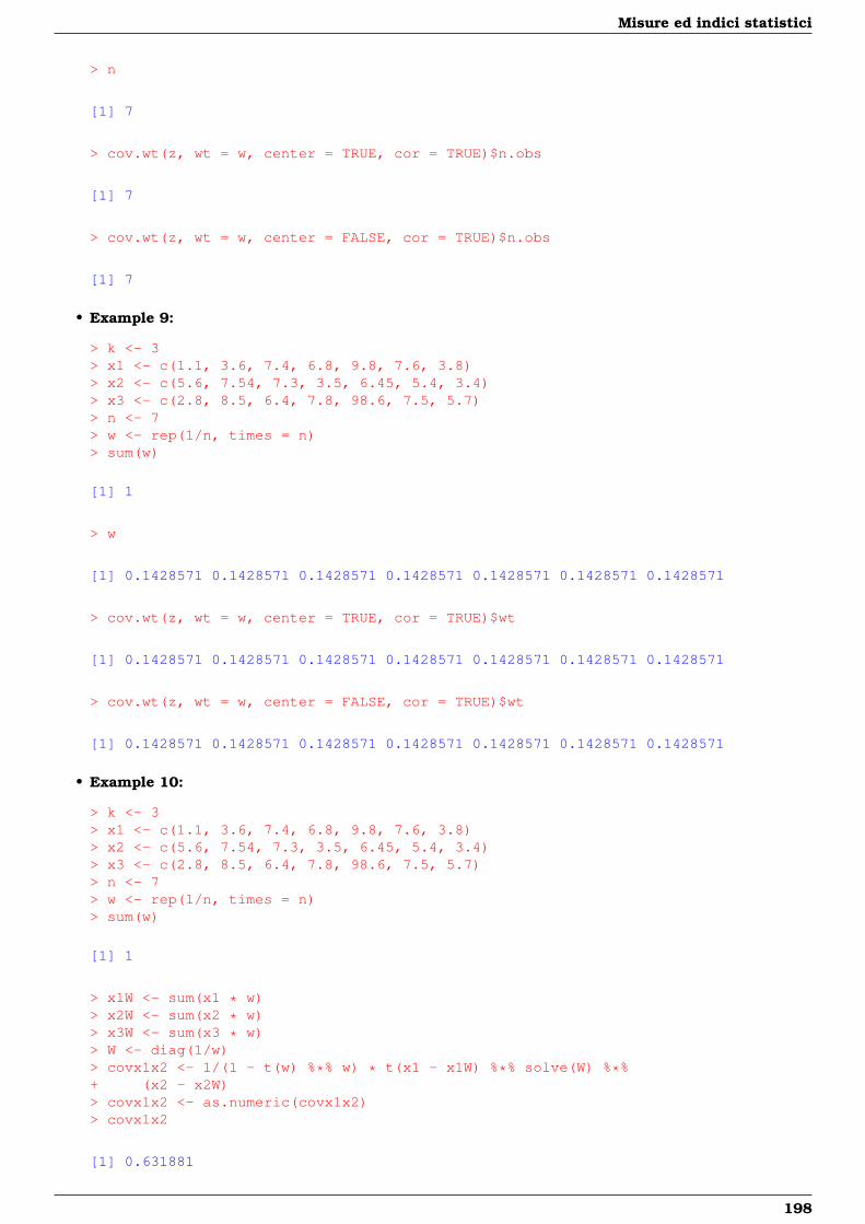
Misure ed indici statistici
> n
[1] 7
> cov.wt(z, wt = w, center = TRUE, cor = TRUE)$n.obs
[1] 7
> cov.wt(z, wt = w, center = FALSE, cor = TRUE)$n.obs
[1] 7
• Example 9:
> k <- 3> x1 <- c(1.1, 3.6, 7.4, 6.8, 9.8, 7.6, 3.8)> x2 <- c(5.6, 7.54, 7.3, 3.5, 6.45, 5.4, 3.4)> x3 <- c(2.8, 8.5, 6.4, 7.8, 98.6, 7.5, 5.7)> n <- 7> w <- rep(1/n, times = n)> sum(w)
[1] 1
> w
[1] 0.1428571 0.1428571 0.1428571 0.1428571 0.1428571 0.1428571 0.1428571
> cov.wt(z, wt = w, center = TRUE, cor = TRUE)$wt
[1] 0.1428571 0.1428571 0.1428571 0.1428571 0.1428571 0.1428571 0.1428571
> cov.wt(z, wt = w, center = FALSE, cor = TRUE)$wt
[1] 0.1428571 0.1428571 0.1428571 0.1428571 0.1428571 0.1428571 0.1428571
• Example 10:
> k <- 3> x1 <- c(1.1, 3.6, 7.4, 6.8, 9.8, 7.6, 3.8)> x2 <- c(5.6, 7.54, 7.3, 3.5, 6.45, 5.4, 3.4)> x3 <- c(2.8, 8.5, 6.4, 7.8, 98.6, 7.5, 5.7)> n <- 7> w <- rep(1/n, times = n)> sum(w)
[1] 1
> x1W <- sum(x1 * w)> x2W <- sum(x2 * w)> x3W <- sum(x3 * w)> W <- diag(1/w)> covx1x2 <- 1/(1 - t(w) %*% w) * t(x1 - x1W) %*% solve(W) %*%+ (x2 - x2W)> covx1x2 <- as.numeric(covx1x2)> covx1x2
[1] 0.631881
198
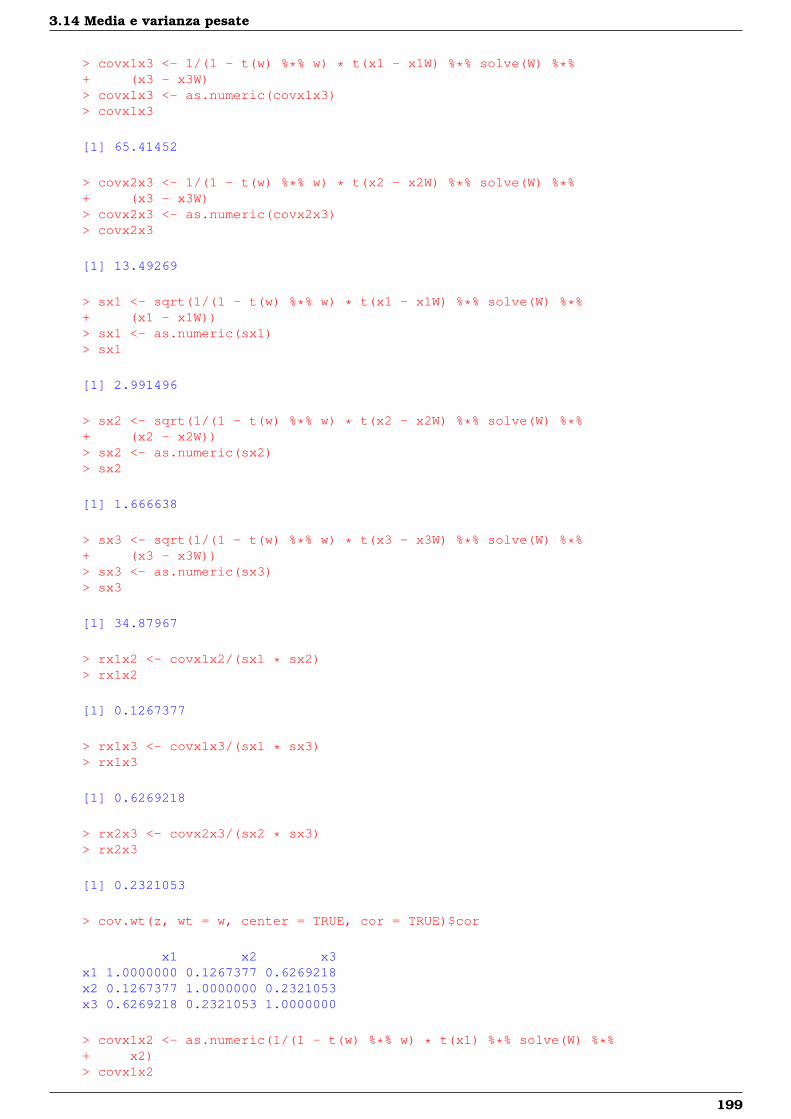
3.14 Media e varianza pesate
> covx1x3 <- 1/(1 - t(w) %*% w) * t(x1 - x1W) %*% solve(W) %*%+ (x3 - x3W)> covx1x3 <- as.numeric(covx1x3)> covx1x3
[1] 65.41452
> covx2x3 <- 1/(1 - t(w) %*% w) * t(x2 - x2W) %*% solve(W) %*%+ (x3 - x3W)> covx2x3 <- as.numeric(covx2x3)> covx2x3
[1] 13.49269
> sx1 <- sqrt(1/(1 - t(w) %*% w) * t(x1 - x1W) %*% solve(W) %*%+ (x1 - x1W))> sx1 <- as.numeric(sx1)> sx1
[1] 2.991496
> sx2 <- sqrt(1/(1 - t(w) %*% w) * t(x2 - x2W) %*% solve(W) %*%+ (x2 - x2W))> sx2 <- as.numeric(sx2)> sx2
[1] 1.666638
> sx3 <- sqrt(1/(1 - t(w) %*% w) * t(x3 - x3W) %*% solve(W) %*%+ (x3 - x3W))> sx3 <- as.numeric(sx3)> sx3
[1] 34.87967
> rx1x2 <- covx1x2/(sx1 * sx2)> rx1x2
[1] 0.1267377
> rx1x3 <- covx1x3/(sx1 * sx3)> rx1x3
[1] 0.6269218
> rx2x3 <- covx2x3/(sx2 * sx3)> rx2x3
[1] 0.2321053
> cov.wt(z, wt = w, center = TRUE, cor = TRUE)$cor
x1 x2 x3x1 1.0000000 0.1267377 0.6269218x2 0.1267377 1.0000000 0.2321053x3 0.6269218 0.2321053 1.0000000
> covx1x2 <- as.numeric(1/(1 - t(w) %*% w) * t(x1) %*% solve(W) %*%+ x2)> covx1x2
199
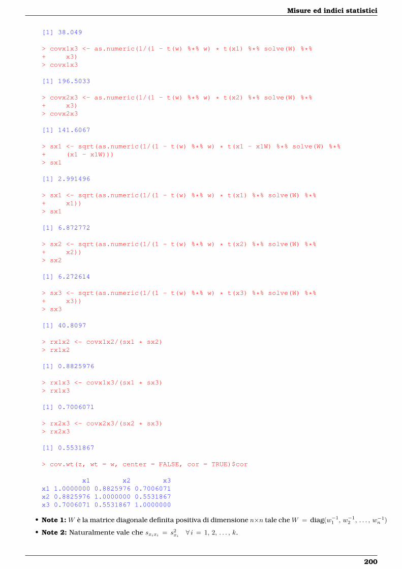
Misure ed indici statistici
[1] 38.049
> covx1x3 <- as.numeric(1/(1 - t(w) %*% w) * t(x1) %*% solve(W) %*%+ x3)> covx1x3
[1] 196.5033
> covx2x3 <- as.numeric(1/(1 - t(w) %*% w) * t(x2) %*% solve(W) %*%+ x3)> covx2x3
[1] 141.6067
> sx1 <- sqrt(as.numeric(1/(1 - t(w) %*% w) * t(x1 - x1W) %*% solve(W) %*%+ (x1 - x1W)))> sx1
[1] 2.991496
> sx1 <- sqrt(as.numeric(1/(1 - t(w) %*% w) * t(x1) %*% solve(W) %*%+ x1))> sx1
[1] 6.872772
> sx2 <- sqrt(as.numeric(1/(1 - t(w) %*% w) * t(x2) %*% solve(W) %*%+ x2))> sx2
[1] 6.272614
> sx3 <- sqrt(as.numeric(1/(1 - t(w) %*% w) * t(x3) %*% solve(W) %*%+ x3))> sx3
[1] 40.8097
> rx1x2 <- covx1x2/(sx1 * sx2)> rx1x2
[1] 0.8825976
> rx1x3 <- covx1x3/(sx1 * sx3)> rx1x3
[1] 0.7006071
> rx2x3 <- covx2x3/(sx2 * sx3)> rx2x3
[1] 0.5531867
> cov.wt(z, wt = w, center = FALSE, cor = TRUE)$cor
x1 x2 x3x1 1.0000000 0.8825976 0.7006071x2 0.8825976 1.0000000 0.5531867x3 0.7006071 0.5531867 1.0000000
• Note 1: W è la matrice diagonale definita positiva di dimensione n×n tale che W = diag(w−11 , w−1
2 , . . . , w−1n )
• Note 2: Naturalmente vale che sxixi = s2xi ∀ i = 1, 2, . . . , k.
200
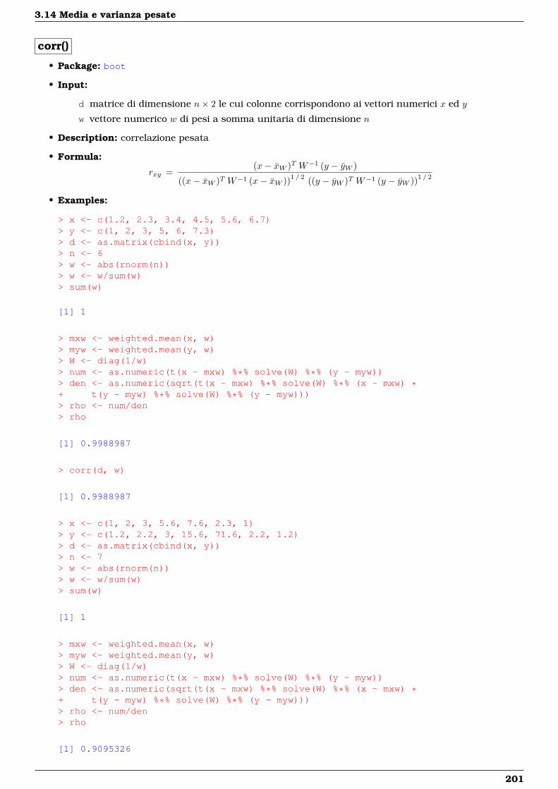
3.14 Media e varianza pesate
corr()
• Package: boot
• Input:
d matrice di dimensione n× 2 le cui colonne corrispondono ai vettori numerici x ed y
w vettore numerico w di pesi a somma unitaria di dimensione n
• Description: correlazione pesata
• Formula:
rxy =(x− xW )T W−1 (y − yW )
((x− xW )T W−1 (x− xW ))1 / 2 ((y − yW )T W−1 (y − yW ))1 / 2
• Examples:
> x <- c(1.2, 2.3, 3.4, 4.5, 5.6, 6.7)> y <- c(1, 2, 3, 5, 6, 7.3)> d <- as.matrix(cbind(x, y))> n <- 6> w <- abs(rnorm(n))> w <- w/sum(w)> sum(w)
[1] 1
> mxw <- weighted.mean(x, w)> myw <- weighted.mean(y, w)> W <- diag(1/w)> num <- as.numeric(t(x - mxw) %*% solve(W) %*% (y - myw))> den <- as.numeric(sqrt(t(x - mxw) %*% solve(W) %*% (x - mxw) *+ t(y - myw) %*% solve(W) %*% (y - myw)))> rho <- num/den> rho
[1] 0.9988987
> corr(d, w)
[1] 0.9988987
> x <- c(1, 2, 3, 5.6, 7.6, 2.3, 1)> y <- c(1.2, 2.2, 3, 15.6, 71.6, 2.2, 1.2)> d <- as.matrix(cbind(x, y))> n <- 7> w <- abs(rnorm(n))> w <- w/sum(w)> sum(w)
[1] 1
> mxw <- weighted.mean(x, w)> myw <- weighted.mean(y, w)> W <- diag(1/w)> num <- as.numeric(t(x - mxw) %*% solve(W) %*% (y - myw))> den <- as.numeric(sqrt(t(x - mxw) %*% solve(W) %*% (x - mxw) *+ t(y - myw) %*% solve(W) %*% (y - myw)))> rho <- num/den> rho
[1] 0.9095326
201
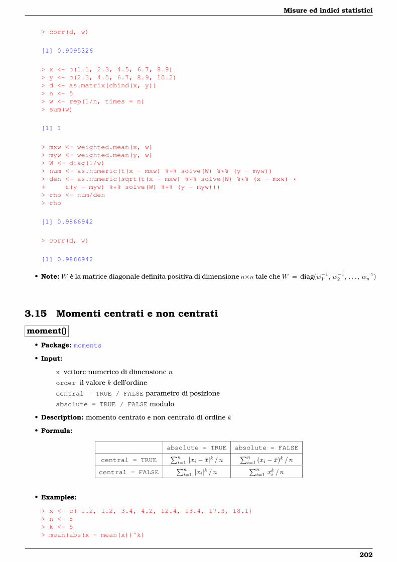
Misure ed indici statistici
> corr(d, w)
[1] 0.9095326
> x <- c(1.1, 2.3, 4.5, 6.7, 8.9)> y <- c(2.3, 4.5, 6.7, 8.9, 10.2)> d <- as.matrix(cbind(x, y))> n <- 5> w <- rep(1/n, times = n)> sum(w)
[1] 1
> mxw <- weighted.mean(x, w)> myw <- weighted.mean(y, w)> W <- diag(1/w)> num <- as.numeric(t(x - mxw) %*% solve(W) %*% (y - myw))> den <- as.numeric(sqrt(t(x - mxw) %*% solve(W) %*% (x - mxw) *+ t(y - myw) %*% solve(W) %*% (y - myw)))> rho <- num/den> rho
[1] 0.9866942
> corr(d, w)
[1] 0.9866942
• Note: W è la matrice diagonale definita positiva di dimensione n×n tale che W = diag(w−11 , w−1
2 , . . . , w−1n )
3.15 Momenti centrati e non centrati
moment()
• Package: moments
• Input:
x vettore numerico di dimensione n
order il valore k dell’ordine
central = TRUE / FALSE parametro di posizione
absolute = TRUE / FALSE modulo
• Description: momento centrato e non centrato di ordine k
• Formula:
absolute = TRUE absolute = FALSE
central = TRUE∑ni=1 |xi − x|k / n
∑ni=1 (xi − x)k / n
central = FALSE∑ni=1 |xi|k / n
∑ni=1 x
ki / n
• Examples:
> x <- c(-1.2, 1.2, 3.4, 4.2, 12.4, 13.4, 17.3, 18.1)> n <- 8> k <- 5> mean(abs(x - mean(x))^k)
202
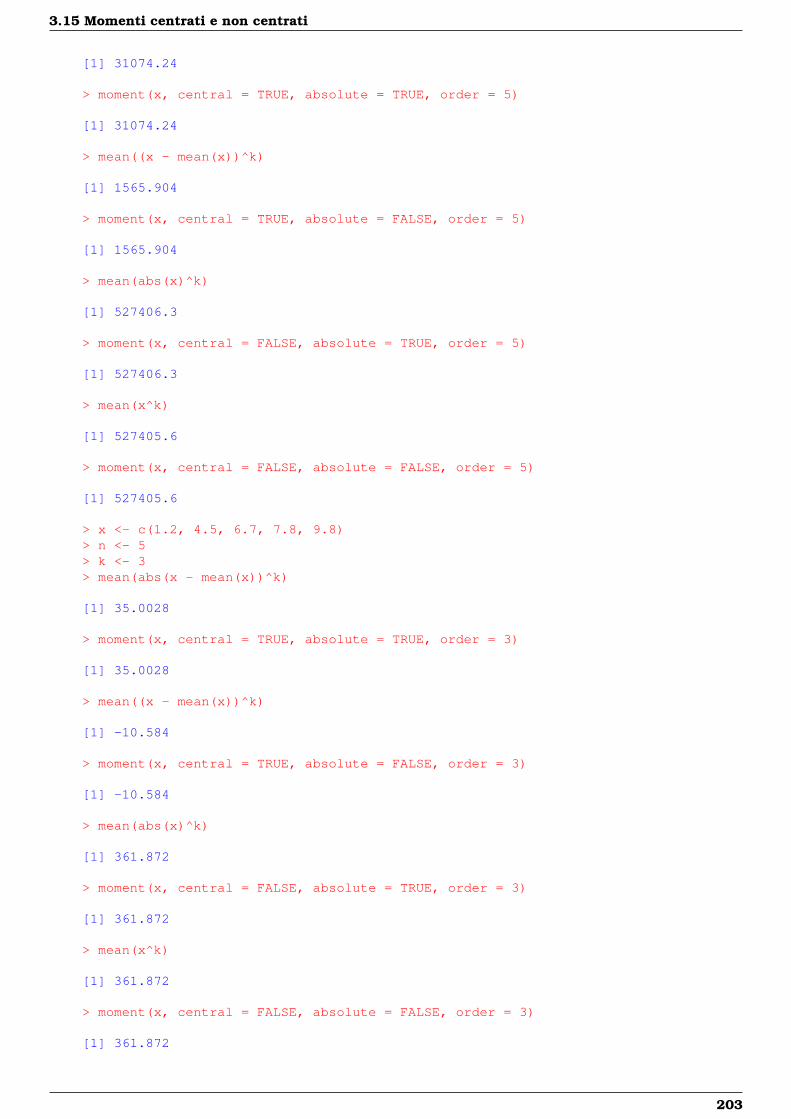
3.15 Momenti centrati e non centrati
[1] 31074.24
> moment(x, central = TRUE, absolute = TRUE, order = 5)
[1] 31074.24
> mean((x - mean(x))^k)
[1] 1565.904
> moment(x, central = TRUE, absolute = FALSE, order = 5)
[1] 1565.904
> mean(abs(x)^k)
[1] 527406.3
> moment(x, central = FALSE, absolute = TRUE, order = 5)
[1] 527406.3
> mean(x^k)
[1] 527405.6
> moment(x, central = FALSE, absolute = FALSE, order = 5)
[1] 527405.6
> x <- c(1.2, 4.5, 6.7, 7.8, 9.8)> n <- 5> k <- 3> mean(abs(x - mean(x))^k)
[1] 35.0028
> moment(x, central = TRUE, absolute = TRUE, order = 3)
[1] 35.0028
> mean((x - mean(x))^k)
[1] -10.584
> moment(x, central = TRUE, absolute = FALSE, order = 3)
[1] -10.584
> mean(abs(x)^k)
[1] 361.872
> moment(x, central = FALSE, absolute = TRUE, order = 3)
[1] 361.872
> mean(x^k)
[1] 361.872
> moment(x, central = FALSE, absolute = FALSE, order = 3)
[1] 361.872
203
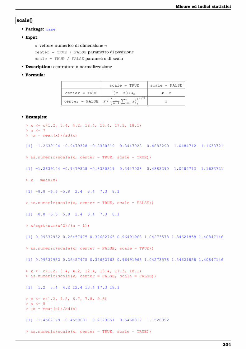
Misure ed indici statistici
scale()
• Package: base
• Input:
x vettore numerico di dimensione n
center = TRUE / FALSE parametro di posizione
scale = TRUE / FALSE parametro di scala
• Description: centratura o normalizzazione
• Formula:
scale = TRUE scale = FALSE
center = TRUE (x− x ) / sx x− x
center = FALSE x /(
1n−1
∑ni=1 x
2i
)1 / 2
x
• Examples:
> x <- c(1.2, 3.4, 4.2, 12.4, 13.4, 17.3, 18.1)> n <- 7> (x - mean(x))/sd(x)
[1] -1.2639104 -0.9479328 -0.8330319 0.3447028 0.4883290 1.0484712 1.1633721
> as.numeric(scale(x, center = TRUE, scale = TRUE))
[1] -1.2639104 -0.9479328 -0.8330319 0.3447028 0.4883290 1.0484712 1.1633721
> x - mean(x)
[1] -8.8 -6.6 -5.8 2.4 3.4 7.3 8.1
> as.numeric(scale(x, center = TRUE, scale = FALSE))
[1] -8.8 -6.6 -5.8 2.4 3.4 7.3 8.1
> x/sqrt(sum(x^2)/(n - 1))
[1] 0.09337932 0.26457475 0.32682763 0.96491968 1.04273578 1.34621858 1.40847146
> as.numeric(scale(x, center = FALSE, scale = TRUE))
[1] 0.09337932 0.26457475 0.32682763 0.96491968 1.04273578 1.34621858 1.40847146
> x <- c(1.2, 3.4, 4.2, 12.4, 13.4, 17.3, 18.1)> as.numeric(scale(x, center = FALSE, scale = FALSE))
[1] 1.2 3.4 4.2 12.4 13.4 17.3 18.1
> x <- c(1.2, 4.5, 6.7, 7.8, 9.8)> n <- 5> (x - mean(x))/sd(x)
[1] -1.4562179 -0.4550681 0.2123651 0.5460817 1.1528392
> as.numeric(scale(x, center = TRUE, scale = TRUE))
204
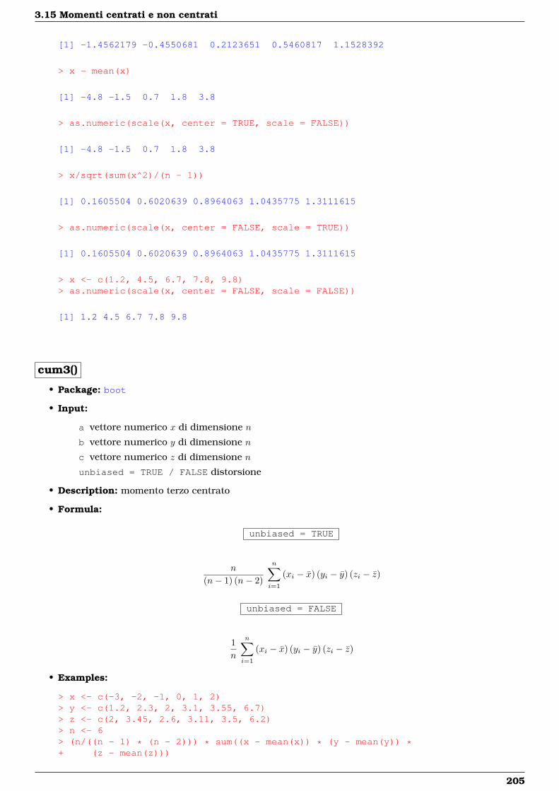
3.15 Momenti centrati e non centrati
[1] -1.4562179 -0.4550681 0.2123651 0.5460817 1.1528392
> x - mean(x)
[1] -4.8 -1.5 0.7 1.8 3.8
> as.numeric(scale(x, center = TRUE, scale = FALSE))
[1] -4.8 -1.5 0.7 1.8 3.8
> x/sqrt(sum(x^2)/(n - 1))
[1] 0.1605504 0.6020639 0.8964063 1.0435775 1.3111615
> as.numeric(scale(x, center = FALSE, scale = TRUE))
[1] 0.1605504 0.6020639 0.8964063 1.0435775 1.3111615
> x <- c(1.2, 4.5, 6.7, 7.8, 9.8)> as.numeric(scale(x, center = FALSE, scale = FALSE))
[1] 1.2 4.5 6.7 7.8 9.8
cum3()
• Package: boot
• Input:
a vettore numerico x di dimensione n
b vettore numerico y di dimensione n
c vettore numerico z di dimensione n
unbiased = TRUE / FALSE distorsione
• Description: momento terzo centrato
• Formula:
unbiased = TRUE
n
(n− 1) (n− 2)
n∑i=1
(xi − x) (yi − y) (zi − z)
unbiased = FALSE
1n
n∑i=1
(xi − x) (yi − y) (zi − z)
• Examples:
> x <- c(-3, -2, -1, 0, 1, 2)> y <- c(1.2, 2.3, 2, 3.1, 3.55, 6.7)> z <- c(2, 3.45, 2.6, 3.11, 3.5, 6.2)> n <- 6> (n/((n - 1) * (n - 2))) * sum((x - mean(x)) * (y - mean(y)) *+ (z - mean(z)))
205
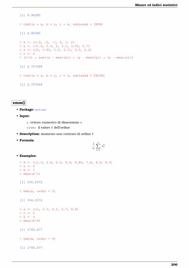
Misure ed indici statistici
[1] 4.96385
> cum3(a = x, b = y, c = z, unbiased = TRUE)
[1] 4.96385
> x <- c(-3, -2, -1, 0, 1, 2)> y <- c(1.2, 2.3, 2, 3.1, 3.55, 6.7)> z <- c(2, 3.45, 2.6, 3.11, 3.5, 6.2)> n <- 6> (1/n) * sum((x - mean(x)) * (y - mean(y)) * (z - mean(z)))
[1] 2.757694
> cum3(a = x, b = y, c = z, unbiased = FALSE)
[1] 2.757694
emm()
• Package: actuar
• Input:
x vettore numerico di dimensione n
order il valore k dell’ordine
• Description: momento non centrato di ordine k
• Formula:1n
n∑i=1
xki
• Examples:
> x <- c(1.5, 6.4, 9.6, 8.8, 8.86, 7.8, 8.6, 8.6)> n <- 8> k <- 3> mean(x^3)
[1] 534.2372
> emm(x, order = 3)
[1] 534.2372
> x <- c(1, 2.3, 4.5, 6.7, 8.9)> n <- 5> k <- 4> mean(x^4)
[1] 1745.677
> emm(x, order = 4)
[1] 1745.677
206
3.16 Connessione e dipendenza in media
3.16 Connessione e dipendenza in media
eta()
• Package: labstatR
• Input:
y vettore numerico di dimensione n
f fattore a k livelli di dimensione n
• Description: rapporto di correlazione η2y|f
• Formula:
η2y|f =
∑kj=1 (yj − y)2 nj∑ni=1 (yi − y)2
• Examples:
> y <- c(1, 1.2, 2.1, 3.4, 5.4, 5.6, 7.2, 3.2, 3, 1, 2.3)> f <- factor(c("a", "b", "c", "b", "a", "c", "a", "b", "b", "c",+ "a"))> f
[1] a b c b a c a b b c aLevels: a b c
> k <- 3> n <- 11> table(f)
fa b c4 4 3
> enne <- tapply(y, f, FUN = length)> enne
a b c4 4 3
> ymedio <- tapply(y, f, FUN = mean)> sum((ymedio - mean(y))^2 * enne)/sum((y - mean(y))^2)
[1] 0.08657807
> eta(f, y)
[1] 0.08657807
> y <- c(1.2, 3.4, 55.6, 5.1, 7.8, 8.4, 8.7, 9.8)> f <- factor(c("a", "b", "b", "b", "b", "a", "a", "b"))> f
[1] a b b b b a a bLevels: a b
> k <- 2> n <- 8> table(f)
207
Misure ed indici statistici
fa b3 5
> enne <- tapply(y, f, FUN = length)> enne
a b3 5
> ymedio <- tapply(y, f, FUN = mean)> sum((ymedio - mean(y))^2 * enne)/sum((y - mean(y))^2)
[1] 0.0900426
> eta(f, y)
[1] 0.0900426
Gini()
• Package: ineq
• Input:
x vettore numerico di dimensione n
• Description: rapporto di concentrazione di Gini
• Formula:n− 1n
G
dove G =2
n− 1
n−1∑i=1
(pi − qi) = 1− 2n− 1
n−1∑i=1
qi =1
n (n− 1) x
n−1∑i=1
n∑j=i+1
(x(j) − x(i)
)• Examples:
> x <- c(1, 1, 1, 4, 4, 5, 7, 10)> x <- sort(x)> x
[1] 1 1 1 4 4 5 7 10
> n <- 8> q <- cumsum(x[1:(n - 1)])/sum(x)> G <- 2/(n - 1) * sum((1:(n - 1))/n - q)> G
[1] 0.4545455
> R <- (n - 1)/n * G> R
[1] 0.3977273
> Gini(x)
[1] 0.3977273
208
3.16 Connessione e dipendenza in media
> x <- c(1.2, 3.4, 55.6, 5.1, 7.8, 8.4, 8.7, 9.8)> x <- sort(x)> x
[1] 1.2 3.4 5.1 7.8 8.4 8.7 9.8 55.6
> n <- 8> q <- cumsum(x[1:(n - 1)])/sum(x)> G <- 2/(n - 1) * sum((1:(n - 1))/n - q)> G
[1] 0.606
> R <- (n - 1)/n * G> R
[1] 0.53025
> Gini(x)
[1] 0.53025
gini()
• Package: labstatR
• Input:
y vettore numerico di dimensione n
plot = FALSE
• Description: indici di concentrazione
• Output:
G indice di Gini
R rapporto di concentrazione di Gini
P proporzioni
Q somme cumulate
• Formula:
G
G =2
n− 1
n−1∑i=1
(pi − qi) = 1− 2n− 1
n−1∑i=1
qi =1
n (n− 1) y
n−1∑i=1
n∑j=i+1
(y(j) − y(i)
)
dove pi = i / n ∀ i = 1, 2, . . . , n
qi =∑ij=1 y(j) /
∑nj=1 yj ∀ i = 1, 2, . . . , n
Rn− 1n
G
P0, pi ∀ i = 1, 2, . . . , n
Q0, qi ∀ i = 1, 2, . . . , n
• Examples:
209
Misure ed indici statistici
> y <- c(1, 1, 1, 4, 4, 5, 7, 10)> y <- sort(y)> y
[1] 1 1 1 4 4 5 7 10
> n <- 8> q <- cumsum(y[1:(n - 1)])/sum(y)> G <- 2/(n - 1) * sum((1:(n - 1))/n - q)> G
[1] 0.4545455
> gini(y, plot = FALSE)$G
[1] 0.4545455
> R <- (n - 1)/n * G> R
[1] 0.3977273
> gini(y, plot = FALSE)$R
[1] 0.3977273
> P <- c(0, (1:n)/n)> P
[1] 0.000 0.125 0.250 0.375 0.500 0.625 0.750 0.875 1.000
> gini(y, plot = FALSE)$P
[1] 0.000 0.125 0.250 0.375 0.500 0.625 0.750 0.875 1.000
> Q <- c(0, cumsum(y)/sum(y))> Q
[1] 0.00000000 0.03030303 0.06060606 0.09090909 0.21212121 0.33333333 0.48484848[8] 0.69696970 1.00000000
> gini(y, plot = FALSE)$Q
[1] 0.00000000 0.03030303 0.06060606 0.09090909 0.21212121 0.33333333 0.48484848[8] 0.69696970 1.00000000
> y <- c(1.2, 3.4, 55.6, 5.1, 7.8, 8.4, 8.7, 9.8)> y <- sort(y)> y
[1] 1.2 3.4 5.1 7.8 8.4 8.7 9.8 55.6
> n <- 8> q <- cumsum(y[1:(n - 1)])/sum(y)> G <- 2/(n - 1) * sum((1:(n - 1))/n - q)> G
[1] 0.606
210
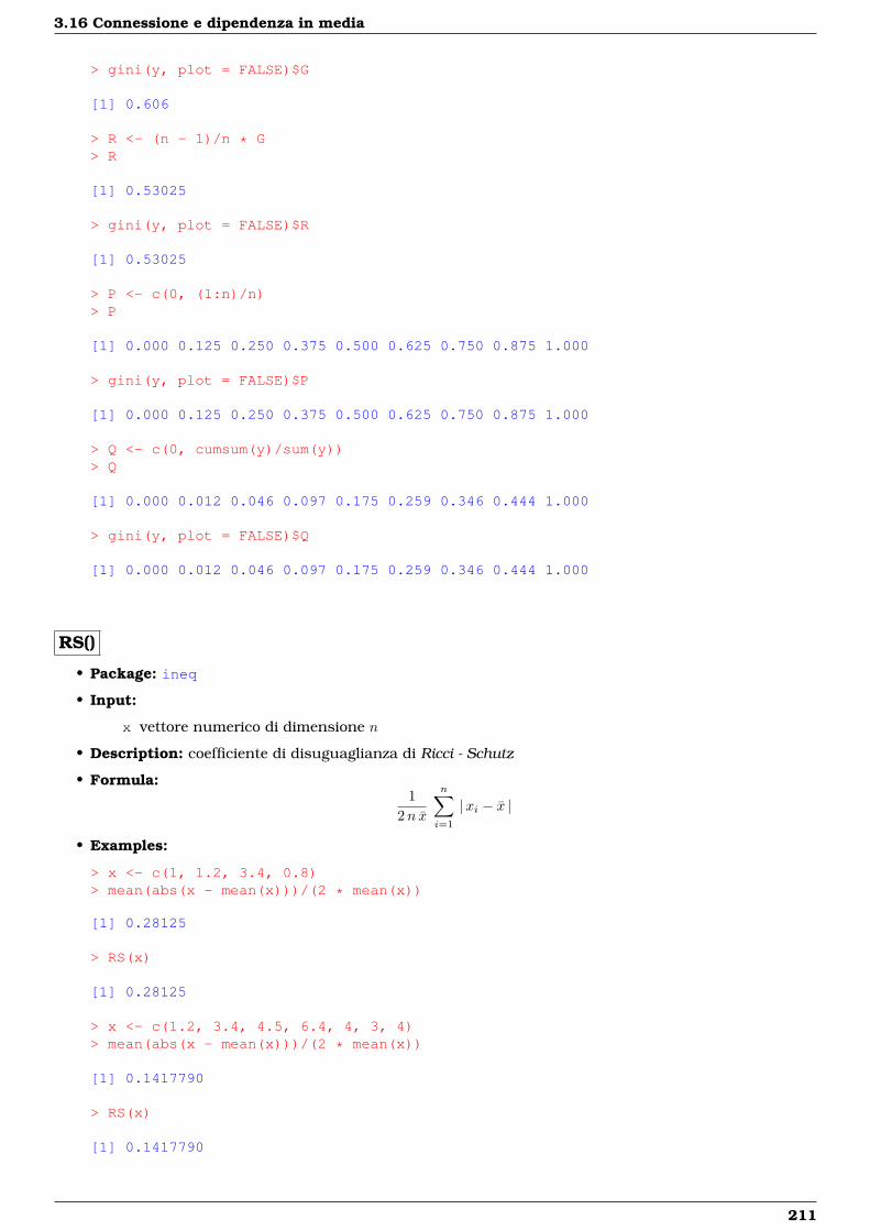
3.16 Connessione e dipendenza in media
> gini(y, plot = FALSE)$G
[1] 0.606
> R <- (n - 1)/n * G> R
[1] 0.53025
> gini(y, plot = FALSE)$R
[1] 0.53025
> P <- c(0, (1:n)/n)> P
[1] 0.000 0.125 0.250 0.375 0.500 0.625 0.750 0.875 1.000
> gini(y, plot = FALSE)$P
[1] 0.000 0.125 0.250 0.375 0.500 0.625 0.750 0.875 1.000
> Q <- c(0, cumsum(y)/sum(y))> Q
[1] 0.000 0.012 0.046 0.097 0.175 0.259 0.346 0.444 1.000
> gini(y, plot = FALSE)$Q
[1] 0.000 0.012 0.046 0.097 0.175 0.259 0.346 0.444 1.000
RS()
• Package: ineq
• Input:
x vettore numerico di dimensione n
• Description: coefficiente di disuguaglianza di Ricci - Schutz
• Formula:1
2n x
n∑i=1
|xi − x |
• Examples:
> x <- c(1, 1.2, 3.4, 0.8)> mean(abs(x - mean(x)))/(2 * mean(x))
[1] 0.28125
> RS(x)
[1] 0.28125
> x <- c(1.2, 3.4, 4.5, 6.4, 4, 3, 4)> mean(abs(x - mean(x)))/(2 * mean(x))
[1] 0.1417790
> RS(x)
[1] 0.1417790
211
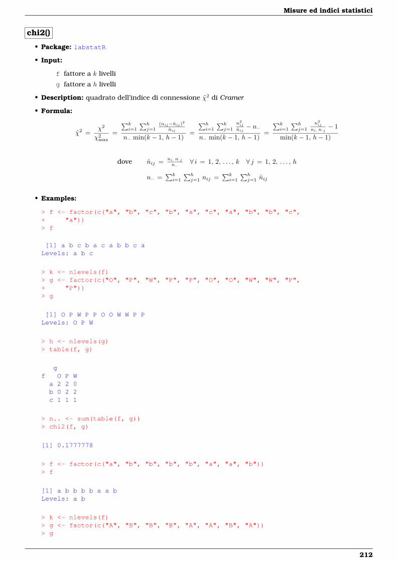
Misure ed indici statistici
chi2()
• Package: labstatR
• Input:
f fattore a k livelli
g fattore a h livelli
• Description: quadrato dell’indice di connessione χ2 di Cramer
• Formula:
χ2 =χ2
χ2max
=
∑ki=1
∑hj=1
(nij−nij)2nij
n·· min(k − 1, h− 1)=
∑hi=1
∑kj=1
n2ij
nij− n··
n·· min(k − 1, h− 1)=
∑ki=1
∑hj=1
n2ij
ni· n·j− 1
min(k − 1, h− 1)
dove nij = ni· n·jn··
∀ i = 1, 2, . . . , k ∀ j = 1, 2, . . . , h
n·· =∑ki=1
∑hj=1 nij =
∑ki=1
∑hj=1 nij
• Examples:
> f <- factor(c("a", "b", "c", "b", "a", "c", "a", "b", "b", "c",+ "a"))> f
[1] a b c b a c a b b c aLevels: a b c
> k <- nlevels(f)> g <- factor(c("O", "P", "W", "P", "P", "O", "O", "W", "W", "P",+ "P"))> g
[1] O P W P P O O W W P PLevels: O P W
> h <- nlevels(g)> table(f, g)
gf O P W
a 2 2 0b 0 2 2c 1 1 1
> n.. <- sum(table(f, g))> chi2(f, g)
[1] 0.1777778
> f <- factor(c("a", "b", "b", "b", "b", "a", "a", "b"))> f
[1] a b b b b a a bLevels: a b
> k <- nlevels(f)> g <- factor(c("A", "B", "B", "B", "A", "A", "B", "A"))> g
212
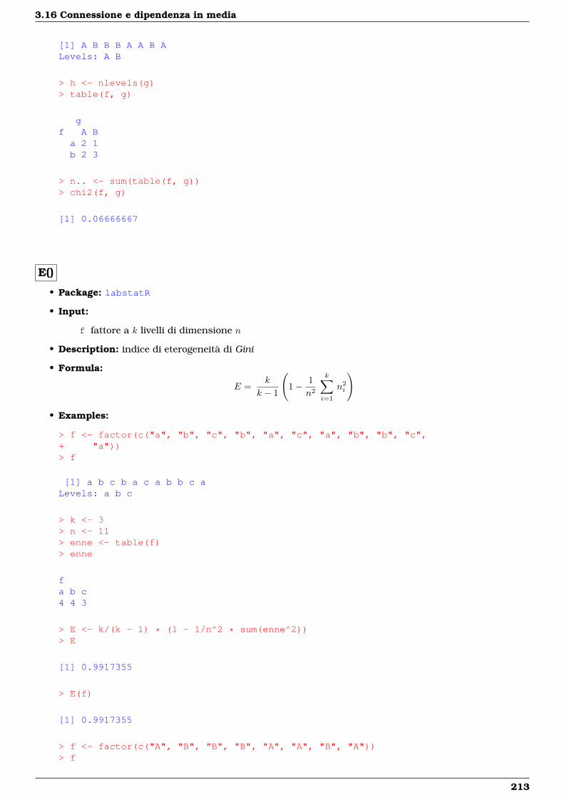
3.16 Connessione e dipendenza in media
[1] A B B B A A B ALevels: A B
> h <- nlevels(g)> table(f, g)
gf A B
a 2 1b 2 3
> n.. <- sum(table(f, g))> chi2(f, g)
[1] 0.06666667
E()
• Package: labstatR
• Input:
f fattore a k livelli di dimensione n
• Description: indice di eterogeneità di Gini
• Formula:
E =k
k − 1
(1− 1
n2
k∑i=1
n2i
)
• Examples:
> f <- factor(c("a", "b", "c", "b", "a", "c", "a", "b", "b", "c",+ "a"))> f
[1] a b c b a c a b b c aLevels: a b c
> k <- 3> n <- 11> enne <- table(f)> enne
fa b c4 4 3
> E <- k/(k - 1) * (1 - 1/n^2 * sum(enne^2))> E
[1] 0.9917355
> E(f)
[1] 0.9917355
> f <- factor(c("A", "B", "B", "B", "A", "A", "B", "A"))> f
213

Misure ed indici statistici
[1] A B B B A A B ALevels: A B
> k <- 2> n <- 8> enne <- table(f)> enne
fA B4 4
> E <- k/(k - 1) * (1 - 1/n^2 * sum(enne^2))> E
[1] 1
> E(g)
[1] 1
3.17 Sintesi di dati
summary()
• Package: base
• Input:
x vettore numerico di dimensione n
• Description: statistiche descrittive
• Output:
Min. minimo
1st Qu. primo quartile
Median mediana
Mean media aritmetica
3rd Qu. terzo quartile
Max. massimo
• Formula:
Min.x(1)
1st Qu.Q0.25(x)
MedianQ0.5(x)
Meanx
3rd Qu.Q0.75(x)
Max.x(n)
• Examples:
214
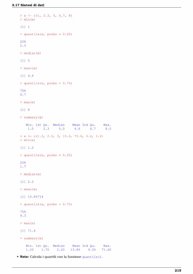
3.17 Sintesi di dati
> x <- c(1, 2.3, 5, 6.7, 8)> min(x)
[1] 1
> quantile(x, probs = 0.25)
25%2.3
> median(x)
[1] 5
> mean(x)
[1] 4.6
> quantile(x, probs = 0.75)
75%6.7
> max(x)
[1] 8
> summary(x)
Min. 1st Qu. Median Mean 3rd Qu. Max.1.0 2.3 5.0 4.6 6.7 8.0
> x <- c(1.2, 2.2, 3, 15.6, 71.6, 2.2, 1.2)> min(x)
[1] 1.2
> quantile(x, probs = 0.25)
25%1.7
> median(x)
[1] 2.2
> mean(x)
[1] 13.85714
> quantile(x, probs = 0.75)
75%9.3
> max(x)
[1] 71.6
> summary(x)
Min. 1st Qu. Median Mean 3rd Qu. Max.1.20 1.70 2.20 13.86 9.30 71.60
• Note: Calcola i quartili con la funzione quantile().
215
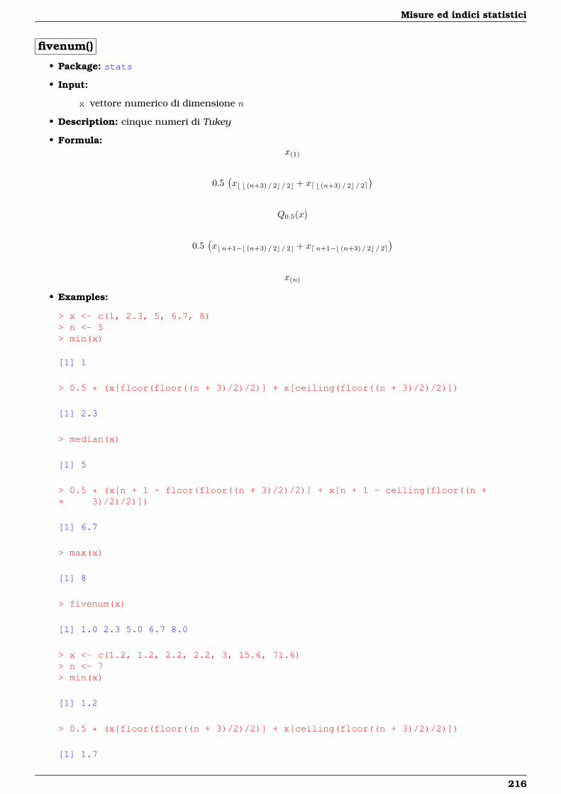
Misure ed indici statistici
fivenum()
• Package: stats
• Input:
x vettore numerico di dimensione n
• Description: cinque numeri di Tukey
• Formula:x(1)
0.5(xb b (n+3) / 2c / 2c + xd b (n+3) / 2c / 2e
)Q0.5(x)
0.5(xbn+1−b (n+3) / 2c / 2c + xdn+1−b (n+3) / 2c / 2e
)x(n)
• Examples:
> x <- c(1, 2.3, 5, 6.7, 8)> n <- 5> min(x)
[1] 1
> 0.5 * (x[floor(floor((n + 3)/2)/2)] + x[ceiling(floor((n + 3)/2)/2)])
[1] 2.3
> median(x)
[1] 5
> 0.5 * (x[n + 1 - floor(floor((n + 3)/2)/2)] + x[n + 1 - ceiling(floor((n ++ 3)/2)/2)])
[1] 6.7
> max(x)
[1] 8
> fivenum(x)
[1] 1.0 2.3 5.0 6.7 8.0
> x <- c(1.2, 1.2, 2.2, 2.2, 3, 15.6, 71.6)> n <- 7> min(x)
[1] 1.2
> 0.5 * (x[floor(floor((n + 3)/2)/2)] + x[ceiling(floor((n + 3)/2)/2)])
[1] 1.7
216
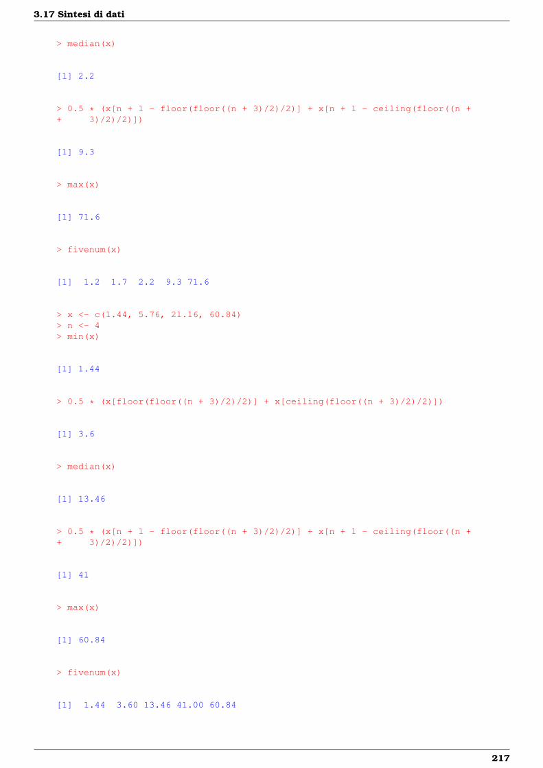
3.17 Sintesi di dati
> median(x)
[1] 2.2
> 0.5 * (x[n + 1 - floor(floor((n + 3)/2)/2)] + x[n + 1 - ceiling(floor((n ++ 3)/2)/2)])
[1] 9.3
> max(x)
[1] 71.6
> fivenum(x)
[1] 1.2 1.7 2.2 9.3 71.6
> x <- c(1.44, 5.76, 21.16, 60.84)> n <- 4> min(x)
[1] 1.44
> 0.5 * (x[floor(floor((n + 3)/2)/2)] + x[ceiling(floor((n + 3)/2)/2)])
[1] 3.6
> median(x)
[1] 13.46
> 0.5 * (x[n + 1 - floor(floor((n + 3)/2)/2)] + x[n + 1 - ceiling(floor((n ++ 3)/2)/2)])
[1] 41
> max(x)
[1] 60.84
> fivenum(x)
[1] 1.44 3.60 13.46 41.00 60.84
217
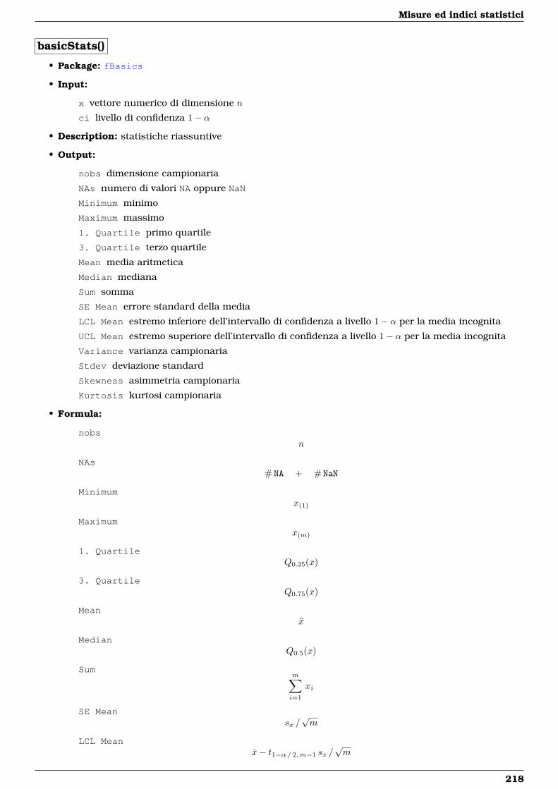
Misure ed indici statistici
basicStats()
• Package: fBasics
• Input:
x vettore numerico di dimensione n
ci livello di confidenza 1− α
• Description: statistiche riassuntive
• Output:
nobs dimensione campionaria
NAs numero di valori NA oppure NaN
Minimum minimo
Maximum massimo
1. Quartile primo quartile
3. Quartile terzo quartile
Mean media aritmetica
Median mediana
Sum somma
SE Mean errore standard della media
LCL Mean estremo inferiore dell’intervallo di confidenza a livello 1− α per la media incognita
UCL Mean estremo superiore dell’intervallo di confidenza a livello 1− α per la media incognita
Variance varianza campionaria
Stdev deviazione standard
Skewness asimmetria campionaria
Kurtosis kurtosi campionaria
• Formula:
nobsn
NAs# NA + # NaN
Minimumx(1)
Maximumx(m)
1. QuartileQ0.25(x)
3. QuartileQ0.75(x)
Meanx
MedianQ0.5(x)
Summ∑i=1
xi
SE Meansx /√m
LCL Meanx− t1−α/ 2,m−1 sx /
√m
218
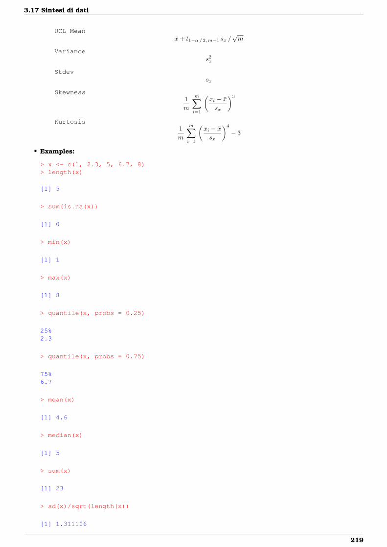
3.17 Sintesi di dati
UCL Meanx+ t1−α/ 2,m−1 sx /
√m
Variances2x
Stdevsx
Skewness1m
m∑i=1
(xi − xsx
)3
Kurtosis1m
m∑i=1
(xi − xsx
)4
− 3
• Examples:
> x <- c(1, 2.3, 5, 6.7, 8)> length(x)
[1] 5
> sum(is.na(x))
[1] 0
> min(x)
[1] 1
> max(x)
[1] 8
> quantile(x, probs = 0.25)
25%2.3
> quantile(x, probs = 0.75)
75%6.7
> mean(x)
[1] 4.6
> median(x)
[1] 5
> sum(x)
[1] 23
> sd(x)/sqrt(length(x))
[1] 1.311106
219
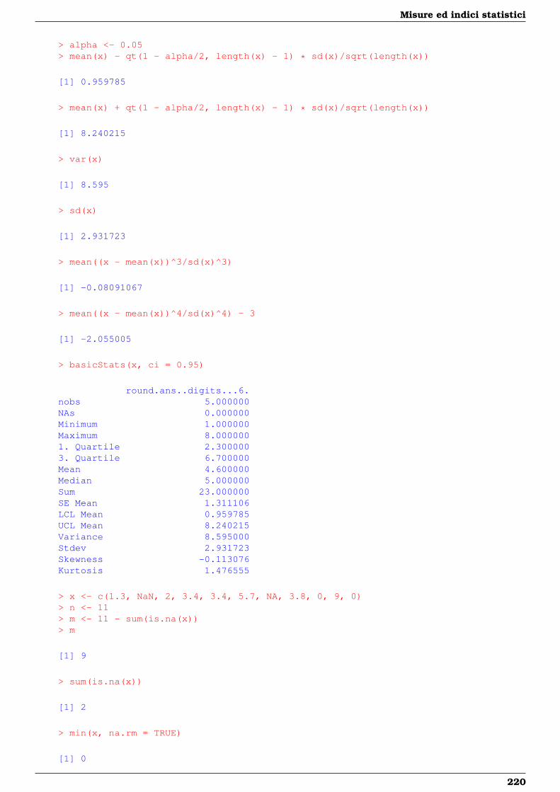
Misure ed indici statistici
> alpha <- 0.05> mean(x) - qt(1 - alpha/2, length(x) - 1) * sd(x)/sqrt(length(x))
[1] 0.959785
> mean(x) + qt(1 - alpha/2, length(x) - 1) * sd(x)/sqrt(length(x))
[1] 8.240215
> var(x)
[1] 8.595
> sd(x)
[1] 2.931723
> mean((x - mean(x))^3/sd(x)^3)
[1] -0.08091067
> mean((x - mean(x))^4/sd(x)^4) - 3
[1] -2.055005
> basicStats(x, ci = 0.95)
round.ans..digits...6.nobs 5.000000NAs 0.000000Minimum 1.000000Maximum 8.0000001. Quartile 2.3000003. Quartile 6.700000Mean 4.600000Median 5.000000Sum 23.000000SE Mean 1.311106LCL Mean 0.959785UCL Mean 8.240215Variance 8.595000Stdev 2.931723Skewness -0.113076Kurtosis 1.476555
> x <- c(1.3, NaN, 2, 3.4, 3.4, 5.7, NA, 3.8, 0, 9, 0)> n <- 11> m <- 11 - sum(is.na(x))> m
[1] 9
> sum(is.na(x))
[1] 2
> min(x, na.rm = TRUE)
[1] 0
220
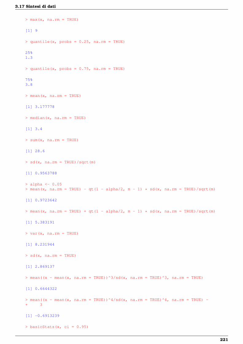
3.17 Sintesi di dati
> max(x, na.rm = TRUE)
[1] 9
> quantile(x, probs = 0.25, na.rm = TRUE)
25%1.3
> quantile(x, probs = 0.75, na.rm = TRUE)
75%3.8
> mean(x, na.rm = TRUE)
[1] 3.177778
> median(x, na.rm = TRUE)
[1] 3.4
> sum(x, na.rm = TRUE)
[1] 28.6
> sd(x, na.rm = TRUE)/sqrt(m)
[1] 0.9563788
> alpha <- 0.05> mean(x, na.rm = TRUE) - qt(1 - alpha/2, m - 1) * sd(x, na.rm = TRUE)/sqrt(m)
[1] 0.9723642
> mean(x, na.rm = TRUE) + qt(1 - alpha/2, m - 1) * sd(x, na.rm = TRUE)/sqrt(m)
[1] 5.383191
> var(x, na.rm = TRUE)
[1] 8.231944
> sd(x, na.rm = TRUE)
[1] 2.869137
> mean((x - mean(x, na.rm = TRUE))^3/sd(x, na.rm = TRUE)^3, na.rm = TRUE)
[1] 0.6644322
> mean((x - mean(x, na.rm = TRUE))^4/sd(x, na.rm = TRUE)^4, na.rm = TRUE) -+ 3
[1] -0.6913239
> basicStats(x, ci = 0.95)
221
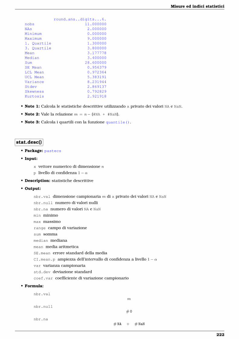
Misure ed indici statistici
round.ans..digits...6.nobs 11.000000NAs 2.000000Minimum 0.000000Maximum 9.0000001. Quartile 1.3000003. Quartile 3.800000Mean 3.177778Median 3.400000Sum 28.600000SE Mean 0.956379LCL Mean 0.972364UCL Mean 5.383191Variance 8.231944Stdev 2.869137Skewness 0.792829Kurtosis 2.921918
• Note 1: Calcola le statistiche descrittive utilizzando x privato dei valori NA e NaN.
• Note 2: Vale la relazione m = n− (#NA + #NaN).
• Note 3: Calcola i quartili con la funzione quantile().
stat.desc()
• Package: pastecs
• Input:
x vettore numerico di dimensione n
p livello di confidenza 1− α
• Description: statistiche descrittive
• Output:
nbr.val dimensione campionaria m di x privato dei valori NA e NaN
nbr.null numero di valori nulli
nbr.na numero di valori NA e NaN
min minimo
max massimo
range campo di variazione
sum somma
median mediana
mean media aritmetica
SE.mean errore standard della media
CI.mean.p ampiezza dell’intervallo di confidenza a livello 1− αvar varianza campionaria
std.dev deviazione standard
coef.var coefficiente di variazione campionario
• Formula:
nbr.valm
nbr.null# 0
nbr.na# NA + # NaN
222
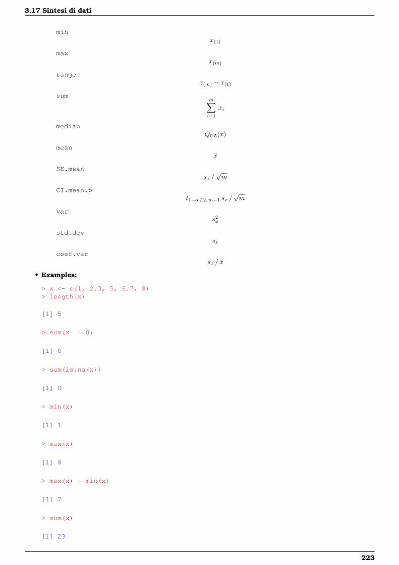
3.17 Sintesi di dati
minx(1)
maxx(m)
rangex(m) − x(1)
summ∑i=1
xi
medianQ0.5(x)
meanx
SE.meansx /√m
CI.mean.pt1−α/ 2,m−1 sx /
√m
vars2x
std.devsx
coef.varsx / x
• Examples:
> x <- c(1, 2.3, 5, 6.7, 8)> length(x)
[1] 5
> sum(x == 0)
[1] 0
> sum(is.na(x))
[1] 0
> min(x)
[1] 1
> max(x)
[1] 8
> max(x) - min(x)
[1] 7
> sum(x)
[1] 23
223
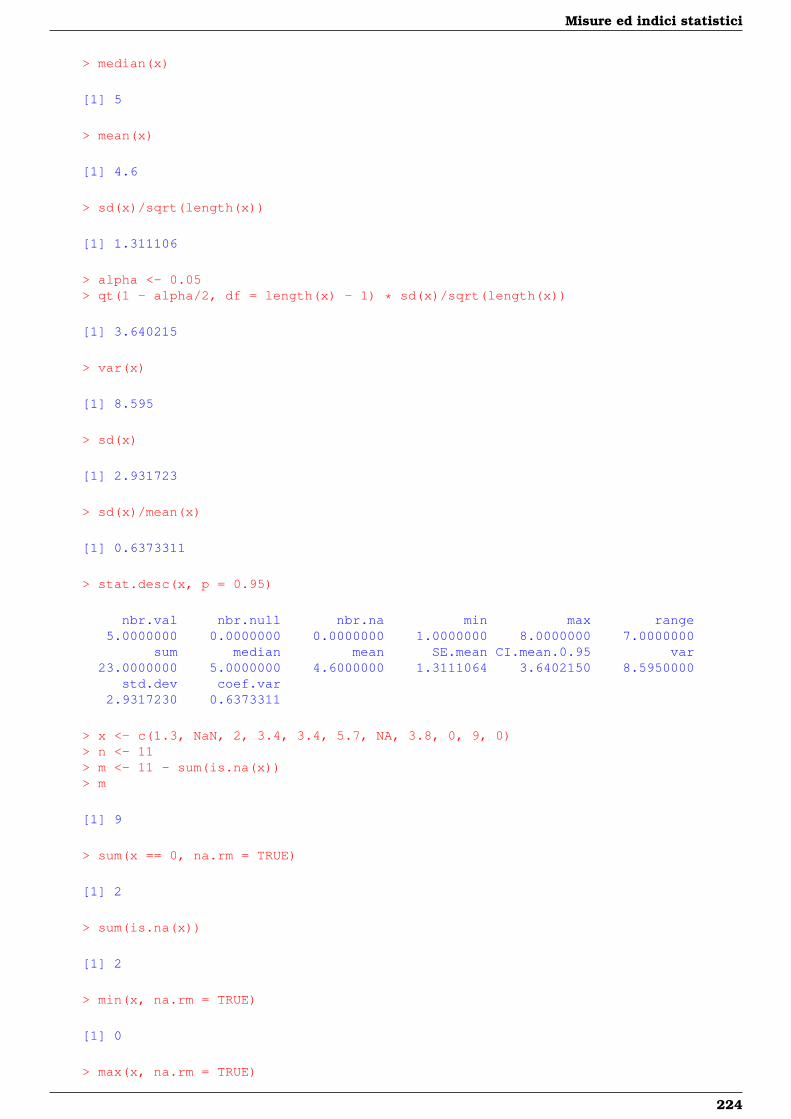
Misure ed indici statistici
> median(x)
[1] 5
> mean(x)
[1] 4.6
> sd(x)/sqrt(length(x))
[1] 1.311106
> alpha <- 0.05> qt(1 - alpha/2, df = length(x) - 1) * sd(x)/sqrt(length(x))
[1] 3.640215
> var(x)
[1] 8.595
> sd(x)
[1] 2.931723
> sd(x)/mean(x)
[1] 0.6373311
> stat.desc(x, p = 0.95)
nbr.val nbr.null nbr.na min max range5.0000000 0.0000000 0.0000000 1.0000000 8.0000000 7.0000000
sum median mean SE.mean CI.mean.0.95 var23.0000000 5.0000000 4.6000000 1.3111064 3.6402150 8.5950000
std.dev coef.var2.9317230 0.6373311
> x <- c(1.3, NaN, 2, 3.4, 3.4, 5.7, NA, 3.8, 0, 9, 0)> n <- 11> m <- 11 - sum(is.na(x))> m
[1] 9
> sum(x == 0, na.rm = TRUE)
[1] 2
> sum(is.na(x))
[1] 2
> min(x, na.rm = TRUE)
[1] 0
> max(x, na.rm = TRUE)
224
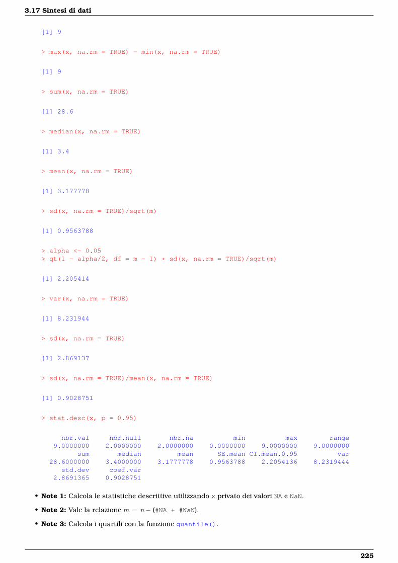
3.17 Sintesi di dati
[1] 9
> max(x, na.rm = TRUE) - min(x, na.rm = TRUE)
[1] 9
> sum(x, na.rm = TRUE)
[1] 28.6
> median(x, na.rm = TRUE)
[1] 3.4
> mean(x, na.rm = TRUE)
[1] 3.177778
> sd(x, na.rm = TRUE)/sqrt(m)
[1] 0.9563788
> alpha <- 0.05> qt(1 - alpha/2, df = m - 1) * sd(x, na.rm = TRUE)/sqrt(m)
[1] 2.205414
> var(x, na.rm = TRUE)
[1] 8.231944
> sd(x, na.rm = TRUE)
[1] 2.869137
> sd(x, na.rm = TRUE)/mean(x, na.rm = TRUE)
[1] 0.9028751
> stat.desc(x, p = 0.95)
nbr.val nbr.null nbr.na min max range9.0000000 2.0000000 2.0000000 0.0000000 9.0000000 9.0000000
sum median mean SE.mean CI.mean.0.95 var28.6000000 3.4000000 3.1777778 0.9563788 2.2054136 8.2319444
std.dev coef.var2.8691365 0.9028751
• Note 1: Calcola le statistiche descrittive utilizzando x privato dei valori NA e NaN.
• Note 2: Vale la relazione m = n− (#NA + #NaN).
• Note 3: Calcola i quartili con la funzione quantile().
225
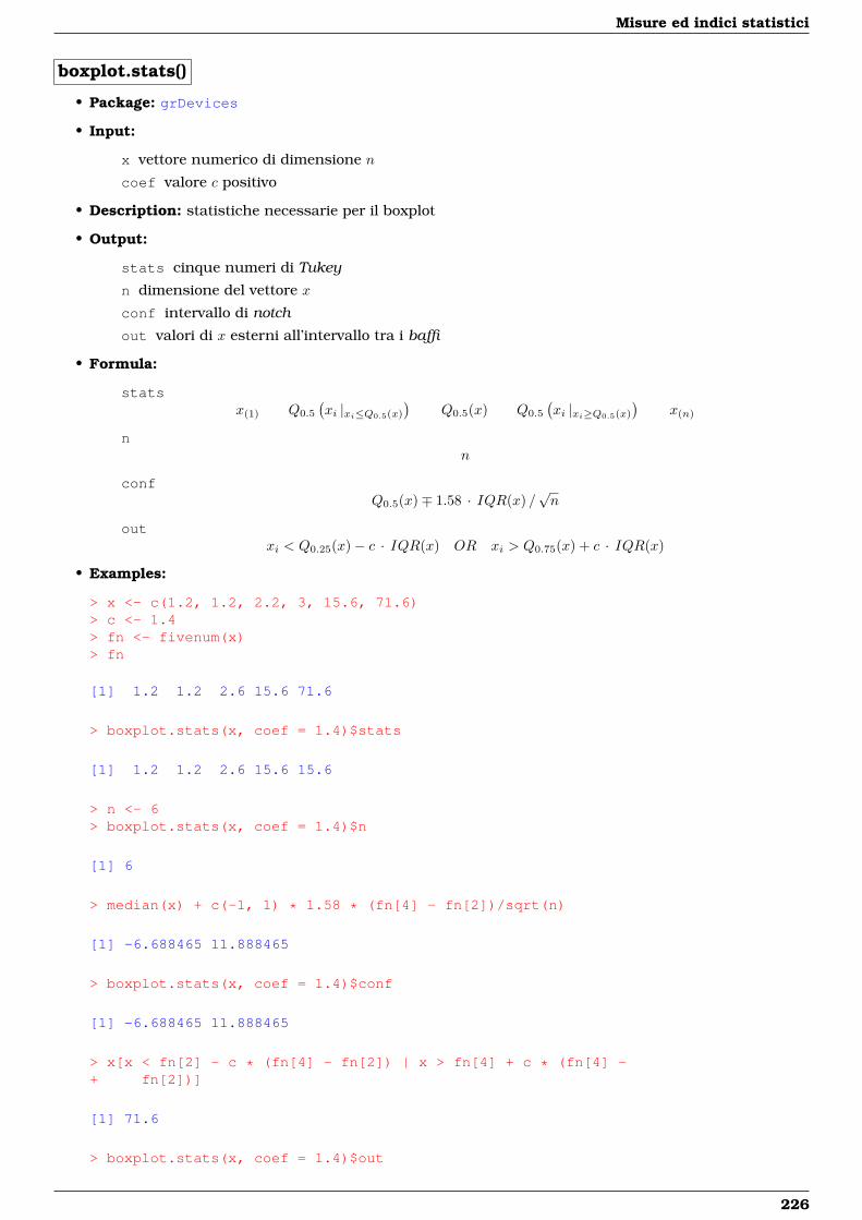
Misure ed indici statistici
boxplot.stats()
• Package: grDevices
• Input:
x vettore numerico di dimensione n
coef valore c positivo
• Description: statistiche necessarie per il boxplot
• Output:
stats cinque numeri di Tukey
n dimensione del vettore x
conf intervallo di notch
out valori di x esterni all’intervallo tra i baffi
• Formula:
statsx(1) Q0.5
(xi |xi≤Q0.5(x)
)Q0.5(x) Q0.5
(xi |xi≥Q0.5(x)
)x(n)
nn
confQ0.5(x)∓ 1.58 · IQR(x) /
√n
outxi < Q0.25(x)− c · IQR(x) OR xi > Q0.75(x) + c · IQR(x)
• Examples:
> x <- c(1.2, 1.2, 2.2, 3, 15.6, 71.6)> c <- 1.4> fn <- fivenum(x)> fn
[1] 1.2 1.2 2.6 15.6 71.6
> boxplot.stats(x, coef = 1.4)$stats
[1] 1.2 1.2 2.6 15.6 15.6
> n <- 6> boxplot.stats(x, coef = 1.4)$n
[1] 6
> median(x) + c(-1, 1) * 1.58 * (fn[4] - fn[2])/sqrt(n)
[1] -6.688465 11.888465
> boxplot.stats(x, coef = 1.4)$conf
[1] -6.688465 11.888465
> x[x < fn[2] - c * (fn[4] - fn[2]) | x > fn[4] + c * (fn[4] -+ fn[2])]
[1] 71.6
> boxplot.stats(x, coef = 1.4)$out
226
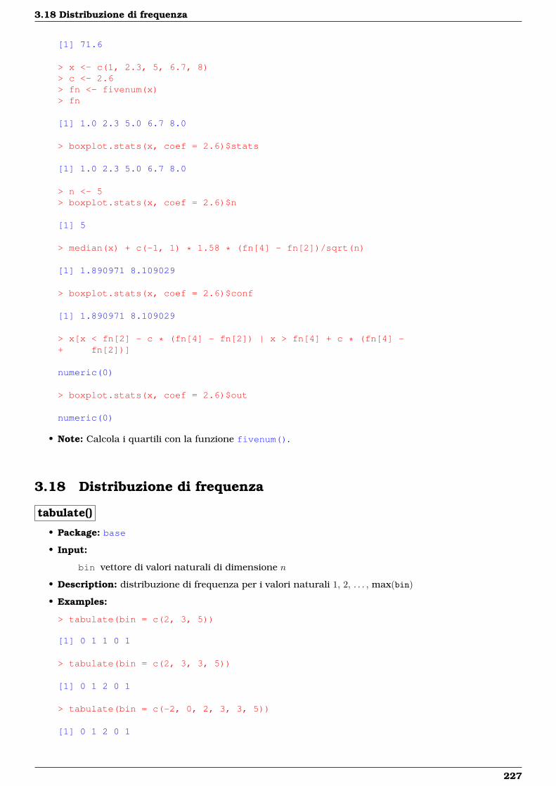
3.18 Distribuzione di frequenza
[1] 71.6
> x <- c(1, 2.3, 5, 6.7, 8)> c <- 2.6> fn <- fivenum(x)> fn
[1] 1.0 2.3 5.0 6.7 8.0
> boxplot.stats(x, coef = 2.6)$stats
[1] 1.0 2.3 5.0 6.7 8.0
> n <- 5> boxplot.stats(x, coef = 2.6)$n
[1] 5
> median(x) + c(-1, 1) * 1.58 * (fn[4] - fn[2])/sqrt(n)
[1] 1.890971 8.109029
> boxplot.stats(x, coef = 2.6)$conf
[1] 1.890971 8.109029
> x[x < fn[2] - c * (fn[4] - fn[2]) | x > fn[4] + c * (fn[4] -+ fn[2])]
numeric(0)
> boxplot.stats(x, coef = 2.6)$out
numeric(0)
• Note: Calcola i quartili con la funzione fivenum().
3.18 Distribuzione di frequenza
tabulate()
• Package: base
• Input:
bin vettore di valori naturali di dimensione n
• Description: distribuzione di frequenza per i valori naturali 1, 2, . . . , max(bin)
• Examples:
> tabulate(bin = c(2, 3, 5))
[1] 0 1 1 0 1
> tabulate(bin = c(2, 3, 3, 5))
[1] 0 1 2 0 1
> tabulate(bin = c(-2, 0, 2, 3, 3, 5))
[1] 0 1 2 0 1
227

Misure ed indici statistici
table()
• Package: base
• Input:
x vettore alfanumerico di dimensione n
• Description: distribuzione di frequenza
• Examples:
> x <- c("a", "a", "b", "c", "a", "c")> table(x)
xa b c3 1 2
> table(x)/length(x)
xa b c
0.5000000 0.1666667 0.3333333
> f <- factor(c("a", "b", "c", "b", "a", "c", "a", "b", "b", "c",+ "a"))> f
[1] a b c b a c a b b c aLevels: a b c
> g <- factor(c("A", "S", "A", "S", "S", "S", "A", "S", "S", "A",+ "A"))> g
[1] A S A S S S A S S A ALevels: A S
> table(f, g)
gf A S
a 3 1b 0 4c 2 1
> x <- c(1, 2, 3, 2, 1, 3, 1, 1, 2, 3)> table(x)
x1 2 34 3 3
228
3.18 Distribuzione di frequenza
unique()
• Package: base
• Input:
x vettore alfanumerico di dimensione n
• Description: supporto (valori distinti di x)
• Examples:
> x <- c("a", "a", "b", "c", "a", "c")> unique(x)
[1] "a" "b" "c"
> x <- c(1, 2, 3, 2, 1, 3, 1, 1, 2, 3)> unique(x)
[1] 1 2 3
> x <- c(12, -3, 7, 12, 4, -3, 12, 7, -3)> x[!duplicated(x)]
[1] 12 -3 7 4
> unique(x)
[1] 12 -3 7 4
duplicated()
• Package: base
• Input:
x vettore numerico di dimensione n
• Description: segnalazione di valori duplicati
• Examples:
> x <- c(1, 2, 1, 3, 2, 2, 4)> duplicated(x)
[1] FALSE FALSE TRUE FALSE TRUE TRUE FALSE
> x <- c(1, 2, 1, 2, 1, 2)> duplicated(x)
[1] FALSE FALSE TRUE TRUE TRUE TRUE
> x <- c(12, -3, 7, 12, 4, -3, 12, 7, -3)> unique(x[duplicated(x)])
[1] 12 -3 7
229
Misure ed indici statistici
3.19 Istogramma
hist()
• Package: graphics
• Input:
x vettore numerico di dimensione n
breaks estremi delle classi di ampiezza bi
right = TRUE / FALSE classi chiuse a destra(a(i), a(i+1)
]oppure a sinistra
[a(i), a(i+1)
)include.lowest = TRUE / FALSE estremo incluso
plot = FALSE
• Description: istogramma
• Output:
breaks estremi delle classi
counts frequenze assolute
density densità di frequenza
mids punti centrali delle classi
• Formula:
breaksa(i) ∀ i = 1, 2, . . . , m
countsni ∀ i = 1, 2, . . . , m− 1
densitynin bi
∀ i = 1, 2, . . . , m− 1
midsa(i) + a(i+1)
2∀ i = 1, 2, . . . , m− 1
• Examples:
> x <- c(51.1, 52.3, 66.7, 77.1, 77.15, 77.17)> n <- 6> m <- 4> a1 <- 50> a2 <- 65> a3 <- 70> a4 <- 85> a <- c(a1, a2, a3, a4)> b1 <- 65 - 50> b2 <- 70 - 65> b3 <- 85 - 70> b <- c(b1, b2, b3)> b
[1] 15 5 15
> hist(x, breaks = a, right = FALSE, include.lowest = FALSE, plot = FALSE)$breaks
[1] 50 65 70 85
> count <- numeric(m - 1)> count[1] <- sum(x >= a1 & x < a2)> count[2] <- sum(x >= a2 & x < a3)> count[3] <- sum(x >= a3 & x < a4)> count
230
3.19 Istogramma
[1] 2 1 3
> hist(x, breaks = a, right = FALSE, include.lowest = FALSE, plot = FALSE)$counts
[1] 2 1 3
> count/(n * b)
[1] 0.02222222 0.03333333 0.03333333
> hist(x, breaks = a, right = FALSE, include.lowest = FALSE, plot = FALSE)$density
[1] 0.02222222 0.03333333 0.03333333
> (a[-m] + a[-1])/2
[1] 57.5 67.5 77.5
> hist(x, breaks = a, right = FALSE, include.lowest = FALSE, plot = FALSE)$mids
[1] 57.5 67.5 77.5
> x <- c(1, 1.2, 2.2, 2.3, 3, 5, 6.7, 8, 15.6)> n <- 9> m <- 5> a1 <- 0> a2 <- 5> a3 <- 10> a4 <- 15> a5 <- 20> a <- c(a1, a2, a3, a4, a5)> a
[1] 0 5 10 15 20
> b1 <- a2 - a1> b2 <- a3 - a2> b3 <- a4 - a3> b4 <- a5 - a4> b <- c(b1, b2, b3, b4)> b
[1] 5 5 5 5
> hist(x, breaks = a, right = FALSE, include.lowest = FALSE, plot = FALSE)$breaks
[1] 0 5 10 15 20
> count <- numeric(m - 1)> count[1] <- sum(x >= a1 & x < a2)> count[2] <- sum(x >= a2 & x < a3)> count[3] <- sum(x >= a3 & x < a4)> count[4] <- sum(x >= a4 & x < a5)> count
[1] 5 3 0 1
> hist(x, breaks = a, right = FALSE, include.lowest = FALSE, plot = FALSE)$counts
231
Misure ed indici statistici
[1] 5 3 0 1
> count/(n * b)
[1] 0.11111111 0.06666667 0.00000000 0.02222222
> hist(x, breaks = a, right = FALSE, include.lowest = FALSE, plot = FALSE)$density
[1] 0.11111111 0.06666667 0.00000000 0.02222222
> (a[-m] + a[-1])/2
[1] 2.5 7.5 12.5 17.5
> hist(x, breaks = a, right = FALSE, include.lowest = FALSE, plot = FALSE)$mids
[1] 2.5 7.5 12.5 17.5
n.bins()
• Package: car
• Input:
x vettore numerico di dimensione n
rule = "freedman.diaconis" / "sturges" / "scott" / "simple" algoritmo
• Description: algoritmo di calcolo per il numero di classi di un istogramma
• Formula:
rule = "freedman.diaconis"
nc =⌈
x(n) − x(1)
2 IQR(x) n−1 / 3
⌉
rule = "sturges"
nc = dlog2(n) + 1e
rule = "scott"
nc =⌈x(n) − x(1)
3.5 sx n−1 / 3
⌉
rule = "simple"
nc ={b2√nc se n ≤ 100
b10 log10(n)c se n > 100
• Examples:
> x <- c(2.3, 1, 5, 6.7, 8)> x <- sort(x)> x
[1] 1.0 2.3 5.0 6.7 8.0
232

3.19 Istogramma
> n <- 5> nc <- ceiling((x[n] - x[1])/(2 * IQR(x) * n^(-1/3)))> nc
[1] 2
> n.bins(x, rule = "freedman.diaconis")
[1] 2
> x <- c(2.3, 1, 5, 6.7, 8)> n <- 5> nc <- ceiling(log2(n) + 1)> nc
[1] 4
> n.bins(x, rule = "sturges")
[1] 4
> x <- c(2.3, 1, 5, 6.7, 8)> x <- sort(x)> x
[1] 1.0 2.3 5.0 6.7 8.0
> n <- 5> sx <- sd(x)> nc <- ceiling((x[n] - x[1])/(3.5 * sx * n^(-1/3)))> nc
[1] 2
> n.bins(x, rule = "scott")
[1] 2
> x <- c(2.3, 1, 5, 6.7, 8)> n <- 5> nc <- floor(2 * sqrt(n))> nc
[1] 4
> n.bins(x, rule = "simple")
[1] 4
• Note: Calcola i quartili con la funzione quantile().
233
Misure ed indici statistici
nclass.FD()
• Package: grDevices
• Input:
x vettore numerico di dimensione n
• Description: numero di classi di un istogramma secondo Freedman - Diaconis
• Formula:
nc =⌈
x(n) − x(1)
2 IQR(x) n−1 / 3
⌉• Examples:
> x <- c(2.3, 1, 5, 6.7, 8)> x <- sort(x)> x
[1] 1.0 2.3 5.0 6.7 8.0
> n <- 5> nc <- ceiling((x[n] - x[1])/(2 * IQR(x) * n^(-1/3)))> nc
[1] 2
> nclass.FD(x)
[1] 2
> x <- c(3.4, 5.52, 6.4, 7.56, 8.7, 8.6, 5.4, 5.5)> x <- sort(x)> x <- c(3.4, 5.4, 5.5, 5.52, 6.4, 7.56, 8.6, 8.7)> n <- 8> nc <- ceiling((x[n] - x[1])/(2 * IQR(x) * n^(-1/3)))> nc
[1] 3
> nclass.FD(x)
[1] 3
• Note: Calcola i quartili con la funzione quantile().
nclass.Sturges()
• Package: grDevices
• Input:
x vettore numerico di dimensione n
• Description: numero di classi di un istogramma secondo Sturges
• Formula:nc = dlog2(n) + 1e
• Examples:
234
3.19 Istogramma
> x <- c(1, 2.3, 5, 6.7, 8)> n <- 5> nc <- ceiling(log2(n) + 1)> nc
[1] 4
> nclass.Sturges(x)
[1] 4
> x <- c(3.4, 5.4, 5.5, 5.52, 6.4, 7.56, 8.6, 8.7)> n <- 8> nc <- ceiling(log2(n) + 1)> nc
[1] 4
> nclass.Sturges(x)
[1] 4
nclass.scott()
• Package: grDevices
• Input:
x vettore numerico di dimensione n
• Description: numero di classi di un istogramma secondo Scott
• Formula:
nc =⌈x(n) − x(1)
3.5 sx n−1 / 3
⌉• Examples:
> x <- c(2.3, 1, 5, 6.7, 8)> x <- sort(x)> x
[1] 1.0 2.3 5.0 6.7 8.0
> n <- 5> sx <- sd(x)> nc <- ceiling((x[n] - x[1])/(3.5 * sx * n^(-1/3)))> nc
[1] 2
> nclass.scott(x)
[1] 2
> x <- c(3.4, 5.4, 5.5, 5.52, 6.4, 7.56, 8.6, 8.7)> x <- sort(x)> x
[1] 3.40 5.40 5.50 5.52 6.40 7.56 8.60 8.70
235
Misure ed indici statistici
> n <- 8> sx <- sd(x)> nc <- ceiling((x[n] - x[1])/(3.5 * sx * n^(-1/3)))> nc
[1] 2
> nclass.scott(x)
[1] 2
3.20 Variabili casuali discrete
Bernoulli
pX(x) = px (1− p)1−x x = 0, 1, 0 < p < 1
µX = p
σ2X = p (1− p)
Binomiale
pX(x) =(mx
)px (1− p)m−x x = 0, 1, 2, . . . , m, m ∈ N / {0}, 0 < p < 1
µX = mp
σ2X = mp (1− p)
Binomiale Negativa
pX(x) =(r+x−1x
)pr (1− p)x =
(r+x−1r−1
)pr (1− p)x x ∈ N, r ∈ N\{0}, 0 < p < 1
µX = r (1− p) / p
σ2X = r (1− p) / p2
Geometrica
pX(x) = p (1− p)x x ∈ N, 0 < p < 1
µX = (1− p) / p
σ2X = (1− p) / p2
Geometrica 2
pX(x) = p (1− p)x−1 x ∈ N\{0}, 0 < p < 1
µX = 1 / p
σ2X = (1− p) / p2
Ipergeometrica
pX(x) =(Mx
) (N−Mk−x
)/(Nk
)x = 0, 1, 2, . . . , k
N ∈ N\{0}
k = 1, 2, . . . , N
236
3.20 Variabili casuali discrete
M = 0, 1, 2, . . . , N − 1
µX = k (M /N)
σ2X = k (M /N) (1−M /N) (N − k) / (N − 1)
Multinomiale
pX1, X2, ..., Xk(x1, x2, . . . , xk) = m !x1 ! x2 !···xk !
∏ki=1 p
xii
xi = 0, 1, 2, . . . , m ∀i = 1, 2, . . . , k
0 < pi < 1 ∀i = 1, 2, . . . , k∑ki=1 xi = m∑ki=1 pi = 1
µXi = mpi ∀i = 1, 2, . . . , k
σ2Xi
= mpi (1− pi) ∀i = 1, 2, . . . , k
σXiXj = −mpi pj ∀i 6= j = 1, 2, . . . , k
Poisson
pX(x) = λx e−λ / x ! x ∈ N, λ > 0
µX = λ
σ2X = λ
Tavola argomenti comandi R
Variabile Casuale Suffisso Parametri PackageBernoulli binom size, prob statsBinomiale binom size, prob statsBinomiale Negativa nbinom size, prob statsGeometrica geom prob statsGeometrica 2 geomet p distributionsIpergeometrica hyper m, n, k statsMultinomiale multinom size, prob statsPoisson pois lambda stats
Tavola esempi comandi R
Variabile Casuale Oggetto Comando in RBernoulli Densità dbinom(x=x,size=1,prob=p)
Ripartizione pbinom(q=x,size=1,prob=p)Quantile qbinom(p=α,size=1,prob=p)Random rbinom(n,size=1,prob=p)
Binomiale Densità dbinom(x=x,size=m,prob=p)Ripartizione pbinom(q=x,size=m,prob=p)Quantile qbinom(p=α,size=m,prob=p)Random rbinom(n,size=m,prob=p)
Binomiale Negativa Densità dnbinom(x=x,size=r,prob=p)Ripartizione pnbinom(q=x,size=r,prob=p)Quantile qnbinom(p=α,size=r,prob=p)Random rnbinom(n,size=r,prob=p)
Geometrica Densità dgeom(x=x,prob=p)Ripartizione pgeom(q=x,prob=p)Quantile qgeom(p=α,prob=p)Random rgeom(n,prob=p)
237
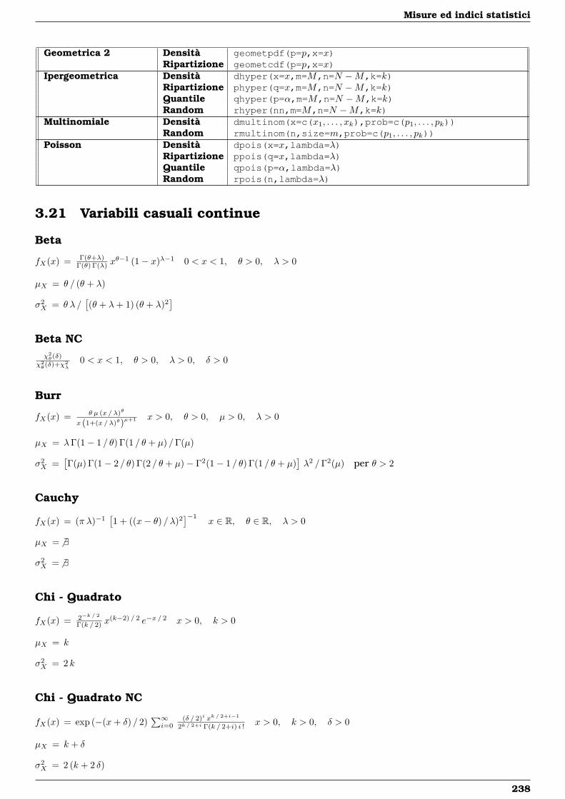
Misure ed indici statistici
Geometrica 2 Densità geometpdf(p=p,x=x)Ripartizione geometcdf(p=p,x=x)
Ipergeometrica Densità dhyper(x=x,m=M,n=N −M,k=k)Ripartizione phyper(q=x,m=M,n=N −M,k=k)Quantile qhyper(p=α,m=M,n=N −M,k=k)Random rhyper(nn,m=M,n=N −M,k=k)
Multinomiale Densità dmultinom(x=c(x1, . . . , xk),prob=c(p1, . . . , pk))Random rmultinom(n,size=m,prob=c(p1, . . . , pk))
Poisson Densità dpois(x=x,lambda=λ)Ripartizione ppois(q=x,lambda=λ)Quantile qpois(p=α,lambda=λ)Random rpois(n,lambda=λ)
3.21 Variabili casuali continue
Beta
fX(x) = Γ(θ+λ)Γ(θ) Γ(λ) x
θ−1 (1− x)λ−1 0 < x < 1, θ > 0, λ > 0
µX = θ / (θ + λ)
σ2X = θ λ /
[(θ + λ+ 1) (θ + λ)2
]Beta NCχ2θ(δ)
χ2θ(δ)+χ2
λ0 < x < 1, θ > 0, λ > 0, δ > 0
Burr
fX(x) = θ µ (x / λ)θ
x (1+(x / λ)θ)µ+1 x > 0, θ > 0, µ > 0, λ > 0
µX = λΓ(1− 1 / θ) Γ(1 / θ + µ) /Γ(µ)
σ2X =
[Γ(µ) Γ(1− 2 / θ) Γ(2 / θ + µ)− Γ2(1− 1 / θ) Γ(1 / θ + µ)
]λ2 /Γ2(µ) per θ > 2
Cauchy
fX(x) = (π λ)−1[1 + ((x− θ) / λ)2
]−1x ∈ R, θ ∈ R, λ > 0
µX = 6 ∃
σ2X = 6 ∃
Chi - Quadrato
fX(x) = 2−k / 2
Γ(k / 2) x(k−2) / 2 e−x / 2 x > 0, k > 0
µX = k
σ2X = 2 k
Chi - Quadrato NC
fX(x) = exp (−(x+ δ) / 2)∑∞i=0
(δ / 2)i xk / 2+i−1
2k / 2+i Γ(k / 2+i) i !x > 0, k > 0, δ > 0
µX = k + δ
σ2X = 2 (k + 2 δ)
238
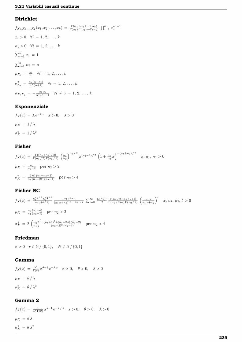
3.21 Variabili casuali continue
Dirichlet
fX1,X2,...,Xk(x1, x2, . . . , xk) = Γ(α1+α2+···+αk)Γ(α1) Γ(α2) ···Γ(αk)
∏ki=1 x
αi−1i
xi > 0 ∀i = 1, 2, . . . , k
αi > 0 ∀i = 1, 2, . . . , k∑ki=1 xi = 1∑ki=1 αi = α
µXi = αiα ∀i = 1, 2, . . . , k
σ2Xi
= αi (α−αi)α2 (α+1) ∀i = 1, 2, . . . , k
σXiXj = − αi αjα2 (α+1) ∀i 6= j = 1, 2, . . . , k
Esponenziale
fX(x) = λ e−λx x > 0, λ > 0
µX = 1 / λ
σ2X = 1 / λ2
Fisher
fX(x) = Γ((n1+n2) / 2)Γ(n1 / 2) Γ(n2 / 2)
(n1n2
)n1 / 2
x(n1−2) / 2(
1 + n1n2x)−(n1+n2) / 2
x, n1, n2 > 0
µX = n2n2−2 per n2 > 2
σ2X = 2n2
2 (n1+n2−2)n1 (n2−2)2 (n2−4) per n2 > 4
Fisher NC
fX(x) = nn1 / 21 n
n2 / 22
exp (δ / 2)xn1 / 2−1
(n1 x+n2)(n1+n2) / 2
∑∞i=0
(δ / 2)i
i !Γ(n1 / 2+n2 / 2+i)
Γ(n1 / 2+i) Γ(n2 / 2)
(n1 x
n1 x+n2
)ix, n1, n2, δ > 0
µX = n2 (n1+δ)n1 (n2−2) per n2 > 2
σ2X = 2
(n2n1
)2(n1+δ)2+(n1+2 δ) (n2−2)
(n2−2)2 (n2−4) per n2 > 4
Friedman
x > 0 r ∈ N / {0, 1}, N ∈ N / {0, 1}
Gamma
fX(x) = λθ
Γ(θ) xθ−1 e−λx x > 0, θ > 0, λ > 0
µX = θ / λ
σ2X = θ / λ2
Gamma 2
fX(x) = 1λθ Γ(θ)
xθ−1 e−x / λ x > 0, θ > 0, λ > 0
µX = θ λ
σ2X = θ λ2
239
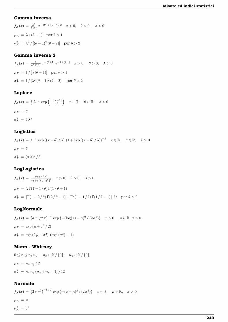
Misure ed indici statistici
Gamma inversa
fX(x) = λθ
Γ(θ) x− (θ+1) e−λ / x x > 0, θ > 0, λ > 0
µX = λ / (θ − 1) per θ > 1
σ2X = λ2 / [(θ − 1)2 (θ − 2)] per θ > 2
Gamma inversa 2
fX(x) = 1λθ Γ(θ)
x− (θ+1) e−1 / (λx) x > 0, θ > 0, λ > 0
µX = 1 / [λ (θ − 1)] per θ > 1
σ2X = 1 / [λ2 (θ − 1)2 (θ − 2)] per θ > 2
Laplace
fX(x) = 12 λ−1 exp
(− | x−θ |λ
)x ∈ R, θ ∈ R, λ > 0
µX = θ
σ2X = 2λ2
Logistica
fX(x) = λ−1 exp ((x− θ) / λ) (1 + exp ((x− θ) / λ))−2x ∈ R, θ ∈ R, λ > 0
µX = θ
σ2X = (π λ)2 / 3
LogLogistica
fX(x) = θ (x / λ)θ
x (1+(x / λ)θ)2 x > 0, θ > 0, λ > 0
µX = λΓ(1− 1 / θ) Γ(1 / θ + 1)
σ2X =
[Γ(1− 2 / θ) Γ(2 / θ + 1)− Γ2(1− 1 / θ) Γ(1 / θ + 1)
]λ2 per θ > 2
LogNormale
fX(x) =(σ x√
2π)−1
exp(−(log(x)− µ)2 / (2σ2)
)x > 0, µ ∈ R, σ > 0
µX = exp (µ+ σ2 / 2)
σ2X = exp (2µ+ σ2)
(exp
(σ2)− 1)
Mann - Whitney
0 ≤ x ≤ nx ny, nx ∈ N / {0}, ny ∈ N / {0}
µX = nx ny / 2
σ2X = nx ny (nx + ny + 1) / 12
Normale
fX(x) =(2π σ2
)−1 / 2 exp(−(x− µ)2 / (2σ2)
)x ∈ R, µ ∈ R, σ > 0
µX = µ
σ2X = σ2
240
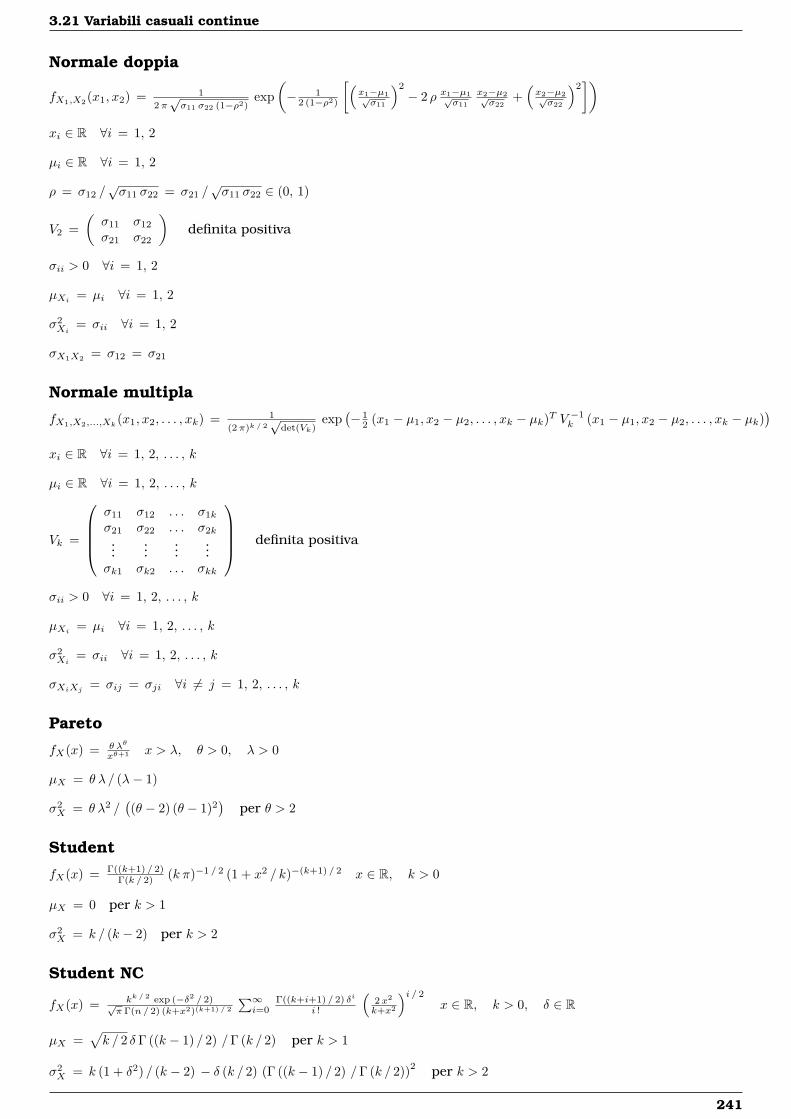
3.21 Variabili casuali continue
Normale doppia
fX1,X2(x1, x2) = 1
2π√σ11 σ22 (1−ρ2)
exp(− 1
2 (1−ρ2)
[(x1−µ1√σ11
)2
− 2 ρ x1−µ1√σ11
x2−µ2√σ22
+(x2−µ2√σ22
)2])
xi ∈ R ∀i = 1, 2
µi ∈ R ∀i = 1, 2
ρ = σ12 /√σ11 σ22 = σ21 /
√σ11 σ22 ∈ (0, 1)
V2 =(σ11 σ12
σ21 σ22
)definita positiva
σii > 0 ∀i = 1, 2
µXi = µi ∀i = 1, 2
σ2Xi
= σii ∀i = 1, 2
σX1X2 = σ12 = σ21
Normale multipla
fX1,X2,...,Xk(x1, x2, . . . , xk) = 1
(2π)k / 2√
det(Vk)exp
(− 1
2 (x1 − µ1, x2 − µ2, . . . , xk − µk)T V −1k (x1 − µ1, x2 − µ2, . . . , xk − µk)
)xi ∈ R ∀i = 1, 2, . . . , k
µi ∈ R ∀i = 1, 2, . . . , k
Vk =
σ11 σ12 . . . σ1k
σ21 σ22 . . . σ2k
......
......
σk1 σk2 . . . σkk
definita positiva
σii > 0 ∀i = 1, 2, . . . , k
µXi = µi ∀i = 1, 2, . . . , k
σ2Xi
= σii ∀i = 1, 2, . . . , k
σXiXj = σij = σji ∀i 6= j = 1, 2, . . . , k
Pareto
fX(x) = θ λθ
xθ+1 x > λ, θ > 0, λ > 0
µX = θ λ / (λ− 1)
σ2X = θ λ2 /
((θ − 2) (θ − 1)2
)per θ > 2
Student
fX(x) = Γ((k+1) / 2)Γ(k / 2) (k π)−1 / 2 (1 + x2 / k)−(k+1) / 2 x ∈ R, k > 0
µX = 0 per k > 1
σ2X = k / (k − 2) per k > 2
Student NC
fX(x) = kk / 2 exp (−δ2 / 2)√π Γ(n / 2) (k+x2)(k+1) / 2
∑∞i=0
Γ((k+i+1) / 2) δi
i !
(2 x2
k+x2
)i / 2
x ∈ R, k > 0, δ ∈ R
µX =√k / 2 δ Γ ((k − 1) / 2) /Γ (k / 2) per k > 1
σ2X = k (1 + δ2) / (k − 2) − δ (k / 2) (Γ ((k − 1) / 2) /Γ (k / 2))2 per k > 2
241
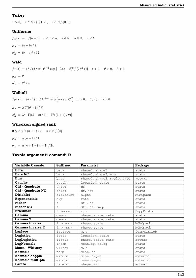
Misure ed indici statistici
Tukey
x > 0, n ∈ N / {0, 1, 2}, p ∈ N / {0, 1}
Uniforme
fX(x) = 1 /(b− a) a < x < b, a ∈ R, b ∈ R, a < b
µX = (a+ b) / 2
σ2X = (b− a)2 / 12
Wald
fX(x) = (λ / (2π x3))1 / 2 exp(−λ (x− θ)2 / (2 θ2 x)
)x > 0, θ > 0, λ > 0
µX = θ
σ2X = θ3 / λ
Weibull
fX(x) = (θ / λ) (x /λ)θ−1 exp(− (x /λ)θ
)x > 0, θ > 0, λ > 0
µX = λΓ((θ + 1) / θ)
σ2X = λ2
[Γ((θ + 2) / θ)− Γ2((θ + 1) / θ)
]Wilcoxon signed rank
0 ≤ x ≤ n (n+ 1) / 2, n ∈ N / {0}
µX = n (n+ 1) / 4
σ2X = n (n+ 1) (2n+ 1) / 24
Tavola argomenti comandi R
Variabile Casuale Suffisso Parametri PackageBeta beta shape1, shape2 statsBeta NC beta shape1, shape2, ncp statsBurr burr shape1, shape2, scale, rate actuarCauchy cauchy location, scale statsChi - Quadrato chisq df statsChi - Quadrato NC chisq df, ncp statsDirichlet dirichlet alpha MCMCpackEsponenziale exp rate statsFisher f df1, df2 statsFisher NC f df1, df2, ncp statsFriedman Friedman r, N SuppDistsGamma gamma shape, scale, rate statsGamma 2 gamma shape, scale, rate statsGamma inversa invgamma shape, scale MCMCpackGamma inversa 2 invgamma shape, scale MCMCpackLaplace laplace m, s formularioRLogistica logis location, scale statsLogLogistica llogis shape, scale, rate actuarLogNormale lnorm meanlog, sdlog statsMann - Whitney wilcox m, n statsNormale norm mean, sd statsNormale doppia mvnorm mean, sigma mvtnormNormale multipla mvnorm mean, sigma mvtnormPareto pareto1 shape, min actuar
242
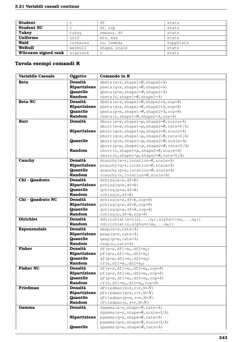
3.21 Variabili casuali continue
Student t df statsStudent NC t df, ncp statsTukey tukey nmeans, df statsUniforme unif min, max statsWald invGauss nu, lambda SuppDistsWeibull weibull shape, scale statsWilcoxon signed rank signrank n stats
Tavola esempi comandi R
Variabile Casuale Oggetto Comando in RBeta Densità dbeta(x=x,shape1=θ,shape2=λ)
Ripartizione pbeta(q=x,shape1=θ,shape2=λ)Quantile qbeta(p=α,shape1=θ,shape2=λ)Random rbeta(n,shape1=θ,shape2=λ)
Beta NC Densità dbeta(x=x,shape1=θ,shape2=λ,ncp=δ)Ripartizione pbeta(q=x,shape1=θ,shape2=λ,ncp=δ)Quantile qbeta(p=α,shape1=θ,shape2=λ,ncp=δ)Random rbeta(n,shape1=θ,shape2=λ,ncp=δ)
Burr Densità dburr(x=x,shape1=µ,shape2=θ,scale=λ)dburr(x=x,shape1=µ,shape2=θ,rate=1 /λ)
Ripartizione pburr(q=x,shape1=µ,shape2=θ,scale=λ)pburr(q=x,shape1=µ,shape2=θ,rate=1 /λ)
Quantile qburr(p=α,shape1=µ,shape2=θ,scale=λ)qburr(p=α,shape1=µ,shape2=θ,rate=1 /λ)
Random rburr(n,shape1=µ,shape2=θ,scale=λ)rburr(n,shape1=µ,shape2=θ,rate=1 /λ)
Cauchy Densità dcauchy(x=x,location=θ,scale=λ)Ripartizione pcauchy(q=x,location=θ,scale=λ)Quantile qcauchy(p=α,location=θ,scale=λ)Random rcauchy(n,location=θ,scale=λ)
Chi - Quadrato Densità dchisq(x=x,df=k)Ripartizione pchisq(q=x,df=k)Quantile qchisq(p=α,df=k)Random rchisq(n,df=k)
Chi - Quadrato NC Densità dchisq(x=x,df=k,ncp=δ)Ripartizione pchisq(q=x,df=k,ncp=δ)Quantile qchisq(p=α,df=k,ncp=δ)Random rchisq(n,df=k,ncp=δ)
Dirichlet Densità ddirichlet(x=c(x1, . . . , xk),alpha=c(α1, . . . , αk))Random rdirichlet(n,alpha=c(α1, . . . , αk))
Esponenziale Densità dexp(x=x,rate=λ)Ripartizione pexp(q=x,rate=λ)Quantile qexp(p=α,rate=λ)Random rexp(n,rate=λ)
Fisher Densità df(x=x,df1=n1,df2=n2)Ripartizione pf(q=x,df1=n1,df2=n2)Quantile qf(p=α,df1=n1,df2=n2)Random rf(n,df1=n1,df2=n2)
Fisher NC Densità df(x=x,df1=n1,df2=n2,ncp=δ)Ripartizione pf(q=x,df1=n1,df2=n2,ncp=δ)Quantile qf(p=α,df1=n1,df2=n2,ncp=δ)Random rf(n,df1=n1,df2=n2,ncp=δ)
Friedman Densità dFriedman(x=x,r=r,N=N)Ripartizione pFriedman(q=x,r=r,N=N)Quantile qFriedman(p=α,r=r,N=N)Random rFriedman(n,r=r,N=N)
Gamma Densità dgamma(x=x,shape=θ,rate=λ)dgamma(x=x,shape=θ,scale=1/λ)
Ripartizione pgamma(q=x,shape=θ,rate=λ)pgamma(q=x,shape=θ,scale=1/λ)
Quantile qgamma(p=α,shape=θ,rate=λ)
243
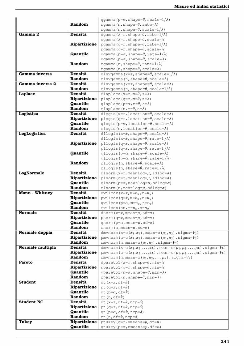
Misure ed indici statistici
qgamma(p=α,shape=θ,scale=1/λ)Random rgamma(n,shape=θ,rate=λ)
rgamma(n,shape=θ,scale=1/λ)Gamma 2 Densità dgamma(x=x,shape=θ,rate=1/λ)
dgamma(x=x,shape=θ,scale=λ)Ripartizione pgamma(q=x,shape=θ,rate=1/λ)
pgamma(q=x,shape=θ,scale=λ)Quantile qgamma(p=α,shape=θ,rate=1/λ)
qgamma(p=α,shape=θ,scale=λ)Random rgamma(n,shape=θ,rate=1/λ)
rgamma(n,shape=θ,scale=λ)Gamma inversa Densità dinvgamma(x=x,shape=θ,scale=1/λ)
Random rinvgamma(n,shape=θ,scale=λ)Gamma inversa 2 Densità dinvgamma(x=x,shape=θ,scale=λ)
Random rinvgamma(n,shape=θ,scale=1/λ)Laplace Densità dlaplace(x=x,m=θ,s=λ)
Ripartizione plaplace(q=x,m=θ,s=λ)Quantile qlaplace(p=α,m=θ,s=λ)Random rlaplace(n,m=θ,s=λ)
Logistica Densità dlogis(x=x,location=θ,scale=λ)Ripartizione plogis(q=x,location=θ,scale=λ)Quantile qlogis(p=α,location=θ,scale=λ)Random rlogis(n,location=θ,scale=λ)
LogLogistica Densità dllogis(x=x,shape=θ,scale=λ)dllogis(x=x,shape=θ,rate=1 /λ)
Ripartizione pllogis(q=x,shape=θ,scale=λ)pllogis(q=x,shape=θ,rate=1 /λ)
Quantile qllogis(p=α,shape=θ,scale=λ)qllogis(p=α,shape=θ,rate=1 /λ)
Random rllogis(n,shape=θ,scale=λ)rllogis(n,shape=θ,rate=1 /λ)
LogNormale Densità dlnorm(x=x,meanlog=µ,sdlog=σ)Ripartizione plnorm(q=x,meanlog=µ,sdlog=σ)Quantile qlnorm(p=α,meanlog=µ,sdlog=σ)Random rlnorm(n,meanlog=µ,sdlog=σ)
Mann - Whitney Densità dwilcox(x=x,m=nx,n=ny)Ripartizione pwilcox(q=x,m=nx,n=ny)Quantile qwilcox(p=α,m=nx,n=ny)Random rwilcox(nn,m=nx,n=ny)
Normale Densità dnorm(x=x,mean=µ,sd=σ)Ripartizione pnorm(q=x,mean=µ,sd=σ)Quantile qnorm(p=α,mean=µ,sd=σ)Random rnorm(n,mean=µ,sd=σ)
Normale doppia Densità dmvnorm(x=c(x1, x2),mean=c(µ1, µ2),sigma=V2)Ripartizione pmvnorm(u=c(x1, x2),mean=c(µ1, µ2),sigma=V2)Random rmvnorm(n,mean=c(µ1, µ2),sigma=V2)
Normale multipla Densità dmvnorm(x=c(x1, x2, . . . , xk),mean=c(µ1, µ2, . . . , µk),sigma=Vk)Ripartizione pmvnorm(u=c(x1, x2, . . . , xk),mean=c(µ1, µ2, . . . , µk),sigma=Vk)Random rmvnorm(n,mean=c(µ1, µ2, . . . , µk),sigma=Vk)
Pareto Densità dpareto1(x=x,shape=θ,min=λ)Ripartizione ppareto1(q=x,shape=θ,min=λ)Quantile qpareto1(p=α,shape=θ,min=λ)Random rpareto1(n,shape=θ,min=λ)
Student Densità dt(x=x,df=k)Ripartizione pt(q=x,df=k)Quantile qt(p=α,df=k)Random rt(n,df=k)
Student NC Densità dt(x=x,df=k,ncp=δ)Ripartizione pt(q=x,df=k,ncp=δ)Quantile qt(p=α,df=k,ncp=δ)Random rt(n,df=k,ncp=δ)
Tukey Ripartizione ptukey(q=x,nmeans=p,df=n)Quantile qtukey(p=α,nmeans=p,df=n)
244
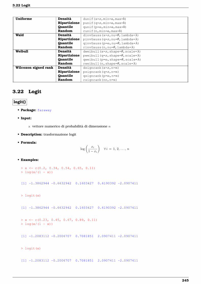
3.22 Logit
Uniforme Densità dunif(x=x,min=a,max=b)Ripartizione punif(q=x,min=a,max=b)Quantile qunif(p=α,min=a,max=b)Random runif(n,min=a,max=b)
Wald Densità dinvGauss(x=x,nu=θ,lambda=λ)Ripartizione pinvGauss(q=x,nu=θ,lambda=λ)Quantile qinvGauss(p=α,nu=θ,lambda=λ)Random rinvGauss(n,nu=θ,lambda=λ)
Weibull Densità dweibull(x=x,shape=θ,scale=λ)Ripartizione pweibull(q=x,shape=θ,scale=λ)Quantile qweibull(p=α,shape=θ,scale=λ)Random rweibull(n,shape=θ,scale=λ)
Wilcoxon signed rank Densità dsignrank(x=x,n=n)Ripartizione psignrank(q=x,n=n)Quantile qsignrank(p=α,n=n)Random rsignrank(nn,n=n)
3.22 Logit
logit()
• Package: faraway
• Input:
x vettore numerico di probabilità di dimensione n
• Description: trasformazione logit
• Formula:
log(
xi1− xi
)∀ i = 1, 2, . . . , n
• Examples:
> x <- c(0.2, 0.34, 0.54, 0.65, 0.11)> log(x/(1 - x))
[1] -1.3862944 -0.6632942 0.1603427 0.6190392 -2.0907411
> logit(x)
[1] -1.3862944 -0.6632942 0.1603427 0.6190392 -2.0907411
> x <- c(0.23, 0.45, 0.67, 0.89, 0.11)> log(x/(1 - x))
[1] -1.2083112 -0.2006707 0.7081851 2.0907411 -2.0907411
> logit(x)
[1] -1.2083112 -0.2006707 0.7081851 2.0907411 -2.0907411
245
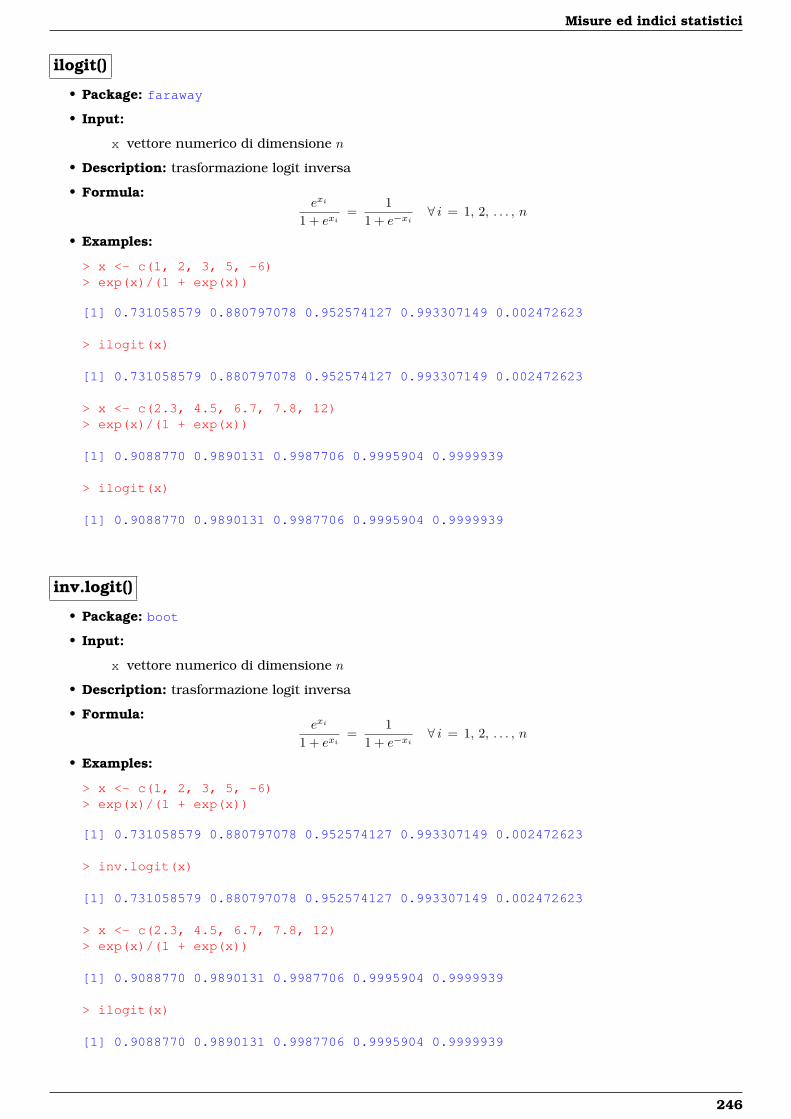
Misure ed indici statistici
ilogit()
• Package: faraway
• Input:
x vettore numerico di dimensione n
• Description: trasformazione logit inversa
• Formula:exi
1 + exi=
11 + e−xi
∀ i = 1, 2, . . . , n
• Examples:
> x <- c(1, 2, 3, 5, -6)> exp(x)/(1 + exp(x))
[1] 0.731058579 0.880797078 0.952574127 0.993307149 0.002472623
> ilogit(x)
[1] 0.731058579 0.880797078 0.952574127 0.993307149 0.002472623
> x <- c(2.3, 4.5, 6.7, 7.8, 12)> exp(x)/(1 + exp(x))
[1] 0.9088770 0.9890131 0.9987706 0.9995904 0.9999939
> ilogit(x)
[1] 0.9088770 0.9890131 0.9987706 0.9995904 0.9999939
inv.logit()
• Package: boot
• Input:
x vettore numerico di dimensione n
• Description: trasformazione logit inversa
• Formula:exi
1 + exi=
11 + e−xi
∀ i = 1, 2, . . . , n
• Examples:
> x <- c(1, 2, 3, 5, -6)> exp(x)/(1 + exp(x))
[1] 0.731058579 0.880797078 0.952574127 0.993307149 0.002472623
> inv.logit(x)
[1] 0.731058579 0.880797078 0.952574127 0.993307149 0.002472623
> x <- c(2.3, 4.5, 6.7, 7.8, 12)> exp(x)/(1 + exp(x))
[1] 0.9088770 0.9890131 0.9987706 0.9995904 0.9999939
> ilogit(x)
[1] 0.9088770 0.9890131 0.9987706 0.9995904 0.9999939
246
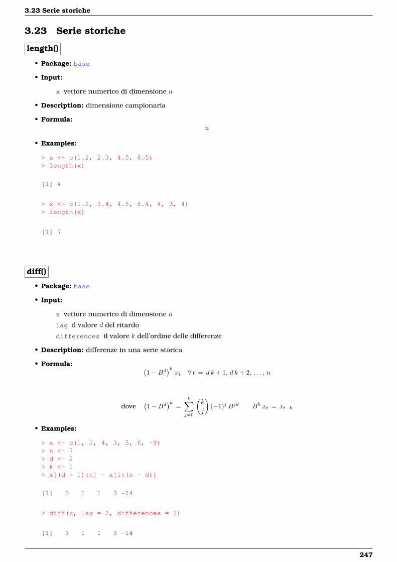
3.23 Serie storiche
3.23 Serie storiche
length()
• Package: base
• Input:
x vettore numerico di dimensione n
• Description: dimensione campionaria
• Formula:n
• Examples:
> x <- c(1.2, 2.3, 4.5, 6.5)> length(x)
[1] 4
> x <- c(1.2, 3.4, 4.5, 6.4, 4, 3, 4)> length(x)
[1] 7
diff()
• Package: base
• Input:
x vettore numerico di dimensione n
lag il valore d del ritardo
differences il valore k dell’ordine delle differenze
• Description: differenze in una serie storica
• Formula: (1−Bd
)kxt ∀ t = d k + 1, d k + 2, . . . , n
dove(1−Bd
)k=
k∑j=0
(k
j
)(−1)j Bjd Bh xt = xt−h
• Examples:
> x <- c(1, 2, 4, 3, 5, 6, -9)> n <- 7> d <- 2> k <- 1> x[(d + 1):n] - x[1:(n - d)]
[1] 3 1 1 3 -14
> diff(x, lag = 2, differences = 1)
[1] 3 1 1 3 -14
247

Misure ed indici statistici
> x <- c(1, 2, 4, 3, 5, 6, -9)> n <- 7> d <- 2> k <- 2> x[(k * d + 1):n] - 2 * x[(k * d + 1 - d):(n - d)] + x[(k * d ++ 1 - k * d):(n - k * d)]
[1] -2 2 -15
> diff(x, lag = 2, differences = 2)
[1] -2 2 -15
> x <- c(2, 6, 10, 9, 9, 8, 9, 9, 10, 12)> n <- 10> d <- 2> k <- 3> x[(k * d + 1):n] - 3 * x[(k * d + 1 - d):(n - d)] + 3 * x[(k *+ d + 1 - 2 * d):(n - 2 * d)] - x[(k * d + 1 - k * d):(n -+ k * d)]
[1] 10 6 0 0
> diff(x, lag = 2, differences = 3)
[1] 10 6 0 0
diffinv()
• Package: stats
• Input:
x vettore numerico di dimensione n
lag il valore d del ritardo
differences il valore k dell’ordine delle differenze
xi valore necessari a ricostruire la serie storica di partenza
• Description: operazione inversa del comando diff()
• Examples:
> x <- c(1, 2, 4, 3, 5, 6, -9)> n <- 7> d <- 2> k <- 1> diff(x, lag = 2, differences = 1)
[1] 3 1 1 3 -14
> diffinv(diff(x, lag = 2, differences = 1), lag = 2, differences = 1,+ xi = c(1, 2))
[1] 1 2 4 3 5 6 -9
> x <- c(1, 2, 4, 3, 5, 6, -9)> n <- 7> d <- 2> k <- 2> diff(x, lag = 2, differences = 2)
248
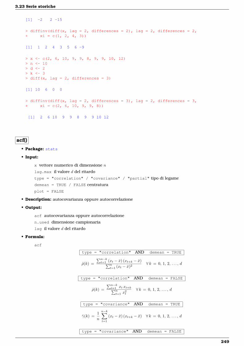
3.23 Serie storiche
[1] -2 2 -15
> diffinv(diff(x, lag = 2, differences = 2), lag = 2, differences = 2,+ xi = c(1, 2, 4, 3))
[1] 1 2 4 3 5 6 -9
> x <- c(2, 6, 10, 9, 9, 8, 9, 9, 10, 12)> n <- 10> d <- 2> k <- 3> diff(x, lag = 2, differences = 3)
[1] 10 6 0 0
> diffinv(diff(x, lag = 2, differences = 3), lag = 2, differences = 3,+ xi = c(2, 6, 10, 9, 9, 8))
[1] 2 6 10 9 9 8 9 9 10 12
acf()
• Package: stats
• Input:
x vettore numerico di dimensione n
lag.max il valore d del ritardo
type = "correlation" / "covariance" / "partial" tipo di legame
demean = TRUE / FALSE centratura
plot = FALSE
• Description: autocovarianza oppure autocorrelazione
• Output:
acf autocovarianza oppure autocorrelazione
n.used dimensione campionaria
lag il valore d del ritardo
• Formula:
acf
type = "correlation" AND demean = TRUE
ρ(k) =∑n−kt=1 (xt − x) (xt+k − x)∑n
t=1 (xt − x)2∀ k = 0, 1, 2, . . . , d
type = "correlation" AND demean = FALSE
ρ(k) =∑n−kt=1 xt xt+k∑n
t=1 x2t
∀ k = 0, 1, 2, . . . , d
type = "covariance" AND demean = TRUE
γ(k) =1n
n−k∑t=1
(xt − x) (xt+k − x) ∀ k = 0, 1, 2, . . . , d
type = "covariance" AND demean = FALSE
249
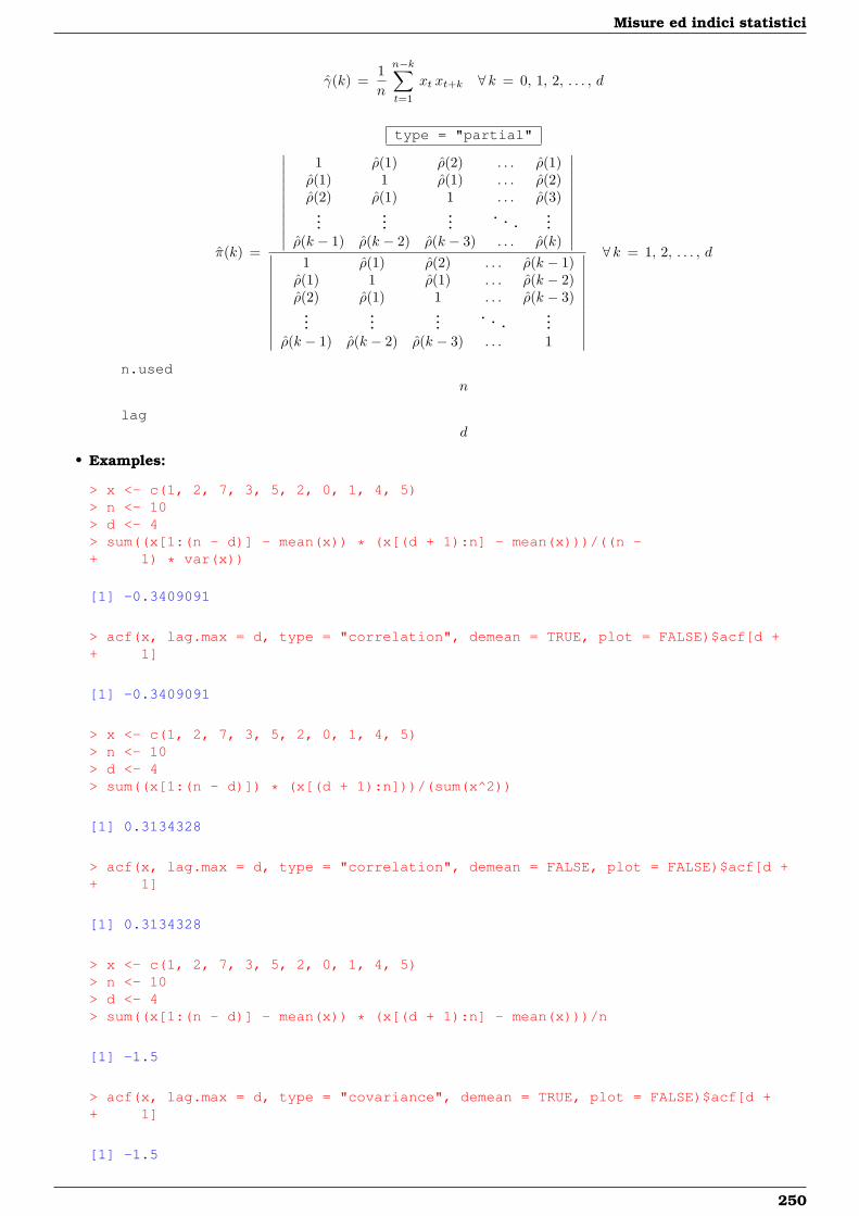
Misure ed indici statistici
γ(k) =1n
n−k∑t=1
xt xt+k ∀ k = 0, 1, 2, . . . , d
type = "partial"
π(k) =
∣∣∣∣∣∣∣∣∣∣∣
1 ρ(1) ρ(2) . . . ρ(1)ρ(1) 1 ρ(1) . . . ρ(2)ρ(2) ρ(1) 1 . . . ρ(3)...
......
......
ρ(k − 1) ρ(k − 2) ρ(k − 3) . . . ρ(k)
∣∣∣∣∣∣∣∣∣∣∣∣∣∣∣∣∣∣∣∣∣∣
1 ρ(1) ρ(2) . . . ρ(k − 1)ρ(1) 1 ρ(1) . . . ρ(k − 2)ρ(2) ρ(1) 1 . . . ρ(k − 3)...
......
......
ρ(k − 1) ρ(k − 2) ρ(k − 3) . . . 1
∣∣∣∣∣∣∣∣∣∣∣
∀ k = 1, 2, . . . , d
n.usedn
lagd
• Examples:
> x <- c(1, 2, 7, 3, 5, 2, 0, 1, 4, 5)> n <- 10> d <- 4> sum((x[1:(n - d)] - mean(x)) * (x[(d + 1):n] - mean(x)))/((n -+ 1) * var(x))
[1] -0.3409091
> acf(x, lag.max = d, type = "correlation", demean = TRUE, plot = FALSE)$acf[d ++ 1]
[1] -0.3409091
> x <- c(1, 2, 7, 3, 5, 2, 0, 1, 4, 5)> n <- 10> d <- 4> sum((x[1:(n - d)]) * (x[(d + 1):n]))/(sum(x^2))
[1] 0.3134328
> acf(x, lag.max = d, type = "correlation", demean = FALSE, plot = FALSE)$acf[d ++ 1]
[1] 0.3134328
> x <- c(1, 2, 7, 3, 5, 2, 0, 1, 4, 5)> n <- 10> d <- 4> sum((x[1:(n - d)] - mean(x)) * (x[(d + 1):n] - mean(x)))/n
[1] -1.5
> acf(x, lag.max = d, type = "covariance", demean = TRUE, plot = FALSE)$acf[d ++ 1]
[1] -1.5
250
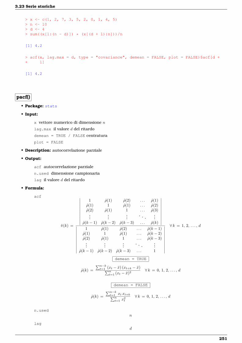
3.23 Serie storiche
> x <- c(1, 2, 7, 3, 5, 2, 0, 1, 4, 5)> n <- 10> d <- 4> sum((x[1:(n - d)]) * (x[(d + 1):n]))/n
[1] 4.2
> acf(x, lag.max = d, type = "covariance", demean = FALSE, plot = FALSE)$acf[d ++ 1]
[1] 4.2
pacf()
• Package: stats
• Input:
x vettore numerico di dimensione n
lag.max il valore d del ritardo
demean = TRUE / FALSE centratura
plot = FALSE
• Description: autocorrelazione parziale
• Output:
acf autocorrelazione parziale
n.used dimensione campionaria
lag il valore d del ritardo
• Formula:
acf
π(k) =
∣∣∣∣∣∣∣∣∣∣∣
1 ρ(1) ρ(2) . . . ρ(1)ρ(1) 1 ρ(1) . . . ρ(2)ρ(2) ρ(1) 1 . . . ρ(3)...
......
......
ρ(k − 1) ρ(k − 2) ρ(k − 3) . . . ρ(k)
∣∣∣∣∣∣∣∣∣∣∣∣∣∣∣∣∣∣∣∣∣∣
1 ρ(1) ρ(2) . . . ρ(k − 1)ρ(1) 1 ρ(1) . . . ρ(k − 2)ρ(2) ρ(1) 1 . . . ρ(k − 3)...
......
......
ρ(k − 1) ρ(k − 2) ρ(k − 3) . . . 1
∣∣∣∣∣∣∣∣∣∣∣
∀ k = 1, 2, . . . , d
demean = TRUE
ρ(k) =∑n−kt=1 (xt − x) (xt+k − x)∑n
t=1 (xt − x)2∀ k = 0, 1, 2, . . . , d
demean = FALSE
ρ(k) =∑n−kt=1 xt xt+k∑n
t=1 x2t
∀ k = 0, 1, 2, . . . , d
n.usedn
lagd
251
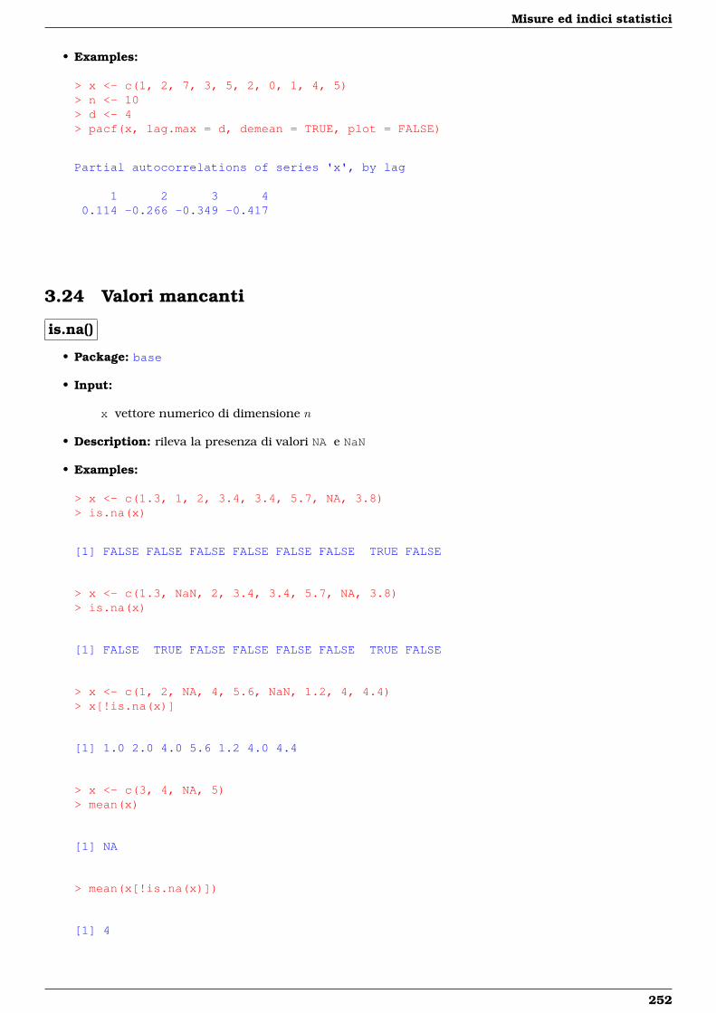
Misure ed indici statistici
• Examples:
> x <- c(1, 2, 7, 3, 5, 2, 0, 1, 4, 5)> n <- 10> d <- 4> pacf(x, lag.max = d, demean = TRUE, plot = FALSE)
Partial autocorrelations of series 'x', by lag
1 2 3 40.114 -0.266 -0.349 -0.417
3.24 Valori mancanti
is.na()
• Package: base
• Input:
x vettore numerico di dimensione n
• Description: rileva la presenza di valori NA e NaN
• Examples:
> x <- c(1.3, 1, 2, 3.4, 3.4, 5.7, NA, 3.8)> is.na(x)
[1] FALSE FALSE FALSE FALSE FALSE FALSE TRUE FALSE
> x <- c(1.3, NaN, 2, 3.4, 3.4, 5.7, NA, 3.8)> is.na(x)
[1] FALSE TRUE FALSE FALSE FALSE FALSE TRUE FALSE
> x <- c(1, 2, NA, 4, 5.6, NaN, 1.2, 4, 4.4)> x[!is.na(x)]
[1] 1.0 2.0 4.0 5.6 1.2 4.0 4.4
> x <- c(3, 4, NA, 5)> mean(x)
[1] NA
> mean(x[!is.na(x)])
[1] 4
252
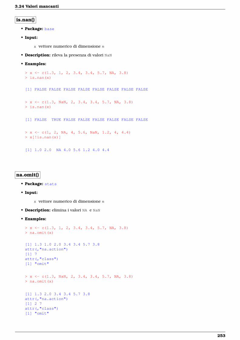
3.24 Valori mancanti
is.nan()
• Package: base
• Input:
x vettore numerico di dimensione n
• Description: rileva la presenza di valori NaN
• Examples:
> x <- c(1.3, 1, 2, 3.4, 3.4, 5.7, NA, 3.8)> is.nan(x)
[1] FALSE FALSE FALSE FALSE FALSE FALSE FALSE FALSE
> x <- c(1.3, NaN, 2, 3.4, 3.4, 5.7, NA, 3.8)> is.nan(x)
[1] FALSE TRUE FALSE FALSE FALSE FALSE FALSE FALSE
> x <- c(1, 2, NA, 4, 5.6, NaN, 1.2, 4, 4.4)> x[!is.nan(x)]
[1] 1.0 2.0 NA 4.0 5.6 1.2 4.0 4.4
na.omit()
• Package: stats
• Input:
x vettore numerico di dimensione n
• Description: elimina i valori NA e NaN
• Examples:
> x <- c(1.3, 1, 2, 3.4, 3.4, 5.7, NA, 3.8)> na.omit(x)
[1] 1.3 1.0 2.0 3.4 3.4 5.7 3.8attr(,"na.action")[1] 7attr(,"class")[1] "omit"
> x <- c(1.3, NaN, 2, 3.4, 3.4, 5.7, NA, 3.8)> na.omit(x)
[1] 1.3 2.0 3.4 3.4 5.7 3.8attr(,"na.action")[1] 2 7attr(,"class")[1] "omit"
253
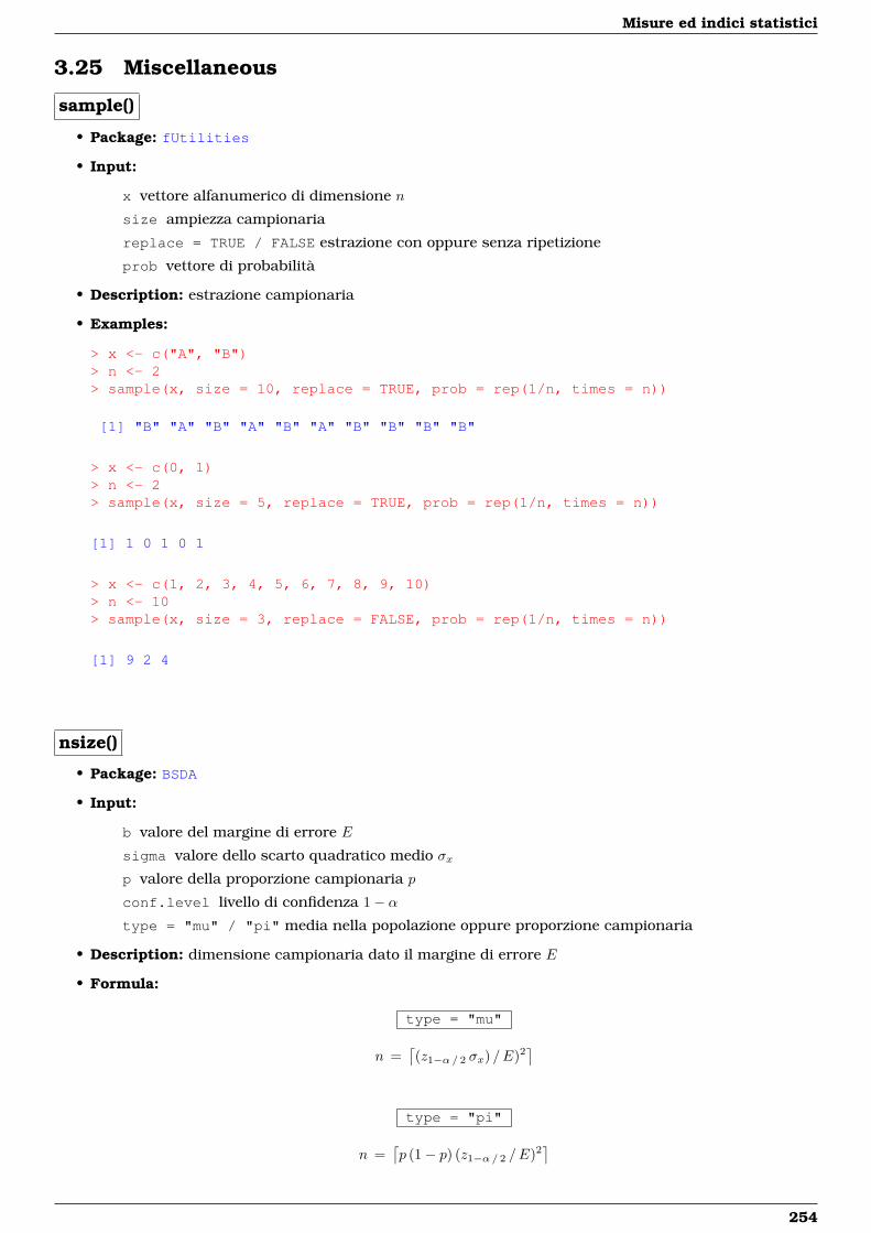
Misure ed indici statistici
3.25 Miscellaneous
sample()
• Package: fUtilities
• Input:
x vettore alfanumerico di dimensione n
size ampiezza campionaria
replace = TRUE / FALSE estrazione con oppure senza ripetizione
prob vettore di probabilità
• Description: estrazione campionaria
• Examples:
> x <- c("A", "B")> n <- 2> sample(x, size = 10, replace = TRUE, prob = rep(1/n, times = n))
[1] "B" "A" "B" "A" "B" "A" "B" "B" "B" "B"
> x <- c(0, 1)> n <- 2> sample(x, size = 5, replace = TRUE, prob = rep(1/n, times = n))
[1] 1 0 1 0 1
> x <- c(1, 2, 3, 4, 5, 6, 7, 8, 9, 10)> n <- 10> sample(x, size = 3, replace = FALSE, prob = rep(1/n, times = n))
[1] 9 2 4
nsize()
• Package: BSDA
• Input:
b valore del margine di errore E
sigma valore dello scarto quadratico medio σxp valore della proporzione campionaria p
conf.level livello di confidenza 1− αtype = "mu" / "pi" media nella popolazione oppure proporzione campionaria
• Description: dimensione campionaria dato il margine di errore E
• Formula:
type = "mu"
n =⌈(z1−α/ 2 σx) /E)2
⌉
type = "pi"
n =⌈p (1− p) (z1−α/ 2 /E)2
⌉
254
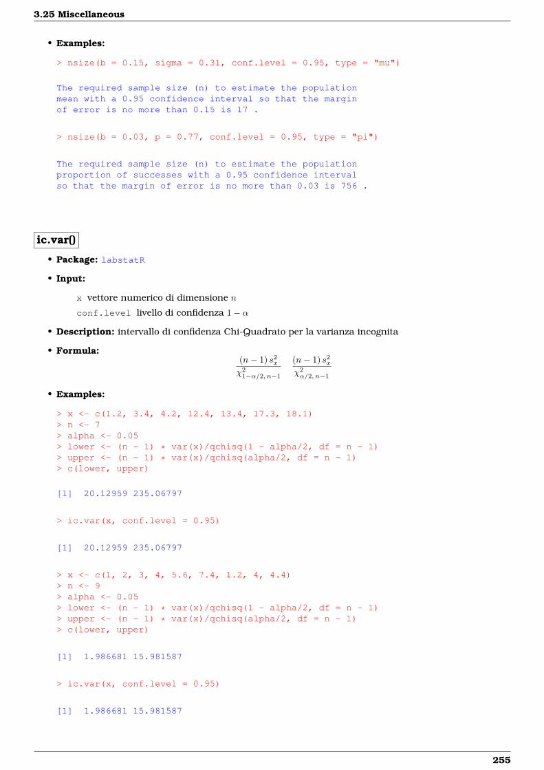
3.25 Miscellaneous
• Examples:
> nsize(b = 0.15, sigma = 0.31, conf.level = 0.95, type = "mu")
The required sample size (n) to estimate the populationmean with a 0.95 confidence interval so that the marginof error is no more than 0.15 is 17 .
> nsize(b = 0.03, p = 0.77, conf.level = 0.95, type = "pi")
The required sample size (n) to estimate the populationproportion of successes with a 0.95 confidence intervalso that the margin of error is no more than 0.03 is 756 .
ic.var()
• Package: labstatR
• Input:
x vettore numerico di dimensione n
conf.level livello di confidenza 1− α
• Description: intervallo di confidenza Chi-Quadrato per la varianza incognita
• Formula:(n− 1) s2
x
χ21−α/2, n−1
(n− 1) s2x
χ2α/2, n−1
• Examples:
> x <- c(1.2, 3.4, 4.2, 12.4, 13.4, 17.3, 18.1)> n <- 7> alpha <- 0.05> lower <- (n - 1) * var(x)/qchisq(1 - alpha/2, df = n - 1)> upper <- (n - 1) * var(x)/qchisq(alpha/2, df = n - 1)> c(lower, upper)
[1] 20.12959 235.06797
> ic.var(x, conf.level = 0.95)
[1] 20.12959 235.06797
> x <- c(1, 2, 3, 4, 5.6, 7.4, 1.2, 4, 4.4)> n <- 9> alpha <- 0.05> lower <- (n - 1) * var(x)/qchisq(1 - alpha/2, df = n - 1)> upper <- (n - 1) * var(x)/qchisq(alpha/2, df = n - 1)> c(lower, upper)
[1] 1.986681 15.981587
> ic.var(x, conf.level = 0.95)
[1] 1.986681 15.981587
255
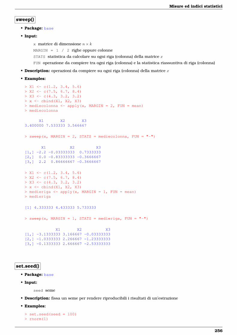
Misure ed indici statistici
sweep()
• Package: base
• Input:
x matrice di dimensione n× kMARGIN = 1 / 2 righe oppure colonne
STATS statistica da calcolare su ogni riga (colonna) della matrice x
FUN operazione da compiere tra ogni riga (colonna) e la statistica riassuntiva di riga (colonna)
• Description: operazioni da compiere su ogni riga (colonna) della matrice x
• Examples:
> X1 <- c(1.2, 3.4, 5.6)> X2 <- c(7.5, 6.7, 8.4)> X3 <- c(4.3, 3.2, 3.2)> x <- cbind(X1, X2, X3)> mediecolonna <- apply(x, MARGIN = 2, FUN = mean)> mediecolonna
X1 X2 X33.400000 7.533333 3.566667
> sweep(x, MARGIN = 2, STATS = mediecolonna, FUN = "-")
X1 X2 X3[1,] -2.2 -0.03333333 0.7333333[2,] 0.0 -0.83333333 -0.3666667[3,] 2.2 0.86666667 -0.3666667
> X1 <- c(1.2, 3.4, 5.6)> X2 <- c(7.5, 6.7, 8.4)> X3 <- c(4.3, 3.2, 3.2)> x <- cbind(X1, X2, X3)> medieriga <- apply(x, MARGIN = 1, FUN = mean)> medieriga
[1] 4.333333 4.433333 5.733333
> sweep(x, MARGIN = 1, STATS = medieriga, FUN = "-")
X1 X2 X3[1,] -3.1333333 3.166667 -0.03333333[2,] -1.0333333 2.266667 -1.23333333[3,] -0.1333333 2.666667 -2.53333333
set.seed()
• Package: base
• Input:
seed seme
• Description: fissa un seme per rendere riproducibili i risultati di un’estrazione
• Examples:
> set.seed(seed = 100)> rnorm(1)
256
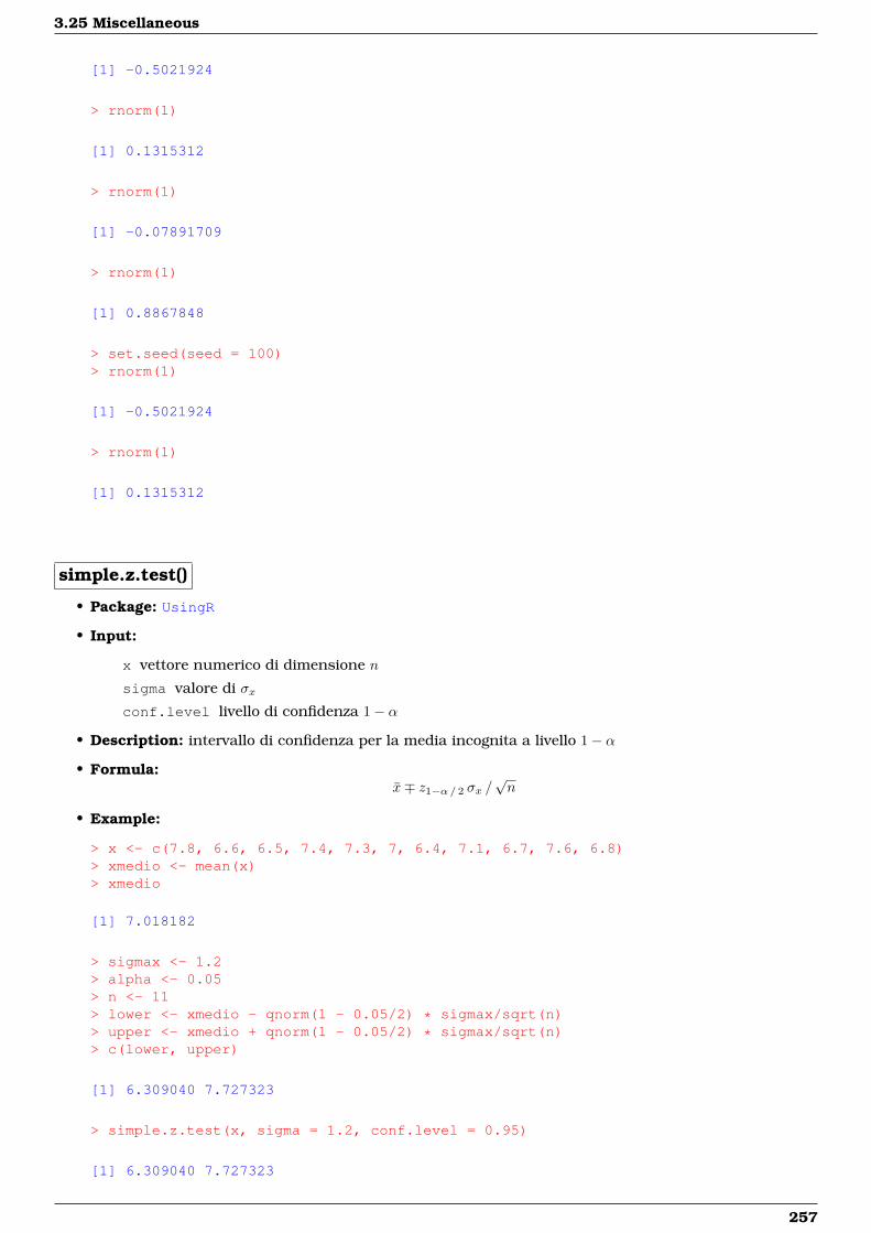
3.25 Miscellaneous
[1] -0.5021924
> rnorm(1)
[1] 0.1315312
> rnorm(1)
[1] -0.07891709
> rnorm(1)
[1] 0.8867848
> set.seed(seed = 100)> rnorm(1)
[1] -0.5021924
> rnorm(1)
[1] 0.1315312
simple.z.test()
• Package: UsingR
• Input:
x vettore numerico di dimensione n
sigma valore di σxconf.level livello di confidenza 1− α
• Description: intervallo di confidenza per la media incognita a livello 1− α
• Formula:x∓ z1−α/ 2 σx /
√n
• Example:
> x <- c(7.8, 6.6, 6.5, 7.4, 7.3, 7, 6.4, 7.1, 6.7, 7.6, 6.8)> xmedio <- mean(x)> xmedio
[1] 7.018182
> sigmax <- 1.2> alpha <- 0.05> n <- 11> lower <- xmedio - qnorm(1 - 0.05/2) * sigmax/sqrt(n)> upper <- xmedio + qnorm(1 - 0.05/2) * sigmax/sqrt(n)> c(lower, upper)
[1] 6.309040 7.727323
> simple.z.test(x, sigma = 1.2, conf.level = 0.95)
[1] 6.309040 7.727323
257
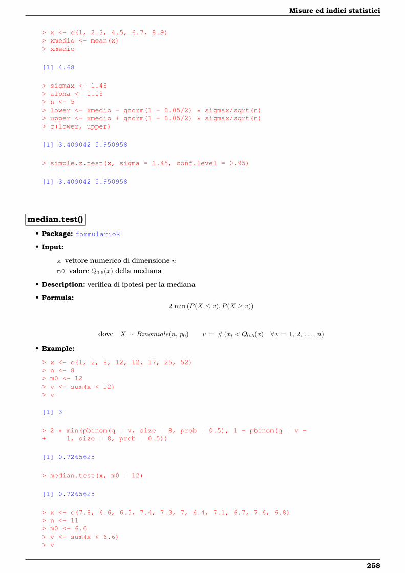
Misure ed indici statistici
> x <- c(1, 2.3, 4.5, 6.7, 8.9)> xmedio <- mean(x)> xmedio
[1] 4.68
> sigmax <- 1.45> alpha <- 0.05> n <- 5> lower <- xmedio - qnorm(1 - 0.05/2) * sigmax/sqrt(n)> upper <- xmedio + qnorm(1 - 0.05/2) * sigmax/sqrt(n)> c(lower, upper)
[1] 3.409042 5.950958
> simple.z.test(x, sigma = 1.45, conf.level = 0.95)
[1] 3.409042 5.950958
median.test()
• Package: formularioR
• Input:
x vettore numerico di dimensione n
m0 valore Q0.5(x) della mediana
• Description: verifica di ipotesi per la mediana
• Formula:2 min (P (X ≤ v), P (X ≥ v))
dove X ∼ Binomiale(n, p0) v = # (xi < Q0.5(x) ∀ i = 1, 2, . . . , n)
• Example:
> x <- c(1, 2, 8, 12, 12, 17, 25, 52)> n <- 8> m0 <- 12> v <- sum(x < 12)> v
[1] 3
> 2 * min(pbinom(q = v, size = 8, prob = 0.5), 1 - pbinom(q = v -+ 1, size = 8, prob = 0.5))
[1] 0.7265625
> median.test(x, m0 = 12)
[1] 0.7265625
> x <- c(7.8, 6.6, 6.5, 7.4, 7.3, 7, 6.4, 7.1, 6.7, 7.6, 6.8)> n <- 11> m0 <- 6.6> v <- sum(x < 6.6)> v
258

3.25 Miscellaneous
[1] 2
> 2 * min(pbinom(q = v, size = 11, prob = 0.5), 1 - pbinom(q = v -+ 1, size = 11, prob = 0.5))
[1] 0.06542969
> median.test(x, m0 = 6.6)
[1] 0.06542969
259

Capitolo 4
Analisi Componenti Principali (ACP)
4.1 ACP con matrice di covarianza di popolazione
Simbologia
• matrice dei dati di dimensione n×k le cui colonne corrispondono ai vettori numerici w1, w2, . . . , wk: W
• media di colonna della matrice dei dati: wj ∀j = 1, 2, . . . , k
• matrice dei dati centrata di dimensione n× k: Z
• elemento di riga i e colonna j della matrice dei dati centrata:zij = wij − wj ∀ i = 1, 2, . . . , n ∀ j = 1, 2, . . . , k
• matrice di covarianza di dimensione k × k: S = ZT Zn = ΓD ΓT
• matrice ortogonale degli autovettori di dimensione k × k: Γ
• j-esima colonna della matrice Γ: Γj ∀ j = 1, 2, . . . , k
• matrice diagonale degli autovalori di dimensione k × k: D = diag(λ1, λ2, . . . , λk)
• componente principale j-esima: xj = Z Γj ∀ j = 1, 2, . . . , k
• scarto quadratico medio della j-esima componente principale:σxj =
√λ(k−j+1) ∀ j = 1, 2, . . . , k
• problema di ottimo vincolato:xj = Z γj ∀ j = 1, 2, . . . , k
σ2xj = xTj xj
n = (Z γj)T (Z γj)n = γTj
ZT Zn γj = γTj S γj ∀ j = 1, 2, . . . , k
maxγTj γj = 1 σ2xj = maxγTj γj = 1 γ
Tj S γj = λ(k−j+1) ∀ j = 1, 2, . . . , k
princomp()
• Package: stats
• Input:
W matrice dei dati
• Output:
sdev scarto quadratico medio delle componenti principali
center media di colonna della matrice W
n.obs dimensione campionaria
scores componenti principali
• Formula:
sdevσxj ∀ j = 1, 2, . . . , k
261
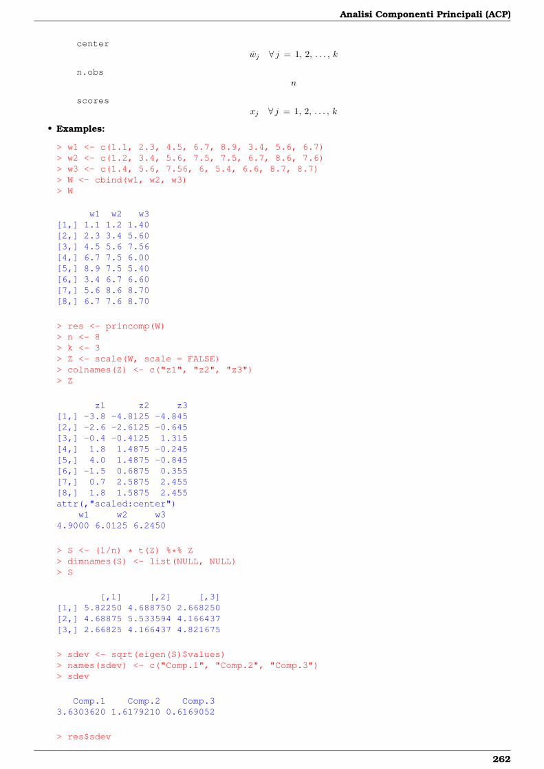
Analisi Componenti Principali (ACP)
centerwj ∀ j = 1, 2, . . . , k
n.obsn
scoresxj ∀ j = 1, 2, . . . , k
• Examples:
> w1 <- c(1.1, 2.3, 4.5, 6.7, 8.9, 3.4, 5.6, 6.7)> w2 <- c(1.2, 3.4, 5.6, 7.5, 7.5, 6.7, 8.6, 7.6)> w3 <- c(1.4, 5.6, 7.56, 6, 5.4, 6.6, 8.7, 8.7)> W <- cbind(w1, w2, w3)> W
w1 w2 w3[1,] 1.1 1.2 1.40[2,] 2.3 3.4 5.60[3,] 4.5 5.6 7.56[4,] 6.7 7.5 6.00[5,] 8.9 7.5 5.40[6,] 3.4 6.7 6.60[7,] 5.6 8.6 8.70[8,] 6.7 7.6 8.70
> res <- princomp(W)> n <- 8> k <- 3> Z <- scale(W, scale = FALSE)> colnames(Z) <- c("z1", "z2", "z3")> Z
z1 z2 z3[1,] -3.8 -4.8125 -4.845[2,] -2.6 -2.6125 -0.645[3,] -0.4 -0.4125 1.315[4,] 1.8 1.4875 -0.245[5,] 4.0 1.4875 -0.845[6,] -1.5 0.6875 0.355[7,] 0.7 2.5875 2.455[8,] 1.8 1.5875 2.455attr(,"scaled:center")
w1 w2 w34.9000 6.0125 6.2450
> S <- (1/n) * t(Z) %*% Z> dimnames(S) <- list(NULL, NULL)> S
[,1] [,2] [,3][1,] 5.82250 4.688750 2.668250[2,] 4.68875 5.533594 4.166437[3,] 2.66825 4.166437 4.821675
> sdev <- sqrt(eigen(S)$values)> names(sdev) <- c("Comp.1", "Comp.2", "Comp.3")> sdev
Comp.1 Comp.2 Comp.33.6303620 1.6179210 0.6169052
> res$sdev
262
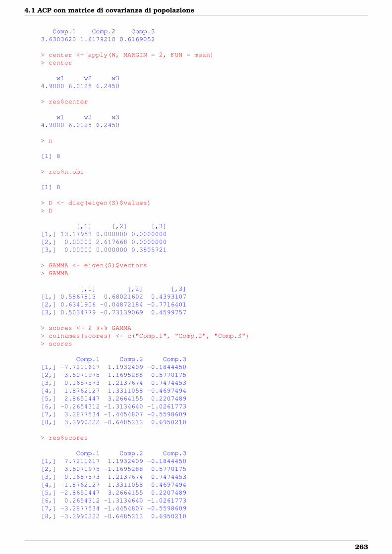
4.1 ACP con matrice di covarianza di popolazione
Comp.1 Comp.2 Comp.33.6303620 1.6179210 0.6169052
> center <- apply(W, MARGIN = 2, FUN = mean)> center
w1 w2 w34.9000 6.0125 6.2450
> res$center
w1 w2 w34.9000 6.0125 6.2450
> n
[1] 8
> res$n.obs
[1] 8
> D <- diag(eigen(S)$values)> D
[,1] [,2] [,3][1,] 13.17953 0.000000 0.0000000[2,] 0.00000 2.617668 0.0000000[3,] 0.00000 0.000000 0.3805721
> GAMMA <- eigen(S)$vectors> GAMMA
[,1] [,2] [,3][1,] 0.5867813 0.68021602 0.4393107[2,] 0.6341906 -0.04872184 -0.7716401[3,] 0.5034779 -0.73139069 0.4599757
> scores <- Z %*% GAMMA> colnames(scores) <- c("Comp.1", "Comp.2", "Comp.3")> scores
Comp.1 Comp.2 Comp.3[1,] -7.7211617 1.1932409 -0.1844450[2,] -3.5071975 -1.1695288 0.5770175[3,] 0.1657573 -1.2137674 0.7474453[4,] 1.8762127 1.3311058 -0.4697494[5,] 2.8650447 3.2664155 0.2207489[6,] -0.2654312 -1.3134640 -1.0261773[7,] 3.2877534 -1.4454807 -0.5598609[8,] 3.2990222 -0.6485212 0.6950210
> res$scores
Comp.1 Comp.2 Comp.3[1,] 7.7211617 1.1932409 -0.1844450[2,] 3.5071975 -1.1695288 0.5770175[3,] -0.1657573 -1.2137674 0.7474453[4,] -1.8762127 1.3311058 -0.4697494[5,] -2.8650447 3.2664155 0.2207489[6,] 0.2654312 -1.3134640 -1.0261773[7,] -3.2877534 -1.4454807 -0.5598609[8,] -3.2990222 -0.6485212 0.6950210
263
Analisi Componenti Principali (ACP)
4.2 ACP con matrice di covarianza campionaria
Simbologia
• matrice dei dati di dimensione n×k le cui colonne corrispondono ai vettori numerici w1, w2, . . . , wk: W
• media di colonna della matrice dei dati: wj ∀j = 1, 2, . . . , k
• matrice dei dati centrata di dimensione n× k: Z
• elemento di riga i e colonna j della matrice dei dati centrata:zij = wij − wj ∀ i = 1, 2, . . . , n ∀ j = 1, 2, . . . , k
• matrice di covarianza di dimensione k × k: S = ZT Zn−1 = ΓD ΓT
• matrice ortogonale degli autovettori di dimensione k × k: Γ
• j-esima colonna della matrice Γ: Γj ∀ j = 1, 2, . . . , k
• matrice diagonale degli autovalori di dimensione k × k: D = diag(λ1, λ2, . . . , λk)
• componente principale j-esima: xj = Z Γj ∀ j = 1, 2, . . . , k
• deviazione standard della j-esima componente principale:sxj =
√λ(k−j+1) ∀ j = 1, 2, . . . , k
• problema di ottimo vincolato:xj = Z γj ∀ j = 1, 2, . . . , k
s2xj = xTj xj
n−1 = (Z γj)T (Z γj)n−1 = γTj
ZT Zn−1 γj = γTj S γj ∀ j = 1, 2, . . . , k
maxγTj γj = 1 s2xj = maxγTj γj = 1 γ
Tj S γj = λ(k−j+1) ∀ j = 1, 2, . . . , k
prcomp()
• Package: stats
• Input:
W matrice dei dati
• Output:
sdev deviazione standard delle componenti principali
rotation matrice ortogonale degli autovettori
center media di colonna della matrice W
x componenti principali
• Formula:
sdevsxj ∀ j = 1, 2, . . . , k
rotationΓ
centerwj ∀ j = 1, 2, . . . , k
xxj ∀ j = 1, 2, . . . , k
• Examples:
> w1 <- c(1.1, 2.3, 4.5, 6.7, 8.9, 3.4, 5.6, 6.7)> w2 <- c(1.2, 3.4, 5.6, 7.5, 7.5, 6.7, 8.6, 7.6)> w3 <- c(1.4, 5.6, 7.56, 6, 5.4, 6.6, 8.7, 8.7)> W <- cbind(w1, w2, w3)> W
264
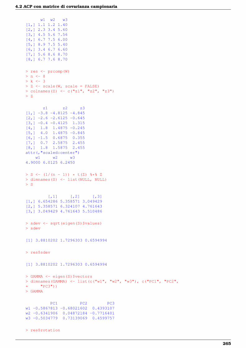
4.2 ACP con matrice di covarianza campionaria
w1 w2 w3[1,] 1.1 1.2 1.40[2,] 2.3 3.4 5.60[3,] 4.5 5.6 7.56[4,] 6.7 7.5 6.00[5,] 8.9 7.5 5.40[6,] 3.4 6.7 6.60[7,] 5.6 8.6 8.70[8,] 6.7 7.6 8.70
> res <- prcomp(W)> n <- 8> k <- 3> Z <- scale(W, scale = FALSE)> colnames(Z) <- c("z1", "z2", "z3")> Z
z1 z2 z3[1,] -3.8 -4.8125 -4.845[2,] -2.6 -2.6125 -0.645[3,] -0.4 -0.4125 1.315[4,] 1.8 1.4875 -0.245[5,] 4.0 1.4875 -0.845[6,] -1.5 0.6875 0.355[7,] 0.7 2.5875 2.455[8,] 1.8 1.5875 2.455attr(,"scaled:center")
w1 w2 w34.9000 6.0125 6.2450
> S <- (1/(n - 1)) * t(Z) %*% Z> dimnames(S) <- list(NULL, NULL)> S
[,1] [,2] [,3][1,] 6.654286 5.358571 3.049429[2,] 5.358571 6.324107 4.761643[3,] 3.049429 4.761643 5.510486
> sdev <- sqrt(eigen(S)$values)> sdev
[1] 3.8810202 1.7296303 0.6594994
> res$sdev
[1] 3.8810202 1.7296303 0.6594994
> GAMMA <- eigen(S)$vectors> dimnames(GAMMA) <- list(c("w1", "w2", "w3"), c("PC1", "PC2",+ "PC3"))> GAMMA
PC1 PC2 PC3w1 -0.5867813 -0.68021602 0.4393107w2 -0.6341906 0.04872184 -0.7716401w3 -0.5034779 0.73139069 0.4599757
> res$rotation
265
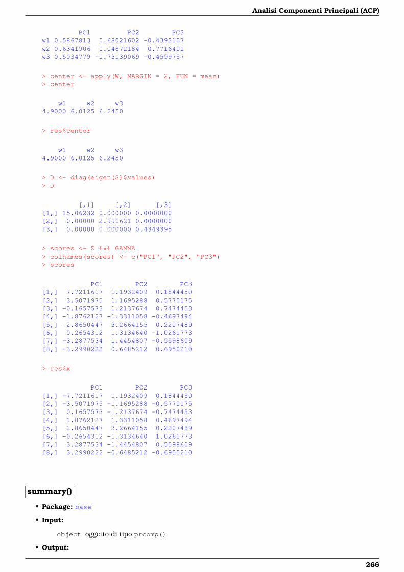
Analisi Componenti Principali (ACP)
PC1 PC2 PC3w1 0.5867813 0.68021602 -0.4393107w2 0.6341906 -0.04872184 0.7716401w3 0.5034779 -0.73139069 -0.4599757
> center <- apply(W, MARGIN = 2, FUN = mean)> center
w1 w2 w34.9000 6.0125 6.2450
> res$center
w1 w2 w34.9000 6.0125 6.2450
> D <- diag(eigen(S)$values)> D
[,1] [,2] [,3][1,] 15.06232 0.000000 0.0000000[2,] 0.00000 2.991621 0.0000000[3,] 0.00000 0.000000 0.4349395
> scores <- Z %*% GAMMA> colnames(scores) <- c("PC1", "PC2", "PC3")> scores
PC1 PC2 PC3[1,] 7.7211617 -1.1932409 -0.1844450[2,] 3.5071975 1.1695288 0.5770175[3,] -0.1657573 1.2137674 0.7474453[4,] -1.8762127 -1.3311058 -0.4697494[5,] -2.8650447 -3.2664155 0.2207489[6,] 0.2654312 1.3134640 -1.0261773[7,] -3.2877534 1.4454807 -0.5598609[8,] -3.2990222 0.6485212 0.6950210
> res$x
PC1 PC2 PC3[1,] -7.7211617 1.1932409 0.1844450[2,] -3.5071975 -1.1695288 -0.5770175[3,] 0.1657573 -1.2137674 -0.7474453[4,] 1.8762127 1.3311058 0.4697494[5,] 2.8650447 3.2664155 -0.2207489[6,] -0.2654312 -1.3134640 1.0261773[7,] 3.2877534 -1.4454807 0.5598609[8,] 3.2990222 -0.6485212 -0.6950210
summary()
• Package: base
• Input:
object oggetto di tipo prcomp()
• Output:
266
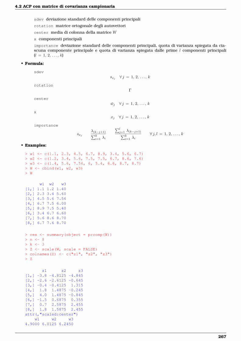
4.2 ACP con matrice di covarianza campionaria
sdev deviazione standard delle componenti principali
rotation matrice ortogonale degli autovettori
center media di colonna della matrice W
x componenti principali
importance deviazione standard delle componenti principali, quota di varianza spiegata da cia-scuna componente principale e quota di varianza spiegata dalle prime l componenti principali(l = 1, 2, . . . , k)
• Formula:
sdevsxj ∀ j = 1, 2, . . . , k
rotationΓ
centerwj ∀ j = 1, 2, . . . , k
xxj ∀ j = 1, 2, . . . , k
importance
sxjλ(k−j+1)∑k
i=1 λi
∑lj=1 λ(k−j+1)∑k
i=1 λi∀ j, l = 1, 2, . . . , k
• Examples:
> w1 <- c(1.1, 2.3, 4.5, 6.7, 8.9, 3.4, 5.6, 6.7)> w2 <- c(1.2, 3.4, 5.6, 7.5, 7.5, 6.7, 8.6, 7.6)> w3 <- c(1.4, 5.6, 7.56, 6, 5.4, 6.6, 8.7, 8.7)> W <- cbind(w1, w2, w3)> W
w1 w2 w3[1,] 1.1 1.2 1.40[2,] 2.3 3.4 5.60[3,] 4.5 5.6 7.56[4,] 6.7 7.5 6.00[5,] 8.9 7.5 5.40[6,] 3.4 6.7 6.60[7,] 5.6 8.6 8.70[8,] 6.7 7.6 8.70
> res <- summary(object = prcomp(W))> n <- 8> k <- 3> Z <- scale(W, scale = FALSE)> colnames(Z) <- c("z1", "z2", "z3")> Z
z1 z2 z3[1,] -3.8 -4.8125 -4.845[2,] -2.6 -2.6125 -0.645[3,] -0.4 -0.4125 1.315[4,] 1.8 1.4875 -0.245[5,] 4.0 1.4875 -0.845[6,] -1.5 0.6875 0.355[7,] 0.7 2.5875 2.455[8,] 1.8 1.5875 2.455attr(,"scaled:center")
w1 w2 w34.9000 6.0125 6.2450
267
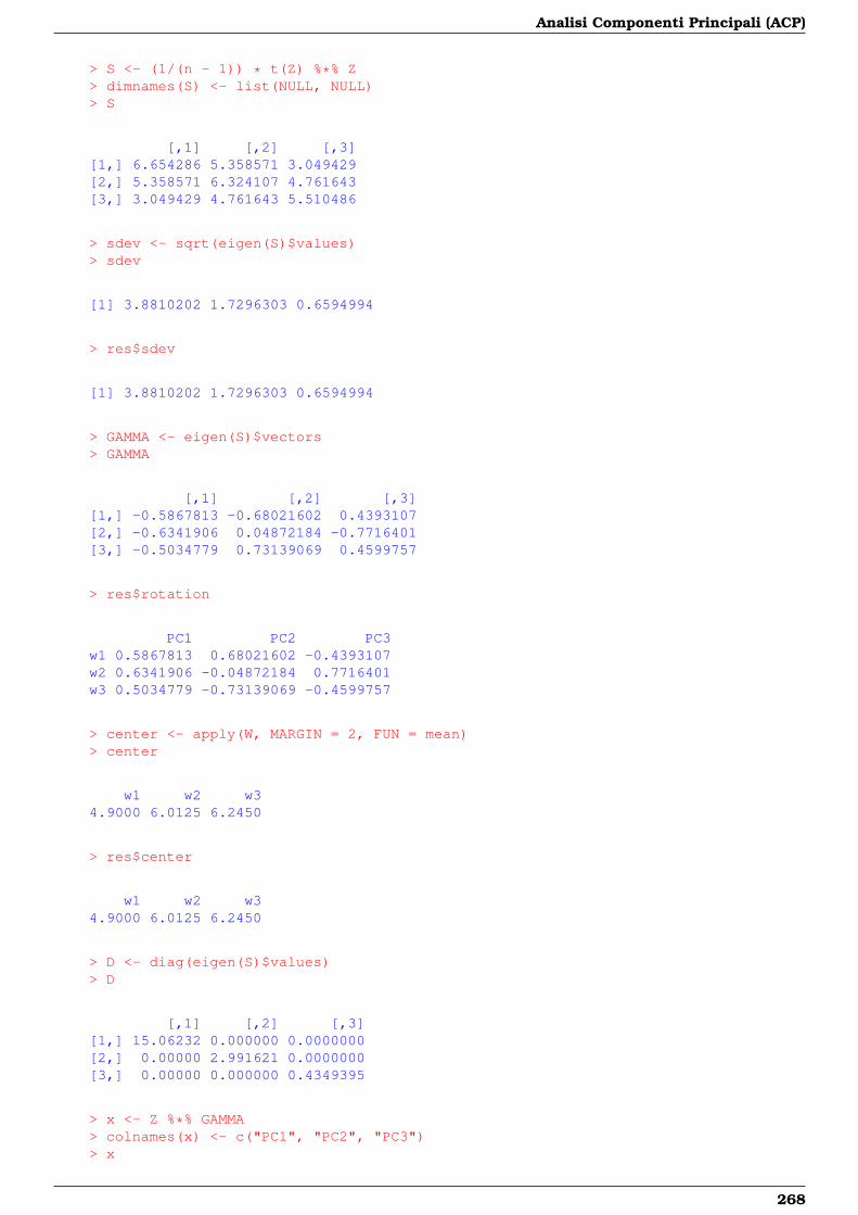
Analisi Componenti Principali (ACP)
> S <- (1/(n - 1)) * t(Z) %*% Z> dimnames(S) <- list(NULL, NULL)> S
[,1] [,2] [,3][1,] 6.654286 5.358571 3.049429[2,] 5.358571 6.324107 4.761643[3,] 3.049429 4.761643 5.510486
> sdev <- sqrt(eigen(S)$values)> sdev
[1] 3.8810202 1.7296303 0.6594994
> res$sdev
[1] 3.8810202 1.7296303 0.6594994
> GAMMA <- eigen(S)$vectors> GAMMA
[,1] [,2] [,3][1,] -0.5867813 -0.68021602 0.4393107[2,] -0.6341906 0.04872184 -0.7716401[3,] -0.5034779 0.73139069 0.4599757
> res$rotation
PC1 PC2 PC3w1 0.5867813 0.68021602 -0.4393107w2 0.6341906 -0.04872184 0.7716401w3 0.5034779 -0.73139069 -0.4599757
> center <- apply(W, MARGIN = 2, FUN = mean)> center
w1 w2 w34.9000 6.0125 6.2450
> res$center
w1 w2 w34.9000 6.0125 6.2450
> D <- diag(eigen(S)$values)> D
[,1] [,2] [,3][1,] 15.06232 0.000000 0.0000000[2,] 0.00000 2.991621 0.0000000[3,] 0.00000 0.000000 0.4349395
> x <- Z %*% GAMMA> colnames(x) <- c("PC1", "PC2", "PC3")> x
268
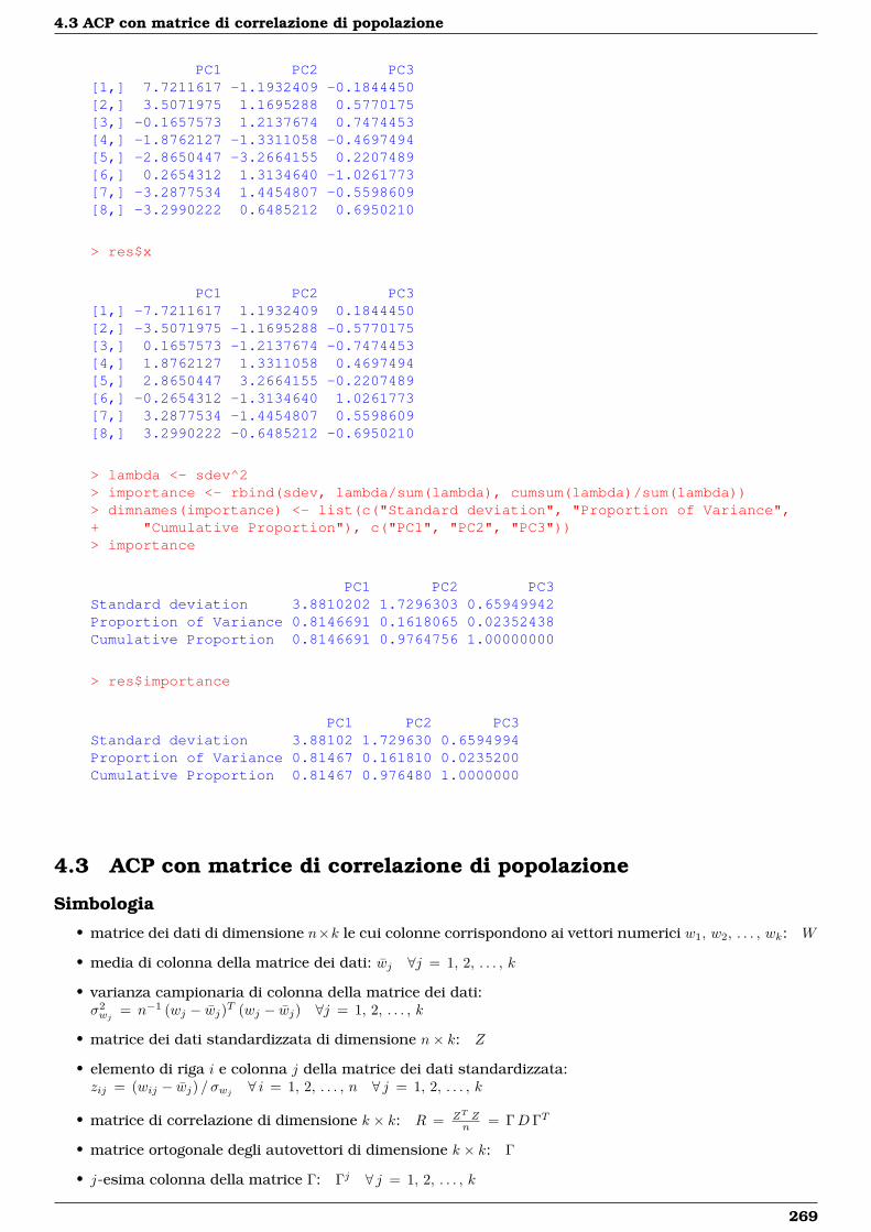
4.3 ACP con matrice di correlazione di popolazione
PC1 PC2 PC3[1,] 7.7211617 -1.1932409 -0.1844450[2,] 3.5071975 1.1695288 0.5770175[3,] -0.1657573 1.2137674 0.7474453[4,] -1.8762127 -1.3311058 -0.4697494[5,] -2.8650447 -3.2664155 0.2207489[6,] 0.2654312 1.3134640 -1.0261773[7,] -3.2877534 1.4454807 -0.5598609[8,] -3.2990222 0.6485212 0.6950210
> res$x
PC1 PC2 PC3[1,] -7.7211617 1.1932409 0.1844450[2,] -3.5071975 -1.1695288 -0.5770175[3,] 0.1657573 -1.2137674 -0.7474453[4,] 1.8762127 1.3311058 0.4697494[5,] 2.8650447 3.2664155 -0.2207489[6,] -0.2654312 -1.3134640 1.0261773[7,] 3.2877534 -1.4454807 0.5598609[8,] 3.2990222 -0.6485212 -0.6950210
> lambda <- sdev^2> importance <- rbind(sdev, lambda/sum(lambda), cumsum(lambda)/sum(lambda))> dimnames(importance) <- list(c("Standard deviation", "Proportion of Variance",+ "Cumulative Proportion"), c("PC1", "PC2", "PC3"))> importance
PC1 PC2 PC3Standard deviation 3.8810202 1.7296303 0.65949942Proportion of Variance 0.8146691 0.1618065 0.02352438Cumulative Proportion 0.8146691 0.9764756 1.00000000
> res$importance
PC1 PC2 PC3Standard deviation 3.88102 1.729630 0.6594994Proportion of Variance 0.81467 0.161810 0.0235200Cumulative Proportion 0.81467 0.976480 1.0000000
4.3 ACP con matrice di correlazione di popolazione
Simbologia
• matrice dei dati di dimensione n×k le cui colonne corrispondono ai vettori numerici w1, w2, . . . , wk: W
• media di colonna della matrice dei dati: wj ∀j = 1, 2, . . . , k
• varianza campionaria di colonna della matrice dei dati:σ2wj = n−1 (wj − wj)T (wj − wj) ∀j = 1, 2, . . . , k
• matrice dei dati standardizzata di dimensione n× k: Z
• elemento di riga i e colonna j della matrice dei dati standardizzata:zij = (wij − wj) / σwj ∀ i = 1, 2, . . . , n ∀ j = 1, 2, . . . , k
• matrice di correlazione di dimensione k × k: R = ZT Zn = ΓD ΓT
• matrice ortogonale degli autovettori di dimensione k × k: Γ
• j-esima colonna della matrice Γ: Γj ∀ j = 1, 2, . . . , k
269
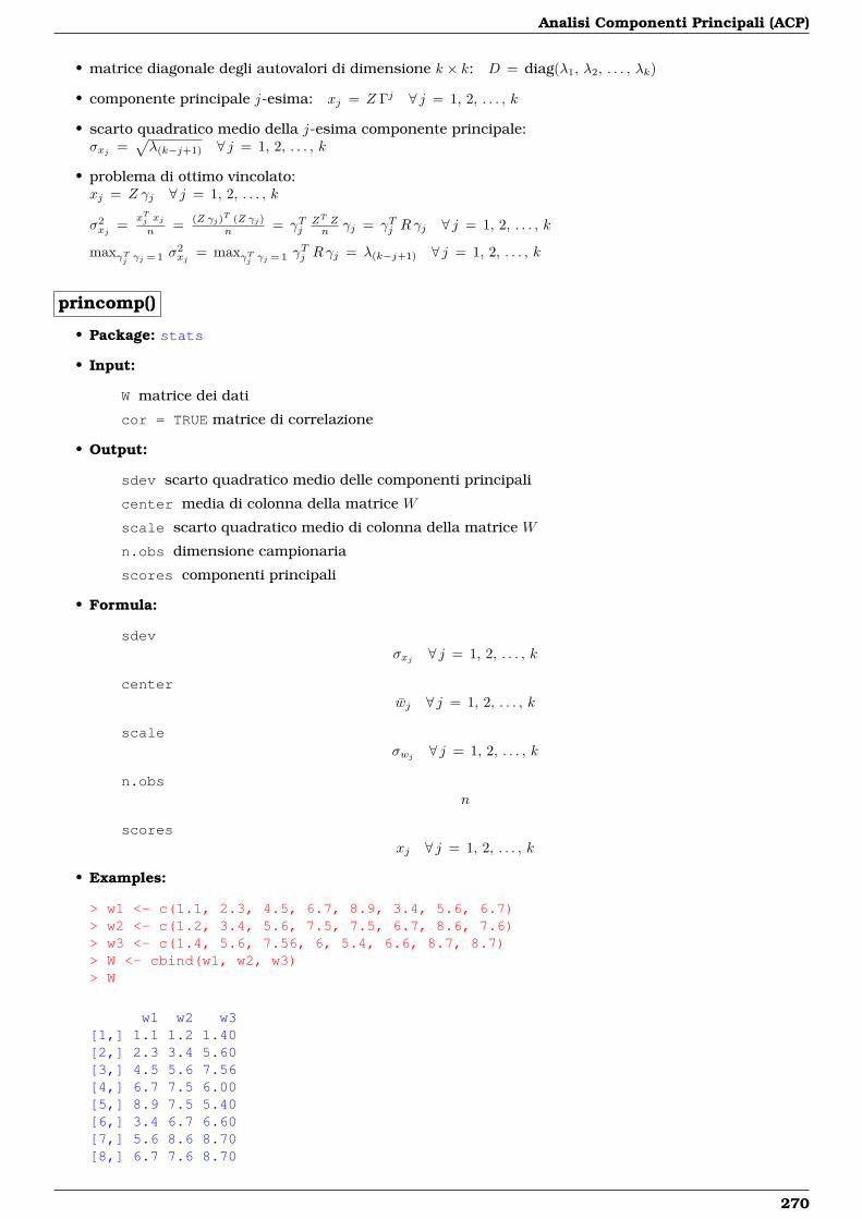
Analisi Componenti Principali (ACP)
• matrice diagonale degli autovalori di dimensione k × k: D = diag(λ1, λ2, . . . , λk)
• componente principale j-esima: xj = Z Γj ∀ j = 1, 2, . . . , k
• scarto quadratico medio della j-esima componente principale:σxj =
√λ(k−j+1) ∀ j = 1, 2, . . . , k
• problema di ottimo vincolato:xj = Z γj ∀ j = 1, 2, . . . , k
σ2xj = xTj xj
n = (Z γj)T (Z γj)n = γTj
ZT Zn γj = γTj Rγj ∀ j = 1, 2, . . . , k
maxγTj γj = 1 σ2xj = maxγTj γj = 1 γ
Tj Rγj = λ(k−j+1) ∀ j = 1, 2, . . . , k
princomp()
• Package: stats
• Input:
W matrice dei dati
cor = TRUE matrice di correlazione
• Output:
sdev scarto quadratico medio delle componenti principali
center media di colonna della matrice W
scale scarto quadratico medio di colonna della matrice W
n.obs dimensione campionaria
scores componenti principali
• Formula:
sdevσxj ∀ j = 1, 2, . . . , k
centerwj ∀ j = 1, 2, . . . , k
scaleσwj ∀ j = 1, 2, . . . , k
n.obsn
scoresxj ∀ j = 1, 2, . . . , k
• Examples:
> w1 <- c(1.1, 2.3, 4.5, 6.7, 8.9, 3.4, 5.6, 6.7)> w2 <- c(1.2, 3.4, 5.6, 7.5, 7.5, 6.7, 8.6, 7.6)> w3 <- c(1.4, 5.6, 7.56, 6, 5.4, 6.6, 8.7, 8.7)> W <- cbind(w1, w2, w3)> W
w1 w2 w3[1,] 1.1 1.2 1.40[2,] 2.3 3.4 5.60[3,] 4.5 5.6 7.56[4,] 6.7 7.5 6.00[5,] 8.9 7.5 5.40[6,] 3.4 6.7 6.60[7,] 5.6 8.6 8.70[8,] 6.7 7.6 8.70
270
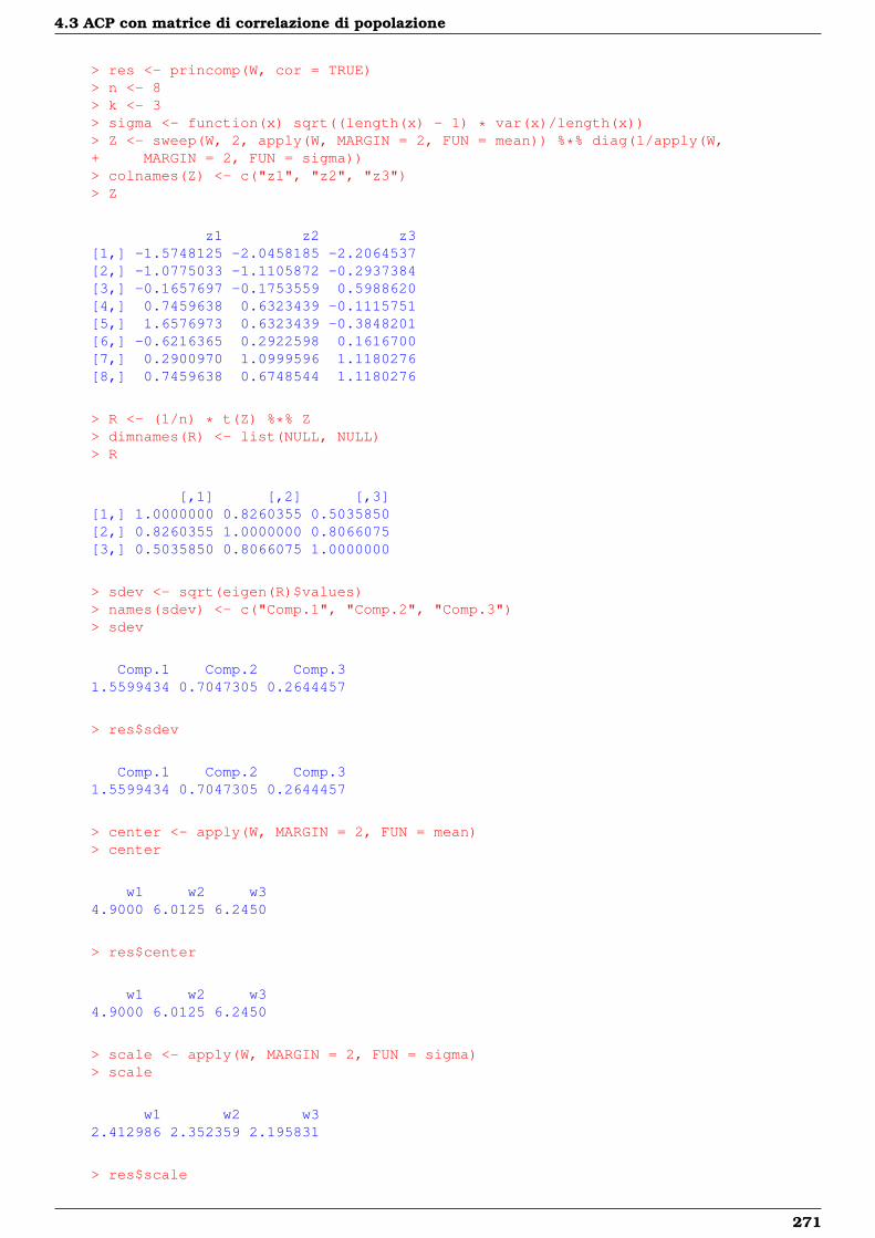
4.3 ACP con matrice di correlazione di popolazione
> res <- princomp(W, cor = TRUE)> n <- 8> k <- 3> sigma <- function(x) sqrt((length(x) - 1) * var(x)/length(x))> Z <- sweep(W, 2, apply(W, MARGIN = 2, FUN = mean)) %*% diag(1/apply(W,+ MARGIN = 2, FUN = sigma))> colnames(Z) <- c("z1", "z2", "z3")> Z
z1 z2 z3[1,] -1.5748125 -2.0458185 -2.2064537[2,] -1.0775033 -1.1105872 -0.2937384[3,] -0.1657697 -0.1753559 0.5988620[4,] 0.7459638 0.6323439 -0.1115751[5,] 1.6576973 0.6323439 -0.3848201[6,] -0.6216365 0.2922598 0.1616700[7,] 0.2900970 1.0999596 1.1180276[8,] 0.7459638 0.6748544 1.1180276
> R <- (1/n) * t(Z) %*% Z> dimnames(R) <- list(NULL, NULL)> R
[,1] [,2] [,3][1,] 1.0000000 0.8260355 0.5035850[2,] 0.8260355 1.0000000 0.8066075[3,] 0.5035850 0.8066075 1.0000000
> sdev <- sqrt(eigen(R)$values)> names(sdev) <- c("Comp.1", "Comp.2", "Comp.3")> sdev
Comp.1 Comp.2 Comp.31.5599434 0.7047305 0.2644457
> res$sdev
Comp.1 Comp.2 Comp.31.5599434 0.7047305 0.2644457
> center <- apply(W, MARGIN = 2, FUN = mean)> center
w1 w2 w34.9000 6.0125 6.2450
> res$center
w1 w2 w34.9000 6.0125 6.2450
> scale <- apply(W, MARGIN = 2, FUN = sigma)> scale
w1 w2 w32.412986 2.352359 2.195831
> res$scale
271
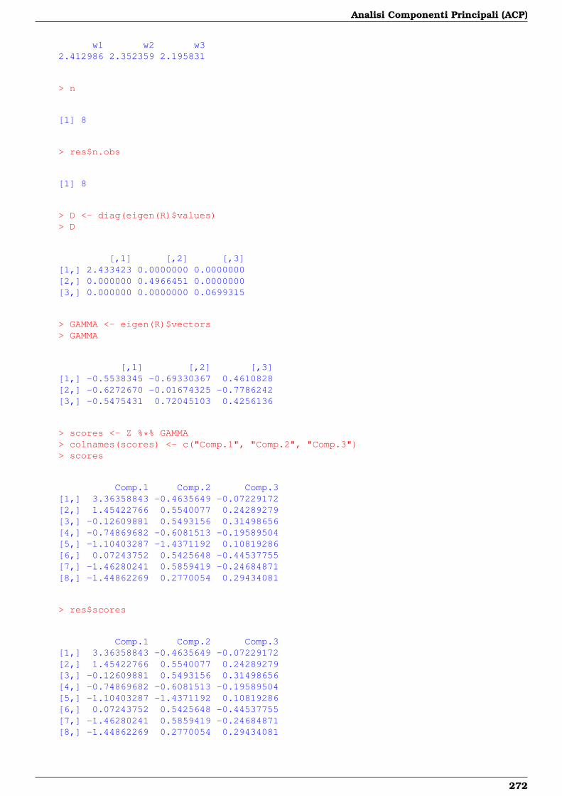
Analisi Componenti Principali (ACP)
w1 w2 w32.412986 2.352359 2.195831
> n
[1] 8
> res$n.obs
[1] 8
> D <- diag(eigen(R)$values)> D
[,1] [,2] [,3][1,] 2.433423 0.0000000 0.0000000[2,] 0.000000 0.4966451 0.0000000[3,] 0.000000 0.0000000 0.0699315
> GAMMA <- eigen(R)$vectors> GAMMA
[,1] [,2] [,3][1,] -0.5538345 -0.69330367 0.4610828[2,] -0.6272670 -0.01674325 -0.7786242[3,] -0.5475431 0.72045103 0.4256136
> scores <- Z %*% GAMMA> colnames(scores) <- c("Comp.1", "Comp.2", "Comp.3")> scores
Comp.1 Comp.2 Comp.3[1,] 3.36358843 -0.4635649 -0.07229172[2,] 1.45422766 0.5540077 0.24289279[3,] -0.12609881 0.5493156 0.31498656[4,] -0.74869682 -0.6081513 -0.19589504[5,] -1.10403287 -1.4371192 0.10819286[6,] 0.07243752 0.5425648 -0.44537755[7,] -1.46280241 0.5859419 -0.24684871[8,] -1.44862269 0.2770054 0.29434081
> res$scores
Comp.1 Comp.2 Comp.3[1,] 3.36358843 -0.4635649 -0.07229172[2,] 1.45422766 0.5540077 0.24289279[3,] -0.12609881 0.5493156 0.31498656[4,] -0.74869682 -0.6081513 -0.19589504[5,] -1.10403287 -1.4371192 0.10819286[6,] 0.07243752 0.5425648 -0.44537755[7,] -1.46280241 0.5859419 -0.24684871[8,] -1.44862269 0.2770054 0.29434081
272
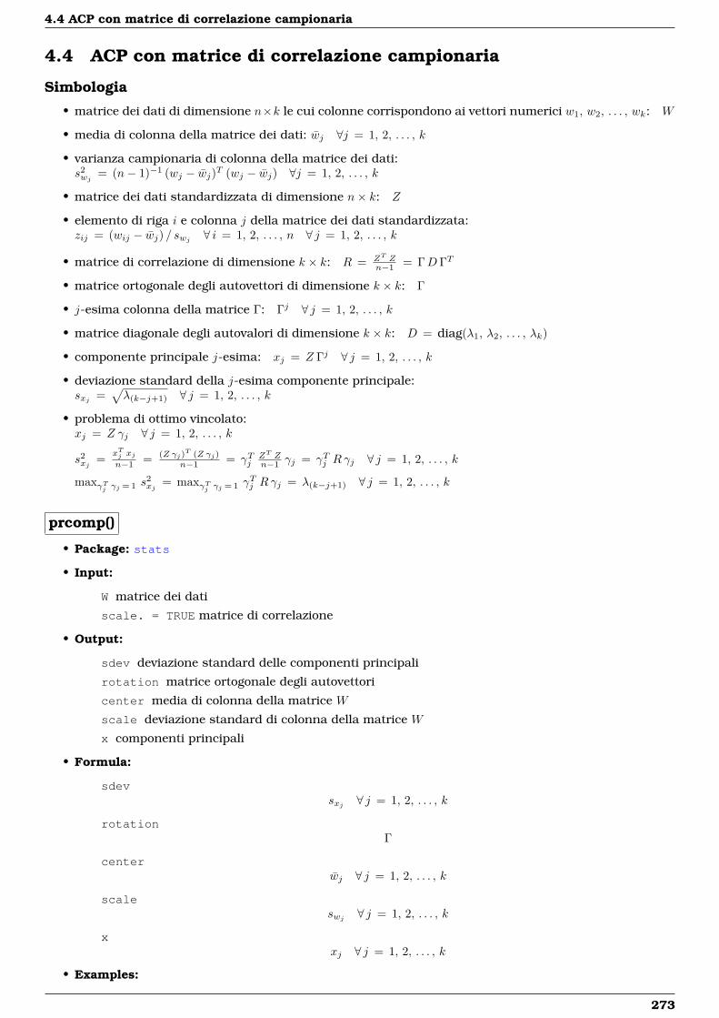
4.4 ACP con matrice di correlazione campionaria
4.4 ACP con matrice di correlazione campionaria
Simbologia
• matrice dei dati di dimensione n×k le cui colonne corrispondono ai vettori numerici w1, w2, . . . , wk: W
• media di colonna della matrice dei dati: wj ∀j = 1, 2, . . . , k
• varianza campionaria di colonna della matrice dei dati:s2wj = (n− 1)−1 (wj − wj)T (wj − wj) ∀j = 1, 2, . . . , k
• matrice dei dati standardizzata di dimensione n× k: Z
• elemento di riga i e colonna j della matrice dei dati standardizzata:zij = (wij − wj) / swj ∀ i = 1, 2, . . . , n ∀ j = 1, 2, . . . , k
• matrice di correlazione di dimensione k × k: R = ZT Zn−1 = ΓD ΓT
• matrice ortogonale degli autovettori di dimensione k × k: Γ
• j-esima colonna della matrice Γ: Γj ∀ j = 1, 2, . . . , k
• matrice diagonale degli autovalori di dimensione k × k: D = diag(λ1, λ2, . . . , λk)
• componente principale j-esima: xj = Z Γj ∀ j = 1, 2, . . . , k
• deviazione standard della j-esima componente principale:sxj =
√λ(k−j+1) ∀ j = 1, 2, . . . , k
• problema di ottimo vincolato:xj = Z γj ∀ j = 1, 2, . . . , k
s2xj = xTj xj
n−1 = (Z γj)T (Z γj)n−1 = γTj
ZT Zn−1 γj = γTj Rγj ∀ j = 1, 2, . . . , k
maxγTj γj = 1 s2xj = maxγTj γj = 1 γ
Tj Rγj = λ(k−j+1) ∀ j = 1, 2, . . . , k
prcomp()
• Package: stats
• Input:
W matrice dei dati
scale. = TRUE matrice di correlazione
• Output:
sdev deviazione standard delle componenti principali
rotation matrice ortogonale degli autovettori
center media di colonna della matrice W
scale deviazione standard di colonna della matrice W
x componenti principali
• Formula:
sdevsxj ∀ j = 1, 2, . . . , k
rotationΓ
centerwj ∀ j = 1, 2, . . . , k
scaleswj ∀ j = 1, 2, . . . , k
xxj ∀ j = 1, 2, . . . , k
• Examples:
273
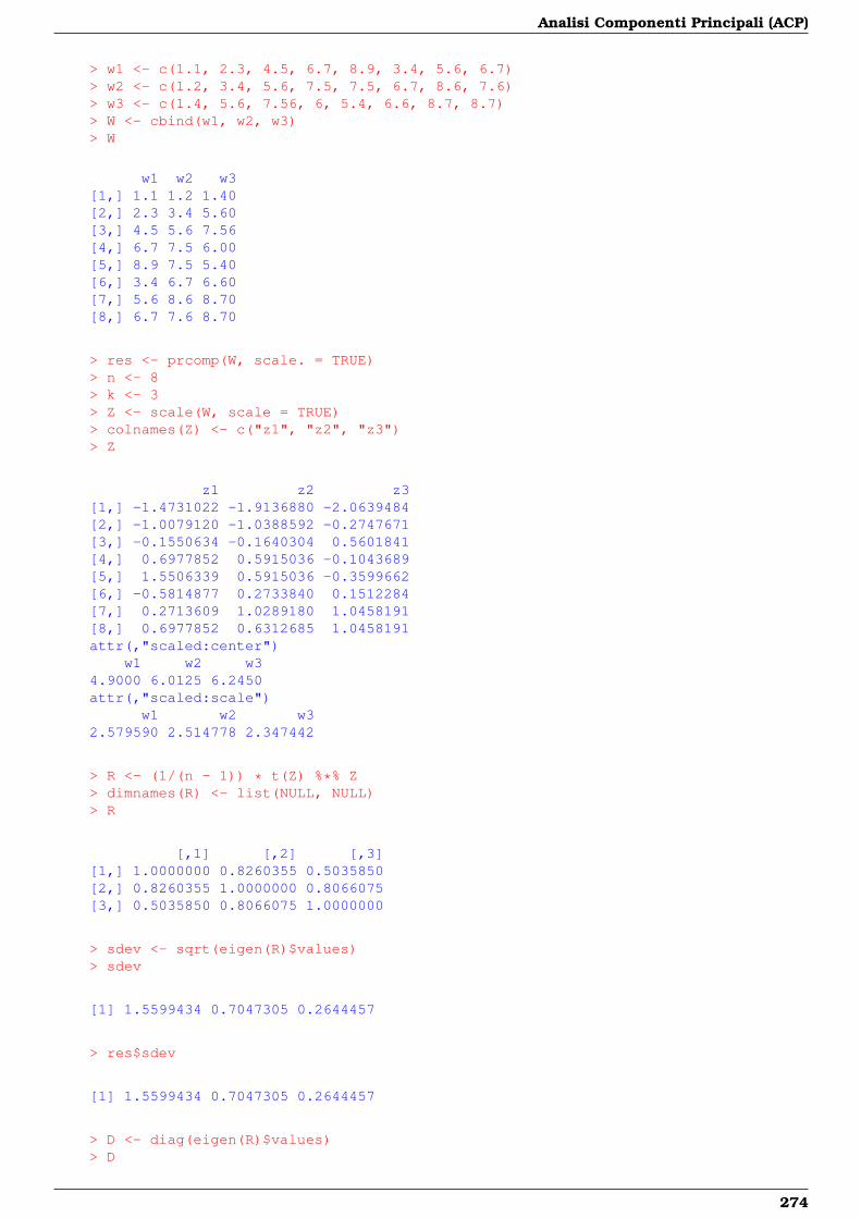
Analisi Componenti Principali (ACP)
> w1 <- c(1.1, 2.3, 4.5, 6.7, 8.9, 3.4, 5.6, 6.7)> w2 <- c(1.2, 3.4, 5.6, 7.5, 7.5, 6.7, 8.6, 7.6)> w3 <- c(1.4, 5.6, 7.56, 6, 5.4, 6.6, 8.7, 8.7)> W <- cbind(w1, w2, w3)> W
w1 w2 w3[1,] 1.1 1.2 1.40[2,] 2.3 3.4 5.60[3,] 4.5 5.6 7.56[4,] 6.7 7.5 6.00[5,] 8.9 7.5 5.40[6,] 3.4 6.7 6.60[7,] 5.6 8.6 8.70[8,] 6.7 7.6 8.70
> res <- prcomp(W, scale. = TRUE)> n <- 8> k <- 3> Z <- scale(W, scale = TRUE)> colnames(Z) <- c("z1", "z2", "z3")> Z
z1 z2 z3[1,] -1.4731022 -1.9136880 -2.0639484[2,] -1.0079120 -1.0388592 -0.2747671[3,] -0.1550634 -0.1640304 0.5601841[4,] 0.6977852 0.5915036 -0.1043689[5,] 1.5506339 0.5915036 -0.3599662[6,] -0.5814877 0.2733840 0.1512284[7,] 0.2713609 1.0289180 1.0458191[8,] 0.6977852 0.6312685 1.0458191attr(,"scaled:center")
w1 w2 w34.9000 6.0125 6.2450attr(,"scaled:scale")
w1 w2 w32.579590 2.514778 2.347442
> R <- (1/(n - 1)) * t(Z) %*% Z> dimnames(R) <- list(NULL, NULL)> R
[,1] [,2] [,3][1,] 1.0000000 0.8260355 0.5035850[2,] 0.8260355 1.0000000 0.8066075[3,] 0.5035850 0.8066075 1.0000000
> sdev <- sqrt(eigen(R)$values)> sdev
[1] 1.5599434 0.7047305 0.2644457
> res$sdev
[1] 1.5599434 0.7047305 0.2644457
> D <- diag(eigen(R)$values)> D
274
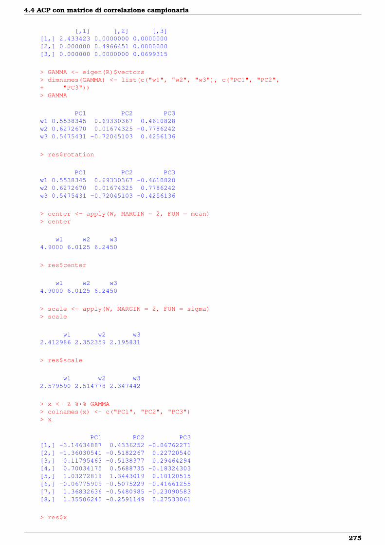
4.4 ACP con matrice di correlazione campionaria
[,1] [,2] [,3][1,] 2.433423 0.0000000 0.0000000[2,] 0.000000 0.4966451 0.0000000[3,] 0.000000 0.0000000 0.0699315
> GAMMA <- eigen(R)$vectors> dimnames(GAMMA) <- list(c("w1", "w2", "w3"), c("PC1", "PC2",+ "PC3"))> GAMMA
PC1 PC2 PC3w1 0.5538345 0.69330367 0.4610828w2 0.6272670 0.01674325 -0.7786242w3 0.5475431 -0.72045103 0.4256136
> res$rotation
PC1 PC2 PC3w1 0.5538345 0.69330367 -0.4610828w2 0.6272670 0.01674325 0.7786242w3 0.5475431 -0.72045103 -0.4256136
> center <- apply(W, MARGIN = 2, FUN = mean)> center
w1 w2 w34.9000 6.0125 6.2450
> res$center
w1 w2 w34.9000 6.0125 6.2450
> scale <- apply(W, MARGIN = 2, FUN = sigma)> scale
w1 w2 w32.412986 2.352359 2.195831
> res$scale
w1 w2 w32.579590 2.514778 2.347442
> x <- Z %*% GAMMA> colnames(x) <- c("PC1", "PC2", "PC3")> x
PC1 PC2 PC3[1,] -3.14634887 0.4336252 -0.06762271[2,] -1.36030541 -0.5182267 0.22720540[3,] 0.11795463 -0.5138377 0.29464294[4,] 0.70034175 0.5688735 -0.18324303[5,] 1.03272818 1.3443019 0.10120515[6,] -0.06775909 -0.5075229 -0.41661255[7,] 1.36832636 -0.5480985 -0.23090583[8,] 1.35506245 -0.2591149 0.27533061
> res$x
275
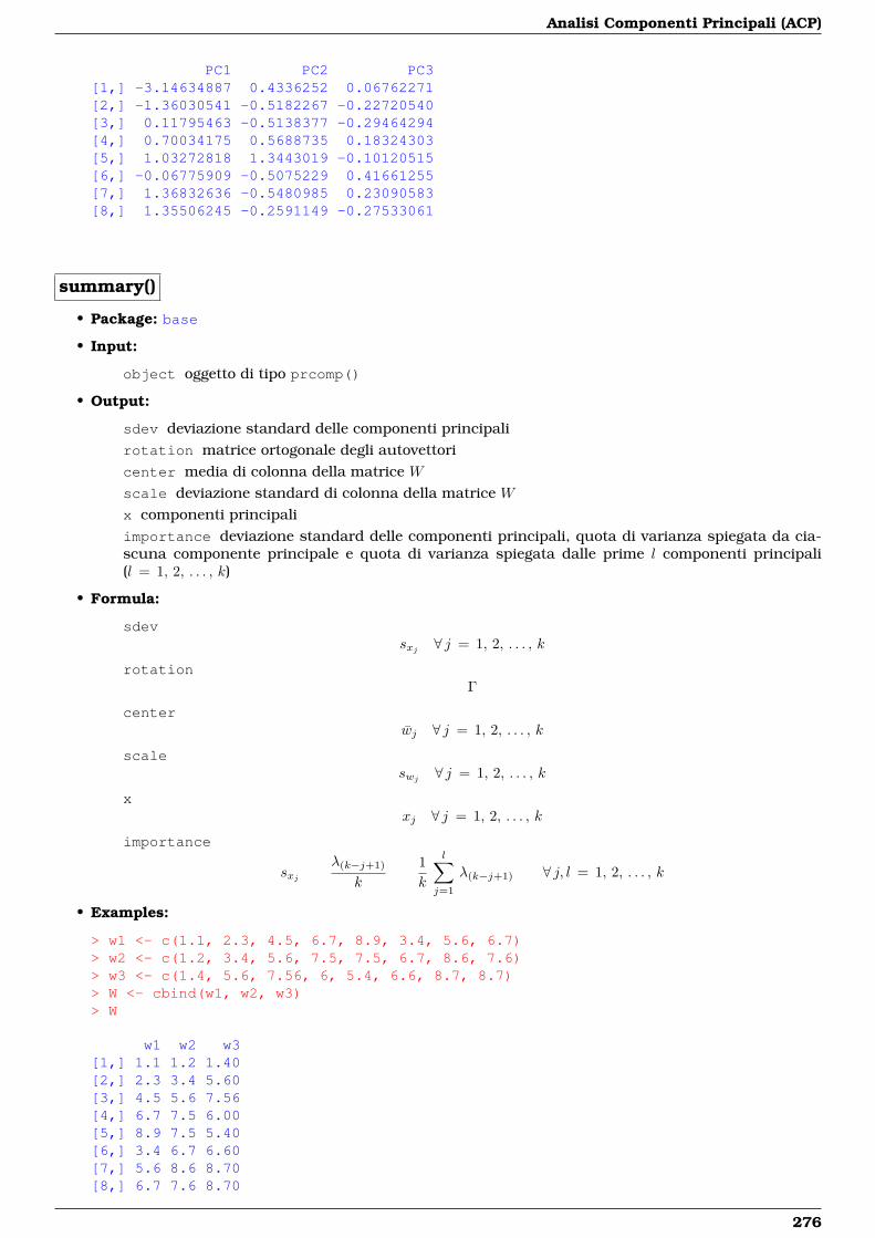
Analisi Componenti Principali (ACP)
PC1 PC2 PC3[1,] -3.14634887 0.4336252 0.06762271[2,] -1.36030541 -0.5182267 -0.22720540[3,] 0.11795463 -0.5138377 -0.29464294[4,] 0.70034175 0.5688735 0.18324303[5,] 1.03272818 1.3443019 -0.10120515[6,] -0.06775909 -0.5075229 0.41661255[7,] 1.36832636 -0.5480985 0.23090583[8,] 1.35506245 -0.2591149 -0.27533061
summary()
• Package: base
• Input:
object oggetto di tipo prcomp()
• Output:
sdev deviazione standard delle componenti principalirotation matrice ortogonale degli autovettoricenter media di colonna della matrice Wscale deviazione standard di colonna della matrice Wx componenti principaliimportance deviazione standard delle componenti principali, quota di varianza spiegata da cia-scuna componente principale e quota di varianza spiegata dalle prime l componenti principali(l = 1, 2, . . . , k)
• Formula:
sdevsxj ∀ j = 1, 2, . . . , k
rotationΓ
centerwj ∀ j = 1, 2, . . . , k
scaleswj ∀ j = 1, 2, . . . , k
xxj ∀ j = 1, 2, . . . , k
importance
sxjλ(k−j+1)
k
1k
l∑j=1
λ(k−j+1) ∀ j, l = 1, 2, . . . , k
• Examples:
> w1 <- c(1.1, 2.3, 4.5, 6.7, 8.9, 3.4, 5.6, 6.7)> w2 <- c(1.2, 3.4, 5.6, 7.5, 7.5, 6.7, 8.6, 7.6)> w3 <- c(1.4, 5.6, 7.56, 6, 5.4, 6.6, 8.7, 8.7)> W <- cbind(w1, w2, w3)> W
w1 w2 w3[1,] 1.1 1.2 1.40[2,] 2.3 3.4 5.60[3,] 4.5 5.6 7.56[4,] 6.7 7.5 6.00[5,] 8.9 7.5 5.40[6,] 3.4 6.7 6.60[7,] 5.6 8.6 8.70[8,] 6.7 7.6 8.70
276
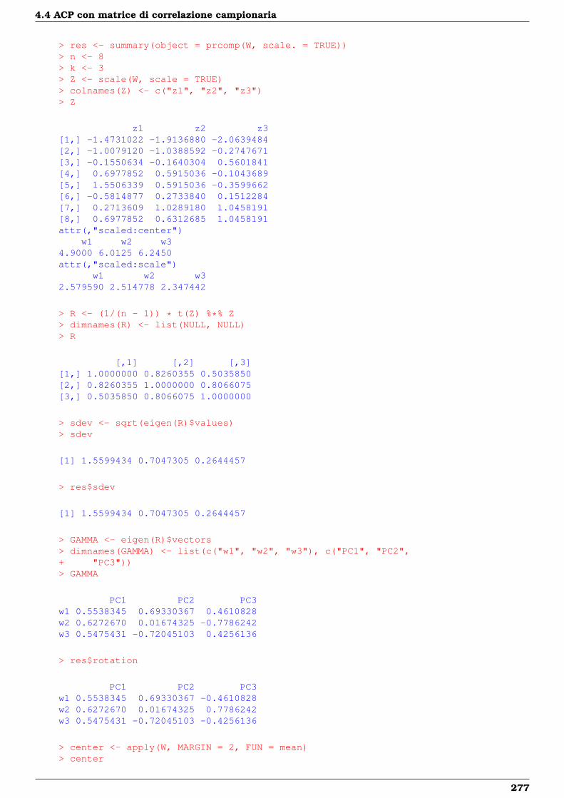
4.4 ACP con matrice di correlazione campionaria
> res <- summary(object = prcomp(W, scale. = TRUE))> n <- 8> k <- 3> Z <- scale(W, scale = TRUE)> colnames(Z) <- c("z1", "z2", "z3")> Z
z1 z2 z3[1,] -1.4731022 -1.9136880 -2.0639484[2,] -1.0079120 -1.0388592 -0.2747671[3,] -0.1550634 -0.1640304 0.5601841[4,] 0.6977852 0.5915036 -0.1043689[5,] 1.5506339 0.5915036 -0.3599662[6,] -0.5814877 0.2733840 0.1512284[7,] 0.2713609 1.0289180 1.0458191[8,] 0.6977852 0.6312685 1.0458191attr(,"scaled:center")
w1 w2 w34.9000 6.0125 6.2450attr(,"scaled:scale")
w1 w2 w32.579590 2.514778 2.347442
> R <- (1/(n - 1)) * t(Z) %*% Z> dimnames(R) <- list(NULL, NULL)> R
[,1] [,2] [,3][1,] 1.0000000 0.8260355 0.5035850[2,] 0.8260355 1.0000000 0.8066075[3,] 0.5035850 0.8066075 1.0000000
> sdev <- sqrt(eigen(R)$values)> sdev
[1] 1.5599434 0.7047305 0.2644457
> res$sdev
[1] 1.5599434 0.7047305 0.2644457
> GAMMA <- eigen(R)$vectors> dimnames(GAMMA) <- list(c("w1", "w2", "w3"), c("PC1", "PC2",+ "PC3"))> GAMMA
PC1 PC2 PC3w1 0.5538345 0.69330367 0.4610828w2 0.6272670 0.01674325 -0.7786242w3 0.5475431 -0.72045103 0.4256136
> res$rotation
PC1 PC2 PC3w1 0.5538345 0.69330367 -0.4610828w2 0.6272670 0.01674325 0.7786242w3 0.5475431 -0.72045103 -0.4256136
> center <- apply(W, MARGIN = 2, FUN = mean)> center
277
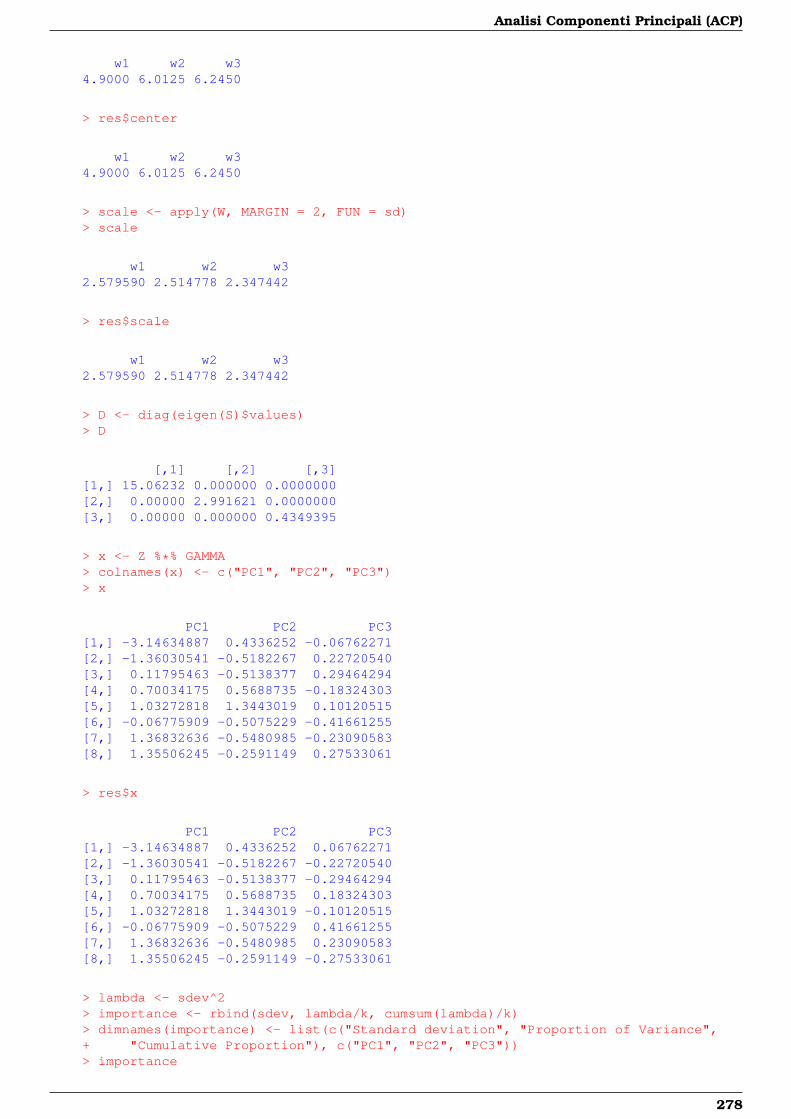
Analisi Componenti Principali (ACP)
w1 w2 w34.9000 6.0125 6.2450
> res$center
w1 w2 w34.9000 6.0125 6.2450
> scale <- apply(W, MARGIN = 2, FUN = sd)> scale
w1 w2 w32.579590 2.514778 2.347442
> res$scale
w1 w2 w32.579590 2.514778 2.347442
> D <- diag(eigen(S)$values)> D
[,1] [,2] [,3][1,] 15.06232 0.000000 0.0000000[2,] 0.00000 2.991621 0.0000000[3,] 0.00000 0.000000 0.4349395
> x <- Z %*% GAMMA> colnames(x) <- c("PC1", "PC2", "PC3")> x
PC1 PC2 PC3[1,] -3.14634887 0.4336252 -0.06762271[2,] -1.36030541 -0.5182267 0.22720540[3,] 0.11795463 -0.5138377 0.29464294[4,] 0.70034175 0.5688735 -0.18324303[5,] 1.03272818 1.3443019 0.10120515[6,] -0.06775909 -0.5075229 -0.41661255[7,] 1.36832636 -0.5480985 -0.23090583[8,] 1.35506245 -0.2591149 0.27533061
> res$x
PC1 PC2 PC3[1,] -3.14634887 0.4336252 0.06762271[2,] -1.36030541 -0.5182267 -0.22720540[3,] 0.11795463 -0.5138377 -0.29464294[4,] 0.70034175 0.5688735 0.18324303[5,] 1.03272818 1.3443019 -0.10120515[6,] -0.06775909 -0.5075229 0.41661255[7,] 1.36832636 -0.5480985 0.23090583[8,] 1.35506245 -0.2591149 -0.27533061
> lambda <- sdev^2> importance <- rbind(sdev, lambda/k, cumsum(lambda)/k)> dimnames(importance) <- list(c("Standard deviation", "Proportion of Variance",+ "Cumulative Proportion"), c("PC1", "PC2", "PC3"))> importance
278

4.4 ACP con matrice di correlazione campionaria
PC1 PC2 PC3Standard deviation 1.5599434 0.7047305 0.2644457Proportion of Variance 0.8111411 0.1655484 0.0233105Cumulative Proportion 0.8111411 0.9766895 1.0000000
> res$importance
PC1 PC2 PC3Standard deviation 1.559943 0.7047305 0.2644457Proportion of Variance 0.811140 0.1655500 0.0233100Cumulative Proportion 0.811140 0.9766900 1.0000000
279

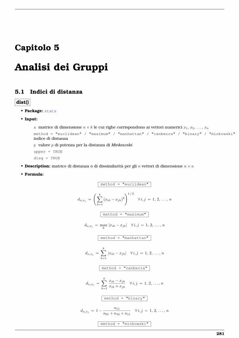
Capitolo 5
Analisi dei Gruppi
5.1 Indici di distanza
dist()
• Package: stats
• Input:
x matrice di dimensione n× k le cui righe corrispondono ai vettori numerici x1, x2, . . . , xn
method = "euclidean" / "maximum" / "manhattan" / "canberra" / "binary" / "minkowski"indice di distanza
p valore p di potenza per la distanza di Minkowski
upper = TRUE
diag = TRUE
• Description: matrice di distanza o di dissimilarità per gli n vettori di dimensione n× n
• Formula:
method = "euclidean"
dxixj =
(k∑h=1
(xih − xjh)2
)1 / 2
∀ i, j = 1, 2, . . . , n
method = "maximum"
dxixj = maxh|xih − xjh| ∀ i, j = 1, 2, . . . , n
method = "manhattan"
dxixj =k∑h=1
|xih − xjh| ∀ i, j = 1, 2, . . . , n
method = "canberra"
dxixj =k∑h=1
xih − xjhxih + xjh
∀ i, j = 1, 2, . . . , n
method = "binary"
dxixj = 1− n11
n01 + n10 + n11∀ i, j = 1, 2, . . . , n
method = "minkowski"
281
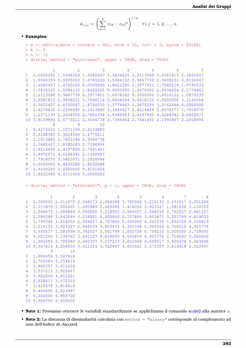
Analisi dei Gruppi
dxixj =
(k∑h=1
|xih − xjh|p)1 / p
∀ i, j = 1, 2, . . . , n
• Examples:
> x <- matrix(data = rnorm(n = 30), nrow = 10, ncol = 3, byrow = FALSE)> k <- 3> n <- 10> dist(x, method = "euclidean", upper = TRUE, diag = TRUE)
1 2 3 4 5 6 71 0.0000000 1.5948359 1.6080407 1.5836525 2.2113048 3.0581815 2.38204072 1.5948359 0.0000000 1.4765220 1.5084132 0.9847730 2.9608231 0.81500473 1.6080407 1.4765220 0.0000000 1.8622265 2.3977451 1.7540114 1.97455334 1.5836525 1.5084132 1.8622265 0.0000000 1.6478362 2.6834204 2.17744635 2.2113048 0.9847730 2.3977451 1.6478362 0.0000000 3.6618122 1.08752396 3.0581815 2.9608231 1.7540114 2.6834204 3.6618122 0.0000000 3.31426647 2.3820407 0.8150047 1.9745533 2.1774463 1.0875239 3.3142664 0.00000008 3.4274432 2.2298585 2.1613885 3.3445427 2.8214454 2.8972571 1.79185709 1.2371199 2.3024300 2.7601394 1.8380083 2.4297830 4.0248341 3.045267110 3.6159883 2.4770211 2.3594738 2.7396964 2.7641401 2.1990887 2.2918994
8 9 101 3.4274432 1.2371199 3.61598832 2.2298585 2.3024300 2.47702113 2.1613885 2.7601394 2.35947384 3.3445427 1.8380083 2.73969645 2.8214454 2.4297830 2.76414016 2.8972571 4.0248341 2.19908877 1.7918570 3.0452671 2.29189948 0.0000000 4.4430280 1.86320889 4.4430280 0.0000000 4.415160410 1.8632088 4.4151604 0.0000000
> dist(x, method = "minkowski", p = 1, upper = TRUE, diag = TRUE)
1 2 3 4 5 6 7 81 0.000000 2.511879 2.548073 2.084588 3.795046 5.216133 3.593517 4.0512062 2.511879 0.000000 1.680889 2.443684 1.416056 3.923327 1.081638 3.1347633 2.548073 1.680889 0.000000 3.218951 2.964057 2.668059 2.762527 2.6811574 2.084588 2.443684 3.218951 0.000000 2.707806 3.603471 3.501799 4.8190335 3.795046 1.416056 2.964057 2.707806 0.000000 4.320338 1.832726 4.5508196 5.216133 3.923327 2.668059 3.603471 4.320338 0.000000 4.704210 4.9257767 3.593517 1.081638 2.762527 3.501799 1.832726 4.704210 0.000000 2.7180938 4.051206 3.134763 2.681157 4.819033 4.550819 4.925776 2.718093 0.0000009 1.984456 2.705089 3.960357 3.037213 3.622008 6.628417 3.420478 5.46349010 5.547416 4.254610 3.611224 3.922487 4.651621 3.572303 3.814418 2.523997
9 101 1.984456 5.5474162 2.705089 4.2546103 3.960357 3.6112244 3.037213 3.9224875 3.622008 4.6516216 6.628417 3.5723037 3.420478 3.8144188 5.463490 2.5239979 0.000000 6.95970010 6.959700 0.000000
• Note 1: Possiamo ottenere le variabili standardizzate se applichiamo il comando scale() alla matrice x.
• Note 2: La distanza di dissimilarità calcolata con method = "binary" corrisponde al complemento aduno dell’indice di Jaccard.
282
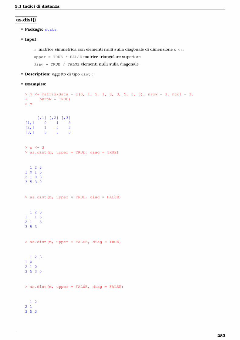
5.1 Indici di distanza
as.dist()
• Package: stats
• Input:
m matrice simmetrica con elementi nulli sulla diagonale di dimensione n× n
upper = TRUE / FALSE matrice triangolare superiore
diag = TRUE / FALSE elementi nulli sulla diagonale
• Description: oggetto di tipo dist()
• Examples:
> m <- matrix(data = c(0, 1, 5, 1, 0, 3, 5, 3, 0), nrow = 3, ncol = 3,+ byrow = TRUE)> m
[,1] [,2] [,3][1,] 0 1 5[2,] 1 0 3[3,] 5 3 0
> n <- 3> as.dist(m, upper = TRUE, diag = TRUE)
1 2 31 0 1 52 1 0 33 5 3 0
> as.dist(m, upper = TRUE, diag = FALSE)
1 2 31 1 52 1 33 5 3
> as.dist(m, upper = FALSE, diag = TRUE)
1 2 31 02 1 03 5 3 0
> as.dist(m, upper = FALSE, diag = FALSE)
1 22 13 5 3
283
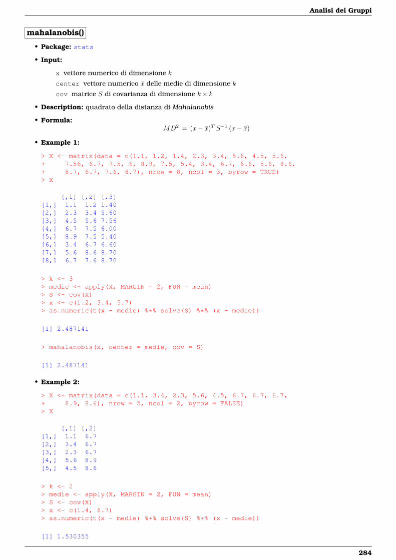
Analisi dei Gruppi
mahalanobis()
• Package: stats
• Input:
x vettore numerico di dimensione k
center vettore numerico x delle medie di dimensione k
cov matrice S di covarianza di dimensione k × k
• Description: quadrato della distanza di Mahalanobis
• Formula:MD2 = (x− x)T S−1 (x− x)
• Example 1:
> X <- matrix(data = c(1.1, 1.2, 1.4, 2.3, 3.4, 5.6, 4.5, 5.6,+ 7.56, 6.7, 7.5, 6, 8.9, 7.5, 5.4, 3.4, 6.7, 6.6, 5.6, 8.6,+ 8.7, 6.7, 7.6, 8.7), nrow = 8, ncol = 3, byrow = TRUE)> X
[,1] [,2] [,3][1,] 1.1 1.2 1.40[2,] 2.3 3.4 5.60[3,] 4.5 5.6 7.56[4,] 6.7 7.5 6.00[5,] 8.9 7.5 5.40[6,] 3.4 6.7 6.60[7,] 5.6 8.6 8.70[8,] 6.7 7.6 8.70
> k <- 3> medie <- apply(X, MARGIN = 2, FUN = mean)> S <- cov(X)> x <- c(1.2, 3.4, 5.7)> as.numeric(t(x - medie) %*% solve(S) %*% (x - medie))
[1] 2.487141
> mahalanobis(x, center = medie, cov = S)
[1] 2.487141
• Example 2:
> X <- matrix(data = c(1.1, 3.4, 2.3, 5.6, 4.5, 6.7, 6.7, 6.7,+ 8.9, 8.6), nrow = 5, ncol = 2, byrow = FALSE)> X
[,1] [,2][1,] 1.1 6.7[2,] 3.4 6.7[3,] 2.3 6.7[4,] 5.6 8.9[5,] 4.5 8.6
> k <- 2> medie <- apply(X, MARGIN = 2, FUN = mean)> S <- cov(X)> x <- c(1.4, 6.7)> as.numeric(t(x - medie) %*% solve(S) %*% (x - medie))
[1] 1.530355
284
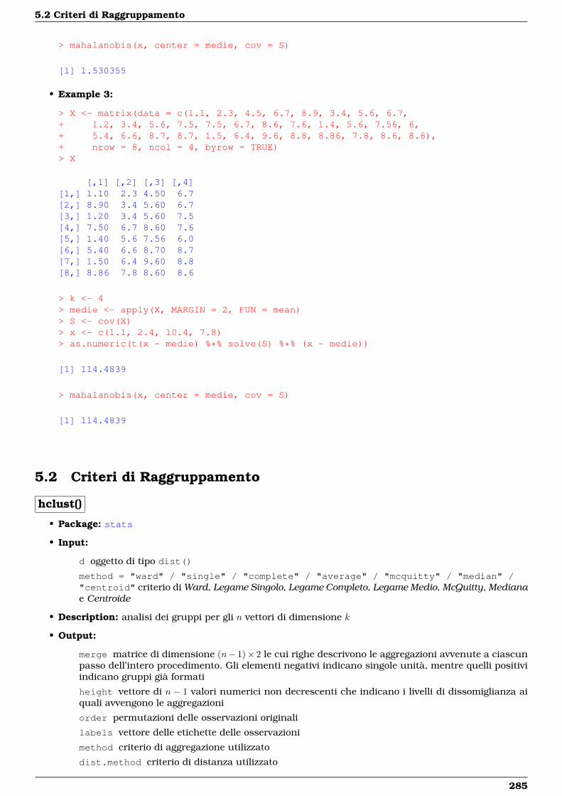
5.2 Criteri di Raggruppamento
> mahalanobis(x, center = medie, cov = S)
[1] 1.530355
• Example 3:
> X <- matrix(data = c(1.1, 2.3, 4.5, 6.7, 8.9, 3.4, 5.6, 6.7,+ 1.2, 3.4, 5.6, 7.5, 7.5, 6.7, 8.6, 7.6, 1.4, 5.6, 7.56, 6,+ 5.4, 6.6, 8.7, 8.7, 1.5, 6.4, 9.6, 8.8, 8.86, 7.8, 8.6, 8.6),+ nrow = 8, ncol = 4, byrow = TRUE)> X
[,1] [,2] [,3] [,4][1,] 1.10 2.3 4.50 6.7[2,] 8.90 3.4 5.60 6.7[3,] 1.20 3.4 5.60 7.5[4,] 7.50 6.7 8.60 7.6[5,] 1.40 5.6 7.56 6.0[6,] 5.40 6.6 8.70 8.7[7,] 1.50 6.4 9.60 8.8[8,] 8.86 7.8 8.60 8.6
> k <- 4> medie <- apply(X, MARGIN = 2, FUN = mean)> S <- cov(X)> x <- c(1.1, 2.4, 10.4, 7.8)> as.numeric(t(x - medie) %*% solve(S) %*% (x - medie))
[1] 114.4839
> mahalanobis(x, center = medie, cov = S)
[1] 114.4839
5.2 Criteri di Raggruppamento
hclust()
• Package: stats
• Input:
d oggetto di tipo dist()
method = "ward" / "single" / "complete" / "average" / "mcquitty" / "median" /"centroid" criterio di Ward, Legame Singolo, Legame Completo, Legame Medio, McQuitty, Medianae Centroide
• Description: analisi dei gruppi per gli n vettori di dimensione k
• Output:
merge matrice di dimensione (n− 1)× 2 le cui righe descrivono le aggregazioni avvenute a ciascunpasso dell’intero procedimento. Gli elementi negativi indicano singole unità, mentre quelli positiviindicano gruppi già formati
height vettore di n − 1 valori numerici non decrescenti che indicano i livelli di dissomiglianza aiquali avvengono le aggregazioni
order permutazioni delle osservazioni originali
labels vettore delle etichette delle osservazioni
method criterio di aggregazione utilizzato
dist.method criterio di distanza utilizzato
285
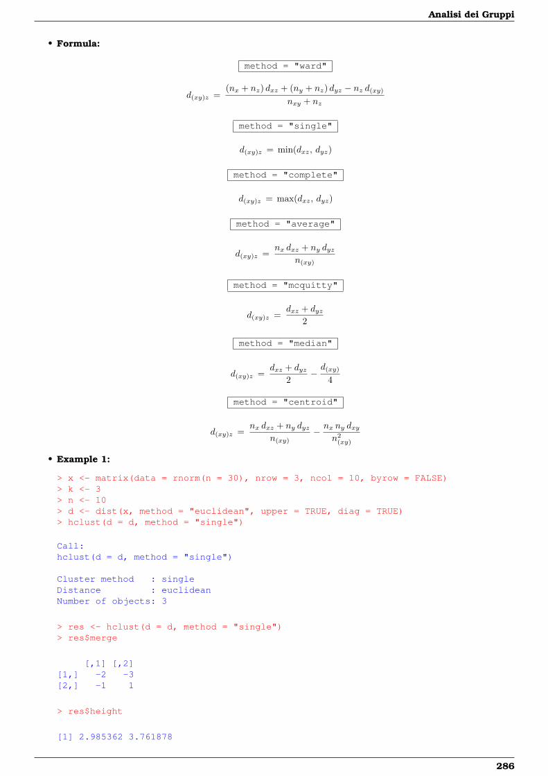
Analisi dei Gruppi
• Formula:
method = "ward"
d(xy)z =(nx + nz) dxz + (ny + nz) dyz − nz d(xy)
nxy + nz
method = "single"
d(xy)z = min(dxz, dyz)
method = "complete"
d(xy)z = max(dxz, dyz)
method = "average"
d(xy)z =nx dxz + ny dyz
n(xy)
method = "mcquitty"
d(xy)z =dxz + dyz
2
method = "median"
d(xy)z =dxz + dyz
2−d(xy)
4
method = "centroid"
d(xy)z =nx dxz + ny dyz
n(xy)− nx ny dxy
n2(xy)
• Example 1:
> x <- matrix(data = rnorm(n = 30), nrow = 3, ncol = 10, byrow = FALSE)> k <- 3> n <- 10> d <- dist(x, method = "euclidean", upper = TRUE, diag = TRUE)> hclust(d = d, method = "single")
Call:hclust(d = d, method = "single")
Cluster method : singleDistance : euclideanNumber of objects: 3
> res <- hclust(d = d, method = "single")> res$merge
[,1] [,2][1,] -2 -3[2,] -1 1
> res$height
[1] 2.985362 3.761878
286
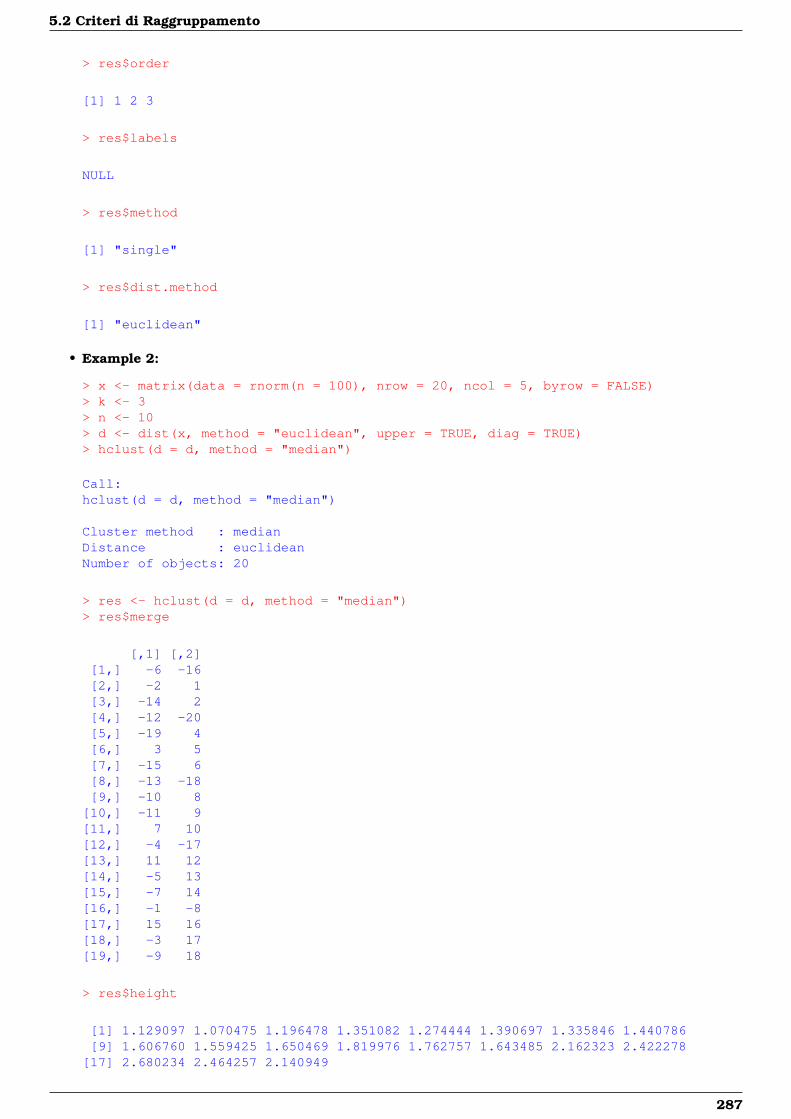
5.2 Criteri di Raggruppamento
> res$order
[1] 1 2 3
> res$labels
NULL
> res$method
[1] "single"
> res$dist.method
[1] "euclidean"
• Example 2:
> x <- matrix(data = rnorm(n = 100), nrow = 20, ncol = 5, byrow = FALSE)> k <- 3> n <- 10> d <- dist(x, method = "euclidean", upper = TRUE, diag = TRUE)> hclust(d = d, method = "median")
Call:hclust(d = d, method = "median")
Cluster method : medianDistance : euclideanNumber of objects: 20
> res <- hclust(d = d, method = "median")> res$merge
[,1] [,2][1,] -6 -16[2,] -2 1[3,] -14 2[4,] -12 -20[5,] -19 4[6,] 3 5[7,] -15 6[8,] -13 -18[9,] -10 8
[10,] -11 9[11,] 7 10[12,] -4 -17[13,] 11 12[14,] -5 13[15,] -7 14[16,] -1 -8[17,] 15 16[18,] -3 17[19,] -9 18
> res$height
[1] 1.129097 1.070475 1.196478 1.351082 1.274444 1.390697 1.335846 1.440786[9] 1.606760 1.559425 1.650469 1.819976 1.762757 1.643485 2.162323 2.422278
[17] 2.680234 2.464257 2.140949
287
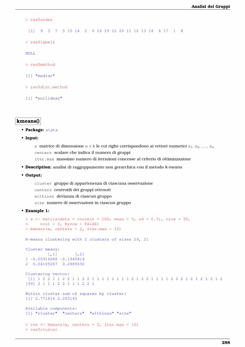
Analisi dei Gruppi
> res$order
[1] 9 3 7 5 15 14 2 6 16 19 12 20 11 10 13 18 4 17 1 8
> res$labels
NULL
> res$method
[1] "median"
> res$dist.method
[1] "euclidean"
kmeans()
• Package: stats
• Input:
x matrice di dimensione n× k le cui righe corrispondono ai vettori numerici x1, x2, . . . , xn
centers scalare che indica il numero di gruppi
iter.max massimo numero di iterazioni concesse al criterio di ottimizzazione
• Description: analisi di ragguppamento non gerarchica con il metodo k-means
• Output:
cluster gruppo di appartenenza di ciascuna osservazione
centers centroidi dei gruppi ottenuti
withinss devianza di ciascun gruppo
size numero di osservazioni in ciascun gruppo
• Example 1:
> x <- matrix(data = rnorm(n = 100, mean = 0, sd = 0.3), nrow = 50,+ ncol = 2, byrow = FALSE)> kmeans(x, centers = 2, iter.max = 10)
K-means clustering with 2 clusters of sizes 29, 21
Cluster means:[,1] [,2]
1 -0.05916688 -0.19458142 0.04105267 0.2989030
Clustering vector:[1] 1 2 2 1 1 2 2 1 1 2 2 1 1 1 1 1 1 1 1 2 1 2 2 1 1 1 1 2 2 2 1 2 1 2 1 2 1 2
[39] 2 1 1 1 2 2 1 1 1 2 2 1
Within cluster sum of squares by cluster:[1] 2.771814 2.263145
Available components:[1] "cluster" "centers" "withinss" "size"
> res <- kmeans(x, centers = 2, iter.max = 10)> res$cluster
288
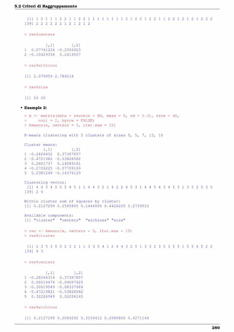
5.2 Criteri di Raggruppamento
[1] 1 2 1 1 1 2 2 1 1 2 2 1 1 1 1 1 1 1 1 2 1 2 2 1 2 2 1 1 2 2 1 2 1 2 1 2 2 2[39] 2 2 2 2 2 2 1 2 1 2 1 2
> res$centers
[,1] [,2]1 0.07741224 -0.23569232 -0.10429336 0.2419507
> res$withinss
[1] 2.079959 2.784218
> res$size
[1] 24 26
• Example 2:
> x <- matrix(data = rnorm(n = 80, mean = 0, sd = 0.3), nrow = 40,+ ncol = 2, byrow = FALSE)> kmeans(x, centers = 5, iter.max = 15)
K-means clustering with 5 clusters of sizes 5, 5, 7, 13, 10
Cluster means:[,1] [,2]
1 -0.2826432 0.373678572 -0.4721982 -0.538285823 0.2601737 0.145891614 -0.2726225 -0.077091695 0.2381249 -0.14376129
Clustering vector:[1] 4 4 3 4 5 5 5 4 5 1 1 4 4 3 2 1 4 2 2 4 5 3 1 4 4 5 4 3 4 5 3 1 3 5 2 5 3 5
[39] 2 4
Within cluster sum of squares by cluster:[1] 0.2127299 0.2585805 0.1444599 0.4426205 0.2739510
Available components:[1] "cluster" "centers" "withinss" "size"
> res <- kmeans(x, centers = 5, iter.max = 15)> res$cluster
[1] 2 3 5 3 5 5 2 3 2 1 1 3 3 5 4 1 2 4 4 3 2 5 1 3 3 2 3 5 3 5 5 1 5 5 4 5 2 2[39] 4 3
> res$centers
[,1] [,2]1 -0.28264316 0.373678572 0.06019474 -0.090674253 -0.30619549 -0.083376844 -0.47219821 -0.538285825 0.32226949 0.02036143
> res$withinss
[1] 0.2127299 0.2084292 0.3159412 0.2585805 0.4271144
289

Analisi dei Gruppi
> res$size
[1] 5 8 11 5 11
290

Parte III
Statistica Inferenziale
291

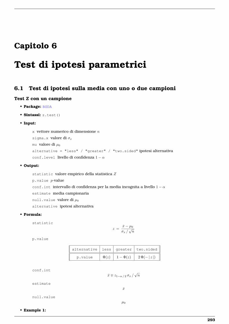
Capitolo 6
Test di ipotesi parametrici
6.1 Test di ipotesi sulla media con uno o due campioni
Test Z con un campione
• Package: BSDA
• Sintassi: z.test()
• Input:
x vettore numerico di dimensione n
sigma.x valore di σx
mu valore di µ0
alternative = "less" / "greater" / "two.sided" ipotesi alternativa
conf.level livello di confidenza 1− α
• Output:
statistic valore empirico della statistica Z
p.value p-value
conf.int intervallo di confidenza per la media incognita a livello 1− αestimate media campionaria
null.value valore di µ0
alternative ipotesi alternativa
• Formula:
statistic
z =x− µ0
σx /√n
p.value
alternative less greater two.sided
p.value Φ(z) 1− Φ(z) 2 Φ(− | z |)
conf.int
x∓ z1−α/ 2 σx /√n
estimate
x
null.value
µ0
• Example 1:
293
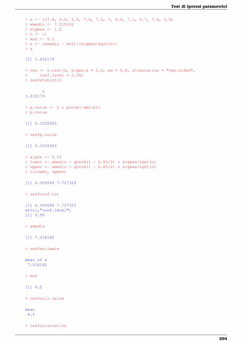
Test di ipotesi parametrici
> x <- c(7.8, 6.6, 6.5, 7.4, 7.3, 7, 6.4, 7.1, 6.7, 7.6, 6.8)> xmedio <- 7.018182> sigmax <- 1.2> n <- 11> mu0 <- 6.5> z <- (xmedio - mu0)/(sigmax/sqrt(n))> z
[1] 1.432179
> res <- z.test(x, sigma.x = 1.2, mu = 6.5, alternative = "two.sided",+ conf.level = 0.95)> res$statistic
z1.432179
> p.value <- 2 * pnorm(-abs(z))> p.value
[1] 0.1520925
> res$p.value
[1] 0.1520926
> alpha <- 0.05> lower <- xmedio - qnorm(1 - 0.05/2) * sigmax/sqrt(n)> upper <- xmedio + qnorm(1 - 0.05/2) * sigmax/sqrt(n)> c(lower, upper)
[1] 6.309040 7.727324
> res$conf.int
[1] 6.309040 7.727323attr(,"conf.level")[1] 0.95
> xmedio
[1] 7.018182
> res$estimate
mean of x7.018182
> mu0
[1] 6.5
> res$null.value
mean6.5
> res$alternative
294
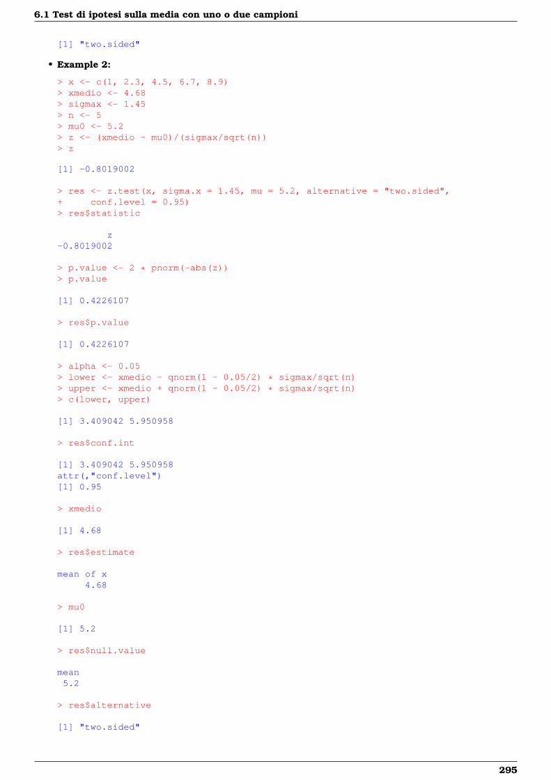
6.1 Test di ipotesi sulla media con uno o due campioni
[1] "two.sided"
• Example 2:
> x <- c(1, 2.3, 4.5, 6.7, 8.9)> xmedio <- 4.68> sigmax <- 1.45> n <- 5> mu0 <- 5.2> z <- (xmedio - mu0)/(sigmax/sqrt(n))> z
[1] -0.8019002
> res <- z.test(x, sigma.x = 1.45, mu = 5.2, alternative = "two.sided",+ conf.level = 0.95)> res$statistic
z-0.8019002
> p.value <- 2 * pnorm(-abs(z))> p.value
[1] 0.4226107
> res$p.value
[1] 0.4226107
> alpha <- 0.05> lower <- xmedio - qnorm(1 - 0.05/2) * sigmax/sqrt(n)> upper <- xmedio + qnorm(1 - 0.05/2) * sigmax/sqrt(n)> c(lower, upper)
[1] 3.409042 5.950958
> res$conf.int
[1] 3.409042 5.950958attr(,"conf.level")[1] 0.95
> xmedio
[1] 4.68
> res$estimate
mean of x4.68
> mu0
[1] 5.2
> res$null.value
mean5.2
> res$alternative
[1] "two.sided"
295
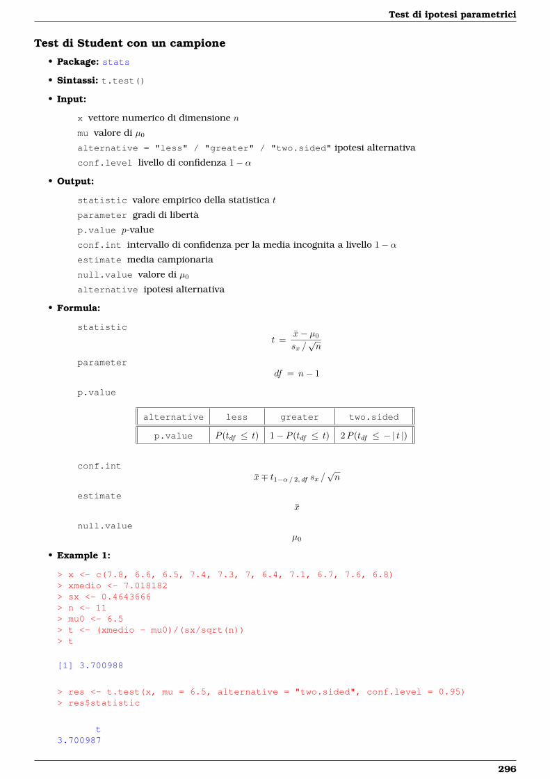
Test di ipotesi parametrici
Test di Student con un campione
• Package: stats
• Sintassi: t.test()
• Input:
x vettore numerico di dimensione n
mu valore di µ0
alternative = "less" / "greater" / "two.sided" ipotesi alternativa
conf.level livello di confidenza 1− α
• Output:
statistic valore empirico della statistica t
parameter gradi di libertà
p.value p-value
conf.int intervallo di confidenza per la media incognita a livello 1− αestimate media campionaria
null.value valore di µ0
alternative ipotesi alternativa
• Formula:
statistic
t =x− µ0
sx /√n
parameterdf = n− 1
p.value
alternative less greater two.sided
p.value P (tdf ≤ t) 1− P (tdf ≤ t) 2P (tdf ≤ − | t |)
conf.intx∓ t1−α/ 2, df sx /
√n
estimatex
null.valueµ0
• Example 1:
> x <- c(7.8, 6.6, 6.5, 7.4, 7.3, 7, 6.4, 7.1, 6.7, 7.6, 6.8)> xmedio <- 7.018182> sx <- 0.4643666> n <- 11> mu0 <- 6.5> t <- (xmedio - mu0)/(sx/sqrt(n))> t
[1] 3.700988
> res <- t.test(x, mu = 6.5, alternative = "two.sided", conf.level = 0.95)> res$statistic
t3.700987
296
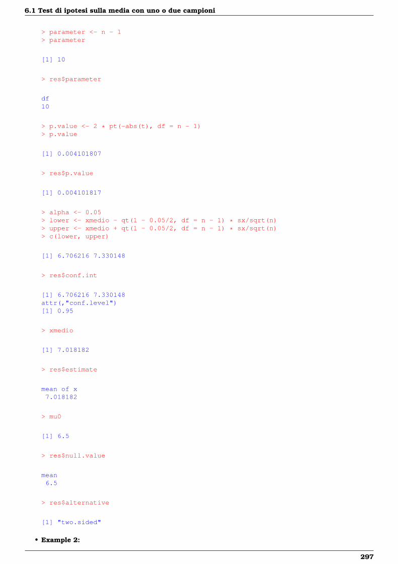
6.1 Test di ipotesi sulla media con uno o due campioni
> parameter <- n - 1> parameter
[1] 10
> res$parameter
df10
> p.value <- 2 * pt(-abs(t), df = n - 1)> p.value
[1] 0.004101807
> res$p.value
[1] 0.004101817
> alpha <- 0.05> lower <- xmedio - qt(1 - 0.05/2, df = n - 1) * sx/sqrt(n)> upper <- xmedio + qt(1 - 0.05/2, df = n - 1) * sx/sqrt(n)> c(lower, upper)
[1] 6.706216 7.330148
> res$conf.int
[1] 6.706216 7.330148attr(,"conf.level")[1] 0.95
> xmedio
[1] 7.018182
> res$estimate
mean of x7.018182
> mu0
[1] 6.5
> res$null.value
mean6.5
> res$alternative
[1] "two.sided"
• Example 2:
297
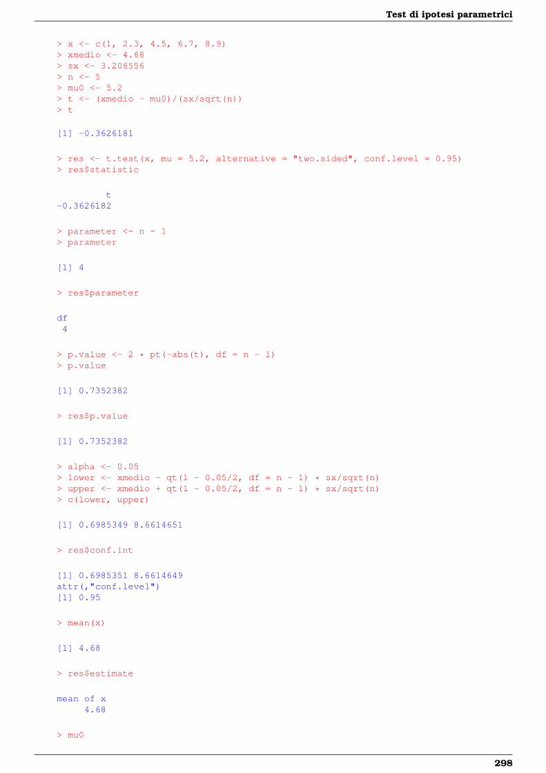
Test di ipotesi parametrici
> x <- c(1, 2.3, 4.5, 6.7, 8.9)> xmedio <- 4.68> sx <- 3.206556> n <- 5> mu0 <- 5.2> t <- (xmedio - mu0)/(sx/sqrt(n))> t
[1] -0.3626181
> res <- t.test(x, mu = 5.2, alternative = "two.sided", conf.level = 0.95)> res$statistic
t-0.3626182
> parameter <- n - 1> parameter
[1] 4
> res$parameter
df4
> p.value <- 2 * pt(-abs(t), df = n - 1)> p.value
[1] 0.7352382
> res$p.value
[1] 0.7352382
> alpha <- 0.05> lower <- xmedio - qt(1 - 0.05/2, df = n - 1) * sx/sqrt(n)> upper <- xmedio + qt(1 - 0.05/2, df = n - 1) * sx/sqrt(n)> c(lower, upper)
[1] 0.6985349 8.6614651
> res$conf.int
[1] 0.6985351 8.6614649attr(,"conf.level")[1] 0.95
> mean(x)
[1] 4.68
> res$estimate
mean of x4.68
> mu0
298
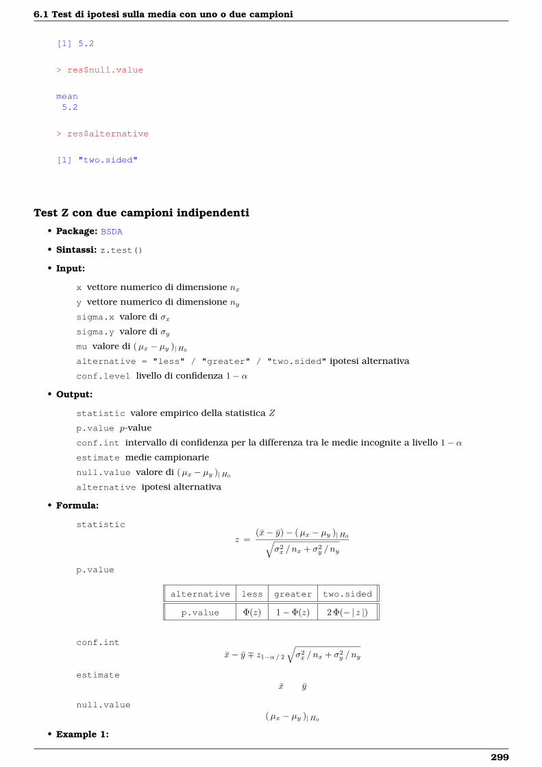
6.1 Test di ipotesi sulla media con uno o due campioni
[1] 5.2
> res$null.value
mean5.2
> res$alternative
[1] "two.sided"
Test Z con due campioni indipendenti
• Package: BSDA
• Sintassi: z.test()
• Input:
x vettore numerico di dimensione nxy vettore numerico di dimensione nysigma.x valore di σxsigma.y valore di σymu valore di (µx − µy )|H0
alternative = "less" / "greater" / "two.sided" ipotesi alternativa
conf.level livello di confidenza 1− α
• Output:
statistic valore empirico della statistica Z
p.value p-value
conf.int intervallo di confidenza per la differenza tra le medie incognite a livello 1− αestimate medie campionarie
null.value valore di (µx − µy )|H0
alternative ipotesi alternativa
• Formula:
statistic
z =(x− y)− (µx − µy )|H0√
σ2x / nx + σ2
y / ny
p.value
alternative less greater two.sided
p.value Φ(z) 1− Φ(z) 2 Φ(− | z |)
conf.int
x− y ∓ z1−α/ 2
√σ2x / nx + σ2
y / ny
estimatex y
null.value(µx − µy )|H0
• Example 1:
299
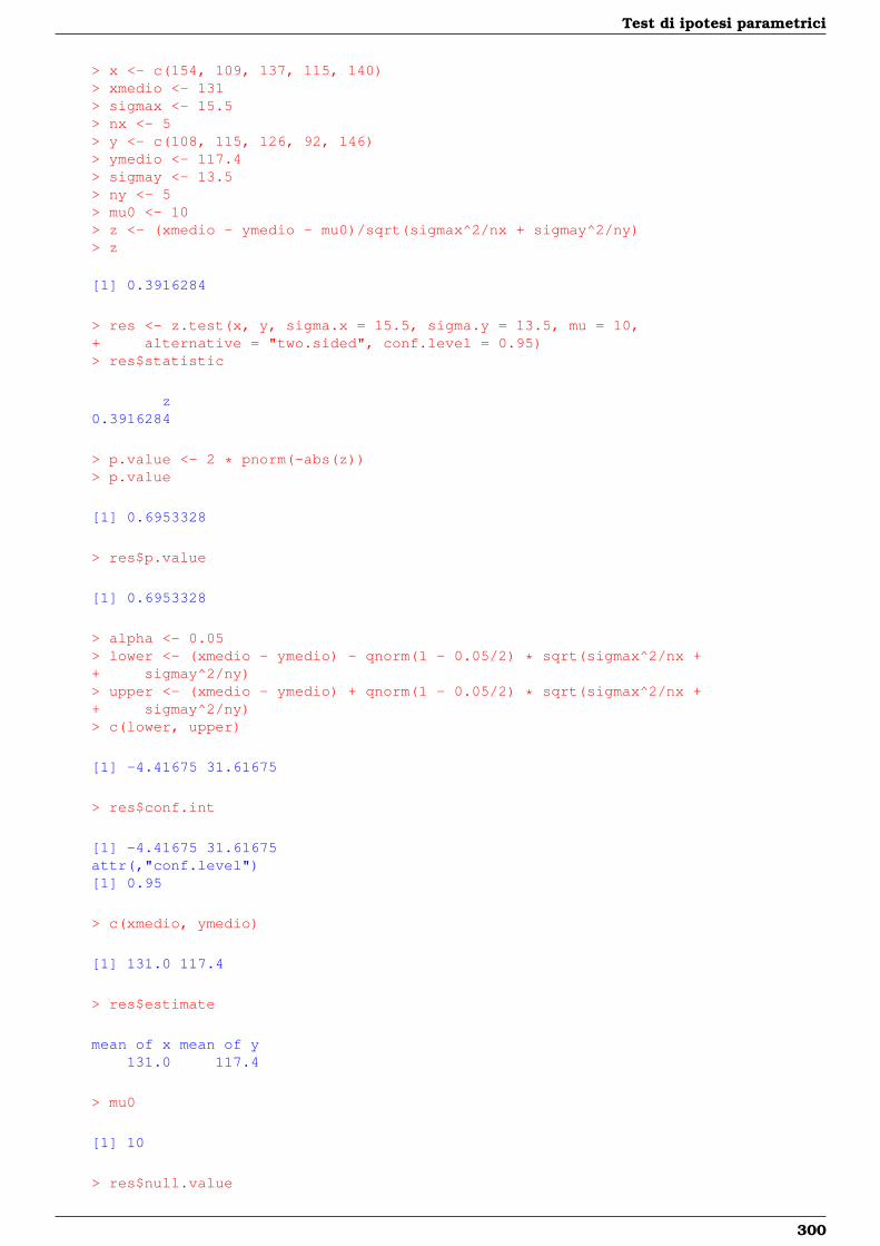
Test di ipotesi parametrici
> x <- c(154, 109, 137, 115, 140)> xmedio <- 131> sigmax <- 15.5> nx <- 5> y <- c(108, 115, 126, 92, 146)> ymedio <- 117.4> sigmay <- 13.5> ny <- 5> mu0 <- 10> z <- (xmedio - ymedio - mu0)/sqrt(sigmax^2/nx + sigmay^2/ny)> z
[1] 0.3916284
> res <- z.test(x, y, sigma.x = 15.5, sigma.y = 13.5, mu = 10,+ alternative = "two.sided", conf.level = 0.95)> res$statistic
z0.3916284
> p.value <- 2 * pnorm(-abs(z))> p.value
[1] 0.6953328
> res$p.value
[1] 0.6953328
> alpha <- 0.05> lower <- (xmedio - ymedio) - qnorm(1 - 0.05/2) * sqrt(sigmax^2/nx ++ sigmay^2/ny)> upper <- (xmedio - ymedio) + qnorm(1 - 0.05/2) * sqrt(sigmax^2/nx ++ sigmay^2/ny)> c(lower, upper)
[1] -4.41675 31.61675
> res$conf.int
[1] -4.41675 31.61675attr(,"conf.level")[1] 0.95
> c(xmedio, ymedio)
[1] 131.0 117.4
> res$estimate
mean of x mean of y131.0 117.4
> mu0
[1] 10
> res$null.value
300
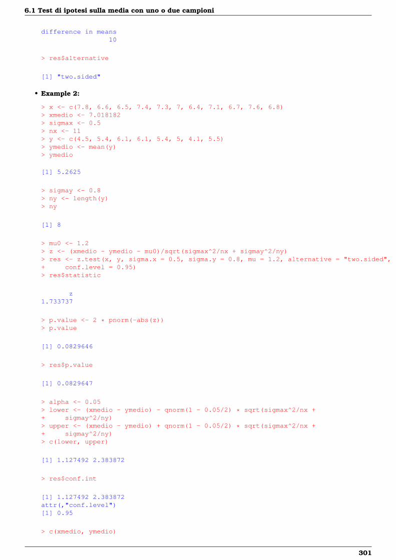
6.1 Test di ipotesi sulla media con uno o due campioni
difference in means10
> res$alternative
[1] "two.sided"
• Example 2:
> x <- c(7.8, 6.6, 6.5, 7.4, 7.3, 7, 6.4, 7.1, 6.7, 7.6, 6.8)> xmedio <- 7.018182> sigmax <- 0.5> nx <- 11> y <- c(4.5, 5.4, 6.1, 6.1, 5.4, 5, 4.1, 5.5)> ymedio <- mean(y)> ymedio
[1] 5.2625
> sigmay <- 0.8> ny <- length(y)> ny
[1] 8
> mu0 <- 1.2> z <- (xmedio - ymedio - mu0)/sqrt(sigmax^2/nx + sigmay^2/ny)> res <- z.test(x, y, sigma.x = 0.5, sigma.y = 0.8, mu = 1.2, alternative = "two.sided",+ conf.level = 0.95)> res$statistic
z1.733737
> p.value <- 2 * pnorm(-abs(z))> p.value
[1] 0.0829646
> res$p.value
[1] 0.0829647
> alpha <- 0.05> lower <- (xmedio - ymedio) - qnorm(1 - 0.05/2) * sqrt(sigmax^2/nx ++ sigmay^2/ny)> upper <- (xmedio - ymedio) + qnorm(1 - 0.05/2) * sqrt(sigmax^2/nx ++ sigmay^2/ny)> c(lower, upper)
[1] 1.127492 2.383872
> res$conf.int
[1] 1.127492 2.383872attr(,"conf.level")[1] 0.95
> c(xmedio, ymedio)
301

Test di ipotesi parametrici
[1] 7.018182 5.262500
> res$estimate
mean of x mean of y7.018182 5.262500
> mu0
[1] 1.2
> res$null.value
difference in means1.2
> res$alternative
[1] "two.sided"
Test di Student con due campioni indipendenti con varianze non note e supposteuguali
• Package: stats
• Sintassi: t.test()
• Input:
x vettore numerico di dimensione nxy vettore numerico di dimensione nymu valore di (µx − µy )|H0
alternative = "less" / "greater" / "two.sided" ipotesi alternativa
conf.level livello di confidenza 1− αvar.equal = TRUE
• Output:
statistic valore empirico della statistica t
parameter gradi di libertà
p.value p-value
conf.int intervallo di confidenza per la differenza tra le medie incognite a livello 1− αestimate medie campionarie
null.value valore di (µx − µy )|H0
alternative ipotesi alternativa
• Formula:
statistic
t =(x− y)− (µx − µy )|H0
sP√
1 / nx + 1 / ny
dove s2P =
(nx − 1) s2x + (ny − 1) s2
y
nx + ny − 2
parameterdf = nx + ny − 2
p.value
302
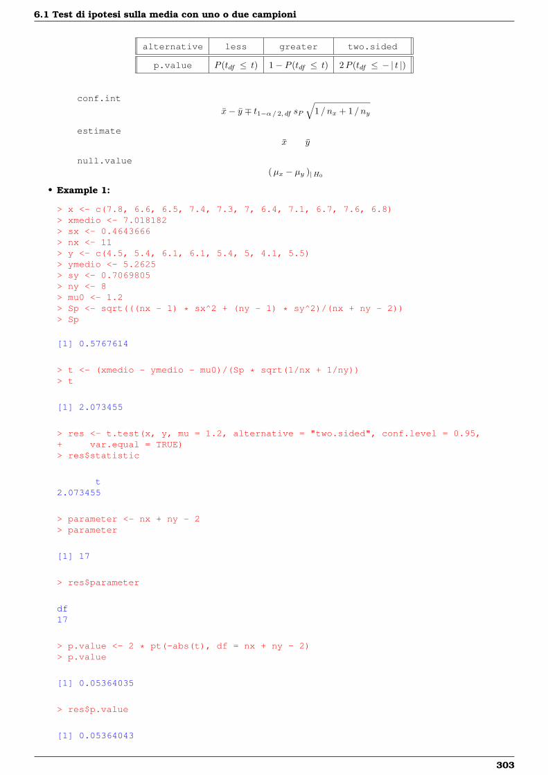
6.1 Test di ipotesi sulla media con uno o due campioni
alternative less greater two.sided
p.value P (tdf ≤ t) 1− P (tdf ≤ t) 2P (tdf ≤ − | t |)
conf.int
x− y ∓ t1−α/ 2, df sP
√1 / nx + 1 / ny
estimatex y
null.value(µx − µy )|H0
• Example 1:
> x <- c(7.8, 6.6, 6.5, 7.4, 7.3, 7, 6.4, 7.1, 6.7, 7.6, 6.8)> xmedio <- 7.018182> sx <- 0.4643666> nx <- 11> y <- c(4.5, 5.4, 6.1, 6.1, 5.4, 5, 4.1, 5.5)> ymedio <- 5.2625> sy <- 0.7069805> ny <- 8> mu0 <- 1.2> Sp <- sqrt(((nx - 1) * sx^2 + (ny - 1) * sy^2)/(nx + ny - 2))> Sp
[1] 0.5767614
> t <- (xmedio - ymedio - mu0)/(Sp * sqrt(1/nx + 1/ny))> t
[1] 2.073455
> res <- t.test(x, y, mu = 1.2, alternative = "two.sided", conf.level = 0.95,+ var.equal = TRUE)> res$statistic
t2.073455
> parameter <- nx + ny - 2> parameter
[1] 17
> res$parameter
df17
> p.value <- 2 * pt(-abs(t), df = nx + ny - 2)> p.value
[1] 0.05364035
> res$p.value
[1] 0.05364043
303
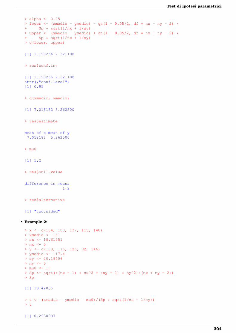
Test di ipotesi parametrici
> alpha <- 0.05> lower <- (xmedio - ymedio) - qt(1 - 0.05/2, df = nx + ny - 2) *+ Sp * sqrt(1/nx + 1/ny)> upper <- (xmedio - ymedio) + qt(1 - 0.05/2, df = nx + ny - 2) *+ Sp * sqrt(1/nx + 1/ny)> c(lower, upper)
[1] 1.190256 2.321108
> res$conf.int
[1] 1.190255 2.321108attr(,"conf.level")[1] 0.95
> c(xmedio, ymedio)
[1] 7.018182 5.262500
> res$estimate
mean of x mean of y7.018182 5.262500
> mu0
[1] 1.2
> res$null.value
difference in means1.2
> res$alternative
[1] "two.sided"
• Example 2:
> x <- c(154, 109, 137, 115, 140)> xmedio <- 131> sx <- 18.61451> nx <- 5> y <- c(108, 115, 126, 92, 146)> ymedio <- 117.4> sy <- 20.19406> ny <- 5> mu0 <- 10> Sp <- sqrt(((nx - 1) * sx^2 + (ny - 1) * sy^2)/(nx + ny - 2))> Sp
[1] 19.42035
> t <- (xmedio - ymedio - mu0)/(Sp * sqrt(1/nx + 1/ny))> t
[1] 0.2930997
304
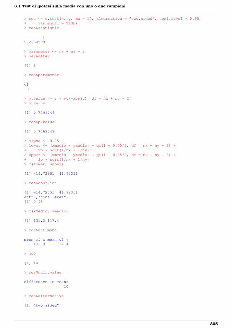
6.1 Test di ipotesi sulla media con uno o due campioni
> res <- t.test(x, y, mu = 10, alternative = "two.sided", conf.level = 0.95,+ var.equal = TRUE)> res$statistic
t0.2930998
> parameter <- nx + ny - 2> parameter
[1] 8
> res$parameter
df8
> p.value <- 2 * pt(-abs(t), df = nx + ny - 2)> p.value
[1] 0.7769049
> res$p.value
[1] 0.7769049
> alpha <- 0.05> lower <- (xmedio - ymedio) - qt(1 - 0.05/2, df = nx + ny - 2) *+ Sp * sqrt(1/nx + 1/ny)> upper <- (xmedio - ymedio) + qt(1 - 0.05/2, df = nx + ny - 2) *+ Sp * sqrt(1/nx + 1/ny)> c(lower, upper)
[1] -14.72351 41.92351
> res$conf.int
[1] -14.72351 41.92351attr(,"conf.level")[1] 0.95
> c(xmedio, ymedio)
[1] 131.0 117.4
> res$estimate
mean of x mean of y131.0 117.4
> mu0
[1] 10
> res$null.value
difference in means10
> res$alternative
[1] "two.sided"
305
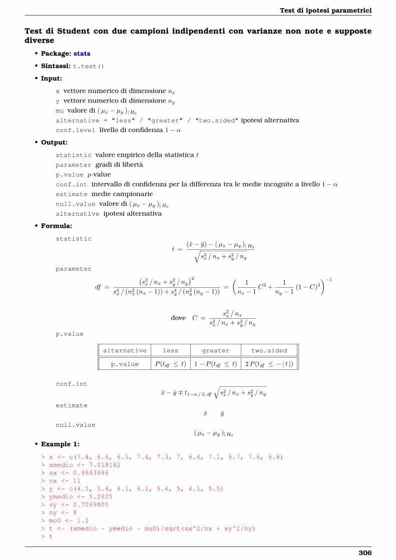
Test di ipotesi parametrici
Test di Student con due campioni indipendenti con varianze non note e suppostediverse
• Package: stats
• Sintassi: t.test()
• Input:
x vettore numerico di dimensione nxy vettore numerico di dimensione nymu valore di (µx − µy )|H0
alternative = "less" / "greater" / "two.sided" ipotesi alternativaconf.level livello di confidenza 1− α
• Output:
statistic valore empirico della statistica t
parameter gradi di libertàp.value p-valueconf.int intervallo di confidenza per la differenza tra le medie incognite a livello 1− αestimate medie campionarienull.value valore di (µx − µy )|H0
alternative ipotesi alternativa
• Formula:
statistic
t =(x− y)− (µx − µy )|H0√
s2x / nx + s2
y / ny
parameter
df =
(s2x / nx + s2
y / ny)2
s4x / (n2
x (nx − 1)) + s4y / (n2
y (ny − 1))=(
1nx − 1
C2 +1
ny − 1(1− C)2
)−1
dove C =s2x / nx
s2x / nx + s2
y / ny
p.value
alternative less greater two.sided
p.value P (tdf ≤ t) 1− P (tdf ≤ t) 2P (tdf ≤ − | t |)
conf.int
x− y ∓ t1−α/ 2, df
√s2x / nx + s2
y / ny
estimatex y
null.value(µx − µy )|H0
• Example 1:
> x <- c(7.8, 6.6, 6.5, 7.4, 7.3, 7, 6.4, 7.1, 6.7, 7.6, 6.8)> xmedio <- 7.018182> sx <- 0.4643666> nx <- 11> y <- c(4.5, 5.4, 6.1, 6.1, 5.4, 5, 4.1, 5.5)> ymedio <- 5.2625> sy <- 0.7069805> ny <- 8> mu0 <- 1.2> t <- (xmedio - ymedio - mu0)/sqrt(sx^2/nx + sy^2/ny)> t
306
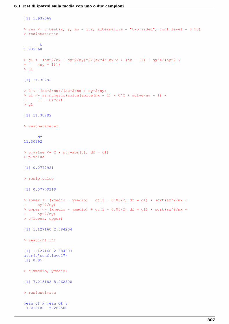
6.1 Test di ipotesi sulla media con uno o due campioni
[1] 1.939568
> res <- t.test(x, y, mu = 1.2, alternative = "two.sided", conf.level = 0.95)> res$statistic
t1.939568
> gl <- (sx^2/nx + sy^2/ny)^2/(sx^4/(nx^2 * (nx - 1)) + sy^4/(ny^2 *+ (ny - 1)))> gl
[1] 11.30292
> C <- (sx^2/nx)/(sx^2/nx + sy^2/ny)> gl <- as.numeric(solve(solve(nx - 1) * C^2 + solve(ny - 1) *+ (1 - C)^2))> gl
[1] 11.30292
> res$parameter
df11.30292
> p.value <- 2 * pt(-abs(t), df = gl)> p.value
[1] 0.0777921
> res$p.value
[1] 0.07779219
> lower <- (xmedio - ymedio) - qt(1 - 0.05/2, df = gl) * sqrt(sx^2/nx ++ sy^2/ny)> upper <- (xmedio - ymedio) + qt(1 - 0.05/2, df = gl) * sqrt(sx^2/nx ++ sy^2/ny)> c(lower, upper)
[1] 1.127160 2.384204
> res$conf.int
[1] 1.127160 2.384203attr(,"conf.level")[1] 0.95
> c(xmedio, ymedio)
[1] 7.018182 5.262500
> res$estimate
mean of x mean of y7.018182 5.262500
307
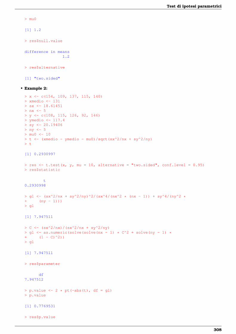
Test di ipotesi parametrici
> mu0
[1] 1.2
> res$null.value
difference in means1.2
> res$alternative
[1] "two.sided"
• Example 2:
> x <- c(154, 109, 137, 115, 140)> xmedio <- 131> sx <- 18.61451> nx <- 5> y <- c(108, 115, 126, 92, 146)> ymedio <- 117.4> sy <- 20.19406> ny <- 5> mu0 <- 10> t <- (xmedio - ymedio - mu0)/sqrt(sx^2/nx + sy^2/ny)> t
[1] 0.2930997
> res <- t.test(x, y, mu = 10, alternative = "two.sided", conf.level = 0.95)> res$statistic
t0.2930998
> gl <- (sx^2/nx + sy^2/ny)^2/(sx^4/(nx^2 * (nx - 1)) + sy^4/(ny^2 *+ (ny - 1)))> gl
[1] 7.947511
> C <- (sx^2/nx)/(sx^2/nx + sy^2/ny)> gl <- as.numeric(solve(solve(nx - 1) * C^2 + solve(ny - 1) *+ (1 - C)^2))> gl
[1] 7.947511
> res$parameter
df7.947512
> p.value <- 2 * pt(-abs(t), df = gl)> p.value
[1] 0.7769531
> res$p.value
308
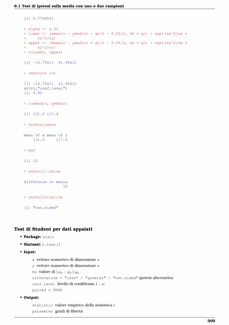
6.1 Test di ipotesi sulla media con uno o due campioni
[1] 0.7769531
> alpha <- 0.05> lower <- (xmedio - ymedio) - qt(1 - 0.05/2, df = gl) * sqrt(sx^2/nx ++ sy^2/ny)> upper <- (xmedio - ymedio) + qt(1 - 0.05/2, df = gl) * sqrt(sx^2/nx ++ sy^2/ny)> c(lower, upper)
[1] -14.75611 41.95611
> res$conf.int
[1] -14.75611 41.95611attr(,"conf.level")[1] 0.95
> c(xmedio, ymedio)
[1] 131.0 117.4
> res$estimate
mean of x mean of y131.0 117.4
> mu0
[1] 10
> res$null.value
difference in means10
> res$alternative
[1] "two.sided"
Test di Student per dati appaiati
• Package: stats
• Sintassi: t.test()
• Input:
x vettore numerico di dimensione n
y vettore numerico di dimensione n
mu valore di (µx − µy )|H0
alternative = "less" / "greater" / "two.sided" ipotesi alternativa
conf.level livello di confidenza 1− αpaired = TRUE
• Output:
statistic valore empirico della statistica t
parameter gradi di libertà
309
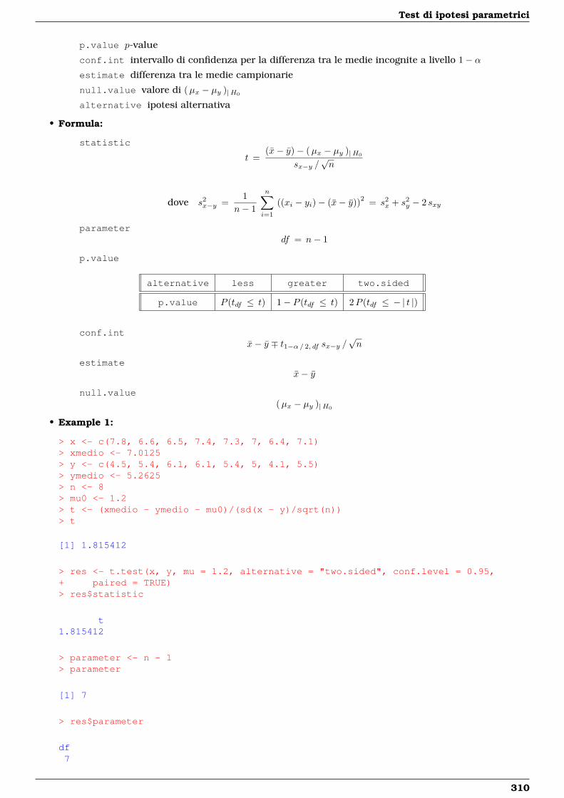
Test di ipotesi parametrici
p.value p-value
conf.int intervallo di confidenza per la differenza tra le medie incognite a livello 1− αestimate differenza tra le medie campionarie
null.value valore di (µx − µy )|H0
alternative ipotesi alternativa
• Formula:
statistic
t =(x− y)− (µx − µy )|H0
sx−y /√n
dove s2x−y =
1n− 1
n∑i=1
((xi − yi)− (x− y))2 = s2x + s2
y − 2 sxy
parameterdf = n− 1
p.value
alternative less greater two.sided
p.value P (tdf ≤ t) 1− P (tdf ≤ t) 2P (tdf ≤ − | t |)
conf.intx− y ∓ t1−α/ 2, df sx−y /
√n
estimatex− y
null.value(µx − µy )|H0
• Example 1:
> x <- c(7.8, 6.6, 6.5, 7.4, 7.3, 7, 6.4, 7.1)> xmedio <- 7.0125> y <- c(4.5, 5.4, 6.1, 6.1, 5.4, 5, 4.1, 5.5)> ymedio <- 5.2625> n <- 8> mu0 <- 1.2> t <- (xmedio - ymedio - mu0)/(sd(x - y)/sqrt(n))> t
[1] 1.815412
> res <- t.test(x, y, mu = 1.2, alternative = "two.sided", conf.level = 0.95,+ paired = TRUE)> res$statistic
t1.815412
> parameter <- n - 1> parameter
[1] 7
> res$parameter
df7
310
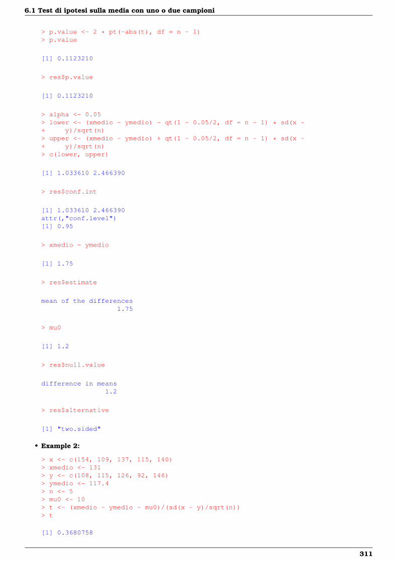
6.1 Test di ipotesi sulla media con uno o due campioni
> p.value <- 2 * pt(-abs(t), df = n - 1)> p.value
[1] 0.1123210
> res$p.value
[1] 0.1123210
> alpha <- 0.05> lower <- (xmedio - ymedio) - qt(1 - 0.05/2, df = n - 1) * sd(x -+ y)/sqrt(n)> upper <- (xmedio - ymedio) + qt(1 - 0.05/2, df = n - 1) * sd(x -+ y)/sqrt(n)> c(lower, upper)
[1] 1.033610 2.466390
> res$conf.int
[1] 1.033610 2.466390attr(,"conf.level")[1] 0.95
> xmedio - ymedio
[1] 1.75
> res$estimate
mean of the differences1.75
> mu0
[1] 1.2
> res$null.value
difference in means1.2
> res$alternative
[1] "two.sided"
• Example 2:
> x <- c(154, 109, 137, 115, 140)> xmedio <- 131> y <- c(108, 115, 126, 92, 146)> ymedio <- 117.4> n <- 5> mu0 <- 10> t <- (xmedio - ymedio - mu0)/(sd(x - y)/sqrt(n))> t
[1] 0.3680758
311
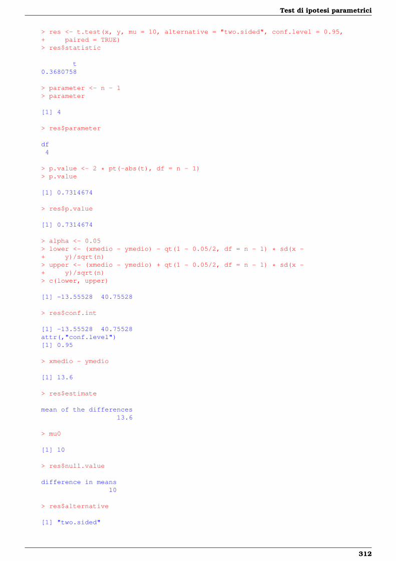
Test di ipotesi parametrici
> res <- t.test(x, y, mu = 10, alternative = "two.sided", conf.level = 0.95,+ paired = TRUE)> res$statistic
t0.3680758
> parameter <- n - 1> parameter
[1] 4
> res$parameter
df4
> p.value <- 2 * pt(-abs(t), df = n - 1)> p.value
[1] 0.7314674
> res$p.value
[1] 0.7314674
> alpha <- 0.05> lower <- (xmedio - ymedio) - qt(1 - 0.05/2, df = n - 1) * sd(x -+ y)/sqrt(n)> upper <- (xmedio - ymedio) + qt(1 - 0.05/2, df = n - 1) * sd(x -+ y)/sqrt(n)> c(lower, upper)
[1] -13.55528 40.75528
> res$conf.int
[1] -13.55528 40.75528attr(,"conf.level")[1] 0.95
> xmedio - ymedio
[1] 13.6
> res$estimate
mean of the differences13.6
> mu0
[1] 10
> res$null.value
difference in means10
> res$alternative
[1] "two.sided"
312
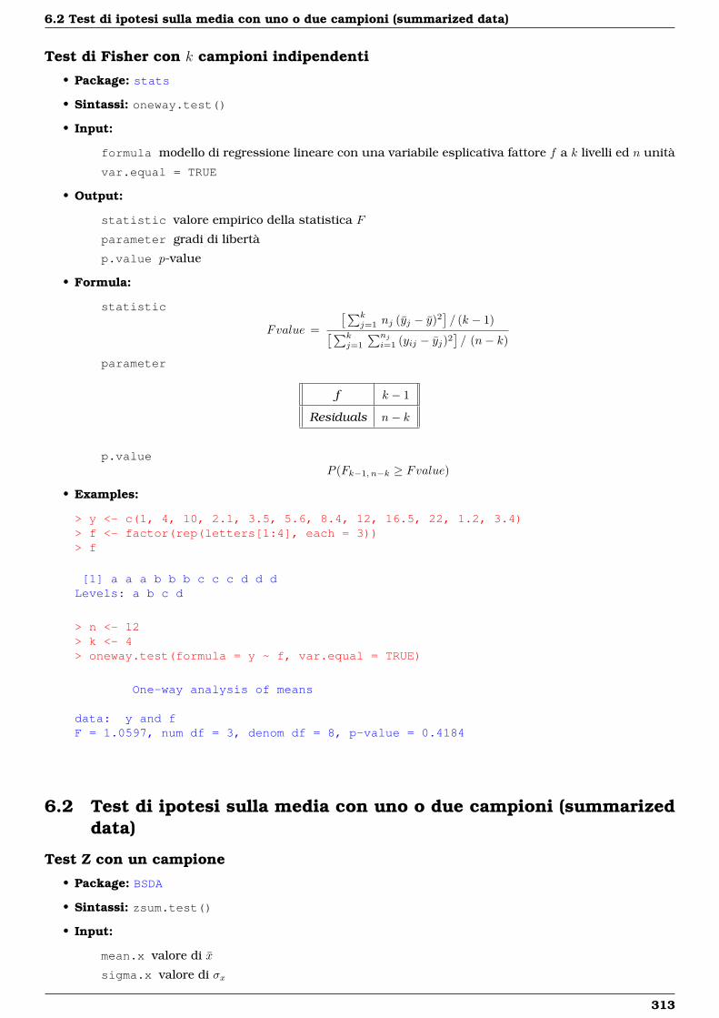
6.2 Test di ipotesi sulla media con uno o due campioni (summarized data)
Test di Fisher con k campioni indipendenti
• Package: stats
• Sintassi: oneway.test()
• Input:
formula modello di regressione lineare con una variabile esplicativa fattore f a k livelli ed n unità
var.equal = TRUE
• Output:
statistic valore empirico della statistica F
parameter gradi di libertà
p.value p-value
• Formula:
statistic
Fvalue =
[∑kj=1 nj (yj − y)2
]/ (k − 1)[∑k
j=1
∑nji=1 (yij − yj)2
]/ (n− k)
parameter
f k − 1
Residuals n− k
p.valueP (Fk−1, n−k ≥ Fvalue)
• Examples:
> y <- c(1, 4, 10, 2.1, 3.5, 5.6, 8.4, 12, 16.5, 22, 1.2, 3.4)> f <- factor(rep(letters[1:4], each = 3))> f
[1] a a a b b b c c c d d dLevels: a b c d
> n <- 12> k <- 4> oneway.test(formula = y ~ f, var.equal = TRUE)
One-way analysis of means
data: y and fF = 1.0597, num df = 3, denom df = 8, p-value = 0.4184
6.2 Test di ipotesi sulla media con uno o due campioni (summarizeddata)
Test Z con un campione
• Package: BSDA
• Sintassi: zsum.test()
• Input:
mean.x valore di x
sigma.x valore di σx
313
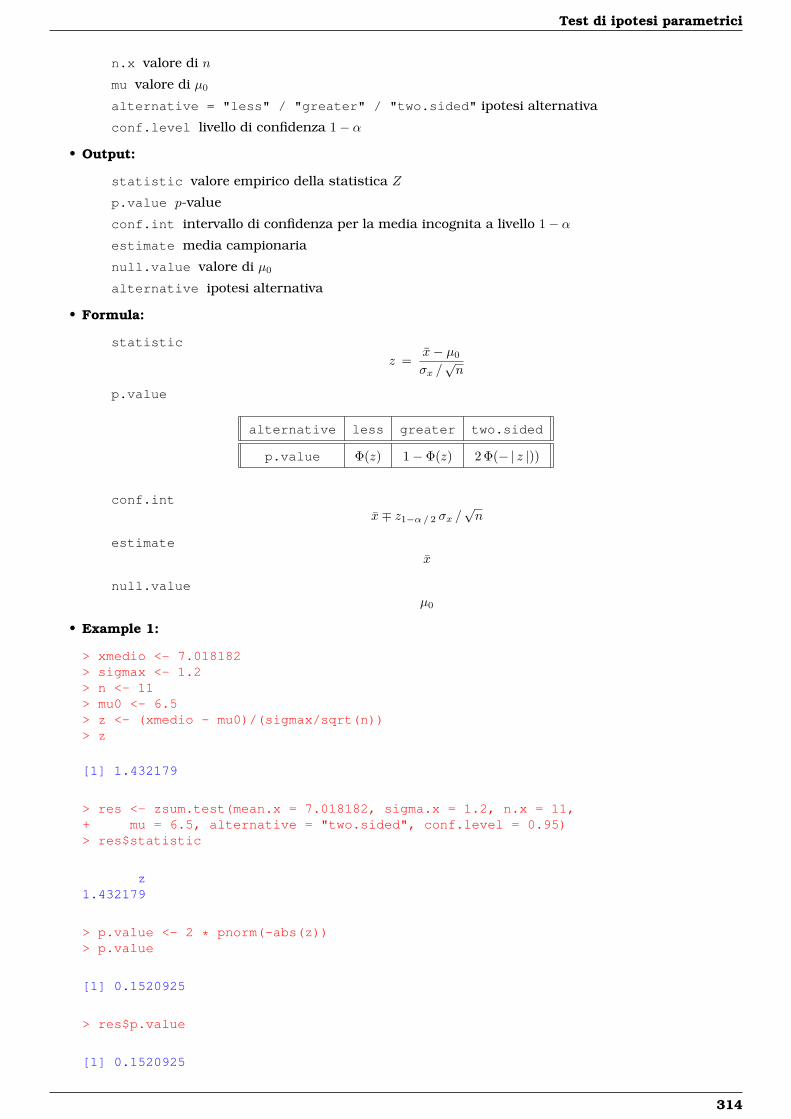
Test di ipotesi parametrici
n.x valore di n
mu valore di µ0
alternative = "less" / "greater" / "two.sided" ipotesi alternativa
conf.level livello di confidenza 1− α
• Output:
statistic valore empirico della statistica Z
p.value p-value
conf.int intervallo di confidenza per la media incognita a livello 1− αestimate media campionaria
null.value valore di µ0
alternative ipotesi alternativa
• Formula:
statistic
z =x− µ0
σx /√n
p.value
alternative less greater two.sided
p.value Φ(z) 1− Φ(z) 2 Φ(− | z |))
conf.intx∓ z1−α/ 2 σx /
√n
estimatex
null.valueµ0
• Example 1:
> xmedio <- 7.018182> sigmax <- 1.2> n <- 11> mu0 <- 6.5> z <- (xmedio - mu0)/(sigmax/sqrt(n))> z
[1] 1.432179
> res <- zsum.test(mean.x = 7.018182, sigma.x = 1.2, n.x = 11,+ mu = 6.5, alternative = "two.sided", conf.level = 0.95)> res$statistic
z1.432179
> p.value <- 2 * pnorm(-abs(z))> p.value
[1] 0.1520925
> res$p.value
[1] 0.1520925
314
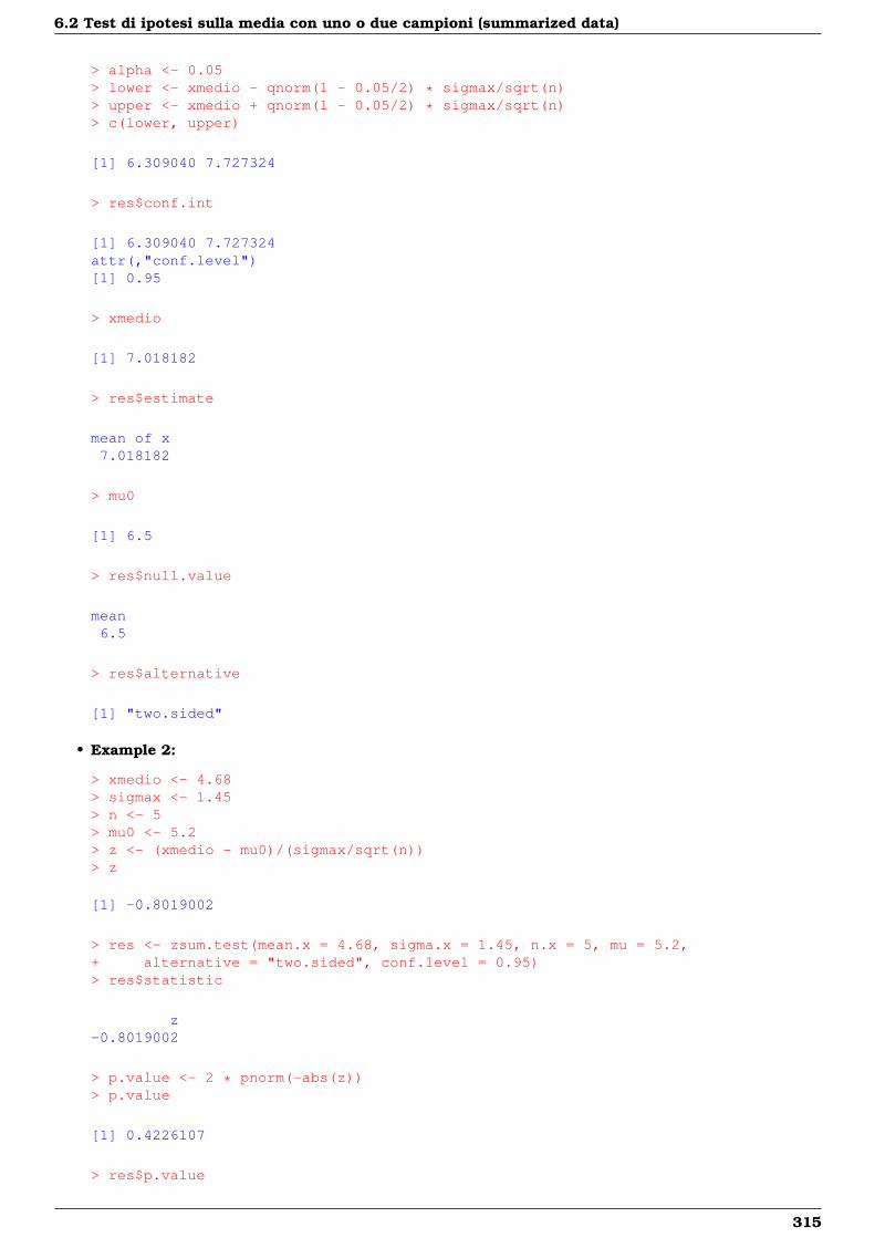
6.2 Test di ipotesi sulla media con uno o due campioni (summarized data)
> alpha <- 0.05> lower <- xmedio - qnorm(1 - 0.05/2) * sigmax/sqrt(n)> upper <- xmedio + qnorm(1 - 0.05/2) * sigmax/sqrt(n)> c(lower, upper)
[1] 6.309040 7.727324
> res$conf.int
[1] 6.309040 7.727324attr(,"conf.level")[1] 0.95
> xmedio
[1] 7.018182
> res$estimate
mean of x7.018182
> mu0
[1] 6.5
> res$null.value
mean6.5
> res$alternative
[1] "two.sided"
• Example 2:
> xmedio <- 4.68> sigmax <- 1.45> n <- 5> mu0 <- 5.2> z <- (xmedio - mu0)/(sigmax/sqrt(n))> z
[1] -0.8019002
> res <- zsum.test(mean.x = 4.68, sigma.x = 1.45, n.x = 5, mu = 5.2,+ alternative = "two.sided", conf.level = 0.95)> res$statistic
z-0.8019002
> p.value <- 2 * pnorm(-abs(z))> p.value
[1] 0.4226107
> res$p.value
315

Test di ipotesi parametrici
[1] 0.4226107
> alpha <- 0.05> lower <- xmedio - qnorm(1 - 0.05/2) * sigmax/sqrt(n)> upper <- xmedio + qnorm(1 - 0.05/2) * sigmax/sqrt(n)> c(lower, upper)
[1] 3.409042 5.950958
> res$conf.int
[1] 3.409042 5.950958attr(,"conf.level")[1] 0.95
> xmedio
[1] 4.68
> res$estimate
mean of x4.68
> mu0
[1] 5.2
> res$null.value
mean5.2
> res$alternative
[1] "two.sided"
Test di Student con un campione
• Package: BSDA
• Sintassi: tsum.test()
• Input:
mean.x valore di x
s.x valore di sxn.x valore di n
mu valore di µ0
alternative = "less" / "greater" / "two.sided" ipotesi alternativa
conf.level livello di confidenza 1− α
• Output:
statistic valore empirico della statistica t
parameter gradi di libertà
p.value p-value
316
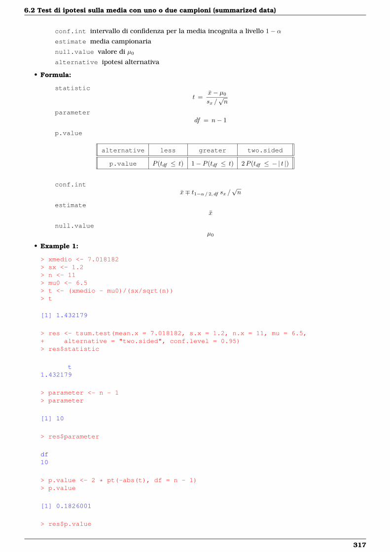
6.2 Test di ipotesi sulla media con uno o due campioni (summarized data)
conf.int intervallo di confidenza per la media incognita a livello 1− αestimate media campionaria
null.value valore di µ0
alternative ipotesi alternativa
• Formula:
statistic
t =x− µ0
sx /√n
parameterdf = n− 1
p.value
alternative less greater two.sided
p.value P (tdf ≤ t) 1− P (tdf ≤ t) 2P (tdf ≤ − | t |)
conf.intx∓ t1−α/ 2, df sx /
√n
estimatex
null.valueµ0
• Example 1:
> xmedio <- 7.018182> sx <- 1.2> n <- 11> mu0 <- 6.5> t <- (xmedio - mu0)/(sx/sqrt(n))> t
[1] 1.432179
> res <- tsum.test(mean.x = 7.018182, s.x = 1.2, n.x = 11, mu = 6.5,+ alternative = "two.sided", conf.level = 0.95)> res$statistic
t1.432179
> parameter <- n - 1> parameter
[1] 10
> res$parameter
df10
> p.value <- 2 * pt(-abs(t), df = n - 1)> p.value
[1] 0.1826001
> res$p.value
317
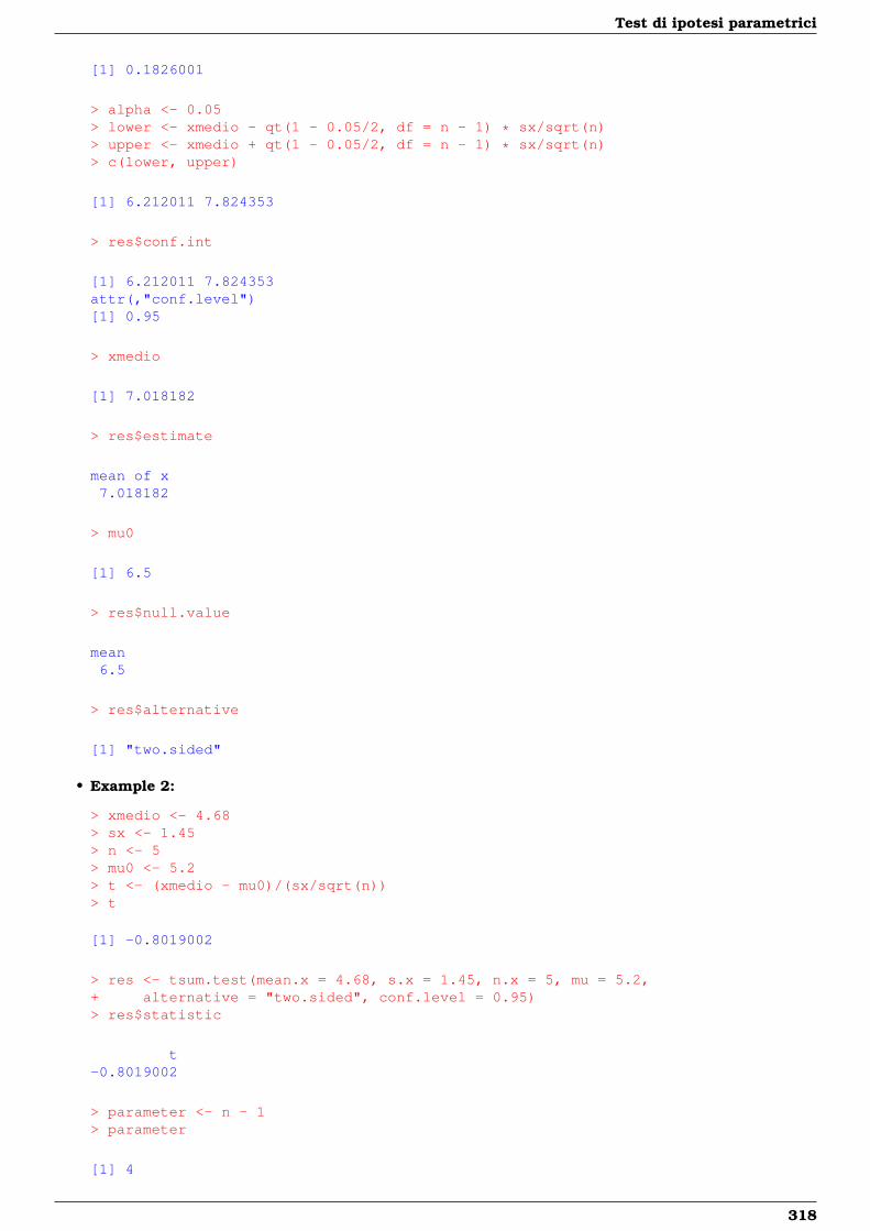
Test di ipotesi parametrici
[1] 0.1826001
> alpha <- 0.05> lower <- xmedio - qt(1 - 0.05/2, df = n - 1) * sx/sqrt(n)> upper <- xmedio + qt(1 - 0.05/2, df = n - 1) * sx/sqrt(n)> c(lower, upper)
[1] 6.212011 7.824353
> res$conf.int
[1] 6.212011 7.824353attr(,"conf.level")[1] 0.95
> xmedio
[1] 7.018182
> res$estimate
mean of x7.018182
> mu0
[1] 6.5
> res$null.value
mean6.5
> res$alternative
[1] "two.sided"
• Example 2:
> xmedio <- 4.68> sx <- 1.45> n <- 5> mu0 <- 5.2> t <- (xmedio - mu0)/(sx/sqrt(n))> t
[1] -0.8019002
> res <- tsum.test(mean.x = 4.68, s.x = 1.45, n.x = 5, mu = 5.2,+ alternative = "two.sided", conf.level = 0.95)> res$statistic
t-0.8019002
> parameter <- n - 1> parameter
[1] 4
318
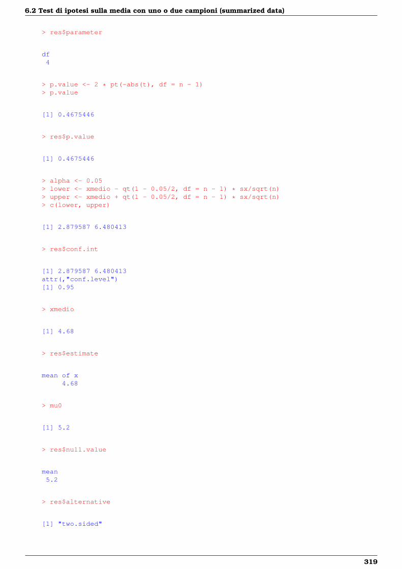
6.2 Test di ipotesi sulla media con uno o due campioni (summarized data)
> res$parameter
df4
> p.value <- 2 * pt(-abs(t), df = n - 1)> p.value
[1] 0.4675446
> res$p.value
[1] 0.4675446
> alpha <- 0.05> lower <- xmedio - qt(1 - 0.05/2, df = n - 1) * sx/sqrt(n)> upper <- xmedio + qt(1 - 0.05/2, df = n - 1) * sx/sqrt(n)> c(lower, upper)
[1] 2.879587 6.480413
> res$conf.int
[1] 2.879587 6.480413attr(,"conf.level")[1] 0.95
> xmedio
[1] 4.68
> res$estimate
mean of x4.68
> mu0
[1] 5.2
> res$null.value
mean5.2
> res$alternative
[1] "two.sided"
319
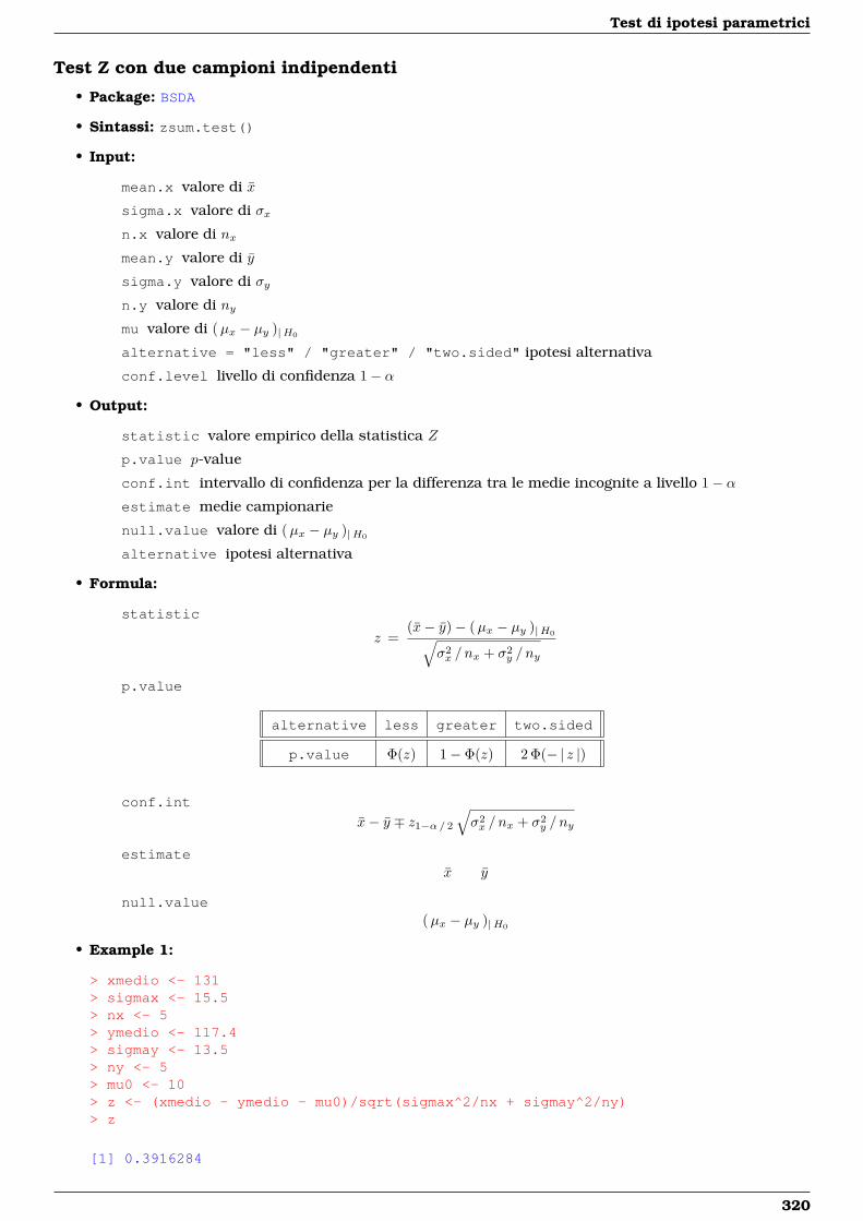
Test di ipotesi parametrici
Test Z con due campioni indipendenti
• Package: BSDA
• Sintassi: zsum.test()
• Input:
mean.x valore di x
sigma.x valore di σxn.x valore di nxmean.y valore di y
sigma.y valore di σyn.y valore di nymu valore di (µx − µy )|H0
alternative = "less" / "greater" / "two.sided" ipotesi alternativa
conf.level livello di confidenza 1− α
• Output:
statistic valore empirico della statistica Z
p.value p-value
conf.int intervallo di confidenza per la differenza tra le medie incognite a livello 1− αestimate medie campionarie
null.value valore di (µx − µy )|H0
alternative ipotesi alternativa
• Formula:
statistic
z =(x− y)− (µx − µy )|H0√
σ2x / nx + σ2
y / ny
p.value
alternative less greater two.sided
p.value Φ(z) 1− Φ(z) 2 Φ(− | z |)
conf.int
x− y ∓ z1−α/ 2
√σ2x / nx + σ2
y / ny
estimatex y
null.value(µx − µy )|H0
• Example 1:
> xmedio <- 131> sigmax <- 15.5> nx <- 5> ymedio <- 117.4> sigmay <- 13.5> ny <- 5> mu0 <- 10> z <- (xmedio - ymedio - mu0)/sqrt(sigmax^2/nx + sigmay^2/ny)> z
[1] 0.3916284
320
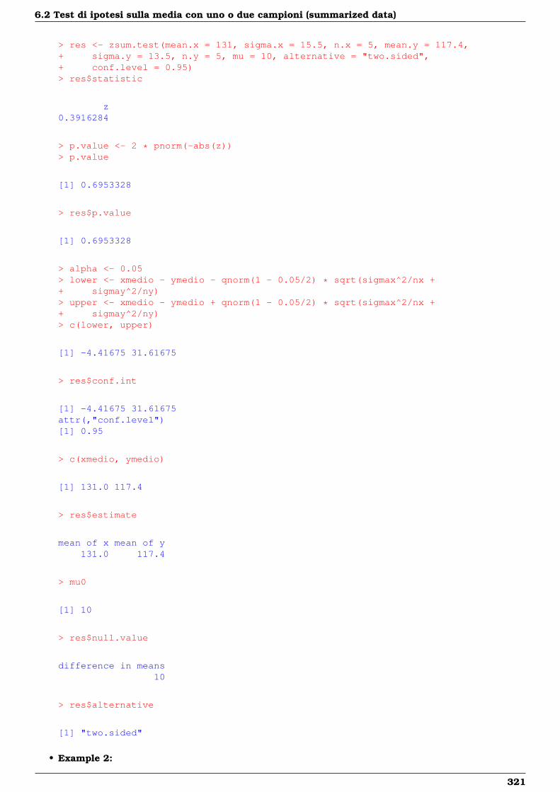
6.2 Test di ipotesi sulla media con uno o due campioni (summarized data)
> res <- zsum.test(mean.x = 131, sigma.x = 15.5, n.x = 5, mean.y = 117.4,+ sigma.y = 13.5, n.y = 5, mu = 10, alternative = "two.sided",+ conf.level = 0.95)> res$statistic
z0.3916284
> p.value <- 2 * pnorm(-abs(z))> p.value
[1] 0.6953328
> res$p.value
[1] 0.6953328
> alpha <- 0.05> lower <- xmedio - ymedio - qnorm(1 - 0.05/2) * sqrt(sigmax^2/nx ++ sigmay^2/ny)> upper <- xmedio - ymedio + qnorm(1 - 0.05/2) * sqrt(sigmax^2/nx ++ sigmay^2/ny)> c(lower, upper)
[1] -4.41675 31.61675
> res$conf.int
[1] -4.41675 31.61675attr(,"conf.level")[1] 0.95
> c(xmedio, ymedio)
[1] 131.0 117.4
> res$estimate
mean of x mean of y131.0 117.4
> mu0
[1] 10
> res$null.value
difference in means10
> res$alternative
[1] "two.sided"
• Example 2:
321
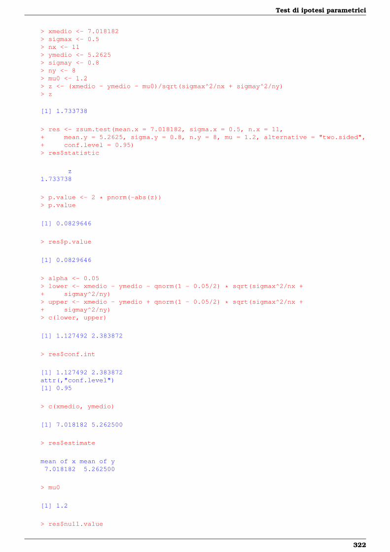
Test di ipotesi parametrici
> xmedio <- 7.018182> sigmax <- 0.5> nx <- 11> ymedio <- 5.2625> sigmay <- 0.8> ny <- 8> mu0 <- 1.2> z <- (xmedio - ymedio - mu0)/sqrt(sigmax^2/nx + sigmay^2/ny)> z
[1] 1.733738
> res <- zsum.test(mean.x = 7.018182, sigma.x = 0.5, n.x = 11,+ mean.y = 5.2625, sigma.y = 0.8, n.y = 8, mu = 1.2, alternative = "two.sided",+ conf.level = 0.95)> res$statistic
z1.733738
> p.value <- 2 * pnorm(-abs(z))> p.value
[1] 0.0829646
> res$p.value
[1] 0.0829646
> alpha <- 0.05> lower <- xmedio - ymedio - qnorm(1 - 0.05/2) * sqrt(sigmax^2/nx ++ sigmay^2/ny)> upper <- xmedio - ymedio + qnorm(1 - 0.05/2) * sqrt(sigmax^2/nx ++ sigmay^2/ny)> c(lower, upper)
[1] 1.127492 2.383872
> res$conf.int
[1] 1.127492 2.383872attr(,"conf.level")[1] 0.95
> c(xmedio, ymedio)
[1] 7.018182 5.262500
> res$estimate
mean of x mean of y7.018182 5.262500
> mu0
[1] 1.2
> res$null.value
322
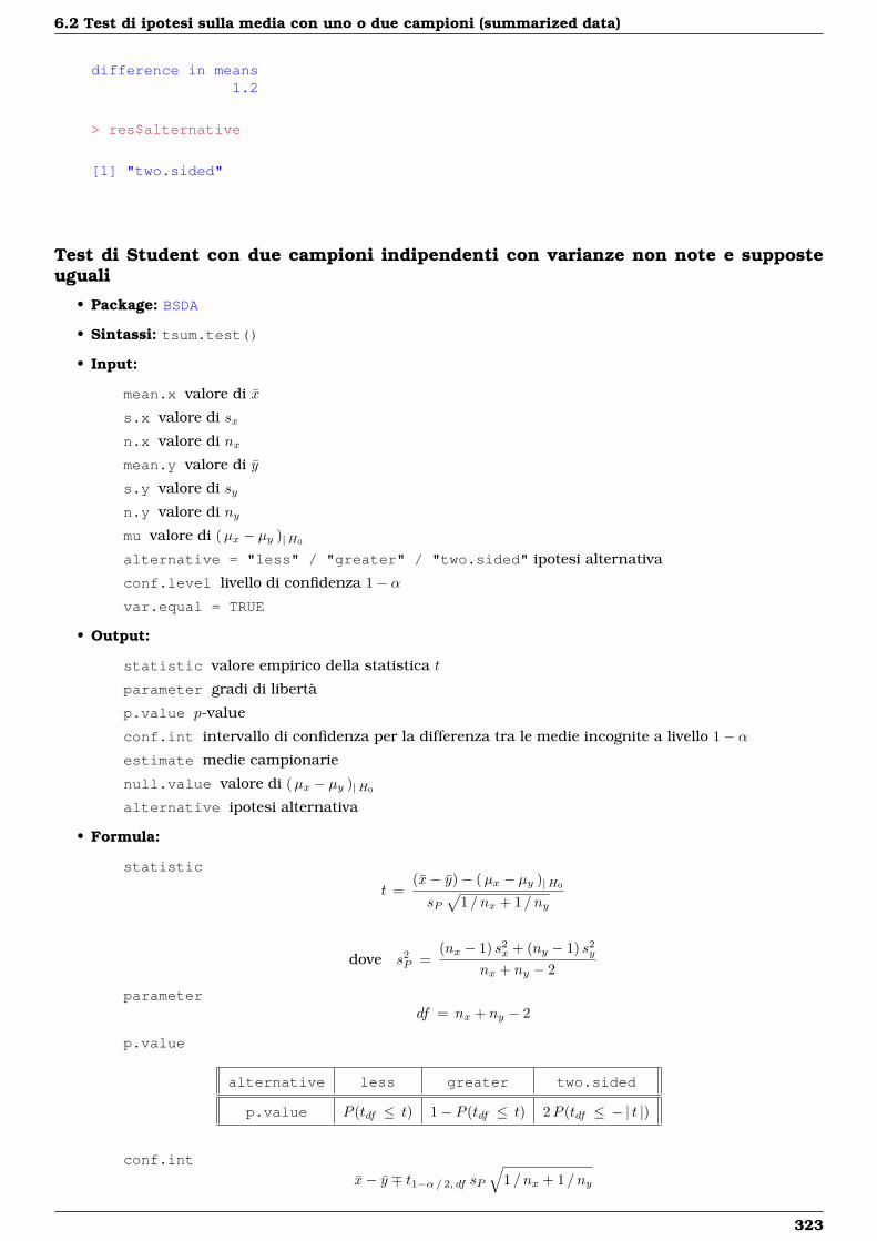
6.2 Test di ipotesi sulla media con uno o due campioni (summarized data)
difference in means1.2
> res$alternative
[1] "two.sided"
Test di Student con due campioni indipendenti con varianze non note e supposteuguali
• Package: BSDA
• Sintassi: tsum.test()
• Input:
mean.x valore di x
s.x valore di sxn.x valore di nxmean.y valore di y
s.y valore di syn.y valore di nymu valore di (µx − µy )|H0
alternative = "less" / "greater" / "two.sided" ipotesi alternativa
conf.level livello di confidenza 1− αvar.equal = TRUE
• Output:
statistic valore empirico della statistica t
parameter gradi di libertà
p.value p-value
conf.int intervallo di confidenza per la differenza tra le medie incognite a livello 1− αestimate medie campionarie
null.value valore di (µx − µy )|H0
alternative ipotesi alternativa
• Formula:
statistic
t =(x− y)− (µx − µy )|H0
sP√
1 / nx + 1 / ny
dove s2P =
(nx − 1) s2x + (ny − 1) s2
y
nx + ny − 2
parameterdf = nx + ny − 2
p.value
alternative less greater two.sided
p.value P (tdf ≤ t) 1− P (tdf ≤ t) 2P (tdf ≤ − | t |)
conf.int
x− y ∓ t1−α/ 2, df sP
√1 / nx + 1 / ny
323
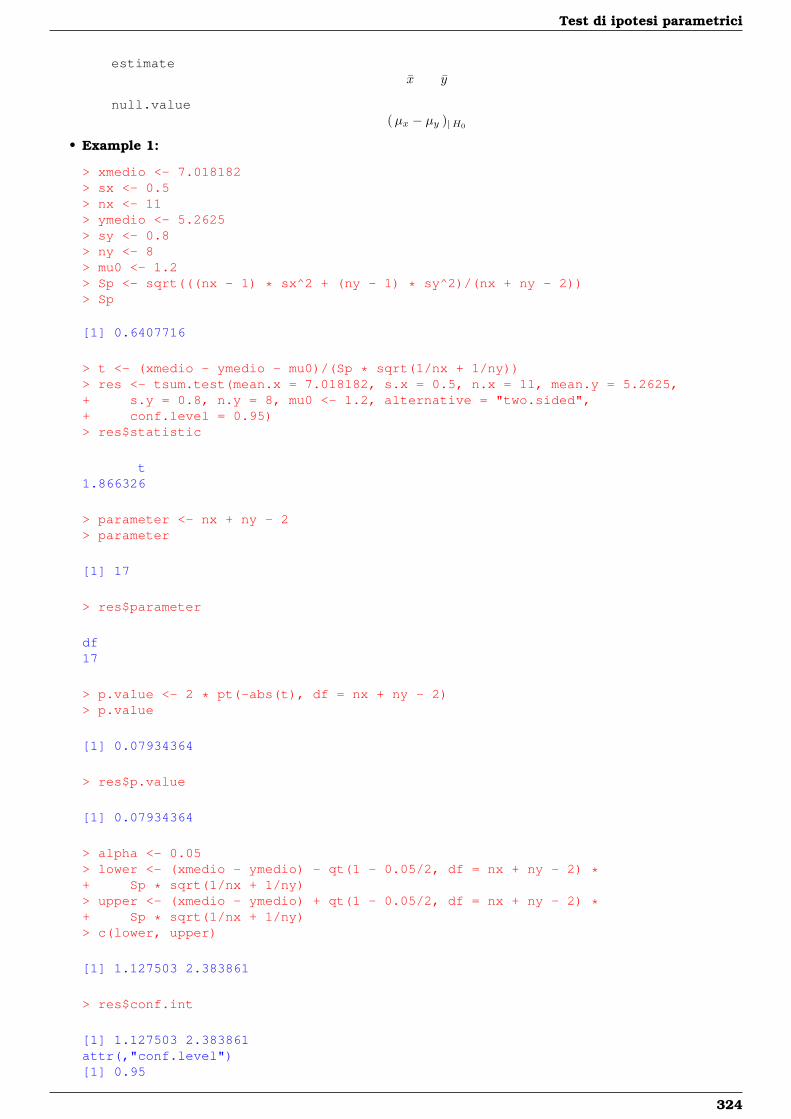
Test di ipotesi parametrici
estimatex y
null.value(µx − µy )|H0
• Example 1:
> xmedio <- 7.018182> sx <- 0.5> nx <- 11> ymedio <- 5.2625> sy <- 0.8> ny <- 8> mu0 <- 1.2> Sp <- sqrt(((nx - 1) * sx^2 + (ny - 1) * sy^2)/(nx + ny - 2))> Sp
[1] 0.6407716
> t <- (xmedio - ymedio - mu0)/(Sp * sqrt(1/nx + 1/ny))> res <- tsum.test(mean.x = 7.018182, s.x = 0.5, n.x = 11, mean.y = 5.2625,+ s.y = 0.8, n.y = 8, mu0 <- 1.2, alternative = "two.sided",+ conf.level = 0.95)> res$statistic
t1.866326
> parameter <- nx + ny - 2> parameter
[1] 17
> res$parameter
df17
> p.value <- 2 * pt(-abs(t), df = nx + ny - 2)> p.value
[1] 0.07934364
> res$p.value
[1] 0.07934364
> alpha <- 0.05> lower <- (xmedio - ymedio) - qt(1 - 0.05/2, df = nx + ny - 2) *+ Sp * sqrt(1/nx + 1/ny)> upper <- (xmedio - ymedio) + qt(1 - 0.05/2, df = nx + ny - 2) *+ Sp * sqrt(1/nx + 1/ny)> c(lower, upper)
[1] 1.127503 2.383861
> res$conf.int
[1] 1.127503 2.383861attr(,"conf.level")[1] 0.95
324
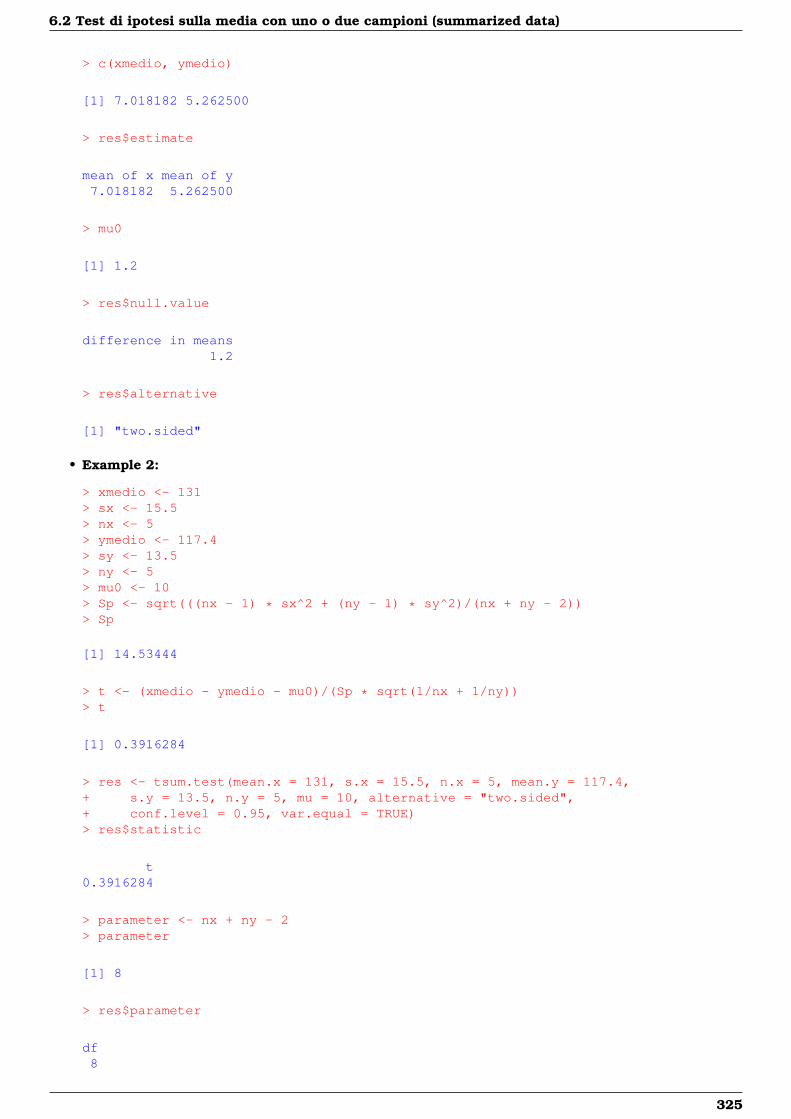
6.2 Test di ipotesi sulla media con uno o due campioni (summarized data)
> c(xmedio, ymedio)
[1] 7.018182 5.262500
> res$estimate
mean of x mean of y7.018182 5.262500
> mu0
[1] 1.2
> res$null.value
difference in means1.2
> res$alternative
[1] "two.sided"
• Example 2:
> xmedio <- 131> sx <- 15.5> nx <- 5> ymedio <- 117.4> sy <- 13.5> ny <- 5> mu0 <- 10> Sp <- sqrt(((nx - 1) * sx^2 + (ny - 1) * sy^2)/(nx + ny - 2))> Sp
[1] 14.53444
> t <- (xmedio - ymedio - mu0)/(Sp * sqrt(1/nx + 1/ny))> t
[1] 0.3916284
> res <- tsum.test(mean.x = 131, s.x = 15.5, n.x = 5, mean.y = 117.4,+ s.y = 13.5, n.y = 5, mu = 10, alternative = "two.sided",+ conf.level = 0.95, var.equal = TRUE)> res$statistic
t0.3916284
> parameter <- nx + ny - 2> parameter
[1] 8
> res$parameter
df8
325
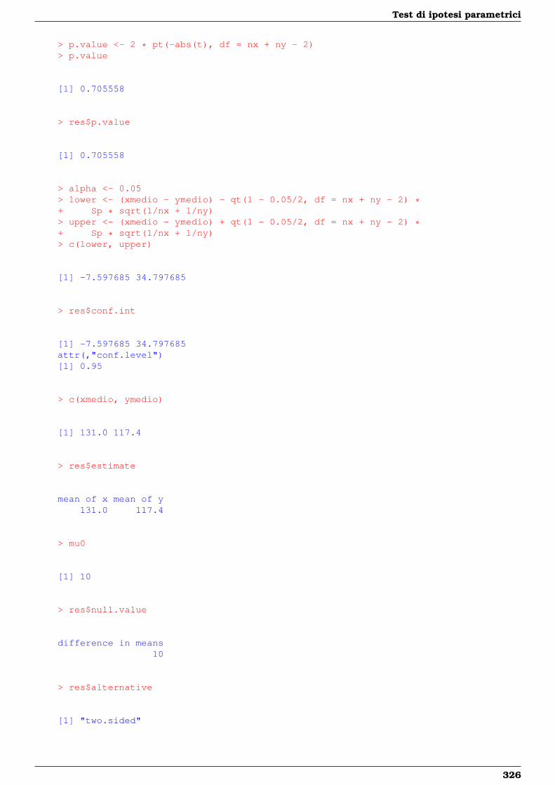
Test di ipotesi parametrici
> p.value <- 2 * pt(-abs(t), df = nx + ny - 2)> p.value
[1] 0.705558
> res$p.value
[1] 0.705558
> alpha <- 0.05> lower <- (xmedio - ymedio) - qt(1 - 0.05/2, df = nx + ny - 2) *+ Sp * sqrt(1/nx + 1/ny)> upper <- (xmedio - ymedio) + qt(1 - 0.05/2, df = nx + ny - 2) *+ Sp * sqrt(1/nx + 1/ny)> c(lower, upper)
[1] -7.597685 34.797685
> res$conf.int
[1] -7.597685 34.797685attr(,"conf.level")[1] 0.95
> c(xmedio, ymedio)
[1] 131.0 117.4
> res$estimate
mean of x mean of y131.0 117.4
> mu0
[1] 10
> res$null.value
difference in means10
> res$alternative
[1] "two.sided"
326
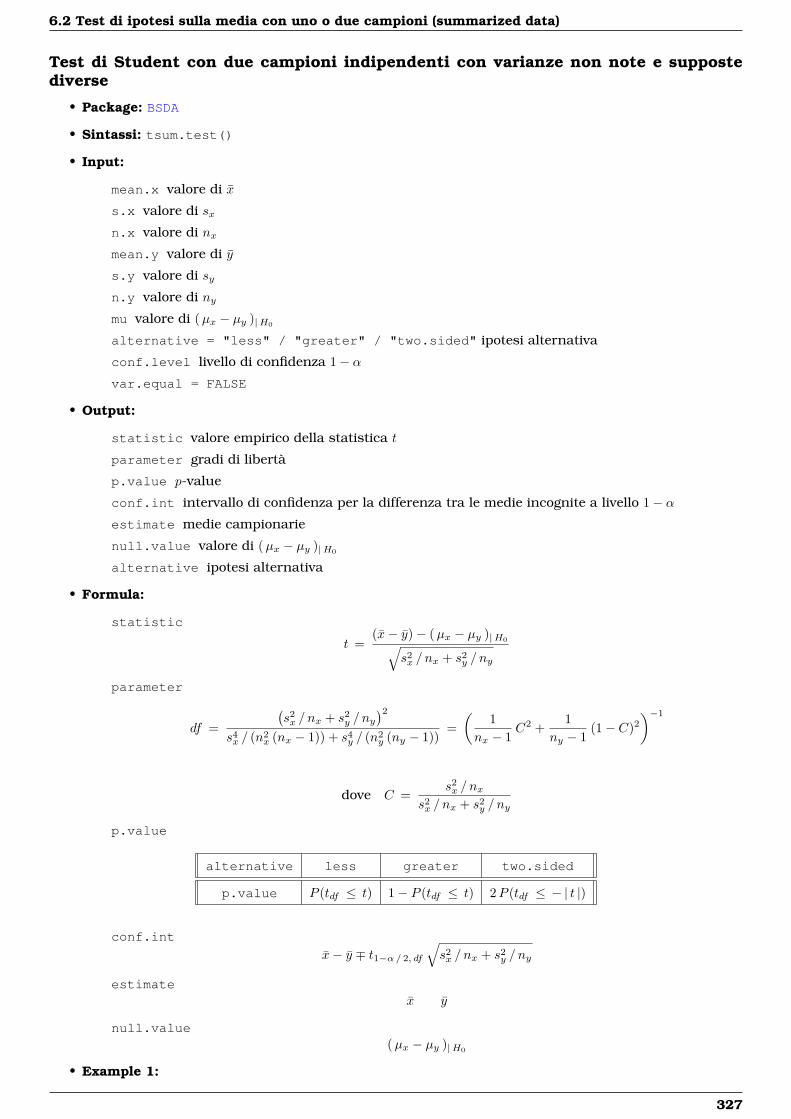
6.2 Test di ipotesi sulla media con uno o due campioni (summarized data)
Test di Student con due campioni indipendenti con varianze non note e suppostediverse
• Package: BSDA
• Sintassi: tsum.test()
• Input:
mean.x valore di x
s.x valore di sxn.x valore di nxmean.y valore di y
s.y valore di syn.y valore di nymu valore di (µx − µy )|H0
alternative = "less" / "greater" / "two.sided" ipotesi alternativa
conf.level livello di confidenza 1− αvar.equal = FALSE
• Output:
statistic valore empirico della statistica t
parameter gradi di libertà
p.value p-value
conf.int intervallo di confidenza per la differenza tra le medie incognite a livello 1− αestimate medie campionarie
null.value valore di (µx − µy )|H0
alternative ipotesi alternativa
• Formula:
statistic
t =(x− y)− (µx − µy )|H0√
s2x / nx + s2
y / ny
parameter
df =
(s2x / nx + s2
y / ny)2
s4x / (n2
x (nx − 1)) + s4y / (n2
y (ny − 1))=(
1nx − 1
C2 +1
ny − 1(1− C)2
)−1
dove C =s2x / nx
s2x / nx + s2
y / ny
p.value
alternative less greater two.sided
p.value P (tdf ≤ t) 1− P (tdf ≤ t) 2P (tdf ≤ − | t |)
conf.int
x− y ∓ t1−α/ 2, df
√s2x / nx + s2
y / ny
estimatex y
null.value(µx − µy )|H0
• Example 1:
327
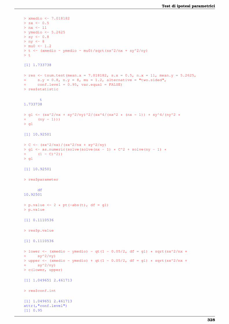
Test di ipotesi parametrici
> xmedio <- 7.018182> sx <- 0.5> nx <- 11> ymedio <- 5.2625> sy <- 0.8> ny <- 8> mu0 <- 1.2> t <- (xmedio - ymedio - mu0)/sqrt(sx^2/nx + sy^2/ny)> t
[1] 1.733738
> res <- tsum.test(mean.x = 7.018182, s.x = 0.5, n.x = 11, mean.y = 5.2625,+ s.y = 0.8, n.y = 8, mu = 1.2, alternative = "two.sided",+ conf.level = 0.95, var.equal = FALSE)> res$statistic
t1.733738
> gl <- (sx^2/nx + sy^2/ny)^2/(sx^4/(nx^2 * (nx - 1)) + sy^4/(ny^2 *+ (ny - 1)))> gl
[1] 10.92501
> C <- (sx^2/nx)/(sx^2/nx + sy^2/ny)> gl <- as.numeric(solve(solve(nx - 1) * C^2 + solve(ny - 1) *+ (1 - C)^2))> gl
[1] 10.92501
> res$parameter
df10.92501
> p.value <- 2 * pt(-abs(t), df = gl)> p.value
[1] 0.1110536
> res$p.value
[1] 0.1110536
> lower <- (xmedio - ymedio) - qt(1 - 0.05/2, df = gl) * sqrt(sx^2/nx ++ sy^2/ny)> upper <- (xmedio - ymedio) + qt(1 - 0.05/2, df = gl) * sqrt(sx^2/nx ++ sy^2/ny)> c(lower, upper)
[1] 1.049651 2.461713
> res$conf.int
[1] 1.049651 2.461713attr(,"conf.level")[1] 0.95
328
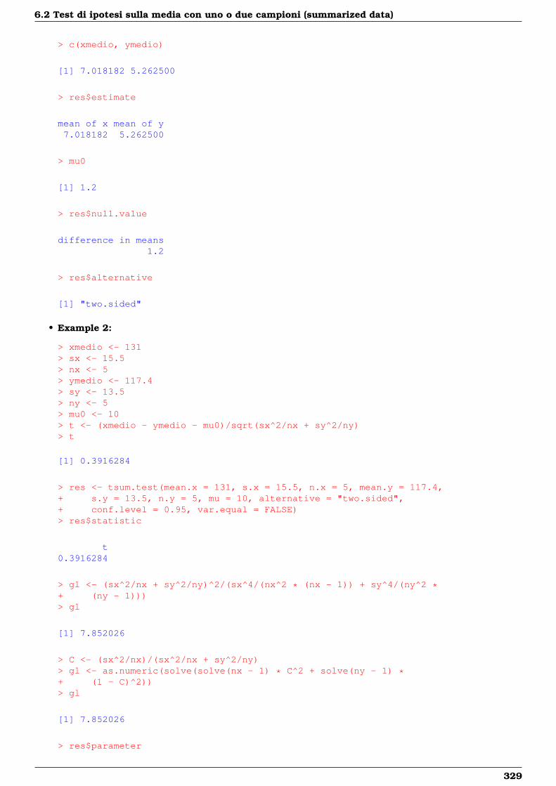
6.2 Test di ipotesi sulla media con uno o due campioni (summarized data)
> c(xmedio, ymedio)
[1] 7.018182 5.262500
> res$estimate
mean of x mean of y7.018182 5.262500
> mu0
[1] 1.2
> res$null.value
difference in means1.2
> res$alternative
[1] "two.sided"
• Example 2:
> xmedio <- 131> sx <- 15.5> nx <- 5> ymedio <- 117.4> sy <- 13.5> ny <- 5> mu0 <- 10> t <- (xmedio - ymedio - mu0)/sqrt(sx^2/nx + sy^2/ny)> t
[1] 0.3916284
> res <- tsum.test(mean.x = 131, s.x = 15.5, n.x = 5, mean.y = 117.4,+ s.y = 13.5, n.y = 5, mu = 10, alternative = "two.sided",+ conf.level = 0.95, var.equal = FALSE)> res$statistic
t0.3916284
> gl <- (sx^2/nx + sy^2/ny)^2/(sx^4/(nx^2 * (nx - 1)) + sy^4/(ny^2 *+ (ny - 1)))> gl
[1] 7.852026
> C <- (sx^2/nx)/(sx^2/nx + sy^2/ny)> gl <- as.numeric(solve(solve(nx - 1) * C^2 + solve(ny - 1) *+ (1 - C)^2))> gl
[1] 7.852026
> res$parameter
329
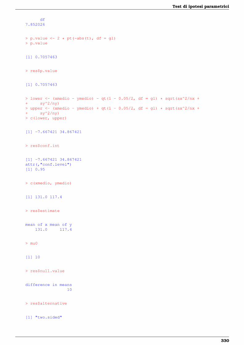
Test di ipotesi parametrici
df7.852026
> p.value <- 2 * pt(-abs(t), df = gl)> p.value
[1] 0.7057463
> res$p.value
[1] 0.7057463
> lower <- (xmedio - ymedio) - qt(1 - 0.05/2, df = gl) * sqrt(sx^2/nx ++ sy^2/ny)> upper <- (xmedio - ymedio) + qt(1 - 0.05/2, df = gl) * sqrt(sx^2/nx ++ sy^2/ny)> c(lower, upper)
[1] -7.667421 34.867421
> res$conf.int
[1] -7.667421 34.867421attr(,"conf.level")[1] 0.95
> c(xmedio, ymedio)
[1] 131.0 117.4
> res$estimate
mean of x mean of y131.0 117.4
> mu0
[1] 10
> res$null.value
difference in means10
> res$alternative
[1] "two.sided"
330
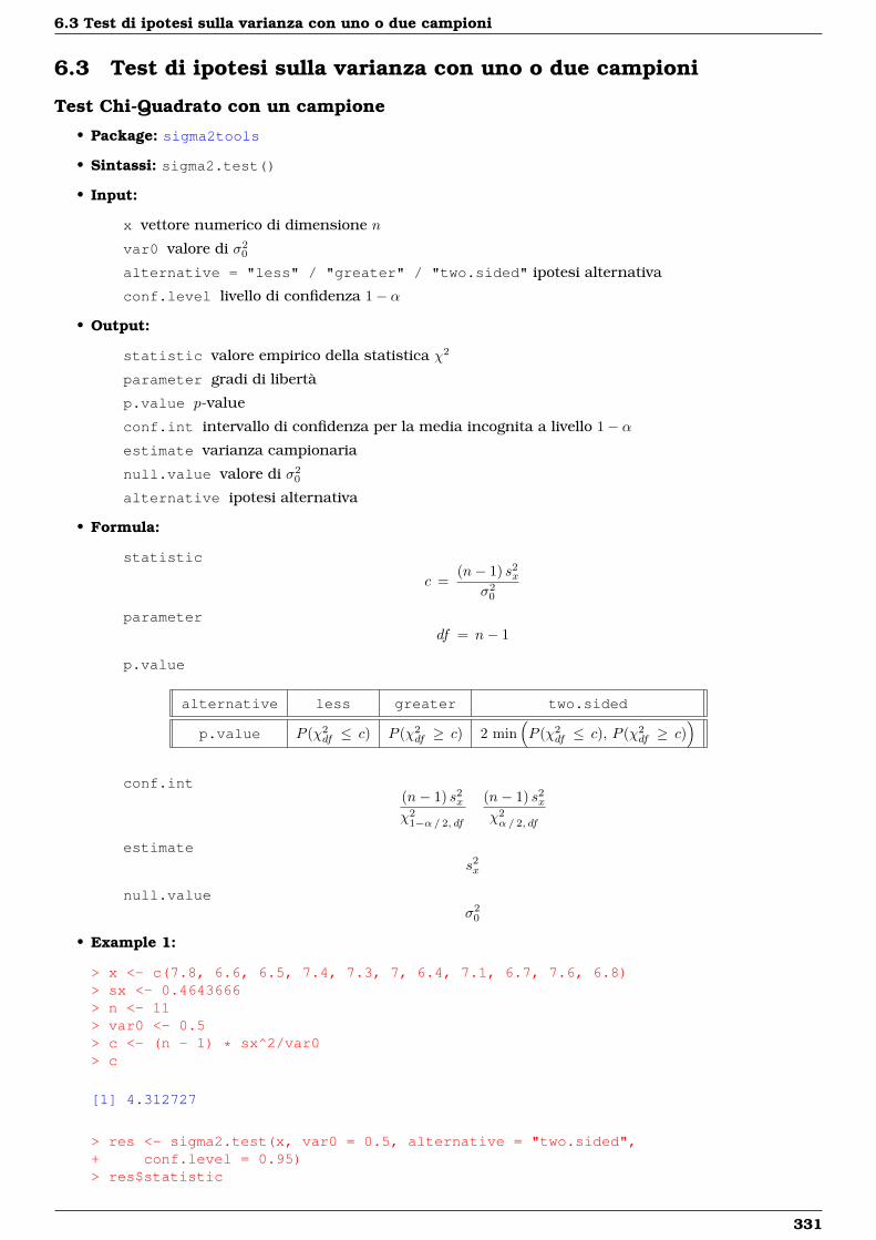
6.3 Test di ipotesi sulla varianza con uno o due campioni
6.3 Test di ipotesi sulla varianza con uno o due campioni
Test Chi-Quadrato con un campione
• Package: sigma2tools
• Sintassi: sigma2.test()
• Input:
x vettore numerico di dimensione n
var0 valore di σ20
alternative = "less" / "greater" / "two.sided" ipotesi alternativa
conf.level livello di confidenza 1− α
• Output:
statistic valore empirico della statistica χ2
parameter gradi di libertà
p.value p-value
conf.int intervallo di confidenza per la media incognita a livello 1− αestimate varianza campionaria
null.value valore di σ20
alternative ipotesi alternativa
• Formula:
statistic
c =(n− 1) s2
x
σ20
parameterdf = n− 1
p.value
alternative less greater two.sided
p.value P (χ2df ≤ c) P (χ2
df ≥ c) 2 min(P (χ2
df ≤ c), P (χ2df ≥ c)
)conf.int
(n− 1) s2x
χ21−α/ 2, df
(n− 1) s2x
χ2α/ 2, df
estimates2x
null.valueσ2
0
• Example 1:
> x <- c(7.8, 6.6, 6.5, 7.4, 7.3, 7, 6.4, 7.1, 6.7, 7.6, 6.8)> sx <- 0.4643666> n <- 11> var0 <- 0.5> c <- (n - 1) * sx^2/var0> c
[1] 4.312727
> res <- sigma2.test(x, var0 = 0.5, alternative = "two.sided",+ conf.level = 0.95)> res$statistic
331
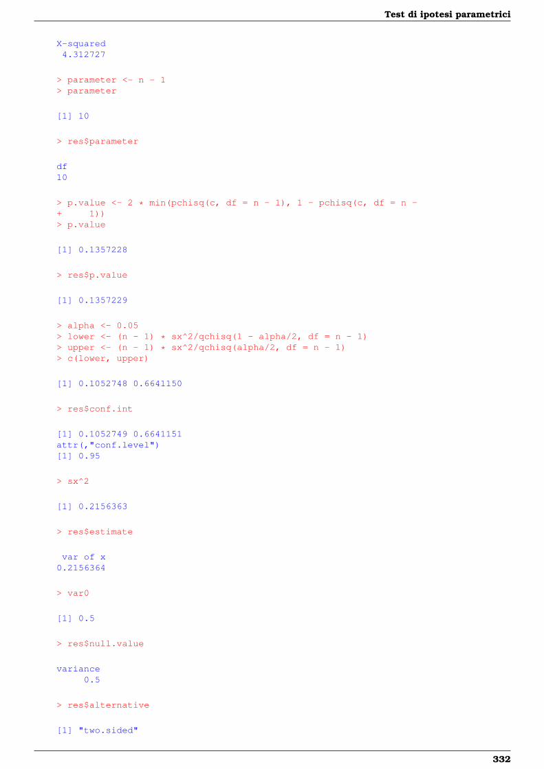
Test di ipotesi parametrici
X-squared4.312727
> parameter <- n - 1> parameter
[1] 10
> res$parameter
df10
> p.value <- 2 * min(pchisq(c, df = n - 1), 1 - pchisq(c, df = n -+ 1))> p.value
[1] 0.1357228
> res$p.value
[1] 0.1357229
> alpha <- 0.05> lower <- (n - 1) * sx^2/qchisq(1 - alpha/2, df = n - 1)> upper <- (n - 1) * sx^2/qchisq(alpha/2, df = n - 1)> c(lower, upper)
[1] 0.1052748 0.6641150
> res$conf.int
[1] 0.1052749 0.6641151attr(,"conf.level")[1] 0.95
> sx^2
[1] 0.2156363
> res$estimate
var of x0.2156364
> var0
[1] 0.5
> res$null.value
variance0.5
> res$alternative
[1] "two.sided"
332
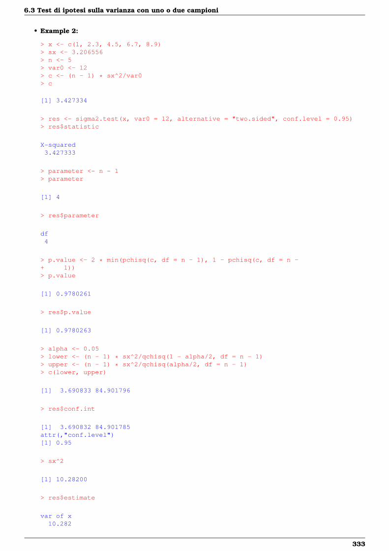
6.3 Test di ipotesi sulla varianza con uno o due campioni
• Example 2:
> x <- c(1, 2.3, 4.5, 6.7, 8.9)> sx <- 3.206556> n <- 5> var0 <- 12> c <- (n - 1) * sx^2/var0> c
[1] 3.427334
> res <- sigma2.test(x, var0 = 12, alternative = "two.sided", conf.level = 0.95)> res$statistic
X-squared3.427333
> parameter <- n - 1> parameter
[1] 4
> res$parameter
df4
> p.value <- 2 * min(pchisq(c, df = n - 1), 1 - pchisq(c, df = n -+ 1))> p.value
[1] 0.9780261
> res$p.value
[1] 0.9780263
> alpha <- 0.05> lower <- (n - 1) * sx^2/qchisq(1 - alpha/2, df = n - 1)> upper <- (n - 1) * sx^2/qchisq(alpha/2, df = n - 1)> c(lower, upper)
[1] 3.690833 84.901796
> res$conf.int
[1] 3.690832 84.901785attr(,"conf.level")[1] 0.95
> sx^2
[1] 10.28200
> res$estimate
var of x10.282
333
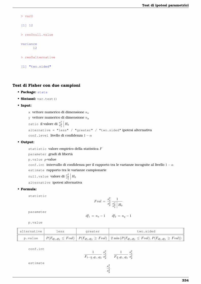
Test di ipotesi parametrici
> var0
[1] 12
> res$null.value
variance12
> res$alternative
[1] "two.sided"
Test di Fisher con due campioni
• Package: stats
• Sintassi: var.test()
• Input:
x vettore numerico di dimensione nxy vettore numerico di dimensione ny
ratio il valore di σ2x
σ2y
∣∣∣H0
alternative = "less" / "greater" / "two.sided" ipotesi alternativa
conf.level livello di confidenza 1− α
• Output:
statistic valore empirico della statistica F
parameter gradi di libertà
p.value p-value
conf.int intervallo di confidenza per il rapporto tra le varianze incognite al livello 1− αestimate rapporto tra le varianze campionarie
null.value valore di σ2x
σ2y
∣∣∣H0
alternative ipotesi alternativa
• Formula:
statistic
Fval =s2x
s2y
1σ2x
σ2y
∣∣∣H0
parameterdf1 = nx − 1 df2 = ny − 1
p.value
alternative less greater two.sided
p.value P (Fdf1,df2 ≤ Fval) P (Fdf1,df2 ≥ Fval) 2 min (P (Fdf1,df2 ≤ Fval), P (Fdf1,df2 ≥ Fval))
conf.int1
F1−α2 ,df1, df2
s2x
s2y
1Fα
2 ,df1, df2
s2x
s2y
estimates2x
s2y
334
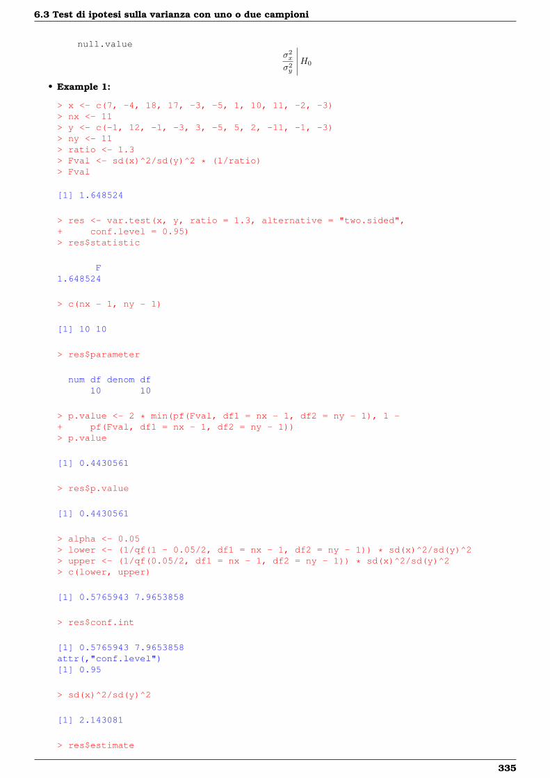
6.3 Test di ipotesi sulla varianza con uno o due campioni
null.valueσ2x
σ2y
∣∣∣∣∣H0
• Example 1:
> x <- c(7, -4, 18, 17, -3, -5, 1, 10, 11, -2, -3)> nx <- 11> y <- c(-1, 12, -1, -3, 3, -5, 5, 2, -11, -1, -3)> ny <- 11> ratio <- 1.3> Fval <- sd(x)^2/sd(y)^2 * (1/ratio)> Fval
[1] 1.648524
> res <- var.test(x, y, ratio = 1.3, alternative = "two.sided",+ conf.level = 0.95)> res$statistic
F1.648524
> c(nx - 1, ny - 1)
[1] 10 10
> res$parameter
num df denom df10 10
> p.value <- 2 * min(pf(Fval, df1 = nx - 1, df2 = ny - 1), 1 -+ pf(Fval, df1 = nx - 1, df2 = ny - 1))> p.value
[1] 0.4430561
> res$p.value
[1] 0.4430561
> alpha <- 0.05> lower <- (1/qf(1 - 0.05/2, df1 = nx - 1, df2 = ny - 1)) * sd(x)^2/sd(y)^2> upper <- (1/qf(0.05/2, df1 = nx - 1, df2 = ny - 1)) * sd(x)^2/sd(y)^2> c(lower, upper)
[1] 0.5765943 7.9653858
> res$conf.int
[1] 0.5765943 7.9653858attr(,"conf.level")[1] 0.95
> sd(x)^2/sd(y)^2
[1] 2.143081
> res$estimate
335
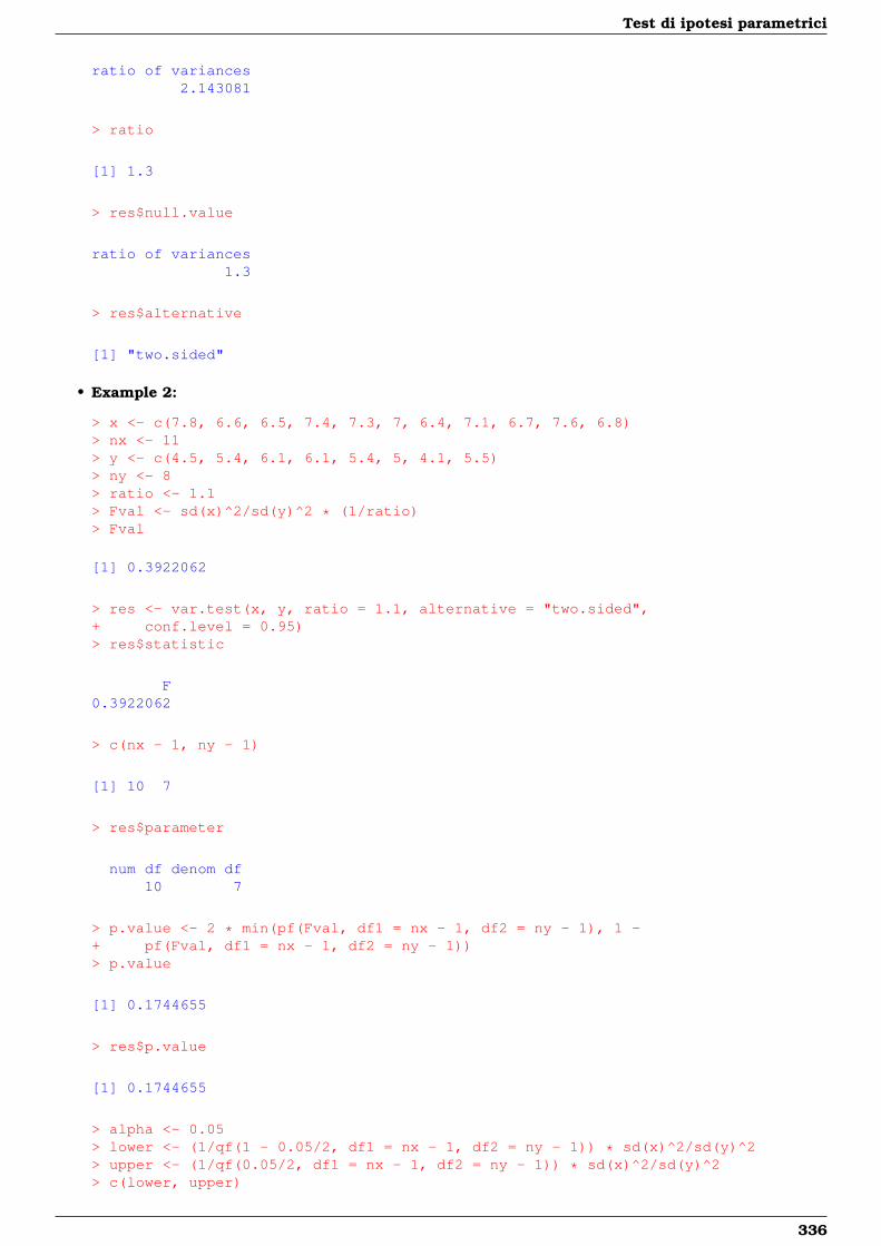
Test di ipotesi parametrici
ratio of variances2.143081
> ratio
[1] 1.3
> res$null.value
ratio of variances1.3
> res$alternative
[1] "two.sided"
• Example 2:
> x <- c(7.8, 6.6, 6.5, 7.4, 7.3, 7, 6.4, 7.1, 6.7, 7.6, 6.8)> nx <- 11> y <- c(4.5, 5.4, 6.1, 6.1, 5.4, 5, 4.1, 5.5)> ny <- 8> ratio <- 1.1> Fval <- sd(x)^2/sd(y)^2 * (1/ratio)> Fval
[1] 0.3922062
> res <- var.test(x, y, ratio = 1.1, alternative = "two.sided",+ conf.level = 0.95)> res$statistic
F0.3922062
> c(nx - 1, ny - 1)
[1] 10 7
> res$parameter
num df denom df10 7
> p.value <- 2 * min(pf(Fval, df1 = nx - 1, df2 = ny - 1), 1 -+ pf(Fval, df1 = nx - 1, df2 = ny - 1))> p.value
[1] 0.1744655
> res$p.value
[1] 0.1744655
> alpha <- 0.05> lower <- (1/qf(1 - 0.05/2, df1 = nx - 1, df2 = ny - 1)) * sd(x)^2/sd(y)^2> upper <- (1/qf(0.05/2, df1 = nx - 1, df2 = ny - 1)) * sd(x)^2/sd(y)^2> c(lower, upper)
336

6.4 Test di ipotesi su proporzioni
[1] 0.09061463 1.70405999
> res$conf.int
[1] 0.09061463 1.70405999attr(,"conf.level")[1] 0.95
> sd(x)^2/sd(y)^2
[1] 0.4314268
> res$estimate
ratio of variances0.4314268
> ratio
[1] 1.1
> res$null.value
ratio of variances1.1
> res$alternative
[1] "two.sided"
6.4 Test di ipotesi su proporzioni
Test con un campione
• Package: stats
• Sintassi: prop.test()
• Input:
x numero di successi
n dimensione campionaria
p il valore di p0
alternative = "less" / "greater" / "two.sided" ipotesi alternativa
conf.level livello di confidenza 1− αcorrect = FALSE
• Output:
statistic valore empirico della statistica χ2
parameter gradi di libertà
p.value p-value
conf.int intervallo di confidenza per la proporzione incognita al livello 1− αestimate proporzione calcolata sulla base del campione
null.value il valore di p0
alternative ipotesi alternativa
337
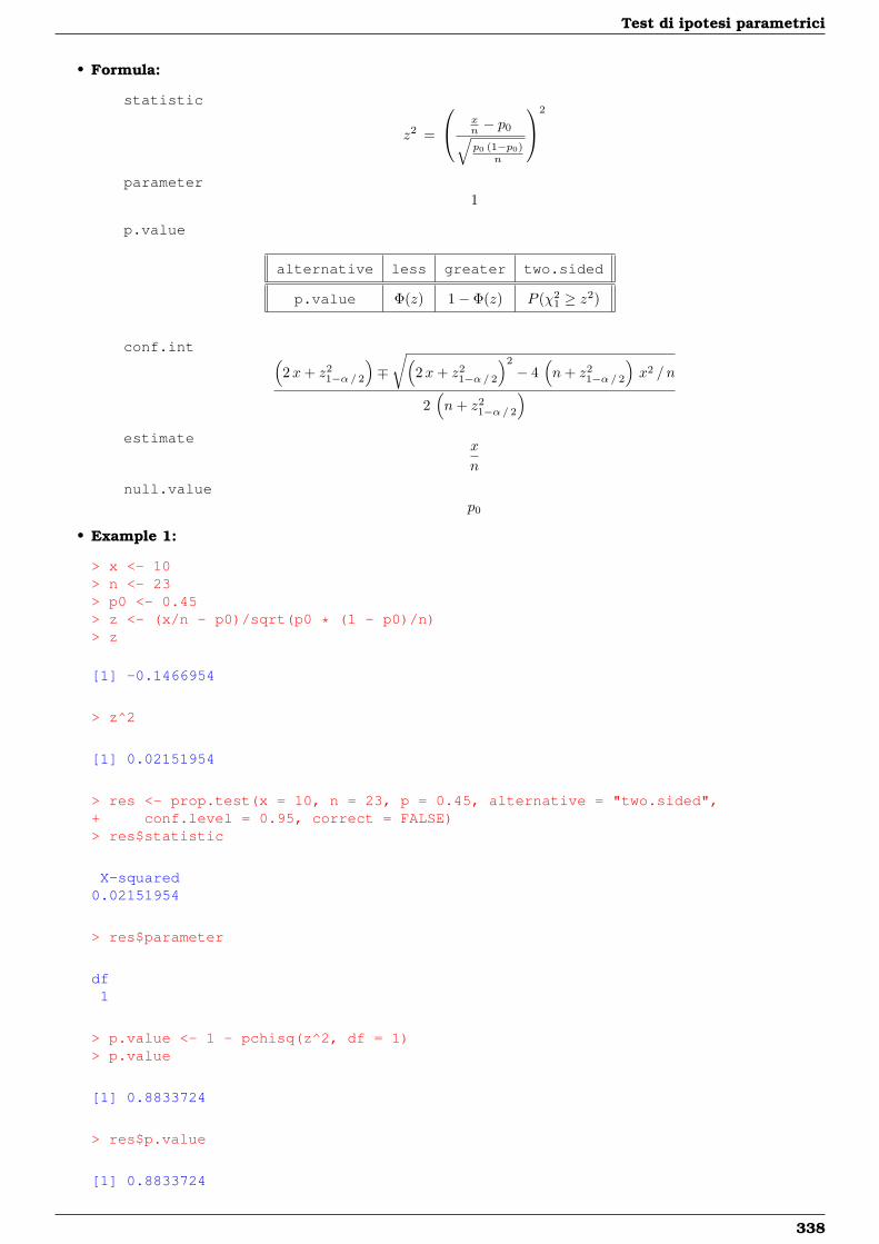
Test di ipotesi parametrici
• Formula:
statistic
z2 =
xn − p0√p0 (1−p0)
n
2
parameter1
p.value
alternative less greater two.sided
p.value Φ(z) 1− Φ(z) P (χ21 ≥ z2)
conf.int (2x+ z2
1−α/ 2
)∓√(
2x+ z21−α/ 2
)2
− 4(n+ z2
1−α/ 2
)x2 / n
2(n+ z2
1−α/ 2
)estimate
x
n
null.valuep0
• Example 1:
> x <- 10> n <- 23> p0 <- 0.45> z <- (x/n - p0)/sqrt(p0 * (1 - p0)/n)> z
[1] -0.1466954
> z^2
[1] 0.02151954
> res <- prop.test(x = 10, n = 23, p = 0.45, alternative = "two.sided",+ conf.level = 0.95, correct = FALSE)> res$statistic
X-squared0.02151954
> res$parameter
df1
> p.value <- 1 - pchisq(z^2, df = 1)> p.value
[1] 0.8833724
> res$p.value
[1] 0.8833724
338
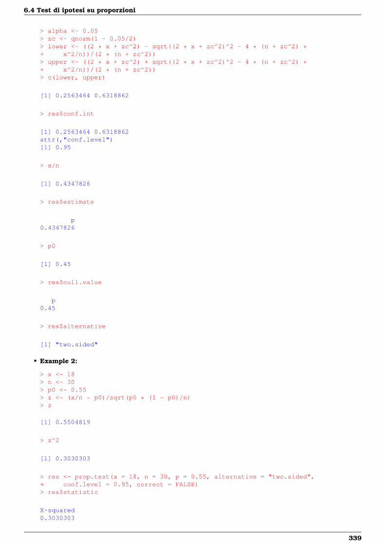
6.4 Test di ipotesi su proporzioni
> alpha <- 0.05> zc <- qnorm(1 - 0.05/2)> lower <- ((2 * x + zc^2) - sqrt((2 * x + zc^2)^2 - 4 * (n + zc^2) *+ x^2/n))/(2 * (n + zc^2))> upper <- ((2 * x + zc^2) + sqrt((2 * x + zc^2)^2 - 4 * (n + zc^2) *+ x^2/n))/(2 * (n + zc^2))> c(lower, upper)
[1] 0.2563464 0.6318862
> res$conf.int
[1] 0.2563464 0.6318862attr(,"conf.level")[1] 0.95
> x/n
[1] 0.4347826
> res$estimate
p0.4347826
> p0
[1] 0.45
> res$null.value
p0.45
> res$alternative
[1] "two.sided"
• Example 2:
> x <- 18> n <- 30> p0 <- 0.55> z <- (x/n - p0)/sqrt(p0 * (1 - p0)/n)> z
[1] 0.5504819
> z^2
[1] 0.3030303
> res <- prop.test(x = 18, n = 30, p = 0.55, alternative = "two.sided",+ conf.level = 0.95, correct = FALSE)> res$statistic
X-squared0.3030303
339
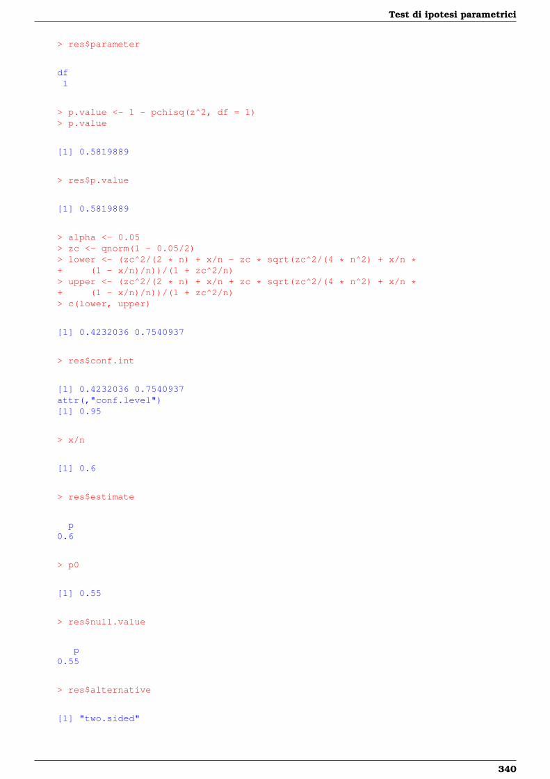
Test di ipotesi parametrici
> res$parameter
df1
> p.value <- 1 - pchisq(z^2, df = 1)> p.value
[1] 0.5819889
> res$p.value
[1] 0.5819889
> alpha <- 0.05> zc <- qnorm(1 - 0.05/2)> lower <- (zc^2/(2 * n) + x/n - zc * sqrt(zc^2/(4 * n^2) + x/n *+ (1 - x/n)/n))/(1 + zc^2/n)> upper <- (zc^2/(2 * n) + x/n + zc * sqrt(zc^2/(4 * n^2) + x/n *+ (1 - x/n)/n))/(1 + zc^2/n)> c(lower, upper)
[1] 0.4232036 0.7540937
> res$conf.int
[1] 0.4232036 0.7540937attr(,"conf.level")[1] 0.95
> x/n
[1] 0.6
> res$estimate
p0.6
> p0
[1] 0.55
> res$null.value
p0.55
> res$alternative
[1] "two.sided"
340
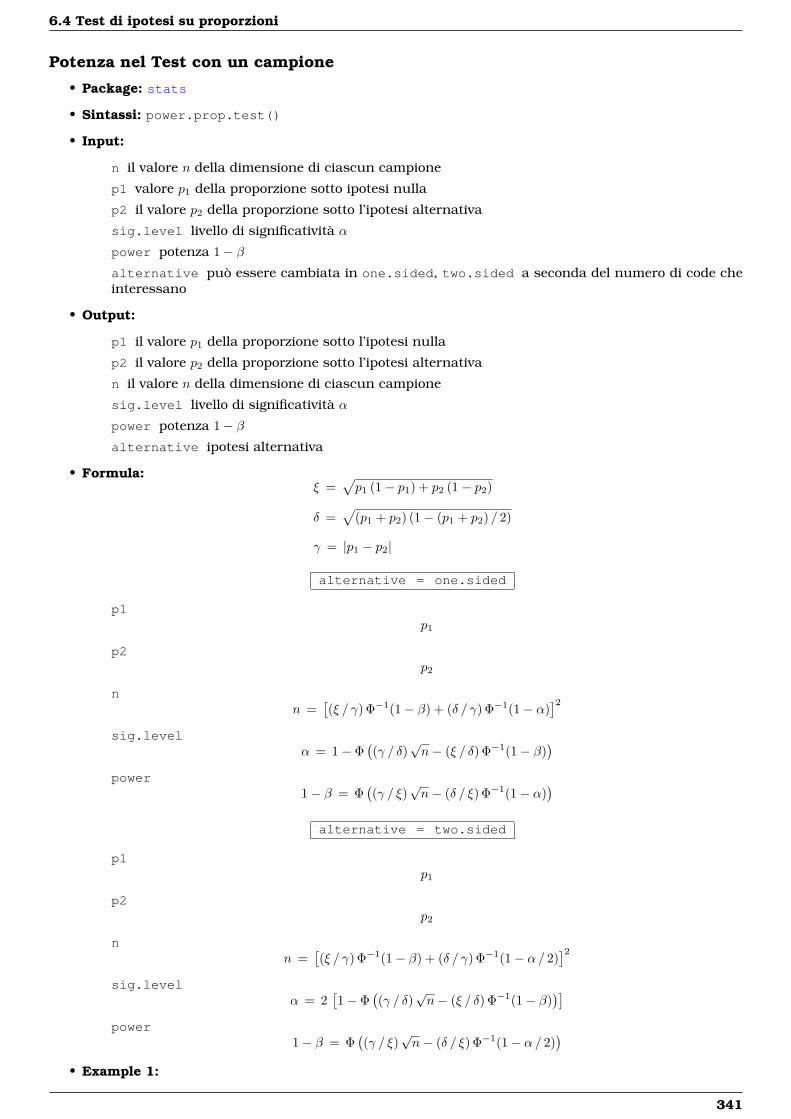
6.4 Test di ipotesi su proporzioni
Potenza nel Test con un campione
• Package: stats
• Sintassi: power.prop.test()
• Input:
n il valore n della dimensione di ciascun campione
p1 valore p1 della proporzione sotto ipotesi nulla
p2 il valore p2 della proporzione sotto l’ipotesi alternativa
sig.level livello di significatività α
power potenza 1− βalternative può essere cambiata in one.sided, two.sided a seconda del numero di code cheinteressano
• Output:
p1 il valore p1 della proporzione sotto l’ipotesi nulla
p2 il valore p2 della proporzione sotto l’ipotesi alternativa
n il valore n della dimensione di ciascun campione
sig.level livello di significatività α
power potenza 1− βalternative ipotesi alternativa
• Formula:ξ =
√p1 (1− p1) + p2 (1− p2)
δ =√
(p1 + p2) (1− (p1 + p2) / 2)
γ = |p1 − p2|
alternative = one.sided
p1p1
p2p2
nn =
[(ξ / γ) Φ−1(1− β) + (δ / γ) Φ−1(1− α)
]2sig.level
α = 1− Φ((γ / δ)
√n− (ξ / δ) Φ−1(1− β)
)power
1− β = Φ((γ / ξ)
√n− (δ / ξ) Φ−1(1− α)
)alternative = two.sided
p1p1
p2p2
nn =
[(ξ / γ) Φ−1(1− β) + (δ / γ) Φ−1(1− α/ 2)
]2sig.level
α = 2[1− Φ
((γ / δ)
√n− (ξ / δ) Φ−1(1− β)
)]power
1− β = Φ((γ / ξ)
√n− (δ / ξ) Φ−1(1− α/ 2)
)• Example 1:
341
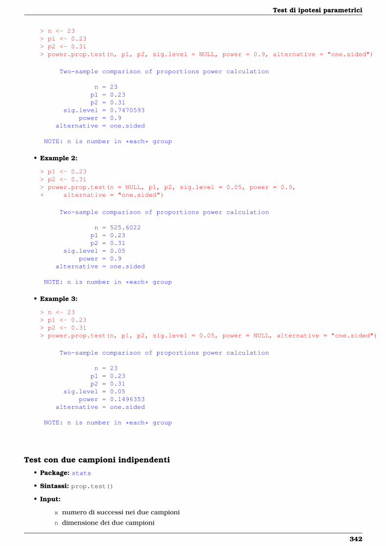
Test di ipotesi parametrici
> n <- 23> p1 <- 0.23> p2 <- 0.31> power.prop.test(n, p1, p2, sig.level = NULL, power = 0.9, alternative = "one.sided")
Two-sample comparison of proportions power calculation
n = 23p1 = 0.23p2 = 0.31
sig.level = 0.7470593power = 0.9
alternative = one.sided
NOTE: n is number in *each* group
• Example 2:
> p1 <- 0.23> p2 <- 0.31> power.prop.test(n = NULL, p1, p2, sig.level = 0.05, power = 0.9,+ alternative = "one.sided")
Two-sample comparison of proportions power calculation
n = 525.6022p1 = 0.23p2 = 0.31
sig.level = 0.05power = 0.9
alternative = one.sided
NOTE: n is number in *each* group
• Example 3:
> n <- 23> p1 <- 0.23> p2 <- 0.31> power.prop.test(n, p1, p2, sig.level = 0.05, power = NULL, alternative = "one.sided")
Two-sample comparison of proportions power calculation
n = 23p1 = 0.23p2 = 0.31
sig.level = 0.05power = 0.1496353
alternative = one.sided
NOTE: n is number in *each* group
Test con due campioni indipendenti
• Package: stats
• Sintassi: prop.test()
• Input:
x numero di successi nei due campioni
n dimensione dei due campioni
342
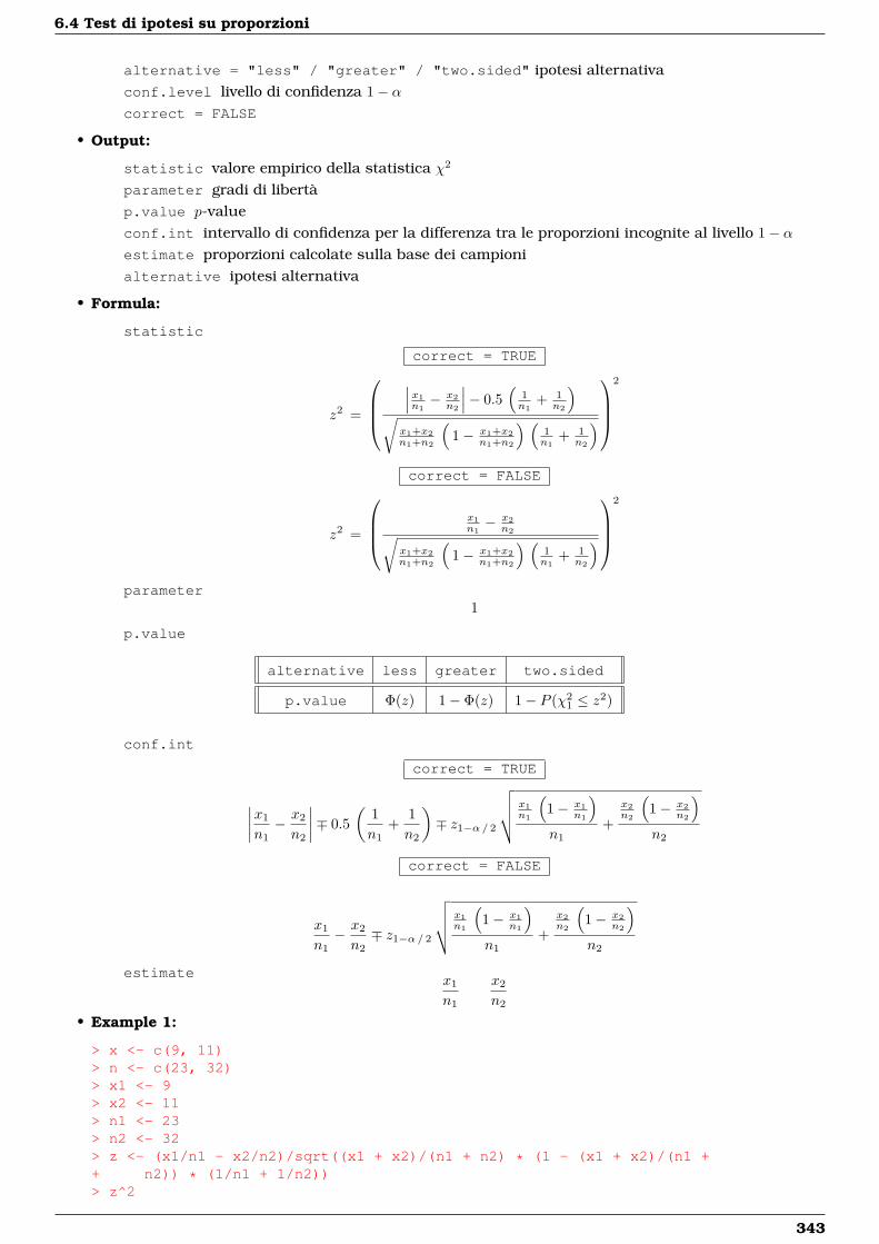
6.4 Test di ipotesi su proporzioni
alternative = "less" / "greater" / "two.sided" ipotesi alternativaconf.level livello di confidenza 1− αcorrect = FALSE
• Output:
statistic valore empirico della statistica χ2
parameter gradi di libertàp.value p-valueconf.int intervallo di confidenza per la differenza tra le proporzioni incognite al livello 1− αestimate proporzioni calcolate sulla base dei campionialternative ipotesi alternativa
• Formula:
statistic
correct = TRUE
z2 =
∣∣∣ x1n1− x2
n2
∣∣∣− 0.5(
1n1
+ 1n2
)√
x1+x2n1+n2
(1− x1+x2
n1+n2
) (1n1
+ 1n2
)
2
correct = FALSE
z2 =
x1n1− x2
n2√x1+x2n1+n2
(1− x1+x2
n1+n2
) (1n1
+ 1n2
)
2
parameter1
p.value
alternative less greater two.sided
p.value Φ(z) 1− Φ(z) 1− P (χ21 ≤ z2)
conf.int
correct = TRUE
∣∣∣∣x1
n1− x2
n2
∣∣∣∣∓ 0.5(
1n1
+1n2
)∓ z1−α/ 2
√√√√ x1n1
(1− x1
n1
)n1
+x2n2
(1− x2
n2
)n2
correct = FALSE
x1
n1− x2
n2∓ z1−α/ 2
√√√√ x1n1
(1− x1
n1
)n1
+x2n2
(1− x2
n2
)n2
estimatex1
n1
x2
n2
• Example 1:
> x <- c(9, 11)> n <- c(23, 32)> x1 <- 9> x2 <- 11> n1 <- 23> n2 <- 32> z <- (x1/n1 - x2/n2)/sqrt((x1 + x2)/(n1 + n2) * (1 - (x1 + x2)/(n1 ++ n2)) * (1/n1 + 1/n2))> z^2
343
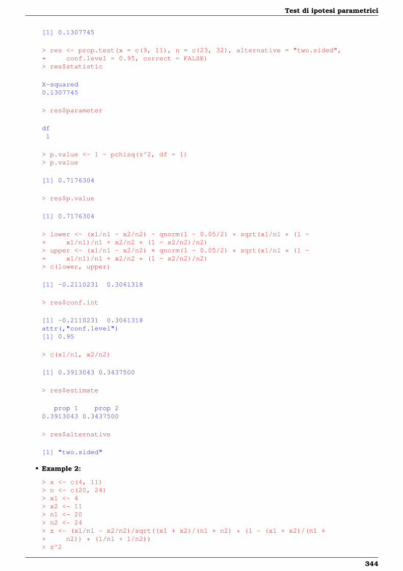
Test di ipotesi parametrici
[1] 0.1307745
> res <- prop.test(x = c(9, 11), n = c(23, 32), alternative = "two.sided",+ conf.level = 0.95, correct = FALSE)> res$statistic
X-squared0.1307745
> res$parameter
df1
> p.value <- 1 - pchisq(z^2, df = 1)> p.value
[1] 0.7176304
> res$p.value
[1] 0.7176304
> lower <- (x1/n1 - x2/n2) - qnorm(1 - 0.05/2) * sqrt(x1/n1 * (1 -+ x1/n1)/n1 + x2/n2 * (1 - x2/n2)/n2)> upper <- (x1/n1 - x2/n2) + qnorm(1 - 0.05/2) * sqrt(x1/n1 * (1 -+ x1/n1)/n1 + x2/n2 * (1 - x2/n2)/n2)> c(lower, upper)
[1] -0.2110231 0.3061318
> res$conf.int
[1] -0.2110231 0.3061318attr(,"conf.level")[1] 0.95
> c(x1/n1, x2/n2)
[1] 0.3913043 0.3437500
> res$estimate
prop 1 prop 20.3913043 0.3437500
> res$alternative
[1] "two.sided"
• Example 2:
> x <- c(4, 11)> n <- c(20, 24)> x1 <- 4> x2 <- 11> n1 <- 20> n2 <- 24> z <- (x1/n1 - x2/n2)/sqrt((x1 + x2)/(n1 + n2) * (1 - (x1 + x2)/(n1 ++ n2)) * (1/n1 + 1/n2))> z^2
344
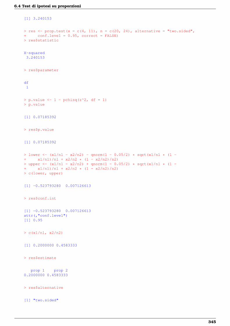
6.4 Test di ipotesi su proporzioni
[1] 3.240153
> res <- prop.test(x = c(4, 11), n = c(20, 24), alternative = "two.sided",+ conf.level = 0.95, correct = FALSE)> res$statistic
X-squared3.240153
> res$parameter
df1
> p.value <- 1 - pchisq(z^2, df = 1)> p.value
[1] 0.07185392
> res$p.value
[1] 0.07185392
> lower <- (x1/n1 - x2/n2) - qnorm(1 - 0.05/2) * sqrt(x1/n1 * (1 -+ x1/n1)/n1 + x2/n2 * (1 - x2/n2)/n2)> upper <- (x1/n1 - x2/n2) + qnorm(1 - 0.05/2) * sqrt(x1/n1 * (1 -+ x1/n1)/n1 + x2/n2 * (1 - x2/n2)/n2)> c(lower, upper)
[1] -0.523793280 0.007126613
> res$conf.int
[1] -0.523793280 0.007126613attr(,"conf.level")[1] 0.95
> c(x1/n1, x2/n2)
[1] 0.2000000 0.4583333
> res$estimate
prop 1 prop 20.2000000 0.4583333
> res$alternative
[1] "two.sided"
345
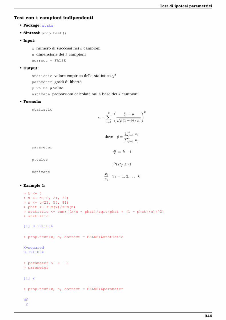
Test di ipotesi parametrici
Test con k campioni indipendenti
• Package: stats
• Sintassi: prop.test()
• Input:
x numero di successi nei k campioni
n dimensione dei k campioni
correct = FALSE
• Output:
statistic valore empirico della statistica χ2
parameter gradi di libertà
p.value p-value
estimate proporzioni calcolate sulla base dei k campioni
• Formula:
statistic
c =k∑i=1
(xini− p√
p (1− p) / ni
)2
dove p =
∑kj=1 xj∑kj=1 nj
parameterdf = k − 1
p.valueP (χ2
df ≥ c)
estimatexini
∀ i = 1, 2, . . . , k
• Example 1:
> k <- 3> x <- c(10, 21, 32)> n <- c(23, 55, 81)> phat <- sum(x)/sum(n)> statistic <- sum(((x/n - phat)/sqrt(phat * (1 - phat)/n))^2)> statistic
[1] 0.1911084
> prop.test(x, n, correct = FALSE)$statistic
X-squared0.1911084
> parameter <- k - 1> parameter
[1] 2
> prop.test(x, n, correct = FALSE)$parameter
df2
346
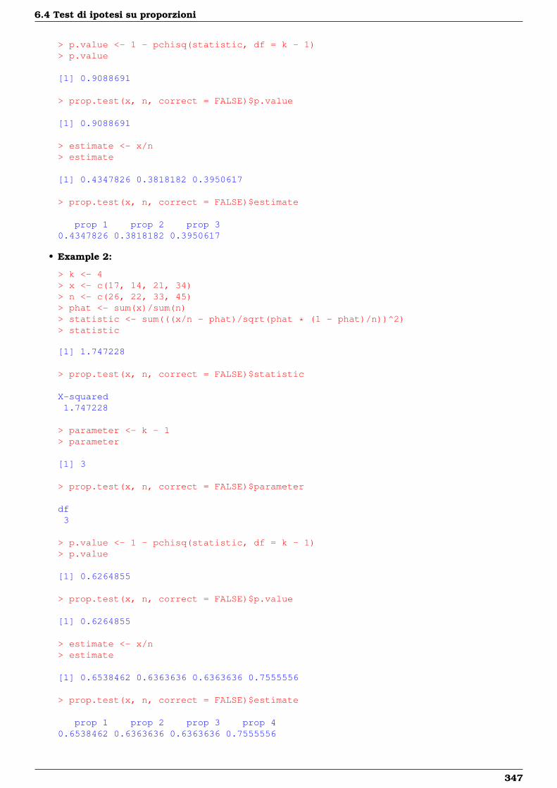
6.4 Test di ipotesi su proporzioni
> p.value <- 1 - pchisq(statistic, df = k - 1)> p.value
[1] 0.9088691
> prop.test(x, n, correct = FALSE)$p.value
[1] 0.9088691
> estimate <- x/n> estimate
[1] 0.4347826 0.3818182 0.3950617
> prop.test(x, n, correct = FALSE)$estimate
prop 1 prop 2 prop 30.4347826 0.3818182 0.3950617
• Example 2:
> k <- 4> x <- c(17, 14, 21, 34)> n <- c(26, 22, 33, 45)> phat <- sum(x)/sum(n)> statistic <- sum(((x/n - phat)/sqrt(phat * (1 - phat)/n))^2)> statistic
[1] 1.747228
> prop.test(x, n, correct = FALSE)$statistic
X-squared1.747228
> parameter <- k - 1> parameter
[1] 3
> prop.test(x, n, correct = FALSE)$parameter
df3
> p.value <- 1 - pchisq(statistic, df = k - 1)> p.value
[1] 0.6264855
> prop.test(x, n, correct = FALSE)$p.value
[1] 0.6264855
> estimate <- x/n> estimate
[1] 0.6538462 0.6363636 0.6363636 0.7555556
> prop.test(x, n, correct = FALSE)$estimate
prop 1 prop 2 prop 3 prop 40.6538462 0.6363636 0.6363636 0.7555556
347
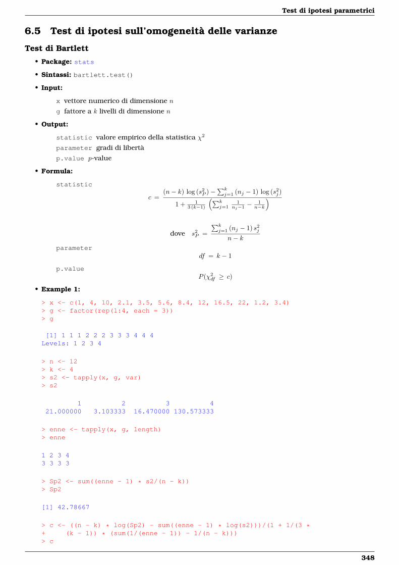
Test di ipotesi parametrici
6.5 Test di ipotesi sull’omogeneità delle varianze
Test di Bartlett
• Package: stats
• Sintassi: bartlett.test()
• Input:
x vettore numerico di dimensione n
g fattore a k livelli di dimensione n
• Output:
statistic valore empirico della statistica χ2
parameter gradi di libertà
p.value p-value
• Formula:
statistic
c =(n− k) log (s2
P )−∑kj=1 (nj − 1) log (s2
j )
1 + 13 (k−1)
(∑kj=1
1nj−1 −
1n−k
)
dove s2P =
∑kj=1 (nj − 1) s2
j
n− kparameter
df = k − 1
p.valueP (χ2
df ≥ c)
• Example 1:
> x <- c(1, 4, 10, 2.1, 3.5, 5.6, 8.4, 12, 16.5, 22, 1.2, 3.4)> g <- factor(rep(1:4, each = 3))> g
[1] 1 1 1 2 2 2 3 3 3 4 4 4Levels: 1 2 3 4
> n <- 12> k <- 4> s2 <- tapply(x, g, var)> s2
1 2 3 421.000000 3.103333 16.470000 130.573333
> enne <- tapply(x, g, length)> enne
1 2 3 43 3 3 3
> Sp2 <- sum((enne - 1) * s2/(n - k))> Sp2
[1] 42.78667
> c <- ((n - k) * log(Sp2) - sum((enne - 1) * log(s2)))/(1 + 1/(3 *+ (k - 1)) * (sum(1/(enne - 1)) - 1/(n - k)))> c
348
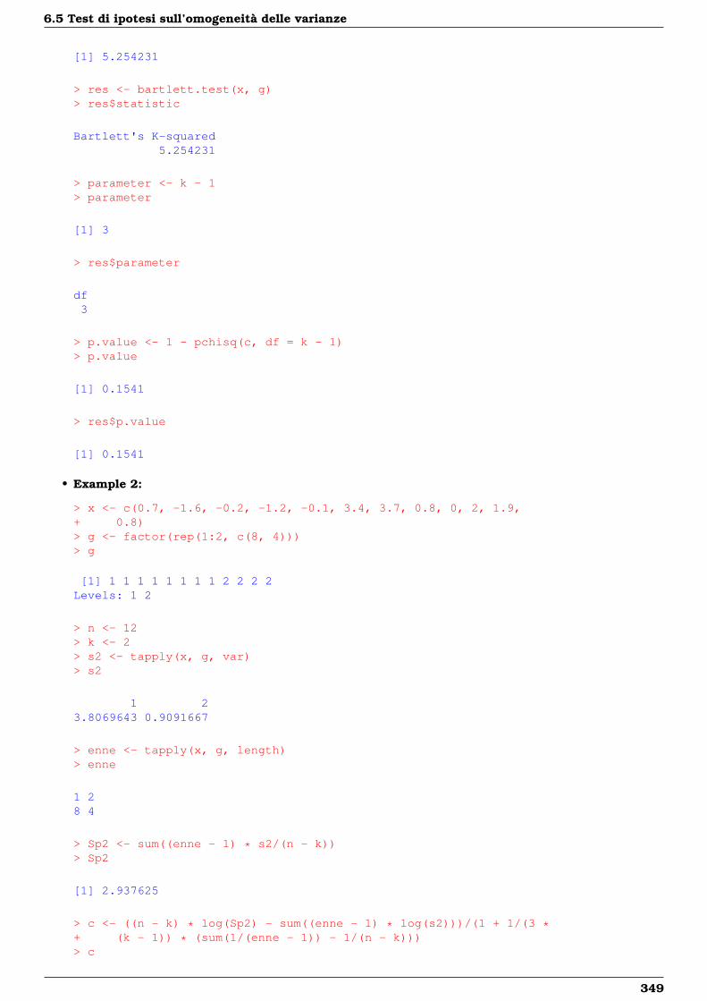
6.5 Test di ipotesi sull’omogeneità delle varianze
[1] 5.254231
> res <- bartlett.test(x, g)> res$statistic
Bartlett's K-squared5.254231
> parameter <- k - 1> parameter
[1] 3
> res$parameter
df3
> p.value <- 1 - pchisq(c, df = k - 1)> p.value
[1] 0.1541
> res$p.value
[1] 0.1541
• Example 2:
> x <- c(0.7, -1.6, -0.2, -1.2, -0.1, 3.4, 3.7, 0.8, 0, 2, 1.9,+ 0.8)> g <- factor(rep(1:2, c(8, 4)))> g
[1] 1 1 1 1 1 1 1 1 2 2 2 2Levels: 1 2
> n <- 12> k <- 2> s2 <- tapply(x, g, var)> s2
1 23.8069643 0.9091667
> enne <- tapply(x, g, length)> enne
1 28 4
> Sp2 <- sum((enne - 1) * s2/(n - k))> Sp2
[1] 2.937625
> c <- ((n - k) * log(Sp2) - sum((enne - 1) * log(s2)))/(1 + 1/(3 *+ (k - 1)) * (sum(1/(enne - 1)) - 1/(n - k)))> c
349
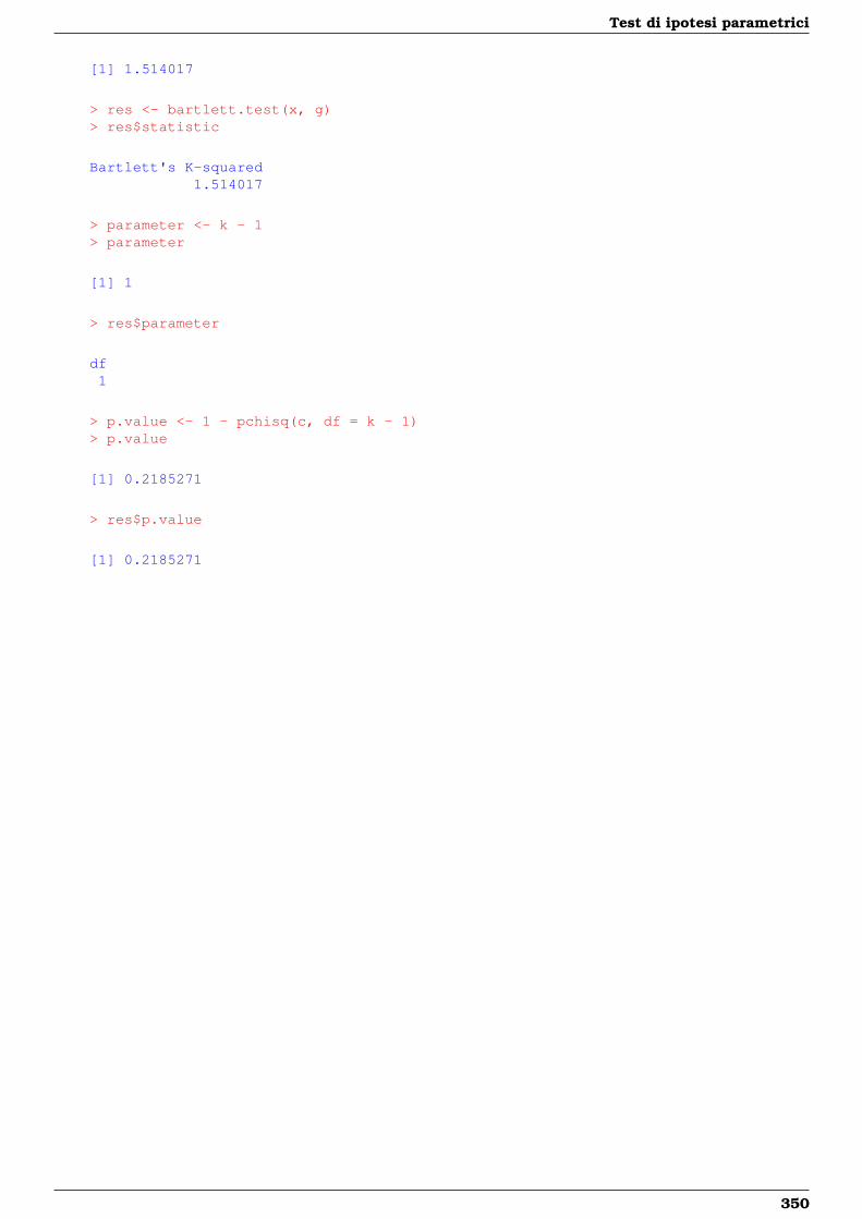
Test di ipotesi parametrici
[1] 1.514017
> res <- bartlett.test(x, g)> res$statistic
Bartlett's K-squared1.514017
> parameter <- k - 1> parameter
[1] 1
> res$parameter
df1
> p.value <- 1 - pchisq(c, df = k - 1)> p.value
[1] 0.2185271
> res$p.value
[1] 0.2185271
350

Capitolo 7
Analisi della varianza (Anova)
7.1 Simbologia
• numero di livelli dei fattori di colonna e di riga:
Anova f (colonna) g (riga)ad un fattore k /
a due fattori senza interazione k ha due fattori con interazione k h
• dimensione campionaria di colonna, di riga e di cella:
Anova j-esima colonna i-esima riga ij-esima cellaad un fattore nj / /
a due fattori senza interazione hl kl la due fattori con interazione hl kl l
• medie campionarie di colonna, di riga e di cella:
Anova j-esima colonna i-esima riga ij-esima cellaad un fattore yj / /
a due fattori senza interazione y·j· yi·· yij·a due fattori con interazione y·j· yi·· yij·
• media campionaria generale: y
7.2 Modelli di analisi della varianza
Anova ad un fattore
• Package: stats
• Sintassi: anova()
• Input:
y vettore numerico di dimensione n
f fattore a k livelli di dimensione n
• Output:
Df gradi di libertà
Sum Sq somma dei quadrati
Mean Sq media dei quadrati
F value valore empirico della statistica F
Pr(>F) p-value
351
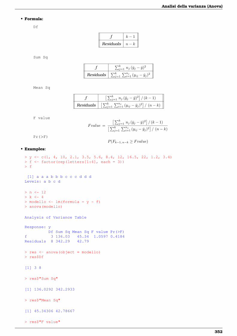
Analisi della varianza (Anova)
• Formula:
Df
f k − 1
Residuals n− k
Sum Sq
f∑kj=1 nj (yj − y)2
Residuals∑kj=1
∑nji=1 (yij − yj)2
Mean Sq
f[∑k
j=1 nj (yj − y)2]/ (k − 1)
Residuals[∑k
j=1
∑nji=1 (yij − yj)2
]/ (n− k)
F value
Fvalue =
[∑kj=1 nj (yj − y)2
]/ (k − 1)[∑k
j=1
∑nji=1 (yij − yj)2
]/ (n− k)
Pr(>F)P (Fk−1, n−k ≥ Fvalue)
• Examples:
> y <- c(1, 4, 10, 2.1, 3.5, 5.6, 8.4, 12, 16.5, 22, 1.2, 3.4)> f <- factor(rep(letters[1:4], each = 3))> f
[1] a a a b b b c c c d d dLevels: a b c d
> n <- 12> k <- 4> modello <- lm(formula = y ~ f)> anova(modello)
Analysis of Variance Table
Response: yDf Sum Sq Mean Sq F value Pr(>F)
f 3 136.03 45.34 1.0597 0.4184Residuals 8 342.29 42.79
> res <- anova(object = modello)> res$Df
[1] 3 8
> res$"Sum Sq"
[1] 136.0292 342.2933
> res$"Mean Sq"
[1] 45.34306 42.78667
> res$"F value"
352
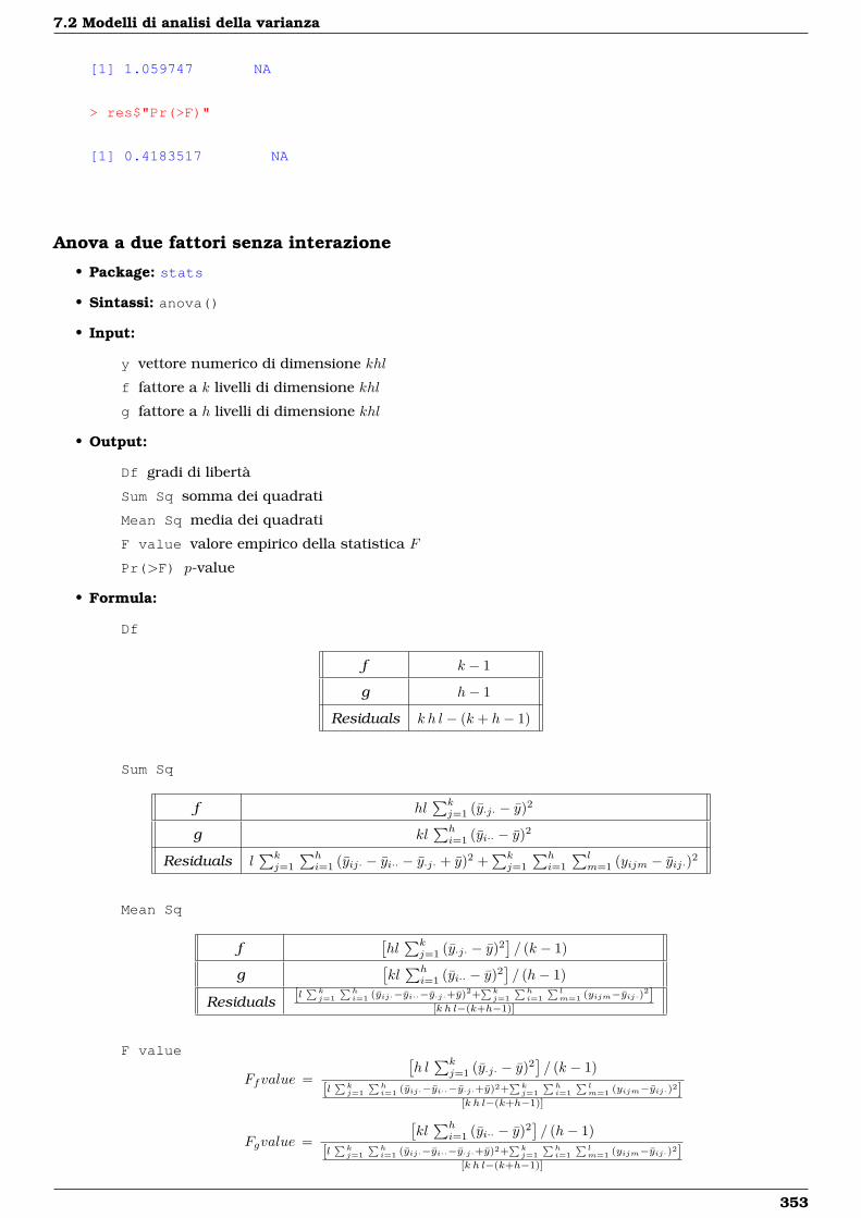
7.2 Modelli di analisi della varianza
[1] 1.059747 NA
> res$"Pr(>F)"
[1] 0.4183517 NA
Anova a due fattori senza interazione
• Package: stats
• Sintassi: anova()
• Input:
y vettore numerico di dimensione khl
f fattore a k livelli di dimensione khl
g fattore a h livelli di dimensione khl
• Output:
Df gradi di libertà
Sum Sq somma dei quadrati
Mean Sq media dei quadrati
F value valore empirico della statistica F
Pr(>F) p-value
• Formula:
Df
f k − 1
g h− 1
Residuals k h l − (k + h− 1)
Sum Sq
f hl∑kj=1 (y·j· − y)2
g kl∑hi=1 (yi·· − y)2
Residuals l∑kj=1
∑hi=1 (yij· − yi·· − y·j· + y)2 +
∑kj=1
∑hi=1
∑lm=1 (yijm − yij·)2
Mean Sq
f[hl∑kj=1 (y·j· − y)2
]/ (k − 1)
g[kl∑hi=1 (yi·· − y)2
]/ (h− 1)
Residuals [l ∑kj=1
∑hi=1 (yij·−yi··−y·j·+y)2+
∑kj=1
∑hi=1
∑lm=1 (yijm−yij·)2]
[k h l−(k+h−1)]
F value
Ffvalue =
[h l∑kj=1 (y·j· − y)2
]/ (k − 1)
[l ∑kj=1
∑hi=1 (yij·−yi··−y·j·+y)2+
∑kj=1
∑hi=1
∑lm=1 (yijm−yij·)2]
[k h l−(k+h−1)]
Fgvalue =
[kl∑hi=1 (yi·· − y)2
]/ (h− 1)
[l ∑kj=1
∑hi=1 (yij·−yi··−y·j·+y)2+
∑kj=1
∑hi=1
∑lm=1 (yijm−yij·)2]
[k h l−(k+h−1)]
353
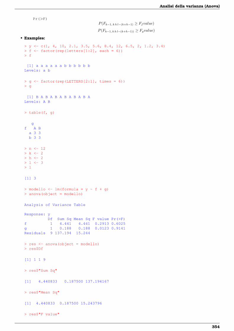
Analisi della varianza (Anova)
Pr(>F)P (Fk−1, k h l−(k+h−1) ≥ Ffvalue)
P (Fh−1, k h l−(k+h−1)) ≥ Fgvalue)
• Examples:
> y <- c(1, 4, 10, 2.1, 3.5, 5.6, 8.4, 12, 6.5, 2, 1.2, 3.4)> f <- factor(rep(letters[1:2], each = 6))> f
[1] a a a a a a b b b b b bLevels: a b
> g <- factor(rep(LETTERS[2:1], times = 6))> g
[1] B A B A B A B A B A B ALevels: A B
> table(f, g)
gf A B
a 3 3b 3 3
> n <- 12> k <- 2> h <- 2> l <- 3> l
[1] 3
> modello <- lm(formula = y ~ f + g)> anova(object = modello)
Analysis of Variance Table
Response: yDf Sum Sq Mean Sq F value Pr(>F)
f 1 4.441 4.441 0.2913 0.6025g 1 0.188 0.188 0.0123 0.9141Residuals 9 137.194 15.244
> res <- anova(object = modello)> res$Df
[1] 1 1 9
> res$"Sum Sq"
[1] 4.440833 0.187500 137.194167
> res$"Mean Sq"
[1] 4.440833 0.187500 15.243796
> res$"F value"
354
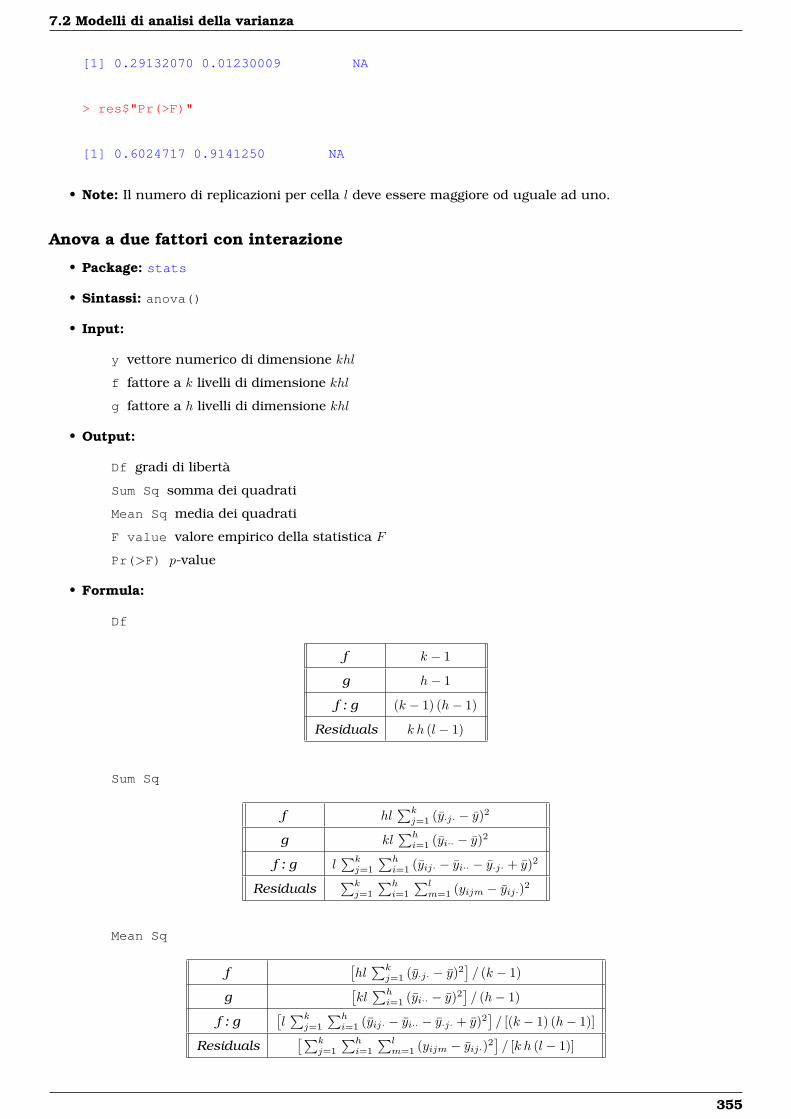
7.2 Modelli di analisi della varianza
[1] 0.29132070 0.01230009 NA
> res$"Pr(>F)"
[1] 0.6024717 0.9141250 NA
• Note: Il numero di replicazioni per cella l deve essere maggiore od uguale ad uno.
Anova a due fattori con interazione
• Package: stats
• Sintassi: anova()
• Input:
y vettore numerico di dimensione khl
f fattore a k livelli di dimensione khl
g fattore a h livelli di dimensione khl
• Output:
Df gradi di libertà
Sum Sq somma dei quadrati
Mean Sq media dei quadrati
F value valore empirico della statistica F
Pr(>F) p-value
• Formula:
Df
f k − 1
g h− 1
f : g (k − 1) (h− 1)
Residuals k h (l − 1)
Sum Sq
f hl∑kj=1 (y·j· − y)2
g kl∑hi=1 (yi·· − y)2
f : g l∑kj=1
∑hi=1 (yij· − yi·· − y·j· + y)2
Residuals∑kj=1
∑hi=1
∑lm=1 (yijm − yij·)2
Mean Sq
f[hl∑kj=1 (y·j· − y)2
]/ (k − 1)
g[kl∑hi=1 (yi·· − y)2
]/ (h− 1)
f : g[l∑kj=1
∑hi=1 (yij· − yi·· − y·j· + y)2
]/ [(k − 1) (h− 1)]
Residuals[∑k
j=1
∑hi=1
∑lm=1 (yijm − yij·)2
]/ [k h (l − 1)]
355
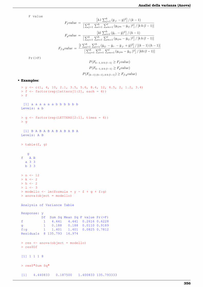
Analisi della varianza (Anova)
F value
Ffvalue =
[h l∑kj=1 (y·j· − y)2
]/ (k − 1)[∑k
j=1
∑hi=1
∑lm=1 (yijm − yij·)2
]/ [k h (l − 1)]
Fgvalue =
[kl∑hi=1 (yi·· − y)2
]/ (h− 1)[∑k
j=1
∑hi=1
∑lm=1 (yijm − yij·)2
]/ [k h (l − 1)]
Ff :gvalue =
[l∑kj=1
∑hi=1 (yij· − yi·· − y·j· + y)2
]/ [(k − 1) (h− 1)][∑k
j=1
∑hi=1
∑lm=1 (yijm − yij·)2
]/ [kh (l − 1)]
Pr(>F)P (Fk−1, k h (l−1) ≥ Ffvalue)
P (Fh−1, k h (l−1) ≥ Fgvalue)
P (F(k−1) (h−1), k h (l−1)) ≥ Ff :gvalue)
• Examples:
> y <- c(1, 4, 10, 2.1, 3.5, 5.6, 8.4, 12, 6.5, 2, 1.2, 3.4)> f <- factor(rep(letters[1:2], each = 6))> f
[1] a a a a a a b b b b b bLevels: a b
> g <- factor(rep(LETTERS[2:1], times = 6))> g
[1] B A B A B A B A B A B ALevels: A B
> table(f, g)
gf A B
a 3 3b 3 3
> n <- 12> k <- 2> h <- 2> l <- 3> modello <- lm(formula = y ~ f + g + f:g)> anova(object = modello)
Analysis of Variance Table
Response: yDf Sum Sq Mean Sq F value Pr(>F)
f 1 4.441 4.441 0.2616 0.6228g 1 0.188 0.188 0.0110 0.9189f:g 1 1.401 1.401 0.0825 0.7812Residuals 8 135.793 16.974
> res <- anova(object = modello)> res$Df
[1] 1 1 1 8
> res$"Sum Sq"
[1] 4.440833 0.187500 1.400833 135.793333
356
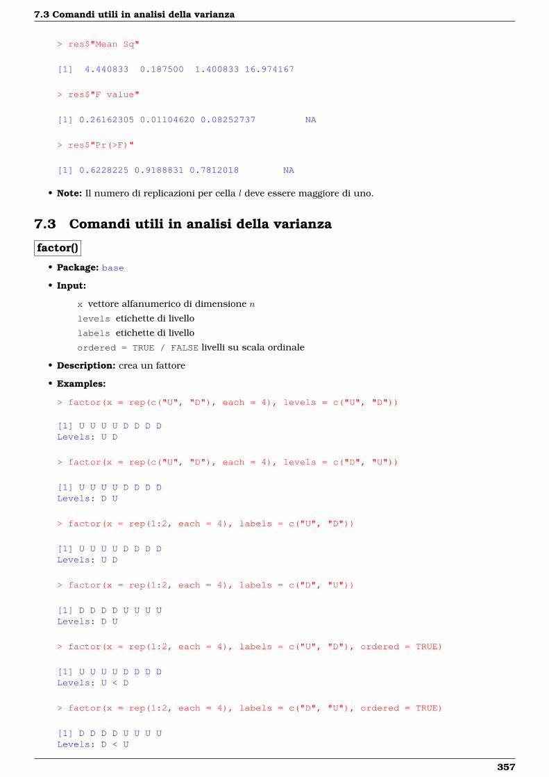
7.3 Comandi utili in analisi della varianza
> res$"Mean Sq"
[1] 4.440833 0.187500 1.400833 16.974167
> res$"F value"
[1] 0.26162305 0.01104620 0.08252737 NA
> res$"Pr(>F)"
[1] 0.6228225 0.9188831 0.7812018 NA
• Note: Il numero di replicazioni per cella l deve essere maggiore di uno.
7.3 Comandi utili in analisi della varianza
factor()
• Package: base
• Input:
x vettore alfanumerico di dimensione n
levels etichette di livello
labels etichette di livello
ordered = TRUE / FALSE livelli su scala ordinale
• Description: crea un fattore
• Examples:
> factor(x = rep(c("U", "D"), each = 4), levels = c("U", "D"))
[1] U U U U D D D DLevels: U D
> factor(x = rep(c("U", "D"), each = 4), levels = c("D", "U"))
[1] U U U U D D D DLevels: D U
> factor(x = rep(1:2, each = 4), labels = c("U", "D"))
[1] U U U U D D D DLevels: U D
> factor(x = rep(1:2, each = 4), labels = c("D", "U"))
[1] D D D D U U U ULevels: D U
> factor(x = rep(1:2, each = 4), labels = c("U", "D"), ordered = TRUE)
[1] U U U U D D D DLevels: U < D
> factor(x = rep(1:2, each = 4), labels = c("D", "U"), ordered = TRUE)
[1] D D D D U U U ULevels: D < U
357
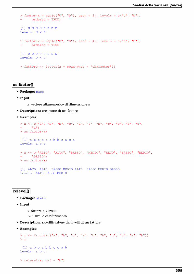
Analisi della varianza (Anova)
> factor(x = rep(c("U", "D"), each = 4), levels = c("U", "D"),+ ordered = TRUE)
[1] U U U U D D D DLevels: U < D
> factor(x = rep(c("U", "D"), each = 4), levels = c("D", "U"),+ ordered = TRUE)
[1] U U U U D D D DLevels: D < U
> fattore <- factor(x = scan(what = "character"))
as.factor()
• Package: base
• Input:
x vettore alfanumerico di dimensione n
• Description: creazione di un fattore
• Examples:
> x <- c("a", "b", "b", "c", "a", "c", "b", "b", "c", "a", "c",+ "a")> as.factor(x)
[1] a b b c a c b b c a c aLevels: a b c
> x <- c("ALTO", "ALTO", "BASSO", "MEDIO", "ALTO", "BASSO", "MEDIO",+ "BASSO")> as.factor(x)
[1] ALTO ALTO BASSO MEDIO ALTO BASSO MEDIO BASSOLevels: ALTO BASSO MEDIO
relevel()
• Package: stats
• Input:
x fattore a k livelli
ref livello di riferimento
• Description: ricodificazione dei livelli di un fattore
• Examples:
> x <- factor(c("a", "b", "c", "a", "b", "b", "c", "c", "a", "b"))> x
[1] a b c a b b c c a bLevels: a b c
> relevel(x, ref = "b")
358

7.3 Comandi utili in analisi della varianza
[1] a b c a b b c c a bLevels: b a c
> relevel(x, ref = "c")
[1] a b c a b b c c a bLevels: c a b
levels()
• Package: base
• Input:
f fattore a k livelli
• Description: nome dei livelli
• Examples:
> f <- factor(rep(1:2, each = 5))> f
[1] 1 1 1 1 1 2 2 2 2 2Levels: 1 2
> levels(f)
[1] "1" "2"
> f <- factor(rep(c("U", "D"), each = 4))> f
[1] U U U U D D D DLevels: D U
> levels(f)
[1] "D" "U"
nlevels()
• Package: base
• Input:
f fattore a k livelli
• Description: numero di livelli
• Examples:
> f <- factor(rep(1:2, each = 5))> f
[1] 1 1 1 1 1 2 2 2 2 2Levels: 1 2
> nlevels(f)
359
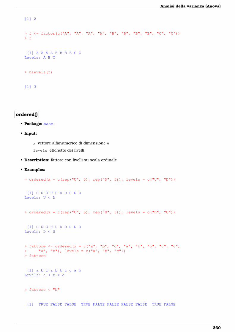
Analisi della varianza (Anova)
[1] 2
> f <- factor(c("A", "A", "A", "A", "B", "B", "B", "B", "C", "C"))> f
[1] A A A A B B B B C CLevels: A B C
> nlevels(f)
[1] 3
ordered()
• Package: base
• Input:
x vettore alfanumerico di dimensione n
levels etichette dei livelli
• Description: fattore con livelli su scala ordinale
• Examples:
> ordered(x = c(rep("U", 5), rep("D", 5)), levels = c("U", "D"))
[1] U U U U U D D D D DLevels: U < D
> ordered(x = c(rep("U", 5), rep("D", 5)), levels = c("D", "U"))
[1] U U U U U D D D D DLevels: D < U
> fattore <- ordered(x = c("a", "b", "c", "a", "b", "b", "c", "c",+ "a", "b"), levels = c("a", "b", "c"))> fattore
[1] a b c a b b c c a bLevels: a < b < c
> fattore < "b"
[1] TRUE FALSE FALSE TRUE FALSE FALSE FALSE FALSE TRUE FALSE
360

7.3 Comandi utili in analisi della varianza
as.ordered()
• Package: base
• Input:
x vettore alfanumerico di dimensione n
• Description: fattore con livelli su scala ordinale
• Examples:
> as.ordered(x = c(rep("U", 5), rep("D", 5)))
[1] U U U U U D D D D DLevels: D < U
> as.ordered(x = c(rep("U", 5), rep("D", 5)))
[1] U U U U U D D D D DLevels: D < U
> as.ordered(x = c("a", "b", "c", "a", "b", "b", "c", "c", "a",+ "b"))
[1] a b c a b b c c a bLevels: a < b < c
letters[ ]
• Package: base
• Description: lettere minuscole
• Examples:
> letters[1:6]
[1] "a" "b" "c" "d" "e" "f"
> letters[c(3, 5, 6, 26)]
[1] "c" "e" "f" "z"
LETTERS[ ]
• Package: base
• Description: lettere maiuscole
• Examples:
> LETTERS[1:6]
[1] "A" "B" "C" "D" "E" "F"
> LETTERS[c(3, 5, 6, 26)]
[1] "C" "E" "F" "Z"
361

Analisi della varianza (Anova)
as.numeric()
• Package: base
• Input:
x fattore a k livelli
• Description: codici dei livelli
• Examples:
> x <- factor(c(2, 3, 1, 1, 1, 3, 4, 4, 1, 2), labels = c("A",+ "B", "C", "D"))> x
[1] B C A A A C D D A BLevels: A B C D
> as.numeric(x)
[1] 2 3 1 1 1 3 4 4 1 2
> x <- factor(c("M", "F", "M", "F", "M", "F", "F", "M"), levels = c("M",+ "F"))> x
[1] M F M F M F F MLevels: M F
> as.numeric(x)
[1] 1 2 1 2 1 2 2 1
as.integer()
• Package: base
• Input:
x fattore a k livelli
• Description: codici dei livelli
• Examples:
> x <- factor(c(2, 3, 1, 1, 1, 3, 4, 4, 1, 2), labels = c("A",+ "B", "C", "D"))> x
[1] B C A A A C D D A BLevels: A B C D
> as.integer(x)
[1] 2 3 1 1 1 3 4 4 1 2
> x <- factor(c("M", "F", "M", "F", "M", "F", "F", "M"), levels = c("M",+ "F"))> x
[1] M F M F M F F MLevels: M F
> as.integer(x)
[1] 1 2 1 2 1 2 2 1
362
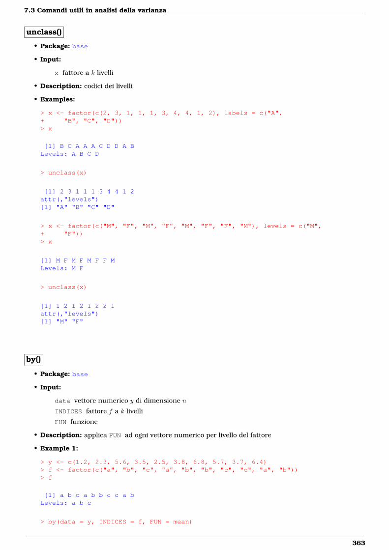
7.3 Comandi utili in analisi della varianza
unclass()
• Package: base
• Input:
x fattore a k livelli
• Description: codici dei livelli
• Examples:
> x <- factor(c(2, 3, 1, 1, 1, 3, 4, 4, 1, 2), labels = c("A",+ "B", "C", "D"))> x
[1] B C A A A C D D A BLevels: A B C D
> unclass(x)
[1] 2 3 1 1 1 3 4 4 1 2attr(,"levels")[1] "A" "B" "C" "D"
> x <- factor(c("M", "F", "M", "F", "M", "F", "F", "M"), levels = c("M",+ "F"))> x
[1] M F M F M F F MLevels: M F
> unclass(x)
[1] 1 2 1 2 1 2 2 1attr(,"levels")[1] "M" "F"
by()
• Package: base
• Input:
data vettore numerico y di dimensione n
INDICES fattore f a k livelli
FUN funzione
• Description: applica FUN ad ogni vettore numerico per livello del fattore
• Example 1:
> y <- c(1.2, 2.3, 5.6, 3.5, 2.5, 3.8, 6.8, 5.7, 3.7, 6.4)> f <- factor(c("a", "b", "c", "a", "b", "b", "c", "c", "a", "b"))> f
[1] a b c a b b c c a bLevels: a b c
> by(data = y, INDICES = f, FUN = mean)
363
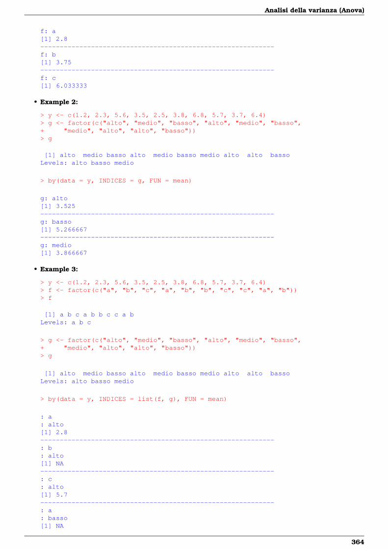
Analisi della varianza (Anova)
f: a[1] 2.8------------------------------------------------------------f: b[1] 3.75------------------------------------------------------------f: c[1] 6.033333
• Example 2:
> y <- c(1.2, 2.3, 5.6, 3.5, 2.5, 3.8, 6.8, 5.7, 3.7, 6.4)> g <- factor(c("alto", "medio", "basso", "alto", "medio", "basso",+ "medio", "alto", "alto", "basso"))> g
[1] alto medio basso alto medio basso medio alto alto bassoLevels: alto basso medio
> by(data = y, INDICES = g, FUN = mean)
g: alto[1] 3.525------------------------------------------------------------g: basso[1] 5.266667------------------------------------------------------------g: medio[1] 3.866667
• Example 3:
> y <- c(1.2, 2.3, 5.6, 3.5, 2.5, 3.8, 6.8, 5.7, 3.7, 6.4)> f <- factor(c("a", "b", "c", "a", "b", "b", "c", "c", "a", "b"))> f
[1] a b c a b b c c a bLevels: a b c
> g <- factor(c("alto", "medio", "basso", "alto", "medio", "basso",+ "medio", "alto", "alto", "basso"))> g
[1] alto medio basso alto medio basso medio alto alto bassoLevels: alto basso medio
> by(data = y, INDICES = list(f, g), FUN = mean)
: a: alto[1] 2.8------------------------------------------------------------: b: alto[1] NA------------------------------------------------------------: c: alto[1] 5.7------------------------------------------------------------: a: basso[1] NA
364
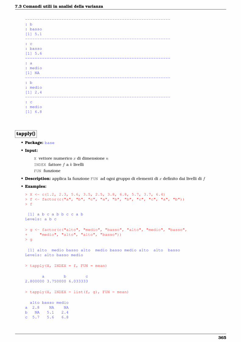
7.3 Comandi utili in analisi della varianza
------------------------------------------------------------: b: basso[1] 5.1------------------------------------------------------------: c: basso[1] 5.6------------------------------------------------------------: a: medio[1] NA------------------------------------------------------------: b: medio[1] 2.4------------------------------------------------------------: c: medio[1] 6.8
tapply()
• Package: base
• Input:
X vettore numerico x di dimensione n
INDEX fattore f a k livelli
FUN funzione
• Description: applica la funzione FUN ad ogni gruppo di elementi di x definito dai livelli di f
• Examples:
> X <- c(1.2, 2.3, 5.6, 3.5, 2.5, 3.8, 6.8, 5.7, 3.7, 6.4)> f <- factor(c("a", "b", "c", "a", "b", "b", "c", "c", "a", "b"))> f
[1] a b c a b b c c a bLevels: a b c
> g <- factor(c("alto", "medio", "basso", "alto", "medio", "basso",+ "medio", "alto", "alto", "basso"))> g
[1] alto medio basso alto medio basso medio alto alto bassoLevels: alto basso medio
> tapply(X, INDEX = f, FUN = mean)
a b c2.800000 3.750000 6.033333
> tapply(X, INDEX = list(f, g), FUN = mean)
alto basso medioa 2.8 NA NAb NA 5.1 2.4c 5.7 5.6 6.8
365
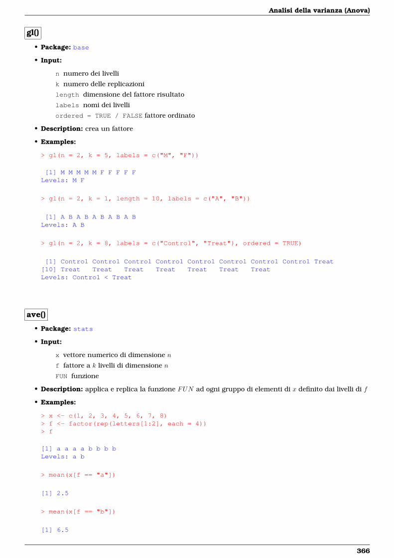
Analisi della varianza (Anova)
gl()
• Package: base
• Input:
n numero dei livelli
k numero delle replicazioni
length dimensione del fattore risultato
labels nomi dei livelli
ordered = TRUE / FALSE fattore ordinato
• Description: crea un fattore
• Examples:
> gl(n = 2, k = 5, labels = c("M", "F"))
[1] M M M M M F F F F FLevels: M F
> gl(n = 2, k = 1, length = 10, labels = c("A", "B"))
[1] A B A B A B A B A BLevels: A B
> gl(n = 2, k = 8, labels = c("Control", "Treat"), ordered = TRUE)
[1] Control Control Control Control Control Control Control Control Treat[10] Treat Treat Treat Treat Treat Treat TreatLevels: Control < Treat
ave()
• Package: stats
• Input:
x vettore numerico di dimensione n
f fattore a k livelli di dimensione n
FUN funzione
• Description: applica e replica la funzione FUN ad ogni gruppo di elementi di x definito dai livelli di f
• Examples:
> x <- c(1, 2, 3, 4, 5, 6, 7, 8)> f <- factor(rep(letters[1:2], each = 4))> f
[1] a a a a b b b bLevels: a b
> mean(x[f == "a"])
[1] 2.5
> mean(x[f == "b"])
[1] 6.5
366

7.3 Comandi utili in analisi della varianza
> ave(x, f, FUN = mean)
[1] 2.5 2.5 2.5 2.5 6.5 6.5 6.5 6.5
> x <- c(1, 2, 3, 4, 5, 6, 7, 8)> f <- factor(rep(letters[1:2], each = 4))> f
[1] a a a a b b b bLevels: a b
> sum(x[f == "a"])
[1] 10
> sum(x[f == "b"])
[1] 26
> ave(x, f, FUN = sum)
[1] 10 10 10 10 26 26 26 26
> x <- c(1, 2, 3, 4, 5, 6, 7, 8)> f <- factor(rep(letters[1:2], each = 4))> f
[1] a a a a b b b bLevels: a b
> mean(x[f == "a"])
[1] 2.5
> mean(x[f == "b"])
[1] 6.5
> ave(x, f, FUN = function(x) mean(x, trim = 0.1))
[1] 2.5 2.5 2.5 2.5 6.5 6.5 6.5 6.5
367
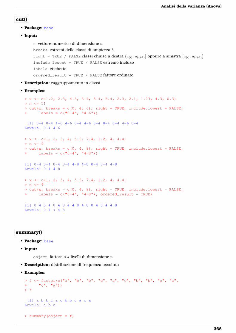
Analisi della varianza (Anova)
cut()
• Package: base
• Input:
x vettore numerico di dimensione n
breaks estremi delle classi di ampiezza bi
right = TRUE / FALSE classi chiuse a destra(a(i), a(i+1)
]oppure a sinistra
[a(i), a(i+1)
)include.lowest = TRUE / FALSE estremo incluso
labels etichette
ordered_result = TRUE / FALSE fattore ordinato
• Description: raggruppamento in classi
• Examples:
> x <- c(1.2, 2.3, 4.5, 5.4, 3.4, 5.4, 2.3, 2.1, 1.23, 4.3, 0.3)> n <- 11> cut(x, breaks = c(0, 4, 6), right = TRUE, include.lowest = FALSE,+ labels = c("0-4", "4-6"))
[1] 0-4 0-4 4-6 4-6 0-4 4-6 0-4 0-4 0-4 4-6 0-4Levels: 0-4 4-6
> x <- c(1, 2, 3, 4, 5.6, 7.4, 1.2, 4, 4.4)> n <- 9> cut(x, breaks = c(0, 4, 8), right = TRUE, include.lowest = FALSE,+ labels = c("0-4", "4-8"))
[1] 0-4 0-4 0-4 0-4 4-8 4-8 0-4 0-4 4-8Levels: 0-4 4-8
> x <- c(1, 2, 3, 4, 5.6, 7.4, 1.2, 4, 4.4)> n <- 9> cut(x, breaks = c(0, 4, 8), right = TRUE, include.lowest = FALSE,+ labels = c("0-4", "4-8"), ordered_result = TRUE)
[1] 0-4 0-4 0-4 0-4 4-8 4-8 0-4 0-4 4-8Levels: 0-4 < 4-8
summary()
• Package: base
• Input:
object fattore a k livelli di dimensione n
• Description: distribuzione di frequenza assoluta
• Examples:
> f <- factor(c("a", "b", "b", "c", "a", "c", "b", "b", "c", "a",+ "c", "a"))> f
[1] a b b c a c b b c a c aLevels: a b c
> summary(object = f)
368
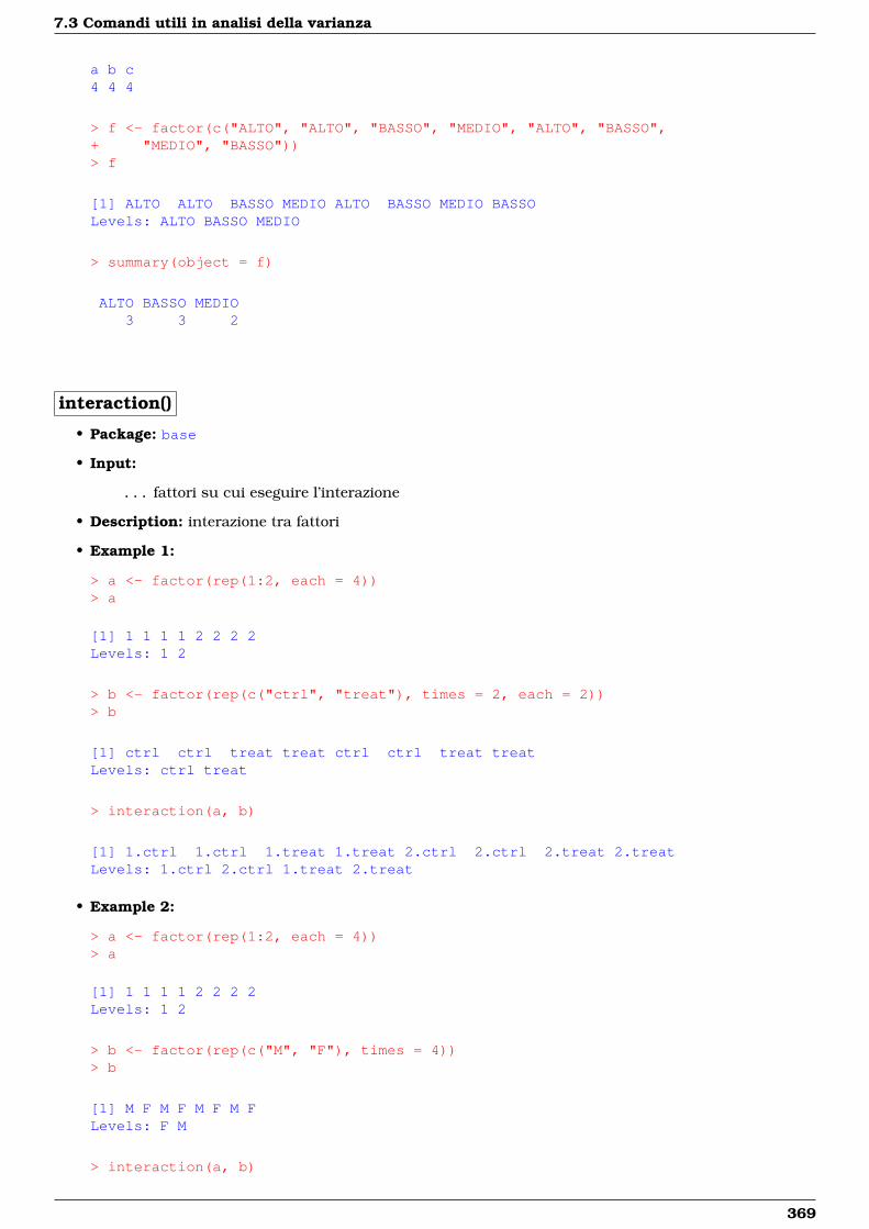
7.3 Comandi utili in analisi della varianza
a b c4 4 4
> f <- factor(c("ALTO", "ALTO", "BASSO", "MEDIO", "ALTO", "BASSO",+ "MEDIO", "BASSO"))> f
[1] ALTO ALTO BASSO MEDIO ALTO BASSO MEDIO BASSOLevels: ALTO BASSO MEDIO
> summary(object = f)
ALTO BASSO MEDIO3 3 2
interaction()
• Package: base
• Input:
... fattori su cui eseguire l’interazione
• Description: interazione tra fattori
• Example 1:
> a <- factor(rep(1:2, each = 4))> a
[1] 1 1 1 1 2 2 2 2Levels: 1 2
> b <- factor(rep(c("ctrl", "treat"), times = 2, each = 2))> b
[1] ctrl ctrl treat treat ctrl ctrl treat treatLevels: ctrl treat
> interaction(a, b)
[1] 1.ctrl 1.ctrl 1.treat 1.treat 2.ctrl 2.ctrl 2.treat 2.treatLevels: 1.ctrl 2.ctrl 1.treat 2.treat
• Example 2:
> a <- factor(rep(1:2, each = 4))> a
[1] 1 1 1 1 2 2 2 2Levels: 1 2
> b <- factor(rep(c("M", "F"), times = 4))> b
[1] M F M F M F M FLevels: F M
> interaction(a, b)
369
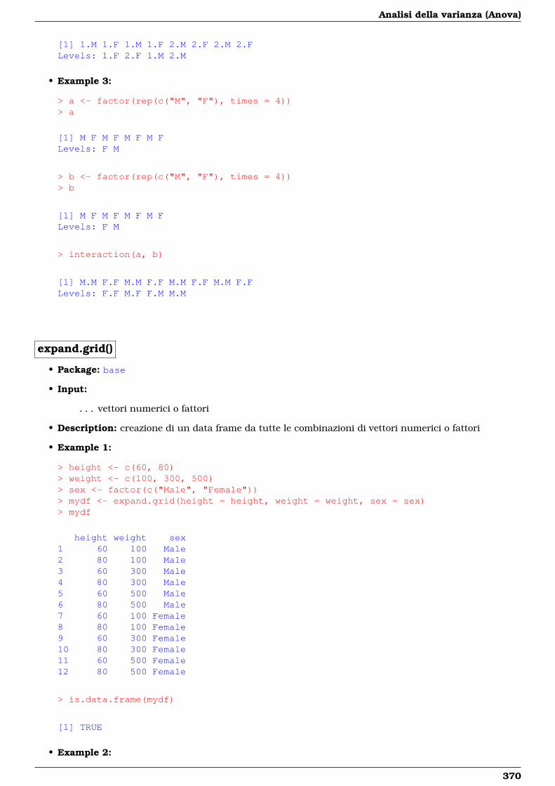
Analisi della varianza (Anova)
[1] 1.M 1.F 1.M 1.F 2.M 2.F 2.M 2.FLevels: 1.F 2.F 1.M 2.M
• Example 3:
> a <- factor(rep(c("M", "F"), times = 4))> a
[1] M F M F M F M FLevels: F M
> b <- factor(rep(c("M", "F"), times = 4))> b
[1] M F M F M F M FLevels: F M
> interaction(a, b)
[1] M.M F.F M.M F.F M.M F.F M.M F.FLevels: F.F M.F F.M M.M
expand.grid()
• Package: base
• Input:
... vettori numerici o fattori
• Description: creazione di un data frame da tutte le combinazioni di vettori numerici o fattori
• Example 1:
> height <- c(60, 80)> weight <- c(100, 300, 500)> sex <- factor(c("Male", "Female"))> mydf <- expand.grid(height = height, weight = weight, sex = sex)> mydf
height weight sex1 60 100 Male2 80 100 Male3 60 300 Male4 80 300 Male5 60 500 Male6 80 500 Male7 60 100 Female8 80 100 Female9 60 300 Female10 80 300 Female11 60 500 Female12 80 500 Female
> is.data.frame(mydf)
[1] TRUE
• Example 2:
370
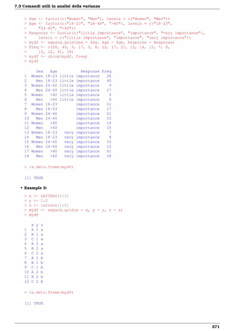
7.3 Comandi utili in analisi della varianza
> Sex <- factor(c("Women", "Men"), levels = c("Women", "Men"))> Age <- factor(c("18-23", "24-40", ">40"), levels = c("18-23",+ "24-40", ">40"))> Response <- factor(c("little importance", "importance", "very importance"),+ levels = c("little importance", "importance", "very importance"))> mydf <- expand.grid(Sex = Sex, Age = Age, Response = Response)> Freq <- c(26, 40, 9, 17, 5, 8, 12, 17, 21, 15, 14, 15, 7, 8,+ 15, 12, 41, 18)> mydf <- cbind(mydf, Freq)> mydf
Sex Age Response Freq1 Women 18-23 little importance 262 Men 18-23 little importance 403 Women 24-40 little importance 94 Men 24-40 little importance 175 Women >40 little importance 56 Men >40 little importance 87 Women 18-23 importance 128 Men 18-23 importance 179 Women 24-40 importance 2110 Men 24-40 importance 1511 Women >40 importance 1412 Men >40 importance 1513 Women 18-23 very importance 714 Men 18-23 very importance 815 Women 24-40 very importance 1516 Men 24-40 very importance 1217 Women >40 very importance 4118 Men >40 very importance 18
> is.data.frame(mydf)
[1] TRUE
• Example 3:
> x <- LETTERS[1:3]> y <- 1:2> z <- letters[1:2]> mydf <- expand.grid(x = x, y = y, z = z)> mydf
x y z1 A 1 a2 B 1 a3 C 1 a4 A 2 a5 B 2 a6 C 2 a7 A 1 b8 B 1 b9 C 1 b10 A 2 b11 B 2 b12 C 2 b
> is.data.frame(mydf)
[1] TRUE
371


Capitolo 8
Confronti multipli
8.1 Simbologia
• numero di livelli dei fattori di colonna e di riga:
Anova f (colonna) g (riga)ad un fattore k /
a due fattori senza interazione k ha due fattori con interazione k h
• dimensione campionaria di colonna, di riga e di cella:
Anova j-esima colonna i-esima riga ij-esima cellaad un fattore nj / /
a due fattori senza interazione hl kl /a due fattori con interazione hl kl l
• medie campionarie di colonna, di riga e di cella:
Anova j-esima colonna i-esima riga ij-esima cellaad un fattore yj / /
a due fattori senza interazione y·j· yi·· yij·a due fattori con interazione y·j· yi·· yij·
• media campionaria generale: y
8.2 Metodo di Tukey
Applicazione in Anova ad un fattore
• Package: stats
• Sintassi: TukeyHSD()
• Input:
y vettore numerico di dimensione n
f fattore con livelli 1, 2, . . . , k
conf.level livello di confidenza 1− α
• Output:
f intervallo di confidenza a livello 1− α per il fattore f
• Formula:
fyi − yj ∀ i > j = 1, 2, . . . , k
yi − yj ∓ q1−α, k, n−k sP
√1 / (2ni) + 1 / (2nj) ∀ i > j = 1, 2, . . . , k
373
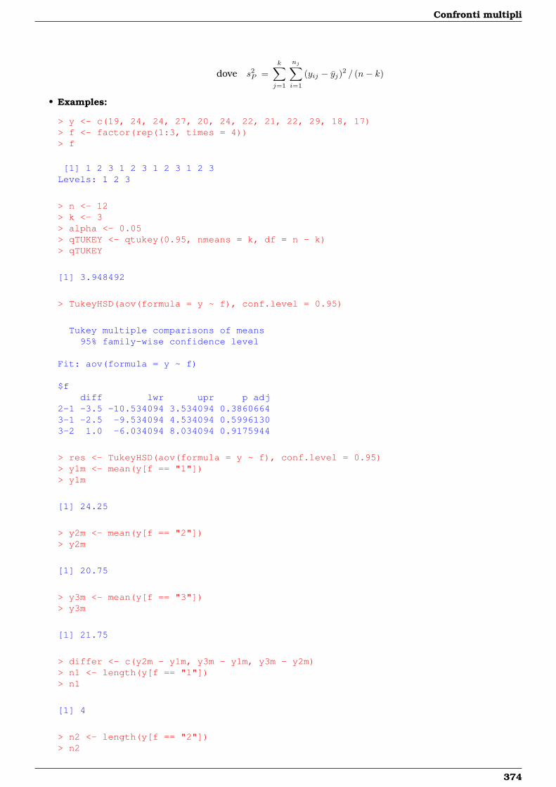
Confronti multipli
dove s2P =
k∑j=1
nj∑i=1
(yij − yj)2 / (n− k)
• Examples:
> y <- c(19, 24, 24, 27, 20, 24, 22, 21, 22, 29, 18, 17)> f <- factor(rep(1:3, times = 4))> f
[1] 1 2 3 1 2 3 1 2 3 1 2 3Levels: 1 2 3
> n <- 12> k <- 3> alpha <- 0.05> qTUKEY <- qtukey(0.95, nmeans = k, df = n - k)> qTUKEY
[1] 3.948492
> TukeyHSD(aov(formula = y ~ f), conf.level = 0.95)
Tukey multiple comparisons of means95% family-wise confidence level
Fit: aov(formula = y ~ f)
$fdiff lwr upr p adj
2-1 -3.5 -10.534094 3.534094 0.38606643-1 -2.5 -9.534094 4.534094 0.59961303-2 1.0 -6.034094 8.034094 0.9175944
> res <- TukeyHSD(aov(formula = y ~ f), conf.level = 0.95)> y1m <- mean(y[f == "1"])> y1m
[1] 24.25
> y2m <- mean(y[f == "2"])> y2m
[1] 20.75
> y3m <- mean(y[f == "3"])> y3m
[1] 21.75
> differ <- c(y2m - y1m, y3m - y1m, y3m - y2m)> n1 <- length(y[f == "1"])> n1
[1] 4
> n2 <- length(y[f == "2"])> n2
374
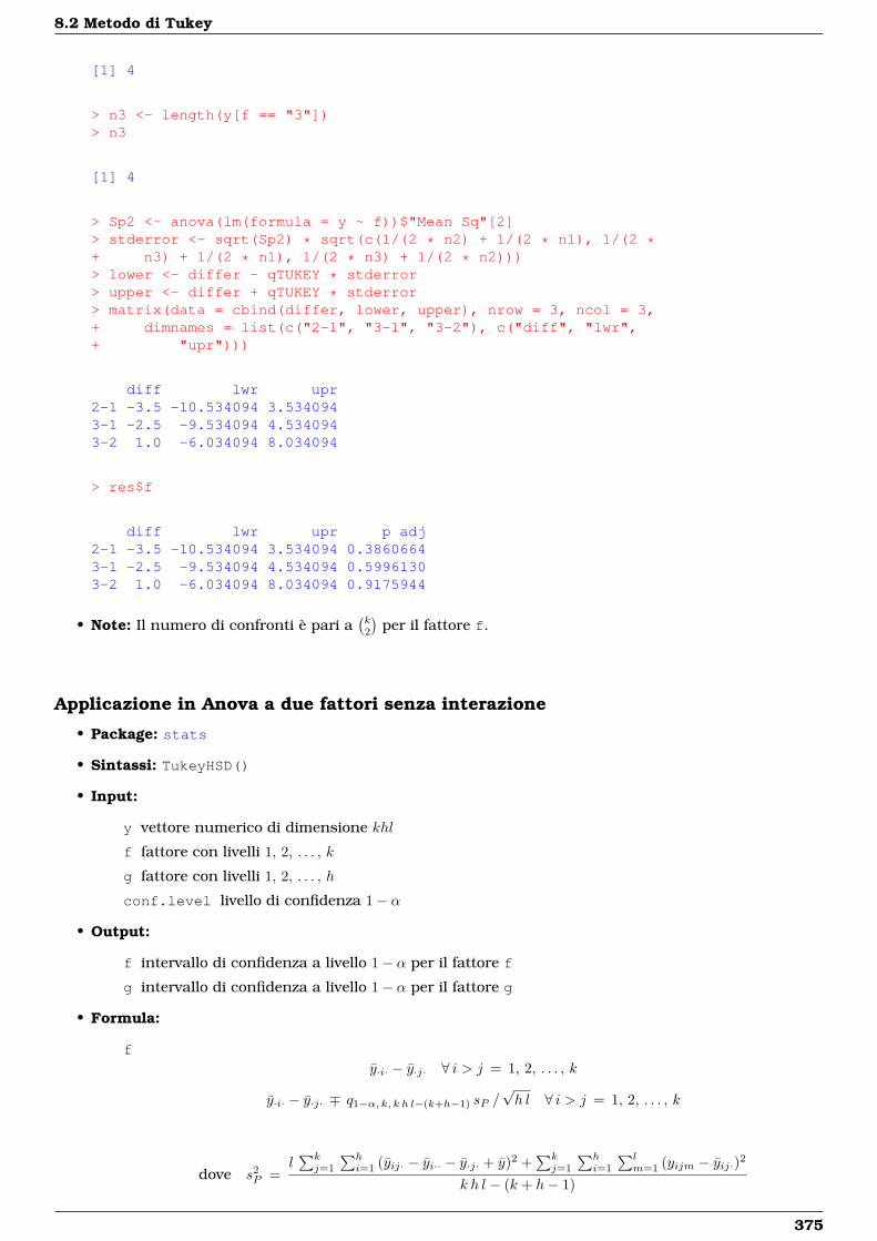
8.2 Metodo di Tukey
[1] 4
> n3 <- length(y[f == "3"])> n3
[1] 4
> Sp2 <- anova(lm(formula = y ~ f))$"Mean Sq"[2]> stderror <- sqrt(Sp2) * sqrt(c(1/(2 * n2) + 1/(2 * n1), 1/(2 *+ n3) + 1/(2 * n1), 1/(2 * n3) + 1/(2 * n2)))> lower <- differ - qTUKEY * stderror> upper <- differ + qTUKEY * stderror> matrix(data = cbind(differ, lower, upper), nrow = 3, ncol = 3,+ dimnames = list(c("2-1", "3-1", "3-2"), c("diff", "lwr",+ "upr")))
diff lwr upr2-1 -3.5 -10.534094 3.5340943-1 -2.5 -9.534094 4.5340943-2 1.0 -6.034094 8.034094
> res$f
diff lwr upr p adj2-1 -3.5 -10.534094 3.534094 0.38606643-1 -2.5 -9.534094 4.534094 0.59961303-2 1.0 -6.034094 8.034094 0.9175944
• Note: Il numero di confronti è pari a(k2
)per il fattore f.
Applicazione in Anova a due fattori senza interazione
• Package: stats
• Sintassi: TukeyHSD()
• Input:
y vettore numerico di dimensione khl
f fattore con livelli 1, 2, . . . , k
g fattore con livelli 1, 2, . . . , h
conf.level livello di confidenza 1− α
• Output:
f intervallo di confidenza a livello 1− α per il fattore f
g intervallo di confidenza a livello 1− α per il fattore g
• Formula:
fy·i· − y·j· ∀ i > j = 1, 2, . . . , k
y·i· − y·j· ∓ q1−α, k, k h l−(k+h−1) sP /√h l ∀ i > j = 1, 2, . . . , k
dove s2P =
l∑kj=1
∑hi=1 (yij· − yi·· − y·j· + y)2 +
∑kj=1
∑hi=1
∑lm=1 (yijm − yij·)2
k h l − (k + h− 1)
375
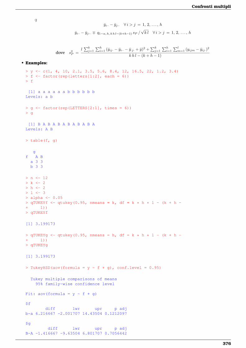
Confronti multipli
gyi·· − yj·· ∀ i > j = 1, 2, . . . , h
yi·· − yj·· ∓ q1−α, h, k h l−(k+h−1) sP /√k l ∀ i > j = 1, 2, . . . , h
dove s2P =
l∑kj=1
∑hi=1 (yij· − yi·· − y·j· + y)2 +
∑kj=1
∑hi=1
∑lm=1 (yijm − yij·)2
k h l − (k + h− 1)
• Examples:
> y <- c(1, 4, 10, 2.1, 3.5, 5.6, 8.4, 12, 16.5, 22, 1.2, 3.4)> f <- factor(rep(letters[1:2], each = 6))> f
[1] a a a a a a b b b b b bLevels: a b
> g <- factor(rep(LETTERS[2:1], times = 6))> g
[1] B A B A B A B A B A B ALevels: A B
> table(f, g)
gf A B
a 3 3b 3 3
> n <- 12> k <- 2> h <- 2> l <- 3> alpha <- 0.05> qTUKEYf <- qtukey(0.95, nmeans = k, df = k * h * l - (k + h -+ 1))> qTUKEYf
[1] 3.199173
> qTUKEYg <- qtukey(0.95, nmeans = h, df = k * h * l - (k + h -+ 1))> qTUKEYg
[1] 3.199173
> TukeyHSD(aov(formula = y ~ f + g), conf.level = 0.95)
Tukey multiple comparisons of means95% family-wise confidence level
Fit: aov(formula = y ~ f + g)
$fdiff lwr upr p adj
b-a 6.216667 -2.001707 14.43504 0.1212097
$gdiff lwr upr p adj
B-A -1.416667 -9.63504 6.801707 0.7056442
376
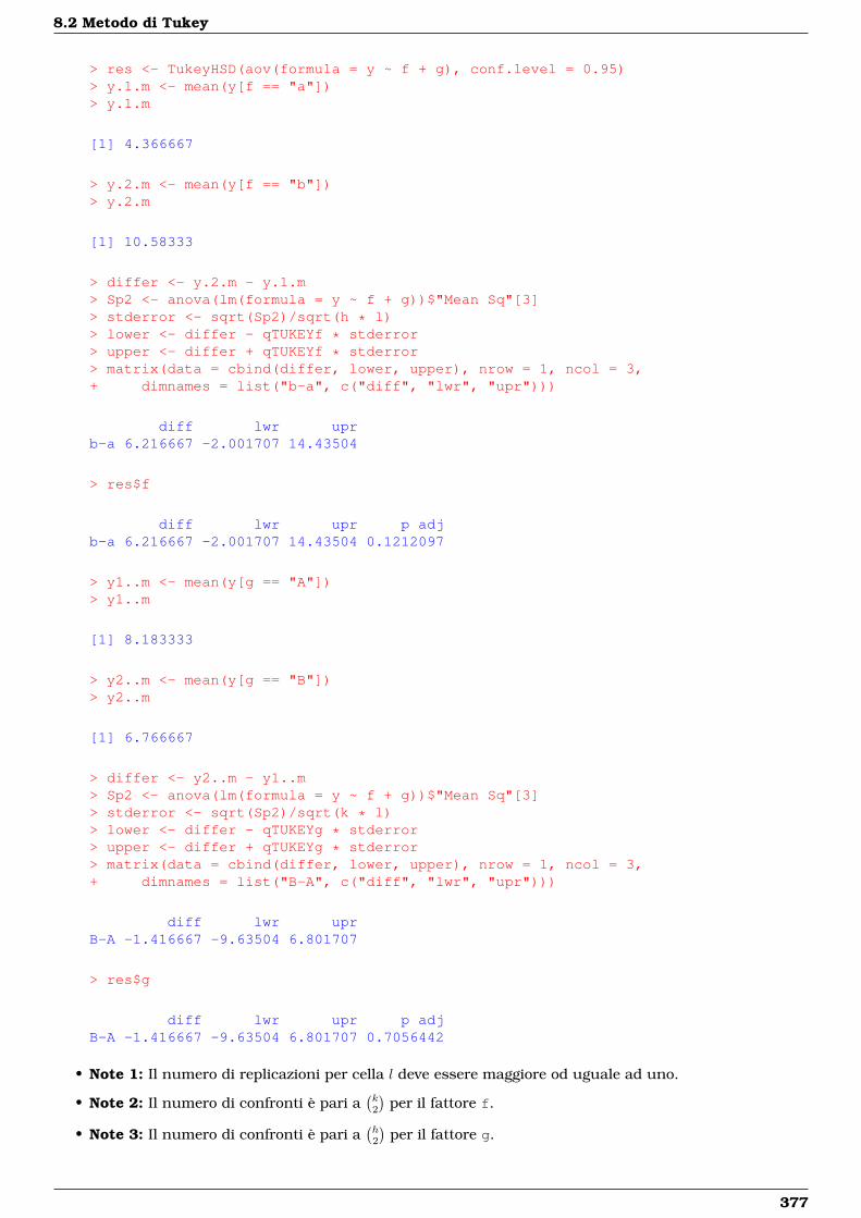
8.2 Metodo di Tukey
> res <- TukeyHSD(aov(formula = y ~ f + g), conf.level = 0.95)> y.1.m <- mean(y[f == "a"])> y.1.m
[1] 4.366667
> y.2.m <- mean(y[f == "b"])> y.2.m
[1] 10.58333
> differ <- y.2.m - y.1.m> Sp2 <- anova(lm(formula = y ~ f + g))$"Mean Sq"[3]> stderror <- sqrt(Sp2)/sqrt(h * l)> lower <- differ - qTUKEYf * stderror> upper <- differ + qTUKEYf * stderror> matrix(data = cbind(differ, lower, upper), nrow = 1, ncol = 3,+ dimnames = list("b-a", c("diff", "lwr", "upr")))
diff lwr uprb-a 6.216667 -2.001707 14.43504
> res$f
diff lwr upr p adjb-a 6.216667 -2.001707 14.43504 0.1212097
> y1..m <- mean(y[g == "A"])> y1..m
[1] 8.183333
> y2..m <- mean(y[g == "B"])> y2..m
[1] 6.766667
> differ <- y2..m - y1..m> Sp2 <- anova(lm(formula = y ~ f + g))$"Mean Sq"[3]> stderror <- sqrt(Sp2)/sqrt(k * l)> lower <- differ - qTUKEYg * stderror> upper <- differ + qTUKEYg * stderror> matrix(data = cbind(differ, lower, upper), nrow = 1, ncol = 3,+ dimnames = list("B-A", c("diff", "lwr", "upr")))
diff lwr uprB-A -1.416667 -9.63504 6.801707
> res$g
diff lwr upr p adjB-A -1.416667 -9.63504 6.801707 0.7056442
• Note 1: Il numero di replicazioni per cella l deve essere maggiore od uguale ad uno.
• Note 2: Il numero di confronti è pari a(k2
)per il fattore f.
• Note 3: Il numero di confronti è pari a(h2
)per il fattore g.
377
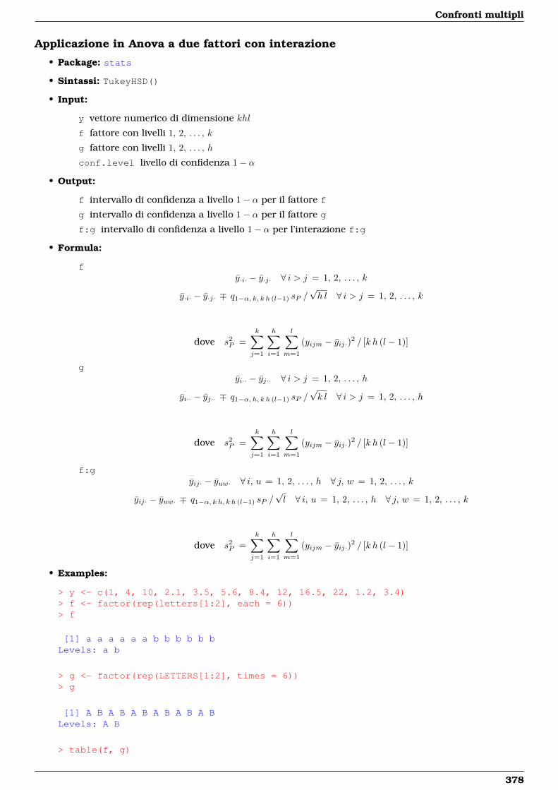
Confronti multipli
Applicazione in Anova a due fattori con interazione
• Package: stats
• Sintassi: TukeyHSD()
• Input:
y vettore numerico di dimensione khl
f fattore con livelli 1, 2, . . . , k
g fattore con livelli 1, 2, . . . , h
conf.level livello di confidenza 1− α
• Output:
f intervallo di confidenza a livello 1− α per il fattore f
g intervallo di confidenza a livello 1− α per il fattore g
f:g intervallo di confidenza a livello 1− α per l’interazione f:g
• Formula:
fy·i· − y·j· ∀ i > j = 1, 2, . . . , k
y·i· − y·j· ∓ q1−α, k, k h (l−1) sP /√h l ∀ i > j = 1, 2, . . . , k
dove s2P =
k∑j=1
h∑i=1
l∑m=1
(yijm − yij·)2 / [k h (l − 1)]
gyi·· − yj·· ∀ i > j = 1, 2, . . . , h
yi·· − yj·· ∓ q1−α, h, k h (l−1) sP /√k l ∀ i > j = 1, 2, . . . , h
dove s2P =
k∑j=1
h∑i=1
l∑m=1
(yijm − yij·)2 / [k h (l − 1)]
f:gyij· − yuw· ∀ i, u = 1, 2, . . . , h ∀ j, w = 1, 2, . . . , k
yij· − yuw· ∓ q1−α, k h, k h (l−1) sP /√l ∀ i, u = 1, 2, . . . , h ∀ j, w = 1, 2, . . . , k
dove s2P =
k∑j=1
h∑i=1
l∑m=1
(yijm − yij·)2 / [k h (l − 1)]
• Examples:
> y <- c(1, 4, 10, 2.1, 3.5, 5.6, 8.4, 12, 16.5, 22, 1.2, 3.4)> f <- factor(rep(letters[1:2], each = 6))> f
[1] a a a a a a b b b b b bLevels: a b
> g <- factor(rep(LETTERS[1:2], times = 6))> g
[1] A B A B A B A B A B A BLevels: A B
> table(f, g)
378
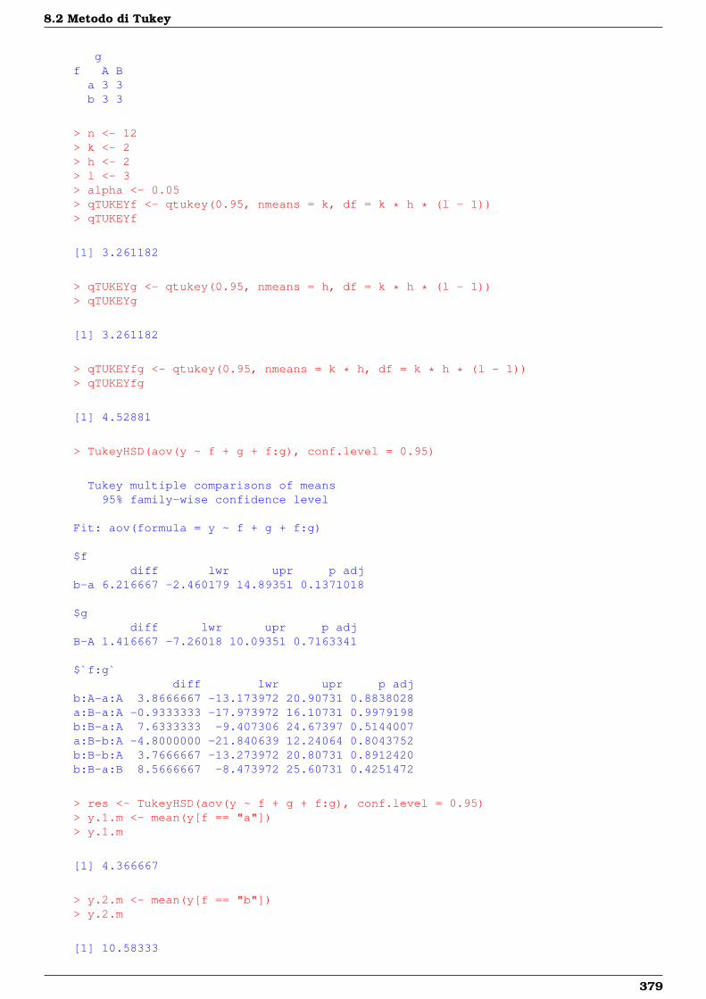
8.2 Metodo di Tukey
gf A B
a 3 3b 3 3
> n <- 12> k <- 2> h <- 2> l <- 3> alpha <- 0.05> qTUKEYf <- qtukey(0.95, nmeans = k, df = k * h * (l - 1))> qTUKEYf
[1] 3.261182
> qTUKEYg <- qtukey(0.95, nmeans = h, df = k * h * (l - 1))> qTUKEYg
[1] 3.261182
> qTUKEYfg <- qtukey(0.95, nmeans = k * h, df = k * h * (l - 1))> qTUKEYfg
[1] 4.52881
> TukeyHSD(aov(y ~ f + g + f:g), conf.level = 0.95)
Tukey multiple comparisons of means95% family-wise confidence level
Fit: aov(formula = y ~ f + g + f:g)
$fdiff lwr upr p adj
b-a 6.216667 -2.460179 14.89351 0.1371018
$gdiff lwr upr p adj
B-A 1.416667 -7.26018 10.09351 0.7163341
$`f:g`diff lwr upr p adj
b:A-a:A 3.8666667 -13.173972 20.90731 0.8838028a:B-a:A -0.9333333 -17.973972 16.10731 0.9979198b:B-a:A 7.6333333 -9.407306 24.67397 0.5144007a:B-b:A -4.8000000 -21.840639 12.24064 0.8043752b:B-b:A 3.7666667 -13.273972 20.80731 0.8912420b:B-a:B 8.5666667 -8.473972 25.60731 0.4251472
> res <- TukeyHSD(aov(y ~ f + g + f:g), conf.level = 0.95)> y.1.m <- mean(y[f == "a"])> y.1.m
[1] 4.366667
> y.2.m <- mean(y[f == "b"])> y.2.m
[1] 10.58333
379
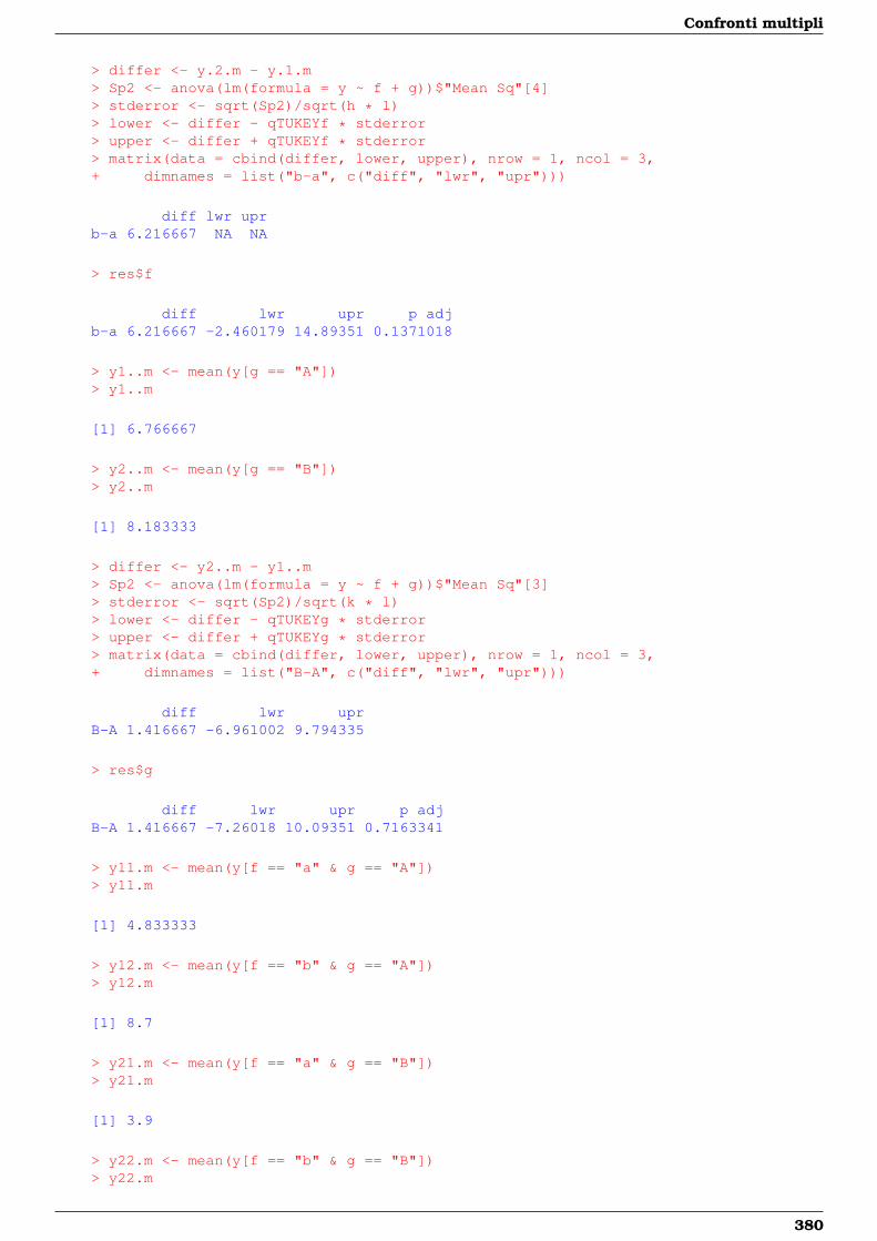
Confronti multipli
> differ <- y.2.m - y.1.m> Sp2 <- anova(lm(formula = y ~ f + g))$"Mean Sq"[4]> stderror <- sqrt(Sp2)/sqrt(h * l)> lower <- differ - qTUKEYf * stderror> upper <- differ + qTUKEYf * stderror> matrix(data = cbind(differ, lower, upper), nrow = 1, ncol = 3,+ dimnames = list("b-a", c("diff", "lwr", "upr")))
diff lwr uprb-a 6.216667 NA NA
> res$f
diff lwr upr p adjb-a 6.216667 -2.460179 14.89351 0.1371018
> y1..m <- mean(y[g == "A"])> y1..m
[1] 6.766667
> y2..m <- mean(y[g == "B"])> y2..m
[1] 8.183333
> differ <- y2..m - y1..m> Sp2 <- anova(lm(formula = y ~ f + g))$"Mean Sq"[3]> stderror <- sqrt(Sp2)/sqrt(k * l)> lower <- differ - qTUKEYg * stderror> upper <- differ + qTUKEYg * stderror> matrix(data = cbind(differ, lower, upper), nrow = 1, ncol = 3,+ dimnames = list("B-A", c("diff", "lwr", "upr")))
diff lwr uprB-A 1.416667 -6.961002 9.794335
> res$g
diff lwr upr p adjB-A 1.416667 -7.26018 10.09351 0.7163341
> y11.m <- mean(y[f == "a" & g == "A"])> y11.m
[1] 4.833333
> y12.m <- mean(y[f == "b" & g == "A"])> y12.m
[1] 8.7
> y21.m <- mean(y[f == "a" & g == "B"])> y21.m
[1] 3.9
> y22.m <- mean(y[f == "b" & g == "B"])> y22.m
380
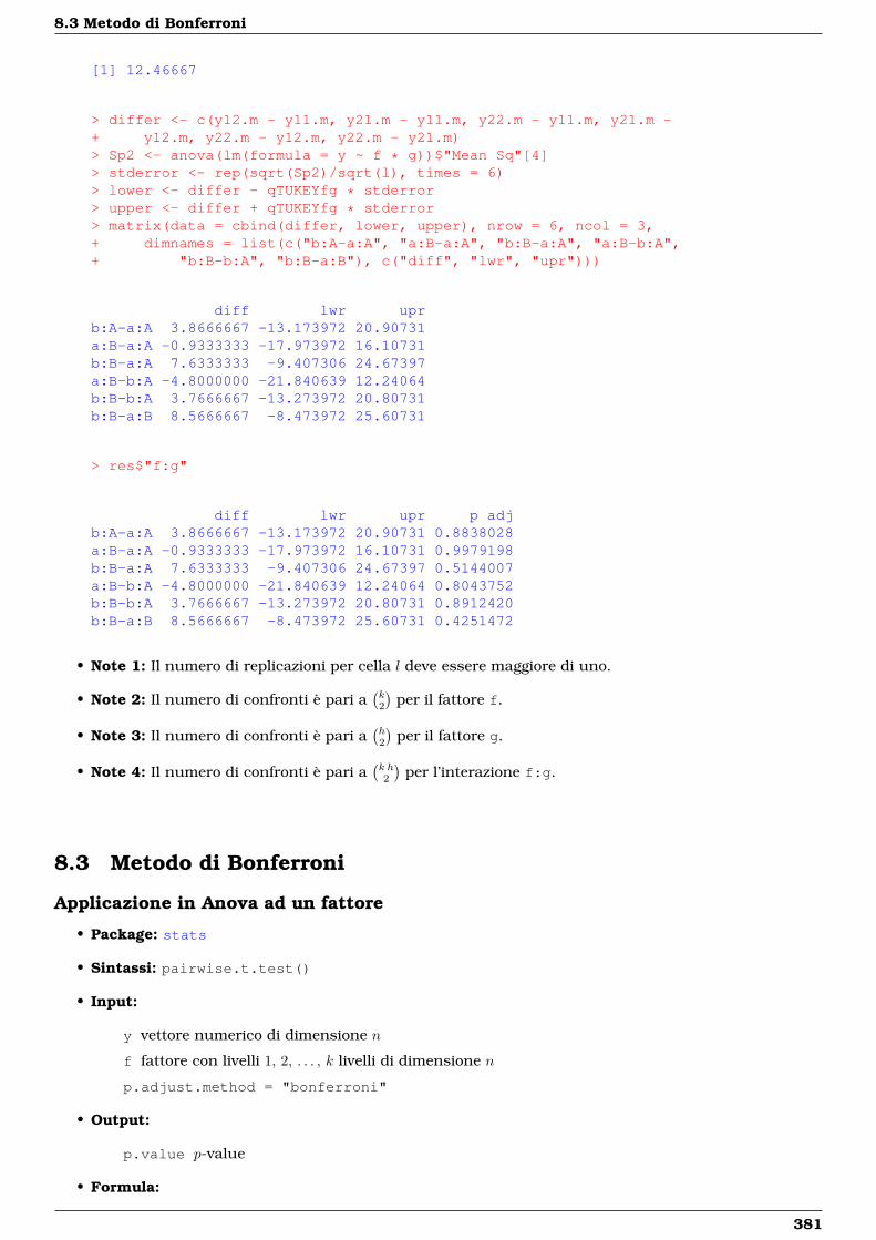
8.3 Metodo di Bonferroni
[1] 12.46667
> differ <- c(y12.m - y11.m, y21.m - y11.m, y22.m - y11.m, y21.m -+ y12.m, y22.m - y12.m, y22.m - y21.m)> Sp2 <- anova(lm(formula = y ~ f * g))$"Mean Sq"[4]> stderror <- rep(sqrt(Sp2)/sqrt(l), times = 6)> lower <- differ - qTUKEYfg * stderror> upper <- differ + qTUKEYfg * stderror> matrix(data = cbind(differ, lower, upper), nrow = 6, ncol = 3,+ dimnames = list(c("b:A-a:A", "a:B-a:A", "b:B-a:A", "a:B-b:A",+ "b:B-b:A", "b:B-a:B"), c("diff", "lwr", "upr")))
diff lwr uprb:A-a:A 3.8666667 -13.173972 20.90731a:B-a:A -0.9333333 -17.973972 16.10731b:B-a:A 7.6333333 -9.407306 24.67397a:B-b:A -4.8000000 -21.840639 12.24064b:B-b:A 3.7666667 -13.273972 20.80731b:B-a:B 8.5666667 -8.473972 25.60731
> res$"f:g"
diff lwr upr p adjb:A-a:A 3.8666667 -13.173972 20.90731 0.8838028a:B-a:A -0.9333333 -17.973972 16.10731 0.9979198b:B-a:A 7.6333333 -9.407306 24.67397 0.5144007a:B-b:A -4.8000000 -21.840639 12.24064 0.8043752b:B-b:A 3.7666667 -13.273972 20.80731 0.8912420b:B-a:B 8.5666667 -8.473972 25.60731 0.4251472
• Note 1: Il numero di replicazioni per cella l deve essere maggiore di uno.
• Note 2: Il numero di confronti è pari a(k2
)per il fattore f.
• Note 3: Il numero di confronti è pari a(h2
)per il fattore g.
• Note 4: Il numero di confronti è pari a(k h2
)per l’interazione f:g.
8.3 Metodo di Bonferroni
Applicazione in Anova ad un fattore
• Package: stats
• Sintassi: pairwise.t.test()
• Input:
y vettore numerico di dimensione n
f fattore con livelli 1, 2, . . . , k livelli di dimensione n
p.adjust.method = "bonferroni"
• Output:
p.value p-value
• Formula:
381
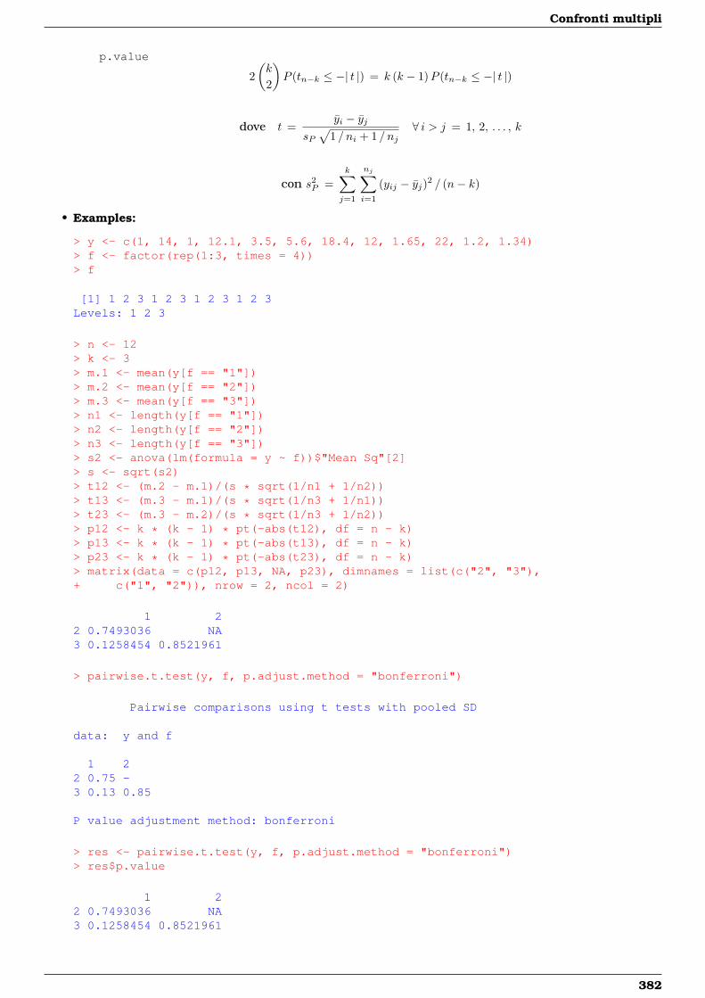
Confronti multipli
p.value
2(k
2
)P (tn−k ≤ −| t |) = k (k − 1)P (tn−k ≤ −| t |)
dove t =yi − yj
sP√
1 / ni + 1 / nj∀ i > j = 1, 2, . . . , k
con s2P =
k∑j=1
nj∑i=1
(yij − yj)2 / (n− k)
• Examples:
> y <- c(1, 14, 1, 12.1, 3.5, 5.6, 18.4, 12, 1.65, 22, 1.2, 1.34)> f <- factor(rep(1:3, times = 4))> f
[1] 1 2 3 1 2 3 1 2 3 1 2 3Levels: 1 2 3
> n <- 12> k <- 3> m.1 <- mean(y[f == "1"])> m.2 <- mean(y[f == "2"])> m.3 <- mean(y[f == "3"])> n1 <- length(y[f == "1"])> n2 <- length(y[f == "2"])> n3 <- length(y[f == "3"])> s2 <- anova(lm(formula = y ~ f))$"Mean Sq"[2]> s <- sqrt(s2)> t12 <- (m.2 - m.1)/(s * sqrt(1/n1 + 1/n2))> t13 <- (m.3 - m.1)/(s * sqrt(1/n3 + 1/n1))> t23 <- (m.3 - m.2)/(s * sqrt(1/n3 + 1/n2))> p12 <- k * (k - 1) * pt(-abs(t12), df = n - k)> p13 <- k * (k - 1) * pt(-abs(t13), df = n - k)> p23 <- k * (k - 1) * pt(-abs(t23), df = n - k)> matrix(data = c(p12, p13, NA, p23), dimnames = list(c("2", "3"),+ c("1", "2")), nrow = 2, ncol = 2)
1 22 0.7493036 NA3 0.1258454 0.8521961
> pairwise.t.test(y, f, p.adjust.method = "bonferroni")
Pairwise comparisons using t tests with pooled SD
data: y and f
1 22 0.75 -3 0.13 0.85
P value adjustment method: bonferroni
> res <- pairwise.t.test(y, f, p.adjust.method = "bonferroni")> res$p.value
1 22 0.7493036 NA3 0.1258454 0.8521961
382
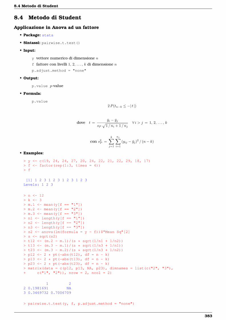
8.4 Metodo di Student
8.4 Metodo di Student
Applicazione in Anova ad un fattore
• Package: stats
• Sintassi: pairwise.t.test()
• Input:
y vettore numerico di dimensione n
f fattore con livelli 1, 2, . . . , k di dimensione n
p.adjust.method = "none"
• Output:
p.value p-value
• Formula:
p.value2P (tn−k ≤ −| t |)
dove t =yi − yj
sP√
1 / ni + 1 / nj∀ i > j = 1, 2, . . . , k
con s2P =
k∑j=1
nj∑i=1
(yij − yj)2 / (n− k)
• Examples:
> y <- c(19, 24, 24, 27, 20, 24, 22, 21, 22, 29, 18, 17)> f <- factor(rep(1:3, times = 4))> f
[1] 1 2 3 1 2 3 1 2 3 1 2 3Levels: 1 2 3
> n <- 12> k <- 3> m.1 <- mean(y[f == "1"])> m.2 <- mean(y[f == "2"])> m.3 <- mean(y[f == "3"])> n1 <- length(y[f == "1"])> n2 <- length(y[f == "2"])> n3 <- length(y[f == "3"])> s2 <- anova(lm(formula = y ~ f))$"Mean Sq"[2]> s <- sqrt(s2)> t12 <- (m.2 - m.1)/(s * sqrt(1/n1 + 1/n2))> t13 <- (m.3 - m.1)/(s * sqrt(1/n3 + 1/n1))> t23 <- (m.3 - m.2)/(s * sqrt(1/n3 + 1/n2))> p12 <- 2 * pt(-abs(t12), df = n - k)> p13 <- 2 * pt(-abs(t13), df = n - k)> p23 <- 2 * pt(-abs(t23), df = n - k)> matrix(data = c(p12, p13, NA, p23), dimnames = list(c("2", "3"),+ c("1", "2")), nrow = 2, ncol = 2)
1 22 0.1981691 NA3 0.3469732 0.7006709
> pairwise.t.test(y, f, p.adjust.method = "none")
383
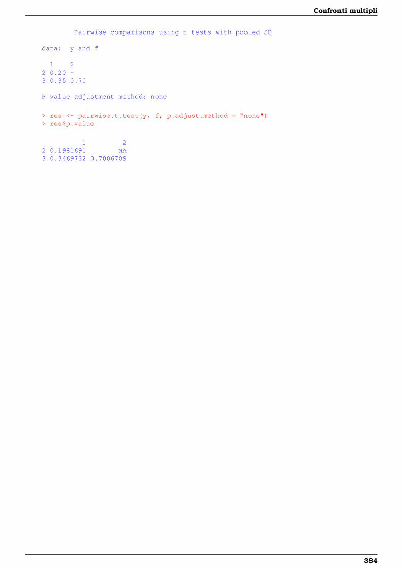
Confronti multipli
Pairwise comparisons using t tests with pooled SD
data: y and f
1 22 0.20 -3 0.35 0.70
P value adjustment method: none
> res <- pairwise.t.test(y, f, p.adjust.method = "none")> res$p.value
1 22 0.1981691 NA3 0.3469732 0.7006709
384
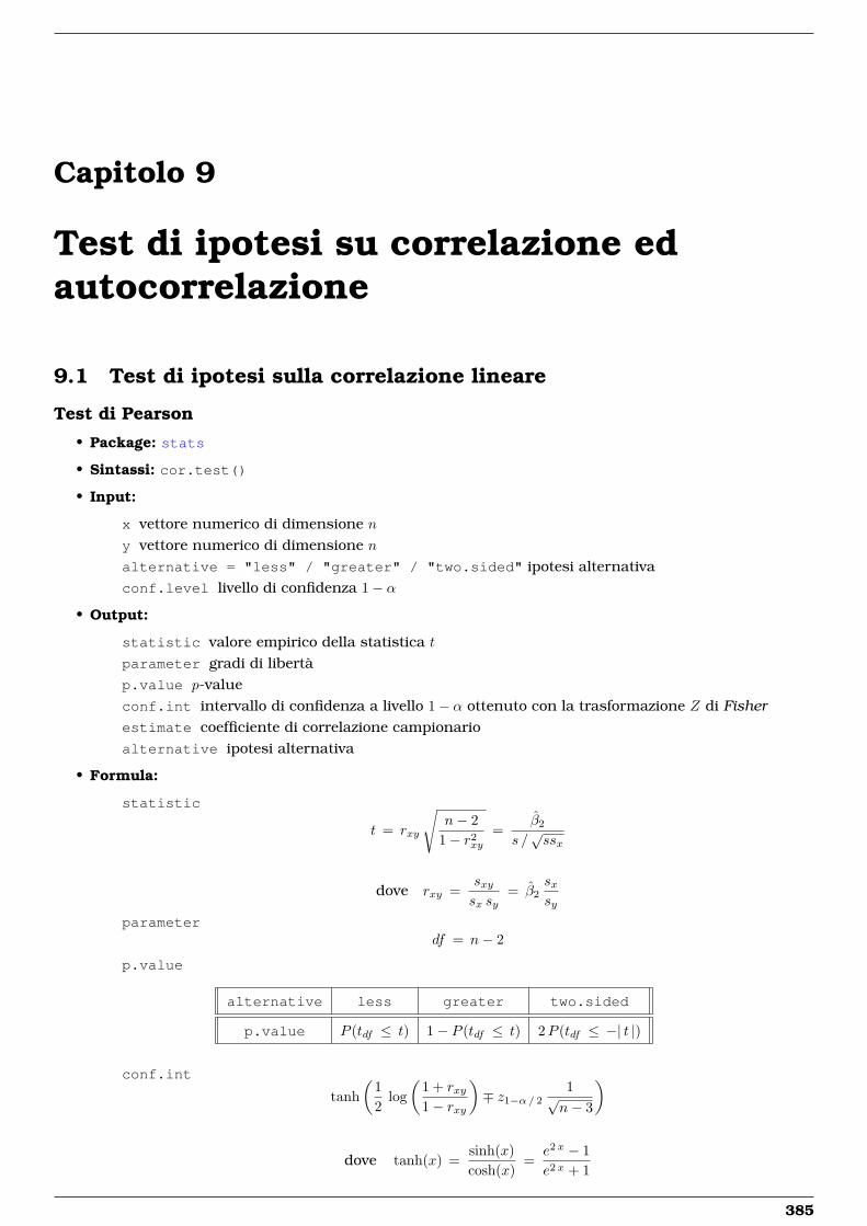
Capitolo 9
Test di ipotesi su correlazione edautocorrelazione
9.1 Test di ipotesi sulla correlazione lineare
Test di Pearson
• Package: stats
• Sintassi: cor.test()
• Input:
x vettore numerico di dimensione ny vettore numerico di dimensione nalternative = "less" / "greater" / "two.sided" ipotesi alternativaconf.level livello di confidenza 1− α
• Output:
statistic valore empirico della statistica t
parameter gradi di libertàp.value p-valueconf.int intervallo di confidenza a livello 1− α ottenuto con la trasformazione Z di Fisherestimate coefficiente di correlazione campionarioalternative ipotesi alternativa
• Formula:
statistic
t = rxy
√n− 2
1− r2xy
=β2
s /√ssx
dove rxy =sxysx sy
= β2sxsy
parameterdf = n− 2
p.value
alternative less greater two.sided
p.value P (tdf ≤ t) 1− P (tdf ≤ t) 2P (tdf ≤ −| t |)
conf.int
tanh(
12
log(
1 + rxy1− rxy
)∓ z1−α/ 2
1√n− 3
)
dove tanh(x) =sinh(x)cosh(x)
=e2 x − 1e2 x + 1
385
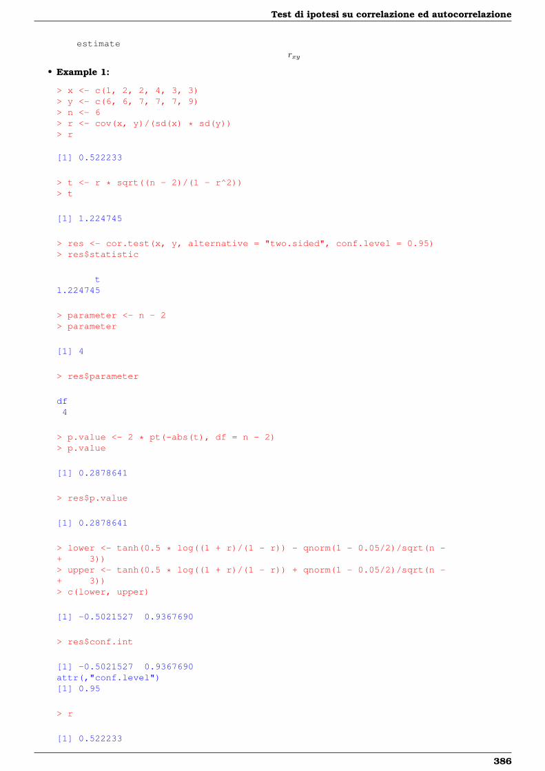
Test di ipotesi su correlazione ed autocorrelazione
estimaterxy
• Example 1:
> x <- c(1, 2, 2, 4, 3, 3)> y <- c(6, 6, 7, 7, 7, 9)> n <- 6> r <- cov(x, y)/(sd(x) * sd(y))> r
[1] 0.522233
> t <- r * sqrt((n - 2)/(1 - r^2))> t
[1] 1.224745
> res <- cor.test(x, y, alternative = "two.sided", conf.level = 0.95)> res$statistic
t1.224745
> parameter <- n - 2> parameter
[1] 4
> res$parameter
df4
> p.value <- 2 * pt(-abs(t), df = n - 2)> p.value
[1] 0.2878641
> res$p.value
[1] 0.2878641
> lower <- tanh(0.5 * log((1 + r)/(1 - r)) - qnorm(1 - 0.05/2)/sqrt(n -+ 3))> upper <- tanh(0.5 * log((1 + r)/(1 - r)) + qnorm(1 - 0.05/2)/sqrt(n -+ 3))> c(lower, upper)
[1] -0.5021527 0.9367690
> res$conf.int
[1] -0.5021527 0.9367690attr(,"conf.level")[1] 0.95
> r
[1] 0.522233
386
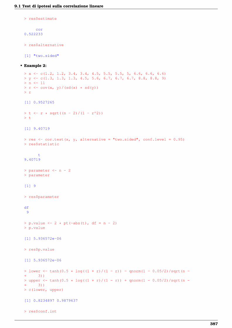
9.1 Test di ipotesi sulla correlazione lineare
> res$estimate
cor0.522233
> res$alternative
[1] "two.sided"
• Example 2:
> x <- c(1.2, 1.2, 3.4, 3.4, 4.5, 5.5, 5.5, 5, 6.6, 6.6, 6.6)> y <- c(1.3, 1.3, 1.3, 4.5, 5.6, 6.7, 6.7, 6.7, 8.8, 8.8, 9)> n <- 11> r <- cov(x, y)/(sd(x) * sd(y))> r
[1] 0.9527265
> t <- r * sqrt((n - 2)/(1 - r^2))> t
[1] 9.40719
> res <- cor.test(x, y, alternative = "two.sided", conf.level = 0.95)> res$statistic
t9.40719
> parameter <- n - 2> parameter
[1] 9
> res$parameter
df9
> p.value <- 2 * pt(-abs(t), df = n - 2)> p.value
[1] 5.936572e-06
> res$p.value
[1] 5.936572e-06
> lower <- tanh(0.5 * log((1 + r)/(1 - r)) - qnorm(1 - 0.05/2)/sqrt(n -+ 3))> upper <- tanh(0.5 * log((1 + r)/(1 - r)) + qnorm(1 - 0.05/2)/sqrt(n -+ 3))> c(lower, upper)
[1] 0.8234897 0.9879637
> res$conf.int
387
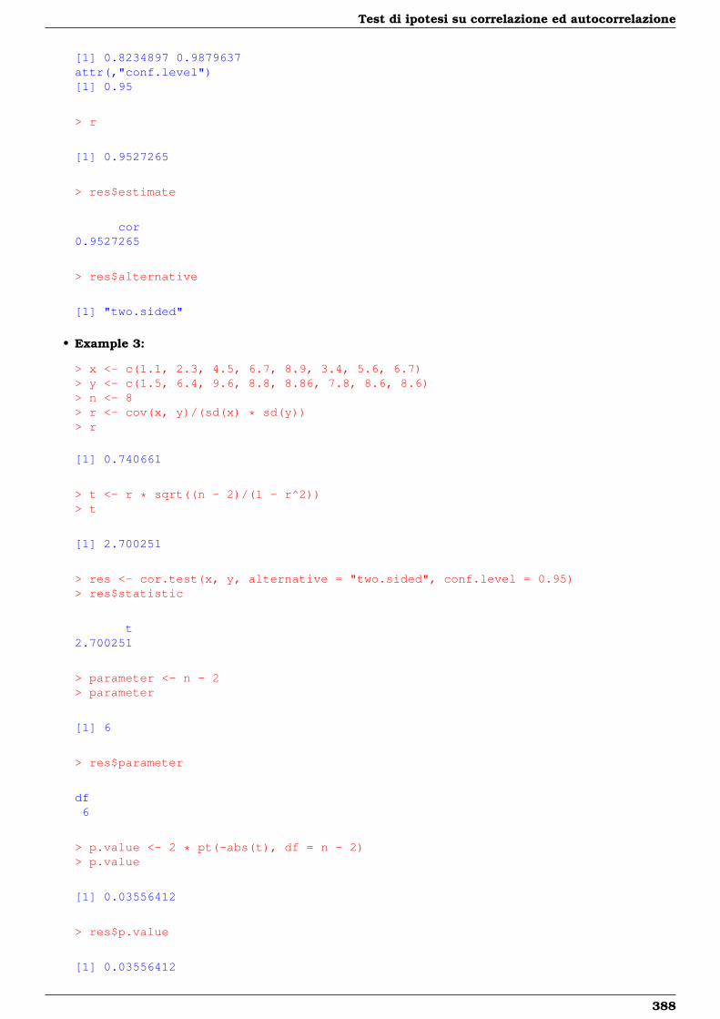
Test di ipotesi su correlazione ed autocorrelazione
[1] 0.8234897 0.9879637attr(,"conf.level")[1] 0.95
> r
[1] 0.9527265
> res$estimate
cor0.9527265
> res$alternative
[1] "two.sided"
• Example 3:
> x <- c(1.1, 2.3, 4.5, 6.7, 8.9, 3.4, 5.6, 6.7)> y <- c(1.5, 6.4, 9.6, 8.8, 8.86, 7.8, 8.6, 8.6)> n <- 8> r <- cov(x, y)/(sd(x) * sd(y))> r
[1] 0.740661
> t <- r * sqrt((n - 2)/(1 - r^2))> t
[1] 2.700251
> res <- cor.test(x, y, alternative = "two.sided", conf.level = 0.95)> res$statistic
t2.700251
> parameter <- n - 2> parameter
[1] 6
> res$parameter
df6
> p.value <- 2 * pt(-abs(t), df = n - 2)> p.value
[1] 0.03556412
> res$p.value
[1] 0.03556412
388
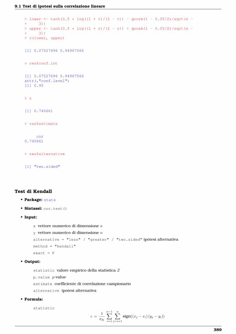
9.1 Test di ipotesi sulla correlazione lineare
> lower <- tanh(0.5 * log((1 + r)/(1 - r)) - qnorm(1 - 0.05/2)/sqrt(n -+ 3))> upper <- tanh(0.5 * log((1 + r)/(1 - r)) + qnorm(1 - 0.05/2)/sqrt(n -+ 3))> c(lower, upper)
[1] 0.07527696 0.94967566
> res$conf.int
[1] 0.07527696 0.94967566attr(,"conf.level")[1] 0.95
> r
[1] 0.740661
> res$estimate
cor0.740661
> res$alternative
[1] "two.sided"
Test di Kendall
• Package: stats
• Sintassi: cor.test()
• Input:
x vettore numerico di dimensione n
y vettore numerico di dimensione n
alternative = "less" / "greater" / "two.sided" ipotesi alternativa
method = "kendall"
exact = F
• Output:
statistic valore empirico della statistica Z
p.value p-value
estimate coefficiente di correlazione campionario
alternative ipotesi alternativa
• Formula:
statistic
z =1σK
n−1∑i=1
n∑j=i+1
sign((xj − xi) (yj − yi))
389
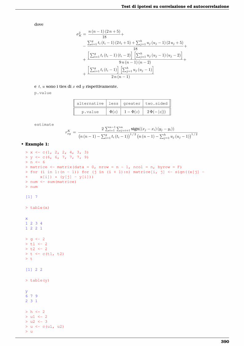
Test di ipotesi su correlazione ed autocorrelazione
dove
σ2K =
n (n− 1) (2n+ 5)18
+
−∑gi=1 ti (ti − 1) (2 ti + 5) +
∑hj=1 uj (uj − 1) (2uj + 5)
18+
+
[∑gi=1 ti (ti − 1) (ti − 2)
] [∑hj=1 uj (uj − 1) (uj − 2)
]9n (n− 1) (n− 2)
+
+
[∑gi=1 ti (ti − 1)
] [∑hj=1 uj (uj − 1)
]2n (n− 1)
e t, u sono i ties di x ed y rispettivamente.
p.value
alternative less greater two.sided
p.value Φ(z) 1− Φ(z) 2 Φ(− |z|))
estimate
rKxy =2∑n−1i=1
∑nj=i+1 sign((xj − xi) (yj − yi))(
n (n− 1)−∑gi=1 ti (ti − 1)
)1 / 2 (n (n− 1)−
∑hj=1 uj (uj − 1)
)1 / 2
• Example 1:
> x <- c(1, 2, 2, 4, 3, 3)> y <- c(6, 6, 7, 7, 7, 9)> n <- 6> matrice <- matrix(data = 0, nrow = n - 1, ncol = n, byrow = F)> for (i in 1:(n - 1)) for (j in (i + 1):n) matrice[i, j] <- sign((x[j] -+ x[i]) * (y[j] - y[i]))> num <- sum(matrice)> num
[1] 7
> table(x)
x1 2 3 41 2 2 1
> g <- 2> t1 <- 2> t2 <- 2> t <- c(t1, t2)> t
[1] 2 2
> table(y)
y6 7 92 3 1
> h <- 2> u1 <- 2> u2 <- 3> u <- c(u1, u2)> u
390
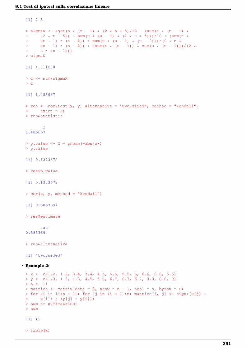
9.1 Test di ipotesi sulla correlazione lineare
[1] 2 3
> sigmaK <- sqrt(n * (n - 1) * (2 * n + 5)/18 - (sum(t * (t - 1) *+ (2 * t + 5)) + sum(u * (u - 1) * (2 * u + 5)))/18 + (sum(t *+ (t - 1) * (t - 2)) * sum(u * (u - 1) * (u - 2)))/(9 * n *+ (n - 1) * (n - 2)) + (sum(t * (t - 1)) * sum(u * (u - 1)))/(2 *+ n * (n - 1)))> sigmaK
[1] 4.711688
> z <- num/sigmaK> z
[1] 1.485667
> res <- cor.test(x, y, alternative = "two.sided", method = "kendall",+ exact = F)> res$statistic
z1.485667
> p.value <- 2 * pnorm(-abs(z))> p.value
[1] 0.1373672
> res$p.value
[1] 0.1373672
> cor(x, y, method = "kendall")
[1] 0.5853694
> res$estimate
tau0.5853694
> res$alternative
[1] "two.sided"
• Example 2:
> x <- c(1.2, 1.2, 3.4, 3.4, 4.5, 5.5, 5.5, 5, 6.6, 6.6, 6.6)> y <- c(1.3, 1.3, 1.3, 4.5, 5.6, 6.7, 6.7, 6.7, 8.8, 8.8, 9)> n <- 11> matrice <- matrix(data = 0, nrow = n - 1, ncol = n, byrow = F)> for (i in 1:(n - 1)) for (j in (i + 1):n) matrice[i, j] <- sign((x[j] -+ x[i]) * (y[j] - y[i]))> num <- sum(matrice)> num
[1] 45
> table(x)
391

Test di ipotesi su correlazione ed autocorrelazione
x1.2 3.4 4.5 5 5.5 6.62 2 1 1 2 3
> g <- 4> t1 <- 2> t2 <- 2> t3 <- 2> t4 <- 3> t <- c(t1, t2, t3, t4)> t
[1] 2 2 2 3
> table(y)
y1.3 4.5 5.6 6.7 8.8 9
3 1 1 3 2 1
> h <- 3> u1 <- 3> u2 <- 3> u3 <- 2> u <- c(u1, u2, u3)> u
[1] 3 3 2
> sigmaK <- sqrt(n * (n - 1) * (2 * n + 5)/18 - (sum(t * (t - 1) *+ (2 * t + 5)) + sum(u * (u - 1) * (2 * u + 5)))/18 + (sum(t *+ (t - 1) * (t - 2)) * sum(u * (u - 1) * (u - 2)))/(9 * n *+ (n - 1) * (n - 2)) + (sum(t * (t - 1)) * sum(u * (u - 1)))/(2 *+ n * (n - 1)))> sigmaK
[1] 12.27891
> z <- num/sigmaK> z
[1] 3.664819
> res <- cor.test(x, y, alternative = "two.sided", method = "kendall",+ exact = F)> res$statistic
z3.664819
> p.value <- 2 * pnorm(-abs(z))> p.value
[1] 0.0002475132
> res$p.value
[1] 0.0002475132
392
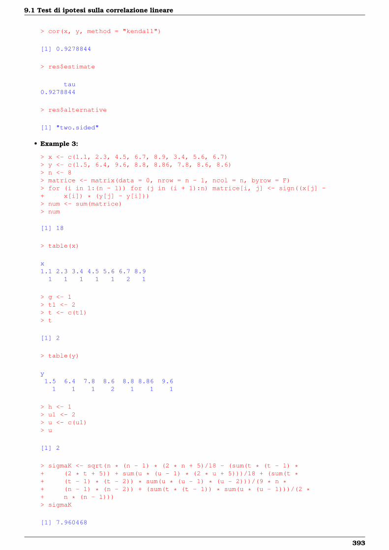
9.1 Test di ipotesi sulla correlazione lineare
> cor(x, y, method = "kendall")
[1] 0.9278844
> res$estimate
tau0.9278844
> res$alternative
[1] "two.sided"
• Example 3:
> x <- c(1.1, 2.3, 4.5, 6.7, 8.9, 3.4, 5.6, 6.7)> y <- c(1.5, 6.4, 9.6, 8.8, 8.86, 7.8, 8.6, 8.6)> n <- 8> matrice <- matrix(data = 0, nrow = n - 1, ncol = n, byrow = F)> for (i in 1:(n - 1)) for (j in (i + 1):n) matrice[i, j] <- sign((x[j] -+ x[i]) * (y[j] - y[i]))> num <- sum(matrice)> num
[1] 18
> table(x)
x1.1 2.3 3.4 4.5 5.6 6.7 8.9
1 1 1 1 1 2 1
> g <- 1> t1 <- 2> t <- c(t1)> t
[1] 2
> table(y)
y1.5 6.4 7.8 8.6 8.8 8.86 9.6
1 1 1 2 1 1 1
> h <- 1> u1 <- 2> u <- c(u1)> u
[1] 2
> sigmaK <- sqrt(n * (n - 1) * (2 * n + 5)/18 - (sum(t * (t - 1) *+ (2 * t + 5)) + sum(u * (u - 1) * (2 * u + 5)))/18 + (sum(t *+ (t - 1) * (t - 2)) * sum(u * (u - 1) * (u - 2)))/(9 * n *+ (n - 1) * (n - 2)) + (sum(t * (t - 1)) * sum(u * (u - 1)))/(2 *+ n * (n - 1)))> sigmaK
[1] 7.960468
393

Test di ipotesi su correlazione ed autocorrelazione
> z <- num/sigmaK> z
[1] 2.261174
> res <- cor.test(x, y, alternative = "two.sided", method = "kendall",+ exact = F)> res$statistic
z2.261174
> p.value <- 2 * pnorm(-abs(z))> p.value
[1] 0.02374851
> res$p.value
[1] 0.02374851
> cor(x, y, method = "kendall")
[1] 0.6666667
> res$estimate
tau0.6666667
> res$alternative
[1] "two.sided"
Test Z con una retta di regressione
• Package: formularioR
• Sintassi: cor2.test()
• Input:
r1 valore di rxyn1 dimensione campionaria n
alternative = "less" / "greater" / "two.sided" ipotesi alternativa
rho valore di ρ0
conf.level livello di confidenza 1− α
• Output:
statistic valore empirico della statistica Z
p.value p-value
conf.int intervallo di confidenza per il coefficiente di correlazione incognito a livello 1− αestimate coefficiente di correlazione
null.value valore di ρ0
alternative ipotesi alternativa
• Formula:
394
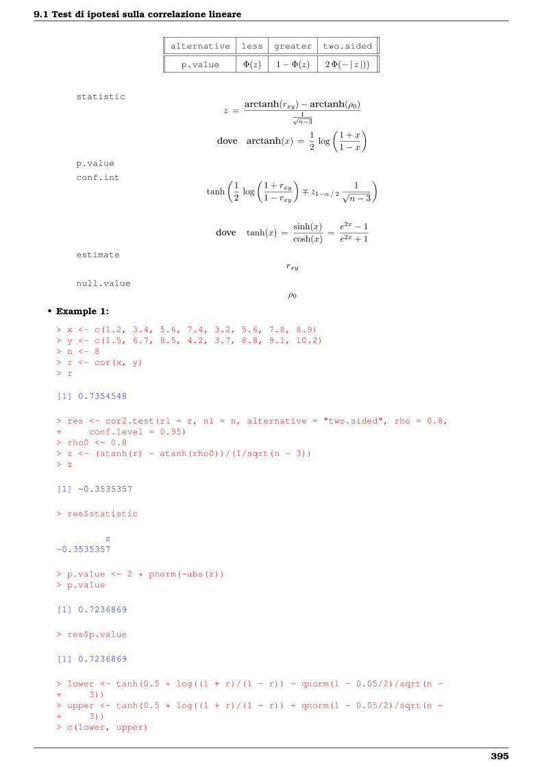
9.1 Test di ipotesi sulla correlazione lineare
alternative less greater two.sided
p.value Φ(z) 1− Φ(z) 2 Φ(− | z |))
statistic
z =arctanh(rxy)− arctanh(ρ0)
1√n−3
dove arctanh(x) =12
log(
1 + x
1− x
)p.value
conf.int
tanh(
12
log(
1 + rxy1− rxy
)∓ z1−α/ 2
1√n− 3
)
dove tanh(x) =sinh(x)cosh(x)
=e2x − 1e2x + 1
estimaterxy
null.valueρ0
• Example 1:
> x <- c(1.2, 3.4, 5.6, 7.4, 3.2, 5.6, 7.8, 8.9)> y <- c(1.5, 6.7, 8.5, 4.2, 3.7, 8.8, 9.1, 10.2)> n <- 8> r <- cor(x, y)> r
[1] 0.7354548
> res <- cor2.test(r1 = r, n1 = n, alternative = "two.sided", rho = 0.8,+ conf.level = 0.95)> rho0 <- 0.8> z <- (atanh(r) - atanh(rho0))/(1/sqrt(n - 3))> z
[1] -0.3535357
> res$statistic
z-0.3535357
> p.value <- 2 * pnorm(-abs(z))> p.value
[1] 0.7236869
> res$p.value
[1] 0.7236869
> lower <- tanh(0.5 * log((1 + r)/(1 - r)) - qnorm(1 - 0.05/2)/sqrt(n -+ 3))> upper <- tanh(0.5 * log((1 + r)/(1 - r)) + qnorm(1 - 0.05/2)/sqrt(n -+ 3))> c(lower, upper)
395
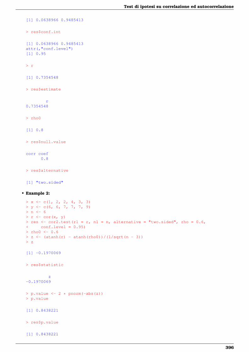
Test di ipotesi su correlazione ed autocorrelazione
[1] 0.0638966 0.9485413
> res$conf.int
[1] 0.0638966 0.9485413attr(,"conf.level")[1] 0.95
> r
[1] 0.7354548
> res$estimate
r0.7354548
> rho0
[1] 0.8
> res$null.value
corr coef0.8
> res$alternative
[1] "two.sided"
• Example 2:
> x <- c(1, 2, 2, 4, 3, 3)> y <- c(6, 6, 7, 7, 7, 9)> n <- 6> r <- cor(x, y)> res <- cor2.test(r1 = r, n1 = n, alternative = "two.sided", rho = 0.6,+ conf.level = 0.95)> rho0 <- 0.6> z <- (atanh(r) - atanh(rho0))/(1/sqrt(n - 3))> z
[1] -0.1970069
> res$statistic
z-0.1970069
> p.value <- 2 * pnorm(-abs(z))> p.value
[1] 0.8438221
> res$p.value
[1] 0.8438221
396
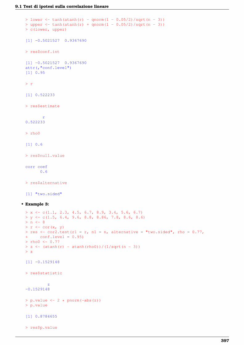
9.1 Test di ipotesi sulla correlazione lineare
> lower <- tanh(atanh(r) - qnorm(1 - 0.05/2)/sqrt(n - 3))> upper <- tanh(atanh(r) + qnorm(1 - 0.05/2)/sqrt(n - 3))> c(lower, upper)
[1] -0.5021527 0.9367690
> res$conf.int
[1] -0.5021527 0.9367690attr(,"conf.level")[1] 0.95
> r
[1] 0.522233
> res$estimate
r0.522233
> rho0
[1] 0.6
> res$null.value
corr coef0.6
> res$alternative
[1] "two.sided"
• Example 3:
> x <- c(1.1, 2.3, 4.5, 6.7, 8.9, 3.4, 5.6, 6.7)> y <- c(1.5, 6.4, 9.6, 8.8, 8.86, 7.8, 8.6, 8.6)> n <- 8> r <- cor(x, y)> res <- cor2.test(r1 = r, n1 = n, alternative = "two.sided", rho = 0.77,+ conf.level = 0.95)> rho0 <- 0.77> z <- (atanh(r) - atanh(rho0))/(1/sqrt(n - 3))> z
[1] -0.1529148
> res$statistic
z-0.1529148
> p.value <- 2 * pnorm(-abs(z))> p.value
[1] 0.8784655
> res$p.value
397

Test di ipotesi su correlazione ed autocorrelazione
[1] 0.8784655
> lower <- tanh(atanh(r) - qnorm(1 - 0.05/2)/sqrt(n - 3))> upper <- tanh(atanh(r) + qnorm(1 - 0.05/2)/sqrt(n - 3))> c(lower, upper)
[1] 0.07527696 0.94967566
> res$conf.int
[1] 0.07527696 0.94967566attr(,"conf.level")[1] 0.95
> r
[1] 0.740661
> res$estimate
r0.740661
> rho0
[1] 0.77
> res$null.value
corr coef0.77
> res$alternative
[1] "two.sided"
Test Z con due rette di regressione
• Package: formularioR
• Sintassi: cor2.test()
• Input:
r1 valore di rx1y1
n1 dimensione campionaria n1
r2 valore di rx2y2
n2 dimensione campionaria n2
alternative = "less" / "greater" / "two.sided" ipotesi alternativa
conf.level livello di confidenza 1− α
• Output:
statistic valore empirico della statistica Z
p.value p-value
conf.int intervallo di confidenza per la differenza tra i coefficienti di correlazione incogniti alivello 1− α
398
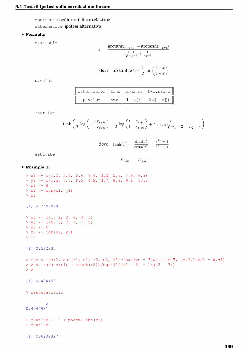
9.1 Test di ipotesi sulla correlazione lineare
estimate coefficienti di correlazione
alternative ipotesi alternativa
• Formula:
statistic
z =arctanh(rx1y1)− arctanh(rx2y2)√
1n1−3 + 1
n2−3
dove arctanh(x) =12
log(
1 + x
1− x
)p.value
alternative less greater two.sided
p.value Φ(z) 1− Φ(z) 2 Φ(− | z |))
conf.int
tanh(
12
log(
1 + rx1y1
1− rx1y1
)− 1
2log(
1 + rx2y2
1− rx2y2
)∓ z1−α/ 2
√1
n1 − 3+
1n2 − 3
)
dove tanh(x) =sinh(x)cosh(x)
=e2x − 1e2x + 1
estimaterx1y1 rx2y2
• Example 1:
> x1 <- c(1.2, 3.4, 5.6, 7.4, 3.2, 5.6, 7.8, 8.9)> y1 <- c(1.5, 6.7, 8.5, 4.2, 3.7, 8.8, 9.1, 10.2)> n1 <- 8> r1 <- cor(x1, y1)> r1
[1] 0.7354548
> x2 <- c(1, 2, 2, 4, 3, 3)> y2 <- c(6, 6, 7, 7, 7, 9)> n2 <- 6> r2 <- cor(x2, y2)> r2
[1] 0.522233
> res <- cor2.test(r1, n1, r2, n2, alternative = "two.sided", conf.level = 0.95)> z <- (atanh(r1) - atanh(r2))/sqrt(1/(n1 - 3) + 1/(n2 - 3))> z
[1] 0.4944581
> res$statistic
z0.4944581
> p.value <- 2 * pnorm(-abs(z))> p.value
[1] 0.6209827
399
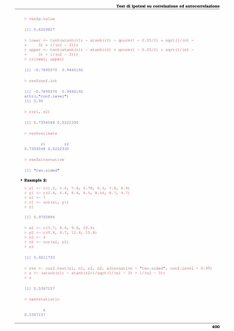
Test di ipotesi su correlazione ed autocorrelazione
> res$p.value
[1] 0.6209827
> lower <- tanh(atanh(r1) - atanh(r2) - qnorm(1 - 0.05/2) * sqrt(1/(n1 -+ 3) + 1/(n2 - 3)))> upper <- tanh(atanh(r1) - atanh(r2) + qnorm(1 - 0.05/2) * sqrt(1/(n1 -+ 3) + 1/(n2 - 3)))> c(lower, upper)
[1] -0.7895570 0.9460192
> res$conf.int
[1] -0.7895570 0.9460192attr(,"conf.level")[1] 0.95
> c(r1, r2)
[1] 0.7354548 0.5222330
> res$estimate
r1 r20.7354548 0.5222330
> res$alternative
[1] "two.sided"
• Example 2:
> x1 <- c(1.2, 5.6, 7.4, 6.78, 6.3, 7.8, 8.9)> y1 <- c(2.4, 6.4, 8.4, 8.5, 8.54, 8.7, 9.7)> n1 <- 7> r1 <- cor(x1, y1)> r1
[1] 0.9755886
> x2 <- c(3.7, 8.6, 9.9, 10.4)> y2 <- c(5.8, 9.7, 12.4, 15.8)> n2 <- 4> r2 <- cor(x2, y2)> r2
[1] 0.9211733
> res <- cor2.test(r1, n1, r2, n2, alternative = "two.sided", conf.level = 0.95)> z <- (atanh(r1) - atanh(r2))/sqrt(1/(n1 - 3) + 1/(n2 - 3))> z
[1] 0.5367157
> res$statistic
z0.5367157
400
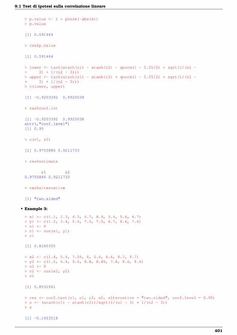
9.1 Test di ipotesi sulla correlazione lineare
> p.value <- 2 * pnorm(-abs(z))> p.value
[1] 0.591464
> res$p.value
[1] 0.591464
> lower <- tanh(atanh(r1) - atanh(r2) - qnorm(1 - 0.05/2) * sqrt(1/(n1 -+ 3) + 1/(n2 - 3)))> upper <- tanh(atanh(r1) - atanh(r2) + qnorm(1 - 0.05/2) * sqrt(1/(n1 -+ 3) + 1/(n2 - 3)))> c(lower, upper)
[1] -0.9203392 0.9925038
> res$conf.int
[1] -0.9203392 0.9925038attr(,"conf.level")[1] 0.95
> c(r1, r2)
[1] 0.9755886 0.9211733
> res$estimate
r1 r20.9755886 0.9211733
> res$alternative
[1] "two.sided"
• Example 3:
> x1 <- c(1.1, 2.3, 4.5, 6.7, 8.9, 3.4, 5.6, 6.7)> y1 <- c(1.2, 3.4, 5.6, 7.5, 7.5, 6.7, 8.6, 7.6)> n1 <- 8> r1 <- cor(x1, y1)> r1
[1] 0.8260355
> x2 <- c(1.4, 5.6, 7.56, 6, 5.4, 6.6, 8.7, 8.7)> y2 <- c(1.5, 6.4, 9.6, 8.8, 8.86, 7.8, 8.6, 8.6)> n2 <- 8> r2 <- cor(x2, y2)> r2
[1] 0.8531061
> res <- cor2.test(r1, n1, r2, n2, alternative = "two.sided", conf.level = 0.95)> z <- (atanh(r1) - atanh(r2))/sqrt(1/(n1 - 3) + 1/(n2 - 3))> z
[1] -0.1453518
401
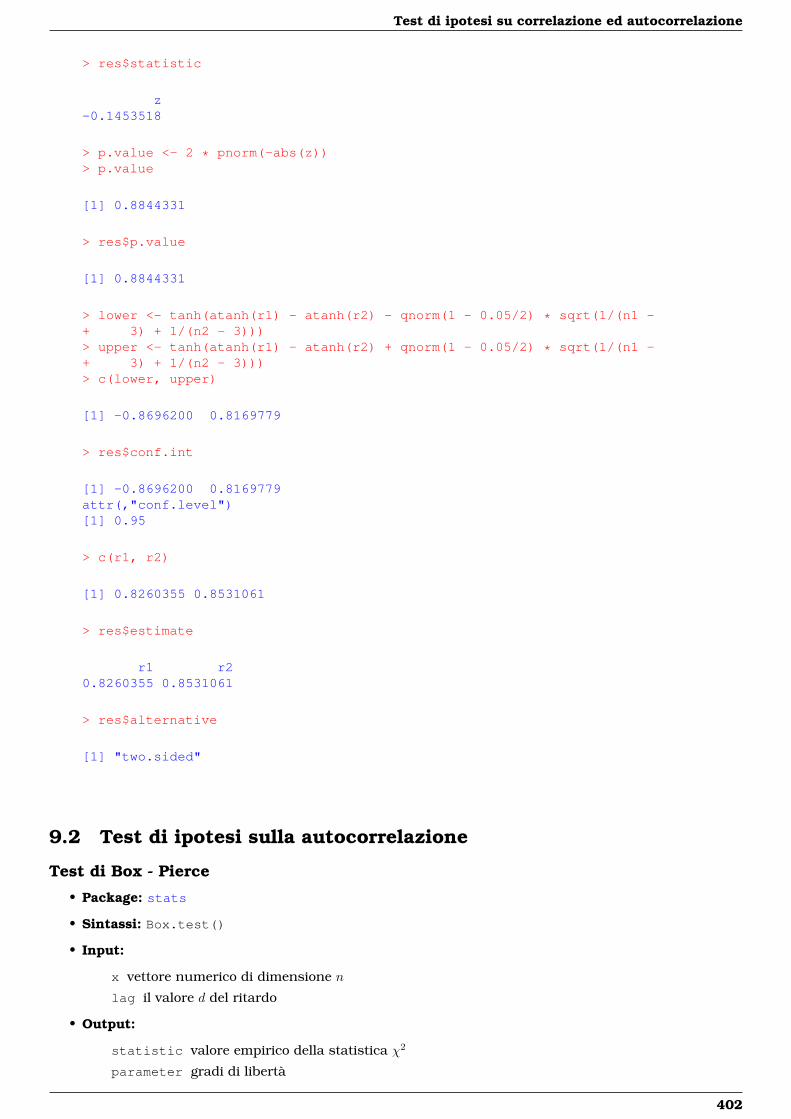
Test di ipotesi su correlazione ed autocorrelazione
> res$statistic
z-0.1453518
> p.value <- 2 * pnorm(-abs(z))> p.value
[1] 0.8844331
> res$p.value
[1] 0.8844331
> lower <- tanh(atanh(r1) - atanh(r2) - qnorm(1 - 0.05/2) * sqrt(1/(n1 -+ 3) + 1/(n2 - 3)))> upper <- tanh(atanh(r1) - atanh(r2) + qnorm(1 - 0.05/2) * sqrt(1/(n1 -+ 3) + 1/(n2 - 3)))> c(lower, upper)
[1] -0.8696200 0.8169779
> res$conf.int
[1] -0.8696200 0.8169779attr(,"conf.level")[1] 0.95
> c(r1, r2)
[1] 0.8260355 0.8531061
> res$estimate
r1 r20.8260355 0.8531061
> res$alternative
[1] "two.sided"
9.2 Test di ipotesi sulla autocorrelazione
Test di Box - Pierce
• Package: stats
• Sintassi: Box.test()
• Input:
x vettore numerico di dimensione n
lag il valore d del ritardo
• Output:
statistic valore empirico della statistica χ2
parameter gradi di libertà
402
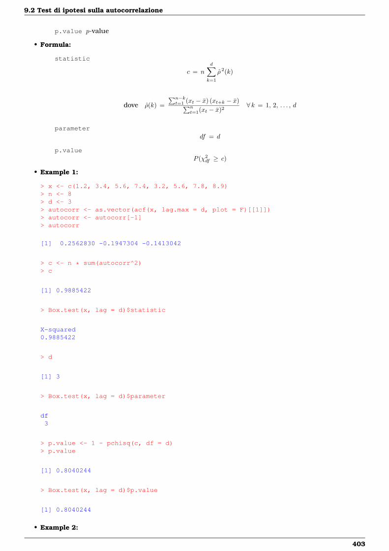
9.2 Test di ipotesi sulla autocorrelazione
p.value p-value
• Formula:
statistic
c = n
d∑k=1
ρ 2(k)
dove ρ(k) =∑n−kt=1 (xt − x) (xt+k − x)∑n
t=1(xt − x)2∀ k = 1, 2, . . . , d
parameterdf = d
p.valueP (χ2
df ≥ c)
• Example 1:
> x <- c(1.2, 3.4, 5.6, 7.4, 3.2, 5.6, 7.8, 8.9)> n <- 8> d <- 3> autocorr <- as.vector(acf(x, lag.max = d, plot = F)[[1]])> autocorr <- autocorr[-1]> autocorr
[1] 0.2562830 -0.1947304 -0.1413042
> c <- n * sum(autocorr^2)> c
[1] 0.9885422
> Box.test(x, lag = d)$statistic
X-squared0.9885422
> d
[1] 3
> Box.test(x, lag = d)$parameter
df3
> p.value <- 1 - pchisq(c, df = d)> p.value
[1] 0.8040244
> Box.test(x, lag = d)$p.value
[1] 0.8040244
• Example 2:
403
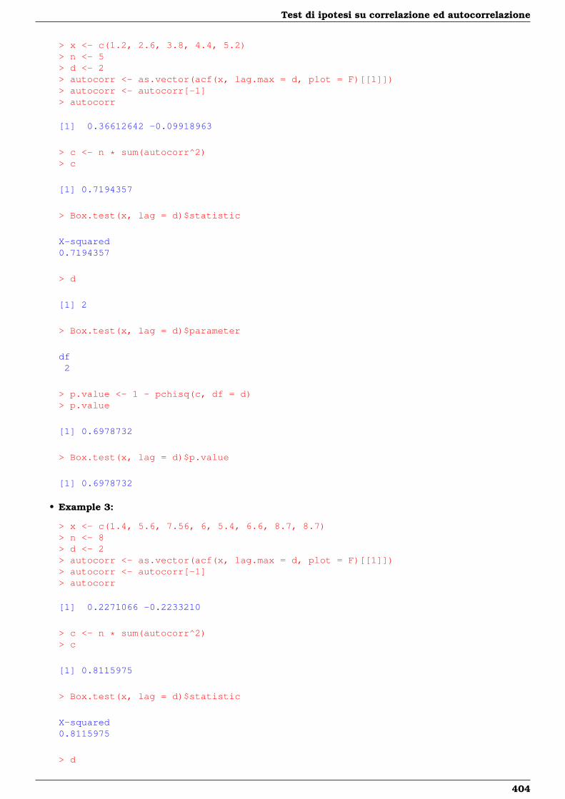
Test di ipotesi su correlazione ed autocorrelazione
> x <- c(1.2, 2.6, 3.8, 4.4, 5.2)> n <- 5> d <- 2> autocorr <- as.vector(acf(x, lag.max = d, plot = F)[[1]])> autocorr <- autocorr[-1]> autocorr
[1] 0.36612642 -0.09918963
> c <- n * sum(autocorr^2)> c
[1] 0.7194357
> Box.test(x, lag = d)$statistic
X-squared0.7194357
> d
[1] 2
> Box.test(x, lag = d)$parameter
df2
> p.value <- 1 - pchisq(c, df = d)> p.value
[1] 0.6978732
> Box.test(x, lag = d)$p.value
[1] 0.6978732
• Example 3:
> x <- c(1.4, 5.6, 7.56, 6, 5.4, 6.6, 8.7, 8.7)> n <- 8> d <- 2> autocorr <- as.vector(acf(x, lag.max = d, plot = F)[[1]])> autocorr <- autocorr[-1]> autocorr
[1] 0.2271066 -0.2233210
> c <- n * sum(autocorr^2)> c
[1] 0.8115975
> Box.test(x, lag = d)$statistic
X-squared0.8115975
> d
404
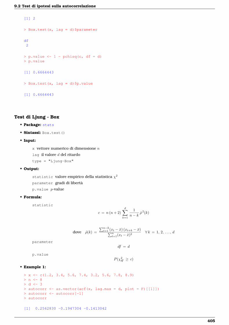
9.2 Test di ipotesi sulla autocorrelazione
[1] 2
> Box.test(x, lag = d)$parameter
df2
> p.value <- 1 - pchisq(c, df = d)> p.value
[1] 0.6664443
> Box.test(x, lag = d)$p.value
[1] 0.6664443
Test di Ljung - Box
• Package: stats
• Sintassi: Box.test()
• Input:
x vettore numerico di dimensione n
lag il valore d del ritardo
type = "Ljung-Box"
• Output:
statistic valore empirico della statistica χ2
parameter gradi di libertà
p.value p-value
• Formula:
statistic
c = n (n+ 2)d∑k=1
1n− k
ρ 2(k)
dove ρ(k) =∑n−kt=1 (xt − x) (xt+k − x)∑n
t=1(xt − x)2∀ k = 1, 2, . . . , d
parameterdf = d
p.valueP (χ2
df ≥ c)
• Example 1:
> x <- c(1.2, 3.4, 5.6, 7.4, 3.2, 5.6, 7.8, 8.9)> n <- 8> d <- 3> autocorr <- as.vector(acf(x, lag.max = d, plot = F)[[1]])> autocorr <- autocorr[-1]> autocorr
[1] 0.2562830 -0.1947304 -0.1413042
405
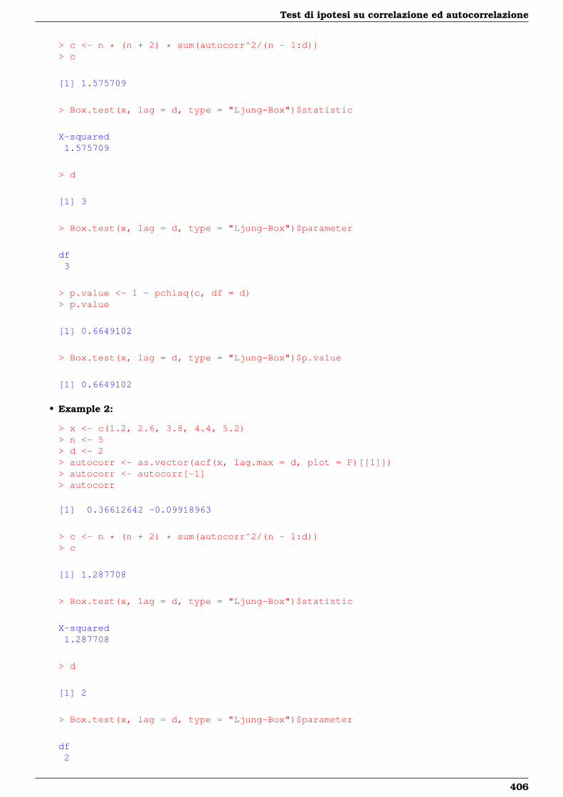
Test di ipotesi su correlazione ed autocorrelazione
> c <- n * (n + 2) * sum(autocorr^2/(n - 1:d))> c
[1] 1.575709
> Box.test(x, lag = d, type = "Ljung-Box")$statistic
X-squared1.575709
> d
[1] 3
> Box.test(x, lag = d, type = "Ljung-Box")$parameter
df3
> p.value <- 1 - pchisq(c, df = d)> p.value
[1] 0.6649102
> Box.test(x, lag = d, type = "Ljung-Box")$p.value
[1] 0.6649102
• Example 2:
> x <- c(1.2, 2.6, 3.8, 4.4, 5.2)> n <- 5> d <- 2> autocorr <- as.vector(acf(x, lag.max = d, plot = F)[[1]])> autocorr <- autocorr[-1]> autocorr
[1] 0.36612642 -0.09918963
> c <- n * (n + 2) * sum(autocorr^2/(n - 1:d))> c
[1] 1.287708
> Box.test(x, lag = d, type = "Ljung-Box")$statistic
X-squared1.287708
> d
[1] 2
> Box.test(x, lag = d, type = "Ljung-Box")$parameter
df2
406
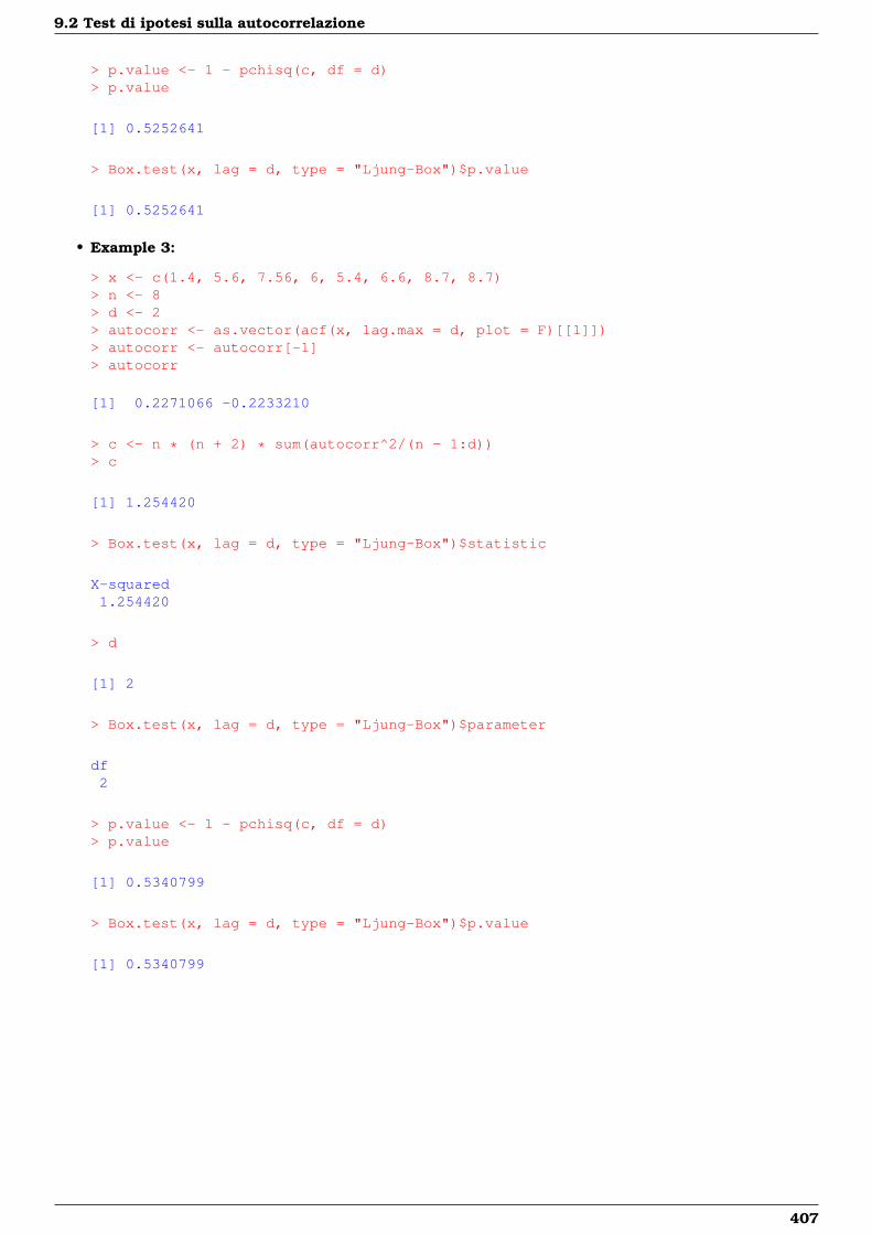
9.2 Test di ipotesi sulla autocorrelazione
> p.value <- 1 - pchisq(c, df = d)> p.value
[1] 0.5252641
> Box.test(x, lag = d, type = "Ljung-Box")$p.value
[1] 0.5252641
• Example 3:
> x <- c(1.4, 5.6, 7.56, 6, 5.4, 6.6, 8.7, 8.7)> n <- 8> d <- 2> autocorr <- as.vector(acf(x, lag.max = d, plot = F)[[1]])> autocorr <- autocorr[-1]> autocorr
[1] 0.2271066 -0.2233210
> c <- n * (n + 2) * sum(autocorr^2/(n - 1:d))> c
[1] 1.254420
> Box.test(x, lag = d, type = "Ljung-Box")$statistic
X-squared1.254420
> d
[1] 2
> Box.test(x, lag = d, type = "Ljung-Box")$parameter
df2
> p.value <- 1 - pchisq(c, df = d)> p.value
[1] 0.5340799
> Box.test(x, lag = d, type = "Ljung-Box")$p.value
[1] 0.5340799
407

Capitolo 10
Test di ipotesi non parametrici
10.1 Simbologia
• dimensione del campione j-esimo: nj ∀ j = 1, 2, . . . , k
• media aritmetica del campione j-esimo: xj = 1nj
∑nji=1 xij ∀ j = 1, 2, . . . , k
• varianza nel campione j-esimo: s2j = 1
nj−1
∑nji=1 (xij − xj)2 ∀ j = 1, 2, . . . , k
• varianza pooled: s2P =
∑kj=1 (nj − 1) s2
j / (n− k)
• somma dei ranghi nel campione j-esimo: Rj ∀ j = 1, 2, . . . , k
• media dei ranghi nel campione j-esimo: Rj ∀ j = 1, 2, . . . , k
• media dei ranghi nel campione di dimensione n: R
• ties nel campione di dimensione n: tj ∀ j = 1, 2, . . . , g∑gj=1 tj = n 1 ≤ g ≤ n
10.2 Test di ipotesi sulla mediana con uno o due campioni
Test esatto Wilcoxon signed rank
• Package: stats
• Sintassi: wilcox.test()
• Input:
x vettore numerico di dimensione n
mu il valore di Q0.5(x)|H0
alternative = "less" / "greater" / "two.sided" ipotesi alternativa
exact = TRUE
• Output:
statistic valore empirico della statistica V
p.value p-value
null.value il valore di Q0.5(x)|H0
alternative ipotesi alternativa
• Formula:
statisticv
p.value
alternative less greater two.sided
p.value P (V ≤ v) P (V ≥ v) 2 min (P (V ≤ v), P (V ≥ v))
409
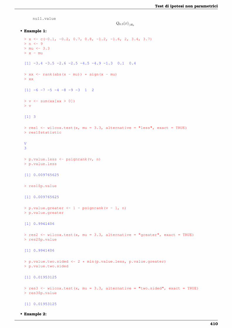
Test di ipotesi non parametrici
null.valueQ0.5(x)|H0
• Example 1:
> x <- c(-0.1, -0.2, 0.7, 0.8, -1.2, -1.6, 2, 3.4, 3.7)> n <- 9> mu <- 3.3> x - mu
[1] -3.4 -3.5 -2.6 -2.5 -4.5 -4.9 -1.3 0.1 0.4
> xx <- rank(abs(x - mu)) * sign(x - mu)> xx
[1] -6 -7 -5 -4 -8 -9 -3 1 2
> v <- sum(xx[xx > 0])> v
[1] 3
> res1 <- wilcox.test(x, mu = 3.3, alternative = "less", exact = TRUE)> res1$statistic
V3
> p.value.less <- psignrank(v, n)> p.value.less
[1] 0.009765625
> res1$p.value
[1] 0.009765625
> p.value.greater <- 1 - psignrank(v - 1, n)> p.value.greater
[1] 0.9941406
> res2 <- wilcox.test(x, mu = 3.3, alternative = "greater", exact = TRUE)> res2$p.value
[1] 0.9941406
> p.value.two.sided <- 2 * min(p.value.less, p.value.greater)> p.value.two.sided
[1] 0.01953125
> res3 <- wilcox.test(x, mu = 3.3, alternative = "two.sided", exact = TRUE)> res3$p.value
[1] 0.01953125
• Example 2:
410
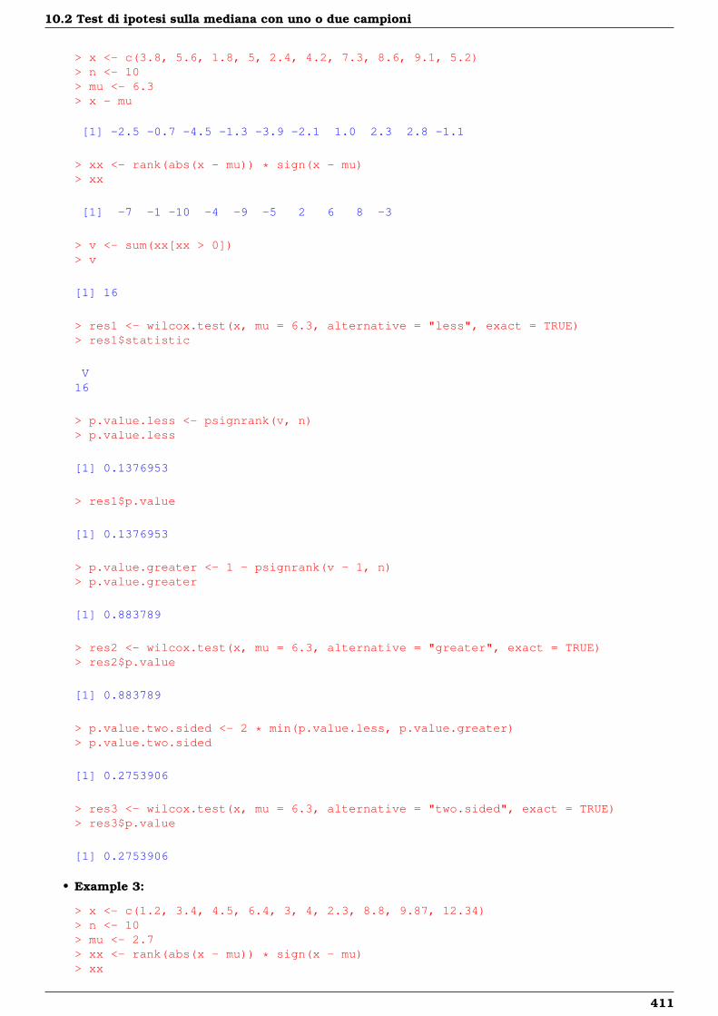
10.2 Test di ipotesi sulla mediana con uno o due campioni
> x <- c(3.8, 5.6, 1.8, 5, 2.4, 4.2, 7.3, 8.6, 9.1, 5.2)> n <- 10> mu <- 6.3> x - mu
[1] -2.5 -0.7 -4.5 -1.3 -3.9 -2.1 1.0 2.3 2.8 -1.1
> xx <- rank(abs(x - mu)) * sign(x - mu)> xx
[1] -7 -1 -10 -4 -9 -5 2 6 8 -3
> v <- sum(xx[xx > 0])> v
[1] 16
> res1 <- wilcox.test(x, mu = 6.3, alternative = "less", exact = TRUE)> res1$statistic
V16
> p.value.less <- psignrank(v, n)> p.value.less
[1] 0.1376953
> res1$p.value
[1] 0.1376953
> p.value.greater <- 1 - psignrank(v - 1, n)> p.value.greater
[1] 0.883789
> res2 <- wilcox.test(x, mu = 6.3, alternative = "greater", exact = TRUE)> res2$p.value
[1] 0.883789
> p.value.two.sided <- 2 * min(p.value.less, p.value.greater)> p.value.two.sided
[1] 0.2753906
> res3 <- wilcox.test(x, mu = 6.3, alternative = "two.sided", exact = TRUE)> res3$p.value
[1] 0.2753906
• Example 3:
> x <- c(1.2, 3.4, 4.5, 6.4, 3, 4, 2.3, 8.8, 9.87, 12.34)> n <- 10> mu <- 2.7> xx <- rank(abs(x - mu)) * sign(x - mu)> xx
411
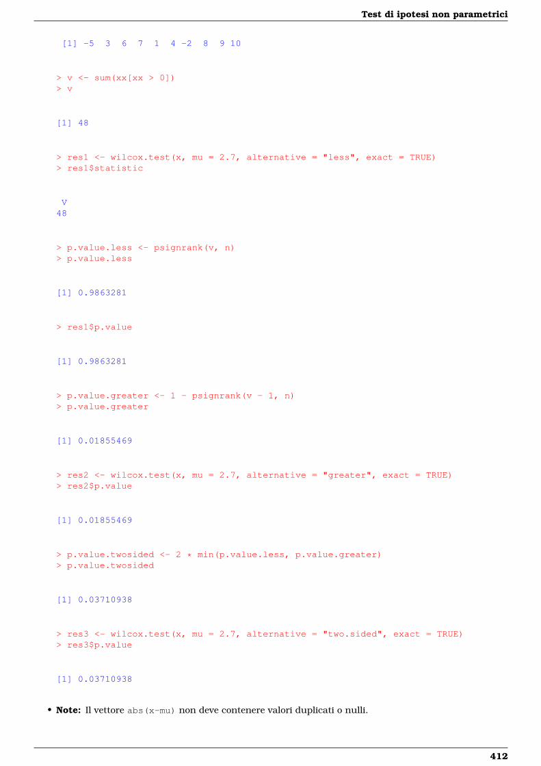
Test di ipotesi non parametrici
[1] -5 3 6 7 1 4 -2 8 9 10
> v <- sum(xx[xx > 0])> v
[1] 48
> res1 <- wilcox.test(x, mu = 2.7, alternative = "less", exact = TRUE)> res1$statistic
V48
> p.value.less <- psignrank(v, n)> p.value.less
[1] 0.9863281
> res1$p.value
[1] 0.9863281
> p.value.greater <- 1 - psignrank(v - 1, n)> p.value.greater
[1] 0.01855469
> res2 <- wilcox.test(x, mu = 2.7, alternative = "greater", exact = TRUE)> res2$p.value
[1] 0.01855469
> p.value.twosided <- 2 * min(p.value.less, p.value.greater)> p.value.twosided
[1] 0.03710938
> res3 <- wilcox.test(x, mu = 2.7, alternative = "two.sided", exact = TRUE)> res3$p.value
[1] 0.03710938
• Note: Il vettore abs(x-mu) non deve contenere valori duplicati o nulli.
412
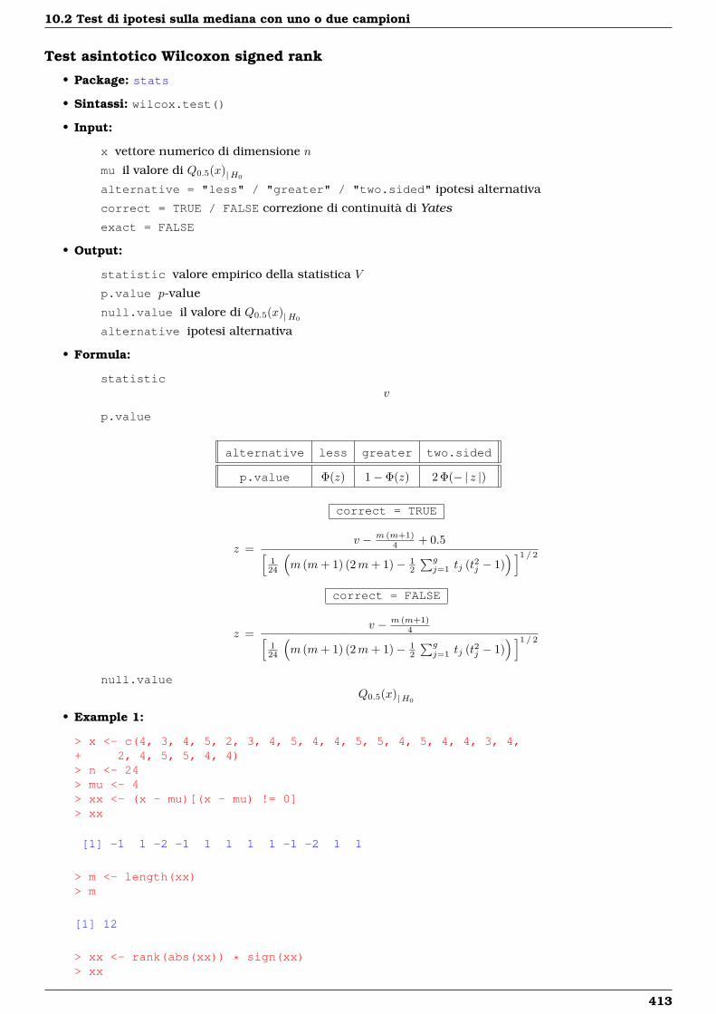
10.2 Test di ipotesi sulla mediana con uno o due campioni
Test asintotico Wilcoxon signed rank
• Package: stats
• Sintassi: wilcox.test()
• Input:
x vettore numerico di dimensione n
mu il valore di Q0.5(x)|H0
alternative = "less" / "greater" / "two.sided" ipotesi alternativa
correct = TRUE / FALSE correzione di continuità di Yates
exact = FALSE
• Output:
statistic valore empirico della statistica V
p.value p-value
null.value il valore di Q0.5(x)|H0
alternative ipotesi alternativa
• Formula:
statisticv
p.value
alternative less greater two.sided
p.value Φ(z) 1− Φ(z) 2 Φ(− | z |)
correct = TRUE
z =v − m (m+1)
4 + 0.5[124
(m (m+ 1) (2m+ 1)− 1
2
∑gj=1 tj (t2j − 1)
) ]1 / 2
correct = FALSE
z =v − m (m+1)
4[124
(m (m+ 1) (2m+ 1)− 1
2
∑gj=1 tj (t2j − 1)
) ]1 / 2
null.valueQ0.5(x)|H0
• Example 1:
> x <- c(4, 3, 4, 5, 2, 3, 4, 5, 4, 4, 5, 5, 4, 5, 4, 4, 3, 4,+ 2, 4, 5, 5, 4, 4)> n <- 24> mu <- 4> xx <- (x - mu)[(x - mu) != 0]> xx
[1] -1 1 -2 -1 1 1 1 1 -1 -2 1 1
> m <- length(xx)> m
[1] 12
> xx <- rank(abs(xx)) * sign(xx)> xx
413
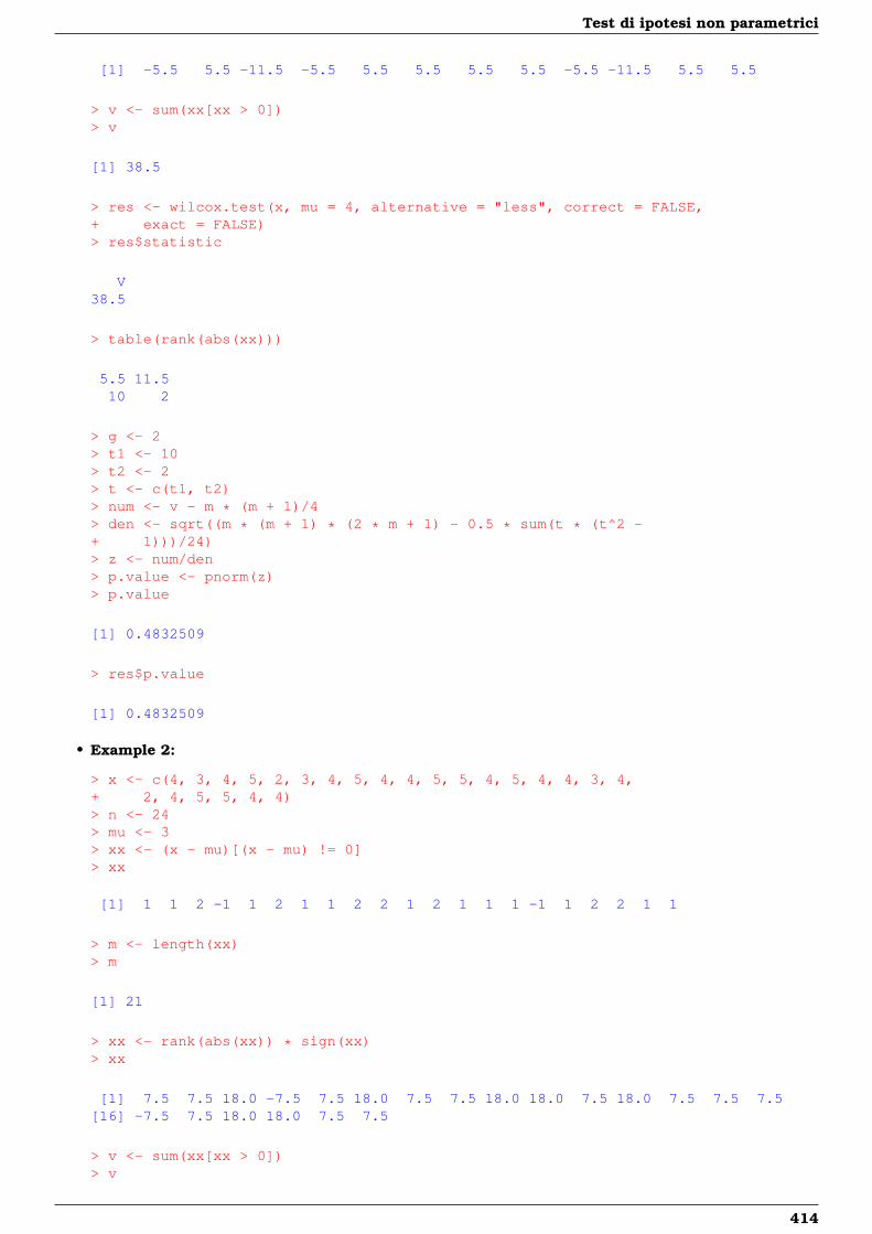
Test di ipotesi non parametrici
[1] -5.5 5.5 -11.5 -5.5 5.5 5.5 5.5 5.5 -5.5 -11.5 5.5 5.5
> v <- sum(xx[xx > 0])> v
[1] 38.5
> res <- wilcox.test(x, mu = 4, alternative = "less", correct = FALSE,+ exact = FALSE)> res$statistic
V38.5
> table(rank(abs(xx)))
5.5 11.510 2
> g <- 2> t1 <- 10> t2 <- 2> t <- c(t1, t2)> num <- v - m * (m + 1)/4> den <- sqrt((m * (m + 1) * (2 * m + 1) - 0.5 * sum(t * (t^2 -+ 1)))/24)> z <- num/den> p.value <- pnorm(z)> p.value
[1] 0.4832509
> res$p.value
[1] 0.4832509
• Example 2:
> x <- c(4, 3, 4, 5, 2, 3, 4, 5, 4, 4, 5, 5, 4, 5, 4, 4, 3, 4,+ 2, 4, 5, 5, 4, 4)> n <- 24> mu <- 3> xx <- (x - mu)[(x - mu) != 0]> xx
[1] 1 1 2 -1 1 2 1 1 2 2 1 2 1 1 1 -1 1 2 2 1 1
> m <- length(xx)> m
[1] 21
> xx <- rank(abs(xx)) * sign(xx)> xx
[1] 7.5 7.5 18.0 -7.5 7.5 18.0 7.5 7.5 18.0 18.0 7.5 18.0 7.5 7.5 7.5[16] -7.5 7.5 18.0 18.0 7.5 7.5
> v <- sum(xx[xx > 0])> v
414
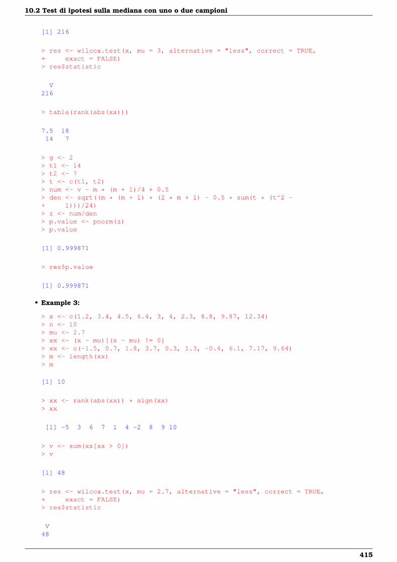
10.2 Test di ipotesi sulla mediana con uno o due campioni
[1] 216
> res <- wilcox.test(x, mu = 3, alternative = "less", correct = TRUE,+ exact = FALSE)> res$statistic
V216
> table(rank(abs(xx)))
7.5 1814 7
> g <- 2> t1 <- 14> t2 <- 7> t <- c(t1, t2)> num <- v - m * (m + 1)/4 + 0.5> den <- sqrt((m * (m + 1) * (2 * m + 1) - 0.5 * sum(t * (t^2 -+ 1)))/24)> z <- num/den> p.value <- pnorm(z)> p.value
[1] 0.999871
> res$p.value
[1] 0.999871
• Example 3:
> x <- c(1.2, 3.4, 4.5, 6.4, 3, 4, 2.3, 8.8, 9.87, 12.34)> n <- 10> mu <- 2.7> xx <- (x - mu)[(x - mu) != 0]> xx <- c(-1.5, 0.7, 1.8, 3.7, 0.3, 1.3, -0.4, 6.1, 7.17, 9.64)> m <- length(xx)> m
[1] 10
> xx <- rank(abs(xx)) * sign(xx)> xx
[1] -5 3 6 7 1 4 -2 8 9 10
> v <- sum(xx[xx > 0])> v
[1] 48
> res <- wilcox.test(x, mu = 2.7, alternative = "less", correct = TRUE,+ exact = FALSE)> res$statistic
V48
415
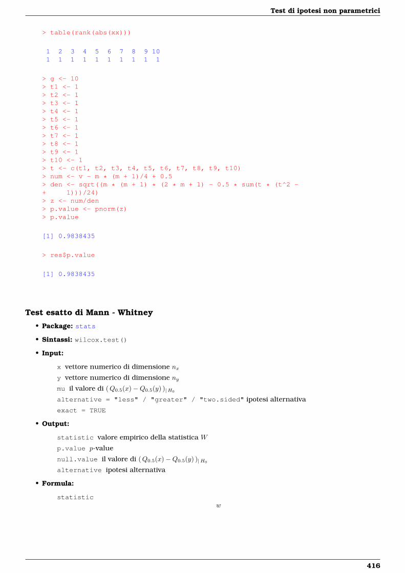
Test di ipotesi non parametrici
> table(rank(abs(xx)))
1 2 3 4 5 6 7 8 9 101 1 1 1 1 1 1 1 1 1
> g <- 10> t1 <- 1> t2 <- 1> t3 <- 1> t4 <- 1> t5 <- 1> t6 <- 1> t7 <- 1> t8 <- 1> t9 <- 1> t10 <- 1> t <- c(t1, t2, t3, t4, t5, t6, t7, t8, t9, t10)> num <- v - m * (m + 1)/4 + 0.5> den <- sqrt((m * (m + 1) * (2 * m + 1) - 0.5 * sum(t * (t^2 -+ 1)))/24)> z <- num/den> p.value <- pnorm(z)> p.value
[1] 0.9838435
> res$p.value
[1] 0.9838435
Test esatto di Mann - Whitney
• Package: stats
• Sintassi: wilcox.test()
• Input:
x vettore numerico di dimensione nxy vettore numerico di dimensione nymu il valore di (Q0.5(x)−Q0.5(y) )|H0
alternative = "less" / "greater" / "two.sided" ipotesi alternativa
exact = TRUE
• Output:
statistic valore empirico della statistica W
p.value p-value
null.value il valore di (Q0.5(x)−Q0.5(y) )|H0
alternative ipotesi alternativa
• Formula:
statisticw
416
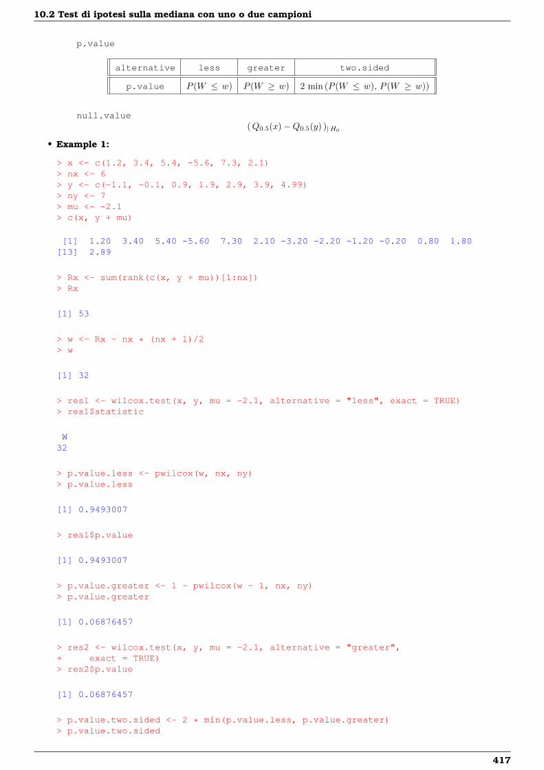
10.2 Test di ipotesi sulla mediana con uno o due campioni
p.value
alternative less greater two.sided
p.value P (W ≤ w) P (W ≥ w) 2 min (P (W ≤ w), P (W ≥ w))
null.value(Q0.5(x)−Q0.5(y) )|H0
• Example 1:
> x <- c(1.2, 3.4, 5.4, -5.6, 7.3, 2.1)> nx <- 6> y <- c(-1.1, -0.1, 0.9, 1.9, 2.9, 3.9, 4.99)> ny <- 7> mu <- -2.1> c(x, y + mu)
[1] 1.20 3.40 5.40 -5.60 7.30 2.10 -3.20 -2.20 -1.20 -0.20 0.80 1.80[13] 2.89
> Rx <- sum(rank(c(x, y + mu))[1:nx])> Rx
[1] 53
> w <- Rx - nx * (nx + 1)/2> w
[1] 32
> res1 <- wilcox.test(x, y, mu = -2.1, alternative = "less", exact = TRUE)> res1$statistic
W32
> p.value.less <- pwilcox(w, nx, ny)> p.value.less
[1] 0.9493007
> res1$p.value
[1] 0.9493007
> p.value.greater <- 1 - pwilcox(w - 1, nx, ny)> p.value.greater
[1] 0.06876457
> res2 <- wilcox.test(x, y, mu = -2.1, alternative = "greater",+ exact = TRUE)> res2$p.value
[1] 0.06876457
> p.value.two.sided <- 2 * min(p.value.less, p.value.greater)> p.value.two.sided
417

Test di ipotesi non parametrici
[1] 0.1375291
> res3 <- wilcox.test(x, y, mu = -2.1, alternative = "two.sided",+ exact = TRUE)> res3$p.value
[1] 0.1375291
418
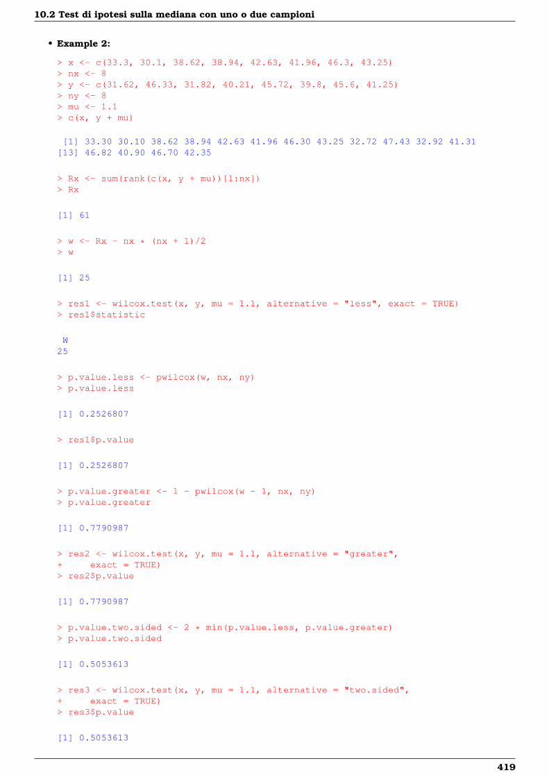
10.2 Test di ipotesi sulla mediana con uno o due campioni
• Example 2:
> x <- c(33.3, 30.1, 38.62, 38.94, 42.63, 41.96, 46.3, 43.25)> nx <- 8> y <- c(31.62, 46.33, 31.82, 40.21, 45.72, 39.8, 45.6, 41.25)> ny <- 8> mu <- 1.1> c(x, y + mu)
[1] 33.30 30.10 38.62 38.94 42.63 41.96 46.30 43.25 32.72 47.43 32.92 41.31[13] 46.82 40.90 46.70 42.35
> Rx <- sum(rank(c(x, y + mu))[1:nx])> Rx
[1] 61
> w <- Rx - nx * (nx + 1)/2> w
[1] 25
> res1 <- wilcox.test(x, y, mu = 1.1, alternative = "less", exact = TRUE)> res1$statistic
W25
> p.value.less <- pwilcox(w, nx, ny)> p.value.less
[1] 0.2526807
> res1$p.value
[1] 0.2526807
> p.value.greater <- 1 - pwilcox(w - 1, nx, ny)> p.value.greater
[1] 0.7790987
> res2 <- wilcox.test(x, y, mu = 1.1, alternative = "greater",+ exact = TRUE)> res2$p.value
[1] 0.7790987
> p.value.two.sided <- 2 * min(p.value.less, p.value.greater)> p.value.two.sided
[1] 0.5053613
> res3 <- wilcox.test(x, y, mu = 1.1, alternative = "two.sided",+ exact = TRUE)> res3$p.value
[1] 0.5053613
419
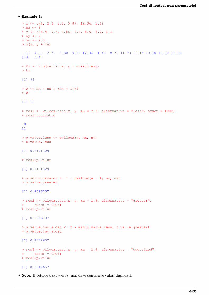
Test di ipotesi non parametrici
• Example 3:
> x <- c(4, 2.3, 8.8, 9.87, 12.34, 1.4)> nx <- 6> y <- c(6.4, 9.6, 8.86, 7.8, 8.6, 8.7, 1.1)> ny <- 7> mu <- 2.3> c(x, y + mu)
[1] 4.00 2.30 8.80 9.87 12.34 1.40 8.70 11.90 11.16 10.10 10.90 11.00[13] 3.40
> Rx <- sum(rank(c(x, y + mu))[1:nx])> Rx
[1] 33
> w <- Rx - nx * (nx + 1)/2> w
[1] 12
> res1 <- wilcox.test(x, y, mu = 2.3, alternative = "less", exact = TRUE)> res1$statistic
W12
> p.value.less <- pwilcox(w, nx, ny)> p.value.less
[1] 0.1171329
> res1$p.value
[1] 0.1171329
> p.value.greater <- 1 - pwilcox(w - 1, nx, ny)> p.value.greater
[1] 0.9096737
> res2 <- wilcox.test(x, y, mu = 2.3, alternative = "greater",+ exact = TRUE)> res2$p.value
[1] 0.9096737
> p.value.two.sided <- 2 * min(p.value.less, p.value.greater)> p.value.two.sided
[1] 0.2342657
> res3 <- wilcox.test(x, y, mu = 2.3, alternative = "two.sided",+ exact = TRUE)> res3$p.value
[1] 0.2342657
• Note: Il vettore c(x,y+mu) non deve contenere valori duplicati.
420
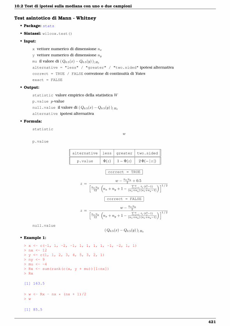
10.2 Test di ipotesi sulla mediana con uno o due campioni
Test asintotico di Mann - Whitney
• Package: stats
• Sintassi: wilcox.test()
• Input:
x vettore numerico di dimensione nxy vettore numerico di dimensione nymu il valore di (Q0.5(x)−Q0.5(y) )|H0
alternative = "less" / "greater" / "two.sided" ipotesi alternativa
correct = TRUE / FALSE correzione di continuità di Yates
exact = FALSE
• Output:
statistic valore empirico della statistica W
p.value p-value
null.value il valore di (Q0.5(x)−Q0.5(y) )|H0
alternative ipotesi alternativa
• Formula:
statisticw
p.value
alternative less greater two.sided
p.value Φ(z) 1− Φ(z) 2 Φ(− | z |)
correct = TRUE
z =w − nx ny
2 + 0.5[nx ny
12
(nx + ny + 1−
∑gj=1 tj (t2j−1)
(nx+ny) (nx+ny−1)
) ]1 / 2
correct = FALSE
z =w − nx ny
2[nx ny
12
(nx + ny + 1−
∑gj=1 tj (t2j−1)
(nx+ny) (nx+ny−1)
) ]1 / 2
null.value(Q0.5(x)−Q0.5(y) )|H0
• Example 1:
> x <- c(-1, 1, -2, -1, 1, 1, 1, 1, -1, -2, 1, 1)> nx <- 12> y <- c(1, 1, 2, 3, 4, 5, 3, 2, 1)> ny <- 9> mu <- -4> Rx <- sum(rank(c(x, y + mu))[1:nx])> Rx
[1] 163.5
> w <- Rx - nx * (nx + 1)/2> w
[1] 85.5
421
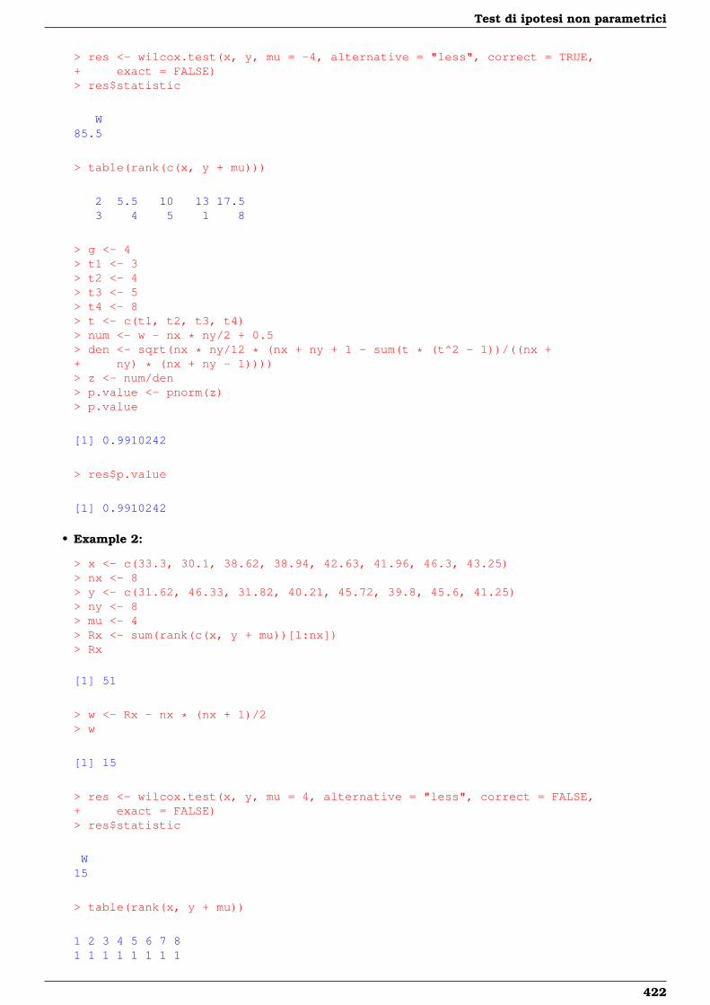
Test di ipotesi non parametrici
> res <- wilcox.test(x, y, mu = -4, alternative = "less", correct = TRUE,+ exact = FALSE)> res$statistic
W85.5
> table(rank(c(x, y + mu)))
2 5.5 10 13 17.53 4 5 1 8
> g <- 4> t1 <- 3> t2 <- 4> t3 <- 5> t4 <- 8> t <- c(t1, t2, t3, t4)> num <- w - nx * ny/2 + 0.5> den <- sqrt(nx * ny/12 * (nx + ny + 1 - sum(t * (t^2 - 1))/((nx ++ ny) * (nx + ny - 1))))> z <- num/den> p.value <- pnorm(z)> p.value
[1] 0.9910242
> res$p.value
[1] 0.9910242
• Example 2:
> x <- c(33.3, 30.1, 38.62, 38.94, 42.63, 41.96, 46.3, 43.25)> nx <- 8> y <- c(31.62, 46.33, 31.82, 40.21, 45.72, 39.8, 45.6, 41.25)> ny <- 8> mu <- 4> Rx <- sum(rank(c(x, y + mu))[1:nx])> Rx
[1] 51
> w <- Rx - nx * (nx + 1)/2> w
[1] 15
> res <- wilcox.test(x, y, mu = 4, alternative = "less", correct = FALSE,+ exact = FALSE)> res$statistic
W15
> table(rank(x, y + mu))
1 2 3 4 5 6 7 81 1 1 1 1 1 1 1
422

10.2 Test di ipotesi sulla mediana con uno o due campioni
> g <- 8> t1 <- 1> t2 <- 1> t3 <- 1> t4 <- 1> t5 <- 1> t6 <- 1> t7 <- 1> t8 <- 1> t <- c(t1, t2, t3, t4, t5, t6, t7, t8)> num <- w - nx * ny/2> den <- sqrt(nx * ny/12 * (nx + ny + 1 - sum(t * (t^2 - 1))/((nx ++ ny) * (nx + ny - 1))))> z <- num/den> p.value <- pnorm(z)> p.value
[1] 0.03710171
> res$p.value
[1] 0.03710171
423
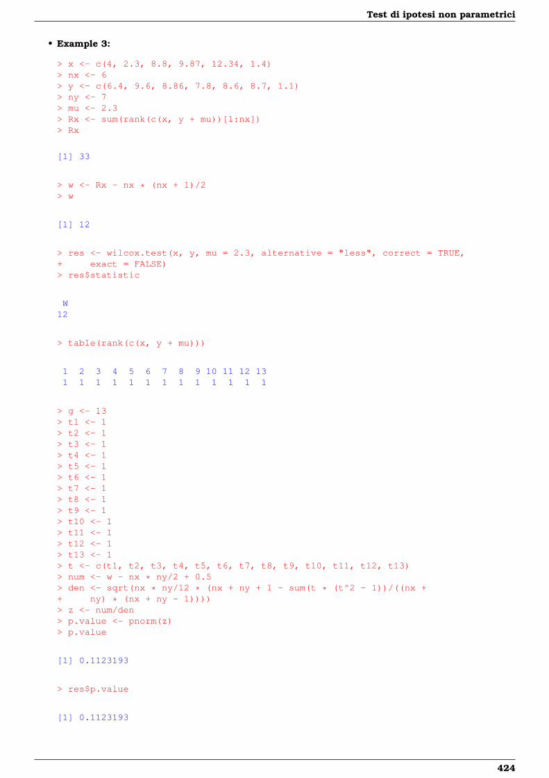
Test di ipotesi non parametrici
• Example 3:
> x <- c(4, 2.3, 8.8, 9.87, 12.34, 1.4)> nx <- 6> y <- c(6.4, 9.6, 8.86, 7.8, 8.6, 8.7, 1.1)> ny <- 7> mu <- 2.3> Rx <- sum(rank(c(x, y + mu))[1:nx])> Rx
[1] 33
> w <- Rx - nx * (nx + 1)/2> w
[1] 12
> res <- wilcox.test(x, y, mu = 2.3, alternative = "less", correct = TRUE,+ exact = FALSE)> res$statistic
W12
> table(rank(c(x, y + mu)))
1 2 3 4 5 6 7 8 9 10 11 12 131 1 1 1 1 1 1 1 1 1 1 1 1
> g <- 13> t1 <- 1> t2 <- 1> t3 <- 1> t4 <- 1> t5 <- 1> t6 <- 1> t7 <- 1> t8 <- 1> t9 <- 1> t10 <- 1> t11 <- 1> t12 <- 1> t13 <- 1> t <- c(t1, t2, t3, t4, t5, t6, t7, t8, t9, t10, t11, t12, t13)> num <- w - nx * ny/2 + 0.5> den <- sqrt(nx * ny/12 * (nx + ny + 1 - sum(t * (t^2 - 1))/((nx ++ ny) * (nx + ny - 1))))> z <- num/den> p.value <- pnorm(z)> p.value
[1] 0.1123193
> res$p.value
[1] 0.1123193
424
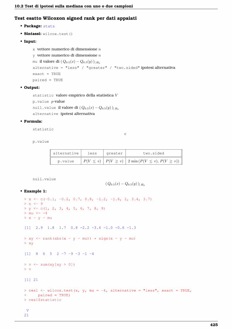
10.2 Test di ipotesi sulla mediana con uno o due campioni
Test esatto Wilcoxon signed rank per dati appaiati
• Package: stats
• Sintassi: wilcox.test()
• Input:
x vettore numerico di dimensione n
y vettore numerico di dimensione n
mu il valore di (Q0.5(x)−Q0.5(y) )|H0
alternative = "less" / "greater" / "two.sided" ipotesi alternativa
exact = TRUE
paired = TRUE
• Output:
statistic valore empirico della statistica V
p.value p-value
null.value il valore di (Q0.5(x)−Q0.5(y) )|H0
alternative ipotesi alternativa
• Formula:
statisticv
p.value
alternative less greater two.sided
p.value P (V ≤ v) P (V ≥ v) 2 min (P (V ≤ v), P (V ≥ v))
null.value(Q0.5(x)−Q0.5(y) )|H0
• Example 1:
> x <- c(-0.1, -0.2, 0.7, 0.8, -1.2, -1.6, 2, 3.4, 3.7)> n <- 9> y <- c(1, 2, 3, 4, 5, 6, 7, 8, 9)> mu <- -4> x - y - mu
[1] 2.9 1.8 1.7 0.8 -2.2 -3.6 -1.0 -0.6 -1.3
> xy <- rank(abs(x - y - mu)) * sign(x - y - mu)> xy
[1] 8 6 5 2 -7 -9 -3 -1 -4
> v <- sum(xy[xy > 0])> v
[1] 21
> res1 <- wilcox.test(x, y, mu = -4, alternative = "less", exact = TRUE,+ paired = TRUE)> res1$statistic
V21
425
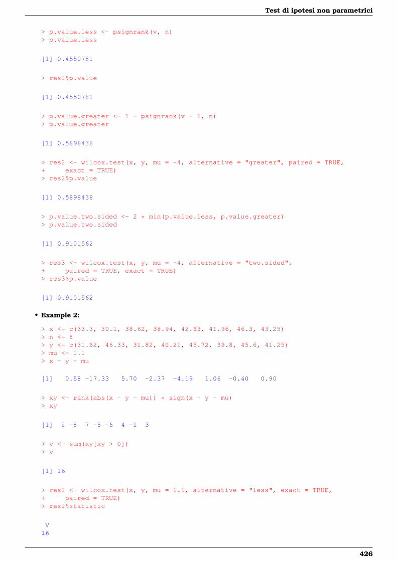
Test di ipotesi non parametrici
> p.value.less <- psignrank(v, n)> p.value.less
[1] 0.4550781
> res1$p.value
[1] 0.4550781
> p.value.greater <- 1 - psignrank(v - 1, n)> p.value.greater
[1] 0.5898438
> res2 <- wilcox.test(x, y, mu = -4, alternative = "greater", paired = TRUE,+ exact = TRUE)> res2$p.value
[1] 0.5898438
> p.value.two.sided <- 2 * min(p.value.less, p.value.greater)> p.value.two.sided
[1] 0.9101562
> res3 <- wilcox.test(x, y, mu = -4, alternative = "two.sided",+ paired = TRUE, exact = TRUE)> res3$p.value
[1] 0.9101562
• Example 2:
> x <- c(33.3, 30.1, 38.62, 38.94, 42.63, 41.96, 46.3, 43.25)> n <- 8> y <- c(31.62, 46.33, 31.82, 40.21, 45.72, 39.8, 45.6, 41.25)> mu <- 1.1> x - y - mu
[1] 0.58 -17.33 5.70 -2.37 -4.19 1.06 -0.40 0.90
> xy <- rank(abs(x - y - mu)) * sign(x - y - mu)> xy
[1] 2 -8 7 -5 -6 4 -1 3
> v <- sum(xy[xy > 0])> v
[1] 16
> res1 <- wilcox.test(x, y, mu = 1.1, alternative = "less", exact = TRUE,+ paired = TRUE)> res1$statistic
V16
426
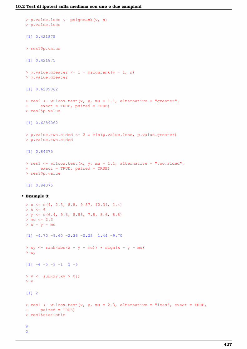
10.2 Test di ipotesi sulla mediana con uno o due campioni
> p.value.less <- psignrank(v, n)> p.value.less
[1] 0.421875
> res1$p.value
[1] 0.421875
> p.value.greater <- 1 - psignrank(v - 1, n)> p.value.greater
[1] 0.6289062
> res2 <- wilcox.test(x, y, mu = 1.1, alternative = "greater",+ exact = TRUE, paired = TRUE)> res2$p.value
[1] 0.6289062
> p.value.two.sided <- 2 * min(p.value.less, p.value.greater)> p.value.two.sided
[1] 0.84375
> res3 <- wilcox.test(x, y, mu = 1.1, alternative = "two.sided",+ exact = TRUE, paired = TRUE)> res3$p.value
[1] 0.84375
• Example 3:
> x <- c(4, 2.3, 8.8, 9.87, 12.34, 1.4)> n <- 6> y <- c(6.4, 9.6, 8.86, 7.8, 8.6, 8.8)> mu <- 2.3> x - y - mu
[1] -4.70 -9.60 -2.36 -0.23 1.44 -9.70
> xy <- rank(abs(x - y - mu)) * sign(x - y - mu)> xy
[1] -4 -5 -3 -1 2 -6
> v <- sum(xy[xy > 0])> v
[1] 2
> res1 <- wilcox.test(x, y, mu = 2.3, alternative = "less", exact = TRUE,+ paired = TRUE)> res1$statistic
V2
427
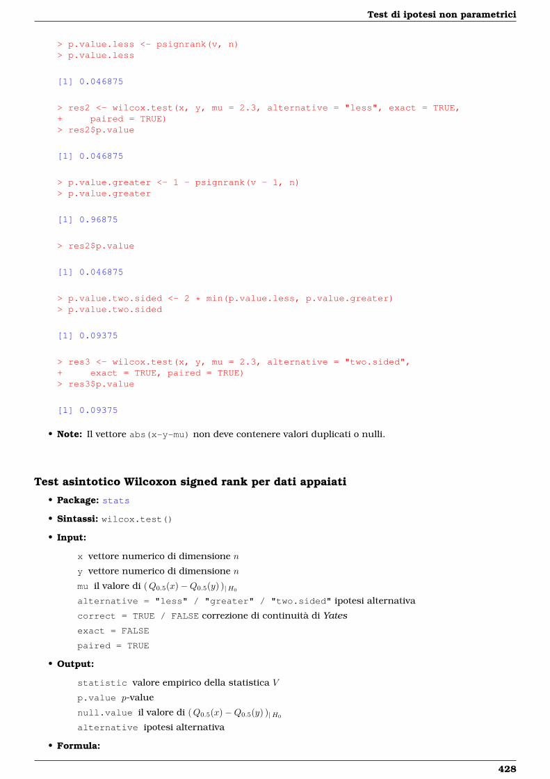
Test di ipotesi non parametrici
> p.value.less <- psignrank(v, n)> p.value.less
[1] 0.046875
> res2 <- wilcox.test(x, y, mu = 2.3, alternative = "less", exact = TRUE,+ paired = TRUE)> res2$p.value
[1] 0.046875
> p.value.greater <- 1 - psignrank(v - 1, n)> p.value.greater
[1] 0.96875
> res2$p.value
[1] 0.046875
> p.value.two.sided <- 2 * min(p.value.less, p.value.greater)> p.value.two.sided
[1] 0.09375
> res3 <- wilcox.test(x, y, mu = 2.3, alternative = "two.sided",+ exact = TRUE, paired = TRUE)> res3$p.value
[1] 0.09375
• Note: Il vettore abs(x-y-mu) non deve contenere valori duplicati o nulli.
Test asintotico Wilcoxon signed rank per dati appaiati
• Package: stats
• Sintassi: wilcox.test()
• Input:
x vettore numerico di dimensione n
y vettore numerico di dimensione n
mu il valore di (Q0.5(x)−Q0.5(y) )|H0
alternative = "less" / "greater" / "two.sided" ipotesi alternativa
correct = TRUE / FALSE correzione di continuità di Yates
exact = FALSE
paired = TRUE
• Output:
statistic valore empirico della statistica V
p.value p-value
null.value il valore di (Q0.5(x)−Q0.5(y) )|H0
alternative ipotesi alternativa
• Formula:
428
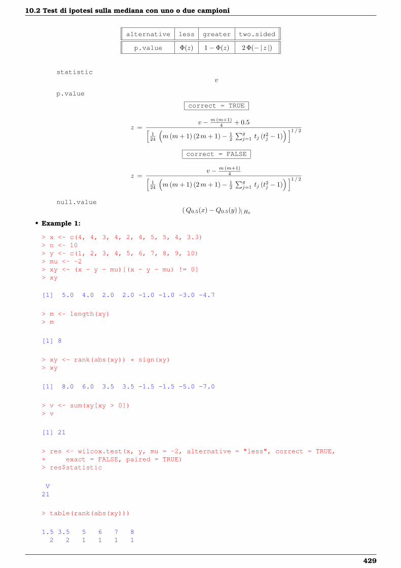
10.2 Test di ipotesi sulla mediana con uno o due campioni
alternative less greater two.sided
p.value Φ(z) 1− Φ(z) 2 Φ(− | z |)
statisticv
p.value
correct = TRUE
z =v − m (m+1)
4 + 0.5[124
(m (m+ 1) (2m+ 1)− 1
2
∑gj=1 tj (t2j − 1)
) ]1 / 2
correct = FALSE
z =v − m (m+1)
4[124
(m (m+ 1) (2m+ 1)− 1
2
∑gj=1 tj (t2j − 1)
) ]1 / 2
null.value(Q0.5(x)−Q0.5(y) )|H0
• Example 1:
> x <- c(4, 4, 3, 4, 2, 4, 5, 5, 4, 3.3)> n <- 10> y <- c(1, 2, 3, 4, 5, 6, 7, 8, 9, 10)> mu <- -2> xy <- (x - y - mu)[(x - y - mu) != 0]> xy
[1] 5.0 4.0 2.0 2.0 -1.0 -1.0 -3.0 -4.7
> m <- length(xy)> m
[1] 8
> xy <- rank(abs(xy)) * sign(xy)> xy
[1] 8.0 6.0 3.5 3.5 -1.5 -1.5 -5.0 -7.0
> v <- sum(xy[xy > 0])> v
[1] 21
> res <- wilcox.test(x, y, mu = -2, alternative = "less", correct = TRUE,+ exact = FALSE, paired = TRUE)> res$statistic
V21
> table(rank(abs(xy)))
1.5 3.5 5 6 7 82 2 1 1 1 1
429
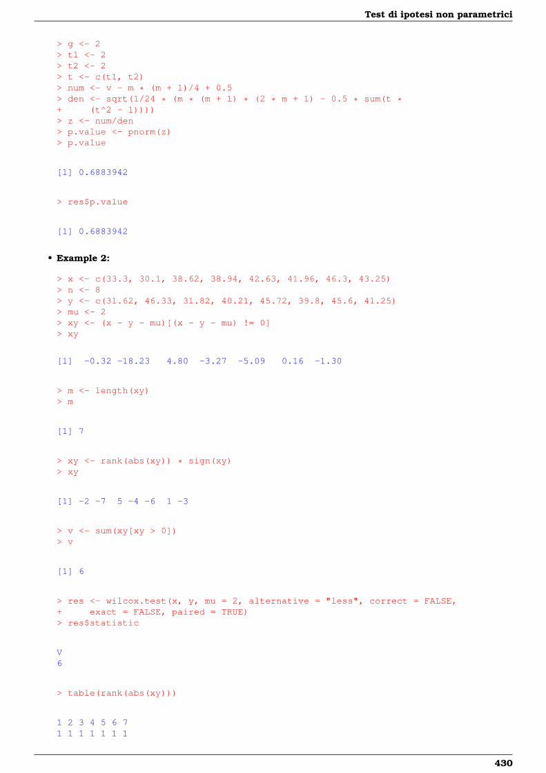
Test di ipotesi non parametrici
> g <- 2> t1 <- 2> t2 <- 2> t <- c(t1, t2)> num <- v - m * (m + 1)/4 + 0.5> den <- sqrt(1/24 * (m * (m + 1) * (2 * m + 1) - 0.5 * sum(t *+ (t^2 - 1))))> z <- num/den> p.value <- pnorm(z)> p.value
[1] 0.6883942
> res$p.value
[1] 0.6883942
• Example 2:
> x <- c(33.3, 30.1, 38.62, 38.94, 42.63, 41.96, 46.3, 43.25)> n <- 8> y <- c(31.62, 46.33, 31.82, 40.21, 45.72, 39.8, 45.6, 41.25)> mu <- 2> xy <- (x - y - mu)[(x - y - mu) != 0]> xy
[1] -0.32 -18.23 4.80 -3.27 -5.09 0.16 -1.30
> m <- length(xy)> m
[1] 7
> xy <- rank(abs(xy)) * sign(xy)> xy
[1] -2 -7 5 -4 -6 1 -3
> v <- sum(xy[xy > 0])> v
[1] 6
> res <- wilcox.test(x, y, mu = 2, alternative = "less", correct = FALSE,+ exact = FALSE, paired = TRUE)> res$statistic
V6
> table(rank(abs(xy)))
1 2 3 4 5 6 71 1 1 1 1 1 1
430
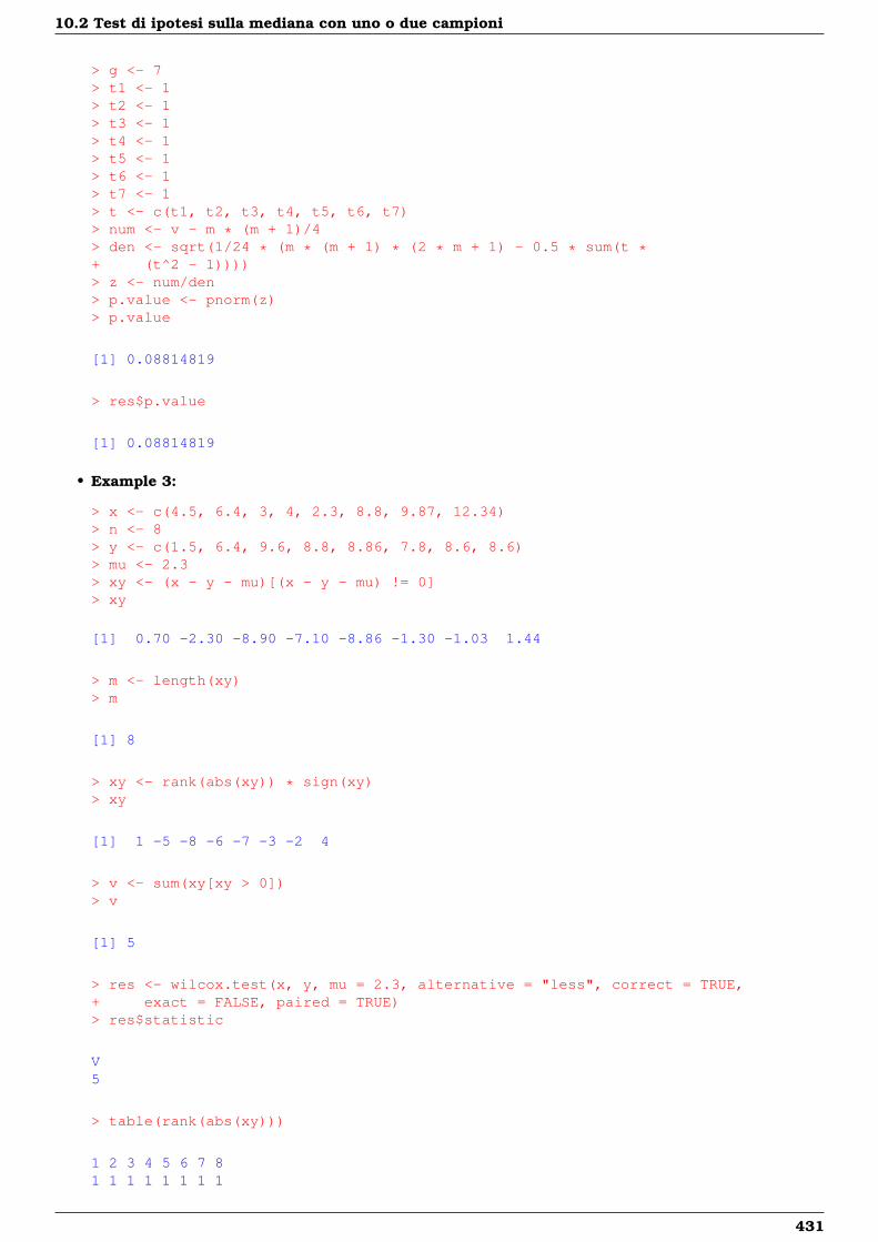
10.2 Test di ipotesi sulla mediana con uno o due campioni
> g <- 7> t1 <- 1> t2 <- 1> t3 <- 1> t4 <- 1> t5 <- 1> t6 <- 1> t7 <- 1> t <- c(t1, t2, t3, t4, t5, t6, t7)> num <- v - m * (m + 1)/4> den <- sqrt(1/24 * (m * (m + 1) * (2 * m + 1) - 0.5 * sum(t *+ (t^2 - 1))))> z <- num/den> p.value <- pnorm(z)> p.value
[1] 0.08814819
> res$p.value
[1] 0.08814819
• Example 3:
> x <- c(4.5, 6.4, 3, 4, 2.3, 8.8, 9.87, 12.34)> n <- 8> y <- c(1.5, 6.4, 9.6, 8.8, 8.86, 7.8, 8.6, 8.6)> mu <- 2.3> xy <- (x - y - mu)[(x - y - mu) != 0]> xy
[1] 0.70 -2.30 -8.90 -7.10 -8.86 -1.30 -1.03 1.44
> m <- length(xy)> m
[1] 8
> xy <- rank(abs(xy)) * sign(xy)> xy
[1] 1 -5 -8 -6 -7 -3 -2 4
> v <- sum(xy[xy > 0])> v
[1] 5
> res <- wilcox.test(x, y, mu = 2.3, alternative = "less", correct = TRUE,+ exact = FALSE, paired = TRUE)> res$statistic
V5
> table(rank(abs(xy)))
1 2 3 4 5 6 7 81 1 1 1 1 1 1 1
431
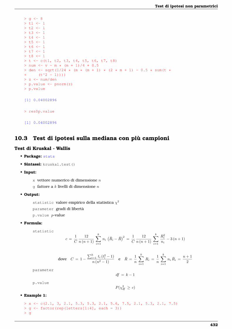
Test di ipotesi non parametrici
> g <- 8> t1 <- 1> t2 <- 1> t3 <- 1> t4 <- 1> t5 <- 1> t6 <- 1> t7 <- 1> t8 <- 1> t <- c(t1, t2, t3, t4, t5, t6, t7, t8)> num <- v - m * (m + 1)/4 + 0.5> den <- sqrt(1/24 * (m * (m + 1) * (2 * m + 1) - 0.5 * sum(t *+ (t^2 - 1))))> z <- num/den> p.value <- pnorm(z)> p.value
[1] 0.04002896
> res$p.value
[1] 0.04002896
10.3 Test di ipotesi sulla mediana con più campioni
Test di Kruskal - Wallis
• Package: stats
• Sintassi: kruskal.test()
• Input:
x vettore numerico di dimensione n
g fattore a k livelli di dimensione n
• Output:
statistic valore empirico della statistica χ2
parameter gradi di libertà
p.value p-value
• Formula:
statistic
c =1C
12n (n+ 1)
k∑i=1
ni(Ri − R
)2 =1C
12n (n+ 1)
k∑i=1
R2i
ni− 3 (n+ 1)
dove C = 1−∑hi=1 ti (t2i − 1)n (n2 − 1)
e R =1n
k∑i=1
Ri =1n
k∑i=1
ni Ri =n+ 1
2
parameterdf = k − 1
p.valueP (χ2
df ≥ c)
• Example 1:
> x <- c(2.1, 3, 2.1, 5.3, 5.3, 2.1, 5.6, 7.5, 2.1, 5.3, 2.1, 7.5)> g <- factor(rep(letters[1:4], each = 3))> g
432
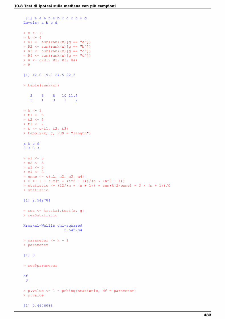
10.3 Test di ipotesi sulla mediana con più campioni
[1] a a a b b b c c c d d dLevels: a b c d
> n <- 12> k <- 4> R1 <- sum(rank(x)[g == "a"])> R2 <- sum(rank(x)[g == "b"])> R3 <- sum(rank(x)[g == "c"])> R4 <- sum(rank(x)[g == "d"])> R <- c(R1, R2, R3, R4)> R
[1] 12.0 19.0 24.5 22.5
> table(rank(x))
3 6 8 10 11.55 1 3 1 2
> h <- 3> t1 <- 5> t2 <- 3> t3 <- 2> t <- c(t1, t2, t3)> tapply(x, g, FUN = "length")
a b c d3 3 3 3
> n1 <- 3> n2 <- 3> n3 <- 3> n4 <- 3> enne <- c(n1, n2, n3, n4)> C <- 1 - sum(t * (t^2 - 1))/(n * (n^2 - 1))> statistic <- (12/(n * (n + 1)) * sum(R^2/enne) - 3 * (n + 1))/C> statistic
[1] 2.542784
> res <- kruskal.test(x, g)> res$statistic
Kruskal-Wallis chi-squared2.542784
> parameter <- k - 1> parameter
[1] 3
> res$parameter
df3
> p.value <- 1 - pchisq(statistic, df = parameter)> p.value
[1] 0.4676086
433
Test di ipotesi non parametrici
> res$p.value
[1] 0.4676086
• Example 2:
> x <- c(0.7, 1.6, 0.2, 1.2, 0.1, 3.4, 3.7, 0.8, 0, 2, 1.9, 0.8,+ 1.1, 0.1, 0.1, 4.4, 5.5, 1.6, 4.6, 3.4)> g <- factor(rep(letters[1:2], each = 10))> g
[1] a a a a a a a a a a b b b b b b b b b bLevels: a b
> n <- 20> k <- 2> R1 <- sum(rank(x)[g == "a"])> R2 <- sum(rank(x)[g == "b"])> R <- c(R1, R2)> R
[1] 90.5 119.5
> table(rank(x))
1 3 5 6 7.5 9 10 11.5 13 14 15.5 17 18 19 201 3 1 1 2 1 1 2 1 1 2 1 1 1 1
> h <- 4> t1 <- 3> t2 <- 2> t3 <- 2> t4 <- 2> t <- c(t1, t2, t3, t4)> tapply(x, g, FUN = "length")
a b10 10
> n1 <- 10> n2 <- 10> enne <- c(n1, n2)> C <- 1 - sum(t * (t^2 - 1))/(n * (n^2 - 1))> statistic <- (12/(n * (n + 1)) * sum(R^2/enne) - 3 * (n + 1))/C> statistic
[1] 1.207785
> res <- kruskal.test(x, g)> res$statistic
Kruskal-Wallis chi-squared1.207785
> parameter <- k - 1> parameter
[1] 1
> res$parameter
434
10.3 Test di ipotesi sulla mediana con più campioni
df1
> p.value <- 1 - pchisq(statistic, df = parameter)> p.value
[1] 0.2717712
> res$p.value
[1] 0.2717712
• Example 3:
> x <- c(4, 2.3, 8.8, 9.87, 12.34, 1.4, 6.4, 9.6, 8.86, 7.8, 8.6,+ 8.8, 2, 0.3)> g <- factor(rep(c("Ctl", "Trt"), times = c(10, 4)))> g
[1] Ctl Ctl Ctl Ctl Ctl Ctl Ctl Ctl Ctl Ctl Trt Trt Trt TrtLevels: Ctl Trt
> n <- 14> k <- 2> R1 <- sum(rank(x)[g == "Ctl"])> R2 <- sum(rank(x)[g == "Trt"])> R <- c(R1, R2)> R
[1] 83.5 21.5
> table(rank(x))
1 2 3 4 5 6 7 8 9.5 11 12 13 141 1 1 1 1 1 1 1 2 1 1 1 1
> h <- 1> t1 <- 2> t <- c(t1)> tapply(x, g, FUN = "length")
Ctl Trt10 4
> n1 <- 10> n2 <- 4> enne <- c(n1, n2)> C <- 1 - sum(t * (t^2 - 1))/(n * (n^2 - 1))> statistic <- (12/(n * (n + 1)) * sum(R^2/enne) - 3 * (n + 1))/C> statistic
[1] 1.448183
> res <- kruskal.test(x, g)> res$statistic
Kruskal-Wallis chi-squared1.448183
435

Test di ipotesi non parametrici
> parameter <- k - 1> parameter
[1] 1
> res$parameter
df1
> p.value <- 1 - pchisq(statistic, df = parameter)> p.value
[1] 0.2288198
> res$p.value
[1] 0.2288198
10.4 Test di ipotesi sull’omogeneità delle varianze
Test di Levene
• Package: car
• Sintassi: levene.test()
• Input:
y vettore numerico di dimensione n
group fattore f a k livelli di dimensione n
• Output:
Df gradi di libertà
F value valore empirico della statistica F
Pr(>F) p-value
• Formula:
Df
f k − 1
Residuals n− k
F value
Fvalue =
[∑kj=1
∑nji=1 (xij − xj)2
]/ (k − 1)[∑k
j=1 (nj − 1) s2j
]/ (n− k)
dove xij =∣∣yij −Q0.5
({y1j , . . . , ynjj
})∣∣ ∀ j = 1, 2, . . . , k ∀ i = 1, 2, . . . , nj
Pr(>F)P (Fk−1, n−k ≥ Fvalue)
• Example 1:
436
10.4 Test di ipotesi sull’omogeneità delle varianze
> y <- c(1, 4, 10, 2.1, 3.5, 5.6, 8.4, 12, 16.5, 22, 1.2, 3.4)> f <- factor(rep(letters[1:4], each = 3))> n <- 12> k <- 4> Df <- c(k - 1, n - k)> Df
[1] 3 8
> res <- levene.test(y, group = f)> res$Df
[1] 3 8
> x <- abs(y - ave(y, f, FUN = "median"))> Fvalue <- anova(lm(formula = x ~ f))$F> Fvalue
[1] 0.608269 NA
> res$"F value"
[1] 0.608269 NA
> p.value <- 1 - pf(Fvalue, df1 = k - 1, df2 = n - k)> p.value
[1] 0.6281414 NA
> res$"Pr(>F)"
[1] 0.6281414 NA
• Example 2:
> y <- c(1.2, 3.4, 4.5, 6.4, 4, 3, 4, 3.4)> f <- factor(c("A", "B", "B", "B", "A", "A", "B", "A"))> n <- 8> k <- 2> Df <- c(k - 1, n - k)> Df
[1] 1 6
> res <- levene.test(y, group = f)> res$Df
[1] 1 6
> x <- abs(y - ave(y, f, FUN = "median"))> Fvalue <- anova(lm(formula = x ~ f))$F> Fvalue
[1] 0.01477833 NA
> res$"F value"
[1] 0.01477833 NA
437
Test di ipotesi non parametrici
> p.value <- 1 - pf(Fvalue, df1 = k - 1, df2 = n - k)> p.value
[1] 0.9072118 NA
> res$"Pr(>F)"
[1] 0.9072118 NA
• Example 3:
> y <- c(4, 2.3, 8.8, 9.87, 12.34, 1.4, 6.4, 9.6, 8.86, 7.8, 8.6,+ 8.8, 2, 0.3)> f <- factor(rep(c("Ctl", "Trt"), times = c(10, 4)))> f
[1] Ctl Ctl Ctl Ctl Ctl Ctl Ctl Ctl Ctl Ctl Trt Trt Trt TrtLevels: Ctl Trt
> n <- 14> k <- 2> Df <- c(k - 1, n - k)> Df
[1] 1 12
> res <- levene.test(y, group = f)> res$Df
[1] 1 12
> x <- abs(y - ave(y, f, FUN = "median"))> Fvalue <- anova(lm(formula = x ~ f))$F> Fvalue
[1] 0.6701819 NA
> res$"F value"
[1] 0.6701819 NA
> p.value <- 1 - pf(Fvalue, df1 = k - 1, df2 = n - k)> p.value
[1] 0.4289462 NA
> res$"Pr(>F)"
[1] 0.4289462 NA
438
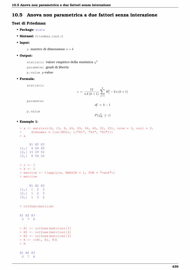
10.5 Anova non parametrica a due fattori senza interazione
10.5 Anova non parametrica a due fattori senza interazione
Test di Friedman
• Package: stats
• Sintassi: friedman.test()
• Input:
x matrice di dimensione n× k
• Output:
statistic valore empirico della statistica χ2
parameter gradi di libertà
p.value p-value
• Formula:
statistic
c =12
nk (k + 1)
k∑j=1
R2j − 3n (k + 1)
parameterdf = k − 1
p.valueP (χ2
df ≥ c)
• Example 1:
> x <- matrix(c(6, 15, 8, 26, 29, 56, 60, 52, 20), nrow = 3, ncol = 3,+ dimnames = list(NULL, c("X1", "X2", "X3")))> x
X1 X2 X3[1,] 6 26 60[2,] 15 29 52[3,] 8 56 20
> n <- 3> k <- 3> matrice <- t(apply(x, MARGIN = 1, FUN = "rank"))> matrice
X1 X2 X3[1,] 1 2 3[2,] 1 2 3[3,] 1 3 2
> colSums(matrice)
X1 X2 X33 7 8
> R1 <- colSums(matrice)[1]> R2 <- colSums(matrice)[2]> R3 <- colSums(matrice)[3]> R <- c(R1, R2, R3)> R
X1 X2 X33 7 8
439
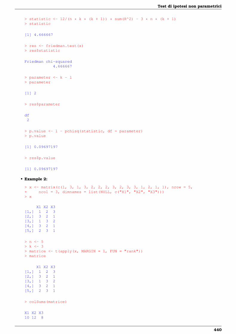
Test di ipotesi non parametrici
> statistic <- 12/(n * k * (k + 1)) * sum(R^2) - 3 * n * (k + 1)> statistic
[1] 4.666667
> res <- friedman.test(x)> res$statistic
Friedman chi-squared4.666667
> parameter <- k - 1> parameter
[1] 2
> res$parameter
df2
> p.value <- 1 - pchisq(statistic, df = parameter)> p.value
[1] 0.09697197
> res$p.value
[1] 0.09697197
• Example 2:
> x <- matrix(c(1, 3, 1, 3, 2, 2, 2, 3, 2, 3, 3, 1, 2, 1, 1), nrow = 5,+ ncol = 3, dimnames = list(NULL, c("X1", "X2", "X3")))> x
X1 X2 X3[1,] 1 2 3[2,] 3 2 1[3,] 1 3 2[4,] 3 2 1[5,] 2 3 1
> n <- 5> k <- 3> matrice <- t(apply(x, MARGIN = 1, FUN = "rank"))> matrice
X1 X2 X3[1,] 1 2 3[2,] 3 2 1[3,] 1 3 2[4,] 3 2 1[5,] 2 3 1
> colSums(matrice)
X1 X2 X310 12 8
440
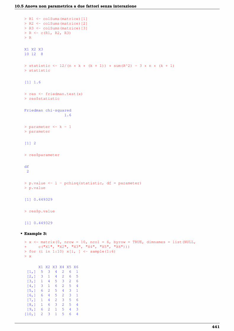
10.5 Anova non parametrica a due fattori senza interazione
> R1 <- colSums(matrice)[1]> R2 <- colSums(matrice)[2]> R3 <- colSums(matrice)[3]> R <- c(R1, R2, R3)> R
X1 X2 X310 12 8
> statistic <- 12/(n * k * (k + 1)) * sum(R^2) - 3 * n * (k + 1)> statistic
[1] 1.6
> res <- friedman.test(x)> res$statistic
Friedman chi-squared1.6
> parameter <- k - 1> parameter
[1] 2
> res$parameter
df2
> p.value <- 1 - pchisq(statistic, df = parameter)> p.value
[1] 0.449329
> res$p.value
[1] 0.449329
• Example 3:
> x <- matrix(0, nrow = 10, ncol = 6, byrow = TRUE, dimnames = list(NULL,+ c("X1", "X2", "X3", "X4", "X5", "X6")))> for (i in 1:10) x[i, ] <- sample(1:6)> x
X1 X2 X3 X4 X5 X6[1,] 5 3 4 2 6 1[2,] 3 1 4 2 6 5[3,] 1 4 5 3 2 6[4,] 3 1 6 2 5 4[5,] 6 2 5 4 3 1[6,] 6 4 5 2 3 1[7,] 1 4 2 3 5 6[8,] 1 6 3 2 5 4[9,] 6 2 1 5 4 3
[10,] 2 3 1 5 6 4
441
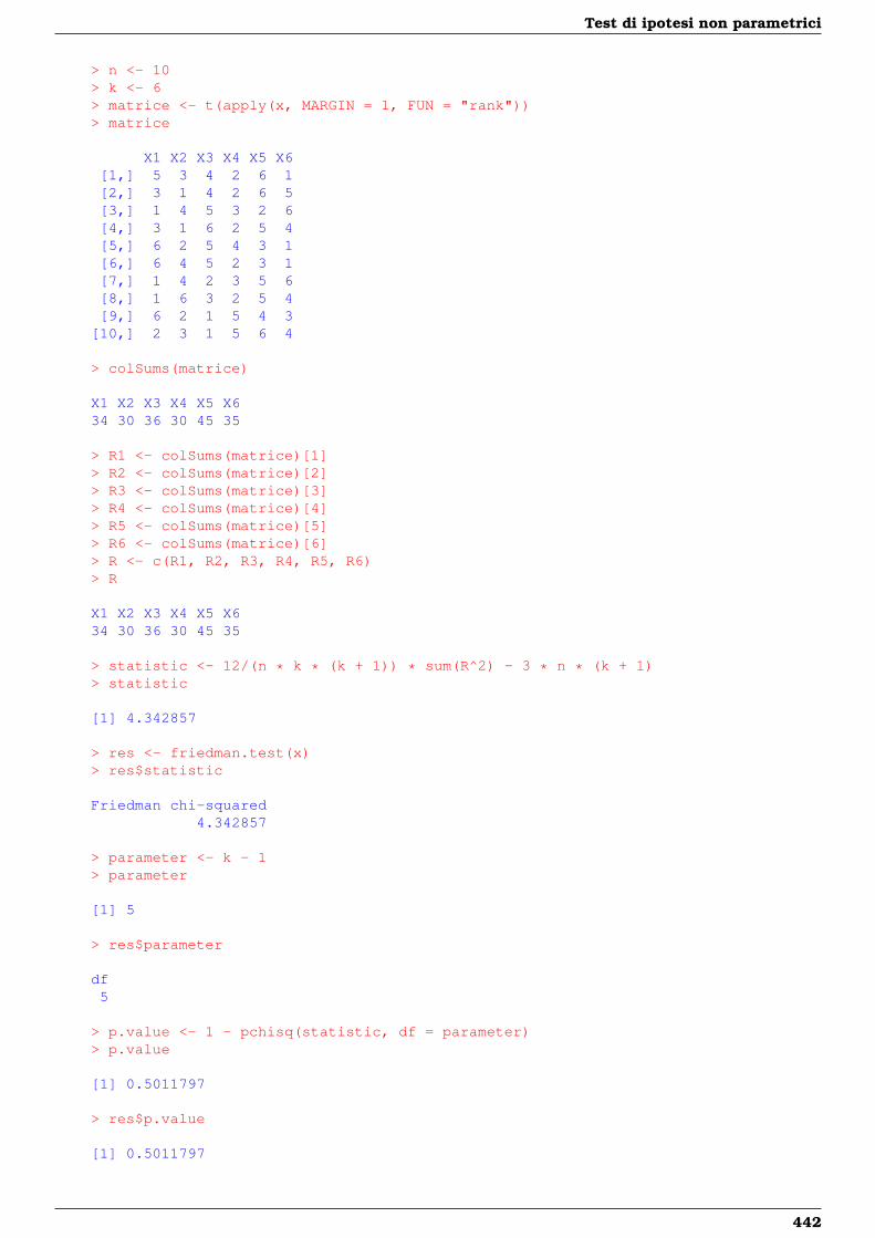
Test di ipotesi non parametrici
> n <- 10> k <- 6> matrice <- t(apply(x, MARGIN = 1, FUN = "rank"))> matrice
X1 X2 X3 X4 X5 X6[1,] 5 3 4 2 6 1[2,] 3 1 4 2 6 5[3,] 1 4 5 3 2 6[4,] 3 1 6 2 5 4[5,] 6 2 5 4 3 1[6,] 6 4 5 2 3 1[7,] 1 4 2 3 5 6[8,] 1 6 3 2 5 4[9,] 6 2 1 5 4 3
[10,] 2 3 1 5 6 4
> colSums(matrice)
X1 X2 X3 X4 X5 X634 30 36 30 45 35
> R1 <- colSums(matrice)[1]> R2 <- colSums(matrice)[2]> R3 <- colSums(matrice)[3]> R4 <- colSums(matrice)[4]> R5 <- colSums(matrice)[5]> R6 <- colSums(matrice)[6]> R <- c(R1, R2, R3, R4, R5, R6)> R
X1 X2 X3 X4 X5 X634 30 36 30 45 35
> statistic <- 12/(n * k * (k + 1)) * sum(R^2) - 3 * n * (k + 1)> statistic
[1] 4.342857
> res <- friedman.test(x)> res$statistic
Friedman chi-squared4.342857
> parameter <- k - 1> parameter
[1] 5
> res$parameter
df5
> p.value <- 1 - pchisq(statistic, df = parameter)> p.value
[1] 0.5011797
> res$p.value
[1] 0.5011797
442
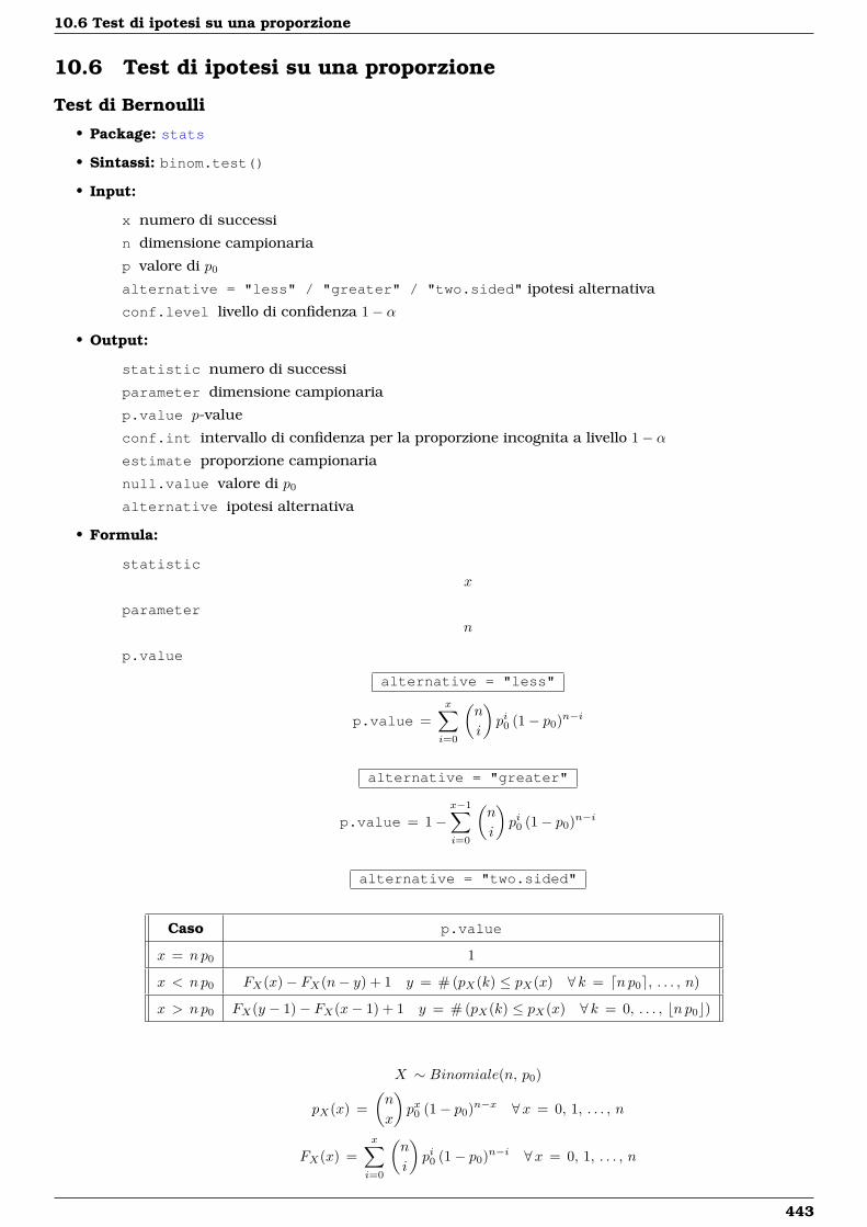
10.6 Test di ipotesi su una proporzione
10.6 Test di ipotesi su una proporzione
Test di Bernoulli
• Package: stats
• Sintassi: binom.test()
• Input:
x numero di successi
n dimensione campionaria
p valore di p0
alternative = "less" / "greater" / "two.sided" ipotesi alternativa
conf.level livello di confidenza 1− α
• Output:
statistic numero di successi
parameter dimensione campionaria
p.value p-value
conf.int intervallo di confidenza per la proporzione incognita a livello 1− αestimate proporzione campionaria
null.value valore di p0
alternative ipotesi alternativa
• Formula:
statisticx
parametern
p.value
alternative = "less"
p.value =x∑i=0
(n
i
)pi0 (1− p0)n−i
alternative = "greater"
p.value = 1−x−1∑i=0
(n
i
)pi0 (1− p0)n−i
alternative = "two.sided"
Caso p.value
x = n p0 1
x < np0 FX(x)− FX(n− y) + 1 y = # (pX(k) ≤ pX(x) ∀ k = dn p0e, . . . , n)
x > np0 FX(y − 1)− FX(x− 1) + 1 y = # (pX(k) ≤ pX(x) ∀ k = 0, . . . , bn p0c)
X ∼ Binomiale(n, p0)
pX(x) =(n
x
)px0 (1− p0)n−x ∀x = 0, 1, . . . , n
FX(x) =x∑i=0
(n
i
)pi0 (1− p0)n−i ∀x = 0, 1, . . . , n
443
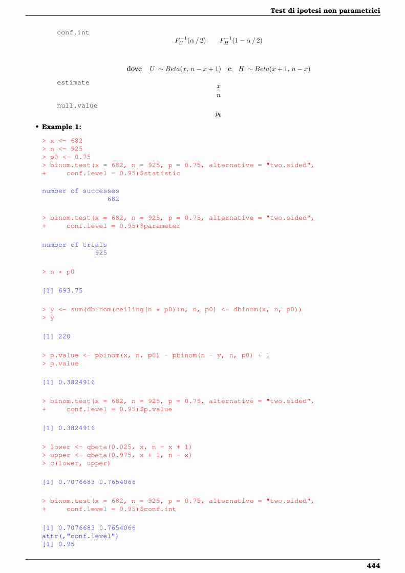
Test di ipotesi non parametrici
conf.intF−1U (α/ 2) F−1
H (1− α/ 2)
dove U ∼ Beta(x, n− x+ 1) e H ∼ Beta(x+ 1, n− x)
estimatex
n
null.valuep0
• Example 1:
> x <- 682> n <- 925> p0 <- 0.75> binom.test(x = 682, n = 925, p = 0.75, alternative = "two.sided",+ conf.level = 0.95)$statistic
number of successes682
> binom.test(x = 682, n = 925, p = 0.75, alternative = "two.sided",+ conf.level = 0.95)$parameter
number of trials925
> n * p0
[1] 693.75
> y <- sum(dbinom(ceiling(n * p0):n, n, p0) <= dbinom(x, n, p0))> y
[1] 220
> p.value <- pbinom(x, n, p0) - pbinom(n - y, n, p0) + 1> p.value
[1] 0.3824916
> binom.test(x = 682, n = 925, p = 0.75, alternative = "two.sided",+ conf.level = 0.95)$p.value
[1] 0.3824916
> lower <- qbeta(0.025, x, n - x + 1)> upper <- qbeta(0.975, x + 1, n - x)> c(lower, upper)
[1] 0.7076683 0.7654066
> binom.test(x = 682, n = 925, p = 0.75, alternative = "two.sided",+ conf.level = 0.95)$conf.int
[1] 0.7076683 0.7654066attr(,"conf.level")[1] 0.95
444
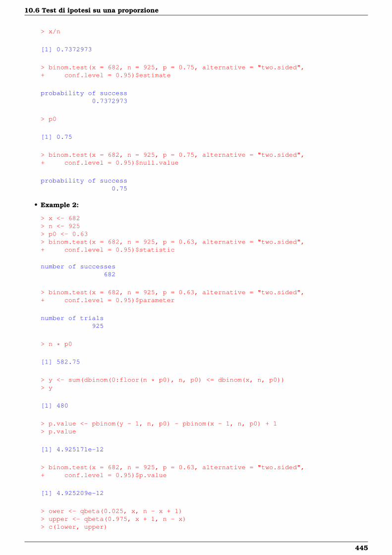
10.6 Test di ipotesi su una proporzione
> x/n
[1] 0.7372973
> binom.test(x = 682, n = 925, p = 0.75, alternative = "two.sided",+ conf.level = 0.95)$estimate
probability of success0.7372973
> p0
[1] 0.75
> binom.test(x = 682, n = 925, p = 0.75, alternative = "two.sided",+ conf.level = 0.95)$null.value
probability of success0.75
• Example 2:
> x <- 682> n <- 925> p0 <- 0.63> binom.test(x = 682, n = 925, p = 0.63, alternative = "two.sided",+ conf.level = 0.95)$statistic
number of successes682
> binom.test(x = 682, n = 925, p = 0.63, alternative = "two.sided",+ conf.level = 0.95)$parameter
number of trials925
> n * p0
[1] 582.75
> y <- sum(dbinom(0:floor(n * p0), n, p0) <= dbinom(x, n, p0))> y
[1] 480
> p.value <- pbinom(y - 1, n, p0) - pbinom(x - 1, n, p0) + 1> p.value
[1] 4.925171e-12
> binom.test(x = 682, n = 925, p = 0.63, alternative = "two.sided",+ conf.level = 0.95)$p.value
[1] 4.925209e-12
> ower <- qbeta(0.025, x, n - x + 1)> upper <- qbeta(0.975, x + 1, n - x)> c(lower, upper)
445

Test di ipotesi non parametrici
[1] 0.7076683 0.7654066
> binom.test(x = 682, n = 925, p = 0.63, alternative = "two.sided",+ conf.level = 0.95)$conf.int
[1] 0.7076683 0.7654066attr(,"conf.level")[1] 0.95
> x/n
[1] 0.7372973
> binom.test(x = 682, n = 925, p = 0.63, alternative = "two.sided",+ conf.level = 0.95)$estimate
probability of success0.7372973
> p0
[1] 0.63
> binom.test(x = 682, n = 925, p = 0.63, alternative = "two.sided",+ conf.level = 0.95)$null.value
probability of success0.63
10.7 Test di ipotesi sul ciclo di casualità
Test dei Runs
• Package: tseries
• Sintassi: runs.test()
• Input:
x fattore a 2 livelli di dimensione n
alternative = "less" / "greater" / "two.sided" ipotesi alternativa
• Output:
statistic valore empirico della statistica Z
p.value p-value
alternative ipotesi alternativa
• Formula:
statistic
z =V − n1+2n1 n2+n2
n1+n2√2n1 n2 (2n1 n2−n1−n2)
(n1+n2)2 (n1+n2−1)
p.value
• Example 1:
446
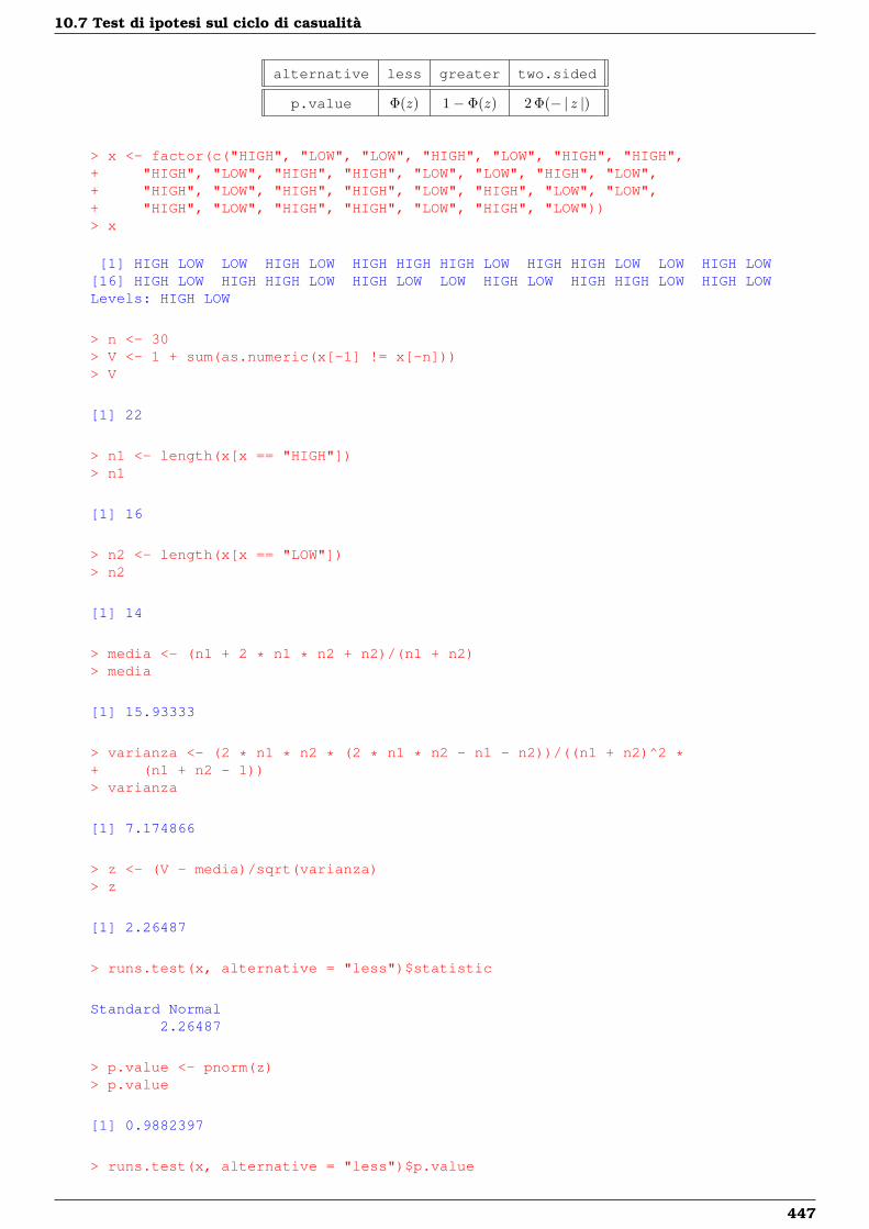
10.7 Test di ipotesi sul ciclo di casualità
alternative less greater two.sided
p.value Φ(z) 1− Φ(z) 2 Φ(− | z |)
> x <- factor(c("HIGH", "LOW", "LOW", "HIGH", "LOW", "HIGH", "HIGH",+ "HIGH", "LOW", "HIGH", "HIGH", "LOW", "LOW", "HIGH", "LOW",+ "HIGH", "LOW", "HIGH", "HIGH", "LOW", "HIGH", "LOW", "LOW",+ "HIGH", "LOW", "HIGH", "HIGH", "LOW", "HIGH", "LOW"))> x
[1] HIGH LOW LOW HIGH LOW HIGH HIGH HIGH LOW HIGH HIGH LOW LOW HIGH LOW[16] HIGH LOW HIGH HIGH LOW HIGH LOW LOW HIGH LOW HIGH HIGH LOW HIGH LOWLevels: HIGH LOW
> n <- 30> V <- 1 + sum(as.numeric(x[-1] != x[-n]))> V
[1] 22
> n1 <- length(x[x == "HIGH"])> n1
[1] 16
> n2 <- length(x[x == "LOW"])> n2
[1] 14
> media <- (n1 + 2 * n1 * n2 + n2)/(n1 + n2)> media
[1] 15.93333
> varianza <- (2 * n1 * n2 * (2 * n1 * n2 - n1 - n2))/((n1 + n2)^2 *+ (n1 + n2 - 1))> varianza
[1] 7.174866
> z <- (V - media)/sqrt(varianza)> z
[1] 2.26487
> runs.test(x, alternative = "less")$statistic
Standard Normal2.26487
> p.value <- pnorm(z)> p.value
[1] 0.9882397
> runs.test(x, alternative = "less")$p.value
447
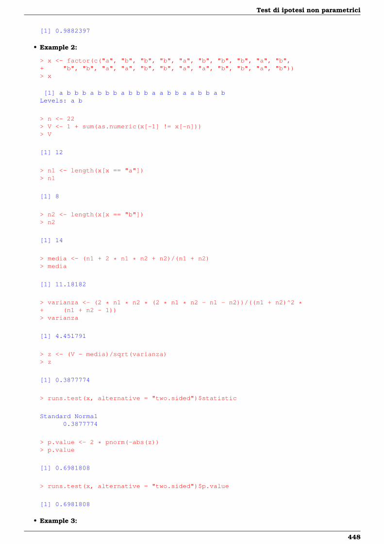
Test di ipotesi non parametrici
[1] 0.9882397
• Example 2:
> x <- factor(c("a", "b", "b", "b", "a", "b", "b", "b", "a", "b",+ "b", "b", "a", "a", "b", "b", "a", "a", "b", "b", "a", "b"))> x
[1] a b b b a b b b a b b b a a b b a a b b a bLevels: a b
> n <- 22> V <- 1 + sum(as.numeric(x[-1] != x[-n]))> V
[1] 12
> n1 <- length(x[x == "a"])> n1
[1] 8
> n2 <- length(x[x == "b"])> n2
[1] 14
> media <- (n1 + 2 * n1 * n2 + n2)/(n1 + n2)> media
[1] 11.18182
> varianza <- (2 * n1 * n2 * (2 * n1 * n2 - n1 - n2))/((n1 + n2)^2 *+ (n1 + n2 - 1))> varianza
[1] 4.451791
> z <- (V - media)/sqrt(varianza)> z
[1] 0.3877774
> runs.test(x, alternative = "two.sided")$statistic
Standard Normal0.3877774
> p.value <- 2 * pnorm(-abs(z))> p.value
[1] 0.6981808
> runs.test(x, alternative = "two.sided")$p.value
[1] 0.6981808
• Example 3:
448
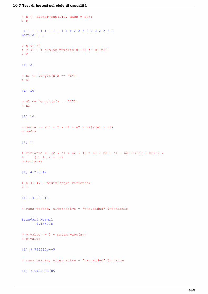
10.7 Test di ipotesi sul ciclo di casualità
> x <- factor(rep(1:2, each = 10))> x
[1] 1 1 1 1 1 1 1 1 1 1 2 2 2 2 2 2 2 2 2 2Levels: 1 2
> n <- 20> V <- 1 + sum(as.numeric(x[-1] != x[-n]))> V
[1] 2
> n1 <- length(x[x == "1"])> n1
[1] 10
> n2 <- length(x[x == "2"])> n2
[1] 10
> media <- (n1 + 2 * n1 * n2 + n2)/(n1 + n2)> media
[1] 11
> varianza <- (2 * n1 * n2 * (2 * n1 * n2 - n1 - n2))/((n1 + n2)^2 *+ (n1 + n2 - 1))> varianza
[1] 4.736842
> z <- (V - media)/sqrt(varianza)> z
[1] -4.135215
> runs.test(x, alternative = "two.sided")$statistic
Standard Normal-4.135215
> p.value <- 2 * pnorm(-abs(z))> p.value
[1] 3.546230e-05
> runs.test(x, alternative = "two.sided")$p.value
[1] 3.546230e-05
449
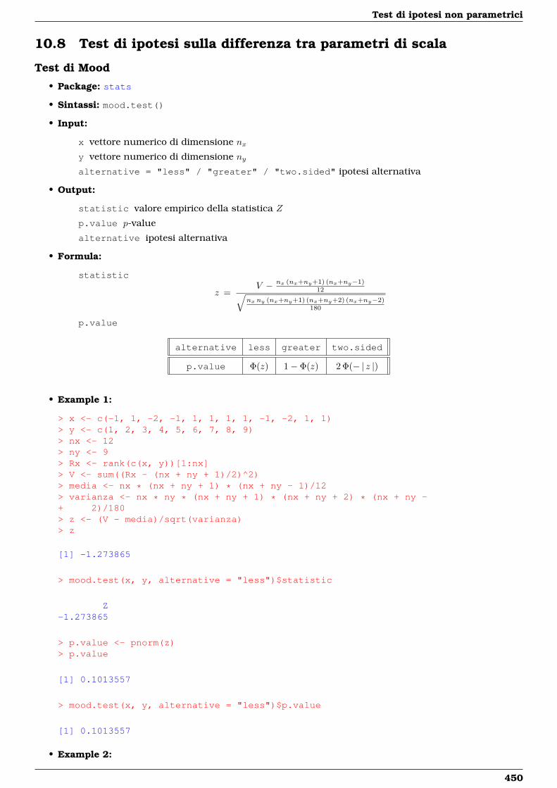
Test di ipotesi non parametrici
10.8 Test di ipotesi sulla differenza tra parametri di scala
Test di Mood
• Package: stats
• Sintassi: mood.test()
• Input:
x vettore numerico di dimensione nxy vettore numerico di dimensione nyalternative = "less" / "greater" / "two.sided" ipotesi alternativa
• Output:
statistic valore empirico della statistica Z
p.value p-value
alternative ipotesi alternativa
• Formula:
statistic
z =V − nx (nx+ny+1) (nx+ny−1)
12√nx ny (nx+ny+1) (nx+ny+2) (nx+ny−2)
180
p.value
alternative less greater two.sided
p.value Φ(z) 1− Φ(z) 2 Φ(− | z |)
• Example 1:
> x <- c(-1, 1, -2, -1, 1, 1, 1, 1, -1, -2, 1, 1)> y <- c(1, 2, 3, 4, 5, 6, 7, 8, 9)> nx <- 12> ny <- 9> Rx <- rank(c(x, y))[1:nx]> V <- sum((Rx - (nx + ny + 1)/2)^2)> media <- nx * (nx + ny + 1) * (nx + ny - 1)/12> varianza <- nx * ny * (nx + ny + 1) * (nx + ny + 2) * (nx + ny -+ 2)/180> z <- (V - media)/sqrt(varianza)> z
[1] -1.273865
> mood.test(x, y, alternative = "less")$statistic
Z-1.273865
> p.value <- pnorm(z)> p.value
[1] 0.1013557
> mood.test(x, y, alternative = "less")$p.value
[1] 0.1013557
• Example 2:
450
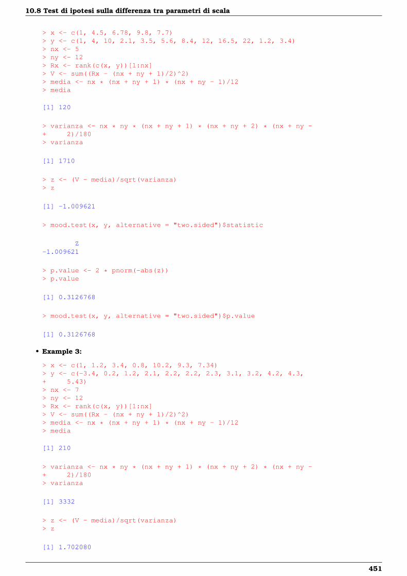
10.8 Test di ipotesi sulla differenza tra parametri di scala
> x <- c(1, 4.5, 6.78, 9.8, 7.7)> y <- c(1, 4, 10, 2.1, 3.5, 5.6, 8.4, 12, 16.5, 22, 1.2, 3.4)> nx <- 5> ny <- 12> Rx <- rank(c(x, y))[1:nx]> V <- sum((Rx - (nx + ny + 1)/2)^2)> media <- nx * (nx + ny + 1) * (nx + ny - 1)/12> media
[1] 120
> varianza <- nx * ny * (nx + ny + 1) * (nx + ny + 2) * (nx + ny -+ 2)/180> varianza
[1] 1710
> z <- (V - media)/sqrt(varianza)> z
[1] -1.009621
> mood.test(x, y, alternative = "two.sided")$statistic
Z-1.009621
> p.value <- 2 * pnorm(-abs(z))> p.value
[1] 0.3126768
> mood.test(x, y, alternative = "two.sided")$p.value
[1] 0.3126768
• Example 3:
> x <- c(1, 1.2, 3.4, 0.8, 10.2, 9.3, 7.34)> y <- c(-3.4, 0.2, 1.2, 2.1, 2.2, 2.2, 2.3, 3.1, 3.2, 4.2, 4.3,+ 5.43)> nx <- 7> ny <- 12> Rx <- rank(c(x, y))[1:nx]> V <- sum((Rx - (nx + ny + 1)/2)^2)> media <- nx * (nx + ny + 1) * (nx + ny - 1)/12> media
[1] 210
> varianza <- nx * ny * (nx + ny + 1) * (nx + ny + 2) * (nx + ny -+ 2)/180> varianza
[1] 3332
> z <- (V - media)/sqrt(varianza)> z
[1] 1.702080
451

Test di ipotesi non parametrici
> mood.test(x, y, alternative = "two.sided")$statistic
Z1.702080
> p.value <- 2 * pnorm(-abs(z))> p.value
[1] 0.0887403
> mood.test(x, y, alternative = "two.sided")$p.value
[1] 0.0887403
452

Capitolo 11
Tabelle di contingenza
11.1 Simbologia
• frequenze osservate: nij ∀ i = 1, 2, . . . , h ∀ j = 1, 2, . . . , k
• frequenze osservate nella m-esima tabella di contingenza 2× 2:
nijm ∀ i, j = 1, 2 ∀m = 1, 2, . . . , l
• frequenze marginali di riga: ni· =∑kj=1 nij ∀ i = 1, 2, . . . , h
• frequenze marginali di riga nella m-esima tabella di contingenza 2× 2:
ni·m =∑2j=1 nijm ∀ i = 1, 2 ∀m = 1, 2, . . . , l
• frequenze marginali di colonna: n·j =∑hi=1 nij ∀ j = 1, 2, . . . , k
• frequenze marginali di colonna nella m-esima tabella di contingenza 2× 2:
n·jm =∑2i=1 nijm ∀ j = 1, 2 ∀m = 1, 2, . . . , l
• frequenze attese: nij = ni· n·j / n·· ∀ i = 1, 2, . . . , h ∀ j = 1, 2, . . . , k
• frequenze attese nella m-esima tabella di contingenza 2× 2:
nijm = ni·m n·jm / n··m ∀ i, j = 1, 2 ∀m = 1, 2, . . . , l
• totale frequenze assolute: n·· =∑hi=1
∑kj=1 nij =
∑hi=1
∑kj=1 nij
• totale frequenze assolute nella m-esima tabella di contingenza 2× 2:
n··m =∑2i=1
∑2j=1 nijm =
∑2i=1
∑2j=1 nijm ∀m = 1, 2, . . . , l
11.2 Test di ipotesi per tabelle di contingenza 2 righe per 2 colonne
Test Chi - Quadrato di indipendenza
• Package: stats
• Sintassi: chisq.test()
• Input:
x matrice di dimensione 2× 2 contenente frequenze assolute
correct = TRUE / FALSE correzione di Yates
• Output:
statistic valore empirico della statistica χ2
parameter gradi di libertà
p.value p-value
observed frequenze osservate
expected frequenze attese
residuals residui di Pearson
• Formula:
453
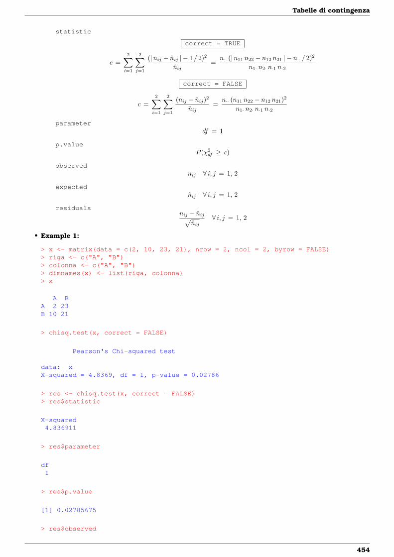
Tabelle di contingenza
statistic
correct = TRUE
c =2∑i=1
2∑j=1
(|nij − nij | − 1 / 2)2
nij=
n·· (|n11 n22 − n12 n21 | − n·· / 2)2
n1· n2· n·1 n·2
correct = FALSE
c =2∑i=1
2∑j=1
(nij − nij)2
nij=
n·· (n11 n22 − n12 n21)2
n1· n2· n·1 n·2
parameterdf = 1
p.valueP (χ2
df ≥ c)
observednij ∀ i, j = 1, 2
expectednij ∀ i, j = 1, 2
residualsnij − nij√
nij∀ i, j = 1, 2
• Example 1:
> x <- matrix(data = c(2, 10, 23, 21), nrow = 2, ncol = 2, byrow = FALSE)> riga <- c("A", "B")> colonna <- c("A", "B")> dimnames(x) <- list(riga, colonna)> x
A BA 2 23B 10 21
> chisq.test(x, correct = FALSE)
Pearson's Chi-squared test
data: xX-squared = 4.8369, df = 1, p-value = 0.02786
> res <- chisq.test(x, correct = FALSE)> res$statistic
X-squared4.836911
> res$parameter
df1
> res$p.value
[1] 0.02785675
> res$observed
454
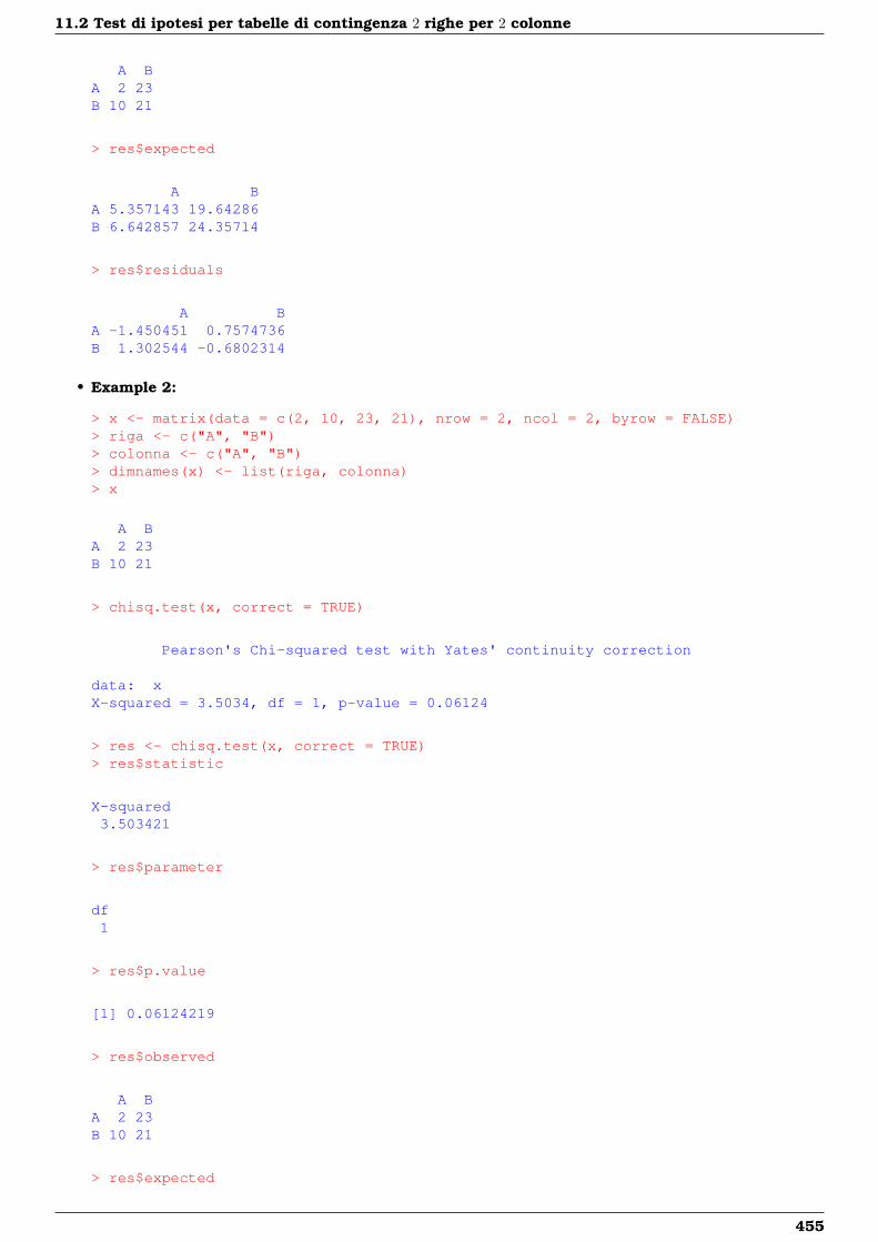
11.2 Test di ipotesi per tabelle di contingenza 2 righe per 2 colonne
A BA 2 23B 10 21
> res$expected
A BA 5.357143 19.64286B 6.642857 24.35714
> res$residuals
A BA -1.450451 0.7574736B 1.302544 -0.6802314
• Example 2:
> x <- matrix(data = c(2, 10, 23, 21), nrow = 2, ncol = 2, byrow = FALSE)> riga <- c("A", "B")> colonna <- c("A", "B")> dimnames(x) <- list(riga, colonna)> x
A BA 2 23B 10 21
> chisq.test(x, correct = TRUE)
Pearson's Chi-squared test with Yates' continuity correction
data: xX-squared = 3.5034, df = 1, p-value = 0.06124
> res <- chisq.test(x, correct = TRUE)> res$statistic
X-squared3.503421
> res$parameter
df1
> res$p.value
[1] 0.06124219
> res$observed
A BA 2 23B 10 21
> res$expected
455
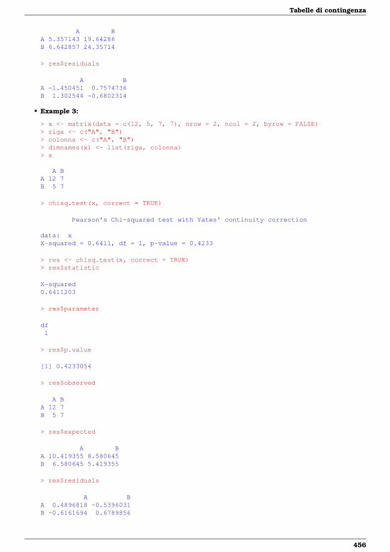
Tabelle di contingenza
A BA 5.357143 19.64286B 6.642857 24.35714
> res$residuals
A BA -1.450451 0.7574736B 1.302544 -0.6802314
• Example 3:
> x <- matrix(data = c(12, 5, 7, 7), nrow = 2, ncol = 2, byrow = FALSE)> riga <- c("A", "B")> colonna <- c("A", "B")> dimnames(x) <- list(riga, colonna)> x
A BA 12 7B 5 7
> chisq.test(x, correct = TRUE)
Pearson's Chi-squared test with Yates' continuity correction
data: xX-squared = 0.6411, df = 1, p-value = 0.4233
> res <- chisq.test(x, correct = TRUE)> res$statistic
X-squared0.6411203
> res$parameter
df1
> res$p.value
[1] 0.4233054
> res$observed
A BA 12 7B 5 7
> res$expected
A BA 10.419355 8.580645B 6.580645 5.419355
> res$residuals
A BA 0.4896818 -0.5396031B -0.6161694 0.6789856
456
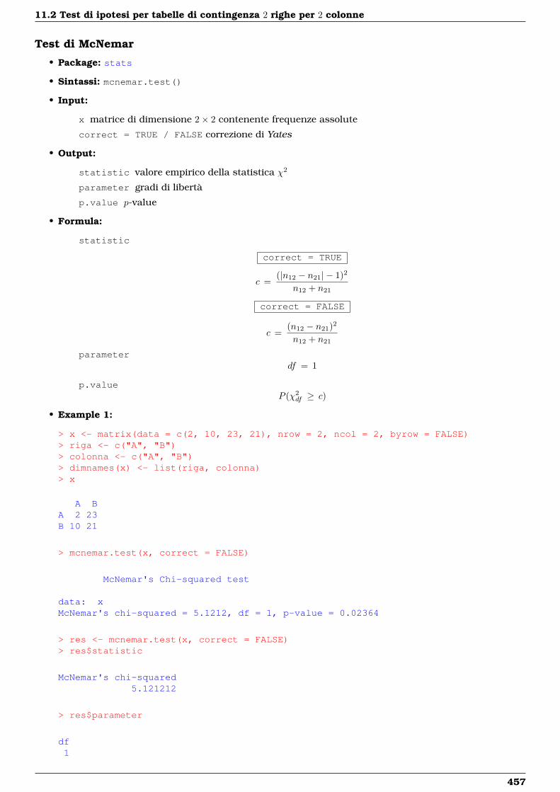
11.2 Test di ipotesi per tabelle di contingenza 2 righe per 2 colonne
Test di McNemar
• Package: stats
• Sintassi: mcnemar.test()
• Input:
x matrice di dimensione 2× 2 contenente frequenze assolute
correct = TRUE / FALSE correzione di Yates
• Output:
statistic valore empirico della statistica χ2
parameter gradi di libertà
p.value p-value
• Formula:
statistic
correct = TRUE
c =(|n12 − n21| − 1)2
n12 + n21
correct = FALSE
c =(n12 − n21)2
n12 + n21
parameterdf = 1
p.valueP (χ2
df ≥ c)
• Example 1:
> x <- matrix(data = c(2, 10, 23, 21), nrow = 2, ncol = 2, byrow = FALSE)> riga <- c("A", "B")> colonna <- c("A", "B")> dimnames(x) <- list(riga, colonna)> x
A BA 2 23B 10 21
> mcnemar.test(x, correct = FALSE)
McNemar's Chi-squared test
data: xMcNemar's chi-squared = 5.1212, df = 1, p-value = 0.02364
> res <- mcnemar.test(x, correct = FALSE)> res$statistic
McNemar's chi-squared5.121212
> res$parameter
df1
457
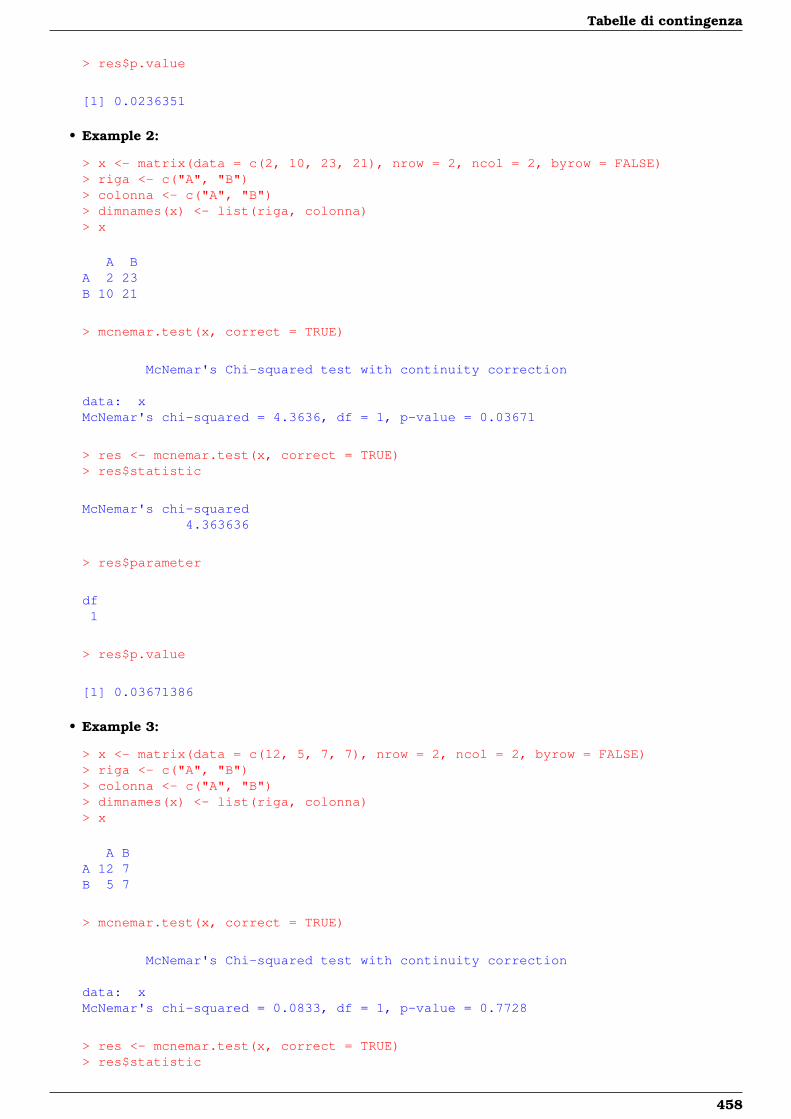
Tabelle di contingenza
> res$p.value
[1] 0.0236351
• Example 2:
> x <- matrix(data = c(2, 10, 23, 21), nrow = 2, ncol = 2, byrow = FALSE)> riga <- c("A", "B")> colonna <- c("A", "B")> dimnames(x) <- list(riga, colonna)> x
A BA 2 23B 10 21
> mcnemar.test(x, correct = TRUE)
McNemar's Chi-squared test with continuity correction
data: xMcNemar's chi-squared = 4.3636, df = 1, p-value = 0.03671
> res <- mcnemar.test(x, correct = TRUE)> res$statistic
McNemar's chi-squared4.363636
> res$parameter
df1
> res$p.value
[1] 0.03671386
• Example 3:
> x <- matrix(data = c(12, 5, 7, 7), nrow = 2, ncol = 2, byrow = FALSE)> riga <- c("A", "B")> colonna <- c("A", "B")> dimnames(x) <- list(riga, colonna)> x
A BA 12 7B 5 7
> mcnemar.test(x, correct = TRUE)
McNemar's Chi-squared test with continuity correction
data: xMcNemar's chi-squared = 0.0833, df = 1, p-value = 0.7728
> res <- mcnemar.test(x, correct = TRUE)> res$statistic
458
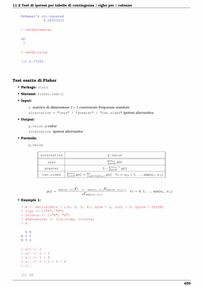
11.2 Test di ipotesi per tabelle di contingenza 2 righe per 2 colonne
McNemar's chi-squared0.08333333
> res$parameter
df1
> res$p.value
[1] 0.77283
Test esatto di Fisher
• Package: stats
• Sintassi: fisher.test()
• Input:
x matrice di dimensione 2× 2 contenente frequenze assolute
alternative = "less" / "greater" / "two.sided" ipotesi alternativa
• Output:
p.value p-value
alternative ipotesi alternativa
• Formula:
p.value
alternative p.value
less∑n11i=0 p(i)
greater 1−∑n11−1i=0 p(i)
two.sided∑n11i=0 p(i) +
∑p(i)≤p(n11) p(i) ∀ i = n11 + 1, . . . , min(n1·, n·1)
p(i) = max (n1·, n·1)Ci n··−max (n1·, n·1)Cmin (n1·, n·1)−i
nCmin (n1·, n·1)∀ i = 0, 1, . . . , min(n1·, n·1)
• Example 1:
> x <- matrix(data = c(2, 9, 5, 4), nrow = 2, ncol = 2, byrow = FALSE)> riga <- c("A", "B")> colonna <- c("A", "B")> dimnames(x) <- list(riga, colonna)> x
A BA 2 5B 9 4
> n11 <- 2> n1. <- 2 + 5> n.1 <- 2 + 9> n.. <- 2 + 5 + 9 + 4> n..
[1] 20
459
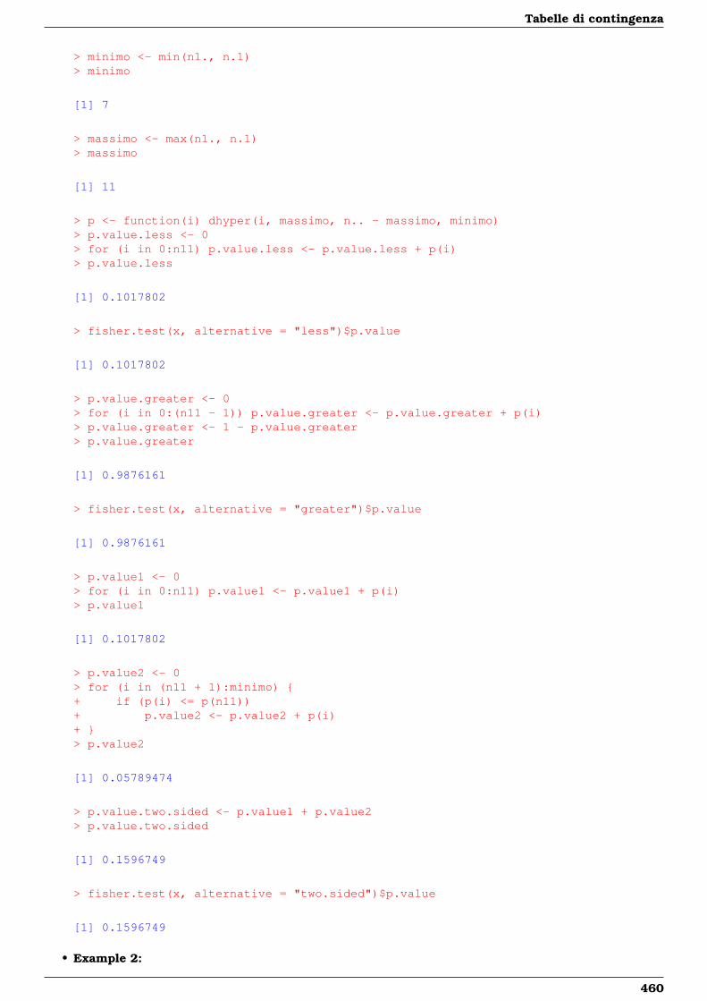
Tabelle di contingenza
> minimo <- min(n1., n.1)> minimo
[1] 7
> massimo <- max(n1., n.1)> massimo
[1] 11
> p <- function(i) dhyper(i, massimo, n.. - massimo, minimo)> p.value.less <- 0> for (i in 0:n11) p.value.less <- p.value.less + p(i)> p.value.less
[1] 0.1017802
> fisher.test(x, alternative = "less")$p.value
[1] 0.1017802
> p.value.greater <- 0> for (i in 0:(n11 - 1)) p.value.greater <- p.value.greater + p(i)> p.value.greater <- 1 - p.value.greater> p.value.greater
[1] 0.9876161
> fisher.test(x, alternative = "greater")$p.value
[1] 0.9876161
> p.value1 <- 0> for (i in 0:n11) p.value1 <- p.value1 + p(i)> p.value1
[1] 0.1017802
> p.value2 <- 0> for (i in (n11 + 1):minimo) {+ if (p(i) <= p(n11))+ p.value2 <- p.value2 + p(i)+ }> p.value2
[1] 0.05789474
> p.value.two.sided <- p.value1 + p.value2> p.value.two.sided
[1] 0.1596749
> fisher.test(x, alternative = "two.sided")$p.value
[1] 0.1596749
• Example 2:
460
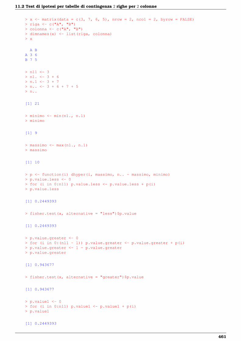
11.2 Test di ipotesi per tabelle di contingenza 2 righe per 2 colonne
> x <- matrix(data = c(3, 7, 6, 5), nrow = 2, ncol = 2, byrow = FALSE)> riga <- c("A", "B")> colonna <- c("A", "B")> dimnames(x) <- list(riga, colonna)> x
A BA 3 6B 7 5
> n11 <- 3> n1. <- 3 + 6> n.1 <- 3 + 7> n.. <- 3 + 6 + 7 + 5> n..
[1] 21
> minimo <- min(n1., n.1)> minimo
[1] 9
> massimo <- max(n1., n.1)> massimo
[1] 10
> p <- function(i) dhyper(i, massimo, n.. - massimo, minimo)> p.value.less <- 0> for (i in 0:n11) p.value.less <- p.value.less + p(i)> p.value.less
[1] 0.2449393
> fisher.test(x, alternative = "less")$p.value
[1] 0.2449393
> p.value.greater <- 0> for (i in 0:(n11 - 1)) p.value.greater <- p.value.greater + p(i)> p.value.greater <- 1 - p.value.greater> p.value.greater
[1] 0.943677
> fisher.test(x, alternative = "greater")$p.value
[1] 0.943677
> p.value1 <- 0> for (i in 0:n11) p.value1 <- p.value1 + p(i)> p.value1
[1] 0.2449393
461
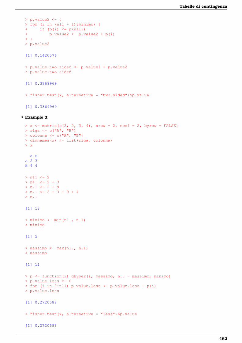
Tabelle di contingenza
> p.value2 <- 0> for (i in (n11 + 1):minimo) {+ if (p(i) <= p(n11))+ p.value2 <- p.value2 + p(i)+ }> p.value2
[1] 0.1420576
> p.value.two.sided <- p.value1 + p.value2> p.value.two.sided
[1] 0.3869969
> fisher.test(x, alternative = "two.sided")$p.value
[1] 0.3869969
• Example 3:
> x <- matrix(c(2, 9, 3, 4), nrow = 2, ncol = 2, byrow = FALSE)> riga <- c("A", "B")> colonna <- c("A", "B")> dimnames(x) <- list(riga, colonna)> x
A BA 2 3B 9 4
> n11 <- 2> n1. <- 2 + 3> n.1 <- 2 + 9> n.. <- 2 + 3 + 9 + 4> n..
[1] 18
> minimo <- min(n1., n.1)> minimo
[1] 5
> massimo <- max(n1., n.1)> massimo
[1] 11
> p <- function(i) dhyper(i, massimo, n.. - massimo, minimo)> p.value.less <- 0> for (i in 0:n11) p.value.less <- p.value.less + p(i)> p.value.less
[1] 0.2720588
> fisher.test(x, alternative = "less")$p.value
[1] 0.2720588
462
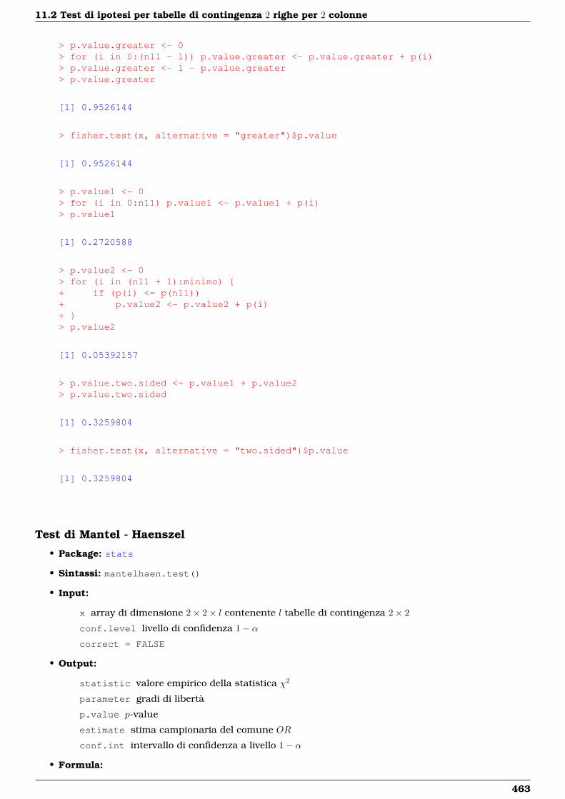
11.2 Test di ipotesi per tabelle di contingenza 2 righe per 2 colonne
> p.value.greater <- 0> for (i in 0:(n11 - 1)) p.value.greater <- p.value.greater + p(i)> p.value.greater <- 1 - p.value.greater> p.value.greater
[1] 0.9526144
> fisher.test(x, alternative = "greater")$p.value
[1] 0.9526144
> p.value1 <- 0> for (i in 0:n11) p.value1 <- p.value1 + p(i)> p.value1
[1] 0.2720588
> p.value2 <- 0> for (i in (n11 + 1):minimo) {+ if (p(i) <= p(n11))+ p.value2 <- p.value2 + p(i)+ }> p.value2
[1] 0.05392157
> p.value.two.sided <- p.value1 + p.value2> p.value.two.sided
[1] 0.3259804
> fisher.test(x, alternative = "two.sided")$p.value
[1] 0.3259804
Test di Mantel - Haenszel
• Package: stats
• Sintassi: mantelhaen.test()
• Input:
x array di dimensione 2× 2× l contenente l tabelle di contingenza 2× 2
conf.level livello di confidenza 1− αcorrect = FALSE
• Output:
statistic valore empirico della statistica χ2
parameter gradi di libertà
p.value p-value
estimate stima campionaria del comune OR
conf.int intervallo di confidenza a livello 1− α
• Formula:
463
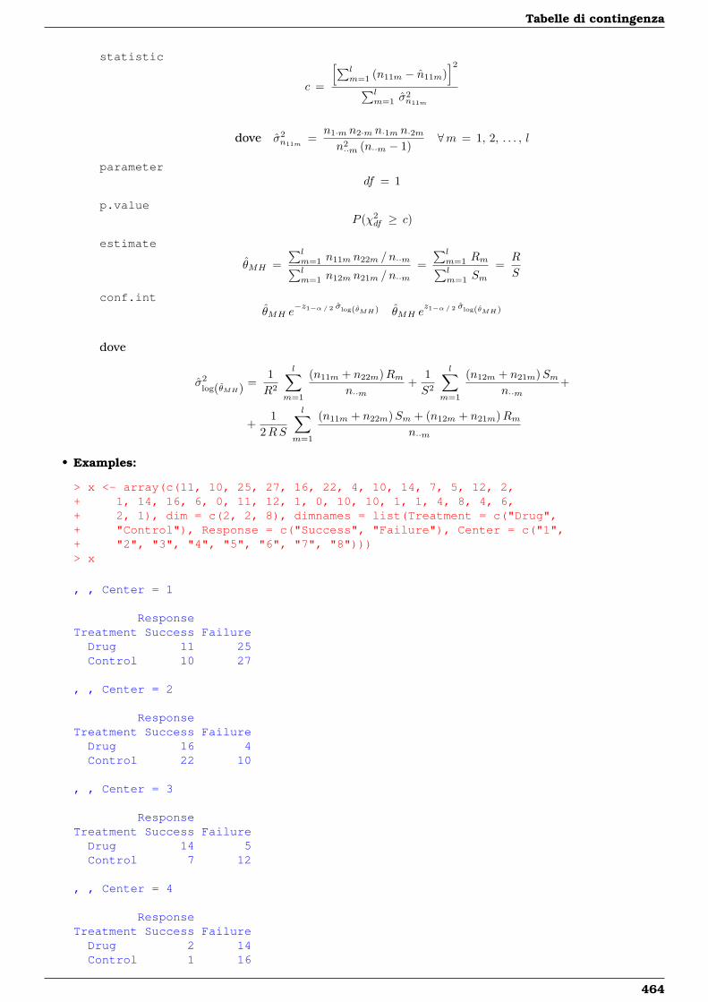
Tabelle di contingenza
statistic
c =
[∑lm=1 (n11m − n11m)
]2∑lm=1 σ
2n11m
dove σ2n11m
=n1·m n2·m n·1m n·2mn2··m (n··m − 1)
∀m = 1, 2, . . . , l
parameterdf = 1
p.valueP (χ2
df ≥ c)
estimate
θMH =∑lm=1 n11m n22m / n··m∑lm=1 n12m n21m / n··m
=∑lm=1 Rm∑lm=1 Sm
=R
S
conf.intθMH e
−z1−α/ 2 σlog(θMH) θMH ez1−α/ 2 σlog(θMH)
dove
σ2log(θMH) =
1R2
l∑m=1
(n11m + n22m)Rmn··m
+1S2
l∑m=1
(n12m + n21m)Smn··m
+
+1
2RS
l∑m=1
(n11m + n22m)Sm + (n12m + n21m)Rmn··m
• Examples:
> x <- array(c(11, 10, 25, 27, 16, 22, 4, 10, 14, 7, 5, 12, 2,+ 1, 14, 16, 6, 0, 11, 12, 1, 0, 10, 10, 1, 1, 4, 8, 4, 6,+ 2, 1), dim = c(2, 2, 8), dimnames = list(Treatment = c("Drug",+ "Control"), Response = c("Success", "Failure"), Center = c("1",+ "2", "3", "4", "5", "6", "7", "8")))> x
, , Center = 1
ResponseTreatment Success FailureDrug 11 25Control 10 27
, , Center = 2
ResponseTreatment Success FailureDrug 16 4Control 22 10
, , Center = 3
ResponseTreatment Success FailureDrug 14 5Control 7 12
, , Center = 4
ResponseTreatment Success FailureDrug 2 14Control 1 16
464
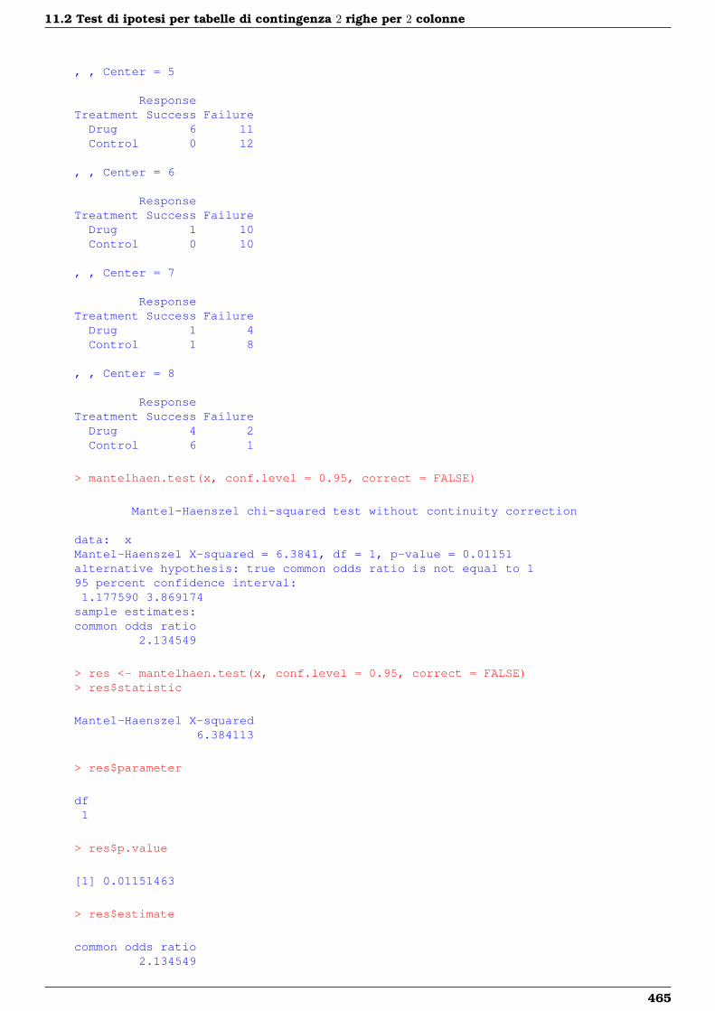
11.2 Test di ipotesi per tabelle di contingenza 2 righe per 2 colonne
, , Center = 5
ResponseTreatment Success FailureDrug 6 11Control 0 12
, , Center = 6
ResponseTreatment Success FailureDrug 1 10Control 0 10
, , Center = 7
ResponseTreatment Success FailureDrug 1 4Control 1 8
, , Center = 8
ResponseTreatment Success FailureDrug 4 2Control 6 1
> mantelhaen.test(x, conf.level = 0.95, correct = FALSE)
Mantel-Haenszel chi-squared test without continuity correction
data: xMantel-Haenszel X-squared = 6.3841, df = 1, p-value = 0.01151alternative hypothesis: true common odds ratio is not equal to 195 percent confidence interval:1.177590 3.869174
sample estimates:common odds ratio
2.134549
> res <- mantelhaen.test(x, conf.level = 0.95, correct = FALSE)> res$statistic
Mantel-Haenszel X-squared6.384113
> res$parameter
df1
> res$p.value
[1] 0.01151463
> res$estimate
common odds ratio2.134549
465
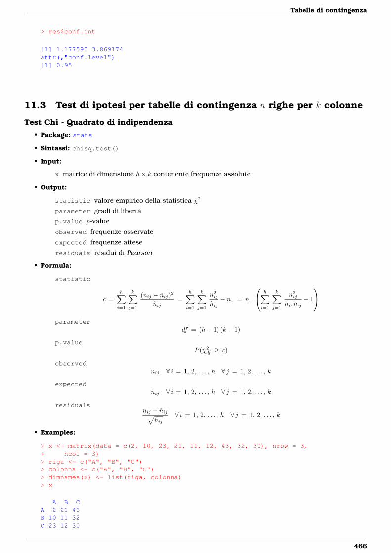
Tabelle di contingenza
> res$conf.int
[1] 1.177590 3.869174attr(,"conf.level")[1] 0.95
11.3 Test di ipotesi per tabelle di contingenza n righe per k colonne
Test Chi - Quadrato di indipendenza
• Package: stats
• Sintassi: chisq.test()
• Input:
x matrice di dimensione h× k contenente frequenze assolute
• Output:
statistic valore empirico della statistica χ2
parameter gradi di libertà
p.value p-value
observed frequenze osservate
expected frequenze attese
residuals residui di Pearson
• Formula:
statistic
c =h∑i=1
k∑j=1
(nij − nij)2
nij=
h∑i=1
k∑j=1
n2ij
nij− n·· = n··
h∑i=1
k∑j=1
n2ij
ni· n·j− 1
parameter
df = (h− 1) (k − 1)
p.valueP (χ2
df ≥ c)
observednij ∀ i = 1, 2, . . . , h ∀ j = 1, 2, . . . , k
expectednij ∀ i = 1, 2, . . . , h ∀ j = 1, 2, . . . , k
residualsnij − nij√
nij∀ i = 1, 2, . . . , h ∀ j = 1, 2, . . . , k
• Examples:
> x <- matrix(data = c(2, 10, 23, 21, 11, 12, 43, 32, 30), nrow = 3,+ ncol = 3)> riga <- c("A", "B", "C")> colonna <- c("A", "B", "C")> dimnames(x) <- list(riga, colonna)> x
A B CA 2 21 43B 10 11 32C 23 12 30
466
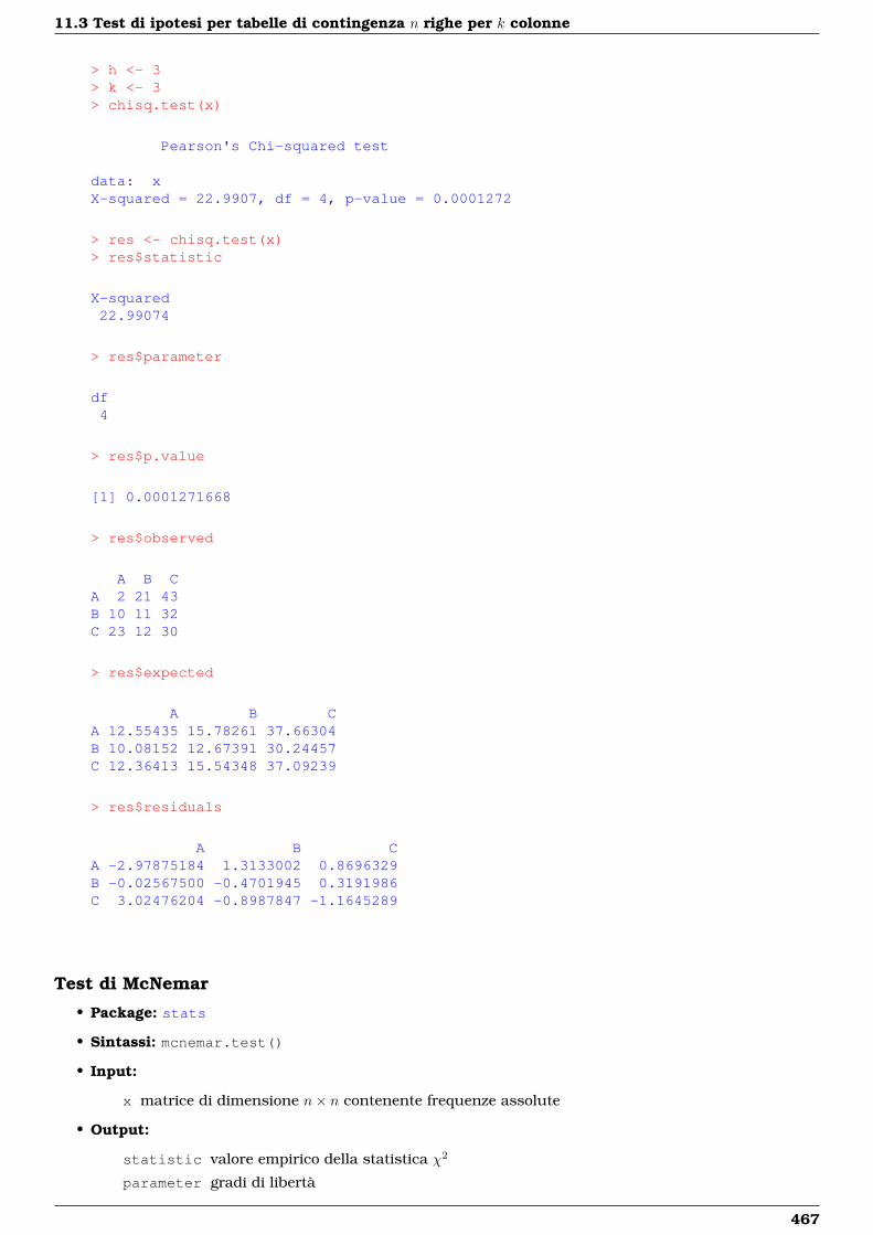
11.3 Test di ipotesi per tabelle di contingenza n righe per k colonne
> h <- 3> k <- 3> chisq.test(x)
Pearson's Chi-squared test
data: xX-squared = 22.9907, df = 4, p-value = 0.0001272
> res <- chisq.test(x)> res$statistic
X-squared22.99074
> res$parameter
df4
> res$p.value
[1] 0.0001271668
> res$observed
A B CA 2 21 43B 10 11 32C 23 12 30
> res$expected
A B CA 12.55435 15.78261 37.66304B 10.08152 12.67391 30.24457C 12.36413 15.54348 37.09239
> res$residuals
A B CA -2.97875184 1.3133002 0.8696329B -0.02567500 -0.4701945 0.3191986C 3.02476204 -0.8987847 -1.1645289
Test di McNemar
• Package: stats
• Sintassi: mcnemar.test()
• Input:
x matrice di dimensione n× n contenente frequenze assolute
• Output:
statistic valore empirico della statistica χ2
parameter gradi di libertà
467
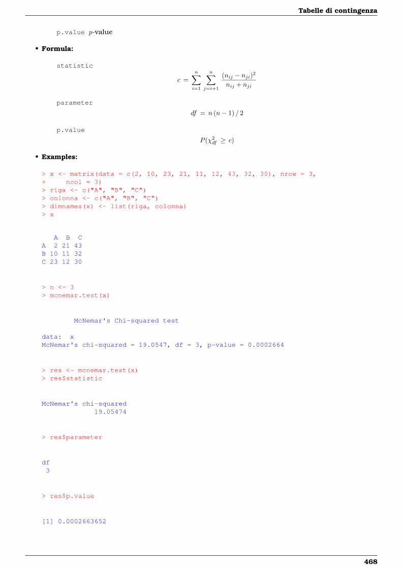
Tabelle di contingenza
p.value p-value
• Formula:
statistic
c =n∑i=1
n∑j=i+1
(nij − nji)2
nij + nji
parameter
df = n (n− 1) / 2
p.value
P (χ2df ≥ c)
• Examples:
> x <- matrix(data = c(2, 10, 23, 21, 11, 12, 43, 32, 30), nrow = 3,+ ncol = 3)> riga <- c("A", "B", "C")> colonna <- c("A", "B", "C")> dimnames(x) <- list(riga, colonna)> x
A B CA 2 21 43B 10 11 32C 23 12 30
> n <- 3> mcnemar.test(x)
McNemar's Chi-squared test
data: xMcNemar's chi-squared = 19.0547, df = 3, p-value = 0.0002664
> res <- mcnemar.test(x)> res$statistic
McNemar's chi-squared19.05474
> res$parameter
df3
> res$p.value
[1] 0.0002663652
468
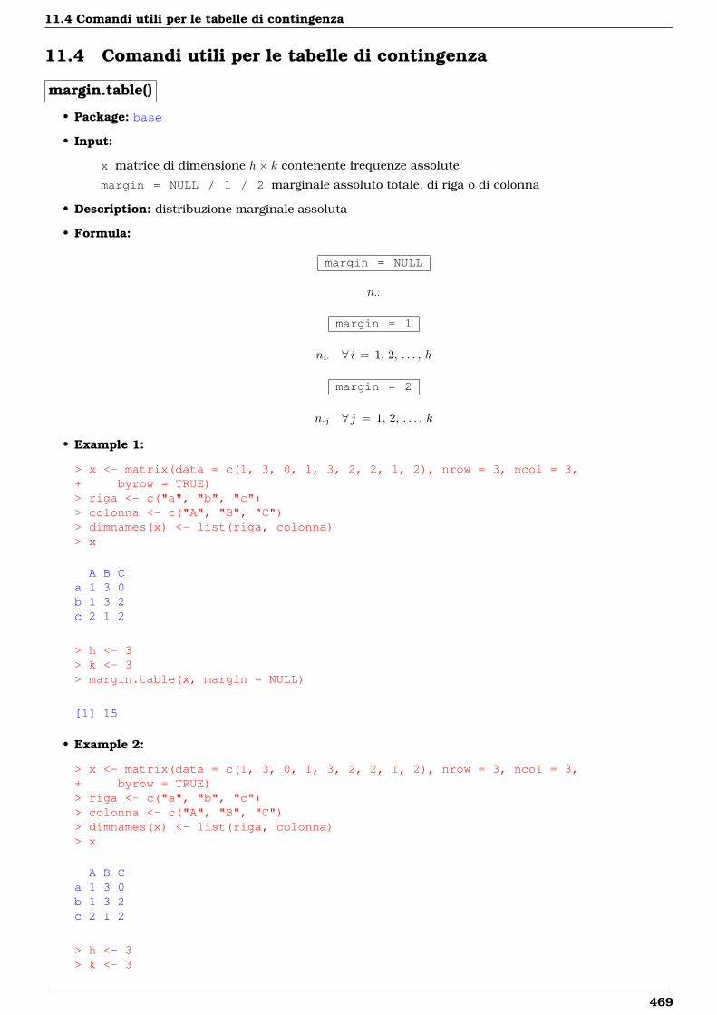
11.4 Comandi utili per le tabelle di contingenza
11.4 Comandi utili per le tabelle di contingenza
margin.table()
• Package: base
• Input:
x matrice di dimensione h× k contenente frequenze assolute
margin = NULL / 1 / 2 marginale assoluto totale, di riga o di colonna
• Description: distribuzione marginale assoluta
• Formula:
margin = NULL
n··
margin = 1
ni· ∀ i = 1, 2, . . . , h
margin = 2
n·j ∀ j = 1, 2, . . . , k
• Example 1:
> x <- matrix(data = c(1, 3, 0, 1, 3, 2, 2, 1, 2), nrow = 3, ncol = 3,+ byrow = TRUE)> riga <- c("a", "b", "c")> colonna <- c("A", "B", "C")> dimnames(x) <- list(riga, colonna)> x
A B Ca 1 3 0b 1 3 2c 2 1 2
> h <- 3> k <- 3> margin.table(x, margin = NULL)
[1] 15
• Example 2:
> x <- matrix(data = c(1, 3, 0, 1, 3, 2, 2, 1, 2), nrow = 3, ncol = 3,+ byrow = TRUE)> riga <- c("a", "b", "c")> colonna <- c("A", "B", "C")> dimnames(x) <- list(riga, colonna)> x
A B Ca 1 3 0b 1 3 2c 2 1 2
> h <- 3> k <- 3
469
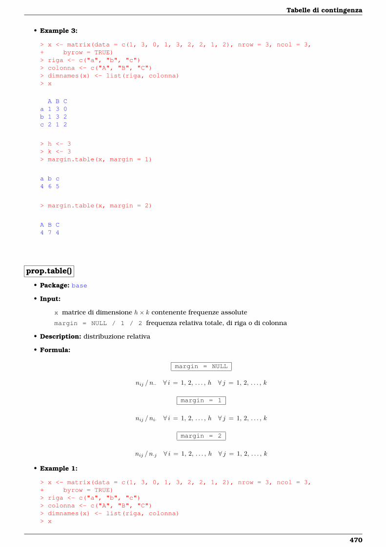
Tabelle di contingenza
• Example 3:
> x <- matrix(data = c(1, 3, 0, 1, 3, 2, 2, 1, 2), nrow = 3, ncol = 3,+ byrow = TRUE)> riga <- c("a", "b", "c")> colonna <- c("A", "B", "C")> dimnames(x) <- list(riga, colonna)> x
A B Ca 1 3 0b 1 3 2c 2 1 2
> h <- 3> k <- 3> margin.table(x, margin = 1)
a b c4 6 5
> margin.table(x, margin = 2)
A B C4 7 4
prop.table()
• Package: base
• Input:
x matrice di dimensione h× k contenente frequenze assolute
margin = NULL / 1 / 2 frequenza relativa totale, di riga o di colonna
• Description: distribuzione relativa
• Formula:
margin = NULL
nij / n·· ∀ i = 1, 2, . . . , h ∀ j = 1, 2, . . . , k
margin = 1
nij / ni· ∀ i = 1, 2, . . . , h ∀ j = 1, 2, . . . , k
margin = 2
nij / n·j ∀ i = 1, 2, . . . , h ∀ j = 1, 2, . . . , k
• Example 1:
> x <- matrix(data = c(1, 3, 0, 1, 3, 2, 2, 1, 2), nrow = 3, ncol = 3,+ byrow = TRUE)> riga <- c("a", "b", "c")> colonna <- c("A", "B", "C")> dimnames(x) <- list(riga, colonna)> x
470
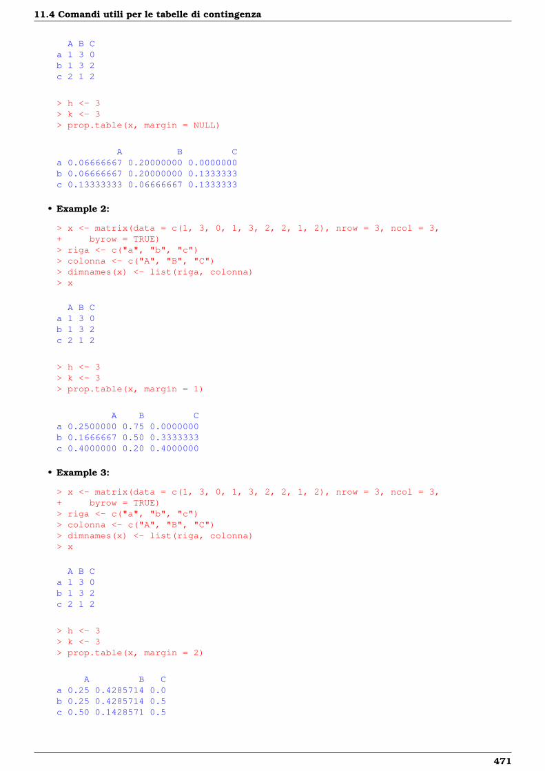
11.4 Comandi utili per le tabelle di contingenza
A B Ca 1 3 0b 1 3 2c 2 1 2
> h <- 3> k <- 3> prop.table(x, margin = NULL)
A B Ca 0.06666667 0.20000000 0.0000000b 0.06666667 0.20000000 0.1333333c 0.13333333 0.06666667 0.1333333
• Example 2:
> x <- matrix(data = c(1, 3, 0, 1, 3, 2, 2, 1, 2), nrow = 3, ncol = 3,+ byrow = TRUE)> riga <- c("a", "b", "c")> colonna <- c("A", "B", "C")> dimnames(x) <- list(riga, colonna)> x
A B Ca 1 3 0b 1 3 2c 2 1 2
> h <- 3> k <- 3> prop.table(x, margin = 1)
A B Ca 0.2500000 0.75 0.0000000b 0.1666667 0.50 0.3333333c 0.4000000 0.20 0.4000000
• Example 3:
> x <- matrix(data = c(1, 3, 0, 1, 3, 2, 2, 1, 2), nrow = 3, ncol = 3,+ byrow = TRUE)> riga <- c("a", "b", "c")> colonna <- c("A", "B", "C")> dimnames(x) <- list(riga, colonna)> x
A B Ca 1 3 0b 1 3 2c 2 1 2
> h <- 3> k <- 3> prop.table(x, margin = 2)
A B Ca 0.25 0.4285714 0.0b 0.25 0.4285714 0.5c 0.50 0.1428571 0.5
471

Tabelle di contingenza
xtabs()
• Package: stats
• Input:
y vettore numerico di dimensione n
f fattore a k livelli
g fattore a h livelli
• Description: costruzione di una tabella di contingenza a partire da un dataframe
• Examples:
> y <- c(1.2, 2.1, 1.1, 2.3, 5.4, 4.3, 3.1, 2.3, 4.3, 5.4, 5.5,+ 5.7)> f <- factor(rep(letters[1:2], each = 6))> f
[1] a a a a a a b b b b b bLevels: a b
> g <- factor(rep(LETTERS[2:1], times = 6))> g
[1] B A B A B A B A B A B ALevels: A B
> data.frame(f, g, y)
f g y1 a B 1.22 a A 2.13 a B 1.14 a A 2.35 a B 5.46 a A 4.37 b B 3.18 b A 2.39 b B 4.310 b A 5.411 b B 5.512 b A 5.7
> xtabs(y ~ f + g)
gf A B
a 8.7 7.7b 13.4 12.9
ftable()
• Package: stats
• Input:
x oggetto di tipo table contenente frequenze assolute
row.vars variabili di riga
col.vars variabili di colonna
• Description: costruzione di flat tables
472
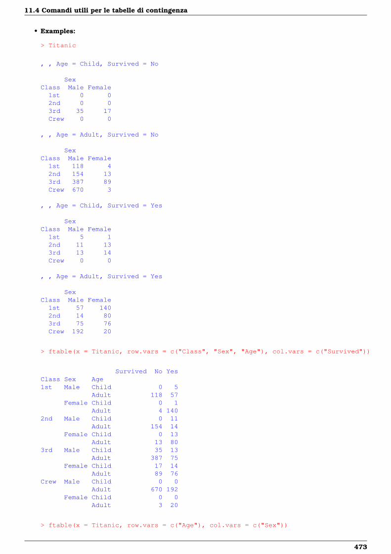
11.4 Comandi utili per le tabelle di contingenza
• Examples:
> Titanic
, , Age = Child, Survived = No
SexClass Male Female1st 0 02nd 0 03rd 35 17Crew 0 0
, , Age = Adult, Survived = No
SexClass Male Female1st 118 42nd 154 133rd 387 89Crew 670 3
, , Age = Child, Survived = Yes
SexClass Male Female1st 5 12nd 11 133rd 13 14Crew 0 0
, , Age = Adult, Survived = Yes
SexClass Male Female1st 57 1402nd 14 803rd 75 76Crew 192 20
> ftable(x = Titanic, row.vars = c("Class", "Sex", "Age"), col.vars = c("Survived"))
Survived No YesClass Sex Age1st Male Child 0 5
Adult 118 57Female Child 0 1
Adult 4 1402nd Male Child 0 11
Adult 154 14Female Child 0 13
Adult 13 803rd Male Child 35 13
Adult 387 75Female Child 17 14
Adult 89 76Crew Male Child 0 0
Adult 670 192Female Child 0 0
Adult 3 20
> ftable(x = Titanic, row.vars = c("Age"), col.vars = c("Sex"))
473
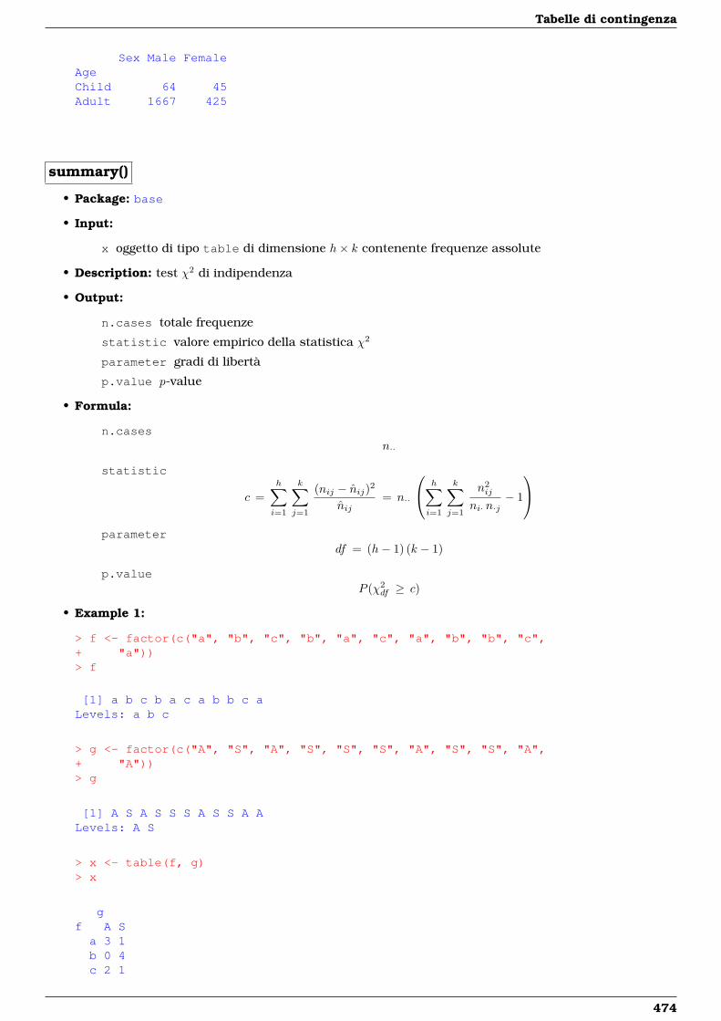
Tabelle di contingenza
Sex Male FemaleAgeChild 64 45Adult 1667 425
summary()
• Package: base
• Input:
x oggetto di tipo table di dimensione h× k contenente frequenze assolute
• Description: test χ2 di indipendenza
• Output:
n.cases totale frequenze
statistic valore empirico della statistica χ2
parameter gradi di libertà
p.value p-value
• Formula:
n.casesn··
statistic
c =h∑i=1
k∑j=1
(nij − nij)2
nij= n··
h∑i=1
k∑j=1
n2ij
ni· n·j− 1
parameter
df = (h− 1) (k − 1)
p.valueP (χ2
df ≥ c)
• Example 1:
> f <- factor(c("a", "b", "c", "b", "a", "c", "a", "b", "b", "c",+ "a"))> f
[1] a b c b a c a b b c aLevels: a b c
> g <- factor(c("A", "S", "A", "S", "S", "S", "A", "S", "S", "A",+ "A"))> g
[1] A S A S S S A S S A ALevels: A S
> x <- table(f, g)> x
gf A S
a 3 1b 0 4c 2 1
474
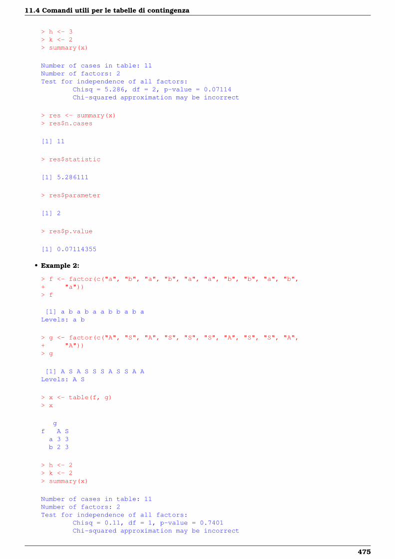
11.4 Comandi utili per le tabelle di contingenza
> h <- 3> k <- 2> summary(x)
Number of cases in table: 11Number of factors: 2Test for independence of all factors:
Chisq = 5.286, df = 2, p-value = 0.07114Chi-squared approximation may be incorrect
> res <- summary(x)> res$n.cases
[1] 11
> res$statistic
[1] 5.286111
> res$parameter
[1] 2
> res$p.value
[1] 0.07114355
• Example 2:
> f <- factor(c("a", "b", "a", "b", "a", "a", "b", "b", "a", "b",+ "a"))> f
[1] a b a b a a b b a b aLevels: a b
> g <- factor(c("A", "S", "A", "S", "S", "S", "A", "S", "S", "A",+ "A"))> g
[1] A S A S S S A S S A ALevels: A S
> x <- table(f, g)> x
gf A S
a 3 3b 2 3
> h <- 2> k <- 2> summary(x)
Number of cases in table: 11Number of factors: 2Test for independence of all factors:
Chisq = 0.11, df = 1, p-value = 0.7401Chi-squared approximation may be incorrect
475

Tabelle di contingenza
> res <- summary(x)> res$n.cases
[1] 11
> res$statistic
[1] 0.11
> res$parameter
[1] 1
> res$p.value
[1] 0.7401441
476
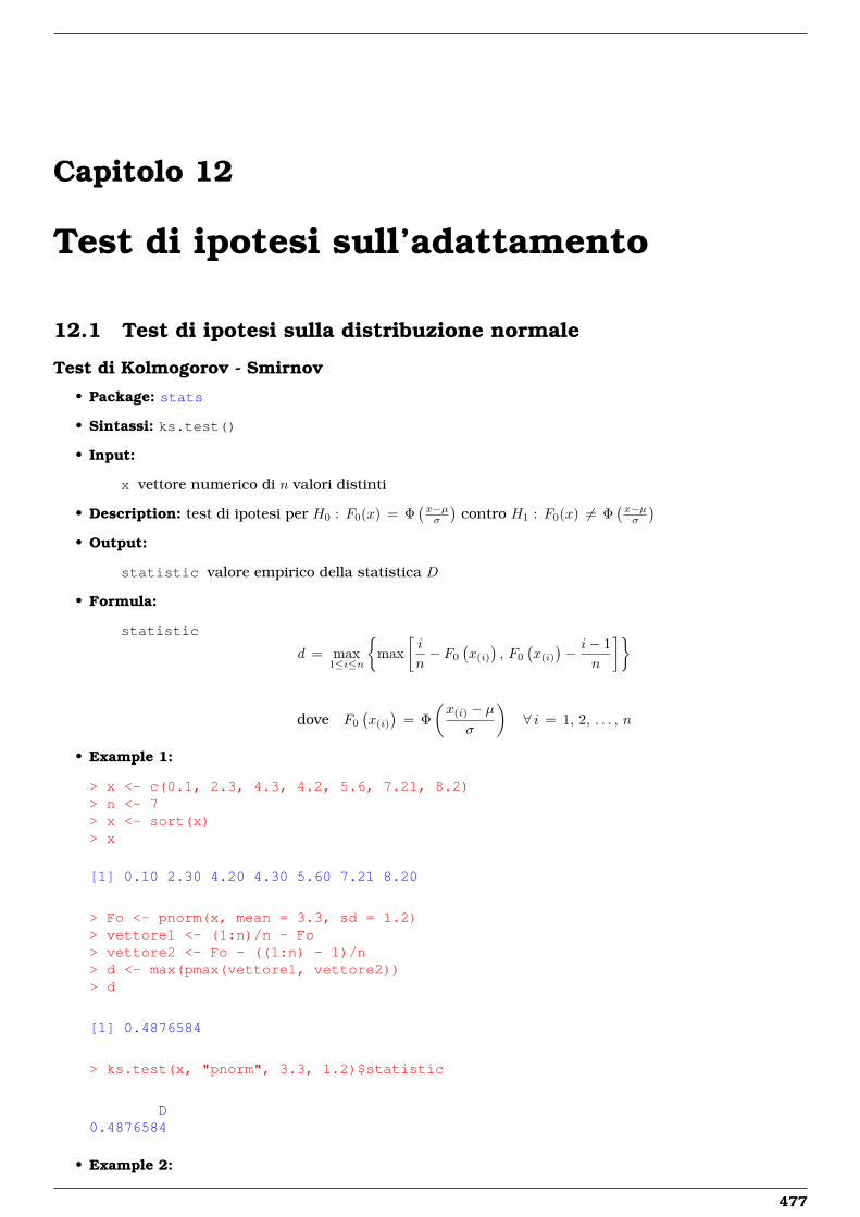
Capitolo 12
Test di ipotesi sull’adattamento
12.1 Test di ipotesi sulla distribuzione normale
Test di Kolmogorov - Smirnov
• Package: stats
• Sintassi: ks.test()
• Input:
x vettore numerico di n valori distinti
• Description: test di ipotesi per H0 : F0(x) = Φ(x−µσ
)contro H1 : F0(x) 6= Φ
(x−µσ
)• Output:
statistic valore empirico della statistica D
• Formula:
statistic
d = max1≤i≤n
{max
[i
n− F0
(x(i)
), F0
(x(i)
)− i− 1
n
]}
dove F0
(x(i)
)= Φ
(x(i) − µ
σ
)∀ i = 1, 2, . . . , n
• Example 1:
> x <- c(0.1, 2.3, 4.3, 4.2, 5.6, 7.21, 8.2)> n <- 7> x <- sort(x)> x
[1] 0.10 2.30 4.20 4.30 5.60 7.21 8.20
> Fo <- pnorm(x, mean = 3.3, sd = 1.2)> vettore1 <- (1:n)/n - Fo> vettore2 <- Fo - ((1:n) - 1)/n> d <- max(pmax(vettore1, vettore2))> d
[1] 0.4876584
> ks.test(x, "pnorm", 3.3, 1.2)$statistic
D0.4876584
• Example 2:
477
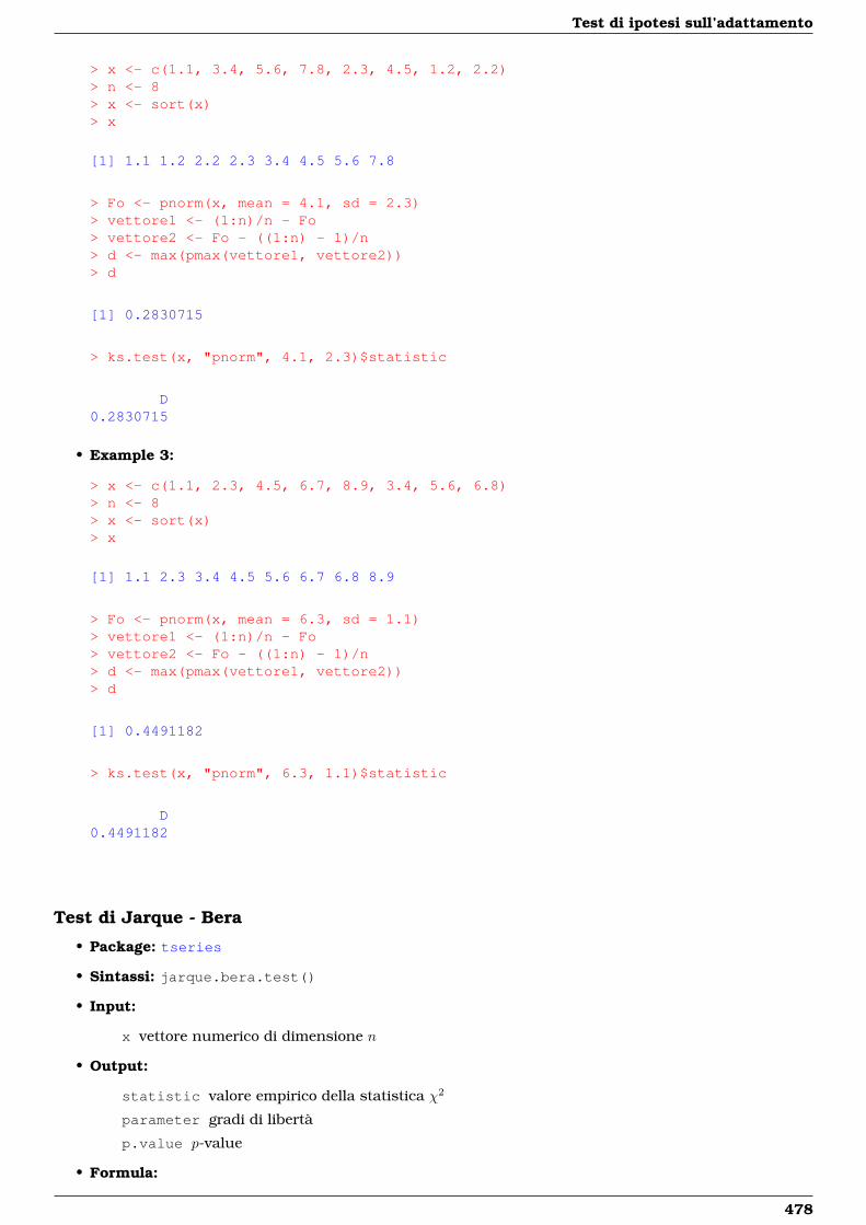
Test di ipotesi sull’adattamento
> x <- c(1.1, 3.4, 5.6, 7.8, 2.3, 4.5, 1.2, 2.2)> n <- 8> x <- sort(x)> x
[1] 1.1 1.2 2.2 2.3 3.4 4.5 5.6 7.8
> Fo <- pnorm(x, mean = 4.1, sd = 2.3)> vettore1 <- (1:n)/n - Fo> vettore2 <- Fo - ((1:n) - 1)/n> d <- max(pmax(vettore1, vettore2))> d
[1] 0.2830715
> ks.test(x, "pnorm", 4.1, 2.3)$statistic
D0.2830715
• Example 3:
> x <- c(1.1, 2.3, 4.5, 6.7, 8.9, 3.4, 5.6, 6.8)> n <- 8> x <- sort(x)> x
[1] 1.1 2.3 3.4 4.5 5.6 6.7 6.8 8.9
> Fo <- pnorm(x, mean = 6.3, sd = 1.1)> vettore1 <- (1:n)/n - Fo> vettore2 <- Fo - ((1:n) - 1)/n> d <- max(pmax(vettore1, vettore2))> d
[1] 0.4491182
> ks.test(x, "pnorm", 6.3, 1.1)$statistic
D0.4491182
Test di Jarque - Bera
• Package: tseries
• Sintassi: jarque.bera.test()
• Input:
x vettore numerico di dimensione n
• Output:
statistic valore empirico della statistica χ2
parameter gradi di libertà
p.value p-value
• Formula:
478
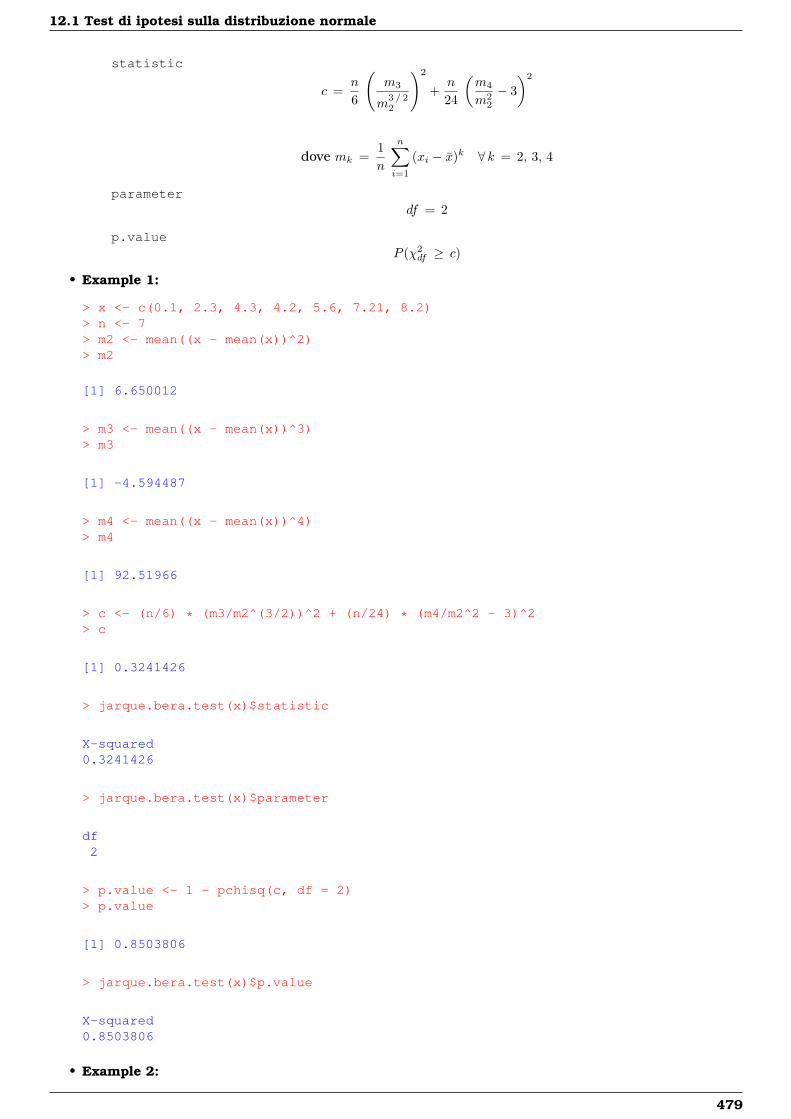
12.1 Test di ipotesi sulla distribuzione normale
statistic
c =n
6
(m3
m3 / 22
)2
+n
24
(m4
m22
− 3)2
dove mk =1n
n∑i=1
(xi − x)k ∀ k = 2, 3, 4
parameterdf = 2
p.valueP (χ2
df ≥ c)
• Example 1:
> x <- c(0.1, 2.3, 4.3, 4.2, 5.6, 7.21, 8.2)> n <- 7> m2 <- mean((x - mean(x))^2)> m2
[1] 6.650012
> m3 <- mean((x - mean(x))^3)> m3
[1] -4.594487
> m4 <- mean((x - mean(x))^4)> m4
[1] 92.51966
> c <- (n/6) * (m3/m2^(3/2))^2 + (n/24) * (m4/m2^2 - 3)^2> c
[1] 0.3241426
> jarque.bera.test(x)$statistic
X-squared0.3241426
> jarque.bera.test(x)$parameter
df2
> p.value <- 1 - pchisq(c, df = 2)> p.value
[1] 0.8503806
> jarque.bera.test(x)$p.value
X-squared0.8503806
• Example 2:
479
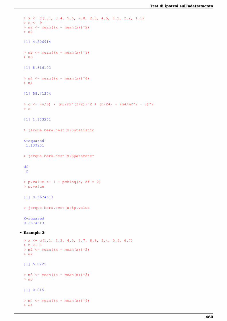
Test di ipotesi sull’adattamento
> x <- c(1.1, 3.4, 5.6, 7.8, 2.3, 4.5, 1.2, 2.2, 1.1)> n <- 9> m2 <- mean((x - mean(x))^2)> m2
[1] 4.806914
> m3 <- mean((x - mean(x))^3)> m3
[1] 8.816102
> m4 <- mean((x - mean(x))^4)> m4
[1] 58.41274
> c <- (n/6) * (m3/m2^(3/2))^2 + (n/24) * (m4/m2^2 - 3)^2> c
[1] 1.133201
> jarque.bera.test(x)$statistic
X-squared1.133201
> jarque.bera.test(x)$parameter
df2
> p.value <- 1 - pchisq(c, df = 2)> p.value
[1] 0.5674513
> jarque.bera.test(x)$p.value
X-squared0.5674513
• Example 3:
> x <- c(1.1, 2.3, 4.5, 6.7, 8.9, 3.4, 5.6, 6.7)> n <- 8> m2 <- mean((x - mean(x))^2)> m2
[1] 5.8225
> m3 <- mean((x - mean(x))^3)> m3
[1] 0.015
> m4 <- mean((x - mean(x))^4)> m4
480

12.1 Test di ipotesi sulla distribuzione normale
[1] 67.06683
> c <- (n/6) * (m3/m2^(3/2))^2 + (n/24) * (m4/m2^2 - 3)^2> c
[1] 0.347969
> jarque.bera.test(x)$statistic
X-squared0.347969
> jarque.bera.test(x)$parameter
df2
> p.value <- 1 - pchisq(c, df = 2)> p.value
[1] 0.8403099
> jarque.bera.test(x)$p.value
X-squared0.8403099
Test di Cramer - von Mises
• Package: nortest
• Sintassi: cvm.test()
• Input:
x vettore numerico di dimensione n ≥ 7
• Output:
statistic valore empirico della statistica Z
p.value p-value
• Formula:
statistic
W =1
12n+
n∑i=1
[Φ(x(i) − xsx
)− 2 i − 1
2n
]2
p.value
WW = (1 + 0.5 / n)W
WW < 0.0275 ≥ 0.0275 AND < 0.051
p.value 1− e−13.953+775.5WW−12542.61WW 21− e−5.903+179.546WW−1515.29WW 2
WW ≥ 0.051 AND < 0.092 ≥ 0.092
p.value e0.886−31.62WW+10.897WW 2e1.111−34.242WW+12.832WW 2
481
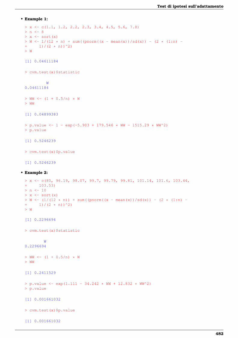
Test di ipotesi sull’adattamento
• Example 1:
> x <- c(1.1, 1.2, 2.2, 2.3, 3.4, 4.5, 5.6, 7.8)> n <- 8> x <- sort(x)> W <- 1/(12 * n) + sum((pnorm((x - mean(x))/sd(x)) - (2 * (1:n) -+ 1)/(2 * n))^2)> W
[1] 0.04611184
> cvm.test(x)$statistic
W0.04611184
> WW <- (1 + 0.5/n) * W> WW
[1] 0.04899383
> p.value <- 1 - exp(-5.903 + 179.546 * WW - 1515.29 * WW^2)> p.value
[1] 0.5246239
> cvm.test(x)$p.value
[1] 0.5246239
• Example 2:
> x <- c(80, 96.19, 98.07, 99.7, 99.79, 99.81, 101.14, 101.6, 103.44,+ 103.53)> n <- 10> x <- sort(x)> W <- (1/(12 * n)) + sum((pnorm((x - mean(x))/sd(x)) - (2 * (1:n) -+ 1)/(2 * n))^2)> W
[1] 0.2296694
> cvm.test(x)$statistic
W0.2296694
> WW <- (1 + 0.5/n) * W> WW
[1] 0.2411529
> p.value <- exp(1.111 - 34.242 * WW + 12.832 * WW^2)> p.value
[1] 0.001661032
> cvm.test(x)$p.value
[1] 0.001661032
482
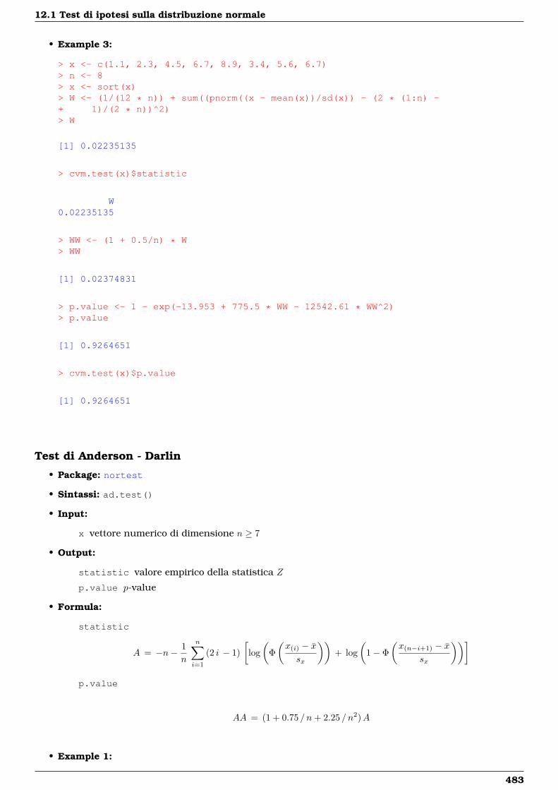
12.1 Test di ipotesi sulla distribuzione normale
• Example 3:
> x <- c(1.1, 2.3, 4.5, 6.7, 8.9, 3.4, 5.6, 6.7)> n <- 8> x <- sort(x)> W <- (1/(12 * n)) + sum((pnorm((x - mean(x))/sd(x)) - (2 * (1:n) -+ 1)/(2 * n))^2)> W
[1] 0.02235135
> cvm.test(x)$statistic
W0.02235135
> WW <- (1 + 0.5/n) * W> WW
[1] 0.02374831
> p.value <- 1 - exp(-13.953 + 775.5 * WW - 12542.61 * WW^2)> p.value
[1] 0.9264651
> cvm.test(x)$p.value
[1] 0.9264651
Test di Anderson - Darlin
• Package: nortest
• Sintassi: ad.test()
• Input:
x vettore numerico di dimensione n ≥ 7
• Output:
statistic valore empirico della statistica Z
p.value p-value
• Formula:
statistic
A = −n− 1n
n∑i=1
(2 i − 1)[log(
Φ(x(i) − xsx
))+ log
(1− Φ
(x(n−i+1) − x
sx
))]
p.value
AA = (1 + 0.75 / n+ 2.25 / n2)A
• Example 1:
483
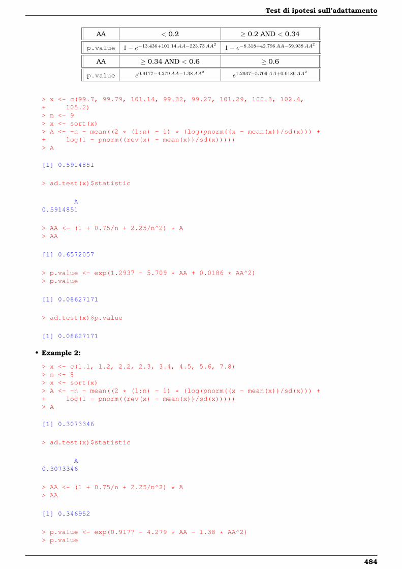
Test di ipotesi sull’adattamento
AA < 0.2 ≥ 0.2 AND < 0.34
p.value 1− e−13.436+101.14AA−223.73AA21− e−8.318+42.796AA−59.938AA2
AA ≥ 0.34 AND < 0.6 ≥ 0.6
p.value e0.9177−4.279AA−1.38AA2e1.2937−5.709AA+0.0186AA2
> x <- c(99.7, 99.79, 101.14, 99.32, 99.27, 101.29, 100.3, 102.4,+ 105.2)> n <- 9> x <- sort(x)> A <- -n - mean((2 * (1:n) - 1) * (log(pnorm((x - mean(x))/sd(x))) ++ log(1 - pnorm((rev(x) - mean(x))/sd(x)))))> A
[1] 0.5914851
> ad.test(x)$statistic
A0.5914851
> AA <- (1 + 0.75/n + 2.25/n^2) * A> AA
[1] 0.6572057
> p.value <- exp(1.2937 - 5.709 * AA + 0.0186 * AA^2)> p.value
[1] 0.08627171
> ad.test(x)$p.value
[1] 0.08627171
• Example 2:
> x <- c(1.1, 1.2, 2.2, 2.3, 3.4, 4.5, 5.6, 7.8)> n <- 8> x <- sort(x)> A <- -n - mean((2 * (1:n) - 1) * (log(pnorm((x - mean(x))/sd(x))) ++ log(1 - pnorm((rev(x) - mean(x))/sd(x)))))> A
[1] 0.3073346
> ad.test(x)$statistic
A0.3073346
> AA <- (1 + 0.75/n + 2.25/n^2) * A> AA
[1] 0.346952
> p.value <- exp(0.9177 - 4.279 * AA - 1.38 * AA^2)> p.value
484
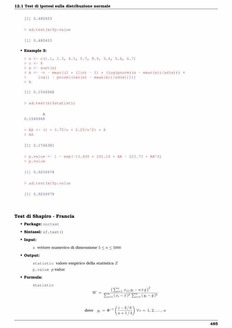
12.1 Test di ipotesi sulla distribuzione normale
[1] 0.480453
> ad.test(x)$p.value
[1] 0.480453
• Example 3:
> x <- c(1.1, 2.3, 4.5, 6.7, 8.9, 3.4, 5.6, 6.7)> n <- 8> x <- sort(x)> A <- -n - mean((2 * (1:n) - 1) * (log(pnorm((x - mean(x))/sd(x))) ++ log(1 - pnorm((rev(x) - mean(x))/sd(x)))))> A
[1] 0.1546968
> ad.test(x)$statistic
A0.1546968
> AA <- (1 + 0.75/n + 2.25/n^2) * A> AA
[1] 0.1746381
> p.value <- 1 - exp(-13.436 + 101.14 * AA - 223.73 * AA^2)> p.value
[1] 0.9254678
> ad.test(x)$p.value
[1] 0.9254678
Test di Shapiro - Francia
• Package: nortest
• Sintassi: sf.test()
• Input:
x vettore numerico di dimensione 5 ≤ n ≤ 5000
• Output:
statistic valore empirico della statistica Z
p.value p-value
• Formula:
statistic
W =
(∑ni=1 x(i) yi − n x y
)2∑ni=1 (xi − x )2
∑ni=1 ( yi − y )2
dove yi = Φ−1
(i− 3 / 8n+ 1 / 4
)∀ i = 1, 2, . . . , n
485
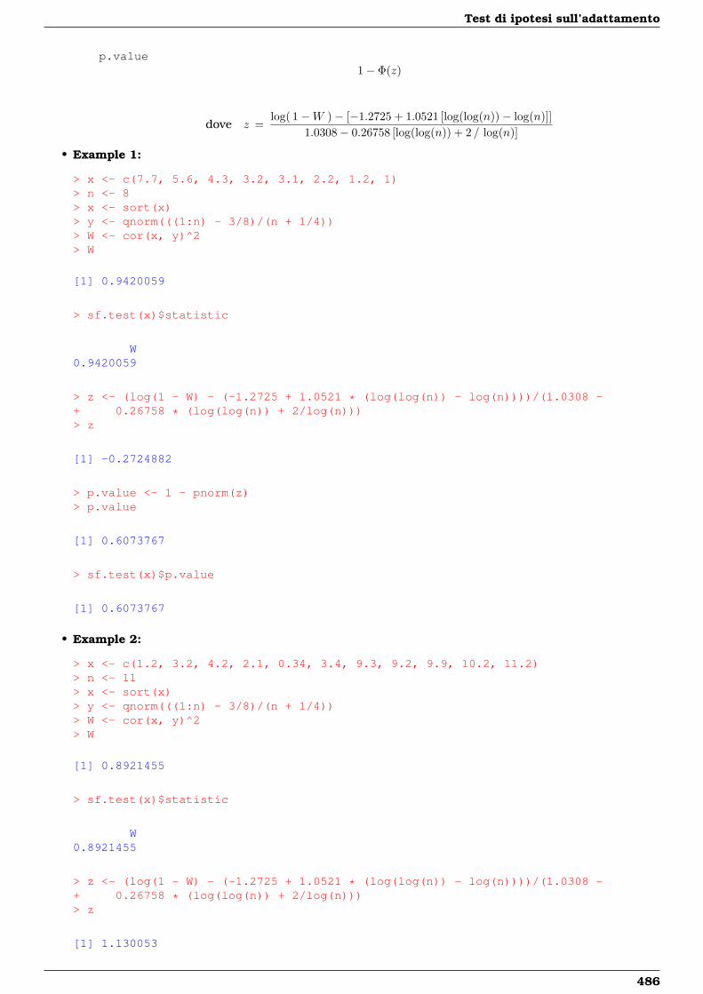
Test di ipotesi sull’adattamento
p.value1− Φ(z)
dove z =log( 1−W )− [−1.2725 + 1.0521 [log(log(n))− log(n)]]
1.0308− 0.26758 [log(log(n)) + 2 / log(n)]
• Example 1:
> x <- c(7.7, 5.6, 4.3, 3.2, 3.1, 2.2, 1.2, 1)> n <- 8> x <- sort(x)> y <- qnorm(((1:n) - 3/8)/(n + 1/4))> W <- cor(x, y)^2> W
[1] 0.9420059
> sf.test(x)$statistic
W0.9420059
> z <- (log(1 - W) - (-1.2725 + 1.0521 * (log(log(n)) - log(n))))/(1.0308 -+ 0.26758 * (log(log(n)) + 2/log(n)))> z
[1] -0.2724882
> p.value <- 1 - pnorm(z)> p.value
[1] 0.6073767
> sf.test(x)$p.value
[1] 0.6073767
• Example 2:
> x <- c(1.2, 3.2, 4.2, 2.1, 0.34, 3.4, 9.3, 9.2, 9.9, 10.2, 11.2)> n <- 11> x <- sort(x)> y <- qnorm(((1:n) - 3/8)/(n + 1/4))> W <- cor(x, y)^2> W
[1] 0.8921455
> sf.test(x)$statistic
W0.8921455
> z <- (log(1 - W) - (-1.2725 + 1.0521 * (log(log(n)) - log(n))))/(1.0308 -+ 0.26758 * (log(log(n)) + 2/log(n)))> z
[1] 1.130053
486
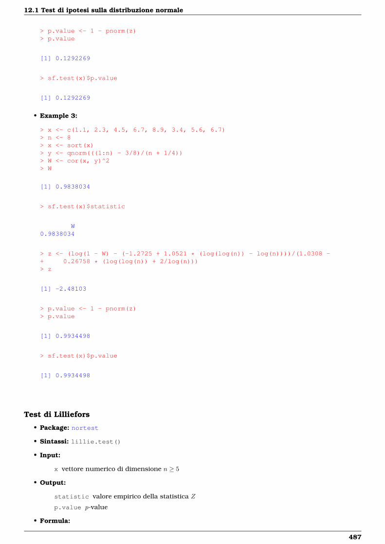
12.1 Test di ipotesi sulla distribuzione normale
> p.value <- 1 - pnorm(z)> p.value
[1] 0.1292269
> sf.test(x)$p.value
[1] 0.1292269
• Example 3:
> x <- c(1.1, 2.3, 4.5, 6.7, 8.9, 3.4, 5.6, 6.7)> n <- 8> x <- sort(x)> y <- qnorm(((1:n) - 3/8)/(n + 1/4))> W <- cor(x, y)^2> W
[1] 0.9838034
> sf.test(x)$statistic
W0.9838034
> z <- (log(1 - W) - (-1.2725 + 1.0521 * (log(log(n)) - log(n))))/(1.0308 -+ 0.26758 * (log(log(n)) + 2/log(n)))> z
[1] -2.48103
> p.value <- 1 - pnorm(z)> p.value
[1] 0.9934498
> sf.test(x)$p.value
[1] 0.9934498
Test di Lilliefors
• Package: nortest
• Sintassi: lillie.test()
• Input:
x vettore numerico di dimensione n ≥ 5
• Output:
statistic valore empirico della statistica Z
p.value p-value
• Formula:
487
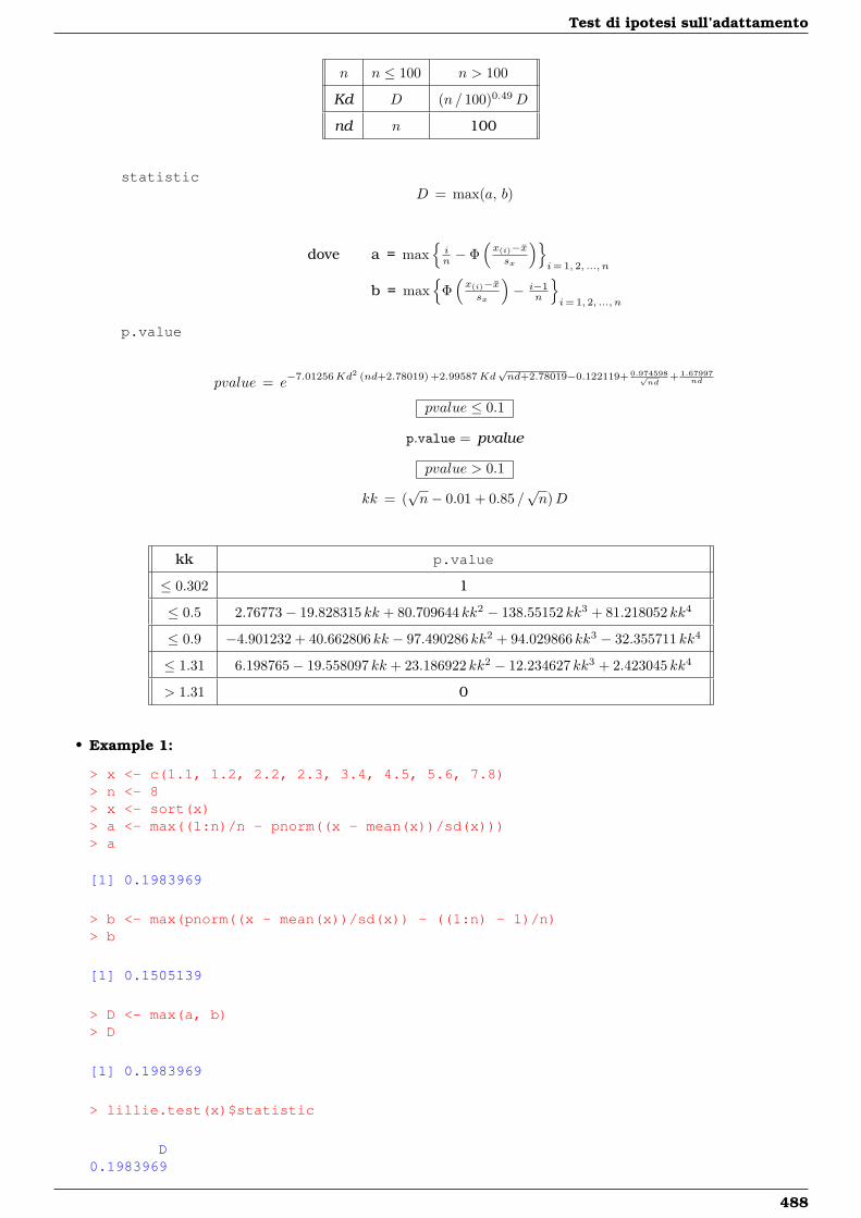
Test di ipotesi sull’adattamento
n n ≤ 100 n > 100
Kd D (n / 100)0.49D
nd n 100
statisticD = max(a, b)
dove a = max{in − Φ
(x(i)−xsx
)}i= 1, 2, ..., n
b = max{
Φ(x(i)−xsx
)− i−1
n
}i= 1, 2, ..., n
p.value
pvalue = e−7.01256Kd2 (nd+2.78019) +2.99587Kd
√nd+2.78019−0.122119+ 0.974598√
nd+ 1.67997
nd
pvalue ≤ 0.1
p.value = pvalue
pvalue > 0.1
kk = (√n− 0.01 + 0.85 /
√n)D
kk p.value
≤ 0.302 1
≤ 0.5 2.76773− 19.828315 kk + 80.709644 kk2 − 138.55152 kk3 + 81.218052 kk4
≤ 0.9 −4.901232 + 40.662806 kk − 97.490286 kk2 + 94.029866 kk3 − 32.355711 kk4
≤ 1.31 6.198765− 19.558097 kk + 23.186922 kk2 − 12.234627 kk3 + 2.423045 kk4
> 1.31 0
• Example 1:
> x <- c(1.1, 1.2, 2.2, 2.3, 3.4, 4.5, 5.6, 7.8)> n <- 8> x <- sort(x)> a <- max((1:n)/n - pnorm((x - mean(x))/sd(x)))> a
[1] 0.1983969
> b <- max(pnorm((x - mean(x))/sd(x)) - ((1:n) - 1)/n)> b
[1] 0.1505139
> D <- max(a, b)> D
[1] 0.1983969
> lillie.test(x)$statistic
D0.1983969
488
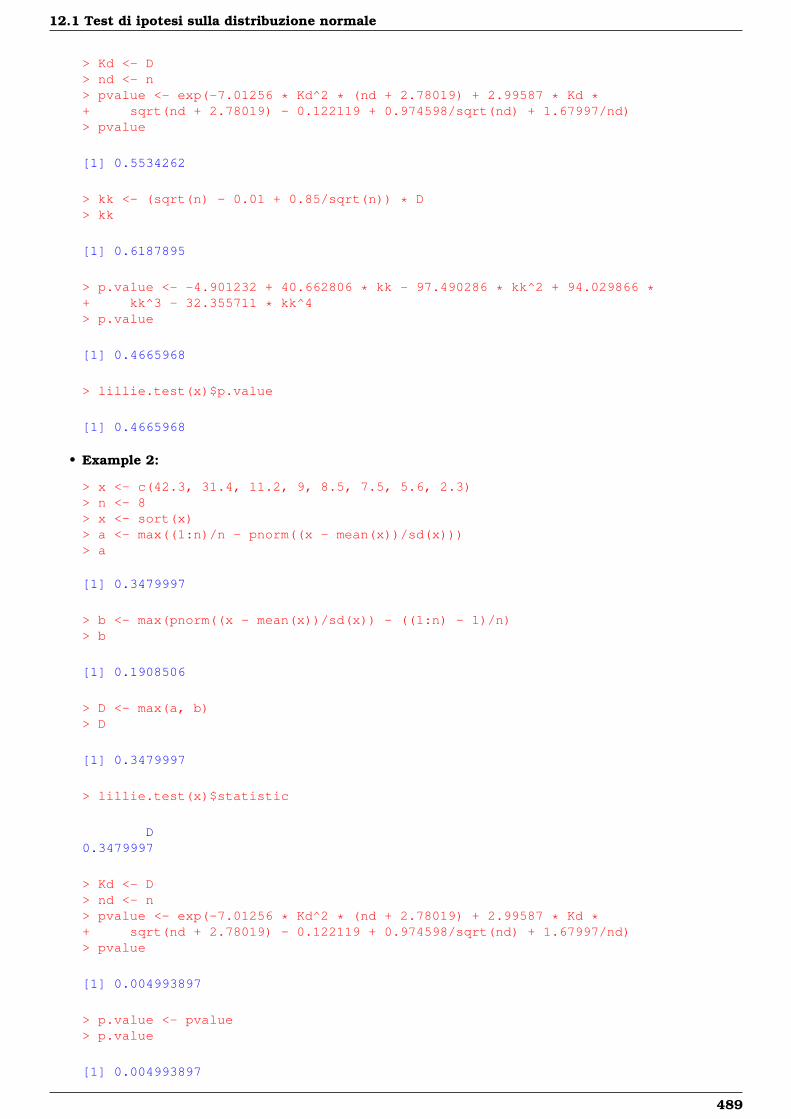
12.1 Test di ipotesi sulla distribuzione normale
> Kd <- D> nd <- n> pvalue <- exp(-7.01256 * Kd^2 * (nd + 2.78019) + 2.99587 * Kd *+ sqrt(nd + 2.78019) - 0.122119 + 0.974598/sqrt(nd) + 1.67997/nd)> pvalue
[1] 0.5534262
> kk <- (sqrt(n) - 0.01 + 0.85/sqrt(n)) * D> kk
[1] 0.6187895
> p.value <- -4.901232 + 40.662806 * kk - 97.490286 * kk^2 + 94.029866 *+ kk^3 - 32.355711 * kk^4> p.value
[1] 0.4665968
> lillie.test(x)$p.value
[1] 0.4665968
• Example 2:
> x <- c(42.3, 31.4, 11.2, 9, 8.5, 7.5, 5.6, 2.3)> n <- 8> x <- sort(x)> a <- max((1:n)/n - pnorm((x - mean(x))/sd(x)))> a
[1] 0.3479997
> b <- max(pnorm((x - mean(x))/sd(x)) - ((1:n) - 1)/n)> b
[1] 0.1908506
> D <- max(a, b)> D
[1] 0.3479997
> lillie.test(x)$statistic
D0.3479997
> Kd <- D> nd <- n> pvalue <- exp(-7.01256 * Kd^2 * (nd + 2.78019) + 2.99587 * Kd *+ sqrt(nd + 2.78019) - 0.122119 + 0.974598/sqrt(nd) + 1.67997/nd)> pvalue
[1] 0.004993897
> p.value <- pvalue> p.value
[1] 0.004993897
489
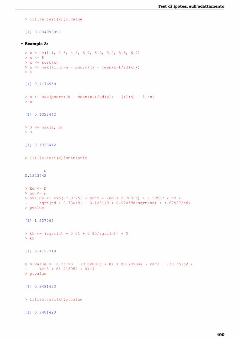
Test di ipotesi sull’adattamento
> lillie.test(x)$p.value
[1] 0.004993897
• Example 3:
> x <- c(1.1, 2.3, 4.5, 6.7, 8.9, 3.4, 5.6, 6.7)> n <- 8> x <- sort(x)> a <- max((1:n)/n - pnorm((x - mean(x))/sd(x)))> a
[1] 0.1176558
> b <- max(pnorm((x - mean(x))/sd(x)) - ((1:n) - 1)/n)> b
[1] 0.1323442
> D <- max(a, b)> D
[1] 0.1323442
> lillie.test(x)$statistic
D0.1323442
> Kd <- D> nd <- n> pvalue <- exp(-7.01256 * Kd^2 * (nd + 2.78019) + 2.99587 * Kd *+ sqrt(nd + 2.78019) - 0.122119 + 0.974598/sqrt(nd) + 1.67997/nd)> pvalue
[1] 1.507065
> kk <- (sqrt(n) - 0.01 + 0.85/sqrt(n)) * D> kk
[1] 0.4127748
> p.value <- 2.76773 - 19.828315 * kk + 80.709644 * kk^2 - 138.55152 *+ kk^3 + 81.218052 * kk^4> p.value
[1] 0.9481423
> lillie.test(x)$p.value
[1] 0.9481423
490
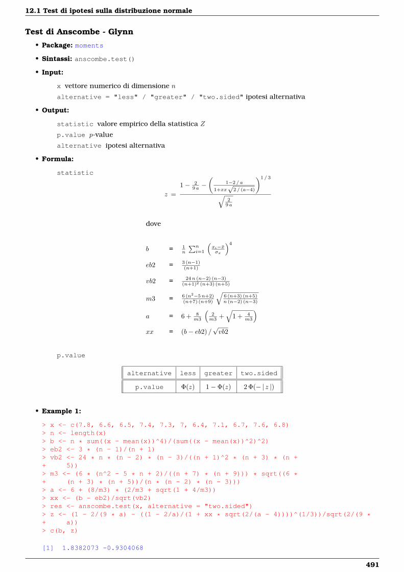
12.1 Test di ipotesi sulla distribuzione normale
Test di Anscombe - Glynn
• Package: moments
• Sintassi: anscombe.test()
• Input:
x vettore numerico di dimensione n
alternative = "less" / "greater" / "two.sided" ipotesi alternativa
• Output:
statistic valore empirico della statistica Z
p.value p-value
alternative ipotesi alternativa
• Formula:
statistic
z =1− 2
9 a −(
1−2 / a
1+xx√
2 / (a−4)
)1 / 3
√2
9 a
dove
b = 1n
∑ni=1
(xi−xσx
)4
eb2 = 3 (n−1)(n+1)
vb2 = 24n (n−2) (n−3)(n+1)2 (n+3) (n+5)
m3 = 6 (n2−5n+2)(n+7) (n+9)
√6 (n+3) (n+5)n (n−2) (n−3)
a = 6 + 8m3
(2m3 +
√1 + 4
m3
)xx = (b− eb2) /
√vb2
p.value
alternative less greater two.sided
p.value Φ(z) 1− Φ(z) 2 Φ(− | z |)
• Example 1:
> x <- c(7.8, 6.6, 6.5, 7.4, 7.3, 7, 6.4, 7.1, 6.7, 7.6, 6.8)> n <- length(x)> b <- n * sum((x - mean(x))^4)/(sum((x - mean(x))^2)^2)> eb2 <- 3 * (n - 1)/(n + 1)> vb2 <- 24 * n * (n - 2) * (n - 3)/((n + 1)^2 * (n + 3) * (n ++ 5))> m3 <- (6 * (n^2 - 5 * n + 2)/((n + 7) * (n + 9))) * sqrt((6 *+ (n + 3) * (n + 5))/(n * (n - 2) * (n - 3)))> a <- 6 + (8/m3) * (2/m3 + sqrt(1 + 4/m3))> xx <- (b - eb2)/sqrt(vb2)> res <- anscombe.test(x, alternative = "two.sided")> z <- (1 - 2/(9 * a) - ((1 - 2/a)/(1 + xx * sqrt(2/(a - 4))))^(1/3))/sqrt(2/(9 *+ a))> c(b, z)
[1] 1.8382073 -0.9304068
491
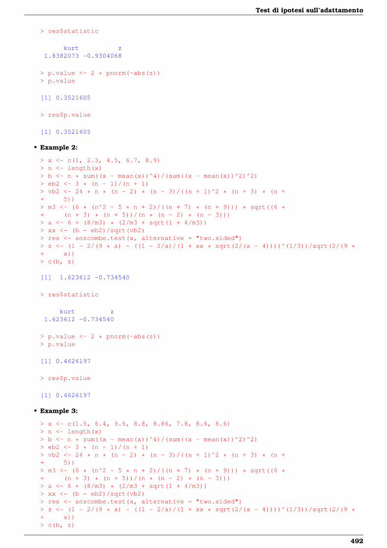
Test di ipotesi sull’adattamento
> res$statistic
kurt z1.8382073 -0.9304068
> p.value <- 2 * pnorm(-abs(z))> p.value
[1] 0.3521605
> res$p.value
[1] 0.3521605
• Example 2:
> x <- c(1, 2.3, 4.5, 6.7, 8.9)> n <- length(x)> b <- n * sum((x - mean(x))^4)/(sum((x - mean(x))^2)^2)> eb2 <- 3 * (n - 1)/(n + 1)> vb2 <- 24 * n * (n - 2) * (n - 3)/((n + 1)^2 * (n + 3) * (n ++ 5))> m3 <- (6 * (n^2 - 5 * n + 2)/((n + 7) * (n + 9))) * sqrt((6 *+ (n + 3) * (n + 5))/(n * (n - 2) * (n - 3)))> a <- 6 + (8/m3) * (2/m3 + sqrt(1 + 4/m3))> xx <- (b - eb2)/sqrt(vb2)> res <- anscombe.test(x, alternative = "two.sided")> z <- (1 - 2/(9 * a) - ((1 - 2/a)/(1 + xx * sqrt(2/(a - 4))))^(1/3))/sqrt(2/(9 *+ a))> c(b, z)
[1] 1.623612 -0.734540
> res$statistic
kurt z1.623612 -0.734540
> p.value <- 2 * pnorm(-abs(z))> p.value
[1] 0.4626197
> res$p.value
[1] 0.4626197
• Example 3:
> x <- c(1.5, 6.4, 9.6, 8.8, 8.86, 7.8, 8.6, 8.6)> n <- length(x)> b <- n * sum((x - mean(x))^4)/(sum((x - mean(x))^2)^2)> eb2 <- 3 * (n - 1)/(n + 1)> vb2 <- 24 * n * (n - 2) * (n - 3)/((n + 1)^2 * (n + 3) * (n ++ 5))> m3 <- (6 * (n^2 - 5 * n + 2)/((n + 7) * (n + 9))) * sqrt((6 *+ (n + 3) * (n + 5))/(n * (n - 2) * (n - 3)))> a <- 6 + (8/m3) * (2/m3 + sqrt(1 + 4/m3))> xx <- (b - eb2)/sqrt(vb2)> res <- anscombe.test(x, alternative = "two.sided")> z <- (1 - 2/(9 * a) - ((1 - 2/a)/(1 + xx * sqrt(2/(a - 4))))^(1/3))/sqrt(2/(9 *+ a))> c(b, z)
492
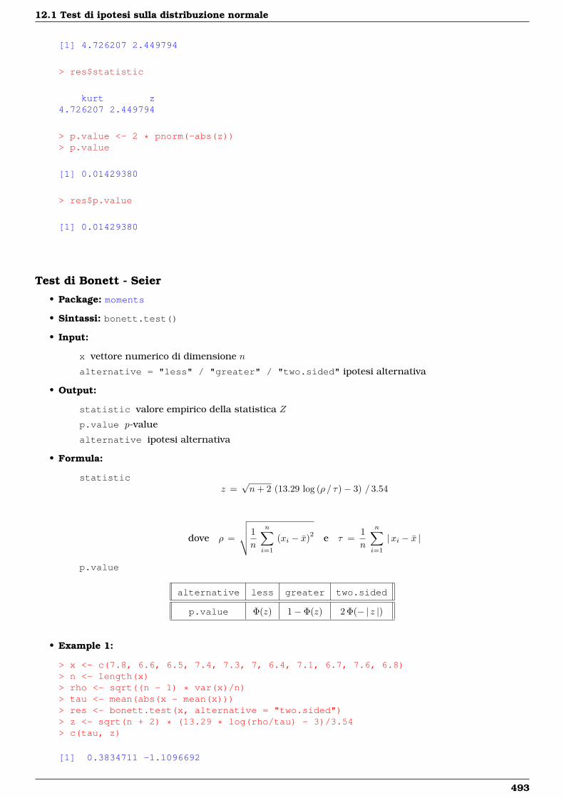
12.1 Test di ipotesi sulla distribuzione normale
[1] 4.726207 2.449794
> res$statistic
kurt z4.726207 2.449794
> p.value <- 2 * pnorm(-abs(z))> p.value
[1] 0.01429380
> res$p.value
[1] 0.01429380
Test di Bonett - Seier
• Package: moments
• Sintassi: bonett.test()
• Input:
x vettore numerico di dimensione n
alternative = "less" / "greater" / "two.sided" ipotesi alternativa
• Output:
statistic valore empirico della statistica Z
p.value p-value
alternative ipotesi alternativa
• Formula:
statisticz =
√n+ 2 (13.29 log (ρ / τ)− 3) / 3.54
dove ρ =
√√√√ 1n
n∑i=1
(xi − x)2 e τ =1n
n∑i=1
|xi − x |
p.value
alternative less greater two.sided
p.value Φ(z) 1− Φ(z) 2 Φ(− | z |)
• Example 1:
> x <- c(7.8, 6.6, 6.5, 7.4, 7.3, 7, 6.4, 7.1, 6.7, 7.6, 6.8)> n <- length(x)> rho <- sqrt((n - 1) * var(x)/n)> tau <- mean(abs(x - mean(x)))> res <- bonett.test(x, alternative = "two.sided")> z <- sqrt(n + 2) * (13.29 * log(rho/tau) - 3)/3.54> c(tau, z)
[1] 0.3834711 -1.1096692
493
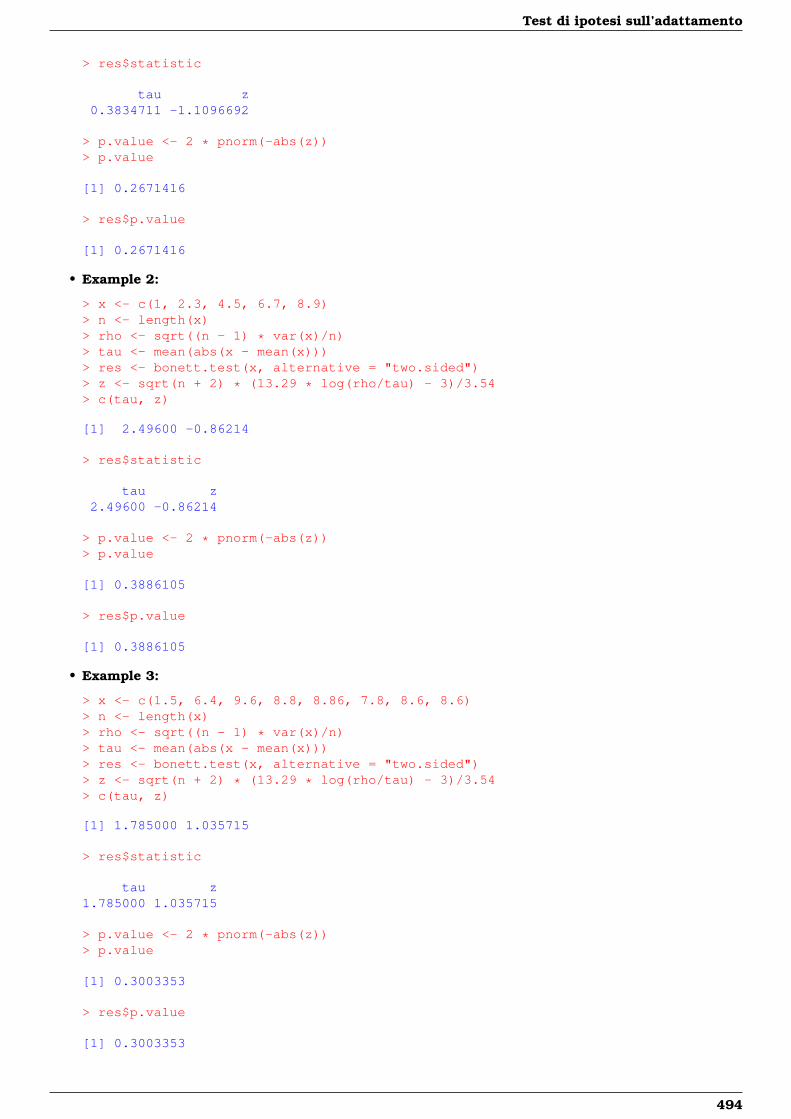
Test di ipotesi sull’adattamento
> res$statistic
tau z0.3834711 -1.1096692
> p.value <- 2 * pnorm(-abs(z))> p.value
[1] 0.2671416
> res$p.value
[1] 0.2671416
• Example 2:
> x <- c(1, 2.3, 4.5, 6.7, 8.9)> n <- length(x)> rho <- sqrt((n - 1) * var(x)/n)> tau <- mean(abs(x - mean(x)))> res <- bonett.test(x, alternative = "two.sided")> z <- sqrt(n + 2) * (13.29 * log(rho/tau) - 3)/3.54> c(tau, z)
[1] 2.49600 -0.86214
> res$statistic
tau z2.49600 -0.86214
> p.value <- 2 * pnorm(-abs(z))> p.value
[1] 0.3886105
> res$p.value
[1] 0.3886105
• Example 3:
> x <- c(1.5, 6.4, 9.6, 8.8, 8.86, 7.8, 8.6, 8.6)> n <- length(x)> rho <- sqrt((n - 1) * var(x)/n)> tau <- mean(abs(x - mean(x)))> res <- bonett.test(x, alternative = "two.sided")> z <- sqrt(n + 2) * (13.29 * log(rho/tau) - 3)/3.54> c(tau, z)
[1] 1.785000 1.035715
> res$statistic
tau z1.785000 1.035715
> p.value <- 2 * pnorm(-abs(z))> p.value
[1] 0.3003353
> res$p.value
[1] 0.3003353
494
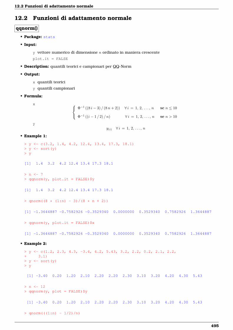
12.2 Funzioni di adattamento normale
12.2 Funzioni di adattamento normale
qqnorm()
• Package: stats
• Input:
y vettore numerico di dimensione n ordinato in maniera crescente
plot.it = FALSE
• Description: quantili teorici e campionari per QQ-Norm
• Output:
x quantili teorici
y quantili campionari
• Formula:
x Φ−1 ((8 i− 3) / (8n+ 2)) ∀ i = 1, 2, . . . , n se n ≤ 10
Φ−1 ((i− 1 / 2) / n) ∀ i = 1, 2, . . . , n se n > 10
yy(i) ∀ i = 1, 2, . . . , n
• Example 1:
> y <- c(3.2, 1.4, 4.2, 12.4, 13.4, 17.3, 18.1)> y <- sort(y)> y
[1] 1.4 3.2 4.2 12.4 13.4 17.3 18.1
> n <- 7> qqnorm(y, plot.it = FALSE)$y
[1] 1.4 3.2 4.2 12.4 13.4 17.3 18.1
> qnorm((8 * (1:n) - 3)/(8 * n + 2))
[1] -1.3644887 -0.7582926 -0.3529340 0.0000000 0.3529340 0.7582926 1.3644887
> qqnorm(y, plot.it = FALSE)$x
[1] -1.3644887 -0.7582926 -0.3529340 0.0000000 0.3529340 0.7582926 1.3644887
• Example 2:
> y <- c(1.2, 2.3, 4.3, -3.4, 4.2, 5.43, 3.2, 2.2, 0.2, 2.1, 2.2,+ 3.1)> y <- sort(y)> y
[1] -3.40 0.20 1.20 2.10 2.20 2.20 2.30 3.10 3.20 4.20 4.30 5.43
> n <- 12> qqnorm(y, plot = FALSE)$y
[1] -3.40 0.20 1.20 2.10 2.20 2.20 2.30 3.10 3.20 4.20 4.30 5.43
> qnorm(((1:n) - 1/2)/n)
495
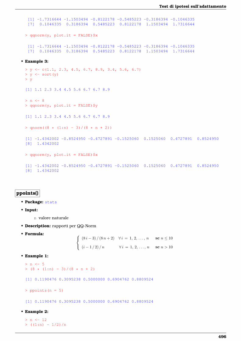
Test di ipotesi sull’adattamento
[1] -1.7316644 -1.1503494 -0.8122178 -0.5485223 -0.3186394 -0.1046335[7] 0.1046335 0.3186394 0.5485223 0.8122178 1.1503494 1.7316644
> qqnorm(y, plot.it = FALSE)$x
[1] -1.7316644 -1.1503494 -0.8122178 -0.5485223 -0.3186394 -0.1046335[7] 0.1046335 0.3186394 0.5485223 0.8122178 1.1503494 1.7316644
• Example 3:
> y <- c(1.1, 2.3, 4.5, 6.7, 8.9, 3.4, 5.6, 6.7)> y <- sort(y)> y
[1] 1.1 2.3 3.4 4.5 5.6 6.7 6.7 8.9
> n <- 8> qqnorm(y, plot.it = FALSE)$y
[1] 1.1 2.3 3.4 4.5 5.6 6.7 6.7 8.9
> qnorm((8 * (1:n) - 3)/(8 * n + 2))
[1] -1.4342002 -0.8524950 -0.4727891 -0.1525060 0.1525060 0.4727891 0.8524950[8] 1.4342002
> qqnorm(y, plot.it = FALSE)$x
[1] -1.4342002 -0.8524950 -0.4727891 -0.1525060 0.1525060 0.4727891 0.8524950[8] 1.4342002
ppoints()
• Package: stats
• Input:
n valore naturale
• Description: rapporti per QQ-Norm
• Formula: (8 i− 3) / (8n+ 2) ∀ i = 1, 2, . . . , n se n ≤ 10
(i− 1 / 2) / n ∀ i = 1, 2, . . . , n se n > 10
• Example 1:
> n <- 5> (8 * (1:n) - 3)/(8 * n + 2)
[1] 0.1190476 0.3095238 0.5000000 0.6904762 0.8809524
> ppoints(n = 5)
[1] 0.1190476 0.3095238 0.5000000 0.6904762 0.8809524
• Example 2:
> n <- 12> ((1:n) - 1/2)/n
496
12.3 Test di ipotesi su una distribuzione generica
[1] 0.04166667 0.12500000 0.20833333 0.29166667 0.37500000 0.45833333[7] 0.54166667 0.62500000 0.70833333 0.79166667 0.87500000 0.95833333
> ppoints(n = 12)
[1] 0.04166667 0.12500000 0.20833333 0.29166667 0.37500000 0.45833333[7] 0.54166667 0.62500000 0.70833333 0.79166667 0.87500000 0.95833333
• Example 3:
> n <- 15> ((1:n) - 1/2)/n
[1] 0.03333333 0.10000000 0.16666667 0.23333333 0.30000000 0.36666667[7] 0.43333333 0.50000000 0.56666667 0.63333333 0.70000000 0.76666667
[13] 0.83333333 0.90000000 0.96666667
> ppoints(n = 15)
[1] 0.03333333 0.10000000 0.16666667 0.23333333 0.30000000 0.36666667[7] 0.43333333 0.50000000 0.56666667 0.63333333 0.70000000 0.76666667
[13] 0.83333333 0.90000000 0.96666667
12.3 Test di ipotesi su una distribuzione generica
Test Chi - Quadrato GOF
• Package: stats
• Sintassi: chisq.test()
• Input:
x vettore di frequenze assolute a somma n di dimensione k
p vettore p di probabilità a somma unitaria di dimensione k
• Output:
statistic valore empirico della statistica χ2
parameter gradi di libertà
p.value p-value
observed valori osservati
expected valori attesi
residuals residui di Pearson
• Formula:
statistic
c =k∑i=1
(ni − ni)2
ni=
k∑i=1
n2i
ni− n
dove ni = n pi ∀ i = 1, 2, . . . , k
parameterdf = k − 1
p.valueP (χ2
df ≥ c)
observedni ∀ i = 1, 2, . . . , k
497
Test di ipotesi sull’adattamento
expectedni = n pi ∀ i = 1, 2, . . . , k
residualsni − ni√
ni∀ i = 1, 2, . . . , k
• Examples:
> x <- c(100, 110, 80, 55, 14)> n <- sum(x)> n
[1] 359
> prob <- c(0.29, 0.21, 0.17, 0.17, 0.16)> k <- 5> osservati <- x> attesi <- n * prob> c <- sum((osservati - attesi)^2/attesi)> c
[1] 55.3955
> chisq.test(x, p = prob)$statistic
X-squared55.3955
> parameter <- k - 1> parameter
[1] 4
> chisq.test(x, p = prob)$parameter
df4
> p.value <- 1 - pchisq(c, df = parameter)> p.value
[1] 2.684530e-11
> chisq.test(x, p = prob)$p.value
[1] 2.684534e-11
> osservati
[1] 100 110 80 55 14
> chisq.test(x, p = prob)$observed
[1] 100 110 80 55 14
> attesi
[1] 104.11 75.39 61.03 61.03 57.44
498
12.3 Test di ipotesi su una distribuzione generica
> chisq.test(x, p = prob)$expected
[1] 104.11 75.39 61.03 61.03 57.44
> residui <- (osservati - attesi)/sqrt(attesi)> residui
[1] -0.4028057 3.9860682 2.4282626 -0.7718726 -5.7316888
> chisq.test(x, p = prob)$residuals
[1] -0.4028057 3.9860682 2.4282626 -0.7718726 -5.7316888
• Example 2:
> x <- c(89, 37, 30, 28, 2)> n <- sum(x)> n
[1] 186
> prob <- c(0.4, 0.2, 0.2, 0.15, 0.05)> k <- 5> osservati <- x> attesi <- n * prob> c <- sum((osservati - attesi)^2/attesi)> c
[1] 9.990143
> chisq.test(x, p = prob)$statistic
X-squared9.990143
> parameter <- k - 1> parameter
[1] 4
> chisq.test(x, p = prob)$parameter
df4
> p.value <- 1 - pchisq(c, df = parameter)> p.value
[1] 0.04059404
> chisq.test(x, p = prob)$p.value
[1] 0.04059404
> osservati
[1] 89 37 30 28 2
> chisq.test(x, p = prob)$observed
499
Test di ipotesi sull’adattamento
[1] 89 37 30 28 2
> attesi
[1] 74.4 37.2 37.2 27.9 9.3
> chisq.test(x, p = prob)$expected
[1] 74.4 37.2 37.2 27.9 9.3
> residui <- (osservati - attesi)/sqrt(attesi)> residui
[1] 1.69264697 -0.03279129 -1.18048650 0.01893206 -2.39376430
> chisq.test(x, p = prob)$residuals
[1] 1.69264697 -0.03279129 -1.18048650 0.01893206 -2.39376430
• Example 3:
> x <- c(54, 29, 5)> n <- sum(x)> n
[1] 88
> prob <- c(0.5, 0.25, 0.25)> k <- 3> osservati <- x> attesi <- n * prob> c <- sum((osservati - attesi)^2/attesi)> c
[1] 17.63636
> chisq.test(x, p = prob)$statistic
X-squared17.63636
> parameter <- k - 1> parameter
[1] 2
> chisq.test(x, p = prob)$parameter
df2
> p.value <- 1 - pchisq(c, df = parameter)> p.value
[1] 0.0001480172
> chisq.test(x, p = prob)$p.value
[1] 0.0001480172
500
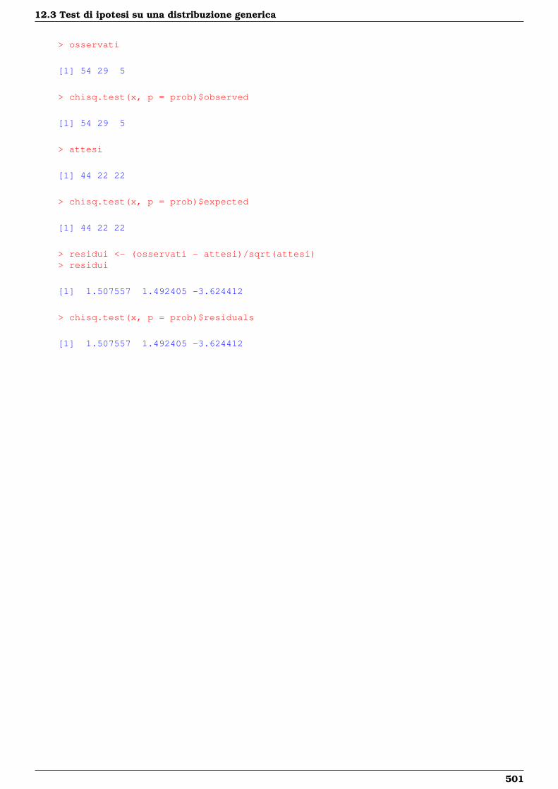
12.3 Test di ipotesi su una distribuzione generica
> osservati
[1] 54 29 5
> chisq.test(x, p = prob)$observed
[1] 54 29 5
> attesi
[1] 44 22 22
> chisq.test(x, p = prob)$expected
[1] 44 22 22
> residui <- (osservati - attesi)/sqrt(attesi)> residui
[1] 1.507557 1.492405 -3.624412
> chisq.test(x, p = prob)$residuals
[1] 1.507557 1.492405 -3.624412
501


Parte IV
Modelli Lineari
503

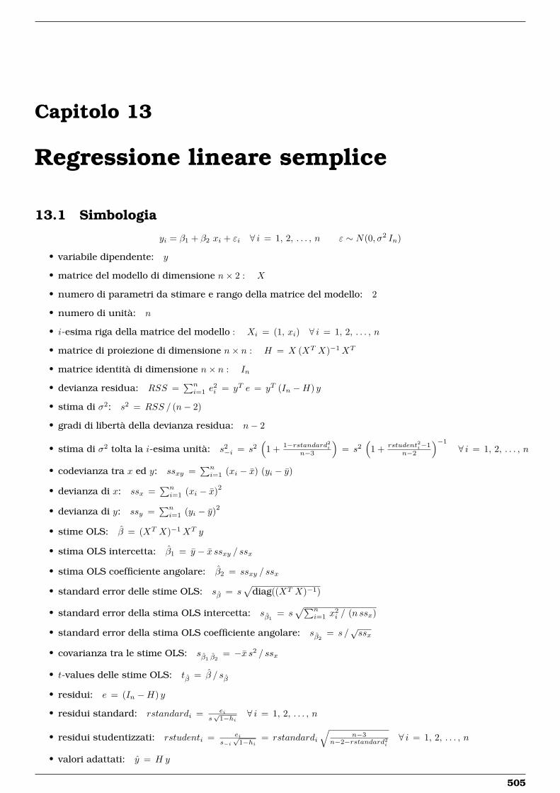
Capitolo 13
Regressione lineare semplice
13.1 Simbologia
yi = β1 + β2 xi + εi ∀ i = 1, 2, . . . , n ε ∼ N(0, σ2 In)
• variabile dipendente: y
• matrice del modello di dimensione n× 2 : X
• numero di parametri da stimare e rango della matrice del modello: 2
• numero di unità: n
• i-esima riga della matrice del modello : Xi = (1, xi) ∀ i = 1, 2, . . . , n
• matrice di proiezione di dimensione n× n : H = X (XT X)−1XT
• matrice identità di dimensione n× n : In
• devianza residua: RSS =∑ni=1 e
2i = yT e = yT (In −H) y
• stima di σ2: s2 = RSS / (n− 2)
• gradi di libertà della devianza residua: n− 2
• stima di σ2 tolta la i-esima unità: s2−i = s2
(1 + 1−rstandard2i
n−3
)= s2
(1 + rstudent2i−1
n−2
)−1
∀ i = 1, 2, . . . , n
• codevianza tra x ed y: ssxy =∑ni=1 (xi − x) (yi − y)
• devianza di x: ssx =∑ni=1 (xi − x)2
• devianza di y: ssy =∑ni=1 (yi − y)2
• stime OLS: β = (XT X)−1XT y
• stima OLS intercetta: β1 = y − x ssxy / ssx
• stima OLS coefficiente angolare: β2 = ssxy / ssx
• standard error delle stime OLS: sβ = s√
diag((XT X)−1)
• standard error della stima OLS intercetta: sβ1= s
√∑ni=1 x
2i / (n ssx)
• standard error della stima OLS coefficiente angolare: sβ2= s /
√ssx
• covarianza tra le stime OLS: sβ1 β2= −x s2 / ssx
• t-values delle stime OLS: tβ = β / sβ
• residui: e = (In −H) y
• residui standard: rstandardi = eis√
1−hi∀ i = 1, 2, . . . , n
• residui studentizzati: rstudenti = eis−i√
1−hi= rstandardi
√n−3
n−2−rstandard2i∀ i = 1, 2, . . . , n
• valori adattati: y = H y
505
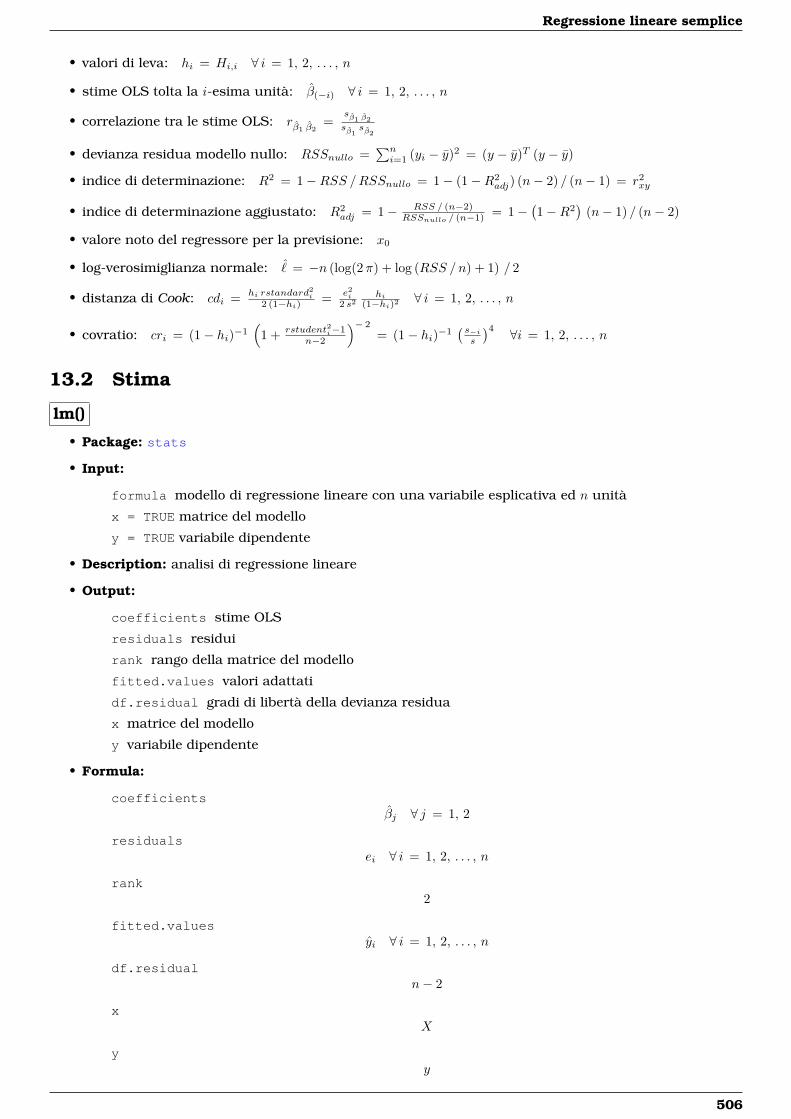
Regressione lineare semplice
• valori di leva: hi = Hi,i ∀ i = 1, 2, . . . , n
• stime OLS tolta la i-esima unità: β(−i) ∀ i = 1, 2, . . . , n
• correlazione tra le stime OLS: rβ1 β2=
sβ1 β2sβ1
sβ2
• devianza residua modello nullo: RSSnullo =∑ni=1 (yi − y)2 = (y − y)T (y − y)
• indice di determinazione: R2 = 1−RSS /RSSnullo = 1− (1−R2adj) (n− 2) / (n− 1) = r2
xy
• indice di determinazione aggiustato: R2adj = 1− RSS / (n−2)
RSSnullo / (n−1) = 1−(1−R2
)(n− 1) / (n− 2)
• valore noto del regressore per la previsione: x0
• log-verosimiglianza normale: ˆ = −n (log(2π) + log (RSS /n) + 1) / 2
• distanza di Cook: cdi = hi rstandard2i
2 (1−hi) = e2i2 s2
hi(1−hi)2 ∀ i = 1, 2, . . . , n
• covratio: cri = (1− hi)−1(
1 + rstudent2i−1n−2
)− 2
= (1− hi)−1( s−is
)4 ∀i = 1, 2, . . . , n
13.2 Stima
lm()
• Package: stats
• Input:
formula modello di regressione lineare con una variabile esplicativa ed n unità
x = TRUE matrice del modello
y = TRUE variabile dipendente
• Description: analisi di regressione lineare
• Output:
coefficients stime OLS
residuals residui
rank rango della matrice del modello
fitted.values valori adattati
df.residual gradi di libertà della devianza residua
x matrice del modello
y variabile dipendente
• Formula:
coefficientsβj ∀ j = 1, 2
residualsei ∀ i = 1, 2, . . . , n
rank2
fitted.valuesyi ∀ i = 1, 2, . . . , n
df.residualn− 2
xX
yy
506
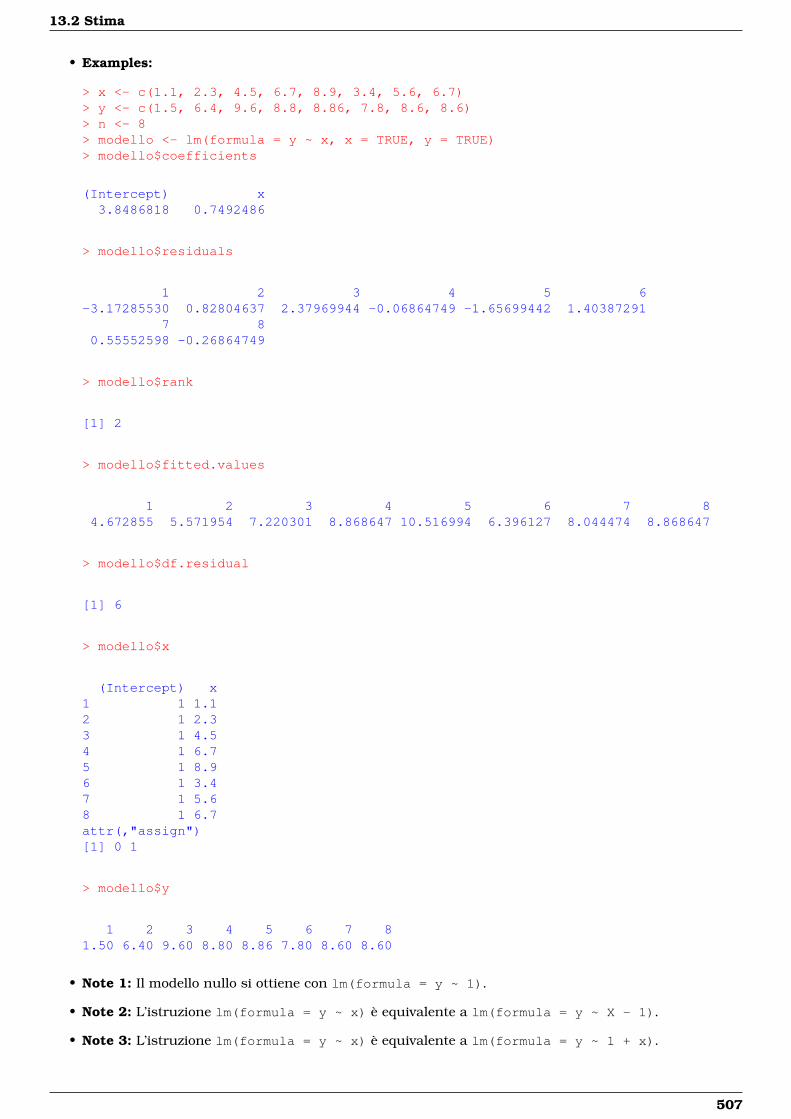
13.2 Stima
• Examples:
> x <- c(1.1, 2.3, 4.5, 6.7, 8.9, 3.4, 5.6, 6.7)> y <- c(1.5, 6.4, 9.6, 8.8, 8.86, 7.8, 8.6, 8.6)> n <- 8> modello <- lm(formula = y ~ x, x = TRUE, y = TRUE)> modello$coefficients
(Intercept) x3.8486818 0.7492486
> modello$residuals
1 2 3 4 5 6-3.17285530 0.82804637 2.37969944 -0.06864749 -1.65699442 1.40387291
7 80.55552598 -0.26864749
> modello$rank
[1] 2
> modello$fitted.values
1 2 3 4 5 6 7 84.672855 5.571954 7.220301 8.868647 10.516994 6.396127 8.044474 8.868647
> modello$df.residual
[1] 6
> modello$x
(Intercept) x1 1 1.12 1 2.33 1 4.54 1 6.75 1 8.96 1 3.47 1 5.68 1 6.7attr(,"assign")[1] 0 1
> modello$y
1 2 3 4 5 6 7 81.50 6.40 9.60 8.80 8.86 7.80 8.60 8.60
• Note 1: Il modello nullo si ottiene con lm(formula = y ~ 1).
• Note 2: L’istruzione lm(formula = y ~ x) è equivalente a lm(formula = y ~ X - 1).
• Note 3: L’istruzione lm(formula = y ~ x) è equivalente a lm(formula = y ~ 1 + x).
507
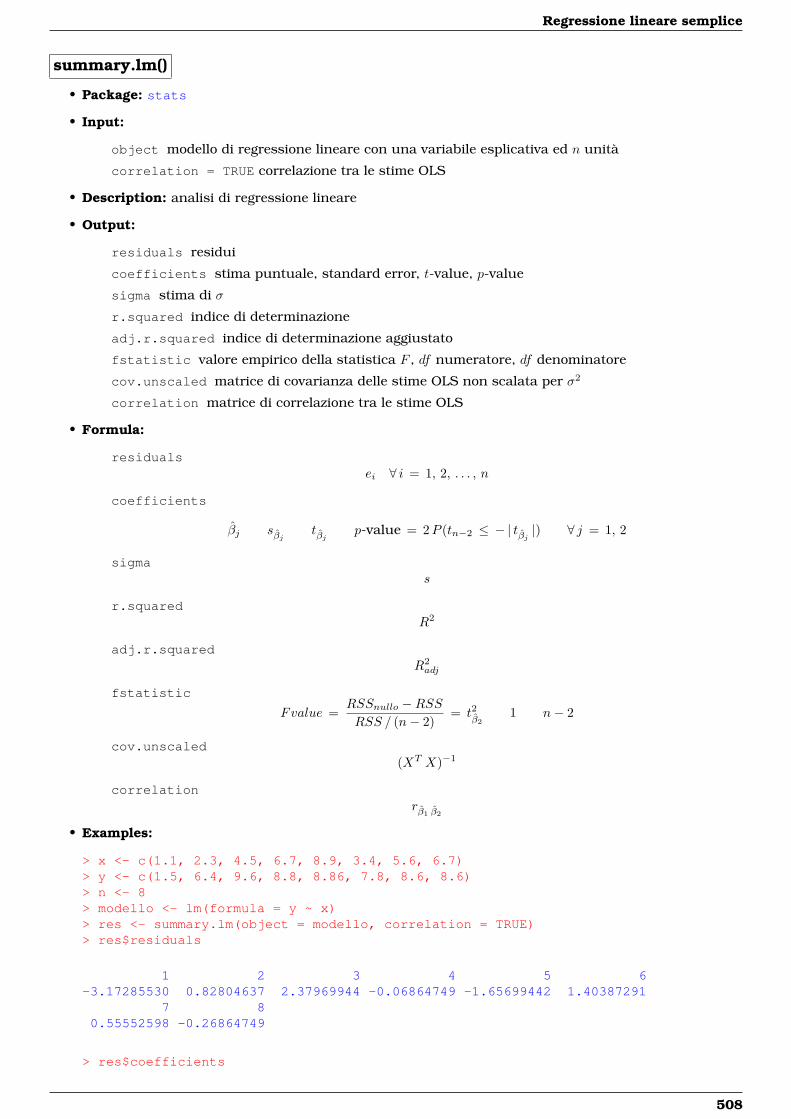
Regressione lineare semplice
summary.lm()
• Package: stats
• Input:
object modello di regressione lineare con una variabile esplicativa ed n unità
correlation = TRUE correlazione tra le stime OLS
• Description: analisi di regressione lineare
• Output:
residuals residui
coefficients stima puntuale, standard error, t-value, p-value
sigma stima di σ
r.squared indice di determinazione
adj.r.squared indice di determinazione aggiustato
fstatistic valore empirico della statistica F , df numeratore, df denominatore
cov.unscaled matrice di covarianza delle stime OLS non scalata per σ2
correlation matrice di correlazione tra le stime OLS
• Formula:
residualsei ∀ i = 1, 2, . . . , n
coefficients
βj sβj tβj p-value = 2P (tn−2 ≤ − | tβj |) ∀ j = 1, 2
sigmas
r.squaredR2
adj.r.squaredR2adj
fstatistic
Fvalue =RSSnullo −RSSRSS / (n− 2)
= t2β2
1 n− 2
cov.unscaled(XT X)−1
correlationrβ1 β2
• Examples:
> x <- c(1.1, 2.3, 4.5, 6.7, 8.9, 3.4, 5.6, 6.7)> y <- c(1.5, 6.4, 9.6, 8.8, 8.86, 7.8, 8.6, 8.6)> n <- 8> modello <- lm(formula = y ~ x)> res <- summary.lm(object = modello, correlation = TRUE)> res$residuals
1 2 3 4 5 6-3.17285530 0.82804637 2.37969944 -0.06864749 -1.65699442 1.40387291
7 80.55552598 -0.26864749
> res$coefficients
508
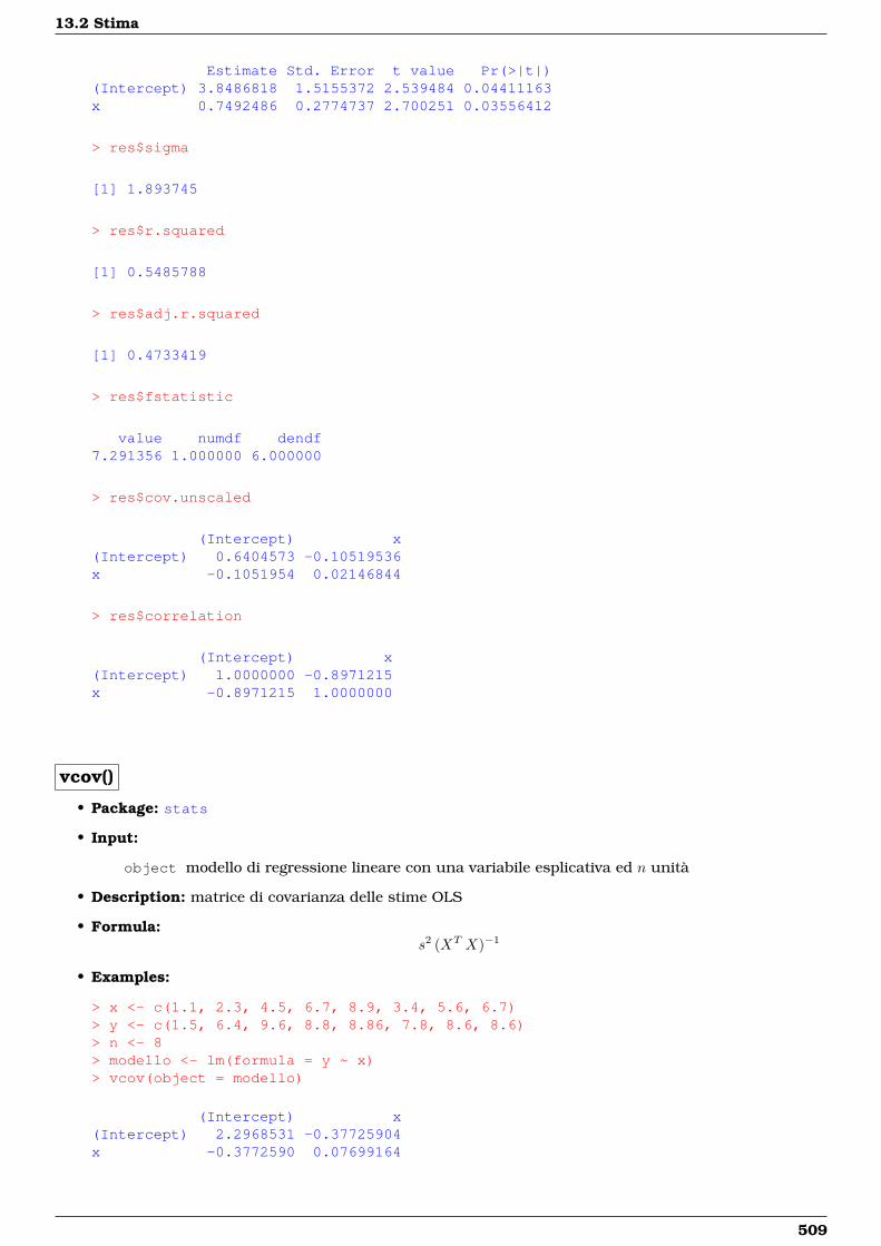
13.2 Stima
Estimate Std. Error t value Pr(>|t|)(Intercept) 3.8486818 1.5155372 2.539484 0.04411163x 0.7492486 0.2774737 2.700251 0.03556412
> res$sigma
[1] 1.893745
> res$r.squared
[1] 0.5485788
> res$adj.r.squared
[1] 0.4733419
> res$fstatistic
value numdf dendf7.291356 1.000000 6.000000
> res$cov.unscaled
(Intercept) x(Intercept) 0.6404573 -0.10519536x -0.1051954 0.02146844
> res$correlation
(Intercept) x(Intercept) 1.0000000 -0.8971215x -0.8971215 1.0000000
vcov()
• Package: stats
• Input:
object modello di regressione lineare con una variabile esplicativa ed n unità
• Description: matrice di covarianza delle stime OLS
• Formula:s2 (XT X)−1
• Examples:
> x <- c(1.1, 2.3, 4.5, 6.7, 8.9, 3.4, 5.6, 6.7)> y <- c(1.5, 6.4, 9.6, 8.8, 8.86, 7.8, 8.6, 8.6)> n <- 8> modello <- lm(formula = y ~ x)> vcov(object = modello)
(Intercept) x(Intercept) 2.2968531 -0.37725904x -0.3772590 0.07699164
509
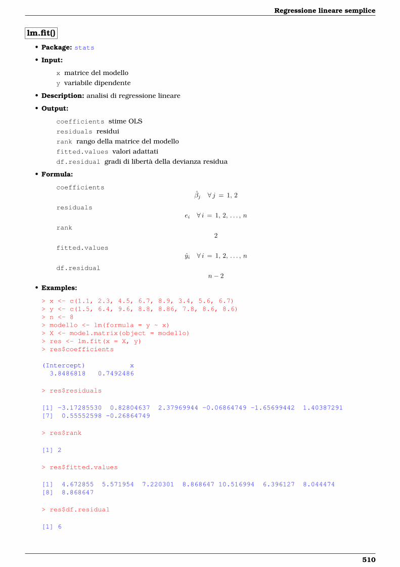
Regressione lineare semplice
lm.fit()
• Package: stats
• Input:
x matrice del modello
y variabile dipendente
• Description: analisi di regressione lineare
• Output:
coefficients stime OLS
residuals residui
rank rango della matrice del modello
fitted.values valori adattati
df.residual gradi di libertà della devianza residua
• Formula:
coefficientsβj ∀ j = 1, 2
residualsei ∀ i = 1, 2, . . . , n
rank2
fitted.valuesyi ∀ i = 1, 2, . . . , n
df.residualn− 2
• Examples:
> x <- c(1.1, 2.3, 4.5, 6.7, 8.9, 3.4, 5.6, 6.7)> y <- c(1.5, 6.4, 9.6, 8.8, 8.86, 7.8, 8.6, 8.6)> n <- 8> modello <- lm(formula = y ~ x)> X <- model.matrix(object = modello)> res <- lm.fit(x = X, y)> res$coefficients
(Intercept) x3.8486818 0.7492486
> res$residuals
[1] -3.17285530 0.82804637 2.37969944 -0.06864749 -1.65699442 1.40387291[7] 0.55552598 -0.26864749
> res$rank
[1] 2
> res$fitted.values
[1] 4.672855 5.571954 7.220301 8.868647 10.516994 6.396127 8.044474[8] 8.868647
> res$df.residual
[1] 6
510
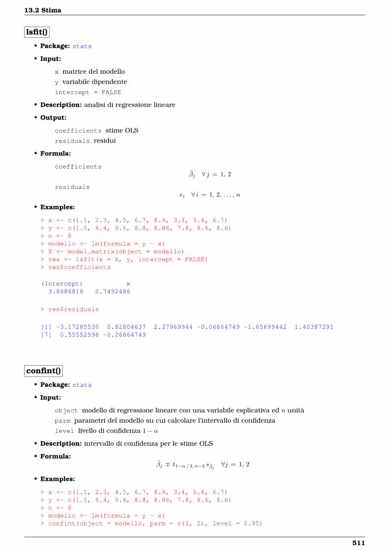
13.2 Stima
lsfit()
• Package: stats
• Input:
x matrice del modello
y variabile dipendente
intercept = FALSE
• Description: analisi di regressione lineare
• Output:
coefficients stime OLS
residuals residui
• Formula:
coefficientsβj ∀ j = 1, 2
residualsei ∀ i = 1, 2, . . . , n
• Examples:
> x <- c(1.1, 2.3, 4.5, 6.7, 8.9, 3.4, 5.6, 6.7)> y <- c(1.5, 6.4, 9.6, 8.8, 8.86, 7.8, 8.6, 8.6)> n <- 8> modello <- lm(formula = y ~ x)> X <- model.matrix(object = modello)> res <- lsfit(x = X, y, intercept = FALSE)> res$coefficients
(Intercept) x3.8486818 0.7492486
> res$residuals
[1] -3.17285530 0.82804637 2.37969944 -0.06864749 -1.65699442 1.40387291[7] 0.55552598 -0.26864749
confint()
• Package: stats
• Input:
object modello di regressione lineare con una variabile esplicativa ed n unità
parm parametri del modello su cui calcolare l’intervallo di confidenza
level livello di confidenza 1− α
• Description: intervallo di confidenza per le stime OLS
• Formula:βj ∓ t1−α/ 2, n−2 sβj ∀j = 1, 2
• Examples:
> x <- c(1.1, 2.3, 4.5, 6.7, 8.9, 3.4, 5.6, 6.7)> y <- c(1.5, 6.4, 9.6, 8.8, 8.86, 7.8, 8.6, 8.6)> n <- 8> modello <- lm(formula = y ~ x)> confint(object = modello, parm = c(1, 2), level = 0.95)
511
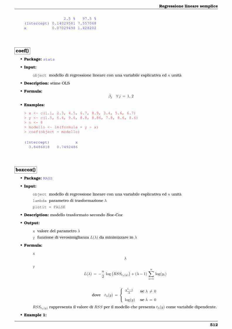
Regressione lineare semplice
2.5 % 97.5 %(Intercept) 0.14029581 7.557068x 0.07029498 1.428202
coef()
• Package: stats
• Input:
object modello di regressione lineare con una variabile esplicativa ed n unità
• Description: stime OLS
• Formula:βj ∀ j = 1, 2
• Examples:
> x <- c(1.1, 2.3, 4.5, 6.7, 8.9, 3.4, 5.6, 6.7)> y <- c(1.5, 6.4, 9.6, 8.8, 8.86, 7.8, 8.6, 8.6)> n <- 8> modello <- lm(formula = y ~ x)> coef(object = modello)
(Intercept) x3.8486818 0.7492486
boxcox()
• Package: MASS
• Input:
object modello di regressione lineare con una variabile esplicativa ed n unità
lambda parametro di trasformazione λ
plotit = FALSE
• Description: modello trasformato secondo Box–Cox
• Output:
x valore del parametro λ
y funzione di verosimiglianza L(λ) da minimizzare in λ
• Formula:
xλ
y
L(λ) = −n2
log(RSStλ(y)
)+ (λ− 1)
n∑i=1
log(yi)
dove tλ(y) =
yλ−1λ se λ 6= 0
log(y) se λ = 0
RSStλ(y) rappresenta il valore di RSS per il modello che presenta tλ(y) come variabile dipendente.
• Example 1:
512
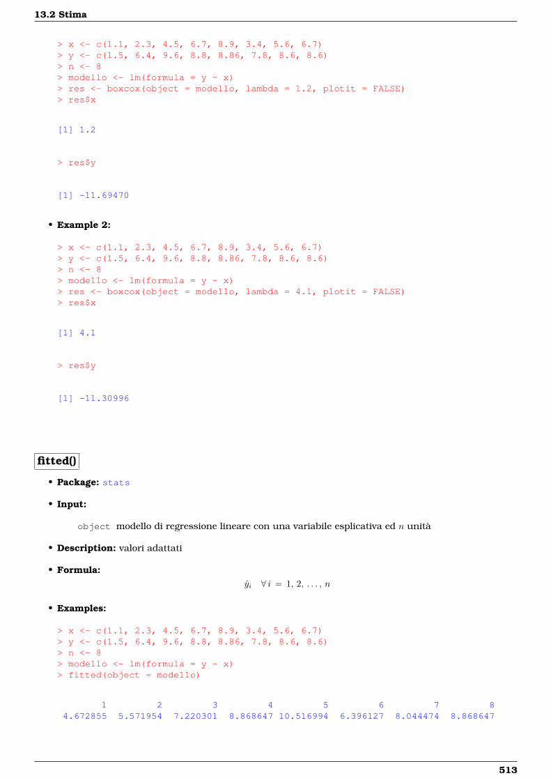
13.2 Stima
> x <- c(1.1, 2.3, 4.5, 6.7, 8.9, 3.4, 5.6, 6.7)> y <- c(1.5, 6.4, 9.6, 8.8, 8.86, 7.8, 8.6, 8.6)> n <- 8> modello <- lm(formula = y ~ x)> res <- boxcox(object = modello, lambda = 1.2, plotit = FALSE)> res$x
[1] 1.2
> res$y
[1] -11.69470
• Example 2:
> x <- c(1.1, 2.3, 4.5, 6.7, 8.9, 3.4, 5.6, 6.7)> y <- c(1.5, 6.4, 9.6, 8.8, 8.86, 7.8, 8.6, 8.6)> n <- 8> modello <- lm(formula = y ~ x)> res <- boxcox(object = modello, lambda = 4.1, plotit = FALSE)> res$x
[1] 4.1
> res$y
[1] -11.30996
fitted()
• Package: stats
• Input:
object modello di regressione lineare con una variabile esplicativa ed n unità
• Description: valori adattati
• Formula:yi ∀ i = 1, 2, . . . , n
• Examples:
> x <- c(1.1, 2.3, 4.5, 6.7, 8.9, 3.4, 5.6, 6.7)> y <- c(1.5, 6.4, 9.6, 8.8, 8.86, 7.8, 8.6, 8.6)> n <- 8> modello <- lm(formula = y ~ x)> fitted(object = modello)
1 2 3 4 5 6 7 84.672855 5.571954 7.220301 8.868647 10.516994 6.396127 8.044474 8.868647
513
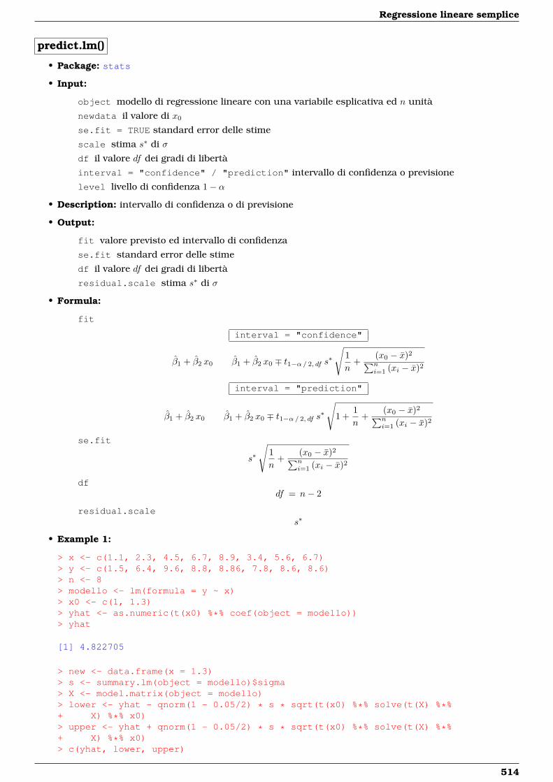
Regressione lineare semplice
predict.lm()
• Package: stats
• Input:
object modello di regressione lineare con una variabile esplicativa ed n unità
newdata il valore di x0
se.fit = TRUE standard error delle stime
scale stima s∗ di σ
df il valore df dei gradi di libertà
interval = "confidence" / "prediction" intervallo di confidenza o previsione
level livello di confidenza 1− α
• Description: intervallo di confidenza o di previsione
• Output:
fit valore previsto ed intervallo di confidenza
se.fit standard error delle stime
df il valore df dei gradi di libertà
residual.scale stima s∗ di σ
• Formula:
fit
interval = "confidence"
β1 + β2 x0 β1 + β2 x0 ∓ t1−α/ 2, df s∗
√1n
+(x0 − x)2∑ni=1 (xi − x)2
interval = "prediction"
β1 + β2 x0 β1 + β2 x0 ∓ t1−α/ 2, df s∗
√1 +
1n
+(x0 − x)2∑ni=1 (xi − x)2
se.fit
s∗
√1n
+(x0 − x)2∑ni=1 (xi − x)2
dfdf = n− 2
residual.scales∗
• Example 1:
> x <- c(1.1, 2.3, 4.5, 6.7, 8.9, 3.4, 5.6, 6.7)> y <- c(1.5, 6.4, 9.6, 8.8, 8.86, 7.8, 8.6, 8.6)> n <- 8> modello <- lm(formula = y ~ x)> x0 <- c(1, 1.3)> yhat <- as.numeric(t(x0) %*% coef(object = modello))> yhat
[1] 4.822705
> new <- data.frame(x = 1.3)> s <- summary.lm(object = modello)$sigma> X <- model.matrix(object = modello)> lower <- yhat - qnorm(1 - 0.05/2) * s * sqrt(t(x0) %*% solve(t(X) %*%+ X) %*% x0)> upper <- yhat + qnorm(1 - 0.05/2) * s * sqrt(t(x0) %*% solve(t(X) %*%+ X) %*% x0)> c(yhat, lower, upper)
514
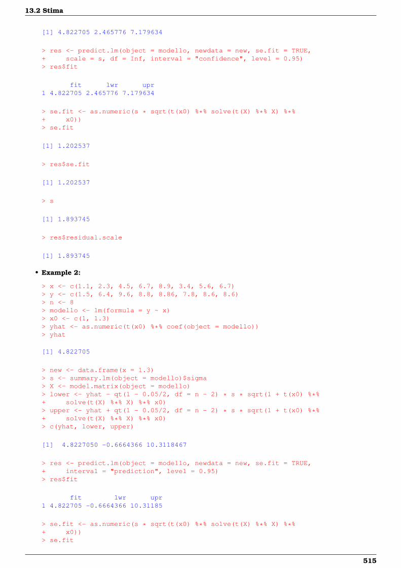
13.2 Stima
[1] 4.822705 2.465776 7.179634
> res <- predict.lm(object = modello, newdata = new, se.fit = TRUE,+ scale = s, df = Inf, interval = "confidence", level = 0.95)> res$fit
fit lwr upr1 4.822705 2.465776 7.179634
> se.fit <- as.numeric(s * sqrt(t(x0) %*% solve(t(X) %*% X) %*%+ x0))> se.fit
[1] 1.202537
> res$se.fit
[1] 1.202537
> s
[1] 1.893745
> res$residual.scale
[1] 1.893745
• Example 2:
> x <- c(1.1, 2.3, 4.5, 6.7, 8.9, 3.4, 5.6, 6.7)> y <- c(1.5, 6.4, 9.6, 8.8, 8.86, 7.8, 8.6, 8.6)> n <- 8> modello <- lm(formula = y ~ x)> x0 <- c(1, 1.3)> yhat <- as.numeric(t(x0) %*% coef(object = modello))> yhat
[1] 4.822705
> new <- data.frame(x = 1.3)> s <- summary.lm(object = modello)$sigma> X <- model.matrix(object = modello)> lower <- yhat - qt(1 - 0.05/2, df = n - 2) * s * sqrt(1 + t(x0) %*%+ solve(t(X) %*% X) %*% x0)> upper <- yhat + qt(1 - 0.05/2, df = n - 2) * s * sqrt(1 + t(x0) %*%+ solve(t(X) %*% X) %*% x0)> c(yhat, lower, upper)
[1] 4.8227050 -0.6664366 10.3118467
> res <- predict.lm(object = modello, newdata = new, se.fit = TRUE,+ interval = "prediction", level = 0.95)> res$fit
fit lwr upr1 4.822705 -0.6664366 10.31185
> se.fit <- as.numeric(s * sqrt(t(x0) %*% solve(t(X) %*% X) %*%+ x0))> se.fit
515
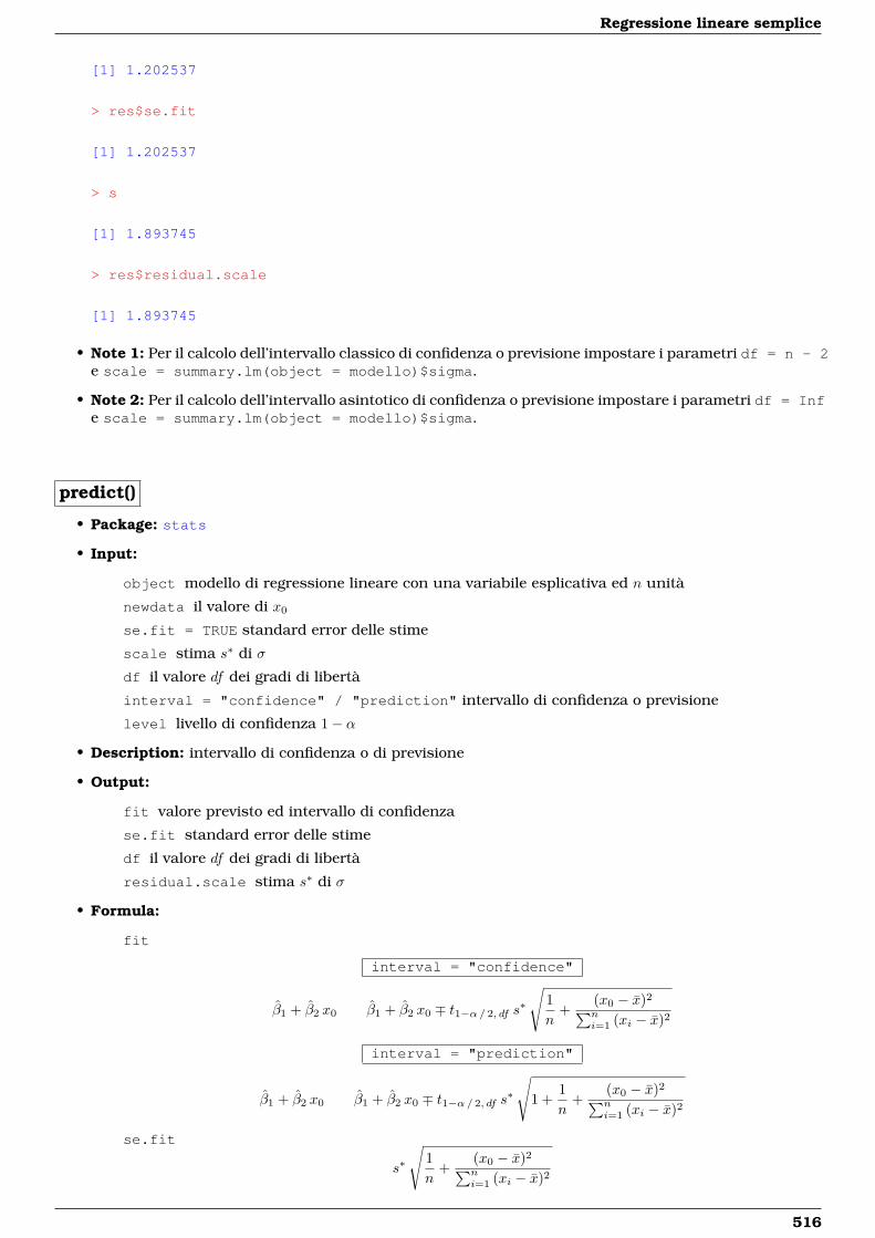
Regressione lineare semplice
[1] 1.202537
> res$se.fit
[1] 1.202537
> s
[1] 1.893745
> res$residual.scale
[1] 1.893745
• Note 1: Per il calcolo dell’intervallo classico di confidenza o previsione impostare i parametri df = n - 2e scale = summary.lm(object = modello)$sigma.
• Note 2: Per il calcolo dell’intervallo asintotico di confidenza o previsione impostare i parametri df = Infe scale = summary.lm(object = modello)$sigma.
predict()
• Package: stats
• Input:
object modello di regressione lineare con una variabile esplicativa ed n unità
newdata il valore di x0
se.fit = TRUE standard error delle stime
scale stima s∗ di σ
df il valore df dei gradi di libertà
interval = "confidence" / "prediction" intervallo di confidenza o previsione
level livello di confidenza 1− α
• Description: intervallo di confidenza o di previsione
• Output:
fit valore previsto ed intervallo di confidenza
se.fit standard error delle stime
df il valore df dei gradi di libertà
residual.scale stima s∗ di σ
• Formula:
fit
interval = "confidence"
β1 + β2 x0 β1 + β2 x0 ∓ t1−α/ 2, df s∗
√1n
+(x0 − x)2∑ni=1 (xi − x)2
interval = "prediction"
β1 + β2 x0 β1 + β2 x0 ∓ t1−α/ 2, df s∗
√1 +
1n
+(x0 − x)2∑ni=1 (xi − x)2
se.fit
s∗
√1n
+(x0 − x)2∑ni=1 (xi − x)2
516
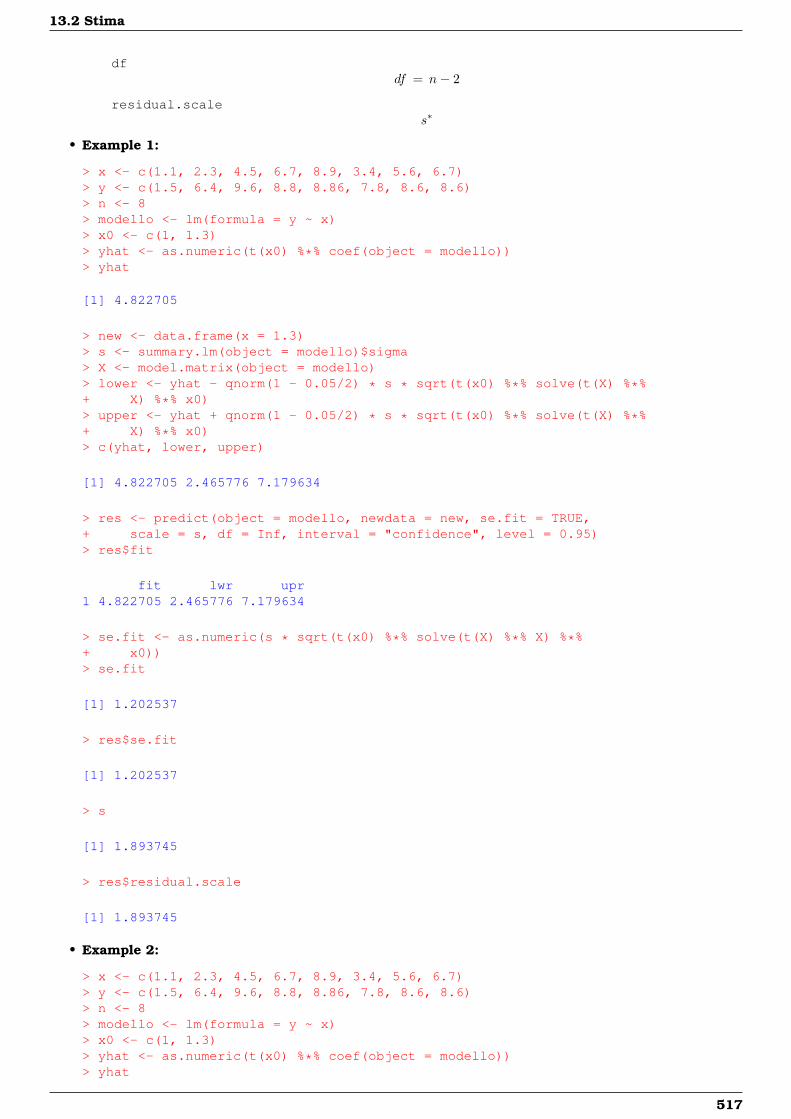
13.2 Stima
dfdf = n− 2
residual.scales∗
• Example 1:
> x <- c(1.1, 2.3, 4.5, 6.7, 8.9, 3.4, 5.6, 6.7)> y <- c(1.5, 6.4, 9.6, 8.8, 8.86, 7.8, 8.6, 8.6)> n <- 8> modello <- lm(formula = y ~ x)> x0 <- c(1, 1.3)> yhat <- as.numeric(t(x0) %*% coef(object = modello))> yhat
[1] 4.822705
> new <- data.frame(x = 1.3)> s <- summary.lm(object = modello)$sigma> X <- model.matrix(object = modello)> lower <- yhat - qnorm(1 - 0.05/2) * s * sqrt(t(x0) %*% solve(t(X) %*%+ X) %*% x0)> upper <- yhat + qnorm(1 - 0.05/2) * s * sqrt(t(x0) %*% solve(t(X) %*%+ X) %*% x0)> c(yhat, lower, upper)
[1] 4.822705 2.465776 7.179634
> res <- predict(object = modello, newdata = new, se.fit = TRUE,+ scale = s, df = Inf, interval = "confidence", level = 0.95)> res$fit
fit lwr upr1 4.822705 2.465776 7.179634
> se.fit <- as.numeric(s * sqrt(t(x0) %*% solve(t(X) %*% X) %*%+ x0))> se.fit
[1] 1.202537
> res$se.fit
[1] 1.202537
> s
[1] 1.893745
> res$residual.scale
[1] 1.893745
• Example 2:
> x <- c(1.1, 2.3, 4.5, 6.7, 8.9, 3.4, 5.6, 6.7)> y <- c(1.5, 6.4, 9.6, 8.8, 8.86, 7.8, 8.6, 8.6)> n <- 8> modello <- lm(formula = y ~ x)> x0 <- c(1, 1.3)> yhat <- as.numeric(t(x0) %*% coef(object = modello))> yhat
517
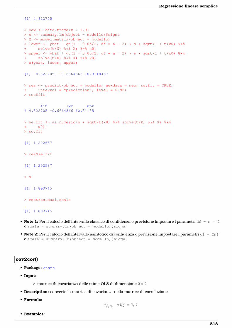
Regressione lineare semplice
[1] 4.822705
> new <- data.frame(x = 1.3)> s <- summary.lm(object = modello)$sigma> X <- model.matrix(object = modello)> lower <- yhat - qt(1 - 0.05/2, df = n - 2) * s * sqrt(1 + t(x0) %*%+ solve(t(X) %*% X) %*% x0)> upper <- yhat + qt(1 - 0.05/2, df = n - 2) * s * sqrt(1 + t(x0) %*%+ solve(t(X) %*% X) %*% x0)> c(yhat, lower, upper)
[1] 4.8227050 -0.6664366 10.3118467
> res <- predict(object = modello, newdata = new, se.fit = TRUE,+ interval = "prediction", level = 0.95)> res$fit
fit lwr upr1 4.822705 -0.6664366 10.31185
> se.fit <- as.numeric(s * sqrt(t(x0) %*% solve(t(X) %*% X) %*%+ x0))> se.fit
[1] 1.202537
> res$se.fit
[1] 1.202537
> s
[1] 1.893745
> res$residual.scale
[1] 1.893745
• Note 1: Per il calcolo dell’intervallo classico di confidenza o previsione impostare i parametri df = n - 2e scale = summary.lm(object = modello)$sigma.
• Note 2: Per il calcolo dell’intervallo asintotico di confidenza o previsione impostare i parametri df = Infe scale = summary.lm(object = modello)$sigma.
cov2cor()
• Package: stats
• Input:
V matrice di covarianza delle stime OLS di dimensione 2× 2
• Description: converte la matrice di covarianza nella matrice di correlazione
• Formula:rβi βj ∀ i, j = 1, 2
• Examples:
518
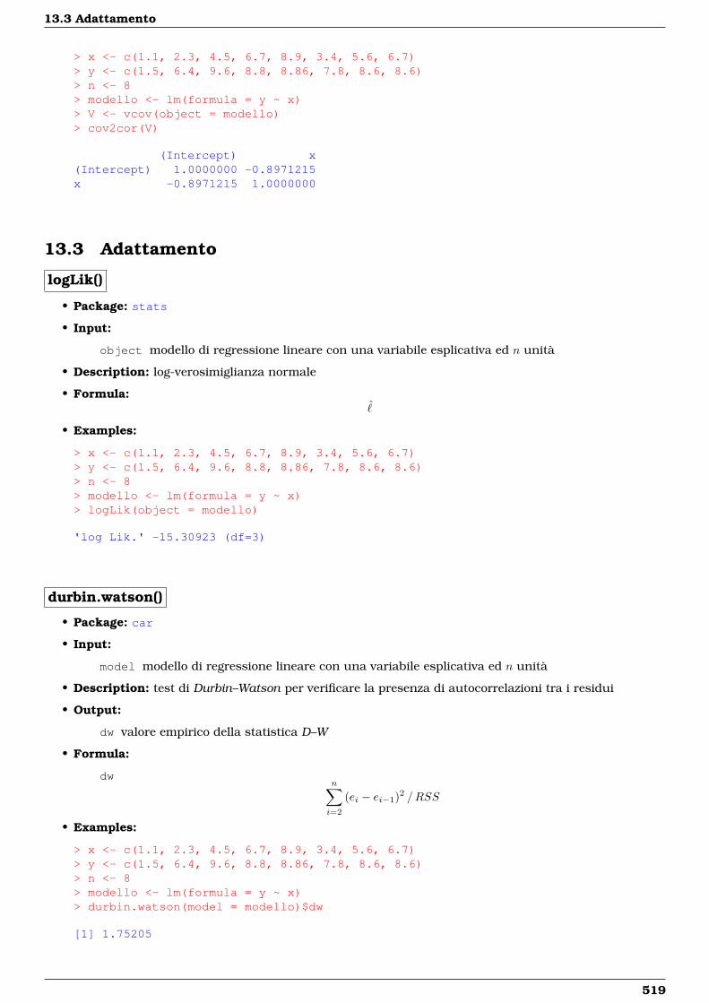
13.3 Adattamento
> x <- c(1.1, 2.3, 4.5, 6.7, 8.9, 3.4, 5.6, 6.7)> y <- c(1.5, 6.4, 9.6, 8.8, 8.86, 7.8, 8.6, 8.6)> n <- 8> modello <- lm(formula = y ~ x)> V <- vcov(object = modello)> cov2cor(V)
(Intercept) x(Intercept) 1.0000000 -0.8971215x -0.8971215 1.0000000
13.3 Adattamento
logLik()
• Package: stats
• Input:
object modello di regressione lineare con una variabile esplicativa ed n unità
• Description: log-verosimiglianza normale
• Formula:ˆ
• Examples:
> x <- c(1.1, 2.3, 4.5, 6.7, 8.9, 3.4, 5.6, 6.7)> y <- c(1.5, 6.4, 9.6, 8.8, 8.86, 7.8, 8.6, 8.6)> n <- 8> modello <- lm(formula = y ~ x)> logLik(object = modello)
'log Lik.' -15.30923 (df=3)
durbin.watson()
• Package: car
• Input:
model modello di regressione lineare con una variabile esplicativa ed n unità
• Description: test di Durbin–Watson per verificare la presenza di autocorrelazioni tra i residui
• Output:
dw valore empirico della statistica D–W
• Formula:
dwn∑i=2
(ei − ei−1)2 /RSS
• Examples:
> x <- c(1.1, 2.3, 4.5, 6.7, 8.9, 3.4, 5.6, 6.7)> y <- c(1.5, 6.4, 9.6, 8.8, 8.86, 7.8, 8.6, 8.6)> n <- 8> modello <- lm(formula = y ~ x)> durbin.watson(model = modello)$dw
[1] 1.75205
519
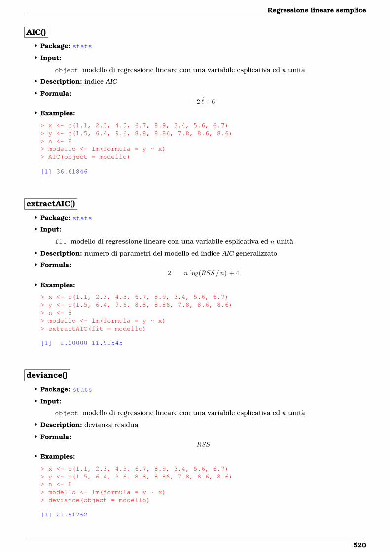
Regressione lineare semplice
AIC()
• Package: stats
• Input:
object modello di regressione lineare con una variabile esplicativa ed n unità
• Description: indice AIC
• Formula:−2 ˆ+ 6
• Examples:
> x <- c(1.1, 2.3, 4.5, 6.7, 8.9, 3.4, 5.6, 6.7)> y <- c(1.5, 6.4, 9.6, 8.8, 8.86, 7.8, 8.6, 8.6)> n <- 8> modello <- lm(formula = y ~ x)> AIC(object = modello)
[1] 36.61846
extractAIC()
• Package: stats
• Input:
fit modello di regressione lineare con una variabile esplicativa ed n unità
• Description: numero di parametri del modello ed indice AIC generalizzato
• Formula:2 n log(RSS /n) + 4
• Examples:
> x <- c(1.1, 2.3, 4.5, 6.7, 8.9, 3.4, 5.6, 6.7)> y <- c(1.5, 6.4, 9.6, 8.8, 8.86, 7.8, 8.6, 8.6)> n <- 8> modello <- lm(formula = y ~ x)> extractAIC(fit = modello)
[1] 2.00000 11.91545
deviance()
• Package: stats
• Input:
object modello di regressione lineare con una variabile esplicativa ed n unità
• Description: devianza residua
• Formula:RSS
• Examples:
> x <- c(1.1, 2.3, 4.5, 6.7, 8.9, 3.4, 5.6, 6.7)> y <- c(1.5, 6.4, 9.6, 8.8, 8.86, 7.8, 8.6, 8.6)> n <- 8> modello <- lm(formula = y ~ x)> deviance(object = modello)
[1] 21.51762
520
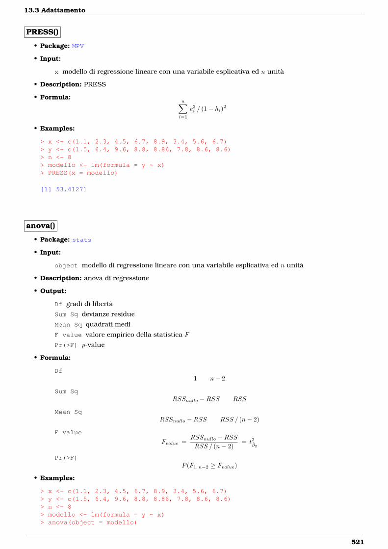
13.3 Adattamento
PRESS()
• Package: MPV
• Input:
x modello di regressione lineare con una variabile esplicativa ed n unità
• Description: PRESS
• Formula:n∑i=1
e2i / (1− hi)2
• Examples:
> x <- c(1.1, 2.3, 4.5, 6.7, 8.9, 3.4, 5.6, 6.7)> y <- c(1.5, 6.4, 9.6, 8.8, 8.86, 7.8, 8.6, 8.6)> n <- 8> modello <- lm(formula = y ~ x)> PRESS(x = modello)
[1] 53.41271
anova()
• Package: stats
• Input:
object modello di regressione lineare con una variabile esplicativa ed n unità
• Description: anova di regressione
• Output:
Df gradi di libertà
Sum Sq devianze residue
Mean Sq quadrati medi
F value valore empirico della statistica F
Pr(>F) p-value
• Formula:
Df1 n− 2
Sum SqRSSnullo −RSS RSS
Mean SqRSSnullo −RSS RSS / (n− 2)
F value
Fvalue =RSSnullo −RSSRSS / (n− 2)
= t2β2
Pr(>F)P (F1, n−2 ≥ Fvalue)
• Examples:
> x <- c(1.1, 2.3, 4.5, 6.7, 8.9, 3.4, 5.6, 6.7)> y <- c(1.5, 6.4, 9.6, 8.8, 8.86, 7.8, 8.6, 8.6)> n <- 8> modello <- lm(formula = y ~ x)> anova(object = modello)
521
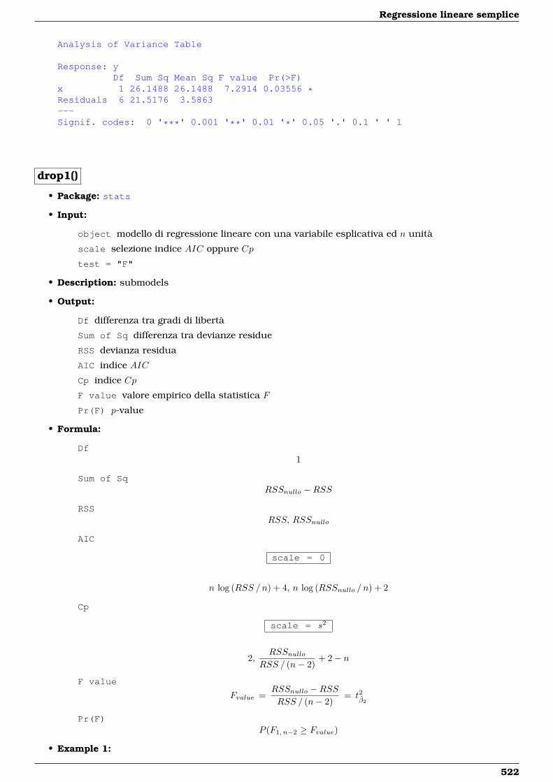
Regressione lineare semplice
Analysis of Variance Table
Response: yDf Sum Sq Mean Sq F value Pr(>F)
x 1 26.1488 26.1488 7.2914 0.03556 *Residuals 6 21.5176 3.5863---Signif. codes: 0 '***' 0.001 '**' 0.01 '*' 0.05 '.' 0.1 ' ' 1
drop1()
• Package: stats
• Input:
object modello di regressione lineare con una variabile esplicativa ed n unità
scale selezione indice AIC oppure Cp
test = "F"
• Description: submodels
• Output:
Df differenza tra gradi di libertà
Sum of Sq differenza tra devianze residue
RSS devianza residua
AIC indice AIC
Cp indice Cp
F value valore empirico della statistica F
Pr(F) p-value
• Formula:
Df1
Sum of SqRSSnullo −RSS
RSSRSS, RSSnullo
AIC
scale = 0
n log (RSS /n) + 4, n log (RSSnullo / n) + 2
Cp
scale = s2
2,RSSnullo
RSS / (n− 2)+ 2− n
F value
Fvalue =RSSnullo −RSSRSS / (n− 2)
= t2β2
Pr(F)P (F1, n−2 ≥ Fvalue)
• Example 1:
522
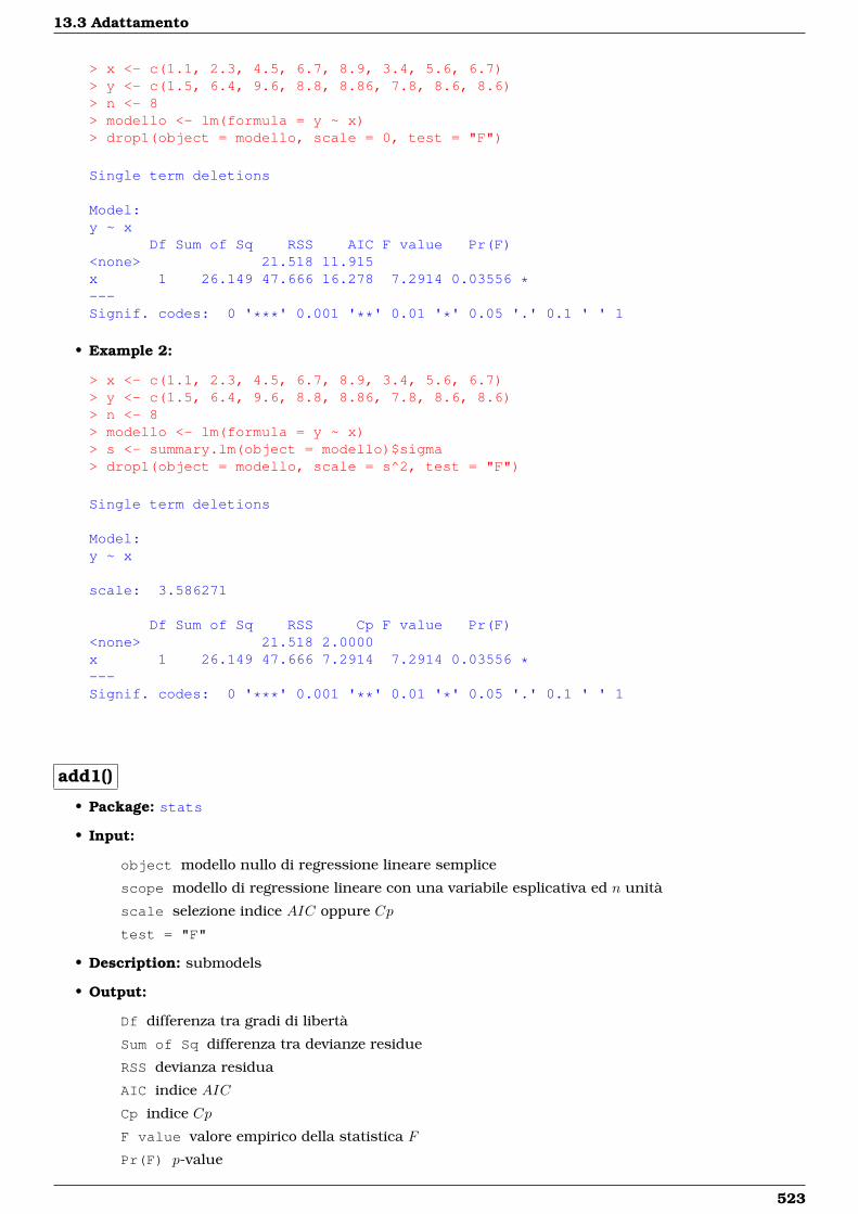
13.3 Adattamento
> x <- c(1.1, 2.3, 4.5, 6.7, 8.9, 3.4, 5.6, 6.7)> y <- c(1.5, 6.4, 9.6, 8.8, 8.86, 7.8, 8.6, 8.6)> n <- 8> modello <- lm(formula = y ~ x)> drop1(object = modello, scale = 0, test = "F")
Single term deletions
Model:y ~ x
Df Sum of Sq RSS AIC F value Pr(F)<none> 21.518 11.915x 1 26.149 47.666 16.278 7.2914 0.03556 *---Signif. codes: 0 '***' 0.001 '**' 0.01 '*' 0.05 '.' 0.1 ' ' 1
• Example 2:
> x <- c(1.1, 2.3, 4.5, 6.7, 8.9, 3.4, 5.6, 6.7)> y <- c(1.5, 6.4, 9.6, 8.8, 8.86, 7.8, 8.6, 8.6)> n <- 8> modello <- lm(formula = y ~ x)> s <- summary.lm(object = modello)$sigma> drop1(object = modello, scale = s^2, test = "F")
Single term deletions
Model:y ~ x
scale: 3.586271
Df Sum of Sq RSS Cp F value Pr(F)<none> 21.518 2.0000x 1 26.149 47.666 7.2914 7.2914 0.03556 *---Signif. codes: 0 '***' 0.001 '**' 0.01 '*' 0.05 '.' 0.1 ' ' 1
add1()
• Package: stats
• Input:
object modello nullo di regressione lineare semplice
scope modello di regressione lineare con una variabile esplicativa ed n unità
scale selezione indice AIC oppure Cp
test = "F"
• Description: submodels
• Output:
Df differenza tra gradi di libertà
Sum of Sq differenza tra devianze residue
RSS devianza residua
AIC indice AIC
Cp indice Cp
F value valore empirico della statistica F
Pr(F) p-value
523
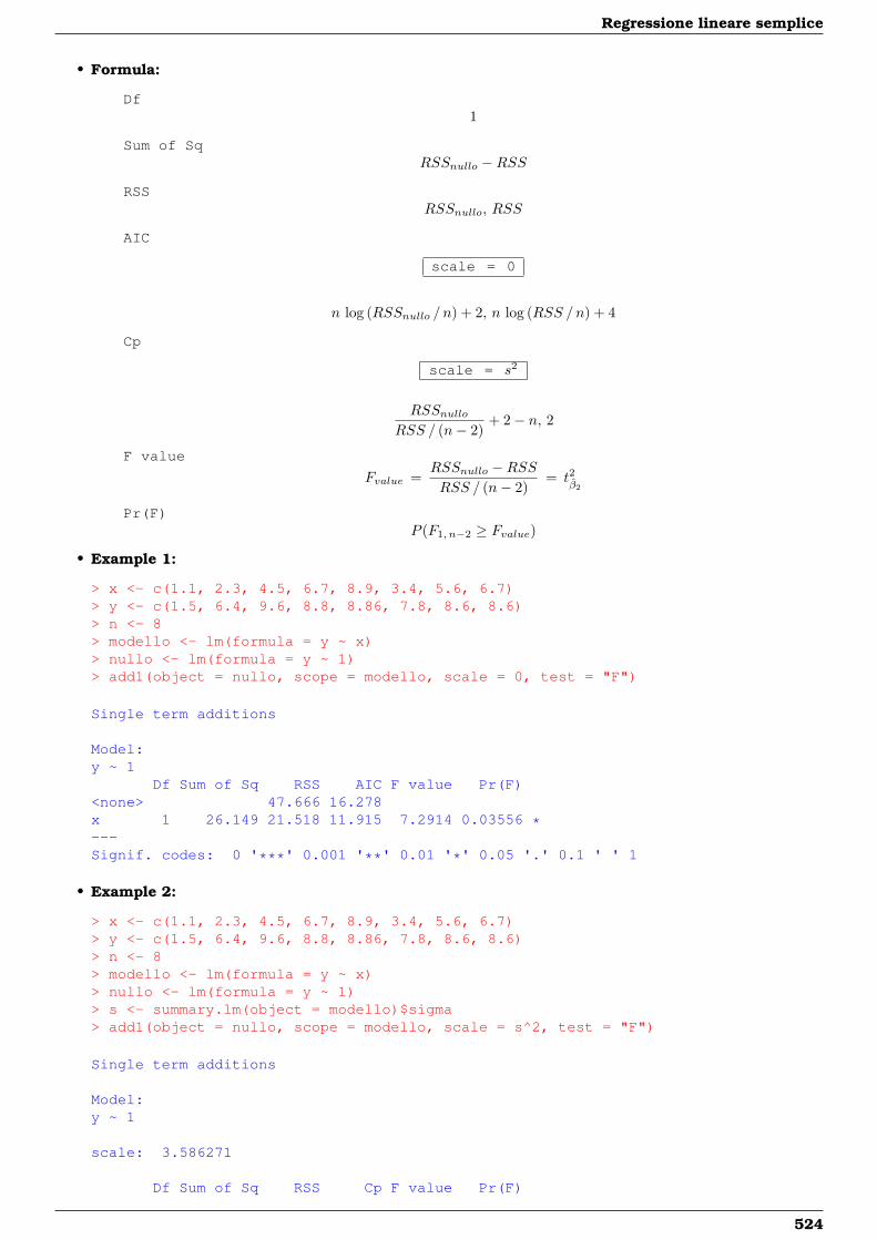
Regressione lineare semplice
• Formula:
Df1
Sum of SqRSSnullo −RSS
RSSRSSnullo, RSS
AIC
scale = 0
n log (RSSnullo / n) + 2, n log (RSS /n) + 4
Cp
scale = s2
RSSnulloRSS / (n− 2)
+ 2− n, 2
F value
Fvalue =RSSnullo −RSSRSS / (n− 2)
= t2β2
Pr(F)P (F1, n−2 ≥ Fvalue)
• Example 1:
> x <- c(1.1, 2.3, 4.5, 6.7, 8.9, 3.4, 5.6, 6.7)> y <- c(1.5, 6.4, 9.6, 8.8, 8.86, 7.8, 8.6, 8.6)> n <- 8> modello <- lm(formula = y ~ x)> nullo <- lm(formula = y ~ 1)> add1(object = nullo, scope = modello, scale = 0, test = "F")
Single term additions
Model:y ~ 1
Df Sum of Sq RSS AIC F value Pr(F)<none> 47.666 16.278x 1 26.149 21.518 11.915 7.2914 0.03556 *---Signif. codes: 0 '***' 0.001 '**' 0.01 '*' 0.05 '.' 0.1 ' ' 1
• Example 2:
> x <- c(1.1, 2.3, 4.5, 6.7, 8.9, 3.4, 5.6, 6.7)> y <- c(1.5, 6.4, 9.6, 8.8, 8.86, 7.8, 8.6, 8.6)> n <- 8> modello <- lm(formula = y ~ x)> nullo <- lm(formula = y ~ 1)> s <- summary.lm(object = modello)$sigma> add1(object = nullo, scope = modello, scale = s^2, test = "F")
Single term additions
Model:y ~ 1
scale: 3.586271
Df Sum of Sq RSS Cp F value Pr(F)
524
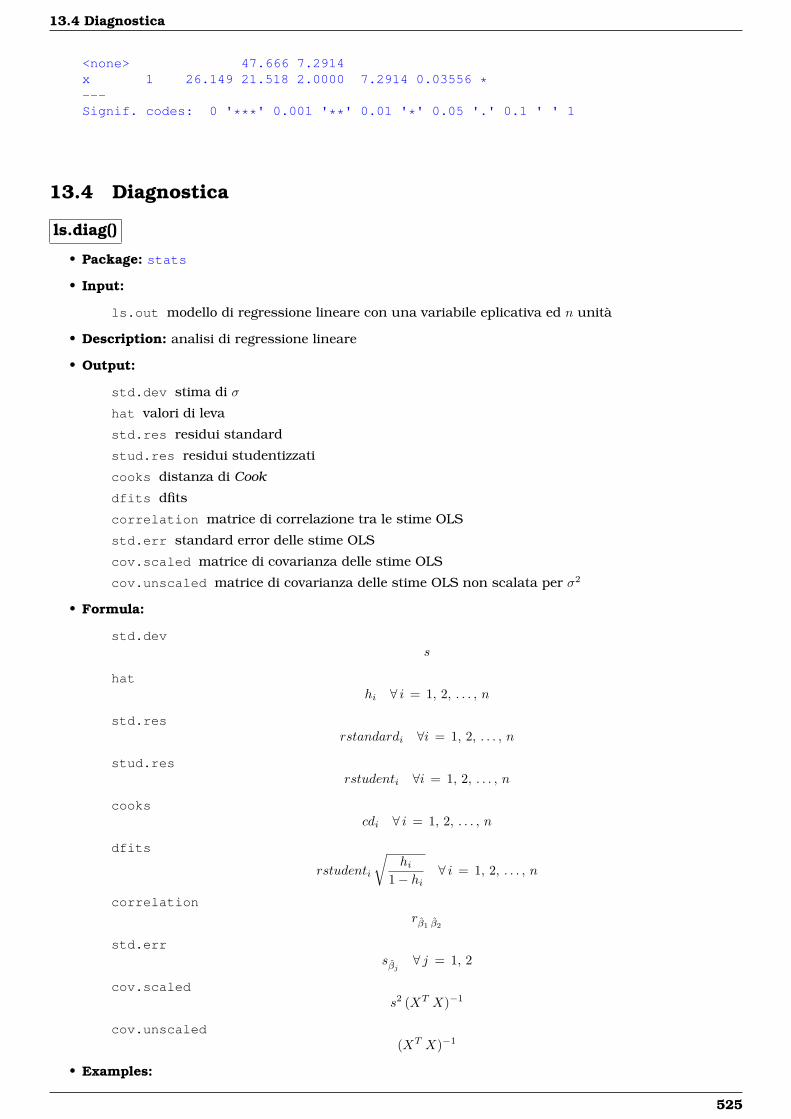
13.4 Diagnostica
<none> 47.666 7.2914x 1 26.149 21.518 2.0000 7.2914 0.03556 *---Signif. codes: 0 '***' 0.001 '**' 0.01 '*' 0.05 '.' 0.1 ' ' 1
13.4 Diagnostica
ls.diag()
• Package: stats
• Input:
ls.out modello di regressione lineare con una variabile eplicativa ed n unità
• Description: analisi di regressione lineare
• Output:
std.dev stima di σ
hat valori di leva
std.res residui standard
stud.res residui studentizzati
cooks distanza di Cook
dfits dfits
correlation matrice di correlazione tra le stime OLS
std.err standard error delle stime OLS
cov.scaled matrice di covarianza delle stime OLS
cov.unscaled matrice di covarianza delle stime OLS non scalata per σ2
• Formula:
std.devs
hathi ∀ i = 1, 2, . . . , n
std.resrstandardi ∀i = 1, 2, . . . , n
stud.resrstudenti ∀i = 1, 2, . . . , n
cookscdi ∀ i = 1, 2, . . . , n
dfits
rstudenti
√hi
1− hi∀ i = 1, 2, . . . , n
correlationrβ1 β2
std.errsβj ∀ j = 1, 2
cov.scaleds2 (XT X)−1
cov.unscaled(XT X)−1
• Examples:
525
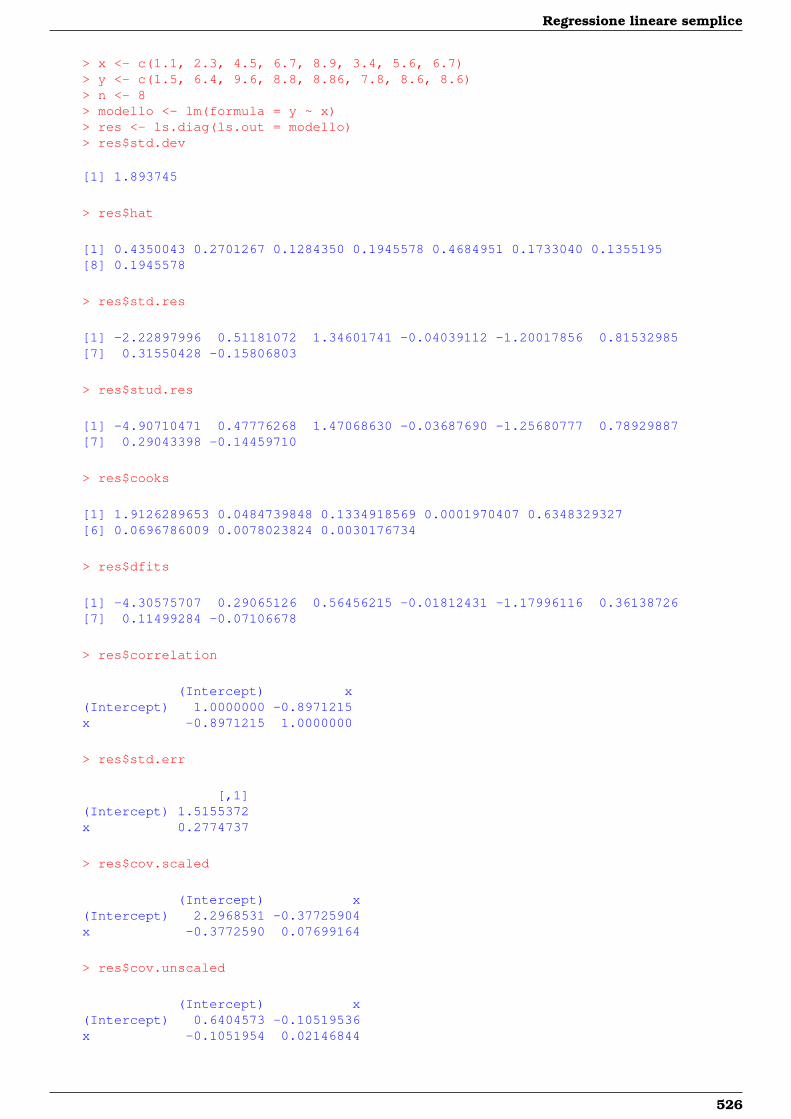
Regressione lineare semplice
> x <- c(1.1, 2.3, 4.5, 6.7, 8.9, 3.4, 5.6, 6.7)> y <- c(1.5, 6.4, 9.6, 8.8, 8.86, 7.8, 8.6, 8.6)> n <- 8> modello <- lm(formula = y ~ x)> res <- ls.diag(ls.out = modello)> res$std.dev
[1] 1.893745
> res$hat
[1] 0.4350043 0.2701267 0.1284350 0.1945578 0.4684951 0.1733040 0.1355195[8] 0.1945578
> res$std.res
[1] -2.22897996 0.51181072 1.34601741 -0.04039112 -1.20017856 0.81532985[7] 0.31550428 -0.15806803
> res$stud.res
[1] -4.90710471 0.47776268 1.47068630 -0.03687690 -1.25680777 0.78929887[7] 0.29043398 -0.14459710
> res$cooks
[1] 1.9126289653 0.0484739848 0.1334918569 0.0001970407 0.6348329327[6] 0.0696786009 0.0078023824 0.0030176734
> res$dfits
[1] -4.30575707 0.29065126 0.56456215 -0.01812431 -1.17996116 0.36138726[7] 0.11499284 -0.07106678
> res$correlation
(Intercept) x(Intercept) 1.0000000 -0.8971215x -0.8971215 1.0000000
> res$std.err
[,1](Intercept) 1.5155372x 0.2774737
> res$cov.scaled
(Intercept) x(Intercept) 2.2968531 -0.37725904x -0.3772590 0.07699164
> res$cov.unscaled
(Intercept) x(Intercept) 0.6404573 -0.10519536x -0.1051954 0.02146844
526
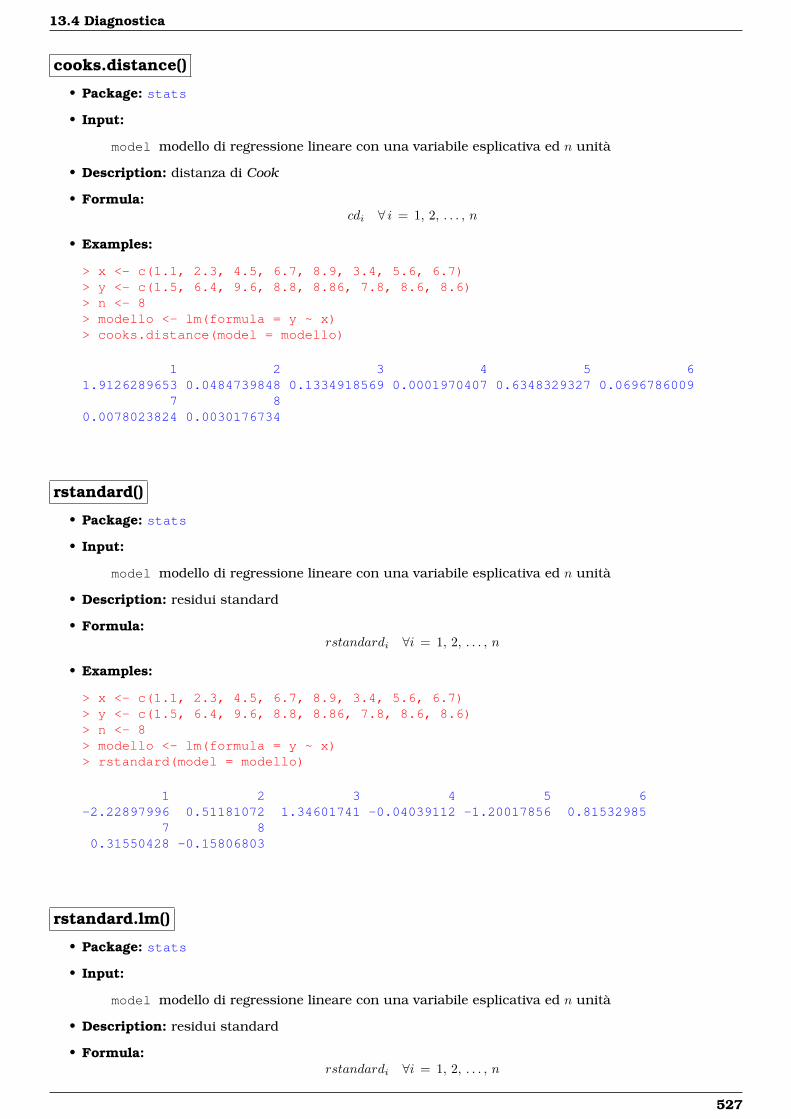
13.4 Diagnostica
cooks.distance()
• Package: stats
• Input:
model modello di regressione lineare con una variabile esplicativa ed n unità
• Description: distanza di Cook
• Formula:cdi ∀ i = 1, 2, . . . , n
• Examples:
> x <- c(1.1, 2.3, 4.5, 6.7, 8.9, 3.4, 5.6, 6.7)> y <- c(1.5, 6.4, 9.6, 8.8, 8.86, 7.8, 8.6, 8.6)> n <- 8> modello <- lm(formula = y ~ x)> cooks.distance(model = modello)
1 2 3 4 5 61.9126289653 0.0484739848 0.1334918569 0.0001970407 0.6348329327 0.0696786009
7 80.0078023824 0.0030176734
rstandard()
• Package: stats
• Input:
model modello di regressione lineare con una variabile esplicativa ed n unità
• Description: residui standard
• Formula:rstandardi ∀i = 1, 2, . . . , n
• Examples:
> x <- c(1.1, 2.3, 4.5, 6.7, 8.9, 3.4, 5.6, 6.7)> y <- c(1.5, 6.4, 9.6, 8.8, 8.86, 7.8, 8.6, 8.6)> n <- 8> modello <- lm(formula = y ~ x)> rstandard(model = modello)
1 2 3 4 5 6-2.22897996 0.51181072 1.34601741 -0.04039112 -1.20017856 0.81532985
7 80.31550428 -0.15806803
rstandard.lm()
• Package: stats
• Input:
model modello di regressione lineare con una variabile esplicativa ed n unità
• Description: residui standard
• Formula:rstandardi ∀i = 1, 2, . . . , n
527
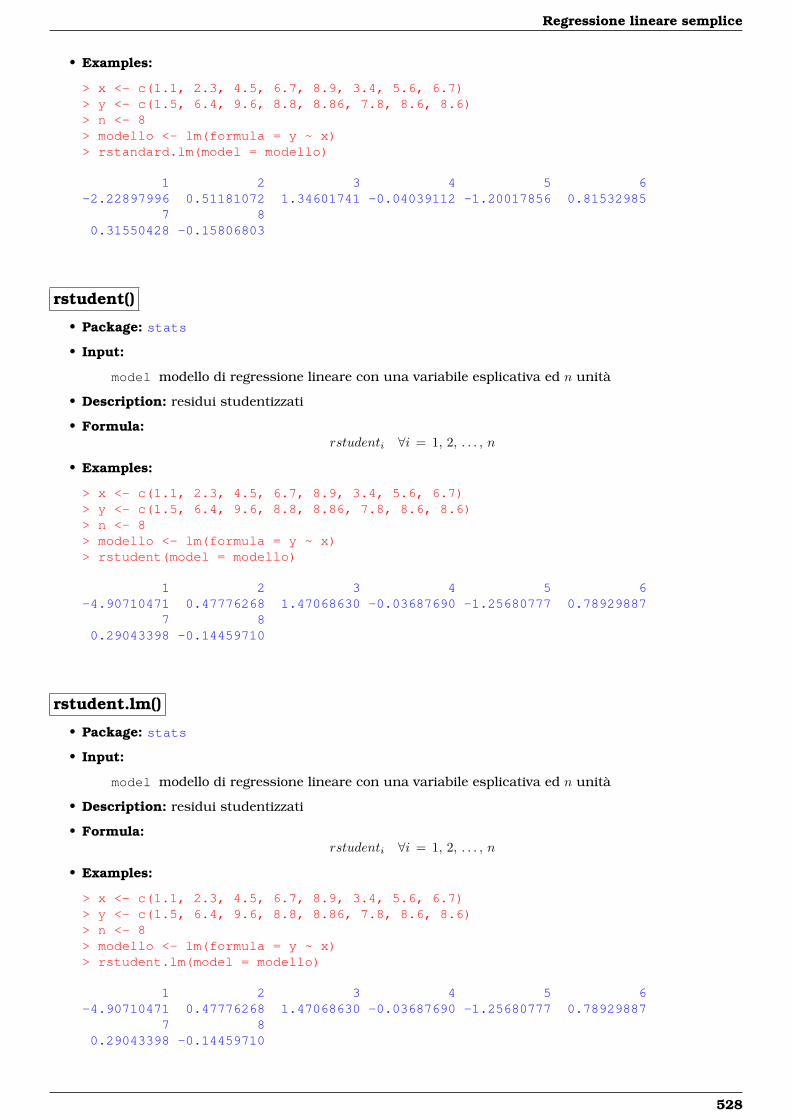
Regressione lineare semplice
• Examples:
> x <- c(1.1, 2.3, 4.5, 6.7, 8.9, 3.4, 5.6, 6.7)> y <- c(1.5, 6.4, 9.6, 8.8, 8.86, 7.8, 8.6, 8.6)> n <- 8> modello <- lm(formula = y ~ x)> rstandard.lm(model = modello)
1 2 3 4 5 6-2.22897996 0.51181072 1.34601741 -0.04039112 -1.20017856 0.81532985
7 80.31550428 -0.15806803
rstudent()
• Package: stats
• Input:
model modello di regressione lineare con una variabile esplicativa ed n unità
• Description: residui studentizzati
• Formula:rstudenti ∀i = 1, 2, . . . , n
• Examples:
> x <- c(1.1, 2.3, 4.5, 6.7, 8.9, 3.4, 5.6, 6.7)> y <- c(1.5, 6.4, 9.6, 8.8, 8.86, 7.8, 8.6, 8.6)> n <- 8> modello <- lm(formula = y ~ x)> rstudent(model = modello)
1 2 3 4 5 6-4.90710471 0.47776268 1.47068630 -0.03687690 -1.25680777 0.78929887
7 80.29043398 -0.14459710
rstudent.lm()
• Package: stats
• Input:
model modello di regressione lineare con una variabile esplicativa ed n unità
• Description: residui studentizzati
• Formula:rstudenti ∀i = 1, 2, . . . , n
• Examples:
> x <- c(1.1, 2.3, 4.5, 6.7, 8.9, 3.4, 5.6, 6.7)> y <- c(1.5, 6.4, 9.6, 8.8, 8.86, 7.8, 8.6, 8.6)> n <- 8> modello <- lm(formula = y ~ x)> rstudent.lm(model = modello)
1 2 3 4 5 6-4.90710471 0.47776268 1.47068630 -0.03687690 -1.25680777 0.78929887
7 80.29043398 -0.14459710
528
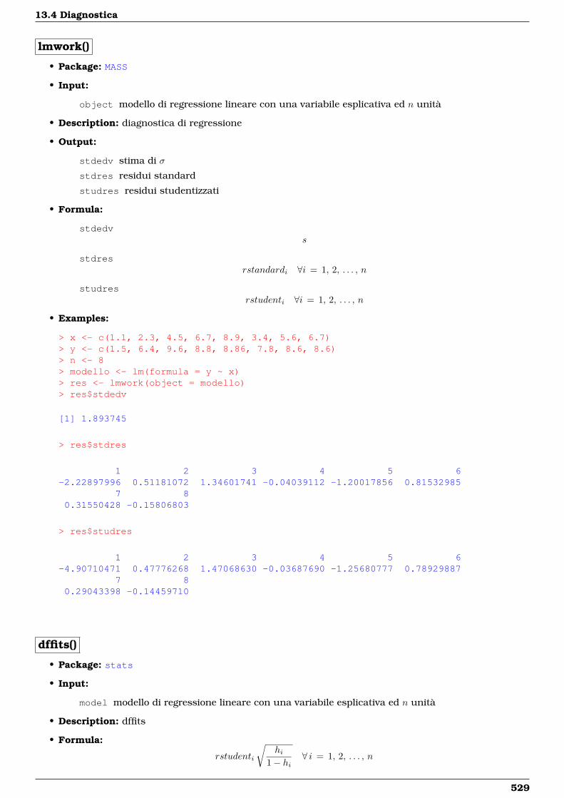
13.4 Diagnostica
lmwork()
• Package: MASS
• Input:
object modello di regressione lineare con una variabile esplicativa ed n unità
• Description: diagnostica di regressione
• Output:
stdedv stima di σ
stdres residui standard
studres residui studentizzati
• Formula:
stdedvs
stdresrstandardi ∀i = 1, 2, . . . , n
studresrstudenti ∀i = 1, 2, . . . , n
• Examples:
> x <- c(1.1, 2.3, 4.5, 6.7, 8.9, 3.4, 5.6, 6.7)> y <- c(1.5, 6.4, 9.6, 8.8, 8.86, 7.8, 8.6, 8.6)> n <- 8> modello <- lm(formula = y ~ x)> res <- lmwork(object = modello)> res$stdedv
[1] 1.893745
> res$stdres
1 2 3 4 5 6-2.22897996 0.51181072 1.34601741 -0.04039112 -1.20017856 0.81532985
7 80.31550428 -0.15806803
> res$studres
1 2 3 4 5 6-4.90710471 0.47776268 1.47068630 -0.03687690 -1.25680777 0.78929887
7 80.29043398 -0.14459710
dffits()
• Package: stats
• Input:
model modello di regressione lineare con una variabile esplicativa ed n unità
• Description: dffits
• Formula:
rstudenti
√hi
1− hi∀ i = 1, 2, . . . , n
529
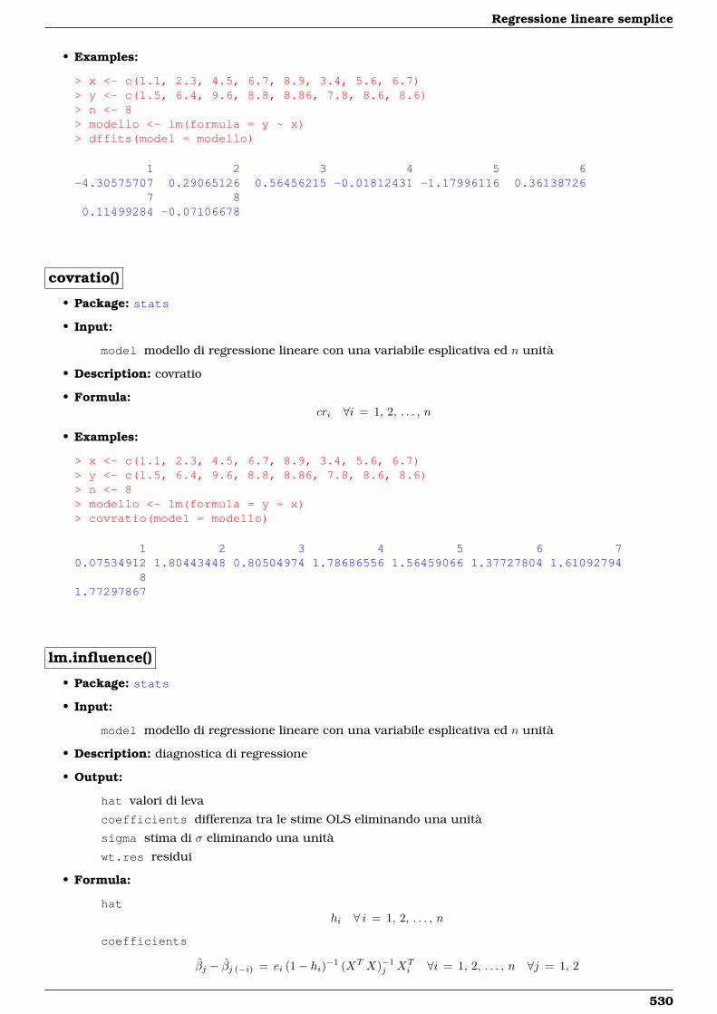
Regressione lineare semplice
• Examples:
> x <- c(1.1, 2.3, 4.5, 6.7, 8.9, 3.4, 5.6, 6.7)> y <- c(1.5, 6.4, 9.6, 8.8, 8.86, 7.8, 8.6, 8.6)> n <- 8> modello <- lm(formula = y ~ x)> dffits(model = modello)
1 2 3 4 5 6-4.30575707 0.29065126 0.56456215 -0.01812431 -1.17996116 0.36138726
7 80.11499284 -0.07106678
covratio()
• Package: stats
• Input:
model modello di regressione lineare con una variabile esplicativa ed n unità
• Description: covratio
• Formula:cri ∀i = 1, 2, . . . , n
• Examples:
> x <- c(1.1, 2.3, 4.5, 6.7, 8.9, 3.4, 5.6, 6.7)> y <- c(1.5, 6.4, 9.6, 8.8, 8.86, 7.8, 8.6, 8.6)> n <- 8> modello <- lm(formula = y ~ x)> covratio(model = modello)
1 2 3 4 5 6 70.07534912 1.80443448 0.80504974 1.78686556 1.56459066 1.37727804 1.61092794
81.77297867
lm.influence()
• Package: stats
• Input:
model modello di regressione lineare con una variabile esplicativa ed n unità
• Description: diagnostica di regressione
• Output:
hat valori di leva
coefficients differenza tra le stime OLS eliminando una unità
sigma stima di σ eliminando una unità
wt.res residui
• Formula:
hathi ∀ i = 1, 2, . . . , n
coefficients
βj − βj (−i) = ei (1− hi)−1 (XT X)−1j XT
i ∀i = 1, 2, . . . , n ∀j = 1, 2
530
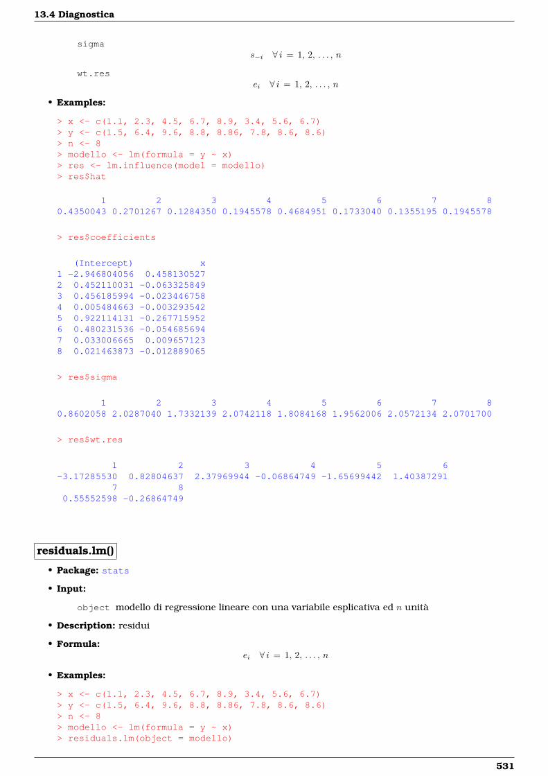
13.4 Diagnostica
sigmas−i ∀ i = 1, 2, . . . , n
wt.resei ∀ i = 1, 2, . . . , n
• Examples:
> x <- c(1.1, 2.3, 4.5, 6.7, 8.9, 3.4, 5.6, 6.7)> y <- c(1.5, 6.4, 9.6, 8.8, 8.86, 7.8, 8.6, 8.6)> n <- 8> modello <- lm(formula = y ~ x)> res <- lm.influence(model = modello)> res$hat
1 2 3 4 5 6 7 80.4350043 0.2701267 0.1284350 0.1945578 0.4684951 0.1733040 0.1355195 0.1945578
> res$coefficients
(Intercept) x1 -2.946804056 0.4581305272 0.452110031 -0.0633258493 0.456185994 -0.0234467584 0.005484663 -0.0032935425 0.922114131 -0.2677159526 0.480231536 -0.0546856947 0.033006665 0.0096571238 0.021463873 -0.012889065
> res$sigma
1 2 3 4 5 6 7 80.8602058 2.0287040 1.7332139 2.0742118 1.8084168 1.9562006 2.0572134 2.0701700
> res$wt.res
1 2 3 4 5 6-3.17285530 0.82804637 2.37969944 -0.06864749 -1.65699442 1.40387291
7 80.55552598 -0.26864749
residuals.lm()
• Package: stats
• Input:
object modello di regressione lineare con una variabile esplicativa ed n unità
• Description: residui
• Formula:ei ∀ i = 1, 2, . . . , n
• Examples:
> x <- c(1.1, 2.3, 4.5, 6.7, 8.9, 3.4, 5.6, 6.7)> y <- c(1.5, 6.4, 9.6, 8.8, 8.86, 7.8, 8.6, 8.6)> n <- 8> modello <- lm(formula = y ~ x)> residuals.lm(object = modello)
531
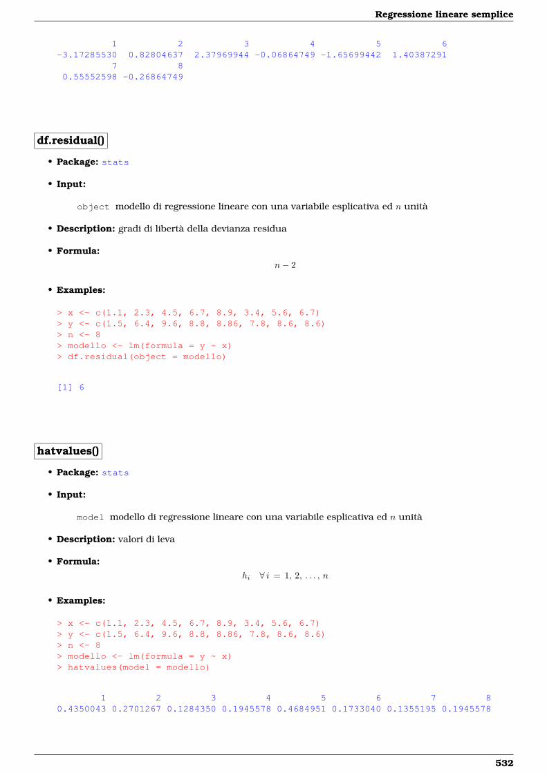
Regressione lineare semplice
1 2 3 4 5 6-3.17285530 0.82804637 2.37969944 -0.06864749 -1.65699442 1.40387291
7 80.55552598 -0.26864749
df.residual()
• Package: stats
• Input:
object modello di regressione lineare con una variabile esplicativa ed n unità
• Description: gradi di libertà della devianza residua
• Formula:n− 2
• Examples:
> x <- c(1.1, 2.3, 4.5, 6.7, 8.9, 3.4, 5.6, 6.7)> y <- c(1.5, 6.4, 9.6, 8.8, 8.86, 7.8, 8.6, 8.6)> n <- 8> modello <- lm(formula = y ~ x)> df.residual(object = modello)
[1] 6
hatvalues()
• Package: stats
• Input:
model modello di regressione lineare con una variabile esplicativa ed n unità
• Description: valori di leva
• Formula:hi ∀ i = 1, 2, . . . , n
• Examples:
> x <- c(1.1, 2.3, 4.5, 6.7, 8.9, 3.4, 5.6, 6.7)> y <- c(1.5, 6.4, 9.6, 8.8, 8.86, 7.8, 8.6, 8.6)> n <- 8> modello <- lm(formula = y ~ x)> hatvalues(model = modello)
1 2 3 4 5 6 7 80.4350043 0.2701267 0.1284350 0.1945578 0.4684951 0.1733040 0.1355195 0.1945578
532
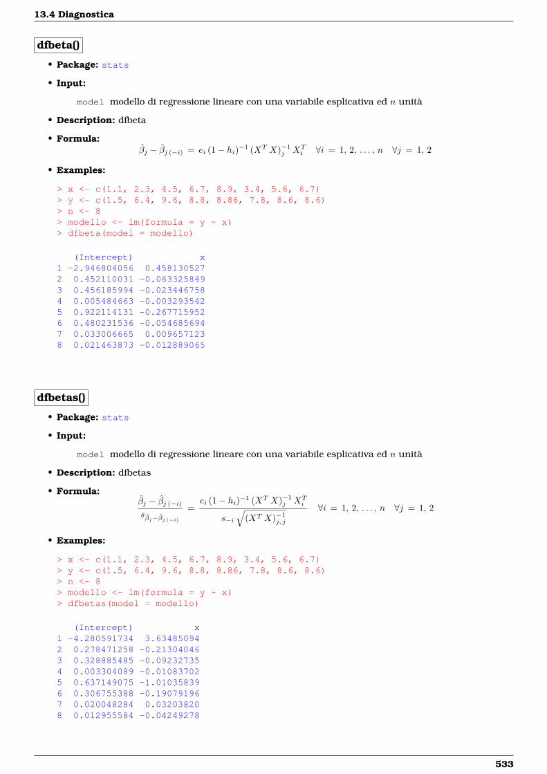
13.4 Diagnostica
dfbeta()
• Package: stats
• Input:
model modello di regressione lineare con una variabile esplicativa ed n unità
• Description: dfbeta
• Formula:βj − βj (−i) = ei (1− hi)−1 (XT X)−1
j XTi ∀i = 1, 2, . . . , n ∀j = 1, 2
• Examples:
> x <- c(1.1, 2.3, 4.5, 6.7, 8.9, 3.4, 5.6, 6.7)> y <- c(1.5, 6.4, 9.6, 8.8, 8.86, 7.8, 8.6, 8.6)> n <- 8> modello <- lm(formula = y ~ x)> dfbeta(model = modello)
(Intercept) x1 -2.946804056 0.4581305272 0.452110031 -0.0633258493 0.456185994 -0.0234467584 0.005484663 -0.0032935425 0.922114131 -0.2677159526 0.480231536 -0.0546856947 0.033006665 0.0096571238 0.021463873 -0.012889065
dfbetas()
• Package: stats
• Input:
model modello di regressione lineare con una variabile esplicativa ed n unità
• Description: dfbetas
• Formula:βj − βj (−i)
sβj−βj (−i)
=ei (1− hi)−1 (XT X)−1
j XTi
s−i
√(XT X)−1
j, j
∀i = 1, 2, . . . , n ∀j = 1, 2
• Examples:
> x <- c(1.1, 2.3, 4.5, 6.7, 8.9, 3.4, 5.6, 6.7)> y <- c(1.5, 6.4, 9.6, 8.8, 8.86, 7.8, 8.6, 8.6)> n <- 8> modello <- lm(formula = y ~ x)> dfbetas(model = modello)
(Intercept) x1 -4.280591734 3.634850942 0.278471258 -0.213040463 0.328885485 -0.092327354 0.003304089 -0.010837025 0.637149075 -1.010358396 0.306755388 -0.190791967 0.020048284 0.032038208 0.012955584 -0.04249278
533
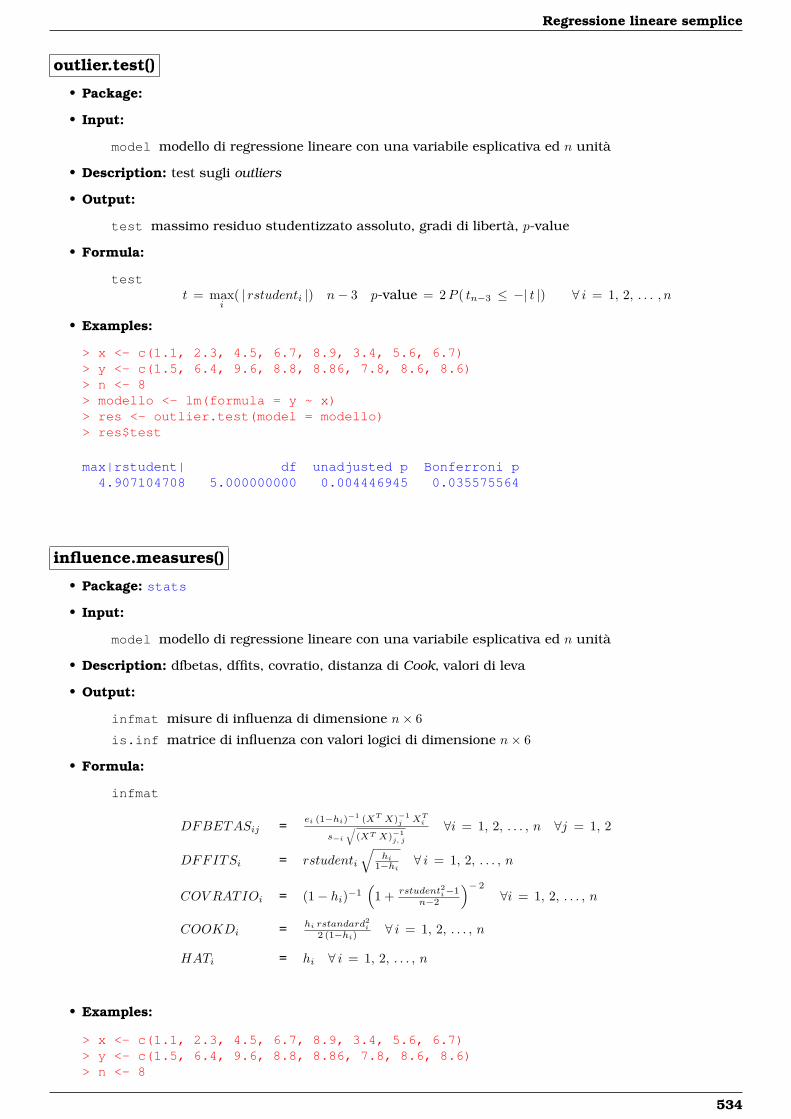
Regressione lineare semplice
outlier.test()
• Package:
• Input:
model modello di regressione lineare con una variabile esplicativa ed n unità
• Description: test sugli outliers
• Output:
test massimo residuo studentizzato assoluto, gradi di libertà, p-value
• Formula:
testt = max
i( | rstudenti |) n− 3 p-value = 2P ( tn−3 ≤ −| t |) ∀ i = 1, 2, . . . , n
• Examples:
> x <- c(1.1, 2.3, 4.5, 6.7, 8.9, 3.4, 5.6, 6.7)> y <- c(1.5, 6.4, 9.6, 8.8, 8.86, 7.8, 8.6, 8.6)> n <- 8> modello <- lm(formula = y ~ x)> res <- outlier.test(model = modello)> res$test
max|rstudent| df unadjusted p Bonferroni p4.907104708 5.000000000 0.004446945 0.035575564
influence.measures()
• Package: stats
• Input:
model modello di regressione lineare con una variabile esplicativa ed n unità
• Description: dfbetas, dffits, covratio, distanza di Cook, valori di leva
• Output:
infmat misure di influenza di dimensione n× 6
is.inf matrice di influenza con valori logici di dimensione n× 6
• Formula:
infmat
DFBETASij =ei (1−hi)−1 (XT X)−1
j XTi
s−i
√(XT X)−1
j, j
∀i = 1, 2, . . . , n ∀j = 1, 2
DFFITSi = rstudenti
√hi
1−hi ∀ i = 1, 2, . . . , n
COV RATIOi = (1− hi)−1(
1 + rstudent2i−1n−2
)− 2
∀i = 1, 2, . . . , n
COOKDi = hi rstandard2i
2 (1−hi) ∀ i = 1, 2, . . . , n
HATi = hi ∀ i = 1, 2, . . . , n
• Examples:
> x <- c(1.1, 2.3, 4.5, 6.7, 8.9, 3.4, 5.6, 6.7)> y <- c(1.5, 6.4, 9.6, 8.8, 8.86, 7.8, 8.6, 8.6)> n <- 8
534
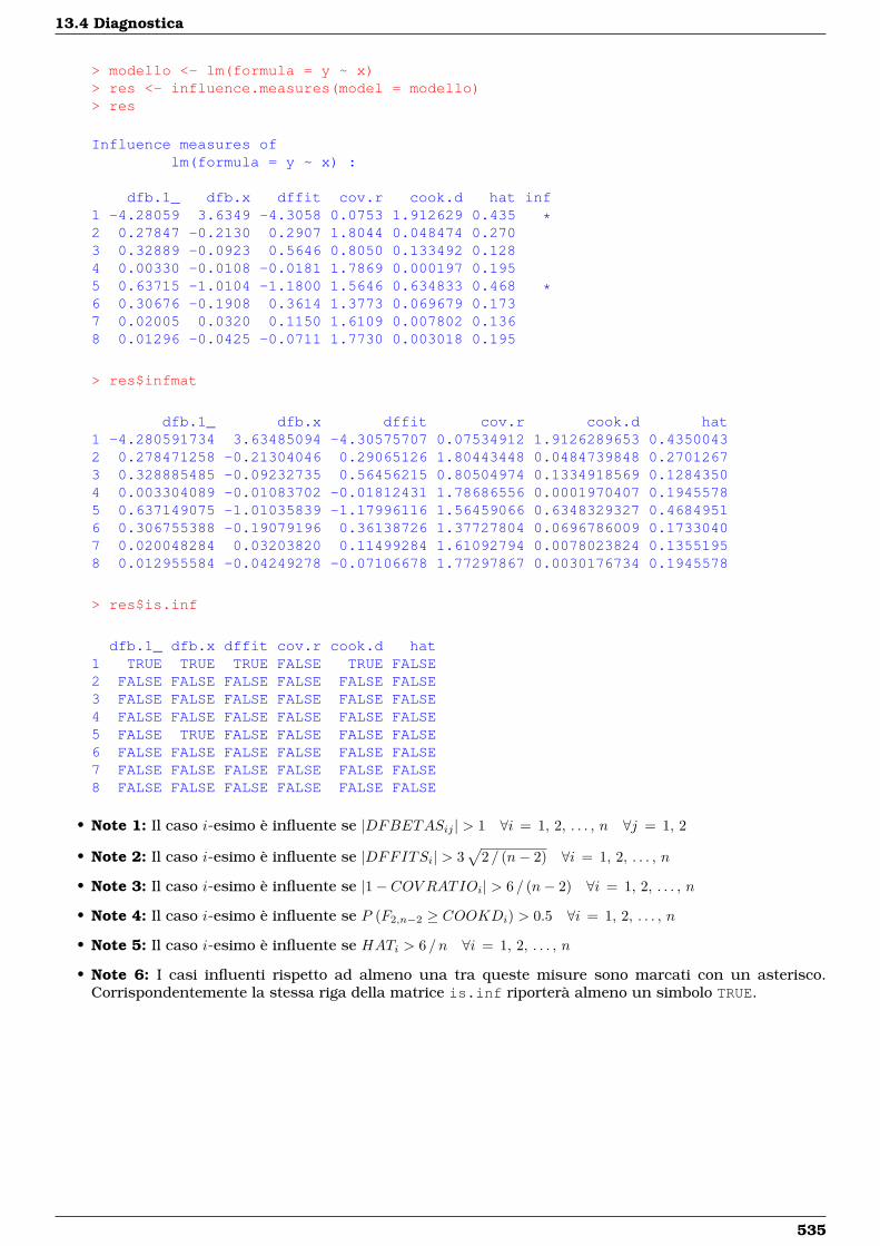
13.4 Diagnostica
> modello <- lm(formula = y ~ x)> res <- influence.measures(model = modello)> res
Influence measures oflm(formula = y ~ x) :
dfb.1_ dfb.x dffit cov.r cook.d hat inf1 -4.28059 3.6349 -4.3058 0.0753 1.912629 0.435 *2 0.27847 -0.2130 0.2907 1.8044 0.048474 0.2703 0.32889 -0.0923 0.5646 0.8050 0.133492 0.1284 0.00330 -0.0108 -0.0181 1.7869 0.000197 0.1955 0.63715 -1.0104 -1.1800 1.5646 0.634833 0.468 *6 0.30676 -0.1908 0.3614 1.3773 0.069679 0.1737 0.02005 0.0320 0.1150 1.6109 0.007802 0.1368 0.01296 -0.0425 -0.0711 1.7730 0.003018 0.195
> res$infmat
dfb.1_ dfb.x dffit cov.r cook.d hat1 -4.280591734 3.63485094 -4.30575707 0.07534912 1.9126289653 0.43500432 0.278471258 -0.21304046 0.29065126 1.80443448 0.0484739848 0.27012673 0.328885485 -0.09232735 0.56456215 0.80504974 0.1334918569 0.12843504 0.003304089 -0.01083702 -0.01812431 1.78686556 0.0001970407 0.19455785 0.637149075 -1.01035839 -1.17996116 1.56459066 0.6348329327 0.46849516 0.306755388 -0.19079196 0.36138726 1.37727804 0.0696786009 0.17330407 0.020048284 0.03203820 0.11499284 1.61092794 0.0078023824 0.13551958 0.012955584 -0.04249278 -0.07106678 1.77297867 0.0030176734 0.1945578
> res$is.inf
dfb.1_ dfb.x dffit cov.r cook.d hat1 TRUE TRUE TRUE FALSE TRUE FALSE2 FALSE FALSE FALSE FALSE FALSE FALSE3 FALSE FALSE FALSE FALSE FALSE FALSE4 FALSE FALSE FALSE FALSE FALSE FALSE5 FALSE TRUE FALSE FALSE FALSE FALSE6 FALSE FALSE FALSE FALSE FALSE FALSE7 FALSE FALSE FALSE FALSE FALSE FALSE8 FALSE FALSE FALSE FALSE FALSE FALSE
• Note 1: Il caso i-esimo è influente se |DFBETASij | > 1 ∀i = 1, 2, . . . , n ∀j = 1, 2
• Note 2: Il caso i-esimo è influente se |DFFITSi| > 3√
2 / (n− 2) ∀i = 1, 2, . . . , n
• Note 3: Il caso i-esimo è influente se |1− COV RATIOi| > 6 / (n− 2) ∀i = 1, 2, . . . , n
• Note 4: Il caso i-esimo è influente se P (F2,n−2 ≥ COOKDi) > 0.5 ∀i = 1, 2, . . . , n
• Note 5: Il caso i-esimo è influente se HATi > 6 / n ∀i = 1, 2, . . . , n
• Note 6: I casi influenti rispetto ad almeno una tra queste misure sono marcati con un asterisco.Corrispondentemente la stessa riga della matrice is.inf riporterà almeno un simbolo TRUE.
535

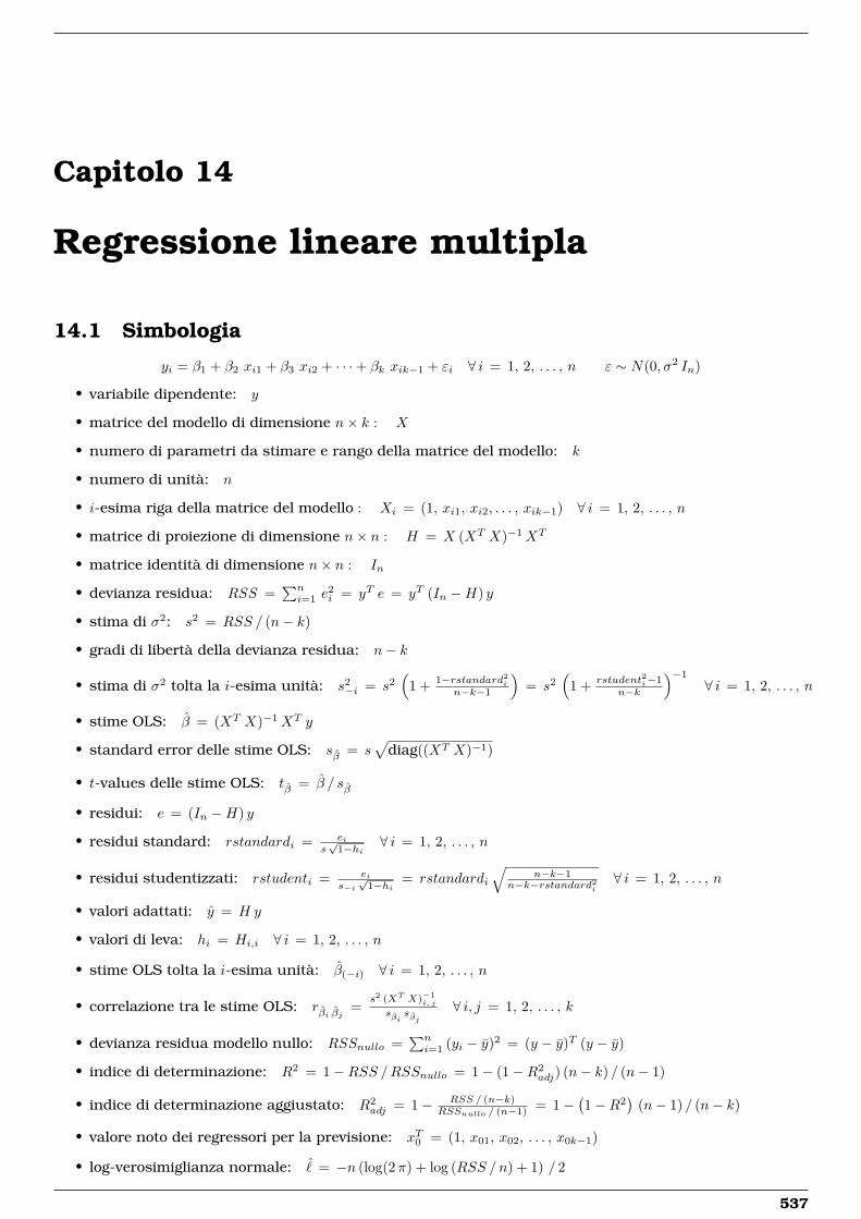
Capitolo 14
Regressione lineare multipla
14.1 Simbologia
yi = β1 + β2 xi1 + β3 xi2 + · · ·+ βk xik−1 + εi ∀ i = 1, 2, . . . , n ε ∼ N(0, σ2 In)
• variabile dipendente: y
• matrice del modello di dimensione n× k : X
• numero di parametri da stimare e rango della matrice del modello: k
• numero di unità: n
• i-esima riga della matrice del modello : Xi = (1, xi1, xi2, . . . , xik−1) ∀ i = 1, 2, . . . , n
• matrice di proiezione di dimensione n× n : H = X (XT X)−1XT
• matrice identità di dimensione n× n : In
• devianza residua: RSS =∑ni=1 e
2i = yT e = yT (In −H) y
• stima di σ2: s2 = RSS / (n− k)
• gradi di libertà della devianza residua: n− k
• stima di σ2 tolta la i-esima unità: s2−i = s2
(1 + 1−rstandard2i
n−k−1
)= s2
(1 + rstudent2i−1
n−k
)−1
∀ i = 1, 2, . . . , n
• stime OLS: β = (XT X)−1XT y
• standard error delle stime OLS: sβ = s√
diag((XT X)−1)
• t-values delle stime OLS: tβ = β / sβ
• residui: e = (In −H) y
• residui standard: rstandardi = eis√
1−hi∀ i = 1, 2, . . . , n
• residui studentizzati: rstudenti = eis−i√
1−hi= rstandardi
√n−k−1
n−k−rstandard2i∀ i = 1, 2, . . . , n
• valori adattati: y = H y
• valori di leva: hi = Hi,i ∀ i = 1, 2, . . . , n
• stime OLS tolta la i-esima unità: β(−i) ∀ i = 1, 2, . . . , n
• correlazione tra le stime OLS: rβi βj =s2 (XT X)−1
i, j
sβisβj
∀ i, j = 1, 2, . . . , k
• devianza residua modello nullo: RSSnullo =∑ni=1 (yi − y)2 = (y − y)T (y − y)
• indice di determinazione: R2 = 1−RSS /RSSnullo = 1− (1−R2adj) (n− k) / (n− 1)
• indice di determinazione aggiustato: R2adj = 1− RSS / (n−k)
RSSnullo / (n−1) = 1−(1−R2
)(n− 1) / (n− k)
• valore noto dei regressori per la previsione: xT0 = (1, x01, x02, . . . , x0k−1)
• log-verosimiglianza normale: ˆ = −n (log(2π) + log (RSS /n) + 1) / 2
537
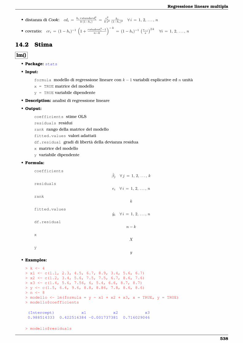
Regressione lineare multipla
• distanza di Cook: cdi = hi rstandard2i
k (1−hi) = e2ik s2
hi(1−hi)2 ∀ i = 1, 2, . . . , n
• covratio: cri = (1− hi)−1(
1 + rstudent2i−1n−k
)− k= (1− hi)−1
( s−is
)2 k ∀i = 1, 2, . . . , n
14.2 Stima
lm()
• Package: stats
• Input:
formula modello di regressione lineare con k − 1 variabili esplicative ed n unità
x = TRUE matrice del modello
y = TRUE variabile dipendente
• Description: analisi di regressione lineare
• Output:
coefficients stime OLS
residuals residui
rank rango della matrice del modello
fitted.values valori adattati
df.residual gradi di libertà della devianza residua
x matrice del modello
y variabile dipendente
• Formula:
coefficientsβj ∀ j = 1, 2, . . . , k
residualsei ∀ i = 1, 2, . . . , n
rankk
fitted.valuesyi ∀ i = 1, 2, . . . , n
df.residualn− k
xX
yy
• Examples:
> k <- 4> x1 <- c(1.1, 2.3, 4.5, 6.7, 8.9, 3.4, 5.6, 6.7)> x2 <- c(1.2, 3.4, 5.6, 7.5, 7.5, 6.7, 8.6, 7.6)> x3 <- c(1.4, 5.6, 7.56, 6, 5.4, 6.6, 8.7, 8.7)> y <- c(1.5, 6.4, 9.6, 8.8, 8.86, 7.8, 8.6, 8.6)> n <- 8> modello <- lm(formula = y ~ x1 + x2 + x3, x = TRUE, y = TRUE)> modello$coefficients
(Intercept) x1 x2 x30.988514333 0.422516384 -0.001737381 0.716029046
> modello$residuals
538

14.2 Stima
1 2 3 4 5 6 7-0.9536382 0.4358424 1.3067117 0.6974820 0.2575634 0.6607787 -0.9691173
8-1.4356227
> modello$rank
[1] 4
> modello$fitted.values
1 2 3 4 5 6 7 82.453638 5.964158 8.293288 8.102518 8.602437 7.139221 9.569117 10.035623
> modello$df.residual
[1] 4
> modello$x
(Intercept) x1 x2 x31 1 1.1 1.2 1.402 1 2.3 3.4 5.603 1 4.5 5.6 7.564 1 6.7 7.5 6.005 1 8.9 7.5 5.406 1 3.4 6.7 6.607 1 5.6 8.6 8.708 1 6.7 7.6 8.70attr(,"assign")[1] 0 1 2 3
> modello$y
1 2 3 4 5 6 7 81.50 6.40 9.60 8.80 8.86 7.80 8.60 8.60
• Note 1: Il modello nullo si ottiene con lm(formula = y ~ 1).
• Note 2: L’istruzione update(object = y ~ x1 + x2,formula = . ~ . + x3) è esattamente equi-valente a lm(formula = y ~ x1 + x2 + x3).
• Note 3: In seguito ad una modifica come ad esempio x1[3] <- 1.2, conviene adoperare il comandoupdate(modello) anziché ripetere modello <- lm(formula = y ~ x1 + x2 + x3) .
• Note 4: L’operatore I() permette di poter modellare regressioni lineari polinomiali. Per un polinomiodi terzo grado occorre scrivere lm(formula = y ~ x + I(x^2) + I(x^3)).
• Note 5: Per regressioni polinomiali occorre usare il comando poly(). Per un polinomio di quarto gradooccorre scrivere lm(formula = y ~ poly(x,degree = 4,raw = TRUE)).
• Note 6: Per regressioni polinomiali ortogonali occorre usare il comando poly(). Per un polinomioortogonale di quarto grado occorre scrivere lm(formula = y ~ poly(x,degree = 4)).
• Note 7: Il comando lm(formula = y ~ x1 + x2) è equivalente a lm(formula = y ~ X-1).
• Note 8: Il comando lm(formula = y ~ x1 + x2) è equivalente a lm(formula = y ~ 1 + x1 + x2).
539
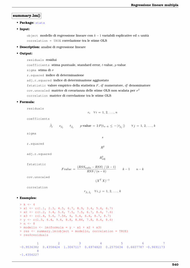
Regressione lineare multipla
summary.lm()
• Package: stats
• Input:
object modello di regressione lineare con k − 1 variabili esplicative ed n unità
correlation = TRUE correlazione tra le stime OLS
• Description: analisi di regressione lineare
• Output:
residuals residui
coefficients stima puntuale, standard error, t-value, p-value
sigma stima di σ
r.squared indice di determinazione
adj.r.squared indice di determinazione aggiustato
fstatistic valore empirico della statistica F , df numeratore, df denominatore
cov.unscaled matrice di covarianza delle stime OLS non scalata per σ2
correlation matrice di correlazione tra le stime OLS
• Formula:
residualsei ∀ i = 1, 2, . . . , n
coefficients
βj sβj tβj p-value = 2P (tn−k ≤ − | tβj |) ∀ j = 1, 2, . . . , k
sigmas
r.squaredR2
adj.r.squaredR2adj
fstatistic
Fvalue =(RSSnullo −RSS) / (k − 1)
RSS / (n− k)k − 1 n− k
cov.unscaled(XT X)−1
correlationrβi βj ∀ i, j = 1, 2, . . . , k
• Examples:
> k <- 4> x1 <- c(1.1, 2.3, 4.5, 6.7, 8.9, 3.4, 5.6, 6.7)> x2 <- c(1.2, 3.4, 5.6, 7.5, 7.5, 6.7, 8.6, 7.6)> x3 <- c(1.4, 5.6, 7.56, 6, 5.4, 6.6, 8.7, 8.7)> y <- c(1.5, 6.4, 9.6, 8.8, 8.86, 7.8, 8.6, 8.6)> n <- 8> modello <- lm(formula = y ~ x1 + x2 + x3)> res <- summary.lm(object = modello, correlation = TRUE)> res$residuals
1 2 3 4 5 6 7-0.9536382 0.4358424 1.3067117 0.6974820 0.2575634 0.6607787 -0.9691173
8-1.4356227
540
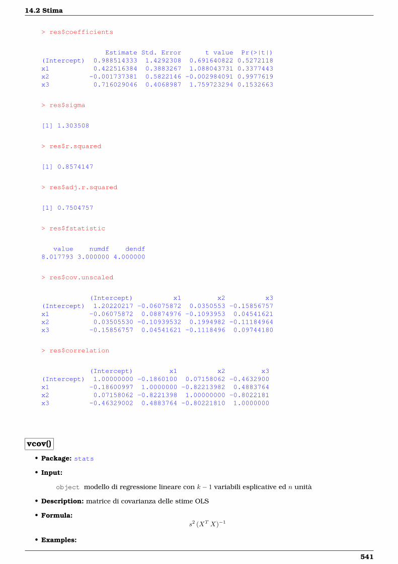
14.2 Stima
> res$coefficients
Estimate Std. Error t value Pr(>|t|)(Intercept) 0.988514333 1.4292308 0.691640822 0.5272118x1 0.422516384 0.3883267 1.088043731 0.3377443x2 -0.001737381 0.5822146 -0.002984091 0.9977619x3 0.716029046 0.4068987 1.759723294 0.1532663
> res$sigma
[1] 1.303508
> res$r.squared
[1] 0.8574147
> res$adj.r.squared
[1] 0.7504757
> res$fstatistic
value numdf dendf8.017793 3.000000 4.000000
> res$cov.unscaled
(Intercept) x1 x2 x3(Intercept) 1.20220217 -0.06075872 0.0350553 -0.15856757x1 -0.06075872 0.08874976 -0.1093953 0.04541621x2 0.03505530 -0.10939532 0.1994982 -0.11184964x3 -0.15856757 0.04541621 -0.1118496 0.09744180
> res$correlation
(Intercept) x1 x2 x3(Intercept) 1.00000000 -0.1860100 0.07158062 -0.4632900x1 -0.18600997 1.0000000 -0.82213982 0.4883764x2 0.07158062 -0.8221398 1.00000000 -0.8022181x3 -0.46329002 0.4883764 -0.80221810 1.0000000
vcov()
• Package: stats
• Input:
object modello di regressione lineare con k − 1 variabili esplicative ed n unità
• Description: matrice di covarianza delle stime OLS
• Formula:s2 (XT X)−1
• Examples:
541
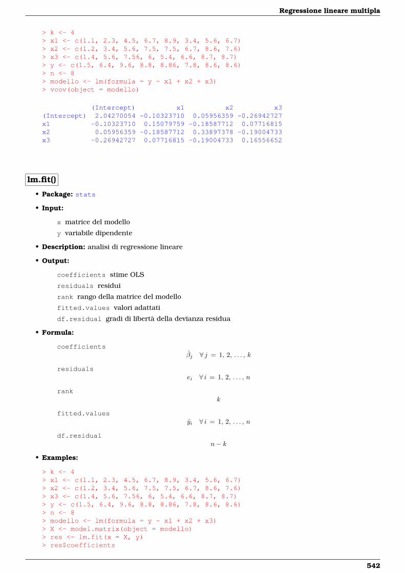
Regressione lineare multipla
> k <- 4> x1 <- c(1.1, 2.3, 4.5, 6.7, 8.9, 3.4, 5.6, 6.7)> x2 <- c(1.2, 3.4, 5.6, 7.5, 7.5, 6.7, 8.6, 7.6)> x3 <- c(1.4, 5.6, 7.56, 6, 5.4, 6.6, 8.7, 8.7)> y <- c(1.5, 6.4, 9.6, 8.8, 8.86, 7.8, 8.6, 8.6)> n <- 8> modello <- lm(formula = y ~ x1 + x2 + x3)> vcov(object = modello)
(Intercept) x1 x2 x3(Intercept) 2.04270054 -0.10323710 0.05956359 -0.26942727x1 -0.10323710 0.15079759 -0.18587712 0.07716815x2 0.05956359 -0.18587712 0.33897378 -0.19004733x3 -0.26942727 0.07716815 -0.19004733 0.16556652
lm.fit()
• Package: stats
• Input:
x matrice del modello
y variabile dipendente
• Description: analisi di regressione lineare
• Output:
coefficients stime OLS
residuals residui
rank rango della matrice del modello
fitted.values valori adattati
df.residual gradi di libertà della devianza residua
• Formula:
coefficientsβj ∀ j = 1, 2, . . . , k
residualsei ∀ i = 1, 2, . . . , n
rankk
fitted.valuesyi ∀ i = 1, 2, . . . , n
df.residualn− k
• Examples:
> k <- 4> x1 <- c(1.1, 2.3, 4.5, 6.7, 8.9, 3.4, 5.6, 6.7)> x2 <- c(1.2, 3.4, 5.6, 7.5, 7.5, 6.7, 8.6, 7.6)> x3 <- c(1.4, 5.6, 7.56, 6, 5.4, 6.6, 8.7, 8.7)> y <- c(1.5, 6.4, 9.6, 8.8, 8.86, 7.8, 8.6, 8.6)> n <- 8> modello <- lm(formula = y ~ x1 + x2 + x3)> X <- model.matrix(object = modello)> res <- lm.fit(x = X, y)> res$coefficients
542
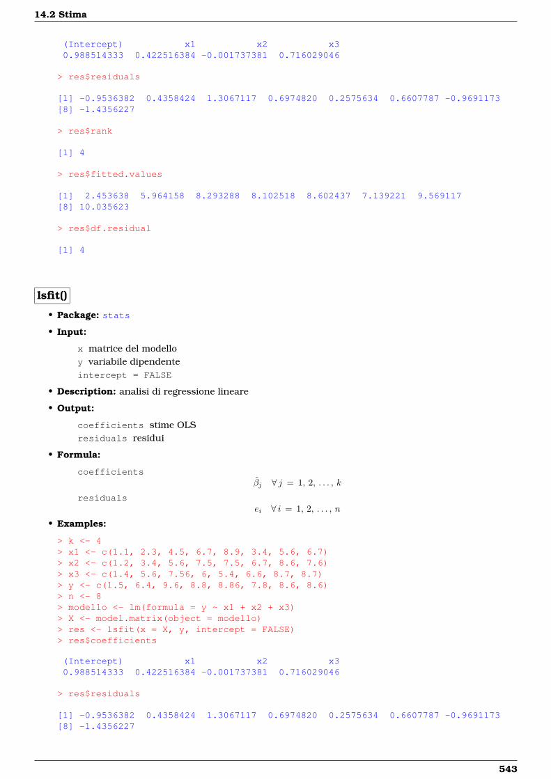
14.2 Stima
(Intercept) x1 x2 x30.988514333 0.422516384 -0.001737381 0.716029046
> res$residuals
[1] -0.9536382 0.4358424 1.3067117 0.6974820 0.2575634 0.6607787 -0.9691173[8] -1.4356227
> res$rank
[1] 4
> res$fitted.values
[1] 2.453638 5.964158 8.293288 8.102518 8.602437 7.139221 9.569117[8] 10.035623
> res$df.residual
[1] 4
lsfit()
• Package: stats
• Input:
x matrice del modelloy variabile dipendenteintercept = FALSE
• Description: analisi di regressione lineare
• Output:
coefficients stime OLSresiduals residui
• Formula:
coefficientsβj ∀ j = 1, 2, . . . , k
residualsei ∀ i = 1, 2, . . . , n
• Examples:
> k <- 4> x1 <- c(1.1, 2.3, 4.5, 6.7, 8.9, 3.4, 5.6, 6.7)> x2 <- c(1.2, 3.4, 5.6, 7.5, 7.5, 6.7, 8.6, 7.6)> x3 <- c(1.4, 5.6, 7.56, 6, 5.4, 6.6, 8.7, 8.7)> y <- c(1.5, 6.4, 9.6, 8.8, 8.86, 7.8, 8.6, 8.6)> n <- 8> modello <- lm(formula = y ~ x1 + x2 + x3)> X <- model.matrix(object = modello)> res <- lsfit(x = X, y, intercept = FALSE)> res$coefficients
(Intercept) x1 x2 x30.988514333 0.422516384 -0.001737381 0.716029046
> res$residuals
[1] -0.9536382 0.4358424 1.3067117 0.6974820 0.2575634 0.6607787 -0.9691173[8] -1.4356227
543
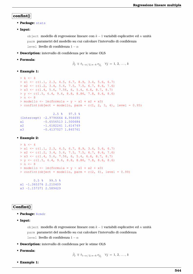
Regressione lineare multipla
confint()
• Package: stats
• Input:
object modello di regressione lineare con k − 1 variabili esplicative ed n unità
parm parametri del modello su cui calcolare l’intervallo di confidenza
level livello di confidenza 1− α
• Description: intervallo di confidenza per le stime OLS
• Formula:βj ∓ t1−α/ 2, n−k sβj ∀j = 1, 2, . . . , k
• Example 1:
> k <- 4> x1 <- c(1.1, 2.3, 4.5, 6.7, 8.9, 3.4, 5.6, 6.7)> x2 <- c(1.2, 3.4, 5.6, 7.5, 7.5, 6.7, 8.6, 7.6)> x3 <- c(1.4, 5.6, 7.56, 6, 5.4, 6.6, 8.7, 8.7)> y <- c(1.5, 6.4, 9.6, 8.8, 8.86, 7.8, 8.6, 8.6)> n <- 8> modello <- lm(formula = y ~ x1 + x2 + x3)> confint(object = modello, parm = c(1, 2, 3, 4), level = 0.95)
2.5 % 97.5 %(Intercept) -2.9796664 4.956695x1 -0.6556513 1.500684x2 -1.6182241 1.614749x3 -0.4137027 1.845761
• Example 2:
> k <- 4> x1 <- c(1.1, 2.3, 4.5, 6.7, 8.9, 3.4, 5.6, 6.7)> x2 <- c(1.2, 3.4, 5.6, 7.5, 7.5, 6.7, 8.6, 7.6)> x3 <- c(1.4, 5.6, 7.56, 6, 5.4, 6.6, 8.7, 8.7)> y <- c(1.5, 6.4, 9.6, 8.8, 8.86, 7.8, 8.6, 8.6)> n <- 8> modello <- lm(formula = y ~ x1 + x2 + x3)> confint(object = modello, parm = c(2, 4), level = 0.99)
0.5 % 99.5 %x1 -1.365376 2.210409x3 -1.157371 2.589429
Confint()
• Package: Rcmdr
• Input:
object modello di regressione lineare con k − 1 variabili esplicative ed n unità
parm parametri del modello su cui calcolare l’intervallo di confidenza
level livello di confidenza 1− α
• Description: intervallo di confidenza per le stime OLS
• Formula:βj ∓ t1−α/ 2, n−k sβj ∀j = 1, 2, . . . , k
• Example 1:
544
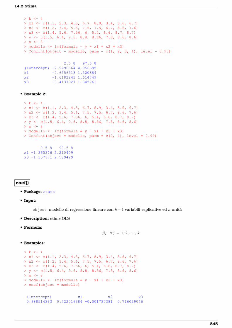
14.2 Stima
> k <- 4> x1 <- c(1.1, 2.3, 4.5, 6.7, 8.9, 3.4, 5.6, 6.7)> x2 <- c(1.2, 3.4, 5.6, 7.5, 7.5, 6.7, 8.6, 7.6)> x3 <- c(1.4, 5.6, 7.56, 6, 5.4, 6.6, 8.7, 8.7)> y <- c(1.5, 6.4, 9.6, 8.8, 8.86, 7.8, 8.6, 8.6)> n <- 8> modello <- lm(formula = y ~ x1 + x2 + x3)> Confint(object = modello, parm = c(1, 2, 3, 4), level = 0.95)
2.5 % 97.5 %(Intercept) -2.9796664 4.956695x1 -0.6556513 1.500684x2 -1.6182241 1.614749x3 -0.4137027 1.845761
• Example 2:
> k <- 4> x1 <- c(1.1, 2.3, 4.5, 6.7, 8.9, 3.4, 5.6, 6.7)> x2 <- c(1.2, 3.4, 5.6, 7.5, 7.5, 6.7, 8.6, 7.6)> x3 <- c(1.4, 5.6, 7.56, 6, 5.4, 6.6, 8.7, 8.7)> y <- c(1.5, 6.4, 9.6, 8.8, 8.86, 7.8, 8.6, 8.6)> n <- 8> modello <- lm(formula = y ~ x1 + x2 + x3)> Confint(object = modello, parm = c(2, 4), level = 0.99)
0.5 % 99.5 %x1 -1.365376 2.210409x3 -1.157371 2.589429
coef()
• Package: stats
• Input:
object modello di regressione lineare con k − 1 variabili esplicative ed n unità
• Description: stime OLS
• Formula:βj ∀ j = 1, 2, . . . , k
• Examples:
> k <- 4> x1 <- c(1.1, 2.3, 4.5, 6.7, 8.9, 3.4, 5.6, 6.7)> x2 <- c(1.2, 3.4, 5.6, 7.5, 7.5, 6.7, 8.6, 7.6)> x3 <- c(1.4, 5.6, 7.56, 6, 5.4, 6.6, 8.7, 8.7)> y <- c(1.5, 6.4, 9.6, 8.8, 8.86, 7.8, 8.6, 8.6)> n <- 8> modello <- lm(formula = y ~ x1 + x2 + x3)> coef(object = modello)
(Intercept) x1 x2 x30.988514333 0.422516384 -0.001737381 0.716029046
545
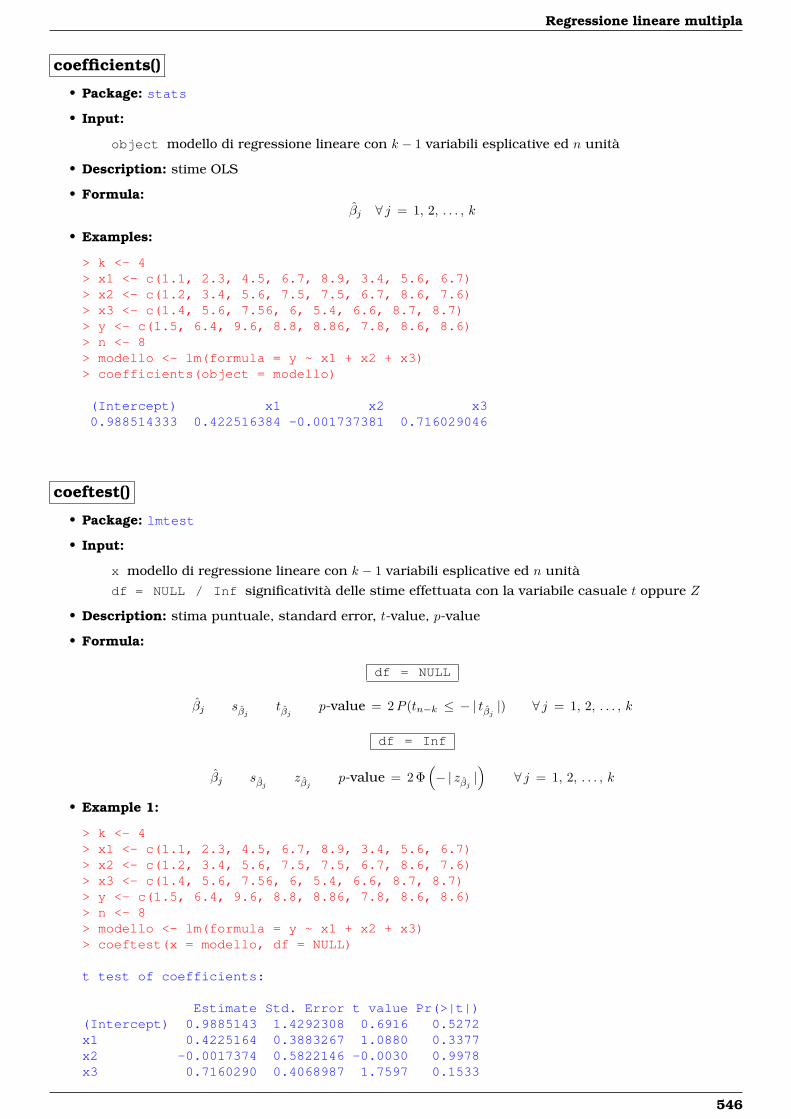
Regressione lineare multipla
coefficients()
• Package: stats
• Input:
object modello di regressione lineare con k − 1 variabili esplicative ed n unità
• Description: stime OLS
• Formula:βj ∀ j = 1, 2, . . . , k
• Examples:
> k <- 4> x1 <- c(1.1, 2.3, 4.5, 6.7, 8.9, 3.4, 5.6, 6.7)> x2 <- c(1.2, 3.4, 5.6, 7.5, 7.5, 6.7, 8.6, 7.6)> x3 <- c(1.4, 5.6, 7.56, 6, 5.4, 6.6, 8.7, 8.7)> y <- c(1.5, 6.4, 9.6, 8.8, 8.86, 7.8, 8.6, 8.6)> n <- 8> modello <- lm(formula = y ~ x1 + x2 + x3)> coefficients(object = modello)
(Intercept) x1 x2 x30.988514333 0.422516384 -0.001737381 0.716029046
coeftest()
• Package: lmtest
• Input:
x modello di regressione lineare con k − 1 variabili esplicative ed n unità
df = NULL / Inf significatività delle stime effettuata con la variabile casuale t oppure Z
• Description: stima puntuale, standard error, t-value, p-value
• Formula:
df = NULL
βj sβj tβj p-value = 2P (tn−k ≤ − | tβj |) ∀ j = 1, 2, . . . , k
df = Inf
βj sβj zβj p-value = 2 Φ(− | zβj |
)∀ j = 1, 2, . . . , k
• Example 1:
> k <- 4> x1 <- c(1.1, 2.3, 4.5, 6.7, 8.9, 3.4, 5.6, 6.7)> x2 <- c(1.2, 3.4, 5.6, 7.5, 7.5, 6.7, 8.6, 7.6)> x3 <- c(1.4, 5.6, 7.56, 6, 5.4, 6.6, 8.7, 8.7)> y <- c(1.5, 6.4, 9.6, 8.8, 8.86, 7.8, 8.6, 8.6)> n <- 8> modello <- lm(formula = y ~ x1 + x2 + x3)> coeftest(x = modello, df = NULL)
t test of coefficients:
Estimate Std. Error t value Pr(>|t|)(Intercept) 0.9885143 1.4292308 0.6916 0.5272x1 0.4225164 0.3883267 1.0880 0.3377x2 -0.0017374 0.5822146 -0.0030 0.9978x3 0.7160290 0.4068987 1.7597 0.1533
546
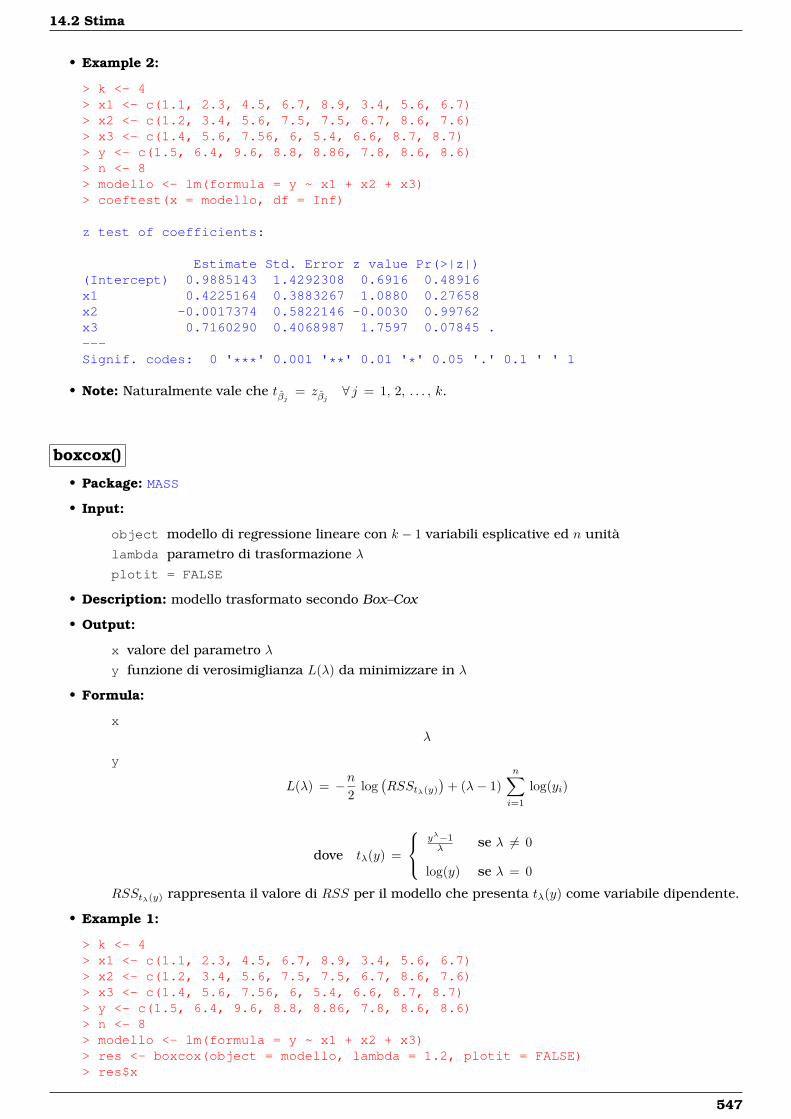
14.2 Stima
• Example 2:
> k <- 4> x1 <- c(1.1, 2.3, 4.5, 6.7, 8.9, 3.4, 5.6, 6.7)> x2 <- c(1.2, 3.4, 5.6, 7.5, 7.5, 6.7, 8.6, 7.6)> x3 <- c(1.4, 5.6, 7.56, 6, 5.4, 6.6, 8.7, 8.7)> y <- c(1.5, 6.4, 9.6, 8.8, 8.86, 7.8, 8.6, 8.6)> n <- 8> modello <- lm(formula = y ~ x1 + x2 + x3)> coeftest(x = modello, df = Inf)
z test of coefficients:
Estimate Std. Error z value Pr(>|z|)(Intercept) 0.9885143 1.4292308 0.6916 0.48916x1 0.4225164 0.3883267 1.0880 0.27658x2 -0.0017374 0.5822146 -0.0030 0.99762x3 0.7160290 0.4068987 1.7597 0.07845 .---Signif. codes: 0 '***' 0.001 '**' 0.01 '*' 0.05 '.' 0.1 ' ' 1
• Note: Naturalmente vale che tβj = zβj ∀ j = 1, 2, . . . , k.
boxcox()
• Package: MASS
• Input:
object modello di regressione lineare con k − 1 variabili esplicative ed n unità
lambda parametro di trasformazione λ
plotit = FALSE
• Description: modello trasformato secondo Box–Cox
• Output:
x valore del parametro λ
y funzione di verosimiglianza L(λ) da minimizzare in λ
• Formula:
xλ
y
L(λ) = −n2
log(RSStλ(y)
)+ (λ− 1)
n∑i=1
log(yi)
dove tλ(y) =
yλ−1λ se λ 6= 0
log(y) se λ = 0
RSStλ(y) rappresenta il valore di RSS per il modello che presenta tλ(y) come variabile dipendente.
• Example 1:
> k <- 4> x1 <- c(1.1, 2.3, 4.5, 6.7, 8.9, 3.4, 5.6, 6.7)> x2 <- c(1.2, 3.4, 5.6, 7.5, 7.5, 6.7, 8.6, 7.6)> x3 <- c(1.4, 5.6, 7.56, 6, 5.4, 6.6, 8.7, 8.7)> y <- c(1.5, 6.4, 9.6, 8.8, 8.86, 7.8, 8.6, 8.6)> n <- 8> modello <- lm(formula = y ~ x1 + x2 + x3)> res <- boxcox(object = modello, lambda = 1.2, plotit = FALSE)> res$x
547
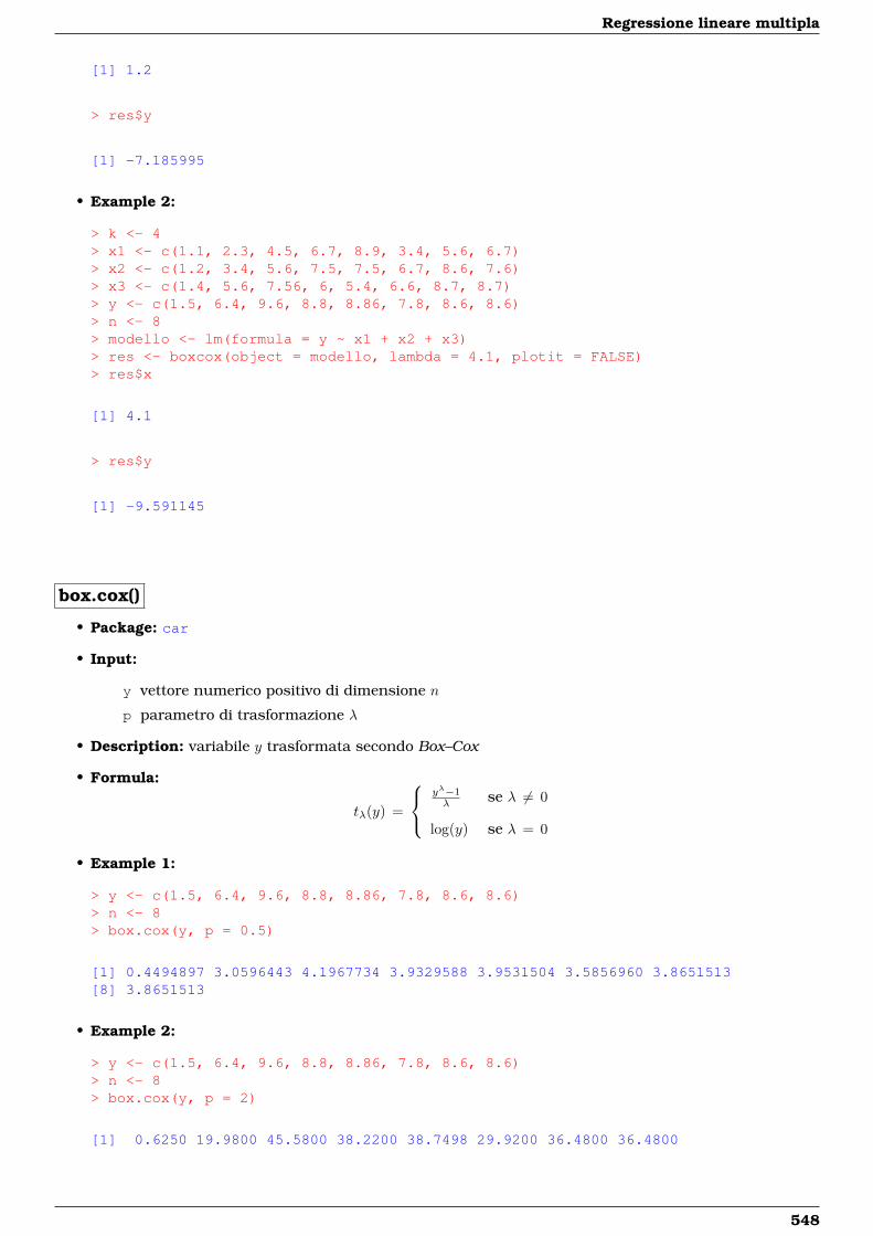
Regressione lineare multipla
[1] 1.2
> res$y
[1] -7.185995
• Example 2:
> k <- 4> x1 <- c(1.1, 2.3, 4.5, 6.7, 8.9, 3.4, 5.6, 6.7)> x2 <- c(1.2, 3.4, 5.6, 7.5, 7.5, 6.7, 8.6, 7.6)> x3 <- c(1.4, 5.6, 7.56, 6, 5.4, 6.6, 8.7, 8.7)> y <- c(1.5, 6.4, 9.6, 8.8, 8.86, 7.8, 8.6, 8.6)> n <- 8> modello <- lm(formula = y ~ x1 + x2 + x3)> res <- boxcox(object = modello, lambda = 4.1, plotit = FALSE)> res$x
[1] 4.1
> res$y
[1] -9.591145
box.cox()
• Package: car
• Input:
y vettore numerico positivo di dimensione n
p parametro di trasformazione λ
• Description: variabile y trasformata secondo Box–Cox
• Formula:
tλ(y) =
yλ−1λ se λ 6= 0
log(y) se λ = 0
• Example 1:
> y <- c(1.5, 6.4, 9.6, 8.8, 8.86, 7.8, 8.6, 8.6)> n <- 8> box.cox(y, p = 0.5)
[1] 0.4494897 3.0596443 4.1967734 3.9329588 3.9531504 3.5856960 3.8651513[8] 3.8651513
• Example 2:
> y <- c(1.5, 6.4, 9.6, 8.8, 8.86, 7.8, 8.6, 8.6)> n <- 8> box.cox(y, p = 2)
[1] 0.6250 19.9800 45.5800 38.2200 38.7498 29.9200 36.4800 36.4800
548
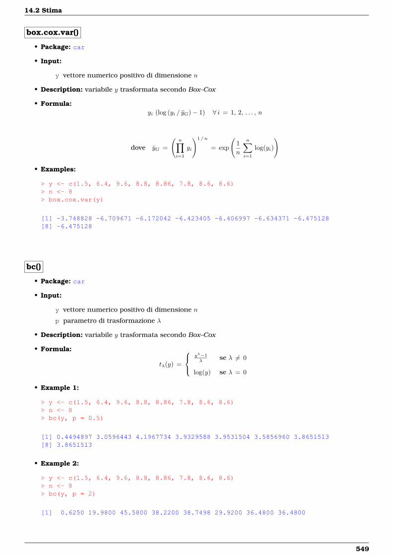
14.2 Stima
box.cox.var()
• Package: car
• Input:
y vettore numerico positivo di dimensione n
• Description: variabile y trasformata secondo Box–Cox
• Formula:yi (log (yi / yG)− 1) ∀ i = 1, 2, . . . , n
dove yG =
(n∏i=1
yi
)1 / n
= exp
(1n
n∑i=1
log(yi)
)
• Examples:
> y <- c(1.5, 6.4, 9.6, 8.8, 8.86, 7.8, 8.6, 8.6)> n <- 8> box.cox.var(y)
[1] -3.748828 -6.709671 -6.172042 -6.423405 -6.406997 -6.634371 -6.475128[8] -6.475128
bc()
• Package: car
• Input:
y vettore numerico positivo di dimensione n
p parametro di trasformazione λ
• Description: variabile y trasformata secondo Box–Cox
• Formula:
tλ(y) =
yλ−1λ se λ 6= 0
log(y) se λ = 0
• Example 1:
> y <- c(1.5, 6.4, 9.6, 8.8, 8.86, 7.8, 8.6, 8.6)> n <- 8> bc(y, p = 0.5)
[1] 0.4494897 3.0596443 4.1967734 3.9329588 3.9531504 3.5856960 3.8651513[8] 3.8651513
• Example 2:
> y <- c(1.5, 6.4, 9.6, 8.8, 8.86, 7.8, 8.6, 8.6)> n <- 8> bc(y, p = 2)
[1] 0.6250 19.9800 45.5800 38.2200 38.7498 29.9200 36.4800 36.4800
549
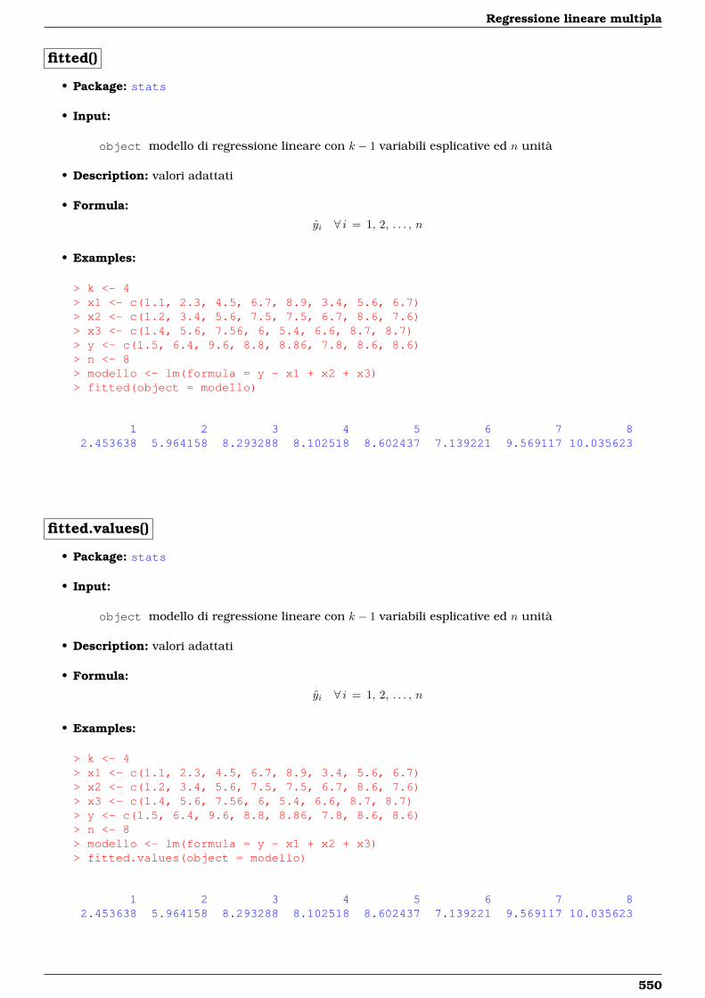
Regressione lineare multipla
fitted()
• Package: stats
• Input:
object modello di regressione lineare con k − 1 variabili esplicative ed n unità
• Description: valori adattati
• Formula:
yi ∀ i = 1, 2, . . . , n
• Examples:
> k <- 4> x1 <- c(1.1, 2.3, 4.5, 6.7, 8.9, 3.4, 5.6, 6.7)> x2 <- c(1.2, 3.4, 5.6, 7.5, 7.5, 6.7, 8.6, 7.6)> x3 <- c(1.4, 5.6, 7.56, 6, 5.4, 6.6, 8.7, 8.7)> y <- c(1.5, 6.4, 9.6, 8.8, 8.86, 7.8, 8.6, 8.6)> n <- 8> modello <- lm(formula = y ~ x1 + x2 + x3)> fitted(object = modello)
1 2 3 4 5 6 7 82.453638 5.964158 8.293288 8.102518 8.602437 7.139221 9.569117 10.035623
fitted.values()
• Package: stats
• Input:
object modello di regressione lineare con k − 1 variabili esplicative ed n unità
• Description: valori adattati
• Formula:
yi ∀ i = 1, 2, . . . , n
• Examples:
> k <- 4> x1 <- c(1.1, 2.3, 4.5, 6.7, 8.9, 3.4, 5.6, 6.7)> x2 <- c(1.2, 3.4, 5.6, 7.5, 7.5, 6.7, 8.6, 7.6)> x3 <- c(1.4, 5.6, 7.56, 6, 5.4, 6.6, 8.7, 8.7)> y <- c(1.5, 6.4, 9.6, 8.8, 8.86, 7.8, 8.6, 8.6)> n <- 8> modello <- lm(formula = y ~ x1 + x2 + x3)> fitted.values(object = modello)
1 2 3 4 5 6 7 82.453638 5.964158 8.293288 8.102518 8.602437 7.139221 9.569117 10.035623
550
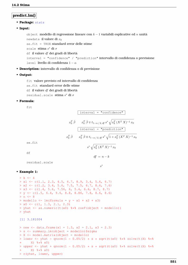
14.2 Stima
predict.lm()
• Package: stats
• Input:
object modello di regressione lineare con k − 1 variabili esplicative ed n unità
newdata il valore di x0
se.fit = TRUE standard error delle stime
scale stima s∗ di σ
df il valore df dei gradi di libertà
interval = "confidence" / "prediction" intervallo di confidenza o previsione
level livello di confidenza 1− α
• Description: intervallo di confidenza o di previsione
• Output:
fit valore previsto ed intervallo di confidenza
se.fit standard error delle stime
df il valore df dei gradi di libertà
residual.scale stima s∗ di σ
• Formula:
fit
interval = "confidence"
xT0 β xT0 β ∓ t1−α/ 2, df s∗√xT0 (XT X)−1 x0
interval = "prediction"
xT0 β xT0 β ∓ t1−α/ 2, df s∗√
1 + xT0 (XT X)−1 x0
se.fit
s∗√xT0 (XT X)−1 x0
dfdf = n− k
residual.scales∗
• Example 1:
> k <- 4> x1 <- c(1.1, 2.3, 4.5, 6.7, 8.9, 3.4, 5.6, 6.7)> x2 <- c(1.2, 3.4, 5.6, 7.5, 7.5, 6.7, 8.6, 7.6)> x3 <- c(1.4, 5.6, 7.56, 6, 5.4, 6.6, 8.7, 8.7)> y <- c(1.5, 6.4, 9.6, 8.8, 8.86, 7.8, 8.6, 8.6)> n <- 8> modello <- lm(formula = y ~ x1 + x2 + x3)> x0 <- c(1, 1.3, 2.1, 2.3)> yhat <- as.numeric(t(x0) %*% coef(object = modello))> yhat
[1] 3.181004
> new <- data.frame(x1 = 1.3, x2 = 2.1, x3 = 2.3)> s <- summary.lm(object = modello)$sigma> X <- model.matrix(object = modello)> lower <- yhat - qnorm(1 - 0.05/2) * s * sqrt(t(x0) %*% solve(t(X) %*%+ X) %*% x0)> upper <- yhat + qnorm(1 - 0.05/2) * s * sqrt(t(x0) %*% solve(t(X) %*%+ X) %*% x0)> c(yhat, lower, upper)
551
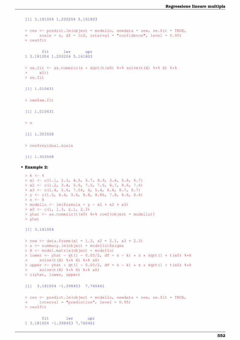
Regressione lineare multipla
[1] 3.181004 1.200204 5.161803
> res <- predict.lm(object = modello, newdata = new, se.fit = TRUE,+ scale = s, df = Inf, interval = "confidence", level = 0.95)> res$fit
fit lwr upr1 3.181004 1.200204 5.161803
> se.fit <- as.numeric(s * sqrt(t(x0) %*% solve(t(X) %*% X) %*%+ x0))> se.fit
[1] 1.010631
> res$se.fit
[1] 1.010631
> s
[1] 1.303508
> res$residual.scale
[1] 1.303508
• Example 2:
> k <- 4> x1 <- c(1.1, 2.3, 4.5, 6.7, 8.9, 3.4, 5.6, 6.7)> x2 <- c(1.2, 3.4, 5.6, 7.5, 7.5, 6.7, 8.6, 7.6)> x3 <- c(1.4, 5.6, 7.56, 6, 5.4, 6.6, 8.7, 8.7)> y <- c(1.5, 6.4, 9.6, 8.8, 8.86, 7.8, 8.6, 8.6)> n <- 8> modello <- lm(formula = y ~ x1 + x2 + x3)> x0 <- c(1, 1.3, 2.1, 2.3)> yhat <- as.numeric(t(x0) %*% coef(object = modello))> yhat
[1] 3.181004
> new <- data.frame(x1 = 1.3, x2 = 2.1, x3 = 2.3)> s <- summary.lm(object = modello)$sigma> X <- model.matrix(object = modello)> lower <- yhat - qt(1 - 0.05/2, df = n - k) * s * sqrt(1 + t(x0) %*%+ solve(t(X) %*% X) %*% x0)> upper <- yhat + qt(1 - 0.05/2, df = n - k) * s * sqrt(1 + t(x0) %*%+ solve(t(X) %*% X) %*% x0)> c(yhat, lower, upper)
[1] 3.181004 -1.398453 7.760461
> res <- predict.lm(object = modello, newdata = new, se.fit = TRUE,+ interval = "prediction", level = 0.95)> res$fit
fit lwr upr1 3.181004 -1.398453 7.760461
552
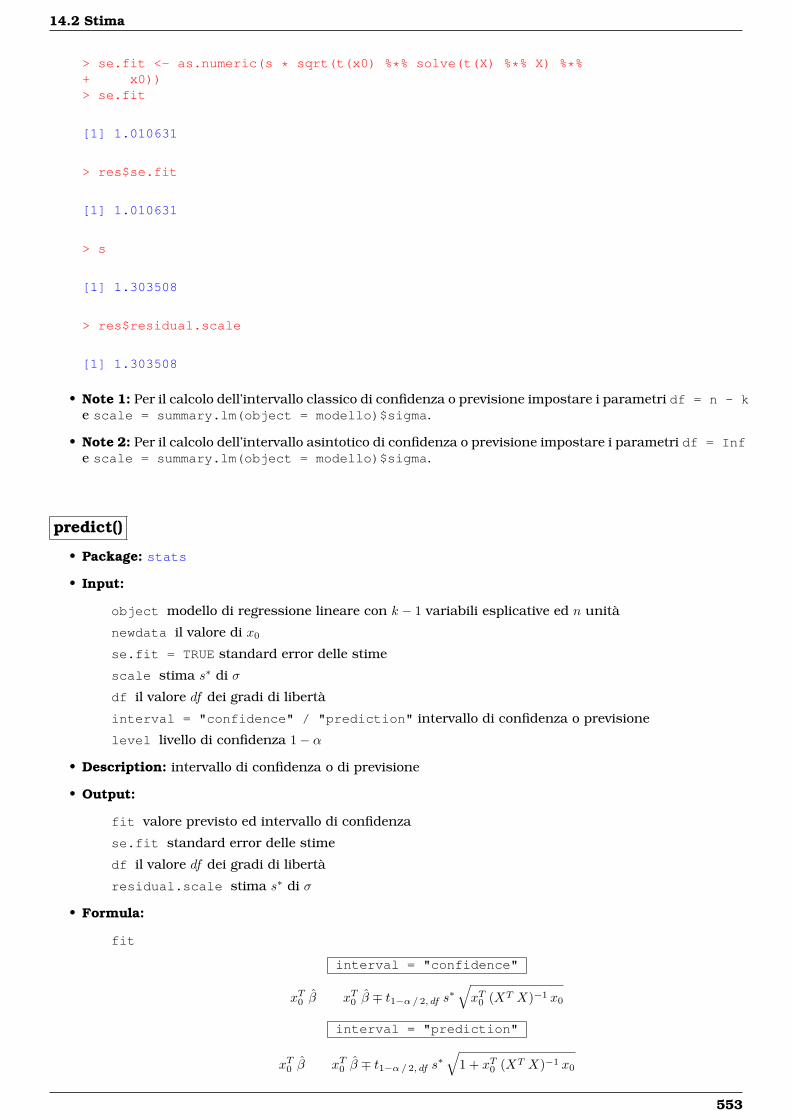
14.2 Stima
> se.fit <- as.numeric(s * sqrt(t(x0) %*% solve(t(X) %*% X) %*%+ x0))> se.fit
[1] 1.010631
> res$se.fit
[1] 1.010631
> s
[1] 1.303508
> res$residual.scale
[1] 1.303508
• Note 1: Per il calcolo dell’intervallo classico di confidenza o previsione impostare i parametri df = n - ke scale = summary.lm(object = modello)$sigma.
• Note 2: Per il calcolo dell’intervallo asintotico di confidenza o previsione impostare i parametri df = Infe scale = summary.lm(object = modello)$sigma.
predict()
• Package: stats
• Input:
object modello di regressione lineare con k − 1 variabili esplicative ed n unità
newdata il valore di x0
se.fit = TRUE standard error delle stime
scale stima s∗ di σ
df il valore df dei gradi di libertà
interval = "confidence" / "prediction" intervallo di confidenza o previsione
level livello di confidenza 1− α
• Description: intervallo di confidenza o di previsione
• Output:
fit valore previsto ed intervallo di confidenza
se.fit standard error delle stime
df il valore df dei gradi di libertà
residual.scale stima s∗ di σ
• Formula:
fit
interval = "confidence"
xT0 β xT0 β ∓ t1−α/ 2, df s∗√xT0 (XT X)−1 x0
interval = "prediction"
xT0 β xT0 β ∓ t1−α/ 2, df s∗√
1 + xT0 (XT X)−1 x0
553
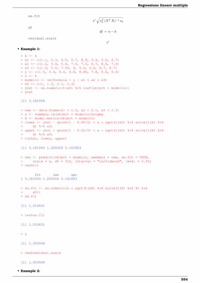
Regressione lineare multipla
se.fit
s∗√xT0 (XT X)−1 x0
dfdf = n− k
residual.scales∗
• Example 1:
> k <- 4> x1 <- c(1.1, 2.3, 4.5, 6.7, 8.9, 3.4, 5.6, 6.7)> x2 <- c(1.2, 3.4, 5.6, 7.5, 7.5, 6.7, 8.6, 7.6)> x3 <- c(1.4, 5.6, 7.56, 6, 5.4, 6.6, 8.7, 8.7)> y <- c(1.5, 6.4, 9.6, 8.8, 8.86, 7.8, 8.6, 8.6)> n <- 8> modello <- lm(formula = y ~ x1 + x2 + x3)> x0 <- c(1, 1.3, 2.1, 2.3)> yhat <- as.numeric(t(x0) %*% coef(object = modello))> yhat
[1] 3.181004
> new <- data.frame(x1 = 1.3, x2 = 2.1, x3 = 2.3)> s <- summary.lm(object = modello)$sigma> X <- model.matrix(object = modello)> lower <- yhat - qnorm(1 - 0.05/2) * s * sqrt(t(x0) %*% solve(t(X) %*%+ X) %*% x0)> upper <- yhat + qnorm(1 - 0.05/2) * s * sqrt(t(x0) %*% solve(t(X) %*%+ X) %*% x0)> c(yhat, lower, upper)
[1] 3.181004 1.200204 5.161803
> res <- predict(object = modello, newdata = new, se.fit = TRUE,+ scale = s, df = Inf, interval = "confidence", level = 0.95)> res$fit
fit lwr upr1 3.181004 1.200204 5.161803
> se.fit <- as.numeric(s * sqrt(t(x0) %*% solve(t(X) %*% X) %*%+ x0))> se.fit
[1] 1.010631
> res$se.fit
[1] 1.010631
> s
[1] 1.303508
> res$residual.scale
[1] 1.303508
• Example 2:
554
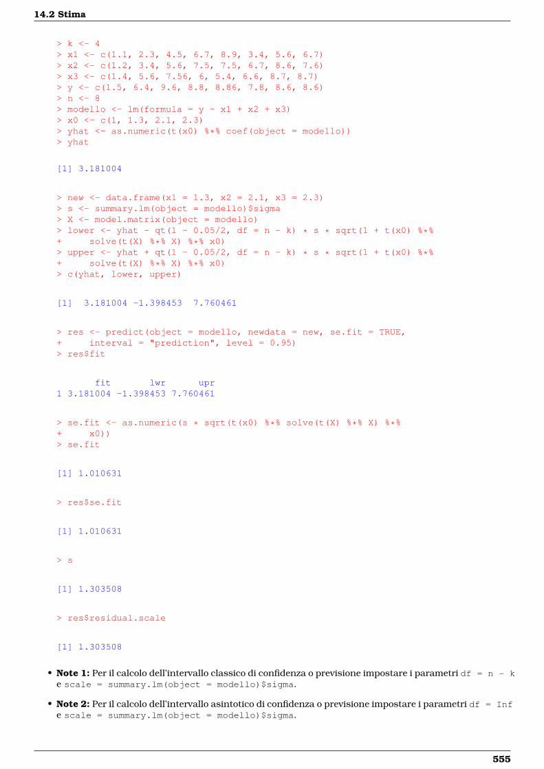
14.2 Stima
> k <- 4> x1 <- c(1.1, 2.3, 4.5, 6.7, 8.9, 3.4, 5.6, 6.7)> x2 <- c(1.2, 3.4, 5.6, 7.5, 7.5, 6.7, 8.6, 7.6)> x3 <- c(1.4, 5.6, 7.56, 6, 5.4, 6.6, 8.7, 8.7)> y <- c(1.5, 6.4, 9.6, 8.8, 8.86, 7.8, 8.6, 8.6)> n <- 8> modello <- lm(formula = y ~ x1 + x2 + x3)> x0 <- c(1, 1.3, 2.1, 2.3)> yhat <- as.numeric(t(x0) %*% coef(object = modello))> yhat
[1] 3.181004
> new <- data.frame(x1 = 1.3, x2 = 2.1, x3 = 2.3)> s <- summary.lm(object = modello)$sigma> X <- model.matrix(object = modello)> lower <- yhat - qt(1 - 0.05/2, df = n - k) * s * sqrt(1 + t(x0) %*%+ solve(t(X) %*% X) %*% x0)> upper <- yhat + qt(1 - 0.05/2, df = n - k) * s * sqrt(1 + t(x0) %*%+ solve(t(X) %*% X) %*% x0)> c(yhat, lower, upper)
[1] 3.181004 -1.398453 7.760461
> res <- predict(object = modello, newdata = new, se.fit = TRUE,+ interval = "prediction", level = 0.95)> res$fit
fit lwr upr1 3.181004 -1.398453 7.760461
> se.fit <- as.numeric(s * sqrt(t(x0) %*% solve(t(X) %*% X) %*%+ x0))> se.fit
[1] 1.010631
> res$se.fit
[1] 1.010631
> s
[1] 1.303508
> res$residual.scale
[1] 1.303508
• Note 1: Per il calcolo dell’intervallo classico di confidenza o previsione impostare i parametri df = n - ke scale = summary.lm(object = modello)$sigma.
• Note 2: Per il calcolo dell’intervallo asintotico di confidenza o previsione impostare i parametri df = Infe scale = summary.lm(object = modello)$sigma.
555
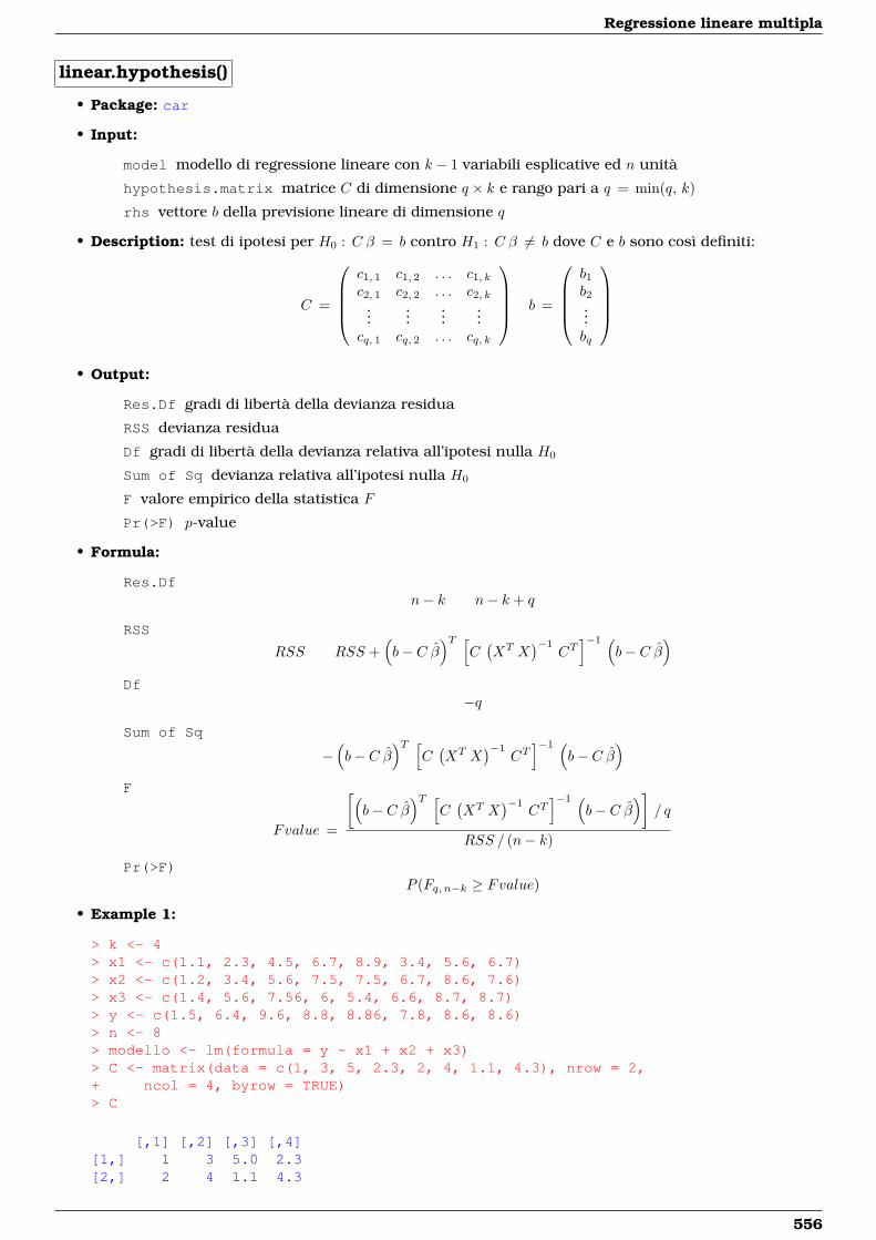
Regressione lineare multipla
linear.hypothesis()
• Package: car
• Input:
model modello di regressione lineare con k − 1 variabili esplicative ed n unità
hypothesis.matrix matrice C di dimensione q × k e rango pari a q = min(q, k)
rhs vettore b della previsione lineare di dimensione q
• Description: test di ipotesi per H0 : C β = b contro H1 : C β 6= b dove C e b sono così definiti:
C =
c1, 1 c1, 2 . . . c1, kc2, 1 c2, 2 . . . c2, k
......
......
cq, 1 cq, 2 . . . cq, k
b =
b1b2...bq
• Output:
Res.Df gradi di libertà della devianza residua
RSS devianza residua
Df gradi di libertà della devianza relativa all’ipotesi nulla H0
Sum of Sq devianza relativa all’ipotesi nulla H0
F valore empirico della statistica F
Pr(>F) p-value
• Formula:
Res.Dfn− k n− k + q
RSS
RSS RSS +(b− C β
)T [C(XT X
)−1CT]−1 (
b− C β)
Df−q
Sum of Sq
−(b− C β
)T [C(XT X
)−1CT]−1 (
b− C β)
F
Fvalue =
[(b− C β
)T [C(XT X
)−1CT]−1 (
b− C β)]
/ q
RSS / (n− k)
Pr(>F)P (Fq, n−k ≥ Fvalue)
• Example 1:
> k <- 4> x1 <- c(1.1, 2.3, 4.5, 6.7, 8.9, 3.4, 5.6, 6.7)> x2 <- c(1.2, 3.4, 5.6, 7.5, 7.5, 6.7, 8.6, 7.6)> x3 <- c(1.4, 5.6, 7.56, 6, 5.4, 6.6, 8.7, 8.7)> y <- c(1.5, 6.4, 9.6, 8.8, 8.86, 7.8, 8.6, 8.6)> n <- 8> modello <- lm(formula = y ~ x1 + x2 + x3)> C <- matrix(data = c(1, 3, 5, 2.3, 2, 4, 1.1, 4.3), nrow = 2,+ ncol = 4, byrow = TRUE)> C
[,1] [,2] [,3] [,4][1,] 1 3 5.0 2.3[2,] 2 4 1.1 4.3
556
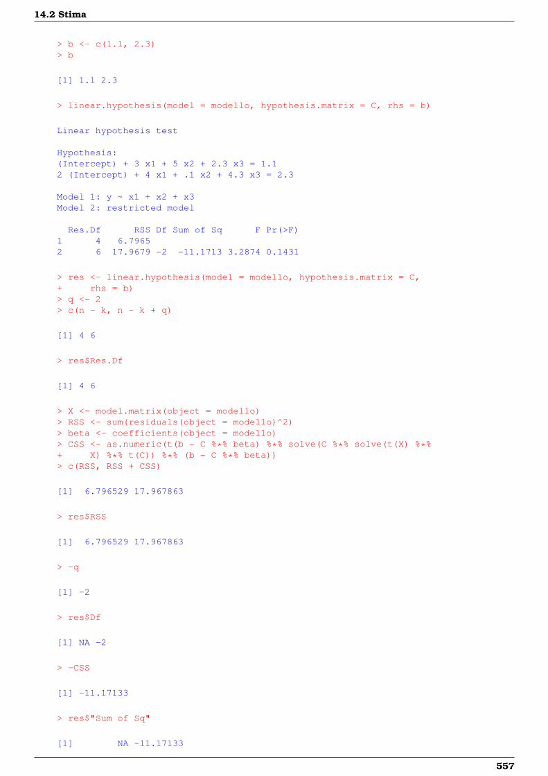
14.2 Stima
> b <- c(1.1, 2.3)> b
[1] 1.1 2.3
> linear.hypothesis(model = modello, hypothesis.matrix = C, rhs = b)
Linear hypothesis test
Hypothesis:(Intercept) + 3 x1 + 5 x2 + 2.3 x3 = 1.12 (Intercept) + 4 x1 + .1 x2 + 4.3 x3 = 2.3
Model 1: y ~ x1 + x2 + x3Model 2: restricted model
Res.Df RSS Df Sum of Sq F Pr(>F)1 4 6.79652 6 17.9679 -2 -11.1713 3.2874 0.1431
> res <- linear.hypothesis(model = modello, hypothesis.matrix = C,+ rhs = b)> q <- 2> c(n - k, n - k + q)
[1] 4 6
> res$Res.Df
[1] 4 6
> X <- model.matrix(object = modello)> RSS <- sum(residuals(object = modello)^2)> beta <- coefficients(object = modello)> CSS <- as.numeric(t(b - C %*% beta) %*% solve(C %*% solve(t(X) %*%+ X) %*% t(C)) %*% (b - C %*% beta))> c(RSS, RSS + CSS)
[1] 6.796529 17.967863
> res$RSS
[1] 6.796529 17.967863
> -q
[1] -2
> res$Df
[1] NA -2
> -CSS
[1] -11.17133
> res$"Sum of Sq"
[1] NA -11.17133
557
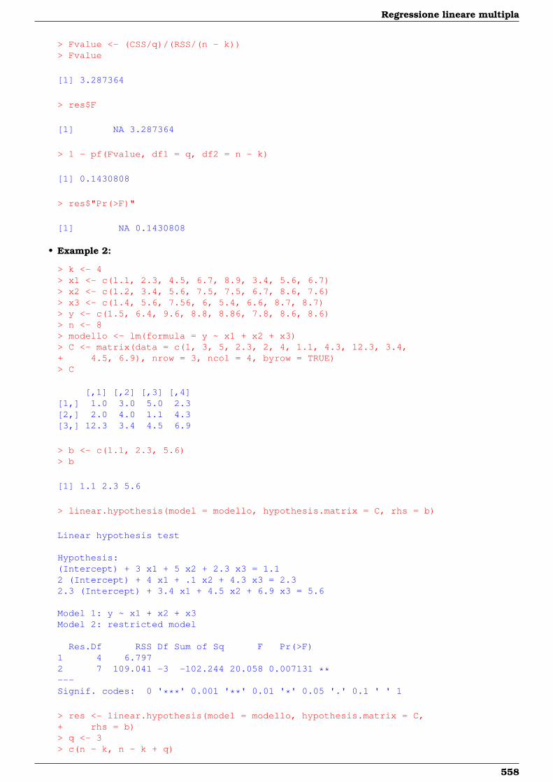
Regressione lineare multipla
> Fvalue <- (CSS/q)/(RSS/(n - k))> Fvalue
[1] 3.287364
> res$F
[1] NA 3.287364
> 1 - pf(Fvalue, df1 = q, df2 = n - k)
[1] 0.1430808
> res$"Pr(>F)"
[1] NA 0.1430808
• Example 2:
> k <- 4> x1 <- c(1.1, 2.3, 4.5, 6.7, 8.9, 3.4, 5.6, 6.7)> x2 <- c(1.2, 3.4, 5.6, 7.5, 7.5, 6.7, 8.6, 7.6)> x3 <- c(1.4, 5.6, 7.56, 6, 5.4, 6.6, 8.7, 8.7)> y <- c(1.5, 6.4, 9.6, 8.8, 8.86, 7.8, 8.6, 8.6)> n <- 8> modello <- lm(formula = y ~ x1 + x2 + x3)> C <- matrix(data = c(1, 3, 5, 2.3, 2, 4, 1.1, 4.3, 12.3, 3.4,+ 4.5, 6.9), nrow = 3, ncol = 4, byrow = TRUE)> C
[,1] [,2] [,3] [,4][1,] 1.0 3.0 5.0 2.3[2,] 2.0 4.0 1.1 4.3[3,] 12.3 3.4 4.5 6.9
> b <- c(1.1, 2.3, 5.6)> b
[1] 1.1 2.3 5.6
> linear.hypothesis(model = modello, hypothesis.matrix = C, rhs = b)
Linear hypothesis test
Hypothesis:(Intercept) + 3 x1 + 5 x2 + 2.3 x3 = 1.12 (Intercept) + 4 x1 + .1 x2 + 4.3 x3 = 2.32.3 (Intercept) + 3.4 x1 + 4.5 x2 + 6.9 x3 = 5.6
Model 1: y ~ x1 + x2 + x3Model 2: restricted model
Res.Df RSS Df Sum of Sq F Pr(>F)1 4 6.7972 7 109.041 -3 -102.244 20.058 0.007131 **---Signif. codes: 0 '***' 0.001 '**' 0.01 '*' 0.05 '.' 0.1 ' ' 1
> res <- linear.hypothesis(model = modello, hypothesis.matrix = C,+ rhs = b)> q <- 3> c(n - k, n - k + q)
558

14.2 Stima
[1] 4 7
> res$Res.Df
[1] 4 7
> X <- model.matrix(object = modello)> RSS <- sum(residuals(object = modello)^2)> beta <- coefficients(object = modello)> CSS <- as.numeric(t(b - C %*% beta) %*% solve(C %*% solve(t(X) %*%+ X) %*% t(C)) %*% (b - C %*% beta))> c(RSS, RSS + CSS)
[1] 6.796529 109.040699
> res$RSS
[1] 6.796529 109.040699
> -q
[1] -3
> res$Df
[1] NA -3
> -CSS
[1] -102.2442
> res$"Sum of Sq"
[1] NA -102.2442
> Fvalue <- (CSS/q)/(RSS/(n - k))> Fvalue
[1] 20.05811
> res$F
[1] NA 20.05811
> 1 - pf(Fvalue, df1 = q, df2 = n - k)
[1] 0.007131315
> res$"Pr(>F)"
[1] NA 0.007131315
559
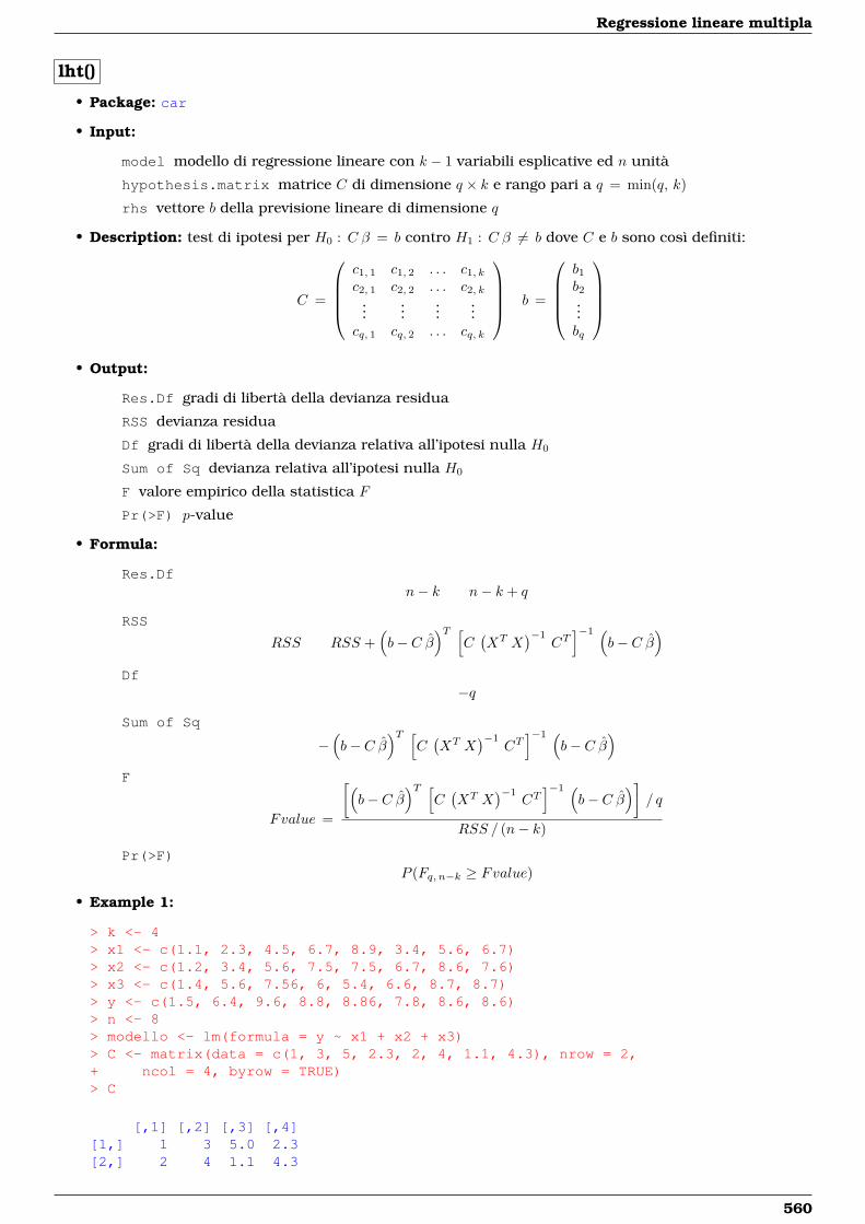
Regressione lineare multipla
lht()
• Package: car
• Input:
model modello di regressione lineare con k − 1 variabili esplicative ed n unità
hypothesis.matrix matrice C di dimensione q × k e rango pari a q = min(q, k)
rhs vettore b della previsione lineare di dimensione q
• Description: test di ipotesi per H0 : C β = b contro H1 : C β 6= b dove C e b sono così definiti:
C =
c1, 1 c1, 2 . . . c1, kc2, 1 c2, 2 . . . c2, k
......
......
cq, 1 cq, 2 . . . cq, k
b =
b1b2...bq
• Output:
Res.Df gradi di libertà della devianza residua
RSS devianza residua
Df gradi di libertà della devianza relativa all’ipotesi nulla H0
Sum of Sq devianza relativa all’ipotesi nulla H0
F valore empirico della statistica F
Pr(>F) p-value
• Formula:
Res.Dfn− k n− k + q
RSS
RSS RSS +(b− C β
)T [C(XT X
)−1CT]−1 (
b− C β)
Df−q
Sum of Sq
−(b− C β
)T [C(XT X
)−1CT]−1 (
b− C β)
F
Fvalue =
[(b− C β
)T [C(XT X
)−1CT]−1 (
b− C β)]
/ q
RSS / (n− k)
Pr(>F)P (Fq, n−k ≥ Fvalue)
• Example 1:
> k <- 4> x1 <- c(1.1, 2.3, 4.5, 6.7, 8.9, 3.4, 5.6, 6.7)> x2 <- c(1.2, 3.4, 5.6, 7.5, 7.5, 6.7, 8.6, 7.6)> x3 <- c(1.4, 5.6, 7.56, 6, 5.4, 6.6, 8.7, 8.7)> y <- c(1.5, 6.4, 9.6, 8.8, 8.86, 7.8, 8.6, 8.6)> n <- 8> modello <- lm(formula = y ~ x1 + x2 + x3)> C <- matrix(data = c(1, 3, 5, 2.3, 2, 4, 1.1, 4.3), nrow = 2,+ ncol = 4, byrow = TRUE)> C
[,1] [,2] [,3] [,4][1,] 1 3 5.0 2.3[2,] 2 4 1.1 4.3
560
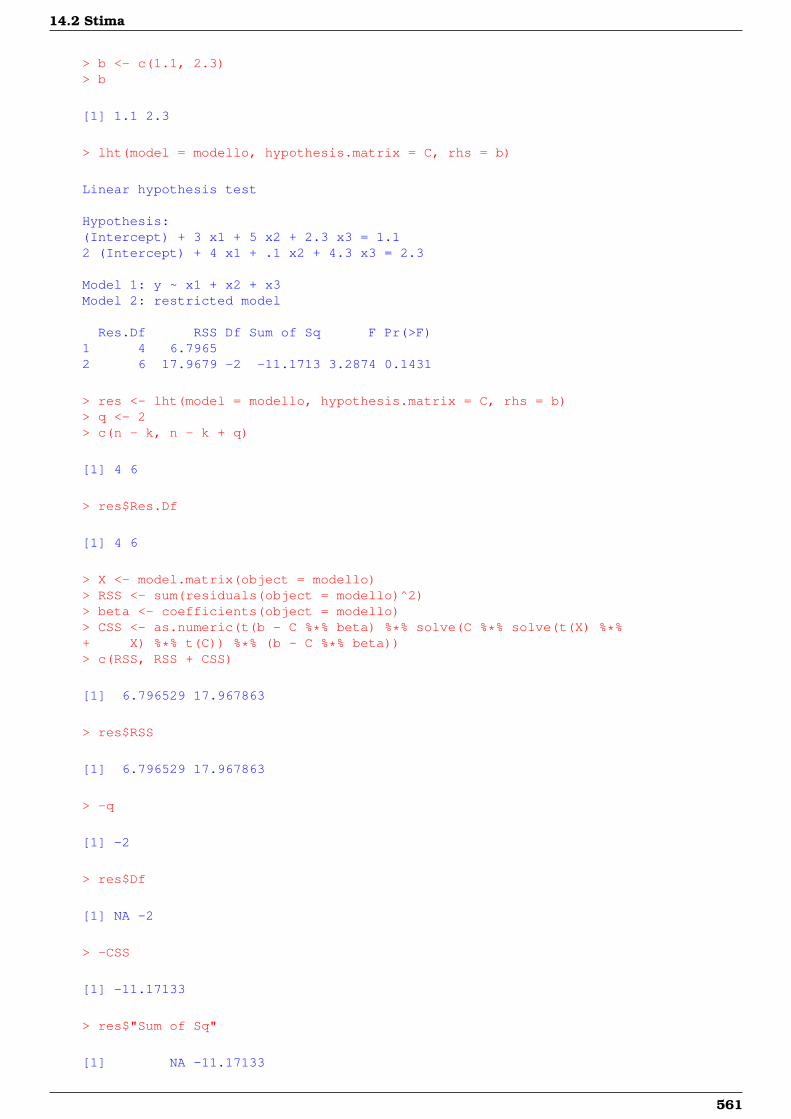
14.2 Stima
> b <- c(1.1, 2.3)> b
[1] 1.1 2.3
> lht(model = modello, hypothesis.matrix = C, rhs = b)
Linear hypothesis test
Hypothesis:(Intercept) + 3 x1 + 5 x2 + 2.3 x3 = 1.12 (Intercept) + 4 x1 + .1 x2 + 4.3 x3 = 2.3
Model 1: y ~ x1 + x2 + x3Model 2: restricted model
Res.Df RSS Df Sum of Sq F Pr(>F)1 4 6.79652 6 17.9679 -2 -11.1713 3.2874 0.1431
> res <- lht(model = modello, hypothesis.matrix = C, rhs = b)> q <- 2> c(n - k, n - k + q)
[1] 4 6
> res$Res.Df
[1] 4 6
> X <- model.matrix(object = modello)> RSS <- sum(residuals(object = modello)^2)> beta <- coefficients(object = modello)> CSS <- as.numeric(t(b - C %*% beta) %*% solve(C %*% solve(t(X) %*%+ X) %*% t(C)) %*% (b - C %*% beta))> c(RSS, RSS + CSS)
[1] 6.796529 17.967863
> res$RSS
[1] 6.796529 17.967863
> -q
[1] -2
> res$Df
[1] NA -2
> -CSS
[1] -11.17133
> res$"Sum of Sq"
[1] NA -11.17133
561
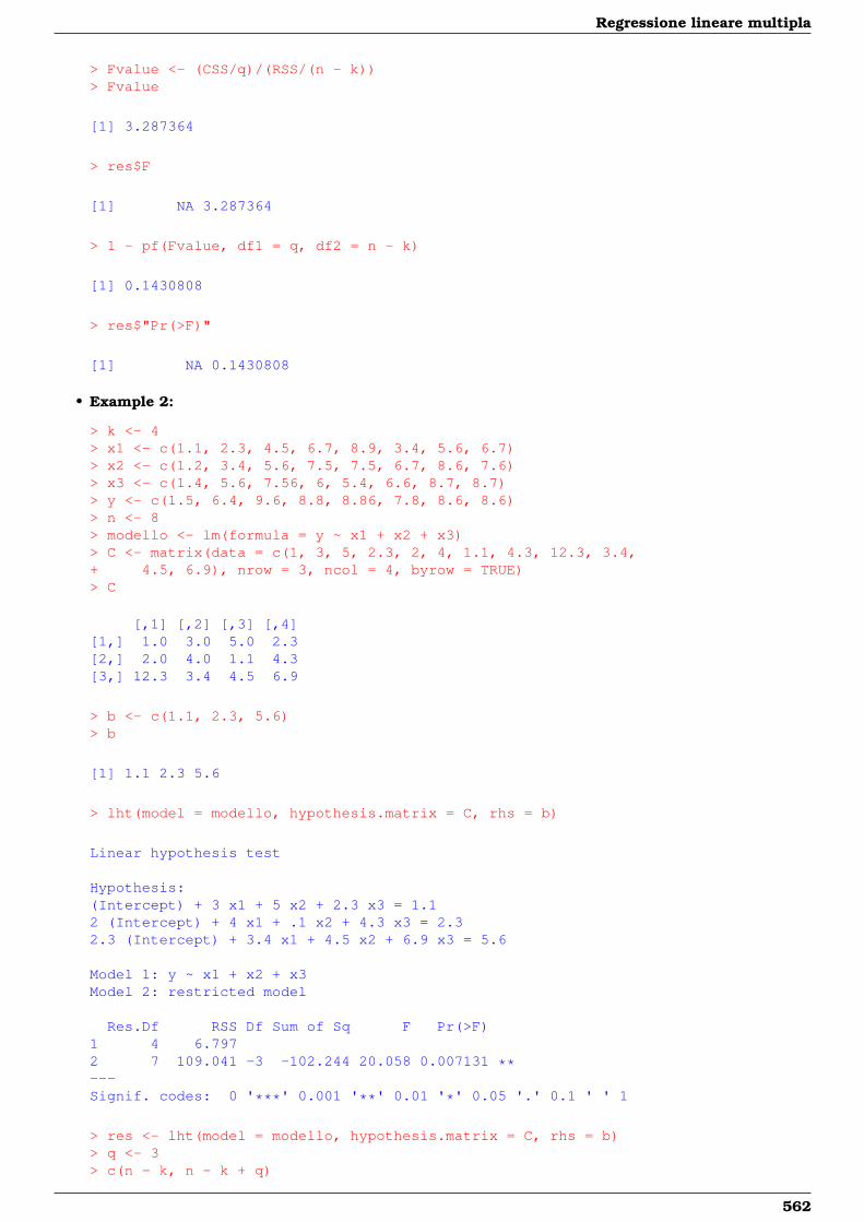
Regressione lineare multipla
> Fvalue <- (CSS/q)/(RSS/(n - k))> Fvalue
[1] 3.287364
> res$F
[1] NA 3.287364
> 1 - pf(Fvalue, df1 = q, df2 = n - k)
[1] 0.1430808
> res$"Pr(>F)"
[1] NA 0.1430808
• Example 2:
> k <- 4> x1 <- c(1.1, 2.3, 4.5, 6.7, 8.9, 3.4, 5.6, 6.7)> x2 <- c(1.2, 3.4, 5.6, 7.5, 7.5, 6.7, 8.6, 7.6)> x3 <- c(1.4, 5.6, 7.56, 6, 5.4, 6.6, 8.7, 8.7)> y <- c(1.5, 6.4, 9.6, 8.8, 8.86, 7.8, 8.6, 8.6)> n <- 8> modello <- lm(formula = y ~ x1 + x2 + x3)> C <- matrix(data = c(1, 3, 5, 2.3, 2, 4, 1.1, 4.3, 12.3, 3.4,+ 4.5, 6.9), nrow = 3, ncol = 4, byrow = TRUE)> C
[,1] [,2] [,3] [,4][1,] 1.0 3.0 5.0 2.3[2,] 2.0 4.0 1.1 4.3[3,] 12.3 3.4 4.5 6.9
> b <- c(1.1, 2.3, 5.6)> b
[1] 1.1 2.3 5.6
> lht(model = modello, hypothesis.matrix = C, rhs = b)
Linear hypothesis test
Hypothesis:(Intercept) + 3 x1 + 5 x2 + 2.3 x3 = 1.12 (Intercept) + 4 x1 + .1 x2 + 4.3 x3 = 2.32.3 (Intercept) + 3.4 x1 + 4.5 x2 + 6.9 x3 = 5.6
Model 1: y ~ x1 + x2 + x3Model 2: restricted model
Res.Df RSS Df Sum of Sq F Pr(>F)1 4 6.7972 7 109.041 -3 -102.244 20.058 0.007131 **---Signif. codes: 0 '***' 0.001 '**' 0.01 '*' 0.05 '.' 0.1 ' ' 1
> res <- lht(model = modello, hypothesis.matrix = C, rhs = b)> q <- 3> c(n - k, n - k + q)
562
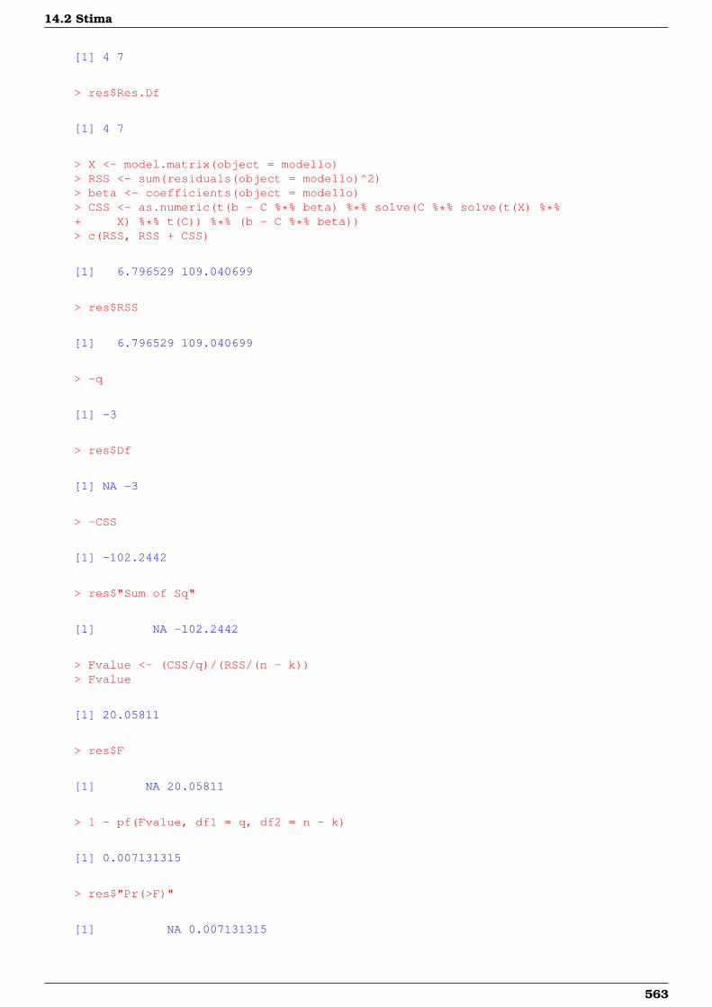
14.2 Stima
[1] 4 7
> res$Res.Df
[1] 4 7
> X <- model.matrix(object = modello)> RSS <- sum(residuals(object = modello)^2)> beta <- coefficients(object = modello)> CSS <- as.numeric(t(b - C %*% beta) %*% solve(C %*% solve(t(X) %*%+ X) %*% t(C)) %*% (b - C %*% beta))> c(RSS, RSS + CSS)
[1] 6.796529 109.040699
> res$RSS
[1] 6.796529 109.040699
> -q
[1] -3
> res$Df
[1] NA -3
> -CSS
[1] -102.2442
> res$"Sum of Sq"
[1] NA -102.2442
> Fvalue <- (CSS/q)/(RSS/(n - k))> Fvalue
[1] 20.05811
> res$F
[1] NA 20.05811
> 1 - pf(Fvalue, df1 = q, df2 = n - k)
[1] 0.007131315
> res$"Pr(>F)"
[1] NA 0.007131315
563
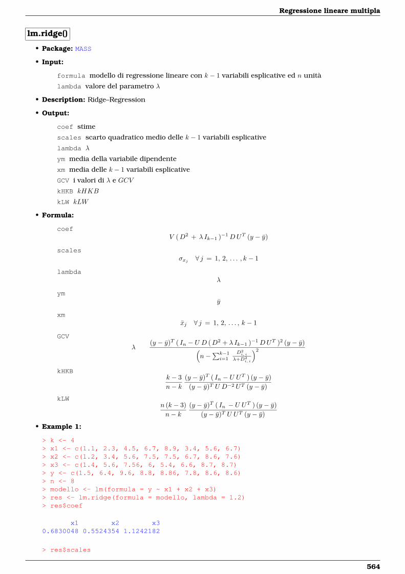
Regressione lineare multipla
lm.ridge()
• Package: MASS
• Input:
formula modello di regressione lineare con k − 1 variabili esplicative ed n unità
lambda valore del parametro λ
• Description: Ridge–Regression
• Output:
coef stime
scales scarto quadratico medio delle k − 1 variabili esplicative
lambda λ
ym media della variabile dipendente
xm media delle k − 1 variabili esplicative
GCV i valori di λ e GCV
kHKB kHKB
kLW kLW
• Formula:
coefV (D2 + λ Ik−1 )−1DUT (y − y)
scalesσxj ∀ j = 1, 2, . . . , k − 1
lambdaλ
ymy
xmxj ∀ j = 1, 2, . . . , k − 1
GCV
λ(y − y)T ( In − U D (D2 + λ Ik−1 )−1DUT )2 (y − y)(
n−∑k−1i=1
D2i, i
λ+D2i, i
)2
kHKBk − 3n− k
(y − y)T ( In − U UT ) (y − y)(y − y)T U D−2 UT (y − y)
kLWn (k − 3)n− k
(y − y)T ( In − U UT ) (y − y)(y − y)T U UT (y − y)
• Example 1:
> k <- 4> x1 <- c(1.1, 2.3, 4.5, 6.7, 8.9, 3.4, 5.6, 6.7)> x2 <- c(1.2, 3.4, 5.6, 7.5, 7.5, 6.7, 8.6, 7.6)> x3 <- c(1.4, 5.6, 7.56, 6, 5.4, 6.6, 8.7, 8.7)> y <- c(1.5, 6.4, 9.6, 8.8, 8.86, 7.8, 8.6, 8.6)> n <- 8> modello <- lm(formula = y ~ x1 + x2 + x3)> res <- lm.ridge(formula = modello, lambda = 1.2)> res$coef
x1 x2 x30.6830048 0.5524354 1.1242182
> res$scales
564
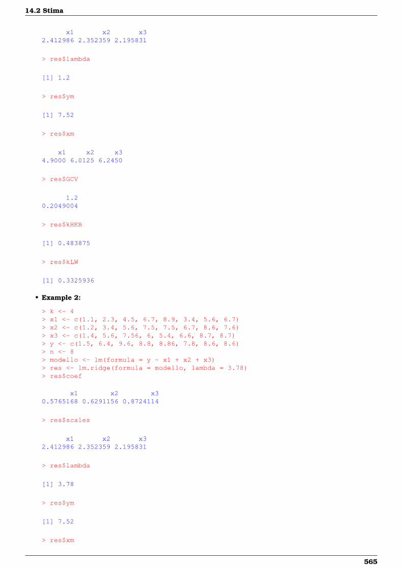
14.2 Stima
x1 x2 x32.412986 2.352359 2.195831
> res$lambda
[1] 1.2
> res$ym
[1] 7.52
> res$xm
x1 x2 x34.9000 6.0125 6.2450
> res$GCV
1.20.2049004
> res$kHKB
[1] 0.483875
> res$kLW
[1] 0.3325936
• Example 2:
> k <- 4> x1 <- c(1.1, 2.3, 4.5, 6.7, 8.9, 3.4, 5.6, 6.7)> x2 <- c(1.2, 3.4, 5.6, 7.5, 7.5, 6.7, 8.6, 7.6)> x3 <- c(1.4, 5.6, 7.56, 6, 5.4, 6.6, 8.7, 8.7)> y <- c(1.5, 6.4, 9.6, 8.8, 8.86, 7.8, 8.6, 8.6)> n <- 8> modello <- lm(formula = y ~ x1 + x2 + x3)> res <- lm.ridge(formula = modello, lambda = 3.78)> res$coef
x1 x2 x30.5765168 0.6291156 0.8724114
> res$scales
x1 x2 x32.412986 2.352359 2.195831
> res$lambda
[1] 3.78
> res$ym
[1] 7.52
> res$xm
565
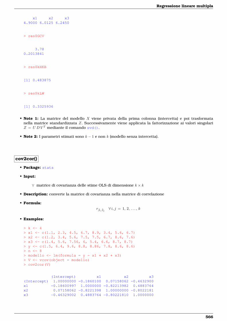
Regressione lineare multipla
x1 x2 x34.9000 6.0125 6.2450
> res$GCV
3.780.2013841
> res$kHKB
[1] 0.483875
> res$kLW
[1] 0.3325936
• Note 1: La matrice del modello X viene privata della prima colonna (intercetta) e poi trasformatanella matrice standardizzata Z. Successivamente viene applicata la fattorizzazione ai valori singolariZ = U DV T mediante il comando svd().
• Note 2: I parametri stimati sono k − 1 e non k (modello senza intercetta).
cov2cor()
• Package: stats
• Input:
V matrice di covarianza delle stime OLS di dimensione k × k
• Description: converte la matrice di covarianza nella matrice di correlazione
• Formula:rβi βj ∀ i, j = 1, 2, . . . , k
• Examples:
> k <- 4> x1 <- c(1.1, 2.3, 4.5, 6.7, 8.9, 3.4, 5.6, 6.7)> x2 <- c(1.2, 3.4, 5.6, 7.5, 7.5, 6.7, 8.6, 7.6)> x3 <- c(1.4, 5.6, 7.56, 6, 5.4, 6.6, 8.7, 8.7)> y <- c(1.5, 6.4, 9.6, 8.8, 8.86, 7.8, 8.6, 8.6)> n <- 8> modello <- lm(formula = y ~ x1 + x2 + x3)> V <- vcov(object = modello)> cov2cor(V)
(Intercept) x1 x2 x3(Intercept) 1.00000000 -0.1860100 0.07158062 -0.4632900x1 -0.18600997 1.0000000 -0.82213982 0.4883764x2 0.07158062 -0.8221398 1.00000000 -0.8022181x3 -0.46329002 0.4883764 -0.80221810 1.0000000
566
14.3 Adattamento
14.3 Adattamento
logLik()
• Package: stats
• Input:
object modello di regressione lineare con k − 1 variabili esplicative ed n unità
• Description: log-verosimiglianza normale
• Formula:ˆ
• Examples:
> k <- 4> x1 <- c(1.1, 2.3, 4.5, 6.7, 8.9, 3.4, 5.6, 6.7)> x2 <- c(1.2, 3.4, 5.6, 7.5, 7.5, 6.7, 8.6, 7.6)> x3 <- c(1.4, 5.6, 7.56, 6, 5.4, 6.6, 8.7, 8.7)> y <- c(1.5, 6.4, 9.6, 8.8, 8.86, 7.8, 8.6, 8.6)> n <- 8> modello <- lm(formula = y ~ x1 + x2 + x3)> logLik(object = modello)
'log Lik.' -10.69939 (df=5)
durbin.watson()
• Package: car
• Input:
model modello di regressione lineare con k − 1 variabili esplicative ed n unità
• Description: test di Durbin–Watson per verificare la presenza di autocorrelazioni tra i residui
• Output:
dw valore empirico della statistica D–W
• Formula:
dwn∑i=2
(ei − ei−1)2 /RSS
• Examples:
> k <- 4> x1 <- c(1.1, 2.3, 4.5, 6.7, 8.9, 3.4, 5.6, 6.7)> x2 <- c(1.2, 3.4, 5.6, 7.5, 7.5, 6.7, 8.6, 7.6)> x3 <- c(1.4, 5.6, 7.56, 6, 5.4, 6.6, 8.7, 8.7)> y <- c(1.5, 6.4, 9.6, 8.8, 8.86, 7.8, 8.6, 8.6)> n <- 8> modello <- lm(formula = y ~ x1 + x2 + x3)> res <- durbin.watson(model = modello)> res$dw
[1] 0.9255503
567
Regressione lineare multipla
AIC()
• Package: stats
• Input:
object modello di regressione lineare con k − 1 variabili esplicative ed n unità
• Description: indice AIC
• Formula:−2 ˆ+ 2 (k + 1)
• Examples:
> k <- 4> x1 <- c(1.1, 2.3, 4.5, 6.7, 8.9, 3.4, 5.6, 6.7)> x2 <- c(1.2, 3.4, 5.6, 7.5, 7.5, 6.7, 8.6, 7.6)> x3 <- c(1.4, 5.6, 7.56, 6, 5.4, 6.6, 8.7, 8.7)> y <- c(1.5, 6.4, 9.6, 8.8, 8.86, 7.8, 8.6, 8.6)> n <- 8> modello <- lm(formula = y ~ x1 + x2 + x3)> AIC(object = modello)
[1] 31.39878
BIC()
• Package: nlme
• Input:
object modello di regressione lineare con k − 1 variabili esplicative ed n unità
• Description: indice BIC
• Formula:−2 ˆ+ (k + 1) log(n)
• Examples:
> k <- 4> x1 <- c(1.1, 2.3, 4.5, 6.7, 8.9, 3.4, 5.6, 6.7)> x2 <- c(1.2, 3.4, 5.6, 7.5, 7.5, 6.7, 8.6, 7.6)> x3 <- c(1.4, 5.6, 7.56, 6, 5.4, 6.6, 8.7, 8.7)> y <- c(1.5, 6.4, 9.6, 8.8, 8.86, 7.8, 8.6, 8.6)> n <- 8> modello <- lm(formula = y ~ x1 + x2 + x3)> BIC(object = modello)
[1] 31.79599
extractAIC()
• Package: stats
• Input:
fit modello di regressione lineare con k − 1 variabili esplicative ed n unità
• Description: numero di parametri del modello ed indice AIC generalizzato
• Formula:k n log(RSS /n) + 2 k
568
14.3 Adattamento
• Examples:
> k <- 4> x1 <- c(1.1, 2.3, 4.5, 6.7, 8.9, 3.4, 5.6, 6.7)> x2 <- c(1.2, 3.4, 5.6, 7.5, 7.5, 6.7, 8.6, 7.6)> x3 <- c(1.4, 5.6, 7.56, 6, 5.4, 6.6, 8.7, 8.7)> y <- c(1.5, 6.4, 9.6, 8.8, 8.86, 7.8, 8.6, 8.6)> n <- 8> modello <- lm(formula = y ~ x1 + x2 + x3)> extractAIC(fit = modello)
[1] 4.000000 6.695764
deviance()
• Package: stats
• Input:
object modello di regressione lineare con k − 1 variabili esplicative ed n unità
• Description: devianza residua
• Formula:RSS
• Examples:
> k <- 4> x1 <- c(1.1, 2.3, 4.5, 6.7, 8.9, 3.4, 5.6, 6.7)> x2 <- c(1.2, 3.4, 5.6, 7.5, 7.5, 6.7, 8.6, 7.6)> x3 <- c(1.4, 5.6, 7.56, 6, 5.4, 6.6, 8.7, 8.7)> y <- c(1.5, 6.4, 9.6, 8.8, 8.86, 7.8, 8.6, 8.6)> n <- 8> modello <- lm(formula = y ~ x1 + x2 + x3)> deviance(object = modello)
[1] 6.796529
PRESS()
• Package: MPV
• Input:
x modello di regressione lineare con k − 1 variabili esplicative ed n unità
• Description: PRESS
• Formula:n∑i=1
e2i / (1− hi)2
• Examples:
> k <- 4> x1 <- c(1.1, 2.3, 4.5, 6.7, 8.9, 3.4, 5.6, 6.7)> x2 <- c(1.2, 3.4, 5.6, 7.5, 7.5, 6.7, 8.6, 7.6)> x3 <- c(1.4, 5.6, 7.56, 6, 5.4, 6.6, 8.7, 8.7)> y <- c(1.5, 6.4, 9.6, 8.8, 8.86, 7.8, 8.6, 8.6)> n <- 8> modello <- lm(formula = y ~ x1 + x2 + x3)> PRESS(x = modello)
[1] 35.00228
569
Regressione lineare multipla
drop1()
• Package: stats
• Input:
object modello di regressione lineare con k − 1 variabili esplicative ed n unità
scale selezione indice AIC oppure Cp
test = "F"
• Description: submodels
• Output:
Df differenza tra gradi di libertà
Sum of Sq differenza tra devianze residue
RSS devianza residua
AIC indice AIC
Cp indice Cp
F value valore empirico della statistica F
Pr(F) p-value
• Formula:
Df1, 1, . . . , 1︸ ︷︷ ︸k−1 volte
Sum of SqRSS−xj −RSS ∀ j = 1, 2, . . . , k − 1
dove RSS−xj rappresenta la devianza residua del modello eliminata la variabile esplicativa xj.
RSSRSS, RSS−xj ∀ j = 1, 2, . . . , k − 1
AIC
scale = 0
n log (RSS /n) + 2 k, n log(RSS−xj / n
)+ 2 (k − 1) ∀ j = 1, 2, . . . , k − 1
Cp
scale = s2
k,RSS−xj
RSS / (n− k)+ 2 (k − 1)− n ∀ j = 1, 2, . . . , k − 1
F value
Fj =RSS−xj −RSSRSS / (n− k)
∀ j = 1, 2, . . . , k − 1
Pr(F)P (F1, n−k ≥ Fj) ∀ j = 1, 2, . . . , k − 1
• Example 1:
> k <- 4> x1 <- c(1.1, 2.3, 4.5, 6.7, 8.9, 3.4, 5.6, 6.7)> x2 <- c(1.2, 3.4, 5.6, 7.5, 7.5, 6.7, 8.6, 7.6)> x3 <- c(1.4, 5.6, 7.56, 6, 5.4, 6.6, 8.7, 8.7)> y <- c(1.5, 6.4, 9.6, 8.8, 8.86, 7.8, 8.6, 8.6)> modello <- lm(formula = y ~ x1 + x2 + x3)> drop1(object = modello, scale = 0, test = "F")
570
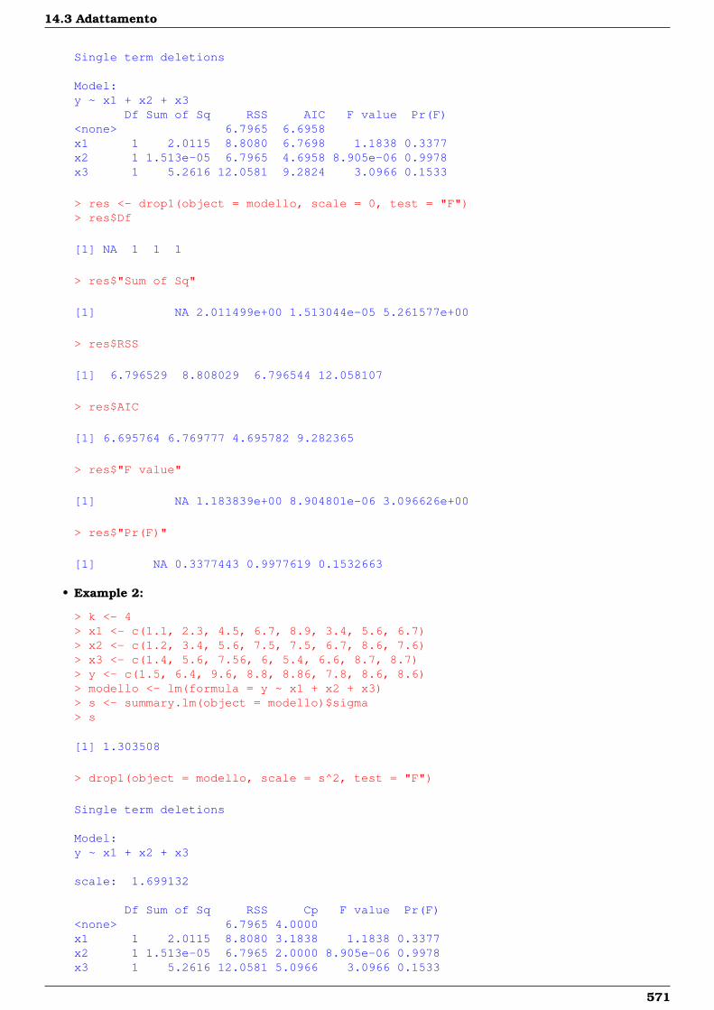
14.3 Adattamento
Single term deletions
Model:y ~ x1 + x2 + x3
Df Sum of Sq RSS AIC F value Pr(F)<none> 6.7965 6.6958x1 1 2.0115 8.8080 6.7698 1.1838 0.3377x2 1 1.513e-05 6.7965 4.6958 8.905e-06 0.9978x3 1 5.2616 12.0581 9.2824 3.0966 0.1533
> res <- drop1(object = modello, scale = 0, test = "F")> res$Df
[1] NA 1 1 1
> res$"Sum of Sq"
[1] NA 2.011499e+00 1.513044e-05 5.261577e+00
> res$RSS
[1] 6.796529 8.808029 6.796544 12.058107
> res$AIC
[1] 6.695764 6.769777 4.695782 9.282365
> res$"F value"
[1] NA 1.183839e+00 8.904801e-06 3.096626e+00
> res$"Pr(F)"
[1] NA 0.3377443 0.9977619 0.1532663
• Example 2:
> k <- 4> x1 <- c(1.1, 2.3, 4.5, 6.7, 8.9, 3.4, 5.6, 6.7)> x2 <- c(1.2, 3.4, 5.6, 7.5, 7.5, 6.7, 8.6, 7.6)> x3 <- c(1.4, 5.6, 7.56, 6, 5.4, 6.6, 8.7, 8.7)> y <- c(1.5, 6.4, 9.6, 8.8, 8.86, 7.8, 8.6, 8.6)> modello <- lm(formula = y ~ x1 + x2 + x3)> s <- summary.lm(object = modello)$sigma> s
[1] 1.303508
> drop1(object = modello, scale = s^2, test = "F")
Single term deletions
Model:y ~ x1 + x2 + x3
scale: 1.699132
Df Sum of Sq RSS Cp F value Pr(F)<none> 6.7965 4.0000x1 1 2.0115 8.8080 3.1838 1.1838 0.3377x2 1 1.513e-05 6.7965 2.0000 8.905e-06 0.9978x3 1 5.2616 12.0581 5.0966 3.0966 0.1533
571
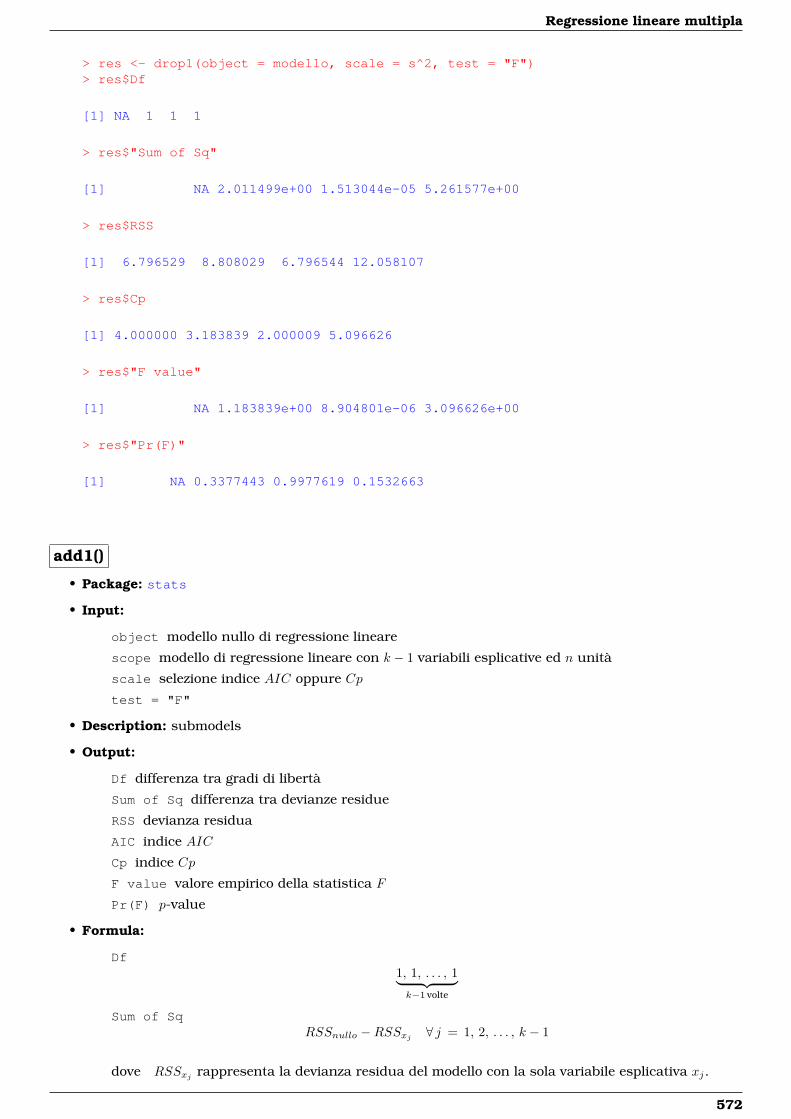
Regressione lineare multipla
> res <- drop1(object = modello, scale = s^2, test = "F")> res$Df
[1] NA 1 1 1
> res$"Sum of Sq"
[1] NA 2.011499e+00 1.513044e-05 5.261577e+00
> res$RSS
[1] 6.796529 8.808029 6.796544 12.058107
> res$Cp
[1] 4.000000 3.183839 2.000009 5.096626
> res$"F value"
[1] NA 1.183839e+00 8.904801e-06 3.096626e+00
> res$"Pr(F)"
[1] NA 0.3377443 0.9977619 0.1532663
add1()
• Package: stats
• Input:
object modello nullo di regressione lineare
scope modello di regressione lineare con k − 1 variabili esplicative ed n unità
scale selezione indice AIC oppure Cp
test = "F"
• Description: submodels
• Output:
Df differenza tra gradi di libertà
Sum of Sq differenza tra devianze residue
RSS devianza residua
AIC indice AIC
Cp indice Cp
F value valore empirico della statistica F
Pr(F) p-value
• Formula:
Df1, 1, . . . , 1︸ ︷︷ ︸k−1 volte
Sum of SqRSSnullo −RSSxj ∀ j = 1, 2, . . . , k − 1
dove RSSxj rappresenta la devianza residua del modello con la sola variabile esplicativa xj.
572
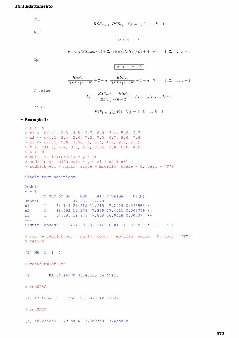
14.3 Adattamento
RSSRSSnullo, RSSxj ∀ j = 1, 2, . . . , k − 1
AIC
scale = 0
n log (RSSnullo / n) + 2, n log(RSSxj / n
)+ 4 ∀ j = 1, 2, . . . , k − 1
Cp
scale = s2
RSSnulloRSS / (n− k)
+ 2− n,RSSxj
RSS / (n− k)+ 4− n ∀ j = 1, 2, . . . , k − 1
F value
Fj =RSSnullo −RSSxjRSSxj / (n− 2)
∀ j = 1, 2, . . . , k − 1
Pr(F)P (F1, n−2 ≥ Fj) ∀ j = 1, 2, . . . , k − 1
• Example 1:
> k <- 4> x1 <- c(1.1, 2.3, 4.5, 6.7, 8.9, 3.4, 5.6, 6.7)> x2 <- c(1.2, 3.4, 5.6, 7.5, 7.5, 6.7, 8.6, 7.6)> x3 <- c(1.4, 5.6, 7.56, 6, 5.4, 6.6, 8.7, 8.7)> y <- c(1.5, 6.4, 9.6, 8.8, 8.86, 7.8, 8.6, 8.6)> n <- 8> nullo <- lm(formula = y ~ 1)> modello <- lm(formula = y ~ x1 + x2 + x3)> add1(object = nullo, scope = modello, scale = 0, test = "F")
Single term additions
Model:y ~ 1
Df Sum of Sq RSS AIC F value Pr(F)<none> 47.666 16.278x1 1 26.149 21.518 11.915 7.2914 0.035564 *x2 1 35.492 12.175 7.359 17.4911 0.005799 **x3 1 34.691 12.975 7.869 16.0418 0.007077 **---Signif. codes: 0 '***' 0.001 '**' 0.01 '*' 0.05 '.' 0.1 ' ' 1
> res <- add1(object = nullo, scope = modello, scale = 0, test = "F")> res$Df
[1] NA 1 1 1
> res$"Sum of Sq"
[1] NA 26.14878 35.49165 34.69113
> res$RSS
[1] 47.66640 21.51762 12.17475 12.97527
> res$AIC
[1] 16.278282 11.915446 7.359380 7.868828
573
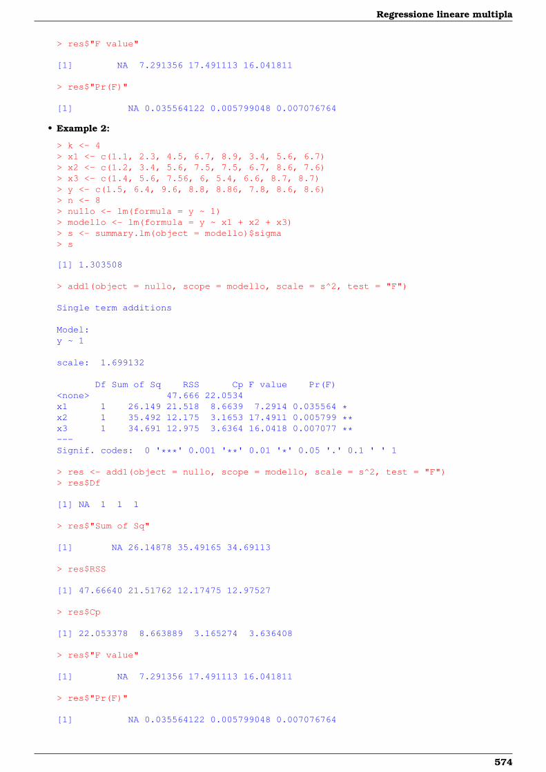
Regressione lineare multipla
> res$"F value"
[1] NA 7.291356 17.491113 16.041811
> res$"Pr(F)"
[1] NA 0.035564122 0.005799048 0.007076764
• Example 2:
> k <- 4> x1 <- c(1.1, 2.3, 4.5, 6.7, 8.9, 3.4, 5.6, 6.7)> x2 <- c(1.2, 3.4, 5.6, 7.5, 7.5, 6.7, 8.6, 7.6)> x3 <- c(1.4, 5.6, 7.56, 6, 5.4, 6.6, 8.7, 8.7)> y <- c(1.5, 6.4, 9.6, 8.8, 8.86, 7.8, 8.6, 8.6)> n <- 8> nullo <- lm(formula = y ~ 1)> modello <- lm(formula = y ~ x1 + x2 + x3)> s <- summary.lm(object = modello)$sigma> s
[1] 1.303508
> add1(object = nullo, scope = modello, scale = s^2, test = "F")
Single term additions
Model:y ~ 1
scale: 1.699132
Df Sum of Sq RSS Cp F value Pr(F)<none> 47.666 22.0534x1 1 26.149 21.518 8.6639 7.2914 0.035564 *x2 1 35.492 12.175 3.1653 17.4911 0.005799 **x3 1 34.691 12.975 3.6364 16.0418 0.007077 **---Signif. codes: 0 '***' 0.001 '**' 0.01 '*' 0.05 '.' 0.1 ' ' 1
> res <- add1(object = nullo, scope = modello, scale = s^2, test = "F")> res$Df
[1] NA 1 1 1
> res$"Sum of Sq"
[1] NA 26.14878 35.49165 34.69113
> res$RSS
[1] 47.66640 21.51762 12.17475 12.97527
> res$Cp
[1] 22.053378 8.663889 3.165274 3.636408
> res$"F value"
[1] NA 7.291356 17.491113 16.041811
> res$"Pr(F)"
[1] NA 0.035564122 0.005799048 0.007076764
574
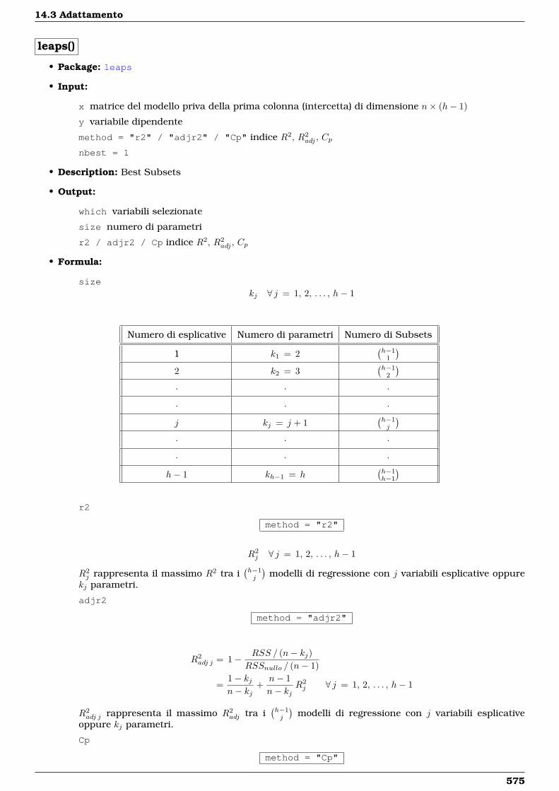
14.3 Adattamento
leaps()
• Package: leaps
• Input:
x matrice del modello priva della prima colonna (intercetta) di dimensione n× (h− 1)
y variabile dipendente
method = "r2" / "adjr2" / "Cp" indice R2, R2adj , Cp
nbest = 1
• Description: Best Subsets
• Output:
which variabili selezionate
size numero di parametri
r2 / adjr2 / Cp indice R2, R2adj , Cp
• Formula:
sizekj ∀ j = 1, 2, . . . , h− 1
Numero di esplicative Numero di parametri Numero di Subsets
1 k1 = 2(h−1
1
)2 k2 = 3
(h−1
2
)· · ·
· · ·
j kj = j + 1(h−1j
)· · ·
· · ·
h− 1 kh−1 = h(h−1h−1
)r2
method = "r2"
R2j ∀ j = 1, 2, . . . , h− 1
R2j rappresenta il massimo R2 tra i
(h−1j
)modelli di regressione con j variabili esplicative oppure
kj parametri.
adjr2
method = "adjr2"
R2adj j = 1− RSS / (n− kj)
RSSnullo / (n− 1)
=1− kjn− kj
+n− 1n− kj
R2j ∀ j = 1, 2, . . . , h− 1
R2adj j rappresenta il massimo R2
adj tra i(h−1j
)modelli di regressione con j variabili esplicative
oppure kj parametri.
Cp
method = "Cp"
575
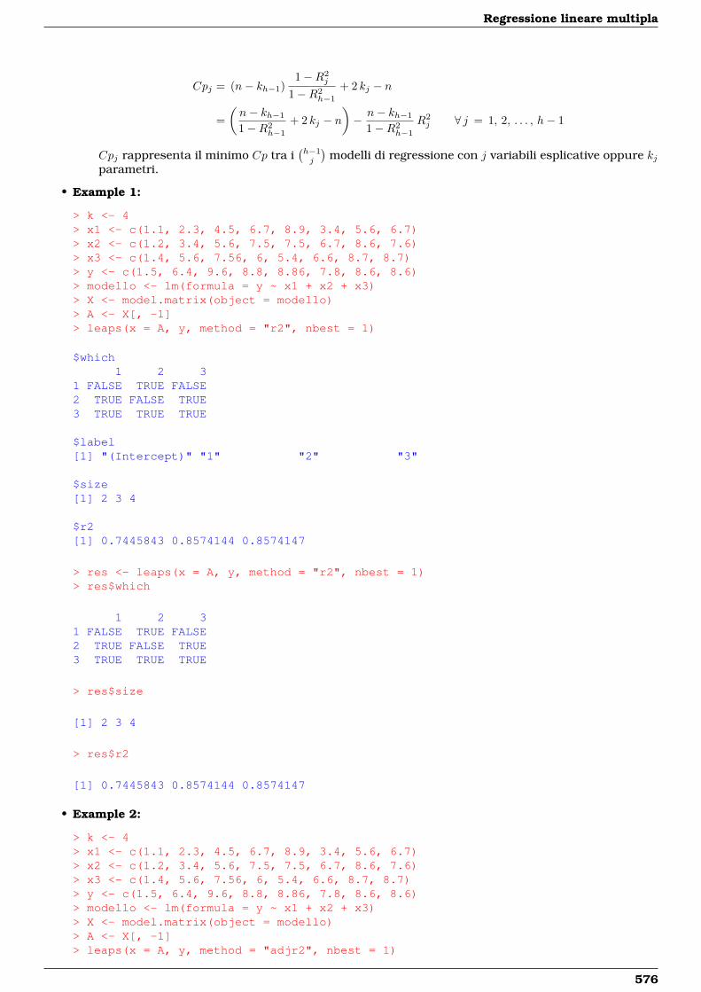
Regressione lineare multipla
Cpj = (n− kh−1)1−R2
j
1−R2h−1
+ 2 kj − n
=(n− kh−1
1−R2h−1
+ 2 kj − n)− n− kh−1
1−R2h−1
R2j ∀ j = 1, 2, . . . , h− 1
Cpj rappresenta il minimo Cp tra i(h−1j
)modelli di regressione con j variabili esplicative oppure kj
parametri.
• Example 1:
> k <- 4> x1 <- c(1.1, 2.3, 4.5, 6.7, 8.9, 3.4, 5.6, 6.7)> x2 <- c(1.2, 3.4, 5.6, 7.5, 7.5, 6.7, 8.6, 7.6)> x3 <- c(1.4, 5.6, 7.56, 6, 5.4, 6.6, 8.7, 8.7)> y <- c(1.5, 6.4, 9.6, 8.8, 8.86, 7.8, 8.6, 8.6)> modello <- lm(formula = y ~ x1 + x2 + x3)> X <- model.matrix(object = modello)> A <- X[, -1]> leaps(x = A, y, method = "r2", nbest = 1)
$which1 2 3
1 FALSE TRUE FALSE2 TRUE FALSE TRUE3 TRUE TRUE TRUE
$label[1] "(Intercept)" "1" "2" "3"
$size[1] 2 3 4
$r2[1] 0.7445843 0.8574144 0.8574147
> res <- leaps(x = A, y, method = "r2", nbest = 1)> res$which
1 2 31 FALSE TRUE FALSE2 TRUE FALSE TRUE3 TRUE TRUE TRUE
> res$size
[1] 2 3 4
> res$r2
[1] 0.7445843 0.8574144 0.8574147
• Example 2:
> k <- 4> x1 <- c(1.1, 2.3, 4.5, 6.7, 8.9, 3.4, 5.6, 6.7)> x2 <- c(1.2, 3.4, 5.6, 7.5, 7.5, 6.7, 8.6, 7.6)> x3 <- c(1.4, 5.6, 7.56, 6, 5.4, 6.6, 8.7, 8.7)> y <- c(1.5, 6.4, 9.6, 8.8, 8.86, 7.8, 8.6, 8.6)> modello <- lm(formula = y ~ x1 + x2 + x3)> X <- model.matrix(object = modello)> A <- X[, -1]> leaps(x = A, y, method = "adjr2", nbest = 1)
576

14.3 Adattamento
$which1 2 3
1 FALSE TRUE FALSE2 TRUE FALSE TRUE3 TRUE TRUE TRUE
$label[1] "(Intercept)" "1" "2" "3"
$size[1] 2 3 4
$adjr2[1] 0.7020150 0.8003801 0.7504757
> res <- leaps(x = A, y, method = "adjr2", nbest = 1)> res$which
1 2 31 FALSE TRUE FALSE2 TRUE FALSE TRUE3 TRUE TRUE TRUE
> res$size
[1] 2 3 4
> res$adjr2
[1] 0.7020150 0.8003801 0.7504757
• Example 3:
> k <- 4> x1 <- c(1.1, 2.3, 4.5, 6.7, 8.9, 3.4, 5.6, 6.7)> x2 <- c(1.2, 3.4, 5.6, 7.5, 7.5, 6.7, 8.6, 7.6)> x3 <- c(1.4, 5.6, 7.56, 6, 5.4, 6.6, 8.7, 8.7)> y <- c(1.5, 6.4, 9.6, 8.8, 8.86, 7.8, 8.6, 8.6)> modello <- lm(formula = y ~ x1 + x2 + x3)> X <- model.matrix(object = modello)> A <- X[, -1]> leaps(x = A, y, method = "Cp", nbest = 1)
$which1 2 3
1 FALSE TRUE FALSE2 TRUE FALSE TRUE3 TRUE TRUE TRUE
$label[1] "(Intercept)" "1" "2" "3"
$size[1] 2 3 4
$Cp[1] 3.165274 2.000009 4.000000
> res <- leaps(x = A, y, method = "Cp", nbest = 1)> res$which
577
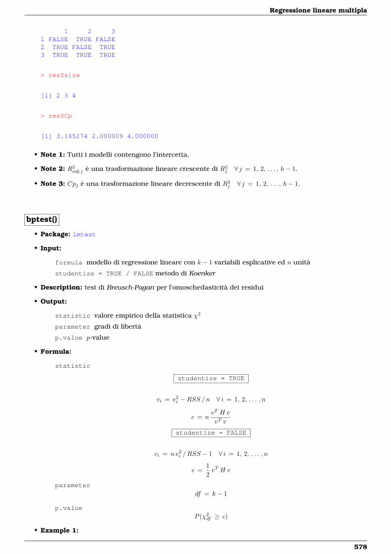
Regressione lineare multipla
1 2 31 FALSE TRUE FALSE2 TRUE FALSE TRUE3 TRUE TRUE TRUE
> res$size
[1] 2 3 4
> res$Cp
[1] 3.165274 2.000009 4.000000
• Note 1: Tutti i modelli contengono l’intercetta.
• Note 2: R2adj j è una trasformazione lineare crescente di R2
j ∀ j = 1, 2, . . . , h− 1.
• Note 3: Cpj è una trasformazione lineare decrescente di R2j ∀ j = 1, 2, . . . , h− 1.
bptest()
• Package: lmtest
• Input:
formula modello di regressione lineare con k − 1 variabili esplicative ed n unità
studentize = TRUE / FALSE metodo di Koenker
• Description: test di Breusch-Pagan per l’omoschedasticità dei residui
• Output:
statistic valore empirico della statistica χ2
parameter gradi di libertà
p.value p-value
• Formula:
statistic
studentize = TRUE
vi = e2i −RSS /n ∀ i = 1, 2, . . . , n
c = nvT H v
vT v
studentize = FALSE
vi = n e2i /RSS − 1 ∀ i = 1, 2, . . . , n
c =12vT H v
parameterdf = k − 1
p.valueP (χ2
df ≥ c)
• Example 1:
578
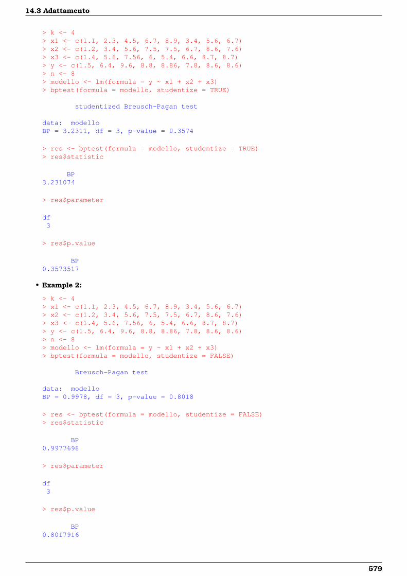
14.3 Adattamento
> k <- 4> x1 <- c(1.1, 2.3, 4.5, 6.7, 8.9, 3.4, 5.6, 6.7)> x2 <- c(1.2, 3.4, 5.6, 7.5, 7.5, 6.7, 8.6, 7.6)> x3 <- c(1.4, 5.6, 7.56, 6, 5.4, 6.6, 8.7, 8.7)> y <- c(1.5, 6.4, 9.6, 8.8, 8.86, 7.8, 8.6, 8.6)> n <- 8> modello <- lm(formula = y ~ x1 + x2 + x3)> bptest(formula = modello, studentize = TRUE)
studentized Breusch-Pagan test
data: modelloBP = 3.2311, df = 3, p-value = 0.3574
> res <- bptest(formula = modello, studentize = TRUE)> res$statistic
BP3.231074
> res$parameter
df3
> res$p.value
BP0.3573517
• Example 2:
> k <- 4> x1 <- c(1.1, 2.3, 4.5, 6.7, 8.9, 3.4, 5.6, 6.7)> x2 <- c(1.2, 3.4, 5.6, 7.5, 7.5, 6.7, 8.6, 7.6)> x3 <- c(1.4, 5.6, 7.56, 6, 5.4, 6.6, 8.7, 8.7)> y <- c(1.5, 6.4, 9.6, 8.8, 8.86, 7.8, 8.6, 8.6)> n <- 8> modello <- lm(formula = y ~ x1 + x2 + x3)> bptest(formula = modello, studentize = FALSE)
Breusch-Pagan test
data: modelloBP = 0.9978, df = 3, p-value = 0.8018
> res <- bptest(formula = modello, studentize = FALSE)> res$statistic
BP0.9977698
> res$parameter
df3
> res$p.value
BP0.8017916
579
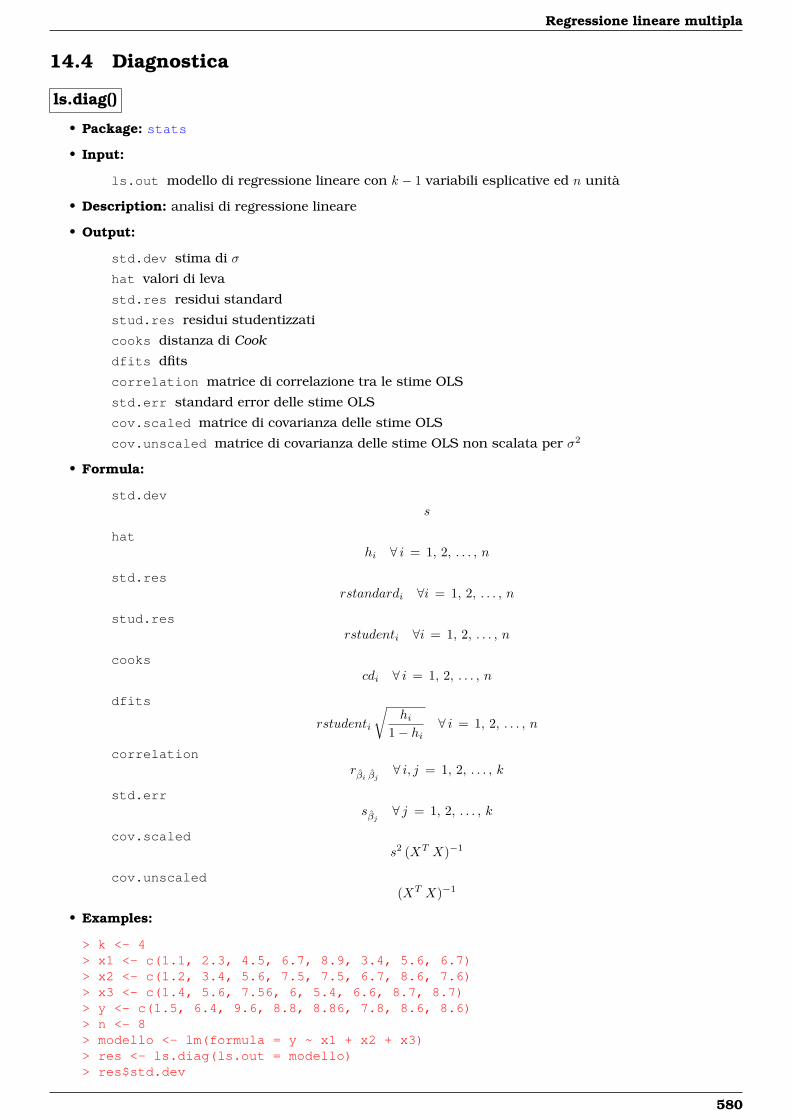
Regressione lineare multipla
14.4 Diagnostica
ls.diag()
• Package: stats
• Input:
ls.out modello di regressione lineare con k − 1 variabili esplicative ed n unità
• Description: analisi di regressione lineare
• Output:
std.dev stima di σ
hat valori di leva
std.res residui standard
stud.res residui studentizzati
cooks distanza di Cook
dfits dfits
correlation matrice di correlazione tra le stime OLS
std.err standard error delle stime OLS
cov.scaled matrice di covarianza delle stime OLS
cov.unscaled matrice di covarianza delle stime OLS non scalata per σ2
• Formula:
std.devs
hathi ∀ i = 1, 2, . . . , n
std.resrstandardi ∀i = 1, 2, . . . , n
stud.resrstudenti ∀i = 1, 2, . . . , n
cookscdi ∀ i = 1, 2, . . . , n
dfits
rstudenti
√hi
1− hi∀ i = 1, 2, . . . , n
correlationrβi βj ∀ i, j = 1, 2, . . . , k
std.errsβj ∀ j = 1, 2, . . . , k
cov.scaleds2 (XT X)−1
cov.unscaled(XT X)−1
• Examples:
> k <- 4> x1 <- c(1.1, 2.3, 4.5, 6.7, 8.9, 3.4, 5.6, 6.7)> x2 <- c(1.2, 3.4, 5.6, 7.5, 7.5, 6.7, 8.6, 7.6)> x3 <- c(1.4, 5.6, 7.56, 6, 5.4, 6.6, 8.7, 8.7)> y <- c(1.5, 6.4, 9.6, 8.8, 8.86, 7.8, 8.6, 8.6)> n <- 8> modello <- lm(formula = y ~ x1 + x2 + x3)> res <- ls.diag(ls.out = modello)> res$std.dev
580
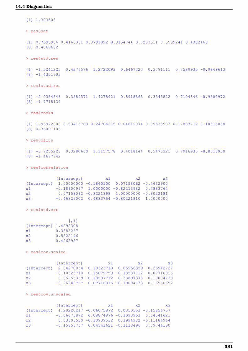
14.4 Diagnostica
[1] 1.303508
> res$hat
[1] 0.7695906 0.4163361 0.3791092 0.3154744 0.7283511 0.5539241 0.4302463[8] 0.4069682
> res$std.res
[1] -1.5241225 0.4376576 1.2722093 0.6467323 0.3791111 0.7589935 -0.9849613[8] -1.4301703
> res$stud.res
[1] -2.0384846 0.3884371 1.4278921 0.5918863 0.3343822 0.7104546 -0.9800972[8] -1.7718134
> res$cooks
[1] 1.93972080 0.03415783 0.24706215 0.04819074 0.09633983 0.17883712 0.18315058[8] 0.35091186
> res$dfits
[1] -3.7255223 0.3280660 1.1157578 0.4018144 0.5475321 0.7916935 -0.8516950[8] -1.4677742
> res$correlation
(Intercept) x1 x2 x3(Intercept) 1.00000000 -0.1860100 0.07158062 -0.4632900x1 -0.18600997 1.0000000 -0.82213982 0.4883764x2 0.07158062 -0.8221398 1.00000000 -0.8022181x3 -0.46329002 0.4883764 -0.80221810 1.0000000
> res$std.err
[,1](Intercept) 1.4292308x1 0.3883267x2 0.5822146x3 0.4068987
> res$cov.scaled
(Intercept) x1 x2 x3(Intercept) 2.04270054 -0.10323710 0.05956359 -0.26942727x1 -0.10323710 0.15079759 -0.18587712 0.07716815x2 0.05956359 -0.18587712 0.33897378 -0.19004733x3 -0.26942727 0.07716815 -0.19004733 0.16556652
> res$cov.unscaled
(Intercept) x1 x2 x3(Intercept) 1.20220217 -0.06075872 0.0350553 -0.15856757x1 -0.06075872 0.08874976 -0.1093953 0.04541621x2 0.03505530 -0.10939532 0.1994982 -0.11184964x3 -0.15856757 0.04541621 -0.1118496 0.09744180
581
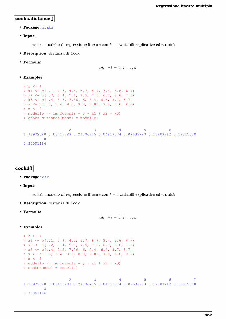
Regressione lineare multipla
cooks.distance()
• Package: stats
• Input:
model modello di regressione lineare con k − 1 variabili esplicative ed n unità
• Description: distanza di Cook
• Formula:cdi ∀ i = 1, 2, . . . , n
• Examples:
> k <- 4> x1 <- c(1.1, 2.3, 4.5, 6.7, 8.9, 3.4, 5.6, 6.7)> x2 <- c(1.2, 3.4, 5.6, 7.5, 7.5, 6.7, 8.6, 7.6)> x3 <- c(1.4, 5.6, 7.56, 6, 5.4, 6.6, 8.7, 8.7)> y <- c(1.5, 6.4, 9.6, 8.8, 8.86, 7.8, 8.6, 8.6)> n <- 8> modello <- lm(formula = y ~ x1 + x2 + x3)> cooks.distance(model = modello)
1 2 3 4 5 6 71.93972080 0.03415783 0.24706215 0.04819074 0.09633983 0.17883712 0.18315058
80.35091186
cookd()
• Package: car
• Input:
model modello di regressione lineare con k − 1 variabili esplicative ed n unità
• Description: distanza di Cook
• Formula:cdi ∀ i = 1, 2, . . . , n
• Examples:
> k <- 4> x1 <- c(1.1, 2.3, 4.5, 6.7, 8.9, 3.4, 5.6, 6.7)> x2 <- c(1.2, 3.4, 5.6, 7.5, 7.5, 6.7, 8.6, 7.6)> x3 <- c(1.4, 5.6, 7.56, 6, 5.4, 6.6, 8.7, 8.7)> y <- c(1.5, 6.4, 9.6, 8.8, 8.86, 7.8, 8.6, 8.6)> n <- 8> modello <- lm(formula = y ~ x1 + x2 + x3)> cookd(model = modello)
1 2 3 4 5 6 71.93972080 0.03415783 0.24706215 0.04819074 0.09633983 0.17883712 0.18315058
80.35091186
582
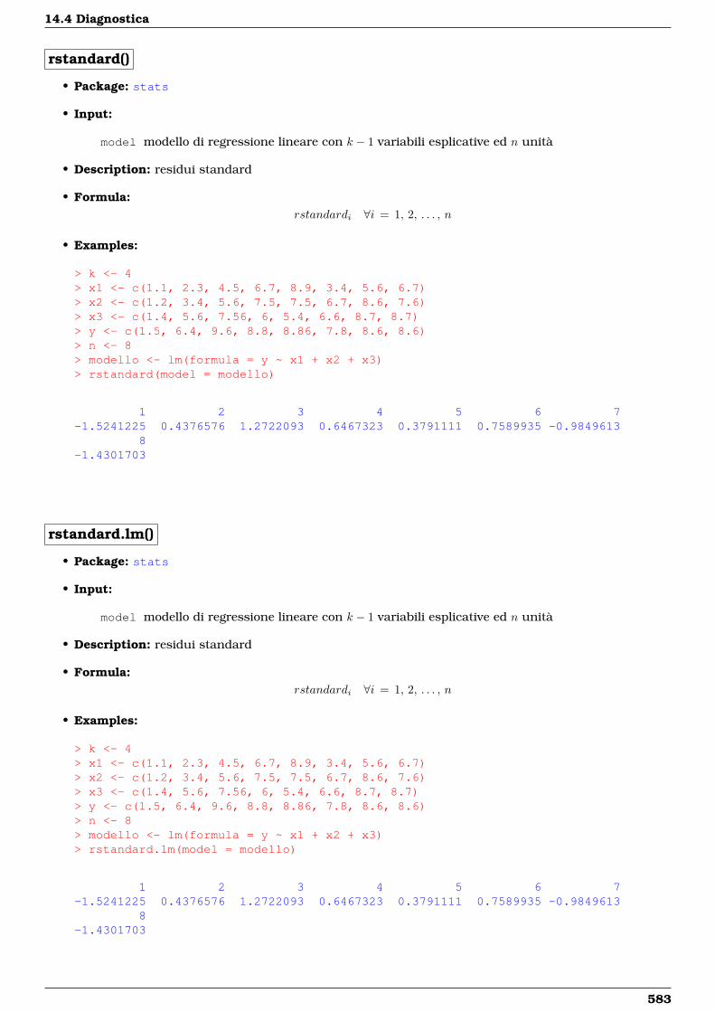
14.4 Diagnostica
rstandard()
• Package: stats
• Input:
model modello di regressione lineare con k − 1 variabili esplicative ed n unità
• Description: residui standard
• Formula:rstandardi ∀i = 1, 2, . . . , n
• Examples:
> k <- 4> x1 <- c(1.1, 2.3, 4.5, 6.7, 8.9, 3.4, 5.6, 6.7)> x2 <- c(1.2, 3.4, 5.6, 7.5, 7.5, 6.7, 8.6, 7.6)> x3 <- c(1.4, 5.6, 7.56, 6, 5.4, 6.6, 8.7, 8.7)> y <- c(1.5, 6.4, 9.6, 8.8, 8.86, 7.8, 8.6, 8.6)> n <- 8> modello <- lm(formula = y ~ x1 + x2 + x3)> rstandard(model = modello)
1 2 3 4 5 6 7-1.5241225 0.4376576 1.2722093 0.6467323 0.3791111 0.7589935 -0.9849613
8-1.4301703
rstandard.lm()
• Package: stats
• Input:
model modello di regressione lineare con k − 1 variabili esplicative ed n unità
• Description: residui standard
• Formula:rstandardi ∀i = 1, 2, . . . , n
• Examples:
> k <- 4> x1 <- c(1.1, 2.3, 4.5, 6.7, 8.9, 3.4, 5.6, 6.7)> x2 <- c(1.2, 3.4, 5.6, 7.5, 7.5, 6.7, 8.6, 7.6)> x3 <- c(1.4, 5.6, 7.56, 6, 5.4, 6.6, 8.7, 8.7)> y <- c(1.5, 6.4, 9.6, 8.8, 8.86, 7.8, 8.6, 8.6)> n <- 8> modello <- lm(formula = y ~ x1 + x2 + x3)> rstandard.lm(model = modello)
1 2 3 4 5 6 7-1.5241225 0.4376576 1.2722093 0.6467323 0.3791111 0.7589935 -0.9849613
8-1.4301703
583
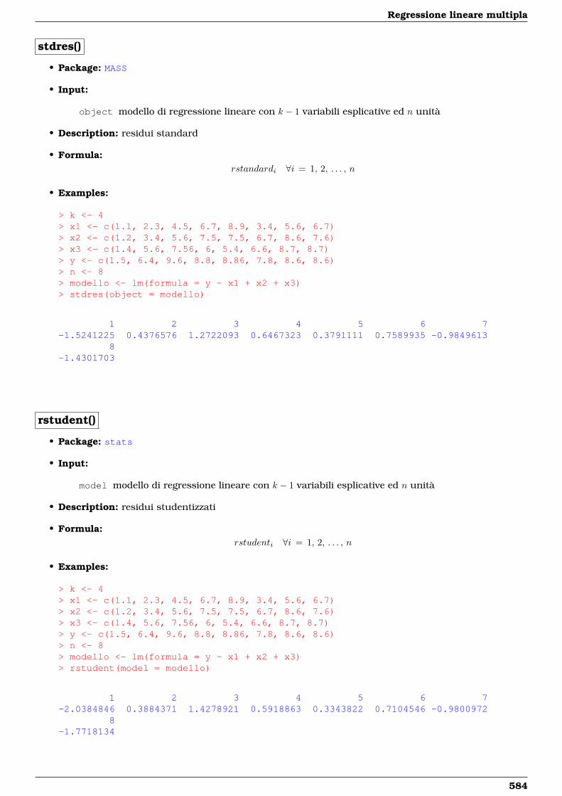
Regressione lineare multipla
stdres()
• Package: MASS
• Input:
object modello di regressione lineare con k − 1 variabili esplicative ed n unità
• Description: residui standard
• Formula:rstandardi ∀i = 1, 2, . . . , n
• Examples:
> k <- 4> x1 <- c(1.1, 2.3, 4.5, 6.7, 8.9, 3.4, 5.6, 6.7)> x2 <- c(1.2, 3.4, 5.6, 7.5, 7.5, 6.7, 8.6, 7.6)> x3 <- c(1.4, 5.6, 7.56, 6, 5.4, 6.6, 8.7, 8.7)> y <- c(1.5, 6.4, 9.6, 8.8, 8.86, 7.8, 8.6, 8.6)> n <- 8> modello <- lm(formula = y ~ x1 + x2 + x3)> stdres(object = modello)
1 2 3 4 5 6 7-1.5241225 0.4376576 1.2722093 0.6467323 0.3791111 0.7589935 -0.9849613
8-1.4301703
rstudent()
• Package: stats
• Input:
model modello di regressione lineare con k − 1 variabili esplicative ed n unità
• Description: residui studentizzati
• Formula:rstudenti ∀i = 1, 2, . . . , n
• Examples:
> k <- 4> x1 <- c(1.1, 2.3, 4.5, 6.7, 8.9, 3.4, 5.6, 6.7)> x2 <- c(1.2, 3.4, 5.6, 7.5, 7.5, 6.7, 8.6, 7.6)> x3 <- c(1.4, 5.6, 7.56, 6, 5.4, 6.6, 8.7, 8.7)> y <- c(1.5, 6.4, 9.6, 8.8, 8.86, 7.8, 8.6, 8.6)> n <- 8> modello <- lm(formula = y ~ x1 + x2 + x3)> rstudent(model = modello)
1 2 3 4 5 6 7-2.0384846 0.3884371 1.4278921 0.5918863 0.3343822 0.7104546 -0.9800972
8-1.7718134
584
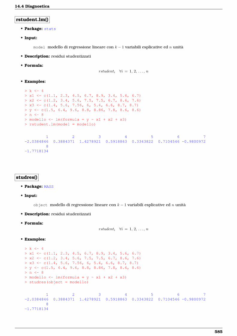
14.4 Diagnostica
rstudent.lm()
• Package: stats
• Input:
model modello di regressione lineare con k − 1 variabili esplicative ed n unità
• Description: residui studentizzati
• Formula:rstudenti ∀i = 1, 2, . . . , n
• Examples:
> k <- 4> x1 <- c(1.1, 2.3, 4.5, 6.7, 8.9, 3.4, 5.6, 6.7)> x2 <- c(1.2, 3.4, 5.6, 7.5, 7.5, 6.7, 8.6, 7.6)> x3 <- c(1.4, 5.6, 7.56, 6, 5.4, 6.6, 8.7, 8.7)> y <- c(1.5, 6.4, 9.6, 8.8, 8.86, 7.8, 8.6, 8.6)> n <- 8> modello <- lm(formula = y ~ x1 + x2 + x3)> rstudent.lm(model = modello)
1 2 3 4 5 6 7-2.0384846 0.3884371 1.4278921 0.5918863 0.3343822 0.7104546 -0.9800972
8-1.7718134
studres()
• Package: MASS
• Input:
object modello di regressione lineare con k − 1 variabili esplicative ed n unità
• Description: residui studentizzati
• Formula:rstudenti ∀i = 1, 2, . . . , n
• Examples:
> k <- 4> x1 <- c(1.1, 2.3, 4.5, 6.7, 8.9, 3.4, 5.6, 6.7)> x2 <- c(1.2, 3.4, 5.6, 7.5, 7.5, 6.7, 8.6, 7.6)> x3 <- c(1.4, 5.6, 7.56, 6, 5.4, 6.6, 8.7, 8.7)> y <- c(1.5, 6.4, 9.6, 8.8, 8.86, 7.8, 8.6, 8.6)> n <- 8> modello <- lm(formula = y ~ x1 + x2 + x3)> studres(object = modello)
1 2 3 4 5 6 7-2.0384846 0.3884371 1.4278921 0.5918863 0.3343822 0.7104546 -0.9800972
8-1.7718134
585
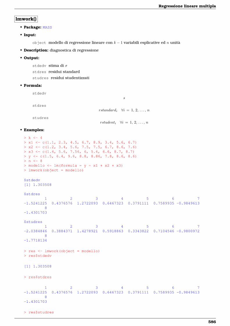
Regressione lineare multipla
lmwork()
• Package: MASS
• Input:
object modello di regressione lineare con k − 1 variabili esplicative ed n unità
• Description: diagnostica di regressione
• Output:
stdedv stima di σ
stdres residui standard
studres residui studentizzati
• Formula:
stdedvs
stdresrstandardi ∀i = 1, 2, . . . , n
studresrstudenti ∀i = 1, 2, . . . , n
• Examples:
> k <- 4> x1 <- c(1.1, 2.3, 4.5, 6.7, 8.9, 3.4, 5.6, 6.7)> x2 <- c(1.2, 3.4, 5.6, 7.5, 7.5, 6.7, 8.6, 7.6)> x3 <- c(1.4, 5.6, 7.56, 6, 5.4, 6.6, 8.7, 8.7)> y <- c(1.5, 6.4, 9.6, 8.8, 8.86, 7.8, 8.6, 8.6)> n <- 8> modello <- lm(formula = y ~ x1 + x2 + x3)> lmwork(object = modello)
$stdedv[1] 1.303508
$stdres1 2 3 4 5 6 7
-1.5241225 0.4376576 1.2722093 0.6467323 0.3791111 0.7589935 -0.98496138
-1.4301703
$studres1 2 3 4 5 6 7
-2.0384846 0.3884371 1.4278921 0.5918863 0.3343822 0.7104546 -0.98009728
-1.7718134
> res <- lmwork(object = modello)> res$stdedv
[1] 1.303508
> res$stdres
1 2 3 4 5 6 7-1.5241225 0.4376576 1.2722093 0.6467323 0.3791111 0.7589935 -0.9849613
8-1.4301703
> res$studres
586
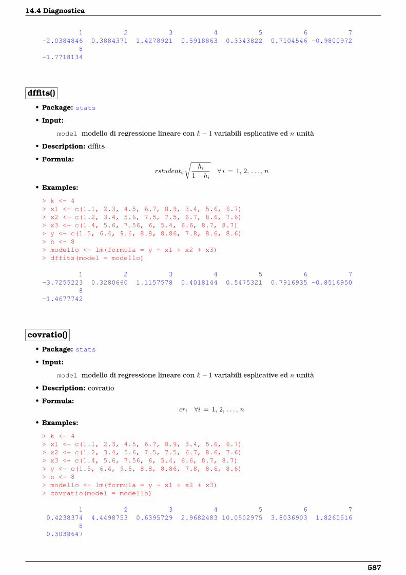
14.4 Diagnostica
1 2 3 4 5 6 7-2.0384846 0.3884371 1.4278921 0.5918863 0.3343822 0.7104546 -0.9800972
8-1.7718134
dffits()
• Package: stats
• Input:
model modello di regressione lineare con k − 1 variabili esplicative ed n unità
• Description: dffits
• Formula:
rstudenti
√hi
1− hi∀ i = 1, 2, . . . , n
• Examples:
> k <- 4> x1 <- c(1.1, 2.3, 4.5, 6.7, 8.9, 3.4, 5.6, 6.7)> x2 <- c(1.2, 3.4, 5.6, 7.5, 7.5, 6.7, 8.6, 7.6)> x3 <- c(1.4, 5.6, 7.56, 6, 5.4, 6.6, 8.7, 8.7)> y <- c(1.5, 6.4, 9.6, 8.8, 8.86, 7.8, 8.6, 8.6)> n <- 8> modello <- lm(formula = y ~ x1 + x2 + x3)> dffits(model = modello)
1 2 3 4 5 6 7-3.7255223 0.3280660 1.1157578 0.4018144 0.5475321 0.7916935 -0.8516950
8-1.4677742
covratio()
• Package: stats
• Input:
model modello di regressione lineare con k − 1 variabili esplicative ed n unità
• Description: covratio
• Formula:cri ∀i = 1, 2, . . . , n
• Examples:
> k <- 4> x1 <- c(1.1, 2.3, 4.5, 6.7, 8.9, 3.4, 5.6, 6.7)> x2 <- c(1.2, 3.4, 5.6, 7.5, 7.5, 6.7, 8.6, 7.6)> x3 <- c(1.4, 5.6, 7.56, 6, 5.4, 6.6, 8.7, 8.7)> y <- c(1.5, 6.4, 9.6, 8.8, 8.86, 7.8, 8.6, 8.6)> n <- 8> modello <- lm(formula = y ~ x1 + x2 + x3)> covratio(model = modello)
1 2 3 4 5 6 70.4238374 4.4498753 0.6395729 2.9682483 10.0502975 3.8036903 1.8260516
80.3038647
587
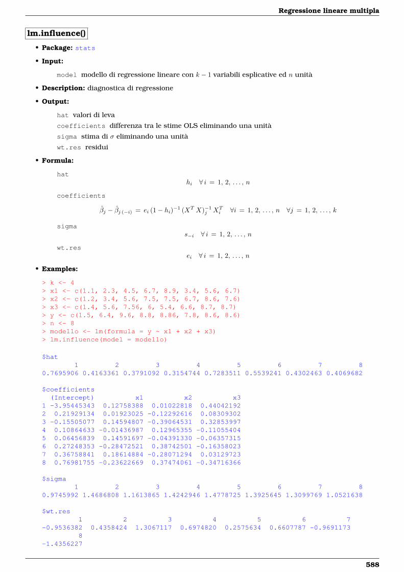
Regressione lineare multipla
lm.influence()
• Package: stats
• Input:
model modello di regressione lineare con k − 1 variabili esplicative ed n unità
• Description: diagnostica di regressione
• Output:
hat valori di leva
coefficients differenza tra le stime OLS eliminando una unità
sigma stima di σ eliminando una unità
wt.res residui
• Formula:
hathi ∀ i = 1, 2, . . . , n
coefficients
βj − βj (−i) = ei (1− hi)−1 (XT X)−1j XT
i ∀i = 1, 2, . . . , n ∀j = 1, 2, . . . , k
sigmas−i ∀ i = 1, 2, . . . , n
wt.resei ∀ i = 1, 2, . . . , n
• Examples:
> k <- 4> x1 <- c(1.1, 2.3, 4.5, 6.7, 8.9, 3.4, 5.6, 6.7)> x2 <- c(1.2, 3.4, 5.6, 7.5, 7.5, 6.7, 8.6, 7.6)> x3 <- c(1.4, 5.6, 7.56, 6, 5.4, 6.6, 8.7, 8.7)> y <- c(1.5, 6.4, 9.6, 8.8, 8.86, 7.8, 8.6, 8.6)> n <- 8> modello <- lm(formula = y ~ x1 + x2 + x3)> lm.influence(model = modello)
$hat1 2 3 4 5 6 7 8
0.7695906 0.4163361 0.3791092 0.3154744 0.7283511 0.5539241 0.4302463 0.4069682
$coefficients(Intercept) x1 x2 x3
1 -3.95445343 0.12758388 0.01022818 0.440421922 0.21929134 0.01923025 -0.12292616 0.083093023 -0.15505077 0.14594807 -0.39064531 0.328539974 0.10864633 -0.01436987 0.12965355 -0.110554045 0.06456839 0.14591697 -0.04391330 -0.063573156 0.27248353 -0.28472521 0.38742501 -0.163580237 0.36758841 0.18614884 -0.28071294 0.031297238 0.76981755 -0.23622669 0.37474061 -0.34716366
$sigma1 2 3 4 5 6 7 8
0.9745992 1.4686808 1.1613865 1.4242946 1.4778725 1.3925645 1.3099769 1.0521638
$wt.res1 2 3 4 5 6 7
-0.9536382 0.4358424 1.3067117 0.6974820 0.2575634 0.6607787 -0.96911738
-1.4356227
588
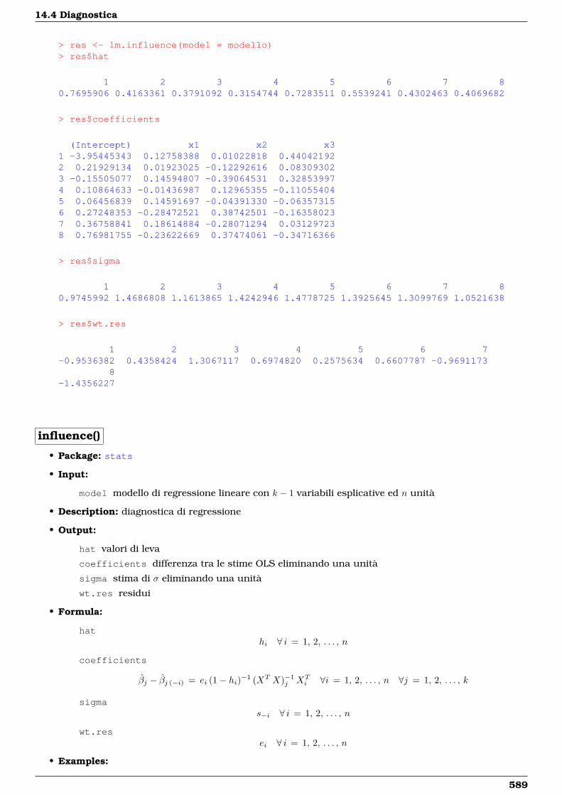
14.4 Diagnostica
> res <- lm.influence(model = modello)> res$hat
1 2 3 4 5 6 7 80.7695906 0.4163361 0.3791092 0.3154744 0.7283511 0.5539241 0.4302463 0.4069682
> res$coefficients
(Intercept) x1 x2 x31 -3.95445343 0.12758388 0.01022818 0.440421922 0.21929134 0.01923025 -0.12292616 0.083093023 -0.15505077 0.14594807 -0.39064531 0.328539974 0.10864633 -0.01436987 0.12965355 -0.110554045 0.06456839 0.14591697 -0.04391330 -0.063573156 0.27248353 -0.28472521 0.38742501 -0.163580237 0.36758841 0.18614884 -0.28071294 0.031297238 0.76981755 -0.23622669 0.37474061 -0.34716366
> res$sigma
1 2 3 4 5 6 7 80.9745992 1.4686808 1.1613865 1.4242946 1.4778725 1.3925645 1.3099769 1.0521638
> res$wt.res
1 2 3 4 5 6 7-0.9536382 0.4358424 1.3067117 0.6974820 0.2575634 0.6607787 -0.9691173
8-1.4356227
influence()
• Package: stats
• Input:
model modello di regressione lineare con k − 1 variabili esplicative ed n unità
• Description: diagnostica di regressione
• Output:
hat valori di leva
coefficients differenza tra le stime OLS eliminando una unità
sigma stima di σ eliminando una unità
wt.res residui
• Formula:
hathi ∀ i = 1, 2, . . . , n
coefficients
βj − βj (−i) = ei (1− hi)−1 (XT X)−1j XT
i ∀i = 1, 2, . . . , n ∀j = 1, 2, . . . , k
sigmas−i ∀ i = 1, 2, . . . , n
wt.resei ∀ i = 1, 2, . . . , n
• Examples:
589
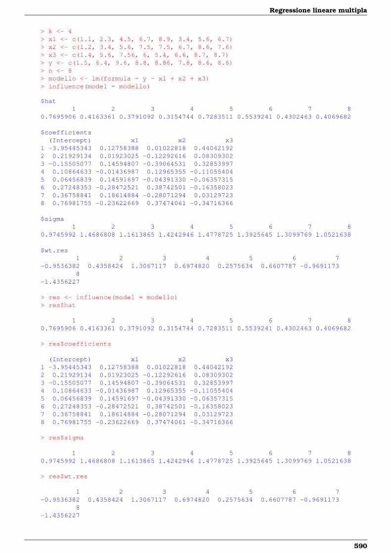
Regressione lineare multipla
> k <- 4> x1 <- c(1.1, 2.3, 4.5, 6.7, 8.9, 3.4, 5.6, 6.7)> x2 <- c(1.2, 3.4, 5.6, 7.5, 7.5, 6.7, 8.6, 7.6)> x3 <- c(1.4, 5.6, 7.56, 6, 5.4, 6.6, 8.7, 8.7)> y <- c(1.5, 6.4, 9.6, 8.8, 8.86, 7.8, 8.6, 8.6)> n <- 8> modello <- lm(formula = y ~ x1 + x2 + x3)> influence(model = modello)
$hat1 2 3 4 5 6 7 8
0.7695906 0.4163361 0.3791092 0.3154744 0.7283511 0.5539241 0.4302463 0.4069682
$coefficients(Intercept) x1 x2 x3
1 -3.95445343 0.12758388 0.01022818 0.440421922 0.21929134 0.01923025 -0.12292616 0.083093023 -0.15505077 0.14594807 -0.39064531 0.328539974 0.10864633 -0.01436987 0.12965355 -0.110554045 0.06456839 0.14591697 -0.04391330 -0.063573156 0.27248353 -0.28472521 0.38742501 -0.163580237 0.36758841 0.18614884 -0.28071294 0.031297238 0.76981755 -0.23622669 0.37474061 -0.34716366
$sigma1 2 3 4 5 6 7 8
0.9745992 1.4686808 1.1613865 1.4242946 1.4778725 1.3925645 1.3099769 1.0521638
$wt.res1 2 3 4 5 6 7
-0.9536382 0.4358424 1.3067117 0.6974820 0.2575634 0.6607787 -0.96911738
-1.4356227
> res <- influence(model = modello)> res$hat
1 2 3 4 5 6 7 80.7695906 0.4163361 0.3791092 0.3154744 0.7283511 0.5539241 0.4302463 0.4069682
> res$coefficients
(Intercept) x1 x2 x31 -3.95445343 0.12758388 0.01022818 0.440421922 0.21929134 0.01923025 -0.12292616 0.083093023 -0.15505077 0.14594807 -0.39064531 0.328539974 0.10864633 -0.01436987 0.12965355 -0.110554045 0.06456839 0.14591697 -0.04391330 -0.063573156 0.27248353 -0.28472521 0.38742501 -0.163580237 0.36758841 0.18614884 -0.28071294 0.031297238 0.76981755 -0.23622669 0.37474061 -0.34716366
> res$sigma
1 2 3 4 5 6 7 80.9745992 1.4686808 1.1613865 1.4242946 1.4778725 1.3925645 1.3099769 1.0521638
> res$wt.res
1 2 3 4 5 6 7-0.9536382 0.4358424 1.3067117 0.6974820 0.2575634 0.6607787 -0.9691173
8-1.4356227
590
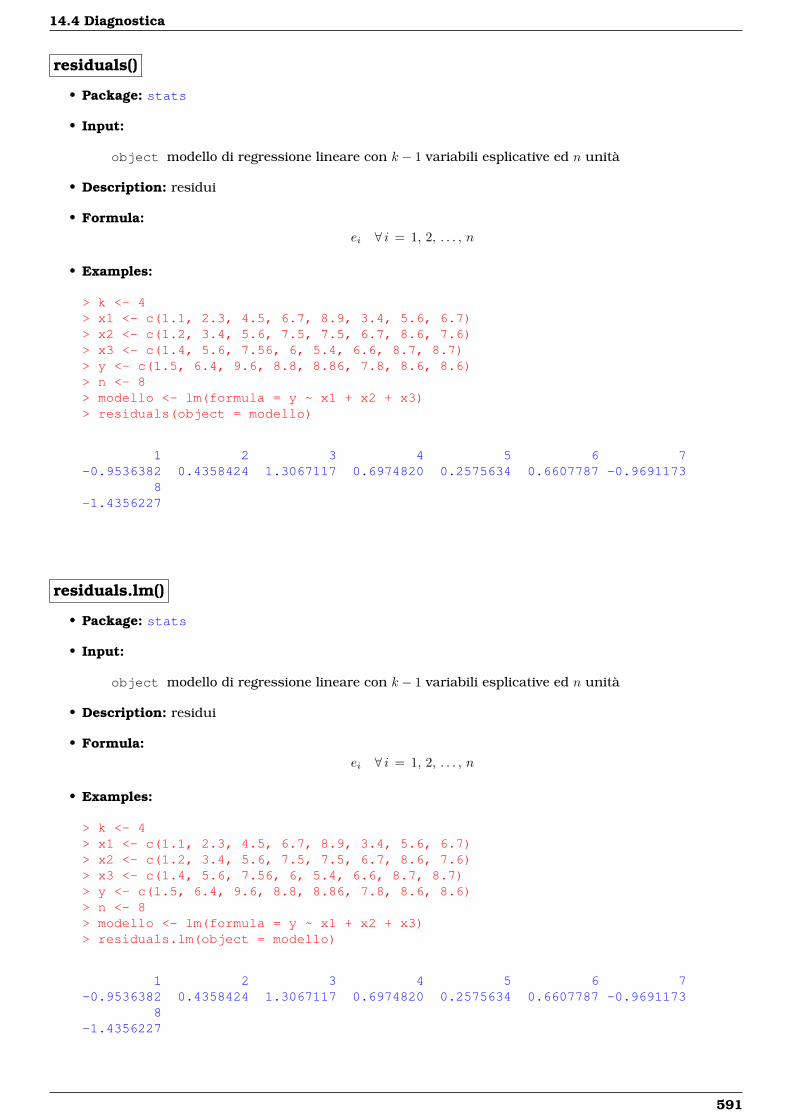
14.4 Diagnostica
residuals()
• Package: stats
• Input:
object modello di regressione lineare con k − 1 variabili esplicative ed n unità
• Description: residui
• Formula:ei ∀ i = 1, 2, . . . , n
• Examples:
> k <- 4> x1 <- c(1.1, 2.3, 4.5, 6.7, 8.9, 3.4, 5.6, 6.7)> x2 <- c(1.2, 3.4, 5.6, 7.5, 7.5, 6.7, 8.6, 7.6)> x3 <- c(1.4, 5.6, 7.56, 6, 5.4, 6.6, 8.7, 8.7)> y <- c(1.5, 6.4, 9.6, 8.8, 8.86, 7.8, 8.6, 8.6)> n <- 8> modello <- lm(formula = y ~ x1 + x2 + x3)> residuals(object = modello)
1 2 3 4 5 6 7-0.9536382 0.4358424 1.3067117 0.6974820 0.2575634 0.6607787 -0.9691173
8-1.4356227
residuals.lm()
• Package: stats
• Input:
object modello di regressione lineare con k − 1 variabili esplicative ed n unità
• Description: residui
• Formula:ei ∀ i = 1, 2, . . . , n
• Examples:
> k <- 4> x1 <- c(1.1, 2.3, 4.5, 6.7, 8.9, 3.4, 5.6, 6.7)> x2 <- c(1.2, 3.4, 5.6, 7.5, 7.5, 6.7, 8.6, 7.6)> x3 <- c(1.4, 5.6, 7.56, 6, 5.4, 6.6, 8.7, 8.7)> y <- c(1.5, 6.4, 9.6, 8.8, 8.86, 7.8, 8.6, 8.6)> n <- 8> modello <- lm(formula = y ~ x1 + x2 + x3)> residuals.lm(object = modello)
1 2 3 4 5 6 7-0.9536382 0.4358424 1.3067117 0.6974820 0.2575634 0.6607787 -0.9691173
8-1.4356227
591
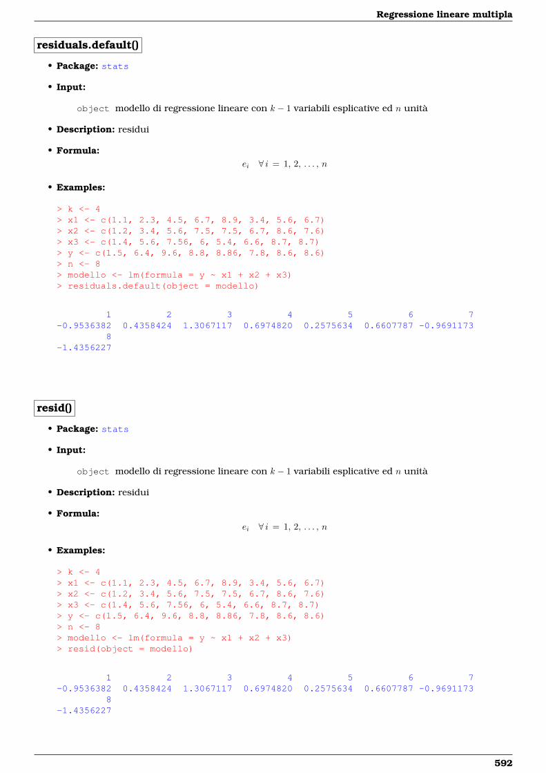
Regressione lineare multipla
residuals.default()
• Package: stats
• Input:
object modello di regressione lineare con k − 1 variabili esplicative ed n unità
• Description: residui
• Formula:ei ∀ i = 1, 2, . . . , n
• Examples:
> k <- 4> x1 <- c(1.1, 2.3, 4.5, 6.7, 8.9, 3.4, 5.6, 6.7)> x2 <- c(1.2, 3.4, 5.6, 7.5, 7.5, 6.7, 8.6, 7.6)> x3 <- c(1.4, 5.6, 7.56, 6, 5.4, 6.6, 8.7, 8.7)> y <- c(1.5, 6.4, 9.6, 8.8, 8.86, 7.8, 8.6, 8.6)> n <- 8> modello <- lm(formula = y ~ x1 + x2 + x3)> residuals.default(object = modello)
1 2 3 4 5 6 7-0.9536382 0.4358424 1.3067117 0.6974820 0.2575634 0.6607787 -0.9691173
8-1.4356227
resid()
• Package: stats
• Input:
object modello di regressione lineare con k − 1 variabili esplicative ed n unità
• Description: residui
• Formula:ei ∀ i = 1, 2, . . . , n
• Examples:
> k <- 4> x1 <- c(1.1, 2.3, 4.5, 6.7, 8.9, 3.4, 5.6, 6.7)> x2 <- c(1.2, 3.4, 5.6, 7.5, 7.5, 6.7, 8.6, 7.6)> x3 <- c(1.4, 5.6, 7.56, 6, 5.4, 6.6, 8.7, 8.7)> y <- c(1.5, 6.4, 9.6, 8.8, 8.86, 7.8, 8.6, 8.6)> n <- 8> modello <- lm(formula = y ~ x1 + x2 + x3)> resid(object = modello)
1 2 3 4 5 6 7-0.9536382 0.4358424 1.3067117 0.6974820 0.2575634 0.6607787 -0.9691173
8-1.4356227
592
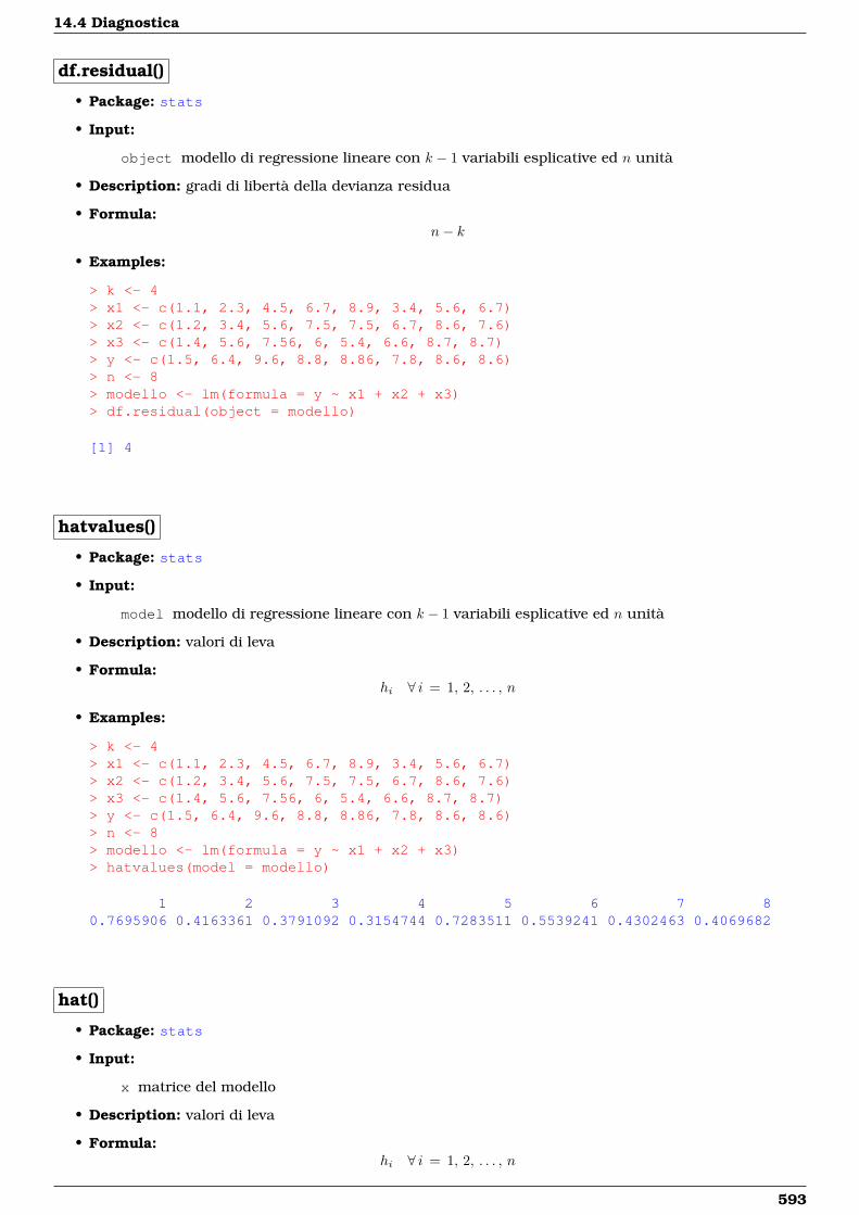
14.4 Diagnostica
df.residual()
• Package: stats
• Input:
object modello di regressione lineare con k − 1 variabili esplicative ed n unità
• Description: gradi di libertà della devianza residua
• Formula:n− k
• Examples:
> k <- 4> x1 <- c(1.1, 2.3, 4.5, 6.7, 8.9, 3.4, 5.6, 6.7)> x2 <- c(1.2, 3.4, 5.6, 7.5, 7.5, 6.7, 8.6, 7.6)> x3 <- c(1.4, 5.6, 7.56, 6, 5.4, 6.6, 8.7, 8.7)> y <- c(1.5, 6.4, 9.6, 8.8, 8.86, 7.8, 8.6, 8.6)> n <- 8> modello <- lm(formula = y ~ x1 + x2 + x3)> df.residual(object = modello)
[1] 4
hatvalues()
• Package: stats
• Input:
model modello di regressione lineare con k − 1 variabili esplicative ed n unità
• Description: valori di leva
• Formula:hi ∀ i = 1, 2, . . . , n
• Examples:
> k <- 4> x1 <- c(1.1, 2.3, 4.5, 6.7, 8.9, 3.4, 5.6, 6.7)> x2 <- c(1.2, 3.4, 5.6, 7.5, 7.5, 6.7, 8.6, 7.6)> x3 <- c(1.4, 5.6, 7.56, 6, 5.4, 6.6, 8.7, 8.7)> y <- c(1.5, 6.4, 9.6, 8.8, 8.86, 7.8, 8.6, 8.6)> n <- 8> modello <- lm(formula = y ~ x1 + x2 + x3)> hatvalues(model = modello)
1 2 3 4 5 6 7 80.7695906 0.4163361 0.3791092 0.3154744 0.7283511 0.5539241 0.4302463 0.4069682
hat()
• Package: stats
• Input:
x matrice del modello
• Description: valori di leva
• Formula:hi ∀ i = 1, 2, . . . , n
593
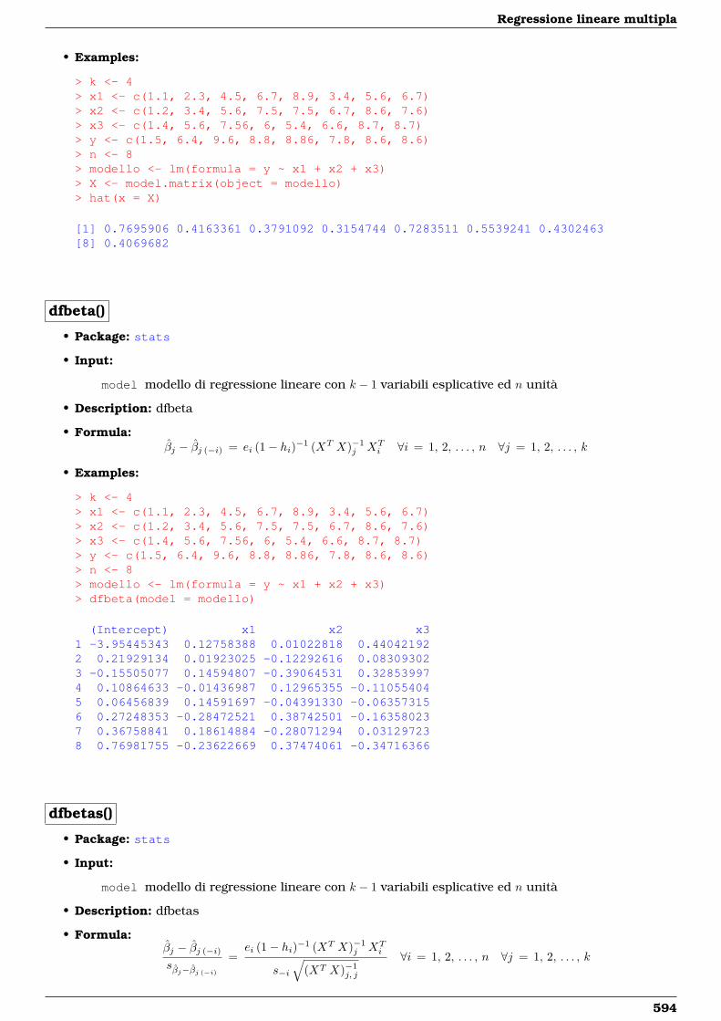
Regressione lineare multipla
• Examples:
> k <- 4> x1 <- c(1.1, 2.3, 4.5, 6.7, 8.9, 3.4, 5.6, 6.7)> x2 <- c(1.2, 3.4, 5.6, 7.5, 7.5, 6.7, 8.6, 7.6)> x3 <- c(1.4, 5.6, 7.56, 6, 5.4, 6.6, 8.7, 8.7)> y <- c(1.5, 6.4, 9.6, 8.8, 8.86, 7.8, 8.6, 8.6)> n <- 8> modello <- lm(formula = y ~ x1 + x2 + x3)> X <- model.matrix(object = modello)> hat(x = X)
[1] 0.7695906 0.4163361 0.3791092 0.3154744 0.7283511 0.5539241 0.4302463[8] 0.4069682
dfbeta()
• Package: stats
• Input:
model modello di regressione lineare con k − 1 variabili esplicative ed n unità
• Description: dfbeta
• Formula:βj − βj (−i) = ei (1− hi)−1 (XT X)−1
j XTi ∀i = 1, 2, . . . , n ∀j = 1, 2, . . . , k
• Examples:
> k <- 4> x1 <- c(1.1, 2.3, 4.5, 6.7, 8.9, 3.4, 5.6, 6.7)> x2 <- c(1.2, 3.4, 5.6, 7.5, 7.5, 6.7, 8.6, 7.6)> x3 <- c(1.4, 5.6, 7.56, 6, 5.4, 6.6, 8.7, 8.7)> y <- c(1.5, 6.4, 9.6, 8.8, 8.86, 7.8, 8.6, 8.6)> n <- 8> modello <- lm(formula = y ~ x1 + x2 + x3)> dfbeta(model = modello)
(Intercept) x1 x2 x31 -3.95445343 0.12758388 0.01022818 0.440421922 0.21929134 0.01923025 -0.12292616 0.083093023 -0.15505077 0.14594807 -0.39064531 0.328539974 0.10864633 -0.01436987 0.12965355 -0.110554045 0.06456839 0.14591697 -0.04391330 -0.063573156 0.27248353 -0.28472521 0.38742501 -0.163580237 0.36758841 0.18614884 -0.28071294 0.031297238 0.76981755 -0.23622669 0.37474061 -0.34716366
dfbetas()
• Package: stats
• Input:
model modello di regressione lineare con k − 1 variabili esplicative ed n unità
• Description: dfbetas
• Formula:βj − βj (−i)
sβj−βj (−i)
=ei (1− hi)−1 (XT X)−1
j XTi
s−i
√(XT X)−1
j, j
∀i = 1, 2, . . . , n ∀j = 1, 2, . . . , k
594
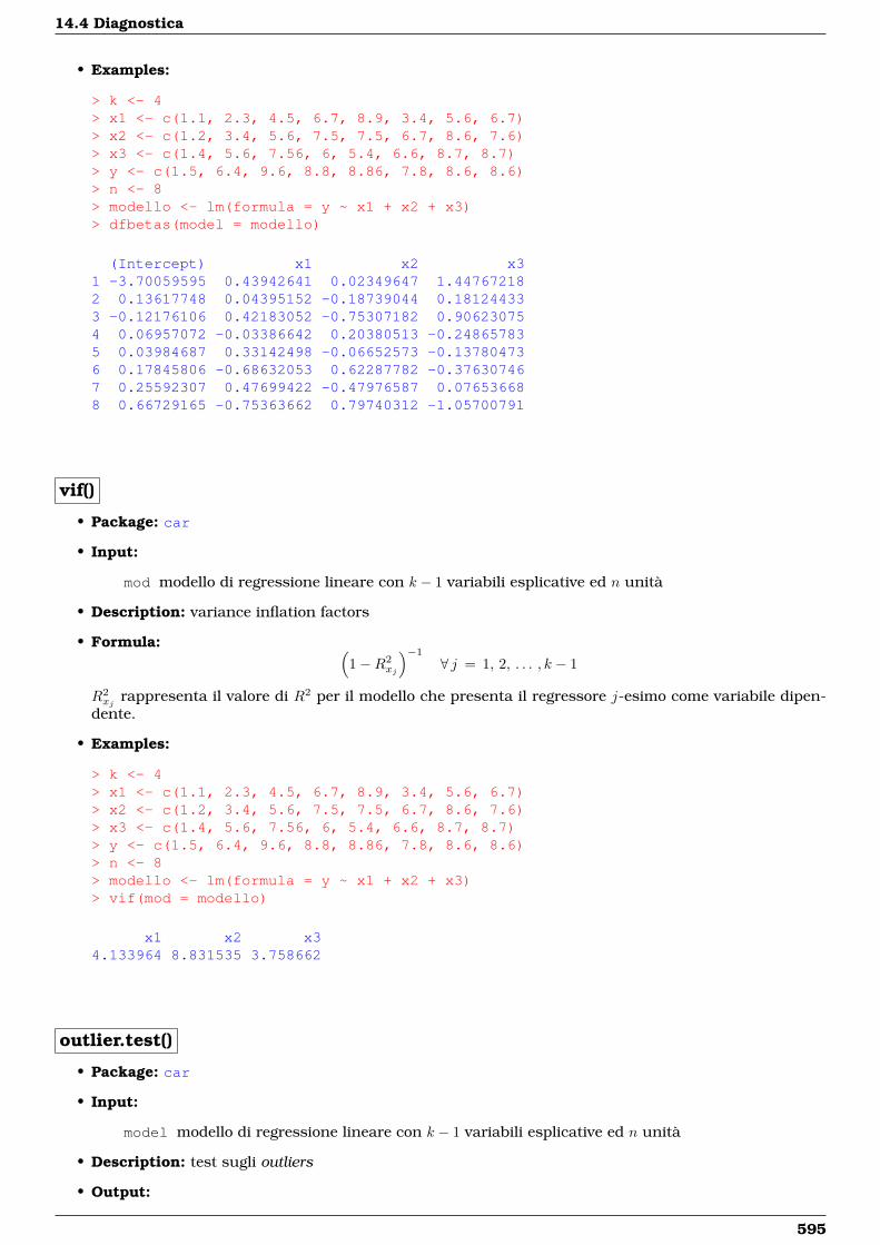
14.4 Diagnostica
• Examples:
> k <- 4> x1 <- c(1.1, 2.3, 4.5, 6.7, 8.9, 3.4, 5.6, 6.7)> x2 <- c(1.2, 3.4, 5.6, 7.5, 7.5, 6.7, 8.6, 7.6)> x3 <- c(1.4, 5.6, 7.56, 6, 5.4, 6.6, 8.7, 8.7)> y <- c(1.5, 6.4, 9.6, 8.8, 8.86, 7.8, 8.6, 8.6)> n <- 8> modello <- lm(formula = y ~ x1 + x2 + x3)> dfbetas(model = modello)
(Intercept) x1 x2 x31 -3.70059595 0.43942641 0.02349647 1.447672182 0.13617748 0.04395152 -0.18739044 0.181244333 -0.12176106 0.42183052 -0.75307182 0.906230754 0.06957072 -0.03386642 0.20380513 -0.248657835 0.03984687 0.33142498 -0.06652573 -0.137804736 0.17845806 -0.68632053 0.62287782 -0.376307467 0.25592307 0.47699422 -0.47976587 0.076536688 0.66729165 -0.75363662 0.79740312 -1.05700791
vif()
• Package: car
• Input:
mod modello di regressione lineare con k − 1 variabili esplicative ed n unità
• Description: variance inflation factors
• Formula: (1−R2
xj
)−1
∀ j = 1, 2, . . . , k − 1
R2xj rappresenta il valore di R2 per il modello che presenta il regressore j-esimo come variabile dipen-
dente.
• Examples:
> k <- 4> x1 <- c(1.1, 2.3, 4.5, 6.7, 8.9, 3.4, 5.6, 6.7)> x2 <- c(1.2, 3.4, 5.6, 7.5, 7.5, 6.7, 8.6, 7.6)> x3 <- c(1.4, 5.6, 7.56, 6, 5.4, 6.6, 8.7, 8.7)> y <- c(1.5, 6.4, 9.6, 8.8, 8.86, 7.8, 8.6, 8.6)> n <- 8> modello <- lm(formula = y ~ x1 + x2 + x3)> vif(mod = modello)
x1 x2 x34.133964 8.831535 3.758662
outlier.test()
• Package: car
• Input:
model modello di regressione lineare con k − 1 variabili esplicative ed n unità
• Description: test sugli outliers
• Output:
595
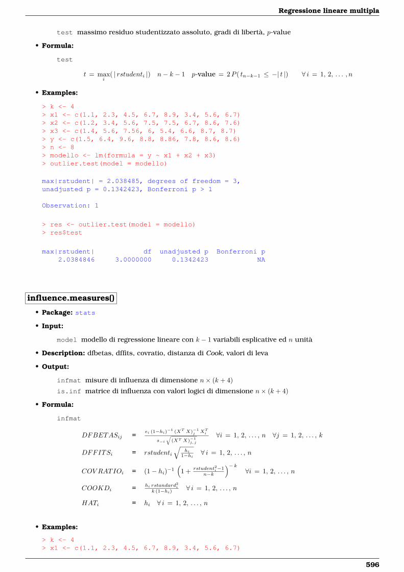
Regressione lineare multipla
test massimo residuo studentizzato assoluto, gradi di libertà, p-value
• Formula:
test
t = maxi
( | rstudenti |) n− k − 1 p-value = 2P ( tn−k−1 ≤ −| t |) ∀ i = 1, 2, . . . , n
• Examples:
> k <- 4> x1 <- c(1.1, 2.3, 4.5, 6.7, 8.9, 3.4, 5.6, 6.7)> x2 <- c(1.2, 3.4, 5.6, 7.5, 7.5, 6.7, 8.6, 7.6)> x3 <- c(1.4, 5.6, 7.56, 6, 5.4, 6.6, 8.7, 8.7)> y <- c(1.5, 6.4, 9.6, 8.8, 8.86, 7.8, 8.6, 8.6)> n <- 8> modello <- lm(formula = y ~ x1 + x2 + x3)> outlier.test(model = modello)
max|rstudent| = 2.038485, degrees of freedom = 3,unadjusted p = 0.1342423, Bonferroni p > 1
Observation: 1
> res <- outlier.test(model = modello)> res$test
max|rstudent| df unadjusted p Bonferroni p2.0384846 3.0000000 0.1342423 NA
influence.measures()
• Package: stats
• Input:
model modello di regressione lineare con k − 1 variabili esplicative ed n unità
• Description: dfbetas, dffits, covratio, distanza di Cook, valori di leva
• Output:
infmat misure di influenza di dimensione n× (k + 4)
is.inf matrice di influenza con valori logici di dimensione n× (k + 4)
• Formula:
infmat
DFBETASij =ei (1−hi)−1 (XT X)−1
j XTi
s−i
√(XT X)−1
j, j
∀i = 1, 2, . . . , n ∀j = 1, 2, . . . , k
DFFITSi = rstudenti
√hi
1−hi ∀ i = 1, 2, . . . , n
COV RATIOi = (1− hi)−1(
1 + rstudent2i−1n−k
)− k∀i = 1, 2, . . . , n
COOKDi = hi rstandard2i
k (1−hi) ∀ i = 1, 2, . . . , n
HATi = hi ∀ i = 1, 2, . . . , n
• Examples:
> k <- 4> x1 <- c(1.1, 2.3, 4.5, 6.7, 8.9, 3.4, 5.6, 6.7)
596
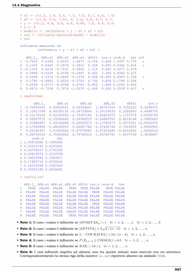
14.4 Diagnostica
> x2 <- c(1.2, 3.4, 5.6, 7.5, 7.5, 6.7, 8.6, 7.6)> x3 <- c(1.4, 5.6, 7.56, 6, 5.4, 6.6, 8.7, 8.7)> y <- c(1.5, 6.4, 9.6, 8.8, 8.86, 7.8, 8.6, 8.6)> n <- 8> modello <- lm(formula = y ~ x1 + x2 + x3)> res <- influence.measures(model = modello)> res
Influence measures oflm(formula = y ~ x1 + x2 + x3) :
dfb.1_ dfb.x1 dfb.x2 dfb.x3 dffit cov.r cook.d hat inf1 -3.7006 0.4394 0.0235 1.4477 -3.726 0.424 1.9397 0.770 *2 0.1362 0.0440 -0.1874 0.1812 0.328 4.450 0.0342 0.416 *3 -0.1218 0.4218 -0.7531 0.9062 1.116 0.640 0.2471 0.3794 0.0696 -0.0339 0.2038 -0.2487 0.402 2.968 0.0482 0.3155 0.0398 0.3314 -0.0665 -0.1378 0.548 10.050 0.0963 0.728 *6 0.1785 -0.6863 0.6229 -0.3763 0.792 3.804 0.1788 0.5547 0.2559 0.4770 -0.4798 0.0765 -0.852 1.826 0.1832 0.4308 0.6673 -0.7536 0.7974 -1.0570 -1.468 0.304 0.3509 0.407 *
> res$infmat
dfb.1_ dfb.x1 dfb.x2 dfb.x3 dffit cov.r1 -3.70059595 0.43942641 0.02349647 1.44767218 -3.7255223 0.42383742 0.13617748 0.04395152 -0.18739044 0.18124433 0.3280660 4.44987533 -0.12176106 0.42183052 -0.75307182 0.90623075 1.1157578 0.63957294 0.06957072 -0.03386642 0.20380513 -0.24865783 0.4018144 2.96824835 0.03984687 0.33142498 -0.06652573 -0.13780473 0.5475321 10.05029756 0.17845806 -0.68632053 0.62287782 -0.37630746 0.7916935 3.80369037 0.25592307 0.47699422 -0.47976587 0.07653668 -0.8516950 1.82605168 0.66729165 -0.75363662 0.79740312 -1.05700791 -1.4677742 0.3038647
cook.d hat1 1.93972080 0.76959062 0.03415783 0.41633613 0.24706215 0.37910924 0.04819074 0.31547445 0.09633983 0.72835116 0.17883712 0.55392417 0.18315058 0.43024638 0.35091186 0.4069682
> res$is.inf
dfb.1_ dfb.x1 dfb.x2 dfb.x3 dffit cov.r cook.d hat1 TRUE FALSE FALSE TRUE TRUE FALSE TRUE FALSE2 FALSE FALSE FALSE FALSE FALSE TRUE FALSE FALSE3 FALSE FALSE FALSE FALSE FALSE FALSE FALSE FALSE4 FALSE FALSE FALSE FALSE FALSE FALSE FALSE FALSE5 FALSE FALSE FALSE FALSE FALSE TRUE FALSE FALSE6 FALSE FALSE FALSE FALSE FALSE FALSE FALSE FALSE7 FALSE FALSE FALSE FALSE FALSE FALSE FALSE FALSE8 FALSE FALSE FALSE TRUE FALSE FALSE FALSE FALSE
• Note 1: Il caso i-esimo è influente se |DFBETASij | > 1 ∀i = 1, 2, . . . , n ∀j = 1, 2, . . . , k
• Note 2: Il caso i-esimo è influente se |DFFITSi| > 3√k / (n− k) ∀i = 1, 2, . . . , n
• Note 3: Il caso i-esimo è influente se |1− COV RATIOi| > 3 k / (n− k) ∀i = 1, 2, . . . , n
• Note 4: Il caso i-esimo è influente se P (Fk,n−k ≥ COOKDi) > 0.5 ∀i = 1, 2, . . . , n
• Note 5: Il caso i-esimo è influente se HATi > 3 k / n ∀i = 1, 2, . . . , n
• Note 6: I casi influenti rispetto ad almeno una tra queste misure sono marcati con un asterisco.Corrispondentemente la stessa riga della matrice is.inf riporterà almeno un simbolo TRUE.
597

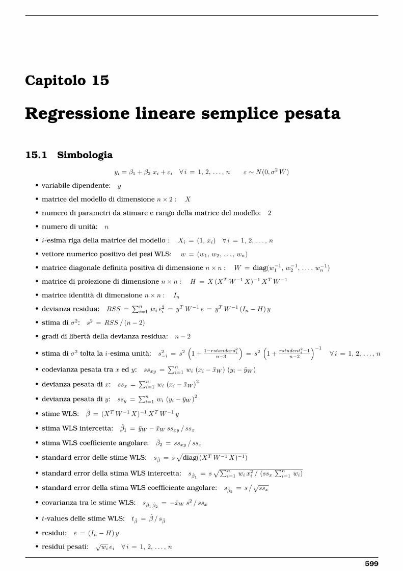
Capitolo 15
Regressione lineare semplice pesata
15.1 Simbologia
yi = β1 + β2 xi + εi ∀ i = 1, 2, . . . , n ε ∼ N(0, σ2W )
• variabile dipendente: y
• matrice del modello di dimensione n× 2 : X
• numero di parametri da stimare e rango della matrice del modello: 2
• numero di unità: n
• i-esima riga della matrice del modello : Xi = (1, xi) ∀ i = 1, 2, . . . , n
• vettore numerico positivo dei pesi WLS: w = (w1, w2, . . . , wn)
• matrice diagonale definita positiva di dimensione n× n : W = diag(w−11 , w−1
2 , . . . , w−1n )
• matrice di proiezione di dimensione n× n : H = X (XT W−1X)−1XT W−1
• matrice identità di dimensione n× n : In
• devianza residua: RSS =∑ni=1 wi e
2i = yT W−1 e = yT W−1 (In −H) y
• stima di σ2: s2 = RSS / (n− 2)
• gradi di libertà della devianza residua: n− 2
• stima di σ2 tolta la i-esima unità: s2−i = s2
(1 + 1−rstandard2i
n−3
)= s2
(1 + rstudent2i−1
n−2
)−1
∀ i = 1, 2, . . . , n
• codevianza pesata tra x ed y: ssxy =∑ni=1 wi (xi − xW ) (yi − yW )
• devianza pesata di x: ssx =∑ni=1 wi (xi − xW )2
• devianza pesata di y: ssy =∑ni=1 wi (yi − yW )2
• stime WLS: β = (XT W−1X)−1XT W−1 y
• stima WLS intercetta: β1 = yW − xW ssxy / ssx
• stima WLS coefficiente angolare: β2 = ssxy / ssx
• standard error delle stime WLS: sβ = s√
diag((XT W−1X)−1)
• standard error della stima WLS intercetta: sβ1= s
√∑ni=1 wi x
2i / (ssx
∑ni=1 wi)
• standard error della stima WLS coefficiente angolare: sβ2= s /
√ssx
• covarianza tra le stime WLS: sβ1 β2= −xW s2 / ssx
• t-values delle stime WLS: tβ = β / sβ
• residui: e = (In −H) y
• residui pesati:√wi ei ∀ i = 1, 2, . . . , n
599
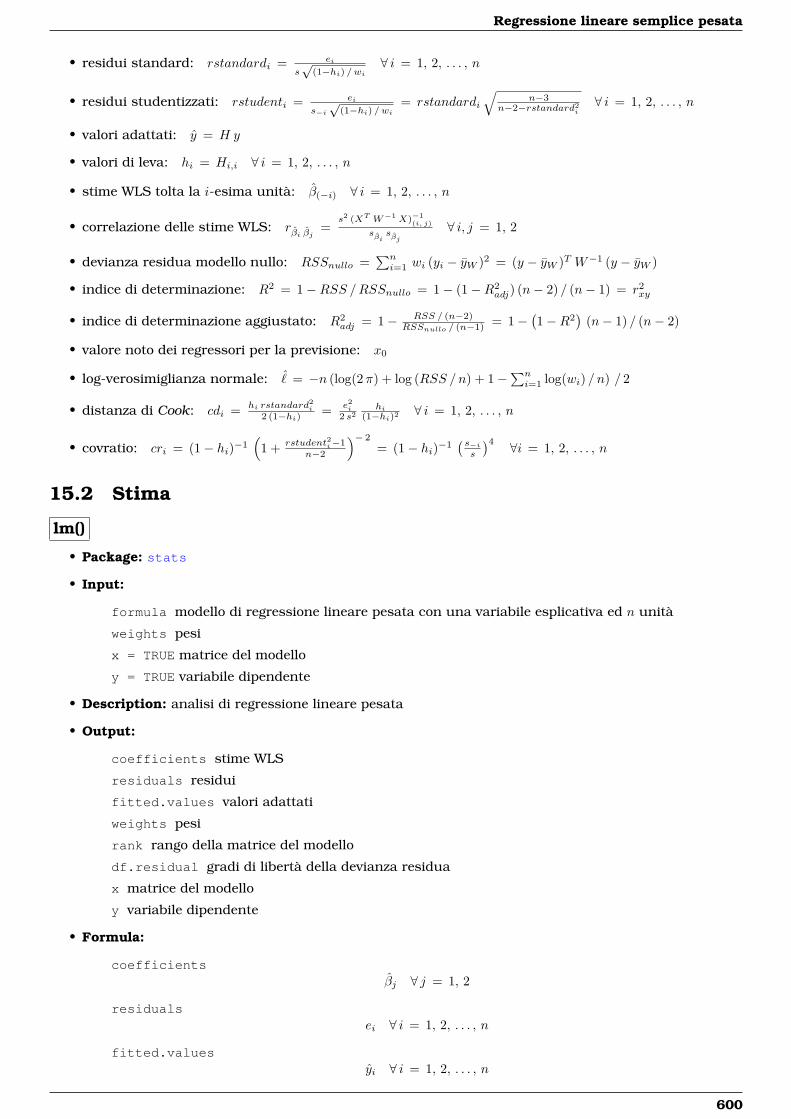
Regressione lineare semplice pesata
• residui standard: rstandardi = ei
s√
(1−hi) /wi∀ i = 1, 2, . . . , n
• residui studentizzati: rstudenti = ei
s−i√
(1−hi) /wi= rstandardi
√n−3
n−2−rstandard2i∀ i = 1, 2, . . . , n
• valori adattati: y = H y
• valori di leva: hi = Hi,i ∀ i = 1, 2, . . . , n
• stime WLS tolta la i-esima unità: β(−i) ∀ i = 1, 2, . . . , n
• correlazione delle stime WLS: rβi βj =s2 (XT W−1X)−1
(i, j)
sβisβj
∀ i, j = 1, 2
• devianza residua modello nullo: RSSnullo =∑ni=1 wi (yi − yW )2 = (y − yW )T W−1 (y − yW )
• indice di determinazione: R2 = 1−RSS /RSSnullo = 1− (1−R2adj) (n− 2) / (n− 1) = r2
xy
• indice di determinazione aggiustato: R2adj = 1− RSS / (n−2)
RSSnullo / (n−1) = 1−(1−R2
)(n− 1) / (n− 2)
• valore noto dei regressori per la previsione: x0
• log-verosimiglianza normale: ˆ = −n (log(2π) + log (RSS /n) + 1−∑ni=1 log(wi) / n) / 2
• distanza di Cook: cdi = hi rstandard2i
2 (1−hi) = e2i2 s2
hi(1−hi)2 ∀ i = 1, 2, . . . , n
• covratio: cri = (1− hi)−1(
1 + rstudent2i−1n−2
)− 2
= (1− hi)−1( s−is
)4 ∀i = 1, 2, . . . , n
15.2 Stima
lm()
• Package: stats
• Input:
formula modello di regressione lineare pesata con una variabile esplicativa ed n unità
weights pesi
x = TRUE matrice del modello
y = TRUE variabile dipendente
• Description: analisi di regressione lineare pesata
• Output:
coefficients stime WLS
residuals residui
fitted.values valori adattati
weights pesi
rank rango della matrice del modello
df.residual gradi di libertà della devianza residua
x matrice del modello
y variabile dipendente
• Formula:
coefficientsβj ∀ j = 1, 2
residualsei ∀ i = 1, 2, . . . , n
fitted.valuesyi ∀ i = 1, 2, . . . , n
600
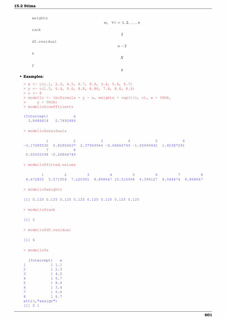
15.2 Stima
weightswi ∀ i = 1, 2, . . . , n
rank2
df.residualn− 2
xX
yy
• Examples:
> x <- c(1.1, 2.3, 4.5, 6.7, 8.9, 3.4, 5.6, 6.7)> y <- c(1.5, 6.4, 9.6, 8.8, 8.86, 7.8, 8.6, 8.6)> n <- 8> modello <- lm(formula = y ~ x, weights = rep(1/n, n), x = TRUE,+ y = TRUE)> modello$coefficients
(Intercept) x3.8486818 0.7492486
> modello$residuals
1 2 3 4 5 6-3.17285530 0.82804637 2.37969944 -0.06864749 -1.65699442 1.40387291
7 80.55552598 -0.26864749
> modello$fitted.values
1 2 3 4 5 6 7 84.672855 5.571954 7.220301 8.868647 10.516994 6.396127 8.044474 8.868647
> modello$weights
[1] 0.125 0.125 0.125 0.125 0.125 0.125 0.125 0.125
> modello$rank
[1] 2
> modello$df.residual
[1] 6
> modello$x
(Intercept) x1 1 1.12 1 2.33 1 4.54 1 6.75 1 8.96 1 3.47 1 5.68 1 6.7attr(,"assign")[1] 0 1
601
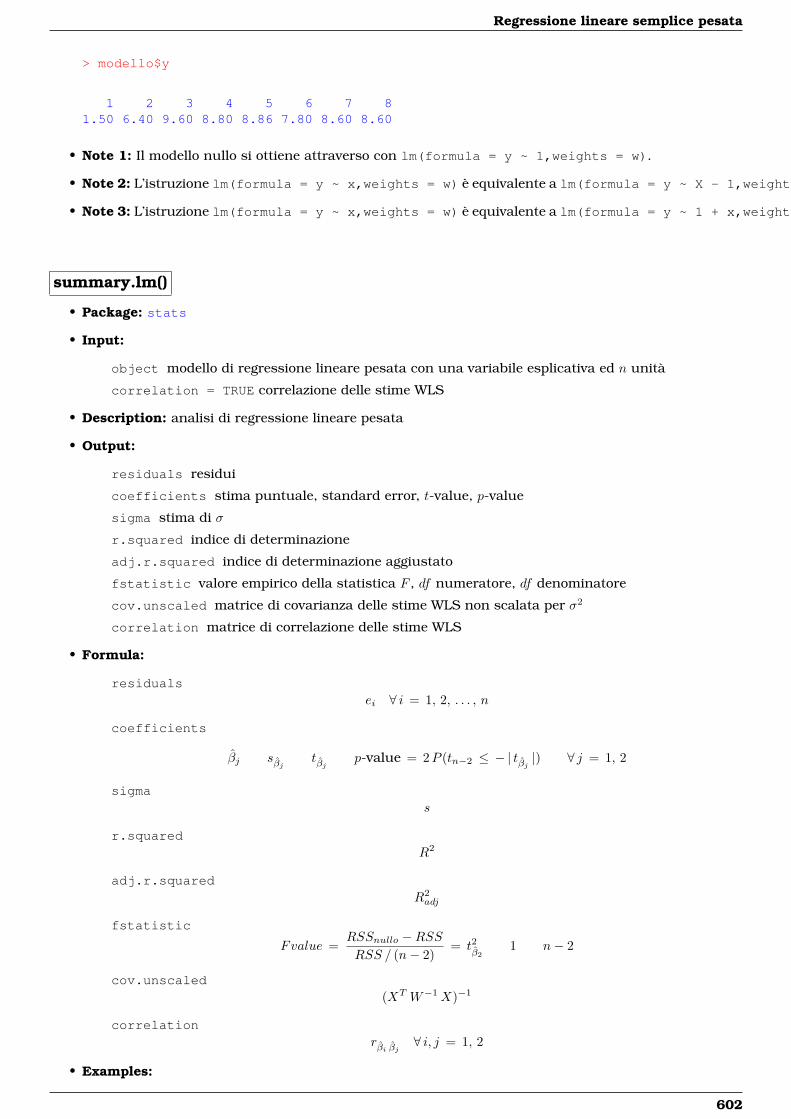
Regressione lineare semplice pesata
> modello$y
1 2 3 4 5 6 7 81.50 6.40 9.60 8.80 8.86 7.80 8.60 8.60
• Note 1: Il modello nullo si ottiene attraverso con lm(formula = y ~ 1,weights = w).
• Note 2: L’istruzione lm(formula = y ~ x,weights = w) è equivalente a lm(formula = y ~ X - 1,weights = w).
• Note 3: L’istruzione lm(formula = y ~ x,weights = w) è equivalente a lm(formula = y ~ 1 + x,weights = w).
summary.lm()
• Package: stats
• Input:
object modello di regressione lineare pesata con una variabile esplicativa ed n unità
correlation = TRUE correlazione delle stime WLS
• Description: analisi di regressione lineare pesata
• Output:
residuals residui
coefficients stima puntuale, standard error, t-value, p-value
sigma stima di σ
r.squared indice di determinazione
adj.r.squared indice di determinazione aggiustato
fstatistic valore empirico della statistica F , df numeratore, df denominatore
cov.unscaled matrice di covarianza delle stime WLS non scalata per σ2
correlation matrice di correlazione delle stime WLS
• Formula:
residualsei ∀ i = 1, 2, . . . , n
coefficients
βj sβj tβj p-value = 2P (tn−2 ≤ − | tβj |) ∀ j = 1, 2
sigmas
r.squaredR2
adj.r.squaredR2adj
fstatistic
Fvalue =RSSnullo −RSSRSS / (n− 2)
= t2β2
1 n− 2
cov.unscaled(XT W−1X)−1
correlationrβi βj ∀ i, j = 1, 2
• Examples:
602
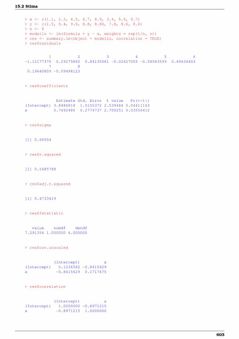
15.2 Stima
> x <- c(1.1, 2.3, 4.5, 6.7, 8.9, 3.4, 5.6, 6.7)> y <- c(1.5, 6.4, 9.6, 8.8, 8.86, 7.8, 8.6, 8.6)> n <- 8> modello <- lm(formula = y ~ x, weights = rep(1/n, n))> res <- summary.lm(object = modello, correlation = TRUE)> res$residuals
1 2 3 4 5 6-1.12177375 0.29275860 0.84135081 -0.02427055 -0.58583599 0.49634403
7 80.19640809 -0.09498123
> res$coefficients
Estimate Std. Error t value Pr(>|t|)(Intercept) 3.8486818 1.5155372 2.539484 0.04411163x 0.7492486 0.2774737 2.700251 0.03556412
> res$sigma
[1] 0.66954
> res$r.squared
[1] 0.5485788
> res$adj.r.squared
[1] 0.4733419
> res$fstatistic
value numdf dendf7.291356 1.000000 6.000000
> res$cov.unscaled
(Intercept) x(Intercept) 5.1236582 -0.8415629x -0.8415629 0.1717475
> res$correlation
(Intercept) x(Intercept) 1.0000000 -0.8971215x -0.8971215 1.0000000
603
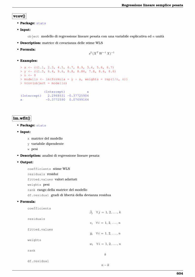
Regressione lineare semplice pesata
vcov()
• Package: stats
• Input:
object modello di regressione lineare pesata con una variabile esplicativa ed n unità
• Description: matrice di covarianza delle stime WLS
• Formula:s2 (XT W−1X)−1
• Examples:
> x <- c(1.1, 2.3, 4.5, 6.7, 8.9, 3.4, 5.6, 6.7)> y <- c(1.5, 6.4, 9.6, 8.8, 8.86, 7.8, 8.6, 8.6)> n <- 8> modello <- lm(formula = y ~ x, weights = rep(1/n, n))> vcov(object = modello)
(Intercept) x(Intercept) 2.2968531 -0.37725904x -0.3772590 0.07699164
lm.wfit()
• Package: stats
• Input:
x matrice del modello
y variabile dipendente
w pesi
• Description: analisi di regressione lineare pesata
• Output:
coefficients stime WLS
residuals residui
fitted.values valori adattati
weights pesi
rank rango della matrice del modello
df.residual gradi di libertà della devianza residua
• Formula:
coefficientsβj ∀ j = 1, 2, . . . , k
residualsei ∀ i = 1, 2, . . . , n
fitted.valuesyi ∀ i = 1, 2, . . . , n
weightswi ∀ i = 1, 2, . . . , n
rankk
df.residualn− k
604
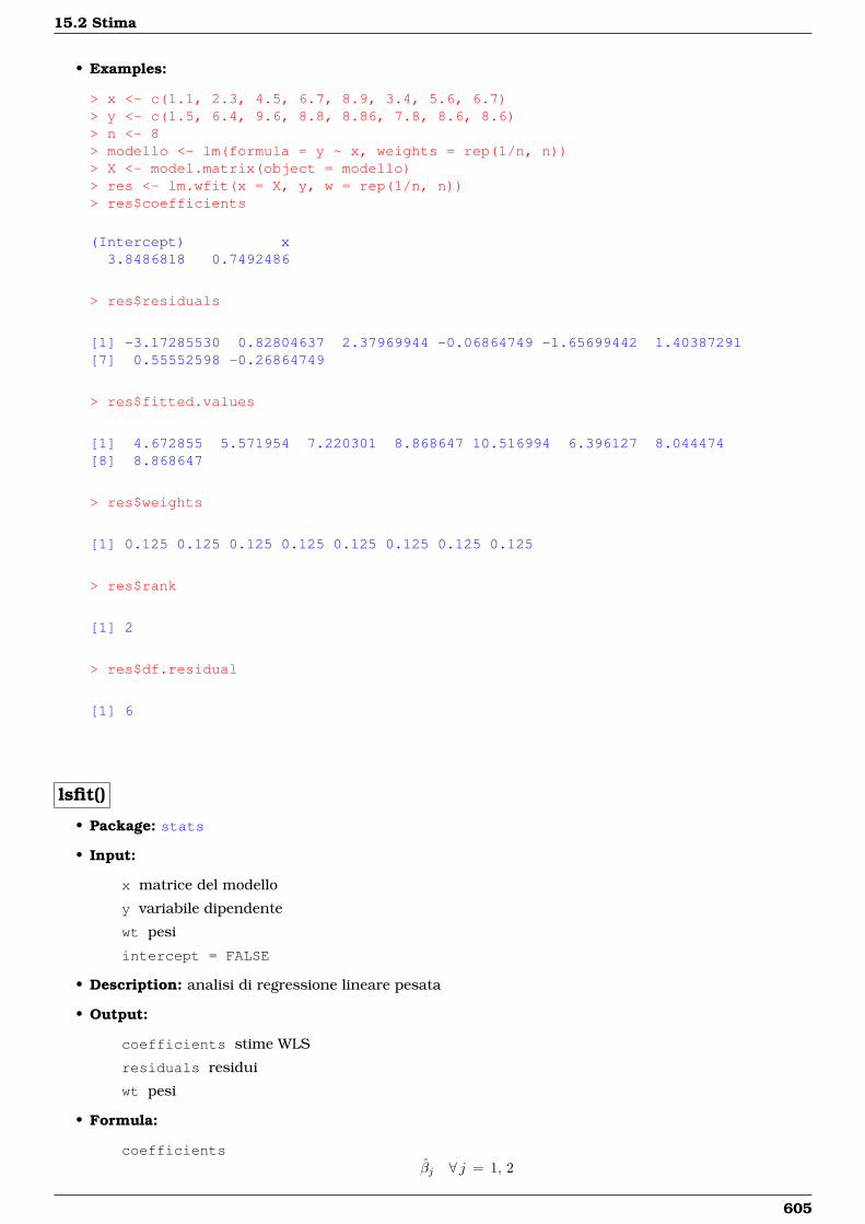
15.2 Stima
• Examples:
> x <- c(1.1, 2.3, 4.5, 6.7, 8.9, 3.4, 5.6, 6.7)> y <- c(1.5, 6.4, 9.6, 8.8, 8.86, 7.8, 8.6, 8.6)> n <- 8> modello <- lm(formula = y ~ x, weights = rep(1/n, n))> X <- model.matrix(object = modello)> res <- lm.wfit(x = X, y, w = rep(1/n, n))> res$coefficients
(Intercept) x3.8486818 0.7492486
> res$residuals
[1] -3.17285530 0.82804637 2.37969944 -0.06864749 -1.65699442 1.40387291[7] 0.55552598 -0.26864749
> res$fitted.values
[1] 4.672855 5.571954 7.220301 8.868647 10.516994 6.396127 8.044474[8] 8.868647
> res$weights
[1] 0.125 0.125 0.125 0.125 0.125 0.125 0.125 0.125
> res$rank
[1] 2
> res$df.residual
[1] 6
lsfit()
• Package: stats
• Input:
x matrice del modello
y variabile dipendente
wt pesi
intercept = FALSE
• Description: analisi di regressione lineare pesata
• Output:
coefficients stime WLS
residuals residui
wt pesi
• Formula:
coefficientsβj ∀ j = 1, 2
605
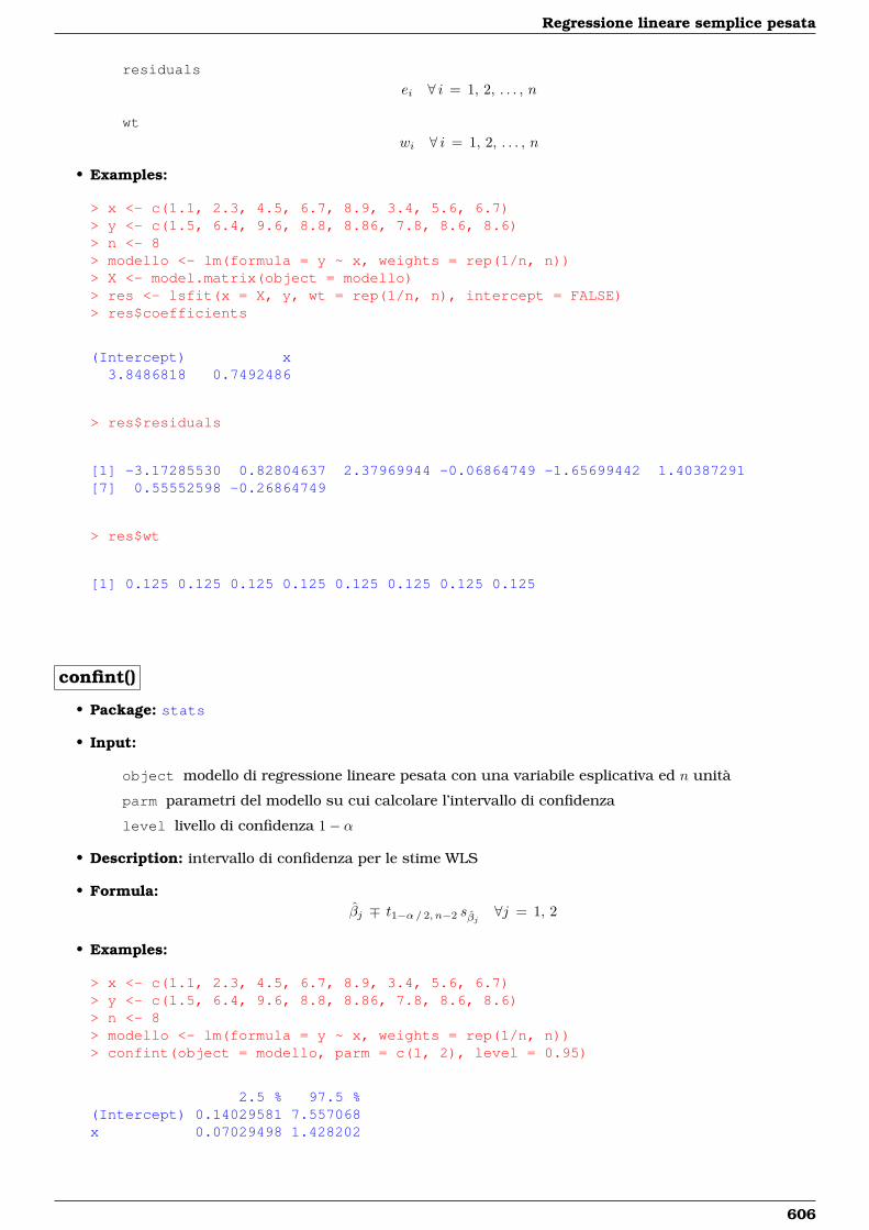
Regressione lineare semplice pesata
residuals
ei ∀ i = 1, 2, . . . , n
wt
wi ∀ i = 1, 2, . . . , n
• Examples:
> x <- c(1.1, 2.3, 4.5, 6.7, 8.9, 3.4, 5.6, 6.7)> y <- c(1.5, 6.4, 9.6, 8.8, 8.86, 7.8, 8.6, 8.6)> n <- 8> modello <- lm(formula = y ~ x, weights = rep(1/n, n))> X <- model.matrix(object = modello)> res <- lsfit(x = X, y, wt = rep(1/n, n), intercept = FALSE)> res$coefficients
(Intercept) x3.8486818 0.7492486
> res$residuals
[1] -3.17285530 0.82804637 2.37969944 -0.06864749 -1.65699442 1.40387291[7] 0.55552598 -0.26864749
> res$wt
[1] 0.125 0.125 0.125 0.125 0.125 0.125 0.125 0.125
confint()
• Package: stats
• Input:
object modello di regressione lineare pesata con una variabile esplicativa ed n unità
parm parametri del modello su cui calcolare l’intervallo di confidenza
level livello di confidenza 1− α
• Description: intervallo di confidenza per le stime WLS
• Formula:βj ∓ t1−α/ 2, n−2 sβj ∀j = 1, 2
• Examples:
> x <- c(1.1, 2.3, 4.5, 6.7, 8.9, 3.4, 5.6, 6.7)> y <- c(1.5, 6.4, 9.6, 8.8, 8.86, 7.8, 8.6, 8.6)> n <- 8> modello <- lm(formula = y ~ x, weights = rep(1/n, n))> confint(object = modello, parm = c(1, 2), level = 0.95)
2.5 % 97.5 %(Intercept) 0.14029581 7.557068x 0.07029498 1.428202
606
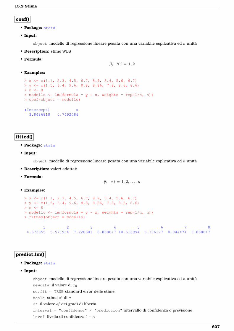
15.2 Stima
coef()
• Package: stats
• Input:
object modello di regressione lineare pesata con una variabile esplicativa ed n unità
• Description: stime WLS
• Formula:βj ∀ j = 1, 2
• Examples:
> x <- c(1.1, 2.3, 4.5, 6.7, 8.9, 3.4, 5.6, 6.7)> y <- c(1.5, 6.4, 9.6, 8.8, 8.86, 7.8, 8.6, 8.6)> n <- 8> modello <- lm(formula = y ~ x, weights = rep(1/n, n))> coef(object = modello)
(Intercept) x3.8486818 0.7492486
fitted()
• Package: stats
• Input:
object modello di regressione lineare pesata con una variabile esplicativa ed n unità
• Description: valori adattati
• Formula:yi ∀ i = 1, 2, . . . , n
• Examples:
> x <- c(1.1, 2.3, 4.5, 6.7, 8.9, 3.4, 5.6, 6.7)> y <- c(1.5, 6.4, 9.6, 8.8, 8.86, 7.8, 8.6, 8.6)> n <- 8> modello <- lm(formula = y ~ x, weights = rep(1/n, n))> fitted(object = modello)
1 2 3 4 5 6 7 84.672855 5.571954 7.220301 8.868647 10.516994 6.396127 8.044474 8.868647
predict.lm()
• Package: stats
• Input:
object modello di regressione lineare pesata con una variabile esplicativa ed n unità
newdata il valore di x0
se.fit = TRUE standard error delle stime
scale stima s∗ di σ
df il valore df dei gradi di libertà
interval = "confidence" / "prediction" intervallo di confidenza o previsione
level livello di confidenza 1− α
607
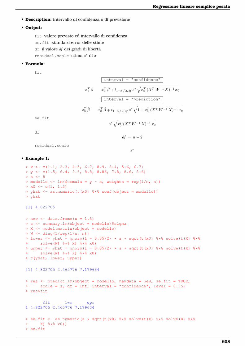
Regressione lineare semplice pesata
• Description: intervallo di confidenza o di previsione
• Output:
fit valore previsto ed intervallo di confidenza
se.fit standard error delle stime
df il valore df dei gradi di libertà
residual.scale stima s∗ di σ
• Formula:
fit
interval = "confidence"
xT0 β xT0 β ∓ t1−α/ 2, df s∗√xT0 (XT W−1X)−1 x0
interval = "prediction"
xT0 β xT0 β ∓ t1−α/ 2, df s∗√
1 + xT0 (XT W−1X)−1 x0
se.fit
s∗√xT0 (XT W−1X)−1 x0
dfdf = n− 2
residual.scales∗
• Example 1:
> x <- c(1.1, 2.3, 4.5, 6.7, 8.9, 3.4, 5.6, 6.7)> y <- c(1.5, 6.4, 9.6, 8.8, 8.86, 7.8, 8.6, 8.6)> n <- 8> modello <- lm(formula = y ~ x, weights = rep(1/n, n))> x0 <- c(1, 1.3)> yhat <- as.numeric(t(x0) %*% coef(object = modello))> yhat
[1] 4.822705
> new <- data.frame(x = 1.3)> s <- summary.lm(object = modello)$sigma> X <- model.matrix(object = modello)> W <- diag(1/rep(1/n, n))> lower <- yhat - qnorm(1 - 0.05/2) * s * sqrt(t(x0) %*% solve(t(X) %*%+ solve(W) %*% X) %*% x0)> upper <- yhat + qnorm(1 - 0.05/2) * s * sqrt(t(x0) %*% solve(t(X) %*%+ solve(W) %*% X) %*% x0)> c(yhat, lower, upper)
[1] 4.822705 2.465776 7.179634
> res <- predict.lm(object = modello, newdata = new, se.fit = TRUE,+ scale = s, df = Inf, interval = "confidence", level = 0.95)> res$fit
fit lwr upr1 4.822705 2.465776 7.179634
> se.fit <- as.numeric(s * sqrt(t(x0) %*% solve(t(X) %*% solve(W) %*%+ X) %*% x0))> se.fit
608
15.2 Stima
[1] 1.202537
> res$se.fit
[1] 1.202537
> s
[1] 0.66954
> res$residual.scale
[1] 0.66954
• Example 2:
> x <- c(1.1, 2.3, 4.5, 6.7, 8.9, 3.4, 5.6, 6.7)> y <- c(1.5, 6.4, 9.6, 8.8, 8.86, 7.8, 8.6, 8.6)> n <- 8> modello <- lm(formula = y ~ x, weights = rep(1/n, n))> x0 <- c(1, 1.3)> yhat <- as.numeric(t(x0) %*% coef(object = modello))> yhat
[1] 4.822705
> new <- data.frame(x = 1.3)> s <- summary.lm(object = modello)$sigma> X <- model.matrix(object = modello)> W <- diag(1/rep(1/n, n))> lower <- yhat - qt(1 - 0.05/2, df = n - 2) * s * sqrt(1 + t(x0) %*%+ solve(t(X) %*% solve(W) %*% X) %*% x0)> upper <- yhat + qt(1 - 0.05/2, df = n - 2) * s * sqrt(1 + t(x0) %*%+ solve(t(X) %*% solve(W) %*% X) %*% x0)> c(yhat, lower, upper)
[1] 4.822705 1.454862 8.190548
> res <- predict.lm(object = modello, newdata = new, se.fit = TRUE,+ interval = "prediction", level = 0.95)> res$fit
fit lwr upr1 4.822705 1.454862 8.190548
> se.fit <- as.numeric(s * sqrt(t(x0) %*% solve(t(X) %*% solve(W) %*%+ X) %*% x0))> se.fit
[1] 1.202537
> res$se.fit
[1] 1.202537
> s
[1] 0.66954
> res$residual.scale
609
Regressione lineare semplice pesata
[1] 0.66954
• Note 1: Per il calcolo dell’intervallo classico di confidenza o previsione impostare i parametri df = n - 2e scale = summary.lm(object = modello)$sigma.
• Note 2: Per il calcolo dell’intervallo asintotico di confidenza o previsione impostare i parametri df = Infe scale = summary.lm(object = modello)$sigma.
predict()
• Package: stats
• Input:
object modello di regressione lineare pesata con una variabile esplicativa ed n unità
newdata il valore di x0
se.fit = TRUE standard error delle stime
scale stima s∗ di σ
df il valore df dei gradi di libertà
interval = "confidence" / "prediction" intervallo di confidenza o previsione
level livello di confidenza 1− α
• Description: intervallo di confidenza o di previsione
• Output:
fit valore previsto ed intervallo di confidenza
se.fit standard error delle stime
df il valore df dei gradi di libertà
residual.scale stima s∗ di σ
• Formula:
fit
interval = "confidence"
xT0 β xT0 β ∓ t1−α/ 2, df s∗√xT0 (XT W−1X)−1 x0
interval = "prediction"
xT0 β xT0 β ∓ t1−α/ 2, df s∗√
1 + xT0 (XT W−1X)−1 x0
se.fit
s∗√xT0 (XT W−1X)−1 x0
dfdf = n− 2
residual.scales∗
• Example 1:
> x <- c(1.1, 2.3, 4.5, 6.7, 8.9, 3.4, 5.6, 6.7)> y <- c(1.5, 6.4, 9.6, 8.8, 8.86, 7.8, 8.6, 8.6)> n <- 8> modello <- lm(formula = y ~ x, weights = rep(1/n, n))> x0 <- c(1, 1.3)> yhat <- as.numeric(t(x0) %*% coef(object = modello))> yhat
[1] 4.822705
610
15.2 Stima
> new <- data.frame(x = 1.3)> s <- summary.lm(object = modello)$sigma> X <- model.matrix(object = modello)> W <- diag(1/rep(1/n, n))> lower <- yhat - qnorm(1 - 0.05/2) * s * sqrt(t(x0) %*% solve(t(X) %*%+ solve(W) %*% X) %*% x0)> upper <- yhat + qnorm(1 - 0.05/2) * s * sqrt(t(x0) %*% solve(t(X) %*%+ solve(W) %*% X) %*% x0)> c(yhat, lower, upper)
[1] 4.822705 2.465776 7.179634
> res <- predict(object = modello, newdata = new, se.fit = TRUE,+ scale = s, df = Inf, interval = "confidence", level = 0.95)> res$fit
fit lwr upr1 4.822705 2.465776 7.179634
> se.fit <- as.numeric(s * sqrt(t(x0) %*% solve(t(X) %*% solve(W) %*%+ X) %*% x0))> se.fit
[1] 1.202537
> res$se.fit
[1] 1.202537
> s
[1] 0.66954
> res$residual.scale
[1] 0.66954
• Example 2:
> x <- c(1.1, 2.3, 4.5, 6.7, 8.9, 3.4, 5.6, 6.7)> y <- c(1.5, 6.4, 9.6, 8.8, 8.86, 7.8, 8.6, 8.6)> n <- 8> modello <- lm(formula = y ~ x, weights = rep(1/n, n))> x0 <- c(1, 1.3)> yhat <- as.numeric(t(x0) %*% coef(object = modello))> yhat
[1] 4.822705
> new <- data.frame(x = 1.3)> s <- summary.lm(object = modello)$sigma> X <- model.matrix(object = modello)> W <- diag(1/rep(1/n, n))> lower <- yhat - qt(1 - 0.05/2, df = n - 2) * s * sqrt(1 + t(x0) %*%+ solve(t(X) %*% solve(W) %*% X) %*% x0)> upper <- yhat + qt(1 - 0.05/2, df = n - 2) * s * sqrt(1 + t(x0) %*%+ solve(t(X) %*% solve(W) %*% X) %*% x0)> c(yhat, lower, upper)
[1] 4.822705 1.454862 8.190548
611
Regressione lineare semplice pesata
> res <- predict(object = modello, newdata = new, se.fit = TRUE,+ interval = "prediction", level = 0.95)> res$fit
fit lwr upr1 4.822705 1.454862 8.190548
> se.fit <- as.numeric(s * sqrt(t(x0) %*% solve(t(X) %*% solve(W) %*%+ X) %*% x0))> se.fit
[1] 1.202537
> res$se.fit
[1] 1.202537
> s
[1] 0.66954
> res$residual.scale
[1] 0.66954
• Note 1: Per il calcolo dell’intervallo classico di confidenza o previsione impostare i parametri df = n - 2e scale = summary.lm(object = modello)$sigma.
• Note 2: Per il calcolo dell’intervallo asintotico di confidenza o previsione impostare i parametri df = Infe scale = summary.lm(object = modello)$sigma.
cov2cor()
• Package: stats
• Input:
V matrice di covarianza delle stime WLS di dimensione 2× 2
• Description: converte la matrice di covarianza nella matrice di correlazione
• Formula:rβi βj ∀ i, j = 1, 2
• Examples:
> x <- c(1.1, 2.3, 4.5, 6.7, 8.9, 3.4, 5.6, 6.7)> y <- c(1.5, 6.4, 9.6, 8.8, 8.86, 7.8, 8.6, 8.6)> n <- 8> modello <- lm(formula = y ~ x, weights = rep(1/n, n))> V <- vcov(object = modello)> cov2cor(V)
(Intercept) x(Intercept) 1.0000000 -0.8971215x -0.8971215 1.0000000
612
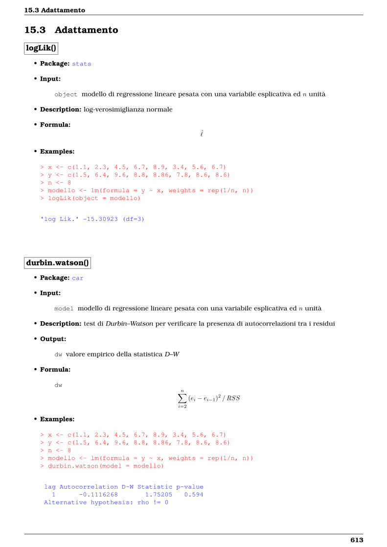
15.3 Adattamento
15.3 Adattamento
logLik()
• Package: stats
• Input:
object modello di regressione lineare pesata con una variabile esplicativa ed n unità
• Description: log-verosimiglianza normale
• Formula:ˆ
• Examples:
> x <- c(1.1, 2.3, 4.5, 6.7, 8.9, 3.4, 5.6, 6.7)> y <- c(1.5, 6.4, 9.6, 8.8, 8.86, 7.8, 8.6, 8.6)> n <- 8> modello <- lm(formula = y ~ x, weights = rep(1/n, n))> logLik(object = modello)
'log Lik.' -15.30923 (df=3)
durbin.watson()
• Package: car
• Input:
model modello di regressione lineare pesata con una variabile esplicativa ed n unità
• Description: test di Durbin–Watson per verificare la presenza di autocorrelazioni tra i residui
• Output:
dw valore empirico della statistica D–W
• Formula:
dwn∑i=2
(ei − ei−1)2 /RSS
• Examples:
> x <- c(1.1, 2.3, 4.5, 6.7, 8.9, 3.4, 5.6, 6.7)> y <- c(1.5, 6.4, 9.6, 8.8, 8.86, 7.8, 8.6, 8.6)> n <- 8> modello <- lm(formula = y ~ x, weights = rep(1/n, n))> durbin.watson(model = modello)
lag Autocorrelation D-W Statistic p-value1 -0.1116268 1.75205 0.594
Alternative hypothesis: rho != 0
613
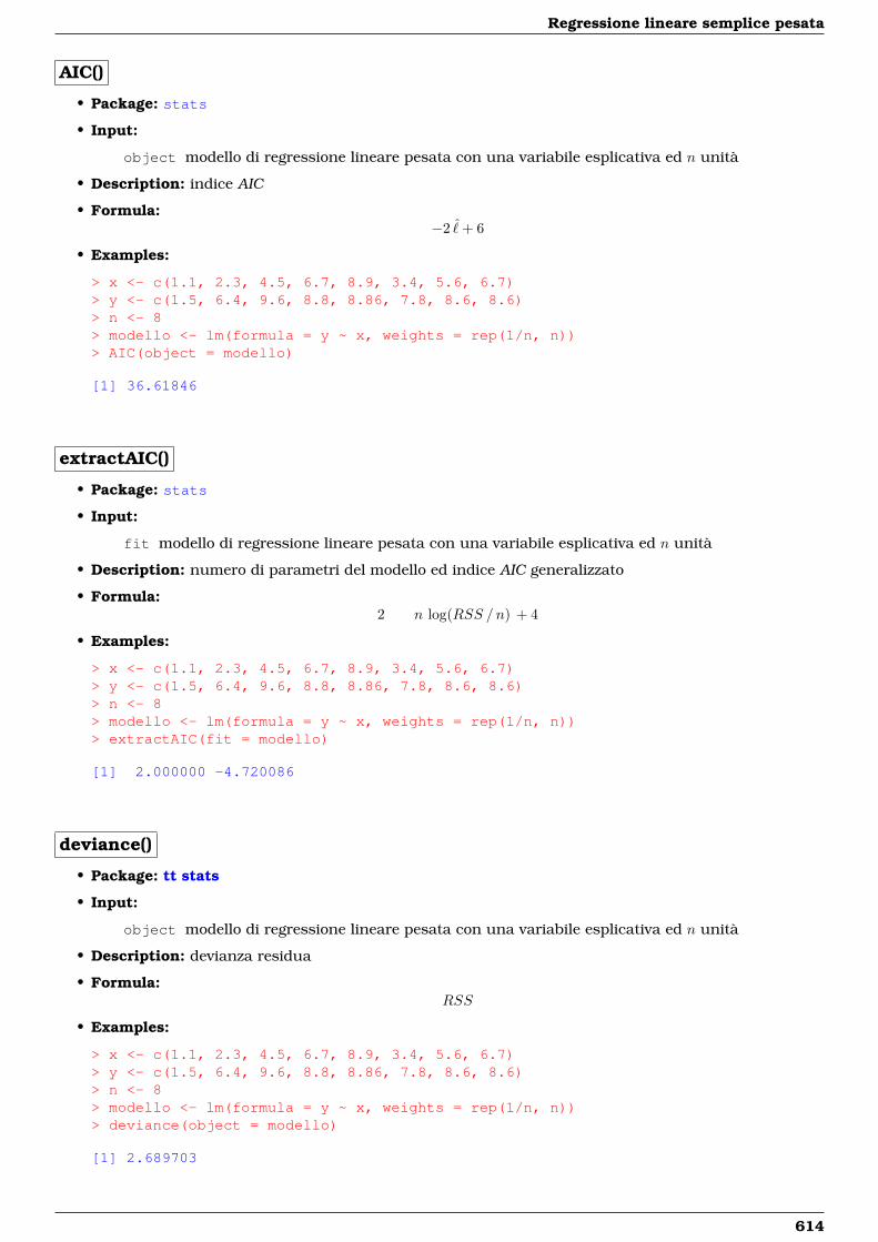
Regressione lineare semplice pesata
AIC()
• Package: stats
• Input:
object modello di regressione lineare pesata con una variabile esplicativa ed n unità
• Description: indice AIC
• Formula:−2 ˆ+ 6
• Examples:
> x <- c(1.1, 2.3, 4.5, 6.7, 8.9, 3.4, 5.6, 6.7)> y <- c(1.5, 6.4, 9.6, 8.8, 8.86, 7.8, 8.6, 8.6)> n <- 8> modello <- lm(formula = y ~ x, weights = rep(1/n, n))> AIC(object = modello)
[1] 36.61846
extractAIC()
• Package: stats
• Input:
fit modello di regressione lineare pesata con una variabile esplicativa ed n unità
• Description: numero di parametri del modello ed indice AIC generalizzato
• Formula:2 n log(RSS /n) + 4
• Examples:
> x <- c(1.1, 2.3, 4.5, 6.7, 8.9, 3.4, 5.6, 6.7)> y <- c(1.5, 6.4, 9.6, 8.8, 8.86, 7.8, 8.6, 8.6)> n <- 8> modello <- lm(formula = y ~ x, weights = rep(1/n, n))> extractAIC(fit = modello)
[1] 2.000000 -4.720086
deviance()
• Package: tt stats
• Input:
object modello di regressione lineare pesata con una variabile esplicativa ed n unità
• Description: devianza residua
• Formula:RSS
• Examples:
> x <- c(1.1, 2.3, 4.5, 6.7, 8.9, 3.4, 5.6, 6.7)> y <- c(1.5, 6.4, 9.6, 8.8, 8.86, 7.8, 8.6, 8.6)> n <- 8> modello <- lm(formula = y ~ x, weights = rep(1/n, n))> deviance(object = modello)
[1] 2.689703
614
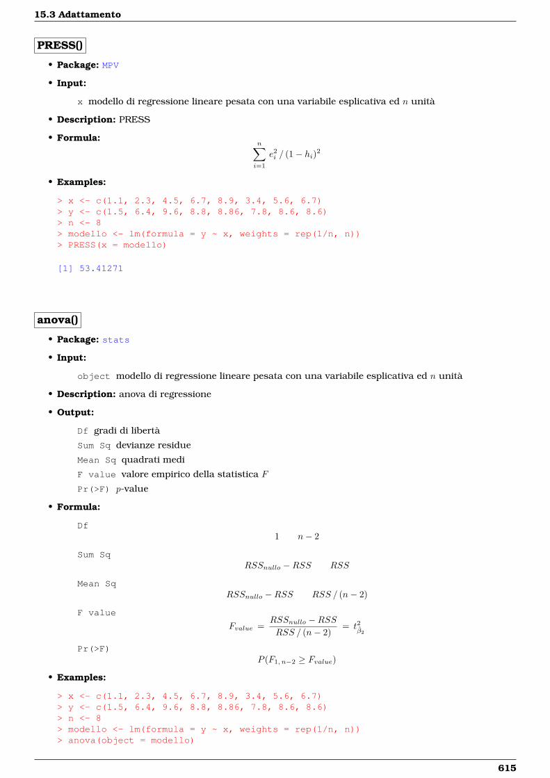
15.3 Adattamento
PRESS()
• Package: MPV
• Input:
x modello di regressione lineare pesata con una variabile esplicativa ed n unità
• Description: PRESS
• Formula:n∑i=1
e2i / (1− hi)2
• Examples:
> x <- c(1.1, 2.3, 4.5, 6.7, 8.9, 3.4, 5.6, 6.7)> y <- c(1.5, 6.4, 9.6, 8.8, 8.86, 7.8, 8.6, 8.6)> n <- 8> modello <- lm(formula = y ~ x, weights = rep(1/n, n))> PRESS(x = modello)
[1] 53.41271
anova()
• Package: stats
• Input:
object modello di regressione lineare pesata con una variabile esplicativa ed n unità
• Description: anova di regressione
• Output:
Df gradi di libertà
Sum Sq devianze residue
Mean Sq quadrati medi
F value valore empirico della statistica F
Pr(>F) p-value
• Formula:
Df1 n− 2
Sum SqRSSnullo −RSS RSS
Mean SqRSSnullo −RSS RSS / (n− 2)
F value
Fvalue =RSSnullo −RSSRSS / (n− 2)
= t2β2
Pr(>F)P (F1, n−2 ≥ Fvalue)
• Examples:
> x <- c(1.1, 2.3, 4.5, 6.7, 8.9, 3.4, 5.6, 6.7)> y <- c(1.5, 6.4, 9.6, 8.8, 8.86, 7.8, 8.6, 8.6)> n <- 8> modello <- lm(formula = y ~ x, weights = rep(1/n, n))> anova(object = modello)
615
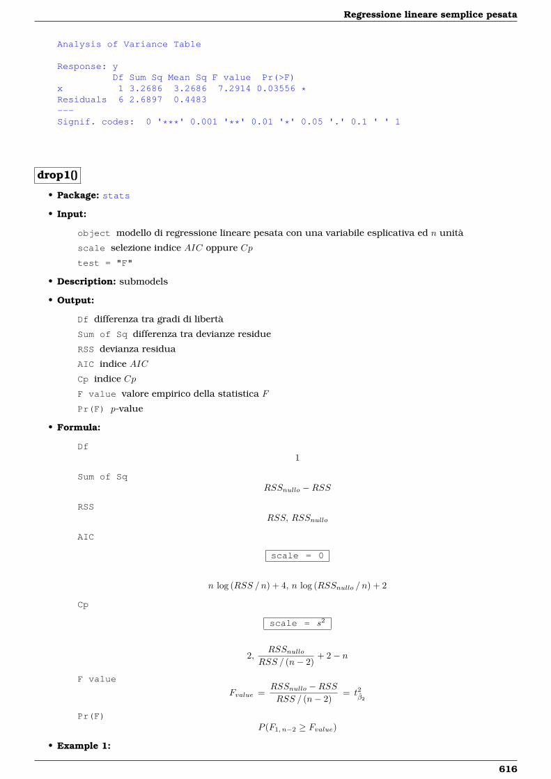
Regressione lineare semplice pesata
Analysis of Variance Table
Response: yDf Sum Sq Mean Sq F value Pr(>F)
x 1 3.2686 3.2686 7.2914 0.03556 *Residuals 6 2.6897 0.4483---Signif. codes: 0 '***' 0.001 '**' 0.01 '*' 0.05 '.' 0.1 ' ' 1
drop1()
• Package: stats
• Input:
object modello di regressione lineare pesata con una variabile esplicativa ed n unità
scale selezione indice AIC oppure Cp
test = "F"
• Description: submodels
• Output:
Df differenza tra gradi di libertà
Sum of Sq differenza tra devianze residue
RSS devianza residua
AIC indice AIC
Cp indice Cp
F value valore empirico della statistica F
Pr(F) p-value
• Formula:
Df1
Sum of SqRSSnullo −RSS
RSSRSS, RSSnullo
AIC
scale = 0
n log (RSS /n) + 4, n log (RSSnullo / n) + 2
Cp
scale = s2
2,RSSnullo
RSS / (n− 2)+ 2− n
F value
Fvalue =RSSnullo −RSSRSS / (n− 2)
= t2β2
Pr(F)P (F1, n−2 ≥ Fvalue)
• Example 1:
616
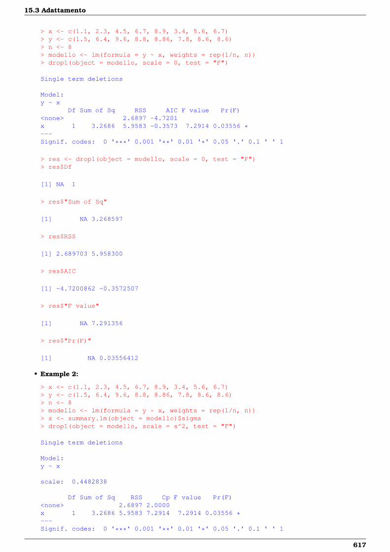
15.3 Adattamento
> x <- c(1.1, 2.3, 4.5, 6.7, 8.9, 3.4, 5.6, 6.7)> y <- c(1.5, 6.4, 9.6, 8.8, 8.86, 7.8, 8.6, 8.6)> n <- 8> modello <- lm(formula = y ~ x, weights = rep(1/n, n))> drop1(object = modello, scale = 0, test = "F")
Single term deletions
Model:y ~ x
Df Sum of Sq RSS AIC F value Pr(F)<none> 2.6897 -4.7201x 1 3.2686 5.9583 -0.3573 7.2914 0.03556 *---Signif. codes: 0 '***' 0.001 '**' 0.01 '*' 0.05 '.' 0.1 ' ' 1
> res <- drop1(object = modello, scale = 0, test = "F")> res$Df
[1] NA 1
> res$"Sum of Sq"
[1] NA 3.268597
> res$RSS
[1] 2.689703 5.958300
> res$AIC
[1] -4.7200862 -0.3572507
> res$"F value"
[1] NA 7.291356
> res$"Pr(F)"
[1] NA 0.03556412
• Example 2:
> x <- c(1.1, 2.3, 4.5, 6.7, 8.9, 3.4, 5.6, 6.7)> y <- c(1.5, 6.4, 9.6, 8.8, 8.86, 7.8, 8.6, 8.6)> n <- 8> modello <- lm(formula = y ~ x, weights = rep(1/n, n))> s <- summary.lm(object = modello)$sigma> drop1(object = modello, scale = s^2, test = "F")
Single term deletions
Model:y ~ x
scale: 0.4482838
Df Sum of Sq RSS Cp F value Pr(F)<none> 2.6897 2.0000x 1 3.2686 5.9583 7.2914 7.2914 0.03556 *---Signif. codes: 0 '***' 0.001 '**' 0.01 '*' 0.05 '.' 0.1 ' ' 1
617
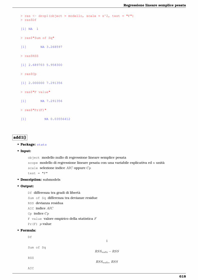
Regressione lineare semplice pesata
> res <- drop1(object = modello, scale = s^2, test = "F")> res$Df
[1] NA 1
> res$"Sum of Sq"
[1] NA 3.268597
> res$RSS
[1] 2.689703 5.958300
> res$Cp
[1] 2.000000 7.291356
> res$"F value"
[1] NA 7.291356
> res$"Pr(F)"
[1] NA 0.03556412
add1()
• Package: stats
• Input:
object modello nullo di regressione lineare semplice pesata
scope modello di regressione lineare pesata con una variabile esplicativa ed n unità
scale selezione indice AIC oppure Cp
test = "F"
• Description: submodels
• Output:
Df differenza tra gradi di libertà
Sum of Sq differenza tra devianze residue
RSS devianza residua
AIC indice AIC
Cp indice Cp
F value valore empirico della statistica F
Pr(F) p-value
• Formula:
Df1
Sum of SqRSSnullo −RSS
RSSRSSnullo, RSS
AIC
618
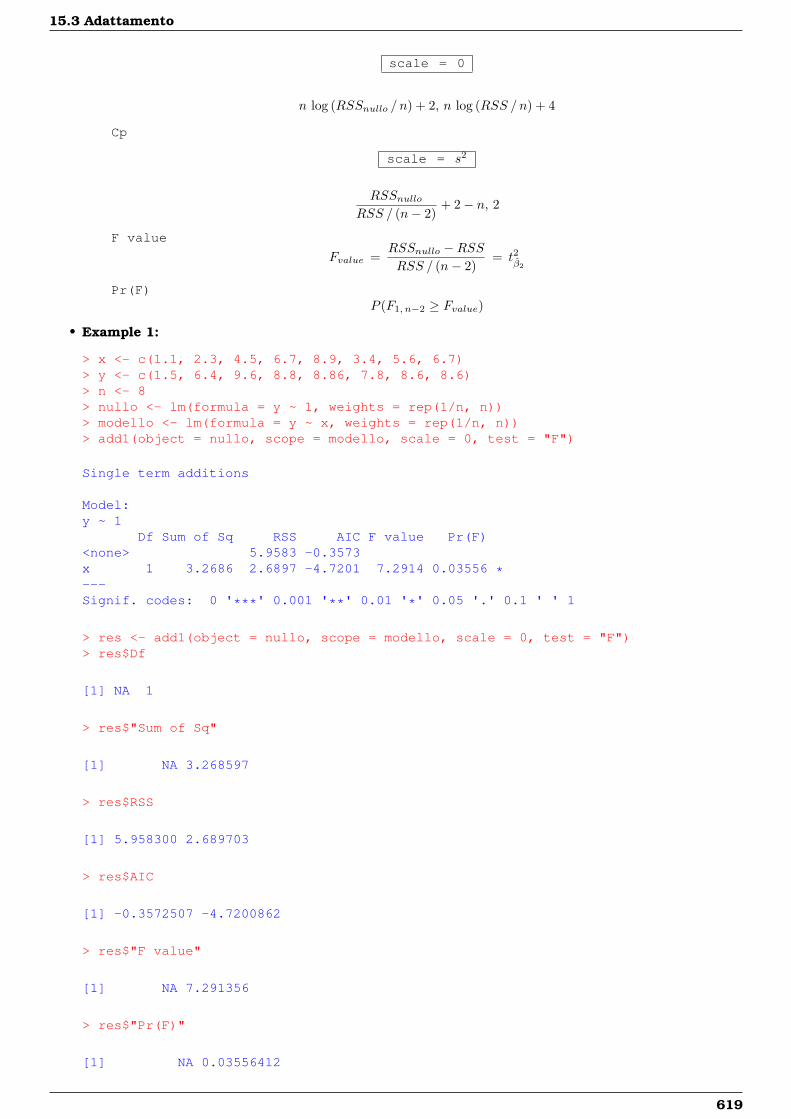
15.3 Adattamento
scale = 0
n log (RSSnullo / n) + 2, n log (RSS /n) + 4
Cp
scale = s2
RSSnulloRSS / (n− 2)
+ 2− n, 2
F value
Fvalue =RSSnullo −RSSRSS / (n− 2)
= t2β2
Pr(F)P (F1, n−2 ≥ Fvalue)
• Example 1:
> x <- c(1.1, 2.3, 4.5, 6.7, 8.9, 3.4, 5.6, 6.7)> y <- c(1.5, 6.4, 9.6, 8.8, 8.86, 7.8, 8.6, 8.6)> n <- 8> nullo <- lm(formula = y ~ 1, weights = rep(1/n, n))> modello <- lm(formula = y ~ x, weights = rep(1/n, n))> add1(object = nullo, scope = modello, scale = 0, test = "F")
Single term additions
Model:y ~ 1
Df Sum of Sq RSS AIC F value Pr(F)<none> 5.9583 -0.3573x 1 3.2686 2.6897 -4.7201 7.2914 0.03556 *---Signif. codes: 0 '***' 0.001 '**' 0.01 '*' 0.05 '.' 0.1 ' ' 1
> res <- add1(object = nullo, scope = modello, scale = 0, test = "F")> res$Df
[1] NA 1
> res$"Sum of Sq"
[1] NA 3.268597
> res$RSS
[1] 5.958300 2.689703
> res$AIC
[1] -0.3572507 -4.7200862
> res$"F value"
[1] NA 7.291356
> res$"Pr(F)"
[1] NA 0.03556412
619
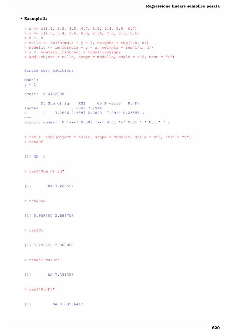
Regressione lineare semplice pesata
• Example 2:
> x <- c(1.1, 2.3, 4.5, 6.7, 8.9, 3.4, 5.6, 6.7)> y <- c(1.5, 6.4, 9.6, 8.8, 8.86, 7.8, 8.6, 8.6)> n <- 8> nullo <- lm(formula = y ~ 1, weights = rep(1/n, n))> modello <- lm(formula = y ~ x, weights = rep(1/n, n))> s <- summary.lm(object = modello)$sigma> add1(object = nullo, scope = modello, scale = s^2, test = "F")
Single term additions
Model:y ~ 1
scale: 0.4482838
Df Sum of Sq RSS Cp F value Pr(F)<none> 5.9583 7.2914x 1 3.2686 2.6897 2.0000 7.2914 0.03556 *---Signif. codes: 0 '***' 0.001 '**' 0.01 '*' 0.05 '.' 0.1 ' ' 1
> res <- add1(object = nullo, scope = modello, scale = s^2, test = "F")> res$Df
[1] NA 1
> res$"Sum of Sq"
[1] NA 3.268597
> res$RSS
[1] 5.958300 2.689703
> res$Cp
[1] 7.291356 2.000000
> res$"F value"
[1] NA 7.291356
> res$"Pr(F)"
[1] NA 0.03556412
620
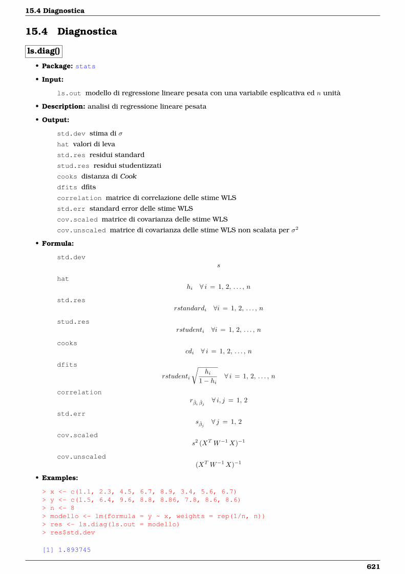
15.4 Diagnostica
15.4 Diagnostica
ls.diag()
• Package: stats
• Input:
ls.out modello di regressione lineare pesata con una variabile esplicativa ed n unità
• Description: analisi di regressione lineare pesata
• Output:
std.dev stima di σ
hat valori di leva
std.res residui standard
stud.res residui studentizzati
cooks distanza di Cook
dfits dfits
correlation matrice di correlazione delle stime WLS
std.err standard error delle stime WLS
cov.scaled matrice di covarianza delle stime WLS
cov.unscaled matrice di covarianza delle stime WLS non scalata per σ2
• Formula:
std.devs
hathi ∀ i = 1, 2, . . . , n
std.resrstandardi ∀i = 1, 2, . . . , n
stud.resrstudenti ∀i = 1, 2, . . . , n
cookscdi ∀ i = 1, 2, . . . , n
dfits
rstudenti
√hi
1− hi∀ i = 1, 2, . . . , n
correlationrβi βj ∀ i, j = 1, 2
std.errsβj ∀ j = 1, 2
cov.scaleds2 (XT W−1X)−1
cov.unscaled(XT W−1X)−1
• Examples:
> x <- c(1.1, 2.3, 4.5, 6.7, 8.9, 3.4, 5.6, 6.7)> y <- c(1.5, 6.4, 9.6, 8.8, 8.86, 7.8, 8.6, 8.6)> n <- 8> modello <- lm(formula = y ~ x, weights = rep(1/n, n))> res <- ls.diag(ls.out = modello)> res$std.dev
[1] 1.893745
621
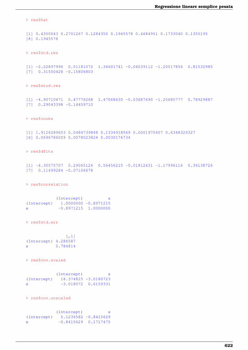
Regressione lineare semplice pesata
> res$hat
[1] 0.4350043 0.2701267 0.1284350 0.1945578 0.4684951 0.1733040 0.1355195[8] 0.1945578
> res$std.res
[1] -2.22897996 0.51181072 1.34601741 -0.04039112 -1.20017856 0.81532985[7] 0.31550428 -0.15806803
> res$stud.res
[1] -4.90710471 0.47776268 1.47068630 -0.03687690 -1.25680777 0.78929887[7] 0.29043398 -0.14459710
> res$cooks
[1] 1.9126289653 0.0484739848 0.1334918569 0.0001970407 0.6348329327[6] 0.0696786009 0.0078023824 0.0030176734
> res$dfits
[1] -4.30575707 0.29065126 0.56456215 -0.01812431 -1.17996116 0.36138726[7] 0.11499284 -0.07106678
> res$correlation
(Intercept) x(Intercept) 1.0000000 -0.8971215x -0.8971215 1.0000000
> res$std.err
[,1](Intercept) 4.286587x 0.784814
> res$cov.scaled
(Intercept) x(Intercept) 18.374825 -3.0180723x -3.018072 0.6159331
> res$cov.unscaled
(Intercept) x(Intercept) 5.1236582 -0.8415629x -0.8415629 0.1717475
622
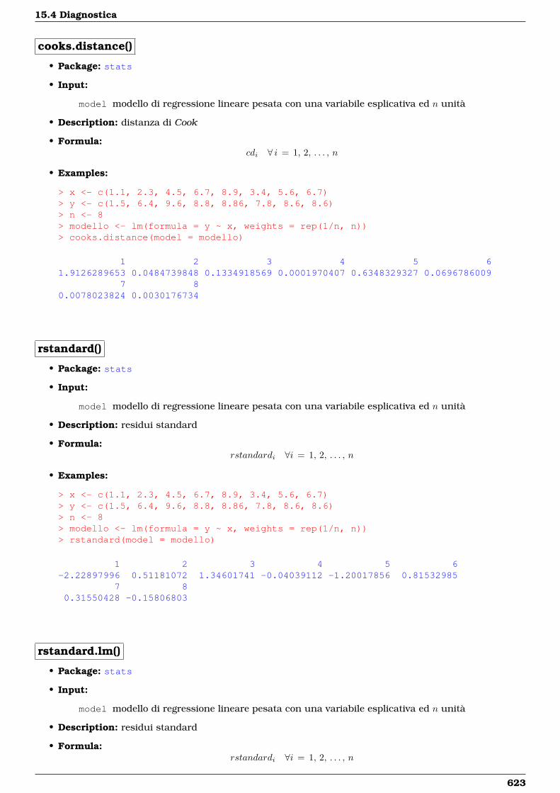
15.4 Diagnostica
cooks.distance()
• Package: stats
• Input:
model modello di regressione lineare pesata con una variabile esplicativa ed n unità
• Description: distanza di Cook
• Formula:cdi ∀ i = 1, 2, . . . , n
• Examples:
> x <- c(1.1, 2.3, 4.5, 6.7, 8.9, 3.4, 5.6, 6.7)> y <- c(1.5, 6.4, 9.6, 8.8, 8.86, 7.8, 8.6, 8.6)> n <- 8> modello <- lm(formula = y ~ x, weights = rep(1/n, n))> cooks.distance(model = modello)
1 2 3 4 5 61.9126289653 0.0484739848 0.1334918569 0.0001970407 0.6348329327 0.0696786009
7 80.0078023824 0.0030176734
rstandard()
• Package: stats
• Input:
model modello di regressione lineare pesata con una variabile esplicativa ed n unità
• Description: residui standard
• Formula:rstandardi ∀i = 1, 2, . . . , n
• Examples:
> x <- c(1.1, 2.3, 4.5, 6.7, 8.9, 3.4, 5.6, 6.7)> y <- c(1.5, 6.4, 9.6, 8.8, 8.86, 7.8, 8.6, 8.6)> n <- 8> modello <- lm(formula = y ~ x, weights = rep(1/n, n))> rstandard(model = modello)
1 2 3 4 5 6-2.22897996 0.51181072 1.34601741 -0.04039112 -1.20017856 0.81532985
7 80.31550428 -0.15806803
rstandard.lm()
• Package: stats
• Input:
model modello di regressione lineare pesata con una variabile esplicativa ed n unità
• Description: residui standard
• Formula:rstandardi ∀i = 1, 2, . . . , n
623
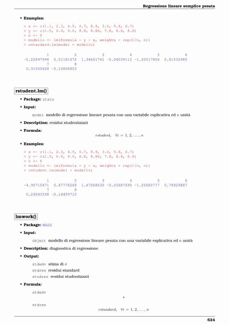
Regressione lineare semplice pesata
• Examples:
> x <- c(1.1, 2.3, 4.5, 6.7, 8.9, 3.4, 5.6, 6.7)> y <- c(1.5, 6.4, 9.6, 8.8, 8.86, 7.8, 8.6, 8.6)> n <- 8> modello <- lm(formula = y ~ x, weights = rep(1/n, n))> rstandard.lm(model = modello)
1 2 3 4 5 6-2.22897996 0.51181072 1.34601741 -0.04039112 -1.20017856 0.81532985
7 80.31550428 -0.15806803
rstudent.lm()
• Package: stats
• Input:
model modello di regressione lineare pesata con una variabile esplicativa ed n unità
• Description: residui studentizzati
• Formula:rstudenti ∀i = 1, 2, . . . , n
• Examples:
> x <- c(1.1, 2.3, 4.5, 6.7, 8.9, 3.4, 5.6, 6.7)> y <- c(1.5, 6.4, 9.6, 8.8, 8.86, 7.8, 8.6, 8.6)> n <- 8> modello <- lm(formula = y ~ x, weights = rep(1/n, n))> rstudent.lm(model = modello)
1 2 3 4 5 6-4.90710471 0.47776268 1.47068630 -0.03687690 -1.25680777 0.78929887
7 80.29043398 -0.14459710
lmwork()
• Package: MASS
• Input:
object modello di regressione lineare pesata con una variabile esplicativa ed n unità
• Description: diagnostica di regressione
• Output:
stdedv stima di σ
stdres residui standard
studres residui studentizzati
• Formula:
stdedvs
stdresrstandardi ∀i = 1, 2, . . . , n
624
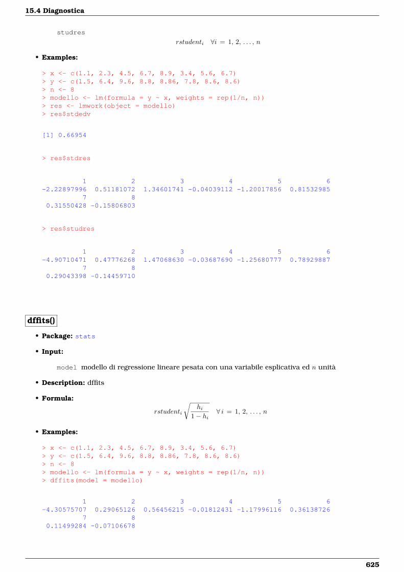
15.4 Diagnostica
studres
rstudenti ∀i = 1, 2, . . . , n
• Examples:
> x <- c(1.1, 2.3, 4.5, 6.7, 8.9, 3.4, 5.6, 6.7)> y <- c(1.5, 6.4, 9.6, 8.8, 8.86, 7.8, 8.6, 8.6)> n <- 8> modello <- lm(formula = y ~ x, weights = rep(1/n, n))> res <- lmwork(object = modello)> res$stdedv
[1] 0.66954
> res$stdres
1 2 3 4 5 6-2.22897996 0.51181072 1.34601741 -0.04039112 -1.20017856 0.81532985
7 80.31550428 -0.15806803
> res$studres
1 2 3 4 5 6-4.90710471 0.47776268 1.47068630 -0.03687690 -1.25680777 0.78929887
7 80.29043398 -0.14459710
dffits()
• Package: stats
• Input:
model modello di regressione lineare pesata con una variabile esplicativa ed n unità
• Description: dffits
• Formula:
rstudenti
√hi
1− hi∀ i = 1, 2, . . . , n
• Examples:
> x <- c(1.1, 2.3, 4.5, 6.7, 8.9, 3.4, 5.6, 6.7)> y <- c(1.5, 6.4, 9.6, 8.8, 8.86, 7.8, 8.6, 8.6)> n <- 8> modello <- lm(formula = y ~ x, weights = rep(1/n, n))> dffits(model = modello)
1 2 3 4 5 6-4.30575707 0.29065126 0.56456215 -0.01812431 -1.17996116 0.36138726
7 80.11499284 -0.07106678
625
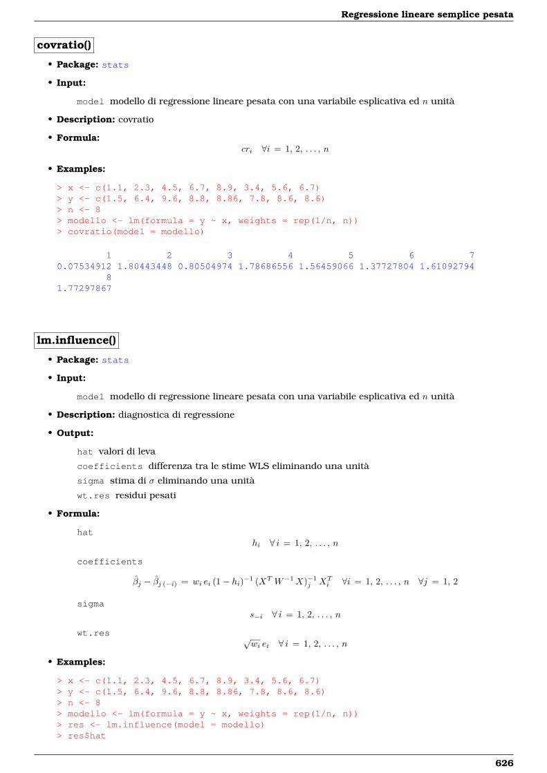
Regressione lineare semplice pesata
covratio()
• Package: stats
• Input:
model modello di regressione lineare pesata con una variabile esplicativa ed n unità
• Description: covratio
• Formula:cri ∀i = 1, 2, . . . , n
• Examples:
> x <- c(1.1, 2.3, 4.5, 6.7, 8.9, 3.4, 5.6, 6.7)> y <- c(1.5, 6.4, 9.6, 8.8, 8.86, 7.8, 8.6, 8.6)> n <- 8> modello <- lm(formula = y ~ x, weights = rep(1/n, n))> covratio(model = modello)
1 2 3 4 5 6 70.07534912 1.80443448 0.80504974 1.78686556 1.56459066 1.37727804 1.61092794
81.77297867
lm.influence()
• Package: stats
• Input:
model modello di regressione lineare pesata con una variabile esplicativa ed n unità
• Description: diagnostica di regressione
• Output:
hat valori di leva
coefficients differenza tra le stime WLS eliminando una unità
sigma stima di σ eliminando una unità
wt.res residui pesati
• Formula:
hathi ∀ i = 1, 2, . . . , n
coefficients
βj − βj (−i) = wi ei (1− hi)−1 (XT W−1X)−1j XT
i ∀i = 1, 2, . . . , n ∀j = 1, 2
sigmas−i ∀ i = 1, 2, . . . , n
wt.res √wi ei ∀ i = 1, 2, . . . , n
• Examples:
> x <- c(1.1, 2.3, 4.5, 6.7, 8.9, 3.4, 5.6, 6.7)> y <- c(1.5, 6.4, 9.6, 8.8, 8.86, 7.8, 8.6, 8.6)> n <- 8> modello <- lm(formula = y ~ x, weights = rep(1/n, n))> res <- lm.influence(model = modello)> res$hat
626
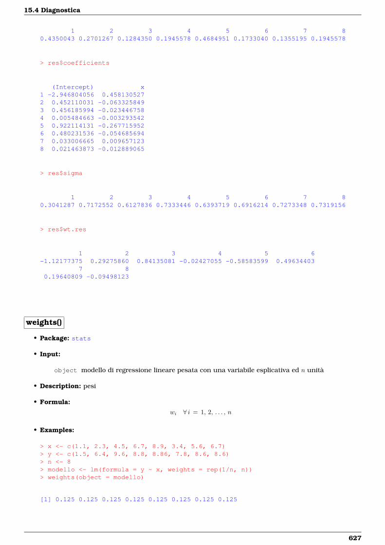
15.4 Diagnostica
1 2 3 4 5 6 7 80.4350043 0.2701267 0.1284350 0.1945578 0.4684951 0.1733040 0.1355195 0.1945578
> res$coefficients
(Intercept) x1 -2.946804056 0.4581305272 0.452110031 -0.0633258493 0.456185994 -0.0234467584 0.005484663 -0.0032935425 0.922114131 -0.2677159526 0.480231536 -0.0546856947 0.033006665 0.0096571238 0.021463873 -0.012889065
> res$sigma
1 2 3 4 5 6 7 80.3041287 0.7172552 0.6127836 0.7333446 0.6393719 0.6916214 0.7273348 0.7319156
> res$wt.res
1 2 3 4 5 6-1.12177375 0.29275860 0.84135081 -0.02427055 -0.58583599 0.49634403
7 80.19640809 -0.09498123
weights()
• Package: stats
• Input:
object modello di regressione lineare pesata con una variabile esplicativa ed n unità
• Description: pesi
• Formula:
wi ∀ i = 1, 2, . . . , n
• Examples:
> x <- c(1.1, 2.3, 4.5, 6.7, 8.9, 3.4, 5.6, 6.7)> y <- c(1.5, 6.4, 9.6, 8.8, 8.86, 7.8, 8.6, 8.6)> n <- 8> modello <- lm(formula = y ~ x, weights = rep(1/n, n))> weights(object = modello)
[1] 0.125 0.125 0.125 0.125 0.125 0.125 0.125 0.125
627
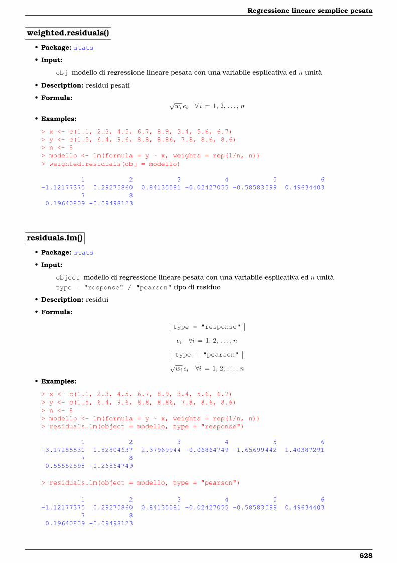
Regressione lineare semplice pesata
weighted.residuals()
• Package: stats
• Input:
obj modello di regressione lineare pesata con una variabile esplicativa ed n unità
• Description: residui pesati
• Formula: √wi ei ∀ i = 1, 2, . . . , n
• Examples:
> x <- c(1.1, 2.3, 4.5, 6.7, 8.9, 3.4, 5.6, 6.7)> y <- c(1.5, 6.4, 9.6, 8.8, 8.86, 7.8, 8.6, 8.6)> n <- 8> modello <- lm(formula = y ~ x, weights = rep(1/n, n))> weighted.residuals(obj = modello)
1 2 3 4 5 6-1.12177375 0.29275860 0.84135081 -0.02427055 -0.58583599 0.49634403
7 80.19640809 -0.09498123
residuals.lm()
• Package: stats
• Input:
object modello di regressione lineare pesata con una variabile esplicativa ed n unitàtype = "response" / "pearson" tipo di residuo
• Description: residui
• Formula:
type = "response"
ei ∀i = 1, 2, . . . , n
type = "pearson"
√wi ei ∀i = 1, 2, . . . , n
• Examples:
> x <- c(1.1, 2.3, 4.5, 6.7, 8.9, 3.4, 5.6, 6.7)> y <- c(1.5, 6.4, 9.6, 8.8, 8.86, 7.8, 8.6, 8.6)> n <- 8> modello <- lm(formula = y ~ x, weights = rep(1/n, n))> residuals.lm(object = modello, type = "response")
1 2 3 4 5 6-3.17285530 0.82804637 2.37969944 -0.06864749 -1.65699442 1.40387291
7 80.55552598 -0.26864749
> residuals.lm(object = modello, type = "pearson")
1 2 3 4 5 6-1.12177375 0.29275860 0.84135081 -0.02427055 -0.58583599 0.49634403
7 80.19640809 -0.09498123
628
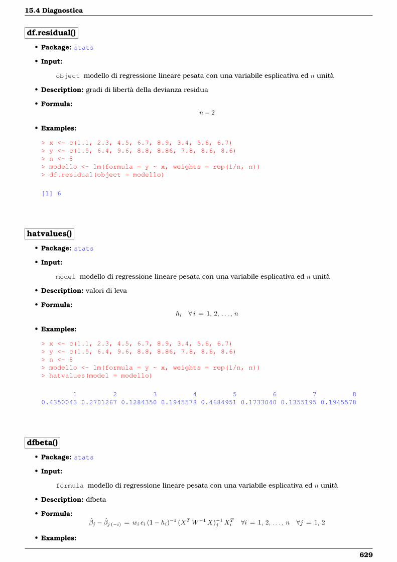
15.4 Diagnostica
df.residual()
• Package: stats
• Input:
object modello di regressione lineare pesata con una variabile esplicativa ed n unità
• Description: gradi di libertà della devianza residua
• Formula:n− 2
• Examples:
> x <- c(1.1, 2.3, 4.5, 6.7, 8.9, 3.4, 5.6, 6.7)> y <- c(1.5, 6.4, 9.6, 8.8, 8.86, 7.8, 8.6, 8.6)> n <- 8> modello <- lm(formula = y ~ x, weights = rep(1/n, n))> df.residual(object = modello)
[1] 6
hatvalues()
• Package: stats
• Input:
model modello di regressione lineare pesata con una variabile esplicativa ed n unità
• Description: valori di leva
• Formula:hi ∀ i = 1, 2, . . . , n
• Examples:
> x <- c(1.1, 2.3, 4.5, 6.7, 8.9, 3.4, 5.6, 6.7)> y <- c(1.5, 6.4, 9.6, 8.8, 8.86, 7.8, 8.6, 8.6)> n <- 8> modello <- lm(formula = y ~ x, weights = rep(1/n, n))> hatvalues(model = modello)
1 2 3 4 5 6 7 80.4350043 0.2701267 0.1284350 0.1945578 0.4684951 0.1733040 0.1355195 0.1945578
dfbeta()
• Package: stats
• Input:
formula modello di regressione lineare pesata con una variabile esplicativa ed n unità
• Description: dfbeta
• Formula:βj − βj (−i) = wi ei (1− hi)−1 (XT W−1X)−1
j XTi ∀i = 1, 2, . . . , n ∀j = 1, 2
• Examples:
629
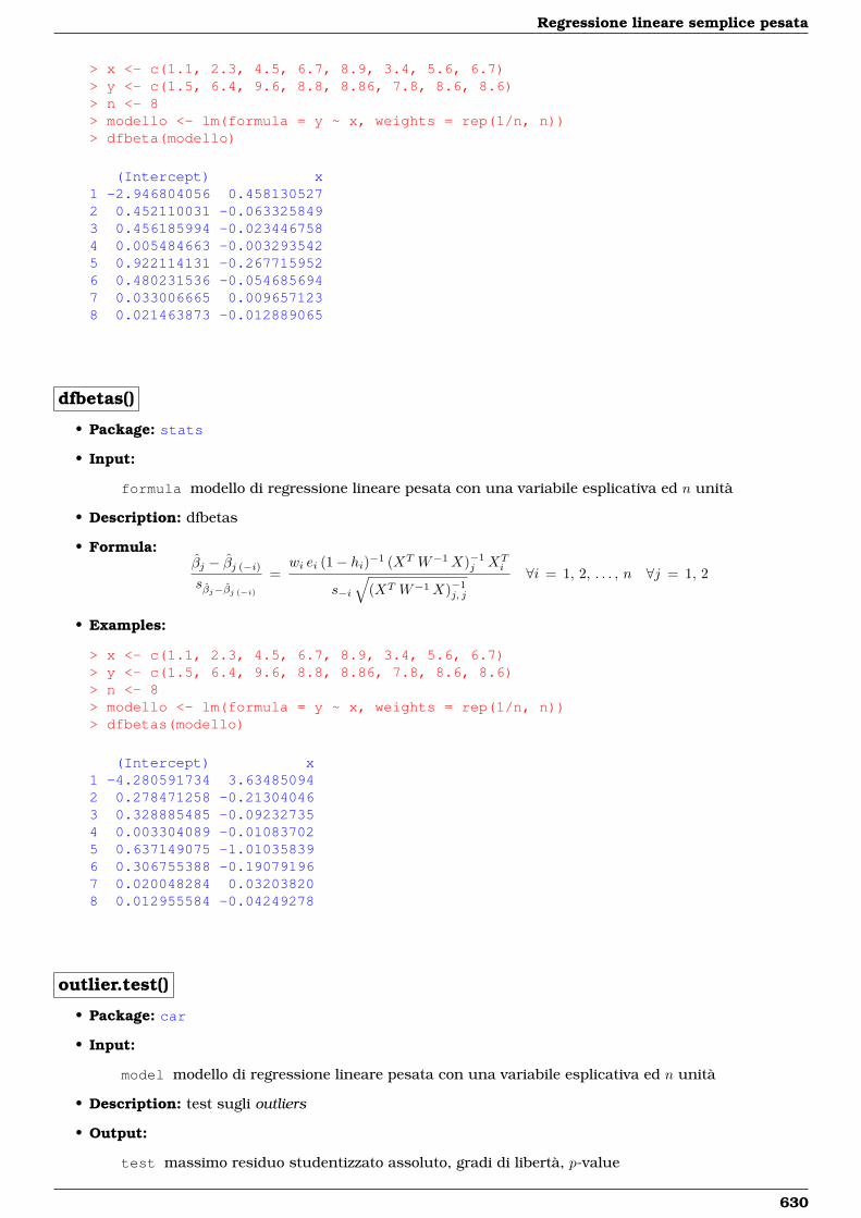
Regressione lineare semplice pesata
> x <- c(1.1, 2.3, 4.5, 6.7, 8.9, 3.4, 5.6, 6.7)> y <- c(1.5, 6.4, 9.6, 8.8, 8.86, 7.8, 8.6, 8.6)> n <- 8> modello <- lm(formula = y ~ x, weights = rep(1/n, n))> dfbeta(modello)
(Intercept) x1 -2.946804056 0.4581305272 0.452110031 -0.0633258493 0.456185994 -0.0234467584 0.005484663 -0.0032935425 0.922114131 -0.2677159526 0.480231536 -0.0546856947 0.033006665 0.0096571238 0.021463873 -0.012889065
dfbetas()
• Package: stats
• Input:
formula modello di regressione lineare pesata con una variabile esplicativa ed n unità
• Description: dfbetas
• Formula:βj − βj (−i)
sβj−βj (−i)
=wi ei (1− hi)−1 (XT W−1X)−1
j XTi
s−i
√(XT W−1X)−1
j, j
∀i = 1, 2, . . . , n ∀j = 1, 2
• Examples:
> x <- c(1.1, 2.3, 4.5, 6.7, 8.9, 3.4, 5.6, 6.7)> y <- c(1.5, 6.4, 9.6, 8.8, 8.86, 7.8, 8.6, 8.6)> n <- 8> modello <- lm(formula = y ~ x, weights = rep(1/n, n))> dfbetas(modello)
(Intercept) x1 -4.280591734 3.634850942 0.278471258 -0.213040463 0.328885485 -0.092327354 0.003304089 -0.010837025 0.637149075 -1.010358396 0.306755388 -0.190791967 0.020048284 0.032038208 0.012955584 -0.04249278
outlier.test()
• Package: car
• Input:
model modello di regressione lineare pesata con una variabile esplicativa ed n unità
• Description: test sugli outliers
• Output:
test massimo residuo studentizzato assoluto, gradi di libertà, p-value
630
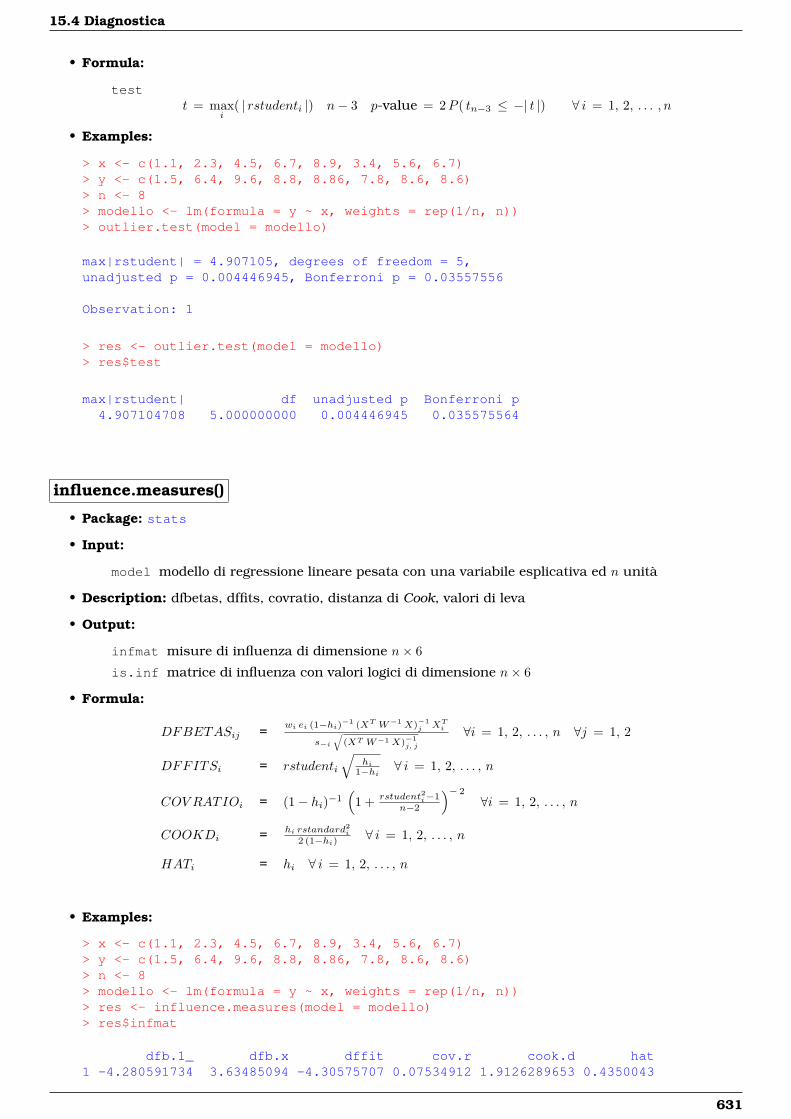
15.4 Diagnostica
• Formula:
testt = max
i( | rstudenti |) n− 3 p-value = 2P ( tn−3 ≤ −| t |) ∀ i = 1, 2, . . . , n
• Examples:
> x <- c(1.1, 2.3, 4.5, 6.7, 8.9, 3.4, 5.6, 6.7)> y <- c(1.5, 6.4, 9.6, 8.8, 8.86, 7.8, 8.6, 8.6)> n <- 8> modello <- lm(formula = y ~ x, weights = rep(1/n, n))> outlier.test(model = modello)
max|rstudent| = 4.907105, degrees of freedom = 5,unadjusted p = 0.004446945, Bonferroni p = 0.03557556
Observation: 1
> res <- outlier.test(model = modello)> res$test
max|rstudent| df unadjusted p Bonferroni p4.907104708 5.000000000 0.004446945 0.035575564
influence.measures()
• Package: stats
• Input:
model modello di regressione lineare pesata con una variabile esplicativa ed n unità
• Description: dfbetas, dffits, covratio, distanza di Cook, valori di leva
• Output:
infmat misure di influenza di dimensione n× 6
is.inf matrice di influenza con valori logici di dimensione n× 6
• Formula:
DFBETASij =wi ei (1−hi)−1 (XT W−1X)−1
j XTi
s−i
√(XT W−1X)−1
j, j
∀i = 1, 2, . . . , n ∀j = 1, 2
DFFITSi = rstudenti
√hi
1−hi ∀ i = 1, 2, . . . , n
COV RATIOi = (1− hi)−1(
1 + rstudent2i−1n−2
)− 2
∀i = 1, 2, . . . , n
COOKDi = hi rstandard2i
2 (1−hi) ∀ i = 1, 2, . . . , n
HATi = hi ∀ i = 1, 2, . . . , n
• Examples:
> x <- c(1.1, 2.3, 4.5, 6.7, 8.9, 3.4, 5.6, 6.7)> y <- c(1.5, 6.4, 9.6, 8.8, 8.86, 7.8, 8.6, 8.6)> n <- 8> modello <- lm(formula = y ~ x, weights = rep(1/n, n))> res <- influence.measures(model = modello)> res$infmat
dfb.1_ dfb.x dffit cov.r cook.d hat1 -4.280591734 3.63485094 -4.30575707 0.07534912 1.9126289653 0.4350043
631
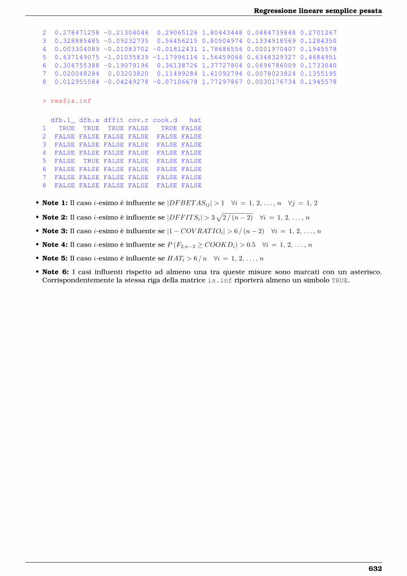
Regressione lineare semplice pesata
2 0.278471258 -0.21304046 0.29065126 1.80443448 0.0484739848 0.27012673 0.328885485 -0.09232735 0.56456215 0.80504974 0.1334918569 0.12843504 0.003304089 -0.01083702 -0.01812431 1.78686556 0.0001970407 0.19455785 0.637149075 -1.01035839 -1.17996116 1.56459066 0.6348329327 0.46849516 0.306755388 -0.19079196 0.36138726 1.37727804 0.0696786009 0.17330407 0.020048284 0.03203820 0.11499284 1.61092794 0.0078023824 0.13551958 0.012955584 -0.04249278 -0.07106678 1.77297867 0.0030176734 0.1945578
> res$is.inf
dfb.1_ dfb.x dffit cov.r cook.d hat1 TRUE TRUE TRUE FALSE TRUE FALSE2 FALSE FALSE FALSE FALSE FALSE FALSE3 FALSE FALSE FALSE FALSE FALSE FALSE4 FALSE FALSE FALSE FALSE FALSE FALSE5 FALSE TRUE FALSE FALSE FALSE FALSE6 FALSE FALSE FALSE FALSE FALSE FALSE7 FALSE FALSE FALSE FALSE FALSE FALSE8 FALSE FALSE FALSE FALSE FALSE FALSE
• Note 1: Il caso i-esimo è influente se |DFBETASij | > 1 ∀i = 1, 2, . . . , n ∀j = 1, 2
• Note 2: Il caso i-esimo è influente se |DFFITSi| > 3√
2 / (n− 2) ∀i = 1, 2, . . . , n
• Note 3: Il caso i-esimo è influente se |1− COV RATIOi| > 6 / (n− 2) ∀i = 1, 2, . . . , n
• Note 4: Il caso i-esimo è influente se P (F2,n−2 ≥ COOKDi) > 0.5 ∀i = 1, 2, . . . , n
• Note 5: Il caso i-esimo è influente se HATi > 6 / n ∀i = 1, 2, . . . , n
• Note 6: I casi influenti rispetto ad almeno una tra queste misure sono marcati con un asterisco.Corrispondentemente la stessa riga della matrice is.inf riporterà almeno un simbolo TRUE.
632
Capitolo 16
Regressione lineare multipla pesata
16.1 Simbologia
yi = β1 + β2 xi1 + β3 xi2 + · · ·+ βk xik−1 + εi ∀ i = 1, 2, . . . , n ε ∼ N(0, σ2W )
• variabile dipendente: y
• matrice del modello di dimensione n× k : X
• numero di parametri da stimare e rango della matrice del modello: k
• numero di unità: n
• i-esima riga della matrice del modello : Xi = (1, xi1, xi2, . . . , xik−1) ∀ i = 1, 2, . . . , n
• vettore numerico positivo dei pesi WLS: w = (w1, w2, . . . , wn)
• matrice diagonale definita positiva di dimensione n× n : W = diag(w−11 , w−1
2 , . . . , w−1n )
• matrice di proiezione di dimensione n× n : H = X (XT W−1X)−1XT W−1
• matrice identità di dimensione n× n : In
• devianza residua: RSS =∑ni=1 wi e
2i = yT W−1 e = yT W−1 (In −H) y
• stima di σ2: s2 = RSS / (n− k)
• gradi di libertà della devianza residua: n− k
• stima di σ2 tolta la i-esima unità: s2−i = s2
(1 + 1−rstandard2i
n−k−1
)= s2
(1 + rstudent2i−1
n−k
)−1
∀ i = 1, 2, . . . , n
• stime WLS: β = (XT W−1X)−1XT W−1 y
• standard error delle stime WLS: sβ = s√
diag((XT W−1X)−1)
• t-values delle stime WLS: tβ = β / sβ
• residui: e = (In −H) y
• residui pesati:√wi ei ∀ i = 1, 2, . . . , n
• residui standard: rstandardi = ei
s√
(1−hi) /wi∀ i = 1, 2, . . . , n
• residui studentizzati: rstudenti = ei
s−i√
(1−hi) /wi= rstandardi
√n−k−1
n−k−rstandard2i∀ i = 1, 2, . . . , n
• valori adattati: y = H y
• valori di leva: hi = Hi,i ∀ i = 1, 2, . . . , n
• stime WLS tolta la i-esima unità: β(−i) ∀ i = 1, 2, . . . , n
• correlazione delle stime WLS: rβi βj =s2 (XT W−1X)−1
i, j
sβisβj
∀ i, j = 1, 2, . . . , k
• devianza residua modello nullo: RSSnullo =∑ni=1 wi (yi − yW )2 = (y − yW )T W−1 (y − yW )
• indice di determinazione: R2 = 1−RSS /RSSnullo = 1− (1−R2adj) (n− k) / (n− 1)
633
Regressione lineare multipla pesata
• indice di determinazione aggiustato: R2adj = 1− RSS / (n−k)
RSSnullo / (n−1) = 1−(1−R2
)(n− 1) / (n− k)
• valore noto dei regressori per la previsione: xT0 = (1, x01, x02, . . . , x0k−1)
• log-verosimiglianza normale: ˆ = −n (log(2π) + log (RSS /n) + 1−∑ni=1 log(wi) / n) / 2
• distanza di Cook: cdi = hi rstandard2i
k (1−hi) = e2ik s2
hi(1−hi)2 ∀ i = 1, 2, . . . , n
• covratio: cri = (1− hi)−1(
1 + rstudent2i−1n−k
)− k= (1− hi)−1
( s−is
)2 k ∀i = 1, 2, . . . , n
16.2 Stima
lm()
• Package: stats
• Input:
formula modello di regressione lineare pesata con k − 1 variabili esplicative ed n unità
weights pesi
x = TRUE matrice del modello
y = TRUE variabile dipendente
• Description: analisi di regressione lineare pesata
• Output:
coefficients stime WLS
residuals residui
fitted.values valori adattati
weights pesi
rank rango della matrice del modello
df.residual gradi di libertà della devianza residua
x matrice del modello
y variabile dipendente
• Formula:
coefficientsβj ∀ j = 1, 2, . . . , k
residualsei ∀ i = 1, 2, . . . , n
fitted.valuesyi ∀ i = 1, 2, . . . , n
weightswi ∀ i = 1, 2, . . . , n
rankk
df.residualn− k
xX
yy
• Examples:
634
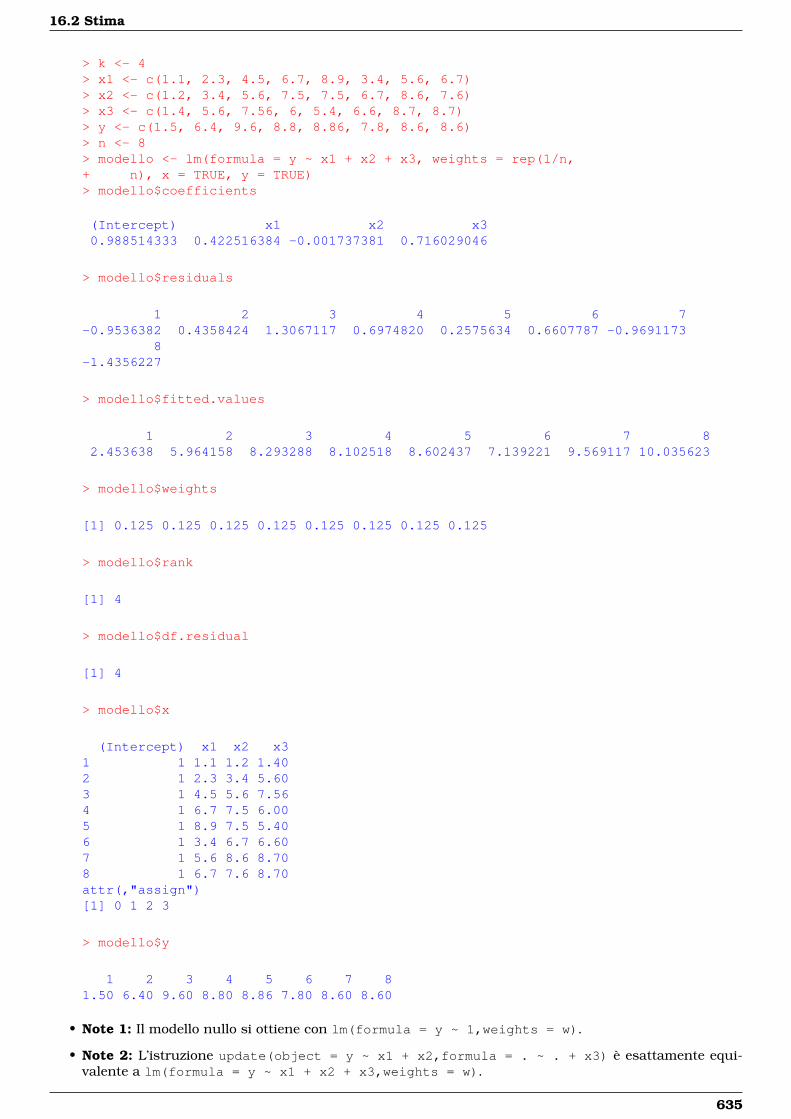
16.2 Stima
> k <- 4> x1 <- c(1.1, 2.3, 4.5, 6.7, 8.9, 3.4, 5.6, 6.7)> x2 <- c(1.2, 3.4, 5.6, 7.5, 7.5, 6.7, 8.6, 7.6)> x3 <- c(1.4, 5.6, 7.56, 6, 5.4, 6.6, 8.7, 8.7)> y <- c(1.5, 6.4, 9.6, 8.8, 8.86, 7.8, 8.6, 8.6)> n <- 8> modello <- lm(formula = y ~ x1 + x2 + x3, weights = rep(1/n,+ n), x = TRUE, y = TRUE)> modello$coefficients
(Intercept) x1 x2 x30.988514333 0.422516384 -0.001737381 0.716029046
> modello$residuals
1 2 3 4 5 6 7-0.9536382 0.4358424 1.3067117 0.6974820 0.2575634 0.6607787 -0.9691173
8-1.4356227
> modello$fitted.values
1 2 3 4 5 6 7 82.453638 5.964158 8.293288 8.102518 8.602437 7.139221 9.569117 10.035623
> modello$weights
[1] 0.125 0.125 0.125 0.125 0.125 0.125 0.125 0.125
> modello$rank
[1] 4
> modello$df.residual
[1] 4
> modello$x
(Intercept) x1 x2 x31 1 1.1 1.2 1.402 1 2.3 3.4 5.603 1 4.5 5.6 7.564 1 6.7 7.5 6.005 1 8.9 7.5 5.406 1 3.4 6.7 6.607 1 5.6 8.6 8.708 1 6.7 7.6 8.70attr(,"assign")[1] 0 1 2 3
> modello$y
1 2 3 4 5 6 7 81.50 6.40 9.60 8.80 8.86 7.80 8.60 8.60
• Note 1: Il modello nullo si ottiene con lm(formula = y ~ 1,weights = w).
• Note 2: L’istruzione update(object = y ~ x1 + x2,formula = . ~ . + x3) è esattamente equi-valente a lm(formula = y ~ x1 + x2 + x3,weights = w).
635
Regressione lineare multipla pesata
• Note 3: In seguito ad una modifica come ad esempio x1[3] <- 1.2, conviene adoperare il comandoupdate(modello) anziché ripetere modello <- lm(formula = y ~ x1 + x2 + x3,weights = w).
• Note 4: L’operatore I() permette di poter modellare regressioni lineari polinomiali. Per un polinomiodi terzo grado occorre scrivere lm(formula = y ~ x + I(x^2) + I(x^3),weights = w).
• Note 5: Per regressioni polinomiali occorre usare il comando poly(). Per un polinomio di quarto gradooccorre scrivere lm(formula = y ~ poly(x,degree = 4,raw = TRUE),weights = w).
• Note 6: Per regressioni polinomiali ortogonali occorre usare il comando poly(). Per un polinomio or-togonale di quarto grado occorre scrivere lm(formula = y ~ poly(x,degree = 4),weights = w).
• Note 7: Il comando uzione lm(formula = y ~ x1 + x2 + x3,weights=w) è esattamente equivalentea lm(formula = y ~ X-1,weights = w).
• Note 8: Il comando lm(formula = y ~ x1 + x2 + x3,weights = w) è esattamente equivalente alm(formula = y ~ 1 + x1 + x2 + x3,weights = w).
summary.lm()
• Package: stats
• Input:
object modello di regressione lineare pesata con k − 1 variabili esplicative ed n unità
correlation = TRUE correlazione delle stime WLS
• Description: analisi di regressione lineare pesata
• Output:
residuals residui
coefficients stima puntuale, standard error, t-value, p-value
sigma stima di σ
r.squared indice di determinazione
adj.r.squared indice di determinazione aggiustato
fstatistic valore empirico della statistica F , df numeratore, df denominatore
cov.unscaled matrice di covarianza delle stime WLS non scalata per σ2
correlation matrice di correlazione delle stime WLS
• Formula:
residualsei ∀ i = 1, 2, . . . , n
coefficients
βj sβj tβj p-value = 2P (tn−k ≤ − | tβj |) ∀ j = 1, 2, . . . , k
sigmas
r.squaredR2
adj.r.squaredR2adj
fstatistic
Fvalue =(RSSnullo −RSS) / (k − 1)
RSS / (n− k)k − 1 n− k
cov.unscaled(XT W−1X)−1
636
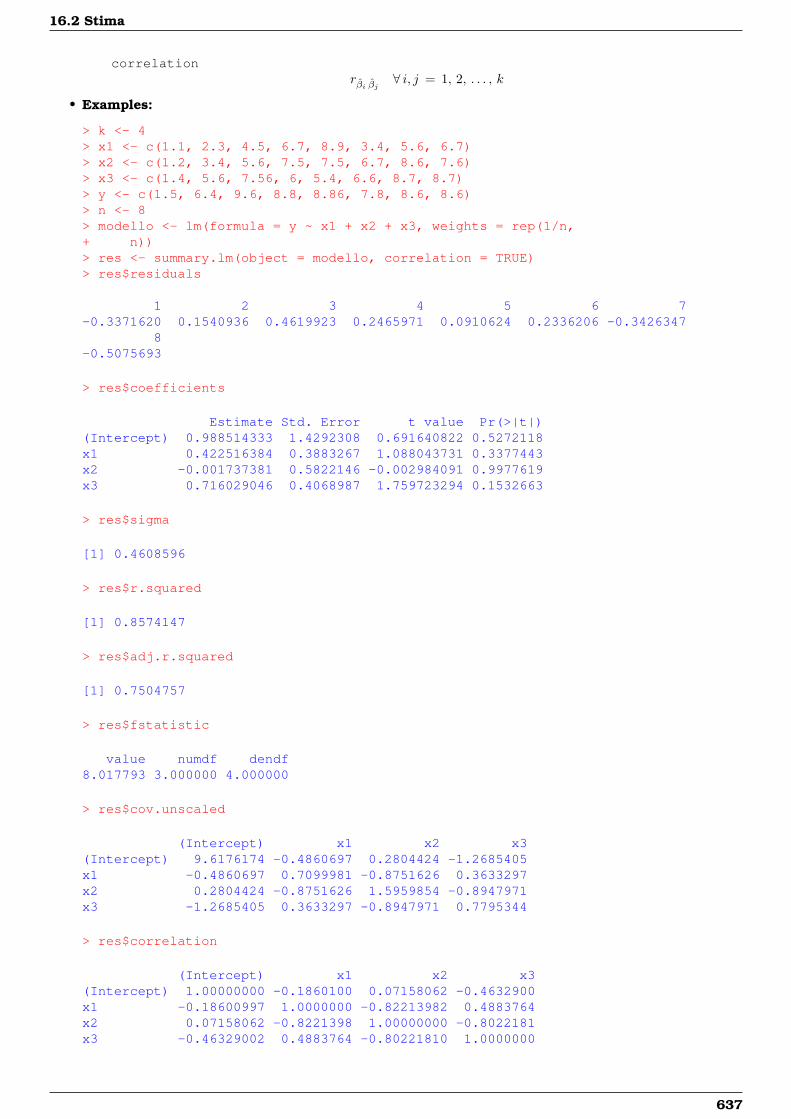
16.2 Stima
correlationrβi βj ∀ i, j = 1, 2, . . . , k
• Examples:
> k <- 4> x1 <- c(1.1, 2.3, 4.5, 6.7, 8.9, 3.4, 5.6, 6.7)> x2 <- c(1.2, 3.4, 5.6, 7.5, 7.5, 6.7, 8.6, 7.6)> x3 <- c(1.4, 5.6, 7.56, 6, 5.4, 6.6, 8.7, 8.7)> y <- c(1.5, 6.4, 9.6, 8.8, 8.86, 7.8, 8.6, 8.6)> n <- 8> modello <- lm(formula = y ~ x1 + x2 + x3, weights = rep(1/n,+ n))> res <- summary.lm(object = modello, correlation = TRUE)> res$residuals
1 2 3 4 5 6 7-0.3371620 0.1540936 0.4619923 0.2465971 0.0910624 0.2336206 -0.3426347
8-0.5075693
> res$coefficients
Estimate Std. Error t value Pr(>|t|)(Intercept) 0.988514333 1.4292308 0.691640822 0.5272118x1 0.422516384 0.3883267 1.088043731 0.3377443x2 -0.001737381 0.5822146 -0.002984091 0.9977619x3 0.716029046 0.4068987 1.759723294 0.1532663
> res$sigma
[1] 0.4608596
> res$r.squared
[1] 0.8574147
> res$adj.r.squared
[1] 0.7504757
> res$fstatistic
value numdf dendf8.017793 3.000000 4.000000
> res$cov.unscaled
(Intercept) x1 x2 x3(Intercept) 9.6176174 -0.4860697 0.2804424 -1.2685405x1 -0.4860697 0.7099981 -0.8751626 0.3633297x2 0.2804424 -0.8751626 1.5959854 -0.8947971x3 -1.2685405 0.3633297 -0.8947971 0.7795344
> res$correlation
(Intercept) x1 x2 x3(Intercept) 1.00000000 -0.1860100 0.07158062 -0.4632900x1 -0.18600997 1.0000000 -0.82213982 0.4883764x2 0.07158062 -0.8221398 1.00000000 -0.8022181x3 -0.46329002 0.4883764 -0.80221810 1.0000000
637
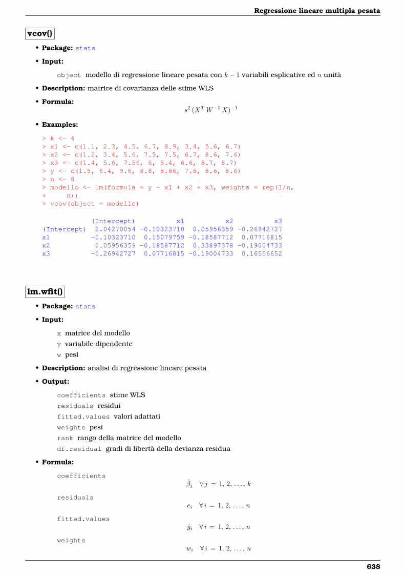
Regressione lineare multipla pesata
vcov()
• Package: stats
• Input:
object modello di regressione lineare pesata con k − 1 variabili esplicative ed n unità
• Description: matrice di covarianza delle stime WLS
• Formula:s2 (XT W−1X)−1
• Examples:
> k <- 4> x1 <- c(1.1, 2.3, 4.5, 6.7, 8.9, 3.4, 5.6, 6.7)> x2 <- c(1.2, 3.4, 5.6, 7.5, 7.5, 6.7, 8.6, 7.6)> x3 <- c(1.4, 5.6, 7.56, 6, 5.4, 6.6, 8.7, 8.7)> y <- c(1.5, 6.4, 9.6, 8.8, 8.86, 7.8, 8.6, 8.6)> n <- 8> modello <- lm(formula = y ~ x1 + x2 + x3, weights = rep(1/n,+ n))> vcov(object = modello)
(Intercept) x1 x2 x3(Intercept) 2.04270054 -0.10323710 0.05956359 -0.26942727x1 -0.10323710 0.15079759 -0.18587712 0.07716815x2 0.05956359 -0.18587712 0.33897378 -0.19004733x3 -0.26942727 0.07716815 -0.19004733 0.16556652
lm.wfit()
• Package: stats
• Input:
x matrice del modello
y variabile dipendente
w pesi
• Description: analisi di regressione lineare pesata
• Output:
coefficients stime WLS
residuals residui
fitted.values valori adattati
weights pesi
rank rango della matrice del modello
df.residual gradi di libertà della devianza residua
• Formula:
coefficientsβj ∀ j = 1, 2, . . . , k
residualsei ∀ i = 1, 2, . . . , n
fitted.valuesyi ∀ i = 1, 2, . . . , n
weightswi ∀ i = 1, 2, . . . , n
638
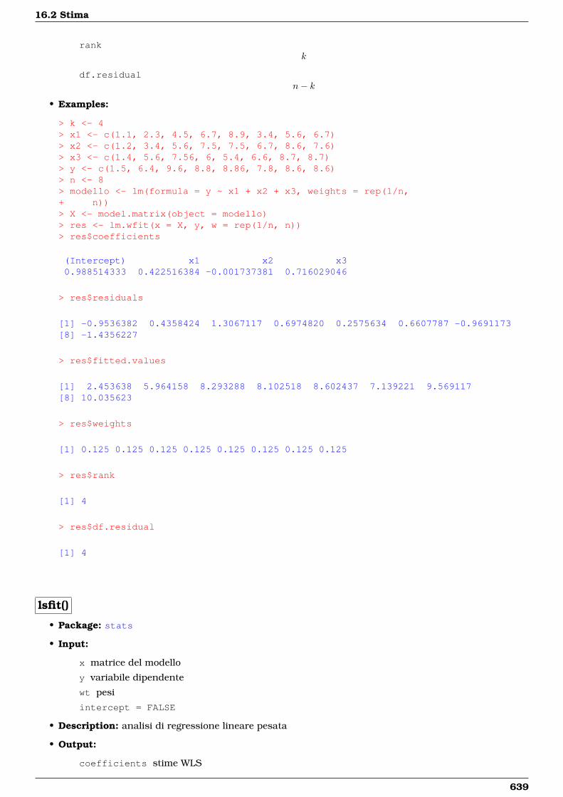
16.2 Stima
rankk
df.residualn− k
• Examples:
> k <- 4> x1 <- c(1.1, 2.3, 4.5, 6.7, 8.9, 3.4, 5.6, 6.7)> x2 <- c(1.2, 3.4, 5.6, 7.5, 7.5, 6.7, 8.6, 7.6)> x3 <- c(1.4, 5.6, 7.56, 6, 5.4, 6.6, 8.7, 8.7)> y <- c(1.5, 6.4, 9.6, 8.8, 8.86, 7.8, 8.6, 8.6)> n <- 8> modello <- lm(formula = y ~ x1 + x2 + x3, weights = rep(1/n,+ n))> X <- model.matrix(object = modello)> res <- lm.wfit(x = X, y, w = rep(1/n, n))> res$coefficients
(Intercept) x1 x2 x30.988514333 0.422516384 -0.001737381 0.716029046
> res$residuals
[1] -0.9536382 0.4358424 1.3067117 0.6974820 0.2575634 0.6607787 -0.9691173[8] -1.4356227
> res$fitted.values
[1] 2.453638 5.964158 8.293288 8.102518 8.602437 7.139221 9.569117[8] 10.035623
> res$weights
[1] 0.125 0.125 0.125 0.125 0.125 0.125 0.125 0.125
> res$rank
[1] 4
> res$df.residual
[1] 4
lsfit()
• Package: stats
• Input:
x matrice del modello
y variabile dipendente
wt pesi
intercept = FALSE
• Description: analisi di regressione lineare pesata
• Output:
coefficients stime WLS
639
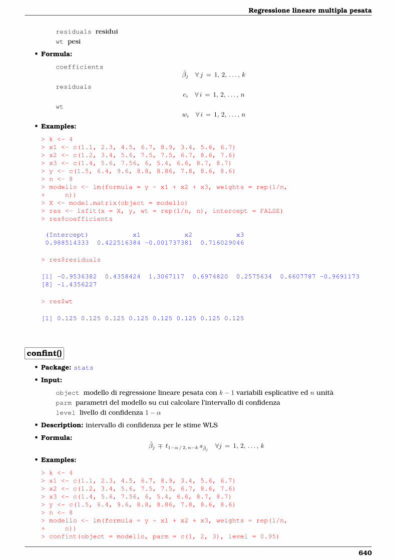
Regressione lineare multipla pesata
residuals residui
wt pesi
• Formula:
coefficientsβj ∀ j = 1, 2, . . . , k
residualsei ∀ i = 1, 2, . . . , n
wtwi ∀ i = 1, 2, . . . , n
• Examples:
> k <- 4> x1 <- c(1.1, 2.3, 4.5, 6.7, 8.9, 3.4, 5.6, 6.7)> x2 <- c(1.2, 3.4, 5.6, 7.5, 7.5, 6.7, 8.6, 7.6)> x3 <- c(1.4, 5.6, 7.56, 6, 5.4, 6.6, 8.7, 8.7)> y <- c(1.5, 6.4, 9.6, 8.8, 8.86, 7.8, 8.6, 8.6)> n <- 8> modello <- lm(formula = y ~ x1 + x2 + x3, weights = rep(1/n,+ n))> X <- model.matrix(object = modello)> res <- lsfit(x = X, y, wt = rep(1/n, n), intercept = FALSE)> res$coefficients
(Intercept) x1 x2 x30.988514333 0.422516384 -0.001737381 0.716029046
> res$residuals
[1] -0.9536382 0.4358424 1.3067117 0.6974820 0.2575634 0.6607787 -0.9691173[8] -1.4356227
> res$wt
[1] 0.125 0.125 0.125 0.125 0.125 0.125 0.125 0.125
confint()
• Package: stats
• Input:
object modello di regressione lineare pesata con k − 1 variabili esplicative ed n unità
parm parametri del modello su cui calcolare l’intervallo di confidenza
level livello di confidenza 1− α
• Description: intervallo di confidenza per le stime WLS
• Formula:βj ∓ t1−α/ 2, n−k sβj ∀j = 1, 2, . . . , k
• Examples:
> k <- 4> x1 <- c(1.1, 2.3, 4.5, 6.7, 8.9, 3.4, 5.6, 6.7)> x2 <- c(1.2, 3.4, 5.6, 7.5, 7.5, 6.7, 8.6, 7.6)> x3 <- c(1.4, 5.6, 7.56, 6, 5.4, 6.6, 8.7, 8.7)> y <- c(1.5, 6.4, 9.6, 8.8, 8.86, 7.8, 8.6, 8.6)> n <- 8> modello <- lm(formula = y ~ x1 + x2 + x3, weights = rep(1/n,+ n))> confint(object = modello, parm = c(1, 2, 3), level = 0.95)
640
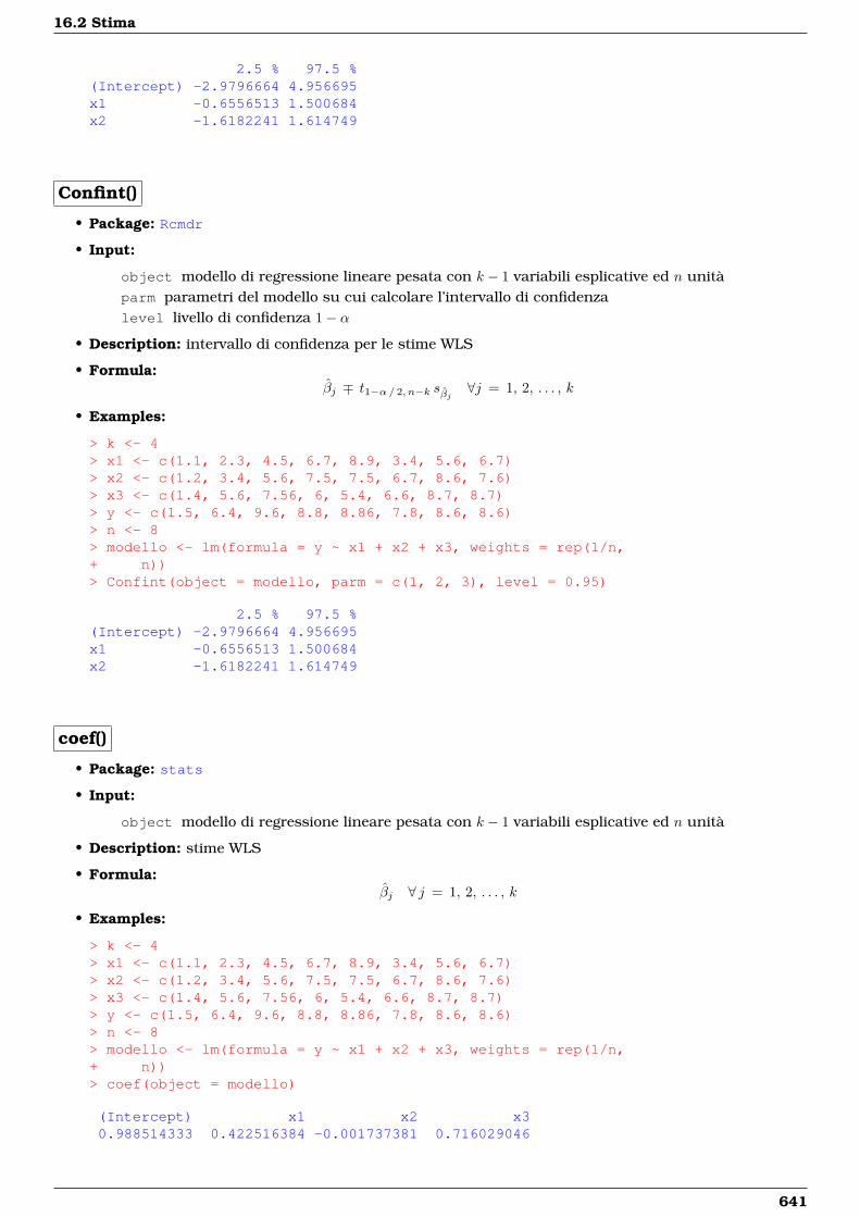
16.2 Stima
2.5 % 97.5 %(Intercept) -2.9796664 4.956695x1 -0.6556513 1.500684x2 -1.6182241 1.614749
Confint()
• Package: Rcmdr
• Input:
object modello di regressione lineare pesata con k − 1 variabili esplicative ed n unitàparm parametri del modello su cui calcolare l’intervallo di confidenzalevel livello di confidenza 1− α
• Description: intervallo di confidenza per le stime WLS
• Formula:βj ∓ t1−α/ 2, n−k sβj ∀j = 1, 2, . . . , k
• Examples:
> k <- 4> x1 <- c(1.1, 2.3, 4.5, 6.7, 8.9, 3.4, 5.6, 6.7)> x2 <- c(1.2, 3.4, 5.6, 7.5, 7.5, 6.7, 8.6, 7.6)> x3 <- c(1.4, 5.6, 7.56, 6, 5.4, 6.6, 8.7, 8.7)> y <- c(1.5, 6.4, 9.6, 8.8, 8.86, 7.8, 8.6, 8.6)> n <- 8> modello <- lm(formula = y ~ x1 + x2 + x3, weights = rep(1/n,+ n))> Confint(object = modello, parm = c(1, 2, 3), level = 0.95)
2.5 % 97.5 %(Intercept) -2.9796664 4.956695x1 -0.6556513 1.500684x2 -1.6182241 1.614749
coef()
• Package: stats
• Input:
object modello di regressione lineare pesata con k − 1 variabili esplicative ed n unità
• Description: stime WLS
• Formula:βj ∀ j = 1, 2, . . . , k
• Examples:
> k <- 4> x1 <- c(1.1, 2.3, 4.5, 6.7, 8.9, 3.4, 5.6, 6.7)> x2 <- c(1.2, 3.4, 5.6, 7.5, 7.5, 6.7, 8.6, 7.6)> x3 <- c(1.4, 5.6, 7.56, 6, 5.4, 6.6, 8.7, 8.7)> y <- c(1.5, 6.4, 9.6, 8.8, 8.86, 7.8, 8.6, 8.6)> n <- 8> modello <- lm(formula = y ~ x1 + x2 + x3, weights = rep(1/n,+ n))> coef(object = modello)
(Intercept) x1 x2 x30.988514333 0.422516384 -0.001737381 0.716029046
641
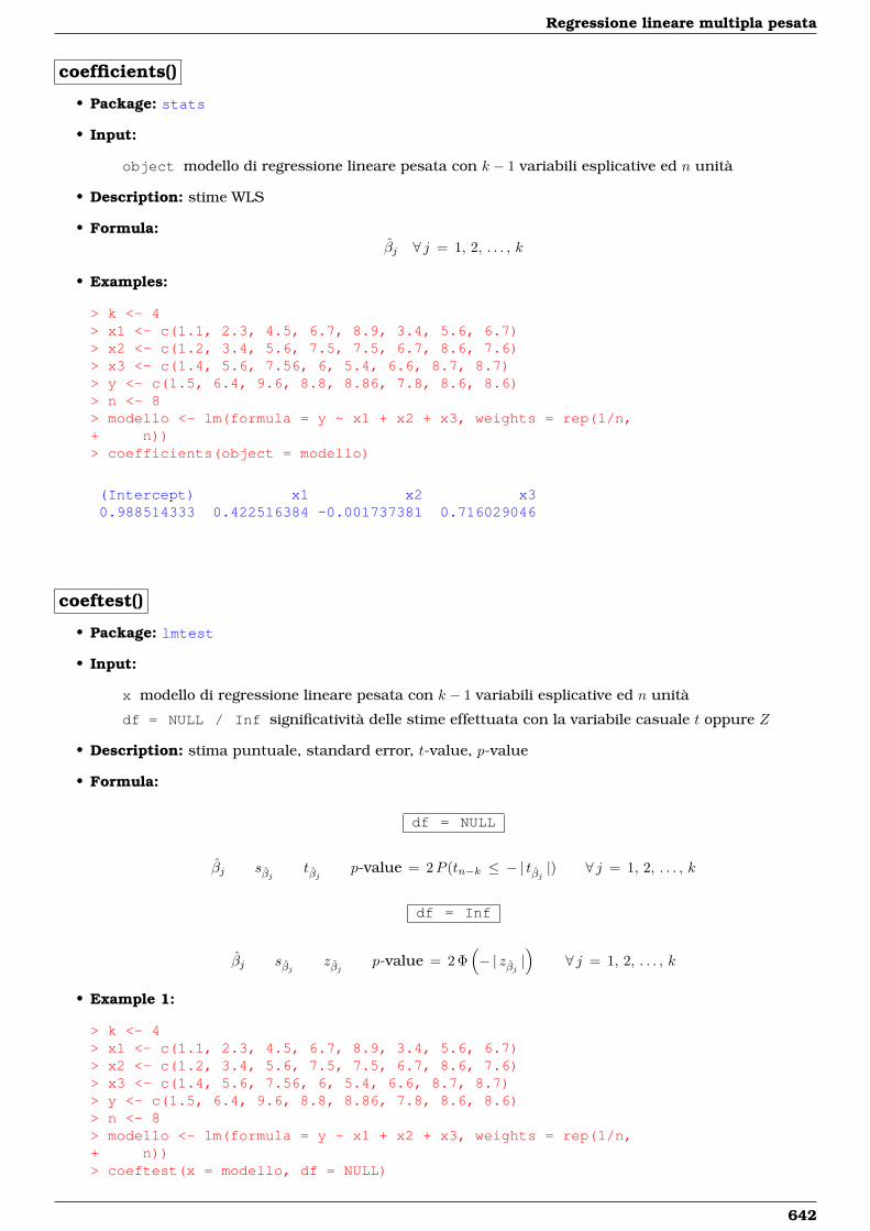
Regressione lineare multipla pesata
coefficients()
• Package: stats
• Input:
object modello di regressione lineare pesata con k − 1 variabili esplicative ed n unità
• Description: stime WLS
• Formula:βj ∀ j = 1, 2, . . . , k
• Examples:
> k <- 4> x1 <- c(1.1, 2.3, 4.5, 6.7, 8.9, 3.4, 5.6, 6.7)> x2 <- c(1.2, 3.4, 5.6, 7.5, 7.5, 6.7, 8.6, 7.6)> x3 <- c(1.4, 5.6, 7.56, 6, 5.4, 6.6, 8.7, 8.7)> y <- c(1.5, 6.4, 9.6, 8.8, 8.86, 7.8, 8.6, 8.6)> n <- 8> modello <- lm(formula = y ~ x1 + x2 + x3, weights = rep(1/n,+ n))> coefficients(object = modello)
(Intercept) x1 x2 x30.988514333 0.422516384 -0.001737381 0.716029046
coeftest()
• Package: lmtest
• Input:
x modello di regressione lineare pesata con k − 1 variabili esplicative ed n unità
df = NULL / Inf significatività delle stime effettuata con la variabile casuale t oppure Z
• Description: stima puntuale, standard error, t-value, p-value
• Formula:
df = NULL
βj sβj tβj p-value = 2P (tn−k ≤ − | tβj |) ∀ j = 1, 2, . . . , k
df = Inf
βj sβj zβj p-value = 2 Φ(− | zβj |
)∀ j = 1, 2, . . . , k
• Example 1:
> k <- 4> x1 <- c(1.1, 2.3, 4.5, 6.7, 8.9, 3.4, 5.6, 6.7)> x2 <- c(1.2, 3.4, 5.6, 7.5, 7.5, 6.7, 8.6, 7.6)> x3 <- c(1.4, 5.6, 7.56, 6, 5.4, 6.6, 8.7, 8.7)> y <- c(1.5, 6.4, 9.6, 8.8, 8.86, 7.8, 8.6, 8.6)> n <- 8> modello <- lm(formula = y ~ x1 + x2 + x3, weights = rep(1/n,+ n))> coeftest(x = modello, df = NULL)
642
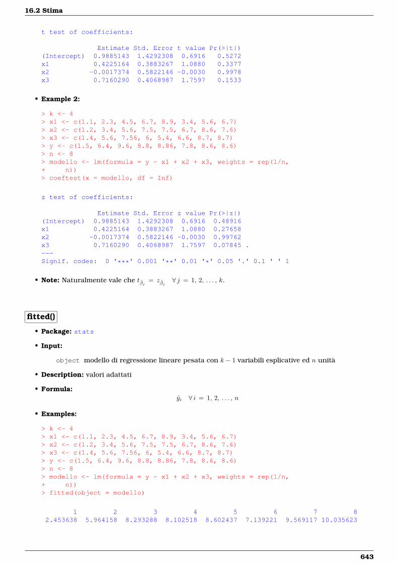
16.2 Stima
t test of coefficients:
Estimate Std. Error t value Pr(>|t|)(Intercept) 0.9885143 1.4292308 0.6916 0.5272x1 0.4225164 0.3883267 1.0880 0.3377x2 -0.0017374 0.5822146 -0.0030 0.9978x3 0.7160290 0.4068987 1.7597 0.1533
• Example 2:
> k <- 4> x1 <- c(1.1, 2.3, 4.5, 6.7, 8.9, 3.4, 5.6, 6.7)> x2 <- c(1.2, 3.4, 5.6, 7.5, 7.5, 6.7, 8.6, 7.6)> x3 <- c(1.4, 5.6, 7.56, 6, 5.4, 6.6, 8.7, 8.7)> y <- c(1.5, 6.4, 9.6, 8.8, 8.86, 7.8, 8.6, 8.6)> n <- 8> modello <- lm(formula = y ~ x1 + x2 + x3, weights = rep(1/n,+ n))> coeftest(x = modello, df = Inf)
z test of coefficients:
Estimate Std. Error z value Pr(>|z|)(Intercept) 0.9885143 1.4292308 0.6916 0.48916x1 0.4225164 0.3883267 1.0880 0.27658x2 -0.0017374 0.5822146 -0.0030 0.99762x3 0.7160290 0.4068987 1.7597 0.07845 .---Signif. codes: 0 '***' 0.001 '**' 0.01 '*' 0.05 '.' 0.1 ' ' 1
• Note: Naturalmente vale che tβj = zβj ∀ j = 1, 2, . . . , k.
fitted()
• Package: stats
• Input:
object modello di regressione lineare pesata con k − 1 variabili esplicative ed n unità
• Description: valori adattati
• Formula:yi ∀ i = 1, 2, . . . , n
• Examples:
> k <- 4> x1 <- c(1.1, 2.3, 4.5, 6.7, 8.9, 3.4, 5.6, 6.7)> x2 <- c(1.2, 3.4, 5.6, 7.5, 7.5, 6.7, 8.6, 7.6)> x3 <- c(1.4, 5.6, 7.56, 6, 5.4, 6.6, 8.7, 8.7)> y <- c(1.5, 6.4, 9.6, 8.8, 8.86, 7.8, 8.6, 8.6)> n <- 8> modello <- lm(formula = y ~ x1 + x2 + x3, weights = rep(1/n,+ n))> fitted(object = modello)
1 2 3 4 5 6 7 82.453638 5.964158 8.293288 8.102518 8.602437 7.139221 9.569117 10.035623
643
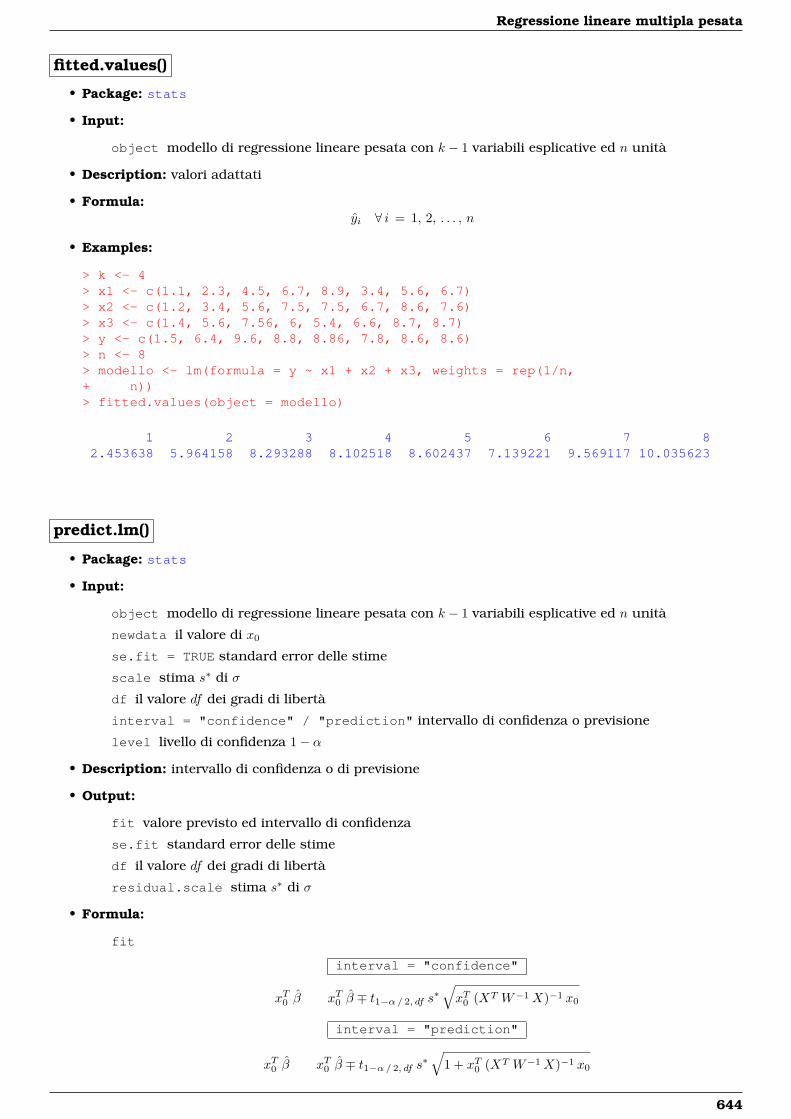
Regressione lineare multipla pesata
fitted.values()
• Package: stats
• Input:
object modello di regressione lineare pesata con k − 1 variabili esplicative ed n unità
• Description: valori adattati
• Formula:yi ∀ i = 1, 2, . . . , n
• Examples:
> k <- 4> x1 <- c(1.1, 2.3, 4.5, 6.7, 8.9, 3.4, 5.6, 6.7)> x2 <- c(1.2, 3.4, 5.6, 7.5, 7.5, 6.7, 8.6, 7.6)> x3 <- c(1.4, 5.6, 7.56, 6, 5.4, 6.6, 8.7, 8.7)> y <- c(1.5, 6.4, 9.6, 8.8, 8.86, 7.8, 8.6, 8.6)> n <- 8> modello <- lm(formula = y ~ x1 + x2 + x3, weights = rep(1/n,+ n))> fitted.values(object = modello)
1 2 3 4 5 6 7 82.453638 5.964158 8.293288 8.102518 8.602437 7.139221 9.569117 10.035623
predict.lm()
• Package: stats
• Input:
object modello di regressione lineare pesata con k − 1 variabili esplicative ed n unità
newdata il valore di x0
se.fit = TRUE standard error delle stime
scale stima s∗ di σ
df il valore df dei gradi di libertà
interval = "confidence" / "prediction" intervallo di confidenza o previsione
level livello di confidenza 1− α
• Description: intervallo di confidenza o di previsione
• Output:
fit valore previsto ed intervallo di confidenza
se.fit standard error delle stime
df il valore df dei gradi di libertà
residual.scale stima s∗ di σ
• Formula:
fit
interval = "confidence"
xT0 β xT0 β ∓ t1−α/ 2, df s∗√xT0 (XT W−1X)−1 x0
interval = "prediction"
xT0 β xT0 β ∓ t1−α/ 2, df s∗√
1 + xT0 (XT W−1X)−1 x0
644
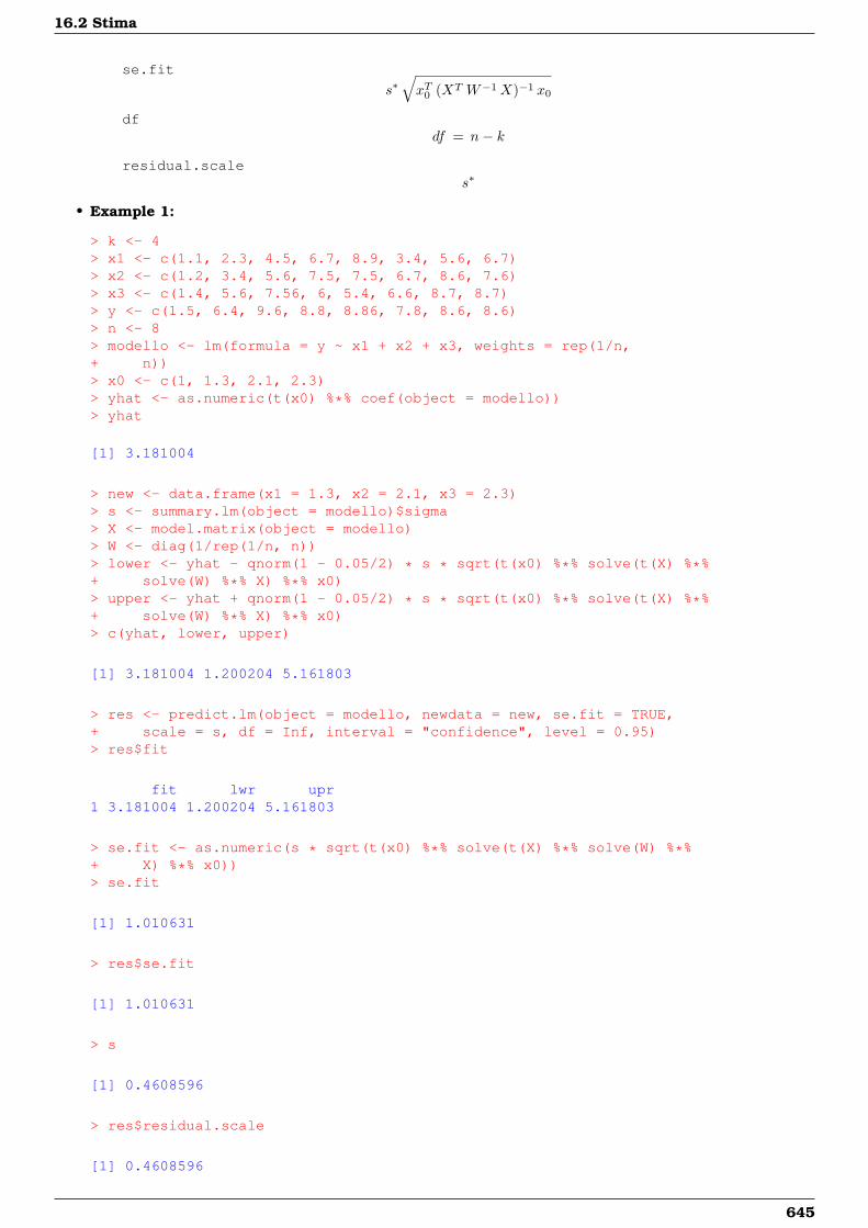
16.2 Stima
se.fit
s∗√xT0 (XT W−1X)−1 x0
dfdf = n− k
residual.scales∗
• Example 1:
> k <- 4> x1 <- c(1.1, 2.3, 4.5, 6.7, 8.9, 3.4, 5.6, 6.7)> x2 <- c(1.2, 3.4, 5.6, 7.5, 7.5, 6.7, 8.6, 7.6)> x3 <- c(1.4, 5.6, 7.56, 6, 5.4, 6.6, 8.7, 8.7)> y <- c(1.5, 6.4, 9.6, 8.8, 8.86, 7.8, 8.6, 8.6)> n <- 8> modello <- lm(formula = y ~ x1 + x2 + x3, weights = rep(1/n,+ n))> x0 <- c(1, 1.3, 2.1, 2.3)> yhat <- as.numeric(t(x0) %*% coef(object = modello))> yhat
[1] 3.181004
> new <- data.frame(x1 = 1.3, x2 = 2.1, x3 = 2.3)> s <- summary.lm(object = modello)$sigma> X <- model.matrix(object = modello)> W <- diag(1/rep(1/n, n))> lower <- yhat - qnorm(1 - 0.05/2) * s * sqrt(t(x0) %*% solve(t(X) %*%+ solve(W) %*% X) %*% x0)> upper <- yhat + qnorm(1 - 0.05/2) * s * sqrt(t(x0) %*% solve(t(X) %*%+ solve(W) %*% X) %*% x0)> c(yhat, lower, upper)
[1] 3.181004 1.200204 5.161803
> res <- predict.lm(object = modello, newdata = new, se.fit = TRUE,+ scale = s, df = Inf, interval = "confidence", level = 0.95)> res$fit
fit lwr upr1 3.181004 1.200204 5.161803
> se.fit <- as.numeric(s * sqrt(t(x0) %*% solve(t(X) %*% solve(W) %*%+ X) %*% x0))> se.fit
[1] 1.010631
> res$se.fit
[1] 1.010631
> s
[1] 0.4608596
> res$residual.scale
[1] 0.4608596
645
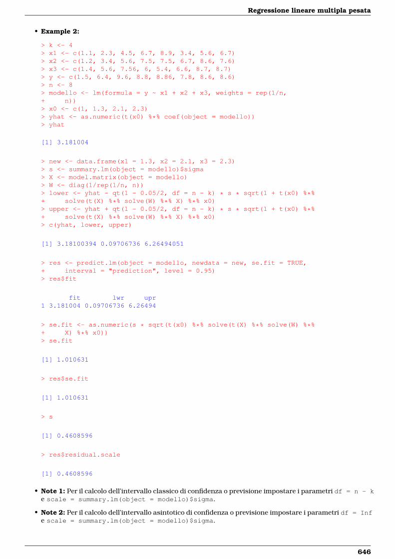
Regressione lineare multipla pesata
• Example 2:
> k <- 4> x1 <- c(1.1, 2.3, 4.5, 6.7, 8.9, 3.4, 5.6, 6.7)> x2 <- c(1.2, 3.4, 5.6, 7.5, 7.5, 6.7, 8.6, 7.6)> x3 <- c(1.4, 5.6, 7.56, 6, 5.4, 6.6, 8.7, 8.7)> y <- c(1.5, 6.4, 9.6, 8.8, 8.86, 7.8, 8.6, 8.6)> n <- 8> modello <- lm(formula = y ~ x1 + x2 + x3, weights = rep(1/n,+ n))> x0 <- c(1, 1.3, 2.1, 2.3)> yhat <- as.numeric(t(x0) %*% coef(object = modello))> yhat
[1] 3.181004
> new <- data.frame(x1 = 1.3, x2 = 2.1, x3 = 2.3)> s <- summary.lm(object = modello)$sigma> X <- model.matrix(object = modello)> W <- diag(1/rep(1/n, n))> lower <- yhat - qt(1 - 0.05/2, df = n - k) * s * sqrt(1 + t(x0) %*%+ solve(t(X) %*% solve(W) %*% X) %*% x0)> upper <- yhat + qt(1 - 0.05/2, df = n - k) * s * sqrt(1 + t(x0) %*%+ solve(t(X) %*% solve(W) %*% X) %*% x0)> c(yhat, lower, upper)
[1] 3.18100394 0.09706736 6.26494051
> res <- predict.lm(object = modello, newdata = new, se.fit = TRUE,+ interval = "prediction", level = 0.95)> res$fit
fit lwr upr1 3.181004 0.09706736 6.26494
> se.fit <- as.numeric(s * sqrt(t(x0) %*% solve(t(X) %*% solve(W) %*%+ X) %*% x0))> se.fit
[1] 1.010631
> res$se.fit
[1] 1.010631
> s
[1] 0.4608596
> res$residual.scale
[1] 0.4608596
• Note 1: Per il calcolo dell’intervallo classico di confidenza o previsione impostare i parametri df = n - ke scale = summary.lm(object = modello)$sigma.
• Note 2: Per il calcolo dell’intervallo asintotico di confidenza o previsione impostare i parametri df = Infe scale = summary.lm(object = modello)$sigma.
646
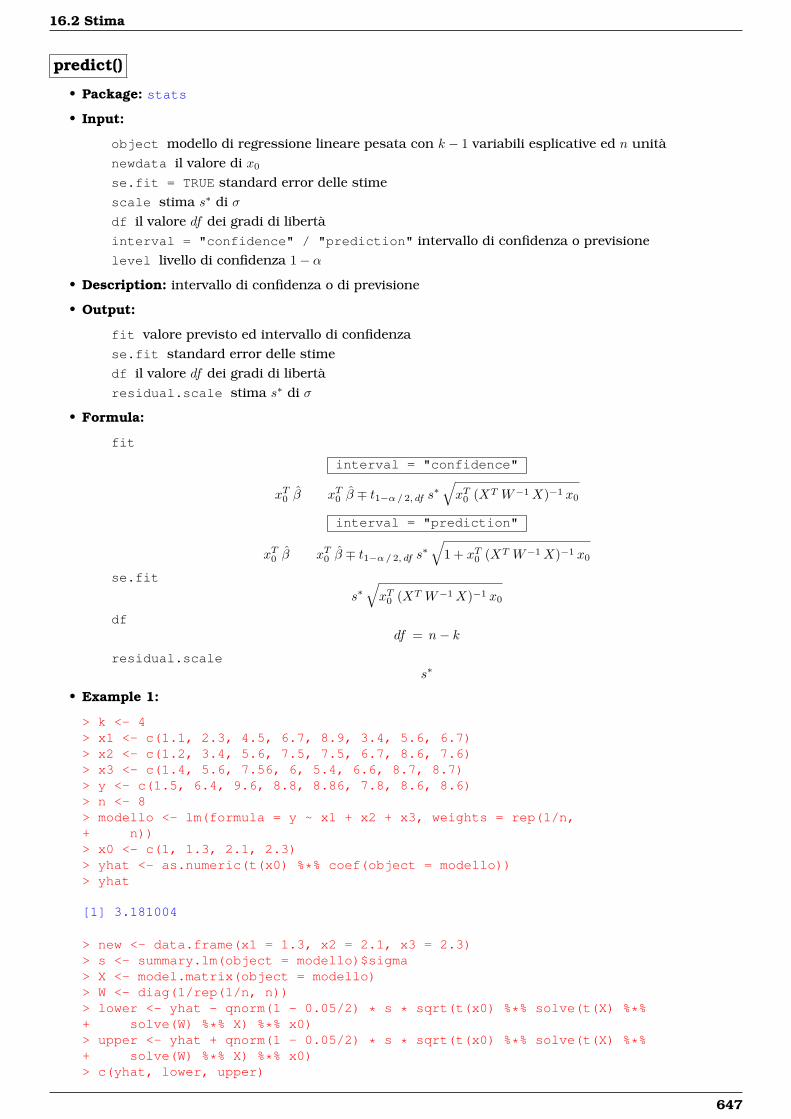
16.2 Stima
predict()
• Package: stats
• Input:
object modello di regressione lineare pesata con k − 1 variabili esplicative ed n unitànewdata il valore di x0
se.fit = TRUE standard error delle stimescale stima s∗ di σdf il valore df dei gradi di libertàinterval = "confidence" / "prediction" intervallo di confidenza o previsionelevel livello di confidenza 1− α
• Description: intervallo di confidenza o di previsione
• Output:
fit valore previsto ed intervallo di confidenzase.fit standard error delle stimedf il valore df dei gradi di libertàresidual.scale stima s∗ di σ
• Formula:
fit
interval = "confidence"
xT0 β xT0 β ∓ t1−α/ 2, df s∗√xT0 (XT W−1X)−1 x0
interval = "prediction"
xT0 β xT0 β ∓ t1−α/ 2, df s∗√
1 + xT0 (XT W−1X)−1 x0
se.fit
s∗√xT0 (XT W−1X)−1 x0
dfdf = n− k
residual.scales∗
• Example 1:
> k <- 4> x1 <- c(1.1, 2.3, 4.5, 6.7, 8.9, 3.4, 5.6, 6.7)> x2 <- c(1.2, 3.4, 5.6, 7.5, 7.5, 6.7, 8.6, 7.6)> x3 <- c(1.4, 5.6, 7.56, 6, 5.4, 6.6, 8.7, 8.7)> y <- c(1.5, 6.4, 9.6, 8.8, 8.86, 7.8, 8.6, 8.6)> n <- 8> modello <- lm(formula = y ~ x1 + x2 + x3, weights = rep(1/n,+ n))> x0 <- c(1, 1.3, 2.1, 2.3)> yhat <- as.numeric(t(x0) %*% coef(object = modello))> yhat
[1] 3.181004
> new <- data.frame(x1 = 1.3, x2 = 2.1, x3 = 2.3)> s <- summary.lm(object = modello)$sigma> X <- model.matrix(object = modello)> W <- diag(1/rep(1/n, n))> lower <- yhat - qnorm(1 - 0.05/2) * s * sqrt(t(x0) %*% solve(t(X) %*%+ solve(W) %*% X) %*% x0)> upper <- yhat + qnorm(1 - 0.05/2) * s * sqrt(t(x0) %*% solve(t(X) %*%+ solve(W) %*% X) %*% x0)> c(yhat, lower, upper)
647
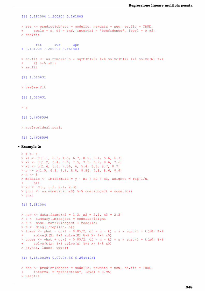
Regressione lineare multipla pesata
[1] 3.181004 1.200204 5.161803
> res <- predict(object = modello, newdata = new, se.fit = TRUE,+ scale = s, df = Inf, interval = "confidence", level = 0.95)> res$fit
fit lwr upr1 3.181004 1.200204 5.161803
> se.fit <- as.numeric(s * sqrt(t(x0) %*% solve(t(X) %*% solve(W) %*%+ X) %*% x0))> se.fit
[1] 1.010631
> res$se.fit
[1] 1.010631
> s
[1] 0.4608596
> res$residual.scale
[1] 0.4608596
• Example 2:
> k <- 4> x1 <- c(1.1, 2.3, 4.5, 6.7, 8.9, 3.4, 5.6, 6.7)> x2 <- c(1.2, 3.4, 5.6, 7.5, 7.5, 6.7, 8.6, 7.6)> x3 <- c(1.4, 5.6, 7.56, 6, 5.4, 6.6, 8.7, 8.7)> y <- c(1.5, 6.4, 9.6, 8.8, 8.86, 7.8, 8.6, 8.6)> n <- 8> modello <- lm(formula = y ~ x1 + x2 + x3, weights = rep(1/n,+ n))> x0 <- c(1, 1.3, 2.1, 2.3)> yhat <- as.numeric(t(x0) %*% coef(object = modello))> yhat
[1] 3.181004
> new <- data.frame(x1 = 1.3, x2 = 2.1, x3 = 2.3)> s <- summary.lm(object = modello)$sigma> X <- model.matrix(object = modello)> W <- diag(1/rep(1/n, n))> lower <- yhat - qt(1 - 0.05/2, df = n - k) * s * sqrt(1 + t(x0) %*%+ solve(t(X) %*% solve(W) %*% X) %*% x0)> upper <- yhat + qt(1 - 0.05/2, df = n - k) * s * sqrt(1 + t(x0) %*%+ solve(t(X) %*% solve(W) %*% X) %*% x0)> c(yhat, lower, upper)
[1] 3.18100394 0.09706736 6.26494051
> res <- predict(object = modello, newdata = new, se.fit = TRUE,+ interval = "prediction", level = 0.95)> res$fit
648
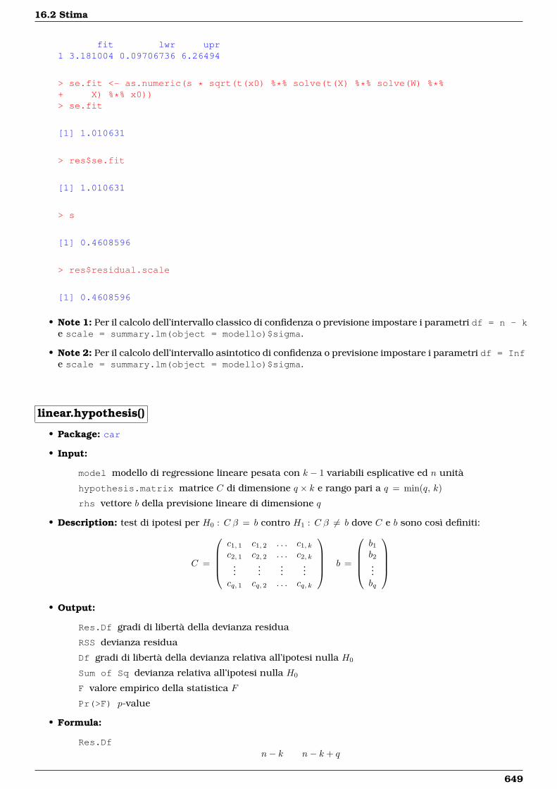
16.2 Stima
fit lwr upr1 3.181004 0.09706736 6.26494
> se.fit <- as.numeric(s * sqrt(t(x0) %*% solve(t(X) %*% solve(W) %*%+ X) %*% x0))> se.fit
[1] 1.010631
> res$se.fit
[1] 1.010631
> s
[1] 0.4608596
> res$residual.scale
[1] 0.4608596
• Note 1: Per il calcolo dell’intervallo classico di confidenza o previsione impostare i parametri df = n - ke scale = summary.lm(object = modello)$sigma.
• Note 2: Per il calcolo dell’intervallo asintotico di confidenza o previsione impostare i parametri df = Infe scale = summary.lm(object = modello)$sigma.
linear.hypothesis()
• Package: car
• Input:
model modello di regressione lineare pesata con k − 1 variabili esplicative ed n unità
hypothesis.matrix matrice C di dimensione q × k e rango pari a q = min(q, k)
rhs vettore b della previsione lineare di dimensione q
• Description: test di ipotesi per H0 : C β = b contro H1 : C β 6= b dove C e b sono così definiti:
C =
c1, 1 c1, 2 . . . c1, kc2, 1 c2, 2 . . . c2, k
......
......
cq, 1 cq, 2 . . . cq, k
b =
b1b2...bq
• Output:
Res.Df gradi di libertà della devianza residua
RSS devianza residua
Df gradi di libertà della devianza relativa all’ipotesi nulla H0
Sum of Sq devianza relativa all’ipotesi nulla H0
F valore empirico della statistica F
Pr(>F) p-value
• Formula:
Res.Dfn− k n− k + q
649
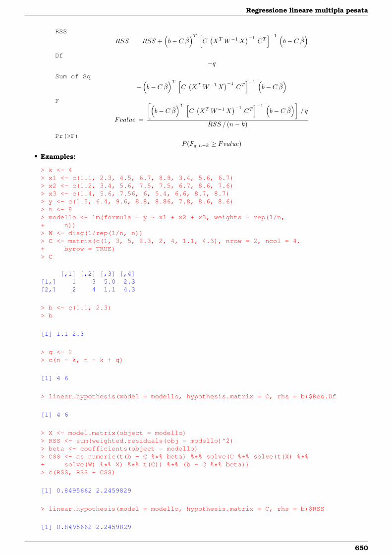
Regressione lineare multipla pesata
RSS
RSS RSS +(b− C β
)T [C(XT W−1X
)−1CT]−1 (
b− C β)
Df−q
Sum of Sq
−(b− C β
)T [C(XT W−1X
)−1CT]−1 (
b− C β)
F
Fvalue =
[(b− C β
)T [C(XT W−1X
)−1CT]−1 (
b− C β)]
/ q
RSS / (n− k)
Pr(>F)P (Fq, n−k ≥ Fvalue)
• Examples:
> k <- 4> x1 <- c(1.1, 2.3, 4.5, 6.7, 8.9, 3.4, 5.6, 6.7)> x2 <- c(1.2, 3.4, 5.6, 7.5, 7.5, 6.7, 8.6, 7.6)> x3 <- c(1.4, 5.6, 7.56, 6, 5.4, 6.6, 8.7, 8.7)> y <- c(1.5, 6.4, 9.6, 8.8, 8.86, 7.8, 8.6, 8.6)> n <- 8> modello <- lm(formula = y ~ x1 + x2 + x3, weights = rep(1/n,+ n))> W <- diag(1/rep(1/n, n))> C <- matrix(c(1, 3, 5, 2.3, 2, 4, 1.1, 4.3), nrow = 2, ncol = 4,+ byrow = TRUE)> C
[,1] [,2] [,3] [,4][1,] 1 3 5.0 2.3[2,] 2 4 1.1 4.3
> b <- c(1.1, 2.3)> b
[1] 1.1 2.3
> q <- 2> c(n - k, n - k + q)
[1] 4 6
> linear.hypothesis(model = modello, hypothesis.matrix = C, rhs = b)$Res.Df
[1] 4 6
> X <- model.matrix(object = modello)> RSS <- sum(weighted.residuals(obj = modello)^2)> beta <- coefficients(object = modello)> CSS <- as.numeric(t(b - C %*% beta) %*% solve(C %*% solve(t(X) %*%+ solve(W) %*% X) %*% t(C)) %*% (b - C %*% beta))> c(RSS, RSS + CSS)
[1] 0.8495662 2.2459829
> linear.hypothesis(model = modello, hypothesis.matrix = C, rhs = b)$RSS
[1] 0.8495662 2.2459829
650
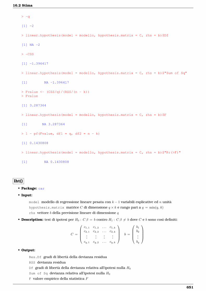
16.2 Stima
> -q
[1] -2
> linear.hypothesis(model = modello, hypothesis.matrix = C, rhs = b)$Df
[1] NA -2
> -CSS
[1] -1.396417
> linear.hypothesis(model = modello, hypothesis.matrix = C, rhs = b)$"Sum of Sq"
[1] NA -1.396417
> Fvalue <- (CSS/q)/(RSS/(n - k))> Fvalue
[1] 3.287364
> linear.hypothesis(model = modello, hypothesis.matrix = C, rhs = b)$F
[1] NA 3.287364
> 1 - pf(Fvalue, df1 = q, df2 = n - k)
[1] 0.1430808
> linear.hypothesis(model = modello, hypothesis.matrix = C, rhs = b)$"Pr(>F)"
[1] NA 0.1430808
lht()
• Package: car
• Input:
model modello di regressione lineare pesata con k − 1 variabili esplicative ed n unità
hypothesis.matrix matrice C di dimensione q × k e rango pari a q = min(q, k)
rhs vettore b della previsione lineare di dimensione q
• Description: test di ipotesi per H0 : C β = b contro H1 : C β 6= b dove C e b sono così definiti:
C =
c1, 1 c1, 2 . . . c1, kc2, 1 c2, 2 . . . c2, k
......
......
cq, 1 cq, 2 . . . cq, k
b =
b1b2...bq
• Output:
Res.Df gradi di libertà della devianza residua
RSS devianza residua
Df gradi di libertà della devianza relativa all’ipotesi nulla H0
Sum of Sq devianza relativa all’ipotesi nulla H0
F valore empirico della statistica F
651
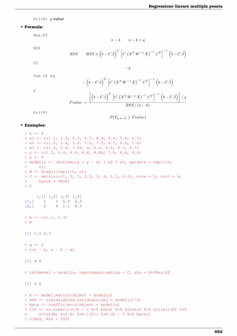
Regressione lineare multipla pesata
Pr(>F) p-value
• Formula:
Res.Dfn− k n− k + q
RSS
RSS RSS +(b− C β
)T [C(XT W−1X
)−1CT]−1 (
b− C β)
Df−q
Sum of Sq
−(b− C β
)T [C(XT W−1X
)−1CT]−1 (
b− C β)
F
Fvalue =
[(b− C β
)T [C(XT W−1X
)−1CT]−1 (
b− C β)]
/ q
RSS / (n− k)
Pr(>F)P (Fq, n−k ≥ Fvalue)
• Examples:
> k <- 4> x1 <- c(1.1, 2.3, 4.5, 6.7, 8.9, 3.4, 5.6, 6.7)> x2 <- c(1.2, 3.4, 5.6, 7.5, 7.5, 6.7, 8.6, 7.6)> x3 <- c(1.4, 5.6, 7.56, 6, 5.4, 6.6, 8.7, 8.7)> y <- c(1.5, 6.4, 9.6, 8.8, 8.86, 7.8, 8.6, 8.6)> n <- 8> modello <- lm(formula = y ~ x1 + x2 + x3, weights = rep(1/n,+ n))> W <- diag(1/rep(1/n, n))> C <- matrix(c(1, 3, 5, 2.3, 2, 4, 1.1, 4.3), nrow = 2, ncol = 4,+ byrow = TRUE)> C
[,1] [,2] [,3] [,4][1,] 1 3 5.0 2.3[2,] 2 4 1.1 4.3
> b <- c(1.1, 2.3)> b
[1] 1.1 2.3
> q <- 2> c(n - k, n - k + q)
[1] 4 6
> lht(model = modello, hypothesis.matrix = C, rhs = b)$Res.Df
[1] 4 6
> X <- model.matrix(object = modello)> RSS <- sum(weighted.residuals(obj = modello)^2)> beta <- coefficients(object = modello)> CSS <- as.numeric(t(b - C %*% beta) %*% solve(C %*% solve(t(X) %*%+ solve(W) %*% X) %*% t(C)) %*% (b - C %*% beta))> c(RSS, RSS + CSS)
652
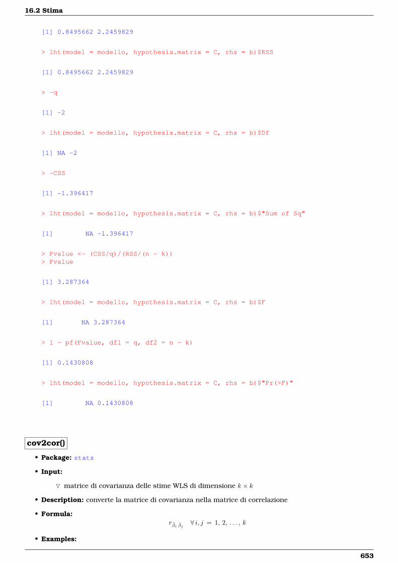
16.2 Stima
[1] 0.8495662 2.2459829
> lht(model = modello, hypothesis.matrix = C, rhs = b)$RSS
[1] 0.8495662 2.2459829
> -q
[1] -2
> lht(model = modello, hypothesis.matrix = C, rhs = b)$Df
[1] NA -2
> -CSS
[1] -1.396417
> lht(model = modello, hypothesis.matrix = C, rhs = b)$"Sum of Sq"
[1] NA -1.396417
> Fvalue <- (CSS/q)/(RSS/(n - k))> Fvalue
[1] 3.287364
> lht(model = modello, hypothesis.matrix = C, rhs = b)$F
[1] NA 3.287364
> 1 - pf(Fvalue, df1 = q, df2 = n - k)
[1] 0.1430808
> lht(model = modello, hypothesis.matrix = C, rhs = b)$"Pr(>F)"
[1] NA 0.1430808
cov2cor()
• Package: stats
• Input:
V matrice di covarianza delle stime WLS di dimensione k × k
• Description: converte la matrice di covarianza nella matrice di correlazione
• Formula:rβi βj ∀ i, j = 1, 2, . . . , k
• Examples:
653
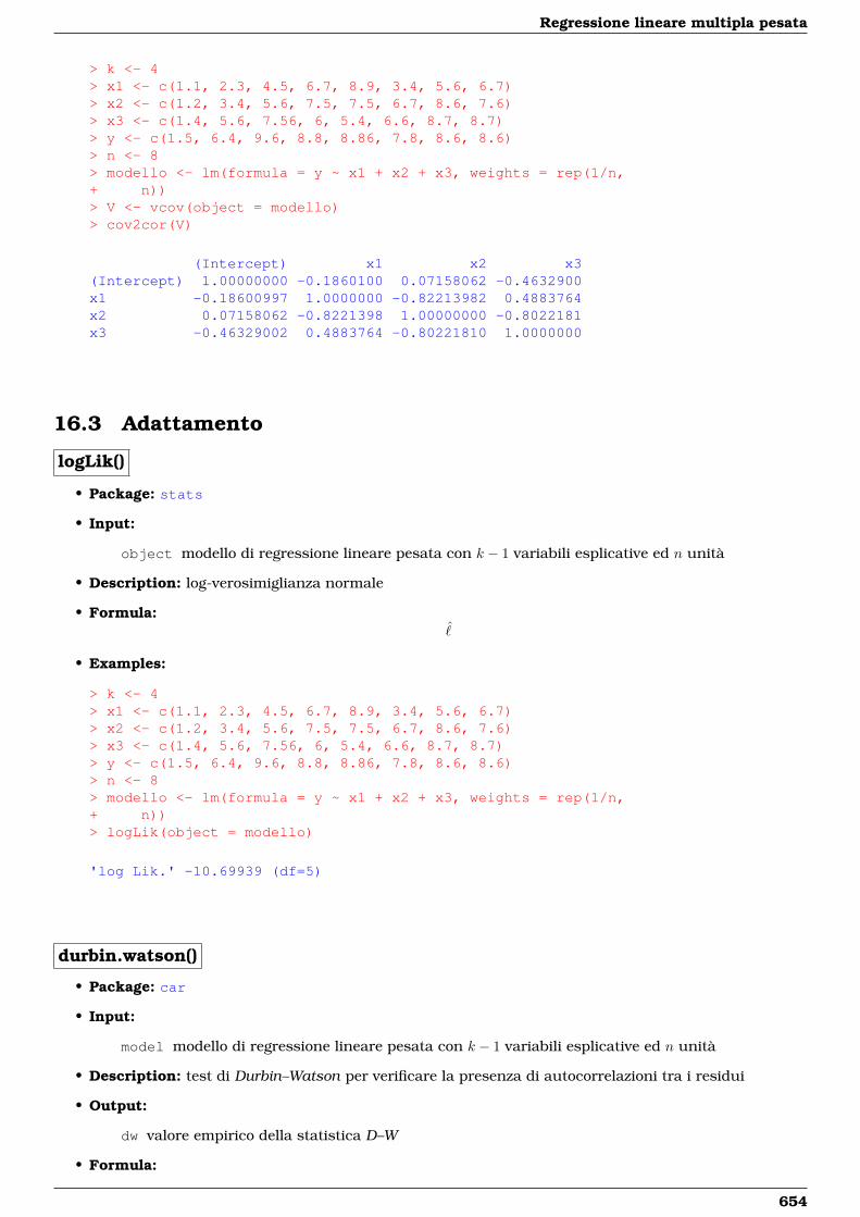
Regressione lineare multipla pesata
> k <- 4> x1 <- c(1.1, 2.3, 4.5, 6.7, 8.9, 3.4, 5.6, 6.7)> x2 <- c(1.2, 3.4, 5.6, 7.5, 7.5, 6.7, 8.6, 7.6)> x3 <- c(1.4, 5.6, 7.56, 6, 5.4, 6.6, 8.7, 8.7)> y <- c(1.5, 6.4, 9.6, 8.8, 8.86, 7.8, 8.6, 8.6)> n <- 8> modello <- lm(formula = y ~ x1 + x2 + x3, weights = rep(1/n,+ n))> V <- vcov(object = modello)> cov2cor(V)
(Intercept) x1 x2 x3(Intercept) 1.00000000 -0.1860100 0.07158062 -0.4632900x1 -0.18600997 1.0000000 -0.82213982 0.4883764x2 0.07158062 -0.8221398 1.00000000 -0.8022181x3 -0.46329002 0.4883764 -0.80221810 1.0000000
16.3 Adattamento
logLik()
• Package: stats
• Input:
object modello di regressione lineare pesata con k − 1 variabili esplicative ed n unità
• Description: log-verosimiglianza normale
• Formula:ˆ
• Examples:
> k <- 4> x1 <- c(1.1, 2.3, 4.5, 6.7, 8.9, 3.4, 5.6, 6.7)> x2 <- c(1.2, 3.4, 5.6, 7.5, 7.5, 6.7, 8.6, 7.6)> x3 <- c(1.4, 5.6, 7.56, 6, 5.4, 6.6, 8.7, 8.7)> y <- c(1.5, 6.4, 9.6, 8.8, 8.86, 7.8, 8.6, 8.6)> n <- 8> modello <- lm(formula = y ~ x1 + x2 + x3, weights = rep(1/n,+ n))> logLik(object = modello)
'log Lik.' -10.69939 (df=5)
durbin.watson()
• Package: car
• Input:
model modello di regressione lineare pesata con k − 1 variabili esplicative ed n unità
• Description: test di Durbin–Watson per verificare la presenza di autocorrelazioni tra i residui
• Output:
dw valore empirico della statistica D–W
• Formula:
654
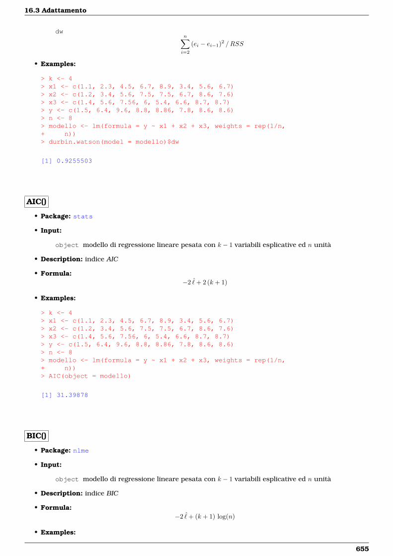
16.3 Adattamento
dwn∑i=2
(ei − ei−1)2 /RSS
• Examples:
> k <- 4> x1 <- c(1.1, 2.3, 4.5, 6.7, 8.9, 3.4, 5.6, 6.7)> x2 <- c(1.2, 3.4, 5.6, 7.5, 7.5, 6.7, 8.6, 7.6)> x3 <- c(1.4, 5.6, 7.56, 6, 5.4, 6.6, 8.7, 8.7)> y <- c(1.5, 6.4, 9.6, 8.8, 8.86, 7.8, 8.6, 8.6)> n <- 8> modello <- lm(formula = y ~ x1 + x2 + x3, weights = rep(1/n,+ n))> durbin.watson(model = modello)$dw
[1] 0.9255503
AIC()
• Package: stats
• Input:
object modello di regressione lineare pesata con k − 1 variabili esplicative ed n unità
• Description: indice AIC
• Formula:−2 ˆ+ 2 (k + 1)
• Examples:
> k <- 4> x1 <- c(1.1, 2.3, 4.5, 6.7, 8.9, 3.4, 5.6, 6.7)> x2 <- c(1.2, 3.4, 5.6, 7.5, 7.5, 6.7, 8.6, 7.6)> x3 <- c(1.4, 5.6, 7.56, 6, 5.4, 6.6, 8.7, 8.7)> y <- c(1.5, 6.4, 9.6, 8.8, 8.86, 7.8, 8.6, 8.6)> n <- 8> modello <- lm(formula = y ~ x1 + x2 + x3, weights = rep(1/n,+ n))> AIC(object = modello)
[1] 31.39878
BIC()
• Package: nlme
• Input:
object modello di regressione lineare pesata con k − 1 variabili esplicative ed n unità
• Description: indice BIC
• Formula:−2 ˆ+ (k + 1) log(n)
• Examples:
655
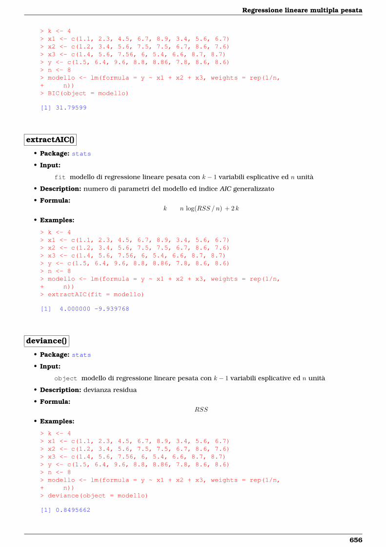
Regressione lineare multipla pesata
> k <- 4> x1 <- c(1.1, 2.3, 4.5, 6.7, 8.9, 3.4, 5.6, 6.7)> x2 <- c(1.2, 3.4, 5.6, 7.5, 7.5, 6.7, 8.6, 7.6)> x3 <- c(1.4, 5.6, 7.56, 6, 5.4, 6.6, 8.7, 8.7)> y <- c(1.5, 6.4, 9.6, 8.8, 8.86, 7.8, 8.6, 8.6)> n <- 8> modello <- lm(formula = y ~ x1 + x2 + x3, weights = rep(1/n,+ n))> BIC(object = modello)
[1] 31.79599
extractAIC()
• Package: stats
• Input:
fit modello di regressione lineare pesata con k − 1 variabili esplicative ed n unità
• Description: numero di parametri del modello ed indice AIC generalizzato
• Formula:k n log(RSS /n) + 2 k
• Examples:
> k <- 4> x1 <- c(1.1, 2.3, 4.5, 6.7, 8.9, 3.4, 5.6, 6.7)> x2 <- c(1.2, 3.4, 5.6, 7.5, 7.5, 6.7, 8.6, 7.6)> x3 <- c(1.4, 5.6, 7.56, 6, 5.4, 6.6, 8.7, 8.7)> y <- c(1.5, 6.4, 9.6, 8.8, 8.86, 7.8, 8.6, 8.6)> n <- 8> modello <- lm(formula = y ~ x1 + x2 + x3, weights = rep(1/n,+ n))> extractAIC(fit = modello)
[1] 4.000000 -9.939768
deviance()
• Package: stats
• Input:
object modello di regressione lineare pesata con k − 1 variabili esplicative ed n unità
• Description: devianza residua
• Formula:RSS
• Examples:
> k <- 4> x1 <- c(1.1, 2.3, 4.5, 6.7, 8.9, 3.4, 5.6, 6.7)> x2 <- c(1.2, 3.4, 5.6, 7.5, 7.5, 6.7, 8.6, 7.6)> x3 <- c(1.4, 5.6, 7.56, 6, 5.4, 6.6, 8.7, 8.7)> y <- c(1.5, 6.4, 9.6, 8.8, 8.86, 7.8, 8.6, 8.6)> n <- 8> modello <- lm(formula = y ~ x1 + x2 + x3, weights = rep(1/n,+ n))> deviance(object = modello)
[1] 0.8495662
656
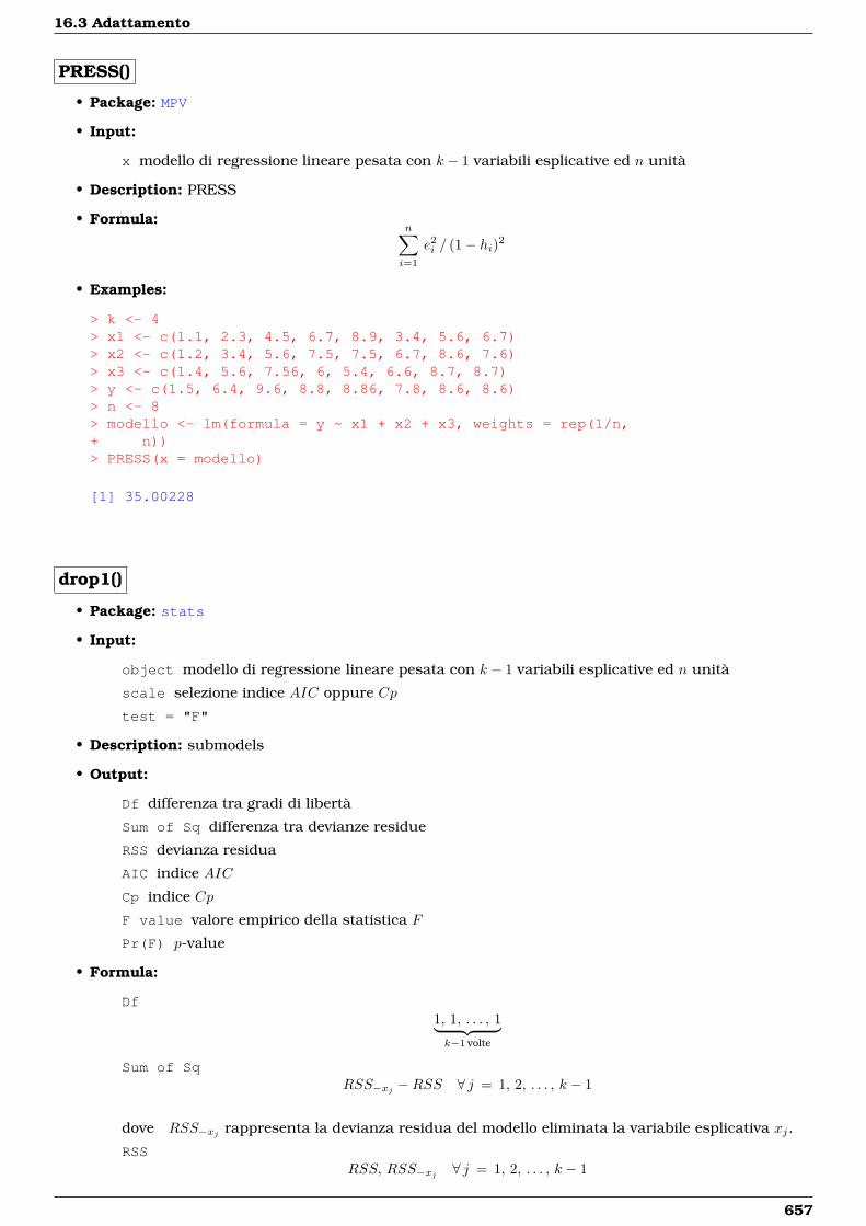
16.3 Adattamento
PRESS()
• Package: MPV
• Input:
x modello di regressione lineare pesata con k − 1 variabili esplicative ed n unità
• Description: PRESS
• Formula:n∑i=1
e2i / (1− hi)2
• Examples:
> k <- 4> x1 <- c(1.1, 2.3, 4.5, 6.7, 8.9, 3.4, 5.6, 6.7)> x2 <- c(1.2, 3.4, 5.6, 7.5, 7.5, 6.7, 8.6, 7.6)> x3 <- c(1.4, 5.6, 7.56, 6, 5.4, 6.6, 8.7, 8.7)> y <- c(1.5, 6.4, 9.6, 8.8, 8.86, 7.8, 8.6, 8.6)> n <- 8> modello <- lm(formula = y ~ x1 + x2 + x3, weights = rep(1/n,+ n))> PRESS(x = modello)
[1] 35.00228
drop1()
• Package: stats
• Input:
object modello di regressione lineare pesata con k − 1 variabili esplicative ed n unità
scale selezione indice AIC oppure Cp
test = "F"
• Description: submodels
• Output:
Df differenza tra gradi di libertà
Sum of Sq differenza tra devianze residue
RSS devianza residua
AIC indice AIC
Cp indice Cp
F value valore empirico della statistica F
Pr(F) p-value
• Formula:
Df1, 1, . . . , 1︸ ︷︷ ︸k−1 volte
Sum of SqRSS−xj −RSS ∀ j = 1, 2, . . . , k − 1
dove RSS−xj rappresenta la devianza residua del modello eliminata la variabile esplicativa xj.
RSSRSS, RSS−xj ∀ j = 1, 2, . . . , k − 1
657
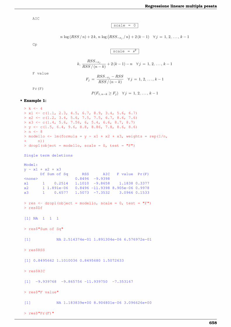
Regressione lineare multipla pesata
AIC
scale = 0
n log (RSS /n) + 2 k, n log(RSS−xj / n
)+ 2 (k − 1) ∀ j = 1, 2, . . . , k − 1
Cp
scale = s2
k,RSS−xj
RSS / (n− k)+ 2 (k − 1)− n ∀ j = 1, 2, . . . , k − 1
F value
Fj =RSS−xj −RSSRSS / (n− k)
∀ j = 1, 2, . . . , k − 1
Pr(F)P (F1, n−k ≥ Fj) ∀ j = 1, 2, . . . , k − 1
• Example 1:
> k <- 4> x1 <- c(1.1, 2.3, 4.5, 6.7, 8.9, 3.4, 5.6, 6.7)> x2 <- c(1.2, 3.4, 5.6, 7.5, 7.5, 6.7, 8.6, 7.6)> x3 <- c(1.4, 5.6, 7.56, 6, 5.4, 6.6, 8.7, 8.7)> y <- c(1.5, 6.4, 9.6, 8.8, 8.86, 7.8, 8.6, 8.6)> n <- 8> modello <- lm(formula = y ~ x1 + x2 + x3, weights = rep(1/n,+ n))> drop1(object = modello, scale = 0, test = "F")
Single term deletions
Model:y ~ x1 + x2 + x3
Df Sum of Sq RSS AIC F value Pr(F)<none> 0.8496 -9.9398x1 1 0.2514 1.1010 -9.8658 1.1838 0.3377x2 1 1.891e-06 0.8496 -11.9398 8.905e-06 0.9978x3 1 0.6577 1.5073 -7.3532 3.0966 0.1533
> res <- drop1(object = modello, scale = 0, test = "F")> res$Df
[1] NA 1 1 1
> res$"Sum of Sq"
[1] NA 2.514374e-01 1.891304e-06 6.576972e-01
> res$RSS
[1] 0.8495662 1.1010036 0.8495680 1.5072633
> res$AIC
[1] -9.939768 -9.865756 -11.939750 -7.353167
> res$"F value"
[1] NA 1.183839e+00 8.904801e-06 3.096626e+00
> res$"Pr(F)"
658
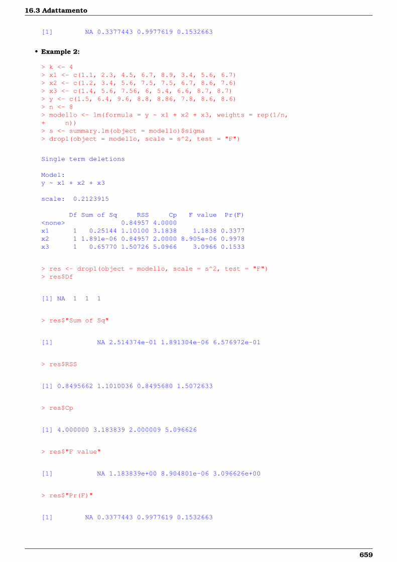
16.3 Adattamento
[1] NA 0.3377443 0.9977619 0.1532663
• Example 2:
> k <- 4> x1 <- c(1.1, 2.3, 4.5, 6.7, 8.9, 3.4, 5.6, 6.7)> x2 <- c(1.2, 3.4, 5.6, 7.5, 7.5, 6.7, 8.6, 7.6)> x3 <- c(1.4, 5.6, 7.56, 6, 5.4, 6.6, 8.7, 8.7)> y <- c(1.5, 6.4, 9.6, 8.8, 8.86, 7.8, 8.6, 8.6)> n <- 8> modello <- lm(formula = y ~ x1 + x2 + x3, weights = rep(1/n,+ n))> s <- summary.lm(object = modello)$sigma> drop1(object = modello, scale = s^2, test = "F")
Single term deletions
Model:y ~ x1 + x2 + x3
scale: 0.2123915
Df Sum of Sq RSS Cp F value Pr(F)<none> 0.84957 4.0000x1 1 0.25144 1.10100 3.1838 1.1838 0.3377x2 1 1.891e-06 0.84957 2.0000 8.905e-06 0.9978x3 1 0.65770 1.50726 5.0966 3.0966 0.1533
> res <- drop1(object = modello, scale = s^2, test = "F")> res$Df
[1] NA 1 1 1
> res$"Sum of Sq"
[1] NA 2.514374e-01 1.891304e-06 6.576972e-01
> res$RSS
[1] 0.8495662 1.1010036 0.8495680 1.5072633
> res$Cp
[1] 4.000000 3.183839 2.000009 5.096626
> res$"F value"
[1] NA 1.183839e+00 8.904801e-06 3.096626e+00
> res$"Pr(F)"
[1] NA 0.3377443 0.9977619 0.1532663
659
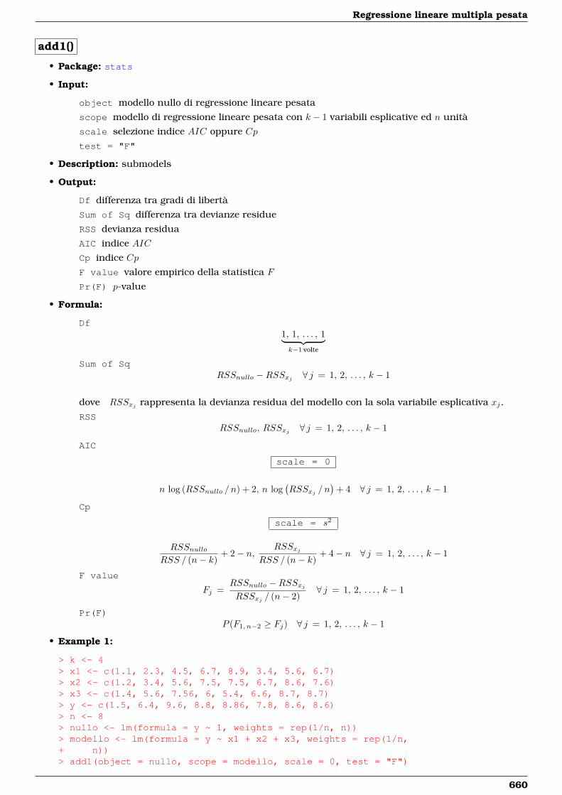
Regressione lineare multipla pesata
add1()
• Package: stats
• Input:
object modello nullo di regressione lineare pesata
scope modello di regressione lineare pesata con k − 1 variabili esplicative ed n unità
scale selezione indice AIC oppure Cp
test = "F"
• Description: submodels
• Output:
Df differenza tra gradi di libertà
Sum of Sq differenza tra devianze residue
RSS devianza residua
AIC indice AIC
Cp indice Cp
F value valore empirico della statistica F
Pr(F) p-value
• Formula:
Df1, 1, . . . , 1︸ ︷︷ ︸k−1 volte
Sum of SqRSSnullo −RSSxj ∀ j = 1, 2, . . . , k − 1
dove RSSxj rappresenta la devianza residua del modello con la sola variabile esplicativa xj.
RSSRSSnullo, RSSxj ∀ j = 1, 2, . . . , k − 1
AIC
scale = 0
n log (RSSnullo / n) + 2, n log(RSSxj / n
)+ 4 ∀ j = 1, 2, . . . , k − 1
Cp
scale = s2
RSSnulloRSS / (n− k)
+ 2− n,RSSxj
RSS / (n− k)+ 4− n ∀ j = 1, 2, . . . , k − 1
F value
Fj =RSSnullo −RSSxjRSSxj / (n− 2)
∀ j = 1, 2, . . . , k − 1
Pr(F)P (F1, n−2 ≥ Fj) ∀ j = 1, 2, . . . , k − 1
• Example 1:
> k <- 4> x1 <- c(1.1, 2.3, 4.5, 6.7, 8.9, 3.4, 5.6, 6.7)> x2 <- c(1.2, 3.4, 5.6, 7.5, 7.5, 6.7, 8.6, 7.6)> x3 <- c(1.4, 5.6, 7.56, 6, 5.4, 6.6, 8.7, 8.7)> y <- c(1.5, 6.4, 9.6, 8.8, 8.86, 7.8, 8.6, 8.6)> n <- 8> nullo <- lm(formula = y ~ 1, weights = rep(1/n, n))> modello <- lm(formula = y ~ x1 + x2 + x3, weights = rep(1/n,+ n))> add1(object = nullo, scope = modello, scale = 0, test = "F")
660
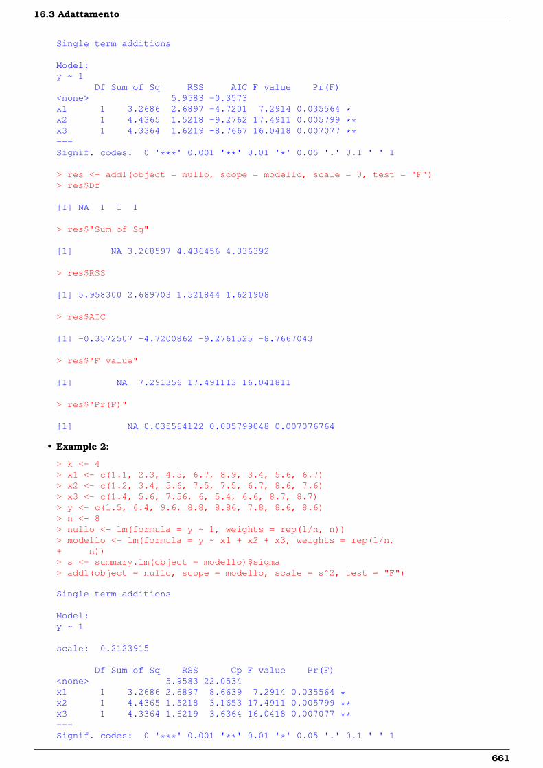
16.3 Adattamento
Single term additions
Model:y ~ 1
Df Sum of Sq RSS AIC F value Pr(F)<none> 5.9583 -0.3573x1 1 3.2686 2.6897 -4.7201 7.2914 0.035564 *x2 1 4.4365 1.5218 -9.2762 17.4911 0.005799 **x3 1 4.3364 1.6219 -8.7667 16.0418 0.007077 **---Signif. codes: 0 '***' 0.001 '**' 0.01 '*' 0.05 '.' 0.1 ' ' 1
> res <- add1(object = nullo, scope = modello, scale = 0, test = "F")> res$Df
[1] NA 1 1 1
> res$"Sum of Sq"
[1] NA 3.268597 4.436456 4.336392
> res$RSS
[1] 5.958300 2.689703 1.521844 1.621908
> res$AIC
[1] -0.3572507 -4.7200862 -9.2761525 -8.7667043
> res$"F value"
[1] NA 7.291356 17.491113 16.041811
> res$"Pr(F)"
[1] NA 0.035564122 0.005799048 0.007076764
• Example 2:
> k <- 4> x1 <- c(1.1, 2.3, 4.5, 6.7, 8.9, 3.4, 5.6, 6.7)> x2 <- c(1.2, 3.4, 5.6, 7.5, 7.5, 6.7, 8.6, 7.6)> x3 <- c(1.4, 5.6, 7.56, 6, 5.4, 6.6, 8.7, 8.7)> y <- c(1.5, 6.4, 9.6, 8.8, 8.86, 7.8, 8.6, 8.6)> n <- 8> nullo <- lm(formula = y ~ 1, weights = rep(1/n, n))> modello <- lm(formula = y ~ x1 + x2 + x3, weights = rep(1/n,+ n))> s <- summary.lm(object = modello)$sigma> add1(object = nullo, scope = modello, scale = s^2, test = "F")
Single term additions
Model:y ~ 1
scale: 0.2123915
Df Sum of Sq RSS Cp F value Pr(F)<none> 5.9583 22.0534x1 1 3.2686 2.6897 8.6639 7.2914 0.035564 *x2 1 4.4365 1.5218 3.1653 17.4911 0.005799 **x3 1 4.3364 1.6219 3.6364 16.0418 0.007077 **---Signif. codes: 0 '***' 0.001 '**' 0.01 '*' 0.05 '.' 0.1 ' ' 1
661
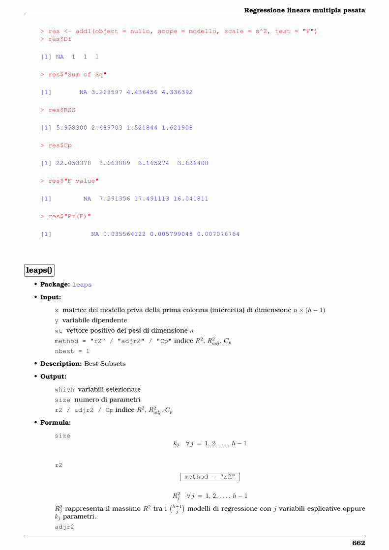
Regressione lineare multipla pesata
> res <- add1(object = nullo, scope = modello, scale = s^2, test = "F")> res$Df
[1] NA 1 1 1
> res$"Sum of Sq"
[1] NA 3.268597 4.436456 4.336392
> res$RSS
[1] 5.958300 2.689703 1.521844 1.621908
> res$Cp
[1] 22.053378 8.663889 3.165274 3.636408
> res$"F value"
[1] NA 7.291356 17.491113 16.041811
> res$"Pr(F)"
[1] NA 0.035564122 0.005799048 0.007076764
leaps()
• Package: leaps
• Input:
x matrice del modello priva della prima colonna (intercetta) di dimensione n× (h− 1)
y variabile dipendente
wt vettore positivo dei pesi di dimensione n
method = "r2" / "adjr2" / "Cp" indice R2, R2adj , Cp
nbest = 1
• Description: Best Subsets
• Output:
which variabili selezionate
size numero di parametri
r2 / adjr2 / Cp indice R2, R2adj , Cp
• Formula:
sizekj ∀ j = 1, 2, . . . , h− 1
r2
method = "r2"
R2j ∀ j = 1, 2, . . . , h− 1
R2j rappresenta il massimo R2 tra i
(h−1j
)modelli di regressione con j variabili esplicative oppure
kj parametri.
adjr2
662
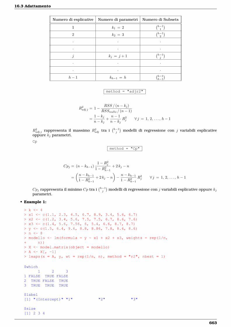
16.3 Adattamento
Numero di esplicative Numero di parametri Numero di Subsets
1 k1 = 2(h−1
1
)2 k2 = 3
(h−1
2
)· · ·
· · ·
j kj = j + 1(h−1j
)· · ·
· · ·
h− 1 kh−1 = h(h−1h−1
)method = "adjr2"
R2adj j = 1− RSS / (n− kj)
RSSnullo / (n− 1)
=1− kjn− kj
+n− 1n− kj
R2j ∀ j = 1, 2, . . . , h− 1
R2adj j rappresenta il massimo R2
adj tra i(h−1j
)modelli di regressione con j variabili esplicative
oppure kj parametri.
Cp
method = "Cp"
Cpj = (n− kh−1)1−R2
j
1−R2h−1
+ 2 kj − n
=(n− kh−1
1−R2h−1
+ 2 kj − n)− n− kh−1
1−R2h−1
R2j ∀ j = 1, 2, . . . , h− 1
Cpj rappresenta il minimo Cp tra i(h−1j
)modelli di regressione con j variabili esplicative oppure kj
parametri.
• Example 1:
> k <- 4> x1 <- c(1.1, 2.3, 4.5, 6.7, 8.9, 3.4, 5.6, 6.7)> x2 <- c(1.2, 3.4, 5.6, 7.5, 7.5, 6.7, 8.6, 7.6)> x3 <- c(1.4, 5.6, 7.56, 6, 5.4, 6.6, 8.7, 8.7)> y <- c(1.5, 6.4, 9.6, 8.8, 8.86, 7.8, 8.6, 8.6)> n <- 8> modello <- lm(formula = y ~ x1 + x2 + x3, weights = rep(1/n,+ n))> X <- model.matrix(object = modello)> A <- X[, -1]> leaps(x = A, y, wt = rep(1/n, n), method = "r2", nbest = 1)
$which1 2 3
1 FALSE TRUE FALSE2 TRUE FALSE TRUE3 TRUE TRUE TRUE
$label[1] "(Intercept)" "1" "2" "3"
$size[1] 2 3 4
663
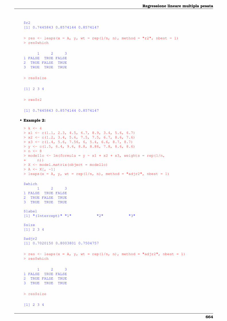
Regressione lineare multipla pesata
$r2[1] 0.7445843 0.8574144 0.8574147
> res <- leaps(x = A, y, wt = rep(1/n, n), method = "r2", nbest = 1)> res$which
1 2 31 FALSE TRUE FALSE2 TRUE FALSE TRUE3 TRUE TRUE TRUE
> res$size
[1] 2 3 4
> res$r2
[1] 0.7445843 0.8574144 0.8574147
• Example 2:
> k <- 4> x1 <- c(1.1, 2.3, 4.5, 6.7, 8.9, 3.4, 5.6, 6.7)> x2 <- c(1.2, 3.4, 5.6, 7.5, 7.5, 6.7, 8.6, 7.6)> x3 <- c(1.4, 5.6, 7.56, 6, 5.4, 6.6, 8.7, 8.7)> y <- c(1.5, 6.4, 9.6, 8.8, 8.86, 7.8, 8.6, 8.6)> n <- 8> modello <- lm(formula = y ~ x1 + x2 + x3, weights = rep(1/n,+ n))> X <- model.matrix(object = modello)> A <- X[, -1]> leaps(x = A, y, wt = rep(1/n, n), method = "adjr2", nbest = 1)
$which1 2 3
1 FALSE TRUE FALSE2 TRUE FALSE TRUE3 TRUE TRUE TRUE
$label[1] "(Intercept)" "1" "2" "3"
$size[1] 2 3 4
$adjr2[1] 0.7020150 0.8003801 0.7504757
> res <- leaps(x = A, y, wt = rep(1/n, n), method = "adjr2", nbest = 1)> res$which
1 2 31 FALSE TRUE FALSE2 TRUE FALSE TRUE3 TRUE TRUE TRUE
> res$size
[1] 2 3 4
664
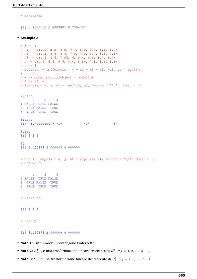
16.3 Adattamento
> res$adjr2
[1] 0.7020150 0.8003801 0.7504757
• Example 3:
> k <- 4> x1 <- c(1.1, 2.3, 4.5, 6.7, 8.9, 3.4, 5.6, 6.7)> x2 <- c(1.2, 3.4, 5.6, 7.5, 7.5, 6.7, 8.6, 7.6)> x3 <- c(1.4, 5.6, 7.56, 6, 5.4, 6.6, 8.7, 8.7)> y <- c(1.5, 6.4, 9.6, 8.8, 8.86, 7.8, 8.6, 8.6)> n <- 8> modello <- lm(formula = y ~ x1 + x2 + x3, weights = rep(1/n,+ n))> X <- model.matrix(object = modello)> A <- X[, -1]> leaps(x = A, y, wt = rep(1/n, n), method = "Cp", nbest = 1)
$which1 2 3
1 FALSE TRUE FALSE2 TRUE FALSE TRUE3 TRUE TRUE TRUE
$label[1] "(Intercept)" "1" "2" "3"
$size[1] 2 3 4
$Cp[1] 3.165274 2.000009 4.000000
> res <- leaps(x = A, y, wt = rep(1/n, n), method = "Cp", nbest = 1)> res$which
1 2 31 FALSE TRUE FALSE2 TRUE FALSE TRUE3 TRUE TRUE TRUE
> res$size
[1] 2 3 4
> res$Cp
[1] 3.165274 2.000009 4.000000
• Note 1: Tutti i modelli contengono l’intercetta.
• Note 2: R2adj j è una trasformazione lineare crescente di R2
j ∀ j = 1, 2, . . . , h− 1.
• Note 3: Cpj è una trasformazione lineare decrescente di R2j ∀ j = 1, 2, . . . , h− 1.
665
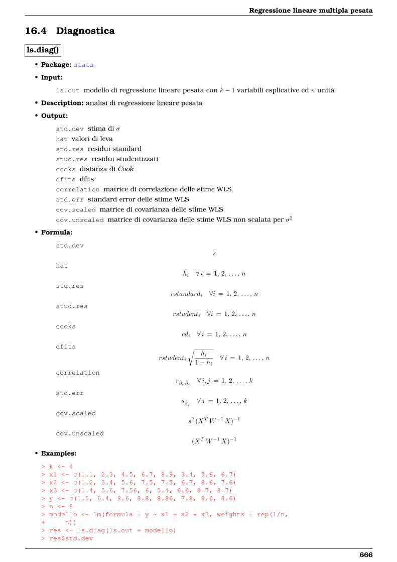
Regressione lineare multipla pesata
16.4 Diagnostica
ls.diag()
• Package: stats
• Input:
ls.out modello di regressione lineare pesata con k − 1 variabili esplicative ed n unità
• Description: analisi di regressione lineare pesata
• Output:
std.dev stima di σ
hat valori di leva
std.res residui standard
stud.res residui studentizzati
cooks distanza di Cook
dfits dfits
correlation matrice di correlazione delle stime WLS
std.err standard error delle stime WLS
cov.scaled matrice di covarianza delle stime WLS
cov.unscaled matrice di covarianza delle stime WLS non scalata per σ2
• Formula:
std.devs
hathi ∀ i = 1, 2, . . . , n
std.resrstandardi ∀i = 1, 2, . . . , n
stud.resrstudenti ∀i = 1, 2, . . . , n
cookscdi ∀ i = 1, 2, . . . , n
dfits
rstudenti
√hi
1− hi∀ i = 1, 2, . . . , n
correlationrβi βj ∀ i, j = 1, 2, . . . , k
std.errsβj ∀ j = 1, 2, . . . , k
cov.scaleds2 (XT W−1X)−1
cov.unscaled(XT W−1X)−1
• Examples:
> k <- 4> x1 <- c(1.1, 2.3, 4.5, 6.7, 8.9, 3.4, 5.6, 6.7)> x2 <- c(1.2, 3.4, 5.6, 7.5, 7.5, 6.7, 8.6, 7.6)> x3 <- c(1.4, 5.6, 7.56, 6, 5.4, 6.6, 8.7, 8.7)> y <- c(1.5, 6.4, 9.6, 8.8, 8.86, 7.8, 8.6, 8.6)> n <- 8> modello <- lm(formula = y ~ x1 + x2 + x3, weights = rep(1/n,+ n))> res <- ls.diag(ls.out = modello)> res$std.dev
666
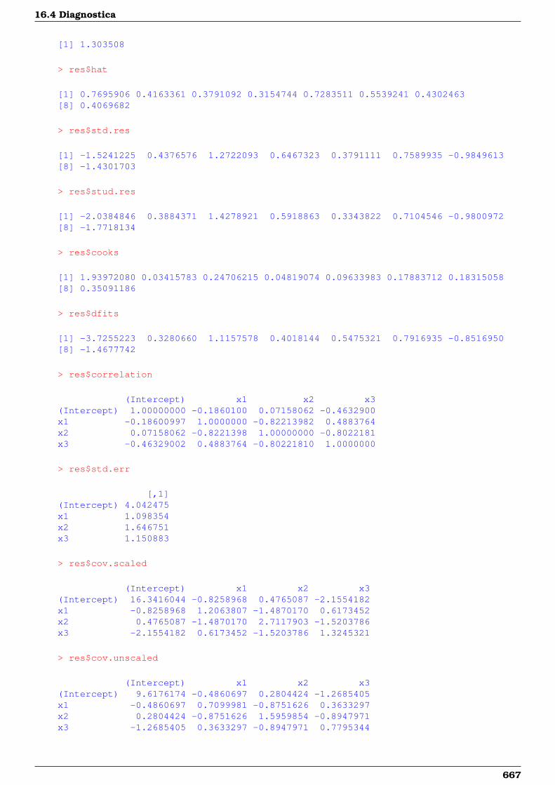
16.4 Diagnostica
[1] 1.303508
> res$hat
[1] 0.7695906 0.4163361 0.3791092 0.3154744 0.7283511 0.5539241 0.4302463[8] 0.4069682
> res$std.res
[1] -1.5241225 0.4376576 1.2722093 0.6467323 0.3791111 0.7589935 -0.9849613[8] -1.4301703
> res$stud.res
[1] -2.0384846 0.3884371 1.4278921 0.5918863 0.3343822 0.7104546 -0.9800972[8] -1.7718134
> res$cooks
[1] 1.93972080 0.03415783 0.24706215 0.04819074 0.09633983 0.17883712 0.18315058[8] 0.35091186
> res$dfits
[1] -3.7255223 0.3280660 1.1157578 0.4018144 0.5475321 0.7916935 -0.8516950[8] -1.4677742
> res$correlation
(Intercept) x1 x2 x3(Intercept) 1.00000000 -0.1860100 0.07158062 -0.4632900x1 -0.18600997 1.0000000 -0.82213982 0.4883764x2 0.07158062 -0.8221398 1.00000000 -0.8022181x3 -0.46329002 0.4883764 -0.80221810 1.0000000
> res$std.err
[,1](Intercept) 4.042475x1 1.098354x2 1.646751x3 1.150883
> res$cov.scaled
(Intercept) x1 x2 x3(Intercept) 16.3416044 -0.8258968 0.4765087 -2.1554182x1 -0.8258968 1.2063807 -1.4870170 0.6173452x2 0.4765087 -1.4870170 2.7117903 -1.5203786x3 -2.1554182 0.6173452 -1.5203786 1.3245321
> res$cov.unscaled
(Intercept) x1 x2 x3(Intercept) 9.6176174 -0.4860697 0.2804424 -1.2685405x1 -0.4860697 0.7099981 -0.8751626 0.3633297x2 0.2804424 -0.8751626 1.5959854 -0.8947971x3 -1.2685405 0.3633297 -0.8947971 0.7795344
667
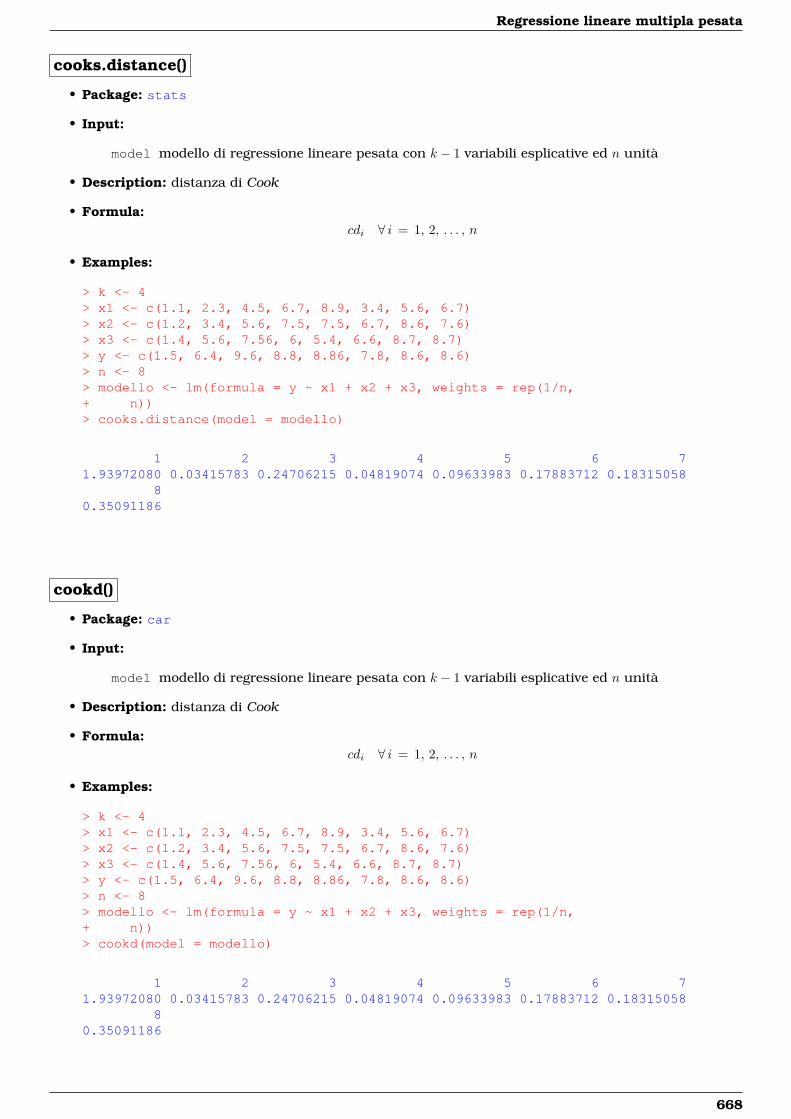
Regressione lineare multipla pesata
cooks.distance()
• Package: stats
• Input:
model modello di regressione lineare pesata con k − 1 variabili esplicative ed n unità
• Description: distanza di Cook
• Formula:cdi ∀ i = 1, 2, . . . , n
• Examples:
> k <- 4> x1 <- c(1.1, 2.3, 4.5, 6.7, 8.9, 3.4, 5.6, 6.7)> x2 <- c(1.2, 3.4, 5.6, 7.5, 7.5, 6.7, 8.6, 7.6)> x3 <- c(1.4, 5.6, 7.56, 6, 5.4, 6.6, 8.7, 8.7)> y <- c(1.5, 6.4, 9.6, 8.8, 8.86, 7.8, 8.6, 8.6)> n <- 8> modello <- lm(formula = y ~ x1 + x2 + x3, weights = rep(1/n,+ n))> cooks.distance(model = modello)
1 2 3 4 5 6 71.93972080 0.03415783 0.24706215 0.04819074 0.09633983 0.17883712 0.18315058
80.35091186
cookd()
• Package: car
• Input:
model modello di regressione lineare pesata con k − 1 variabili esplicative ed n unità
• Description: distanza di Cook
• Formula:cdi ∀ i = 1, 2, . . . , n
• Examples:
> k <- 4> x1 <- c(1.1, 2.3, 4.5, 6.7, 8.9, 3.4, 5.6, 6.7)> x2 <- c(1.2, 3.4, 5.6, 7.5, 7.5, 6.7, 8.6, 7.6)> x3 <- c(1.4, 5.6, 7.56, 6, 5.4, 6.6, 8.7, 8.7)> y <- c(1.5, 6.4, 9.6, 8.8, 8.86, 7.8, 8.6, 8.6)> n <- 8> modello <- lm(formula = y ~ x1 + x2 + x3, weights = rep(1/n,+ n))> cookd(model = modello)
1 2 3 4 5 6 71.93972080 0.03415783 0.24706215 0.04819074 0.09633983 0.17883712 0.18315058
80.35091186
668

16.4 Diagnostica
rstandard()
• Package: stats
• Input:
model modello di regressione lineare pesata con k − 1 variabili esplicative ed n unità
• Description: residui standard
• Formula:rstandardi ∀i = 1, 2, . . . , n
• Examples:
> k <- 4> x1 <- c(1.1, 2.3, 4.5, 6.7, 8.9, 3.4, 5.6, 6.7)> x2 <- c(1.2, 3.4, 5.6, 7.5, 7.5, 6.7, 8.6, 7.6)> x3 <- c(1.4, 5.6, 7.56, 6, 5.4, 6.6, 8.7, 8.7)> y <- c(1.5, 6.4, 9.6, 8.8, 8.86, 7.8, 8.6, 8.6)> n <- 8> modello <- lm(formula = y ~ x1 + x2 + x3, weights = rep(1/n,+ n))> rstandard(model = modello)
1 2 3 4 5 6 7-1.5241225 0.4376576 1.2722093 0.6467323 0.3791111 0.7589935 -0.9849613
8-1.4301703
rstandard.lm()
• Package: stats
• Input:
model modello di regressione lineare pesata con k − 1 variabili esplicative ed n unità
• Description: residui standard
• Formula:rstandardi ∀i = 1, 2, . . . , n
• Examples:
> k <- 4> x1 <- c(1.1, 2.3, 4.5, 6.7, 8.9, 3.4, 5.6, 6.7)> x2 <- c(1.2, 3.4, 5.6, 7.5, 7.5, 6.7, 8.6, 7.6)> x3 <- c(1.4, 5.6, 7.56, 6, 5.4, 6.6, 8.7, 8.7)> y <- c(1.5, 6.4, 9.6, 8.8, 8.86, 7.8, 8.6, 8.6)> n <- 8> modello <- lm(formula = y ~ x1 + x2 + x3, weights = rep(1/n,+ n))> rstandard.lm(model = modello)
1 2 3 4 5 6 7-1.5241225 0.4376576 1.2722093 0.6467323 0.3791111 0.7589935 -0.9849613
8-1.4301703
669
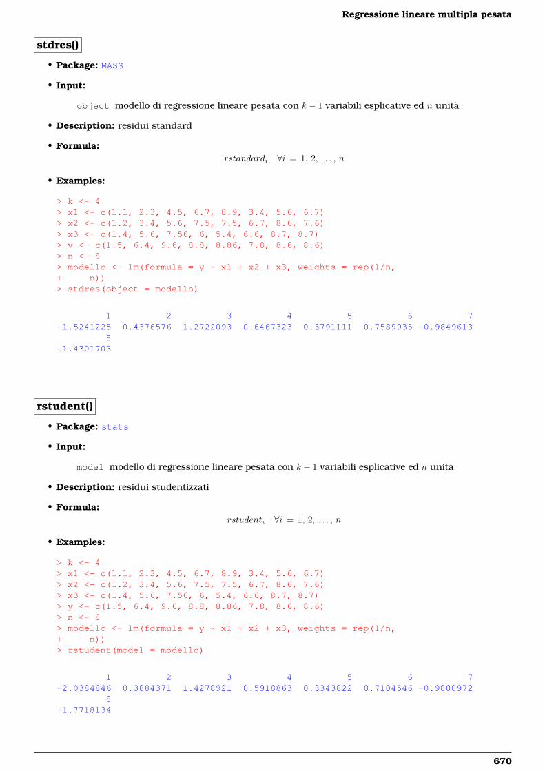
Regressione lineare multipla pesata
stdres()
• Package: MASS
• Input:
object modello di regressione lineare pesata con k − 1 variabili esplicative ed n unità
• Description: residui standard
• Formula:rstandardi ∀i = 1, 2, . . . , n
• Examples:
> k <- 4> x1 <- c(1.1, 2.3, 4.5, 6.7, 8.9, 3.4, 5.6, 6.7)> x2 <- c(1.2, 3.4, 5.6, 7.5, 7.5, 6.7, 8.6, 7.6)> x3 <- c(1.4, 5.6, 7.56, 6, 5.4, 6.6, 8.7, 8.7)> y <- c(1.5, 6.4, 9.6, 8.8, 8.86, 7.8, 8.6, 8.6)> n <- 8> modello <- lm(formula = y ~ x1 + x2 + x3, weights = rep(1/n,+ n))> stdres(object = modello)
1 2 3 4 5 6 7-1.5241225 0.4376576 1.2722093 0.6467323 0.3791111 0.7589935 -0.9849613
8-1.4301703
rstudent()
• Package: stats
• Input:
model modello di regressione lineare pesata con k − 1 variabili esplicative ed n unità
• Description: residui studentizzati
• Formula:rstudenti ∀i = 1, 2, . . . , n
• Examples:
> k <- 4> x1 <- c(1.1, 2.3, 4.5, 6.7, 8.9, 3.4, 5.6, 6.7)> x2 <- c(1.2, 3.4, 5.6, 7.5, 7.5, 6.7, 8.6, 7.6)> x3 <- c(1.4, 5.6, 7.56, 6, 5.4, 6.6, 8.7, 8.7)> y <- c(1.5, 6.4, 9.6, 8.8, 8.86, 7.8, 8.6, 8.6)> n <- 8> modello <- lm(formula = y ~ x1 + x2 + x3, weights = rep(1/n,+ n))> rstudent(model = modello)
1 2 3 4 5 6 7-2.0384846 0.3884371 1.4278921 0.5918863 0.3343822 0.7104546 -0.9800972
8-1.7718134
670
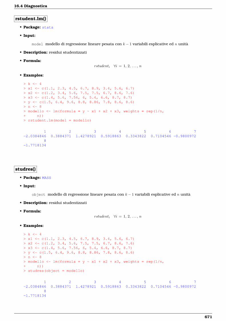
16.4 Diagnostica
rstudent.lm()
• Package: stats
• Input:
model modello di regressione lineare pesata con k − 1 variabili esplicative ed n unità
• Description: residui studentizzati
• Formula:rstudenti ∀i = 1, 2, . . . , n
• Examples:
> k <- 4> x1 <- c(1.1, 2.3, 4.5, 6.7, 8.9, 3.4, 5.6, 6.7)> x2 <- c(1.2, 3.4, 5.6, 7.5, 7.5, 6.7, 8.6, 7.6)> x3 <- c(1.4, 5.6, 7.56, 6, 5.4, 6.6, 8.7, 8.7)> y <- c(1.5, 6.4, 9.6, 8.8, 8.86, 7.8, 8.6, 8.6)> n <- 8> modello <- lm(formula = y ~ x1 + x2 + x3, weights = rep(1/n,+ n))> rstudent.lm(model = modello)
1 2 3 4 5 6 7-2.0384846 0.3884371 1.4278921 0.5918863 0.3343822 0.7104546 -0.9800972
8-1.7718134
studres()
• Package: MASS
• Input:
object modello di regressione lineare pesata con k − 1 variabili esplicative ed n unità
• Description: residui studentizzati
• Formula:rstudenti ∀i = 1, 2, . . . , n
• Examples:
> k <- 4> x1 <- c(1.1, 2.3, 4.5, 6.7, 8.9, 3.4, 5.6, 6.7)> x2 <- c(1.2, 3.4, 5.6, 7.5, 7.5, 6.7, 8.6, 7.6)> x3 <- c(1.4, 5.6, 7.56, 6, 5.4, 6.6, 8.7, 8.7)> y <- c(1.5, 6.4, 9.6, 8.8, 8.86, 7.8, 8.6, 8.6)> n <- 8> modello <- lm(formula = y ~ x1 + x2 + x3, weights = rep(1/n,+ n))> studres(object = modello)
1 2 3 4 5 6 7-2.0384846 0.3884371 1.4278921 0.5918863 0.3343822 0.7104546 -0.9800972
8-1.7718134
671
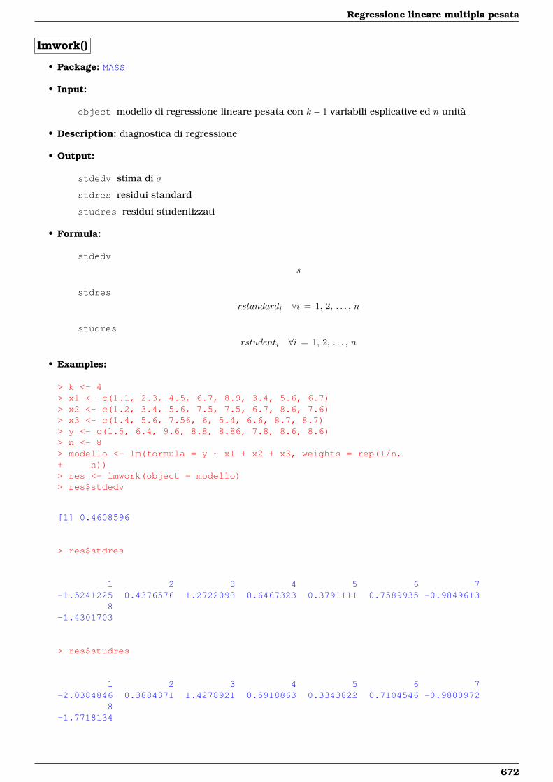
Regressione lineare multipla pesata
lmwork()
• Package: MASS
• Input:
object modello di regressione lineare pesata con k − 1 variabili esplicative ed n unità
• Description: diagnostica di regressione
• Output:
stdedv stima di σ
stdres residui standard
studres residui studentizzati
• Formula:
stdedv
s
stdres
rstandardi ∀i = 1, 2, . . . , n
studres
rstudenti ∀i = 1, 2, . . . , n
• Examples:
> k <- 4> x1 <- c(1.1, 2.3, 4.5, 6.7, 8.9, 3.4, 5.6, 6.7)> x2 <- c(1.2, 3.4, 5.6, 7.5, 7.5, 6.7, 8.6, 7.6)> x3 <- c(1.4, 5.6, 7.56, 6, 5.4, 6.6, 8.7, 8.7)> y <- c(1.5, 6.4, 9.6, 8.8, 8.86, 7.8, 8.6, 8.6)> n <- 8> modello <- lm(formula = y ~ x1 + x2 + x3, weights = rep(1/n,+ n))> res <- lmwork(object = modello)> res$stdedv
[1] 0.4608596
> res$stdres
1 2 3 4 5 6 7-1.5241225 0.4376576 1.2722093 0.6467323 0.3791111 0.7589935 -0.9849613
8-1.4301703
> res$studres
1 2 3 4 5 6 7-2.0384846 0.3884371 1.4278921 0.5918863 0.3343822 0.7104546 -0.9800972
8-1.7718134
672
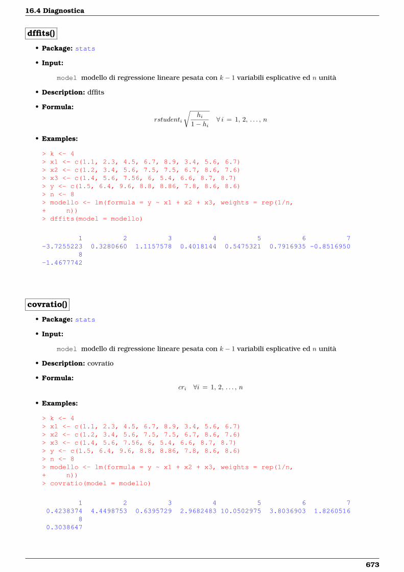
16.4 Diagnostica
dffits()
• Package: stats
• Input:
model modello di regressione lineare pesata con k − 1 variabili esplicative ed n unità
• Description: dffits
• Formula:
rstudenti
√hi
1− hi∀ i = 1, 2, . . . , n
• Examples:
> k <- 4> x1 <- c(1.1, 2.3, 4.5, 6.7, 8.9, 3.4, 5.6, 6.7)> x2 <- c(1.2, 3.4, 5.6, 7.5, 7.5, 6.7, 8.6, 7.6)> x3 <- c(1.4, 5.6, 7.56, 6, 5.4, 6.6, 8.7, 8.7)> y <- c(1.5, 6.4, 9.6, 8.8, 8.86, 7.8, 8.6, 8.6)> n <- 8> modello <- lm(formula = y ~ x1 + x2 + x3, weights = rep(1/n,+ n))> dffits(model = modello)
1 2 3 4 5 6 7-3.7255223 0.3280660 1.1157578 0.4018144 0.5475321 0.7916935 -0.8516950
8-1.4677742
covratio()
• Package: stats
• Input:
model modello di regressione lineare pesata con k − 1 variabili esplicative ed n unità
• Description: covratio
• Formula:cri ∀i = 1, 2, . . . , n
• Examples:
> k <- 4> x1 <- c(1.1, 2.3, 4.5, 6.7, 8.9, 3.4, 5.6, 6.7)> x2 <- c(1.2, 3.4, 5.6, 7.5, 7.5, 6.7, 8.6, 7.6)> x3 <- c(1.4, 5.6, 7.56, 6, 5.4, 6.6, 8.7, 8.7)> y <- c(1.5, 6.4, 9.6, 8.8, 8.86, 7.8, 8.6, 8.6)> n <- 8> modello <- lm(formula = y ~ x1 + x2 + x3, weights = rep(1/n,+ n))> covratio(model = modello)
1 2 3 4 5 6 70.4238374 4.4498753 0.6395729 2.9682483 10.0502975 3.8036903 1.8260516
80.3038647
673
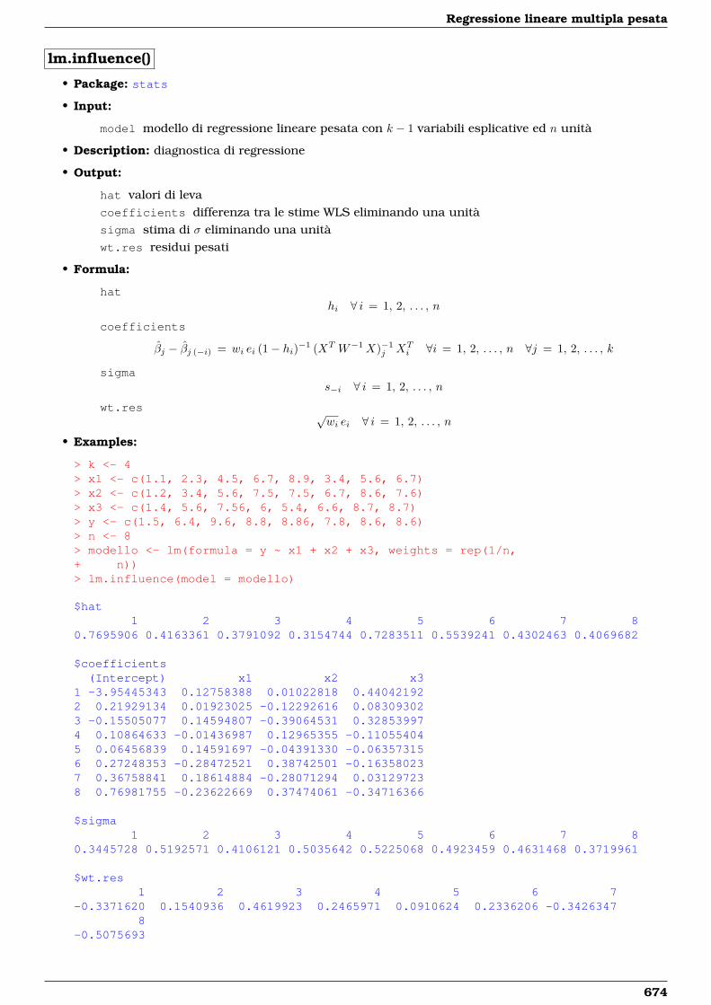
Regressione lineare multipla pesata
lm.influence()
• Package: stats
• Input:
model modello di regressione lineare pesata con k − 1 variabili esplicative ed n unità
• Description: diagnostica di regressione
• Output:
hat valori di levacoefficients differenza tra le stime WLS eliminando una unitàsigma stima di σ eliminando una unitàwt.res residui pesati
• Formula:
hathi ∀ i = 1, 2, . . . , n
coefficients
βj − βj (−i) = wi ei (1− hi)−1 (XT W−1X)−1j XT
i ∀i = 1, 2, . . . , n ∀j = 1, 2, . . . , k
sigmas−i ∀ i = 1, 2, . . . , n
wt.res √wi ei ∀ i = 1, 2, . . . , n
• Examples:
> k <- 4> x1 <- c(1.1, 2.3, 4.5, 6.7, 8.9, 3.4, 5.6, 6.7)> x2 <- c(1.2, 3.4, 5.6, 7.5, 7.5, 6.7, 8.6, 7.6)> x3 <- c(1.4, 5.6, 7.56, 6, 5.4, 6.6, 8.7, 8.7)> y <- c(1.5, 6.4, 9.6, 8.8, 8.86, 7.8, 8.6, 8.6)> n <- 8> modello <- lm(formula = y ~ x1 + x2 + x3, weights = rep(1/n,+ n))> lm.influence(model = modello)
$hat1 2 3 4 5 6 7 8
0.7695906 0.4163361 0.3791092 0.3154744 0.7283511 0.5539241 0.4302463 0.4069682
$coefficients(Intercept) x1 x2 x3
1 -3.95445343 0.12758388 0.01022818 0.440421922 0.21929134 0.01923025 -0.12292616 0.083093023 -0.15505077 0.14594807 -0.39064531 0.328539974 0.10864633 -0.01436987 0.12965355 -0.110554045 0.06456839 0.14591697 -0.04391330 -0.063573156 0.27248353 -0.28472521 0.38742501 -0.163580237 0.36758841 0.18614884 -0.28071294 0.031297238 0.76981755 -0.23622669 0.37474061 -0.34716366
$sigma1 2 3 4 5 6 7 8
0.3445728 0.5192571 0.4106121 0.5035642 0.5225068 0.4923459 0.4631468 0.3719961
$wt.res1 2 3 4 5 6 7
-0.3371620 0.1540936 0.4619923 0.2465971 0.0910624 0.2336206 -0.34263478
-0.5075693
674
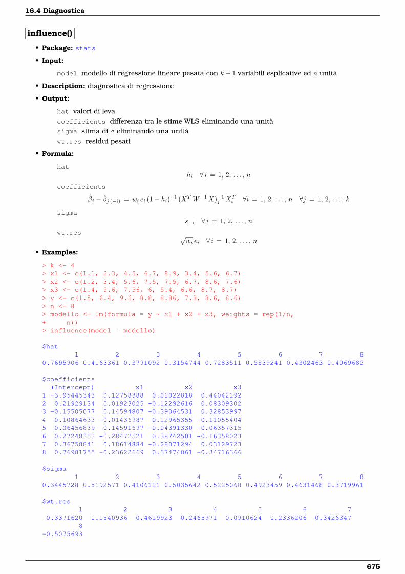
16.4 Diagnostica
influence()
• Package: stats
• Input:
model modello di regressione lineare pesata con k − 1 variabili esplicative ed n unità
• Description: diagnostica di regressione
• Output:
hat valori di levacoefficients differenza tra le stime WLS eliminando una unitàsigma stima di σ eliminando una unitàwt.res residui pesati
• Formula:
hathi ∀ i = 1, 2, . . . , n
coefficients
βj − βj (−i) = wi ei (1− hi)−1 (XT W−1X)−1j XT
i ∀i = 1, 2, . . . , n ∀j = 1, 2, . . . , k
sigmas−i ∀ i = 1, 2, . . . , n
wt.res √wi ei ∀ i = 1, 2, . . . , n
• Examples:
> k <- 4> x1 <- c(1.1, 2.3, 4.5, 6.7, 8.9, 3.4, 5.6, 6.7)> x2 <- c(1.2, 3.4, 5.6, 7.5, 7.5, 6.7, 8.6, 7.6)> x3 <- c(1.4, 5.6, 7.56, 6, 5.4, 6.6, 8.7, 8.7)> y <- c(1.5, 6.4, 9.6, 8.8, 8.86, 7.8, 8.6, 8.6)> n <- 8> modello <- lm(formula = y ~ x1 + x2 + x3, weights = rep(1/n,+ n))> influence(model = modello)
$hat1 2 3 4 5 6 7 8
0.7695906 0.4163361 0.3791092 0.3154744 0.7283511 0.5539241 0.4302463 0.4069682
$coefficients(Intercept) x1 x2 x3
1 -3.95445343 0.12758388 0.01022818 0.440421922 0.21929134 0.01923025 -0.12292616 0.083093023 -0.15505077 0.14594807 -0.39064531 0.328539974 0.10864633 -0.01436987 0.12965355 -0.110554045 0.06456839 0.14591697 -0.04391330 -0.063573156 0.27248353 -0.28472521 0.38742501 -0.163580237 0.36758841 0.18614884 -0.28071294 0.031297238 0.76981755 -0.23622669 0.37474061 -0.34716366
$sigma1 2 3 4 5 6 7 8
0.3445728 0.5192571 0.4106121 0.5035642 0.5225068 0.4923459 0.4631468 0.3719961
$wt.res1 2 3 4 5 6 7
-0.3371620 0.1540936 0.4619923 0.2465971 0.0910624 0.2336206 -0.34263478
-0.5075693
675
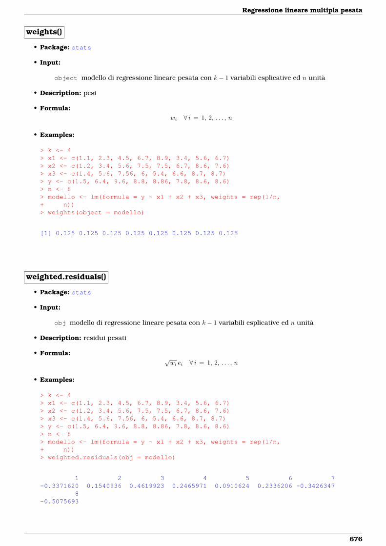
Regressione lineare multipla pesata
weights()
• Package: stats
• Input:
object modello di regressione lineare pesata con k − 1 variabili esplicative ed n unità
• Description: pesi
• Formula:wi ∀ i = 1, 2, . . . , n
• Examples:
> k <- 4> x1 <- c(1.1, 2.3, 4.5, 6.7, 8.9, 3.4, 5.6, 6.7)> x2 <- c(1.2, 3.4, 5.6, 7.5, 7.5, 6.7, 8.6, 7.6)> x3 <- c(1.4, 5.6, 7.56, 6, 5.4, 6.6, 8.7, 8.7)> y <- c(1.5, 6.4, 9.6, 8.8, 8.86, 7.8, 8.6, 8.6)> n <- 8> modello <- lm(formula = y ~ x1 + x2 + x3, weights = rep(1/n,+ n))> weights(object = modello)
[1] 0.125 0.125 0.125 0.125 0.125 0.125 0.125 0.125
weighted.residuals()
• Package: stats
• Input:
obj modello di regressione lineare pesata con k − 1 variabili esplicative ed n unità
• Description: residui pesati
• Formula:√wi ei ∀ i = 1, 2, . . . , n
• Examples:
> k <- 4> x1 <- c(1.1, 2.3, 4.5, 6.7, 8.9, 3.4, 5.6, 6.7)> x2 <- c(1.2, 3.4, 5.6, 7.5, 7.5, 6.7, 8.6, 7.6)> x3 <- c(1.4, 5.6, 7.56, 6, 5.4, 6.6, 8.7, 8.7)> y <- c(1.5, 6.4, 9.6, 8.8, 8.86, 7.8, 8.6, 8.6)> n <- 8> modello <- lm(formula = y ~ x1 + x2 + x3, weights = rep(1/n,+ n))> weighted.residuals(obj = modello)
1 2 3 4 5 6 7-0.3371620 0.1540936 0.4619923 0.2465971 0.0910624 0.2336206 -0.3426347
8-0.5075693
676
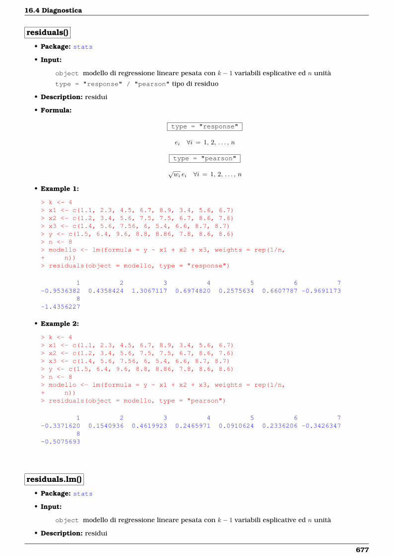
16.4 Diagnostica
residuals()
• Package: stats
• Input:
object modello di regressione lineare pesata con k − 1 variabili esplicative ed n unità
type = "response" / "pearson" tipo di residuo
• Description: residui
• Formula:
type = "response"
ei ∀i = 1, 2, . . . , n
type = "pearson"
√wi ei ∀i = 1, 2, . . . , n
• Example 1:
> k <- 4> x1 <- c(1.1, 2.3, 4.5, 6.7, 8.9, 3.4, 5.6, 6.7)> x2 <- c(1.2, 3.4, 5.6, 7.5, 7.5, 6.7, 8.6, 7.6)> x3 <- c(1.4, 5.6, 7.56, 6, 5.4, 6.6, 8.7, 8.7)> y <- c(1.5, 6.4, 9.6, 8.8, 8.86, 7.8, 8.6, 8.6)> n <- 8> modello <- lm(formula = y ~ x1 + x2 + x3, weights = rep(1/n,+ n))> residuals(object = modello, type = "response")
1 2 3 4 5 6 7-0.9536382 0.4358424 1.3067117 0.6974820 0.2575634 0.6607787 -0.9691173
8-1.4356227
• Example 2:
> k <- 4> x1 <- c(1.1, 2.3, 4.5, 6.7, 8.9, 3.4, 5.6, 6.7)> x2 <- c(1.2, 3.4, 5.6, 7.5, 7.5, 6.7, 8.6, 7.6)> x3 <- c(1.4, 5.6, 7.56, 6, 5.4, 6.6, 8.7, 8.7)> y <- c(1.5, 6.4, 9.6, 8.8, 8.86, 7.8, 8.6, 8.6)> n <- 8> modello <- lm(formula = y ~ x1 + x2 + x3, weights = rep(1/n,+ n))> residuals(object = modello, type = "pearson")
1 2 3 4 5 6 7-0.3371620 0.1540936 0.4619923 0.2465971 0.0910624 0.2336206 -0.3426347
8-0.5075693
residuals.lm()
• Package: stats
• Input:
object modello di regressione lineare pesata con k − 1 variabili esplicative ed n unità
• Description: residui
677
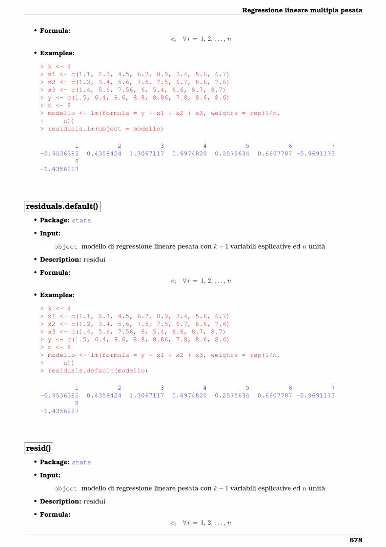
Regressione lineare multipla pesata
• Formula:ei ∀ i = 1, 2, . . . , n
• Examples:
> k <- 4> x1 <- c(1.1, 2.3, 4.5, 6.7, 8.9, 3.4, 5.6, 6.7)> x2 <- c(1.2, 3.4, 5.6, 7.5, 7.5, 6.7, 8.6, 7.6)> x3 <- c(1.4, 5.6, 7.56, 6, 5.4, 6.6, 8.7, 8.7)> y <- c(1.5, 6.4, 9.6, 8.8, 8.86, 7.8, 8.6, 8.6)> n <- 8> modello <- lm(formula = y ~ x1 + x2 + x3, weights = rep(1/n,+ n))> residuals.lm(object = modello)
1 2 3 4 5 6 7-0.9536382 0.4358424 1.3067117 0.6974820 0.2575634 0.6607787 -0.9691173
8-1.4356227
residuals.default()
• Package: stats
• Input:
object modello di regressione lineare pesata con k − 1 variabili esplicative ed n unità
• Description: residui
• Formula:ei ∀ i = 1, 2, . . . , n
• Examples:
> k <- 4> x1 <- c(1.1, 2.3, 4.5, 6.7, 8.9, 3.4, 5.6, 6.7)> x2 <- c(1.2, 3.4, 5.6, 7.5, 7.5, 6.7, 8.6, 7.6)> x3 <- c(1.4, 5.6, 7.56, 6, 5.4, 6.6, 8.7, 8.7)> y <- c(1.5, 6.4, 9.6, 8.8, 8.86, 7.8, 8.6, 8.6)> n <- 8> modello <- lm(formula = y ~ x1 + x2 + x3, weights = rep(1/n,+ n))> residuals.default(modello)
1 2 3 4 5 6 7-0.9536382 0.4358424 1.3067117 0.6974820 0.2575634 0.6607787 -0.9691173
8-1.4356227
resid()
• Package: stats
• Input:
object modello di regressione lineare pesata con k − 1 variabili esplicative ed n unità
• Description: residui
• Formula:ei ∀ i = 1, 2, . . . , n
678
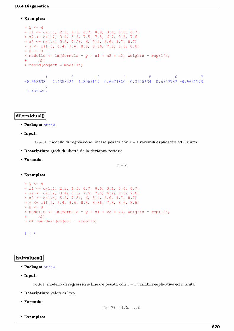
16.4 Diagnostica
• Examples:
> k <- 4> x1 <- c(1.1, 2.3, 4.5, 6.7, 8.9, 3.4, 5.6, 6.7)> x2 <- c(1.2, 3.4, 5.6, 7.5, 7.5, 6.7, 8.6, 7.6)> x3 <- c(1.4, 5.6, 7.56, 6, 5.4, 6.6, 8.7, 8.7)> y <- c(1.5, 6.4, 9.6, 8.8, 8.86, 7.8, 8.6, 8.6)> n <- 8> modello <- lm(formula = y ~ x1 + x2 + x3, weights = rep(1/n,+ n))> resid(object = modello)
1 2 3 4 5 6 7-0.9536382 0.4358424 1.3067117 0.6974820 0.2575634 0.6607787 -0.9691173
8-1.4356227
df.residual()
• Package: stats
• Input:
object modello di regressione lineare pesata con k − 1 variabili esplicative ed n unità
• Description: gradi di libertà della devianza residua
• Formula:n− k
• Examples:
> k <- 4> x1 <- c(1.1, 2.3, 4.5, 6.7, 8.9, 3.4, 5.6, 6.7)> x2 <- c(1.2, 3.4, 5.6, 7.5, 7.5, 6.7, 8.6, 7.6)> x3 <- c(1.4, 5.6, 7.56, 6, 5.4, 6.6, 8.7, 8.7)> y <- c(1.5, 6.4, 9.6, 8.8, 8.86, 7.8, 8.6, 8.6)> n <- 8> modello <- lm(formula = y ~ x1 + x2 + x3, weights = rep(1/n,+ n))> df.residual(object = modello)
[1] 4
hatvalues()
• Package: stats
• Input:
model modello di regressione lineare pesata con k − 1 variabili esplicative ed n unità
• Description: valori di leva
• Formula:hi ∀ i = 1, 2, . . . , n
• Examples:
679
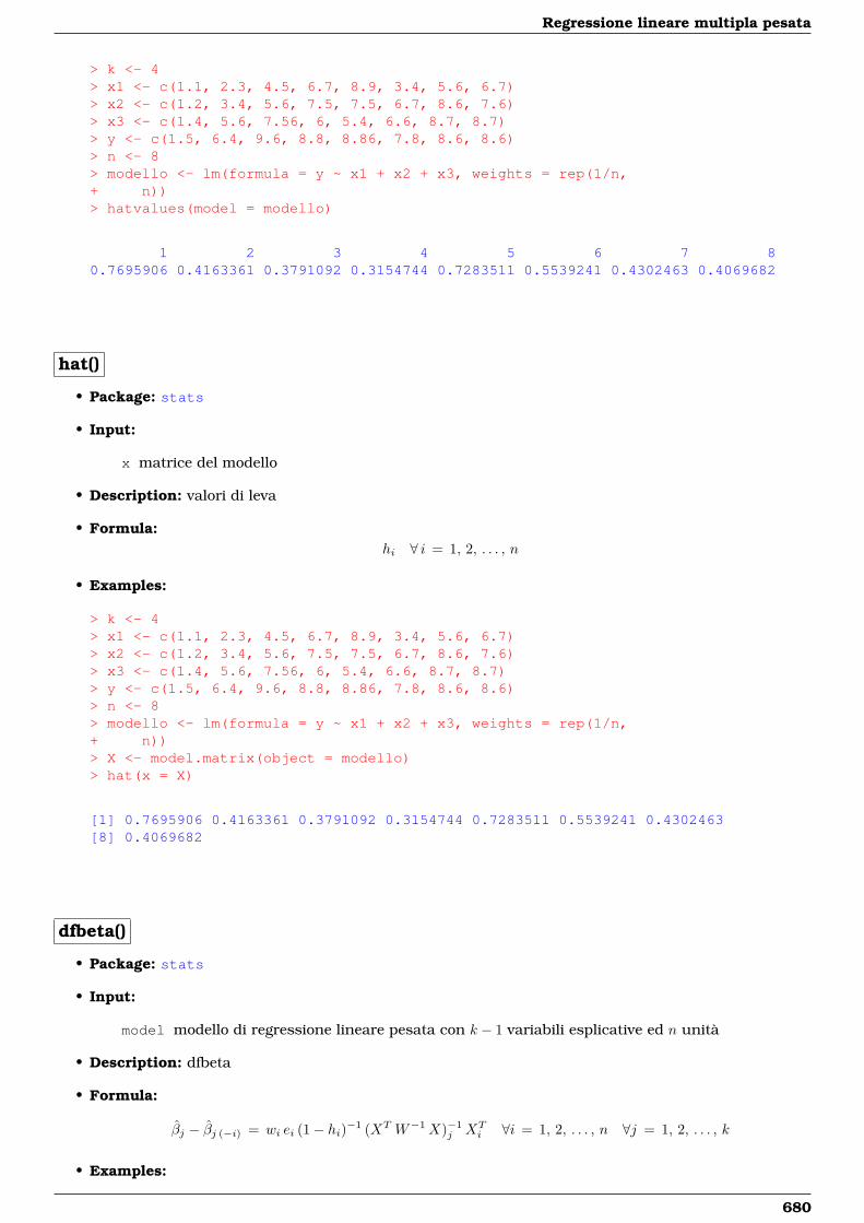
Regressione lineare multipla pesata
> k <- 4> x1 <- c(1.1, 2.3, 4.5, 6.7, 8.9, 3.4, 5.6, 6.7)> x2 <- c(1.2, 3.4, 5.6, 7.5, 7.5, 6.7, 8.6, 7.6)> x3 <- c(1.4, 5.6, 7.56, 6, 5.4, 6.6, 8.7, 8.7)> y <- c(1.5, 6.4, 9.6, 8.8, 8.86, 7.8, 8.6, 8.6)> n <- 8> modello <- lm(formula = y ~ x1 + x2 + x3, weights = rep(1/n,+ n))> hatvalues(model = modello)
1 2 3 4 5 6 7 80.7695906 0.4163361 0.3791092 0.3154744 0.7283511 0.5539241 0.4302463 0.4069682
hat()
• Package: stats
• Input:
x matrice del modello
• Description: valori di leva
• Formula:hi ∀ i = 1, 2, . . . , n
• Examples:
> k <- 4> x1 <- c(1.1, 2.3, 4.5, 6.7, 8.9, 3.4, 5.6, 6.7)> x2 <- c(1.2, 3.4, 5.6, 7.5, 7.5, 6.7, 8.6, 7.6)> x3 <- c(1.4, 5.6, 7.56, 6, 5.4, 6.6, 8.7, 8.7)> y <- c(1.5, 6.4, 9.6, 8.8, 8.86, 7.8, 8.6, 8.6)> n <- 8> modello <- lm(formula = y ~ x1 + x2 + x3, weights = rep(1/n,+ n))> X <- model.matrix(object = modello)> hat(x = X)
[1] 0.7695906 0.4163361 0.3791092 0.3154744 0.7283511 0.5539241 0.4302463[8] 0.4069682
dfbeta()
• Package: stats
• Input:
model modello di regressione lineare pesata con k − 1 variabili esplicative ed n unità
• Description: dfbeta
• Formula:
βj − βj (−i) = wi ei (1− hi)−1 (XT W−1X)−1j XT
i ∀i = 1, 2, . . . , n ∀j = 1, 2, . . . , k
• Examples:
680
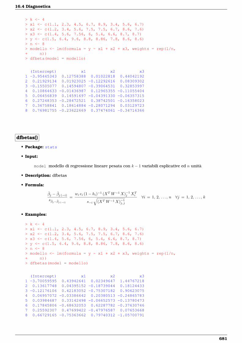
16.4 Diagnostica
> k <- 4> x1 <- c(1.1, 2.3, 4.5, 6.7, 8.9, 3.4, 5.6, 6.7)> x2 <- c(1.2, 3.4, 5.6, 7.5, 7.5, 6.7, 8.6, 7.6)> x3 <- c(1.4, 5.6, 7.56, 6, 5.4, 6.6, 8.7, 8.7)> y <- c(1.5, 6.4, 9.6, 8.8, 8.86, 7.8, 8.6, 8.6)> n <- 8> modello <- lm(formula = y ~ x1 + x2 + x3, weights = rep(1/n,+ n))> dfbeta(model = modello)
(Intercept) x1 x2 x31 -3.95445343 0.12758388 0.01022818 0.440421922 0.21929134 0.01923025 -0.12292616 0.083093023 -0.15505077 0.14594807 -0.39064531 0.328539974 0.10864633 -0.01436987 0.12965355 -0.110554045 0.06456839 0.14591697 -0.04391330 -0.063573156 0.27248353 -0.28472521 0.38742501 -0.163580237 0.36758841 0.18614884 -0.28071294 0.031297238 0.76981755 -0.23622669 0.37474061 -0.34716366
dfbetas()
• Package: stats
• Input:
model modello di regressione lineare pesata con k − 1 variabili esplicative ed n unità
• Description: dfbetas
• Formula:
βj − βj (−i)
sβj−βj (−i)
=wi ei (1− hi)−1 (XT W−1X)−1
j XTi
s−i
√(XT W−1X)−1
j, j
∀i = 1, 2, . . . , n ∀j = 1, 2, . . . , k
• Examples:
> k <- 4> x1 <- c(1.1, 2.3, 4.5, 6.7, 8.9, 3.4, 5.6, 6.7)> x2 <- c(1.2, 3.4, 5.6, 7.5, 7.5, 6.7, 8.6, 7.6)> x3 <- c(1.4, 5.6, 7.56, 6, 5.4, 6.6, 8.7, 8.7)> y <- c(1.5, 6.4, 9.6, 8.8, 8.86, 7.8, 8.6, 8.6)> n <- 8> modello <- lm(formula = y ~ x1 + x2 + x3, weights = rep(1/n,+ n))> dfbetas(model = modello)
(Intercept) x1 x2 x31 -3.70059595 0.43942641 0.02349647 1.447672182 0.13617748 0.04395152 -0.18739044 0.181244333 -0.12176106 0.42183052 -0.75307182 0.906230754 0.06957072 -0.03386642 0.20380513 -0.248657835 0.03984687 0.33142498 -0.06652573 -0.137804736 0.17845806 -0.68632053 0.62287782 -0.376307467 0.25592307 0.47699422 -0.47976587 0.076536688 0.66729165 -0.75363662 0.79740312 -1.05700791
681
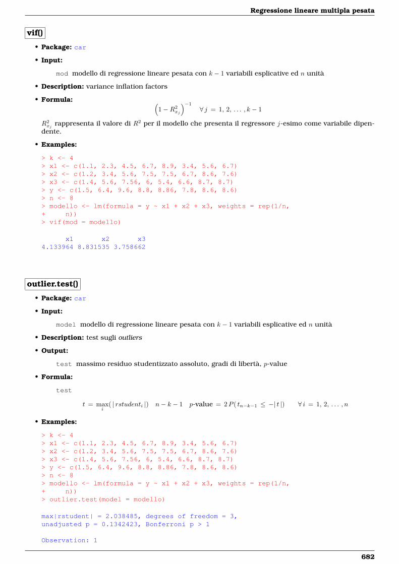
Regressione lineare multipla pesata
vif()
• Package: car
• Input:
mod modello di regressione lineare pesata con k − 1 variabili esplicative ed n unità
• Description: variance inflation factors
• Formula: (1−R2
xj
)−1
∀ j = 1, 2, . . . , k − 1
R2xj rappresenta il valore di R2 per il modello che presenta il regressore j-esimo come variabile dipen-
dente.
• Examples:
> k <- 4> x1 <- c(1.1, 2.3, 4.5, 6.7, 8.9, 3.4, 5.6, 6.7)> x2 <- c(1.2, 3.4, 5.6, 7.5, 7.5, 6.7, 8.6, 7.6)> x3 <- c(1.4, 5.6, 7.56, 6, 5.4, 6.6, 8.7, 8.7)> y <- c(1.5, 6.4, 9.6, 8.8, 8.86, 7.8, 8.6, 8.6)> n <- 8> modello <- lm(formula = y ~ x1 + x2 + x3, weights = rep(1/n,+ n))> vif(mod = modello)
x1 x2 x34.133964 8.831535 3.758662
outlier.test()
• Package: car
• Input:
model modello di regressione lineare pesata con k − 1 variabili esplicative ed n unità
• Description: test sugli outliers
• Output:
test massimo residuo studentizzato assoluto, gradi di libertà, p-value
• Formula:
test
t = maxi
( | rstudenti |) n− k − 1 p-value = 2P ( tn−k−1 ≤ −| t |) ∀ i = 1, 2, . . . , n
• Examples:
> k <- 4> x1 <- c(1.1, 2.3, 4.5, 6.7, 8.9, 3.4, 5.6, 6.7)> x2 <- c(1.2, 3.4, 5.6, 7.5, 7.5, 6.7, 8.6, 7.6)> x3 <- c(1.4, 5.6, 7.56, 6, 5.4, 6.6, 8.7, 8.7)> y <- c(1.5, 6.4, 9.6, 8.8, 8.86, 7.8, 8.6, 8.6)> n <- 8> modello <- lm(formula = y ~ x1 + x2 + x3, weights = rep(1/n,+ n))> outlier.test(model = modello)
max|rstudent| = 2.038485, degrees of freedom = 3,unadjusted p = 0.1342423, Bonferroni p > 1
Observation: 1
682
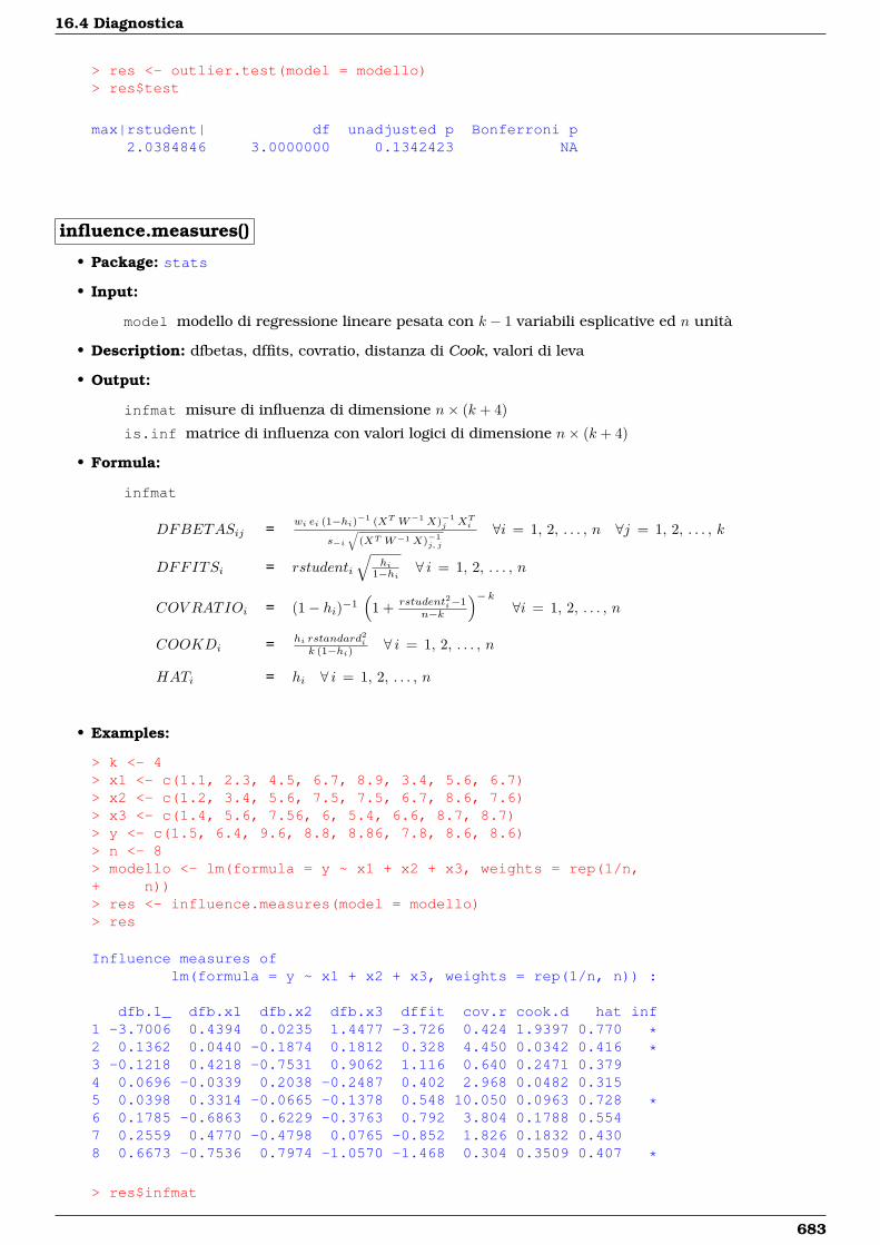
16.4 Diagnostica
> res <- outlier.test(model = modello)> res$test
max|rstudent| df unadjusted p Bonferroni p2.0384846 3.0000000 0.1342423 NA
influence.measures()
• Package: stats
• Input:
model modello di regressione lineare pesata con k − 1 variabili esplicative ed n unità
• Description: dfbetas, dffits, covratio, distanza di Cook, valori di leva
• Output:
infmat misure di influenza di dimensione n× (k + 4)
is.inf matrice di influenza con valori logici di dimensione n× (k + 4)
• Formula:
infmat
DFBETASij =wi ei (1−hi)−1 (XT W−1X)−1
j XTi
s−i
√(XT W−1X)−1
j, j
∀i = 1, 2, . . . , n ∀j = 1, 2, . . . , k
DFFITSi = rstudenti
√hi
1−hi ∀ i = 1, 2, . . . , n
COV RATIOi = (1− hi)−1(
1 + rstudent2i−1n−k
)− k∀i = 1, 2, . . . , n
COOKDi = hi rstandard2i
k (1−hi) ∀ i = 1, 2, . . . , n
HATi = hi ∀ i = 1, 2, . . . , n
• Examples:
> k <- 4> x1 <- c(1.1, 2.3, 4.5, 6.7, 8.9, 3.4, 5.6, 6.7)> x2 <- c(1.2, 3.4, 5.6, 7.5, 7.5, 6.7, 8.6, 7.6)> x3 <- c(1.4, 5.6, 7.56, 6, 5.4, 6.6, 8.7, 8.7)> y <- c(1.5, 6.4, 9.6, 8.8, 8.86, 7.8, 8.6, 8.6)> n <- 8> modello <- lm(formula = y ~ x1 + x2 + x3, weights = rep(1/n,+ n))> res <- influence.measures(model = modello)> res
Influence measures oflm(formula = y ~ x1 + x2 + x3, weights = rep(1/n, n)) :
dfb.1_ dfb.x1 dfb.x2 dfb.x3 dffit cov.r cook.d hat inf1 -3.7006 0.4394 0.0235 1.4477 -3.726 0.424 1.9397 0.770 *2 0.1362 0.0440 -0.1874 0.1812 0.328 4.450 0.0342 0.416 *3 -0.1218 0.4218 -0.7531 0.9062 1.116 0.640 0.2471 0.3794 0.0696 -0.0339 0.2038 -0.2487 0.402 2.968 0.0482 0.3155 0.0398 0.3314 -0.0665 -0.1378 0.548 10.050 0.0963 0.728 *6 0.1785 -0.6863 0.6229 -0.3763 0.792 3.804 0.1788 0.5547 0.2559 0.4770 -0.4798 0.0765 -0.852 1.826 0.1832 0.4308 0.6673 -0.7536 0.7974 -1.0570 -1.468 0.304 0.3509 0.407 *
> res$infmat
683
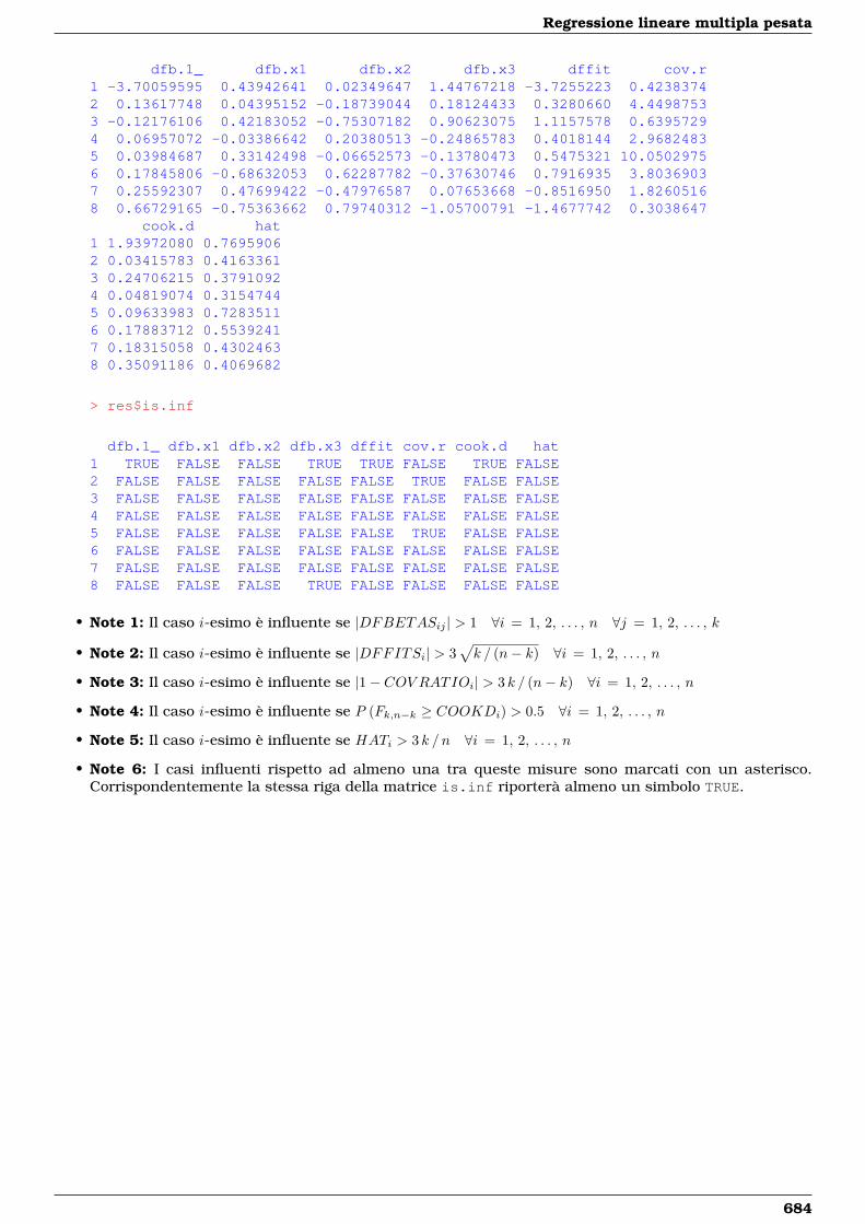
Regressione lineare multipla pesata
dfb.1_ dfb.x1 dfb.x2 dfb.x3 dffit cov.r1 -3.70059595 0.43942641 0.02349647 1.44767218 -3.7255223 0.42383742 0.13617748 0.04395152 -0.18739044 0.18124433 0.3280660 4.44987533 -0.12176106 0.42183052 -0.75307182 0.90623075 1.1157578 0.63957294 0.06957072 -0.03386642 0.20380513 -0.24865783 0.4018144 2.96824835 0.03984687 0.33142498 -0.06652573 -0.13780473 0.5475321 10.05029756 0.17845806 -0.68632053 0.62287782 -0.37630746 0.7916935 3.80369037 0.25592307 0.47699422 -0.47976587 0.07653668 -0.8516950 1.82605168 0.66729165 -0.75363662 0.79740312 -1.05700791 -1.4677742 0.3038647
cook.d hat1 1.93972080 0.76959062 0.03415783 0.41633613 0.24706215 0.37910924 0.04819074 0.31547445 0.09633983 0.72835116 0.17883712 0.55392417 0.18315058 0.43024638 0.35091186 0.4069682
> res$is.inf
dfb.1_ dfb.x1 dfb.x2 dfb.x3 dffit cov.r cook.d hat1 TRUE FALSE FALSE TRUE TRUE FALSE TRUE FALSE2 FALSE FALSE FALSE FALSE FALSE TRUE FALSE FALSE3 FALSE FALSE FALSE FALSE FALSE FALSE FALSE FALSE4 FALSE FALSE FALSE FALSE FALSE FALSE FALSE FALSE5 FALSE FALSE FALSE FALSE FALSE TRUE FALSE FALSE6 FALSE FALSE FALSE FALSE FALSE FALSE FALSE FALSE7 FALSE FALSE FALSE FALSE FALSE FALSE FALSE FALSE8 FALSE FALSE FALSE TRUE FALSE FALSE FALSE FALSE
• Note 1: Il caso i-esimo è influente se |DFBETASij | > 1 ∀i = 1, 2, . . . , n ∀j = 1, 2, . . . , k
• Note 2: Il caso i-esimo è influente se |DFFITSi| > 3√k / (n− k) ∀i = 1, 2, . . . , n
• Note 3: Il caso i-esimo è influente se |1− COV RATIOi| > 3 k / (n− k) ∀i = 1, 2, . . . , n
• Note 4: Il caso i-esimo è influente se P (Fk,n−k ≥ COOKDi) > 0.5 ∀i = 1, 2, . . . , n
• Note 5: Il caso i-esimo è influente se HATi > 3 k / n ∀i = 1, 2, . . . , n
• Note 6: I casi influenti rispetto ad almeno una tra queste misure sono marcati con un asterisco.Corrispondentemente la stessa riga della matrice is.inf riporterà almeno un simbolo TRUE.
684

Parte V
Modelli Lineari Generalizzati
685


Capitolo 17
Regressione Logit
17.1 Simbologia
log(
πi1− πi
)= β1 + β2 xi1 + β3 xi2 + · · ·+ βk xik−1 Yi ∼ Bin(πi, ni) ∀ i = 1, 2, . . . , n
• numero di successi: yi ∀ i = 1, 2, . . . , n
• numero di prove: ni ∀ i = 1, 2, . . . , n
• matrice del modello di dimensione n× k : X
• numero di parametri da stimare e rango della matrice del modello: k
• numero di unità: n
• i-esima riga della matrice del modello : Xi = (1, xi1, xi2, . . . , xik−1) ∀ i = 1, 2, . . . , n
• vettore numerico positivo dei pesi IWLS: w = (w1, w2, . . . , wn)
• matrice diagonale dei pesi IWLS di dimensione n× n : W = diag(w−11 , w−1
2 , . . . , w−1n )
• matrice di proiezione di dimensione n× n : H = X (XT W−1X)−1XT W−1
• valori di leva: hi = Hi,i ∀ i = 1, 2, . . . , n
• distanza di Cook: cdi =(ePi)2 hi
k (1−hi)2 ∀ i = 1, 2, . . . , n
• stime IWLS: β =(β1, β2, . . . , βk
)T• standard error delle stime IWLS: sβ =
√diag((XT W−1X)−1)
• z-values delle stime IWLS: zβ = β / sβ
• correlazione delle stime IWLS: rβi βj =(XT W−1X)−1
i, j
sβisβj
∀ i, j = 1, 2, . . . , k
• residui di devianza: ei = sign (yi − yi)√
2[yi log
(yiyi
+ Ci1
)+ (ni − yi) log
(ni−yini−yi + Ci2
)]∀ i = 1, 2, . . . , n dove Ci1 = 0.5 (1− sign(yi)) / yi e Ci2 = 0.5 (1− sign(ni − yi)) / (ni − yi)
• residui standard: rstandardi = ei /√
1− hi ∀ i = 1, 2, . . . , n
• residui studentizzati: rstudenti = sign (yi − yi)√e2i + hi
(ePi)2/ (1− hi) ∀ i = 1, 2, . . . , n
• residui di Pearson: ePi = yi−ni πi√ni πi (1−πi)
∀i = 1, 2, . . . , n
• residui di lavoro: eWi = yi−ni πini πi (1−πi) ∀i = 1, 2, . . . , n
• residui di riposta: eRi = yi / ni − πi ∀i = 1, 2, . . . , n
• log-verosimiglianza binomiale: ˆ =∑ni=1
[log(niyi
)+ yi log
(yini
)+ (ni − yi) log
(1− yi
ni
)]• valori adattati: πi =
exp (Xi β)1+exp (Xi β) ∀ i = 1, 2, . . . , n
687
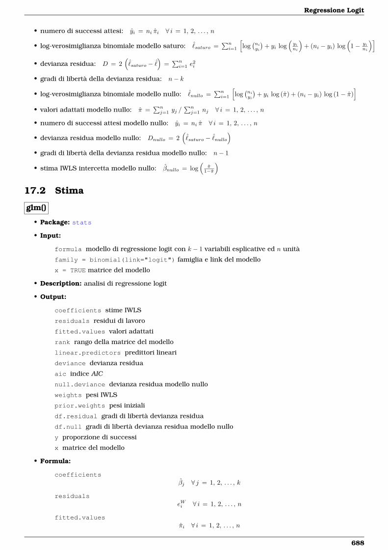
Regressione Logit
• numero di successi attesi: yi = ni πi ∀ i = 1, 2, . . . , n
• log-verosimiglianza binomiale modello saturo: ˆsaturo =
∑ni=1
[log(niyi
)+ yi log
(yini
)+ (ni − yi) log
(1− yi
ni
)]• devianza residua: D = 2
(ˆsaturo − ˆ
)=∑ni=1 e
2i
• gradi di libertà della devianza residua: n− k
• log-verosimiglianza binomiale modello nullo: ˆnullo =
∑ni=1
[log(niyi
)+ yi log (π) + (ni − yi) log (1− π)
]• valori adattati modello nullo: π =
∑nj=1 yj /
∑nj=1 nj ∀ i = 1, 2, . . . , n
• numero di successi attesi modello nullo: yi = ni π ∀ i = 1, 2, . . . , n
• devianza residua modello nullo: Dnullo = 2(
ˆsaturo − ˆ
nullo
)• gradi di libertà della devianza residua modello nullo: n− 1
• stima IWLS intercetta modello nullo: βnullo = log(
π1−π
)
17.2 Stima
glm()
• Package: stats
• Input:
formula modello di regressione logit con k − 1 variabili esplicative ed n unità
family = binomial(link="logit") famiglia e link del modello
x = TRUE matrice del modello
• Description: analisi di regressione logit
• Output:
coefficients stime IWLS
residuals residui di lavoro
fitted.values valori adattati
rank rango della matrice del modello
linear.predictors predittori lineari
deviance devianza residua
aic indice AIC
null.deviance devianza residua modello nullo
weights pesi IWLS
prior.weights pesi iniziali
df.residual gradi di libertà devianza residua
df.null gradi di libertà devianza residua modello nullo
y proporzione di successi
x matrice del modello
• Formula:
coefficientsβj ∀ j = 1, 2, . . . , k
residualseWi ∀ i = 1, 2, . . . , n
fitted.valuesπi ∀ i = 1, 2, . . . , n
688
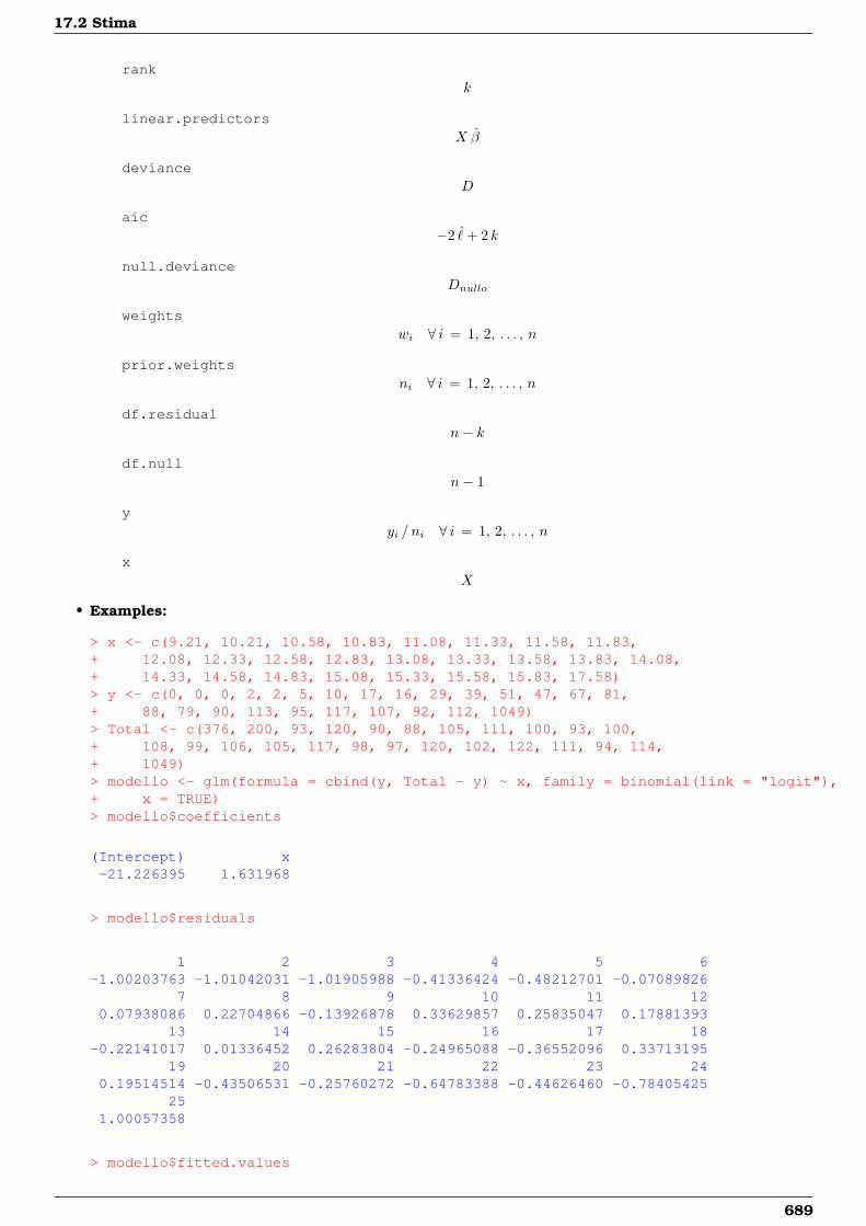
17.2 Stima
rankk
linear.predictorsX β
devianceD
aic−2 ˆ+ 2 k
null.devianceDnullo
weightswi ∀ i = 1, 2, . . . , n
prior.weightsni ∀ i = 1, 2, . . . , n
df.residualn− k
df.nulln− 1
yyi / ni ∀ i = 1, 2, . . . , n
xX
• Examples:
> x <- c(9.21, 10.21, 10.58, 10.83, 11.08, 11.33, 11.58, 11.83,+ 12.08, 12.33, 12.58, 12.83, 13.08, 13.33, 13.58, 13.83, 14.08,+ 14.33, 14.58, 14.83, 15.08, 15.33, 15.58, 15.83, 17.58)> y <- c(0, 0, 0, 2, 2, 5, 10, 17, 16, 29, 39, 51, 47, 67, 81,+ 88, 79, 90, 113, 95, 117, 107, 92, 112, 1049)> Total <- c(376, 200, 93, 120, 90, 88, 105, 111, 100, 93, 100,+ 108, 99, 106, 105, 117, 98, 97, 120, 102, 122, 111, 94, 114,+ 1049)> modello <- glm(formula = cbind(y, Total - y) ~ x, family = binomial(link = "logit"),+ x = TRUE)> modello$coefficients
(Intercept) x-21.226395 1.631968
> modello$residuals
1 2 3 4 5 6-1.00203763 -1.01042031 -1.01905988 -0.41336424 -0.48212701 -0.07089826
7 8 9 10 11 120.07938086 0.22704866 -0.13926878 0.33629857 0.25835047 0.17881393
13 14 15 16 17 18-0.22141017 0.01336452 0.26283804 -0.24965088 -0.36552096 0.33713195
19 20 21 22 23 240.19514514 -0.43506531 -0.25760272 -0.64783388 -0.44626460 -0.78405425
251.00057358
> modello$fitted.values
689
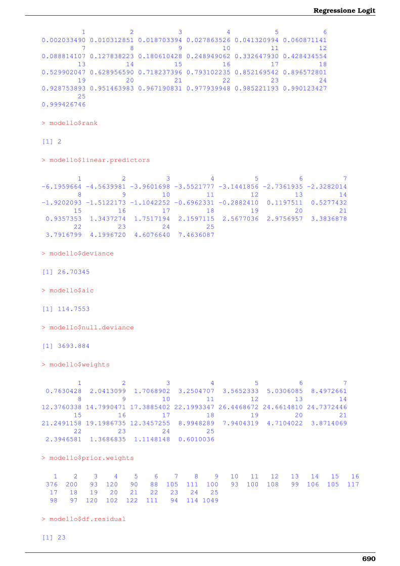
Regressione Logit
1 2 3 4 5 60.002033490 0.010312851 0.018703394 0.027863526 0.041320994 0.060871141
7 8 9 10 11 120.088814107 0.127838223 0.180610428 0.248949062 0.332647930 0.428434554
13 14 15 16 17 180.529902047 0.628956590 0.718237396 0.793102235 0.852169542 0.896572801
19 20 21 22 23 240.928753893 0.951463983 0.967190831 0.977939948 0.985221193 0.990123427
250.999426746
> modello$rank
[1] 2
> modello$linear.predictors
1 2 3 4 5 6 7-6.1959664 -4.5639981 -3.9601698 -3.5521777 -3.1441856 -2.7361935 -2.3282014
8 9 10 11 12 13 14-1.9202093 -1.5122173 -1.1042252 -0.6962331 -0.2882410 0.1197511 0.5277432
15 16 17 18 19 20 210.9357353 1.3437274 1.7517194 2.1597115 2.5677036 2.9756957 3.3836878
22 23 24 253.7916799 4.1996720 4.6076640 7.4636087
> modello$deviance
[1] 26.70345
> modello$aic
[1] 114.7553
> modello$null.deviance
[1] 3693.884
> modello$weights
1 2 3 4 5 6 70.7630428 2.0413099 1.7068902 3.2504707 3.5652333 5.0306085 8.4972661
8 9 10 11 12 13 1412.3760338 14.7990471 17.3885402 22.1993347 26.4468672 24.6614810 24.7372446
15 16 17 18 19 20 2121.2491158 19.1986735 12.3457255 8.9948289 7.9404319 4.7104022 3.8714069
22 23 24 252.3946581 1.3686835 1.1148148 0.6010036
> modello$prior.weights
1 2 3 4 5 6 7 8 9 10 11 12 13 14 15 16376 200 93 120 90 88 105 111 100 93 100 108 99 106 105 11717 18 19 20 21 22 23 24 2598 97 120 102 122 111 94 114 1049
> modello$df.residual
[1] 23
690
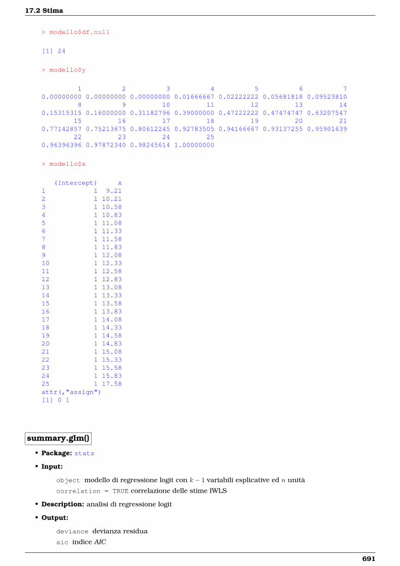
17.2 Stima
> modello$df.null
[1] 24
> modello$y
1 2 3 4 5 6 70.00000000 0.00000000 0.00000000 0.01666667 0.02222222 0.05681818 0.09523810
8 9 10 11 12 13 140.15315315 0.16000000 0.31182796 0.39000000 0.47222222 0.47474747 0.63207547
15 16 17 18 19 20 210.77142857 0.75213675 0.80612245 0.92783505 0.94166667 0.93137255 0.95901639
22 23 24 250.96396396 0.97872340 0.98245614 1.00000000
> modello$x
(Intercept) x1 1 9.212 1 10.213 1 10.584 1 10.835 1 11.086 1 11.337 1 11.588 1 11.839 1 12.0810 1 12.3311 1 12.5812 1 12.8313 1 13.0814 1 13.3315 1 13.5816 1 13.8317 1 14.0818 1 14.3319 1 14.5820 1 14.8321 1 15.0822 1 15.3323 1 15.5824 1 15.8325 1 17.58attr(,"assign")[1] 0 1
summary.glm()
• Package: stats
• Input:
object modello di regressione logit con k − 1 variabili esplicative ed n unità
correlation = TRUE correlazione delle stime IWLS
• Description: analisi di regressione logit
• Output:
deviance devianza residua
aic indice AIC
691
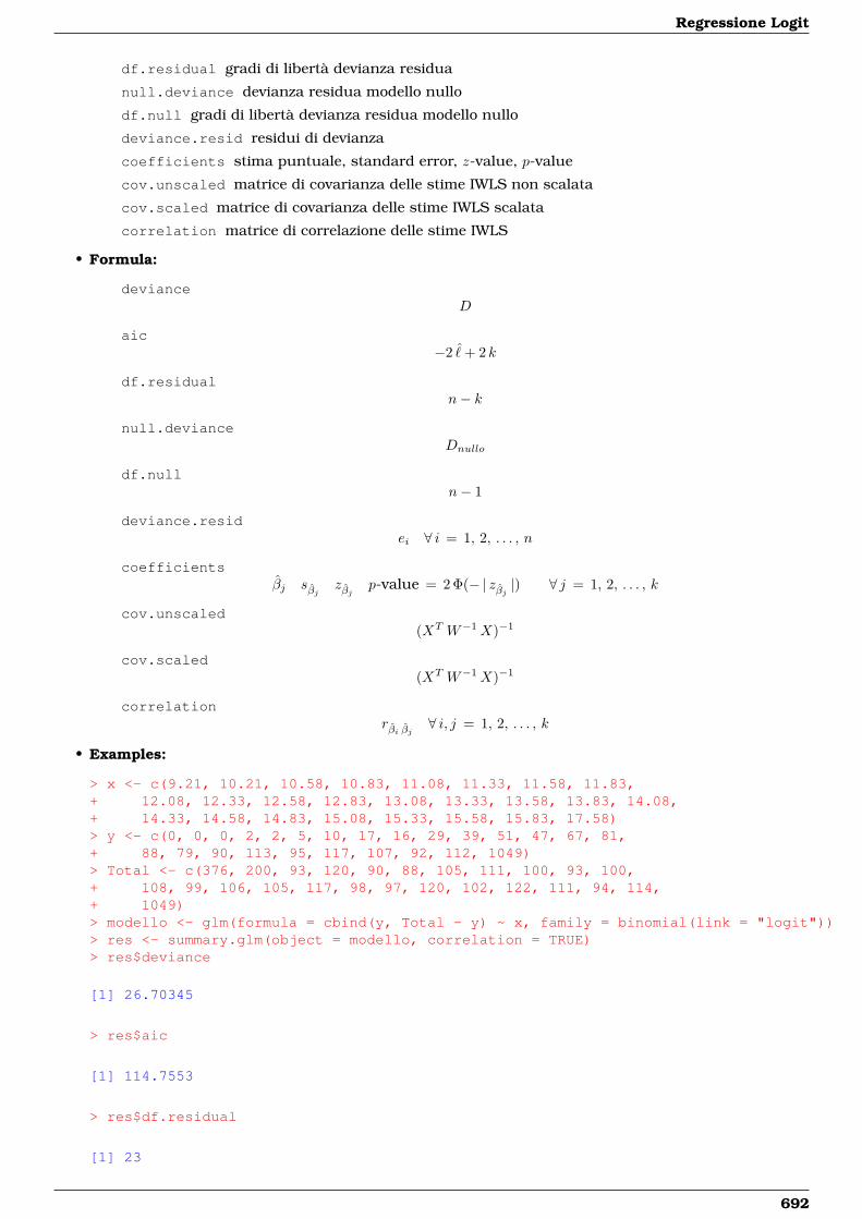
Regressione Logit
df.residual gradi di libertà devianza residua
null.deviance devianza residua modello nullo
df.null gradi di libertà devianza residua modello nullo
deviance.resid residui di devianza
coefficients stima puntuale, standard error, z-value, p-value
cov.unscaled matrice di covarianza delle stime IWLS non scalata
cov.scaled matrice di covarianza delle stime IWLS scalata
correlation matrice di correlazione delle stime IWLS
• Formula:
devianceD
aic−2 ˆ+ 2 k
df.residualn− k
null.devianceDnullo
df.nulln− 1
deviance.residei ∀ i = 1, 2, . . . , n
coefficientsβj sβj zβj p-value = 2 Φ(− | zβj |) ∀ j = 1, 2, . . . , k
cov.unscaled(XT W−1X)−1
cov.scaled(XT W−1X)−1
correlationrβi βj ∀ i, j = 1, 2, . . . , k
• Examples:
> x <- c(9.21, 10.21, 10.58, 10.83, 11.08, 11.33, 11.58, 11.83,+ 12.08, 12.33, 12.58, 12.83, 13.08, 13.33, 13.58, 13.83, 14.08,+ 14.33, 14.58, 14.83, 15.08, 15.33, 15.58, 15.83, 17.58)> y <- c(0, 0, 0, 2, 2, 5, 10, 17, 16, 29, 39, 51, 47, 67, 81,+ 88, 79, 90, 113, 95, 117, 107, 92, 112, 1049)> Total <- c(376, 200, 93, 120, 90, 88, 105, 111, 100, 93, 100,+ 108, 99, 106, 105, 117, 98, 97, 120, 102, 122, 111, 94, 114,+ 1049)> modello <- glm(formula = cbind(y, Total - y) ~ x, family = binomial(link = "logit"))> res <- summary.glm(object = modello, correlation = TRUE)> res$deviance
[1] 26.70345
> res$aic
[1] 114.7553
> res$df.residual
[1] 23
692
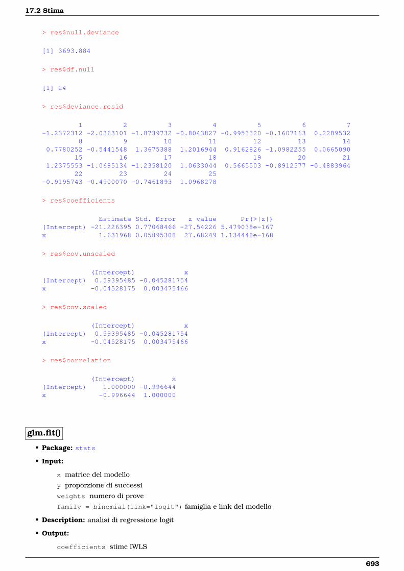
17.2 Stima
> res$null.deviance
[1] 3693.884
> res$df.null
[1] 24
> res$deviance.resid
1 2 3 4 5 6 7-1.2372312 -2.0363101 -1.8739732 -0.8043827 -0.9953320 -0.1607163 0.2289532
8 9 10 11 12 13 140.7780252 -0.5441548 1.3675388 1.2016944 0.9162826 -1.0982255 0.0665090
15 16 17 18 19 20 211.2375553 -1.0695134 -1.2358120 1.0633044 0.5665503 -0.8912577 -0.4883964
22 23 24 25-0.9195743 -0.4900070 -0.7461893 1.0968278
> res$coefficients
Estimate Std. Error z value Pr(>|z|)(Intercept) -21.226395 0.77068466 -27.54226 5.479038e-167x 1.631968 0.05895308 27.68249 1.134448e-168
> res$cov.unscaled
(Intercept) x(Intercept) 0.59395485 -0.045281754x -0.04528175 0.003475466
> res$cov.scaled
(Intercept) x(Intercept) 0.59395485 -0.045281754x -0.04528175 0.003475466
> res$correlation
(Intercept) x(Intercept) 1.000000 -0.996644x -0.996644 1.000000
glm.fit()
• Package: stats
• Input:
x matrice del modello
y proporzione di successi
weights numero di prove
family = binomial(link="logit") famiglia e link del modello
• Description: analisi di regressione logit
• Output:
coefficients stime IWLS
693
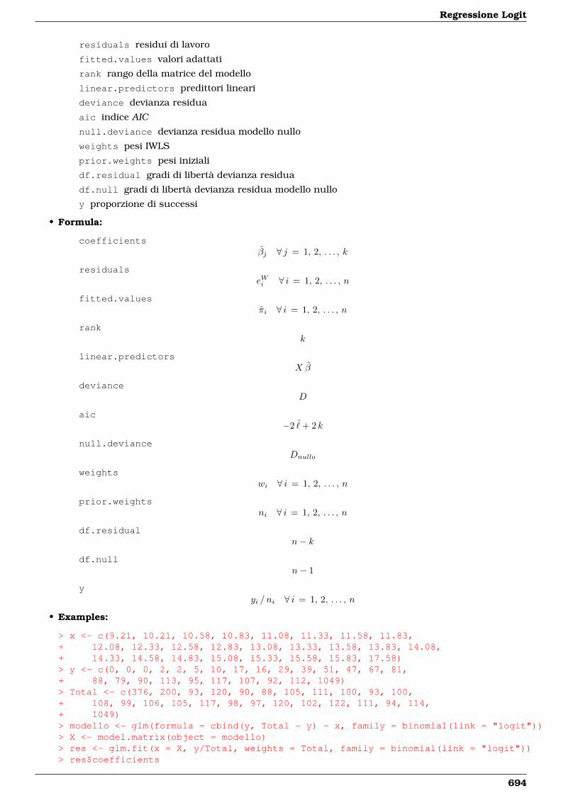
Regressione Logit
residuals residui di lavoro
fitted.values valori adattati
rank rango della matrice del modello
linear.predictors predittori lineari
deviance devianza residua
aic indice AIC
null.deviance devianza residua modello nullo
weights pesi IWLS
prior.weights pesi iniziali
df.residual gradi di libertà devianza residua
df.null gradi di libertà devianza residua modello nullo
y proporzione di successi
• Formula:
coefficientsβj ∀ j = 1, 2, . . . , k
residualseWi ∀ i = 1, 2, . . . , n
fitted.valuesπi ∀ i = 1, 2, . . . , n
rankk
linear.predictorsX β
devianceD
aic−2 ˆ+ 2 k
null.devianceDnullo
weightswi ∀ i = 1, 2, . . . , n
prior.weightsni ∀ i = 1, 2, . . . , n
df.residualn− k
df.nulln− 1
yyi / ni ∀ i = 1, 2, . . . , n
• Examples:
> x <- c(9.21, 10.21, 10.58, 10.83, 11.08, 11.33, 11.58, 11.83,+ 12.08, 12.33, 12.58, 12.83, 13.08, 13.33, 13.58, 13.83, 14.08,+ 14.33, 14.58, 14.83, 15.08, 15.33, 15.58, 15.83, 17.58)> y <- c(0, 0, 0, 2, 2, 5, 10, 17, 16, 29, 39, 51, 47, 67, 81,+ 88, 79, 90, 113, 95, 117, 107, 92, 112, 1049)> Total <- c(376, 200, 93, 120, 90, 88, 105, 111, 100, 93, 100,+ 108, 99, 106, 105, 117, 98, 97, 120, 102, 122, 111, 94, 114,+ 1049)> modello <- glm(formula = cbind(y, Total - y) ~ x, family = binomial(link = "logit"))> X <- model.matrix(object = modello)> res <- glm.fit(x = X, y/Total, weights = Total, family = binomial(link = "logit"))> res$coefficients
694

17.2 Stima
(Intercept) x-21.226395 1.631968
> res$residuals
[1] -1.00203763 -1.01042031 -1.01905988 -0.41336424 -0.48212701 -0.07089826[7] 0.07938086 0.22704866 -0.13926878 0.33629857 0.25835047 0.17881393
[13] -0.22141017 0.01336452 0.26283804 -0.24965088 -0.36552096 0.33713195[19] 0.19514514 -0.43506531 -0.25760272 -0.64783388 -0.44626460 -0.78405425[25] 1.00057358
> res$fitted.values
[1] 0.002033490 0.010312851 0.018703394 0.027863526 0.041320994 0.060871141[7] 0.088814107 0.127838223 0.180610428 0.248949062 0.332647930 0.428434554
[13] 0.529902047 0.628956590 0.718237396 0.793102235 0.852169542 0.896572801[19] 0.928753893 0.951463983 0.967190831 0.977939948 0.985221193 0.990123427[25] 0.999426746
> res$rank
[1] 2
> res$linear.predictors
[1] -6.1959664 -4.5639981 -3.9601698 -3.5521777 -3.1441856 -2.7361935[7] -2.3282014 -1.9202093 -1.5122173 -1.1042252 -0.6962331 -0.2882410
[13] 0.1197511 0.5277432 0.9357353 1.3437274 1.7517194 2.1597115[19] 2.5677036 2.9756957 3.3836878 3.7916799 4.1996720 4.6076640[25] 7.4636087
> res$deviance
[1] 26.70345
> res$aic
[1] 114.7553
> res$null.deviance
[1] 3693.884
> res$weights
[1] 0.7630428 2.0413099 1.7068902 3.2504707 3.5652333 5.0306085[7] 8.4972661 12.3760338 14.7990471 17.3885402 22.1993347 26.4468672
[13] 24.6614810 24.7372446 21.2491158 19.1986735 12.3457255 8.9948289[19] 7.9404319 4.7104022 3.8714069 2.3946581 1.3686835 1.1148148[25] 0.6010036
> res$prior.weights
[1] 376 200 93 120 90 88 105 111 100 93 100 108 99 106 105[16] 117 98 97 120 102 122 111 94 114 1049
> res$df.residual
[1] 23
695

Regressione Logit
> res$df.null
[1] 24
> res$y
[1] 0.00000000 0.00000000 0.00000000 0.01666667 0.02222222 0.05681818[7] 0.09523810 0.15315315 0.16000000 0.31182796 0.39000000 0.47222222
[13] 0.47474747 0.63207547 0.77142857 0.75213675 0.80612245 0.92783505[19] 0.94166667 0.93137255 0.95901639 0.96396396 0.97872340 0.98245614[25] 1.00000000
vcov()
• Package: stats
• Input:
object modello di regressione logit con k − 1 variabili esplicative ed n unità
• Description: matrice di covarianza delle stime IWLS
• Formula:(XT W−1X)−1
• Examples:
> x <- c(9.21, 10.21, 10.58, 10.83, 11.08, 11.33, 11.58, 11.83,+ 12.08, 12.33, 12.58, 12.83, 13.08, 13.33, 13.58, 13.83, 14.08,+ 14.33, 14.58, 14.83, 15.08, 15.33, 15.58, 15.83, 17.58)> y <- c(0, 0, 0, 2, 2, 5, 10, 17, 16, 29, 39, 51, 47, 67, 81,+ 88, 79, 90, 113, 95, 117, 107, 92, 112, 1049)> Total <- c(376, 200, 93, 120, 90, 88, 105, 111, 100, 93, 100,+ 108, 99, 106, 105, 117, 98, 97, 120, 102, 122, 111, 94, 114,+ 1049)> modello <- glm(formula = cbind(y, Total - y) ~ x, family = binomial(link = "logit"))> vcov(object = modello)
(Intercept) x(Intercept) 0.59395485 -0.045281754x -0.04528175 0.003475466
coef()
• Package: stats
• Input:
object modello di regressione logit con k − 1 variabili esplicative ed n unità
• Description: stime IWLS
• Formula:βj ∀ j = 1, 2, . . . , k
• Examples:
696
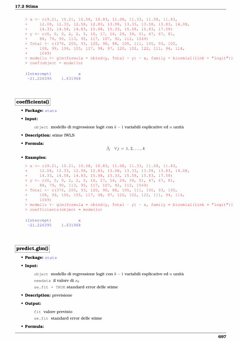
17.2 Stima
> x <- c(9.21, 10.21, 10.58, 10.83, 11.08, 11.33, 11.58, 11.83,+ 12.08, 12.33, 12.58, 12.83, 13.08, 13.33, 13.58, 13.83, 14.08,+ 14.33, 14.58, 14.83, 15.08, 15.33, 15.58, 15.83, 17.58)> y <- c(0, 0, 0, 2, 2, 5, 10, 17, 16, 29, 39, 51, 47, 67, 81,+ 88, 79, 90, 113, 95, 117, 107, 92, 112, 1049)> Total <- c(376, 200, 93, 120, 90, 88, 105, 111, 100, 93, 100,+ 108, 99, 106, 105, 117, 98, 97, 120, 102, 122, 111, 94, 114,+ 1049)> modello <- glm(formula = cbind(y, Total - y) ~ x, family = binomial(link = "logit"))> coef(object = modello)
(Intercept) x-21.226395 1.631968
coefficients()
• Package: stats
• Input:
object modello di regressione logit con k − 1 variabili esplicative ed n unità
• Description: stime IWLS
• Formula:βj ∀ j = 1, 2, . . . , k
• Examples:
> x <- c(9.21, 10.21, 10.58, 10.83, 11.08, 11.33, 11.58, 11.83,+ 12.08, 12.33, 12.58, 12.83, 13.08, 13.33, 13.58, 13.83, 14.08,+ 14.33, 14.58, 14.83, 15.08, 15.33, 15.58, 15.83, 17.58)> y <- c(0, 0, 0, 2, 2, 5, 10, 17, 16, 29, 39, 51, 47, 67, 81,+ 88, 79, 90, 113, 95, 117, 107, 92, 112, 1049)> Total <- c(376, 200, 93, 120, 90, 88, 105, 111, 100, 93, 100,+ 108, 99, 106, 105, 117, 98, 97, 120, 102, 122, 111, 94, 114,+ 1049)> modello <- glm(formula = cbind(y, Total - y) ~ x, family = binomial(link = "logit"))> coefficients(object = modello)
(Intercept) x-21.226395 1.631968
predict.glm()
• Package: stats
• Input:
object modello di regressione logit con k − 1 variabili esplicative ed n unità
newdata il valore di x0
se.fit = TRUE standard error delle stime
• Description: previsione
• Output:
fit valore previsto
se.fit standard error delle stime
• Formula:
697
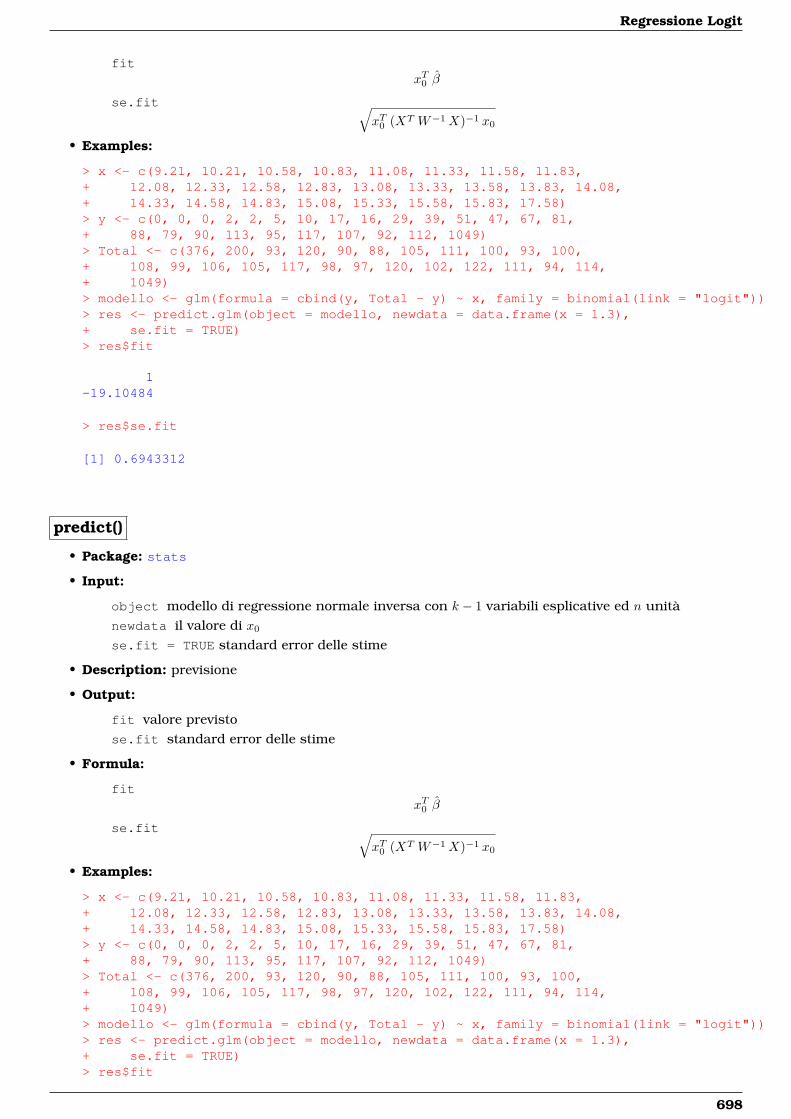
Regressione Logit
fitxT0 β
se.fit √xT0 (XT W−1X)−1 x0
• Examples:
> x <- c(9.21, 10.21, 10.58, 10.83, 11.08, 11.33, 11.58, 11.83,+ 12.08, 12.33, 12.58, 12.83, 13.08, 13.33, 13.58, 13.83, 14.08,+ 14.33, 14.58, 14.83, 15.08, 15.33, 15.58, 15.83, 17.58)> y <- c(0, 0, 0, 2, 2, 5, 10, 17, 16, 29, 39, 51, 47, 67, 81,+ 88, 79, 90, 113, 95, 117, 107, 92, 112, 1049)> Total <- c(376, 200, 93, 120, 90, 88, 105, 111, 100, 93, 100,+ 108, 99, 106, 105, 117, 98, 97, 120, 102, 122, 111, 94, 114,+ 1049)> modello <- glm(formula = cbind(y, Total - y) ~ x, family = binomial(link = "logit"))> res <- predict.glm(object = modello, newdata = data.frame(x = 1.3),+ se.fit = TRUE)> res$fit
1-19.10484
> res$se.fit
[1] 0.6943312
predict()
• Package: stats
• Input:
object modello di regressione normale inversa con k − 1 variabili esplicative ed n unitànewdata il valore di x0
se.fit = TRUE standard error delle stime
• Description: previsione
• Output:
fit valore previstose.fit standard error delle stime
• Formula:
fitxT0 β
se.fit √xT0 (XT W−1X)−1 x0
• Examples:
> x <- c(9.21, 10.21, 10.58, 10.83, 11.08, 11.33, 11.58, 11.83,+ 12.08, 12.33, 12.58, 12.83, 13.08, 13.33, 13.58, 13.83, 14.08,+ 14.33, 14.58, 14.83, 15.08, 15.33, 15.58, 15.83, 17.58)> y <- c(0, 0, 0, 2, 2, 5, 10, 17, 16, 29, 39, 51, 47, 67, 81,+ 88, 79, 90, 113, 95, 117, 107, 92, 112, 1049)> Total <- c(376, 200, 93, 120, 90, 88, 105, 111, 100, 93, 100,+ 108, 99, 106, 105, 117, 98, 97, 120, 102, 122, 111, 94, 114,+ 1049)> modello <- glm(formula = cbind(y, Total - y) ~ x, family = binomial(link = "logit"))> res <- predict.glm(object = modello, newdata = data.frame(x = 1.3),+ se.fit = TRUE)> res$fit
698
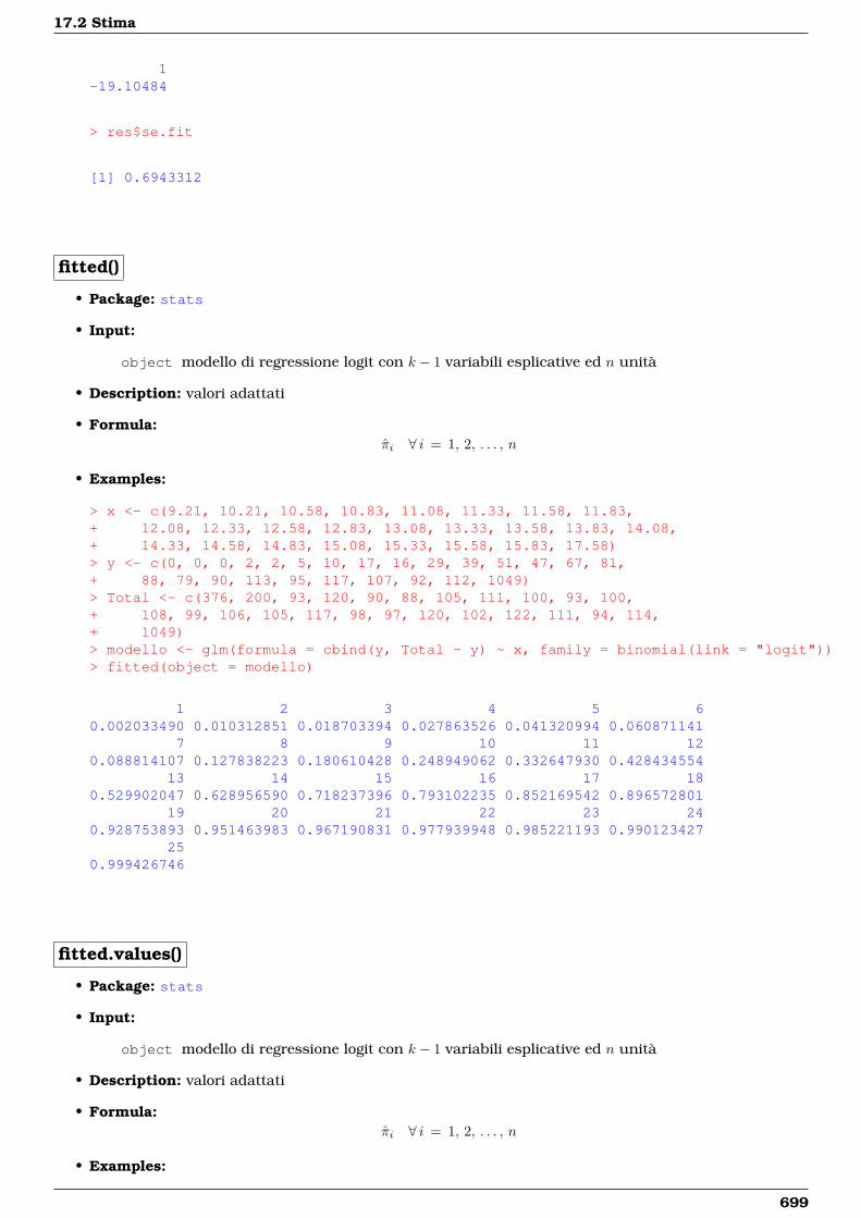
17.2 Stima
1-19.10484
> res$se.fit
[1] 0.6943312
fitted()
• Package: stats
• Input:
object modello di regressione logit con k − 1 variabili esplicative ed n unità
• Description: valori adattati
• Formula:πi ∀ i = 1, 2, . . . , n
• Examples:
> x <- c(9.21, 10.21, 10.58, 10.83, 11.08, 11.33, 11.58, 11.83,+ 12.08, 12.33, 12.58, 12.83, 13.08, 13.33, 13.58, 13.83, 14.08,+ 14.33, 14.58, 14.83, 15.08, 15.33, 15.58, 15.83, 17.58)> y <- c(0, 0, 0, 2, 2, 5, 10, 17, 16, 29, 39, 51, 47, 67, 81,+ 88, 79, 90, 113, 95, 117, 107, 92, 112, 1049)> Total <- c(376, 200, 93, 120, 90, 88, 105, 111, 100, 93, 100,+ 108, 99, 106, 105, 117, 98, 97, 120, 102, 122, 111, 94, 114,+ 1049)> modello <- glm(formula = cbind(y, Total - y) ~ x, family = binomial(link = "logit"))> fitted(object = modello)
1 2 3 4 5 60.002033490 0.010312851 0.018703394 0.027863526 0.041320994 0.060871141
7 8 9 10 11 120.088814107 0.127838223 0.180610428 0.248949062 0.332647930 0.428434554
13 14 15 16 17 180.529902047 0.628956590 0.718237396 0.793102235 0.852169542 0.896572801
19 20 21 22 23 240.928753893 0.951463983 0.967190831 0.977939948 0.985221193 0.990123427
250.999426746
fitted.values()
• Package: stats
• Input:
object modello di regressione logit con k − 1 variabili esplicative ed n unità
• Description: valori adattati
• Formula:πi ∀ i = 1, 2, . . . , n
• Examples:
699
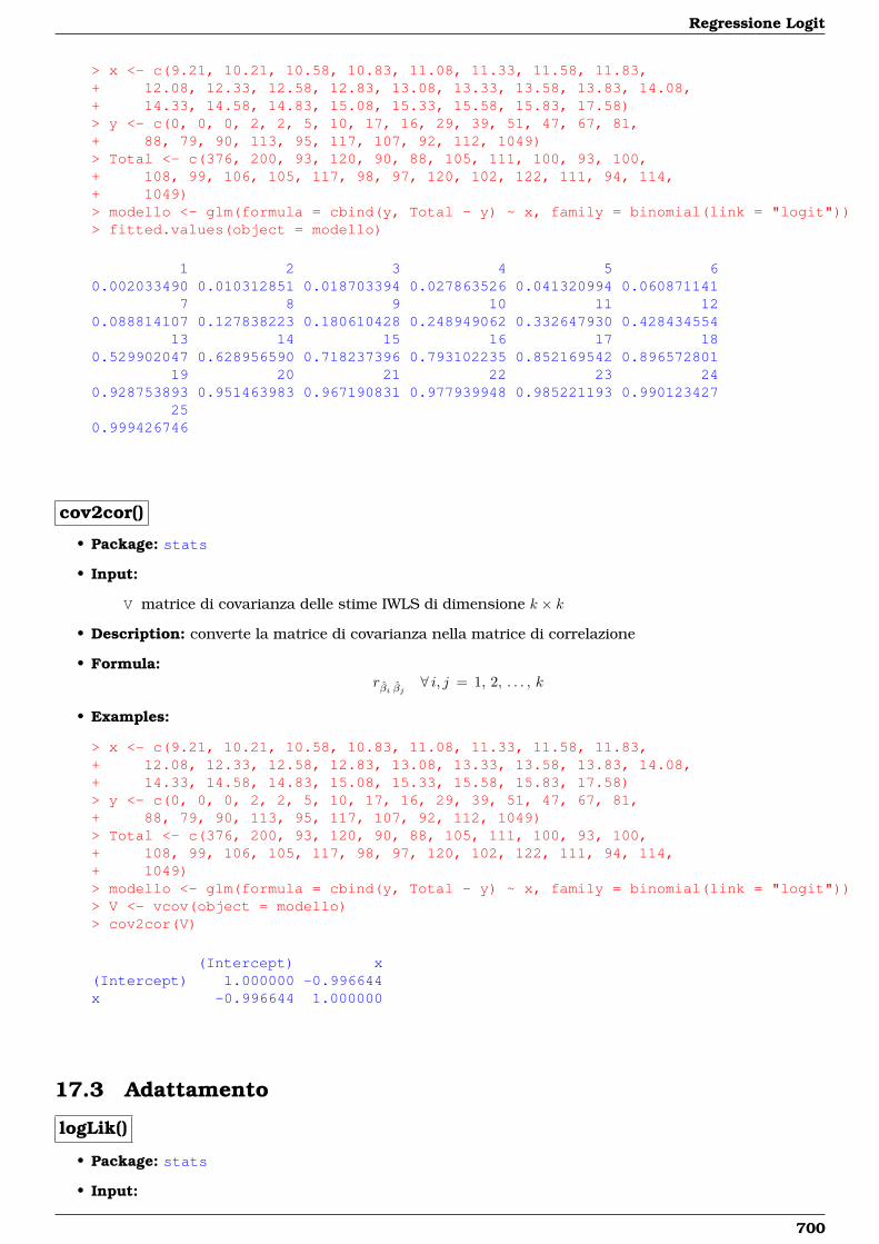
Regressione Logit
> x <- c(9.21, 10.21, 10.58, 10.83, 11.08, 11.33, 11.58, 11.83,+ 12.08, 12.33, 12.58, 12.83, 13.08, 13.33, 13.58, 13.83, 14.08,+ 14.33, 14.58, 14.83, 15.08, 15.33, 15.58, 15.83, 17.58)> y <- c(0, 0, 0, 2, 2, 5, 10, 17, 16, 29, 39, 51, 47, 67, 81,+ 88, 79, 90, 113, 95, 117, 107, 92, 112, 1049)> Total <- c(376, 200, 93, 120, 90, 88, 105, 111, 100, 93, 100,+ 108, 99, 106, 105, 117, 98, 97, 120, 102, 122, 111, 94, 114,+ 1049)> modello <- glm(formula = cbind(y, Total - y) ~ x, family = binomial(link = "logit"))> fitted.values(object = modello)
1 2 3 4 5 60.002033490 0.010312851 0.018703394 0.027863526 0.041320994 0.060871141
7 8 9 10 11 120.088814107 0.127838223 0.180610428 0.248949062 0.332647930 0.428434554
13 14 15 16 17 180.529902047 0.628956590 0.718237396 0.793102235 0.852169542 0.896572801
19 20 21 22 23 240.928753893 0.951463983 0.967190831 0.977939948 0.985221193 0.990123427
250.999426746
cov2cor()
• Package: stats
• Input:
V matrice di covarianza delle stime IWLS di dimensione k × k
• Description: converte la matrice di covarianza nella matrice di correlazione
• Formula:rβi βj ∀ i, j = 1, 2, . . . , k
• Examples:
> x <- c(9.21, 10.21, 10.58, 10.83, 11.08, 11.33, 11.58, 11.83,+ 12.08, 12.33, 12.58, 12.83, 13.08, 13.33, 13.58, 13.83, 14.08,+ 14.33, 14.58, 14.83, 15.08, 15.33, 15.58, 15.83, 17.58)> y <- c(0, 0, 0, 2, 2, 5, 10, 17, 16, 29, 39, 51, 47, 67, 81,+ 88, 79, 90, 113, 95, 117, 107, 92, 112, 1049)> Total <- c(376, 200, 93, 120, 90, 88, 105, 111, 100, 93, 100,+ 108, 99, 106, 105, 117, 98, 97, 120, 102, 122, 111, 94, 114,+ 1049)> modello <- glm(formula = cbind(y, Total - y) ~ x, family = binomial(link = "logit"))> V <- vcov(object = modello)> cov2cor(V)
(Intercept) x(Intercept) 1.000000 -0.996644x -0.996644 1.000000
17.3 Adattamento
logLik()
• Package: stats
• Input:
700

17.3 Adattamento
object modello di regressione logit con k − 1 variabili esplicative ed n unità
• Description: log-verosimiglianza binomiale
• Formula:ˆ
• Examples:
> x <- c(9.21, 10.21, 10.58, 10.83, 11.08, 11.33, 11.58, 11.83,+ 12.08, 12.33, 12.58, 12.83, 13.08, 13.33, 13.58, 13.83, 14.08,+ 14.33, 14.58, 14.83, 15.08, 15.33, 15.58, 15.83, 17.58)> y <- c(0, 0, 0, 2, 2, 5, 10, 17, 16, 29, 39, 51, 47, 67, 81,+ 88, 79, 90, 113, 95, 117, 107, 92, 112, 1049)> Total <- c(376, 200, 93, 120, 90, 88, 105, 111, 100, 93, 100,+ 108, 99, 106, 105, 117, 98, 97, 120, 102, 122, 111, 94, 114,+ 1049)> modello <- glm(formula = cbind(y, Total - y) ~ x, family = binomial(link = "logit"))> logLik(object = modello)
'log Lik.' -55.37763 (df=2)
AIC()
• Package: stats
• Input:
object modello di regressione logit con k − 1 variabili esplicative ed n unità
• Description: indice AIC
• Formula:−2 ˆ+ 2 k
• Examples:
> x <- c(9.21, 10.21, 10.58, 10.83, 11.08, 11.33, 11.58, 11.83,+ 12.08, 12.33, 12.58, 12.83, 13.08, 13.33, 13.58, 13.83, 14.08,+ 14.33, 14.58, 14.83, 15.08, 15.33, 15.58, 15.83, 17.58)> y <- c(0, 0, 0, 2, 2, 5, 10, 17, 16, 29, 39, 51, 47, 67, 81,+ 88, 79, 90, 113, 95, 117, 107, 92, 112, 1049)> Total <- c(376, 200, 93, 120, 90, 88, 105, 111, 100, 93, 100,+ 108, 99, 106, 105, 117, 98, 97, 120, 102, 122, 111, 94, 114,+ 1049)> modello <- glm(formula = cbind(y, Total - y) ~ x, family = binomial(link = "logit"))> AIC(object = modello)
[1] 114.7553
durbin.watson()
• Package: car
• Input:
model modello di regressione logit con k − 1 variabili esplicative ed n unità
• Description: test di Durbin–Watson per verificare la presenza di autocorrelazioni tra i residui
• Output:
dw valore empirico della statistica D–W
701
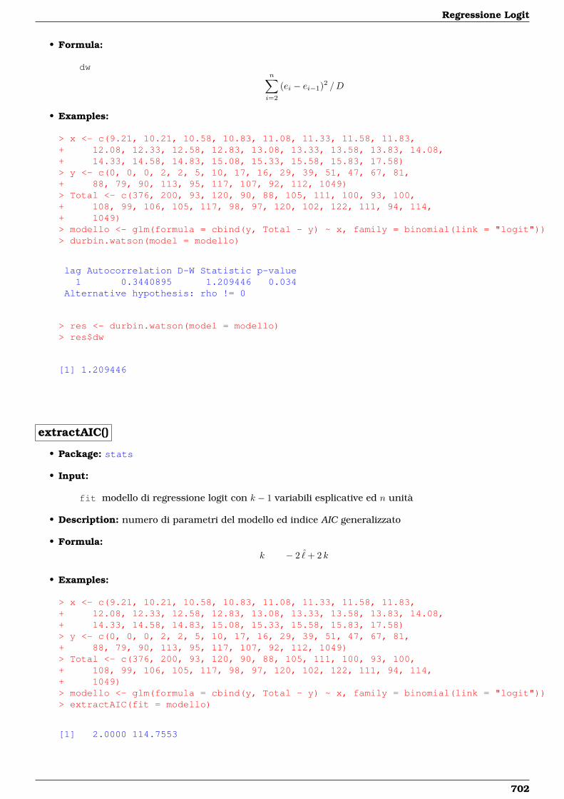
Regressione Logit
• Formula:
dwn∑i=2
(ei − ei−1)2 /D
• Examples:
> x <- c(9.21, 10.21, 10.58, 10.83, 11.08, 11.33, 11.58, 11.83,+ 12.08, 12.33, 12.58, 12.83, 13.08, 13.33, 13.58, 13.83, 14.08,+ 14.33, 14.58, 14.83, 15.08, 15.33, 15.58, 15.83, 17.58)> y <- c(0, 0, 0, 2, 2, 5, 10, 17, 16, 29, 39, 51, 47, 67, 81,+ 88, 79, 90, 113, 95, 117, 107, 92, 112, 1049)> Total <- c(376, 200, 93, 120, 90, 88, 105, 111, 100, 93, 100,+ 108, 99, 106, 105, 117, 98, 97, 120, 102, 122, 111, 94, 114,+ 1049)> modello <- glm(formula = cbind(y, Total - y) ~ x, family = binomial(link = "logit"))> durbin.watson(model = modello)
lag Autocorrelation D-W Statistic p-value1 0.3440895 1.209446 0.034
Alternative hypothesis: rho != 0
> res <- durbin.watson(model = modello)> res$dw
[1] 1.209446
extractAIC()
• Package: stats
• Input:
fit modello di regressione logit con k − 1 variabili esplicative ed n unità
• Description: numero di parametri del modello ed indice AIC generalizzato
• Formula:k − 2 ˆ+ 2 k
• Examples:
> x <- c(9.21, 10.21, 10.58, 10.83, 11.08, 11.33, 11.58, 11.83,+ 12.08, 12.33, 12.58, 12.83, 13.08, 13.33, 13.58, 13.83, 14.08,+ 14.33, 14.58, 14.83, 15.08, 15.33, 15.58, 15.83, 17.58)> y <- c(0, 0, 0, 2, 2, 5, 10, 17, 16, 29, 39, 51, 47, 67, 81,+ 88, 79, 90, 113, 95, 117, 107, 92, 112, 1049)> Total <- c(376, 200, 93, 120, 90, 88, 105, 111, 100, 93, 100,+ 108, 99, 106, 105, 117, 98, 97, 120, 102, 122, 111, 94, 114,+ 1049)> modello <- glm(formula = cbind(y, Total - y) ~ x, family = binomial(link = "logit"))> extractAIC(fit = modello)
[1] 2.0000 114.7553
702
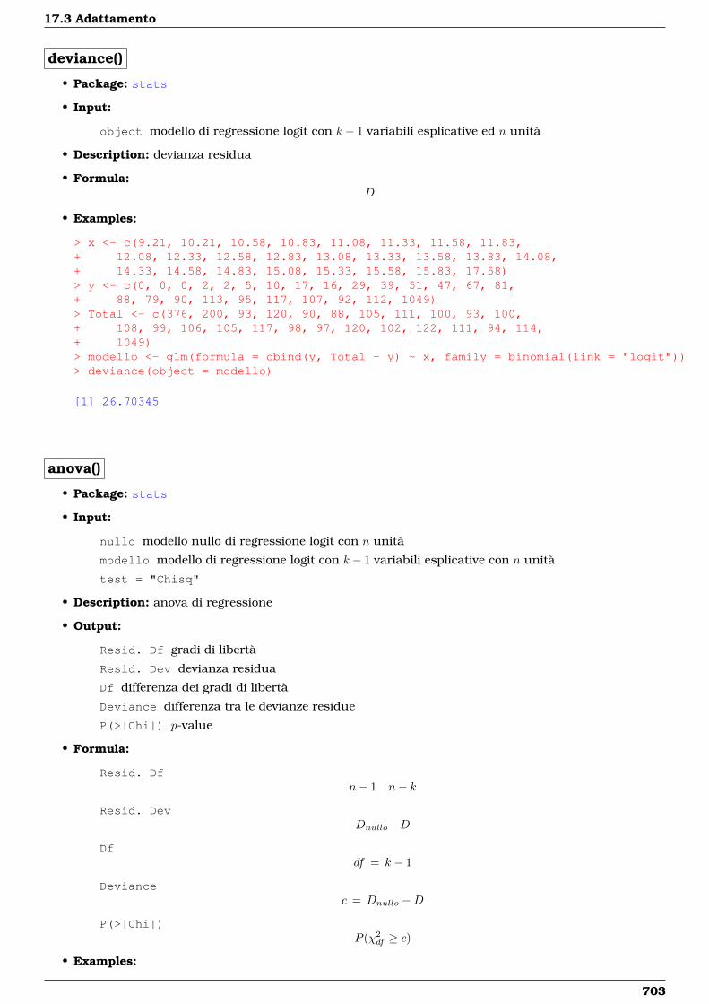
17.3 Adattamento
deviance()
• Package: stats
• Input:
object modello di regressione logit con k − 1 variabili esplicative ed n unità
• Description: devianza residua
• Formula:D
• Examples:
> x <- c(9.21, 10.21, 10.58, 10.83, 11.08, 11.33, 11.58, 11.83,+ 12.08, 12.33, 12.58, 12.83, 13.08, 13.33, 13.58, 13.83, 14.08,+ 14.33, 14.58, 14.83, 15.08, 15.33, 15.58, 15.83, 17.58)> y <- c(0, 0, 0, 2, 2, 5, 10, 17, 16, 29, 39, 51, 47, 67, 81,+ 88, 79, 90, 113, 95, 117, 107, 92, 112, 1049)> Total <- c(376, 200, 93, 120, 90, 88, 105, 111, 100, 93, 100,+ 108, 99, 106, 105, 117, 98, 97, 120, 102, 122, 111, 94, 114,+ 1049)> modello <- glm(formula = cbind(y, Total - y) ~ x, family = binomial(link = "logit"))> deviance(object = modello)
[1] 26.70345
anova()
• Package: stats
• Input:
nullo modello nullo di regressione logit con n unità
modello modello di regressione logit con k − 1 variabili esplicative con n unità
test = "Chisq"
• Description: anova di regressione
• Output:
Resid. Df gradi di libertà
Resid. Dev devianza residua
Df differenza dei gradi di libertà
Deviance differenza tra le devianze residue
P(>|Chi|) p-value
• Formula:
Resid. Dfn− 1 n− k
Resid. DevDnullo D
Dfdf = k − 1
Deviancec = Dnullo −D
P(>|Chi|)P (χ2
df ≥ c)
• Examples:
703
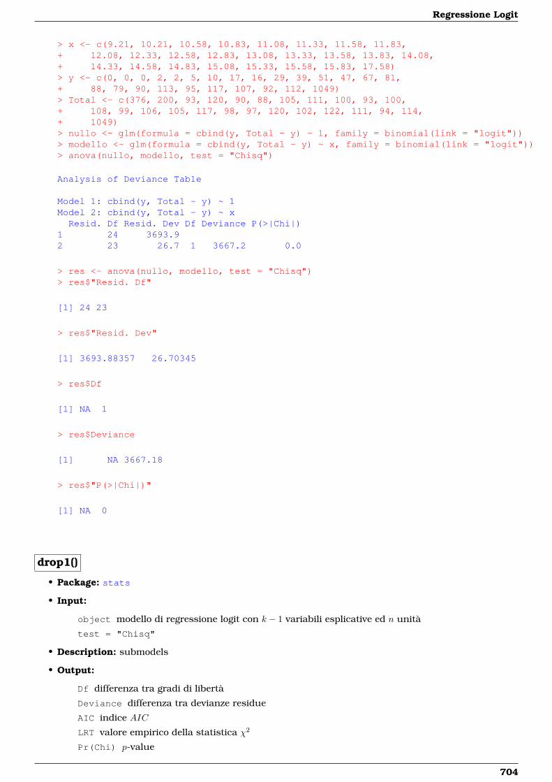
Regressione Logit
> x <- c(9.21, 10.21, 10.58, 10.83, 11.08, 11.33, 11.58, 11.83,+ 12.08, 12.33, 12.58, 12.83, 13.08, 13.33, 13.58, 13.83, 14.08,+ 14.33, 14.58, 14.83, 15.08, 15.33, 15.58, 15.83, 17.58)> y <- c(0, 0, 0, 2, 2, 5, 10, 17, 16, 29, 39, 51, 47, 67, 81,+ 88, 79, 90, 113, 95, 117, 107, 92, 112, 1049)> Total <- c(376, 200, 93, 120, 90, 88, 105, 111, 100, 93, 100,+ 108, 99, 106, 105, 117, 98, 97, 120, 102, 122, 111, 94, 114,+ 1049)> nullo <- glm(formula = cbind(y, Total - y) ~ 1, family = binomial(link = "logit"))> modello <- glm(formula = cbind(y, Total - y) ~ x, family = binomial(link = "logit"))> anova(nullo, modello, test = "Chisq")
Analysis of Deviance Table
Model 1: cbind(y, Total - y) ~ 1Model 2: cbind(y, Total - y) ~ xResid. Df Resid. Dev Df Deviance P(>|Chi|)
1 24 3693.92 23 26.7 1 3667.2 0.0
> res <- anova(nullo, modello, test = "Chisq")> res$"Resid. Df"
[1] 24 23
> res$"Resid. Dev"
[1] 3693.88357 26.70345
> res$Df
[1] NA 1
> res$Deviance
[1] NA 3667.18
> res$"P(>|Chi|)"
[1] NA 0
drop1()
• Package: stats
• Input:
object modello di regressione logit con k − 1 variabili esplicative ed n unità
test = "Chisq"
• Description: submodels
• Output:
Df differenza tra gradi di libertà
Deviance differenza tra devianze residue
AIC indice AIC
LRT valore empirico della statistica χ2
Pr(Chi) p-value
704
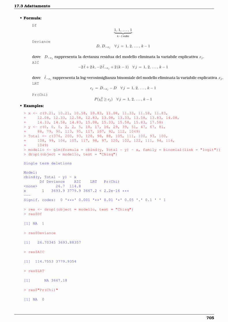
17.3 Adattamento
• Formula:
Df1, 1, . . . , 1︸ ︷︷ ︸k−1 volte
DevianceD, D−xj ∀ j = 1, 2, . . . , k − 1
dove D−xj rappresenta la devianza residua del modello eliminata la variabile esplicativa xj.AIC
−2 ˆ+ 2 k, −2 ˆ−xj + 2 (k − 1) ∀ j = 1, 2, . . . , k − 1
dove ˆ−xj rappresenta la log-verosimiglianza binomiale del modello eliminata la variabile esplicativa xj.LRT
cj = D−xj −D ∀ j = 1, 2, . . . , k − 1
Pr(Chi)P (χ2
1 ≥ cj) ∀ j = 1, 2, . . . , k − 1
• Examples:
> x <- c(9.21, 10.21, 10.58, 10.83, 11.08, 11.33, 11.58, 11.83,+ 12.08, 12.33, 12.58, 12.83, 13.08, 13.33, 13.58, 13.83, 14.08,+ 14.33, 14.58, 14.83, 15.08, 15.33, 15.58, 15.83, 17.58)> y <- c(0, 0, 0, 2, 2, 5, 10, 17, 16, 29, 39, 51, 47, 67, 81,+ 88, 79, 90, 113, 95, 117, 107, 92, 112, 1049)> Total <- c(376, 200, 93, 120, 90, 88, 105, 111, 100, 93, 100,+ 108, 99, 106, 105, 117, 98, 97, 120, 102, 122, 111, 94, 114,+ 1049)> modello <- glm(formula = cbind(y, Total - y) ~ x, family = binomial(link = "logit"))> drop1(object = modello, test = "Chisq")
Single term deletions
Model:cbind(y, Total - y) ~ x
Df Deviance AIC LRT Pr(Chi)<none> 26.7 114.8x 1 3693.9 3779.9 3667.2 < 2.2e-16 ***---Signif. codes: 0 '***' 0.001 '**' 0.01 '*' 0.05 '.' 0.1 ' ' 1
> res <- drop1(object = modello, test = "Chisq")> res$Df
[1] NA 1
> res$Deviance
[1] 26.70345 3693.88357
> res$AIC
[1] 114.7553 3779.9354
> res$LRT
[1] NA 3667.18
> res$"Pr(Chi)"
[1] NA 0
705
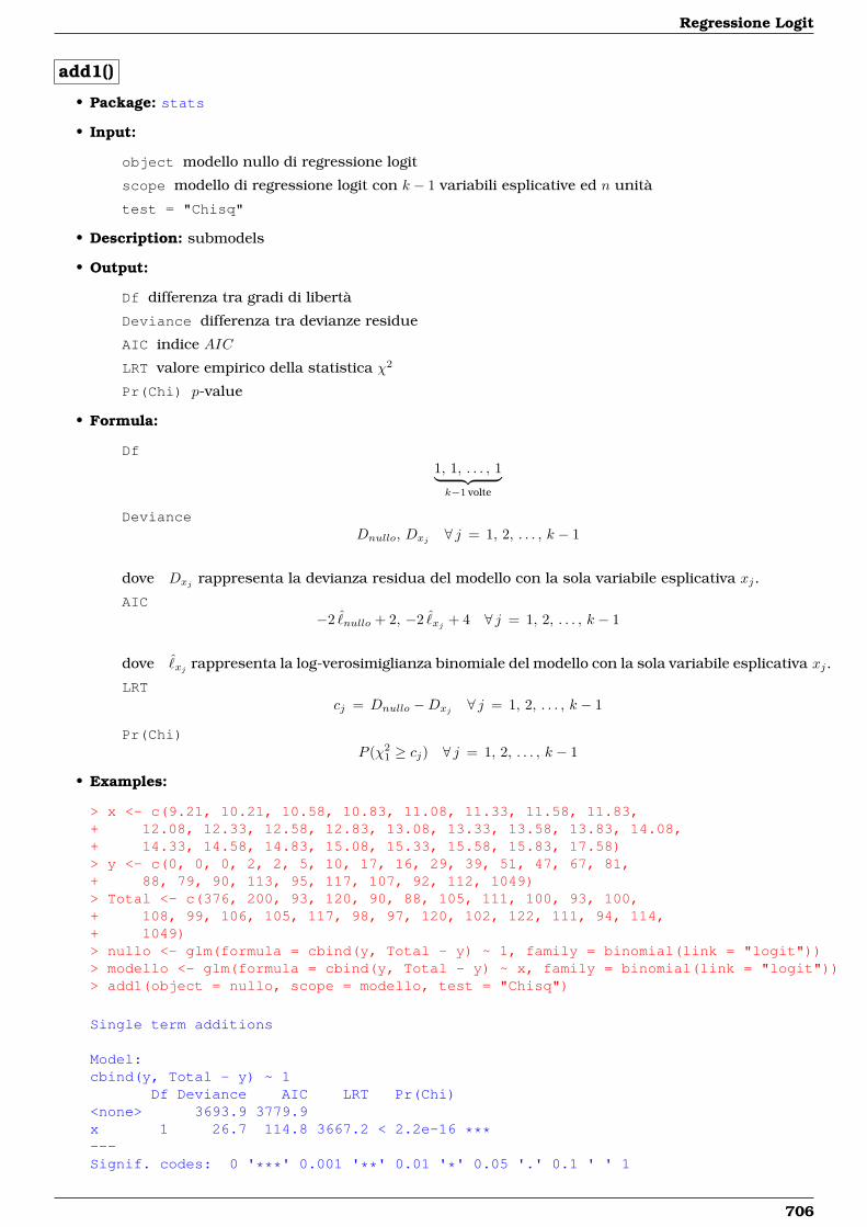
Regressione Logit
add1()
• Package: stats
• Input:
object modello nullo di regressione logit
scope modello di regressione logit con k − 1 variabili esplicative ed n unità
test = "Chisq"
• Description: submodels
• Output:
Df differenza tra gradi di libertà
Deviance differenza tra devianze residue
AIC indice AIC
LRT valore empirico della statistica χ2
Pr(Chi) p-value
• Formula:
Df1, 1, . . . , 1︸ ︷︷ ︸k−1 volte
DevianceDnullo, Dxj ∀ j = 1, 2, . . . , k − 1
dove Dxj rappresenta la devianza residua del modello con la sola variabile esplicativa xj.
AIC−2 ˆ
nullo + 2, −2 ˆxj + 4 ∀ j = 1, 2, . . . , k − 1
dove ˆxj rappresenta la log-verosimiglianza binomiale del modello con la sola variabile esplicativa xj.
LRTcj = Dnullo −Dxj ∀ j = 1, 2, . . . , k − 1
Pr(Chi)P (χ2
1 ≥ cj) ∀ j = 1, 2, . . . , k − 1
• Examples:
> x <- c(9.21, 10.21, 10.58, 10.83, 11.08, 11.33, 11.58, 11.83,+ 12.08, 12.33, 12.58, 12.83, 13.08, 13.33, 13.58, 13.83, 14.08,+ 14.33, 14.58, 14.83, 15.08, 15.33, 15.58, 15.83, 17.58)> y <- c(0, 0, 0, 2, 2, 5, 10, 17, 16, 29, 39, 51, 47, 67, 81,+ 88, 79, 90, 113, 95, 117, 107, 92, 112, 1049)> Total <- c(376, 200, 93, 120, 90, 88, 105, 111, 100, 93, 100,+ 108, 99, 106, 105, 117, 98, 97, 120, 102, 122, 111, 94, 114,+ 1049)> nullo <- glm(formula = cbind(y, Total - y) ~ 1, family = binomial(link = "logit"))> modello <- glm(formula = cbind(y, Total - y) ~ x, family = binomial(link = "logit"))> add1(object = nullo, scope = modello, test = "Chisq")
Single term additions
Model:cbind(y, Total - y) ~ 1
Df Deviance AIC LRT Pr(Chi)<none> 3693.9 3779.9x 1 26.7 114.8 3667.2 < 2.2e-16 ***---Signif. codes: 0 '***' 0.001 '**' 0.01 '*' 0.05 '.' 0.1 ' ' 1
706
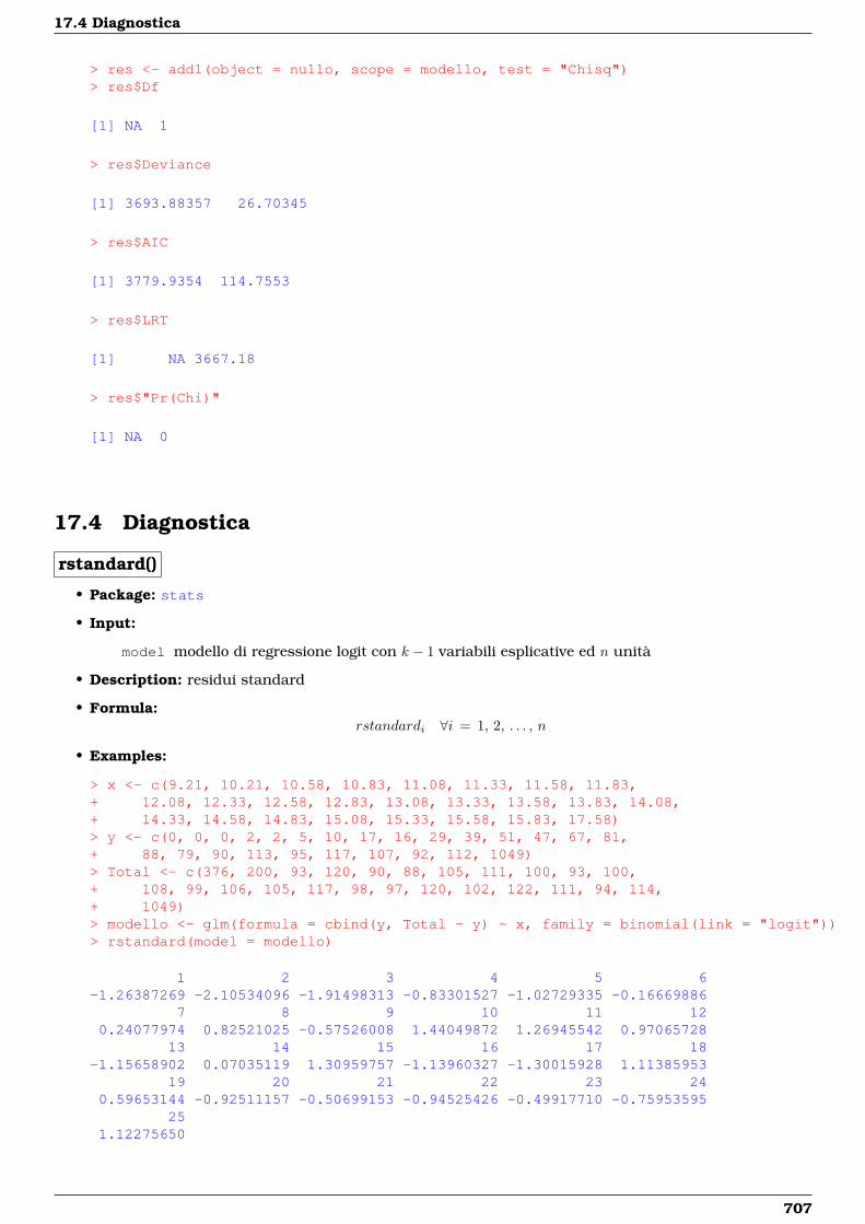
17.4 Diagnostica
> res <- add1(object = nullo, scope = modello, test = "Chisq")> res$Df
[1] NA 1
> res$Deviance
[1] 3693.88357 26.70345
> res$AIC
[1] 3779.9354 114.7553
> res$LRT
[1] NA 3667.18
> res$"Pr(Chi)"
[1] NA 0
17.4 Diagnostica
rstandard()
• Package: stats
• Input:
model modello di regressione logit con k − 1 variabili esplicative ed n unità
• Description: residui standard
• Formula:rstandardi ∀i = 1, 2, . . . , n
• Examples:
> x <- c(9.21, 10.21, 10.58, 10.83, 11.08, 11.33, 11.58, 11.83,+ 12.08, 12.33, 12.58, 12.83, 13.08, 13.33, 13.58, 13.83, 14.08,+ 14.33, 14.58, 14.83, 15.08, 15.33, 15.58, 15.83, 17.58)> y <- c(0, 0, 0, 2, 2, 5, 10, 17, 16, 29, 39, 51, 47, 67, 81,+ 88, 79, 90, 113, 95, 117, 107, 92, 112, 1049)> Total <- c(376, 200, 93, 120, 90, 88, 105, 111, 100, 93, 100,+ 108, 99, 106, 105, 117, 98, 97, 120, 102, 122, 111, 94, 114,+ 1049)> modello <- glm(formula = cbind(y, Total - y) ~ x, family = binomial(link = "logit"))> rstandard(model = modello)
1 2 3 4 5 6-1.26387269 -2.10534096 -1.91498313 -0.83301527 -1.02729335 -0.16669886
7 8 9 10 11 120.24077974 0.82521025 -0.57526008 1.44049872 1.26945542 0.97065728
13 14 15 16 17 18-1.15658902 0.07035119 1.30959757 -1.13960327 -1.30015928 1.11385953
19 20 21 22 23 240.59653144 -0.92511157 -0.50699153 -0.94525426 -0.49917710 -0.75953595
251.12275650
707
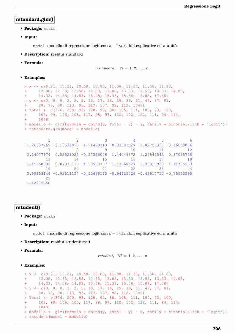
Regressione Logit
rstandard.glm()
• Package: stats
• Input:
model modello di regressione logit con k − 1 variabili esplicative ed n unità
• Description: residui standard
• Formula:rstandardi ∀i = 1, 2, . . . , n
• Examples:
> x <- c(9.21, 10.21, 10.58, 10.83, 11.08, 11.33, 11.58, 11.83,+ 12.08, 12.33, 12.58, 12.83, 13.08, 13.33, 13.58, 13.83, 14.08,+ 14.33, 14.58, 14.83, 15.08, 15.33, 15.58, 15.83, 17.58)> y <- c(0, 0, 0, 2, 2, 5, 10, 17, 16, 29, 39, 51, 47, 67, 81,+ 88, 79, 90, 113, 95, 117, 107, 92, 112, 1049)> Total <- c(376, 200, 93, 120, 90, 88, 105, 111, 100, 93, 100,+ 108, 99, 106, 105, 117, 98, 97, 120, 102, 122, 111, 94, 114,+ 1049)> modello <- glm(formula = cbind(y, Total - y) ~ x, family = binomial(link = "logit"))> rstandard.glm(model = modello)
1 2 3 4 5 6-1.26387269 -2.10534096 -1.91498313 -0.83301527 -1.02729335 -0.16669886
7 8 9 10 11 120.24077974 0.82521025 -0.57526008 1.44049872 1.26945542 0.97065728
13 14 15 16 17 18-1.15658902 0.07035119 1.30959757 -1.13960327 -1.30015928 1.11385953
19 20 21 22 23 240.59653144 -0.92511157 -0.50699153 -0.94525426 -0.49917710 -0.75953595
251.12275650
rstudent()
• Package: stats
• Input:
model modello di regressione logit con k − 1 variabili esplicative ed n unità
• Description: residui studentizzati
• Formula:rstudenti ∀i = 1, 2, . . . , n
• Examples:
> x <- c(9.21, 10.21, 10.58, 10.83, 11.08, 11.33, 11.58, 11.83,+ 12.08, 12.33, 12.58, 12.83, 13.08, 13.33, 13.58, 13.83, 14.08,+ 14.33, 14.58, 14.83, 15.08, 15.33, 15.58, 15.83, 17.58)> y <- c(0, 0, 0, 2, 2, 5, 10, 17, 16, 29, 39, 51, 47, 67, 81,+ 88, 79, 90, 113, 95, 117, 107, 92, 112, 1049)> Total <- c(376, 200, 93, 120, 90, 88, 105, 111, 100, 93, 100,+ 108, 99, 106, 105, 117, 98, 97, 120, 102, 122, 111, 94, 114,+ 1049)> modello <- glm(formula = cbind(y, Total - y) ~ x, family = binomial(link = "logit"))> rstudent(model = modello)
708
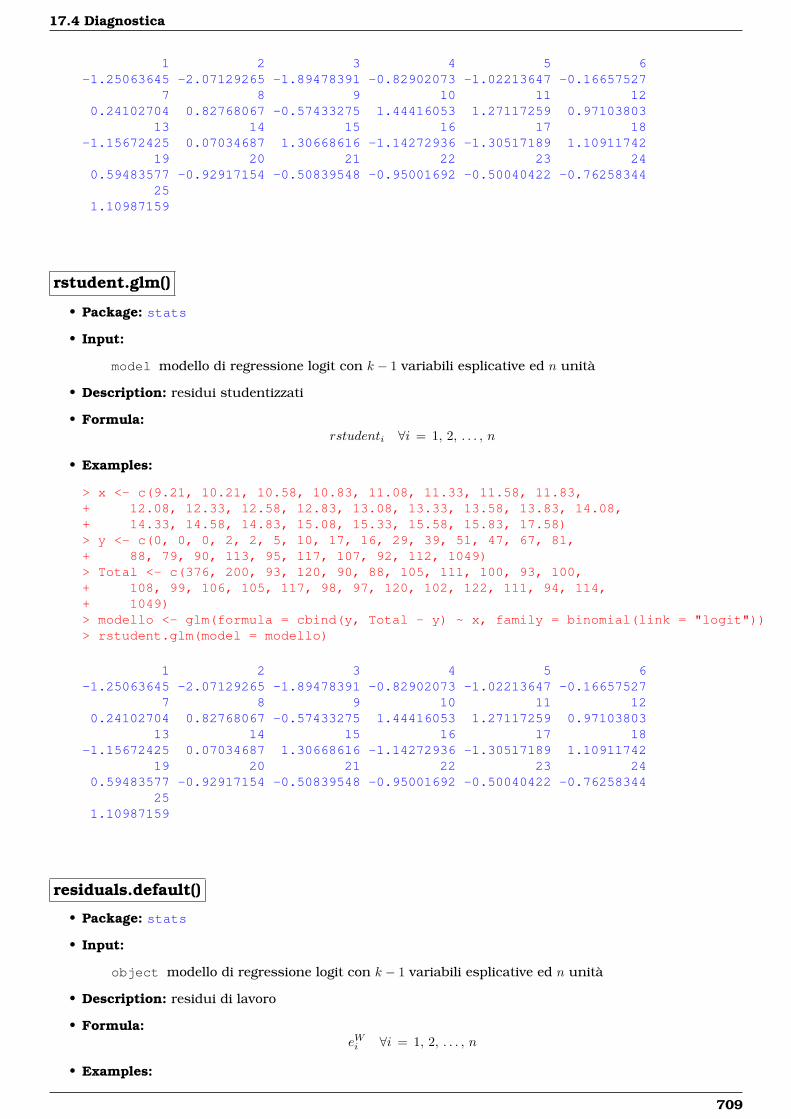
17.4 Diagnostica
1 2 3 4 5 6-1.25063645 -2.07129265 -1.89478391 -0.82902073 -1.02213647 -0.16657527
7 8 9 10 11 120.24102704 0.82768067 -0.57433275 1.44416053 1.27117259 0.97103803
13 14 15 16 17 18-1.15672425 0.07034687 1.30668616 -1.14272936 -1.30517189 1.10911742
19 20 21 22 23 240.59483577 -0.92917154 -0.50839548 -0.95001692 -0.50040422 -0.76258344
251.10987159
rstudent.glm()
• Package: stats
• Input:
model modello di regressione logit con k − 1 variabili esplicative ed n unità
• Description: residui studentizzati
• Formula:rstudenti ∀i = 1, 2, . . . , n
• Examples:
> x <- c(9.21, 10.21, 10.58, 10.83, 11.08, 11.33, 11.58, 11.83,+ 12.08, 12.33, 12.58, 12.83, 13.08, 13.33, 13.58, 13.83, 14.08,+ 14.33, 14.58, 14.83, 15.08, 15.33, 15.58, 15.83, 17.58)> y <- c(0, 0, 0, 2, 2, 5, 10, 17, 16, 29, 39, 51, 47, 67, 81,+ 88, 79, 90, 113, 95, 117, 107, 92, 112, 1049)> Total <- c(376, 200, 93, 120, 90, 88, 105, 111, 100, 93, 100,+ 108, 99, 106, 105, 117, 98, 97, 120, 102, 122, 111, 94, 114,+ 1049)> modello <- glm(formula = cbind(y, Total - y) ~ x, family = binomial(link = "logit"))> rstudent.glm(model = modello)
1 2 3 4 5 6-1.25063645 -2.07129265 -1.89478391 -0.82902073 -1.02213647 -0.16657527
7 8 9 10 11 120.24102704 0.82768067 -0.57433275 1.44416053 1.27117259 0.97103803
13 14 15 16 17 18-1.15672425 0.07034687 1.30668616 -1.14272936 -1.30517189 1.10911742
19 20 21 22 23 240.59483577 -0.92917154 -0.50839548 -0.95001692 -0.50040422 -0.76258344
251.10987159
residuals.default()
• Package: stats
• Input:
object modello di regressione logit con k − 1 variabili esplicative ed n unità
• Description: residui di lavoro
• Formula:eWi ∀i = 1, 2, . . . , n
• Examples:
709
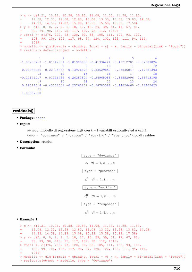
Regressione Logit
> x <- c(9.21, 10.21, 10.58, 10.83, 11.08, 11.33, 11.58, 11.83,+ 12.08, 12.33, 12.58, 12.83, 13.08, 13.33, 13.58, 13.83, 14.08,+ 14.33, 14.58, 14.83, 15.08, 15.33, 15.58, 15.83, 17.58)> y <- c(0, 0, 0, 2, 2, 5, 10, 17, 16, 29, 39, 51, 47, 67, 81,+ 88, 79, 90, 113, 95, 117, 107, 92, 112, 1049)> Total <- c(376, 200, 93, 120, 90, 88, 105, 111, 100, 93, 100,+ 108, 99, 106, 105, 117, 98, 97, 120, 102, 122, 111, 94, 114,+ 1049)> modello <- glm(formula = cbind(y, Total - y) ~ x, family = binomial(link = "logit"))> residuals.default(object = modello)
1 2 3 4 5 6-1.00203763 -1.01042031 -1.01905988 -0.41336424 -0.48212701 -0.07089826
7 8 9 10 11 120.07938086 0.22704866 -0.13926878 0.33629857 0.25835047 0.17881393
13 14 15 16 17 18-0.22141017 0.01336452 0.26283804 -0.24965088 -0.36552096 0.33713195
19 20 21 22 23 240.19514514 -0.43506531 -0.25760272 -0.64783388 -0.44626460 -0.78405425
251.00057358
residuals()
• Package: stats
• Input:
object modello di regressione logit con k − 1 variabili esplicative ed n unità
type = "deviance" / "pearson" / "working" / "response" tipo di residuo
• Description: residui
• Formula:
type = "deviance"
ei ∀i = 1, 2, . . . , n
type = "pearson"
ePi ∀i = 1, 2, . . . , n
type = "working"
eWi ∀i = 1, 2, . . . , n
type = "response"
eRi ∀i = 1, 2, . . . , n
• Example 1:
> x <- c(9.21, 10.21, 10.58, 10.83, 11.08, 11.33, 11.58, 11.83,+ 12.08, 12.33, 12.58, 12.83, 13.08, 13.33, 13.58, 13.83, 14.08,+ 14.33, 14.58, 14.83, 15.08, 15.33, 15.58, 15.83, 17.58)> y <- c(0, 0, 0, 2, 2, 5, 10, 17, 16, 29, 39, 51, 47, 67, 81,+ 88, 79, 90, 113, 95, 117, 107, 92, 112, 1049)> Total <- c(376, 200, 93, 120, 90, 88, 105, 111, 100, 93, 100,+ 108, 99, 106, 105, 117, 98, 97, 120, 102, 122, 111, 94, 114,+ 1049)> modello <- glm(formula = cbind(y, Total - y) ~ x, family = binomial(link = "logit"))> residuals(object = modello, type = "deviance")
710

17.4 Diagnostica
1 2 3 4 5 6 7-1.2372312 -2.0363101 -1.8739732 -0.8043827 -0.9953320 -0.1607163 0.2289532
8 9 10 11 12 13 140.7780252 -0.5441548 1.3675388 1.2016944 0.9162826 -1.0982255 0.0665090
15 16 17 18 19 20 211.2375553 -1.0695134 -1.2358120 1.0633044 0.5665503 -0.8912577 -0.4883964
22 23 24 25-0.9195743 -0.4900070 -0.7461893 1.0968278
• Example 2:
> x <- c(9.21, 10.21, 10.58, 10.83, 11.08, 11.33, 11.58, 11.83,+ 12.08, 12.33, 12.58, 12.83, 13.08, 13.33, 13.58, 13.83, 14.08,+ 14.33, 14.58, 14.83, 15.08, 15.33, 15.58, 15.83, 17.58)> y <- c(0, 0, 0, 2, 2, 5, 10, 17, 16, 29, 39, 51, 47, 67, 81,+ 88, 79, 90, 113, 95, 117, 107, 92, 112, 1049)> Total <- c(376, 200, 93, 120, 90, 88, 105, 111, 100, 93, 100,+ 108, 99, 106, 105, 117, 98, 97, 120, 102, 122, 111, 94, 114,+ 1049)> modello <- glm(formula = cbind(y, Total - y) ~ x, family = binomial(link = "logit"))> residuals(object = modello, type = "pearson")
1 2 3 4 5 6-0.87529996 -1.44362837 -1.33137848 -0.74525548 -0.91034225 -0.15901761
7 8 9 10 11 120.23139551 0.79874716 -0.53576012 1.40235004 1.21724831 0.91957777
13 14 15 16 17 18-1.09953015 0.06647053 1.21159801 -1.09387707 -1.28431127 1.01110426
19 20 21 22 23 240.54989436 -0.94424085 -0.50685539 -1.00250029 -0.52208706 -0.82783987
250.77568558
• Example 3:
> x <- c(9.21, 10.21, 10.58, 10.83, 11.08, 11.33, 11.58, 11.83,+ 12.08, 12.33, 12.58, 12.83, 13.08, 13.33, 13.58, 13.83, 14.08,+ 14.33, 14.58, 14.83, 15.08, 15.33, 15.58, 15.83, 17.58)> y <- c(0, 0, 0, 2, 2, 5, 10, 17, 16, 29, 39, 51, 47, 67, 81,+ 88, 79, 90, 113, 95, 117, 107, 92, 112, 1049)> Total <- c(376, 200, 93, 120, 90, 88, 105, 111, 100, 93, 100,+ 108, 99, 106, 105, 117, 98, 97, 120, 102, 122, 111, 94, 114,+ 1049)> modello <- glm(formula = cbind(y, Total - y) ~ x, family = binomial(link = "logit"))> residuals(object = modello, type = "working")
1 2 3 4 5 6-1.00203763 -1.01042031 -1.01905988 -0.41336424 -0.48212701 -0.07089826
7 8 9 10 11 120.07938086 0.22704866 -0.13926878 0.33629857 0.25835047 0.17881393
13 14 15 16 17 18-0.22141017 0.01336452 0.26283804 -0.24965088 -0.36552096 0.33713195
19 20 21 22 23 240.19514514 -0.43506531 -0.25760272 -0.64783388 -0.44626460 -0.78405425
251.00057358
• Example 4:
> x <- c(9.21, 10.21, 10.58, 10.83, 11.08, 11.33, 11.58, 11.83,+ 12.08, 12.33, 12.58, 12.83, 13.08, 13.33, 13.58, 13.83, 14.08,+ 14.33, 14.58, 14.83, 15.08, 15.33, 15.58, 15.83, 17.58)> y <- c(0, 0, 0, 2, 2, 5, 10, 17, 16, 29, 39, 51, 47, 67, 81,+ 88, 79, 90, 113, 95, 117, 107, 92, 112, 1049)
711
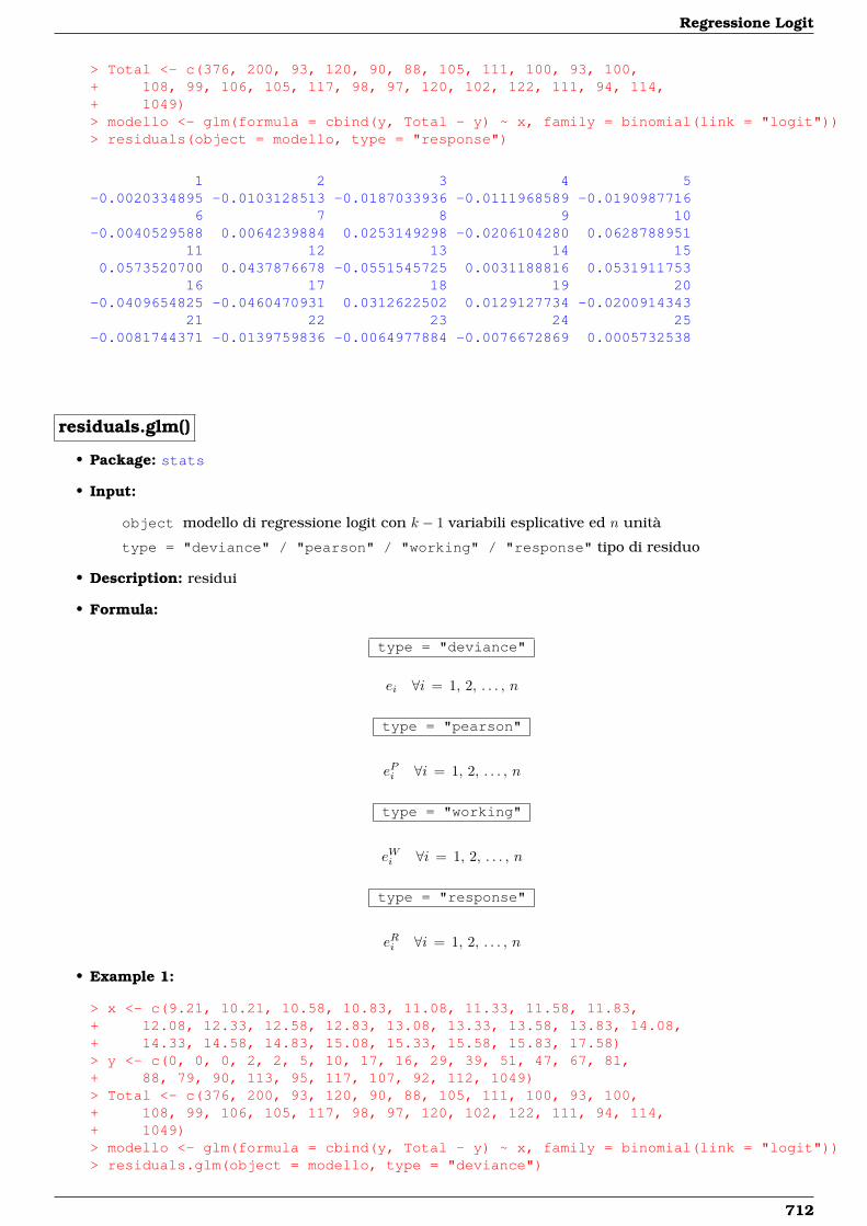
Regressione Logit
> Total <- c(376, 200, 93, 120, 90, 88, 105, 111, 100, 93, 100,+ 108, 99, 106, 105, 117, 98, 97, 120, 102, 122, 111, 94, 114,+ 1049)> modello <- glm(formula = cbind(y, Total - y) ~ x, family = binomial(link = "logit"))> residuals(object = modello, type = "response")
1 2 3 4 5-0.0020334895 -0.0103128513 -0.0187033936 -0.0111968589 -0.0190987716
6 7 8 9 10-0.0040529588 0.0064239884 0.0253149298 -0.0206104280 0.0628788951
11 12 13 14 150.0573520700 0.0437876678 -0.0551545725 0.0031188816 0.0531911753
16 17 18 19 20-0.0409654825 -0.0460470931 0.0312622502 0.0129127734 -0.0200914343
21 22 23 24 25-0.0081744371 -0.0139759836 -0.0064977884 -0.0076672869 0.0005732538
residuals.glm()
• Package: stats
• Input:
object modello di regressione logit con k − 1 variabili esplicative ed n unità
type = "deviance" / "pearson" / "working" / "response" tipo di residuo
• Description: residui
• Formula:
type = "deviance"
ei ∀i = 1, 2, . . . , n
type = "pearson"
ePi ∀i = 1, 2, . . . , n
type = "working"
eWi ∀i = 1, 2, . . . , n
type = "response"
eRi ∀i = 1, 2, . . . , n
• Example 1:
> x <- c(9.21, 10.21, 10.58, 10.83, 11.08, 11.33, 11.58, 11.83,+ 12.08, 12.33, 12.58, 12.83, 13.08, 13.33, 13.58, 13.83, 14.08,+ 14.33, 14.58, 14.83, 15.08, 15.33, 15.58, 15.83, 17.58)> y <- c(0, 0, 0, 2, 2, 5, 10, 17, 16, 29, 39, 51, 47, 67, 81,+ 88, 79, 90, 113, 95, 117, 107, 92, 112, 1049)> Total <- c(376, 200, 93, 120, 90, 88, 105, 111, 100, 93, 100,+ 108, 99, 106, 105, 117, 98, 97, 120, 102, 122, 111, 94, 114,+ 1049)> modello <- glm(formula = cbind(y, Total - y) ~ x, family = binomial(link = "logit"))> residuals.glm(object = modello, type = "deviance")
712
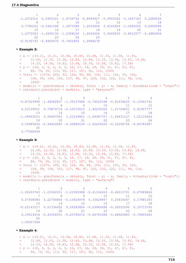
17.4 Diagnostica
1 2 3 4 5 6 7-1.2372312 -2.0363101 -1.8739732 -0.8043827 -0.9953320 -0.1607163 0.2289532
8 9 10 11 12 13 140.7780252 -0.5441548 1.3675388 1.2016944 0.9162826 -1.0982255 0.0665090
15 16 17 18 19 20 211.2375553 -1.0695134 -1.2358120 1.0633044 0.5665503 -0.8912577 -0.4883964
22 23 24 25-0.9195743 -0.4900070 -0.7461893 1.0968278
• Example 2:
> x <- c(9.21, 10.21, 10.58, 10.83, 11.08, 11.33, 11.58, 11.83,+ 12.08, 12.33, 12.58, 12.83, 13.08, 13.33, 13.58, 13.83, 14.08,+ 14.33, 14.58, 14.83, 15.08, 15.33, 15.58, 15.83, 17.58)> y <- c(0, 0, 0, 2, 2, 5, 10, 17, 16, 29, 39, 51, 47, 67, 81,+ 88, 79, 90, 113, 95, 117, 107, 92, 112, 1049)> Total <- c(376, 200, 93, 120, 90, 88, 105, 111, 100, 93, 100,+ 108, 99, 106, 105, 117, 98, 97, 120, 102, 122, 111, 94, 114,+ 1049)> modello <- glm(formula = cbind(y, Total - y) ~ x, family = binomial(link = "logit"))> residuals.glm(object = modello, type = "pearson")
1 2 3 4 5 6-0.87529996 -1.44362837 -1.33137848 -0.74525548 -0.91034225 -0.15901761
7 8 9 10 11 120.23139551 0.79874716 -0.53576012 1.40235004 1.21724831 0.91957777
13 14 15 16 17 18-1.09953015 0.06647053 1.21159801 -1.09387707 -1.28431127 1.01110426
19 20 21 22 23 240.54989436 -0.94424085 -0.50685539 -1.00250029 -0.52208706 -0.82783987
250.77568558
• Example 3:
> x <- c(9.21, 10.21, 10.58, 10.83, 11.08, 11.33, 11.58, 11.83,+ 12.08, 12.33, 12.58, 12.83, 13.08, 13.33, 13.58, 13.83, 14.08,+ 14.33, 14.58, 14.83, 15.08, 15.33, 15.58, 15.83, 17.58)> y <- c(0, 0, 0, 2, 2, 5, 10, 17, 16, 29, 39, 51, 47, 67, 81,+ 88, 79, 90, 113, 95, 117, 107, 92, 112, 1049)> Total <- c(376, 200, 93, 120, 90, 88, 105, 111, 100, 93, 100,+ 108, 99, 106, 105, 117, 98, 97, 120, 102, 122, 111, 94, 114,+ 1049)> modello <- glm(formula = cbind(y, Total - y) ~ x, family = binomial(link = "logit"))> residuals.glm(object = modello, type = "working")
1 2 3 4 5 6-1.00203763 -1.01042031 -1.01905988 -0.41336424 -0.48212701 -0.07089826
7 8 9 10 11 120.07938086 0.22704866 -0.13926878 0.33629857 0.25835047 0.17881393
13 14 15 16 17 18-0.22141017 0.01336452 0.26283804 -0.24965088 -0.36552096 0.33713195
19 20 21 22 23 240.19514514 -0.43506531 -0.25760272 -0.64783388 -0.44626460 -0.78405425
251.00057358
• Example 4:
> x <- c(9.21, 10.21, 10.58, 10.83, 11.08, 11.33, 11.58, 11.83,+ 12.08, 12.33, 12.58, 12.83, 13.08, 13.33, 13.58, 13.83, 14.08,+ 14.33, 14.58, 14.83, 15.08, 15.33, 15.58, 15.83, 17.58)> y <- c(0, 0, 0, 2, 2, 5, 10, 17, 16, 29, 39, 51, 47, 67, 81,+ 88, 79, 90, 113, 95, 117, 107, 92, 112, 1049)
713
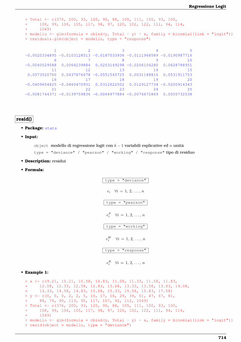
Regressione Logit
> Total <- c(376, 200, 93, 120, 90, 88, 105, 111, 100, 93, 100,+ 108, 99, 106, 105, 117, 98, 97, 120, 102, 122, 111, 94, 114,+ 1049)> modello <- glm(formula = cbind(y, Total - y) ~ x, family = binomial(link = "logit"))> residuals.glm(object = modello, type = "response")
1 2 3 4 5-0.0020334895 -0.0103128513 -0.0187033936 -0.0111968589 -0.0190987716
6 7 8 9 10-0.0040529588 0.0064239884 0.0253149298 -0.0206104280 0.0628788951
11 12 13 14 150.0573520700 0.0437876678 -0.0551545725 0.0031188816 0.0531911753
16 17 18 19 20-0.0409654825 -0.0460470931 0.0312622502 0.0129127734 -0.0200914343
21 22 23 24 25-0.0081744371 -0.0139759836 -0.0064977884 -0.0076672869 0.0005732538
resid()
• Package: stats
• Input:
object modello di regressione logit con k − 1 variabili esplicative ed n unità
type = "deviance" / "pearson" / "working" / "response" tipo di residuo
• Description: residui
• Formula:
type = "deviance"
ei ∀i = 1, 2, . . . , n
type = "pearson"
ePi ∀i = 1, 2, . . . , n
type = "working"
eWi ∀i = 1, 2, . . . , n
type = "response"
eRi ∀i = 1, 2, . . . , n
• Example 1:
> x <- c(9.21, 10.21, 10.58, 10.83, 11.08, 11.33, 11.58, 11.83,+ 12.08, 12.33, 12.58, 12.83, 13.08, 13.33, 13.58, 13.83, 14.08,+ 14.33, 14.58, 14.83, 15.08, 15.33, 15.58, 15.83, 17.58)> y <- c(0, 0, 0, 2, 2, 5, 10, 17, 16, 29, 39, 51, 47, 67, 81,+ 88, 79, 90, 113, 95, 117, 107, 92, 112, 1049)> Total <- c(376, 200, 93, 120, 90, 88, 105, 111, 100, 93, 100,+ 108, 99, 106, 105, 117, 98, 97, 120, 102, 122, 111, 94, 114,+ 1049)> modello <- glm(formula = cbind(y, Total - y) ~ x, family = binomial(link = "logit"))> resid(object = modello, type = "deviance")
714
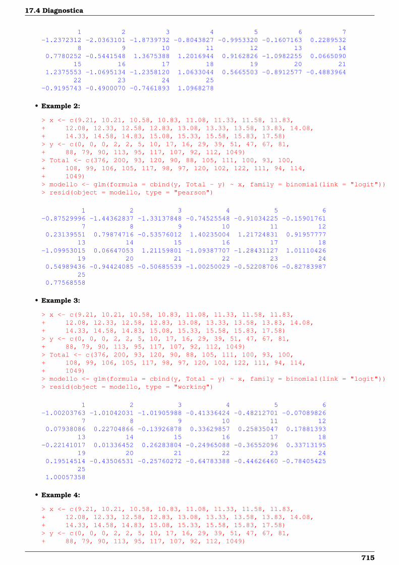
17.4 Diagnostica
1 2 3 4 5 6 7-1.2372312 -2.0363101 -1.8739732 -0.8043827 -0.9953320 -0.1607163 0.2289532
8 9 10 11 12 13 140.7780252 -0.5441548 1.3675388 1.2016944 0.9162826 -1.0982255 0.0665090
15 16 17 18 19 20 211.2375553 -1.0695134 -1.2358120 1.0633044 0.5665503 -0.8912577 -0.4883964
22 23 24 25-0.9195743 -0.4900070 -0.7461893 1.0968278
• Example 2:
> x <- c(9.21, 10.21, 10.58, 10.83, 11.08, 11.33, 11.58, 11.83,+ 12.08, 12.33, 12.58, 12.83, 13.08, 13.33, 13.58, 13.83, 14.08,+ 14.33, 14.58, 14.83, 15.08, 15.33, 15.58, 15.83, 17.58)> y <- c(0, 0, 0, 2, 2, 5, 10, 17, 16, 29, 39, 51, 47, 67, 81,+ 88, 79, 90, 113, 95, 117, 107, 92, 112, 1049)> Total <- c(376, 200, 93, 120, 90, 88, 105, 111, 100, 93, 100,+ 108, 99, 106, 105, 117, 98, 97, 120, 102, 122, 111, 94, 114,+ 1049)> modello <- glm(formula = cbind(y, Total - y) ~ x, family = binomial(link = "logit"))> resid(object = modello, type = "pearson")
1 2 3 4 5 6-0.87529996 -1.44362837 -1.33137848 -0.74525548 -0.91034225 -0.15901761
7 8 9 10 11 120.23139551 0.79874716 -0.53576012 1.40235004 1.21724831 0.91957777
13 14 15 16 17 18-1.09953015 0.06647053 1.21159801 -1.09387707 -1.28431127 1.01110426
19 20 21 22 23 240.54989436 -0.94424085 -0.50685539 -1.00250029 -0.52208706 -0.82783987
250.77568558
• Example 3:
> x <- c(9.21, 10.21, 10.58, 10.83, 11.08, 11.33, 11.58, 11.83,+ 12.08, 12.33, 12.58, 12.83, 13.08, 13.33, 13.58, 13.83, 14.08,+ 14.33, 14.58, 14.83, 15.08, 15.33, 15.58, 15.83, 17.58)> y <- c(0, 0, 0, 2, 2, 5, 10, 17, 16, 29, 39, 51, 47, 67, 81,+ 88, 79, 90, 113, 95, 117, 107, 92, 112, 1049)> Total <- c(376, 200, 93, 120, 90, 88, 105, 111, 100, 93, 100,+ 108, 99, 106, 105, 117, 98, 97, 120, 102, 122, 111, 94, 114,+ 1049)> modello <- glm(formula = cbind(y, Total - y) ~ x, family = binomial(link = "logit"))> resid(object = modello, type = "working")
1 2 3 4 5 6-1.00203763 -1.01042031 -1.01905988 -0.41336424 -0.48212701 -0.07089826
7 8 9 10 11 120.07938086 0.22704866 -0.13926878 0.33629857 0.25835047 0.17881393
13 14 15 16 17 18-0.22141017 0.01336452 0.26283804 -0.24965088 -0.36552096 0.33713195
19 20 21 22 23 240.19514514 -0.43506531 -0.25760272 -0.64783388 -0.44626460 -0.78405425
251.00057358
• Example 4:
> x <- c(9.21, 10.21, 10.58, 10.83, 11.08, 11.33, 11.58, 11.83,+ 12.08, 12.33, 12.58, 12.83, 13.08, 13.33, 13.58, 13.83, 14.08,+ 14.33, 14.58, 14.83, 15.08, 15.33, 15.58, 15.83, 17.58)> y <- c(0, 0, 0, 2, 2, 5, 10, 17, 16, 29, 39, 51, 47, 67, 81,+ 88, 79, 90, 113, 95, 117, 107, 92, 112, 1049)
715
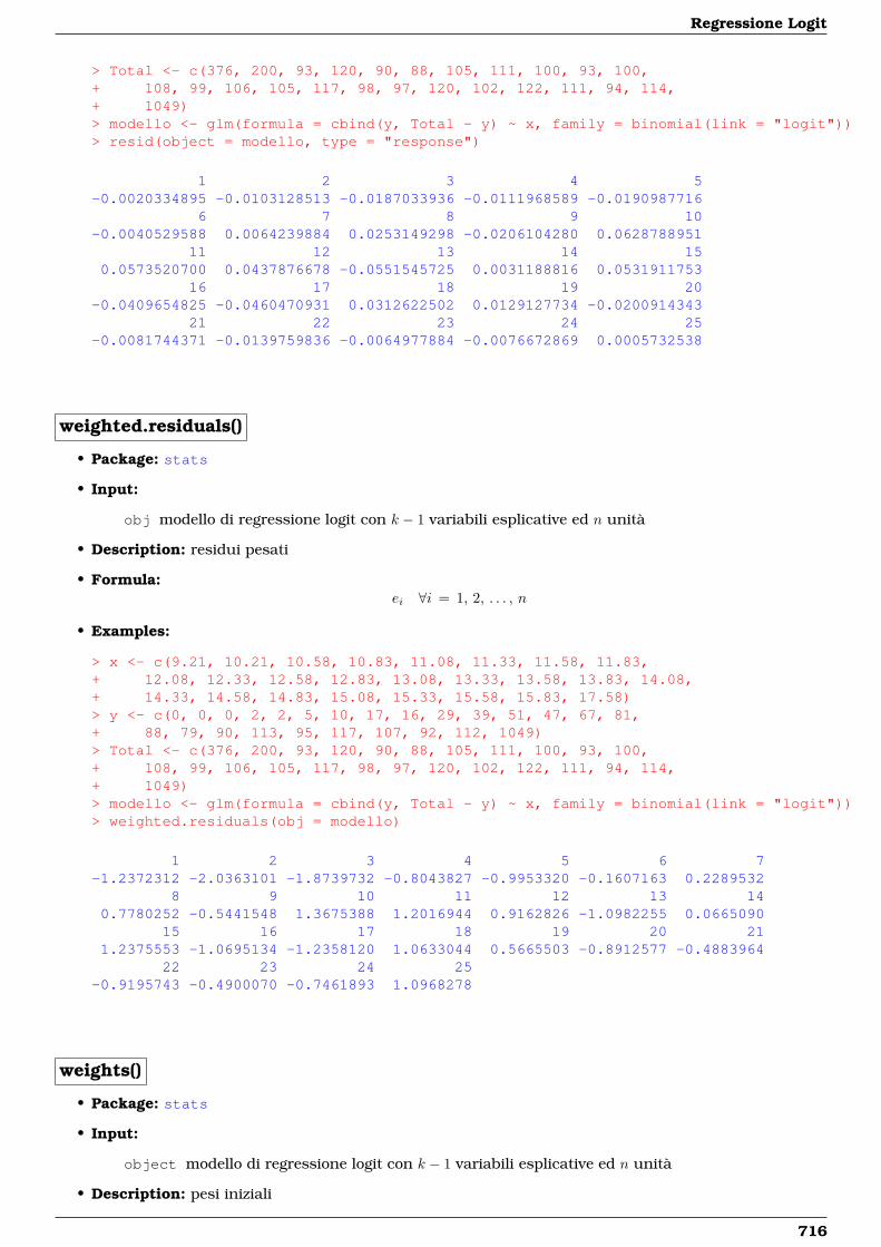
Regressione Logit
> Total <- c(376, 200, 93, 120, 90, 88, 105, 111, 100, 93, 100,+ 108, 99, 106, 105, 117, 98, 97, 120, 102, 122, 111, 94, 114,+ 1049)> modello <- glm(formula = cbind(y, Total - y) ~ x, family = binomial(link = "logit"))> resid(object = modello, type = "response")
1 2 3 4 5-0.0020334895 -0.0103128513 -0.0187033936 -0.0111968589 -0.0190987716
6 7 8 9 10-0.0040529588 0.0064239884 0.0253149298 -0.0206104280 0.0628788951
11 12 13 14 150.0573520700 0.0437876678 -0.0551545725 0.0031188816 0.0531911753
16 17 18 19 20-0.0409654825 -0.0460470931 0.0312622502 0.0129127734 -0.0200914343
21 22 23 24 25-0.0081744371 -0.0139759836 -0.0064977884 -0.0076672869 0.0005732538
weighted.residuals()
• Package: stats
• Input:
obj modello di regressione logit con k − 1 variabili esplicative ed n unità
• Description: residui pesati
• Formula:ei ∀i = 1, 2, . . . , n
• Examples:
> x <- c(9.21, 10.21, 10.58, 10.83, 11.08, 11.33, 11.58, 11.83,+ 12.08, 12.33, 12.58, 12.83, 13.08, 13.33, 13.58, 13.83, 14.08,+ 14.33, 14.58, 14.83, 15.08, 15.33, 15.58, 15.83, 17.58)> y <- c(0, 0, 0, 2, 2, 5, 10, 17, 16, 29, 39, 51, 47, 67, 81,+ 88, 79, 90, 113, 95, 117, 107, 92, 112, 1049)> Total <- c(376, 200, 93, 120, 90, 88, 105, 111, 100, 93, 100,+ 108, 99, 106, 105, 117, 98, 97, 120, 102, 122, 111, 94, 114,+ 1049)> modello <- glm(formula = cbind(y, Total - y) ~ x, family = binomial(link = "logit"))> weighted.residuals(obj = modello)
1 2 3 4 5 6 7-1.2372312 -2.0363101 -1.8739732 -0.8043827 -0.9953320 -0.1607163 0.2289532
8 9 10 11 12 13 140.7780252 -0.5441548 1.3675388 1.2016944 0.9162826 -1.0982255 0.0665090
15 16 17 18 19 20 211.2375553 -1.0695134 -1.2358120 1.0633044 0.5665503 -0.8912577 -0.4883964
22 23 24 25-0.9195743 -0.4900070 -0.7461893 1.0968278
weights()
• Package: stats
• Input:
object modello di regressione logit con k − 1 variabili esplicative ed n unità
• Description: pesi iniziali
716
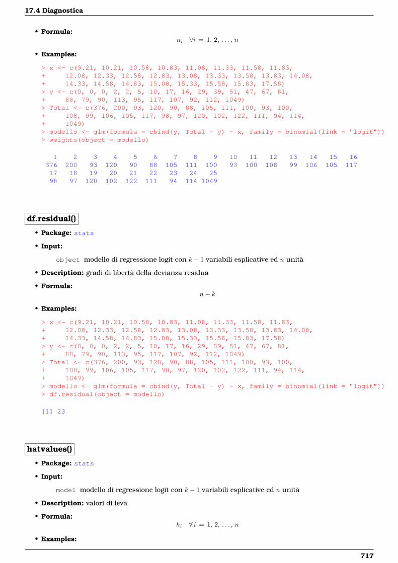
17.4 Diagnostica
• Formula:ni ∀i = 1, 2, . . . , n
• Examples:
> x <- c(9.21, 10.21, 10.58, 10.83, 11.08, 11.33, 11.58, 11.83,+ 12.08, 12.33, 12.58, 12.83, 13.08, 13.33, 13.58, 13.83, 14.08,+ 14.33, 14.58, 14.83, 15.08, 15.33, 15.58, 15.83, 17.58)> y <- c(0, 0, 0, 2, 2, 5, 10, 17, 16, 29, 39, 51, 47, 67, 81,+ 88, 79, 90, 113, 95, 117, 107, 92, 112, 1049)> Total <- c(376, 200, 93, 120, 90, 88, 105, 111, 100, 93, 100,+ 108, 99, 106, 105, 117, 98, 97, 120, 102, 122, 111, 94, 114,+ 1049)> modello <- glm(formula = cbind(y, Total - y) ~ x, family = binomial(link = "logit"))> weights(object = modello)
1 2 3 4 5 6 7 8 9 10 11 12 13 14 15 16376 200 93 120 90 88 105 111 100 93 100 108 99 106 105 11717 18 19 20 21 22 23 24 2598 97 120 102 122 111 94 114 1049
df.residual()
• Package: stats
• Input:
object modello di regressione logit con k − 1 variabili esplicative ed n unità
• Description: gradi di libertà della devianza residua
• Formula:n− k
• Examples:
> x <- c(9.21, 10.21, 10.58, 10.83, 11.08, 11.33, 11.58, 11.83,+ 12.08, 12.33, 12.58, 12.83, 13.08, 13.33, 13.58, 13.83, 14.08,+ 14.33, 14.58, 14.83, 15.08, 15.33, 15.58, 15.83, 17.58)> y <- c(0, 0, 0, 2, 2, 5, 10, 17, 16, 29, 39, 51, 47, 67, 81,+ 88, 79, 90, 113, 95, 117, 107, 92, 112, 1049)> Total <- c(376, 200, 93, 120, 90, 88, 105, 111, 100, 93, 100,+ 108, 99, 106, 105, 117, 98, 97, 120, 102, 122, 111, 94, 114,+ 1049)> modello <- glm(formula = cbind(y, Total - y) ~ x, family = binomial(link = "logit"))> df.residual(object = modello)
[1] 23
hatvalues()
• Package: stats
• Input:
model modello di regressione logit con k − 1 variabili esplicative ed n unità
• Description: valori di leva
• Formula:hi ∀ i = 1, 2, . . . , n
• Examples:
717
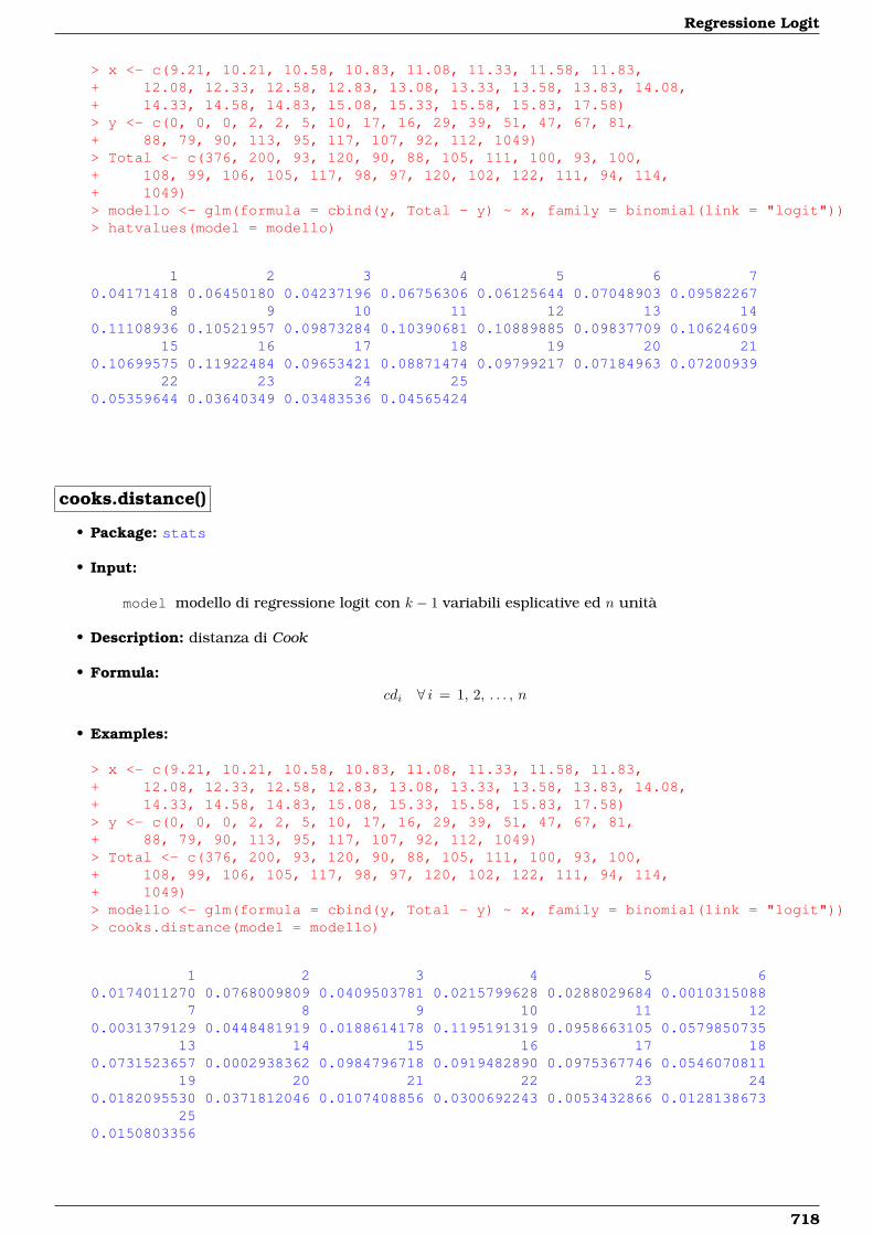
Regressione Logit
> x <- c(9.21, 10.21, 10.58, 10.83, 11.08, 11.33, 11.58, 11.83,+ 12.08, 12.33, 12.58, 12.83, 13.08, 13.33, 13.58, 13.83, 14.08,+ 14.33, 14.58, 14.83, 15.08, 15.33, 15.58, 15.83, 17.58)> y <- c(0, 0, 0, 2, 2, 5, 10, 17, 16, 29, 39, 51, 47, 67, 81,+ 88, 79, 90, 113, 95, 117, 107, 92, 112, 1049)> Total <- c(376, 200, 93, 120, 90, 88, 105, 111, 100, 93, 100,+ 108, 99, 106, 105, 117, 98, 97, 120, 102, 122, 111, 94, 114,+ 1049)> modello <- glm(formula = cbind(y, Total - y) ~ x, family = binomial(link = "logit"))> hatvalues(model = modello)
1 2 3 4 5 6 70.04171418 0.06450180 0.04237196 0.06756306 0.06125644 0.07048903 0.09582267
8 9 10 11 12 13 140.11108936 0.10521957 0.09873284 0.10390681 0.10889885 0.09837709 0.10624609
15 16 17 18 19 20 210.10699575 0.11922484 0.09653421 0.08871474 0.09799217 0.07184963 0.07200939
22 23 24 250.05359644 0.03640349 0.03483536 0.04565424
cooks.distance()
• Package: stats
• Input:
model modello di regressione logit con k − 1 variabili esplicative ed n unità
• Description: distanza di Cook
• Formula:cdi ∀ i = 1, 2, . . . , n
• Examples:
> x <- c(9.21, 10.21, 10.58, 10.83, 11.08, 11.33, 11.58, 11.83,+ 12.08, 12.33, 12.58, 12.83, 13.08, 13.33, 13.58, 13.83, 14.08,+ 14.33, 14.58, 14.83, 15.08, 15.33, 15.58, 15.83, 17.58)> y <- c(0, 0, 0, 2, 2, 5, 10, 17, 16, 29, 39, 51, 47, 67, 81,+ 88, 79, 90, 113, 95, 117, 107, 92, 112, 1049)> Total <- c(376, 200, 93, 120, 90, 88, 105, 111, 100, 93, 100,+ 108, 99, 106, 105, 117, 98, 97, 120, 102, 122, 111, 94, 114,+ 1049)> modello <- glm(formula = cbind(y, Total - y) ~ x, family = binomial(link = "logit"))> cooks.distance(model = modello)
1 2 3 4 5 60.0174011270 0.0768009809 0.0409503781 0.0215799628 0.0288029684 0.0010315088
7 8 9 10 11 120.0031379129 0.0448481919 0.0188614178 0.1195191319 0.0958663105 0.0579850735
13 14 15 16 17 180.0731523657 0.0002938362 0.0984796718 0.0919482890 0.0975367746 0.0546070811
19 20 21 22 23 240.0182095530 0.0371812046 0.0107408856 0.0300692243 0.0053432866 0.0128138673
250.0150803356
718
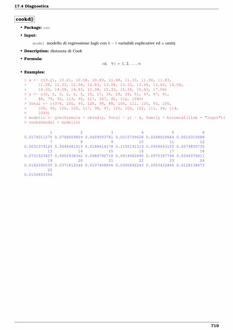
17.4 Diagnostica
cookd()
• Package: car
• Input:
model modello di regressione logit con k − 1 variabili esplicative ed n unità
• Description: distanza di Cook
• Formula:cdi ∀ i = 1, 2, . . . , n
• Examples:
> x <- c(9.21, 10.21, 10.58, 10.83, 11.08, 11.33, 11.58, 11.83,+ 12.08, 12.33, 12.58, 12.83, 13.08, 13.33, 13.58, 13.83, 14.08,+ 14.33, 14.58, 14.83, 15.08, 15.33, 15.58, 15.83, 17.58)> y <- c(0, 0, 0, 2, 2, 5, 10, 17, 16, 29, 39, 51, 47, 67, 81,+ 88, 79, 90, 113, 95, 117, 107, 92, 112, 1049)> Total <- c(376, 200, 93, 120, 90, 88, 105, 111, 100, 93, 100,+ 108, 99, 106, 105, 117, 98, 97, 120, 102, 122, 111, 94, 114,+ 1049)> modello <- glm(formula = cbind(y, Total - y) ~ x, family = binomial(link = "logit"))> cookd(model = modello)
1 2 3 4 5 60.0174011270 0.0768009809 0.0409503781 0.0215799628 0.0288029684 0.0010315088
7 8 9 10 11 120.0031379129 0.0448481919 0.0188614178 0.1195191319 0.0958663105 0.0579850735
13 14 15 16 17 180.0731523657 0.0002938362 0.0984796718 0.0919482890 0.0975367746 0.0546070811
19 20 21 22 23 240.0182095530 0.0371812046 0.0107408856 0.0300692243 0.0053432866 0.0128138673
250.0150803356
719

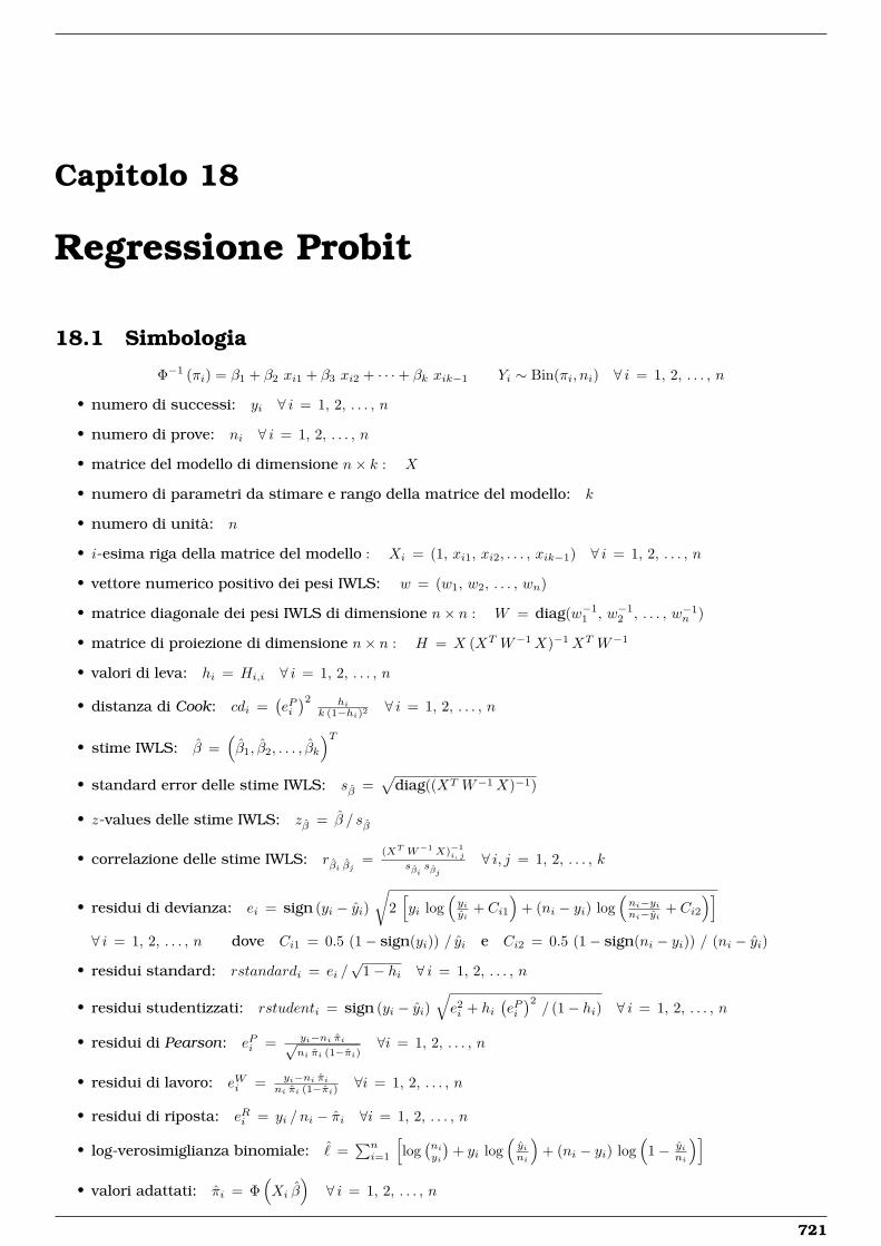
Capitolo 18
Regressione Probit
18.1 Simbologia
Φ−1 (πi) = β1 + β2 xi1 + β3 xi2 + · · ·+ βk xik−1 Yi ∼ Bin(πi, ni) ∀ i = 1, 2, . . . , n
• numero di successi: yi ∀ i = 1, 2, . . . , n
• numero di prove: ni ∀ i = 1, 2, . . . , n
• matrice del modello di dimensione n× k : X
• numero di parametri da stimare e rango della matrice del modello: k
• numero di unità: n
• i-esima riga della matrice del modello : Xi = (1, xi1, xi2, . . . , xik−1) ∀ i = 1, 2, . . . , n
• vettore numerico positivo dei pesi IWLS: w = (w1, w2, . . . , wn)
• matrice diagonale dei pesi IWLS di dimensione n× n : W = diag(w−11 , w−1
2 , . . . , w−1n )
• matrice di proiezione di dimensione n× n : H = X (XT W−1X)−1XT W−1
• valori di leva: hi = Hi,i ∀ i = 1, 2, . . . , n
• distanza di Cook: cdi =(ePi)2 hi
k (1−hi)2 ∀ i = 1, 2, . . . , n
• stime IWLS: β =(β1, β2, . . . , βk
)T• standard error delle stime IWLS: sβ =
√diag((XT W−1X)−1)
• z-values delle stime IWLS: zβ = β / sβ
• correlazione delle stime IWLS: rβi βj =(XT W−1X)−1
i, j
sβisβj
∀ i, j = 1, 2, . . . , k
• residui di devianza: ei = sign (yi − yi)√
2[yi log
(yiyi
+ Ci1
)+ (ni − yi) log
(ni−yini−yi + Ci2
)]∀ i = 1, 2, . . . , n dove Ci1 = 0.5 (1− sign(yi)) / yi e Ci2 = 0.5 (1− sign(ni − yi)) / (ni − yi)
• residui standard: rstandardi = ei /√
1− hi ∀ i = 1, 2, . . . , n
• residui studentizzati: rstudenti = sign (yi − yi)√e2i + hi
(ePi)2/ (1− hi) ∀ i = 1, 2, . . . , n
• residui di Pearson: ePi = yi−ni πi√ni πi (1−πi)
∀i = 1, 2, . . . , n
• residui di lavoro: eWi = yi−ni πini πi (1−πi) ∀i = 1, 2, . . . , n
• residui di riposta: eRi = yi / ni − πi ∀i = 1, 2, . . . , n
• log-verosimiglianza binomiale: ˆ =∑ni=1
[log(niyi
)+ yi log
(yini
)+ (ni − yi) log
(1− yi
ni
)]• valori adattati: πi = Φ
(Xi β
)∀ i = 1, 2, . . . , n
721
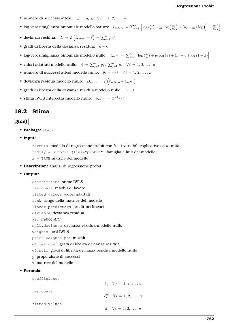
Regressione Probit
• numero di successi attesi: yi = ni πi ∀ i = 1, 2, . . . , n
• log-verosimiglianza binomiale modello saturo: ˆsaturo =
∑ni=1
[log(niyi
)+ yi log
(yini
)+ (ni − yi) log
(1− yi
ni
)]• devianza residua: D = 2
(ˆsaturo − ˆ
)=∑ni=1 e
2i
• gradi di libertà della devianza residua: n− k
• log-verosimiglianza binomiale modello nullo: ˆnullo =
∑ni=1
[log(niyi
)+ yi log (π) + (ni − yi) log (1− π)
]• valori adattati modello nullo: π =
∑nj=1 yj /
∑nj=1 nj ∀ i = 1, 2, . . . , n
• numero di successi attesi modello nullo: yi = ni π ∀ i = 1, 2, . . . , n
• devianza residua modello nullo: Dnullo = 2(
ˆsaturo − ˆ
nullo
)• gradi di libertà della devianza residua modello nullo: n− 1
• stima IWLS intercetta modello nullo: βnullo = Φ−1 (π)
18.2 Stima
glm()
• Package: stats
• Input:
formula modello di regressione probit con k − 1 variabili esplicative ed n unità
family = binomial(link="probit") famiglia e link del modello
x = TRUE matrice del modello
• Description: analisi di regressione probit
• Output:
coefficients stime IWLS
residuals residui di lavoro
fitted.values valori adattati
rank rango della matrice del modello
linear.predictors predittori lineari
deviance devianza residua
aic indice AIC
null.deviance devianza residua modello nullo
weights pesi IWLS
prior.weights pesi iniziali
df.residual gradi di libertà devianza residua
df.null gradi di libertà devianza residua modello nullo
y proporzione di successi
x matrice del modello
• Formula:
coefficientsβj ∀ j = 1, 2, . . . , k
residualseWi ∀ i = 1, 2, . . . , n
fitted.valuesπi ∀ i = 1, 2, . . . , n
722
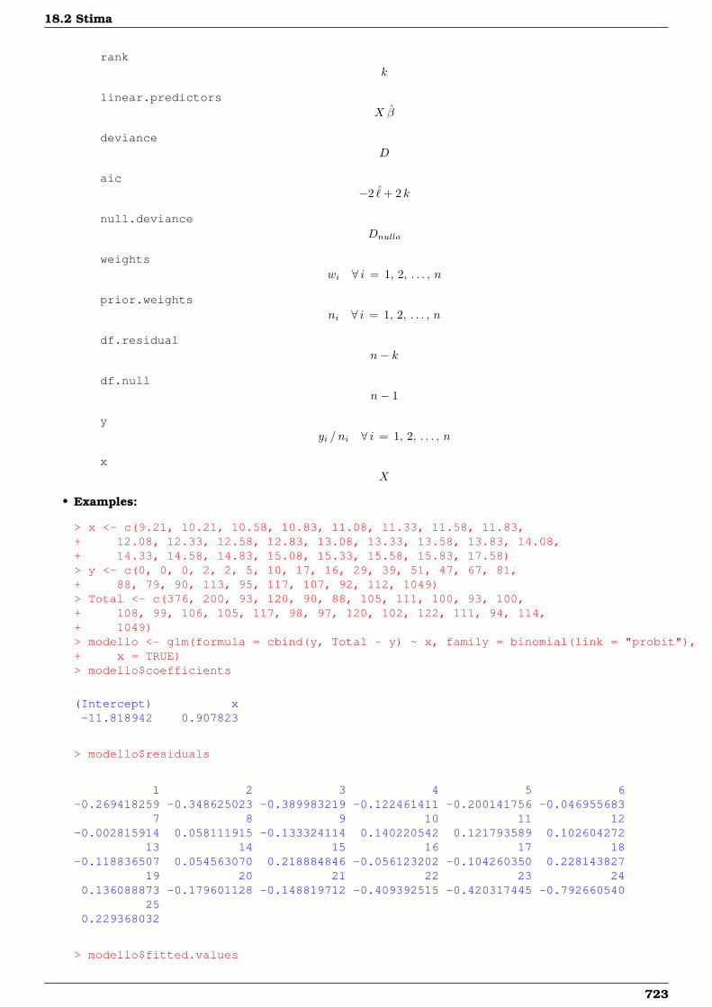
18.2 Stima
rankk
linear.predictorsX β
devianceD
aic−2 ˆ+ 2 k
null.devianceDnullo
weightswi ∀ i = 1, 2, . . . , n
prior.weightsni ∀ i = 1, 2, . . . , n
df.residualn− k
df.nulln− 1
yyi / ni ∀ i = 1, 2, . . . , n
xX
• Examples:
> x <- c(9.21, 10.21, 10.58, 10.83, 11.08, 11.33, 11.58, 11.83,+ 12.08, 12.33, 12.58, 12.83, 13.08, 13.33, 13.58, 13.83, 14.08,+ 14.33, 14.58, 14.83, 15.08, 15.33, 15.58, 15.83, 17.58)> y <- c(0, 0, 0, 2, 2, 5, 10, 17, 16, 29, 39, 51, 47, 67, 81,+ 88, 79, 90, 113, 95, 117, 107, 92, 112, 1049)> Total <- c(376, 200, 93, 120, 90, 88, 105, 111, 100, 93, 100,+ 108, 99, 106, 105, 117, 98, 97, 120, 102, 122, 111, 94, 114,+ 1049)> modello <- glm(formula = cbind(y, Total - y) ~ x, family = binomial(link = "probit"),+ x = TRUE)> modello$coefficients
(Intercept) x-11.818942 0.907823
> modello$residuals
1 2 3 4 5 6-0.269418259 -0.348625023 -0.389983219 -0.122461411 -0.200141756 -0.046955683
7 8 9 10 11 12-0.002815914 0.058111915 -0.133324114 0.140220542 0.121793589 0.102604272
13 14 15 16 17 18-0.118836507 0.054563070 0.218884846 -0.056123202 -0.104260350 0.228143827
19 20 21 22 23 240.136088873 -0.179601128 -0.148819712 -0.409392515 -0.420317445 -0.792660540
250.229368032
> modello$fitted.values
723
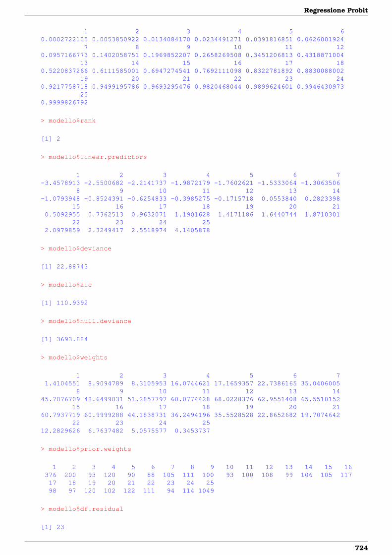
Regressione Probit
1 2 3 4 5 60.0002722105 0.0053850922 0.0134084170 0.0234491271 0.0391816851 0.0626001924
7 8 9 10 11 120.0957166773 0.1402058751 0.1969852207 0.2658269508 0.3451206813 0.4318871004
13 14 15 16 17 180.5220837266 0.6111585001 0.6947274541 0.7692111098 0.8322781892 0.8830088002
19 20 21 22 23 240.9217758718 0.9499195786 0.9693295476 0.9820468044 0.9899624601 0.9946430973
250.9999826792
> modello$rank
[1] 2
> modello$linear.predictors
1 2 3 4 5 6 7-3.4578913 -2.5500682 -2.2141737 -1.9872179 -1.7602621 -1.5333064 -1.3063506
8 9 10 11 12 13 14-1.0793948 -0.8524391 -0.6254833 -0.3985275 -0.1715718 0.0553840 0.2823398
15 16 17 18 19 20 210.5092955 0.7362513 0.9632071 1.1901628 1.4171186 1.6440744 1.8710301
22 23 24 252.0979859 2.3249417 2.5518974 4.1405878
> modello$deviance
[1] 22.88743
> modello$aic
[1] 110.9392
> modello$null.deviance
[1] 3693.884
> modello$weights
1 2 3 4 5 6 71.4104551 8.9094789 8.3105953 16.0744621 17.1659357 22.7386165 35.0406005
8 9 10 11 12 13 1445.7076709 48.6499031 51.2857797 60.0774428 68.0228376 62.9551408 65.5510152
15 16 17 18 19 20 2160.7937719 60.9999288 44.1838731 36.2494196 35.5528528 22.8652682 19.7074642
22 23 24 2512.2829626 6.7637482 5.0575577 0.3453737
> modello$prior.weights
1 2 3 4 5 6 7 8 9 10 11 12 13 14 15 16376 200 93 120 90 88 105 111 100 93 100 108 99 106 105 11717 18 19 20 21 22 23 24 2598 97 120 102 122 111 94 114 1049
> modello$df.residual
[1] 23
724
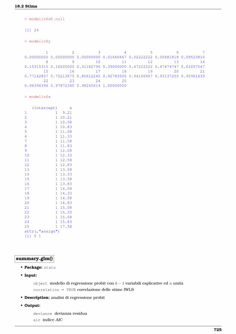
18.2 Stima
> modello$df.null
[1] 24
> modello$y
1 2 3 4 5 6 70.00000000 0.00000000 0.00000000 0.01666667 0.02222222 0.05681818 0.09523810
8 9 10 11 12 13 140.15315315 0.16000000 0.31182796 0.39000000 0.47222222 0.47474747 0.63207547
15 16 17 18 19 20 210.77142857 0.75213675 0.80612245 0.92783505 0.94166667 0.93137255 0.95901639
22 23 24 250.96396396 0.97872340 0.98245614 1.00000000
> modello$x
(Intercept) x1 1 9.212 1 10.213 1 10.584 1 10.835 1 11.086 1 11.337 1 11.588 1 11.839 1 12.0810 1 12.3311 1 12.5812 1 12.8313 1 13.0814 1 13.3315 1 13.5816 1 13.8317 1 14.0818 1 14.3319 1 14.5820 1 14.8321 1 15.0822 1 15.3323 1 15.5824 1 15.8325 1 17.58attr(,"assign")[1] 0 1
summary.glm()
• Package: stats
• Input:
object modello di regressione probit con k − 1 variabili esplicative ed n unità
correlation = TRUE correlazione delle stime IWLS
• Description: analisi di regressione probit
• Output:
deviance devianza residua
aic indice AIC
725
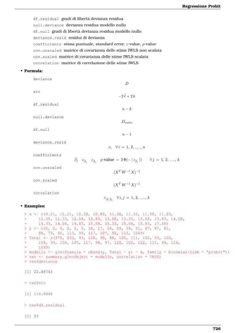
Regressione Probit
df.residual gradi di libertà devianza residua
null.deviance devianza residua modello nullo
df.null gradi di libertà devianza residua modello nullo
deviance.resid residui di devianza
coefficients stima puntuale, standard error, z-value, p-value
cov.unscaled matrice di covarianza delle stime IWLS non scalata
cov.scaled matrice di covarianza delle stime IWLS scalata
correlation matrice di correlazione delle stime IWLS
• Formula:
devianceD
aic−2 ˆ+ 2 k
df.residualn− k
null.devianceDnullo
df.nulln− 1
deviance.residei ∀ i = 1, 2, . . . , n
coefficientsβj sβj zβj p-value = 2 Φ(− | zβj |) ∀ j = 1, 2, . . . , k
cov.unscaled(XT W−1X)−1
cov.scaled(XT W−1X)−1
correlationrβi βj ∀ i, j = 1, 2, . . . , k
• Examples:
> x <- c(9.21, 10.21, 10.58, 10.83, 11.08, 11.33, 11.58, 11.83,+ 12.08, 12.33, 12.58, 12.83, 13.08, 13.33, 13.58, 13.83, 14.08,+ 14.33, 14.58, 14.83, 15.08, 15.33, 15.58, 15.83, 17.58)> y <- c(0, 0, 0, 2, 2, 5, 10, 17, 16, 29, 39, 51, 47, 67, 81,+ 88, 79, 90, 113, 95, 117, 107, 92, 112, 1049)> Total <- c(376, 200, 93, 120, 90, 88, 105, 111, 100, 93, 100,+ 108, 99, 106, 105, 117, 98, 97, 120, 102, 122, 111, 94, 114,+ 1049)> modello <- glm(formula = cbind(y, Total - y) ~ x, family = binomial(link = "probit"))> res <- summary.glm(object = modello, correlation = TRUE)> res$deviance
[1] 22.88743
> res$aic
[1] 110.9392
> res$df.residual
[1] 23
726
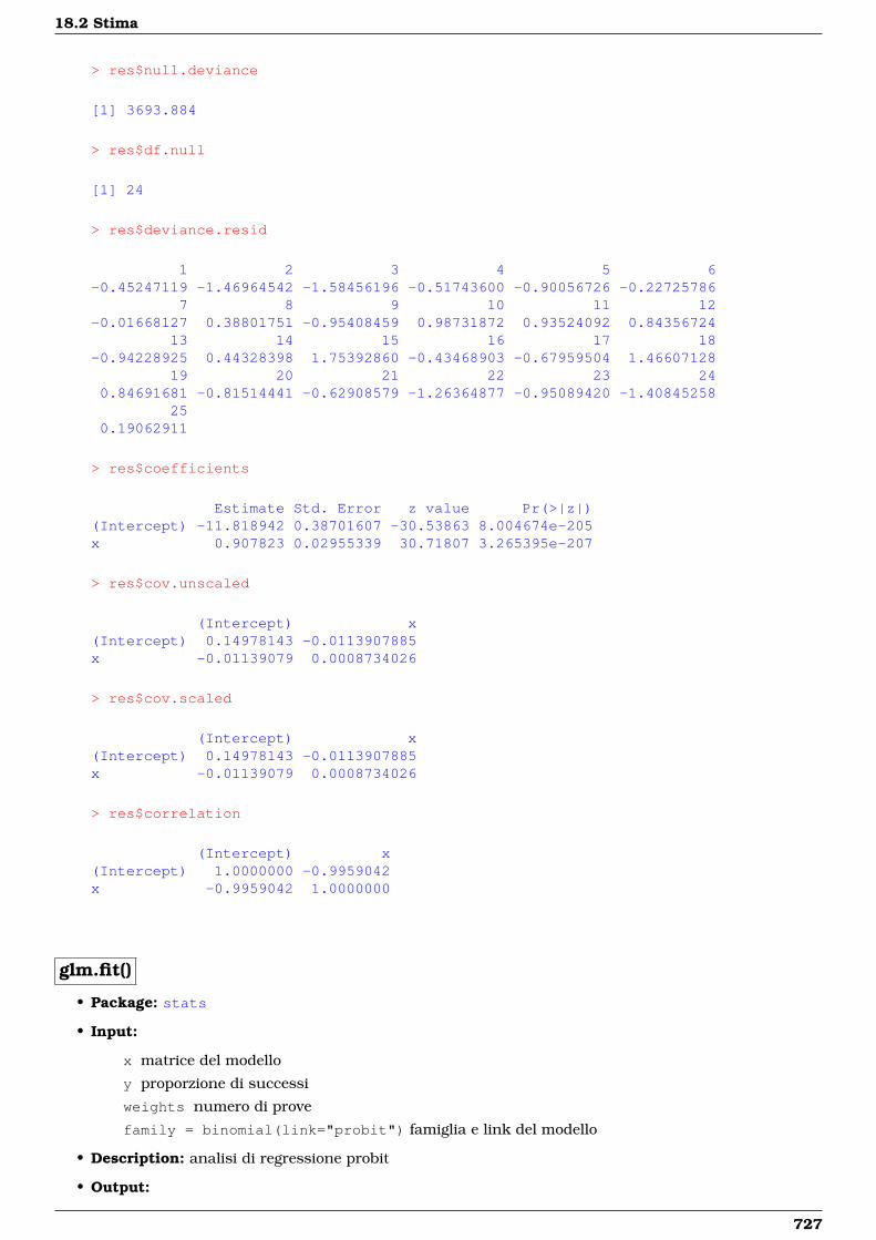
18.2 Stima
> res$null.deviance
[1] 3693.884
> res$df.null
[1] 24
> res$deviance.resid
1 2 3 4 5 6-0.45247119 -1.46964542 -1.58456196 -0.51743600 -0.90056726 -0.22725786
7 8 9 10 11 12-0.01668127 0.38801751 -0.95408459 0.98731872 0.93524092 0.84356724
13 14 15 16 17 18-0.94228925 0.44328398 1.75392860 -0.43468903 -0.67959504 1.46607128
19 20 21 22 23 240.84691681 -0.81514441 -0.62908579 -1.26364877 -0.95089420 -1.40845258
250.19062911
> res$coefficients
Estimate Std. Error z value Pr(>|z|)(Intercept) -11.818942 0.38701607 -30.53863 8.004674e-205x 0.907823 0.02955339 30.71807 3.265395e-207
> res$cov.unscaled
(Intercept) x(Intercept) 0.14978143 -0.0113907885x -0.01139079 0.0008734026
> res$cov.scaled
(Intercept) x(Intercept) 0.14978143 -0.0113907885x -0.01139079 0.0008734026
> res$correlation
(Intercept) x(Intercept) 1.0000000 -0.9959042x -0.9959042 1.0000000
glm.fit()
• Package: stats
• Input:
x matrice del modello
y proporzione di successi
weights numero di prove
family = binomial(link="probit") famiglia e link del modello
• Description: analisi di regressione probit
• Output:
727
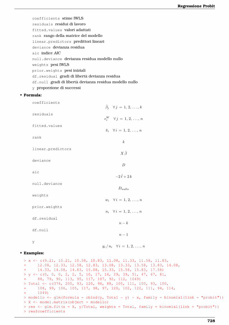
Regressione Probit
coefficients stime IWLS
residuals residui di lavoro
fitted.values valori adattati
rank rango della matrice del modello
linear.predictors predittori lineari
deviance devianza residua
aic indice AICnull.deviance devianza residua modello nullo
weights pesi IWLS
prior.weights pesi iniziali
df.residual gradi di libertà devianza residua
df.null gradi di libertà devianza residua modello nullo
y proporzione di successi
• Formula:
coefficientsβj ∀ j = 1, 2, . . . , k
residualseWi ∀ j = 1, 2, . . . , n
fitted.valuesπi ∀ i = 1, 2, . . . , n
rankk
linear.predictorsX β
devianceD
aic−2 ˆ+ 2 k
null.devianceDnullo
weightswi ∀ i = 1, 2, . . . , n
prior.weightsni ∀ i = 1, 2, . . . , n
df.residualn− k
df.nulln− 1
yyi / ni ∀ i = 1, 2, . . . , n
• Examples:
> x <- c(9.21, 10.21, 10.58, 10.83, 11.08, 11.33, 11.58, 11.83,+ 12.08, 12.33, 12.58, 12.83, 13.08, 13.33, 13.58, 13.83, 14.08,+ 14.33, 14.58, 14.83, 15.08, 15.33, 15.58, 15.83, 17.58)> y <- c(0, 0, 0, 2, 2, 5, 10, 17, 16, 29, 39, 51, 47, 67, 81,+ 88, 79, 90, 113, 95, 117, 107, 92, 112, 1049)> Total <- c(376, 200, 93, 120, 90, 88, 105, 111, 100, 93, 100,+ 108, 99, 106, 105, 117, 98, 97, 120, 102, 122, 111, 94, 114,+ 1049)> modello <- glm(formula = cbind(y, Total - y) ~ x, family = binomial(link = "probit"))> X <- model.matrix(object = modello)> res <- glm.fit(x = X, y/Total, weights = Total, family = binomial(link = "probit"))> res$coefficients
728
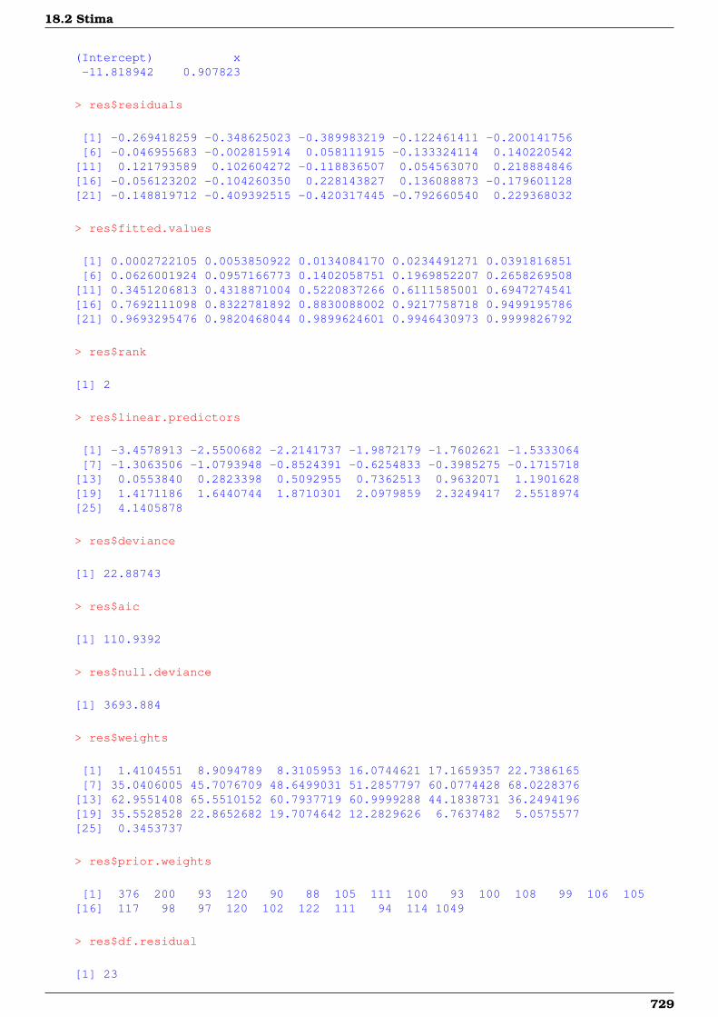
18.2 Stima
(Intercept) x-11.818942 0.907823
> res$residuals
[1] -0.269418259 -0.348625023 -0.389983219 -0.122461411 -0.200141756[6] -0.046955683 -0.002815914 0.058111915 -0.133324114 0.140220542
[11] 0.121793589 0.102604272 -0.118836507 0.054563070 0.218884846[16] -0.056123202 -0.104260350 0.228143827 0.136088873 -0.179601128[21] -0.148819712 -0.409392515 -0.420317445 -0.792660540 0.229368032
> res$fitted.values
[1] 0.0002722105 0.0053850922 0.0134084170 0.0234491271 0.0391816851[6] 0.0626001924 0.0957166773 0.1402058751 0.1969852207 0.2658269508
[11] 0.3451206813 0.4318871004 0.5220837266 0.6111585001 0.6947274541[16] 0.7692111098 0.8322781892 0.8830088002 0.9217758718 0.9499195786[21] 0.9693295476 0.9820468044 0.9899624601 0.9946430973 0.9999826792
> res$rank
[1] 2
> res$linear.predictors
[1] -3.4578913 -2.5500682 -2.2141737 -1.9872179 -1.7602621 -1.5333064[7] -1.3063506 -1.0793948 -0.8524391 -0.6254833 -0.3985275 -0.1715718
[13] 0.0553840 0.2823398 0.5092955 0.7362513 0.9632071 1.1901628[19] 1.4171186 1.6440744 1.8710301 2.0979859 2.3249417 2.5518974[25] 4.1405878
> res$deviance
[1] 22.88743
> res$aic
[1] 110.9392
> res$null.deviance
[1] 3693.884
> res$weights
[1] 1.4104551 8.9094789 8.3105953 16.0744621 17.1659357 22.7386165[7] 35.0406005 45.7076709 48.6499031 51.2857797 60.0774428 68.0228376
[13] 62.9551408 65.5510152 60.7937719 60.9999288 44.1838731 36.2494196[19] 35.5528528 22.8652682 19.7074642 12.2829626 6.7637482 5.0575577[25] 0.3453737
> res$prior.weights
[1] 376 200 93 120 90 88 105 111 100 93 100 108 99 106 105[16] 117 98 97 120 102 122 111 94 114 1049
> res$df.residual
[1] 23
729
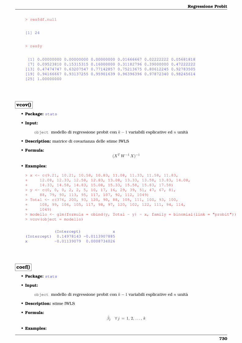
Regressione Probit
> res$df.null
[1] 24
> res$y
[1] 0.00000000 0.00000000 0.00000000 0.01666667 0.02222222 0.05681818[7] 0.09523810 0.15315315 0.16000000 0.31182796 0.39000000 0.47222222
[13] 0.47474747 0.63207547 0.77142857 0.75213675 0.80612245 0.92783505[19] 0.94166667 0.93137255 0.95901639 0.96396396 0.97872340 0.98245614[25] 1.00000000
vcov()
• Package: stats
• Input:
object modello di regressione probit con k − 1 variabili esplicative ed n unità
• Description: matrice di covarianza delle stime IWLS
• Formula:(XT W−1X)−1
• Examples:
> x <- c(9.21, 10.21, 10.58, 10.83, 11.08, 11.33, 11.58, 11.83,+ 12.08, 12.33, 12.58, 12.83, 13.08, 13.33, 13.58, 13.83, 14.08,+ 14.33, 14.58, 14.83, 15.08, 15.33, 15.58, 15.83, 17.58)> y <- c(0, 0, 0, 2, 2, 5, 10, 17, 16, 29, 39, 51, 47, 67, 81,+ 88, 79, 90, 113, 95, 117, 107, 92, 112, 1049)> Total <- c(376, 200, 93, 120, 90, 88, 105, 111, 100, 93, 100,+ 108, 99, 106, 105, 117, 98, 97, 120, 102, 122, 111, 94, 114,+ 1049)> modello <- glm(formula = cbind(y, Total - y) ~ x, family = binomial(link = "probit"))> vcov(object = modello)
(Intercept) x(Intercept) 0.14978143 -0.0113907885x -0.01139079 0.0008734026
coef()
• Package: stats
• Input:
object modello di regressione probit con k − 1 variabili esplicative ed n unità
• Description: stime IWLS
• Formula:βj ∀ j = 1, 2, . . . , k
• Examples:
730
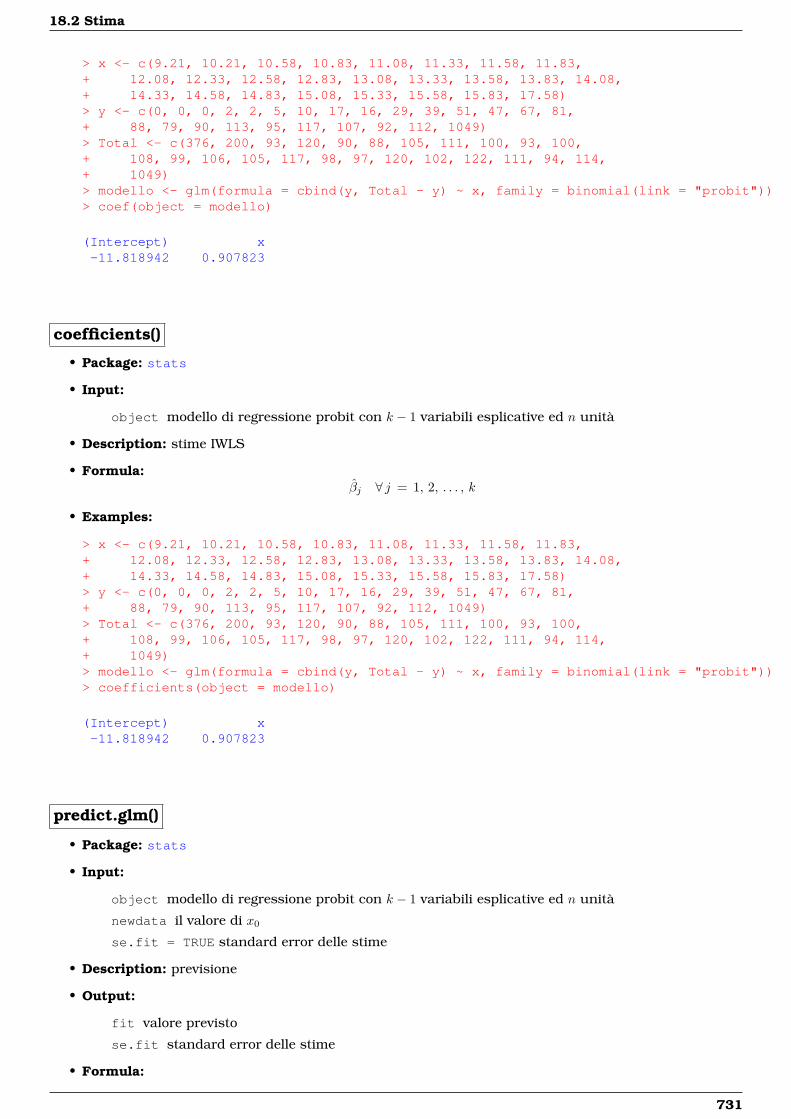
18.2 Stima
> x <- c(9.21, 10.21, 10.58, 10.83, 11.08, 11.33, 11.58, 11.83,+ 12.08, 12.33, 12.58, 12.83, 13.08, 13.33, 13.58, 13.83, 14.08,+ 14.33, 14.58, 14.83, 15.08, 15.33, 15.58, 15.83, 17.58)> y <- c(0, 0, 0, 2, 2, 5, 10, 17, 16, 29, 39, 51, 47, 67, 81,+ 88, 79, 90, 113, 95, 117, 107, 92, 112, 1049)> Total <- c(376, 200, 93, 120, 90, 88, 105, 111, 100, 93, 100,+ 108, 99, 106, 105, 117, 98, 97, 120, 102, 122, 111, 94, 114,+ 1049)> modello <- glm(formula = cbind(y, Total - y) ~ x, family = binomial(link = "probit"))> coef(object = modello)
(Intercept) x-11.818942 0.907823
coefficients()
• Package: stats
• Input:
object modello di regressione probit con k − 1 variabili esplicative ed n unità
• Description: stime IWLS
• Formula:βj ∀ j = 1, 2, . . . , k
• Examples:
> x <- c(9.21, 10.21, 10.58, 10.83, 11.08, 11.33, 11.58, 11.83,+ 12.08, 12.33, 12.58, 12.83, 13.08, 13.33, 13.58, 13.83, 14.08,+ 14.33, 14.58, 14.83, 15.08, 15.33, 15.58, 15.83, 17.58)> y <- c(0, 0, 0, 2, 2, 5, 10, 17, 16, 29, 39, 51, 47, 67, 81,+ 88, 79, 90, 113, 95, 117, 107, 92, 112, 1049)> Total <- c(376, 200, 93, 120, 90, 88, 105, 111, 100, 93, 100,+ 108, 99, 106, 105, 117, 98, 97, 120, 102, 122, 111, 94, 114,+ 1049)> modello <- glm(formula = cbind(y, Total - y) ~ x, family = binomial(link = "probit"))> coefficients(object = modello)
(Intercept) x-11.818942 0.907823
predict.glm()
• Package: stats
• Input:
object modello di regressione probit con k − 1 variabili esplicative ed n unità
newdata il valore di x0
se.fit = TRUE standard error delle stime
• Description: previsione
• Output:
fit valore previsto
se.fit standard error delle stime
• Formula:
731
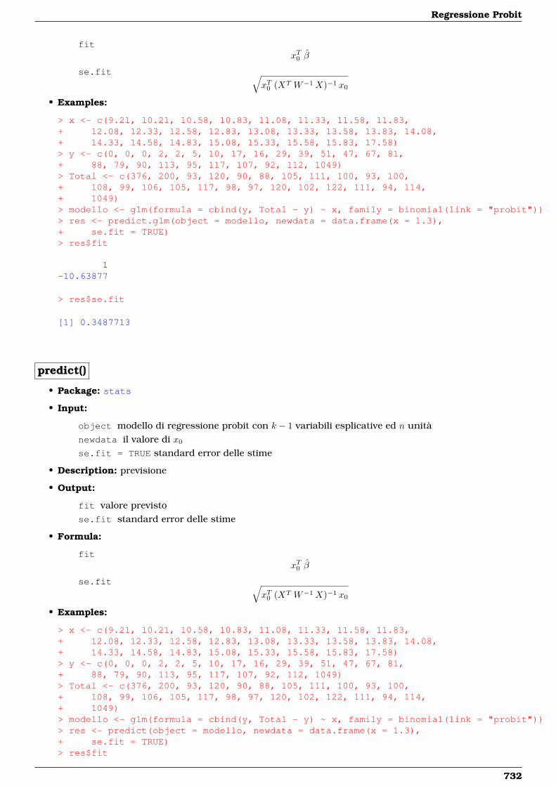
Regressione Probit
fitxT0 β
se.fit √xT0 (XT W−1X)−1 x0
• Examples:
> x <- c(9.21, 10.21, 10.58, 10.83, 11.08, 11.33, 11.58, 11.83,+ 12.08, 12.33, 12.58, 12.83, 13.08, 13.33, 13.58, 13.83, 14.08,+ 14.33, 14.58, 14.83, 15.08, 15.33, 15.58, 15.83, 17.58)> y <- c(0, 0, 0, 2, 2, 5, 10, 17, 16, 29, 39, 51, 47, 67, 81,+ 88, 79, 90, 113, 95, 117, 107, 92, 112, 1049)> Total <- c(376, 200, 93, 120, 90, 88, 105, 111, 100, 93, 100,+ 108, 99, 106, 105, 117, 98, 97, 120, 102, 122, 111, 94, 114,+ 1049)> modello <- glm(formula = cbind(y, Total - y) ~ x, family = binomial(link = "probit"))> res <- predict.glm(object = modello, newdata = data.frame(x = 1.3),+ se.fit = TRUE)> res$fit
1-10.63877
> res$se.fit
[1] 0.3487713
predict()
• Package: stats
• Input:
object modello di regressione probit con k − 1 variabili esplicative ed n unitànewdata il valore di x0
se.fit = TRUE standard error delle stime
• Description: previsione
• Output:
fit valore previstose.fit standard error delle stime
• Formula:
fitxT0 β
se.fit √xT0 (XT W−1X)−1 x0
• Examples:
> x <- c(9.21, 10.21, 10.58, 10.83, 11.08, 11.33, 11.58, 11.83,+ 12.08, 12.33, 12.58, 12.83, 13.08, 13.33, 13.58, 13.83, 14.08,+ 14.33, 14.58, 14.83, 15.08, 15.33, 15.58, 15.83, 17.58)> y <- c(0, 0, 0, 2, 2, 5, 10, 17, 16, 29, 39, 51, 47, 67, 81,+ 88, 79, 90, 113, 95, 117, 107, 92, 112, 1049)> Total <- c(376, 200, 93, 120, 90, 88, 105, 111, 100, 93, 100,+ 108, 99, 106, 105, 117, 98, 97, 120, 102, 122, 111, 94, 114,+ 1049)> modello <- glm(formula = cbind(y, Total - y) ~ x, family = binomial(link = "probit"))> res <- predict(object = modello, newdata = data.frame(x = 1.3),+ se.fit = TRUE)> res$fit
732
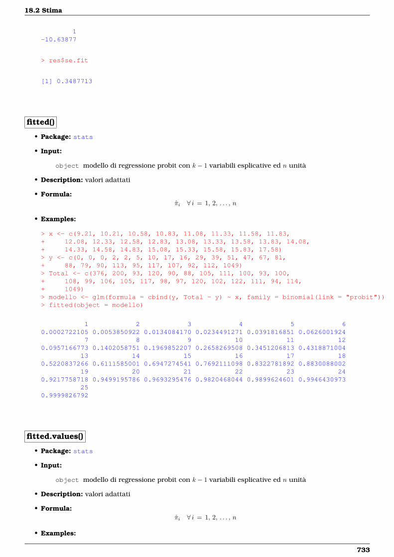
18.2 Stima
1-10.63877
> res$se.fit
[1] 0.3487713
fitted()
• Package: stats
• Input:
object modello di regressione probit con k − 1 variabili esplicative ed n unità
• Description: valori adattati
• Formula:πi ∀ i = 1, 2, . . . , n
• Examples:
> x <- c(9.21, 10.21, 10.58, 10.83, 11.08, 11.33, 11.58, 11.83,+ 12.08, 12.33, 12.58, 12.83, 13.08, 13.33, 13.58, 13.83, 14.08,+ 14.33, 14.58, 14.83, 15.08, 15.33, 15.58, 15.83, 17.58)> y <- c(0, 0, 0, 2, 2, 5, 10, 17, 16, 29, 39, 51, 47, 67, 81,+ 88, 79, 90, 113, 95, 117, 107, 92, 112, 1049)> Total <- c(376, 200, 93, 120, 90, 88, 105, 111, 100, 93, 100,+ 108, 99, 106, 105, 117, 98, 97, 120, 102, 122, 111, 94, 114,+ 1049)> modello <- glm(formula = cbind(y, Total - y) ~ x, family = binomial(link = "probit"))> fitted(object = modello)
1 2 3 4 5 60.0002722105 0.0053850922 0.0134084170 0.0234491271 0.0391816851 0.0626001924
7 8 9 10 11 120.0957166773 0.1402058751 0.1969852207 0.2658269508 0.3451206813 0.4318871004
13 14 15 16 17 180.5220837266 0.6111585001 0.6947274541 0.7692111098 0.8322781892 0.8830088002
19 20 21 22 23 240.9217758718 0.9499195786 0.9693295476 0.9820468044 0.9899624601 0.9946430973
250.9999826792
fitted.values()
• Package: stats
• Input:
object modello di regressione probit con k − 1 variabili esplicative ed n unità
• Description: valori adattati
• Formula:πi ∀ i = 1, 2, . . . , n
• Examples:
733
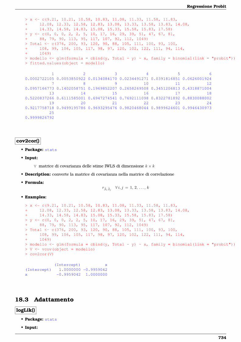
Regressione Probit
> x <- c(9.21, 10.21, 10.58, 10.83, 11.08, 11.33, 11.58, 11.83,+ 12.08, 12.33, 12.58, 12.83, 13.08, 13.33, 13.58, 13.83, 14.08,+ 14.33, 14.58, 14.83, 15.08, 15.33, 15.58, 15.83, 17.58)> y <- c(0, 0, 0, 2, 2, 5, 10, 17, 16, 29, 39, 51, 47, 67, 81,+ 88, 79, 90, 113, 95, 117, 107, 92, 112, 1049)> Total <- c(376, 200, 93, 120, 90, 88, 105, 111, 100, 93, 100,+ 108, 99, 106, 105, 117, 98, 97, 120, 102, 122, 111, 94, 114,+ 1049)> modello <- glm(formula = cbind(y, Total - y) ~ x, family = binomial(link = "probit"))> fitted.values(object = modello)
1 2 3 4 5 60.0002722105 0.0053850922 0.0134084170 0.0234491271 0.0391816851 0.0626001924
7 8 9 10 11 120.0957166773 0.1402058751 0.1969852207 0.2658269508 0.3451206813 0.4318871004
13 14 15 16 17 180.5220837266 0.6111585001 0.6947274541 0.7692111098 0.8322781892 0.8830088002
19 20 21 22 23 240.9217758718 0.9499195786 0.9693295476 0.9820468044 0.9899624601 0.9946430973
250.9999826792
cov2cor()
• Package: stats
• Input:
V matrice di covarianza delle stime IWLS di dimensione k × k
• Description: converte la matrice di covarianza nella matrice di correlazione
• Formula:rβi βj ∀ i, j = 1, 2, . . . , k
• Examples:
> x <- c(9.21, 10.21, 10.58, 10.83, 11.08, 11.33, 11.58, 11.83,+ 12.08, 12.33, 12.58, 12.83, 13.08, 13.33, 13.58, 13.83, 14.08,+ 14.33, 14.58, 14.83, 15.08, 15.33, 15.58, 15.83, 17.58)> y <- c(0, 0, 0, 2, 2, 5, 10, 17, 16, 29, 39, 51, 47, 67, 81,+ 88, 79, 90, 113, 95, 117, 107, 92, 112, 1049)> Total <- c(376, 200, 93, 120, 90, 88, 105, 111, 100, 93, 100,+ 108, 99, 106, 105, 117, 98, 97, 120, 102, 122, 111, 94, 114,+ 1049)> modello <- glm(formula = cbind(y, Total - y) ~ x, family = binomial(link = "probit"))> V <- vcov(object = modello)> cov2cor(V)
(Intercept) x(Intercept) 1.0000000 -0.9959042x -0.9959042 1.0000000
18.3 Adattamento
logLik()
• Package: stats
• Input:
734
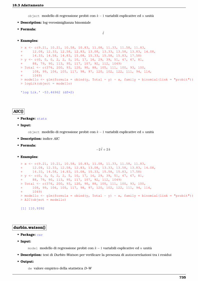
18.3 Adattamento
object modello di regressione probit con k − 1 variabili esplicative ed n unità
• Description: log-verosimiglianza binomiale
• Formula:ˆ
• Examples:
> x <- c(9.21, 10.21, 10.58, 10.83, 11.08, 11.33, 11.58, 11.83,+ 12.08, 12.33, 12.58, 12.83, 13.08, 13.33, 13.58, 13.83, 14.08,+ 14.33, 14.58, 14.83, 15.08, 15.33, 15.58, 15.83, 17.58)> y <- c(0, 0, 0, 2, 2, 5, 10, 17, 16, 29, 39, 51, 47, 67, 81,+ 88, 79, 90, 113, 95, 117, 107, 92, 112, 1049)> Total <- c(376, 200, 93, 120, 90, 88, 105, 111, 100, 93, 100,+ 108, 99, 106, 105, 117, 98, 97, 120, 102, 122, 111, 94, 114,+ 1049)> modello <- glm(formula = cbind(y, Total - y) ~ x, family = binomial(link = "probit"))> logLik(object = modello)
'log Lik.' -53.46962 (df=2)
AIC()
• Package: stats
• Input:
object modello di regressione probit con k − 1 variabili esplicative ed n unità
• Description: indice AIC
• Formula:−2 ˆ+ 2 k
• Examples:
> x <- c(9.21, 10.21, 10.58, 10.83, 11.08, 11.33, 11.58, 11.83,+ 12.08, 12.33, 12.58, 12.83, 13.08, 13.33, 13.58, 13.83, 14.08,+ 14.33, 14.58, 14.83, 15.08, 15.33, 15.58, 15.83, 17.58)> y <- c(0, 0, 0, 2, 2, 5, 10, 17, 16, 29, 39, 51, 47, 67, 81,+ 88, 79, 90, 113, 95, 117, 107, 92, 112, 1049)> Total <- c(376, 200, 93, 120, 90, 88, 105, 111, 100, 93, 100,+ 108, 99, 106, 105, 117, 98, 97, 120, 102, 122, 111, 94, 114,+ 1049)> modello <- glm(formula = cbind(y, Total - y) ~ x, family = binomial(link = "probit"))> AIC(object = modello)
[1] 110.9392
durbin.watson()
• Package: car
• Input:
model modello di regressione probit con k − 1 variabili esplicative ed n unità
• Description: test di Durbin–Watson per verificare la presenza di autocorrelazioni tra i residui
• Output:
dw valore empirico della statistica D–W
735
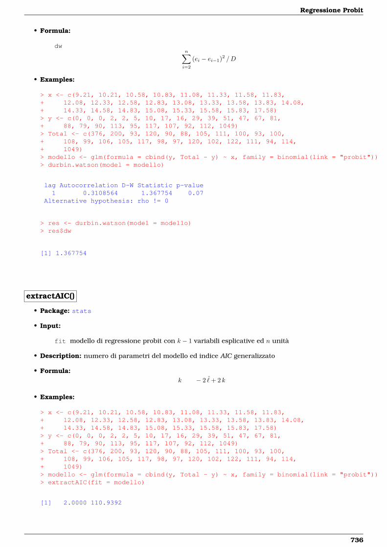
Regressione Probit
• Formula:
dwn∑i=2
(ei − ei−1)2 /D
• Examples:
> x <- c(9.21, 10.21, 10.58, 10.83, 11.08, 11.33, 11.58, 11.83,+ 12.08, 12.33, 12.58, 12.83, 13.08, 13.33, 13.58, 13.83, 14.08,+ 14.33, 14.58, 14.83, 15.08, 15.33, 15.58, 15.83, 17.58)> y <- c(0, 0, 0, 2, 2, 5, 10, 17, 16, 29, 39, 51, 47, 67, 81,+ 88, 79, 90, 113, 95, 117, 107, 92, 112, 1049)> Total <- c(376, 200, 93, 120, 90, 88, 105, 111, 100, 93, 100,+ 108, 99, 106, 105, 117, 98, 97, 120, 102, 122, 111, 94, 114,+ 1049)> modello <- glm(formula = cbind(y, Total - y) ~ x, family = binomial(link = "probit"))> durbin.watson(model = modello)
lag Autocorrelation D-W Statistic p-value1 0.3108564 1.367754 0.07
Alternative hypothesis: rho != 0
> res <- durbin.watson(model = modello)> res$dw
[1] 1.367754
extractAIC()
• Package: stats
• Input:
fit modello di regressione probit con k − 1 variabili esplicative ed n unità
• Description: numero di parametri del modello ed indice AIC generalizzato
• Formula:k − 2 ˆ+ 2 k
• Examples:
> x <- c(9.21, 10.21, 10.58, 10.83, 11.08, 11.33, 11.58, 11.83,+ 12.08, 12.33, 12.58, 12.83, 13.08, 13.33, 13.58, 13.83, 14.08,+ 14.33, 14.58, 14.83, 15.08, 15.33, 15.58, 15.83, 17.58)> y <- c(0, 0, 0, 2, 2, 5, 10, 17, 16, 29, 39, 51, 47, 67, 81,+ 88, 79, 90, 113, 95, 117, 107, 92, 112, 1049)> Total <- c(376, 200, 93, 120, 90, 88, 105, 111, 100, 93, 100,+ 108, 99, 106, 105, 117, 98, 97, 120, 102, 122, 111, 94, 114,+ 1049)> modello <- glm(formula = cbind(y, Total - y) ~ x, family = binomial(link = "probit"))> extractAIC(fit = modello)
[1] 2.0000 110.9392
736

18.3 Adattamento
deviance()
• Package: stats
• Input:
object modello di regressione probit con k − 1 variabili esplicative ed n unità
• Description: devianza residua
• Formula:D
• Examples:
> x <- c(9.21, 10.21, 10.58, 10.83, 11.08, 11.33, 11.58, 11.83,+ 12.08, 12.33, 12.58, 12.83, 13.08, 13.33, 13.58, 13.83, 14.08,+ 14.33, 14.58, 14.83, 15.08, 15.33, 15.58, 15.83, 17.58)> y <- c(0, 0, 0, 2, 2, 5, 10, 17, 16, 29, 39, 51, 47, 67, 81,+ 88, 79, 90, 113, 95, 117, 107, 92, 112, 1049)> Total <- c(376, 200, 93, 120, 90, 88, 105, 111, 100, 93, 100,+ 108, 99, 106, 105, 117, 98, 97, 120, 102, 122, 111, 94, 114,+ 1049)> modello <- glm(formula = cbind(y, Total - y) ~ x, family = binomial(link = "probit"))> deviance(object = modello)
[1] 22.88743
anova()
• Package: stats
• Input:
nullo modello nullo di regressione probit con n unità
modello modello di regressione probit con k − 1 variabili esplicative con n unità
test = "Chisq"
• Description: anova di regressione
• Output:
Resid. Df gradi di libertà
Resid. Dev devianza residua
Df differenza dei gradi di libertà
Deviance differenza tra le devianze residue
P(>|Chi|) p-value
• Formula:
Resid. Dfn− 1 n− k
Resid. DevDnullo D
Dfdf = k − 1
Deviancec = Dnullo −D
P(>|Chi|)P (χ2
df ≥ c)
• Examples:
737

Regressione Probit
> x <- c(9.21, 10.21, 10.58, 10.83, 11.08, 11.33, 11.58, 11.83,+ 12.08, 12.33, 12.58, 12.83, 13.08, 13.33, 13.58, 13.83, 14.08,+ 14.33, 14.58, 14.83, 15.08, 15.33, 15.58, 15.83, 17.58)> y <- c(0, 0, 0, 2, 2, 5, 10, 17, 16, 29, 39, 51, 47, 67, 81,+ 88, 79, 90, 113, 95, 117, 107, 92, 112, 1049)> Total <- c(376, 200, 93, 120, 90, 88, 105, 111, 100, 93, 100,+ 108, 99, 106, 105, 117, 98, 97, 120, 102, 122, 111, 94, 114,+ 1049)> nullo <- glm(formula = cbind(y, Total - y) ~ 1, family = binomial(link = "probit"))> modello <- glm(formula = cbind(y, Total - y) ~ x, family = binomial(link = "probit"))> anova(nullo, modello, test = "Chisq")
Analysis of Deviance Table
Model 1: cbind(y, Total - y) ~ 1Model 2: cbind(y, Total - y) ~ xResid. Df Resid. Dev Df Deviance P(>|Chi|)
1 24 3693.92 23 22.9 1 3671.0 0.0
> res <- anova(nullo, modello, test = "Chisq")> res$"Resid. Df"
[1] 24 23
> res$"Resid. Dev"
[1] 3693.88357 22.88743
> res$Df
[1] NA 1
> res$Deviance
[1] NA 3670.996
> res$"P(>|Chi|)"
[1] NA 0
drop1()
• Package: stats
• Input:
object modello di regressione probit con k − 1 variabili esplicative ed n unità
test = "Chisq"
• Description: submodels
• Output:
Df differenza tra gradi di libertà
Deviance differenza tra devianze residue
AIC indice AIC
LRT valore empirico della statistica χ2
Pr(Chi) p-value
738

18.3 Adattamento
• Formula:
Df1, 1, . . . , 1︸ ︷︷ ︸k−1 volte
DevianceD, D−xj ∀ j = 1, 2, . . . , k − 1
dove D−xj rappresenta la devianza residua del modello eliminata la variabile esplicativa xj.AIC
−2 ˆ+ 2 k, −2 ˆ−xj + 2 (k − 1) ∀ j = 1, 2, . . . , k − 1
dove ˆ−xj rappresenta la log-verosimiglianza binomiale del modello eliminata la variabile esplicativa xj.LRT
cj = D−xj −D ∀ j = 1, 2, . . . , k − 1
Pr(Chi)P (χ2
1 ≥ cj) ∀ j = 1, 2, . . . , k − 1
• Examples:
> x <- c(9.21, 10.21, 10.58, 10.83, 11.08, 11.33, 11.58, 11.83,+ 12.08, 12.33, 12.58, 12.83, 13.08, 13.33, 13.58, 13.83, 14.08,+ 14.33, 14.58, 14.83, 15.08, 15.33, 15.58, 15.83, 17.58)> y <- c(0, 0, 0, 2, 2, 5, 10, 17, 16, 29, 39, 51, 47, 67, 81,+ 88, 79, 90, 113, 95, 117, 107, 92, 112, 1049)> Total <- c(376, 200, 93, 120, 90, 88, 105, 111, 100, 93, 100,+ 108, 99, 106, 105, 117, 98, 97, 120, 102, 122, 111, 94, 114,+ 1049)> modello <- glm(formula = cbind(y, Total - y) ~ x, family = binomial(link = "probit"))> drop1(object = modello, test = "Chisq")
Single term deletions
Model:cbind(y, Total - y) ~ x
Df Deviance AIC LRT Pr(Chi)<none> 22.9 110.9x 1 3693.9 3779.9 3671.0 < 2.2e-16 ***---Signif. codes: 0 '***' 0.001 '**' 0.01 '*' 0.05 '.' 0.1 ' ' 1
> res <- drop1(object = modello, test = "Chisq")> res$Df
[1] NA 1
> res$Deviance
[1] 22.88743 3693.88357
> res$AIC
[1] 110.9392 3779.9354
> res$LRT
[1] NA 3670.996
> res$"Pr(Chi)"
[1] NA 0
739

Regressione Probit
add1()
• Package: stats
• Input:
object modello nullo di regressione probit
scope modello di regressione probit con k − 1 variabili esplicative ed n unità
test = "Chisq"
• Description: submodels
• Output:
Df differenza tra gradi di libertà
Deviance differenza tra devianze residue
AIC indice AIC
LRT valore empirico della statistica χ2
Pr(Chi) p-value
• Formula:
Df1, 1, . . . , 1︸ ︷︷ ︸k−1 volte
DevianceDnullo, Dxj ∀ j = 1, 2, . . . , k − 1
dove Dxj rappresenta la devianza residua del modello con la sola variabile esplicativa xj.
AIC−2 ˆ
nullo + 2, −2 ˆxj + 4 ∀ j = 1, 2, . . . , k − 1
dove ˆxj rappresenta la log-verosimiglianza binomiale del modello con la sola variabile esplicativa xj.
LRTcj = Dnullo −Dxj ∀ j = 1, 2, . . . , k − 1
Pr(Chi)P (χ2
1 ≥ cj) ∀ j = 1, 2, . . . , k − 1
• Examples:
> x <- c(9.21, 10.21, 10.58, 10.83, 11.08, 11.33, 11.58, 11.83,+ 12.08, 12.33, 12.58, 12.83, 13.08, 13.33, 13.58, 13.83, 14.08,+ 14.33, 14.58, 14.83, 15.08, 15.33, 15.58, 15.83, 17.58)> y <- c(0, 0, 0, 2, 2, 5, 10, 17, 16, 29, 39, 51, 47, 67, 81,+ 88, 79, 90, 113, 95, 117, 107, 92, 112, 1049)> Total <- c(376, 200, 93, 120, 90, 88, 105, 111, 100, 93, 100,+ 108, 99, 106, 105, 117, 98, 97, 120, 102, 122, 111, 94, 114,+ 1049)> nullo <- glm(formula = cbind(y, Total - y) ~ 1, family = binomial(link = "probit"))> modello <- glm(formula = cbind(y, Total - y) ~ x, family = binomial(link = "probit"))> add1(object = nullo, scope = modello, test = "Chisq")
Single term additions
Model:cbind(y, Total - y) ~ 1
Df Deviance AIC LRT Pr(Chi)<none> 3693.9 3779.9x 1 22.9 110.9 3671.0 < 2.2e-16 ***---Signif. codes: 0 '***' 0.001 '**' 0.01 '*' 0.05 '.' 0.1 ' ' 1
740
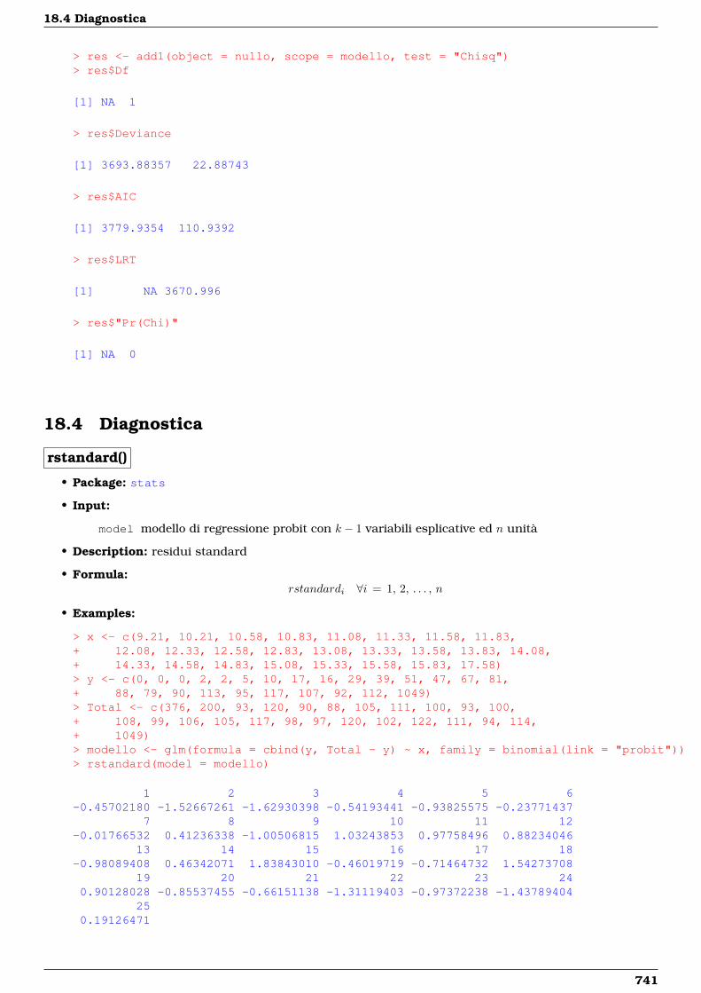
18.4 Diagnostica
> res <- add1(object = nullo, scope = modello, test = "Chisq")> res$Df
[1] NA 1
> res$Deviance
[1] 3693.88357 22.88743
> res$AIC
[1] 3779.9354 110.9392
> res$LRT
[1] NA 3670.996
> res$"Pr(Chi)"
[1] NA 0
18.4 Diagnostica
rstandard()
• Package: stats
• Input:
model modello di regressione probit con k − 1 variabili esplicative ed n unità
• Description: residui standard
• Formula:rstandardi ∀i = 1, 2, . . . , n
• Examples:
> x <- c(9.21, 10.21, 10.58, 10.83, 11.08, 11.33, 11.58, 11.83,+ 12.08, 12.33, 12.58, 12.83, 13.08, 13.33, 13.58, 13.83, 14.08,+ 14.33, 14.58, 14.83, 15.08, 15.33, 15.58, 15.83, 17.58)> y <- c(0, 0, 0, 2, 2, 5, 10, 17, 16, 29, 39, 51, 47, 67, 81,+ 88, 79, 90, 113, 95, 117, 107, 92, 112, 1049)> Total <- c(376, 200, 93, 120, 90, 88, 105, 111, 100, 93, 100,+ 108, 99, 106, 105, 117, 98, 97, 120, 102, 122, 111, 94, 114,+ 1049)> modello <- glm(formula = cbind(y, Total - y) ~ x, family = binomial(link = "probit"))> rstandard(model = modello)
1 2 3 4 5 6-0.45702180 -1.52667261 -1.62930398 -0.54193441 -0.93825575 -0.23771437
7 8 9 10 11 12-0.01766532 0.41236338 -1.00506815 1.03243853 0.97758496 0.88234046
13 14 15 16 17 18-0.98089408 0.46342071 1.83843010 -0.46019719 -0.71464732 1.54273708
19 20 21 22 23 240.90128028 -0.85537455 -0.66151138 -1.31119403 -0.97372238 -1.43789404
250.19126471
741
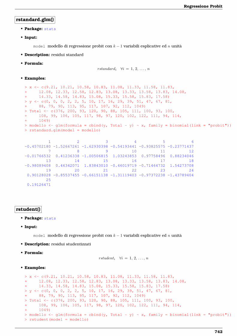
Regressione Probit
rstandard.glm()
• Package: stats
• Input:
model modello di regressione probit con k − 1 variabili esplicative ed n unità
• Description: residui standard
• Formula:rstandardi ∀i = 1, 2, . . . , n
• Examples:
> x <- c(9.21, 10.21, 10.58, 10.83, 11.08, 11.33, 11.58, 11.83,+ 12.08, 12.33, 12.58, 12.83, 13.08, 13.33, 13.58, 13.83, 14.08,+ 14.33, 14.58, 14.83, 15.08, 15.33, 15.58, 15.83, 17.58)> y <- c(0, 0, 0, 2, 2, 5, 10, 17, 16, 29, 39, 51, 47, 67, 81,+ 88, 79, 90, 113, 95, 117, 107, 92, 112, 1049)> Total <- c(376, 200, 93, 120, 90, 88, 105, 111, 100, 93, 100,+ 108, 99, 106, 105, 117, 98, 97, 120, 102, 122, 111, 94, 114,+ 1049)> modello <- glm(formula = cbind(y, Total - y) ~ x, family = binomial(link = "probit"))> rstandard.glm(model = modello)
1 2 3 4 5 6-0.45702180 -1.52667261 -1.62930398 -0.54193441 -0.93825575 -0.23771437
7 8 9 10 11 12-0.01766532 0.41236338 -1.00506815 1.03243853 0.97758496 0.88234046
13 14 15 16 17 18-0.98089408 0.46342071 1.83843010 -0.46019719 -0.71464732 1.54273708
19 20 21 22 23 240.90128028 -0.85537455 -0.66151138 -1.31119403 -0.97372238 -1.43789404
250.19126471
rstudent()
• Package: stats
• Input:
model modello di regressione probit con k − 1 variabili esplicative ed n unità
• Description: residui studentizzati
• Formula:rstudenti ∀i = 1, 2, . . . , n
• Examples:
> x <- c(9.21, 10.21, 10.58, 10.83, 11.08, 11.33, 11.58, 11.83,+ 12.08, 12.33, 12.58, 12.83, 13.08, 13.33, 13.58, 13.83, 14.08,+ 14.33, 14.58, 14.83, 15.08, 15.33, 15.58, 15.83, 17.58)> y <- c(0, 0, 0, 2, 2, 5, 10, 17, 16, 29, 39, 51, 47, 67, 81,+ 88, 79, 90, 113, 95, 117, 107, 92, 112, 1049)> Total <- c(376, 200, 93, 120, 90, 88, 105, 111, 100, 93, 100,+ 108, 99, 106, 105, 117, 98, 97, 120, 102, 122, 111, 94, 114,+ 1049)> modello <- glm(formula = cbind(y, Total - y) ~ x, family = binomial(link = "probit"))> rstudent(model = modello)
742
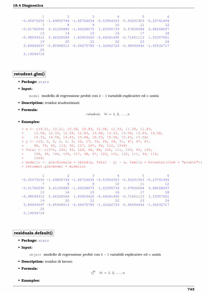
18.4 Diagnostica
1 2 3 4 5 6-0.45475250 -1.49850744 -1.60724034 -0.53954353 -0.93261903 -0.23741494
7 8 9 10 11 12-0.01766390 0.41295880 -1.00258075 1.03395739 0.97836584 0.88258097
13 14 15 16 17 18-0.98094312 0.46328566 1.83403420 -0.46061490 -0.71601113 1.53357601
19 20 21 22 23 240.89694597 -0.85968513 -0.66475785 -1.32462729 -0.98094946 -1.45532717
250.19094718
rstudent.glm()
• Package: stats
• Input:
model modello di regressione probit con k − 1 variabili esplicative ed n unità
• Description: residui studentizzati
• Formula:rstudenti ∀i = 1, 2, . . . , n
• Examples:
> x <- c(9.21, 10.21, 10.58, 10.83, 11.08, 11.33, 11.58, 11.83,+ 12.08, 12.33, 12.58, 12.83, 13.08, 13.33, 13.58, 13.83, 14.08,+ 14.33, 14.58, 14.83, 15.08, 15.33, 15.58, 15.83, 17.58)> y <- c(0, 0, 0, 2, 2, 5, 10, 17, 16, 29, 39, 51, 47, 67, 81,+ 88, 79, 90, 113, 95, 117, 107, 92, 112, 1049)> Total <- c(376, 200, 93, 120, 90, 88, 105, 111, 100, 93, 100,+ 108, 99, 106, 105, 117, 98, 97, 120, 102, 122, 111, 94, 114,+ 1049)> modello <- glm(formula = cbind(y, Total - y) ~ x, family = binomial(link = "probit"))> rstudent.glm(model = modello)
1 2 3 4 5 6-0.45475250 -1.49850744 -1.60724034 -0.53954353 -0.93261903 -0.23741494
7 8 9 10 11 12-0.01766390 0.41295880 -1.00258075 1.03395739 0.97836584 0.88258097
13 14 15 16 17 18-0.98094312 0.46328566 1.83403420 -0.46061490 -0.71601113 1.53357601
19 20 21 22 23 240.89694597 -0.85968513 -0.66475785 -1.32462729 -0.98094946 -1.45532717
250.19094718
residuals.default()
• Package: stats
• Input:
object modello di regressione probit con k − 1 variabili esplicative ed n unità
• Description: residui di lavoro
• Formula:eWi ∀i = 1, 2, . . . , n
• Examples:
743
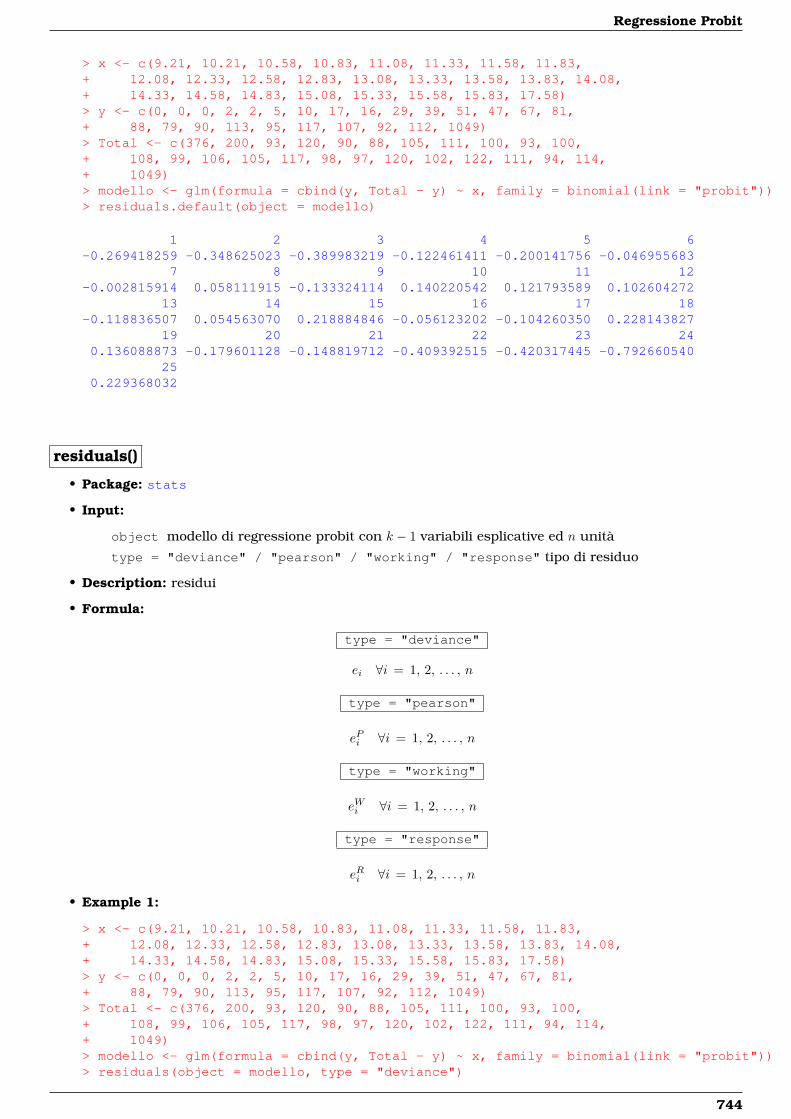
Regressione Probit
> x <- c(9.21, 10.21, 10.58, 10.83, 11.08, 11.33, 11.58, 11.83,+ 12.08, 12.33, 12.58, 12.83, 13.08, 13.33, 13.58, 13.83, 14.08,+ 14.33, 14.58, 14.83, 15.08, 15.33, 15.58, 15.83, 17.58)> y <- c(0, 0, 0, 2, 2, 5, 10, 17, 16, 29, 39, 51, 47, 67, 81,+ 88, 79, 90, 113, 95, 117, 107, 92, 112, 1049)> Total <- c(376, 200, 93, 120, 90, 88, 105, 111, 100, 93, 100,+ 108, 99, 106, 105, 117, 98, 97, 120, 102, 122, 111, 94, 114,+ 1049)> modello <- glm(formula = cbind(y, Total - y) ~ x, family = binomial(link = "probit"))> residuals.default(object = modello)
1 2 3 4 5 6-0.269418259 -0.348625023 -0.389983219 -0.122461411 -0.200141756 -0.046955683
7 8 9 10 11 12-0.002815914 0.058111915 -0.133324114 0.140220542 0.121793589 0.102604272
13 14 15 16 17 18-0.118836507 0.054563070 0.218884846 -0.056123202 -0.104260350 0.228143827
19 20 21 22 23 240.136088873 -0.179601128 -0.148819712 -0.409392515 -0.420317445 -0.792660540
250.229368032
residuals()
• Package: stats
• Input:
object modello di regressione probit con k − 1 variabili esplicative ed n unità
type = "deviance" / "pearson" / "working" / "response" tipo di residuo
• Description: residui
• Formula:
type = "deviance"
ei ∀i = 1, 2, . . . , n
type = "pearson"
ePi ∀i = 1, 2, . . . , n
type = "working"
eWi ∀i = 1, 2, . . . , n
type = "response"
eRi ∀i = 1, 2, . . . , n
• Example 1:
> x <- c(9.21, 10.21, 10.58, 10.83, 11.08, 11.33, 11.58, 11.83,+ 12.08, 12.33, 12.58, 12.83, 13.08, 13.33, 13.58, 13.83, 14.08,+ 14.33, 14.58, 14.83, 15.08, 15.33, 15.58, 15.83, 17.58)> y <- c(0, 0, 0, 2, 2, 5, 10, 17, 16, 29, 39, 51, 47, 67, 81,+ 88, 79, 90, 113, 95, 117, 107, 92, 112, 1049)> Total <- c(376, 200, 93, 120, 90, 88, 105, 111, 100, 93, 100,+ 108, 99, 106, 105, 117, 98, 97, 120, 102, 122, 111, 94, 114,+ 1049)> modello <- glm(formula = cbind(y, Total - y) ~ x, family = binomial(link = "probit"))> residuals(object = modello, type = "deviance")
744

18.4 Diagnostica
1 2 3 4 5 6-0.45247119 -1.46964542 -1.58456196 -0.51743600 -0.90056726 -0.22725786
7 8 9 10 11 12-0.01668127 0.38801751 -0.95408459 0.98731872 0.93524092 0.84356724
13 14 15 16 17 18-0.94228925 0.44328398 1.75392860 -0.43468903 -0.67959504 1.46607128
19 20 21 22 23 240.84691681 -0.81514441 -0.62908579 -1.26364877 -0.95089420 -1.40845258
250.19062911
• Example 2:
> x <- c(9.21, 10.21, 10.58, 10.83, 11.08, 11.33, 11.58, 11.83,+ 12.08, 12.33, 12.58, 12.83, 13.08, 13.33, 13.58, 13.83, 14.08,+ 14.33, 14.58, 14.83, 15.08, 15.33, 15.58, 15.83, 17.58)> y <- c(0, 0, 0, 2, 2, 5, 10, 17, 16, 29, 39, 51, 47, 67, 81,+ 88, 79, 90, 113, 95, 117, 107, 92, 112, 1049)> Total <- c(376, 200, 93, 120, 90, 88, 105, 111, 100, 93, 100,+ 108, 99, 106, 105, 117, 98, 97, 120, 102, 122, 111, 94, 114,+ 1049)> modello <- glm(formula = cbind(y, Total - y) ~ x, family = binomial(link = "probit"))> residuals(object = modello, type = "pearson")
1 2 3 4 5 6-0.31996722 -1.04060064 -1.12424645 -0.49098375 -0.82922265 -0.22390818
7 8 9 10 11 12-0.01666883 0.39287973 -0.92992864 1.00417656 0.94401767 0.84623856
13 14 15 16 17 18-0.94289966 0.44176215 1.70665302 -0.43833594 -0.69302839 1.37359650
19 20 21 22 23 240.81144619 -0.85880990 -0.66065634 -1.43479933 -1.09312733 -1.78261348
250.13479572
• Example 3:
> x <- c(9.21, 10.21, 10.58, 10.83, 11.08, 11.33, 11.58, 11.83,+ 12.08, 12.33, 12.58, 12.83, 13.08, 13.33, 13.58, 13.83, 14.08,+ 14.33, 14.58, 14.83, 15.08, 15.33, 15.58, 15.83, 17.58)> y <- c(0, 0, 0, 2, 2, 5, 10, 17, 16, 29, 39, 51, 47, 67, 81,+ 88, 79, 90, 113, 95, 117, 107, 92, 112, 1049)> Total <- c(376, 200, 93, 120, 90, 88, 105, 111, 100, 93, 100,+ 108, 99, 106, 105, 117, 98, 97, 120, 102, 122, 111, 94, 114,+ 1049)> modello <- glm(formula = cbind(y, Total - y) ~ x, family = binomial(link = "probit"))> residuals(object = modello, type = "working")
1 2 3 4 5 6-0.269418259 -0.348625023 -0.389983219 -0.122461411 -0.200141756 -0.046955683
7 8 9 10 11 12-0.002815914 0.058111915 -0.133324114 0.140220542 0.121793589 0.102604272
13 14 15 16 17 18-0.118836507 0.054563070 0.218884846 -0.056123202 -0.104260350 0.228143827
19 20 21 22 23 240.136088873 -0.179601128 -0.148819712 -0.409392515 -0.420317445 -0.792660540
250.229368032
• Example 4:
> x <- c(9.21, 10.21, 10.58, 10.83, 11.08, 11.33, 11.58, 11.83,+ 12.08, 12.33, 12.58, 12.83, 13.08, 13.33, 13.58, 13.83, 14.08,+ 14.33, 14.58, 14.83, 15.08, 15.33, 15.58, 15.83, 17.58)
745
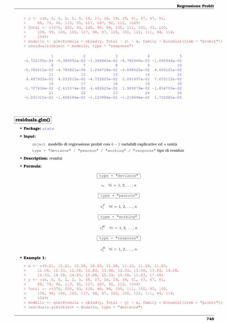
Regressione Probit
> y <- c(0, 0, 0, 2, 2, 5, 10, 17, 16, 29, 39, 51, 47, 67, 81,+ 88, 79, 90, 113, 95, 117, 107, 92, 112, 1049)> Total <- c(376, 200, 93, 120, 90, 88, 105, 111, 100, 93, 100,+ 108, 99, 106, 105, 117, 98, 97, 120, 102, 122, 111, 94, 114,+ 1049)> modello <- glm(formula = cbind(y, Total - y) ~ x, family = binomial(link = "probit"))> residuals(object = modello, type = "response")
1 2 3 4 5-2.722105e-04 -5.385092e-03 -1.340842e-02 -6.782460e-03 -1.695946e-02
6 7 8 9 10-5.782011e-03 -4.785821e-04 1.294728e-02 -3.698522e-02 4.600101e-02
11 12 13 14 154.487932e-02 4.033512e-02 -4.733625e-02 2.091697e-02 7.670112e-02
16 17 18 19 20-1.707436e-02 -2.615574e-02 4.482625e-02 1.989079e-02 -1.854703e-02
21 22 23 24 25-1.031315e-02 -1.808284e-02 -1.123906e-02 -1.218696e-02 1.732085e-05
residuals.glm()
• Package: stats
• Input:
object modello di regressione probit con k − 1 variabili esplicative ed n unità
type = "deviance" / "pearson" / "working" / "response" tipo di residuo
• Description: residui
• Formula:
type = "deviance"
ei ∀i = 1, 2, . . . , n
type = "pearson"
ePi ∀i = 1, 2, . . . , n
type = "working"
eWi ∀i = 1, 2, . . . , n
type = "response"
eRi ∀i = 1, 2, . . . , n
• Example 1:
> x <- c(9.21, 10.21, 10.58, 10.83, 11.08, 11.33, 11.58, 11.83,+ 12.08, 12.33, 12.58, 12.83, 13.08, 13.33, 13.58, 13.83, 14.08,+ 14.33, 14.58, 14.83, 15.08, 15.33, 15.58, 15.83, 17.58)> y <- c(0, 0, 0, 2, 2, 5, 10, 17, 16, 29, 39, 51, 47, 67, 81,+ 88, 79, 90, 113, 95, 117, 107, 92, 112, 1049)> Total <- c(376, 200, 93, 120, 90, 88, 105, 111, 100, 93, 100,+ 108, 99, 106, 105, 117, 98, 97, 120, 102, 122, 111, 94, 114,+ 1049)> modello <- glm(formula = cbind(y, Total - y) ~ x, family = binomial(link = "probit"))> residuals.glm(object = modello, type = "deviance")
746
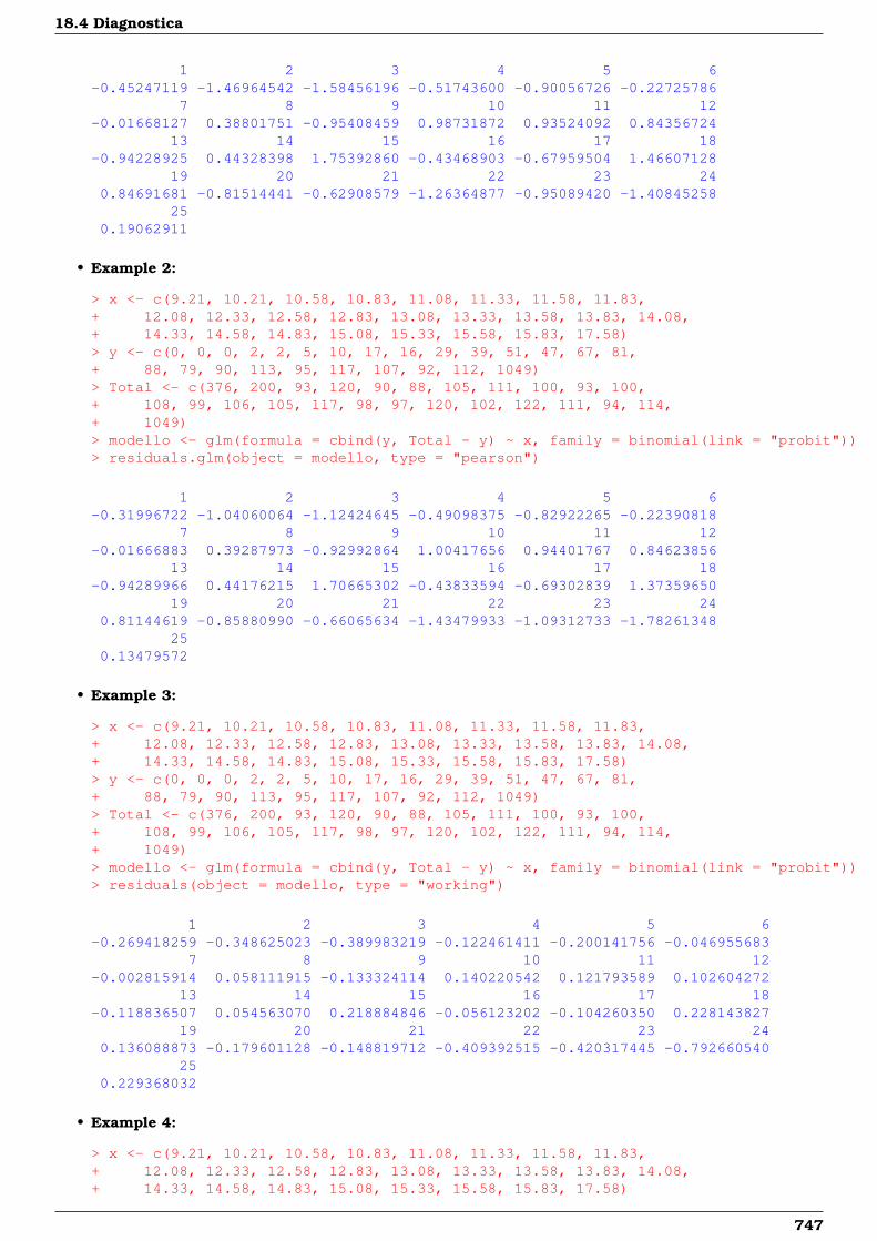
18.4 Diagnostica
1 2 3 4 5 6-0.45247119 -1.46964542 -1.58456196 -0.51743600 -0.90056726 -0.22725786
7 8 9 10 11 12-0.01668127 0.38801751 -0.95408459 0.98731872 0.93524092 0.84356724
13 14 15 16 17 18-0.94228925 0.44328398 1.75392860 -0.43468903 -0.67959504 1.46607128
19 20 21 22 23 240.84691681 -0.81514441 -0.62908579 -1.26364877 -0.95089420 -1.40845258
250.19062911
• Example 2:
> x <- c(9.21, 10.21, 10.58, 10.83, 11.08, 11.33, 11.58, 11.83,+ 12.08, 12.33, 12.58, 12.83, 13.08, 13.33, 13.58, 13.83, 14.08,+ 14.33, 14.58, 14.83, 15.08, 15.33, 15.58, 15.83, 17.58)> y <- c(0, 0, 0, 2, 2, 5, 10, 17, 16, 29, 39, 51, 47, 67, 81,+ 88, 79, 90, 113, 95, 117, 107, 92, 112, 1049)> Total <- c(376, 200, 93, 120, 90, 88, 105, 111, 100, 93, 100,+ 108, 99, 106, 105, 117, 98, 97, 120, 102, 122, 111, 94, 114,+ 1049)> modello <- glm(formula = cbind(y, Total - y) ~ x, family = binomial(link = "probit"))> residuals.glm(object = modello, type = "pearson")
1 2 3 4 5 6-0.31996722 -1.04060064 -1.12424645 -0.49098375 -0.82922265 -0.22390818
7 8 9 10 11 12-0.01666883 0.39287973 -0.92992864 1.00417656 0.94401767 0.84623856
13 14 15 16 17 18-0.94289966 0.44176215 1.70665302 -0.43833594 -0.69302839 1.37359650
19 20 21 22 23 240.81144619 -0.85880990 -0.66065634 -1.43479933 -1.09312733 -1.78261348
250.13479572
• Example 3:
> x <- c(9.21, 10.21, 10.58, 10.83, 11.08, 11.33, 11.58, 11.83,+ 12.08, 12.33, 12.58, 12.83, 13.08, 13.33, 13.58, 13.83, 14.08,+ 14.33, 14.58, 14.83, 15.08, 15.33, 15.58, 15.83, 17.58)> y <- c(0, 0, 0, 2, 2, 5, 10, 17, 16, 29, 39, 51, 47, 67, 81,+ 88, 79, 90, 113, 95, 117, 107, 92, 112, 1049)> Total <- c(376, 200, 93, 120, 90, 88, 105, 111, 100, 93, 100,+ 108, 99, 106, 105, 117, 98, 97, 120, 102, 122, 111, 94, 114,+ 1049)> modello <- glm(formula = cbind(y, Total - y) ~ x, family = binomial(link = "probit"))> residuals(object = modello, type = "working")
1 2 3 4 5 6-0.269418259 -0.348625023 -0.389983219 -0.122461411 -0.200141756 -0.046955683
7 8 9 10 11 12-0.002815914 0.058111915 -0.133324114 0.140220542 0.121793589 0.102604272
13 14 15 16 17 18-0.118836507 0.054563070 0.218884846 -0.056123202 -0.104260350 0.228143827
19 20 21 22 23 240.136088873 -0.179601128 -0.148819712 -0.409392515 -0.420317445 -0.792660540
250.229368032
• Example 4:
> x <- c(9.21, 10.21, 10.58, 10.83, 11.08, 11.33, 11.58, 11.83,+ 12.08, 12.33, 12.58, 12.83, 13.08, 13.33, 13.58, 13.83, 14.08,+ 14.33, 14.58, 14.83, 15.08, 15.33, 15.58, 15.83, 17.58)
747
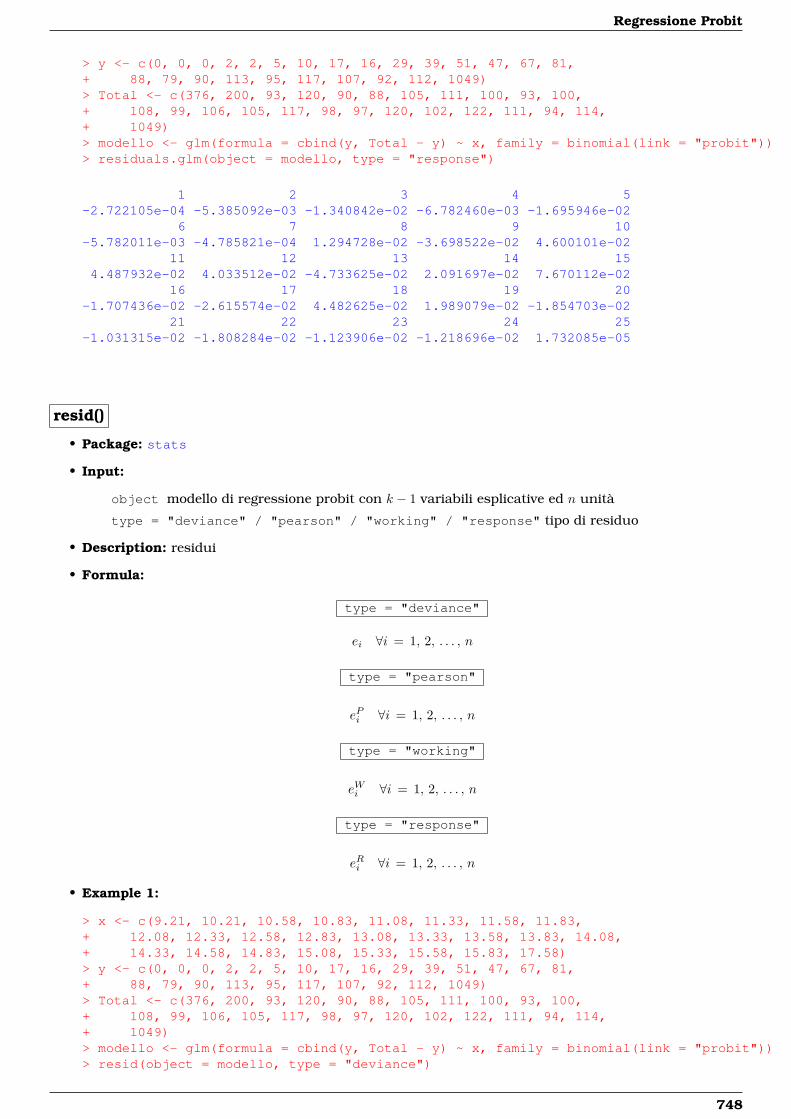
Regressione Probit
> y <- c(0, 0, 0, 2, 2, 5, 10, 17, 16, 29, 39, 51, 47, 67, 81,+ 88, 79, 90, 113, 95, 117, 107, 92, 112, 1049)> Total <- c(376, 200, 93, 120, 90, 88, 105, 111, 100, 93, 100,+ 108, 99, 106, 105, 117, 98, 97, 120, 102, 122, 111, 94, 114,+ 1049)> modello <- glm(formula = cbind(y, Total - y) ~ x, family = binomial(link = "probit"))> residuals.glm(object = modello, type = "response")
1 2 3 4 5-2.722105e-04 -5.385092e-03 -1.340842e-02 -6.782460e-03 -1.695946e-02
6 7 8 9 10-5.782011e-03 -4.785821e-04 1.294728e-02 -3.698522e-02 4.600101e-02
11 12 13 14 154.487932e-02 4.033512e-02 -4.733625e-02 2.091697e-02 7.670112e-02
16 17 18 19 20-1.707436e-02 -2.615574e-02 4.482625e-02 1.989079e-02 -1.854703e-02
21 22 23 24 25-1.031315e-02 -1.808284e-02 -1.123906e-02 -1.218696e-02 1.732085e-05
resid()
• Package: stats
• Input:
object modello di regressione probit con k − 1 variabili esplicative ed n unità
type = "deviance" / "pearson" / "working" / "response" tipo di residuo
• Description: residui
• Formula:
type = "deviance"
ei ∀i = 1, 2, . . . , n
type = "pearson"
ePi ∀i = 1, 2, . . . , n
type = "working"
eWi ∀i = 1, 2, . . . , n
type = "response"
eRi ∀i = 1, 2, . . . , n
• Example 1:
> x <- c(9.21, 10.21, 10.58, 10.83, 11.08, 11.33, 11.58, 11.83,+ 12.08, 12.33, 12.58, 12.83, 13.08, 13.33, 13.58, 13.83, 14.08,+ 14.33, 14.58, 14.83, 15.08, 15.33, 15.58, 15.83, 17.58)> y <- c(0, 0, 0, 2, 2, 5, 10, 17, 16, 29, 39, 51, 47, 67, 81,+ 88, 79, 90, 113, 95, 117, 107, 92, 112, 1049)> Total <- c(376, 200, 93, 120, 90, 88, 105, 111, 100, 93, 100,+ 108, 99, 106, 105, 117, 98, 97, 120, 102, 122, 111, 94, 114,+ 1049)> modello <- glm(formula = cbind(y, Total - y) ~ x, family = binomial(link = "probit"))> resid(object = modello, type = "deviance")
748
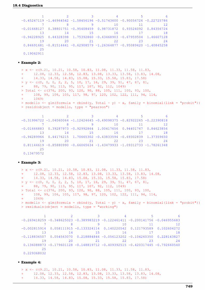
18.4 Diagnostica
1 2 3 4 5 6-0.45247119 -1.46964542 -1.58456196 -0.51743600 -0.90056726 -0.22725786
7 8 9 10 11 12-0.01668127 0.38801751 -0.95408459 0.98731872 0.93524092 0.84356724
13 14 15 16 17 18-0.94228925 0.44328398 1.75392860 -0.43468903 -0.67959504 1.46607128
19 20 21 22 23 240.84691681 -0.81514441 -0.62908579 -1.26364877 -0.95089420 -1.40845258
250.19062911
• Example 2:
> x <- c(9.21, 10.21, 10.58, 10.83, 11.08, 11.33, 11.58, 11.83,+ 12.08, 12.33, 12.58, 12.83, 13.08, 13.33, 13.58, 13.83, 14.08,+ 14.33, 14.58, 14.83, 15.08, 15.33, 15.58, 15.83, 17.58)> y <- c(0, 0, 0, 2, 2, 5, 10, 17, 16, 29, 39, 51, 47, 67, 81,+ 88, 79, 90, 113, 95, 117, 107, 92, 112, 1049)> Total <- c(376, 200, 93, 120, 90, 88, 105, 111, 100, 93, 100,+ 108, 99, 106, 105, 117, 98, 97, 120, 102, 122, 111, 94, 114,+ 1049)> modello <- glm(formula = cbind(y, Total - y) ~ x, family = binomial(link = "probit"))> resid(object = modello, type = "pearson")
1 2 3 4 5 6-0.31996722 -1.04060064 -1.12424645 -0.49098375 -0.82922265 -0.22390818
7 8 9 10 11 12-0.01666883 0.39287973 -0.92992864 1.00417656 0.94401767 0.84623856
13 14 15 16 17 18-0.94289966 0.44176215 1.70665302 -0.43833594 -0.69302839 1.37359650
19 20 21 22 23 240.81144619 -0.85880990 -0.66065634 -1.43479933 -1.09312733 -1.78261348
250.13479572
• Example 3:
> x <- c(9.21, 10.21, 10.58, 10.83, 11.08, 11.33, 11.58, 11.83,+ 12.08, 12.33, 12.58, 12.83, 13.08, 13.33, 13.58, 13.83, 14.08,+ 14.33, 14.58, 14.83, 15.08, 15.33, 15.58, 15.83, 17.58)> y <- c(0, 0, 0, 2, 2, 5, 10, 17, 16, 29, 39, 51, 47, 67, 81,+ 88, 79, 90, 113, 95, 117, 107, 92, 112, 1049)> Total <- c(376, 200, 93, 120, 90, 88, 105, 111, 100, 93, 100,+ 108, 99, 106, 105, 117, 98, 97, 120, 102, 122, 111, 94, 114,+ 1049)> modello <- glm(formula = cbind(y, Total - y) ~ x, family = binomial(link = "probit"))> residuals(object = modello, type = "working")
1 2 3 4 5 6-0.269418259 -0.348625023 -0.389983219 -0.122461411 -0.200141756 -0.046955683
7 8 9 10 11 12-0.002815914 0.058111915 -0.133324114 0.140220542 0.121793589 0.102604272
13 14 15 16 17 18-0.118836507 0.054563070 0.218884846 -0.056123202 -0.104260350 0.228143827
19 20 21 22 23 240.136088873 -0.179601128 -0.148819712 -0.409392515 -0.420317445 -0.792660540
250.229368032
• Example 4:
> x <- c(9.21, 10.21, 10.58, 10.83, 11.08, 11.33, 11.58, 11.83,+ 12.08, 12.33, 12.58, 12.83, 13.08, 13.33, 13.58, 13.83, 14.08,+ 14.33, 14.58, 14.83, 15.08, 15.33, 15.58, 15.83, 17.58)
749
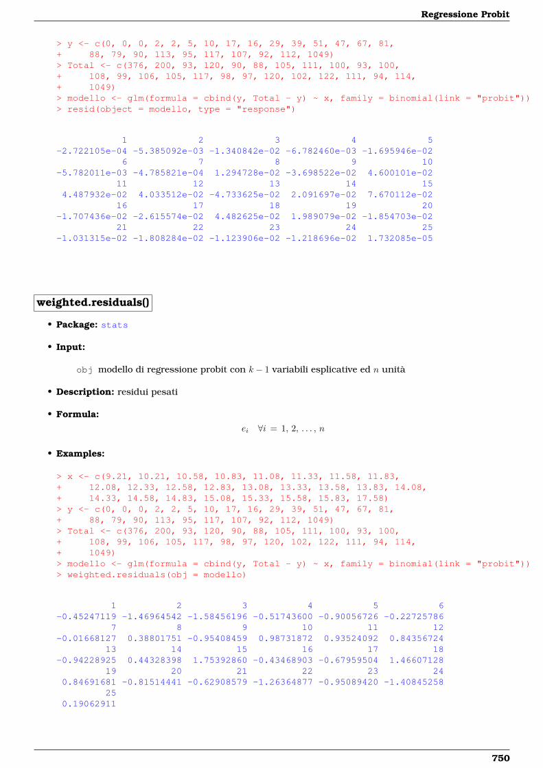
Regressione Probit
> y <- c(0, 0, 0, 2, 2, 5, 10, 17, 16, 29, 39, 51, 47, 67, 81,+ 88, 79, 90, 113, 95, 117, 107, 92, 112, 1049)> Total <- c(376, 200, 93, 120, 90, 88, 105, 111, 100, 93, 100,+ 108, 99, 106, 105, 117, 98, 97, 120, 102, 122, 111, 94, 114,+ 1049)> modello <- glm(formula = cbind(y, Total - y) ~ x, family = binomial(link = "probit"))> resid(object = modello, type = "response")
1 2 3 4 5-2.722105e-04 -5.385092e-03 -1.340842e-02 -6.782460e-03 -1.695946e-02
6 7 8 9 10-5.782011e-03 -4.785821e-04 1.294728e-02 -3.698522e-02 4.600101e-02
11 12 13 14 154.487932e-02 4.033512e-02 -4.733625e-02 2.091697e-02 7.670112e-02
16 17 18 19 20-1.707436e-02 -2.615574e-02 4.482625e-02 1.989079e-02 -1.854703e-02
21 22 23 24 25-1.031315e-02 -1.808284e-02 -1.123906e-02 -1.218696e-02 1.732085e-05
weighted.residuals()
• Package: stats
• Input:
obj modello di regressione probit con k − 1 variabili esplicative ed n unità
• Description: residui pesati
• Formula:
ei ∀i = 1, 2, . . . , n
• Examples:
> x <- c(9.21, 10.21, 10.58, 10.83, 11.08, 11.33, 11.58, 11.83,+ 12.08, 12.33, 12.58, 12.83, 13.08, 13.33, 13.58, 13.83, 14.08,+ 14.33, 14.58, 14.83, 15.08, 15.33, 15.58, 15.83, 17.58)> y <- c(0, 0, 0, 2, 2, 5, 10, 17, 16, 29, 39, 51, 47, 67, 81,+ 88, 79, 90, 113, 95, 117, 107, 92, 112, 1049)> Total <- c(376, 200, 93, 120, 90, 88, 105, 111, 100, 93, 100,+ 108, 99, 106, 105, 117, 98, 97, 120, 102, 122, 111, 94, 114,+ 1049)> modello <- glm(formula = cbind(y, Total - y) ~ x, family = binomial(link = "probit"))> weighted.residuals(obj = modello)
1 2 3 4 5 6-0.45247119 -1.46964542 -1.58456196 -0.51743600 -0.90056726 -0.22725786
7 8 9 10 11 12-0.01668127 0.38801751 -0.95408459 0.98731872 0.93524092 0.84356724
13 14 15 16 17 18-0.94228925 0.44328398 1.75392860 -0.43468903 -0.67959504 1.46607128
19 20 21 22 23 240.84691681 -0.81514441 -0.62908579 -1.26364877 -0.95089420 -1.40845258
250.19062911
750
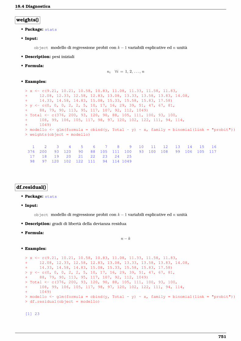
18.4 Diagnostica
weights()
• Package: stats
• Input:
object modello di regressione probit con k − 1 variabili esplicative ed n unità
• Description: pesi iniziali
• Formula:ni ∀i = 1, 2, . . . , n
• Examples:
> x <- c(9.21, 10.21, 10.58, 10.83, 11.08, 11.33, 11.58, 11.83,+ 12.08, 12.33, 12.58, 12.83, 13.08, 13.33, 13.58, 13.83, 14.08,+ 14.33, 14.58, 14.83, 15.08, 15.33, 15.58, 15.83, 17.58)> y <- c(0, 0, 0, 2, 2, 5, 10, 17, 16, 29, 39, 51, 47, 67, 81,+ 88, 79, 90, 113, 95, 117, 107, 92, 112, 1049)> Total <- c(376, 200, 93, 120, 90, 88, 105, 111, 100, 93, 100,+ 108, 99, 106, 105, 117, 98, 97, 120, 102, 122, 111, 94, 114,+ 1049)> modello <- glm(formula = cbind(y, Total - y) ~ x, family = binomial(link = "probit"))> weights(object = modello)
1 2 3 4 5 6 7 8 9 10 11 12 13 14 15 16376 200 93 120 90 88 105 111 100 93 100 108 99 106 105 11717 18 19 20 21 22 23 24 2598 97 120 102 122 111 94 114 1049
df.residual()
• Package: stats
• Input:
object modello di regressione probit con k − 1 variabili esplicative ed n unità
• Description: gradi di libertà della devianza residua
• Formula:n− k
• Examples:
> x <- c(9.21, 10.21, 10.58, 10.83, 11.08, 11.33, 11.58, 11.83,+ 12.08, 12.33, 12.58, 12.83, 13.08, 13.33, 13.58, 13.83, 14.08,+ 14.33, 14.58, 14.83, 15.08, 15.33, 15.58, 15.83, 17.58)> y <- c(0, 0, 0, 2, 2, 5, 10, 17, 16, 29, 39, 51, 47, 67, 81,+ 88, 79, 90, 113, 95, 117, 107, 92, 112, 1049)> Total <- c(376, 200, 93, 120, 90, 88, 105, 111, 100, 93, 100,+ 108, 99, 106, 105, 117, 98, 97, 120, 102, 122, 111, 94, 114,+ 1049)> modello <- glm(formula = cbind(y, Total - y) ~ x, family = binomial(link = "probit"))> df.residual(object = modello)
[1] 23
751
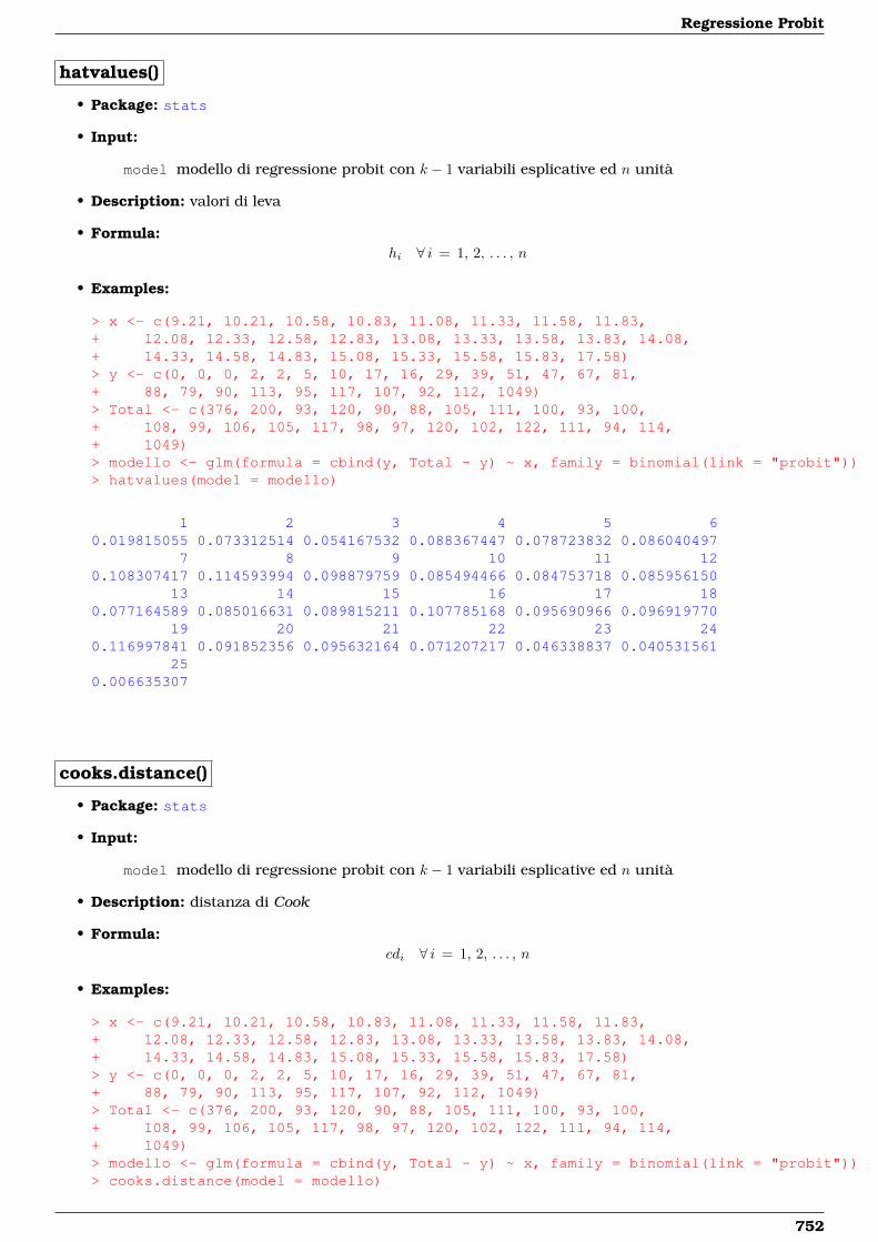
Regressione Probit
hatvalues()
• Package: stats
• Input:
model modello di regressione probit con k − 1 variabili esplicative ed n unità
• Description: valori di leva
• Formula:hi ∀ i = 1, 2, . . . , n
• Examples:
> x <- c(9.21, 10.21, 10.58, 10.83, 11.08, 11.33, 11.58, 11.83,+ 12.08, 12.33, 12.58, 12.83, 13.08, 13.33, 13.58, 13.83, 14.08,+ 14.33, 14.58, 14.83, 15.08, 15.33, 15.58, 15.83, 17.58)> y <- c(0, 0, 0, 2, 2, 5, 10, 17, 16, 29, 39, 51, 47, 67, 81,+ 88, 79, 90, 113, 95, 117, 107, 92, 112, 1049)> Total <- c(376, 200, 93, 120, 90, 88, 105, 111, 100, 93, 100,+ 108, 99, 106, 105, 117, 98, 97, 120, 102, 122, 111, 94, 114,+ 1049)> modello <- glm(formula = cbind(y, Total - y) ~ x, family = binomial(link = "probit"))> hatvalues(model = modello)
1 2 3 4 5 60.019815055 0.073312514 0.054167532 0.088367447 0.078723832 0.086040497
7 8 9 10 11 120.108307417 0.114593994 0.098879759 0.085494466 0.084753718 0.085956150
13 14 15 16 17 180.077164589 0.085016631 0.089815211 0.107785168 0.095690966 0.096919770
19 20 21 22 23 240.116997841 0.091852356 0.095632164 0.071207217 0.046338837 0.040531561
250.006635307
cooks.distance()
• Package: stats
• Input:
model modello di regressione probit con k − 1 variabili esplicative ed n unità
• Description: distanza di Cook
• Formula:cdi ∀ i = 1, 2, . . . , n
• Examples:
> x <- c(9.21, 10.21, 10.58, 10.83, 11.08, 11.33, 11.58, 11.83,+ 12.08, 12.33, 12.58, 12.83, 13.08, 13.33, 13.58, 13.83, 14.08,+ 14.33, 14.58, 14.83, 15.08, 15.33, 15.58, 15.83, 17.58)> y <- c(0, 0, 0, 2, 2, 5, 10, 17, 16, 29, 39, 51, 47, 67, 81,+ 88, 79, 90, 113, 95, 117, 107, 92, 112, 1049)> Total <- c(376, 200, 93, 120, 90, 88, 105, 111, 100, 93, 100,+ 108, 99, 106, 105, 117, 98, 97, 120, 102, 122, 111, 94, 114,+ 1049)> modello <- glm(formula = cbind(y, Total - y) ~ x, family = binomial(link = "probit"))> cooks.distance(model = modello)
752
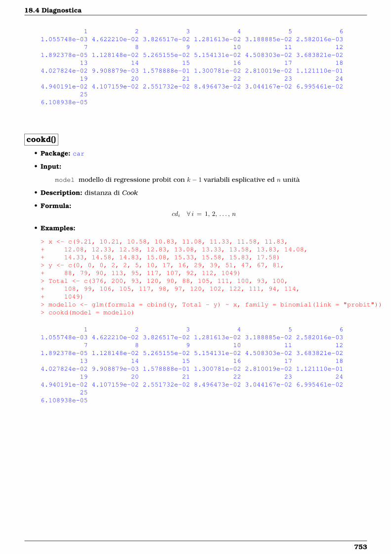
18.4 Diagnostica
1 2 3 4 5 61.055748e-03 4.622210e-02 3.826517e-02 1.281613e-02 3.188885e-02 2.582016e-03
7 8 9 10 11 121.892378e-05 1.128148e-02 5.265155e-02 5.154131e-02 4.508303e-02 3.683821e-02
13 14 15 16 17 184.027824e-02 9.908879e-03 1.578888e-01 1.300781e-02 2.810019e-02 1.121110e-01
19 20 21 22 23 244.940191e-02 4.107159e-02 2.551732e-02 8.496473e-02 3.044167e-02 6.995461e-02
256.108938e-05
cookd()
• Package: car
• Input:
model modello di regressione probit con k − 1 variabili esplicative ed n unità
• Description: distanza di Cook
• Formula:cdi ∀ i = 1, 2, . . . , n
• Examples:
> x <- c(9.21, 10.21, 10.58, 10.83, 11.08, 11.33, 11.58, 11.83,+ 12.08, 12.33, 12.58, 12.83, 13.08, 13.33, 13.58, 13.83, 14.08,+ 14.33, 14.58, 14.83, 15.08, 15.33, 15.58, 15.83, 17.58)> y <- c(0, 0, 0, 2, 2, 5, 10, 17, 16, 29, 39, 51, 47, 67, 81,+ 88, 79, 90, 113, 95, 117, 107, 92, 112, 1049)> Total <- c(376, 200, 93, 120, 90, 88, 105, 111, 100, 93, 100,+ 108, 99, 106, 105, 117, 98, 97, 120, 102, 122, 111, 94, 114,+ 1049)> modello <- glm(formula = cbind(y, Total - y) ~ x, family = binomial(link = "probit"))> cookd(model = modello)
1 2 3 4 5 61.055748e-03 4.622210e-02 3.826517e-02 1.281613e-02 3.188885e-02 2.582016e-03
7 8 9 10 11 121.892378e-05 1.128148e-02 5.265155e-02 5.154131e-02 4.508303e-02 3.683821e-02
13 14 15 16 17 184.027824e-02 9.908879e-03 1.578888e-01 1.300781e-02 2.810019e-02 1.121110e-01
19 20 21 22 23 244.940191e-02 4.107159e-02 2.551732e-02 8.496473e-02 3.044167e-02 6.995461e-02
256.108938e-05
753

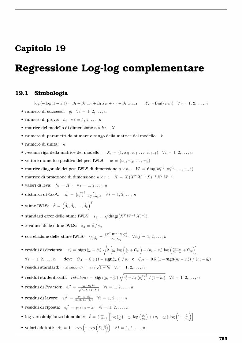
Capitolo 19
Regressione Log-log complementare
19.1 Simbologia
log (− log (1− πi)) = β1 + β2 xi1 + β3 xi2 + · · ·+ βk xik−1 Yi ∼ Bin(πi, ni) ∀ i = 1, 2, . . . , n
• numero di successi: yi ∀ i = 1, 2, . . . , n
• numero di prove: ni ∀ i = 1, 2, . . . , n
• matrice del modello di dimensione n× k : X
• numero di parametri da stimare e rango della matrice del modello: k
• numero di unità: n
• i-esima riga della matrice del modello : Xi = (1, xi1, xi2, . . . , xik−1) ∀ i = 1, 2, . . . , n
• vettore numerico positivo dei pesi IWLS: w = (w1, w2, . . . , wn)
• matrice diagonale dei pesi IWLS di dimensione n× n : W = diag(w−11 , w−1
2 , . . . , w−1n )
• matrice di proiezione di dimensione n× n : H = X (XT W−1X)−1XT W−1
• valori di leva: hi = Hi,i ∀ i = 1, 2, . . . , n
• distanza di Cook: cdi =(ePi)2 hi
k (1−hi)2 ∀ i = 1, 2, . . . , n
• stime IWLS: β =(β1, β2, . . . , βk
)T• standard error delle stime IWLS: sβ =
√diag((XT W−1X)−1)
• z-values delle stime IWLS: zβ = β / sβ
• correlazione delle stime IWLS: rβi βj =(XT W−1X)−1
i, j
sβisβj
∀ i, j = 1, 2, . . . , k
• residui di devianza: ei = sign (yi − yi)√
2[yi log
(yiyi
+ Ci1
)+ (ni − yi) log
(ni−yini−yi + Ci2
)]∀ i = 1, 2, . . . , n dove Ci1 = 0.5 (1− sign(yi)) / yi e Ci2 = 0.5 (1− sign(ni − yi)) / (ni − yi)
• residui standard: rstandardi = ei /√
1− hi ∀ i = 1, 2, . . . , n
• residui studentizzati: rstudenti = sign (yi − yi)√e2i + hi
(ePi)2/ (1− hi) ∀ i = 1, 2, . . . , n
• residui di Pearson: ePi = yi−ni πi√ni πi (1−πi)
∀i = 1, 2, . . . , n
• residui di lavoro: eWi = yi−ni πini πi (1−πi) ∀i = 1, 2, . . . , n
• residui di riposta: eRi = yi / ni − πi ∀i = 1, 2, . . . , n
• log-verosimiglianza binomiale: ˆ =∑ni=1
[log(niyi
)+ yi log
(yini
)+ (ni − yi) log
(1− yi
ni
)]• valori adattati: πi = 1− exp
(− exp
(Xi β
))∀ i = 1, 2, . . . , n
755
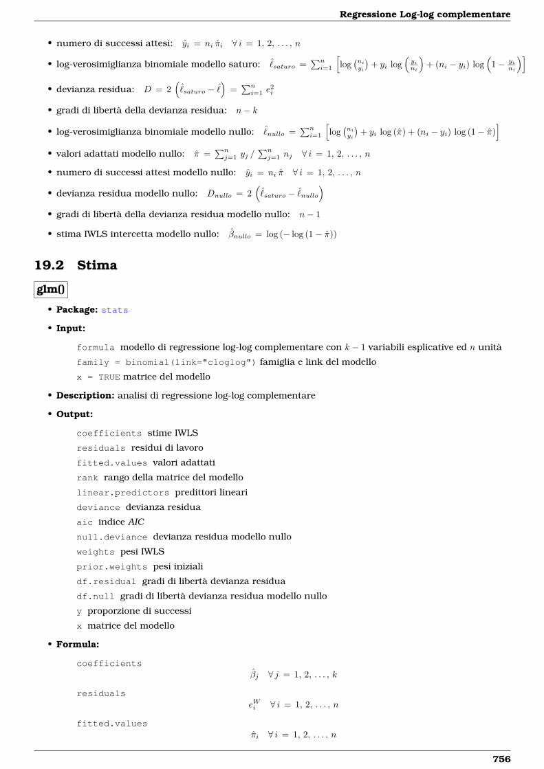
Regressione Log-log complementare
• numero di successi attesi: yi = ni πi ∀ i = 1, 2, . . . , n
• log-verosimiglianza binomiale modello saturo: ˆsaturo =
∑ni=1
[log(niyi
)+ yi log
(yini
)+ (ni − yi) log
(1− yi
ni
)]• devianza residua: D = 2
(ˆsaturo − ˆ
)=∑ni=1 e
2i
• gradi di libertà della devianza residua: n− k
• log-verosimiglianza binomiale modello nullo: ˆnullo =
∑ni=1
[log(niyi
)+ yi log (π) + (ni − yi) log (1− π)
]• valori adattati modello nullo: π =
∑nj=1 yj /
∑nj=1 nj ∀ i = 1, 2, . . . , n
• numero di successi attesi modello nullo: yi = ni π ∀ i = 1, 2, . . . , n
• devianza residua modello nullo: Dnullo = 2(
ˆsaturo − ˆ
nullo
)• gradi di libertà della devianza residua modello nullo: n− 1
• stima IWLS intercetta modello nullo: βnullo = log (− log (1− π))
19.2 Stima
glm()
• Package: stats
• Input:
formula modello di regressione log-log complementare con k − 1 variabili esplicative ed n unità
family = binomial(link="cloglog") famiglia e link del modello
x = TRUE matrice del modello
• Description: analisi di regressione log-log complementare
• Output:
coefficients stime IWLS
residuals residui di lavoro
fitted.values valori adattati
rank rango della matrice del modello
linear.predictors predittori lineari
deviance devianza residua
aic indice AIC
null.deviance devianza residua modello nullo
weights pesi IWLS
prior.weights pesi iniziali
df.residual gradi di libertà devianza residua
df.null gradi di libertà devianza residua modello nullo
y proporzione di successi
x matrice del modello
• Formula:
coefficientsβj ∀ j = 1, 2, . . . , k
residualseWi ∀ i = 1, 2, . . . , n
fitted.valuesπi ∀ i = 1, 2, . . . , n
756
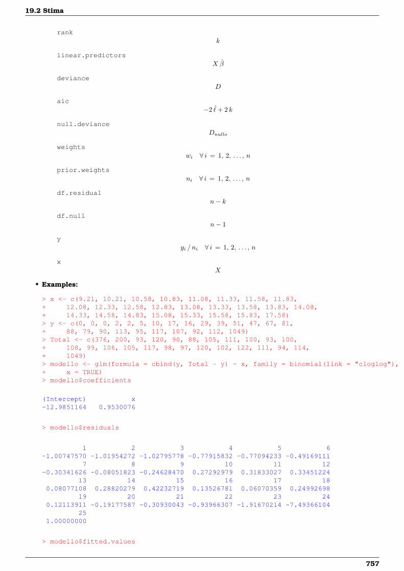
19.2 Stima
rankk
linear.predictorsX β
devianceD
aic−2 ˆ+ 2 k
null.devianceDnullo
weightswi ∀ i = 1, 2, . . . , n
prior.weightsni ∀ i = 1, 2, . . . , n
df.residualn− k
df.nulln− 1
yyi / ni ∀ i = 1, 2, . . . , n
xX
• Examples:
> x <- c(9.21, 10.21, 10.58, 10.83, 11.08, 11.33, 11.58, 11.83,+ 12.08, 12.33, 12.58, 12.83, 13.08, 13.33, 13.58, 13.83, 14.08,+ 14.33, 14.58, 14.83, 15.08, 15.33, 15.58, 15.83, 17.58)> y <- c(0, 0, 0, 2, 2, 5, 10, 17, 16, 29, 39, 51, 47, 67, 81,+ 88, 79, 90, 113, 95, 117, 107, 92, 112, 1049)> Total <- c(376, 200, 93, 120, 90, 88, 105, 111, 100, 93, 100,+ 108, 99, 106, 105, 117, 98, 97, 120, 102, 122, 111, 94, 114,+ 1049)> modello <- glm(formula = cbind(y, Total - y) ~ x, family = binomial(link = "cloglog"),+ x = TRUE)> modello$coefficients
(Intercept) x-12.9851164 0.9530076
> modello$residuals
1 2 3 4 5 6-1.00747570 -1.01954272 -1.02795778 -0.77915832 -0.77094233 -0.49169111
7 8 9 10 11 12-0.30341626 -0.08051823 -0.24628470 0.27292979 0.31833027 0.33451224
13 14 15 16 17 180.08077108 0.28820279 0.42232719 0.13526781 0.06070359 0.24992698
19 20 21 22 23 240.12113911 -0.19177587 -0.30930043 -0.93966307 -1.91670214 -7.49366104
251.00000000
> modello$fitted.values
757
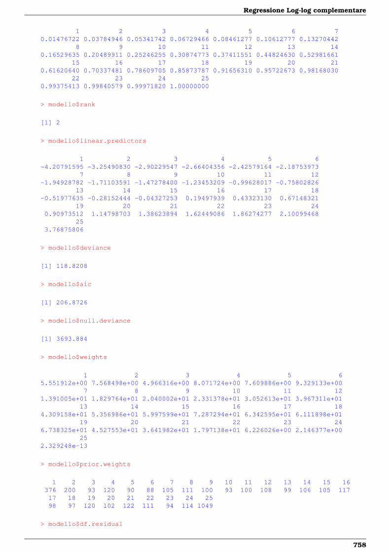
Regressione Log-log complementare
1 2 3 4 5 6 70.01476722 0.03784946 0.05341742 0.06729466 0.08461277 0.10612777 0.13270442
8 9 10 11 12 13 140.16529635 0.20489911 0.25246255 0.30874773 0.37411551 0.44824630 0.52981661
15 16 17 18 19 20 210.61620640 0.70337481 0.78609705 0.85873787 0.91656310 0.95722673 0.98168030
22 23 24 250.99375413 0.99840579 0.99971820 1.00000000
> modello$rank
[1] 2
> modello$linear.predictors
1 2 3 4 5 6-4.20791595 -3.25490830 -2.90229547 -2.66404356 -2.42579164 -2.18753973
7 8 9 10 11 12-1.94928782 -1.71103591 -1.47278400 -1.23453209 -0.99628017 -0.75802826
13 14 15 16 17 18-0.51977635 -0.28152444 -0.04327253 0.19497939 0.43323130 0.67148321
19 20 21 22 23 240.90973512 1.14798703 1.38623894 1.62449086 1.86274277 2.10099468
253.76875806
> modello$deviance
[1] 118.8208
> modello$aic
[1] 206.8726
> modello$null.deviance
[1] 3693.884
> modello$weights
1 2 3 4 5 65.551912e+00 7.568498e+00 4.966316e+00 8.071724e+00 7.609886e+00 9.329133e+00
7 8 9 10 11 121.391005e+01 1.829764e+01 2.040002e+01 2.331378e+01 3.052613e+01 3.967311e+01
13 14 15 16 17 184.309158e+01 5.356986e+01 5.997599e+01 7.287294e+01 6.342595e+01 6.111898e+01
19 20 21 22 23 246.738325e+01 4.527553e+01 3.641982e+01 1.797138e+01 6.226026e+00 2.146377e+00
252.329248e-13
> modello$prior.weights
1 2 3 4 5 6 7 8 9 10 11 12 13 14 15 16376 200 93 120 90 88 105 111 100 93 100 108 99 106 105 11717 18 19 20 21 22 23 24 2598 97 120 102 122 111 94 114 1049
> modello$df.residual
758
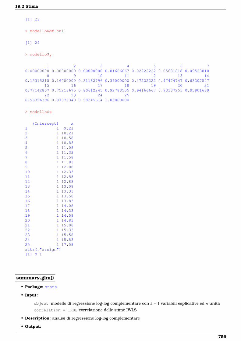
19.2 Stima
[1] 23
> modello$df.null
[1] 24
> modello$y
1 2 3 4 5 6 70.00000000 0.00000000 0.00000000 0.01666667 0.02222222 0.05681818 0.09523810
8 9 10 11 12 13 140.15315315 0.16000000 0.31182796 0.39000000 0.47222222 0.47474747 0.63207547
15 16 17 18 19 20 210.77142857 0.75213675 0.80612245 0.92783505 0.94166667 0.93137255 0.95901639
22 23 24 250.96396396 0.97872340 0.98245614 1.00000000
> modello$x
(Intercept) x1 1 9.212 1 10.213 1 10.584 1 10.835 1 11.086 1 11.337 1 11.588 1 11.839 1 12.0810 1 12.3311 1 12.5812 1 12.8313 1 13.0814 1 13.3315 1 13.5816 1 13.8317 1 14.0818 1 14.3319 1 14.5820 1 14.8321 1 15.0822 1 15.3323 1 15.5824 1 15.8325 1 17.58attr(,"assign")[1] 0 1
summary.glm()
• Package: stats
• Input:
object modello di regressione log-log complementare con k − 1 variabili esplicative ed n unità
correlation = TRUE correlazione delle stime IWLS
• Description: analisi di regressione log-log complementare
• Output:
759
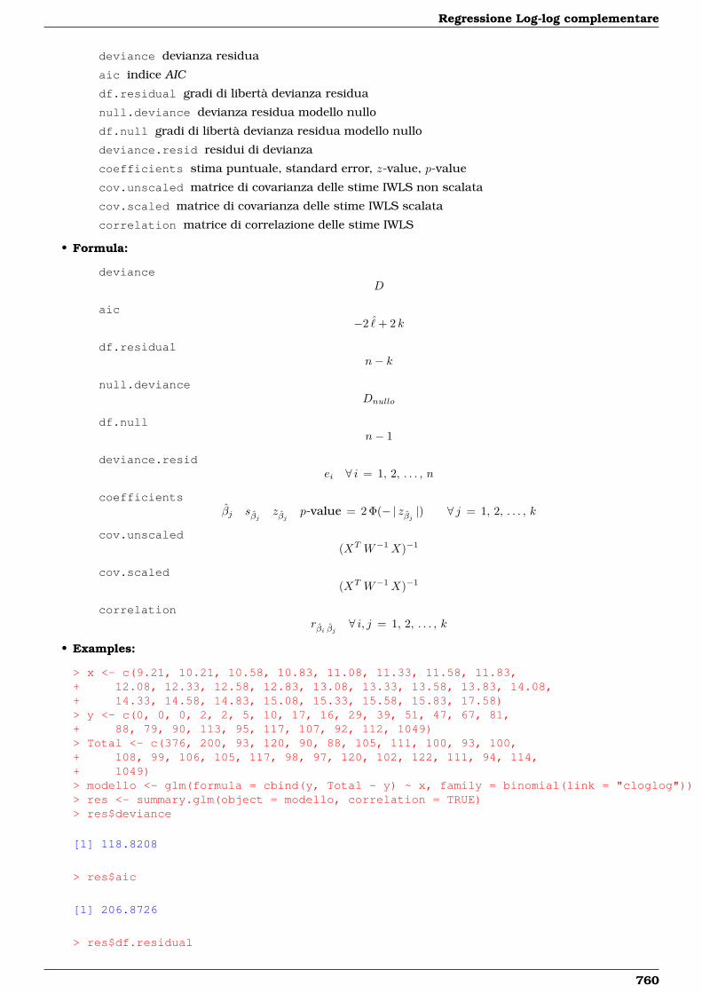
Regressione Log-log complementare
deviance devianza residua
aic indice AIC
df.residual gradi di libertà devianza residua
null.deviance devianza residua modello nullo
df.null gradi di libertà devianza residua modello nullo
deviance.resid residui di devianza
coefficients stima puntuale, standard error, z-value, p-value
cov.unscaled matrice di covarianza delle stime IWLS non scalata
cov.scaled matrice di covarianza delle stime IWLS scalata
correlation matrice di correlazione delle stime IWLS
• Formula:
devianceD
aic−2 ˆ+ 2 k
df.residualn− k
null.devianceDnullo
df.nulln− 1
deviance.residei ∀ i = 1, 2, . . . , n
coefficientsβj sβj zβj p-value = 2 Φ(− | zβj |) ∀ j = 1, 2, . . . , k
cov.unscaled(XT W−1X)−1
cov.scaled(XT W−1X)−1
correlationrβi βj ∀ i, j = 1, 2, . . . , k
• Examples:
> x <- c(9.21, 10.21, 10.58, 10.83, 11.08, 11.33, 11.58, 11.83,+ 12.08, 12.33, 12.58, 12.83, 13.08, 13.33, 13.58, 13.83, 14.08,+ 14.33, 14.58, 14.83, 15.08, 15.33, 15.58, 15.83, 17.58)> y <- c(0, 0, 0, 2, 2, 5, 10, 17, 16, 29, 39, 51, 47, 67, 81,+ 88, 79, 90, 113, 95, 117, 107, 92, 112, 1049)> Total <- c(376, 200, 93, 120, 90, 88, 105, 111, 100, 93, 100,+ 108, 99, 106, 105, 117, 98, 97, 120, 102, 122, 111, 94, 114,+ 1049)> modello <- glm(formula = cbind(y, Total - y) ~ x, family = binomial(link = "cloglog"))> res <- summary.glm(object = modello, correlation = TRUE)> res$deviance
[1] 118.8208
> res$aic
[1] 206.8726
> res$df.residual
760
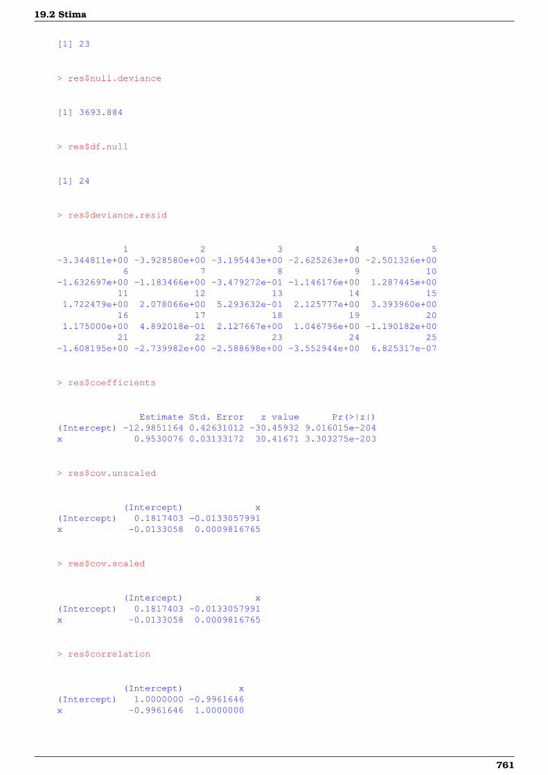
19.2 Stima
[1] 23
> res$null.deviance
[1] 3693.884
> res$df.null
[1] 24
> res$deviance.resid
1 2 3 4 5-3.344811e+00 -3.928580e+00 -3.195443e+00 -2.625263e+00 -2.501326e+00
6 7 8 9 10-1.632697e+00 -1.183466e+00 -3.479272e-01 -1.146176e+00 1.287445e+00
11 12 13 14 151.722479e+00 2.078066e+00 5.293632e-01 2.125777e+00 3.393960e+00
16 17 18 19 201.175000e+00 4.892018e-01 2.127667e+00 1.046796e+00 -1.190182e+00
21 22 23 24 25-1.608195e+00 -2.739982e+00 -2.588698e+00 -3.552944e+00 6.825317e-07
> res$coefficients
Estimate Std. Error z value Pr(>|z|)(Intercept) -12.9851164 0.42631012 -30.45932 9.016015e-204x 0.9530076 0.03133172 30.41671 3.303275e-203
> res$cov.unscaled
(Intercept) x(Intercept) 0.1817403 -0.0133057991x -0.0133058 0.0009816765
> res$cov.scaled
(Intercept) x(Intercept) 0.1817403 -0.0133057991x -0.0133058 0.0009816765
> res$correlation
(Intercept) x(Intercept) 1.0000000 -0.9961646x -0.9961646 1.0000000
761
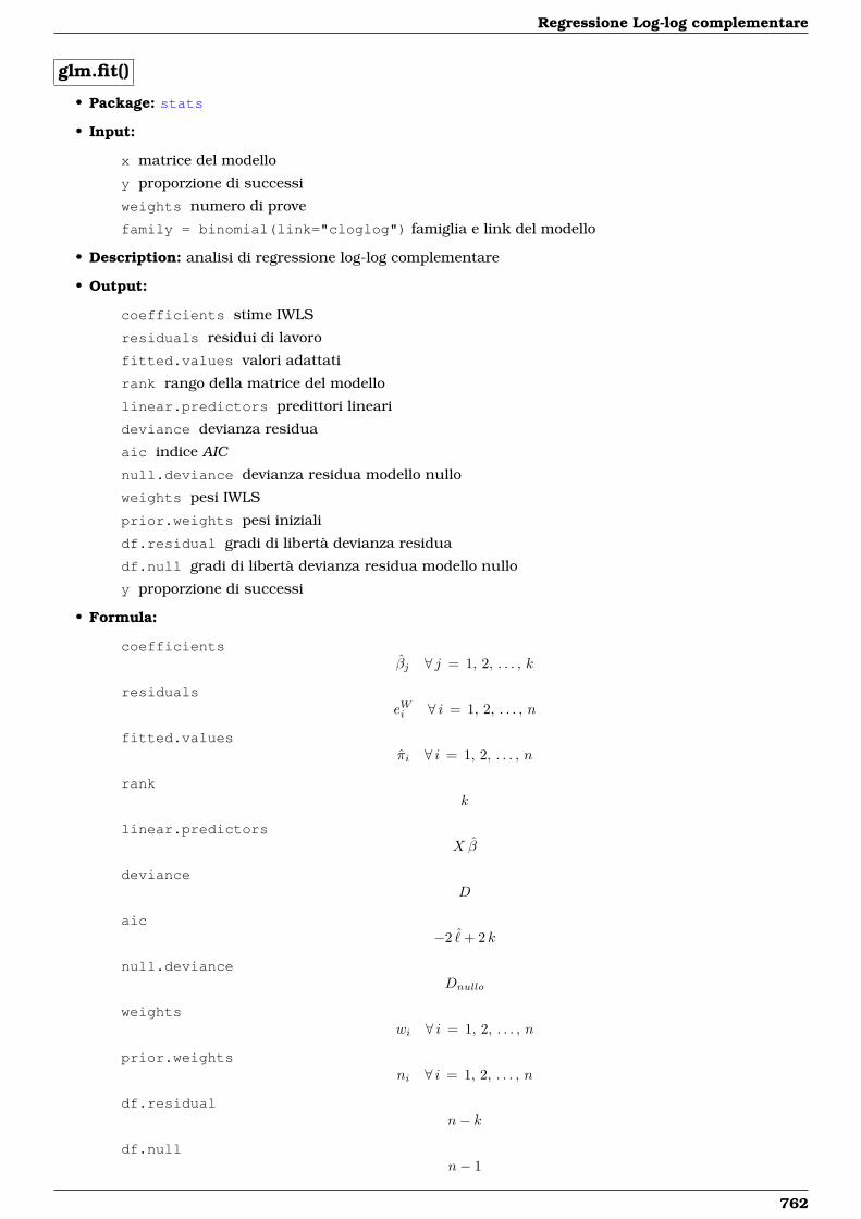
Regressione Log-log complementare
glm.fit()
• Package: stats
• Input:
x matrice del modello
y proporzione di successi
weights numero di prove
family = binomial(link="cloglog") famiglia e link del modello
• Description: analisi di regressione log-log complementare
• Output:
coefficients stime IWLS
residuals residui di lavoro
fitted.values valori adattati
rank rango della matrice del modello
linear.predictors predittori lineari
deviance devianza residua
aic indice AIC
null.deviance devianza residua modello nullo
weights pesi IWLS
prior.weights pesi iniziali
df.residual gradi di libertà devianza residua
df.null gradi di libertà devianza residua modello nullo
y proporzione di successi
• Formula:
coefficientsβj ∀ j = 1, 2, . . . , k
residualseWi ∀ i = 1, 2, . . . , n
fitted.valuesπi ∀ i = 1, 2, . . . , n
rankk
linear.predictorsX β
devianceD
aic−2 ˆ+ 2 k
null.devianceDnullo
weightswi ∀ i = 1, 2, . . . , n
prior.weightsni ∀ i = 1, 2, . . . , n
df.residualn− k
df.nulln− 1
762
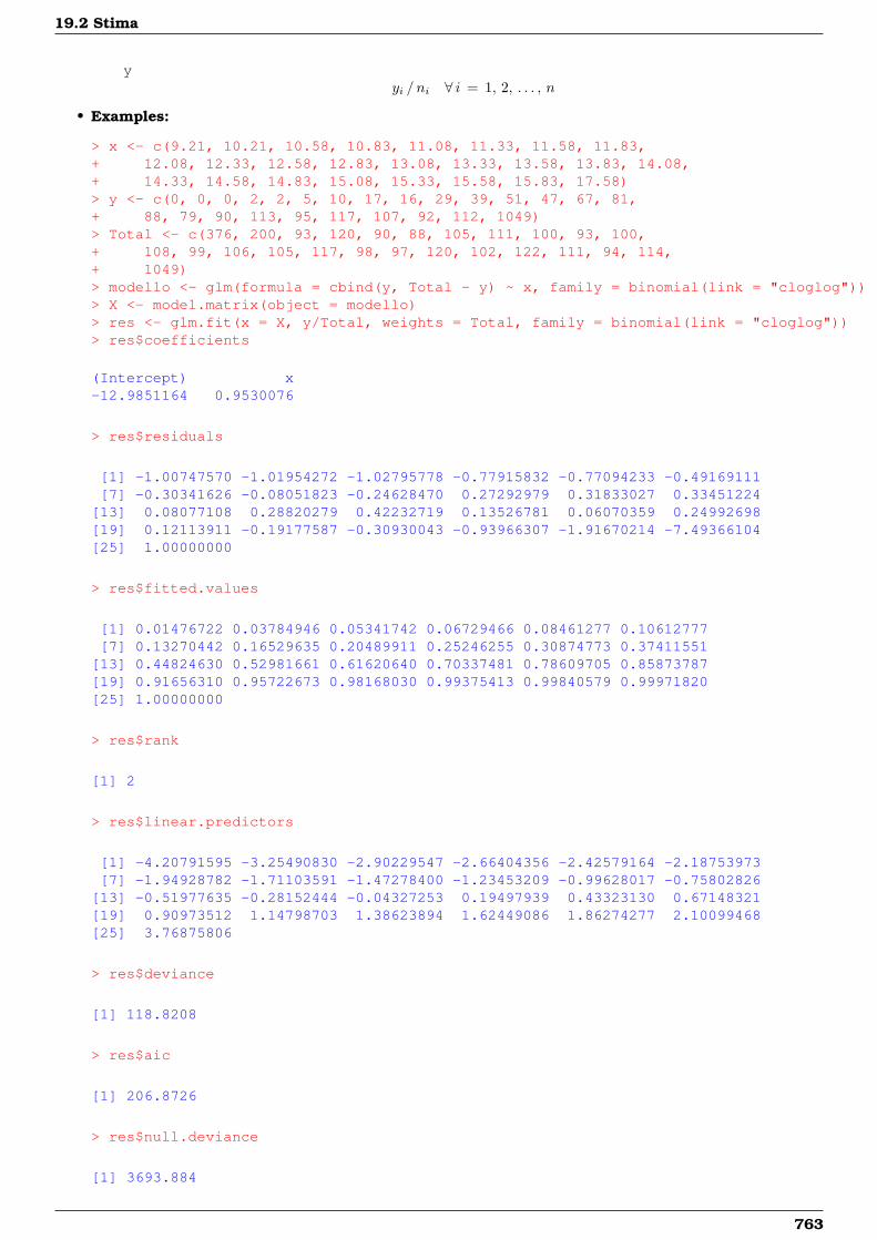
19.2 Stima
yyi / ni ∀ i = 1, 2, . . . , n
• Examples:
> x <- c(9.21, 10.21, 10.58, 10.83, 11.08, 11.33, 11.58, 11.83,+ 12.08, 12.33, 12.58, 12.83, 13.08, 13.33, 13.58, 13.83, 14.08,+ 14.33, 14.58, 14.83, 15.08, 15.33, 15.58, 15.83, 17.58)> y <- c(0, 0, 0, 2, 2, 5, 10, 17, 16, 29, 39, 51, 47, 67, 81,+ 88, 79, 90, 113, 95, 117, 107, 92, 112, 1049)> Total <- c(376, 200, 93, 120, 90, 88, 105, 111, 100, 93, 100,+ 108, 99, 106, 105, 117, 98, 97, 120, 102, 122, 111, 94, 114,+ 1049)> modello <- glm(formula = cbind(y, Total - y) ~ x, family = binomial(link = "cloglog"))> X <- model.matrix(object = modello)> res <- glm.fit(x = X, y/Total, weights = Total, family = binomial(link = "cloglog"))> res$coefficients
(Intercept) x-12.9851164 0.9530076
> res$residuals
[1] -1.00747570 -1.01954272 -1.02795778 -0.77915832 -0.77094233 -0.49169111[7] -0.30341626 -0.08051823 -0.24628470 0.27292979 0.31833027 0.33451224
[13] 0.08077108 0.28820279 0.42232719 0.13526781 0.06070359 0.24992698[19] 0.12113911 -0.19177587 -0.30930043 -0.93966307 -1.91670214 -7.49366104[25] 1.00000000
> res$fitted.values
[1] 0.01476722 0.03784946 0.05341742 0.06729466 0.08461277 0.10612777[7] 0.13270442 0.16529635 0.20489911 0.25246255 0.30874773 0.37411551
[13] 0.44824630 0.52981661 0.61620640 0.70337481 0.78609705 0.85873787[19] 0.91656310 0.95722673 0.98168030 0.99375413 0.99840579 0.99971820[25] 1.00000000
> res$rank
[1] 2
> res$linear.predictors
[1] -4.20791595 -3.25490830 -2.90229547 -2.66404356 -2.42579164 -2.18753973[7] -1.94928782 -1.71103591 -1.47278400 -1.23453209 -0.99628017 -0.75802826
[13] -0.51977635 -0.28152444 -0.04327253 0.19497939 0.43323130 0.67148321[19] 0.90973512 1.14798703 1.38623894 1.62449086 1.86274277 2.10099468[25] 3.76875806
> res$deviance
[1] 118.8208
> res$aic
[1] 206.8726
> res$null.deviance
[1] 3693.884
763
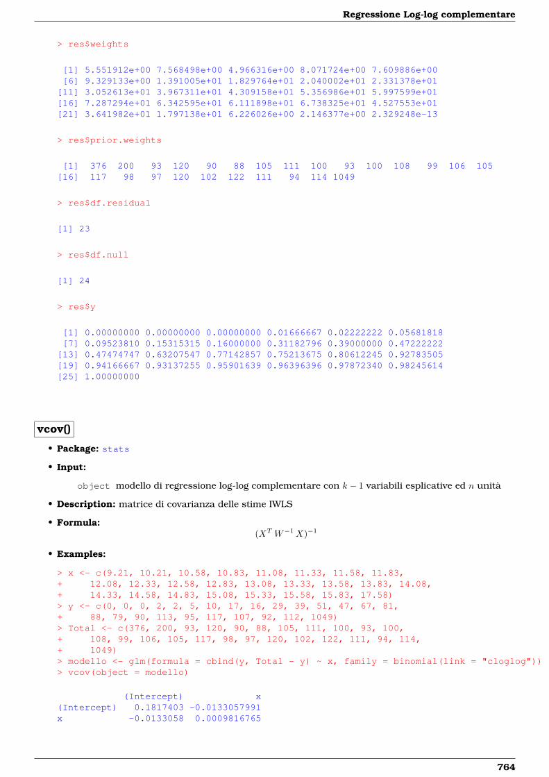
Regressione Log-log complementare
> res$weights
[1] 5.551912e+00 7.568498e+00 4.966316e+00 8.071724e+00 7.609886e+00[6] 9.329133e+00 1.391005e+01 1.829764e+01 2.040002e+01 2.331378e+01
[11] 3.052613e+01 3.967311e+01 4.309158e+01 5.356986e+01 5.997599e+01[16] 7.287294e+01 6.342595e+01 6.111898e+01 6.738325e+01 4.527553e+01[21] 3.641982e+01 1.797138e+01 6.226026e+00 2.146377e+00 2.329248e-13
> res$prior.weights
[1] 376 200 93 120 90 88 105 111 100 93 100 108 99 106 105[16] 117 98 97 120 102 122 111 94 114 1049
> res$df.residual
[1] 23
> res$df.null
[1] 24
> res$y
[1] 0.00000000 0.00000000 0.00000000 0.01666667 0.02222222 0.05681818[7] 0.09523810 0.15315315 0.16000000 0.31182796 0.39000000 0.47222222
[13] 0.47474747 0.63207547 0.77142857 0.75213675 0.80612245 0.92783505[19] 0.94166667 0.93137255 0.95901639 0.96396396 0.97872340 0.98245614[25] 1.00000000
vcov()
• Package: stats
• Input:
object modello di regressione log-log complementare con k − 1 variabili esplicative ed n unità
• Description: matrice di covarianza delle stime IWLS
• Formula:(XT W−1X)−1
• Examples:
> x <- c(9.21, 10.21, 10.58, 10.83, 11.08, 11.33, 11.58, 11.83,+ 12.08, 12.33, 12.58, 12.83, 13.08, 13.33, 13.58, 13.83, 14.08,+ 14.33, 14.58, 14.83, 15.08, 15.33, 15.58, 15.83, 17.58)> y <- c(0, 0, 0, 2, 2, 5, 10, 17, 16, 29, 39, 51, 47, 67, 81,+ 88, 79, 90, 113, 95, 117, 107, 92, 112, 1049)> Total <- c(376, 200, 93, 120, 90, 88, 105, 111, 100, 93, 100,+ 108, 99, 106, 105, 117, 98, 97, 120, 102, 122, 111, 94, 114,+ 1049)> modello <- glm(formula = cbind(y, Total - y) ~ x, family = binomial(link = "cloglog"))> vcov(object = modello)
(Intercept) x(Intercept) 0.1817403 -0.0133057991x -0.0133058 0.0009816765
764
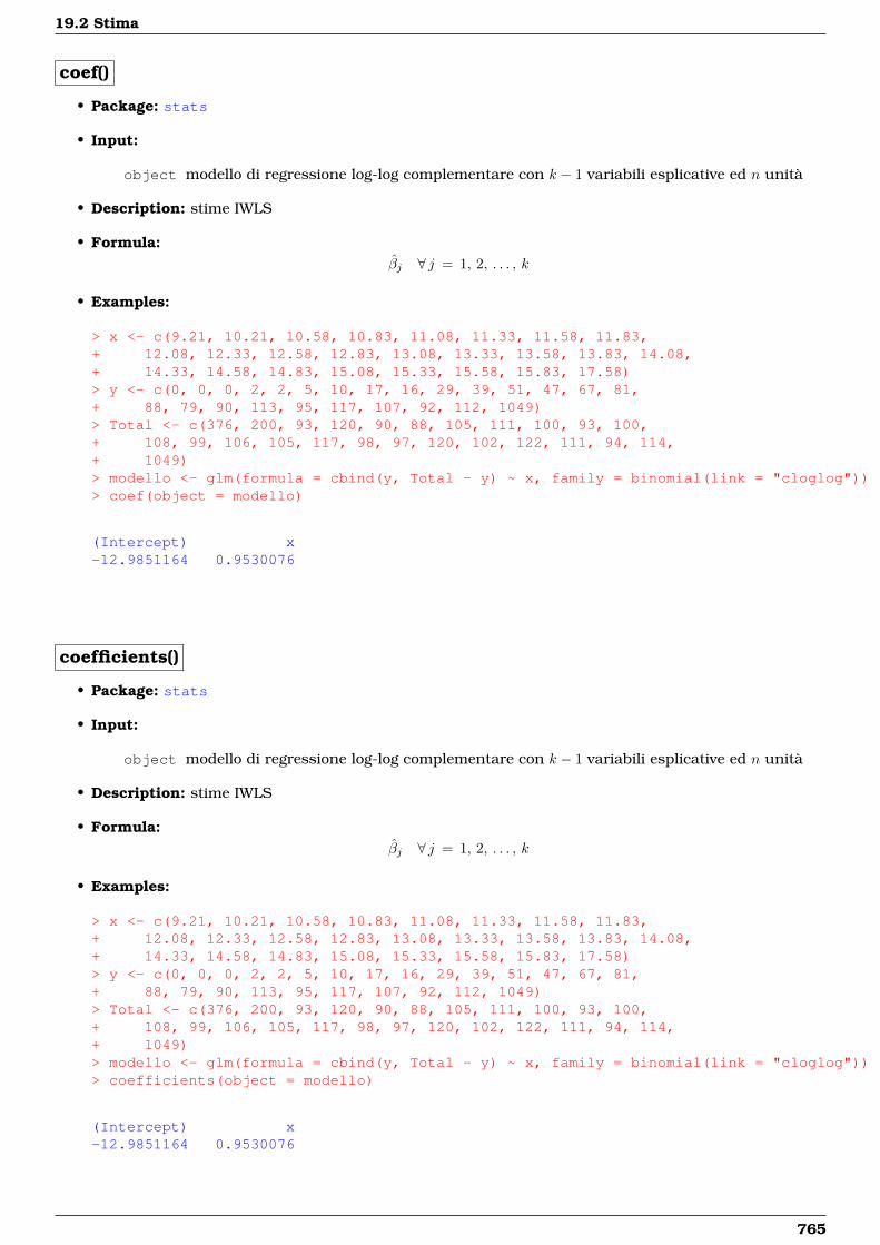
19.2 Stima
coef()
• Package: stats
• Input:
object modello di regressione log-log complementare con k − 1 variabili esplicative ed n unità
• Description: stime IWLS
• Formula:βj ∀ j = 1, 2, . . . , k
• Examples:
> x <- c(9.21, 10.21, 10.58, 10.83, 11.08, 11.33, 11.58, 11.83,+ 12.08, 12.33, 12.58, 12.83, 13.08, 13.33, 13.58, 13.83, 14.08,+ 14.33, 14.58, 14.83, 15.08, 15.33, 15.58, 15.83, 17.58)> y <- c(0, 0, 0, 2, 2, 5, 10, 17, 16, 29, 39, 51, 47, 67, 81,+ 88, 79, 90, 113, 95, 117, 107, 92, 112, 1049)> Total <- c(376, 200, 93, 120, 90, 88, 105, 111, 100, 93, 100,+ 108, 99, 106, 105, 117, 98, 97, 120, 102, 122, 111, 94, 114,+ 1049)> modello <- glm(formula = cbind(y, Total - y) ~ x, family = binomial(link = "cloglog"))> coef(object = modello)
(Intercept) x-12.9851164 0.9530076
coefficients()
• Package: stats
• Input:
object modello di regressione log-log complementare con k − 1 variabili esplicative ed n unità
• Description: stime IWLS
• Formula:βj ∀ j = 1, 2, . . . , k
• Examples:
> x <- c(9.21, 10.21, 10.58, 10.83, 11.08, 11.33, 11.58, 11.83,+ 12.08, 12.33, 12.58, 12.83, 13.08, 13.33, 13.58, 13.83, 14.08,+ 14.33, 14.58, 14.83, 15.08, 15.33, 15.58, 15.83, 17.58)> y <- c(0, 0, 0, 2, 2, 5, 10, 17, 16, 29, 39, 51, 47, 67, 81,+ 88, 79, 90, 113, 95, 117, 107, 92, 112, 1049)> Total <- c(376, 200, 93, 120, 90, 88, 105, 111, 100, 93, 100,+ 108, 99, 106, 105, 117, 98, 97, 120, 102, 122, 111, 94, 114,+ 1049)> modello <- glm(formula = cbind(y, Total - y) ~ x, family = binomial(link = "cloglog"))> coefficients(object = modello)
(Intercept) x-12.9851164 0.9530076
765
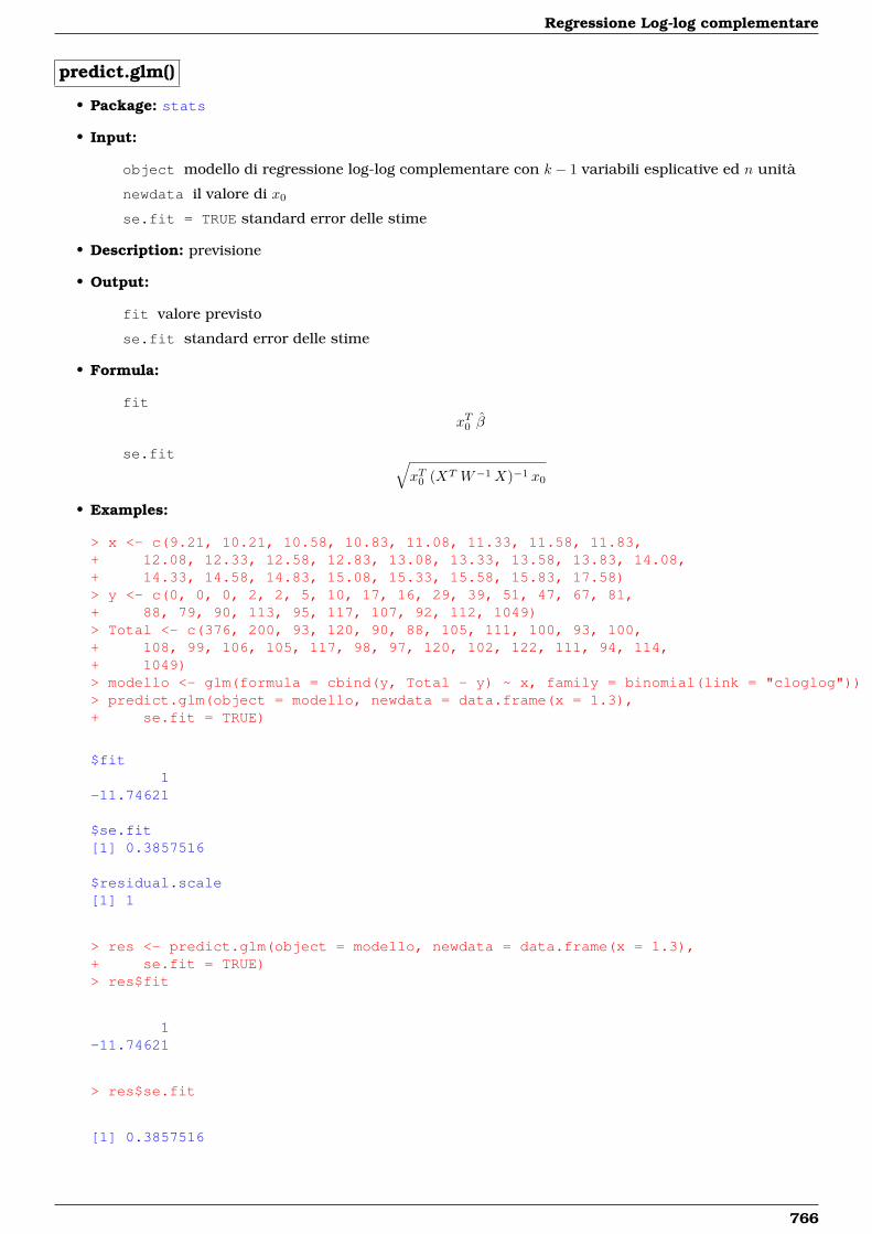
Regressione Log-log complementare
predict.glm()
• Package: stats
• Input:
object modello di regressione log-log complementare con k − 1 variabili esplicative ed n unità
newdata il valore di x0
se.fit = TRUE standard error delle stime
• Description: previsione
• Output:
fit valore previsto
se.fit standard error delle stime
• Formula:
fit
xT0 β
se.fit √xT0 (XT W−1X)−1 x0
• Examples:
> x <- c(9.21, 10.21, 10.58, 10.83, 11.08, 11.33, 11.58, 11.83,+ 12.08, 12.33, 12.58, 12.83, 13.08, 13.33, 13.58, 13.83, 14.08,+ 14.33, 14.58, 14.83, 15.08, 15.33, 15.58, 15.83, 17.58)> y <- c(0, 0, 0, 2, 2, 5, 10, 17, 16, 29, 39, 51, 47, 67, 81,+ 88, 79, 90, 113, 95, 117, 107, 92, 112, 1049)> Total <- c(376, 200, 93, 120, 90, 88, 105, 111, 100, 93, 100,+ 108, 99, 106, 105, 117, 98, 97, 120, 102, 122, 111, 94, 114,+ 1049)> modello <- glm(formula = cbind(y, Total - y) ~ x, family = binomial(link = "cloglog"))> predict.glm(object = modello, newdata = data.frame(x = 1.3),+ se.fit = TRUE)
$fit1
-11.74621
$se.fit[1] 0.3857516
$residual.scale[1] 1
> res <- predict.glm(object = modello, newdata = data.frame(x = 1.3),+ se.fit = TRUE)> res$fit
1-11.74621
> res$se.fit
[1] 0.3857516
766
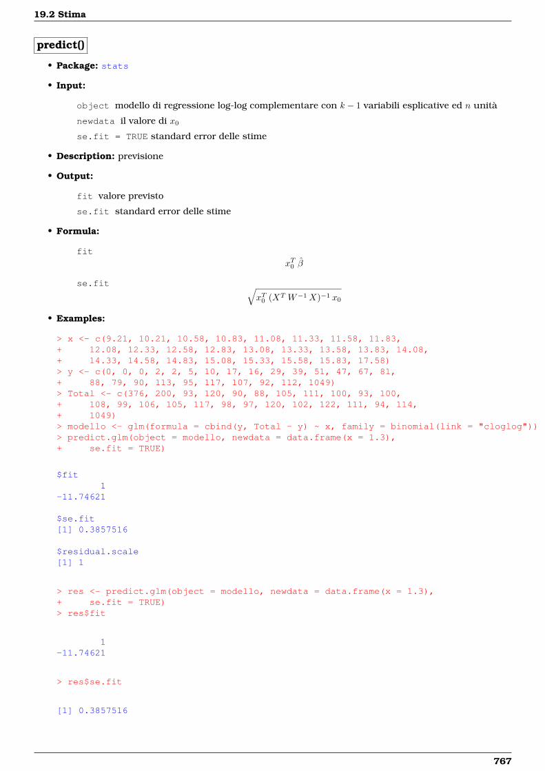
19.2 Stima
predict()
• Package: stats
• Input:
object modello di regressione log-log complementare con k − 1 variabili esplicative ed n unità
newdata il valore di x0
se.fit = TRUE standard error delle stime
• Description: previsione
• Output:
fit valore previsto
se.fit standard error delle stime
• Formula:
fit
xT0 β
se.fit √xT0 (XT W−1X)−1 x0
• Examples:
> x <- c(9.21, 10.21, 10.58, 10.83, 11.08, 11.33, 11.58, 11.83,+ 12.08, 12.33, 12.58, 12.83, 13.08, 13.33, 13.58, 13.83, 14.08,+ 14.33, 14.58, 14.83, 15.08, 15.33, 15.58, 15.83, 17.58)> y <- c(0, 0, 0, 2, 2, 5, 10, 17, 16, 29, 39, 51, 47, 67, 81,+ 88, 79, 90, 113, 95, 117, 107, 92, 112, 1049)> Total <- c(376, 200, 93, 120, 90, 88, 105, 111, 100, 93, 100,+ 108, 99, 106, 105, 117, 98, 97, 120, 102, 122, 111, 94, 114,+ 1049)> modello <- glm(formula = cbind(y, Total - y) ~ x, family = binomial(link = "cloglog"))> predict.glm(object = modello, newdata = data.frame(x = 1.3),+ se.fit = TRUE)
$fit1
-11.74621
$se.fit[1] 0.3857516
$residual.scale[1] 1
> res <- predict.glm(object = modello, newdata = data.frame(x = 1.3),+ se.fit = TRUE)> res$fit
1-11.74621
> res$se.fit
[1] 0.3857516
767
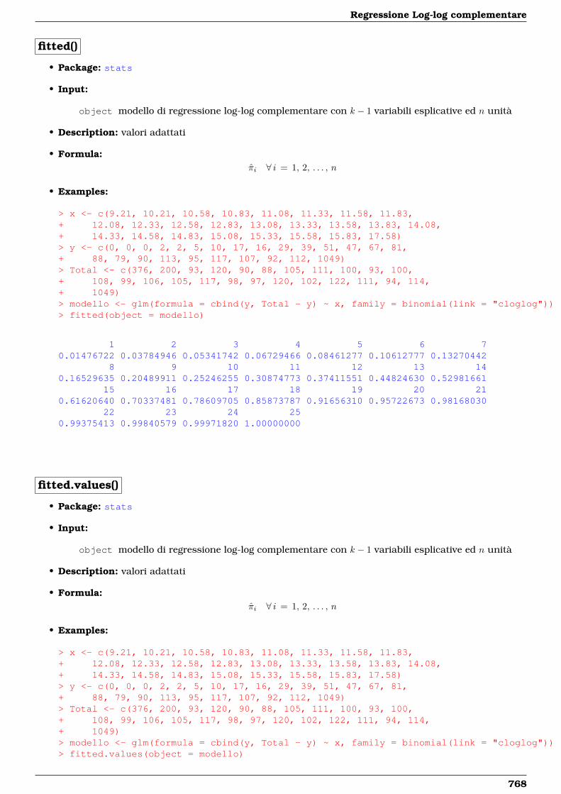
Regressione Log-log complementare
fitted()
• Package: stats
• Input:
object modello di regressione log-log complementare con k − 1 variabili esplicative ed n unità
• Description: valori adattati
• Formula:πi ∀ i = 1, 2, . . . , n
• Examples:
> x <- c(9.21, 10.21, 10.58, 10.83, 11.08, 11.33, 11.58, 11.83,+ 12.08, 12.33, 12.58, 12.83, 13.08, 13.33, 13.58, 13.83, 14.08,+ 14.33, 14.58, 14.83, 15.08, 15.33, 15.58, 15.83, 17.58)> y <- c(0, 0, 0, 2, 2, 5, 10, 17, 16, 29, 39, 51, 47, 67, 81,+ 88, 79, 90, 113, 95, 117, 107, 92, 112, 1049)> Total <- c(376, 200, 93, 120, 90, 88, 105, 111, 100, 93, 100,+ 108, 99, 106, 105, 117, 98, 97, 120, 102, 122, 111, 94, 114,+ 1049)> modello <- glm(formula = cbind(y, Total - y) ~ x, family = binomial(link = "cloglog"))> fitted(object = modello)
1 2 3 4 5 6 70.01476722 0.03784946 0.05341742 0.06729466 0.08461277 0.10612777 0.13270442
8 9 10 11 12 13 140.16529635 0.20489911 0.25246255 0.30874773 0.37411551 0.44824630 0.52981661
15 16 17 18 19 20 210.61620640 0.70337481 0.78609705 0.85873787 0.91656310 0.95722673 0.98168030
22 23 24 250.99375413 0.99840579 0.99971820 1.00000000
fitted.values()
• Package: stats
• Input:
object modello di regressione log-log complementare con k − 1 variabili esplicative ed n unità
• Description: valori adattati
• Formula:πi ∀ i = 1, 2, . . . , n
• Examples:
> x <- c(9.21, 10.21, 10.58, 10.83, 11.08, 11.33, 11.58, 11.83,+ 12.08, 12.33, 12.58, 12.83, 13.08, 13.33, 13.58, 13.83, 14.08,+ 14.33, 14.58, 14.83, 15.08, 15.33, 15.58, 15.83, 17.58)> y <- c(0, 0, 0, 2, 2, 5, 10, 17, 16, 29, 39, 51, 47, 67, 81,+ 88, 79, 90, 113, 95, 117, 107, 92, 112, 1049)> Total <- c(376, 200, 93, 120, 90, 88, 105, 111, 100, 93, 100,+ 108, 99, 106, 105, 117, 98, 97, 120, 102, 122, 111, 94, 114,+ 1049)> modello <- glm(formula = cbind(y, Total - y) ~ x, family = binomial(link = "cloglog"))> fitted.values(object = modello)
768
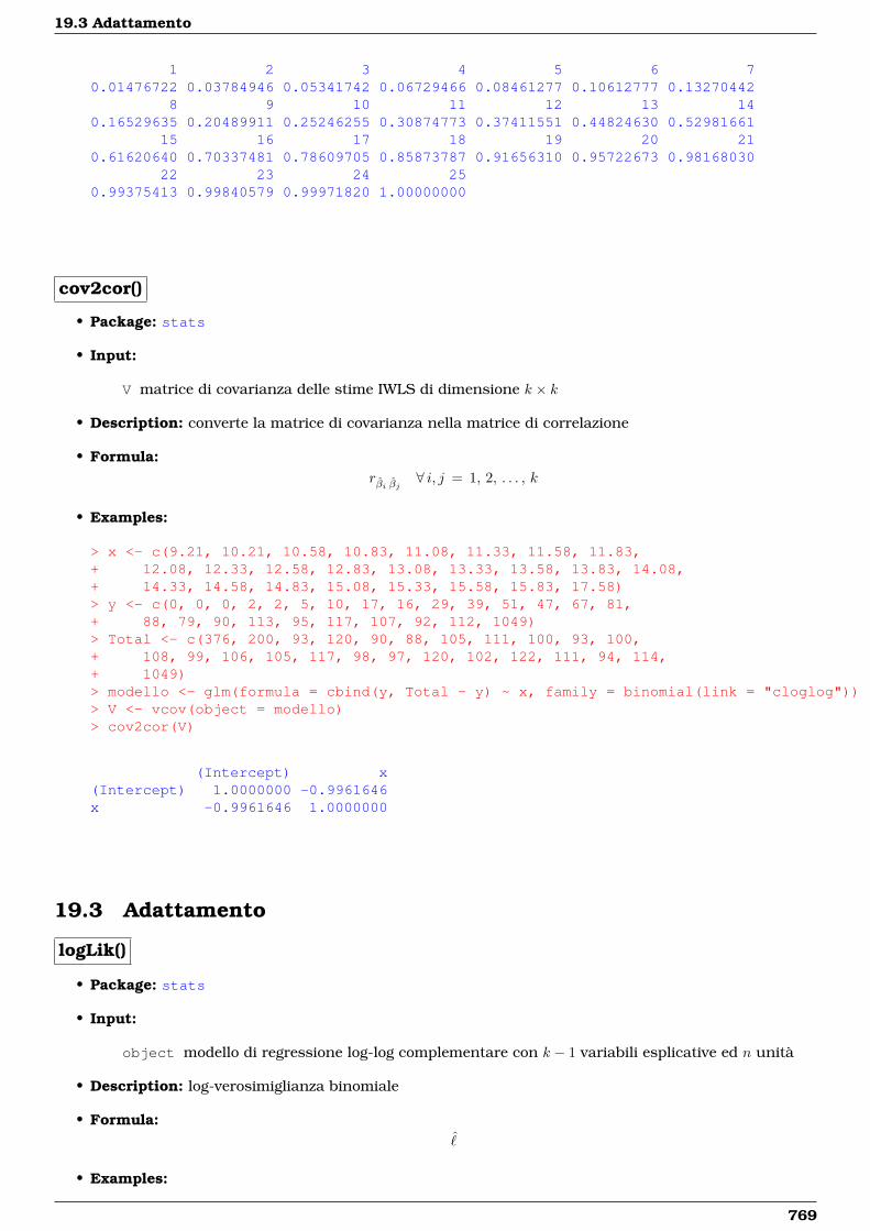
19.3 Adattamento
1 2 3 4 5 6 70.01476722 0.03784946 0.05341742 0.06729466 0.08461277 0.10612777 0.13270442
8 9 10 11 12 13 140.16529635 0.20489911 0.25246255 0.30874773 0.37411551 0.44824630 0.52981661
15 16 17 18 19 20 210.61620640 0.70337481 0.78609705 0.85873787 0.91656310 0.95722673 0.98168030
22 23 24 250.99375413 0.99840579 0.99971820 1.00000000
cov2cor()
• Package: stats
• Input:
V matrice di covarianza delle stime IWLS di dimensione k × k
• Description: converte la matrice di covarianza nella matrice di correlazione
• Formula:rβi βj ∀ i, j = 1, 2, . . . , k
• Examples:
> x <- c(9.21, 10.21, 10.58, 10.83, 11.08, 11.33, 11.58, 11.83,+ 12.08, 12.33, 12.58, 12.83, 13.08, 13.33, 13.58, 13.83, 14.08,+ 14.33, 14.58, 14.83, 15.08, 15.33, 15.58, 15.83, 17.58)> y <- c(0, 0, 0, 2, 2, 5, 10, 17, 16, 29, 39, 51, 47, 67, 81,+ 88, 79, 90, 113, 95, 117, 107, 92, 112, 1049)> Total <- c(376, 200, 93, 120, 90, 88, 105, 111, 100, 93, 100,+ 108, 99, 106, 105, 117, 98, 97, 120, 102, 122, 111, 94, 114,+ 1049)> modello <- glm(formula = cbind(y, Total - y) ~ x, family = binomial(link = "cloglog"))> V <- vcov(object = modello)> cov2cor(V)
(Intercept) x(Intercept) 1.0000000 -0.9961646x -0.9961646 1.0000000
19.3 Adattamento
logLik()
• Package: stats
• Input:
object modello di regressione log-log complementare con k − 1 variabili esplicative ed n unità
• Description: log-verosimiglianza binomiale
• Formula:ˆ
• Examples:
769
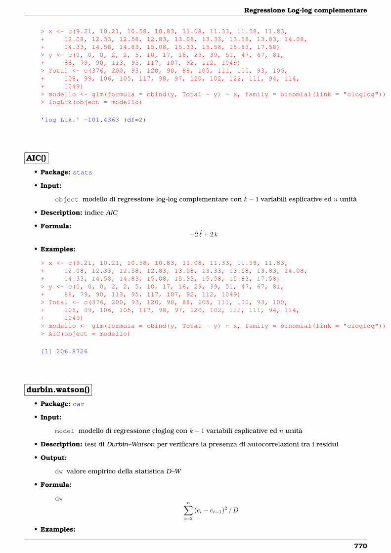
Regressione Log-log complementare
> x <- c(9.21, 10.21, 10.58, 10.83, 11.08, 11.33, 11.58, 11.83,+ 12.08, 12.33, 12.58, 12.83, 13.08, 13.33, 13.58, 13.83, 14.08,+ 14.33, 14.58, 14.83, 15.08, 15.33, 15.58, 15.83, 17.58)> y <- c(0, 0, 0, 2, 2, 5, 10, 17, 16, 29, 39, 51, 47, 67, 81,+ 88, 79, 90, 113, 95, 117, 107, 92, 112, 1049)> Total <- c(376, 200, 93, 120, 90, 88, 105, 111, 100, 93, 100,+ 108, 99, 106, 105, 117, 98, 97, 120, 102, 122, 111, 94, 114,+ 1049)> modello <- glm(formula = cbind(y, Total - y) ~ x, family = binomial(link = "cloglog"))> logLik(object = modello)
'log Lik.' -101.4363 (df=2)
AIC()
• Package: stats
• Input:
object modello di regressione log-log complementare con k − 1 variabili esplicative ed n unità
• Description: indice AIC
• Formula:−2 ˆ+ 2 k
• Examples:
> x <- c(9.21, 10.21, 10.58, 10.83, 11.08, 11.33, 11.58, 11.83,+ 12.08, 12.33, 12.58, 12.83, 13.08, 13.33, 13.58, 13.83, 14.08,+ 14.33, 14.58, 14.83, 15.08, 15.33, 15.58, 15.83, 17.58)> y <- c(0, 0, 0, 2, 2, 5, 10, 17, 16, 29, 39, 51, 47, 67, 81,+ 88, 79, 90, 113, 95, 117, 107, 92, 112, 1049)> Total <- c(376, 200, 93, 120, 90, 88, 105, 111, 100, 93, 100,+ 108, 99, 106, 105, 117, 98, 97, 120, 102, 122, 111, 94, 114,+ 1049)> modello <- glm(formula = cbind(y, Total - y) ~ x, family = binomial(link = "cloglog"))> AIC(object = modello)
[1] 206.8726
durbin.watson()
• Package: car
• Input:
model modello di regressione cloglog con k − 1 variabili esplicative ed n unità
• Description: test di Durbin–Watson per verificare la presenza di autocorrelazioni tra i residui
• Output:
dw valore empirico della statistica D–W
• Formula:
dwn∑i=2
(ei − ei−1)2 /D
• Examples:
770
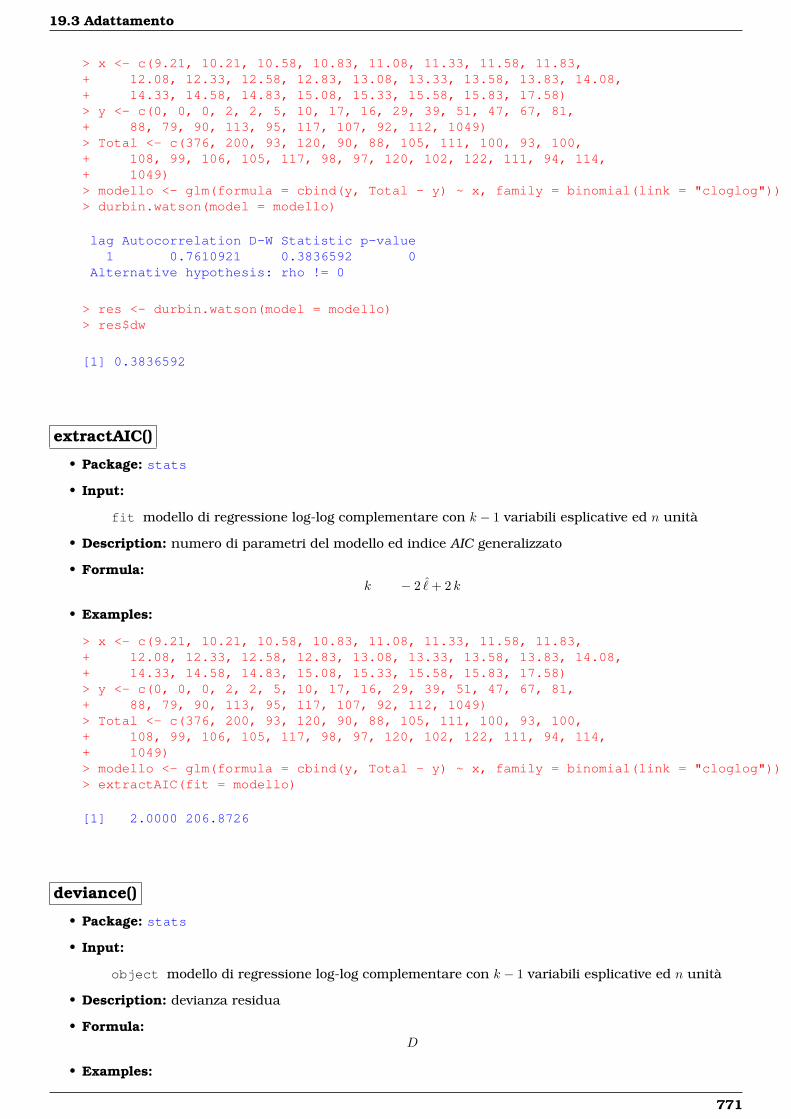
19.3 Adattamento
> x <- c(9.21, 10.21, 10.58, 10.83, 11.08, 11.33, 11.58, 11.83,+ 12.08, 12.33, 12.58, 12.83, 13.08, 13.33, 13.58, 13.83, 14.08,+ 14.33, 14.58, 14.83, 15.08, 15.33, 15.58, 15.83, 17.58)> y <- c(0, 0, 0, 2, 2, 5, 10, 17, 16, 29, 39, 51, 47, 67, 81,+ 88, 79, 90, 113, 95, 117, 107, 92, 112, 1049)> Total <- c(376, 200, 93, 120, 90, 88, 105, 111, 100, 93, 100,+ 108, 99, 106, 105, 117, 98, 97, 120, 102, 122, 111, 94, 114,+ 1049)> modello <- glm(formula = cbind(y, Total - y) ~ x, family = binomial(link = "cloglog"))> durbin.watson(model = modello)
lag Autocorrelation D-W Statistic p-value1 0.7610921 0.3836592 0
Alternative hypothesis: rho != 0
> res <- durbin.watson(model = modello)> res$dw
[1] 0.3836592
extractAIC()
• Package: stats
• Input:
fit modello di regressione log-log complementare con k − 1 variabili esplicative ed n unità
• Description: numero di parametri del modello ed indice AIC generalizzato
• Formula:k − 2 ˆ+ 2 k
• Examples:
> x <- c(9.21, 10.21, 10.58, 10.83, 11.08, 11.33, 11.58, 11.83,+ 12.08, 12.33, 12.58, 12.83, 13.08, 13.33, 13.58, 13.83, 14.08,+ 14.33, 14.58, 14.83, 15.08, 15.33, 15.58, 15.83, 17.58)> y <- c(0, 0, 0, 2, 2, 5, 10, 17, 16, 29, 39, 51, 47, 67, 81,+ 88, 79, 90, 113, 95, 117, 107, 92, 112, 1049)> Total <- c(376, 200, 93, 120, 90, 88, 105, 111, 100, 93, 100,+ 108, 99, 106, 105, 117, 98, 97, 120, 102, 122, 111, 94, 114,+ 1049)> modello <- glm(formula = cbind(y, Total - y) ~ x, family = binomial(link = "cloglog"))> extractAIC(fit = modello)
[1] 2.0000 206.8726
deviance()
• Package: stats
• Input:
object modello di regressione log-log complementare con k − 1 variabili esplicative ed n unità
• Description: devianza residua
• Formula:D
• Examples:
771
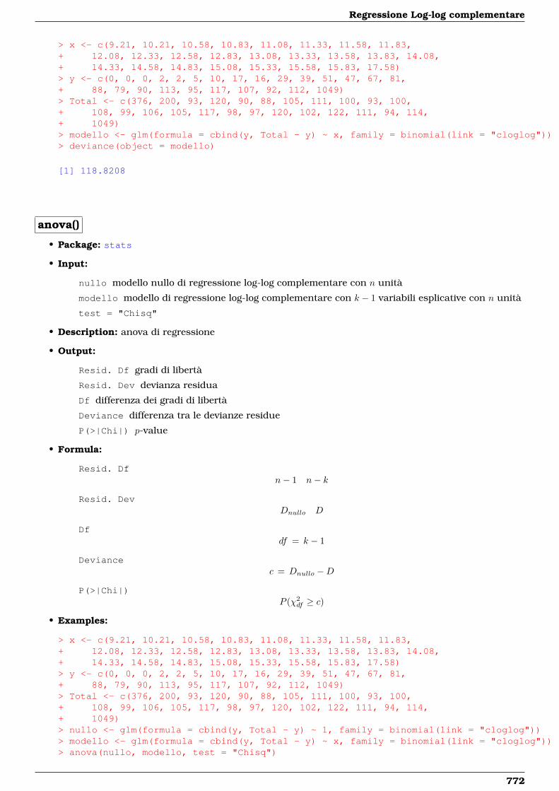
Regressione Log-log complementare
> x <- c(9.21, 10.21, 10.58, 10.83, 11.08, 11.33, 11.58, 11.83,+ 12.08, 12.33, 12.58, 12.83, 13.08, 13.33, 13.58, 13.83, 14.08,+ 14.33, 14.58, 14.83, 15.08, 15.33, 15.58, 15.83, 17.58)> y <- c(0, 0, 0, 2, 2, 5, 10, 17, 16, 29, 39, 51, 47, 67, 81,+ 88, 79, 90, 113, 95, 117, 107, 92, 112, 1049)> Total <- c(376, 200, 93, 120, 90, 88, 105, 111, 100, 93, 100,+ 108, 99, 106, 105, 117, 98, 97, 120, 102, 122, 111, 94, 114,+ 1049)> modello <- glm(formula = cbind(y, Total - y) ~ x, family = binomial(link = "cloglog"))> deviance(object = modello)
[1] 118.8208
anova()
• Package: stats
• Input:
nullo modello nullo di regressione log-log complementare con n unità
modello modello di regressione log-log complementare con k − 1 variabili esplicative con n unità
test = "Chisq"
• Description: anova di regressione
• Output:
Resid. Df gradi di libertà
Resid. Dev devianza residua
Df differenza dei gradi di libertà
Deviance differenza tra le devianze residue
P(>|Chi|) p-value
• Formula:
Resid. Dfn− 1 n− k
Resid. DevDnullo D
Dfdf = k − 1
Deviancec = Dnullo −D
P(>|Chi|)P (χ2
df ≥ c)
• Examples:
> x <- c(9.21, 10.21, 10.58, 10.83, 11.08, 11.33, 11.58, 11.83,+ 12.08, 12.33, 12.58, 12.83, 13.08, 13.33, 13.58, 13.83, 14.08,+ 14.33, 14.58, 14.83, 15.08, 15.33, 15.58, 15.83, 17.58)> y <- c(0, 0, 0, 2, 2, 5, 10, 17, 16, 29, 39, 51, 47, 67, 81,+ 88, 79, 90, 113, 95, 117, 107, 92, 112, 1049)> Total <- c(376, 200, 93, 120, 90, 88, 105, 111, 100, 93, 100,+ 108, 99, 106, 105, 117, 98, 97, 120, 102, 122, 111, 94, 114,+ 1049)> nullo <- glm(formula = cbind(y, Total - y) ~ 1, family = binomial(link = "cloglog"))> modello <- glm(formula = cbind(y, Total - y) ~ x, family = binomial(link = "cloglog"))> anova(nullo, modello, test = "Chisq")
772
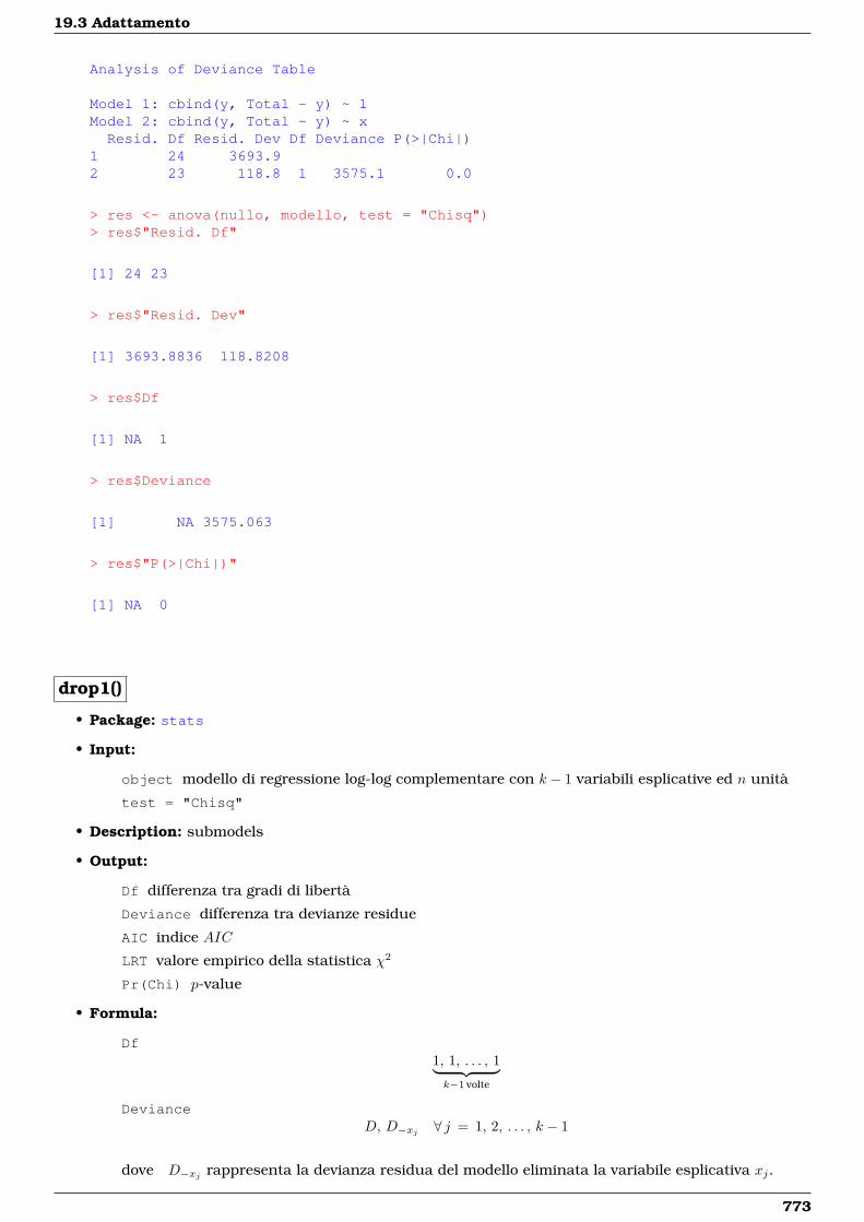
19.3 Adattamento
Analysis of Deviance Table
Model 1: cbind(y, Total - y) ~ 1Model 2: cbind(y, Total - y) ~ xResid. Df Resid. Dev Df Deviance P(>|Chi|)
1 24 3693.92 23 118.8 1 3575.1 0.0
> res <- anova(nullo, modello, test = "Chisq")> res$"Resid. Df"
[1] 24 23
> res$"Resid. Dev"
[1] 3693.8836 118.8208
> res$Df
[1] NA 1
> res$Deviance
[1] NA 3575.063
> res$"P(>|Chi|)"
[1] NA 0
drop1()
• Package: stats
• Input:
object modello di regressione log-log complementare con k − 1 variabili esplicative ed n unità
test = "Chisq"
• Description: submodels
• Output:
Df differenza tra gradi di libertà
Deviance differenza tra devianze residue
AIC indice AIC
LRT valore empirico della statistica χ2
Pr(Chi) p-value
• Formula:
Df1, 1, . . . , 1︸ ︷︷ ︸k−1 volte
DevianceD, D−xj ∀ j = 1, 2, . . . , k − 1
dove D−xj rappresenta la devianza residua del modello eliminata la variabile esplicativa xj.
773
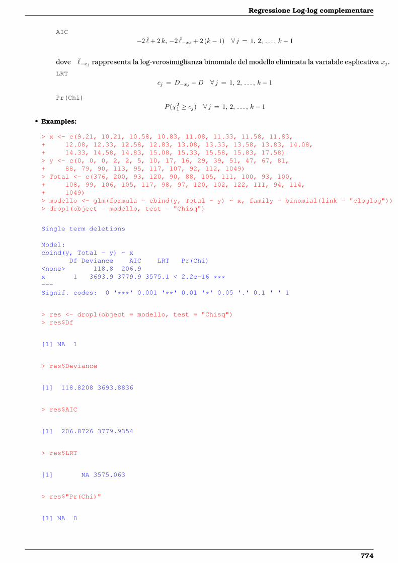
Regressione Log-log complementare
AIC
−2 ˆ+ 2 k, −2 ˆ−xj + 2 (k − 1) ∀ j = 1, 2, . . . , k − 1
dove ˆ−xj rappresenta la log-verosimiglianza binomiale del modello eliminata la variabile esplicativa xj.
LRT
cj = D−xj −D ∀ j = 1, 2, . . . , k − 1
Pr(Chi)
P (χ21 ≥ cj) ∀ j = 1, 2, . . . , k − 1
• Examples:
> x <- c(9.21, 10.21, 10.58, 10.83, 11.08, 11.33, 11.58, 11.83,+ 12.08, 12.33, 12.58, 12.83, 13.08, 13.33, 13.58, 13.83, 14.08,+ 14.33, 14.58, 14.83, 15.08, 15.33, 15.58, 15.83, 17.58)> y <- c(0, 0, 0, 2, 2, 5, 10, 17, 16, 29, 39, 51, 47, 67, 81,+ 88, 79, 90, 113, 95, 117, 107, 92, 112, 1049)> Total <- c(376, 200, 93, 120, 90, 88, 105, 111, 100, 93, 100,+ 108, 99, 106, 105, 117, 98, 97, 120, 102, 122, 111, 94, 114,+ 1049)> modello <- glm(formula = cbind(y, Total - y) ~ x, family = binomial(link = "cloglog"))> drop1(object = modello, test = "Chisq")
Single term deletions
Model:cbind(y, Total - y) ~ x
Df Deviance AIC LRT Pr(Chi)<none> 118.8 206.9x 1 3693.9 3779.9 3575.1 < 2.2e-16 ***---Signif. codes: 0 '***' 0.001 '**' 0.01 '*' 0.05 '.' 0.1 ' ' 1
> res <- drop1(object = modello, test = "Chisq")> res$Df
[1] NA 1
> res$Deviance
[1] 118.8208 3693.8836
> res$AIC
[1] 206.8726 3779.9354
> res$LRT
[1] NA 3575.063
> res$"Pr(Chi)"
[1] NA 0
774
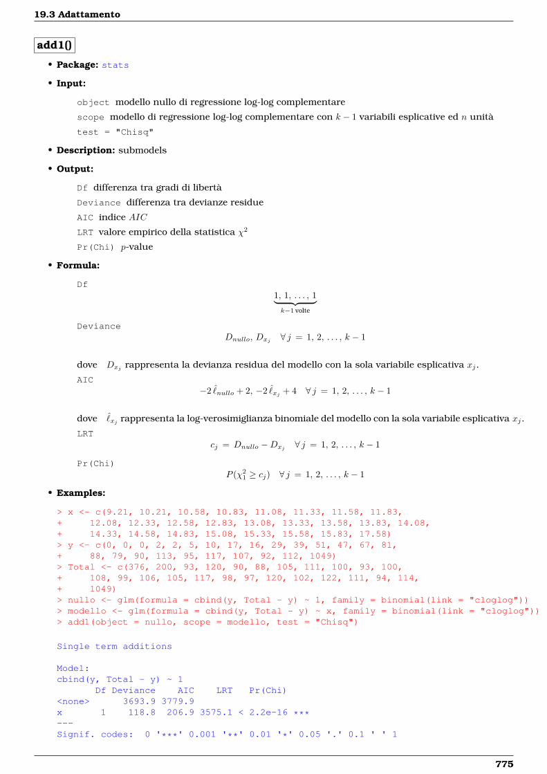
19.3 Adattamento
add1()
• Package: stats
• Input:
object modello nullo di regressione log-log complementare
scope modello di regressione log-log complementare con k − 1 variabili esplicative ed n unità
test = "Chisq"
• Description: submodels
• Output:
Df differenza tra gradi di libertà
Deviance differenza tra devianze residue
AIC indice AIC
LRT valore empirico della statistica χ2
Pr(Chi) p-value
• Formula:
Df1, 1, . . . , 1︸ ︷︷ ︸k−1 volte
DevianceDnullo, Dxj ∀ j = 1, 2, . . . , k − 1
dove Dxj rappresenta la devianza residua del modello con la sola variabile esplicativa xj.
AIC−2 ˆ
nullo + 2, −2 ˆxj + 4 ∀ j = 1, 2, . . . , k − 1
dove ˆxj rappresenta la log-verosimiglianza binomiale del modello con la sola variabile esplicativa xj.
LRTcj = Dnullo −Dxj ∀ j = 1, 2, . . . , k − 1
Pr(Chi)P (χ2
1 ≥ cj) ∀ j = 1, 2, . . . , k − 1
• Examples:
> x <- c(9.21, 10.21, 10.58, 10.83, 11.08, 11.33, 11.58, 11.83,+ 12.08, 12.33, 12.58, 12.83, 13.08, 13.33, 13.58, 13.83, 14.08,+ 14.33, 14.58, 14.83, 15.08, 15.33, 15.58, 15.83, 17.58)> y <- c(0, 0, 0, 2, 2, 5, 10, 17, 16, 29, 39, 51, 47, 67, 81,+ 88, 79, 90, 113, 95, 117, 107, 92, 112, 1049)> Total <- c(376, 200, 93, 120, 90, 88, 105, 111, 100, 93, 100,+ 108, 99, 106, 105, 117, 98, 97, 120, 102, 122, 111, 94, 114,+ 1049)> nullo <- glm(formula = cbind(y, Total - y) ~ 1, family = binomial(link = "cloglog"))> modello <- glm(formula = cbind(y, Total - y) ~ x, family = binomial(link = "cloglog"))> add1(object = nullo, scope = modello, test = "Chisq")
Single term additions
Model:cbind(y, Total - y) ~ 1
Df Deviance AIC LRT Pr(Chi)<none> 3693.9 3779.9x 1 118.8 206.9 3575.1 < 2.2e-16 ***---Signif. codes: 0 '***' 0.001 '**' 0.01 '*' 0.05 '.' 0.1 ' ' 1
775
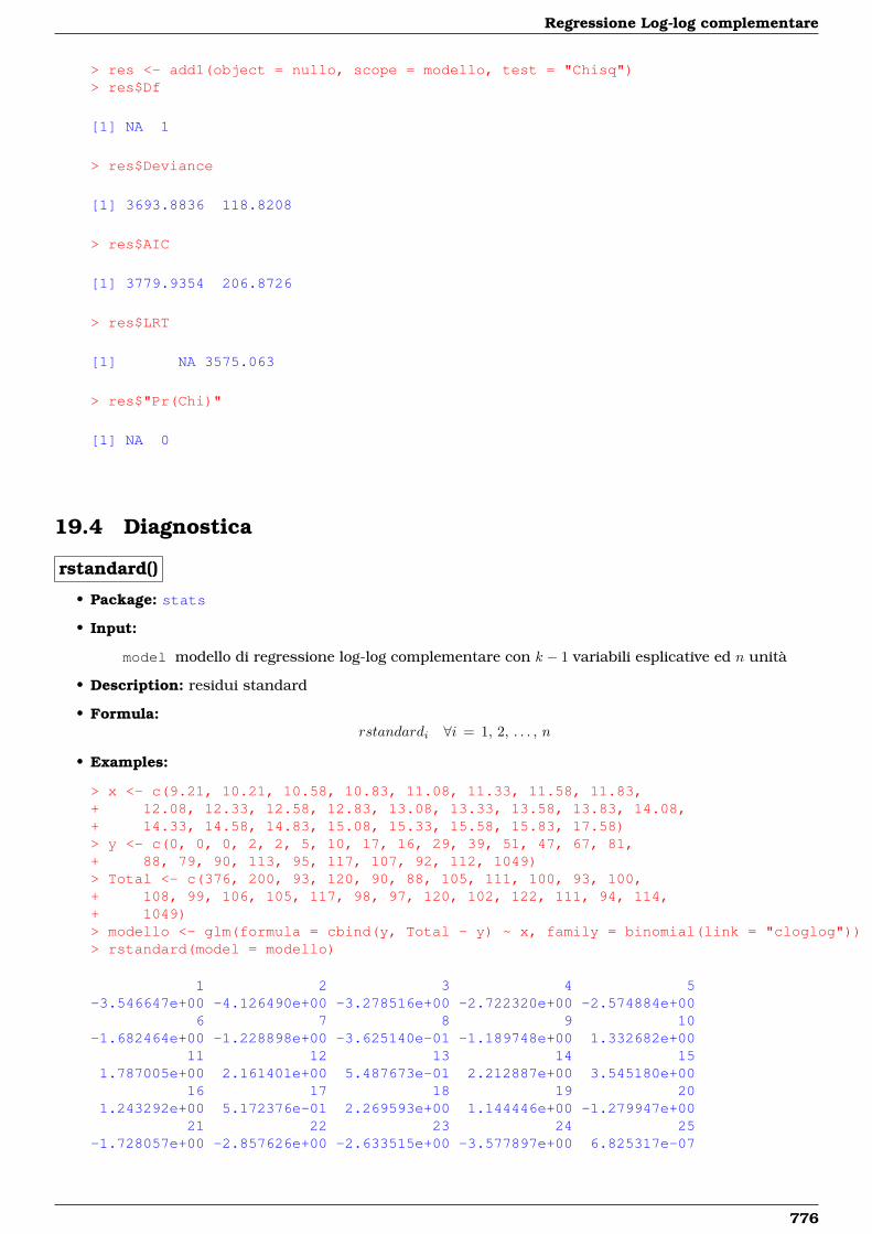
Regressione Log-log complementare
> res <- add1(object = nullo, scope = modello, test = "Chisq")> res$Df
[1] NA 1
> res$Deviance
[1] 3693.8836 118.8208
> res$AIC
[1] 3779.9354 206.8726
> res$LRT
[1] NA 3575.063
> res$"Pr(Chi)"
[1] NA 0
19.4 Diagnostica
rstandard()
• Package: stats
• Input:
model modello di regressione log-log complementare con k − 1 variabili esplicative ed n unità
• Description: residui standard
• Formula:rstandardi ∀i = 1, 2, . . . , n
• Examples:
> x <- c(9.21, 10.21, 10.58, 10.83, 11.08, 11.33, 11.58, 11.83,+ 12.08, 12.33, 12.58, 12.83, 13.08, 13.33, 13.58, 13.83, 14.08,+ 14.33, 14.58, 14.83, 15.08, 15.33, 15.58, 15.83, 17.58)> y <- c(0, 0, 0, 2, 2, 5, 10, 17, 16, 29, 39, 51, 47, 67, 81,+ 88, 79, 90, 113, 95, 117, 107, 92, 112, 1049)> Total <- c(376, 200, 93, 120, 90, 88, 105, 111, 100, 93, 100,+ 108, 99, 106, 105, 117, 98, 97, 120, 102, 122, 111, 94, 114,+ 1049)> modello <- glm(formula = cbind(y, Total - y) ~ x, family = binomial(link = "cloglog"))> rstandard(model = modello)
1 2 3 4 5-3.546647e+00 -4.126490e+00 -3.278516e+00 -2.722320e+00 -2.574884e+00
6 7 8 9 10-1.682464e+00 -1.228898e+00 -3.625140e-01 -1.189748e+00 1.332682e+00
11 12 13 14 151.787005e+00 2.161401e+00 5.487673e-01 2.212887e+00 3.545180e+00
16 17 18 19 201.243292e+00 5.172376e-01 2.269593e+00 1.144446e+00 -1.279947e+00
21 22 23 24 25-1.728057e+00 -2.857626e+00 -2.633515e+00 -3.577897e+00 6.825317e-07
776
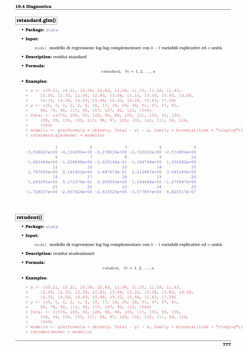
19.4 Diagnostica
rstandard.glm()
• Package: stats
• Input:
model modello di regressione log-log complementare con k − 1 variabili esplicative ed n unità
• Description: residui standard
• Formula:rstandardi ∀i = 1, 2, . . . , n
• Examples:
> x <- c(9.21, 10.21, 10.58, 10.83, 11.08, 11.33, 11.58, 11.83,+ 12.08, 12.33, 12.58, 12.83, 13.08, 13.33, 13.58, 13.83, 14.08,+ 14.33, 14.58, 14.83, 15.08, 15.33, 15.58, 15.83, 17.58)> y <- c(0, 0, 0, 2, 2, 5, 10, 17, 16, 29, 39, 51, 47, 67, 81,+ 88, 79, 90, 113, 95, 117, 107, 92, 112, 1049)> Total <- c(376, 200, 93, 120, 90, 88, 105, 111, 100, 93, 100,+ 108, 99, 106, 105, 117, 98, 97, 120, 102, 122, 111, 94, 114,+ 1049)> modello <- glm(formula = cbind(y, Total - y) ~ x, family = binomial(link = "cloglog"))> rstandard.glm(model = modello)
1 2 3 4 5-3.546647e+00 -4.126490e+00 -3.278516e+00 -2.722320e+00 -2.574884e+00
6 7 8 9 10-1.682464e+00 -1.228898e+00 -3.625140e-01 -1.189748e+00 1.332682e+00
11 12 13 14 151.787005e+00 2.161401e+00 5.487673e-01 2.212887e+00 3.545180e+00
16 17 18 19 201.243292e+00 5.172376e-01 2.269593e+00 1.144446e+00 -1.279947e+00
21 22 23 24 25-1.728057e+00 -2.857626e+00 -2.633515e+00 -3.577897e+00 6.825317e-07
rstudent()
• Package: stats
• Input:
model modello di regressione log-log complementare con k − 1 variabili esplicative ed n unità
• Description: residui studentizzati
• Formula:rstudenti ∀i = 1, 2, . . . , n
• Examples:
> x <- c(9.21, 10.21, 10.58, 10.83, 11.08, 11.33, 11.58, 11.83,+ 12.08, 12.33, 12.58, 12.83, 13.08, 13.33, 13.58, 13.83, 14.08,+ 14.33, 14.58, 14.83, 15.08, 15.33, 15.58, 15.83, 17.58)> y <- c(0, 0, 0, 2, 2, 5, 10, 17, 16, 29, 39, 51, 47, 67, 81,+ 88, 79, 90, 113, 95, 117, 107, 92, 112, 1049)> Total <- c(376, 200, 93, 120, 90, 88, 105, 111, 100, 93, 100,+ 108, 99, 106, 105, 117, 98, 97, 120, 102, 122, 111, 94, 114,+ 1049)> modello <- glm(formula = cbind(y, Total - y) ~ x, family = binomial(link = "cloglog"))> rstudent(model = modello)
777
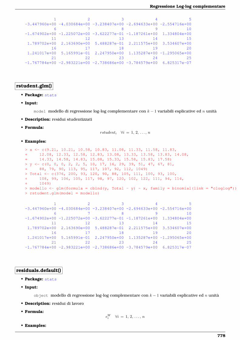
Regressione Log-log complementare
1 2 3 4 5-3.447960e+00 -4.030684e+00 -3.238407e+00 -2.694633e+00 -2.554716e+00
6 7 8 9 10-1.674902e+00 -1.225072e+00 -3.622277e-01 -1.187261e+00 1.334804e+00
11 12 13 14 151.789702e+00 2.163690e+00 5.488287e-01 2.211575e+00 3.534607e+00
16 17 18 19 201.241017e+00 5.165991e-01 2.247950e+00 1.135287e+00 -1.295065e+00
21 22 23 24 25-1.767784e+00 -2.983221e+00 -2.738686e+00 -3.784579e+00 6.825317e-07
rstudent.glm()
• Package: stats
• Input:
model modello di regressione log-log complementare con k − 1 variabili esplicative ed n unità
• Description: residui studentizzati
• Formula:rstudenti ∀i = 1, 2, . . . , n
• Examples:
> x <- c(9.21, 10.21, 10.58, 10.83, 11.08, 11.33, 11.58, 11.83,+ 12.08, 12.33, 12.58, 12.83, 13.08, 13.33, 13.58, 13.83, 14.08,+ 14.33, 14.58, 14.83, 15.08, 15.33, 15.58, 15.83, 17.58)> y <- c(0, 0, 0, 2, 2, 5, 10, 17, 16, 29, 39, 51, 47, 67, 81,+ 88, 79, 90, 113, 95, 117, 107, 92, 112, 1049)> Total <- c(376, 200, 93, 120, 90, 88, 105, 111, 100, 93, 100,+ 108, 99, 106, 105, 117, 98, 97, 120, 102, 122, 111, 94, 114,+ 1049)> modello <- glm(formula = cbind(y, Total - y) ~ x, family = binomial(link = "cloglog"))> rstudent.glm(model = modello)
1 2 3 4 5-3.447960e+00 -4.030684e+00 -3.238407e+00 -2.694633e+00 -2.554716e+00
6 7 8 9 10-1.674902e+00 -1.225072e+00 -3.622277e-01 -1.187261e+00 1.334804e+00
11 12 13 14 151.789702e+00 2.163690e+00 5.488287e-01 2.211575e+00 3.534607e+00
16 17 18 19 201.241017e+00 5.165991e-01 2.247950e+00 1.135287e+00 -1.295065e+00
21 22 23 24 25-1.767784e+00 -2.983221e+00 -2.738686e+00 -3.784579e+00 6.825317e-07
residuals.default()
• Package: stats
• Input:
object modello di regressione log-log complementare con k − 1 variabili esplicative ed n unità
• Description: residui di lavoro
• Formula:eWi ∀i = 1, 2, . . . , n
• Examples:
778
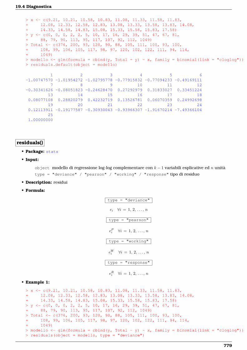
19.4 Diagnostica
> x <- c(9.21, 10.21, 10.58, 10.83, 11.08, 11.33, 11.58, 11.83,+ 12.08, 12.33, 12.58, 12.83, 13.08, 13.33, 13.58, 13.83, 14.08,+ 14.33, 14.58, 14.83, 15.08, 15.33, 15.58, 15.83, 17.58)> y <- c(0, 0, 0, 2, 2, 5, 10, 17, 16, 29, 39, 51, 47, 67, 81,+ 88, 79, 90, 113, 95, 117, 107, 92, 112, 1049)> Total <- c(376, 200, 93, 120, 90, 88, 105, 111, 100, 93, 100,+ 108, 99, 106, 105, 117, 98, 97, 120, 102, 122, 111, 94, 114,+ 1049)> modello <- glm(formula = cbind(y, Total - y) ~ x, family = binomial(link = "cloglog"))> residuals.default(object = modello)
1 2 3 4 5 6-1.00747570 -1.01954272 -1.02795778 -0.77915832 -0.77094233 -0.49169111
7 8 9 10 11 12-0.30341626 -0.08051823 -0.24628470 0.27292979 0.31833027 0.33451224
13 14 15 16 17 180.08077108 0.28820279 0.42232719 0.13526781 0.06070359 0.24992698
19 20 21 22 23 240.12113911 -0.19177587 -0.30930043 -0.93966307 -1.91670214 -7.49366104
251.00000000
residuals()
• Package: stats
• Input:
object modello di regressione log-log complementare con k − 1 variabili esplicative ed n unità
type = "deviance" / "pearson" / "working" / "response" tipo di residuo
• Description: residui
• Formula:
type = "deviance"
ei ∀i = 1, 2, . . . , n
type = "pearson"
ePi ∀i = 1, 2, . . . , n
type = "working"
eWi ∀i = 1, 2, . . . , n
type = "response"
eRi ∀i = 1, 2, . . . , n
• Example 1:
> x <- c(9.21, 10.21, 10.58, 10.83, 11.08, 11.33, 11.58, 11.83,+ 12.08, 12.33, 12.58, 12.83, 13.08, 13.33, 13.58, 13.83, 14.08,+ 14.33, 14.58, 14.83, 15.08, 15.33, 15.58, 15.83, 17.58)> y <- c(0, 0, 0, 2, 2, 5, 10, 17, 16, 29, 39, 51, 47, 67, 81,+ 88, 79, 90, 113, 95, 117, 107, 92, 112, 1049)> Total <- c(376, 200, 93, 120, 90, 88, 105, 111, 100, 93, 100,+ 108, 99, 106, 105, 117, 98, 97, 120, 102, 122, 111, 94, 114,+ 1049)> modello <- glm(formula = cbind(y, Total - y) ~ x, family = binomial(link = "cloglog"))> residuals(object = modello, type = "deviance")
779

Regressione Log-log complementare
1 2 3 4 5-3.344811e+00 -3.928580e+00 -3.195443e+00 -2.625263e+00 -2.501326e+00
6 7 8 9 10-1.632697e+00 -1.183466e+00 -3.479272e-01 -1.146176e+00 1.287445e+00
11 12 13 14 151.722479e+00 2.078066e+00 5.293632e-01 2.125777e+00 3.393960e+00
16 17 18 19 201.175000e+00 4.892018e-01 2.127667e+00 1.046796e+00 -1.190182e+00
21 22 23 24 25-1.608195e+00 -2.739982e+00 -2.588698e+00 -3.552944e+00 6.825317e-07
• Example 2:
> x <- c(9.21, 10.21, 10.58, 10.83, 11.08, 11.33, 11.58, 11.83,+ 12.08, 12.33, 12.58, 12.83, 13.08, 13.33, 13.58, 13.83, 14.08,+ 14.33, 14.58, 14.83, 15.08, 15.33, 15.58, 15.83, 17.58)> y <- c(0, 0, 0, 2, 2, 5, 10, 17, 16, 29, 39, 51, 47, 67, 81,+ 88, 79, 90, 113, 95, 117, 107, 92, 112, 1049)> Total <- c(376, 200, 93, 120, 90, 88, 105, 111, 100, 93, 100,+ 108, 99, 106, 105, 117, 98, 97, 120, 102, 122, 111, 94, 114,+ 1049)> modello <- glm(formula = cbind(y, Total - y) ~ x, family = binomial(link = "cloglog"))> residuals(object = modello, type = "pearson")
1 2 3 4 5-2.373963e+00 -2.804939e+00 -2.290887e+00 -2.213700e+00 -2.126766e+00
6 7 8 9 10-1.501829e+00 -1.131643e+00 -3.444267e-01 -1.112389e+00 1.317832e+00
11 12 13 14 151.758796e+00 2.106981e+00 5.302147e-01 2.109393e+00 3.270668e+00
16 17 18 19 201.154719e+00 4.834456e-01 1.953903e+00 9.944108e-01 -1.290438e+00
21 22 23 24 25-1.866683e+00 -3.983806e+00 -4.783173e+00 -1.098075e+01 4.826228e-07
• Example 3:
> x <- c(9.21, 10.21, 10.58, 10.83, 11.08, 11.33, 11.58, 11.83,+ 12.08, 12.33, 12.58, 12.83, 13.08, 13.33, 13.58, 13.83, 14.08,+ 14.33, 14.58, 14.83, 15.08, 15.33, 15.58, 15.83, 17.58)> y <- c(0, 0, 0, 2, 2, 5, 10, 17, 16, 29, 39, 51, 47, 67, 81,+ 88, 79, 90, 113, 95, 117, 107, 92, 112, 1049)> Total <- c(376, 200, 93, 120, 90, 88, 105, 111, 100, 93, 100,+ 108, 99, 106, 105, 117, 98, 97, 120, 102, 122, 111, 94, 114,+ 1049)> modello <- glm(formula = cbind(y, Total - y) ~ x, family = binomial(link = "cloglog"))> residuals(object = modello, type = "working")
1 2 3 4 5 6-1.00747570 -1.01954272 -1.02795778 -0.77915832 -0.77094233 -0.49169111
7 8 9 10 11 12-0.30341626 -0.08051823 -0.24628470 0.27292979 0.31833027 0.33451224
13 14 15 16 17 180.08077108 0.28820279 0.42232719 0.13526781 0.06070359 0.24992698
19 20 21 22 23 240.12113911 -0.19177587 -0.30930043 -0.93966307 -1.91670214 -7.49366104
251.00000000
• Example 4:
> x <- c(9.21, 10.21, 10.58, 10.83, 11.08, 11.33, 11.58, 11.83,+ 12.08, 12.33, 12.58, 12.83, 13.08, 13.33, 13.58, 13.83, 14.08,+ 14.33, 14.58, 14.83, 15.08, 15.33, 15.58, 15.83, 17.58)
780
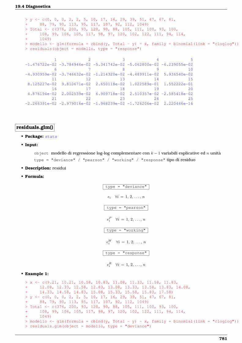
19.4 Diagnostica
> y <- c(0, 0, 0, 2, 2, 5, 10, 17, 16, 29, 39, 51, 47, 67, 81,+ 88, 79, 90, 113, 95, 117, 107, 92, 112, 1049)> Total <- c(376, 200, 93, 120, 90, 88, 105, 111, 100, 93, 100,+ 108, 99, 106, 105, 117, 98, 97, 120, 102, 122, 111, 94, 114,+ 1049)> modello <- glm(formula = cbind(y, Total - y) ~ x, family = binomial(link = "cloglog"))> residuals(object = modello, type = "response")
1 2 3 4 5-1.476722e-02 -3.784946e-02 -5.341742e-02 -5.062800e-02 -6.239055e-02
6 7 8 9 10-4.930959e-02 -3.746632e-02 -1.214320e-02 -4.489911e-02 5.936540e-02
11 12 13 14 158.125227e-02 9.810671e-02 2.650118e-02 1.022589e-01 1.552222e-01
16 17 18 19 204.876194e-02 2.002539e-02 6.909718e-02 2.510357e-02 -2.585418e-02
21 22 23 24 25-2.266391e-02 -2.979016e-02 -1.968239e-02 -1.726206e-02 2.220446e-16
residuals.glm()
• Package: stats
• Input:
object modello di regressione log-log complementare con k − 1 variabili esplicative ed n unità
type = "deviance" / "pearson" / "working" / "response" tipo di residuo
• Description: residui
• Formula:
type = "deviance"
ei ∀i = 1, 2, . . . , n
type = "pearson"
ePi ∀i = 1, 2, . . . , n
type = "working"
eWi ∀i = 1, 2, . . . , n
type = "response"
eRi ∀i = 1, 2, . . . , n
• Example 1:
> x <- c(9.21, 10.21, 10.58, 10.83, 11.08, 11.33, 11.58, 11.83,+ 12.08, 12.33, 12.58, 12.83, 13.08, 13.33, 13.58, 13.83, 14.08,+ 14.33, 14.58, 14.83, 15.08, 15.33, 15.58, 15.83, 17.58)> y <- c(0, 0, 0, 2, 2, 5, 10, 17, 16, 29, 39, 51, 47, 67, 81,+ 88, 79, 90, 113, 95, 117, 107, 92, 112, 1049)> Total <- c(376, 200, 93, 120, 90, 88, 105, 111, 100, 93, 100,+ 108, 99, 106, 105, 117, 98, 97, 120, 102, 122, 111, 94, 114,+ 1049)> modello <- glm(formula = cbind(y, Total - y) ~ x, family = binomial(link = "cloglog"))> residuals.glm(object = modello, type = "deviance")
781
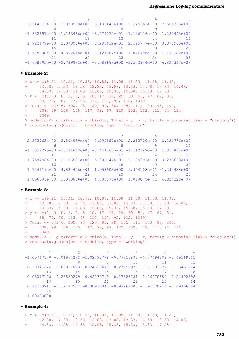
Regressione Log-log complementare
1 2 3 4 5-3.344811e+00 -3.928580e+00 -3.195443e+00 -2.625263e+00 -2.501326e+00
6 7 8 9 10-1.632697e+00 -1.183466e+00 -3.479272e-01 -1.146176e+00 1.287445e+00
11 12 13 14 151.722479e+00 2.078066e+00 5.293632e-01 2.125777e+00 3.393960e+00
16 17 18 19 201.175000e+00 4.892018e-01 2.127667e+00 1.046796e+00 -1.190182e+00
21 22 23 24 25-1.608195e+00 -2.739982e+00 -2.588698e+00 -3.552944e+00 6.825317e-07
• Example 2:
> x <- c(9.21, 10.21, 10.58, 10.83, 11.08, 11.33, 11.58, 11.83,+ 12.08, 12.33, 12.58, 12.83, 13.08, 13.33, 13.58, 13.83, 14.08,+ 14.33, 14.58, 14.83, 15.08, 15.33, 15.58, 15.83, 17.58)> y <- c(0, 0, 0, 2, 2, 5, 10, 17, 16, 29, 39, 51, 47, 67, 81,+ 88, 79, 90, 113, 95, 117, 107, 92, 112, 1049)> Total <- c(376, 200, 93, 120, 90, 88, 105, 111, 100, 93, 100,+ 108, 99, 106, 105, 117, 98, 97, 120, 102, 122, 111, 94, 114,+ 1049)> modello <- glm(formula = cbind(y, Total - y) ~ x, family = binomial(link = "cloglog"))> residuals.glm(object = modello, type = "pearson")
1 2 3 4 5-2.373963e+00 -2.804939e+00 -2.290887e+00 -2.213700e+00 -2.126766e+00
6 7 8 9 10-1.501829e+00 -1.131643e+00 -3.444267e-01 -1.112389e+00 1.317832e+00
11 12 13 14 151.758796e+00 2.106981e+00 5.302147e-01 2.109393e+00 3.270668e+00
16 17 18 19 201.154719e+00 4.834456e-01 1.953903e+00 9.944108e-01 -1.290438e+00
21 22 23 24 25-1.866683e+00 -3.983806e+00 -4.783173e+00 -1.098075e+01 4.826228e-07
• Example 3:
> x <- c(9.21, 10.21, 10.58, 10.83, 11.08, 11.33, 11.58, 11.83,+ 12.08, 12.33, 12.58, 12.83, 13.08, 13.33, 13.58, 13.83, 14.08,+ 14.33, 14.58, 14.83, 15.08, 15.33, 15.58, 15.83, 17.58)> y <- c(0, 0, 0, 2, 2, 5, 10, 17, 16, 29, 39, 51, 47, 67, 81,+ 88, 79, 90, 113, 95, 117, 107, 92, 112, 1049)> Total <- c(376, 200, 93, 120, 90, 88, 105, 111, 100, 93, 100,+ 108, 99, 106, 105, 117, 98, 97, 120, 102, 122, 111, 94, 114,+ 1049)> modello <- glm(formula = cbind(y, Total - y) ~ x, family = binomial(link = "cloglog"))> residuals.glm(object = modello, type = "working")
1 2 3 4 5 6-1.00747570 -1.01954272 -1.02795778 -0.77915832 -0.77094233 -0.49169111
7 8 9 10 11 12-0.30341626 -0.08051823 -0.24628470 0.27292979 0.31833027 0.33451224
13 14 15 16 17 180.08077108 0.28820279 0.42232719 0.13526781 0.06070359 0.24992698
19 20 21 22 23 240.12113911 -0.19177587 -0.30930043 -0.93966307 -1.91670214 -7.49366104
251.00000000
• Example 4:
> x <- c(9.21, 10.21, 10.58, 10.83, 11.08, 11.33, 11.58, 11.83,+ 12.08, 12.33, 12.58, 12.83, 13.08, 13.33, 13.58, 13.83, 14.08,+ 14.33, 14.58, 14.83, 15.08, 15.33, 15.58, 15.83, 17.58)
782
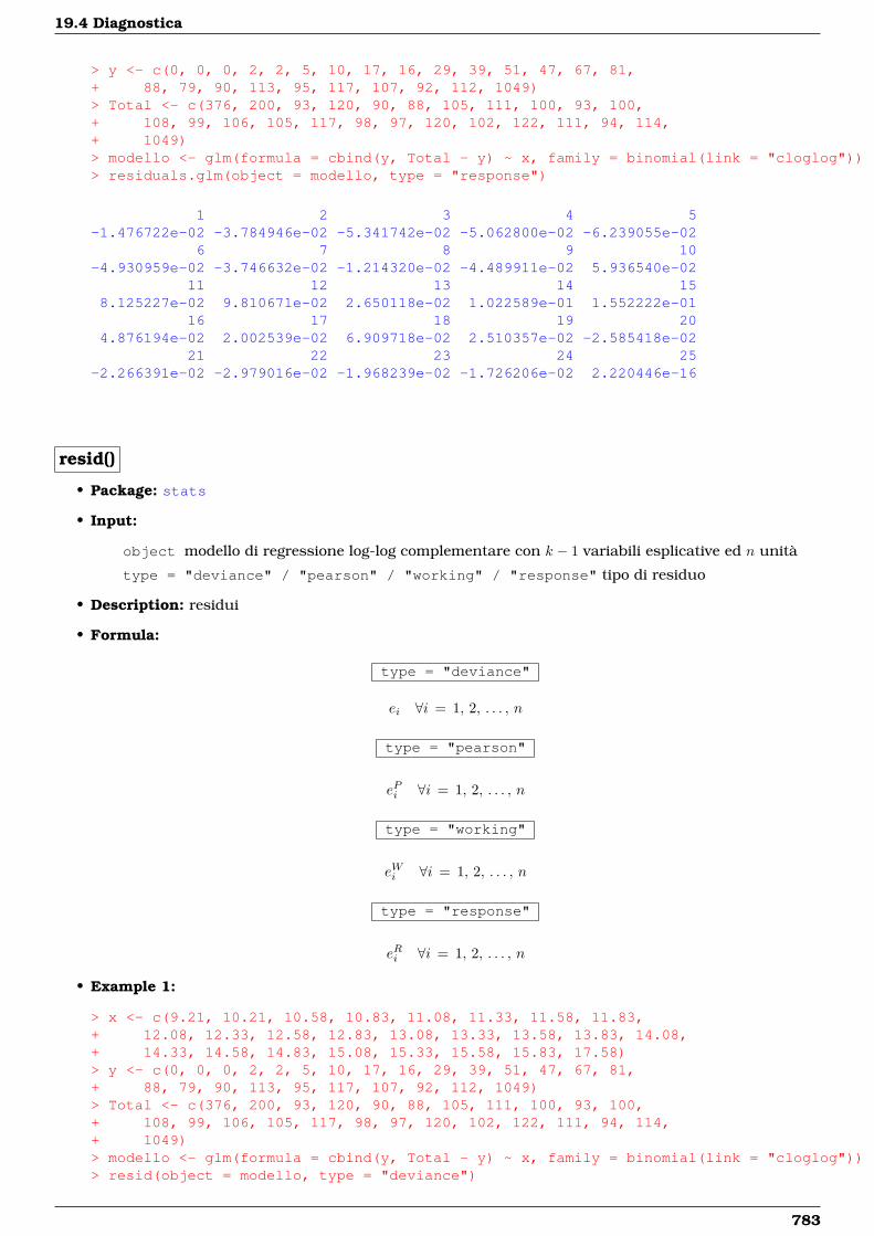
19.4 Diagnostica
> y <- c(0, 0, 0, 2, 2, 5, 10, 17, 16, 29, 39, 51, 47, 67, 81,+ 88, 79, 90, 113, 95, 117, 107, 92, 112, 1049)> Total <- c(376, 200, 93, 120, 90, 88, 105, 111, 100, 93, 100,+ 108, 99, 106, 105, 117, 98, 97, 120, 102, 122, 111, 94, 114,+ 1049)> modello <- glm(formula = cbind(y, Total - y) ~ x, family = binomial(link = "cloglog"))> residuals.glm(object = modello, type = "response")
1 2 3 4 5-1.476722e-02 -3.784946e-02 -5.341742e-02 -5.062800e-02 -6.239055e-02
6 7 8 9 10-4.930959e-02 -3.746632e-02 -1.214320e-02 -4.489911e-02 5.936540e-02
11 12 13 14 158.125227e-02 9.810671e-02 2.650118e-02 1.022589e-01 1.552222e-01
16 17 18 19 204.876194e-02 2.002539e-02 6.909718e-02 2.510357e-02 -2.585418e-02
21 22 23 24 25-2.266391e-02 -2.979016e-02 -1.968239e-02 -1.726206e-02 2.220446e-16
resid()
• Package: stats
• Input:
object modello di regressione log-log complementare con k − 1 variabili esplicative ed n unità
type = "deviance" / "pearson" / "working" / "response" tipo di residuo
• Description: residui
• Formula:
type = "deviance"
ei ∀i = 1, 2, . . . , n
type = "pearson"
ePi ∀i = 1, 2, . . . , n
type = "working"
eWi ∀i = 1, 2, . . . , n
type = "response"
eRi ∀i = 1, 2, . . . , n
• Example 1:
> x <- c(9.21, 10.21, 10.58, 10.83, 11.08, 11.33, 11.58, 11.83,+ 12.08, 12.33, 12.58, 12.83, 13.08, 13.33, 13.58, 13.83, 14.08,+ 14.33, 14.58, 14.83, 15.08, 15.33, 15.58, 15.83, 17.58)> y <- c(0, 0, 0, 2, 2, 5, 10, 17, 16, 29, 39, 51, 47, 67, 81,+ 88, 79, 90, 113, 95, 117, 107, 92, 112, 1049)> Total <- c(376, 200, 93, 120, 90, 88, 105, 111, 100, 93, 100,+ 108, 99, 106, 105, 117, 98, 97, 120, 102, 122, 111, 94, 114,+ 1049)> modello <- glm(formula = cbind(y, Total - y) ~ x, family = binomial(link = "cloglog"))> resid(object = modello, type = "deviance")
783
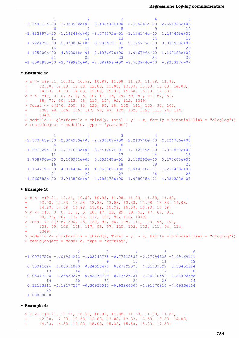
Regressione Log-log complementare
1 2 3 4 5-3.344811e+00 -3.928580e+00 -3.195443e+00 -2.625263e+00 -2.501326e+00
6 7 8 9 10-1.632697e+00 -1.183466e+00 -3.479272e-01 -1.146176e+00 1.287445e+00
11 12 13 14 151.722479e+00 2.078066e+00 5.293632e-01 2.125777e+00 3.393960e+00
16 17 18 19 201.175000e+00 4.892018e-01 2.127667e+00 1.046796e+00 -1.190182e+00
21 22 23 24 25-1.608195e+00 -2.739982e+00 -2.588698e+00 -3.552944e+00 6.825317e-07
• Example 2:
> x <- c(9.21, 10.21, 10.58, 10.83, 11.08, 11.33, 11.58, 11.83,+ 12.08, 12.33, 12.58, 12.83, 13.08, 13.33, 13.58, 13.83, 14.08,+ 14.33, 14.58, 14.83, 15.08, 15.33, 15.58, 15.83, 17.58)> y <- c(0, 0, 0, 2, 2, 5, 10, 17, 16, 29, 39, 51, 47, 67, 81,+ 88, 79, 90, 113, 95, 117, 107, 92, 112, 1049)> Total <- c(376, 200, 93, 120, 90, 88, 105, 111, 100, 93, 100,+ 108, 99, 106, 105, 117, 98, 97, 120, 102, 122, 111, 94, 114,+ 1049)> modello <- glm(formula = cbind(y, Total - y) ~ x, family = binomial(link = "cloglog"))> resid(object = modello, type = "pearson")
1 2 3 4 5-2.373963e+00 -2.804939e+00 -2.290887e+00 -2.213700e+00 -2.126766e+00
6 7 8 9 10-1.501829e+00 -1.131643e+00 -3.444267e-01 -1.112389e+00 1.317832e+00
11 12 13 14 151.758796e+00 2.106981e+00 5.302147e-01 2.109393e+00 3.270668e+00
16 17 18 19 201.154719e+00 4.834456e-01 1.953903e+00 9.944108e-01 -1.290438e+00
21 22 23 24 25-1.866683e+00 -3.983806e+00 -4.783173e+00 -1.098075e+01 4.826228e-07
• Example 3:
> x <- c(9.21, 10.21, 10.58, 10.83, 11.08, 11.33, 11.58, 11.83,+ 12.08, 12.33, 12.58, 12.83, 13.08, 13.33, 13.58, 13.83, 14.08,+ 14.33, 14.58, 14.83, 15.08, 15.33, 15.58, 15.83, 17.58)> y <- c(0, 0, 0, 2, 2, 5, 10, 17, 16, 29, 39, 51, 47, 67, 81,+ 88, 79, 90, 113, 95, 117, 107, 92, 112, 1049)> Total <- c(376, 200, 93, 120, 90, 88, 105, 111, 100, 93, 100,+ 108, 99, 106, 105, 117, 98, 97, 120, 102, 122, 111, 94, 114,+ 1049)> modello <- glm(formula = cbind(y, Total - y) ~ x, family = binomial(link = "cloglog"))> resid(object = modello, type = "working")
1 2 3 4 5 6-1.00747570 -1.01954272 -1.02795778 -0.77915832 -0.77094233 -0.49169111
7 8 9 10 11 12-0.30341626 -0.08051823 -0.24628470 0.27292979 0.31833027 0.33451224
13 14 15 16 17 180.08077108 0.28820279 0.42232719 0.13526781 0.06070359 0.24992698
19 20 21 22 23 240.12113911 -0.19177587 -0.30930043 -0.93966307 -1.91670214 -7.49366104
251.00000000
• Example 4:
> x <- c(9.21, 10.21, 10.58, 10.83, 11.08, 11.33, 11.58, 11.83,+ 12.08, 12.33, 12.58, 12.83, 13.08, 13.33, 13.58, 13.83, 14.08,+ 14.33, 14.58, 14.83, 15.08, 15.33, 15.58, 15.83, 17.58)
784
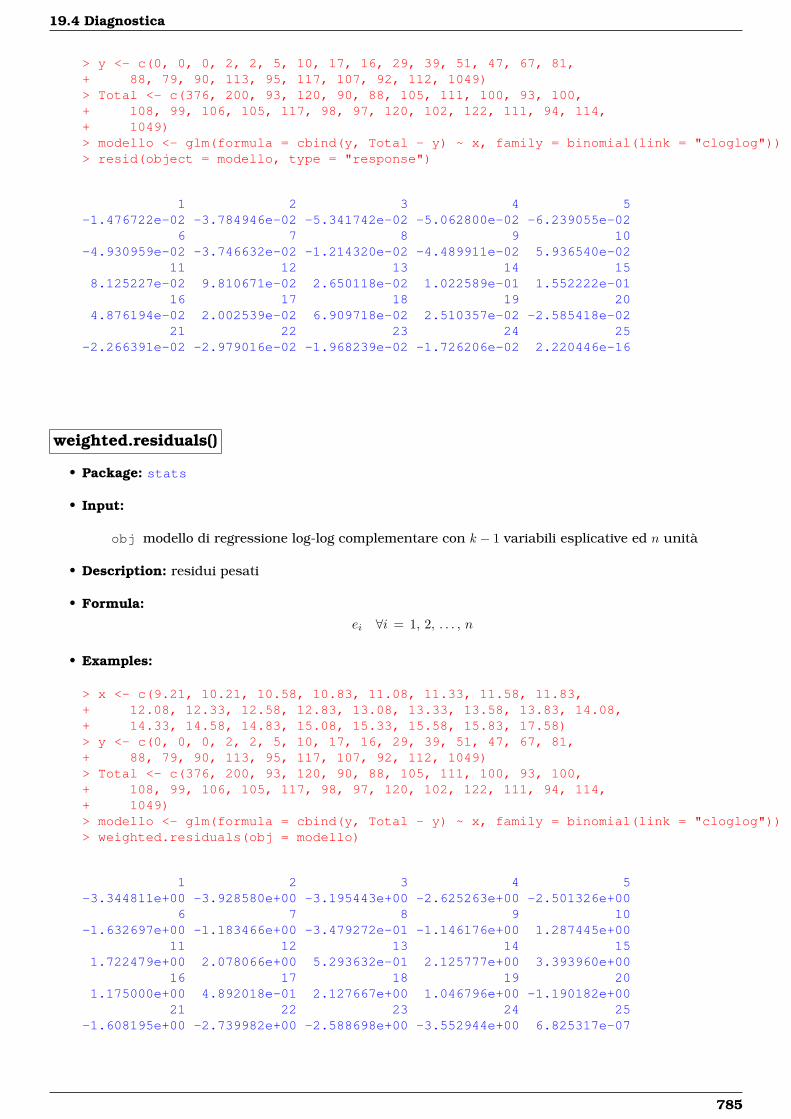
19.4 Diagnostica
> y <- c(0, 0, 0, 2, 2, 5, 10, 17, 16, 29, 39, 51, 47, 67, 81,+ 88, 79, 90, 113, 95, 117, 107, 92, 112, 1049)> Total <- c(376, 200, 93, 120, 90, 88, 105, 111, 100, 93, 100,+ 108, 99, 106, 105, 117, 98, 97, 120, 102, 122, 111, 94, 114,+ 1049)> modello <- glm(formula = cbind(y, Total - y) ~ x, family = binomial(link = "cloglog"))> resid(object = modello, type = "response")
1 2 3 4 5-1.476722e-02 -3.784946e-02 -5.341742e-02 -5.062800e-02 -6.239055e-02
6 7 8 9 10-4.930959e-02 -3.746632e-02 -1.214320e-02 -4.489911e-02 5.936540e-02
11 12 13 14 158.125227e-02 9.810671e-02 2.650118e-02 1.022589e-01 1.552222e-01
16 17 18 19 204.876194e-02 2.002539e-02 6.909718e-02 2.510357e-02 -2.585418e-02
21 22 23 24 25-2.266391e-02 -2.979016e-02 -1.968239e-02 -1.726206e-02 2.220446e-16
weighted.residuals()
• Package: stats
• Input:
obj modello di regressione log-log complementare con k − 1 variabili esplicative ed n unità
• Description: residui pesati
• Formula:
ei ∀i = 1, 2, . . . , n
• Examples:
> x <- c(9.21, 10.21, 10.58, 10.83, 11.08, 11.33, 11.58, 11.83,+ 12.08, 12.33, 12.58, 12.83, 13.08, 13.33, 13.58, 13.83, 14.08,+ 14.33, 14.58, 14.83, 15.08, 15.33, 15.58, 15.83, 17.58)> y <- c(0, 0, 0, 2, 2, 5, 10, 17, 16, 29, 39, 51, 47, 67, 81,+ 88, 79, 90, 113, 95, 117, 107, 92, 112, 1049)> Total <- c(376, 200, 93, 120, 90, 88, 105, 111, 100, 93, 100,+ 108, 99, 106, 105, 117, 98, 97, 120, 102, 122, 111, 94, 114,+ 1049)> modello <- glm(formula = cbind(y, Total - y) ~ x, family = binomial(link = "cloglog"))> weighted.residuals(obj = modello)
1 2 3 4 5-3.344811e+00 -3.928580e+00 -3.195443e+00 -2.625263e+00 -2.501326e+00
6 7 8 9 10-1.632697e+00 -1.183466e+00 -3.479272e-01 -1.146176e+00 1.287445e+00
11 12 13 14 151.722479e+00 2.078066e+00 5.293632e-01 2.125777e+00 3.393960e+00
16 17 18 19 201.175000e+00 4.892018e-01 2.127667e+00 1.046796e+00 -1.190182e+00
21 22 23 24 25-1.608195e+00 -2.739982e+00 -2.588698e+00 -3.552944e+00 6.825317e-07
785
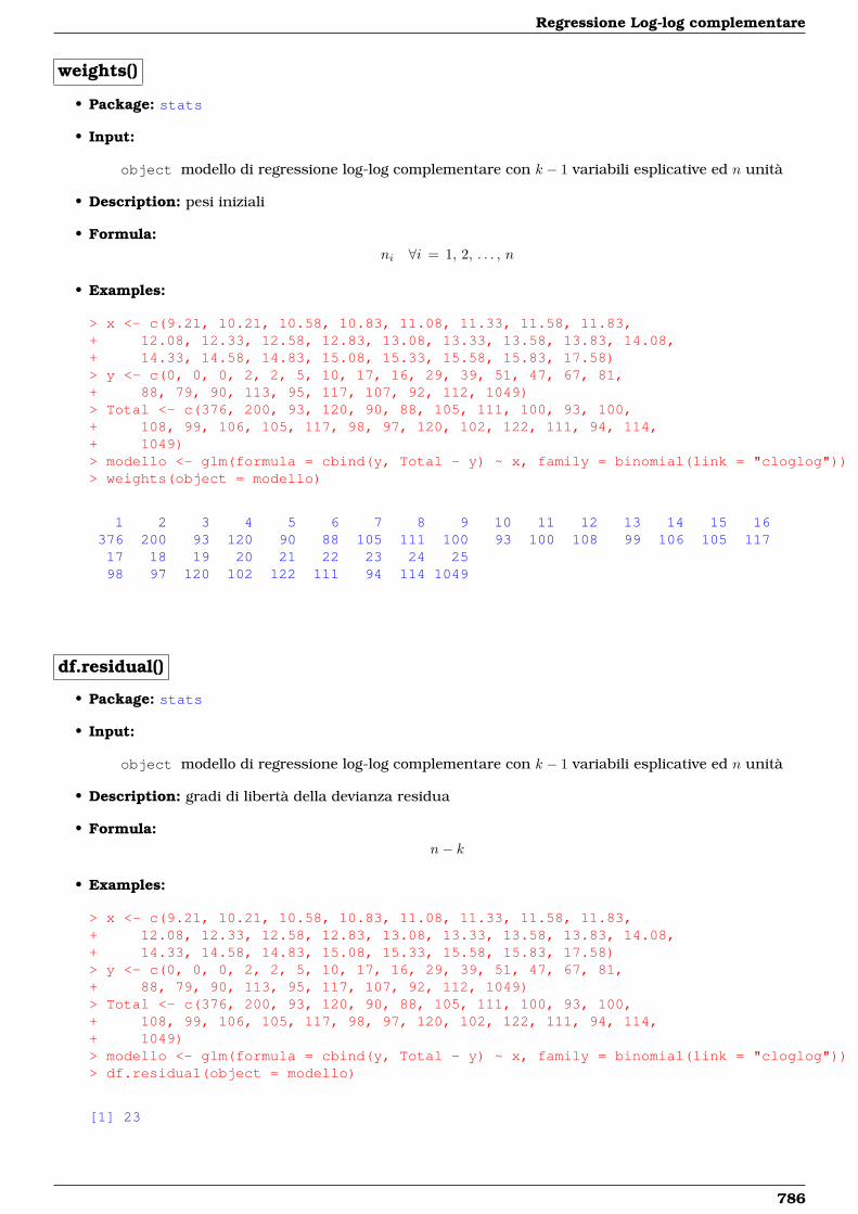
Regressione Log-log complementare
weights()
• Package: stats
• Input:
object modello di regressione log-log complementare con k − 1 variabili esplicative ed n unità
• Description: pesi iniziali
• Formula:ni ∀i = 1, 2, . . . , n
• Examples:
> x <- c(9.21, 10.21, 10.58, 10.83, 11.08, 11.33, 11.58, 11.83,+ 12.08, 12.33, 12.58, 12.83, 13.08, 13.33, 13.58, 13.83, 14.08,+ 14.33, 14.58, 14.83, 15.08, 15.33, 15.58, 15.83, 17.58)> y <- c(0, 0, 0, 2, 2, 5, 10, 17, 16, 29, 39, 51, 47, 67, 81,+ 88, 79, 90, 113, 95, 117, 107, 92, 112, 1049)> Total <- c(376, 200, 93, 120, 90, 88, 105, 111, 100, 93, 100,+ 108, 99, 106, 105, 117, 98, 97, 120, 102, 122, 111, 94, 114,+ 1049)> modello <- glm(formula = cbind(y, Total - y) ~ x, family = binomial(link = "cloglog"))> weights(object = modello)
1 2 3 4 5 6 7 8 9 10 11 12 13 14 15 16376 200 93 120 90 88 105 111 100 93 100 108 99 106 105 11717 18 19 20 21 22 23 24 2598 97 120 102 122 111 94 114 1049
df.residual()
• Package: stats
• Input:
object modello di regressione log-log complementare con k − 1 variabili esplicative ed n unità
• Description: gradi di libertà della devianza residua
• Formula:n− k
• Examples:
> x <- c(9.21, 10.21, 10.58, 10.83, 11.08, 11.33, 11.58, 11.83,+ 12.08, 12.33, 12.58, 12.83, 13.08, 13.33, 13.58, 13.83, 14.08,+ 14.33, 14.58, 14.83, 15.08, 15.33, 15.58, 15.83, 17.58)> y <- c(0, 0, 0, 2, 2, 5, 10, 17, 16, 29, 39, 51, 47, 67, 81,+ 88, 79, 90, 113, 95, 117, 107, 92, 112, 1049)> Total <- c(376, 200, 93, 120, 90, 88, 105, 111, 100, 93, 100,+ 108, 99, 106, 105, 117, 98, 97, 120, 102, 122, 111, 94, 114,+ 1049)> modello <- glm(formula = cbind(y, Total - y) ~ x, family = binomial(link = "cloglog"))> df.residual(object = modello)
[1] 23
786
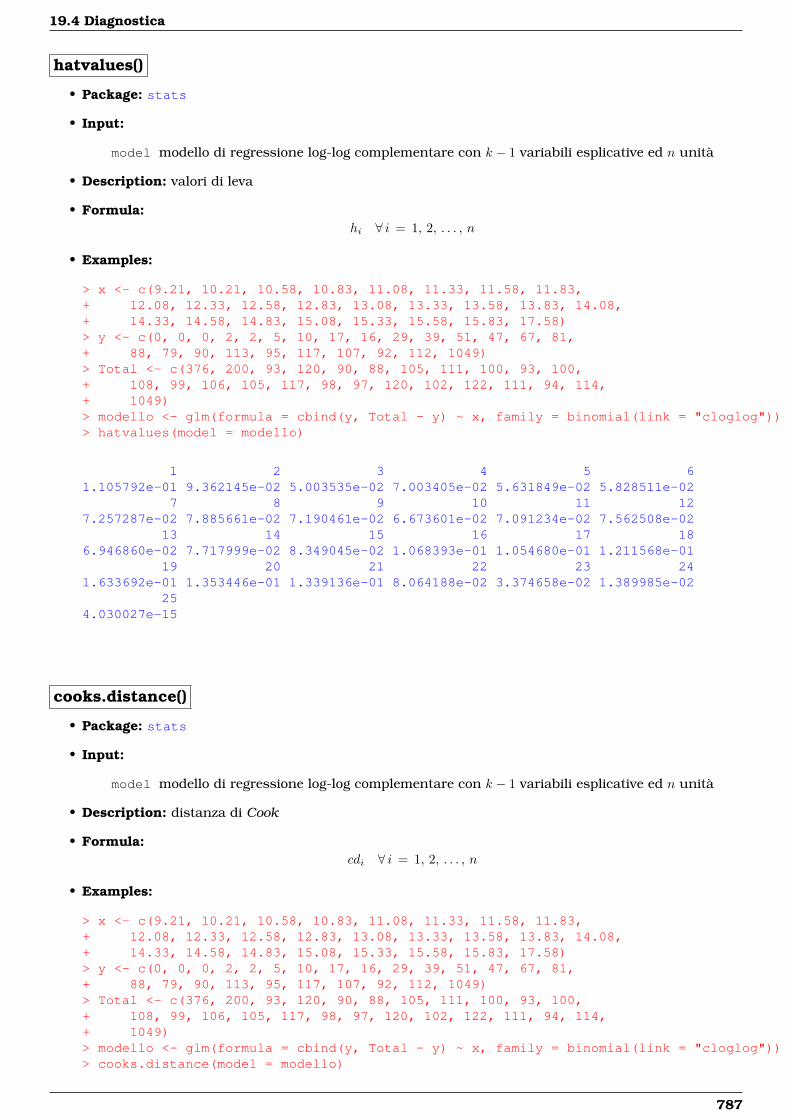
19.4 Diagnostica
hatvalues()
• Package: stats
• Input:
model modello di regressione log-log complementare con k − 1 variabili esplicative ed n unità
• Description: valori di leva
• Formula:hi ∀ i = 1, 2, . . . , n
• Examples:
> x <- c(9.21, 10.21, 10.58, 10.83, 11.08, 11.33, 11.58, 11.83,+ 12.08, 12.33, 12.58, 12.83, 13.08, 13.33, 13.58, 13.83, 14.08,+ 14.33, 14.58, 14.83, 15.08, 15.33, 15.58, 15.83, 17.58)> y <- c(0, 0, 0, 2, 2, 5, 10, 17, 16, 29, 39, 51, 47, 67, 81,+ 88, 79, 90, 113, 95, 117, 107, 92, 112, 1049)> Total <- c(376, 200, 93, 120, 90, 88, 105, 111, 100, 93, 100,+ 108, 99, 106, 105, 117, 98, 97, 120, 102, 122, 111, 94, 114,+ 1049)> modello <- glm(formula = cbind(y, Total - y) ~ x, family = binomial(link = "cloglog"))> hatvalues(model = modello)
1 2 3 4 5 61.105792e-01 9.362145e-02 5.003535e-02 7.003405e-02 5.631849e-02 5.828511e-02
7 8 9 10 11 127.257287e-02 7.885661e-02 7.190461e-02 6.673601e-02 7.091234e-02 7.562508e-02
13 14 15 16 17 186.946860e-02 7.717999e-02 8.349045e-02 1.068393e-01 1.054680e-01 1.211568e-01
19 20 21 22 23 241.633692e-01 1.353446e-01 1.339136e-01 8.064188e-02 3.374658e-02 1.389985e-02
254.030027e-15
cooks.distance()
• Package: stats
• Input:
model modello di regressione log-log complementare con k − 1 variabili esplicative ed n unità
• Description: distanza di Cook
• Formula:cdi ∀ i = 1, 2, . . . , n
• Examples:
> x <- c(9.21, 10.21, 10.58, 10.83, 11.08, 11.33, 11.58, 11.83,+ 12.08, 12.33, 12.58, 12.83, 13.08, 13.33, 13.58, 13.83, 14.08,+ 14.33, 14.58, 14.83, 15.08, 15.33, 15.58, 15.83, 17.58)> y <- c(0, 0, 0, 2, 2, 5, 10, 17, 16, 29, 39, 51, 47, 67, 81,+ 88, 79, 90, 113, 95, 117, 107, 92, 112, 1049)> Total <- c(376, 200, 93, 120, 90, 88, 105, 111, 100, 93, 100,+ 108, 99, 106, 105, 117, 98, 97, 120, 102, 122, 111, 94, 114,+ 1049)> modello <- glm(formula = cbind(y, Total - y) ~ x, family = binomial(link = "cloglog"))> cooks.distance(model = modello)
787
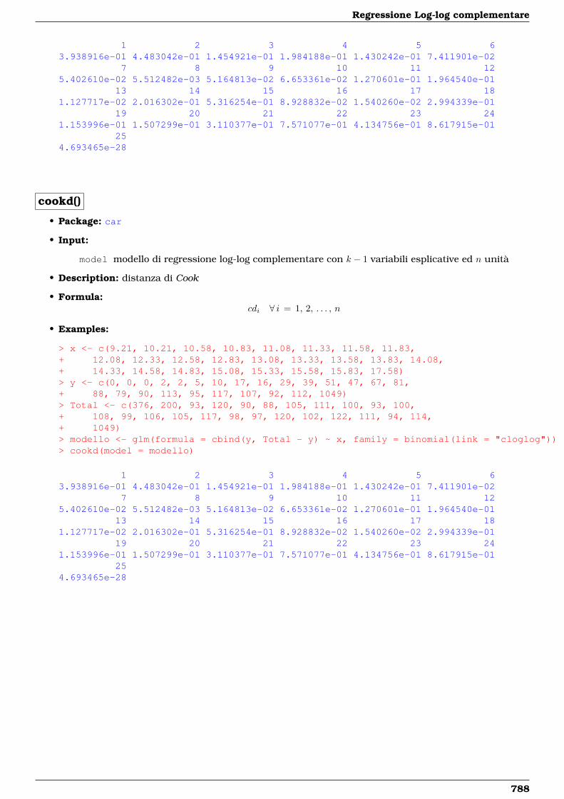
Regressione Log-log complementare
1 2 3 4 5 63.938916e-01 4.483042e-01 1.454921e-01 1.984188e-01 1.430242e-01 7.411901e-02
7 8 9 10 11 125.402610e-02 5.512482e-03 5.164813e-02 6.653361e-02 1.270601e-01 1.964540e-01
13 14 15 16 17 181.127717e-02 2.016302e-01 5.316254e-01 8.928832e-02 1.540260e-02 2.994339e-01
19 20 21 22 23 241.153996e-01 1.507299e-01 3.110377e-01 7.571077e-01 4.134756e-01 8.617915e-01
254.693465e-28
cookd()
• Package: car
• Input:
model modello di regressione log-log complementare con k − 1 variabili esplicative ed n unità
• Description: distanza di Cook
• Formula:cdi ∀ i = 1, 2, . . . , n
• Examples:
> x <- c(9.21, 10.21, 10.58, 10.83, 11.08, 11.33, 11.58, 11.83,+ 12.08, 12.33, 12.58, 12.83, 13.08, 13.33, 13.58, 13.83, 14.08,+ 14.33, 14.58, 14.83, 15.08, 15.33, 15.58, 15.83, 17.58)> y <- c(0, 0, 0, 2, 2, 5, 10, 17, 16, 29, 39, 51, 47, 67, 81,+ 88, 79, 90, 113, 95, 117, 107, 92, 112, 1049)> Total <- c(376, 200, 93, 120, 90, 88, 105, 111, 100, 93, 100,+ 108, 99, 106, 105, 117, 98, 97, 120, 102, 122, 111, 94, 114,+ 1049)> modello <- glm(formula = cbind(y, Total - y) ~ x, family = binomial(link = "cloglog"))> cookd(model = modello)
1 2 3 4 5 63.938916e-01 4.483042e-01 1.454921e-01 1.984188e-01 1.430242e-01 7.411901e-02
7 8 9 10 11 125.402610e-02 5.512482e-03 5.164813e-02 6.653361e-02 1.270601e-01 1.964540e-01
13 14 15 16 17 181.127717e-02 2.016302e-01 5.316254e-01 8.928832e-02 1.540260e-02 2.994339e-01
19 20 21 22 23 241.153996e-01 1.507299e-01 3.110377e-01 7.571077e-01 4.134756e-01 8.617915e-01
254.693465e-28
788
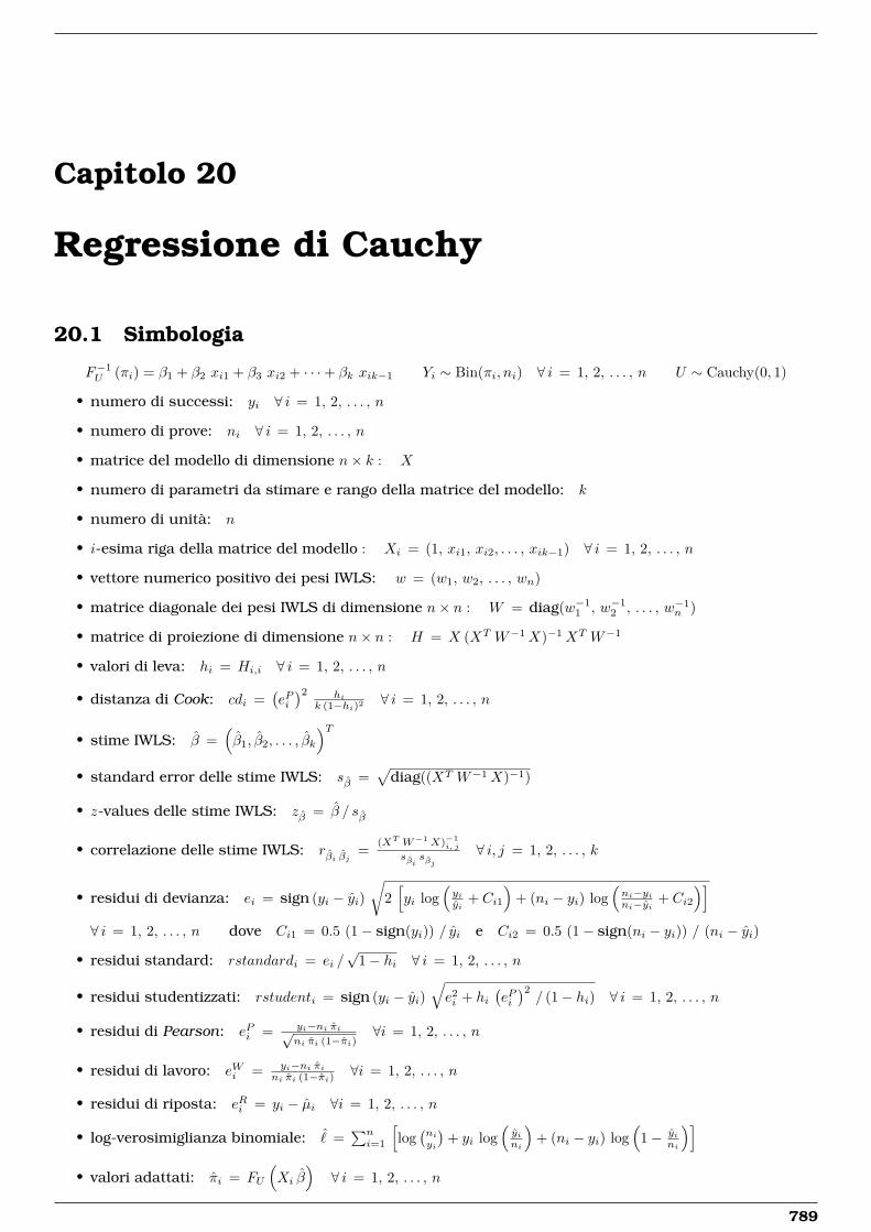
Capitolo 20
Regressione di Cauchy
20.1 Simbologia
F−1U (πi) = β1 + β2 xi1 + β3 xi2 + · · ·+ βk xik−1 Yi ∼ Bin(πi, ni) ∀ i = 1, 2, . . . , n U ∼ Cauchy(0, 1)
• numero di successi: yi ∀ i = 1, 2, . . . , n
• numero di prove: ni ∀ i = 1, 2, . . . , n
• matrice del modello di dimensione n× k : X
• numero di parametri da stimare e rango della matrice del modello: k
• numero di unità: n
• i-esima riga della matrice del modello : Xi = (1, xi1, xi2, . . . , xik−1) ∀ i = 1, 2, . . . , n
• vettore numerico positivo dei pesi IWLS: w = (w1, w2, . . . , wn)
• matrice diagonale dei pesi IWLS di dimensione n× n : W = diag(w−11 , w−1
2 , . . . , w−1n )
• matrice di proiezione di dimensione n× n : H = X (XT W−1X)−1XT W−1
• valori di leva: hi = Hi,i ∀ i = 1, 2, . . . , n
• distanza di Cook: cdi =(ePi)2 hi
k (1−hi)2 ∀ i = 1, 2, . . . , n
• stime IWLS: β =(β1, β2, . . . , βk
)T• standard error delle stime IWLS: sβ =
√diag((XT W−1X)−1)
• z-values delle stime IWLS: zβ = β / sβ
• correlazione delle stime IWLS: rβi βj =(XT W−1X)−1
i, j
sβisβj
∀ i, j = 1, 2, . . . , k
• residui di devianza: ei = sign (yi − yi)√
2[yi log
(yiyi
+ Ci1
)+ (ni − yi) log
(ni−yini−yi + Ci2
)]∀ i = 1, 2, . . . , n dove Ci1 = 0.5 (1− sign(yi)) / yi e Ci2 = 0.5 (1− sign(ni − yi)) / (ni − yi)
• residui standard: rstandardi = ei /√
1− hi ∀ i = 1, 2, . . . , n
• residui studentizzati: rstudenti = sign (yi − yi)√e2i + hi
(ePi)2/ (1− hi) ∀ i = 1, 2, . . . , n
• residui di Pearson: ePi = yi−ni πi√ni πi (1−πi)
∀i = 1, 2, . . . , n
• residui di lavoro: eWi = yi−ni πini πi (1−πi) ∀i = 1, 2, . . . , n
• residui di riposta: eRi = yi − µi ∀i = 1, 2, . . . , n
• log-verosimiglianza binomiale: ˆ =∑ni=1
[log(niyi
)+ yi log
(yini
)+ (ni − yi) log
(1− yi
ni
)]• valori adattati: πi = FU
(Xi β
)∀ i = 1, 2, . . . , n
789
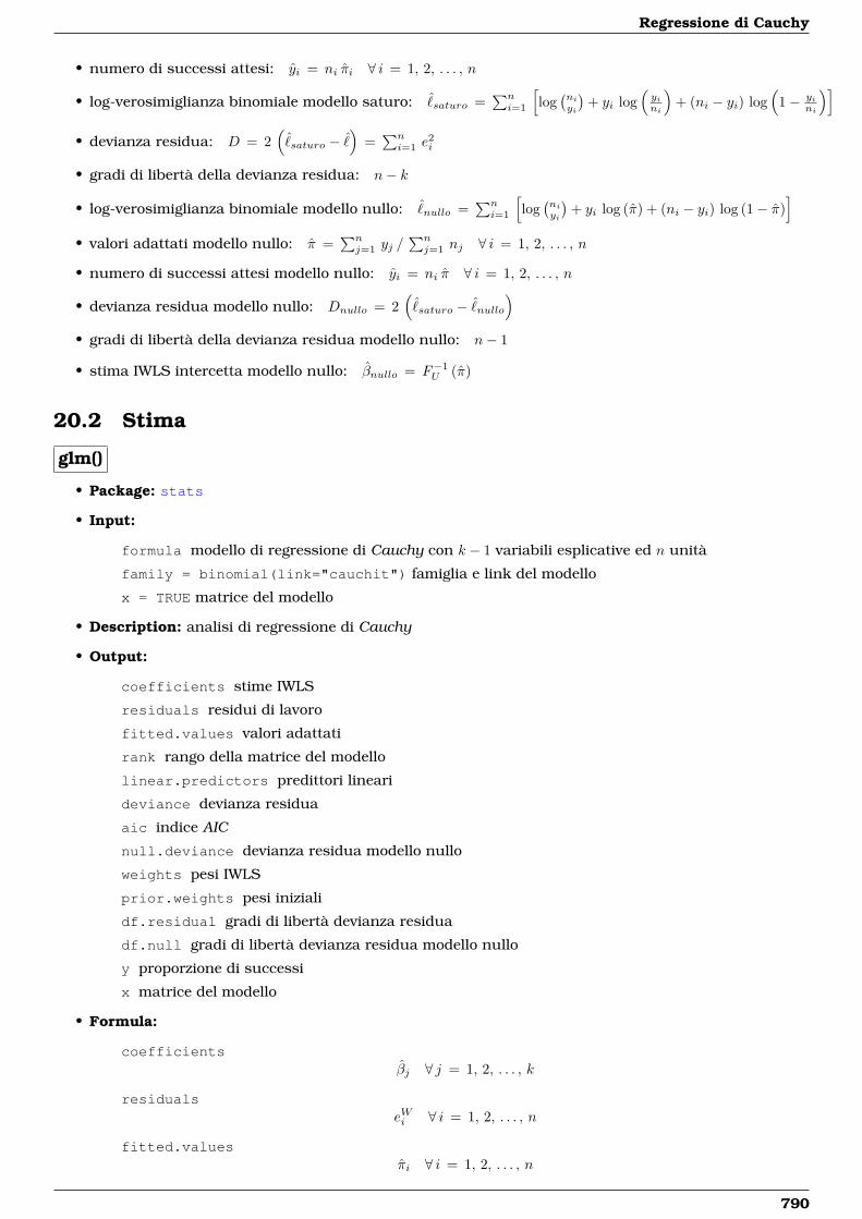
Regressione di Cauchy
• numero di successi attesi: yi = ni πi ∀ i = 1, 2, . . . , n
• log-verosimiglianza binomiale modello saturo: ˆsaturo =
∑ni=1
[log(niyi
)+ yi log
(yini
)+ (ni − yi) log
(1− yi
ni
)]• devianza residua: D = 2
(ˆsaturo − ˆ
)=∑ni=1 e
2i
• gradi di libertà della devianza residua: n− k
• log-verosimiglianza binomiale modello nullo: ˆnullo =
∑ni=1
[log(niyi
)+ yi log (π) + (ni − yi) log (1− π)
]• valori adattati modello nullo: π =
∑nj=1 yj /
∑nj=1 nj ∀ i = 1, 2, . . . , n
• numero di successi attesi modello nullo: yi = ni π ∀ i = 1, 2, . . . , n
• devianza residua modello nullo: Dnullo = 2(
ˆsaturo − ˆ
nullo
)• gradi di libertà della devianza residua modello nullo: n− 1
• stima IWLS intercetta modello nullo: βnullo = F−1U (π)
20.2 Stima
glm()
• Package: stats
• Input:
formula modello di regressione di Cauchy con k − 1 variabili esplicative ed n unità
family = binomial(link="cauchit") famiglia e link del modello
x = TRUE matrice del modello
• Description: analisi di regressione di Cauchy
• Output:
coefficients stime IWLS
residuals residui di lavoro
fitted.values valori adattati
rank rango della matrice del modello
linear.predictors predittori lineari
deviance devianza residua
aic indice AIC
null.deviance devianza residua modello nullo
weights pesi IWLS
prior.weights pesi iniziali
df.residual gradi di libertà devianza residua
df.null gradi di libertà devianza residua modello nullo
y proporzione di successi
x matrice del modello
• Formula:
coefficientsβj ∀ j = 1, 2, . . . , k
residualseWi ∀ i = 1, 2, . . . , n
fitted.valuesπi ∀ i = 1, 2, . . . , n
790
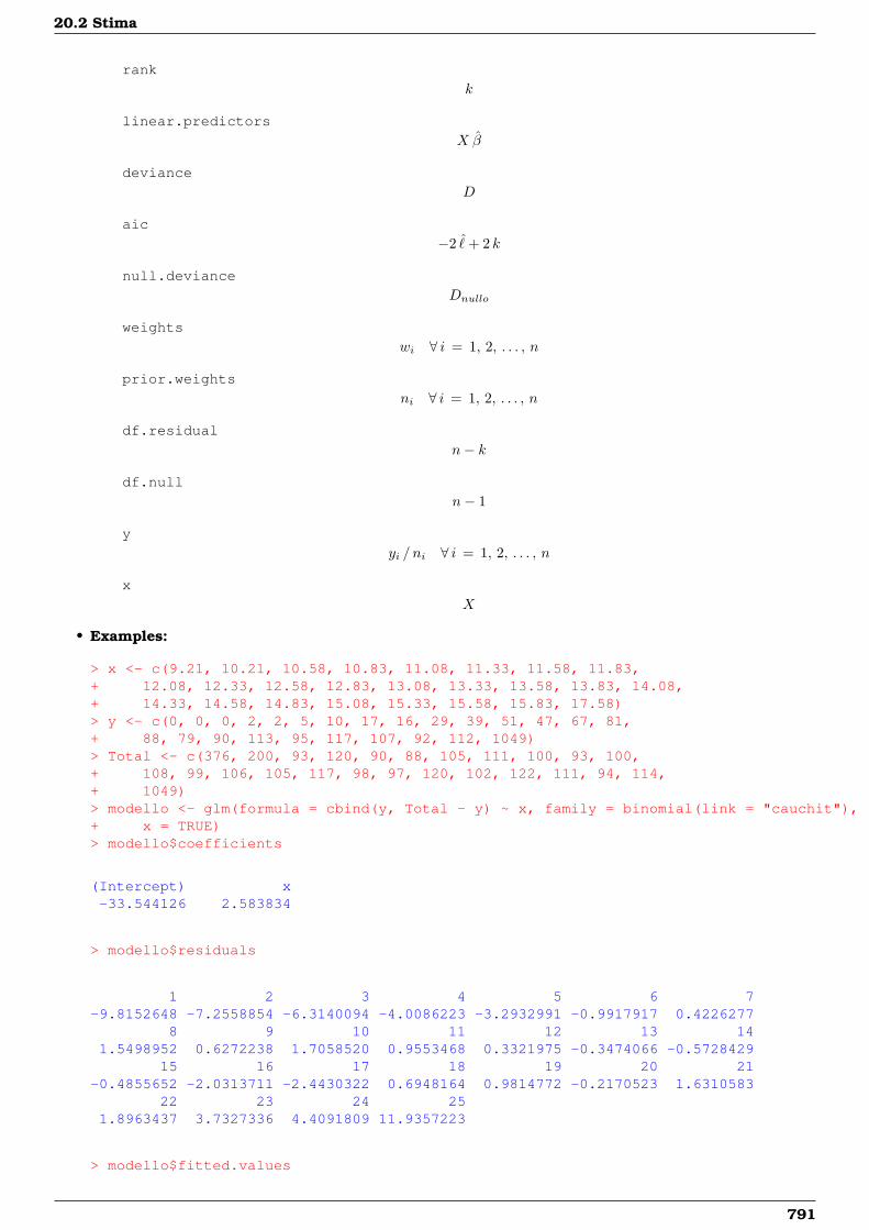
20.2 Stima
rank
k
linear.predictors
X β
deviance
D
aic
−2 ˆ+ 2 k
null.deviance
Dnullo
weights
wi ∀ i = 1, 2, . . . , n
prior.weights
ni ∀ i = 1, 2, . . . , n
df.residual
n− k
df.null
n− 1
y
yi / ni ∀ i = 1, 2, . . . , n
x
X
• Examples:
> x <- c(9.21, 10.21, 10.58, 10.83, 11.08, 11.33, 11.58, 11.83,+ 12.08, 12.33, 12.58, 12.83, 13.08, 13.33, 13.58, 13.83, 14.08,+ 14.33, 14.58, 14.83, 15.08, 15.33, 15.58, 15.83, 17.58)> y <- c(0, 0, 0, 2, 2, 5, 10, 17, 16, 29, 39, 51, 47, 67, 81,+ 88, 79, 90, 113, 95, 117, 107, 92, 112, 1049)> Total <- c(376, 200, 93, 120, 90, 88, 105, 111, 100, 93, 100,+ 108, 99, 106, 105, 117, 98, 97, 120, 102, 122, 111, 94, 114,+ 1049)> modello <- glm(formula = cbind(y, Total - y) ~ x, family = binomial(link = "cauchit"),+ x = TRUE)> modello$coefficients
(Intercept) x-33.544126 2.583834
> modello$residuals
1 2 3 4 5 6 7-9.8152648 -7.2558854 -6.3140094 -4.0086223 -3.2932991 -0.9917917 0.4226277
8 9 10 11 12 13 141.5498952 0.6272238 1.7058520 0.9553468 0.3321975 -0.3474066 -0.5728429
15 16 17 18 19 20 21-0.4855652 -2.0313711 -2.4430322 0.6948164 0.9814772 -0.2170523 1.6310583
22 23 24 251.8963437 3.7327336 4.4091809 11.9357223
> modello$fitted.values
791
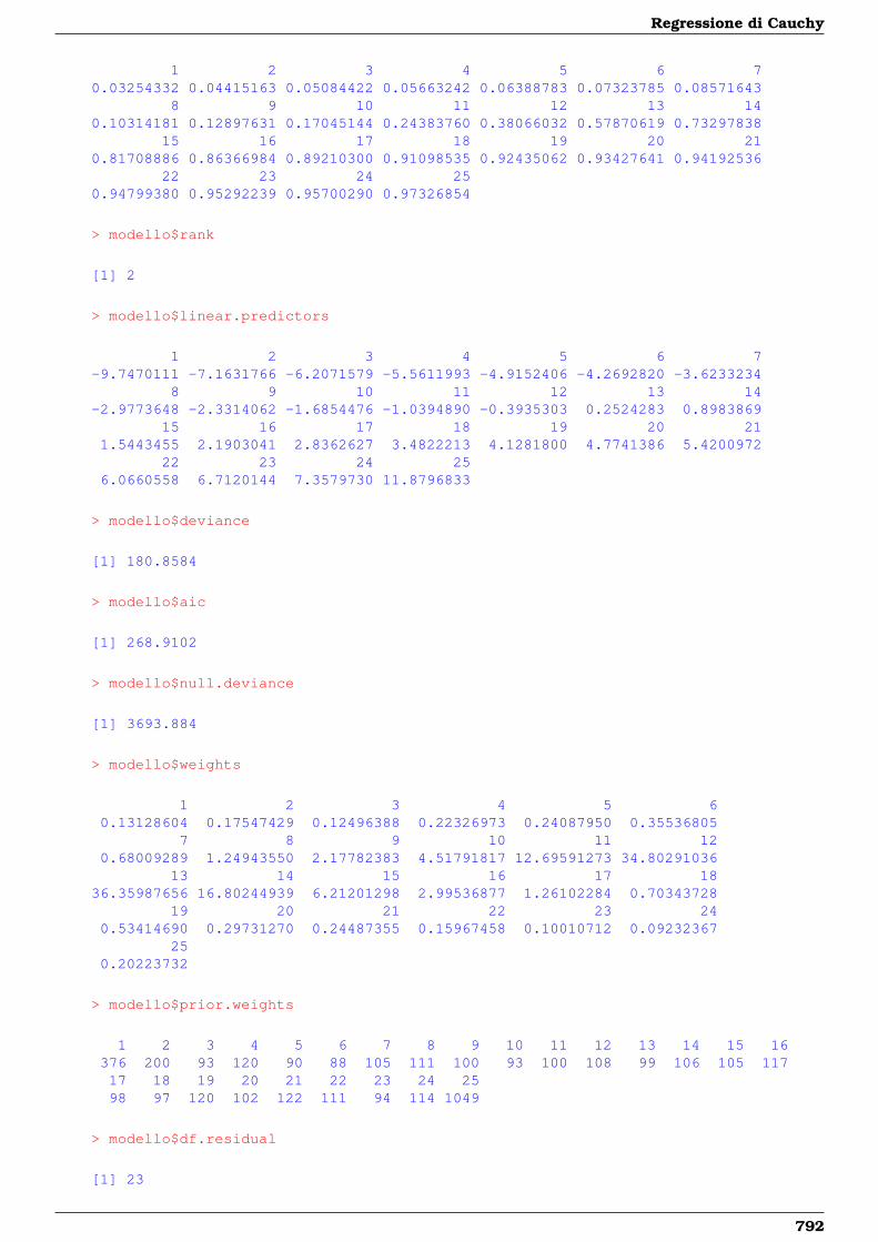
Regressione di Cauchy
1 2 3 4 5 6 70.03254332 0.04415163 0.05084422 0.05663242 0.06388783 0.07323785 0.08571643
8 9 10 11 12 13 140.10314181 0.12897631 0.17045144 0.24383760 0.38066032 0.57870619 0.73297838
15 16 17 18 19 20 210.81708886 0.86366984 0.89210300 0.91098535 0.92435062 0.93427641 0.94192536
22 23 24 250.94799380 0.95292239 0.95700290 0.97326854
> modello$rank
[1] 2
> modello$linear.predictors
1 2 3 4 5 6 7-9.7470111 -7.1631766 -6.2071579 -5.5611993 -4.9152406 -4.2692820 -3.6233234
8 9 10 11 12 13 14-2.9773648 -2.3314062 -1.6854476 -1.0394890 -0.3935303 0.2524283 0.8983869
15 16 17 18 19 20 211.5443455 2.1903041 2.8362627 3.4822213 4.1281800 4.7741386 5.4200972
22 23 24 256.0660558 6.7120144 7.3579730 11.8796833
> modello$deviance
[1] 180.8584
> modello$aic
[1] 268.9102
> modello$null.deviance
[1] 3693.884
> modello$weights
1 2 3 4 5 60.13128604 0.17547429 0.12496388 0.22326973 0.24087950 0.35536805
7 8 9 10 11 120.68009289 1.24943550 2.17782383 4.51791817 12.69591273 34.80291036
13 14 15 16 17 1836.35987656 16.80244939 6.21201298 2.99536877 1.26102284 0.70343728
19 20 21 22 23 240.53414690 0.29731270 0.24487355 0.15967458 0.10010712 0.09232367
250.20223732
> modello$prior.weights
1 2 3 4 5 6 7 8 9 10 11 12 13 14 15 16376 200 93 120 90 88 105 111 100 93 100 108 99 106 105 11717 18 19 20 21 22 23 24 2598 97 120 102 122 111 94 114 1049
> modello$df.residual
[1] 23
792

20.2 Stima
> modello$df.null
[1] 24
> modello$y
1 2 3 4 5 6 70.00000000 0.00000000 0.00000000 0.01666667 0.02222222 0.05681818 0.09523810
8 9 10 11 12 13 140.15315315 0.16000000 0.31182796 0.39000000 0.47222222 0.47474747 0.63207547
15 16 17 18 19 20 210.77142857 0.75213675 0.80612245 0.92783505 0.94166667 0.93137255 0.95901639
22 23 24 250.96396396 0.97872340 0.98245614 1.00000000
> modello$x
(Intercept) x1 1 9.212 1 10.213 1 10.584 1 10.835 1 11.086 1 11.337 1 11.588 1 11.839 1 12.0810 1 12.3311 1 12.5812 1 12.8313 1 13.0814 1 13.3315 1 13.5816 1 13.8317 1 14.0818 1 14.3319 1 14.5820 1 14.8321 1 15.0822 1 15.3323 1 15.5824 1 15.8325 1 17.58attr(,"assign")[1] 0 1
summary.glm()
• Package: stats
• Input:
object modello di regressione di Cauchy con k − 1 variabili esplicative ed n unità
correlation = TRUE correlazione delle stime IWLS
• Description: analisi di regressione di Cauchy
• Output:
deviance devianza residua
aic indice AIC
793
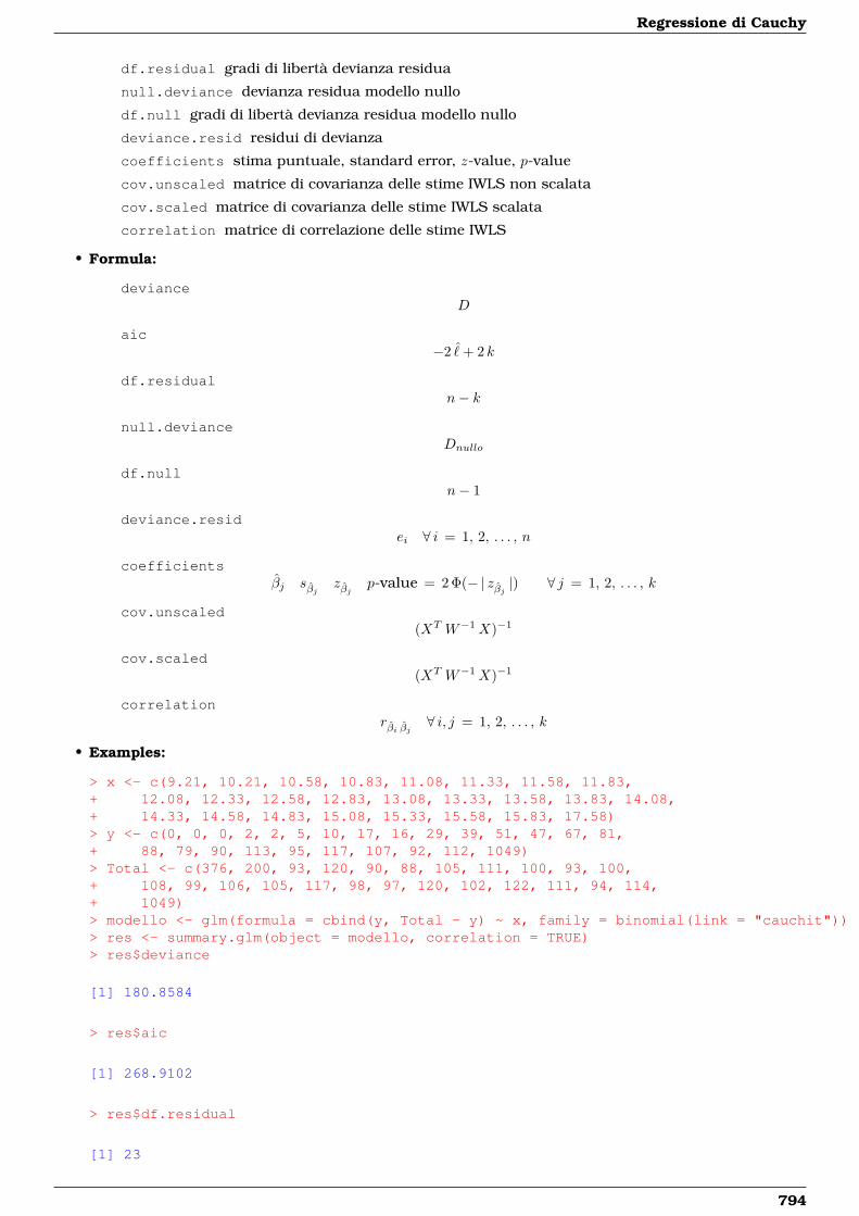
Regressione di Cauchy
df.residual gradi di libertà devianza residua
null.deviance devianza residua modello nullo
df.null gradi di libertà devianza residua modello nullo
deviance.resid residui di devianza
coefficients stima puntuale, standard error, z-value, p-value
cov.unscaled matrice di covarianza delle stime IWLS non scalata
cov.scaled matrice di covarianza delle stime IWLS scalata
correlation matrice di correlazione delle stime IWLS
• Formula:
devianceD
aic−2 ˆ+ 2 k
df.residualn− k
null.devianceDnullo
df.nulln− 1
deviance.residei ∀ i = 1, 2, . . . , n
coefficientsβj sβj zβj p-value = 2 Φ(− | zβj |) ∀ j = 1, 2, . . . , k
cov.unscaled(XT W−1X)−1
cov.scaled(XT W−1X)−1
correlationrβi βj ∀ i, j = 1, 2, . . . , k
• Examples:
> x <- c(9.21, 10.21, 10.58, 10.83, 11.08, 11.33, 11.58, 11.83,+ 12.08, 12.33, 12.58, 12.83, 13.08, 13.33, 13.58, 13.83, 14.08,+ 14.33, 14.58, 14.83, 15.08, 15.33, 15.58, 15.83, 17.58)> y <- c(0, 0, 0, 2, 2, 5, 10, 17, 16, 29, 39, 51, 47, 67, 81,+ 88, 79, 90, 113, 95, 117, 107, 92, 112, 1049)> Total <- c(376, 200, 93, 120, 90, 88, 105, 111, 100, 93, 100,+ 108, 99, 106, 105, 117, 98, 97, 120, 102, 122, 111, 94, 114,+ 1049)> modello <- glm(formula = cbind(y, Total - y) ~ x, family = binomial(link = "cauchit"))> res <- summary.glm(object = modello, correlation = TRUE)> res$deviance
[1] 180.8584
> res$aic
[1] 268.9102
> res$df.residual
[1] 23
794
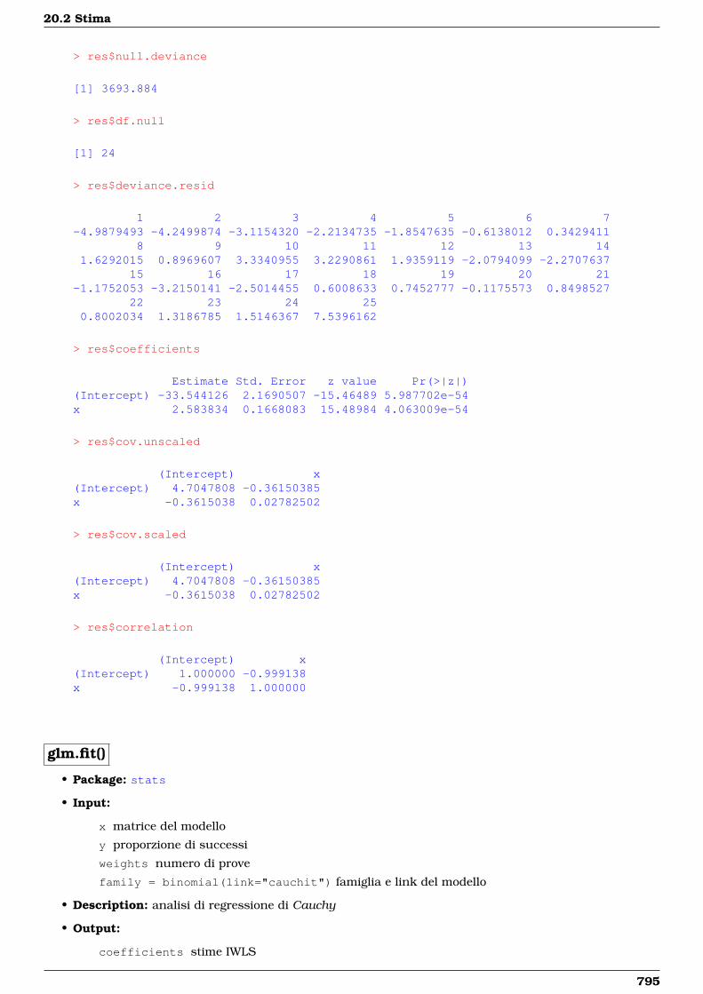
20.2 Stima
> res$null.deviance
[1] 3693.884
> res$df.null
[1] 24
> res$deviance.resid
1 2 3 4 5 6 7-4.9879493 -4.2499874 -3.1154320 -2.2134735 -1.8547635 -0.6138012 0.3429411
8 9 10 11 12 13 141.6292015 0.8969607 3.3340955 3.2290861 1.9359119 -2.0794099 -2.2707637
15 16 17 18 19 20 21-1.1752053 -3.2150141 -2.5014455 0.6008633 0.7452777 -0.1175573 0.8498527
22 23 24 250.8002034 1.3186785 1.5146367 7.5396162
> res$coefficients
Estimate Std. Error z value Pr(>|z|)(Intercept) -33.544126 2.1690507 -15.46489 5.987702e-54x 2.583834 0.1668083 15.48984 4.063009e-54
> res$cov.unscaled
(Intercept) x(Intercept) 4.7047808 -0.36150385x -0.3615038 0.02782502
> res$cov.scaled
(Intercept) x(Intercept) 4.7047808 -0.36150385x -0.3615038 0.02782502
> res$correlation
(Intercept) x(Intercept) 1.000000 -0.999138x -0.999138 1.000000
glm.fit()
• Package: stats
• Input:
x matrice del modello
y proporzione di successi
weights numero di prove
family = binomial(link="cauchit") famiglia e link del modello
• Description: analisi di regressione di Cauchy
• Output:
coefficients stime IWLS
795
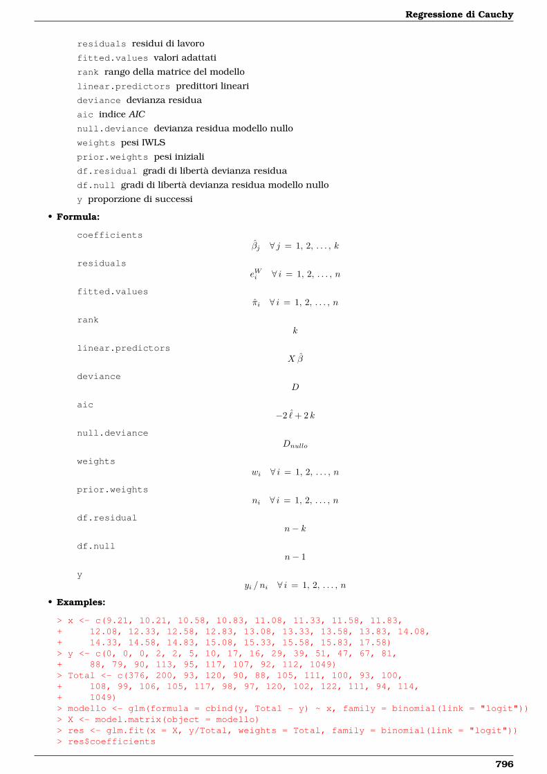
Regressione di Cauchy
residuals residui di lavoro
fitted.values valori adattati
rank rango della matrice del modello
linear.predictors predittori lineari
deviance devianza residua
aic indice AIC
null.deviance devianza residua modello nullo
weights pesi IWLS
prior.weights pesi iniziali
df.residual gradi di libertà devianza residua
df.null gradi di libertà devianza residua modello nullo
y proporzione di successi
• Formula:
coefficientsβj ∀ j = 1, 2, . . . , k
residualseWi ∀ i = 1, 2, . . . , n
fitted.valuesπi ∀ i = 1, 2, . . . , n
rankk
linear.predictorsX β
devianceD
aic−2 ˆ+ 2 k
null.devianceDnullo
weightswi ∀ i = 1, 2, . . . , n
prior.weightsni ∀ i = 1, 2, . . . , n
df.residualn− k
df.nulln− 1
yyi / ni ∀ i = 1, 2, . . . , n
• Examples:
> x <- c(9.21, 10.21, 10.58, 10.83, 11.08, 11.33, 11.58, 11.83,+ 12.08, 12.33, 12.58, 12.83, 13.08, 13.33, 13.58, 13.83, 14.08,+ 14.33, 14.58, 14.83, 15.08, 15.33, 15.58, 15.83, 17.58)> y <- c(0, 0, 0, 2, 2, 5, 10, 17, 16, 29, 39, 51, 47, 67, 81,+ 88, 79, 90, 113, 95, 117, 107, 92, 112, 1049)> Total <- c(376, 200, 93, 120, 90, 88, 105, 111, 100, 93, 100,+ 108, 99, 106, 105, 117, 98, 97, 120, 102, 122, 111, 94, 114,+ 1049)> modello <- glm(formula = cbind(y, Total - y) ~ x, family = binomial(link = "logit"))> X <- model.matrix(object = modello)> res <- glm.fit(x = X, y/Total, weights = Total, family = binomial(link = "logit"))> res$coefficients
796
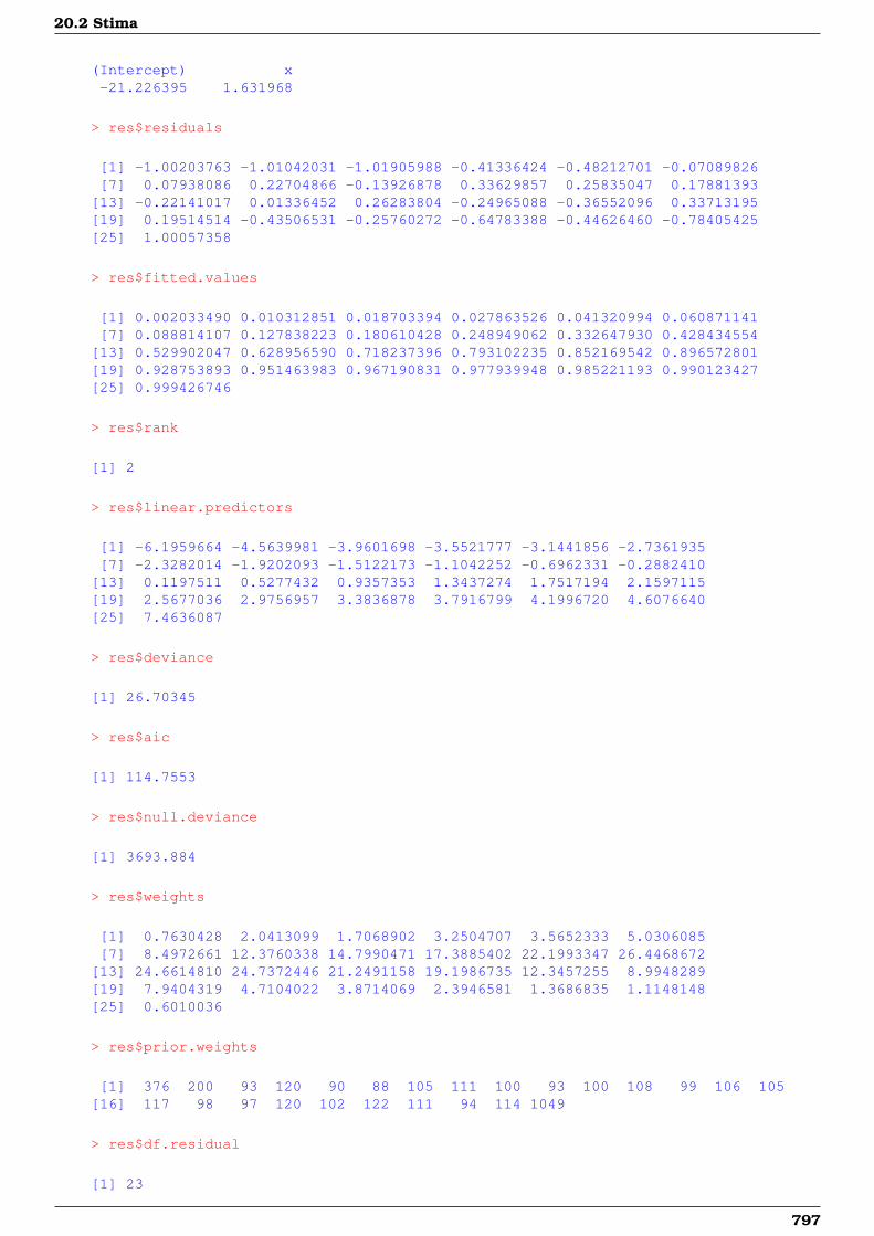
20.2 Stima
(Intercept) x-21.226395 1.631968
> res$residuals
[1] -1.00203763 -1.01042031 -1.01905988 -0.41336424 -0.48212701 -0.07089826[7] 0.07938086 0.22704866 -0.13926878 0.33629857 0.25835047 0.17881393
[13] -0.22141017 0.01336452 0.26283804 -0.24965088 -0.36552096 0.33713195[19] 0.19514514 -0.43506531 -0.25760272 -0.64783388 -0.44626460 -0.78405425[25] 1.00057358
> res$fitted.values
[1] 0.002033490 0.010312851 0.018703394 0.027863526 0.041320994 0.060871141[7] 0.088814107 0.127838223 0.180610428 0.248949062 0.332647930 0.428434554
[13] 0.529902047 0.628956590 0.718237396 0.793102235 0.852169542 0.896572801[19] 0.928753893 0.951463983 0.967190831 0.977939948 0.985221193 0.990123427[25] 0.999426746
> res$rank
[1] 2
> res$linear.predictors
[1] -6.1959664 -4.5639981 -3.9601698 -3.5521777 -3.1441856 -2.7361935[7] -2.3282014 -1.9202093 -1.5122173 -1.1042252 -0.6962331 -0.2882410
[13] 0.1197511 0.5277432 0.9357353 1.3437274 1.7517194 2.1597115[19] 2.5677036 2.9756957 3.3836878 3.7916799 4.1996720 4.6076640[25] 7.4636087
> res$deviance
[1] 26.70345
> res$aic
[1] 114.7553
> res$null.deviance
[1] 3693.884
> res$weights
[1] 0.7630428 2.0413099 1.7068902 3.2504707 3.5652333 5.0306085[7] 8.4972661 12.3760338 14.7990471 17.3885402 22.1993347 26.4468672
[13] 24.6614810 24.7372446 21.2491158 19.1986735 12.3457255 8.9948289[19] 7.9404319 4.7104022 3.8714069 2.3946581 1.3686835 1.1148148[25] 0.6010036
> res$prior.weights
[1] 376 200 93 120 90 88 105 111 100 93 100 108 99 106 105[16] 117 98 97 120 102 122 111 94 114 1049
> res$df.residual
[1] 23
797
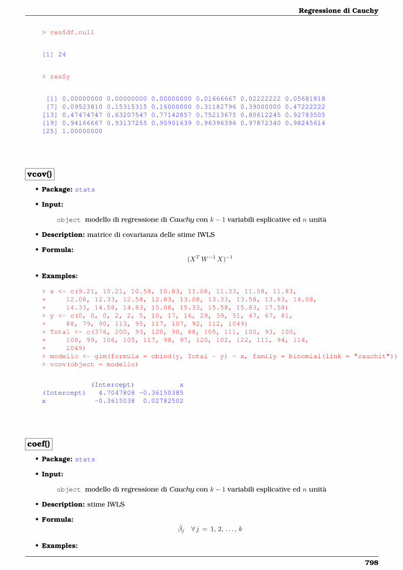
Regressione di Cauchy
> res$df.null
[1] 24
> res$y
[1] 0.00000000 0.00000000 0.00000000 0.01666667 0.02222222 0.05681818[7] 0.09523810 0.15315315 0.16000000 0.31182796 0.39000000 0.47222222
[13] 0.47474747 0.63207547 0.77142857 0.75213675 0.80612245 0.92783505[19] 0.94166667 0.93137255 0.95901639 0.96396396 0.97872340 0.98245614[25] 1.00000000
vcov()
• Package: stats
• Input:
object modello di regressione di Cauchy con k − 1 variabili esplicative ed n unità
• Description: matrice di covarianza delle stime IWLS
• Formula:(XT W−1X)−1
• Examples:
> x <- c(9.21, 10.21, 10.58, 10.83, 11.08, 11.33, 11.58, 11.83,+ 12.08, 12.33, 12.58, 12.83, 13.08, 13.33, 13.58, 13.83, 14.08,+ 14.33, 14.58, 14.83, 15.08, 15.33, 15.58, 15.83, 17.58)> y <- c(0, 0, 0, 2, 2, 5, 10, 17, 16, 29, 39, 51, 47, 67, 81,+ 88, 79, 90, 113, 95, 117, 107, 92, 112, 1049)> Total <- c(376, 200, 93, 120, 90, 88, 105, 111, 100, 93, 100,+ 108, 99, 106, 105, 117, 98, 97, 120, 102, 122, 111, 94, 114,+ 1049)> modello <- glm(formula = cbind(y, Total - y) ~ x, family = binomial(link = "cauchit"))> vcov(object = modello)
(Intercept) x(Intercept) 4.7047808 -0.36150385x -0.3615038 0.02782502
coef()
• Package: stats
• Input:
object modello di regressione di Cauchy con k − 1 variabili esplicative ed n unità
• Description: stime IWLS
• Formula:βj ∀ j = 1, 2, . . . , k
• Examples:
798

20.2 Stima
> x <- c(9.21, 10.21, 10.58, 10.83, 11.08, 11.33, 11.58, 11.83,+ 12.08, 12.33, 12.58, 12.83, 13.08, 13.33, 13.58, 13.83, 14.08,+ 14.33, 14.58, 14.83, 15.08, 15.33, 15.58, 15.83, 17.58)> y <- c(0, 0, 0, 2, 2, 5, 10, 17, 16, 29, 39, 51, 47, 67, 81,+ 88, 79, 90, 113, 95, 117, 107, 92, 112, 1049)> Total <- c(376, 200, 93, 120, 90, 88, 105, 111, 100, 93, 100,+ 108, 99, 106, 105, 117, 98, 97, 120, 102, 122, 111, 94, 114,+ 1049)> modello <- glm(formula = cbind(y, Total - y) ~ x, family = binomial(link = "cauchit"))> coef(object = modello)
(Intercept) x-33.544126 2.583834
coefficients()
• Package: stats
• Input:
object modello di regressione di Cauchy con k − 1 variabili esplicative ed n unità
• Description: stime IWLS
• Formula:βj ∀ j = 1, 2, . . . , k
• Examples:
> x <- c(9.21, 10.21, 10.58, 10.83, 11.08, 11.33, 11.58, 11.83,+ 12.08, 12.33, 12.58, 12.83, 13.08, 13.33, 13.58, 13.83, 14.08,+ 14.33, 14.58, 14.83, 15.08, 15.33, 15.58, 15.83, 17.58)> y <- c(0, 0, 0, 2, 2, 5, 10, 17, 16, 29, 39, 51, 47, 67, 81,+ 88, 79, 90, 113, 95, 117, 107, 92, 112, 1049)> Total <- c(376, 200, 93, 120, 90, 88, 105, 111, 100, 93, 100,+ 108, 99, 106, 105, 117, 98, 97, 120, 102, 122, 111, 94, 114,+ 1049)> modello <- glm(formula = cbind(y, Total - y) ~ x, family = binomial(link = "cauchit"))> coefficients(object = modello)
(Intercept) x-33.544126 2.583834
predict.glm()
• Package: stats
• Input:
object modello di regressione di Cauchy con k − 1 variabili esplicative ed n unità
newdata il valore di x0
se.fit = TRUE standard error delle stime
• Description: previsione
• Output:
fit valore previsto
se.fit standard error delle stime
• Formula:
799
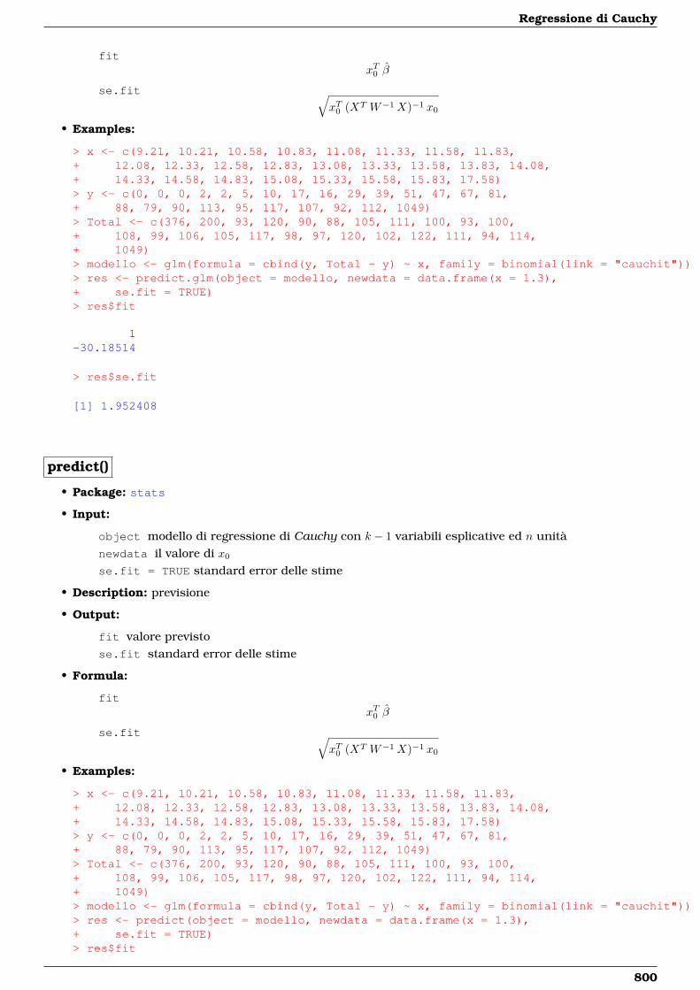
Regressione di Cauchy
fitxT0 β
se.fit √xT0 (XT W−1X)−1 x0
• Examples:
> x <- c(9.21, 10.21, 10.58, 10.83, 11.08, 11.33, 11.58, 11.83,+ 12.08, 12.33, 12.58, 12.83, 13.08, 13.33, 13.58, 13.83, 14.08,+ 14.33, 14.58, 14.83, 15.08, 15.33, 15.58, 15.83, 17.58)> y <- c(0, 0, 0, 2, 2, 5, 10, 17, 16, 29, 39, 51, 47, 67, 81,+ 88, 79, 90, 113, 95, 117, 107, 92, 112, 1049)> Total <- c(376, 200, 93, 120, 90, 88, 105, 111, 100, 93, 100,+ 108, 99, 106, 105, 117, 98, 97, 120, 102, 122, 111, 94, 114,+ 1049)> modello <- glm(formula = cbind(y, Total - y) ~ x, family = binomial(link = "cauchit"))> res <- predict.glm(object = modello, newdata = data.frame(x = 1.3),+ se.fit = TRUE)> res$fit
1-30.18514
> res$se.fit
[1] 1.952408
predict()
• Package: stats
• Input:
object modello di regressione di Cauchy con k − 1 variabili esplicative ed n unitànewdata il valore di x0
se.fit = TRUE standard error delle stime
• Description: previsione
• Output:
fit valore previstose.fit standard error delle stime
• Formula:
fitxT0 β
se.fit √xT0 (XT W−1X)−1 x0
• Examples:
> x <- c(9.21, 10.21, 10.58, 10.83, 11.08, 11.33, 11.58, 11.83,+ 12.08, 12.33, 12.58, 12.83, 13.08, 13.33, 13.58, 13.83, 14.08,+ 14.33, 14.58, 14.83, 15.08, 15.33, 15.58, 15.83, 17.58)> y <- c(0, 0, 0, 2, 2, 5, 10, 17, 16, 29, 39, 51, 47, 67, 81,+ 88, 79, 90, 113, 95, 117, 107, 92, 112, 1049)> Total <- c(376, 200, 93, 120, 90, 88, 105, 111, 100, 93, 100,+ 108, 99, 106, 105, 117, 98, 97, 120, 102, 122, 111, 94, 114,+ 1049)> modello <- glm(formula = cbind(y, Total - y) ~ x, family = binomial(link = "cauchit"))> res <- predict(object = modello, newdata = data.frame(x = 1.3),+ se.fit = TRUE)> res$fit
800
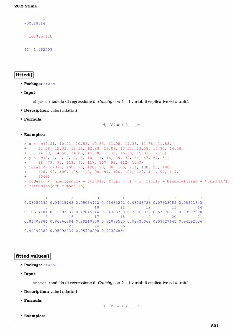
20.2 Stima
1-30.18514
> res$se.fit
[1] 1.952408
fitted()
• Package: stats
• Input:
object modello di regressione di Cauchy con k − 1 variabili esplicative ed n unità
• Description: valori adattati
• Formula:πi ∀ i = 1, 2, . . . , n
• Examples:
> x <- c(9.21, 10.21, 10.58, 10.83, 11.08, 11.33, 11.58, 11.83,+ 12.08, 12.33, 12.58, 12.83, 13.08, 13.33, 13.58, 13.83, 14.08,+ 14.33, 14.58, 14.83, 15.08, 15.33, 15.58, 15.83, 17.58)> y <- c(0, 0, 0, 2, 2, 5, 10, 17, 16, 29, 39, 51, 47, 67, 81,+ 88, 79, 90, 113, 95, 117, 107, 92, 112, 1049)> Total <- c(376, 200, 93, 120, 90, 88, 105, 111, 100, 93, 100,+ 108, 99, 106, 105, 117, 98, 97, 120, 102, 122, 111, 94, 114,+ 1049)> modello <- glm(formula = cbind(y, Total - y) ~ x, family = binomial(link = "cauchit"))> fitted(object = modello)
1 2 3 4 5 6 70.03254332 0.04415163 0.05084422 0.05663242 0.06388783 0.07323785 0.08571643
8 9 10 11 12 13 140.10314181 0.12897631 0.17045144 0.24383760 0.38066032 0.57870619 0.73297838
15 16 17 18 19 20 210.81708886 0.86366984 0.89210300 0.91098535 0.92435062 0.93427641 0.94192536
22 23 24 250.94799380 0.95292239 0.95700290 0.97326854
fitted.values()
• Package: stats
• Input:
object modello di regressione di Cauchy con k − 1 variabili esplicative ed n unità
• Description: valori adattati
• Formula:πi ∀ i = 1, 2, . . . , n
• Examples:
801
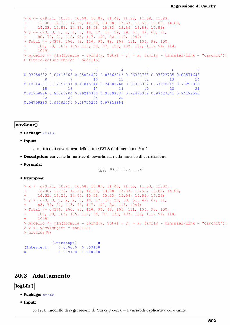
Regressione di Cauchy
> x <- c(9.21, 10.21, 10.58, 10.83, 11.08, 11.33, 11.58, 11.83,+ 12.08, 12.33, 12.58, 12.83, 13.08, 13.33, 13.58, 13.83, 14.08,+ 14.33, 14.58, 14.83, 15.08, 15.33, 15.58, 15.83, 17.58)> y <- c(0, 0, 0, 2, 2, 5, 10, 17, 16, 29, 39, 51, 47, 67, 81,+ 88, 79, 90, 113, 95, 117, 107, 92, 112, 1049)> Total <- c(376, 200, 93, 120, 90, 88, 105, 111, 100, 93, 100,+ 108, 99, 106, 105, 117, 98, 97, 120, 102, 122, 111, 94, 114,+ 1049)> modello <- glm(formula = cbind(y, Total - y) ~ x, family = binomial(link = "cauchit"))> fitted.values(object = modello)
1 2 3 4 5 6 70.03254332 0.04415163 0.05084422 0.05663242 0.06388783 0.07323785 0.08571643
8 9 10 11 12 13 140.10314181 0.12897631 0.17045144 0.24383760 0.38066032 0.57870619 0.73297838
15 16 17 18 19 20 210.81708886 0.86366984 0.89210300 0.91098535 0.92435062 0.93427641 0.94192536
22 23 24 250.94799380 0.95292239 0.95700290 0.97326854
cov2cor()
• Package: stats
• Input:
V matrice di covarianza delle stime IWLS di dimensione k × k
• Description: converte la matrice di covarianza nella matrice di correlazione
• Formula:rβi βj ∀ i, j = 1, 2, . . . , k
• Examples:
> x <- c(9.21, 10.21, 10.58, 10.83, 11.08, 11.33, 11.58, 11.83,+ 12.08, 12.33, 12.58, 12.83, 13.08, 13.33, 13.58, 13.83, 14.08,+ 14.33, 14.58, 14.83, 15.08, 15.33, 15.58, 15.83, 17.58)> y <- c(0, 0, 0, 2, 2, 5, 10, 17, 16, 29, 39, 51, 47, 67, 81,+ 88, 79, 90, 113, 95, 117, 107, 92, 112, 1049)> Total <- c(376, 200, 93, 120, 90, 88, 105, 111, 100, 93, 100,+ 108, 99, 106, 105, 117, 98, 97, 120, 102, 122, 111, 94, 114,+ 1049)> modello <- glm(formula = cbind(y, Total - y) ~ x, family = binomial(link = "cauchit"))> V <- vcov(object = modello)> cov2cor(V)
(Intercept) x(Intercept) 1.000000 -0.999138x -0.999138 1.000000
20.3 Adattamento
logLik()
• Package: stats
• Input:
object modello di regressione di Cauchy con k − 1 variabili esplicative ed n unità
802
20.3 Adattamento
• Description: log-verosimiglianza binomiale
• Formula:ˆ
• Examples:
> x <- c(9.21, 10.21, 10.58, 10.83, 11.08, 11.33, 11.58, 11.83,+ 12.08, 12.33, 12.58, 12.83, 13.08, 13.33, 13.58, 13.83, 14.08,+ 14.33, 14.58, 14.83, 15.08, 15.33, 15.58, 15.83, 17.58)> y <- c(0, 0, 0, 2, 2, 5, 10, 17, 16, 29, 39, 51, 47, 67, 81,+ 88, 79, 90, 113, 95, 117, 107, 92, 112, 1049)> Total <- c(376, 200, 93, 120, 90, 88, 105, 111, 100, 93, 100,+ 108, 99, 106, 105, 117, 98, 97, 120, 102, 122, 111, 94, 114,+ 1049)> modello <- glm(formula = cbind(y, Total - y) ~ x, family = binomial(link = "cauchit"))> logLik(object = modello)
'log Lik.' -132.4551 (df=2)
AIC()
• Package: stats
• Input:
object modello di regressione di Cauchy con k − 1 variabili esplicative ed n unità
• Description: indice AIC
• Formula:−2 ˆ+ 2 k
• Examples:
> x <- c(9.21, 10.21, 10.58, 10.83, 11.08, 11.33, 11.58, 11.83,+ 12.08, 12.33, 12.58, 12.83, 13.08, 13.33, 13.58, 13.83, 14.08,+ 14.33, 14.58, 14.83, 15.08, 15.33, 15.58, 15.83, 17.58)> y <- c(0, 0, 0, 2, 2, 5, 10, 17, 16, 29, 39, 51, 47, 67, 81,+ 88, 79, 90, 113, 95, 117, 107, 92, 112, 1049)> Total <- c(376, 200, 93, 120, 90, 88, 105, 111, 100, 93, 100,+ 108, 99, 106, 105, 117, 98, 97, 120, 102, 122, 111, 94, 114,+ 1049)> modello <- glm(formula = cbind(y, Total - y) ~ x, family = binomial(link = "cauchit"))> AIC(object = modello)
[1] 268.9102
durbin.watson()
• Package: car
• Input:
model modello di regressione di Cauchy con k − 1 variabili esplicative ed n unità
• Description: test di Durbin–Watson per verificare la presenza di autocorrelazioni tra i residui
• Output:
dw valore empirico della statistica D–W
• Formula:
803
Regressione di Cauchy
dwn∑i=2
(ei − ei−1)2 /D
• Examples:
> x <- c(9.21, 10.21, 10.58, 10.83, 11.08, 11.33, 11.58, 11.83,+ 12.08, 12.33, 12.58, 12.83, 13.08, 13.33, 13.58, 13.83, 14.08,+ 14.33, 14.58, 14.83, 15.08, 15.33, 15.58, 15.83, 17.58)> y <- c(0, 0, 0, 2, 2, 5, 10, 17, 16, 29, 39, 51, 47, 67, 81,+ 88, 79, 90, 113, 95, 117, 107, 92, 112, 1049)> Total <- c(376, 200, 93, 120, 90, 88, 105, 111, 100, 93, 100,+ 108, 99, 106, 105, 117, 98, 97, 120, 102, 122, 111, 94, 114,+ 1049)> modello <- glm(formula = cbind(y, Total - y) ~ x, family = binomial(link = "cauchit"))> durbin.watson(model = modello)
lag Autocorrelation D-W Statistic p-value1 0.5390491 0.4700264 0
Alternative hypothesis: rho != 0
> res <- durbin.watson(model = modello)> res$dw
[1] 0.4700264
extractAIC()
• Package: stats
• Input:
fit modello di regressione di Cauchy con k − 1 variabili esplicative ed n unità
• Description: numero di parametri del modello ed indice AIC generalizzato
• Formula:k − 2 ˆ+ 2 k
• Examples:
> x <- c(9.21, 10.21, 10.58, 10.83, 11.08, 11.33, 11.58, 11.83,+ 12.08, 12.33, 12.58, 12.83, 13.08, 13.33, 13.58, 13.83, 14.08,+ 14.33, 14.58, 14.83, 15.08, 15.33, 15.58, 15.83, 17.58)> y <- c(0, 0, 0, 2, 2, 5, 10, 17, 16, 29, 39, 51, 47, 67, 81,+ 88, 79, 90, 113, 95, 117, 107, 92, 112, 1049)> Total <- c(376, 200, 93, 120, 90, 88, 105, 111, 100, 93, 100,+ 108, 99, 106, 105, 117, 98, 97, 120, 102, 122, 111, 94, 114,+ 1049)> modello <- glm(formula = cbind(y, Total - y) ~ x, family = binomial(link = "cauchit"))> extractAIC(fit = modello)
[1] 2.0000 268.9102
804
20.3 Adattamento
deviance()
• Package: stats
• Input:
object modello di regressione di Cauchy con k − 1 variabili esplicative ed n unità
• Description: devianza residua
• Formula:D
• Examples:
> x <- c(9.21, 10.21, 10.58, 10.83, 11.08, 11.33, 11.58, 11.83,+ 12.08, 12.33, 12.58, 12.83, 13.08, 13.33, 13.58, 13.83, 14.08,+ 14.33, 14.58, 14.83, 15.08, 15.33, 15.58, 15.83, 17.58)> y <- c(0, 0, 0, 2, 2, 5, 10, 17, 16, 29, 39, 51, 47, 67, 81,+ 88, 79, 90, 113, 95, 117, 107, 92, 112, 1049)> Total <- c(376, 200, 93, 120, 90, 88, 105, 111, 100, 93, 100,+ 108, 99, 106, 105, 117, 98, 97, 120, 102, 122, 111, 94, 114,+ 1049)> modello <- glm(formula = cbind(y, Total - y) ~ x, family = binomial(link = "cauchit"))> deviance(object = modello)
[1] 180.8584
anova()
• Package: stats
• Input:
nullo modello nullo di regressione di Cauchy con n unità
modello modello di regressione di Cauchy con k − 1 variabili esplicative con n unità
test = "Chisq"
• Description: anova di regressione
• Output:
Resid. Df gradi di libertà
Resid. Dev devianza residua
Df differenza dei gradi di libertà
Deviance differenza tra le devianze residue
P(>|Chi|) p-value
• Formula:
Resid. Dfn− 1 n− k
Resid. DevDnullo D
Dfdf = k − 1
Deviancec = Dnullo −D
P(>|Chi|)P (χ2
df ≥ c)
• Examples:
805
Regressione di Cauchy
> x <- c(9.21, 10.21, 10.58, 10.83, 11.08, 11.33, 11.58, 11.83,+ 12.08, 12.33, 12.58, 12.83, 13.08, 13.33, 13.58, 13.83, 14.08,+ 14.33, 14.58, 14.83, 15.08, 15.33, 15.58, 15.83, 17.58)> y <- c(0, 0, 0, 2, 2, 5, 10, 17, 16, 29, 39, 51, 47, 67, 81,+ 88, 79, 90, 113, 95, 117, 107, 92, 112, 1049)> Total <- c(376, 200, 93, 120, 90, 88, 105, 111, 100, 93, 100,+ 108, 99, 106, 105, 117, 98, 97, 120, 102, 122, 111, 94, 114,+ 1049)> nullo <- glm(formula = cbind(y, Total - y) ~ 1, family = binomial(link = "cauchit"))> modello <- glm(formula = cbind(y, Total - y) ~ x, family = binomial(link = "cauchit"))> anova(nullo, modello, test = "Chisq")
Analysis of Deviance Table
Model 1: cbind(y, Total - y) ~ 1Model 2: cbind(y, Total - y) ~ xResid. Df Resid. Dev Df Deviance P(>|Chi|)
1 24 3693.92 23 180.9 1 3513.0 0.0
> res <- anova(nullo, modello, test = "Chisq")> res$"Resid. Df"
[1] 24 23
> res$"Resid. Dev"
[1] 3693.8836 180.8584
> res$Df
[1] NA 1
> res$Deviance
[1] NA 3513.025
> res$"P(>|Chi|)"
[1] NA 0
drop1()
• Package: stats
• Input:
object modello di regressione di Cauchy con k − 1 variabili esplicative ed n unità
test = "Chisq"
• Description: submodels
• Output:
Df differenza tra gradi di libertà
Deviance differenza tra devianze residue
AIC indice AIC
LRT valore empirico della statistica χ2
Pr(Chi) p-value
806

20.3 Adattamento
• Formula:
Df1, 1, . . . , 1︸ ︷︷ ︸k−1 volte
DevianceD, D−xj ∀ j = 1, 2, . . . , k − 1
dove D−xj rappresenta la devianza residua del modello eliminata la variabile esplicativa xj.AIC
−2 ˆ+ 2 k, −2 ˆ−xj + 2 (k − 1) ∀ j = 1, 2, . . . , k − 1
dove ˆ−xj rappresenta la log-verosimiglianza binomiale del modello eliminata la variabile esplicativa xj.LRT
cj = D−xj −D ∀ j = 1, 2, . . . , k − 1
Pr(Chi)P (χ2
1 ≥ cj) ∀ j = 1, 2, . . . , k − 1
• Examples:
> x <- c(9.21, 10.21, 10.58, 10.83, 11.08, 11.33, 11.58, 11.83,+ 12.08, 12.33, 12.58, 12.83, 13.08, 13.33, 13.58, 13.83, 14.08,+ 14.33, 14.58, 14.83, 15.08, 15.33, 15.58, 15.83, 17.58)> y <- c(0, 0, 0, 2, 2, 5, 10, 17, 16, 29, 39, 51, 47, 67, 81,+ 88, 79, 90, 113, 95, 117, 107, 92, 112, 1049)> Total <- c(376, 200, 93, 120, 90, 88, 105, 111, 100, 93, 100,+ 108, 99, 106, 105, 117, 98, 97, 120, 102, 122, 111, 94, 114,+ 1049)> modello <- glm(formula = cbind(y, Total - y) ~ x, family = binomial(link = "cauchit"))> drop1(object = modello, test = "Chisq")
Single term deletions
Model:cbind(y, Total - y) ~ x
Df Deviance AIC LRT Pr(Chi)<none> 180.9 268.9x 1 3693.9 3779.9 3513.0 < 2.2e-16 ***---Signif. codes: 0 '***' 0.001 '**' 0.01 '*' 0.05 '.' 0.1 ' ' 1
> res <- drop1(object = modello, test = "Chisq")> res$Df
[1] NA 1
> res$Deviance
[1] 180.8584 3693.8836
> res$AIC
[1] 268.9102 3779.9354
> res$LRT
[1] NA 3513.025
> res$"Pr(Chi)"
[1] NA 0
807
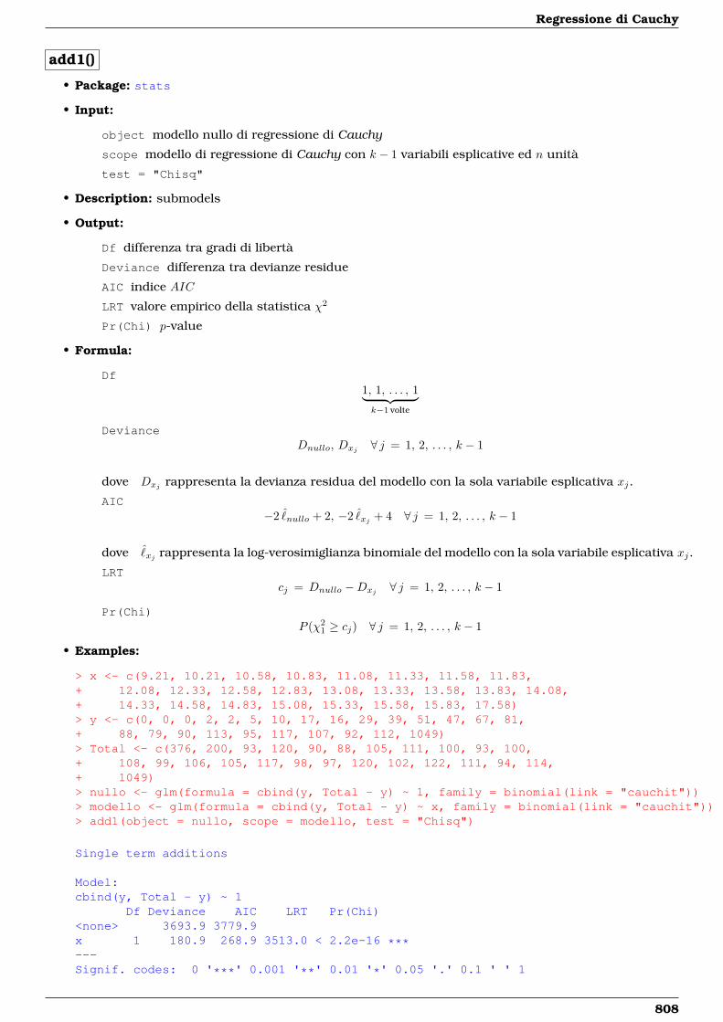
Regressione di Cauchy
add1()
• Package: stats
• Input:
object modello nullo di regressione di Cauchy
scope modello di regressione di Cauchy con k − 1 variabili esplicative ed n unità
test = "Chisq"
• Description: submodels
• Output:
Df differenza tra gradi di libertà
Deviance differenza tra devianze residue
AIC indice AIC
LRT valore empirico della statistica χ2
Pr(Chi) p-value
• Formula:
Df1, 1, . . . , 1︸ ︷︷ ︸k−1 volte
DevianceDnullo, Dxj ∀ j = 1, 2, . . . , k − 1
dove Dxj rappresenta la devianza residua del modello con la sola variabile esplicativa xj.
AIC−2 ˆ
nullo + 2, −2 ˆxj + 4 ∀ j = 1, 2, . . . , k − 1
dove ˆxj rappresenta la log-verosimiglianza binomiale del modello con la sola variabile esplicativa xj.
LRTcj = Dnullo −Dxj ∀ j = 1, 2, . . . , k − 1
Pr(Chi)P (χ2
1 ≥ cj) ∀ j = 1, 2, . . . , k − 1
• Examples:
> x <- c(9.21, 10.21, 10.58, 10.83, 11.08, 11.33, 11.58, 11.83,+ 12.08, 12.33, 12.58, 12.83, 13.08, 13.33, 13.58, 13.83, 14.08,+ 14.33, 14.58, 14.83, 15.08, 15.33, 15.58, 15.83, 17.58)> y <- c(0, 0, 0, 2, 2, 5, 10, 17, 16, 29, 39, 51, 47, 67, 81,+ 88, 79, 90, 113, 95, 117, 107, 92, 112, 1049)> Total <- c(376, 200, 93, 120, 90, 88, 105, 111, 100, 93, 100,+ 108, 99, 106, 105, 117, 98, 97, 120, 102, 122, 111, 94, 114,+ 1049)> nullo <- glm(formula = cbind(y, Total - y) ~ 1, family = binomial(link = "cauchit"))> modello <- glm(formula = cbind(y, Total - y) ~ x, family = binomial(link = "cauchit"))> add1(object = nullo, scope = modello, test = "Chisq")
Single term additions
Model:cbind(y, Total - y) ~ 1
Df Deviance AIC LRT Pr(Chi)<none> 3693.9 3779.9x 1 180.9 268.9 3513.0 < 2.2e-16 ***---Signif. codes: 0 '***' 0.001 '**' 0.01 '*' 0.05 '.' 0.1 ' ' 1
808
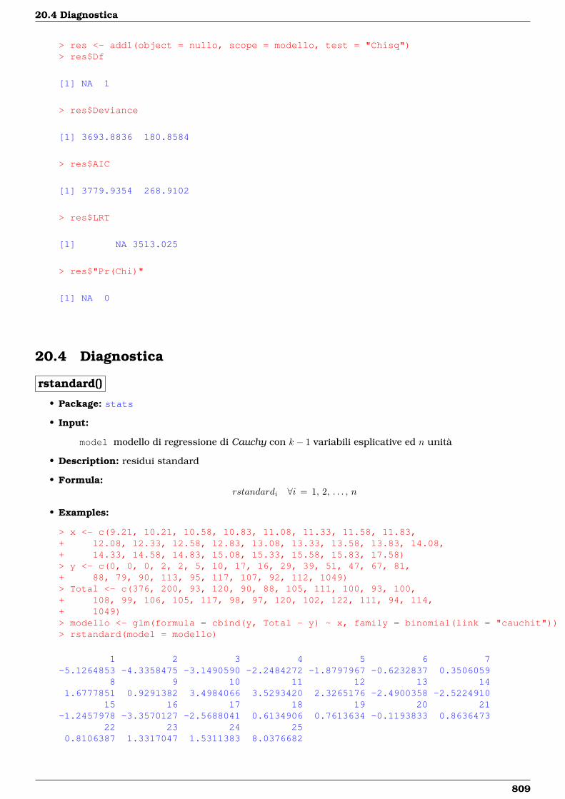
20.4 Diagnostica
> res <- add1(object = nullo, scope = modello, test = "Chisq")> res$Df
[1] NA 1
> res$Deviance
[1] 3693.8836 180.8584
> res$AIC
[1] 3779.9354 268.9102
> res$LRT
[1] NA 3513.025
> res$"Pr(Chi)"
[1] NA 0
20.4 Diagnostica
rstandard()
• Package: stats
• Input:
model modello di regressione di Cauchy con k − 1 variabili esplicative ed n unità
• Description: residui standard
• Formula:rstandardi ∀i = 1, 2, . . . , n
• Examples:
> x <- c(9.21, 10.21, 10.58, 10.83, 11.08, 11.33, 11.58, 11.83,+ 12.08, 12.33, 12.58, 12.83, 13.08, 13.33, 13.58, 13.83, 14.08,+ 14.33, 14.58, 14.83, 15.08, 15.33, 15.58, 15.83, 17.58)> y <- c(0, 0, 0, 2, 2, 5, 10, 17, 16, 29, 39, 51, 47, 67, 81,+ 88, 79, 90, 113, 95, 117, 107, 92, 112, 1049)> Total <- c(376, 200, 93, 120, 90, 88, 105, 111, 100, 93, 100,+ 108, 99, 106, 105, 117, 98, 97, 120, 102, 122, 111, 94, 114,+ 1049)> modello <- glm(formula = cbind(y, Total - y) ~ x, family = binomial(link = "cauchit"))> rstandard(model = modello)
1 2 3 4 5 6 7-5.1264853 -4.3358475 -3.1490590 -2.2484272 -1.8797967 -0.6232837 0.3506059
8 9 10 11 12 13 141.6777851 0.9291382 3.4984066 3.5293420 2.3265176 -2.4900358 -2.5224910
15 16 17 18 19 20 21-1.2457978 -3.3570127 -2.5688041 0.6134906 0.7613634 -0.1193833 0.8636473
22 23 24 250.8106387 1.3317047 1.5311383 8.0376682
809
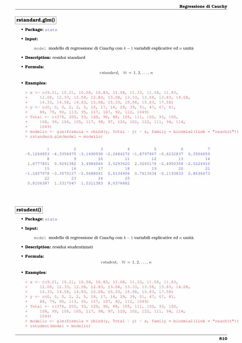
Regressione di Cauchy
rstandard.glm()
• Package: stats
• Input:
model modello di regressione di Cauchy con k − 1 variabili esplicative ed n unità
• Description: residui standard
• Formula:rstandardi ∀i = 1, 2, . . . , n
• Examples:
> x <- c(9.21, 10.21, 10.58, 10.83, 11.08, 11.33, 11.58, 11.83,+ 12.08, 12.33, 12.58, 12.83, 13.08, 13.33, 13.58, 13.83, 14.08,+ 14.33, 14.58, 14.83, 15.08, 15.33, 15.58, 15.83, 17.58)> y <- c(0, 0, 0, 2, 2, 5, 10, 17, 16, 29, 39, 51, 47, 67, 81,+ 88, 79, 90, 113, 95, 117, 107, 92, 112, 1049)> Total <- c(376, 200, 93, 120, 90, 88, 105, 111, 100, 93, 100,+ 108, 99, 106, 105, 117, 98, 97, 120, 102, 122, 111, 94, 114,+ 1049)> modello <- glm(formula = cbind(y, Total - y) ~ x, family = binomial(link = "cauchit"))> rstandard.glm(model = modello)
1 2 3 4 5 6 7-5.1264853 -4.3358475 -3.1490590 -2.2484272 -1.8797967 -0.6232837 0.3506059
8 9 10 11 12 13 141.6777851 0.9291382 3.4984066 3.5293420 2.3265176 -2.4900358 -2.5224910
15 16 17 18 19 20 21-1.2457978 -3.3570127 -2.5688041 0.6134906 0.7613634 -0.1193833 0.8636473
22 23 24 250.8106387 1.3317047 1.5311383 8.0376682
rstudent()
• Package: stats
• Input:
model modello di regressione di Cauchy con k − 1 variabili esplicative ed n unità
• Description: residui studentizzati
• Formula:rstudenti ∀i = 1, 2, . . . , n
• Examples:
> x <- c(9.21, 10.21, 10.58, 10.83, 11.08, 11.33, 11.58, 11.83,+ 12.08, 12.33, 12.58, 12.83, 13.08, 13.33, 13.58, 13.83, 14.08,+ 14.33, 14.58, 14.83, 15.08, 15.33, 15.58, 15.83, 17.58)> y <- c(0, 0, 0, 2, 2, 5, 10, 17, 16, 29, 39, 51, 47, 67, 81,+ 88, 79, 90, 113, 95, 117, 107, 92, 112, 1049)> Total <- c(376, 200, 93, 120, 90, 88, 105, 111, 100, 93, 100,+ 108, 99, 106, 105, 117, 98, 97, 120, 102, 122, 111, 94, 114,+ 1049)> modello <- glm(formula = cbind(y, Total - y) ~ x, family = binomial(link = "cauchit"))> rstudent(model = modello)
810
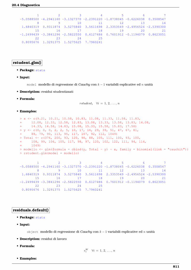
20.4 Diagnostica
1 2 3 4 5 6 7-5.0588500 -4.2941160 -3.1327370 -2.2391220 -1.8738045 -0.6226038 0.3508547
8 9 10 11 12 13 141.6840319 0.9311874 3.5275840 3.5611698 2.3353549 -2.4956524 -2.5390300
15 16 17 18 19 20 21-1.2499439 -3.3841296 -2.5822550 0.6127486 0.7601912 -0.1194079 0.8623051
22 23 24 250.8095676 1.3291375 1.5275625 7.7960241
rstudent.glm()
• Package: stats
• Input:
model modello di regressione di Cauchy con k − 1 variabili esplicative ed n unità
• Description: residui studentizzati
• Formula:rstudenti ∀i = 1, 2, . . . , n
• Examples:
> x <- c(9.21, 10.21, 10.58, 10.83, 11.08, 11.33, 11.58, 11.83,+ 12.08, 12.33, 12.58, 12.83, 13.08, 13.33, 13.58, 13.83, 14.08,+ 14.33, 14.58, 14.83, 15.08, 15.33, 15.58, 15.83, 17.58)> y <- c(0, 0, 0, 2, 2, 5, 10, 17, 16, 29, 39, 51, 47, 67, 81,+ 88, 79, 90, 113, 95, 117, 107, 92, 112, 1049)> Total <- c(376, 200, 93, 120, 90, 88, 105, 111, 100, 93, 100,+ 108, 99, 106, 105, 117, 98, 97, 120, 102, 122, 111, 94, 114,+ 1049)> modello <- glm(formula = cbind(y, Total - y) ~ x, family = binomial(link = "cauchit"))> rstudent.glm(model = modello)
1 2 3 4 5 6 7-5.0588500 -4.2941160 -3.1327370 -2.2391220 -1.8738045 -0.6226038 0.3508547
8 9 10 11 12 13 141.6840319 0.9311874 3.5275840 3.5611698 2.3353549 -2.4956524 -2.5390300
15 16 17 18 19 20 21-1.2499439 -3.3841296 -2.5822550 0.6127486 0.7601912 -0.1194079 0.8623051
22 23 24 250.8095676 1.3291375 1.5275625 7.7960241
residuals.default()
• Package: stats
• Input:
object modello di regressione di Cauchy con k − 1 variabili esplicative ed n unità
• Description: residui di lavoro
• Formula:eWi ∀i = 1, 2, . . . , n
• Examples:
811
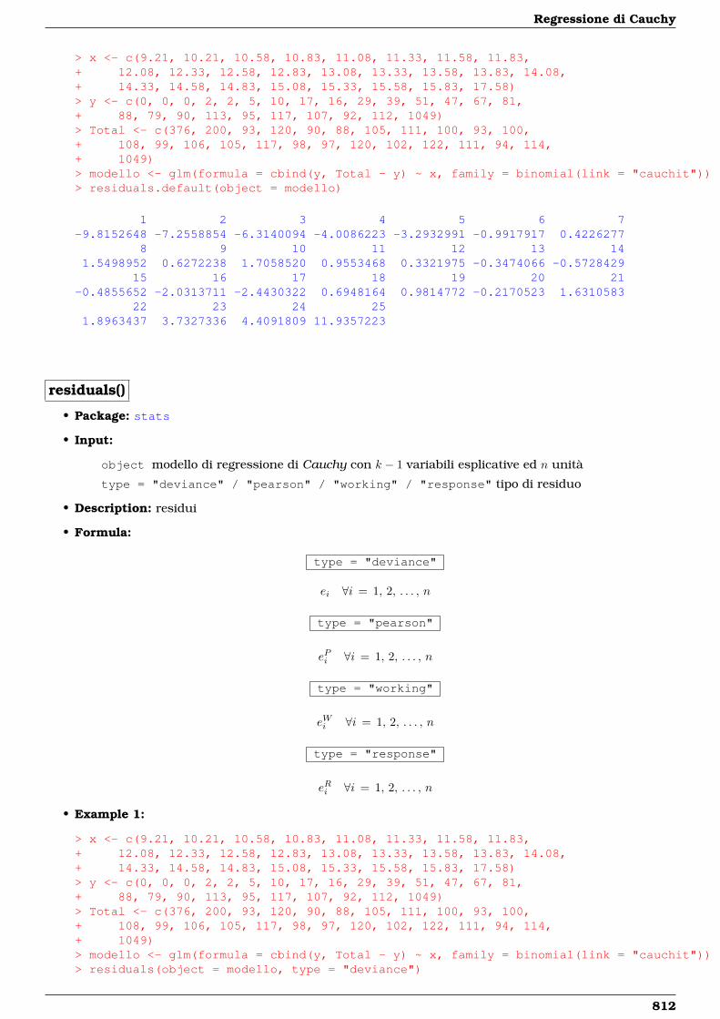
Regressione di Cauchy
> x <- c(9.21, 10.21, 10.58, 10.83, 11.08, 11.33, 11.58, 11.83,+ 12.08, 12.33, 12.58, 12.83, 13.08, 13.33, 13.58, 13.83, 14.08,+ 14.33, 14.58, 14.83, 15.08, 15.33, 15.58, 15.83, 17.58)> y <- c(0, 0, 0, 2, 2, 5, 10, 17, 16, 29, 39, 51, 47, 67, 81,+ 88, 79, 90, 113, 95, 117, 107, 92, 112, 1049)> Total <- c(376, 200, 93, 120, 90, 88, 105, 111, 100, 93, 100,+ 108, 99, 106, 105, 117, 98, 97, 120, 102, 122, 111, 94, 114,+ 1049)> modello <- glm(formula = cbind(y, Total - y) ~ x, family = binomial(link = "cauchit"))> residuals.default(object = modello)
1 2 3 4 5 6 7-9.8152648 -7.2558854 -6.3140094 -4.0086223 -3.2932991 -0.9917917 0.4226277
8 9 10 11 12 13 141.5498952 0.6272238 1.7058520 0.9553468 0.3321975 -0.3474066 -0.5728429
15 16 17 18 19 20 21-0.4855652 -2.0313711 -2.4430322 0.6948164 0.9814772 -0.2170523 1.6310583
22 23 24 251.8963437 3.7327336 4.4091809 11.9357223
residuals()
• Package: stats
• Input:
object modello di regressione di Cauchy con k − 1 variabili esplicative ed n unità
type = "deviance" / "pearson" / "working" / "response" tipo di residuo
• Description: residui
• Formula:
type = "deviance"
ei ∀i = 1, 2, . . . , n
type = "pearson"
ePi ∀i = 1, 2, . . . , n
type = "working"
eWi ∀i = 1, 2, . . . , n
type = "response"
eRi ∀i = 1, 2, . . . , n
• Example 1:
> x <- c(9.21, 10.21, 10.58, 10.83, 11.08, 11.33, 11.58, 11.83,+ 12.08, 12.33, 12.58, 12.83, 13.08, 13.33, 13.58, 13.83, 14.08,+ 14.33, 14.58, 14.83, 15.08, 15.33, 15.58, 15.83, 17.58)> y <- c(0, 0, 0, 2, 2, 5, 10, 17, 16, 29, 39, 51, 47, 67, 81,+ 88, 79, 90, 113, 95, 117, 107, 92, 112, 1049)> Total <- c(376, 200, 93, 120, 90, 88, 105, 111, 100, 93, 100,+ 108, 99, 106, 105, 117, 98, 97, 120, 102, 122, 111, 94, 114,+ 1049)> modello <- glm(formula = cbind(y, Total - y) ~ x, family = binomial(link = "cauchit"))> residuals(object = modello, type = "deviance")
812
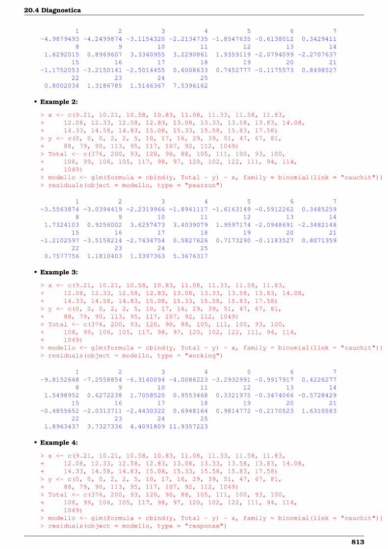
20.4 Diagnostica
1 2 3 4 5 6 7-4.9879493 -4.2499874 -3.1154320 -2.2134735 -1.8547635 -0.6138012 0.3429411
8 9 10 11 12 13 141.6292015 0.8969607 3.3340955 3.2290861 1.9359119 -2.0794099 -2.2707637
15 16 17 18 19 20 21-1.1752053 -3.2150141 -2.5014455 0.6008633 0.7452777 -0.1175573 0.8498527
22 23 24 250.8002034 1.3186785 1.5146367 7.5396162
• Example 2:
> x <- c(9.21, 10.21, 10.58, 10.83, 11.08, 11.33, 11.58, 11.83,+ 12.08, 12.33, 12.58, 12.83, 13.08, 13.33, 13.58, 13.83, 14.08,+ 14.33, 14.58, 14.83, 15.08, 15.33, 15.58, 15.83, 17.58)> y <- c(0, 0, 0, 2, 2, 5, 10, 17, 16, 29, 39, 51, 47, 67, 81,+ 88, 79, 90, 113, 95, 117, 107, 92, 112, 1049)> Total <- c(376, 200, 93, 120, 90, 88, 105, 111, 100, 93, 100,+ 108, 99, 106, 105, 117, 98, 97, 120, 102, 122, 111, 94, 114,+ 1049)> modello <- glm(formula = cbind(y, Total - y) ~ x, family = binomial(link = "cauchit"))> residuals(object = modello, type = "pearson")
1 2 3 4 5 6 7-3.5563874 -3.0394419 -2.2319966 -1.8941117 -1.6163149 -0.5912262 0.3485259
8 9 10 11 12 13 141.7324103 0.9256002 3.6257473 3.4039079 1.9597174 -2.0948691 -2.3482148
15 16 17 18 19 20 21-1.2102597 -3.5158214 -2.7434754 0.5827626 0.7173290 -0.1183527 0.8071359
22 23 24 250.7577756 1.1810403 1.3397363 5.3676317
• Example 3:
> x <- c(9.21, 10.21, 10.58, 10.83, 11.08, 11.33, 11.58, 11.83,+ 12.08, 12.33, 12.58, 12.83, 13.08, 13.33, 13.58, 13.83, 14.08,+ 14.33, 14.58, 14.83, 15.08, 15.33, 15.58, 15.83, 17.58)> y <- c(0, 0, 0, 2, 2, 5, 10, 17, 16, 29, 39, 51, 47, 67, 81,+ 88, 79, 90, 113, 95, 117, 107, 92, 112, 1049)> Total <- c(376, 200, 93, 120, 90, 88, 105, 111, 100, 93, 100,+ 108, 99, 106, 105, 117, 98, 97, 120, 102, 122, 111, 94, 114,+ 1049)> modello <- glm(formula = cbind(y, Total - y) ~ x, family = binomial(link = "cauchit"))> residuals(object = modello, type = "working")
1 2 3 4 5 6 7-9.8152648 -7.2558854 -6.3140094 -4.0086223 -3.2932991 -0.9917917 0.4226277
8 9 10 11 12 13 141.5498952 0.6272238 1.7058520 0.9553468 0.3321975 -0.3474066 -0.5728429
15 16 17 18 19 20 21-0.4855652 -2.0313711 -2.4430322 0.6948164 0.9814772 -0.2170523 1.6310583
22 23 24 251.8963437 3.7327336 4.4091809 11.9357223
• Example 4:
> x <- c(9.21, 10.21, 10.58, 10.83, 11.08, 11.33, 11.58, 11.83,+ 12.08, 12.33, 12.58, 12.83, 13.08, 13.33, 13.58, 13.83, 14.08,+ 14.33, 14.58, 14.83, 15.08, 15.33, 15.58, 15.83, 17.58)> y <- c(0, 0, 0, 2, 2, 5, 10, 17, 16, 29, 39, 51, 47, 67, 81,+ 88, 79, 90, 113, 95, 117, 107, 92, 112, 1049)> Total <- c(376, 200, 93, 120, 90, 88, 105, 111, 100, 93, 100,+ 108, 99, 106, 105, 117, 98, 97, 120, 102, 122, 111, 94, 114,+ 1049)> modello <- glm(formula = cbind(y, Total - y) ~ x, family = binomial(link = "cauchit"))> residuals(object = modello, type = "response")
813
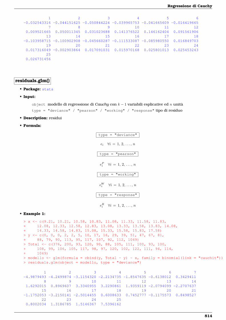
Regressione di Cauchy
1 2 3 4 5 6-0.032543316 -0.044151625 -0.050844224 -0.039965753 -0.041665609 -0.016419665
7 8 9 10 11 120.009521665 0.050011345 0.031023688 0.141376522 0.146162404 0.091561906
13 14 15 16 17 18-0.103958715 -0.100902908 -0.045660287 -0.111533087 -0.085980550 0.016849703
19 20 21 22 23 240.017316049 -0.002903864 0.017091031 0.015970168 0.025801013 0.025453243
250.026731456
residuals.glm()
• Package: stats
• Input:
object modello di regressione di Cauchy con k − 1 variabili esplicative ed n unità
type = "deviance" / "pearson" / "working" / "response" tipo di residuo
• Description: residui
• Formula:
type = "deviance"
ei ∀i = 1, 2, . . . , n
type = "pearson"
ePi ∀i = 1, 2, . . . , n
type = "working"
eWi ∀i = 1, 2, . . . , n
type = "response"
eRi ∀i = 1, 2, . . . , n
• Example 1:
> x <- c(9.21, 10.21, 10.58, 10.83, 11.08, 11.33, 11.58, 11.83,+ 12.08, 12.33, 12.58, 12.83, 13.08, 13.33, 13.58, 13.83, 14.08,+ 14.33, 14.58, 14.83, 15.08, 15.33, 15.58, 15.83, 17.58)> y <- c(0, 0, 0, 2, 2, 5, 10, 17, 16, 29, 39, 51, 47, 67, 81,+ 88, 79, 90, 113, 95, 117, 107, 92, 112, 1049)> Total <- c(376, 200, 93, 120, 90, 88, 105, 111, 100, 93, 100,+ 108, 99, 106, 105, 117, 98, 97, 120, 102, 122, 111, 94, 114,+ 1049)> modello <- glm(formula = cbind(y, Total - y) ~ x, family = binomial(link = "cauchit"))> residuals.glm(object = modello, type = "deviance")
1 2 3 4 5 6 7-4.9879493 -4.2499874 -3.1154320 -2.2134735 -1.8547635 -0.6138012 0.3429411
8 9 10 11 12 13 141.6292015 0.8969607 3.3340955 3.2290861 1.9359119 -2.0794099 -2.2707637
15 16 17 18 19 20 21-1.1752053 -3.2150141 -2.5014455 0.6008633 0.7452777 -0.1175573 0.8498527
22 23 24 250.8002034 1.3186785 1.5146367 7.5396162
814
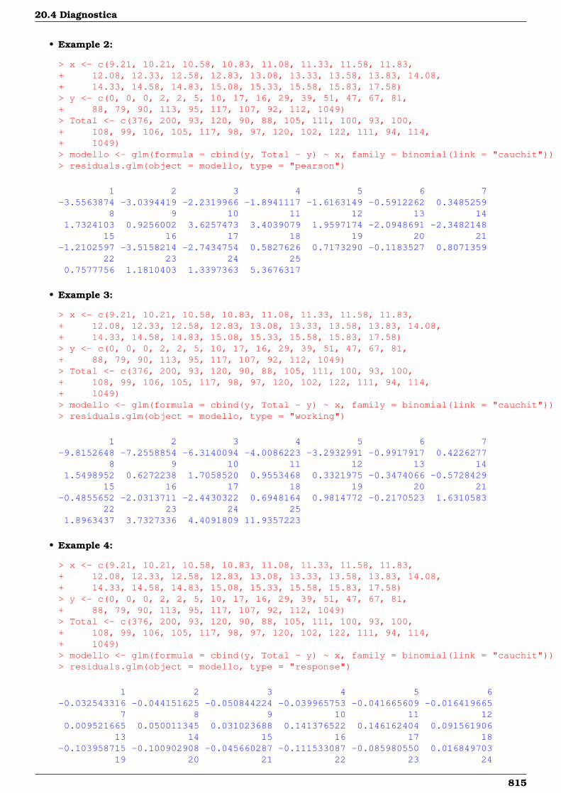
20.4 Diagnostica
• Example 2:
> x <- c(9.21, 10.21, 10.58, 10.83, 11.08, 11.33, 11.58, 11.83,+ 12.08, 12.33, 12.58, 12.83, 13.08, 13.33, 13.58, 13.83, 14.08,+ 14.33, 14.58, 14.83, 15.08, 15.33, 15.58, 15.83, 17.58)> y <- c(0, 0, 0, 2, 2, 5, 10, 17, 16, 29, 39, 51, 47, 67, 81,+ 88, 79, 90, 113, 95, 117, 107, 92, 112, 1049)> Total <- c(376, 200, 93, 120, 90, 88, 105, 111, 100, 93, 100,+ 108, 99, 106, 105, 117, 98, 97, 120, 102, 122, 111, 94, 114,+ 1049)> modello <- glm(formula = cbind(y, Total - y) ~ x, family = binomial(link = "cauchit"))> residuals.glm(object = modello, type = "pearson")
1 2 3 4 5 6 7-3.5563874 -3.0394419 -2.2319966 -1.8941117 -1.6163149 -0.5912262 0.3485259
8 9 10 11 12 13 141.7324103 0.9256002 3.6257473 3.4039079 1.9597174 -2.0948691 -2.3482148
15 16 17 18 19 20 21-1.2102597 -3.5158214 -2.7434754 0.5827626 0.7173290 -0.1183527 0.8071359
22 23 24 250.7577756 1.1810403 1.3397363 5.3676317
• Example 3:
> x <- c(9.21, 10.21, 10.58, 10.83, 11.08, 11.33, 11.58, 11.83,+ 12.08, 12.33, 12.58, 12.83, 13.08, 13.33, 13.58, 13.83, 14.08,+ 14.33, 14.58, 14.83, 15.08, 15.33, 15.58, 15.83, 17.58)> y <- c(0, 0, 0, 2, 2, 5, 10, 17, 16, 29, 39, 51, 47, 67, 81,+ 88, 79, 90, 113, 95, 117, 107, 92, 112, 1049)> Total <- c(376, 200, 93, 120, 90, 88, 105, 111, 100, 93, 100,+ 108, 99, 106, 105, 117, 98, 97, 120, 102, 122, 111, 94, 114,+ 1049)> modello <- glm(formula = cbind(y, Total - y) ~ x, family = binomial(link = "cauchit"))> residuals.glm(object = modello, type = "working")
1 2 3 4 5 6 7-9.8152648 -7.2558854 -6.3140094 -4.0086223 -3.2932991 -0.9917917 0.4226277
8 9 10 11 12 13 141.5498952 0.6272238 1.7058520 0.9553468 0.3321975 -0.3474066 -0.5728429
15 16 17 18 19 20 21-0.4855652 -2.0313711 -2.4430322 0.6948164 0.9814772 -0.2170523 1.6310583
22 23 24 251.8963437 3.7327336 4.4091809 11.9357223
• Example 4:
> x <- c(9.21, 10.21, 10.58, 10.83, 11.08, 11.33, 11.58, 11.83,+ 12.08, 12.33, 12.58, 12.83, 13.08, 13.33, 13.58, 13.83, 14.08,+ 14.33, 14.58, 14.83, 15.08, 15.33, 15.58, 15.83, 17.58)> y <- c(0, 0, 0, 2, 2, 5, 10, 17, 16, 29, 39, 51, 47, 67, 81,+ 88, 79, 90, 113, 95, 117, 107, 92, 112, 1049)> Total <- c(376, 200, 93, 120, 90, 88, 105, 111, 100, 93, 100,+ 108, 99, 106, 105, 117, 98, 97, 120, 102, 122, 111, 94, 114,+ 1049)> modello <- glm(formula = cbind(y, Total - y) ~ x, family = binomial(link = "cauchit"))> residuals.glm(object = modello, type = "response")
1 2 3 4 5 6-0.032543316 -0.044151625 -0.050844224 -0.039965753 -0.041665609 -0.016419665
7 8 9 10 11 120.009521665 0.050011345 0.031023688 0.141376522 0.146162404 0.091561906
13 14 15 16 17 18-0.103958715 -0.100902908 -0.045660287 -0.111533087 -0.085980550 0.016849703
19 20 21 22 23 24
815
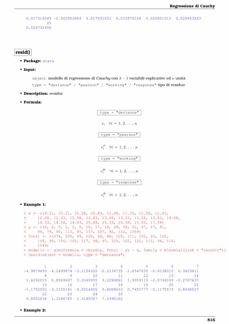
Regressione di Cauchy
0.017316049 -0.002903864 0.017091031 0.015970168 0.025801013 0.02545324325
0.026731456
resid()
• Package: stats
• Input:
object modello di regressione di Cauchy con k − 1 variabili esplicative ed n unità
type = "deviance" / "pearson" / "working" / "response" tipo di residuo
• Description: residui
• Formula:
type = "deviance"
ei ∀i = 1, 2, . . . , n
type = "pearson"
ePi ∀i = 1, 2, . . . , n
type = "working"
eWi ∀i = 1, 2, . . . , n
type = "response"
eRi ∀i = 1, 2, . . . , n
• Example 1:
> x <- c(9.21, 10.21, 10.58, 10.83, 11.08, 11.33, 11.58, 11.83,+ 12.08, 12.33, 12.58, 12.83, 13.08, 13.33, 13.58, 13.83, 14.08,+ 14.33, 14.58, 14.83, 15.08, 15.33, 15.58, 15.83, 17.58)> y <- c(0, 0, 0, 2, 2, 5, 10, 17, 16, 29, 39, 51, 47, 67, 81,+ 88, 79, 90, 113, 95, 117, 107, 92, 112, 1049)> Total <- c(376, 200, 93, 120, 90, 88, 105, 111, 100, 93, 100,+ 108, 99, 106, 105, 117, 98, 97, 120, 102, 122, 111, 94, 114,+ 1049)> modello <- glm(formula = cbind(y, Total - y) ~ x, family = binomial(link = "cauchit"))> resid(object = modello, type = "deviance")
1 2 3 4 5 6 7-4.9879493 -4.2499874 -3.1154320 -2.2134735 -1.8547635 -0.6138012 0.3429411
8 9 10 11 12 13 141.6292015 0.8969607 3.3340955 3.2290861 1.9359119 -2.0794099 -2.2707637
15 16 17 18 19 20 21-1.1752053 -3.2150141 -2.5014455 0.6008633 0.7452777 -0.1175573 0.8498527
22 23 24 250.8002034 1.3186785 1.5146367 7.5396162
• Example 2:
816
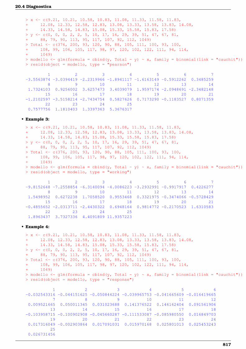
20.4 Diagnostica
> x <- c(9.21, 10.21, 10.58, 10.83, 11.08, 11.33, 11.58, 11.83,+ 12.08, 12.33, 12.58, 12.83, 13.08, 13.33, 13.58, 13.83, 14.08,+ 14.33, 14.58, 14.83, 15.08, 15.33, 15.58, 15.83, 17.58)> y <- c(0, 0, 0, 2, 2, 5, 10, 17, 16, 29, 39, 51, 47, 67, 81,+ 88, 79, 90, 113, 95, 117, 107, 92, 112, 1049)> Total <- c(376, 200, 93, 120, 90, 88, 105, 111, 100, 93, 100,+ 108, 99, 106, 105, 117, 98, 97, 120, 102, 122, 111, 94, 114,+ 1049)> modello <- glm(formula = cbind(y, Total - y) ~ x, family = binomial(link = "cauchit"))> resid(object = modello, type = "pearson")
1 2 3 4 5 6 7-3.5563874 -3.0394419 -2.2319966 -1.8941117 -1.6163149 -0.5912262 0.3485259
8 9 10 11 12 13 141.7324103 0.9256002 3.6257473 3.4039079 1.9597174 -2.0948691 -2.3482148
15 16 17 18 19 20 21-1.2102597 -3.5158214 -2.7434754 0.5827626 0.7173290 -0.1183527 0.8071359
22 23 24 250.7577756 1.1810403 1.3397363 5.3676317
• Example 3:
> x <- c(9.21, 10.21, 10.58, 10.83, 11.08, 11.33, 11.58, 11.83,+ 12.08, 12.33, 12.58, 12.83, 13.08, 13.33, 13.58, 13.83, 14.08,+ 14.33, 14.58, 14.83, 15.08, 15.33, 15.58, 15.83, 17.58)> y <- c(0, 0, 0, 2, 2, 5, 10, 17, 16, 29, 39, 51, 47, 67, 81,+ 88, 79, 90, 113, 95, 117, 107, 92, 112, 1049)> Total <- c(376, 200, 93, 120, 90, 88, 105, 111, 100, 93, 100,+ 108, 99, 106, 105, 117, 98, 97, 120, 102, 122, 111, 94, 114,+ 1049)> modello <- glm(formula = cbind(y, Total - y) ~ x, family = binomial(link = "cauchit"))> resid(object = modello, type = "working")
1 2 3 4 5 6 7-9.8152648 -7.2558854 -6.3140094 -4.0086223 -3.2932991 -0.9917917 0.4226277
8 9 10 11 12 13 141.5498952 0.6272238 1.7058520 0.9553468 0.3321975 -0.3474066 -0.5728429
15 16 17 18 19 20 21-0.4855652 -2.0313711 -2.4430322 0.6948164 0.9814772 -0.2170523 1.6310583
22 23 24 251.8963437 3.7327336 4.4091809 11.9357223
• Example 4:
> x <- c(9.21, 10.21, 10.58, 10.83, 11.08, 11.33, 11.58, 11.83,+ 12.08, 12.33, 12.58, 12.83, 13.08, 13.33, 13.58, 13.83, 14.08,+ 14.33, 14.58, 14.83, 15.08, 15.33, 15.58, 15.83, 17.58)> y <- c(0, 0, 0, 2, 2, 5, 10, 17, 16, 29, 39, 51, 47, 67, 81,+ 88, 79, 90, 113, 95, 117, 107, 92, 112, 1049)> Total <- c(376, 200, 93, 120, 90, 88, 105, 111, 100, 93, 100,+ 108, 99, 106, 105, 117, 98, 97, 120, 102, 122, 111, 94, 114,+ 1049)> modello <- glm(formula = cbind(y, Total - y) ~ x, family = binomial(link = "cauchit"))> resid(object = modello, type = "response")
1 2 3 4 5 6-0.032543316 -0.044151625 -0.050844224 -0.039965753 -0.041665609 -0.016419665
7 8 9 10 11 120.009521665 0.050011345 0.031023688 0.141376522 0.146162404 0.091561906
13 14 15 16 17 18-0.103958715 -0.100902908 -0.045660287 -0.111533087 -0.085980550 0.016849703
19 20 21 22 23 240.017316049 -0.002903864 0.017091031 0.015970168 0.025801013 0.025453243
250.026731456
817
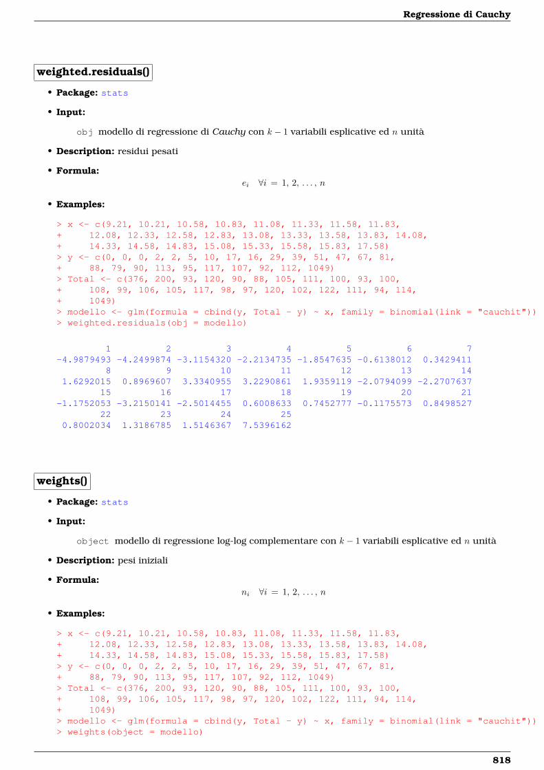
Regressione di Cauchy
weighted.residuals()
• Package: stats
• Input:
obj modello di regressione di Cauchy con k − 1 variabili esplicative ed n unità
• Description: residui pesati
• Formula:ei ∀i = 1, 2, . . . , n
• Examples:
> x <- c(9.21, 10.21, 10.58, 10.83, 11.08, 11.33, 11.58, 11.83,+ 12.08, 12.33, 12.58, 12.83, 13.08, 13.33, 13.58, 13.83, 14.08,+ 14.33, 14.58, 14.83, 15.08, 15.33, 15.58, 15.83, 17.58)> y <- c(0, 0, 0, 2, 2, 5, 10, 17, 16, 29, 39, 51, 47, 67, 81,+ 88, 79, 90, 113, 95, 117, 107, 92, 112, 1049)> Total <- c(376, 200, 93, 120, 90, 88, 105, 111, 100, 93, 100,+ 108, 99, 106, 105, 117, 98, 97, 120, 102, 122, 111, 94, 114,+ 1049)> modello <- glm(formula = cbind(y, Total - y) ~ x, family = binomial(link = "cauchit"))> weighted.residuals(obj = modello)
1 2 3 4 5 6 7-4.9879493 -4.2499874 -3.1154320 -2.2134735 -1.8547635 -0.6138012 0.3429411
8 9 10 11 12 13 141.6292015 0.8969607 3.3340955 3.2290861 1.9359119 -2.0794099 -2.2707637
15 16 17 18 19 20 21-1.1752053 -3.2150141 -2.5014455 0.6008633 0.7452777 -0.1175573 0.8498527
22 23 24 250.8002034 1.3186785 1.5146367 7.5396162
weights()
• Package: stats
• Input:
object modello di regressione log-log complementare con k − 1 variabili esplicative ed n unità
• Description: pesi iniziali
• Formula:ni ∀i = 1, 2, . . . , n
• Examples:
> x <- c(9.21, 10.21, 10.58, 10.83, 11.08, 11.33, 11.58, 11.83,+ 12.08, 12.33, 12.58, 12.83, 13.08, 13.33, 13.58, 13.83, 14.08,+ 14.33, 14.58, 14.83, 15.08, 15.33, 15.58, 15.83, 17.58)> y <- c(0, 0, 0, 2, 2, 5, 10, 17, 16, 29, 39, 51, 47, 67, 81,+ 88, 79, 90, 113, 95, 117, 107, 92, 112, 1049)> Total <- c(376, 200, 93, 120, 90, 88, 105, 111, 100, 93, 100,+ 108, 99, 106, 105, 117, 98, 97, 120, 102, 122, 111, 94, 114,+ 1049)> modello <- glm(formula = cbind(y, Total - y) ~ x, family = binomial(link = "cauchit"))> weights(object = modello)
818
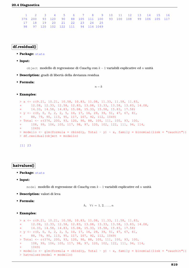
20.4 Diagnostica
1 2 3 4 5 6 7 8 9 10 11 12 13 14 15 16376 200 93 120 90 88 105 111 100 93 100 108 99 106 105 11717 18 19 20 21 22 23 24 2598 97 120 102 122 111 94 114 1049
df.residual()
• Package: stats
• Input:
object modello di regressione di Cauchy con k − 1 variabili esplicative ed n unità
• Description: gradi di libertà della devianza residua
• Formula:n− k
• Examples:
> x <- c(9.21, 10.21, 10.58, 10.83, 11.08, 11.33, 11.58, 11.83,+ 12.08, 12.33, 12.58, 12.83, 13.08, 13.33, 13.58, 13.83, 14.08,+ 14.33, 14.58, 14.83, 15.08, 15.33, 15.58, 15.83, 17.58)> y <- c(0, 0, 0, 2, 2, 5, 10, 17, 16, 29, 39, 51, 47, 67, 81,+ 88, 79, 90, 113, 95, 117, 107, 92, 112, 1049)> Total <- c(376, 200, 93, 120, 90, 88, 105, 111, 100, 93, 100,+ 108, 99, 106, 105, 117, 98, 97, 120, 102, 122, 111, 94, 114,+ 1049)> modello <- glm(formula = cbind(y, Total - y) ~ x, family = binomial(link = "cauchit"))> df.residual(object = modello)
[1] 23
hatvalues()
• Package: stats
• Input:
model modello di regressione di Cauchy con k − 1 variabili esplicative ed n unità
• Description: valori di leva
• Formula:hi ∀ i = 1, 2, . . . , n
• Examples:
> x <- c(9.21, 10.21, 10.58, 10.83, 11.08, 11.33, 11.58, 11.83,+ 12.08, 12.33, 12.58, 12.83, 13.08, 13.33, 13.58, 13.83, 14.08,+ 14.33, 14.58, 14.83, 15.08, 15.33, 15.58, 15.83, 17.58)> y <- c(0, 0, 0, 2, 2, 5, 10, 17, 16, 29, 39, 51, 47, 67, 81,+ 88, 79, 90, 113, 95, 117, 107, 92, 112, 1049)> Total <- c(376, 200, 93, 120, 90, 88, 105, 111, 100, 93, 100,+ 108, 99, 106, 105, 117, 98, 97, 120, 102, 122, 111, 94, 114,+ 1049)> modello <- glm(formula = cbind(y, Total - y) ~ x, family = binomial(link = "cauchit"))> hatvalues(model = modello)
819
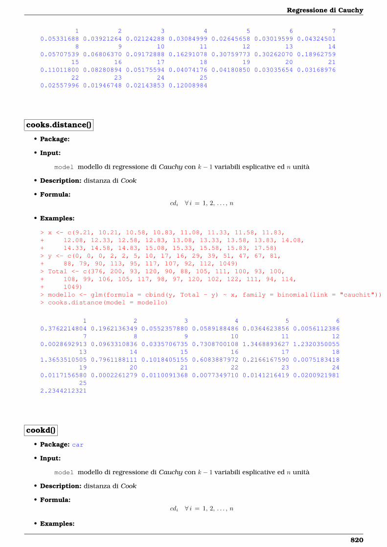
Regressione di Cauchy
1 2 3 4 5 6 70.05331688 0.03921264 0.02124288 0.03084999 0.02645658 0.03019599 0.04324501
8 9 10 11 12 13 140.05707539 0.06806370 0.09172888 0.16291078 0.30759773 0.30262070 0.18962759
15 16 17 18 19 20 210.11011800 0.08280894 0.05175594 0.04074176 0.04180850 0.03035654 0.03168976
22 23 24 250.02557996 0.01946748 0.02143853 0.12008984
cooks.distance()
• Package:
• Input:
model modello di regressione di Cauchy con k − 1 variabili esplicative ed n unità
• Description: distanza di Cook
• Formula:cdi ∀ i = 1, 2, . . . , n
• Examples:
> x <- c(9.21, 10.21, 10.58, 10.83, 11.08, 11.33, 11.58, 11.83,+ 12.08, 12.33, 12.58, 12.83, 13.08, 13.33, 13.58, 13.83, 14.08,+ 14.33, 14.58, 14.83, 15.08, 15.33, 15.58, 15.83, 17.58)> y <- c(0, 0, 0, 2, 2, 5, 10, 17, 16, 29, 39, 51, 47, 67, 81,+ 88, 79, 90, 113, 95, 117, 107, 92, 112, 1049)> Total <- c(376, 200, 93, 120, 90, 88, 105, 111, 100, 93, 100,+ 108, 99, 106, 105, 117, 98, 97, 120, 102, 122, 111, 94, 114,+ 1049)> modello <- glm(formula = cbind(y, Total - y) ~ x, family = binomial(link = "cauchit"))> cooks.distance(model = modello)
1 2 3 4 5 60.3762214804 0.1962136349 0.0552357880 0.0589188486 0.0364623856 0.0056112386
7 8 9 10 11 120.0028692913 0.0963310836 0.0335706735 0.7308700108 1.3468893627 1.2320350055
13 14 15 16 17 181.3653510505 0.7961188111 0.1018405155 0.6083887972 0.2166167590 0.0075183418
19 20 21 22 23 240.0117156580 0.0002261279 0.0110091368 0.0077349710 0.0141216419 0.0200921981
252.2344212321
cookd()
• Package: car
• Input:
model modello di regressione di Cauchy con k − 1 variabili esplicative ed n unità
• Description: distanza di Cook
• Formula:cdi ∀ i = 1, 2, . . . , n
• Examples:
820

20.4 Diagnostica
> x <- c(9.21, 10.21, 10.58, 10.83, 11.08, 11.33, 11.58, 11.83,+ 12.08, 12.33, 12.58, 12.83, 13.08, 13.33, 13.58, 13.83, 14.08,+ 14.33, 14.58, 14.83, 15.08, 15.33, 15.58, 15.83, 17.58)> y <- c(0, 0, 0, 2, 2, 5, 10, 17, 16, 29, 39, 51, 47, 67, 81,+ 88, 79, 90, 113, 95, 117, 107, 92, 112, 1049)> Total <- c(376, 200, 93, 120, 90, 88, 105, 111, 100, 93, 100,+ 108, 99, 106, 105, 117, 98, 97, 120, 102, 122, 111, 94, 114,+ 1049)> modello <- glm(formula = cbind(y, Total - y) ~ x, family = binomial(link = "cauchit"))> cookd(model = modello)
1 2 3 4 5 60.3762214804 0.1962136349 0.0552357880 0.0589188486 0.0364623856 0.0056112386
7 8 9 10 11 120.0028692913 0.0963310836 0.0335706735 0.7308700108 1.3468893627 1.2320350055
13 14 15 16 17 181.3653510505 0.7961188111 0.1018405155 0.6083887972 0.2166167590 0.0075183418
19 20 21 22 23 240.0117156580 0.0002261279 0.0110091368 0.0077349710 0.0141216419 0.0200921981
252.2344212321
821

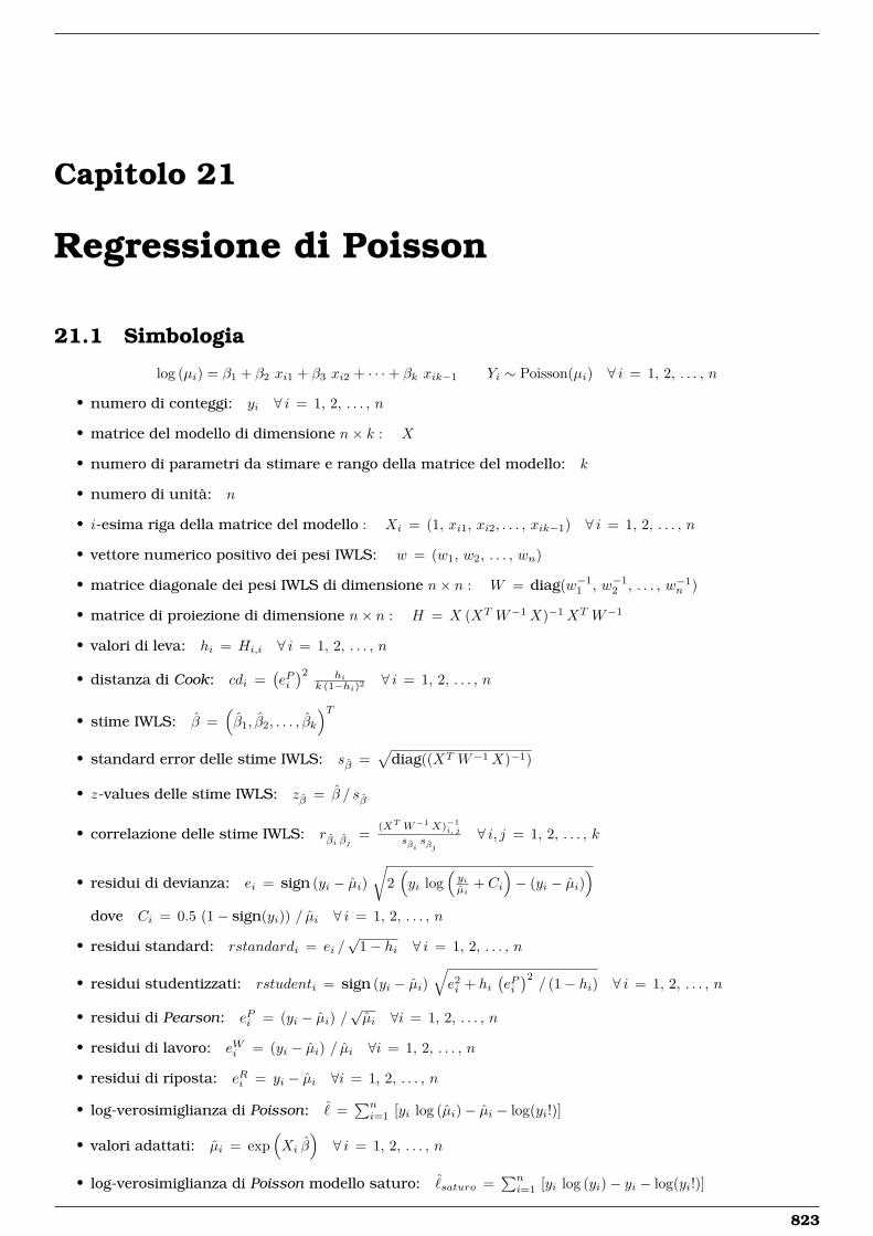
Capitolo 21
Regressione di Poisson
21.1 Simbologia
log (µi) = β1 + β2 xi1 + β3 xi2 + · · ·+ βk xik−1 Yi ∼ Poisson(µi) ∀ i = 1, 2, . . . , n
• numero di conteggi: yi ∀ i = 1, 2, . . . , n
• matrice del modello di dimensione n× k : X
• numero di parametri da stimare e rango della matrice del modello: k
• numero di unità: n
• i-esima riga della matrice del modello : Xi = (1, xi1, xi2, . . . , xik−1) ∀ i = 1, 2, . . . , n
• vettore numerico positivo dei pesi IWLS: w = (w1, w2, . . . , wn)
• matrice diagonale dei pesi IWLS di dimensione n× n : W = diag(w−11 , w−1
2 , . . . , w−1n )
• matrice di proiezione di dimensione n× n : H = X (XT W−1X)−1XT W−1
• valori di leva: hi = Hi,i ∀ i = 1, 2, . . . , n
• distanza di Cook: cdi =(ePi)2 hi
k (1−hi)2 ∀ i = 1, 2, . . . , n
• stime IWLS: β =(β1, β2, . . . , βk
)T• standard error delle stime IWLS: sβ =
√diag((XT W−1X)−1)
• z-values delle stime IWLS: zβ = β / sβ
• correlazione delle stime IWLS: rβi βj =(XT W−1X)−1
i, j
sβisβj
∀ i, j = 1, 2, . . . , k
• residui di devianza: ei = sign (yi − µi)√
2(yi log
(yiµi
+ Ci
)− (yi − µi)
)dove Ci = 0.5 (1− sign(yi)) / µi ∀ i = 1, 2, . . . , n
• residui standard: rstandardi = ei /√
1− hi ∀ i = 1, 2, . . . , n
• residui studentizzati: rstudenti = sign (yi − µi)√e2i + hi
(ePi)2/ (1− hi) ∀ i = 1, 2, . . . , n
• residui di Pearson: ePi = (yi − µi) /√µi ∀i = 1, 2, . . . , n
• residui di lavoro: eWi = (yi − µi) / µi ∀i = 1, 2, . . . , n
• residui di riposta: eRi = yi − µi ∀i = 1, 2, . . . , n
• log-verosimiglianza di Poisson: ˆ =∑ni=1 [yi log (µi)− µi − log(yi!)]
• valori adattati: µi = exp(Xi β
)∀ i = 1, 2, . . . , n
• log-verosimiglianza di Poisson modello saturo: ˆsaturo =
∑ni=1 [yi log (yi)− yi − log(yi!)]
823
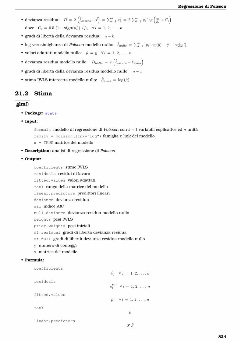
Regressione di Poisson
• devianza residua: D = 2(
ˆsaturo − ˆ
)=∑ni=1 e
2i = 2
∑ni=1 yi log
(yiµi
+ Ci
)dove Ci = 0.5 (1− sign(yi)) / µi ∀ i = 1, 2, . . . , n
• gradi di libertà della devianza residua: n− k
• log-verosimiglianza di Poisson modello nullo: ˆnullo =
∑ni=1 [yi log (y)− y − log(yi!)]
• valori adattati modello nullo: µ = y ∀ i = 1, 2, . . . , n
• devianza residua modello nullo: Dnullo = 2(
ˆsaturo − ˆ
nullo
)• gradi di libertà della devianza residua modello nullo: n− 1
• stima IWLS intercetta modello nullo: βnullo = log (µ)
21.2 Stima
glm()
• Package: stats
• Input:
formula modello di regressione di Poisson con k − 1 variabili esplicative ed n unità
family = poisson(link="log") famiglia e link del modello
x = TRUE matrice del modello
• Description: analisi di regressione di Poisson
• Output:
coefficients stime IWLS
residuals residui di lavoro
fitted.values valori adattati
rank rango della matrice del modello
linear.predictors predittori lineari
deviance devianza residua
aic indice AIC
null.deviance devianza residua modello nullo
weights pesi IWLS
prior.weights pesi iniziali
df.residual gradi di libertà devianza residua
df.null gradi di libertà devianza residua modello nullo
y numero di conteggi
x matrice del modello
• Formula:
coefficientsβj ∀ j = 1, 2, . . . , k
residualseWi ∀ i = 1, 2, . . . , n
fitted.valuesµi ∀ i = 1, 2, . . . , n
rankk
linear.predictorsX β
824
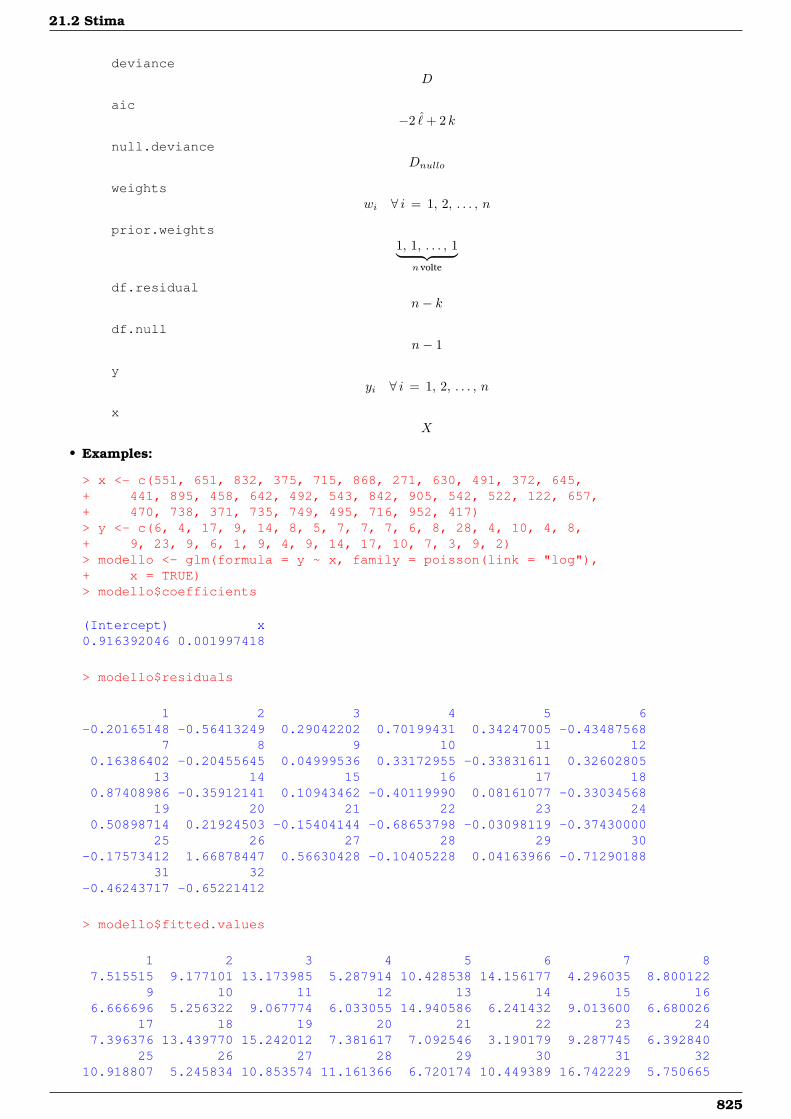
21.2 Stima
devianceD
aic−2 ˆ+ 2 k
null.devianceDnullo
weightswi ∀ i = 1, 2, . . . , n
prior.weights1, 1, . . . , 1︸ ︷︷ ︸
n volte
df.residualn− k
df.nulln− 1
yyi ∀ i = 1, 2, . . . , n
xX
• Examples:
> x <- c(551, 651, 832, 375, 715, 868, 271, 630, 491, 372, 645,+ 441, 895, 458, 642, 492, 543, 842, 905, 542, 522, 122, 657,+ 470, 738, 371, 735, 749, 495, 716, 952, 417)> y <- c(6, 4, 17, 9, 14, 8, 5, 7, 7, 7, 6, 8, 28, 4, 10, 4, 8,+ 9, 23, 9, 6, 1, 9, 4, 9, 14, 17, 10, 7, 3, 9, 2)> modello <- glm(formula = y ~ x, family = poisson(link = "log"),+ x = TRUE)> modello$coefficients
(Intercept) x0.916392046 0.001997418
> modello$residuals
1 2 3 4 5 6-0.20165148 -0.56413249 0.29042202 0.70199431 0.34247005 -0.43487568
7 8 9 10 11 120.16386402 -0.20455645 0.04999536 0.33172955 -0.33831611 0.32602805
13 14 15 16 17 180.87408986 -0.35912141 0.10943462 -0.40119990 0.08161077 -0.33034568
19 20 21 22 23 240.50898714 0.21924503 -0.15404144 -0.68653798 -0.03098119 -0.37430000
25 26 27 28 29 30-0.17573412 1.66878447 0.56630428 -0.10405228 0.04163966 -0.71290188
31 32-0.46243717 -0.65221412
> modello$fitted.values
1 2 3 4 5 6 7 87.515515 9.177101 13.173985 5.287914 10.428538 14.156177 4.296035 8.800122
9 10 11 12 13 14 15 166.666696 5.256322 9.067774 6.033055 14.940586 6.241432 9.013600 6.680026
17 18 19 20 21 22 23 247.396376 13.439770 15.242012 7.381617 7.092546 3.190179 9.287745 6.392840
25 26 27 28 29 30 31 3210.918807 5.245834 10.853574 11.161366 6.720174 10.449389 16.742229 5.750665
825
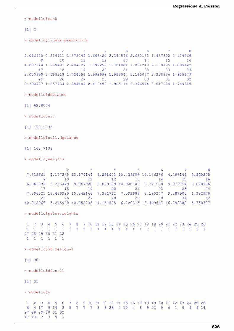
Regressione di Poisson
> modello$rank
[1] 2
> modello$linear.predictors
1 2 3 4 5 6 7 82.016970 2.216711 2.578244 1.665424 2.344546 2.650151 1.457692 2.174766
9 10 11 12 13 14 15 161.897124 1.659432 2.204727 1.797253 2.704081 1.831210 2.198735 1.899122
17 18 19 20 21 22 23 242.000990 2.598218 2.724056 1.998993 1.959044 1.160077 2.228696 1.855179
25 26 27 28 29 30 31 322.390487 1.657434 2.384494 2.412458 1.905114 2.346544 2.817934 1.749315
> modello$deviance
[1] 62.8054
> modello$aic
[1] 190.1035
> modello$null.deviance
[1] 103.7138
> modello$weights
1 2 3 4 5 6 7 87.515661 9.177255 13.174144 5.288041 10.428696 14.156336 4.296149 8.800275
9 10 11 12 13 14 15 166.666836 5.256449 9.067928 6.033189 14.940742 6.241568 9.013754 6.680166
17 18 19 20 21 22 23 247.396521 13.439929 15.242168 7.381762 7.092689 3.190277 9.287900 6.392978
25 26 27 28 29 30 31 3210.918966 5.245960 10.853733 11.161525 6.720315 10.449547 16.742380 5.750797
> modello$prior.weights
1 2 3 4 5 6 7 8 9 10 11 12 13 14 15 16 17 18 19 20 21 22 23 24 25 261 1 1 1 1 1 1 1 1 1 1 1 1 1 1 1 1 1 1 1 1 1 1 1 1 1
27 28 29 30 31 321 1 1 1 1 1
> modello$df.residual
[1] 30
> modello$df.null
[1] 31
> modello$y
1 2 3 4 5 6 7 8 9 10 11 12 13 14 15 16 17 18 19 20 21 22 23 24 25 266 4 17 9 14 8 5 7 7 7 6 8 28 4 10 4 8 9 23 9 6 1 9 4 9 14
27 28 29 30 31 3217 10 7 3 9 2
826
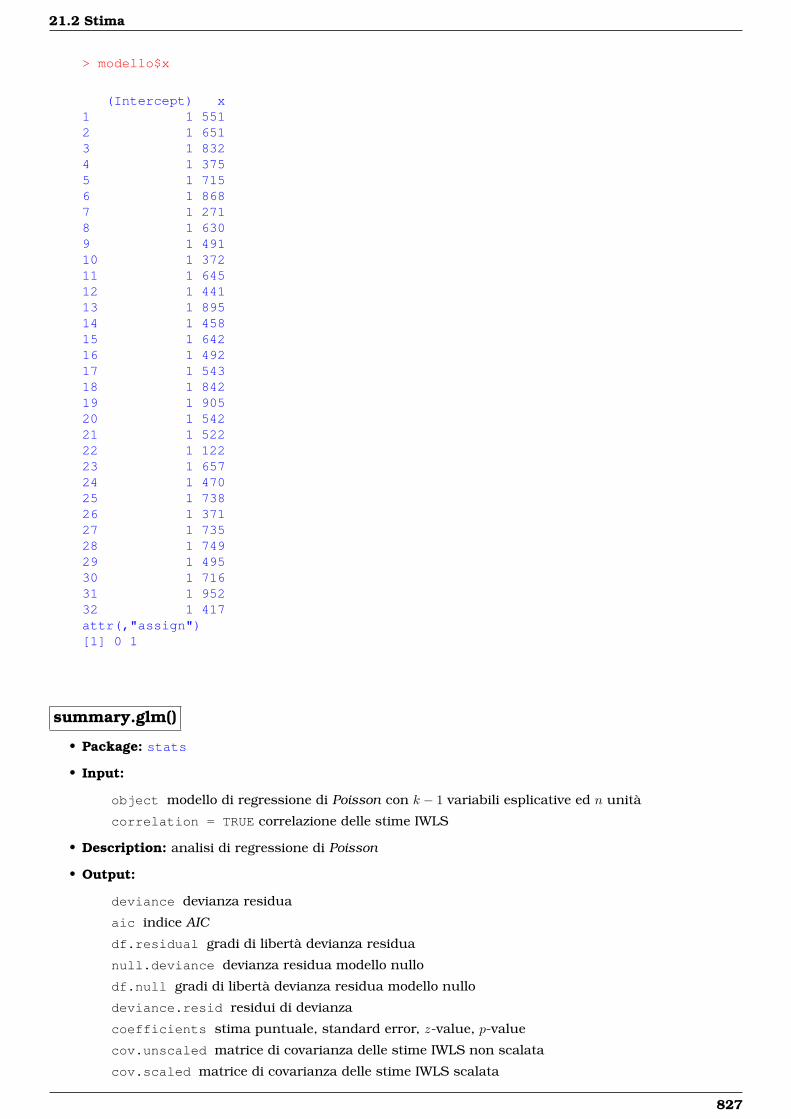
21.2 Stima
> modello$x
(Intercept) x1 1 5512 1 6513 1 8324 1 3755 1 7156 1 8687 1 2718 1 6309 1 49110 1 37211 1 64512 1 44113 1 89514 1 45815 1 64216 1 49217 1 54318 1 84219 1 90520 1 54221 1 52222 1 12223 1 65724 1 47025 1 73826 1 37127 1 73528 1 74929 1 49530 1 71631 1 95232 1 417attr(,"assign")[1] 0 1
summary.glm()
• Package: stats
• Input:
object modello di regressione di Poisson con k − 1 variabili esplicative ed n unità
correlation = TRUE correlazione delle stime IWLS
• Description: analisi di regressione di Poisson
• Output:
deviance devianza residua
aic indice AIC
df.residual gradi di libertà devianza residua
null.deviance devianza residua modello nullo
df.null gradi di libertà devianza residua modello nullo
deviance.resid residui di devianza
coefficients stima puntuale, standard error, z-value, p-value
cov.unscaled matrice di covarianza delle stime IWLS non scalata
cov.scaled matrice di covarianza delle stime IWLS scalata
827
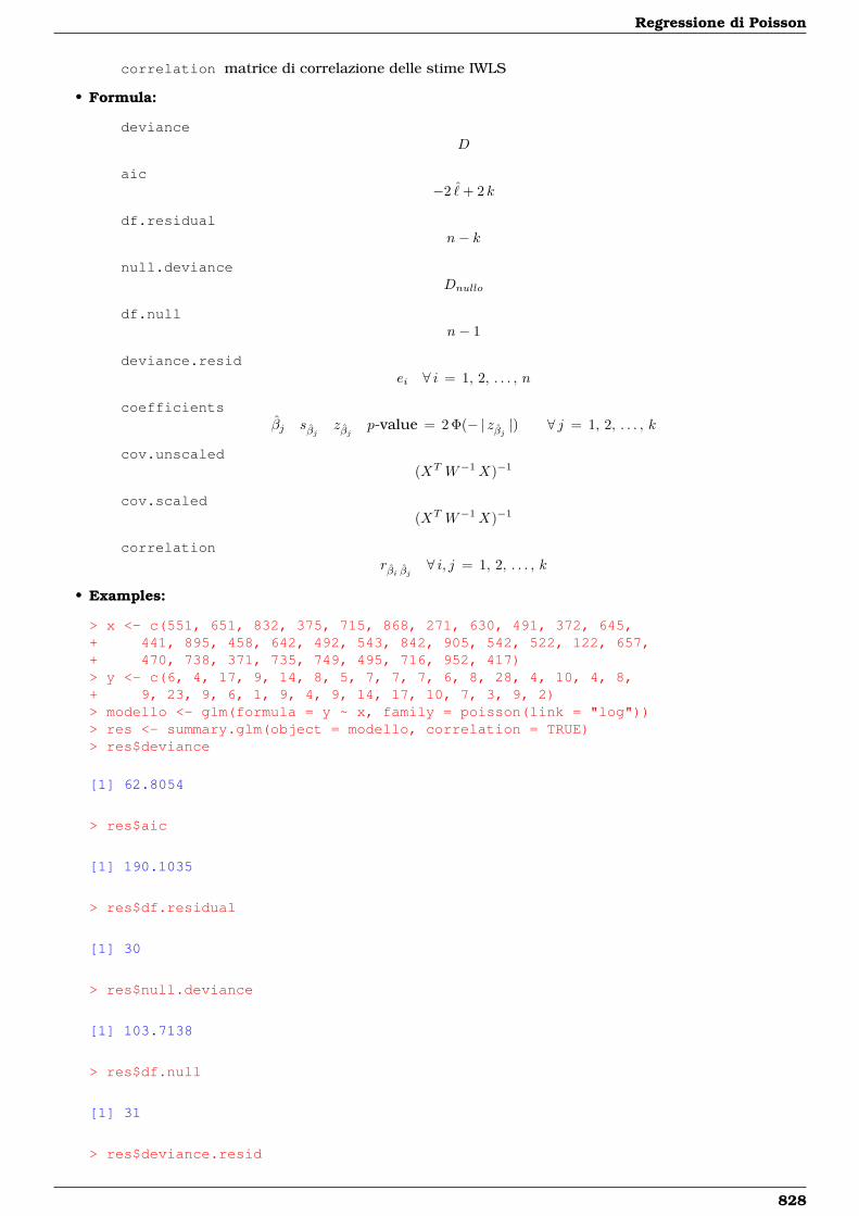
Regressione di Poisson
correlation matrice di correlazione delle stime IWLS
• Formula:
devianceD
aic−2 ˆ+ 2 k
df.residualn− k
null.devianceDnullo
df.nulln− 1
deviance.residei ∀ i = 1, 2, . . . , n
coefficientsβj sβj zβj p-value = 2 Φ(− | zβj |) ∀ j = 1, 2, . . . , k
cov.unscaled(XT W−1X)−1
cov.scaled(XT W−1X)−1
correlationrβi βj ∀ i, j = 1, 2, . . . , k
• Examples:
> x <- c(551, 651, 832, 375, 715, 868, 271, 630, 491, 372, 645,+ 441, 895, 458, 642, 492, 543, 842, 905, 542, 522, 122, 657,+ 470, 738, 371, 735, 749, 495, 716, 952, 417)> y <- c(6, 4, 17, 9, 14, 8, 5, 7, 7, 7, 6, 8, 28, 4, 10, 4, 8,+ 9, 23, 9, 6, 1, 9, 4, 9, 14, 17, 10, 7, 3, 9, 2)> modello <- glm(formula = y ~ x, family = poisson(link = "log"))> res <- summary.glm(object = modello, correlation = TRUE)> res$deviance
[1] 62.8054
> res$aic
[1] 190.1035
> res$df.residual
[1] 30
> res$null.deviance
[1] 103.7138
> res$df.null
[1] 31
> res$deviance.resid
828
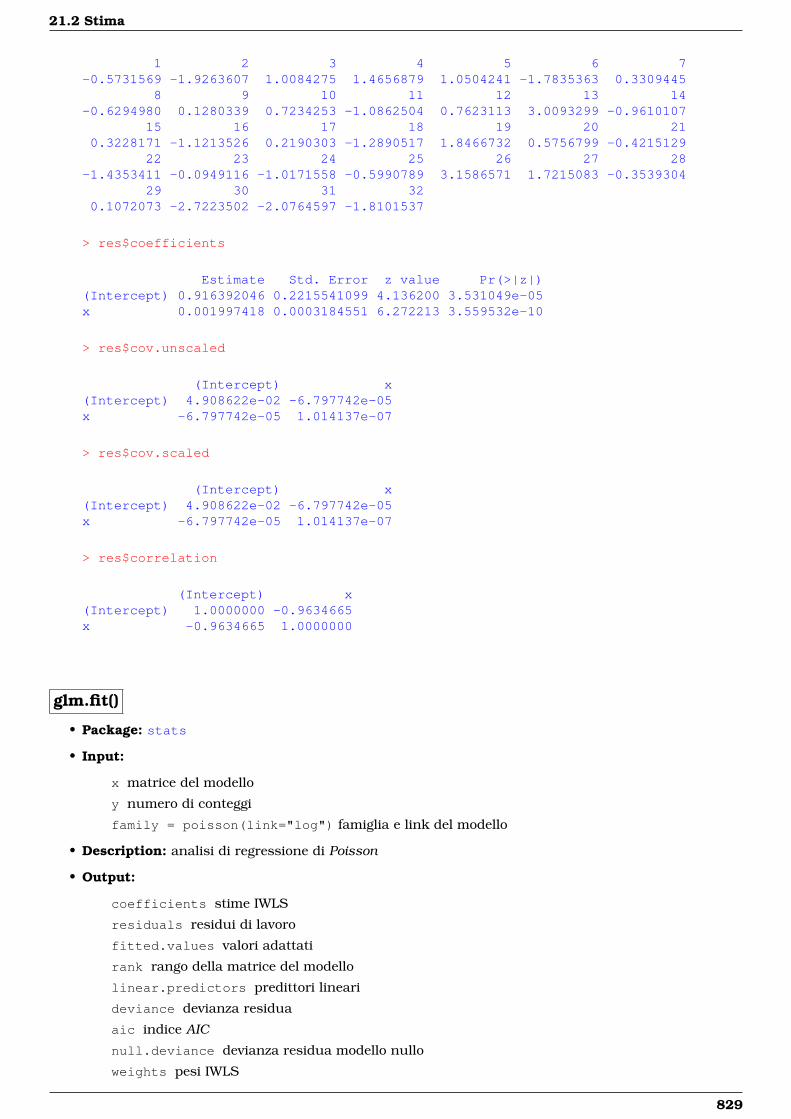
21.2 Stima
1 2 3 4 5 6 7-0.5731569 -1.9263607 1.0084275 1.4656879 1.0504241 -1.7835363 0.3309445
8 9 10 11 12 13 14-0.6294980 0.1280339 0.7234253 -1.0862504 0.7623113 3.0093299 -0.9610107
15 16 17 18 19 20 210.3228171 -1.1213526 0.2190303 -1.2890517 1.8466732 0.5756799 -0.4215129
22 23 24 25 26 27 28-1.4353411 -0.0949116 -1.0171558 -0.5990789 3.1586571 1.7215083 -0.3539304
29 30 31 320.1072073 -2.7223502 -2.0764597 -1.8101537
> res$coefficients
Estimate Std. Error z value Pr(>|z|)(Intercept) 0.916392046 0.2215541099 4.136200 3.531049e-05x 0.001997418 0.0003184551 6.272213 3.559532e-10
> res$cov.unscaled
(Intercept) x(Intercept) 4.908622e-02 -6.797742e-05x -6.797742e-05 1.014137e-07
> res$cov.scaled
(Intercept) x(Intercept) 4.908622e-02 -6.797742e-05x -6.797742e-05 1.014137e-07
> res$correlation
(Intercept) x(Intercept) 1.0000000 -0.9634665x -0.9634665 1.0000000
glm.fit()
• Package: stats
• Input:
x matrice del modello
y numero di conteggi
family = poisson(link="log") famiglia e link del modello
• Description: analisi di regressione di Poisson
• Output:
coefficients stime IWLS
residuals residui di lavoro
fitted.values valori adattati
rank rango della matrice del modello
linear.predictors predittori lineari
deviance devianza residua
aic indice AIC
null.deviance devianza residua modello nullo
weights pesi IWLS
829
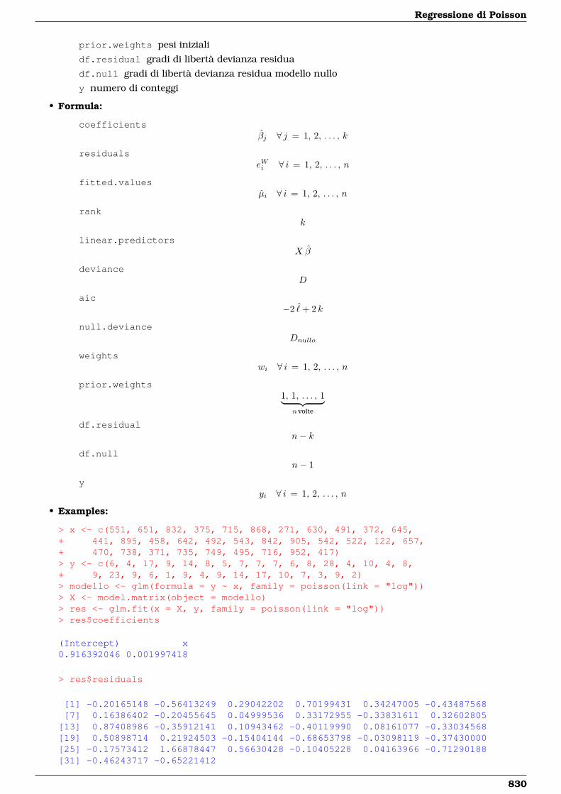
Regressione di Poisson
prior.weights pesi iniziali
df.residual gradi di libertà devianza residua
df.null gradi di libertà devianza residua modello nullo
y numero di conteggi
• Formula:
coefficientsβj ∀ j = 1, 2, . . . , k
residualseWi ∀ i = 1, 2, . . . , n
fitted.valuesµi ∀ i = 1, 2, . . . , n
rankk
linear.predictorsX β
devianceD
aic−2 ˆ+ 2 k
null.devianceDnullo
weightswi ∀ i = 1, 2, . . . , n
prior.weights1, 1, . . . , 1︸ ︷︷ ︸
n volte
df.residualn− k
df.nulln− 1
yyi ∀ i = 1, 2, . . . , n
• Examples:
> x <- c(551, 651, 832, 375, 715, 868, 271, 630, 491, 372, 645,+ 441, 895, 458, 642, 492, 543, 842, 905, 542, 522, 122, 657,+ 470, 738, 371, 735, 749, 495, 716, 952, 417)> y <- c(6, 4, 17, 9, 14, 8, 5, 7, 7, 7, 6, 8, 28, 4, 10, 4, 8,+ 9, 23, 9, 6, 1, 9, 4, 9, 14, 17, 10, 7, 3, 9, 2)> modello <- glm(formula = y ~ x, family = poisson(link = "log"))> X <- model.matrix(object = modello)> res <- glm.fit(x = X, y, family = poisson(link = "log"))> res$coefficients
(Intercept) x0.916392046 0.001997418
> res$residuals
[1] -0.20165148 -0.56413249 0.29042202 0.70199431 0.34247005 -0.43487568[7] 0.16386402 -0.20455645 0.04999536 0.33172955 -0.33831611 0.32602805
[13] 0.87408986 -0.35912141 0.10943462 -0.40119990 0.08161077 -0.33034568[19] 0.50898714 0.21924503 -0.15404144 -0.68653798 -0.03098119 -0.37430000[25] -0.17573412 1.66878447 0.56630428 -0.10405228 0.04163966 -0.71290188[31] -0.46243717 -0.65221412
830
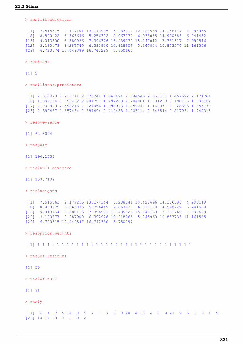
21.2 Stima
> res$fitted.values
[1] 7.515515 9.177101 13.173985 5.287914 10.428538 14.156177 4.296035[8] 8.800122 6.666696 5.256322 9.067774 6.033055 14.940586 6.241432
[15] 9.013600 6.680026 7.396376 13.439770 15.242012 7.381617 7.092546[22] 3.190179 9.287745 6.392840 10.918807 5.245834 10.853574 11.161366[29] 6.720174 10.449389 16.742229 5.750665
> res$rank
[1] 2
> res$linear.predictors
[1] 2.016970 2.216711 2.578244 1.665424 2.344546 2.650151 1.457692 2.174766[9] 1.897124 1.659432 2.204727 1.797253 2.704081 1.831210 2.198735 1.899122
[17] 2.000990 2.598218 2.724056 1.998993 1.959044 1.160077 2.228696 1.855179[25] 2.390487 1.657434 2.384494 2.412458 1.905114 2.346544 2.817934 1.749315
> res$deviance
[1] 62.8054
> res$aic
[1] 190.1035
> res$null.deviance
[1] 103.7138
> res$weights
[1] 7.515661 9.177255 13.174144 5.288041 10.428696 14.156336 4.296149[8] 8.800275 6.666836 5.256449 9.067928 6.033189 14.940742 6.241568
[15] 9.013754 6.680166 7.396521 13.439929 15.242168 7.381762 7.092689[22] 3.190277 9.287900 6.392978 10.918966 5.245960 10.853733 11.161525[29] 6.720315 10.449547 16.742380 5.750797
> res$prior.weights
[1] 1 1 1 1 1 1 1 1 1 1 1 1 1 1 1 1 1 1 1 1 1 1 1 1 1 1 1 1 1 1 1 1
> res$df.residual
[1] 30
> res$df.null
[1] 31
> res$y
[1] 6 4 17 9 14 8 5 7 7 7 6 8 28 4 10 4 8 9 23 9 6 1 9 4 9[26] 14 17 10 7 3 9 2
831
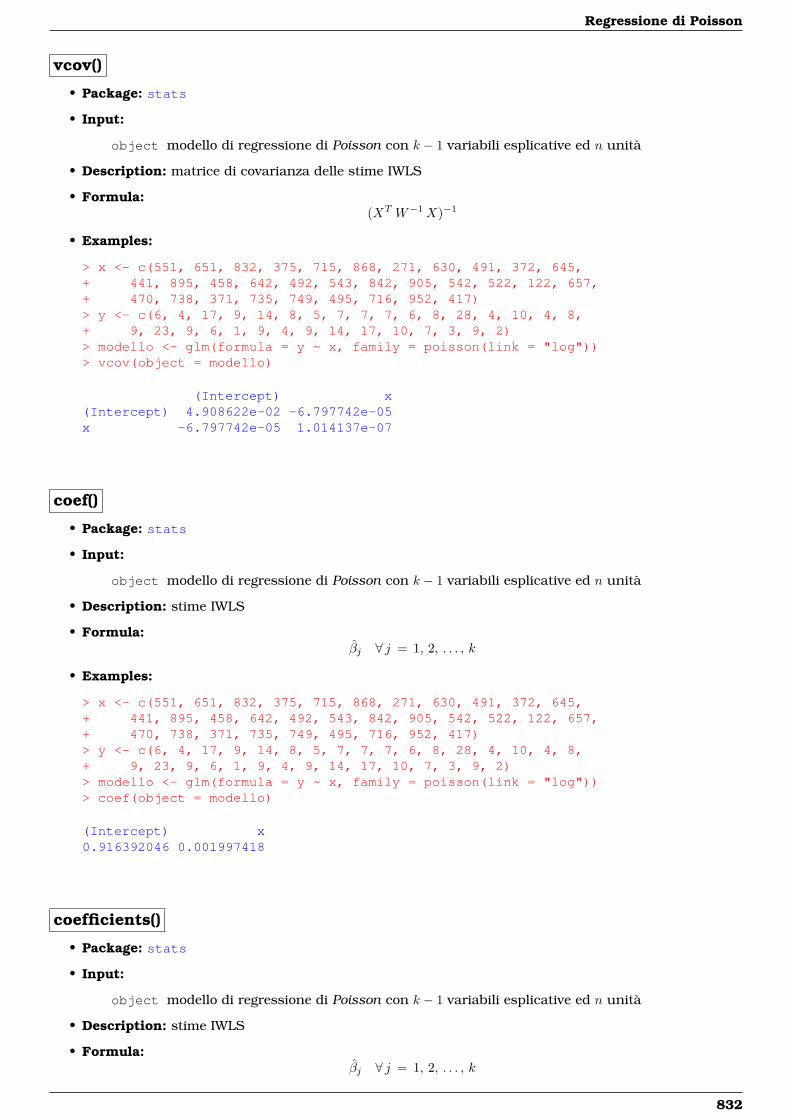
Regressione di Poisson
vcov()
• Package: stats
• Input:
object modello di regressione di Poisson con k − 1 variabili esplicative ed n unità
• Description: matrice di covarianza delle stime IWLS
• Formula:(XT W−1X)−1
• Examples:
> x <- c(551, 651, 832, 375, 715, 868, 271, 630, 491, 372, 645,+ 441, 895, 458, 642, 492, 543, 842, 905, 542, 522, 122, 657,+ 470, 738, 371, 735, 749, 495, 716, 952, 417)> y <- c(6, 4, 17, 9, 14, 8, 5, 7, 7, 7, 6, 8, 28, 4, 10, 4, 8,+ 9, 23, 9, 6, 1, 9, 4, 9, 14, 17, 10, 7, 3, 9, 2)> modello <- glm(formula = y ~ x, family = poisson(link = "log"))> vcov(object = modello)
(Intercept) x(Intercept) 4.908622e-02 -6.797742e-05x -6.797742e-05 1.014137e-07
coef()
• Package: stats
• Input:
object modello di regressione di Poisson con k − 1 variabili esplicative ed n unità
• Description: stime IWLS
• Formula:βj ∀ j = 1, 2, . . . , k
• Examples:
> x <- c(551, 651, 832, 375, 715, 868, 271, 630, 491, 372, 645,+ 441, 895, 458, 642, 492, 543, 842, 905, 542, 522, 122, 657,+ 470, 738, 371, 735, 749, 495, 716, 952, 417)> y <- c(6, 4, 17, 9, 14, 8, 5, 7, 7, 7, 6, 8, 28, 4, 10, 4, 8,+ 9, 23, 9, 6, 1, 9, 4, 9, 14, 17, 10, 7, 3, 9, 2)> modello <- glm(formula = y ~ x, family = poisson(link = "log"))> coef(object = modello)
(Intercept) x0.916392046 0.001997418
coefficients()
• Package: stats
• Input:
object modello di regressione di Poisson con k − 1 variabili esplicative ed n unità
• Description: stime IWLS
• Formula:βj ∀ j = 1, 2, . . . , k
832
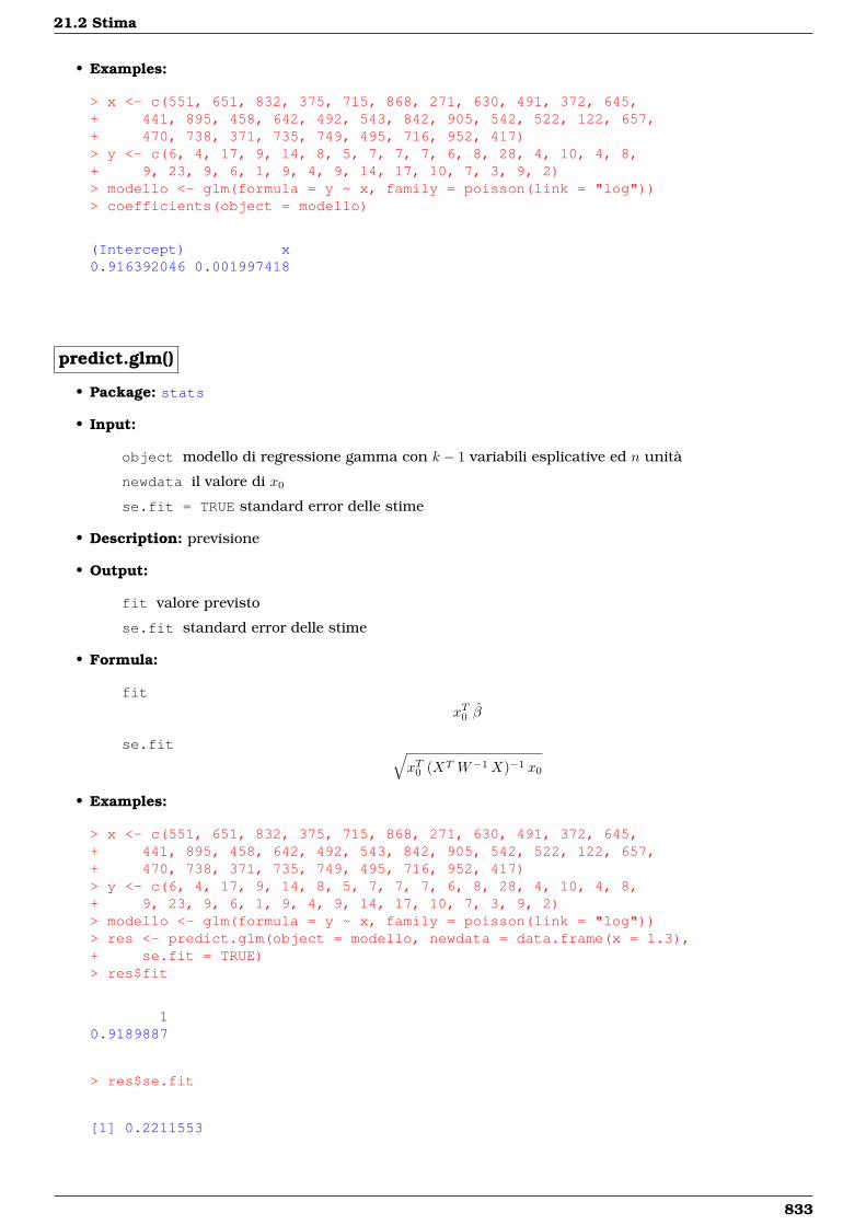
21.2 Stima
• Examples:
> x <- c(551, 651, 832, 375, 715, 868, 271, 630, 491, 372, 645,+ 441, 895, 458, 642, 492, 543, 842, 905, 542, 522, 122, 657,+ 470, 738, 371, 735, 749, 495, 716, 952, 417)> y <- c(6, 4, 17, 9, 14, 8, 5, 7, 7, 7, 6, 8, 28, 4, 10, 4, 8,+ 9, 23, 9, 6, 1, 9, 4, 9, 14, 17, 10, 7, 3, 9, 2)> modello <- glm(formula = y ~ x, family = poisson(link = "log"))> coefficients(object = modello)
(Intercept) x0.916392046 0.001997418
predict.glm()
• Package: stats
• Input:
object modello di regressione gamma con k − 1 variabili esplicative ed n unità
newdata il valore di x0
se.fit = TRUE standard error delle stime
• Description: previsione
• Output:
fit valore previsto
se.fit standard error delle stime
• Formula:
fit
xT0 β
se.fit √xT0 (XT W−1X)−1 x0
• Examples:
> x <- c(551, 651, 832, 375, 715, 868, 271, 630, 491, 372, 645,+ 441, 895, 458, 642, 492, 543, 842, 905, 542, 522, 122, 657,+ 470, 738, 371, 735, 749, 495, 716, 952, 417)> y <- c(6, 4, 17, 9, 14, 8, 5, 7, 7, 7, 6, 8, 28, 4, 10, 4, 8,+ 9, 23, 9, 6, 1, 9, 4, 9, 14, 17, 10, 7, 3, 9, 2)> modello <- glm(formula = y ~ x, family = poisson(link = "log"))> res <- predict.glm(object = modello, newdata = data.frame(x = 1.3),+ se.fit = TRUE)> res$fit
10.9189887
> res$se.fit
[1] 0.2211553
833
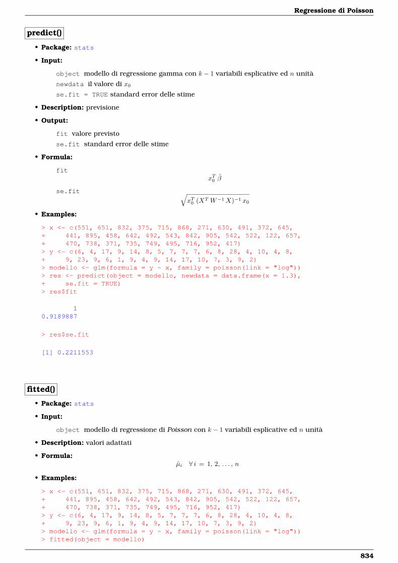
Regressione di Poisson
predict()
• Package: stats
• Input:
object modello di regressione gamma con k − 1 variabili esplicative ed n unità
newdata il valore di x0
se.fit = TRUE standard error delle stime
• Description: previsione
• Output:
fit valore previsto
se.fit standard error delle stime
• Formula:
fitxT0 β
se.fit √xT0 (XT W−1X)−1 x0
• Examples:
> x <- c(551, 651, 832, 375, 715, 868, 271, 630, 491, 372, 645,+ 441, 895, 458, 642, 492, 543, 842, 905, 542, 522, 122, 657,+ 470, 738, 371, 735, 749, 495, 716, 952, 417)> y <- c(6, 4, 17, 9, 14, 8, 5, 7, 7, 7, 6, 8, 28, 4, 10, 4, 8,+ 9, 23, 9, 6, 1, 9, 4, 9, 14, 17, 10, 7, 3, 9, 2)> modello <- glm(formula = y ~ x, family = poisson(link = "log"))> res <- predict(object = modello, newdata = data.frame(x = 1.3),+ se.fit = TRUE)> res$fit
10.9189887
> res$se.fit
[1] 0.2211553
fitted()
• Package: stats
• Input:
object modello di regressione di Poisson con k − 1 variabili esplicative ed n unità
• Description: valori adattati
• Formula:µi ∀ i = 1, 2, . . . , n
• Examples:
> x <- c(551, 651, 832, 375, 715, 868, 271, 630, 491, 372, 645,+ 441, 895, 458, 642, 492, 543, 842, 905, 542, 522, 122, 657,+ 470, 738, 371, 735, 749, 495, 716, 952, 417)> y <- c(6, 4, 17, 9, 14, 8, 5, 7, 7, 7, 6, 8, 28, 4, 10, 4, 8,+ 9, 23, 9, 6, 1, 9, 4, 9, 14, 17, 10, 7, 3, 9, 2)> modello <- glm(formula = y ~ x, family = poisson(link = "log"))> fitted(object = modello)
834
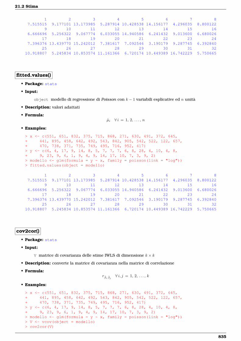
21.2 Stima
1 2 3 4 5 6 7 87.515515 9.177101 13.173985 5.287914 10.428538 14.156177 4.296035 8.800122
9 10 11 12 13 14 15 166.666696 5.256322 9.067774 6.033055 14.940586 6.241432 9.013600 6.680026
17 18 19 20 21 22 23 247.396376 13.439770 15.242012 7.381617 7.092546 3.190179 9.287745 6.392840
25 26 27 28 29 30 31 3210.918807 5.245834 10.853574 11.161366 6.720174 10.449389 16.742229 5.750665
fitted.values()
• Package: stats
• Input:
object modello di regressione di Poisson con k − 1 variabili esplicative ed n unità
• Description: valori adattati
• Formula:µi ∀ i = 1, 2, . . . , n
• Examples:
> x <- c(551, 651, 832, 375, 715, 868, 271, 630, 491, 372, 645,+ 441, 895, 458, 642, 492, 543, 842, 905, 542, 522, 122, 657,+ 470, 738, 371, 735, 749, 495, 716, 952, 417)> y <- c(6, 4, 17, 9, 14, 8, 5, 7, 7, 7, 6, 8, 28, 4, 10, 4, 8,+ 9, 23, 9, 6, 1, 9, 4, 9, 14, 17, 10, 7, 3, 9, 2)> modello <- glm(formula = y ~ x, family = poisson(link = "log"))> fitted.values(object = modello)
1 2 3 4 5 6 7 87.515515 9.177101 13.173985 5.287914 10.428538 14.156177 4.296035 8.800122
9 10 11 12 13 14 15 166.666696 5.256322 9.067774 6.033055 14.940586 6.241432 9.013600 6.680026
17 18 19 20 21 22 23 247.396376 13.439770 15.242012 7.381617 7.092546 3.190179 9.287745 6.392840
25 26 27 28 29 30 31 3210.918807 5.245834 10.853574 11.161366 6.720174 10.449389 16.742229 5.750665
cov2cor()
• Package: stats
• Input:
V matrice di covarianza delle stime IWLS di dimensione k × k
• Description: converte la matrice di covarianza nella matrice di correlazione
• Formula:rβi βj ∀ i, j = 1, 2, . . . , k
• Examples:
> x <- c(551, 651, 832, 375, 715, 868, 271, 630, 491, 372, 645,+ 441, 895, 458, 642, 492, 543, 842, 905, 542, 522, 122, 657,+ 470, 738, 371, 735, 749, 495, 716, 952, 417)> y <- c(6, 4, 17, 9, 14, 8, 5, 7, 7, 7, 6, 8, 28, 4, 10, 4, 8,+ 9, 23, 9, 6, 1, 9, 4, 9, 14, 17, 10, 7, 3, 9, 2)> modello <- glm(formula = y ~ x, family = poisson(link = "log"))> V <- vcov(object = modello)> cov2cor(V)
835
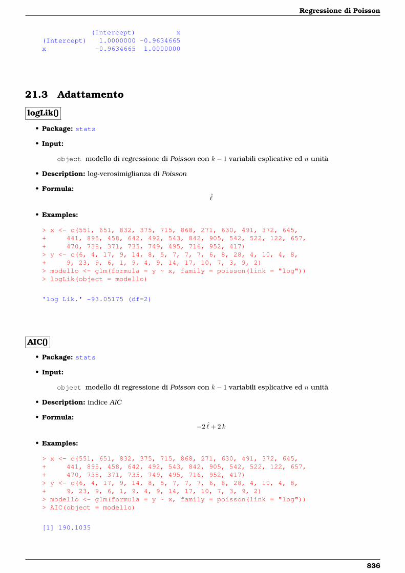
Regressione di Poisson
(Intercept) x(Intercept) 1.0000000 -0.9634665x -0.9634665 1.0000000
21.3 Adattamento
logLik()
• Package: stats
• Input:
object modello di regressione di Poisson con k − 1 variabili esplicative ed n unità
• Description: log-verosimiglianza di Poisson
• Formula:ˆ
• Examples:
> x <- c(551, 651, 832, 375, 715, 868, 271, 630, 491, 372, 645,+ 441, 895, 458, 642, 492, 543, 842, 905, 542, 522, 122, 657,+ 470, 738, 371, 735, 749, 495, 716, 952, 417)> y <- c(6, 4, 17, 9, 14, 8, 5, 7, 7, 7, 6, 8, 28, 4, 10, 4, 8,+ 9, 23, 9, 6, 1, 9, 4, 9, 14, 17, 10, 7, 3, 9, 2)> modello <- glm(formula = y ~ x, family = poisson(link = "log"))> logLik(object = modello)
'log Lik.' -93.05175 (df=2)
AIC()
• Package: stats
• Input:
object modello di regressione di Poisson con k − 1 variabili esplicative ed n unità
• Description: indice AIC
• Formula:−2 ˆ+ 2 k
• Examples:
> x <- c(551, 651, 832, 375, 715, 868, 271, 630, 491, 372, 645,+ 441, 895, 458, 642, 492, 543, 842, 905, 542, 522, 122, 657,+ 470, 738, 371, 735, 749, 495, 716, 952, 417)> y <- c(6, 4, 17, 9, 14, 8, 5, 7, 7, 7, 6, 8, 28, 4, 10, 4, 8,+ 9, 23, 9, 6, 1, 9, 4, 9, 14, 17, 10, 7, 3, 9, 2)> modello <- glm(formula = y ~ x, family = poisson(link = "log"))> AIC(object = modello)
[1] 190.1035
836
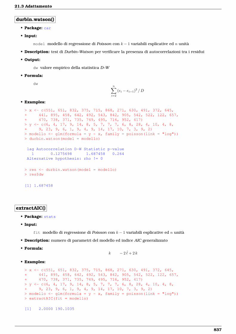
21.3 Adattamento
durbin.watson()
• Package: car
• Input:
model modello di regressione di Poisson con k − 1 variabili esplicative ed n unità
• Description: test di Durbin–Watson per verificare la presenza di autocorrelazioni tra i residui
• Output:
dw valore empirico della statistica D–W
• Formula:
dwn∑i=2
(ei − ei−1)2 /D
• Examples:
> x <- c(551, 651, 832, 375, 715, 868, 271, 630, 491, 372, 645,+ 441, 895, 458, 642, 492, 543, 842, 905, 542, 522, 122, 657,+ 470, 738, 371, 735, 749, 495, 716, 952, 417)> y <- c(6, 4, 17, 9, 14, 8, 5, 7, 7, 7, 6, 8, 28, 4, 10, 4, 8,+ 9, 23, 9, 6, 1, 9, 4, 9, 14, 17, 10, 7, 3, 9, 2)> modello <- glm(formula = y ~ x, family = poisson(link = "log"))> durbin.watson(model = modello)
lag Autocorrelation D-W Statistic p-value1 0.1275698 1.687458 0.264
Alternative hypothesis: rho != 0
> res <- durbin.watson(model = modello)> res$dw
[1] 1.687458
extractAIC()
• Package: stats
• Input:
fit modello di regressione di Poisson con k − 1 variabili esplicative ed n unità
• Description: numero di parametri del modello ed indice AIC generalizzato
• Formula:k − 2 ˆ+ 2 k
• Examples:
> x <- c(551, 651, 832, 375, 715, 868, 271, 630, 491, 372, 645,+ 441, 895, 458, 642, 492, 543, 842, 905, 542, 522, 122, 657,+ 470, 738, 371, 735, 749, 495, 716, 952, 417)> y <- c(6, 4, 17, 9, 14, 8, 5, 7, 7, 7, 6, 8, 28, 4, 10, 4, 8,+ 9, 23, 9, 6, 1, 9, 4, 9, 14, 17, 10, 7, 3, 9, 2)> modello <- glm(formula = y ~ x, family = poisson(link = "log"))> extractAIC(fit = modello)
[1] 2.0000 190.1035
837
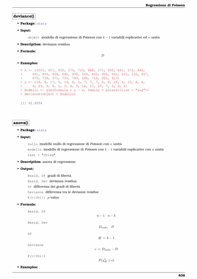
Regressione di Poisson
deviance()
• Package: stats
• Input:
object modello di regressione di Poisson con k − 1 variabili esplicative ed n unità
• Description: devianza residua
• Formula:D
• Examples:
> x <- c(551, 651, 832, 375, 715, 868, 271, 630, 491, 372, 645,+ 441, 895, 458, 642, 492, 543, 842, 905, 542, 522, 122, 657,+ 470, 738, 371, 735, 749, 495, 716, 952, 417)> y <- c(6, 4, 17, 9, 14, 8, 5, 7, 7, 7, 6, 8, 28, 4, 10, 4, 8,+ 9, 23, 9, 6, 1, 9, 4, 9, 14, 17, 10, 7, 3, 9, 2)> modello <- glm(formula = y ~ x, family = poisson(link = "log"))> deviance(object = modello)
[1] 62.8054
anova()
• Package: stats
• Input:
nullo modello nullo di regressione di Poisson con n unità
modello modello di regressione di Poisson con k − 1 variabili esplicative con n unità
test = "Chisq"
• Description: anova di regressione
• Output:
Resid. Df gradi di libertà
Resid. Dev devianza residua
Df differenza dei gradi di libertà
Deviance differenza tra le devianze residue
P(>|Chi|) p-value
• Formula:
Resid. Dfn− 1 n− k
Resid. DevDnullo D
Dfdf = k − 1
Deviancec = Dnullo −D
P(>|Chi|)P (χ2
df ≥ c)
• Examples:
838
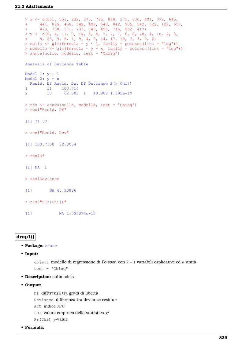
21.3 Adattamento
> x <- c(551, 651, 832, 375, 715, 868, 271, 630, 491, 372, 645,+ 441, 895, 458, 642, 492, 543, 842, 905, 542, 522, 122, 657,+ 470, 738, 371, 735, 749, 495, 716, 952, 417)> y <- c(6, 4, 17, 9, 14, 8, 5, 7, 7, 7, 6, 8, 28, 4, 10, 4, 8,+ 9, 23, 9, 6, 1, 9, 4, 9, 14, 17, 10, 7, 3, 9, 2)> nullo <- glm(formula = y ~ 1, family = poisson(link = "log"))> modello <- glm(formula = y ~ x, family = poisson(link = "log"))> anova(nullo, modello, test = "Chisq")
Analysis of Deviance Table
Model 1: y ~ 1Model 2: y ~ xResid. Df Resid. Dev Df Deviance P(>|Chi|)
1 31 103.7142 30 62.805 1 40.908 1.595e-10
> res <- anova(nullo, modello, test = "Chisq")> res$"Resid. Df"
[1] 31 30
> res$"Resid. Dev"
[1] 103.7138 62.8054
> res$Df
[1] NA 1
> res$Deviance
[1] NA 40.90836
> res$"P(>|Chi|)"
[1] NA 1.595374e-10
drop1()
• Package: stats
• Input:
object modello di regressione di Poisson con k − 1 variabili esplicative ed n unità
test = "Chisq"
• Description: submodels
• Output:
Df differenza tra gradi di libertà
Deviance differenza tra devianze residue
AIC indice AIC
LRT valore empirico della statistica χ2
Pr(Chi) p-value
• Formula:
839
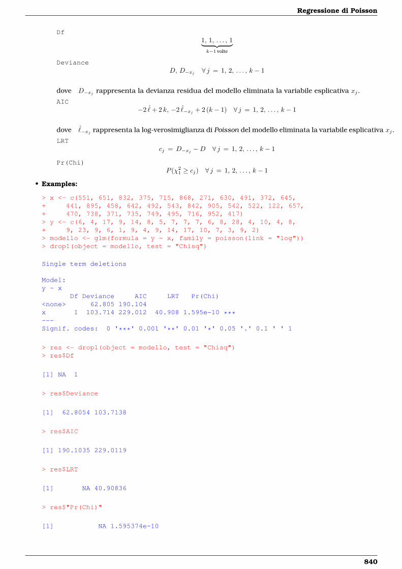
Regressione di Poisson
Df1, 1, . . . , 1︸ ︷︷ ︸k−1 volte
DevianceD, D−xj ∀ j = 1, 2, . . . , k − 1
dove D−xj rappresenta la devianza residua del modello eliminata la variabile esplicativa xj.
AIC−2 ˆ+ 2 k, −2 ˆ−xj + 2 (k − 1) ∀ j = 1, 2, . . . , k − 1
dove ˆ−xj rappresenta la log-verosimiglianza di Poisson del modello eliminata la variabile esplicativa xj.
LRTcj = D−xj −D ∀ j = 1, 2, . . . , k − 1
Pr(Chi)P (χ2
1 ≥ cj) ∀ j = 1, 2, . . . , k − 1
• Examples:
> x <- c(551, 651, 832, 375, 715, 868, 271, 630, 491, 372, 645,+ 441, 895, 458, 642, 492, 543, 842, 905, 542, 522, 122, 657,+ 470, 738, 371, 735, 749, 495, 716, 952, 417)> y <- c(6, 4, 17, 9, 14, 8, 5, 7, 7, 7, 6, 8, 28, 4, 10, 4, 8,+ 9, 23, 9, 6, 1, 9, 4, 9, 14, 17, 10, 7, 3, 9, 2)> modello <- glm(formula = y ~ x, family = poisson(link = "log"))> drop1(object = modello, test = "Chisq")
Single term deletions
Model:y ~ x
Df Deviance AIC LRT Pr(Chi)<none> 62.805 190.104x 1 103.714 229.012 40.908 1.595e-10 ***---Signif. codes: 0 '***' 0.001 '**' 0.01 '*' 0.05 '.' 0.1 ' ' 1
> res <- drop1(object = modello, test = "Chisq")> res$Df
[1] NA 1
> res$Deviance
[1] 62.8054 103.7138
> res$AIC
[1] 190.1035 229.0119
> res$LRT
[1] NA 40.90836
> res$"Pr(Chi)"
[1] NA 1.595374e-10
840
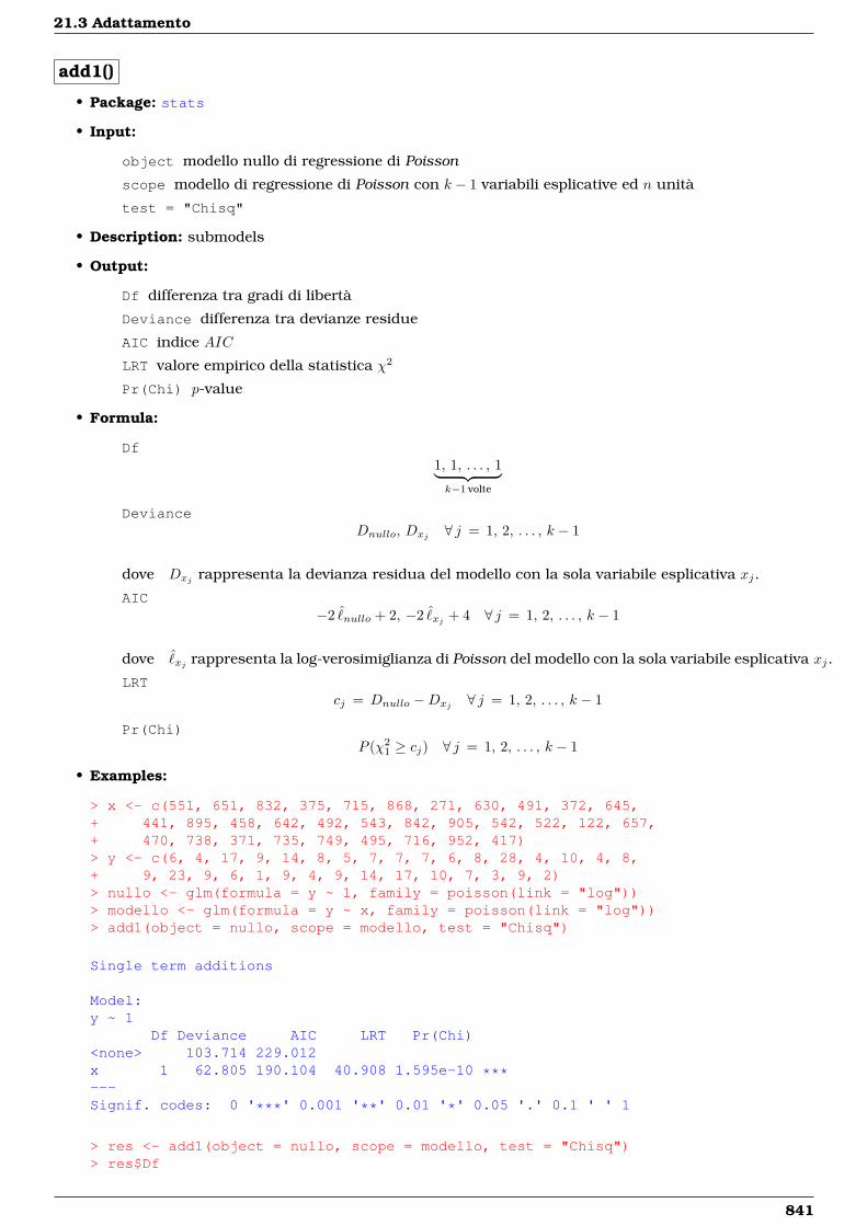
21.3 Adattamento
add1()
• Package: stats
• Input:
object modello nullo di regressione di Poisson
scope modello di regressione di Poisson con k − 1 variabili esplicative ed n unità
test = "Chisq"
• Description: submodels
• Output:
Df differenza tra gradi di libertà
Deviance differenza tra devianze residue
AIC indice AIC
LRT valore empirico della statistica χ2
Pr(Chi) p-value
• Formula:
Df1, 1, . . . , 1︸ ︷︷ ︸k−1 volte
DevianceDnullo, Dxj ∀ j = 1, 2, . . . , k − 1
dove Dxj rappresenta la devianza residua del modello con la sola variabile esplicativa xj.
AIC−2 ˆ
nullo + 2, −2 ˆxj + 4 ∀ j = 1, 2, . . . , k − 1
dove ˆxj rappresenta la log-verosimiglianza di Poisson del modello con la sola variabile esplicativa xj.
LRTcj = Dnullo −Dxj ∀ j = 1, 2, . . . , k − 1
Pr(Chi)P (χ2
1 ≥ cj) ∀ j = 1, 2, . . . , k − 1
• Examples:
> x <- c(551, 651, 832, 375, 715, 868, 271, 630, 491, 372, 645,+ 441, 895, 458, 642, 492, 543, 842, 905, 542, 522, 122, 657,+ 470, 738, 371, 735, 749, 495, 716, 952, 417)> y <- c(6, 4, 17, 9, 14, 8, 5, 7, 7, 7, 6, 8, 28, 4, 10, 4, 8,+ 9, 23, 9, 6, 1, 9, 4, 9, 14, 17, 10, 7, 3, 9, 2)> nullo <- glm(formula = y ~ 1, family = poisson(link = "log"))> modello <- glm(formula = y ~ x, family = poisson(link = "log"))> add1(object = nullo, scope = modello, test = "Chisq")
Single term additions
Model:y ~ 1
Df Deviance AIC LRT Pr(Chi)<none> 103.714 229.012x 1 62.805 190.104 40.908 1.595e-10 ***---Signif. codes: 0 '***' 0.001 '**' 0.01 '*' 0.05 '.' 0.1 ' ' 1
> res <- add1(object = nullo, scope = modello, test = "Chisq")> res$Df
841
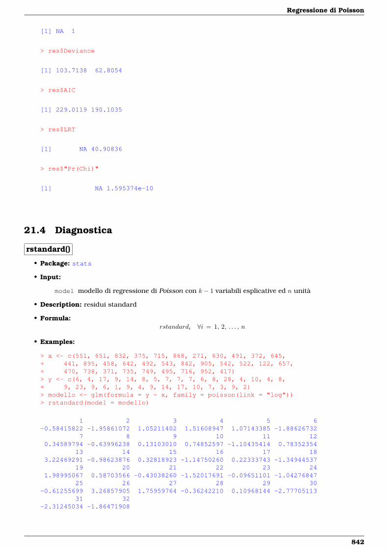
Regressione di Poisson
[1] NA 1
> res$Deviance
[1] 103.7138 62.8054
> res$AIC
[1] 229.0119 190.1035
> res$LRT
[1] NA 40.90836
> res$"Pr(Chi)"
[1] NA 1.595374e-10
21.4 Diagnostica
rstandard()
• Package: stats
• Input:
model modello di regressione di Poisson con k − 1 variabili esplicative ed n unità
• Description: residui standard
• Formula:rstandardi ∀i = 1, 2, . . . , n
• Examples:
> x <- c(551, 651, 832, 375, 715, 868, 271, 630, 491, 372, 645,+ 441, 895, 458, 642, 492, 543, 842, 905, 542, 522, 122, 657,+ 470, 738, 371, 735, 749, 495, 716, 952, 417)> y <- c(6, 4, 17, 9, 14, 8, 5, 7, 7, 7, 6, 8, 28, 4, 10, 4, 8,+ 9, 23, 9, 6, 1, 9, 4, 9, 14, 17, 10, 7, 3, 9, 2)> modello <- glm(formula = y ~ x, family = poisson(link = "log"))> rstandard(model = modello)
1 2 3 4 5 6-0.58415822 -1.95861072 1.05211402 1.51608947 1.07143385 -1.88626732
7 8 9 10 11 120.34589794 -0.63996238 0.13103010 0.74852597 -1.10435414 0.78352354
13 14 15 16 17 183.22469291 -0.98623876 0.32818923 -1.14750260 0.22333743 -1.34944537
19 20 21 22 23 241.98995067 0.58703566 -0.43038260 -1.52017691 -0.09651101 -1.04276847
25 26 27 28 29 30-0.61255699 3.26857905 1.75959764 -0.36242210 0.10968144 -2.77705113
31 32-2.31245034 -1.86471908
842
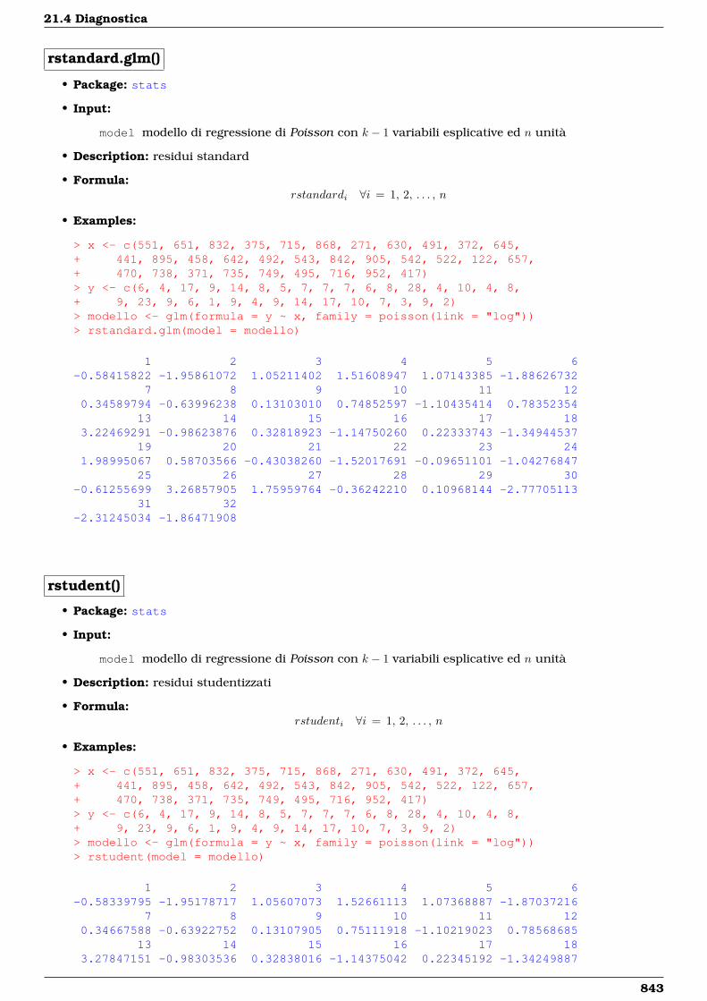
21.4 Diagnostica
rstandard.glm()
• Package: stats
• Input:
model modello di regressione di Poisson con k − 1 variabili esplicative ed n unità
• Description: residui standard
• Formula:rstandardi ∀i = 1, 2, . . . , n
• Examples:
> x <- c(551, 651, 832, 375, 715, 868, 271, 630, 491, 372, 645,+ 441, 895, 458, 642, 492, 543, 842, 905, 542, 522, 122, 657,+ 470, 738, 371, 735, 749, 495, 716, 952, 417)> y <- c(6, 4, 17, 9, 14, 8, 5, 7, 7, 7, 6, 8, 28, 4, 10, 4, 8,+ 9, 23, 9, 6, 1, 9, 4, 9, 14, 17, 10, 7, 3, 9, 2)> modello <- glm(formula = y ~ x, family = poisson(link = "log"))> rstandard.glm(model = modello)
1 2 3 4 5 6-0.58415822 -1.95861072 1.05211402 1.51608947 1.07143385 -1.88626732
7 8 9 10 11 120.34589794 -0.63996238 0.13103010 0.74852597 -1.10435414 0.78352354
13 14 15 16 17 183.22469291 -0.98623876 0.32818923 -1.14750260 0.22333743 -1.34944537
19 20 21 22 23 241.98995067 0.58703566 -0.43038260 -1.52017691 -0.09651101 -1.04276847
25 26 27 28 29 30-0.61255699 3.26857905 1.75959764 -0.36242210 0.10968144 -2.77705113
31 32-2.31245034 -1.86471908
rstudent()
• Package: stats
• Input:
model modello di regressione di Poisson con k − 1 variabili esplicative ed n unità
• Description: residui studentizzati
• Formula:rstudenti ∀i = 1, 2, . . . , n
• Examples:
> x <- c(551, 651, 832, 375, 715, 868, 271, 630, 491, 372, 645,+ 441, 895, 458, 642, 492, 543, 842, 905, 542, 522, 122, 657,+ 470, 738, 371, 735, 749, 495, 716, 952, 417)> y <- c(6, 4, 17, 9, 14, 8, 5, 7, 7, 7, 6, 8, 28, 4, 10, 4, 8,+ 9, 23, 9, 6, 1, 9, 4, 9, 14, 17, 10, 7, 3, 9, 2)> modello <- glm(formula = y ~ x, family = poisson(link = "log"))> rstudent(model = modello)
1 2 3 4 5 6-0.58339795 -1.95178717 1.05607073 1.52661113 1.07368887 -1.87037216
7 8 9 10 11 120.34667588 -0.63922752 0.13107905 0.75111918 -1.10219023 0.78568685
13 14 15 16 17 183.27847151 -0.98303536 0.32838016 -1.14375042 0.22345192 -1.34249887
843
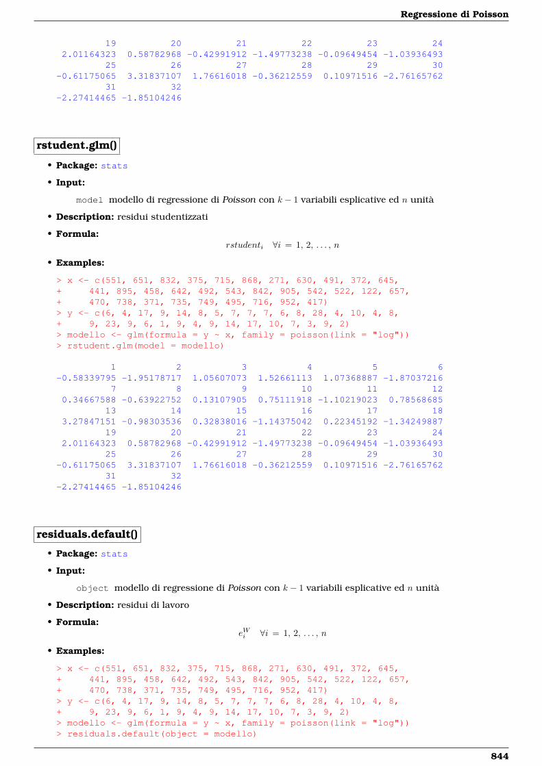
Regressione di Poisson
19 20 21 22 23 242.01164323 0.58782968 -0.42991912 -1.49773238 -0.09649454 -1.03936493
25 26 27 28 29 30-0.61175065 3.31837107 1.76616018 -0.36212559 0.10971516 -2.76165762
31 32-2.27414465 -1.85104246
rstudent.glm()
• Package: stats
• Input:
model modello di regressione di Poisson con k − 1 variabili esplicative ed n unità
• Description: residui studentizzati
• Formula:rstudenti ∀i = 1, 2, . . . , n
• Examples:
> x <- c(551, 651, 832, 375, 715, 868, 271, 630, 491, 372, 645,+ 441, 895, 458, 642, 492, 543, 842, 905, 542, 522, 122, 657,+ 470, 738, 371, 735, 749, 495, 716, 952, 417)> y <- c(6, 4, 17, 9, 14, 8, 5, 7, 7, 7, 6, 8, 28, 4, 10, 4, 8,+ 9, 23, 9, 6, 1, 9, 4, 9, 14, 17, 10, 7, 3, 9, 2)> modello <- glm(formula = y ~ x, family = poisson(link = "log"))> rstudent.glm(model = modello)
1 2 3 4 5 6-0.58339795 -1.95178717 1.05607073 1.52661113 1.07368887 -1.87037216
7 8 9 10 11 120.34667588 -0.63922752 0.13107905 0.75111918 -1.10219023 0.78568685
13 14 15 16 17 183.27847151 -0.98303536 0.32838016 -1.14375042 0.22345192 -1.34249887
19 20 21 22 23 242.01164323 0.58782968 -0.42991912 -1.49773238 -0.09649454 -1.03936493
25 26 27 28 29 30-0.61175065 3.31837107 1.76616018 -0.36212559 0.10971516 -2.76165762
31 32-2.27414465 -1.85104246
residuals.default()
• Package: stats
• Input:
object modello di regressione di Poisson con k − 1 variabili esplicative ed n unità
• Description: residui di lavoro
• Formula:eWi ∀i = 1, 2, . . . , n
• Examples:
> x <- c(551, 651, 832, 375, 715, 868, 271, 630, 491, 372, 645,+ 441, 895, 458, 642, 492, 543, 842, 905, 542, 522, 122, 657,+ 470, 738, 371, 735, 749, 495, 716, 952, 417)> y <- c(6, 4, 17, 9, 14, 8, 5, 7, 7, 7, 6, 8, 28, 4, 10, 4, 8,+ 9, 23, 9, 6, 1, 9, 4, 9, 14, 17, 10, 7, 3, 9, 2)> modello <- glm(formula = y ~ x, family = poisson(link = "log"))> residuals.default(object = modello)
844
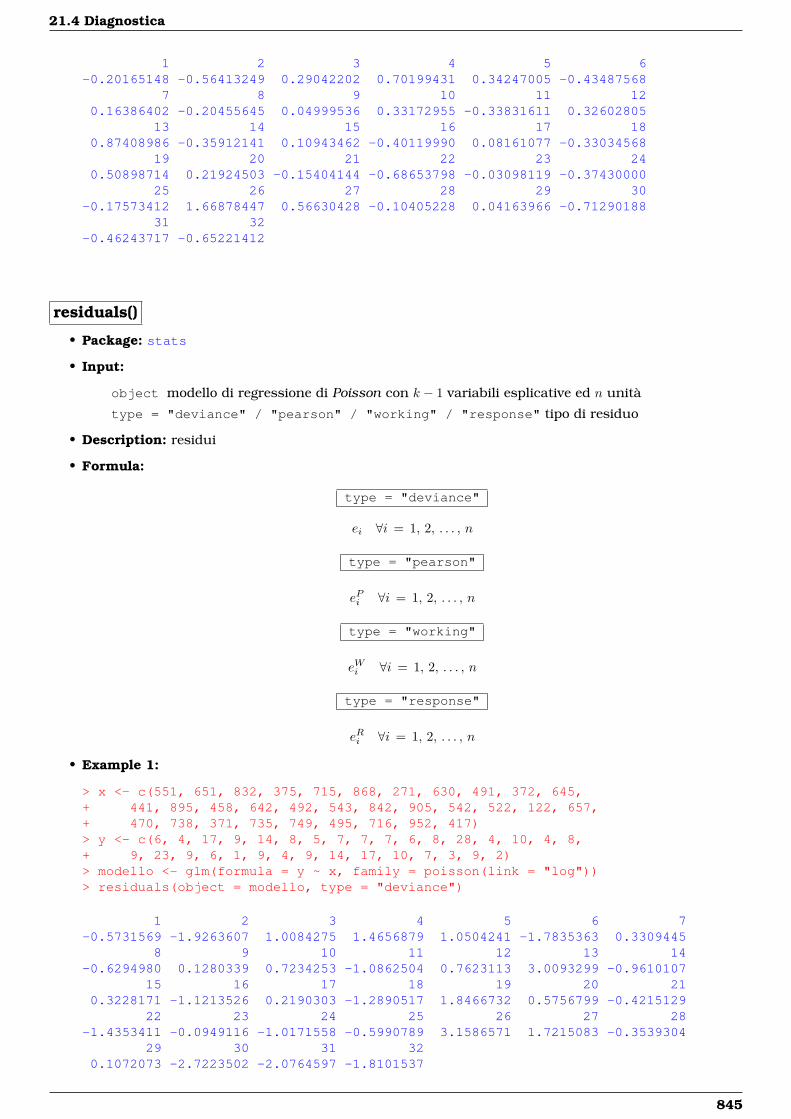
21.4 Diagnostica
1 2 3 4 5 6-0.20165148 -0.56413249 0.29042202 0.70199431 0.34247005 -0.43487568
7 8 9 10 11 120.16386402 -0.20455645 0.04999536 0.33172955 -0.33831611 0.32602805
13 14 15 16 17 180.87408986 -0.35912141 0.10943462 -0.40119990 0.08161077 -0.33034568
19 20 21 22 23 240.50898714 0.21924503 -0.15404144 -0.68653798 -0.03098119 -0.37430000
25 26 27 28 29 30-0.17573412 1.66878447 0.56630428 -0.10405228 0.04163966 -0.71290188
31 32-0.46243717 -0.65221412
residuals()
• Package: stats
• Input:
object modello di regressione di Poisson con k − 1 variabili esplicative ed n unità
type = "deviance" / "pearson" / "working" / "response" tipo di residuo
• Description: residui
• Formula:
type = "deviance"
ei ∀i = 1, 2, . . . , n
type = "pearson"
ePi ∀i = 1, 2, . . . , n
type = "working"
eWi ∀i = 1, 2, . . . , n
type = "response"
eRi ∀i = 1, 2, . . . , n
• Example 1:
> x <- c(551, 651, 832, 375, 715, 868, 271, 630, 491, 372, 645,+ 441, 895, 458, 642, 492, 543, 842, 905, 542, 522, 122, 657,+ 470, 738, 371, 735, 749, 495, 716, 952, 417)> y <- c(6, 4, 17, 9, 14, 8, 5, 7, 7, 7, 6, 8, 28, 4, 10, 4, 8,+ 9, 23, 9, 6, 1, 9, 4, 9, 14, 17, 10, 7, 3, 9, 2)> modello <- glm(formula = y ~ x, family = poisson(link = "log"))> residuals(object = modello, type = "deviance")
1 2 3 4 5 6 7-0.5731569 -1.9263607 1.0084275 1.4656879 1.0504241 -1.7835363 0.3309445
8 9 10 11 12 13 14-0.6294980 0.1280339 0.7234253 -1.0862504 0.7623113 3.0093299 -0.9610107
15 16 17 18 19 20 210.3228171 -1.1213526 0.2190303 -1.2890517 1.8466732 0.5756799 -0.4215129
22 23 24 25 26 27 28-1.4353411 -0.0949116 -1.0171558 -0.5990789 3.1586571 1.7215083 -0.3539304
29 30 31 320.1072073 -2.7223502 -2.0764597 -1.8101537
845
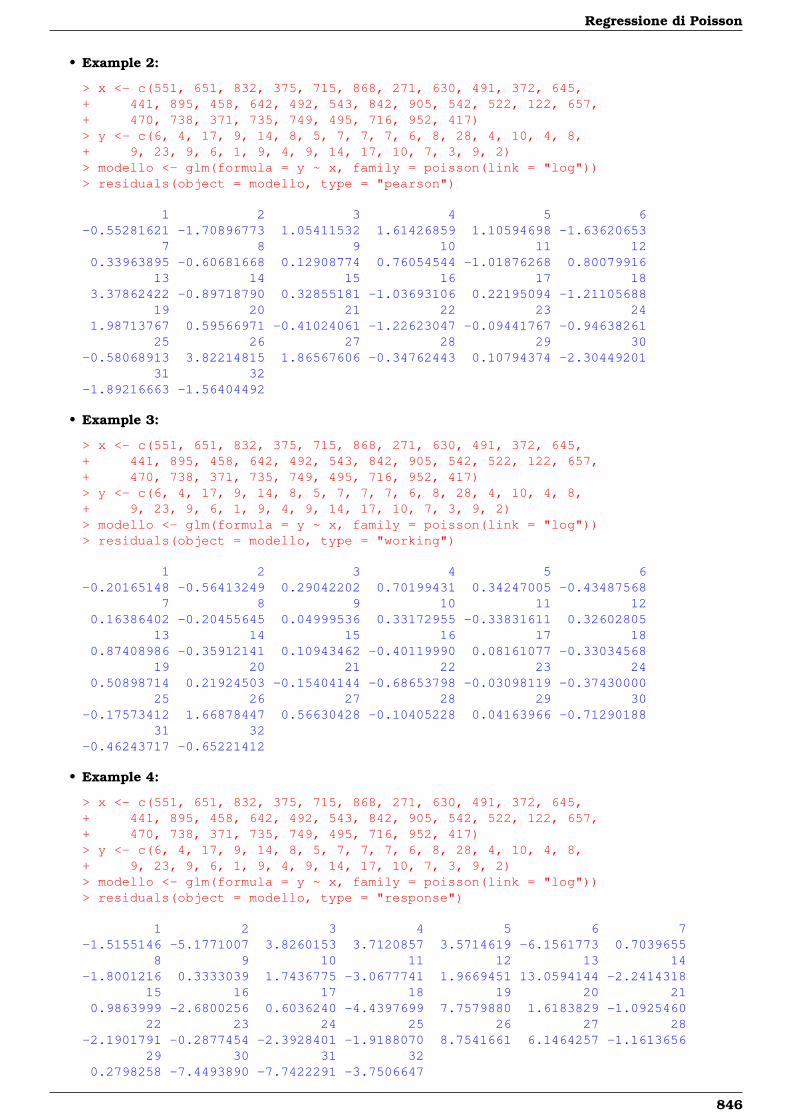
Regressione di Poisson
• Example 2:
> x <- c(551, 651, 832, 375, 715, 868, 271, 630, 491, 372, 645,+ 441, 895, 458, 642, 492, 543, 842, 905, 542, 522, 122, 657,+ 470, 738, 371, 735, 749, 495, 716, 952, 417)> y <- c(6, 4, 17, 9, 14, 8, 5, 7, 7, 7, 6, 8, 28, 4, 10, 4, 8,+ 9, 23, 9, 6, 1, 9, 4, 9, 14, 17, 10, 7, 3, 9, 2)> modello <- glm(formula = y ~ x, family = poisson(link = "log"))> residuals(object = modello, type = "pearson")
1 2 3 4 5 6-0.55281621 -1.70896773 1.05411532 1.61426859 1.10594698 -1.63620653
7 8 9 10 11 120.33963895 -0.60681668 0.12908774 0.76054544 -1.01876268 0.80079916
13 14 15 16 17 183.37862422 -0.89718790 0.32855181 -1.03693106 0.22195094 -1.21105688
19 20 21 22 23 241.98713767 0.59566971 -0.41024061 -1.22623047 -0.09441767 -0.94638261
25 26 27 28 29 30-0.58068913 3.82214815 1.86567606 -0.34762443 0.10794374 -2.30449201
31 32-1.89216663 -1.56404492
• Example 3:
> x <- c(551, 651, 832, 375, 715, 868, 271, 630, 491, 372, 645,+ 441, 895, 458, 642, 492, 543, 842, 905, 542, 522, 122, 657,+ 470, 738, 371, 735, 749, 495, 716, 952, 417)> y <- c(6, 4, 17, 9, 14, 8, 5, 7, 7, 7, 6, 8, 28, 4, 10, 4, 8,+ 9, 23, 9, 6, 1, 9, 4, 9, 14, 17, 10, 7, 3, 9, 2)> modello <- glm(formula = y ~ x, family = poisson(link = "log"))> residuals(object = modello, type = "working")
1 2 3 4 5 6-0.20165148 -0.56413249 0.29042202 0.70199431 0.34247005 -0.43487568
7 8 9 10 11 120.16386402 -0.20455645 0.04999536 0.33172955 -0.33831611 0.32602805
13 14 15 16 17 180.87408986 -0.35912141 0.10943462 -0.40119990 0.08161077 -0.33034568
19 20 21 22 23 240.50898714 0.21924503 -0.15404144 -0.68653798 -0.03098119 -0.37430000
25 26 27 28 29 30-0.17573412 1.66878447 0.56630428 -0.10405228 0.04163966 -0.71290188
31 32-0.46243717 -0.65221412
• Example 4:
> x <- c(551, 651, 832, 375, 715, 868, 271, 630, 491, 372, 645,+ 441, 895, 458, 642, 492, 543, 842, 905, 542, 522, 122, 657,+ 470, 738, 371, 735, 749, 495, 716, 952, 417)> y <- c(6, 4, 17, 9, 14, 8, 5, 7, 7, 7, 6, 8, 28, 4, 10, 4, 8,+ 9, 23, 9, 6, 1, 9, 4, 9, 14, 17, 10, 7, 3, 9, 2)> modello <- glm(formula = y ~ x, family = poisson(link = "log"))> residuals(object = modello, type = "response")
1 2 3 4 5 6 7-1.5155146 -5.1771007 3.8260153 3.7120857 3.5714619 -6.1561773 0.7039655
8 9 10 11 12 13 14-1.8001216 0.3333039 1.7436775 -3.0677741 1.9669451 13.0594144 -2.2414318
15 16 17 18 19 20 210.9863999 -2.6800256 0.6036240 -4.4397699 7.7579880 1.6183829 -1.0925460
22 23 24 25 26 27 28-2.1901791 -0.2877454 -2.3928401 -1.9188070 8.7541661 6.1464257 -1.1613656
29 30 31 320.2798258 -7.4493890 -7.7422291 -3.7506647
846
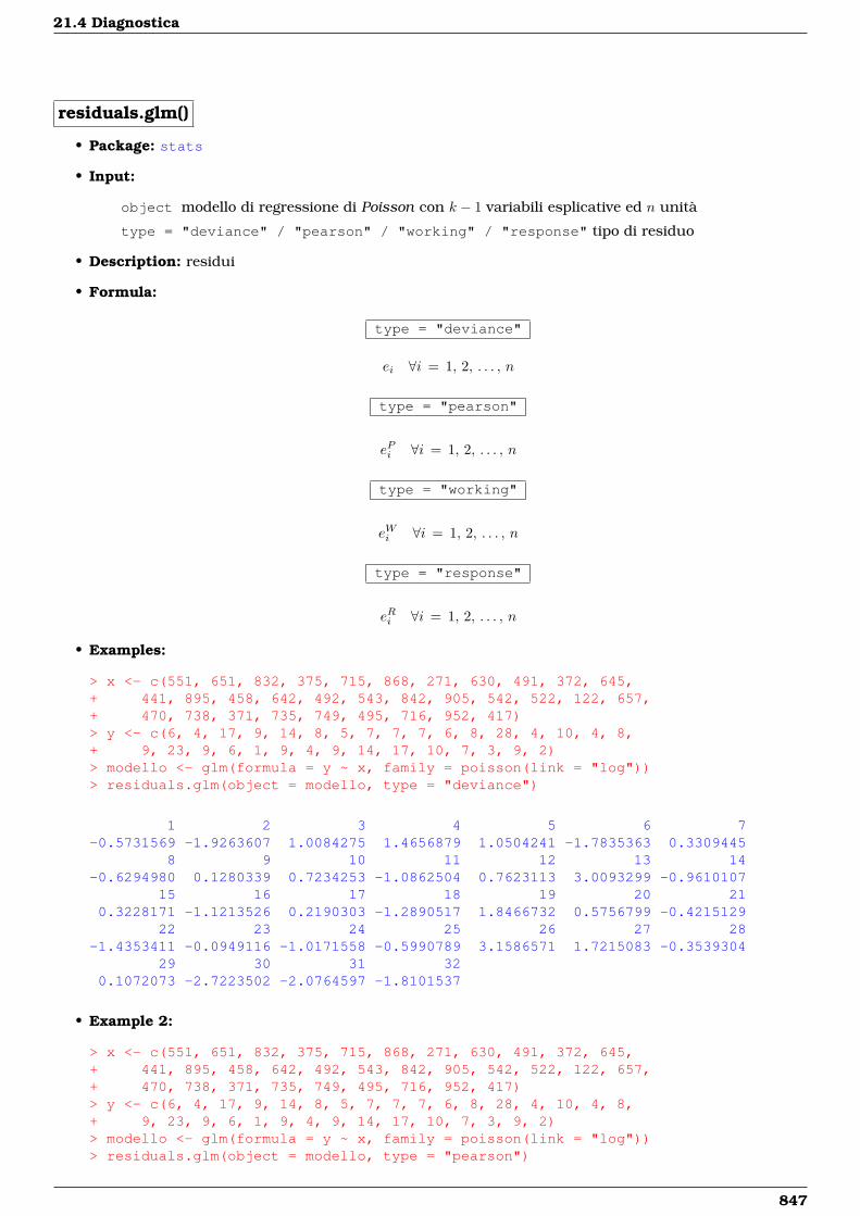
21.4 Diagnostica
residuals.glm()
• Package: stats
• Input:
object modello di regressione di Poisson con k − 1 variabili esplicative ed n unità
type = "deviance" / "pearson" / "working" / "response" tipo di residuo
• Description: residui
• Formula:
type = "deviance"
ei ∀i = 1, 2, . . . , n
type = "pearson"
ePi ∀i = 1, 2, . . . , n
type = "working"
eWi ∀i = 1, 2, . . . , n
type = "response"
eRi ∀i = 1, 2, . . . , n
• Examples:
> x <- c(551, 651, 832, 375, 715, 868, 271, 630, 491, 372, 645,+ 441, 895, 458, 642, 492, 543, 842, 905, 542, 522, 122, 657,+ 470, 738, 371, 735, 749, 495, 716, 952, 417)> y <- c(6, 4, 17, 9, 14, 8, 5, 7, 7, 7, 6, 8, 28, 4, 10, 4, 8,+ 9, 23, 9, 6, 1, 9, 4, 9, 14, 17, 10, 7, 3, 9, 2)> modello <- glm(formula = y ~ x, family = poisson(link = "log"))> residuals.glm(object = modello, type = "deviance")
1 2 3 4 5 6 7-0.5731569 -1.9263607 1.0084275 1.4656879 1.0504241 -1.7835363 0.3309445
8 9 10 11 12 13 14-0.6294980 0.1280339 0.7234253 -1.0862504 0.7623113 3.0093299 -0.9610107
15 16 17 18 19 20 210.3228171 -1.1213526 0.2190303 -1.2890517 1.8466732 0.5756799 -0.4215129
22 23 24 25 26 27 28-1.4353411 -0.0949116 -1.0171558 -0.5990789 3.1586571 1.7215083 -0.3539304
29 30 31 320.1072073 -2.7223502 -2.0764597 -1.8101537
• Example 2:
> x <- c(551, 651, 832, 375, 715, 868, 271, 630, 491, 372, 645,+ 441, 895, 458, 642, 492, 543, 842, 905, 542, 522, 122, 657,+ 470, 738, 371, 735, 749, 495, 716, 952, 417)> y <- c(6, 4, 17, 9, 14, 8, 5, 7, 7, 7, 6, 8, 28, 4, 10, 4, 8,+ 9, 23, 9, 6, 1, 9, 4, 9, 14, 17, 10, 7, 3, 9, 2)> modello <- glm(formula = y ~ x, family = poisson(link = "log"))> residuals.glm(object = modello, type = "pearson")
847
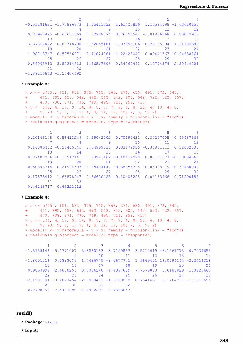
Regressione di Poisson
1 2 3 4 5 6-0.55281621 -1.70896773 1.05411532 1.61426859 1.10594698 -1.63620653
7 8 9 10 11 120.33963895 -0.60681668 0.12908774 0.76054544 -1.01876268 0.80079916
13 14 15 16 17 183.37862422 -0.89718790 0.32855181 -1.03693106 0.22195094 -1.21105688
19 20 21 22 23 241.98713767 0.59566971 -0.41024061 -1.22623047 -0.09441767 -0.94638261
25 26 27 28 29 30-0.58068913 3.82214815 1.86567606 -0.34762443 0.10794374 -2.30449201
31 32-1.89216663 -1.56404492
• Example 3:
> x <- c(551, 651, 832, 375, 715, 868, 271, 630, 491, 372, 645,+ 441, 895, 458, 642, 492, 543, 842, 905, 542, 522, 122, 657,+ 470, 738, 371, 735, 749, 495, 716, 952, 417)> y <- c(6, 4, 17, 9, 14, 8, 5, 7, 7, 7, 6, 8, 28, 4, 10, 4, 8,+ 9, 23, 9, 6, 1, 9, 4, 9, 14, 17, 10, 7, 3, 9, 2)> modello <- glm(formula = y ~ x, family = poisson(link = "log"))> residuals.glm(object = modello, type = "working")
1 2 3 4 5 6-0.20165148 -0.56413249 0.29042202 0.70199431 0.34247005 -0.43487568
7 8 9 10 11 120.16386402 -0.20455645 0.04999536 0.33172955 -0.33831611 0.32602805
13 14 15 16 17 180.87408986 -0.35912141 0.10943462 -0.40119990 0.08161077 -0.33034568
19 20 21 22 23 240.50898714 0.21924503 -0.15404144 -0.68653798 -0.03098119 -0.37430000
25 26 27 28 29 30-0.17573412 1.66878447 0.56630428 -0.10405228 0.04163966 -0.71290188
31 32-0.46243717 -0.65221412
• Example 4:
> x <- c(551, 651, 832, 375, 715, 868, 271, 630, 491, 372, 645,+ 441, 895, 458, 642, 492, 543, 842, 905, 542, 522, 122, 657,+ 470, 738, 371, 735, 749, 495, 716, 952, 417)> y <- c(6, 4, 17, 9, 14, 8, 5, 7, 7, 7, 6, 8, 28, 4, 10, 4, 8,+ 9, 23, 9, 6, 1, 9, 4, 9, 14, 17, 10, 7, 3, 9, 2)> modello <- glm(formula = y ~ x, family = poisson(link = "log"))> residuals.glm(object = modello, type = "response")
1 2 3 4 5 6 7-1.5155146 -5.1771007 3.8260153 3.7120857 3.5714619 -6.1561773 0.7039655
8 9 10 11 12 13 14-1.8001216 0.3333039 1.7436775 -3.0677741 1.9669451 13.0594144 -2.2414318
15 16 17 18 19 20 210.9863999 -2.6800256 0.6036240 -4.4397699 7.7579880 1.6183829 -1.0925460
22 23 24 25 26 27 28-2.1901791 -0.2877454 -2.3928401 -1.9188070 8.7541661 6.1464257 -1.1613656
29 30 31 320.2798258 -7.4493890 -7.7422291 -3.7506647
resid()
• Package: stats
• Input:
848
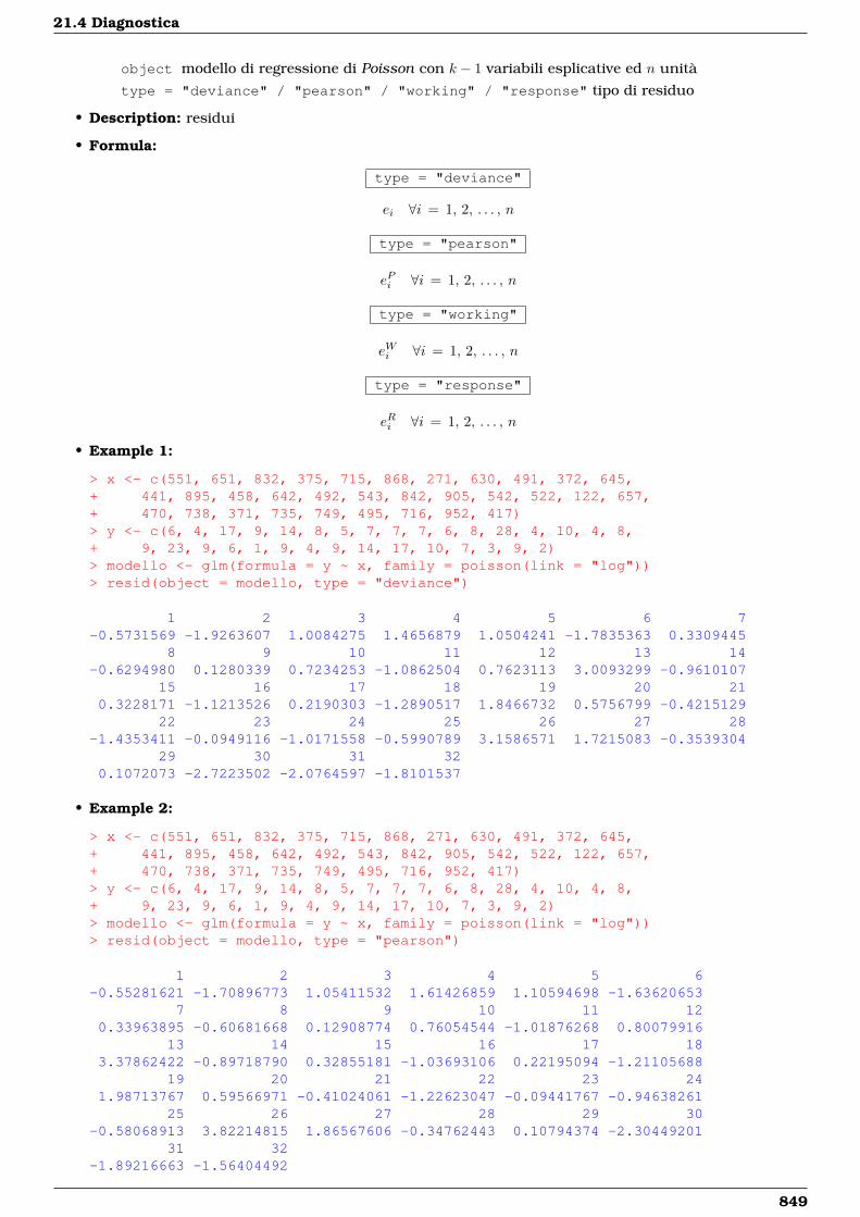
21.4 Diagnostica
object modello di regressione di Poisson con k − 1 variabili esplicative ed n unità
type = "deviance" / "pearson" / "working" / "response" tipo di residuo
• Description: residui
• Formula:
type = "deviance"
ei ∀i = 1, 2, . . . , n
type = "pearson"
ePi ∀i = 1, 2, . . . , n
type = "working"
eWi ∀i = 1, 2, . . . , n
type = "response"
eRi ∀i = 1, 2, . . . , n
• Example 1:
> x <- c(551, 651, 832, 375, 715, 868, 271, 630, 491, 372, 645,+ 441, 895, 458, 642, 492, 543, 842, 905, 542, 522, 122, 657,+ 470, 738, 371, 735, 749, 495, 716, 952, 417)> y <- c(6, 4, 17, 9, 14, 8, 5, 7, 7, 7, 6, 8, 28, 4, 10, 4, 8,+ 9, 23, 9, 6, 1, 9, 4, 9, 14, 17, 10, 7, 3, 9, 2)> modello <- glm(formula = y ~ x, family = poisson(link = "log"))> resid(object = modello, type = "deviance")
1 2 3 4 5 6 7-0.5731569 -1.9263607 1.0084275 1.4656879 1.0504241 -1.7835363 0.3309445
8 9 10 11 12 13 14-0.6294980 0.1280339 0.7234253 -1.0862504 0.7623113 3.0093299 -0.9610107
15 16 17 18 19 20 210.3228171 -1.1213526 0.2190303 -1.2890517 1.8466732 0.5756799 -0.4215129
22 23 24 25 26 27 28-1.4353411 -0.0949116 -1.0171558 -0.5990789 3.1586571 1.7215083 -0.3539304
29 30 31 320.1072073 -2.7223502 -2.0764597 -1.8101537
• Example 2:
> x <- c(551, 651, 832, 375, 715, 868, 271, 630, 491, 372, 645,+ 441, 895, 458, 642, 492, 543, 842, 905, 542, 522, 122, 657,+ 470, 738, 371, 735, 749, 495, 716, 952, 417)> y <- c(6, 4, 17, 9, 14, 8, 5, 7, 7, 7, 6, 8, 28, 4, 10, 4, 8,+ 9, 23, 9, 6, 1, 9, 4, 9, 14, 17, 10, 7, 3, 9, 2)> modello <- glm(formula = y ~ x, family = poisson(link = "log"))> resid(object = modello, type = "pearson")
1 2 3 4 5 6-0.55281621 -1.70896773 1.05411532 1.61426859 1.10594698 -1.63620653
7 8 9 10 11 120.33963895 -0.60681668 0.12908774 0.76054544 -1.01876268 0.80079916
13 14 15 16 17 183.37862422 -0.89718790 0.32855181 -1.03693106 0.22195094 -1.21105688
19 20 21 22 23 241.98713767 0.59566971 -0.41024061 -1.22623047 -0.09441767 -0.94638261
25 26 27 28 29 30-0.58068913 3.82214815 1.86567606 -0.34762443 0.10794374 -2.30449201
31 32-1.89216663 -1.56404492
849
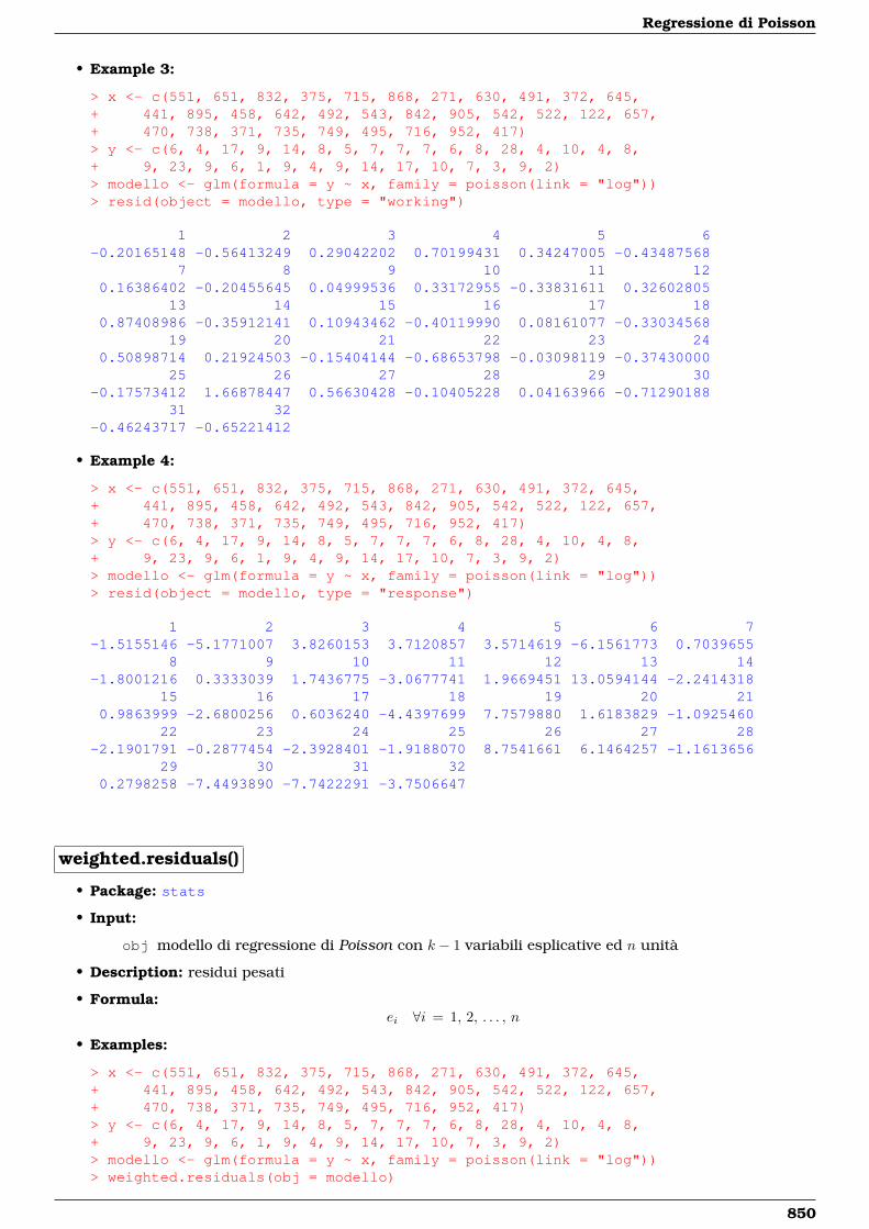
Regressione di Poisson
• Example 3:
> x <- c(551, 651, 832, 375, 715, 868, 271, 630, 491, 372, 645,+ 441, 895, 458, 642, 492, 543, 842, 905, 542, 522, 122, 657,+ 470, 738, 371, 735, 749, 495, 716, 952, 417)> y <- c(6, 4, 17, 9, 14, 8, 5, 7, 7, 7, 6, 8, 28, 4, 10, 4, 8,+ 9, 23, 9, 6, 1, 9, 4, 9, 14, 17, 10, 7, 3, 9, 2)> modello <- glm(formula = y ~ x, family = poisson(link = "log"))> resid(object = modello, type = "working")
1 2 3 4 5 6-0.20165148 -0.56413249 0.29042202 0.70199431 0.34247005 -0.43487568
7 8 9 10 11 120.16386402 -0.20455645 0.04999536 0.33172955 -0.33831611 0.32602805
13 14 15 16 17 180.87408986 -0.35912141 0.10943462 -0.40119990 0.08161077 -0.33034568
19 20 21 22 23 240.50898714 0.21924503 -0.15404144 -0.68653798 -0.03098119 -0.37430000
25 26 27 28 29 30-0.17573412 1.66878447 0.56630428 -0.10405228 0.04163966 -0.71290188
31 32-0.46243717 -0.65221412
• Example 4:
> x <- c(551, 651, 832, 375, 715, 868, 271, 630, 491, 372, 645,+ 441, 895, 458, 642, 492, 543, 842, 905, 542, 522, 122, 657,+ 470, 738, 371, 735, 749, 495, 716, 952, 417)> y <- c(6, 4, 17, 9, 14, 8, 5, 7, 7, 7, 6, 8, 28, 4, 10, 4, 8,+ 9, 23, 9, 6, 1, 9, 4, 9, 14, 17, 10, 7, 3, 9, 2)> modello <- glm(formula = y ~ x, family = poisson(link = "log"))> resid(object = modello, type = "response")
1 2 3 4 5 6 7-1.5155146 -5.1771007 3.8260153 3.7120857 3.5714619 -6.1561773 0.7039655
8 9 10 11 12 13 14-1.8001216 0.3333039 1.7436775 -3.0677741 1.9669451 13.0594144 -2.2414318
15 16 17 18 19 20 210.9863999 -2.6800256 0.6036240 -4.4397699 7.7579880 1.6183829 -1.0925460
22 23 24 25 26 27 28-2.1901791 -0.2877454 -2.3928401 -1.9188070 8.7541661 6.1464257 -1.1613656
29 30 31 320.2798258 -7.4493890 -7.7422291 -3.7506647
weighted.residuals()
• Package: stats
• Input:
obj modello di regressione di Poisson con k − 1 variabili esplicative ed n unità
• Description: residui pesati
• Formula:ei ∀i = 1, 2, . . . , n
• Examples:
> x <- c(551, 651, 832, 375, 715, 868, 271, 630, 491, 372, 645,+ 441, 895, 458, 642, 492, 543, 842, 905, 542, 522, 122, 657,+ 470, 738, 371, 735, 749, 495, 716, 952, 417)> y <- c(6, 4, 17, 9, 14, 8, 5, 7, 7, 7, 6, 8, 28, 4, 10, 4, 8,+ 9, 23, 9, 6, 1, 9, 4, 9, 14, 17, 10, 7, 3, 9, 2)> modello <- glm(formula = y ~ x, family = poisson(link = "log"))> weighted.residuals(obj = modello)
850
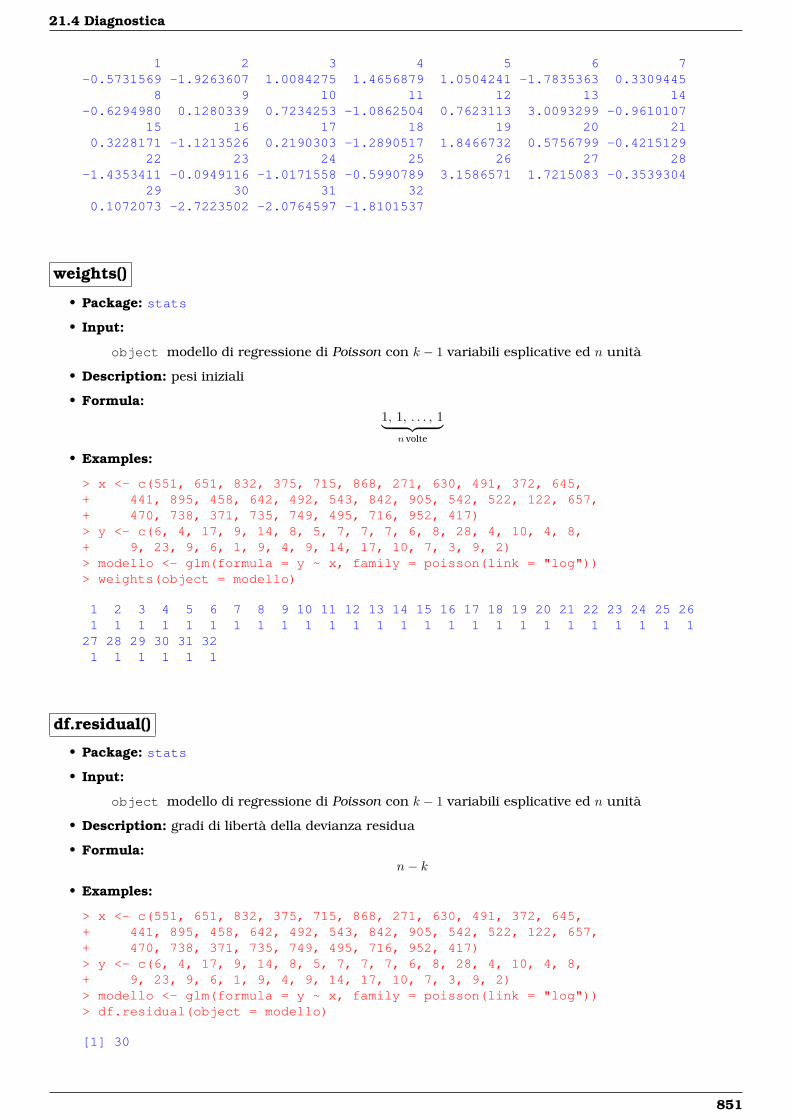
21.4 Diagnostica
1 2 3 4 5 6 7-0.5731569 -1.9263607 1.0084275 1.4656879 1.0504241 -1.7835363 0.3309445
8 9 10 11 12 13 14-0.6294980 0.1280339 0.7234253 -1.0862504 0.7623113 3.0093299 -0.9610107
15 16 17 18 19 20 210.3228171 -1.1213526 0.2190303 -1.2890517 1.8466732 0.5756799 -0.4215129
22 23 24 25 26 27 28-1.4353411 -0.0949116 -1.0171558 -0.5990789 3.1586571 1.7215083 -0.3539304
29 30 31 320.1072073 -2.7223502 -2.0764597 -1.8101537
weights()
• Package: stats
• Input:
object modello di regressione di Poisson con k − 1 variabili esplicative ed n unità
• Description: pesi iniziali
• Formula:1, 1, . . . , 1︸ ︷︷ ︸
n volte
• Examples:
> x <- c(551, 651, 832, 375, 715, 868, 271, 630, 491, 372, 645,+ 441, 895, 458, 642, 492, 543, 842, 905, 542, 522, 122, 657,+ 470, 738, 371, 735, 749, 495, 716, 952, 417)> y <- c(6, 4, 17, 9, 14, 8, 5, 7, 7, 7, 6, 8, 28, 4, 10, 4, 8,+ 9, 23, 9, 6, 1, 9, 4, 9, 14, 17, 10, 7, 3, 9, 2)> modello <- glm(formula = y ~ x, family = poisson(link = "log"))> weights(object = modello)
1 2 3 4 5 6 7 8 9 10 11 12 13 14 15 16 17 18 19 20 21 22 23 24 25 261 1 1 1 1 1 1 1 1 1 1 1 1 1 1 1 1 1 1 1 1 1 1 1 1 1
27 28 29 30 31 321 1 1 1 1 1
df.residual()
• Package: stats
• Input:
object modello di regressione di Poisson con k − 1 variabili esplicative ed n unità
• Description: gradi di libertà della devianza residua
• Formula:n− k
• Examples:
> x <- c(551, 651, 832, 375, 715, 868, 271, 630, 491, 372, 645,+ 441, 895, 458, 642, 492, 543, 842, 905, 542, 522, 122, 657,+ 470, 738, 371, 735, 749, 495, 716, 952, 417)> y <- c(6, 4, 17, 9, 14, 8, 5, 7, 7, 7, 6, 8, 28, 4, 10, 4, 8,+ 9, 23, 9, 6, 1, 9, 4, 9, 14, 17, 10, 7, 3, 9, 2)> modello <- glm(formula = y ~ x, family = poisson(link = "log"))> df.residual(object = modello)
[1] 30
851
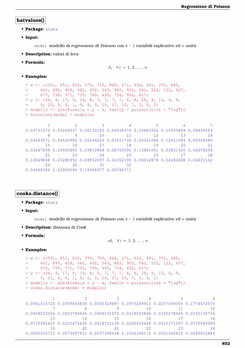
Regressione di Poisson
hatvalues()
• Package: stats
• Input:
model modello di regressione di Poisson con k − 1 variabili esplicative ed n unità
• Description: valori di leva
• Formula:hi ∀ i = 1, 2, . . . , n
• Examples:
> x <- c(551, 651, 832, 375, 715, 868, 271, 630, 491, 372, 645,+ 441, 895, 458, 642, 492, 543, 842, 905, 542, 522, 122, 657,+ 470, 738, 371, 735, 749, 495, 716, 952, 417)> y <- c(6, 4, 17, 9, 14, 8, 5, 7, 7, 7, 6, 8, 28, 4, 10, 4, 8,+ 9, 23, 9, 6, 1, 9, 4, 9, 14, 17, 10, 7, 3, 9, 2)> modello <- glm(formula = y ~ x, family = poisson(link = "log"))> hatvalues(model = modello)
1 2 3 4 5 6 70.03731074 0.03266037 0.08132102 0.06538376 0.03883352 0.10595899 0.08459283
8 9 10 11 12 13 140.03243571 0.04520986 0.06594243 0.03251736 0.05341286 0.12911084 0.05050580
15 16 17 18 19 20 210.03247008 0.04505800 0.03819908 0.08750591 0.13881691 0.03831420 0.04079290
22 23 24 25 26 27 280.10849868 0.03286992 0.04852097 0.04352190 0.06612878 0.04282468 0.04631162
29 30 31 320.04460584 0.03900696 0.19368977 0.05766771
cooks.distance()
• Package: stats
• Input:
model modello di regressione di Poisson con k − 1 variabili esplicative ed n unità
• Description: distanza di Cook
• Formula:cdi ∀ i = 1, 2, . . . , n
• Examples:
> x <- c(551, 651, 832, 375, 715, 868, 271, 630, 491, 372, 645,+ 441, 895, 458, 642, 492, 543, 842, 905, 542, 522, 122, 657,+ 470, 738, 371, 735, 749, 495, 716, 952, 417)> y <- c(6, 4, 17, 9, 14, 8, 5, 7, 7, 7, 6, 8, 28, 4, 10, 4, 8,+ 9, 23, 9, 6, 1, 9, 4, 9, 14, 17, 10, 7, 3, 9, 2)> modello <- glm(formula = y ~ x, family = poisson(link = "log"))> cooks.distance(model = modello)
1 2 3 4 5 60.0061516720 0.0509683838 0.0535329887 0.0975269911 0.0257068065 0.1774472070
7 8 9 10 11 120.0058225056 0.0063789436 0.0004131972 0.0218593896 0.0180278945 0.0191135734
13 14 15 16 17 180.9715982423 0.0225472435 0.0018721138 0.0265636449 0.0010171067 0.0770683993
19 20 21 22 23 240.3695534723 0.0073497811 0.0037308438 0.1026348110 0.0001566410 0.0240012884
852
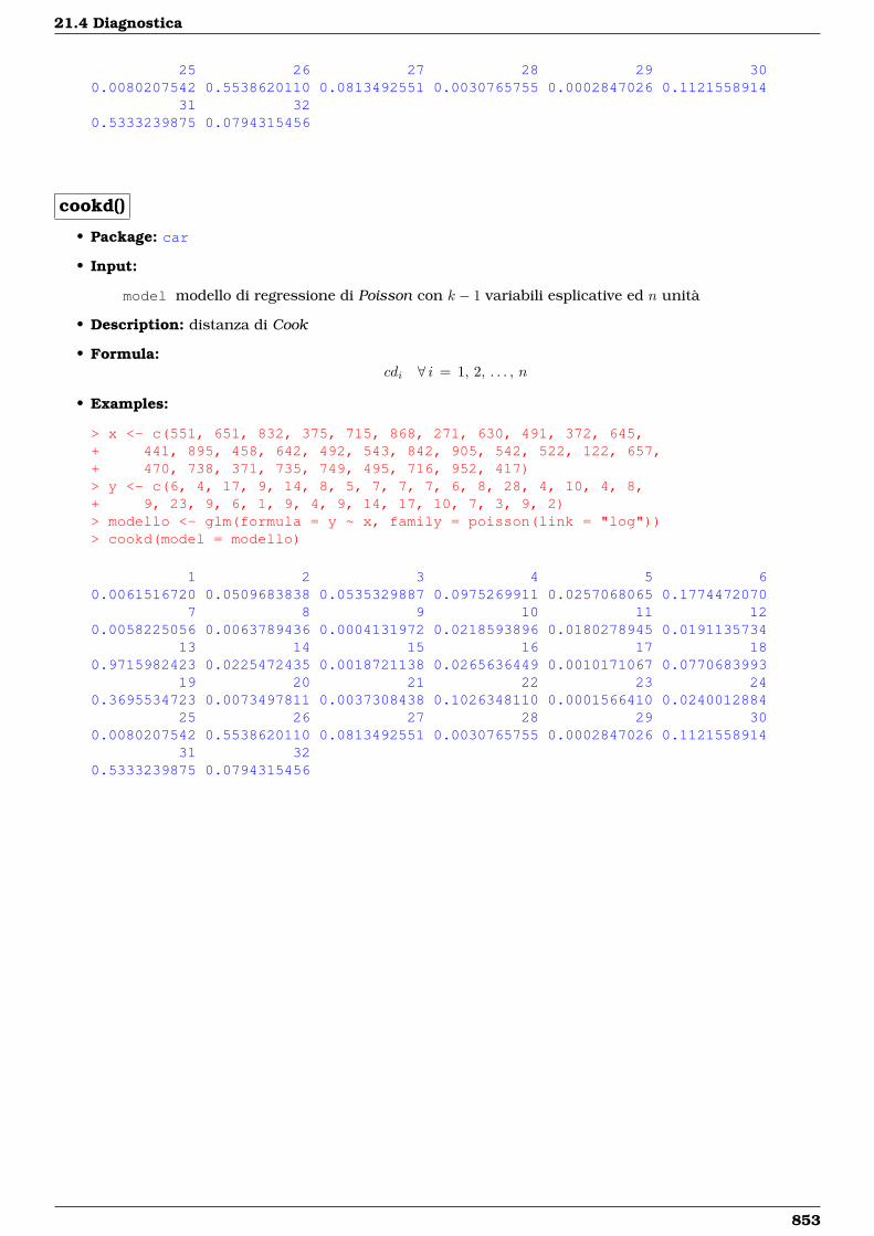
21.4 Diagnostica
25 26 27 28 29 300.0080207542 0.5538620110 0.0813492551 0.0030765755 0.0002847026 0.1121558914
31 320.5333239875 0.0794315456
cookd()
• Package: car
• Input:
model modello di regressione di Poisson con k − 1 variabili esplicative ed n unità
• Description: distanza di Cook
• Formula:cdi ∀ i = 1, 2, . . . , n
• Examples:
> x <- c(551, 651, 832, 375, 715, 868, 271, 630, 491, 372, 645,+ 441, 895, 458, 642, 492, 543, 842, 905, 542, 522, 122, 657,+ 470, 738, 371, 735, 749, 495, 716, 952, 417)> y <- c(6, 4, 17, 9, 14, 8, 5, 7, 7, 7, 6, 8, 28, 4, 10, 4, 8,+ 9, 23, 9, 6, 1, 9, 4, 9, 14, 17, 10, 7, 3, 9, 2)> modello <- glm(formula = y ~ x, family = poisson(link = "log"))> cookd(model = modello)
1 2 3 4 5 60.0061516720 0.0509683838 0.0535329887 0.0975269911 0.0257068065 0.1774472070
7 8 9 10 11 120.0058225056 0.0063789436 0.0004131972 0.0218593896 0.0180278945 0.0191135734
13 14 15 16 17 180.9715982423 0.0225472435 0.0018721138 0.0265636449 0.0010171067 0.0770683993
19 20 21 22 23 240.3695534723 0.0073497811 0.0037308438 0.1026348110 0.0001566410 0.0240012884
25 26 27 28 29 300.0080207542 0.5538620110 0.0813492551 0.0030765755 0.0002847026 0.1121558914
31 320.5333239875 0.0794315456
853

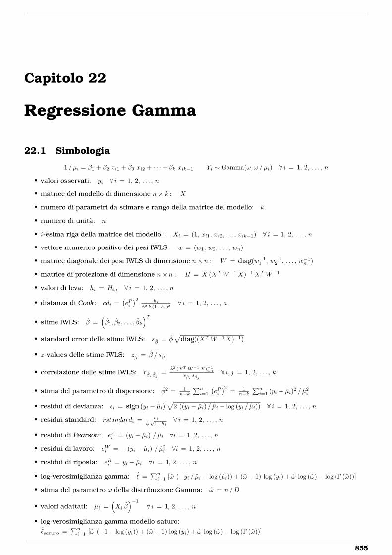
Capitolo 22
Regressione Gamma
22.1 Simbologia
1 / µi = β1 + β2 xi1 + β3 xi2 + · · ·+ βk xik−1 Yi ∼ Gamma(ω, ω /µi) ∀ i = 1, 2, . . . , n
• valori osservati: yi ∀ i = 1, 2, . . . , n
• matrice del modello di dimensione n× k : X
• numero di parametri da stimare e rango della matrice del modello: k
• numero di unità: n
• i-esima riga della matrice del modello : Xi = (1, xi1, xi2, . . . , xik−1) ∀ i = 1, 2, . . . , n
• vettore numerico positivo dei pesi IWLS: w = (w1, w2, . . . , wn)
• matrice diagonale dei pesi IWLS di dimensione n× n : W = diag(w−11 , w−1
2 , . . . , w−1n )
• matrice di proiezione di dimensione n× n : H = X (XT W−1X)−1XT W−1
• valori di leva: hi = Hi,i ∀ i = 1, 2, . . . , n
• distanza di Cook: cdi =(ePi)2 hi
φ2 k (1−hi)2∀ i = 1, 2, . . . , n
• stime IWLS: β =(β1, β2, . . . , βk
)T• standard error delle stime IWLS: sβ = φ
√diag((XT W−1X)−1)
• z-values delle stime IWLS: zβ = β / sβ
• correlazione delle stime IWLS: rβi βj =φ2 (XT W−1X)−1
i, j
sβisβj
∀ i, j = 1, 2, . . . , k
• stima del parametro di dispersione: φ2 = 1n−k
∑ni=1
(ePi)2 = 1
n−k∑ni=1 (yi − µi)2 / µ2
i
• residui di devianza: ei = sign (yi − µi)√
2 ((yi − µi) / µi − log (yi / µi)) ∀ i = 1, 2, . . . , n
• residui standard: rstandardi = eiφ√
1−hi∀ i = 1, 2, . . . , n
• residui di Pearson: ePi = (yi − µi) / µi ∀i = 1, 2, . . . , n
• residui di lavoro: eWi = − (yi − µi) / µ2i ∀i = 1, 2, . . . , n
• residui di riposta: eRi = yi − µi ∀i = 1, 2, . . . , n
• log-verosimiglianza gamma: ˆ =∑ni=1 [ω (−yi / µi − log (µi)) + (ω − 1) log (yi) + ω log (ω)− log (Γ (ω))]
• stima del parametro ω della distribuzione Gamma: ω = n /D
• valori adattati: µi =(Xi β
)−1
∀ i = 1, 2, . . . , n
• log-verosimiglianza gamma modello saturo:ˆsaturo =
∑ni=1 [ω (−1− log (yi)) + (ω − 1) log (yi) + ω log (ω)− log (Γ (ω))]
855
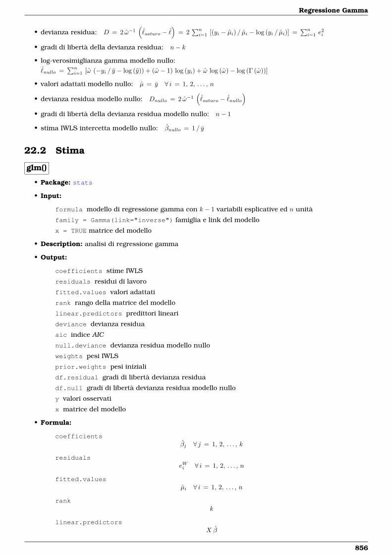
Regressione Gamma
• devianza residua: D = 2 ω−1(
ˆsaturo − ˆ
)= 2
∑ni=1 [(yi − µi) / µi − log (yi / µi)] =
∑ni=1 e
2i
• gradi di libertà della devianza residua: n− k
• log-verosimiglianza gamma modello nullo:ˆnullo =
∑ni=1 [ω (−yi / y − log (y)) + (ω − 1) log (yi) + ω log (ω)− log (Γ (ω))]
• valori adattati modello nullo: µ = y ∀ i = 1, 2, . . . , n
• devianza residua modello nullo: Dnullo = 2 ω−1(
ˆsaturo − ˆ
nullo
)• gradi di libertà della devianza residua modello nullo: n− 1
• stima IWLS intercetta modello nullo: βnullo = 1 / y
22.2 Stima
glm()
• Package: stats
• Input:
formula modello di regressione gamma con k − 1 variabili esplicative ed n unità
family = Gamma(link="inverse") famiglia e link del modello
x = TRUE matrice del modello
• Description: analisi di regressione gamma
• Output:
coefficients stime IWLS
residuals residui di lavoro
fitted.values valori adattati
rank rango della matrice del modello
linear.predictors predittori lineari
deviance devianza residua
aic indice AIC
null.deviance devianza residua modello nullo
weights pesi IWLS
prior.weights pesi iniziali
df.residual gradi di libertà devianza residua
df.null gradi di libertà devianza residua modello nullo
y valori osservati
x matrice del modello
• Formula:
coefficientsβj ∀ j = 1, 2, . . . , k
residualseWi ∀ i = 1, 2, . . . , n
fitted.valuesµi ∀ i = 1, 2, . . . , n
rankk
linear.predictorsX β
856
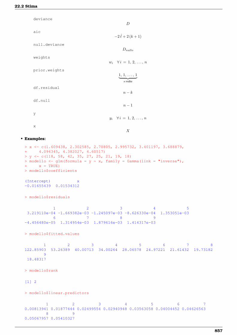
22.2 Stima
devianceD
aic−2 ˆ+ 2 (k + 1)
null.devianceDnullo
weightswi ∀ i = 1, 2, . . . , n
prior.weights1, 1, . . . , 1︸ ︷︷ ︸
n volte
df.residualn− k
df.nulln− 1
yyi ∀ i = 1, 2, . . . , n
xX
• Examples:
> x <- c(1.609438, 2.302585, 2.70805, 2.995732, 3.401197, 3.688879,+ 4.094345, 4.382027, 4.60517)> y <- c(118, 58, 42, 35, 27, 25, 21, 19, 18)> modello <- glm(formula = y ~ x, family = Gamma(link = "inverse"),+ x = TRUE)> modello$coefficients
(Intercept) x-0.01655439 0.01534312
> modello$residuals
1 2 3 4 53.219110e-04 -1.669382e-03 -1.245097e-03 -8.626330e-04 1.353051e-03
6 7 8 9-4.456480e-05 1.314954e-03 1.879616e-03 1.414317e-03
> modello$fitted.values
1 2 3 4 5 6 7 8122.85903 53.26389 40.00713 34.00264 28.06578 24.97221 21.61432 19.73182
918.48317
> modello$rank
[1] 2
> modello$linear.predictors
1 2 3 4 5 6 70.00813941 0.01877444 0.02499554 0.02940948 0.03563058 0.04004452 0.04626563
8 90.05067957 0.05410327
857
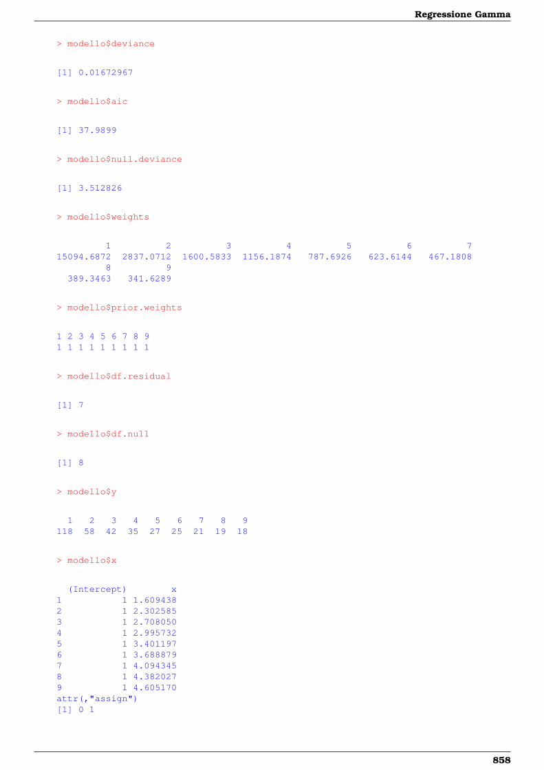
Regressione Gamma
> modello$deviance
[1] 0.01672967
> modello$aic
[1] 37.9899
> modello$null.deviance
[1] 3.512826
> modello$weights
1 2 3 4 5 6 715094.6872 2837.0712 1600.5833 1156.1874 787.6926 623.6144 467.1808
8 9389.3463 341.6289
> modello$prior.weights
1 2 3 4 5 6 7 8 91 1 1 1 1 1 1 1 1
> modello$df.residual
[1] 7
> modello$df.null
[1] 8
> modello$y
1 2 3 4 5 6 7 8 9118 58 42 35 27 25 21 19 18
> modello$x
(Intercept) x1 1 1.6094382 1 2.3025853 1 2.7080504 1 2.9957325 1 3.4011976 1 3.6888797 1 4.0943458 1 4.3820279 1 4.605170attr(,"assign")[1] 0 1
858

22.2 Stima
summary.glm()
• Package: stats
• Input:
object modello di regressione gamma con k − 1 variabili esplicative ed n unità
correlation = TRUE correlazione delle stime IWLS
• Description: analisi di regressione gamma
• Output:
deviance devianza residua
aic indice AIC
df.residual gradi di libertà devianza residua
null.deviance devianza residua modello nullo
df.null gradi di libertà devianza residua modello nullo
deviance.resid residui di devianza
coefficients stima puntuale, standard error, z-value, p-value
cov.unscaled matrice di covarianza delle stime IWLS non scalata
cov.scaled matrice di covarianza delle stime IWLS scalata
correlation matrice di correlazione delle stime IWLS
• Formula:
devianceD
aic−2 ˆ+ 2 (k + 1)
df.residualn− k
null.devianceDnullo
df.nulln− 1
deviance.residej ∀ j = 1, 2, . . . , k
coefficientsβj sβj zβj p-value = 2 Φ(− | zβj |) ∀ j = 1, 2, . . . , k
cov.unscaled(XT W−1X)−1
cov.scaledφ2 (XT W−1X)−1
correlationrβi βj ∀ i, j = 1, 2, . . . , k
• Examples:
> x <- c(1.609438, 2.302585, 2.70805, 2.995732, 3.401197, 3.688879,+ 4.094345, 4.382027, 4.60517)> y <- c(118, 58, 42, 35, 27, 25, 21, 19, 18)> modello <- glm(formula = y ~ x, family = Gamma(link = "inverse"))> res <- summary.glm(object = modello, correlation = TRUE)> res$deviance
[1] 0.01672967
859
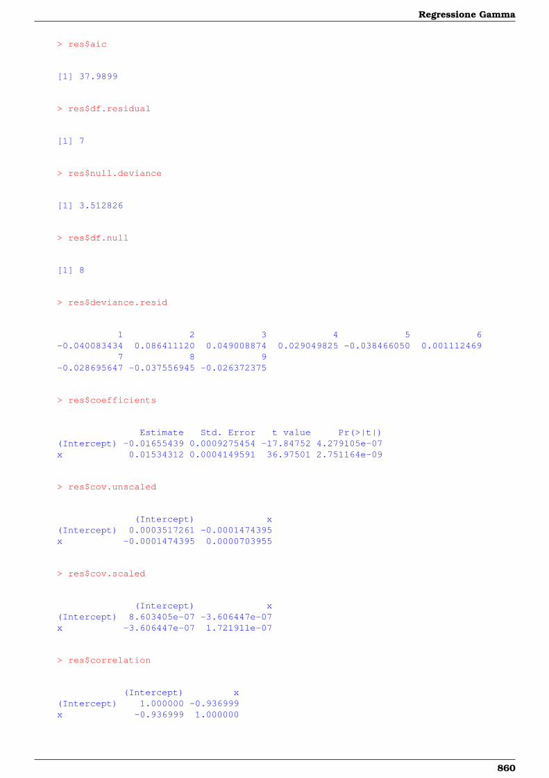
Regressione Gamma
> res$aic
[1] 37.9899
> res$df.residual
[1] 7
> res$null.deviance
[1] 3.512826
> res$df.null
[1] 8
> res$deviance.resid
1 2 3 4 5 6-0.040083434 0.086411120 0.049008874 0.029049825 -0.038466050 0.001112469
7 8 9-0.028695647 -0.037556945 -0.026372375
> res$coefficients
Estimate Std. Error t value Pr(>|t|)(Intercept) -0.01655439 0.0009275454 -17.84752 4.279105e-07x 0.01534312 0.0004149591 36.97501 2.751164e-09
> res$cov.unscaled
(Intercept) x(Intercept) 0.0003517261 -0.0001474395x -0.0001474395 0.0000703955
> res$cov.scaled
(Intercept) x(Intercept) 8.603405e-07 -3.606447e-07x -3.606447e-07 1.721911e-07
> res$correlation
(Intercept) x(Intercept) 1.000000 -0.936999x -0.936999 1.000000
860
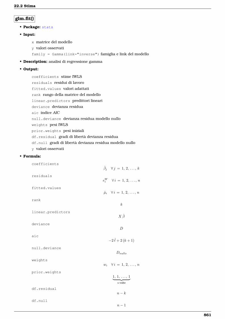
22.2 Stima
glm.fit()
• Package: stats
• Input:
x matrice del modello
y valori osservati
family = Gamma(link="inverse") famiglia e link del modello
• Description: analisi di regressione gamma
• Output:
coefficients stime IWLS
residuals residui di lavoro
fitted.values valori adattati
rank rango della matrice del modello
linear.predictors predittori lineari
deviance devianza residua
aic indice AIC
null.deviance devianza residua modello nullo
weights pesi IWLS
prior.weights pesi iniziali
df.residual gradi di libertà devianza residua
df.null gradi di libertà devianza residua modello nullo
y valori osservati
• Formula:
coefficientsβj ∀ j = 1, 2, . . . , k
residualseWi ∀ i = 1, 2, . . . , n
fitted.valuesµi ∀ i = 1, 2, . . . , n
rankk
linear.predictorsX β
devianceD
aic−2 ˆ+ 2 (k + 1)
null.devianceDnullo
weightswi ∀ i = 1, 2, . . . , n
prior.weights1, 1, . . . , 1︸ ︷︷ ︸
n volte
df.residualn− k
df.nulln− 1
861
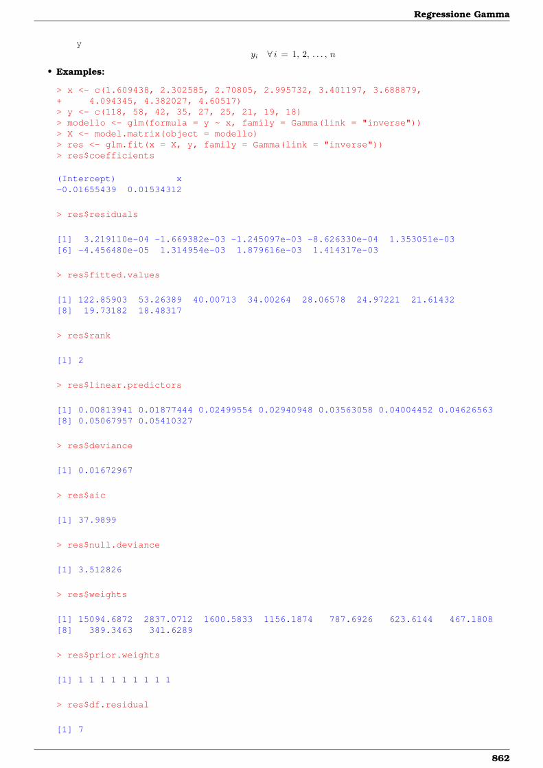
Regressione Gamma
yyi ∀ i = 1, 2, . . . , n
• Examples:
> x <- c(1.609438, 2.302585, 2.70805, 2.995732, 3.401197, 3.688879,+ 4.094345, 4.382027, 4.60517)> y <- c(118, 58, 42, 35, 27, 25, 21, 19, 18)> modello <- glm(formula = y ~ x, family = Gamma(link = "inverse"))> X <- model.matrix(object = modello)> res <- glm.fit(x = X, y, family = Gamma(link = "inverse"))> res$coefficients
(Intercept) x-0.01655439 0.01534312
> res$residuals
[1] 3.219110e-04 -1.669382e-03 -1.245097e-03 -8.626330e-04 1.353051e-03[6] -4.456480e-05 1.314954e-03 1.879616e-03 1.414317e-03
> res$fitted.values
[1] 122.85903 53.26389 40.00713 34.00264 28.06578 24.97221 21.61432[8] 19.73182 18.48317
> res$rank
[1] 2
> res$linear.predictors
[1] 0.00813941 0.01877444 0.02499554 0.02940948 0.03563058 0.04004452 0.04626563[8] 0.05067957 0.05410327
> res$deviance
[1] 0.01672967
> res$aic
[1] 37.9899
> res$null.deviance
[1] 3.512826
> res$weights
[1] 15094.6872 2837.0712 1600.5833 1156.1874 787.6926 623.6144 467.1808[8] 389.3463 341.6289
> res$prior.weights
[1] 1 1 1 1 1 1 1 1 1
> res$df.residual
[1] 7
862
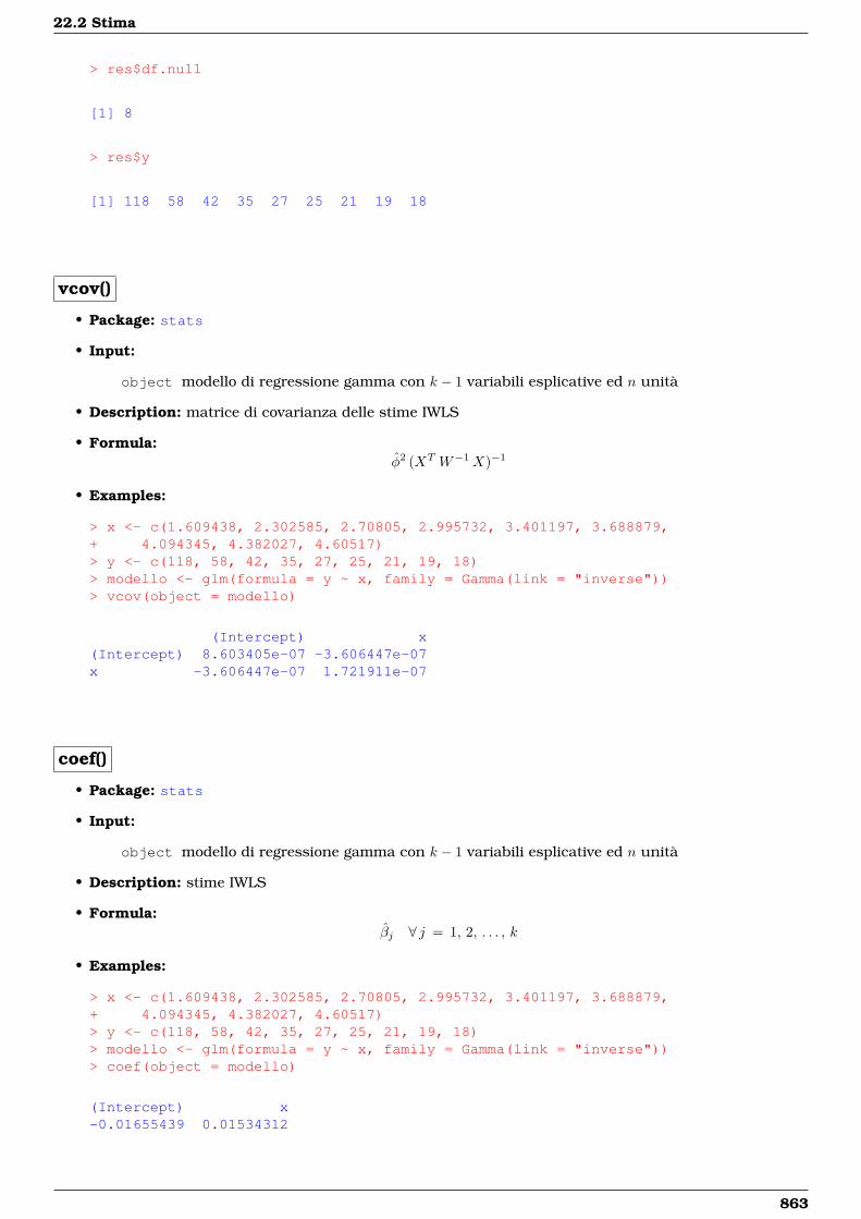
22.2 Stima
> res$df.null
[1] 8
> res$y
[1] 118 58 42 35 27 25 21 19 18
vcov()
• Package: stats
• Input:
object modello di regressione gamma con k − 1 variabili esplicative ed n unità
• Description: matrice di covarianza delle stime IWLS
• Formula:φ2 (XT W−1X)−1
• Examples:
> x <- c(1.609438, 2.302585, 2.70805, 2.995732, 3.401197, 3.688879,+ 4.094345, 4.382027, 4.60517)> y <- c(118, 58, 42, 35, 27, 25, 21, 19, 18)> modello <- glm(formula = y ~ x, family = Gamma(link = "inverse"))> vcov(object = modello)
(Intercept) x(Intercept) 8.603405e-07 -3.606447e-07x -3.606447e-07 1.721911e-07
coef()
• Package: stats
• Input:
object modello di regressione gamma con k − 1 variabili esplicative ed n unità
• Description: stime IWLS
• Formula:βj ∀ j = 1, 2, . . . , k
• Examples:
> x <- c(1.609438, 2.302585, 2.70805, 2.995732, 3.401197, 3.688879,+ 4.094345, 4.382027, 4.60517)> y <- c(118, 58, 42, 35, 27, 25, 21, 19, 18)> modello <- glm(formula = y ~ x, family = Gamma(link = "inverse"))> coef(object = modello)
(Intercept) x-0.01655439 0.01534312
863
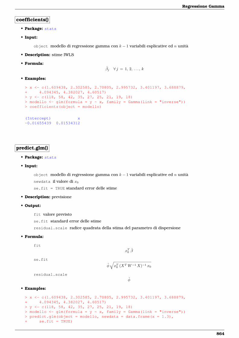
Regressione Gamma
coefficients()
• Package: stats
• Input:
object modello di regressione gamma con k − 1 variabili esplicative ed n unità
• Description: stime IWLS
• Formula:βj ∀ j = 1, 2, . . . , k
• Examples:
> x <- c(1.609438, 2.302585, 2.70805, 2.995732, 3.401197, 3.688879,+ 4.094345, 4.382027, 4.60517)> y <- c(118, 58, 42, 35, 27, 25, 21, 19, 18)> modello <- glm(formula = y ~ x, family = Gamma(link = "inverse"))> coefficients(object = modello)
(Intercept) x-0.01655439 0.01534312
predict.glm()
• Package: stats
• Input:
object modello di regressione gamma con k − 1 variabili esplicative ed n unità
newdata il valore di x0
se.fit = TRUE standard error delle stime
• Description: previsione
• Output:
fit valore previsto
se.fit standard error delle stime
residual.scale radice quadrata della stima del parametro di dispersione
• Formula:
fit
xT0 β
se.fit
φ√xT0 (XT W−1X)−1 x0
residual.scale
φ
• Examples:
> x <- c(1.609438, 2.302585, 2.70805, 2.995732, 3.401197, 3.688879,+ 4.094345, 4.382027, 4.60517)> y <- c(118, 58, 42, 35, 27, 25, 21, 19, 18)> modello <- glm(formula = y ~ x, family = Gamma(link = "inverse"))> predict.glm(object = modello, newdata = data.frame(x = 1.3),+ se.fit = TRUE)
864

22.2 Stima
$fit1
0.003391666
$se.fit[1] 0.0004622413
$residual.scale[1] 0.04945758
> res <- predict.glm(object = modello, newdata = data.frame(x = 1.3),+ se.fit = TRUE)> res$fit
10.003391666
> res$se.fit
[1] 0.0004622413
> res$residual.scale
[1] 0.04945758
predict()
• Package: stats
• Input:
object modello di regressione gamma con k − 1 variabili esplicative ed n unità
newdata il valore di x0
se.fit = TRUE standard error delle stime
• Description: previsione
• Output:
fit valore previsto
se.fit standard error delle stime
residual.scale radice quadrata della stima del parametro di dispersione
• Formula:
fitxT0 β
se.fit
φ√xT0 (XT W−1X)−1 x0
residual.scaleφ
• Examples:
> x <- c(1.609438, 2.302585, 2.70805, 2.995732, 3.401197, 3.688879,+ 4.094345, 4.382027, 4.60517)> y <- c(118, 58, 42, 35, 27, 25, 21, 19, 18)> modello <- glm(formula = y ~ x, family = Gamma(link = "inverse"))> predict(object = modello, newdata = data.frame(x = 1.3), se.fit = TRUE)
865

Regressione Gamma
$fit1
0.003391666
$se.fit[1] 0.0004622413
$residual.scale[1] 0.04945758
> res <- predict(object = modello, newdata = data.frame(x = 1.3),+ se.fit = TRUE)> res$fit
10.003391666
> res$se.fit
[1] 0.0004622413
> res$residual.scale
[1] 0.04945758
fitted()
• Package: stats
• Input:
object modello di regressione gamma con k − 1 variabili esplicative ed n unità
• Description: valori adattati
• Formula:µi ∀ i = 1, 2, . . . , n
• Examples:
> x <- c(1.609438, 2.302585, 2.70805, 2.995732, 3.401197, 3.688879,+ 4.094345, 4.382027, 4.60517)> y <- c(118, 58, 42, 35, 27, 25, 21, 19, 18)> modello <- glm(formula = y ~ x, family = Gamma(link = "inverse"))> fitted(object = modello)
1 2 3 4 5 6 7 8122.85903 53.26389 40.00713 34.00264 28.06578 24.97221 21.61432 19.73182
918.48317
866
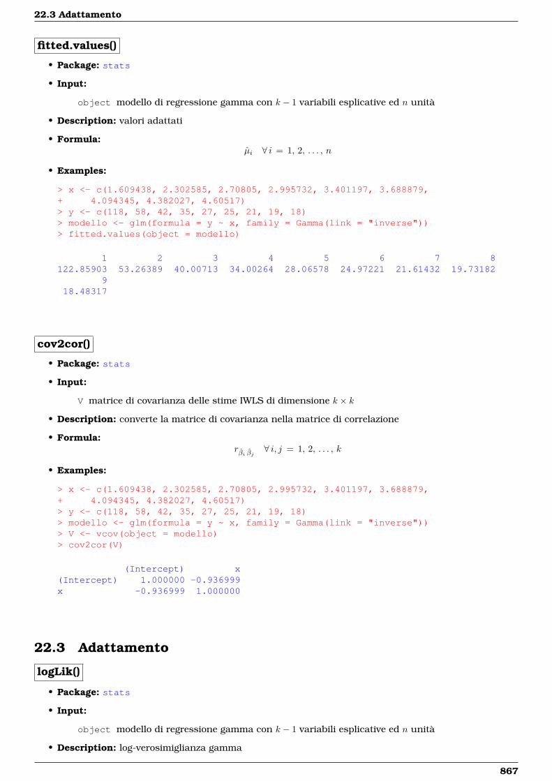
22.3 Adattamento
fitted.values()
• Package: stats
• Input:
object modello di regressione gamma con k − 1 variabili esplicative ed n unità
• Description: valori adattati
• Formula:µi ∀ i = 1, 2, . . . , n
• Examples:
> x <- c(1.609438, 2.302585, 2.70805, 2.995732, 3.401197, 3.688879,+ 4.094345, 4.382027, 4.60517)> y <- c(118, 58, 42, 35, 27, 25, 21, 19, 18)> modello <- glm(formula = y ~ x, family = Gamma(link = "inverse"))> fitted.values(object = modello)
1 2 3 4 5 6 7 8122.85903 53.26389 40.00713 34.00264 28.06578 24.97221 21.61432 19.73182
918.48317
cov2cor()
• Package: stats
• Input:
V matrice di covarianza delle stime IWLS di dimensione k × k
• Description: converte la matrice di covarianza nella matrice di correlazione
• Formula:rβi βj ∀ i, j = 1, 2, . . . , k
• Examples:
> x <- c(1.609438, 2.302585, 2.70805, 2.995732, 3.401197, 3.688879,+ 4.094345, 4.382027, 4.60517)> y <- c(118, 58, 42, 35, 27, 25, 21, 19, 18)> modello <- glm(formula = y ~ x, family = Gamma(link = "inverse"))> V <- vcov(object = modello)> cov2cor(V)
(Intercept) x(Intercept) 1.000000 -0.936999x -0.936999 1.000000
22.3 Adattamento
logLik()
• Package: stats
• Input:
object modello di regressione gamma con k − 1 variabili esplicative ed n unità
• Description: log-verosimiglianza gamma
867
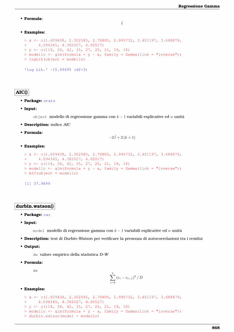
Regressione Gamma
• Formula:ˆ
• Examples:
> x <- c(1.609438, 2.302585, 2.70805, 2.995732, 3.401197, 3.688879,+ 4.094345, 4.382027, 4.60517)> y <- c(118, 58, 42, 35, 27, 25, 21, 19, 18)> modello <- glm(formula = y ~ x, family = Gamma(link = "inverse"))> logLik(object = modello)
'log Lik.' -15.99495 (df=3)
AIC()
• Package: stats
• Input:
object modello di regressione gamma con k − 1 variabili esplicative ed n unità
• Description: indice AIC
• Formula:−2 ˆ+ 2 (k + 1)
• Examples:
> x <- c(1.609438, 2.302585, 2.70805, 2.995732, 3.401197, 3.688879,+ 4.094345, 4.382027, 4.60517)> y <- c(118, 58, 42, 35, 27, 25, 21, 19, 18)> modello <- glm(formula = y ~ x, family = Gamma(link = "inverse"))> AIC(object = modello)
[1] 37.9899
durbin.watson()
• Package: car
• Input:
model modello di regressione gamma con k − 1 variabili esplicative ed n unità
• Description: test di Durbin–Watson per verificare la presenza di autocorrelazioni tra i residui
• Output:
dw valore empirico della statistica D–W
• Formula:
dwn∑i=2
(ei − ei−1)2 /D
• Examples:
> x <- c(1.609438, 2.302585, 2.70805, 2.995732, 3.401197, 3.688879,+ 4.094345, 4.382027, 4.60517)> y <- c(118, 58, 42, 35, 27, 25, 21, 19, 18)> modello <- glm(formula = y ~ x, family = Gamma(link = "inverse"))> durbin.watson(model = modello)
868

22.3 Adattamento
lag Autocorrelation D-W Statistic p-value1 0.1835659 1.495257 0
Alternative hypothesis: rho != 0
> res <- durbin.watson(model = modello)> res$dw
[1] 1.495257
extractAIC()
• Package: stats
• Input:
fit modello di regressione gamma con k − 1 variabili esplicative ed n unità
• Description: numero di parametri del modello ed indice AIC generalizzato
• Formula:k − 2 ˆ+ 2 (k + 1)
• Examples:
> x <- c(1.609438, 2.302585, 2.70805, 2.995732, 3.401197, 3.688879,+ 4.094345, 4.382027, 4.60517)> y <- c(118, 58, 42, 35, 27, 25, 21, 19, 18)> modello <- glm(formula = y ~ x, family = Gamma(link = "inverse"))> extractAIC(fit = modello)
[1] 2.0000 37.9899
deviance()
• Package: stats
• Input:
object modello di regressione gamma con k − 1 variabili esplicative ed n unità
• Description: devianza residua
• Formula:D
• Examples:
> x <- c(1.609438, 2.302585, 2.70805, 2.995732, 3.401197, 3.688879,+ 4.094345, 4.382027, 4.60517)> y <- c(118, 58, 42, 35, 27, 25, 21, 19, 18)> modello <- glm(formula = y ~ x, family = Gamma(link = "inverse"))> deviance(object = modello)
[1] 0.01672967
869
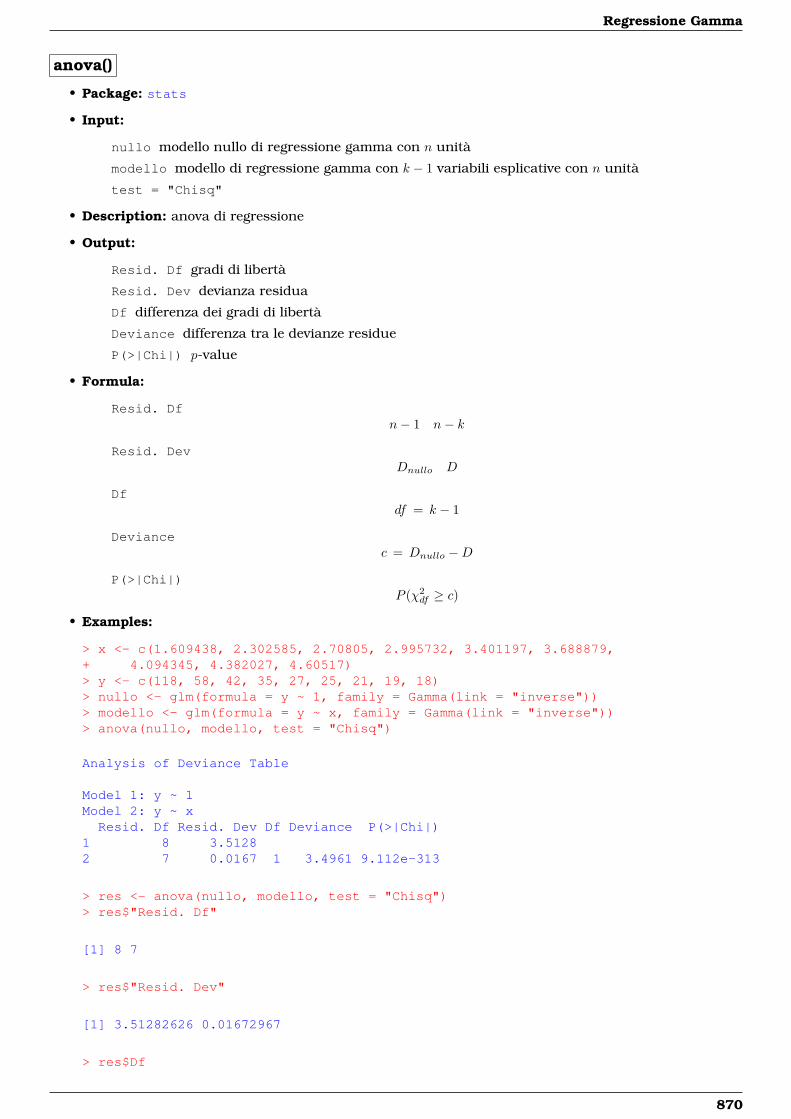
Regressione Gamma
anova()
• Package: stats
• Input:
nullo modello nullo di regressione gamma con n unità
modello modello di regressione gamma con k − 1 variabili esplicative con n unità
test = "Chisq"
• Description: anova di regressione
• Output:
Resid. Df gradi di libertà
Resid. Dev devianza residua
Df differenza dei gradi di libertà
Deviance differenza tra le devianze residue
P(>|Chi|) p-value
• Formula:
Resid. Dfn− 1 n− k
Resid. DevDnullo D
Dfdf = k − 1
Deviancec = Dnullo −D
P(>|Chi|)P (χ2
df ≥ c)
• Examples:
> x <- c(1.609438, 2.302585, 2.70805, 2.995732, 3.401197, 3.688879,+ 4.094345, 4.382027, 4.60517)> y <- c(118, 58, 42, 35, 27, 25, 21, 19, 18)> nullo <- glm(formula = y ~ 1, family = Gamma(link = "inverse"))> modello <- glm(formula = y ~ x, family = Gamma(link = "inverse"))> anova(nullo, modello, test = "Chisq")
Analysis of Deviance Table
Model 1: y ~ 1Model 2: y ~ xResid. Df Resid. Dev Df Deviance P(>|Chi|)
1 8 3.51282 7 0.0167 1 3.4961 9.112e-313
> res <- anova(nullo, modello, test = "Chisq")> res$"Resid. Df"
[1] 8 7
> res$"Resid. Dev"
[1] 3.51282626 0.01672967
> res$Df
870
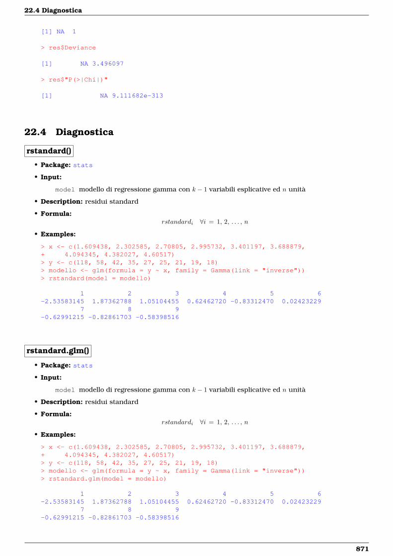
22.4 Diagnostica
[1] NA 1
> res$Deviance
[1] NA 3.496097
> res$"P(>|Chi|)"
[1] NA 9.111682e-313
22.4 Diagnostica
rstandard()
• Package: stats
• Input:
model modello di regressione gamma con k − 1 variabili esplicative ed n unità
• Description: residui standard
• Formula:rstandardi ∀i = 1, 2, . . . , n
• Examples:
> x <- c(1.609438, 2.302585, 2.70805, 2.995732, 3.401197, 3.688879,+ 4.094345, 4.382027, 4.60517)> y <- c(118, 58, 42, 35, 27, 25, 21, 19, 18)> modello <- glm(formula = y ~ x, family = Gamma(link = "inverse"))> rstandard(model = modello)
1 2 3 4 5 6-2.53583145 1.87362788 1.05104455 0.62462720 -0.83312470 0.02423229
7 8 9-0.62991215 -0.82861703 -0.58398516
rstandard.glm()
• Package: stats
• Input:
model modello di regressione gamma con k − 1 variabili esplicative ed n unità
• Description: residui standard
• Formula:rstandardi ∀i = 1, 2, . . . , n
• Examples:
> x <- c(1.609438, 2.302585, 2.70805, 2.995732, 3.401197, 3.688879,+ 4.094345, 4.382027, 4.60517)> y <- c(118, 58, 42, 35, 27, 25, 21, 19, 18)> modello <- glm(formula = y ~ x, family = Gamma(link = "inverse"))> rstandard.glm(model = modello)
1 2 3 4 5 6-2.53583145 1.87362788 1.05104455 0.62462720 -0.83312470 0.02423229
7 8 9-0.62991215 -0.82861703 -0.58398516
871
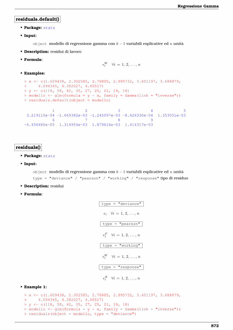
Regressione Gamma
residuals.default()
• Package: stats
• Input:
object modello di regressione gamma con k − 1 variabili esplicative ed n unità
• Description: residui di lavoro
• Formula:eWi ∀i = 1, 2, . . . , n
• Examples:
> x <- c(1.609438, 2.302585, 2.70805, 2.995732, 3.401197, 3.688879,+ 4.094345, 4.382027, 4.60517)> y <- c(118, 58, 42, 35, 27, 25, 21, 19, 18)> modello <- glm(formula = y ~ x, family = Gamma(link = "inverse"))> residuals.default(object = modello)
1 2 3 4 53.219110e-04 -1.669382e-03 -1.245097e-03 -8.626330e-04 1.353051e-03
6 7 8 9-4.456480e-05 1.314954e-03 1.879616e-03 1.414317e-03
residuals()
• Package: stats
• Input:
object modello di regressione gamma con k − 1 variabili esplicative ed n unità
type = "deviance" / "pearson" / "working" / "response" tipo di residuo
• Description: residui
• Formula:
type = "deviance"
ei ∀i = 1, 2, . . . , n
type = "pearson"
ePi ∀i = 1, 2, . . . , n
type = "working"
eWi ∀i = 1, 2, . . . , n
type = "response"
eRi ∀i = 1, 2, . . . , n
• Example 1:
> x <- c(1.609438, 2.302585, 2.70805, 2.995732, 3.401197, 3.688879,+ 4.094345, 4.382027, 4.60517)> y <- c(118, 58, 42, 35, 27, 25, 21, 19, 18)> modello <- glm(formula = y ~ x, family = Gamma(link = "inverse"))> residuals(object = modello, type = "deviance")
872
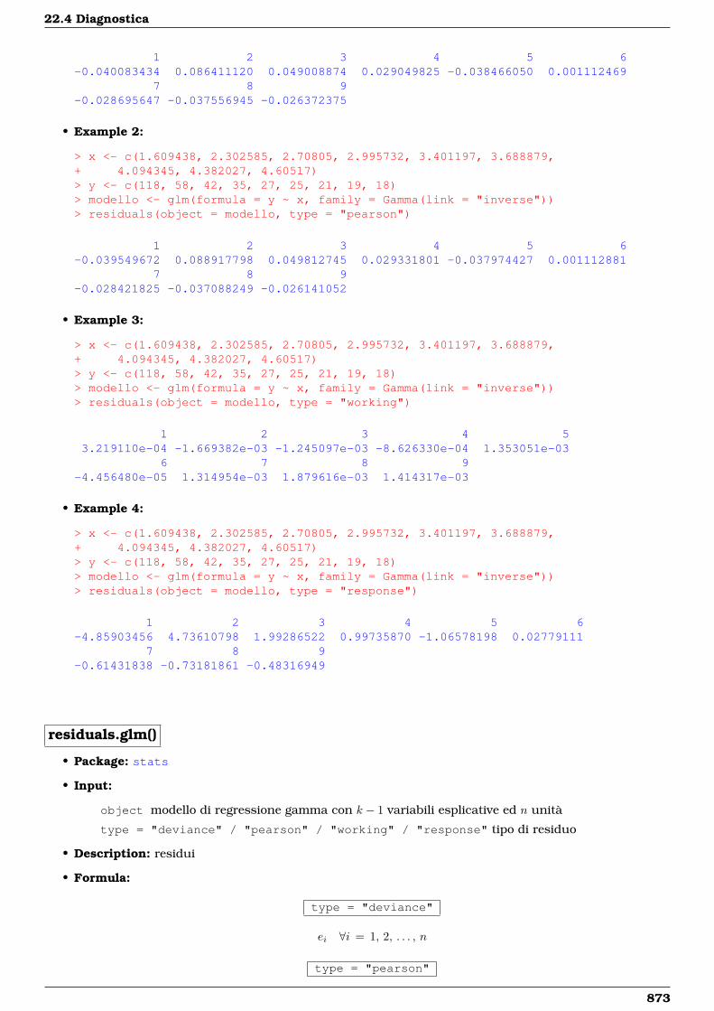
22.4 Diagnostica
1 2 3 4 5 6-0.040083434 0.086411120 0.049008874 0.029049825 -0.038466050 0.001112469
7 8 9-0.028695647 -0.037556945 -0.026372375
• Example 2:
> x <- c(1.609438, 2.302585, 2.70805, 2.995732, 3.401197, 3.688879,+ 4.094345, 4.382027, 4.60517)> y <- c(118, 58, 42, 35, 27, 25, 21, 19, 18)> modello <- glm(formula = y ~ x, family = Gamma(link = "inverse"))> residuals(object = modello, type = "pearson")
1 2 3 4 5 6-0.039549672 0.088917798 0.049812745 0.029331801 -0.037974427 0.001112881
7 8 9-0.028421825 -0.037088249 -0.026141052
• Example 3:
> x <- c(1.609438, 2.302585, 2.70805, 2.995732, 3.401197, 3.688879,+ 4.094345, 4.382027, 4.60517)> y <- c(118, 58, 42, 35, 27, 25, 21, 19, 18)> modello <- glm(formula = y ~ x, family = Gamma(link = "inverse"))> residuals(object = modello, type = "working")
1 2 3 4 53.219110e-04 -1.669382e-03 -1.245097e-03 -8.626330e-04 1.353051e-03
6 7 8 9-4.456480e-05 1.314954e-03 1.879616e-03 1.414317e-03
• Example 4:
> x <- c(1.609438, 2.302585, 2.70805, 2.995732, 3.401197, 3.688879,+ 4.094345, 4.382027, 4.60517)> y <- c(118, 58, 42, 35, 27, 25, 21, 19, 18)> modello <- glm(formula = y ~ x, family = Gamma(link = "inverse"))> residuals(object = modello, type = "response")
1 2 3 4 5 6-4.85903456 4.73610798 1.99286522 0.99735870 -1.06578198 0.02779111
7 8 9-0.61431838 -0.73181861 -0.48316949
residuals.glm()
• Package: stats
• Input:
object modello di regressione gamma con k − 1 variabili esplicative ed n unità
type = "deviance" / "pearson" / "working" / "response" tipo di residuo
• Description: residui
• Formula:
type = "deviance"
ei ∀i = 1, 2, . . . , n
type = "pearson"
873
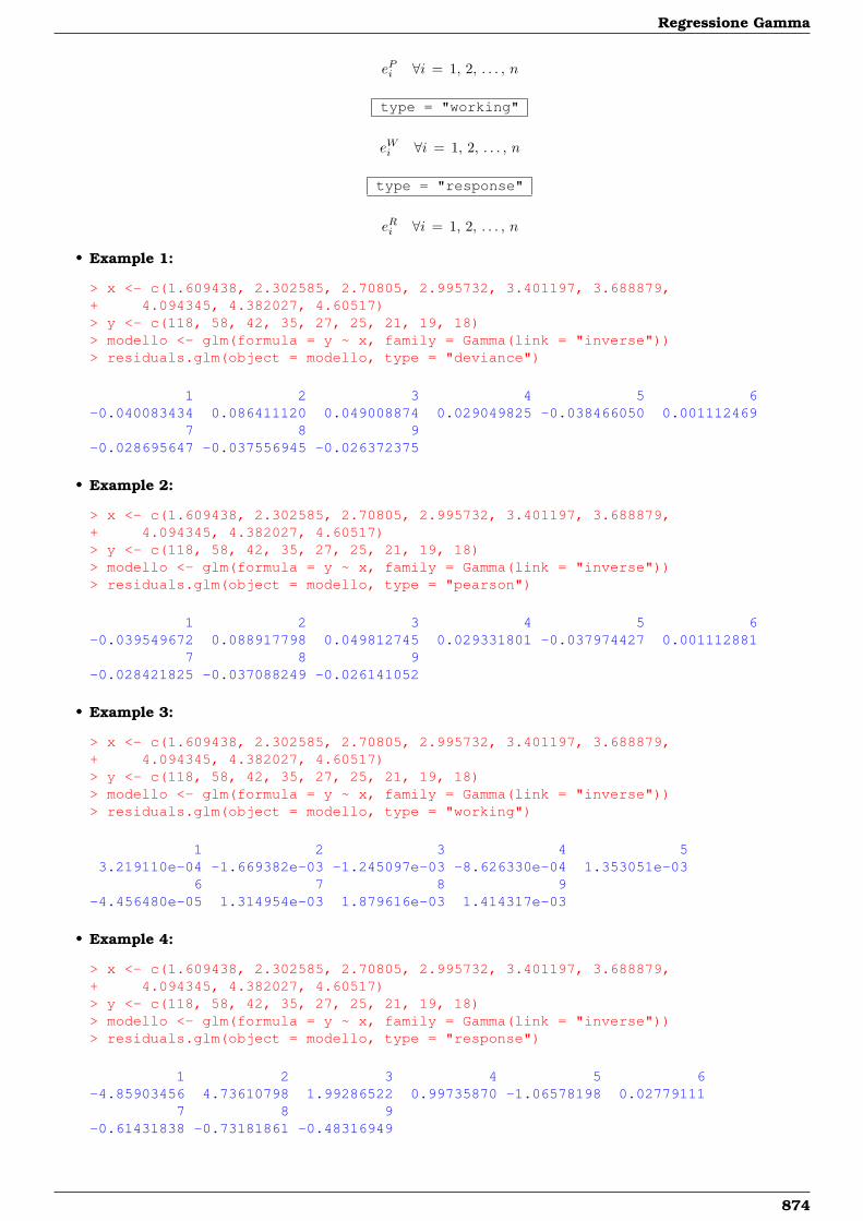
Regressione Gamma
ePi ∀i = 1, 2, . . . , n
type = "working"
eWi ∀i = 1, 2, . . . , n
type = "response"
eRi ∀i = 1, 2, . . . , n
• Example 1:
> x <- c(1.609438, 2.302585, 2.70805, 2.995732, 3.401197, 3.688879,+ 4.094345, 4.382027, 4.60517)> y <- c(118, 58, 42, 35, 27, 25, 21, 19, 18)> modello <- glm(formula = y ~ x, family = Gamma(link = "inverse"))> residuals.glm(object = modello, type = "deviance")
1 2 3 4 5 6-0.040083434 0.086411120 0.049008874 0.029049825 -0.038466050 0.001112469
7 8 9-0.028695647 -0.037556945 -0.026372375
• Example 2:
> x <- c(1.609438, 2.302585, 2.70805, 2.995732, 3.401197, 3.688879,+ 4.094345, 4.382027, 4.60517)> y <- c(118, 58, 42, 35, 27, 25, 21, 19, 18)> modello <- glm(formula = y ~ x, family = Gamma(link = "inverse"))> residuals.glm(object = modello, type = "pearson")
1 2 3 4 5 6-0.039549672 0.088917798 0.049812745 0.029331801 -0.037974427 0.001112881
7 8 9-0.028421825 -0.037088249 -0.026141052
• Example 3:
> x <- c(1.609438, 2.302585, 2.70805, 2.995732, 3.401197, 3.688879,+ 4.094345, 4.382027, 4.60517)> y <- c(118, 58, 42, 35, 27, 25, 21, 19, 18)> modello <- glm(formula = y ~ x, family = Gamma(link = "inverse"))> residuals.glm(object = modello, type = "working")
1 2 3 4 53.219110e-04 -1.669382e-03 -1.245097e-03 -8.626330e-04 1.353051e-03
6 7 8 9-4.456480e-05 1.314954e-03 1.879616e-03 1.414317e-03
• Example 4:
> x <- c(1.609438, 2.302585, 2.70805, 2.995732, 3.401197, 3.688879,+ 4.094345, 4.382027, 4.60517)> y <- c(118, 58, 42, 35, 27, 25, 21, 19, 18)> modello <- glm(formula = y ~ x, family = Gamma(link = "inverse"))> residuals.glm(object = modello, type = "response")
1 2 3 4 5 6-4.85903456 4.73610798 1.99286522 0.99735870 -1.06578198 0.02779111
7 8 9-0.61431838 -0.73181861 -0.48316949
874
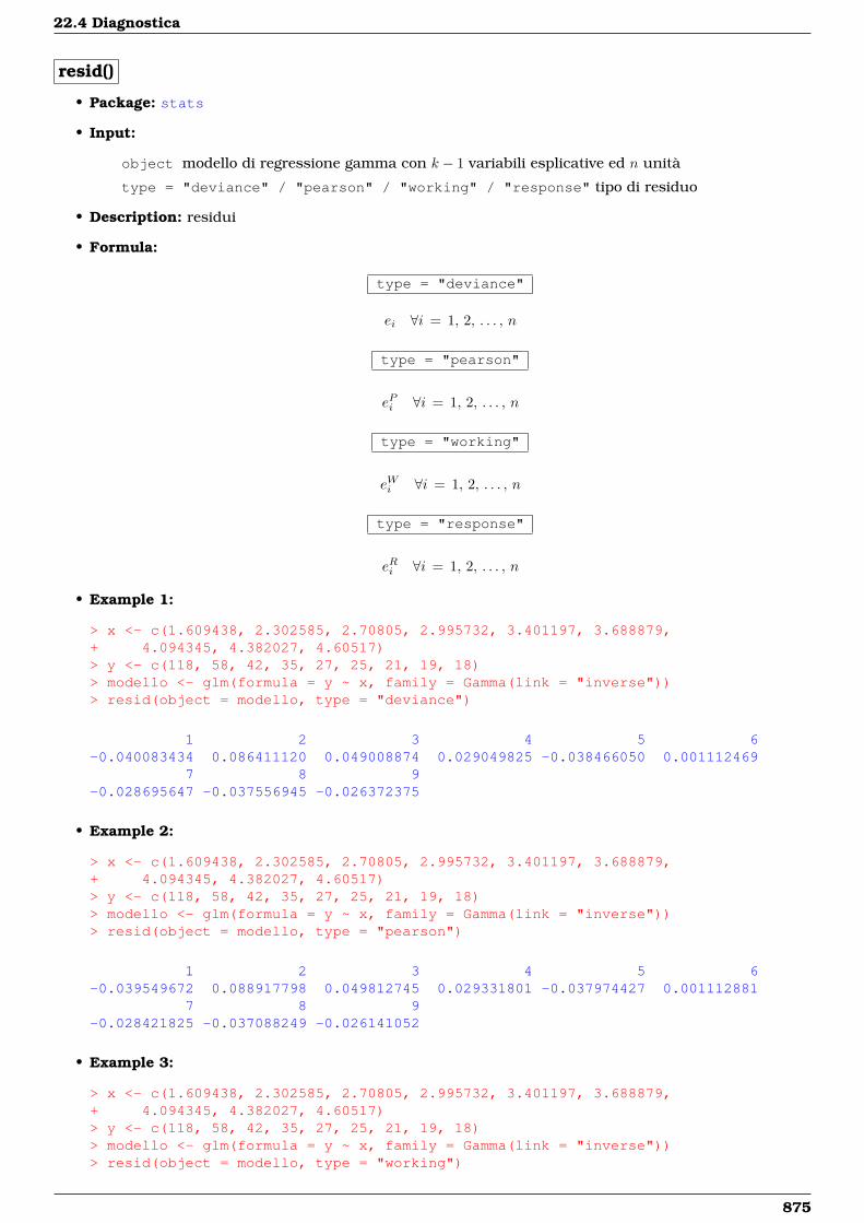
22.4 Diagnostica
resid()
• Package: stats
• Input:
object modello di regressione gamma con k − 1 variabili esplicative ed n unità
type = "deviance" / "pearson" / "working" / "response" tipo di residuo
• Description: residui
• Formula:
type = "deviance"
ei ∀i = 1, 2, . . . , n
type = "pearson"
ePi ∀i = 1, 2, . . . , n
type = "working"
eWi ∀i = 1, 2, . . . , n
type = "response"
eRi ∀i = 1, 2, . . . , n
• Example 1:
> x <- c(1.609438, 2.302585, 2.70805, 2.995732, 3.401197, 3.688879,+ 4.094345, 4.382027, 4.60517)> y <- c(118, 58, 42, 35, 27, 25, 21, 19, 18)> modello <- glm(formula = y ~ x, family = Gamma(link = "inverse"))> resid(object = modello, type = "deviance")
1 2 3 4 5 6-0.040083434 0.086411120 0.049008874 0.029049825 -0.038466050 0.001112469
7 8 9-0.028695647 -0.037556945 -0.026372375
• Example 2:
> x <- c(1.609438, 2.302585, 2.70805, 2.995732, 3.401197, 3.688879,+ 4.094345, 4.382027, 4.60517)> y <- c(118, 58, 42, 35, 27, 25, 21, 19, 18)> modello <- glm(formula = y ~ x, family = Gamma(link = "inverse"))> resid(object = modello, type = "pearson")
1 2 3 4 5 6-0.039549672 0.088917798 0.049812745 0.029331801 -0.037974427 0.001112881
7 8 9-0.028421825 -0.037088249 -0.026141052
• Example 3:
> x <- c(1.609438, 2.302585, 2.70805, 2.995732, 3.401197, 3.688879,+ 4.094345, 4.382027, 4.60517)> y <- c(118, 58, 42, 35, 27, 25, 21, 19, 18)> modello <- glm(formula = y ~ x, family = Gamma(link = "inverse"))> resid(object = modello, type = "working")
875
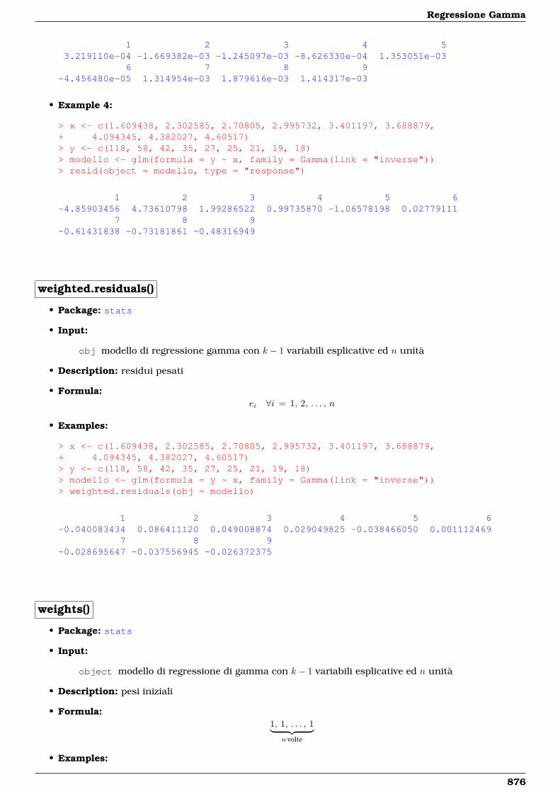
Regressione Gamma
1 2 3 4 53.219110e-04 -1.669382e-03 -1.245097e-03 -8.626330e-04 1.353051e-03
6 7 8 9-4.456480e-05 1.314954e-03 1.879616e-03 1.414317e-03
• Example 4:
> x <- c(1.609438, 2.302585, 2.70805, 2.995732, 3.401197, 3.688879,+ 4.094345, 4.382027, 4.60517)> y <- c(118, 58, 42, 35, 27, 25, 21, 19, 18)> modello <- glm(formula = y ~ x, family = Gamma(link = "inverse"))> resid(object = modello, type = "response")
1 2 3 4 5 6-4.85903456 4.73610798 1.99286522 0.99735870 -1.06578198 0.02779111
7 8 9-0.61431838 -0.73181861 -0.48316949
weighted.residuals()
• Package: stats
• Input:
obj modello di regressione gamma con k − 1 variabili esplicative ed n unità
• Description: residui pesati
• Formula:ei ∀i = 1, 2, . . . , n
• Examples:
> x <- c(1.609438, 2.302585, 2.70805, 2.995732, 3.401197, 3.688879,+ 4.094345, 4.382027, 4.60517)> y <- c(118, 58, 42, 35, 27, 25, 21, 19, 18)> modello <- glm(formula = y ~ x, family = Gamma(link = "inverse"))> weighted.residuals(obj = modello)
1 2 3 4 5 6-0.040083434 0.086411120 0.049008874 0.029049825 -0.038466050 0.001112469
7 8 9-0.028695647 -0.037556945 -0.026372375
weights()
• Package: stats
• Input:
object modello di regressione di gamma con k − 1 variabili esplicative ed n unità
• Description: pesi iniziali
• Formula:1, 1, . . . , 1︸ ︷︷ ︸
n volte
• Examples:
876
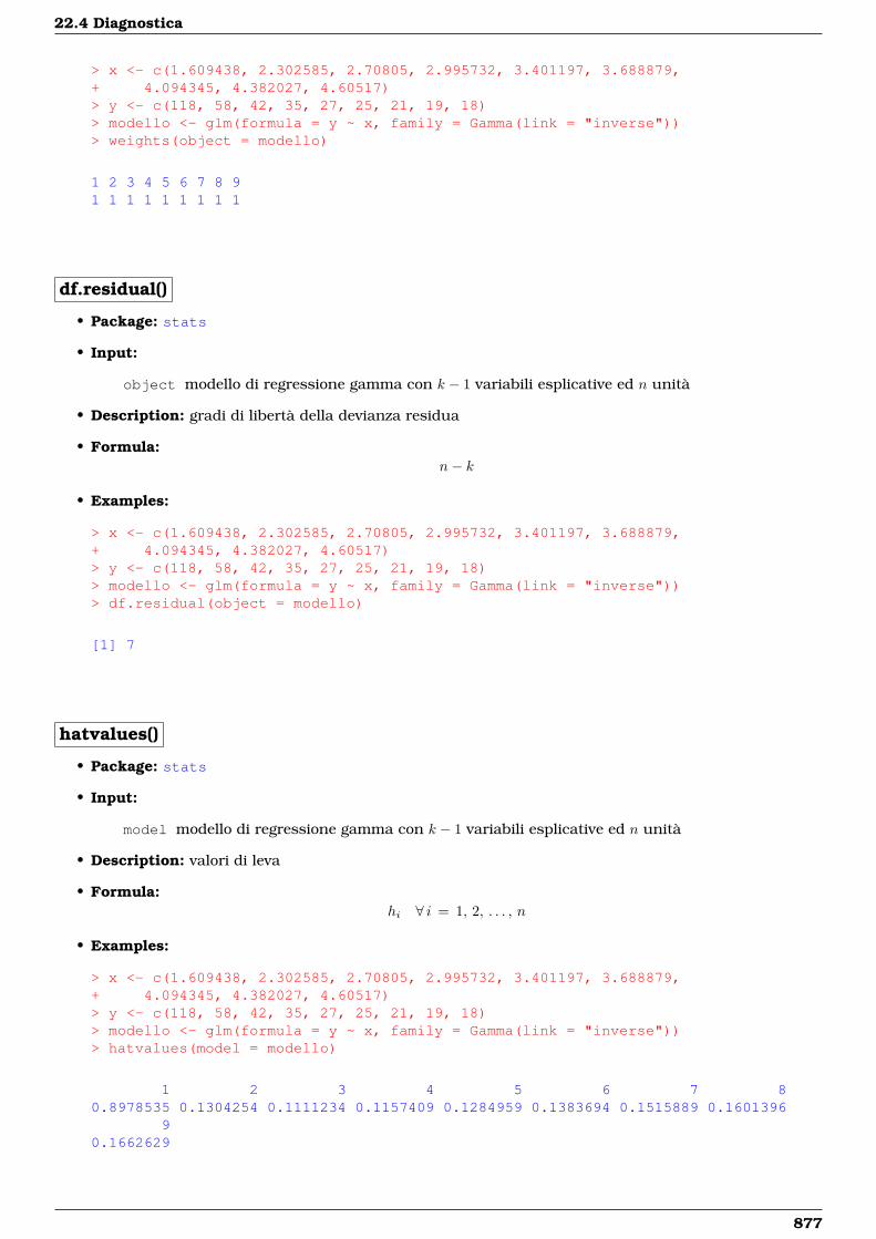
22.4 Diagnostica
> x <- c(1.609438, 2.302585, 2.70805, 2.995732, 3.401197, 3.688879,+ 4.094345, 4.382027, 4.60517)> y <- c(118, 58, 42, 35, 27, 25, 21, 19, 18)> modello <- glm(formula = y ~ x, family = Gamma(link = "inverse"))> weights(object = modello)
1 2 3 4 5 6 7 8 91 1 1 1 1 1 1 1 1
df.residual()
• Package: stats
• Input:
object modello di regressione gamma con k − 1 variabili esplicative ed n unità
• Description: gradi di libertà della devianza residua
• Formula:n− k
• Examples:
> x <- c(1.609438, 2.302585, 2.70805, 2.995732, 3.401197, 3.688879,+ 4.094345, 4.382027, 4.60517)> y <- c(118, 58, 42, 35, 27, 25, 21, 19, 18)> modello <- glm(formula = y ~ x, family = Gamma(link = "inverse"))> df.residual(object = modello)
[1] 7
hatvalues()
• Package: stats
• Input:
model modello di regressione gamma con k − 1 variabili esplicative ed n unità
• Description: valori di leva
• Formula:hi ∀ i = 1, 2, . . . , n
• Examples:
> x <- c(1.609438, 2.302585, 2.70805, 2.995732, 3.401197, 3.688879,+ 4.094345, 4.382027, 4.60517)> y <- c(118, 58, 42, 35, 27, 25, 21, 19, 18)> modello <- glm(formula = y ~ x, family = Gamma(link = "inverse"))> hatvalues(model = modello)
1 2 3 4 5 6 7 80.8978535 0.1304254 0.1111234 0.1157409 0.1284959 0.1383694 0.1515889 0.1601396
90.1662629
877
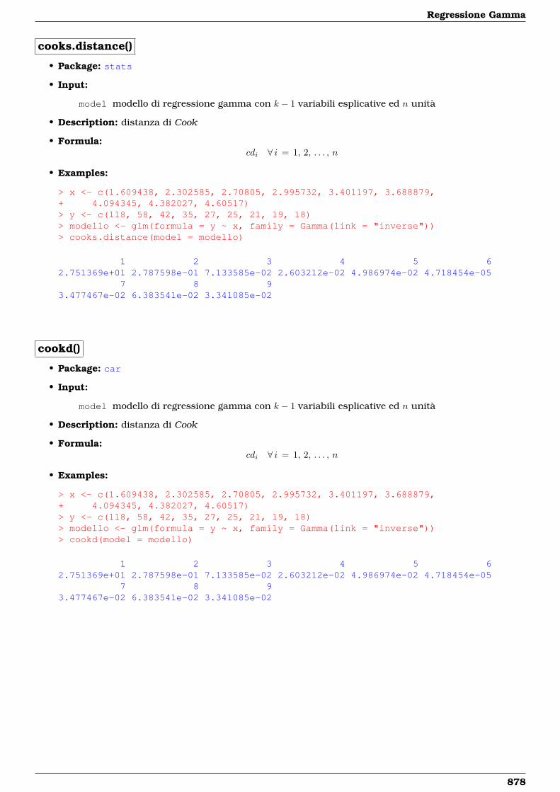
Regressione Gamma
cooks.distance()
• Package: stats
• Input:
model modello di regressione gamma con k − 1 variabili esplicative ed n unità
• Description: distanza di Cook
• Formula:cdi ∀ i = 1, 2, . . . , n
• Examples:
> x <- c(1.609438, 2.302585, 2.70805, 2.995732, 3.401197, 3.688879,+ 4.094345, 4.382027, 4.60517)> y <- c(118, 58, 42, 35, 27, 25, 21, 19, 18)> modello <- glm(formula = y ~ x, family = Gamma(link = "inverse"))> cooks.distance(model = modello)
1 2 3 4 5 62.751369e+01 2.787598e-01 7.133585e-02 2.603212e-02 4.986974e-02 4.718454e-05
7 8 93.477467e-02 6.383541e-02 3.341085e-02
cookd()
• Package: car
• Input:
model modello di regressione gamma con k − 1 variabili esplicative ed n unità
• Description: distanza di Cook
• Formula:cdi ∀ i = 1, 2, . . . , n
• Examples:
> x <- c(1.609438, 2.302585, 2.70805, 2.995732, 3.401197, 3.688879,+ 4.094345, 4.382027, 4.60517)> y <- c(118, 58, 42, 35, 27, 25, 21, 19, 18)> modello <- glm(formula = y ~ x, family = Gamma(link = "inverse"))> cookd(model = modello)
1 2 3 4 5 62.751369e+01 2.787598e-01 7.133585e-02 2.603212e-02 4.986974e-02 4.718454e-05
7 8 93.477467e-02 6.383541e-02 3.341085e-02
878
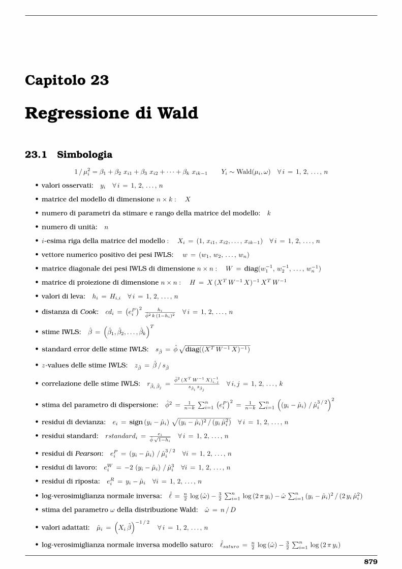
Capitolo 23
Regressione di Wald
23.1 Simbologia
1 / µ2i = β1 + β2 xi1 + β3 xi2 + · · ·+ βk xik−1 Yi ∼Wald(µi, ω) ∀ i = 1, 2, . . . , n
• valori osservati: yi ∀ i = 1, 2, . . . , n
• matrice del modello di dimensione n× k : X
• numero di parametri da stimare e rango della matrice del modello: k
• numero di unità: n
• i-esima riga della matrice del modello : Xi = (1, xi1, xi2, . . . , xik−1) ∀ i = 1, 2, . . . , n
• vettore numerico positivo dei pesi IWLS: w = (w1, w2, . . . , wn)
• matrice diagonale dei pesi IWLS di dimensione n× n : W = diag(w−11 , w−1
2 , . . . , w−1n )
• matrice di proiezione di dimensione n× n : H = X (XT W−1X)−1XT W−1
• valori di leva: hi = Hi,i ∀ i = 1, 2, . . . , n
• distanza di Cook: cdi =(ePi)2 hi
φ2 k (1−hi)2∀ i = 1, 2, . . . , n
• stime IWLS: β =(β1, β2, . . . , βk
)T• standard error delle stime IWLS: sβ = φ
√diag((XT W−1X)−1)
• z-values delle stime IWLS: zβ = β / sβ
• correlazione delle stime IWLS: rβi βj =φ2 (XT W−1X)−1
i, j
sβisβj
∀ i, j = 1, 2, . . . , k
• stima del parametro di dispersione: φ2 = 1n−k
∑ni=1
(ePi)2 = 1
n−k∑ni=1
((yi − µi) / µ3 / 2
i
)2
• residui di devianza: ei = sign (yi − µi)√
(yi − µi)2 / (yi µ2i ) ∀ i = 1, 2, . . . , n
• residui standard: rstandardi = eiφ√
1−hi∀ i = 1, 2, . . . , n
• residui di Pearson: ePi = (yi − µi) / µ3 / 2i ∀i = 1, 2, . . . , n
• residui di lavoro: eWi = −2 (yi − µi) / µ3i ∀i = 1, 2, . . . , n
• residui di riposta: eRi = yi − µi ∀i = 1, 2, . . . , n
• log-verosimiglianza normale inversa: ˆ = n2 log (ω)− 3
2
∑ni=1 log (2π yi)− ω
∑ni=1 (yi − µi)2 / (2 yi µ2
i )
• stima del parametro ω della distribuzione Wald: ω = n /D
• valori adattati: µi =(Xi β
)−1 / 2
∀ i = 1, 2, . . . , n
• log-verosimiglianza normale inversa modello saturo: ˆsaturo = n
2 log (ω)− 32
∑ni=1 log (2π yi)
879
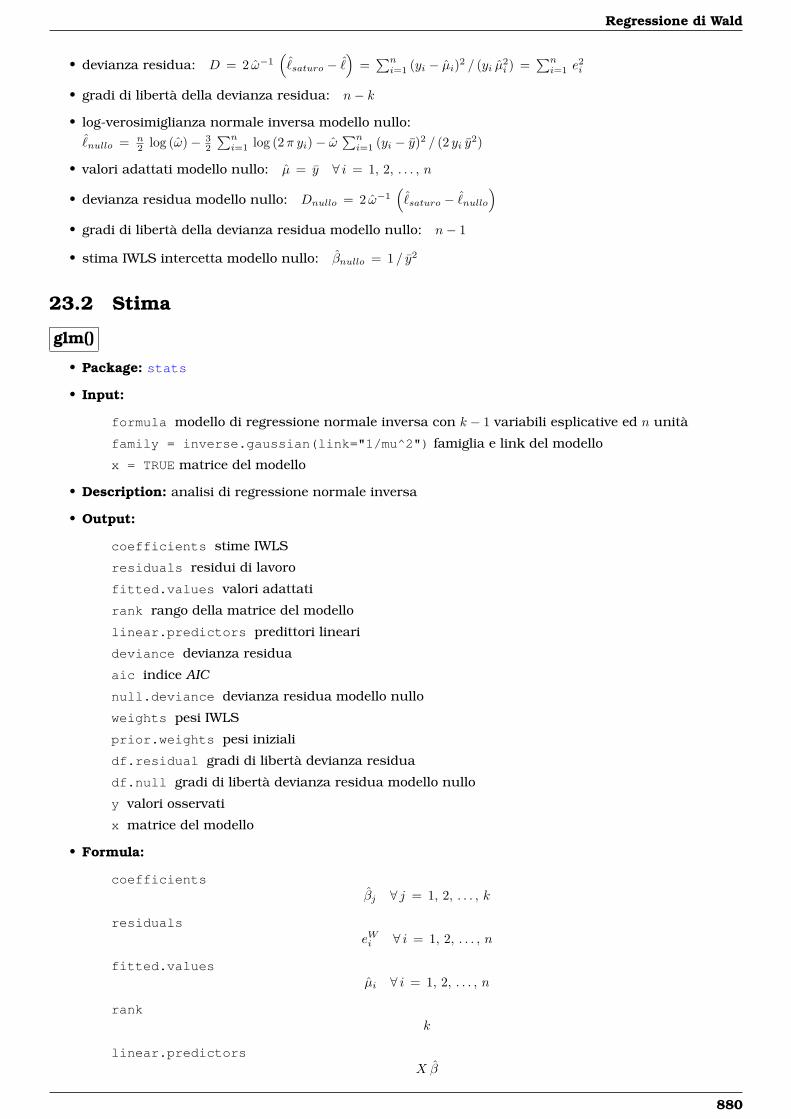
Regressione di Wald
• devianza residua: D = 2 ω−1(
ˆsaturo − ˆ
)=∑ni=1 (yi − µi)2 / (yi µ2
i ) =∑ni=1 e
2i
• gradi di libertà della devianza residua: n− k
• log-verosimiglianza normale inversa modello nullo:ˆnullo = n
2 log (ω)− 32
∑ni=1 log (2π yi)− ω
∑ni=1 (yi − y)2 / (2 yi y2)
• valori adattati modello nullo: µ = y ∀ i = 1, 2, . . . , n
• devianza residua modello nullo: Dnullo = 2 ω−1(
ˆsaturo − ˆ
nullo
)• gradi di libertà della devianza residua modello nullo: n− 1
• stima IWLS intercetta modello nullo: βnullo = 1 / y2
23.2 Stima
glm()
• Package: stats
• Input:
formula modello di regressione normale inversa con k − 1 variabili esplicative ed n unità
family = inverse.gaussian(link="1/mu^2") famiglia e link del modello
x = TRUE matrice del modello
• Description: analisi di regressione normale inversa
• Output:
coefficients stime IWLS
residuals residui di lavoro
fitted.values valori adattati
rank rango della matrice del modello
linear.predictors predittori lineari
deviance devianza residua
aic indice AIC
null.deviance devianza residua modello nullo
weights pesi IWLS
prior.weights pesi iniziali
df.residual gradi di libertà devianza residua
df.null gradi di libertà devianza residua modello nullo
y valori osservati
x matrice del modello
• Formula:
coefficientsβj ∀ j = 1, 2, . . . , k
residualseWi ∀ i = 1, 2, . . . , n
fitted.valuesµi ∀ i = 1, 2, . . . , n
rankk
linear.predictorsX β
880
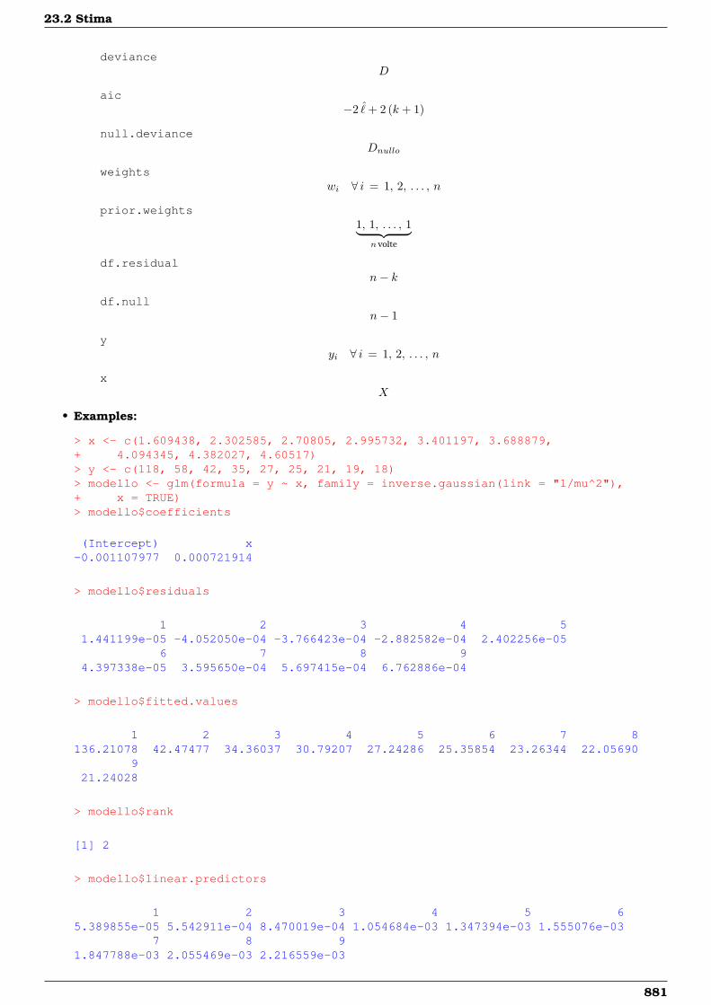
23.2 Stima
devianceD
aic−2 ˆ+ 2 (k + 1)
null.devianceDnullo
weightswi ∀ i = 1, 2, . . . , n
prior.weights1, 1, . . . , 1︸ ︷︷ ︸
n volte
df.residualn− k
df.nulln− 1
yyi ∀ i = 1, 2, . . . , n
xX
• Examples:
> x <- c(1.609438, 2.302585, 2.70805, 2.995732, 3.401197, 3.688879,+ 4.094345, 4.382027, 4.60517)> y <- c(118, 58, 42, 35, 27, 25, 21, 19, 18)> modello <- glm(formula = y ~ x, family = inverse.gaussian(link = "1/mu^2"),+ x = TRUE)> modello$coefficients
(Intercept) x-0.001107977 0.000721914
> modello$residuals
1 2 3 4 51.441199e-05 -4.052050e-04 -3.766423e-04 -2.882582e-04 2.402256e-05
6 7 8 94.397338e-05 3.595650e-04 5.697415e-04 6.762886e-04
> modello$fitted.values
1 2 3 4 5 6 7 8136.21078 42.47477 34.36037 30.79207 27.24286 25.35854 23.26344 22.05690
921.24028
> modello$rank
[1] 2
> modello$linear.predictors
1 2 3 4 5 65.389855e-05 5.542911e-04 8.470019e-04 1.054684e-03 1.347394e-03 1.555076e-03
7 8 91.847788e-03 2.055469e-03 2.216559e-03
881
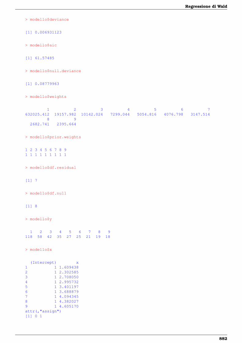
Regressione di Wald
> modello$deviance
[1] 0.006931123
> modello$aic
[1] 61.57485
> modello$null.deviance
[1] 0.08779963
> modello$weights
1 2 3 4 5 6 7632025.412 19157.982 10142.024 7299.044 5054.816 4076.798 3147.514
8 92682.741 2395.664
> modello$prior.weights
1 2 3 4 5 6 7 8 91 1 1 1 1 1 1 1 1
> modello$df.residual
[1] 7
> modello$df.null
[1] 8
> modello$y
1 2 3 4 5 6 7 8 9118 58 42 35 27 25 21 19 18
> modello$x
(Intercept) x1 1 1.6094382 1 2.3025853 1 2.7080504 1 2.9957325 1 3.4011976 1 3.6888797 1 4.0943458 1 4.3820279 1 4.605170attr(,"assign")[1] 0 1
882
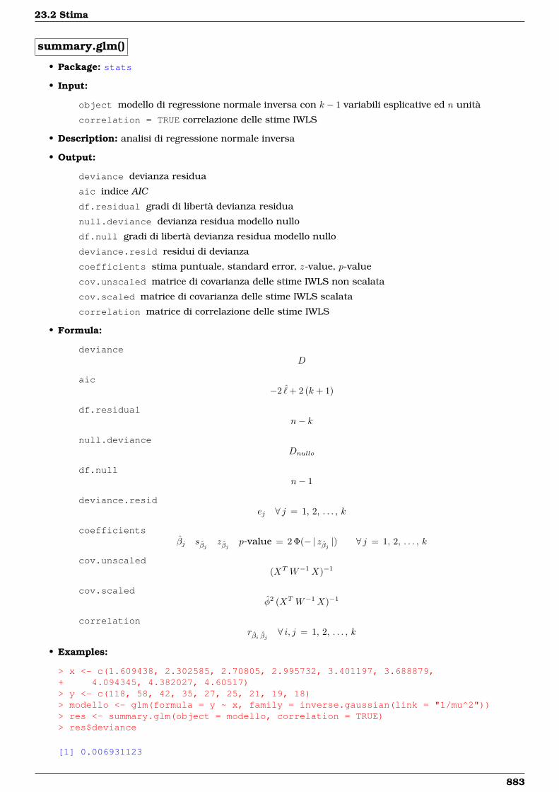
23.2 Stima
summary.glm()
• Package: stats
• Input:
object modello di regressione normale inversa con k − 1 variabili esplicative ed n unità
correlation = TRUE correlazione delle stime IWLS
• Description: analisi di regressione normale inversa
• Output:
deviance devianza residua
aic indice AIC
df.residual gradi di libertà devianza residua
null.deviance devianza residua modello nullo
df.null gradi di libertà devianza residua modello nullo
deviance.resid residui di devianza
coefficients stima puntuale, standard error, z-value, p-value
cov.unscaled matrice di covarianza delle stime IWLS non scalata
cov.scaled matrice di covarianza delle stime IWLS scalata
correlation matrice di correlazione delle stime IWLS
• Formula:
devianceD
aic−2 ˆ+ 2 (k + 1)
df.residualn− k
null.devianceDnullo
df.nulln− 1
deviance.residej ∀ j = 1, 2, . . . , k
coefficientsβj sβj zβj p-value = 2 Φ(− | zβj |) ∀ j = 1, 2, . . . , k
cov.unscaled(XT W−1X)−1
cov.scaledφ2 (XT W−1X)−1
correlationrβi βj ∀ i, j = 1, 2, . . . , k
• Examples:
> x <- c(1.609438, 2.302585, 2.70805, 2.995732, 3.401197, 3.688879,+ 4.094345, 4.382027, 4.60517)> y <- c(118, 58, 42, 35, 27, 25, 21, 19, 18)> modello <- glm(formula = y ~ x, family = inverse.gaussian(link = "1/mu^2"))> res <- summary.glm(object = modello, correlation = TRUE)> res$deviance
[1] 0.006931123
883
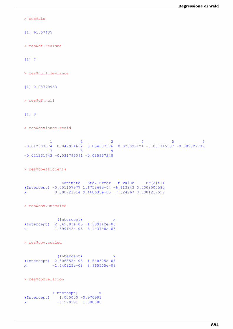
Regressione di Wald
> res$aic
[1] 61.57485
> res$df.residual
[1] 7
> res$null.deviance
[1] 0.08779963
> res$df.null
[1] 8
> res$deviance.resid
1 2 3 4 5 6-0.012307674 0.047994662 0.034307576 0.023099121 -0.001715587 -0.002827732
7 8 9-0.021231743 -0.031795091 -0.035957248
> res$coefficients
Estimate Std. Error t value Pr(>|t|)(Intercept) -0.001107977 1.675366e-04 -6.613343 0.0003005580x 0.000721914 9.468635e-05 7.624267 0.0001237599
> res$cov.unscaled
(Intercept) x(Intercept) 2.549583e-05 -1.399142e-05x -1.399142e-05 8.143748e-06
> res$cov.scaled
(Intercept) x(Intercept) 2.806852e-08 -1.540325e-08x -1.540325e-08 8.965505e-09
> res$correlation
(Intercept) x(Intercept) 1.000000 -0.970991x -0.970991 1.000000
884
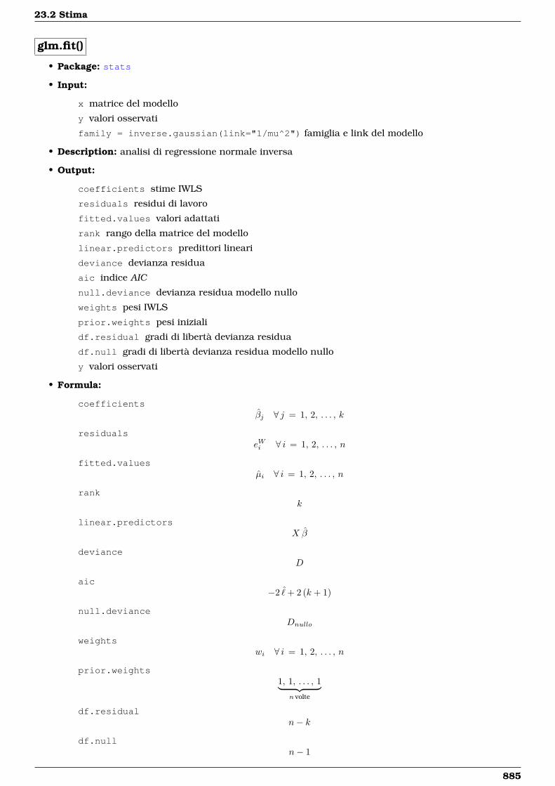
23.2 Stima
glm.fit()
• Package: stats
• Input:
x matrice del modello
y valori osservati
family = inverse.gaussian(link="1/mu^2") famiglia e link del modello
• Description: analisi di regressione normale inversa
• Output:
coefficients stime IWLS
residuals residui di lavoro
fitted.values valori adattati
rank rango della matrice del modello
linear.predictors predittori lineari
deviance devianza residua
aic indice AIC
null.deviance devianza residua modello nullo
weights pesi IWLS
prior.weights pesi iniziali
df.residual gradi di libertà devianza residua
df.null gradi di libertà devianza residua modello nullo
y valori osservati
• Formula:
coefficientsβj ∀ j = 1, 2, . . . , k
residualseWi ∀ i = 1, 2, . . . , n
fitted.valuesµi ∀ i = 1, 2, . . . , n
rankk
linear.predictorsX β
devianceD
aic−2 ˆ+ 2 (k + 1)
null.devianceDnullo
weightswi ∀ i = 1, 2, . . . , n
prior.weights1, 1, . . . , 1︸ ︷︷ ︸
n volte
df.residualn− k
df.nulln− 1
885
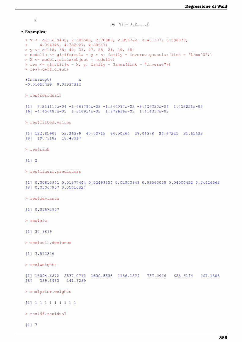
Regressione di Wald
yyi ∀ i = 1, 2, . . . , n
• Examples:
> x <- c(1.609438, 2.302585, 2.70805, 2.995732, 3.401197, 3.688879,+ 4.094345, 4.382027, 4.60517)> y <- c(118, 58, 42, 35, 27, 25, 21, 19, 18)> modello <- glm(formula = y ~ x, family = inverse.gaussian(link = "1/mu^2"))> X <- model.matrix(object = modello)> res <- glm.fit(x = X, y, family = Gamma(link = "inverse"))> res$coefficients
(Intercept) x-0.01655439 0.01534312
> res$residuals
[1] 3.219110e-04 -1.669382e-03 -1.245097e-03 -8.626330e-04 1.353051e-03[6] -4.456480e-05 1.314954e-03 1.879616e-03 1.414317e-03
> res$fitted.values
[1] 122.85903 53.26389 40.00713 34.00264 28.06578 24.97221 21.61432[8] 19.73182 18.48317
> res$rank
[1] 2
> res$linear.predictors
[1] 0.00813941 0.01877444 0.02499554 0.02940948 0.03563058 0.04004452 0.04626563[8] 0.05067957 0.05410327
> res$deviance
[1] 0.01672967
> res$aic
[1] 37.9899
> res$null.deviance
[1] 3.512826
> res$weights
[1] 15094.6872 2837.0712 1600.5833 1156.1874 787.6926 623.6144 467.1808[8] 389.3463 341.6289
> res$prior.weights
[1] 1 1 1 1 1 1 1 1 1
> res$df.residual
[1] 7
886
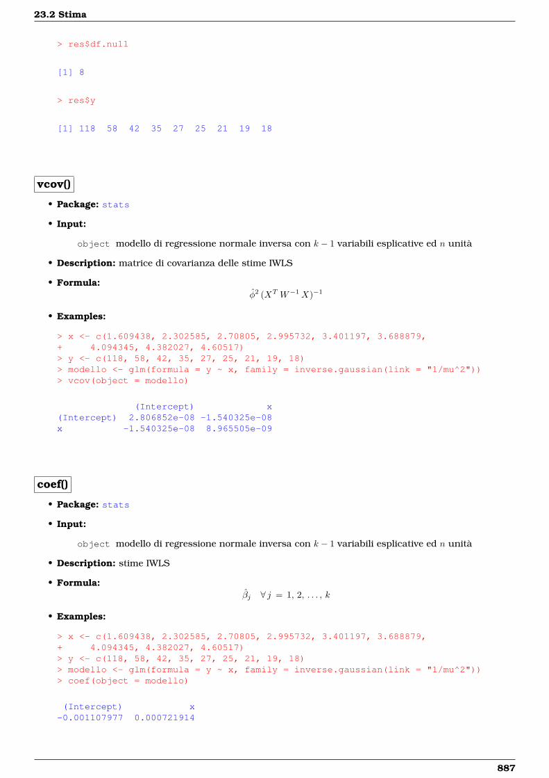
23.2 Stima
> res$df.null
[1] 8
> res$y
[1] 118 58 42 35 27 25 21 19 18
vcov()
• Package: stats
• Input:
object modello di regressione normale inversa con k − 1 variabili esplicative ed n unità
• Description: matrice di covarianza delle stime IWLS
• Formula:φ2 (XT W−1X)−1
• Examples:
> x <- c(1.609438, 2.302585, 2.70805, 2.995732, 3.401197, 3.688879,+ 4.094345, 4.382027, 4.60517)> y <- c(118, 58, 42, 35, 27, 25, 21, 19, 18)> modello <- glm(formula = y ~ x, family = inverse.gaussian(link = "1/mu^2"))> vcov(object = modello)
(Intercept) x(Intercept) 2.806852e-08 -1.540325e-08x -1.540325e-08 8.965505e-09
coef()
• Package: stats
• Input:
object modello di regressione normale inversa con k − 1 variabili esplicative ed n unità
• Description: stime IWLS
• Formula:βj ∀ j = 1, 2, . . . , k
• Examples:
> x <- c(1.609438, 2.302585, 2.70805, 2.995732, 3.401197, 3.688879,+ 4.094345, 4.382027, 4.60517)> y <- c(118, 58, 42, 35, 27, 25, 21, 19, 18)> modello <- glm(formula = y ~ x, family = inverse.gaussian(link = "1/mu^2"))> coef(object = modello)
(Intercept) x-0.001107977 0.000721914
887
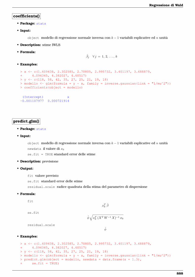
Regressione di Wald
coefficients()
• Package: stats
• Input:
object modello di regressione normale inversa con k − 1 variabili esplicative ed n unità
• Description: stime IWLS
• Formula:βj ∀ j = 1, 2, . . . , k
• Examples:
> x <- c(1.609438, 2.302585, 2.70805, 2.995732, 3.401197, 3.688879,+ 4.094345, 4.382027, 4.60517)> y <- c(118, 58, 42, 35, 27, 25, 21, 19, 18)> modello <- glm(formula = y ~ x, family = inverse.gaussian(link = "1/mu^2"))> coefficients(object = modello)
(Intercept) x-0.001107977 0.000721914
predict.glm()
• Package: stats
• Input:
object modello di regressione normale inversa con k − 1 variabili esplicative ed n unità
newdata il valore di x0
se.fit = TRUE standard error delle stime
• Description: previsione
• Output:
fit valore previsto
se.fit standard error delle stime
residual.scale radice quadrata della stima del parametro di dispersione
• Formula:
fit
xT0 β
se.fit
φ√xT0 (XT W−1X)−1 x0
residual.scale
φ
• Examples:
> x <- c(1.609438, 2.302585, 2.70805, 2.995732, 3.401197, 3.688879,+ 4.094345, 4.382027, 4.60517)> y <- c(118, 58, 42, 35, 27, 25, 21, 19, 18)> modello <- glm(formula = y ~ x, family = inverse.gaussian(link = "1/mu^2"))> predict.glm(object = modello, newdata = data.frame(x = 1.3),+ se.fit = TRUE)
888
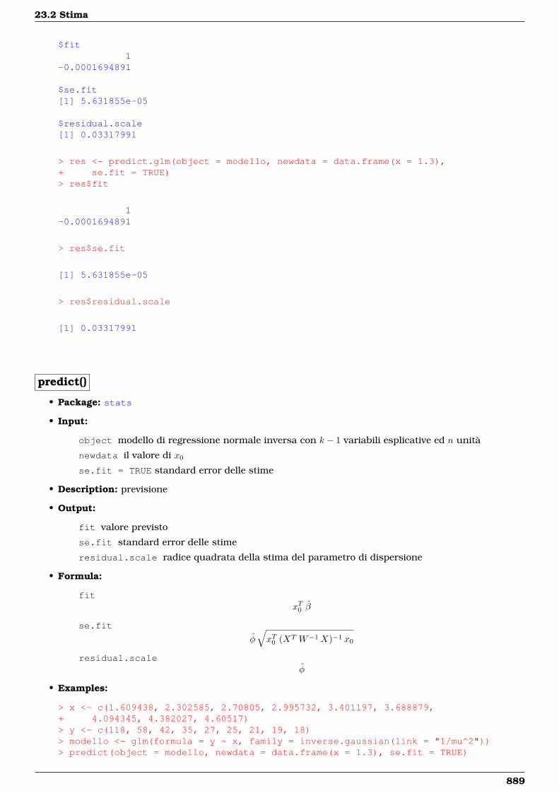
23.2 Stima
$fit1
-0.0001694891
$se.fit[1] 5.631855e-05
$residual.scale[1] 0.03317991
> res <- predict.glm(object = modello, newdata = data.frame(x = 1.3),+ se.fit = TRUE)> res$fit
1-0.0001694891
> res$se.fit
[1] 5.631855e-05
> res$residual.scale
[1] 0.03317991
predict()
• Package: stats
• Input:
object modello di regressione normale inversa con k − 1 variabili esplicative ed n unità
newdata il valore di x0
se.fit = TRUE standard error delle stime
• Description: previsione
• Output:
fit valore previsto
se.fit standard error delle stime
residual.scale radice quadrata della stima del parametro di dispersione
• Formula:
fitxT0 β
se.fit
φ√xT0 (XT W−1X)−1 x0
residual.scaleφ
• Examples:
> x <- c(1.609438, 2.302585, 2.70805, 2.995732, 3.401197, 3.688879,+ 4.094345, 4.382027, 4.60517)> y <- c(118, 58, 42, 35, 27, 25, 21, 19, 18)> modello <- glm(formula = y ~ x, family = inverse.gaussian(link = "1/mu^2"))> predict(object = modello, newdata = data.frame(x = 1.3), se.fit = TRUE)
889
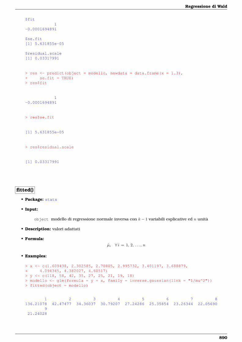
Regressione di Wald
$fit1
-0.0001694891
$se.fit[1] 5.631855e-05
$residual.scale[1] 0.03317991
> res <- predict(object = modello, newdata = data.frame(x = 1.3),+ se.fit = TRUE)> res$fit
1-0.0001694891
> res$se.fit
[1] 5.631855e-05
> res$residual.scale
[1] 0.03317991
fitted()
• Package: stats
• Input:
object modello di regressione normale inversa con k − 1 variabili esplicative ed n unità
• Description: valori adattati
• Formula:µi ∀ i = 1, 2, . . . , n
• Examples:
> x <- c(1.609438, 2.302585, 2.70805, 2.995732, 3.401197, 3.688879,+ 4.094345, 4.382027, 4.60517)> y <- c(118, 58, 42, 35, 27, 25, 21, 19, 18)> modello <- glm(formula = y ~ x, family = inverse.gaussian(link = "1/mu^2"))> fitted(object = modello)
1 2 3 4 5 6 7 8136.21078 42.47477 34.36037 30.79207 27.24286 25.35854 23.26344 22.05690
921.24028
890
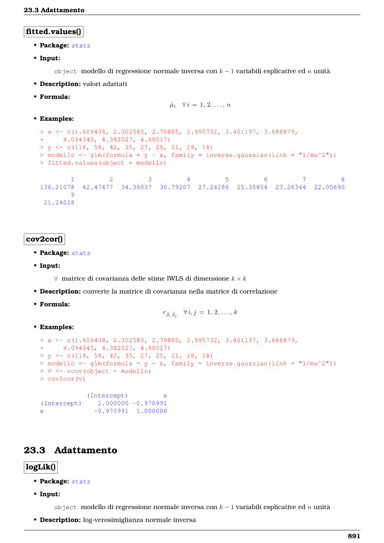
23.3 Adattamento
fitted.values()
• Package: stats
• Input:
object modello di regressione normale inversa con k − 1 variabili esplicative ed n unità
• Description: valori adattati
• Formula:µi ∀ i = 1, 2, . . . , n
• Examples:
> x <- c(1.609438, 2.302585, 2.70805, 2.995732, 3.401197, 3.688879,+ 4.094345, 4.382027, 4.60517)> y <- c(118, 58, 42, 35, 27, 25, 21, 19, 18)> modello <- glm(formula = y ~ x, family = inverse.gaussian(link = "1/mu^2"))> fitted.values(object = modello)
1 2 3 4 5 6 7 8136.21078 42.47477 34.36037 30.79207 27.24286 25.35854 23.26344 22.05690
921.24028
cov2cor()
• Package: stats
• Input:
V matrice di covarianza delle stime IWLS di dimensione k × k
• Description: converte la matrice di covarianza nella matrice di correlazione
• Formula:rβi βj ∀ i, j = 1, 2, . . . , k
• Examples:
> x <- c(1.609438, 2.302585, 2.70805, 2.995732, 3.401197, 3.688879,+ 4.094345, 4.382027, 4.60517)> y <- c(118, 58, 42, 35, 27, 25, 21, 19, 18)> modello <- glm(formula = y ~ x, family = inverse.gaussian(link = "1/mu^2"))> V <- vcov(object = modello)> cov2cor(V)
(Intercept) x(Intercept) 1.000000 -0.970991x -0.970991 1.000000
23.3 Adattamento
logLik()
• Package: stats
• Input:
object modello di regressione normale inversa con k − 1 variabili esplicative ed n unità
• Description: log-verosimiglianza normale inversa
891
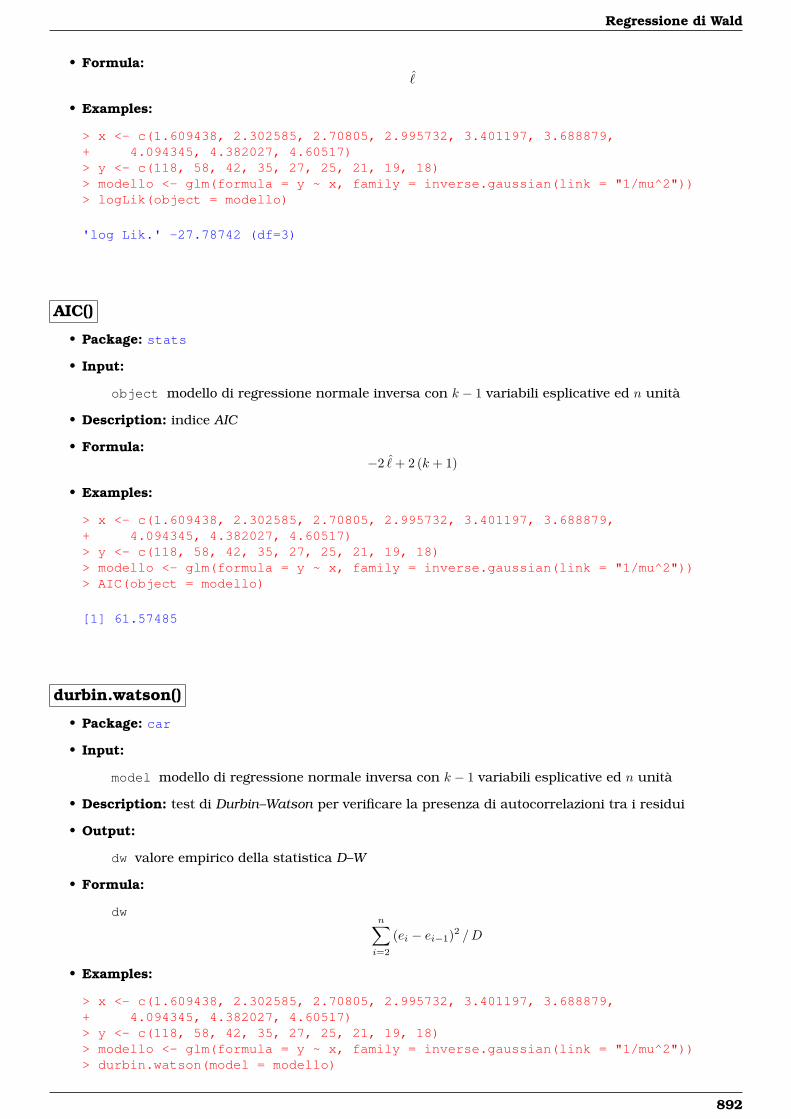
Regressione di Wald
• Formula:ˆ
• Examples:
> x <- c(1.609438, 2.302585, 2.70805, 2.995732, 3.401197, 3.688879,+ 4.094345, 4.382027, 4.60517)> y <- c(118, 58, 42, 35, 27, 25, 21, 19, 18)> modello <- glm(formula = y ~ x, family = inverse.gaussian(link = "1/mu^2"))> logLik(object = modello)
'log Lik.' -27.78742 (df=3)
AIC()
• Package: stats
• Input:
object modello di regressione normale inversa con k − 1 variabili esplicative ed n unità
• Description: indice AIC
• Formula:−2 ˆ+ 2 (k + 1)
• Examples:
> x <- c(1.609438, 2.302585, 2.70805, 2.995732, 3.401197, 3.688879,+ 4.094345, 4.382027, 4.60517)> y <- c(118, 58, 42, 35, 27, 25, 21, 19, 18)> modello <- glm(formula = y ~ x, family = inverse.gaussian(link = "1/mu^2"))> AIC(object = modello)
[1] 61.57485
durbin.watson()
• Package: car
• Input:
model modello di regressione normale inversa con k − 1 variabili esplicative ed n unità
• Description: test di Durbin–Watson per verificare la presenza di autocorrelazioni tra i residui
• Output:
dw valore empirico della statistica D–W
• Formula:
dwn∑i=2
(ei − ei−1)2 /D
• Examples:
> x <- c(1.609438, 2.302585, 2.70805, 2.995732, 3.401197, 3.688879,+ 4.094345, 4.382027, 4.60517)> y <- c(118, 58, 42, 35, 27, 25, 21, 19, 18)> modello <- glm(formula = y ~ x, family = inverse.gaussian(link = "1/mu^2"))> durbin.watson(model = modello)
892
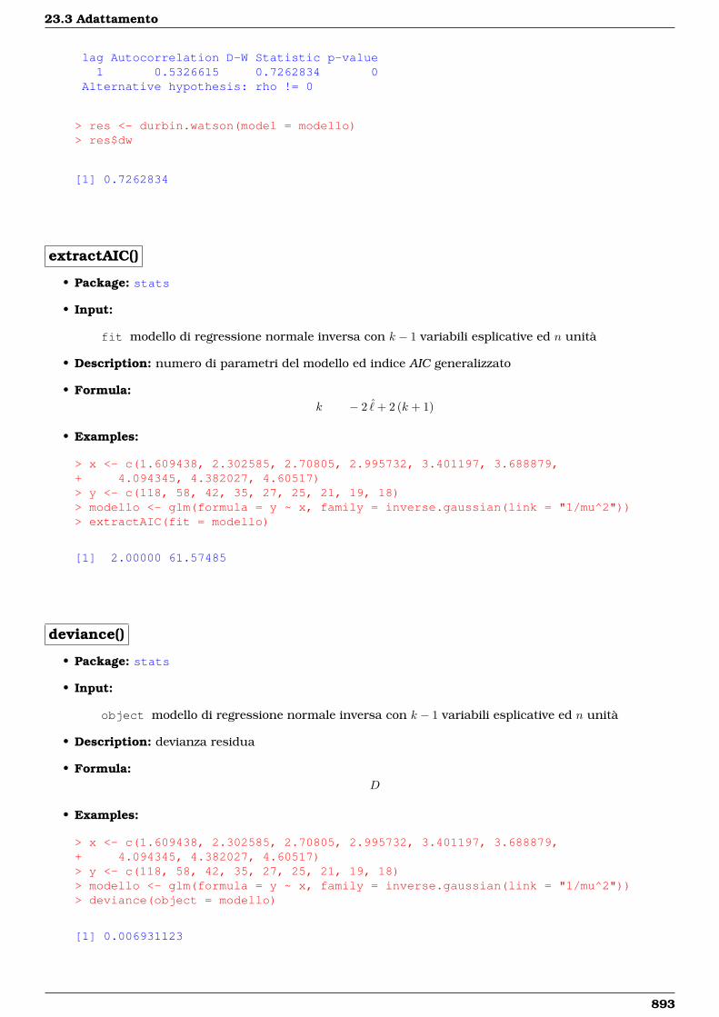
23.3 Adattamento
lag Autocorrelation D-W Statistic p-value1 0.5326615 0.7262834 0
Alternative hypothesis: rho != 0
> res <- durbin.watson(model = modello)> res$dw
[1] 0.7262834
extractAIC()
• Package: stats
• Input:
fit modello di regressione normale inversa con k − 1 variabili esplicative ed n unità
• Description: numero di parametri del modello ed indice AIC generalizzato
• Formula:k − 2 ˆ+ 2 (k + 1)
• Examples:
> x <- c(1.609438, 2.302585, 2.70805, 2.995732, 3.401197, 3.688879,+ 4.094345, 4.382027, 4.60517)> y <- c(118, 58, 42, 35, 27, 25, 21, 19, 18)> modello <- glm(formula = y ~ x, family = inverse.gaussian(link = "1/mu^2"))> extractAIC(fit = modello)
[1] 2.00000 61.57485
deviance()
• Package: stats
• Input:
object modello di regressione normale inversa con k − 1 variabili esplicative ed n unità
• Description: devianza residua
• Formula:D
• Examples:
> x <- c(1.609438, 2.302585, 2.70805, 2.995732, 3.401197, 3.688879,+ 4.094345, 4.382027, 4.60517)> y <- c(118, 58, 42, 35, 27, 25, 21, 19, 18)> modello <- glm(formula = y ~ x, family = inverse.gaussian(link = "1/mu^2"))> deviance(object = modello)
[1] 0.006931123
893
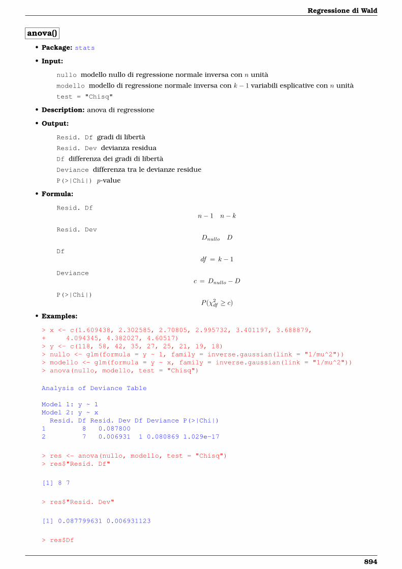
Regressione di Wald
anova()
• Package: stats
• Input:
nullo modello nullo di regressione normale inversa con n unità
modello modello di regressione normale inversa con k − 1 variabili esplicative con n unità
test = "Chisq"
• Description: anova di regressione
• Output:
Resid. Df gradi di libertà
Resid. Dev devianza residua
Df differenza dei gradi di libertà
Deviance differenza tra le devianze residue
P(>|Chi|) p-value
• Formula:
Resid. Dfn− 1 n− k
Resid. DevDnullo D
Dfdf = k − 1
Deviancec = Dnullo −D
P(>|Chi|)P (χ2
df ≥ c)
• Examples:
> x <- c(1.609438, 2.302585, 2.70805, 2.995732, 3.401197, 3.688879,+ 4.094345, 4.382027, 4.60517)> y <- c(118, 58, 42, 35, 27, 25, 21, 19, 18)> nullo <- glm(formula = y ~ 1, family = inverse.gaussian(link = "1/mu^2"))> modello <- glm(formula = y ~ x, family = inverse.gaussian(link = "1/mu^2"))> anova(nullo, modello, test = "Chisq")
Analysis of Deviance Table
Model 1: y ~ 1Model 2: y ~ xResid. Df Resid. Dev Df Deviance P(>|Chi|)
1 8 0.0878002 7 0.006931 1 0.080869 1.029e-17
> res <- anova(nullo, modello, test = "Chisq")> res$"Resid. Df"
[1] 8 7
> res$"Resid. Dev"
[1] 0.087799631 0.006931123
> res$Df
894
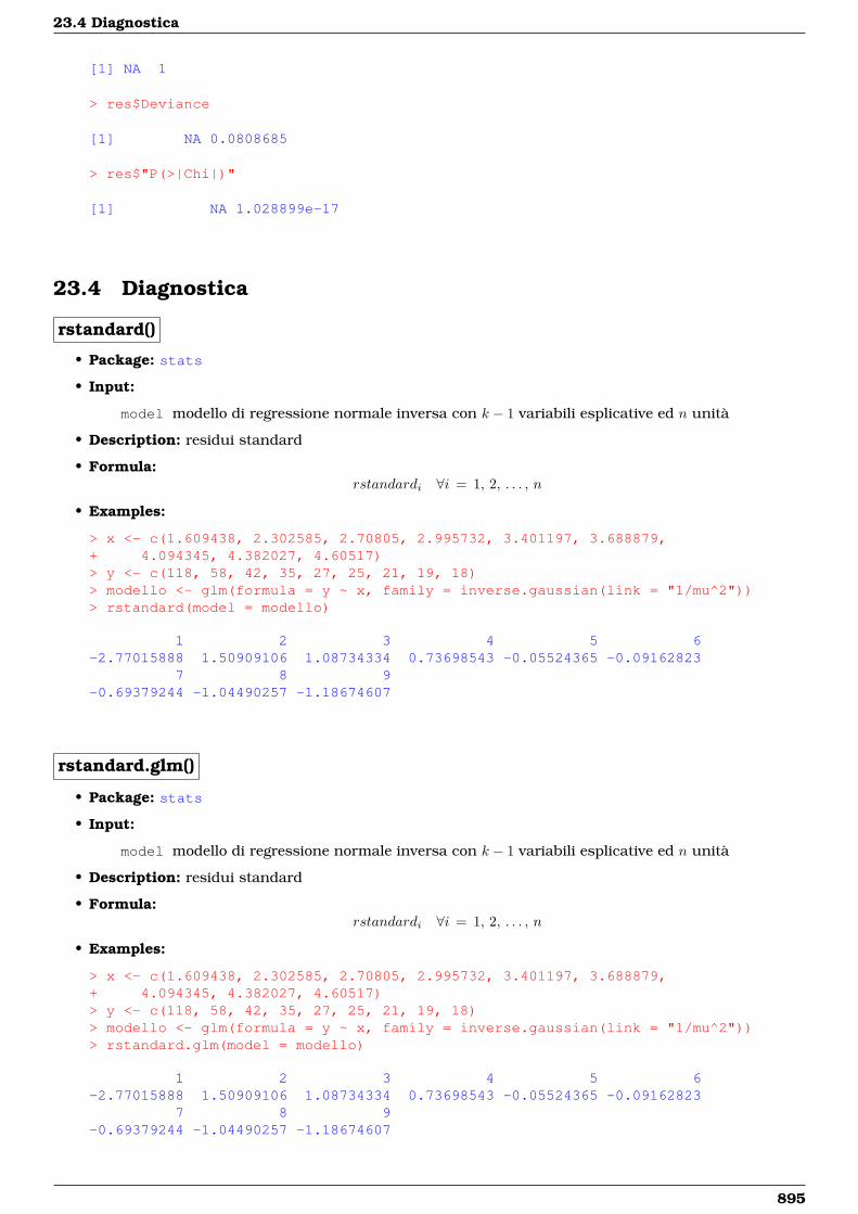
23.4 Diagnostica
[1] NA 1
> res$Deviance
[1] NA 0.0808685
> res$"P(>|Chi|)"
[1] NA 1.028899e-17
23.4 Diagnostica
rstandard()
• Package: stats
• Input:
model modello di regressione normale inversa con k − 1 variabili esplicative ed n unità
• Description: residui standard
• Formula:rstandardi ∀i = 1, 2, . . . , n
• Examples:
> x <- c(1.609438, 2.302585, 2.70805, 2.995732, 3.401197, 3.688879,+ 4.094345, 4.382027, 4.60517)> y <- c(118, 58, 42, 35, 27, 25, 21, 19, 18)> modello <- glm(formula = y ~ x, family = inverse.gaussian(link = "1/mu^2"))> rstandard(model = modello)
1 2 3 4 5 6-2.77015888 1.50909106 1.08734334 0.73698543 -0.05524365 -0.09162823
7 8 9-0.69379244 -1.04490257 -1.18674607
rstandard.glm()
• Package: stats
• Input:
model modello di regressione normale inversa con k − 1 variabili esplicative ed n unità
• Description: residui standard
• Formula:rstandardi ∀i = 1, 2, . . . , n
• Examples:
> x <- c(1.609438, 2.302585, 2.70805, 2.995732, 3.401197, 3.688879,+ 4.094345, 4.382027, 4.60517)> y <- c(118, 58, 42, 35, 27, 25, 21, 19, 18)> modello <- glm(formula = y ~ x, family = inverse.gaussian(link = "1/mu^2"))> rstandard.glm(model = modello)
1 2 3 4 5 6-2.77015888 1.50909106 1.08734334 0.73698543 -0.05524365 -0.09162823
7 8 9-0.69379244 -1.04490257 -1.18674607
895
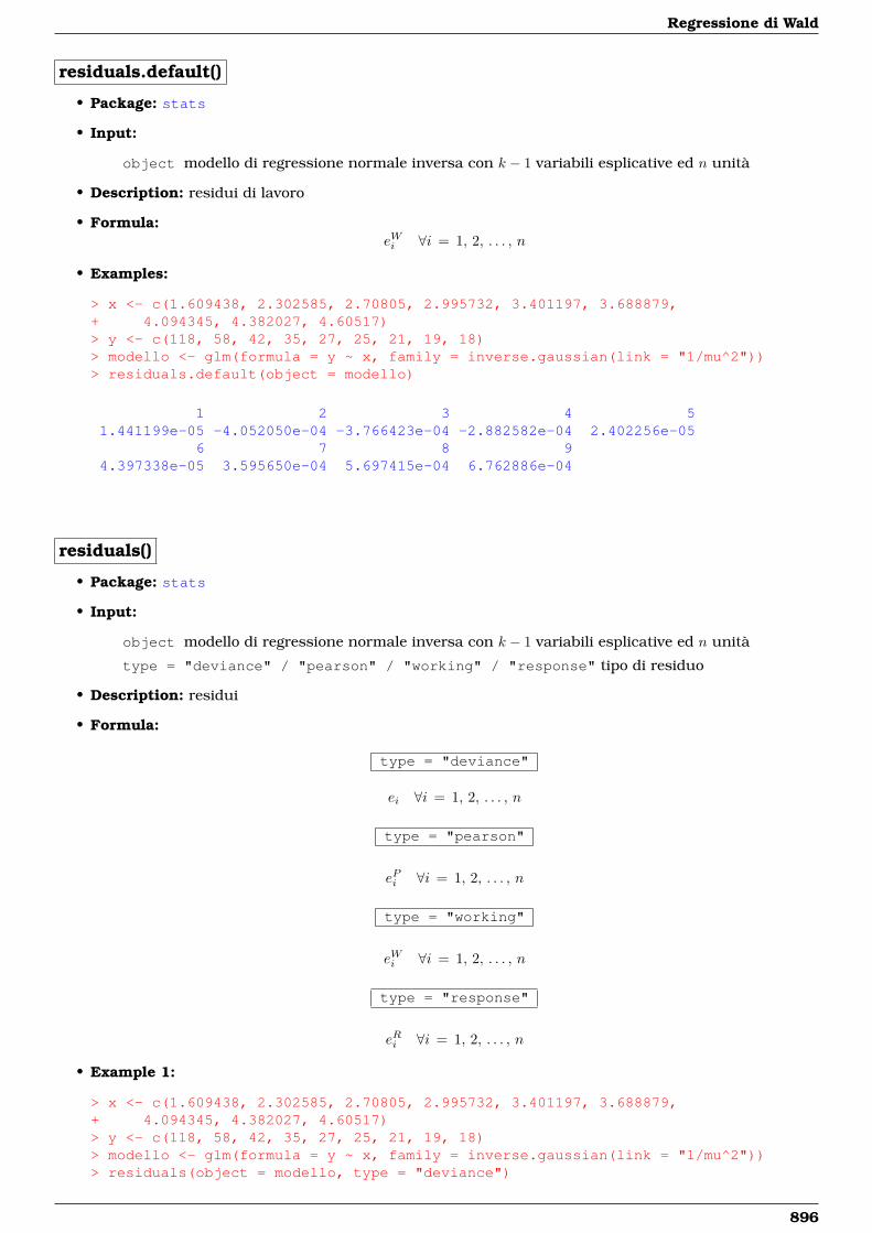
Regressione di Wald
residuals.default()
• Package: stats
• Input:
object modello di regressione normale inversa con k − 1 variabili esplicative ed n unità
• Description: residui di lavoro
• Formula:eWi ∀i = 1, 2, . . . , n
• Examples:
> x <- c(1.609438, 2.302585, 2.70805, 2.995732, 3.401197, 3.688879,+ 4.094345, 4.382027, 4.60517)> y <- c(118, 58, 42, 35, 27, 25, 21, 19, 18)> modello <- glm(formula = y ~ x, family = inverse.gaussian(link = "1/mu^2"))> residuals.default(object = modello)
1 2 3 4 51.441199e-05 -4.052050e-04 -3.766423e-04 -2.882582e-04 2.402256e-05
6 7 8 94.397338e-05 3.595650e-04 5.697415e-04 6.762886e-04
residuals()
• Package: stats
• Input:
object modello di regressione normale inversa con k − 1 variabili esplicative ed n unità
type = "deviance" / "pearson" / "working" / "response" tipo di residuo
• Description: residui
• Formula:
type = "deviance"
ei ∀i = 1, 2, . . . , n
type = "pearson"
ePi ∀i = 1, 2, . . . , n
type = "working"
eWi ∀i = 1, 2, . . . , n
type = "response"
eRi ∀i = 1, 2, . . . , n
• Example 1:
> x <- c(1.609438, 2.302585, 2.70805, 2.995732, 3.401197, 3.688879,+ 4.094345, 4.382027, 4.60517)> y <- c(118, 58, 42, 35, 27, 25, 21, 19, 18)> modello <- glm(formula = y ~ x, family = inverse.gaussian(link = "1/mu^2"))> residuals(object = modello, type = "deviance")
896
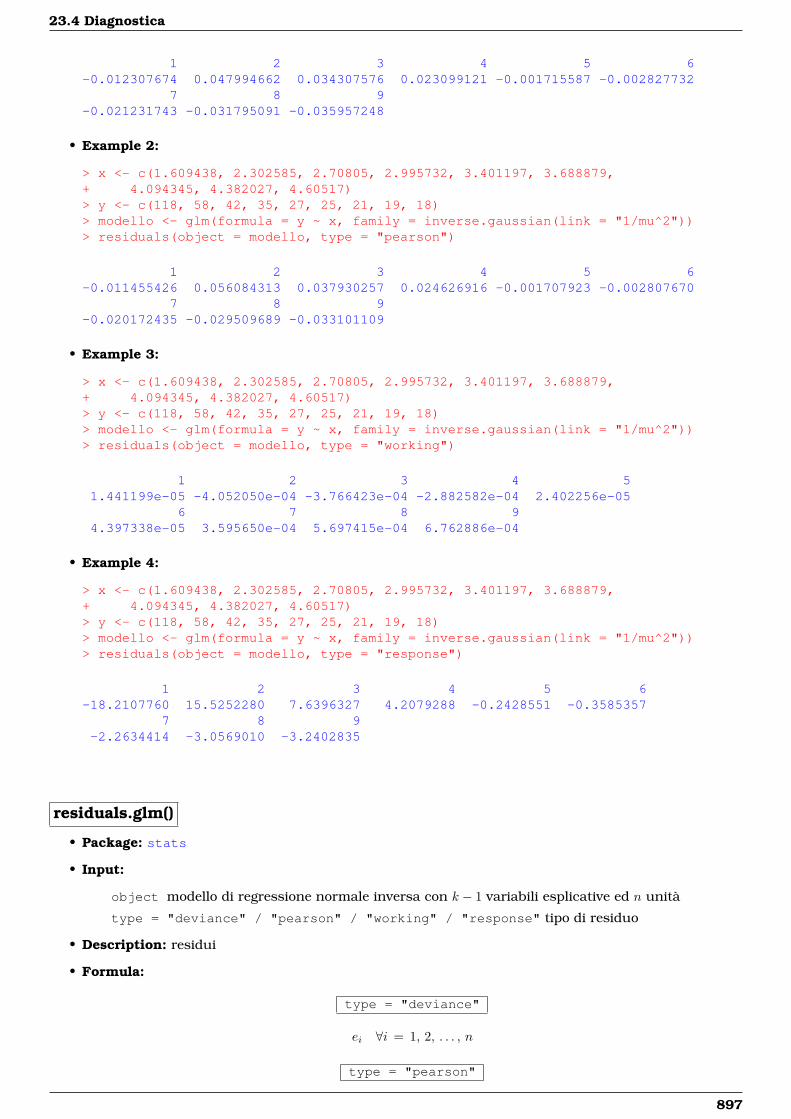
23.4 Diagnostica
1 2 3 4 5 6-0.012307674 0.047994662 0.034307576 0.023099121 -0.001715587 -0.002827732
7 8 9-0.021231743 -0.031795091 -0.035957248
• Example 2:
> x <- c(1.609438, 2.302585, 2.70805, 2.995732, 3.401197, 3.688879,+ 4.094345, 4.382027, 4.60517)> y <- c(118, 58, 42, 35, 27, 25, 21, 19, 18)> modello <- glm(formula = y ~ x, family = inverse.gaussian(link = "1/mu^2"))> residuals(object = modello, type = "pearson")
1 2 3 4 5 6-0.011455426 0.056084313 0.037930257 0.024626916 -0.001707923 -0.002807670
7 8 9-0.020172435 -0.029509689 -0.033101109
• Example 3:
> x <- c(1.609438, 2.302585, 2.70805, 2.995732, 3.401197, 3.688879,+ 4.094345, 4.382027, 4.60517)> y <- c(118, 58, 42, 35, 27, 25, 21, 19, 18)> modello <- glm(formula = y ~ x, family = inverse.gaussian(link = "1/mu^2"))> residuals(object = modello, type = "working")
1 2 3 4 51.441199e-05 -4.052050e-04 -3.766423e-04 -2.882582e-04 2.402256e-05
6 7 8 94.397338e-05 3.595650e-04 5.697415e-04 6.762886e-04
• Example 4:
> x <- c(1.609438, 2.302585, 2.70805, 2.995732, 3.401197, 3.688879,+ 4.094345, 4.382027, 4.60517)> y <- c(118, 58, 42, 35, 27, 25, 21, 19, 18)> modello <- glm(formula = y ~ x, family = inverse.gaussian(link = "1/mu^2"))> residuals(object = modello, type = "response")
1 2 3 4 5 6-18.2107760 15.5252280 7.6396327 4.2079288 -0.2428551 -0.3585357
7 8 9-2.2634414 -3.0569010 -3.2402835
residuals.glm()
• Package: stats
• Input:
object modello di regressione normale inversa con k − 1 variabili esplicative ed n unità
type = "deviance" / "pearson" / "working" / "response" tipo di residuo
• Description: residui
• Formula:
type = "deviance"
ei ∀i = 1, 2, . . . , n
type = "pearson"
897
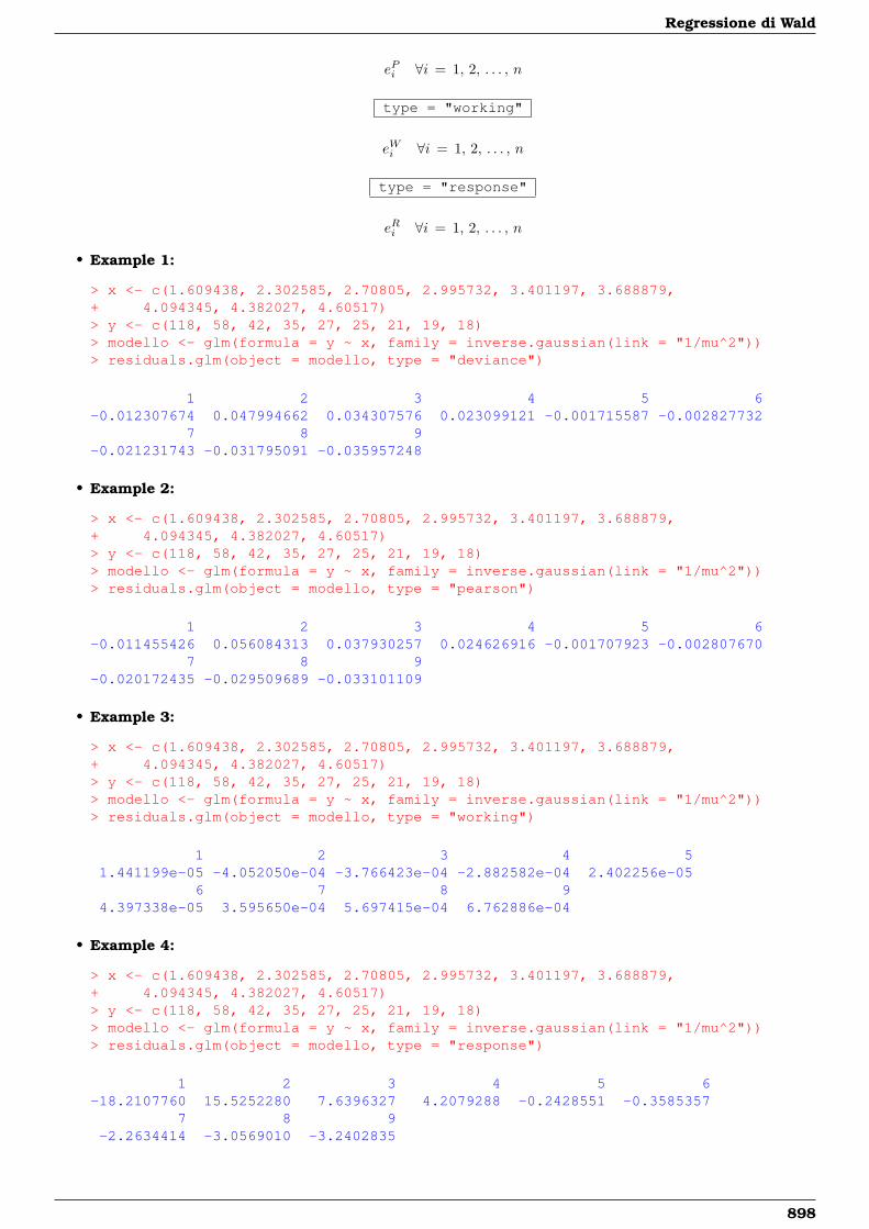
Regressione di Wald
ePi ∀i = 1, 2, . . . , n
type = "working"
eWi ∀i = 1, 2, . . . , n
type = "response"
eRi ∀i = 1, 2, . . . , n
• Example 1:
> x <- c(1.609438, 2.302585, 2.70805, 2.995732, 3.401197, 3.688879,+ 4.094345, 4.382027, 4.60517)> y <- c(118, 58, 42, 35, 27, 25, 21, 19, 18)> modello <- glm(formula = y ~ x, family = inverse.gaussian(link = "1/mu^2"))> residuals.glm(object = modello, type = "deviance")
1 2 3 4 5 6-0.012307674 0.047994662 0.034307576 0.023099121 -0.001715587 -0.002827732
7 8 9-0.021231743 -0.031795091 -0.035957248
• Example 2:
> x <- c(1.609438, 2.302585, 2.70805, 2.995732, 3.401197, 3.688879,+ 4.094345, 4.382027, 4.60517)> y <- c(118, 58, 42, 35, 27, 25, 21, 19, 18)> modello <- glm(formula = y ~ x, family = inverse.gaussian(link = "1/mu^2"))> residuals.glm(object = modello, type = "pearson")
1 2 3 4 5 6-0.011455426 0.056084313 0.037930257 0.024626916 -0.001707923 -0.002807670
7 8 9-0.020172435 -0.029509689 -0.033101109
• Example 3:
> x <- c(1.609438, 2.302585, 2.70805, 2.995732, 3.401197, 3.688879,+ 4.094345, 4.382027, 4.60517)> y <- c(118, 58, 42, 35, 27, 25, 21, 19, 18)> modello <- glm(formula = y ~ x, family = inverse.gaussian(link = "1/mu^2"))> residuals.glm(object = modello, type = "working")
1 2 3 4 51.441199e-05 -4.052050e-04 -3.766423e-04 -2.882582e-04 2.402256e-05
6 7 8 94.397338e-05 3.595650e-04 5.697415e-04 6.762886e-04
• Example 4:
> x <- c(1.609438, 2.302585, 2.70805, 2.995732, 3.401197, 3.688879,+ 4.094345, 4.382027, 4.60517)> y <- c(118, 58, 42, 35, 27, 25, 21, 19, 18)> modello <- glm(formula = y ~ x, family = inverse.gaussian(link = "1/mu^2"))> residuals.glm(object = modello, type = "response")
1 2 3 4 5 6-18.2107760 15.5252280 7.6396327 4.2079288 -0.2428551 -0.3585357
7 8 9-2.2634414 -3.0569010 -3.2402835
898
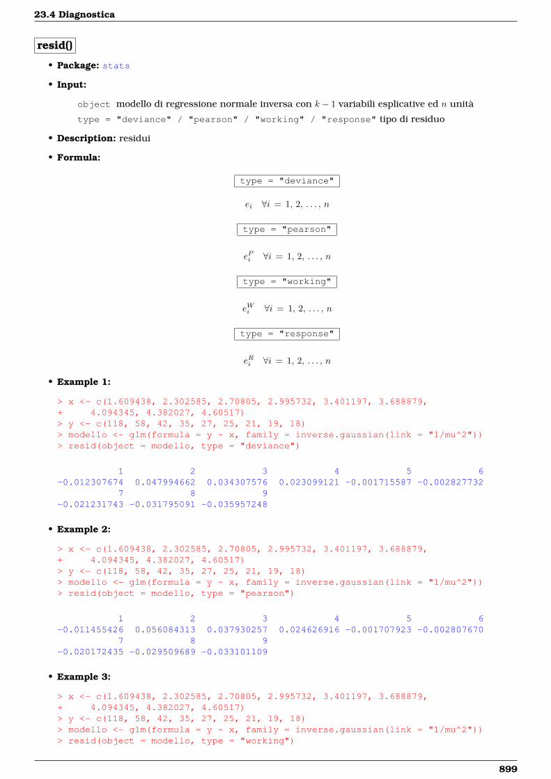
23.4 Diagnostica
resid()
• Package: stats
• Input:
object modello di regressione normale inversa con k − 1 variabili esplicative ed n unità
type = "deviance" / "pearson" / "working" / "response" tipo di residuo
• Description: residui
• Formula:
type = "deviance"
ei ∀i = 1, 2, . . . , n
type = "pearson"
ePi ∀i = 1, 2, . . . , n
type = "working"
eWi ∀i = 1, 2, . . . , n
type = "response"
eRi ∀i = 1, 2, . . . , n
• Example 1:
> x <- c(1.609438, 2.302585, 2.70805, 2.995732, 3.401197, 3.688879,+ 4.094345, 4.382027, 4.60517)> y <- c(118, 58, 42, 35, 27, 25, 21, 19, 18)> modello <- glm(formula = y ~ x, family = inverse.gaussian(link = "1/mu^2"))> resid(object = modello, type = "deviance")
1 2 3 4 5 6-0.012307674 0.047994662 0.034307576 0.023099121 -0.001715587 -0.002827732
7 8 9-0.021231743 -0.031795091 -0.035957248
• Example 2:
> x <- c(1.609438, 2.302585, 2.70805, 2.995732, 3.401197, 3.688879,+ 4.094345, 4.382027, 4.60517)> y <- c(118, 58, 42, 35, 27, 25, 21, 19, 18)> modello <- glm(formula = y ~ x, family = inverse.gaussian(link = "1/mu^2"))> resid(object = modello, type = "pearson")
1 2 3 4 5 6-0.011455426 0.056084313 0.037930257 0.024626916 -0.001707923 -0.002807670
7 8 9-0.020172435 -0.029509689 -0.033101109
• Example 3:
> x <- c(1.609438, 2.302585, 2.70805, 2.995732, 3.401197, 3.688879,+ 4.094345, 4.382027, 4.60517)> y <- c(118, 58, 42, 35, 27, 25, 21, 19, 18)> modello <- glm(formula = y ~ x, family = inverse.gaussian(link = "1/mu^2"))> resid(object = modello, type = "working")
899
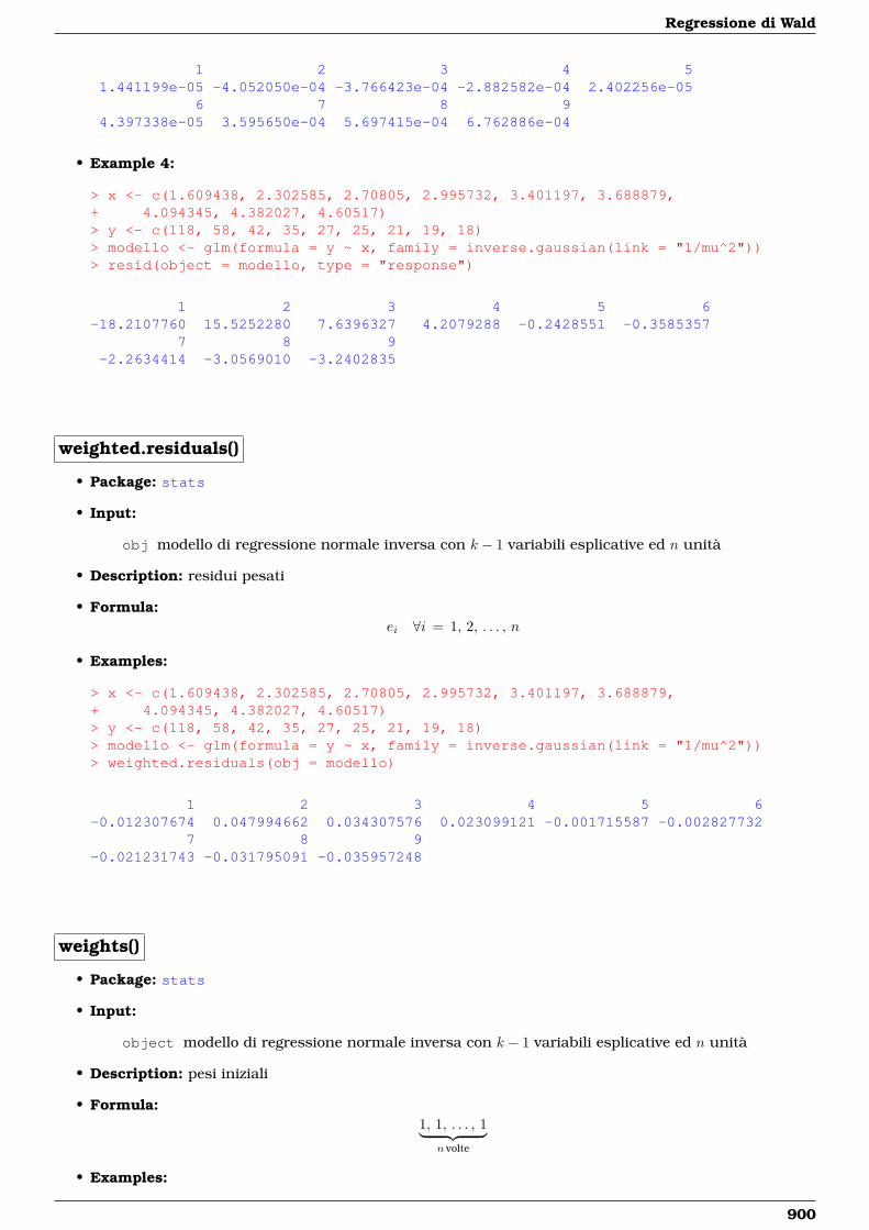
Regressione di Wald
1 2 3 4 51.441199e-05 -4.052050e-04 -3.766423e-04 -2.882582e-04 2.402256e-05
6 7 8 94.397338e-05 3.595650e-04 5.697415e-04 6.762886e-04
• Example 4:
> x <- c(1.609438, 2.302585, 2.70805, 2.995732, 3.401197, 3.688879,+ 4.094345, 4.382027, 4.60517)> y <- c(118, 58, 42, 35, 27, 25, 21, 19, 18)> modello <- glm(formula = y ~ x, family = inverse.gaussian(link = "1/mu^2"))> resid(object = modello, type = "response")
1 2 3 4 5 6-18.2107760 15.5252280 7.6396327 4.2079288 -0.2428551 -0.3585357
7 8 9-2.2634414 -3.0569010 -3.2402835
weighted.residuals()
• Package: stats
• Input:
obj modello di regressione normale inversa con k − 1 variabili esplicative ed n unità
• Description: residui pesati
• Formula:ei ∀i = 1, 2, . . . , n
• Examples:
> x <- c(1.609438, 2.302585, 2.70805, 2.995732, 3.401197, 3.688879,+ 4.094345, 4.382027, 4.60517)> y <- c(118, 58, 42, 35, 27, 25, 21, 19, 18)> modello <- glm(formula = y ~ x, family = inverse.gaussian(link = "1/mu^2"))> weighted.residuals(obj = modello)
1 2 3 4 5 6-0.012307674 0.047994662 0.034307576 0.023099121 -0.001715587 -0.002827732
7 8 9-0.021231743 -0.031795091 -0.035957248
weights()
• Package: stats
• Input:
object modello di regressione normale inversa con k − 1 variabili esplicative ed n unità
• Description: pesi iniziali
• Formula:1, 1, . . . , 1︸ ︷︷ ︸
n volte
• Examples:
900
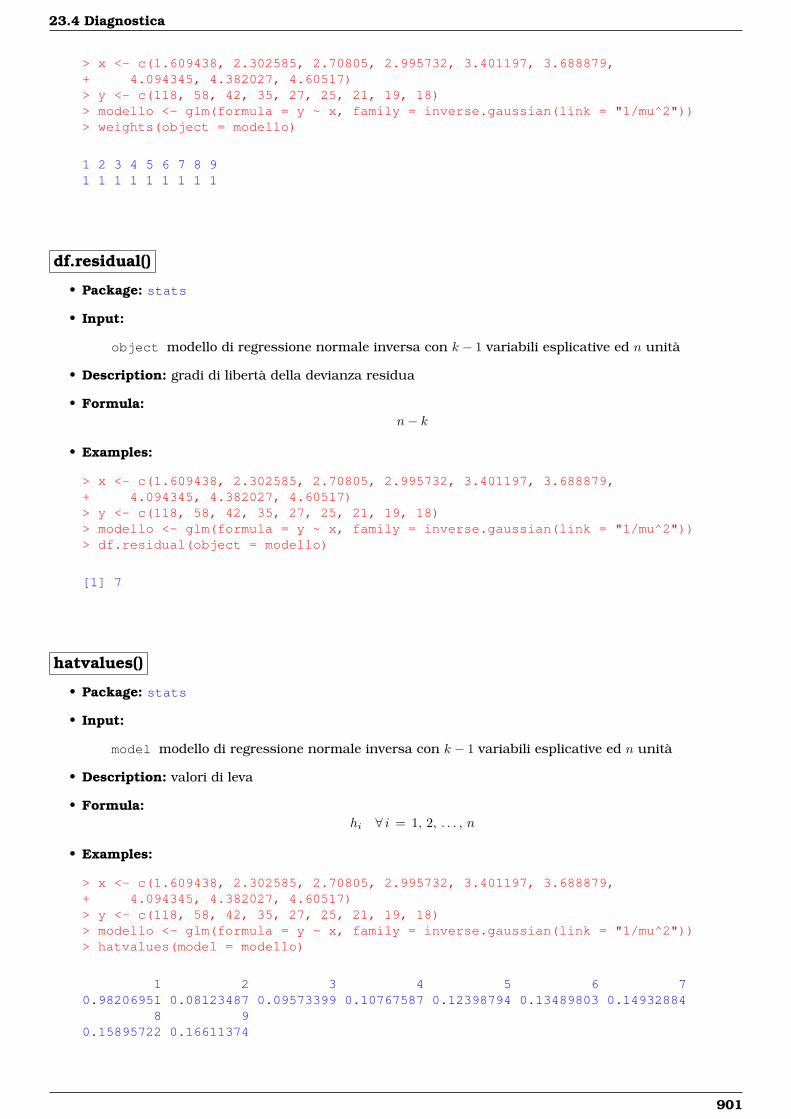
23.4 Diagnostica
> x <- c(1.609438, 2.302585, 2.70805, 2.995732, 3.401197, 3.688879,+ 4.094345, 4.382027, 4.60517)> y <- c(118, 58, 42, 35, 27, 25, 21, 19, 18)> modello <- glm(formula = y ~ x, family = inverse.gaussian(link = "1/mu^2"))> weights(object = modello)
1 2 3 4 5 6 7 8 91 1 1 1 1 1 1 1 1
df.residual()
• Package: stats
• Input:
object modello di regressione normale inversa con k − 1 variabili esplicative ed n unità
• Description: gradi di libertà della devianza residua
• Formula:n− k
• Examples:
> x <- c(1.609438, 2.302585, 2.70805, 2.995732, 3.401197, 3.688879,+ 4.094345, 4.382027, 4.60517)> y <- c(118, 58, 42, 35, 27, 25, 21, 19, 18)> modello <- glm(formula = y ~ x, family = inverse.gaussian(link = "1/mu^2"))> df.residual(object = modello)
[1] 7
hatvalues()
• Package: stats
• Input:
model modello di regressione normale inversa con k − 1 variabili esplicative ed n unità
• Description: valori di leva
• Formula:hi ∀ i = 1, 2, . . . , n
• Examples:
> x <- c(1.609438, 2.302585, 2.70805, 2.995732, 3.401197, 3.688879,+ 4.094345, 4.382027, 4.60517)> y <- c(118, 58, 42, 35, 27, 25, 21, 19, 18)> modello <- glm(formula = y ~ x, family = inverse.gaussian(link = "1/mu^2"))> hatvalues(model = modello)
1 2 3 4 5 6 70.98206951 0.08123487 0.09573399 0.10767587 0.12398794 0.13489803 0.14932884
8 90.15895722 0.16611374
901
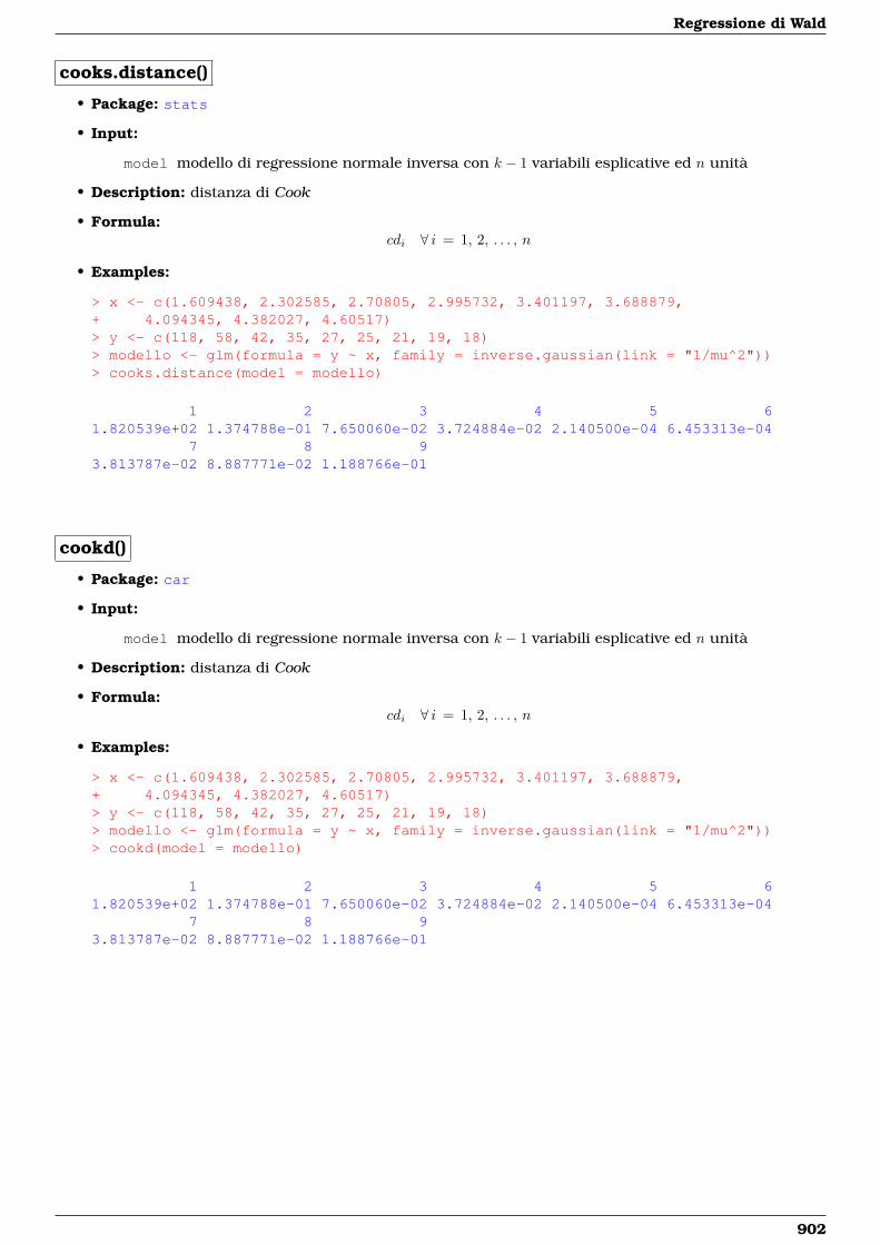
Regressione di Wald
cooks.distance()
• Package: stats
• Input:
model modello di regressione normale inversa con k − 1 variabili esplicative ed n unità
• Description: distanza di Cook
• Formula:cdi ∀ i = 1, 2, . . . , n
• Examples:
> x <- c(1.609438, 2.302585, 2.70805, 2.995732, 3.401197, 3.688879,+ 4.094345, 4.382027, 4.60517)> y <- c(118, 58, 42, 35, 27, 25, 21, 19, 18)> modello <- glm(formula = y ~ x, family = inverse.gaussian(link = "1/mu^2"))> cooks.distance(model = modello)
1 2 3 4 5 61.820539e+02 1.374788e-01 7.650060e-02 3.724884e-02 2.140500e-04 6.453313e-04
7 8 93.813787e-02 8.887771e-02 1.188766e-01
cookd()
• Package: car
• Input:
model modello di regressione normale inversa con k − 1 variabili esplicative ed n unità
• Description: distanza di Cook
• Formula:cdi ∀ i = 1, 2, . . . , n
• Examples:
> x <- c(1.609438, 2.302585, 2.70805, 2.995732, 3.401197, 3.688879,+ 4.094345, 4.382027, 4.60517)> y <- c(118, 58, 42, 35, 27, 25, 21, 19, 18)> modello <- glm(formula = y ~ x, family = inverse.gaussian(link = "1/mu^2"))> cookd(model = modello)
1 2 3 4 5 61.820539e+02 1.374788e-01 7.650060e-02 3.724884e-02 2.140500e-04 6.453313e-04
7 8 93.813787e-02 8.887771e-02 1.188766e-01
902

Parte VI
Appendice
903

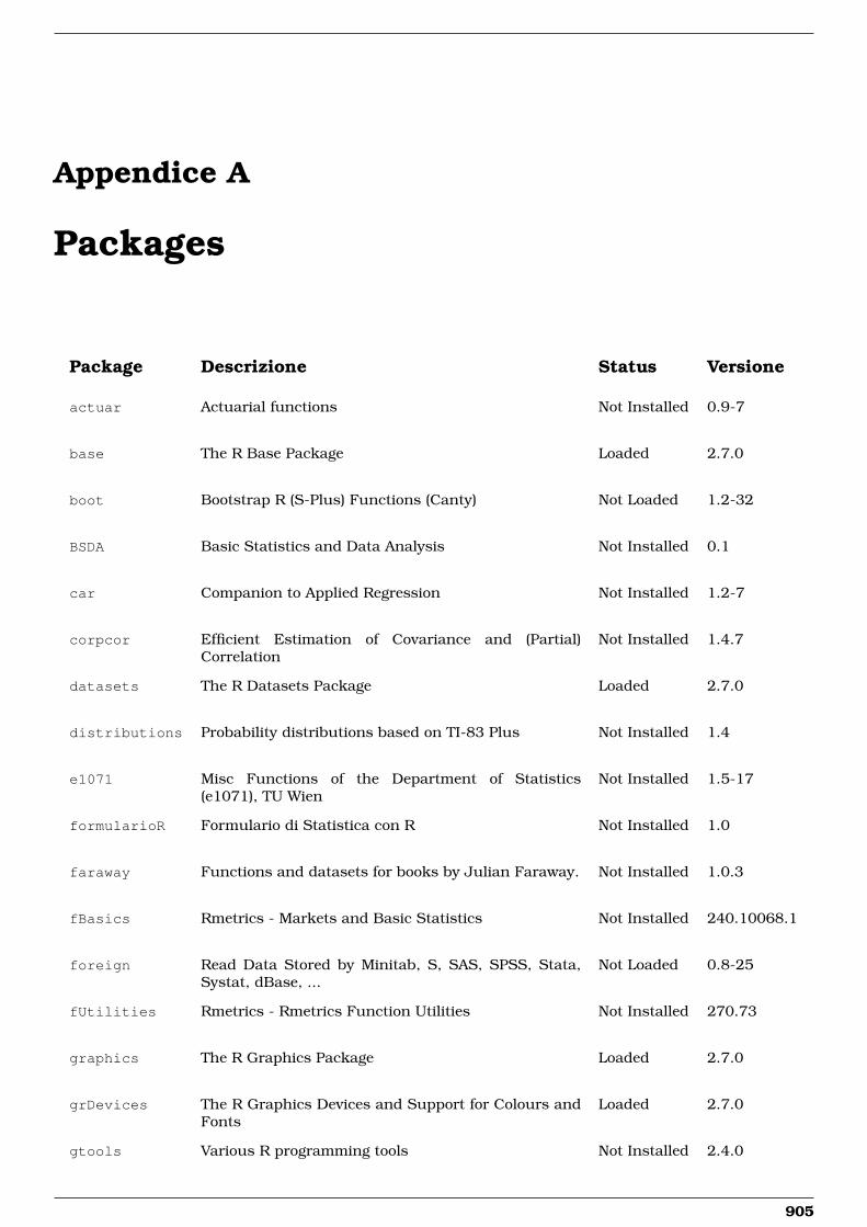
Appendice A
Packages
Package Descrizione Status Versione
actuar Actuarial functions Not Installed 0.9-7
base The R Base Package Loaded 2.7.0
boot Bootstrap R (S-Plus) Functions (Canty) Not Loaded 1.2-32
BSDA Basic Statistics and Data Analysis Not Installed 0.1
car Companion to Applied Regression Not Installed 1.2-7
corpcor Efficient Estimation of Covariance and (Partial)Correlation
Not Installed 1.4.7
datasets The R Datasets Package Loaded 2.7.0
distributions Probability distributions based on TI-83 Plus Not Installed 1.4
e1071 Misc Functions of the Department of Statistics(e1071), TU Wien
Not Installed 1.5-17
formularioR Formulario di Statistica con R Not Installed 1.0
faraway Functions and datasets for books by Julian Faraway. Not Installed 1.0.3
fBasics Rmetrics - Markets and Basic Statistics Not Installed 240.10068.1
foreign Read Data Stored by Minitab, S, SAS, SPSS, Stata,Systat, dBase, ...
Not Loaded 0.8-25
fUtilities Rmetrics - Rmetrics Function Utilities Not Installed 270.73
graphics The R Graphics Package Loaded 2.7.0
grDevices The R Graphics Devices and Support for Colours andFonts
Loaded 2.7.0
gtools Various R programming tools Not Installed 2.4.0
905

ineq Measuring inequality, concentration and poverty Not Installed 0.2-8
labstatR Libreria del Laboratorio di Statistica con R Not Installed 1.0.4
leaps regression subset selection Not Installed 2.7
lmtest Testing Linear Regression Models Not Installed 0.9-21
MASS Main Package of Venables and Ripley’s MASS Not Loaded 7.2-41
MCMCpack Markov chain Monte Carlo (MCMC) Package Not Installed 0.9-4
methods Formal Methods and Classes Loaded 2.7.0
moments Moments, cumulants, skewness, kurtosis and relatedtests
Not Installed 0.11
MPV Data Sets from Montgomery, Peck and Vining’s Book Not Installed 1.25
mvtnorm Multivariate Normal and T Distribution Not Installed 0.8-1
nlme Linear and Nonlinear Mixed Effects Models Not Loaded 3.1-88
nortest Tests for Normality Not Installed 1.0
pastecs Package for Analysis of Space-Time Ecological Series Not Installed 1.3-4
Rcmdr R Commander Not Installed 1.3-11
schoolmath Functions and datasets for math used in school Not Installed 0.2
sigma2tools Test of hypothesis about sigma2 Not Installed 1.2.6
stats The R Stats Package Loaded 2.7.0
strucchange Testing, Monitoring and Dating Structural Changes Not Installed 1.3-2
SuppDists Supplementary distributions Not Installed 1.1-2
tseries Time series analysis and computational finance Not Installed 0.10-13
UsingR Data sets for the text Using R for IntroductoryStatistics
Not Installed 0.1-8
utils The R Utils Package Loaded 2.7.0
Download Packages from CRAN site

Appendice B
Links
R site search
Site search http://finzi.psych.upenn.edu/search.html
Mailing list archives http://tolstoy.newcastle.edu.au/R/
Help center http://www.stat.ucl.ac.be/ISdidactique/Rhelp/
Help for R (Jonathan Baron) http://finzi.psych.upenn.edu/
r-help mailing list informa-tion
http://www.mail-archive.com/[email protected]/info.html
R information
CRAN http://cran.r-project.org/
Web site http://www.r-project.org/
News http://cran.r-project.org/doc/Rnews/
R Wiki http://wiki.r-project.org/
Bioconductor http://www.bioconductor.org/
R GUIs
Projects (CRAN) http://www.sciviews.org/_rgui/
R Commander http://socserv.socsci.mcmaster.ca/jfox/Misc/Rcmdr/index.html
Rpad http://www.rpad.org/Rpad/
SciViews http://www.sciviews.org/SciViews-R/
907

JGR http://stats.math.uni-augsburg.de/JGR/
Tinn-R
SourceForge (main) http://sourceforge.net/projects/tinn-r
SciViews http://www.sciviews.org/Tinn-R
Statistics
Journal of Statistical Soft-ware
http://www.jstatsoft.org/
HyperStat Text Book http://davidmlane.com/hyperstat/index.html
Electronic Textbook Sta-tSoft
http://www.statsoftinc.com/textbook/stathome.html
Processing
Miktex http://miktex.org/
Deplate http://deplate.sourceforge.net/index.php
Txt2tags http://txt2tags.sourceforge.net/

Bibliografia
Agostinelli C. (2000). Introduzione ad R. Published on the URL: http://www.dst.unive.it/~laboratorior/doc/materiale/unaintroduzioneadR.pdf.
Bashir S. (2004). Getting Started in R. Published on the URL: http://www.sbtc.ltd.uk/notes/Rintro.pdf.
Boggiani R. (2004). Introduzione ad R. Published on the URL: http://digilander.libero.it/robicox/manuali/pdf/mainr.pdf.
Brazzale A.; Chiogna M.; Gaetan C.; Sartori N. (2001). Laboratorio di R, Materiale didattico per i labo-ratori del corso di Modelli Statistici I. Published on the URL: http://www.isib.cnr.it/~brazzale/ModStatI/.
Crawley M. (2007). The R book. Wiley, England.
Crivellari F. (2006). Analisi Statistica dei dati con R. APOGEO, Milano.
D’Agostini G. (2005). Il linguaggio R: Un invito ad approfondire. Published on the URL: http://www.roma1.infn.it/~dagos/R/R.pdf, Università degli Studi di Roma La Sapienza e INFN.
Dalgaard P. (2002). Introductory Statistics with R. Springer-Verlag, New York.
Dell’Omodarme M. (2007). Alcune note su R. Published on the URL: http://www.cran.r-project.org/doc/contrib/DellOmodarme-esercitazioni-R.pdf.
Faraway J. (2002). Practical Regression and Anova using R. Published on the URL: http://www.cran.r-project.org/doc/contrib/Faraway-PRA.pdf.
Fox J. (2002). An R and S-Plus Companion to Applied Regression. SAGE Pubblications, Thousand Oaks,California.
Green C. (2004). The Stat 390 R Primer. Published on the URL: http://www.stat.washington.edu/cggreen/rprimer/rprimer.pdf.
Højsgaard S. (2005). R - In Two HouRs – a very brief introduction. Published on the URL:http://gbi.agrsci.dk/statistics/courses/phd05/material/src/R-2hours-Notes.pdf, BiometryResearch Unit, Danish Institute of Agricultural Sciences.
Iacus S.; Masarotto G. (2007). Laboratorio di statistica con R. McGraw-Hill, Milano, seconda edizione.
Kim D.-Y. (2004). R Tutorial. Published on the URL: http://www.math.ilstu.edu/dhkim/Rstuff/Rtutor.html, Department of Mathematics Illinois State University.
Lemon J. (2005). Kickstarting R. Published on the URL: http://www.cran.r-project.org/doc/contrib/Lemon-kickstart/index.html.
Maindonald J. H. (2004). Using R for Data Analysis and Graphics Introduction, Code and Commentary.Published on the URL: http://www.cran.r-project.org/doc/contrib/usingR.pdf.
Mineo A. M. (2003). Una guida all’utilizzo dell’ambiente statistico R. Published on the URL: http://www.cran.r-project.org/doc/contrib/Mineo-dispensaR.pdf.
Muggeo V. M. R. (2002). Il linguaggio R: concetti introduttivi ed esempi. Published on the URL: http://www.cran.r-project.org/doc/contrib/nozioniR.pdf.
Owen W. J. (2006). The R Guide. Published on the URL: http://cran.r-project.org/doc/contrib/Owen-TheRGuide.pdf.
Paradis E. (2002). R for beginners. Published on the URL: http://cran.r-project.org/doc/contrib/Paradis-rdebuts_en.pdf.
909

Parpinel F. (2000). La statistica applicata attraverso l’uso del programma R. Published on the URL: http://venus.unive.it/statcomp/r/man_Parpinel.pdf.
Polettini S. (2004). Introduzione ad R. Published on the URL: http://www.dipstat.unina.it/stat_appl/labo1.pdf.
Pollice A. (2000). La statistica applicata attraverso l’uso del programma R. Published on the URL: http://www.dip-statistica.uniba.it/html/docenti/pollice/materiale.htm, Dipartimento di ScienzeStatistiche, Università di Bari.
Ricci V. (2004). ANALISI DELLE SERIE STORICHE CON R. Published on the URL: http://www.cran.r-project.org/doc/contrib/Ricci-ts-italian.pdf.
Robinson A. (2006). Objects in R. Published on the URL: http://www.forestry.ubc.ca/biometrics/documents/R-Workshop/objects.pdf.
Scott T. (2004). An Introduction to R. Published on the URL: http://www.mc.vanderbilt.edu/gcrc/workshop_files/2004-08-20.pdf.
Scrucca L. (2005). Note sul linguaggio e ambiente statistico R. Published on the URL: http://www.stat.unipg.it/~luca/LabStat/R-note.pdf, Dipartimento di Scienze Statistiche, Università degli Studi diPerugia.
Soliani L. (2005). Manuale di Statistica per la Ricerca e la Professione. Published on the URL: http://www.dsa.unipr.it/soliani/soliani.html.
Stefanini F. M. (2007). INTRODUZIONE ALLA STATISTICA APPLICATA con esempi in R. PEARSON Education,Milano.
Tancredi A. (2005). Inferenza statistica in applicazioni economiche ed aziendali. Published on the URL:http://geostasto.eco.uniroma1.it/utenti/tancredi/isaea1-2x1.pdf, Università degli Studi diRoma La Sapienza.
Venables W. N.; Ripley B. D. (2002). Modern Applied Statistics with S. Springer-Verlag, New York.
Verzani J. (2002). Using R for Introductory Statistics. Published on the URL: http://www.cran.r-project.org/doc/contrib/Verzani-SimpleR.pdf.
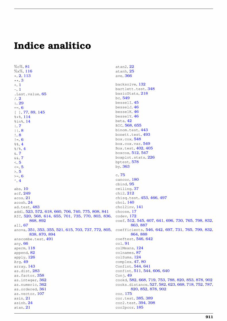
Indice analitico
%o%, 81%x%, 116*, 2, 113**, 3+, 1-, 1.Last.value, 65/, 2:, 29==, 6[ ], 77, 89, 145%*%, 114%in%, 14|, 7||, 8!, 8!=, 6%%, 4%/%, 4&, 7&&, 7<, 5<=, 5>, 5>=, 6^, 4
abs, 10acf, 249acos, 21acosh, 24ad.test, 483add1, 523, 572, 618, 660, 706, 740, 775, 808, 841AIC, 520, 568, 614, 655, 701, 735, 770, 803, 836,
868, 892all, 67anova, 351, 353, 355, 521, 615, 703, 737, 772, 805,
838, 870, 894anscombe.test, 491any, 66aperm, 118append, 82apply, 126Arg, 49array, 143as.dist, 283as.factor, 358as.integer, 362as.numeric, 362as.ordered, 361as.vector, 107asin, 21asinh, 24atan, 21
atan2, 22atanh, 25ave, 366
backsolve, 132bartlett.test, 348basicStats, 218bc, 549besselI, 45besselJ, 46besselK, 46besselY, 46beta, 42BIC, 568, 655binom.test, 443bonett.test, 493box.cox, 548box.cox.var, 549Box.test, 402, 405boxcox, 512, 547boxplot.stats, 226bptest, 578by, 363
c, 75cancor, 180cbind, 95ceiling, 37chi2, 212chisq.test, 453, 466, 497chol, 140chol2inv, 141choose, 17codev, 172coef, 512, 545, 607, 641, 696, 730, 765, 798, 832,
863, 887coefficients, 546, 642, 697, 731, 765, 799, 832,
864, 888coeftest, 546, 642col, 91colMeans, 124colnames, 87colSums, 124complex, 47, 80Confint, 544, 641confint, 511, 544, 606, 640Conj, 49cookd, 582, 668, 719, 753, 788, 820, 853, 878, 902cooks.distance, 527, 582, 623, 668, 718, 752, 787,
820, 852, 878, 902cor, 175cor.test, 385, 389cor2.test, 394, 398cor2pcor, 185
911

corr, 201cos, 20cosh, 23COV, 170cov, 171cov.wt, 191cov2cor, 178, 518, 566, 612, 653, 700, 734, 769,
802, 835, 867, 891covratio, 530, 587, 626, 673crossprod, 110cum3, 205cummax, 52cummin, 51cumprod, 51cumsum, 50cut, 368cv, 164cv2, 165cvm.test, 481
D, 57d2sigmoid, 45dbeta, 243dbinom, 237dburr, 243dcauchy, 243dchisq, 243DD, 58ddirichlet, 243det, 100determinant, 101determinant.matrix, 102deviance, 520, 569, 614, 656, 703, 737, 771, 805,
838, 869, 893dexp, 243df, 243df.residual, 532, 593, 629, 679, 717, 751, 786,
819, 851, 877, 901dfbeta, 533, 594, 629, 680dfbetas, 533, 594, 630, 681dffits, 529, 587, 625, 673dFriedman, 243dgamma, 243, 244dgeom, 237dhyper, 238diag, 117diff, 247diffinv, 248digamma, 40dim, 85, 119, 144dimnames, 88, 146dinvgamma, 244dinvGauss, 245dist, 281dlaplace, 244dllogis, 244dlnorm, 244dlogis, 244dmultinom, 238dmvnorm, 244dnbinom, 237dnorm, 244dpareto1, 244dpois, 238
drop1, 522, 570, 616, 657, 704, 738, 773, 806, 839dsigmoid, 44dsignrank, 245dt, 244dunif, 245duplicated, 229durbin.watson, 519, 567, 613, 654, 701, 735, 770,
803, 837, 868, 892dweibull, 245dwilcox, 244
E, 213e, 70eigen, 109emm, 206eta, 207eval, 69even, 70exp, 25expand.grid, 370expm1, 26expression, 68extendrange, 152extractAIC, 520, 568, 614, 656, 702, 736, 771, 804,
837, 869, 893
F, 61factor, 357factorial, 18FALSE, 61fbeta, 43fisher.test, 459fitted, 513, 550, 607, 643, 699, 733, 768, 801,
834, 866, 890fitted.values, 550, 644, 699, 733, 768, 801, 835,
867, 891fivenum, 216floor, 36forwardsolve, 134fractions, 38friedman.test, 439ftable, 472
gamma, 39gcd, 71geary, 163geometcdf, 238geometpdf, 238Gini, 208gini, 209ginv, 142gl, 366glm, 688, 722, 756, 790, 824, 856, 880glm.fit, 693, 727, 762, 795, 829, 861, 885
hat, 593, 680hatvalues, 532, 593, 629, 679, 717, 752, 787, 819,
852, 877, 901hclust, 285head, 80, 92hilbert, 98hist, 230
ic.var, 255identical, 66
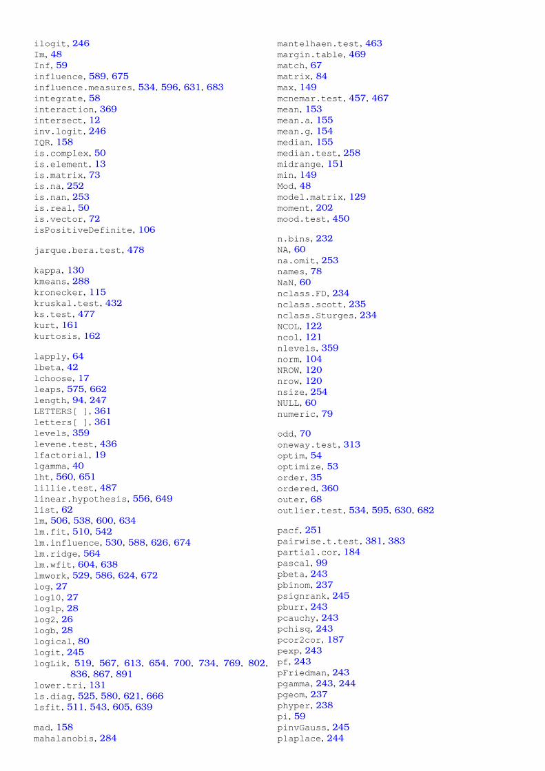
ilogit, 246Im, 48Inf, 59influence, 589, 675influence.measures, 534, 596, 631, 683integrate, 58interaction, 369intersect, 12inv.logit, 246IQR, 158is.complex, 50is.element, 13is.matrix, 73is.na, 252is.nan, 253is.real, 50is.vector, 72isPositiveDefinite, 106
jarque.bera.test, 478
kappa, 130kmeans, 288kronecker, 115kruskal.test, 432ks.test, 477kurt, 161kurtosis, 162
lapply, 64lbeta, 42lchoose, 17leaps, 575, 662length, 94, 247LETTERS[ ], 361letters[ ], 361levels, 359levene.test, 436lfactorial, 19lgamma, 40lht, 560, 651lillie.test, 487linear.hypothesis, 556, 649list, 62lm, 506, 538, 600, 634lm.fit, 510, 542lm.influence, 530, 588, 626, 674lm.ridge, 564lm.wfit, 604, 638lmwork, 529, 586, 624, 672log, 27log10, 27log1p, 28log2, 26logb, 28logical, 80logit, 245logLik, 519, 567, 613, 654, 700, 734, 769, 802,
836, 867, 891lower.tri, 131ls.diag, 525, 580, 621, 666lsfit, 511, 543, 605, 639
mad, 158mahalanobis, 284
mantelhaen.test, 463margin.table, 469match, 67matrix, 84max, 149mcnemar.test, 457, 467mean, 153mean.a, 155mean.g, 154median, 155median.test, 258midrange, 151min, 149Mod, 48model.matrix, 129moment, 202mood.test, 450
n.bins, 232NA, 60na.omit, 253names, 78NaN, 60nclass.FD, 234nclass.scott, 235nclass.Sturges, 234NCOL, 122ncol, 121nlevels, 359norm, 104NROW, 120nrow, 120nsize, 254NULL, 60numeric, 79
odd, 70oneway.test, 313optim, 54optimize, 53order, 35ordered, 360outer, 68outlier.test, 534, 595, 630, 682
pacf, 251pairwise.t.test, 381, 383partial.cor, 184pascal, 99pbeta, 243pbinom, 237psignrank, 245pburr, 243pcauchy, 243pchisq, 243pcor2cor, 187pexp, 243pf, 243pFriedman, 243pgamma, 243, 244pgeom, 237phyper, 238pi, 59pinvGauss, 245plaplace, 244
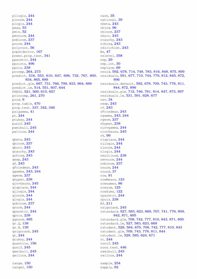
pllogis, 244plnorm, 244plogis, 244pmax, 53pmin, 52pmvnorm, 244pnbinom, 237pnorm, 244polyroot, 56popstderror, 167power.prop.test, 341ppareto1, 244ppoints, 496ppois, 238prcomp, 264, 273predict, 516, 553, 610, 647, 698, 732, 767, 800,
834, 865, 889predict.glm, 697, 731, 766, 799, 833, 864, 888predict.lm, 514, 551, 607, 644PRESS, 521, 569, 615, 657princomp, 261, 270prod, 9prop.table, 470prop.test, 337, 342, 346psigamma, 41pt, 244ptukey, 244punif, 245pweibull, 245pwilcox, 244
qbeta, 243qbinom, 237qburr, 243qcauchy, 243qchisq, 243qexp, 243qf, 243qFriedman, 243qgamma, 243, 244qgeom, 237qhyper, 238qinvGauss, 245qlaplace, 244qllogis, 244qlnorm, 244qlogis, 244qnbinom, 237qnorm, 244qpareto1, 244qpois, 238qqnorm, 495qr.Q, 138qr.R, 139qsignrank, 245qt, 244qtukey, 244quantile, 156qunif, 245qweibull, 245qwilcox, 244
range, 150range2, 150
rank, 35rational, 39rbeta, 243rbind, 96rbinom, 237rburr, 243rcauchy, 243rchisq, 243rdirichlet, 243Re, 47relevel, 358rep, 29rep.int, 30replace, 69resid, 592, 678, 714, 748, 783, 816, 848, 875, 899residuals, 591, 677, 710, 744, 779, 812, 845, 872,
896residuals.default, 592, 678, 709, 743, 778, 811,
844, 872, 896residuals.glm, 712, 746, 781, 814, 847, 873, 897residuals.lm, 531, 591, 628, 677rev, 34rexp, 243rf, 243rFriedman, 243rgamma, 243, 244rgeom, 237rhyper, 238rinvgamma, 244rinvGauss, 245rk, 99rlaplace, 244rllogis, 244rlnorm, 244rlogis, 244rmultinom, 238rmvnorm, 244rnbinom, 237rnorm, 244round, 37row, 91rowMeans, 123rownames, 86rowsum, 125rowSums, 122rpareto1, 244rpois, 238RS, 211rsignrank, 245rstandard, 527, 583, 623, 669, 707, 741, 776, 809,
842, 871, 895rstandard.glm, 708, 742, 777, 810, 843, 871, 895rstandard.lm, 527, 583, 623, 669rstudent, 528, 584, 670, 708, 742, 777, 810, 843rstudent.glm, 709, 743, 778, 811, 844rstudent.lm, 528, 585, 624, 671rt, 244runif, 245runs.test, 446rweibull, 245rwilcox, 244
sample, 254sapply, 82
scale, 204scan, 77scm, 71sd, 166seq, 31seq_along, 32seq_len, 33sequence, 31set.seed, 256setdiff, 13setequal, 14sf.test, 485sigma, 166sigma2, 168sigma2.test, 331sigma2m, 172sigmoid, 44sign, 11signif, 38simple.z.test, 257sin, 19sinh, 22skew, 159skewness, 160solve, 107solveCrossprod, 128sort, 33sqrt, 11ssdev, 170stat.desc, 222stderror, 168stdres, 584, 670studres, 585, 671subset, 84sum, 9summary, 214, 266, 276, 368, 474summary.glm, 691, 725, 759, 793, 827, 859, 883summary.lm, 508, 540, 602, 636svd, 135sweep, 256
T, 61t, 117t.test, 296, 302, 306, 309table, 228tabulate, 227tail, 81, 93tan, 20tanh, 23tapply, 365tcrossprod, 111toeplitz, 97tr, 104trigamma, 41TRUE, 60trunc, 36tsum.test, 316, 323, 327TukeyHSD, 373, 375, 378
unclass, 363union, 12unique, 229uniroot, 55upper.tri, 131
Var, 174var, 169var.coeff, 164var.test, 334vcov, 509, 541, 604, 638, 696, 730, 764, 798, 832,
863, 887vech, 93vector, 79vif, 595, 682
weighted.mean, 188weighted.residuals, 628, 676, 716, 750, 785, 818,
850, 876, 900weights, 627, 676, 716, 751, 786, 818, 851, 876,
900which, 15which.max, 16which.min, 15wilcox.test, 409, 413, 416, 421, 425, 428wt.moments, 190wt.var, 189
xor, 8xpnd, 94xtabs, 472
z.test, 293, 299zsum.test, 313, 320