Sede Amministrativa: Università degli Studi di Padova

Dipartimento di Tecnica e Gestione dei Sistemi Industriali

CORSO DI DOTTORATO DI RICERCA IN: INGEGNERIA MECCATRONICA E

DELL’INNOVAZIONE MECCANICA DEL PRODOTTO

CURRICOLO: MECCATRONICA

CICLO XXIX

EIGENSTRUCTURE ASSIGNMENT IN VIBRATING SYSTEMS

THROUGH ACTIVE AND PASSIVE APPROACHES

Tesi redatta con il contributo finanziario della Fondazione Studi Universitari di Vicenza

Coordinatore: Ch.mo Prof. Roberto Caracciolo

Supervisore: Ch.mo Prof. Dario Richiedei

Dottorando: Roberto Belotti

2

3

Abstract The dynamic behaviour of a vibrating system depends on its eigenstructure, which consists of

the eigenvalues and the eigenvectors. In fact, eigenvalues define natural frequencies, damping

and settling time, while eigenvectors define the spatial distribution of vibrations, i.e. the mode

shape, and also affect the sensitivity of eigenvalues with respect to the system parameters.

Therefore, eigenstructure assignment, which is aimed at modifying the system in such a way

that it features the desired set of eigenvalues and eigenvectors, is of fundamental importance in

mechanical design. However, similarly to several other inverse problems, eigenstructure

assignment is inherently challenging, due to its ill-posed nature. Despite the recent

advancements of the state of the art in eigenstructure assignment, in fact, there are still important

open issues.

The available methods for eigenstructure assignment can be grouped into two classes: passive

approaches, which consist in modifying the physical parameters of the system, and active

approaches, which consist in employing actuators and sensors to exert suitable control forces

as determined by a specified control law. Since both these approaches have advantages and

drawbacks, it is important to choose the most appropriate strategy for the application of interest.

In the present thesis, in fact, are collected passive, active, and even hybrid methods, in which

active and passive techniques are concurrently employed. All the methods proposed in the thesis

are aimed at solving open issues that emerged from the literature and which have applicative

relevance, as well as theoretical. In contrast to several state-of-the-art methods, in fact, the

proposed ones implement strategies that enable to ensure that the computed solutions are

meaningful and feasible. Moreover, given that in modern mechanical design large-scale systems

are increasingly common, computational issues have become a major concern and thus have

been adequately addressed in the thesis.

The proposed methods have been developed to be general and broadly applicable. In order to

demonstrate the versatility of the methods, in the thesis it is provided an extensive numerical

assessment, hence diverse test-cases have been used for validation purposes. In order to evaluate

without bias the performances of the proposed methods, it has been chosen to employ well-

4

established benchmarks from the literature. Moreover, selected experimental applications are

presented in the thesis, in order to determine the capabilities of the developed methods when

critically challenged.

Given the focus on these issues, it is expected that the methods here proposed can constitute

effective tools to improve the dynamic behaviour of vibrating systems and it is hoped that the

present work could contribute to spread the use of eigenstructure assignment in the solution of

engineering design problems.

5

6

Table of contents Chapter 1. Introduction .............................................................................................................. 9

1.1. Scope of the thesis ...................................................................................................... 9

1.2. Literature review ...................................................................................................... 11

1.3. Objectives of the thesis ............................................................................................ 19

1.4. Outline of the thesis.................................................................................................. 20

Chapter 2. Assignment of partial eigenvectors ........................................................................ 23

2.1. Introduction .............................................................................................................. 23

2.2. Problem forumlation ................................................................................................ 24

2.3. The proposed method ............................................................................................... 26

2.4. Numerical examples and method validation ............................................................ 32

2.5. Conclusion ................................................................................................................ 41

Chapter 3. Auxiliary subsystems .............................................................................................. 43

3.1. Introduction .............................................................................................................. 43

3.2. Problem theoretical development ............................................................................. 44

3.3. Problem solution ...................................................................................................... 49

3.4. Numerical examples ................................................................................................. 50

3.5. Conclusion ................................................................................................................ 58

Chapter 4. Passive control without spill-over .......................................................................... 59

4.1. Introduction .............................................................................................................. 59

4.2. Method description ................................................................................................... 60

4.3. Numerical examples ................................................................................................. 70

4.4. Conclusion ................................................................................................................ 81

Chapter 5. Model updating for flexible link mechanisms ........................................................ 83

7

5.1. Introduction .............................................................................................................. 83

5.2. Model based on the equivalent rigid-link system ..................................................... 85

5.3. Data consistency between model and experimental modal analysis ........................ 90

5.4. The model updating technique ................................................................................. 92

5.5. Experimental validation ........................................................................................... 97

5.6. Conclusions ............................................................................................................ 106

Chapter 6. Partial pole placement .......................................................................................... 109

6.1. Introduction ............................................................................................................ 109

6.2. Description of the method ...................................................................................... 111

6.3. Numerical assessment ............................................................................................ 118

6.4. Conclusion.............................................................................................................. 122

Chapter 7. Hybrid control ...................................................................................................... 123

7.1. Introduction ............................................................................................................ 123

7.2. Problem formulation .............................................................................................. 124

7.3. Proposed solution ................................................................................................... 126

7.4. Numerical examples ............................................................................................... 132

7.5. Conclusion.............................................................................................................. 139

Chapter 8. Experimental application of Hybrid Control ........................................................ 141

8.1. Description of the system ....................................................................................... 141

8.2. The piezoelectric actuator ...................................................................................... 142

8.3. The system model .................................................................................................. 143

8.4. Hybrid control ........................................................................................................ 145

8.5. State estimation ...................................................................................................... 147

8.6. Model identification and updating ......................................................................... 151

8.7. Experimental setup ................................................................................................. 154

8

8.8. Experimental results ............................................................................................... 158

Conclusions ............................................................................................................................ 163

References .............................................................................................................................. 167

9

Chapter 1. Introduction 1.1. Scope of the thesis

Vibration occurs in every mechanical system that have elastic forces, and hence a proper

understanding and mastery of such a phenomenon is of primary importance in mechanical

design. Vibrations might be unwanted, being a major cause of stress and fatigue and reducing

precision and accuracy of machines, or desired, since required by the processes of interest. In

both cases, it is often necessary to comply with design specifications that concerns the vibratory

behaviour of mechanical systems.

The most established model for the analysis of multiple degrees of freedom vibrating systems

is the well-known second order linear model

( ) ( ) ( ) ( )t t t t+ + =M C Kq q q fɺɺ ɺ (1.1)

where , , N N×∈M C K ℝ are the mass, damping and stiffness matrices, respectively, N∈q ℝ is

the displacements vector and N∈f ℝ represents the external forces that are exerted on the

system (e.g. disturbances, control forces). From the theory of linear ordinary differential

equations, it follows that the dynamical behaviour of a vibrating system is determined by the

eigenvalues λ ∈ℂ and the eigenvectors N∈u ℂ associated to the system, namely the solutions

of the quadratic eigenproblem

2 .λ λ + = + CM K 0u (1.2)

The pair ( ),λ u is called eigenpair and it can be easily proved that the set of eigenpairs consists

of 2N complex self-conjugate elements. Eigenvalues define the natural frequency (or

eigenfrequency) ω and the damping factor ζ of each mode of vibration, being such quantities

related by

21 .iλ ζω ω ζ= − ± − (1.3)

Eigenvectors instead define the mode shapes, namely the spatial distribution of vibrations over

the system. Moreover, eigenvectors affect the sensitivity of eigenvalues with respect to system

10

parameters, and hence robustness. In fact, let us consider a parameter x , then the following

formula [1] expresses the sensitivity of an eigenvalue λ with respect to x :

2

2,

T

x

T

x x

x

iλ λλλ

λ

∂ ∂∂∂ ∂ ∂

−∂ =+

+

∂

K M C

M K

u u

u u (1.4)

where u is the eigenvector associate to λ .

At this point it is worth to mention the special case in which the system is undamped, i.e. ,=C 0

the mass matrix is symmetric and positive definite and the stiffness matrix is symmetric and

positive semi-definite. Such assumptions are reasonable, since they allow to accurately

represent most of the vibrating system of interest. Moreover, the mathematical complexity of

the problem can be significantly simplified. In fact, in this case it holds

iλ ω= ± (1.5)

which is exactly (1.3) for 0ζ = . Hence it is convenient to solve the equivalent linear

eigenproblem

2 .ω − = M K 0u (1.6)

In such a case, there are N real and non-negative eigenvalues, each one associated to a real

eigenvector.

Regardless of the employed system model and the resulting eigenproblem to be solved, it is

evident that the eigenvalues and eigenvectors, which together constitute the eigenstructure,

strongly characterize the dynamic behaviour of the system. The design of vibrating systems

aimed at satisfying specifications on eigenvalues and eigenvectors, which is commonly known

as eigenstructure assignment (EA), has drawn increasing interest over the last few decades. The

most natural mathematical framework for such problems is constituted by the inverse

eigenproblems, which consist in the determination of the system model that features a desired

set of eigenvalues and eigenvectors, indeed. The development of effective and reliable

numerical methods is inherently challenging, due to the ill-posed nature of this kind of inverse

problems. In fact, despite the remarkable advancements made over the recent years, the state of

the art is still unable to solve some relevant design problems.

11

In the present thesis are collected novel techniques for eigenstructure assignment, whose aim is

to solve open problems emerged from the literature that reflect actual design needs. It has been

chosen to develop methods as general as possible, thus allowing a broad scope of application.

Feasibility of the computed solutions, although neglected by several methods available in the

literature, has been considered a mandatory requirement since it is often necessary to comply

with technical and economic constraints. Moreover, attention has been paid to computational

issues, such as numerical conditioning and CPU time, which are critical especially in case of

large-scale models. In fact, for an accurate approximation of complex mechanical systems,

typically by means of Finite Element models, it is required to increase substantially the number

of degrees of freedom of the model and, despite the considerable capabilities of modern

computers, computational issues can still be concerning. Finally, an extensive numerical

validation of the proposed methods has been carried out. The chosen benchmarks are taken from

the literature, allowing an unbiased assessment of the performances achieved.

1.2. Literature review

The approaches to eigenstructure assignment can be basically divided into passive control and

active control.

Passive control, also known as Dynamic Structural Modification (DSM), aims at achieving the

desired eigenstructure by modifying the physical properties of the system (typically the inertial

and elastic parameters). From the mathematical point of view, the matrices in (1.1) are altered,

usually by additive modification, in such a way that the system features the desired

eigenstructure. Such an approach is often chosen because it does not require neither electronic

devices nor external power. Moreover, the resulting system is assured to be stable, in fact the

system modifications are inherently symmetric. However, in practice, not every desired

specification can be obtained, because there are constraints on the modifications that naturally

arise from feasibility considerations. Therefore, passive control is not always capable of

assigning the desired eigenstructure with sufficient accuracy.

Active control consists in employing a feedback closed-loop scheme in such a way that the

controlled system features the desired eigenstructure. In practice, suitable external forces are

12

exerted on the system by controlled actuators. Although such an approach requires the use of

electronic devices, active control is preferable when structural modifications are impractical or

inconvenient. Moreover, active control is capable of stabilizing unstable systems and it ensures

adequate performances regardless of the operating conditions, even in the presence of external

disturbances. Active vibration control relies on a solid theoretical background. For the

assignment of just the eigenvalues, i.e. the so-called “pole placement”, several methods based

on state-feedback are available. The assignment of eigenvectors, in contrast, is affected by an

inherent limitation that restricts the range of eigenvectors that can be actually obtained.

Both passive and active control have advantages and shortcomings. Recently in the literature

appeared also hybrid methods that combine these two approaches, in order to achieve superior

performances with respect to the sole employment of either passive or active control, but the

state of the art is still undeveloped. In this Section, a brief literature review of passive and active

control is given.

1.2.1. Passive control

Passive control, or Dynamic Structural Modification, is related to two distinct problems. The

direct problem is the prediction of the modified natural frequencies and mode shapes when the

employed perturbation of the system is known. In contrast, the inverse problem is the

computation of the appropriate values of the physical parameters of the system that results in

the desired dynamic behaviour. In such a sense, inverse structural modification is a suitable

technique for eigenstructure assignment, as demonstrated by numerous paper appeared in

literature. Such methods can be used either for the design of new vibrating systems or for the

optimization of existing ones. In both the cases, some knowledge of the original system model,

although approximated, is required. The criterion that is chosen to classify the methods for

passive control is the employed description of the system model. Hence the works in the

literature can be organized as follows:

• the approaches based on the physical model of the system, i.e. its mass, damping and

stiffness matrices;

• the approaches based on modal data, i.e. a (not necessarily complete) set of eigenpairs;

13

• the approaches based on the Frequency Response Functions, and in particular the

system receptances.

Approaches based on physical models

Given the popularity of Finite Element modelling in modern mechanical design, it is not

surprising that several methods for passive control rely on the physical system model. This

approach is suitable at the design stage of new mechanical systems, in which are often employed

Finite Element models. The earliest techniques arise from the investigation of eigenvalue and

eigenvector sensitivity to system parameters. For example, in [2], Farahani and Bahai

approximate the modification of the system eigenstructure through its first derivative with

respect to the parameter modification. In [3] the same authors extend the previous method

employing the second order Taylor expansion. Such an approach is effective and

computationally efficient as long as the desired changes are small, otherwise it is necessary to

perform multiple iterations, affecting the reliability and the convergence of the method.

Liangsheng in [4] proposes to simultaneously modify the mass and stiffness matrices for

assigning a subset of the modes. Arbitrary topologies of the matrices are allowed, and the

structural modifications are conveniently computed solving a linear system. The number of

assigned modes, however, is not arbitrary as it depends on the model dimension and the number

of modifiable parameters. Moreover, no constraints are taken into account to ensure feasibility

of the modifications.

Wang et al., in [5], manage to maximize the fundamental frequency of beams and plates by a

proper positioning of elastic or rigid supports. An iterative procedure, which relies on the

sensitivity of the frequency with respect to the support position, is developed and a strategy to

improve convergence is proposed. The minimum stiffness of an elastic support that enables to

maximize the fundamental frequency is investigated by Wang et al. in [6], where analytical

solutions for different boundary conditions are given.

In [7] Ram determines the distribution of mass that enables to maximize the lowest eigenvalue

or to minimize the highest. Closed-form solutions are provided for an axially vibrating rod and

an Euler-Bernoulli beam. The problem is cast as a quadratic program with quadratic constraints

(the latter to constrain the total mass) and a recursive strategy of solution is proposed.

14

The work of Richiedei et al. [8] aims to handle very general eigenstructure assignment tasks,

allowing to assign an arbitrary number of modes and dealing with matrices with arbitrary

topology. The method exploits convex optimization to ensure that the computed solution is

globally optimal. Moreover, constraints on the modification of the physical parameters can be

considered. Such an approach has been later extended by Ouyang et al. [9] that recast the

problem as a mixed-integer optimization problem to take into account discrete modifications,

in order to reflect the industrial need of modularisation.

Approaches based on modal data

Although the mass, damping and stiffness matrices represent a simple and powerful way to

model vibrating systems, the measurement of the physical quantities that appear in such

matrices is often impractical and prone to errors. Nevertheless, the sole eigenstructure of the

original system, without the underlying physical matrices, has been proved to be sufficient for

performing eigenstructure assignment. Even the knowledge of few dominant eigenpairs can be

satisfactory, according to numerous papers in the literature. Moreover, eigenvalues and

eigenvector can be directly obtained with appropriate measurements.

The pioneering work by Ram and Braun [10] deals exactly with the incompleteness of the

original system model imposing that the assigned eigenvectors are selected within the space

generated by the ones of the original system. As a consequence, the number of modifiable

parameters is limited by the number of known modes. In the paper, the family of all the

mathematical solutions of the modification problem is characterized. Feasibility of the solution

is addressed but no algorithm to compute a feasible approximation of the theoretical solution is

provided. The work of Sivan and Ram [11] is devoted to such an issue, which is overcome

introducing suitable conditions that are solved in a least-square sense.

Sivan and Ram in [12] propose a method for computing mass and stiffness matrices with

prescribed eigenstructure. Since the obtained mass matrix is diagonal, the method can be applied

only to multiple-connected mass-spring systems. The stiffness matrix instead is computed

solving an optimization problem by means of two algorithms: one that is slow but provides a

global solution and another one that is more efficient but ensures the attainment of a local

15

minimum only. System feasibility is ensured imposing non-negative constraints. The method

requires to prescribe all the modes, namely only the complete eigenstructure can be assigned.

Bucher and Braun in [13] address the eigenstructure assignment problem using modal test

results only. The modified eigenvectors are forced to belong to the space spanned by the original

system eigenvectors, in order to overcome the incompleteness of the eigenstructure available

from the tests. Moreover, it is addressed the extraction of modal data from experimental FRFs,

which is an ill-posed problem, and the sensitivity to measurement noise is examined. The

method has been later improved, in fact in [14] it is proved that if both left and right eigenvectors

of the system are known then it is possible to solve the eigenstructure assignment problem

without truncation error.

Sivan and Ram in [15] analyse the assignment of natural frequencies with incomplete modal

data. The inadequateness of the original model representation is tackled casting the assignment

as an optimization problem. Feasibility of the modifications is ensured by appropriate non-

negativity constraints. It is considered also the case of interrelated modifications of mass and

stiffness matrices, which is often necessary in the design of distributed-parameter systems.

Approaches based on FRFs model

The characterization of the system through frequency response functions has several

advantages, which motivate its popularity in the recent literature. Frequency response functions

can be obtained from measurements, but in contrast to modal data, they are marginally affected

by ill-conditioning. Therefore, such a description of the original system model is often

preferable for eigenstructure assignment purposes.

For example, in [16] Mottershead managed to assign antiresonances solving the inverse

eigenvalue problem for a subsidiary system. It is proved that only few measurements of the

unmodified structure are required. In Kyprianou et al. [17] the assignment of natural frequencies

by one added mass connected to the original system by one or two springs is studied. The

problem is recast as a system of non-linear multivariate polynomial equations which are solved

by means of Groebner bases. In a similar way, the same authors in [18] address the assignment

of resonances or antiresonances to the original system by adding a beam, whose cross-section

dimensions are to be determined.

16

In [19], Ouyang proposes a method for assignment of latent roots of damped asymmetric

systems that consists in the modification of the mass, damping and stiffness matrices but relies

on the receptance of the symmetric system. The challenge is due to the asymmetry, which causes

instability. Park and Park in [20] address the eigenstructure assignment by modifying the mass,

damping and stiffness matrices. The problem is recast as a linear system of equations, which

can be also underdetermined (i.e. there are more modifiable parameters than equations). In [21]

Mottershead and Lallement investigate the pole-zero cancellation by unit-rank modifications.

In [22] Mottershead et al. deal with the same topic, focusing on the special case of repeated

poles and zeros.

The general eigenstructure assignment problem is addressed by Ouyang et al. in [23], which is

an extension of [8] that enable to exploit the convex optimization formulation simply from the

knowledge of the FRFs. Similarly to [8], also for such a method the number of modifiable

parameters is arbitrary, as well as the topology of the modification matrices and the number of

assigned modes. Moreover, feasibility can be ensured specifying suitable constraints. The

computed solution is globally optimal as a consequence of convexity of the formulation.

Open issues in Dynamic Structural Modification

Although the state-of-the-art enables to solve very diverse assignment tasks by means of DSM,

there are several noteworthy open problems. For example, the available methods allow

assigning only complete eigenvectors, and hence require the dynamic response to be prescribed

for the entire system at once (i.e. for all the degrees of freedom). In practice, however, it is often

more desirable to specify exactly only the dynamic behaviour of the parts of the system that

have the greatest importance. The assignment of partial eigenvectors, however, cannot be

obtained with any of the methods available.

A problem that cannot be tackled satisfactorily is the possibility of modifying the dynamical

properties of a system through the addition of auxiliary subsystems, despite the fact that it is of

considerable practical interest, since often the original design of a system cannot be changed

significantly. There are indeed several results that require the modifications of the system to

have very specific topologies, but the general problem is rarely investigated.

17

Another relevant issue of passive control is that it is affected by spill-over. Such a phenomenon

occurs when a subset of the natural frequencies is altered, thus modifying also the other

frequencies. Spill-over should be avoided in order to prevent an unexpected and unwanted

behaviour of the system. The available methods that enable to inhibit spill-over can deal only

with simple mass-spring systems, while a method that can deal with general system models,

such as the ones obtained with Finite Element modelling, is missing.

Structural modification is related also to another important problem, which is model updating,

namely the tuning of a model parameters in such a way that the computed eigenvalues and

eigenvectors of the model match the measured ones. Given the complexity of the Finite Element

models currently employed in mechanical design, there is an increasing need of methods to

perform accurate model updating, which cannot be fulfilled by the state-of-the-art.

1.2.2. Pole assignment through state-feedback control

Active vibration control is usually oriented to the assignment of sole eigenvalues, i.e. the so-

called “pole placement”. It is a very well established topic, in fact early results in such a field

date back to the 1960s. For example, in [24] Wonham proved that the poles can be assigned by

means of state feedback if and only if the system is controllable. In [25], Kautsky et al.

investigate sensitivity of closed-loop poles with respect to perturbation of system and gain

matrices. Since the pole placement problem is underdetermined for multivariable control, a

technique to determine a robust solution is proposed. Ackermann in [26] introduced a well-

known formula that provide a closed form expression of control gains for single-input systems.

In such a case, instead, the solution is unique, but the computation through Ackermann’s

formula is not numerically stable, as it requires the inversion of the controllability matrix.

The methods cited so far require to recast the second-order model (1.1) into a first-order form.

In such a way, however, the matrices involved double the dimension and lose some desirable

properties (e.g symmetry and sparsity). In fact, in vibration control a great effort has been put

in tackling the problem directly through the second-order system model. In [27] Chu and Datta

propose two methods for eigenvalue assignment and proved that if the desired poles are self-

conjugated then the feedback gains are real. Datta et al. in [28] address the partial pole

placement, in which chosen eigenvalues are relocated and all the other eigenvalues are left

18

unchanged. Orthogonality conditions for the eigenvectors of the system are derived and

exploited to prove a closed form expression for the control gains.

Ram and Elhay in [29] consider the partial pole placement for multi input systems. It is proposed

to solve a sequence of pole assignment tasks by single-input control and it is demonstrated that

such a procedure reduces the control effort. Chu in [30] presents algorithms for robust

eigenvalue assignment through state and output feedback and partial pole assignment through

state feedback. In [31] Qian and Xu achieve robust partial pole placement minimizing the

condition number of the closed-loop eigenvectors matrix.

The assignment of eigenstructure by active control has been first recognized by Moore in [32]

and Andry et al. in [33]. Such works, that employ a first order model, characterize the class of

eigenvectors that can be obtained by state feedback control. Additional references can be found

in the review paper by White [34]. The assignment of partial eigenstructure using a second-

order model has been tackled by Datta et al. in [35].

Receptance-based methods have also gained popularity, since the paper by Ram and

Mottershead [36] in which the assignment of poles and zeros by single-input feedback control

is addressed. In [37] Tehrani et al. propose a receptance method for partial pole placement by

multi-input control. The chief advantage of such methods, similarly to the case of receptance-

based passive control method, is that there is no need to know the mass, damping and stiffness

matrices, which is often impractical and not adequate to model the dynamic behaviour of the

systems of interest.

Open issues in active eigenstructure assignment

As pointed out in the literature review, pole placement is often oriented to the assignment of

few dominant poles, which are the ones that affect the dynamics the most. The literature on

partial pole placement is almost always restricted to methods for avoiding spill-over. In several

cases, it is desired to perform partial pole placement allowing spill-over, as long as it can be

constrained and unexpected dynamics can be prevented. In such a way, the additional freedom

in pole location could be exploited to improve performances.

19

The assignment of eigenvectors by state-feedback control is also a relevant problem that cannot

be tackled satisfactorily. In fact it can be proved that an eigenvector can be assigned if and only

if it belongs to a particular vector subspace, that depends on the physical properties of the system

and on the characteristics of the actuation. In particular, the dimension of such a space equals

the number of actuation forces, hence for underactuated systems such a limitation can prevent

the attainment of the desired eigenstructure. A design strategy that effectively deals with this

issue is missing in the literature.

1.3. Objectives of the thesis

Although the state-of-the-art methods reviewed in the previous Section enable to achieve

eigenstructure assignment in several contexts, the design of vibrating systems often requires to

face issues that the state-of-the-art cannot handle. In the present thesis are proposed methods

for eigenstructure assignment that aim to solve open problems emerged from the literature.

Both passive and active control have been investigated. Structural modification has been

employed for the assignment of eigenvalues and partial eigenvectors in undamped systems. An

approach similar to [8] has been developed, which consists in minimizing the residual of the

eigenproblem equation (1.6) in a least-square sense. Given the non-convexity of the resulting

optimization problem, a strategy inspired by homotopy optimization has been implemented to

boost the attainment of a global minimum.

A similar optimization scheme has been applied also to the eigenstructure assignment problem

through the addition of auxiliary subsystems. The main advantage of the method proposed over

the state-of-the-art ones is the possibility to handle very general systems and any modification

matrix which is linear in the system parameters.

The problem of eigenfrequency assignment without spill-over is also addressed. It is indeed

proposed a method that enable to modify a subset of the natural frequencies of a vibrating

system keeping the other ones unchanged or at least affected by very limited spill-over. Such a

problem has been solved in the literature only for mass-spring systems, while the proposed

method aims to avoid spill-over also for system with distributed parameters.

20

To conclude the contribution of the thesis to the field of Dynamic Structural Modification, a

method for model updating specifically conceived for flexible link mechanisms is proposed and

experimentally applied to the tuning of the Finite Element model of a planar robot.

Two issues related to active control have been also addressed. In particular, it is proposed a

method for state-feedback gain synthesis that enables to perform partial pole placement through

rank-1 control. The spill-over that affects the poles that are not assigned is limited employing

suitable constraints. Such an approach is rarely employed in the literature and the proposed

method intends to constitute a more numerically stable alternative to the available methods.

Finally, the assignment of eigenvectors by state feedback control is addressed. It is proposed a

method of structural modification that enable to suitably modify the range of eigenvectors that

can be obtained through state feedback control. Hence, the proposed method constitutes a hybrid

active/passive strategy for eigenstructure assignment. An extensive numerical and experimental

validation is also provided.

1.4. Outline of the thesis

The thesis is organized as follows. In Chapter 2 the assignment of eigenvalues and partial

eigenvectors through passive control is investigated. In fact, eigenvectors define the distribution

of vibrations over the whole system, but in several applications it would be desirable to focus

on the response of the most concerning parts of the system. The proposed method allows to

specify only the most relevant parts of the assigned eigenvectors, while the others are

represented by optimization variables. It has been developed an optimization algorithm that is

explained in detail. The proposed method is validated through two test-cases: a five-dof lumped

parameter system and a 39-dof lumped-and-distributed parameter system.

The same approach can be used to tackle another relevant problem: the eigenstructure

assignment through the addition of auxiliary subsystems. In Chapter 3 such a problem is

addressed, employing the strategy for assignment of partial eigenvectors. In particular, the

response of the primary system is assigned, while the eigenvector components correspondent to

21

the auxiliary systems are considered as unknowns. The proposed method is also validated with

favourable results in comparison to other methods available in the literature

Chapter 4 is devoted to frequency spill-over caused by structural modification. It has been

developed a novel method, that allows to inhibit spill-over, which consists of two steps: first a

system with the desired eigenvalues is sought, regardless of its feasibility, and then it is

computed an equivalent system which is also feasible, exploiting a special class of ordinary

differential equations called isospectral flows. The method has been numerically validated with

three examples: one system with lumped parameters, one with distributed parameters and finally

one with lumped-and-distributed parameters.

In Chapter 5 it is presented a method for model updating specifically developed for flexible link

mechanism. The proposed approach ultimately casts model updating as an optimization

problem in the presence of bounds on the feasible values, by also using techniques to improve

the numerical conditioning. The method is applied experimentally to the model updating of a

lightweight planar robot.

Chapter 6 is devoted to a method for partial pole placement by state feedback single-input

control, that allows to specify exact locations for the most important poles and a region of the

complex plane to which the remaining poles are constrained to belong. To achieve such a result,

a receptance based method for partial pole placement and a state-space method for regional pole

placement are combined, the latter exploiting Linear Matrix Inequalities to express the regional

constraint. The freedom in the placement of the non-assigned poles is exploited to minimize the

controller effort. The method is validated in the control of a four-bar flexible link mechanism.

Chapter 7 investigates a limitation that affects the assignment of eigenvectors through active

control. It is proposed a hybrid method that exploits passive control to modify the range of

eigenvectors attainable by active control. The problem is proved to be equivalent to the

minimization of the rank of a matrix. Two algorithms are proposed to compute the numerical

solution. A numerical validation of the method is carried out, in order to assess the effectiveness

of the proposed hybrid approach. Moreover, the two algorithms are thoroughly compared.

Chapter 8 is devoted to the experimental application of the hybrid method proposed in the

previous Chapter. The employed test case is a cantilever beam made of aluminium. A modal

22

characterization of such a beam is performed and the Finite Element model is tuned accordingly.

In order to modify the second lowest frequency mode, a piezoelectric actuator is placed on the

beam. Verified that it is not possible to control adequately the beam, two suitable lumped masses

are added to the beam as computed by means of the method described in the previous Chapter.

Finally, the employed control scheme is described and the measurements that prove the

attainment of the design specifications are provided.

23

Chapter 2. Assignment of partial eigenvectors

2.1. Introduction

A relevant open issue in Dynamic Structural Modification is that none of the available methods

can deal with design specifications that involve only some arbitrary parts of the system. Indeed

they allow assigning only complete eigenvectors, and hence the dynamic response should be

prescribed for the entire system at once (i.e. for all the model degrees of freedom). In contrast,

it would be often desirable to specify exactly only the dynamic behaviour of the parts of the

system that have the greatest importance. Hence, only some entries of the eigenvectors are

exactly imposed. This problem is referred to as the partial eigenvector assignment problem and

it is of great interest in particular in the presence of large scale models. Indeed, it is reasonable

to expect that weakening the requests on the least concerning parts of the system might lead to

a better assignment of the parts of interest, by improving the overall design of the system.

Additionally, defining precise specifications for all the parts of the system, and therefore for all

the degrees of freedom (dofs) of the system model employed, is often difficult. This fact may

occur for instance whenever hybrid coordinates are employed (e.g. through the Craig-Bampton

method).

The methods for DSM reviewed in Chapter 1, however, cannot be trivially extended to the

assignment of partial eigenvectors since such a problem has some mathematical difficulties. To

solve this issue, in this Chapter it is presented a novel method that allows partial eigenvector

assignment, in the presence of an arbitrary number of assigned entries. The method relies on

the optimization-based approach introduced in [8], and thus it inherits its peculiarities such as

the possibility to assign an arbitrary number of eigenpairs, the generality of the topology of the

admissible additive modifications and the ease of inclusion of feasibility constraints. The

extension of method [8] to partial assignment is not straightforward, since the presence of some

entries of the mode shape that are not assigned leads to a non-convex formulation of the cost

function. Thus an algorithm to mitigate the issues of non-convex optimization and to boost the

convergence to the global optimal solution should be adopted.

24

2.2. Problem forumlation

Let us suppose that the N -dof vibrating system to be modified is defined through its mass

matrix N N×∈M ℝ and stiffness matrix N N×∈K ℝ . Damping is neglected, as it is often done in

most of the papers on structural modifications, since, in practice, several vibrating systems of

interest for this kind of applications are lightly damped. These matrices represent both the

original system model, in the case of improving the design and optimizing an existing system,

as well as an initial guess design in the case of designing new systems.

The aim of the system modification is to find feasible additive modifications M∆ and K∆ of

the inertial and elastic parameters such that the modified system with mass matrix +M M∆

and stiffness matrix +K K∆ features a desired set of e

N N≤ natural frequencies ( 1ω , 2ω ,…,

)eNω , and hence the eigenvalues, and some entries of the associated mode shapes (the

eigenvectors) ( 1u , 2u ,…, )eNu . The topologies of M∆ and K∆ are assumed a-priori in order

to reflect feasible modifications of the system parameters, on the basis of technical constraints

and design choices. Nevertheless, there is no limitation on the topology of these matrices, except

that they should be symmetric in order to ensure the modifications to be physically meaningful.

All the modifications of the system parameters, which are in practice regarded as the design

variables, are then collected in vector xN∈x ℝ . Thus it holds that ( )=M M x∆ ∆ and

( )=K K x∆ ∆ , and it is assumed that the dependence on x is linear. This hypothesis allows to

represent a wide class of possible system modifications, as corroborated by most of the papers

in literature that make the same assumption.

In order to enable the assignment of partial eigenvectors, in this work it is proposed to regard

the desired eigenvectors as dependent on a set of eyN NN< ⋅ additional unknowns, denoted

yN∈y ℝ . Vector y collects all the eigenvector entries whose values are not exactly specified

in the assignment, i.e. those of least interest in the design. Hence the eigenpairs to be assigned

are denoted ( hω , ( ) )hu y , for , ,1e

h N= … .

25

Since both the physical modifications and the mode shape entries of the least concerning parts

should be feasible, a set of constraints bounding x and y must be introduced. Such a set should

include lower and upper bounds on each variable (i.e. UL ≤ ≤x x x , for some lower and upper

bounds , xL U N∈x x ℝ , and UL ≤ ≤y y y , for some , yL U N∈y y ℝ , where the inequalities are

element-wise). Constraints simultaneously relating different, and also inhomogeneous,

variables can be also included in the design problem by means of Nγ inequalities setting a

convex polyhedron (defined through matrix ( )x yN N Nγ × +∈A ℝ and vector Nγ∈c ℝ ). The

intersection of these two types of constraints leads to the feasible domain Γ :

: , ,x yN N L U L U+ Γ =

∈

≤ ≤ ≤ ≤ ≤

A

x xx x x y y y c

y yℝ (2.1)

Hence, the assignment problem can be solved by finding

∈Γ

x

y such that the eigenvalue

problem related to each desired eigenpair is satisfied:

( )( ) ( )( ) ( )2 0, for 1, , .hh eh Nω + − + = = M M K Kx x u y …∆ ∆ (2.2)

Since the solvability of the latter system of equations is not always ensured, in particular

because of the specifications on the topology of the modification matrices and the presence of

the feasible domain, the problem is recast as a constrained least-square minimization accounting

simultaneously for all the desired eigenpairs:

( ) ( )( ) ( )( ) ( )2

2

, 1

, ,min ,eN

h h

h

hf ωα=

= + − + ∈Γ∑ M M K K

x y

xx y x x u y

y∆ ∆ (2.3)

The scalar coefficients h

α are introduced to reflect different levels of concern on the attainment

of each eigenpair, i.e. to weigh the importance of each eigenpair. The problem can be also

regularized through the approach described in [8] to boost the achievement of small norm

solutions, i.e. small modifications.

It is important to remark that the cost function f in problem (2.3) is, in general, non-convex.

In fact, some bilinear terms of the form sr

x y⋅ (for arbitrary r and s , 1x

r N≤ ≤ and

26

1 )ys N≤ ≤ , might appear in its expression, leading to a non-linear and non-convex least square

problem. Therefore, a strategy to deal with this issue is needed, since standard optimization

tools are likely to find local minima that are not global minima, and therefore are not reliable

for achieving optimal system design. The lack of convexity of the optimization problem in Eq.

(2.3) is the main difference with respect to the formulation adopted in [8], where the cost

function is the squared residual of a linear system and hence is convex.

2.3. The proposed method

2.3.1. Homotopy optimization

In order to tackle the issues related to non-convex optimization, this work proposes an approach

inspired by the technique of homotopy optimization (see e.g. [38, 39]). Although the attainment

of a global minimal solution is not deterministically guaranteed, homotopy optimization has

several advantages and has been often successfully adopted. First of all, homotopy optimization

boosts effectively the convergence to the global optimal solution and therefore it improves

significantly the chances to attain modifications of the system parameters leading to a very close

fulfilment of the design requirements. Secondly, if compared to standard local solvers, it is less

sensitive to the initial guess assumed for the numerical solution [40], once that the homotopy

transformation of the cost function is performed judiciously. Additionally, compared to other

global optimization methods such as for instance genetic algorithms or global search techniques,

the computational effort required by homotopy is usually lower and therefore it is suitable also

for medium and large scale models. In contrast, global optimization standard methods are often

very time-consuming and unsuitable for large-scale and badly-conditioned systems, like

eigenstructure assignment problems are. These two issues often do not allow obtaining the

global optimum through such standard strategies. A novel strategy devoted to the partial

eigenvector assignment problem is therefore suggested, by taking advantage of homotopy

optimization.

Generally speaking, the fundamental idea behind homotopy is to replace the objective function

to be minimized, f , with a modified one defined as an affine combination of the original

27

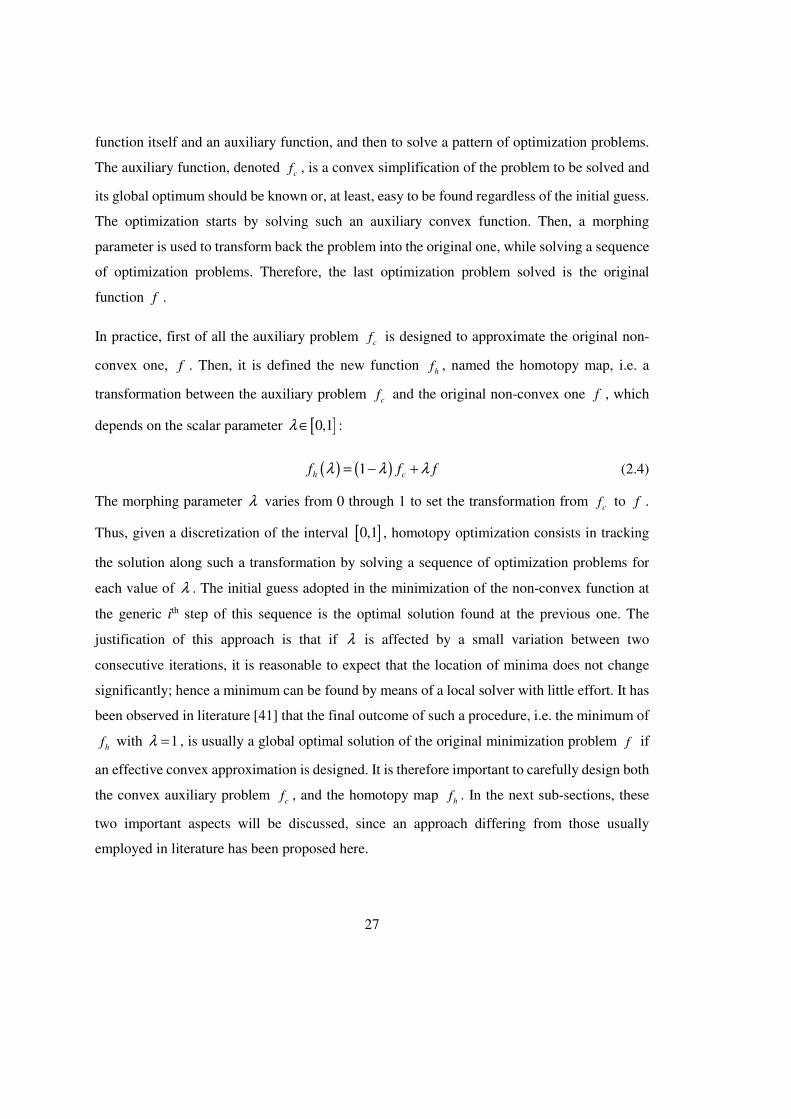
function itself and an auxiliary function, and then to solve a pattern of optimization problems.

The auxiliary function, denoted c

f , is a convex simplification of the problem to be solved and

its global optimum should be known or, at least, easy to be found regardless of the initial guess.

The optimization starts by solving such an auxiliary convex function. Then, a morphing

parameter is used to transform back the problem into the original one, while solving a sequence

of optimization problems. Therefore, the last optimization problem solved is the original

function f .

In practice, first of all the auxiliary problem c

f is designed to approximate the original non-

convex one, f . Then, it is defined the new function h

f , named the homotopy map, i.e. a

transformation between the auxiliary problem c

f and the original non-convex one f , which

depends on the scalar parameter [ ]0,1λ ∈ :

( ) ( )1h cf f fλ λ λ= − + (2.4)

The morphing parameter λ varies from 0 through 1 to set the transformation from c

f to f .

Thus, given a discretization of the interval [ ]0,1 , homotopy optimization consists in tracking

the solution along such a transformation by solving a sequence of optimization problems for

each value of λ . The initial guess adopted in the minimization of the non-convex function at

the generic ith step of this sequence is the optimal solution found at the previous one. The

justification of this approach is that if λ is affected by a small variation between two

consecutive iterations, it is reasonable to expect that the location of minima does not change

significantly; hence a minimum can be found by means of a local solver with little effort. It has

been observed in literature [41] that the final outcome of such a procedure, i.e. the minimum of

hf with 1λ = , is usually a global optimal solution of the original minimization problem f if

an effective convex approximation is designed. It is therefore important to carefully design both

the convex auxiliary problem c

f , and the homotopy map h

f . In the next sub-sections, these

two important aspects will be discussed, since an approach differing from those usually

employed in literature has been proposed here.

28

2.3.2. Convex relaxation: introduction of the auxiliary variables

The convex approximation proposed in this work is achieved by replacing the bilinear terms

appearing in f with a suitable number tN of new auxiliary variables, denoted 1,...,

tNt t and

collected in vector tN∈t ℝ . The following variable substitution is therefore performed for

appropriate values of the indices { } { }1, , , 1, ,x yr N s N∈ … ∈ … and { }1, , ti N∈ … :

s ir yx t⋅ → (2.5)

The function obtained in such a way is denoted ( ), ,cf x y t , and it is immediate proving its

convexity. This approach is sometimes adopted in optimization and it is often referred to as

“lifting”, because the introduction of new variables lifts the problem into a space of higher

dimension, compared with the original problem.

2.3.3. McCormick’s constraints

Since new variables have been added, the feasible domain should be modified to include

constraints on the new auxiliary variables and to represent their relation with the variables

collected in x and y . Ideally, since the variable it replaces the bilinear term

srx y⋅ , it should

be added the bilinear constraint 0si rt x y⋅ =− , which is however non-convex. In order to

represent this constraint by preserving convexity, an approximation is performed by taking

advantage of the results demonstrated in [42], which defines the tightest convex envelopes of

such constraints. This transformation is known as the so-called McCormick’s relaxation [43],

and can be computed given the lower and upper bounds of the variables involved. In fact,

provided that r

L U

r rx x x≤ ≤ and s

L U

s sy y y≤ ≤ , the equality si rt yx= ⋅ can be approximated by

the following four inequalities:

L L L L

r s s r r s

U U U U

r s s r r s

U L U L

r s s r r s

L

i

i

i

i

U L U

r s s r r s

x y y x x y

x y y x x y

x

t

t

t y y x x y

x y y x xt y

≥ ⋅ + ⋅ − ⋅

≥ ⋅ + ⋅ − ⋅

≤ ⋅ + ⋅ − ⋅

≤

⋅ + ⋅ − ⋅

(2.6)

29

The convex set defined through the inequalities in Eq. (2.6) for all the auxiliary variables it is

henceforth denoted tΓ , and should be included in the feasible domain:

: , x y tN N N

t

+ +

Γ′ = ∈ ∈Γ ∈Γ

xx

y ty

t

ℝ (2.7)

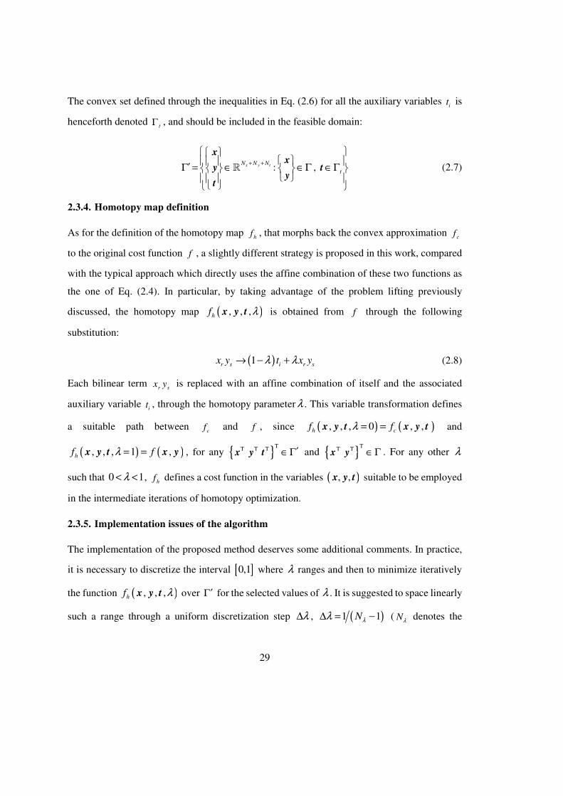
2.3.4. Homotopy map definition

As for the definition of the homotopy map hf , that morphs back the convex approximation

cf

to the original cost function f , a slightly different strategy is proposed in this work, compared

with the typical approach which directly uses the affine combination of these two functions as

the one of Eq. (2.4). In particular, by taking advantage of the problem lifting previously

discussed, the homotopy map ( ), , ,hf λx y t is obtained from f through the following

substitution:

( )1 ir rs sy tx x yλ λ→ − + (2.8)

Each bilinear term r sx y is replaced with an affine combination of itself and the associated

auxiliary variable it , through the homotopy parameter λ . This variable transformation defines

a suitable path between cf and f , since ( ) ( ), , , 0 , ,h cf fλ = =x y t x y t and

( ) ( ), , , 1 ,hf fλ = =x y t x y , for any { }TT T T ′∈ Γx y t and { }

TT T ∈ Γx y . For any other λ

such that 0 1λ< < , hf defines a cost function in the variables ( ), ,x y t suitable to be employed

in the intermediate iterations of homotopy optimization.

2.3.5. Implementation issues of the algorithm

The implementation of the proposed method deserves some additional comments. In practice,

it is necessary to discretize the interval [ ]0,1 where λ ranges and then to minimize iteratively

the function ( ), , ,hf λx y t over Γ′ for the selected values of λ . It is suggested to space linearly

such a range through a uniform discretization step λ∆ , ( )1 1Nλλ∆ = − ( Nλ denotes the

30

number of iterations), i.e. { }0, ,2 ,...,1 ,1λ λ λ λ∈ ∆ ∆ − ∆ [ ]0,1⊂ . The result is not affected by the

choice of λ∆ , unless unreasonable “large values” are assumed.

The problem solved in the first iteration, i.e. the minimization of ( ), , , 0hf λ =x y t over Γ′ , is

a convex optimization program, thus a global minimum can be found regardless of the initial

guess ( )0 0 0, ,x y t . Afterwards, the cost function is not convex in the other iterations. Therefore,

supposed that a minimizer ( ), ,opt opt opt

λ λ λ λ λ λ= = = ′∈Γx y t of ( ), , ,hf λx y t has been found for a certain

λ λ= { }0, ,2 ,...,1 ,1λ λ λ∈ ∆ ∆ − ∆ , then at the subsequent step the function ( ), , ,hf λλ + ∆x y t

is minimized by using ( ), ,opt opt opt

λ λ λ λ λ λ= = =x y t as the initial guess. This process is continued until

1λ = , i.e. when the original non-convex problem is morphed back. Finally, the optimal and

feasible modifications of the mass and stiffness matrices are computed as ( )1opt opt

λ==M M x∆ ∆

and ( )1opt opt

λ==K K x∆ ∆ .

The algorithm is briefly summarized in the pseudo code of Table 2.1.

31

Table 2.1. Pseudo code of the method implementation.

Input: system model M , K ; admissible modifications ( )M x∆ , ( )K x∆ ; feasibility constraints Γ ; desired

eigenpairs ( )( ),h h

ω u y ; number of iterations of the homotopy map Nλ

Output: optimal feasible modifications ( )opt opt

=M M x∆ ∆ , ( )opt opt

=K K x∆ ∆

Description

1 Formulation of the cost function f according to Eq. (2.3)

2 Introduction of new auxiliary variables i

t

3 Definition of the homotopy map h

f by the symbolic substitution in Eq. (2.5)

4 Symbolic computation of the McCormick’s constraint and definition of ′Γ (see Eq. (2.6)

and (2.7))

5 Set : 0i = and : 0i

λ =

6 Choose arbitrary ( )0 0 0, ,x y t and solve the convex program over ′Γ : ( ){ }min , , , 0

hf x y t

7 while i Nλ

< do

8 Set : 1i i= +

9 Set 1:i i

λ λ λ−= + ∆

10 Solve the non-convex program ( ){ }min , , ,h i

f λx y t over ′Γ taking ( )1 1 1, ,

i i i− − −x y t as

initial guess and set ( ), ,i i i

x y t as the optimal point

11 end while

12 Minimize ( ),f x y over Γ taking as initial guess ( )1 1,N Nλ λ− −x y and set ( ),opt opt

x y as the

optimal point

13 Set ( ):opt opt

=M M x∆ ∆ and ( ):opt opt

=K K x∆ ∆

32

2.4. Numerical examples and method validation

2.4.1. Five degrees of freedom lumped parameter system

In the present Section, a first example of partial assignment is examined, in order to prove the

effectiveness of the proposed method. The system to which structural modification is applied is

the 5-dof system shown in Figure 2.1. It consists of five lumped masses ( 1m , 2m , 3m , 4m and

5m ), connected to the frame by linear springs, whose stiffnesses are respectively 1gk , 2gk , 3,gk

4gk and 5gk . The springs that connect two adjacent masses are, instead, 12 75.14k kN m= ,

23 67.74k kN m= , 34 75.47k kN m= and 45 83.40k kN m= . a

Such a system has been employed to validate other methods for eigenstructure assignment in

several papers, such as [9, 23, 44]. Papers [9, 23] also provide the experimental characterization

of the system modal properties.

The solution of the optimization problems has been performed through the interior point

algorithm of Mosek for convex programming [45] and the interior point algorithm of fmincon

from the Optimization Toolbox by Mathworks [46] for non-convex programming. The

homotopy has been implemented exploiting the YALMIP [47] modelling language for Matlab.

In the test, it is supposed that dynamic response of the masses 1m , 3m and 5m is much more

significant with respect to the other ones, whose eigenvector entries are just required to belong

to prescribed intervals. In particular, the assignment of two natural frequencies and the

associated three entries of the two eigenvectors is required. Besides showing the results

Figure 2.1. Picture of the five degrees of freedom test-case.

m1 m2 m3 m4 m5

uh,1 uh,2 uh,3 uh,4 uh,5

k12 k23 k34 k45

kg1 kg2 kg3 kg4 kg5

33

obtained, the comparison with the assignment of two complete eigenpairs obtained in [9] is

proposed, where, in contrast, complete assignment is performed. On the one hand the numerical

results are aimed at showing the capability of the novel method to compute the correct

modifications by taking into account design specifications that involve only some degrees of

freedom. On the other, the comparison with the complete assignment demonstrates that partial

assignment boosts the achievement of the mode shape specifications at the dofs of interest.

The values of the masses and the springs of the original (unmodified) system are taken from [9]

and are shown in the second column of Table 2.2. It is supposed that only the five masses and

the five ground springs can be modified. Therefore the physical modifications sets the following

Table 2.2. Inertial and elastic parameters of the original and of the modified system in the

first test-case.

Original

values

Constraints Full

assignment [9]

Proposed

method

1m (kg) 1.727 [0; +1.08] + 1.0800 + 0.8829

2m (kg) 5.123 [0; +1.08] + 0.1103 + 0.4977

3m (kg) 8.214 [0; +1.08] + 0.9819 + 0.0013

4m (kg) 2.609 [0; +1.08] + 0.0360 + 0.4784

5m (kg) 1.339 [0; +1.08] + 1.0800 + 0.9841

1gk (kN/m) 94.26 [0; +144.9] + 80.3229 + 63.4018

2gk (kN/m) 94.26 [0; +144.9] + 62.5002 + 78.5887

3gk (kN/m) 94.26 [0; +144.9] + 144.9000 + 125.4621

4gk (kN/m) 94.26 [0; +144.9] + 0.0000 + 39.8018

5gk (kN/m) 94.26 [0; +144.9] + 106.5498 + 102.3471

34

unknown vector { 1m= ∆x 2m∆ 3m∆ 4m∆ 5m∆ 1gk∆ 2gk∆ 3gk∆ 4gk∆ }T

5gk∆ . As far as the

physical constraints Lx and Ux are concerned, in accordance with the cited paper, it is supposed

that the mass modifications are constrained between 0 and 1.08 kg, while the stiffness

modifications must be greater than 0 and less than 144.9 kN/m.

The goal of the assignment is to compute the suitable parameter modifications to assign two

eigenfrequencies 1ω and 2ω , and two associated eigenvectors, named 1u and 2u , whose first,

third and fifth entries are requested to match those defined in [9]. In contrast, the second and

the fourth entries are not assigned and then considered as unknowns, thus the vector of the

unassigned eigenvector entries is { 1,2u=y 1,4u 2,2u }T

2,4u (the first subscript denotes the

number of the assigned mode shape; the second one the number of the dof). The desired

eigenpairs are shown in Table 2.3: it should be noticed that the normalization of the eigenvector

is different from the one adopted in [9], and it is such that the first component of the first mode

and the fifth component of the second mode are set to 1. Nonetheless, the final result is not

affected by the eigenvector normalization. As for the unassigned components, Table 2.3

supplies the lower and upper bounds Ly , U

y . Indeed, the corresponding eigenvector entries

have been constrained with appropriate intervals including the values requested in the cited

paper [8], in order to avoid unfeasible and unreasonable displacements of the second and the

fourth mass. To make clearer the distinction between assigned and unassigned components, the

latter ones are printed with italic font in Table 2.3.

35

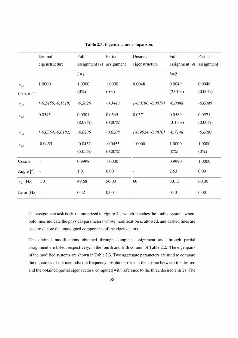
The assignment task is also summarized in Figure 2.1, which sketches the studied system, where

bold lines indicate the physical parameters whose modification is allowed, and dashed lines are

used to denote the unassigned components of the eigenvectors.

The optimal modifications obtained through complete assignment and through partial

assignment are listed, respectively, in the fourth and fifth column of Table 2.2. The eigenpairs

of the modified systems are shown in Table 2.3. Two aggregate parameters are used to compare

the outcomes of the methods: the frequency absolute error and the cosine between the desired

and the obtained partial eigenvectors, computed with reference to the three desired entries. The

Table 2.3. Eigenstructure comparison.

Desired

eigenstructure

Full

assignment [9]

Partial

assignment

Desired

eigenstructure

Full

assignment [9]

Partial

assignment

h=1 h=2

,1hu

(% error)

1.0000 1.0000

(0%)

1.0000

(0%)

0.0048 0.0049

(2.01%)

0.0048

(0.00%)

,2hu [-0.5455;-0.1818] -0.3626 -0.3443 [-0.0190;-0.0019] -0.0098 -0.0090

,3hu 0.0545 0.0501

(8.07%)

0.0545

(0.00%)

0.0571 0.0589

(3.15%)

0.0571

(0.00%)

,4hu [-0.0364;-0.0182] -0.0235 -0.0208 [-0.9524;-0.3810] -0.7148 -0.6091

,5hu -0.0455 -0.0432

(5.05%)

-0.0455

(0.00%)

1.0000 1.0000

(0%)

1.0000

(0%)

Cosine - 0.9998 1.0000 - 0.9990 1.0000

Angle [°] - 1.01 0.00 - 2.53 0.00

hω [Hz] 50 49.68 50.00 60 60.13 60.00

Error [Hz] -- 0.32 0.00 - 0.13 0.00

36

results clearly show that the proposed method actually provides exact assignment both on the

eigenvector specifications and on the eigenvalues and satisfies all the design constraints (listed

in the second and fifth columns of Table 2.3). Such result is expected because the residual of

the cost function (2.3) is 95.834 10−⋅ . In contrast, if the complete eigenvector is forced to assume

the values proposed in [8], the specifications are partially missed both in terms of frequency

and mode shape, as a consequence of the constraints on the allowable modifications. Table 2.3

shows that a small adjustment in the desired response of the second and fourth mass, compared

with those of the complete assignment, results in a substantial improvement in the attainment

of the desired dynamic behaviour for the other three masses of interest.

The comparison of the two strategies of eigenstructure assignment clearly confirms the

hypotheses that relaxing the requirements on the degrees of freedom of least concern results in

a more accurate fulfilment of the specifications of interest (both in terms of mode shapes and

eigenfrequencies).

As a further proof of the results obtained, Figure 2.2 shows the absolute value of some sample

Frequency Response Functions (FRFs) (i.e. ( ),5iH ω , ,51,i = … ), obtained from 12ω

− − M K

of the original system (dashed line) and from ( ) ( )12ω

− + ∆ − + ∆ M M K K of the system

modified by the proposed method (solid line). A small damping has been assumed for clarity of

representation. The comparison with the vertical lines, defining the desired eigenfrequencies,

clearly shows the presence of the resonance peaks at the frequencies of interest for the modified

system. In contrast, the original system misses the design specifications.

37

Figure 2.2. System FRFs.

38

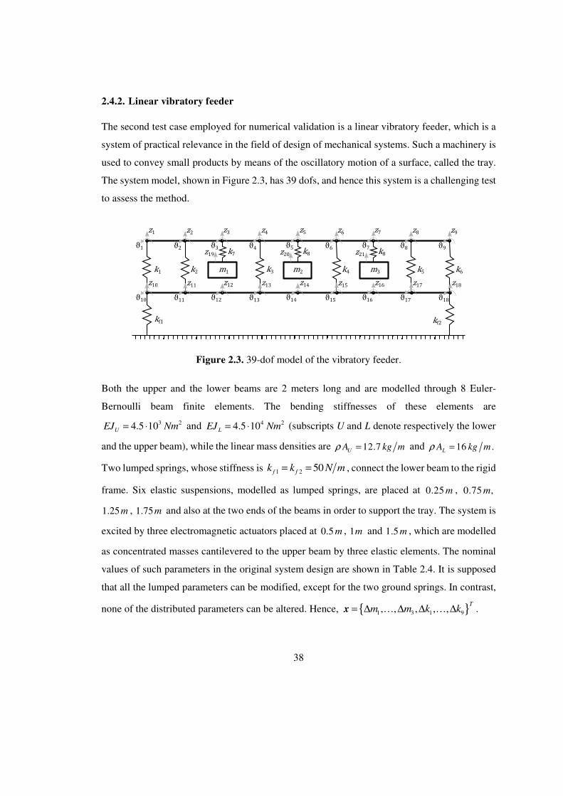
2.4.2. Linear vibratory feeder

The second test case employed for numerical validation is a linear vibratory feeder, which is a

system of practical relevance in the field of design of mechanical systems. Such a machinery is

used to convey small products by means of the oscillatory motion of a surface, called the tray.

The system model, shown in Figure 2.3, has 39 dofs, and hence this system is a challenging test

to assess the method.

Both the upper and the lower beams are 2 meters long and are modelled through 8 Euler-

Bernoulli beam finite elements. The bending stiffnesses of these elements are

3 24.5 10U mEJ N⋅= and 4 24.5 10L mEJ N⋅= (subscripts U and L denote respectively the lower

and the upper beam), while the linear mass densities are 12.7UA kg mρ = and 16 .LA kg mρ =

Two lumped springs, whose stiffness is 1 2 50f fk k N m= = , connect the lower beam to the rigid

frame. Six elastic suspensions, modelled as lumped springs, are placed at 0.25 m , 0.75 ,m

1.25m , 1.75m and also at the two ends of the beams in order to support the tray. The system is

excited by three electromagnetic actuators placed at 0.5 m , 1m and 1.5 m , which are modelled

as concentrated masses cantilevered to the upper beam by three elastic elements. The nominal

values of such parameters in the original system design are shown in Table 2.4. It is supposed

that all the lumped parameters can be modified, except for the two ground springs. In contrast,

none of the distributed parameters can be altered. Hence, { }1 3 1 9, , , , ,T

m m k k∆ … ∆ ∆ … ∆=x .

Figure 2.3. 39-dof model of the vibratory feeder.

39

Just one eigenpair is assigned since vibratory feeders are forced through single harmonic

excitation whose frequency should match the one of a mode of vibration featuring a uniform

vertical oscillation of the tray, in such a way that the products are uniformly conveyed. The

vertical displacements are prescribed to equal 1 (although the method does not require any

specific normalization of the desired eigenvector). The elastic rotation of the upper tray and the

motion of the lower beam instead belong to the unknown vector y . The displacements of the

three counterweights are required to be the same, thus are represented by one variable only,

named CWzu . In practice, the unknown vector is { }

1 9 18 10 1810, , , , , ,, , ,

CWz

T

z zu u u u u uuϑ ϑ ϑ ϑ… … …=y .

The variables x are constrained according to the second column of Table 2.4. The variables

,y instead, are required to belong to the interval [ ]3,3− , except CWzu that must belong to

83, 10− − − (negative values are chosen to force the counterweights to oscillate in anti-phase

with respect to the upper beam. As for the eigenfrequency, it is required to be 40 Hz, which is

a frequency that is often assumed for conveying small parts.

The implemented homotopy optimization method succeed in finding a global optimum of the

cost function (2.3), in fact the residual is 84.806 10−⋅ . The computed optimal modifications of

the physical parameters are shown in the third column of Table 2.4. The resulting system

features a resonance at 40.000 Hzω = , whose corresponding mode shape matches quite

accurately the design specifications: in fact the cosine between the first 18 components of the

obtained eigenvector (those related to the upper beam) and the optimal vector ( )1,0,1,0,T

… (that

represents, for each node, uniform vertical displacement and zero degrees rotation) is 0.9995 ,

thus very close to the ideal value 1.

40

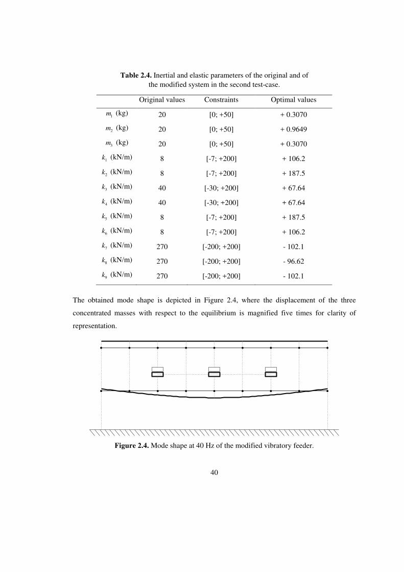
The obtained mode shape is depicted in Figure 2.4, where the displacement of the three

concentrated masses with respect to the equilibrium is magnified five times for clarity of

representation.

Table 2.4. Inertial and elastic parameters of the original and of the modified system in the second test-case.

Original values Constraints Optimal values

1m (kg) 20 [0; +50] + 0.3070

2m (kg) 20 [0; +50] + 0.9649

3m (kg) 20 [0; +50] + 0.3070

1k (kN/m) 8 [-7; +200] + 106.2

2k (kN/m) 8 [-7; +200] + 187.5

3k (kN/m) 40 [-30; +200] + 67.64

4k (kN/m) 40 [-30; +200] + 67.64

5k (kN/m) 8 [-7; +200] + 187.5

6k (kN/m) 8 [-7; +200] + 106.2

7k (kN/m) 270 [-200; +200] - 102.1

8k (kN/m) 270 [-200; +200] - 96.62

9k (kN/m) 270 [-200; +200] - 102.1

Figure 2.4. Mode shape at 40 Hz of the modified vibratory feeder.

41

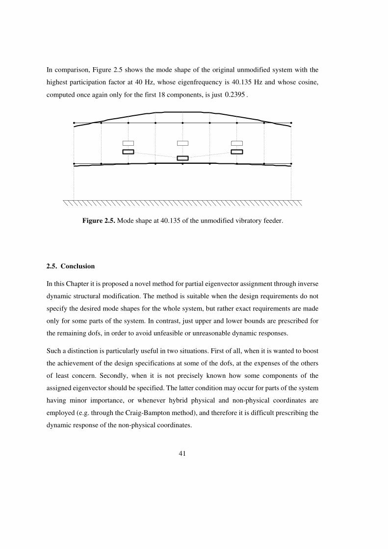
In comparison, Figure 2.5 shows the mode shape of the original unmodified system with the

highest participation factor at 40 Hz, whose eigenfrequency is 40.135 Hz and whose cosine,

computed once again only for the first 18 components, is just 0.2395 .

2.5. Conclusion

In this Chapter it is proposed a novel method for partial eigenvector assignment through inverse

dynamic structural modification. The method is suitable when the design requirements do not

specify the desired mode shapes for the whole system, but rather exact requirements are made

only for some parts of the system. In contrast, just upper and lower bounds are prescribed for

the remaining dofs, in order to avoid unfeasible or unreasonable dynamic responses.

Such a distinction is particularly useful in two situations. First of all, when it is wanted to boost

the achievement of the design specifications at some of the dofs, at the expenses of the others

of least concern. Secondly, when it is not precisely known how some components of the

assigned eigenvector should be specified. The latter condition may occur for parts of the system

having minor importance, or whenever hybrid physical and non-physical coordinates are

employed (e.g. through the Craig-Bampton method), and therefore it is difficult prescribing the

dynamic response of the non-physical coordinates.

Figure 2.5. Mode shape at 40.135 of the unmodified vibratory feeder.

42

The method therefore deserves both theoretical and practical interest in the field of mechanical

design. On the one hand it proposes an effective method to solve an open issue in the literature

on inverse structural modification, by tackling effectively some mathematical issues. On the

other, it provides a useful tool in designing and optimizing vibrating systems.

Besides solving an open issue, another novel contribution of the method is its formulation,

which is based on the problem lifting to make it convex (i.e. the introduction of some auxiliary

variables, constrained through a tight convex feasible domain) and then the use of the homotopy

optimization to overcome the non-convex nature of the partial assignment problem and to boost

the achievement of the global optimal solution.

The method has been tested numerically with two benchmark systems, often employed in the

literature on inverse dynamic structural modification: a five-dof system made by lumped masses

and springs and a linear vibratory feeder modeled through 39 dofs. Concerning the first test-

case, the partial assignment of two eigenpairs (by specifying only three entries of each

eigenvector) has been performed with very effective results. First of all, it is shown that the

proposed strategy based on the homotopy optimization effectively boosts the achievement of

the global optimal solution. Then, it has been assessed the initial assumption claiming that

weakening the requirements on some dofs results in a more accurate assignment of the others.

Indeed it is a duty of the proposed method to determine the best assignment for the dofs of least

concern, in order to meet more closely the design specifications on the dofs of interest. The

second test-case, which is more challenging, also allows to assess the method in a meaningful

design example.

43

Chapter 3. Auxiliary subsystems 3.1. Introduction

The most popular way to employ structural modification for the design and the optimization of

vibrating systems is certainly to focus on the modification of the inertial and elastic parameters

(damping is usually neglected) of the existing components of the system, without modifying the

number of degrees of freedom. The possibility of modifying the dynamical properties of a

system through the addition of auxiliary subsystems is rarely investigated, instead. However,

such a problem is of considerable practical interest because, when the original design of a

system cannot be changed, the only possible alternative is to add one or more external

subsystems to the primary one.

The direct problem related to structural modifications that increase the number of degrees of

freedom has been tackled in the recent literature, especially concerning distributed

modifications, such as in the works by Canbaloğlu and Özgüven [48] and Hang, Shankar and

Lai [49, 50]. The inverse problem, instead, is mainly devoted to vibration suppression, as in

[51] in which multiple tuned mass dampers are exploited to control a bridge-like structure, or

in [52] that deals with the control of a vibrating plate by a proper choice and positioning of

dynamic absorbers. The assignment of natural frequencies by added masses and springs also

appeared in literature over the last years. In particular Kyprianou, Mottershead and Ouyang in

[17] recast the problem as a system of non-linear multivariate polynomial equations and propose

a method to solve it by means of the Groebner bases. A different insight on this approach is

provided by the recent work of Liu et al. [44], in which the non-linear equations are effectively

solved in a least-square sense. Moreover, they also take into account the system mode shapes,

making the method suitable for eigenstructure assignment through the addition of multiple

mass–spring systems.

In this Chapter, it is presented a method to perform structural modifications by means of added

auxiliary systems, that allows to assign the desired dynamic behaviour of the original system

both in terms of natural frequencies and mode shapes. The formulation adopted, which casts the

assignment as an optimization problem, allows to attain a dynamic behaviour which is more

44

fitting to the desired one, in comparison to that of the original system, even when an exact

assignment is not possible because of feasibility constraints. The topology of the auxiliary

systems must be pre-determined but it can be chosen as arbitrary as possible. Moreover, it is

possible to ensure the feasibility of the solution defining a constraint set in the optimization

variable space.

3.2. Problem theoretical development

3.2.1. Problem formulation

Let us consider an undamped vibrating system, that should be modified to feature a desired set

of eigenpairs. The system is modeled through its mass matrix o oN N×∈oM ℝ and stiffness matrix

o oN N×∈oK ℝ , where oN denotes the number of degrees of freedom (dofs). Damping is

neglected, as it is usually assumed in the literature on structural modification, since most of the

vibrating systems of interest for this kind of applications are lightly damped. The system free

response is governed by the first-order eigenvalue problem:

2oω − = o o oM K u 0 (3.1)

where oω is the eigenfrequency and oN∈ou ℝ is the related real eigenvector (the subscript o

denotes the original system).

The system modification, aimed at assigning the prescribed dynamic behaviour through the

assignment of an arbitrary number of eigenpairs, is performed by adding one or more additional

“external” systems having arbitrary topology and number of dofs, denoted eN . It is only

assumed that such a topology is pre-defined, in accordance with technical constraints and

specifications. It is important to restate that the number of assigned eigenpairs is arbitrary and

it is often less than the total number of degrees of freedom.

For ease of explanation it is also initially assumed that just one eigenpair is assigned and that

the original masses and stiffnesses of the original “primary” system ( ),o o

M K are not modified.

Both these hypotheses will be lately relaxed and the method will be extended to account for the

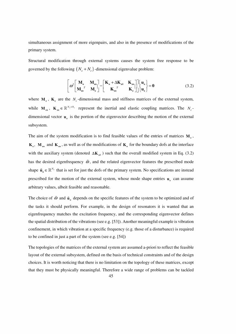
45

simultaneous assignment of more eigenpairs, and also in the presence of modifications of the

primary system.

Structural modification through external systems causes the system free response to be

governed by the following ( )o eN N+ -dimensional eigenvalue problem:

2 b

T Tω + ∆

− =

o eo o o eo o

eo e eo e e

M M K K K u0

M M K K u (3.2)

where e

M , e

K are the eN -dimensional mass and stiffness matrices of the external system,

while eo

M , eo

K o eN N×∈ℝ represent the inertial and elastic coupling matrices. The eN -

dimensional vector e

u is the portion of the eigenvector describing the motion of the external

subsystem.

The aim of the system modification is to find feasible values of the entries of matrices e

M ,

,e

K eo

M and eo

K , as well as of the modifications of o

K for the boundary dofs at the interface

with the auxiliary system (denoted b∆

oK ) such that the overall modified system in Eq. (3.2)

has the desired eigenfrequency ωɶ , and the related eigenvector features the prescribed mode

shape oN∈ouɶ ℝ that is set for just the dofs of the primary system. No specifications are instead

prescribed for the motion of the external system, whose mode shape entries e

u can assume

arbitrary values, albeit feasible and reasonable.

The choice of ωɶ and o

uɶ depends on the specific features of the system to be optimized and of

the tasks it should perform. For example, in the design of resonators it is wanted that an

eigenfrequency matches the excitation frequency, and the corresponding eigenvector defines

the spatial distribution of the vibrations (see e.g. [53]). Another meaningful example is vibration

confinement, in which vibration at a specific frequency (e.g. those of a disturbance) is required

to be confined in just a part of the system (see e.g. [54])

The topologies of the matrices of the external system are assumed a-priori to reflect the feasible

layout of the external subsystem, defined on the basis of technical constraints and of the design

choices. It is worth noticing that there is no limitation on the topology of these matrices, except

that they must be physically meaningful. Therefore a wide range of problems can be tackled

46

through the proposed method. It is actually recommendable to choose such matrices as general

as possible, in order to improve the chances to obtain the desired eigenstructure. The method

itself will neglect the modifications that are not necessary, if there are any. Moreover, the least

desirable modifications can be penalized by means of regularization techniques that will be

detailed in the following.

All the modifications of the system parameters, which are in practice the design variables, are

then collected in the unknown vector xN∈x ℝ . Thus it holds that ( )=e e

M M x , ( )=e e

K K x ,

( )=eo eo

M M x , ( )=eo eo

K K x and ( )b b∆ = ∆o o

K K x , and it is assumed that the dependence on

x is linear. This hypothesis allows representing a wide class of possible system modifications,

as corroborated by most of the papers in literature assuming the same representation, since a

proper definition of x allows also representing correlated modifications or modifications of

continuous (distributed) mass and stiffness parameters (see e.g. [8]).

Even though assignment is of interest only for the eigenvector entries concerning the original

subsystem, the whole system model should be accounted for in the eigenvalue problem, and

therefore also e

u should be included in the problem formulation. In particular, it is proposed to

regard these eigenvector entries as additional unknowns in the assignment problem. The

resulting unknown vector is therefore the ( )x eN N+ -dimensional column vector { }T

T T

ex u .

In principle, such unknowns are not independent, in fact they are implicitly related by (3.2).

Since it is difficult to make such relation explicit, unless local approximations are used, it is

advantageous to regard the unknowns as independent. The numerical validation of the method

has proved that such an assumption has no significant drawbacks.

Since also physical feasibility of the values of the external system parameters should be assured,

a constraint set Γ bounding x and e

u is introduced. Such a set represents lower and upper

bounds on each variable (i.e. L U≤ ≤x x x and L U≤ ≤e e e

u u u , given the prescribed lower and

upper bounds , xNL U ∈x x ℝ and , eNL U ∈e e

u u ℝ , where the inequalities are element-wise). While

the variables x are bounded due to technical and economical reasons, the variables e

u represent

the relative displacements of the auxiliary system with respect to the primary one, thus the

47

bounds must be set in accordance with layout constraints, safety requirements (i.e. presence of

obstacles) or other design choices.

Constraints simultaneously relating different, and also inhomogeneous, variables can be also

included in the design problem by means of inequalities setting a convex polyhedron (defined

through proper real coefficient matrix A and vector c). The intersection of these two convex

sets of constraints leads to the feasible domain Γ , which is still a convex set:

: , ,x eN N L U L U+ ∈ ≤ ≤ ≤

≤ ≤

Γ =

e e e

e e

u u uu u

x xx x x A cℝ (3.3)

The assignment problem is therefore finding

∈ Γ e

x

u such that the eigenvalue problem related

to the desired eigenpair is satisfied:

( ) ( ) ( )

( ) ( ) ( ) ( )

2 2

2 2

b

T

ω ω

ω ω

− − ∆ − − = − + −

eo eo e o oo o o

eo eo o e e e

M x K x u K x u M K u

0M x K x u M x K x u

ɶ ɶ ɶ ɶ

ɶ ɶɶ

(3.4)

The right-hand-side term collects the known terms, related to the desired eigenpair and to the

matrices of the primary system. The left-hand-side terms collect instead all the unknowns: the

terms ( ) ( )2 T

ω − eo eo oM x K x uɶ ɶ and ( )b∆

o oK x uɶ are linear functions of the unknowns and can

be recast as a linear system Ux = b , through a suitable matrix U and vector b (see Ref. [8]). In

contrast, ( ) ( )2ω − eo eo eM x K x uɶ and ( ) ( )2ω − e e e

M x K x uɶ have some non-linear terms. In

particular, bilinear terms of the type ,i e jx u⋅ appear, where ix and ,e ju are entries of the

unknown vectors x and e

u (for some indexes i and j).

Since, in the general case, the solvability of the system of equations in Eq. (3.4) is not always

assured, e.g. because of the specifications on the topology of the modification matrices and the

presence of the feasible domain, the problem is recast as a constrained minimization of the norm

of the residual of Eq. (3.4), to be solved through numerical optimization algorithms:

48

( ) ( ) ( )

( ) ( ) ( ) ( )

22 2

2 2,

2

min ,b

T

ω ω

ω ω

− − ∆ + −

− + −

∈

Γ

e

eo eo e o o o o o

x ue

eo eo o e e e

M x K x u K x u M K u x

uM x K x u M x K x u

ɶ ɶɶ ɶ

ɶ ɶɶ

(3.5)

In the case more pairs ( ),,i iωo

uɶ ɶ are required, i=1,…,Np, the problem is cast as the weighed sum

of the residuals of the inverse eigenvalue problem of each eigenpair:

( ) ( ) ( )

( ) ( ) ( ) ( )

22 2

, , ,

2 2, 1, ,

2

,minpN

i i b i i i

i Ti

i i i i

ω ωα

ω ω=

− − ∆ + −

− + −

∈Γ∑e

eo eo e o o o o o

x ue

eo eo o e e e

M x K x u K x u M K u x

uM x K x u M x K x u

ɶ ɶɶ ɶ

ɶ ɶɶ

(3.6)

where { },1 ,...p

TTT

N=e e eu u u collects all the unknowns of the mode shape entries of the

external system. The real, positive, scalar coefficients αi are introduced to reflect different levels

of concern on the attainment of each eigenpair. The problem can be also regularized through

the approach described in [8] to improve its numerical conditioning and to boost the

achievement of small norm solutions, i.e. small modifications.

3.2.2. Inclusion of modifications of the primary system

In the case modifications of the primary systems are allowed, through additive modification

mass matrix o oN N×∈∆ oM ℝ and stiffness matrix o oN N×∈∆ oK ℝ (the latter collects all the

modifications of the stiffness parameters, both at the interface dofs and in the internal ones), the

problem extension is straightforward, due to the kind of formulation adopted. Let us, once again,

assume that the topologies of these two modification matrices are a priori specified on the basis

of the parameters considered to be modifiable, as it is common in practice: design requirements

and constraints usually impose that the system modifications can be performed on just a reduced

subset of masses and stiffnesses. By including in the unknown vector x also the unknown

entries of ∆o

M and ∆o

K , the assignment problem is written as the following function that

couples all the modification matrices:

( ) ( ) ( ) ( )

( ) ( ) ( ) ( )

22 2 2

, , ,

2 2, 1, ,

2

minpN

i i i i i i

i Ti

i i i i

ω ω ωα

ω ω=

− + − + ∆ − ∆

− + −

∑e

eo eo e o o o o o o

x ueo eo o e e e

M x K x u M K u M x K x u

M x K x u M x K x u

ɶ ɶ ɶɶ ɶ

ɶ ɶɶ

(3.7)

49

The newly introduced term, ( ) ( )2,i iω ∆ − ∆ o o o

M x K x uɶ ɶ , can be written as a linear function of

the unknowns, and therefore Eq. (3.7) can be solved as Eq. (3.6).

3.3. Problem solution

The abovementioned bilinear terms lead to a non-linear least squares minimization problem in

a convex domain, which is however a non-convex optimization problem. Therefore, standard

optimization tools are likely to find local minima that are not global minima, and therefore are

not reliable for the purpose.

In order to tackle these issues, it is proposed to exploit the homotopy-based strategy explained

in the previous Chapter.

3.3.1. The proposed solution

The method proposed in the previous Chapter applies to the optimization of (3.7). In fact, the

convex approximation cf is achieved replacing the bilinear terms in f with a suitable number

tN of new auxiliary variables 1,...,tNt t which are collected in vector tN∈t ℝ :

, r e s ix u t→ (3.8)

(for appropriate values of the indices { } { }1, , , 1, ,x er N s N∈ … ∈ … and { }1, , ti N∈ … ).

The auxiliary function obtained in this way is denoted ( ), ,cf ex u t .

The non-convex constraints , = 0r e s ix tu − are approximated by taking advantage of the results

demonstrated in [42, 43]. Provided that U

r

L

rr xx x≤ ≤ and , ,,U

e s e s

L

e su u u≤ ≤ , the McCormick’s

inequalities hold:

, , ,

, , ,

, , ,

, , ,

L L

r r r

U U

r r r

U U

r r r

L

L L

i e s e s e s

U U

i e s e s e s

L L

i e s e s e s

U U

i e s e sr r r s

L

e

x x x

x x x

x

t u u u

t u u u

t u u u

t u

x

xu u

x

x x

≥ ⋅ + ⋅ − ⋅

≥ ⋅ + ⋅ − ⋅

≤ ⋅ + ⋅ − ⋅

≤ ⋅ +

⋅ −

⋅

(3.9)

50

The convex set defined through Eq. (3.9), herein denoted tΓ for brevity, is included in the

convex feasible domain of the auxiliary function and the homotopy map:

t:x e tN N N+ +

Γ′ = ∈ ∈Γ ∩ Γ

e

e

xx

uu

t

ℝ (3.10)

The homotopy map ( ),, , ,h e sf λx u t is obtained from ( ),fe

x u through the substitution of each

bilinear term ,r e sx u with an affine combination of ,r e sx u itself and the associated auxiliary

variable:

( ), ,1r e s i r e stx u x uλ λ→ − + (3.11)

It is easy to verify that ( ) ( ), , , 0 , ,h cf fλ = =e e

x u t x u t and ( ) ( ), , , 1 ,h cf fλ = =e e

x u t x u , for

any { }, , ′∈Γe

x u t and { }, ∈Γe

x u . For any other ( )0,1λ ∈ , ( ), , ,hf λe

x u t is suitable to be

employed in the intermediate iterations of homotopy optimization.

The optimal modifications of the external and the primary systems are computed as those

collected in the solution of the function with 1λ = , denoted as 1opt

λ=x : ( )1

opt

λ=e

M x , ( )1opt

λ=e

K x ,

( )1opt

λ =eo

M x , ( )1opt

λ=eo

K x , ( )1opt

λ=∆o

M x and ( )1opt

λ=∆o

K x .

3.4. Numerical examples

3.4.1. Example 1

In this Section an EA task is performed in two different ways, in order to prove the effectiveness

and versatility of the proposed method. The primary system to which structural modification is

applied is the 5-dof system shown in Figure 3.1. The system consists of five lumped masses

1(m , 2m , 3m , 4m and 5m ), each one connected to a rigid frame by a linear spring, whose

stiffnesses are respectively 1gk , 2gk , 3gk , 4gk and 5gk . Four springs also connect each mass

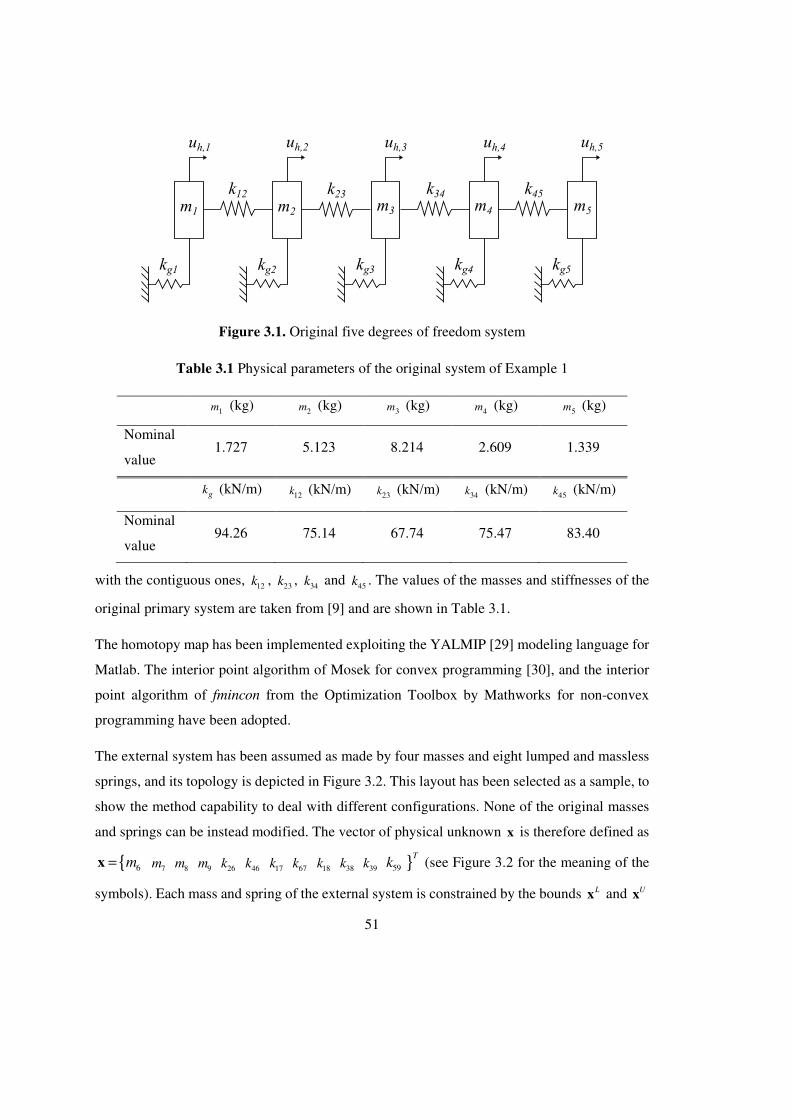
51

with the contiguous ones, 12k , 23k , 34k and 45k . The values of the masses and stiffnesses of the

original primary system are taken from [9] and are shown in Table 3.1.

The homotopy map has been implemented exploiting the YALMIP [29] modeling language for

Matlab. The interior point algorithm of Mosek for convex programming [30], and the interior

point algorithm of fmincon from the Optimization Toolbox by Mathworks for non-convex

programming have been adopted.

The external system has been assumed as made by four masses and eight lumped and massless

springs, and its topology is depicted in Figure 3.2. This layout has been selected as a sample, to

show the method capability to deal with different configurations. None of the original masses

and springs can be instead modified. The vector of physical unknown x is therefore defined as

{ 6m=x 7m 8m 9m 26k 46k 17k 67k 18k 38k 39k }59

Tk (see Figure 3.2 for the meaning of the

symbols). Each mass and spring of the external system is constrained by the bounds Lx and U

x

Table 3.1 Physical parameters of the original system of Example 1

1m (kg) 2m (kg) 3m (kg) 4m (kg) 5m (kg)

Nominal

value 1.727 5.123 8.214 2.609 1.339

gk (kN/m) 12k (kN/m) 23k (kN/m) 34k (kN/m) 45k (kN/m)

Nominal

value 94.26 75.14 67.74 75.47 83.40

Figure 3.1. Original five degrees of freedom system

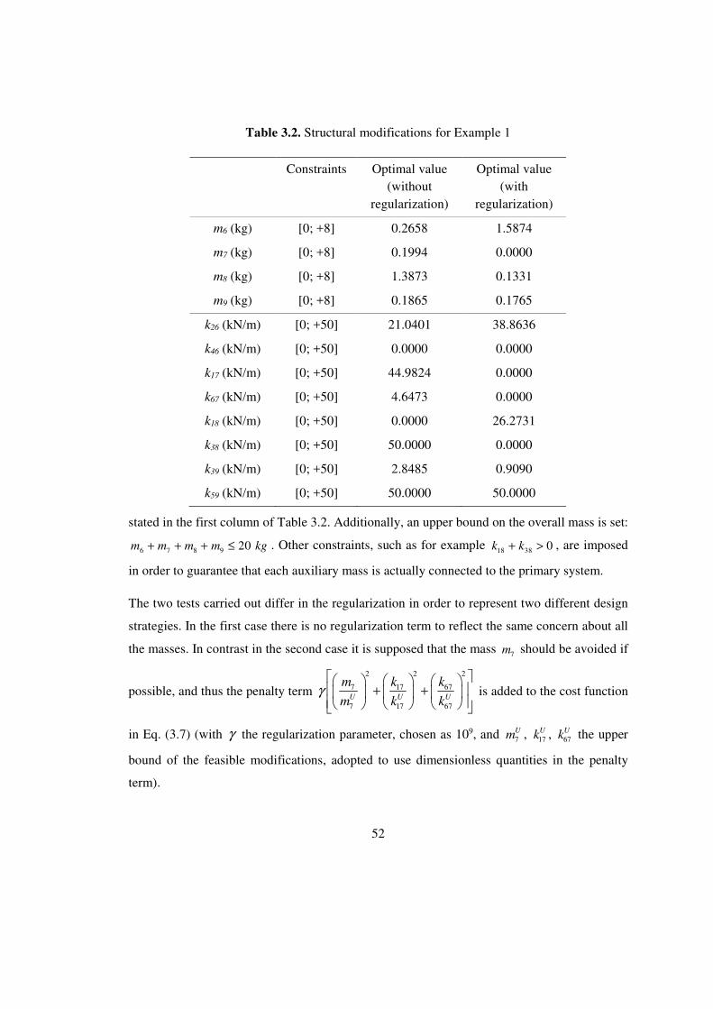
52

stated in the first column of Table 3.2. Additionally, an upper bound on the overall mass is set:

6 7 8 9 20 m m m m kg+ + + ≤ . Other constraints, such as for example 18 38 0k k+ > , are imposed

in order to guarantee that each auxiliary mass is actually connected to the primary system.

The two tests carried out differ in the regularization in order to represent two different design

strategies. In the first case there is no regularization term to reflect the same concern about all

the masses. In contrast in the second case it is supposed that the mass 7m should be avoided if

possible, and thus the penalty term

2 2 2

7 17 67

7 17 67U U U

m k k

m k kγ + +

is added to the cost function

in Eq. (3.7) (with γ the regularization parameter, chosen as 109, and 7U

m , 17U

k , 67U

k the upper

bound of the feasible modifications, adopted to use dimensionless quantities in the penalty

term).

Table 3.2. Structural modifications for Example 1

Constraints Optimal value (without

regularization)

Optimal value (with

regularization)

m6 (kg) [0; +8] 0.2658 1.5874

m7 (kg) [0; +8] 0.1994 0.0000

m8 (kg) [0; +8] 1.3873 0.1331

m9 (kg) [0; +8] 0.1865 0.1765

k26 (kN/m) [0; +50] 21.0401 38.8636

k46 (kN/m) [0; +50] 0.0000 0.0000

k17 (kN/m) [0; +50] 44.9824 0.0000

k67 (kN/m) [0; +50] 4.6473 0.0000

k18 (kN/m) [0; +50] 0.0000 26.2731

k38 (kN/m) [0; +50] 50.0000 0.0000

k39 (kN/m) [0; +50] 2.8485 0.9090

k59 (kN/m) [0; +50] 50.0000 50.0000

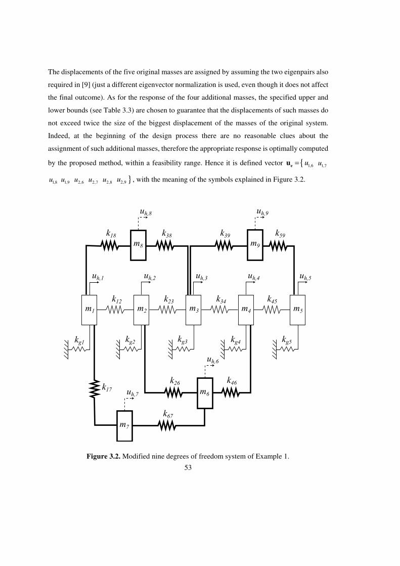
53

The displacements of the five original masses are assigned by assuming the two eigenpairs also

required in [9] (just a different eigenvector normalization is used, even though it does not affect

the final outcome). As for the response of the four additional masses, the specified upper and

lower bounds (see Table 3.3) are chosen to guarantee that the displacements of such masses do

not exceed twice the size of the biggest displacement of the masses of the original system.

Indeed, at the beginning of the design process there are no reasonable clues about the

assignment of such additional masses, therefore the appropriate response is optimally computed

by the proposed method, within a feasibility range. Hence it is defined vector { 1,6u=e

u 1,7u

1,8u 1,9u 2,6u 2,7u 2,8u }2,9u , with the meaning of the symbols explained in Figure 3.2.

Figure 3.2. Modified nine degrees of freedom system of Example 1.

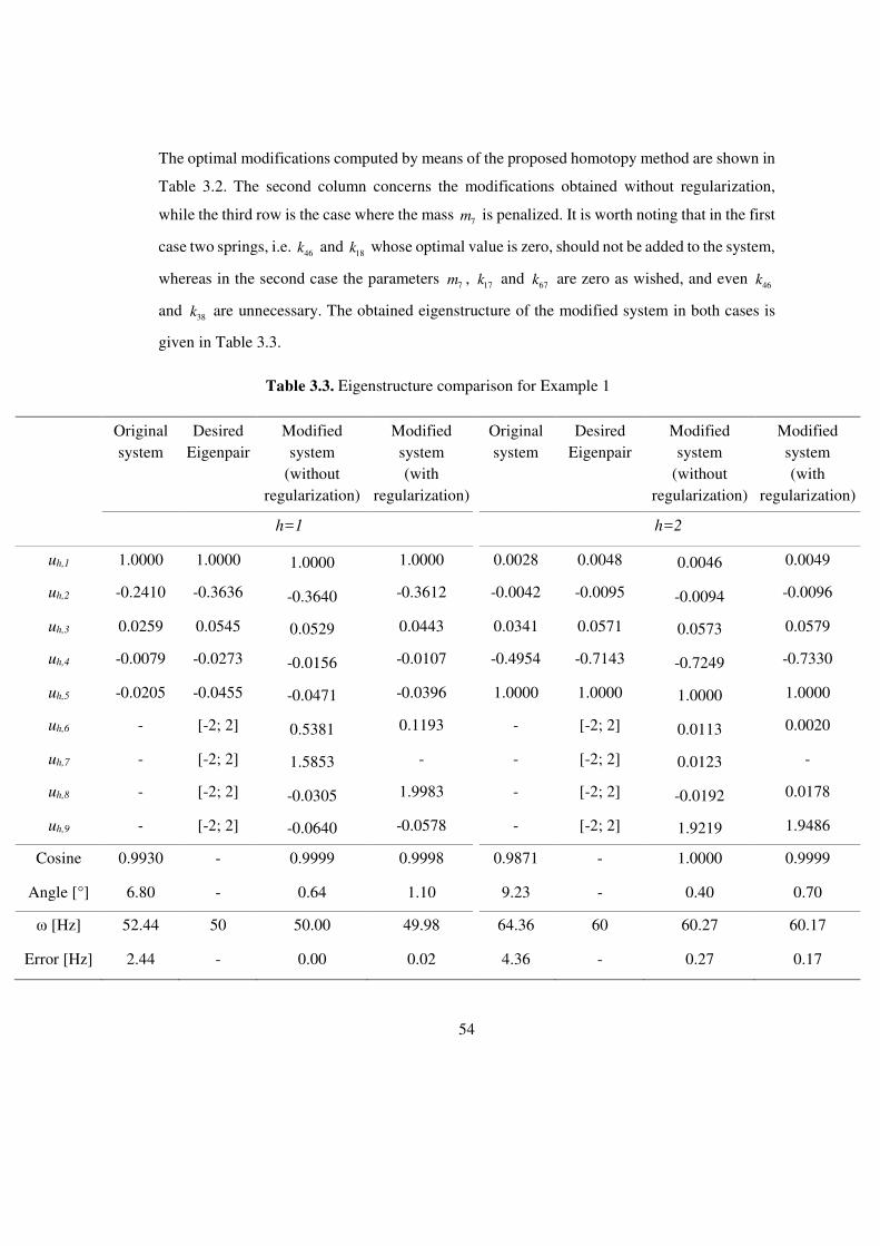
54

The optimal modifications computed by means of the proposed homotopy method are shown in

Table 3.2. The second column concerns the modifications obtained without regularization,

while the third row is the case where the mass 7m is penalized. It is worth noting that in the first

case two springs, i.e. 46k and 18k whose optimal value is zero, should not be added to the system,

whereas in the second case the parameters 7m , 17k and 67k are zero as wished, and even 46k

and 38k are unnecessary. The obtained eigenstructure of the modified system in both cases is

given in Table 3.3.

Table 3.3. Eigenstructure comparison for Example 1

Original system

Desired Eigenpair

Modified system

(without regularization)

Modified system (with

regularization)

Original system

Desired Eigenpair

Modified system

(without regularization)

Modified system (with

regularization)

h=1 h=2

uh,1 1.0000 1.0000 1.0000 1.0000 0.0028 0.0048 0.0046 0.0049

uh,2 -0.2410 -0.3636 -0.3640 -0.3612 -0.0042 -0.0095 -0.0094 -0.0096

uh,3 0.0259 0.0545 0.0529 0.0443 0.0341 0.0571 0.0573 0.0579

uh,4 -0.0079 -0.0273 -0.0156 -0.0107 -0.4954 -0.7143 -0.7249 -0.7330

uh,5 -0.0205 -0.0455 -0.0471 -0.0396 1.0000 1.0000 1.0000 1.0000

uh,6 - [-2; 2] 0.5381 0.1193 - [-2; 2] 0.0113 0.0020

uh,7 - [-2; 2] 1.5853 - - [-2; 2] 0.0123 -

uh,8 - [-2; 2] -0.0305 1.9983 - [-2; 2] -0.0192 0.0178

uh,9 - [-2; 2] -0.0640 -0.0578 - [-2; 2] 1.9219 1.9486

Cosine 0.9930 - 0.9999 0.9998 0.9871 - 1.0000 0.9999

Angle [°] 6.80 - 0.64 1.10 9.23 - 0.40 0.70

ω [Hz] 52.44 50 50.00 49.98 64.36 60 60.27 60.17

Error [Hz] 2.44 - 0.00 0.02 4.36 - 0.27 0.17

55

The parameters used to evaluate the method effectiveness are the absolute error in the

achievement of the desired eigenfrequency and the cosine of the angle between the desired

eigenvector and the obtained one, computed with respect of the first 5 entries only. Such

parameters clearly prove that the design specifications are met with excellent accuracy with

both the configurations of the system. Indeed, in each case, both the mode shapes and the

eigenfrequencies very closely approach the desired ones, with negligible errors: almost unitary

cosines are obtained between the mode shapes, while the frequency errors closely approach

zero. This result is remarkable, especially if considered that the parameters of the original

(primary) system (to which it is wanted to assign the response) have not been altered.

As a final remark about the employed regularization technique, it is interesting to note that it

has been attempted to perform the assignment without explicitly introducing the mass 7m ,

namely with only three additional degrees of freedom, and the obtained results are almost

identical to those obtained adding the penalty terms to the cost function.

3.4.2. Example 2

The second example consists in a much more challenging EA task, since the assigned eigenpairs

are very different from the ones of the original system. Moreover, such example allows to

compare the proposed method with another state-of-the-art method [44]. The vibrating system

under consideration is once again the one of the previous example, but different values of the

physical parameter are assumed. Such values are shown in Table 3.4. It is supposed that the

system can be modified as in Figure 3.3, namely adding five concentrated masses, each one

Figure 3.3. Modified system of Example 2.

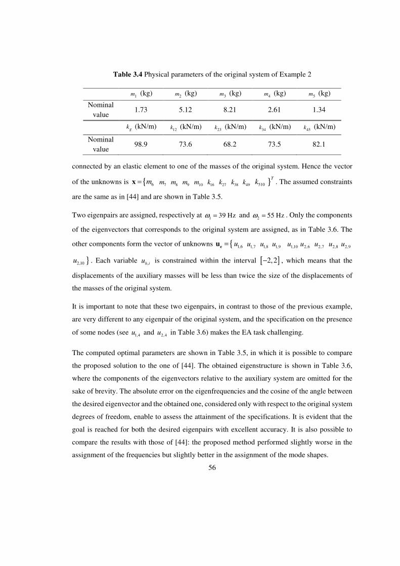
56

connected by an elastic element to one of the masses of the original system. Hence the vector

of the unknowns is { 6m=x 7m 8m 9m 10m 16k 27k 38k 49k }510

Tk . The assumed constraints

are the same as in [44] and are shown in Table 3.5.

Two eigenpairs are assigned, respectively at 1 39 Hzω = and 2 55 Hzω = . Only the components

of the eigenvectors that corresponds to the original system are assigned, as in Table 3.6. The

other components form the vector of unknowns { 1,6u=e

u 1,7u 1,8u 1,9u 1,10u 2,6u 2,7u 2,8u 2,9u

}2,10u . Each variable ,h iu is constrained within the interval [ ]2,2− , which means that the

displacements of the auxiliary masses will be less than twice the size of the displacements of

the masses of the original system.

It is important to note that these two eigenpairs, in contrast to those of the previous example,

are very different to any eigenpair of the original system, and the specification on the presence

of some nodes (see 1,4u and 2,4u in Table 3.6) makes the EA task challenging.

The computed optimal parameters are shown in Table 3.5, in which it is possible to compare

the proposed solution to the one of [44]. The obtained eigenstructure is shown in Table 3.6,

where the components of the eigenvectors relative to the auxiliary system are omitted for the

sake of brevity. The absolute error on the eigenfrequencies and the cosine of the angle between

the desired eigenvector and the obtained one, considered only with respect to the original system

degrees of freedom, enable to assess the attainment of the specifications. It is evident that the

goal is reached for both the desired eigenpairs with excellent accuracy. It is also possible to

compare the results with those of [44]: the proposed method performed slightly worse in the

assignment of the frequencies but slightly better in the assignment of the mode shapes.

Table 3.4 Physical parameters of the original system of Example 2

1m (kg) 2m (kg) 3m (kg) 4m (kg) 5m (kg)

Nominal value

1.73 5.12 8.21 2.61 1.34

gk (kN/m) 12k (kN/m) 23k (kN/m) 34k (kN/m) 45k (kN/m)

Nominal value

98.9 73.6 68.2 73.5 82.1

57

Table 3.5 Structural modifications for Example 2

Constraints Reference [44] Proposed method

m6 (kg) [0; +2] 0.9044 0.9033

m7 (kg) [0; +2] 0.7336 1.0483

m8 (kg) [0; +2] 0.7187 2.0000

m9 (kg) [0; +2] 0.9962 1.2472

m10 (kg) [0; +2] 1.5344 0.2562

k16 (kN/m) [0; +200] 108.62 107.8799

k27 (kN/m) [0; +200] 93.94 200.0000

k38 (kN/m) [0; +200] 73.46 49.2394

k49 (kN/m) [0; +200] 61.78 74.8915

k510 (kN/m) [0; +200] 38.81 18.1657

Table 3.6. Eigenstructure comparison for Example 2

Desired Eigenpair

Method [44]

Proposed method

Desired Eigenpair

Method [44]

Proposed method

h=1 h=2

uh,1 1.00 1.000 1.000 0 0.000 -0.000

uh,2 0.55 -0.538 -0.558 0.01 0.011 0.009

uh,3 0.20 0.104 0.224 -0.10 -0.278 -0.089

uh,4 0 -0.004 0.000 0.80 0.864 0.804

uh,5 0.05 -0.002 -0.022 1.00 1.000 1.000

Cosine - 0.9955 0.9979 - 0.9910 1.0000

Angle [°] - 5.44 3.72 - 7.69 0.55

ω [Hz] 39 39.00 39.03 55 55.01 54.96

Error [Hz] - 0.004 0.034 - 0.005 0.038

58

3.5. Conclusion

In this Chapter it is proposed a novel approach to eigenstructure assignment through the use of

auxiliary external systems with arbitrary topology and number of degrees of freedom. In

particular, the method aims at determining optimal mass and stiffness modification parameters

leading to the assignment of an arbitrary number of eigenpairs, defined in terms of

eigenfrequency and mode shape for just the entries concerning the original primary system. No

specifications are posed on the mode shape entries concerning the external systems, to which

only upper and lower bounds are set, to avoid unfeasible and unreasonable displacements. The

proposed approach casts the assignment as a minimization problem. Since some bilinear terms

appear, the homotopy optimization approach of Chapter 2 has been exploited. The numerical

validation has been carried out through a five-mass system, which is modified through the

addition of four or five external masses (although in the first example it is proved that it is

possible to lower the number of additional masses to three). The parameters of the auxiliary

external system that have been computed are to alter the response of the original system in order

to obtain two different eigenstructures, in both cases with good results. Excellent performances

and ease of implementation are granted by the proposed method.

59

Chapter 4. Passive control without spill-over

4.1. Introduction

The assignment of just natural frequencies (i.e. eigenvalues) is often performed through

Dynamic Structural Modification. The problem that is typically addressed is the case in which

only few eigenvalues are assigned, because in practice there is a small number of dominant

eigenvalues that characterize the dynamic behaviour. The modification of a subset of the natural

frequencies, however, can lead to undesired change of the remaining ones, which is a

phenomenon known as frequency spill-over.

In active control, spill-over can be easily avoided, since there are many methods available that

can perform partial eigenvalue assignment while keeping the non-assigned eigenvalues

unchanged, both using a first-order [55, 56] and a second-order [28, 29, 57] system model. For

passive control, in contrast, few techniques for avoiding spill-over are available, and most of

them are devoted to the preservation of just one specific frequency [58, 59, 60]. The general

problem, instead, has been tackled only in [61], in which two methods are proposed. The first

one concerns simply connected in-line mass-spring systems, while the second one deals with

multiple-connected mass-spring systems.

The method proposed in this thesis intends to extend the one in [61] to general vibrating

systems, with arbitrary modifiable parameters (e.g. distributed ones). Frequency assignment

will be achieved in two steps: first of all, a system model that has the desired eigenvalues is

sought, regardless of the feasibility constraints. After that, it is computed an equivalent system,

which also complies with feasibility constraints, by integration of a matrix differential equation.

The numerical issues related to the solution of the differential equation will be discussed.

Finally, the proposed method is validated in three different test-cases of interest.

60

4.2. Method description

Let us suppose that the undamped vibrating system under consideration can be represented by

means of the mass matrix 0n n×∈M ℝ and the stiffness matrix 0

n n×∈K ℝ . The system will be

denoted as the pair ( )0 0,M K . It is supposed that a subset of the eigenvalues of the system, i.e.

1 2, , , pλ λ λ… , is known. It is wanted to modify the system in such a way that the p

abovementioned eigenvalues are replaced by 1 2, , , pµ µ µ… , while the other n p− eigenvalues

are left unchanged, if possible, or at least the shift of such eigenvalues is kept to a minimum. It

is also of fundamental importance that such modifications are feasible, and that the resulting

matrices are physically meaningful.

In order to achieve such a result, the proposed method relies on a two-steps scheme, similar to

the one that has been proposed in [61]. First of all, it is sought a system ( ),s sM K that features

the desired eigenvalues, without taking into account the physical constraints, by taking

advantage of the method proposed in [62]. The second step, instead, consists in the search of a

system ( ),∞ ∞M K , within the space of systems that have the same eigenvalues as ( ),s sM K ,

such that it is as close as possible to the space of feasible systems. In order to perform the second

step, a class of matrix differential equations, known as isospectral flows, has been exploited.

Finally, the feasible system that provides the best approximation of the desired eigenvalues is

computed as the orthogonal projection of ( ),∞ ∞M K onto the space of feasible systems. Figure

4.1 schematically represent the proposed method. The present Section is devoted to give a

detailed explanation of the stages that constitutes the method.

61

4.2.1. Direct updating of the system

The method that is described in this Chapter has been proposed by Yang et al. in [62], thus it

will be briefly explained, and for the details it is suggested to refer to the original paper.

In order to employ such a method, it is required the knowledge of the eigenvectors 1 ,, p…u u

correspondent to the eigenvalues to be modified 1, , pλ λ… . Such eigenvectors will be retained

in the modified system design, after the first step, and they will be associated to the desired

eigenvalues 1, , pµ µ… . This feature is not of interest, because the assignment of eigenvectors is

not addressed, and in fact in the second step eigenvectors will be neglected.

For convenience, the following matrices are defined:

( )

( )

1 1

1 1

1 1

diag , ,

,

,

, .

diag ,

p

p

p

λ λ

µ µ

= …

= …

… = U u u

Λ

Σ (4.1)

Figure 4.1. Method description

( ),∞ ∞M K

( ),M K

( ),s sM K

EIGENVALUE CONSTRAINT

( )0 0,M K

FEASIBILITY

CONSTRAINT

STEP 1 STEP 2

62

It is wanted to find a new system ( ),s sM K that features the same eigenpairs as ( )0 0,M K ,

except for ( ) ( )1 1, , , ,p pλ λ…u u which are to be replaced with ( ) ( )1 1, , , ,p pµ µ…u u . Such a

request can be split into two constraints:

1) a condition that imposes the new eigenpairs, which can be expressed in matrix form as

( ) ( )1 10 0 1=+ +MM U K K U∆ Σ ∆ (4.2)

2) a condition that assures that spill-over does not take place, while assigning the desired

eigenpairs with Eq. (4.2).

It is not trivial to express such a condition without the knowledge of the eigenpairs to be

retained. In [63], however, it has been proposed the following equation

( ) ( )1 1 10 1 1 0 0 0 1 1 1 ,T T− − −− − − =K M U U M M K M U U 0∆ ∆ Λ (4.3)

which requires only the knowledge of the eigenpairs to be modified, but assures that the

remaining eigenpairs are left unchanged by the additive modification ΔM and .ΔK

In order to avoid the inversion of the mass matrix 10−

M , in [62] it is also suggested to choose

the modification matrices as

0 0

0 0

=

=

ΔM M ΨM

ΔK M ΦM (4.4)

where , n n×∈Ψ Φ ℝ are real symmetric matrices. In fact, in such a way, the two conditions (4.2)

and (4.3) are equivalent to

( ) ( )

( ) ( )1 1 0 0 0 1

0 0 1 1 0 0 0 1 1 1

0

0

0 0

.T T

= +

− − −

+

=

U K M M U

M M

M M

U U M K M U U M 0

MΨ Σ Φ

Φ Ψ Λ (4.5)

It is recommendable to solve such equations for the optimal Φ and Ψ in a least-square sense.

In particular, it is suggested to solve the following optimization problem:

( ) ( )

( ) ( )

2

0 0 0 1 1 0 0 0 1,

0 0 1 1 0 0 0 1 1 1 0

min

subject to .T T

+ − +

− − − =

Φ ΨM M ΨM U Σ K M ΦM U

Φ M M U U M Ψ K M U Λ U M 0

(4.6)

63

Given the convexity of the proposed formulation, it is possible to find a numerical solution with

moderately low effort. In fact, convex optimization is a well understood topic in numerical

computing, the state-of-the-art algorithm are highly satisfactory and there are many software

packages available for the purpose. Supposed that Φ̂ and Ψ̂ are the optimal matrices of

problem (4.6), then the modified system can be obtained as

0 0 0

0 0 0 .

ˆ

ˆs

s

= +

= +

M M M M

K K M M

Ψ

Φ (4.7)

An important issue is that the mass and stiffness matrices should be positive definite and

positive semidefinite, respectively. The numerical validation of the method showed that the

obtained matrices comply with the positive definite constraint, without explicitly requiring so.

If it is necessary, however, it is possible to exploit one of the popular algorithm for semidefinite

optimization, that allows to take into account constraints on the positive definiteness of the

matrices. Software that implement such algorithms are, for example, Mosek [45], SeDuMi [64]

and SDPT3 [65]. For the sake of efficiency, however, semidefinite constraint should be imposed

only if the optimization of (4.6) fails.

4.2.2. Isospectral flow

The system ( ),s sM K obtained in the first step meets the requirements regarding the

eigenvalues, but does not correspond to a physically meaningful system. In fact, the matrices

sM and sK are dense and unstructured matrices. Such an issue is taken into consideration in

the second step.

In practice, it is wanted to find a system ( ),M K that has the same eigenvalues as ( ),s sM K ,

namely that belongs to the space

( ) ( ){ }, , such that is invertible .T T n n

s s s

n n

s

× ××= ⊆M K P M P P K P P ℝ ℝM (4.8)

Moreover, it is wanted that ( ),M K belongs also to the space V of the feasible systems. The

definition of such a subspace requires knowledge of the system design and it depends on the

physical parameters that can be reasonably modified. Moreover, it is supposed that the mass

64

and stiffness matrices depend linearly on the modifiable parameters. Such an assumption is

made in many other works about structural modification (e.g. [23]) since it allows to represent

most of the types of modifications, so it does not invalidate the generality of the method.

Thus, the space n n nn× ××⊆ ℝ ℝV can be defined as follows:

( ) 0 01 1

: , for some coefficients and , ,M Kn n

i i i i i i

i i

x y x y= =

= +

=

=

+∑ ∑M M M K KK KMV

(4.9)

where Mn and

Kn are, respectively, the number of mass elements and stiffness elements that

can be modified. The matrices iM and

iK represent the topology of the contribution of each

modifiable parameter, while the coefficients ix and

iy represent the magnitude of the

modification.

From a geometrical point of view, the search of a system that complies with both the constraints

on the natural frequencies and the feasibility constraints is equivalent to the search of the

intersection of ( ),s sM KM and V . If such an intersection is empty, it is still interesting to

find the system that minimizes the distance between such spaces, because it could be interpreted

as a least-squares solution of the optimal design problem.

In order to describe the proposed method, let us define the projection : n n n n× ×× →ℝ ℝ VP of a

generic system ( ),X Y as

( ) ( ) ( )( )1 2, , ,=X Y X YP P P (4.10)

where 1P and 2P are the orthogonal projection of the mass and stiffness matrices, respectively.

The computation of the projection is very straightforward, if the matrices are considered as

vectors. As an example, the algorithm for the projection of the mass matrix 1P is described. It

is wanted to find the coefficients 1 ,,Mnx x… such that

( )1 0 1 1 M Mn nxx …+ + +=X M M MP (4.11)

65

Let us denote ( )vec the operator that stacks the columns of a matrix one below the other. For

convenience it is also defined

( ) ( )

( )

1

0

vec

vec .

vecMM n

= …

= −

MS

X

M

Mmδ (4.12)

By exploiting the orthogonality of the least-squares residual to the range of MS , the appropriate

coefficients in (4.11) are computed solving the following problem:

2

min M −Sx

x mδ (4.13)

where ( )1, ,Mn

T

x x…=x . Being x̂ the least-squares solution, the projection itself is

( ) ( )11 0 ˆvec .M

−= +X M S xP (4.14)

The definition of 2P is analogous and thus it is omitted.

The projection onto V is the tool that allows to express the distance of a general system on

( ),s sM KM to the space V . It is worth to remark that, given the definition (4.8), any system

in ( ),s sM KM is uniquely determined by an invertible matrix P , hence the distance function

is dependent on P . For clarity of notation, it is defined

( ) ( )( ) ( )

1 1

2 2 .

T T

s s

T T

s s

γ

γ

= −

= −

P P M P P M P

P P K P P K P

P

P (4.15)

Hence, the distance function F is expressed by

( ) ( ) ( )( )1

2 2

2

1.

2F γ γ= +P PP (4.16)

Such a function has been also proposed in [66] to solve the inverse eigenvalue problem for

linear pencils. In practice, the function is minimized by integrating the so-called descent flow,

which is

66

( ) ( )( )( )0 ,

Ft t = −

=

∇P

P I

Pɺ

(4.17)

where I is the identity matrix. In the cited paper it is also given a closed form for the gradient

of F , particularly useful for numerical computations, that is

( ) ( ) ( )( )1 22 .s sF γ γ∇ = +P M P P K P P (4.18)

A remarkable property of the descent flow is that its solution ( )tP asymptotically converges.

Thus, defined ( )limt

t∞

∞→+

=P P , the system that (locally) minimizes the distance to V is

.

T

s

T

s

∞ ∞ ∞

∞ ∞ ∞

=

=

M P M P

K P K P (4.19)

Then, the system in V that minimizes the distance to ( ),s sM KM is exactly the projection of

( ),∞ ∞M K , namely

( )

( )1

2 .

∞

∞

=

=

M M

K K

P

P (4.20)

The system ( ),M K computed by means of the described procedure actually correspond to a

physically meaningful system, and it has the desired eigenvalues, or at least is affected by

limited spill-over, as proven in Section 4.3 where different tests are shown. Despite the

computed solution representing an actual mechanical system, it might not be sufficient for many

design applications, in which other technical constraints have a fundamental role. Moreover,

the algorithm for computing the solution of (4.17) requires a more detailed explanation if

constraints are defined.

In the next Sections the constrained problem and its numerical integration are addressed.

4.2.3. Projections with constraints

It is evident that the unbounded space V also contains systems that can be hardly implemented

in practice, due to technical reasons. Hence, it is recommendable to introduce constraints on the

67

coefficients ix and

iy that appear in the definition (4.9). Collecting the coefficients into vectors

( )1, ,M

T

nx x= …x and ( )1, ,K

T

ny y= …y , the constraint sets are defined by

{ }

{ },eq ,eq

,eq ,eq

: , ,

: , ,

M

K

n

x x x x x L U

n

y y y y y L U

Γ = ∈ ≤ = ≤ ≤

Γ = ∈ ≤ = ≤ ≤

A A

A A

x x b x b x x x

y y b y b y y y

ℝ

ℝ (4.21)

for some appropriate matrices xA , ,eqxA , yA , ,eqyA and vectors

xb , ,eqxb , Lx ,

Ux , yb , ,eqyb ,

Ly , Uy . Hence the constrained feasible space is defined by

( ) 0 01 1

: ,ˆ , ., ,M Kn n

i i i i x y

i i

x y= =

= + = + ∈Γ ∈

=

Γ

∑ ∑M M MK M K K K x yV (4.22)

From the theoretical point of view, the projection onto V̂ is not different from the projection

described in the previous Section, except for the fact that the unconstrained least-squares

problem (4.13) must be replaced with a constrained least-squares problem. From the numerical

point of view, in contrast, the presence of constraints considerably affects the computational

performances. Considering that the projections 1P and 2P must be evaluated at each iteration

of the numerical integration of (4.17), it is obvious that it is critical to be able to compute least-

squares solutions fast and accurately. Nevertheless, while testing the proposed method, it has

been observed that the linear least-squares solvers implemented in commercial software gave

unsatisfactory results.

Such a relevant issue has been tackled employing a scaling strategy, which allows a substantial

improvement of the obtained results in terms of accuracy of the computed solution. Scaling is

aimed at recasting the problem with dimensionless unknowns, which is advantageous in many

ways, including the numerical point of view [67]. In practice, it is suggested to choose the basis

of V̂ in such a way that all the coefficients 1 ,,Mnx x… (or 1 ,,

Kny y… ) have roughly order of

magnitude 010 . This can be achieved simply multiplying by suitable scalar factors the matrices

iM and iK . In fact, given non-zero scalars 1, ,

Mnη η… and 1, ,Knτ τ… , the space V̂ can be

represented as

68

( ) 0 01 1

ˆ ˆˆ ,, : , , .M Kn n

i i i i i i x y

i i

x yη τ= =

=

=

+ = + ∈Γ ∈Γ

∑ ∑M MM K M K K K x yV (4.23)

It is clear that this is equivalent to (4.22), provided that the constraint sets xΓ and yΓ are

replaced properly by new constraint sets ˆxΓ and ˆ

yΓ . A judicious choice of the iη and of the

iτ

allows to keep the components of x and y roughly of the same magnitude, which is beneficial

to the accuracy of the projection and to the CPU time.

4.2.4. Numerical integration

Although (4.17) can be compactly represented as one matrix differential equation, it is actually

a system of 2n scalar differential equations and thus it can be big even for small-scale system

models. For such a reason, the numerical integration must be performed with care, in order to

reach convergence in a reasonable time even with limited hardware resources.

The tests carried out for validating the proposed method have shown that the differential

equation under consideration is stiff, thus the standard algorithms for numerical integration tend

to require small discretization steps. Such an occurrence is common when the differential

equation contains terms that are very different in magnitude and hence it is ill-conditioned, as

it is the case in (4.18). In fact, mass and stiffness matrices can have very different orders of

magnitude, in real mechanical vibrating systems.

To overcome such a problem, it is beneficial using specific algorithms for stiff equations, which

are already implemented in many software packages for scientific computing. Moreover, it is

suggested to employ a scaling strategy, similar to the one explained in Section 4.2.3. In practice,

it is solved an equivalent problem in which the mass and stiffness matrices are scaled to match

the desired order of magnitude, and also the feasible space V is modified accordingly. In fact,

given the scaling factors 0α > and 0β > , the system ( ),s sM K is replaced by the scaled

system

.

s s

s s

α

β

=

=

M M

K K

ɶ

ɶ (4.24)

The space of feasible systems (4.9), instead, is replaced by:

69

( ) 0 01 1

: , for some coefficients and . ,M Kn n

i i i i i i

i i

x y x yα β= =

=

=

+ = +∑ ∑M M M KM K KK ɶ ɶɶ ɶ ɶV

(4.25)

It is easy to prove that a matrix P that minimizes the distance to the feasible space for the scaled

system, also works for the original system. In fact, let us suppose that ( ),T T

s s ∈P M P P K Pɶ ɶ ɶV ,

then there exist coefficients 1 ,,Mnx x…ɶ ɶ such that

0

1

01

.

M

M

n

i i

T

s

i

n

i

i

T

si

x

x

α

α αα

=

=

+

⇔

= +

=

∑

∑

P M P

P M

M

M MP

Mɶ

ɶ

ɶ

(4.26)

Hence for iix x α= ɶ it holds 0 1

Mn

is i

T

ix=

= +∑M MP M P . The same argument can be used to

prove an analogous assertion for stiffness matrices, therefore ( ),T T

s s ∈P M P P K P V and then

the original and the scaled problems are equivalent.

It should be remarked that the scaled problem can be solved also in the presence of constraints,

as described in Section 4.2.3. It is necessary, however, to compensate the effect of the factors

α and β by an appropriate choice of the coefficients iη and

iτ , and also of the constraint sets

xΓ and yΓ . For example, if the coefficient iη is employed for a variable of the original problem,

then ˆi iη α η= ⋅ would be a recommendable choice for the same coefficient in the scaled

problem.

According to the numerical validation that has been carried out, the proposed method enables

to find a stationary point of Eq. (4.17) within a reasonable time span, for models that can be

actually used to represent real mechanical systems with good accuracy. Some examples are

shown in the next Section.

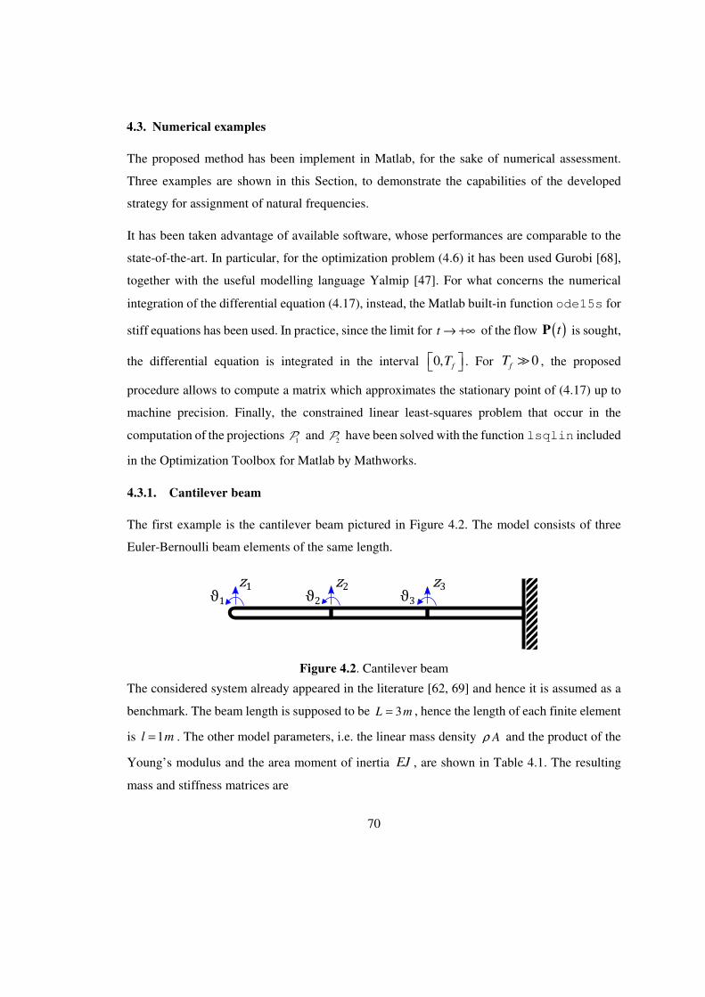
70

4.3. Numerical examples

The proposed method has been implement in Matlab, for the sake of numerical assessment.

Three examples are shown in this Section, to demonstrate the capabilities of the developed

strategy for assignment of natural frequencies.

It has been taken advantage of available software, whose performances are comparable to the

state-of-the-art. In particular, for the optimization problem (4.6) it has been used Gurobi [68],

together with the useful modelling language Yalmip [47]. For what concerns the numerical

integration of the differential equation (4.17), instead, the Matlab built-in function ode15s for

stiff equations has been used. In practice, since the limit for t → +∞ of the flow ( )tP is sought,

the differential equation is integrated in the interval 0, fT . For 0fT ≫ , the proposed

procedure allows to compute a matrix which approximates the stationary point of (4.17) up to

machine precision. Finally, the constrained linear least-squares problem that occur in the

computation of the projections 1P and 2P have been solved with the function lsqlin included

in the Optimization Toolbox for Matlab by Mathworks.

4.3.1. Cantilever beam

The first example is the cantilever beam pictured in Figure 4.2. The model consists of three

Euler-Bernoulli beam elements of the same length.

The considered system already appeared in the literature [62, 69] and hence it is assumed as a

benchmark. The beam length is supposed to be 3L m= , hence the length of each finite element

is 1l m= . The other model parameters, i.e. the linear mass density Aρ and the product of the

Young’s modulus and the area moment of inertia EJ , are shown in Table 4.1. The resulting

mass and stiffness matrices are

Figure 4.2. Cantilever beam

71

0

0

1.56 0.66 0.54 0.39 0 0

0.66 0.36 0.39 0.27 0 0

0.54 0.39 3.12 0 0.54 0.39;

0.39 0.27 0 0.72 0.39 0.27

0 0 0.54 0.39 3.12 0

0 0 0.39 0.27 0 0.72

12 18 12 18 0 0

18 36 18 18 0 0

12 18 24 0 12 18

18 18 0 72 18 18

0 0 12 18 2

− − −

= − − −

− −

−

−

− − −=

−

− −

M

K .

4 0

0 0 18 18 0 72

(4.27)

The eigenvalues of the original system are shown in the first column of Table 4.2. The three

lowest eigenvalues are wanted to be equal to 1 0.05µ = , 2 1.50µ = and 3 11.0µ = , while the

others should remain the same. The system matrices computed after direct updating are

1.5442 0.6523 0.5324 -0.3788 0.0352 -0.0004

0.6523 0.3567 0.3891 -0.2662 0.0079 -0.0007

0.5324 0.3891 3.1192 -0.0119 0.4651 -0.3905

-0.3788 -0.2662 -0.0119 0.7145 0.3798 -0.2664

0.0352 0.0079 0.4651 0.3798 3.1274 0.0183

-0.0004

s =M

-0.0007 -0.3905 -0.2664 0.0183

12.0203 18.0091 -11.9892 17.9917 -0.0121 0.0004

18.0091 36.0039 -17.9947 17.9971 -0.0029 -0.0001

-11.9892 -17.9947 24.0277 0.0037 -11.9658 17.9955

17.991

;

0.7

7 17

200

.9971s

=K0.0037 72.0027 -17.9915 17.9994

-0.0121 -0.0029 -11.9658 -17.9915 24.0202 -0.0084

0.0004 -0.0001 17.9955 17.9994 -0.0084 71.9992

.

(4.28)

The eigenvalues of ( ),s sM K are shown in the second column of Table 4.2. It is supposed that

the system parameters that can be modified are the linear mass densities iAρ and the products

of the Young’s modulus and area moment of inertia iEJ , for each beam element 1,2,3i = .

Hence the space of feasible systems is defined as in (4.9), with 3M Kn n= = and

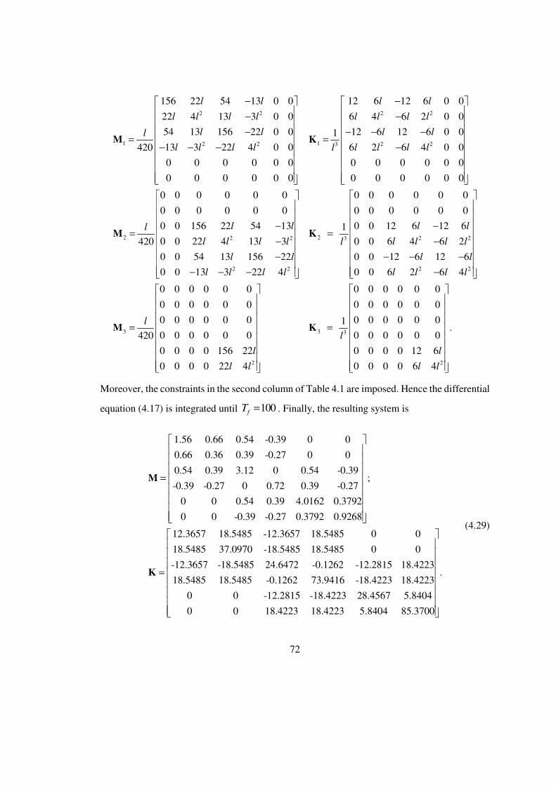
72

2 2 2 2

1 12 2 3 2 2

2

156 22 54 13 0 0 12 6 12 6 0 0

22 4 13 3 0 0 6 4 6 2 0 0

54 13 156 22 0 0 12 6 12 6 0 01

13 3 22 4 0 0 6 2 6 4 0 0420

0 0 0 0 0 0 0 0 0 0 0 0

0 0 0 0 0 0 0 0 0 0 0 0

0 0 0 0 0 0

420

l

l l l l

l l l l l l l l

l l l ll

l l l l l l l l

l

− − − − − − − −

= = − − − −

=

M K

M 2 2 2 2

2 2 2 2

3

2 3

0 0 0 0

0

0 0

0 0 0 0 0 0 0 0

0 0 156 22 54 13 12 6 12 61

0 0 22 4 13 3 6

4 6 2

0 0 54 13 156 22 0 0 12 6 12 6

0 0 13 3 22 4 0 0 6 2 6 4

0 0 0 0 0 0

0 0 0 0 0 0

0 0 0 0 0

420

0 0 0

0 0

0 0

l l l l

l l l l l l l l

l l l l

l l l l l l l l

l

l

− −

= − −

− − − −

− − − −

=

K

M

2 2

3 3

0 0 0 0

0 0 0 0

0 0

0 0

0 0 0 01.

0 0 0 0 0 0 0 0 0 0

0 0 0 0 156 22 0 0 0 0 12 6

0

0 0 0

0 0

0 0 0 22 4 0 0 6

4

00

l

l

l

l l l l

=

K

Moreover, the constraints in the second column of Table 4.1 are imposed. Hence the differential

equation (4.17) is integrated until 100fT = . Finally, the resulting system is

-

-

-

- - -

4.0162 0.37

1.56 0.66 0.54 0.39 0 0

0.66 0.36 0.39 0.27 0 0

0.54 0.39 3.12 0 0.54 0.39;

0.39 0.27 0 0.72 0.39 0.27

0 0 0.54 0.39

0

92

- - 0.3792 0.9268

12.3657 18.5485 -12.3657 18.5485

18.5485 37.09

0 0.39 0.2

0

0

7

0

7

=

=

M

K

-18.5485 18.5485

-12.3657 -18.5485 24.6472 -0.1262 -12.2815 18.4223

18.5485 18.5485 -0.1262 73.9416 -18.4223 18.4223

-12.2815 -18.4223 28.4567 5.8404

18.4223 18.4223 5.8404 85.3700

0 0

.

0 0

0 0

(4.29)

73

Such a system can be actually obtained modifying the original system as in the third column of

Table 4.2. The eigenvalues of the system ( ),M K are shown in Table 4.2. Such results prove

that the three lowest eigenvalues are actually closer to the objective, with respect to the original

system design. The spill-over that affects the remaining eigenvalues, however, is very limited,

in fact the relative error is about 2% for all the three cases.

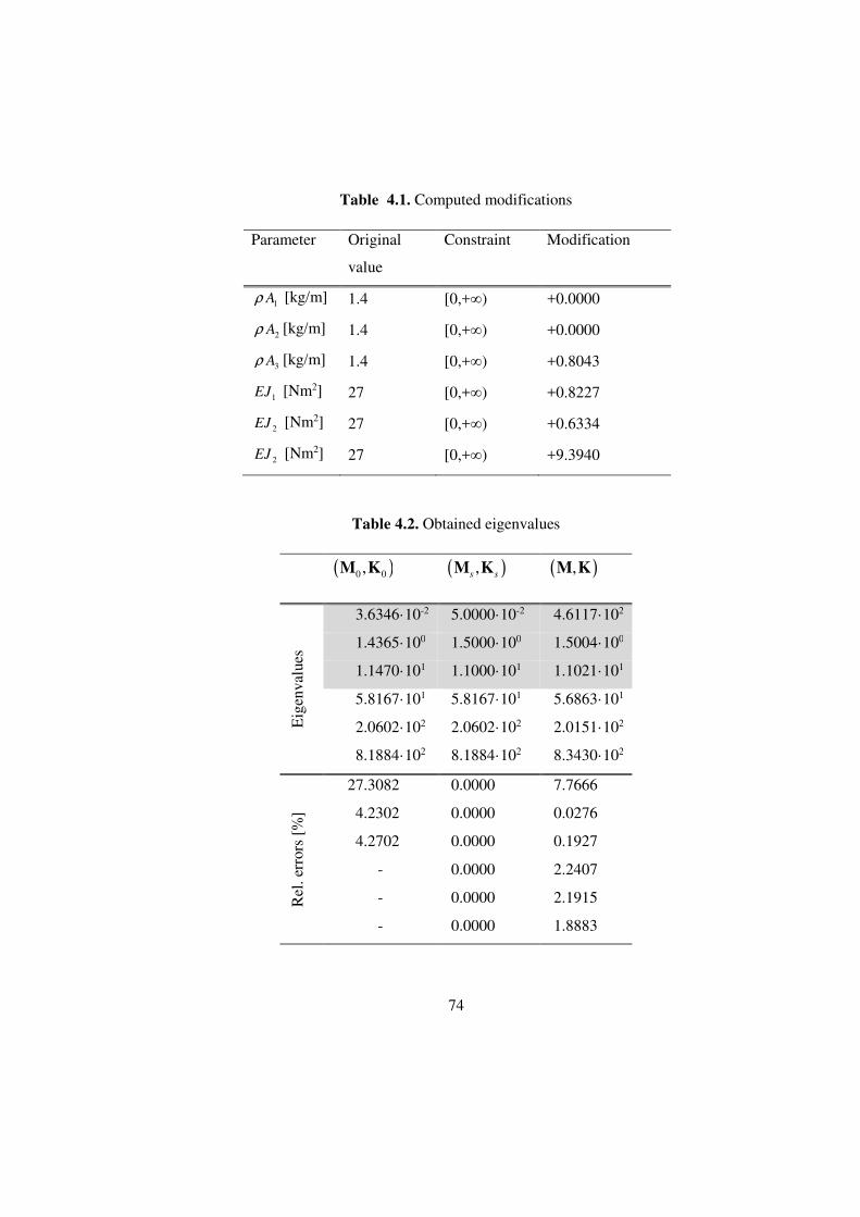
74

Table 4.1. Computed modifications

Parameter Original

value

Constraint Modification

1Aρ [kg/m] 1.4 [0,+∞) +0.0000

2Aρ [kg/m] 1.4 [0,+∞) +0.0000

3Aρ [kg/m] 1.4 [0,+∞) +0.8043

1EJ [Nm2] 27 [0,+∞) +0.8227

2EJ [Nm2] 27 [0,+∞) +0.6334

2EJ [Nm2] 27 [0,+∞) +9.3940

Table 4.2. Obtained eigenvalues

( )0 0,M K ( ),s sM K ( ),M K

Eig

enva

lues

3.6346·10-2 5.0000·10-2 4.6117·102

1.4365·100 1.5000·100 1.5004·100

1.1470·101 1.1000·101 1.1021·101

5.8167·101 5.8167·101 5.6863·101

2.0602·102 2.0602·102 2.0151·102

8.1884·102 8.1884·102 8.3430·102

Rel

. err

ors

[%]

27.3082 0.0000 7.7666

4.2302 0.0000 0.0276

4.2702 0.0000 0.1927

- 0.0000 2.2407

- 0.0000 2.1915

- 0.0000 1.8883

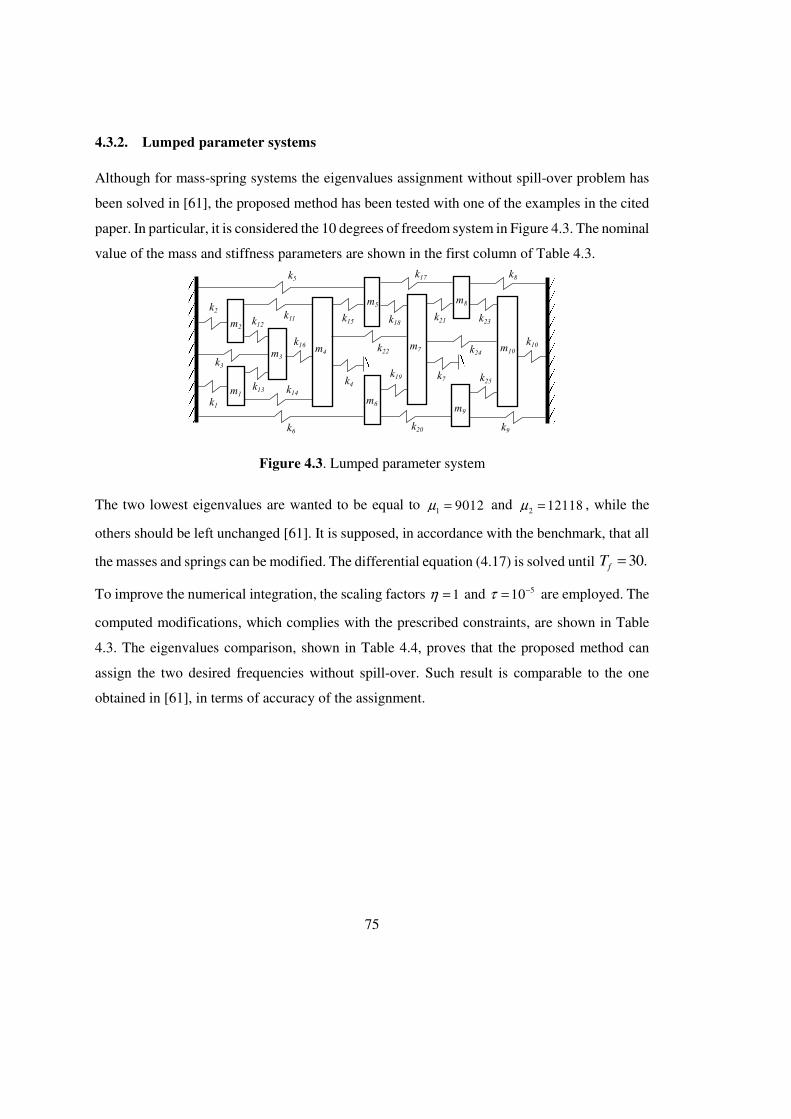
75

4.3.2. Lumped parameter systems

Although for mass-spring systems the eigenvalues assignment without spill-over problem has

been solved in [61], the proposed method has been tested with one of the examples in the cited

paper. In particular, it is considered the 10 degrees of freedom system in Figure 4.3. The nominal

value of the mass and stiffness parameters are shown in the first column of Table 4.3.

The two lowest eigenvalues are wanted to be equal to 1 9012µ = and 2 12118µ = , while the

others should be left unchanged [61]. It is supposed, in accordance with the benchmark, that all

the masses and springs can be modified. The differential equation (4.17) is solved until 30.fT =

To improve the numerical integration, the scaling factors 1η = and 510τ −= are employed. The

computed modifications, which complies with the prescribed constraints, are shown in Table

4.3. The eigenvalues comparison, shown in Table 4.4, proves that the proposed method can

assign the two desired frequencies without spill-over. Such result is comparable to the one

obtained in [61], in terms of accuracy of the assignment.

Figure 4.3. Lumped parameter system

76

Table 4.3. Computed modifications.

Parameter Original

value Constraint Modification

m1 [kg] 30 [-30,+∞) -1.3354 m2 [kg] 35 [-35,+∞) -1.9799 m3 [kg] 40 [-40,+∞) -2.6579 m4 [kg] 45 [-45,+∞) -3.4365 m5 [kg] 45 [-45,+∞) -4.2918 m6 [kg] 45 [-45,+∞) -5.4105 m7 [kg] 40 [-40,+∞) -2.1045 m8 [kg] 35 [-35,+∞) -1.9893 m9 [kg] 30 [-30,+∞) -1.5407 m10 [kg] 25 [-25,+∞) -0.1986 k1 [N/m] 2.4∙105 [-2.4∙105,+∞) 3.0118∙104 k2 [N/m] 2.4∙105 [-2.4∙105,+∞) 6.1159∙104 k3 [N/m] 2.4∙105 [-2.4∙105,+∞) 1.2533∙105 k4 [N/m] 2.4∙105 [-2.4∙105,+∞) 1.8437∙105 k5 [N/m] 2.4∙105 [-2.4∙105,+∞) -5.1242∙104 k6 [N/m] 2.4∙105 [-2.4∙105,+∞) 1.1121∙105 k7 [N/m] 2.4∙105 [-2.4∙105,+∞) 2.3010∙105 k8 [N/m] 2.4∙105 [-2.4∙105,+∞) 6.5613∙103 k9 [N/m] 2.4∙105 [-2.4∙105,+∞) 5.9681∙104 k10 [N/m] 2.4∙105 [-2.4∙105,+∞) 7.5688∙104 k11 [N/m] 2.4∙105 [-2.4∙105,+∞) -5.6379∙104 k12 [N/m] 2.4∙105 [-2.4∙105,+∞) -4.1956∙104 k13 [N/m] 2.4∙105 [-2.4∙105,+∞) -2.6967∙104 k14 [N/m] 2.4∙105 [-2.4∙105,+∞) -3.3854∙104 k15 [N/m] 2.4∙105 [-2.4∙105,+∞) -3.7155∙104 k16 [N/m] 2.4∙105 [-2.4∙105,+∞) -7.0636∙104 k17 [N/m] 2.4∙105 [-2.4∙105,+∞) -9.1187∙103 k18 [N/m] 2.4∙105 [-2.4∙105,+∞) -3.4443∙104 k19 [N/m] 2.4∙105 [-2.4∙105,+∞) -1.2269∙105 k20 [N/m] 2.4∙105 [-2.4∙105,+∞) -6.2758∙104 k21 [N/m] 2.4∙105 [-2.4∙105,+∞) -3.7457∙104 k12 [N/m] 2.4∙105 [-2.4∙105,+∞) -3.1824∙104 k23 [N/m] 2.4∙105 [-2.4∙105,+∞) -1.3914∙104 k24 [N/m] 2.4∙105 [-2.4∙105,+∞) -1.5011∙104 k25 [N/m] 2.4∙105 [-2.4∙105,+∞) -3.1275∙104

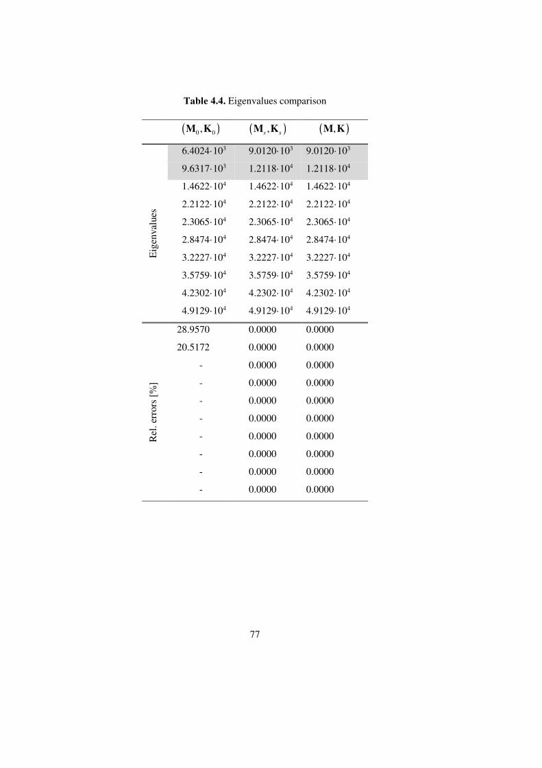
77

Table 4.4. Eigenvalues comparison

( )0 0,M K ( ),s sM K ( ),M K

Eig

enva

lues

6.4024·103 9.0120·103 9.0120·103

9.6317·103 1.2118·104 1.2118·104

1.4622·104 1.4622·104 1.4622·104

2.2122·104 2.2122·104 2.2122·104

2.3065·104 2.3065·104 2.3065·104

2.8474·104 2.8474·104 2.8474·104

3.2227·104 3.2227·104 3.2227·104

3.5759·104 3.5759·104 3.5759·104

4.2302·104 4.2302·104 4.2302·104

4.9129·104 4.9129·104 4.9129·104

Rel

. err

ors

[%]

28.9570 0.0000 0.0000

20.5172 0.0000 0.0000

- 0.0000 0.0000

- 0.0000 0.0000

- 0.0000 0.0000

- 0.0000 0.0000

- 0.0000 0.0000

- 0.0000 0.0000

- 0.0000 0.0000

- 0.0000 0.0000

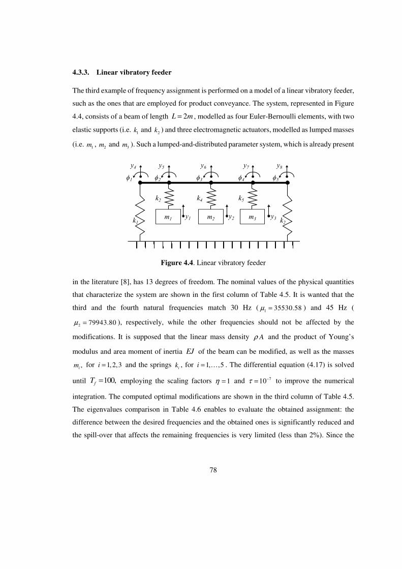
78

4.3.3. Linear vibratory feeder

The third example of frequency assignment is performed on a model of a linear vibratory feeder,

such as the ones that are employed for product conveyance. The system, represented in Figure

4.4, consists of a beam of length 2L m= , modelled as four Euler-Bernoulli elements, with two

elastic supports (i.e. 1k and 2k ) and three electromagnetic actuators, modelled as lumped masses

(i.e. 1m , 2m and 3m ). Such a lumped-and-distributed parameter system, which is already present

in the literature [8], has 13 degrees of freedom. The nominal values of the physical quantities

that characterize the system are shown in the first column of Table 4.5. It is wanted that the

third and the fourth natural frequencies match 30 Hz ( 1 35530.58µ = ) and 45 Hz (

2 79943.80µ = ), respectively, while the other frequencies should not be affected by the

modifications. It is supposed that the linear mass density Aρ and the product of Young’s

modulus and area moment of inertia EJ of the beam can be modified, as well as the masses

,im for 1,2,3i = and the springs ik , for ,51,i = … . The differential equation (4.17) is solved

until 100,fT = employing the scaling factors 1η = and 710τ −= to improve the numerical

integration. The computed optimal modifications are shown in the third column of Table 4.5.

The eigenvalues comparison in Table 4.6 enables to evaluate the obtained assignment: the

difference between the desired frequencies and the obtained ones is significantly reduced and

the spill-over that affects the remaining frequencies is very limited (less than 2%). Since the

Figure 4.4. Linear vibratory feeder

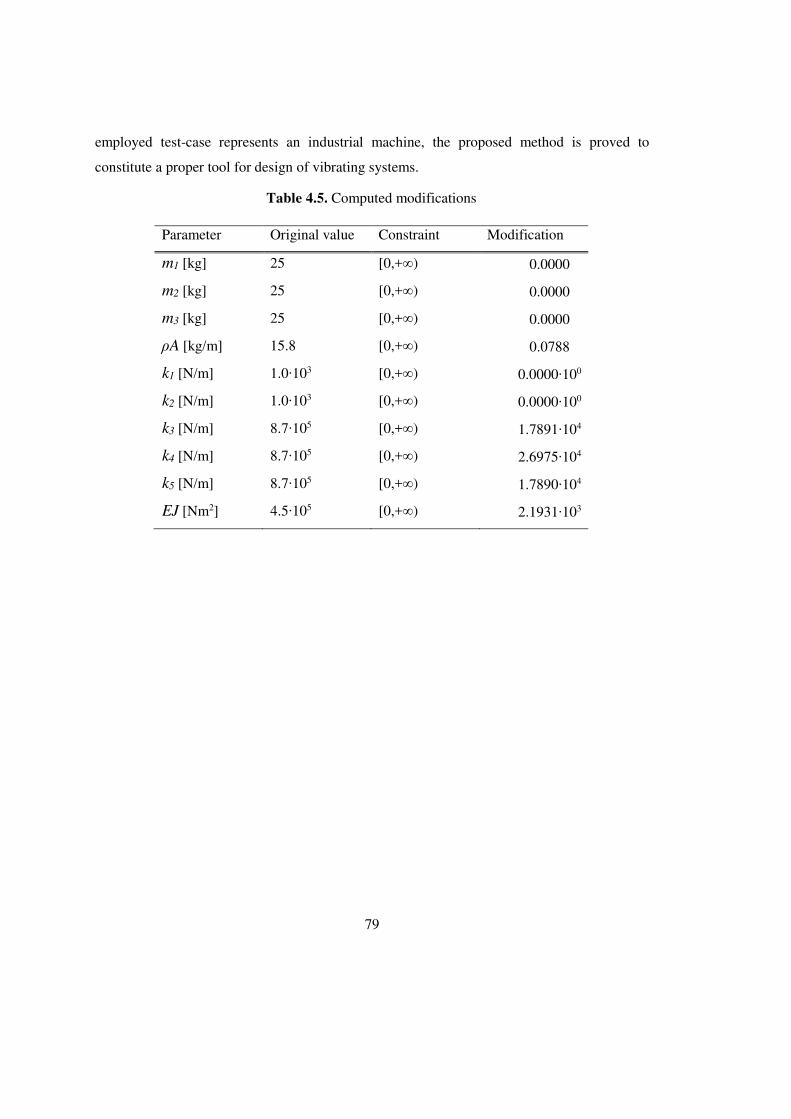
79

employed test-case represents an industrial machine, the proposed method is proved to

constitute a proper tool for design of vibrating systems.

Table 4.5. Computed modifications

Parameter Original value Constraint Modification

m1 [kg] 25 [0,+∞) 0.0000

m2 [kg] 25 [0,+∞) 0.0000

m3 [kg] 25 [0,+∞) 0.0000

ρA [kg/m] 15.8 [0,+∞) 0.0788

k1 [N/m] 1.0∙103 [0,+∞) 0.0000∙100

k2 [N/m] 1.0∙103 [0,+∞) 0.0000∙100

k3 [N/m] 8.7∙105 [0,+∞) 1.7891∙104

k4 [N/m] 8.7∙105 [0,+∞) 2.6975∙104

k5 [N/m] 8.7∙105 [0,+∞) 1.7890∙104

EJ [Nm2] 4.5∙105 [0,+∞) 2.1931∙103

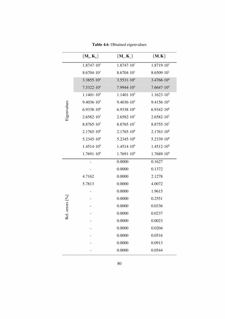
80

Table 4.6. Obtained eigenvalues

( )0 0,M K ( ),s sM K ( ),M K

Eig

enva

lues

1.8747·101 1.8747·101 1.8719·101

8.6704·101 8.6704·101 8.6509·101

3.3855·104 3.5531·104 3.4766·104

7.5322·104 7.9944·104 7.6647·104

1.1401·105 1.1401·105 1.1623·105

9.4036·105 9.4036·105 9.4156·105

6.9338·106 6.9338·106 6.9342·106

2.6582·107 2.6582·107 2.6582·107

8.8765·107 8.8765·107 8.8755·107

2.1765·108 2.1765·108 2.1763·108

5.2345·108 5.2345·108 5.2339·108

1.4514·109 1.4514·109 1.4512·109

1.7691·109 1.7691·109 1.7689·109

Rel

. err

ors

[%]

- 0.0000 0.1627

- 0.0000 0.1372

4.7162 0.0000 2.1278

5.7813 0.0000 4.0072

- 0.0000 1.9615

- 0.0000 0.2551

- 0.0000 0.0336

- 0.0000 0.0237

- 0.0000 0.0023

- 0.0000 0.0204

- 0.0000 0.0516

- 0.0000 0.0913

- 0.0000 0.0544

81

4.4. Conclusion

The proposed method intends to fill a gap in the state-of-the-art, since there was no way to

assign natural frequencies while avoiding spill-over, for general vibrating systems. The tests

carried out show that the two-steps approach is a practical way to alter a subset of the natural

frequencies by computing suitable modifications of the system parameters. Spill-over can be

often prevented, or it is very moderate, whenever it occurs. The numerical difficulties arisen in

the validation of the method have been effectively overcome, improving its reliability. In

conclusion, the proposed method actually widens the capabilities of passive control, making

partial eigenvalues assignment attainable without spill-over, even for complex systems.

The proposed method can be also employed for model updating, which consists in tuning the

physical parameters of a system to make the natural frequencies of a model match those

obtained from experimental measurements. An example of such an application can be found in

Chapter 8.

82

83

Chapter 5. Model updating for flexible link mechanisms

5.1. Introduction

The use of lightweight multibody systems, such as mechanisms or manipulators, has been

increasing significantly over the last years [70]. Indeed this kind of construction ensures smaller

material and power consumption, thus allowing for smaller actuators. On the other hand, the

flexibility of the links makes the motion planning and control critical and hence imposes the

use of advanced techniques that account for the system resonant dynamics. Therefore, great

attention has been paid to dynamic modelling of flexible-link multibody systems (FLMSs) [71],

in order to boost the development of effective model-based design or control techniques or to

allow for numerical simulations.

Several modelling approaches are proposed in literature. A widespread approach is to take

advantage of finite element (FE) methods to discretize the link flexibility through a finite

number of elastic degrees of freedom (dofs) and to represent the total motion of the system as

the superposition of a large amplitude rigid-body motion and the coupled small-amplitude

elastic deformation [72, 73, 74].

The availability of a correct model formulation is however not sufficient to predict correctly the

dynamic response. Indeed, these FE models are not effective if the inertial and elastic properties

of the model are not correctly tuned. Therefore, it is necessary paying attention to the correct

estimation of the model parameters, either through direct physical measurement or using

experimental parameter identification techniques. The latter process of correcting the FE model

parameters to feature a set of experimental measurements is known in the field of structural

dynamics as model updating [75].

Model updating can be performed by following two different types of approach: non-iterative

or iterative techniques [75, 76]. Non-iterative techniques (also denoted direct or one-step)

provide analytical solutions to model updating problem through a single step. Nonetheless, such

solutions are often without physical meaning, and scarcely robust to measurement noise.

84

Conversely, iterative techniques (also denoted parametric techniques) preserve the physical

meaning of the updated parameters at the cost of an increase of the computational complexity

due to the numerical iterations adopted to reduce the mismatch between experimental and model

responses. Basically, iterative techniques compute the updated parameters through an objective

function that represents the difference between analytical and experimental results. Therefore,

they may lead to local optimal solutions if the updating problem is formulated as a non-convex

optimization problem. In the last years, the use of iterative techniques has been boosted by the

advanced techniques and toolbox for numerical optimization [77, 78].

Although, several model updating techniques have been developed and implemented in the field

of structural mechanics, in the multibody field the issue of model updating has been just

marginally addressed, while great attention has been paid to the development of theoretical

models. This fact is mainly due to the challenges in the problem formulation for multibody

systems. Indeed, on the one hand, dynamic models representing FLMSs are nonlinear. On the

other hand, flexible-link multibody models are typically formulated by means of elastic and

rigid coordinates, which simplify the mathematical development of the FE model [74], but are

notional.

In this Chapter it is introduced a model updating approach in the modal domain for flexible-

link multibody models based on the equivalent rigid link system (ERLS) [74] and formulated

through ordinary differential equations (ODEs). The proposed technique starts from the model

linearization, in order to apply linear modal analysis, and tackles the peculiarities of the model

of FLMSs to ensure a correct comparison between the experimental measurements and the

model. In order to provide a more accurate updating, both the measured eigenfrequencies and

mode shapes are employed. A numerical technique based on convex optimization is then

proposed, to ensure convergence to global optimal solution while accounting for bounds on the

feasible values of the updated inertial and elastic parameters.

85

5.2. Model based on the equivalent rigid-link system

5.2.1. Definitions

Let us consider an arbitrary FLMS with holonomic and scleronomous constraints. The motion

of each link can be notionally separated into the large rigid-body motion of an equivalent rigid-

link system (ERLS) and the small elastic displacements of the link with respect to the ERLS

itself [74]. Basically, the ERLS represents a moving reference configuration from which the

elastic displacements are measured by taking advantage of the FE representations. Such an

approach allows for a simple formulation and solution of the nonlinear differential equations

governing the system motion. Indeed, once the mutual dynamic coupling between the ERLS

and the elastic displacements is correctly accounted for, the ERLS can be studied by taking

advantage of the kinematics of rigid body systems as a function of its generalized coordinates

q. Additionally, a suitable definition of the ERLS allows to place the moving reference very

close to the actual deformed system and hence ensures correctness of the small displacement

assumption.

The flexible links of the mechanism are discretized using classical FEs. The absolute position

vector ib of the nodes belonging to the i-th FE can be expressed with reference to a global

reference frame {X,Y,Z} as the sum of two contributions:

i i i= +b r u (5.1)

where:

• iu is the vector of the nodal elastic displacements of the i-th element expressed with

respect to the ERLS;

• ir is the vector of the nodal positions of the i-th element of the ERLS and it is a function

of the ERLS generalized coordinatesq , i.e. it can be computed through the rigid-body

kinematics:

( )i i=r r q (5.2)

The rigid-body kinematics in Eq. (5.2) leads to the following relation between the velocities

and the accelerations of the ERLS generalized coordinates and those of the nodes of the ERLS

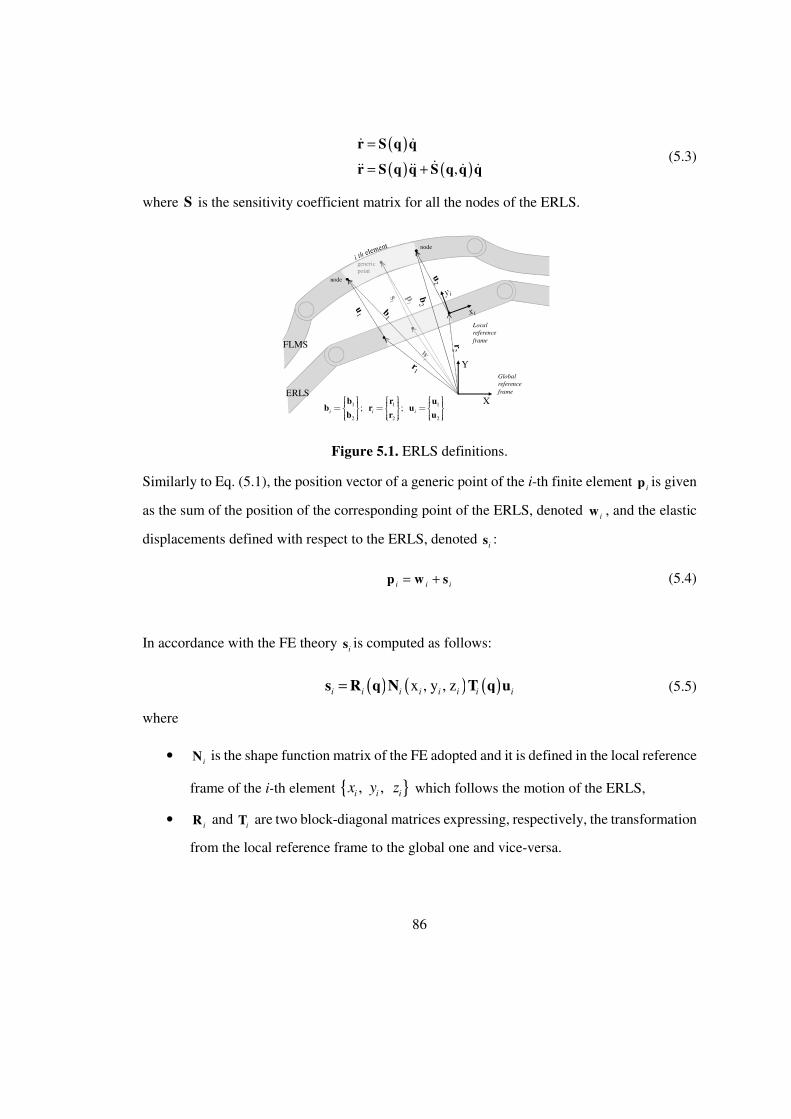
86

( )

( ) ( ),

=

= +

r S q q

r S q q S q q q

ɺ ɺ

ɺɺɺ ɺɺ ɺ ɺ (5.3)

where S is the sensitivity coefficient matrix for all the nodes of the ERLS.

Figure 5.1. ERLS definitions.

Similarly to Eq. (5.1), the position vector of a generic point of the i-th finite element ip is given

as the sum of the position of the corresponding point of the ERLS, denoted iw , and the elastic

displacements defined with respect to the ERLS, denoted is :

i i i= +p w s (5.4)

In accordance with the FE theory is is computed as follows:

( ) ( ) ( )x , y , zi i i i i i i i=s R q N T q u (5.5)

where

• iN is the shape function matrix of the FE adopted and it is defined in the local reference

frame of the i-th element { }, , i i ix y z which follows the motion of the ERLS,

• iR and

iT are two block-diagonal matrices expressing, respectively, the transformation

from the local reference frame to the global one and vice-versa.

FLMS

ERLSX

Y

Local

reference

frame

Global

reference

frame

1 1 1

2 2 2

; ; i i i

= = =

b r ub r u

b r u

node

node

genericpoint

87

A schematic representation of such kinematic definitions is provided in Figure 5.1: a planar case

with two-node elements is considered to simplify the drawing.

Let u be the vector collecting the elastic displacement of all the nodes, and analogously let b

be the vector of the position of all the nodes of the FLMS. Equations (5.1) and (5.3) lead to the

following expression that holds in the case of infinitesimal nodal displacements db , dr , and

du :

[ ]d

d d dd

= + =

ub r u I S

q (5.6)

where I is the identity matrix. The resulting matrix [ ]I S is not square since it has 'un rows

and 'u qn n+ columns, with 'un and qn being the numbers of the elastic dofs and of the ERLS

generalized coordinates respectively. This means that the linear system in Eq. (5.6) is

underdetermined and hence any arbitrary given configuration db corresponds to infinitely many

sets of { }TT T

d du q . In order to overcome such an issue, matrix [ ]I S should be made square

by forcing to zero qn elements of u . In this way, if the resulting matrix is not singular for all

the configurations of the mechanism, the system in Eq. (5.6) is determined and hence the

position of the ERLS is defined univocally with respect to the actual deformed mechanism.

Let du be partitioned into its independent part ( 'u u qn n n

ind= −

∈u ℝ ) and into its zeroed part (

0qn

d ∈u ℝ ) and let S be accordingly partitioned into inS and 0S , then Eq. (5.6) can be rewritten

as:

0

in indd

d

=

I S ub

0 S q (5.7)

Hereafter, the subscript in will be omitted and symbol u will have the meaning of independent

elastic coordinates.

88

5.2.2. The nonlinear model

The governing equations of motion are obtained by expressing the dynamic equilibrium of the

system through the principle of virtual work by splitting the total virtual work into the elemental

contributions:

( )T T T T T

i i ii i i i i i i i

v v vi i i

dv dv dvδ ρ δ δ ρ δ δ+ = + +∑ ∑ ∑∫ ∫ ∫p p ε D ε p g u r vɺɺ (5.8)

where:

• iε is the strain vector for the i-th element;

• iD is the stress-strain matrix for the i-th element;

• iρ is the mass density for the i-th element;

• g is the gravity acceleration vector;

• v is the vector of the concentrated external forces and torques;

• δu and δr refer to the virtual displacements of all the nodes of the model.

The final expression of the system equations of motion is given by the following set of nonlinear

ordinary differential equations (ODEs):

{ }

( ) ( )

( ) ( )

( )( )

( )

T T T T

G

T

t t

t t

tt

t

α β

α

− +

+ =

e e e e e e

e e e e

e

S u u2 + + S

S S S q qS (2 + ) S S

0 u Iv

0 0 q S

ɺɺɺ ɺ

ɺɺɺ ɺ

M M M M K M

M M M M M

K (5.9)

In Eq. (5.9), matrix ( )G G= q,qɺM M represents the centrifugal and Coriolis effects of all the

elements, while ( )=e e

qM M and ( )=e e

qK K are the matrices obtained assembling the

consistent mass and stiffness matrices of all the FEs. In Eq. (5.9) damping is modelled by means

of the Rayleigh coefficients α and β .The presence of the off-diagonal terms in the matrices in

Eq. (5.9) clearly highlights the coupling between the ERLS generalized coordinates and the

elastic displacements. Hence, the dynamic behaviour of the ERLS is not assumed independent

from vibration and vice-versa, and the ERLS position is set by the elastic behaviour of the

mechanism.

89

5.2.3. The linearized model

Even if the dynamics of flexible link mechanisms and manipulators is nonlinear, it is widely

recognized that linearized models are very satisfactory in the case of small deformations about

operating points and can be successfully used in the synthesis of control schemes and state

observers [79]. On the other hand, linear models represented through ODEs allow for the

straightforward application of the modal analysis. Hence, updating the model of a FLMS by

means of linearized model is an effective mean for the identifications of the parameters of the

non-linear model, which is instead not suitable for the modal analysis.

As for the use of ODEs for the model synthesis, despite the large use of differential algebraic

equations (DAEs) for modelling FLMSs, it is again justified by the possibility to employ the

modal analysis. Indeed, models employing DAEs, which are formulated through second-order

ordinary differential equations coupled to a set of algebraic constraint equations, do not allow

for such a kind of analysis. More complicate and computational challenging methods should be

therefore adopted to handle this kind of mathematical formulation [80].

In order to linearize the model, let us consider small displacements about a static equilibrium

configuration, which is set by the equilibrium configuration of the ERLS qe. Then the following

linear model is obtained by just considering the first-order terms of the Taylor’s expansion:

{ }

( ) ( )

( ) ( )

( )d( ) d

( )d dq

e e

e

e

T T T

T TT

t t

t t

t

t

α β

α≡ ≡

≡

≡

+

+ = − ⊗ ⊗

e e e e

e e eq q q q

e

e

e q q

q q

S + 0u u

S S S S 0q q

0u I

vS S0 g + v q S

q

ɺɺ ɺ

ɺɺ ɺ

M M M K

M M M

K

M

(5.10)

In Eq. (5.10), the matrices eM , S,

eK and the derivatives d( ) dT

eS qM and d dTS q are

computed about the equilibrium configuration. The term T(d d ) ⊗ eS q v represents the inner

product of matrix ,1 ,[ ]i j i n jS q S q∂ ∂ ∂ ∂⋯ with vector e

v , for all the subscripts i, j (obvious

extension to (d( ) d )T ⊗eS q gM ).

90

Since model updating should be performed by investigating the system in a stable equilibrium

configuration, gravity forces should be compensated in the experimental analysis whenever the

mechanism lies in the vertical plane. Indeed, the absence of a stable equilibrium would make

the mechanism diverge from the initial configuration after the excitation and therefore the

system dynamics would not meet the hypothesis of the linearized model. One of the possible

approaches is to balance gravity force through tuned external springs that determine asymptotic

stability of the equilibrium point. Clearly, springs should be then included in the stiffness matrix

of the model. In contrast the use of brakes, such as those of the actuators, modifies the boundary

conditions and makes the mechanism behave as a structure by removing all the model terms

representing the coupling between the ERLS and the elastic displacements. Therefore model

updating may lead to less reliable results.

5.3. Data consistency between model and experimental modal analysis

5.3.1. Size compatibility between the FE model and the measurements

Model updating requires one-to-one correspondence between the model coordinates and

measurement data. From a practical view point this requirement is usually not satisfied because

of the reduced number of sensors used in the experimental measurements and the presence of

some inaccessible locations. Additionally, rotational dofs cannot be easily measured. Thus, the

displacement vector of the experimental data is usually not compatible with the FE model of

the FLMS and hence, as a preliminary step before the model updating, it should be properly

modified.

The most suitable approach, that is the one adopted in this work, is expanding the experimental

data to match the dimension of the FE model [76, 81, 82]. The use of curve fitting, by means of

the shape functions of the FEs, is for example an effective and simple way.

5.3.2. Data representation from the physical reference frame to the ERLS reference

frame

The second relevant issue that should tackled is the transformation of the measured eigenvectors

from the reference adopted to measure the mode shapes, which is physical, to the fictitious one

91

adopted in the ERLS-based FE model. Indeed, the sensors employed to perform experimental

modal analysis tests, such as for example the accelerometers, typically provide measurements

with respect to local reference frames corresponding to the mechanism in its initial static

configuration. Conversely the displacement vector of the FLMS model (u) includes the elastic

displacements with respect to the ERLS and expressed in a global reference frame. Hence, in

accordance with Eq. (5.7) and with the final model in Eq. (5.10), some of the elastic

displacements are forced to zero to make the ERLS follow the actual elastic mechanism. At the

same time, the ERLS coordinates should be included in the displacement vector and therefore

in the eigenvectors.

Let eq be the static equilibrium configuration corresponding to the actual position of the

mechanism, adopted for both the experimental modal analysis and the model linearization. Let

us assume that the mechanism is vibrating in accordance with the i-th mode about the

equilibrium configuration. The absolute position of the nodes of the FEM, denoted ib , can be

represented both through the eigenvector defined in the physical frame adopted for the

experimental analysis, iη , and through the one defined with the model coordinates,

iη . If ib is

defined in a global frame, the eigenvector measured in the physical frame should be rotated

onto the global reference frame through the ERLS kinematic constraint equations:

( ) ( )i e e i= +b r q Θ q η (5.11)

r is the vector of the nodal position of the FLMS in the configuration set by eq , while Θ is a

block transformation matrix which depends on the rigid-body kinematic constraints.

If, in contrast, the same configuration is represented through the eigenvector of the linearized

model iη expressed with respect to the ERLS at configuration

i e= + ∆q q q , the following

relation holds

( )i i i= +b r q η (5.12)

where ( )ir q is the vector of the nodal position of the ERLS in the configuration set by iq . The

displacement of the ERLS generalized coordinates ∆q represents the rotation of the ERLS

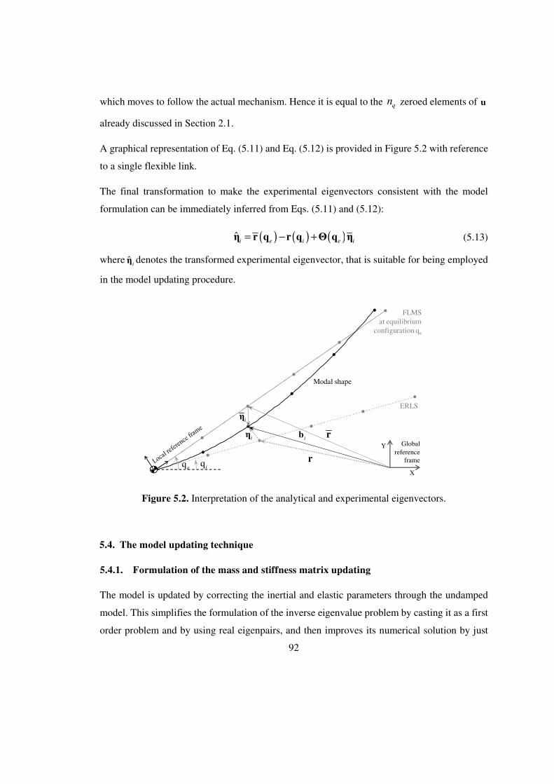
92

which moves to follow the actual mechanism. Hence it is equal to the qn zeroed elements of u

already discussed in Section 2.1.

A graphical representation of Eq. (5.11) and Eq. (5.12) is provided in Figure 5.2 with reference

to a single flexible link.

The final transformation to make the experimental eigenvectors consistent with the model

formulation can be immediately inferred from Eqs. (5.11) and (5.12):

( ) ( ) ( )ˆi e i e i= − +η r q r q Θ q η (5.13)

where ˆiη denotes the transformed experimental eigenvector, that is suitable for being employed

in the model updating procedure.

Figure 5.2. Interpretation of the analytical and experimental eigenvectors.

5.4. The model updating technique

5.4.1. Formulation of the mass and stiffness matrix updating

The model is updated by correcting the inertial and elastic parameters through the undamped

model. This simplifies the formulation of the inverse eigenvalue problem by casting it as a first

order problem and by using real eigenpairs, and then improves its numerical solution by just

FLMS at equilibrium

configuration qe

ERLS

Modal shape

X

Yiη

iη

r

r

qe

qi

ib

Globalreference

frame

93

handling real numbers. The use of the undamped models is widely adopted in structural

dynamics and is justified by the negligible internal damping of the beams and of the low friction

of the joints. Hence, the identification of the Rayleigh coefficients can be performed separately,

through the well established methods [83, 84], once the inertial an elastic parameters have been

updated.

The linearized undamped model in Eq. (5.10) is represented through the mass O N N×∈M ℝ and

the stiffness O N N×∈K ℝ matrices, which are the initial (nominal) system matrices based on the

nominal inertial and elastic parameters (N is number of model dofs, including both rigid and

elastic coordinates: q uN n n= + ). The updating of the model matrices is here represented

through the additive correction matrices, the so called updating matrices N N×∈ΔM ℝ and

N N×∈ΔK ℝ which collect the parameters that are affected by uncertainty and hence should be

corrected. The topology of the updating matrices depends on the topology of MO and KO. The

following representations are therefore proposed for ΔM and ΔK :

1 1 1 1

; m m k mN N N NO O

j j h hO Oj j h hj h

m km k= = = =

∂ ∂= = ∆ = = ∆

∂ ∂ ∑ ∑ ∑ ∑

M KΔM ΔM ΔK ΔK (5.14)

jΔM and hΔK are the updating sub-matrices related to each updating parameter O

jm or O

hk

that should be updated through the additive corrections jm∆ and hk∆ .

; O O

j j j h h hm m m k h k= + ∆ = + ∆ (5.15)

Hence, the mass and stiffness matrices of the N-dimensional updated model are O +M ΔM and

O +K ΔK . Finally, Nm and Nk denote the number of parameters that can be updated in the mass

and stiffness matrix, respectively.

In order to improve the numerical conditioning of the problem by tackling the different scaling

of the inertial and elastic parameters, dimensionless corrections jm and hk are defined and

hereafter adopted in the updating:

; j h

j hO O

j h

m km k

m k

∆ ∆= = (5.16)

94

For those O

jm or O

hk whose value is zero in the nominal model, the reference value might be

defined as the upper bound of their allowed modifications. Nonetheless other arbitrary, though

reasonable, reference numbers can be assumed. All the variables jm and hk are collected in the

( )m kN N+ -dimensional vector of the updating parameters T1 1{ }

m kN Nm m k k=χ … … ,

which collects all the problem unknown.

By taking advantage of the definitions in Eqs. (5.14), (5.15) and (5.16), the updating matrices

can be written as follows:

1 1 1 1

: ; :m m k kN N N NO O

O O

j j j j h h h hO Oj j h hj h

m m m k k km k= = = =

∂ ∂= = = =

∂ ∂ ∑ ∑ ∑ ∑

M KΔM A ΔK B (5.17)

where the sub-matrices jA and hB have been introduced for brevity of notation. The partial

derivatives in Eq. (5.17) are constant whenever Young’s modulus, mass density, nodal masses,

nodal inertias, sectional area or lumped springs should be updated. In contrast, if some m or k

represent the length of the beams, the derivatives are not constant and therefore iterations should

be made in the updating procedure. However, it is often reasonable assuming the beam length

as a known and exact parameter.

5.4.2. Constraints on the updating parameters

The correction of the model parameters should be also bounded to ensure physical meaning of

the numerical solution and to avoid unreasonable solutions. Hence, lower and upper bounds on

the single variables (denoted respectively Lχ and Uχ ) and on combinations of more variables

(such as on the total mass) should be defined. The latter type of constraint is defined through a

convex polyhedron (by means of a matrix G and a vector γ ). These two types of constraint

define the following convex feasible set Γ (where the inequalities are element-wise):

( ){ }L U|Γ = ≤ ≤ ∩ ≤χ χ χ χ Gχ γ (5.18)

95

5.4.3. Formulation of the model updating problem

On the basis of the model assumed for representing the updating matrices, the following

eigenvalue problem must hold for any measured eigenpairs ( )2ˆ ˆ, , 1, ,i i i nω =η … , where n N≤

is the number of measured vibrational modes and ˆiω is the natural frequency associated to the

eigenvector ˆiη :

2ˆ ˆ ˆO O

i i iω + − + = M ΔM η K ΔK η 0 (5.19)

Any arbitrary normalization of the measured eigenvectors can be adopted.

By introducing the representation of the updating matrices given in Eq. (5.17) and pre-

multiplying by Tˆiη , the eigenvalue problem related to each eigenpair can be written as a scalar

equation, which is a linear problem in the unknown{ },j hm k :

2 2

1 1

ˆ ˆ ˆ ˆ ˆ ˆ 0m kN N

T O O T T

i i i i i j i j i h i h

j h

m kω ω= =

− + − = ∑ ∑η M K η η A η η B η (5.20)

Equation (5.20) can be represented in the typical compact form of a linear algebraic system

through the vector ia , which collects the known coefficients, and the scalar

2ˆ ˆ ˆT O O

i i i ib ω = − − η M K η which is the known term:

0i ib− =a χ (5.21) Since the problem unknowns are constrained by the feasible set Γ and the condition in Eq.

(5.21) should be simultaneously satisfied for all the measured eigenpairs ( 1, ,i n= … ), an exact

solution might not exist. Hence the problem should be approximated as a 2-norm minimization

problem (least square minimization):

( )2

2min −W Aχ b (5.22)

( )m kn N N× +∈A ℝ and n∈b ℝ collect the terms of each eigenvalue problem in Eq. (5.21): the rows

of matrix A are the vectors ia while the entries of b are the scalar coefficients

ib . The diagonal

matrix n n×∈W ℝ is defined to weight the residual of each eigenvalue problem through the

96

positive and scalar weights wi, with 1, ,i n= … . The introduction of the weighing matrix has

several practical advantages. Indeed it allows to give less importance to those eigenpairs whose

measurements are less reliable, e.g. because of the presence of noise or uncertainty, as well as

to give higher importance to the vibrational modes that are more observable and controllable

and hence provide more relevant contributions to the forced response.

The numerical solution of the minimization problem should be improved through

preconditioning to compensate for the simultaneous presence of low-frequency and high-

frequency modes. The use of the pseudo-inverse matrix (denoted with the superscript † ) as the

preconditioner allows to write the system in Eq. (5.22) in the following equivalent form, whose

condition number is one:

[ ]2†

2min −χ WA Wb (5.23)

Finally, regularization can be adopted to penalize selectively the components of χ [85]. Indeed,

some model parameters might be more uncertain than the others and therefore it is more

desirable the updating procedure to modify them. Therefore, the term 2

2λ Ωχ is added to the

minimization problem in Eq. (5.23). The scalar value λ is named the regularization parameter

and trades-off between the cost of missing the eigenpair specifications (i.e. Eq. (5.21)) and the

cost of using large values of the design variables (i.e. 2

2χ ). The positive-definite real matrix

( ) ( )m k m kN N N N+ × +∈Ω ℝ is the regularization operator and can be adopted to define the relative

weight between the updates of the different model parameters.

The model updating problem is therefore finally represented as the following constrained

minimization problem:

[ ]

2†

2

minλ

−

∈Γ

χ

I WA Wbχ

Ω 0

χ

(5.24)

Both the objective function and the feasible domain are convex. Hence model updating is cast

as a convex, constrained minimization problem whose solution is straightforward. Indeed the

97

problem convexity ensures that the global optimal solution can be found regardless of the

selection of the initial guess required by the numerical minimization. In addition, several

reliable and efficient numerical algorithms are available in commercial software.

5.5. Experimental validation

5.5.1. Description of the experimental setup

The model updating strategy proposed has been applied to the manipulator with flexible links

shown in Figure 5.3(a). Such a manipulator consists of five rods with circular cross-sections

made of Aluminum Anticorodal. The links are connected to each other by means of revolute

joints, created by means of double ball bearings with negligible clearance and friction losses,

inserted in Aluminum housings. A hybrid serial-parallel kinematic topology is obtained. Links

1, 2 and 5 are driven by three brushless motors. The mechanism is equipped with two balancing

springs, modelled as a single lumped spring, which are employed to reduce the static torque

required by the servomotors to compensate for gravity force.

All the links have been modelled with two-node and six-degree-of-freedom Euler-Bernoulli's

beam elements to represent the planar motion of the mechanism, overall nine beam elements

have been adopted (see Figure 5.3(b)). Lumped masses and nodal inertias have been adopted to

represent the joints and the motors. The resulting model has 27 elastic dofs and three ERLS

generalized coordinates { }T

1 2 3q q q=q , which are the absolute rotations of the actuators.

The rigid moving reference is then defined by forcing the ERLS to coincide with the actual

flexible mechanism at the rotation of these three joints. Hence, three elastic displacements with

respect to the ERLS are forced to zero in the FLMS model, in order to place correctly the

moving reference defined by the equivalent rigid mechanism (see Section 2 for the theoretical

discussion of this issue).

Model updating has been done by investigating the mechanism in the stable equilibrium

configuration, where gravity forces are exactly compensated by the balancing force exerted by

the two external springs, which corresponds to { }T

1.0821 2.6354 4.7123 [ ]e rad=q .

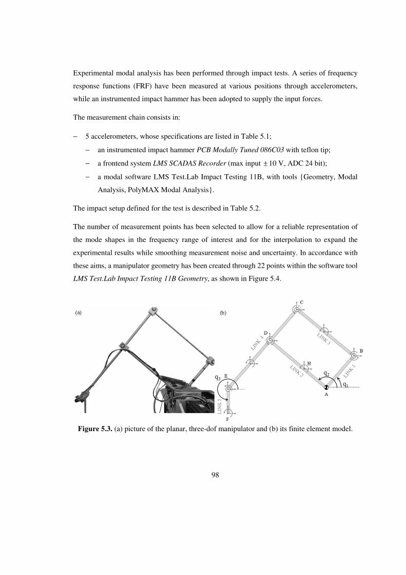
98

Experimental modal analysis has been performed through impact tests. A series of frequency

response functions (FRF) have been measured at various positions through accelerometers,

while an instrumented impact hammer has been adopted to supply the input forces.

The measurement chain consists in:

− 5 accelerometers, whose specifications are listed in Table 5.1;

− an instrumented impact hammer PCB Modally Tuned 086C03 with teflon tip;

− a frontend system LMS SCADAS Recorder (max input ± 10 V, ADC 24 bit);

− a modal software LMS Test.Lab Impact Testing 11B, with tools {Geometry, Modal

Analysis, PolyMAX Modal Analysis}.

The impact setup defined for the test is described in Table 5.2.

The number of measurement points has been selected to allow for a reliable representation of

the mode shapes in the frequency range of interest and for the interpolation to expand the

experimental results while smoothing measurement noise and uncertainty. In accordance with

these aims, a manipulator geometry has been created through 22 points within the software tool

LMS Test.Lab Impact Testing 11B Geometry, as shown in Figure 5.4.

Figure 5.3. (a) picture of the planar, three-dof manipulator and (b) its finite element model.

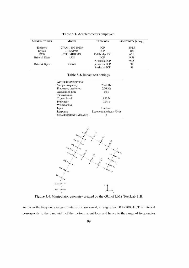
99

Table 5.1. Accelerometers employed.

MANUFACTURER

Endevco Dytran PCB

Brüel & Kjær

Brüel & Kjær

MODEL

27AM1-100 10203 3136A1945

3741D4HB30G 4508

4506B

TYPOLOGY

ICP ICP

Full bridge DC ICP

X-triaxial ICP Y-triaxial ICP Z-triaxial ICP

SENSITIVITY [mV/g ]

102.4 100 66.7 9.78 93.5 94 98

Table 5.2. Impact test settings.

ACQUISITION SETTING

Sample frequency Frequency resolution Acquisition time TRIGGERING

Trigger level Pretrigger WINDOWING

Input Response MEASUREMENT AVERAGES

2048 Hz 0.06 Hz

16 s

5.72 N 0.01 s

Uniform

Exponential (decay 90%) 3

Figure 5.4. Manipulator geometry created by the GUI of LMS Test.Lab 11B.

As far as the frequency range of interest is concerned, it ranges from 0 to 200 Hz. This interval

corresponds to the bandwidth of the motor current loop and hence to the range of frequencies

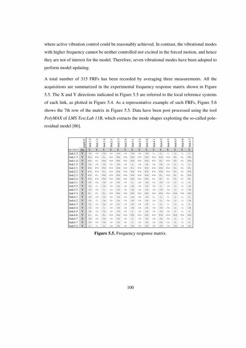
100

where active vibration control could be reasonably achieved. In contrast, the vibrational modes

with higher frequency cannot be neither controlled nor excited in the forced motion, and hence

they are not of interest for the model. Therefore, seven vibrational modes have been adopted to

perform model updating.

A total number of 315 FRFs has been recorded by averaging three measurements. All the

acquisitions are summarized in the experimental frequency response matrix shown in Figure

5.5. The X and Y directions indicated in Figure 5.5 are referred to the local reference systems

of each link, as plotted in Figure 5.4. As a representative example of such FRFs, Figure 5.6

shows the 7th row of the matrix in Figure 5.5. Data have been post processed using the tool

PolyMAX of LMS Test.Lab 11B, which extracts the mode shapes exploiting the so-called pole-

residual model [86].

Figure 5.5. Frequency response matrix.

INP

UT

link1

:2

link1

:3

link1

:4

link2

:1

link2

:3

link2

:4

link3

:1

link3

:2

link3

:4

link4

:1

link4

:2

link4

:3

link4

:5

link4

:6

link4

:7

OUTPUT Dir Y Y Y Y Y Y Y Y Y Y Y Y Y Y Ylink1:2 Y -\+ -\+ -\+ -\+ -\+ -\+ -\+ -\+ -\+ -\- -\- -\- -\- -\- -\-link1:3 Y +\+ +\+ +\- +\+ +\+ +\+ +\+ +\+ +\+ +\+ +\+ +\+ +\- +\- +\+link1:4 Y +\+ +\- +\+ +\+ +\+ +\+ +\+ +\+ +\+ +\+ +\- +\+ +\- +\- +\+link1:5 Y -\+ -\+ -\+ -\+ -\+ -\+ -\- -\+ -\+ -\+ -\+ -\+ -\- -\- -\-link2:1 Y +\+ +\+ +\+ +\+ +\+ +\+ +\- +\+ +\+ +\+ +\+ +\+ +\- +\- +\-link2:2 Y +\+ +\+ +\- +\+ +\+ +\+ +\+ +\+ +\+ +\+ +\+ +\+ +\- +\- +\+link2:3 Y +\+ +\- +\+ +\+ +\+ +\+ +\+ +\+ +\+ +\+ +\- +\+ +\- +\- +\+link2:4 Y +\+ +\+ +\+ +\+ +\+ +\+ +\+ +\+ +\+ +\- +\- +\- +\- +\- +\-link3:1 Y -\+ -\+ -\+ -\+ -\+ -\+ -\- -\+ -\+ -\+ -\+ -\+ -\- -\- -\-link3:2 Y -\+ -\- -\+ -\+ -\+ -\+ -\+ -\+ -\+ -\+ -\- -\+ -\- -\- -\+link3:3 Y -\+ -\+ -\- -\+ -\+ -\+ -\+ -\+ -\+ -\+ -\+ -\+ -\- -\- -\+link3:4 X +\- +\- +\- +\+ +\+ +\+ +\+ +\+ +\+ +\+ +\+ +\+ +\+ +\+ +\+link4:1 Y -\+ -\+ -\+ -\+ -\+ -\+ -\+ -\+ -\+ -\- -\- -\- -\- -\- -\-link4:2 Y -\+ -\- -\+ -\+ -\+ -\+ -\+ -\+ -\+ -\+ -\- -\+ -\- -\- -\+link4:3 Y -\+ -\+ -\+ -\+ -\+ -\+ -\+ -\+ -\+ -\- -\- -\- -\- -\- -\-link4:4 Y -\+ -\+ -\- -\+ -\+ -\+ -\+ -\+ -\+ -\+ -\+ -\+ -\- -\- -\+link4:5 Y -\+ -\+ -\+ -\+ -\+ -\+ -\- -\+ -\+ -\+ -\+ -\+ -\- -\- -\-link4:6 Y +\- +\- +\- +\+ +\+ +\+ +\+ +\+ +\+ +\+ +\+ +\+ +\+ +\+ +\+link4:7 X -\+ -\+ -\+ -\+ -\+ -\+ -\- -\+ -\+ -\+ -\+ -\+ -\- -\- -\-link4:7 Y -\+ -\+ -\+ -\+ -\+ -\+ -\- -\+ -\+ -\+ -\+ -\+ -\- -\- -\-link5:2 Y -\- -\- -\- -\+ -\+ -\+ -\+ -\+ -\+ -\+ -\+ -\+ -\+ -\+ -\+

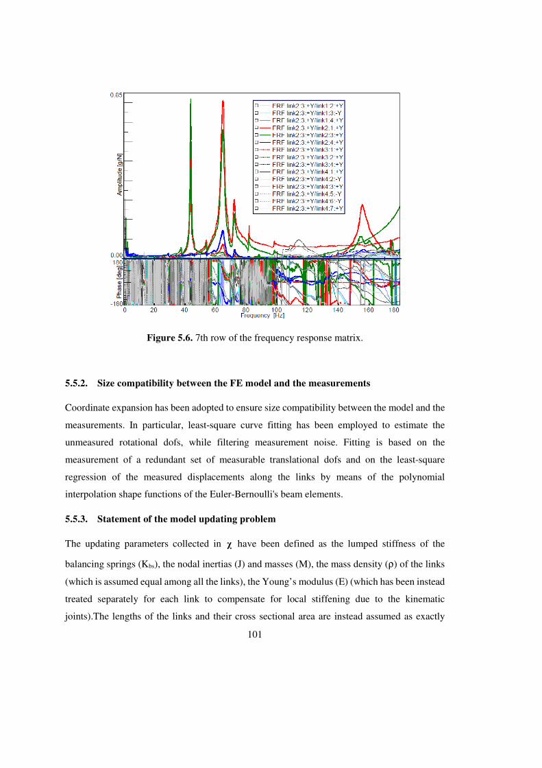
101

Figure 5.6. 7th row of the frequency response matrix.

5.5.2. Size compatibility between the FE model and the measurements

Coordinate expansion has been adopted to ensure size compatibility between the model and the

measurements. In particular, least-square curve fitting has been employed to estimate the

unmeasured rotational dofs, while filtering measurement noise. Fitting is based on the

measurement of a redundant set of measurable translational dofs and on the least-square

regression of the measured displacements along the links by means of the polynomial

interpolation shape functions of the Euler-Bernoulli's beam elements.

5.5.3. Statement of the model updating problem

The updating parameters collected in χ have been defined as the lumped stiffness of the

balancing springs (Kbs), the nodal inertias (J) and masses (M), the mass density (ρ) of the links

(which is assumed equal among all the links), the Young’s modulus (E) (which has been instead

treated separately for each link to compensate for local stiffening due to the kinematic

joints).The lengths of the links and their cross sectional area are instead assumed as exactly

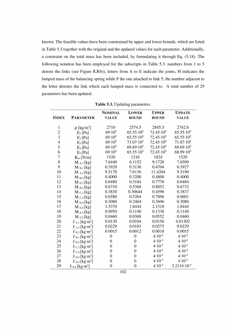
102

known. The feasible values have been constrained by upper and lower bounds, which are listed

in Table 5.3 together with the original and the updated values for each parameter. Additionally,

a constraint on the total mass has been included, by formulating it through Eq. (5.18). The

following notation has been employed for the subscripts in Table 5.3: numbers from 1 to 5

denote the links (see Figure 5.3(b)), letters from A to E indicate the joints, H indicates the

lumped mass of the balancing spring while F the one attached to link 5; the number adjacent to

the letter denotes the link which each lumped mass is connected to. A total number of 29

parameters has been updated.

Table 5.3. Updating parameters.

INDEX

1 2 3 4 5 6 7 8 9

10 11 12 13 14 15 16 17 18 19 20 21 22 23 24 25 26 27 28 29

PARAMETER

ρ [kg/m3]

E1 [Pa] E2 [Pa] E3 [Pa] E4 [Pa] E5 [Pa]

Kbs [N/m] M A,1 [kg] M B,1 [kg] M A,2 [kg] M H,2 [kg] M D,2 [kg] M B,3 [kg] M C,3 [kg] M C,4 [kg] M D,4 [kg] M E,4 [kg] M E,5 [kg] M F,5 [kg]

J A,1 [kg∙m2] J A,2 [kg∙m2] J E,5 [kg∙m2] J B,1 [kg∙m2] J B,3 [kg∙m2] J C,3 [kg∙m2] J C,4 [kg∙m2] J D,4 [kg∙m2] J D,2 [kg∙m2]

J E,4 [kg∙m2]

NOMINAL

VALUE

2710

69∙109 69∙109 69∙109 69∙109 69∙109 1520

7.6440 0.3920 9.5170 0.4000 0.6480 0.6710 0.3830 0.6580 0.3080 1.5370 0.0950 0.0460 0.0130 0.0229 0.0015

0 0 0 0 0 0 0

LOWER

BOUND

2574.5

65.55∙109 65.55∙109 71.07∙109 69.69∙109 65.55∙109

1216 6.1152 0.3136 7.6136 0.3200 0.5184 0.5368

0.30644 0.5264 0.2464 1.8444 0.1140 0.0368 0.0104 0.0183 0.0012

0 0 0 0 0 0 0

UPPER

BOUND

2845.5

72.45∙109 72.45∙109 72.45∙109 72.45∙109 72.45∙109

1824 9.1728 0.4704

11.4204 0.4800 0.7776 0.8052 0.4596 0.7896 0.3696 2.1518 0.1330 0.0552 0.0156 0.0275 0.0018 4∙10-4 4∙10-4 4∙10-4 4∙10-4 4∙10-4 4∙10-4 4∙10-4

UPDATE

VALUE

2742.6

65.55∙109 65.55∙109 71.07∙109 69.69∙109 68.99∙109

1520 7.6509 0.3927 9.5190 0.4000 0.6484 0.6732 0.3837 0.6601 0.3080 1.8444 0.1140 0.0460

0.01302 0.0229 0.0015 4∙10-4 4∙10-4 4∙10-4 4∙10-4 4∙10-4 4∙10-4

3.2134∙10-4

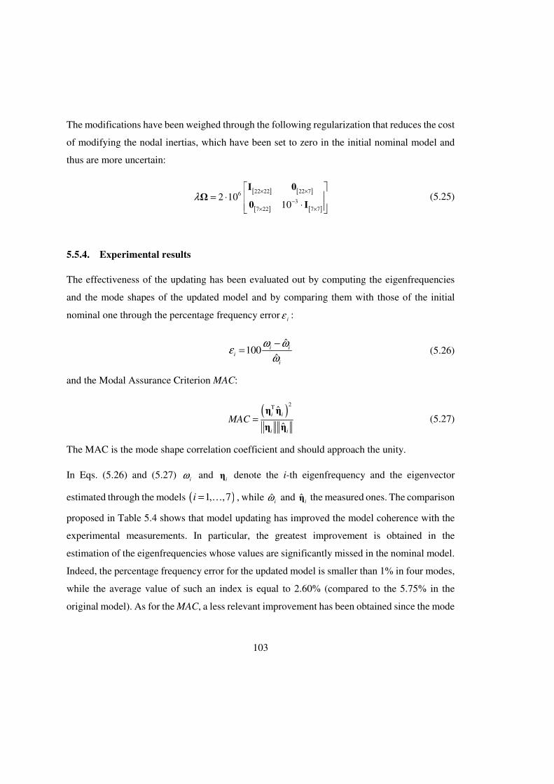
103

The modifications have been weighed through the following regularization that reduces the cost

of modifying the nodal inertias, which have been set to zero in the initial nominal model and

thus are more uncertain:

[ ] [ ]

[ ] [ ]

22 22 22 763

7 22 7 7

2 1010

λ× ×

−

× ×

= ⋅

⋅

I 0Ω

0 I (5.25)

5.5.4. Experimental results

The effectiveness of the updating has been evaluated out by computing the eigenfrequencies

and the mode shapes of the updated model and by comparing them with those of the initial

nominal one through the percentage frequency erroriε :

ˆ

100ˆ

i ii

i

ω ωε

ω

−= (5.26)

and the Modal Assurance Criterion MAC:

( )

2T ˆ

ˆi i

i i

MAC =η η

η η (5.27)

The MAC is the mode shape correlation coefficient and should approach the unity.

In Eqs. (5.26) and (5.27) iω and

iη denote the i-th eigenfrequency and the eigenvector

estimated through the models ( )1, ,7i = … , while ˆiω and ˆ

iη the measured ones. The comparison

proposed in Table 5.4 shows that model updating has improved the model coherence with the

experimental measurements. In particular, the greatest improvement is obtained in the

estimation of the eigenfrequencies whose values are significantly missed in the nominal model.

Indeed, the percentage frequency error for the updated model is smaller than 1% in four modes,

while the average value of such an index is equal to 2.60% (compared to the 5.75% in the

original model). As for the MAC, a less relevant improvement has been obtained since the mode

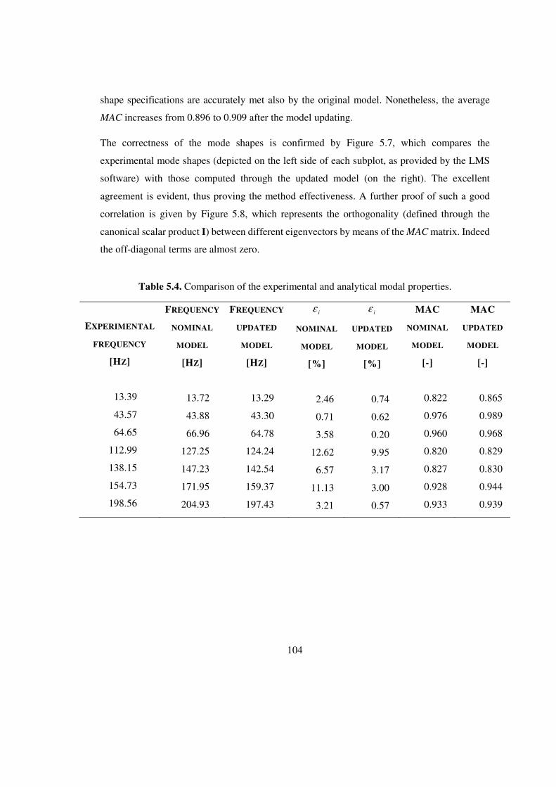
104

shape specifications are accurately met also by the original model. Nonetheless, the average

MAC increases from 0.896 to 0.909 after the model updating.

The correctness of the mode shapes is confirmed by Figure 5.7, which compares the

experimental mode shapes (depicted on the left side of each subplot, as provided by the LMS

software) with those computed through the updated model (on the right). The excellent

agreement is evident, thus proving the method effectiveness. A further proof of such a good

correlation is given by Figure 5.8, which represents the orthogonality (defined through the

canonical scalar product I) between different eigenvectors by means of the MAC matrix. Indeed

the off-diagonal terms are almost zero.

Table 5.4. Comparison of the experimental and analytical modal properties.

EXPERIMENTAL

FREQUENCY

[HZ]

13.39

43.57

64.65

112.99

138.15

154.73

198.56

FREQUENCY

NOMINAL

MODEL

[HZ]

13.72

43.88

66.96

127.25

147.23

171.95

204.93

FREQUENCY

UPDATED

MODEL

[HZ]

13.29

43.30

64.78

124.24

142.54

159.37

197.43

iε

NOMINAL

MODEL

[%]

2.46

0.71

3.58

12.62

6.57

11.13

3.21

iε

UPDATED

MODEL

[%]

0.74

0.62

0.20

9.95

3.17

3.00

0.57

MAC

NOMINAL

MODEL

[-]

0.822

0.976

0.960

0.820

0.827

0.928

0.933

MAC

UPDATED

MODEL

[-]

0.865

0.989

0.968

0.829

0.830

0.944

0.939

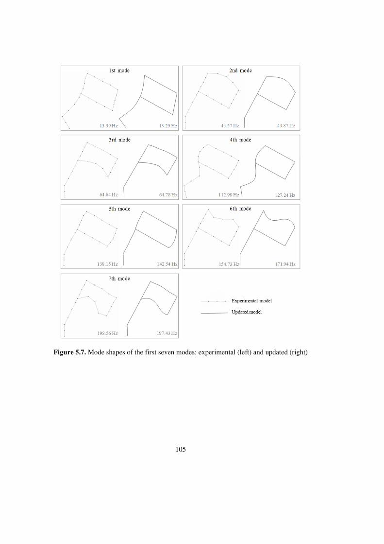
105

Figure 5.7. Mode shapes of the first seven modes: experimental (left) and updated (right)

106

Figure 5.8. MAC matrix between the experimental modes and the updated model modes

5.6. Conclusions

A strategy for updating models of flexible link mechanisms has been proposed and validated.

The system dynamics is represented through a nonlinear FE model which expresses the coupling

between the small elastic deformations and the large motion. The latter can be represented

through the rigid-body motion of an equivalent rigid-link system, named the ERLS, which is

assumed as a moving reference for defining the small elastic displacements and which is forced

to track the real flexible mechanism. The use of the ERLS simplifies the model formulation and

allows for the correct representation of the system dynamics, as long as the inertial and elastic

parameters are correctly tuned through model updating.

In order to perform model updating through modal analysis, the nonlinear model is linearized

about a stable equilibrium configuration where the experimental modal analysis is performed.

Then, the measured eigenvectors are transformed from the physical frame to the moving

reference defined by the ERLS, by means of the kinematic constraint equations of the rigid-link

mechanism and of the definition of the ERLS. Coordinate expansion is also adopted to meet the

size of the model and to estimate the elastic rotations.

The calculation of the update of the model parameters is cast as a constrained inverse eigenvalue

problem, whose solution can take advantage of several effective and reliable numerical methods

available in commercial software. Constraints on the single updating parameters and on

107

combination of more parameters define a feasible set, which ensures the physical meaning of

the computed values. The use of preconditioners and of the regularization also improves the

numerical reliability of the convex formulation proposed.

The proposed formulation has some strengths that make it suitable for the updating of these

complicate models:

• the method can handle an arbitrary number of eigenpairs and updating parameters;

• the experimental eigenvectors can have any arbitrary normalization;

• constraints assure the physical meaning of the updating;

• no iterations are required.

The method has been applied to a very challenging test: the model of a planar, six-bar linkage

mechanism with five flexible links. The model is updated to improve the representation of the

7 lowest frequency modes, within the range from 0 to 200 Hz. The experimental results obtained

are highly satisfactory, given the complexity of the system investigated, the simultaneous

presence of more eigenpairs to be matched, the unavoidable uncertainty in performing accurate

measurements in a mechanism (which has “rigid-body” motion) and the presence of constraints

bounding the parameter updating. Overall, a meaningful improvement in the eigenvector and

eigenfrequency estimation has been obtained.

108

109

Chapter 6. Partial pole placement 6.1. Introduction

The eigenvalues of a vibrating system, which are usually called poles in control theory, define

the frequency of the dynamic response, the damping ratio and the settling time. In fact, pole

placement is a widely employed technique for vibration control. The aim of pole placement is

to properly design a controller in such a way that the closed-loop poles are exactly the desired

complex numbers. In particular, in this Chapter it is addressed the case in which only one

independent control force is exerted on the system, that is known as rank-1 control. In practice,

the controlled system equations are

T T

u

u

+ + =

= − −

M C Kq q q b

f q g q

ɺɺ ɺ

ɺ (6.1)

where , , N N×∈M C K ℝ are, respectively, the mass, damping and stiffness matrices, N∈q ℝ is

the displacements vector, N∈b ℝ represents the distribution of the control forces and

, N∈f g ℝ are the control gains. Given a self-conjugate set of desired poles 1 2, , Nµ µ… ∈ℂ , the

aim of pole placement is to find such values for f and g that the closed-loop poles are exactly

the prescribed ones. It can be proved that a solution exists if and only if

2rank |i i Nλ λ + + = M C K b (6.2)

for all the open-loop poles iλ , , 21,i N= … . A system that satisfies this condition is said to be

controllable.

For what concerns gain computation, many methods have been proposed in the literature, thus

far. A groundbreaking advancement in this field is constituted by the method [36] that relies

only on the receptances of the system, rather than on the usual state-space model. The

receptance formulation has been later applied to suppression of friction-induced vibration [87],

robust pole placement [88], control of flexible link mechanisms [89] and more.

110

Another significant progress is represented by the methods for partial pole placement, that

consist in the assignment of an incomplete set of poles, that is 1, , pµ µ… with 2p N< . Such a

necessity is motivated by the fact that often only few dominant poles characterize the dynamics

of the system, thus it is advantageous to modify only the most important poles. In such a way,

the order of the problem can be considerably reduced, with a great benefit in numerical

computation, which is critical for large-scale systems. The difficulty in partial pole placement

relies in the fact that if the assignment of p poles changes appreciably the remaining 2N p−

ones, the closed-loop system can behave unexpectedly, in some cases even exhibiting

instability. Typically, this issue is overcome using conditions that assure that the 2N p− open-

loop poles are retained in the closed-loop configuration.

In some applications, however, the exact location of the poles is not a critical issue, as long as

poles are contained in suitable regions of the complex plane. Indeed, active control has been

also employed for such a task, that is usually referred to as regional pole placement. Notable

examples of this approach are [90, 91], in which Linear Matrix Inequalities are exploited. Such

a mathematical formulation allows to conveniently handle rather complicated specifications on

poles location.

In the present Chapter it is proposed a new method for control gain synthesis that enables to

perform exact pole placement of p poles, and regional pole placement of the remaining

2N p− ones. This problem has been solved for the control of power systems in [92, 93], but

such a method employs mathematical tools which are not numerically reliable (e.g. the

characteristic polynomial, the controllability matrix) and hence are not suitable for ill-

conditioned vibrating systems represented through medium or large dimensional matrices with

high condition number.

In this work, a new receptance based method for partial pole placement and a state-space method

for regional pole placement are combined. The capabilities of the proposed approach are

assessed in the design of a controller for a four-bar flexible link mechanism of the type described

in Chapter 5.

111

6.2. Description of the method

Let us consider the controlled system (6.1) and suppose that it is wanted to find such control

gains ,f g that the complex scalars 1, , pµ µ… , with 2p N≤ are closed-loop poles. The case

of complete pole placement, i.e. 2p N= , is addressed in [36], where it is defined

( )ii µ= Ht b (6.3)

with ( )12λ λ λ

− = + + C KH M being the receptance matrix, and then it is proposed to solve

the linear system

1 1

2 2

1

2

1

1.

1

T T

T T

T T

p pp

µ

µ

µ

− − =

−

t t

t t f

g

t t

⋮ ⋮ ⋮ (6.4)

If 2p N= , the matrix

1

2 2

1

2

1

p

T T

T T

T T

p p

µ

µ

µ

=

T

t t

t t

t t

⋮ ⋮ (6.5)

is a square matrix and, under mild assumptions specified in [36], it is invertible, hence the

solution of (6.4) exists, it is real and unique.

If 2p N< , the matrix T is rectangular and the system (6.4) is underdetermined. Without loss

of generality, it can be assumed that ( )rank p=T thus the solutions can be represented as

0

0

,r

= +

V

ffk

gg (6.6)

where { } 20 0

TT T N∈f g ℝ is a particular solution of (6.4), V is a ( )2 2N N p× − matrix whose

columns span ( )ker T and 2r

N p−∈k ℝ is a vector of parameters that are to be determined. The

particular solution { }0 0

TT T

f g can be computed either solving a least-squares problem, or

112

arbitrarily adding 2N p− rows to T , corresponding to as many poles, which must be

judiciously chosen to make the matrix invertible. In the first case, the explicit solution is

( )10

0

1

1.

1

T T−

− −

=

−

T T Tf

g ⋮ (6.7)

Regardless of how { }0 0

TT T

f g is computed, it follows from [36] that for any choice of

2 ,r

N p−∈k ℝ the control gains ,f g computed as in (6.6) lead to a closed-loop system featuring

the poles 1 ,, pµ µ… .

The aim of the following sections is to cast the condition of the remaining 2N p− poles to

belong to certain regions of the complex plane in a computationally sound way and to explain

how to choose properly the parameter vector rk to assure that such a condition is fulfilled.

6.2.1. Linear Matrix Inequalities

The most suitable mathematical tool for regional pole placement is constituted by Linear Matrix

Inequalities (or LMIs). In order to exploit LMIs it is necessary to recast the system model in a

first-order state-space form, namely

.u= +A Bx xɺ (6.8)

The chief advantage of the LMIs is that they allow a characterization of the desired constraints

that is linear in the state matrix A . Other representations, such as [94], are polynomial and

hence not necessarily convex. A brief explanation of Linear Matrix Inequality theory is

provided in the present Section, whereas for the details it is suggested to refer to [91].

Let D be a subset of the complex plane. The system (6.8) is said to be D -stable if all its poles

belong to D . There is a class of regions for which there is a simple characterization of D -

stability: the LMI regions. ⊆ ℂD is a LMI region if there exist a symmetric matrix m m×∈R ℝ

and a matrix m m×∈S ℝ such that

( ){ }: 0z f z∈= ℂ ≺D

D (6.9)

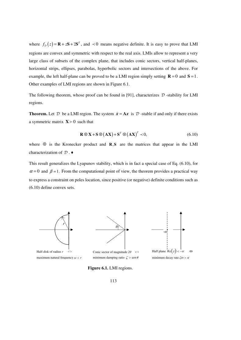
113

where ( ) Tz zf z = + +R S SD

, and 0≺ means negative definite. It is easy to prove that LMI

regions are convex and symmetric with respect to the real axis. LMIs allow to represent a very

large class of subsets of the complex plane, that includes conic sectors, vertical half-planes,

horizontal strips, ellipses, parabolas, hyperbolic sectors and intersections of the above. For

example, the left half-plane can be proved to be a LMI region simply setting 0=R and 1=S .

Other examples of LMI regions are shown in Figure 6.1.

The following theorem, whose proof can be found in [91], characterizes D -stability for LMI

regions.

Theorem. Let D be a LMI region. The system = Ax xɺ is D -stable if and only if there exists

a symmetric matrix 0X≻ such that

( ) ( ) 0,TT⊗ + ⊗ + ⊗R X S AX S AX ≺ (6.10)

where ⊗ is the Kronecker product and ,R S are the matrices that appear in the LMI

characterization of D . ♦

This result generalizes the Lyapunov stability, which is in fact a special case of Eq. (6.10), for

0α = and 1.β = From the computational point of view, the theorem provides a practical way

to express a constraint on poles location, since positive (or negative) definite conditions such as

(6.10) define convex sets.

Figure 6.1. LMI regions.

Conic sector of magnitude 2θ

minimum damping ratio

Half plane

minimum decay rate

Half-disk of radius r

maximum natural frequency

r

θ

-α

114

6.2.2. Control gain synthesis

The actual computation of the control gains ,f g that comply with the desired specifications is

the results of three stages: first of all, a state-space representation of the controlled system is

employed, then the system is reduced to take into account only the 2N p− poles whose

location is not exactly imposed, and finally the gains are computed solving an optimization

problem with LMI constraints.

The state-space representation that is suggested for the purpose is the very common first-order

model

T

u

u

= +

= −

A Bx x

k x

ɺ (6.11)

where

. − −

= = = =

-1 -1 -1M C M K M

A BI 0 0

q fbx k

q g

ɺ

In order to achieve the desired reduction, it is employed the non-invertible transformation

ˆ= Vx x , where 2ˆ N p−∈x ℝ is the state of the reduced system and V is defined in (6.6). Let

( )2 2N p N− ×∈U ℝ be the Moore-Penrose pseudoinverse of V , then since V has linearly

independent columns, U is its left inverse, that is 2 .N p−=UV I Hence the reduced system is

ˆ ˆ ˆ

ˆˆ .T

u

u

= +

= −

UAV UB

V

x x

k x

ɺ

(6.12)

The dynamics of the closed-loop system is described by the equation

ˆ ˆ ˆT= −UAV UB Vx x k xɺ (6.13)

and recalling that the control gains are wanted to satisfy (6.6), that is 0 r= + Vk k k , where

{ }0 0 0

TT T=k f g , the new control system becomes

( )

( )0

ˆ ˆ ˆ

ˆˆ .T

T

r

u

u

= − +

= −

U A B V UB

V V

x k x

k x

ɺ

(6.14)

115

For clarity, it is defined ( )0ˆ = −A U A B Vk , ˆ =B UB and ˆ T

r= V Vk k in such a way that the

system can be written as

ˆ ˆˆ ˆ ˆ

ˆ ˆˆ .T

u

u

= +

= −

A Bx x

k x

ɺ

(6.15)

The remarkable property of this system is that its closed-loop poles are exactly the 2N p−

non-assigned closed-loop poles of (6.11). This property will be further analysed in the next

Section.

The goal is to find a control gain k̂ such that the closed-loop poles of (6.15) lie in a prescribed

LMI region .D In practice, it is wanted that Eq. (6.10) holds for CLˆ ˆ ˆˆ T= −A A Bk . Substituting,

the matrix inequality becomes non-linear, in fact both k̂ and X are unknown and hence the

following

( ) ( )ˆ ˆ ˆ ˆˆ ˆT TT

T⊗ + ⊗ ⊗− −+R X S X X XAS BXA Bk k (6.16)

contains bilinear unknown terms. Linearity is easily restored introducing the auxiliary variables

ˆT= Xl k , thus leading to the Linear Matrix Inequality

( ) ( ) ( )ˆ, 0.ˆ ˆˆT

T− −= ⊗ + ⊗ + ⊗A BX R X A BS X S Xl l l ≺F (6.17)

It is suggested to compute the control gains solving the following convex optimization problem

( ),

2

00

min ,X

X

ll

≺

≻

F

(6.18)

and then computing the desired k̂ from the relation 1ˆT −= Xk l . The knowledge of k̂ enables to

obtain rk and, finally, f and g from (6.6). A controlled system with such gains is assured to

feature 1, , pµ µ… as closed-loop poles, and the other ones are proved to belong to D .

Moreover, it is worth to notice that

ˆ ˆ ,T= =X Xl k k (6.19)

116

and, since X is a positive definite matrix, the minimization of the norm of l allows to keep the

controller effort small.

6.2.3. Details on the reduced system model

The aim of the present Section is to give a deeper insight on the fact that the non-assigned poles

of (6.11) are indeed the poles of the reduced system (6.15).

In [95] it is introduced the notion of inclusion in dynamic systems. Although such a notion does

not apply to the systems of interest, the proof in the cited paper gives a hint on a possible way

to prove that the poles of the full-order system are exactly the p desired poles 1, , pµ µ… plus

the 2n p− poles of the reduced system.

Let us denote Vɶ a matrix whose columns span ( )ker U , and Uɶ the unique left inverse of Vɶ

such that ( ) ( )ker im=U Vɶ ɶ . It is also defined = W V Vɶ and CL CLˆ= −Z A VA U . It can be

proved that

1 CLCL

ˆ,−

=

A UZVW A W

UZV UZV

ɶ

ɶ ɶ ɶ (6.20)

hence the closed-loop full order system has the same poles as the right hand side of (6.20). For

the latter matrix, it is particularly easy to compute the poles, in fact it has been numerically

verified that =UZV 0ɶ . The general proof of this fact is still missing, but it has been verified in

all the numerical tests performed, as well as the fact that the eigenvalues of UZVɶ ɶ are exactly

1, , pµ µ… .

6.2.4. Extension to asymmetric systems

Even though the linear system (6.4) has been introduced in [36] for symmetric systems only,

such a limitation has been overcome in [89] and thus the method can be also employed for the

control of systems that feature non-symmetric damping and stiffness matrices, such as for

example flexible link mechanisms.

117

The linear system (6.4) can be adjusted as follows. Let us decompose the damping and stiffness

matrices into the sum of the symmetric parts , N

s

N

s

×∈C K ℝ and asymmetric ones

, N

a

N

a

×∈C K ℝ , namely:

, .s a s a= + = +C C C K K K (6.21)

Such a decomposition is not unique and it must be chosen carefully. Thus it is defined

( )12

s sS λ λ λ−

+ = + H C KM to be the receptance matrix of the open-loop symmetric system,

with ( )s

Njh λ being its entry at the N-th row and j-th column. jak is the entry at the j-th row and

N-th column of aK and

jac is the entry at the j-th row and N-th column of aC . Moreover,

N

N ∈e ℝ denotes the vector whose N-th entry is 1, while the others are 0, and ( ) N

N λ ∈e ℝ is

the vector whose j-th entry is j jaak cλ+ , for , 11, Nj … −= and the N-th entry is 0. Finally, the

definition (6.3) is adjusted as follows

( ) ( ) ( ) ( ) ( )1

1

1j ji a i i i i

Ns T

i a Nj S S N S N

j

k hcµ µ µ µ µ−

=

= + + − ∑ H H Ht b e b e (6.22)

and the linear system (6.4) becomes

( ) ( )

( ) ( )

( ) ( )

1 1

1

2 22

1

1

1 1 1

2 21

1

1

1

1.

1

j

j

j

j

jj

Ns

a Nj

jT T

NsT T

a Nj

j

T T

p p Ns

a Nj

j

a

a

p

p a p

c

c

k h

k h

hck

µ µ

µ

µ µµ

µ

µ µ

−

=

−

=

−

=

+ +

+ + = −

+ +

∑

∑

∑

t t

t t f

g

t t

⋮ ⋮⋮

(6.23)

The detailed calculations that lead to these expressions can be found in [89]. Nevertheless, the

tests carried out, such as the one shown in the next Section, prove that if the definition of T in

Eq. (6.5) is suitably updated, the proposed method allows to effectively perform partial pole

placement for asymmetric systems.

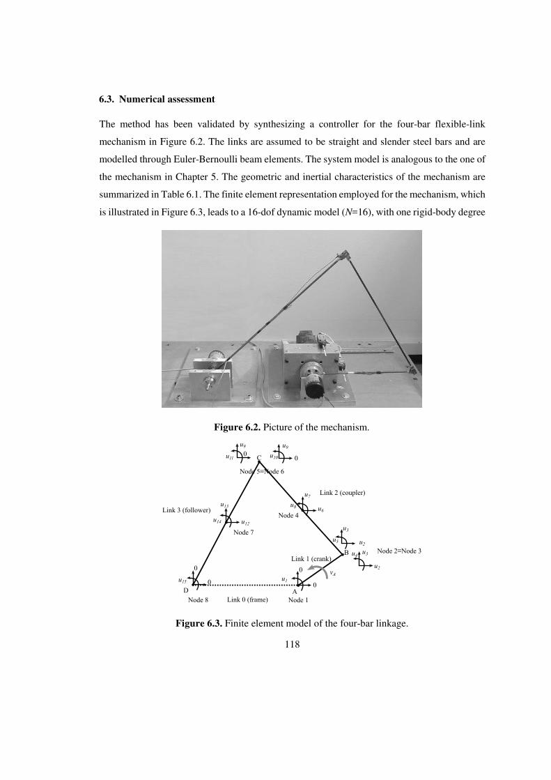
118

6.3. Numerical assessment

The method has been validated by synthesizing a controller for the four-bar flexible-link

mechanism in Figure 6.2. The links are assumed to be straight and slender steel bars and are

modelled through Euler-Bernoulli beam elements. The system model is analogous to the one of

the mechanism in Chapter 5. The geometric and inertial characteristics of the mechanism are

summarized in Table 6.1. The finite element representation employed for the mechanism, which

is illustrated in Figure 6.3, leads to a 16-dof dynamic model (N=16), with one rigid-body degree

Figure 6.2. Picture of the mechanism.

Figure 6.3. Finite element model of the four-bar linkage.

119

of freedom and 15 vibrational modes. A single motor actuates the mechanism, driving the

rotation of the crank. This ensures the controllability of the whole 16-dof system.

Finally, the mechanism is supposed to move on a vertical plane, and so the open-loop system is

unstable as a consequence of the presence of gravity. Further details on the system model can

be found in [79, 89].

The pole placement problem has been solved in a neighbourhood of the crank horizontal

configuration, and it consists in the assignment of 22 poles, while the remaining 10 poles are

constrained into a LMI region.

Table 6.1. Parameters of the four-bar linkage.

Parameter Value

Young’s modulus 210·109 [Pa]

Flexural inertia moment 11.102·10-10 [m4]

Beams width 6·10-3 [m]

Beams thickness 6·10-3 [m]

Mass/unit of length of links 272·10-3 [kg/m]

Crank (link 1) length 0.360 [m]

Coupler (link 2) length 0.390 [m]

Follower (link 3) length 0.535 [m]

Frame (link 4) length 0.632 [m]

Rayleigh damping constants α=8.5·10-2 [s-1]

β=2·10-5 [s]

Joint masses:

- Joint A 0

- Joint B 70·10-3 [kg]

- Joint C 70·10-3 [kg]

- Joint D 0

Joint inertia:

- Joint A 5·10-4 [kgm2]

- Joint B 0

- Joint C 0

- Joint D 12·10-6 [kgm2]

120

The 22 poles that are exactly assigned are shown in the second column of Table 6.2. The

remaining 10 poles are required to belong to the intersection of a conic sector 1D of magnitude

56 π (which means that the damping ratio of the associated modes is at least min 0.25ζ = ) and

the left half-plane 2D defined by ( )Re 1000z < − (which forces the settling time of such modes

to be less than max 0.003T s= ). It is easy to prove that such sets are LMI regions, in fact they

can both be represented as in (6.9), with

( )

( )

1

2

2 2 2 2

2 2 2 2

sin cos sin cos 5,

cos sin cos sin 6

1000 .

,

2

f z z z

f zz z

ϑ ϑ ϑ ϑ

ϑ ϑ ϑ ϑϑ π

= +

−=

−

⋅ += +

D

D

(6.24)

The resulting LMI constraints are defined as in (6.17) and are denoted 1F and 2F . Rather than

imposing ( )1 1 1, 0X l ≺F for some 1 0X ≻ and ( )2 2 2, 0X l ≺F for some 2 0X ≻ separately, it is

convenient to seek a common solution 1 2= =X X X and 1 2= =l l l , which is more conservative

but allows to reduce the number of involved unknowns.

The poles obtained with the proposed partial pole placement method are shown in the third

column of Table 6.2, which proves that the 22 assigned poles are accurately matched. For

clarity, not all the closed-loop poles are represented in Figure 6.4, but the plot allows to verify

that the remaining poles actually belong to the prescribed LMI region 1 2∩D D .

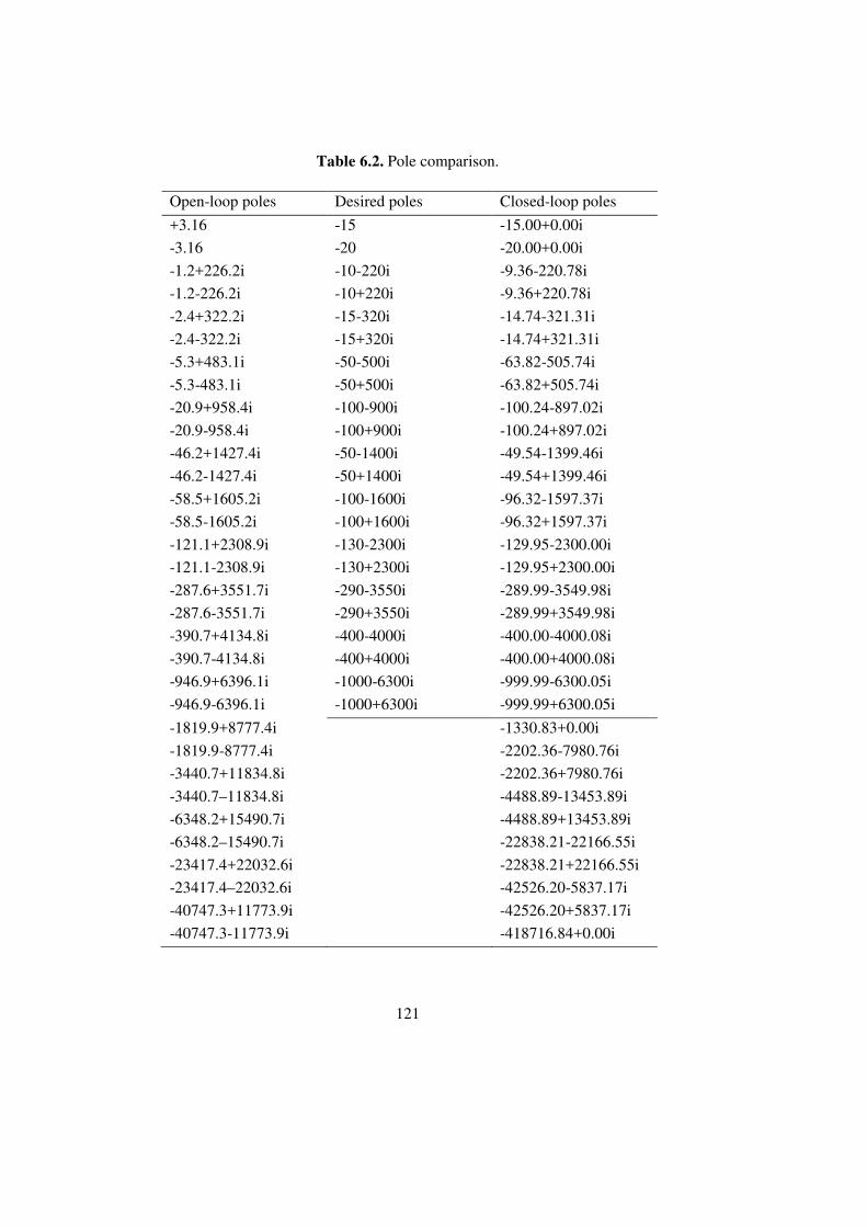
121

Table 6.2. Pole comparison.

Open-loop poles Desired poles Closed-loop poles

+3.16 -15 -15.00+0.00i

-3.16 -20 -20.00+0.00i

-1.2+226.2i -10-220i -9.36-220.78i

-1.2-226.2i -10+220i -9.36+220.78i

-2.4+322.2i -15-320i -14.74-321.31i

-2.4-322.2i -15+320i -14.74+321.31i

-5.3+483.1i -50-500i -63.82-505.74i

-5.3-483.1i -50+500i -63.82+505.74i

-20.9+958.4i -100-900i -100.24-897.02i

-20.9-958.4i -100+900i -100.24+897.02i

-46.2+1427.4i -50-1400i -49.54-1399.46i

-46.2-1427.4i -50+1400i -49.54+1399.46i

-58.5+1605.2i -100-1600i -96.32-1597.37i

-58.5-1605.2i -100+1600i -96.32+1597.37i

-121.1+2308.9i -130-2300i -129.95-2300.00i

-121.1-2308.9i -130+2300i -129.95+2300.00i

-287.6+3551.7i -290-3550i -289.99-3549.98i

-287.6-3551.7i -290+3550i -289.99+3549.98i

-390.7+4134.8i -400-4000i -400.00-4000.08i

-390.7-4134.8i -400+4000i -400.00+4000.08i

-946.9+6396.1i -1000-6300i -999.99-6300.05i

-946.9-6396.1i -1000+6300i -999.99+6300.05i

-1819.9+8777.4i -1330.83+0.00i

-1819.9-8777.4i -2202.36-7980.76i

-3440.7+11834.8i -2202.36+7980.76i

-3440.7–11834.8i -4488.89-13453.89i

-6348.2+15490.7i -4488.89+13453.89i

-6348.2–15490.7i -22838.21-22166.55i

-23417.4+22032.6i -22838.21+22166.55i

-23417.4–22032.6i -42526.20-5837.17i

-40747.3+11773.9i -42526.20+5837.17i

-40747.3-11773.9i -418716.84+0.00i

122

6.4. Conclusion

Partial pole placement is a common task in the design of vibrating systems, because it is often

necessary to set the location only of the most relevant poles. The remaining poles can often

constitute an issue, if not dealt with properly, because spill-over of such poles can lead to

instability. Techniques that allow to prevent spill-over are available in the literature, but in this

work it is rather proposed to constrain the non-assigned poles into desired regions of the

complex plane. The greater freedom in the location of the poles can be exploited to minimize

the norm of the control gains, and other properties to be optimized are under investigation. The

method has been successfully employed to synthesize the gains for the controller of a four-bar

flexible link mechanisms, thus showing the capabilities of the proposed approach.

Figure 6.4. Pole map: low frequency detail.

-7000 -6000 -5000 -4000 -3000 -2000 -1000 0

-1.5

-1

-0.5

0

0.5

1

1.5

104

Desired poles

Closed loop poles

123

Chapter 7. Hybrid control 7.1. Introduction

Let us consider the N degrees of freedom undamped vibrating system which can be controlled

exerting B

N control forces, namely:

( ) ( ) ( ).t t t+ =M K Bq q vɺɺ (7.1)

where , N N×∈M K ℝ are respectively the symmetric mass and stiffness matrices, N∈q ℝ is the

displacement vector, BN N×∈B ℝ represents the distribution of B

N independent control forces

and ( ) BNt ∈v ℝ is the control force vector.

Although such an approach requires the use of actuators and sensors, it is often employed in

eigenstructure assignment. For what concerns the assignment of just the eigenvalues, i.e. the

so-called “pole placement”, several methods are available [29, 30, 87]. The assignment of

eigenvectors, in contrast, is a much more challenging problem which is not completely solved.

In fact, it can be proven that active control can assign only eigenvectors that belong to certain

vector spaces which depend on the physical properties of the system and on the characteristics

of its actuation [33, 63]. In particular, the dimension of the space of allowable eigenvectors

matches the number of independent actuation forces. Thus if the system is highly underactuated

it is very unlikely that exact assignment of eigenvectors can be accomplished.

Recently, passive and active control have been combined also to develop hybrid methods, and

few promising results have appeared in the literature, so far. For example, Corr and Clark in

[96] achieve vibration confinement using mechanical dampers to reduce active power

requirements for active control. In a similar way, Tang and Wang in [97] obtain the same

objective employing piezoelectric materials both as active actuators and as passive dampers.

Diaz et al. in [98], instead, manage to improve the performances of input shaping by modifying

the link in a flexible manipulator. More recently, Ouyang in [99] consecutively employed

structural modification and feedback control for eigenvalue assignment in asymmetric systems.

The general problem of eigenstructure assignment has been instead tackled in [100] by

Richiedei and Trevisani, who developed a method for the simultaneous computation of the

124

structural modifications and control gains synthesis to overcome the inherent limitations active

control, for what concerns the assignment of eigenvectors.

Starting from such a work, a different mathematical frame for the problem solution is proposed

in this Chapter to handle highly underactuated systems and large dimensional models, by taking

advantage of some recent results of matrix analysis. Similarly to [100], the idea consists in

exploiting Dynamic Structural Modification to widen the range of the eigenvectors that can be

achieved through active control, even when the number of available actuation forces is low. The

assignment problem is handled by solving a matrix rank minimization problem. To that end,

two different algorithms are discussed, one that relies on non-convex optimization and the other

that, instead, is based on semi-definite optimization. The effectiveness of the developed hybrid

approach is assessed in two different test-cases. The first one allows to compare the proposed

method with the state-of-the art methods in a benchmark problem. The second one, instead,

enables to show the peculiarities of the two considered algorithms, with regard to the choice of

the actuation.

7.2. Problem formulation

7.2.1. Eigenstructure assignment through state feedback active control

The aim of this Section is to discuss the limitation of Eigenstructure Assignment through active

control. It is supposed that the system model (7.1) is employed, with the following control force:

( ) ( ) ,C t t= Bf v (7.2)

where BN N×∈B ℝ represents the distribution of B

N independent control forces and ( ) BNt ∈v ℝ

is the control force vector.

It is also supposed that a position-feedback control law is employed, such as

( ) ( ) ( )( )ref ,Tt t t= −Gv q q (7.3)

where BN N×∈G ℝ is the control gain matrix and ( )ref tq is the position reference.

The closed-loop system is therefore:

125

( ) ( ) ( ) ( )ref .T Tt t t+ − = −M K BG BGq q qɺɺ (7.4)

The closed-loop system eigenvalues and eigenvectors are, respectively, the scalars 2ω ∈ℝ and

the vectors N∈u ℝ that solve the following equation:

2 .T ω − =−K BG M 0u (7.5)

The eigenfrequency ω and its associated eigenvector u , constitute together an eigenpair.

Given a set of e

N desired eigenpairs ( ) ( ) ( )1 1 2 2, , , , , ,e eN Nω ω ω…u u u , eigenstructure assignment

consists in finding the controller gain matrix BN N×∈G ℝ such that the closed-loop system

features the eigenpairs ( ),i iω u for , ,1e

i N= … .

7.2.2. Existence of solutions for active eigenstructure assignment

The existence of feedback gains that result in the assignment of a prescribed set of eigenvalues

is a problem exhaustively investigated in literature and is governed by the notion of system

controllability. In particular, a system is said to be controllable if and only if the following

condition holds,

( )2ank |r i Nω =− K M B (7.6)

for all the open-loop eigenfrequencies i

ω ( , ,1i N= … ). If the system is controllable then it is

possible to place the closed-loop eigenvalues in the desired locations of the complex plane by

means of state-feedback control.

The fulfillment of condition (7.6), however, is not sufficient to assure that also the closed-loop

eigenvectors can be properly assigned. In fact, it can be proved that for any eigenfrequency ,ω

the corresponding eigenvector must belong to a particular vector space ( ) NωΨ ⊆ℝ . Indeed

equation (7.5), that must be satisfied in order to assign the eigenpair ( ),ω u , can be rearranged

as follows:

2 .Tω −K M BGu = u (7.7)

126

If equation (7.7) is left multiplied by the open-loop system receptance matrix at ω , i.e.

( ) 2 1ω ω

− = − H MK , then it follows that

( ) ,ω= H Bu x (7.8)

where BNT= ∈Gx u ℝ . Given the arbitrariness of the gain matrix G , equation (7.8) implies that

any assignable eigenvector u must belong to the vector space spanned by the columns of matrix

( ) BN Nω × ∈H B ℝ . Hence such a space, henceforth denoted the allowable subspace ( )ωΨ ,

collects the eigenvectors that can be obtained by active control, associated with the

eigenfrequency ω . Thus,

( ) ( ){ }span .ω ωΨ = H B (7.9)

Since both ( )ωH and B have maximum rank, the space Ψ is B

N -dimensional. Therefore, if

BN N< , namely the system is underactuated, it is not guaranteed that the eigenvector can be

exactly assigned. Such a limitation is particularly serious if few control forces are used, that is

BN N≪ , because the desired eigenvector u is unlikely to lie in the allowable subspace. A

workaround that is often used in the literature is to assign the projection of u onto Ψ , rather

than u itself [33]. In the most critical cases, however, this strategy leads to inadequate closed-

loop system performances because the projection just roughly approximate u . A proposed

solution to solve this issue is discussed in the next Section.

7.3. Proposed solution

7.3.1. Matrix rank minimization problem

By following and improving the idea proposed in [100], it is exploited Dynamic Structural

Modification to obtain a new allowable subspace ( )ˆiωΨ in such a way that ( )ˆ

ii ω∈Ψu for all

the e

N desired eigenpairs ( ),i iω u . Compared to such a work, which proposes the first idea of

hybrid control to eigenstructure assignment, this one formulates a more effective solution that

127

takes advantage of some recent theorems in the field of matrix analysis and of the state-of-the-

art methods for gain computation.

According to the definition of allowable subspace in equation (7.9), Ψ depends on the

receptance matrix computed at the desired eigenfrequency, i.e. ( )iωH , and on the input matrix

B . It will be henceforth assumed that the matrix B cannot be modified, which is a plausible

assumption since there are often technical constraints on the number and the location of the

actuators. Therefore, an effective way to shape the allowable subspaces is to exploit DSM to

modify the receptance matrix for each eigenvalue of interest. In practice, it is wanted to find

modification matrices M∆ and K∆ such that the following relation holds for each assigned

eigenpair ( ),i iω u :

( ) ( ){ } ( )12 ˆspan .i ii ω ω

− ∈ + − + = Ψ K K M M Bu ∆ ∆ (7.10)

The computation of the appropriate modification matrices can be recast as a rank minimization

problem. Such a formulation is advantageous because it is not necessary to cope with the

receptance matrix and thus no inversions of the matrix collecting the unknowns are needed.

Moreover, since rank minimization problems have many applications in different fields [101,

102, 103], several numerical algorithms have been recently proposed [104, 105, 106].

The proposed formulation is obtained by taking advantage of the well-known Rouché-Capelli

theorem of linear algebra. In fact, Eq. (7.10) holds if there are coefficient vectors BN

i ∈x ℝ such

that

( ) ( )2 .i i iω = + − + B K K M Mx u∆ ∆ (7.11)

By defining vectors i

c as follows,

( ) ( )2 ,N

i ii ω + − + ∈ = K K M Mc u ℝ∆ ∆ (7.12)

equations (7.11) can be conveniently written as

.i i

=Bx c (7.13)

128

According to the Rouché-Capelli theorem, each one of the systems in Eq. (7.13) can be solved

if and only if the rank of the matrix B (which is assumed to be B

N ) is equal to the rank of the

augmented matrix [ ]| iB c . Therefore, the systems in Eq. (7.13) can be solved for all the indices

, ,1e

i N= … if and only if

( )1| | |rank .eN BN … =B c c (7.14)

In practice, the computation of the suitable modification of the allowable subspaces consists in

finding the matrices M∆ and K∆ such that Eq. (7.14) holds. It is reasonable to restrict the

research of the structural modifications to a constraint set N N N N× ×Γ ⊆ ×ℝ ℝ to take into account

the physical feasibility of the solution, due to the technical or economic constraints on the

allowable modifications. In such a way, however, the existence of a solution is not guaranteed.

Therefore, it is convenient to use an optimization-based formulation: it is wanted to find the

modification matrices ,M K∆ ∆ that solve the following problem:

( )

1|minimize rank

subject to

| |

,eN…

∈Γ

M K

B c c

∆ ∆ (7.15)

Since the rank of a matrix is numerically difficult to handle in an optimization problem, the

algorithms to solve problem (7.15) must be carefully discussed.

7.3.2. Numerical algorithms

Two different numerical algorithms for matrix rank minimization are taken into consideration,

by taking advantage of some theoretical results of the linear algebra. The peculiarities of each

algorithm will be discussed in the next Sections.

Algorithm 1

The first algorithm relies on the following theorem of linear algebra [105].

Theorem 1. Let m n×∈X ℝ , with arbitrary m n≤ . Then ( )rank r≤X if and only if there exists

a full row-rank matrix ( )m r m− ×∈R ℝ such that

.=RX 0 (7.16) ♦

129

Let us suppose, without loss of generality, that e B

N NN+ ≤ . Then, the theorem is applied for

( )1| | | e B

e

N N N

N

T + × = … ∈X B c c ℝ and B

r N= , thus ( )e e BN N N× +∈R ℝ . Since the full row-rank

condition still involves the rank, it is convenient to replace it with the orthogonality condition

e

T

N=RR I , where eNI denotes the

eeN N× identity. It is evident that orthogonality implies full

row-rank. Thus problem (7.15) can be recast as

( )

2

1minimize

subject

|

, ,to

| |e

T

N

T

…

=

∈Γ

RR

B

M

R

I

K

c c

∆ ∆

(7.17)

where ⋅ denotes the matrix 2-norm. The resulting problem can be numerically solved with

appropriate algorithms that are implemented in commercial software. Since the problem is non-

convex, the choice of the initial guess for the optimization variables is of fundamental

importance. Two alternatives are proposed.

Initial guess 1. Concerning matrices M∆ and K∆ , a natural choice is to set both the

modification matrices to be zero, in order to obtain structural modifications that are close to the

original system design.

Concerning matrix R , this work proposes a strategy that has been tested with favorable results.

Let us denote 0ic the vectors (7.12) where M∆ and K∆ are set to zero, in accordance with the

initial guess for the optimization variables. Let us define 10 0 0: | | |

eN… = X B c c and compute

the singular value decomposition of its transpose:

( )0 .TT

=X U VΣ (7.18)

The smallest e

N singular values are approximated to zero, leading to a new matrix ɶΣ whose

rank is B

N . Thus a rank-B

N approximation of 0X can be defined as

( )0 .TT

=X U Vɶ ɶΣ (7.19)

130

Finally, the initial guess for R , denoted 0R , is chosen in such a way that the column of ( )0 T

R

are an orthogonal basis of ( )( )0KerT

Xɶ . Such a heuristic choice is justified by the fact that

0 0 =R X 0ɶ , and since it is fair to assume 0 0 0 0≈R X R Xɶ , the cost function of (7.17) can be

expected to be small since the first iteration.

Initial guess 2. As a second choice, matrices M∆ and K∆ can be chosen as the ones that

allows the assignment of ( ),i iω u , for , ,1e

i N= … , by means of DSM, computed using the

convex optimization problem proposed in [23]. As far as R is concerned, instead, the same

strategy proposed in the previous approach should be employed, provided that the vectors 0ic

are defined accordingly to the choice of M∆ and K∆ .

Algorithm 2

The second algorithm exploits the following theorem, which is known as the semidefinite

embedding lemma [107].

Theorem 2. Let m n×∈X ℝ , with arbitrary m and n . Then ( )rank r≤X if and only if there exist

matrices m mT ×∈=Y Y ℂ and n nT ×∈=Z Z ℂ such that

( ) ( ) 2 ,rank rank 0T

r

≤

+Y X

X ZY Z (7.20)

where the symbol means that the matrix must be positive semidefinite. ♦

Such a theorem allows to recast the rank minimization of a general rectangular matrix to the

rank minimization of a square symmetric matrix, i.e. ( )diag ,Y Z . In such a way, it can be

employed the popular trace heuristic [108], which consists in replacing ( )( )rank diag ,Y Z with

( )( )trace diag ,Y Z in the objective function of the optimization problem. An intuitive

explanation of the trace heuristic is that a small trace forces the numerical rank to be low in the

case of symmetric positive semidefinite matrices. In fact, for such matrices eigenvalues are real

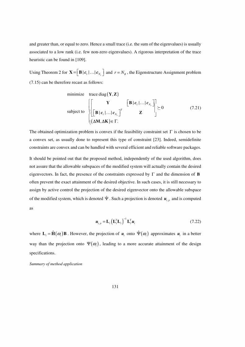
131

and greater than, or equal to zero. Hence a small trace (i.e. the sum of the eigenvalues) is usually

associated to a low rank (i.e. few non-zero eigenvalues). A rigorous interpretation of the trace

heuristic can be found in [109].

Using Theorem 2 for 1| | |eN … = X B c c and

Br N= , the Eigenstructure Assignment problem

(7.15) can be therefore recast as follows:

( )

( )

1

1

minimize trace diag ,

sub

| | |0

|ject t |

, .

o |

e

e

N

N

T

… … ∈Γ

Y Z

Z

B

M K

B

Y c c

c c

∆ ∆

(7.21)

The obtained optimization problem is convex if the feasibility constraint set Γ is chosen to be

a convex set, as usually done to represent this type of constraint [23]. Indeed, semidefinite

constraints are convex and can be handled with several efficient and reliable software packages.

It should be pointed out that the proposed method, independently of the used algorithm, does

not assure that the allowable subspaces of the modified system will actually contain the desired

eigenvectors. In fact, the presence of the constraints expressed by Γ and the dimension of B

often prevent the exact attainment of the desired objective. In such cases, it is still necessary to

assign by active control the projection of the desired eigenvector onto the allowable subspace

of the modified system, which is denoted Ψ̂ . Such a projection is denoted ,i pu and is computed

as

( )1

,T T

i p i i i i i

−

= L L L Lu u (7.22)

where ( )ˆi iω=L H B . However, the projection of

iu onto ( )ˆ

iωΨ approximates i

u in a better

way than the projection onto ( )iωΨ , leading to a more accurate attainment of the design

specifications.

Summary of method application

132

In conclusion, the proposed method can be summarized as follows. Given a set of desired

eigenpairs ( )1 1,ω u ,…, ( ),e eN Nω u , the suitable modifications of the mass and stiffness matrices,

i.e. M∆ and K∆ , are sought. It is wanted that the allowable subspace contains the associated

eigenvectors, in the modified system design. Namely,

( )ˆ , for all 1, , .i i ei Nω∈Ψ = …u (7.23)

The modifications are computed either solving the optimization problem (7.17) or (7.21), and

in both cases the solution is constrained into a set Γ .

The desired eigenvectors are then projected as in Eq. (7.22) onto their respective allowable

subspaces, and the control gain matrix G that allows to attain the desired closed-loop eigenpairs

is computed. In principle, any method for active eigenstructure assignment could be employed,

thus the appropriate method can be chosen according to specific design needs. For example, in

this work it is used the method proposed in [35], which is capable of partial eigenstructure

assignment, thus only e

N selected open-loop eigenpairs are replaced with the desired ones,

while the others are left unchanged, in such a way that spill-over is prevented. Moreover, such

a method relies on a second-order system model, which is more suitable to vibration control

with respect to the more common first-order model.

7.4. Numerical examples

7.4.1. Five degrees of freedom system

The first example is aimed at assessing the effectiveness of the proposed method and it will be

proved that it can be used to achieve superior performances with respect to either sole passive

control or sole active control. This example also justifies the need of a method specifically

designed for hybrid control, performing concurrently synthesis of controller gains and structural

modification, which offers better performances compared to the sequential combination of

passive and active control.

133

A lumped parameter 5-degrees of freedom system is considered. This system has been used in

several papers to validate some methods of Dynamic Structural Modification [9, 23, 44], and

hence it is an interesting benchmark. Such a system, pictured in Figure 7.1, consists of 5 lumped

masses. Each mass is connected to the adjacent ones and to the frame by linear springs. The

original values of the masses and springs are shown in the first row of Table 7.1.

The original system eigenstructure is shown in Table 7.2 (the meaning of the eigenvector

components can be inferred from Figure 7.1). It is wanted that the system features the two

eigenpairs shown in Table 7.3, which are those required in [23]. In order to achieve this result,

it is supposed that the five masses and the five ground springs can be modified, according to the

constraints specified in the second and third rows of Table 7.1. Moreover, it is supposed that

two independent control forces 1v and 2v are exerted on the first two masses on the left, as

shown in Figure 7.1.

Figure 7.1. Five degrees of freedom system

Table 7.1. Mass and stiffness parameters of the five degrees of freedom system.

m1 [kg] m2 [kg] m3 [kg] m4 [kg] m5 [kg] k12

[kN/m] k23

[kN/m] k34

[kN/m] k45

[kN/m] kg,i

[kN/m] Nominal value

1.34 2.61 8.21 5.12 1.73 82.1 73.5 68.2 73.6 98.9

Lower bound

0 0 0 0 0 - - - - 0

Upper bound

2 2 2 2 2 - - - - 483

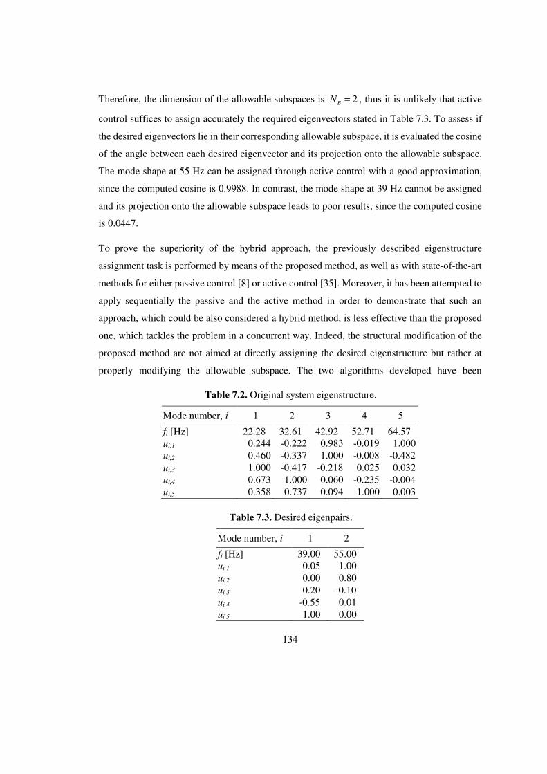
134

Therefore, the dimension of the allowable subspaces is 2B

N = , thus it is unlikely that active

control suffices to assign accurately the required eigenvectors stated in Table 7.3. To assess if

the desired eigenvectors lie in their corresponding allowable subspace, it is evaluated the cosine

of the angle between each desired eigenvector and its projection onto the allowable subspace.

The mode shape at 55 Hz can be assigned through active control with a good approximation,

since the computed cosine is 0.9988. In contrast, the mode shape at 39 Hz cannot be assigned

and its projection onto the allowable subspace leads to poor results, since the computed cosine

is 0.0447.

To prove the superiority of the hybrid approach, the previously described eigenstructure

assignment task is performed by means of the proposed method, as well as with state-of-the-art

methods for either passive control [8] or active control [35]. Moreover, it has been attempted to

apply sequentially the passive and the active method in order to demonstrate that such an

approach, which could be also considered a hybrid method, is less effective than the proposed

one, which tackles the problem in a concurrent way. Indeed, the structural modification of the

proposed method are not aimed at directly assigning the desired eigenstructure but rather at

properly modifying the allowable subspace. The two algorithms developed have been

Table 7.2. Original system eigenstructure.

Mode number, i 1 2 3 4 5

fi [Hz] 22.28 32.61 42.92 52.71 64.57 ui,1 0.244 -0.222 0.983 -0.019 1.000 ui,2 0.460 -0.337 1.000 -0.008 -0.482 ui,3 1.000 -0.417 -0.218 0.025 0.032 ui,4 0.673 1.000 0.060 -0.235 -0.004 ui,5 0.358 0.737 0.094 1.000 0.003

Table 7.3. Desired eigenpairs.

Mode number, i 1 2

fi [Hz] 39.00 55.00 ui,1 0.05 1.00 ui,2 0.00 0.80 ui,3 0.20 -0.10 ui,4 -0.55 0.01 ui,5 1.00 0.00

135

implemented in Matlab, by exploiting the YALMIP [47] modeling language for optimization

problems. The numerical solvers employed are fmincon from the Optimization Toolbox by

Mathworks for the non-convex optimization of Eq. (7.17), and SeDuMi [64] for the semidefinite

optimization of Eq. (7.21).

Table 7.4 shows the modifications of the physical parameters for all the methods involving

structural modification. The quantities evaluated to assess the system performances are shown

in Table 7.5. The first one is the absolute error of the obtained eigenfrequencies ,obtiω with

respect to the desired ones ,des ,iω which should approach 0. The second one is the cosine of the

angle between each desired eigenvector ,desiu and the obtained one ,obtiu , which should

approach 1. Finally, the 2-norm of the two modification matrices and the gain matrix are

Table 7.4. System modifications.

DSM [23] Hybrid method (Algorithm 1) Hybrid method

(Algorithm 2) Initial guess 1 Initial guess 2

m1 [kg] 0.878 1.857 2.000 0.000

m2 [kg] 0.000 1.852 1.999 0.965

m3 [kg] 0.808 0.045 0.239 0.000

m4 [kg] 1.495 1.767 1.999 2.000

m5 [kg] 1.816 1.908 1.998 1.927

kg,1 [kN/m] 149.69 28.948 44.360 47.103

kg,2 [kN/m] 153.20 22.485 150.636 258.234

kg,3 [kN/m] 0.000 69.105 80.905 113.385

kg,4 [kN/m] 11.94 14.094 28.096 22.897

kg,5 [kN/m] 0.000 5.421 10.861 4.355

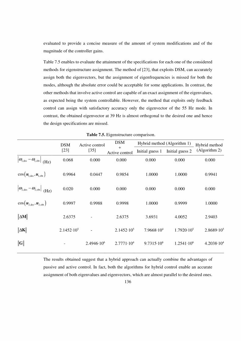
136

evaluated to provide a concise measure of the amount of system modifications and of the

magnitude of the controller gains.

Table 7.5 enables to evaluate the attainment of the specifications for each one of the considered

methods for eigenstructure assignment. The method of [23], that exploits DSM, can accurately

assign both the eigenvectors, but the assignment of eigenfrequencies is missed for both the

modes, although the absolute error could be acceptable for some applications. In contrast, the

other methods that involve active control are capable of an exact assignment of the eigenvalues,

as expected being the system controllable. However, the method that exploits only feedback

control can assign with satisfactory accuracy only the eigenvector of the 55 Hz mode. In

contrast, the obtained eigenvector at 39 Hz is almost orthogonal to the desired one and hence

the design specifications are missed.

The results obtained suggest that a hybrid approach can actually combine the advantages of

passive and active control. In fact, both the algorithms for hybrid control enable an accurate

assignment of both eigenvalues and eigenvectors, which are almost parallel to the desired ones.

Table 7.5. Eigenstructure comparison.

DSM [23]

Active control [35]

DSM +

Active control

Hybrid method (Algorithm 1) Hybrid method (Algorithm 2) Initial guess 1 Initial guess 2

1,des 1,obtω ω− (Hz) 0.068 0.000 0.000 0.000 0.000 0.000

( )1,des 1,obtcos ,u u

0.9964 0.0447 0.9854 1.0000 1.0000 0.9941

2,des 2,obtω ω− (Hz) 0.020 0.000 0.000 0.000 0.000 0.000

( )2,des 2,obtcos ,u u

0.9997 0.9988 0.9998 1.0000 0.9999 1.0000

M∆ 2.6375 - 2.6375 3.6931 4.0052 2.9403

K∆ 2.1452∙105 - 2.1452∙105 7.9668∙104 1.7920∙105 2.8689∙105

G - 2.4946∙106 2.7771∙104 9.7315∙106 1.2541∙106 4.2038∙104

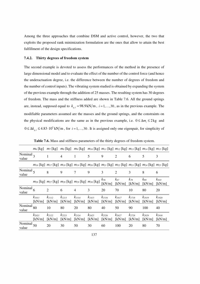
137

Among the three approaches that combine DSM and active control, however, the two that

exploits the proposed rank minimization formulation are the ones that allow to attain the best

fulfillment of the design specifications.

7.4.2. Thirty degrees of freedom system

The second example is devoted to assess the performances of the method in the presence of

large dimensional model and to evaluate the effect of the number of the control force (and hence

the underactuation degree, i.e. the difference between the number of degrees of freedom and

the number of control inputs). The vibrating system studied is obtained by expanding the system

of the previous example through the addition of 25 masses. The resulting system has 30 degrees

of freedom. The mass and the stiffness added are shown in Table 7.6. All the ground springs

are, instead, supposed equal to , 98.9kN mg ik = , ,31, 0i = … , as in the previous example. The

modifiable parameters assumed are the masses and the ground springs, and the constraints on

the physical modifications are the same as in the previous example, i.e. 0 kg2i

m≤ ∆ ≤ and

5, 4.83 10 kN0 mg ik≤ ∆ ≤ ⋅ , for ,31, 0i = … . It is assigned only one eigenpair, for simplicity of

Table 7.6. Mass and stiffness parameters of the thirty degrees of freedom system.

m6 [kg] m7 [kg] m8 [kg] m9 [kg] m10 [kg] m11 [kg] m12 [kg] m13 [kg] m14 [kg] m15 [kg]

Nominal value

3 1 4 1 5 9 2 6 5 3

m16 [kg] m17 [kg] m18 [kg] m19 [kg] m20 [kg] m21 [kg] m22 [kg] m23 [kg] m24 [kg] m25 [kg]

Nominal value

5 8 9 7 9 3 2 3 8 6

m26 [kg] m27 [kg] m28 [kg] m29 [kg] m30 [kg] k56 [kN/m]

k67 [kN/m]

k78 [kN/m]

k89 [kN/m]

k910 [kN/m]

Nominal value

6 2 6 4 3 20 70 10 80 20

k1011 [kN/m]

k1112 [kN/m]

k1213 [kN/m]

k1314 [kN/m]

k1415 [kN/m]

k1516 [kN/m]

k1617 [kN/m]

k1718 [kN/m]

k1819 [kN/m]

k1920 [kN/m]

Nominal value

80 10 80 20 80 40 50 90 100 40

k2021 [kN/m]

k2122 [kN/m]

k2223 [kN/m]

k2324 [kN/m]

k2425 [kN/m]

k2526 [kN/m]

k2627 [kN/m]

k2728 [kN/m]

k2829 [kN/m]

k2930 [kN/m]

Nominal value

50 20 30 50 30 60 100 20 80 70

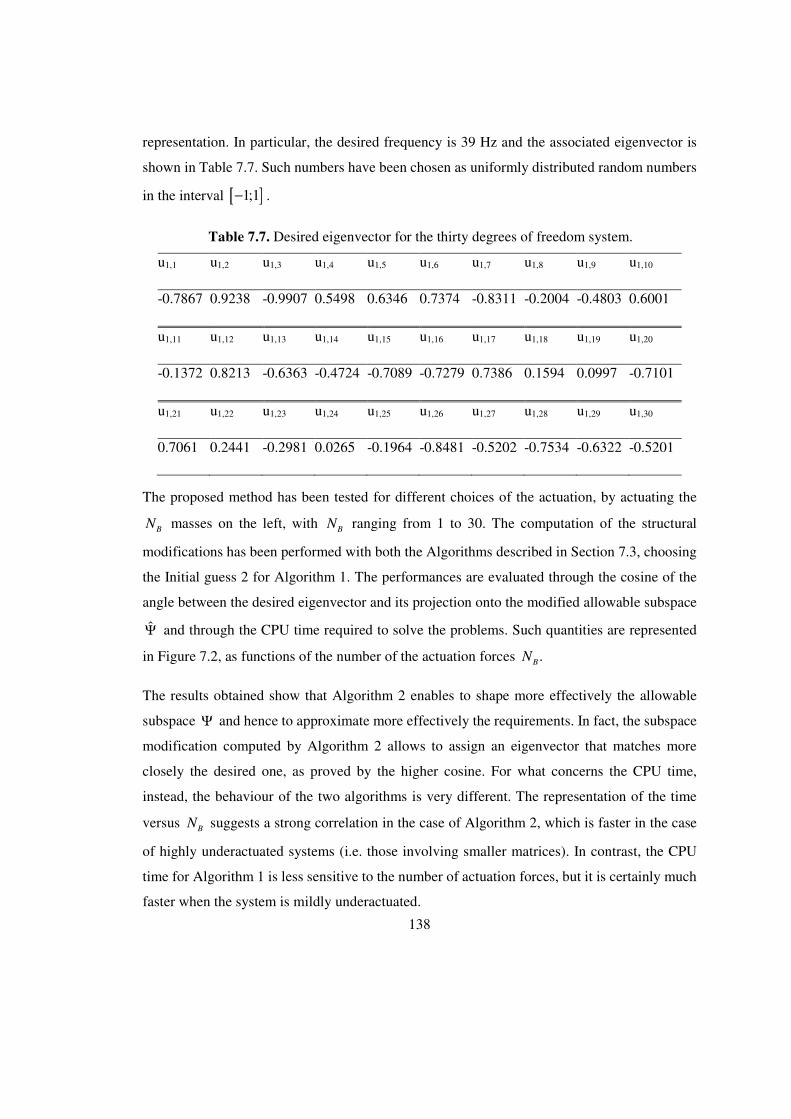
138

representation. In particular, the desired frequency is 39 Hz and the associated eigenvector is

shown in Table 7.7. Such numbers have been chosen as uniformly distributed random numbers

in the interval [ ]1;1− .

The proposed method has been tested for different choices of the actuation, by actuating the

BN masses on the left, with

BN ranging from 1 to 30. The computation of the structural

modifications has been performed with both the Algorithms described in Section 7.3, choosing

the Initial guess 2 for Algorithm 1. The performances are evaluated through the cosine of the

angle between the desired eigenvector and its projection onto the modified allowable subspace

Ψ̂ and through the CPU time required to solve the problems. Such quantities are represented

in Figure 7.2, as functions of the number of the actuation forces .B

N

The results obtained show that Algorithm 2 enables to shape more effectively the allowable

subspace Ψ and hence to approximate more effectively the requirements. In fact, the subspace

modification computed by Algorithm 2 allows to assign an eigenvector that matches more

closely the desired one, as proved by the higher cosine. For what concerns the CPU time,

instead, the behaviour of the two algorithms is very different. The representation of the time

versus B

N suggests a strong correlation in the case of Algorithm 2, which is faster in the case

of highly underactuated systems (i.e. those involving smaller matrices). In contrast, the CPU

time for Algorithm 1 is less sensitive to the number of actuation forces, but it is certainly much

faster when the system is mildly underactuated.

Table 7.7. Desired eigenvector for the thirty degrees of freedom system.

u1,1 u1,2 u1,3 u1,4 u1,5 u1,6 u1,7 u1,8 u1,9 u1,10

-0.7867 0.9238 -0.9907 0.5498 0.6346 0.7374 -0.8311 -0.2004 -0.4803 0.6001

u1,11 u1,12 u1,13 u1,14 u1,15 u1,16 u1,17 u1,18 u1,19 u1,20

-0.1372 0.8213 -0.6363 -0.4724 -0.7089 -0.7279 0.7386 0.1594 0.0997 -0.7101

u1,21 u1,22 u1,23 u1,24 u1,25 u1,26 u1,27 u1,28 u1,29 u1,30

0.7061 0.2441 -0.2981 0.0265 -0.1964 -0.8481 -0.5202 -0.7534 -0.6322 -0.5201

139

For the above reasons, Algorithm 2 should be preferred to achieve the best performance, unless

a system with low underactuation degree is considered and CPU time is a critical issue.

7.5. Conclusion

In this Chapter, a limitation of active vibration control that affects the capability of assigning

eigenvectors is addressed. It is demonstrated that, with a proper adjustment of the inertial and/or

elastic parameters of the system, such a limitation can be overcome. It is proposed a method to

numerically compute the optimal values of such parameters, that consists in the minimization

of the rank of a matrix. Two algorithms have been developed to solve such a problem, each one

relying on a different mathematical framework.

The proposed approach has been numerically validated in two cases of interest. The first test-

case aims to assign two eigenpairs to a five degrees of freedom system. Such an objective can

be fairly accomplished with techniques of Dynamic Structural Modification available in the

literature. It is nevertheless demonstrated that the proposed hybrid approach outperforms both

the methods of DSM and those of active control. Moreover, it is shown that sequentially

employing DSM and active control actually results in a good eigenstructure assignment, but it

is still inferior with respect to the proposed concurrent method. The second test-case concerns

Figure 7.2. Comparison of the algorithms.

cos

Tim

e [s

]

140

a single-mode assignment to a 30 degrees of freedom system, in different actuation conditions.

In such a way, it has been possible also to compare the two developed algorithms and to validate

the method in a large-scale example.

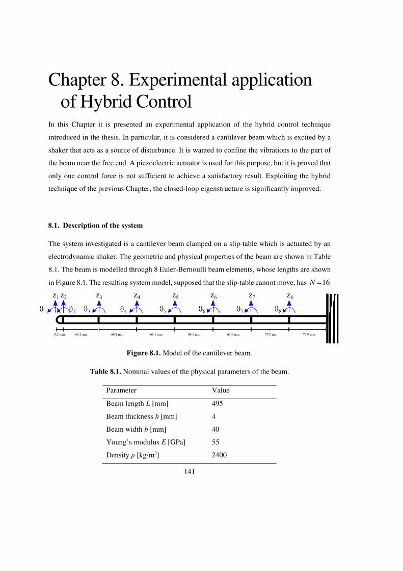
141

Chapter 8. Experimental application of Hybrid Control

In this Chapter it is presented an experimental application of the hybrid control technique

introduced in the thesis. In particular, it is considered a cantilever beam which is excited by a

shaker that acts as a source of disturbance. It is wanted to confine the vibrations to the part of

the beam near the free end. A piezoelectric actuator is used for this purpose, but it is proved that

only one control force is not sufficient to achieve a satisfactory result. Exploiting the hybrid

technique of the previous Chapter, the closed-loop eigenstructure is significantly improved.

8.1. Description of the system

The system investigated is a cantilever beam clamped on a slip-table which is actuated by an

electrodynamic shaker. The geometric and physical properties of the beam are shown in Table

8.1. The beam is modelled through 8 Euler-Bernoulli beam elements, whose lengths are shown

in Figure 8.1. The resulting system model, supposed that the slip-table cannot move, has 16N =

Table 8.1. Nominal values of the physical parameters of the beam.

Parameter Value

Beam length L [mm] 495

Beam thickness h [mm] 4

Beam width b [mm] 40

Young’s modulus E [GPa] 55

Density ρ [kg/m3] 2400

Figure 8.1. Model of the cantilever beam.

142

degrees of freedom. It is considered that at selected locations of the beam can be placed two

masses of the desired magnitude.

8.2. The piezoelectric actuator

A piezoelectric actuator is employed for vibration control. The actuator has been placed on the

desired location of the beam by bonding it to the beam surface. Linear theory has been adopted

to model it, even if some nonlienarities such as hysteresis and variable gains might occur, and

it is assumed that there is no slip at the interface. The fundamental properties of the actuator are

shown in Table 8.2. Consistently with the literature on piezoelectric actuators [110, 111], the

assumption that the applied voltage is uniform over the element allows to represent the force

exerted by the control device as two opposite torques of magnitude CF , as represented in Figure

8.2.

These torques are, in turn, proportional to the applied voltage, with a gain that is approximately

constant and is equal to 0.034 Nm/V. In practice, the experimental characterization of the

actuator has shown that this gain might oscillate about this nominal value (the highest deviation

Table 8.2. Nominal value of the physical parameters of the piezoelectric actuator.

Parameter Value

Length Lp [mm] 61

Thickness hp [mm] 0.8

Beam width bp [mm] 35

Young’s modulus Ep [GPa] 34.7

Mass Mp [g] 7.2

Figure 8.2. Passive and active modification of the beam.

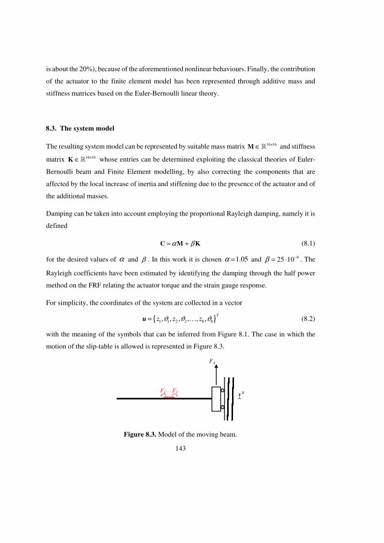
143

is about the 20%), because of the aforementioned nonlinear behaviours. Finally, the contribution

of the actuator to the finite element model has been represented through additive mass and

stiffness matrices based on the Euler-Bernoulli linear theory.

8.3. The system model

The resulting system model can be represented by suitable mass matrix 16 16×∈M ℝ and stiffness

matrix 16 16×∈K ℝ whose entries can be determined exploiting the classical theories of Euler-

Bernoulli beam and Finite Element modelling, by also correcting the components that are

affected by the local increase of inertia and stiffening due to the presence of the actuator and of

the additional masses.

Damping can be taken into account employing the proportional Rayleigh damping, namely it is

defined

α β+=C M K (8.1)

for the desired values of α and β . In this work it is chosen 1.05α = and 625 10β −= ⋅ . The

Rayleigh coefficients have been estimated by identifying the damping through the half power

method on the FRF relating the actuator torque and the strain gauge response.

For simplicity, the coordinates of the system are collected in a vector

{ }1 2 81 2 8, , , , ,,T

z zz ϑ ϑ ϑ…=u (8.2)

with the meaning of the symbols that can be inferred from Figure 8.1. The case in which the

motion of the slip-table is allowed is represented in Figure 8.3.

Figure 8.3. Model of the moving beam.

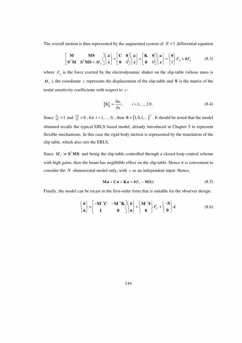
144

The overall motion is thus represented by the augmented system of 1N + differential equation

0 0 1 A CT T

C

F FM

+ + = + +

M MS C 0 K 0 0

S M S MS 0 0

u u ub

x x x

ɺɺ ɺ

ɺɺ ɺ (8.3)

where AF is the force exerted by the electrodynamic shaker on the slip-table (whose mass is

CM ), the coordinate x represents the displacement of the slip-table and S is the matrix of the

nodal sensitivity coefficients with respect to x :

[ ] , , , 2 .1i

i iu

Nx

∂…=

∂=S (8.4)

Since 1iz

x

∂

∂= and 0i

x

ϑ∂

∂= , for , ,1i N= … , then { }1,0,1,

T= …S . It should be noted that the model

obtained recalls the typical ERLS based model, already introduced in Chapter 5 to represent

flexible mechanisms. In this case the rigid body motion is represented by the translation of the

slip table, which also sets the ERLS.

Since T

CM S MS≫ and being the slip-table controlled through a closed-loop control scheme

with high gains, then the beam has neglibible effect on the slip-table. Hence it is convenient to

consider the N -dimensional model only, with x as an independent input. Hence,

.CF x+ + = −M C K MSu u u bɺɺ ɺ ɺɺ (8.5)

Finally, the model can be recast in the first-order form that is suitable for the observer design:

1 1 1

.CF− − − − − −

= + +

SM C M K M

0I 0 0

u u bx

u u

ɺɺ ɺɺɺ

ɺ (8.6)

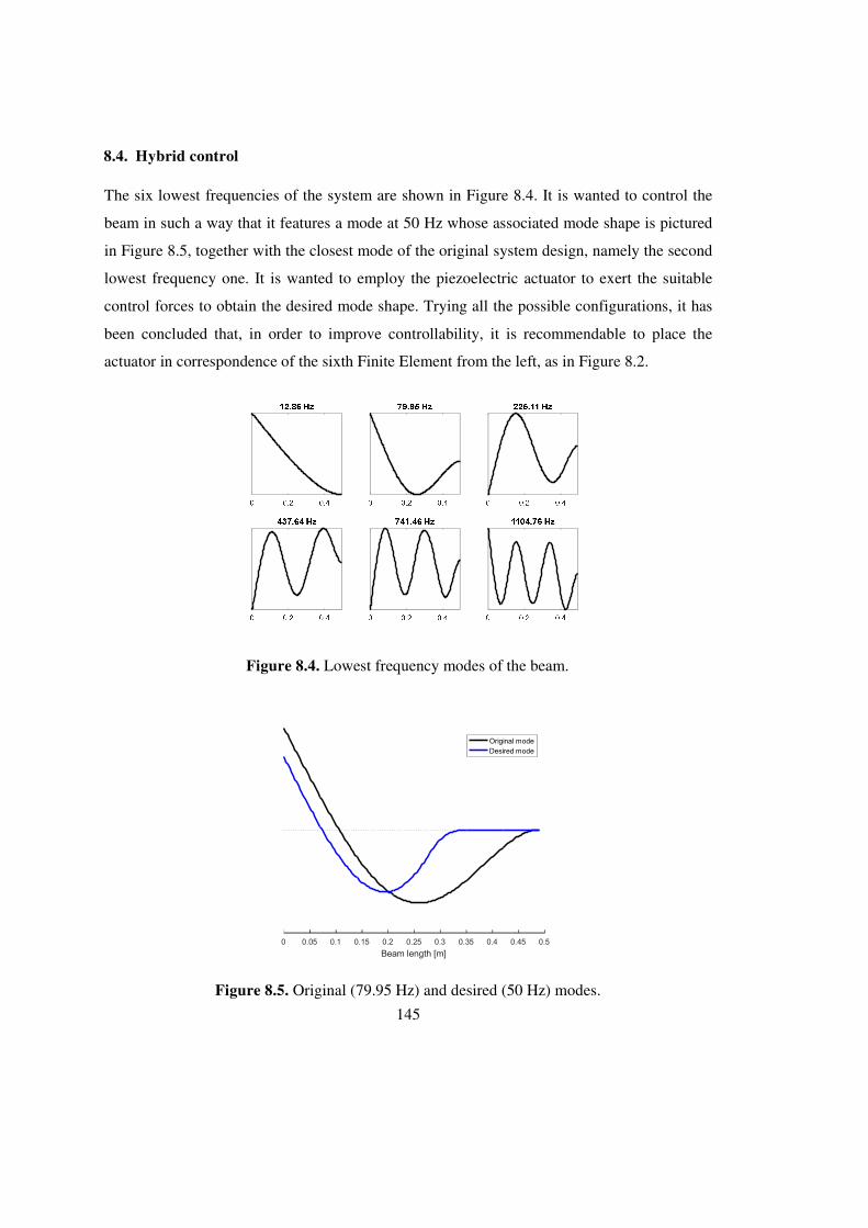
145

8.4. Hybrid control

The six lowest frequencies of the system are shown in Figure 8.4. It is wanted to control the

beam in such a way that it features a mode at 50 Hz whose associated mode shape is pictured

in Figure 8.5, together with the closest mode of the original system design, namely the second

lowest frequency one. It is wanted to employ the piezoelectric actuator to exert the suitable

control forces to obtain the desired mode shape. Trying all the possible configurations, it has

been concluded that, in order to improve controllability, it is recommendable to place the

actuator in correspondence of the sixth Finite Element from the left, as in Figure 8.2.

Figure 8.4. Lowest frequency modes of the beam.

Figure 8.5. Original (79.95 Hz) and desired (50 Hz) modes.

0 0.05 0.1 0.15 0.2 0.25 0.3 0.35 0.4 0.45 0.5

Beam length [m]

Original mode

Desired mode

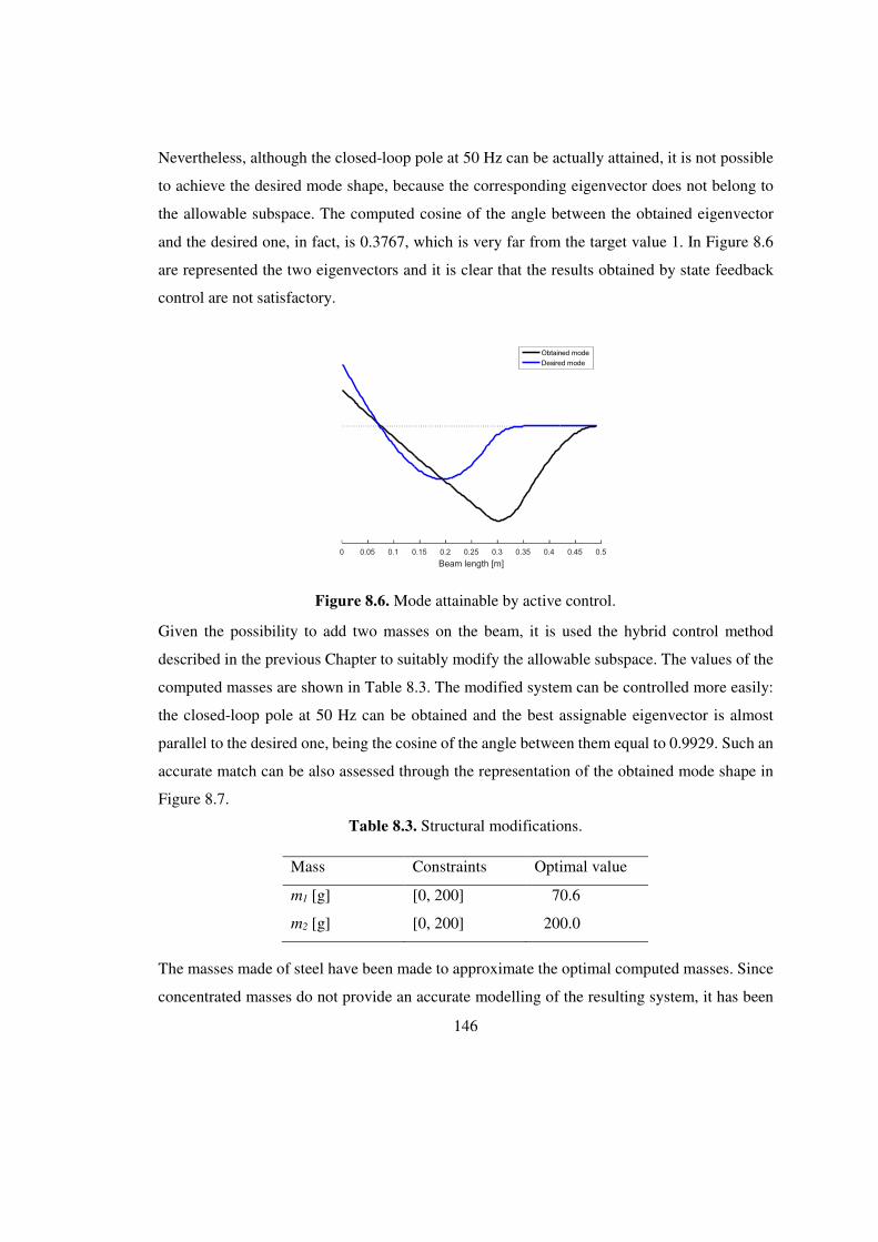
146

Nevertheless, although the closed-loop pole at 50 Hz can be actually attained, it is not possible

to achieve the desired mode shape, because the corresponding eigenvector does not belong to

the allowable subspace. The computed cosine of the angle between the obtained eigenvector

and the desired one, in fact, is 0.3767, which is very far from the target value 1. In Figure 8.6

are represented the two eigenvectors and it is clear that the results obtained by state feedback

control are not satisfactory.

Given the possibility to add two masses on the beam, it is used the hybrid control method

described in the previous Chapter to suitably modify the allowable subspace. The values of the

computed masses are shown in Table 8.3. The modified system can be controlled more easily:

the closed-loop pole at 50 Hz can be obtained and the best assignable eigenvector is almost

parallel to the desired one, being the cosine of the angle between them equal to 0.9929. Such an

accurate match can be also assessed through the representation of the obtained mode shape in

Figure 8.7.

The masses made of steel have been made to approximate the optimal computed masses. Since

concentrated masses do not provide an accurate modelling of the resulting system, it has been

Figure 8.6. Mode attainable by active control.

0 0.05 0.1 0.15 0.2 0.25 0.3 0.35 0.4 0.45 0.5

Beam length [m]

Obtained mode

Desired mode

Table 8.3. Structural modifications.

Mass Constraints Optimal value

m1 [g] [0, 200] 70.6

m2 [g] [0, 200] 200.0

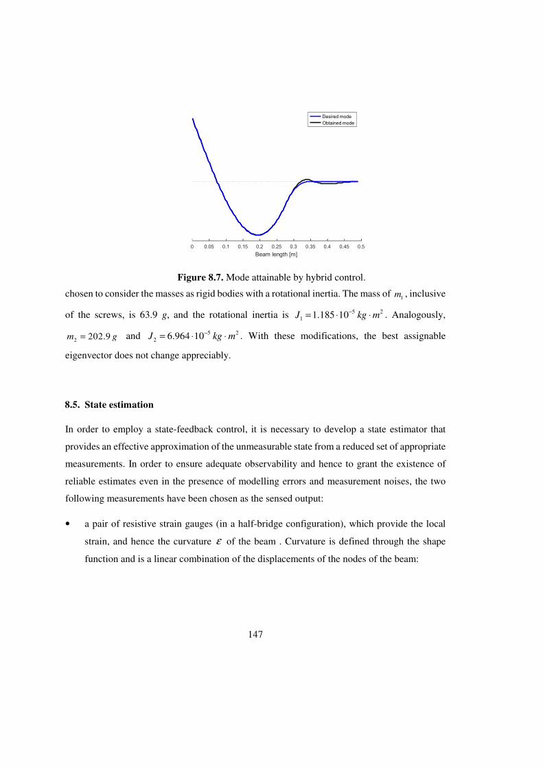
147

chosen to consider the masses as rigid bodies with a rotational inertia. The mass of 1m , inclusive

of the screws, is 63.9 g, and the rotational inertia is 51

2101.185J kg m−⋅ ⋅= . Analogously,

2 202.9m g= and 52

26.964 10 kg mJ −⋅ ⋅= . With these modifications, the best assignable

eigenvector does not change appreciably.

8.5. State estimation

In order to employ a state-feedback control, it is necessary to develop a state estimator that

provides an effective approximation of the unmeasurable state from a reduced set of appropriate

measurements. In order to ensure adequate observability and hence to grant the existence of

reliable estimates even in the presence of modelling errors and measurement noises, the two

following measurements have been chosen as the sensed output:

• a pair of resistive strain gauges (in a half-bridge configuration), which provide the local

strain, and hence the curvature ε of the beam . Curvature is defined through the shape

function and is a linear combination of the displacements of the nodes of the beam:

Figure 8.7. Mode attainable by hybrid control.

0 0.05 0.1 0.15 0.2 0.25 0.3 0.35 0.4 0.45 0.5

Beam length [m]

Desired mode

Obtained mode

148

2 3 2 2 3 2

1

1

6 12 4 6 6 12 2 6i

i

i

i

z

s s s s

zl l l l l l l l

ϑε

ϑ+

+

= − + − + − − +

(8.7)

where the meaning of the symbols can be found in Figure 8.8.

• a laser vibrometer employed to measure directly the velocity of a node.

The position of the two sensors has been chosen to maximize observability and to improve the

signal-to-noise ratio. In particular, in Figure 8.9 are plotted the values of the curvature in the

middle of each finite element, for both the lowest frequency open-loop mode (on the left) and

the best achievable mode at 50 Hz (on the right). It has been chosen to position the strain gauge

in the middle of the fourth Finite Element, namely at roughly 175 mm from the free end of the

beam. The laser vibrometer, instead, has been positioned to measure the velocity of a point near

the free end of the beam, which is the part of the system that vibrates the most.

Figure 8.8. Definition of curvature

Figure 8.9. Curvatures of the two modes of interest

1 2 3 4 5 6 7 8

Finite Element

-8

-7

-6

-5

-4

-3

-2

-1

Cu

rva

ture

[1

/m]

1st mode

1 2 3 4 5 6 7 8

Finite Element

-15

-10

-5

0

5

Cu

rva

ture

[1

/m]

2nd mode

149

The estimator that has been implemented is a linear Kalman filter based on a reduced-order

model on a modal base. Such a choice is motivated by the need of reducing the computational

effort for the real-time solution of the observer differential equations. Indeed, adopting the full-

order model with 32 dofs would have required a relevant CPU time for each time step and, at

the same time, a reduced time step to avoid aliasing of the high frequency modes and the

numerical instability due to the presence of such high frequency dynamics. On the other hand,

high frequency modes are weakly observable, given the low-pass filters on the sensors and given

the presence of high-frequency noise, and weakly excited in the range of frequency of interest

for the application developed.

The first-order formulation of the system model can be written in the following compact form

by defining the nodal state vector as { }T TT

=χ u uɺ :

u

y

= +

=

A B

C

χ χ

χ

ɺ (8.8)

The model in (8.8) is recast in the modal canonical form by using the linear transformation

= Tz χ ( 2 2N N×∈T ℝ ) where z are the modal coordinates of the first-order model :

M

M

u

y

= +

=

A B

C

z z

z

ɺ (8.9)

The matrices of the transformed system are 1M

−=A TAT , M =B TB and 1

M

−=C CT . In

particular, MA has 2 2× blocks on the diagonal for each vibrational mode and it is zero

everywhere else. Thus there is a block σ ν

ν σ

−

for any complex conjugate pair of eigenvalues

iσ ν± .

The reduction consists in subdividing the modal base z into a set of neglected modes Nz , that

will be discarded in the model adopted for the observer, and a small set of retained ones Rz , i.e.

150

[ ]

N N N N

R R R R

N

N R

R

u

y

= +

=

A 0 B

0 A B

C C

z z

z z

z

z

ɺ

ɺ (8.10)

The block-diagonal form of the model allows the straightforward model reduction by truncating

the neglected modes, leading to the reduced order model

.

R R R R

R R

u

y

= +

=

A B

C

z z

z

ɺ (8.11)

The state estimator is based on the classical Luenberger closed-loop observer on a modal base:

( )ˆ ˆ ˆ

ˆ ˆR R R R

R R

u y y

y

= + + −

=

A B L

C

z z

z

ɺ (8.12)

with L being the estimator gain and the hat ɵ marking the estimated quantities. In the present

work, it has been chosen to retain just the 3 lowest frequency modes. The neglected state

variables are instead estimated as zero: ˆN = 0z and ˆ

N = 0zɺ

Finally, the estimated state on the nodal base, as required by the controller, is computed through

the inverse of the transformation matrix

1 1 1ˆ ˆˆ

ˆ ˆN

R R

− − − == =

0T T Tχ z

z

z z (8.13)

where the neglected modes have been considered equal to zero.

The observer gains have been computed through the Kalman approach, so as to minimize the

mean square error between the estimated and the actual values of the state variables. Since the

problem is linear (except for the presence of some nonlinearities due to the actuators), a

stationary Kalman filter has been adopted and a time-infinite Riccati equation has been solved

to compute the gain starting from an estimation of the measurement and process noise

covariance matrices.

151

8.6. Model identification and updating

In order for the estimator to reliably approximate the state of the system, it is important that the

model of the system is accurate. Therefore, the system parameters have been tuned in such a

way that the model features a set of natural frequencies that match the measured ones, shown

in Figure 8.10.

It has been chosen to use the method of Chapter 4 to perform model updating, in such a way

that only the lowest frequencies are adjusted without affecting the highest. Moreover, such a

method enables to modify only the parameters of interest, thus assuring that the updated model

is physically meaningful. In particular, it has been chosen to update the quantities that are more

prone to measurement errors, namely the Young’s modulus of the beam E , the density of the

beam ρ and the rotational inertias 1J and 2J .

Figure 8.10. Measured natural frequencies.

7.7 Hz

42.0 Hz

169.7 Hz

307.1 Hz

487.5 Hz

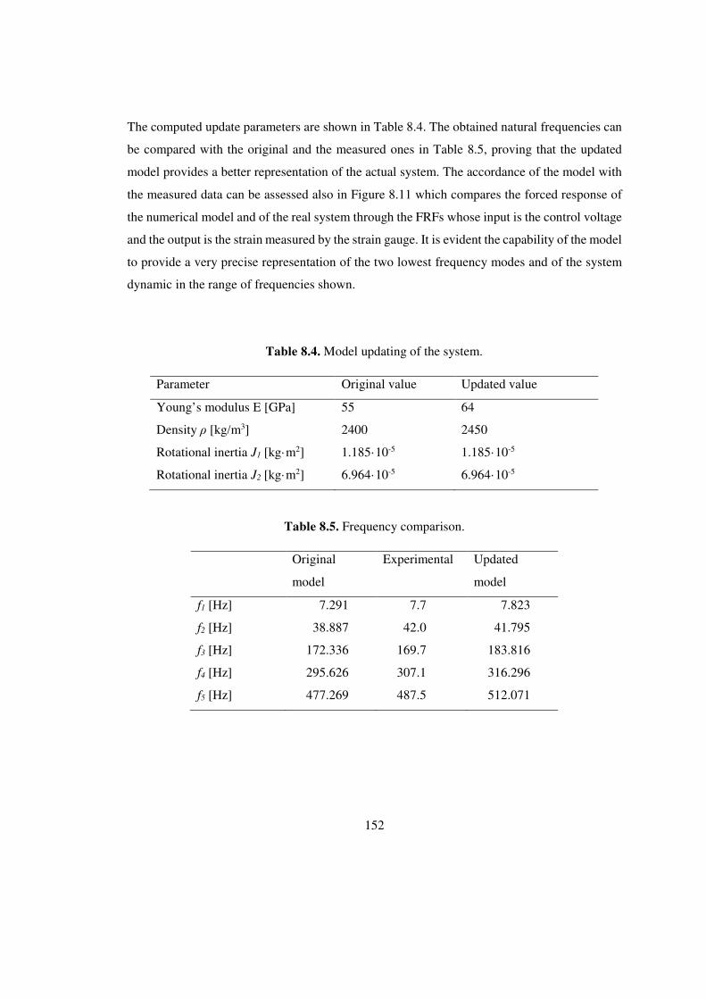
152

The computed update parameters are shown in Table 8.4. The obtained natural frequencies can

be compared with the original and the measured ones in Table 8.5, proving that the updated

model provides a better representation of the actual system. The accordance of the model with

the measured data can be assessed also in Figure 8.11 which compares the forced response of

the numerical model and of the real system through the FRFs whose input is the control voltage

and the output is the strain measured by the strain gauge. It is evident the capability of the model

to provide a very precise representation of the two lowest frequency modes and of the system

dynamic in the range of frequencies shown.

Table 8.4. Model updating of the system.

Parameter Original value Updated value

Young’s modulus E [GPa] 55 64

Density ρ [kg/m3] 2400 2450

Rotational inertia J1 [kg·m2] 1.185·10-5 1.185·10-5

Rotational inertia J2 [kg·m2] 6.964·10-5 6.964·10-5

Table 8.5. Frequency comparison.

Original

model

Experimental Updated

model

f1 [Hz] 7.291 7.7 7.823

f2 [Hz] 38.887 42.0 41.795

f3 [Hz] 172.336 169.7 183.816

f4 [Hz] 295.626 307.1 316.296

f5 [Hz] 477.269 487.5 512.071

153

Once that the model has been updated, the hybrid control synthesis has been corrected to

account for the actual model parameters that slightly differ from the nominal one. The best

assignable eigenvector of the updated system at 50 Hz is plotted in Figure 8.12, in comparison

with the desired one. Despite the difference between the two eigenvectors being appreciable,

the attainable one is valid for the purpose of vibration confinement, as proved by the computed

cosine, which is 0.9917.

Figure 8.12. Mode attainable by hybrid control after model updating

Figure 8.11. Comparison of the measured receptances with the ones of the updated model

0 10 20 30 40 50 60

Frequency [Hz]

0

0.005

0.01

0.015

0.02

0.025

Measured

Model

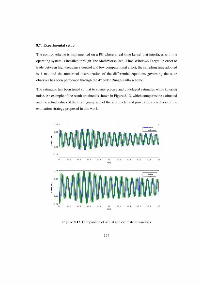
154

8.7. Experimental setup

The control scheme is implemented on a PC where a real-time kernel that interfaces with the

operating system is installed through The MathWorks Real-Time Windows Target. In order to

trade between high-frequency control and low computational effort, the sampling time adopted

is 1 ms, and the numerical discretization of the differential equations governing the state

observer has been performed through the 4th order Runge-Kutta scheme.

The estimator has been tuned so that to ensure precise and undelayed estimates while filtering

noise. An example of the result obtained is shown in Figure 8.13, which compares the estimated

and the actual values of the strain gauge and of the vibrometer and proves the correctness of the

estimation strategy proposed in this work.

Figure 8.13. Comparison of actual and estimated quantities

41 41.2 41.4 41.6 41.8 42 42.2 42.4 42.6 42.8 43

t [s]

-0.02

-0.01

0

0.01

0.02

actual

estimated

41 41.2 41.4 41.6 41.8 42 42.2 42.4 42.6 42.8 43

t [s]

-0.04

-0.02

0

0.02

0.04

actual

estimated

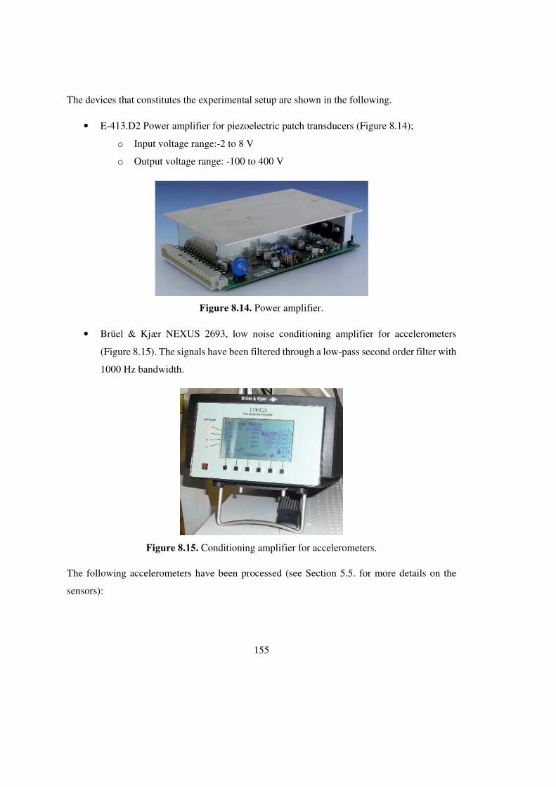
155

The devices that constitutes the experimental setup are shown in the following.

• E-413.D2 Power amplifier for piezoelectric patch transducers (Figure 8.14);

o Input voltage range:-2 to 8 V

o Output voltage range: -100 to 400 V

Figure 8.14. Power amplifier.

• Brüel & Kjær NEXUS 2693, low noise conditioning amplifier for accelerometers

(Figure 8.15). The signals have been filtered through a low-pass second order filter with

1000 Hz bandwidth.

Figure 8.15. Conditioning amplifier for accelerometers.

The following accelerometers have been processed (see Section 5.5. for more details on the

sensors):

156

o Endevco 27AM1-100 10203, miniaturized ICP accelerometer, adopted to

verify local acelerations or speed (through integration performed by the Nexus

amplifier)

o Brüel & Kjær 4508 ICP accelerometer, to measure the acceleration of the slip-

table to be input to the observer

• HBM QuantumX MX878B + QuantumX MX840B, multichannel data acquisition

system for conditioning the strain gauge bridge (Figure 8.16). To eliminate

measurement noise and to prevent aliasing problems, the strain-gauge signals are

passed through a low-pass filter cut-off frequency of 500 Hz.

Figure 8.16. Data acquisition system.

• Polytec OFV 525 laser vibrometer (Figure 8.17) with OFV 5000 controller, to measure

the nodal speed employed for the synthesis of the state observer

Figure 8.17. Laser vibrometer.

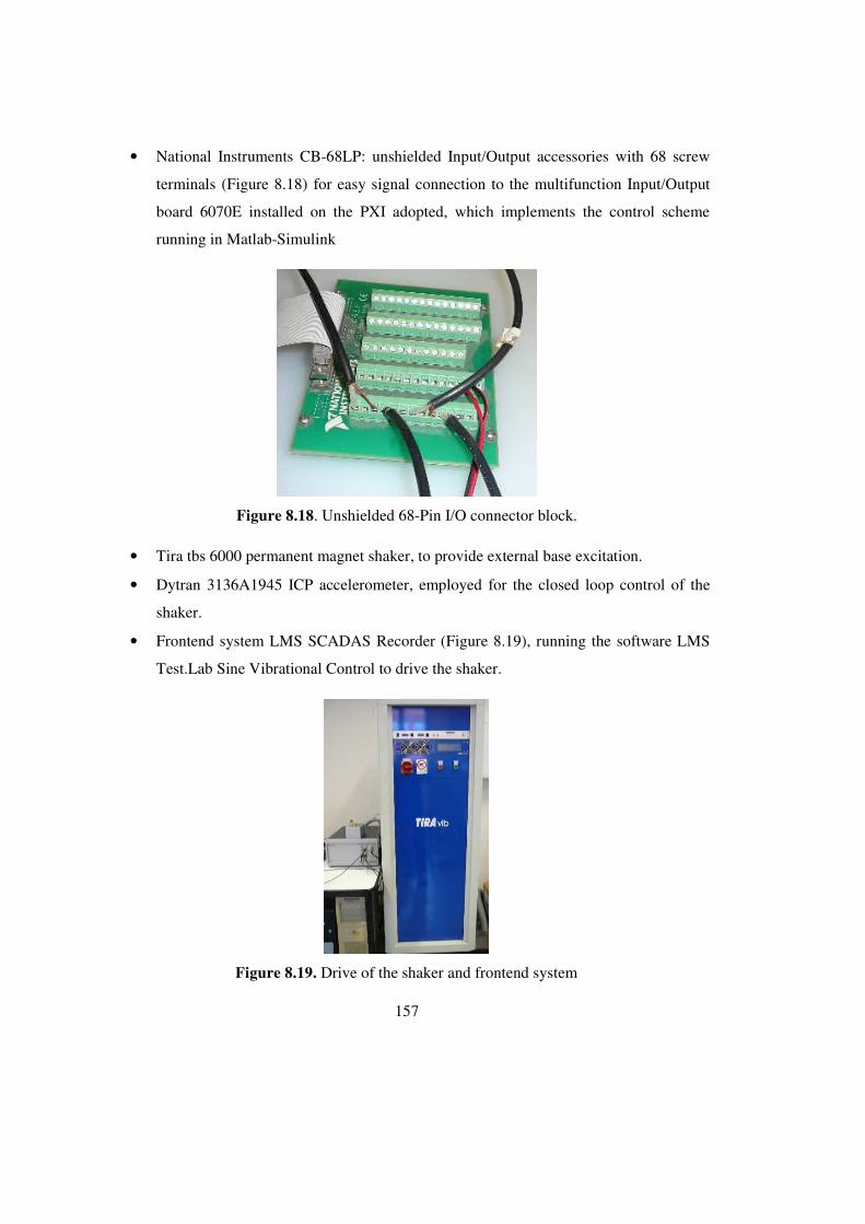
157

• National Instruments CB-68LP: unshielded Input/Output accessories with 68 screw

terminals (Figure 8.18) for easy signal connection to the multifunction Input/Output

board 6070E installed on the PXI adopted, which implements the control scheme

running in Matlab-Simulink

Figure 8.18. Unshielded 68-Pin I/O connector block.

• Tira tbs 6000 permanent magnet shaker, to provide external base excitation.

• Dytran 3136A1945 ICP accelerometer, employed for the closed loop control of the

shaker.

• Frontend system LMS SCADAS Recorder (Figure 8.19), running the software LMS

Test.Lab Sine Vibrational Control to drive the shaker.

Figure 8.19. Drive of the shaker and frontend system

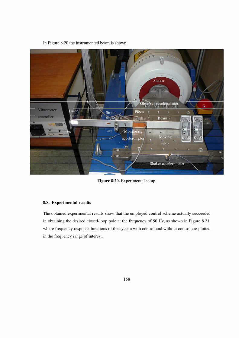
158

In Figure 8.20 the instrumented beam is shown.

Figure 8.20. Experimental setup.

8.8. Experimental results

The obtained experimental results show that the employed control scheme actually succeeded

in obtaining the desired closed-loop pole at the frequency of 50 Hz, as shown in Figure 8.21,

where frequency response functions of the system with control and without control are plotted

in the frequency range of interest.

Beam

Piezo

actuator

Shaker accelerometer

Observer accelerometer

Monitoring

accelerometer

Strain gauge

Vibrometer

controller

Laser spot

Shaker

Moving

table

m1 m2

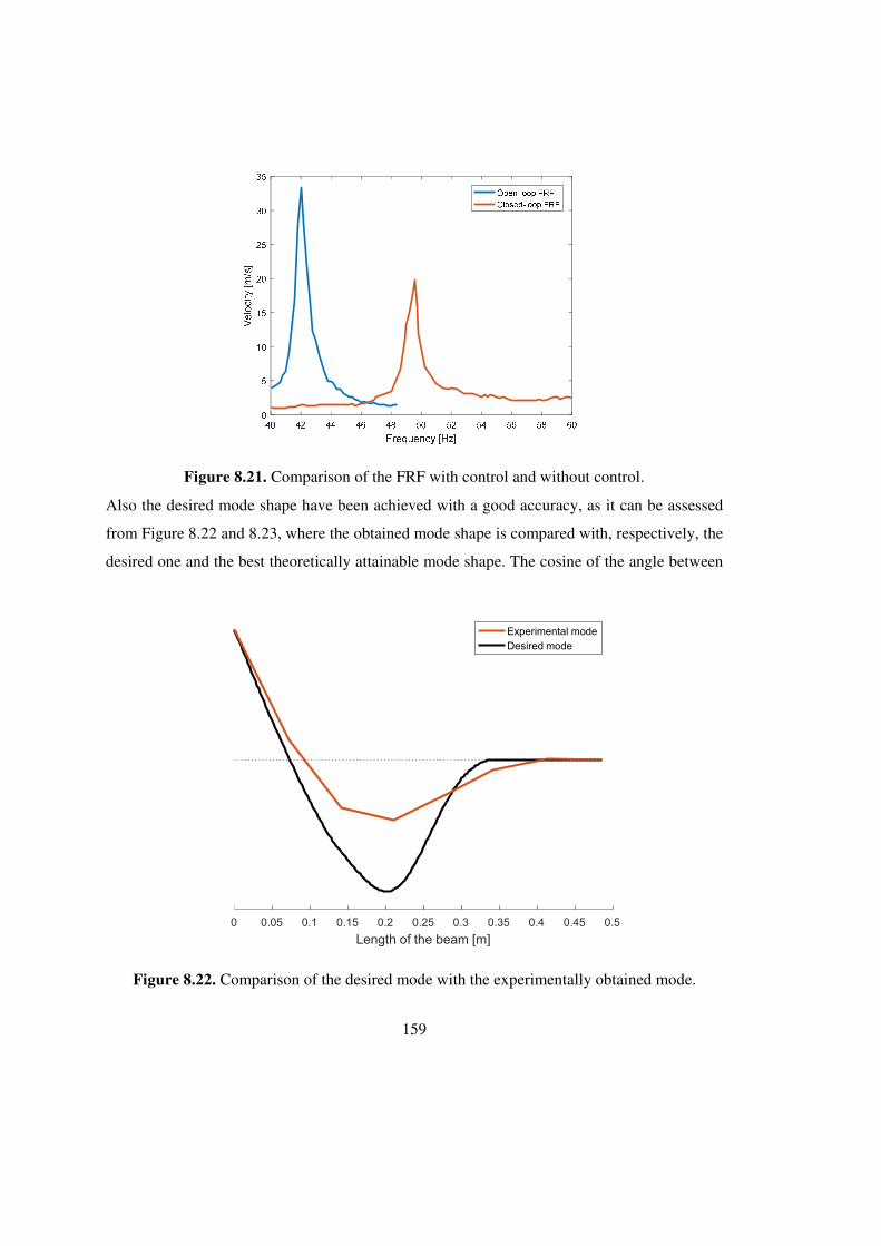
159

Also the desired mode shape have been achieved with a good accuracy, as it can be assessed

from Figure 8.22 and 8.23, where the obtained mode shape is compared with, respectively, the

desired one and the best theoretically attainable mode shape. The cosine of the angle between

Figure 8.21. Comparison of the FRF with control and without control.

Figure 8.22. Comparison of the desired mode with the experimentally obtained mode.

0 0.05 0.1 0.15 0.2 0.25 0.3 0.35 0.4 0.45 0.5

Length of the beam [m]

Experimental mode

Desired mode

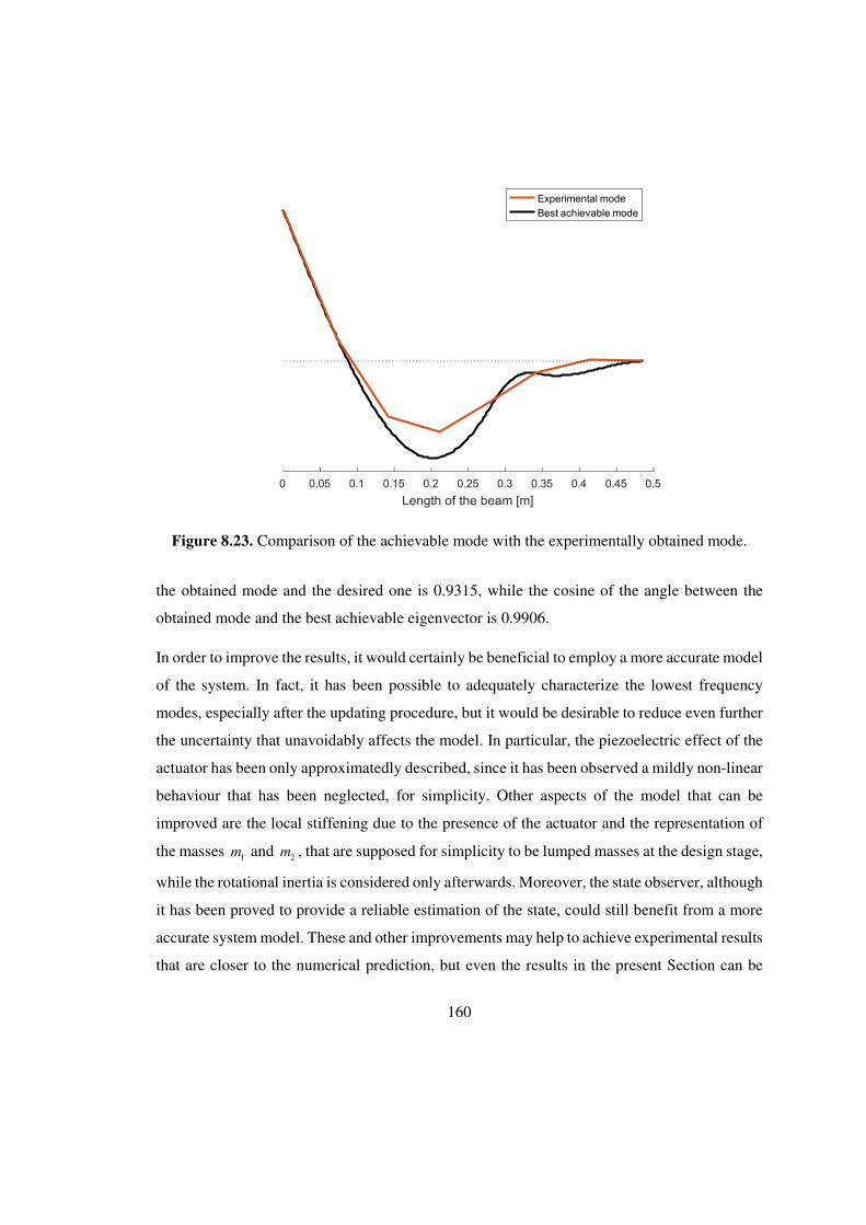
160

the obtained mode and the desired one is 0.9315, while the cosine of the angle between the

obtained mode and the best achievable eigenvector is 0.9906.

In order to improve the results, it would certainly be beneficial to employ a more accurate model

of the system. In fact, it has been possible to adequately characterize the lowest frequency

modes, especially after the updating procedure, but it would be desirable to reduce even further

the uncertainty that unavoidably affects the model. In particular, the piezoelectric effect of the

actuator has been only approximatedly described, since it has been observed a mildly non-linear

behaviour that has been neglected, for simplicity. Other aspects of the model that can be

improved are the local stiffening due to the presence of the actuator and the representation of

the masses 1m and 2m , that are supposed for simplicity to be lumped masses at the design stage,

while the rotational inertia is considered only afterwards. Moreover, the state observer, although

it has been proved to provide a reliable estimation of the state, could still benefit from a more

accurate system model. These and other improvements may help to achieve experimental results

that are closer to the numerical prediction, but even the results in the present Section can be

Figure 8.23. Comparison of the achievable mode with the experimentally obtained mode.

0 0.05 0.1 0.15 0.2 0.25 0.3 0.35 0.4 0.45 0.5

Length of the beam [m]

Experimental mode

Best achievable mode

161

considered very satisfactory, since they enable to assess that the developed hybrid technique

can be successfully applied to the control of a meaningful vibrating system.

162

163

Conclusions The present thesis addresses several open issues of theoretical and applicative interest in the

field of eigenstructure assignment through active, passive and hybrid control. The main results

achieved can be summarized through the following points.

• It has been developed a method for passive control that enables to assign partial mode

shapes, in order to attain a better fulfilment of the design specification in the parts of

the system whose vibrating behaviour is particularly relevant. The proposed method

relies on a homotopy optimization strategy that is proven to boost the achievement of a

globally optimal solution of the assignment problem. Such a method has been tested

with established benchmarks and in the solution of practical design problems thus

proving its effectiveness.

• A novel method for eigenstructure assignment with the addition of auxiliary subsystems

has been proposed. For the investigated issue, few methods are available, despite its

relevance. The homotopy optimization strategy developed for the assignment of partial

eigenvectors have been successfully employed also in this case. The numerical

validation of the method proves that the proposed solution is general and reliable and

can be applied with different topology of the auxiliary system.

• A method for avoiding spill-over in the assignment of natural frequencies by means of

passive control has been also developed. Such an issue can be tackled only for simple

systems by the state-of-the-art methods, while the proposed one can handle systems of

general topology, even containing distributed parameters, as proved in the thesis.

• The knowledge in the field of the solution of inverse eigenvalue problems has been

devoted to another relevant problem in the field of vibrationg system, namely the model

updating, which is a field closely related to eigenstructure assignment. The problem has

been addressed and a method that enable to perform model updating for flexible link

mechanisms is proposed. Such a method has been experimentally applied to a very

164

challenging updating task, i.e. the tuning of the parameters of a flexible planar robot.

by showing that remarkable improvement of the model can be achieved.

• As far as active control is concerned, it has beend developed a method for partial pole

placement that enables to deal with spill-over of the non-assigned poles by specifying

a regional constraint through Linear Matrix Inequalities. Such a method, in contrast to

alternative methods in the literature, employes reliable numerical tools to synthesize

the desired control gains. The numerical validation that has been carried out through

the challenging test of a flexible link mechanism shows the effectiveness of the

proposed approach.

• The capability of assigning the mode shape and the frequency has been significantly

enlarged through the last approach proposed in the Thesis, which is a method that

exploits passive control to improve the assignment of mode shapes through state-

feedback control. Such a hybrid approach has been rarely used in the literature. The

proposed method consists in recasting the assignment problem as the minimization of

the rank of a matrix, that can be solved exploiting some recent results in the field of

numerical optimization. The numerical application has demonstrated the effectiveness

of the method and its superiority over the active control and the dynamic structural

modification when both used alone and when applied sequentially. In contrast, the

proposed method considers both the approaches in a concurrent way.

• Finally, the hybrid method proposed in the thesis has been applied to the experimental

control of a cantilever beam by means of a piezoelectric actuator. Despite the fact that

the system is highly underactuated, the obtained numerical results proved that the

proposed method could achieve a very accurate assignment. Given the impossibility to

feed back the whole state vector, the experimental application has imposed to develop

a state estimator that enabled to approximate the state of the system even if few

measurements are available. The results obtained corroborate all the theoretical

expectations and show that the proposed method can be applied to the control of real

systems, by taking advantage of state observers suitable for real time control.

The overview of all the results obtained through the different approaches, shows that

eigenstructure assignment is an effective tool to improve the dynamic behaviour of vibrating

165

systems. This statement is corroborated also by the fact that physical feasibility of the computed

solution has been taken into account in all the developed methods, as well as their numerical

reliability has been carefully addressed. Given the focus on these issues, it is expected that the

methods here proposed might be an effective bridge towards the use of eigenstructure

assignment in the solution of engineering design problems, such as the mechanical design, the

control scheme synthesis, the mechatronics design. With reference to the latter, in particular,

the inclusion of the controlled system expected performances in the design of the mechanical

part as the hybrid control does, decreases the need of iterating and hence allows to handle

effectively more complicated problems.

166

167

References [1] S. Adhikari. Rates of change of eigenvalues and eigenvectors in damped dynamic

system. AIAA journal, 37(11):1452–1458, 1999.

[2] K. Farahani and H. Bahai. An inverse strategy for relocation of eigenfrequencies in

structural design. Part I: first order approximate solutions. Journal of Sound and Vibration,

274(3):481–505, 2004.

[3] K. Farahani and H. Bahai. An inverse strategy for relocation of eigenfrequencies in

structural design. Part II: second order approximate solutions. Journal of Sound and Vibration,

274(3):507–528, 2004.

[4] W. Liangsheng. Direct method of inverse eigenvalue problems for structure redesign.

Journal of Mechanical Design, 125(4):845–847, 2003.

[5] D. Wang, J. Jiang, and W. Zhang. Optimization of support positions to maximize the

fundamental frequency of structures. International journal for numerical methods in

engineering, 61(10):1584–1602, 2004.

[6] D. Wang, M. Friswell, and Y. Lei. Maximizing the natural frequency of a beam with an

intermediate elastic support. Journal of Sound and Vibration, 291(3):1229–1238, 2006.

[7] Y. Ram. Optimal mass distribution in vibrating systems. Mechanical Systems and

Signal Processing, 23(7):2130–2140, 2009.

[8] D. Richiedei, A. Trevisani, and G. Zanardo. A constrained convex approach to modal

design optimization of vibrating systems. Journal of Mechanical Design, 133(6):061011, 2011.

[9] H. Ouyang, D. Richiedei, A. Trevisani, and G. Zanardo. Discrete mass and stiffness

modifications for the inverse eigenstructure assignment in vibrating systems: Theory and

experimental validation. International Journal of Mechanical Sciences, 64(1):211–220, 2012.

[10] Y. Ram and S. Braun. An inverse problem associated with modification of incomplete

dynamic systems. Journal of Applied Mechanics, 58(1):233–237, 1991.

168

[11] D. D. Sivan and Y. M. Ram. Physical modifications to vibratory systems with assigned

eigendata. Journal of Applied Mechanics, 66(2):427–431, 1999.

[12] D. Sivan and Y. Ram. Optimal construction of a mass-spring system from prescribed

modal and spectral data. Journal of Sound and Vibration, 201(3):323–334, 1997.

[13] I. Bucher and S. Braun. The structural modification inverse problem: an exact solution.

Mechanical Systems and Signal Processing, 7(3):217–238, 1993.

[14] S. Braun and Y. Ram. Modal modification of vibrating systems: some problems and

their solutions. Mechanical Systems and Signal Processing, 15(1):101–119, 2001.

[15] D. D. Sivan and Y. M. Ram. Mass and stiffness modifications to achieve desired natural

frequencies. Communications in numerical methods in engineering, 12(9):531–542, 1996.

[16] J. Mottershead. Structural modification for the assignment of zeros using measured

receptances. Journal of Applied Mechanics, 68(5):791–798, 2001.

[17] A. Kyprianou, J. E. Mottershead, and H. Ouyang. Assignment of natural frequencies by

an added mass and one or more springs. Mechanical Systems and Signal Processing, 18(2):263–

289, 2004.

[18] A. Kyprianou, J. E. Mottershead, and H. Ouyang. Structural modification. Part 2:

assignment of natural frequencies and antiresonances by an added beam. Journal of Sound and

Vibration, 284(1):267–281, 2005.

[19] H. Ouyang. Prediction and assignment of latent roots of damped asymmetric systems

by structural modifications. Mechanical Systems and Signal Processing, 23(6):1920–1930,

2009.

[20] Y. H. Park and Y. S. Park. Structural modification based on measured frequency

response functions: an exact eigenproperties reallocation. Journal of Sound and Vibration,

237(3):411–426, 2000.

[21] J. Mottershead and G. Lallement. Vibration nodes, and the cancellation of poles and

zeros by unit-rank modifications to structures. Journal of Sound and Vibration, 222(5):833–

851, 1999.

169

[22] J. Mottershead, T. Li, and J. He. Pole–zero cancellation in structures: repeated roots.

Journal of Sound and Vibration, 231(1):219–231, 2000.

[23] H. Ouyang, D. Richiedei, A. Trevisani, and G. Zanardo. Eigenstructure assignment in

undamped vibrating systems: a convex-constrained modification method based on receptances.

Mechanical Systems and Signal Processing, 27:397–409, 2012.

[24] W. Wonham. On pole assignment in multi-input controllable linear systems. IEEE

Transactions on Automatic Control, 12(6):660–665, 1967.

[25] J. Kautsky, N. K. Nichols, and P. Van Dooren. Robust pole assignment in linear state

feedback. International Journal of Control, 41(5):1129–1155, 1985.

[26] J. Ackermann. Der entwurf linearer regelungssysteme im zustandsraum. at-

Automatisierungstechnik, 20(1-12):297–300, 1972.

[27] E. Chu and B. Datta. Numerically robust pole assignment for second-order systems.

International Journal of Control, 64(6):1113–1127, 1996.

[28] B. N. Datta, S. Elhay, and Y. M. Ram. Orthogonality and partial pole assignment for

the symmetric definite quadratic pencil. Linear Algebra and its Applications, 257:29–48, 1997.

[29] Y. Ram and S. Elhay. Pole assignment in vibratory systems by multi-input control.

Journal of Sound and Vibration, 230(2):309–321, 2000.

[30] E. Chu. Pole assignment for second-order systems. Mechanical Systems and Signal

Processing, 16(1):39–59, 2002.

[31] J. Qian and S. Xu. Robust partial eigenvalue assignment problem for the second-order

system. Journal of Sound and Vibration, 282(3):937–948, 2005.

[32] B. C. Moore. On the flexibility offered by state feedback in multivariable systems

beyond closed loop eigenvalue assignment. In Decision and Control including the 14th

Symposium on Adaptive Processes, 1975 IEEE Conference on, pages 207–214. IEEE, 1975.

[33] A. Andry, E. Shapiro, and J. Chung. Eigenstructure assignment for linear systems.

IEEE transactions on aerospace and electronic systems, 19(5):711–729, 1983.

170

[34] B. White. Eigenstructure assignment: a survey. Proceedings of the Institution of

Mechanical Engineers, Part I: Journal of Systems and Control Engineering, 209(1):1–11, 1995.

[35] B. N. Datta, S. Elhay, Y. a. Ram, and D. R. Sarkissian. Partial eigenstructure

assignment for the quadratic pencil. Journal of Sound and Vibration, 230(1):101–110, 2000.

[36] J. E. Mottershead and Y. M. Ram. Receptance method in active vibration control. AIAA

journal, 45(3):562–567, 2007.

[37] M. G. Tehrani, R. N. Elliott, and J. E. Mottershead. Partial pole placement in structures

by the method of receptances: theory and experiments. Journal of Sound and Vibration,

329(24):5017–5035, 2010.

[38] E. Allgower and K. Georg. Introduction to Numerical Continuation Methods. Classics

in Applied Mathematics. Society for Industrial and Applied Mathematics, 2003.

[39] W. Forster. Homotopy methods. In R. Horst and P. Pardalos, editors, Handbook of

Global Optimization, volume 2 of Nonconvex Optimization and Its Applications, pages 669–

750. Springer US, 1995.

[40] D. M. Dunlavy and D. P. O’Leary. Homotopy optimization methods for global

optimization. Sandia National Laboratories, Report SAND2005-7495, 2005.

[41] C. P. Vyasarayani, T. Uchida, A. Carvalho, and J. McPhee. Parameter identification in

dynamic systems using the homotopy optimization approach. Multibody System Dynamics,

26(4):411–424, 2011.

[42] F. A. Al-Khayyal and J. E. Falk. Jointly constrained biconvex programming.

Mathematics of Operations Research, 8(2):273–286, 1983.

[43] G. P. McCormick. Computability of global solutions to factorable nonconvex

programs: Part I—Convex underestimating problems. Mathematical programming, 10(1):147–

175, 1976.

[44] Z. Liu, W. Li, H. Ouyang, and D. Wang. Eigenstructure assignment in vibrating

systems based on receptances. Archive of Applied Mechanics, 85(6):713–724, 2015.

171

[45] E. D. Andersen and K. D. Andersen. The Mosek Interior Point Optimizer for Linear

Programming: An Implementation of the Homogeneous Algorithm, pages 197–232. Springer

US, Boston, MA, 2000.

[46] R. H. Byrd, M. E. Hribar, and J. Nocedal. An interior point algorithm for large-scale

nonlinear programming. SIAM Journal on Optimization, 9(4):877–900, 1999.

[47] J. Löfberg. YALMIP: A toolbox for modeling and optimization in MATLAB. In

Proceedings of the CACSD Conference, Taipei, Taiwan, 2004.

[48] G. Canbaloglu and H. N. Özgüven. Structural modifications with additional DOF

applications to real structures. In Proceedings of the 27th International Modal Analysis

Conference, IMAC, Orlando, 2009.

[49] H. Hang, K. Shankar, and J. C. Lai. Prediction of the effects on dynamic response due

to distributed structural modification with additional degrees of freedom. Mechanical Systems

and Signal Processing, 22(8):1809–1825, 2008.

[50] H. Hang, K. Shankar, and J. C. Lai. Effects of distributed structural dynamic

modification with additional degrees of freedom on 3d structure. Mechanical Systems and

Signal Processing, 24(5):1349–1368, 2010.

[51] D. Stăncioiu and H. Ouyang. Structural modification formula and iterative design

method using multiple tuned mass dampers for structures subjected to moving loads.

Mechanical Systems and Signal Processing, 28:542–560, 2012.

[52] R. Jacquot. Suppression of random vibration in plates using vibration absorbers.

Journal of Sound and Vibration, 248(4):585–596, 2001.

[53] R. Caracciolo, D. Richiedei, A. Trevisani, and G. Zanardo. Designing vibratory linear

feeders through an inverse dynamic structural modification approach. The International Journal

of Advanced Manufacturing Technology, 80(9):1587–1599, 2015.

[54] D. Richiedei and A. Trevisani. Vibration confinement in lightly damped multibody

systems: An hybrid active-passive approach. In Proceedings of the ECCOMAS thematic

conference on multibody dynamics, pages 789–795, Zagreb, Croatia, 2013.

172

[55] Y. Saad. Projection and deflation method for partial pole assignment in linear state

feedback. IEEE Transactions on Automatic Control, 33(3):290–297, 1988.

[56] B. N. Datta and D. R. Sarkissian. Partial eigenvalue assignment in linear systems:

existence, uniqueness and numerical solution. In Proceedings of the Mathematical Theory of

Networks and Systems (MTNS), Notre Dame. Citeseer, 2002.

[57] D. J. Inman. Active modal control for smart structures. Philosophical Transactions of

the Royal Society of London A: Mathematical, Physical and Engineering Sciences,

359(1778):205–219, 2001.

[58] M. Gürgöze et al. Preserving the fundamental frequencies of beams despite mass

attachments. Journal of Sound and Vibration, 235(2):345–359, 2000.

[59] V. Mermertas and M. Gürgöze. Preservation of the fundamental natural frequencies of

rectangular plates with mass and spring modifications. Journal of Sound and Vibration,

276(1):440–448, 2004.

[60] O. Çakar. Mass and stiffness modifications without changing any specified natural

frequency of a structure. Journal of Vibration and Control, 17(5):769–776, 2011.

[61] H. Ouyang and J. Zhang. Passive modifications for partial assignment of natural

frequencies of mass–spring systems. Mechanical Systems and Signal Processing, 50:214–226,

2015.

[62] J. Yang, H. Ouyang, and J.-F. Zhang. A new method of updating mass and stiffness

matrices simultaneously with no spillover. Journal of Vibration and Control, 22(5):1181–1189,

2014.

[63] J. Zhang, H. Ouyang, and J. Yang. Partial eigenstructure assignment for undamped

vibration systems using acceleration and displacement feedback. Journal of Sound and

Vibration, 333(1):1–12, 2014.

[64] J. Sturm. Using SeDuMi 1.02, a MATLAB toolbox for optimization over symmetric

cones. Optimization Methods and Software, 11–12:625–653, 1999. Version 1.05 available from

http://fewcal.kub.nl/sturm.

173

[65] K.-C. Toh, M. J. Todd, and R. H. Tütüncü. SDPT3—A MATLAB software package for

semidefinite programming, version 1.3. Optimization Methods and Software, 11(1-4):545–581,

1999.

[66] M. T. Chu and Q. Guo. On the least squares approximation of symmetric-definite

pencils subject to generalized spectral constraints. SIAM Journal on Matrix Analysis and

Applications, 19(1):1–20, 1998.

[67] H. P. Langtangen and G. K. Pedersen. Scaling of Differential Equations. Springer,

2016.

[68] I. Gurobi Optimization. Gurobi optimizer reference manual, 2016.

[69] X. Mao and H. Dai. Finite element model updating with positive definiteness and no

spill-over. Mechanical Systems and Signal Processing, 28:387–398, 2012.

[70] M. Bratland, B. Haugen, and T. Rølvåg. Modal analysis of active flexible multibody

systems containing PID controllers with non-collocated sensors and actuators. Finite Elements

in Analysis and Design, 91:16–29, 2014.

[71] S. K. Dwivedy and P. Eberhard. Dynamic analysis of flexible manipulators, a literature

review. Mechanism and Machine Theory, 41(7):749–777, 2006.

[72] R. J. Theodore and A. Ghosal. Comparison of the assumed modes and finite element

models for flexible multilink manipulators. The International journal of robotics research,

14(2):91–111, 1995.

[73] P. Kalra and A. M. Sharan. Accurate modelling of flexible manipulators using finite

element analysis. Mechanism and Machine Theory, 26(3):299–313, 1991.

[74] M. Giovagnoni. A numerical and experimental analysis of a chain of flexible bodies.

Journal of dynamic systems, measurement, and control, 116(1):73–80, 1994.

[75] J. Mottershead and M. Friswell. Model updating in structural dynamics: a survey.

Journal of Sound and Vibration, 167(2):347–375, 1993.

174

[76] S. Sehgal and H. Kumar. Structural dynamic model updating techniques: A state of the

art review. Archives of Computational Methods in Engineering, pages 1–19, 2015.

[77] G.-H. Kim and Y.-S. Park. An improved updating parameter selection method and finite

element model update using multiobjective optimisation technique. Mechanical Systems and

Signal Processing, 18(1):59–78, 2004.

[78] S. Weng, Y. Xia, Y.-L. Xu, and H.-P. Zhu. Substructure based approach to finite

element model updating. Computers & structures, 89(9):772–782, 2011.

[79] R. Caracciolo, D. Richiedei, and A. Trevisani. Experimental validation of a model-

based robust controller for multi-body mechanisms with flexible links. Multibody System

Dynamics, 20(2):129–145, 2008.

[80] T. Uchida, C. Vyasarayani, M. Smart, and J. McPhee. Parameter identification for

multibody systems expressed in differential-algebraic form. Multibody System Dynamics,

31(4):393–403, 2014.

[81] J. O’Challan, I. Liew, P. Avitabile, and R. Madden. An efficient method of determining

rotational degrees of freedom from analytical and experimental modal data. In Proceedings of

the fourth International Modal Analysis conference, Los Angeles, USA, pages 50–58, 1986.

[82] A. Ng’andu, C. Fox, and E. Williams. Estimation of rotational degrees-of-freedom

using curve and surface fitting. In Proceedings of the International Modal Analysis Conference,

pages 620–626. SEM Society for Experimental Mechanics Inc., 1993.

[83] M. Liu and D. Gorman. Formulation of Rayleigh damping and its extensions.

Computers & structures, 57(2):277–285, 1995.

[84] I. Chowdhury and S. P. Dasgupta. Computation of Rayleigh damping coefficients for

large systems. The Electronic Journal of Geotechnical Engineering, 8(0), 2003.

[85] H. Ahmadian, J. Mottershead, and M. Friswell. Regularisation methods for finite

element model updating. Mechanical Systems and Signal Processing, 12(1):47–64, 1998.

[86] B. Peeters, G. Lowet, H. Van der Auweraer, and J. Leuridan. A new procedure for

modal parameter estimation. Sound and Vibration, 38(1):24–29, 2004.

175

[87] H. Ouyang. Pole assignment of friction-induced vibration for stabilisation through

state-feedback control. Journal of Sound and Vibration, 329(11):1985–1991, 2010.

[88] M. G. Tehrani, J. E. Mottershead, A. T. Shenton, and Y. M. Ram. Robust pole

placement in structures by the method of receptances. Mechanical Systems and Signal

Processing, 25(1):112–122, 2011.

[89] H. Ouyang, D. Richiedei, and A. Trevisani. Pole assignment for control of flexible link

mechanisms. Journal of Sound and Vibration, 332(12):2884–2899, 2013.

[90] W. M. Haddad and D. S. Bernstein. Controller design with regional pole constraints.

IEEE Transactions on Automatic Control, 37(1):54–69, 1992.

[91] M. Chilali and P. Gahinet. H∞ design with pole placement constraints: an LMI

approach. IEEE Transactions on Automatic Control, 41(3):358–367, 1996.

[92] S. Datta, B. Chaudhuri, and D. Chakraborty. Partial pole placement with minimum

norm controller. In 49th IEEE Conference on Decision and Control (CDC), pages 5001–5006.

IEEE, 2010.

[93] S. Datta, D. Chakraborty, and B. Chaudhuri. Partial pole placement with controller

optimization. IEEE Transactions on Automatic Control, 57(4):1051–1056, 2012.

[94] S. Gutman and E. Jury. A general theory for matrix root-clustering in subregions of the

complex plane. IEEE Transactions on Automatic Control, 26(4):853–863, 1981.

[95] M. Ikeda, D. Šiljak, and D. White. An inclusion principle for dynamic systems. IEEE

Transactions on Automatic Control, 29(3):244–249, 1984.

[96] L. R. Corr and W. W. Clark. Active and passive vibration confinement using

piezoelectric transducers and dynamic vibration absorbers. In 1999 Symposium on Smart

Structures and Materials, pages 747–758. International Society for Optics and Photonics, 1999.

[97] J. Tang and K. Wang. Vibration confinement via optimal eigenvector assignment and

piezoelectric networks. Journal of Vibration and Acoustics, 126(1):27–36, 2004.

176

[98] I. M. Diaz, E. Pereira, V. Feliu, and J. J. Cela. Concurrent design of multimode input

shapers and link dynamics for flexible manipulators. Mechatronics, IEEE/ASME Transactions

on, 15(4):646–651, 2010.

[99] H. Ouyang. A hybrid control approach for pole assignment to second-order asymmetric

systems. Mechanical Systems and Signal Processing, 25(1):123–132, 2011.

[100] D. Richiedei and A. Trevisani. Simultaneous active and passive control for

eigenstructure assignment in lightly damped systems. Mechanical Systems and Signal

Processing, 85:556 – 566, 2017.

[101] M. Fazel. Matrix rank minimization with applications. PhD thesis, PhD thesis, Stanford

University, 2002.

[102] M. Fazel, H. Hindi, and S. Boyd. Rank minimization and applications in system theory.

In American Control Conference, 2004. Proceedings of the 2004, volume 4, pages 3273–3278.

IEEE, 2004.

[103] M. Mesbahi. On the rank minimization problem and its control applications. Systems &

control letters, 33(1):31–36, 1998.

[104] P. Jain, R. Meka, and I. S. Dhillon. Guaranteed rank minimization via singular value

projection. In Advances in Neural Information Processing Systems, pages 937–945, 2010.

[105] I. Markovsky and K. Usevich. Structured low-rank approximation with missing data.

SIAM Journal on Matrix Analysis and Applications, 34(2):814–830, 2013.

[106] Z.-F. Jin, Z. Wan, X. Zhao, and Y. Xiao. A penalty decomposition method for rank

minimization problem with affine constraints. Applied Mathematical Modelling, 39(16):4859–

4870, 2015.

[107] M. Fazel, H. Hindi, and S. P. Boyd. Log-det heuristic for matrix rank minimization with

applications to Hankel and Euclidean distance matrices. In American Control Conference, 2003.

Proceedings of the 2003, volume 3, pages 2156–2162. IEEE, 2003.

177

[108] M. Mesbahi. On the semi-definite programming solution of the least order dynamic

output feedback synthesis. In American Control Conference, 1999. Proceedings of the 1999,

volume 4, pages 2355–2359. IEEE, 1999.

[109] M. Fazel, H. Hindi, and S. P. Boyd. A rank minimization heuristic with application to

minimum order system approximation. In American Control Conference, 2001. Proceedings of

the 2001, volume 6, pages 4734–4739. IEEE, 2001.

[110] P. Gaudenzi, R. Carbonaro, and E. Benzi. Control of beam vibrations by means of

piezoelectric devices: theory and experiments. Composite structures, 50(4):373–379, 2000.

[111] A. Preumont. Vibration control of active structures: an introduction, volume 179.

Springer Science & Business Media, 2011.