POLITECNICO DI MILANOCorso di Laurea Magistrale in Ingegneria dell’AutomazioneDipartimento di Elettronica Informazione e Bioingegneria

CONTROL OF A SPAR–BUOY FLOATINGWIND TURBINE

Relatore: Prof. Alberto LevaCorrelatore: Prof. Emilio García Moreno

Tesi di Laurea di:Mattia Valtorta, matricola 804403

Anno Accademico 2015–2016

Abstract

Floating wind turbines take advantage of the offshore wind force to producea renewable and clean electric energy. Such systems offer a solution to over-come offshore barriers due to the deep water. Nevertheless, adopting a floaterplatform introduces an additional motion that must be taken into account inthe control system, which aims at achieving a better efficiency and systemlongevity. In this work, the development, implementation and simulation ofa multi-objectives state feedback obtained with a Linear Quadratic Regulatorand Disturbance Accommodating controllers are addressed. The results areapplied in simulation to a spar-buoy floating platform.

The spar-buoy platform achieves hydrostatic stability using a deep draftedballast with three catenary mooring lines. The deep draft increases the plat-form roll and pitch inertias, reducing their respective natural frequency. Thisaffects the DOFs choice in the control design. Adding the platform surge andthe first tower fore-aft, a correct representation of the platform pitch responseto the collective blade pitch is achieved. Simulation are carried out using ahigh-fidelity model obtained with FAST within MATLAB Simulink and thefatigue analysis is obtained according to design load case (DLC) 1.1 of theIEC 61400-3 standard for normal operation conditions.

The simulation results, compared to a gain scheduled PI controller, showthat a multi-objective state feedback controller obtained with collective bladepitch is able to improve the rotor speed regulation, thus the power quality.Furthermore, it is able to reduce tower-base side-to-side bending fatigue loadby an average of 15%. Disturbance Accommodating Controller using the col-lective blade pitch further improves the rotor speed regulation. The statefeedback controller obtained with the individual blade pitch is able to improvethe rotor speed regulation reducing the RMS value of the rotor speed error byan average of 69%. Moreover it is able to reduce tower-base fore-aft bendingfatigue load by an average of 8%. Disturbance Accommodation Controller,using the individual blade pitch, is able to improve the rotor speed regulation,thus diminishing the RMS value of the generator power error by an average of70%, a better power quality is obtained.

The performances achieved by creating asymmetric loads, over symmetricload, help in a better regulation of the rotor speed keeping a limited motionof the platform rotation about its pitch axis. Furthermore, individual bladepitch prevents the controller from conflict issues arising when rotor speed andplatform pitch are regulated simultaneously.

Sommario

Le turbine eoliche galleggianti, destinate alla produzione di energia elet-trica pulita sfruttando la forza del vento in mare aperto, offrono una soluzionerealizzabile per superare gli ostacoli causati delle acque profonde. Il fatto di uti-lizzare un sistema galleggiante, introduce un ulteriore movimento che assumeun aspetto rilevante al fine del controllo destinato al miglioramento del rendi-mento e della longevità del sistema. In questo progetto è stato affrontato losviluppo, l’implementazione e la simulazione di due controllori multi-obiettivoa retrazione dello stato. Il primo è stato ricavato utilizzando un regolatorelineare quadratico (LQR) e il secondo utilizzando un Disturbance Accommo-dation Control (DAC) finalizzato alla reiezione dei disturbi. Entrambi i con-trollori sono stati applicati a una piattaforma galleggiante di tipo Spar-Buoy.

Questa tipologia di piattaforma raggiunge la stabilità idrostatica per mezzodi un profondo pescaggio e tre linee di ancoraggio. La profondità del pescag-gio aumenta le inerzie di rollio e beccheggio, riducendo le frequenze naturalidella piattaforma, interagendo con la scelta dei gradi di libertà da considerarenel modello di controllo. Al fine di ottenere una corretta rappresentazionedella risposta in frequenza del beccheggio della piattaforma è necessario con-siderarne l’avanzamento della stessa in direzione-x (surge) e il primo mododi vibrare della torre in direzione prua-poppa. Le simulazioni sono effettuateutilizzando un modello ad alta fedeltà ottenuto con il simulatore FAST e MAT-LAB Simulink. Rispettando le norme IEC 61400-3, l’analisi a fatica è ricavatautilizzando il disegno di carico (DLC 1.1) adottato per le normali condizionioperative.

I risultati delle simulazioni, comparati con un controllore PI a guadagnovariabile, mostrano che un controllo multi-obbiettivo a retrazione dello stato,ottenuto con un beccheggio collettivo delle pale, migliora la regolazione dellavelocità del rotore e di conseguenza la qualità della potenza prodotta. Appli-cando questo controllo si riscontra, risultante dall’analisi a fatica, la riduzionemedia del 15% sul carico alla base della torre, in direzione lato-lato. Il control-lore DAC, anch’esso realizzato con un controllo collettivo delle pale, evidenziaun ulteriore miglioramento nella regolazione della velocità di rotazione delrotore. Il controllore a retrazione dello stato, ottenuto con una regolazione in-dividuale della pale, migliora la prestazione della velocità del rotore riducendoil valore RMS del 69%. In questo caso i carichi a fatica alla base della torre,in direzione prua-poppa, risultano ridotti del 8%. Il regolatore DAC, ottenutocon una regolazione individuale delle pale, migliora ulteriormente la perfor-mance del controllo di velocità, diminuendone il valore RMS del 70%.

Rispetto a carichi aerodinamici simmetrici, l’utilizzo di carichi asimmetricipermette una migliore regolazione della velocità del rotore mantenendo limi-tato il movimento di beccheggio della piattaforma. Inoltre, preserva il control-lore da eventuali conflitti che sorgono durante la regolazione simultanea dellavelocità del rotore e il beccheggio della piattaforma.

To Emma

Contents

1 Introduction 11.1 Offshore Wind Energy . . . . . . . . . . . . . . . . . . . . . . . 11.2 Thesis Objectives . . . . . . . . . . . . . . . . . . . . . . . . . . 31.3 Thesis Outline . . . . . . . . . . . . . . . . . . . . . . . . . . . . 3

2 Wind and Wave Models 42.1 Wind Model . . . . . . . . . . . . . . . . . . . . . . . . . . . . . 42.2 Spectral Model . . . . . . . . . . . . . . . . . . . . . . . . . . . 4

2.2.1 Kaimal Model . . . . . . . . . . . . . . . . . . . . . . . . 42.3 Turbulence Intensity . . . . . . . . . . . . . . . . . . . . . . . . 62.4 Wind Profiles . . . . . . . . . . . . . . . . . . . . . . . . . . . . 7

2.4.1 Power-Law Wind Profile . . . . . . . . . . . . . . . . . . 72.4.2 Logarithmic Wind Profile . . . . . . . . . . . . . . . . . 72.4.3 Surface Roughness Length . . . . . . . . . . . . . . . . . 8

2.5 Wave Model . . . . . . . . . . . . . . . . . . . . . . . . . . . . . 82.5.1 JONSWAP Spectrum . . . . . . . . . . . . . . . . . . . . 92.5.2 Pierson-Moskowitz Spectrum . . . . . . . . . . . . . . . 9

2.6 Wave Kinematic . . . . . . . . . . . . . . . . . . . . . . . . . . . 12

3 Hydrodynamic Model 143.1 Floating Platform Structural Properties . . . . . . . . . . . . . . 143.2 Support Platform Loads . . . . . . . . . . . . . . . . . . . . . . 15

3.2.1 Hydrodynamics Forces . . . . . . . . . . . . . . . . . . . 153.3 The True Linear Hydrodynamic Model in the Time Domain . . 18

3.3.1 Hydrostatic Problem . . . . . . . . . . . . . . . . . . . . 183.3.2 Diffraction Problem . . . . . . . . . . . . . . . . . . . . . 183.3.3 Radiation Problem . . . . . . . . . . . . . . . . . . . . . 19

3.4 Morison’s Equation . . . . . . . . . . . . . . . . . . . . . . . . . 223.5 Additional Damping . . . . . . . . . . . . . . . . . . . . . . . . 233.6 Mooring Line . . . . . . . . . . . . . . . . . . . . . . . . . . . . 24

4 Aerodynamic Loads 284.1 Blade Element Momentum Theory . . . . . . . . . . . . . . . . 28

4.1.1 Tip–Loss Model . . . . . . . . . . . . . . . . . . . . . . . 314.1.2 Hub–Loss Model . . . . . . . . . . . . . . . . . . . . . . 31

4.2 Drivetrain Model . . . . . . . . . . . . . . . . . . . . . . . . . . 324.3 Tower Model and Deflections . . . . . . . . . . . . . . . . . . . . 334.4 System Actuators . . . . . . . . . . . . . . . . . . . . . . . . . . 36

i

4.4.1 Electric Generator . . . . . . . . . . . . . . . . . . . . . 374.4.2 Blade Pitch Actuator . . . . . . . . . . . . . . . . . . . . 37

5 Control Models 385.1 Speed–Measurement Filter . . . . . . . . . . . . . . . . . . . . . 385.2 Generator–Torque Controller . . . . . . . . . . . . . . . . . . . . 38

5.2.1 Rotor Power Coefficient – Cp . . . . . . . . . . . . . . . 395.2.2 Optimal Constant in Region 2 . . . . . . . . . . . . . . . 40

5.3 Gain Scheduling PI . . . . . . . . . . . . . . . . . . . . . . . . . 415.4 LQR Control with Collective Blade Pitch . . . . . . . . . . . . . 475.5 DAC with Collective Blade Pitch . . . . . . . . . . . . . . . . . 49

5.5.1 Collective Blade Pitch Drift . . . . . . . . . . . . . . . . 505.6 LQR Control with Individual Pitch Blade . . . . . . . . . . . . 51

5.6.1 Multi-Blade Coordinate Transformation - MBC . . . . . 525.6.2 LQR after MBC Transformation . . . . . . . . . . . . . . 54

5.7 DAC with Individual Blade Pitch . . . . . . . . . . . . . . . . . 545.7.1 Including Wind Share Effect . . . . . . . . . . . . . . . . 555.7.2 DAC after MBC Transformation . . . . . . . . . . . . . . 56

6 Results 576.1 Results Comparisons . . . . . . . . . . . . . . . . . . . . . . . . 586.2 Normalized Indices Comparison . . . . . . . . . . . . . . . . . . 68

7 Conclusions and Further Developments 70

A Model Linearization 72

B Fatigue Analysis 75B.1 Lifetime Damage . . . . . . . . . . . . . . . . . . . . . . . . . . 75

B.1.1 Goodman Exponent . . . . . . . . . . . . . . . . . . . . 76B.2 Time Until Failure . . . . . . . . . . . . . . . . . . . . . . . . . 76B.3 Damage Equivalent Loads . . . . . . . . . . . . . . . . . . . . . 76

Bibliography 78

ii

List of Figures

1.1 Mains Floating Platform Concepts for Offshore Wind Turbines . 2

2.1 Kaimal Spectrum for u-component . . . . . . . . . . . . . . . . 52.2 Longitudinal wind-speed standard deviation and turbulence in-

tensity (TI) categories . . . . . . . . . . . . . . . . . . . . . . . 62.3 The Wind Speed profile generated from the combination of

Power-Law and Logarithmic . . . . . . . . . . . . . . . . . . . . 82.4 Comparison between Pierson-Moskowitz and JONSWAP spec-

tra realized with Hs = 11.8 and Tp = 15.5 . . . . . . . . . . . . 112.5 Pierson-Moskowitz spectrum . . . . . . . . . . . . . . . . . . . . 112.6 Wind Speed Time Series . . . . . . . . . . . . . . . . . . . . . . 132.7 Wave Elevation Time Series . . . . . . . . . . . . . . . . . . . . 13

3.1 The Support Platform Degrees of Freedom . . . . . . . . . . . . 143.2 Dimensionless parameter with T and H defined in Tab. 2.2 . . . 173.3 Hydrodynamic wave excitation per unit amplitude . . . . . . . . 193.4 Hydrodynamic–added–mass and –damping . . . . . . . . . . . . 213.5 Single Mooring Line in xz local axis . . . . . . . . . . . . . . . . 26

4.1 Annular plane used in BEMT . . . . . . . . . . . . . . . . . . . 284.2 Blade Element Theory . . . . . . . . . . . . . . . . . . . . . . . 294.3 Helical Wake caused by tip-blade . . . . . . . . . . . . . . . . . 314.4 Tip-Loss and Hub-Loss Factor with constant θ = 10 deg . . . . . 324.5 Two–mass drivetrain model . . . . . . . . . . . . . . . . . . . . 334.6 Tower Bending . . . . . . . . . . . . . . . . . . . . . . . . . . . 334.7 Tower deflection geometry . . . . . . . . . . . . . . . . . . . . . 354.8 Blade Pitch Step Response . . . . . . . . . . . . . . . . . . . . . 37

5.1 Wind Turbines Operation Regions . . . . . . . . . . . . . . . . . 395.2 Power Coefficient . . . . . . . . . . . . . . . . . . . . . . . . . . 405.3 Variable-Speed Controller . . . . . . . . . . . . . . . . . . . . . 415.4 Linear Approximation of pitch sensitivity in Region 3 . . . . . 445.5 Blade Pitch Control Gain Scheduling Law . . . . . . . . . . . . 455.6 Platform pitch frequency response to collective blade pitch . . . 475.7 Platform pitch response to collective blade pitch step . . . . . . 485.8 Collective Blade Pitch Drift . . . . . . . . . . . . . . . . . . . . 515.9 Platform Pitch restoring mechanism using IBP . . . . . . . . . . 515.10 Blade 1 periodic gain and constant gain . . . . . . . . . . . . . . 525.11 MBC Coordinate Transformation . . . . . . . . . . . . . . . . . 53

iii

6.1 Comparison between the outputs obtained with GSPI and LQR–CBP . . . . . . . . . . . . . . . . . . . . . . . . . . . . . . . . . 59

6.2 Comparison between the inputs obtained with GSPI and LQR–CBP . . . . . . . . . . . . . . . . . . . . . . . . . . . . . . . . . 60

6.3 Tower-Base Bending moment frequency content comparision obteinedwith GSPI and LQR–CBP . . . . . . . . . . . . . . . . . . . . 61

6.4 Comparison between the outputs obtained with LQR–CBP andDAC–CBP . . . . . . . . . . . . . . . . . . . . . . . . . . . . . 61

6.5 Comparison between the controllable inputs obtained with LQR–CBP and DAC–CBP . . . . . . . . . . . . . . . . . . . . . . . . 62

6.6 Tower-Base Bending moment frequency content comparision obteinedwith LQR–CBP and DAC–CBP . . . . . . . . . . . . . . . . . 63

6.7 Comparison between the outputs obtained with LQR–CBP andLQR–IBP . . . . . . . . . . . . . . . . . . . . . . . . . . . . . . 64

6.8 Comparison between the controllable inputs obtained with LQR–CBP and LQR–IBP . . . . . . . . . . . . . . . . . . . . . . . . 64

6.9 Tower-Base Bending moment frequency content comparision obteinedwith LQR–CBP and LQR–IBP . . . . . . . . . . . . . . . . . . 65

6.10 Comparison between the outputs obtained with LQR–IBP andDAC–IBP . . . . . . . . . . . . . . . . . . . . . . . . . . . . . . 66

6.11 Comparison between the controllable blade pitch inputs ob-tained with LQR–IBP and DAC–IBP . . . . . . . . . . . . . . 66

6.12 Tower-Base Bending moment frequency content comparision obteinedwith LQR–IBP and DAC–IBP . . . . . . . . . . . . . . . . . . 67

6.13 Normalized Performance index of the implemented controllersover the GSPI . . . . . . . . . . . . . . . . . . . . . . . . . . . . 68

iv

List of Tables

2.1 Wind Model Parameters . . . . . . . . . . . . . . . . . . . . . . 72.2 Wave Model Parameters . . . . . . . . . . . . . . . . . . . . . . 10

3.1 Floating Platform Structural Properties . . . . . . . . . . . . . . 153.2 Floating Platform Hydrodynamic Properties . . . . . . . . . . . 243.3 Mooring System Properties . . . . . . . . . . . . . . . . . . . . . 25

4.1 Drivetrain Properties . . . . . . . . . . . . . . . . . . . . . . . . 334.2 Undistributed Tower Properties . . . . . . . . . . . . . . . . . . 36

5.1 Sensitivity of Aerodynamic Power to Blade Pitch in Region 3 . . 435.2 DOFs List for figure 5.6 . . . . . . . . . . . . . . . . . . . . . . 48

6.1 OC3-Hywind Natural Frequencies . . . . . . . . . . . . . . . . . 576.2 Mean values and their respective errors . . . . . . . . . . . . . . 59

B.1 Design Load Case for Power Production . . . . . . . . . . . . . 75

v

Chapter 1

Introduction

After the black gold of the 20th century, shall we discover blue gold in the 21st

one? Only in theory oceans offer a wide range of renewable energy sourcessuch as wind, tidal, wave and thermal, and those energies could hypotheticallybe used without any limits. Theoretically yes, but not necessarily in practice,given that each of those energies requires complex and expensive installationsthat are actually in conflict with other marine activities, such as fishing andtourism. This is the reason why we are facing a step-by-step growth of marineenergy utilization.

1.1 Offshore Wind Energy

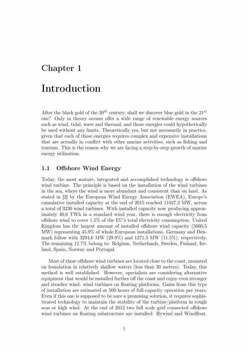
Today, the most mature, integrated and accomplished technology is offshorewind turbine. The principle is based on the installation of the wind turbinesin the sea, where the wind is more abundant and consistent than on land. Asstated in [2] by the European Wind Energy Association (EWEA), Europe’scumulative installed capacity at the end of 2015 reached 11027,3 MW, acrossa total of 3230 wind turbines. With installed capacity now producing approx-imately 40,6 TWh in a standard wind year, there is enough electricity fromoffshore wind to cover 1,5% of the EU’s total electricity consumption. UnitedKingdom has the largest amount of installed offshore wind capacity (5060,5MW) representing 45.9% of whole European installations. Germany and Den-mark follow with 3294,6 MW (29.9%) and 1271,3 MW (11.5%), respectively.The remaining 12.7% belong to: Belgium, Netherlands, Sweden, Finland, Ire-land, Spain, Norway and Portugal.

Most of these offshore wind turbines are located close to the coast, mountedon foundation in relatively shallow waters (less than 30 meters). Today, thismethod is well established. However, specialists are considering alternativeequipment that would be installed further off the coast and enjoy even strongerand steadier wind: wind turbines on floating platforms. Gains from this typeof installation are estimated at 500 hours of full-capacity operation per years.Even if this one is supposed to be sure a promising solution, it requires sophis-ticated technology to maintain the stability of the turbine/platform in roughseas or high wind. At the end of 2012 two full scale grid connected offshorewind turbines on floating substructure are installed: Hywind and Windfloat.

1

They are both located in Europe, one in the North Sea and one in the AtlanticOcean. Today seven experimental floating substructures (four in Europe, twoin Japan and one in the United States) are in a test phase. In year 2014,after five years testing on the Hywind prototype, Statoil deployed the HywindScotland Pilot Park [31], which will be completed in the year 2017. The parkwill include five Hywind wind-turbine generator units with a total maximumcapacity of up to 30 MW.

Numerous floating platform concepts are available for offshore wind tur-bines. Figure (1.1) represents the three mains: ballast stabilized (Spar–Buoy),mooring line stabilized (Tension Leg Platform) and buoyancy stabilized (Barge).

Figure 1-2. Floating platform concepts for offshore wind turbines

and the wind turbine, as well as for the dynamic characterization of the mooring system for

compliant floating platforms.

1.2 Previous Research

In recent years, a variety of wind turbine aero-servo-elastic simulation tools have been expanded

to include the additional loading and responses representative of fixed-bottom offshore support

structures [4,15,19,52,61,77,97]. For the hydrodynamic-loading calculations, all of these codes

use Morison’s equation [22,74]. The incident-wave kinematics are determined using an

appropriate wave spectrum together with linear Airy wave theory for irregular seas or one of the

various forms of nonlinear stream-function wave theory for extreme regular seas. The effects of

sea currents are also included. Morison’s representation, which is most valid for slender vertical

surface-piercing cylinders that extend to the sea floor, accounts for the relative kinematics

between the fluid and substructure motions, including added mass, incident-wave inertia, and

viscous drag. It ignores the potential effects of free-surface memory and atypical added-mass-

induced couplings between modes of motion in the radiation problem [16,76], and takes

advantage of G. I. Taylor’s long-wavelength approximation [16,76,85] to simplify the diffraction

problem. These neglections and approximations inherent in Morison’s representation limit its

4

Figure 1.1: Mains Floating Platform Concepts for Offshore Wind Turbines

In this dissertation a spar-buoy platform model has been considered: moreprecisely the OC3-Hywind model developed from Phase IV of the OC3 projectand based on the Hywind model defined in [22]. This concept has been chosendue to its simple design, to its suitability to modelling and to its propinquityto commercialization.

2

1.2 Thesis Objectives

In collaboration with the Universidad Politécnica de Valencia (UPV), with theaim of analysing different control strategies, a study has been adopted usingtwo different control mechanisms:• Collective Blade Pitch

• Individual Blade PitchThe main purpose is to quantify the performance of different control sys-

tems aiming at achieving a better rotor speed regulation, thus a better powerquality. Another important objective is the reduction in tower loads, given bythe decrease of the platform motions.

In this thesis two multi-objective controllers are applied to spar-buoy plat-form concept to improve the system performances: i) State Feedback Control(SFC), obtained with a Linear Quadratic Regulator (LQR), and ii) Distur-bance Accommodation Control (DAC). These controllers are compared with abaseline Gain Scheduled PI (GSPI) used as reference. Furthermore ten perfor-mance indices are used to evaluate the control quality (see Chapter 6 for moredetails).

Design Load Case (DLC) 1.1 in the IEC 61400-3 standard for offshore windturbine is used to analyse the fatigue load performance under normal operat-ing conditions (more details are given in Appendix B).

Simulations and control models are carried out using FAST (Fatigue, Aero-dynamics, Structure and Turbulence) [19], a National Renewable Energy Lab-oratory (NREL) CAE tool to simulate the coupled dynamics response of windturbines. It is used in conjunction with MATLAB Simulink for control designand implementation.

1.3 Thesis Outline

• Chapter 2 describes the wind and sea-wave models.

• Chapter 3 introduces the hydrodynamic model.

• Chapter 4 describes the aerodynamic model, the tower flexibility and themodel actuators.

• Chapter 5 presents the control strategies and their implementation.

• Chapter 6 shows the comparative analysis between implemented con-trollers.

• Chapter 7 reports the work conclusions and further developments.

• Appendix A describes the linearized model obtained with FAST.

• Appendix B describes the the fatigue analysis.

3

Chapter 2

Wind and Wave Models

In this chapter the mathematical models used to develop the wind and the sea-waves are presented. In particular, the first part introduces the wind model, itsturbulence intensity and its power-law profile. The wind speed represents themain exogenous signal with the biggest influence on a wind turbine. Thereforea detailed model ensures better control performances. The second part presentstwo sea-wave models. The first is used to describe fully developed seas, whereasthe second is a fetch-limited version of the first.

2.1 Wind Model

The wind model has been developed with TurbSim [6], a stochastic, full-field,turbulent-wind simulator. TurbSim adopts a statistical approach instead of aphysics-based model. It numerically simulates time series of three-componentwind-speed vectors in a two-dimensional vertical rectangular grid that is fixedin space. TurbSim output will be used as input for AeroDyn [8].

2.2 Spectral Model

This section describes the velocity spectrum used in the model and discussesthe measurements adopted to develop scaling for the site-specific model. Stan-dard deviations, σ, have been calculated by integrating the velocity spectra,S:

σ2 =

∫ ∞0

S(f) dt, (2.1)

2.2.1 Kaimal Model

The IEC Kaimal model has been defined in 2nd and 3nd edition of the IEC61400–1. It assumes a neutral atmospheric stability while the velocity spectrafor u, v and w wind components are given by:

Sk(f) =4σ2

KLK/uhub

(1 + 6fLK/uhub)53

for K = u, v, w (2.2)

4

where uhub is the mean wind speed, f is the cyclic frequency and LK is theintegral scale parameter defined as follows:

LK =

8.10ΛU , K = u,

2.70ΛU , K = v,

0.66ΛU , K = w

(2.3)

where the turbulence parameter (ΛU) can be described as indicated in equa-tion (2.4).

ΛU =

0.7min(30m,HubHt), Edition 2

0.7min(60m,HubHt), Edition 3(2.4)

The relationships between the standard deviations are defined as:

σv = 0.8σu

σw = 0.5σu(2.5)

Both the velocity spectra and the standard deviations are assumed to be in-variant across the grid. The effect is a small variation of the u-componentstandard deviation due to the spatial coherence model (not specified here).

ω [rad/sec]

0 0.5 1 1.5 2 2.5

Su [

m2/s

ec]

0

50

100

150

200

250

300

350

400

(a)ω [rad/sec]

10-3 10-2 10-1 100 101

Su [

dB

]

-30

-20

-10

0

10

20

30

40

50

60

(b)

Figure 2.1: Kaimal Spectrum for u-component

5

2.3 Turbulence Intensity

The description of the turbulent component has been provided adopting aNormal Turbulence Model (NTM) in conjunction with the IEC Kaimal model.

uhub

, [m/sec]

0 10 20 30

σu,

[m/s

ec]

0.5

1

1.5

2

2.5

3

3.5

4

4.5

uhub

, [m/sec]

0 10 20 30

Tu

rbu

len

ce

In

ten

sity,

%

5

10

15

20

25

30

35

40

45

50

NTM Class A

NTM Class B

NTM Class C

Figure 2.2: Longitudinal wind-speed standard deviation and turbulence intensity (TI) cat-egories

The standard deviation of the u-component, σu can be approximated usingthe following relationship:

σu = σu = Iref (0.75 uhub + 5.6) (2.6)

where, Iref is the expected value of turbulence intensity at 15m/s.

The standards are:

• 16% for Class A

• 14% for Class B

• 12% for Class C

In this model, Iref = 0.14, namely the B category, has been used for equa-tion (2.6).

Table (2.1) summarizes the parameters used to create the wind spectralmodel.

6

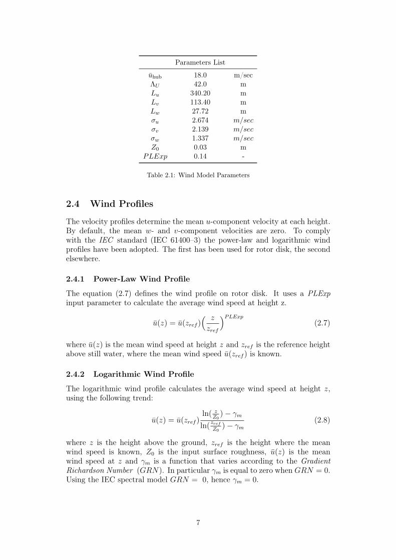
Parameters List

uhub 18.0 m/secΛU 42.0 mLu 340.20 mLv 113.40 mLw 27.72 mσu 2.674 m/secσv 2.139 m/secσw 1.337 m/secZ0 0.03 m

PLExp 0.14 -

Table 2.1: Wind Model Parameters

2.4 Wind Profiles

The velocity profiles determine the mean u-component velocity at each height.By default, the mean w- and v-component velocities are zero. To complywith the IEC standard (IEC 61400–3) the power-law and logarithmic windprofiles have been adopted. The first has been used for rotor disk, the secondelsewhere.

2.4.1 Power-Law Wind Profile

The equation (2.7) defines the wind profile on rotor disk. It uses a PLExpinput parameter to calculate the average wind speed at height z.

u(z) = u(zref )( z

zref

)PLExp(2.7)

where u(z) is the mean wind speed at height z and zref is the reference heightabove still water, where the mean wind speed u(zref ) is known.

2.4.2 Logarithmic Wind Profile

The logarithmic wind profile calculates the average wind speed at height z,using the following trend:

u(z) = u(zref )ln( z

Z0)− γm

ln(zrefZ0

)− γm(2.8)

where z is the height above the ground, zref is the height where the meanwind speed is known, Z0 is the input surface roughness, u(z) is the meanwind speed at z and γm is a function that varies according to the GradientRichardson Number (GRN). In particular γm is equal to zero when GRN = 0.Using the IEC spectral model GRN = 0, hence γm = 0.

7

Wind Velocity (u) [m/sec]

11 12 13 14 15 16 17 18 19 20

He

igh

t a

bo

ve

still

wa

ter

leve

l [m

]

0

20

40

60

80

100

120

140

160

180

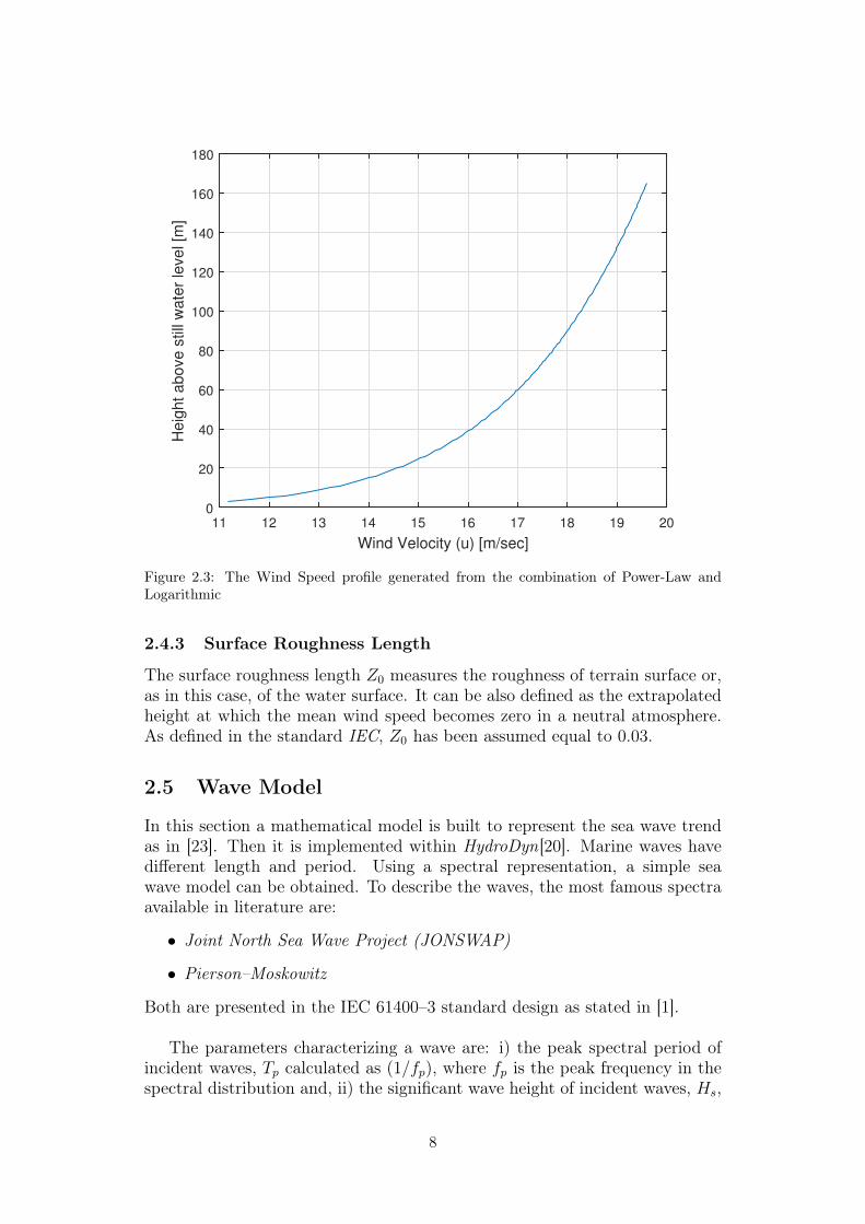
Figure 2.3: The Wind Speed profile generated from the combination of Power-Law andLogarithmic

2.4.3 Surface Roughness Length

The surface roughness length Z0 measures the roughness of terrain surface or,as in this case, of the water surface. It can be also defined as the extrapolatedheight at which the mean wind speed becomes zero in a neutral atmosphere.As defined in the standard IEC, Z0 has been assumed equal to 0.03.

2.5 Wave Model

In this section a mathematical model is built to represent the sea wave trendas in [23]. Then it is implemented within HydroDyn[20]. Marine waves havedifferent length and period. Using a spectral representation, a simple seawave model can be obtained. To describe the waves, the most famous spectraavailable in literature are:

• Joint North Sea Wave Project (JONSWAP)

• Pierson–Moskowitz

Both are presented in the IEC 61400–3 standard design as stated in [1].

The parameters characterizing a wave are: i) the peak spectral period ofincident waves, Tp calculated as (1/fp), where fp is the peak frequency in thespectral distribution and, ii) the significant wave height of incident waves, Hs,

8

defined as 1/3 of the largest waves height observed over a period. Anotherimportant parameter is the fetch. It describes the ocean area over the windblows with a constant intensity and direction, thus generating waves. ThePierson-Moskowitz wave spectrum is generally used to describe the statisticalproperties of fully developed seas. On the contrary, the JONSWAP spectrumis normally used in a limited fetch situation.

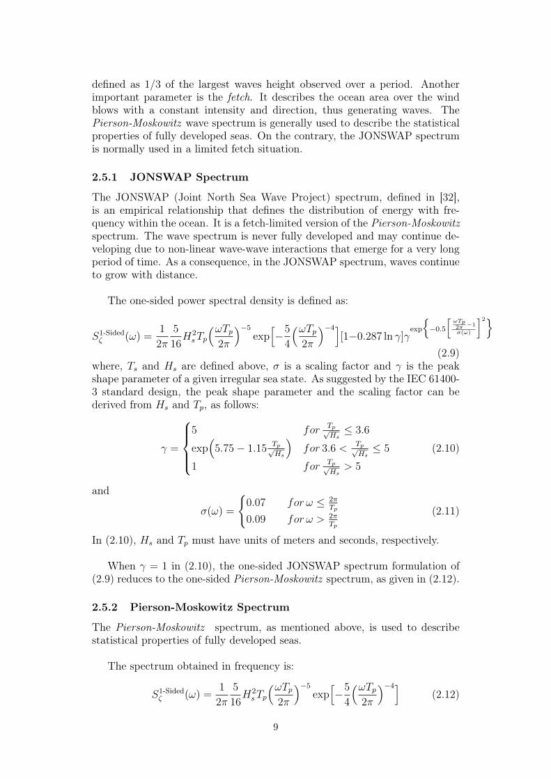
2.5.1 JONSWAP Spectrum

The JONSWAP (Joint North Sea Wave Project) spectrum, defined in [32],is an empirical relationship that defines the distribution of energy with fre-quency within the ocean. It is a fetch-limited version of the Pierson-Moskowitzspectrum. The wave spectrum is never fully developed and may continue de-veloping due to non-linear wave-wave interactions that emerge for a very longperiod of time. As a consequence, in the JONSWAP spectrum, waves continueto grow with distance.

The one-sided power spectral density is defined as:

S1-Sidedζ (ω) =

1

2π

5

16H2sTp

(ωTp2π

)−5

exp[−5

4

(ωTp2π

)−4][1−0.287 ln γ]γ

exp

−0.5

[ωTp2π −1

σ(ω)

]2(2.9)

where, Ts and Hs are defined above, σ is a scaling factor and γ is the peakshape parameter of a given irregular sea state. As suggested by the IEC 61400-3 standard design, the peak shape parameter and the scaling factor can bederived from Hs and Tp, as follows:

γ =

5 for Tp√

Hs≤ 3.6

exp(

5.75− 1.15 Tp√Hs

)for 3.6 < Tp√

Hs≤ 5

1 for Tp√Hs

> 5

(2.10)

and

σ(ω) =

0.07 for ω ≤ 2π

Tp

0.09 for ω > 2πTp

(2.11)

In (2.10), Hs and Tp must have units of meters and seconds, respectively.

When γ = 1 in (2.10), the one-sided JONSWAP spectrum formulation of(2.9) reduces to the one-sided Pierson-Moskowitz spectrum, as given in (2.12).

2.5.2 Pierson-Moskowitz Spectrum

The Pierson-Moskowitz spectrum, as mentioned above, is used to describestatistical properties of fully developed seas.

The spectrum obtained in frequency is:

S1-Sidedζ (ω) =

1

2π

5

16H2sTp

(ωTp2π

)−5

exp[−5

4

(ωTp2π

)−4](2.12)

9

where Ts and Hs are the same parameters reported in equation (2.9).

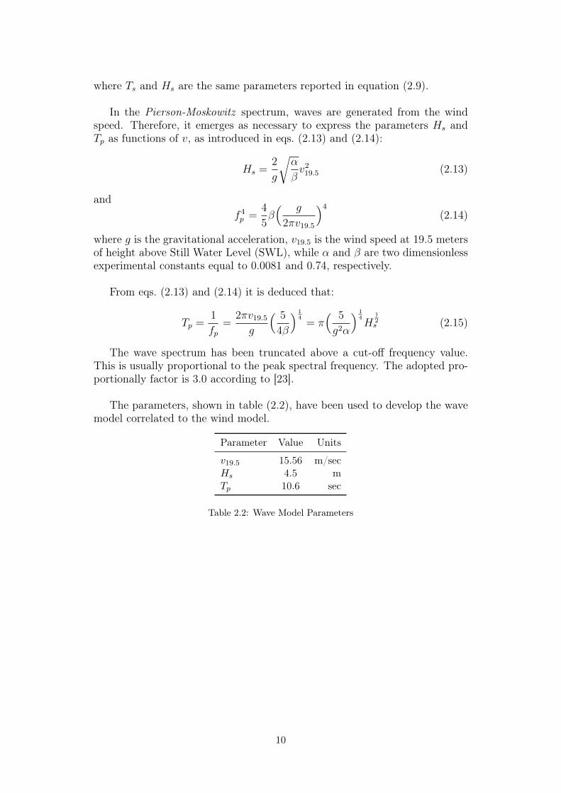
In the Pierson-Moskowitz spectrum, waves are generated from the windspeed. Therefore, it emerges as necessary to express the parameters Hs andTp as functions of v, as introduced in eqs. (2.13) and (2.14):

Hs =2

g

√α

βv2

19.5 (2.13)

andf 4p =

4

5β( g

2πv19.5

)4

(2.14)

where g is the gravitational acceleration, v19.5 is the wind speed at 19.5 metersof height above Still Water Level (SWL), while α and β are two dimensionlessexperimental constants equal to 0.0081 and 0.74, respectively.

From eqs. (2.13) and (2.14) it is deduced that:

Tp =1

fp=

2πv19.5

g

( 5

4β

) 14

= π( 5

g2α

) 14H

12s (2.15)

The wave spectrum has been truncated above a cut-off frequency value.This is usually proportional to the peak spectral frequency. The adopted pro-portionally factor is 3.0 according to [23].

The parameters, shown in table (2.2), have been used to develop the wavemodel correlated to the wind model.

Parameter Value Units

v19.5 15.56 m/secHs 4.5 mTp 10.6 sec

Table 2.2: Wave Model Parameters

10

ω [rad/sec]

0 0.2 0.4 0.6 0.8 1 1.2 1.4

Sζ [

m2 s

ec]

0

5

10

15

20

25

30

35

40

45

Pierson-Moskovitz

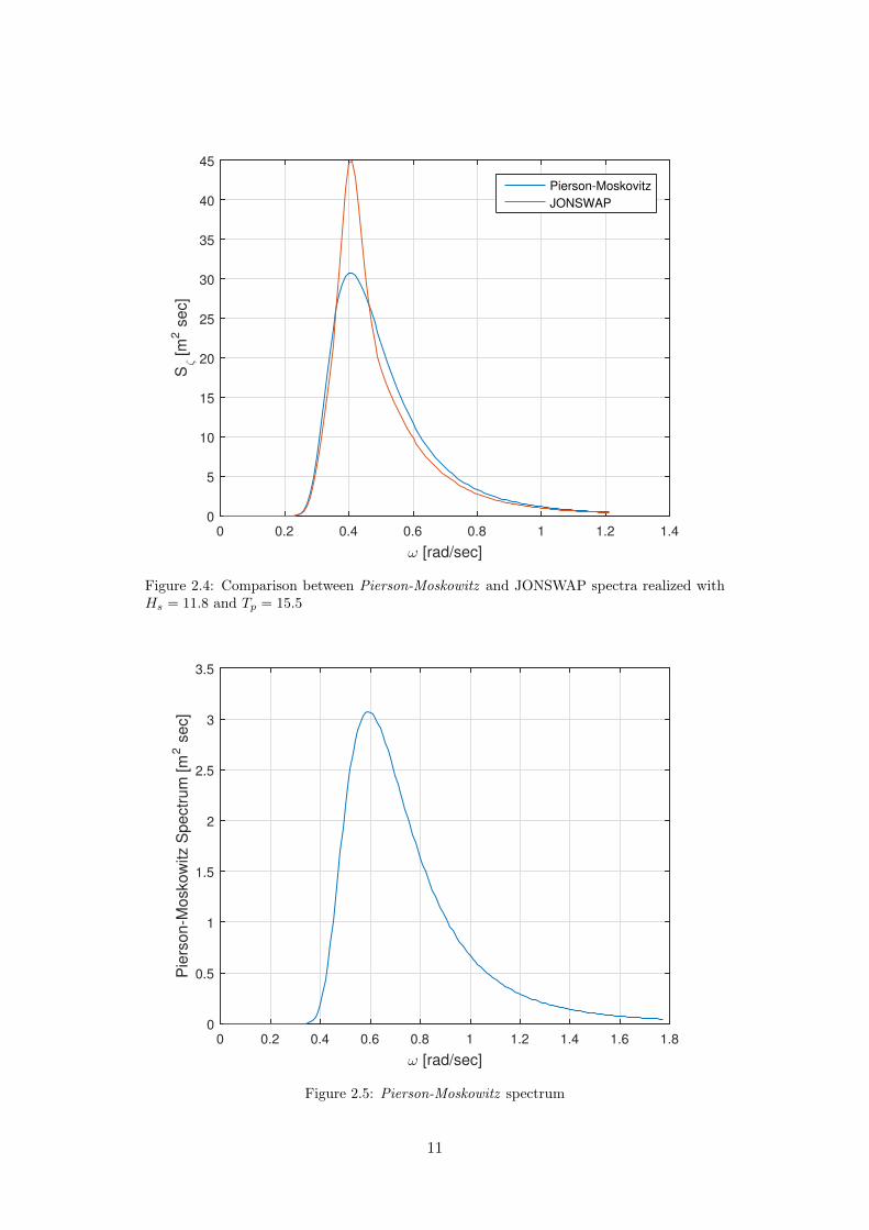
JONSWAP

Figure 2.4: Comparison between Pierson-Moskowitz and JONSWAP spectra realized withHs = 11.8 and Tp = 15.5

ω [rad/sec]

0 0.2 0.4 0.6 0.8 1 1.2 1.4 1.6 1.8

Pie

rso

n-M

osko

witz S

pe

ctr

um

[m

2 s

ec]

0

0.5

1

1.5

2

2.5

3

3.5

Figure 2.5: Pierson-Moskowitz spectrum

11

2.6 Wave Kinematic

The wave elevation is defined as in [23], namely:

ζ(t,X, Y ) =1

2π

∫ ∞−∞

W (ω)√

2πS2−sidedζ (ω)e−jk(ω)[X cos ξ+Y sin ξ]ejωtdω (2.16)

In the inertial reference frame, (X, Y ) are the coordinates of a general pointbelonging to the SWL plane, ξ is the wave-propagation direction, k(ω) is thewave number and W (ω) is the Fourier transform of a White Gaussian noise(WGN) time-series process, characterized by a mean value E[W ] = 0 and avariance σW = 1.

For water depth h, the wave number is correlated to the incident wavefrequency, ω, and the gravitational acceleration constant g, as:

k(ω) tanh(k(ω)h

)=ω2

g(2.17)

Solving the eq. (2.17) could result difficult. However considering the deepwater hypothesis:

h

λ>

1

2(2.18)

where λ is the wavelength, it is possible to assume a simpler form:

k(ω) =ω2

g(2.19)

S2−sidedζ is the two-sided power spectral density of wave elevation per unit time.

It is defined as:

S2-Sidedζ (ω) =

12S1-Sidedζ (ω) for ω ≥ 0,

12S1-Sidedζ (−ω) for ω < 0

(2.20)

12

Time [sec]

0 100 200 300 400 500 600

Hu

b-H

eig

ht

Win

d S

pe

ed

[m

/se

c]

10

15

18

20

25

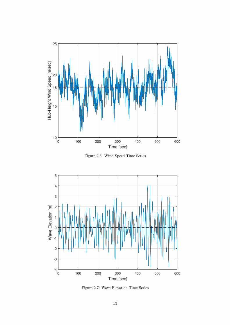
Figure 2.6: Wind Speed Time Series

Time [sec]

0 100 200 300 400 500 600

Wa

ve

Ele

va

tio

n [

m]

-4

-3

-2

-1

0

1

2

3

4

5

Figure 2.7: Wave Elevation Time Series

13

Chapter 3

Hydrodynamic Model

Shallow-water fixed-bottom offshore or onshore turbine loads are mainly dom-inated by aerodynamics. For offshore deepwater floating turbines, hydrody-namics loads become more important. The significance of hydrodynamics loadsdepends on the particular floating concept as well as on the wind severity andwave conditions, namely wind-speed, wave height and wave period. To com-pute the total hydrodynamics loads, HydroDyn [20], a NREL software coupledwithin FAST, has been used.

3.1 Floating Platform Structural Properties

Figure 3.1: The Support Platform Degrees of Freedom

The tower is cantilevered ata height of 10 meters abovethe SWL at the top of thefloating platform. The latter,as defined in [22], has beenconsidered a rigid body andthe platform draft length hasbeen evaluated equal to 120meters. The OC3-Hywindspar-buoy consists in twocylindrical regions connectedby a linear tapered conical re-gion. The cylinder diameteris 6.5 meters above the taperand 9.4 meters below. In thisway the hydrodynamics loadsnear the free surface are re-duced.

Figure 3.1 shows the support platform DOFs while table 3.1 summarizesthe platform structural properties.

14

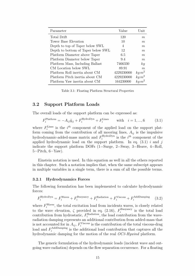
Parameter Value Unit

Total Drift 120 mTower Base Elevation 10 mDepth to top of Taper below SWL 4 mDepth to bottom of Taper below SWL 12 mPlatform Diameter above Taper 6.5 mPlatform Diameter below Taper 9.4 mPlatform Mass, Including Ballast 7466330 kgCM Location below SWL 89.91 mPlatform Roll inertia about CM 4229230000 kgm2

Platform Pitch inertia about CM 4229230000 kgm2

Platform Yaw inertia about CM 164230000 kgm2

Table 3.1: Floating Platform Structural Properties

3.2 Support Platform Loads

The overall loads of the support platform can be expressed as:

FPlatformi = −Aij qij + FHydroDyn

i + F Linesi with i = 1, ..., 6 (3.1)

where F Linesi is the ith component of the applied load on the support plat-

form coming from the contribution of all mooring lines, Aij is the impulsivehydrodynamic-added-mass matrix and FHydroDyn

i is the ith component of theapplied hydrodynamic load on the support platform. In eq. (3.1) i and jindicate the support platform DOFs (1=Surge, 2=Sway, 3=Heave, 4=Roll,5=Pitch, 6=Yaw).

Einstein notation is used. In this equation as well in all the others reportedin this chapter. Such a notation implies that, when the same subscript appearsin multiple variables in a single term, there is a sum of all the possible terms.

3.2.1 Hydrodynamics Forces

The following formulation has been implemented to calculate hydrodynamicforces:

FHydroDyni = FWaves

i + FBuoyancyi + FRadiation

i + FViscousi + FAddDamping

i (3.2)

where FWavesi , the total excitation load from incidents waves, is closely related

to the wave elevation, ζ provided in eq. (2.16), FBuoyancyi is the total load

contribution from hydrostatic, FRadiationi , the load contribution from the wave-

radiation damping represents an additional contribution from added-mass thatis not accounted for in Aij, FViscous

i is the contribution of the total viscous-dragload and FAddDamping

i is the additional load contribution that captures all thehydrodynamic damping for the motion of the real OC3-Hywind platform.

The generic formulation of the hydrodynamic loads (incident wave and out-going wave radiation) depends on the flow separation occurrence. For a floating

15

platform interacting with surface waves, different formulation are applied toseparated and not separated flows. For cylinders, the fitting formulation de-pends on the Keulegan-Carpenter number, K and on the oscillatory Reynoldsnumber, Re, defined in [22] as:

K =V T

D(3.3)

andRe =

V D

ν(3.4)

where ν is the kinematic viscosity of the fluid, V is the amplitude of the fluidvelocity normal to the cylinder, T is the wave period and D is the cylinderdiameter. The latter, as explained above, is not constant but changes accordingto the draft length, as indicated in following equation:

D(Z) =

6.5 |Z| < 4

9.4 |Z| > 12

6.5 + 2|Z| tan (ε) otherwise

(3.5)

where, D(Z) is expressed in meters (m), |Z| is the magnitude depth and ε is theangle formed between the oblique and shorter side of the isosceles trapezoid. Inthis study, the D(Z) function has been calculated considering the cross sectionof the spar conical region, on the xz plane. The amplitude of the normal fluidvelocity, V , has been derived a function of the wave height, H, and of the waveperiod, T . Hence:

V =πH

T

cosh [k(Z + h)]

sinh (kh)(3.6)

where k is the wave number, defined in eq. (2.19) and h is the water depth.Another important coefficient is the D/λ ratio, where λ is the wavelengthdefined as:

λ =2π

k(3.7)

As shown in fig. (3.2a) and fig. (3.2b), the Keulegan-Carpenter (K) and os-cillatory Reynolds numbers (Re) decrease according to depth along the spar,whereas D/λ ratio, in fig. (3.2c), is nearly constant along the spar except forthe tapered region where it appears lower. As defined in [22], flow separationoccurs when Keulegan-Carpenter number exceeds 2. For values lower than 2,potential flow theory can be applied. In this case, K results bigger than 2 onlyfor a little portion of spar that is located above the tapered region. Diffrac-tion effect is important when D/λ exceeds 0.2 and is unimportant for smallerratios. In this case, D/λ is always lower than 0.2, hence the diffraction effectwill be small.

In view of the validity of the potential flow theory, it is possible to applyand solve the potential-flow problem using WAMIT computer program [7].WAMIT uses a three-dimensional numerical-panel method in the frequencydomain to solve the linearized potential flow hydrodynamic radiation anddiffraction problems for the interaction of surface waves with offshore plat-form of arbitrary geometry.

16

Keulegan-Carpenter (K) [-]

0 0.5 1 1.5 2 2.5

Dept

h al

ong

Spar

(Z) [

m]

-120

-100

-80

-60

-40

-20

0

(a)

Oscillatory Reynolds Number(Re) [-] ×106

0 0.5 1 1.5 2 2.5 3 3.5 4 4.5 5

Dept

h al

ong

Spar

(Z) [

m]

-120

-100

-80

-60

-40

-20

0

(b)

Diameter to Wavelength Ratio (D/λ)

0 0.05 0.1 0.15 0.2 0.25 0.3

Dept

h al

ong

Spar

(Z) [

m]

-120

-100

-80

-60

-40

-20

0

(c)

Figure 3.2: Dimensionless parameter with T and H defined in Tab. 2.2

17

3.3 The True Linear Hydrodynamic Model in the TimeDomain

The true linear hydrodynamic model is useful for transient analysis when op-tional nonlinear effect and irregular wave formulation are introduced. Thehydrodynamic problem can be split into three separate and simpler problems:

• Hydrostatic problem

• Diffraction problem

• Radiation problem

3.3.1 Hydrostatic Problem

The total load on the floating platform from linear hydrostatic is defined as:

FBuoyancyi = ρgV0δi3 − CHydro

ij qj (3.8)

where ρ is the water density, g is the gravitational acceleration constant, V0

is the displaced volume of the fluid when the support platform is in its undis-placed position, δi3 is the (i, 3) component of the Kronecker-Delta function,CHydroij is the linear hydrostatic-restoring matrix of the incident and outgoing

wave from diffraction and radiation problems and the qj coefficient is the jthsupport platform DOF.

The first term in eq. (3.8) represents the buoyancy force from Archimedes’principle, namely the vertical force directed upward and equal to the weight ofthe displaced fluid, when the support platform is in its undisplaced position.This term is different from zero only for the vertical heave-displacement DOFof the support platform (DOF i = 3).

The second term in eq. (3.8) represents the variations in the hydrodynamicforce and moment. These changes are caused by the effects of the water-planearea and by the COB (Center of Buoyancy), when the support platform isdisplaced. CHydro

ij matrix is formed by the following coefficients:0 0 0 0 0 00 0 0 0 0 00 0 ρgA0 0 −ρg

∫∫A0x dA 0

0 0 0 ρg∫∫

A0y2 dA+ ρgV0zCOB 0 0

0 0 −ρg∫∫

A0x dA 0 ρg

∫∫A0x2 dA+ ρgV0zCOB 0

0 0 0 0 0 0

(3.9)

3.3.2 Diffraction Problem

The solution to the diffraction problem, which considers the hydrodynamicloads on the platform associated with excitation from incident wave, is givenin terms of the wave-frequency and direction-dependent vector. This vector,

18

taken from WAMIT, is a complex vector whose magnitude is normalized perunit wave amplitude, water density and gravitational acceleration constant.The vector phase determines the lag between the wave elevation loads. Definedin [22] and shown in (3.3), the magnitude and the phase of the hydrodynamic-wave-excitation vector have been derived as functions of wave-frequency for theincident-waves propagated along the positive X-axis, namely with null wavedirection, ξ = 0 deg. For these waves, the loads in direction of sway, roll andyaw are equal to zero because of the spar symmetries. The force magnitude ofthe surge DOF reaches a peak just above a wave frequency of 0.5 rad/sec, whilethe moment magnitude of the pitch DOF reaches a peak just below the samefrequency. The heave force changes sign at about 0.25 rad/sec and reaches apeak at 0.5 rad/sec. It is possible to observe that at a higher wave frequency,over 1.145 rad/sec, diffraction effects become important and loads drop.

0 0.5 1 1.5 2 2.5 3 3.5 4 4.5 5

Ma

gn

itu

de

[N

/m]

×105

0

5

10

15Force

Surge

Sway

Heave

Frequency [rad/sec]

0 0.5 1 1.5 2 2.5 3 3.5 4 4.5 5

Ph

ase

[d

eg

]

-200

-100

0

100

200

(a)

0 0.5 1 1.5 2 2.5 3 3.5 4 4.5 5

Ma

gn

itu

de

[N

m/m

]

×107

0

2

4

6Momentum

Roll

Pitch

Yaw

Frequency [rad/sec]

0 0.5 1 1.5 2 2.5 3 3.5 4 4.5 5

Ph

ase

[d

eg

]

-200

-100

0

100

200

(b)

Figure 3.3: Hydrodynamic wave excitation per unit amplitude

The diffraction loads, FWavesi in eq. (3.2), are expressed as:

FWavesi (t) =

1

2π

∫ ∞−∞

W (ω)√

2πS2-Sidedζ (ω)Xi(ω, ξ)e

jωt dω (3.10)

Such relationship is closely related with the wave elevation ζ reported ineq. (2.16). The Xi term, extrapolated vector from WAMIT, represents thenormalized load factor due to the incident waves. In this equation the waveelevation has been evaluated at the mean position of the support platform.

3.3.3 Radiation Problem

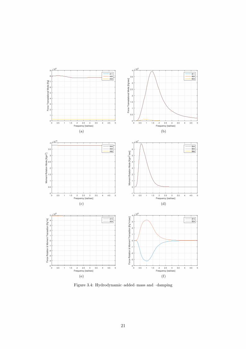
The solution to the radiation problem considers the hydrodynamic loads onthe platform associated with oscillation of the platform in its various modes ofmotion. The hydrodynamic loads are given in terms of oscillatory-frequencydependent on hydrodynamic added-mass matrix, Aij(ω), and hydrodynamicdamping matrix, Bij(ω), respectively. Unlike the Xi term, the coefficientsare normalized per water density and frequency. As defined in [22], thesematrices from the linear radiation problem are shown in fig. (3.4) as functionof the oscillation frequency. Because of the Aij(ω) and Bij(ω) symmetries,

19

only the upper triangular matrix elements are shown. Moreover, due to thespar’s symmetries, ∀ω: A11 = A22 and B11 = B22 and likewise A44 = A55 andB44 = B55. The other matrix elements, not shown, are zero-valued.

As shown in figs. (3.4a), (3.4c) and (3.4e) the added-mass coefficient varieslittle across the frequency. Moreover, the values of the damping in the moment-rotation (fig. (3.4d)), force-rotation and moment-translational modes (fig. (3.4f)),emerge smaller than added-mass modes. This implies that also the linear radi-ation damping and the associated memory effect in the time domain are smallin those modes. However, the contribution to the force-translational modes,shown in fig. (3.4b), can not be neglected.

In eq. (3.1), the impulsive hydrodynamic-added-mass components, Aij, rep-resent, as in [23], a force mechanism proportional to the acceleration of thesupport platform in the time-domain radiation problem. It is defined as:

Aij = limω→∞

Aij(ω) = Aij(∞) (3.11)

where the (i, j) component indicates the hydrodynamic force in direction ofi−DOF . It results from the integration (over the wetter surface of the supportplatform) of the component of the outgoing-wave pressure field. This one isinducted by a unit acceleration of the jth–DOF of the support platform. TheAij matrix in eq. (3.11) does not consider the memory effect that is capturedfrom a integral of convolution representing the load contribution from wave-radiation damping, defined as:

FRadiationi (t) = −

∫ t

0

Kij(t− τ)qj(τ) dτ (3.12)

where, τ is a dummy variable with the same units as the simulation time, t.Kij, defined in eq. (3.13), represents the radiation-retardation kernel, whichhas been obtained applying Fourier-transform at Bij(ω).

Kij(t) =2

π

∫ ∞0

Bij(ω) cos (ωt) dω (3.13)

20

Frequency [rad/sec]

0 0.5 1 1.5 2 2.5 3 3.5 4 4.5 5

Fo

rce

Tra

nsa

latio

na

l M

od

e [

Kg

]

×106

0

1

2

3

4

5

6

7

8

9

A11

A22

A33

(a)Frequency [rad/sec]

0 0.5 1 1.5 2 2.5 3 3.5 4 4.5 5

Fo

rce

Tra

nsa

latio

na

l M

od

e [

Kg

/se

c]

×105

0

0.5

1

1.5

2

2.5

3

3.5

4

B11

B22

B33

(b)

Frequency [rad/sec]

0 0.5 1 1.5 2 2.5 3 3.5 4 4.5 5

Mo

me

nt-

Ro

tatio

n M

od

e [

Kg

m2]

×1010

0

0.5

1

1.5

2

2.5

3

3.5

4

A44

A55

A66

(c)Frequency [rad/sec]

0 0.5 1 1.5 2 2.5 3 3.5 4 4.5 5

Mo

me

nt-

Ro

tatio

n M

od

e [

Kg

m2/s

ec]

×107

-1

0

1

2

3

4

5

6

7

B44

B55

B66

(d)

Frequency [rad/sec]

0 0.5 1 1.5 2 2.5 3 3.5 4 4.5 5

Fo

rce

-Ro

tatio

n &

Mo

me

nt-

Tra

nsa

ltio

n [

Kg

*m]

×108

-5

-4

-3

-2

-1

0

1

2

3

4

5

A15

A24

(e)Frequency [rad/sec]

0 0.5 1 1.5 2 2.5 3 3.5 4 4.5 5

Fo

rce

-Ro

tatio

n &

Mo

me

nt-

Tra

nsa

ltio

n [

Kg

*m/s

ec]

×106

-4

-3

-2

-1

0

1

2

3

4

B15

B24

(f)

Figure 3.4: Hydrodynamic–added–mass and –damping

21

3.4 Morison’s Equation

In severe sea conditions, the hydrodynamic loads formulation from linearpotential-flow must be augmented with the loads brought about by flow sepa-ration. The most famous hydrodynamic formulation adopted for offshore windturbines is the Morison’s formulation. Morison’s equation is applicable for thecalculation of the hydrodynamic loads on cylindrical structures when:

1. The effects of diffraction are negligible

2. Radiation damping is negligible

3. Flow separation may occur

In this model a mixed formulation, namely the Morison’s equation, has beenused only for viscous forces applied along the portion of the spar, l, where flowseparation occurs. The total contribution from viscous-drag load is representedas:

FViscousi (t) =

∫l

dFViscousi (t, z) dz (3.14)

where the contribution along surge, sway and heave is defined as reported ineq. (3.15):

dFViscousi (t, z) =

12CDρ(Ddz)[vi(t, 0, 0, z)− qi]|v(t, 0, 0, z)− q(z)| for i=1, 2

0 for i=3(3.15)

where CD is the normalized viscous-drag coefficient, vi is the component of theundisturbed fluid particle velocity in the direction of i − DOF and (Ddz) isthe frontal area for the cylinder strip, where dz is the length of the differentialstrip and D is the diameter of the cylinder.

A similar expression can be written for roll, pitch and yaw moments:

dFViscousi (t, z) =

−dFViscous

2 (t, z)z for i = 4

dFViscous1 (t, z)z for i = 5

0 for i = 6

(3.16)

The undisturbed fluid-particle acceleration and velocity in the direction ofDOF-i, ai and vi respectively, at point (X,Y,Z) in the inertia reference frameare:

v1(t,X, Y, Z) =cosφ

2π

∫ ∞−∞

W (ω)√

2πS2-Sidedζ (ω)e−jk(ω)[X cosφ+Y sinφ] ωΠ dω

(3.17)

v2(t,X, Y, Z) =sinφ

2π

∫ ∞−∞

W (ω)√

2πS2-Sidedζ (ω)e−jk(ω)[X cosφ+Y sinφ] ωΠ dω

(3.18)

22

and

a1(t,X, Y, Z) =j cosφ

2π

∫ ∞−∞

W (ω)√

2πS2-Sidedζ (ω)e−jk(ω)[X cosφ+Y sinφ] ω2 Π dω

(3.19)

a2(t,X, Y, Z) =j sinφ

2π

∫ ∞−∞

W (ω)√

2πS2-Sidedζ (ω)e−jk(ω)[X cosφ+Y sinφ] ω2 Π dω

(3.20)

where Π relationship has been reported below due to a graphic issue. It isdefined as:

Π =cosh [k(ω)(Z + h)]

sinh [k(ω)h]ejωt (3.21)

Morison’s representation assumes that viscous drag prevails on the damp-ing. This assumption implies that wave-radiation can be ignored. Indeed, theviscous-drag load is not part of the linear hydrodynamic loading equation sincethe viscous-drag load is proportional to the square of the velocity between thefluid particles and the platform.

3.5 Additional Damping

The linear radiation damping resulting from potential-flow theory, and thenon linear viscous-drag, derived from the relative Morison’s formulation, whenadded up do not capture all of the hydrodynamic damping for the motions ofa real Hywind platform. For this reason, this support needs to be augmentedas indicated in [22] with an additional linear damping. This is defined as:

FAddDampingi (q) = BLinear

ij qj (3.22)

with

BLinearij =

105 Nm/s

0 0 0 0 0

0 105 Nm/s

0 0 0 0

0 0 13 ∗ 104 Nm/s

0 0 0

0 0 0 0 0 00 0 0 0 0 00 0 0 0 0 13 ∗ 106 Nm

rad/s

(3.23)

where BLinearij is the additional linear damping matrix and qj is the first time

derivative of the jth platform DOF.

The second order potential flow solution that includes mean-drift, slow-drift, and sum frequency solution excitation and higher order solution, havenot been solved and have been presupposed to be negligible for the OC3-Hywind spar.

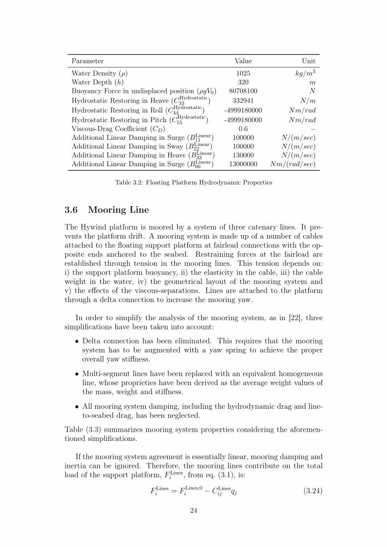
Table (3.2) summarizes the adopted hydrodynamic properties.

23

Parameter Value Unit

Water Density (ρ) 1025 kg/m3

Water Depth (h) 320 mBuoyancy Force in undisplaced position (ρgV0) 80708100 N

Hydrostatic Restoring in Heave (CHydrostatic33 ) 332941 N/m

Hydrostatic Restoring in Roll (CHydrostatic44 ) -4999180000 Nm/rad

Hydrostatic Restoring in Pitch (CHydrostatic55 ) -4999180000 Nm/rad

Viscous-Drag Coefficient (CD) 0.6 −Additional Linear Damping in Surge (BLinear

11 ) 100000 N/(m/sec)Additional Linear Damping in Sway (BLinear

22 ) 100000 N/(m/sec)Additional Linear Damping in Heave (BLinear

33 ) 130000 N/(m/sec)Additional Linear Damping in Surge (BLinear

66 ) 13000000 Nm/(rad/sec)

Table 3.2: Floating Platform Hydrodynamic Properties

3.6 Mooring Line

The Hywind platform is moored by a system of three catenary lines. It pre-vents the platform drift. A mooring system is made up of a number of cablesattached to the floating support platform at fairlead connections with the op-posite ends anchored to the seabed. Restraining forces at the fairlead areestablished through tension in the mooring lines. This tension depends on:i) the support platform buoyancy, ii) the elasticity in the cable, iii) the cableweight in the water, iv) the geometrical layout of the mooring system andv) the effects of the viscous-separations. Lines are attached to the platformthrough a delta connection to increase the mooring yaw.

In order to simplify the analysis of the mooring system, as in [22], threesimplifications have been taken into account:

• Delta connection has been eliminated. This requires that the mooringsystem has to be augmented with a yaw spring to achieve the properoverall yaw stiffness.

• Multi-segment lines have been replaced with an equivalent homogeneousline, whose proprieties have been derived as the average weight values ofthe mass, weight and stiffness.

• All mooring system damping, including the hydrodynamic drag and line-to-seabed drag, has been neglected.

Table (3.3) summarizes mooring system properties considering the aforemen-tioned simplifications.

If the mooring system agreement is essentially linear, mooring damping andinertia can be ignored. Therefore, the mooring lines contribute on the totalload of the support platform, F Lines

i , from eq. (3.1), is:

F Linesi = F Lines,0

i − CLinesij qj (3.24)

24

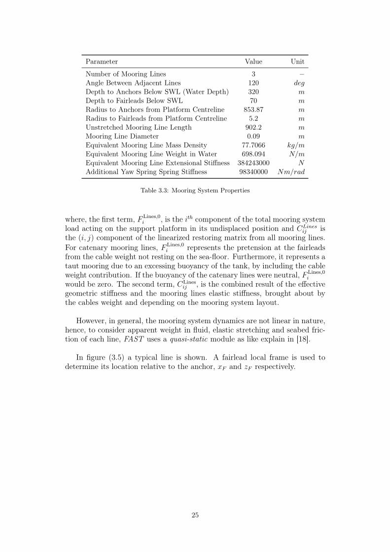
Parameter Value Unit

Number of Mooring Lines 3 −Angle Between Adjacent Lines 120 degDepth to Anchors Below SWL (Water Depth) 320 mDepth to Fairleads Below SWL 70 mRadius to Anchors from Platform Centreline 853.87 mRadius to Fairleads from Platform Centreline 5.2 mUnstretched Mooring Line Length 902.2 mMooring Line Diameter 0.09 mEquivalent Mooring Line Mass Density 77.7066 kg/mEquivalent Mooring Line Weight in Water 698.094 N/mEquivalent Mooring Line Extensional Stiffness 384243000 NAdditional Yaw Spring Spring Stiffness 98340000 Nm/rad

Table 3.3: Mooring System Properties

where, the first term, F Lines,0i , is the ith component of the total mooring system

load acting on the support platform in its undisplaced position and CLinesij is

the (i, j) component of the linearized restoring matrix from all mooring lines.For catenary mooring lines, F Lines,0

i represents the pretension at the fairleadsfrom the cable weight not resting on the sea-floor. Furthermore, it represents ataut mooring due to an excessing buoyancy of the tank, by including the cableweight contribution. If the buoyancy of the catenary lines were neutral, F Lines,0

i

would be zero. The second term, CLinesij , is the combined result of the effective

geometric stiffness and the mooring lines elastic stiffness, brought about bythe cables weight and depending on the mooring system layout.

However, in general, the mooring system dynamics are not linear in nature,hence, to consider apparent weight in fluid, elastic stretching and seabed fric-tion of each line, FAST uses a quasi-static module as like explain in [18].

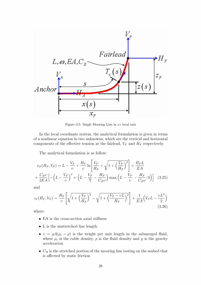
In figure (3.5) a typical line is shown. A fairlead local frame is used todetermine its location relative to the anchor, xF and zF respectively.

25

where ρ is the water density, g is the gravitational acceleration constant, and Dc is the effective

diameter of the mooring line. Because I have limited the model to simulating only homogenous

mooring lines, I handle multisegment lines (i.e., chain plus wire plus chain segments in series) by

using an equivalent line with weighted-average values of the weight and stiffness (weighted

based on the unstretched lengths of each segment).

Each mooring line is analyzed in a local coordinate system that originates at the anchor. The

local z-axis of this coordinate system is vertical and the local x-axis is directed horizontally from

the anchor to the instantaneous position of the fairlead. Figure 2-5 illustrates a typical line.

When the mooring system module is called for a given support platform displacement, the

module first transforms each fairlead position from the global frame to this local system to

determine its location relative to the anchor, xF and zF.

Figure 2-5. Mooring line in a local coordinate system

I took advantage of the analytical formulation for an elastic cable suspended between two points,

hanging under its own weight (in fluid). I derived this analytical formulation following a

procedure similar to that presented in Ref. [22], which I do not give here for brevity. (The

derivation was not exactly the same because Ref. [22] did not account for seabed interaction nor

did it account for taut lines where the angle of the line at the anchor was nonzero). The

derivation required the assumption that the extensional stiffness of the mooring line, EA, was

much greater than the hydrostatic pressure at all locations along the line.

In the local coordinate system, the analytical formulation is given in terms of two nonlinear

equations in two unknowns—the unknowns are the horizontal and vertical components of the

effective tension in the mooring line at the fairlead, HF and VF, respectively. (The effective

tension is defined as the actual cable [wall] tension plus the hydrostatic pressure.) When no

portion of the line rests on the seabed, the analytical formulation is as follows:

38

Figure 3.5: Single Mooring Line in xz local axis

In the local coordinate system, the analytical formulation is given in termsof a nonlinear equation in two unknowns, which are the vertical and horizontalcomponents of the effective tension at the fairlead, VF and HF respectively.

The analytical formulation is as follow:

xF (HF , VF ) = L− VFυ

+HF

υln

[VFHF

+

√1 +

( VFHF

)2]

+HFL

EA

+CBυ

2EA

[−(L− VF

υ

)2

+(L− VF

Υ− HF

CBυ

)max

(L− VF

υ− HF

CBυ, 0)]

(3.25)

and

zF (HF , VF ) =HF

υ

[√1 +

( VFHF

)2

−√

1 +(VF − υL

HF

)2]

+1

EA

(VFL−

υL2

2

)(3.26)

where:

• EA is the cross-section axial stiffness

• L is the unstretched line length

• υ = gA(ρc − ρ) is the weight per unit length in the submerged fluid,where ρc is the cable density, ρ is the fluid density and g is the gravityacceleration

• CB is the stretched portion of the mooring line resting on the seabed thatis affected by static friction

26

The seabed friction has been modelled as a simply drag force per unit lengthof CBυ. It is important to note that the first two terms on the right-side ofequation (3.25) represent the unstretched portion of the mooring line restingin the seabed, LB:

LB = L− VFυ

(3.27)

If there is not a portion of the mooring line on the seabed, then LB = 0. Themax -function, in (3.25), is needed to handle cases with and without anchortension. Specifically:

max(L− VF

υ− HF

CBυ, 0)→

= 0 if HA 6= 0 ∨ VA 6= 0

6= 0 ifHA = 0 ∨ VA = 0(3.28)

where HA and VA are the horizontal and vertical components of the effectivetension at the anchor. Hence, max -function is equal to zero if the seabed fric-tion is too weak to overcome the horizontal tension in the mooring line.

The mooring system module uses a Newton-Raphson iteration scheme tosolve non-linear eqs. (3.25) and (3.26). Its implementation within FAST hasbeen explicated in [18].

Once the effective tensions, HF and VF , have been found, the anchor ten-sions can be derived simply. Looking at fig. (3.5) from a balance of externalforces, it can be verified that:

HA = max(HF − CBυLB

)(3.29)

VA =

VF − υL, when line does not rest on the seabed0, when line rests on the seabed

(3.30)

The total load on the support from the contribution of all mooring lines,F Linesi from eq. (3.1) is calculated firstly by transforming each fairlead tension

from its local mooring line coordinate system to the global frame and thensumming up the tensions from all lines.

27

Chapter 4

Aerodynamic Loads

In this chapter the aerodynamic loads and the tower deflections are explained.The firsts have been developed using AeroDyn [8], a NREL software, whichtakes as input the wind model developed in chapter 2.1. The seconds do notneed an external CAE but their modelization is integrated in FAST. For thisreasons a brief description on how they are implemented is provided. Finally,a brief focus about the drivetrain model and the system actuators is reported.

4.1 Blade Element Momentum Theory

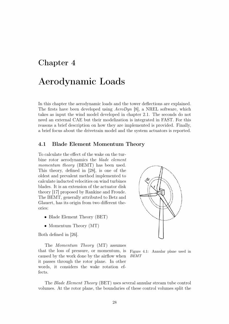
Figure 4.1: Annular plane used inBEMT

To calculate the effect of the wake on the tur-bine rotor aerodynamics the blade elementmomentum theory (BEMT) has been used.This theory, defined in [28], is one of theoldest and prevalent method implemented tocalculate inducted velocities on wind turbinesblades. It is an extension of the actuator disktheory [17] proposed by Rankine and Froude.The BEMT, generally attributed to Betz andGlauert, has its origin from two different the-ories:

• Blade Element Theory (BET)

• Momentum Theory (MT)

Both defined in [26].

The Momentum Theory (MT) assumesthat the loss of pressure, or momentum, iscaused by the work done by the airflow whenit passes through the rotor plane. In otherwords, it considers the wake rotation ef-fects.

The Blade Element Theory (BET) uses several annular stream tube controlvolumes. At the rotor plane, the boundaries of these control volumes split the

28

blade into a number of distinct elements, each long dr (fig. 4.1). Blade geome-try and flow stream properties, at each element, can be related to a differentialrotor torque, dQ, and to a differential rotor thrust, dT .

As stated in [24], the aforementioned connections can be applied in theBET only under the following assumptions:

• There is no interaction between the analysis of each blade element. Inother words, every annular stream tube control volume is assumed with-out interactions.

• The forces exerted on the blade elements by the flow stream are deter-mined by the two-dimensional lift and drug coefficients only. These arecharacteristics of the blade element airfoil shape and orientation relativeto the incoming flow.

The differential rotor thrust and the differential rotor torque, acting on eachblade element, can be found from a geometry analysis depicted in figure (4.2).As shown, the blade is specified as propagating to the left as a result of bladerotation. The contribution of the pitching moment is absent because it is nullto the rotor torque and trust. In the same figure, β is the blade collective pitchangle and θ is the angle of the relative incoming flow stream with respect tothe plane of rotation.

Figure 4.2: Blade Element Theory

29

From the analysis of the blade element geometry presented in figure (4.2),it is possible to achieve the following relationships:

dT = L cos θ +D sin θ (4.1)

anddQ = r[L sin θ −D cos θ] (4.2)

where r is the local radius, L and D are the lift and drug forces, respectively.

To be more precise, the lift and the drug forces shown in fig. (4.2) and usedin eqs. (4.1) and (4.2), represent the differential components of the forces givenby the flow stream on the blade element, whose cross- section is shown. More-over, all differential forces used in those equations are the differential forcesaction on a single blade. Hence, since the wind turbine has a B = 3 identicalblades, the differential, dT , and the differential rotor torque, dQ, are equalsto the following equations when substituting the dimensionless coefficients forthe forces:

dT = B1

2ρairV

2rel

[CL cos θ + CD sin θ

]c dr (4.3)

anddQ = B

1

2ρairV

2rel

[CL cos θ − CD sin θ

]c dr (4.4)

where B is the number of blades, ρair is the air density, Vrel is the velocity ofthe incoming flow stream, CL is the lift coefficient, CD is the drug coefficient,c is the chord length and dr is the radius thickness.

In order to relate the inducted velocities in the rotor plane to the elemen-tal forces of eqs. (4.3) and (4.4), the momentum part of the theory must beincorporated. According to [28], the thrust and the torque, extracted by eachrotor annulus, are equivalent to:

dT = 4πrρairV2

0 (1− a)adr (4.5)

dQ = 4πr3ρairV0Ω(1− a)a′dr (4.6)

where V0 is the mean wind speed, Ω is the rotor rotational speed, a is the axialinduction factor and a′ is the rotational induction factor. In particular, thecoefficient a is defined as:

a =V0 − VV

(4.7)

where V is the flow velocity through the rotor disc and V0− V is the inductedvelocity. The coefficient a′ is defined as:

a′ =1

2

(√1 +

4

λ2r

a(1− a)− 1)

(4.8)

where λr is the local speed ratio, defined as:

λr =Ωr

V0

(4.9)

30

The previous equations do not include terms for coning angle of the rotorplane. This is because AeroDyn assumes that the aerodynamics of a rotor inoperation do not change significantly.

Figure 4.3: Helical Wakecaused by tip-blade

One of the major limitations of the BEMT, isthat there is no influence of vortices created fromthe blade extremity into the wake on the inductedvelocity field. These vortices create multiple helicalstructures in the wake and have a great influence inthe inducted velocity distribution in the rotor. Theseeffects are most pronounced near the blade tips andthe rotor hub. However, it is possible to compen-sate such deficiencies introducing the Tip–Loss andHub–Loss Models.

4.1.1 Tip–Loss Model

Prandtl simplified the wake by modelling an helicalvortex wake pattern to a convected vortex sheet bythe mean flow and have no direct effect on the wake itself. This theory issummarized by the factor, F ,defined as:

Ftip =2

πcos−1 e−ftip (4.10)

where,

ftip =B

2

(R− rr sin θ

)(4.11)

4.1.2 Hub–Loss Model

Much like the Tip–Loss Model, the Hub–Loss Model can be used to correctthe inducted velocity resulting from a vortex created near a rotor hub. In thiscase, the factor can be summarized as follows:

Fhub =2

πcos−1 e−fhub (4.12)

where,

fhub =B

2

( r −Rhub

Rhub sin θ

)(4.13)

where Rhub is the hub radius.

For a given element, the local aerodynamics may be affected by both thetip-loss and hub-loss, as represented in fig. (4.4). In this case the correctionfactors are multiplied to calculate the total loss factor:

F = Ftip Fhub (4.14)

31

Normalized Radius (r/R)

0 0.2 0.4 0.6 0.8 1 1.2

Tip

&H

ub

-Lo

ss F

acto

r (F

)

0

0.2

0.4

0.6

0.8

1

1.2

1.4

Figure 4.4: Tip-Loss and Hub-Loss Factor with constant θ = 10 deg

This correction factor is used to modify the momentum part of the bladeelement momentum equation, replacing eqs. (4.5) and (4.6) with the following:

dT = 4πrρV 20 (1− a)aFdr (4.15)

dQ = 4πr2ρV0Ω(1− a)a′Fdr (4.16)

As soon as all the equations and corrections of BEMT have been estab-lished, AeroDyn [8] can identify the inducted velocities, the angles of attackand the thrust coefficients for each blade. The iterative procedure is not pre-sented because it is not included in the scope of this thesis.

The power extracted from the wind by rotor, PA, can be calculated asfollows:

PA =

∫ΩdQ (4.17)

where the product of the differential torque and the angular speed of the rotorrepresents the differential power extracted from the turbine, dPA.

4.2 Drivetrain Model

The drivetrain is modelled as an equivalent shaft that separates the generatorand the hub. The shaft is characterized by a linear torsional spring and adumper, kls and cls, respectively. The equation governing the low-speed-shafttorque of the spring-damper is:

Tls = kls(Ψ−Υ) + cls(Ψ− Υ) (4.18)

where Ψ is the rotor azimuth and Υ is the shaft angle entering in the gear boxlow–speed side.

32

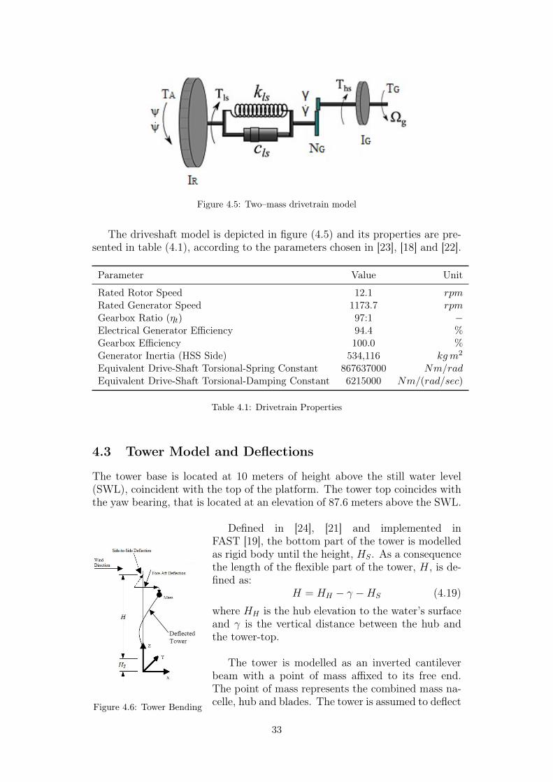
Figure 4.5: Two–mass drivetrain model

The driveshaft model is depicted in figure (4.5) and its properties are pre-sented in table (4.1), according to the parameters chosen in [23], [18] and [22].

Parameter Value Unit

Rated Rotor Speed 12.1 rpmRated Generator Speed 1173.7 rpmGearbox Ratio (ηt) 97:1 −Electrical Generator Efficiency 94.4 %Gearbox Efficiency 100.0 %Generator Inertia (HSS Side) 534,116 kgm2

Equivalent Drive-Shaft Torsional-Spring Constant 867637000 Nm/radEquivalent Drive-Shaft Torsional-Damping Constant 6215000 Nm/(rad/sec)

Table 4.1: Drivetrain Properties

4.3 Tower Model and Deflections

The tower base is located at 10 meters of height above the still water level(SWL), coincident with the top of the platform. The tower top coincides withthe yaw bearing, that is located at an elevation of 87.6 meters above the SWL.

Figure 4.6: Tower Bending

Defined in [24], [21] and implemented inFAST [19], the bottom part of the tower is modelledas rigid body until the height, HS. As a consequencethe length of the flexible part of the tower, H, is de-fined as:

H = HH − γ −HS (4.19)

where HH is the hub elevation to the water’s surfaceand γ is the vertical distance between the hub andthe tower-top.

The tower is modelled as an inverted cantileverbeam with a point of mass affixed to its free end.The point of mass represents the combined mass na-celle, hub and blades. The tower is assumed to deflect

33

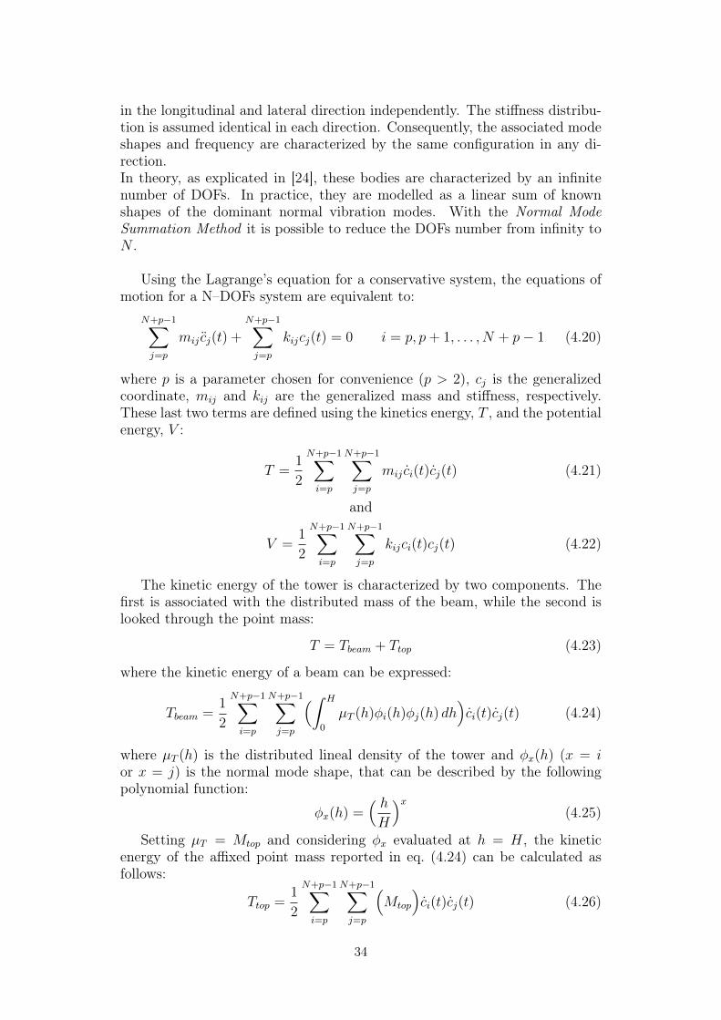
in the longitudinal and lateral direction independently. The stiffness distribu-tion is assumed identical in each direction. Consequently, the associated modeshapes and frequency are characterized by the same configuration in any di-rection.In theory, as explicated in [24], these bodies are characterized by an infinitenumber of DOFs. In practice, they are modelled as a linear sum of knownshapes of the dominant normal vibration modes. With the Normal ModeSummation Method it is possible to reduce the DOFs number from infinity toN .

Using the Lagrange’s equation for a conservative system, the equations ofmotion for a N–DOFs system are equivalent to:

N+p−1∑j=p

mij cj(t) +

N+p−1∑j=p

kijcj(t) = 0 i = p, p+ 1, . . . , N + p− 1 (4.20)

where p is a parameter chosen for convenience (p > 2), cj is the generalizedcoordinate, mij and kij are the generalized mass and stiffness, respectively.These last two terms are defined using the kinetics energy, T , and the potentialenergy, V :

T =1

2

N+p−1∑i=p

N+p−1∑j=p

mij ci(t)cj(t) (4.21)

and

V =1

2

N+p−1∑i=p

N+p−1∑j=p

kijci(t)cj(t) (4.22)

The kinetic energy of the tower is characterized by two components. Thefirst is associated with the distributed mass of the beam, while the second islooked through the point mass:

T = Tbeam + Ttop (4.23)

where the kinetic energy of a beam can be expressed:

Tbeam =1

2

N+p−1∑i=p

N+p−1∑j=p

(∫ H

0

µT (h)φi(h)φj(h) dh)ci(t)cj(t) (4.24)

where µT (h) is the distributed lineal density of the tower and φx(h) (x = ior x = j) is the normal mode shape, that can be described by the followingpolynomial function:

φx(h) =( hH

)x(4.25)

Setting µT = Mtop and considering φx evaluated at h = H, the kineticenergy of the affixed point mass reported in eq. (4.24) can be calculated asfollows:

Ttop =1

2

N+p−1∑i=p

N+p−1∑j=p

(Mtop

)ci(t)cj(t) (4.26)

34

Equations (4.21), (4.22), (4.24) and (4.26) show that the generalized massof the tower is:

mij = Mtop +

∫ H

0

µT (h)φi(h)φj(h) dh (4.27)

According to eq. (4.28), the potential energy is characterized by two com-ponents; the first is related to the stiffness, while the second is associated withthe gravity:

V = Vbeam + Vgravity (4.28)

In particular the potential energy can be expressed as:

Vbeam =1

2

N+p−1∑i=p

N+p−1∑j=p

(∫ H

0

EIT (h)d2φi(h)

dh2

d2φj(h)

dh2 dh)ci(t)cj(t) (4.29)

where EIT is the distributed stiffness of the tower.

Moreover, since the gravity action on an inverted beam tends to reduce thetower stiffness, it can be defined as:

Vgravity = −g[Mtopκ(H, t) +

∫ H

0

µT (h)κ(h, t) dh]

(4.30)

where the negative sign promotes the notation that gravity reduces the stiff-ness, κ(h, t) is the axial deflection of the flexible cantilever beam at time t andan elevation h. The axial deflection is the combined result of two assumptions:i) the flexible beam remains fixed in length (measured along the beam’s centralaxis) and ii) the free end can be moved closer to the fixed end when the beamdeflects laterally. As a consequence, the axial deflection is related to the lateraldeflection and their relationship can be obtained by examining the deflectiongeometry as shown in figure (4.7).

Figure 4.7: Tower deflection geometry

35

Expanding the lateral and the axial deflection about any h elevation, usinga first Taylor series approximation, and applying the Pythagorean theorem tothe geometry as stated in [24], it emerges that:

κ(h, t) =1

2

∫ h

0

[∂Γ(h′, t)

∂h′]2dh′ (4.31)

where h′ is a dummy variable representing the elevation along the flexible partof the tower. Therefore the equation (4.31) can be rewritten:

κ(h, t) =1

2

N+p−1∑i=p

N+p−1∑j=p

(∫ h

0

dφi(h′)

dh′dφj(h

′)

dh′dh′)ci(t)cj(t) (4.32)

Substituting eq. (4.32) into eq. (4.30), the potential energy caused by gravitycan be expressed by the following formula:

Vgravity =− g1

2

N+p−1∑i=p

N+p−1∑j=p

[Mtop

∫ H

0

dφi(h)

dh

dφj(h)

dhdh+

∫ H

0

µT (h)

(∫ h

0

dφi(h′)

dh′dφj(h

′)

dh′dh′)dh

]ci(t)cj(t)

(4.33)

After some simplifications, equations (4.22), (4.28), (4.29) and (4.33) show thatthe generalized tower stiffness is:

kij =

∫ H

0

EIT (h)d2φi(h)

dh2

d2φj(h)

dh2dh

− g∫ H

0

[Mtop +

∫ H

h

µT (h′) dh′]dφi(h)

dh

dφj(h)

dhdh

(4.34)

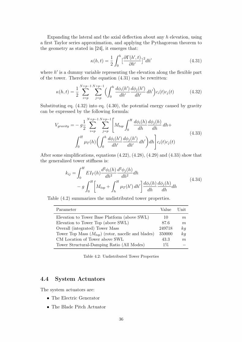
Table (4.2) summarizes the undistributed tower properties.

Parameter Value Unit

Elevation to Tower Base Platform (above SWL) 10 mElevation to Tower Top (above SWL) 87.6 mOverall (integrated) Tower Mass 249718 kgTower Top Mass (Mtop) (rotor, nacelle and blades) 350000 kgCM Location of Tower above SWL 43.3 mTower Structural-Damping Ratio (All Modes) 1% −

Table 4.2: Undistributed Tower Properties

4.4 System Actuators

The system actuators are:

• The Electric Generator

• The Blade Pitch Actuator

36

4.4.1 Electric Generator

The wind turbines are usually variable-speed, where the rotor can rotate atvariable frequencies independently of the electrical grid frequency. Using anelectronic converter, it is possible to provide a variable rotational speed thatallows achieving the maximum power in an ample wind speed range. Usually,the electric machine is an asynchronous motor controlled thought a vecto-rial controller, which produces rapid and precise torque variation. For thesereasons, as in [3], the control system of the overall electric system can be ap-proximated with a first order system characterised by a very small constanttransfer. Moreover, since the generator dynamic is faster than the wind turbinemechanical dynamics, it is not taken into consideration.

4.4.2 Blade Pitch Actuator

The blades rotations allow to get the desired step angle, typically thought aservo-motor that can be electric or hydraulic. In the last years a servo-electricmotor has been preferred because it is not influenced from the environmentalconditions, since there is not fluid to move blades.

FAST can not model the system actuators. Since making an accurate modelis useful for the purpose of this thesis, a second order transfer function with anatural frequency of 5.0265 rad/sec and dumping coefficient of 0.8, as in [3],has been used to model the blade pitch actuator.

Figure (4.8) shows the step response of the pitch blade actuator model.

-1 -0.5 0 0.5 1 1.5 2 2.5 30

0.2

0.4

0.6

0.8

1

1.2

Step Response

Time (seconds)

Am

plit

ud

e

Figure 4.8: Blade Pitch Step Response

37

Chapter 5

Control Models

For the OC3–Hywind wind turbine a conventional variable-speed, definedin ([18], [23]), and a variable blade-pitch-to-father configuration have beenused. The conventional approach for power production control and for me-chanical stability relies on the design of two basic control systems:

• Generator–Torque Controller

• Full–Span Blade–Pitch Controller

The two control systems are designed to work independently, below and abovethe rated wind speed range. The objective of the Generator–Torque Con-troller is the power maximization below the rated operation point (vwind < 11.4m/sec), whereas the blade pitch controller has to regulate the generator speedabove the rated operation point (vwind > 11.4 m/sec) and below the cut-offregion (vwind > 25 m/sec). According to the purpose of this thesis, only thecase above the rated operation point is considered.

5.1 Speed–Measurement Filter

Usually in multi-megawatt wind turbines, both generator-torque and bladepitch controllers have a generator speed measurement as feedback input. Tomitigate the high-frequency excitation of the control system, a filtered genera-tor speed has been used, as in [18]. The corner frequency of the low-pass filterwas set to be roughly one-quarter of the blade first edgewise natural frequency(see table 6.1). The corner frequency will be 5.46 rad/s.

5.2 Generator–Torque Controller

The generator–torque controller is a tabulated function that incorporates fivecontrol regions as in [18]:

• Region 1 – Before cut-in wind speed, the generator torque is equal tozero and no electrical power is extracted. The wind energy is used toaccelerate the rotor.

• Region 112– Start-up region. It is a linear transition between regions 2

and 1.

38

• Region 2 – Optimizing power capture. Here, the generator torque isproportional to the square of the generator speed to maintain a con-stant (optimal) tip-speed ratio.

• Region 212– Added region. This region is typically needed to limit tip

speed (and noise emission) at a rated power.

• Region 3 – The generator power is held constant. Hence, the generatortorque is inversely proportional to the generator speed.

Chapter 1: Introduction

Region 2 This is where the turbine will spend most of its operational life in the designed wind

speed region. Therefore, the main objective is to maximise power capture in this region.

This region is also known as the below rated wind speed region.

Region 3 This is the above rated wind speed region where the extracted power of the wind must

be limited to the rated power to avoid damaging the turbine components. Hence, the

turbine is reducing its aerodynamic efficiency to limit power capture to the rated power

of the generator.

Figure 1.7: Wind turbine operating regions

An upper limit for region 3 exists

where the wind speed is too fast

for safe operation of the wind tur-

bine. Therefore, the wind turbine

goes into shut-down mode for wind

speeds higher than the cut-off wind

speed. The blades are feathered into

the wind to minimise the lift gen-

erated and the shaft brakes are ap-

plied. The control logic that de-

termines the operational state of the

wind turbine and controls start-up

and shut-down is the supervisory

control. This higher control layer is

not considered in this work.

1.2.2 Overall Controller Objectives

The main purpose of a wind turbine is to generate power with a competitive cost of energy.

There are many factors that affect the cost of energy such as the location and wind speed dis-

tribution, turbine efficiency, etc. From a control system point of view, there are two factors that

the controller can influence to reduce the cost of energy: power capture and component fatigue

life. To reduce the cost of energy, the control system must

1. maximise power capture subject to

(a) limits on the captured power according to the operating regions (i.e. limit power

capture in regions 1 and 3);

(b) actuation constraints for each region.

i. To maximise power in region 2, the blade pitch is set to the fixed optimum angle

that maximises the aerodynamic torque and the generator torque is used to con-

trol the rotor speed to achieve a desired tip speed ratio3 [33, 34].

3Tip speed ratio is dimensionless number defined as the ratio of the blade’s tip velocity to the upstream windvelocity [28, 29].

12

Figure 5.1: Wind Turbines Operation Regions

5.2.1 Rotor Power Coefficient – Cp

The power coefficient is a measurement of how the wind turbine converts thewind energy into electrical energy efficiently. According to the Rankine-FroudeActuator Disc Theory and Betz Limit [17], using an approach simpler thanthe BEM theory, presented in section 4.1, it possible to define the followingrelationship:

Pwind =1

2ρair AV

30 (5.1)

where ρair is the air density, A is the rotor sweep area and V0 is the wind speed.

The aerodynamic power, PA, can be found as:

PA = PwindCp(λ, β, α) (5.2)

39

where Cp is a function of the blade pitch, β, of the platform pitch, α, and ofthe Tip–Speed Ratio (TSR), λ, which is defined as:

λ =ΩR

V0

(5.3)

where Ω is the rotor angular speed and R is the rotor radius.

The typical power coefficient map for this wind turbine model has beenobtained running FAST with AeroDyn simulations at a given rotor speed(Ω0 = 12.1 rpm), collective blade-pitch angle (0 deg to 30 deg), platform pitch(0 deg to 5 deg), and with a wind specific speed ramp. From these simulationsit has been found that the peak power coefficient of 0.4906 occurred at a tip-speed ratio of 8.1692 and with a rotor collective pitch angle of 0.0 deg.

Tip Speed Ratio [-]

0 2 4 6 8 10 12 14 16 18 20

Po

we

r C

off

icie

nt

[-]

0

0.1

0.2

0.3

0.4

0.5

Maps of Power Cofficient

Beta=0 [deg]

Beta=5 [deg]

Beta=10 [deg]

Beta=15 [deg]

Beta=20 [deg]

(a) Power Coefficient MapsTSR [-]

0 2 4 6 8 10 12 14 16 18 20

Ro

tor

Po

we

r C

off

icie

nt

[-]

0

0.05

0.1

0.15

0.2

0.25

0.3

0.35

0.4

0.45

0.5Cp - Real Curve

beta=0

(b) Real Power Maps

Figure 5.2: Power Coefficient

Hence:

• Cpmax = 0.4906

• λopt = 8.1692

5.2.2 Optimal Constant in Region 2

In region 2, it is necessary to maximize the power production. On thesepremises, it has been found the optimal value of Kopt to get the maximumpower keeping the optimal tip-speed ratio.Using the previous values of Cp and λ, the optimal value of K (HSS side) canbe defined as in [10], namely:

Kopt =1

2πρR5 Cpmax

(λoptNG)3= 0.0256 Nm/rpm2 (5.4)

where NG = 97 is the HSS/LSS gearbox ratio.

40

Generator Speed [rpm]

0 500 1000 1500

Ge

ne

rato

r T

orq

ue

[W

]

×104

0

1

2

3

4

5

6

Variable-Speed Controller

Optimal

Figure 5.3: Variable-Speed Controller

5.3 Gain Scheduling PI

The first control type adopted is the full-span rotor collective blade pitch anglecommand. It uses a gain-scheduled proportional-integral (GSPI) control on thespeed error between rotor speed and rated rotor speed, as indicated in [18].Considering a simple single degree of freedom model and a rigid drivetrain,the motion equation can be described as follows:

TA −NGTG = (IR +N2GIG)

d

dt(Ω0 + ∆Ω) = ID∆Ω (5.5)

where t is the simulation time, TA is the LSS (Low-Speed Shaft) aerodynamictorque, TG is the HSS (High-Speed Shaft) generator torque, NG is the gearboxratio defined above, ID is the drivetrain inertia cast to LSS part, IR is therotor inertia, IG is the generator inertia relative to HSS part, Ω0 is the ratedLSS rotational speed and ∆Ω is the perturbed LSS rotational acceleration.

Using a Proportional-Integral-Derivative control (PID), it is possible todefine the perturbed blade pitch angle, ∆β:

∆β = KPNG∆Ω +KI

∫ t

0

NG∆Ωdt+KDNG∆Ω (5.6)

where KP , KI and KD are the controller proportional, integral, and derivativegains, respectively.

41

In Region 3, as shown in figure (5.3), the generator torque controller main-tains the generator power steady and the generator torque is inversely propor-tional to the generator speed:

TG(NGΩ) =P0

NGΩ(5.7)

where Ω is the LSS rotational speed and P0 is the rated mechanical power.

Similarly, assuming ∂TA∂Ω' 0, the aerodynamic torque becomes:

TA(β) =P (β,Ω0)

Ω0

(5.8)

where β is the collective blade pitch angle and P is the mechanical power.

Expanding the eqs. (5.7) and (5.8) using the first-order Taylor series, itemerges that:

TG 'P0

NGΩ0

− P0

NGΩ20

∆Ω (5.9)

andTA '

P0

Ω0

+1

Ω0

(∂P∂β

)∆β (5.10)

where ∆β is a small perturbation of the blade pitch angle about their operatingpoint. Hence, setting η = ∆Ω and combining the eqs. (5.9) and (5.10) withthe eqs. (5.6) and (5.5), the rotor speed error equation becomes:[ID +

1

Ω0

(−∂P∂β

)NGKD

]︸ ︷︷ ︸

Mη

η+[ 1

Ω0

(−∂P∂β

)NGKP −

P0

Ω20

]︸ ︷︷ ︸

Cη

η+[ 1

Ω0

(−∂P∂β

)NGKI

]︸ ︷︷ ︸

Kη

η = 0

(5.11)The PID controlled rotor speed error responds as a second-order system witha damping ratio, ζη and a natural frequency, ωηn, equal to:

ωηn =

√Kη

Mη

(5.12)

andζη =

Cη2Mηωηn

=Cη

2√KηMη

(5.13)

In region 3, ∂P∂β

is negative. Thus, choosing a positive control gains, thederivative term increases the effective inertia, the proportional term addsdamping and the integral term increases the stiffness term. Furthermore, thegenerator torque controller introduces a negative damping by the term −P0/Ω

20

in equation (5.11). Such a negative damping must be compensated by the pro-portional term KP included in the blade pitch controller.

In the design of the blade pitch control, the controller-response naturalfrequency and damping ratio have been chosen equals to 0.2 rad/sec and 0.7,

42

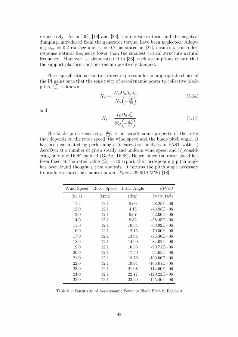
respectively. As in [30], [18] and [23], the derivative term and the negativedumping, introduced from the generator torque, have been neglected. Adopt-ing ωηn = 0.2 rad/sec and ζη = 0.7, as stated in [22], ensures a controller-response natural frequency lower than the smallest critical structure naturalfrequency. Moreover, as demonstrated in [33], such assumptions ensure thatthe support platform motions remain positively damped.

These specifications lead to a direct expression for an appropriate choice ofthe PI gains once that the sensitivity of aerodynamic power to collective bladepitch, ∂P

∂β, is known:

KP =2IDΩ0βηωηn

NG

(−∂P

∂β

) (5.14)

and

KI =IDΩ0ω

2ηn

NG

(−∂P

∂β

) (5.15)

The blade pitch sensitivity, ∂P∂β

, is an aerodynamic property of the rotorthat depends on the rotor speed, the wind speed and the blade pitch angle. Ithas been calculated by performing a linearization analysis in FAST with: i)AeroDyn at a number of given steady and uniform wind speed and ii) consid-ering only one DOF enabled (GeAz_DOF). Hence, since the rotor speed hasbeen fixed at the rated value (Ω0 = 12.1rpm), the corresponding pitch anglehas been found thought a trim analysis. It returns the pitch angle necessaryto produce a rated mechanical power (P0 = 5.296619 MW) [18].

Wind Speed Rotor Speed Pitch Angle ∂P/∂β

(m/s) (rpm) (deg) (watt/rad)

11.4 12.1 0.00 -28.25E+0612.0 12.1 4.15 -43.98E+0613.0 12.1 6.67 -52.00E+0614.0 12.1 8.82 -58.45E+0615.0 12.1 10.54 -63.92E+0616.0 12.1 12.15 -70.30E+0617.0 12.1 13.64 -76.30E+0618.0 12.1 14.90 -84.02E+0619.0 12.1 16.33 -90.71E+0620.0 12.1 17.59 -94.65E+0621.0 12.1 18.79 -100.00E+0622.0 12.1 19.94 -106.01E+0623.0 12.1 21.08 -114.60E+0624.0 12.1 22.17 -120.22E+0625.0 12.1 23.20 -125.40E+06

Table 5.1: Sensitivity of Aerodynamic Power to Blade Pitch in Region 3

43

Colletive Blade Pitch Angle [deg]

0 5 10 15 20 25 30

Pitch

Se

nsitiv

ity [

wa

tt/r

ad

]

×107

-16

-14

-12

-10

-8

-6

-4

-2

Original Data

Linear Approximation

Figure 5.4: Linear Approximation of pitch sensitivity in Region 3

In table (5.1) it is possible to see that(∂P∂β

)is a highly variable term, hence

constant PI gains are not adequate for effective speed control. Furthermore, itcan be also observed that

(∂P∂β

)is characterized by a downward trend respect

the blade pitch angle.

Plotting the results (fig. 5.4), it is easy to see that the pitch sensitivityvaries linearly with blade pitch angle. By applying a linear regression it ispossible to affirm that:

∂P

∂β=[ ∂P∂β

(β = 0)

βK

]β +

[∂P∂β

(β = 0)]

(5.16)

where ∂P∂β

(β = 0) is the pitch sensitivity at rated and βK is the blade pitchangle at which the pitch sensitivity has doubled its value respect to the ratedoperating point. Hence, before these considerations:

∂P

∂β(β = βK) = 2

∂P

∂β(β = 0) (5.17)

where βK = 5.577 deg with ∂P∂β

(β = 0) = −28.25E + 06 watt/rad.

The linear relation between pitch sensitivity and blade pitch angle presentsa simple technique for implementing a gain scheduling. As a consequenceequations (5.14) and (5.15) become:

KP (β) =2IDΩ0ζϕωϕn

NG

[−∂P

∂β(β = 0)

]GK(β) (5.18)

44

and

KI(β) =IDΩ0ω

2ϕn

NG

[−∂P

∂β(β = 0)

]GK(β) (5.19)

where GK(β) is the dimensionless gain corrector factor, which depends on theblade pitch angle according to the following relationship:

GK(β) =1

1 + ββK

(5.20)

Figure (5.5) shows the KP , KI and GK trends as functions of the blade pitchangle, β (hundred factor is only to a graphic matter).

Collective Pitch Blade Angle [deg]

0 5 10 15 20 25 30

Ga

in C

orr

ecto

r F

acto

r

0

0.001

0.002

0.003

0.004

0.005

0.006

0.007

0.008

0.009

0.01

GK/100

Kp

Ki

Figure 5.5: Blade Pitch Control Gain Scheduling Law

where:

• KP (β = 0) = 0.006

• KI(β = 0) = 0.0009

During the implementation of the GSPI, the blade pitch angle from theprevious controller time-step has been used to calculate the gain-correctionfactor at the next time step. After a first implementation with a power con-stant generator control, another control law with a constant generator torque,as in [22], has been implemented. This change does not introduce negativedamping in the rotor speed response, namely the term

(P0

Ω0

)is equal to zero,

45

but reduces the rotor speed excursion that has been exaggerated by a very lit-tle proportional gain. Furthermore, a blade pitch angle limit from 0 to 90 degand a blade pitch rate limit range to [−8,+8] deg/sec, which is a conventionallimits of a 5–MW machines, have been set.

46

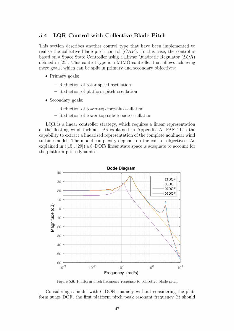
5.4 LQR Control with Collective Blade Pitch

This section describes another control type that have been implemented torealise the collective blade pitch control (CBP ). In this case, the control isbased on a Space State Controller using a Linear Quadratic Regulator (LQR)defined in [25]. This control type is a MIMO controller that allows achievingmore goals, which can be split in primary and secondary objectives:

• Primary goals:

– Reduction of rotor speed oscillation– Reduction of platform pitch oscillation

• Secondary goals:

– Reduction of tower-top fore-aft oscillation– Reduction of tower-top side-to-side oscillation

LQR is a linear controller strategy, which requires a linear representationof the floating wind turbine. As explained in Appendix A, FAST has thecapability to extract a linearized representation of the complete nonlinear windturbine model. The model complexity depends on the control objectives. Asexplained in ([15], [29]) a 8–DOFs linear state space is adequate to account forthe platform pitch dynamics.

10-3 10-2 10-1 100 101-60

-50

-40

-30

-20

-10

0

10

20

30

40

Ma

gn

itu

de

(d

B)

21DOF

08DOF

07DOF

06DOF

Bode Diagram

Frequency (rad/s)

Figure 5.6: Platform pitch frequency response to collective blade pitch

Considering a model with 6–DOFs, namely without considering the plat-form surge DOF, the first platform pitch peak resonant frequency (it should

47

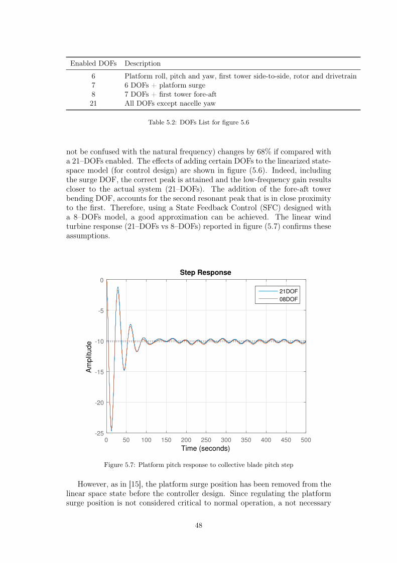
Enabled DOFs Description

6 Platform roll, pitch and yaw, first tower side-to-side, rotor and drivetrain7 6 DOFs + platform surge8 7 DOFs + first tower fore-aft21 All DOFs except nacelle yaw

Table 5.2: DOFs List for figure 5.6

not be confused with the natural frequency) changes by 68% if compared witha 21–DOFs enabled. The effects of adding certain DOFs to the linearized state-space model (for control design) are shown in figure (5.6). Indeed, includingthe surge DOF, the correct peak is attained and the low-frequency gain resultscloser to the actual system (21–DOFs). The addition of the fore-aft towerbending DOF, accounts for the second resonant peak that is in close proximityto the first. Therefore, using a State Feedback Control (SFC) designed witha 8–DOFs model, a good approximation can be achieved. The linear windturbine response (21–DOFs vs 8–DOFs) reported in figure (5.7) confirms theseassumptions.

0 50 100 150 200 250 300 350 400 450 500-25

-20

-15

-10

-5

0

21DOF

08DOF

Step Response

Time (seconds)

Am

plit

ud

e

Figure 5.7: Platform pitch response to collective blade pitch step

However, as in [15], the platform surge position has been removed from thelinear space state before the controller design. Since regulating the platformsurge position is not considered critical to normal operation, a not necessary

48

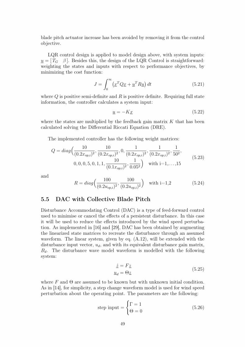
blade pitch actuator increase has been avoided by removing it from the controlobjective.

LQR control design is applied to model design above, with system inputs:u = [TG β ]. Besides this, the design of the LQR Control is straightforward:weighting the states and inputs with respect to performance objectives, byminimizing the cost function:

J =

∫ ∞0

(xTQx+ uTRu

)dt (5.21)

where Q is positive semi-definite and R is positive definite. Requiring full stateinformation, the controller calculates a system input:

u = −Kx (5.22)

where the states are multiplied by the feedback gain matrix K that has beencalculated solving the Differential Riccati Equation (DRE).

The implemented controller has the following weight matrices:

Q = diag( 10

(0.2xop,i)2,

10

(0.2xop,i)2, 0,

1

(0.2xop,i)2,

1

(0.2xop,i)2,

1

502,

0, 0, 0, 5, 0, 1, 1,10

(0.1xop,i)2,

1

0.052

)with i=1,. . . ,15

(5.23)

andR = diag

( 100

(0.2uop,i)2,

100

(0.2uop,i)2

)with i=1,2 (5.24)

5.5 DAC with Collective Blade Pitch

Disturbance Accommodating Control (DAC) is a type of feed-forward controlused to minimise or cancel the effects of a persistent disturbance. In this caseit will be used to reduce the effects introduced by the wind speed perturba-tion. As implemented in [16] and [29], DAC has been obtained by augmentingthe linearized state matrices to recreate the disturbance through an assumedwaveform. The linear system, given by eq. (A.12), will be extended with thedisturbance input vector, ud, and with its equivalent disturbance gain matrix,Bd. The disturbance wave model waveform is modelled with the followingsystem:

z = Fz

ud = Θz(5.25)

where F and Θ are assumed to be known but with unknown initial condition.As in [14], for simplicity, a step change waveform model is used for wind speedperturbation about the operating point. The parameters are the following:

step input =

Γ = 1

Θ = 0(5.26)

49

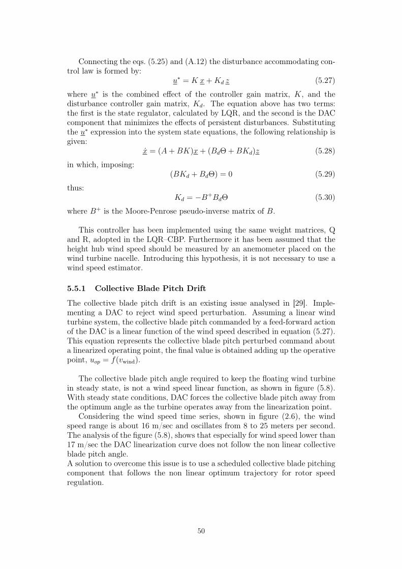
Connecting the eqs. (5.25) and (A.12) the disturbance accommodating con-trol law is formed by:

u∗ = K x+Kd z (5.27)

where u∗ is the combined effect of the controller gain matrix, K, and thedisturbance controller gain matrix, Kd. The equation above has two terms:the first is the state regulator, calculated by LQR, and the second is the DACcomponent that minimizes the effects of persistent disturbances. Substitutingthe u∗ expression into the system state equations, the following relationship isgiven:

x = (A+BK)x+ (BdΘ +BKd)z (5.28)

in which, imposing:(BKd +BdΘ) = 0 (5.29)

thus:Kd = −B+BdΘ (5.30)

where B+ is the Moore-Penrose pseudo-inverse matrix of B.

This controller has been implemented using the same weight matrices, Qand R, adopted in the LQR–CBP. Furthermore it has been assumed that theheight hub wind speed should be measured by an anemometer placed on thewind turbine nacelle. Introducing this hypothesis, it is not necessary to use awind speed estimator.

5.5.1 Collective Blade Pitch Drift

The collective blade pitch drift is an existing issue analysed in [29]. Imple-menting a DAC to reject wind speed perturbation. Assuming a linear windturbine system, the collective blade pitch commanded by a feed-forward actionof the DAC is a linear function of the wind speed described in equation (5.27).This equation represents the collective blade pitch perturbed command abouta linearized operating point, the final value is obtained adding up the operativepoint, uop = f(vwind).

The collective blade pitch angle required to keep the floating wind turbinein steady state, is not a wind speed linear function, as shown in figure (5.8).With steady state conditions, DAC forces the collective blade pitch away fromthe optimum angle as the turbine operates away from the linearization point.

Considering the wind speed time series, shown in figure (2.6), the windspeed range is about 16 m/sec and oscillates from 8 to 25 meters per second.The analysis of the figure (5.8), shows that especially for wind speed lower than17 m/sec the DAC linearization curve does not follow the non linear collectiveblade pitch angle.A solution to overcome this issue is to use a scheduled collective blade pitchingcomponent that follows the non linear optimum trajectory for rotor speedregulation.

50

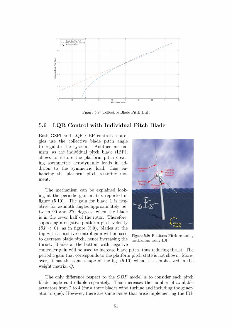
Wind Speed [m/sec]

8 10 12 14 16 18 20 22 24 26

Colle

ctive B

lade P

itch [deg]

0

5

10

15

20

25

Steady-State Pitch Angle

DAC-collective pitch command

Linearization Point

Figure 5.8: Collective Blade Pitch Drift

5.6 LQR Control with Individual Pitch Blade

Figure 5.9: Platform Pitch restoringmechanism using IBP

Both GSPI and LQR–CBP controls strate-gies use the collective blade pitch angleto regulate the system. Another mecha-nism, as the individual pitch blade (IBP),allows to restore the platform pitch creat-ing asymmetric aerodynamic loads in ad-dition to the symmetric load, thus en-hancing the platform pitch restoring mo-ment.

The mechanism can be explained look-ing at the periodic gain matrix reported infigure (5.10). The gain for blade 1 is neg-ative for azimuth angles approximately be-tween 90 and 270 degrees, when the bladeis in the lower half of the rotor. Therefore,supposing a negative platform pitch velocity(∂x < 0), as in figure (5.9), blades at thetop with a positive control gain will be usedto decrease blade pitch, hence increasing thethrust. Blades at the bottom with negativecontroller gain will be used to increase blade pitch, thus reducing thrust. Theperiodic gain that corresponds to the platform pitch state is not shown. More-over, it has the same shape of the fig. (5.10) when it is emphasized in theweight matrix, Q.

The only difference respect to the CBP model is to consider each pitchblade angle controllable separately. This increases the number of availableactuators from 2 to 4 (for a three blades wind turbine and including the gener-ator torque). However, there are some issues that arise implementing the IBP

51

Azimuth [deg]

0 50 100 150 200 250 300 350

Gain

s

-0.04

-0.03

-0.02

-0.01

0

0.01

0.02

0.03

0.04

0.05Platform Pitch Velocity State

Periodic after MBC

Costant

Figure 5.10: Blade 1 periodic gain and constant gain

controller, which are:

• Increased blade pitch actuation which may result in blade pitch satura-tion.

• Setting too high weight in Q, R matrices may produce an increase of theblade load.

• The possibility of exciting or destabilising other turbine modes due tocoupling with no modelled DOFs.

The issues above involve a more careful choice of Q and R matrices. Withthis setting is not possible to use a control system based on a LTI model. Sincethe control law depends on the blade position on the rotor plane, it needs aperiodic model in function of the rotor azimuth angle. To avoid this increaseof complexity, the MBC transformation allows to implement a control systembased on a LTI model even though the model periodicity.

5.6.1 Multi-Blade Coordinate Transformation - MBC

The wind turbine dynamics like rotor blades are generally expressed in rotatingframe attached to the individual blades. The tower and nacelle subsystem areaffected by the combined effect of all rotor blades, not the individual blades.This is because the rotor responds as a whole to excitations such as aerody-namics gusts, control inputs and tower-nacelle motion, all of which occurringa non-rotating frame. MBC transformation, defined in [4], expresses the dy-namics of individual blades in a fixed (non-rotating) frame. MBC offer severalbenefits:

• Providing the exact dynamic interaction between the non-rotating tower-nacelle and the spinning rotor.

• Offering insights concerning rotor dynamics and the way the rotor inter-acts with fixed-system entities, such as wind, controls, tower and nacellesubsystem.

52

• Removing all periodic terms except those which are integral multiples ofΩB, where Ω is the rotor angular speed and B is the number of the rotorblades.

Figure 5.11: MBC CoordinateTransformation

MBC Concept and Associated Transfor-mation – Considering a rotor with B bladesthat are spaced equally around the rotor disk,the azimuth location of the bth blade is givenby:

Ψb = Ψ + (b− 1)2π

B(5.31)

where Ψ is the azimuth of the first (reference)blade and it is assumed equal to zero, imply-ing that the first blade is vertically up. Sincethe number of blades is B = 3 and theMBCis a linear transformation, which relates therotating degrees of freedom to new degrees offreedom, they are defined as:

q0 =1

B

B∑b=1

qb

qc =2

3

B∑b=1

qb cos Ψb

qs =2

3

B∑b=1

qb sin Ψb

(5.32)

where q0 is the collective mode, qc is the cosine-cyclic mode and qs is the sine-cyclic mode. The equations in (5.32) determine the rotor coordinate, given theblades coordinates. The inverse transformation yielding the blade coordinategiven the rotor coordinate is:

qb = q0 + qc cos Ψb + qs sin Ψb with b = 1, 2, 3 (5.33)

where, in this equation and in the equations above, qb is a particular rotatingdegree of freedom (more detailed informations can be found in [5]).

In the linearized representation of the 8–DOFs model, the u vector containscontrol inputs that are in the rotating frames references whereas the distur-bance vector, ud, has been assumed to have no input in the rotating frame ofreference. Applying the MBC transformation, the new transformed matricesANR , BNR , BdNR , CNR andDNR are obtained passing through the transformationmatrices Ts(Ψ), Tc(Ψ) and To(Ψ), where:

x = Ts(Ψ)xNR

(5.34)u = Tc(Ψ)u

NR(5.35)

y = To(Ψ)yNR

(5.36)

53

and considering:u =

[TG β1 β2 β3

]T (5.37)

then,

Tc(Ψ) =

1 0 0 00 1 cos(Ψ) sin(Ψ)0 1 cos(Ψ + 2π

3) sin(Ψ + 2π

3)

0 1 cos(Ψ + 4π3

) sin(Ψ + 4π3

)

(5.38)

The new input vector achieved after the transformation assumes a differentphysic interpretation:

uNR

=[TG β0 βc βs

]T (5.39)

where TG is the same that in rotating frame, whereas β0, βc and βs are thecollective, cosine and sine contributions, respectively.

In this particular case, there are not states and outputs in rotating framereferences, thus:

Ts(Ψ) = In,n (5.40)and

To(Ψ) = Ip,p (5.41)

where I is the identical matrix, n is the number of the states and p in thenumber of the outputs.

5.6.2 LQR after MBC Transformation

After applying MBC Transformation on a periodic system, the LQR law inthe non-rotating frame becomes:

uNR

= −KNR xNR(5.42)

Equations (5.34), (5.35) and (5.42) have been used to transform back theblade pitch commands in the mixed frame, getting the following relationship:

u = Tc(Ψ)uNR

= −Tc(Ψ)KNR xNR

= −Tc(Ψ)KNR T−1s (Ψ)x

= −Tc(Ψ)KNR I−1n,n x

= KMBC(Ψ)x

(5.43)

thus,KMBC(Ψ) = −Tc(Ψ)KNR In,n (5.44)

5.7 DAC with Individual Blade Pitch

This section presents the Disturbance Accommodation Control (DAC) basedon Individual Blade Pitch. The basic rules are the same as explained in sec-tion 5.5.

54

Using an individual blade pitch, where the control is azimuth angle depen-dent, it is possible to include the wind share effect. Wind share describes thehorizontal increase of the wind speed with the height. It is expected that, byincluding this effect in the linearized models, especially for periodic controller,the performance of the wind turbine will improve.

5.7.1 Including Wind Share Effect

To develop a wind-share linearized model, the same approach as in [34] hasbeen used. The wind-speed variation with height is expressed as:

V (z) = Vhub

(1 +

z

H

)m(5.45)

where Vhub is the wind speed at hub-height, H, z is the height above thehub and the coefficient m is the power wind-shear coefficient, defined in sec-tion 2.4.1.

Equation (5.45) can be expressed as a binomial series in(zH

):

(1 +

z

H

)m= 1 +m

( zH

)+m(m− 1)

2

( zH

)2

+m(m− 1)(m− 2)

6

( zH

)3

+ . . .

(5.46)Using the polar coordinates (R and Ψ), z becomes:

z = R cos(Ψ) (5.47)

where, R is the rotor radius and Ψ is the rotor azimuth angle.

Substituting equation (5.47) in equation (5.46), and considering until thethird-order terms, the following expression results, involving in: Vhub, H, R,m and Ψ:

V (R,Ψ) ∼=Vhub6h3

[6h3+6h2mR cos(Ψ)+3hm(m−1)R2 cos2(Ψ)+m(m−1)(m−2)R3 cos3(Ψ)

](5.48)

For the OC3–Hwind the equation (5.48) becomes:

V (R,Ψ) ∼= Vhub

[0.97 + 0.115 cos(Ψ)− 0.004 cos(3Ψ)

](5.49)

where the dominant periodic term is 0.115 cos(Ψ), thus the other term will beneglected.

The first term in equation (5.49) is the wind component, which is no de-pendent on azimuth position and it will be modelled with the DAC step wave-form. The second term represents the azimuth-dependent component. Thisadditional term, not present in the DAC–CBP, must be represented with anew DAC waveform.

55

To represent this new term, the matrices of the general disturbance wavemodel, in eq (5.25), become:

Θ =

[1 0 00 1 0

], F =

0 0 00 0 10 −Ω2 0

(5.50)

these matrices were achieved using the following variables:

ud,1 = zd,1

ud,2 = zd,2 = Ad cos(Ψ) = Ad cos(Ωt)

zd,3 = zd,2

(5.51)

where Ad = 0.115Vhub and Ψ = Ωt.

5.7.2 DAC after MBC Transformation

In this work the disturbance states, z, are modelled in the non-rotating frame.Such assumption avoids their transformation from the rotating frame. Af-ter MBC transformation on a periodic system, DAC design becomes time-invariant. The DAC law in the non-rotating frame is given by equation (5.52)and the time-invariant DAC gain is found by solving the equation (5.53).

uNR

= −KNRxNR+KdNRz (5.52)

KdNR = −B+NRBdNRΘ (5.53)

The DAC law is now in the non-rotating frame and therefore, blade pitchcommand have to be transformed back to mixed frame. Using equations (5.35), (5.52)and (5.53) the following relationship has been achieved:

u = −Tc(Ψ)KNR T−1s (Ψ)x+ Tc(Ψ)KdNR z

= −Tc(Ψ)KNR I−1n,n x+KdMBC(Ψ) z

= KMBC(Ψ)x+KdMBC(Ψ) z

(5.54)

where KMBC(Ψ) is the same as in equation (5.44).

In a control model considering IBP command and MBC transformation, de-spite what affirmed said about the collective blade pitch drift in section 5.5.1,it is easily possible to overcome the problem, as in [14], where the element inthe KdNR vector corresponding to collective blade pitch, that is β0 in equa-tion (5.39) has been zeroing. Removing this gain components, the DAC con-troller tries to compensate the wind speed perturbations using the cosine- andsine-cyclic pitch. Furthermore, to force the state-space part of the DAC toonly remove the residual periodic effects, some elements in the BdNR must beset to zero. These states are those corresponding to drivetrain state and to anyother state on which the periodic blade pitching has a limited control authority.

This controller has been implemented using the same weight matrices, Qand R, used in LQR–IBP.

56

Chapter 6

Results

In this chapter the results of several simulations achieved using the NRELFAST within Matlab Simulink are presented. The control systems explainedin the previous chapter have been tested on the created wind turbine structureusing a non linear system with 21–DOFs enabled (Nacelle–Yaw DOF has notbeen taken into account since the wind direction has been considered alignedwith the rotor axis). To facilitate the comparisons between all simulations,the wind turbine structure has been exposed with the same exogenous inputs,namely the wind and wave temporal series shown in figures (2.6) and (2.7),respectively. To comply with the IEC 61400–3 standard, as stated in [1], aswell as to compute a load and fatigue analysis [27], the simulation time hasbeen selected equal to 630 seconds. However, the first 30 seconds of simulationdata achieved have not been recorded. The time-step integrator, DT , shouldbe set less than or equal to one over ten times the highest full system naturalfrequency. To calculate the full system natural frequency the Campbell Dia-gram has been adopted. It allows the identification of the energy contributionthat each DOF has on each mode of the overall coupled system.

Mode Nat. Freq. [Hz] Mode Nat. Freq. [Hz]

Platform Surge 0.0081 1st BldFlap Collective 0.7103Platform Sway 0.0081 1st BldEdge Sine 1.0818Platform Heave 0.0324 1st BldEdge Cosine 1.0952Platform Roll 0.0340 2nd BldFlap Cosine 1.9327Platform Pitch 0.0340 2nd BldFlap Sine 2.0176Platform Yaw 0.1210 2nd BldFlap Collective 2.02331st Tower Side-to-Side 0.4578 1st Drivetrain 2.96241st Tower Fore-Aft 0.4732 1st BldEdge Collective 3.47591st BldFlap Cosine 0.6784 2nd Tower Fore-Aft 3.75111st BldFlap Sine 0.7032 2nd Tower Side-to-Side 4.2672

Table 6.1: OC3-Hywind Natural Frequencies

In the OC3-Hywind model the highest full system natural frequency is4.2672 Hz, that corresponds to the second side-to-side tower blending mode.Hence, a DT value equal to 0.0125 seconds is sufficiently small to consider allstructure dynamics.

57

Ten performances indices have been used to evaluate the simulated con-trollers qualities. Three types of different calculations have been carried out:Mean Value, RMS (Root Mean Square) and Damage Equivalent Load (DEL).The Damage Equivalent Load calculation is explained in Appendix B.

A brief description of each performance index is given below:

• The Mean Rotor Speed is used to evaluate the reference tracking on rotorspeed.

• The RMS of the Rotor Speed Error (from rated speed). The lower thevalue, the better the rotor speed regulation.

• The Mean Generator Power is used to evaluate the reference tracking ongenerator power.

• The RMS of the Generator Power Error (from rated power). The smallerthe error, the better the power regulation, and thus the higher the powerquality.

• The RMS of the Platform Roll is used to evaluate the platform rotationabout its roll axis. This index should be kept as low as possible to reducethe tower side-to-side bending loads.

• The RMS of the Platfrom Pitch evaluates the platform rotation about itspitch axis. This parameter should be kept as low as possible to reducethe tower fore-aft bending load.

• The Maximum RMS of the Blade Pitch Rate is used to indicate theactuator usage. A high value means a high use of the blade pitch actuator.

• The Tower-Base Fore-Aft (FA) Bending fatigue DEL.

• The Tower-Base Side-to-Side (SS) Bending fatigue DEL.

• The LSS DEL indicates total rotating LSS bending moment DEL in kN-m.

6.1 Results Comparisons

Table (6.2) reports the mean values and their respective errors. These indicescan be used to asses the fundamental objectives, that are 5 MW of producedpower and a rotor rotational speed of 12.1 rpm.

58

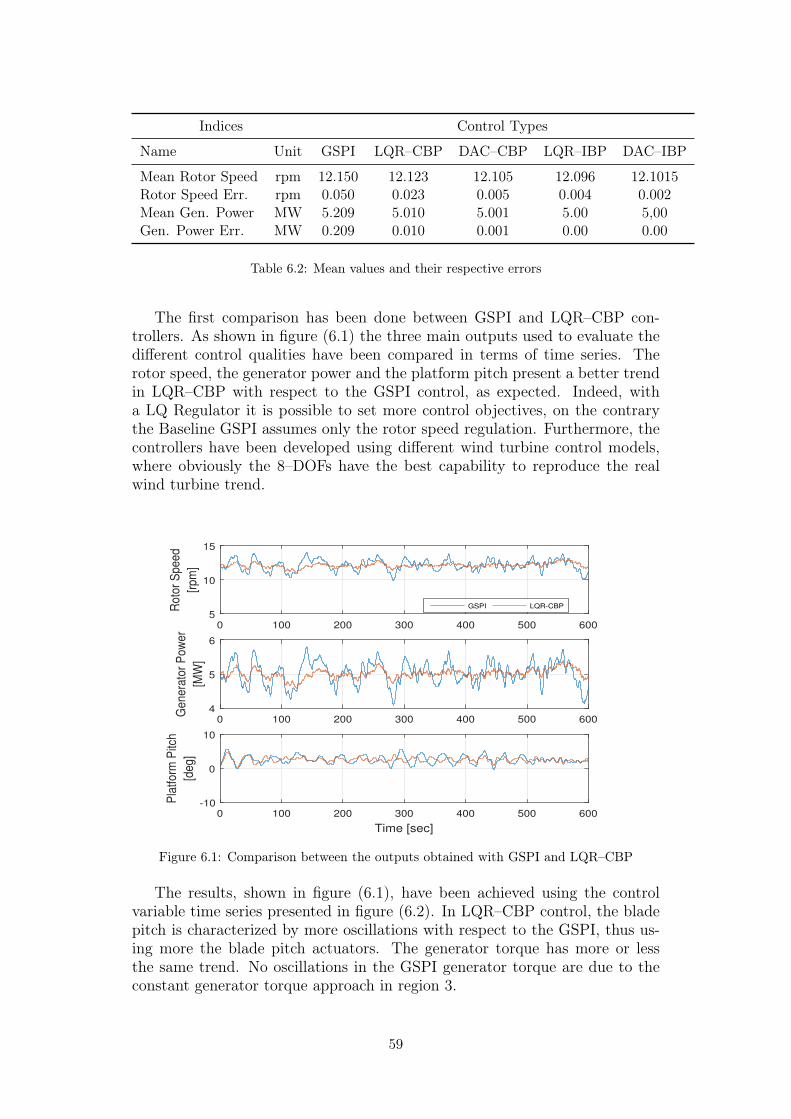
Indices Control Types

Name Unit GSPI LQR–CBP DAC–CBP LQR–IBP DAC–IBP

Mean Rotor Speed rpm 12.150 12.123 12.105 12.096 12.1015Rotor Speed Err. rpm 0.050 0.023 0.005 0.004 0.002Mean Gen. Power MW 5.209 5.010 5.001 5.00 5,00Gen. Power Err. MW 0.209 0.010 0.001 0.00 0.00

Table 6.2: Mean values and their respective errors

The first comparison has been done between GSPI and LQR–CBP con-trollers. As shown in figure (6.1) the three main outputs used to evaluate thedifferent control qualities have been compared in terms of time series. Therotor speed, the generator power and the platform pitch present a better trendin LQR–CBP with respect to the GSPI control, as expected. Indeed, witha LQ Regulator it is possible to set more control objectives, on the contrarythe Baseline GSPI assumes only the rotor speed regulation. Furthermore, thecontrollers have been developed using different wind turbine control models,where obviously the 8–DOFs have the best capability to reproduce the realwind turbine trend.

0 100 200 300 400 500 6005

10

15

Roto

r S

peed

[rpm

]

GSPI LQR-CBP

0 100 200 300 400 500 6004

5

6

Genera

tor

Pow

er

[MW

]

0 100 200 300 400 500 600

Time [sec]

-10

0

10

Pla

tform

Pitc

h

[deg]

Figure 6.1: Comparison between the outputs obtained with GSPI and LQR–CBP

The results, shown in figure (6.1), have been achieved using the controlvariable time series presented in figure (6.2). In LQR–CBP control, the bladepitch is characterized by more oscillations with respect to the GSPI, thus us-ing more the blade pitch actuators. The generator torque has more or lessthe same trend. No oscillations in the GSPI generator torque are due to theconstant generator torque approach in region 3.

59

0 100 200 300 400 500 60043.093599

43.0935995

43.0936

43.0936005

43.093601

Genera

tor

Torq

ue

[kN

*m]

GSPI LQR-CBP

0 100 200 300 400 500 600

Time [sec]

5

10

15

20

25

Colle

ctiv

e B

lade P

itch

[deg]

Figure 6.2: Comparison between the inputs obtained with GSPI and LQR–CBP

The tower-base fore-aft and side-to-side frequency content are presented infigure (6.3). The hight frequency contributions are the tower FA and SS firstbending mode natural frequencies (∼ 0.5 Hz). The low frequency variationsare caused by the platform pitch and the platform roll motions, respectively.The figure shows an amplitude reduction at certain frequencies, especially atthe platform pitch resonant frequency (0.034 Hz) for tower-base FA and at theplatform roll natural frequency (0.034 Hz) for tower-base SS. These results areexpected because in the LQR control the second objective was the tower FAand SS bending reduction.

60

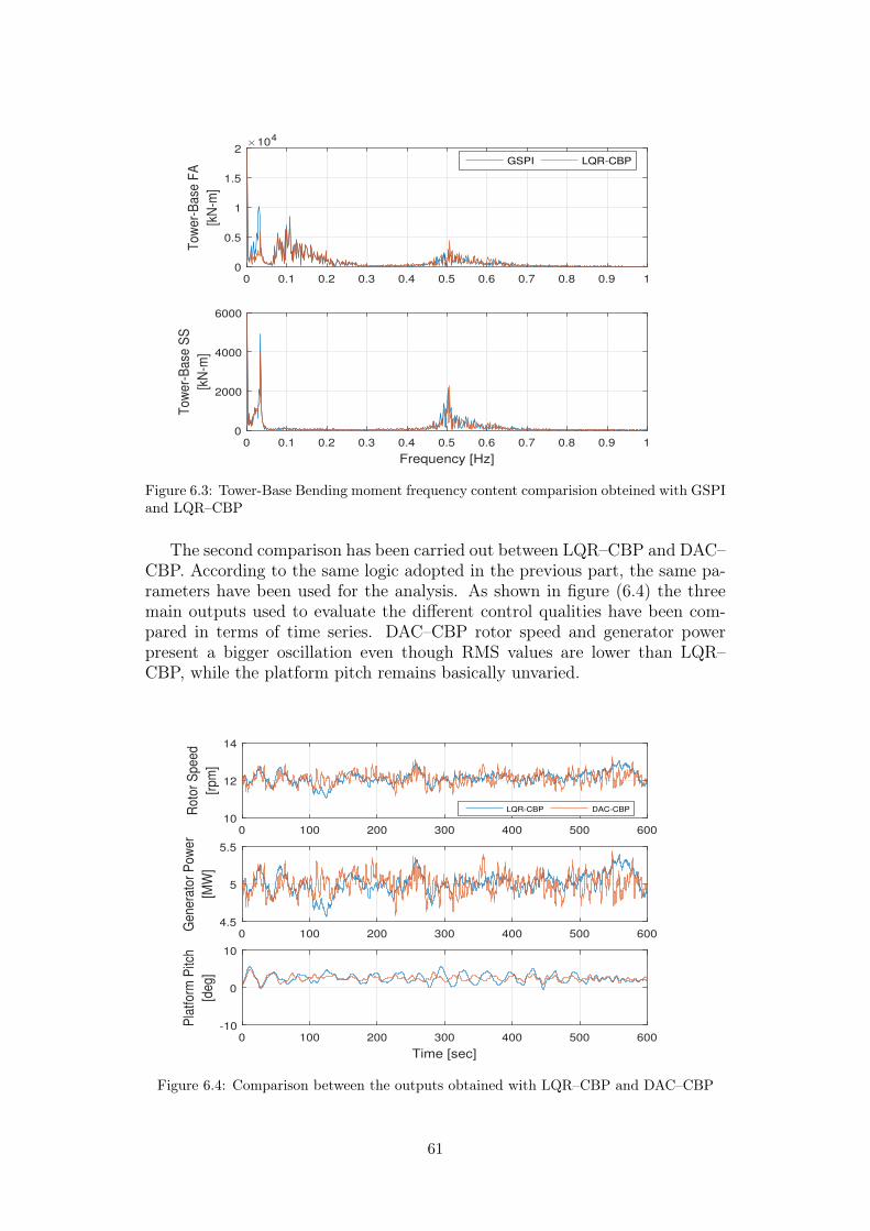
0 0.1 0.2 0.3 0.4 0.5 0.6 0.7 0.8 0.9 10

0.5

1

1.5

2

Tow

er-

Base

FA

[kN

-m]

×104

GSPI LQR-CBP

0 0.1 0.2 0.3 0.4 0.5 0.6 0.7 0.8 0.9 1

Frequency [Hz]

0

2000

4000

6000

Tow

er-

Base

SS

[kN

-m]

Figure 6.3: Tower-Base Bending moment frequency content comparision obteined with GSPIand LQR–CBP

The second comparison has been carried out between LQR–CBP and DAC–CBP. According to the same logic adopted in the previous part, the same pa-rameters have been used for the analysis. As shown in figure (6.4) the threemain outputs used to evaluate the different control qualities have been com-pared in terms of time series. DAC–CBP rotor speed and generator powerpresent a bigger oscillation even though RMS values are lower than LQR–CBP, while the platform pitch remains basically unvaried.

0 100 200 300 400 500 60010

12

14

Roto

r S

peed

[rpm

]

LQR-CBP DAC-CBP

0 100 200 300 400 500 6004.5

5

5.5

Genera

tor

Pow

er

[MW

]

0 100 200 300 400 500 600

Time [sec]

-10

0

10

Pla

tform

Pitc

h

[deg]

Figure 6.4: Comparison between the outputs obtained with LQR–CBP and DAC–CBP

61

The results, shown in figure (6.4), have been achieved using the controlvariable time series presented in figure (6.5). Using the DAC controller thecollective blade pitch and the generator torque present more oscillations. Thisimplies that the DAC uses the actuators with more frequency than the LQR–CBP. The bigger oscillations shown in figure (6.4) are probably caused by ahigher utilization of the blade pitch actuators.

0 100 200 300 400 500 60042

42.5

43

43.5

44

Genera

tor

Torq

ue

[kN

*m]

LQR-CBP DAC-CBP

0 100 200 300 400 500 600

Time [sec]

0

10

20

30

Colle

ctiv

e B

lade P

itch

[deg]

Figure 6.5: Comparison between the controllable inputs obtained with LQR–CBP and DAC–CBP

In this comparison, the tower-base fore-aft and side-to-side frequency con-tent are presented in figure (6.6). DAC control has the capability to furtherreduce the frequency content both FA and SS. It is caused by its ability todecrease the platform motions.

62

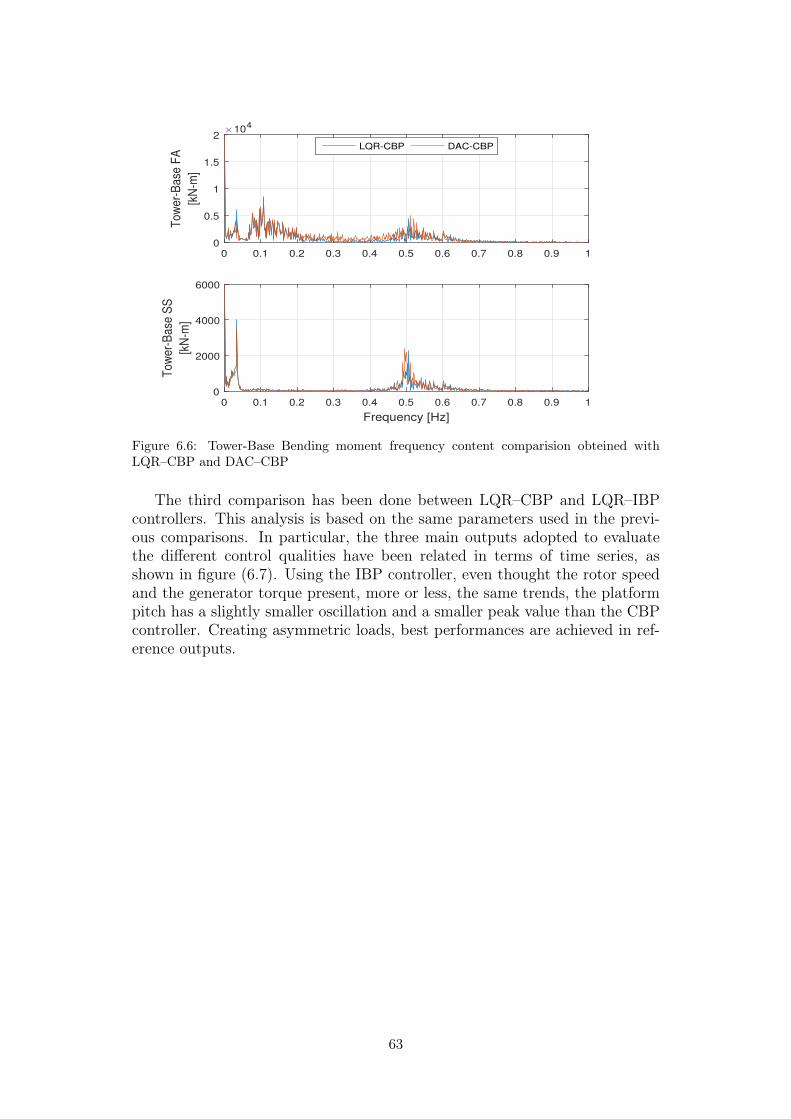
0 0.1 0.2 0.3 0.4 0.5 0.6 0.7 0.8 0.9 10

0.5

1

1.5

2

Tow

er-

Base

FA

[kN

-m]

×104

LQR-CBP DAC-CBP

0 0.1 0.2 0.3 0.4 0.5 0.6 0.7 0.8 0.9 1

Frequency [Hz]

0

2000

4000

6000

Tow

er-

Base

SS

[kN

-m]

Figure 6.6: Tower-Base Bending moment frequency content comparision obteined withLQR–CBP and DAC–CBP

The third comparison has been done between LQR–CBP and LQR–IBPcontrollers. This analysis is based on the same parameters used in the previ-ous comparisons. In particular, the three main outputs adopted to evaluatethe different control qualities have been related in terms of time series, asshown in figure (6.7). Using the IBP controller, even thought the rotor speedand the generator torque present, more or less, the same trends, the platformpitch has a slightly smaller oscillation and a smaller peak value than the CBPcontroller. Creating asymmetric loads, best performances are achieved in ref-erence outputs.

63

0 100 200 300 400 500 60010

12

14

Roto

r S

peed

[rpm

]LQR-CBP LQR-IBP

0 100 200 300 400 500 6004.5

5

5.5

Genera

tor

Pow

er

[MW

]

0 100 200 300 400 500 600

Time [sec]

0

5

Pla

tform

Pitc

h

[deg]

Figure 6.7: Comparison between the outputs obtained with LQR–CBP and LQR–IBP

The results, shown in figure (6.7), have been achieved using the controlvariable time series displayed in figure (6.8). Using the IBP controller theblade pitches present more oscillation than CBP controller. The differencesreported in the figure are not very clear. Moreover, from the analysis reportedin table (6.13), it is possible to note that the IBP blade pitch is characterizedby a bigger RMS value. This means that the blade pitch actuators are usedmore intensively. However, the generator torque actuation remains somewhatlimited in both controls.

0 100 200 300 400 500 60043.093599

43.0935995

43.0936

43.0936005

43.093601

Genera

tor

Torq

ue

[kN

*m]

LQR-CBP LQR-IBP

0 100 200 300 400 500 600

Time [sec]

5

10

15

20

25

Indiv

idual B

lade P

itch

[deg]

LQR-CBP IBP-B1 IBP-B2 IBP-B3

Figure 6.8: Comparison between the controllable inputs obtained with LQR–CBP and LQR–IBP

64

In the third comparison, the tower-base fore-aft and side-to-side frequencycontents are presented in figure (6.9). The IBP controller decreases the tower-base FA contribution to the platform pitch natural frequency. Moreover,analysing the tower-base SS frequency content, it is possible to note that theIBP does not reduce the frequency contribution at the platform roll natural fre-quency, but equal frequency contribution is obtained with the GSPI controller.Although a reduction on tower SS oscillation was a secondary objective, thisincrease is probably due to the asymmetric load management introduced bythe IBP controller.

0 0.1 0.2 0.3 0.4 0.5 0.6 0.7 0.8 0.9 10

0.5

1

1.5

2

Tow

er-

Base

FA

[kN

-m]

×104

LQR-CBP LQR-IBP

0 0.1 0.2 0.3 0.4 0.5 0.6 0.7 0.8 0.9 1

Frequency [Hz]

0

2000

4000

6000

Tow

er-

Base

SS

[kN

-m]

Figure 6.9: Tower-Base Bending moment frequency content comparision obteined withLQR–CBP and LQR–IBP

The fourth comparison has been carried out between LQR–IBP and DAC–IBP. In this analysis the same parameters used previously are shown. In fig-ure (6.10) the three main outputs used to evaluate the different control qualitiesare compared in terms of time series. Similarly to the DAC–CBP, the feed-forward wind speed rejection provokes bigger oscillations than the LQR–IBP.Moreover it emerges that the platform pitch presents a slightly better trend.Details of the numeric comparison are depicted in table (6.13).

65

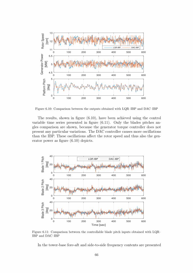
0 100 200 300 400 500 60011

12

13

Roto

r S

peed

[rpm

]LQR-IBP DAC-IBP

0 100 200 300 400 500 6004.5

5

5.5

Genera

tor

Pow

er

[MW

]

0 100 200 300 400 500 6000

5

Pla

tform

Pitc

h

[deg]

Figure 6.10: Comparison between the outputs obtained with LQR–IBP and DAC–IBP

The results, shown in figure (6.10), have been achieved using the controlvariable time series presented in figure (6.11). Only the blades pitches an-gles comparison are shown, because the generator torque controller does notpresent any particular variations. The DAC controller causes more oscillationsthan the IBP. These oscillations affect the rotor speed and thus also the gen-erator power as figure (6.10) depicts.

0 100 200 300 400 500 6000

20

40

Bla

de 1

Pitc

h

[deg]

LQR-IBP DAC-IBP

0 100 200 300 400 500 6000

20

40

Bla

de 2

Pitc

h

[deg]

0 100 200 300 400 500 600

Time [sec]

0

20

40

Bla

de 3

Pitc

h

[deg]

Figure 6.11: Comparison between the controllable blade pitch inputs obtained with LQR–IBP and DAC–IBP

In the tower-base fore-aft and side-to-side frequency contents are presented

66

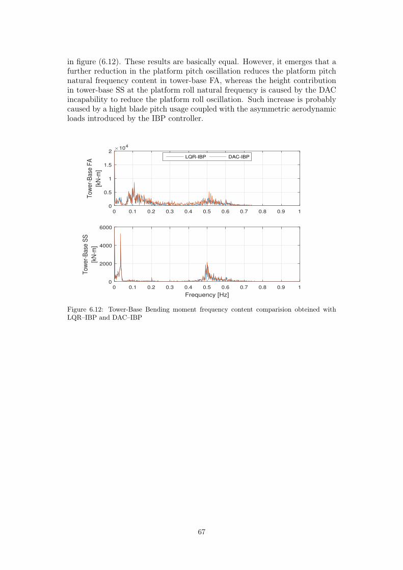
in figure (6.12). These results are basically equal. However, it emerges that afurther reduction in the platform pitch oscillation reduces the platform pitchnatural frequency content in tower-base FA, whereas the height contributionin tower-base SS at the platform roll natural frequency is caused by the DACincapability to reduce the platform roll oscillation. Such increase is probablycaused by a hight blade pitch usage coupled with the asymmetric aerodynamicloads introduced by the IBP controller.

0 0.1 0.2 0.3 0.4 0.5 0.6 0.7 0.8 0.9 10

0.5

1

1.5

2

Tow

er-

Base

FA

[kN

-m]

×104

LQR-IBP DAC-IBP

0 0.1 0.2 0.3 0.4 0.5 0.6 0.7 0.8 0.9 1

Frequency [Hz]

0

2000

4000

6000

Tow

er-

Base

SS

[kN

-m]

Figure 6.12: Tower-Base Bending moment frequency content comparision obteined withLQR–IBP and DAC–IBP

67

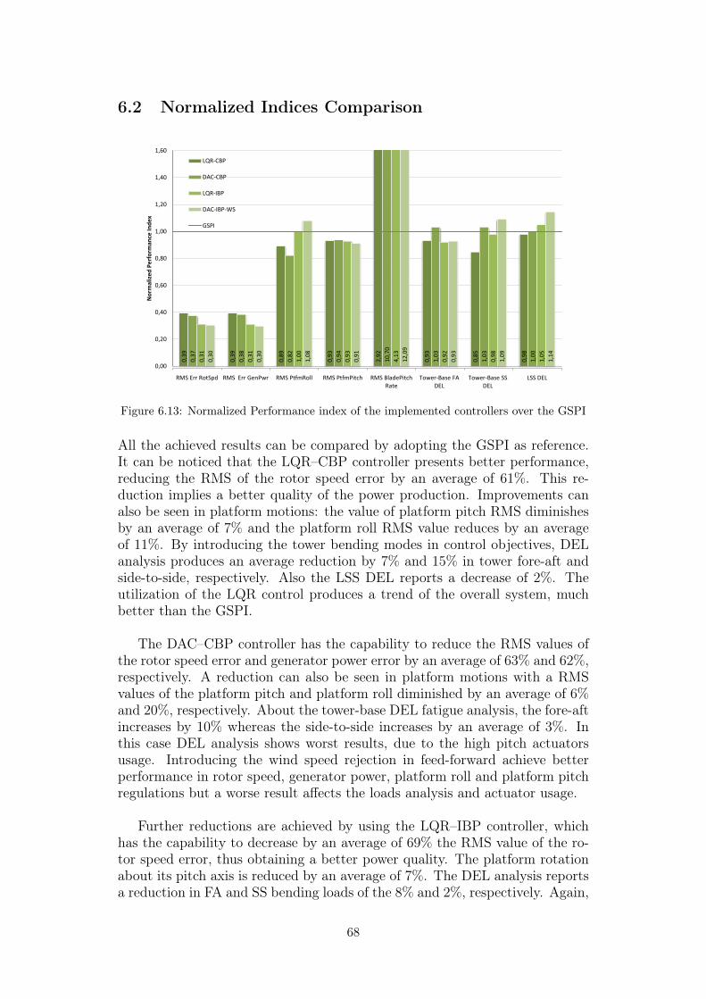
6.2 Normalized Indices Comparison

0,3

9

0,3

9

0,8

9

0,9

3

2,9

2

0,9

3

0,8

5

0,9

8

0,3

7

0,3

8

0,8

2

0,9

4

10

,70

1,0

3

1,0

3

1,0

0

0,3

1

0,3

1

1,0

0

0,9

3

4,1

3

0,9

2

0,9

8

1,0

5

0,3

0

0,3

0

1,0

8

0,9

1

12

,09

0,9

3

1,0

9

1,1

4

0,00

0,20

0,40

0,60

0,80

1,00

1,20

1,40

1,60

RMS Err RotSpd RMS Err GenPwr RMS PtfmRoll RMS PtfmPitch RMS BladePitch Rate

Tower-Base FA DEL

Tower-Base SS DEL

LSS DEL

No

rmal

ize

d P

erf

orm

ance

Ind

ex

LQR-CBP

DAC-CBP

LQR-IBP

DAC-IBP-WS

GSPI

Figure 6.13: Normalized Performance index of the implemented controllers over the GSPI

All the achieved results can be compared by adopting the GSPI as reference.It can be noticed that the LQR–CBP controller presents better performance,reducing the RMS of the rotor speed error by an average of 61%. This re-duction implies a better quality of the power production. Improvements canalso be seen in platform motions: the value of platform pitch RMS diminishesby an average of 7% and the platform roll RMS value reduces by an averageof 11%. By introducing the tower bending modes in control objectives, DELanalysis produces an average reduction by 7% and 15% in tower fore-aft andside-to-side, respectively. Also the LSS DEL reports a decrease of 2%. Theutilization of the LQR control produces a trend of the overall system, muchbetter than the GSPI.

The DAC–CBP controller has the capability to reduce the RMS values ofthe rotor speed error and generator power error by an average of 63% and 62%,respectively. A reduction can also be seen in platform motions with a RMSvalues of the platform pitch and platform roll diminished by an average of 6%and 20%, respectively. About the tower-base DEL fatigue analysis, the fore-aftincreases by 10% whereas the side-to-side increases by an average of 3%. Inthis case DEL analysis shows worst results, due to the high pitch actuatorsusage. Introducing the wind speed rejection in feed-forward achieve betterperformance in rotor speed, generator power, platform roll and platform pitchregulations but a worse result affects the loads analysis and actuator usage.

Further reductions are achieved by using the LQR–IBP controller, whichhas the capability to decrease by an average of 69% the RMS value of the ro-tor speed error, thus obtaining a better power quality. The platform rotationabout its pitch axis is reduced by an average of 7%. The DEL analysis reportsa reduction in FA and SS bending loads of the 8% and 2%, respectively. Again,

68

introducing the asymmetric loads increments the DEL LSS fatigue analysis byan average of 5%.

The DAC controller with wind share rejection achieved results comparablewith LQR–IBP. DAC has the capability to reduce the RMS rotor speed errorof 70%, thus improving the power quality. The platform pitch motion dimin-ishes by an average of 9%. However, no reduction in platform roll oscillationaffects tower-base SS DEL analysis, which reports an increase of 9%. Finally,the DEL analysis of the LSS bending reports an average increment of 14%.

69

Chapter 7

Conclusions and FurtherDevelopments

The spar-buoy platform achieves hydrostatic stability using a deep draftedballast with three catenary mooring lines to remain in a fixed position. Thedeep draft of the spar-buoy increases the platform roll and pitch inertias, thusreducing their respective natural frequencies. A low platform pitch naturalfrequency affects the DOFs choice in the control design. Adding the platformsurge DOF and the first tower fore-aft DOF to the linearized model, it cap-tures all the essential features of the platform pitch dynamic.

A Gain Scheduled PI (GSPI) controller has been used as a reference to com-pare the performances of a State Feedback Controller (SFC) obtained with theLinear Quadratic Regulator (LQR). Initially it has been implemented using acollective blade pitch (CBP) and afterwards using an individual blade pitch(IBP). Furthermore, to minimize the wind speed perturbation effect, a Distur-bance Accommodation Control (DAC) has been implemented with both theprevious configurations. Using the DAC-CBP, only the hub-height uniformwind disturbance has been considered. On the contrary, the use of the DAC-IBP allows to take into account the wind share effect. The latter is a periodiceffect that describes the horizontal increase of the wind speed according to theheight.

The achieved results prove that using a multi-objective control improvesthe overall system trend, decreases the RMS value to the rotor speed error,and thus, increases the power quality. Furthermore, the state-feedback control(SFC) obtained with collective and individual blade pitch presents the capa-bility to reduce the tower-base FA and SS fatigue loads, extending the windturbine tower lifetime. Such results are very important because the main pur-pose is to produce a better power quality for the longest possible period. Usingasymmetric aerodynamics loads helps prevent the controller from conflicting is-sues arising when rotor speed and platform pitch are regulated simultaneously.The IBP controller applied to a spar-buoy platform has a limited effectivenessdue to a very low platform natural frequency, especially the platform pitch.Moreover, blade pitch saturations impose an upper limit to the controller gains,thus further limiting the IBP effectiveness.

70

The Disturbance Accommodating Control (DAC), obtained with CBP, al-lows a further reduction of the rotor speed error RMS value and of the platformmotions RMS value. However, a hight actuators’usage affects the DEL fatigueon the tower-base FA and SS. Introducing the wind share effect on the DACwith IBP does not improve the performances, due to a hight blade pitch ac-tuation that, coupled with the asymmetric loads, produces an extreme growthin the platform roll motions, thus increasing the tower-base DEL fatigue. Fur-thermore, the asymmetric aerodynamic load introduces a further fatigue loadon the Low-Speed-Shaft bending moment.

As further developments of this dissertation, it would be interesting toexpand the research field focusing on:

• Introducing the Light Detection and Ranging (LIDAR) system [9], whichhas the capability to measure the incoming wind speed before its inter-action with the wind turbine rotor.

• Introduce a sea-wave estimator, aiming at rejecting the sea-wave distur-bance.

• Introduce a Model Predictive Control (MPC) to take into account thecontrol input constraints.

• Introduce a Hydro–Wind Kinetics Integrated Module for Renewable En-ergy Co-generation project, aiming at exploiting resources in an inte-grated manner thought the utilization of wind and marine current tur-bines in offshore plants.

71

Appendix A

Model Linearization

The geometry, coordinate system and DOFs of a three-bladed wind turbineoffshore modelled with FAST and discussed in the chapters 2, 3 and 4 areused to develop the kinematic expressions for the entire structure [24]. Thesekinematic expressions are adopted to form kinetic expressions through Kane’sequations. Kane’s equations of motion, for a system with P generalized co-ordinates (DOF), use two sets of scalar quantities called generalized inertiaforces, F ∗r , and generalized active forces, Fr, which are defined:

Fr =w∑i=1

EvXiFXi + EωNir MNi (r = 1, 2, . . . , P ) (A.1)

and

F ∗r =w∑i=1

EvXi(−mi

EaXi)

+ EωNir(−EHNi

)(r = 1, 2, . . . , P ) (A.2)

where it is assumed that for each rigid body, Ni, the active forces, FXi andMNi , are applied at the centre of point mass, Xi. The acceleration of thecentre of mass point is given by EaXi and the time derivative of the angularmoment of the rigid body in the inertial frame, E, is given by EHNi . Thequantities EvXir and EωNir represent the partial lineal and angular velocities,respectively.

By a direct result of Newton’s laws of motion, the Kane’s equations ofmotion can be expressed as:

Fr + F ∗r = 0 (r = 1, 2, . . . , P ) (A.3)

These complete nonlinear equation of motion can we written as follows:

M(q, u, t)q + f(q, q, u, ud, t) = 0 (A.4)

where, M is the mass matrix, f is the nonlinear “forcing function” vector, q isthe DOF displacements vector, q is the DOF velocities vector, q is the accel-eration vector, u is the control input vector, ud is the wind input disturbancevector and t is the time. FAST numerically linearizes the equations (A.4) byperturbing each of the system variables about their respective operating point

72

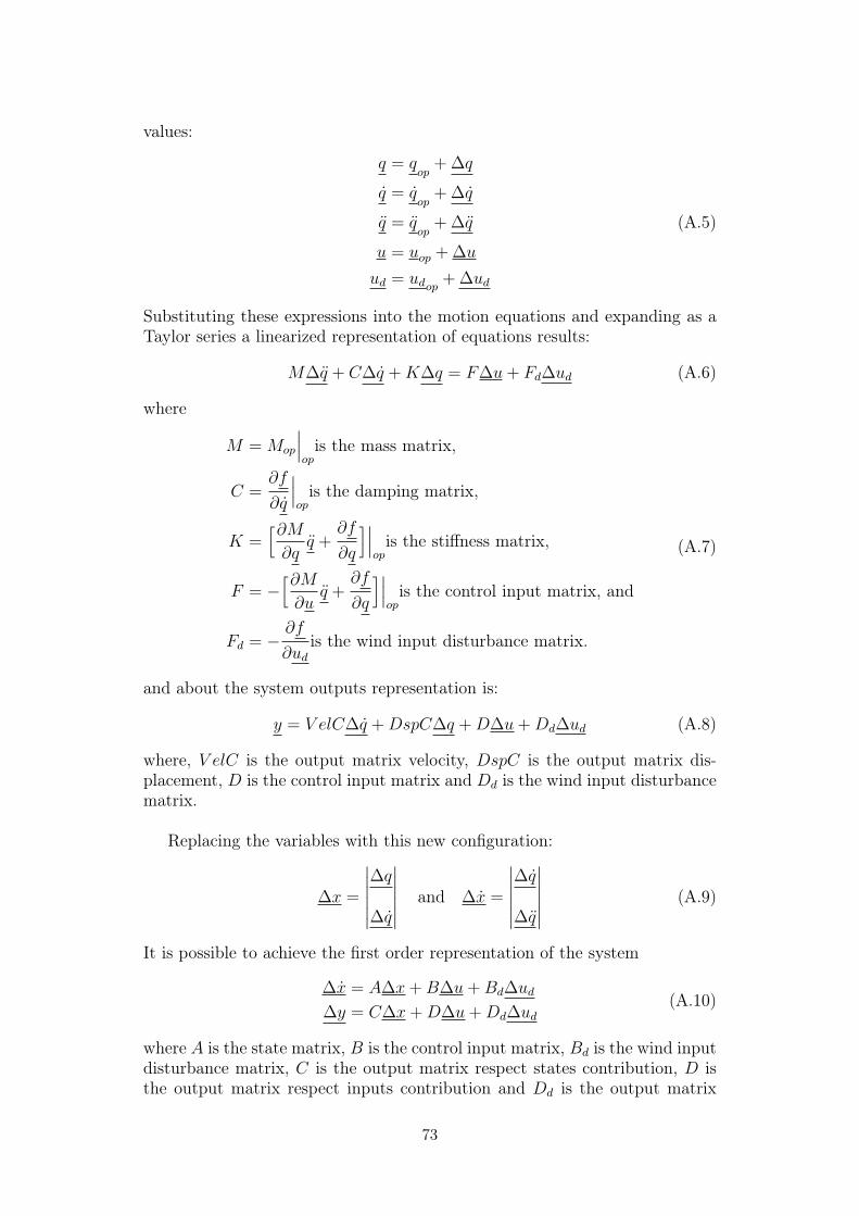
values:

q = qop

+ ∆q

q = qop

+ ∆q

q = qop

+ ∆q

u = uop + ∆u

ud = udop + ∆ud

(A.5)

Substituting these expressions into the motion equations and expanding as aTaylor series a linearized representation of equations results:

M∆q + C∆q +K∆q = F∆u+ Fd∆ud (A.6)

where

M = Mop

∣∣∣opis the mass matrix,

C =∂f

∂q

∣∣∣opis the damping matrix,

K =[∂M∂q

q +∂f

∂q

]∣∣∣opis the stiffness matrix,

F = −[∂M∂u

q +∂f

∂q

]∣∣∣opis the control input matrix, and

Fd = −∂f

∂udis the wind input disturbance matrix.

(A.7)

and about the system outputs representation is:

y = V elC∆q +DspC∆q +D∆u+Dd∆ud (A.8)

where, V elC is the output matrix velocity, DspC is the output matrix dis-placement, D is the control input matrix and Dd is the wind input disturbancematrix.

Replacing the variables with this new configuration:

∆x =

∣∣∣∣∣∣∆q

∆q

∣∣∣∣∣∣ and ∆x =

∣∣∣∣∣∣∆q

∆q

∣∣∣∣∣∣ (A.9)

It is possible to achieve the first order representation of the system

∆x = A∆x+B∆u+Bd∆ud

∆y = C∆x+D∆u+Dd∆ud(A.10)

where A is the state matrix, B is the control input matrix, Bd is the wind inputdisturbance matrix, C is the output matrix respect states contribution, D isthe output matrix respect inputs contribution and Dd is the output matrix

73

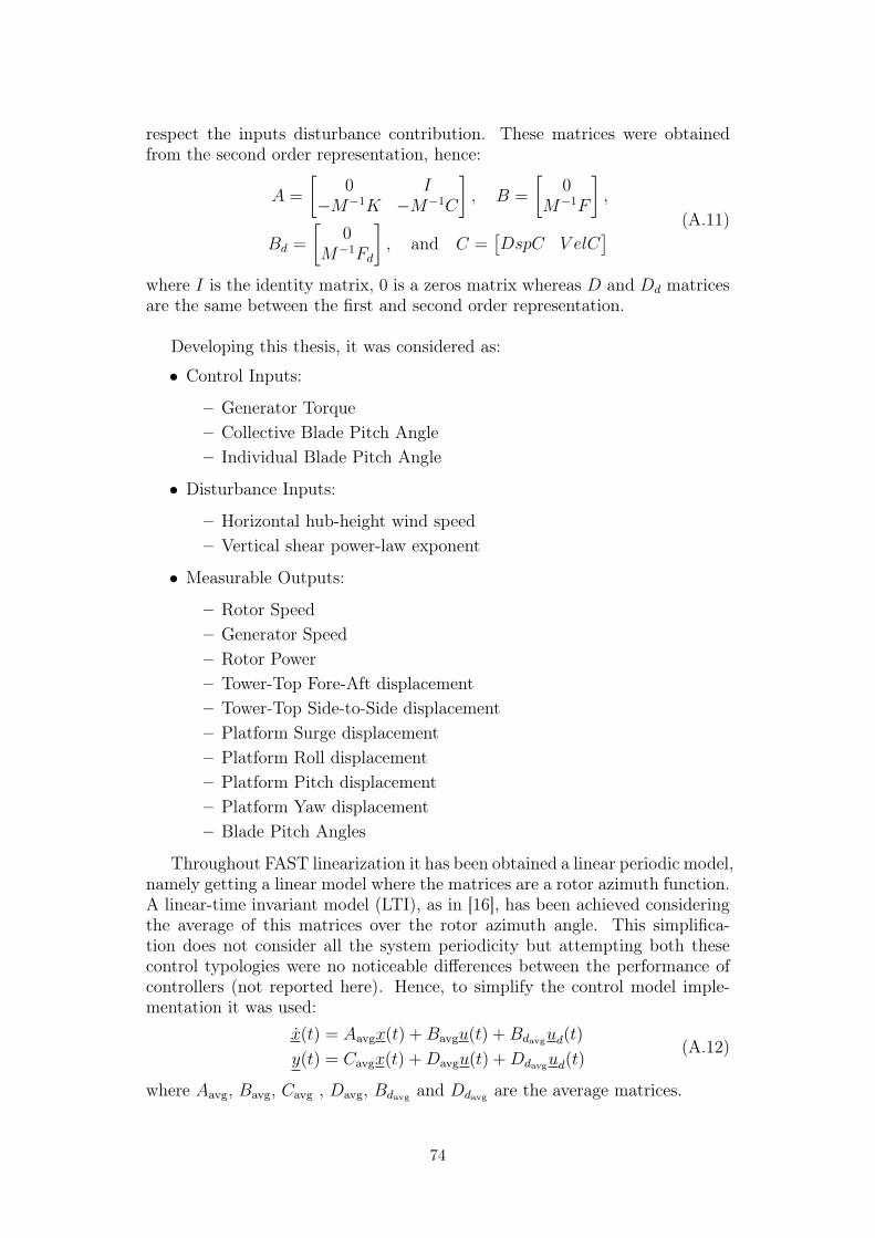
respect the inputs disturbance contribution. These matrices were obtainedfrom the second order representation, hence:

A =

[0 I

−M−1K −M−1C

], B =

[0

M−1F

],

Bd =

[0

M−1Fd

], and C =

[DspC V elC

] (A.11)

where I is the identity matrix, 0 is a zeros matrix whereas D and Dd matricesare the same between the first and second order representation.

Developing this thesis, it was considered as:

• Control Inputs:

– Generator Torque– Collective Blade Pitch Angle– Individual Blade Pitch Angle

• Disturbance Inputs:

– Horizontal hub-height wind speed– Vertical shear power-law exponent

• Measurable Outputs:

– Rotor Speed– Generator Speed– Rotor Power– Tower-Top Fore-Aft displacement– Tower-Top Side-to-Side displacement– Platform Surge displacement– Platform Roll displacement– Platform Pitch displacement– Platform Yaw displacement– Blade Pitch Angles

Throughout FAST linearization it has been obtained a linear periodic model,namely getting a linear model where the matrices are a rotor azimuth function.A linear-time invariant model (LTI), as in [16], has been achieved consideringthe average of this matrices over the rotor azimuth angle. This simplifica-tion does not consider all the system periodicity but attempting both thesecontrol typologies were no noticeable differences between the performance ofcontrollers (not reported here). Hence, to simplify the control model imple-mentation it was used:

x(t) = Aavgx(t) +Bavgu(t) +Bdavgud(t)

y(t) = Cavgx(t) +Davgu(t) +Ddavgud(t)(A.12)

where Aavg, Bavg, Cavg , Davg, Bdavg and Ddavg are the average matrices.

74

Appendix B

Fatigue Analysis

The processing of the fatigue analysis data has been conducted using MLife [11].MLife is a post–processor CAE, which uses a rainflow-counting algorithm tocount Damage Equivalent Loads (DELs) for each simulation. It also appliesa probability distribution and material properties to estimate lifetime damageand time to failure.

MLife extrapolates the damage cycles counts differently on the design loadcase (DLC) classification of the time-series data. In this dissertation it wasconsidered only the design load cases for power production in normal operation(DLC 1.1). The parameters are summarized in table (B.1).

Wind Wave E T F

Model Speed Model Height Direction

NTM Vin<Vhub<Vout NSS Hs = E[Hs|Vhub] ξ = 0 N.O. U 1.25x1.2

Table B.1: Design Load Case for Power Production

where E is the Event, N.O. is the normal operation, T is the Load Type,U is the ultimate load, F is the load factor, NTM is the Normal TurbulenceModel, NSS is Normal Sea State, Vin and Vout are the cut–in and cut–out windspeed, respectively.

B.1 Lifetime Damage

The program accumulates fatigue damage due to fluctuating loads over thewind turbine design life. These fluctuating loads are split into individual hys-teresis cycles by matching minimum and maximum in each time series. Assum-ing that the damage accumulated linearly with each cycles and in accordingwith Miner’s Rule, it is possible to define the lifetime damage as:

DLife =∑i

nLifei

Ni(LRFi )(B.1)

75

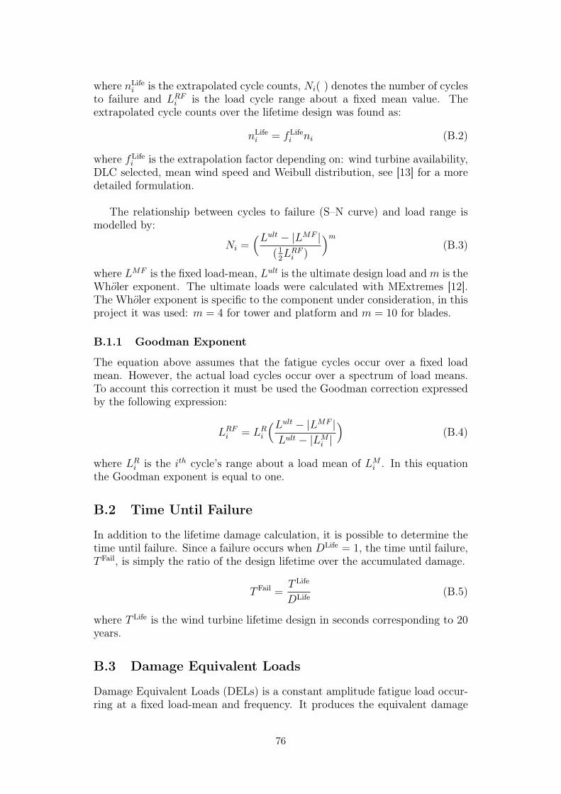
where nLifei is the extrapolated cycle counts, Ni( ) denotes the number of cycles

to failure and LRFi is the load cycle range about a fixed mean value. Theextrapolated cycle counts over the lifetime design was found as:

nLifei = fLife

i ni (B.2)

where fLifei is the extrapolation factor depending on: wind turbine availability,

DLC selected, mean wind speed and Weibull distribution, see [13] for a moredetailed formulation.

The relationship between cycles to failure (S–N curve) and load range ismodelled by:

Ni =(Lult − |LMF |

(12LRFi )

)m(B.3)

where LMF is the fixed load-mean, Lult is the ultimate design load andm is theWholer exponent. The ultimate loads were calculated with MExtremes [12].The Wholer exponent is specific to the component under consideration, in thisproject it was used: m = 4 for tower and platform and m = 10 for blades.

B.1.1 Goodman Exponent

The equation above assumes that the fatigue cycles occur over a fixed loadmean. However, the actual load cycles occur over a spectrum of load means.To account this correction it must be used the Goodman correction expressedby the following expression:

LRFi = LRi

(Lult − |LMF |Lult − |LMi |

)(B.4)

where LRi is the ith cycle’s range about a load mean of LMi . In this equationthe Goodman exponent is equal to one.

B.2 Time Until Failure

In addition to the lifetime damage calculation, it is possible to determine thetime until failure. Since a failure occurs when DLife = 1, the time until failure,TFail, is simply the ratio of the design lifetime over the accumulated damage.

TFail =T Life

DLife (B.5)

where T Life is the wind turbine lifetime design in seconds corresponding to 20years.

B.3 Damage Equivalent Loads

Damage Equivalent Loads (DELs) is a constant amplitude fatigue load occur-ring at a fixed load-mean and frequency. It produces the equivalent damage

76

as the variable spectrum such that:

Dj =∑i

nijNij

=neqjN eqi

(B.6)

neqj = f eq Tj (B.7)

N eqj =

(Lult − |LMF|(12DELF

j

) )m (B.8)

where Tj is the elapsed time of the jth time series, f eq is the DEL frequencyset to 1 Hz, neqj is the total equivalent fatigue counts for jth time series, N eq

j isthe equivalent number of cycles until failure for jth time series and DELF

j isthe DEL for the jth time series. Solving the equation (B.8) for DELF

j , results:

DELFj =

(∑i

(Nij(L

RFij )m

)neqj

) 1m (B.9)

This term will be used in the controller comparative analysis to evaluatethe fatigue load on the wind turbine.

77

Bibliography

[1] IEC 61400-3, ed. Wind Turbines - Part 3: Design Requirements for OffshoreWind Turbines. Technical Report. International Electrotechnical Commission(IEC), 2006.

[2] G. Corbetta A. Ho A. Mbistrova. The European offshore wind industry – keytrends and statistics 2015. Technical Report. The European Wind Energy As-sociation, 2015.

[3] Marzorati A. Modellistica e Controllo di turbine offshore per acque profonde.Tesi di laurea Magistrale. Politecnico di Milano, 2012.

[4] G. Bir. Multiblade Coordinate Transformation and Its Application to WindTurbine Analysis. Conference Paper. NREL, 2008.

[5] G. Bir. User’s Guide to MBC3 (Multi-Blade Coordinate Transformation Utilityfor 3-Bladed Turbines). Technical Report. NREL, 2008.

[6] L. Kilcher B.J. Jonkman. TurbSim User’s Guide. Technical Report. NREL,2012.

[7] Newman J.N. C.H. Lee. WAMIT User Manual. Technical Report. MIT, 2006.

[8] A. Craig Hansen David J. Laino. AeroDyn User’s Guide. Technical Report.NREL, 2002.

[9] L.Y. Pao E. Simley. LIDAR Wind Speed Measurement of Evolving Wind Fields.Technical Report. NREL, 2012.

[10] A.S. Wright L.J. Fingersh. Advanced Control Design for Wind Turbines - PartI: Control Design, Implementation and Initial Test. Technical Report. NREL,2008.

[11] M. Buhl Jr. G.J. Hayman. Mlife User’s Guidel for Version 1.00. TechnicalReport. NREL, 2012.

[12] G.J. Hayman. MExtremes Theory Manual for Version 1.00. Technical Report.NREL, 2015.

[13] G.J. Hayman.Mlife Theory Manual for Version 1.00. Technical Report. NREL,2012.

[14] Karl Stol Hazim Namik. “Disturbance Accommodating Control of Floating Off-shore Wind Turbines”. In: American Institute of Aeronautics and Astronautics(2009).

[15] Karl Stol Hazim Namik. “Individual Blade Pitch Control of a Spar-Buoy Float-ing Wind Turbine”. In: IEEE transactions on control systems technology, vol.22 (2014).

78

[16] Karl Stol Hazim Namik. “Individual Blade Pitch Control of Floating OffshoreWind Turbines on a Tension Leg Platform”. In: American Institute of Aero-nautics and Astronautics (2010).

[17] J.H. Horlock. Actuator disc theory: discontinuities in thermo fluid dynamics.International series of engineering fluid dynamics. McGraw-Hill, 1978. isbn:9780070303607. url: https://books.google.it/books?id=0a5RAAAAMAAJ.

[18] S. Butterfield J. Jonkman. Definition of a 5-MW Reference Wind Turbine forOffshore System Development. Technical Report. NREL, 2009.

[19] Marshall L. Buhl Jr. Jason M. Jonkman. FAST User’s Guide. Technical Re-port. NREL, 2005.

[20] A.N. Robertson J.M. Jonkman and G.J. Hayman. HydroDyn User’s Guide andTheory Manual. Technical Report. NREL, 2013.

[21] M.L. Buhl J.M. Jonkman. New Developments for the NWTC’s FAST Aeroe-lastic HAWT Simulator. Conference Paper. NREL, 2004.

[22] J. Jonkman. Definition of the Floating System for Phase IV of OC3. TechnicalReport. NREL, 2010.

[23] J.M. Jonkman. Dynamics Modeling and Loads Analysis of an Offshore FloatingWind Turbine. Technical Report. NREL, 2007.

[24] J.M. Jonkman. Modeling of the UAE Wind Turbine for Refinement of theFAST_AD. Technical Report. NREL, 2003.

[25] R. Scattolini L. Magni. Complementi di Controlli Automatici. Ed. by PitagoraEditrice. 2006.

[26] J.G. Leishman. Principles of Helicopter Aerodynamics. Cambridge AerospaceSeries. Cambridge University Press, 2002. isbn: 9780521523967. url: https://books.google.cz/books?id=-PnV2JuLZi4C.

[27] Denis Matha. Model Development and Loads Analysis of an Offshore WindTurbine on a Tension Leg Platform, with Comparison to Other Floating Tur-bine Concept. Technical Report. NREL, 2009.

[28] Patrik J. Moriarty. AeroDyn Theory Manual. Technical Report. NREL, 2004.

[29] Hazim Namik. “Individual Blade Pitch and Disturbance Accommodating Con-trol of Floating Offshore Wind Turbines”. PhD thesis. The University of Auck-land, 2012.

[30] M. Hansen H. Hansen A. Larsen T.J. Oye S. Sorensen. Control Design fora Pitch-Regulated, Variable-Speed Wind Turbine. Technical Report. Risø Na-tional Laboratory Information Service Department, 2005.

[31] Statoil. Hywind Scotland Pilot Park Project. Technical Report. Statoil, 2015.

[32] Robert H. Stewart. Chapter 16 - Ocean Waves. 2006. url: http://oceanworld.tamu.edu/resources/ocng%5C_textbook/chapter16/chapter16%5C_04.htm.

[33] T.D. Hanson T.J. Larsen. “A method to avoid negative damping low frequenttower vibrations for a floating, pitch controlled wind turbine”. In: IOP Science(2007).

[34] A.S. Wright. Modern Control Design for flexible Wind Turbines. Technical Re-port. NREL, 2004.

79